radiation impedance for square piston sources on infinite

ARCHIVES OF ACOUSTICSVol. 45, No. 4, pp. 663–679 (2020)DOI: 10.24425/aoa.2020.135254

Research Paper

Radiation Impedance for Square Piston Sourceson Infinite Circular Cylindrical Baffles

John L. VALACAS

65 Ag. Varvaras St., Athens,19004 Greecee-mail: [email protected]

(received May 31, 2020; accepted July 31, 2020 )

The evaluation of complex radiation impedance for a square piston source on an infinite circular-cylindrical baffle is associated to the Greenspon-Sherman formulation for which novel evaluation methodsare proposed. Unlike existing methods results are produced in a very wide range of frequencies and sourcesemi-angles with controllable precision. For this reason closed-form expressions are used to describe thetruncation errors of all integrals and infinite sums involved. Impedance values of increased accuracy arealso provided in tabulated form for engineering use and a new radiation mass-load model is derived forlow-frequencies.

Keywords: cylindrical baffle; radiation impedance; radiation mass-load; piston source.

1. Introduction

The notion of the piston source is fundamentalin theoretical Acoustics both in free- and enclosed-space wave propagation. Pressure field and self- or mu-tual acoustic impedance for piston sources mountedon planar, spherical, cylindrical and spheroidal baffles,play a key-role in textbooks although the realisationof a source vibrating with a uniform velocity profile isnot feasible at high frequencies. For rectangular pistonsources mounted on infinite planar baffles, several re-search papers have addressed the evaluation of acousticimpedance with quite different results in terms of preci-sion and (frequency) range of applicability (Swenson,Johnson, 1952; Arase, 1964; Stepanishen, 1977;Levine, 1983; Bank, Wright, 1990; Lee, Seo, 1996;Mellow, Kärkkäinen, 2016). In addition, tabulatedimpedance values provided by Burnett and Soroka(1972) have become available.

For a cylindrical baffle of radius a (in m), withgeometry similar to that of Fig. 1, self- and mutual-radiation impedances have been investigated and theirmathematical framework has been established byGreenspon and Sherman (1964). In this frameworkthe evaluation of radiation load is based on a set ofthree integrals for which no analytic solutions haveyet been given. However for this formulation onlyone numerical evaluation scheme has been proposed

Fig. 1. A rigid square source is mounted on the surfaceof an infinite cylindrical baffle. It has an angular span 2ϕo,a vertical side 2zo (zo = aϕo) and is located at z = 0, ϕo = 0,r = a. ϕo is usually called the source’s semi-angle. It is

vibrating with a uniform normal vibration velocity.

by Kim et al. (2004), with limited frequency range,source dimensions and accuracy. There has not beenany other contribution of extended frequency rangeand/or source dimensions.

In the next sections, the original Greenspon-Sherman integrals are briefly presented and novel nu-merical evaluation methods are described in detail fora wide range of conventional (dimensionless) frequencyvalues ka (where k stands for the usual wavenum-

664 Archives of Acoustics – Volume 45, Number 4, 2020

ber, in m−1) and source semi-angles ϕo (in rad). Forpractical reasons normalised frequency variable k

√S

(where S stands for the source’s emitting area) isadopted. However when the use of frequency ka sim-plifies expressions it is preferred. Frequency variablesand source semi-angle are related as follows:

k√S = 2kaϕo. (1)

For the first time to our knowledge, results of signif-icant precision are derived for frequencies in the rangek√Sε [0.001, 100] and source semi-angles ϕoε [1, 30] de-

grees. For the lowest value of source semi-angle ϕo = 1○,this range leads to conventional normalised frequencyvalues as high as ka = 2865. For convenience these re-sults have been tabulated (see Supplement at the endof article). They are also compared to the radiationimpedance values of square piston sources on infiniteplanar baffles so that further verification and usefulconclusions be obtained. In addition the low frequencybehaviour of radiation reactance values is associated tothe widely used mass-load equivalent for which a newapproximation model is produced for practical use.

2. The Greenspon-Sherman formulation

Radiation load Zmr is a mechanical impedancequantity expressed in mechanical ohms (N ⋅ s ⋅m−1).For convenience it is normalised against the medium’scharacteristic impedance ρcS, where ρ is the me-dium’s density and c the propagation speed:

nZmr (k√S,ϕo) =

ZmrρcS

= nRmr−inXmr, (2)

where nRmr stands for the normalised radiation re-sistance and nXmr for reactance. Imaginary unit i isdefined as i2 = −1.

In their original paper, Greenspon and Shermanpresented a formulation for mutual impedance be-tween rectangular pistons on the cylinder’s surfacethat simplifies further in the case of self-radiationimpedance. In this framework the equation of (nor-malised) impedance was broken down to a set of threeinfinite series of integrals; the first one of them de-termining the radiation resistance and the other twocombining to give reactance. Kim et al. (2004) elabo-rated on this set of equations and added the necessarynotation which is adopted in this work as much as pos-sible. After some arrangements of parameters k

√S, ka

and ϕo and narrowing the analysis to square sources(zo = aϕo) the normalised resistance is written as an in-finite sum whose terms contain definite integrals Imsre:

nRmr (k√S,ϕo) =

32ϕ20

π3Isre (k

√S,ϕo) ,

Isre =∞

∑m=0

sinc2 (mϕo)εm

Imsre (m,k√S,ϕo) ,

(3)

where sinc(x) stands for the usual sin(x)/x functionand εm is 2 for m = 0 and 1 for any other m. IntegralsImsre are defined as follows:

Imsre =1

∫0

sinc2 ( 12k√S

√1 − t2)

t√

1 − t2Dm(ka t)dt, (4)

where Dm(z) is an expression of Bessel functions ofthe first (Jm) and the second kind (Ym):

Dm(z)=(Jm−1(z) − Jm+1(z))2+(Ym−1(z) − Ym+1(z))2.

(5)In a similar sense reactance is also written as an infinitesum with terms which, this time, are proportional tothe difference of two distinct integrals:

nXmr (k√S,ϕo) = 8kaϕ2

0

π2[Isiy (k

√S,ϕo)

−Isix (k√S,ϕo)], (6)

Isiy =∞

∑m=0

sinc2 (mϕ0)εm

Imsiy (m,k√S,ϕo),

Isix =∞

∑m=0

sinc2 (mϕo)εm

Imsix (m,k√S,ϕo).

(7)

Imsiy are definite integrals while Imsix are improper:

Imsiy =1

∫0

Bm(ka t)Dm(ka t)

sinc2 ( 12k√S√

1 − t2)√

1 − t2dt, (8)

Imsix =∞

∫0

sinc2 ( 12k√S√

1 + x2)√

1 + x2

⋅ Km (kax)Km−1 (kax) +Km+1 (kax)

dx, (9)

where Km stands for the modified Bessel function ofthe second kind and Bm is defined as another expres-sion of Bessel functions of the first and second kind:

Bm(z) = Jm(z) [Jm−1(z) − Jm+1(z)]

+Ym(z) [Ym−1(z) − Ym+1(z)] . (10)

In their integration method, Kim et al. (2004) pre-sented results in the frequency range ka < 51 and forsource semi-angles ϕo < π/18. They regarded orders upto m = 50 as sufficient for the sums of Eqs (3) and (7)to converge. They also stopped integration of variablex in Imsix at x = 15 for an acceptable truncation er-ror to be introduced. In all three integrals they useda variable integration step in order to handle integrandvariations in the ranges tε [0, 1) and xε [0, 15]. As a re-sult the computation error was estimated to be 0.5%for nRmr and 0.1% for nXmr. The contribution of thesingularity point t = 1 to definite integrals Imsre andImsiy was not considered. In both cases integration wascarried up to a t value of 0.9999.

J.L. Valacas – Radiation Impedance for Square Piston Sources on Infinite Circular Cylindrical Baffles 665

3. The case of Imsiy integrals

As already mentioned these are definite integrals inthe finite integration range tε [0, 1]. Their integrandhas an obvious singularity at t = 1 as per Eq. (8).A change of integration variable (x =

√1 − t2) leads

to a more convenient definition:

Imsiyb (m,ka,ϕo) = ka1

∫0

Fm (ka√

1 − x2)

⋅ sinc2 (kaϕo x) dx, (11)

whereFm(y) = Bm(y)

yDm(y). (12)

Using ordinary properties of Bessel functions likeEq. (10.6.1) and their series expansions around y = 0,like Eqs (10.7.3), (10.8.1) and (10.8.2) in NIST hand-book of mathematical functions (Olver et al., 2010),it can be shown that for all orders m above zero Fm(y)tends to −1/(2m) as y tends to 0 (or x tends to 1) andtherefore is not singular. In the case of zero-eth orderFo(y), for y tending to zero, we have a logarithmicsingularity:

limy→0

Fo(y) = limy→0

1

2(ln(y

2) + γ) = −∞, (13)

where γ = 0.57721566 stands for the Euler constant.However, the major problem is that typical math

software fails to compute Bessel functions of the secondkind inside Fm, whenever the argument becomes muchsmaller than the order. To overcome this we note thatfor small argument values Fm(y) simplifies to:

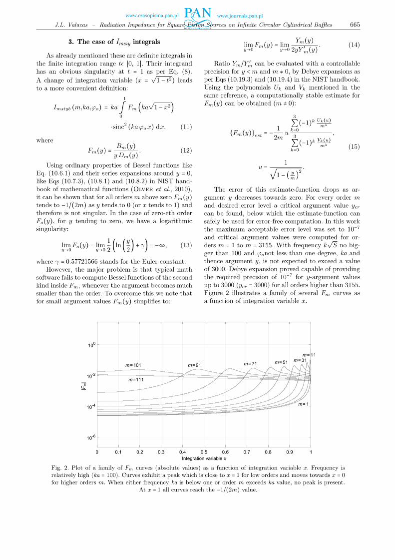
Fig. 2. Plot of a family of Fm curves (absolute values) as a function of integration variable x. Frequency isrelatively high (ka = 100). Curves exhibit a peak which is close to x = 1 for low orders and moves towards x = 0for higher orders m. When either frequency ka is below one or order m exceeds ka value, no peak is present.

At x = 1 all curves reach the −1/(2m) value.

limy→0

Fm(y) = limy→0

Ym(y)2yY ′

m(y). (14)

Ratio Ym/Y ′m can be evaluated with a controllable

precision for y <m and m ≠ 0, by Debye expansions asper Eqs (10.19.3) and (10.19.4) in the NIST handbook.Using the polynomials Uk and Vk mentioned in thesame reference, a computationally stable estimate forFm(y) can be obtained (m ≠ 0):

{Fm(y)}est = −1

2mu

3

∑k=0

(−1)k Uk(u)mk

3

∑k=0

(−1)k Vk(u)mk

,

u = 1√

1 − ( ym)2.

(15)

The error of this estimate-function drops as ar-gument y decreases towards zero. For every order mand desired error level a critical argument value ycrcan be found, below which the estimate-function cansafely be used for error-free computation. In this workthe maximum acceptable error level was set to 10−7

and critical argument values were computed for or-ders m = 1 to m = 3155. With frequency k

√S no big-

ger than 100 and ϕonot less than one degree, ka andthence argument y, is not expected to exceed a valueof 3000. Debye expansion proved capable of providingthe required precision of 10−7 for y-argument valuesup to 3000 (ycr = 3000) for all orders higher than 3155.Figure 2 illustrates a family of several Fm curves asa function of integration variable x.


4. Imsiy integration schemes

4.1. Non-singular integrand orders (m ≠ 0)

The presence of sinc squared factor within the in-tegrand function introduces a number of null points(at k

√S x/2 equal to integer multiples of π) depend-

ing on frequency k√S. This number will not exceed 15

and may well be zero at low frequencies (see Fig. 3).To ensure a successful evaluation of Imsiy integrals, in-tegration range is segmented around these null-points(if any) and Romberg’s method is applied to each seg-ment.

4.2. Singular integrand for m = 0

To overcome the singularity of the first factor ofintegrand function, Fo(y), at x = 1 (y = 0), integrationis split into two parts:

Iosiy (ka,ϕo) =1−∂x

∫0

+1

∫1−∂x

= Iosiya + Iosiyb, (16)

where the first part can be numerically evaluated whilethe second one can be addressed analytically. ∂x isa small value which must roughly meet three condi-tions:

• Simple investigation proves that argument y ofFo will go down to a small value ∂y close to zerofor which we have ∂y = ka

√2∂x. The value of ∂y

must allow for a successful evaluation of Fo bytypical math software:

Fo(y) =− (Jo(y)J1(y) + Yo(y)Y1(y))

2y(J1(y)2 + Y1(y)2). (17)

It was found that for this purpose ∂y should notbe smaller than 10−20.

Fig. 3. Plot of absolute value of Imsiy Integrand of order m = 1 at a frequency of k√

S = 100 and sourcesemi-angle ϕo = 1 degree, as a function of integration variable x. Null points due to sinc squared factor lead to

segmentation of the integration range for a successful application of Romberg’s method.

• On the other hand, ∂y must be small enough toallow Fo(y) to be approximated by the expressionin Eq. (13), in the range 0 to ∂y with a high levelof precision. In order to have a worst-case relativeerror of 10−6 at y = ∂y, the value of ∂y must notexceed 5 ⋅ 10−4.

• Finally ∂x, being the span of the integrationrange in Iosiyb, must be small enough to allow forthe swing of sinc squared factor to be modelledby a simple first-order Taylor expansion or, evenbetter, be considered constant.

All conditions can be met by selecting ∂x to havea fixed value of 10−14, leading to a variable value for∂y: 1.41 ⋅ 10−10 at ka = 0.001 and 4.23 ⋅ 10−4 at ka =3000. Sinc squared factor proves to remain practicallyunchanged throughout this narrow integration range.The analytic expression for Iosiyb becomes:

Iosiyb (ka,ϕo) = ka

2

1

∫1−∂x

(ln(ka√

1 − x2

2) + γ)

⋅sinc2 (kaϕox) dx = ka2

sinc2 (kaϕo)

⋅1

∫1−∂x

(ln(ka√

1 − x2

2) + γ) dx

= ka

2sinc2 (kaϕo)

⎡⎢⎢⎢⎢⎣(ln(ka

2) + γ)∂x

+ 1

2(2 ln(2) − (2 − ∂x) ln(2 − ∂x)

+∂x ln(∂x) − 2∂x)⎤⎥⎥⎥⎥⎦. (18)


For the numerical evaluation of Iosiya, the segmen-tation based on sinc squared null-points which was sug-gested in Subsec. 4.1, is also adopted here along withRomberg’s rule. However it must be taken into accountthat convergence is significantly accelerated by the in-troduction of additional break-points (and thereforesegments) very close to one. Three such points wereadded close to the right-hand side of the integrationrange: 1–10−3, 1–10−6, 1–10−10.

At all frequencies and source semi-angles Iosiyb va-lues were found several orders of magnitude smallerthan the respective Iosiya values.

5. Isiy summation process

Before addressing the summation process in Isiy’sdefinition in Eq. (7) useful conclusions can be pro-

a)

b)

Fig. 4. Graphs of absolute value of ∣Imsiy ∣ integrals as a function of orderm for source semi-angles ϕo = 30, 15, 5, and1 degrees. Above their peak value the decay slope tends asymptotically to −10 dB/decade: a) frequency k

√

S = 20,b) k√

S = 0.001.

duced by close inspection of Imsiy (negative) values’ se-quences. Figure 4 depicts the decaying nature of thesesequences both at low and high frequencies.

At high frequencies a peak is formed at an ordermp approximately equal to frequency parameter ka:

mp ≈ ⌈ka⌉ , (19)

where ⌈x⌉ is the usual function returning the smallestinteger greater than or equal to x. At frequencies closeto zero the ∣Imsiy ∣ sequences start to decay just abovetheir first order, i.e. mp = 1 (Fig. 4b).

A second aspect of ∣Imsiy ∣ values is that when plot-ted with log-log axes, they form, above mp, a log-logconvex sequence. The slope of this sequence is morenegative than −10 dB/decade but tends to this valueasymptotically. As it is discussed in Appendix A,∣Imsiy(m)∣ values will decay faster than a sequence


proportional to 1/m passing through the point (mo,∣Imsiy(mo)∣):

∀mo >mp, ∣Imsiy(m ≥mo)∣ ≤ ∣Imsiy(mo)∣ ⋅mo

m. (20)

Having the upper bound described in Eq. (20) al-lows for the evaluation of the truncation error whichwill be introduced whenever Isiy summation stops ata specific order mo − 1:

∣∞

∑m=mo

Imsiy(m)sinc2(mϕo)∣

<∞

∑m=mo

∣Imsiy (mo)∣mo

m

sin2(mϕo)(mϕo)2

= ∣Imsiy (mo)∣mo

ϕ2o

∞

∑m=mo

sin2 (mϕo)m3

= ∣Imsiy (mo)∣mo

ϕ2o

[1

2Li3 (1) − 1

4Li3 (e2iϕo)

−1

4Li3 (e−2iϕo) −

mo−1

∑m=1

sin2 (mϕo)m3

] , (21)

where Li3(z) stands for the trilogarithm function,a special case of polylogarithm function:

Lik (z) =∞

∑m=1

zm

mk.

To put everything together, Isiy may proceed un-conditionally to sum all orders at least up to mp andthen exit whenever the ratio of the truncation error,per Eq. (21), over the accumulated sum’s value, dropsbelow a preselected precision level. In this work thisfirst part of summation was set to include orders up to70 ⋅mp.

6. Investigation of Imsix integrals

Integrand function of Imsix integrals, given inEq. (9), can be separated in two factors for furtheranalysis:

Ax (ka,ϕo,x) =sinc2 ( 1

2k√S√

1 + x2)√

1 + x2,

Krm(y) = Km(y)Km−1(y) +Km+1(y)

= − Km(y)2K ′

m(y),

(22)

where y stands for k√Sx/(2ϕo) or ka x and K ′

m de-notes first-order derivative with respect to argument y.

6.1. The K-function ratio Krm

Although Km is singular at y = 0, the respec-tive ratio Krm is not. Using the limiting forms of

Eqs (10.30.2) and (10.31.2) in NIST handbook (Olveret al., 2010) for very small argument, and typical prop-erties of the modified Bessel functions per Watson(1966, p. 79), it can be shown that as y tends to zeroKrm tends to y/(2m) for m > 0 and to −(y/2) ln(y/2)for m = 0. That is, Krm tends to zero without beingsingular. On the other hand, when the argument isvery large Krm tends to 1/2. In general, Km(y) hasa fast decay so usual mathematical software roundsit to zero when its argument goes beyond a value of700 approximately and thus reports an error for theratio Krm. At a frequency of ka = 100 this would hap-pen even for relatively small values of integration vari-able x. Hopefully Krm ratio can be evaluated undersome well-stated conditions by other means. For m = 0Yang and Chu (2017, left-hand side of Corollary 3.3with p = 1/4) have provided an upper bound functionwhich can also approximate it as follows:

{Kr0(y)}est =Ko(y)2K1(y)

≈ 1

2

y + 14

y + 34

. (23)

A direct comparison of values obtained by typicalmath software to those given by Eq. (23) proves thatfor the relative error to be always less than 10−5 wemust have y ≥ 21. For all other orders m the Debyeexpansions per Eqs (10.41.4) and (10.41.6) describedin NIST handbook can be used, based on the samepolynomials Uk and Vk as in Eq. (15):

{Krm(y)}est =1

2

( ym)

√1 − ( y

m)2

3

∑k=0

(−1)k Uk(u)mk

3

∑k=0

(−1)k Vk(u)mk

,

u = 1√

1 − ( ym)2.

(24)

Relative error of Eq. (24) is less than 10−7 for allorders m ≥ 25. Table 1 provides the necessary details.

Table 1. Evaluation rules for Krm ratio.

Order Range and computation means

m = 0y < 21, math softwarey ≥ 21, Eq. (23)

1 ≤m < 9

y < 10−4, Eq. (24)10−4 ≤ y < 40, math software

y ≥ 40, Eq. (24)

9 ≤m < 25

y < 0.10, Eq. (24)0.10 ≤ y < 40, math software

y ≥ 40, Eq. (24)m ≥ 25 all y, Eq. (24)

In short, for m = 0, Krm starts at y = 0 as −(y/2)log(y/2) and then tends asymptotically to 1/2. For allother orders m it starts as y/(2m) and then tends to1/2 too.


6.2. The Ax factor

This factor introduces oscillations to Imsix inte-grand with null points nonlinearly spread in integra-tion variable x. It will prove quite useful to knowthe exact location of either the first fnp or the n-thnull point nnp of this factor and the integrand asa whole:

fnp =

⎧⎪⎪⎪⎪⎪⎪⎪⎪⎪⎪⎪⎪⎪⎪⎪⎪⎨⎪⎪⎪⎪⎪⎪⎪⎪⎪⎪⎪⎪⎪⎪⎪⎪⎩

k√S< 2π ∶

¿ÁÁÀ( 2π

k√S)

2

−1,

k√S≥ 2π ∶

¿ÁÁÁÁÁÁÁÀ

⎛⎜⎜⎜⎜⎝

⌈ 2π

k√S⌉

2π

k√S

⎞⎟⎟⎟⎟⎠

2

−1,

(25)

nnp =

⎧⎪⎪⎪⎪⎪⎪⎪⎪⎪⎪⎪⎪⎪⎪⎪⎪⎨⎪⎪⎪⎪⎪⎪⎪⎪⎪⎪⎪⎪⎪⎪⎪⎪⎩

k√S< 2π ∶

¿ÁÁÀ( 2nπ

k√S)

2

−1,

k√S≥ 2π ∶

¿ÁÁÁÁÁÁÁÀ

⎛⎜⎜⎜⎜⎝

⌈ 2π

k√S⌉ + n−1

2π

k√S

⎞⎟⎟⎟⎟⎠

2

−1,

(26)

where n stands for the integer index of the requiredn-th null point and ⌈z⌉ is the usual routine thatrounds its argument z to the least integer greater thanor equal to it.

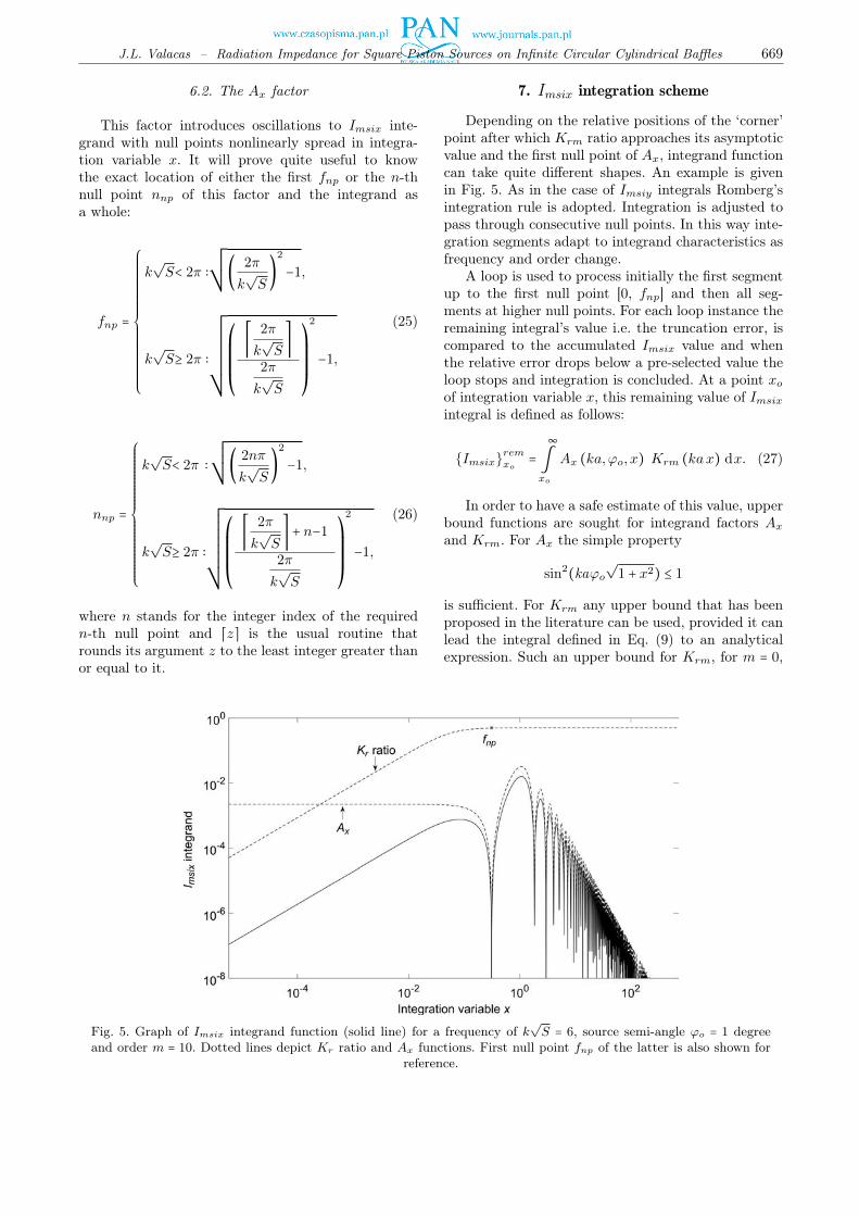
Fig. 5. Graph of Imsix integrand function (solid line) for a frequency of k√

S = 6, source semi-angle ϕo = 1 degreeand order m = 10. Dotted lines depict Kr ratio and Ax functions. First null point fnp of the latter is also shown for

reference.

7. Imsix integration scheme

Depending on the relative positions of the ‘corner’point after which Krm ratio approaches its asymptoticvalue and the first null point of Ax, integrand functioncan take quite different shapes. An example is givenin Fig. 5. As in the case of Imsiy integrals Romberg’sintegration rule is adopted. Integration is adjusted topass through consecutive null points. In this way inte-gration segments adapt to integrand characteristics asfrequency and order change.

A loop is used to process initially the first segmentup to the first null point [0, fnp] and then all seg-ments at higher null points. For each loop instance theremaining integral’s value i.e. the truncation error, iscompared to the accumulated Imsix value and whenthe relative error drops below a pre-selected value theloop stops and integration is concluded. At a point xoof integration variable x, this remaining value of Imsixintegral is defined as follows:

{Imsix}remxo=

∞

∫xo

Ax (ka,ϕo, x) Krm (kax) dx. (27)

In order to have a safe estimate of this value, upperbound functions are sought for integrand factors Axand Krm. For Ax the simple property

sin2(kaϕo√

1 + x2) ≤ 1

is sufficient. For Krm any upper bound that has beenproposed in the literature can be used, provided it canlead the integral defined in Eq. (9) to an analyticalexpression. Such an upper bound for Krm, for m = 0,


is Eq. (23) while for m ≠ 0 the work of Baricz et al.(2011, Eq. (5)) can be utilized:

Krm(y) < 1

2

y√m2 + y2

. (28)

As a result, the remaining Imsix value can be upperbounded by the following integrals:

{Imsix}remxo<

⎧⎪⎪⎪⎪⎪⎪⎪⎪⎪⎨⎪⎪⎪⎪⎪⎪⎪⎪⎪⎩

m= 0 ∶ 12

∞

∫xo

1

a∗x + 1

4ka

x + 34ka

dx,

m≠ 0 ∶ 12

∞

∫xo

xdx

a∗√

(mka

)2 + x2

,

(29)

wherea∗ = ka2ϕ2

o (1 + x2)3/2.

Analytical expressions are obtained and usedwithin the integration process whenever the latterreaches the end of an integration segment:

{Imsix}remxo,m=0 <1

(2ka2 ϕ2o)

⎡⎢⎢⎢⎢⎢⎣

(3q2 + 1) (√

1 + x2o − xo)+2q

(9q2+1)√

1 + x2o

+ 2q

(9q2+1)3/2log

⎛⎜⎝

(√

9q2 + 1−3q) (xo+3q)√

9q2 + 1√

1 + x2o−3qxo + 1

⎞⎟⎠

⎤⎥⎥⎥⎥⎥⎦, (30)

where q = 1/(4ka) and

{Imsix}remxo,m≠0 < 1

(2ka2 ϕ2o)

⋅

⎧⎪⎪⎪⎪⎪⎪⎪⎨⎪⎪⎪⎪⎪⎪⎪⎩

m = ka ∶ 1

2 (1 + x2o),

m≠ka ∶ 1

1 − p2

⎛⎜⎝

1 −

¿ÁÁÀp2+x2

o

1+x2o

⎞⎟⎠,

(31)

where p =m/ka.

Fig. 6. Plot of Imsix sequences for source semi-angles ϕo = 1, 10, and 30 degrees at a frequency k√

S = 0.1 (solid line).Their asymptotes (dashed) are all lines (powers of m) with slope (exponent) equal to −1.

8. Upper bounds of Imsix sequences

When the values of Imsix integrals are plotted asa function of order m in a log-log plot, it can be ob-served that at all frequencies and source semi-anglesunder consideration, they form decreasing sequenceswhich apart from being log-log concave they also haveasymptotes with a slope of −10 dB per decade, i.e. ofthe form: constant/m. Figure 6 illustrates an examplewhich is quite representative of all frequencies.

Using the property of log-log concavity discussedin Appendix B, provides an upper bound for Imsix se-quences above an order ko:

Imsix (m ≥ ko)≤ Imsix(ko) ⋅ (kom

)∣D∣

, (32)

where D is the log-log slope of Imsix sequence at ko(per Eq. (50))

D =⎛⎜⎝

log10 ( Imsix(ko+1)Imsix(ko)

)

log10 (ko+1ko

)

⎞⎟⎠. (33)

9. The Isix sum

Generally speaking, the terms of Isix sum, definedin Eq. (7), oscillate according to the sinc squaredfactor and decay at the same time. Their decay is dueto the inherent 1/m2 decay of the sinc squared factorand the corresponding decay of Imsix sequences. Thelatter was found to tend asymptotically to 1/m. Asa result Isix terms are expected to decay as 1/m3 atvery high orders. As summation advances an effectiveway to conclude it at a specific order with a control-lable truncation error, is to have an estimate of thesum of the remaining infinite terms above that orderand thence of the associated relative truncation error.


When the latter drops below a pre-selected value, thewhole process can be successfully stopped. In orderto apply this idea and after considering several ap-proaches it was decided to work as follows:

• Isix sum is carried initially up to an order ko − 1

where ko = ⌈ 4502ϕo

⌉ and an upper bound of the sumof the remaining terms is estimated in the follow-ing manner:

∞

∑m=ko

Imsix(m) ⋅ sinc2(mϕo)

<∞

∑m=ko

Imsix(ko) ⋅ (kom

)∣D∣

⋅ 1

(mϕo)2

= Imsix(ko) ⋅k∣D∣o

ϕ2o

∞

∑m=ko

1

m2+∣D∣, (34)

where the infinite sum in the right-hand side canbe obtained in several ways by means of Zeta,Hurwitz-Zeta or Lerch special functions. For sim-plicity the use of Zeta function, ζ(s), was selected(Olver et al., 2010, p. 602):

∞

∑m=ko

1

m2+∣D∣= ζ (2 + ∣D∣) −

m=ko−1

∑m=1

1

m2+∣D∣, (35)

where the finite summ=ko−1

∑m=1

1m2+∣D∣ is separately

computed during the integration process.• If the ratio of this upper bound (per Eq. (34)) to

the current value of Isix sum is better (lower) thana target value, the process is concluded, otherwise

Fig. 7. Comparative graph of the radiation reactance of a square piston on an infinite cylinder (solid lines) anda square piston on an infinite plane as per Burnett and Soroka (1972) (circular marks). Results are given

for four source semi-angles.

summation carries on until the relative truncationerror drops below the desired value.

10. Radiation reactance

The results of the previous sections on integralsImsiy and Imsix along with the associated sums inEq. (7) produce the radiation reactance nXmr which isa function of frequency k

√S and source semi-angle ϕo.

Two major conclusions can be drawn:

• In the case of the square piston on an infinitecylinder with a source semi-angle going down tozero (Figs 7 and 8) the values of normalised re-actance tend to the respective values of a square(rectangular) piston on an infinite plane.

• Since low-frequency reactance exhibits a lineardependence on frequency, a mass-load equivalentthat the medium presents to the source can be de-fined as per Beranek (1996, Chap. 5). This massdecreases with increasing semi-angle.

11. Radiation reactance as a mass load

In the field of transducer technology whenevera mechanical reactance is linearly dependent onfrequency an equivalent mass load can be defined andused. For piston sources mounted on baffles of infiniteextent the quotient of radiation reactance Xmr tocyclic frequency ω in the low frequency range wherelinearity is dominant, defines a mass load Mmr in kgr,acting on that side of the vibrating source diaphragmwhere the medium of propagation is located. A nor-


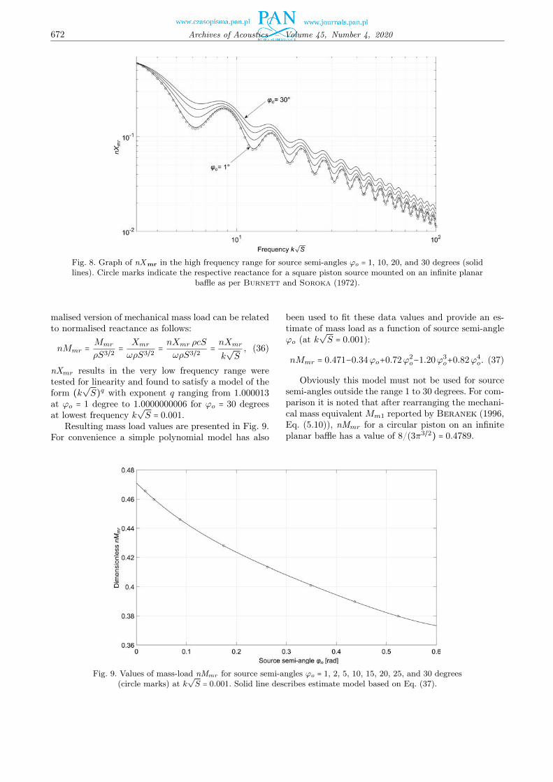
Fig. 8. Graph of nXmr in the high frequency range for source semi-angles ϕo = 1, 10, 20, and 30 degrees (solidlines). Circle marks indicate the respective reactance for a square piston source mounted on an infinite planar

baffle as per Burnett and Soroka (1972).

malised version of mechanical mass load can be relatedto normalised reactance as follows:

nMmr =Mmr

ρS3/2= Xmr

ωρS3/2= nXmr ρcS

ωρS3/2= nXmr

k√S, (36)

nXmr results in the very low frequency range weretested for linearity and found to satisfy a model of theform (k

√S)q with exponent q ranging from 1.000013

at ϕo = 1 degree to 1.0000000006 for ϕo = 30 degreesat lowest frequency k

√S = 0.001.

Resulting mass load values are presented in Fig. 9.For convenience a simple polynomial model has also

Fig. 9. Values of mass-load nMmr for source semi-angles ϕo = 1, 2, 5, 10, 15, 20, 25, and 30 degrees(circle marks) at k

√

S = 0.001. Solid line describes estimate model based on Eq. (37).

been used to fit these data values and provide an es-timate of mass load as a function of source semi-angleϕo (at k

√S = 0.001):

nMmr = 0.471−0.34ϕo+0.72ϕ2o−1.20ϕ3

o+0.82ϕ4o. (37)

Obviously this model must not be used for sourcesemi-angles outside the range 1 to 30 degrees. For com-parison it is noted that after rearranging the mechani-cal mass equivalentMm1 reported by Beranek (1996,Eq. (5.10)), nMmr for a circular piston on an infiniteplanar baffle has a value of 8/(3π3/2) = 0.4789.


12. Evaluation of Imsre integrals

12.1. Integrand’s behaviour

To overcome the singularity of the integrand out-lined in Eq. (4) at the rightmost point of the integra-tion range (t = 1), a change of integration variable isadopted. Setting y =

√1 − t2, Imsre integral becomes:

Imsre =1

∫0

sinc2 ( 12k√S y)

(1 − y2)1

Dm (ka√

1 − y2)dy

=1

∫0

sinc2 (1

2k√S y) Cm(ka, y)dy, (38)

where Cm function is defined as follows:

Cm(ka, y) = 1

(1−y2) Dm (ka√

1 − y2). (39)

Using typical power series for the leading terms ofJ ′m(z) and Y ′

m(z) (Olver et al., 2010, Eqs (10.2.2)and (10.8.1), respectively), it becomes apparent that itis the latter that dominates Dm, as argument z tendsto zero (y tends to one). The limiting behaviour of Cmfor non-zero order m, can therefore be estimated asfollows:

limz→0

Y ′m(z) = −m!

2π(z

2)−m−1

⇒ limz→0

1

Dm(z)

= ( π

m!)

2

(z2)

2m+2

⇒ limy→1

Cm = 0. (40)

Fig. 10. Graphs of Cm factor for three orders, as a function of integration variable y. Frequency isk√

S = 100 and source semi-angle ϕo = 30○. Cm decays just after point y = yp which generally shiftstowards lower values as order m increases.

The case of m = 0 is simpler:

limz→0

Y ′0(z) = lim

z→0−Y1(z)⇒ lim

z→0

1

D0(z)

= (π2)

2

(z2)

2

⇒ limy→1

Cm = (π4ka)

2

. (41)

Conclusively for m ≠ 0 Cm decays rapidly as theintegration variable approaches unity while for m = 0it gets a finite non-zero value. Other interesting prop-erties of factor Cm for non-zero orders m are the fol-lowing:

• When frequency ka = k√S/(2ϕo) is below unity

the decay of Cm starts right after y = 0.• When ka exceeds unity this decay is rapid and

starts approximately just after a certain value ofintegration variable, yp, which depends on orderm and frequency ka:

yp =

⎧⎪⎪⎪⎪⎪⎪⎨⎪⎪⎪⎪⎪⎪⎩

m ≤ ⌊ka⌋ ∶

¿ÁÁÀ1 − ( m

⌊ka⌋)

2

,

m > ⌊ka⌋ ∶ 0.

(42)

• At high frequency values ka and for ordersm lowerthan the integer part of ka, Cm forms a peakaround yp.

• For orders m higher than the integer part of ka,Eq. (42) reports yp = 0 and Cm decays just aftery = 0.

Figure 10 outlines a typical case of Cm factor forseveral orders m.


On the other hand, sinc squared function inEq. (38) is independent of order m and has the fol-lowing features:

• It exhibits oscillations only for frequencies k√S ≥

2π.• Its first null-point within integration range is lo-

cated at yfnp = 2π/k√S.

• Integration range includes nmax null points:nmax = ⌊k

√S/2π⌋.

• Its n-th null-point is at ynnp = nyfnp providedn ≤ nmax.

• Integration variable can not have a null-point atzero but can definitely have one at unity.

12.2. Integration scheme

It is almost impossible to provide a generalised de-scription of the form that Imsre integrand functiontakes within its finite integration range due to the di-versity of its dependencies on frequency k

√S (or ka),

semi-angle ϕo and order m. For this reason it is moreefficient to divide integration range into segments de-fined by critical points. Such points are the null pointsof the sinc-squared oscillations (if any) and yp; the lat-ter possibly being zero form > ⌊ka⌋ or one whenm = 0.It is very practical to use a vector holding these pointsprior to the numerical integration process.

Thorough investigation proved that for m = 0 thisvector is optimum if it takes the generalised form[0, LHSynp, 0.99, RHSynp, 1 − ∂, 1] where:

• LHSynp is the set of all the null points below 0.99and RHSynp the remaining null points above thisvalue and below 1 − ∂).

• The injection of point y = 0.99 resolves the steepincrease of integrand (only form = 0) close to y = 1and is closely related to the required frequencyand semi-angle range of values, in this work.

• A very narrow integration segment is defined atthe end through the use of a very small quantity ∂.Its purpose is to prevent the computation of in-tegrand (and especially of Eq. (39)) very close toor at y = 1 where math software will report errorsrelated to Bessel function of the second kind.

Romberg’s integration rule is then applied to allsegments except for the last one. Fast convergence andhigh precision is achieved. Numerical evaluation of theintegrand remains successful for a value of ∂ as lowas 10−15.

The remaining part of integral (i.e. of the last seg-ment) is evaluated as the area of the trapezoid betweenpoints y = 1 − ∂ and y = 1. Integrand value at y = 1 isanalytically obtained by Eqs (38) and (41).

For m ≠ 0 the only general rule is that integrandexhibits a very steep decay close to y = 1. This wouldnormally allow for the integration to be ended before

reaching the right-hand side integration limit. Unfortu-nately the location of such a point can not be a-prioridetermined for a given level of truncation error to bemaintained. Taking into account that Romberg’s rulecan not be used for a segment with undetermined lim-its, a different approach is adopted:

Vector holding the necessary critical points forRomberg’s rule to apply, is defined as [0, LHSynp, yp,RHSynp, yd], where:

• The newly introduced yd denotes a point at whicha preselected level of decay of Cm factor has oc-curred. The introduction of this point extendsRomberg’s integration close to the end of the over-all integration range leaving a relatively narrowrange to be separately (and rather slowly) han-dled.

• Apparently LHSynp is the set of all possible nullpoints below yp and RHSynp the rest of thesepoints above yp and below yd.

• Since it is already known that point yd is definitelyin the range (yp, 1) its evaluation can easily beachieved via an ordinary bisection method target-ing a Cm value roughly two orders of magnitudeless than the respective value at yp. Experimen-tation proved that there is no need for a biggervalue of Cm decay.

To ensure both low computation time and highaccuracy the remaining integral’s part, above yd, istreated in two phases. In the first one integration ad-vances from yd towards y = 1 in groups of three pointsvia the 1/3 Simpson’s rule and at each step an upperbound of the remaining (truncated) integral’s value isevaluated and a relative error is associated with it. Assoon as the latter drops below a pre-selected value in-tegration is finished and the end-point yf is marked. Inthis way points very close to y = 1 causing evaluationerrors in math software, are avoided. The contributionof this phase to the overall integral is very approxi-mate and therefore should not be stored. In the secondphase Romberg’s method is applied to segment [yd,yf ]and the respective contribution is re-evaluated fast andwith controllable precision.

To ensure that the end-point yf always providesthe pre-selected level of truncation error without se-riously affecting the overall integration time, the firstphase employs a very simple, yet overestimated, upperbound of the integral’s area to be truncated: the prod-uct of the fast-decaying integrand’s value (at the pointat which the truncation error is sought) and the widthof the integration range to be omitted.

13. Sequences of Imsre values

Plotting the resulting Imsre values for a fixed fre-quency k

√S as a function of order m allows for three

major conclusions to be derived (see Fig. 11):


a)

b)

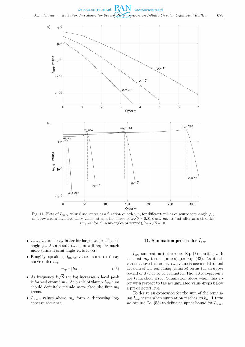
Fig. 11. Plots of Imsre values’ sequences as a function of order m, for different values of source semi-angle ϕo,at a low and a high frequency value: a) at a frequency of k

√

S = 0.01 decay occurs just after zero-th order(mp = 0 for all semi-angles presented), b) k

√

S = 10.

• Imsre values decay faster for larger values of semi-angle ϕo. As a result Isre sum will require muchmore terms if semi-angle ϕo is lower.

• Roughly speaking Imsre values start to decayabove order mp:

mp = ⌊ka⌋ . (43)

• As frequency k√S (or ka) increases a local peak

is formed around mp. As a rule of thumb Isre sumshould definitely include more than the first mp

terms.• Imsre values above mp form a decreasing log-

concave sequence.

14. Summation process for Isre

Isre summation is done per Eq. (3) starting withthe first mp terms (orders) per Eq. (43). As it ad-vances above this order, Isre value is accumulated andthe sum of the remaining (infinite) terms (or an upperbound of it) has to be evaluated. The latter representsthe truncation error. Summation stops when this er-ror with respect to the accumulated value drops belowa pre-selected level.

To derive an expression for the sum of the remain-ing Isre terms when summation reaches its ko −1 termwe can use Eq. (53) to define an upper bound for Imsre


integrals and several quite typical properties of sincfunction. A very practical two-fold upper bound forthe latter can be expressed according to the value ofits argument:

sinc2(kϕo) <

⎧⎪⎪⎪⎪⎨⎪⎪⎪⎪⎩

k < kϕ ∶ 1,

k ≥ kϕ ∶1

(mϕo)2,

(44)

wherekϕ = ⌈ 1

ϕo⌉.

As a result we get an expression for the upperbound of the remaining sum which has to break sum-mation depending on the value of orderm with respectto kϕ:

∞

∑m=ko

Imsre(m) ⋅ sinc2(mϕo)

<

⎧⎪⎪⎪⎪⎪⎪⎪⎪⎪⎪⎪⎪⎪⎪⎪⎪⎨⎪⎪⎪⎪⎪⎪⎪⎪⎪⎪⎪⎪⎪⎪⎪⎪⎩

ko < kϕ ∶kϕ−1

∑m=ko

Imsre (ko) eD(m−ko)

+∞

∑m=kϕ

Imsre (ko) eD(m−ko) 1

(mϕo)2,

ko ≥ kϕ ∶∞

∑m=ko

Imsre (ko) eD(m−ko) 1

(mϕo)2.

(45)Using the Lerch transcendent special function Φ to

hold the required infinite sums for the evaluation ofEq. (45) we end up with the following practical ex-pression:

∞

∑m=ko

Imsre(m) ⋅ sinc2(mϕo)

<

⎧⎪⎪⎪⎪⎪⎪⎪⎪⎪⎪⎪⎪⎪⎪⎨⎪⎪⎪⎪⎪⎪⎪⎪⎪⎪⎪⎪⎪⎪⎩

ko < kϕ ∶ Imsre(ko)eD(kϕ−ko) − 1

eD − 1

+Imsre (ko) eD(kϕ−ko)

ϕ2o

Φ (eD,2, kϕ)

ko ≥ kϕ ∶Imsre(ko)

ϕ2o

Φ (eD,2, ko)

(46)Lerch function is generally defined as the infinite

sum:

Φ(z, n, q) =∞

∑k=0

zk

(k + q)n. (47)

15. Radiation resistance

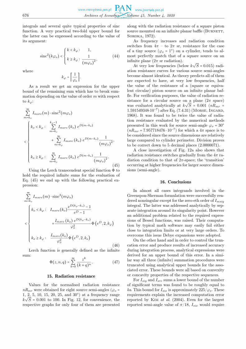
Values for the normalised radiation resistancenRmr were obtained for eight source semi-angles (ϕo =1, 2, 5, 10, 15, 20, 25, and 30○) at a frequency rangek√S = 0.001 to 100. In Fig. 12, for convenience, the

respective graphs for only four of them are presented

along with the radiation resistance of a square pistonsource mounted on an infinite planar baffle (Burnett,Soroka, 1972).

As frequency increases and radiation conditionswitches from 4π – to 2π sr, resistance for the caseof a tiny source (ϕo = 1○) on a cylinder, tends to al-most perfectly match that of a square source on aninfinite plane (2π sr radiation).

At very low frequencies (below k√S = 0.015) radi-

ation resistance curves for various source semi-anglesbecome almost identical. As theory predicts all of themare expected to have, at very low frequencies, halfthe value of the resistance of a (square or equiva-lent circular) piston source on an infinite planar baf-fle. For verification purposes, the value of radiation re-sistance for a circular source on a plane (2π space)was evaluated analytically at k

√S = 0.001 (nRmr =

1.591549348⋅10−7) after Eq. (7.4.31) (Morse, Ingard,1968). It was found to be twice the value of radia-tion resistance evaluated by the numerical methodspresented in this work for source semi-angle ϕo = 30○

(nRmr = 7.957718476 ⋅ 10−7) for which a 4π space is tobe considered since the source dimensions are relativelylarge compared to cylinder perimeter. Division provesto be correct down to 5 decimal places (2.0000071).

A close investigation of Fig. 12a also shows thatradiation resistance switches gradually from the 4π ra-diation condition to that of 2π-space; the ‘transition’occurring at higher frequencies for larger source dimen-sions (semi-angle).

16. Conclusions

In almost all cases integrands involved in theGreenspon-Sherman formulation were successfully ren-dered nonsingular except for the zero-eth order of Imsiyintegral. The latter was addressed analytically by sep-arate integration around its singularity point. Howeveran additional problem related to the required expres-sions of Bessel functions, was raised. Their computa-tion by typical math software may easily fail eitherclose to integration limits or at very large orders. Toovercome this issue Debye expansions were adopted.

On the other hand and in order to control the trun-cation error and produce results of increased accuracyduring integration process, analytical expressions werederived for an upper bound of this error. In a simi-lar way all three (infinite) summation procedures weretruncated using analytical upper bounds for the asso-ciated error. These bounds were all based on convexityor concavity properties of the respective sequences.

For Isiy and Isre sums a lower bound of the numberof significant terms was found to be roughly equal toka. This bound for Isix is approximately 225/ϕo. Theserequirements explain the increased computation errorreported by Kim at al. (2004). Even for the largestreported semi-angle value of π/18, Isix would require


a)

b)

c)

Fig. 12. Normalised radiation resistance nRmr of a square piston on an infinite cylindrical baffle for various source semi-angles ϕo as a function of frequency variable k

√

S. Circle marks correspond to a square piston source mounted on aninfinite planar baffle as per Burnett and Soroka (1972): a) very low frequency range; radiation condition changes from4π to 2π sr at lower frequencies for smaller source semi-angles; b) mid-frequency range; resistance values for a squarepiston on a planar baffle (circle marks) behaves as an asymptote for sources on a cylinder with semi-angles tending to

zero; c) high-frequency range.


more than 1000 terms. The use of orders up to m = 50even for the relatively low frequency range, ka < 51,was not sufficient.

Resulting reactance values in the low frequencyrange were used to derive a model of a radiation mass-load as a function of source semi-angle (Fig. 9). For thefirst time a clear picture of the decaying oscillations ofnormalised reactance at high frequencies was also ob-tained (Fig. 8). As expected when source semi-angle(and thence the source size) tends to zero these valuestend to coincide with the respective values of a squarepiston on a planar baffle as they share a common half-space radiation condition and shape as well.

In the case of radiation resistance results showedthat each source semi-angle features its own transitionfrequency above which the 2π condition is gradually es-tablished by the surface of the cylindrical baffle aroundthe source (Fig. 12). As in the case of reactance whensource semi-angle approaches zero, resistance valuescoincide with those of the square piston on a planarbaffle.

Impedance values as a function of normalised fre-quency and source semi-angle were tabulated for con-venience (Valacas, 2020). In order for the relativeprecision of radiation resistance to be always betterthan 10−5, maximum truncation errors for Imsre inte-gral and Isre sum were set to 10−7 and 10−6 respec-tively. Romberg’s integration routine was adjusted toexit when a relative change of 10−7 is achieved. Dueto extremely high computation time the target rela-tive error for radiation reactance values was reduced to10−4. For this purpose the maximum truncation errorfor Imsix integrals was set to 10−6 and for the associ-ated Isix, Isiy sums to 10−5.

In their tabulated form the derived impedance val-ues can be easily related to the design of acoustic emis-sion systems where sources of square (and with a rathergood degree of accuracy, of circular) shape are mountedon acoustically-hard cylindrical surfaces as in the caseof sonar transducers.

Appendix A

A decreasing log-log convex sequence b(n) of posi-tive terms that above an index no has an asymptote ofknown (log-log) negative slope D, is expected to decayfaster than the line g(n) that intersects b(n) at no andis parallel to the asymptote:

g (n ≥ no) = b(no) (non

)∣D∣

. (48)

As a result all terms of b(n) have values less thanthe respective terms of g(n) above no:

∀n ≥ no, b(n) ≤ b(no) (non

)∣D∣

. (49)

Appendix B

Decreasing log-log concave sequences b(n) (of pos-itive terms) above an index no are known to decayfaster than the tangent line g(n) that ‘touches’ b(n)at no and has the same slope with b(n) at no. In orderfor sequence g(n) to maintain the linear form in a log-log plot, it has to be proportional to an inverse powerof n as per Eq. (48) with D as the negative slope ofsequence b(n) at no:

D =⎛⎜⎝

log10 ( b(no+1b(no)

)

log10 (no+1no

)

⎞⎟⎠. (50)

It can therefore be stated that g(n) serves as anupper bound of b(n) above no as per Eq. (49).

Appendix C

In the case of a decreasing sequence b(n) (of pos-itive terms) which above an index no exhibits log-concavity we can define its tangent line g(n), at no anduse it as an upper bound for sequence b(n) above no.For sequence g(n) to exhibit the linear form in a logplot and at the same time be tangent to b(n) at no, itmust be of an exponential type:

g(n ≥ no) = b(no)eD(n−no), (51)

where D stands for the logarithmic slope of g(n) (andb(n)) at no:

D = ln(b(no + 1)b(no)

) . (52)

Although log-concave sequences and their tangentlines can be described with logarithms of any base, thenatural logarithm and its associated base were selectedin this work for convenience.

As before it can be asserted that values of b(n)sequence, above no, are bounded as follows:

b(n ≥ no) ≤ b(no) eD(n−no). (53)

References

1. Arase E.M. (1964), Mutual radiation impedance ofsquare and rectangular pistons in a rigid infinite baffle,The Journal of Acoustical Society of America, 36(8):1521–1525, doi: 10.1121/1.1919236.

2. Bank G., Wright J.R. (1990), Radiation impedancecalculations for a rectangular piston, Journal of theAudio Engineering Society, 38: 350–354.

3. Baricz Á., Ponnusamy S., Vuorinen M. (2011),Functional inequalities for modified Bessel func-tions, Expositiones Mathematicae, 29(4): 399–414, doi:10.1016/j.exmath.2011.07.001.

4. Beranek L.L. (1996), Acoustics, Acoustical Societyof America, Cambridge, MA.


5. Burnett D.S., Soroka W.W. (1972), Tables of rect-angular piston radiation impedance functions, with ap-plication to sound transmission loss through deep aper-tures, The Journal of Acoustical Society of America,51(5B): 1618–1623, doi: 10.1121/1.1913008.

6. Greenspon J.E., Sherman C.H. (1964), Mutual-radiation impedance and nearfield pressure for pistonson a cylinder, The Journal of Acoustical Society ofAmerica, 36(1): 149–153, doi: 10.1121/1.1918925.

7. Kim J.S., Kim M.J., Ha K.L., Kim C.D. (2004),Improvement of calculation for radiation impedanceof the vibrators with cylindrical baffle, JapaneseJournal of Applied Physics, 43(5B): 3188–3192, doi:10.1143/JJAP.43.3188.

8. Lee J., Seo I. (1996), Radiation impedance compu-tations of a square piston in a rigid infinite baffle,Journal of Sound and Vibration, 198(3): 299–312, doi:10.1006/jsvi.1996.0571.

9. Levine H. (1983), On the radiation impedance of arectangular piston, Journal of Sound and Vibration,89(4): 447–455, doi: 10.1016/0022-460X(83)90346-2.

10. Mellow T., Kärkkäinen L. (2016), Expansions forthe radiation impedance of a rectangular piston in aninfinite baffle, The Journal of Acoustical Society ofAmerica, 140(4): 2867–2875, doi: 10.1121/1.4964632.

11. Morse P.M., Ingard K.U. (1968), TheoreticalAcoustics, Princeton University Press, Princeton, NewJersey.

12. Olver F.W.J., Lozier D.W., Boisvert R.F.,Clark C.W. [Eds], (2010), NIST Handbook of Math-ematical Functions, NIST & Cambridge UniversityPress.

13. Stepanishen P.R. (1977), The radiation impedance ofa rectangular piston, Journal of Sound and Vibration,55(2): 275–288, doi: 10.1016/0022-460X(77)90599-5.

14. Swenson G.W., Johnson W.E. (1952), Radiationimpedance of a rigid square piston in an infinite baffle,The Journal of Acoustical Society of America, 24(1):84, doi: 10.1121/1.1906856.

15. Valacas J. (2020), Tabulated values for radiationimpedance of a square piston source on a cir-cular cylindrical baffle, Mendeley Data Repository,http://dx.doi.org/10.17632/rvwffybpdw.3.

16. Watson G.N. (1966), A Treatise on the theory ofBessel Functions, 2nd Ed., Cambridge UniversityPress.

17. Yang Z.H., Chu Y.M. (2017), On approximat-ing the modified Bessel function of the second kind,Journal of Inequalities and Applications, 1: 1–8, doi:10.1186/s13660-017-1317-z.

radiation impedance for square piston sources on infinite

Documents