Femtosecond Laser Pulses

Claude Rulliere (Ed.)

FemtosecondLaser PulsesPrinciples and Experiments

Second Edition

With 296 Figures, Including 3 Color Plates,and Numerous Experiments

Professor Dr. Claude RulliereCentre de Physique Moleeculaire Optique et Hertzienne (CPMOH)Universite Bordeaux 1351, cours de la Liberation33405 TALENCE CEDEX, France

and

Commissariat a l’Energie Aromique (CEA)Centre d’Etudes Scientifiques et Techniques d’AquitarineBP 233114 LE BARP, France

Library of Congress Cataloging-in-Publication DataFemtosecond laser pulses: principles and experiments / Claude Rulliere, (ed.). – [2nd ed.].

p. cm. – (Advanced texts in physics, ISSN 1439-2674)Includes bibliographical references and index.ISBN 3-387-01769-0 (acid-free paper)

1. Laser pulses, Ultrashort. 2. Nonlinear optics. I. Rulliere, Claude, 1947– . II. Series.QC689.5L37F46 2003621.36’6—dc22 2003062207

ISBN 0-387-01769-0 Printed on acid-free paper.

c© 2005 Springer Science+Business Media, Inc.All rights reserved. This work may not be translated or copied in whole or in part withoutthe written permission of the publisher (Springer Science+Business Media, Inc., 233 SpringStreet, New York, NY 10013, USA), except for brief excerpts in connection with reviewsor scholarly analysis. Use in connection with any form of information storage and retrieval,electronic adaptation, computer software, or by similar or dissimilar methodology nowknown or hereafter developed is forbidden.The use in this publication of trade names, trademarks, service marks, and similar terms,even if they are not identified as such, is not to be taken as an expression of opinion as towhether or not they are subject to proprietary rights.

Printed in the United States of America.

9 8 7 6 5 4 3 2 1 SPIN 10925751

springeronline.com

Preface

This is the second edition of this advanced textbook written for scientistswho require further training in femtosecond science. Four years after publi-cation of the first edition, femtosecond science has overcome new challengesand new application fields have become mature. It is necessary to take intoaccount these new developments. Two main topics merged during this periodthat support important scientific activities: attosecond pulses are now gener-ated in the X-UV spectral domain, and coherent control of chemical eventsis now possible by tailoring the shape of femtosecond pulses. To update thisadvanced textbook, it was necessary to introduce these fields; two new chap-ters are in this second edition: “Coherent Control in Atoms, Molecules, andSolids” (Chap. 11) and “Attosecond Pulses” (Chap. 12) with well-documentedreferences.

Some changes, addenda, and new references are introduced in the firstedition’s ten original chapters to take into account new developments andupdate this advanced textbook which is the result of a scientific adventure thatstarted in 1991. At that time, the French Ministry of Education decided that,in view of the growing importance of ultrashort laser pulses for the nationalscientific community, a Femtosecond Centre should be created in France anddevoted to the further education of scientists who use femtosecond pulses asa research tool and who are not specialists in lasers or even in optics.

After proposals from different institutions, Universite Bordeaux I and ourlaboratory were finally selected to ensure the success of this new centre. Sincethe scientists involved were located throughout France, it was decided that thetraining courses should be concentrated into a short period of at least 5 days. Itis certainly a challenge to give a good grounding in the science of femtosecondpulses in such a short period to scientists who do not necessarily have therequired scientific background and are in some cases involved only as usersof these pulses as a tool. To start, we contacted well-known specialists fromthe French femtosecond community; we are very thankful that they showedenthusiasm and immediately started work on this fascinating project.

vi Preface

Our adventure began in 1992 and each year since, generally in spring,we have organized a one-week femtosecond training course at the BordeauxUniversity. Each morning of the course is devoted to theoretical lectures con-cerning different aspects of femtosecond pulses; the afternoons are spent in thelaboratory, where a very simple experimental demonstration illustrates eachpoint developed in the morning lectures. At the end of the afternoon, thesaturation threshold of the attendees is generally reached, so the evenings aredevoted to discovering Bordeaux wines and vineyards, which helps the other-wise shy attendees enter into discussions concerning femtosecond science.

A document including all the lectures is always distributed to the partici-pants. Step by step this document has been improved as a result of feedbackfrom the attendees and lecturers, who were forced to find pedagogic answersto the many questions arising during the courses. The result is a very com-prehensive textbook that we decided to make available to the wider scientificcommunity; i.e., the result is this book.

The people who will gain the most from this book are the scientists (grad-uate students, engineers, researchers) who are not necessarily trained as laserscientists but who want to use femtosecond pulses and/or gain a real under-standing of this tool. Laser specialists will also find the book useful, particu-larly if they have to teach the subject to graduate or PhD students. For everyreader, this book provides a simple progressive and pedagogic approach tothis field. It is particularly enhanced by the descriptions of basic experimentsor exercises that can be used for further study or practice.

The first chapter simply recalls the basic laser principles necessary to un-derstand the generation process of ultrashort pulses. The second chapter is abrief introduction to the basics behind the experimental problems generatedby ultrashort laser pulses when they travel through different optical devicesor samples. Chapter 3 describes how ultrashort pulses are generated indepen-dently of the laser medium. In Chaps. 4 and 5 the main laser sources usedto generate ultrashort laser pulses and their characteristics are described.Chapter 6 presents the different methods currently used to characterize thesepulses, and Chap. 7 describes how to change these characteristics (pulse dura-tion, amplification, wavelength tuning, etc.). The rest of the book is devotedto applications, essentially the different experimental methods based on theuse of ultrashort laser pulses. Chapter 8 describes the principal spectroscopicmethods, presenting some typical results, and Chap. 9 addresses mainly theproblems that may arise when the pulse duration is as short as the coherencetime of the sample being studied. Chapter 10 describes typical applicationsof ultrashort laser pulses for the characterisation of electronic devices and theelectromagnetic pulses generated at low frequency. Chapter 11 is an overviewof the coherent control physical processes making it possible to control evo-lution channels in atoms, molecules and solids. Several examples of orientedreactions in this chapter illustrate the possible applications of such a tech-nique. Chapter 12 introduces the attosecond pulse generation by femtosecondpulse-matter interaction. It is designed for a best understanding of the physics

Preface vii

principles sustaining attosecond pulse creation as well as the encountered dif-ficulties in such processes.

I would like to acknowledge all persons and companies whose names donot directly appear in this book but whose participation has been essentialto the final goal of this adventure. My colleague Gediminas Jonusauskas wasgreatly involved in the design of the experiments presented during the coursesand at the end of the chapters in this book. Daniele Hulin, Jean-Rene Lalanneand Arnold Migus gave much time during the initial stages, particularly inwriting the first version of the course document. The publication of this bookwould not have been possible without their important support and contri-bution. My colleagues Eric Freysz, Francois Dupuy, Frederic Adamietz andPatricia Segonds also participated in the organization of the courses, as did thepost-doc and PhD students Anatoli Ivanov, Corinne Rajchenbach, EmmanuelAbraham, Bruno Chassagne and Benoit Lourdelet.

Essential financial support and participation in the courses, particularlyby the loan of equipment, came from the following laser or optics companies:B.M. Industries, Coherent France, Hamamatsu France, A.R.P. Photonetics,Spectra-Physics France, Optilas, Continuum France, Princeton InstrumentsSA and Quantel France.

I hope that every reader will enjoy reading this book. The best result wouldbe if they conclude that femtosecond pulses are wonderful tools for scientificinvestigation and want to use them and know more.

Bordeaux, April 2004 Claude Rulliere

Contents

Preface . . . . . . . . . . . . . . . . . . . . . . . . . . . . . . . . . . . . . . . . . . . . . . . . . . . . . . . . v

Contributors . . . . . . . . . . . . . . . . . . . . . . . . . . . . . . . . . . . . . . . . . . . . . . . . . . . xv

1 Laser BasicsC. Hirlimann . . . . . . . . . . . . . . . . . . . . . . . . . . . . . . . . . . . . . . . . . . . . . . . . . . . . 11.1 Introduction . . . . . . . . . . . . . . . . . . . . . . . . . . . . . . . . . . . . . . . . . . . . . . . . . 11.2 Stimulated Emission . . . . . . . . . . . . . . . . . . . . . . . . . . . . . . . . . . . . . . . . . . 1

1.2.1 Absorption . . . . . . . . . . . . . . . . . . . . . . . . . . . . . . . . . . . . . . . . . . . . . 31.2.2 Spontaneous Emission . . . . . . . . . . . . . . . . . . . . . . . . . . . . . . . . . . . . 31.2.3 Stimulated Emission . . . . . . . . . . . . . . . . . . . . . . . . . . . . . . . . . . . . . 4

1.3 Light Amplification by Stimulated Emission . . . . . . . . . . . . . . . . . . . . . 41.4 Population Inversion . . . . . . . . . . . . . . . . . . . . . . . . . . . . . . . . . . . . . . . . . . 5

1.4.1 Two-Level System . . . . . . . . . . . . . . . . . . . . . . . . . . . . . . . . . . . . . . . 51.4.2 Optical Pumping . . . . . . . . . . . . . . . . . . . . . . . . . . . . . . . . . . . . . . . . 61.4.3 Light Amplification . . . . . . . . . . . . . . . . . . . . . . . . . . . . . . . . . . . . . . 8

1.5 Amplified Spontaneous Emission (ASE) . . . . . . . . . . . . . . . . . . . . . . . . . 101.5.1 Amplifier Decoupling . . . . . . . . . . . . . . . . . . . . . . . . . . . . . . . . . . . . . 11

1.6 The Optical Cavity . . . . . . . . . . . . . . . . . . . . . . . . . . . . . . . . . . . . . . . . . . . 131.6.1 The Fabry–Perot Interferometer . . . . . . . . . . . . . . . . . . . . . . . . . . . 131.6.2 Geometric Point of View . . . . . . . . . . . . . . . . . . . . . . . . . . . . . . . . . 141.6.3 Diffractive-Optics Point of View . . . . . . . . . . . . . . . . . . . . . . . . . . . 151.6.4 Stability of a Two-Mirror Cavity . . . . . . . . . . . . . . . . . . . . . . . . . . 171.6.5 Longitudinal Modes . . . . . . . . . . . . . . . . . . . . . . . . . . . . . . . . . . . . . . 20

1.7 Here Comes the Laser! . . . . . . . . . . . . . . . . . . . . . . . . . . . . . . . . . . . . . . . . 221.8 Conclusion . . . . . . . . . . . . . . . . . . . . . . . . . . . . . . . . . . . . . . . . . . . . . . . . . . 221.9 Problems . . . . . . . . . . . . . . . . . . . . . . . . . . . . . . . . . . . . . . . . . . . . . . . . . . . . 22Further Reading . . . . . . . . . . . . . . . . . . . . . . . . . . . . . . . . . . . . . . . . . . . . . . . . . 23Historial References . . . . . . . . . . . . . . . . . . . . . . . . . . . . . . . . . . . . . . . . . . . . . . 23

x Contents

2 Pulsed OpticsC. Hirlimann . . . . . . . . . . . . . . . . . . . . . . . . . . . . . . . . . . . . . . . . . . . . . . . . . . . . 252.1 Introduction . . . . . . . . . . . . . . . . . . . . . . . . . . . . . . . . . . . . . . . . . . . . . . . . . 252.2 Linear Optics . . . . . . . . . . . . . . . . . . . . . . . . . . . . . . . . . . . . . . . . . . . . . . . . 26

2.2.1 Light . . . . . . . . . . . . . . . . . . . . . . . . . . . . . . . . . . . . . . . . . . . . . . . . . . 262.2.2 Light Pulses . . . . . . . . . . . . . . . . . . . . . . . . . . . . . . . . . . . . . . . . . . . . 282.2.3 Relationship Between Duration and Spectral Width . . . . . . . . . . 302.2.4 Propagation of a Light Pulse in a Transparent Medium . . . . . . . 32

2.3 Nonlinear Optics . . . . . . . . . . . . . . . . . . . . . . . . . . . . . . . . . . . . . . . . . . . . . 382.3.1 Second-Order Susceptibility . . . . . . . . . . . . . . . . . . . . . . . . . . . . . . . 382.3.2 Third-Order Susceptibility . . . . . . . . . . . . . . . . . . . . . . . . . . . . . . . . 45

2.4 Cascaded Nonlinearities . . . . . . . . . . . . . . . . . . . . . . . . . . . . . . . . . . . . . . . 532.5 Problems . . . . . . . . . . . . . . . . . . . . . . . . . . . . . . . . . . . . . . . . . . . . . . . . . . . . 55Further Reading . . . . . . . . . . . . . . . . . . . . . . . . . . . . . . . . . . . . . . . . . . . . . . . . . 56References . . . . . . . . . . . . . . . . . . . . . . . . . . . . . . . . . . . . . . . . . . . . . . . . . . . . . . 56

3 Methods for the Generation of Ultrashort Laser Pulses:Mode-LockingA. Ducasse, C. Rulliere and B. Couillaud . . . . . . . . . . . . . . . . . . . . . . . . . . . 573.1 Introduction . . . . . . . . . . . . . . . . . . . . . . . . . . . . . . . . . . . . . . . . . . . . . . . . . 573.2 Principle of the Mode-Locked Operating Regime . . . . . . . . . . . . . . . . . 603.3 General Considerations Concerning Mode-Locking . . . . . . . . . . . . . . . . 663.4 The Active Mode-Locking Method . . . . . . . . . . . . . . . . . . . . . . . . . . . . . . 673.5 Passive and Hybrid Mode-Locking Methods . . . . . . . . . . . . . . . . . . . . . . 743.6 Self-Locking of the Modes . . . . . . . . . . . . . . . . . . . . . . . . . . . . . . . . . . . . . 81References . . . . . . . . . . . . . . . . . . . . . . . . . . . . . . . . . . . . . . . . . . . . . . . . . . . . . . 87

4 Further Methods for the Generation of UltrashortOptical PulsesC. Hirlimann . . . . . . . . . . . . . . . . . . . . . . . . . . . . . . . . . . . . . . . . . . . . . . . . . . . . 894.1 Introduction . . . . . . . . . . . . . . . . . . . . . . . . . . . . . . . . . . . . . . . . . . . . . . . . . 89

4.1.1 Time–Frequency Fourier Relationship . . . . . . . . . . . . . . . . . . . . . . 894.2 Gas Lasers . . . . . . . . . . . . . . . . . . . . . . . . . . . . . . . . . . . . . . . . . . . . . . . . . . 91

4.2.1 Mode-Locking . . . . . . . . . . . . . . . . . . . . . . . . . . . . . . . . . . . . . . . . . . . 924.2.2 Pulse Compression . . . . . . . . . . . . . . . . . . . . . . . . . . . . . . . . . . . . . . . 92

4.3 Dye Lasers . . . . . . . . . . . . . . . . . . . . . . . . . . . . . . . . . . . . . . . . . . . . . . . . . . 944.3.1 Synchronously Pumped Dye Lasers . . . . . . . . . . . . . . . . . . . . . . . . 944.3.2 Passive Mode-Locking . . . . . . . . . . . . . . . . . . . . . . . . . . . . . . . . . . . . 964.3.3 Really Short Pulses . . . . . . . . . . . . . . . . . . . . . . . . . . . . . . . . . . . . . . 1014.3.4 Hybrid Mode-Locking . . . . . . . . . . . . . . . . . . . . . . . . . . . . . . . . . . . . 1024.3.5 Wavelength Tuning . . . . . . . . . . . . . . . . . . . . . . . . . . . . . . . . . . . . . . 104

4.4 Solid-State Lasers . . . . . . . . . . . . . . . . . . . . . . . . . . . . . . . . . . . . . . . . . . . . 1064.4.1 The Neodymium Ion . . . . . . . . . . . . . . . . . . . . . . . . . . . . . . . . . . . . . 1064.4.2 The Titanium Ion . . . . . . . . . . . . . . . . . . . . . . . . . . . . . . . . . . . . . . . 1074.4.3 F -Centers . . . . . . . . . . . . . . . . . . . . . . . . . . . . . . . . . . . . . . . . . . . . . . 109

Contents xi

4.4.4 Soliton Laser . . . . . . . . . . . . . . . . . . . . . . . . . . . . . . . . . . . . . . . . . . . . 1094.5 Pulse Generation Without Mode-Locking . . . . . . . . . . . . . . . . . . . . . . . . 111

4.5.1 Distributed Feedback Dye Laser (DFDL) . . . . . . . . . . . . . . . . . . . 1114.5.2 Traveling-Wave Excitation . . . . . . . . . . . . . . . . . . . . . . . . . . . . . . . . 1124.5.3 Space–Time Selection . . . . . . . . . . . . . . . . . . . . . . . . . . . . . . . . . . . . 1124.5.4 Quenched Cavity . . . . . . . . . . . . . . . . . . . . . . . . . . . . . . . . . . . . . . . . 113

4.6 New Developments . . . . . . . . . . . . . . . . . . . . . . . . . . . . . . . . . . . . . . . . . . . 1144.6.1 Diode Pumped Lasers . . . . . . . . . . . . . . . . . . . . . . . . . . . . . . . . . . . . 1144.6.2 Femtosecond Fibber Lasers . . . . . . . . . . . . . . . . . . . . . . . . . . . . . . . 1144.6.3 Femtosecond Diode Lasers . . . . . . . . . . . . . . . . . . . . . . . . . . . . . . . . 1154.6.4 New Gain Materials . . . . . . . . . . . . . . . . . . . . . . . . . . . . . . . . . . . . . . 117

4.7 Trends . . . . . . . . . . . . . . . . . . . . . . . . . . . . . . . . . . . . . . . . . . . . . . . . . . . . . . 118References . . . . . . . . . . . . . . . . . . . . . . . . . . . . . . . . . . . . . . . . . . . . . . . . . . . . . . 119

5 Pulsed Semiconductor LasersT. Amand and X. Marie . . . . . . . . . . . . . . . . . . . . . . . . . . . . . . . . . . . . . . . . . . 1255.1 Introduction . . . . . . . . . . . . . . . . . . . . . . . . . . . . . . . . . . . . . . . . . . . . . . . . . 1255.2 Semiconductor Lasers: Principle of Operation . . . . . . . . . . . . . . . . . . . . 126

5.2.1 Semiconductor Physics Background . . . . . . . . . . . . . . . . . . . . . . . . 1265.2.2 pn Junction – Homojunction Laser . . . . . . . . . . . . . . . . . . . . . . . . 129

5.3 Semiconductor Laser Devices . . . . . . . . . . . . . . . . . . . . . . . . . . . . . . . . . . 1315.3.1 Double-Heterostructure Laser . . . . . . . . . . . . . . . . . . . . . . . . . . . . . 1325.3.2 Quantum Well Lasers . . . . . . . . . . . . . . . . . . . . . . . . . . . . . . . . . . . . 1375.3.3 Strained Quantum Well and Vertical-Cavity Surface-Emitting

Lasers . . . . . . . . . . . . . . . . . . . . . . . . . . . . . . . . . . . . . . . . . . . . . . . . . . 1395.4 Semiconductor Lasers in Pulsed-Mode Operation . . . . . . . . . . . . . . . . . 141

5.4.1 Gain-Switched Operation . . . . . . . . . . . . . . . . . . . . . . . . . . . . . . . . . 1435.4.2 Q-Switched Operation . . . . . . . . . . . . . . . . . . . . . . . . . . . . . . . . . . . . 1505.4.3 Mode-Locked Operation . . . . . . . . . . . . . . . . . . . . . . . . . . . . . . . . . . 1595.4.4 Mode-Locking by Gain Modulation . . . . . . . . . . . . . . . . . . . . . . . . 1605.4.5 Mode-Locking by Loss Modulation: Passive Mode-Locking by

Absorption Saturation . . . . . . . . . . . . . . . . . . . . . . . . . . . . . . . . . . . 1635.4.6 Prospects for Further Developments . . . . . . . . . . . . . . . . . . . . . . . . 170

References . . . . . . . . . . . . . . . . . . . . . . . . . . . . . . . . . . . . . . . . . . . . . . . . . . . . . . 172

6 How to Manipulate and Change the Characteristics ofLaser PulsesF. Salin . . . . . . . . . . . . . . . . . . . . . . . . . . . . . . . . . . . . . . . . . . . . . . . . . . . . . . . . 1756.1 Introduction . . . . . . . . . . . . . . . . . . . . . . . . . . . . . . . . . . . . . . . . . . . . . . . . . 1756.2 Pulse Compression . . . . . . . . . . . . . . . . . . . . . . . . . . . . . . . . . . . . . . . . . . . 1756.3 Amplification . . . . . . . . . . . . . . . . . . . . . . . . . . . . . . . . . . . . . . . . . . . . . . . . 1786.4 Wavelength Tunability . . . . . . . . . . . . . . . . . . . . . . . . . . . . . . . . . . . . . . . . 185

6.4.1 Second- and Third-Harmonic Generation . . . . . . . . . . . . . . . . . . . 1866.4.2 Optical Parametric Generators (OPGs) and Amplifiers (OPAs) 187

6.5 Conclusion . . . . . . . . . . . . . . . . . . . . . . . . . . . . . . . . . . . . . . . . . . . . . . . . . . 192

xii Contents

6.6 Problems . . . . . . . . . . . . . . . . . . . . . . . . . . . . . . . . . . . . . . . . . . . . . . . . . . . . 192References . . . . . . . . . . . . . . . . . . . . . . . . . . . . . . . . . . . . . . . . . . . . . . . . . . . . . . 193

7 How to Measure the Characteristics of Laser PulsesL. Sarger and J. Oberle . . . . . . . . . . . . . . . . . . . . . . . . . . . . . . . . . . . . . . . . . . . 1957.1 Introduction . . . . . . . . . . . . . . . . . . . . . . . . . . . . . . . . . . . . . . . . . . . . . . . . . 1957.2 Energy Measurements . . . . . . . . . . . . . . . . . . . . . . . . . . . . . . . . . . . . . . . . . 1967.3 Power Measurements . . . . . . . . . . . . . . . . . . . . . . . . . . . . . . . . . . . . . . . . . 1977.4 Measurement of the Pulse Temporal Profile . . . . . . . . . . . . . . . . . . . . . . 198

7.4.1 Pure Electronic Methods . . . . . . . . . . . . . . . . . . . . . . . . . . . . . . . . . 1987.4.2 All-Optical Methods . . . . . . . . . . . . . . . . . . . . . . . . . . . . . . . . . . . . . 202

7.5 Spectral Measurements . . . . . . . . . . . . . . . . . . . . . . . . . . . . . . . . . . . . . . . . 2157.6 Amplitude–Phase Measurements . . . . . . . . . . . . . . . . . . . . . . . . . . . . . . . 216

7.6.1 FROG Technique . . . . . . . . . . . . . . . . . . . . . . . . . . . . . . . . . . . . . . . . 2177.6.2 Frequency Gating . . . . . . . . . . . . . . . . . . . . . . . . . . . . . . . . . . . . . . . 2187.6.3 Spectal Interferometry and SPIDER . . . . . . . . . . . . . . . . . . . . . . . 219

References . . . . . . . . . . . . . . . . . . . . . . . . . . . . . . . . . . . . . . . . . . . . . . . . . . . . . . 221

8 Spectroscopic Methods for Analysis of Sample DynamicsC. Rulliere, T. Amand and X. Marie . . . . . . . . . . . . . . . . . . . . . . . . . . . . . . . 2238.1 Introduction . . . . . . . . . . . . . . . . . . . . . . . . . . . . . . . . . . . . . . . . . . . . . . . . . 2238.2 “Pump–Probe” Methods . . . . . . . . . . . . . . . . . . . . . . . . . . . . . . . . . . . . . . 224

8.2.1 General Principles . . . . . . . . . . . . . . . . . . . . . . . . . . . . . . . . . . . . . . . 2248.2.2 Time-Resolved Absorption in the UV–Visible Spectral Domain 2258.2.3 Time-Resolved Absorption in the IR Spectral Domain . . . . . . . . 2338.2.4 Pump–Probe Induced Fluorescence . . . . . . . . . . . . . . . . . . . . . . . . 2358.2.5 Probe-Induced Raman Scattering . . . . . . . . . . . . . . . . . . . . . . . . . . 2378.2.6 Coherent Anti-Stokes Raman Scattering (CARS) . . . . . . . . . . . . 241

8.3 Time-Resolved Emission Spectroscopy: Electronic Methods . . . . . . . . 2498.3.1 Broad-Bandwidth Photodetectors . . . . . . . . . . . . . . . . . . . . . . . . . . 2508.3.2 The Streak Camera . . . . . . . . . . . . . . . . . . . . . . . . . . . . . . . . . . . . . . 2508.3.3 “Single”-Photon Counting . . . . . . . . . . . . . . . . . . . . . . . . . . . . . . . . 250

8.4 Time-Resolved Emission Spectroscopy: Optical Methods . . . . . . . . . . . 2528.4.1 The Kerr Shutter . . . . . . . . . . . . . . . . . . . . . . . . . . . . . . . . . . . . . . . . 2528.4.2 Up-conversion Method . . . . . . . . . . . . . . . . . . . . . . . . . . . . . . . . . . . 255

8.5 Time-Resolved Spectroscopy by Excitation Correlation . . . . . . . . . . . . 2608.5.1 Experimental Setup . . . . . . . . . . . . . . . . . . . . . . . . . . . . . . . . . . . . . . 2618.5.2 Interpretation of the Correlation Signal . . . . . . . . . . . . . . . . . . . . . 2628.5.3 Example of Application . . . . . . . . . . . . . . . . . . . . . . . . . . . . . . . . . . 263

8.6 Transient-Grating Techniques . . . . . . . . . . . . . . . . . . . . . . . . . . . . . . . . . . 2648.6.1 Principle of the Method: Degenerate Four-Wave Mixing

(DFWM) . . . . . . . . . . . . . . . . . . . . . . . . . . . . . . . . . . . . . . . . . . . . . . . 2648.6.2 Example of Application: t-Stilbene Molecule . . . . . . . . . . . . . . . . 2668.6.3 Experimental Tricks . . . . . . . . . . . . . . . . . . . . . . . . . . . . . . . . . . . . . 269

8.7 Studies Using the Kerr Effect . . . . . . . . . . . . . . . . . . . . . . . . . . . . . . . . . . 270

Contents xiii

8.7.1 Kerr “Ellipsometry” . . . . . . . . . . . . . . . . . . . . . . . . . . . . . . . . . . . . . 2708.8 Laboratory Demonstrations . . . . . . . . . . . . . . . . . . . . . . . . . . . . . . . . . . . . 273

8.8.1 How to Demonstrate Pump–Probe Experiments Directly . . . . . 2738.8.2 How to Observe Generation of a CARS Signal by Eye . . . . . . . . 2768.8.3 How to Build a Kerr Shutter Easily for Demonstration . . . . . . . 2788.8.4 How to Observe a DFWM Diffraction Pattern Directly . . . . . . . 279

References . . . . . . . . . . . . . . . . . . . . . . . . . . . . . . . . . . . . . . . . . . . . . . . . . . . . . . 280

9 Coherent Effects in Femtosecond Spectroscopy: A SimplePicture Using the Bloch EquationM. Joffre . . . . . . . . . . . . . . . . . . . . . . . . . . . . . . . . . . . . . . . . . . . . . . . . . . . . . . . 2839.1 Introduction . . . . . . . . . . . . . . . . . . . . . . . . . . . . . . . . . . . . . . . . . . . . . . . . . 2839.2 Theoretical Model . . . . . . . . . . . . . . . . . . . . . . . . . . . . . . . . . . . . . . . . . . . . 283

9.2.1 Equation of Evolution . . . . . . . . . . . . . . . . . . . . . . . . . . . . . . . . . . . . 2849.2.2 Perturbation Theory . . . . . . . . . . . . . . . . . . . . . . . . . . . . . . . . . . . . . 2869.2.3 Two-Level Model . . . . . . . . . . . . . . . . . . . . . . . . . . . . . . . . . . . . . . . . 2899.2.4 Induced Polarization . . . . . . . . . . . . . . . . . . . . . . . . . . . . . . . . . . . . . 290

9.3 Applications to Femtosecond Spectroscopy . . . . . . . . . . . . . . . . . . . . . . . 2919.3.1 First Order . . . . . . . . . . . . . . . . . . . . . . . . . . . . . . . . . . . . . . . . . . . . . 2919.3.2 Second Order . . . . . . . . . . . . . . . . . . . . . . . . . . . . . . . . . . . . . . . . . . . 2929.3.3 Third Order . . . . . . . . . . . . . . . . . . . . . . . . . . . . . . . . . . . . . . . . . . . . 296

9.4 Multidimensional Spectroscopy . . . . . . . . . . . . . . . . . . . . . . . . . . . . . . . . . 3049.5 Conclusion . . . . . . . . . . . . . . . . . . . . . . . . . . . . . . . . . . . . . . . . . . . . . . . . . . 3069.6 Problems . . . . . . . . . . . . . . . . . . . . . . . . . . . . . . . . . . . . . . . . . . . . . . . . . . . . 306References . . . . . . . . . . . . . . . . . . . . . . . . . . . . . . . . . . . . . . . . . . . . . . . . . . . . . . 307

10 Terahertz Femtosecond PulsesA. Bonvalet and M. Joffre . . . . . . . . . . . . . . . . . . . . . . . . . . . . . . . . . . . . . . . . 30910.1 Introduction . . . . . . . . . . . . . . . . . . . . . . . . . . . . . . . . . . . . . . . . . . . . . . . . 30910.2 Generation of Terahertz Pulses . . . . . . . . . . . . . . . . . . . . . . . . . . . . . . . . 310

10.2.1 Photoconductive Switching . . . . . . . . . . . . . . . . . . . . . . . . . . . . . 31110.2.2 Optical Rectification in a Nonlinear Medium . . . . . . . . . . . . . . 314

10.3 Measurement of Terahertz Pulses . . . . . . . . . . . . . . . . . . . . . . . . . . . . . . 31610.3.1 Fourier Transform Spectroscopy . . . . . . . . . . . . . . . . . . . . . . . . . 31610.3.2 Photoconductive Sampling . . . . . . . . . . . . . . . . . . . . . . . . . . . . . . 31910.3.3 Free-Space Electro-Optic Sampling . . . . . . . . . . . . . . . . . . . . . . 319

10.4 Some Experimental Results . . . . . . . . . . . . . . . . . . . . . . . . . . . . . . . . . . . 32110.5 Time-Domain Terahertz Spectroscopy . . . . . . . . . . . . . . . . . . . . . . . . . . 32510.6 Conclusion . . . . . . . . . . . . . . . . . . . . . . . . . . . . . . . . . . . . . . . . . . . . . . . . . . 32610.7 Problems . . . . . . . . . . . . . . . . . . . . . . . . . . . . . . . . . . . . . . . . . . . . . . . . . . . 329References . . . . . . . . . . . . . . . . . . . . . . . . . . . . . . . . . . . . . . . . . . . . . . . . . . . . . . 330

xiv Contents

11 Coherent Control in Atoms, Molecules and SolidsT. Amand, V. Blanchet, B. Girard and X. Marie . . . . . . . . . . . . . . . . . . . . 33311.1 Introduction . . . . . . . . . . . . . . . . . . . . . . . . . . . . . . . . . . . . . . . . . . . . . . . . 33311.2 Coherent Control in the Frequency Domain . . . . . . . . . . . . . . . . . . . . . 33411.3 Temporal Coherent Control . . . . . . . . . . . . . . . . . . . . . . . . . . . . . . . . . . . 339

11.3.1 Principles of Temporal Coherent Control . . . . . . . . . . . . . . . . . 33911.3.2 Temporal Coherent Control in Solid State Physics . . . . . . . . . 347

11.4 Coherent Control with Shaped Laser Pulses . . . . . . . . . . . . . . . . . . . . . 35611.4.1 Generation of Chirped or Shaped Laser Pulses . . . . . . . . . . . . 35711.4.2 Coherent Control with Chirped Laser Pulses . . . . . . . . . . . . . . 36011.4.3 Coherent Control with Shaped Laser Pulses . . . . . . . . . . . . . . . 365

11.5 Coherent Control in Strong Field . . . . . . . . . . . . . . . . . . . . . . . . . . . . . . 37411.6 Conclusion . . . . . . . . . . . . . . . . . . . . . . . . . . . . . . . . . . . . . . . . . . . . . . . . . . 385References . . . . . . . . . . . . . . . . . . . . . . . . . . . . . . . . . . . . . . . . . . . . . . . . . . . . . . 387

12 Attosecond PulsesE. Constant and E. Mevel . . . . . . . . . . . . . . . . . . . . . . . . . . . . . . . . . . . . . . . . . 39512.1 Introduction . . . . . . . . . . . . . . . . . . . . . . . . . . . . . . . . . . . . . . . . . . . . . . . . 39512.2 High-Order Harmonic Generation: A Coherent, Short-Pulse

XUV Source . . . . . . . . . . . . . . . . . . . . . . . . . . . . . . . . . . . . . . . . . . . . . . . . 39612.3 Semiclassical Picture of HHG . . . . . . . . . . . . . . . . . . . . . . . . . . . . . . . . . 398

12.3.1 Atomic Ionization in the Tunnel Domain . . . . . . . . . . . . . . . . . 39912.3.2 Electronic Motion in an Electric Field . . . . . . . . . . . . . . . . . . . . 40012.3.3 Semiclassical View of HHG . . . . . . . . . . . . . . . . . . . . . . . . . . . . . 402

12.4 High-Order Harmonic Generation as an AttosecondPulse Source . . . . . . . . . . . . . . . . . . . . . . . . . . . . . . . . . . . . . . . . . . . . . . . . 40512.4.1 Emission of an Isolated Attosecond Pulse . . . . . . . . . . . . . . . . . 408

12.5 Techniques for Measurement of Attosecond Pulses . . . . . . . . . . . . . . . 41212.5.1 Cross Correlation . . . . . . . . . . . . . . . . . . . . . . . . . . . . . . . . . . . . . . 41212.5.2 Laser Streaking . . . . . . . . . . . . . . . . . . . . . . . . . . . . . . . . . . . . . . . 41412.5.3 Autocorrelation . . . . . . . . . . . . . . . . . . . . . . . . . . . . . . . . . . . . . . . 41512.5.4 XUV-induced Nonlinear Processes . . . . . . . . . . . . . . . . . . . . . . . 41612.5.5 Splitting, Delay Control and Recombination of

Attosecond Pulses . . . . . . . . . . . . . . . . . . . . . . . . . . . . . . . . . . . . . 41612.6 Applications of Attosecond Pulses . . . . . . . . . . . . . . . . . . . . . . . . . . . . . 41712.7 Conclusion . . . . . . . . . . . . . . . . . . . . . . . . . . . . . . . . . . . . . . . . . . . . . . . . . . 419References . . . . . . . . . . . . . . . . . . . . . . . . . . . . . . . . . . . . . . . . . . . . . . . . . . . . . . 419

Index . . . . . . . . . . . . . . . . . . . . . . . . . . . . . . . . . . . . . . . . . . . . . . . . . . . . . . . . . . 423

Contributors

T.AmandLaboratoire de Physique de la MatiereCondensee, INSA/CNRS,Complexe Scientifique de Rangueil,F-31077 Toulouse Cedex 4, France

V. BlanchetLaboratoire Collisions Agregats ReactiviteCNRS UMR 5589Universite Paul Sabatier118 Route de Narbonne31062 Toulouse Cedex, France

A. BonvaletLaboratoire d’Optique et Biosciences (LOB)CNRS UMR 7645 – INSERM U541-X-ENSTAEcole Polytechnique91128 Palaiseau Cedex (France)

E. ConstantCentre Lasers Intenses at Applications(CELIA)UMR 5107 (Universite Bordeaux I-CNRS-CEA)351 cours de la Liberation33405 Talence Cedex, France

B. CouillaudCoherent, 5100 Patrick Henry Drive,Santa Clara, CA 95054, USA

A. DucasseCentre de Physique MoleculaireOptique et Hertzienne, UniversiteBordeaux I, 351 cours de la Liberation,F-33405 Talence Cedex, France

B. GirardLaboratoire Collisions Agregats ReactiviteCNRS UMR 5589Universite Paul Sabatier118 Route de Narbonne31062 Toulouse Cedex, France

C. HirlimannInstitut de Physique et Chimiedes Materiaux de Strasbourg (IPCMS),UMR7504 CNRS-ULP-ECPM,23 rue du Loess, BP 43F-67034 Strasbourg Cedex2, Francech@valholl.u-strasbg.fr

xvi Contributors

M. JoffreLaboratoire d’Optique et Biosciences (LOB)CNRS UMR7645 – INSERM U541-X-ENSTAEcole Polytechnique91128 Palaiseau Cedex (France)manuel.joffre@polytechnique.fr

X. MarieLaboratoire de Physique de laMatiere Condensee, INSA/CNRS,Complexe Scientifique de RangueilF-31077 Toulouse Cedex 4, France

E. MevelCentre Lasers Intenses at Applications(CELIA)UMR 5107 (Universite Bordeaux I-CNRS-CEA)351 cours de la Liberation33405 Talence Cedex, France

J. OberleCentre de Physique MoleculaireOptique et Hertzienne (CPMOH),UMR5798 (CNRS-Universite Bordeaux I)351 Cours de la Liberation,F-33405 Talence, Franceoberle@cpmoh.u-bordeaux.fr

C. RulliereCentre de Physique MoleculaireOptique et Hertzienne (CPMOH)UMR5798 (CNRS-Universite Bordeaux I)351 cours de la Liberation,F-33405 Talence Cedex, Francerulliere@cribx1.u-bordeaux.frandCommissariat a l’Energie Atomique (CEA)CESTA BPNo233114-Le Barp (FRANCE)claude.rulliere@cea.fr

F. SalinCentre Lasers Intenses et Applications(CELIA)UMR 5107 (Universite Bordeaux I-CNRS-CEA)351 cours de la Liberation33405 Talence Cedex, Francesalin@celia.u-bordeaux.fr

L. SargerCentre de Physique MoleculaireOptique et Hertzienne (CPMOH),UMR5798 (CNRS-Universite Bordeaux I)351 Cours de la Liberation,F-33405 Talence, Francesarger@cpmoh.u-bordeaux.fr

1

Laser Basics

C. Hirlimann

With 18 Figures

1.1 Introduction

Lasers are the basic building block of the technologies for the generationof short light pulses. Only two decades after the laser had been invented,the duration of the shortest produced pulse had shrunk down six orders ofmagnitude, going from the nanosecond regime to the femtosecond regime.“Light amplification by stimulated emission of radiation” is the misleadingmeaning of the word “laser”. The real instrument is not only an amplifier butalso a resonant optical cavity implementing a positive feedback between theemitted light and the amplifying medium. A laser also needs to be fed withenergy of some sort.

1.2 Stimulated Emission

Max Planck, in 1900, found a theoretical derivation for the experimentallyobserved frequency distribution of black-body radiation. In a very simplifiedview, a black body is the thermal equilibrium between matter and light ata given temperature. For this purpose Planck had to divide the phase spaceassociated with the black body into small, finite volumes. Quanta were born.The distribution law he found can be written as

I(ω) dω =hω3 dω

π2c2(ehω/kT − 1), (1.1)

where I(ω) stands for the intensity of the angular frequency distribution inthe small interval dω, h = h/2π, h is a constant factor which was later namedafter Planck, k is Boltzmann’s constant, T is the equilibrium temperatureand c the velocity of light in vacuum. Planck first considered his findings asa heretical mathematical trick giving the right answer; it took him sometimeto realize that quantization has a physical meaning.

2 C. Hirlimann

Fig. 1.1. Energy diagram of an atomic two-level system. Energies Em and En aremeasured with reference to some lowest level

In 1905, Albert Einstein, though, had to postulate the quantization of elec-tromagnetic energy in order to give the first interpretation of the photo-electriceffect. This step had him wondering for a long time about the compatibilityof this quantization and Planck’s black-body theory. Things started to clarifyin 1913 when Bohr published his atomic model, in which electrons are con-strained to stay on fixed energy levels and may exchange only energy quantawith the outside world. Let us consider (see Figure 1.1) two electronic levels nand m in an atom, with energies Em and En referenced to some fundamentallevel; one quantum of light, called a photon, with energy hω = En − Em, isabsorbed with a probability Bmn and its energy is transferred to an electronjumping from level m to level n. There is a probability Anm that an electronon level n steps down to level m, emitting a photon with the same energy.This spontaneous light emission is analogous to the general spontaneous en-ergy decay found in classical mechanical systems. In the year 1917, endinghis thinking on black-body radiation, Einstein came out with the postulatethat, for an excited state, there should be another de-excitation channel withprobability Bnm: the “induced” or “stimulated” emission. This new emissionprocess only occurs when an electromagnetic field hω is present in the vicinityof the atom and it is proportional to the intensity of the field. The quantitiesAnm, Bnm, Bmn are called Einstein’s coefficients.

Let us now consider a set of N atoms, of which Nm are in state m andNn in state n, and assume that this set is illuminated with a light waveof angular frequency ω such that hω = En − Em, with intensity I(ω). Ata given temperature T , in a steady-state regime, the number of absorbedphotons equals the number of emitted photons (equilibrium situation of ablack body). The number of absorbed photons per unit time is proportionalto the transition probability Bmn for an electron to jump from state m to staten, to the incident intensity I(ω) and to the number of atoms in the set Nm. Asimple inversion of the role played by the indices m and n gives the number ofelectrons per unit time relaxing from state n to state m by emitting a photonunder the influence of the electromagnetic field. The last contribution to theinteraction, spontaneous emission, does not depend on the intensity but only

1 Laser Basics 3

on the number of electrons in state n and on the transition probability Amn.This can be simply formalized in a simple energy conservation equation

NmBmnI(ω) = NnBnmI(ω) + NnAnm. (1.2)

Boltzmann’s law, deduced from the statistical analysis of gases, gives therelative populations on two levels separated by an energy hω at temperatureT , Nn/Nm = exp(−hω/kT ). When applied to (1.2) one gets

BmnI(ω) ehω/kT = Anm + BnmI(ω) (1.3)

andI(ω) =

Anm

Bmn ehω/kT − Bnm. (1.4)

This black-body frequency distribution function is exactly equivalent toPlanck’s distribution (1.1). At this point it is important to notice that Ein-stein wouldn’t have succeeded without introducing the stimulated emission.Comparison of expressions (1.1) and (1.4) shows that Bmn = Bnm: for a pho-ton the probability to be absorbed equals the probability to be emitted bystimulation. These two effects are perfectly symmetrical; they both take placewhen an electromagnetic field is present around an atom.

Strangely enough, by giving a physical interpretation to Planck’s law basedon photons interacting with an energy-quantized matter, Einstein has madethe spontaneous emission appear mysterious. Why is an excited atom notstable? If light is not the cause of the spontaneous emission, then what is thehidden cause? This point still gives rise to a passionate debate today about therole played by the fluctuations of the field present in the vacuum. Comparisonof expressions (1.1) and (1.4) also leads to Anm/Bnm = hω3/π2c2, so thatwhen the light absorption probability is known then the spontaneous andstimulated emission probabilities are also known.

According to Einstein’s theory, three different processes can take placeduring the interaction of light with matter, as described below.

1.2.1 Absorption

In this process one photon from the radiation field disappears and the energyis transferred to an electron as potential energy when it changes state from Em

to En. The probability for an electron to undergo the absorption transition isBmn.

1.2.2 Spontaneous Emission

When being in an excited state En, an electron in an atom has a probabilityAnm to spontaneously fall to the lower state Em. The loss of potential energygives rise to the simultaneous emission of a photon with energy hω = En−Em.The direction, phase and polarization of the photon are random quantities.

4 C. Hirlimann

Em

En

Fig. 1.2. The three elementary electron–photon interaction processes in atoms:(a) absorption, (b) spontaneous emission, (c) stimulated emission

1.2.3 Stimulated Emission

This contribution to light emission only occurs under the influence of an elec-tromagnetic wave. When a photon with energy hω passes by an excited atomit may stimulate the emission by this atom of a twin photon, with a probabil-ity Bnm strictly equal to the absorption probability Bmn. The emitted twinphoton has the same energy, the same direction of propagation, the samepolarization state and its associated wave has the same phase as the originalinducing photon. In an elementary stimulated emission process the net opticalgain is two.

1.3 Light Amplification by Stimulated Emission

In what follows we will discuss the conditions that have to be fulfilled for thestimulated emission to be used for the amplification of electromagnetic waves.

What we need now is a set of N atoms, which will simulate a two-levelmaterial. The levels are called E1 and E2 (Fig. 1.3).

Their respective populations are N1 and N2 per unit volume; the systemis illuminated by a light beam of n photons per second per unit volume withindividual energy hω = E2 − E1. The absorption of light in this medium isproportional to the electronic transition probability, to the number of photonsat position z in the medium and to the number of available atoms in state 1per unit volume.

To model the variation of the number of photons n as a function of thedistance z inside the medium, the use of energy conservation leads to the

E2 N2

E1 N1

b12 b21 a21

Fig. 1.3. Energy diagram for a set of atoms with two electronic levels

1 Laser Basics 5

following differential equation:

dn

dz= (N2 − N1)b12n + a21N2, (1.5)

where b12 = b21 and a21 are related to the Einstein coefficients by constantquantities. For the sake of simplicity we will neglect the spontaneous emissionprocess and thus the number of photons as a function of the propagationdistance is given as

n(z) = n0 e(N2−N1)b12z, (1.6)

with n0 = n(0) being the number of photons impinging on the medium.When N2 < N1, expression (1.6) simply reduces to the usual Beer–

Lambert law for absorption, n(z) = n0 e−αz, where α = (N1 − N2)b12 > 0 isthe linear absorption coefficient. This limit is found with any absorbing ma-terial at room temperature: there are more atoms in the ground state readyto absorb photons than atoms in the excited state able to emit a photon.

When N1 = N2, expression (1.6) shows that the number of photons re-mains constant along the propagation distance. In this case the full symmetrybetween absorption and stimulated emission plays a central role: the elemen-tary absorption and stimulated emission processes are balanced. If sponta-neous emission had been kept in expression (1.6), a slow increase of the num-ber of photons with distance would have been found due to the spontaneouscreation of photons.

When N2 > N1, there are more excited atoms than atoms in the groundstate. The population is said to be “inverted”. Expression (1.6) can be writtenn(z) = n0 egz, g = (N1 − N2)b12 being the low-signal gain coefficient. Thisprocess is very similar to a chain reaction: in an inverted medium each in-coming photon stimulates the emission of a twin photon and its descendantstoo. The net growth of the number of photons is exponential but does not ex-actly correspond to the fast doubling every generation mentioned at the endof Sect. 1.2.3. Because the emitted photons are resonant with the two-levelsystem, some of them are reabsorbed; also, some of the electrons available inthe excited state are lost for stimulated emission because of their spontaneousdecay. The elementary growth factor is therefore less than 2.

1.4 Population Inversion

To build an optical oscillator, the first step is to find how to amplify lightwaves, and we have just seen that amplification is possible under the conditionthat there exist some way to create an inverted population in some materialmedium.

1.4.1 Two-Level System

Let us first consider, again, the two-electronic-level system (Fig. 1.3). Elec-trons, because they have wave functions that are antisymmetric under inter-

6 C. Hirlimann

2P1/2

2S1/2spin -1/2 spin 1/2

π

πσ −

σ +

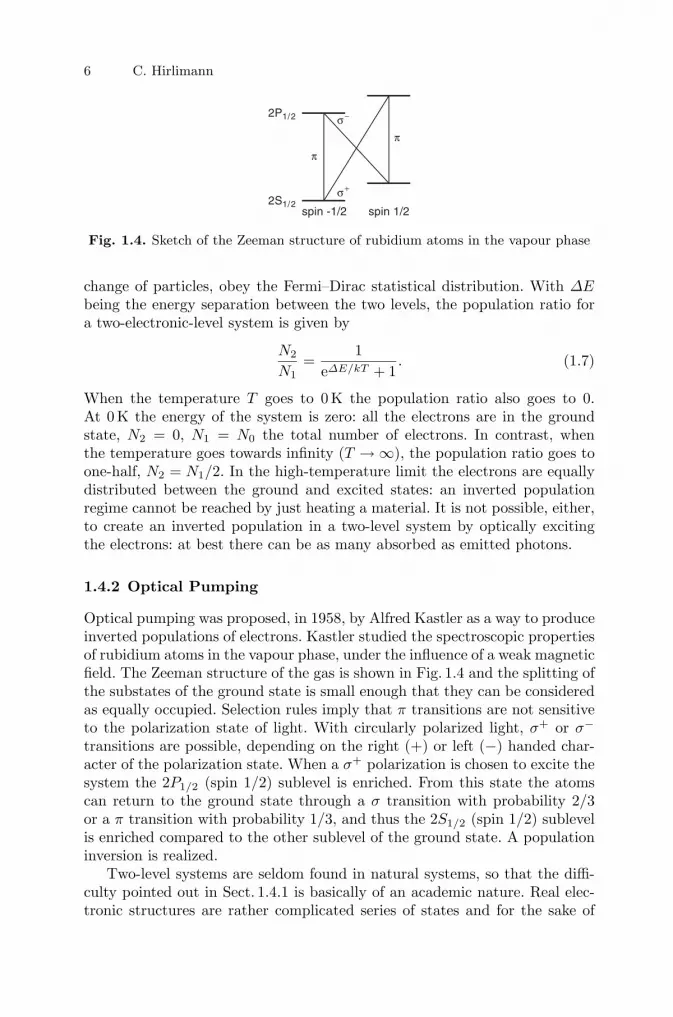
Fig. 1.4. Sketch of the Zeeman structure of rubidium atoms in the vapour phase

change of particles, obey the Fermi–Dirac statistical distribution. With ΔEbeing the energy separation between the two levels, the population ratio fora two-electronic-level system is given by

N2

N1=

1eΔE/kT + 1

. (1.7)

When the temperature T goes to 0 K the population ratio also goes to 0.At 0 K the energy of the system is zero: all the electrons are in the groundstate, N2 = 0, N1 = N0 the total number of electrons. In contrast, whenthe temperature goes towards infinity (T → ∞), the population ratio goes toone-half, N2 = N1/2. In the high-temperature limit the electrons are equallydistributed between the ground and excited states: an inverted populationregime cannot be reached by just heating a material. It is not possible, either,to create an inverted population in a two-level system by optically excitingthe electrons: at best there can be as many absorbed as emitted photons.

1.4.2 Optical Pumping

Optical pumping was proposed, in 1958, by Alfred Kastler as a way to produceinverted populations of electrons. Kastler studied the spectroscopic propertiesof rubidium atoms in the vapour phase, under the influence of a weak magneticfield. The Zeeman structure of the gas is shown in Fig. 1.4 and the splitting ofthe substates of the ground state is small enough that they can be consideredas equally occupied. Selection rules imply that π transitions are not sensitiveto the polarization state of light. With circularly polarized light, σ+ or σ−

transitions are possible, depending on the right (+) or left (−) handed char-acter of the polarization state. When a σ+ polarization is chosen to excite thesystem the 2P1/2 (spin 1/2) sublevel is enriched. From this state the atomscan return to the ground state through a σ transition with probability 2/3or a π transition with probability 1/3, and thus the 2S1/2 (spin 1/2) sublevelis enriched compared to the other sublevel of the ground state. A populationinversion is realized.

Two-level systems are seldom found in natural systems, so that the diffi-culty pointed out in Sect. 1.4.1 is basically of an academic nature. Real elec-tronic structures are rather complicated series of states and for the sake of

1 Laser Basics 7

1

Wp W31

W32

W21

2

3

Fig. 1.5. Three-level system used to model the population inversion in opticalpumping

simplicity we will consider a three-level system illuminated with photons ofenergy hω = E3 − E1 (Fig. 1.5). Electrons are promoted from state 1 to state3 with a probability per unit time Wp, which accounts for both the absorptioncross-section of the material and the intensity of the incoming light.

From state 3, electrons can decay either to state 2 with probability W32 orto the ground state with probability W31. We assume now that the transitionprobability from state 3 to state 2 is much larger than to state 1 (W32 � W31).The electronic transition 2 → 1 is supposed to be the radiative transition ofinterest and we suppose that state 2 has a large lifetime compared to state 3(W21 � W32). State 2 is called a metastable state.

Rate equations can be easily derived that model the dynamical behaviorof such a three-level system:

dN3

dt= WpN1 − W32N3 − W31N3, (1.8a)

dN2

dt= W32N3 − W21N2. (1.8b)

State 3 is populated from state 1 with probability Wp and in proportion tothe population N1 of state 1 (first right term in (1.8a)); it decays with a largerprobability to state 2 than to state 1 and in proportion to its population N3(two decay terms in (1.8a)). State 2 is populated from state 3 according toW32 and N3 (source term in (1.8b)) and decays to state 1 through spontaneousemission of light and in proportion to its population N2 (decay term in (1.8b)).

A steady dynamical behavior is a solution of (1.8) and corresponds toconstant state populations with time; in this regime time derivatives vanishand (1.8) simply gives on

N2

N1≈ Wp

W21

(1 − W31

W32

). (1.9)

When the pumping rate is large enough to overcome the spontaneous emissionbetween states 2 and 1 (Wp � W21), then (1.9) shows that the average number

8 C. Hirlimann

1

fast

3

4

2

fast

slow slowradiative

Fig. 1.6. Sketch of the four-level system found in most laser gain media

of atoms in state 2 can be larger that the average number of atoms in state 1:the population is inverted between states 2 and 1. This population inversionis reached when (i) the pumping rate is large enough to overcome the naturaldecay of the metastable level, (ii) the electronic decay from the pumping stateto the radiative state is faster than any other decay, and (iii) the radiativedecay time is long enough to ensure that the intermediate metastable state issubstantially overoccupied. Because of all these stringent physical conditionsthe three-level model might seem to be unrealistic; this is actually not thecase, for it mimics quite accurately the electronic structure and dynamicsfound in chromium ions dissolved in alumina (ruby)!

A large variety of materials have shown their ability to sustain a popu-lation inversion when, some way or another, energy is fed to their electronicsystem. Optical pumping still remains a common way of producing populationinversion but many other ways have been developed to reach that goal, e.g.electrical excitation, collisional energy transfer and chemical reaction. Mostof the efficient media used in lasers have proved to be four-level structures asfar as population inversion is concerned (Fig. 1.6).

In these systems, state 3 is populated and the various transition proba-bilities are as follows: W43 � W41, W21 � W32, W21 ≈ W43. Therefore inthe steady-state regime the population of states 4 and 2 can be kept close tozero and the population inversion contrast can be made larger than in a threelevel-system (N3 − N2 � N2). This favorable situation is relevant to argonand krypton ion lasers, dye lasers and the neodymium ion in solid matrices,for example.

1.4.3 Light Amplification

Once a population inversion is established in a medium it can be used toamplify light. In order to simplify calculations let us consider a medium inwhich a population inversion is realized (ΔN = N1 −N2, ΔN < 0) in a three-level system (Fig. 1.5). In such a medium, the intensity of a low-intensity

1 Laser Basics 9

electromagnetic wave propagating along z is proportional to the populationinversion ΔN and to the wave intensity. This can be formally written as

dI(z)dz

= −I(z) ΔNσ21, (1.10)

where σ21, the proportionality factor, is called the stimulated-emission cross-section of the transition. It depends on both the medium and the wavelengthof the light. Equation (1.10) describes light amplification in an inverted-population medium.

During the amplification process a depletion of the inverted level is tobe expected due to the stimulated emission process itself: ΔN must dependon the intensity of the light. This dependence can be qualitatively exploredusing (1.9) as a starting point. If an efficient gain medium is assumed, thenW31/W32 � 1 can be neglected and one gets

ΔN ≈ N2

(W21

Wp− 1

). (1.11)

One can also make the assumption that N2 ≈ N , all the available atoms(N) being in the inverted state 2. This regime corresponds to a situationwhere the pumping is strong so that W21 � Wp. In the framework of theseapproximations, an inverted expansion leads to

ΔN ≈ −N/(

1 +W21

Wp

). (1.12)

Replacing the probabilities by intensities because they are only involved inratios gives the following expression, in which Is is a constant intensity de-pending on the gain medium:

ΔN ≈ −N/(

1 +I(z)Is

). (1.13)

When expression (1.13) is introduced into (1.10) we obtain

1I(z)

dI(z)dz

= g0

/(1 +

I(z)Is

), (1.14)

where g0 = Nσ21 > 0 is the low-intensity gain. The saturation intensity Isallows one to distinguish between the low-and high-intensity regimes for lightamplification in a gain medium.

1.4.3.1 Low-Intensity Regime, I(z) � Is. In this regime the evolutionof the light intensity as a function of the distance z in the medium simplifiesto I(z) = I(0)eg0z. Starting from its incoming value I(0), the intensity growsas an exponential function along the propagation direction. This behaviorcould be intuitively predicted from the previous discussion on the stimulatedemission process and the chain reaction.

10 C. Hirlimann

Fig. 1.7. Simple hyperbolic intensity dependence of the gain in a light amplifier

1.4.3.2 High-Intensity Regime, I(z) � Is. When, in the gain medium,the intensity becomes larger than the saturation intensity, (1.14) reduces toI(z) = I(0)+Isg0z; the intensity only grows as a linear function of the distancez. In the high-intensity regime the amplification process is much less efficientthan in the low-intensity regime. The gain is said to saturate in the high-intensity regime.

It is far beyond the scope of this introduction to laser physics to rigorouslydiscuss gain saturation; we will only focus on the simple hyperbolic model

g(I) =g0

1 + I/Is. (1.15)

In this very approximate framework, the saturation intensity Is is theintensity for which the gain value is reduced by a factor of two. This is verysimilar to the saturation of the absorption in saturable absorbers, and thisagain arises from the fact that light absorption and stimulated emission aresymmetrical effects. The simplest gain model simply mimics the Beer–Lambertlaw for absorption: I(z) = I(0)egz, where g is given by (1.15).

Gain saturation is of prime importance in the field of ultrashort lightpulse generation; this mechanism is a key ingredient for pulse shortening.But it also becomes a limiting factor in the process of amplifying ultrashortpulses: the intensity in these pulses rapidly reaches the saturation value. Beambroadening and pulse stretching are ways used to overcome this difficulty, aswill be described in the following chapters.

1.5 Amplified Spontaneous Emission (ASE)

Spontaneous light emission from an excited medium is isotropic: photons arerandomly emitted in every possible space direction with equal probability;the polarization states are also randomly distributed when the emission takesplace from an isotropic medium. Stimulated emission, on the contrary, retains

1 Laser Basics 11

Fig. 1.8. Schematic illustration of amplified spontaneous emission (ASE). Sponta-neously emitted photons are amplified when propagating along the major dimensionof the gain medium

the characteristics of the inducing waves. This memory effect is responsiblefor the unwanted amplified spontaneous emission which takes place in laseramplifiers.

Most of the gain media in which a population inversion is created have ageometrical shape such that one of their dimensions is larger than the others(Fig. 1.8). At the beginning of the population inversion, when net gain be-comes available, there are always spontaneously emitted photons propagatingin directions close to the major dimension of the medium which trigger stim-ulated emission. In both space and phase, ASE does not have good coherenceproperties, because it is seeded by many incoherently, spontaneously emittedphotons.

Amplified spontaneous emission is a problem when using light amplifiersin series to amplify light pulses: the ASE emitted by one amplifying stageis further amplified in the next stage and competes for gain with the usefulsignal. ASE returns in oscillators are also undesirable; they may damage thesolid-state gain medium or induce temporal instabilities. To overcome thesedifficulties it is necessary to use amplifier decoupling.

1.5.1 Amplifier Decoupling

1.5.1.1 Static Decoupling. For light pulses that are not too short (>100 fs), a Faraday polarizer (Fig. 1.9) can be used to stop any return of lin-early polarized light. Depending on the wavelength, properly chosen materialsexhibit a strong rotatory power when a static magnetic field is applied. Ad-justment of the magnetic field intensity and of the length of the materialallows one to rotate the linear polarization of a light beam by a 45◦ angle.

Owing to the pseudovector nature of a magnetic field, the polarizationrotation direction is reversed for a beam propagating in the reverse direction.

12 C. Hirlimann

B

P

Fig. 1.9. Schematic of a Faraday polarizer. P is a linear polarizer; the cylinder is amaterial exhibiting strong rotatory power under the influence of a magnetic field B

t

t

a)

b)

Fig. 1.10. (a) Train of pulses from a laser amplifier consisting of weak, unamplifiedpulses with high repetition rate and low-repetition-rate, amplified, short pulses,associated with long-lasting ASE. (b) Cleaning-up produced by a saturable absorber

Therefore the linear polarization of a reflected beam is rotated 90◦ and canbe stopped by an analyzer.

1.5.1.2 Dynamic Decoupling. Amplifier stages are often decoupled usingsaturable absorbers. Absorption saturation (see Chap. 2) is a nonlinear opticaleffect that is symmetrical to gain saturation. It can be described by replacingthe gain g by the absorption α in expression (1.15) and changing the signin the evolution of the intensity with propagation. For a low-intensity signal,the intensity decreases as an exponential function with distance, while it onlydecreases linearly at high intensity. Only short, intense pulses can cross thesaturable absorber. As an example we will consider a light output of an ampli-fier stage consisting of a superposition of light pulses: a high-repetition-ratetrain of weak, short pulses and a low-repetition-rate train of intense, shortpulses superimposed on low-intensity, long-lasting ASE pulses (Fig. 1.10a).

1 Laser Basics 13

Fig. 1.11. General sketch of an oscillator. An oscillator is basically made of an am-plifier and a positive feedback. The feedback must ensure a constructive interferencebetween the input and amplified waves

The optical density of the saturable absorber is adjusted in such a waythat it only saturates when crossed by the amplified pulses. When the pulsetrain crosses the saturable absorber the unamplified pulses and the leadingedge of the ASE are absorbed. In order to improve the energy ratio betweenthe amplified pulses and the remaining ASE the saturable absorber must bechosen to have a short recovery time. That way the long-lasting trailing partof the ASE can be partly absorbed. Malachite green, for example, with a 3 psrecovery time, has been widely used as a stage separator in dye amplifiers.

1.6 The Optical Cavity

We now know how to create and use stimulated emission to amplify light. Froma very general point of view an oscillator is the association of an amplifier witha positive feedback (Fig. 1.11). The net gain of the amplifier must be largerthan one in order to overcome the losses, including the external coupling. Thephase change created by the feedback loop must be an integer multiple of2π in order to maintain a constructive interference between the input andamplified waves. What is the way to use an amplifier in the building of anoptical oscillator?

1.6.1 The Fabry–Perot Interferometer

In the year 1955, Gordon et al. [1.1] developed the ammonia maser, clearlyproving, in the microwave wavelength range, the possibility to amplify weaksignals using stimulated emission. A metallic box, with suitably chosen sizeand shape, surrounding a gain medium was proved to create efficient positive

14 C. Hirlimann

feedback, allowing the device to run as an oscillator. In order for the oscillationto operate in a single mode the size of the box had to be of the order of a fewwavelengths, i.e. a few centimeters. A large number of research groups triedto transpose the technique to the visible range using appropriate gain media.They were stopped by the necessity to design an optical box having a volumeof the order of λ3, which in the visible means 0.1 μm3. A tractable much largerbox would have had a large number of modes fitting the gain bandwidth, andthis was expected to create mode beating which in turn would destroy thebuild-up of a coherent oscillation.

In the following years, Schawlow and Townes [1.2], as well as Basov andProkhorov [1.3], came up with calculations showing that the number of modesin an optical cavity could be greatly reduced by confining light in only onedimension to create a feedback. The Fabry–Perot resonator then came intothe picture.

A gain medium would be put between the two high-reflectivity (≈ 100 %)mirrors of a Fabry–Perot interferometer so that a coherent wave could beconstructed after several round trips of the light through the amplifier. At thestarting time of the device, when the inverted population was established inthe gain medium, a unique spontaneously emitted photon propagating alongthe cavity axis would start stimulated emission, increasing the number of co-herent photons. If, after a round trip between the mirrors, the gain was largerthan the losses then the intensity of the visible electromagnetic wave wouldincrease as an exponential function after each round trip, and a self-sustainedoscillation would start. But in a cavity, owing for example to diffraction at theedge of the mirrors or spurious reflections and absorption, photons are lost.The value of the gain which overcomes the losses is called the laser threshold.

1.6.2 Geometric Point of View

We will now focus on the properties of an optical cavity, and specificallylook for the necessary conditions that must be fulfilled so that the cavity canaccommodate an infinite number of round trips of the light. The cavity underconsideration consists simply of two concave, spherical mirrors with radii ofcurvature R1 and R2, spaced by a length L (Fig. 1.12). From a geometric pointof view, Fig. 1.12 shows that the light ray coincident with the mirrors’ axiswill repeat itself after an arbitrary number of back-and-forth reflections fromthe mirrors. Other rays may or may not escape the volume defined by the twomirrors. A cavity is said to be stable when there exists at least one family ofrays which never escape. When there is no such ray the cavity is said to beunstable; any ray will eventually escape the volume defined by the mirrors.

A very simple geometric method allows one to predict whether a givencavity is stable or not [1.4]. Consider now the cavity defined in Fig. 1.13. Twocircles having their centers on the axis of the cavity are drawn with theirdiameters equal to the radii of curvature of the mirrors so as to be tangentto the reflecting face of the mirrors. The center of each is coincident with the

1 Laser Basics 15

R1

R2

M1

M2L

Fig. 1.12. Optical cavity consisting of two concave mirrors. Two ray paths areshown. The axial ray is stable, the other is not

Fig. 1.13. Concave–convex laser cavity. Geometric determination of the stabilityof the cavity [1.4]

real or virtual focus point of the mirror. The straight line joining the pointsof intersection of the two circles crosses the axis of the cavity at a point whichdefines the position of the beam waist of the first-order transverse mode. Ifthe two circles do not cross, the cavity is unstable.

1.6.3 Diffractive-Optics Point of View

Geometrical optics is not enough to estimate quantitatively the propertiesof the modes which may be established in a Fabry–Perot cavity. The full

16 C. Hirlimann

calculation of these modes is rather tedious and we will concentrate only onsome of the most important features. In a Fabry–Perot interferometer lightbounces back and forth from one mirror to the other with a constant time offlight, so that its dynamics is periodic by nature. A wave propagating insidea cavity remains unchanged after one period in the simple case in whichthe polarization direction does not change. The propagation is governed bydiffraction laws because of the finite diameter of the mirrors, but also becauseof the presence of apertures inside the cavity; the most common aperture issimply the finite diameter of the gain volume. From a mathematical point ofview, the radial distribution of the electric field in a given mode inside thecavity is described through a two-dimensional spatial Fourier transformation.For the periodicity condition to be respected it is therefore necessary that thefunction describing the radial distribution is its own Fourier transform. TheGaussian function is its own Fourier transform and is therefore the very basisof the transverse electromagnetic structure for spherical-mirror cavities.

It can be shown that the electric field distribution of the fundamentaltransverse mode in a spherical-mirror cavity can be written as

E(x, y, z) = E0W0

W (z)exp

{− i[k

(z +

x2 + y2

2R(z)

)− Φ(z)

]}

× exp−x2 + y2

W 2(z), (1.16)

where

R(z) = z

(1 +

(πW 2

0

λz

)2)

, Φ(z) = tan−1(

λz

πW 20

). (1.17)

Here R(z) is the radius of curvature of the wave surface (Fig. 1.14), Φ(z) isthe phase as a function of the distance z,

W 2(z) = W 20

(1 +

(λz

πW 20

)2)

(1.18)

is the radius of the beam andk =

2π

λ(1.19)

is the propagation factor in vacuum.The propagation origin z = 0 is chosen to be coincident with the position

of the minimum radius of the beam, the beam waist W0. When z = 0 thenR(0) = Φ(0) = ∞, the wave surface is plane and the electric field amplitude

E(x, y, 0) = E0 exp− (x2 + y2/W 2

0)

(1.20)

decays as a Gaussian function along the radius of the beam.

1 Laser Basics 17

Fig. 1.14. Schematic structure of a Gaussian light beam in the vicinity of a focalvolume. The y axis is perpendicular to the paper sheet. The z = 0 origin is at theminimum radius W0 of the beam

Along the axis, the radius of curvature of the wave surface R(z) variesas a hyperbola and its asymptotes make an angle θ with the axis such thattan θ = λ/πW0. This angle is a good definition of the beam divergence.

For large z the hyperbola may be replaced by its asymptotes and theradius of curvature varies linearly with the distance z; R(z) ≈ z when z goesto infinity in (1.17). In this long-distance regime the amplitude of the electricfield varies as the inverse of the beam radius, i.e. E(z) ≈ W−1(z), alongz, and as a Gaussian function along the radius. Putting aside the Gaussianattenuation, the fundamental mode behaves like a spherical wave. Such awavefront has the right shape to fit nicely the surface of spherical mirrors.

This structure of the fundamental transverse mode is referred to as TEM00(fundamental transverse electric and magnetic mode). Many other transversemodes can propagate inside the cavity; they can be expressed as the super-position of higher-order fundamental modes TEMnm. These modes can becalculated by multiplying the fundamental lowest-order mode (1.16) by theHermite polynomials of integer orders n and m,

Hn

( √2 x

W (z)

), Hm

( √2 y

W (z)

), (1.21)

and multiplying the phase term Φ(z) by (1 + n + m).

1.6.4 Stability of a Two-Mirror Cavity

The problem is now to find which Gaussian mode with a far-field sphericalbehavior can fit a given pair of spherical mirrors with radii R1 and R2, spacedby a distance L. In Fig. 1.15, the mirror positions z1 and z2 are measuredfrom the yet unknown position of the beam waist. For a cavity to be stableit must be able to accommodate a mode in which spherical wavefronts willfit the reflecting surfaces of the two spherical mirrors. From a formal point ofview, one simply has to make the radii of curvature of the wavefront, given by(1.17), equal to the radii of curvature of the mirrors; adding the conservationof length leads to the three equations

18 C. Hirlimann

R1

R2

M1M2

Lz1 z2

z=0

Fig. 1.15. Schematic diagram of a simple transverse Gaussian beam fitting a two-spherical-mirror cavity

R1 = −z1 − z2R

z1, (1.22)

R2 = +z2 +z2R

z2, (1.23)

L = z2 − z1, (1.24)

where zR = πW0/λ, called the Rayleigh range, is the distance, measured fromthe beam waist position, where the radius of the beam is equal to

√2 W0. This

length defines the focal volume, which, to first order in z, is almost cylindrical.These simple equations have been generally solved using the special cavity

parameters

g1 = 1 − L

R1and g2 = 1 − L

R2, (1.25)

tying the distances z1, z2, zR to the geometric cavity parameters R1, R2, L.Solving the equations in this new notation leads to the following results:

– the beam waist position measured from the mirror position

z1 =g2(1 − g1)

g1 + g2 − 2g1g2L, z2 =

g1(1 − g2)g1 + g2 − 2g1g2

L; (1.26)

– the beam waist radius,

W 20 =

Lλ

π

√g1g2(1 − g1g2)

(g1 + g2 − 2g1g2)2; (1.27)

– the beam radius at the surface of the mirrors,

W 21 =

Lλ

π

√g2

g1(1 − g1g2), W 2

2 =Lλ

π

√g1

g2(1 − g1g2). (1.28)

1 Laser Basics 19

g2

g1

–1

–1

1

1

( )

( )

Fig. 1.16. Stability diagram for a laser cavity. The shaded areas define the set ofvalues of the cavity parameters g1 and g2 for which the cavity is unstable [1.5]

From (1.27) one notices that the radius of the beam may only be a real numberif the argument of the square root function is a positive and finite number.This leads to the following inequalities:

0 ≤ g1g2 ≤ 1, (1.29)

which put stringent conditions on the mirrors’ radii of curvature and on theirspacing.

The stability conditions (1.29), define a hyperbola g1g2 = 1 in the g1, g2plane. The two white regions in Fig. 1.16 correspond to stable cavities wheng1 and g2 are both positive or negative. The shaded regions correspond tounstable resonators. Three specific, commonly used cavities are shown in thefigure: (i) the symmetrical concentric resonator (R1 = R2 = −L/2, g1 = g2 =−1), (ii) the symmetrical confocal resonator (R1 = R2 = −L, g1 = g2 = 0)and (iii) the planar resonator (R1 = R2 = ∞, g1 = g2 = 1). The fact that acavity is optically unstable does not mean that it cannot produce any laseroscillation, nor does it mean that its emitted intensity is necessarily unstable.It only means that the number of round trips of the light it allows is limited.

Some gain media are short-lived (a few nanoseconds) compared to thecavity period; it is of no use in this situation to pile up round trips. On thecontrary, it might be of great help to use an unstable cavity accommodatingthe right number of round trips. But as the number of passes of the light in thegain medium is limited, such unstable cavities do not show good transverse

20 C. Hirlimann

modal qualities. This situation is encountered, for example, in high gain laserslike exciplex lasers or copper-vapor lasers.

1.6.5 Longitudinal Modes

When it comes to the use of lasers as short-pulse generators, the most im-portant property of optical resonators is the existence of longitudinal modes.Transverse modes, as we saw, are a geometric consequence of light propaga-tion, while longitudinal modes are a time–frequency property. In other words,we now know how to apply a feedback to a gain medium; we need to explorethe conditions under which this feedback can constructively interfere with themain signal. Fabry–Perot interferometers were originally developed as high-resolution bandpass filters. The interferential treatment of optical resonatorscan be found in most textbooks on optics; here, as a remainder of the time–frequency duality, we will consider a time-domain analysis of the Fabry–Perotinterferometer. This way of looking will prove useful in the understanding ofmode-locking.

An electromagnetic field can be established between two parallel mirrorsonly when a wave propagating in one direction adds constructively with thewave propagating in the reverse direction. The result of this superpositionis a standing wave, which is established if the distance L between the twomirrors is an integer multiple of the half-wavelength of the light. Writing τfor the period of the wave and c for its velocity in vacuum, 3 × 108 m/s, andremembering that λ = cτ , the standing wave condition is

mcτ

2= L, m ∈ N+, (1.30)

which fixes the value of the positive integer m. The cavity has a specific periodT = mτ , which is also a round-trip time of flight T = 2L/c.

For a typical laser cavity with length L = 1.5 m, the period is T = 10 nsand the characteristic frequency ν = 100 MHz. These numbers do fix therepetition rate of mode-locked lasers and also the period of the pulse train.

In the continuous-wave (CW) regime the amplification process in a lasercavity is basically coherent and linear; the gain balances the losses. At anypoint inside the cavity the signal which can be observed at some instant willbe repeated unchanged after the time T has elapsed. In the time domain theelectromagnetic field in a laser cavity can be seen as a periodic repetitionof the same distribution such that ε(t) = ε(t + nT ), n being an integer (seeFig. 1.17).

E(ω) is the Fourier transform of one period of the electric field; its spectralextent is determined by the spectral bandwidth of the various active andpassive elements present in the cavity. The Fourier transformation is a linearoperation, and therefore the Fourier transform of the total electric field, from0 to N periods, is the simple sum of the delayed partial Fourier transforms,

1 Laser Basics 21

Fig. 1.17. Schematic representation, in the time domain, of the electric field at somepoint in a laser cavity. The field is repeated unchanged so that ε(t) = ε(t+nT ) aftereach period T = 2L/c

I (ν)

Fig. 1.18. Schematic emission spectrum of a laser

EN (ω) =N−1∑n=0

e−iωnT E(ω) =1 − e−iNωT

1 − e−iωTE(ω). (1.31)

The resulting sum is a geometric series which gives the power spectrum forN periods,

IN (ω) = |EN (ω)|2 =1 − cos NωT

1 − cos ωTI(ω) =

sin2 (NωT/2)sin2 (ωT/2)

I(ω). (1.32)

When N goes to infinity, the intensity response of a laser cavity tends to-wards an infinite periodic series of Dirac δ distributions spaced by the quan-tity δω = 2π/T = πc/L, or δν = c/2L. As is well known from the usualfrequency analysis, the Fabry–Perot cavity only allows specific frequencies topass through; the energy is quantized.

Real laser spectra are more likely to look like Fig. 1.18, where the band-width δf of the axial modes is finite and governed by the resonator finesse,depending on the reflectivity of the mirrors. Moreover, the number of activemodes is also finite, depending on the bandwidth of the net gain Δν.

22 C. Hirlimann

1.7 Here Comes the Laser!

The first operating laser was set up by Maiman [1.6], at this time workingwith the Hughes aircraft company, in the middle of the year 1960, and thefirst gas laser by A. Javan at MIT at the end of that same year.

Ruby was used as the gain medium in Maiman’s laser. Ruby is alumina,Al2O3, also known as corundum or sapphire, in which a small fraction of theAl3+ ions are replaced by Cr3+ ions. The electronic structure of Cr3+: Al2O3consists of bands and discrete states. The absorption takes place in greenand violet bands in the spectrum, giving the material its pink color, and theemission at 694.3 nm takes place between a discrete state and the ground state.The overall structure is that of a three-level system. Inversion of the electronicpopulation was produced by a broadband, helical flash-tube surrounding theruby rod and the resonator was simply made from the parallel, polished endsof the rod, which were silver coated for high reflectivity.

Very rapidly following Maiman’s achievement, A. Javan came out withthe first gas laser, in which a mixture of helium and neon was continuouslyexcited by an electric discharge [1.7].

1.8 Conclusion

In this chapter some laser basics were introduced as a background to the un-derstanding of ultrashort laser pulse generation. It was not the aim to presentdetails of the physics of lasers, but rather to point out specific key points nec-essary to understand the following chapters. For more information on laserphysics we recommend the references contained in the “Further Reading” sec-tion of this chapter.

1.9 Problems

1. Remove the stimulated emission in (1.2) and show that the intensity distri-bution does not vanish to zero when the frequency does. In the pre-Planckera this was called the ‘infrared catastrophe’.

2. Solve the photon population evolution equation

dn

dz= (N2 − N1)b12n + a21N2

taking into account the spontaneous emission term a21N2.(a) Show that in the low-and negative-temperature limits (T → 0, N2 �N1 and T → −∞, N2 � N1) there is no qualitative change in the responseof the medium.(b) In the high temperature-limit (T → ∞, N2 = N1), show that thenumber of photons grows linearly with the distance.

1 Laser Basics 23

3. Assume a 1.5 m long linear laser cavity. One of the mirrors is flat(R1 = ∞).(a) Using the diagram technique, what is the minimum radius of curvatureR2 of the other mirror for the cavity to be optically stable? (Answer:R2/2 = 1.5 m). What is the position of the beam waist? (Answer: z1 = 0,z2 = 1.5 m).Turning now to the analytical expressions in Sect. 1.6.4, answer the fol-lowing questions.(b) Check the position of the beam waist by directly calculating z1 andz2. What is the diameter of the beam waist for an operating wavelengthλ = 514.5 nm? (Answer: 2W0 = 832μm).(c) What are the radii of the first fundamental transverse mode at thecavity mirrors? (Answer: 2W1 = 2W0, 2W2 = 1.44 mm).(d) Calculate the Rayleigh range for which the mode can be consideredas cylindrical. (Answer: zR = 1.05 m).

Further Reading

W. Koechner: Solid-State Laser Engineering, 4th edn., Springer Ser. Opt. Sci.,Vol. 1 (Springer, Berlin, Heidelberg 1996)

J.R. Lalanne, S. Kielich, A. Ducasse: Laser–Molecule Interaction and Molec-ular Nonlinear Optics (Wiley, New York 1996)

B. Saleh, M. Teich: Fundamentals of Photonics (Wiley, New York 1991)K. Shimoda: Introduction to Laser Physics, 2nd edn., Springer Ser. Opt. Sci.,

Vol. 44 (Springer, Berlin, Heidelberg 1991)A.E. Siegman: Lasers (University Science Books, Mill Valley, CA 1986)O. Svelto: Principles of Lasers, 3rd edn. (Plenum Press, New York 1989)J.T. Verdeyen: Laser Electronics (Prentice Hall, New Jersey 1989)A. Yariv: Quantum Electronics, 3rd edn. (Wiley, New York 1989)

Historial References

[1.1] J.P. Gordon, H.J. Zeiger, C.H. Townes: Phys. Rev. 99, 1264 (1955)[1.2] A.L. Schawlow, C.H. Townes: Phys. Rev. 112, 1940 (1958)[1.3] N.G. Basov, A.M. Prokhorov: Sov. Phys.-JETP 1, 184 (1955)[1.4] G.A. Deschamps, P.E. Mast: Proc. Symposium on Quasi-Optics, ed. J. Fox

(Brooklyn Polytechnic Press, New York 1964); P. Laures: Appl. Optics 6, 747(1967)

[1.5] H. Kogelnik, T. Li: Appl. Optics 5, 1550 (1966)[1.6] T.H. Maiman: Nature 187, 493 (1960)[1.7] A. Javan, W.R. Bennet, D.R. Herriot: Phys. Rev. Lett. 6, 106 (1961)

2

Pulsed Optics

C. Hirlimann

With 23 Figures

2.1 Introduction

Optics is the field of physics which comprises knowledge on the interactionbetween light and matter. When the superposition principle can be appliedto electromagnetic waves or when the properties of matter do not depend onthe intensity of light, one speaks of linear optics. This situation occurs withregular light sources such as light bulbs, low-intensity light-emitting diodesand the sun. With such low-intensity sources the reaction of matter to lightcan be characterized by a set of parameters such as the index of refraction,the absorption and reflection coefficients and the orientation of the mediumwith respect to the polarization of the light. These parameters depend onlyon the nature of the medium. The situation changed dramatically after thedevelopment of lasers in the early sixties, which allowed the generation of lightintensities larger than a kilowatt per square centimeter. Actual large-scaleshort-pulse lasers can generate peak powers in the petawatt regime. In thatlarge-intensity regime the optical parameters of a material become functions ofthe intensity of the impinging light. In 1818 Fresnel wrote a letter to the FrenchAcademy of Sciences in which he noted that the proportionality between thevibration of the light and the subsequent vibration of matter was only truebecause no high intensities were available. The intensity dependence of thematerial response is what usually defines nonlinear optics. This distinctionbetween the linear and nonlinear regimes clearly shows up in the polynomialexpansion of the macroscopic polarization of a medium when it is illuminatedwith an electric field E :

Pε0

= χ(1) · E Linear optics, index, absorption

+χ(2) : EE Nonlinear optics, second-harmonicgeneration, parametric effects

+χ(3) ··· EEE third-harmonic generation, nonlinearindex

+ · · ·

(2.1)

26 C. Hirlimann

In this expansion, the linear first-order term in the electric field describeslinear optics, while the nonlinear higher-order terms account for nonlinearoptical effects (ε0 is the electric permittivity).

The development of ultrashort light pulses has led to the emergence of anew class of phase effects taking place during the propagation of these pulsesthrough a material medium or an optical device. These effects are mostlyrelated to the wide spectral bandwidth of short light pulses, which are affectedby the wavelength dispersion of the linear index of refraction. Their analyticaldescription requires the Taylor expansion of the light propagation factor k asa function of the angular frequency ω,

k(ω) = k(ω0) + k′(ω − ω0) + 12k′′(ω − ω0)2 + . . . . (2.2)

Contrary to what happens in “classical” nonlinear optics, these nonlineareffects occur for an arbitrarily low light intensity, provided one is dealing withshort (< 100 fs) light pulses. Both classes of optical effects can be classifiedunder the more general title of “pulsed optics.”

2.2 Linear Optics

2.2.1 Light

If one varies either a magnetic or an electric field at some point in space, anelectromagnetic wave propagates from that point, which can be completelydetermined by Maxwell’s equations.

If the magnetic field has an amplitude which is negligible when comparedto the electric field, the propagation equation for light can be written as

∇2E =1c2

∂2E∂t

,1c2 = μ0ε0, (2.3)

where c is a parameter, usually called the velocity of light, depending on theelectric and the magnetic permittivity, ε0 and μ0 respectively, of the mate-rial medium in which the wave is propagating. Equation 2.3 is a second-orderdifferential equation, for which retarded plane waves are the simplest propa-gating solutions,

Ey = Re(E0 eiω(t−x/c)

). (2.4)

This particular solution 2.4 describes the propagation of a transverse electricfield Ey along the positive x axis. The amplitude of the electric field variesperiodically as a cosine function in time with angular frequency ω and in spacewith wavelength λ = 2πc/ω. At any given point x along the propagation axisthe amplitude has the same value as it had at the earlier time t − x/c, whenit was at the origin (x = 0).

A rewriting of 2.4 as

2 Pulsed Optics 27

rR

Fig. 2.1. Plane-wave propagation

Ey = Re(E0 ei(ωt−k ·r )

), |k | =

ω

c=

2π

λ, (2.5)

allows the introduction of the wave vector k of the light. Figure 2.1 showsthe geometry of the propagation of a plane wave. Let us consider the plane Porthogonal to the propagation vector k , at distance x from the origin O. Forany point in this plane, at distance r from the origin O, the scalar productk · r = kx = ωx/c is constant; therefore, at a given time t, plane P is a planeof equal phase or equal time delay for a plane wave. A plane wave with awavelength in the visible range (400 > λ > 800 nm) has an angular frequencyω equal to a few petahertz.

It is to be noticed that a plane wave, being a simple sine or cosine function,has an infinite duration and its spectrum, which contains only one angularfrequency ω, is a δ distribution. A plane wave is the absolute opposite of alight pulse!

Up to this point light has been considered as a wave, but its particle behav-ior cannot be ignored. The wave–particle duality has the following meaning.The wave description of light is continuous in both time and space, while theparticle description is discrete. In our classical culture these two visions areantithetical and one cannot be reduced to the other. Nowadays physics saysand experiments show that light is both continuous and discrete. In the parti-cle description light is made of photons, energy packets equal to the productof the frequency and Planck’s constant hν = hω. Photons have never beenobserved at rest and as they travel at the speed of light, relativity implies thattheir mass would be zero.

Fermat’s principle states that the path of a ray propagating between twofixed point, A and B must be a stationary path, which in a mathematicalpoint of view translates as

δ

∫k · dl = 0, (2.6)

δ standing for a variation of the path integral and dl for an elementary pathelement anywhere between A and B.

28 C. Hirlimann

Doublingcrystal

k1+k2, 2ω

k2 , ω, 2ω

k 1,ω, 2ω

Fig. 2.2. Energy and momentum conservation in the doubling geometry used torecord background-free autocorrelation traces of short optical pulses. Both the en-ergy and the momentum are conserved during the mixing process

The path of the light is either the fastest one or the slowest one (in thelatter some cases of reflection geometry with concave mirrors).

For a material particle with momentum p, Maupertuis’s principle statesthat the integrated action of the particle between two fixed points A and Bmust be a minimum, which translates as

δ

∫p · dl = 0. (2.7)

By analogy, the wave vector k for the light can be seen as the momentum ofa zero-mass particle travelling along the light rays.

When light interacts with matter, both the energy and the momentumare conserved quantities. As an example, let us consider the dual-beamfrequency-doubling process used in the background-free autocorrelation tech-nique (Fig. 2.2).

In this geometry, two beams are incident, at an angle α, on a doublingcrystal that can mix two photons with angular frequency ω and momenta k1and k2, and produce one photon with angular frequency ω2 and momentumk . Energy conservation implies that ω2 = 2ω, while momentum conservationyields k = k1 +k2, k = 2k1 or k = 2k2. Five rays therefore exit the doublingmaterial: two rays are at the fundamental frequency ω in the directions k1 andk2 of the incident rays, and superimposed on them are two rays with doubledfrequency 2ω and momentum vectors 2k1 and 2k2. The fifth ray, with angularfrequency 2ω, is oriented along the bisector of the angle α, corresponding tothe geometrical sum k1 + k2.

2.2.2 Light Pulses

It is quite easy to produce “gedanken” light pulses. Let us start with amonochromatic plane wave, previously defined as (Fig. 2.3)

Ey = Re(E0 eiω0t

). (2.8)

The time representation of the field is an unlimited cosine function. Con-structing a light pulse implies multiplying 2.8 by a bell-shaped function. To

2 Pulsed Optics 29

t

1

–1

Fig. 2.3. Schematic time evolution of the electric field of a monochromatic planewave. Notice that because of the finite width of the figure this picture is alreadyrepresentative of a light pulse having a rectangular envelope

t

1

–1

Fig. 2.4. Time evolution of the electric field in a Gaussian-shaped pulse. This pulseis built up by multiplying a cosine function by a Gaussian envelope function

simplify further calculation, we choose to multiply by a Gaussian function. AGaussian pulse can be written

Ey = Re(E0 e(−Γt2+iω0t)

)(2.9)

and its time evolution is shown in Fig. 2.4.Γ is the shape factor of the Gaussian envelope; it is proportional to the

inverse of the squared duration t0, i.e. Γ ∝ t−20 .

Let us now turn to the spectral content of a light pulse. This can beobtained by calculating the modulus of the Fourier transform of the timeevolution function of the pulse. As said earlier, a plane wave oscillates with theunique angular frequency ω0 and its Fourier transform is a Dirac distributionδ(ω0) (Fig. 2.5).

The Fourier transform of a Gaussian pulse is also a Gaussian function(Fig. 2.6). Therefore the frequency content of a light pulse is larger than the

30 C. Hirlimann

i

Fig. 2.5. Numerical Fourier transform of the truncated cosine function shown inFig. 2.3. As the width of the cosine function grows larger and larger (t0 → ∞), theFourier transform tends toward a Dirac distribution δ(ω0) with zero width

Fig. 2.6. Numerical Fourier transform of the Gaussian pulse shown in Fig. 2.4. Thetransformed function is also a Gaussian function with a frequency width proportionalto Γ

unique frequency of a plane wave. The mathematical expression for the spec-trum is given in Fig. 2.6 and the width of the spectrum is proportional toΓ .

2.2.3 Relationship Between Duration and Spectral Width

We have just empirically observed that the spectral width and the duration ofa pulse are related quantities. What is the exact relationship? We start fromthe general time and frequency Fourier transforms of a pulse:

2 Pulsed Optics 31

ε(t) =12π

∫ +∞

−∞E(ω) e−iωt dω, E(ω) =

∫ +∞

−∞ε(t) eiωt dt. (2.10)

When the duration and the spectral width of the pulse are calculated usingthe standard statistical definitions

〈Δt〉 =

∫ +∞−∞ t|ε(t)|2 dt∫ +∞−∞ |ε(t)|2 dt

,

〈Δω2〉 =

∫ +∞−∞ ω2|E(ω)|2 dω∫ +∞

−∞ |E(ω)|2 dω, (2.11)

it can be shown that these quantities are related through the following uni-versal inequality:

Δt Δω ≥ 12 . (2.12)

This classical-physics relationship, which leads to the quantum-mechanicaltime–energy uncertainty principle, has several important consequences in thefield of ultrashort light pulses.

– In order to produce a light pulse with a given duration it is necessaryto use a broad enough spectral bandwidth. A Gaussian-shaped pulselasting for one picosecond (10−12 s) has a minimum spectral bandwidthof 441 MHz (Δω = 4.41 × 1011 Hz). If the central frequency ν0 ofthe pulse lies in the visible part of the electromagnetic spectrum, sayν0 = 4.84 × 1014 Hz (wavelength λ0 = 620 nm), then the relative fre-quency bandwidth is Δν/ν0 ≈ 10−3. But for a 100 times shorter pulse(Δt = 10 fs), Δν/ν0 ∼ 0.1. As |Δλ/λ0| = Δν/ν0, the wavelength ex-tension of this pulse is 62 nm, covering 15 % of the visible window of theelectromagnetic spectrum. Taking into account the wings of the spectrum,a 10 fs pulse actually covers most of the visible window!

– Equality to 1/2 in 2.12 can only be reached with Gaussian time and spec-tral envelopes. The Gaussian pulse shape “consumes” a minimum amountof spectral components. When the equality is reached in (2.12), the pulseis called a Fourier-transform-limited pulse. The phase variation of such apulse has a linear time dependence as described by (2.9); in other words,the instantaneous frequency is time-independent.

– For a given spectrum, one pulse envelope can be constructed that has theshortest possible duration.

– The shortest constructed pulse can only be transform-limited if its spec-trum is symmetrical.

– If a transform-limited pulse is not Gaussian-shaped, then the equality inan expression similar to 2.12 applies, but for a constant quantity largerthan 1/2 which depends on the shape of the pulse.

From the experimental point of view, half-maximum quantities are easierto measure; the Fourier inequality is then usually written as ΔνΔt = K, where

32 C. Hirlimann

Δν is the frequency full width at half-maximum and Δt the half maximumduration. K is a number which depends on the shape of the pulse. Table 2.1gives values of K for some symmetrical pulse shapes.

Shape ε(t) K

Gaussian function exp[−(t/t0)2/2] 0.441Exponential function exp[−(t/t0)/2] 0.140Hyperbolic secant 1/ cosh(t/t0) 0.315Rectangle – 0.892Cardinal sine sin2(t/t0)/(t/t0)2 0.336Lorentzian function [1 + (t/t0)2]−1 0.142

Table 2.1. Values of K for various pulse shapes, in the inequality Δν Δt ≥ K,when Δν and Δt are half-maximum quantities

Let us now consider a simple Gaussian light pulse

Ey = Re(E0 e(−Γt2+iω0t)

). (2.13)

The instantaneous frequency is obtained by calculating the time derivative ofthe phase,

ω(t) = ∂Φ/∂t = ω0. (2.14)

In this situation the angular frequency is constant and equals the centralangular frequency ω0. The light pulse is transform-limited; Δν Δt = 0.441.Let us now suppose that the phase of the pulse obeys a quadratic law in time,

Ey = Re(E0 e[−Γt2+i(ω0t−at2)]

), Γ ∈ �, (2.15)

then the instantaneous angular frequency varies linearly with time (Fig. 2.7):

ω(t) = ∂Φ/∂t = ω0 + αt, α > 0. (2.16)

When a quadratic time dependence is added to the original phase term,the instantaneous frequency is more red in the leading part of the pulse andmore blue in the trailing part (compare Fig. 2.4). The pulse is said to be“chirped.” This result describes the self-phase modulation process in the limitwhen t � Γ (see (2.54) and (2.57)).

2.2.4 Propagation of a Light Pulse in a Transparent Medium

What happens to a short optical pulse propagating in a transparent medium?Because of its wide spectral width and because of group velocity dispersionin transparent media, it undergoes a phase distortion inducing an increase ofits duration. This happens with any optical element and needs to be properlycorrected for in the course of experiments.

2 Pulsed Optics 33

Fig. 2.7. Time evolution of the electric field in a Gaussian pulse having a quadratictime dependence of the phase

The frequency Fourier transform of a Gaussian pulse has already beengiven as

E0(ω) = exp(−(ω − ω0)2

4Γ

). (2.17)

After the pulse has propagated a distance x, its spectrum is modified to

E(ω, x) = E0(ω) exp[−ik(ω)x], k(ω) = nω/c, (2.18)

where k(ω) is now a frequency-dependent propagation factor. In order to allowfor a partial analytical calculation of the propagation effects, the propagationfactor is rewritten using a Taylor expansion as a function of the angular fre-quency, assuming that Δω � ω0 (this condition is only weakly true for theshortest pulses). Applying the Taylor’s expansion

k(ω) = k(ω0) + k′(ω − ω0) + 12k′′(ω − ω2)2 + . . . , (2.19)

where

k′ =(

dk(ω)dω

)ω0

(2.20)

and

k′′ =(

d2k(ω)dω2

)ω0

, (2.21)

to 2.18, the pulse spectrum becomes

E(ω, x) = exp(

− ik(ω0)x − ik′x(ω − ω0)

−(

14Γ

+i2k′′)

(ω − ω0)2]. (2.22)

The time evolution of the electric field in the pulse is then derived from thecalculation of the inverse Fourier transform of 2.22,

34 C. Hirlimann

Fig. 2.8. Schematic relationship between the phase and group velocities in an ordi-nary transparent medium. Note that this relationship does not depend on the signof the curvature of the dispersion curve ω(k)

ε(t, x) =12π

∫ +∞

−∞E(ω, x) eiωt dω, (2.23)

so that

ε(t, x) =

√Γ (x)

πexp

[iω0

(t − x

vφ(ω0)

)]× exp

[−Γ (x)

(t − x

vg(ω0)

)2]

,

(2.24)where

vφ(ω0) =(ω

k

)ω0

, vg(ω0) =(

dω

dk

)ω0

,1

Γ (x)=

1Γ

+ 2ik′′x. (2.25)

In the first exponential term of 2.24, it can be observed that the phase of thecentral frequency ω0 is delayed by an amount x/vφ after propagation over adistance x. Because the phase is not a measurable quantity, this effect has noobservable consequence. The phase velocity vφ(ω) measures the propagationspeed of the plane-wave components of the pulse in the medium. These planewaves do not carry any information, because of their infinite duration.

The second term in 2.24 shows that, after propagation over a distance x,the pulse keeps a Gaussian envelope. This envelope is delayed by an amountx/vg, vg being the group velocity. Figure 2.8 shows schematically the relation-ship between the phase and the group velocities.

The phase velocity vφ(ω0) = (ω0/k) is the slope of a straight line starting atthe origin and crossing the dispersion curve ω(k) where the angular frequencyequals ω0. The group velocity vg(ω0) = (dω/dk)ω0 is the slope of the linetangential to the dispersion curve at the same point. In ordinary matter,vg < vφ.

From the expression for the propagation factor k = 2π/λ and the expres-sion for the wavelength in a medium λ = 2πc/ωn(ω), n(ω) being the index of

2 Pulsed Optics 35

refraction, one gets

vφ =c

n(ω), (2.26)

vg =dω

dk=

1(dk/dω)

,dk

dω=

1c

(n(ω) + ω

dn(ω)dω

), (2.27)

vg ≈ vφ

(1 − ω

n(ω)dn(ω)

dω

). (2.28)

The second term in 2.24 also shows that the pulse envelope is distorted duringits propagation because its form factor Γ (x), defined as

1Γ (x)

=1Γ

+ 2ik′′x, (2.29)

depends on the angular frequency ω through k′′(ω),

k′′ =(

d2k

dω2

)ω0

=ddω

(1

vg(ω)

)ω0

. (2.30)

This term is called the “group velocity dispersion”.Rewriting Γ (x) as

Γ (x) =Γ

1 + ξ2x2 − iΓξx

1 + ξ2x2 , ξ = 2Γk′′ (2.31)

and substituting 2.31 into the second term of the right-hand side of 2.24 yieldsthe following expression:

exp

[− Γ

1 + ξ2x2

(t − x

vg

)2

+ iΓξx

1 + ξ2x2

(t − x

vg

)2]

. (2.32)

The real part of 2.32 is still a delayed Gaussian function. Its form factor

Γ

1 + ξ2x2 (2.33)

is always smaller than the original one Γ , which means that the pulse under-goes a duration broadening. Figure 2.9 shows a sketch of the pulse envelopebroadening during its propagation through a transparent medium.

The phase, i.e. imaginary part in 2.32, contains a quadratic time term andwe have already seen that this creates a linear frequency chirp in the pulse(Sect. 2.2.3).

In summary, the propagation of a short optical pulse through a transparentmedium results in a delay of the pulse, a duration broadening and a frequencychirp.

36 C. Hirlimann

x

t

I

Fig. 2.9. Numerical calculation of the intensity envelope of a pulse propagatingalong x, in a lossless, transparent medium. The pulse broadens with time but, fromenergy conservation, its time-integrated intensity remains constant

2.2.4.1 Dispersion Parameter of a Transparent Medium. The disper-sion of an index of refraction is usually tabulated as a function of the wave-length of light in vacuum. We therefore need to recalculate the dispersion asa function of the wavelength. From 2.30 we obtain

k′′ = − λ2

2πcD, D =

1L

dtgdλ

, (2.34)

with tg being the group delay induced by propagation over length L. D iscalled the dispersion parameter. The group delay tg is calculated using 2.28for the group velocity and the simple definition tg = L/vg, which leads to

k′′ =λ3

2πc2

d2n

dλ2 . (2.35)

The sign of k′′ depends on the curvature of the dispersion of the indexd2n/dλ2.

A one-resonance Drude model is the simplest way to describe the electronicproperties of matter. In this very simple model the variation of the index ofrefraction in the vicinity of the resonance looks as shown in Fig. 2.10.

For wavelengths larger than the resonance wavelength the curvature of theindex dispersion curve is positive (upward concavity) and the group velocitydispersion is positive (k′′ > 0). This situation is the most usual one, encoun-tered in ordinary optical glasses in the visible range. The index of refractiondiminishes as the wavelength increases, which in turn implies an increase of

2 Pulsed Optics 37

Fig. 2.10. (Top) sketch of an electronic resonance, from which the index of refraction(bottom) can be calculated

the group velocity: in a light pulse propagating through a transparent medium,the instantaneous frequency varies from its lowest value in the leading edge toits highest value in the trailing edge. Notice from 2.34 that a positive groupvelocity dispersion corresponds to a negative dispersion parameter D.

For wavelengths below the electronic resonance the situation is reversedand the group velocity dispersion is negative. This situation can be found insilica optical fibers, where a single resonance takes place, due to OH vibrations.For wavelengths around 1.55 μm, the group velocity is negative, allowing thepropagation of optical solitons.

2.2.4.2 Time Compression with a Pair of Gratings. In order to correctfor group-velocity-dispersion distortions, several optical devices have been de-signed that have an overall negative group velocity dispersion. As an examplewe consider a pair of transmission gratings R1 and R2. These gratings have agroove spacing d and their separation is l (Fig. 2.11).

A light ray, with wavelength λ, impinges on grating R1 with an angle ofincidence γ and is scattered with an angle θ. The gratings are set in sucha way that their wavelength dispersions are reversed, which implies that theexiting ray at point B is parallel to the incident ray. P1 and P2 are wave planesat the entrance A and exit B of the system. P2 crosses the emerging ray atpoint C. Between points A and B the light travels a distance b = l/ cos θ. Thediffraction due to a grating can be written as

d(sin γ + sin θ) = λ. (2.36)

In order to calculate the dispersion from 2.34, the group delay experiencedby the light must first be evaluated. In this specific case, where propagationtakes place only in air, the group delay is simply equal to the travel time of

38 C. Hirlimann

Fig. 2.11. Optical path through a pair of transmission gratings

light along ABC,

t = L/c = (AB + BC)/c, BC = DB sin γ = b sin θ sin γ, (2.37)

t =b

c(1 + sin θ sin γ), (2.38)

and the dispersion parameter is expressed as

D =1b

dt

dλ, (2.39)

which from 2.36, applying a small-angle approximation, yields

D =λ

cd2

[1 −

(λ

d− sin γ

)2]−1

, (2.40)

k′′ = − λ3

2πc2d2

[1 −

(λ

d− sin γ

)2]−1

. (2.41)

This expression demonstrates the possibility of selecting a set of parametersin such a way as to design a pair of gratings producing a positive or a negativegroup velocity dispersion. Therefore optical devices can be built that compen-sate a positive group velocity dispersion suffered by optical pulses travellingthrough a transparent material. Optical compressors have been a key to thedevelopment of various fields in which short optical pulses have been used asa primary tool. Figure 2.12 shows a typical arrangement for a reflective pulsecompressor.

2.3 Nonlinear Optics

2.3.1 Second-Order Susceptibility

The second-order susceptibility χ(2) governs several nonlinear optical effects,some of which will be considered in this section. Second-harmonic generation

2 Pulsed Optics 39

Fig. 2.12. Grating optical compressor. Two gratings are set in a subtractive diffrac-tion geometry. Red components of a light pulse have a longer optical path than blueones. The various components of a positively dispersed pulse can therefore be resetin phase

will be explored in some detail, while other effects will only be mentionedbecause of their importance in the physics of pulsed lasers.

2.3.1.1 Second-Harmonic Generation. Second-harmonic generation wasthe first nonlinear optical effect to be observed after lasers became available.

In this process, two photons having the same angular frequency ω, whenpropagating through a suitable material, can mix together, giving rise to asingle photon with twice the original frequency. In the framework of classicalphysics, light propagation is described in terms of coherent emission by har-monic electronic dipoles, which have been set to oscillate by the light itself.This picture can be extended to the nonlinear regime by assuming that athigh excitation intensities (meaning large oscillation amplitude of the elec-tronic oscillators), the oscillations become strongly anharmonic. Under thisassumption, the emitting dipoles can radiate energy at frequencies which areinteger multiples of the original frequency.

Fig. 2.13. When a noncentrosymmetric crystal is illuminated with photons with an-gular frequency ω some pairs of these photons disappear, replaced by single photonswith angular frequency 2ω. This effect is called second-harmonic generation

The polarization of a material can be written as

Pi(2ω) =∑j,k

χ(2)ijkEj(ω)Ek(ω). (2.42)

In a dipole approximation of the electron–photon interaction, the second-ordersusceptibility χ(2) is a third-order tensor, with components corresponding to

40 C. Hirlimann

the various possible orientations of the crystal axis and of light polarization.In the specific case in which the structure of the medium has an inversioncentre the tensor is identical to zero: no second harmonic can be generated(the central symmetry of a material is relaxed on its surface and mixing ofphotons is possible there with a weak yield). In the ideal case of a plane wavethe intensity of the generated second harmonic is as follows:

I(2ω) =27π3ω2χ2

eff l2

n3c3 I2(ω)(

sin(Δkl/2)Δkl/2

)2

. (2.43)

The dependence on both the length of the material l and the incident intensityI(ω) is quadratic; n is the index of refraction and c the velocity of light.The intensity of the doubled frequency is proportional to the square of aneffective susceptibility χ

(2)eff , which depends on the material and reflects the

mean doubling properties of this material in a given working direction. Forthe doubling yield to be maximum, the dephasing quantity Δk = k2−2k1 mustbe zero. This dephasing term accounts for the propagation effects during thedoubling process. At any one point along the propagation axis the electronicoscillators radiate at angular frequency ω and 2ω in the same direction k.After propagation over a distance l in the medium the fundamental frequencygenerates the second-harmonic frequency with a time delay k1l, while thepreviously generated second harmonic reaches the same point with a timedelay k2l. If the distance l is such that the dephasing quantity Δkl = (k2 −2k1)l is zero, then the two contributions add constructively; otherwise theyinterfere destructively.

The coherence length of a doubling crystal is defined as the characteristicdistance along which the second-harmonic waves remain in phase, and it canbe calculated using (2.43). To achieve efficient frequency-doubling devices itis now clearly apparent that dephasing must be overcome. The most commonway to do this is to use birefringent crystals for which the ordinary and ex-traordinary index surfaces for the fundamental and doubled frequencies crossone another (Fig. 2.14).

In the propagation directions defined by these intersections, the indicesof refraction at the fundamental and doubled frequencies are equal and thephase mismatch quantity Δk = 0. When this condition is fulfilled, the sincfunction in (2.43) is equal to unity and the coherence length is infinite. Cal-culation of the phase-matching angle θc between the propagation direction,taken orthogonal to the surface of the crystal, and the c axis of the crystalcan be made using(

1n2ω

e (θ)

)2

=sin2 θ

(n2ωe )2

+cos2 θ

(n2ωo )2

=(

1nω

o (θ)

)2

. (2.44)

Various situations can be encountered depending on the birefringent crystal:in positive crystals, like quartz, ne > no, while in negative crystals, like calcite,ne < no. For type I phase-matching crystals the two mixing photons have the

2 Pulsed Optics 41

optical axis

Fig. 2.14. Thin lines: intersection of the plane containing the c axis of a bire-fringent crystal with its ordinary index surfaces. Thick lines: intersection with theextraordinary surfaces

same polarization direction, while in type II crystals they are orthogonallypolarized.

Nowadays excellent doubling efficiencies are reached, close to 100 % insome cases.

Because of their wide spectral width, doubling of ultrashort light pulsesneeds special care. The doubling bandwidth of the crystal must accommodatethe full spectral width of the pulse. For a negative uniaxial crystal, such asKDP, the wavelength bandwidth can be written as

dλ1 =±1.39λ1

2πl

(∂nω

o

∂λ1− 1

2∂n2ω

e

∂λ2

), (2.45)

where λ1 and λ2 are the wavelengths of the light at the fundamental anddoubled frequencies. Examination of 2.45 shows that to enlarge the doublingbandwidth of a crystal one has to decrease its thickness l, which of courseis detrimental to the conversion yield, which is proportional to the squareof that thickness (see (2.43)). The first ultashort pulses ever produced, 6 fsat 620 nm, have been characterized using a second-harmonic autocorrelationtechnique based on a 30 μm thick KDP crystal. Increasing the thickness ofthe crystal would have reduced its bandwidth, leading to an overestimationof the duration of the pulses.

Real life is always more complex: even if a perfect phase-matching isachieved, group velocity dispersion remains different for the fundamental andthe doubled frequencies, inducing time broadening of the pulses.

2.3.1.2 Parametric Interactions. The second-order susceptibility is re-sponsible for a large variety of other effects involving three photons and gener-

42 C. Hirlimann

Fig. 2.15. Second-order susceptibility is responsible for various parametric effects,in which one photon is split into two other ones or two photons are mixed

ating new frequencies. These effects are called parametric effects, as a referenceto forced oscillators and related techniques, which were previously developedin the field of radio-frequency electronics.

A classification of these parametric effects can be based on energy and mo-mentum conservation for the three photons involved in the process. A nonlin-ear crystal with second-order susceptibility χ(2) is illuminated with an intensepump pulse containing n2 photons at angular frequency ω2 and a weak signalpulse containing n1 photons at angular frequency ω1; n3 photons are emittedwith angular frequency ω3. Such a classification is given in Table 2.2.

Photon number ω1 > ω2 ω1 < ω2 Photon numbervariation variation

n1 − 1 Frequency difference Frequency sum n1 − 1n2 + 1 ω3 = ω1 − ω2 ω3 = ω2 + ω1 n2 − 1n3 + 1 k1 = k2 + k3 k3 = k1 + k2 n3 + 1

n1 − 1 Frequency sum Parametric amplification n1 + 1n2 − 1 ω3 = ω1 + ω2 ω3 = ω2 − ω1 n2 − 1n3 + 1 k3 = k1 + k2 k2 = k1 + k3 n3 + 1

Table 2.2. Optical parametric interactions ordered according to energy and mo-mentum conservation

ω1 > ω2. The pump frequency is smaller than the signal frequency. There aretwo cases to consider.

• Case 1. One photon with angular frequency ω1 is annihilated (photonnumber becomes n1 − 1) while two photons with angular frequencies ω2(n2 + 1) and ω3 (n3 + 1) are created. Energy conservation implies theequality ω3 = ω1 − ω2. Every parametric interaction is a coherent effectwhich must respect a phase-matching condition between the various wavespropagating in the crystal; this is implied by momentum conservation,k1 = k2 + k3. In this case photons are emitted with a frequency which isequal to the frequency difference between the two incident photons. Thesignal (ω1) intensity decreases (n1 decreases), while the intensity of thepump (ω2) and the frequency difference (ω3) increase.

2 Pulsed Optics 43

• Case 2. One photon with angular frequency ω1 is destroyed (n1 − 1) alongwith a pump photon (ω2) (n2 − 1), while one photon is created (n3 + 1)with angular frequency ω3. Energy conservation implies ω3 = ω1+ω2 whilemomentum conservation implies k3 = k1 + k2. This parametric effect iscalled “up-conversion”. The pump and signal intensities decrease, favoringthe resulting emission, contrary to Case 1, in which the pump intensityincreases.

As in the case of second-harmonic generation, these processes can onlytake place in crystals having a large χ(2), and where there are propagationdirections allowing index matching and momentum conservation. When theseprerequisites are fulfilled, waves produced in phase can add constructively,giving rise to significant light intensities. Selection of one effect or the other isrealized by adjusting the angles of incidence of the incident light beams withrespect to the crystal axes.

In a semiclassical model in which only the electronic system is quantized,these effects are described, in the transparency regime, via virtual electronictransitions. Therefore, as they are not related to any specific electronic res-onance, tunability can be achieved by adjusting the incidence angles of thebeam, on the crystal. However, the tunability bandwidth is limited by thephase-matching condition. On any timescale down to a few femtoseconds theseeffects can be considered as instantaneous.

ω1 < ω2. The pump frequency is greater than the signal frequency. Again,there are two cases.

• Case 1 corresponds again to up-conversion with a reversal of the rolesplayed by the pump and the signal, compared to the previous Case 2.

• Case 2. One photon with angular frequency ω2 is destroyed (n2 − 1) whiletwo photons are created, one with the signal frequency ω1(n1 + 1) andone with the new frequency ω3 (n3 + 1), in such a way as to ensure ω2 =ω1 +ω3 and k2 = k1 +k3. This is called “optical parametric amplification”(OPA) because the weak signal is amplified, in contrast to the strong pumpintensity.

Other combinations could be added to the table which would not respectthe realistic condition that a frequency must be positive. For example, onecannot expect a process to start with the destruction of a photon with angularfrequency ω3.

These effects are not totally independent. Let us consider, for example,the parametric frequency difference effect. For long enough propagation pathsin matter, the implicit assumption that there is no depletion of the beams isnot necessarily valid; the intensity of the signal can drop to 0 (n1 = 0). Theprocess then stops but the situation is such that up-conversion may start,one photon with angular frequency ω3 mixing with one photon with angularfrequency ω2.

44 C. Hirlimann

2.3.1.3 Spontaneous Parametric Fluorescence. Spontaneous paramet-ric fluorescence is a special case of the parametric amplification process, inwhich the signal with angular frequency ω1 < ω2 is turned off. A χ(2) nonlin-ear crystal spontaneously emits radiation with angular frequency ω1 and ω3when irradiated with a strong pump beam made up of photons with angularfrequency ω2 such that ω3 = ω2 − ω1 and k1 + k3 = k2. Although only aquantum-mechanical treatment can rigorously account for this effect, a rathergood classical picture is to consider the effect as being started by the ambientnoise, replacing the ω1 signal photons. For a given orientation of the nonlinearcrystal, numerous photons simultaneously satisfy the energy and momentumconservation conditions and therefore the spectral bandwidth of the para-metric emission is large. This is being widely studied for the amplification ofstretched ultrashort light pulses.

2.3.1.4 Applications of Parametric Effects. Second-harmonic genera-tion is by far the most commonly used optical nonlinear effect in the fieldof lasers. Argon ion lasers are poor converters of electrical energy to light; a10−3 conversion yield is a good figure. Solid-state lasers, on the contrary, aremore efficient converters, for which a yield ten times larger is readily achiev-able. Nd:YAG, Nd:YLF, Nd:glass, etc. lasers emit light around 1.06 μm andit is therefore of useful policy to double this frequency, since a 30 % doublingyield is easy to realize. This is clearly illustrated by the introduction ontothe market of doubled frequency diode-pumped solid-state lasers, generatingmore than 5 W of CW green light, needing only a regular electrical socket as anenergy source. Doubling is also commonly used for ultrashort pulse metrology.

Up-conversion, also used to increase the frequency of laser pulses, is usefulas well for time resolution of photoluminescence. The spontaneous emission ofa material can be mixed in a χ(2) nonlinear crystal with a short reference, pulseallowing a spectro-temporal study of the emission. Detectors in the infraredspectrum are less sensitive than their equivalents in the visible range, so it canbe of great interest to up-convert a weak signal to the visible range, using astrong pump. More applications are described in some detail in the followingchapters.OPA. Optical parametric amplification has already been described above andwe have learned that the angular frequencies ω1 and ω3 are amplified viaan intensity decrease of the pump. This amplification process should not beconfused with the amplification by stimulated emission in a medium whichhas an inverted electronic population. Because of the instantaneous characterof the process there is no time delay between excitation and emission.

The Manley–Rowe equation

−Δ

(I2

ω2

)= Δ

(I1

ω1

)Δ

(I3

ω3

)(2.46)

relates the intensity variations of the various beams. Using a LiNbO3 crystalhaving a susceptibility χ

(2)eff = 0.5 × 10−22 MKS, pumped in the vicinity of

2 Pulsed Optics 45

λ2 = 1μm with an intensity I2 = 106 W/cm2, a gain of only 0.667 cm−1 isreached for the emitted wavelengths λ3 = 3 μm and λ1 = 0.5μm. Parametricgains are always low and are of best use in laser cavities.

OPO. An optical parametric oscillator is a laser in which the optical gainis produced in a parametric crystal rather than by an electronic invertedpopulation. The analysis of this application is beyond the scope of this shortintroduction and is usually described in quantum-electronics textbooks. Wewill merely point out that one can set up laser cavities oscillating at bothamplified frequencies or only one, depending on needs.

These techniques are developing rapidly and are worth the work they im-ply, because of the nonresonant character of the parametric amplificationprocess, which allows the tuning of the emitted light by adjustment of thephase-matching angles. In practice this means that tunability is achieved byorienting a nonlinear crystal with respect to the axis of an optical resonator.

The parametric techniques have already reached a point of developmentwhich makes them commercially available. Several companies are presentlycompeting in niche markets.

2.3.2 Third-Order Susceptibility

Four photons are involved in the nonlinear optical effects due to the third-order susceptibility term of the expansion of the polarization of a material.In contrast with second-order effects, the various third-order effects do notvanish in centrosymmetric materials and they can be observed in liquids oramorphous materials, such as fused silica for instance. For all the possibleeffects, energy and momentum are conserved quantities and phase-matchingconditions must be fulfilled.

One of the possible effects is the mixing of two photons of a laser beamin a χ(3) nonlinear medium, generating two frequency-shifted photons suchthat 2ωL = ω1 + ω2, with ω1 > ωL and ω2 < ωL. When two laser beams arepresent a more general interaction occurs, such as, for instance, the mixing ofthree photons into one high-frequency photon. A single photon can also splitinto three lower-frequency photons. However, the efficiency of these effects isalways poor. Degenerate and nondegenerate four-wave mixing have no popularapplication in the field of lasers; rather, they are used for the measurement ofenergy and phase relaxation dynamics in matter.

Stimulated fluorescence, amplification and Raman and Brillouin scatter-ing, as well as two-photon absorption, belong to this class of χ(3) effects. Ob-viously the number of observable effects is a rapidly growing function of thesusceptibility order, and we will now focus only on the variations of the indexof refraction induced by a strong pulse in a transparent isotropic medium.

2.3.2.1 Nonlinear Index of Refraction. When an intense electromagneticwave passes into an isotropic medium its dielectric response is changed:

46 C. Hirlimann

εt = ε + ε2〈E · E〉. (2.47)

Where 〈E · E〉 is the time average of the squared electric field. Therefore〈E · E〉 = 1

2 |E |2. It can be demonstrated that such a dielectric functionoccurs when the polarization is written as

P = ε0χ(1) + ε0χ

(3)〈E · E〉E ; (2.48)

therefore ε = 1 + χ(1) and ε2 = 1 + χ(3). The χ(2) term is zero because of thechoice of a centrosymmetric medium.

As the index of refraction is given by the square root of the dielectricfunction, one easily finds that

n =√

εt =√

ε + ε2〈E · E〉 ≈ n0 + n2〈E · E〉 (2.49)

and one eventually getsn = n0 + 1

2n2I, (2.50)

where I = |E |2 is the intensity of the light.Numerous physical effects can yield a nonlinear polarization of the form

ε0χ(3)〈E · E〉E and therefore an intensity-dependent index of refraction.When an applied electric field is strong enough the electronic cloud of an

atom or a molecule is strongly distorted. This happens when the mean elec-trostatic energy of the field 1

2ε0ε〈E · E〉EV (V being the interaction volume)becomes comparable to the energy of the electronic states (a few eV). Alsothe rotational Kerr effect can take place in liquids with anisotropic dissolvedmolecules whose polarisability is different along their large and small axes.A linearly polarized electric field favors the alignment of one of the axis ofthe molecules along its direction. This effect is generally stronger than theelectric-field effect; it is also slower because it involves the full mass of themolecules instead of only the mass of the electrons.

From 2.50 we know that in the χ(3) limit the change of index of refractionin a transparent medium is simply proportional to the intensity of the appliedelectric field. Closer examination also indicates that properties of the intensitydistribution must be mapped onto the index change. Generally speaking, thelight emitted by a pulsed laser is distributed in both space and time, I =I(r , t).

The analysis of the nonlinear propagation of a light pulse is a complexproblem which needs numerical approaches; we will only consider situationswhich can be studied analytically.

2.3.2.2 Kerr Lens Effect. We will start with the spatial dependence of thelight intensity and for the sake of simplicity we will study the propagationof a Gaussian laser beam in a χ(3) material. This beam is described by aGaussian function of its radius with shape parameter g. In this case the indexdistribution can be written as:

2 Pulsed Optics 47

Fig. 2.16. (a) Intensity distribution of a Gaussian beam along one of its diameters.(b) Assuming the propagation of this intensity distribution along the x directionin a thin slab of χ(3) material, the variation of the index of refraction follows theintensity distribution along the diameter. Depending on the sign of the nonlinearindex of refraction, the index of refraction increases (n2 > 0) or decreases (n2 < 0)when going toward the center of the laser beam

n(r) = n0 + 12n2I(r), with I(r) = e−gr2

. (2.51)

Figure 2.16a shows the intensity distribution along a diameter of a Gaus-sian beam. If this beam is propagating through a thin slab of χ(3) transparentmaterial (Fig. 2.16b), then the index change follows the intensity along thatsame diameter. For a positive n2 the index of refraction is larger at the centerof the slab than at the side. In the framework of geometrical optics, the quan-tity relevant to the propagation of a light ray is the optical path, i.e. the prod-uct of the index of refraction and the propagation distance e, P (r) = n(r)e.To visualize the Kerr lens effect we replace the constant thickness e by a vari-able one such that its product with a constant index of refraction leads to thesame optical path:

P (r) = n(r)e = e(r)n0. (2.52)

Then

e(r) =en(r)n0

(2.53)

and one gets a Gaussian lens, which focuses the optical beam. During thepropagation of a pulse through a thick material (Fig. 2.17) this process isenhanced along the path because focusing of the beam increases the focalpower of the dynamical lens. This increase of the focusing stops when thediameter of the beam is small enough so that the linear diffraction is largeenough to balance the Kerr effect. This effect, named self-focusing, is of primeimportance in the understanding of self-mode-locking, or Kerr lens mode-locking (KLM) which occurs in titanium-doped sapphire lasers.

48 C. Hirlimann

Fig. 2.17. Self-focusing of a laser beam crossing a medium with positive n2

2.3.2.3 Self-Phase-Modulation. Similarly, the nonlinear index of a mate-rial depends on the time dependence of a light pulse intensity envelope, whichcan be expressed as

n = n0 + 12n2I(t), with I(t) = e−Γt2 . (2.54)

What is the influence of this time-varying index on the frequency of the light?To simplify the analysis we only consider a plane wave propagating in a non-linear medium:

E(t, x) = E0 ei(ω0t−kx), k =ω0

cn(t). (2.55)

The instantaneous frequency, being the time derivative of the phase, can bewritten as

ω(t) =∂

∂tΦ(t) = ω0 − ω0

c

∂n(t)∂t

x (2.56)

and the frequency variation as

δω(t) = ω(t) − ω0 = −ω0n2

2cx

∂I(t)∂t

(2.57)

(Fig. 2.18).As a very general consequence of the Fourier duality between time and fre-

quency, any time a periodic amplitude or phase modulation is applied to a pe-riodic signal new frequency components are created in its frequency spectrum.In the self-phase-modulation process, with n2 positive, new low frequencies arecreated in the leading edge of the pulse envelope and new high frequencies arecreated in the trailing edge. These new frequencies are not synchronized, butare still created inside the original pulse envelope. Self-phase-modulation isnot a dispersive effect in itself, but a pulse does not remain transform-limitedwhen it crosses a transparent material. The transparent material in whichthe pulse propagates is dispersive, however, and therefore the frequencies arefurther chirped along the propagation.

Self-phase-modulation, because it opens the way to a spectral broadeningof a light pulse, has been (and still is) the very basis of the optical compression

2 Pulsed Optics 49

Fig. 2.18. Left, intensity dynamics of a Gaussian light pulse; the earlier times, i.e.the leading edge of the pulse, lie on the left side of the graph. Right, time variationof the central pulsation, which is proportional to the negative of the pulse envelopederivative when the nonlinear index of refraction is positive

technique used for producing ultrashort light pulses less than 10 fs in durationin the visible spectral range. When propagating light in a monomode silicafiber, only light with momentum along the fiber axis can be coupled; forthat reason intense light pulses cannot undergo self-focusing, which wouldcorrespond to forbidden light momentum directions, and as a consequenceself-phase-modulation is favored. Self-focusing down to the diffraction limitin sapphire leads to the generation of the large white light continua used asseeds in commercially available OPA.

Induced index variations can also be observed in degenerate or nondegen-erate pump-and-probe experiments. A strong pump pulse can induce an indexchange in a medium, which can be experienced by a weak probe pulse. In thetime domain the dynamical index change created by the pump shifts the cen-tral frequency of the probe. A record of the frequency shift versus time delaymaps the derivative of the pump envelope. When n2 is positive the probe fre-quency is red-shifted when it leads the pump pulse and blue-shifted when ittrails the pump. This is the physical basis of the famous FROG technique usedto simultaneously characterize phase and amplitude of short optical pulses (seeChap. 7). In the space domain the probe beam undergoes focusing, or defo-cusing as well as deflection, depending on the relative geometry of the pumpand the probe beams.

Fourier transformation allows us to calculate the spectrum which resultsfrom the self-phase-modulation process. Figure 2.19 shows the spectrum of aself-phase-modulated pulse when the total nonlinearly induced phase shift isequal to 2π.

The spectral signature of self-phase-modulation is a “channeled” spectrum:as can be noticed from 2.57 and seen in Fig. 2.18, pairs of identical frequenciesare created at two different time delays, t1 and t2, inside the pulse envelope.For values ω of the angular frequency such that the time delay t2 − t1 =nπ/ω, n an odd integer, there is a destructive interference between the two

50 C. Hirlimann

Fig. 2.19. Frequency spectrum of an originally Gaussian pulse which has sufferedan induced phase shift equal to 2π

generated waves and a subsequent dip in the spectrum. At a time for whicht2 − t1 = n2π/ω (n is an integer) the interference is constructive and thespectrum passes through a maximum. A simple examination of the spectrumtherefore allows one to determine the maximum phase change and to estimatethe absolute value of the nonlinear index of refraction.

Two other χ(3) nonlinear effects are of great importance in the under-standing of laser physics: gain saturation and absorption saturation. Gainsaturation has already been examined in Chap. 1, so we will now only con-sider absorption saturation.

2.3.2.4 Saturable Absorbers. A saturable absorber is a material in whichthe transmittance increases with increasing light illumination. To describe theprocess we will consider simple qualitative arguments based on a two-levelelectronic model, for which saturable absorption is symmetrical to gain satu-ration. In this simple framework, a hyperbolic dependence of the absorptioncoefficient on the intensity is again a satisfactory approximation:

α(I) = α0

(1 +

I

Isat

)−1

, (2.58)

where α0 is the low-intensity (linear) absorption coefficient and Isat is thesaturation intensity, a phenomenological parameter.

For increasing intensities the absorption coefficient decreases, which trans-lates for the transmitted intensity as

T (Ii) =It

Ii= exp

[ −α0L

1 + Ii/Isat

]. (2.59)

Equation 2.59 is obtained by replacing the constant low-intensity absorptioncoefficient in the Beer–Lambert law It = I0 exp(−α0L) by expression 2.58.Ii is the intensity incident on the absorbing medium of length L, and It isthe transmitted intensity. Figure 2.21 shows a numerical simulation of thetransmission behavior as a function of the incoming light intensity.

2 Pulsed Optics 51

Fig. 2.20. Simple hyperbolic model of the absorption coefficient α of a two-levelsystem versus incident intensity. When the intensity reaches the saturation valueIsat the low-intensity absorption α0 is reduced by a factor of two

0.8

0.6

0.4

0.2

0

T

I

Fig. 2.21. Numerical simulation of transmission versus incoming intensity in atwo-level electronic system

Saturable absorbers can be split into two classes depending on the speedof the change of transmission. Fast saturable absorbers have an instantaneousresponse under light illumination. Figure 2.22 shows a simulation of the effectof such a saturable absorber on a Gaussian pulse.

On the wings of the pulse, where the intensity is low, absorption takesplace, while the summit of the pulse remains mostly unchanged. As a resultof its propagation through the fast saturable absorber the pulse undergoes atemporal narrowing.

Saturation in a slow saturable absorber depends on the light intensityintegrated over some characteristic time duration. As a result, the leading partof the pulse is strongly absorbed. Once saturation is reached, the saturationof the absorption decays with some other characteristic time and the trailingpart of the pulse passes through the medium with no distortion. The resultof the nonlinear absorption is asymmetric, as can be seen in Fig. 2.23.

52 C. Hirlimann

Fig. 2.22. Numerical simulation of the effect of a fast saturable absorber on aGaussian light pulse. In order to make clear the narrowing of the pulsation of thepulse, the modified pulse has been normalized to the original one

Fig. 2.23. Numerical simulation of the effect of a slow saturable absorber on aGaussian light pulse

“Slow” and “fast” only have a meaning when comparing the characteristictime of the saturable absorber with the duration of the light pulses. For ul-trashort light pulses, say less than a few picoseconds, all saturable absorbersare slow ones.

In a simple description, the photons from the leading part of a light pulsepenetrating a saturable absorber disappear when promoting electrons from aground to an excited state. As the pulse propagates further, more and morephotons are absorbed, promoting more and more electrons, up to the pointat which the ground-state and excited electronic populations are equalized(see Chap. 1) and no more absorption can take place. The dynamics of thesaturation are under the control of the electronic relaxations.

2 Pulsed Optics 53

2.4 Cascaded Nonlinearities

Cascading effects were discovered in 1986 when U. Osterberg and W. Margulis[2.1] observed the doubling of a Nd:YAG laser beam in a centrally symmetricoptical fibre with a 10% yield. They had, however, been discovered in 1972by E. Yablanovitch, C. Flytzanis, and N. Bloembergen [2.2]. The electric fieldE which appears in the development of the material polarization (expres-sion (2.1)) is the total macroscopic field and, as the polarization modifies thefield through Maxwell’s equations, it is an unknown quantity. In the devel-opment of the optical nonlinearities we have considered so far, the effect ofthe medium polarization on the field in the medium was not considered: onlythe contribution E(1) to the field that would occur if the medium would havea linear response was taken into account. The total response of a materialto an applied electric field is therefore a nonlinear function of this E(1) field,and it contains products of the nonlinear susceptibilities χ(i). These terms arereferred to as cascaded nonlinearities.

No cascading effect has to be considered including the linear susceptibilityχ(1) because this term depends only on the linear field. Therefore the lowest-order cascading term contains χ(2).χ(2) a fourth-order rank tensor which istherefore equivalent to a direct χ(3) third-order optical nonlinearity.

To exemplify a cascading process we will examine the third-harmonic gen-eration in a material with no central symmetry. For the sake of simplicity,scalar susceptibilities and no polarizations of the field will be considered. Westart with the linear field E(l) = Eω = Aωeikωx being a plane wave propagat-ing in the x direction. This wave induces a material polarization at pulsation2ω

P2ω =ε0

2χ(2)EωEω, (2.60)

as well as a polarization at pulsation 3ω

P3ω =ε0

4χ(3)EωEωEω. (2.61)

The second-order polarization induces a second harmonic field

E2ω = A2ωeik2ωx, (2.62)

which amplitude can be calculated in the nondepletive regime, when the de-crease of the fundamental amplitude is negligible, from the light propagationequation

E2ω =ω

2n2ωcχ(2) 1

Δk

(1 − e−iΔkx

)EωEω (2.63)

where n2ω is the index of refraction of light at the two-photon pulsation, and

Δk = 2kω − k2ω =2ω

c(nω − n2ω) (2.64)

54 C. Hirlimann

is the phase mismatch between the fundamental and the doubled waves. Thegenerated second harmonic wave mixes with the fundamental wave throughup-conversion (sum-frequency generation)

P ′3ω = ε0χ

(2)E2ωEω, (2.65)

which by using equation (2.63) leads to the following cascading contribution:

P ′3ω = ε0

ω

2n2ωcχ(2)χ(2) 1

Δk(1 − e−iΔkx)EωEωEω (2.66)

so that the real material polarization at the third harmonic pulsation con-tains a term depending on χ(2)χ(2). In this simplified model the cascadedthird-order polarization diverges when the phase-matching condition for thesecond-harmonic generation Δk = 0 is realised so that it becomes the maincontribution to the third harmonic generation. The enlarged third-order sus-ceptibility is written as:

χ(3)t = χ(3) +

ω

2n2ωcχ(2)χ(2) 1

Δk

(1 − e−iΔkx

), (2.67)

which depends on the propagation length x. In the case when phase matchingis realized for the pure third harmonic generation process (first contribution inEq. (2.67)) the phase-matching condition for the second harmonic generationprocess is not fulfilled and the exponential term in (2.67) becomes negligibleand the expression simplifies to

χ(3)t = χ(3) +

ω

2n2ωcΔkχ(2)χ(2), (2.68)

which is now independent of the length of propagation.The simple appearance of the effect as described earlier is deceptive be-

cause cascading effects are vector dependent, they vary with the propagationvectors of the light beams as well as with their polarization. They cannot alwaybe distinguished from the direct-order nonlinear effects and their amplitudeis generally of the same order of magnitude. Generally, an nth-order polariza-tion has contributions arising from any set {ni} of multistep processes suchthat

∑i(ni −1) = n−1. General solutions for the optical cascading equations

describing the χ(2) : χ(2) process have been developed in reference [2.3].The frequency doubling in a fibre mentioned in the introduction was tricky.

It was shown that, because of surface symmetry breaking, a small amount ofdoubled frequency is created at the entrance of the fibre. The interferencebetween the rectified field from the fundamental and doubled frequencies cre-ates a static grating that in turn creates and organises macroscropic dipolesowed to the presence of doping atoms in the fibre (the original experimentswere performed in germanium-doped fibres). This optical polling of the fibrebreaks down the central symmetry and efficient frequency doubling can takeplace [2.4].

2 Pulsed Optics 55

Considerable energy has been spent developing the cascaded Kerr withthe perspective of developing optronic devices [2.5]. Non-phase-matched sec-ond harmonic is generated in a fibre that is down-converted to the fundamen-tal frequency because of the non-phase-matched case. Then the phase shiftbetween the fundamental light and the down-converted one translates as anintensity-dependent index change equivalent to a classical Kerr effect.

Cascading has been recognised as a way to efficiently generate fourth har-monic [2.6] of optical spatiotemporal solitons [2.7]; quantum optics shouldrapidly benefit from the recent advances of the field.

2.5 Problems

1. A light pulse has an intensity envelope shaped as a Gaussian functionI(t) = exp(t/t0)2. Calculate the full width at half maximum Δt (FWHM)for this pulse.The autocorrelation function of the pulse envelope can be measured andis expressed as G(τ) =

∫ +∞−∞ I(t)I(t − τ) dt. Explicitly calculate the auto-

correlation function of the pulse.What is the FWHM Δt′ of this pulse autocorrelation function? What isthe value of the ratio Δt′/Δt? (Answer:

√2)

2. Coherence length for frequency doubling in a quartz crystal.For quartz, the ordinary index no is isotropic. In a plane which containsthe c axis and the propagation direction k , the ordinary index lies ona circle with radius no. In that same plane the extraordinary index lieson an ellipse described by [1/ne(θ)]2 = cos2 θ/n2

o + sin2 θ/n2e , θ being the

angle between c and k .Consider a fundamental wavelength in vacuum λ

(1)0 = 620 nm and its

doubled counterpart λ(2)0 = 310 nm; the indices for quartz close to these

wavelengths are given in the following table:

λ (μm) no ne

0.62782 1.542819 1.5518800.312279 1.57433 1.584485

Show that under these circumstances there is no crossing between theindex curves for the fundamental and doubled frequencies. Phase matchingis not possible in quartz, at least for these wavelengths.From 2.43 it can be used that I(2ω) ∝ sin c2 ΔkL/2, L being the thicknessof the crystal. This expression shows that the length Lc = 2π/Δk, calledthe coherence length, maximizes the intensity of the doubled frequency.Assuming type I propagation in a quartz crystal of a single beam withcentral wavelength 620 nm, the phase mismatch can be written as

Δk = k2ωe − 2kω

o and k = 2πn(λ0)/λ0. (2.69)

56 C. Hirlimann

What is the value of the coherence length when the beam propagatesalong the c axes, θ = 0? Using your favored mathematics software, plotthe dependence of the coherence length on θ, under these conditions.

3. Show that the pulsation chirp law described by expression (2.16)

ω(t) = ∂φ/∂t = ω0 + at

is a limit when the observation time t is smaller than the duration ofthe pulse (Γt2 � 1). Deduce the value of the parameter a. (Answer:a = ω0n2xΓ/c).

Further Reading

S.A. Akhmanov, V.A. Vysloukh, A.S. Chirkin: Optics of Femtosecond LaserPulses (American Institute of Physics, New York 1992)

R.R. Alfano (ed.): The Supercontinuum Laser Source (Springer, Berlin, Hei-delberg 1989)

M. Born, E. Wolf: Principles of Optics (Pergamon, Oxford 1993)H. Haken: Light, Vol. 1, “Waves, photons, atoms” (North-Holland, Amsterdam

1986)J.D. Jackson: Classical Electrodynamics, 2nd edn. (Wiley, New York 1974)L. Landau, E. Lifschitz: Field Theory (Mir, Moscow 1966)S.L. Shapiro (ed.): Ultrashort Light Pulses, Topics in Applied Physics, Vol. 18

(Springer, Berlin, Heidelberg 1977)A.E. Siegman: Lasers (University Science Books, Mill Valley, CA 1986)A. Yariv: Quantum Electronics, 3rd edn. (Wiley, New York 1989)

References

[2.1] U. Osterberg, W. Margulis: Optics Lett. 11, 516 (1986)[2.2] E. Yablanovitch, C. Flyzanis, N. Bloembergen: Phys. Lett. 29, 865 (1972)[2.3] S. Lafortune, P. Winternitz, C.R. Menuyk: Phys. Rev. E., 58, 2518 (1998)[2.4] B.P. Antonyuk: V.B. Antonyuk Physics-Uspekhi, 44, 53 (2001)[2.5] R. Schiek: J. Opt. Soc. Am. 10, 1848 (1993)[2.6] A.A. Sukhorukov, T.J. Alexander, Y.S. Kivshar, S.M. Saltiel: Phys. Lett. A,

281, 34 (2001)[2.7] M. de Sterke, S.M. Saltiel, Y.S. Kivshar: Opt. Lett., 26, 539 (2001)[2.8] X. Liu, L.J. Qian, F.W. Wise: Phys. Rev. Lett., 82, 4631 (1999)

3

Methods for the Generation of UltrashortLaser Pulses: Mode-Locking

A. Ducasse, C. Rulliere and B. Couillaud

With 26 Figures

3.1 Introduction

After the considerations developed in the preceding chapter, it seems contra-dictory, a priori, to generate ultrashort pulses with a laser source, becauseof the frequency selection imposed by the laser cavity. Indeed, the Fouriertransform of an extremely short light pulse is spectrally very broad. Yet, alaser cavity will allow oscillation in only a few very narrow frequency domainsaround the discrete resonance frequencies νq = qc/2L (where q is an integer,c the speed of light and L the optical length of the laser cavity). Thereforea laser cannot deliver ultrashort pulses while functioning in its usual regime,in which the cavity plays the part of a frequency selector. However, it hasbeen shown in Chap. 1 that when a laser operates in its most usual regime,it oscillates simultaneously over all the resonance frequencies of the cavity forwhich the unsaturated gain is greater than the cavity losses. These frequenciesmake up the set of longitudinal modes of the laser. While operating in themultimode regime, the output intensity of the laser is no longer necessarilyconstant with time. Its time distribution depends essentially on the phase re-lations existing between the different modes, as illustrated by the simulationin Fig. 3.1. Figure 3.1a shows the intensity of oscillation of a single mode,Fig. 3.1b that of the resultant intensity of two modes in phase, and Figs. 3.1cand d that of eight modes. In the case of Fig. 3.1c, where the phase differ-ences between the modes were chosen randomly, the time distribution of theintensity shows a random distribution of maxima. In the case of Fig. 3.1d, theeight modes oscillate with the same initial phase, and the time distributionshows a periodic repetition of a wave packet resulting from the constructiveinterference of the eight modes.

This very simple simulation, which can be done with a home computer,points out the importance of phase relations to the time distribution of laserintensity. This role can be very simply understood with Fresnel visualization,as shown in Fig. 3.2.

58 A. Ducasse, C. Rulliere and B. Couillaud

0

Inte

nsity

10

20

30

40

50

(a)

Time

Single Mode

0

Inte

nsity

10

20

30

40

50

(d)

Two Modes

0

Inte

nsity

10

20

30

40

50

(c)8 Modes,

Random phases

0

Inte

nsity

10

20

30

40

50

(b)

8 ModesPhases = 0 at t = 0

Fig. 3.1. Illustration of the influence of the phase relation between the modes on theresultant intensity of oscillation. (a) One mode, (b) two modes in phase, (c) eightmodes with random phases, (d) eight modes with the same phase

Let us assume n modes, with sinusoidal oscillation at angular frequenciesωi, with identical phases at time t = 0 and with equal amplitude E (Ei =E sinωit). Further, let us assume that ωi+k−ωi = kΔω, k being an integer andΔω a fixed spectral interval. At t = 0, the resultant amplitude ET = nE, sinceall the components are aligned along the x axis of the diagram (Fig. 3.2a). Atsome later time Δt, the representative vector has rotated through an angleequal to ωi Δt and the angle difference θ between two adjacent modes will be(Fig. 3.2b):

3 Methods for the Generation of Ultrashort Laser Pulses: Mode-Locking 59

Δt = Δτ = 2πmΔω Δt = T = 2π

Δω

θ = ΔωΔt

Fig. 3.2. Fresnel representation of m modes. The sum of the vectors represents theamplitude of the field inside a laser cavity at different times, when all the modes aresupposed to be in phase at time t = 0 (see text)

θ = Δω Δt. (3.1)

As shown in Fig. 3.2c, when θ = 2π/m the resultant amplitude ET goesto zero. This occurs at time Δt = Δτ , where

Δτ =2π

m Δω. (3.2)

The larger the number of modes m, the shorter is the time Δτ for theamplitude to go from its maximum to zero.

Each time θ = 2kπ, ET will again reach a maximum (ET = mE), andthis will occur at time T = 2kπ/Δω (Fig. 3.1d). To summarize, for a largenumber of modes m and a spectral interval Δω, the resultant amplitude willperiodically reach its maximum, with period T , and will go to zero very fast attime kT +Δτ . This very simple representation illustrates the role of the phasein constructive and destructive interference between the different modes. Notethat if Δω = 2πc/2L then T = 2L/c.

We see that the laser output will consist of a periodic sequence of pulsesinstead of just a single pulse. The width of each pulse will be inversely pro-

60 A. Ducasse, C. Rulliere and B. Couillaud

T = 2L /c

t

Δτ

Fig. 3.3. Illustration of Fourier-transform-limited pulses

portional to the number of modes contributing to the oscillation. The valueof the period T is given by T = 2L/c.

Figure 3.3 shows a calculated simulation of this kind of behavior. Pulseswhich are obtained by assuming that the initial phases are rigorously equal aresaid to be Fourier-transform-limited and the laser is said to be “mode-locked”.

The aim of this chapter is, first of all, to examine the mode-locked regimeof the laser in detail, as compared to its usual free multimode regime. We shallpay special attention to the various methods actually used to lock the modephases relative to one another. In the rest of the chapter, we shall implic-itly assume that all longitudinal oscillation modes are transverse fundamentalTEM00 modes. In this book, we shall not go into the phase-locking of othertransverse modes, which may also give rise to interesting laser behavior [3.1].

3.2 Principle of the Mode-Locked Operating Regime

The longitudinal modes which are able to self-oscillate in the free multimoderegime of the laser are those for which the unsaturated gain is greater than thecavity losses, as shown in Fig. 3.4. The number of these modes, N , can varyfrom just a few (in He–Ne lasers for example) to some 104 (in dye lasers andin Ti:sapphire lasers for example). Under these conditions, the instantaneousintensity shows fluctuations, with lines whose mean width Δτ ≈ 1/ΔνL is ofthe order of the inverse of the width of the gain curve [3.2]. The larger thenumber of modes concerned, the smaller the value of Δτ . If now we assumethe modes to have constant phase differences, the laser output will consistof a periodic succession of single pulses, each lasting Δτ , the repetition rate

3 Methods for the Generation of Ultrashort Laser Pulses: Mode-Locking 61

Δν=c/2L

Fig. 3.4. Allowed oscillating modes in a cavity of optical length L, with net gainG > 0

being T = 2L/c. Under these conditions, the laser is said to operate in themode-locked regime.

The fundamental difference in behavior between these two cases is dueto the beat terms of modes with different frequencies. These terms influencethe fluctuations only slightly in the random-phase case, but they completelydetermine the time distribution in the fixed-phase case. Let us try to give aphysical meaning to this remark. First, let us consider the case of just twolocked modes [3.3]. The two modes are assumed to be linearly polarized inthe same direction so that a scalar description of their fields can be used. Lete1 and e2 stand for these fields. We then have

e1 = E1 cos[ω1t + ϕ1(t)],

e2 = E2 cos[ω2t + ϕ2(t)]. (3.3)

The operating regime of the laser – whether with two free modes or with twolocked modes – will depend on whether or not a time relation exists betweenthe two initial phase factors ϕ1(t) and ϕ2(t).

No matter what type of detector is placed at the output of the laser, itwill only react to the intensity I of the field, that is, to the square of the totalelectric field amplitude:

I = (e1 + e2)2 = E21 cos2[ω1t + ϕ1(t)] + E2

2 cos2[ω2t + ϕ2(t)]+2E1E2 cos[ω1t + ϕ1(t)] cos[ω2t + ϕ2(t)]. (3.4)

However, the response time τD of all existing actual detectors is muchgreater than the period of optical oscillation (∼ 10−14 s). Therefore, the de-tector will respond with a signal proportional to the mean value 〈I〉 of theintensity I over a time τD, and this response will represent the experimentallaser intensity. We have

〈I〉 =E2

1

2+

E22

2+

E1E2

τ

∫ τD

0cos [(ω1 − ω2)t + ϕ1(t) − ϕ2(t)] dt. (3.5)

62 A. Ducasse, C. Rulliere and B. Couillaud

In (3.5), the first two terms correspond to the intensity of each of the modestaken separately. The third term expresses the beating between the two modes.If the phase factors ϕ1(t) and ϕ2(t) have random and independent fluctuationswith time and if, moreover, the characteristic time of these fluctuations τf ismuch shorter than τD, the effect of the beating term on the detector averagesout to zero; this is true even if the detector is very fast and should, in theory,be able to record the beating of the two modes at ω1 − ω2, that is, whenwe have 2π/ω0 � τf � τD < 2π/(ω1 − ω2) with ω0 the central frequencycorresponding to the gain maximum. When this condition is true, the laseroperates in a multimode (two-mode in this case) regime and the detectorrecords an intensity which is constant in time.

Let us now consider the case in which the two modes still fluctuate inde-pendently, but with a characteristic time slower than that of the intermodebeats. We thus have the situation where 2π/ω0 � τD < 2π/(ω1−ω2) < τf . Ontop of the invariant component, this fast detector will now record a beatingof period 2π/(ω1 − ω2), and the phase of this beating varies at random witha characteristic time τf . Generalizing this to the case of multimode operationwith N modes will lead, for large N , to the recording of extremely strongintensity fluctuations of the kind shown in Fig. 3.1c. Two characteristic timesdescribe the fluctuations: a slow period of 2π/(ω1 − ω2) corresponding to theintermode beating, and a time Δτ ∼ 2π/N(ω1 −ω2) which is due to the phasefluctuations of the large number N of modes, as shown in Figs. 3.2 and 3.4.

Next, let us consider the case where the phases ϕ1(t) and ϕ2(t) are totallycorrelated so that ϕ1(t)−ϕ2(t) = 0. Then (3.5) shows us that, for all τf char-acterizing the phase fluctuations, the recorded intensity will show a sinusoidalmodulation with time, of period 2π/(ω1 − ω2) (Fig. 3.1b). In fact, saying thatϕ1(t) − ϕ2(t) = 0 is saying that the phases of the modes corresponding to ω1and to ω2 are strictly constant with respect to each other. So we have redis-covered a very general result about the sinusoidal beating arising from twointerfering pure sine waves recorded by a quadratic detector. If ϕ1(t) − ϕ2(t)fluctuates, this fluctuation of the instantaneous phase difference will partiallyor totally destroy the beating.

If, instead of two modes, N modes interfere, with N a large number, thetwo-wave beating term has to be replaced by a multiple-wave beating term.The sine-shaped beating of the two-mode case then becomes an intensityvariation with very intense periodic maxima, at least in the case where the Nphases are constant with respect to each other, i.e. when ϕi(t) − ϕj(t) = 0,∀ i, j. Note that this progression from a sinusoidal curve to a much narrowercurve as one goes from two-wave beating to multiple-wave beating illustratesa very general principle in physics. In optics, for instance, the response curveof a Michelson interferometer – which is a two-wave interferometer – is asine function, while a Fabry–Perot interferometer, which is a multiple-waveinterferometer, has a response curve, called the Airy curve, with a very narrowstructure.

3 Methods for the Generation of Ultrashort Laser Pulses: Mode-Locking 63

To illustrate the influence of multiple beating on the time distributionof the intensity, let us consider the case of a laser with an infinite numberof phase-locked modes: ϕi(t) = ϕj(t), ∀ i, j. It can be shown that the exactfluctuations of the phases are not important, provided they fluctuate in thesame way, and therefore we may write ϕi(t) = 0, ∀ i, j. In complex notation,the total electric field E(t) can then be written as:

E(t) =+∞∑−∞

En exp iωnt, (3.6)

where the frequencies ωn of the different modes are distributed around acentral frequency ω0:

ωn = ω0 + n Δω. (3.7)

Δω is the frequency interval between two adjacent modes (Δω = 2πc/2L). Inorder to simplify the calculations, we choose a Gaussian distribution for theamplitudes En centered around ω0:

En = E0 exp

[−(

2n Δω

Δω0

)2

ln 2

]. (3.8)

E0 is the amplitude of the central mode at ω0 and Δω0 the total width athalf maximum of the total field distribution. E(t) can also be written as

E(t) = exp iω0t

+∞∑−∞

En exp(in Δωt). (3.9)

Therefore, E(t) can be considered as a carrier wave with the optical frequencyω0 which is modulated by a function k(t) varying slowly with time; k(t) isdefined by

k(t) =+∞∑−∞

En exp(in Δωt). (3.10)

Writing k(t) like this as a Fourier series shows that k(t) is a real-valued peri-odic function with period T = 2π/Δω = 2L/c. Hence, the laser intensity 〈I〉is also periodic:

〈I〉 = E(t)E∗(t) = k2(t). (3.11)

In the case of a Gaussian amplitude distribution, the shape of the laser inten-sity curve is easy to calculate. Remembering that the Fourier transform of aGaussian is a Gaussian, and approximating the Fourier series by an integralover n, we find that this integral has the following value:

k′2(t) ∝ exp

[−(

2t

τp

)2

ln 2

](3.12)

64 A. Ducasse, C. Rulliere and B. Couillaud

0 time

0 time

c/2L

frequency

A

Fig. 3.5. Illustration of a pulse building up in a ring laser cavity

where τp, the total pulse duration at half maximum, is given by

τp =2√

2π Δω0

ln 2. (3.13)

However, upon approximating the Fourier series by an integral, the periodicityof the function k2(t) was lost for mathematical reasons. Actually, the detectorwill record a periodic series of pulses, each with a Gaussian shape describedby k′2(t), with a period of T = 2L/c.

Though a Gaussian amplitude distribution of the modes was chosen forthe sake of simplifying the mathematics, the actual shape of the amplitudedistribution only influences the shape of the pulse. Any other amplitude dis-tribution of modes with the same frequency spacing and with an equivalentspectral width Δω0 would lead, in a similar way, to a periodic series of pulses ofnon-Gaussian shape, but having an approximate pulse duration of τp ∝ 1/Δω0and a period of T = 2L/c. In order to understand the cause of the period-icity of the laser pulses, we can analyze the space–time distribution of thestationary electromagnetic wave which exists inside the laser cavity when itoperates with phase-locked modes. It is possible to do a similar calculationfor the beating of N axial modes, but taking into account the specific space–time distribution of each mode inside the cavity. This calculation shows thatif constructive beating occurs at a specific instant and at a specific point B ofthe cavity, then at this same instant, the modes beat destructively at all otherpoints of the cavity (Figs. 3.5 and 3.6). This is due to the presence of a largenumber of modes whose wavelengths λn all differ slightly from each other. Ifall the waves have their maximum amplitude at point B, that implies that

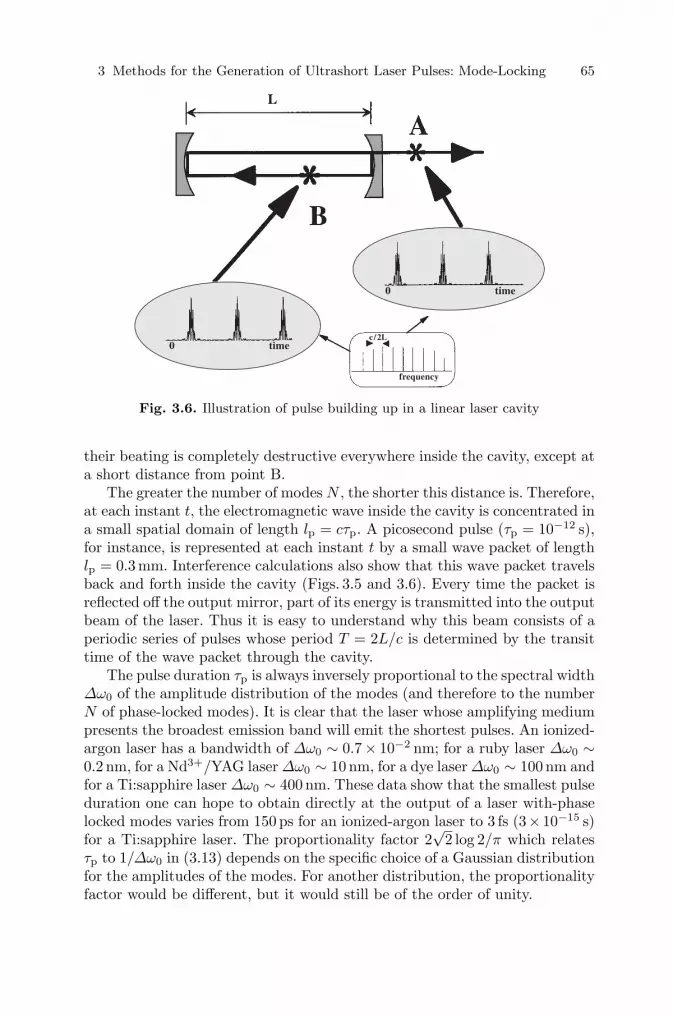
3 Methods for the Generation of Ultrashort Laser Pulses: Mode-Locking 65

0 time

c/2L

frequency

0 time

Fig. 3.6. Illustration of pulse building up in a linear laser cavity

their beating is completely destructive everywhere inside the cavity, except ata short distance from point B.

The greater the number of modes N , the shorter this distance is. Therefore,at each instant t, the electromagnetic wave inside the cavity is concentrated ina small spatial domain of length lp = cτp. A picosecond pulse (τp = 10−12 s),for instance, is represented at each instant t by a small wave packet of lengthlp = 0.3 mm. Interference calculations also show that this wave packet travelsback and forth inside the cavity (Figs. 3.5 and 3.6). Every time the packet isreflected off the output mirror, part of its energy is transmitted into the outputbeam of the laser. Thus it is easy to understand why this beam consists of aperiodic series of pulses whose period T = 2L/c is determined by the transittime of the wave packet through the cavity.

The pulse duration τp is always inversely proportional to the spectral widthΔω0 of the amplitude distribution of the modes (and therefore to the numberN of phase-locked modes). It is clear that the laser whose amplifying mediumpresents the broadest emission band will emit the shortest pulses. An ionized-argon laser has a bandwidth of Δω0 ∼ 0.7 × 10−2 nm; for a ruby laser Δω0 ∼0.2 nm, for a Nd3+/YAG laser Δω0 ∼ 10 nm, for a dye laser Δω0 ∼ 100 nm andfor a Ti:sapphire laser Δω0 ∼ 400 nm. These data show that the smallest pulseduration one can hope to obtain directly at the output of a laser with-phaselocked modes varies from 150 ps for an ionized-argon laser to 3 fs (3×10−15 s)for a Ti:sapphire laser. The proportionality factor 2

√2 log 2/π which relates

τp to 1/Δω0 in (3.13) depends on the specific choice of a Gaussian distributionfor the amplitudes of the modes. For another distribution, the proportionalityfactor would be different, but it would still be of the order of unity.

66 A. Ducasse, C. Rulliere and B. Couillaud

A pulse is said to be Fourier-transform-limited if τp and Δω0 are relatedto each other by an equation of type (3.13) with a proportionality constant ofthe order of unity. To verify experimentally whether or not a pulse is Fourier-transform-limited, τp can be measured with the help of a fast photodiode, astreak camera or an autocorrelator. The width of the spectral distribution canbe measured by means of a spectrograph or with a Fabry–Perot interferome-ter. In both cases, since the detector is quadratic, the measurement will givethe spectral distribution of the intensity; let us call the spectral width thusmeasured Δω′

0. The exact relation between Δω′0 and the spectral width of the

field Δω0 depends on the shape of the distribution. However, it can be shownthat, for a Gaussian distribution, Δω′

0 = Δω0/√

2 and that this ratio remainsof the same order of magnitude for all distributions encountered in practice.If there is a large discrepency between the measured value of Δω0 and thevalue obtained by calculation using (3.13) along with the measured value ofτp, this proves that the mode-locking is not optimal. For instance, the laseroutput can consist of a series of recurrent pulses while the central frequencyω0 of the carrier wave wanders within a band of width Δω0. For a preciseanalysis of the laser output signal corresponding to this more complicatedmode-locking regime, more complex testing is needed. If the phase-locking ofthe modes is perfect, knowing the spectral distribution is equivalent to know-ing the modulating function k(t) since one can go from one to the other by asimple mathematical transformation. Therefore, in the phase-locked regime,the situation can be described in an equivalent way either in the frequencydomain or in the time domain without loss of generality. We shall use thisproperty in the following paragraphs, in which we describe how the condi-tions for phase-locked modes, i.e. ϕ1(t) = ϕ2(t), may be obtained in practice.

3.3 General Considerations Concerning Mode-Locking

When the laser operates in the free multimode regime, there is usually a com-petition going on among the different modes to be amplified by stimulatedemission of the same atoms, molecules or ions. This competition causes bigfluctuations in the relative phases and amplitudes of the modes, which ex-plains the big fluctuations of the instantaneous intensity observed in this typeof laser (Fig. 3.1c). The purpose of locking the modes is to organize the com-petition between modes in such a way that the relative phases stay constantor, alternatively (but this is equivalent through Fourier transformation), insuch a way that the output intensity of the laser consists of a periodic se-ries of pulses resulting from the shuttling back and forth of a wave packetwithin the laser cavity. The first idea which comes to mind is best explainedin the time domain. Since in a free-mode regime, spatial concentration occurswithin the cavity at several points, it should be possible to concentrate thelaser energy even more by inserting a nonlinear medium – or any other systempromoting stronger intensities – inside the cavity. As the wave travels back

3 Methods for the Generation of Ultrashort Laser Pulses: Mode-Locking 67

and forth in the cavity, maxima that are initially slightly stronger will growmuch stronger at the expense of lesser maxima because of the competitionwithin the amplifying medium. If the conditions are well chosen, the situationmay arise where all the energy of the cavity is concentrated in one single pulse.This is the mode-locked situation: selecting a single intensity maximum in thetime domain is equivalent to establishing a phase relation between the longi-tudinal modes in the frequency domain. A second fundamental idea is bestformulated in the frequency domain. If something is inserted inside the cavitywhich modulates the modes at a frequency close to the intermode frequencyinterval c/2L, competition for maximum gain inside the amplifying mediumwill result in a coupling between each mode and the sidebands created by themodulation of its neighboring modes. The phases of the modes could then lockonto each other. One must bear in mind that selecting an intensity maximuminside the cavity by way of a nonlinear medium is equivalent to modulating thewave packet at frequency c/2L (the frequency corresponding to the back-and-forth movement of the packet in the cavity). The first method indeed inducesa self-modulation of the modes at frequency c/2L and thus establishes a phaserelation between these modes.

These two ideas form the starting point of the two main mode-lockingmethods developed so far:

– passive mode-locking resulting from the insertion of a saturable absorbingmedium into the cavity in order to select one single pulse;

– active mode-locking resulting from an external modulation at frequency Ωeither of the cavity losses (by inserting an acousto-optical crystal insidethe cavity, for instance) or of the gain of the amplifying medium (forexample by pumping this medium with another mode-locked laser).

Lately, however, the advent of the Ti:sapphire laser, in which mode-lockingis especially simple to obtain, has made an old method popular again. Thismethod was already well known, but it has now found new and fruitful ap-plications. We are speaking about a self-locking mechanism of the modes bywhich the nonlinear properties of the amplifying medium naturally enhancethe intensity maxima arising within the cavity.

Let us now look at the details of these various methods, starting with theone which is easiest to understand and easiest to put into practice: the activemethod.

3.4 The Active Mode-Locking Method

Let us insert an element inside the cavity which modulates its losses (Fig. 3.7).This element will induce a modulation of the amplitude of each longitudinalmode.

If we assume the modulation to be sinusoidal, of angular frequency Ω, andto have a modulation depth α, the time dependency of mode n of frequency

68 A. Ducasse, C. Rulliere and B. Couillaud

Ω / 2π ≅ Δwith Δ = c /2L

Fig. 3.7. Illustration of an actively mode-locked laser cavity

ωn can be written as

en(t) = En cos(ωnt + ϕn)[1 − α(1 − cos(Ωt + ϕ))]. (3.14)

This expression can also be written as follows, showing that in the frequencydomain two sidebands show up at either side of mode en(t):

en(t) = En(1 − α) cos(ωnt + ϕn) + Enα

2cos[(ωn − Ω)t + ϕn − ϕ]

+Enα

2cos[(ωn + Ω)t + ϕn − ϕ]. (3.15)

Now if the modulation frequency Ω/2π is close to the intermode frequencyseparation c/2L, the two sidebands will be very close to the two neighboringmodes n + 1 and n − 1, as shown in Fig. 3.7 (a modulation frequency of theorder of mc/2L, where m is an integer, can also be used to couple mode nto modes n + m and n − m [3.4]). The sidebands and the longitudinal modesthemselves therefore compete inside the amplifying medium for maximumgain. The situation in which the medium is used most efficiently is that inwhich the longitudinal modes lock their phases onto the sidebands, causing aglobal phase-locking over the whole spectral distribution. This global phase-locking, in turn, is the condition under which the competition will give rise tothe concentration of all the electromagnetic energy of the cavity into a singlepulse traveling back and forth inside it.

This technique goes by the name of mode-locking by amplitude modulation(AM) [3.5, 3.6] and it is used to lock the modes of ionic lasers and Nd3+:YAGlasers, for example. Usually, an acousto-optical modulator is placed inside

3 Methods for the Generation of Ultrashort Laser Pulses: Mode-Locking 69

Fig. 3.8. Acousto-optical modulator generally used for active mode-locking of lasers

Actively mode- locked laser(argon ion or doubled Nd:YAG)

Fig. 3.9. Illustration of the synchronous pumping method for mode-locking of alaser

the cavity to modulate the cavity losses. For example, in Fig. 3.8 an acousto-optical prism is shown; it can be used in an ionic laser, where it serves tolock the modes and at the same time to select the desired mean wavelength.Similar mode-locking may also be achieved by frequency modulation (FM)[3.7–9]. Whether using an AM or an FM method, an external radio-frequencypower source, whose angular frequency Ω should be as well defined as possible,must be imposed upon the system. These AM and FM methods make up onekind of active mode-locking method. Of course, one could also modulate thegain of the amplifying medium at a frequency Ω/2π. We shall now go intothis second type of active method, most often referred to as the synchronouspumping method.

Usually, synchronous pumping is obtained by pumping the amplifyingmedium of the laser with the output beam of another mode-locked laser.

70 A. Ducasse, C. Rulliere and B. Couillaud

Fine tuning of the length L of the cavity makes it possible to adapt the in-termode frequency separation c/2L to the frequency of recurrence Ω/2π ofthe pump laser pulses. Figure 3.9 shows the general layout of a synchronouslypumped dye laser. The pump is usually either a mode-locked argon laser ora frequency-doubled mode-locked YAG:Nd3+ laser. The mode-locked regimeof the pump laser is most often obtained by modulating its cavity losses withan acousto-optical modulator set at frequency c/2L1 (L1 is the length of thepump cavity). The dye laser will go into the mode-locked regime if the inter-val between its modes, c/2L2, is adjusted to the frequency c/2L1 of the gainmodulation. The purpose of this example to illustrate synchronous pumpingis twofold. First, it shows that it is possible to combine two kinds of activepumping – modulation of the cavity losses and modulation of the gain – withinthe same laser system. But second, and more importantly, it shows how onecan use a mode-locked laser as a source of a continuous train of 150 ps pulsesto pump a second laser and thus obtain a series of subpicosecond pulses. In-deed, the mode-locking of the pump laser leads to pulse durations τp whichare limited by the bandwidth of the gain (about 10−2 nm for an argon laser).However, the bandwidth of the dye laser is much broader (typically 100 nm).Therefore the output of the second synchronously pumped laser will consist ofa continuous train of picosecond or subpicosecond pulses with tunable wave-lengths, provided one stays within the gain band.

Let us look at the behavior of a mode-locked dye laser when its cavitylength L2 varies around the value of L1. First, let us consider the case of astationary regime: a narrow pulse travels back and forth inside the cavity.The oscillation condition implies that the pulse is crossing the center of theamplifying medium when the gain induced by the pump pulse is greater thanthe cavity losses. Figure 3.10 shows how the gain changes as the pump pulseand the dye laser pulse travel through the amplifying medium, i.e. throughthe dye.

The horizontal axis of the figure represents time in arbitrary units and thegain is measured at a given position inside the amplifying medium. At t = 0,the pump pulse arrives at this position, where it excites the dye molecules.The gain grows proportionally to the integral (i.e. the total accumulated sum)of the pulse intensity until the arrival of the dye laser pulse in the medium. Atthat instant, stimulated emission due to the dye laser photons will diminishthe number of excited molecules in the dye, thereby decreasing the populationinversion of the dye. This decrease shows up as a narrow dip (hole) in the gaincurve during the time the dye laser pulse passes through the medium. Whenthe gain becomes smaller than the intracavity losses, the long pulse durationof the pump makes it possible for the gain to restore itself after the passageof the dye laser pulse.

What influence would a change of the cavity length of ΔL = L2 −L1, say,have on this behavior? One must not forget that the transit time of a pulsein the cavity is determined by the repetition frequency of the pump pulses.Therefore, it is very critical that the cavity lengths are well adapted. However,

3 Methods for the Generation of Ultrashort Laser Pulses: Mode-Locking 71

Inte

nsit

y (a

rb.

unit

s)Gain

Fig. 3.10. Illustration of the generation of a pulse in a dye laser pumped by a mode-locked pumping laser. The pulse is created by competition between population ofthe emitting level by the pump and depopulation by stimulated emission (see text)

a distortion of the dye pulse inside the amplifying medium turns out to be ableto compensate small transit-time changes automatically, so that changes oflength ΔL of the order of 100μm can occur without hampering the stability ofthe system. The causes of pulse distortion can be understood by looking at thegain saturation induced by the dye pulse inside the amplifying medium. Beforethe pulse arrives, the gain is unsaturated, so the pulse front feels a larger gainthan the tail of the pulse. This differential amplification of the wavefrontresults in a pulse which seems to be ahead of where it should have been, if ithad not been distorted. The transit time of the pulse in the amplifying mediumis shortened. The shortening of the transit time is directly proportional to thedifference between the saturated and the unsaturated values of the gain, andmoreover, it always occurs, no matter what the cavity length corresponding ornot to a stable regime is. This explains, among other things, why the perfectmode-locked regime occurs for very small positive values of ΔL = +ε [3.10].

Let us now shorten the cavity length of the dye laser L2 with respect toits optimal length. The dye pulse which travels in the cavity arrives in theamplifying medium slightly earlier than it would have done in the optimumcondition. The wavefront thus feels a slightly weaker unsaturated gain thanit would otherwise have done. The pulse is somewhat less distorted, so thatits transit time through the medium is longer than it would have been. Thisproduces an effective lengthening of the total transit time. A new steady statearises in which the shortening of the transit time due to the shorter lengthof the cavity is compensated by the longer time needed to go through theamplifying medium. A similar reasoning can be applied to a slightly length-ened cavity. In this case, the dye pulse is late because of the longer cavity, but

72 A. Ducasse, C. Rulliere and B. Couillaud

Fig. 3.11. Autocorrelation curve shape as a function of the mismatch between thecavity optical lengths of the pump laser and of the pumped laser (see text)

it feels a stronger unsaturated gain than it would have done in the optimumcondition, so its transit time through the amplifying medium is proportionallyshortened.

Thus, small changes in the length of the cavity in stable operating con-ditions translate into changes in the shape of the dye pulse. More generally,most of the behavior of the pulse as a function of cavity length can be obtainedqualitatively from the model of gain variation shown in Fig. 3.10. Figure 3.11shows the autocorrelation traces of the pulses for different values of the dyecavity length L2. Figure 3.11b shows the trace of the pulse associated withan optimal cavity length. Figure 3.11a shows what happens in a longer cav-ity. Lengthening the cavity delays the arrival of the pulse in the amplifyingmedium, so that on the gain curve it shows up further from the point wherethe gain curve cuts the loss curve.

The maximum intensity of the pulse is stronger because of the larger unsat-urated gain. Simultaneously, the pulse broadens in order to adapt its transittime to the pumping period. When the change in length is sufficiently large,greater than 50μm, the intensity maximum decreases after having reacheda maximum, because the unsaturated gain decreases owing to spontaneousemission. Finally, lengthening the cavity makes total mode-locking impossi-ble since the characteristic form of the autocorrelation trace of the pulse,reminiscent of a Prussian helmet, shows that the pulses are no longer Fourier-transform-limited.

3 Methods for the Generation of Ultrashort Laser Pulses: Mode-Locking 73

On the other hand, if one shortens the cavity length with respect to theoptimal length (Fig. 3.11c, d), the pulse shows up closer to the point where thegain curve cuts the loss curve. The maximum pulse intensity decreases sincethe unsaturated gain is smaller, and the pulse duration decreases slightly inorder to stay synchronized with the pump pulse. However, if the gain decreaseinduced by the dye pulse occurs early enough, the amplifying medium, whichstill feels the pump pulse, may retrieve enough gain for it to overcome thecavity losses. The reconstitution of the oscillation condition allows a secondpulse to form in the cavity, and this second pulse is time-delayed by severaltens of picoseconds with respect to the main pulse. This satellite pulse is thecause of the two secondary maxima in the autocorrelation trace of Fig. 3.11c–e.If the cavity length is shortened even more, the delay between the two pulsescan decrease so much that one may observe a third and even a fourth pulseinside the cavity. If the pulse arrives just before the point where the gaincurve crosses the loss curve, it is damped. Still, the laser effect continues inthe form of a very broad pulse whose parameters are determined by the pumppulse and by the saturation characteristics of the amplifying medium. Onlyvery slight mode-locking occurs under these conditions, and no short pulse isformed.

All this shows that the pulse structure depends critically on the adjustmentof the two cavity lengths. For instance, a Rhodamine 6G laser whose dispersiveelement is a three-slide birefringent filter and which is synchronously pumpedby a mode-locked Ar+ laser displays the whole range of pulse shapes shownin Fig. 3.11 for a total length variation of only 130μm. It is not always easy toobtain, or even to identify, the proper mode-locked regime of the synchronouspump source. However, a qualitative approach is possible by producing a pulsewith an autocorrelation trace similar to that of Fig. 3.11b, and then reducingthe pulse width experimentally until a second pulse arises. For a dye laser witha three-slide birefringent filter and with an output of 6 ps pulses, the tolerancein the change in cavity length is about 10μm. If only one birefringent slide isused to obtain subpicosecond pulses, the tolerance drops to about 1 μm.

In fact, the second pulse must be suppressed in order to obtain subpi-cosecond pulses with a synchronously pulsed laser. Two methods have beensuggested to achieve this. As was said earlier, the second pulse arises fromthe retrieval of the gain after the passage of the first pulse. There is a criticalvalue of the intracavity power density such that if the power density is greaterthan this value, a second pulse is generated provided the cavity lengths areproperly adapted. If, however, the power density is lower than this criticalvalue, and if the system is designed to operate near enough to the functioningpower threshold, the gain curve cannot increase above the loss curve evenafter the passage of the dye pulse [3.11]. One way to avoid the formation of asecond pulse is therefore to widen the beam waist in the amplifying mediumso that the power density remains below the critical density. A second methodinvolves the simultaneous use of a passive mode-locking method and is calledthe hybrid mode-locking method. It will be described in the next section. The

74 A. Ducasse, C. Rulliere and B. Couillaud

Fig. 3.12. Round-trip pulse in a laser cavity including saturable absorber andamplifying medium

extreme sensitivity of active mode-locking methods to the relative fluctuationsof the imposed frequency Ω and the intermode frequency interval c/2L makesit very difficult to establish subpicosecond regimes with just a single activelocking procedure. These regimes are easier to obtain with hybrid methods orwith passive methods in which no exterior frequency Ω intervenes.

3.5 Passive and Hybrid Mode-Locking Methods

The dynamics of the gain saturation in the amplifying medium are responsiblefor distorting the pulse shape, as was discussed in the previous section. Nowwe want to show that if an absorbing medium with a saturable absorptioncoefficient (Fig. 3.12) is placed inside the cavity, the association between thissaturable absorber and the saturable amplifying medium leads to a naturalmode-locking of the laser, without any need for external monitoring. The mostcommonly used saturable absorbers usually consist of liquid dye solutions.However, especially since the advent of Ti:sapphire lasers, an active searchis going on to find solid media which could serve as saturable absorbers,especially among the semiconductors.

This mode-locking process is simpler to explain in the time domain [3.12].Let us look at the transmission characteristics of a saturable absorber. Atlow incident intensity, the transmission T stays practically constant, with avalue of T0 which is almost independent of the incident intensity (Fig. 3.13).But if the incident intensity increases, the population of the upper level in-volved in the absorption process increases, as does the stimulated emissionfrom this level. At the same time, the population of the lower level decreases.The combination of these two effects results in a nonlinear behavior of thetransmission coefficient, as shown in Fig. 3.13. The absorber is characterizedby its saturation intensity Iabs

s . This parameter is defined as the intensityat which the population difference that exists between the two levels at lowintensity is reduced by a factor of two. This definition thus implies that theabsorption coefficient α must be proportional to the population difference.

Moreover, as was said earlier, the amplifying medium also possesses satu-ration properties. At low intensity, the gain G has a constant value G0, which

3 Methods for the Generation of Ultrashort Laser Pulses: Mode-Locking 75

T0

I sabs

1

Transmission (T)

Intensity (I)

1/2

0

Fig. 3.13. Transmission through a saturable absorber as a function of the inputintensity

G0

G0

I samp

1

Gain (G)

Intensity (I)

2

Fig. 3.14. Gain through an amplifying medium as a function of the input intensity

is rather large (Fig. 3.14). It is said to be unsaturated. At higher input inten-sities, there is a lessening of the population inversion between the two levelsinvolved in the process, and the gain G decreases. As can be seen in Fig. 3.14,we can define Iamp

s , the saturation intensity for G, in an equivalent way tothe saturation intensity Iabs

s for the absorption.Using these parameters, we can describe how a pulse arises in a passively

mode-locked laser comprising the elements shown in Fig. 3.12. At the instantt = 0 the pump beam is applied to the amplifying medium. The power insidethe cavity is initially zero and the unsaturated gain G0 is greater than thesum of all the cavity losses. An oscillation arises inside the cavity with acharacteristic electromagnetic field showing very strong fluctuations at lowpower (Fig. 3.1c). As the power increases, the strongest intensity maxima startto saturate the absorbing medium. These stronger maxima thus suffer smaller

76 A. Ducasse, C. Rulliere and B. Couillaud

Fig. 3.15. Illustration of pulse shape modification after crossing a saturable ab-sorber

Fig. 3.16. Illustration of pulse shape modification after crossing an amplifyingmedium

losses than the lesser intensity maxima of the fluctuating field. Therefore thestrongest maximum will eliminate the others in the competition for gain whichoccurs inside the amplifying medium, since it will grow faster and will stifle allcompeting processes. If the conditions are favorable, it will end up by beingthe only intensity maximum in the cavity and will contain all the energy ofthe wave.

Let us now follow the pulse along its round trip through the cavity. Let usstart at the point where the pulse which will eventually take over is alreadyformed, but has not reached its final shape nor its final duration. As the pulsetravels through the saturable absorber, the pulse front is strongly absorbed(Fig. 3.15), but if the maximum of the pulse saturates the absorber mediumand if – as is the case in a dye laser or in a Ti:sapphire laser – the relaxationtime of the medium is longer than the pulse duration, the tail of the pulsewill benefit from the induced transparency of the medium and travel throughit without being attenuated. When the pulse reaches the amplifying medium,the pulse front will come upon the unsaturated gain G0 and will be stronglyamplified while the tail of the pulse will feel a much weaker gain, which has justbeen saturated by the front of the pulse, and thus it will be much less amplified(Fig. 3.16). It is clear that after many back-and-forth trips, the resulting pulsewill have narrowed and will have a very strong maximum, since the center ofthe initially broad pulse is not affected by the absorber but is amplified bythe amplifying medium. This process is illustrated in Fig. 3.17. The fact thatthe saturation dynamics of the absorber are more rapid than those of theamplifying medium explains why only the center of the pulse is amplified, thewings, on the contrary, being attenuated.

3 Methods for the Generation of Ultrashort Laser Pulses: Mode-Locking 77

t

Fig. 3.17. Illustration of the pulse-shortening process by simultaneous action of asaturable absorber and amplifying medium, due to saturation effects of the absorp-tion and of the gain

The pulse reaches its final shape when it becomes self-consistent in thecavity, that is, when the system reaches a steady state. For the pulse to beself-consistent, it must keep the same shape after a round trip through thecavity. However, the previous paragraph suggests that the pulse should growever narrower upon traveling constantly back and forth. Of course, if appliedwith sufficient care, the laws of physics will show that there is a limit tothis process. As said earlier, the pulse duration under perfect mode-lockedconditions is inversely proportional to the spectral width of the amplitudedistribution. Therefore, each element of the cavity which tends to limit thewidth of the oscillation band will tend to lengthen the pulse duration. Theelement which is determining from this point of view may be an externaloptical element such as a prism, a grating or a Lyot filter. The amplifyingmedium itself may also be the determining element.

This broadening effect is best explained in the frequency domain [3.13].Just before entering the filtering element, the pulse has a spectral distri-bution with certain amplitudes. The transmission filter, which is frequency-dependent, changes the distribution by decreasing the amplitudes of the wingfrequencies while leaving the central frequencies unchanged (Fig. 3.18). Thenarrowing of the spectrum explains the lengthening of the pulse durationas it passes through the filtering element. Similarly, each dispersive element

78 A. Ducasse, C. Rulliere and B. Couillaud

Fig. 3.18. Influence of a spectral filter on the spectral distribution and duration ofa pulse

of the cavity will also affect the pulse duration by time-delaying the vari-ous frequency components of the spectral distribution by different amounts.The pulse reaches steady state when the narrowing effect due to the satu-ration properties of the absorber and of the amplifying medium is exactlycompensated by the broadening effects of the various elements in the cavity,of which the main two have been described above. In fact, the actual studyof the propagation of the pulse through the various elements of the cavity isextremely complex, especially if one remembers that amplifying media andabsorbers are nonlinear media. To tackle the problem in a reasonably realisticway, one should take into account, among other things, the variation of therefractive index with intensity inside these media. This variation results ina self-modulation of the phase of the pulse. This point has been covered inChap. 2.

Figure 3.19 shows an example of a passively mode-locked laser. It is adye laser whose amplifying medium consists of Rhodamine 6G pumped by acontinuously emitting argon ion laser. The saturable absorber is a DODCI(3,3′-diethyl oxadicarbo cyanine iodide) jet. In order to reach the saturationthreshold of the absorber, the laser beam is strongly focused inside the ab-sorber medium by means of spherical mirrors of short focal length. The cavityshape is calculated so that the astigmatism introduced by the mirrors, whichare used off axis, is compensated by the jets placed at the Brewster angle.One should remember, as said before, that by passing through the absorbingmedium and the amplifying medium every 2L/c seconds, the pulse createsa modulation of each of its longitudinal modes at frequency c/2L. Lateralbands therefore arise at the intermode frequency distance. These in turn in-duce mode-locking of the phases, and the frequency spectrum tends to broaden

3 Methods for the Generation of Ultrashort Laser Pulses: Mode-Locking 79

argon laser pump beam

internal dye laser beam

Rhodamine 6Gdye jet

DODCIsaturableabsorber

Fig. 3.19. Typical laser cavity of a passively mode-locked laser using a saturableabsorber. This example is for a dye laser pumped by a CW argon laser

while the pulse narrows. Here we have presented the frequency description ofthe passive mode-locking process.

The problems which arise in the passive mode-locking method are, firstof all, the fact that there are not many compatible pairs of saturable ab-sorbing and amplifying media with the correct properties, and, second, thefact that the pulses obtained by this method are not very powerful and thattheir wavelength is only slightly tunable. A hybrid method was devised totry to overcome the drawbacks of both the passive and the active mode-locking methods. It consists of inserting a saturable absorbing medium insidethe synchronously pumped cavity [3.14]. This hybrid locking method allows awider choice of wavelengths and powers than a simple passive mode-lockingmethod would. On the other hand, when compared with the simple activemode-locking method, hybrid locking makes it easier to obtain subpicosecondpulses and it avoids the formation of secondary pulses.

Figure 3.20 shows an example of a mode-locked laser using the hybridmethod. The system is similar to the one shown in Fig. 3.19 to illustrate thepassive method, but now the pumping is done with an Ar+ laser whose modesare locked using the active method. In this case, the cavity length must beadjusted to the cavity length of the Ar+ laser, as explained in Sect. 3.4. Onecan see that the pumping inside the amplifying medium is not colinear with thelaser wave of the cavity. This kind of pumping, which avoids the inconvenienceof having a prism inside the cavity, is also frequently used in the passive

80 A. Ducasse, C. Rulliere and B. Couillaud

Fig. 3.20. Typical cavity design of a hybrid mode-locked laser

method instead of the pumping method shown in Fig. 3.19. Some examplesof pairs of amplifying dyes and saturable absorbers, covering a wide spectralrange between 575 nm and 860 nm, are shown in Table 3.1. In Figs. 3.19 and3.20, the dispersive element (a Lyot filter for example) which determines themean wavelength of the pulse has not been shown. The cavity also usuallycontains a device which compensates for the dispersive effects of the groupvelocity of the pulse, which limit the pulse duration, as explained earlier. Allthese elements (series of prisms for instance) will be discussed in detail in thefollowing chapters. Figure 3.21 shows how a series of prisms is used in a hybridpumping setup. In Fig. 3.22 one can see that such a system, compensating thedispersion of the group velocity, is needed in order to obtain subpicosecondpulses with a hybrid pumping method.

Table 3.1. Some examples of dye-amplifier–dye-absorber pairs for generation ofshort pulses in different spectral ranges

Saturable WavelengthGain dye absorber in nmRh6G DODCI, DDI 575–620Kiton Red DQOCI 600–655DCM DODCI, DTDCI 620–660Pyridine 1 DTDCI, DDI 670–740LD 700 DTDCI, DDI, IR 140 700–800Pyridine 2 IR 140, HITC 690–770Styryl 9M DDI, IR 140 780–860

3 Methods for the Generation of Ultrashort Laser Pulses: Mode-Locking 81

Fig. 3.21. Cavity design of hybrid mode-locked laser with inserted prisms for groupvelocity dispersion (GVD) compensation

Inte

nsit

y (a

rb.

unit

s)

Time (ps)

Fig. 3.22. Illustration of the effect of GVD compensation on the pulse duration ina hybrid mode-locked laser

3.6 Self-Locking of the Modes

We have seen that the nonlinear properties of the amplifying medium arealways very important for the locking process, whether the locking method isactive or passive. In some types of lasers, these properties are so fundamentalthat the modes may lock, partially or totally, without any need for an externalmodulation (active locking) or for a saturable absorbing medium (passivelocking). This situation is called self-locking of the modes. For such a situationto arise, the amplifying medium must induce a narrowing of the pulse at eachof its round trips through the cavity. The dynamics which were described forthe passive locking method show that saturation of the gain is not sufficient.There needs to be an associated effect which favors strong intensity maximaat the expense of weak ones. This effect is provided by the saturable absorberin the passive mode-locking method. We shall now describe a specific self-locking situation in which the amplifying medium decreases the losses of the

82 A. Ducasse, C. Rulliere and B. Couillaud

stronger intensity peaks of the cavity by modifying the transverse structureof the laser wave selectively with respect to intensity. This situation existsin the Ti:sapphire laser, explaining why the interest in self-locking of modessuddenly flared up recently.

Historically speaking, the self-locking of modes was first observed acciden-tally in a laser whose amplifying medium consisted of a Ti:sapphire crystalpumped by an Ar+ laser, which, in principle, operated in a continuous regime,in a cavity without a saturable absorber. Scottish scientists [3.15] then noticedthat the laser went into a pulsed regime when they jerked the table on whichthe laser was mounted. The pulsed regime consisted of very short pulses, andonce initiated, maintained itself. It was first called “magic mode-locking”, butit stayed magic only for a few months, an explanation having been foundmeanwhile. In fact, it was a case of self-locking by a Kerr lens effect [Kerrlens mode-locking (KLM)], a self-locking process which clearly reveals thatthe following conditions are needed for this kind of behavior to appear:

– The pulsed regime must somehow be favored over the continuous regime.– The overall system must possess the property of shortening the pulses.– Some mechanism must initiate the self-locking process.

Figure 3.23 shows the classical configuration of a self-mode-locked Ti:sap-phire laser. The Ti:Al2O3 crystal is pumped by the output of a continuousAr+ laser through M2, a dichroic mirror which is transparent at 0.5μm andwhich reflects at the emission wavelengths of Ti:sapphire around 0.8μm. Thebirefringent filter (B.R.F.) determines the central wavelength of the oscilla-tion. The two prisms P1 and P2 compensate for the dispersion of the groupvelocity inside the cavity, as was explained above. The mode-locking processarises exclusively from the amplifying medium and an associated pinhole withadjustable diameter. This process results from the Kerr effect and can besummarized in the following way.

The fact that the amplifying medium is nonlinear implies that its refrac-tive index is a function of the intensity (Kerr effect): n = n0 + n2I. TheGaussian wave therefore does not feel a homogeneous refractive index as itpasses through the medium. If n2, the nonlinear coefficient of the refractiveindex, is positive, the refraction is stronger on the axis of the beam than awayfrom it. So the amplifying medium behaves like a converging lens and focusesthe beam just like a lens (Kerr lens). We are speaking of the phenomenon ofself-focusing, which has been known for a long time in nonlinear optics andis explained in Chap. 2. However, self-focusing is proportionally more impor-tant for strong intensities. This means that the strong intensity maxima ofthe laser cavity will be much more strongly focused than the weaker ones, forwhich focusing will be negligible (Fig. 3.24).

These strong intensity maxima, whose transverse structures have now beenreduced in size, are usually less subject to losses in the cavity than the weakerintensities, which occupy a large volume, so they are enhanced. Clearly, theintensity-differentiated self-focusing associated with the natural cavity losses

3 Methods for the Generation of Ultrashort Laser Pulses: Mode-Locking 83

Fig. 3.23. Typical cavity design of a self-mode-locked Ti:sapphire laser using theKLM (Kerr lens mode-locking) process (see text)

Fig. 3.24. Illustration of the self-focusing effect by the optical Kerr effect on thebeam waist of a laser beam at high and low intensity

plays a part similar to that of the saturable absorber in the passive mode-locking method, and, indeed, self-mode-locking of the modes arises. A slit canbe placed inside the cavity to help the self-locking process since it increasesthe difference between the losses undergone by the weak intensities and thoseundergone by the intensity maxima. The exact position, diameter, and shapeof the slit must be calculated so that it lets through most of the power ofthe stronger intensity maxima while it stops the greater part of the weakerintensities. Figure 3.25 illustrates the passage from a continuous regime (withopen slit) to a mode-locked regime. The experimental data of Fig. 3.25 clearlyshow the broadening of the spectrum and its transformation into a spectrum

84 A. Ducasse, C. Rulliere and B. Couillaud

Pulse Spectrum vs. Slit WidthDemonstrating Slit as SaturableAbsorber

Inte

nsit

y (a

rb.

unit

s)

Wavelength

Fig. 3.25. Spectral distribution of laser output for different widths of the slit in-serted in the cavity, which controls the mode-locking by the optical Kerr effect

corresponding to a correctly mode-locked regime for a slit width of 0.47 mm.It should be noted that the amplifying medium must be relatively thick toobserve a strong lens effect. This explains why the lens effect, which is soimportant in the Ti:sapphire laser, is negligible in dye lasers.

The laser illustrated in Fig. 3.23 has the drawback that it does not go intothe pulsed regime spontaneously. As long as no important intensity fluctua-tions arise to create sufficiently strong Kerr lens effects, the continuous regimeprevails over the pulsed regime, as shown in Fig. 3.25. To start the pulsed pro-cess, one can insert a rapidly rotating optical slide so as to create a changingoptical path, or one can simply give a quick jolt to one of the mirrors of thecavity to create an intensity pulse which triggers off the process.

We see therefore that in a Kerr-lens mode-locked (KLM) laser, the dis-crimination between a continuous regime and a pulsed regime is due to theself-focusing in the amplifying medium, and this discrimination becomes ef-fective after a rapid transient change in the optical length of the cavity. Westill have to explain how the pulses shorten and stabilize their duration byfollowing their journey back and forth through the cavity in the proper self-locking conditions defined above. In fact, on top of its influence on the spatialevolution of the wavefront (self-focusing), the change of refractive index asa function of intensity in the amplifying medium also has very importantconsequences for the time structure of the laser wave. Indeed, the intensityI(t) being a rapidly varying function of time, the change of refractive indexas a function of the intensity, following the equation n = n0 + n2I(t), im-plies a rapid change of the phase of the wave as a function of time. This

3 Methods for the Generation of Ultrashort Laser Pulses: Mode-Locking 85

Inte

nsit

y (a

rb.

unit

s)

Wavelength (arb. units)

Time (arb. units)

Fig. 3.26. (a) Autocorrelation trace (b) and spectrum of the pulse a few hundredsof femtoseconds wide obtained with the laser shown in Fig. 3.23 after starting themode-locking process

self-modulation of the phase broadens the spectrum of the wave and thereforeshortens its duration. As was the case for the passive mode-locking method,an equilibrium is reached between this process of pulse shortening and thedispersion of the group velocity, which tends to lengthen the pulse. The com-pensation between the self-modulation of the phase and the dispersion of thegroup velocity gives rise to a pulse which travels back and forth in the cavitywhile keeping its shape. This pulse is called a quasi-soliton. Here again, it isessential to be able to keep control of the group velocity inside the cavity,which is the reason for the two prisms in the system shown in Fig. 3.23.

This kind of mode-locking leads to excellent results for the pulse durationas well as for its stability. In Fig. 3.26 we show the autocorrelation trace andthe spectrum of the pulse a few tens of femtoseconds wide obtained withthe laser shown in Fig. 3.23. The ease with which these systems are made towork, their great reliability and the great stability from pulse to pulse placethem among today’s most popular mode-locked systems. At present, they arechosen routinely each time a good-quality femtosecond oscillator is required.

Further improvements of this mode-locking can produce even shorterpulses in the sub-10-fs range as a routine [3.17]. These improvements are ob-tained using cavity chirped mirrors and/or SESAMs (semiconductor saturableabsorber mirror).

86 A. Ducasse, C. Rulliere and B. Couillaud

a) Chirped Mirrors: The main limitation of the pulse duration in a Kerr lensmode-locking cavity is due to the difficulty of obtaining exact compensa-tion of the GVD and SPM effects using pair prisms. Indeed, higher-orderdispersion introduced by the prisms is the main limitation factor. Chirpedmirrors make it possible to overcome this difficulty [3.18–3.20].

Such mirrors consist of stacks of different transparent layers with highand low refraction indexes. Tuning the thickness of layers to a correspond-ing λB/4 phase delay makes constructive interferences of the differentwaves reflected at λB (Bragg wavelength).

If the thickness of the layers is made different along the mirror structure,it will be possible to reflect different waves at different λB wavelengths toaccommodate the bandwidth of the laser cavity. Then the different wavesat λB will have different optical pathways inside the mirror before it isreflected. These different waves will be more or less delayed after reflectionon this mirror, depending on the thickness of the different layers. In sucha way, a chirp is created by this type of mirror which can be tailored,adjusting the thickness layers, to compensate exactly the highter-orderdispersion effects and obtain shorter pulses near the theoretical limit (3 fs)of Ti/Sa material.

b) SESAM mirrors: As the pulses become shorter, self-starting of mode-locking by KLM is more difficult. One interesting solution is to use asaturable absorber designed for such lasers. A SESAM makes it possibleto help the self-starting of Ti/Sa lasers when an ultimate pulse durationbelow 10 fs is required [3.21].

Different designs of SESAMs have been employed. Four parameters haveto be taken into acount for proper design of SESAMs: the modulationdepth introduced by the saturable absorber, the spectral bandwidth tobe accommodated, the saturation energy, and the recovery time constant.For this last parameter, the time response should be biexponetial with afast answer for ultrashort pulse generation and a slow answer for makingit possible for the mode-locking to sef-start [3.21].

Semiconductors as absorbers are well suited because they absorb in alarge spectral bandwidth compatible with Ti/Sa emission range and be-cause they have fast and slow responses correlated with the thermalizedprocess inside the band (fast response) and carrier trapping and recombi-nation (slow response).

SESAMs use different designs to account for the different parameters.Sandwiches of saturable absorber between a dielectric reflector and a semi-conductor Bragg mirror are, for example, a simple solution [3.22–3.23]. Toaccount for large bandwidth supporting very short pulses, the Bragg mir-ror can also be replaced by a silver mirror [3.22, 3.24–3.26].

A panel of solutions is described in [3.21], and cited references makepossible to tailor the pulse duration in the range of 50 fs–sub-10 fs withself-starting mode-locking and stable laser running.

3 Methods for the Generation of Ultrashort Laser Pulses: Mode-Locking 87

References

[3.1] D.H. Auston: IEEE J. Quant. Electr. QE4, 420 (1968)[3.2] D.J. Bradley, G.H.C. New: Proc. IEEE 62, 313 (1974)[3.3] B. Couillaud, A. Ducasse: Rev. Phys. Appl. 14, 331 (1979)[3.4] M.F. Becker, D.J. Kuizenka, A.E. Siegman: IEEE J. Quant. Electr. QE8,

687 (1972)[3.5] L.E. Hargrove, R.L. Fork, M.A. Pollack: Appl. Phys. Lett. 5, 4 (1964)[3.6] O.P. McDuff, S.E. Harris: IEEE J. Quant. Electr. QE3, 101 (1967)[3.7] S.E. Harris, B.J. McMurtry: Appl. Phys. Lett. 7, 265 (1965)[3.8] S.E. Harris, O.P. McDuff: IEEE J. Quant. Electr. QE1, 243 (1965)[3.9] D.J. Kuizenga, A.E. Siegman: IEEE J. Quant. Electr. QE6, 709 (1970)[3.10] A. Scavennec: Opt. Commun. 17, 14 (1976)[3.11] J. Kluge, D. Wiechert, D. von der Linde: Opt. Commun. 45, 278 (1083)[3.12] U. Keller, N.H. Knose, H. Roskos: Opt. Lett. 15, 1377 (1990)[3.13] H.A. Haus: IEEE J. Quant. Electr. QE11, 736 (1975)[3.14] J.P. Ryan, L.S. Goldberg, D.J. Bradley: Opt. Commun. 27, 127 (1978)[3.15] U. Keller, W.H. Knose, G.W. ’tHooft, H. Roskos, T.R. Woodward, J.E. Cun-

ningham, D.L. Sivco, A.Y. Cho: Adv. Sol. State Lasers 10, 115 (1991)[3.16] G.R. Jacobovitz-Veleska, U. Keller, M.T. Asom: Proceedings of Conference

on Lasers and Electro-Optics (CLEO), 1992, p. 188[3.17] G. Steinmayer, L. Gallmann, F. Helbing, U. Keller: C.R. Acad. Sci. Paris t.2,

Serie IV, 1389 (2001)[3.18] R. Szipocs, K. Ferencz, C. Spielmann, F. Krausz: Opt. Lett. 19, 201 (1994)[3.19] A Stingl, C. Spielmann, F. Krausz, R. Sipocs: Opt. Lett. 19, 204 (1994)[3.20] M. Zalevani-Rossi, G. Cerullo, S. De Silvestri, L. Gallmann, N. Matuschek,

G. Steinmeyer, U. Keller, G. Angelow, V. Scheuer, T. Tschudi: Opt. Lett.26, 1155 (2001)

[3.21] I.D. Jung, F.X. Kartner, N. Matuschek, D.H. Sutter, F. Gorier-Genoud, Z.Shi, V. Scheuer, M. Tilsch, T. Tschudi, U. Keller: App. Phys. B 65, 137(1997)

[3.22] U. Keller, K.J. Weingarten, F.X. Kartner, D Kopf, B Braun, I.D. Jung, R.Fluck, C. Honninger, N. Matuschek, J. Aus der Au: IEEE J. Selected Topicsin Quantum Electronics 2, Sept. (1996)

[3.23] U. Keller, D.A.B. Miller, G.D. Boyd, T.H. Chu, J.F. Ferguson, M.T. Asom:Opt. Lett. 17, 505 (1992)

[3.24] R. Fluck, I.D. Jung, G. Zhang, F.X. Kartner, U. Keller: Opt. Lett. 21, 743(1996)

[3.25] C. Honninger, G. Zhang, U. Keller, A. Giesen: Opt. Lett. 20, 2402 (1995)[3.26] I.D. Jung, L.R. Brovelli, M. Kamp, U.Keller, M. Moser: Opt. Lett. 20, 1559

(1995)

4

Further Methods for the Generation ofUltrashort Optical Pulses

C. Hirlimann

With 23 Figures

4.1 Introduction

Up to the beginning of the sixties, the shortest measurable time duration wasof the order of one nanosecond (10−9 s). Short pulses were produced throughthe generation of short electrical discharges. After the laser was invented in1960, the situation quite rapidly changed. In 1965, the picosecond (10−12 s)regime was reached by placing a saturable absorber inside a laser cavity.Twenty years of continuous progress led to the production of light pulsesof less than 10 femtoseconds. In the race towards ever shorter pulses, recentdevelopments in the generation of tabletop X-ray lasers have opened the wayto dynamical studies in the attosecond (10−18 s) regime [4.1–2]. In the mean-time, progress was made on the tunability of the pulsed-laser sources. Today’stunability extends from the near ultraviolet to the near infrared [4.2–6].

Periodic trains of ultrashort light pulses, with duration less than 10−12 s,can be generated using mode-locking techniques in laser cavities: active, pas-sive or self-mode-locking. A large variety of lasers have been designed butonly a few of them have been made commercially available. In this chapterwe will discuss some of the lasers which have been of key importance in thefield of short pulse generation. Although mode-locking is the most popularway to have a laser generate light pulses, we will also describe some other,more exotic techniques, based on the specific dynamical behavior of ampli-fied spontaneous emission (ASE). A short section will also be devoted to thedevelopment of ultra-intense lasers, which has led to the arrival of table-topX-ray lasers.

4.1.1 Time–Frequency Fourier Relationship

Following L. Euler, who gave in 1748 the cosine representation of an analyticalfunction, Joseph Fourier introduced in 1807 the more general trigonometricanalysis, named after him, which was to become one of the most powerful

90 C. Hirlimann

mathematical tools used in physics. Fourier analysis can be applied to periodicpulse trains. If one defines Δν as the full spectral width at half maximum andΔt as the duration of a light pulse at half maximum, then these quantitiesobey in the following inequality (see Chaps. 2 and 3):

Δν Δt ≥ K, (4.1)

where K is some constant number depending on the profile of the light pulse[4.7]. The Fourier relationship (4.1) has important consequences in the fieldof the generation and transfer of ultrashort light pulses.

To generate a short duration one has to be able to manipulate wide spectra.For a Gaussian pulse shape K = 0.441, and the spectral width of a onepicosecond pulse (10−12 s) is at least Δν = 4.41 × 1011 Hz, while it is already4.41 × 1013 Hz for a 10 fs pulse. Such large spectra need special care becausethey suffer group velocity dispersion when propagating through transparentmaterials. As an example, a 100 fs transform-limited pulse, crossing a 50 cmlong cell filled with ethyl alcohol [4.8], broadens to 400 fs, a situation easilyfound early in dye amplifiers and now in modern large scale glass amplifiers.The instantaneous frequency of the pulse is then not constant any more; thepulse is chirped along the propagation direction.

Another dispersion effect takes place when light is reflected from a mul-tilayered dielectric mirror like the ones used in laser cavities [4.9]. Reflectionof light from such mirrors is the result of a constructive interference effectbetween rays which have been partially reflected at the interfaces of λ/4 di-electric layers. The frequency dispersion introduced by such mirrors is turnedto advantage in Gires–Tournois interferometric optical compressors, but hasproved to be particularly treacherous in broadband multistack multilayer di-electric mirrors [4.10]. The group velocity dispersion which takes place in thesemirrors has also been turned to advantage in the so-called chirped mirrors[4.11–12].

Optical compressors are used to correct positively-group-velocity-chirpedpulses by introducing negative group velocity dispersion. In a grating opticalcompressor, for instance, the various frequency components of the pulse arespatially separated and the device can be set up in such a way that theiroptical path is shortest when their frequency is highest.

The wide spectral width of short optical pulses also implies that each andevery optical element used in an experimental setup must have a large enoughbandwidth to be able to accommodate all the frequency components of thepulses. Ultrashort light pulses are fragile entities: from (4.1) it can be deducedthat any spectral narrowing induces a broadening in the time domain. As aconsequence these pulses can only be generated by laser oscillators havinga wide gain bandwidth; a 100 fs pulse needs a gain spectrum 10 nm wide inthe mid-visible spectral range. Outside the oscillator, ultrashort light pulsesare better transferred from one point to another using aluminum- or silver-protected mirrors in order to avoid spurious phase distortions.

4 Further Methods for the Generation of Ultrashort Optical Pulses 91

Fig. 4.1. Schematic diagram showing the orbital electronic states involved in a gaslaser. Direct or collision excitation moves electrons from a ground state E1 to anexcited state E4. Nonradiative relaxation of electrons from E4 to E3 and from E2

to E1 is faster than the spontaneous radiative relaxation of electrons between statesE3 and E2. An inversion of the electronic population may grow between states E3

and E2

To provide the structure for this chapter, the arbitrary choice has beenmade to classify the laser oscillators according to the density of their gainmedium, from gases to solids.

4.2 Gas Lasers

In gas lasers inverted populations are created between electronic levels ineither gases, ion plasmas or metal vapors. The following discussion will berestricted to the visible and near-infrared regions of the electromagnetic spec-trum, so that molecules as gain media will not be discussed.

Figure 4.1 shows a very general sketch of the electronic transitions involvedin a gas laser. Most often, energy is transferred to the gas through an electricaldischarge inside a sealed tube. Excitation may be direct, as in ionized argonor ionized krypton lasers, or indirect as in He–Ne lasers, where the energy istransferred through collisions from electrically excited helium to inert neon.From a highly excited state the electrons relax nonradiatively down to anintermediate metastable state, creating an inverted population.

Atomic-like states have energetically narrow bandwidths, but in a gas theatoms or ions move around with a distribution of speeds which depends onthe working condition of the laser. For each atom velocity, the electronic state

92 C. Hirlimann

Fig. 4.2. The axial modes of a laser cavity are equally spaced with intermodefrequency spacing c/2L. The effective gain curve (gain minus losses) is Doppler-broadened up to Δν and in this sketch only six modes may participate in the laseraction [4.13]. The spectral width Δν of the axial modes is related to the finesse ofthe Fabry–Perot cavity

is shifted in energy according to the Doppler effect; therefore the emissionradiation of a gas is inhomogeneously broadened to a width Δν (Fig. 4.2).Figure 4.2 shows the Dirac’s comb of the Doppler-broadened axial modes of alaser cavity, which are equally spaced in frequency with a frequency separationequal to c/2L (see Chaps. 1 and 3), c being the velocity of light and L theoptical length of the cavity. Only the modes for which the gain is larger thanthe losses are involved in the coherent laser emission. For a typical gas laser theDoppler broadening is of the order of 1500 MHz, while the frequency spacing,for a 1 m cavity length, is of the order of 150 MHz, so that there are only a fewtens of modes really involved in the laser process. With this kind of spectralbandwidth the shortest pulse achievable with gas lasers is of the order of afew hundreds of picoseconds; these lasers are not well suited for generatingultrashort pulses.

4.2.1 Mode-Locking

Active mode-locking (e.g. [4.14]) of ionized-argon [4.15] or krypton [4.16] lasersis widely used, as commercial lasers are available. Mode-locking is achievedby placing in the laser cavity an acousto-optical device which periodicallymodulates the losses of the laser at frequency c/2L (see Chap. 3). In this waypulses lasting for about 150 ps can be generated, with a repetition rate of theorder of 80 MHz and an average power of several watts or more.

4.2.2 Pulse Compression

Gas lasers, even if they are not good short-pulse generators, have been widelyused as primary light sources in optical setups which allow the generation of

4 Further Methods for the Generation of Ultrashort Optical Pulses 93

30m

5.9ps

0.5m

200fs

90fs

1

2

Fig. 4.3. Compound optical compressor. Two optical compressors made of a lengthof single-mode optical fiber followed by a dual-pass-grating time compressor are usedin series. As the self-phase-modulation process broadens the spectrum of the pulsesin a manner proportional to the intensity derivative of the pulses, the fiber needs tobe longer in the first stage, where the peak intensity is smaller, than in the secondstage, where it is larger

really ultrashort pulses. One basic idea is to use nonlinear optical effects toenlarge the spectral content of the pulses and to synchronize all the frequencycomponents through an optical compressor.

The first demonstration of pulse shortening was achieved using a mode-locked He–Ne laser generating 500 ps pulses [4.17]. The spectrum of the pulseswas broadened by up to 2.8 MHz by externally applying a strong acousto-optical modulation. The modulation creates new frequencies in the sameway as in mode-locking. The frequency-broadened pulses were then time-compressed, using a specially designed Gires–Tournois interferometer [4.18],down to 250 ps.

Self-phase-modulation (see also Chap. 2) in single-mode optical fibers wasdeveloped at the end of the 1970s as a powerful tool for generating shortoptical pulses. Figure 4.3 shows the optical path of a dual-stage pulse com-pressor [4.19]. A mode-locked argon ion laser generates light pulses which arecoupled into a 30 m long single-mode optical fiber. After propagation alongthe fiber, the spectral bandwidth is enlarged by a factor of 30 because of self-phase-modulation. The pulses are then chirp-corrected in a dual-pass gratingcompressor and coupled to a second but shorter optical fiber. After final timecompression in another compressor the pulse shortening is as large as 65 times.

This technique is totally general and can be used with any kind of picosec-ond or subpicosecond laser source (see also Sect. 4.3.3). Its use is of partic-ularly great importance when the original pulses are generated by a tunablepicosecond laser, because tunability is maintained in the process.

94 C. Hirlimann

Fig. 4.4. In a dye molecule the electronic states are split into numerous substatescorresponding to deformations of the electron clouds of the molecule induced byvibration and rotation of various parts of the molecule relative to each other. S0

and S1 are singlet states, T1 is the lowest triplet state

4.3 Dye Lasers

Liquids are of higher density than gases, so they give rise to better yields whenused as gain media, even though the real active media are organic moleculesdissolved in polar solvents such as water, alcohols and glycols. These moleculesabsorb light in a specific wavelength range and emit light in some other, red-shifted range (Stokes shift).

Figure 4.4 shows a simplified electronic structure for a dye molecule (seee.g. [4.20]). This structure is much more complex than the electronic structureof gases because of interactions of the electron clouds with various rotationsand vibrations inside the molecule, as well as interactions of the moleculewith the solvent. These movements distort the electronic structure, each statebeing split into a great many rotation–vibration substates. The speed of themolecules in their solvent is much smaller than the speed of atoms in a gas,and therefore Doppler broadening may be totally neglected. Contrary to gasesagain, the energy positions of states and substates in a molecule are stronglydependent on the molecular environment. Electronic states are inhomoge-neously broadened because of the interactions of the electron clouds withthe neighbouring solvent molecules. For the purpose of understanding dyelasers, it is legitimate to assume that the electronic structure in these mediais made of quasi-continuous energy bands. Between these bands one finds aquasi-continuous distribution of four-level electronic systems from which laseremission may take place. The spectral width of these bands is of the order ofa few tens of terahertz (a few tens of nanometers for the wavelength), whichopens direct access to the generation of ultrashort light pulses.

4.3.1 Synchronously Pumped Dye Lasers

The technique of synchronously pumping a dye laser (see Chap. 3 and [4.21])is commonly used to generate short light pulses in the visible and in the nearinfrared. The primary source of energy for optically pumping the dye in thesedevices is an actively mode-locked laser generating pulses lasting for about

4 Further Methods for the Generation of Ultrashort Optical Pulses 95

Fig. 4.5. Dye laser cavity, optically pumped by a mode-locked laser. The lengths ofthe laser cavities are made equal in order for the build-up of the pulse in the cavityto be synchronous with the pumping of the population inversion in the gain medium

100 ps. This primary oscillator may be either a gas laser or a solid-state laser(Fig. 4.5).

The mode-locked laser source excites dye molecules dissolved in a solvent;the liquid gain medium is either contained in a cell or dynamically shaped asa jet [4.22]. The dye laser is set up with the same optical length as the sourcelaser to ensure the equality of the times of flight in both cavities. That way,the light pulse traveling in the dye cavity encounters the gain medium at theexact time it is optically pumped. Because of gain saturation (Fig. 4.6) andbecause the spectral bandwidth of a dye is wider than the bandwidth of themode-locked laser, much shorter pulses may be generated.

Gain saturation has been explained in Chaps. 1 and 2; this nonlinear effectis such that for large incoming intensities the population inversion in the gainmedium is depleted and stimulated emission stops. During the amplificationof short pulses, the pumping rate of the inverted population is generally atleast one order of magnitude slower than the duration of the pulse to beamplified. Therefore the incoming intensity rapidly grows, followed quicklyby the stopping of the stimulated emission. By this mechanism the leadingfront of the pulse is preferentially amplified, compared with the trailing edge;this leads to a duration narrowing of the pulse from its trailing part.

These dual-cavity lasers generate light pulses with a duration of the orderof a few picoseconds, a repetition rate of the order of 80 MHz and an averagepower ranging from 10 mW to a few hundreds of milliwatts. Various designshave been proposed, using a large number of dye molecules, allowing thegeneration of pulses with wavelengths ranging from 500 nm to the infrared.

96 C. Hirlimann

Fig. 4.6. Pulse shortening through gain saturation. Left, the time envelope of thepump pulses and the corresponding gain increase in the dye (in arbitrary normal-ized units). Right, result of the synchronized propagation of the dye oscillator pulsethrough the gain medium. The leading part of the pulse is strongly amplified up tothe point when the gain saturates. The trailing part is not amplified, which resultsin a narrowing of the pulse [4.23–24]

4.3.2 Passive Mode-Locking

For general information, see for example [4.25–26]. The most famous memberof this family is the so-called colliding-pulse mode-locked (CPM) dye laser, ofwhich one variation is shown in Fig. 4.7 [4.27–28].

We will first consider the operation of a CPM laser without any compen-sation element. In a ring laser cavity two light pulses can counter-propagate,clockwise and counterclockwise. The saturable absorber is chosen to have aconcentration such that it only saturates when the two pulses are simulta-neously present. As a consequence, the two pulses automatically synchronizetheir flight in the cavity so as to cross in the saturable absorber. The super-position of the two pulses results in a transient stationary wave, creating atransient phase and amplitude modulation. Part of the light of each of thepulses is diffracted back into the other pulse by these modulations, improvingthe locking of the modes [4.29]. For the amplification of the two pulses to besymmetrical the gain medium and the saturable absorber are placed in thecavity according to the geometry shown in Fig. 4.8.

When the gain medium is placed at a quarter of the total cavity lengthL from the saturable absorber, the total pumping duration L/2c is the samefor both pulses. This geometrical rule is not very stringent as long as the gainrecovers its full value between consecutive saturation processes [4.30–31].

Figure 4.9 illustrates the three mechanisms responsible for the final du-ration of the pulses. Gain saturation has already been discussed as a time-shortening mechanism in which the trailing edge of a pulse is clipped off.Symmetrically, in the saturable absorption process, the leading part of thepulse is absorbed (see Chaps. 2 and 3), which time-shortens them from thefront edge. Time-shortening by gain and absorption saturation is balancedby group velocity dispersion. Along their propagation the pulses encounterthe two jets and the coatings of the cavity mirrors, which introduce time-

4 Further Methods for the Generation of Ultrashort Optical Pulses 97

Fig. 4.7. Sketch of a balanced colliding-pulse mode-locked dye laser. The geom-etry of the cavity is that of a ring laser with Rhodamine 6G as a gain medium.These molecules are optically pumped by a CW argon ion laser delivering 5W inits 515 nm green line. To ensure mode-locking, a second jet, dyed with DODCI(3,3′-diethyloxadicarbocyanine iodide), is placed at the focal point of a short-focal-length telescope. The emission maximum of Rhodamine 6G is close to 590 nm. Thiswavelength is strongly absorbed by the DODCI molecules, for which the absorptionmaximum is close to 580 nm in the ground state. Absorption of photons induces aconformation change of the DODCI molecules to a photoisomeric state, for whichthe absorption is red-shifted down to 620 nm. The resulting photoisomer is the actualsaturable absorber acting as a mode-locker in the cavity. This photoisomerizationexplains why, without a dispersive element in the cavity, CPM lasers emit light at620 nm rather that at 590 nm

broadening by group velocity dispersion. The strong focusing of the light inthe saturable-absorber jet induces self-phase-modulation, which introducesphase distortion. When the laser runs in a steady regime the balance of thesevarious effects leads to the generation of 60 fs pulses. The repetition rate ofsuch a laser is of the order of 80 MHz, the central wavelength is 620 nm andthe average power is of the order of 20 mW.

Note that the generation of ultrashort light pulses is not based on the useof ultrafast phenomena. Both the gain medium and the saturable absorber re-cover from saturation on timescales which are of the order of one nanosecond!

Up to this point, a temporal picture has been used to describe the pulse-shortening effects acting in a passively mode-locked laser. The Fourier dualitybetween time and frequency implies that there must be an equivalent fre-quency description of the working condition of the laser. Let us consider nowsuch a frequency description. It has been shown in Chap. 3 that the applica-tion of an amplitude modulation to one of the axial modes of a laser cavitythrough, for instance, an acousto-optic modulator induces sideband frequen-cies. The frequency shift of these sidebands is equal to the modulation fre-quency, and mode-locking occurs when the modulation frequency is properly

98 C. Hirlimann

Fig. 4.8. Circulation of the pulses in CPM lasers. The two counterpropagatingpulses automatically cross in the saturable absorber because the value of its opti-cal density is chosen so that twice the intensity of one pulse is necessary to reachsaturation. With the saturable absorber as origin, the gain medium is placed at adistance which is a quarter of the total length of the cavity. This ensures symmetricalamplification of the two pulses

adjusted to the axial-mode frequency spacing. In a passively mode-locked dyelaser, the amplitude modulation responsible for the locking of the modes isproduced by the light pulses themselves. When the light pulses make theirway inside the gain and saturable-absorber media they induce a time-periodicamplitude modulation through gain and absorption saturation. The periodof the modulation is exactly coincident with the time of flight of the pulsesaround the cavity, L/c (here L is the perimeter of the ring cavity). These twomodulations create, for each light component, sidebands with a frequency shift±c/L, which is exactly coincident with the intermode frequency of the cavityc/L, leading to efficient mode-locking. This frequency description teaches usthat there is no basic difference from active mode-locking.

One of the major advances in the technique of short-pulse generation hasbeen to introduce a prism optical compressor inside the cavity of a CPM laserin order to compensate for group velocity dispersion [4.32].

Even when properly blazed, gratings are lossy optical devices because oftheir numerous diffraction orders. As at least two gratings are necessary forphase corrections, a Treacy compressor [4.33] (grating compressor) cannotbe used in a laser cavity because it would introduce too much loss. Prismoptical compressors were originally designed as intracavity devices. This is

4 Further Methods for the Generation of Ultrashort Optical Pulses 99

Fig. 4.9. Pulse-shaping mechanisms in passively mode-locked lasers. When it crossesthe saturable absorber, the leading edge of a pulse disappears, while the trailing edgeis clipped off in the gain medium. The final duration of the pulses is the result ofthe balance of these effects with the time-broadening induced by group velocitydispersion

made possible by the fact that the apex angle of a prism with a given indexof refraction can be chosen so that a ray which passes through the prism atthe minimum-deviation angle also falls onto the faces at the Brewster angle.At the minimum-deviation angle there is no geometrical distortion of a beamrefracted through a prism. Not being at the minimum-deviation angle woulddistort the beam and this would be deleterious to the cavity quality factor.When in-plane linearly polarized light is used, the reflection from the facesat the Brewster angle is almost zero, therefore limiting additional losses in acavity. A pair of prisms set in a subtractive refraction geometry with a longenough separation distance induces a negative group velocity dispersion in alight pulse. At the same time the various frequency components of a shortpulse are spread across the diameter of the refracted beam, but this is easilycorrected for by using a second pair of symmetrical prisms, which recollimatesthe rays. A four-prism device does not introduce much loss, so that it can beused harmlessly in a laser cavity (Fig. 4.7). The distance between the prismsmust be chosen to be sufficiently long to induce net negative group velocitydispersion when the laser beam passes through the apices of the prisms. Ifone of the prisms can be translated in a direction perpendicular to the beamthen the sign and the amplitude of the group velocity dispersion may beadjusted: introducing more glass into the beam path, i.e. introducing positivegroup velocity dispersion, balances or overcomes the negative dispersion ofthe device.

100 C. Hirlimann

The dispersion parameter of the prism compressor is related to the secondderivative of the optical path with respect to the wavelength:

D =λ0

cL

d2P

dλ2 , (4.2)

L being the geometrical path of the light and P its optical path. It can beshown that d2P/dλ2 = 1.0354−l(7.481×10−3) for silica glass, with l being thedistance between the two prism apices (measured in cm) and λ the wavelength(measured in μm). When l = 13.8 cm, the four prisms in the sequence shownin Fig. 4.7 are dispersionless, while for l = 25 cm the negative group velocitydispersion is enough to compensate for the addition of a 6.5 mm thick slab ofsilica inside the laser cavity [4.34].

Prisms have been introduced into CPM lasers with the primary purpose ofbalancing the linear dispersion effect and therefore reaching shorter duration.The shortest measured duration obtained in this way has been 27 fs [4.35].Now what is the mechanism which prevents the collapse of the pulse to zeroduration? Bandwidth limitation is the answer. The gain of Rhodamine 6G is62 nm wide; from the time–frequency relationship one can deduce that pulsescannot be shorter than 30 fs. This limitation is dramatically illustrated bythe experimental fact that the shortest duration may only be achieved withfresh dyes. In one hour of running, Rhodamine 6G undergoes a bandwidthnarrowing which shifts the duration of the pulses toward the more familiar50 fs figure.

Beyond reducing the duration of the pulses, the addition of a prism com-pressor greatly changed the operation of CPM lasers [4.36–37], introducinga quasi-soliton way of working. In a simplified description, solitons are func-tions one obtains as solutions to nonlinear propagation equations. They arefound in a large variety of physical systems which have lost at least one spacedimension; a “tsunami” (the solitary wave caused by an underwater earth-quake in the Sea of Japan) is a good example of a solitary wave in a two-dimensional space. In their simplest expression, they can be seen as a uniqueintensity envelope which propagates without any deformation. Optical soli-tons are generated by propagating optical pulses in silica optical fibers [4.38].To do so, the central wavelength of the pulse must be chosen to be on the high-energy side of the OH absorption band of silica, around 1.5μm. In this con-figuration the linear group velocity dispersion is negative. For a high enoughintensity, during the propagation of the pulse a self-phase-modulation is in-duced in which frequencies are positively chirped. With the right amount ofself-phase-modulation, the linear and nonlinear effects completely compensateeach other and the pulse propagates with no temporal distortion. The totalpropagation length is only limited by the residual absorption in the fiber andby light scattering. A light pulse traveling in a balanced CPM laser alternatelyencounters the saturable absorbing medium and the optical compressor. Self-phase-modulation, with positive chirp, occurs in the former, while negativegroup velocity dispersion is induced in the later. When the laser is in good

4 Further Methods for the Generation of Ultrashort Optical Pulses 101

working order, these two effects exactly compensate each other. Because ofthe periodic nature of the group velocity dispersion and self-phase-modulation,this propagation mode is not a solution of a continuous nonlinear propagationequation, and is called a quasi-soliton mode. This kind of propagation is verystable and the addition of prisms in the laser cavities has mainly improvedthe intensity stability of passively mode-locked lasers.

One of the drawbacks of the CPM laser is the weakness of the generatedpulses. A few tens of milliwatts is a typical value of the average power for arepetition rate of the order of 100 MHz. This corresponds to only a few tensof picojoules for the energy per pulse, and a peak power not larger than a fewhundred watts.

Amplification by stimulated emission has been widely used for the purposeof generating far more intense light pulses. An alternative way is to introducea pulse-picker inside the cavity, to extract pulses at a repetition rate rangingfrom a few kilohertz to a few megahertz, with an energy of one nanojoule[4.39].

4.3.3 Really Short Pulses

The ultrashort light pulses described in Sect. 4.1 were generated using theoptical fiber compression technique; we will describe here the first generationof 6 fs pulses [4.40]. A CPM laser is used as the primary source, generating50 fs pulses. Some of these pulses are amplified in a multipass dye amplifierpumped by a copper-vapor laser, with a repetition rate of 8 kHz.

The pulse duration of copper-vapor lasers or Q-switched Nd:YAG lasers isof the order of 10 ns, which makes them last five orders of magnitude longerthan the pulses to be amplified. This quasi-steady-state situation suggeststhe use of a thin gain medium to minimize group velocity dispersion andmaking the pulse cross the gain medium repeatedly for as long as there isgain available. During each pass of the amplified pulse the gain saturates, andthen recovers during the flight of the pulse inside the device. Pulses of 9–10microjoules can be generated in this way.

After being amplified, the pulses are first corrected for residual chirp downto 40–50 fs and then coupled into an optical fiber. The fiber is a single-modefiber, in order to favor self-phase-modulation, and only a few millimeters long,to avoid Brillouin and Raman stimulated emission. The spectrum of the exit-ing pulses spans almost the full visible spectrum.

The real difficulty in generating ultrashort pulses is to properly compensatethe phase distortion in the broadened spectrum. It has long been recognizedthat compensation up to the cubic phase distortion is a key ingredient fortaking full advantage of the full spectral width. The solution to this problemcame from the discovery that cubic phase distortion generated by a cubicprism compressor can be made negative, while the equivalent distortion in agrating compressor remains positive. This change in sign indicates that theuse of both type of optical compressor allows one to compensate for phase

102 C. Hirlimann

Fig. 4.10. Sketch of the setup used to generate 6 fs light pulses

distortion up to the third order. In this way, in 1987, 6 fs pulses were gen-erated at 620 nm, which corresponds to only three oscillations of the electricfield at half intensity maximum. 10 fs pulses were also produced between 690and 750 nm [4.41]. More recently, a similar compression technique based ona hollow fiber filled with noble gases and a Ti:sapphire laser generating 20 fspulses has been used to reduce the old record slightly to 4.5 fs [4.42].

4.3.4 Hybrid Mode-Locking

Various laser cavities have been designed in an attempt to take advantage ofboth the good duration shortening achieved with passively mode-locked dyelasers and the rather high intensities reached with synchronously pumped dyelasers.

Figure 4.11 shows one of these variations. The primary source is a Nd:YAGsolid-state laser. The population inversion between Nd3+ states is producedwith CW flashlights and the axial modes are actively mode-locked (CWmode-locked YAG laser). This laser emits 100 ps pulses at 532 nm when its1.064μm fundamental wavelength is frequency-doubled; it optically pumpsa synchronous dye laser. The dye laser subcavity also contains a saturable-absorber jet and a prism compressor. When only two prisms are used for thecompressor, they must be placed in front of the high reflector of the cavityso as to ensure that spatial frequency spreading is cured when recrossing theprisms. In front of the output coupling mirror, four prisms should be used toavoid any spurious spatial dispersion in the transmitted beam.

When pulse duration of 0.5–1 ps are short enough for an envisioned appli-cation, a bandpass filter can be added to the cavity to provide tunability of thecentral wavelength of the pulses. When pumped with 70 ps pulses at 532 nm,such lasers generate subpicosecond pulses in the range 560–974 nm with anaverage power of 650 mW [4.43]. The covering of such a large tunability range

4 Further Methods for the Generation of Ultrashort Optical Pulses 103

Fig. 4.11. Hybrid synchronously pumped dye laser. A saturable-absorber jet anda prism compressor are added to the cavity shown in Fig. 4.6 or 4.7

Fig. 4.12. Antiresonant cavity in a hybrid synchronously pumped dye laser. Thesaturable-absorber jet is placed in the middle of the Sagnac interferometer whichcloses the laser cavity. Fine geometrical tuning is necessary to achieve collision ofpulses in the saturable absorber

requires the use of several pairs of gain and saturable-absorber dyes. On theother hand, generation of ultrashort pulses of less than 200 fs needs to be donewith a large gain bandwidth, and tunability must be sacrificed. The shortestpublished duration with these hybrid mode-locked dye lasers is of the orderof 50 fs [4.44]. This family of dye lasers is probably the most versatile in thefield of short and ultrashort pulse generation.

At the price of added complexity, pulse collision can also be added tohybrid lasers [4.45–47]. For this purpose a Sagnac interferometer is placed atone end of the laser cavity. It consists of a ring subcavity coupled by a 50 %beam-splitter to the main cavity (Fig. 4.12). The saturable-absorber jet isplaced exactly midway in the subcavity, so that the two counterpropagatingpulses can cross there, as they do in CPM lasers. Dephasing at the beam-splitter is such that the lossy reflection (beam 3 in Fig. 4.12) is interferentiallydestroyed [4.48].

104 C. Hirlimann

A good spatial superposition of the beams at the beam-splitter is manda-tory for minimization of losses. Such a configuration generates 50 fs pulses at620 nm, with an average power larger than 100 mW and a repetition rate of100 MHz.

As already mentioned, synchronously pumped cavities must have exactlythe same length, as the shortening of pulses is based on the time coincidencebetween gain and amplification. The spectral and temporal shapes of thepulses are very sensitive to minute length differences between the two cavities.As an example, in the picosecond regime a 1 μm difference is enough to disturbthe working condition of the setup; the shorter the pulse the greater thenecessary accuracy [4.49]. Many methods have been tested to create errorsignals allowing a feedback control of the cavity length. A simple one takesadvantage of the fact that a 1μm difference between the cavity lengths shiftsthe central wavelength of the emitted light by 10 nm. Placing a grating anda pair of photodiodes in one of the mirrors’ leakage is enough to generate anerror signal, which activates a PZT translator to move the end mirror of thecavity. The pump laser must be carefully stabilized because its phase jitterhas also been recognized as a limiting factor in generating ultrashort lightpulses.

4.3.5 Wavelength Tuning

Most of the lasers we have considered up to here emit light at a fixed centralwavelength, at least in the femtosecond regime. By using another pair of dyes,pulses have been generated at 800 nm [4.50]; doubling of the pulses’ frequencygives access to near-UV wavelengths around 300 nm [4.51].

The setup shown in Fig. 4.13 has been used to generate blue–green 10 fspulses with the help of continuum generation [4.52]. In this technique the pri-mary pulse generator is a CPM laser delivering 50 fs pulses at 620 nm. Thesepulses have a low energy content, only a few tens of picojoules, so that the firstpart of the device is devoted to the amplification of the pulses up to a few mi-crojoules. The gain medium is a 2 mm thick cell filled with sulforhodamine-640dye dissolved in water. A multipass amplifier is set up, with plane mirrors andlenses in order to adjust the beam diameter for intensity control on each passof the pulses through the gain medium. The population inversion is realized byoptical pumping of the dye with the 351 nm UV light of a XeF excimer laser.The duration of the pumping pulses is 10 ns at a repetition rate of 400 Hz.Multipass amplifiers [4.53] with longitudinal pumping, by taking advantage oflong-lasting gains, give access to large amplification yields, and also they donot produce too much phase distortion. After amplification, phase distortionsare corrected by a folded dual-pass prism compressor.

The red pulses amplified in the first amplification stage are used to generatea white-light continuum. When pulses shorter than 100 fs are focused on atransparent material, a strong spectral broadening starts because of self-phase-modulation. The newly created frequencies act as seeds for a large variety of

4 Further Methods for the Generation of Ultrashort Optical Pulses 105

Fig. 4.13. External wavelength tunability using dual-stage multipass amplifierpumped in the UV by an excimer laser. The dyed solvent circulates in 2mm thickcells, crossed three times by the pulses to be amplified. The primary pulse generatoris a CPM laser. Each amplifier is followed by a folded dual-pass prism compressor(labeled 1 and 2). A white-light continuum is generated by focusing the amplifiedpulses on an ethylene glycol jet (EG). Part of the continuum is selected using aninterference filter (F) and then amplified

high-order nonlinear optical processes, such as wave mixing and parametriceffects, resulting in a wide spectrum which spans from the near infrared to thenear ultraviolet [4.54–55], as will be shown in Chap. 6. In the setup describedon Fig. 4.13 the continuum is generated by tightly focusing the pulses on apure ethylene glycol jet. Blue pulses, 450 nm, are selected by an interferencefilter having a 17 nm wide spectral width. These blue pulses are then amplifiedin a second multipass amplifier in which the gain medium is made of coumarindyes pumped again by the light of the excimer laser. When compressed, theblue pulses last for only 20 fs with an energy of a few microjoules.

The technique we have just described is quite general; by changing the in-terference filter, as well as the dye acting as a gain medium in the second-stageamplifier, one can generate ultrashort light pulses at any convenient centralwavelength in the visible spectrum [4.53]. The white-light continuum gener-ated in ethylene glycol has the specific temporal behavior shown in Fig. 4.14.In the blue and red parts of the continuum spectrum the frequency chirp isclose to linear and can easily be compressed down to 10 fs. This technique cantherefore be recognized as another time-shortening technique.

106 C. Hirlimann

Fig. 4.14. Dynamics of angular frequency in a white-light continuum generated bytightly focusing 620 nm, 100 fs pulses on a jet of ethylene glycol. The overall time-spreading of the resulting pulses is not dramatically large. In the blue and red partsof the spectrum the frequency chirp is close to linear. The pulsation variation δω ismeasured by sum-frequency mixing selected parts of the continuum with a referencepulse [4.54–55]

4.4 Solid-State Lasers

The first laser ever built was a ruby laser and it has always been a strongtrend in laser physics to try to substitute solids for gases and dyes as gainmedia. This has been done for the purpose of increasing the generated powerdensity and therefore the optical yield of lasers, and to minimize the amountof effort necessary to operate them. In the following, we will discuss some ofthe applications of solid-state media relevant to the generation of ultrashortpulses.

4.4.1 The Neodymium Ion

Neodymium, in its three-times ionized state Nd3+, has been widely studiedand used as a gain medium. This ion can be dissolved, with a concentra-tion by weight of the order of 1 %, in a large variety of solid-state matrices:phosphate glasses, yttrium–aluminum garnets (YAG), yttrium orthoalumi-nate perovskites YAlO3 (YAP) and lithium–yttrium fluorides LiYF4 (YLF).In all cases, as far as the 1.06 μm emission is concerned, the electronic struc-ture of the Nd3+ ion can be schematized as shown in Fig. 4.1. Because ofinteractions of the ion with its surrounding solid matrix, the absorption andemission bands are wider for Nd3+ than for gases, despite the fact that thesebands are only homogeneously broadened. Shorter pulse durations can there-fore be expected from Nd3+-doped matrices than from gases. For short pulsedurations these gain media are most often continuously optically pumped and

4 Further Methods for the Generation of Ultrashort Optical Pulses 107

used in cavities which are actively mode-locked (CW mode-locked lasers). Thetypical duration of the generated pulses is of the order of or less than 100 psin neodymium-doped glasses [4.56], Nd:YLF [4.57] and Nd:YAG [4.58]. Therepetition rate of these lasers is of the order of 80 MHz due to their length(f = c/2L), and they emit, close to 1.06 μm, pulse trains for which the av-erage power can be as high as several watts. The most popular versions ofthese lasers are based on Nd:YAG and Nd:YLF; they deliver pulses with du-rations of the order of 100 ps when nonlinearly frequency-doubled to 532 nm.As already said, they are commonly used as primary light sources to excitesynchronously pumped dye lasers running in the subpicosecond regime.

The larger the pump intensity in a gain medium, the larger the number ofmodes for which the gain is greater than the losses. When one increases thegain in a laser cavity the number of modes involved in a mode-locking processbecomes larger, thus allowing shorter pulses to be generated. Gain increasecan be achieved by Q-switching a mode-locked cavity, leaving more time forthe gain to grow. Typical Q-switch frequencies range from a few hertz to afew kilohertz. Combining active and passive mode-locking with Q-switchingleads to the generation of 1 ps pulses with Nd:YAG, Nd:YLF and Nd:YAP asgain media [4.59]. Since the local disorder of a glass matrix is greater thanthe disorder in crystal matrices, linewidths are inhomogeneously broadenedin Nd-doped glasses and subpicosecond pulses may be generated [4.60].

4.4.2 The Titanium Ion

In the past few years, the most spectacular advances in laser physics and,particullary, in the field of ultrashort light pulse generation [4.61–62] havebeen based on the development of titanium-doped aluminum oxide (Ti:Al2O3,Ti:sapphire) [4.63–64] as a gain medium.

Titanium is only weakly soluble in aluminium oxide, but progress in crystalgrowth now allows doping up to a few percent. The Ti3+ ion substitutes forthe Al3+ ion in the sapphire structure. The absorption band in the blue–greenpart of the visible spectrum is unusually wide. This is due to the fact that theionic radius of the titanium ion is 26 % larger than that of the aluminum ion,which induces a strong distortion of the local environment of the titanium ion.This distortion, in turn, creates a strong local electric field. The absorptionof visible wavelengths promotes electrons from a 2Tg ground state to a 2Egexcited state, which splits into two sublevels 50 nm apart under the influenceof the local electric field. The ground and excited states are strongly coupledto vibrational modes of the sapphire matrix, inducing strong homogeneousbroadening (Fig. 4.15).

The emission band of Ti:sapphire is shifted towards low energies (∼750 nm) and its width is as large as 200 nm [4.65]. Titanium-doped sapphire,used as a gain medium, beats dye gain media as far as CW tuning and short-pulse generation are concerned. It is also of prime importance to recognizethat synthetic sapphire has a thermal conductivity as high as metals [4.66]

108 C. Hirlimann

Fig. 4.15. Normalized absorption and emission spectra of Ti3+ ions embedded asimpurities in a sapphire matrix (Ti:Al2O3)

Fig. 4.16. Simplified sketch of a Ti:sapphire laser

at low temperature, a simple fact that explains why very high CW opticalpumping powers (≈ 20 W) are achievable in this material.

A large number of mode-locking techniques have been developed to gen-erate short pulses with Ti:sapphire as a gain medium: active mode-locking[4.67] and passive mode-locking with a dye jet [4.68] or with a coloured glass[4.69]. Self-mode-locking (or Kerr lens mode-locking) has proved to be thebest way to achieve this. Kerr lens mode-locking (see Chap. 3) is based on thespatial phase-modulation effect, which favors coherent short-pulse emission.This effect starts at an intensity fluctuation in the laser cavity and variousways have been explored to generate the starting fluctuation in a reproducibleway, e.g. synchronous pumping [4.70] and a moving mirror [4.71]. These tech-niques do not keep the laser in a steady working condition, but the additionof an external cavity containing a nonlinear optical element does [4.72–73].

Figure 4.16 shows a simplified sketch of a possible design for a Ti:sapphirelaser cavity. The primary light source is an all-line blue-green argon-ion lasergenerating about 10 W of CW emission or a diode pumped green emitting

4 Further Methods for the Generation of Ultrashort Optical Pulses 109

laser. The length of the gain crystal being of the order of 1 cm, the intracavitylaser beam and the pumping beams must be kept collinear. For this purpose,pumping is generally done through one of the gain collimating mirrors. If thiscolinearity is not respected, then the spatial phase modulation is inefficient.In Fig. 4.16, the device which keeps the laser running steadily is not shown,because there is no unique solution.

A pulse duration of 50 fs from a Ti:sapphire laser was rapidly published[4.74], and nowadays durations are close to 10 fs. This is achieved directlyfrom the laser cavity with no external treatment of the pulses, because ofthe extra-large gain bandwidth of Ti:sapphire crystals. Commercially avail-able lasers routinely generate pulses of less than 100 fs at a repetition rate of80 MHz, with an average power of the order of one watt. Peak powers close to100 kW are easily and directly reached. A great many nonlinear optical effectstherefore come into the hands of more experimentalists, since no amplificationis necessary, and this dramatically simplifies the experimental setups.

4.4.3 F -Centers

In alkali halides, when an electron fills a halide vacancy it creates an F -centerdefect. The trapped electron is responsible for wide-spectral-width absorptionand emission bands in the near infrared. F -center defects in alkali halidecrystals have been used as gain media in synchronously pumped lasers. Gainlevels are low in these materials and high pumping intensities are required,which require one to cool the crystal down to liquid-nitrogen temperature. Thefirst laser in this family was made using the LiF:F2+ color center pumped inthe red by an actively mode-locked krypton-ion laser [4.75]. Pulses lasting fora few picoseconds were generated, which were tunable in the wavelength range0.82–1.07μm. Passive mode-locking in a balanced CPM-like cavity using thedye IR 140 as a saturable absorber has allowed the generation of 180 fs pulses[4.76].

4.4.4 Soliton Laser

The development of optical communications has lead to the design of lasersspecifically devoted to the study of optical fibers. We will now briefly discussthe soliton laser [4.77]. In this experimental setup, a color-center laser is cou-pled to an external cavity containing a single-mode optical fiber. The losses inthe chosen fiber are as low as 0.2 dB/km for wavelengths larger than 1.3μm,a region where group velocity dispersion is negative. As we have already dis-cussed in Sect. 4.2.2, solitons can propagate in such a fiber, and self-phase-modulation broadens the spectrum of the pulses, so soliton propagation is apulse-shortening technique.

Figure 4.17 shows a sketch of a soliton laser. The first part is a color-center(Tl0(1):KCl) laser synchronously pumped by a mode-locked krypton-ion laser.A de Lyot filter inside the KCl laser tunes the emitted wavelength to 1.55 μm,

110 C. Hirlimann

optical fiber

Fig. 4.17. Sketch of a soliton laser. The main oscillator is an alkali halide cavity,synchronously pumped by an actively mode-locked krypton-ion laser. This cavity iscoupled to an optical-fiber cavity, which accommodates the propagation of a second-order soliton

in the negative-group-velocity-dispersion spectral region of the fiber. The maincavity is coupled through a 50 % beam-splitter to an external cavity whichcontains the optical fiber. Again, as in the antiresonant cavity (Fig. 4.12), theinterference conditions are such that no light is lost at the beam-splitter whenthe superposition of the beams is properly adjusted.

The length of the optical fiber in the secondary cavity is chosen to be halfof the characteristic propagation length of a second-order soliton. A second-order soliton splits into two pulses that recombine as a single pulse after somespecific propagation length. In this way, the soliton pulse-shortening processtakes place along one complete back-and-forth propagation cycle inside thesecondary cavity.

Unlike to what happens in the Sagnac interferometer, the destructive in-terference condition must be actively monitored. In this way, 60 fs pulses at1.5μm have been externally compressed down to 20 fs, which corresponds toonly 4 cycles of the electric field of the light. This kind of laser, being designedaround specific optical properties of silica fibers, is not tunable, and it is in noway easy to set up or to service. Three coupled cavities must be actively keptto the same length, an interference condition must be continuously monitored,the coupling of the pulses into the fiber is quite delicate and coupling lossesmust be kept low. Using a better gain medium, Tl0(1):NaCl, 200 fs pulses havebeen generated with an average power of 300 mW at 1.56μm [4.78].

4 Further Methods for the Generation of Ultrashort Optical Pulses 111

Fig. 4.18. Distributed feedback dye laser (DFDL). (a) The pump beam is splitinto two beams by means of reflections in the two first-order diffraction beams of agrating. The two beams interfere in a dye cell. (b) The interference pattern createsa gain modulation which behaves like a giant, amplifying, multilayered mirror

4.5 Pulse Generation Without Mode-Locking

From what has been previously said several times, one should not associatelight-pulse generation only with mode-locking. Mode-locking remains the mostwidely used technique for the generation of periodic series of pulses, but isunable to generate single or low-repetition-rate pulses.

In what follows we will briefly consider other methods which have beenused to generate short and ultrashort light pulses.

4.5.1 Distributed Feedback Dye Laser (DFDL)

Distributed feedback dye lasers are a quite simple and inexpensive way toenter the world of ultrashort pulse generation [4.79–80].

DFDLs have no mirror cavity, the feedback necessary for a laser resonanceto take place being produced by a periodic spatial modulation of the gain. Thetwo halves of a pumping beam are superposed in a dye cell, where they createan interference pattern. Bright interference fringes create periodic gain regionsin the amplifying medium. One of the best ways to split the pump beam is touse symmetrical diffraction orders of a grating, as shown in Fig. 4.18a. Thisway the gain is structured as a single, thick, amplifying, multilayered mirror.As in a Lippmann optical filter, the gain modulation partly reflects waves forwhich half the wavelength is equal to the optical thickness of the modulationperiod. Amplified spontaneous emission is partially reflected back and forthin the distributed structure and further amplified by stimulated emission.

Coherently poor lasers, such as nitrogen or exciplex lasers (e.g. XeCl, XeF),can be used as the pump. The light emitted by a DFDL has complex dynam-ics. When the excitation intensity is slightly above the laser action threshold,a short, 100 ps pulse is generated. For 10 ns excitation pulses the compression

112 C. Hirlimann

Fig. 4.19. Traveling-wave excitation. The excitation pulse is linearly time-delayedacross a diameter of the light beam. This pulse creates a traveling gain region whichamplifies traveling ASE (amplified spontaneous emission)

ratio is a factor of 100. The pulse narrowing is based on the fast decline of thedistributed quality factor induced by gain saturation. Gain saturation dimin-ishes the gain modulation contrast, which in turn kills the laser action. Whenthe excitation intensity is increased, the gain can recover between two satu-ration processes: DFDLs emit trains of 10 ps pulses from which a single pulsecan be extracted. Subpicosecond emission has been obtained by combiningseveral DFDLs [4.81–83].

4.5.2 Traveling-Wave Excitation

In this technique the spatial phase of an excitation pulse is prepared in such away that the pulse group delay is linearly distributed across the diameter of thelinearly focused beam (Fig. 4.19). Transverse excitation of a gain cell with sucha tailored pulse creates a moving gain front that can be made to propagatein the cell with the same group velocity as the spontaneous emission. Whenit first hits the cell, the excitation pulse generates a burst of spontaneousemission which travels along the cell, accompanying the gain packet and beingcontinuously amplified. By this technique, poor-quality pulses are generatedbut short-lived, low-quantum-yield dyes can be used. Picosecond pulses in thewavelength range 1.2 to 1.8 μm have been generated in this way [4.84–86].Even though it is not used any more at present, this simple technique couldprove to be useful for generating far-UV or near-X-ray short pulses.

4.5.3 Space–Time Selection

Space–time selection allows one to directly generate picosecond pulses using ananosecond laser. A dye cell is transversely pumped on one face and the twofaces orthogonal to the excited volume constitute a low-quality optical lasercavity (Fig. 4.20). Such a low-Q-factor cavity, when excited by a long-lastingpulse, emits a strongly chirped broadband burst of light. This frequency chirp

4 Further Methods for the Generation of Ultrashort Optical Pulses 113

Fig. 4.20. Space–time selection of part of the emission from a low-Q-factor cavitygenerates 100 ps pulses

Fig. 4.21. Quenched-cavity laser. The natural reflections in the dye cell act as alow-quality-factor cavity. An external, folded, high-quality-factor cavity competesfor the same gain with a short delay due to its longer length

is changed into a space sweep by dispersing the emission with a grating.A simple slit selects a 100 ps pulse of light when placed in the dispersedfrequencies. This source is easily tunable by translating the slit or rotatingthe grating. As in most of these unconventional pulse generators, the emittedlight pulses need to be amplified and multipass amplifiers are well suited forthis purpose [4.87–89].

4.5.4 Quenched Cavity

Figure 4.21 shows another way to generate short optical pulses without mode-locking. In this technique the gain in a cavity is dynamically killed (quenched)after the rise of a laser emission in order to tailor explicitly a pulse shape. Forthis purpose two optical cavities are setup to compete one with the other. Asin the previous setup, the natural reflections in a transversely pumped dyecell are used as a low-quality-factor cavity (weak feedback). A second externalcavity is built, making a small angle with the same gain volume and having

114 C. Hirlimann

a longer length. This cavity has a high quality factor and high-reflectivitymultilayered dielectric mirrors. The laser effect first starts in the short, low-Q-factor cavity, and then because of its longer length the laser effect starts withsome time delay in the high-Q-factor cavity. This later effect is more efficientthan the former and rapidly saturates the gain, ending the laser emission [4.90–92]. To some extent, this quenched-cavity technique allows some control of thepulse duration by simply adjusting the length of the high-Q-factor cavity.

4.6 New Developments

4.6.1 Diode Pumped Lasers

Over the past decade the most important advance in the field of short opticalpulse generation has been the replacement of ion gas lasers as a primary sourceof energy by solid-state diode pumped lasers. This has been made possibleby the continuous improvement of the technology of III–V semiconductorheterostructures and multiquantum wells based on Ga, As, Sb, In, As, and P.The driving force behind this move is the need for new technologies in the fieldsof optical communications and computer processors and memories. Nowadays,very sophisticated material structures allow the mass production of diode laserarrays, with CW emitting up to 40 Watts in the far-red or near infrared. Ina very popular design, laser diodes are used to optically pump ND3+:YVO4crystals, in a Q-switched cavity running at a repetition rate of a few kilohertz,at a wavelength close to 1.04 μm. Like in YAG lasers, the light is frequencydoubled and used as a light source for short-pulse laser cavities. Despite atwo-step generation process the overall optical yield is better than in ion gaslasers. Following this line, the need for electrical power and water cooling hasdramatically decreased, saving maintenance. This new concept was introducedby Wilson Sibbett and his collaborators from St Andrews University in 1994.In these all solid-state laser sources, the diode pumping is indirect and theneed was pointed out for a direct diode pumping oscillator [4.93].

Figure 4.22 shows a schematic of such a laser in which the gain mediumis directly pumped through the subcavity mirrors by a couple of laser diodes.The difficulty in this scheme is related to the optical adaptation of the focivolume of the laser cavity and the pumping diodes.

4.6.2 Femtosecond Fibber Lasers

As has been seen, fibbers lasers were designed in the course of optical telecom-munication technology development. They now are able to produce light pulsesin the femtosecond regime [4.94], and their development is such that theyare commercially available in niche markets. Because of their robustness andcompactness, these lasers might have a bright commercial future for variousindustrial applications, ranging from mechanics to medicine.

4 Further Methods for the Generation of Ultrashort Optical Pulses 115

Fig. 4.22. Schematics of a laser diode pumped solid-state laser

Femtosecond fibber lasers are based on fibbers doped with rare earths,mainly erbium and ytterbium, used for optical amplification and regenerationprocesses in telecommunication repeaters. The gain bandwidth of these fibbersis large enough (≈ 6 THz) to ensure via the Fourier relationship a minimumduration of the order of 100 fs [4.95] and small enough for a large family ofapplications. Because of their simplicity, semiconductor saturable absorbersare mainly used to ensure mode-locking in these lasers. The main advantage ofthis technological method is the concomitant development of adapted diodesfor the optical pumping of the ion-doped fibbers.

4.6.3 Femtosecond Diode Lasers

Studies of diode lasers are still very active to further decrease the duration ofthe pulses that can be directly generated. The aim of these studies is to usefemtosecond light sources in compact opto-electronic devices on the one hand,and to dispose of the tiniest possible laser oscillators one could use as a seedfor large-scale amplifying chains generating intense pulses on the other hand.Two ways are actively explored for the generation of short light pulses fromlaser diodes: Q-switching and mode-locking. In both techniques, picosecondpulses are first directly produced by a diode and then recompressed in thefemtosecond regime.

In the Q-switched regime, optical pulses as short as 20 fs have been demon-strated [4.97] at a central wavelength of 1541 nm, with a repetition rate of 2GHz and an energy per pulse of 0.5 nJ. The starting point of this generator

116 C. Hirlimann

Fig. 4.23. Schematics of a femtosecond CPM laser diode. A multiquantum wellacts as a gain medium. Electrons are confined and light is guided in the structure(a). Three electrodes are used: (b) gain pumping, (c) saturable absorber command,(d) active light guiding [4.96]. Light pulses are generated on both ends of the gainstrip and collide inside the saturable absorption region

is a high-frequency gain-modulated diode, CW pumped by a tunable source.The first relaxation oscillation in the diode cavity on each modulation cycleis then launched in a series of optical fibbers, then propagating as high-ordersolitons. This experiment clearly demonstrated the potential of diode lasersfor generating ultrashort light pulses.

Passive mode-locking is also applied to laser diodes by placing a saturableabsorber inside the cavity of the laser. The saturable absorber can be either aspecial multiquantum well structure or a perturbed layer of material. Broad-band gain diodes can emit highly chirped light pulses that can be nonlinearlyrecompressed down to 150 fs [4.98]. Nonlinear pulse compression can be re-alized, for example, by using a multipass Treacy compressor and deformablemirrors or a phase modulator. The ultimate improvement in passive mode-locking of diode lasers would be to integrate the compression function insidethe laser cavity and to have it run in the quasisoliton mode. Along this line,a principal demonstration has been made [4.99] in which it was shown thatduring its propagation through a semiconductor a short optical pulse couldundergo self-narrowing. This happens under the specific condition that thecentral wavelength of the pulse lies in the upper energies of the band gap.In this situation the self-phase modulation process does create new bluerfrequencies on the leading edge of the propagating pulse while new redder

4 Further Methods for the Generation of Ultrashort Optical Pulses 117

frequencies are crated on the trailing edge. As the group velocity dispersionof semiconductors in their gap is positive (blue travels faster than red) thenewly created frequencies recompress along the propagation in a manner thatmimics a soliton propagation process. Therefore one could imagine that partof a semiconductor laser is made of the right material or concentration toensure self-compression.

4.6.4 New Gain Materials

One of the most active fields of the past few years has been the search fornew gain materials. Despite the fact that Ti:sapphire lasers have become aresearch and industrial standard, the need for new gain materials is still highfor specific applications such as direct generation of specific wavelength rangesin the infrared of the near UV, more efficient use of available devices (diodes,fibbers . . . ), better yield, etc.

4.6.4.1 Chromium Doping

Forsterite. Large emission band crystals that had been intensively scrutinizedin the 1970s for their potential as rivals to tunable dye lasers have been re-visited during the last decade for their potential as short pulse generators.One of the best examples is given by forsterites. Forsterities are a crystallinephase of magnesium and/or iron silicates (Mg, Fe) SiO4 that can be dopedwith chromium. A low repetition rate operated Cr4+:Mg2SiO4 cavity pro-duced pulses as short as 14 fs [4.100] at 1.3 μm. As forsterites have a lowgain value, low repetition rate cavities have been developed to allow moretime for the gain to grow between two pulses. This is achieved by folding thelaser cavity between mirrors. That way, high energy (17 nJ) pulses have beengenerated at a repetition rate of 26.5 MHz. In this specific case the cavity endmirror was a SESAME that insured the locking of the cavity modes [4.101].

YAG. Suffering spectral and thermal conductivity limitations, Cr4+:YAGcannot be used for the generation of ultrashort pulses. But because of theexcellent quality of the substate material, original applications such as highrepetition rate (2.6 GHz) pulse generation at 1.5 μm, have been developed[4.102].

Colquirites. Chromium doped LiSAF, LiSGaF, and LiCaF do belong to thatfamily [4.103–104] of gain media. They can be laser diode pumped at 670 nm.

4.6.4.2 Rare Earth Doping. The aspect regarding the use of telecommu-nication devices has been only hinted at in the fibber laser part; it will nowbe developed more.

The Ytterbium ion has a simple electronic structure so that there is noabsorption starting from excited states, no up-conversion, and no decline ofthe fluorescence time for high concentrations. This minimizes the losses at

118 C. Hirlimann

pumping time. The fluorescence gain width is of the order 20 nm, allowing forthe generation of 60-fs duration pulses and even less in the vicinity of 1040 nm.A possible drawback of this ion is its quasi-three-level structure that inducesreabsorption of the emitted light.

One of the most important points, in terms of experimental setups, is thecommercial availability of powerful pumping laser diodes at 980 nm, designedfor the pumping of ytterbium doped fibbers used for amplification and re-shaping of signals in all optical long-distance telecommunication cables. Adeveloping market is favorable to both continued production and a decreaseof prices.

Glasses. Glasses have been worked out to accommodate ytterbium doping andhave allowed for the generation of femtosecond pulses [4.105]. Tunable diodepumped cavities produced 60 fs pulses around 1.06 μm [4.106]. Poor thermalconductivity certainly slows down the development of ultrafast lasers.

Oxoborates. Calcium and gadolinium oxoborate (GdCOB) doped with yt-terbium is a promising new gain material: doping as high as 27% is possi-ble and the thermal conductivity is of the order of 3 times larger than inglasses. This new material is a good compromise between the large fluores-cence band of glasses and the good thermal conductivity of crystals. Lightpulses of 90 fs at 1045 nm have been produced with a 15% doped Gd-COB (Yb3+:Ca4GdO(Bo3)3) crystal directly pumped by a 976 nm laser diode[4.107]. In the same family the newly developed Yd:BOYS (Yb3+:Sr3Y(Bo3)3)sounds very promising. Because two different sites are available for the Yb ionin the crystal structure, disorder is induced in the crystals and large absorptionand emission bands are available. Pulses of 70 fs have already been generatedin one or two laser diode pumped cavities around 1062 nm [4.108].

YAG. Because of emission bandwidth limitations Yb:YAG does not allow forthe generation of ultrashort light pulses. Despite this limitation, it can be ofinterest to use such a gain medium when quite long-lasting (≈ 100 fs) pulsesare enough, because the setup could be based on well-mastered technologies[4.109].

Tungstates. Because of their large emission cross section, tungstates are alsoexplored as possible gain candidates for ultrashort light pulse generators. Ref-erence materials are: Yb:KY(WO4)2 and Yb:KGd(WO4)2 [4.110–111].

4.7 Trends

Evolution toward the generation of ever-shorter duration has been driven bythe desire to gain knowledge of the fastest events that occur in nature. Thestudy of fast events has long been dominated by the science of electricityand then by electronics. For forty years now, optics, through the science oflasers, has been leading the quest. Lasers generating short pulses have become

4 Further Methods for the Generation of Ultrashort Optical Pulses 119

commercially available instruments, which have proved to be valuable toolsfor many scientific fields including physics, chemistry, and biology.

No physical argument can be given to predict that diving towards shorterduration should stop. The shorter a pulse, the wider its spectrum; when theduration of a pulse comes close to the period of the central wavelength thespectral width is close to the value of that central frequency. In the visibleit is therefore difficult to generate pulses shorter than a few femtoseconds.This is not a limitation of principle, but rather a technical one. To go to evenshorter pulses it is evidently necessary to increase the central frequency ofthe pulse to keep the spectral bandwidth smaller than this central frequency.Two ways are being actively explored. In the first one, X ray bursts, 300 fs induration, are generated by shining relativistic electrons with amplified 50 fsvisible pulses [4.112], while other groups try to phase-lock very high-orderharmonics generated by short optical pulses in rare gases. Recent progresshave been made along these directions, and even an experiment has beenpublished in the attosecond regime [4.113].

As short optical pulses in the visible have probably reached their shortestpractical duration, large efforts are devoted to the generation of very intensepulses. For a given reasonable amount of energy, the narrower the time en-velope of this energy amount the higher the peak power. One hundred mJdelivered in 100 fs correspond to a 10-terawatt peak power. What could thesepowerful pulses be useful for? When focused down, the intensity can reacha value as high a 1020 W/cm2 and the electric field 2 × 1014 V/cm. In suchelectric fields the velocity of excited electrons comes close to the velocity oflight and relativistic effects are to be expected. The effect of the magneticfield of an electromagnetic wave cannot be neglected anymore. New tabletoptechniques for accelerating electrons are actively explored. Ultrashort pow-erful lasers in the visible allow the fast development of tabletop X ray laserphysics [4.114], nuclear physics [4.115–116], and further openings in the fieldof nuclear fusion [4.117].

References

[4.1] N.A. Papadogiannis, B. Witzel, C. Kalpouzos, D. Caralambidis: Phys. Rev.Lett. 83, 4289–92 (1999)

[4.2] M. Hentschel, R. Kienberger, Ch. Spielmann, G.A. Reider, N. Milosevic, T.Brabec, P. Corkum, U. Heinzmann, M. Drescher, F. Krausz: Nature 414,509–13 (2001)

[4.3] A. Brun, P. Georges, G. Le Saux, G. Roger, F. Salin: Pour La Science 135,46 (1989)

[4.4] J.D. Simon: Rev. Sci Instrum., 60, 3597–3624 (1989)[4.5] W.H. Knox: IEEE J. Quantum Electron. QE 24, 388–97 (1988)[4.6] A.E. Siegman: Lasers, University Science Books, Mill Valley, CA (1986)[4.7] W.H. Lowdermilk: Technology of Bandwidth-Limited Ultrashort Pulses

Generation, In Laser Handbook, 3, M.L. Stick, ed. North-Holland, Ams-terdam (1979)

120 C. Hirlimann

[4.8] O. Seddiki: Thesis, University Pierre et Marie Curie, Paris (1986)[4.9] E. Spiller: Appl. Opt. 10, 557–66 (1971)[4.10] W.H. Knox, N.M. Pearson, K.D. Li, C. Hirlimann: Opt. Lett. 13, 574–76

(1988)[4.11] R. Szipocs, C. Spielmann, F. Krausz: Opt. Lett. 19, 201 (1994)[4.12] F.X. Kartner, N. Matuschek, T. Schibili, U. Keller, H.A. Haus, C. Heine,

M. Morf, V. Scheuer, M. Tilsch, T. Tschudi: Opt. Lett. 22, 831–3 (1997)[4.13] cf. [4.6] p. 42[4.14] See, for instance, A. Yariv. Quantum Electronics, 2nd ed. (John Wiley &

Sons, New York, 1975) chap. 11[4.15] P.G. May, W. Sibbett, K. Smith, J.R. Taylor, J.P. Wilson: Opt. Commun.

42, 285 (1982)[4.16] L.L. Steinmetz, J.H. Richardson, B.W. Wallin: Appl. Phys. Lett. 33, 163

(1978)[4.17] M.A. Duguay, J.W. Hansen: Appl. Phys. Lett. 14, 14 (1969)[4.18] F. Gires, P. Tournois: C. R. Acad. Sci. (Paris) 258, 6112 (1964)[4.19] B. Nikolaus, D. Grischkowsky: Appl. Phys. Lett. 43, 228–30 (1983)[4.20] cf. [4.14], p. 238[4.21] A. Dienes, E.P. Ippen, C.V. Shank: Appl. Phys. Lett. 19, 258 (1971)[4.22] C.K. Chan, S.O. Sari: Appl. Phys. Lett. 25, 403 (1974)[4.23] D.J. Bradley: Ultrashort Light Pulses, S.L. Shapiro, Ed., Topics in Applied

Physics, vol. 18 (Springer-Verlag, Berlin (1977), p. 60[4.24] cf. [4.4], p. 3602[4.25] cf. [4.14], p. 277[4.26] cf. [4.6], p. 1057, chap. 28, p. 1104[4.27] R.L. Fork, C.V. Shank, R.T. Yen, C. Hirlimann: IEEE J. Quantum Electron.

QE-19, 500 (1983)[4.28] C.V. Shank, C. Hirlimann: Helv. Phys. Acta 56, 373–81 (1983)[4.29] M.S. Stix, E.P. Ippen: IEEE J. Quantum Electron. QE-19, 520 (1983)[4.30] C.V. Shank, E.P. Ippen: Appl. Phys. Lett. 24, 373 (1974)[4.31] cf. [4.27][4.32] J.A. Valdmanis, R.L. Fork, J.P. Gordon: Opt. Lett. 10, 131–3 (1985)[4.33] E.B. Treacy: IEEE J. Quantum Electron QE-5, 456 (1969)[4.34] R.L. Fork, O.E. Martinez, J.P. Gordon: Opt. Lett. 9, 150 (1984)[4.35] [4.32][4.36] F. Salin, P. Grangier, G. Roger, A. Brun: Phys. Rev. Lett. 56, 1132 (1986)[4.37] F. Salin, P. Grangier, G. Roger, A. Brun: Phys. Rev. Lett. 60, 569 (1988)[4.38] L.F. Mollenauer, R.H. Stollen, J.P. Gordon: Phys. Rev. Lett. 45, 1095

(1980)[4.39] R.L. Fork, B.I. Green, C.V. Shank: Appl. Phys. Lett. 38, 671 (1981)[4.40] R.L. Fork, C.H. Brito Cruz, P.C. Becker, C.V. Shank: Opt. Lett. 12, 483

(1987)[4.41] C.H. Brito Cruz, A.G. Prosser, P.C. Becker: Opt. Commun. 86, 65 (1991)[4.42] Ch. Spielmann, S. Sartania, F. Kransz, K. Ferencz, M. Nisoli, S. de Silvestri,

O. Svelto: Laser Focus World 33, 127 (1997)Ch. Spielmann, S. Sartania, F. Kransz, R. Szipocs, K. Ferencz, M. Nisoli,S. de Silvestri, O. Svelto: QELS’97, OSA Technical Digest Series 12, JTuA3(1997)

[4.43] D. Dawson, T.F. Boggess, D.W. Gawey: Opt. Commun. 60, 79 (1986)

4 Further Methods for the Generation of Ultrashort Optical Pulses 121

[4.44] H. Kubota, K. Kurokawa, M. Nakazawa: Opt. Lett. 13, 749 (1988)[4.45] A.E. Siegman: Opt. Lett. 6, 334 (1981)[4.46] T. Norris, T. Sizer II, G. Mourou: J. Opt. Soc. Am. B 2, 613 (1985)[4.47] J. Chesnoy, L. Fini: Opt. Lett. 11, 635 (1986)[4.48] cf. [4.6][4.49] M.C. Nuss, R. Leonhardt, W. Zinth: Opt. Lett. 10, 16 (1985)[4.50] A. Migus, A. Antonetti, J. Etchepare, D. Hulin, A. Orszag: J. Opt. Soc.

Am. B2, 584 (1985)[4.51] D.C. Edelstein, E.S. Wachman, L.K. Cheng, W.R. Bosenberg, C.L. Tang:

Appl. Phys. Lett. 52, 221 (1988)[4.52] R.W. Schoenlein, J.-Y. Bigot, M.T. Portella, C.V. Shank: Appl. Phys. Lett.

58, 801 (1991)[4.53] S. Petit, O. Cregut, C. Hirlimann: Opt. Commun. 124, 49 (1996)[4.54] R.L. Fork, C.V. Shank, R.T. Yen, C. Hirlimann, W.J. Tomlinson: in Picosec-

ond Phenomena III, Chemical Physics series 23, ed.: K.B. Eisenthal, R.M.Hochstrasser, W. Kaiser, A. Laubereau Springer-Verlag, Berlin, (1982)

[4.55] R.L. Fork, C.V. Shank, R.T. Yen, C. Hirlimann, W.J. Tomlinson: Opt. Lett.8, (1983)

[4.56] P. Heinz, M. Fickenscher, A. Laubereau: Opt. Commun. 62, 343 (1987)[4.57] J. Weston, P.H. Chin, R. Aubert: Opt. Commun. 61, 208 (1987)[4.58] H.P. Kortz: IEEE J. Quantum Electron QE-19, 578 (1983)[4.59] P. Heinz, A. Laubereau: J. Opt. Soc. Am. B7, 182–6 (1990)[4.60] P. Heinz, A. Laubereau: J. Opt. Soc. Am. B6, 1574 (1989)[4.61] P. Lacovara, L. Estorovitz, M. Kokta: IEEE J. Quantum Electron. QE-21,

1614 (1985)[4.62] C.E. Byvik and A.M. Buoncristiani: IEEE J. Quantum Electron. QE 21,

1619 (1985)[4.63] D.E. Spence, P.N. Kean, W. Sibbett: Opt. Lett. 16, 42 (1991)[4.64] D.E. Spence, J.M. Evans, W.E. Sleat, W. Sibbett: Opt. Lett. 22, 1762

(1991)[4.65] Lasers and Optronics, December 1989, p. 49[4.66] C. Kittel: Introduction to Solid State Physics, 3rd ed. John Wiley, New York

(1967), p. 194[4.67] P.F. Curley, A.I. Ferguson: Opt. Lett. 16, 1016 (1991)[4.68] N. Sarukura, Y. Ishida, H. Nakano: Opt. Lett. 16, 153 (1991)[4.69] N. Sarukura, Y. Ishida, T. Yanagawa, H. Nakano: Appl. Phys. Lett. 57, 229

(1990)[4.70] C. Speilmann, F. Krausz, T. Brabec, E. Wintner, A.J. Schmidt: Opt. Lett.

16, 1180 (1991)[4.71] P.M.W. French, D.K. Naske, N.H. Rizvi, J.A.R. Williams, J.R. Taylor: Opt.

Commun. 83, 185 (1991)[4.72] U. Keller, G.W. t’Hooft, W.H. Knox, J.E. Cunningham: Opt. Lett. 16, 1022

(1991)[4.73] G. Gabetta, D. Huang, J. Jacobson, M. Ramaswamy, E.P. Ippen, J.G. Fu-

jimoto: Opt. Lett. 16, 1756 (1991)[4.74] N.H. Rizvi, P.M.W. French, J.R. Taylor: Opt. Lett. 17, 279 (1992)[4.75] L.F. Mollenauer, D.M. Bloom, A.M. Del Gaudio: Opt. Lett. 3, 45 (1978)[4.76] N. Langford, R.S. Grant, C.I. Fohnston, K. Smith, W. Sibbett: Opt. Lett.

14, 45 (1989)

122 C. Hirlimann

[4.77] cf. [4.38][4.78] C.R. Pollock, J.F. Pinto, E. Georgiou: J. Appl. Phys. B 48, 287 (1989)[4.79] C.V. Shank, J.E. Bjorkholm, H. Kogelnik: Appl. Phys. Lett. 18, 396 (1971)[4.80] Z. Bor, B. Racz, G. Szabo: Helv. Phys. Acta 56, 383 (1983)[4.81] S. Szatmari, B. Racz: Appl. Phys. B 43, 93 (1987)[4.82] G. Szabo, Z. Bor: Appl. Phys. B 47, 299 (1988)[4.83] F. Raksi, W. Hener, H. Zacharias: Appl. Phys. B 53, 97–100 (1991)[4.84] H.J. Polland, T. Elsaesser, A. Seilmeier, W. Kaiser: J. Appl. Phys. B 32,

53 (1983)[4.85] P.O. Scherer, A. Seilmeier, W. Kaiser: J. Chem. Phys. 83, 3948 (1985)[4.86] Z. Bor, S. Szatmari, A. Muller: J. Appl. Phys. B 32, 101 (1983)[4.87] M.M. Martin, E. Breheret, Y.H. Meyer: Opt. Commun. 56, 61 (1985)[4.88] F. Nisa, M.M. Martin, Y.H. Meyer: Opt. Commun. 75, 294 (1990)[4.89] N.D. Hung, Y.H. Meyer: Appl. Phys. B 53, 226 (1991)[4.90] S. Szatmari, and F.P. Schafer: Opt. Commun. 48, 279 (1983)[4.91] S. Szatmari, and F.P. Schafer: Appl. Phys. B 33, 219 (1984)[4.92] P. Simon, J. Klebniczki, G. Szabo: Opt. Commun. 56, 359 (1986)[4.93] F. Falcoz, F. Balembois, P. Georges, A. Brun: Opt. Lett. 20 1874 (1995)[4.94] M.E Fermann, A Galvanauskas, G. Sucha, D. Harter: Appl. Phys. B65, 259

(1997)[4.95] M.E. Fermann, A. Galvanauskas, M. Hofer: Appl. Phys. B70, S13–S23

(2000)[4.96] M.C. Wu, Y.K. Chen, T. Tanbun, R.A. Logan: Ultrafast Phenomena VIII,

J.-L. Martin, A. Mingus, G.A. Mourou, and A.H. Ziwail Eds., Springer-Verlag, Berlin (1993), p. 212

[4.97] M. Matsui, M.D. Pelusi, A. Suzuki: IEEE Photonics Tech. Lett. 11, 1217(1999)

[4.98] A Azouz, N. Stelmakh, P. Langlois, J.M. Lourtioz, P. Gravilovic: IEEEJSTQE 1, 577 (1995)

[4.99] J.F. Lami and C. Hirlimann: Phys. Rev. Lett. 82, 1032 (1999)[4.100] C. Chudoba, J.G. Fujimoto, E P. Ippen, H.A. Haus, U. Morgner, F.X. Krt-

ner, V. Scheuer, G. Angelow, T. Tschudi: Optics Lett. 26, 292 (2001)[4.101] V. Shcheslavshiy, V.V. Yakovlev, A. Ivanov: Optics Lett. 26, 1999 (2001)[4.102] T. Tomaru: Optics Lett. 26, 1439 (2001)[4.103] R. Holzwarth, M. Zimmermann, Th. Udem, T.W. Hnsch, P. Russboldt, K.

Gbel, R. Poprawe, J.C. Knight, W.J. Wadsworth, P. St. J. Russell: Opt.Lett. 26, 1376 (2001)

[4.104] F. Falcoz, F. Balembois, P. Georges, A. Brun: Optics Lett. 20, 1874 (2001)[4.105] C. Honninger, R. Paschotta, M. Graf, F. Morier-Genoud, G. Zhang, M.

Moser, S. Biswal, J. Nees, A. Braun, G.A. Mourou, I. Johannsen, A. Giesen,W. Seeber, U. Keller: Appl. Phys. B69, 3 (1999)

[4.106] C. Honninger, F. Morier-Genoud, M. Moser, U. Keller, L.R. Brovelli, C.Harder: Opt. Lett. 23, 126 (1998)

[4.107] F. Druon, G. Balembois, P. Georges, A. Brun, A. Courjaud, C. Honninger,F. Salin, A. Aron, G. Aka, D. Vivien: Opt. Lett. 25, 423 (2000)

[4.108] F. Druon, S. Chenais, P. Raybaut, F. Balembois, P. Georges, R. Gaume, G.Aka, B. Viana, S. Mohr, D. Kopf: Opt. Lett. (2002)

[4.109] C. Honninger, G. Zhang, U. Keller, A. Giesen: Opt. Lett. 20, 2402 (1995)

4 Further Methods for the Generation of Ultrashort Optical Pulses 123

[4.110] F. Brunner, G.J. Sphler, J. Aus der Au, L. Kranier, F. Morier-Genoud,R. Paschotta, N. Lichtenstein, S. Weiss, C. Harder, A.A. Lagatshy, A. Ab-dolvand, N.V. Kuleshov, U. Keller: Opt. Lett. 25, 1119 (2000)

[4.111] H. Liu, J. Nees, G. Mourou: Opt. Lett. 26, 1723 (2001)[4.112] R.W. Schoenlein, W.P. Leemans, A.H. Chin, P. Volfbeyn, T.E. Glover, P.

Balling, M. Zolotorev, K.J. Kim, S. Chattopadhyay and C.V. Shanh: Science274, 236 (1996)

[4.113] M. Hentschel, R. Kienberger, Ch. Spielmann, G.A. Reider, N. Milosevic, T.Brabec, P. Corkum, U. Heintzmann, M. Drescher, F. Krausz: Nature 414,509 (2001)

[4.114] A. Rousse, C. Rischel, J.C. Gauther: Rev. Mod. Phys. 73, 17–31 (2001)[4.115] K.W.D. Ledingham, I. Spencer, T. Mccanny, R.P. Singhal, M.I.K. Santala,

E. Clark, I. Watts, F.N. Beg, M. Zepf, K. Krushelnick, M. Tatarakis, A.E.Dangor, P.A. Norreys, R. Allott, D. Neely, R.J. Clark, A.C. Machacek, J.S.Wark, A.J. Cresswell, D.C.W. Sanderson, and J. Magill: Phys. Rev. Lett.84, 899 (2000)

[4.116] T.E. Cowan, A.W. Hunt, T.W. Phillips, S.C. Wilks, M.D. Perry, C. Brown,W. Fountain, S. Hatchett, J. Johnson, M.H. Key, T. Parnell, D.M. Penning-ton, R.A. Snavely, and Y. Takahashi: Phys. Rev. Lett. 84, 903 (2000)

[4.117] T. Ditmire, J. Zweiback, V.P. Yanovshy, T.E. Cowan, G. Hays, K.B. Whar-ton: Nature 398, 489 (1999)

5

Pulsed Semiconductor Lasers

T. Amand and X. Marie

With 39 Figures

5.1 Introduction

Semiconductor (SC) lasers are widely used as coherent light sources in manyapplications. Their pulsed operation is particularly attractive in the fields ofoptical sampling, optical spectroscopy and telecommunications. SC lasers havevery different characteristics compared to conventional atomic or molecularlaser sources [5.1, 2]. We recall here briefly the main features of SC lasers [5.3]:

• very small size (300 × 300 × 100 μm3 typically);• high efficiency (up to 50 % in commercial devices); for instance, an optical

output power Popt. of 100 mW for an electric input power of 2 V×100 mA;• low prices thanks to the performance of semiconductor fabrication tech-

nology.

Two other characteristics of SC lasers are very important for the pulsedoperation mode:

• direct pumping by current injection, and consequently the possibility ofdirect optical modulation;

• the possibility to make SC modulators and of subsequent integration ofthe laser, the driving circuit and the modulator on the same chip.

The main drawbacks of SC lasers in the pulsed operation mode are theirlimited pulse energies (a few tens of pJ typically, in the picosecond regime)and their very high divergence. Their temperature sensitivity is also a problemin many applications.

We propose first to recall the basic semiconductor physics backgroundwhich is essential for the understanding of the operation of SC lasers. Wepresent then the main semiconductor laser devices which are commerciallyavailable (double-heterostructure, quantum well and vertical-cavity surface-emitting lasers). The second part of the chapter is devoted to the pulsedoperation, with a detailed description of the gain-switching method, which

126 T. Amand and X. Marie

Eg

Distance

Energy

Valence Band

Conduction Band

Fig. 5.1. Schematic energy-level diagram of a semiconductor

gives picosecond pulses very easily. Q-switched and mode-locked SC lasers,which are being studied in different laboratories, will also be described.

5.2 Semiconductor Lasers: Principle of Operation

5.2.1 Semiconductor Physics Background

Unlike those of other active media (such as in atomic lasers), the energy levelsof the states which describe the electronic excitations in crystal semiconduc-tors are spread into energy bands. This spreading is due to the strong interac-tions between the atoms which constitute these dense materials (about 1023

active atoms per cm3). The two highest energy bands are determinative forlaser emission: the valence band (VB) and the conduction band (CB), whichare separated by an energy gap Eg (Fig. 5.1). At low temperature, the valenceband is the last populated one, filled by electrons, while the conduction band,which lies at higher energies, is the first empty band. The latter correspondsto excited states of the electrons which, under the influence of an electric field,can move throughout the crystal and conduct an electrical current. Light emis-sion occurs when an electron, in an activated state of the conduction band,makes a transition down to a valence-band state. The photon liberated bythis process has an energy determined by the energy difference between thetwo states. Figure 5.2 shows the typical energy dispersion curves E(K) of adirect semiconductor (E is the electron energy and K its wavevector). For thesake of simplicity, the band edges of the conduction and valence bands areassumed to be parabolic. The electrons can then be treated as free electronsby introducing the concept of the effective mass mc, which takes into accountthe shape of the dispersion curve around K = 0 (m−1

c = (1/h2)(∂2E/∂K2),

5 Pulsed Semiconductor Lasers 127

ConductionBand

ValenceBand

E

K

HH

LH

Eg

Fig. 5.2. Dispersion curve E(K) of a direct-band-gap semiconductor

where h = h/2π, and h is the Planck constant); the effective mass decreaseswhen the band curvature around K = 0 increases.

The crystal state corresponding to a full valence band from which oneelectron has been removed can be conveniently represented by a pseudoparticlecalled a hole, for which an effective mass mh can also be defined. The VBstructure is quite complex, but we see in Fig. 5.2 that it is mainly divided intoa heavy-hole (HH) and a light-hole (LH) band, which are degenerate at K = 0in a bulk semiconductor. Under these conditions, the energies associated withan electron in the CB and a hole in the VB are

E − Ec =h2K2

2mcand E − Ev =

h2K2

2mh(5.1)

(the hole energy axis is opposite to the electron one).The electronic properties of semiconductor materials depend also on the

densities of states (DOS) of the conduction and the valence bands; it is definedas the number of electron (or hole) states per unit energy and per unit volumeof the crystal. In bulk material, it can be written as:

ρ(E − Ec) =1

2π2

(2mc

h2

)3/2

(E − Ec)1/2 (CB),

ρ(E − Ev) =1

2π2

(2mv

h2

)3/2

(E − Ev)1/2 (VB). (5.2)

128 T. Amand and X. Marie

In a semiconductor material, the three mechanisms of light–matter inter-action, namely absorption, spontaneous emission and stimulated emission, canbe summarized as follows:

(i) photon −→ electron + hole (absorption);(ii) electron + hole −→ photon (spontaneous emission);(iii) electron + hole + photon −→ 2 photons (stimulated emission).

The distributions of electrons in the CB and holes in the VB obey Fermi–Dirac statistics, characterized by a Fermi level EF and a temperature T . Theoccupation probability of a state with an energy E is given by

f c(h)(E) =1

1 + e(E−E

c(h)F

)/KBT

. (5.3)

Ec(h)F is the quasi-Fermi level of electrons (or holes) in their band (the same

origin is chosen, at the top of the valence band, for both conduction electronsand valence holes) and T is their temperature. This means, for instance, thatat T = 0 K all the electron energy levels above Ec

F are empty, whereas belowthey are full (if the thermal equilibrium is disturbed, as in a pn junction underforward bias, Ec

F and EhF may be different).

Neglecting the correlations in the electron–hole system, one can deducefrom the quantum-mechanical theory of time-dependent perturbation appliedto electron–photon interaction in semiconductors, the net rate of optical tran-sitions per unit time for a given optical mode (ωq, q):

W (ωq, q)=4πe2P 2

0

n2ωqV

∑K

[f c

K+qfhK +

(f c

K+q + fhK − 1

)nq

]δ(Ec

K+q + EhK − hωq

),

(ii) (i or iii) (5.4)

where P0 is the matrix element which characterizes the optical transition fora given semiconductor material, V is the volume, nq is the average numberof photons in the mode (ωq, q), ωq = cq/n with n the refractive index of thematerial and δ is the Dirac distribution, which ensures energy conservation.In the summation over K, the first term represents the spontaneous emissionrate (ii):

Rspont(q, hωq) =4πe2P 2

0

n2ωqV

∑K

f cK+qf

hKδ

(Ec

K+q + EhK − hωq

), (5.4a)

while the second term represents the balance between stimulated emission (iii)and absorption (i):

Rstim(q, hωq) =4πe2P 2

0

n2ωqV

∑K

(f c

K+q + fhK − 1

)nqδ

(Ec

K+q + EhK − hωq

).

(5.4b)

5 Pulsed Semiconductor Lasers 129

The amplification/absorption coefficient of the optical mode (q, hωq) in thematerial is then simply given by

α(q, hωq) =n

c

4πe2P 20

n2ωqV

∑K

(f c

K+q + fhK − 1

)δ(Ec

K+q + EhK − hωq

). (5.5)

Using the energy conservation specified by the Dirac function, one can easilydeduce the general relation between absorption/amplification and emission:

α(q, hωq) =n

c

(1 − e−(hωq−μ)/kT

)Rspont(q, hωq), (5.5a)

where μ = EcF + Eh

F represents the chemical potential of the electron–holepairs.

The condition for obtaining net gain (α(q, hωq) > 0) in the material follows

Eg < hωq < EcF + Eh

F. (5.6)

The left-hand inequality results from the fact that there is no interaction, inthe first-order approximation, between light and the semiconductor for pho-tons with energies below the material gap (Rspont = Rstim = 0 for hωq < Eg).The right-hand inequality is the so-called Bernard and Duraffourg condition.It means that only the photons with energy hωq smaller than the chemicalpotential μ of the electron–hole pair can be amplified. This condition sim-ply states that light amplification will occur at a spectral energy hωq in asemiconductor if, in the subset of electron and hole states involved in thecorresponding optical transitions, there are more electrons in the conductionband than in the valence band.

In direct semiconductors, in which the electron–photon coupling intensityis strong, the optical transition is vertical in K space (the optical wavelengthis very large compared to the interatomic distances, so that |q| � |K|). Wededuce, in the vicinity of the gap, after integrating over K, the expression forthe amplification/absorption coefficient:

α3D(ω) ∝ ρ(ω)[f c(

Ec +mh

mc + mh(hω − Eg)

)

+ fh(

Ev +mc

mc + mh(hω − Eg)

)− 1

],

where ρ(ω) = (1/2π2)[2mcmh/h2(mc +mh)]3/2(hω−Eg/)1/2 is the joint DOSper optical transition at the energy hω, per unit energy and per unit volumeof the crystal. As usual the convention is α > 0 or α < 0 for gain or absorptionrespectively.

5.2.2 pn Junction – Homojunction Laser

In an intrinsic semiconductor at equilibrium, the electron population in theCB and the hole population in the VB are usually very small (f c(h) � 1).

130 T. Amand and X. Marie

p n

EV

EC

EFV

t

EFC EFV

EFC

EC

EV

Active region

+

–

Fig. 5.3. Quasi-Fermi levels in a forward-biased pn junction

The light will thus be strongly absorbed under these conditions, according tomechanism (i) [see (5.4)]. On the other hand, light amplification may occur ifthere are, simultaneously and in the same region, a high density of electronsin the CB and of holes in the VB: the semiconductor must be out of ther-modynamical equilibrium. These conditions can be fulfilled in a pn junctionunder forward bias. A junction is obtained when two types of semiconduc-tor material are brought into contact with each other. In the first material,impurities (called donors) have been added so that there are extra electronsin the crystal. Such a semiconductor is called n-type. On the other side ofthe junction, other impurities (called acceptors) have been added to make thesemiconductor p-type: there are in this case extra holes. If both sides of thejunction are composed of the same semiconductor (for instance GaAs), it iscalled a homojunction. If the semiconductor materials on the two sides aredifferent (for instance GaAs and AlGaAs), it is a heterojunction.

Most electronic and optoelectronic devices are based on the electronicproperties of these junctions. If a pn junction is forward biased (direction ofcurrent p → n), the electrons and the holes diffuse and recombine radiatively,creating a depleted region, also called the active region (Fig. 5.3); such a deviceis called an LED (light-emitting diode).

If we want to obtain laser action, it is first necessary to find the conditionsfor amplification: we must have a population inversion. In atomic or molecularfour-level lasers (such as the argon-ion or the Nd:YAG laser), the conditionfor amplification is simply given by N2 − N1 > 0, where N1 and N2 are thepopulations of the lower and higher levels involved in the optical transition. Ina semiconductor, light amplification will occur if the Bernard and Duraffourgcondition expressed in (5.6) is fulfilled. This condition can be reached in ahighly doped pn junction under forward bias. If the pn junction is placed in aFabry–Perot resonator, laser light can be obtained. This resonator geometry is

5 Pulsed Semiconductor Lasers 131

p

n

ROUGH FACETS

METAL CONTACT

OPTICAL BEAM

CLEAVED FACETS

METAL CONTACT

Fig. 5.4. Homojunction laser

very specific to SC lasers. The cavity length can be very short (200 to 300μmtypically) since the semiconductor can exhibit very large gain coefficients, upto 103 cm−1. This very large gain also allows larger losses than in conventionallasers. As a matter of fact, no external mirrors are needed. The refractive-index discontinuity at the semiconductor–air interface leads to a reflectivityof about 30 %. This is enough to maintain laser operation. So the two cleavedfacets of the diode perpendicular to the junction plane act simply as mirrors.When the bias current reaches a critical value, called the threshold current, acoherent light beam is emitted perpendicular to the cleaved facets (Fig. 5.4).The first SC laser operated in 1962; it was a homojunction which operatedonly at liquid-nitrogen temperature in a pulsed regime with a fantasticallyhigh current density to reach threshold (Jth. ≈ 105A/cm2).

5.3 Semiconductor Laser Devices

Most of the commercial SC lasers use III–V compounds. In terms of applica-tions, we can mention three important families:

• (AlxGa1−x)y In1−yP 0.6 < λ < 0.8μm;• AlxGa1−xAs 0.7 < λ < 0.9μm;• In1−xGaxAsyP1−y 1 < λ < 1.65μm.

We see that it is possible to combine two semiconductors, for instanceGaAs and AlAs, to make AlxGa1−xAs. This ternary compound has a band-gapenergy which varies monotonically with x. This band-gap energy control offersthe possibility to obtain various wavelengths for specific applications. Forexample, there is a very important transmission window for silica-glass opticalfibers at 1.3 μm (low attenuation, zero chromatic dispersion). A quaternary

132 T. Amand and X. Marie

compound In0.73Ga0.27As0.4P0.6, lattice-matched to an InP substrate, is usedto generate a laser beam at 1.3 μm in telecommunications systems. There is avery active research activity in the field of SC-laser blue light emission; GaNor II–VI materials such as ZnSe are good candidates.

Note that commonly used semiconductor materials such as silicon or ger-manium are not used as laser sources. The reason is that silicon and germa-nium are indirect semiconductors. This means that the band edges of the CBand the VB do not coincide in K space. In other words, the optical transitionmust be accompanied by the emission of a phonon. The optical transitionprobability is thus much lower than in direct semiconductors, which leads tomuch lower gain.

We present now the most common laser structures.

5.3.1 Double-Heterostructure Laser

The great majority of commercial laser diodes are double-heterostrucure (DH)lasers.

5.3.1.1 Optical and Electronic Confinement. In contrast to the homo-junction of Fig. 5.4, the double heterostructure ensures the confinement ofboth the electronic carriers and the electromagnetic wave. A DH laser con-sists of a very thin layer (approximately 0.2 μm) of a semiconductor A, sand-wiched between two thicker layers of a semiconductor B (Fig. 5.5; A = GaAs,B = AlGaAs).

The electronic carrier confinement is obtained thanks to the band-gapenergy difference between the two semiconductors. When the structure isforward-biased, the electrons and the holes are injected from the outer p and nregions respectively into the central active layer; they become trapped betweenthe potential-energy barriers created by the wider band gap of semiconductorB. The laser efficiency is thus much increased with respect to the homojunc-tion laser, since the carriers do not diffuse out of the active region (wherepopulation inversion is achieved).

The optical confinement is achieved through the refractive-index discon-tinuity between the two semiconductors, which creates a planar waveguide(Fig. 5.5). There is a much better guiding of the electromagnetic wave in thestructure and consequently a better overlap between the change carriers andthe electromagnetic wave.

The combined electronic and optical confinements of a DH laser lead tohigh gain, a low threshold and high efficiencies. As a matter of fact, CW room-temperature operation of an SC laser became possible in the early seventiesthrough the development of the DH laser. The threshold current density of aDH laser is of the order of 1 kA/cm2.

5.3.1.2 Gain-Guided and Index-Guided Double Heterostructures.To improve DH laser performances, lateral confinement (in the junction plane)

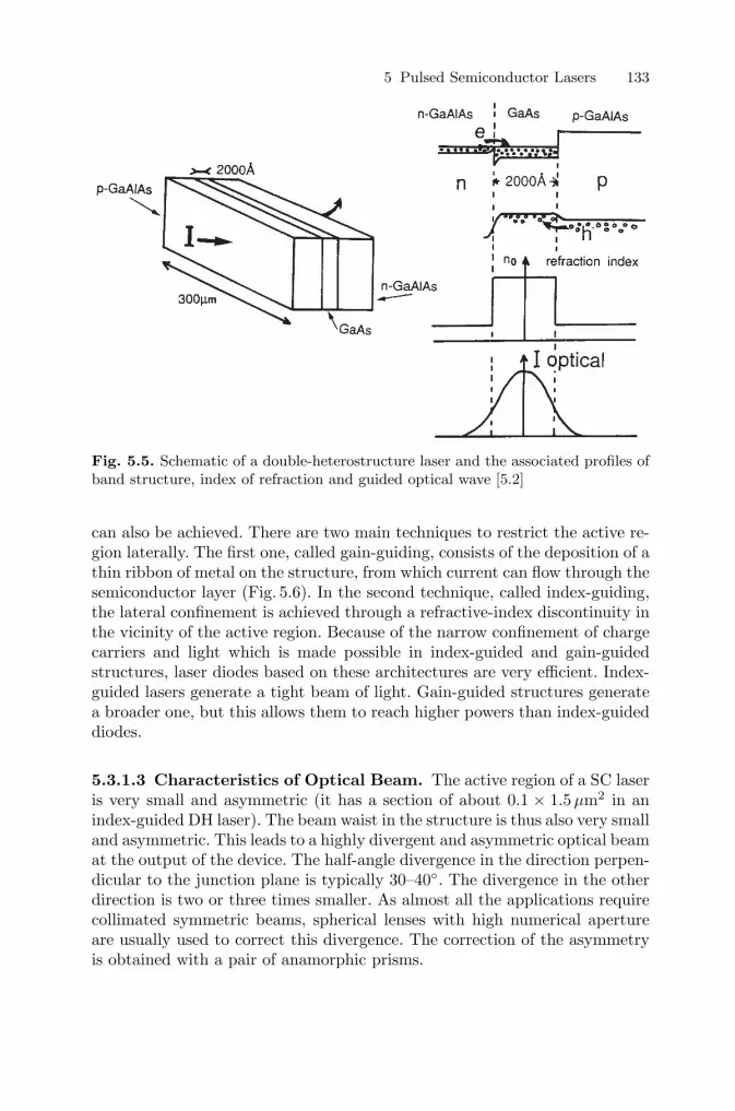
5 Pulsed Semiconductor Lasers 133

Fig. 5.5. Schematic of a double-heterostructure laser and the associated profiles ofband structure, index of refraction and guided optical wave [5.2]

can also be achieved. There are two main techniques to restrict the active re-gion laterally. The first one, called gain-guiding, consists of the deposition of athin ribbon of metal on the structure, from which current can flow through thesemiconductor layer (Fig. 5.6). In the second technique, called index-guiding,the lateral confinement is achieved through a refractive-index discontinuity inthe vicinity of the active region. Because of the narrow confinement of chargecarriers and light which is made possible in index-guided and gain-guidedstructures, laser diodes based on these architectures are very efficient. Index-guided lasers generate a tight beam of light. Gain-guided structures generatea broader one, but this allows them to reach higher powers than index-guideddiodes.

5.3.1.3 Characteristics of Optical Beam. The active region of a SC laseris very small and asymmetric (it has a section of about 0.1 × 1.5μm2 in anindex-guided DH laser). The beam waist in the structure is thus also very smalland asymmetric. This leads to a highly divergent and asymmetric optical beamat the output of the device. The half-angle divergence in the direction perpen-dicular to the junction plane is typically 30–40◦. The divergence in the otherdirection is two or three times smaller. As almost all the applications requirecollimated symmetric beams, spherical lenses with high numerical apertureare usually used to correct this divergence. The correction of the asymmetryis obtained with a pair of anamorphic prisms.

134 T. Amand and X. Marie

Dielectric p- InGaAsP Metallic contact

Gain Guided

Weakly IndexGuided

Fig. 5.6. Gain-guided and index-guided double-hetero-structure lasers [5.1]

5.3.1.4 Optical Confinement, Differential Gain and Threshold Cur-rent. In order to understand the further improvements of SC lasers, it isnecessary to give the precise definitions of three parameters which are veryimportant for the optimization of the device.

The Optical Confinement Factor Γ . Γ is the ratio between the electromag-netic energy in the active region and the total electromagnetic energy of theoptical wave in the structure:

Γ =

∫ d/2−d/2 |E(z)|2 dz∫ +∞−∞ |E(z)|2 dz

, (5.7)

where d is the thickness of the active region in the z direction. It characterizesthe overlap between the electromagnetic wave and the confined electronicstates. Figure 5.7 shows that the optimum width for a GaInAsP laser is aboutd = 1μm (Γ ≈ 1).

The Differential Gain. For a bulk semiconductor laser, the variation of thegain curve maximum as a function of the injected current density is linear(Fig. 5.8a). This variation can be written as

gmax = AJ(J − J0), (5.8)

5 Pulsed Semiconductor Lasers 135

λ = 1.3μmμ1 = 3.22μ2 = 3.51

Active Layer Thickness d (μm)

Con

finem

ent F

acto

r Γ

T

Fig. 5.7. Optical confinement factor of the fundamental TE and TM modes as afunction of the active-layer thickness for a 1.3 μm GaInAsP DH laser [5.1]

where AJ is the current differential gain, defined more generally as AJ =∂g/∂J , and J0 is the transparency current density (for J = J0, α = 0 andEc

F + EhF = Eg).

The Threshold Current. By equating the gain and the losses in the cavity, weobtain the threshold current density

Jth. = J0 +αi

AJ+

(1 − Γ )αc

ΓAJ+(

1ΓAJ

)(1

2L

)ln(

1R1R2

), (5.9)

where αi is the internal loss coefficient of the active region (Auger effects,free-carrier absorption, carrier trapping on impurities, etc.), αc is the losscoefficient of the optical confinement region, L is the cavity length and R1 andR2 are the reflectivities of the facets. It is clear from (5.9) that the thresholdcurrent decreases when the differential gain AJ and the optical confinementfactor Γ increase (and obviously when the losses are reduced). An importantoptimization step of SC laser structures consists of finding the best (AJ , Γ )pairs which minimize Jth. for a given wavelength.

5.3.1.5 Distributed-Feedback (DFB) Structures. In a conventional SClaser (such as a DH laser), the gain curve is much wider than the longitudinalintermode frequency spacing c/2nL (where n is the refractive index and L the

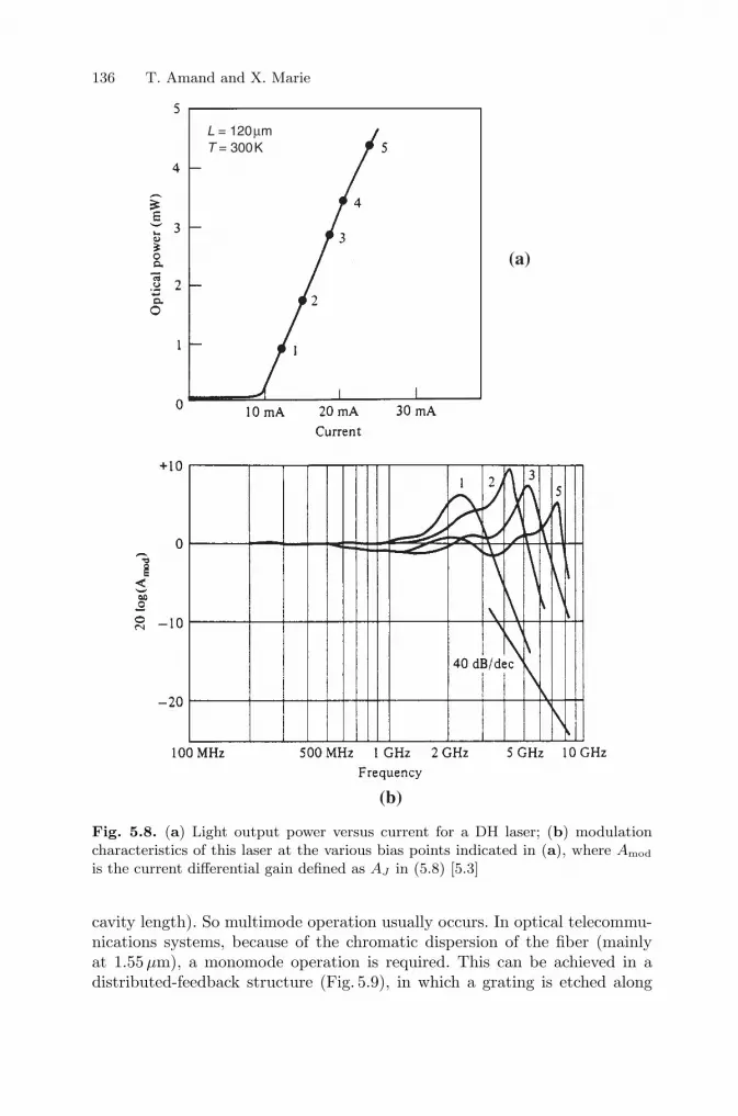
136 T. Amand and X. Marie

L = 120μmT = 300K

(a)

(b)

Fig. 5.8. (a) Light output power versus current for a DH laser; (b) modulationcharacteristics of this laser at the various bias points indicated in (a), where Amod

is the current differential gain defined as AJ in (5.8) [5.3]

cavity length). So multimode operation usually occurs. In optical telecommu-nications systems, because of the chromatic dispersion of the fiber (mainlyat 1.55μm), a monomode operation is required. This can be achieved in adistributed-feedback structure (Fig. 5.9), in which a grating is etched along

5 Pulsed Semiconductor Lasers 137

Fig. 5.9. Schematic illustration of a distributed-feedback (DFB) laser

the cavity so that the thickness of one of the cladding layers varies periodi-cally. The wavelength selection rule results from the Bragg condition, whichdepends on the grating period.

5.3.2 Quantum Well Lasers

In a DH structure, the active-region thickness d varies typically between 0.1and 1μm. If this thickness decreases further so that

d < Λd, (5.10)

where Λd is the de Broglie wavelength, the electrons in the CB and the holesin the VB are still free to move in the plane of the layers but are confined in awell in the perpendicular direction (z). Such a structure is called a quantumwell (QW). In practice, significant effects are observed if d is less than 20 nm,the Bohr radius of the excitons. With the development of semiconductor fab-rication techniques, such as molecular beam epitaxy, it is now possible to growsuch thin layers. The electronic and optical properties of these two-dimensional(2D) structures are drastically changed compared to bulk materials. The mainfeatures are the following.

The energy levels of the CB and the VB are quantized (Fig. 5.10a). Thedispersion curves E(K) (in the infinite-well approximation) become

Enc(h)(K) = Ec(h) +

π2h2

2mc(h)dn2 +

h2K2

2mc(h)(n integer). (5.11)

Laser operation thus occurs at photon energies fixed by the band-gap energyand the confinement energies (π2h2/2mc(h)d)n2. Consequently, for a givensemiconductor material, the emission wavelength can be adjusted by slightvariations of the well width d.

Another consequence of quantum confinement is that there is a liftingat K = 0 of the heavy-hole–light-hole degeneracy. This leads to a reductionof the hole density of states, since light holes do not contribute to it nearthe gap of the quantum well. Moreover, the confinement leads to a reductionof the heavy-hole effective mass near the band edge, which leads in turn toa further reduction of the hole DOS, which in two-dimensional structures

138 T. Amand and X. Marie

EC

(a)

φ3

φ2

φ1

E1

E3

E2

1 2 3

(b)E

ε1

ε2

ε3

ρ (E) / (mAS/πh2)

Fig. 5.10. (a) Energy levels of the conduction band in a semiconductor quantumwell. (b) Density of states. ϕ1, ϕ2, ϕ3 are the different electron wavefunctions andε1, ε2, ε3 are the corresponding energies; mA is the electron effective mass in the wellmaterial; S is the QW surface

is simply equal to m/πh2 per surface unit (Fig. 5.10b). The carrier injectiondensity current required to reach the threshold is thus also reduced. By similararguments to those for bulk semiconductors, we find the expression for theamplification/absorption coefficient in 2D semiconductors:

α2Dn,n′(ω) ∝ ρ2D(ω)|〈φcn|φhn′〉|2

×[f c(

Ecn +mh

mc + mh(hω − Eg − Ecn − Evn′)

)

+ fh(

Evn′ +mc

mc + mh(hω − Eg − Ecn − Evn′)

)− 1

], (5.12)

where |〈φcn|φhn′〉|2 characterizes the spatial overlap between the electron andhole envelope wavefunctions in their respective subbands n and n′, and ρ2D(ω)is the joint 2D DOS (ρ2D(ω) = [memh/(me + mh)](1/πh2), which is energy-independent for a 2D system). Figure 5.11b shows the gain curves for in-creasing injected carrier densities in a DH and in a quantum well structure.We see that the carriers in quantum wells are more “efficient” in 2D struc-tures compared to bulk structures [5.2], since the added carriers contributeto the gain at its maximum, whereas in the bulk the added carriers move thegain peak away from the band edge, so the carriers with energies lower thangmax are lost for the laser effect. The density differential gain An defined byAn = ∂g/∂n is thus stronger in 2D structures than in the bulk in the vicinity

5 Pulsed Semiconductor Lasers 139

CB

VB

(a) (b) (c)

Fig. 5.11. Schematic illustrations of gain formation in DH lasers (top) and QWlasers (bottom), after [5.2]

of the transparency threshold n0 (Fig. 5.11c). But the disadvantage of quan-tum well lasers is that their gain will saturate at a finite value when all theelectron and hole states are inverted (Fig. 5.11c). In bulk lasers, gmax neversaturates since the DOS increases with energy (see (5.2)).

Figure 5.12 shows that the optical confinement factor Γ in a single quan-tum well (SQW) is worse than in a classical DH. In order to overcome thisproblem of optical-wave leakage into the barrier, separate-confinement het-erostructures (SCHs) or graded-index separate-confinement heterostructures(GRINSCHs) are grown, in which the confinement of the electromagneticwave occurs in an optical-confinement layer, whereas the electronic confine-ment occurs in the quantum well (Fig. 5.13). So both optical and electronicconfinement can be optimized separately.

5.3.3 Strained Quantum Well and Vertical-CavitySurface-Emitting Lasers

The latest developments of SC lasers are based on the so-called strained quan-tum wells [5.4]. In these structures, the lattice parameters of the semiconduc-tor materials constituting the well and the barrier are different in the relaxedmaterials. If one grows a thin layer of the well semiconductor on a thick layerof the barrier semiconductor, the barrier semiconductor imposes its latticeparameter in the well plane. It is thus possible to grow elastically strainedquantum wells in compression or extension. The strain is then a new degreeof freedom available to optimize the SC laser characteristics: the structuralmodifications with respect to a bulk, relaxed semiconductor, added to the sizequantization effects, lead to drastic changes of the electronic properties. Figure5.14 shows that in a compressively strained structure, the heavy-hole–light-hole splitting at K = 0 increases and the heavy-hole effective mass decreases.

140 T. Amand and X. Marie

DHΓ ≈ 1

SQWΓ ≈ Δn d2

SCHΓ ≈ Δn d

d

d

d

Fig. 5.12. Schematic illustrations of the confinement of an optical guided wavefor a double heterostructure (DH), a single quantum well (SQW) and a separate-confinement heterostructure (SCH) [5.2]

GRINSCH QUANTUM WELL SCH QUANTUM WELL

z ρ z ρ

Fig. 5.13. Energy diagram of the conduction-band edge and corresponding DOSρ for graded-index separate-confinement heterostructure (GRINSCH) and separate-confinement heterostructure (SCH) quantum well lasers [5.2]

This leads to the reduction of the hole DOS and thus to a reduction of thethreshold current density. Moreover, the light-hole states, which do not par-ticipate in the lasing transition, are further in energy from the heavy-holestates in compressively strained structures compared to the unstrained one.These states are thus less populated, which leads to an increase of the SC laserefficiency. On can also demonstrate that the differential gain AJ is higher in a

5 Pulsed Semiconductor Lasers 141

(a)

LM (x = 0.53)Lz = 80Å

(b)

1.2 % Compr. (x = 0.7)Lz = 25Å

HH

LH

0 0.1

0

-50

-100

-150

Ene

rgy

(meV

)

0 0.1

Wave Vector Κ (2π /a0)

Fig. 5.14. Calculated valence band structure of (a) a lattice-matched (LM) and(b) a compressively strained InxGa1−xAs/InGaAsP quantum well laser designedfor emission at 1.5 μm (from [5.4] c© 1994 IEEE). a0 is the lattice parameter. Lz isthe QW width

strained structure than in a lattice-matched one. The most common strainedlasers are based on InGaAs/GaAs and InGaAsP/InP quantum well structures;they exhibit excellent Jth. and AJ parameters.

We finish this very quick review of the common SC laser structures withthe most recent ones, called vertical-cavity surface-emitting lasers (VCSELs)[5.5].

All of the SC laser structures discussed so far emit light from their edges.In a VCSEL, however, the laser cavity is perpendicular to the junction plane.A VCSEL structure consists of a large number of layers with a Bragg reflectorat each end and an active region composed of a quantum well (Fig. 5.15).The VCSELs are very compact (the cavity length is a few microns) and thelight beam is circular and less divergent than in conventional horizontal lasers.From the point of view of pulsed operation, they are characterized by a veryhigh intracavity photon density, which leads to high relaxation oscillationfrequencies (see Sect. 5.4). The main advantage for applications is that two-dimensional arrays of VCSELs can now be grown.

5.4 Semiconductor Lasers in Pulsed-Mode Operation

Generation of ultrashort optical pulses from SC lasers has been the subjectof intense activity since the end of the seventies. Potential applications in the

142 T. Amand and X. Marie

GaAs Substrate

p-GaAlAs Multilayer Mirror

GaInAs Quantum Wells

n-GaAlAs Multilayer Mirror

Fig. 5.15. Schematic illustration of a vertical-cavity surface-emitting laser (VCSEL)

fields of optical telecommunications and time-resolved spectroscopy are at theorigin of such interest.

Several approaches have been investigated in order to generate short op-tical pulses from semiconductor lasers.

The simplest mode of operation, specific to semiconductor lasers, andwhich was the subject of the most intense research effort, is the gain-switchingmode [5.7]. This mode of operation was investigated by Lasher in 1964 [5.8].In contrast to other laser sources, where optical modulators are used, semicon-ductor lasers can be modulated directly through the injection current. More-over, here one can take advantage of the possibility of monolithic integrationof both the laser and the electronic modulator circuit. The gain-switchingoperation mode consists of driving the laser with ultrashort current pulseswhich are superimposed on a stationary (DC) polarization current below orat the laser threshold. We show in Sect. 5.4.1 that this allows one to generatepulses of variable temporal width, frequency and peak power, which makesthis mode of operation probably the most versatile.

The second approach to the generation of ultrafast optical pulses was toapply classical Q-switching techniques to semiconductor lasers. The early at-tempts at this approach were performed by Kurnosov et al. [5.9] in 1966, usinga two-section laser geometry. This will be described further in Sect. 5.4.2.

The third approach one might think of relies on conventional mode-locking,active or passive. It is based on the large gain bandwidth of the active medium,which allows, in principle, the generation of ultrashort pulses. Passive mode-locking was primarily investigated by Van der Ziel et al. in 1981 [5.10] andYokoyama et al. in 1982 [5.11], while active mode-locking was demonstratedlater by Bowers et al. in 1989 [5.12]. We shall see in Sect. 5.4.3 that regularly

5 Pulsed Semiconductor Lasers 143

spaced picosecond or subpicosecond pulses can be obtained in such a way.However, in the active mode-locking method, the applied modulation signalmust be accurately matched to the laser cavity length. In the passive mode-locking configuration, the pulsed operation depends critically on the saturableabsorber used.

In the description of these different modes of operation, we will stressthe specific details of the semiconductor lasers, in particular those concerningpumping and the possibilities of integration in the same device of the opticalamplifier, the modulator and the waveguide.

5.4.1 Gain-Switched Operation

The output light intensity of SC lasers can be quite easily modified by chang-ing the excitation level of the amplifying medium. This allows one to obtain anoptical replica of an electrical pulse train. Owing to the small size of the semi-conductor laser cavities, the build-up and disappearance of the light intensitycan occur on a timescale of a few picoseconds, thus making this approachquite attractive for generating short optical pulses. Two modes of operationare currently used: the pulsed mode and the amplitude-modulation mode.Although the latter is not equivalent, strictly speaking, to the generation ofpulse trains, we will present it here, because of its considerable technologicalapplications in the fields of telecommunications and information processing.The specifications reached in both operation modes are basically determinedby the oscillations of the relaxation process, which we describe now.

5.4.1.1 Relaxation Oscillation Phenomenon. This phenomenon is com-mon to all laser sources, but the frequency of these oscillations is much higherin SC lasers than in conventional sources. Here, they can be observed whenpolarizing the device with a current step above the current threshold. Theoutput power increases first and oscillates before reaching the new steady-state operation point, as displayed in Fig. 5.16a. These periodic oscillationsare basically due to the time delay between the photon generation and thebuild-up of the gain in the active medium (a delay which may be as long asa few tens of picoseconds, typically). It can be understood qualitatively asfollows: owing to the injection current increase, the carrier population in theactive medium first rises, since its decay time is long (of the order of 1 ns),governed by spontaneous recombination. Net positive gain is then obtainedwithin the medium, thus allowing the electromagnetic field to build up fromthe spontaneous radiation by stimulated emission. As the photon density rises,the carrier lifetime quickly decreases to the stimulated radiative time (of theorder of 10 ps), thus leading to the collapse of the free-carrier density, even-tually to values below the transparency threshold. The gain within the cavitythen drops, leading to a decrease of the electromagnetic field intensity, and asubsequent increase of the carrier lifetime. A new cycle can then start [5.6].

144 T. Amand and X. Marie

Fig. 5.16. Laser responses under strong electrical excitation. (a) Single-step exci-tation, (b) rectangular pulse-excitation [5.6]

The relaxation oscillation process can be described in terms of a nonlinearsystem of two coupled differential equations, which expresses the interplaybetween the injected electron (or hole) density N and the photon density Pwithin the active medium. Neglecting the fraction of spontaneous emissionentering the laser mode, it can be written as [5.13]

dN

dt=

J

ed− N

τ− c

nAN (N − Nth)P, (5.12a)

dP

dt=

c

nAN (N − Nth)P − N

τp, (5.12b)

where J/ed is the injection rate of the electrons in cm−3s−1 (J is the cur-rent density, e the electron charge and d the thickness of the active region);(c/n)P = F is the photon fluence within the active region in cm−2s−1 (c is thespeed of light and n the refractive index in the active region); AN (N − Nth)is the gain within the active region in cm−1 (AN is the optical differentialgain and Nth is the threshold carrier density), so that (c/n)AN (N − Nth)Prepresents the rate of stimulated recombinations per unit volume; τ is thefree-carrier spontaneous lifetime within the active region; and τp, the photon

5 Pulsed Semiconductor Lasers 145

lifetime inside the cavity, is limited primarily by the transmission of the cavitymirrors; it is given basically by the expression

τp = − 2nL

cln(R1R2), (5.13)

where L is the cavity length, n is the refractive index of the amplifying mediumand R1, R2 are the reflectivities of the facets. The absorption in the activeregion (essentially the free-carrier absorption and Auger effect) and diffusionalso limit the photon lifetime (we neglect these in this simple approach).Linearizing the system around a given operating point and solving the corre-sponding characteristic equation yields the oscillation frequency of the laserrelaxation:

fr =12π

(ANF0

τp

)1/2

, (5.14)

where F0 is the mean photon fluence within the cavity at the operating point.

5.4.1.2 Pulsed-Operation Mode. The basic idea here, to obtain a shortoptical pulse, is to switch off the current polarization step just after the firstoscillation of the output power, as shown in Fig. 5.16b. So, by pumping thelaser with an ultrashort electrical pulse, a single light pulse can be generatedfor each excitation pulse. The temporal width of the pulse is basically of theorder of half the period of the relaxation oscillations. The cavity length playsan important part in determining the pulse duration, as can be inferred from(5.13) and (5.14). It can be shown that the differential gain AN is inverselyproportional to the number of inverted states for a given device, which in turnis proportional to the volume of the active region. Thus AN is proportional toL−1 (where L is the cavity length). From (5.13), one can see that the photonlifetime is proportional to L. So, fr is inversely proportional to L (5.14). Asa consequence, the minimum pulse width increases linearly with the cavitylength, as is observed experimentally (Fig. 5.17) [5.14]. The fundamental lim-itation comes indeed from the laser relaxation oscillation frequency. Possibleimprovements will be described in the following.

As early as 1980, this technique allowed the generation of 40 ps FWHMoptical pulses from 50 ps wide current pulses, at a repetition frequency of up to400 MHz [5.15]. This result was obtained by using a DC polarization currentjust below the threshold and driving the laser with an electrical pulse train.The amplitude of the optical pulse increased with that of the electrical pulses,and the spectral width was about 3 nm.

Recently, 16 ps FWHM pulses were obtained by Luo et al. [5.16] from amonomode DFB laser working in gain-switched mode at a repetition rateof 100 MHz. The mean power was 10 mW. More advanced techniques arepresently under investigation to generate pulses of the order of 1–2 ps at repe-tition frequencies of the order of 10–20 GHz. These depend on shortening thepulse width using a pulse compressor made of an optical fiber and gratings[5.17].

146 T. Amand and X. Marie

60

40

20

00 100 200 300 400 500

Laser Length (microns)

Pul

se W

idth

(ps

)

Fig. 5.17. Laser pulse width as a function of the laser cavity length (reprinted from[5.14] c© 1981 American Institute of Physics)

5.4.1.3 Amplitude-Modulation Mode. The applications of SC lasers inthe field of optical telecommunications stimulated research efforts on opticalencoding of information and the possibility of obtaining very high modulationfrequencies. The most direct way to transfer information to the output beamof the laser is to modulate the amplitude of the optical wave by varying thepolarization current of the laser. The current–optical power characteristic ofa 3D semiconductor laser is linear over a large range (Fig. 5.8a). Moreover, asthe photon lifetime in the laser cavity (5.13) can be extremely short (typicallyless than 10 ps), amplitude modulation can be performed at high frequencies.This modulation is achieved by superimposing a small time-dependent signalI(t) on the average pumping current Im (Im > Ith). We see from (5.14) andon Fig. 5.8b that the modulation bandwidth is then limited by the relaxationoscillation frequency fr, which is due to the combined effects of the invertedpopulation within the cavity and the electromagnetic field. Equation (5.12)suggests three simple means to increase the relaxation oscillation frequency:

(i) increase the optical differential gain AN ,(ii) increase the photon fluence F0,(iii) decrease the photon lifetime within the cavity.

The increase in the gain coefficient AN can be obtained by optimizing thestructure. In the case of a QW laser, the number of states which must beinverted to achieve the inversion condition is much lower than in a DH laser.Moreover, the injected carriers are more efficient in 2D systems than in 3Dones, since they all contribute to the gain at its peak, near the band edge.So a QW laser is better than a DH one in this respect (see Sect. 5.3.2). In1985, it was shown theoretically that the modulation bandwidth could thusbe increased by a factor 2 in multiple-quantum-well (MQW) lasers relative tothe usual DH structures [5.18]. Numerous experimental verifications followed.

5 Pulsed Semiconductor Lasers 147

0.50 1.0 1.5 2.0 2.50

1

2

3

4

5

6

7

8

Rel

axat

ion

Osc

illat

ion

Freq

uenc

y (G

Hz)

120 μm

165 μm

284 μm1

2

3

4

5

√P0 (mW1/2 )

Fig. 5.18. Relaxation oscillation frequency measurements for various laser cavitylengths as a function of

√P0. P0 is the CW optical output power (vertical arrows:

catastrophic damage threshold) (from [5.13] c© 1995 IEEE)

Increasing the laser polarization current allows the internal fluence torise in the active region, which results in an increase of the output inten-sity (Fig. 5.8a). The problem which arises here comes from the catastrophicmirror damage which occurs for irradiances of the order of 1 MW/cm2 forAlGaAs SC lasers. This puts a definite limit on the photon fluence and thuson the maximum frequency bandwidth, as can be seen in Fig. 5.18.

The third means of increasing the bandwidth consists of reducing the pho-ton lifetime by decreasing the cavity length. By this means, modulation fre-quencies up to 8 GHz were obtained with 120μm cavities in DH lasers, asshown in Fig. 5.18.

Frequencies fr higher than 15 GHz were obtained in this way in MQWsmade from the GaAs/AlGaAs system.

An additional increase of the bandwidth can be achieved using a p-typedoped active region. In this case, the differential gain is greater than thatobtained in a similar laser with an intrinsic active region, since the electronquasi-Fermi level Ec

F changes very quickly with the injected electron density.According to the Bernard and Duraffourg condition (5.6), the population in-version condition is achieved as soon as Ec

F reaches the conduction-band mini-mum (or the confined-electron level in a QW laser), since the holes are alreadyquasi-degenerated because of the doping. The current threshold is thus low-ered, as seen in Fig. 5.20a. When the active region is n-doped or undoped, the

148 T. Amand and X. Marie

100 ps

(a) (b) (c)

Fig. 5.19. Output pulse of a p-doped MQW laser at different output powers: (a)P0 = 18.5mW, fr = 11.5GHz; (b) P0 = 64mW, fr = 20.5GHz; (c) P0 = 160mW,fr = 30GHz (reprinted from [5.19] c© 1987 American Institute of Physics)

(a) (b)

Current (mA) (Output Power)1/2 (mW1/2)0 100 200 300 5 10 150

Out

put

Pow

er (

mW

)

Rel

axat

ion

Osc

illat

ion

Freq

uenc

y (G

Hz)

0

10

20

30

0

20

40

60

RTW = 9 μm

RTLW = 100 Å

MD-MQW

undopedMQW

uniformp-dopedMQW

MD-MQW

uniformp-dopedMQW

undopedMQW

Fig. 5.20. (a) Light output power versus current for a p-type modulation-doped(MD) MQW laser, a uniformly p-doped MQW laser and an undoped MQW laser.(b) Measured relaxation oscillation frequency of a p-type MD-MQW laser (•), auniformly p-doped MQW laser (×) and an undoped MQW laser (◦) as a functionof the square root of the output power (preprinted from [5.20] c© 1990 AmericanInstitute of Physics). LW and W are resepectively the QW and strip widths

5 Pulsed Semiconductor Lasers 149

00

Rel

axat

ion

Osc

illat

ion

Freq

uenc

y (G

Hz)

1 2 3 4 5

2

4

6

8

10

√P (mW1/2)

10 μm × 400 μm Cavities

35%

InG

aAs

MQ

W

25 % InGaAs

MQW

35 % InGaAs SQW

GaAs SQW

Fig. 5.21. Relaxation oscillation frequency versus the square root of the outputpower for unstrained GaAs SQW laser, and x = 35% SQW, x = 25% MQW andx = 35% MQW strained InxGa1−xAs quantum well lasers (from [5.21] c© 1991IEEE)

situation is less favorable since it is then necessary to populate hole statesfor which the density of states is high, and the condition (5.6) is harder toachieve. Figure 5.19 displays relaxation oscillations of the transient charac-teristics of a p-doped MQW laser at room temperature [5.19]. The frequencyfr is deduced from the measurement of the time delay between two successiveoscillations. Using such p-doped structures, relaxation oscillation frequenciesgreater than 30 GHz were measured [5.20], as seen in Fig. 5.20b.

To sum up in a rule of thumb, the relaxation oscillation frequencies ob-tained in the various structures analyzed so far scale as follows:

fr (MQW p-doped) ≈ 2.5fr (MQW undoped) ≈ 5fr (DH).

Progress in the fabrication process has allowed one to achieve compres-sively (or extensively) strained quantum wells (see Sect. 5.3.3). We have seenthat reducing the hole transverse effective mass results in an increase of thedifferential gain (since the hole density of states decreases), leading to an in-crease of fr in strained structures relative to those without lattice mismatch.Recent results (1991) showed a differential gain for a strained InGaAs QWthree times greater than that for a lattice-matched one [5.21]. Figure 5.21shows that fr increases with the compressive strain, for both single-quantum-well (SQW) and multiple-quantum-well (MQW) lasers.

This method of direct intensity modulation, specific to semiconductorlasers, allows nowadays a modulation rate of 20 Gbit/s [5.22]. MQW InGaAsPDFB laser diodes operating at a wavelength of 1.55 μm and at modulationfrequencies up to 4 Gbits/s are now currently available [5.23]. The serious

150 T. Amand and X. Marie

drawback of this technique comes from the spectral broadening of the pulsesdue to the phase modulation induced by the injection current variations andthe correlative frequency chirp which occurs [5.6, 24]. As a matter of fact,when the injection current rises suddenly, the carrier density inside the activeregion increases before it can be compensated by stimulated recombination,owing to the time delay necessary to build up the electromagnetic field, asseen in the previous section. A jump in the carrier density then occurs, re-sulting in a temporary decrease of the refractive index in the active region,as the electronic contribution to this index is a decreasing function of theelectron density. The optical path within the cavity thus decreases, and con-sequently the laser wavelength shifts initially towards the blue. Similarly, asudden decrease of the injection current results in a decrease of the carrierdensity within the active region to below its steady-state value because ofstrong stimulated emission, and the laser wavelength temporarily shifts to-wards the infrared. This effect is shown in Fig. 5.22. For structures lasing at1.55μm, the resulting frequency chirp is enhanced when transmitted in siliciaoptical fibers, for which the dispersion is negative in this spectral region, thusleading to a further temporal broadening of the pulse, and limiting the max-imum modulation rate. However, long-distance communication networks arenow operating with such devices, without intermediary amplifiers, over morethan 100 km.

Research attempts have been made to minimize the combined effect offrequency chirp and dispersion by compressing the pulse with, for example,a grating-pair pulse compressor, with a spatial filter in its telescope to selectonly the frequency domain which contains a linear chirp. It is also possible tomatch the laser and the fiber, e.g. by operating in a spectral domain wherethe fiber dispersion is positive. Actually, because of this temporal broadeningof pulses in the case of direct amplitude modulation of SC lasers, very-high-repetition-rate optical telecommunications systems use SC lasers operatingin CW mode, coupled to an external light modulator. Amplitude modulationwith a narrow spectrum and high extinction rates is thus obtained. Two typesof modulators are currently used for such a purpose: the LiNbO3 electro-optical modulator [5.25] and electroabsorptive modulators, which allow oneto obtain information transmission rates higher than 12 Gbit/s.

5.4.2 Q-Switched Operation

5.4.2.1 Q-Switching in the Context of SC Lasers. Semiconductor lasersoperating in Q-switched mode are potentially interesting in optical telecom-munications systems, or more generally as optical pulse sources when highpeak power, high amplitude modulation and high repetition rates are required.

The basic idea is to modulate the intracavity losses. This modulation isobtained by creating regions of saturable absorption in series with the gainmedium (Fig. 5.23). High losses allow the build-up – without oscillations – of

5 Pulsed Semiconductor Lasers 151

Time

Inte

nsity

Inte

nsity

Inte

nsity

Turn

ing

on

Cur

rent

Turn

ing

off

Time (ns)

λ (Å) λ (Å)

Car

rier

Den

sity

Inte

nsity

Wav

elen

gth

Transient Chirping

Ith

0

λ0

Δ λ t c

(a)

(b)

(c)

(d) Time(ns)

1.6

1.7

1.8

1.9

2.0

2.1

0.4

0.3

0.2

0.1

0

-0.1

Time(ns)

15498 15500 15502 15498 15500 15502

-1

1

0

0 1 2 3

(e)

Fig. 5.22. Transient chirping phenomena in gain-switched operation: schematicrepresentation of the time dependence of (a) the light intensity, (b) the wavelengthand (c) the current. (d) Time-resolved emission spectra showing the frequency chirpon the leading and falling edges of a gain-switched SC laser; the wavelength is seen tomove briefly towards the blue on start-up and towards the (infra)red on shutdown.(e) Total light intensity versus time (after [5.24])

152 T. Amand and X. Marie

Saturable absorberτa

Active mediumτn

τc

Fig. 5.23. Basic scheme of a semiconductor laser with a saturable absorber. τa, τn

and τc are respectively the absorber relaxation time, the gain recovery time and thecavity round-trip time (see text) [5.6]

carrier densities greater than the threshold density corresponding to the min-imum losses, thus increasing the energy stored within the amplifying section.Then the losses are suddenly reduced, in order to extract this energy fromthe active medium resulting in the formation of a short pulse. The mecha-nisms involved in SC laser Q-switching depend on the absorber relaxationtime τa [5.6]. The latter must always be shorter than the gain relaxation timeτn in order to obtain a pulsed emission. However, it may be shorter or longerthan the cavity round-trip time τc, depending on the cavity length and theabsorption process. The first situation a priori leads to mode-locking, whichwill be described further in Sect. 5.4.3. The laser dynamics in the second sit-uation are similar to those of gain switching. We consider this situation now(τc < τa < τn). One difference from gain switching is the possibility of gener-ating optical pulses using a DC laser bias. In this pure Q-switching case, thepulse periodicity is fixed by τn. Another difference is that Q-switched pulsesexhibit shorter tails than gain-switched ones, due to the absorber recovery atthe end of the pulse.

As for gain switching, the Q-switching operation mode can be describedby rate equations [5.6]. Equations (5.12a) and (5.12b) of Sect. 5.4.1.1 are nowaccompanied by a third equation for the absorber population density Na:

dNa

dt= −Na − Neq

τa− c

nAaNaP, (5.15)

where the first term on the right-hand side of this equation represents thespontaneous carrier relaxation and the second represents the induced absorp-tion. Neq is the equilibrium absorber population in the absence of light, and Aais the absorber cross-section. The induced absorption term must be included

5 Pulsed Semiconductor Lasers 153

ModulatorDrive

PopulationInversion

LaserOutput

≈150 mW

N = 0

N thN (t)

500 ps

Fig. 5.24. Typical response of a Q-switched SC laser to repetitive modulation ofthe intracavity absorption. The modulation frequency is 2GHz (from [5.26] c© 1983IEEE)

as a loss term in (5.12b). Approximate solutions of these rate equations havebeen proposed in [5.30]. Figure 5.24 displays a simulation obtained for repeti-tive Q-switching [5.26] in the case of inversion-dumped Q-switching (in whichthe electron population fluctuates about the threshold value). As the cavitylengths of SC lasers are much shorter than in the usual laser sources, theobtained Q-switched pulses are short, with a duration of the order of 10 ps(conventional Q-switched lasers have pulse widths in the nanosecond range).

The intracavity loss modulation can be either passively or actively achieved.Passive Q-switching due to absorption saturation was observed in SC laserswith two amplification sections, nonuniformly pumped (one of the sectionsacts as a saturable absorber) [5.8]; more generally, it is obtained in multisec-tion laser geometries, where some of the sections are unbiased or reverse-biased[5.26–29]. It can be also achieved by implantation of ions through the diodefacets [5.10, 30, 31]. But most of the research efforts have been concentrated onactive Q-switching. Before describing the different devices which have beentested, we give now a brief review of a few specific ways to modulate ab-sorption in semiconductors, which are the most used currently and lead totechnical solutions which can be integrated with the SC laser.

5.4.2.2 A Few Techniques Used to Modulate Absorption in Semi-conductor Lasers. The first actively Q-switched SC lasers were built withexternal electro-optical or acousto-optical modulators. With the aim of inte-gration of all the functional parts of the laser within the same device, methodsto achieve light modulation specific to semiconductors were developed. Tech-

154 T. Amand and X. Marie

nological progress in fabrication now allows one to reach this goal, allowingthe development of SC lasers with the light modulator integrated in the samedevice.

Most of these modulators rely on electroabsorptive effects, due to the mod-ification of the electronic band structure under an external electric field. Themost famous effect is the Franz–Keldysh effect.

Franz–Keldysh Effect in Bulk Semiconductors. This effect was predicted in1958 independently by Franz and Keldysh, and was experimentally observedin germanium by Seraphin in 1964 [5.32]. Under an external electric field,the electronic bands are tilted in direct space, as shown in Fig. 5.25a. Owingto the spatial overlap of the evanescent tails of the electronic wave functionswhich develops in the band gap, some absorption appears for photon energiesbelow the band gap Eg, as shown in Fig. 5.25b. Applying an electric field inthe range 102–103 kV/cm results in an absorption tail below the band gap ofa few 102 cm−1.

This absorption can be directly modulated by modulating the externallyapplied electric field. Thus active Q-switching, as well as active mode-locking,can be achieved. As the density of states corresponding to the absorption tailis low, the absorption below Eg can be easily saturated when the density ofphotogenerated carriers increases, under a steady electric field, leading to self-modulation effects. In this case, the semiconductor acts as a passive saturableabsorber, for photon energies around Eg, and can be integrated for passiveQ-switching or mode-locking of the SC laser.

Quantum-Confined Stark Effect (QCSE) in Quantum Wells. The principle ofthis effect relies on the modifications of the potentials in a quantum well whenapplying an electric field perpendicular to the material layers. The main effectof the tilt of the electronic bands in the bottom of the quantum well is thatit modifies the confinement energy of the electrons and the holes. Thus theenergy of the fundamental optical transition in the quantum well is reduced,providing absorption below the position that the fundamental transition haswithout an electric field, as shown in Fig. 5.26 [5.33]. Although the electricfield draws apart the occupation probabilities of the electrons and the holes toopposite sides of the QW, the overlap of the electron and hole wave functions isbetter than in the case of the Franz–Keldysh effect, owing to their confinementwithin the QW along the growth axis of the device. So the oscillator strengthremains relatively large under an electric field, leading to higher absorptioncoefficients below the band gap of the structure than in the case of the bulkelectro-optic effect.

As before, active Q-switching (or mode-locking) can be achieved. In thiscase direct modulation of the transmission of the QW absorber is obtainedby modulating its electrical polarization. On the other hand, under constantelectrical bias, the device acts as a saturable absorber, owing to the bleachingof the lower optical transition in the QW by the photogenerated carriers. Pas-sive Q-switching (or mode-locking) results. Such a device can be integrated

5 Pulsed Semiconductor Lasers 155

0

2

4

6

8

-8 -4 E0 4 8

Eg

hν

hω – E0 [eV ·10-2]

X

hν Eg

(b)

(a)

Val

ence

Ban

dC

ondu

ctio

n B

and

Fig. 5.25. Schematic illustration of the action of an electric field on a bulk semi-conductor (Franz–Keldysh effect) (a) Tilt of the band structure, and the conductionand valence band wave functions, and (b) the resulting absorption below the bandedge [5.2]. Dashed lines, band-edge absorption with applied electric field; solid line,without electric field

156 T. Amand and X. Marie

Fig. 5.26. Action on the conduction- and valence-band states of an electric field ap-plied perpendicular to the plane of a quantum well (quantum-confined Stark effect)(reprinted from [5.33] c© 1988 American Institute of Physics)

in AlGaAs/GaAs or GaInAsP/GaInAs QW lasers, GRINSCH structures andsemiconductor colliding-pulse mode-locked lasers, as will be demonstrated be-low.

Semiconductor Saturable Absorber Created by Ion Implantation. This ideaconsists of creating localized defect states below the band gap in a limited zoneof the SC laser. This can be achieved by proton irradiation in the SC laserfacets, but heavy ion implantation (O5+, for instance) gives better results. Asshown in Fig. 5.27a, spatial fluctuations of the conduction- and valence-bandenergies result, leading to optical transitions between states which are eventu-ally localized on different sites. Density-of-states tails appear below and abovethe conduction and valence bands respectively (Fig. 5.27b), allowing opticalabsorption for energies below the band gap of the material. These transitionscan be bleached at the SC laser wavelength: the photogenerated carriers sat-urate the localized states, thus providing a self-modulation of the absorption.As the cross-section σA of the saturable absorber is greater than the cross-section of the amplifying medium σG, and the recovery time of the absorber

5 Pulsed Semiconductor Lasers 157

E E

C.B.

V.B.

x N (E)

(a) (b)

Fig. 5.27. Schematic illustration of (a) the perturbation of the band edges byCoulomb interaction with inhomogeneously distributed impurities, and of (b) theresulting formation of density-of-states tails. The dashed lines show the distributionof states in the unperturbed case

is of the order of a few picoseconds, such processes can be efficiently used forpassive Q-switching or mode-locking in SC lasers.

5.4.2.3 Active Q-Switching. Figure 5.28 shows a quaternary-compoundInGaAsP DH diode operating in the Q-switched mode [5.26]. In this schematicdrawing, we can clearly identify the following three sections:

• the amplifying section, the length of which is about 200μm,• the passive optical waveguide,• the electroabsorption modulator section.

The electroabsorption modulator consists of a pn junction, built close tothe quaternary layer, which provides the controlled intracavity loss. When thisjunction is reverse biased, the optical absorption of the light emitted in the ac-tive region, increases in the modulator section, because of the Franz–Keldysheffect. In InGaAsP material under an electric field of about 400 kV/cm, theoptical absorption can reach 1000 cm−1 for photon energies down to 60 meVbelow the gap of the unbiased material.

The waveguide section has two simultaneous actions: it optically couplesthe amplifier and the modulator, but isolates them electrically.

Note that the amplifying GaInAsP quaternary region is p-doped. Thisdevice generates 100 ps pulses, with 50 pJ energy per pulse (corresponding toa peak power of 500 mW), at a repetition frequency of 8 GHz [5.26]. More

158 T. Amand and X. Marie

Fig. 5.28. Schematic drawing of a Q-switched SC laser. The device consists ofa zinc-diffused amplifier section, a beryllium-implanted modulator section and apassive waveguide section (from [5.26] c© 1983 IEEE)

1-x x

1-y y

1-x x

Fig. 5.29. Schematic drawing of a quantum-mechanical size-effect modulation SClaser (from [5.34] c© 1986 IEEE)

recently, a similar device allowed one to obtain 40 ps pulses, with 300 pJ perpulse at a repetition frequency of 400 MHz [5.29] .

Another technique for the generation of short optical pulses is obtainedfrom a three-terminal “quantum-mechanical size-effect modulation” laser[5.34]. This quantum well laser is sketched in Fig. 5.29. The gain modula-tion on which it relies is based on a quantum size effect. Although it couldbe classified among the gain-switched SC lasers, it leads to similar carrierdensity dynamics in the active region to those in Q-switched SC lasers. Themodulation is obtained in the following way.

5 Pulsed Semiconductor Lasers 159

The electrons and holes are injected into the GaAs quantum-well activeregion from the lateral n-doped and p-doped AlGaAs regions. Applying a biasto the top and bottom gate electrodes creates an electric field in the GaAsquantum well through the AlGaAs layers, leading to the spatial separationof the electron and hole wave functions (as in Fig. 5.26). A decrease of theoptical transition matrix element, and consequently a decrease of the opticalrecombination probability results (see (5.12)). This allows the building of anelectron–hole population above the threshold density, corresponding to a zerobias on the top and bottom electrodes. When the latter is suppressed, stronggain sets in and the energy stored within the amplifier is converted into ashort optical pulse. Owing to the applied potentials on the gates, the transittime of the carriers through the structure is less than one picosecond; a veryfast switching of the emission results. Repetition frequencies up to 12 GHz canthus be obtained.

5.4.2.4 Passive Q-Switching. Passive Q-switching was obtained in 1981by Van der Ziel [5.10] from an SC laser which was ion-implanted, thus creat-ing a saturable absorber within the laser device near one end facet. The precisedescription of phase modulation effects in the Q-switching regime is somewhatdifficult, owing to the presence of the saturable absorber. The most simple ap-proach is to assume that the chirp amplitude during the pulse is proportionalto the gain variations as well as to the electron density. This is due to the linearrelation existing between the gain and the electron density. Since the numberof emitted photons is approximately equal to the number of lost electrons, thetotal chirp amplitude is expected to be proportional to the pulse energy [5.6].Figure 5.30 displays the autocorrelation traces of Q-switched pulses emittedby a gain-guided AlGaAs laser implanted with 20 MeV oxygen. The pulsewidth is ∼ 22 ps before compression; after compression, it reduces to ∼ 1.3 ps(a factor of 0.65 is used to deduce the laser pulse widths from the autocorrela-tion traces), one of the best reported results to date for a Q-switched SC laserwith electrical pumping. Note the extremely high value of the compressionratio. This illustrates the possibility of very large phase modulation in single-mode Q-switched SC lasers. Owing to high power levels, resulting in stronglaser nonlinearities, the ultimate performances of Q-switching may be differ-ent from those previously established for gain-switched lasers. In principle, theultimate limit of chirp amplitude is given by the gain bandwidth. More realis-tically, a chirp amplitude of about 4 nm can be expected at 0.8μm for a pulseof ∼ 30 pJ, which should correspond to ∼ 240 fs pulses after compression.

5.4.3 Mode-Locked Operation

As for all laser systems, the technique which leads to the generation of theshortest optical pulses in SC lasers is that of mode-locked operation. It issignificantly superior to the gain-switching and Q-switching techniques with

160 T. Amand and X. Marie

Fig. 5.30. Second-harmonic autocorrelation traces of Q-switched pulses emitted bya gain-guided AlGaAs laser implanted with 20MeV oxygen. The energy per pulseis about 33 pJ. The trace width is 38 ps without external compression. It reduces to2 ps after compression by a ∼ 200m long fiber with a total dispertion of ∼ 24 ps/nm[5.6]

respect to the amplitude and the timing jitter [5.12], as well as the minimumwidth of the obtainable pulses [5.10, 11, 35, 36]. It should lead, in principle,to ultrashort pulses, owing to the large bandwidth of semiconductor spectralgain: for instance, a usual spectral gain spanning 30 nm would lead, in the caseof Fourier-transform-limited pulses, to durations of about 30 fs. It is, however,more complex. Mode-locking is achieved by introducing a mechanism insidethe laser cavity to cause the longitudinal modes to interact with one another,thereby locking them in phase. As we shall see now, this mode-locking can beactive or passive.

5.4.4 Mode-Locking by Gain Modulation

5.4.4.1 Synchronous Pumping by Current Injection. Active mode-locking is based on a direct modulation of the injection current at a frequencyf = c/2nL matched to the cavity length. It corresponds to synchronous pump-ing, but here it is obtained directly through the injection current. The usuallength of SC lasers being of the order of 300μm, this leads to modulation fre-quencies about 150 GHz, much higher than the relaxation oscillation frequen-cies fr. It is thus necessary to extend the laser cavity, to lower the frequencyof operation below fr. The first solution consists of coupling the SC laser toan external cavity of the order of 1 cm length, as represented in Fig. 5.31a,thus reducing the longitudinal intermode spacing to a few GHz, i.e. withinthe electrical modulation bandwidth of the device, which is typically about

5 Pulsed Semiconductor Lasers 161

Fig. 5.31. Basic schemes of a mode-locked SC laser with extended cavity. (a) Activemode-locking by injection current modulation; (b) passive mode-locking [5.6]

20 GHz (Sect. 5.3.1.1). The SC laser facet corresponding to the extended partof the cavity is covered with an antireflection coating.

Optical pulses of 5 ps duration and 0.1 pJ energy, corresponding to a peakoutput power of 18 mW, were obtained at a repetition rate of 20 GHz, and thusa mean power of 2 mW, from a 1.55 μm InGaAsP laser coupled to a single-mode output fiber [5.37]. However, this technique suffers from two drawbacks:first, the external cavity length must correspond accurately to the appliedcurrent modulation frequency. The second drawback comes from the residualreflectivity of the coating deposited on the internal facet of the laser diode:a reflectivity as low as 10−3 creates a modulation of the modal structure ofthe external resonator of the order of the intermode spacing of the subcavityconstituted by the semiconductor (about 150 GHz). Owing to reflection fromthe internal facet, the laser emission thus consists of trains of pulses separatedby the round-trip time of the diode cavity. In fact, the mode-locked laser mustbe treated as a two-cavity system, as first analyzed by Haus [5.38, 39]. Figure5.32 gives a schematic representation in the frequency domain [5.6, 38]. Owingto the presence of the diode cavity, the longitudinal modes of the extendedcavity can be gathered into different cluster, each clusters being centeredaround one of the diode-cavity resonances. The different modes of a givencluster can easily lock together. In contrast, modes from neighboring clustersare not necessarily in phase with one another. In the theoretical description

162 T. Amand and X. Marie

Compoundcavity gain

Intrinsic gainprofile

Cluster oflocked modes

1/τd

1/τext

ω

Fig. 5.32. Mode-locking of a nonideally antireflection-coated laser diode in an ex-ternal cavity. The influence of the diode-cavity resonances is simulated by a periodicgain profile (compound cavity gain) [5.38]; τext and τd are the round-trip times inthe external cavity and in the diode subcavity respectively. Modes from neighboringclusters are not necessarily in phase with one another [5.6]

given by Haus [5.38, 39], the diode-cavity resonances were simulated using aperiodic profile for the laser gain, as shown in Fig. 5.32.

So mode-locked operation with an external cavity composed of opticalcomponents suffers from both bad mechanical stability and multiple pulseemission. One solution consists of lowering the reflectivity of the internal facetto 10−4 with an antireflection coating. A better solution consists of integrat-ing the passive resonator with the laser waveguide, which efficiently remediesboth drawbacks. This is shown in Fig. 5.33, which displays a schematic ofan extended-cavity laser with an integrated Bragg reflector for active mode-locking [5.40]. The device generates 20 ps wide transform-limited pulses, at arepetition frequency of 8.1 GHz.

Recent improvements in the design of extended cavities have led to betterperformances with respect to the peak power and pulse width. For instance,mode-locking of monolithic GaAs/AlGaAs single-quantum-well lasers withactive waveguide cavities was achieved, leading to 110 mW peak power (1.5 pJ)and 10 ps pulses at a repetition rate of 5.9 GHz [5.41].

5.4.4.2 Synchronous Pumping by Optical Injection. Mode-locking canalso be achieved by optical pumping of the amplifying medium of the semi-conductor laser, a technique widely used formerly for dye lasers. The SC gainis modulated by an external laser source, the repetition rate of which cor-responds to the round-trip time within the semiconductor laser resonator.As the stimulated lifetime of the photogenerated excitations in the activemedium is much shorter than the round-trip time, the locking of the longitu-

5 Pulsed Semiconductor Lasers 163

Fig. 5.33. Schematic of a monolithic extended-cavity laser with integrated Braggreflector for active mode-locking (from [5.40] c© 1992 IEEE)

dinal modes of the resonator occurs. We describe this technique here in thecontext of vertical-cavity surface-emitting lasers [5.42], a device described inSect. 5.3.3. The aim here is to characterize the potential applications of suchdevices in pulsed-operation mode. The laser cavity is extended as indicatedin Fig. 5.34a. The internal facet of the VCSEL is covered with an antire-flection coating (Fig. 5.34b). The device is colinearly pumped by an externalpulsed-laser source. The length of the extended resonator is tuned so that theoverall round-trip time in the laser cavity corresponds to the time betweentwo successive pulses of the external pump. The output pulses are temporallyshortened using an external two-grating pulse compressor. The characteris-tics of the compressed pulses are displayed in Fig. 5.34c,d. The pulse durationdeduced from the autocorrelation curve is about 320 fs. A high mode quality(TEM00), reduction of all the losses due to the small active volume (about2 μm diameter and less than 10 μm thickness, including the Bragg mirror), thehigh quantum efficiency, the optimal coupling to optical fibers and the possi-bility of arranging VCSELs in two-dimentional arrays motivate the researcheffort in this direction.

5.4.5 Mode-Locking by Loss Modulation: Passive Mode-Lockingby Absorption Saturation

This method of laser operation is based on the self-modulation of the absorbertransmission, which is bleached by the absorption of the stimulated fluores-cence emitted by the active zone. As in Q-switching, the saturable absorbersharpens up the leading edge of the pulse, while gain saturation effects com-bined with fast absorber recovery provide an abrupt termination of the pulse[5.43, 44]. The difference from Q-switching lies in the supplementary condi-tions imposed on the absorber relaxation time τa and the cavity round-trip

164 T. Amand and X. Marie

(a)

(b)

(c) (d)

Fig. 5.34. (a) VCSEL mode-locked by synchronous optical pumping, and a grating–telescope compression system. The laser gain is provided by 120GaAs/Al0.3Ga0.7Asquantum wells (b). (c) Autocorrelation and (d) spectrum of the compressed pulse(reprinted from [5.42] c© 1992 American Institute of Physics)

time τc. The most favorable situation for passive mode-locking occurs whenthe condition τa < τn < τc is fulfilled, τn being the recovery time of thegain medium. Since τn is of the order of 1 ns in SC lasers, this condition canbe fulfilled only if the cavity length exceeds a few centimeters. As in activemode-locking, the technical solution is to use an external cavity (Fig. 5.31b).However, passive mode-locking may occur when the condition τa < τc ≤ τnis satisfied. In principle, no external cavity is needed in this case, but a veryfast absorber must be used. Interest in such a configuration stems from theachievement of very high repetition rates, as will be shown below. The majordrawback is the weak level of peak emitted power. Since the gain medium

5 Pulsed Semiconductor Lasers 165

cannot recover between two successive pulses, the population inversion ratealways remains at a low value.

The main difficulty for passive mode-locking was the identification andcharacterization of a suitable saturable absorber. In the first work in thisfield, the absorption due to optically created defects in the laser was used. So,by aging the device, pulses as short as 0.5 ps (at 6 GHz) were obtained [5.11].This mode of operation is associated with an absorption saturation mechanisminduced inside the laser diode by aging. More generally, the absorption maybe due to interface inhomogeneities, defects of the black-line type or regionswith a very high nonradiative recombination rate.

Progress in the control of the saturable absorber properties may be madeby creating the defects by heavy-ion implantation in some definite zones ofthe laser. The first attempts were made by Van der Ziel in 1981 [5.45] andYokoyama in 1982 [5.11]. An SC laser ion-implanted on one side is used as inSect. 5.4.2.4, but now the device is put into an extended external resonator.The laser facet coupled to the resonator is antireflection-coated. More recently,pulses of 5–10 ps duration and 25–50 pJ energy, leading to a peak power ofabout 5 W, were obtained [5.46, 47], by implanting 20 MeV O5+ ions to a depthLi of about 10μm from the cleaved laser-diode facets. Figure 5.35 displaysresults obtained in [5.6] with a passively mode-locked AlGaAs laser. The ex-perimental scheme is close to that shown in Fig. 5.31b. The saturable absorberis created by a 10 MeV implantation of oxygen ions through the rear facet ofthe diode. The external cavity is about 15 cm long. From the autocorrelationtraces shown in Fig. 5.34b, it is clear that the output of the mode-locked laseris composed of pulse trains, the pulse spacing (∼ 8 ps) being the round-triptime in the semiconductor amplifier. For most of the experimental conditions,the contrast between the pulses is moderate: the modulation ratio is less than60 % (dotted curve in Fig. 5.35b). However, an abrupt change is observedfor certain tunings of the external cavity, and the modulation ratio increasesto 90 % (solid curves in Fig. 5.35). Simultaneously, the emitted spectrum isshifted towards shorter wavelengths and the spectral width is increased from2.5 to 4.0 nm (Fig. 5.34a). The minimum pulse width deduced under theseconditions is about 0.7 ps, which corresponds approximately to the phase-locking of a cluster of five modes. The average output power is 4 mW, therebyindicating a peak power of around 1 W.

Another way to mode-lock a laser diode was obtained using a multiplequantum well as a saturable absorber in an external cavity coupled to theSC laser [5.48, 49], as shown in Fig. 5.36. Note that the use of an externalcoupled cavity brings some drawbacks, as described previously in Sect. 5.4.3.1,but the interest here lies in the fact that, in this configuration, the absorberis completely independent of the laser structure, allowing one to study theimpact of its physical characteristics on the laser operation. The physical effectused here is the saturation of excitonic absorption in the quantum well. Owingto Coulomb interaction, an electron and a hole can bind together, so forminga small hydrogenoid system, which is called an exciton. A strong absorption

166 T. Amand and X. Marie

(a) (b)

Delay [ps]Wavelength [nm]

Inte

nsit

y [a

.u.]

SHI

[a.u

.]

Fig. 5.35. (a) Measured spectrum and (b) autocorrelation traces of a passivelymode-locked SC laser with a 15 cm long external cavity. Dotted and solid curves in(b) correspond to two different tunings of the the external cavity (see text) [5.6]

thus takes place in the crystal, at an energy corresponding to the energy of theinteracting electron–hole pair; this corresponds to the band gap of the materialminus the binding energy of the exciton (of the order of 10 meV in quantumwells). When the photon irradiance I on the semiconductor increases, theoptical absorption α saturates according to

α =α0

1 + I/I0, (5.16)

where α0 is the absorption at low irradiance and I0 the saturation irradiance.The latter corresponds, roughly speaking, to the case where all possible exci-tonic transitions have been made in the semiconductor. The use of a multiple-quantum-well system is more favorable since it is possible to design the quan-tum well in such a way that the exciton resonance corresponds to the energyof the photons emitted by the laser diode. Moreover, the nonlinear behavior isenhanced in quantum wells compared to the bulk situation. Self-modulationoccurs, due to photocreated excitons in the quantum wells. Haus has analyzedthe conditions necessary for mode-locking a homogeneously broadened laserwith a saturable absorber having a relaxation time longer than the pulse width[5.43]. He showed that the relaxation time of the absorber must be faster thanthat of the gain and that the condition

σA

SA>

σG

SG(5.17)

5 Pulsed Semiconductor Lasers 167

(c) (d)

-4 -2 0 2 4 -4 -2 0 2 4Time (ps) Time (ps)

(b)

(a)

Laser Diode

LensesAntireflectionCoating

AnamorphicPrism

SaturableAbsorber

Mirror

Retro-ReflectingPrism

Grating

Mode Locked Laser

Mirror MQWAbsorber

ARCoating

Diode

AnamorphicPrisms

Output

Fig. 5.36. GaAs DH laser diode passively mode-locked using an externalGaAs/AlGaAs multiple-quantum-well saturable absorber. (a) Experimental setup[5.48]. (b) Setup with external grating compressor. Intensity (c) and interferometric(d) autocorrelation traces for the compressed output pulses [5.49]

must be fulfilled, where σA and σG are the cross-sections of the absorber andgain medium, respectively, and SA and SG are the cross-sectional areas of thelaser beam in the absorber and in the gain medium.

It is thus possible to generate pulses of 1–2 ps duration at a repetition fre-quency of 1 GHz. The temporal width of the pulses in such a mode-locked laseris determined by the balance between two opposing effects: the compression

168 T. Amand and X. Marie

Suturable Absorber

Gain Section

Ground(n Contact) GRIN-SCH

Active Region

Fe:InP

n+InP Substrate

(a)

(b)

100

80

60

40

20

0-10 -5 0 5 10

Measured

Sech

SH

G In

tens

ity (

a.u.

)

Delay (ps)

τ = 640fs

Fig. 5.37. Passive monolithic colliding-pulse mode-locked (CPM) quantum welllaser. (a) Schematic diagram. (b) Autocorrelation trace of the CPM laser outputwith 350GHz repetition rate. The pulse width is 640 fs [5.50, 5.51]

due to the combined effect of the gain and losses, and the broadening due tothe positive group velocity dispersion (GVD) resulting from wave propagationin the amplifying medium, the saturable absorber and the optical componentsof the cavity. To compensate this temporal broadening, the pulse can be com-pressed by passing it through in an optical device providing a GVD of thesame amplitude, but with opposite sign. A grating pair (or a single gratingused twice, as in Fig. 5.36b) placed outside the cavity provides the requirednegative GVD. Pulses as short as about 500 fs have been generated in such away.

Recently, progress in semiconductor integration technology has allowed oneto apply the technique of colliding-pulse mode-locking (CPM), already used indye lasers (see Chap. 4), to semiconductor lasers [5.50, 51]. Figure 5.37a showsa schematic of a monolithic multiple-quantum-well CPM laser. The linear

5 Pulsed Semiconductor Lasers 169

cavity consists of a GRINSCH including InGaAsP/InGaAs strained multiplequantum wells. The cleaved end facets are used as mirrors. The optical cavityis divided into three sections, corresponding to the ribbon metallic contacts onthe top. The quantum wells in the central region are polarized with a reversebias, so that this section acts as a saturable absorber working on the principleof the QCSE (see Sect. 5.4.2.2). The two neighboring regions are polarizedwith a forward bias, so that they constitute the gain region of the laser. Asin dye CPM lasers, two optical pulses travel in opposite directions withinthe laser resonator (see Chap. 4). These two pulses interfere constructivelyin the saturable absorber to achieve its bleaching. The synchronization ofthe two pulses results automatically. The transient grating produced in thesaturable absorber by the coherent superposition of these two pulses stabilizesand shortens the pulses. The repetition frequency corresponds then to half theround-trip time of the resonator, i.e. the travel time between the two facets.Figure 5.37b displays the autocorrelation trace of this monolithic CPM laser,with a repetition frequency of 350 GHz and a temporal width of 640 fs.

This particular mode-locked configuration presents numerous advantages.The use of a cavity with an integrated waveguide eliminates the problemsencountered by SC lasers with external extended cavities. On the other hand,the repetition frequency is not limited by the relaxation oscillation frequency,as in active mode-locking by current injection (Sect. 5.4.3.1). So, very highrepetition frequencies can be achieved, by decreasing the cavity length (upto 350 GHz, as in the example here, which corresponds to a cavity length of250 μm). This system is thus a very promising one for the optical generationof waves in the millimetric wavelength range. Finally, this CPM laser allowsone to generate subpicosecond pulses without external pulse compression. Ahybrid version of this monolithic CPM laser was developed more recently[5.51]. An electro-optical modulator based on the QCSE was integrated withinthe laser structure, which allows one to modify the repetition frequency from30 to 350 GHz. Cavities shorter than 100μm are expected to produce pulses atrepetition rates in the THz range in CPM laser diodes, but such short-cavitydevices will inevitably impose a limitation on the output power.

Harmonic mode-locking in monolithic laser diodes provides an alternativefor generating ultrafast pulses without using a short-cavity laser [5.52]. Amulticontact, monolithic, passively mode-locked distributed Bragg reflector(DBR) is achieved according to the scheme shown in Fig. 5.38. The deviceincludes an intracavity electro-absorptive saturable absorber. Mode-lockingis achieved at very high repetition rates of more than a terahertz, with highoutput power. Operating this laser at a high gain level and using the selectivityof the harmonic numbers related to the spectrum-filtering properties of theintracavity Bragg reflector allows one to generate transform-limited pulses atrepetition rates from 500 GHz to 1.54 THz, with an output power exceeding15 mW. The device is tunable in terms of wavelength and pulse repetitionfrequency: the central wavelength of the emitted pulses (∼ 1.55μm) can betuned over a wide range (∼ 4 nm) by changing the refractive index of the

170 T. Amand and X. Marie

Fig. 5.38. Monolithic mode-locked DBR laser for passive harmonic mode-locking(from [5.52] c© 1996 IEEE)

Bragg reflector section, either by carrier injection or by thermal effects, whilemaintaining the pulses transform-limited. Tuning the repetition rate can beachieved over a total range of more than 1GHz by combining different tuningschemes, namely current injection in the passive phase-control section, varyingthe reverse bias applied to the absorber, varying the injection current in thegain region and using thermal effects.

5.4.6 Prospects for Further Developments

As is clear from the previous sections, the main desirable aims in improvingthe characteristics of pulsed SC lasers concern the lowering of the thresholdcurrent, the reduction of its temperature dependence, the increase of the dif-ferential gain, the shortening of the generated pulses down to 100 fs (or less)and the increase of the energy of short laser pulses from SC lasers.

On the basis of the considerable progress achieved since quantum well SClasers appeared, the route towards further reduced dimensionality (quantumwires, 1D, and quantum boxes, 0D) offers encouraging prospects for the nextfew years. The main characteristic of low-dimensional structures consists of areduced density of allowed states E(K). Calculations show that quantum dotlasers should have threshold currents 10 to 100 times lower than in quantumwell lasers, and a reduced temperature dependence of this threshold current.An increase of the modulation bandwidth is also predicted, related to po-tentially higher differential gain, due to the reduced density of states whichneed to be inverted, and to the fact that the excited states contribute more

5 Pulsed Semiconductor Lasers 171

S × ρ2D × fc[eV -1]

S L

40meV

Fe E E

2.8×1013

E

L × ρ1D × fc

ρ0D × fc

(b)(a) (c)

Fig. 5.39. Schematic illustrations of gain curves in (a) 2D, (b) 1D and (c) 0Dstructures. Here, similar numbers of electrons and holes are being injected abovetransparency, yielding equal integrated gain. ρ2D, ρ1D, ρ0D are the 2D, 1D, 0D DOS,respectively. S is the QW surface; L is the length of the quantum wires; fc is theconduction Fermi function (after [5.2, 53])

efficiently to the gain when the dimensionality of the active region decreases,as shown in Fig. 5.39. Up to now, the technical difficulties met in the processof fabrication of 1D devices have resulted in specifications which are merelysimilar to those of quantum well SC lasers. A promising way for the fabri-cation of quantum dot lasers was opened recently by using 3D self-organizedgrowth of strained InAs 0D islands on a GaAs substrate [5.54].

From the discussion in the previous sections, it is also clear that pulsedurations shorter than 300 fs will soon be feasible. Mode-locking remains themost efficient technique for the generation of short pulses. However, integra-tion of the laser diode and the passive waveguide in the same device is prefer-able to external extended cavities in order to avoid parasitic subcavity effects(Sect. 5.4.3). On the other hand, gain-switched and Q-switched in VCSELsare promising devices. The main advantages of the VCSEL are (i) low beamdivergence, (ii) dynamical single-mode operation due to a very short cavitylength (< 10 μm), (iii) the ease of forming a two-dimensional laser array and(iv) the capability for high-speed modulation [5.55, 56].

Finally, it is desirable to increase the energy of short pulses from SC lasers,for several applications such as long-haul soliton transmission in optical fibersand the triggering of fast electronic circuits. Up to now, the output energyof semiconductor lasers has seldom exceeded 30 pJ per pulse in the short-pulse regime, and further improvements are still possible. However, one must

172 T. Amand and X. Marie

be aware of the fundamental limitation which arises in semiconductors, dic-tated by two-photon absorption (TPA). A typical value for TPA in III–Vcompound semiconductors is about 0.03 cmMW−1, which leads to a thresholdpower of the order 109 W cm−2. Thus for a laser stripe of standard dimen-sions (∼ 0.2×2.5 μm2), the maximum peak power is then about 5 W, and themaximum energy emitted in a 10 ps pulse is 50 pJ [5.6]. Further improvementrequires the use of SC lasers with larger emitting surfaces. Various solutionsare under investigation, such as broad stripe lasers, laser diode arrays (bothcommercially available now) and thick stripe lasers, for which peak powers ofabout 100 W should be obtained. However, VCSELs, in which all losses arereduced owing to the small size of the device, here again present the most fa-vorable geometry, since they provide the largest emitting surface. One shouldthen expect to increase the peak emitted power by up to one order of magni-tude. Optical pumping of external-cavity surface-emitting InGaAs/InP MQWlasers demonstrates the potential in this respect, since 36 ps pulses with a highaverage power of 260 mW were obtained, leading to 150 fs pulses with peakpowers exceeding 1 kW by means of pulse compression [5.57].

References

[5.1] G.P. Agrawal, N.K. Dutta: Long Wavelength Semiconductor Lasers (Chap-man and Hall, New York 1986)

[5.2] C. Weisbuch, B. Vinter (ed.): Quantum Semiconductor Structures (AcademicPress, San Diego 1991)

[5.3] A. Yariv: Optical Electronics, 3rd edn. (Wiley, New York 1989)[5.4] P.J.A. This, L.F. Tiemeijer, J.J.M. Binsma, T.V. Dongen: IEEE J. Quant.

Electr. 30, 2 (1994); E. Yablonovitch, E.O. Kane: J. Lightwave Technology6, 8 (1988)

[5.5] J.L. Jewel, A. Scherer, S.L. McCall, Y.H. Lee, S. Walker, J.P. Harbison, L.T.Florez: Electron. Lett. 25, 1124 (1989); A. Scherer, J.L. Jewel, Y.H. Lee, J.P.Harbison, L.T. Florez: Appl. Phys. Lett. 55, 2724 (1989)

[5.6] J.-M. Lourtioz, L. Chusseau, N. Stelmakh: J. Phys. III (France) 2, 1673(1992)

[5.7] P.L. Liu, Chinlon Lin, T.C. Damen, D.J. Eilenberger: Picosecond PhenomenaII, ed. R.M. Hochstrasser, W. Kaiser, C.V. Shank, Springer Ser. in Chem.Phys., Vol. 14, (Springer, Berlin, Heidelberg 1980) p. 30

[5.8] G.J. Lasher: Solid State Electr. 7, 707 (1964)[5.9] V.D. Kurnosov, V.I. Magalyas, A.A. Pleshkov, L.A. Rivlin, V.G. Trukhan,

V.V. Tsvetkov: JETP Lett. 4, 303 (1966)[5.10] J.P. Van der Ziel, W.T. Tsang, R.A. Logan, R.M. Mikulyak, W.M. Augusty-

niak: Appl. Phys. Lett. 39, 525 (1981)[5.11] H. Yokoyama, H. Ito, H. Inaba: Appl. Phys. Lett. 40, 105 (1982)[5.12] J.E. Bowers, P.A. Morton, A. Mar, S.W. Corzine: IEEE J. Quant. Electr.

QE 25, 1426 (1989)[5.13] K.Y. Lau, A. Yariv: IEEE J. Quant. Electr. QE 21, 121 (1985)[5.14] J. Aspin, J.E. Caroll, R.G. Plumb: Appl. Phys. Lett. 39, 11 (1981)

5 Pulsed Semiconductor Lasers 173

[5.15] P.L. Liu, Chinlon Lin, T.C. Damen, D.J. Eilenberger: in Picosecond Phenom-ena II, ed. R. M. Hochstrasser, W. Kaiser, C.V. Shank. Springer Ser. Chem.Phys., Vol. 14 (Springer, Berlin, Heidelberg 1980) p. 30

[5.16] Y. Luo, R. Takahashi, Y. Nakano, K. Tada, H. Hosomatsu: Appl. Phys. Lett.59, 1 (1991)

[5.17] M. Cavelier, N. Stelmakh, J.M. Xie, L. Chusseau, J.M. Lourtioz, C. Kazmier-ski, N. Bouadma: Electr. Lett. 28, 3 (1992)

[5.18] K. Uomi, N. Chinone, T. Ohtoshi, T. Kajimura: Japan J. Appl. Phys. 24,L539 (1985)

[5.19] K. Uomi, T. Mishima, N. Chinone: Appl. Phys. Lett. 51, 78 (1987)[5.20] K. Uomi, T. Mishima, N. Chinone: Japan J. Appl. Phys. 29, 88 (1990)[5.21] D. Offsey, W.J. Schaff, L.F. Lester, L.F. Eastman, S.K. McKernan: IEEE J.

Quant. Electr. QE 27, 1455 (1991)[5.22] M. Shirasaki, I. Yokota, T. Touge: Electr. Lett. 26, 33 (1990)[5.23] T.L. Koch, T.J. Bridges, E.G. Burkhardt, P.J. Corvini, L.A. Coldren, R.A.

Linke, W.T. Tsang: Appl. Phys. Lett. 47, 12 (1985)[5.24] R.A. Linke: IEEE J. Quant. Electr. QE 21, 593 (1985)[5.25] C.M. Gee, G.D. Thurmond, H.W. Yen: Appl. Phys. Lett. 43, 998 (1983)[5.26] D.Z. Tsang, J.N. Walpole: IEEE J. Quant. Electr. QE 19, 145 (1983)[5.27] H. Ito, N. Onodera, K. Gen-Ei, H. Inaba: Electr. Lett. 17, 15 (1981)[5.28] K.A. Williams, D. Burns, I.H. White, W. Sibbett, M.J. Fice: IEEE Photonics

Technology Lett. 5, 867 (1993)[5.29] P. Gavrilovic, N. Stelmakh, J.H. Zarrabi, D.M. Beyea: Electr. Lett. 31, 1154

(1995)[5.30] M. Kuznetsov: IEEE J. Quant. Electr. QE 21, 587 (1985)[5.31] Zh.I. Alferov, A.B. Zhularev, E.L. Portnoi, N.M. Stelmakh: Sov. Tech. Phys.

Lett. 12, 452 (1986)[5.32] L.V. Keldysh: Sov. Phys. JETP 7, 788 (1958); W. Franz: Z. Naturforsch.

13a, 484 (1958); B.O. Seraphin, R.B. Hess, N. Bottka: Bull. Am. Phys. Soc.,Ser. II 9, 714 (1964)

[5.33] S. Schmitt-Rink, D.S. Chemla, D.A.B. Miller: Adv. Phys. 38, 89 (1988);D.A.B. Miller, D.S. Chemla, S. Schmitt-Rink: Phys. Rev. B 33, 6976 (1986)

[5.34] I. Suemene, T. Takeoka, M. Yamanishi, Y. Lee: IEEE J. Quant. Elect. QE22, 1900 (1986)

[5.35] S.W. Corzine, J.E. Bowers, G. Przybylek, U. Koren, B.I. Miller, C.E. Soc-cholich: Appl. Phys. Lett. 52, 348 (1987)

[5.36] P.J. Delfyett, C.H. Lee, L.T. Florez, N.G. Stoffel, T.J. Gmitter, N.C. An-dreakis, G.A. Alphonse, J.C. Conolly: Opt. Lett. 15, 1371 (1990)

[5.37] R.S. Tucker, S.K. Korotky, G. Eisenstein, U. Koren, L.W. Stulz, J.J. Veselka:Electr. Lett. 21, 239 (1985)

[5.38] H.A. Haus: J. Appl. Phys. 51, 4042 (1980)[5.39] H.A. Haus: Japan. J. Appl. Phys. 20, 1007 (1981)[5.40] P.B. Hansen, G. Raybon, U. Koren, B.I. Miller, M.G. Young, M. Chien, C.A.

Burrus, R.C. Alferness: IEEE Photonics Technology Lett. 4, 1041 (1992)[5.41] L.R. Brovelli, H. Jackel: Electr. Lett. 27, 1104 (1991)[5.42] W.B. Jiang, R. Mirin, J.E. Bowers: Appl. Phys. Lett. 60, 677 (1992)[5.43] H.A. Haus: IEEE J. Quant. Electr. QE 11, 736 (1975)[5.44] H.A. Haus: J. Appl. Phys. 46, 3049 (1975)[5.45] J.P. Van der Ziel: J. Appl. Phys. 52, 4435 (1981)

174 T. Amand and X. Marie

[5.46] E.L. Portnoy, N.M. Stel’makh, A.V. Chelnokov: Sov. Tech. Phys. Lett. 15,432 (1989)

[5.47] A.G. Deryagin, D.V. Kuksenkov, V.I. Kuchinskii, E.L. Portnoi, I.Yu.Khrushchev: Electr. Lett. 30, 309 (1994)

[5.48] Y. Silberberg, P.W. Smith, D.J. Eilenberger, D.A.B. Miller, A.C. Gossard,W. Woiegman: Opt. Lett. 9, 507 (1984)

[5.49] Y. Silberberg, P.W. Smith: IEEE J. Quant. Electr. QE 22, 759 (1986)[5.50] Y.K. Chen, M.C. Wu, T. Tanbun-Ek, R.A. Logan, M.A. Chin: Appl. Phys.

Lett. 58, 12 (1991)[5.51] M.C. Wu, Y.K. Chen, T. Tanbun-Ek, R.A. Logan: in Ultrafast Phenomena

VIII, ed. J.-L. Martin, A. Migus, G.A. Mourou, A.H. Zewail, Springer Ser.Chem. Phys., Vol. 55, (Springer, Berlin, Heidelberg 1993) p. 211

[5.52] S. Arahira, Y. Matsui, Y. Ogawa: IEEE J. Quant. Electr. QE 32, 1211 (1996)[5.53] J. Nagle, C. Weisbuch: in Science and Engineering of 1 and 0 Dimen-

sional Semiconductor Systems, ed. C.M. Sotomayor-Torres, S.P. Beaumont(Plenum, New York 1990)

[5.54] N. Kirstaedter, N.N. Ledentsov, M. Grundmann, D. Bimberg, V.M. Ustinov,S.S. Ruvimov, M.V. Maximov, P.S. Kop’ev, Zh.I. Alferov, U. Richter, P.Werner, U. Gosele, J. Heydenreich: Electr. Lett. 30, 1416 (1994)

[5.55] J.-P. Zhang, K. Peterman: IEEE J. Quant. Electr. 30, 1529 (1994)[5.56] K.L. Lear, A. Mar, K.D. Choquette, S.P. Kilcoyne, R.P. Schneider Jr., K.M.

Geib: Electr. Lett. 32, 457 (1996)[5.57] W.-H. Xiang, S.R. Friberg, K. Wanatabe, S. Machida, Y. Sakai, H. Iwamura,

Y. Yamamoto: Appl. Phys. Lett. 59, 2076 (1991); W.H. Xiang, S.R. Friberg,K. Wanatabe, S. Machida, W. Jiang, H. Iwamura, Y. Yamamoto: Opt. Lett.16, 1394 (1991)

6

How to Manipulate and Change theCharacteristics of Laser Pulses

F. Salin

With 15 Figures

6.1 Introduction

Up to this point in this book, we have dealt successively with the basics ofproducing ultrashort laser pulses and the main types of laser sources thatmake it possible to generate these pulses. However, for a given laser systemthe pulse duration, wavelength and energy are, in practice, fixed. But specificapplications may require one to change the pulse duration, or to get moreenergy or even generate pulse replicas at different wavelengths. This chapterwill present various ways to compress or stretch femtosecond optical pulses,amplify them or change their wavelength. This description is not aimed atan exhaustive description of all the various techniques or technologies usedin these fields, but more as an introduction to these techniques based onparticular examples.

6.2 Pulse Compression

We have seen in previous chapters that the propagation of an intense pulsein a nonlinear medium is affected mainly by two phenomena: group veloc-ity dispersion (GVD) and self-phase-modulation (SPM). GVD introduces aspectral dephasing and does not affect the spectral amplitude of the pulse.Conversely, SPM induces a temporal dephasing and hence does not changethe temporal profile. Nevertheless, SPM creates new frequencies, which areredder than the pulse central frequency in the leading edge of the pulse andbluer in the trailing edge. This larger spectrum provides an opportunity toreduce the pulse duration but does not compress the pulse by itself. In orderto get a shorter pulse, SPM must be followed by a dispersive stage in whichthe new frequencies are rephased (i.e. the redder are slowed down comparedto the bluer). The dispersion introduced by this stage must have a spectralvariation which follows as much as possible the dispersion introduced by theSPM.

176 F. Salin

Fig. 6.1. Typical setup for pulse compression

In practice, femtosecond pulses can be compressed using two stages, onefor SPM and the other using GVD to compensate for the spectral dephasing.One must remember that these two stages are absolutely necessary in order toreduce the duration of an initially transform-limited pulse. If only SPM is used,the pulse spectrum will broaden, but with no change or sometimes an increasein the pulse duration. A broad spectrum is not automatically a sign of shortpulses, as the light bulb shows. It has a very broad spectrum but is a very poorshort-pulse source. On the other hand, GVD can rephase an initially chirpedpulse but will never be able to reduce its duration below the limit imposedby the Fourier relation. In order to get an uniform broadening of the pulsespectrum over the whole beam, one must use a nonlinear waveguide. Withoutthis precaution, the broadening would be much smaller on the edge of thebeam, where the intensity is lower than at the beam center. The most commonoptical waveguide is a single-mode optical fiber [6.1]. The very high peakpower achieved with ultrashort pulses makes a normal fiber a very nonlinearmedium. Furthermore, the nonlinear effect can be accumulated over a longdistance with almost no loss. A typical compression experiment is shown inFig. 6.1 [6.2].

An actively mode-locked Nd:YAG laser is used as a source of transform-limited 100 ps pulses around 1064 nm. This laser produces a typical averagepower of 1–10 W at a 100 MHz repetition rate. Its TEM00 beam can be effi-ciently coupled into a single-mode fiber. During its propagation in the fiberthe pulse suffers the effect of both SPM and GVD. For a typical length of1 km, the pulse can accumulate a nonlinear dephasing of over 200π, whichimplies a broadening of its spectrum by a factor 100 [6.3]. Owing to the com-bined effects of SPM and GVD in the fiber, the pulse becomes strongly butalmost linearly chirped. After the fiber, the pulse duration is slightly largerthan the initial 100 ps. The beam is then sent through a dispersive delay lineformed by two diffraction gratings [6.4]. The first grating spatially dispersesthe different wavelengths and the second grating recollimates the beam.

As seen in Fig. 6.2, the optical path through the grating pair is longerfor the long wavelengths than for the short ones. This system introduces anegative group velocity dispersion, which can be used to compensate for thepositive chirp of the self-phase-modulated pulse. A pair of mirrors acting asa retroreflector is used to reflect the beam back into the grating pair at a

6 How to Manipulate and Change the Characteristics of Laser Pulses 177

Fig. 6.2. Group velocity dispersion of a pair of gratings

different height. This second pass cancels the spatial chirp on the beam whiledoubling the dispersion of the system. When a transform-limited pulse is sentthrough such a compressor, the output pulse is negatively chirped (the frontof the pulse is bluer than the tail) and its duration is increased. Conversely,when the input pulse is positively chirped, the grating pair can cancel partof this chirp and the output pulse becomes shorter than the input one. Themaximum compression occurs when the different wavelengths are broughtback together, which corresponds to the minimum chirp or the flattest spectralphase. Since the negative chirp introduced by the compressor may not havethe very same spectral variations as the positive chirp carried by the inputpulse, the compensation may not be perfect and the residual phase may notbe identically zero.

Figure 6.3 shows a typical example of a calculation for a Gaussian pulseexhibiting a nonlinear chirp which can be fitted by a third order polynomial(Fig. 6.3a, c). This pulse was sent through a dispersive delay line (a pair ofgratings, for instance), for which the spectral phase was essentially parabolic.The final pulse is shown in (Fig. 6.3b) (phase) and (Fig. 6.3d) (amplitude).Several observations can be made on this figure. First, the spectrum amplitudeis not affected by the dispersive delay line; only the spectral phase changes.As the pulse goes through the delay line the curvature of the spectral phase iscanceled, leaving a residual phase with a complicated shape. At the same timethe temporal profile of the pulse is compressed (i.e. the FWHM is reduced)but rebounds appear on the pulse profile. The compression has effectivelydecreased the pulse duration, but the imperfect match of the phase functionleaves a pulse of poorer quality [6.5, 6.6]. This is exactly what happens exper-imentally. Figure 6.4 shows the autocorrelation trace (see Chap. 7 for moreinformation on the measurement of pulse durations) of a 100 ps pulse whichhas been compressed, in a setup similar to that of Fig. 6.1, to 1 ps [6.2, 6.7–10].

The pulse duration has been reduced by a factor of 100 but the compressionhas introduced wings on the pulse profile. The same kind of setup has beenused to compress 100 fs pulses to 10 fs [6.11]. In that case, the optical fiberwas replaced by a hollow waveguide, providing over 500μJ energy per pulse.

178 F. Salin

10

790-2

0

2

4

6

8

-500

800 810 820

Wavelength (nm)

Pha

se (

rd)

b

a

-400 -300 -200 -100 0 100 200 300 400 5000

20

40

60

80

100

120

140

160

180

Time (fs)

Inte

nsity

(ar

b. u

nits

)

d

c

Fig. 6.3. Phase (a) and amplitude (c) of a chirped pulse. Same pulse after passingthrough a quadratic dispersive line: residual phase (b) and compressed pulse (d)

6.3 Amplification

Amplification of short pulses is similar to that of any optical radiation. It isbased on the population inversion introduced in Chap. 1. The main differenceis that hereafter we will focus only on the amplification of pulses. The pa-rameters used are slightly different because all the calculations are done for asingle pulse regardless of the repetition rate, average power, and so on. Theparameters of practical interest, then, are the energy, the fluence (energy perunit area), and the total amplification through the amplifier. The relations

6 How to Manipulate and Change the Characteristics of Laser Pulses 179

Fig. 6.4. Typical autocorrelation trace of a compressed pulse. The bottom linerepresents the real zero intensity level

driving the physics of an amplifier are similar to those of a cw laser, althoughthey are expressed in different units.

A laser medium is pumped by an external source of radiation, which inmost cases is a laser. If the excited state lifetime of the amplifier medium isassumed to be longer than any other time involved in the process, one caneasily calculate the small signal gain of the amplifier [6.12]:

g0 =Jsto

Jsat, (6.1)

where Jsto is the pump fluence (energy density in J/cm2) stored in the mediumand Jsat is an intrinsic parameter called saturation fluence (J/cm2). Jsat isgiven by the inverse of the gain cross section σe:

Jsat =hv

σe,

where h is the Plank constant and v the frequency of the transition. Jsat isrelated to the saturation intensity by:

Isat =Jsat

τf,

where τf is the fluorescence lifetime of the laser medium.Note that the physical length of the amplifier is meaningless; only the

amount of energy stored in the amplification medium is of interest. The fluencestored in the laser medium Jsto can be deduced from experimental values:

Jsto =Epα

S· λp

λL, (6.2)

where Ep is the pump energy incident on the amplifier, α is the fraction ofthe pump radiation absorbed in the crystal, and S is the pump beam crosssection. λP and λL are, respectively, the pump and laser wavelengths. Note

180 F. Salin

that the stored fluence differs from the absorbed fluence Ep/S by a factorλp/λL called the quantum defect. Because one pump photon can only giverise to one excited atom, which can in turn only give one signal photon, themaximum efficiency (extracted energy / pump energy) is given by the rationof the pump to signal wavelengths: ηmax = (λp/λs). A pulse with a smallenergy Ein will be amplified by passing through the amplifier and its outputenergy will be:

Eout = Ein exp(g0). (6.3)

This very simple formula is only valid for small input fluences. As soon asthe input fluence reaches a level comparable to that of the saturation fluenceJsat of the amplifier, one must use a more complicated expression derived byFrantz and Nodvick [6.13]:

Jout = Eout/S = JsatLog[g0(exp(Jin/Jsat) − 1 + 1], (6.4)

where Jout is the output fluence of the amplified pulse. It is recommended tospend some time on this formula, which is the basis of pulse amplification.The role of the parameter Jsat is obvious and will dictate the precise tech-nology that one can use with a particular laser medium. Examples of typicalsaturation fluences are given in Table 6.1.

Table 6.1. Saturation fluences of typical amplifier media used in short pulses am-plification

Amplifier medium Jsat

Dyes ∼ 1mJ/cm2

Excimers ∼ 1mJ/cm2

Nd:YAG 0.5 J/cm2

Ti:Al2O3 1 J/cm2 At 800 nmCr:LiSAF 5 J/cm2 At 830 nmNd:glass 5 J/cm2

Yb:YAG 5J/cm2

Yb:glass 100 J/cm2

One can see in this table that two groups can be found: on the one handliquids and gases with low Jsat, and on the other hand solids with large Jsat.This distinction leads naturally to two different types of amplifier.

Dye amplifiers were the first to be used for femtosecond pulses [6.14–16].They have now been surpassed by solid-state materials and we will not de-scribe their technology in detail. The typical structure of a dye amplifier isa series of dye cells, in general four or five, which are pumped transverselyby a nanosecond blue or green laser (excimer, second harmonic of Nd:YAGor copper-vapor laser). The optical gain per stage can be higher than a thou-sand, with the gain after four stages reaching 106. The major drawback ofthese amplifiers is the high optical gain. It is very difficult to avoid photons

6 How to Manipulate and Change the Characteristics of Laser Pulses 181

spontaneously emitted by fluorescence in the first stage being amplified in thechain. When nanosecond pulses are used to pump the amplifier, the outputof the amplifier consists of a short amplified pulse on top of a very broadpedestal. This nanosecond pedestal, the so-called ASE, explained in Chaps. 3and 4, corresponds to noise photons following the same optical path as thefemtosecond pulse and hence undergoing the same amplification. Several tech-niques are used to reduce the amount of ASE, such as saturable absorbers orspatial filtering, but the ASE generally amounts to 5–10 % of the total outputenergy. The efficiency of a dye amplifier pumped by the second harmonic ofa Nd:YAG laser is low, typically 0.1 to 0.3 %. This kind of amplifier has beenadapted to several pump lasers with various characteristics. High-repetition-rate, low-energy pulses have been obtained using copper-vapor lasers [6.16].Picosecond lasers running at 1 kHz have been used to produce high-quality,low-ASE pulses at the expense of considerable complication in the pump sys-tem [6.17, 18]. Direct amplification in excimer amplifiers has been the subjectof several studies [6.19]. Excimers, owing to their low saturation fluence, havethe same advantages (high optical gain) and drawbacks (ASE) as dyes, withthe complication of working in the UV. They are still used in some high-energy systems, since they can be relatively easily scaled up to large amplifierdiameters and hence large energies. However, except for very particular ap-plications, dye amplifiers have now been abandoned and are replaced by theirsolid-state counterpart.

As seen in Table 6.1, solid state materials have in general a high saturationfluence, leading to a much smaller optical gain per pass in the amplifier thanin dyes or excimers. In order to extract the energy stored in the medium,one must use multiple passes in the amplifier. Two techniques have beendeveloped, namely multipass [6.20] and regenerative amplification [6.21].

Multipass amplification is based on a bow-tie type of amplifier, in whichthe different passes in the amplifier are separated geometrically (Fig. 6.5).The number of passes is limited by the geometrical complexity of the designand by the increasing difficulty of focusing all the passes on a single spot ofthe crystal. The typical number of passes is four to eight. For higher gains,several multipass amplifiers can be cascaded [6.22] or alternative schemes canbe used [6.23]. This technique is simple and cheap but requires long andtedious adjustments, and the crystal is used close to the damage threshold inorder to keep the gain high enough to be compatible with the small numberof passes. It is nevertheless the only technique usable for producing energiesabove 50 mJ.

Regenerative amplification (Fig. 6.6) is based on a pulse trapped in a laserresonator. Regardless of the gain per pass, the pulse is kept in the resonatoruntil it has extracted all the energy stored in the amplification medium.

Trapping and dumping the pulse is done using a Pockels cell and a broad-band polarizer. The Pockels cell is initially set to be equivalent to a quarter-wave plate. When a pulse is in the resonator, the voltage on the Pockels-cellcrystal is switched so that it becomes equivalent to a half-wave plate. The

182 F. Salin

Pump

Amplificationmedium

In

Out

Fig. 6.5. Setup of multipass amplifier

Pockels Cell

Polarizer Ti :sapphire

Pump

In

Out

Fig. 6.6. Setup of regenerative amplifier

pulse stays in the cavity until it reaches saturation, and a second voltagestep is applied to extract the pulse. From a physical point of view, the onlydifference between multipass and regenerative amplification is the way inputand output beams are distinguished: in a multipass amplifier this is donegeometrically and in a regenerative amplifier polarization is used. The propa-gation in a regenerative or multipass amplifier can be easily simulated usinga Frantz–Nodvick model [6.13]. Equation (6.4) is applied at each pass, tak-ing into account the depletion of the excited-state population due the gainprocess. One typically obtains the picture shown in Fig. 6.7. From this figureit is obvious that the pulse should be extracted from the amplifier after 20passes, in this particular example. These calculations also show that quitegood efficiencies can be expected from these amplifiers.

The amplifiers presented here can be used with any kind of pulses and anykind of laser media, and are not specific to ultrashort pulses. When femtosec-ond pulses are to be amplified, new problems arise. First of all, the amplifierbandwidth must be broad enough to support the pulse spectrum. As a matterof fact, the effective gain bandwidth of an amplifier is much narrower thanits fluorescence spectrum. This is due to the very high gain seen by the pulseand can be explained by looking at the amplifier as a spectral filter. At eachpass, wavelengths at the peak of the gain are amplified more than those on theedge of the gain curve. Pass after pass, this leads to a relative reduction of thewings of the pulse spectrum compared to its central part. This phenomenonis called “gain narrowing” and plays an important role in the amplification

6 How to Manipulate and Change the Characteristics of Laser Pulses 183

1 6 11 16 21 26Number of passes

1102030405060708090

100

Out

put e

nerg

y (a

rb. u

nits

)

Fig. 6.7. Theoretical evolution of the pulse energy versus the number of passes ina regenerative amplifier

of short pulses [6.23]. Among the various materials which have been used inlasers, only a few can potentially be used in femtosecond amplifiers:

• Ti:sapphire (Ti:Al2O3) 650–1100 nm• alexandrite (Cr:Be2O3) 700–820 nm• colquirites (Cr:LiSAF, Cr:LiCAF, etc.) 800–1000 nm• Fosterite 1250–1300 nm• Yb doped materials 1030–1080 nm• glasses (Nd:glass) 1040–1070 nm.

A second problem arises from the high fluence used in these amplifiers,which for short pulses leads to intensities above the damage threshold ofthe amplifier. The technique now widely used to avoid this problem is calledchirped pulse amplification (CPA) [6.24]. In this technique a pulse is firststretched by a large factor (typically 10 000) in order to reduce its peak power.The pulse can then be safely amplified, and is finally recompressed to itsinitial duration. The stretcher uses a pair of gratings separated by an afocalsystem of magnification −1 [6.25]. This setup works in a similar way to thecompressor described at the beginning of this chapter. The main differenceis that the afocal system introduces an image inversion which makes the redoptical path shorter than the blue one (Fig. 6.8). It can be shown that if theoptical system included in the stretcher is free of chromatic and geometricalaberrations, the dispersion it introduces can be exactly compensated by a pairof parallel gratings used at the same incidence angle. After passing through thestretcher, the pulse duration is increased by up to 400 ps and can be amplified.Depending on the pump laser, a Ti:sapphire amplifier can work at repetitionrates from 10 Hz [6.26] to 1 kHz [6.27] and is now commercially available at250 kHz. Similar techniques can be used with other wavelengths and lasermedia. A typical amplifier setup is shown in Fig. 6.9. The gain medium isa Ti:sapphire crystal pumped by the second harmonic of a Nd:YAG laser

184 F. Salin

Fig. 6.8. Typical stretcher setup. The lenses located between the two gratings canbe replaced by mirrors to reduce the chromatic aberrations

Nd:YAG

Argon Ion

Femtosecond Oscillator

Fig. 6.9. Typical setup of a CPA amplifier, including a stretcher, a regenerativeamplifier, a multipass amplifier and a compressor

running at 10 Hz. The very same design can be used at 1000 Hz by replacingthe Nd:YAG laser by a Q-switched Nd:YLF laser. Higher repetition rateswould require a continuously pumped laser.

Once trapped in the cavity, the pulse is amplified at each pass in thecrystal, with a typical gain per pass of 2. After 15–20 round trips the pulsesaturates the gain and reaches its maximum energy. It is extracted from theamplifier, and sent into a multipass power amplifier and finally into the com-pressor. It recovers its initial duration there, and pulses as short as 30 fs withenergies in the joule range can be obtained [6.24]. The peak power at thatpoint is over 10 TW, which is more than the total electrical power producedon earth (but of course only during 30 fs). The efficiency of this kind of am-plifier can be in excess of 10 %, over 100 times better than a dye amplifier. At1 kHz, energies up to 3 mJ are obtained. When focused, these amplified pulseslead to intensities up to 1019 W/cm2.

The major drawback of chirped pulse amplification is the difficulty in re-covering the initial pulse duration and pulse quality. Besides the dispersion ofthe stretcher, the compressor must compensate for the dispersion introducedby the amplifier itself. This means that the distance between the gratings

6 How to Manipulate and Change the Characteristics of Laser Pulses 185

must be set to a larger value in the compressor than in the stretcher. Thisdifference in length makes it possible to cancel the overall second-order dis-persion and hence get relatively short pulses, but also brings in higher-orderdispersion terms which translate into wings and prepulses. These prepulsesmake the system unsuitable for high-intensity applications, and several de-signs have been introduced to keep the final pulse quality as good as possible[6.29–31].

6.4 Wavelength Tunability

Most of the femtosecond systems built nowadays are based on Ti:sapphire andcan only be tuned in a small spectral range around 800 nm. Few applicationsneed only a single wavelength in this spectral region, and pulses tunable fromthe UV to the IR are highly desirable.

The easiest way to get broadband tunability is to focus a high-energy(E > 1 μJ) pulse in a transparent material such as glass, water or sapphire.When the intensity reaches 1013 W/cm2, the beam undergoes self-focusingand self-phase-modulation. The beam breaks up into small filaments, whilethe spectrum of each filament increases until the radiation becomes perfectlywhite [6.31]. A continuous spectrum ranging from 200 nm to 1500 nm canthen be produced. The spectral density decreases rapidly when the wave-length is tuned away from the fundamental wavelength (800 nm). Moreover,the initial pulse energy of the input pulse is spread over the whole bandwidth,leading to small intensities in wavelength ranges far from the fundamentalwavelength. Although continuum generation is widely used and very versatilefor probe pulses (see Chap. 8), it cannot in general provide a high enoughenergy per pulse in a reasonable bandwidth to be used to pump or triggerthe phenomenon under study. In order to get higher energies while keeping oreven extending the tuning range, one must rely on parametric interactions innonlinear crystals.

Parametric devices are based on the use of nonlinear quadratic crystalshaving a large χ(2), such as BBO (β-barium borate), LBO (lithium triborate)or KTP (KTiOPO4). In such a medium two incident fields at frequencies ω1and ω2 can produce a new radiation at ω3 = ω1 + ω2 or ω3 = ω1 − ω2 (seeChap. 2). This is also true for femtosecond pulses, and all the usual second-order nonlinear phenomena such as second-harmonic generation, frequencymixing and parametric amplification can be obtained. For the mathematicalbackground to these effects, we recommend [6.33–36]. It is enough to knowthat three-wave mixing can exist only if the following two conditions are ful-filled:

ω1 + ω2 = ω3, (6.5)k1 + k2 = k3. (6.6)

186 F. Salin

Here, the k j are the wave vectors of the three waves. When the threewaves propagate colinearly, the second relation, known as the phase-matchingcondition, can be rewritten as

n1

λ1+

n2

λ2=

n3

λ3. (6.7)

In normal materials, where the index varies as 1/λ, this relation can neverbe fulfilled; one must use birefringent materials, in which the waves can prop-agate with different polarizations. By adjusting the angle between the opti-cal axis of the birefringent crystal and the direction of propagation, one canchange the wavelength for which (6.7) is fulfilled and hence tune the paramet-ric interaction. General formulae giving the phase-matching angle as a functionof the type of interaction and the crystal can be found in [6.35]. When ultra-short pulses are used for parametric interactions, one must pay attention tohigher-order phenomena. First, the phase-matching condition must be fulfilledover the whole spectrum of the input pulses. Mathematically this translatesinto so-called “group velocity dispersion matching”, which means that thefirst derivatives of the wave vector with respect to frequency for the differentwaves must be as close as possible. In practice, this condition means that onlythin crystals can be used in three-wave interactions with short pulses. A finalcondition is related to the group velocity dispersion of each wave. GVD tendsto chirp the pulses and hence reduces their peak power. This eventually re-duces the efficiency of the process and leads also to the use of thin crystals. Ina first approximation, the efficiency of a parametric process is proportional tothe product of the intensity and the interaction length. With short pulses theuse of thin crystals can be easily compensated by the very high peak powerobtained, without damage to the crystals.

6.4.1 Second- and Third-Harmonic Generation

UV spectral range is interesting for several applications. The easiest way toproduce UV femtosecond pulses is to start with a near-infrared laser sourceand use second- or third-harmonic generation. The ideal crystal for this appli-cation must have a small group velocity difference between the fundamentaland harmonic waves and a large nonlinearity, and must exhibit no absorptionat both the fundamental and the harmonic wavelengths. The crystal shouldalso be transparent at twice the harmonic frequency to avoid two-photon ab-sorption. A typical choice is BBO because of its high nonlinearity, which makesthe use of very thin crystals possible [6.36]. The crystal thickness should bearound 0.5 mm for 80–100 fs pulses and below 200μm for 30 fs pulses. Evenwith such thin crystals, 40–50 % conversion efficiency from 800 nm to 400 nm istypically observed. Further tuning in the UV is obtained by mixing the 400 nmand 800 nm pulses to produce radiation at the third-harmonic wavelength(266 nm). However, the group velocity difference between the fundamentaland second-harmonic pulses in the first crystal (about 200 fs/mm) shifts these

6 How to Manipulate and Change the Characteristics of Laser Pulses 187

Fig. 6.10. Experimental setup for second- and third-harmonic generation (SHG,second-harmonic generator; THG, third-harmonic generator)

two pulses in time and must be compensated prior to any mixing. A typicalsetup for second- and third-harmonic generation is shown in Fig. 6.10.

Using a second BBO crystal of about the same thickness as the previousone, one can typically obtain a tripling efficiency I(3ω)/I(ω) around 10 %.Owing to the large dispersion between the fundamental and third-harmonicgroup velocities, the third-harmonic pulses are longer than the fundamentalones. Shorter UV pulses can be obtained at the expense of efficiency by usingthinner crystals. It is important to note that the peak power of the pulsesproduced at 266 nm exceeds 1 GW, which leads to unexpected effects. Forinstance, most of the UV materials exhibit two-photon absorption at 266 nmand, although the absorption cross-section is low, the very high peak powerleads to very important absorption. One must be careful when using powerfulUV pulses and check for any parasitic effect due to the short duration or thehigh peak power of these pulses. Radiation around 200 nm can subsequentlybe obtained by mixing the fundamental and the third-harmonic radiationswith efficiencies around 1 % [6.38].

6.4.2 Optical Parametric Generators (OPGs) and Amplifiers(OPAs)

The same phenomenon as that which produces harmonic generation can bealso used to produce tunable infrared pulses: in second-harmonic generation,two infrared photons add to produce a visible photon; in a parametric gen-erator, one visible photon splits to produce two infrared photons. The maindifference is that, although the total energy must be conserved, the two in-frared photons can have different frequencies. Equations (6.5) and (6.6) arestill valid, and the wavelengths of the photon pair are fixed by the same phase-matching condition as before. Owing to this phase matching condition, onlya narrow range of frequencies can be produced for a given crystal orientation.

188 F. Salin

Fig. 6.11. Phase-matching curve for parametric generation in type I BBO with apump at 400 nm

I

I

Fig. 6.12. Experimental setup for femtosecond parametric generation

A much broader range can be covered step by step, by rotating the crystaland hence changing the pair of wavelengths for which phase-matching exists.A typical phase-matching curve for an optical parametric generator (OPG)pumped at 400 nm is shown in Fig. 6.11.

One can see that each angle corresponds to a pair of wavelengths. Theshort-wavelength radiation is called the signal and the long wavelength radi-ation the idler. A particular situation is obtained when the signal and idlerfrequencies merge. This situation is called degeneracy and corresponds to theproduction of two fundamental photons by one second-harmonic photon. Atypical setup for optical parametric generation is shown in Fig. 6.12 [6.39–42].

6 How to Manipulate and Change the Characteristics of Laser Pulses 189

Fig. 6.13. Tuning curve of a two-stage parametric generator pumped by 100 fs,400 nm pulses at a 1 kHz repetition rate

An input beam at 400 nm is incident on a nonlinear crystal cut at thecorrect angle to ensure phase matching. The small-signal gain of a femtosecondparametric amplifier can be as high as 106 for a single pass in the crystal. Asingle input photon gives 106 photons after one pass and about 1012 photonsafter two passes. Starting with a photon energy of a few times 10−19 J, oneobtains after two passes a typical energy of 1 μJ. This means that even thephotons coming from the thermal agitation in the crystal are sufficient toproduce a measurable output and that there is no need to inject an externalsignal into an OPG to produce tunable femtosecond pulses. Of course, onlythe wavelengths fulfilling the phase-matching condition can be amplified, andthe output is not a white noise but a well-defined spectral band, the centralwavelength of which is tuned by rotating the crystal. As seen in Fig. 6.12, thepump beam and the parametrically amplified light coming out of the crystalafter the first pass are redirected toward the crystal for a second pass, afterbeing retimed together. A typical OPG uses a 5 mm BBO crystal cut fortype I interaction and produces a few microjoules tunable from 450 nm to2500 nm. The pump intensity incident on the crystal is around 50 GW/cm2.When more energy is needed, a second crystal is used as a power amplifier. Thegain is much lower because of saturation but the output energies can reach50 μJ per pulse at 1 kHz and 500 μJ at 10 Hz. A typical tuning curve obtainedwith a two-stage BBO OPG pumped at 1 kHz by the second harmonic ofa Ti:sapphire-amplified system is shown in Fig. 6.13. Although this type ofOPG, when pumped by UV pulses, produces light in the highly desirablevisible range, it is difficult to optimize and to use with very short pulsesowing to the large group velocity difference between the pump at 400 nm and

190 F. Salin

Time (fs)

SH

G In

ten

sity

(ar

b. u

nit

s)

Fig. 6.14. Ultrashort 20 fs pulse obtained at 1.3 μm from a parametric amplifierpumped at 800 nm

the signal and idler waves. The pulses must be retimed after each crystal andthe pulse duration is limited to 100 fs or so.

There is an alternative to the use of parametric fluorescence as the sourceof a broadband seed for the OPG, which is to use a single-filament white-lightcontinuum [6.41]. The spectral part of the continuum fulfilling the phase-matching condition will be amplified, and gives rise to a high-power coherentradiation. The main advantage is that the diffraction-limited nature of thesingle-filament continuum can be transferred to the OPG output and lead toa high-power, diffraction-limited, tunable beam.

The same principle can be applied to an 800 nm pump wavelength [6.42].In such a configuration, the OPG output is tunable from 1μm to 3.2μm forBBO crystals, and can be extended to 4μm with KTP and up to 5μm withKNbO3. When 800 nm pulses are used as the pump, much shorter pulses canbe obtained because of the very low group velocity difference between thepump and signal waves. Longer crystals can be used without sacrificing theperformance. An example of 20 fs pulses obtained around 1.3μm in a type IBBO OPG is shown in Fig. 6.14. The smaller group velocity difference alsoleads to higher efficiencies and energies over 100μJ per pulse at 1 kHz areobtained [6.42]. These pulses can always be converted to the visible by mixingthe OPG output with the residual 800 nm radiation in an extra BBO crystal.Working at 800 nm has the advantage of strongly reducing the effects of dis-persion issue, and produces shorter pulses with overall efficiencies equivalentto a 400 nm pumped OPG.

Longer wavelengths can be produced by difference-frequency mixing ina crystal transparent in the infrared [6.43]. For instance, mixing a signal at1.5μm with an idler at 1.7 μm, produced simultaneously in a first OPG, wouldproduce a radiation around 13μm. Typical crystals used to produce radiationaround 10μm are AgGaS2, AgGaSe2 and ZnGeP2. The efficiency is of course

6 How to Manipulate and Change the Characteristics of Laser Pulses 191

Fig. 6.15. Example of NOPA configuration in BBO nonlinear crystal (see text)

quite low since only one photon at 10μm is produced per pair of photonsaround 1.6μm. With the much lower energy of a 10μm photon, this trans-lates into lower energies for the same number of photons. Furthermore, thelarge group velocity difference between 1.6 μm and 10μm waves makes it verydifficult to produce short pulses at 10 μm.

As seen in Fig. 6.11, the angle dependence of phase matching can be usedto tune the OPA output wavelength over a large band. Because of the groupvelocity dispersion between the pump, signal and idler waves, only a relativelynarrow spectrum can be produced for a given angle. Using noncollinear phasematching can change this [6.50]. In a noncollinear optical parametric amplifier(NOPA) the pump and the signal are incident on a nonlinear crystal, with anangle between the two beams. This angle provides an extra parameter, whichcan be optimized to provide an almost vertical phase matching curve. A typicalexample obtained for BBO is given in Fig. 6.15. The pump wavelength is 532nm and the angle between the pump and the signal beam is 2.6◦. The OPAis then equivalent to an ultra-broadband amplifier. When seeded by a single-filament spectral continuum, amplified spectrum width over 300 nm can beobtained. The amplifier keeps the phase properties of the seeding pulse and, ifthe phase dispersion is controlled, such a broadband pulse can be recompressedto duration as short as 4.5 fs [6.51]. With spectra that broad, tunability is,of course, meaningless. Note that NOPAs are not restricted to 400-nm pumps[6.52] nor to BBO, but it requires the right couple of phase matching andincident angles, which cannot be found in all crystals.

192 F. Salin

6.5 Conclusion

In summary, we have seen that it is possible to reduce the durations of pulses,to increase their energy or to change their wavelength. These techniques arebeing widely used to push the limits of ultrashort pulse generation. New wave-lengths in the vacuum ultraviolet can be obtained using high-harmonic gen-eration in a gas jet. Theoretical studies already predict that these pulses canbe compressed down to attosecond durations. On the other hand, peak pow-ers in the petawatt range are now a reality and average powers in the 100 Wrange should be obtained soon. Although these manipulations open the doorfor many applications, one should always remember that any change in thepulse characteristics is accompanied by a decrease of the pulse quality. Forinstance, compression leads to wings in the pulse, and parametric generationincreases pulse-amplitude instabilities.

6.6 Problems

1. Setup a fast photodiode near a Ti:sapphire crystal used as an amplifier(regenerative or multipass). Block the input to the amplifier (by blockingthe input beam in a multipass amplifier or switching off the Pockels cell ina regenerative amplifier). Connect the photodiode to a fast (> 100 MHz)oscilloscope using a 50Ω load. Record the fluorescence signal from theTi:sapphire crystal by looking at the oscilloscope screen. Then unblockthe input to the amplifier. Compare the signal with the previous one.Can you deduce from this measurement the extraction efficiency of theamplifier?Try reducing the number of passes (by blocking the beam after a variablenumber of passes in a multipass amplifier or by adjusting the timing in aregenerative amplifier) and check the effect on the extraction efficiency.

2. Setup an autocorrelator at the output of an amplification chain that in-cludes a regenerative amplifier. Adjust the compressor to get the shortestpulses and record the position of the grating. Then reduce the number ofround trips in the regenerative amplifier by one. Check the pulse dura-tion. Why did the pulse duration increase? Try to adjust the compressorto get the shortest pulses. Measure the displacement between the previ-ous position and this new one. From the grating-pair dispersion formulagiven in [6.1] or [6.4], try to compute the dispersion per round trip in theregenerative amplifier.

3. We assume that a Ti:sapphire regenerative amplifier is pumped by a 100-mJ 532-nm pulse focused on an area 3 mm in diameter. The crystal ab-sorption is 90% at the pump wavelength. Starting from the fact that a re-generative amplifier will almost never reach the saturation level and keepsworking in the small gain, calculate the number of round trips needed toamplify a 1-nJ pulse to 10-mJ. This amplifier is followed by a multipass

6 How to Manipulate and Change the Characteristics of Laser Pulses 193

amplifier pumped by another 100-mJ pump pulse over the same 3-mm di-ameter. Compute the small signal gain of the amplifier and the saturatedgain for a 10-mJ input at 800 nm. What is the extracted energy after 1pass, 2 passes, and 3 passes? Do not forget that each pass of the pulse tobe amplified decreases the excited population and reduces the gain.

References

[6.1] G.P. Agrawal: Nonlinear Fiber Optics (Academic Press, London 1989)[6.2] A.M. Johnson, R.H. Stolen, W.M. Simpson: Appl. Phys. Lett. 44, 729 (1984)[6.3] W.J. Tomlinson, R.H. Stolen, C.V. Shank: J. Opt. Soc. Am. B 1, 139 (1984)[6.4] E.B. Treacy: Phys. Lett. 29A, 539 (1968)[6.5] W.J. Tomlinson, W.H. Knox: J. Opt. Soc. Am. B4, 1404 (1987)[6.6] A.M. Weiner, J.P. Heritage, A.M. Weiner, W.J. Tomlinson: IEEE J. Quant.

Electr. QE22, 682 (1986)[6.7] J.D. Kafka, B.H. Kolner, T. Baer, D.M. Bloom: Opt. Lett. 10, 176 (1985)[6.8] E.M. Dianov, A.Ya. Karasik, P.V. Mamyshev, A.M. Prokorov, D.G. Fursa:

Sov. J. Quant. Electr. 17, 415 (1987)[6.9] B. Zysset, W. Hodel, P. Beaud, P. Weber: Opt. Lett. 11, 156 (1986)[6.10] A.S.L. Gomes, W. Sibett, J.R. Taylor: Opt. Lett. 10, 338 (1985)[6.11] M. Nisoli, S. De Silvestri, O. Svelto: Appl. Phys. Lett. 68, 20 (1996)[6.12] A.E. Siegman: Lasers, (University Science Books, Mill Valley, CA 1986)[6.13] L.M. Frantz, J.S. Nodvick: J. Appl. Phys. 34, 2346 (1963)[6.14] R.L. Fork, C.V. Shank, R.T. Yen: Appl. Phys Lett. 41, 223 (1982)[6.15] A. Migus, C.V. Shank, E.P. Ippen, R.L. Fork: IEEE J. Quant. Electr. QE18,

101 (1982)[6.16] W.H. Knox, M.C. Downer, R.L. Fork, C.V. Shank: Opt. Lett. 9, 552 (1984)[6.17] I. Duling III, T. Norris, T. Sizer II, P. Bado, G. Mourou: J. Opt. Soc. Am.

B2, 616 (1985)[6.18] V.J. Newell, F.W. Deeg, S.R. Greefield, M.D. Fayer: J. Opt. Soc. Am. B 6,

257 (1989)[6.19] S. Szatmari, F.P. Schafer, E. Muller-Horsche, W. Muckenheim: Opt. Com-

mun. 63, 305 (1987)[6.20] P. Georges, F. Estable, F. Salin, J.P. Poizat, P. Grangier, A. Brun: Opt. Lett.

16, 144 (1991)[6.21] J.E. Murray, W.H. Lowdermilk: J. Appl. Phys 51, 3548 (1980)[6.22] J.P. Chambaret, C. Le Blanc, A. Antonetti, G. Cheriaux, P.F. Curley, G.

Darpentigny, F. Salin: Opt. Lett. 21, 1921 (1996)[6.23] C. Le Blanc, P. Curley, F. Salin: Opt. Commun. 131, 391 (1996)[6.24] D. Strickland, G. Mourou: Opt. Commun. 62, 419 (1985)[6.25] O.E. Martinez: IEEE J. Quant. Electr. QE23, 59 (1987)[6.26] J. Squier, F. Salin, G. Mourou, D. Harter: Opt. Lett. 16, 324 (1991)[6.27] F. Salin, J. Squier, G. Mourou, G. Vaillancourt: Opt. Lett. 16, 1964 (1991)[6.28] A. Sullivan, W.E. White: Opt. Lett. 20, 192 (1995)[6.29] B.E. Lemoff, C.P.J. Barty: Opt. Lett. 18, 1651 (1993)[6.30] G. Cheriaux, P. Rousseau, F. Salin, J.P. Chambaret, B. Walker, L.F. Di-

mauro: Opt. Lett. 21, 414 (1996)

194 F. Salin

[6.31] G. Mourou, C.P. Barty, M.D. Perry: Phys. Today 51, 22 (1998)[6.32] K.Yamakawa, M. Aoyama, S. Matsuoka, T. Kase, Y, Akahane, H. Takuma:

Opt. Lett. 23, 1468 (1998) and personal communication for a 500 TW record[6.33] V. Bagnoud, F. Salin: Appl. Phys. B, 70, S165 (2000)[6.34] A. Courjaud, R. Maleck-Rassoul, N. Deguil, C. Honniger, F. Salin: ASSL2002[6.35] A Liem, D. Nickel, J. Limpert, H. Zellmer, U. Griebner, S. Unger, A.

Tunnermann, G. Korn: Appl Phys B 71 889, (2000)[6.36] R.R. Alfano, S.L. Shapiro: Phys. Rev. Lett. 24, 584 (1970)[6.37] Y.R. Shen: The Principles of Nonlinear Optics Wiley, New York (1984)[6.38] A. Yariv, P. Yeh: Optical Waves in Crystals Wiley, New York (1984)[6.39] R.W. Boyd: Nonlinear Optics (Academic Press, Boston 1992)[6.40] V.G. Dmitriev, G.G. Gurzadyan, D.N. Nikogosyan: Handbook of Nonlinear

Optical Crystals, 2nd edn., Series in Optical Sciences, 64 (1991)[6.41] H. Liu, J. Yao, A. Puri: Opt. Commun. 109, 139 (1994)[6.42] F. Salin, F. Estable, F. Saviot: Ultrafast Phenomena IX, Springer-Verlag,

194(1994)[6.43] J. Ringling, O. Kittelman, F. Noack, G. Korn, J. Squier: Opt. Lett 18, 2035

(1994)[6.44] F. Seifert, V. Petrov, F. Noack: Opt. Lett. 19, 837 (1994)[6.45] V.V. Yakovlev, B. Kohler, K.R. Wilson: Opt. Lett. 19, 2000 (1994)[6.46] M. Reed, M.K. Steiner-Shepard, D.K. Negus: Opt. Lett. 19, 1855 (1994)[6.47] M. Nisoli, S. De Silvestri, V. Magni, O. Svelto, R. Danielus, A. Piskarskas,

G. Valiulis, V. Varanavicius: Opt. Lett. 19, 1973 (1994)[6.48] V. Petrov, F. Noack: J. Opt. Soc. Am. B12, 2214 (1995)[6.49] S. Fournier, F. Lopez-Martens, C. Le Blanc, E. Baubeau, F. Salin: Opt. Lett.

23, 627 (1998)[6.50] G. Gale, M. Cavallari, T. Driscoll, F. Hache: Opt. Lett. 20, 1562 (1995)[6.51] T. Kobayachi, A. Shirakawa: Appl. Phys. B 70, S339 (2000)[6.52] R.Maleck-Rasoul, A. Courjaud, F. Salin: OSA TOPS, 68 (2002)

7

How to Measure the Characteristics of LaserPulses

L. Sarger and J. Oberle

With 22 Figures

7.1 Introduction

In the previous chapter we showed how to produce and how to manipulateultrashort laser pulses. But before such pulses are used for experiments, it isnecessary to characterize these pulses properly to determine the experimentalconditions. This chapter deals with such characterization.

Indeed to extract any kind of data from experimental results, one has toanalyze carefully the tools used. This aphorism is of great importance whendealing with (ultra) short light pulses as one does not usually control therequired parameters, at least with conventional equipment. In this chapter,we will emphasize some specific parameters, such as

• energy in each pulse or average power;• shape, duration and spectrum of the laser pulse.

Of course, the wide diversity of lasers in the picosecond and femtosecondrange, with different peak powers, repetition rates and stabilities, and theprecision required for a given experiment allows a large variety of charac-terization techniques. All of these techniques exist because of the absence of(sufficiently) fast photodetectors with a large dynamic range, such as one canuse for rather longer laser pulses. The speed and dynamic range fall short byorders of magnitude. This is why this field is always a changing domain; manylaboratories are using and, at the same time, designing their tools to continuetheir research. We will present here some simple ideas, as well as commer-cially available data, to introduce the world of short-pulse characterization.Of course, a laser experiment requires measurement of other parameters suchas beam sizes, beam shapes, wavelength and beam overlap in pump–probeexperiments. These will not be addressed here, as they do not basically differfrom what is needed for CW laser experiments. We will first focus on thatenergy and power of the laser beam before addressing the very special aspectof temporal characterization.

196 L. Sarger and J. Oberle

7.2 Energy Measurements

Measurement of the energy of a laser pulse (in joules, or more often, in mi-crojoules) from either a single-shot or a high-repetition-rate system is al-ways done using a pyroelectric device. In such a material, an increase in thetemperature will give a proportional electrical response. This is quite similarto the piezoelectric effect, where such an electrical signal is related to a me-chanical constraint. These behaviors are obviously linked through the samematerial coefficient – susceptibility – and thus are present at the same time.Here, as the thermal loading is a problem, there is a strong need to wait untilthe material temperature returns to its original value before each new mea-surement. This type of detector must be used either in the single-shot modeor, at maximum, for a very low-repetition-rate system at moderate energy, ofthe order of few millijoules. The state of the art for such pyroelectric sensors israther fast detectors, but working only in the AC mode at low repetition rate.

The electrical response, generally a voltage, is strictly proportional to thetemperature rise due to the energy deposited by the laser pulse in the material.As this is a thermal effect, it is essentially due to the overall absorbing powerof the material, with or without an adequate coating. The spectral domainis thus exceptionally wide, as shown in Fig. 7.1, and extends essentially witha flat response function from the deep UV to the far infrared, covering theregion in which all the measurements have to be made. The linearity of thesedetectors is excellent and their calibration is a fairly easy task.

Wavelength [μm]

Rel

ativ

e S

pect

ral R

espo

nse

Fig. 7.1. Relative spectral response of pyroelectric detectors and joulemeter (Molec-tron)

7 How to Measure the Characteristics of Laser Pulses 197

500μs/Div

100

mV

/Div

Fig. 7.2. Typical voltage output from a joulemeter

The impulse response of the detector-head–electronics system correspondsto the integral over time of the laser pulse intensity, and the peak value ofthe signal is proportional to the pulse energy. After that, thermal exchangestake place and the signal decreases, with a long time constant reflecting thereturn to equilibrium. Typical electronic responses (voltage) are similar to theone shown in Fig. 7.2 and can be seen on a remanent or storage oscilloscopeduring laser optimization, or, after optimization, on a peak detector used toperform a calibrated measurement.

Typical sensitivities of pyroelectric detectors are in the range of milliampsper watt, with a thermal time constant of the order of few milliseconds. Thusthey are well suited for ultrashort laser pulses from amplified systems at rep-etition rates up to kilohertz, giving an electronic response of the order of afew volts per millijoule.

7.3 Power Measurements

For CW mode-locked laser systems at high repetition rate, the measurementof the average power is the only way to deduce the pulse amplitude, andrequires a good knowledge of the temporal aspect of the laser pulse train, i.e.the duration, repetition rate and stability of the laser output. Thus one prefersto integrate the signal fully over time using a thermoelectric photodetector,where the electrical signal reflects the equilibrium temperature reached by afully absorbing material under quasi-permanent laser illumination. As it alsorelies on absorption, it has to be virtually insensitive to the laser wavelength.The rather long time constant of this detector gives, after calibration, anaverage value of the laser power, as long as the power dissipated inside the

198 L. Sarger and J. Oberle

detector head is mainly due to the laser flux. Special care has to be takenwhen the power to be measured is very low, but fortunately this is not oftenthe case even for the weakest laser oscillator.

As in the energy measurement case, the detector surface has to be coveredwith an appropriate coating to absorb all the impinging power. On its back, aset of thermodetectors measures the voltage associated with the steady-statetemperature. The average sensitivity is of the order of 100 μV per watt, witha time constant of a fraction of a second. Examples of specifications for thepower meter are given in Table 7.1.

This kind of detector can be easily replaced during the laser optimizationprocess by simple photoelectric diode. Using photodiodes with a large sensitivearea and a response time of the order of few nanoseconds greatly improves thecomfort during laser tweaking. Indeed, the sensitivity of the order of amperesper watt really speeds up the preliminary alignment, but as these detectorsare wavelength-sensitive (as with any photoelectric process) and have a ratherlow damage threshold, they only can be used on a small part of the laser beamand, in any case, have to be backed up with a real power meter for a validmeasurement.

Table 7.1. Example specifications for the power meters

Wavelength range 190 nm–11 μmPower range 0.1 mW–200 WMax power density 25 kW/cm2

Damage resistance Up to 5 J/cm2

Sensitivity variation ±2%,Response time 0.5 s–10 s

7.4 Measurement of the Pulse Temporal Profile

The characterization of the temporal profile of the laser pulse is the basis ofany laser optimization and, moreover, of any measurement in ultrashort-pulselaser techniques. Unfortunately, photoelectric response times are seriously lim-ited when one is dealing with femtosecond or even picosecond laser pulses. Al-though novel photodetectors with picosecond response have been developedin the last decade, we will describe in more detail the optical methods basedon autocorrelation techniques to measure directly not only the amplitude butalso the phase of the laser pulse. These techniques are the cornerstone of anylab involved with ultrashort pulses and have to be fully understood, in alltheir variety in terms of precision and limitations.

7.4.1 Pure Electronic Methods

7 How to Measure the Characteristics of Laser Pulses 199

Fig. 7.3. Typical electrical signal given by a photodiode (Antel AR-S2) in responseto a femtosecond laser pulse, and the corresponding electric circuit

7.4.1.1 Photodiodes. The direct photoelectric effect, with the photon en-ergy larger than the band gap of a semiconductor, is currently used at leastto visualize the laser pulse train. The finite time required to completely cleanup the depletion zone of all the free carriers induced by the laser field usuallyprevents the true measurement of the pulse envelope. Even using an ultrasmallactive area (a few microns square) and a high reverse voltage, a limit close totens of picoseconds for both the leading and the trailing edge of the electricpulse can be found. Using either heterostructures such as PIN (a sandwich ofintrinsic semiconductor between n- and p-doped semiconductors) or avalanchephotodiodes can only be useful for long laser pulses and high repetition rates.In fact, the visualization itself requires an oscilloscope with a bandwidth solarge that only a sampling technique can give a correct answer. This techniqueis currently used for CW mode-locked argon lasers and even Nd-YAG oscil-lators at a repetition rate of a few tens of megahertz. These systems deliverrelatively long laser pulses (> 100 ps), with a stable triggering signal from theactive mode-locker.

Figure 7.3 displays a typical signal obtained using an ultrashort laser pulseon a photoelectric detector. Clearly, the appearance of the pulse envelope isgreatly affected on this timescale by the overall electronic circuit surroundingthe detector itself. The impedance imbalance is a real difficulty and will greatlymodify the trailing edge, even hiding satellite pulses for example.

Recently, new high-speed MSM (metal-semiconductor-metal) photodetec-tors have been developed and commercialized. These MSM detectors consistof two contact pads and interdigitated Schottky contact fingers, which formthe active area of the device, on a semiconductor layer. MSMs operate onthe same principle as PIN photodetectors, but the interdigitated design min-imizes parasitic resistances and the planar structure reduces the capacitance,making them suitable for high-speed operation. Commercially available MSMdetectors have impulse responses below 10 ps.

200 L. Sarger and J. Oberle

Fig. 7.4. Operating principle of streak tube (Hamamatsu)

Fig. 7.5. Timing of operations of streak tube (at time of sweep) (Hamamatsu)

7.4.1.2 Streak Camera. A more complex photoelectric instrument can bealso used to characterize the pulse envelope. Although its use (and its price)can only be justified in time-resolved spectroscopic experiments, where it isthe only option, its characteristics allow a good analysis of laser pulses inthe range of a picosecond and above. This device will measure ultrafast lightphenomena, and its name goes back to early developments when high-speedrotating drums where used as shutters in standard cameras. These cameraswill streak reflected light on a film.

The basics of the streak camera is depicted in Figs. 7.4 and 7.5. The in-cident light pulse, or eventually a sequence of pulses, is converted into pho-toelectrons inside a photocathode very similar to the one found in a photo-multiplier tube. The resulting electron flux is collimated, strongly acceleratedand deflected by an ultrahigh-speed sweep. The impact of the electrons on aphosphor screen is spread out along an axis calibrated in time by the sweepitself. The light intensity of this trace reflects the electron density and thus isa true image of the laser pulse.

7 How to Measure the Characteristics of Laser Pulses 201

The time resolution is related to the spatial electron (photon) profile, andusually a slit at the entrance window, orthogonal to the ultimate “time axis”,defines the lateral extent. The laser light pulse impinges on this slit and alens images it onto a photocathode. The temporal profile of the electrons inthe beam reflects the temporal evolution of the light intensity on the slit. Anelectric field due to an accelerating voltage between 2 and 5 kV acceleratesthe electrons into the sweeping field, whose sweep rate is a function of therequired time resolution. The relative timing between the electron flux andthe sweep has to be precisely set, with more precision as one goes to highertime resolution and higher-speed sweeps. Thus a really fast electronic systemis required in order to provide sufficiently good timing, and generally this isthe most important difficulty. Part of the beam is detected prior to the streaktube for synchronization purposes. Either the synchronization signal can beprovided by an independent PIN photodiode which triggers a built-in sweep orthrough a photo-switch in a simple high-voltage circuit that connects directlyto the streak tube’s deflection plates to produce a jitter-free timing.

Usually one has to reduce the photocathode emissivity to keep the spacecharge as low as possible. Then the overall luminosity of the phosphor screenis not sufficient and it is found more practical to insert a microchannel plate,acting as an electron multiplier, before the phosphor plate. A net gain of 103

for this image intensifier is usually sufficient and the final image can easily beread by standard CCD techniques using a frame grabber and a computer.

The analysis relies on two basic facts:

• the electron creation times (at the photocathode) is linked to their deflec-tion angle and thus to their position on the time axis;

• the number of photoelectrons, i.e. the image of the laser envelope, is linkedto the “streak image” density.

Then a simple densitometric reading of the “streak image” gives a correctrepresentation of the incoming laser pulse.

In order to calibrate the device easily, one generally shines, not a singlelaser pulse onto the input slit, but rather a sequence of four or five pulses com-ing out of a simple reflective scheme (a high-loss Fabry–Perot interferometerwith a spacing greater than the coherence length of the light) excited by thepulse itself. The light pulse bounces back and forth and leaks out of the deviceat a known rate and amplitude. As the geometrical length and the reflectivitycan be precisely measured, one has a cheap calibration tool not only in timebut also in amplitude.

Two different ways of recording the streak images can be implemented,depending on the type of laser and/or the type of measurement. Either asingle shot “single sweep” can give the required data or an averaged set ofdata can be recorded in the synchroscan mode.

Synchroscan Mode. The high-speed sweep is periodically repeated and care-fully set to be synchronous with the incoming laser pulses. This is very similar

202 L. Sarger and J. Oberle

to a sampling approach, with a very powerful accumulating effect; each pulseof the train reaches the very same position on the time axis, as long as thejitter problem is solved. Figure 7.6 shows the advantages of such a synchroscanmode compared to a single shot of the same laser sequence.

The current state of the art of this technique for pulse characterizationcorresponds to a time resolution, at its best, of the order of hundreds of fem-toseconds. But the fact that it can then be associated with spectroscopesand have sweep capabilities ranging from tens of picoseconds to a few mil-liseconds, with a dynamic range of the order of 1000, are unique features fortime-resolved spectroscopic measurements.

7.4.2 All-Optical Methods

7.4.2.1 Introduction. All the preceding devices we have described are ob-viously limited to light pulses longer than a few hundreds of femtoseconds(streak camera) or picoseconds, at their best. Other methods are thus verymuch needed to characterize the ultrashort pulses now easily available, whichare often much shorter than 100 fs. The techniques we are to describe here areindirect approaches, and one has not only to take into account the techniqueitself but also to use a model to retrieve pulse shapes from the experimentaldata.

The general principle uses two different ingredients. First of all, these tech-niques have their basis in the time–space transformation, as it takes only apicosecond for a light pulse to travel 300 microns in air, and this length is easyto measure and calibrate. The other key point is the correlation function de-scribed in mathematics textbooks. Given two time-dependent functions F (t)and F ′(t), then if one is already known, say F ′(t), the measurement of G(τ),defined as

G(τ) =∫ +∞

−∞F ′(t)F (t − τ) dt, (7.1)

directly gives the other one. Here G(τ) is the first-order correlation function.Higher orders can be also defined; all can give the same results as long as oneknows the test function F ′(t).

In the approach to laser pulses, unfortunately, this test function cannotbe synthesized on this short timescale and the pulse is used as its own testfunction. In this case we use the so-called “autocorrelation functions”. Byvarious means [7.1–2], one splits the laser pulse under measurement into tworeplicas F (t) and F (t − τ), to be compared within an interferometric setupable to construct the autocorrelation function. The arm imbalance betweenthe two paths inside the interferometer in Fig. 7.7 acts as the delay τ in themathematical expressions.

7.4.2.2 Optical Correlation. In interferometric techniques, one easily ac-cesses the instantaneous electromagnetic field E(t), which plays the role of

7 How to Measure the Characteristics of Laser Pulses 203

(a)

(b)

Fig. 7.6. Typical temporal resolution of a streak camera measured in (a) single-shotand (b) synchroscan mode (courtesy of ARP Photonetics)

F (t). Usually only the laser field intensity I(t) = 〈E(t) ·E∗(t)〉, the temporalevolution of the pulse, is to be characterized, and it can be computed using theMaxwell equations. The interferometric output of the setup shown in Fig. 7.7

204 L. Sarger and J. Oberle

Fig. 7.7. Basic principle of interferometric cross-correlator

is given by I1(t) as a function of the delay τ :

I1(τ) =∫ +∞

−∞|E(t) + E(t − τ)|2 dt. (7.2)

This can be expressed using the first-order autocorrelation function G(τ):

I1(τ) ∝ 2∫

I(t) dt + 2G(τ). (7.3)

Using only autocorrelation functions, it can be shown that the full knowledgeof E(t) requires the measurement of all the successive Gn(τ) (or equivalentIn(τ)). For example, the second-order correlation function can be written as

I2(τ) =∫ +∞

−∞

∣∣[E(t) + E(t − τ)]2∣∣2 dt (7.4)

and so on.Experimentally, all these higher-order correlation functions can be ob-

tained using multiphoton processes. For example, the second-order functioncan be mimicked using either two-photon absorption or second-harmonic gen-eration, and the third-order one through a Kerr experiment or third-harmonicgeneration.

As already said, the first-order autocorelation function is included in theoutput of the Michelson interferometer and the width of the function I1(t)is related to the coherence length of the laser pulse. It is by no means aunique measurement of the duration of the pulse. As has been well knownsince Fourier, this signal is the strict analog of the light spectrum. Neverthe-less, a white-light spectrum gives a very short coherence length due to the lackof coherence but is not a signature of an ultrashort pulse. Yet, on the other

7 How to Measure the Characteristics of Laser Pulses 205

Fig. 7.8. Basic scheme of second-order autocorrelator

hand, if one knows that the incoming light is really a laser pulse, the relation-ship between the coherence length and the pulse duration can be computedassuming the actual phase of the field E(t).

There is usually a need to go on through all the orders of the Gn functions,but practically, and hopefully, one has to stop at the second order and assumea given realistic pulse envelope to analyze the experimental results. The resultsobtained in this restricted approach will appear fully symmetric but do notreflect for sure the exact reality. These assumptions have to be cross-checkedwith more sophisticated approaches, to be described later.

We will first focus on measurements of high-repetition-rate systems, asthey are often the start of any laser system using an oscillator. In this case,one only has access to an average of a very large number of light pulses.Then, we will describe the single-shot approach, which is mainly applied tohigh-peak-power amplified sources.

7.4.2.3 High-Repetition-Rate Second-Order Autocorrelator.The classical way to get the required second-order function is to start withand adapt the first-order technique already introduced (Fig. 7.8).

Practically, one can use the two-photon process which takes place in asemiconductor detector excited at a wavelength below the band-gap cutoff.Only a high peak power such as in laser pulses can gives a two-photon signalwhich can be directly recorded on an oscilloscope as a function of the delay τ .Alternatively, a phase-matched doubling crystal, properly filtered to provideonly the second-harmonic field, can extract from the interferometer outputthe correct answer. This harmonic field, recorded by a photodetector – aphotomultiplier, or a simple photodiode if the average signal is sufficient – asa function of the delay will give essentially the same result.

Either of these two processes can be written as a function of I2 (7.4), whereE(t)+E(t− τ) is either the actual driving force for two-photon absorption orthe output field from the doubling crystal at the harmonic frequency. If onerecords the whole signal, one gets a response proportional to

206 L. Sarger and J. Oberle

Fig. 7.9. First-order autocorrelation of 800 nm 100 fs pulse

I2(τ) =∫ +∞

−∞

∣∣{E(t) exp i[ωt + Φ(t)]

+E(t − τ) exp i[ω(t − τ) + Φ(t − τ)]}2∣∣2 dt (7.5)

so therefore

I2(τ) =∫ ∞

−∞

∣∣2E4 + 4E2(t)E2(t − τ)

+4E(t)E(t − τ)[E2(t) + E2(t − τ)] cos[ωτ + Φ(t) − Φ(t − τ)]+2E2(t)E2(t − τ) cos[2(ωτ + Φ(t) − Φ(t − τ))]

∣∣ dt. (7.6)

Interferometric Autocorrelations.

Figures 7.9 and 7.10 are the corresponding recordings of the first-order andthe second-order functions for the same laser pulse of 100 fs at 800 nm (theoutput of a Kerr lens mode-locked Ti:sapphire laser); details of these twofigures are shown in Fig. 7.11. As one can see, the normalized first-order signalgoes classically from 0.5, far from the coherence length, where the pulse andits replica successively give their own signal, to 1 when they fully interfere atzero delay. For the second order, correspondingly, the signal increases to

I2(τ = 0) = 24∫

E4(t) dt (7.7)

at the coherent superposition, while far from the superposition it only reaches

I2(τ → ∞) = 2∫

E4(t) dt, (7.8)

7 How to Measure the Characteristics of Laser Pulses 207

Fig. 7.10. Second-order autocorrelation of some pulse as in Fig. 7.9

giving a contrast of 8:1 (Fig. 7.10).The shapes of both fringe envelopes are very sensitive to the actual pulse

amplitude but, furthermore, are a particularly complicated function of theinstantaneous frequency of the laser pulse. For example, as fringes only appearwhen the optical frequencies of interfering beams are equal, any possible chirpalong the pulse will produce a very complicated fringe set, keeping neverthelessthe same contrast ratio at τ = 0 and τ → ∞ for both interferograms. Forexample, in a pulse affected by self-phase-modulation, the optical frequencychanges mainly at the pulse peak, giving a narrower interferometric trace,while at the end and beginning of the pulse it is mostly unchanged and willstill produce fringes in the wings. This effect is more evident in the correlationfunction than in the spectrum as classically observed. The overall appearancecan then be interpreted only in terms of pulse quality, and any further analysisis far too complicated. One can use a simpler signal obtained by averagingthe second-order interferometric autocorrelation.

Intensity Autocorrelations.

As the full signal is not so easy to analyze, one used to average over the(interferometric) delay either by using a numerical filter to wash out the fringesor, experimentally, by sweeping the delay fast enough that the detection timeconstant performed the same task. This much simpler signal appears as

SI = 2∫

I2 dt + 4∫

I(t)I(t − τ) dt, (7.9)

208 L. Sarger and J. Oberle

Fig. 7.11. Details of (a) Fig. 7.9, (b) Fig. 7.10

directly proportional to the second-order autocorrelation function G2(τ) givenby

G2(τ) =∫

I(t)I(t − τ) dt∣∣ ∫ I2 dt∣∣ , (7.10)

where I is the pulse intensity. This corresponding curve – often called improp-erly the “intensity autocorrelation with background” due to the first term in(7.9) – is shown in Fig. 7.12, and has a contrast of only 3:1. It can be exploitedin order to get the actual pulse width.

If the integration constant is not too high, the signal far from the centralpeak will be greatly affected by any amplitude noise in the laser pulse. As itis well known with modern laser oscillators that one has first to worry aboutthe laser stability before trying to reduce and measure the pulse width, thisspecial behavior gives the interferometric setup a superiority over any otherscheme “without background” such as is often seen in the literature.

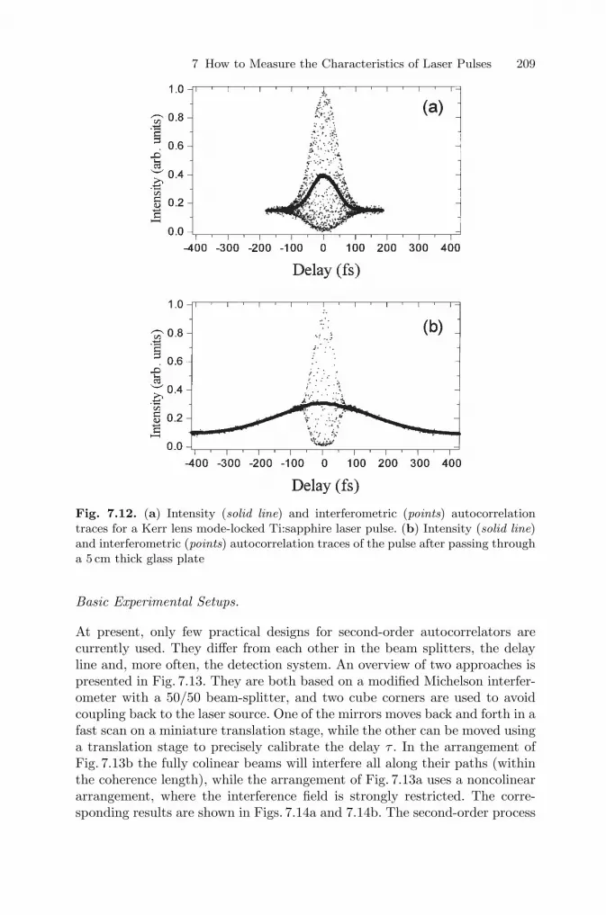
7 How to Measure the Characteristics of Laser Pulses 209

Fig. 7.12. (a) Intensity (solid line) and interferometric (points) autocorrelationtraces for a Kerr lens mode-locked Ti:sapphire laser pulse. (b) Intensity (solid line)and interferometric (points) autocorrelation traces of the pulse after passing througha 5 cm thick glass plate

Basic Experimental Setups.

At present, only few practical designs for second-order autocorrelators arecurrently used. They differ from each other in the beam splitters, the delayline and, more often, the detection system. An overview of two approaches ispresented in Fig. 7.13. They are both based on a modified Michelson interfer-ometer with a 50/50 beam-splitter, and two cube corners are used to avoidcoupling back to the laser source. One of the mirrors moves back and forth in afast scan on a miniature translation stage, while the other can be moved usinga translation stage to precisely calibrate the delay τ . In the arrangement ofFig. 7.13b the fully colinear beams will interfere all along their paths (withinthe coherence length), while the arrangement of Fig. 7.13a uses a noncolineararrangement, where the interference field is strongly restricted. The corre-sponding results are shown in Figs. 7.14a and 7.14b. The second-order process

210 L. Sarger and J. Oberle

Cube Corner

Position Sensor

Lens

Calibration

Cube Corner

Position Sensor

Lens

Calibration

KDP

UV FilterUV

PM

KDP

UV FilterUV

PM

Sha

ker

Sha

ker

Fig. 7.13. Basic principle of second-order autocorrelator: noncolinear (a) and col-inear (b) arrangements

needed requires a reasonable peak power, and a short-focal-length lens is useddifferently in both arrangements.

Both systems can be equipped with one of the following:

(1) a nonlinear crystal, a high-pass filter and a photodetector to detect thesecond harmonic;

(2) a photodiode with a band gap greater than the photon energy.

For detection (i.e. (2) above), one has to choose a suitable photodetector.For example, an AsGaP photodiode will give excellent results for wavelengthsabove 600 nm [7.3], while a standard silicon photodiode will do the same forthe near infrared (> 1.2 μm). The focusing lens in both setups focuses insidethe depletion zone and only the setup of Fig. 7.13b can provide the interferencefringes already described. The other setup directly gives the averaged intensityautocorrelation. The sensitivity may be so high that one has to reduce thepulse power to stay out of the saturation in the case of a photovoltaic detector.One can instead use an inexpensive LED whose band gap is adequate, but inthis case one has then to worry about the extremely small size of the emittingzone, which is used here as a photodetector [7.4].

For a doubling-crystal approach, one has to choose, cut and tune the crys-tal axis in order to produce frequency doubling effectively. In the fully colinearcase (Fig. 7.13b), of course, the interference fringes are present in the funda-

7 How to Measure the Characteristics of Laser Pulses 211

Fig. 7.14. Intensity autocorrelation traces for a self-mode-locked Cr:forsteritelaser: (a) interferometric autocorrelation trace obtained using the setup shown inFig. 7.13b(1), (b) intensity autocorrelation without background obtained using thesetup shown in Fig. 7.13a(1)

mental as well as in the harmonic wavelength and a high-pass filter has tobe used to select only the second-order process. In the noncolinear arrange-ment, the cut is obviously different and only a harmonic signal can be gen-erated along the bisector of the incoming beams. Here, only a spatial filter

212 L. Sarger and J. Oberle

can extract the required signal, so that it appears without background. Thecorresponding signal is then given by

SII = 4∫

I(t)I(t − τ) dt. (7.11)

The choice of doubling crystals is generally an easy task. BBO or KDP crys-tals can be phase-matched over a wide range of laser wavelengths, but theactual thickness is of major importance. In fact, as the interaction length in-creases, the group-velocity mismatch, particularly with femtosecond pulses,can greatly affect the harmonic generation and thus the recorded signal. Toovercome this difficulty, one can either use a very short crystal length, of theorder of 100μm, or focus strongly into the entrance face of the crystal with amicroscope lens to get a short confocal parameter.

Different scanning systems for the moving cube corner can be used, de-pending on the laser repetition rate and/or the level of averaging required.The most frequently used systems is either a DC motor and a translationstage or a speakerphone. These systems can be equipped with any kind ofmotion or position sensor to synchronize the measurement system, althoughthe inherent fringes present in these setups can easily be used as an automaticposition control. Nevertheless, the speed of motion and time constants haveto be carefully chosen to retrieve a nonintegrated signal in the measurement.

Comments.

• Experimentally, if one is measuring pulses shorter than 50 fs, one has to becareful to avoid any pulse broadening before and inside the correlator. Apellicle beam splitter and a thin lens have to be selected and, in any case,will give a practical limit for the accuracy. Obviously, when a two-photonphotodiode is used, the protective resin or the plastic window included inthe diode housing have to be removed.

• Interferometric autocorrelations present the advantage of a direct cali-bration of the time axis by the fringes, but the drawback is a constantbackground precluding any high-dynamic range measurements. For someexperiments, the signal to noise ratio is not sufficient to provide a correctdynamic range for pulse characterization. For example, an eventual pre-pulse at a level of 10−6, undetectable in second-order autocorrelations, canbe strongly detrimental for any experiment in high field plasma physics.Moreover, asymmetric pulses in time cannot be revealed by second-orderautocorrelations. Recently, it has been demonstrated that a third-orderautocorrelation, between the second harmonic of the investigated pulseand the pulse itself, can solve this issue and lead to dynamic range in-crease of the measurement [7.5].

Signal Analysis: Pulse Width. The intensity autocorrelation trace has an ex-perimental full width at half maximum (FWHM) Δτ (easily calibrated using

7 How to Measure the Characteristics of Laser Pulses 213

the speed of light: 0.3 μm/fs). As already mentioned, we have to select somerealistic pulse shape and compute the expected signal in the intensity auto-correlation function. For example, if the pulse intensity has a full width at halfmaximum of Δt, how large will be the autocorrelation function Δτ? Table 7.2lists some mathematical results obtained using various pulse shapes.

Table 7.2. Mathematical results (after J.C. Diels [7.2])

Obviously, the best (most optimistic) result can be obtained for a sech2

pulse, with a reduction factor Δτ/Δt = 1.54. This is one of the main reasonswhy all the scientific community agrees to choose this standard, regardless ofthe actual pulse shape; the latter has to be analyzed by more sophisticatedmethods. The “rule of thumb” will then be the ratio Δτ = 1.54Δt.

Table 7.3 lists also the product Δt Δω for each different function. Thisalso has to be cross-checked using the laser pulse spectrum for that particularfunction.

7.4.2.4 Single-Shot Second-Order Autocorrelator. For an amplifiedsystem, after tuning the oscillator and measuring the laser pulse width withone of the systems described above, one has to tune the output of the system,generally at a very low repetition rate. As many different processes affect thepulse before this final stage, a single-shot measurement is usually needed.

214 L. Sarger and J. Oberle

Detector

Fig. 7.15. Principle of a single-shot noncolinear interferometric autocorrelator. Theincident beam (at frequency ω) is split into two equal parts by the beam-splitter(BS). The intensity distribution across the second-harmonic signal (generated bythe KDP crystal) gives the autocorrelation function

As the delay cannot be incremented, a geometrical arrangement should beused to transform the autocorrelation function into a spatial intensity distri-bution, which can be recorded with a CCD matrix. The use of a noncolinearinterferometer [7.6], as represented in Fig. 7.15, provides the required temporalscan.

In the setup shown in Fig. 7.15, the beam is split into two equal parts usinga beam-splitter (BS). Beam crossing is performed inside the doubling crystalat a small angle Φ (Fig. 7.16). A high-pass filter and a lens relay this linearcrossing zone into a CCD detector.

As the two beams are noncolinear and with a beam diameter in the overlapregion much larger than the pulse length (cΔt), a certain effect ensures thatthe second harmonic is generated only when both pulses coincide in time andspace. As shown in Fig. 7.16, if the two beams are uniform, with I1(t) and I2(t)the temporal shapes of the beams at a given distance x0 from the center, theradiated field at the harmonic frequency is proportional to I1(t − τ)I2(t + τ),where the delay τ is given geometrically by

τ =nx0 sin(Φ/2)

c. (7.12)

As a result, the filtered signal observed at the linear detector is a functionof position along the crossing line and is proportional to

S(x) =∫

I1(t + τ)I2(t − τ) dt, (7.13)

and so it is directly proportional to the second-order autocorrelation functionG2(2τ) of the incident pulse

G2(2τ) ∝∫

I(t)I(t − 2τ)dt. (7.14)

The calibration is easily performed by inserting a calibrated delay ΔT(such as a glass plate) in one of the two arms of the autocorrelator. As aconsequence, the translated image on the CCD detector corresponds to thetranslation of the second-order autocorrelation function G2(2τ) by ΔT/2.

7 How to Measure the Characteristics of Laser Pulses 215

Fig. 7.16. Detail of Fig. 7.15. The second-harmonic signal at frequency 2ω is gener-ated by the KDP crystal, oriented for phase-matched type I SHG for the two beamsintersecting at an angle Φ. The crossing of the pulse wavefronts induces second-orderprocess and transforms autocorrelation in time into a spatial intensity distributionalong the x axis

7.5 Spectral Measurements

Basically, the spectral measurement of an ultrashort pulse does not requireany special tools. The spectrum associated with femtosecond laser pulses onlyrequires a moderate resolution but one has to control carefully the oscillatingbackground of the laser. In fact, most of the conventional oscillators can alsorun fully CW and, as a result, will introduce a sharp line into the spectrum.The correct optimization of the laser source requires one, then, to monitorthis behavior. In some commercial products, the response of a Fabry–Perotinterferometer to either the CW or the pulsed regime is used as an automaticcontrol of the laser pulse.

As already said, the FWHM of the laser spectrum, Δν, can be relatedto the measured pulse width Δt through autocorrelation techniques. If oneassumes a transfom-limited laser pulse, the product Δt Δν can be accuratelycomputed as a function of the actual pulse shape (see Table 7.3).

216 L. Sarger and J. Oberle

For the “standard” sech2 pulse shape, this “magic” product is (in appro-priate units)

Δt Δν = 0.315. (7.15)

Any deviation from this value will reflect a phase problem completelymissed in all the preceding measurements. It has been shown that completelydifferent laser behaviors can be obtained starting from the same setup. In anantiresonant colliding-pulse dye laser, in either passive or hybrid mode-lockedoperation, the same autocorrelation trace can be obtained [7.6], generatedby completely different spectra. In this case, gain and saturation dynamicsstrongly modify the pulse phase and there is a need for a more completecharacterization.

We will now describe new approaches to retrieve the pulse in terms ofamplitude and phase and then to compute the expected spectrum.

7.6 Amplitude–Phase Measurements

In the simple approach of the temporal characterization presented in sec-tion 7.4.2, the real pulse shape is hidden within an autocorrelation function.Although these autocorrelation techniques have been widely used in all thediagnostic approaches, they are far to qualify unambiguously the laser pulseelectric field (amplitude and phase). The complete characterization of ultra-short pulses is of great importance in many femtosecond experiments, suchas those involving coherent and optimal control, where complicated pulsesmust be generated using elaborate pulse-shaping techniques. Although someimprovement can be made and few assumptions can be made to overcome thislimitation, the inherent symmetry of the interferometric setup remains. Forexample, one can infer the actual pulse shape by analytically comparing therecorded interferometric autocorrelation trace and the theoretical one with agiven standard shape (either Gaussian or sech2 with a given phase), and thushave a better control. This will find some limitations, first experimentally, dueto signal over noise ratio, and then theoretically, as the analytical shape is notclearly established [7.8]. An alternative combining interferometic autocorre-lation and spectrum has also been proposed and demonstrated convincingresults [7.9].

A more rigorous approach can be found in the simultaneous measurementof the amplitude and phase of the laser pulse. Two different approaches havebeen demonstrated either in the frequency domain, where the time of arrivalof a given frequency is recorded, or in the time domain, where frequencies arerecorded at a given time. The first approach, referred to as FDPM (FrequencyDomain Phase Measurement) [7.10–13], is equivalent to a sonogram usuallyused in acoustic wave analysis, while the second is widely nicknamed as FROG(frequency resolved optical gating) [7.14–17].

7 How to Measure the Characteristics of Laser Pulses 217

Spectro-meter

Fig. 7.17. Principle of FROG technique. The pulse to be measured is split into tworeplicas, which are crossed in a nonlinear optical medium to create a signal field, asin autocorrelation. The signal pulse is then spectrally resolved

7.6.1 FROG Technique

In the FROG approach shown in Fig. 7.17 an nth-order correlation function isspectrally resolved. The nonlinear device can be either a Kerr gate (3rd-orderprocess) or more commonly a doubling crystal, in which case the technique iscalled “SHG FROG”.

A FROG trace is obtained in the (ω, τ) plane, where the projection alongthe frequency axis gives the classical autocorrelation function. The amplitudeand phase of the incident laser field E(t) are then retrieved from the FROGtrace by using an iterative algorithm (usually convergent in realistic cases).

For example, in SHG FROG, the frequency-doubled light of the autocor-relation forms the signal beam:

ESHGsig (t, τ) = E(t)E(t − τ). (7.16)

This signal is imaged onto the entrance slit of an imaging spectrometer, wherethe relative time delay (τ) between the two replicas is parametrized along theslit. The spectrometer disperses the light in a direction perpendicular to theslit, resulting in a two-dimensional image with delay time and frequency asaxes. The linear detector (a CCD array) detects the intensity (the FROGtrace):

IFROG(ω, τ) =∣∣ ∫ +∞

−∞Esig(t, τ) exp(iωt) dt

∣∣2. (7.17)

This approach has been extensively studied and documented [7.16]. Recently, avery useful experimental setup was proposed, which greatly simplifies the pro-cedure. The so-called single-shot GRENOUILLE device uses a Fresnel biprism,which replaces the beam splitter and the delay line, followed by a thick dou-bling crystal, acting as both the nonlinear-optical time-gating element andthe spectrometer. Spectral resolution proceeds from the output light of thecrystal, which is angularly resolved. By use of cylindrical lenses a SHG FROGtrace is directly formed on the CCD camera. The amplitude and phase of thelaser field are retrieved using the same FROG algorithm.

218 L. Sarger and J. Oberle

Fig. 7.18. A portion of the pulse spectrum is selected by a spectral filter in one armof the interferometer. The cross-correlation of the selected portion with the inputpulse is generated by crossing the two in a nonlinear medium (e.g. an SHG crystal)

7.6.2 Frequency Gating

One can also spectrally filter the laser pulse before gating it with the originalpulse, in an arrangement of the kind shown in Fig. 7.18 [7.10].

At each frequency ωi, one scans the delay τ to find the position of themaximum of the cross-correlation τi, while measuring the amplitude A(ωi).In the (ω, τ) plane, one obtains directly the derivative of the spectral phaseas a function of frequency:

τ(ωi) =∂Φ

∂ω(ωi). (7.18)

This function is easily integrated and gives the characteristic of the pulse inthe frequency domain. There is here no need of any algorithm, and most ofthe time this is sufficient to fully chararacterize the pulse.

Here, experimentally, the spectral filtering is not trivial, as one has to filterout a given frequency without altering its chronology. This is done using a zerodispersion delay line, highlighted (ZDL) in the sonogram scheme presented inFig. 7.19.

This device, discussed in Chap. 6, usually stretches or compresses the im-pinging laser pulse depending on the respective spacing of the lenses and grat-ings. When precisely tuned, i.e., the first grating image exactly correspondsto the second grating position, the output pulse exactly reproduces the in-put one, whereas in the symmetry plane (at the Fourier plane), all the pulsefrequencies are uncoupled and can be safely selected using a simple slit. Bymoving the slit across this plane, a given frequency is selected and nonlinearprocess, such as an up-conversion with a reference pulse (the unfiltered one),directly gives the time of arrival. A sequential scanning of the slit position andthe delay for the up-conversion map the pulse parameters, as presented in theFig. 7.20. Any deformation of the contour lines can be related to deviationfrom a prefect Fourier-transformed laser pulse in a very similar way as theFROG trace does. Obviously, a thinner slit gives a better spectral resolutionbut a worse timing precision. This apparent limitation can be easily overcomeas many numerical techniques of (a known) signal analysis can be used [7.18].

7 How to Measure the Characteristics of Laser Pulses 219

Fig. 7.19. FDMP technique. The enclosed part highlights the zero dispersion line(ZDL) used to frequency-filter the laser pulse. D I, D II: detectors.

Fig. 7.20. (a): Sonogram of a Ti:Sa oscillator as recorded with the FDMP technique.The satellite along the delay axis is due to the cross correlation between a Dirac (thereference laser pulse) and a filtered pulse with a square window slit; (b): Amplitudeand phase of a Ti:Sa oscillator corresponding to the sonogram

Basically, the sonogram technique is not easily seen as a single-shot tech-nique as the FROG one.

7.6.3 Spectal Interferometry and SPIDER

Recently, an old point of view, referred to as shearing interferometry, wasproposed as a powerful alternative to pulse measurements. Here, the spectral

220 L. Sarger and J. Oberle

Fig. 7.21. Schematic of the spectral interferometry technique

Fig. 7.22. Schematic of the SPIDER technique: The two up-converted pulses haveslightly different frequencies.

interferogram of two delayed pulses (delay by a time τ) can reveal the phaseand amplitude characteristic:

S(ω) = |E0(ω) + E(ω)eiωτ |2 = I0(ω) + I(ω) +2

√I0(ω)I(ω) cos(ϕ(ω) −ϕ0(ω) +ωτ).

(7.19)In the basic principle of this linear technique, presented in Fig. 7.21, the

pulse to be characterized is combined with a reference-delayed pulse (delay τ)at the input slit of a grating spectrometer. A Fourier analysis of the spectralinterferogram gives the differences is spectral amplitude (by the contrast)and spectral phase (by the beating frequency along the spectrum) betweenthe two pulses. As always, the need for a reference pulse greatly reduces theconvenience of this approach, as one needs, to prepare the reference pulse formthe pulse under measurement [7.19–20].

Some improvements have been implemented, and the power of this tech-nique is now fully demonstrated in commercially available instruments. Theacronym SPIDER (Spectral Phase Interferometry for Direct Electric field Re-construction) describes the following setup, where the two spectrally inter-fering pulses are also spectrally sheared of a known amount. Thus, all theambiguities coming form the replica approach vanish and quasi-single-shotmeasurements are routinely performed and enable the precise tuning of thelow repetition rate of amplified femtosecond pulses. [7.21–24].

The scheme of the instrument is presented in Fig. 7.22. First, the measuredpulse is split in three parts by a thin plate. The two reflections, delayed by atime τ (due to the etalon thickness), are up converted in a doubling crystalwith the remaining pulse on which a controlled chirp has been applied throughspectral dispersion (stetcher or glass sample). Thus, the two up-converted

7 How to Measure the Characteristics of Laser Pulses 221

pulses, with different center frequencies (2ω and 2ω + Ω), exhibit spectralshear interference fringes that are analyzed by a spectrometer. The spectralinterferogram will then be written as:

S(2ω) ∝ ∣∣E0(2ω+Ω) + E(2ω)ei2ωτ

∣∣2= I0(ω+Ω) + I(2ω) + 2

√I0(ω+Ω)I(2ω) cos(ϕ(2ω) − ϕ0(2ω+Ω) + 2ωτ),

(7.20)

and thus the amplitude and phase of the laser pulse are provided by a standardFourier analysis.

References

[7.1] J.C. Diels, J. Fontaine, W. Rudolph: Rev. Phys. Appl. 22, 1605 (1987)[7.2] J.-C. Diels, W. Rudolph: Ultrashort Laser Pulse Phenomenon: Fundamen-

tals, Techniques and Applications on a Femtosecond Time Scale, AcademicPress, Boston (1996)

[7.3] J.K. Ranka, A.L. Gaeta, A. Baltsuka, M.S. Pshenichnikov, D.A. Wiersma:Opt. Lett, 22, 1344 (1997)

[7.4] D.T. Reid, M. Padgett, C. McGowan, W. Sleat, W. Sibbett: Opt. Lett 22233 (1997)

[7.5] J.P. Chambaret, C. Dorrer, M. Franco, A. Mysyrowicz, B. Prade, S. Ranc,J.F. Ripoche, J.P. Rousseau: “High-Dynamic Range Measurements of Unl-trshort Pulses,” UltraFast Optics Conference (1999)

[7.6] A. Brun, P. Georges, G. Le Saux, F. Salin: J. Phys. D 24, 1225 (1991)[7.7] N. Jamasbi, J.C. Diels, L. Sarger: J. Modern. Opt. 35, 1891 (1988)[7.8] J.-H. Chung, A.M. Weiner: IEEE J. Sel. Top. Quantum Elect. 7, 656 (2001)[7.9] J.W. Nicholson, J. Jaspara, W. Ruldolph, F.G. Omenetto, A.J. Taylor, Opt.

Lett 24 1774 (1999)[7.10] J. Chilla, O. Martinez: IEEE J. Quantum Elect. 27, 1228 (1991)[7.11] J. Chilla, O. Martinez: Opt. Lett. 16, 39 (1991)[7.12] D.T. Reid, I.G. Cormack: Opt. Lett. 27, 658 (2002)[7.13] V. Wong, I.A. Walmsley: J. Opt. Soc. Am. B 14, 944 (1997)[7.14] R. Trebino, D.J. Kane: J. Opt. Soc. Am. A 11, 2429 (1993)[7.15] G. Taft, A. Rundquist, M.M. Murname, H.C. Kapteyn, K.W. Delong, R.

Trabino, I.P. Christov: Opt. Lett. 7, 743 (1995)[7.16] K.W. DeLong, D.N. Fittinghoff, R. Trebino, B.K. Kohler, K. Wilson: Opt.

Lett. 19, 2152 (1994)[7.17] R. Trebino, K.W. DeLong, D.N. Fittingholf, J.N. Sweetser, M.A. Krumbugel,

B.A. Richman, D.J. Kane: Rev. Sci. Inst. 68, 3277 (1997)[7.18] S. Rivet; “Caracherisation complete d’un faisceau laser impulsionnel fem-

toseconde: mise en evidence et analyse du couplage spatio-temporel dansla propagation lineaire et non lineaire”, PhD thesis, Univesite Bordeaux 1(2001) http://147.210.235.3/proprietes.html?numero ordre=2448

[7.19] L. Lepetit, G. Cheriaux, M. Joffre: JOSA B 12 (12), 2467 (1995)[7.20] C. Froehly, A. Lacourt, J.C. Vienot, J. Opt. (Paris) 4, 183 (1973)

222 L. Sarger and J. Oberle

[7.21] C. Iaconis and I.A. Walmsley: Opt. Lett. 23, 792 (1998)[7.22] C. Dorrer: JOSA B 16 (7), 1160 (1999)[7.23] L. Gallmann, D.H. Sutter, N. Matuschek, G. Steinmeyer, U. Keller, C. Iaco-

nis, I.A. Walmsley: Opt. Lett. 24, 1314 (1999)[7.24] C. Dorrer, B. deBeauvoir, C. Le Blanc, J.-P. Rousseau, S. Ranc, P. Rousseau,

J.-P. Chambaret, F. Salin: Appl. Phys. B 70 (7), S77 (2000)

8

Spectroscopic Methods for Analysis of SampleDynamics

C. Rulliere, T. Amand and X. Marie

With 42 Figures

8.1 Introduction

In the previous chapters of this book, we dealt with ultrashort laser pulses bythemselves, without paying attention to their possible uses. Since you are nowfamiliar with the methods of generation of ultrashort laser pulses, with theirmanipulation and with the associated difficulties, it is now time to consideran important topic: what can we do with these ultrashort laser pulses?.

One important application domain of ultrashort laser pulses is the behav-ior analysis of a sample perturbed by such a light pulse. Let us explain whatexactly we mean by “sample” and “behavior analysis” by giving some typicalexamples. The sample can be a semiconductor, in which the light pulse willcreate charge carriers by excitation into the conduction band. In this case, af-ter being created, the charge carriers may migrate or annihilate, and behavioranalysis will provide information on the migration or annihilation dynamics ofthe charge carriers. The sample can also consist of a molecule or of an ensem-ble of molecules, which after absorption of photons from the light pulse willbe changed photochemically into other kinds of molecules: the photoproducts.Behavior analysis will lie in observation of the transformation of the moleculesin order to identify the photoproducts or the intermediate chemical speciesin the transformation pathway, or in order to study the associated reactionrates. But the sample can also be a simple piece of glass, which under theaction of the light pulse will see its refractive index temporarily changed and,as a consequence, its optical properties too. In this case, behavior analysis willconsist of measuring these changes and observing how long they last.

This chapter will deal with experimental methods which use ultrashortlaser pulses to make such behavior analysis possible.

However, in this chapter we will assume generally that the laser-pulse du-rations are long compared to the dephasing time and that the analysis ismade after the perturbed systems have lost their phase. Oscillating dipoles,for example, will oscillate in phase until dephasing processes induce phaseloss. If analysis is made during the in-phase conditions, coherent processes

224 C. Rulliere, T. Amand and X. Marie

may be superposed on incoherent processes. This very interesting aspect willbe described seperately in the next chapter because it deserves specific com-ments and explanations. The techniques described in the present chapter areassociated with mainly with incoherent processes.

First of all, why are ultrashort laser pulses interesting to use for behavioranalysis of light-induced perturbations?

During the perturbation of a sample, it is generally difficult to make mea-surements. It is usually necessary to wait till the end of the perturbation beforeanalyzing the consequences of the perturbation. However, if some processesare very fast compared to the duration of the perturbation, these processeswill be hidden during the perturbation so that only those processes which areslower than the pulse duration will be observed. Some slower processes can bethe consequences of faster processes. In this case it will be difficult to under-stand the origin of the slower processes in the absence of information on thefaster processes. Therefore, the shorter the perturbation, the easier it will beto understand the faster processes. Clearly, the unique property of ultrashortlaser pulses, namely their very shortness, makes them ideally suited for theinitial perturbation of a sample.

But sample evolution should also be analyzed as a function of time. Fine-scale analysis requires detection methods with response times which are asshort as possible, so as to lose as little information as possible. Using ultrashortlaser pulses for the analysis will therefore be very suitable for overcomingthis response-time problem. Since the response time is limited by the pulseduration, very short pulses will improve the time resolution.

Last but not least, ultrashort laser pulses can have a very large peak power,even for weak pulse energies. Thus, intensity effects may appear at moderateenergy, so that data can be taken on the sample while remaining below itsdamage threshold. This specific aspect of ultrashort laser pulses must be keptin mind.

Short pulse duration and high peak power are the two main characteristicsof the ultrashort laser pulses that have been decisive in the behavior analysisof samples under light perturbation. Let us now describe the various methodsfor behavior analysis, and let us give a few pedagogic examples of applicationsshowing the potential of these methods.

8.2 “Pump–Probe” Methods

8.2.1 General Principles

These methods need at least two ultrashort light pulses. The first one, theso-called “pump” pulse, perturbs the sample at time t = 0. The second one,delayed with respect to the “pump” pulse, crosses the perturbed sample andacts as a probe (this is the so-called “probe” pulse).

8 Spectroscopic Methods for Analysis of Sample Dynamics 225

Sample

Pump Pulse

Probe Pulse

Det

ecto

r

I0 (ν) ΔL

Δt = 2ΔL/c

I (ν, Δt)

Fig. 8.1. Typical scheme of a “pump–probe” experiment

The action of the pump pulse on the sample may be analyzed in two differ-ent ways: (1) by comparing the modifications of the probe pulse characteristics(intensity, phase and wave vector) after crossing the sample, before and afterthe action of the pump pulse: we are speaking of the time-resolved absorp-tion technique; (2) by observing new effects created by the probe itself beforeand after the action of the pump pulse: we are speaking of Raman scatter-ing spectroscopy, laser-induced fluorescence and coherent anti-Stokes Ramanspectroscopy (CARS), for example. The following sections of this chapter willdescribe these different methods.

8.2.2 Time-Resolved Absorption in the UV–Visible SpectralDomain

With this method, changes in the absorption spectrum of a sample after per-turbation by an ultrashort pulse can be observed and measured.

Changes in the absorption spectrum may involve the spectral character-istics (new transitions appearing under perturbation) and/or the absorbancecharacteristics (increase or decrease of the optical density). The electronic ab-sorption spectrum is the signature of a sample. Spectral analysis of changessuch as new electronic transitions will give the signature of the new electronicstates created by the pump pulse (for example photochemical products), whiletemporal analysis will yield the dynamics of the transformations (for examplechemical reaction rates). The principle of this method is shown in Fig. 8.1.

At time t = 0, the pump pulse perturbs the sample. At time t + Δt theprobe pulse crosses the sample, Δt being tunable by means of an optical delayline. The detector then measures the probe pulse intensity before (I0(ν)) andafter (I(ν, Δt)) the perturbed sample. Applying the Beer–Lambert law, wecan write

I(ν, Δt) = I0(ν) × 10−ενN(Δt)l, (8.1)

226 C. Rulliere, T. Amand and X. Marie

where εν is the absorption coefficient of the sample at frequency ν, N(Δt)is the population absorbing at time Δt at frequency ν and l is the length ofsample excited.

In fact, the quantity of interest is the measured optical density (OD),defined as

OD (ν, Δt) = logI0(ν)

I(ν, Δt)= ενN(Δt)l. (8.2)

For a fixed delay Δt, at each frequency ν a quantity will be measuredwhich is proportional to εν : we thus construct the absorption spectrum of theexcited sample at time Δt.

For a given frequency ν, varying Δt will yield a quantity proportionalto N(Δt): we can now construct the population dynamics. If the populationN decays exponentially, the decay time τ can be measured by varying Δtaccording to

ln OD (Δt) = lnN(0)εν l − Δt/τ. (8.3)

The above considerations form the basis of the method. Let us now presentits practical aspects.

8.2.2.1 Probe Characteristics. The probe can have a broad spectrum, orit can be quasi-monochromatic. Let us recall that in any case, as was thor-oughly explained in the previous chapters, the spectral width will be lim-ited by the relation Δν Δτ = constant. Probe pulses with narrow spectralranges can be generated from dye lasers (CPM mode), tunable solid-statelasers (Ti3+:sapphire, etc.), OPOs, OPAs or OPGs, as explained in previouschapters. The probe wavelengths should be in a spectral domain in which it isknown (or expected) that some species created by excitation will be presentin the sample at a certain time Δt after excitation and will have resonant elec-tronic transitions in the probe spectral domain. When such a probe pulse isused, one assumes that the behavior of the sample has already been character-ized by other preliminary studies which have indicated the frequency domainof interest. When this spectral domain is not known, it is best to use a probewhich is spectrally as broad as possible.

In this case two possibilities exist: (1) continuum generation, and (2)broadband laser emission.

(1) Continuum Generation. Focusing a high-peak-power light pulse in amedium (liquid, glass, etc.) generates a continuum of light (Sect. 4.3.5) witha very broad spectral domain, which may even appear as white light [8.1].The origin of this process is well described elsewhere [8.2], and is mainly gov-erned by self-phase-modulation and stimulated Raman emission. The rathergood directivity of this white-light pulse makes it possible to use it as a spec-trally broad probe and to record transient absorption at different wavelengthssimultaneously.

As to the medium used to generate this light continuum, each scientistgenerally has his or her own method, as in cooking. But the most popular

8 Spectroscopic Methods for Analysis of Sample Dynamics 227

Sample

Pump Pulse

I (ν, Δt)

I 0 (ν)

Probe Pulse

R = 50 %

Det

ecto

r

Fig. 8.2. Dual-beam pump–probe experiment

media are D2O, H2O, ethylene glycol, phosphoric acid and quartz glass. Themain problem is to produce a spectral distribution which is as flat as possible.Depending on the medium, the wavelength and the peak power available togenerate the continuum, it may prove necessary to use filters (liquids or solids)to flatten this spectral profile [8.3].

(2) Broadband Dye Laser. Another method which is sometimes employed is togenerate amplified spontaneous emission (ASE) in a laser medium, generallya dye (see Chaps. 3 and 4). Used as a probe, ASE is spectrally less broad thana continuum, but it usually has a stronger intensity, which can be an advan-tage in some cases. However, the shape and duration of these probe pulses,which depend strongly on the pumping conditions, need to be controlled veryprecisely. Nevertheless, it can be a useful alternative to continuum generationin those cases which do not need a very broad spectral range.

8.2.2.2 Detection Systems. To improve the sensitivity of the measure-ment, it is better to record the spectral distribution of the probe simultane-ously in the presence and in the absence of the perturbation of the sampleat each laser shot. This is done, as shown in Fig. 8.2, by splitting the probebeam into two equal beams: the first partial beam crosses the perturbed partof the sample while the other beam crosses an unperturbed part of the sam-ple. These two beams are then directed onto the slit of a spectrograph at twodifferent heights, and are read by a double photodiode array or by a CCDcamera coupled to a microcomputer. The optical density OD(ν, Δt) can thusbe measured directly as a function of the frequency.

When simultaneous measurements at different wavelengths are not nec-essary, the detectors may consist of two photodiodes (or photomultipliers)coupled to a lock-in amplifier.

228 C. Rulliere, T. Amand and X. Marie

8.2.2.3 Experimental Tricks to Avoid Artifacts. Even though these ex-periments are based on a very simple idea, experimental artifacts may stillarise. They are related to the probe and pump pulse polarizations, to the GVDalong the optical pathways, to noise of various origins and to the detectionsystem.

(1) Polarizations of the Pump and Probe. If, for example, the exciting beamis linearly polarized, the sample will be perturbed preferentially along thepolarization direction. If the beam is resonant with an electronic transition,the absorbing entities whose transition moment is oriented along this polar-ization direction will be excited preferentially, and the spatial distribution ofperturbed entities will be anisotropic. If these entities can reorient themselves,a spatial randomization will occur which will be controlled by the mean re-orientation time. If the probe is polarized parallel to the pump beam, it willprobe preferentially the excited entities whose transition moment is orientedin the polarization direction, and the measurements will be perturbed by thereorientation process. In the same way, if the probe beam is polarized per-pendicularly to the pump beam, the measurement will be affected by themolecules which have reoriented to the polarization direction of the probe.The dynamics measured for perpendicular and parallel polarizations of theprobe beam will not be the same. The dynamics will depend not only on thelifetime of the population of the perturbed entities, but also on their reorien-tation time. Depending on the process of interest, the respective polarizationswill have to be adjusted. For example, to measure the dynamics free fromreorientation effects, the angle between the pump and probe polarizationsshould be set at 54.6◦ (the so-called “magic” angle in the literature [8.4]).On the other hand, in order to measure exclusively the effects of reorien-tation, one must measure the dynamics for parallel (OD‖) and perpendicu-lar (OD⊥) polarizations independently. The depolarization ratio, defined asR(t) = [OD‖(t)−OD⊥(t)]/[OD‖(t)+2OD⊥(t)], is proportional to exp(−t/τor)and gives the reorientation time τor [8.5].

(2) Probe and GVD. Not all the probe frequencies travel through the opticalcomponents at the same speed, including the medium used for continuum gen-eration, because of GVD. As a consequence, the different spectral componentsdo not all reach the sample at the same time: the blue wavelengths arrive atthe sample later than the red wavelengths. Therefore, if the delay between thepump beam and the probe beam is changed, the shape of the recorded spec-trum may also change. Suppose that the pump beam arrives at the samplelater than the probe beam. In this case the probe beam will not be perturbed.If this delay is changed a little, the red wavelengths could still arrive beforethe pump beam and not be affected. But now the blue wavelengths could bein phase with the pump beam, and would thus be perturbed. Only the bluepart of the spectrum would then reflect the perturbation. Changing this delaymore and more would shift the interaction into the red part of the spectrum.

8 Spectroscopic Methods for Analysis of Sample Dynamics 229

It is possible to remove this effect, by using gratings for example, as ina stretcher/compressor (see Chap. 6), and to rephase all the spectral compo-nents of the probe on the sample. But this procedure is somewhat delicate andit is better to correct the spectra numerically by using appropriate software.This can only be done if the dispersion for the continuum is well known. Toobtain an exact measurement of the GVD, it should be measured by severaldifferent methods.

The first method consists of measuring two-photon interaction. The secondone uses frequency mixing in a nonlinear crystal. The third one uses theelectronic optical Kerr effect (OKE).

The first method is described in [8.3]. The absorbance of a sample ofbenzene diluted in methanol is probed at different probe wavelengths. Thedepletion process is a coherent two-color, two-photon absorption involvingabsorption from the pump and from the probe. This instantaneous processrequires a perfect temporal coincidence between the two pulses (pump andprobe) to reach maximum efficiency. Changing the delay time between thepump and probe makes it possible to determine at what time the maximumsignal is reached, i.e. the time at which the pump and probe pulses coincideperfectly for a given wavelength. In this way, one obtains the dispersion curve,which can then be used for the numerical corrections of the spectra.

The second method consists of obtaining the sum frequency of the probeand the pump using a nonlinear crystal. The crystal should be chosen to be asthin as possible so as to avoid dispersion effects. In this method the maximumsignal at the sum frequency is obtained when the two pulses coincide perfectly,thus yielding the dispersion curve.

The third method uses the optical Kerr effect in a liquid such as hexane. Acell containing hexane is inserted between two crossed polarizers. The pumppulse, polarized at 45◦ relative to the polarizers, is directed into the cell andinduces instantaneous birefringence (more details about this method will begiven later in this chapter). The probe pulse is passed through the polarizers.When the probe wavelengths are exactly synchronized with the pump pulsein the cell, the induced birefringence allows these components to be trans-mitted and detected. By changing the time delay between the pump and theprobe, the dispersion curve can be measured. The cell and the entrance po-larizers should be as thin as possible to avoid GVD in these components andto increase the sensitivity of the method.

In our opinion the third method is the simplest, because n-hexane isstrongly nonlinear, resulting in very efficient transmission and detection mech-anisms.

(3) Noise and Reference Beam. To measure transient spectra, the direct mea-surement of the ratio

I0(ν)/I(ν, Δt),

as described in Sect. 8.2.2, is not sufficient. Indeed, some parts of the recordedsignal are not directly related to the transient absorption and should be ac-

230 C. Rulliere, T. Amand and X. Marie

Pump

(a)

Probe

Reference

Sample Detector

I0 (ν)

I (ν)

Pump

(b)

Sample Detector

I0F (ν)

IF (ν)

Fig. 8.3. Illustration of the different contributions to the recorded signals in pump–probe experiments. (a) The total signal recorded. (b) The contribution of the sampleemission to the recorded signals in (a)

(a)

Probe

Reference

Sample Detector

IB (ν)

(b)

Sample Detector

In2 (ν)

I n1 (ν)IA (ν)

Fig. 8.4. Illustration of the different contributions to the recorded signals in pump–probe experiments. (a) Recorded signals allowing one to correct for spectral dif-ferences between the probe and test beams in the absence of excitation. (b) Thecontribution of noise (ambient light and electronic noise) to the recorded signal

counted for (e.g. ambient light, electronic noise and fluorescence or emissionby the excited sample). In any case, the spectral profile of the two beams can-not be exactly the same, owing to their different optical paths. These effectsshould be taken into account as shown in Figs. 8.3 and 8.4.

Let us define the following quantities.

• I(ν) and I0(ν) are the spectral distribution of the recorded signals in thepresence of the pump, probe and reference beams in the sample (Fig. 8.3a).

• IF(ν) and I0F(ν) are the spectral distributions of the recorded signalswhen only the pump is present in the sample, and the probe and referencebeams are absent (Fig. 8.3b). In this case the detectors record only sampleemission and noise.

• IA(ν) and IB(ν) are the spectral distributions of the recorded signals inthe absence of the pump beam but in the presence of the probe and ref-erence beams (Fig. 8.4a). In this case the detectors record the spectraldistributions of the probe and reference beams superposed to noise.

8 Spectroscopic Methods for Analysis of Sample Dynamics 231

(LM)∗ (L∗/S/M)

Fig. 8.5. Structure of a molecule involved in a cation photoejection mech-anism: The PDS-crown (4-N-(1-monaza-4,7,10,13-tetraoxacyclopentadecane)-4′-phenyl-stilbene) molecule [8.6, 8]

• In1(ν) and In2(ν) are the recorded signals in the absence of all of the beams(Fig. 8.4b). In this case the detectors record only electronic and ambientnoise.

With these definitions and for a given delay Δt, the real optical density,corrected for all parasitic light and all possible changes of the spectral distri-bution along the different optical paths, can be calculated according to

OD(ν, Δt) = log(

I0(ν) − I0F(ν)I(ν) − IF(ν)

)(IB(ν) − In2(ν)IA(ν) − In1(ν)

). (8.4)

Note that probe and reference beams also induce emission from the sample.

(4) Detector Linearity. Some problems may appear which are due to shortpulses, especially in detectors using a light amplifier. Indeed, a great number ofphotons arriving on the photocathode within a short time interval may causea saturation effect due to the limited current available, and this may affectthe detection linearity. To overcome this problem, the pulse to be processedshould be injected into a long optical fiber before entering the spectrograph.Propagation through the fiber will increase the pulse length by GVD by asufficient amount to be in the linear regime of the detector. Some care mustbe taken to inject the right part of the pulse into the fiber.

8.2.2.4 Example of Application: Cation Ejection. To illustrate the pos-sible applications of this technique, we shall describe here an example relatedto transient absorption changes during a photochemical reaction involving thebreaking of a dative bond. Such events may occur in the molecules shown inFig. 8.5.

In this kind of molecule, the emission properties are different depending onthe presence or absence of Ca2+ cations in the solution [8.6]. In the absenceof calcium ions in the solution, this molecule has an emission transition atabout 450 nm. In the presence of calcium ions in the solution, the molecule inits ground state traps a Ca2+ cation inside the ether-crown, where it forms adative bond with the nitrogen atom. In this state, the emission of the moleculeis shifted to the blue, to 375 nm.

232 C. Rulliere, T. Amand and X. Marie

Wavelength (nm)

Opt

ical

den

sity

(ar

b. u

nits

)

Fig. 8.6. Gain bands for different time intervals after excitation of a solution of10−4 M PDS-crown and 5mM Ca(ClO4)2 in BuCN at 20◦ C (see [8.7])

By absorbing a photon, the dative bond can break, releasing the Ca2+ ionand putting the molecule into a state in which it ignores the calcium ion. Theemission at 450 nm, corresponding to the breaking of the dative bond, shouldshow up on the experimental emission curve, recorded as a function of time.Thanks to pump–probe techniques, this chemical process can be observed. Asa matter of fact, if the gain is sufficient, amplification of light may occur at theemission transition. This behavior is shown in Fig. 8.6. Just after excitation,the band at 450 nm is absent and the gain spectrum corresponds to the spec-trum of a molecule with a calcium ion bonded to the nitrogen atom. But astime passes, this bond is broken at a certain rate, and the band correspondingto the molecule without a calcium ion bonded to the nitrogen atom beginsto appear and grows until the process is terminated. As long as this band at450 nm is growing, the process of chemical-bond breaking is going on. In thecase of this specific molecule, the breaking process has a rate of 8 ps−1 [8.7].

This example shows how powerful pump–probe experiments are for observ-ing the kinetics of excited states or the evolution of their spectral properties.Let us now present some techniques used in the IR spectral range.

8 Spectroscopic Methods for Analysis of Sample Dynamics 233

Fig. 8.7. Possible methods using IR pulses for recording behavior of modes of (a)ground or (b) excited states

8.2.3 Time-Resolved Absorption in the IR Spectral Domain

8.2.3.1 Principle of the Method. IR methods are based on the same prin-ciples as UV–visible methods, the only difference lying in the laser sources andthe detection systems.

The IR sources may be OPOs, OPAs or diode lasers, as described in earlierchapters. Detectors must have a sensitivity extending into the IR spectralrange (photodiode, etc.) and are usually coupled to IR spectrographs or to IRmonochromators. As shown in Fig. 8.7, the excitation may lie in the IR, whilethe probing of the perturbed system takes place in the UV–visible range, orelse the perturbation of the sample may occur in the UV–visible range, whilethe induced perturbations are probed in the IR. The choice of pump and probefrequencies will depend on the information we are seeking from the sample.

The probing of vibration modes in the ground state of a molecule fol-lows Fig. 8.7a, while the probing of vibration modes of excited states followsFig. 8.7b.

However, IR sources and detectors usually require a technology which iscompletely different from than used in the UV–visible domain. An interestingalternative method was presented ten years ago [8.8], and is described below.

8.2.3.2 Time-Resolved IR Spectroscopy Without IR Detection. Thismethod, illustrated in Fig. 8.8, may appear paradoxical since it performstime-resolved spectroscopy in the IR domain using neither IR pulses nor IR-sensitive spectrographs or detection systems.

A continuous diode laser, emitting at an active IR vibration frequencyωIR of the sample, is directed through the sample and then passes through anonlinear crystal. A mode-locked Nd3+/YAG laser is used for the synchronouspumping of two dye lasers. The first one (pump dye laser), which deliversthe pump pulse, perturbs the sample and its frequency ωpump is adjusted

234 C. Rulliere, T. Amand and X. Marie

Fig. 8.8. Experimental setup for time-resolved IR spectroscopy (adapted from [8.8])

to an electronic transition of the sample, for example. The pulse emittedby the second dye laser, at frequency ωprobe, in the visible domain, is sentthrough a delay line and is superposed on the diode laser beam in a nonlinearcrystal. The phase-matching angle of the crystal is adjusted to generate thefrequency ωsignal = ωprobe + ωIR by sum-frequency mixing. In the crystal, apulse is generated in the visible domain. This pulse can be detected easilyby conventional photodetectors (photomultiplier, etc.), and its intensity isproportional to the probe dye laser intensity and to the diode laser intensityafter it has crossed the sample (Isignal ∝ Iprobe × Idiode). The crystal actsas a booster for the diode laser intensity: if a small change occurs in thediode laser beam intensity after crossing the sample, it is multiplied by theprobe laser intensity. Furthermore, the detected signal intensity will dependon the time delay between the pump pulse and the probe pulse. The photonsof the diode laser which mix with the probe photons inside the crystal willbe the ones that crossed the sample at a particular time after the samplewas excited. Then, if after excitation some changes occur in the sample whichaffect the IR absorption, the intensity of the diode laser beam will be changedafter crossing the sample and it will modulate the signal generated insidethe nonlinear crystal. The intensity of the generated signal will therefore becontrolled by the dynamics of the sample. In other words, by changing theoptical delay, the IR activity of the probed vibration mode can be measureddirectly as a function of time.

As an example, an interesting application is described below.

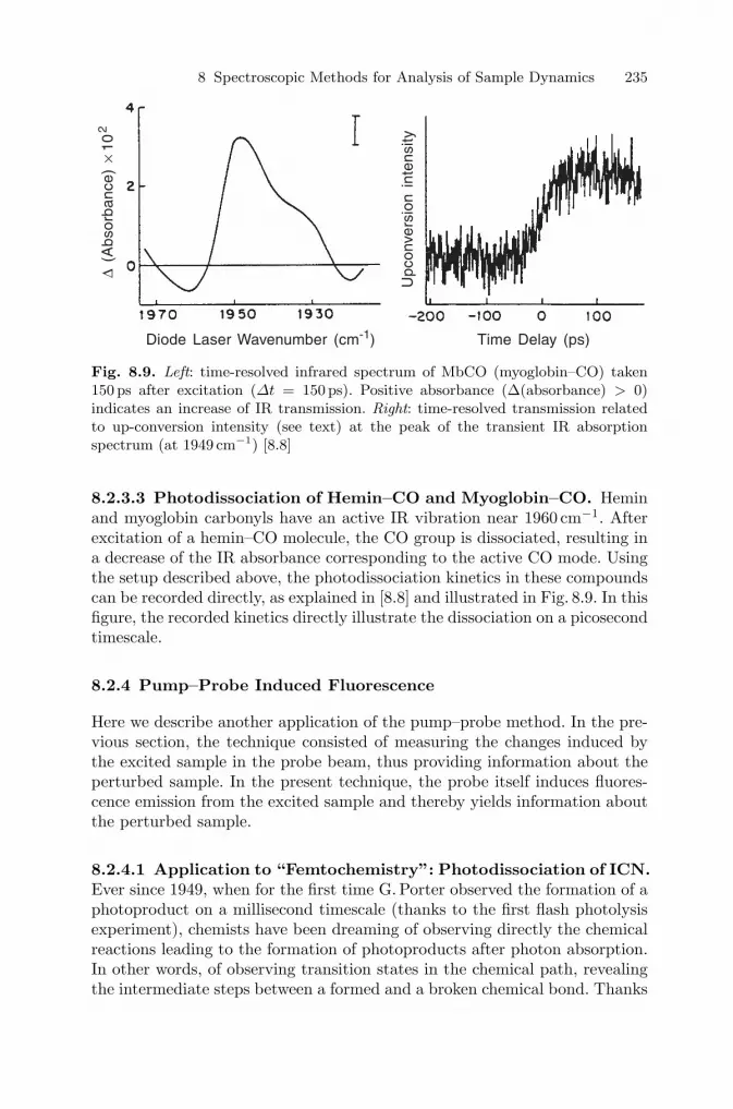
8 Spectroscopic Methods for Analysis of Sample Dynamics 235

Time Delay (ps)Diode Laser Wavenumber (cm-1)

Upc

onve

rsio

n in

tens

ity

Δ (A

bsor

banc

e) ×

102

Fig. 8.9. Left: time-resolved infrared spectrum of MbCO (myoglobin–CO) taken150 ps after excitation (Δt = 150 ps). Positive absorbance (Δ(absorbance) > 0)indicates an increase of IR transmission. Right: time-resolved transmission relatedto up-conversion intensity (see text) at the peak of the transient IR absorptionspectrum (at 1949 cm−1) [8.8]

8.2.3.3 Photodissociation of Hemin–CO and Myoglobin–CO. Heminand myoglobin carbonyls have an active IR vibration near 1960 cm−1. Afterexcitation of a hemin–CO molecule, the CO group is dissociated, resulting ina decrease of the IR absorbance corresponding to the active CO mode. Usingthe setup described above, the photodissociation kinetics in these compoundscan be recorded directly, as explained in [8.8] and illustrated in Fig. 8.9. In thisfigure, the recorded kinetics directly illustrate the dissociation on a picosecondtimescale.

8.2.4 Pump–Probe Induced Fluorescence

Here we describe another application of the pump–probe method. In the pre-vious section, the technique consisted of measuring the changes induced bythe excited sample in the probe beam, thus providing information about theperturbed sample. In the present technique, the probe itself induces fluores-cence emission from the excited sample and thereby yields information aboutthe perturbed sample.

8.2.4.1 Application to “Femtochemistry”: Photodissociation of ICN.Ever since 1949, when for the first time G. Porter observed the formation of aphotoproduct on a millisecond timescale (thanks to the first flash photolysisexperiment), chemists have been dreaming of observing directly the chemicalreactions leading to the formation of photoproducts after photon absorption.In other words, of observing transition states in the chemical path, revealingthe intermediate steps between a formed and a broken chemical bond. Thanks

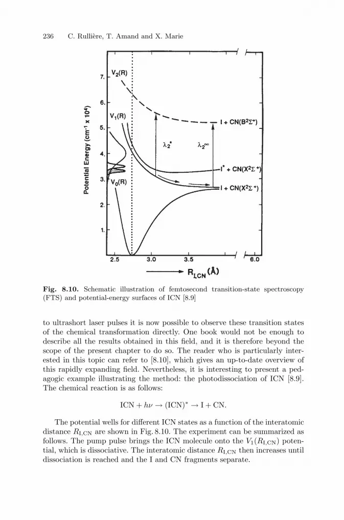
236 C. Rulliere, T. Amand and X. Marie

Fig. 8.10. Schematic illustration of femtosecond transition-state spectroscopy(FTS) and potential-energy surfaces of ICN [8.9]

to ultrashort laser pulses it is now possible to observe these transition statesof the chemical transformation directly. One book would not be enough todescribe all the results obtained in this field, and it is therefore beyond thescope of the present chapter to do so. The reader who is particularly inter-ested in this topic can refer to [8.10], which gives an up-to-date overview ofthis rapidly expanding field. Nevertheless, it is interesting to present a ped-agogic example illustrating the method: the photodissociation of ICN [8.9].The chemical reaction is as follows:

ICN + hν → (ICN)∗ → I + CN.

The potential wells for different ICN states as a function of the interatomicdistance RI,CN are shown in Fig. 8.10. The experiment can be summarized asfollows. The pump pulse brings the ICN molecule onto the V1(RI,CN) poten-tial, which is dissociative. The interatomic distance RI,CN then increases untildissociation is reached and the I and CN fragments separate.

8 Spectroscopic Methods for Analysis of Sample Dynamics 237

With the pump–probe method, it is possible to probe the different transi-tion states corresponding to different interatomic distances RI,CN along thisreaction coordinate. Indeed, if for a given delay Δt after excitation the probebeam is in resonance with the V1(RI,CN) → V2(RI,CN) transition, CN(B2Σ+)excited fragments will be created by the probe, as depicted in Fig. 8.10, andwill emit fluorescence (transition from CN(B2Σ+) to CN(X2Σ+) states) TheCN(B2Σ+) fluorescence intensity will at first be proportional to the transitionstate population on the V1(RI,CN) potential curve, and then, depending on theprobe wavelength, it will be proportional to the population corresponding toa well-defined interatomic distance RI,CN. Choosing a particular probe wave-length will determine a specific observation window on the V1(RI,CN) curve, aswell as a class of ICN molecules with a specific value of RI,CN. Varying Δt willprobe the dynamics of this population through the selected spectral window.By recording the fluorescence intensity of the CN(B2Σ+) population, one canfollow the movement of the ICN molecules on the photodissociation potentialcurve V1(RI,CN).

Figure 8.11 illustrates this behavior for different wavelengths of the probebeam. At high wavelengths (top left) the corresponding value of RI,CN is farfrom the equilibrium value of RI,CN in the ground state, and the fragmentsare well separated. A rise time of the CN(B2Σ+) fluorescence of the orderof 250 fs is observed, which corresponds to the photodissociation rate. Butat lower probe wavelengths (bottom right), the corresponding value of RI,CNis close to the equilibrium distance in the ground state: the first observedstep of the photodissociation consists in a rapid sliding of the ICN moleculealong the potential curve. We arrive at the remarkable result that one single,specific transition state with a very short lifetime, of the order of a few tenfemtosecond, is observed directly through the selected spectral window.

This example shows how the pump–probe method can reveal directly suchprocesses as a photochemical transformation, along with the different transi-tion states in the chemical pathway, thereby demonstrating how powerful thismethod is.

8.2.5 Probe-Induced Raman Scattering

Just as in UV, visible and IR absorption spectra, Raman spectra also charac-terize a sample in a given state. Observing the evolution of the Raman spec-trum after perturbation will then give information about the transformation(and its associated structure) of a sample. In this section, we shall describe atechnique in which the probe induces Raman scattering in the sample.

8.2.5.1 Time-Resolved Raman Technique. The principle of the methodis displayed in Fig. 8.12. It is basically very simple. The pump pulse perturbsthe sample at time t = 0. The probe pulse, at frequency ωp, is incident onthe sample at time Δt and creates Raman scattering at frequencies ωRi =

238 C. Rulliere, T. Amand and X. Marie

-400 -200 0 200 400 600 800

Time Delay (fs)-400 -200 0 200 400 600 800

Time Delay (fs)

Sig

nal

inte

nsity

0

0.5

1.0

1.5

Sig

nal

inte

nsity

0

0.5

1.0

1.5

Fig. 8.11. Typical ICN transients as a function of probe wavelength. The probewavelengths were (top left) 388.9 nm, (top right) 389.8 nm, (bottom left) 390.4 nmand (bottom right) 391.4 nm [8.9]

ωp±∑i ωvi (where ωvi are the frequencies of the Raman modes of the sample),corresponding to the Raman spectrum of the sample at time Δt. The Ramanspectrum is recorded by a detection system and is studied as a function of Δt.

8.2.5.2 Experimental Tricks. The quantum yield of Raman scattering isvery weak and as much care should be used in this case as in “classical” Ra-

8 Spectroscopic Methods for Analysis of Sample Dynamics 239

Sample

Pump Pulse

Probe Pulse

RamanScattering

RamanDetector

Fig. 8.12. Experimental setup for time-resolved Raman spectroscopy

man spectroscopy (removing probe beam and pump beam scattering by ap-propriate filters, using double or triple monochromators, sensitive detection,etc.). But in time-resolved Raman spectroscopy these problems are empha-sized since the contribution to the Raman signal from the excited part of thesample is hidden under an important contribution from the solvent and fromthe unexcited part, even if the probe is in resonance with excited states. Forexample, it is generally difficult to obtain a concentration of excited moleculeslarger than 10−3 M. Extracting the contribution of the excited sample fromthe total signal requires a high reproducibility of the laser from shot to shot,since the signal will have to be recorded once without excitation and once withexcitation. To overcome this problem, one can use a probe with a frequencyωp close to one of the electronic transitions of the excited sample; in resonanceconditions, the Raman scattering due to the excited molecules is greatly en-hanced. However, to tune ωp to the resonance frequency requires a previousknowledge of this frequency; this can be obtained by a preliminary record-ing of the absorption spectrum of the excited states using the time-resolvedabsorption technique described in Sect. 8.2.2.

Furthermore, to determine the spectral resolution, one must take into ac-count the pulse duration. Spectral details may be hidden by the intrinsicbandwidth of the laser pulse. Time resolution can only be improved at theexpense of spectral resolution, so that a compromise must be found for eachspecific experiment. Let us now present an application of this technique.

8.2.5.3 The Photochemical Sigmatropic Shift of 1,3,5-Cyclohepta-triene. Among many other examples, a very nice application of the probe-

240 C. Rulliere, T. Amand and X. Marie

1A''

1A'

2A'

60 fs

IVR

hν

Reaction Coordinate

= 26ps

H

H

H

H

1k1

= 15ps1k1

Fig. 8.13. Schematic reaction coordinate for the photochemical (1,7)-sigmatropicshift of 1,3,5-cycloheptatriene [8.11]

induced Raman technique is the photochemical sigmatropic shift of 1,3,5-cycloheptatriene [8.11]. In this molecule, as shown in Fig. 8.13, the doublebonds change places along the heptatriene ring after photoexcitation, andduring the process the molecule passes through a transition state (state 2A′)in which the vibration pattern is completely changed compared to that ofthe ground state. In the ground state 1A′, a Raman-active mode appears atthe frequency 1536 cm−1, corresponding to the double-bond stretch. Whenthe molecule is excited into the 2A′ state, this mode disappears during thelifetime of the 2A′ state, and then reappears when the 1A′ state is populatedagain from the 2A′ state. The dynamics of this photochemical process can beobtained by studying the dynamics of this particular Raman-active mode.

The time-resolved Raman spectra shown in Fig. 8.14 illustrate the recov-ery dynamics of the ground state population after photoexcitation, via theintensity of the Raman-active mode at 1536 cm−1. Some experimental detailsare given in the figure caption. This example is a good illustration of theconvenience of this technique for elucidating photochemical processes.

8 Spectroscopic Methods for Analysis of Sample Dynamics 241

Energy [cm-1]

Ram

an In

tens

ity

Fig. 8.14. Resonance Raman difference spectra of the photochemical (1,7)-sigmatropic rearrangement of 1,3,5-cycloheptatriene excited at 284 nm. A groundstate spectrum of cycloheptatriene is given at the bottom of the figure for compar-ison. Lines due to the cyclohexane solvent are marked with asterisks. The ground-state (probe) spectrum has been divided by a factor of 3 [8.11]

8.2.6 Coherent Anti-Stokes Raman Scattering (CARS)

As mentioned above, Raman scattering has a very low quantum yield. Whenthe excited sample is fluorescent, or if there is a high level of parasitic light(as in flames), Raman scattering is difficult to detect with a good precision. Incomparison with spontaneous Raman scattering, coherent anti-Stokes Ramanscattering (CARS) offers various advantages, the main ones being that theCARS signal is much more intense than the spontaneous Raman signal, and,furthermore, it is collimated in a well-known and precise direction. Takingadvantage of this, a CARS signal can be observed with an excellent sensitivityeven in the presence of a strong luminescent or ambient-light background[8.12].

242 C. Rulliere, T. Amand and X. Marie

ω1 ω2

ωV

k2

kV

k1

φ

Fig. 8.15. Illustration of energy and momentum conservation laws for CARS, fortwo beams at frequencies ω1 and ω2

ω3

ωCARS

ωV

k3

kV

kCARS

φ

Fig. 8.16. Illustration of energy and momentum conservation laws for CARS, forthe two beams at frequencies ω3 and ωCARS

Before presenting some experimental details concerning this technique, letus recall the principle on which it is based.

8.2.6.1 Basic Principle and Technique. If a sample has a vibration modeat frequency ωV, this mode can be excited coherently by using two light pulsesof central frequencies ω1, ω2. The frequencies (ω1 and ω2) and the wave vectors(k1 = n(ω1)ω1/c, k2 = n(ω2)ω2/c), where c is the speed of light in vacuumand n(ω) the refractive index of the material at frequency ω, must obey theenergy and momentum conservation laws expressed by the following equationsand depicted in Fig. 8.15:

ω1 − ω2 = ωV and k1 − k2 = kV. (8.5)

If, during the coherence time of the excited level which has been populated,a third pulse of frequency ω3 is sent into the sample, a coherent pulse isgenerated at frequency ωCARS = ω3 +ωV which travels in the direction shownin Fig. 8.16.

This process is nonlinear, and the CARS signal intensity depends on thethird-order nonlinear optical susceptibility χ(3)(ωCARS; ω1, −ω2, ω3) and onthe intensity of the three pulses as

ICARS ∝ ∣∣χ(3)(ωCARS; ω1, −ω2, ω3)∣∣2I(ω1)I(ω2)I(ω3). (8.6)

8 Spectroscopic Methods for Analysis of Sample Dynamics 243

Delay

Sample

SpatialFiltering

Detector

ω3

ωCARSω2

ω1

P

P

P

θ

P

φ '

φ ''

Fig. 8.17. Typical experimental setup for CARS measurements. P: polarizers

The signal at the frequency ωCARS = ω3 + ωV may be very intense ifthe peak powers of the pulses are high. Since, owing to the conservation ofmomentum, this signal is generated in a well-defined direction (Fig. 8.16), itis possible to use spatial filtering to select only the signal of interest, amongthe parasitic light or fluorescence emitted in all directions. Thanks to thistechnique, the Raman spectrum of a sample can be recorded by tuning thepulse frequency ω2, even under experimental conditions in which a “normal”Raman scattering signal would not be detectable.

The CARS signal also depends on the fraction of the population of thestudied vibration which is “in phase”, since the signal is related to the macro-scopic quantity χ(3) ∝ γ(3)〈n〉 (〈n〉 is the average density of oscillators andγ(3) the molecular hyperpolarizability). Recording the signal as a function ofthe delay between the ω1, ω2 and ω3 pulses will yield the dephasing time T2of the vibration. The experimental setup is shown in Fig. 8.17.

The CARS technique associated with ultrashort pulses is also an interest-ing tool to measure the dephasing time of the vibration population, as will bedescribed in the next section.

8.2.6.2 Dephasing-Time Measurements in Benzonitrile. Before pre-senting some typical results, let us recall that the CARS signal is sensitive topolarization. Indeed, depending on the polarization directions of the ω1, ω2and ω3 pulses, different components of the susceptibility tensor χ(3)(ωCARS;ω1, −ω2, ω3) may be observed using the proper polarization analysis [8.13].It is beyond the scope of this book to present this technique in detail, but itis explained very well in [8.14]. In short, the idea is that using different com-binations of pulse polarizations, one can, for instance, observe selectively theisotropic or the anisotropic components of the dephasing relaxation. A typ-ical example is shown in Fig. 8.18 for the vibration mode of the C≡N triplebond of benzonitrile [8.15]. The dynamics of the CARS signal are plotted forseveral different polarization directions of the incoming beams and for differ-

244 C. Rulliere, T. Amand and X. Marie

Delay Time [ps]

Inte

nsit

y

Fig. 8.18. Typical polarized time-resolved CARS, observed using neat benzonitrile.The angles in parentheses are the polarization directions with respect to the polar-ization of the ω1 beam of the ω2, ω3 and ωCARS beams respectively. The isotropicdecay is measured for the [0◦, 54.7◦, 54.7◦] configuration and the anisotropic decayfor the [90◦, 0◦, 90◦] configuration [8.15]

ent analyzer angles. This way, either the pure vibrational component or thevibrational plus rotational component of the dephasing time of the studiedmode can be measured [8.15].

8.2.6.3 Time-Resolved CARS of Excited States. Another interestingapplication of the CARS technique is to record the CARS spectrum of anexcited sample and to observe the changes of the vibrational mode in theexcited state and the evolution of the population of the excited state. It canbe an interesting alternative to the pump–probe absorption method describedin Sect. 8.2.2, in cases in which different species are present in the sample,but in which it is impossible to get information about the different speciesbecause of accidental overlapping of electronic transitions, or even becauseof absorption which is too weak to be detected. Indeed, especially for largemolecules, the widths of Raman bands are generally narrower than those inelectronic absorption spectra, and overlap happens only occasionally. In thiscase CARS spectra, rather than the electronic absorption spectra, should beused as a signature of the different species whose population dynamics are tobe recorded. Figure 8.19 shows an experimental setup in which the frequenciesof the ω1 and ω3 pulses are identical. This particular configuration, called“degenerate” CARS [8.12], is simpler. Although, the dephasing time of thevibration mode cannot be obtained using this setup, it will yield the CARSspectrum of the vibration and its population dynamics.

8 Spectroscopic Methods for Analysis of Sample Dynamics 245

CARS

Fig. 8.19. Experimental setup for studying time-resoved CARS of excited states

In the degenerate (two-color) polarization-sensitive CARS technique, twopulses are required to generate the CARS signal: one pulse (the so-called“pump beam”) with a fixed frequency ω1, and a second pulse (the so-called“Stokes beam”) with an adjustable frequency ω2, such that ω1 − ω2 = ωV,the molecular vibration frequency to be observed. CARS experiments wereperformed using the apparatus shown in Fig. 8.19 in the following way [8.16].

The pulse of frequency ω1 corresponding to 600 nm, generated by the lasersystem, was split into three parts by means of several partially reflectingmirrors. One part of the beam (10 % of the total energy at 600 nm) was usedas the ω1 pump beam to generate the CARS signal. Another part (about 40 %of the total energy at 600 nm) was focused into a 2 cm water cell by a 15 cmfocal-length lens to produce a 2 ps light continuum extending from ∼ 340 to∼ 900 nm.

This continuum was used as the Stokes beam with the variable frequencyω2. A spectral selector, composed mainly of 60◦ prisms (TF5 heavy flint)and an adjustable slit, was used to select the desired spectral region withoutchanging the time delay. The group velocity dispersion was minimized byadjusting the dispersive elements. A spectral bandwidth range of 2700 cm−1

was selected so as to study the CARS spectrum of the sample over a widespectral range (frequency ω1−ω2 = ωV from 800 to 2500 cm−1). The spectrallyselected part of the continuum was then amplified by a two-stage dye amplifier.

246 C. Rulliere, T. Amand and X. Marie

The last part of the beam (50 % of the total energy at 600 nm) wasfrequency-doubled in a KDP crystal (ωUV = 300 nm) and used to excite thesample and to populate the excited state under study.

As described above, polarizers and analyzers were used to control thepolarization directions of the various incoming pulses, and were carefully con-trolled and adjusted by means of wave plates and high-quality Thomson–Glanprisms. The ωUV, ω1 and ω2 pulses were focused onto the sample by a 15 cmfocal-length lens. The energies of these pulses could be adjusted by rotatingthe wave plates in front of the Thomson–Glan prisms. The relative delaysbetween the ωUV, ω1 and ω2 pulses could be adjusted with optical delay linesto record the dynamics of the CARS signal. The CARS pulse, generated ina different direction from the incoming pulses, was spatially filtered by anaperture, sent through a polarizer and focused on the slit of the detectorspectrograph.

The CARS spectrum was then recorded according to the following proce-dure. Without UV excitation of the sample, the CARS signal was optimizedand recorded by adjusting the propagation directions and the delays betweenω1 and ω2. The UV pulse was then sent onto the sample and the CARS signalwas recorded again for a given delay ΔtUV between the ωUV pulse and the ω1and ω2 pulses. The same procedure was repeated for different delays ΔtUV tostudy the time evolution of the CARS spectrum of the excited sample.

The calculation of the CARS spectral parameters can be performed byusing a CARS fitting program which optimizes the vibrational wavenumber,bandwidth and amplitude for each Raman band [8.17]. A typical applicationof this experimental setup is described below.

8.2.6.4 Photoinduced Formation of Cations Studied by Time-Re-solved CARS: 1,4 Diphenylbutadiene (DPB). Among the possible pro-cesses which can occur after excitation of DPB, direct photoionization andproduction of ion radicals have been observed at nanosecond time resolutionin polar solvents [8.18]. However, owing to the nanosecond time resolution,the formation rate of the radical ions could not be measured directly, since ul-trashort laser pulses are needed to observe this process. Transient absorptionexperiments with subpicosecond time resolution were made, revealing the for-mation of the radical ion. Unfortunately, owing to the strong overlap betweenthe radical-cation absorption bands and the main, broad S1 → Sn absorptionband, it was very difficult to deduce a reasonably accurate formation rate(rise time) for the radical cations in polar solvents [8.16]. In this situation, thetime-resolved CARS technique appears well suited to overcome the overlapproblem, since it should be able to resolve the corresponding Raman bands.

Typical transient resonance CARS spectra of excited and unexcited DPBdissolved in ethanol (measured in the 1100–1800 cm−1 anti-Stokes region) areshown in Fig. 8.20. After UV excitation, new Raman bands, which are due tothis UV excitation, develop on top of the Raman solvent bands. The mainnew band near 1580 cm−1 is due to the radical cation formed after excitation.

8 Spectroscopic Methods for Analysis of Sample Dynamics 247

Wavenumber [cm-1]

CA

RS

int

ensi

ty[a

rb.

units

]

Without UVΔtUV = 13 psΔtUV = 60 ps

Fig. 8.20. Transient polarization-sensitive CARS spectra of DPB at different delays(Δtuν) after UV excitation. The nonresonant CARS signal has been suppressed usingpolarization selection. The solvent and ground-state contribution is shown by thespectrum obtained without UV excitation. The DPB was dissolved in ethanol atconcentration c = 2.5 × 10−3 M [8.16]

Delay Δ t uv [ps]

rise time = 15 ± 3 ps

(CA

RS

int

ensi

ty)1/

2

[arb

. un

its]

Fig. 8.21. Kinetics of the square root of the intensity of the DPB CARS signalin the 1580 cm−1 band, after correction for the reabsorption process by scaling tothe solvent bands [8.16]. The DPB was dissolved in ethanol at concentration c =2.5 × 10−3 M

Its kinetics can be recorded, as shown in Fig. 8.21, and these yield a value forthe formation time of the radical cation of DPB in the range 15±3 ps, as wellas an extremely slow decay time (> 1 ns), which is correlated with the timeevolution of the DPB•+ radical cation [8.16].

This example shows that the time-resolved CARS technique is a power-ful tool to study photophysical behavior when techniques such as transientabsorption or spontaneous Raman spectroscopy are unable to do so. How-ever, even if this technique appears very interesting, from the practical pointof view there are some experimental tricks and conditions which should beknown, and should be used routinely in the lab. Let us now introduce thisaspect.

248 C. Rulliere, T. Amand and X. Marie

ω3

ωCARS

ωV

ω2

ω1

Fig. 8.22. Illustration of the nonresonant contribution in CARS experiments

8.2.6.5 Experimental Tricks. There are three fundamental issues whichmust be dealt with in order to obtain time-resolved CARS spectra: these arethe phase-matching conditions, the non-resonant contribution to the CARSsignal and the electronic resonance conditions.

(1) Phase-Matching Conditions. As explained above, a CARS signal is gen-erated only if the law of momentum conservation is respected, meaning thatinside the sample phase-matching must exist between the different incomingpulses. When a spectrally broad incoming pulse of frequency ω2 ±Δω2 is usedto generate CARS spectra over a wide spectral range, phase-matching con-ditions cannot be strictly respected for all the spectral components, so thatthe available spectral range is reduced. The conditions under which phase-matching applies must then be minimized. This problem can be solved bymaking the samples as thin as possible. When the sample is a liquid solution,a jet is recommended. For example, a jet with a thickness of 300μm can yieldsimultaneous recordings of CARS spectra over a 700 cm−1 spectral range, asshown in Fig. 8.20.

(2) Nonresonant Contribution. When the difference frequency ω1 − ω2 = ωVcorresponds to a specific vibration mode of the sample, the CARS signal iscalled “vibration-resonant” and is enhanced because of an increase of thethird-order nonlinear susceptibility χ(3)(ωCARS; ω1, −ω2, ω3) in the neigh-borhood of resonance frequencies. However, in all cases, a nonresonant signalwhich is superposed on this resonant signal is generated, as shown in Fig. 8.22,because the laws of phase-matching and energy conservation are respected forthis pattern of interaction between four photons.

The CARS signal will be of the form:

ICARS ∝ ∣∣χ(3)∣∣2 =

∣∣χNR(3) + χR(3)∣∣2, (8.7)

where χNR(3) and χR(3) are the nonresonant and the resonant contributionsrespectively.

8 Spectroscopic Methods for Analysis of Sample Dynamics 249

It is well known that the nonresonant contribution affects the spectralshape of CARS spectra, and this effect makes CARS spectra difficult to an-alyze [8.19]. However, it is possible to suppress this nonresonant part of theCARS signal by adjusting the polarization of the pump (ω1) and Stokes (ω2)pulses, as well as the orientation angle of the analyzer with respect to thesetwo pulses. This is called “polarization-sensitive CARS spectroscopy”, as men-tioned above, and has been widely discussed in the literature [8.13]. The basicprinciples of this technique are as follows.

Taking into account the angles ϕ (angle between the polarizations ofthe ω1 and ω2 pulses) and ψ (angle between the polarization of the ω1pulse and the analyzer), the nonresonant susceptibility can be expressed asχNR = (cos ϕ cos ψ − ρNR sinϕ sinψ)χNR

1111, where ρNR is the depolarizationratio [8.19].

For an isotropic medium such as a liquid, and provided that the electronictransitions of the solvent are far away from the ω1, ω2 and ωCARS frequencies,the Kleinman relation requires that

ρNR =χ

(3)NR1221

χ(3)NR1111

=13. (8.8)

Under these conditions the nonresonant contribution can be suppressed iftanϕ tanψ = 3. This means that to suppress the nonresonant contributionsto the CARS signal, the angles between the polarizations must be adjustedto ϕ = 60◦ and ψ = −60◦. Under these conditions, a CARS band appears asa Lorentzian, free from nonresonant contributions.

(3) Electronic Resonance Conditions. It is well known that Raman scatteringis enhanced in the neighborhood of electronic transitions (resonant Raman).The same applies to CARS. Since the ratio between the concentrations ofexcited and unexcited of molecules is usually small, it can be useful to takeadvantage of this property to enhance the contribution to the CARS signalfrom the excited part of the sample. Pump–probe absorption experiments, asdescribed earlier, can help to determine the electronic resonance conditionsby giving the absorption spectra of the excited states. These spectra beingknown, it is then easy to adjust the ω1, ω2 and then ωCARS frequencies in thedesired spectral absorption regions. Under these conditions, the contributionto the CARS signal from the excited part becomes very intense comparedto the contribution from the non-excited part. A typical example in whichadvantage is taken of this effect is given in [8.16].

8.3 Time-Resolved Emission Spectroscopy: ElectronicMethods

Just like IR absorption spectra or Raman spectra, emission spectra providea signature of a sample. The changes which occur in these spectra after the

250 C. Rulliere, T. Amand and X. Marie

sample has been perturbed by a light pulse can give information about theevolution of the sample. It is therefore very important to observe the evolu-tion of the emission spectrum and the associated dynamics to analyze samplebehavior; the emission lifetime and spectral changes should be measured. Twokinds of methods exist to obtain the time-resolved emission of a sample: elec-tronic methods using only electronic devices, described in this section, andoptical methods exploiting the correlation between the exciting pulse and theobserved emission, which are described in Sect. 8.4.

8.3.1 Broad-Bandwidth Photodetectors

The principles of the methods using broad-bandwidth photodetectors for char-acterization of short pulses have already been described in Chap. 7. Theyconsist of collecting the emission of the sample, after dispersion in a spec-trograph, in a photodetector (photodiode or photomultiplier) coupled to anoscilloscope or any other recording system. The time resolution is limited bythe bandwidth of the electronic system and can reach a few picoseconds. Thesensitivity of these systems is limited, however, especially with photodiodes,and they can only be applied to strongly emissive samples.

8.3.2 The Streak Camera

The streak camera, the principle of which was explained in Chap. 7, is an use-ful tool to use for emission and dynamics measurements. The time resolutionroutinely reaches a picosecond, and may reach a few hundreds of femtosec-onds with up-to-date equipment. The main limitation is the dynamic rangeof single-shot measurements. Accumulation of many shots greatly improvesthis dynamic range, but the jitter from one shot to the next in the cameratriggering remains a limitation. However, using optoelectronic devices to dothe triggering can greatly reduce this jitter, sometimes even to less than 1 ps[8.20]. The main advantage of the streak camera is that it obtains the wholeemission spectrum simultaneously with the associated dynamics at each emis-sion wavelength, after dispersion in the focal plane of a spectrograph.

8.3.3 “Single”-Photon Counting

This technique is especially interesting when a high-repetition-rate lasersource is available. It is based on the following principle.

Suppose that a molecule absorbs a photon at time t = 0. Depending onthe emission probability per unit time, this photon will be re-emitted at timeΔt. Let us assume that Δt can be measured. If it is measured many times,different values of Δt will be obtained, but some values will be obtained moreoften than others. The number of times a specific value is observed is relatedto the emission probability per unit time. A histogram of the number of times

8 Spectroscopic Methods for Analysis of Sample Dynamics 251

P.M.T.STOP

P.M.T.START

T.A.C.

SAMPLE

LASERPULSE

Fig. 8.23. Single-photon counting apparatus (P.M.T. = photomultiplier tube)

n(Δti) a photon is re-emitted at time Δti will reconstruct the decay curveof the emission sample. By using the single-photon counting technique, thishistogram can be recorded directly, as shown in Fig. 8.23.

A high-repetition-rate pulsed-laser source sends photons onto the sam-ple. One part of the laser pulse is sent to a fast photodetector coupled toa constant-fraction discriminator. The generated electronic signal, called the“start” signal, is sent to a time–amplitude converter (TAC) to trigger the lat-ter device. The level of the signal is adjusted in order to minimize the jitterbetween the laser pulse and the electronic devices. The photons emitted bythe sample are detected by a photomultiplier tube (PMT). The excitationlevel is adjusted in such a way that a single event is seen by this PMT, gen-erating a “stop” signal which is sent to the TAC. With this procedure, theTAC can easily record the time interval between the absorption of a photonby the sample and the re-emission of a photon. By making this measurementa great number of times and storing each result in a multichannel analyzer,

252 C. Rulliere, T. Amand and X. Marie

the decay profile of the excited sample can be constructed. The decay profilewill in turn yield the associated lifetime. With this method, the dynamics ofthe measurement (signal/noise ratio) may be very high if the repetition rateof the laser source is high. A rate of a few MHz is quite common, and givesaccess to dynamics ranging over as much as 10 orders of magnitude.

The time resolution is limited by the laser pulse duration and by the re-sponse functions of the electronic devices, in particular of the photomultiplier“stop”. The response function can be measured directly with a purely scat-tering sample. An accurate measurement of the response function allows so-phisticated deconvolution procedures to reach time resolutions of the order often picoseconds. Making this measurement at different emission wavelengthsyields the emission spectra for different time intervals after excitation. Thismethod is the so-called “global analysis”, and it will give the spectral evolutionas well as the dynamics of the sample.

8.4 Time-Resolved Emission Spectroscopy: OpticalMethods

In Chap. 7, it was shown that measurements of the autocorrelation functionare possible by optical methods, and from these measurements the pulse du-ration can be deduced provided the pulse shape is known. The same principlecan be used to measure the emission dynamics of a sample, by measuringcross-correlations between the excitation pulse and the emission decay. Let usnow present some typical optical methods.

8.4.1 The Kerr Shutter

8.4.1.1 Principle of the Method. This method was used for the first timein 1969 by Duguay [8.21]. This method uses the ability of isotropic samples(liquids or glasses) to become anisotropic under the action of an applied elec-tric field (Kerr effect). The electric field associated with an intense light pulseinduces the Kerr effect (optical Kerr effect). The experimental setup is shownin Fig. 8.24a.

A Kerr sample (a cell containing a liquid such as CS2, or a piece of amaterial such as glass) is inserted between two crossed polarizers (P1 andP2). A probe pulse cannot cross this arrangement, but if an intense linearlypolarized light pulse (the opening pulse) is sent into this Kerr cell, it inducesan anisotropy. The linear polarization (after the P1 polarizer) of the probewill change after crossing the Kerr cell so that transmisson through polarizerP2 will be possible. In other words, the optical shutter is open. It will be openas long as the induced anisotropy holds. The time aperture depends on the“pump” (opening) pulse duration and on the relaxation time of the anisotropy.The setup can be used to study the Kerr characteristics of a sample, as will be

8 Spectroscopic Methods for Analysis of Sample Dynamics 253

(a)

(b)

Fig. 8.24. (a) Schematic illustration of Kerr shutter. (b) Time-resolved emissiontechnique using an optical Kerr gate. P1 and P2 are polarizers

described at the end of this chapter, but it can also be used for time-resolvedemission, as described below.

Suppose now, as shown in Fig. 8.24b, that the “probe” light is the fluo-rescence emission of a sample placed in front of the P1 polarizer and excitedat time t = 0. If the optical shutter is open at time Δt, the intensity of thetransmitted light will be proportional to the number of photons emitted attime Δt after excitation. Recording the transmitted intensity as a function ofΔt will then yield the decay time of the sample. Moreover, if the fluorescenceis dispersed by a spectrograph, the fluorescence spectrum at time Δt will berecorded, so that the spectral evolution of the fluorescence after excitationcan also be observed.

The main advantage of this experimental setup is that the whole emissionspectrum is obtained directly at each time interval after excitation. Recon-struction of the decays at different emission wavelengths is then easy. However,this very simple experiment has some limitations, and a few specific require-ments should be taken into consideration, as described below.

254 C. Rulliere, T. Amand and X. Marie

8.4.1.2 Experimental Tricks

(1) Respective Polarizations of “Probe” and “Pump” Pulses. The transmis-sion efficiency of the optical shutter is greatest when the polarization of theincoming light in the Kerr cell is at 45◦ to the polarization of the “pump”(opening) pulse. This means that the linear polarization of the opening pulseshould be oriented at 45◦ to the entrance polarizer [8.21].

(2) Leakage Through Polarizers P1 and P2. Even with good-quality polariz-ers (Glan are recommended) and precise adjustment, it is impossible to obtaincomplete extinction between crossed polarizers. The leakage through the po-larizers may even be very significant compared to the true signal due to theopening of the shutter. Let us assume, for example, a transmission efficiencyof 10 % (which is a very good value), an extinction ratio between polarizersof 10−5, a fluorescence lifetime of τf = 5 ns and a time aperture of τop = 1 ps.Then the ratio between the signal due to leakage and the signal due to theopening of the gate will be equal to

R =10−5 × ∫∞

0 e−t/τf dt

10−1 × ∫∞0 e−t/τop dt

= 0.5. (8.9)

This simple (but realistic) estimate shows that leakages may not be negligi-ble. It is therefore necessary to measure the fluorescence leakage (without theopening pulse) and the total signal (with the opening pulse) independentlyand then to subtract the two quantities, in order to measure the true sig-nal recorded during the opening time and corresponding to the fluorescenceemission at time Δt.

(3) Spectral Dispersion of the Transmission Function. The transmission effi-ciency is not the same for all wavelengths, particularly near a resonance of theKerr material; this is mainly due to the spectrally dependent Kerr constant.This fact must be taken into account, for instance by recording the emis-sion spectrum of a standard solution and introducing a spectral correctionfunction.

(4) Parasitic Light from the Opening Beam. The intensity of the opening pulseis generally very strong compared to the transmitted signal. Scattering of thispulse through the system is difficult to avoid and can perturb the experiment.One way to overcome this problem is to choose, if possible, an opening pulseat a wavelength which lies well outside the fluorescence domain of interest.

(5) Spectral Limitation. The main spectral limitation is due to the absorptionbands of the Kerr cell (for example, CS2 begins to absorb near 400 nm). Theintrinsic cutoff frequency of the Kerr cell has to be taken into account.

(6) Time Resolution. This is limited by the optical response of the Kerrmedium. Liquids generally have a short electronic response (quasi-instanta-neous), but they also have a “slow” response due to reorientation dynamics,usually in the range of a few picoseconds, which affects the time resolution.

8 Spectroscopic Methods for Analysis of Sample Dynamics 255

Fig. 8.25. Illustration of the effect of spatial dispersion on the response time. Pho-tons 1 and 2 emitted at times separated by Δt may arrive at the same time at theKerr cell if L1 − L2 = cΔt

Glasses, and solid materials in general, do not have this reorientation problemand their response time is exclusively of electronic origin. Depending on therequirements, this limitation may have to be taken into account.

The response time also depends on the GVD, owing to the influence of thevarious optical elements. These effects have to be corrected for. The geometryof the excitation and of the collimation also affect the response time. Theexcited volume should be as small as possible to avoid spatial dispersion, butit is also recommended to collimate the collected light with a small aperture,so as to avoid photons emitted at different times but following different opticalpaths (as shown in Fig. 8.25) arriving fortuitously at the same time throughthe Kerr cell. The sample and the Kerr cell should therefore be as thin aspossible and one should reduce the aperture of optical collection.

8.4.2 Up-conversion Method

The up-conversion technique, which we shall describe below requires a non-linear crystal, a spectrometer and a photon counting system. This opticalsampling technique is very well suited to low-energy laser pulses with a highrepetition rate. Time resolutions of less than 100 fs can be achieved, and thespectral range of this detection technique is wider in the infrared region thanthat of photocathodes [8.22, 23].

8.4.2.1 Principle of the Technique. The up-conversion method is an op-tical sampling technique which is based on the nonlinear properties of a di-electric crystal (LiIO3, LBO or BBO for instance). Mode-locked picosecondor sub-picosecond dye or Ti:sapphire lasers are normally used as excitationsources. Figure 8.26 shows a diagram of the experimental setup.

The pulsed laser beam is divided into two parts. The first part excitesthe sample. The induced sample emission is collected by an optical systemof lenses (or parabolic mirrors) and focused on the nonlinear crystal. The

256 C. Rulliere, T. Amand and X. Marie

Delay Line

Computer

Detection Monochromator

LiIO3Sample

Fig. 8.26. Experimental setup for time-resolved luminescence using the up-conversion technique

second part of the laser beam passes through an optical delay line and isalso focused on the nonlinear crystal. When the laser beam and the emissionsignal are present simultaneously in the nonlinear crystal, frequency mixingoccurs, which results in the generation of an up-converted signal. For a givendetection axis, the up-converted frequency is determined both by the anglebetween the optical axis of the crystal and the incoming beams, and by theoptical frequencies of these incoming beams (Fig. 8.27a). The nonlinear crystalthus acts as an optical gate which is opened only when the laser pulse is presentin the crystal. By varying the optical path of the laser pulse which opens thisoptical gate, the photoluminescence signal is sampled at different time delays(Fig. 8.27b). The up-converted signal is then dispersed by a monochromatorand detected by a photomultiplier linked to a photon-counting system.

8.4.2.2 Frequency Mixing in the Nonlinear Crystal. The generationof the sum frequency results from the nonlinear properties of the dielectricsusceptibility of the crystal. The lithium iodate (LiIO3) crystal, which is oneof the most widely used nonlinear crystals for the up-conversion technique, isa negative uniaxial crystal (i.e. ne < no, where ne and no are the extraordi-nary and the ordinary refractive indices). When spatial and temporal overlapof the beams is achieved inside the crystal, phase-matching conditions mustbe fulfilled for sum-frequency generation to occur. These conditions can besummarized as follows:

KΣ = KS + KL and ωΣ = ωS + ωL. (8.10)

8 Spectroscopic Methods for Analysis of Sample Dynamics 257

(a)

(b)

Fig. 8.27. Principle of the temporal and spectral sampling of the luminescencesignal by the up-conversion technique see text

These equations just express the photon energy and wave vector conservationrules. The subscripts Σ, S and L correspond to the up-converted, the pho-toluminescence and the laser waves respectively. For the sake of simplicity,we assume in the following that the incoming beams are colinear. Equations(8.10) can be satisfied if the up-converted beam polarization is extraordinary.In the usual configuration of type I frequency mixing, the incoming beams areordinary polarized. In this case, (8.10) can be rewritten in the following way:

cos2 θ =1/n2

e(λΣ) − 1/n2eff(θ, λΣ)

1/n2e(λΣ) − 1/n2

o(λΣ), (8.11)

with neff defined by

neff(θ, λΣ)λΣ

=no(λS)

λS+

no(λL)λL

, (8.12a)

and λΣ by

258 C. Rulliere, T. Amand and X. Marie

Luminescence

Laser

Crystal optical axis (C)

ES

EL

EΣ

Fig. 8.28. Beam polarization in type I frequency mixing

1λΣ

=1λS

+1λL

. (8.12b)

Here, θ is the angle between the incoming beams and the optical axis ofthe crystal. Note that the crystal acts as a polarizer: only the part of theluminescence which is ordinary polarized is converted (Fig. 8.28).

8.4.2.3 Quantum Efficiency and Spectral Selectivity of the Nonlin-ear Crystal. A good approximation of the quantum efficiency is given [8.24]by

ηqu(ΔK = 0) =2π2deff(θ)βL2(PP/A)

cε20λSλΣno(λL)neff(θ, λΣ)

, (8.13)

with deff the effective nonlinear susceptibility for a given angle θ, PP thelaser beam power, A the surface area of the laser beam on the nonlinearcrystal (the signal beam (S) cross-sectional area in the crystal is assumed tobe smaller than A), L the interaction length within the crystal, ε0 the vacuumpermittivity and c the speed of light.

ΔK = 0 corresponds to the strict phase-matching conditions: ΔK = KΣ −KS + KL = 0. Typical values for ηqu(ΔK = 0) are of the order of 1 × 10−3. IfΔK �= 0, the conversion efficiency decreases according to the law.

ηqu(ΔK) = ηqu(ΔK = 0)sin2(ΔK L/2)(ΔK L/2)2

. (8.14)

For a given angle between the incoming beams and the crystal axis and fora given laser wavelength, frequency up-conversion occurs within a limited spec-tral width ΔE of the photoluminescence spectrum. Assuming a monochro-matic laser source, the spectral acceptance ΔE for the LiIO3 crystal is givenby

ΔE(meV) =3.5 × 10−2

L(cm)(∂KL/∂ωL − ∂KS/∂ωS)(s cm−1). (8.15)

In an experiment in which the output direction KΣ is fixed, the crystal acts asa monochromator, since for a given angle it converts only the small spectral

8 Spectroscopic Methods for Analysis of Sample Dynamics 259

domain defined by (8.15). However, another severe limitation in the spec-tral resolution occurs when ultrafast laser sources are used. Equations (8.10)and (8.11) can be satisfied, for a given up-converted wavelength, by differentpairs of signal and laser wavelengths; as a consequence, the converted spectraldomain in the up-conversion technique is primarily determined by the laserspectral width.

8.4.2.4 Time Resolution of the Up-conversion Technique. The timeresolution of the setup is basically limited by the temporal width of the laserpulse which opens the optical gate. However, if the laser source delivers subpi-cosecond pulses, the group velocity dispersion (GVD) induced by the nonlinearcrystal and by the various optical elements may alter this time resolution. Forcase of the type I mixing (O + O → E) discussed here, the broadening of thetemporal response of the system induced by a group-velocity mismatch in thenonlinear crystal is given by [8.22]

Δt = L (cm)(

∂KL

∂ωL− ∂KS

∂ωS

)(s cm−1). (8.16)

In this case, a thin nonlinear crystal (typically 1 or 2 mm thick) should beused, along with parabolic mirrors (instead of lenses) for the collection of theluminescence, in order to optimize the time resolution.

8.4.2.5 Calibrations

(1) Angular Calibration. An angular calibration is required in order to knowthe crystal angle θ which corresponds to the generation and detection ofthe up-converted signal wavelength λΣ for a given laser wavelength λL anda given detection direction. These angular calibration curves are obtainedexperimentally by frequency mixing, in the setup, between the laser and aquasi-continuous spectrum delivered by an incandescent lamp. The data forλΣ = f(θ, λL) are then recorded in a file used by the computer program whichcontrols the whole experiment. During the experiment, the nonlinear-crystalangle and the monochromator grating angle will thus move together accord-ing to this calibration file. The monochromator acts as an optical filter whichrejects stray light coming from the frequency-doubling of the laser (whichoccurs at λL/2).

(2) Temporal Calibration. Temporal calibration consists of defining the timeorigin of the setup. This is achieved when the optical path of the excitation–collection setup is equal to the optical path of the delay line. By performing anautocorrelation experiment with the light scattered from the sample surface,this temporal origin can be determined. The laser pulse width can be measuredat the same time (in the subpicosecond regime, the GVD in the setup mustbe taken into account).

260 C. Rulliere, T. Amand and X. Marie

8.4.2.6 Example of Application. Figure 8.29 shows a typical example oftime-resolved photoluminescence spectroscopy using the up-conversion tech-nique, in this case for the study of the electronic properties of low-dimensionalsemiconductor heterostructures [8.25]. The sample is a 3 nm GaAs multiplequantum well. The laser source is a mode-locked Ti:sapphire laser whichdelivers 1.2 ps (FWHM) pulses at a repetition rate of 80 MHz. The excita-tion laser beam is circularly polarized (σ+). The exciton luminescence com-ponents of opposite helicities I+ and I− are detected by the up-conversiontechnique. Figures 8.29a,b correspond to different excitation conditions (non-resonant and resonant respectively with the heavy-hole exciton absorptionpeak). When a magnetic field (B) is applied perpendicular to the growth di-rection, quantum beats are observed in the luminescence components. Thesequantum beats correspond to the Larmor precession frequency ω of free elec-trons (Fig. 8.29a) and that of the heavy-hole exciton Ω (Fig. 8.29b). Figure8.29c shows the oscillations of the luminescence intensity component I+ un-der resonant excitation (dashed line) and of the luminescence polarizationPL = (I+ − I−)/(I+ + I−) under nonresonant excitation (full line), under thesame magnetic field B = 3 T. These time-resolved data yield the effective elec-tron Lande g factor and the exciton exchange energy with very high accuracy(inset of Fig. 8.29c).

8.5 Time-Resolved Spectroscopy by ExcitationCorrelation

In 1981, Von der Linde et al. [8.26] proposed a new time-resolved spectroscopytechnique based on a correlation principle. We briefly describe this techniqueas applied to the particular case of time-resolved photoluminescence of semi-conductor materials.

In this technique, called population mixing or excitation correlation (EC),the laser pulses are divided into two separated pulse trains, delayed withrespect to each other and modulated separately at two different frequencies.The photoluminescence signal at the sum of or at the difference between thetwo modulation frequencies is detected by a conventional photodetector. Theobserved signal gives the cross-correlation of the population levels involvedin the photoluminescence process; the temporal resolution of the system islimited by the laser pulse width.

The main advantage of this technique lies in its simplicity (no ultrafastelectronics are required). It allows a direct detection of the photoluminescencesignal and is therefore a very sensitive technique. The main drawback comesfrom its principle: the correlation signal does not reflect directly the timeevolution of the individual carrier populations. A model is required in orderto obtain this information.

8 Spectroscopic Methods for Analysis of Sample Dynamics 261

Time [ps]

Inte

nsity

[arb

. uni

ts]

Fig. 8.29. Luminescence intensity dynamics of multiple quantum well after σ± po-larized excitation. (a) The excitation energy is nonresonant and B = 3T (inset,B = 0T ); (b) the excitation energy is resonant with the heavy-hole exciton en-ergy and B = 3T (inset, B = 0T); (c) oscillations of the luminescence intensitycomponent I+ under resonant excitation (dashed line) and of the luminescence po-larization under nonresonant excitation (full line) for B = 3T. Inset: the well-widthdependence of the measured exciton exchange energy δ [8.25]

8.5.1 Experimental Setup

Figure 8.30 shows the experimental setup. The excitation source is usually amode-locked picosecond or subpicosecond dye or Ti:sapphire laser. The laserbeam is divided into two beams by a polarizing beam-splitter (PBS1). Thefirst beam, which is horizontally polarized, passes through a delay line. Thesecond one, vertically polarized, follows a fixed optical path. Each beam ismodulated at a different frequency, ω1 for beam 1 and ω2 for beam 2, bytwo optical choppers (CH1 and CH2 respectively). The two beams are thenmixed again in polarizing the beam-splitter 2 (PBS2) and focused on thesample. The induced luminescence is collected by the lens L2, dispersed by amonochromator and detected by a conventional slow-response photodetector(a silicon photodiode for instance).

262 C. Rulliere, T. Amand and X. Marie

Fig. 8.30. Experimental setup of the excitation correlation experiment

8.5.2 Interpretation of the Correlation Signal

In the correlation excitation technique, the two pulse trains, delayed with re-spect to each other by a time interval Δt, excite the sample (a semiconductor,for example). The electron and hole densities created by the first pulse at timet are labeled NA(t) and NB(t); NA(t + Δt) and NB(t + Δt) are the photo-generated densities created by the second pulse. The photoluminescence IFdue to the radiative recombination of these carriers is usually given by thefollowing bimolecular law:

IF(t, Δt) ∝ (NA(t) + NA(t + Δt))×(NB(t) + NB(t + Δt)), (8.17)

neglecting the carrier density at equilibrium (without any laser excitation).The average photoluminescence 〈IF(t, Δt)〉 detected by the photodetector

is then given by〈IF(t, Δt)〉 = I1(Δt) + I2, (8.18)

with

I1(Δt) ∝∫ +∞

−∞NA(t + Δt)NB(t) dt +

∫ +∞

−∞NA(t)NB(t + Δt) dt (8.19)

and

8 Spectroscopic Methods for Analysis of Sample Dynamics 263

I2 ∝∫ +∞

−∞NA(t)NB(t) dt +

∫ +∞

−∞NA(t + Δt)NB(t + Δt) dt, (8.20)

where only I1(Δt) depends on Δt.The signal I1(Δt) is thus proportional to the cross-correlation of the elec-

tron (or hole) density generated by the first pulse and the hole (or electron)density generated by the second one. The EC technique is also applicablewhen the carrier lifetime depends not only on the bimolecular recombinationprocess but also on another mechanism of a different order. For instance, inthe simplest case, if we assume exponential relaxation times τA and τB for theNA and NB populations, the correlation signal can be written as

I1(Δt) ∝ NA(0)NB(0)[exp(−Δt/τA) + exp(−Δt/τB)]. (8.21)

In this example, the ratio of the correlation signal dependence versus the timedelay Δt between the excitation pulses directly reflects the combined temporalvariations of the electron and hole densities.

The difficulty of the EC technique is due to the fact that the signal I2 isusually much greater than the signal I1(Δt) (see (8.19) and (8.20)). I2 musttherefore be subtracted from 〈IF(t, Δt)〉 by a heterodyne signal-processingtechnique. The suppression of the I2 component is achieved through the in-dependent frequency modulation of the two excitation beams. The photode-tected signal is subsequently modulated at the frequencies given by the Fourierspectrum ω1, ω2, ω1 + ω2, ω1 −ω2, ω1 +2ω2, . . . , nω1 +mω2 (n, m ∈ B). Thephotoluminescence signal modulated at ω1, I(ω1), corresponds to the radia-tive recombination of carriers generated by the first pulse train, modulatedat ω1; symmetrically, the photoluminescence signal modulated at ω2, I(ω2),corresponds to the radiative recombination of carriers generated by the secondpulse train, modulated at ω2. All the other Fourier components I(nω1 +mω2)correspond to the radiative recombination of the carriers generated by a mix-ing of the two pulses, i.e. to I1(Δt).

In practice, the photodetector signal is processed by a lock-in amplifierwith a reference signal at ω1 + ω2 or ω1 − ω2.

8.5.3 Example of Application

Relaxation processes which compete with the radiative recombination mech-anism can be measured with the EC method. It has been used both in thepicosecond and in the subpicosecond regime. Initially, Von der Linde et al.[8.26] used the technique to study the cooling process of electron–hole pairs inbulk GaAs (Fig. 8.31). The decrease of the correlation signal as a function ofthe delay time Δt is a measure of the temporal dependence of the hot-carrierpopulations. The same kind of study has been performed in GaAs/AlGaAsquantum well structures [8.27]. The EC technique has also been applied onthe subpicosecond domain with time resolutions of down to 40 fs [8.28]. We

264 C. Rulliere, T. Amand and X. Marie

5

4

3

2

1

0-60 -40 -20 0 20 40 60

Delay Time [ps]

Lum

ines

cenc

e

1.55

Ga As TL = 10K

1.53

1.591.63

[eV]

hωexc = 1.66eV

tp = 2.5ps

Fig. 8.31. Luminescence correlation traces in bulk GaAs for different detectionenergies, for an investigation of the cooling of hot carriers by phonon emission. TL

is the lattice temperature ([8.26] c© Springer-Verlag 1982)

have presented the excitation correlation technique in the framework of thephotoluminescence of semiconductor materials, but it has also been used in atransmission geometry for the study of organic molecules [8.29].

8.6 Transient-Grating Techniques

Transient-grating techniques are powerful tools, with which the dynamic re-sponse of a perturbed sample can be tested and which can give informationabout changes in the refractive index, changes of the absorption and the asso-ciated population dynamics, as well as about thermal relaxations, electronicresponses, and nonlinearities in the optical responses. The aim of this sectionis not to give a complete review of these techniques, since they are well doc-umented in [8.30]. We would just like to emphasize the general principle andto give a few typical examples.

8.6.1 Principle of the Method: Degenerate Four-Wave Mixing(DFWM)

The basic principle of the method is shown in Fig. 8.32 and can be describedas follows. Two synchronized pulses (called the k1 and the k2 pulse) prop-agating in two slightly different directions (k1, k2) interfere in the sampleto form a grating by spatially modulating its optical properties. Depending

8 Spectroscopic Methods for Analysis of Sample Dynamics 265

k 1– k 2

+ k 3

Fig. 8.32. Schematic diagram of a DFWM experiment. To study excited samples,the excitation pulse is sent into the sample before the arrival of the test pulses

on the experimental conditions, the absorption (amplitude grating) or the re-fractive index (phase grating) can be modulated. After laser pulse interaction,the amplitude of the modulation decreases: the dynamics of the modulation(i.e. the grating) will depend on the population lifetime (for an amplitudegrating) and/or on the dynamics of the changes in the refractive index (fora phase grating). A third beam, k3, propagating in direction k3, is sent intothe sample and is diffracted by the grating in directions k0, which satisfiesthe conservation of momentum: for example, k0 = k1 − k2 + k3 as shown inFig. 8.32. By changing the optical delay of the k3 pulse with respect to thek1, k2 pulses, one can measure the diffracted intensity ID, which depends onthe modulation amplitude, as a function of time.

The diffracted intensity is equal to

ID(ω) =ω2d2

ε20n

40c

4

∣∣χ(3)∣∣2(1 − e−αd

αd

)e−αd I1I2I3, (8.22)

where ID, I1, I2, I3 are respectively the diffracted intensity and the intensitiesof the k1, k2 and k3 pulses, ω is the pulse frequency, α and d are the absorbanceand the length of the sample, ε0 is the permittivity and n0 the refractive indexof the sample, c is the speed of light and χ(3) is the third-order nonlinearoptical susceptibility. As indicated in (8.22), the diffracted intensity dependson the third-order nonlinear susceptibility χ(3) of the sample. If χ(3) changes,the dynamics of χ(3) can be studied by observing the changes in the diffractedintensity. Moreover, by changing the polarizations of the various incomingbeams and selecting a specific diffracted beam using an analyzer, differentcomponents χijkl of the third-order nonlinear optical susceptibility χ(3) canbe observed [8.30].

As with other techniques, one can also study the behavior of an excitedsample. In this case, a fourth pulse (the excitation pulse) is sent into thesample before the arrival of the k1, k2 and k3 pulses. The relaxation of theexcited sample can then be studied by changing the delay time ΔtEXC betweenthe excitation pulse and the other pulses.

266 C. Rulliere, T. Amand and X. Marie

8.6.2 Example of Application: t-Stilbene Molecule

The experimental setup used in these experiments was as shown in Fig. 8.32:the wavelenghts of the k1, k2 and k3 pulses are 600 nm, and the excitationpulse has a wavelength of 300 nm to populate the excited singlet states ofthe t-stilbene molecules. The polarization of the k3 beam is chosen to beparallel to that of the k1 beam in order to measure χ1212 components of thenonlinear susceptibility [8.31]. To study the properties of the excited states ofthe sample, the 300 nm pulse is sent into the sample after passing through adelay line. By changing the delay between the 300 nm excitation pulse and thethree other pulses (k1, k2, k3), the optical nonlinear properties of the excitedmolecule can be studied for different time intervals after excitation, up to thelifetime of the excited states. The UV beam was circularly polarized to ensurean isotropic distribution of the excited molecules.

Using this setup, two kinds of kinetics can be measured.

(1) For a fixed delay between the k1, k2 pulses and the excitation pulse andfor a variable time delay of the k3 pulse with respect to the other pulses,one can measure the kinetics of χ(3)(−ω; ω, −ω, ω) at a given time afterexcitation. Under these conditions one obtains the dynamic response ofχ(3)(−ω; ω, −ω, ω).

(2) By fixing the delays between the k1, k2 and k3 pulses and by varying thedelay of the UV pulse relative to the other pulses, one can record theevolution of the amplitude of χ(3)(−ω; ω, −ω, ω) during the formationand the lifetime of the excited states.

The corresponding physical characteristics for the ground state can beobserved without UV excitation, and can then be compared with those of theexcited sample.

8.6.2.1 Observation of χ(3)(−ω; ω, −ω, ω) in the Excited States. Toobserve χ(3)(−ω; ω, −ω, ω) in the excited states, one must ensure a zero timedelay between the k1, the k2 and the k3 pulses [8.32]. The diffracted signalfrom the k3 pulse, which is proportional to |χ(3)(−ω; ω, −ω, ω)|2, is thenrecorded with and without excitation of the sample and for different delaysΔtEXC of the UV pulse with respect to the other three pulses. Typical resultsare shown in Fig. 8.33 (curve 1), where the diffracted signal intensity is plottedas a function of the excitation pulse delay time.

For comparison, the inset in Fig. 8.33 shows a typical transient absorptionspectrum of excited t-stilbene obtained by the pump–probe method (excita-tion at 300 nm), as well as the typical kinetics of the optical density (curve2, Fig. 8.33). The inset shows a strong absorption band centered near 580 nmand extending from 450 to 650 nm. An excited-state lifetime of 100 ± 5 ps isdeduced from the kinetic intensity curve (curve 2 of Fig. 8.33). This decaytime is comparable to the decay time deduced from DFWM experiments.

8 Spectroscopic Methods for Analysis of Sample Dynamics 267

Delay of UV pulse [ps]

DF

WM

sig

nal S

(t)

[arb

. uni

ts]

OD

(t)

λ =

600

nm

Fig. 8.33. Kinetics as a function of the delay of the UV excitation pulse. (Curve1) DFWM signal S(t) at wavelength 600 nm. (Curve 2) Optical density OD(t) atwavelength 600 nm. The inset shows the transient absorption spectrum measured20 ps after excitation. A negative optical density corresponds to a measured gainin the fluorescence spectral region. Solution of t-stilbene in heptane at c = 10−3 M[8.32]

These results demonstrate that a diffracted signal from the excited-statepopulation is really observed and that the nonlinear optical properties of theexcited t-stilbene molecules can indeed be measured correctly. We have tonote, however, that the decay of the DFWM signal S(t) due to the excitedpopulation must be corrected for reabsorption effects according to the formula√

S(ΔtEXC) ∝ NS∗1(0) exp

(−ΔtEXC

τS1

)A(ΔτEXC), (8.23)

with

A(ΔtEXC) =1 − exp[−α(ΔtEXC)d]

α(ΔtEXC)dexp

(−α(ΔtEXC + Δt31)d2

)(8.24)

and

α(ΔtEXC) ∝ NS∗1(ΔtEXC) = NS∗

1(0) exp

(−ΔtEXC

τS1

), (8.25)

where NS∗1(ΔtEXC) is the excited-state population for a delay ΔtEXC between

the UV pulse and the k1, k2 pulses; α is the absorption coefficient and d is thethickness of the excited sample. Δt31 is the delay time between the k3 andk1, k2 pulses and τS1 is the lifetime of the excited state S∗

1.In the measurements described above [8.31], the kinetics were corrected

by deducing the decay times using these formulae.

268 C. Rulliere, T. Amand and X. Marie

Delay of pulse k3 [ps]

DF

WM

sig

nal [

arb.

uni

ts]

Fig. 8.34. Intensity of the DFWM signal as a function of the delay of the k3

pulse and for different delays ΔtEXC of the excitation pulse. Curve 1, without UVexcitation. Curve 2, ΔtEXC = −500 fs; Curve 3, ΔtEXC = 500 fs; Curve 4, ΔtEXC =5.5 ps. The signal was recorded at 600 nm for a t-stilbene solution in heptane (c =10−3 M). These results can be exploited to yield information about the enhancementand dynamics of optical non-linearities in the excited states [8.31]

8.6.2.2 Dynamic Response of the DFWM Signal from the ExcitedStates. The procedure to measure the dynamic response of the DFWM sig-nal is as follows. The time delay between the k1 and k2 pulses is adjustedto obtain the greatest possible diffracted signal from the k3 beam (Fig. 8.34).The delay of the UV pulse with respect to the k1 and k2 pulses is fixed.The diffracted signal from the k3 beam is then recorded for different delaystime Δt31 between this pulse and the other pulses. So, for a given delay timeof the UV pulse, the kinetics of the diffracted k3 beam, i.e. the response ofthe excited-state population at this delay, are recorded. The same measure-ment is repeated for different delays of the UV pulse relative to the k1 andk2 pulses. This procedure yields the kinetics of the DFWM signal (whichis proportional to |χ(3)(−ω; ω, −ω, ω)|2) corresponding to the excited-statepopulations present at different times after excitation. Under resonant condi-tions, the signal S(Δt31) is expected to decay (because of the excited decayof the molecules) according to the following equation [8.30, 33]:

√S(Δt31) ∝ NS∗

1(0) exp

(−ΔtEXC

τS1

)

× A(ΔtEXC, Δt31) exp[−Δt31

(1

τSn

+1

τor

)], (8.26)

8 Spectroscopic Methods for Analysis of Sample Dynamics 269

where τSnis the lifetime of the upper excited state S∗

n and τor is the reorien-tation time of the excited stilbene in the solvent.

This example shows that DFWM is an alternative tool to pump–probetransient absorption for the characterization of the behavior of excited states.Further examples can be found in [8.34–36].

8.6.3 Experimental Tricks

In practical applications, some care should be taken when performing the kindof experiment described above.

8.6.3.1 Length of Sample. A grating will be generated in each slice ofthe sample along the propagation direction of the k1, k2 pulses. Destructive orconstructive interference may occur between the beams diffracted from each ofthese gratings. In fact, this process is related to the phase-matching conditionsinside the sample [8.30]. To avoid this problem, it is best to work with a thinsample. It has been shown that if the length of the sample is of the order ofthe interfringe distance, one may consider that “thin grating” conditions aresatisfied [8.30]. Depending on the angle between the propagation directionsof the k1, k2 input pulses, these experimental conditions should be easy tocalculate.

8.6.3.2 “Thermal Grating” and “Polarization Grating.” In the case ofresonant conditions (when the frequency ω of the k1 and k2 pulses correspondsto an electronic transition of the sample), depopulation of the ground stateand population of the excited states occurs. If the polarization directions ofthe incoming k1, k2 beams are parallel, a population grating will be formedby the spatial succession of excited and unexcited zones. During relaxation ofthe excited states by internal conversion, thermal energy may be deposited inthe sample, creating a “thermal” grating and a modulation of the refractiveindex of thermal origin. This grating will decay because of dynamics relatedto the thermal diffusion characteristics of the sample; these dynamics are slowcompared to the relaxation of the excited molecules. It adds a slow relaxationcomponent, which can obscure other processes and limit the time resolution.We would like to avoid this detrimental effect, by studying the relaxationdynamics free from thermal effects. Fortunately, this can be done very easilyby making a “polarization grating” as explained in [8.30]. If the polarizationsof the k1 and k2 pulses are linear but orthogonal, the amplitude of the resultantfield is constant and the thermal effects are the same at all points of space.But the polarization of this field is spatially modulated, creating a so-called“polarization grating”. Thanks to the constant amplitude of the resultantfield, thermal effects are avoided with this setup.

270 C. Rulliere, T. Amand and X. Marie

8.6.3.3 Selecting the Different Components of the SusceptibilityTensor χ

(3)ijkl. By varying the polarizations of the k1, k2 and k3 beams, differ-

ent components of the third-order nonlinear susceptibility can be selected. Forexample, if the k1 and k2 polarizations are orthogonal (polarization grating)and the k1 and k3 polarizations are parallel, the diffracted signal will dependonly on the component χ

(3)1212. If the k1 and k3 polarizations are instead orthog-

onal, the χ(3)1122 component will be measured. By placing an analyzer in the

diffracted pulse, other components can be selected for different combinationsof the k1, k2 and k3 polarization directions (see for example [8.30]).

8.7 Studies Using the Kerr Effect

In Sect. 8.3.2, we have already described the application of the optical Kerreffect to time-resolved emission, using an optical Kerr shutter. But the Kerrshutter can also be used to study the Kerr effect in a sample: In this casethe Kerr cell itself constitutes the sample. The transmission of the probebeam through the system will change as a function of the delay between theprobe and the opening pulse, and this change will give information about thedynamics and the amplitude of the Kerr effect in the sample. If the openingpulse is resonant with the sample, one can investigate the behavior of theexcited sample.

A typical experimental setup is shown in Fig. 8.35a. It uses two beams,one at 300 nm for the opening pulse, and a continuum for the probe pulse.The 300 nm beam, which is in resonance with electronic transitions of thesample, is linearly polarized and is sent into the sample. It creates an excited-state population, but at the same time, because of its linear polarization, italso creates anisotropy within the sample [8.31, 32, 37]. In this configuration,this beam works at the same time as an “excitation” pulse (excitation of thesample) and as an opening pulse. The induced anisotropy is then tested by thecontinuum of light which is sent through the excited sample, placed betweentwo crossed polarizers. If the polarization of the 300 nm beam is set at 45◦ fromthe entrance polarization (Fig. 8.35b), anisotropy is created by the interactionbetween the excited-state population and the concomitant hole created in theground state population. The Kerr effect and its associated third-order opticalsusceptibility χ(3)(−ωc; ωc, −ω, ω) can be probed at different frequencies ωcbecause of the wide spectral range of the continuum. This method is welladapted to study the dynamics of the Kerr effect in liquids or in molecules insolutions, as can be clearly seen in the striking examples given in [8.38–8.43].

8.7.1 Kerr “Ellipsometry”

In the experimental setup shown in Fig. 8.35a, a dephasing of δϕ = ωd(n‖ −n⊥)/c occurs between the probe field components polarized parallel and per-pendicular to the polarization of the opening pulse, so that transmission

8 Spectroscopic Methods for Analysis of Sample Dynamics 271

(a)

(b)

(c)

ΔΩ

Analyzer angle ΔΩ [deg.]

Tra

nsm

itted

inte

nsity

T(ω

c,Δt

,ΔΩ

) [a

rb. u

nits

]

ΔΩmin

Fig. 8.35. (a) Kerr ellipsometry: experimental setup. OMA: optical multichannelanalyser. (b) Polarization scheme of pump and probe beams. (c) Typical transmittedintensity dependence as a function of the analyzer angle ΔΩ: data correspondingto a 560 nm probe beam with (•) and without (◦) the pump beam. The negativevalue of ΔΩmin after excitation indicates a gain band at 560 nm, the sample beingDCS (4-dimethylamino 4′-cyanostilbene) in acetonitrile. The experimental pointsare fitted according to (8.29). (From [8.47])

through the analyzer becomes possible. But the refractive index n may havea real (birefringence) and an imaginary (dichroism) part, depending on theresonance conditions. Taking into account the absorption α of a sample oflength d, the transmitted intensity has the following form:

272 C. Rulliere, T. Amand and X. Marie

IT(ω, d) = I0 e−αd{[Re(δφ)]2 + [Im(δφ)]2

}. (8.27)

Unfortunately, measuring this transmission will not give access independentlyto the real and the imaginary parts of the nonlinear refractive index, which isan important limitation.

However, using a procedure developed in [8.44], it is possible to obtainthe real (birefringence) and the imaginary (dichroism) part of the third-orderKerr-type nonlinear optical susceptibility and their spectral dependence withthis same setup. The method, called Kerr “ellipsometry”, is as follows.

Let us assume that the opening pulse is linearly polarized along the labo-ratory z axis and that it propagates along the y axis. Let us also assume thatthe entrance polarizer polarizes the probe light (the light continuum) at anangle ψ with respect to the pump polarization, and that the analyzer behindthe sample is orientated at an angle θ with respect to the pump polariza-tion. According to the Jones matrix procedure, the general expression for theintensity transmitted through the analyzer at frequency ωc at time Δt afterpumping is [8.45]

IT(ωc, Δt) ∝ I∣∣exp

[− 23Δφ′′(ωc, Δt) + iΔφ′(ωc, Δt)

]cos ψ cos θ

+exp[− 2

3Δφ′′(ωc, Δt) + iΔφ′(ωc, Δt)]sinψ sin θ

∣∣2 ,(8.28)

where Δφ′′(ωc, Δt) and Δφ′(ωc, Δt) are the imaginary and the real partsrespectively of the phase delay, and I is the probe intensity. In the classicalKerr gate configuration ψ (= −45◦) and θ (= 45◦) have fixed values. Letthe analyzer now be twisted by a small angle ΔΩ as shown in Fig. 8.35b.Assuming the weak-signal limit and expanding (8.28) to the second order inΔφ and ΔΩ, we get a

IT(ωc, Δt) = I exp [−2φ′′(ωc, Δt)]

×{

[Δφ′′(ωc, Δt) − ΔΩ]2 + [Δφ′(ωc, Δt)]2}

. (8.29)

The signal evaluated in (8.29) is a quadratic function of ΔΩ, whose minimumabscissa ΔΩmin is the pump-induced dichroism Δφ′′(ωc, Δt) and whose mini-mum ordinate is the magnitude of the pump-induced birefringence|Δφ′(ωc, Δt)| (Fig. 8.35c). The phase change is the consequence of changesin the refractive indices nz and nx, which are characterized by χ(3)(−ωc; ωc,−ω, ω), the third-order Kerr-type optical nonlinearity of the medium. Mea-surement of IT for at least three different angles ΔΩ provides the anglesΔΩmin = Δφ′′ and |Δφ′| as solutions of (8.32), without knowledge of the in-cident probe intensity I, the detector sensitivity or the sample transmissionexp[−2φ′′(ωc, Δt)] in either the ground or the excited state, in the case of a res-onance condition for the opening beam. Recording IT at different frequencieswill give the spectral dependence of the dichroism and of the birefringence.

For a resonance condition of the opening beam, the correspondence be-tween the dichroism and the measured excited-state absorption spectra canbe found by comparing the theoretical results of [8.44] and [8.45]:

8 Spectroscopic Methods for Analysis of Sample Dynamics 273

ΔΩmin(ωc, Δt) = Δφ′′(ωc, Δt) =12

∑i

εi(ωc)Ni(Δt)ri(Δt)d. (8.30)

The difference between (8.30) and (8.2) is only in the reorientational factorri(Δt) [8.46], which does not change the shape of the excited-state spectrum.It can only modify the dichroism kinetics, as compared to the transient ab-sorption measured by using the pump–probe method described in Sect. 8.2.

In Kerr ellipsometry experiments, the dichroism angle obtained from theparabolic fit depends only on the nonlinear optical properties of the sample(dichroism angles smaller than 0.2◦ can be measured easily [8.47]). It is there-fore possible to obtain excited-state spectra with a better sensitivity than ispossible in pump–probe experiments [8.44]. An illustration is given in Fig. 8.36which compares the two methods under the same experimental conditions.The similarity between the spectra obtained with the two methods is striking,but the Kerr ellipsometry has a better sensitivity for determining transientexcited spectra. The dichroism spectrum in Fig. 8.36b appears as a smoothedform of the optical density spectrum (Fig. 8.36a), so that the gain band ap-pearing at 560 nm and the component at 440 nm inside the main absorptionband centered at 490 nm can be properly resolved.

8.8 Laboratory Demonstrations

In this section we would like to describe some pedagogic experiments to per-form in the lab as demonstrations. These experiments require laser sourcesof the kinds which are the most popular in “femtosecond” labs (amplifiedTi:sapphire or dye lasers), as well as common nonlinear crystals and ordinaryoptical items such as lenses, mirrors and optical delay lines. No detectors arerequired since it is possible to observe the phenomena directly with the eyes.This makes group demonstrations possible; the size of the group should notexceed ten persons for reasons of comfort. Naturally, in such a case, it will benecessary before the demonstration to point out the safety rules concerninglasers and to take care of this aspect (verifying the optical pathway and thereflections of the laser beams, checking the safety of electrical power, etc.).

8.8.1 How to Demonstrate Pump–Probe Experiments Directly

The laser system (Fig. 8.37) employed in this experiment is a hybrid mode-locked dye laser (Coherent 702) synchronously pumped by the second har-monic of an actively mode-locked CW-pumped Nd3+:YAG laser (Coherent“Antares-76”). The dye laser operates with Rhodamine 6G as an amplifiermedium and pinacyanol chloride as a saturable absorber. The dye laser output,centered at 600 nm (0.5 W CW, pulse duration 500 fs FWHM), is amplifiedby a dye amplifier (Continuum PTA 60) pumped by the frequency-doubledoutput (532 nm, 10 Hz, 70 ps, 25 mJ) of the Nd3+:YAG regenerative amplifier

274 C. Rulliere, T. Amand and X. Marie

Fig. 8.36. Comparison between pump–probe (a) and Kerr ellipsometry (b) experi-ments. The excited spectra were obtained with the same sample (DCS (4-di-methyl-amino 4′-cyanostilbene) in acetonitrile), under the same conditions (low concentra-tion, 10−4 M; weak excitation, 3 μJ/pulse)

(Continuum RGA 10). The dye amplifier delivers pulses with an energy of theorder of 1 mJ at a 10 Hz repetition rate.

The dye laser pulse at 600 nm is frequency-doubled in a KDP crystal andthe energy at 300 nm used in the experiment is 65μJ. The pulses at 300 nmand 600 nm are separated by a beam-splitter. The UV pulse (300 nm) is usedto excite the sample. The 600 nm pulse, after passing through an optical delayline, is focused on a rotating quartz plate (5 mm thickness) to generate thecontinuum of light used as a probe beam. This continuum is sent through thesample, dispersed by a grating (600 lines/mm) and imaged on a white sheetof paper. As shown in Fig. 8.38, it appears as a rainbow extending from redto blue.

8 Spectroscopic Methods for Analysis of Sample Dynamics 275

Nd/YAGlaser

Fig. 8.37. Broadband pump–probe experimental setup

Fig. 8.38. Photograph of probe continuum as it appears on a white screen. Top:without excitation beam on sample. Bottom: with excitation beam on sample. (Forexperimental conditions, see text)

The sample is a quartz cuvette (1 cm length) filled with a solution of 1-(p-N,N-dimethylamino)-4-(p-cyanophenyl)-1,3-butadiene (DCB)� dissolved inethanol (10−3 M). This DCB compound is chosen because it shows under UVexcitation, strong transient absorption in the blue–green spectral region anda strong gain in the red spectral region. These absorption and gain transitionsoccur in polar solvents such as ethanol, from the singlet excited state, whichhas a strong charge transfer character.

The demonstration is then as follows.

(1) While preventing the excitation beam reaching from the sample, show theprobe continuum on the paper sheet appearing as a rainbow and observethe limits on the blue and red sides, as shown at the top of Fig. 8.38.

� Contact Claude Rulliere directly for details of availability of DCB.

276 C. Rulliere, T. Amand and X. Marie

(2) Adjust the optical delay line so that the excitation beam reaches thesample 100 ps before the probe continuum. Then allow the excitation beamto reach the sample and show, as at the bottom of Fig. 8.38, that the blue–green part of the probe continuum has disappeared (absorption by theexcited sample) and that at the same time the red part is extends furtherinto the red (amplification by the excited sample). Then alternately blockand allow through the excitation beam to demonstrate the role of theexcitation beam.

(3) Move the optical delay line in both directions. Then two effects maybe demonstrated. Reducing the delay between the excitation and probebeams will show that when the probe arrives at the sample just beforethe excitation, the absorption and gain disappear suddenly, for an opticaldelay range corresponding roughly to the pulse duration. Increasing thedelay will show that the gain and absorption also progressively disappear(in this case for a total delay of the order of 500 ps); this correspondsroughly to the excited-state lifetime.

8.8.2 How to Observe Generation of a CARS Signal by Eye

The experimental setup used for this demonstration is shown in Fig. 8.39 andis a modified version of the setup described in Sect. 8.2.6.3.

The ω1 pulse at 600 nm is focused on the sample by means of a convergentlens (f = 20 cm) with an incident energy of 3.8μJ, and appears as a brightyellow spot on a screen placed after the sample. The ω2 pulse, generated byamplification of a continuum in dye laser cells (DCM (4-dicyanomethylene-2-methyl-6-p-dimethyl-amino-styryl-4H-pyran) as a dye laser), extends spec-trally from 630 nm to 700 nm, with an overall energy of 5.7μJ, and appearsas a bright red spot.

The sample is a glass cell (1 cm length) containing pure water. The anglebetween the ω1 and ω2 beams on the sample is of the order of 2–3◦ (adjustedby tuning the separation between the two beams just before the focusing lens)and ensures phase-matching conditions. The demonstration is then as follows.

(1) The delay between the ω1 and ω2 pulses is adjusted to zero by meansof the optical delay line. When the two beams simultaneously cross thesample cell, observation of the screen shows the generation of a thirdpulse appearing as a green spot on the screen. This is the CARS signalgenerated at the anti-Stokes (ω2 + ωV) frequency corresponding to thewater vibration ωV near 1650 cm−1. Point out that the direction of thisgenerated pulse, relative to the yellow and red spots corresponds well tothe phase-matching conditions.

(2) Block alternately the ω1 and ω2 pulses and show that the green spot disap-pears, showing that the CARS generation really is due to the interactionbetween the two pulses.

8 Spectroscopic Methods for Analysis of Sample Dynamics 277

CARS

Fig. 8.39. Experimental setup used for demonstration of CARS signal generation.“regen”: Nd3+:YAG regenerative amplifier

(3) Change progressively the delay between the ω1 and ω2 pulses and showthat the green spot disappears for delays of the order of the pulse dura-tions. This demonstrates that the the two incident pulses must coincidein the sample to make CARS generation possible.

(4) Then, by means of the translation stage of mirror M1 (Fig. 8.39), changethe spatial separation between the ω1 and ω2 pulses, while keeping themparallel, in front of the convergent lens. Explain that, after focusing, thischanges the angle between the two beams in the sample so that the phase-matching conditions are not strictly respected. Show that the green spotdisappears or its intensity is progressively reduced when the translationstage is moved forwards and backwards. Comment on the ellipsoidal shapeof the green spot in relation to the phase-matching conditions and thenear-Gaussian shapes of the incident beams.

278 C. Rulliere, T. Amand and X. Marie

Fig. 8.40. Experimental setup used for demonstration of Kerr gate

8.8.3 How to Build a Kerr Shutter Easily for Demonstration

The experimental setup is shown in Fig. 8.40 and is of the type described inSect. 8.7.1.

The sample cell is a cuvette (1 cm length) filled with a solution of cresylviolet in ethanol (10−3 M). This cell is placed between two crossed polarizers.The opening beam is a part of a dye-amplified laser pulse at 600 nm (energy≈ 13 μJ) as described in Sect. 8.8.1. The probe beam passed through the Kerrshutter is a continuum of light generated, as described above, in a quartz disk.The polarizations of the two beams are linear and at 45◦ to each other. Thedemonstration is as follows.

(1) When the optical delay line is adjusted to zero a bright red spot appears ona screen placed behind the analyzer. When the opening beam is blocked,no spot appears on the screen, demonstrating that the Kerr gate really isopened by the pulse at 600 nm. In fact, the bright red spot is a part ofthe continuum amplified by the transition gain of cresyl violet excited bythe 600 nm pulse. It creates, at the same time, anisotropy in the sample[8.48], making transmission through the analyzer possible (see Sect. 8.7).

(2) Change the position of the delay line so that the opening pulse arrives laterthan the probe continuum. In this case no spot appears on the screen,demonstrating once again that the 600 nm pulse really opens the Kerrgate.

(3) Change progressively the adjustment of the delay line so that the probepulse is more and more delayed with respect to the opening pulse. Inthis situation the intensity of the red spot decreases until it disappears.Measuring the optical delay gives an indication of the reorientation timeof cresyl violet in ethanol.

8 Spectroscopic Methods for Analysis of Sample Dynamics 279

Pulse 1

Pulse 2

Sample

Screen

Delay Line

Fig. 8.41. Experimental setup for demonstration of DFWM technique

Fig. 8.42. Diffraction pattern observed on the screen in the setup shown in Fig. 8.41.Left to right : second order, first order, pulse 1, pulse 2, first order

8.8.4 How to Observe a DFWM Diffraction Pattern Directly

The experimental setup is shown in Fig. 8.41 and is very simple. Pulses froman amplified dye laser at 600 nm are divided into two parts, made paralleland focused by a convergent lens (f = 20 cm) so to interfere in a cell. Thecell (400 μm thick) is filled with carbon disulfide (CS2). This highly non-linear material produces a large self-diffraction efficiency from the inducedgrating, making it possible to observe several orders of diffraction, as shownin Fig. 8.42. The energies of the pulses are respectively 3.8 and 1.6 μJ. Thedemonstration is as follows.

(1) Adjust the optical delay line to ensure zero delay between the two pulsesat the sample. Block alternately one pulse and the other to show that thediffraction pattern disappears.

(2) Adjust the delay line to show that when the pulses are not coincident inthe sample the diffraction pattern also disappears.

280 C. Rulliere, T. Amand and X. Marie

References

[8.1] R.R. Alfano, S.L. Shapiro: Phys. Rev. Lett. 24, 592 (1970)[8.2] F. Salin, J. Watson, J.F. Cormier, P. Georges, A. Brun: Ultrafast Phenomena

VIII, Springer Ser. Chem. Phys., Vol. 55 (Springer, Berlin, Heidelberg 1992)p. 306

[8.3] N.P. Ernsting, M. Kaschke: Rev. Sci. Instrum. 62, 600 (1991)[8.4] G.R. Fleming: Chemical Applications of Ultrafast Spectroscopy (Oxford Uni-

versity Press, New York 1986)[8.5] H.E. Von Lessing, A. Von Jena: Chem. Phys. Lett. 42, 213 (1976)[8.6] J.F. Letard, R. Lapouyade, W. Rettig: Pure Appl. Chem. 65, 1705 (1993)[8.7] J.F. Letard, P. Dumon, G. Jonusauskas, F. Dupuy, P. Pee, C. Rulliere, R.

Lapouyade: J. Phys. Chem. 98, 10391 (1994)[8.8] J.N. Moore, P.A. Hansen, R.M. Hochstrasser: Chem. Phys. Lett. 138, 110

(1987)[8.9] M. Dantus, M.J. Rosker, A.H. Zewail: J. Phys. Chem. 89, 6128 (1988)[8.10] J. Manz, L. Weste (eds.): Femtosecond Chemistry (VCH, Weinheim 1995)[8.11] P.J. Reid, S.D. Wickham, R. Mathies: J. Chem. Phys. 96, 5720 (1992)[8.12] R.J.H. Clark, R.E. Hester (eds): Time Resolved Spectroscopy, Advances

in Spectroscopy, Vol. 18 (Wiley, New York 1989). G.H. Atkinson (ed):Time-Resolved Vibrational Spectroscopy: Proc. JSPS/NSF Symp. (Honolulu,Hawaii, November 1985) (Gordon and Breach, Newark, NJ 1987)

[8.13] H.G. Purucker, V. Tunkin, A. Laubereau: J. Raman Spectrosc. 24, 453 (1993)[8.14] R. Brakel, V. Mudogo, F.W. Schneider: J. Chem. Phys. 84, 2451 (1986)[8.15] H. Okamato, R. Inaba, K. Yoshihara, M. Tasumi: Chem. Phys. Lett. 202,

161 (1993)[8.16] J. Oberle, E. Abraham, A. Ivanov, G. Jonusauskas, C. Rulliere: J. Phys.

Chem. 100, 10179 (1996)[8.17] G. Lucassen: Polarization Sensitive Coherent Raman Spectroscopy on

(Bio)Molecules in Solutions, PhD thesis, University of Twente, Netherlands(1992)

[8.18] T. Dudev, T. Kamisuki, N. Akamatsu, C. Hirose: J. Phys. Chem. 95, 4999(1991)

[8.19] N.I. Koroteev, A.P. Shkurinov, B.N. Toleutaev: in Coherent Raman Spec-troscopy, Springer Proceedings in Physics Vol. 63, eds.G. Marowsky and V.V.Smirnov (Springer, Berlin, Heidelberg 1992), p. 182

[8.20] G. Mourou, W. Knox: Appl. Phys. Lett. 36, 623 (1980)[8.21] M.A. Duguay: Prog. Opt. 14, 161 (1976)[8.22] J. Shah: IEEE J. Quant. Electr. 24, 276 (1988)[8.23] S. Vallogia: These de doctorat, INSA, Toulouse, France (1988)[8.24] F. Zernike, J.E. Midwinter: Applied Non Linear Optics (Wiley, New York

1973)[8.25] T. Amand, X. Marie, P. Le Jeune, M. Brousseau, D. Robart, J. Barrau, R.

Planel: Phys. Rev. Lett. 78, 7 (1997)[8.26] D. Von der Linde, N. Fabricius, J. Kuhl, E. Rosengart: in Picosecond Phe-

nomena III, Springer Series in Chemical Physics, Vol. 23, eds: K.B. Eisenthal,R.M. Hochstrasser, W. Kaiser, A. Laubereau (Springer, Berlin, Heidelberg1982) p. 336

[8.27] R. Christanell, R.A. Hopfel: J. Appl. Phys. 66, 10 (1989)

8 Spectroscopic Methods for Analysis of Sample Dynamics 281

[8.28] M.J. Rosker, F.W. Wise, C.L. Tang: Appl. Phys. Lett. 49, 25 (1986)[8.29] A.J. Taylor, D.J. Erskine, C.L. Tang: Appl. Phys. Lett. 43, 11 (1983)[8.30] H.J. Eichler, P. Gunter, D.W. Pohl: in Laser Induced Dynamic Gratings

(Springer, Berlin, Heidelberg 1985)[8.31] J. Oberle, G. Jonusauskas, E. Abraham, C. Rulliere: Chem. Phys. Lett. 241,

281 (1995)[8.32] J. Oberle, G. Jonusauskas, E. Abraham, C. Rulliere: Opt. Commun. 124,

616 (1996)[8.33] D.W. Phillion, D.J. Kuizenga, A.E. Siegman: Appl. Phys. Lett. 27, 85 (1975)[8.34] T. Hofer, P. Kruck, W. Kaiser: Chem. Phys. Lett. 224, 411 (1994)[8.35] T. Hofer, P. Kruck, T. Elsaesser, W. Kaiser: J. Phys. Chem. 99, 4380 (1995)[8.36] G.P. Wiederrecht, W.A. Svec, M.P. Niemczyk, M. Wasielewski: J. Phys.

Chem. 99, 8918 (1995)[8.37] P.P. Ho, R.R. Alfano: Phys. Rev. A 20, 2170 (1979)[8.38] M.E. Orczyk, J. Swiatkiewicz, G. Huang, P.N. Prasad: J. Phys. Chem. 98,

7307 (1994)[8.39] M.G. Giorgini, P. Foggi, R.S. Cataliotti, M.R. Distefano, A. Morresi, L. Mar-

iani: J. Chem. Phys. 102, 8763 (1995)[8.40] M. Ricci, R. Torre, P. Foggi, V. Kamalov, R. Righini: J. Chem. Phys. 102,

9537 (1995)[8.41] H.P. Deuel, P. Cong, J.D. Simon: J. Phys. Chem. 98, 12600 (1994)[8.42] P. Foggi, V.F. Kamalov, R. Righini, R. Torre: Opt. Lett. 17, 775 (1992)[8.43] I. Santa, P. Foggi, R. Righini, J.H. Williams: J. Phys. Chem. 98, 7692 (1994)[8.44] N. Pfeffer, F. Charra, J.M. Nunzi: Opt. Lett. 16, 1987 (1991)[8.45] D.S. Alavi, R.S. Hartman, D.H. Waldeck: J. Chem. Phys. 92, 4055 (1990)[8.46] A.J. Cross, D.H. Waldeck, G.R. Fleming: J. Chem. Phys. 78, 6455 (1983)[8.47] E. Abraham, J. Oberle, G. Jonusauskas, R. Lapouyade, C. Rulliere: Chem.

Phys. 214, 409 (1997)[8.48] G. Jonusauskas, J. Oberle, E. Abraham, C. Rulliere: Opt. Commun. 137,

199 (1997)

9

Coherent Effects in Femtosecond Spectroscopy:A Simple Picture Using the Bloch Equation

M. Joffre

With 16 Figures

9.1 Introduction

Femtosecond spectroscopy aims at characterizing the dynamics of elemen-tary excitations in material systems. One of the most common experimentaltechniques, spectrally resolved pump–probe spectroscopy, may in some casespresent artifacts, the so-called coherent effects, which make data interpreta-tion less straightforward than the incoherent picture would lead one to believe.It is therefore desirable to be able to rely on a theoretical model in order toassess the importance of coherent effects in these experiments. In this chapter,we will introduce such a formalism, which will also help in the discussion ofother experimental techniques, such as photon echo, wave-packet excitation,and multidimensional spectroscopy.

We follow closely the standard nonlinear-optics textbooks, such as that byButcher and Cotter [9.1], as well as the work of Brito-Cruz et al. [9.2] and thefirst chapters of the book by Mukamel [9.3] on nonlinear optical spectroscopy.

9.2 Theoretical Model

The number of degrees of freedom being usually far too large to allow anexact solution of the problem of light–matter interaction, it is usual to dividethe system into two parts, a small quantum system containing only a fewenergy levels, and a macroscopic thermal bath, as shown in Fig. 9.1. Onlythe quantum system is coupled to light, but its phase coherence is stronglyaffected by its own coupling to the thermal bath. For example, for a dyemolecule in a liquid, the quantum system consists of the electronic energylevels of the dye molecule, while the bath corresponds to all the degrees offreedom of the solvent. In a semiconductor, the quantum system could be theexciton, coupled to a large phonon bath.

The advantage of such an approach [9.3] is that the quantum system hasa limited number of degrees of freedom, so that its reduced density matrix is

284 M. Joffre

Fig. 9.1. Separation of the system into a quantum system, with only a few energylevels, and a macroscopic bath. H0 is the Hamiltonian of the quantum system, W (t)is the coupling to the electric field of the incident light and WB is the coupling tothe bath

of reasonable size. The coupling to the bath can be treated through approxi-mations, or in a phenomenological way, so that the reduced density operatorcan be assumed to follow an equation whose solution is not beyond reach.

Among the various methods allowing one to take account of the couplingbetween the quantum system and the bath [9.3], we will discuss only thesimplest one, which involves the Bloch equation. This is a very crude approx-imation, limiting relaxation to purely Markovian processes, which has beenshown to fail in several cases, including liquids [9.3–5] and semiconductors[9.6, 7]. However, as the simplest model, it is very useful as an illustration andfor understanding the basic physics of femtosecond dynamics, even thoughthis is only an approximation, and a very drastic one.

9.2.1 Equation of Evolution

The quantum system is described by its density operator ρ, which is assumedto obey the Bloch equation; this is derived directly from the Schrodingerequation with an additional term accounting for relaxation due to the couplingto the bath:

ihdρ

dt= [H0, ρ] + [W (t), ρ] + ih

∂ρ

∂t

∣∣∣∣relax

, (9.1)

where H0 is the reduced unperturbed Hamiltonian, W (t) = −μE(t) is thedipolar interaction with the total electric field E(t) of the incident femtosecondpulses, and μ is the electric-dipole operator. The eigenstates of H0 are

H0|n〉 = hωn|n〉.The last term in (9.1) corresponds to the interaction with the bath, leadingto relaxation. In the Bloch model [9.1], this term is written in the form

Title Suppressed Due to Excessive Length 285

∂ρnm

∂t

∣∣∣∣relax

= −Γnm

(ρnm − ρ(0)

nm

),

so that it leads to an exponential relaxation with a decay rate Γnm. Γnm cor-responds to a dephasing rate when n �= m and to a population relaxation ratewhen n = m. ρ(0) is the density operator at thermal equilibrium, whose non-diagonal terms are all zero. In the following, we will assume that kT is muchsmaller than any transition energy from the ground state. As a consequence,only the ground state is populated, so that ρ

(0)00 = 1 and all other matrix

elements are zero. Let us now take the matrix element of (9.1) between states|n〉 and |m〉. The matrix elements of the two commutators are

〈n|[H0, ρ]|m〉 = 〈n|H0ρ − ρH0|m〉 = 〈n|hωnρ − ρhωm|m〉= hωnmρnm,

with ωnm = ωn − ωm, and

〈n|[W,ρ]|m〉 = 〈n|Wρ − ρW |m〉=∑

l

(Wnlρlm − ρnlWlm)

= −E(t)∑

l

(μnlρlm − ρnlμlm) .

The evolution equation of the density matrix elements can therefore be writtenas (

iddt

− ωnm + iΓnm

)ρnm(t) = −E(t)

h

∑l

[μnlρlm(t) − ρnl(t)μlm] . (9.2)

In order to solve this equation, we define Gnm(t), the zeroth-order Greenfunction, which obeys a similar equation in which the right-hand side hasbeen replaced with an impulsive source term:(

iddt

− ωnm + iΓnm

)Gnm(t) = −δ(t)

h, (9.3)

where δ(t) is the Dirac distribution. This equation is easily solved, giving

Gnm(t) =ih

Θ(t) exp(−iωnmt − Γnmt),

where Θ(t) is the Heaviside function. The Fourier transform of (9.3) can bewritten as

Gnm(ω) =−1/h

ω − ωnm + iΓnm.

Similarly, the Fourier transform of (9.2) reads

286 M. Joffre

Time [fs]Time [fs]

Gee

(t)

Geg

(t)

Fig. 9.2. Imaginary parts of the Green functions (a) Geg(t) and (b) Gee(t) in thecase of a two-level system {|g〉, |e〉}

ρnm(ω) =−1/h

ω − ωnm + iΓnmF.T.

(E(t)

∑l

[μnlρlm(t) − ρnl(t)μlm]

)

= Gnm(ω) F.T.

(E(t)

∑l

[μnlρlm(t) − ρnl(t)μlm]

),

where “F.T.” stands for Fourier transformation. After an inverse Fouriertransform, we obtain the following equation:

ρnm(t) = Gnm(t) ⊗(

E(t)∑

l

[μnlρlm(t) − ρnl(t)μlm]

). (9.4)

The Green function can be interpreted as the impulsive response functionof the material. The density operator is simply the convolution product of thisresponse function and a source term (see the right-hand side of (9.2)), whichis itself a product of the electric field and a term depending on the densityoperator. Figure 9.2 shows the Green functions for both the nondiagonal andthe diagonal matrix elements.

9.2.2 Perturbation Theory

We now assume that the electric field is small enough that we can perform aperturbation expansion of the density operator [9.1, 2, 8, 9]

ρ(t) = ρ(1)(t) + ρ(2)(t) + ρ(3)(t) + . . . ,

where ρ(p) is of order p in the electric field. Equation (9.4) is particularlysuited for a perturbation expansion, as it allows one to compute the term of

Title Suppressed Due to Excessive Length 287

ρ(p)lm

(a)

ρ(p+1)nm

|n ⟩

| l ⟩ ⟨m |

W(t)

ρ(p)nl

(b)

ρ(p+1)nm

|n ⟩ ⟨ l |

⟨m |

W(t)

Fig. 9.3. Double-sided Feynman diagrams showing the action of the perturbationW (t), either on the ket side (a), or on the bra side (b)

order p + 1 from the term of order p. Indeed, if ρ(p)(t) is known, its productwith the electric field is of order p + 1. Using (9.4), we find

ρ(p+1)nm (t) = Gnm(t) ⊗

(E(t)

∑l

[μnlρ

(p)lm (t) − ρ

(p)nl (t)μlm

]), (9.5)

which provides us with a sequence of equations allowing us to compute iter-atively the density matrix up to any order in the electric field. This equationis often represented graphically using double-sided Feynman diagrams [9.3],as shown in Fig. 9.3.

We use the following conventions, as in [9.3]. A matrix element is rep-resented as two vertical lines, with time going upwards. The left-hand linerepresents the ket |n〉, while the right-hand line stands for the bra 〈m|. Theeffect of each interaction appears as a vertex, with a wavy line representingthe photon. For each interaction on the ket side, involving a transition from|l〉 to |n〉, a term μnlE(t) appears in the equation (Fig. 9.3a). This contribu-tion is complex-conjugated and changes sign when the vertex is on the braside (Fig. 9.3b). Finally, when the complex notation E(t) = ReE(t) is used,the arrow points to the right, or the left when the interaction involves E(t),or E∗(t) respectively. The propagation of the matrix element ρnm(t) to thenext vertex is taken into account through a convolution product with theGreen function Gnm(t). Note that these conventions allow us to write downdirectly (9.5) from the two diagrams shown in Fig. 9.3. Indeed, using theabove rules, we write down Gnm(t) ⊗

[μnlE(t)ρ(p)

lm (t)]

for diagram (a) and

−Gnm(t)⊗[μlmE(t)ρ(p)

nl (t)]

for diagram (b). By adding these two terms, onerecovers (9.5).

As an example, let us write down the second-order density operator, firstby using only the equations, and second by drawing all possible diagrams andthen translating them into equations.

288 M. Joffre

We start from the density operator at zeroth order, which verifies thatρ(0)gg = 1. Using (9.5), we find, at first order,

ρ(1)ng (t) = Gng(t) ⊗

[E(t)μngρ

(0)gg

]= μngGng(t) ⊗ E(t),

ρ(1)gn (t) = Ggn(t) ⊗

[−E(t)ρ(0)

gg μgn

]= −μgnGgn(t) ⊗ E(t) =

[ρ(1)

ng (t)]∗

.

Then, at second order,

ρ(2)nm = Gnm(t) ⊗

{E(t)

[μngρ

(1)gm(t) − ρ(1)

ng (t)μgm

]}= μngμgmGnm(t) ⊗ {E(t) [(−Ggm(t) − Gng(t)) ⊗ E(t)]} , (9.6)

where we have again made use of (9.5). Using the complex notation for theelectric field, E(t) = ReE(t) = (E(t) + E∗(t))/2, (9.6) can be expressed as asum of eight terms. We now keep only the terms that are not too far off reso-nance, for which the ωng are of the same order of magnitude as the frequencyof the optical wave. We can therefore make use of the standard rotating-waveapproximation (RWA), which means we keep only resonant terms. For exam-ple, in Gng(t) ⊗ E(t) = [Gng(t) ⊗ E(t) + Gng(t) ⊗ E∗(t)]/2, E(t) is resonantwhile E∗(t) is not, as it is rotating the wrong way. This is also apparent inthe frequency domain: Gng(ω)E(ω) provides a much larger contribution thanGng(ω)E∗(−ω), due to a much greater overlap in the spectra. According to theRWA, only two of the eight terms in (9.6) have a nonnegligible contribution.This yields

ρ(2)nm(t) = −μngμgm

4Gnm(t)

⊗ {E(t) [Ggm(t) ⊗ E∗(t)] + E∗(t) [Gng(t) ⊗ E(t)]} . (9.7)

The second method of reaching this result consists of drawing the eightpossible double-sided Feynman diagrams, shown in Fig. 9.4. It is easy to keeponly the resonant diagrams, also called RWA diagrams, whose contributionsare nonnegligible within the rotating-wave approximation. For this purpose,one makes use of the following rule, which is reminiscent of energy conserva-tion. For example, in the case of diagram (a), the ket |g〉 “absorbs” a photonand goes into state |n〉, then the bra 〈g| “absorbs” a photon and goes intostate 〈m|. Energy conservation is roughly fulfilled so that this diagram satis-fies the RWA. In contrast, in the case of diagram (c), the bra 〈g| “emits” aphoton and goes into state 〈m|. There is an energy mismatch of about twicethe optical frequency, so that this diagram can be neglected. It can thus beshown easily that of all the

To summarize, the perturbative method allows one to write the densityoperator at any order as a succession of products and convolution products.Besides the advantage of this approach in terms of a physical picture, allowingone to draw the various terms as Feynman diagrams, it has also an advantagein terms of numerical computation. Indeed, (9.5) allows one to compute the

Title Suppressed Due to Excessive Length 289

ρ(2)nm

ρ(1)ng

ρ(0)gg

ε

ε∗

(a)

ρ(2)nm

ρ(1)gm

ρ(0)gg

ε

(b)

ε∗

ρ(2)nm

ρ(1)ng

ρ(0)gg

ε

(c)

ρ(2)nm

ρ(1)gm

ρ(0)gg

(d)

ε∗

ε ε∗

ρ(2)nm

ρ(1)ng

ρ(0)gg

(e)

ρ(2)nm

ρ(1)gm

ρ(0)gg

ε

(f)

ρ(2)nm

ρ(1)ng

ρ(0)gg

(g)

ρ(2)nm

ρ(1)ng

ρ(0)gg

(h)

ε∗

ε∗

ε

ε

ε∗

ε∗

ε

Fig. 9.4. The eight double-sided Feynman diagrams leading to ρ(2)nm. Only the first

two (a and b) contribute within the rotating-wave approximation

density operator very easily, since convolution products can be evaluated veryefficiently using fast-Fourier-transform routines. This method [9.2] is morestable than a direct integration of the Bloch equation in the time domain.

9.2.3 Two-Level Model

We consider here the important case of a two-level system, consisting of levels|g〉 and |e〉. Furthermore, we assume the system to have a center of inversion,so that μeg is the only non-zero matrix element of the electric-dipole operator:there are no permanent dipoles. Using (9.4), we have

ρeg(t) = μegGeg(t) ⊗ {E(t)[ρgg(t) − ρee(t)]} , (9.8)

which connects population terms to coherence terms, and

ρee(t) = Gee(t) ⊗ {E(t)[μegρge(t) − ρeg(t)μge]} , (9.9)

connecting coherence terms to population terms. The perturbation expansiontherefore leads to an alternating development:

ρ(0)gg → ρ(1)

eg → ρ(2)ee → ρ(3)

eg → . . . .

Starting from the system at equilibrium at zero temperature (ρ(0)gg = 1), (9.8)

yields the first-order coherence:

290 M. Joffre

ρ(1)eg (t) = μegGeg(t) ⊗ E(t),

which itself can be used, through (9.9), to compute the second-order popula-tion term:

ρ(2)ee (t) = −|μeg|2Gee(t) ⊗ (E(t) {[Geg(t) + Gge(t)] ⊗ E(t)}) . (9.10)

The second-order population difference is deduced easily from the fact thatTr ρ = 1, so that Tr ρ(2) = 0. This yields ρ

(2)gg − ρ

(2)ee = −2ρ

(2)ee , which, when

substituted in (9.8), provides the third-order coherence term:

ρ(3)eg (t) = 2μegμgeμegGeg(t)

⊗ {E(t) [Gee(t) ⊗ (E(t) {[Geg(t) + Gge(t)] ⊗ E(t)})]} . (9.11)

Note that in a two-level system, only two relaxation rates appear: Γeg = 1/T2,where T2 is the dephasing time, and Γee = 1/T1, where T1 is the populationrelaxation time.

9.2.4 Induced Polarization

The optical properties of the system can be deduced entirely from the polar-ization induced in the material. Indeed, it is the polarization oscillation whichis responsible for the emission of the radiated electric field. Assuming that thematerial can be modeled as an assembly of N identical, independent systemsper unit volume, the total polarization per unit volume reads

P (t) = N〈μ〉 = N Tr μρ(t) = N∑nm

μmnρnm. (9.12)

Corresponding to the perturbation expansion of the density operator, there isa similar expansion of the polarization

P (t) = P (1)(t) + P (2)(t) + P (3)(t) + . . . .

The computation of the density operator allows one to compute the nonlinearsusceptibility tensors [9.1], defined in the following equation:

P (p)(t) = ε0

∫ +∞

−∞

dω1

2π· · ·∫ +∞

−∞

dωp

2π

×χ(p)(−ωσ;ω1, . . . , ωp)E(ω1) . . . E(ωp) exp(−iωσt),

where ωσ = ω1 + ω2 + . . . + ωp. The frequency dependence of the nonlinearsusceptibility allows one to take into account memory effects in the material,and hence to compute the response of the material to any sequence of fem-tosecond pulses. However, in the following, we shall not use the susceptibilityformalism; instead, we shall directly compute the relevant polarization terms,to show the physical picture more clearly.

Title Suppressed Due to Excessive Length 291

9.3 Applications to Femtosecond Spectroscopy

We now discuss a few examples of optical responses, in order to illustrate afew of the most common femtosecond techniques. We will first consider thewell-known linear response, and then proceed to the quadratic and third-orderresponses.

9.3.1 First Order

Let us compute the expression for the density operator to first order in theelectric field, using (9.5):

ρ(1)nm(t) = Gnm(t) ⊗

[E(t)

(μnmρ(0)

mm − ρ(0)nnμnm

)].

Through a Fourier transformation, we obtain

ρ(1)nm(ω) = μnmGnm(ω)E(ω)

(ρ(0)

mm − ρ(0)nn

),

from which we can deduce the induced polarization, using (9.12):P (ω) = N

∑nm

μmnμnmGnm(ω)(ρ(0)

mm − ρ(0)nn

)E(ω).

Using P (ω) = ε0χ(1)(ω)E(ω), we deduce the expression for the linear suscep-

tibility:

χ(1)(ω) = N∑nm

−|μnm|2hε0

ρ(0)mm − ρ

(0)nn

ω − ωnm + iΓnm.

The real part of the susceptibility yields the refractive index, while the imag-inary part yields the absorption coefficient, which can be expressed in termsof the linear polarization:

α(ω) =nω

cImχ(1)(ω) =

nω

ε0cIm

P (ω)E(ω)

. (9.13)

Replacing the linear susceptibility with the expression obtained above, weobtain

α(ω) = N∑nm

|μnm|2hε0

Γnm

(ρ(0)mm − ρ

(0)nn

)(ω − ωnm)2 + Γ 2

nm

. (9.14)

The absorption spectrum is therefore an assembly of Lorentzian lines, centeredon the transition frequencies ωnm, with full widths at half maximum 2Γnm.Figure 9.5 shows the linear susceptibility in the case of a two-level system.

Note that (9.14) also includes stimulated emission, since the populationdifference occurs as a factor in the susceptibility. When the excited-state pop-ulation is larger than the ground state population, the absorption coefficientis negative, which means that amplification can be observed. Figure 9.5 also

292 M. Joffre

Fig. 9.5. Real part (dashed line) and imaginary part (solid line) of the linear sus-ceptibility for a two-level model

shows that the refractive index is always increasing in regions of transparency(normal dispersion).

All the above results are well known in linear optics, and only show thatthe formalism yields reasonable results in this regime. Let us now considerthe nonlinear terms, which are the only ones actually relevant to femtosecondspectroscopy.

9.3.2 Second Order

The second-order coherence terms of the density operator lead to a second-order polarization, responsible for sum- and difference-frequency mixing. Suchprocesses occur only in noncentrosymmetric systems. The second-order den-sity operator is also the lowest order in which a population appears. We willconsider only two examples below.

9.3.2.1 Excited Population in a Two-Level System Let us consider atwo-level system with an infinite population relaxation time. This means thatany absorbed photon leaves the system in an excited state, with no relaxationpath. The results obtained in this section will be relevant to the case wherethe pulse duration is much shorter than any of the population relaxationtimes. Applying (9.7) to the case of a two-level system, we obtain, within therotating-wave approximation,

ρ(2)ee (t) = −|μeg|2

4Gee(t) ⊗ {E∗(t) [Geg(t) ⊗ E(t)] − E(t)

[G∗

eg(t) ⊗ E∗(t)]}

= − i|μeg|22

Gee(t) ⊗ Im {E∗(t) [Geg(t) ⊗ E(t)]} .

Title Suppressed Due to Excessive Length 293

Using the expression Gee(t) = iΘ(t)/h, we find

ρ(2)ee (t) =

|μeg|22h

Im∫ t

−∞E∗(t′) [Geg(t′) ⊗ E(t′)] dt′. (9.15)

The energy absorbed per unit time is therefore not equal to the integral of theincident power, owing to the noninstantaneous nature of the medium response.Indeed, some frequency components will be favored because of the shape ofthe absorption spectrum. If we compute the excited population after the pulseis turned off, we obtain

ρ(2)ee (+∞) =

|μeg|22h

Im∫ +∞

−∞E∗(t′) [Geg(t′) ⊗ E(t′)] dt′

=|μeg|2

2hIm

∫ +∞

−∞E∗(ω)Geg(ω)E(ω)

dω

2π

=|μeg|2

2h

∫ +∞

−∞|E(ω)|2ImGeg(ω)

dω

2π, (9.16)

where we have made use of the Parseval–Plancherel theorem. ImGeg(ω) beingclosely connected to the absorption coefficient (see (9.14)), (9.16) can be in-terpreted in terms of energy conservation: the population excited by the shortpulse is proportional to the absorbed energy, which is itself connected to theoverlap between the pulse spectrum and the absorption spectrum.

We conclude that it is only after the pulse is turned off that the excitedpopulation assumes the simple form of (9.16). During the population buildup,(9.15) should be used instead, where the exact pulse profile appears in a moreintricate form than simply its power spectrum.

9.3.2.2 Wave-Packet Excitation Let us now consider the more complexcase where several energy levels are excited simultaneously by the incidentpulse, as in the various examples shown in Fig. 9.6. This can involve nuclearvibrational levels, electronic levels in a Rydberg atom or electronic levels ina quantum well structure, to name a few. For the purposes of illustration, weshall consider only three levels here, as shown in Fig. 9.6c: the ground state |0〉,and two excited states, |1〉 and |2〉, both within the laser bandwidth. However,the calculation could be easily extended to take more states into account.

As shown in the diagrams of Fig. 9.7, it is possible to excite not only thepopulation terms ρ11 and ρ22, but also coherence terms, such as ρ21. Similarlyto (9.10), we obtain the following expression for the coherence term betweentwo excited states:

ρ(2)21 (t) = −μ20μ01G21(t) ⊗ (E(t) {[G01(t) + G20(t)] ⊗ E(t)}) ,

from which it is possible to compute the polarization induced in the material:

P (t) = −μ01μ12μ20G21(t) ⊗ (E(t) {[G01(t) + G20(t)] ⊗ E(t)}) . (9.17)

294 M. Joffre

Fig. 9.6. Wave-packet oscillations from (a) coherent excitation of a vibrationalmanifold and (b) in the case of coupled electronic levels in a quantumwell structure.(c) Three-level model used in the calculation

ρ(2)11

ρ(1)10

ρ(0)00

ε

ε∗

(a)

ρ(2)22

ρ(1)20

ρ(0)00

ε

(b)

ρ(2)21

ρ(1)20

ρ(0)00

ε

(c)

ρ(2)12

ρ(1)10

ρ(0)00

(d)

ε∗ε∗ ε∗

ε

Fig. 9.7. Feynman diagrams associated with the excitation of (a) ρ11, (b) ρ22, (c)ρ21, and (d) ρ12

This polarization oscillates at frequency ω21 and decays with the dephasingrate Γ21, as shown in Fig. 9.8. Unlike G21(t), this polarization exhibits a finiterise time corresponding to the duration of the exciting pulse. Note that the in-duced polarization vanishes in a centrosymmetric medium, where the productμ01μ12μ20 is zero as a result of the well-defined parity of the eigenstates. Thisis unsurprising since the induced polarization, oscillating at ω21, can also beinterpreted in terms of a resonant difference-frequency-mixing process, whichcan occur only in noncentrosymmetric systems, as for any quadratic opticalnonlinearity.

The polarization is responsible for the radiation of an electromagneticwave of frequency ω21, typically in the infrared. This phenomenon has beenreported by Roskos et al. [9.10] in the case of a far-infrared emission from acoupled quantum-well structure, and by Bonvalet et al. [9.11] in the case of amid-infrared emission from an asymmetric quantum-well structure. We nowshall discuss the latter case in more detail.

Title Suppressed Due to Excessive Length 295

Fig. 9.8. Polarization induced in the system after wave-packet excitation. The twoexcited states are spaced by 30THz and the pulse duration is 30 fs

Figure 9.9 shows the experimental setup used to monitor the electromag-netic wave emitted from a wave packet oscillating in an asymmetric quantumwell. As shown in the inset, a 12 fs pulse initially creates a linear superpo-sition of the first two electronic levels of the quantum well. The subsequentquantum beat between the two stationary states leads to an oscillation of theaverage position of the electron in the well. This charge oscillation resultsin the emission of an electromagnetic wave, which, considering the energyseparation between the two states, lies in the mid-infrared domain, as is typ-ical for intersubband transitions in GaAs quantum wells. The quantum-wellemission is detected through linear interferometry, using an ultrashort, mid-infrared pulse as a reference. For this purpose, the beam delivered by a 12 fsTi:sapphire oscillator is split into two parts. The first beam is simply focusedon the quantum-well sample, tilted so that there is a nonvanishing componentof the oscillating electric field perpendicular to the propagation axis. The mid-infrared emission is then collected using a gold-coated parabolic mirror andfocused on a HgCdTe detector.

The other part of the Ti:sapphire beam first passes through a translationstage. It is then focused on a [110] GaAs sample, where the 12 fs near-visiblepulses undergo optical rectification. This results in the emission of nearlysingle-cycle mid-IR pulses, whose spectrum accordingly covers a large partof the whole mid-IR spectral domain [9.12]. The resulting reference beam iscollected using a gold-coated parabolic mirror and transmitted through thequantum-well sample, where it undergoes no significant absorption. Finally,the reference beam interferes on the detector with the beam resulting fromthe wave-packet emission.

Figure 9.10 shows the experimental data obtained when the time delayis varied. It corresponds to the linear correlation between the reference pulse

296 M. Joffre

12- fs opticalpulse

BSTS

GaAs

τ

PM

PM

Visiblefspulse

PM

PMD

E1

E2

Mid- IRradiation

S

Fig. 9.9. Experimental setup used to observe the oscillation of electronic wavepackets in asymmetric quantum wells. BS, beam-splitter; TS, translation stage; PM,gold-coated parabolic mirror; S, multiple-quantum-well sample; D, HgCdTe detector.The inset shows schematically the energy levels of the asymmetric quantum well.From [9.11]

and the quantum-well emission. Because the reference pulse is much shorterthan the emission we want to characterize, the experimental data is closelyrelated to the electric field emitted by the quantum well; this radiation itselfis proportional to the first derivative of the second-order polarization. Thisexplains the qualitative agreement between the data shown in Fig. 9.10 andthe calculation shown in Fig. 9.8. The period of the wave-packet oscillationis observed to be about 33 fs, corresponding to a frequency of 30 THz, i.e. anemission wavelength of 10μm. The oscillation decay results from dephasing,yielding a dephasing time T2 = 180 fs. The inset shows the data in the fre-quency domain, exhibiting good agreement with a calculation based on (9.17).

The study of wave-packet oscillations thus provides spectroscopic data onthe system under investigation, in this case relevant to intersubband transi-tions between unpopulated states. Wave-packet oscillations are also very usefulin molecular physics, as a way to explore energy surfaces corresponding to nu-clear motion in chemical reactions.

9.3.3 Third Order

In experiments aiming at measuring higher-order response functions, morethan one beam is typically used to excite the sample, so that the additional

Title Suppressed Due to Excessive Length 297

Fig. 9.10. Experimental observation of the electric field emitted by an electronicwave-packet oscillating in an asymmetric quantum well. The main group showsthe linear correlation with an ultrashort, mid-IR reference pulse. The inset showsthe magnitude of the Fourier transform of the data (squares). The solid line isa calculation based on (9.17), using an excitation pulse duration of 12 fs and adephasing time of 180 fs. From [9.11]

parameters corresponding to the time delays between the various pulses allowbetter exploration of the response function. Figure 9.11 shows two commonexperimental arrangements, corresponding to the pump–probe and the four-wave-mixing (FWM) geometry. In these experiments, the total electric fieldapplied to the material is therefore a sum of terms with different spatial de-pendences, so that the polarization induced in the material will include manydifferent possibilities for spatial variation. It is by selecting the relevant termsin the polarization, as we will show below, that one is able to compute theelectric field associated with the beam propagating in the direction of thedetector. This is illustrated in the following for the case of a two-level system.

9.3.3.1 Pump–Probe Experiment We consider here the case of the pump–probe experiment, depicted in Fig. 9.11a. Two pulses are incident on the sam-ple in a noncolinear geometry: the pump pulse, EP(r , t) ∝ exp(ikP·r), prop-agating along the direction kP, and the test pulse, ET(r , t) ∝ exp(ikT·r),propagating in the direction kT. The detector collects the beam propagatingin the direction kT. Assuming the sample is thin, the total electric field in thematerial is simply the sum of all incident electric fields, namely

E(r , t) = 12 [EP(r , t) + ET(r , t) + E∗

P(r , t) + E∗T(r , t)] . (9.18)

This total electric field should then be substituted into (9.11) in order tocompute the third-order density operator and third-order polarization. As the

298 M. Joffre

(b)

(a)

k4 = k2 + k3 – k1

k3

k2

k1

kT

kP

2kP – kT

Fig. 9.11. Experimental geometries used to perform third-order nonlinear opticalmeasurements. In (a) two excitation beams are used, referred to as the pump and thetest (or probe). When the detector is placed in the direction of the test beam, thissetup corresponds to the pump–probe geometry. The four-wave-mixing geometry isschematized in (b)

electric field appears three times in (9.11), many different combinations of thefour terms of (9.18) will appear in the subsequent computation. However, fewof these terms will be of relevance to the signal detected in a pump-probe ex-periment. For example, the term involving EP(r , t) ∝ exp(ikP·r) three timescorresponds to frequency-tripling in the direction of the pump, of no inter-est here. The term involving EP(r , t) twice and E∗

P(r , t) once corresponds tosaturation absorption of the pump beam, again of no interest here. Of allthe possible combinations, it is straightforward to show that only the onewhere EP(r , t), E∗

P(r , t) and ET(r , t) all appear once should be considered.Indeed, this particular combination will exhibit a spatial dependence of theform exp(ikPr) exp(−ikPr) exp(ikTr). The corresponding polarization willtherefore radiate an electric field with a spatial phase dependence leading toits propagation in the direction kP − kP + kT = kT, i.e. in the direction ofthe probe beam and the detector.

The third-order polarization thus computed, P(3)(t), can be shown to ra-diate an electric field ER(t), the expression for which reads

ER(t) = − nL

2ε0c

∂P(3)

∂t,

where we have assumed a very thin sample (thickness L) and the slowly-varying-envelope approximation. The total electric field incident on the de-tector is thus E ′

T(t)+ER(t), where E ′T(t) is the linearly transmitted probe field.

This leads to the following spectrum:

I(ω) = |E ′T(ω) + ER(ω)|2 ≈ |E ′

T(ω)|2 + 2ReE ′∗T (ω)ER(ω),

Title Suppressed Due to Excessive Length 299

ρ(3)eg

ρ(1)eg

ρ(0)gg

εp∗

(a)

εT

ρ(2)ee

εp

ρ(3)eg

ρ(1)ge

ρ(0)gg

εp∗

(b)

εT

ρ(2)ee

εp

ρ(3)eg

ρ(1)ge

ρ(0)gg

εp∗

(c)

εp

ρ(2)ee

εT

ρ(3)eg

ρ(1)eg

ρ(0)gg

εp∗

(d)

εp

ρ(2)ee

εT

Population Polarizationcoupling

Perturbedpolarization

Fig. 9.12. RWA diagrams leading to the nonlinear polarization terms relevant intoa pump–probe experiment

if we assume that the energy of the pump pulse is sufficiently small that thethird-order radiated field is much smaller than the transmitted probe. In aspectrally resolved pump–probe experiment, one usually records the followingsignal:

ΔI(ω)I0(ω)

≈ 2ReE ′∗T (ω)ER(ω)

|E ′T(ω)|2 =

nωL

ε0cIm

P(3)(ω)E ′T(ω)

, (9.19)

where I0(ω) is the unperturbed transmitted probe intensity. Equation (9.19)is easily evaluated once the density operator is known. Note that in someexperiments, the term ln[I(ω)/I0(ω)] is measured instead of the differentialtransmission signal, although both expressions are identical in the small-signallimit. Since I(ω) = I0(ω) exp[−Δα(ω)L], the expression ln[I(ω)/I0(ω)] is sim-ply equal to −Δα(ω)L, so that the corresponding spectra are referred to asdifferential-absorption spectra. In the following calculations, we will assumethe sample to be extremely thin so that E ′

T(ω) can be simply replaced withET(ω) in (9.19).

We now proceed with the calculation of the density operator, keeping onlythose Feynman diagrams in which the probe appears once and the pumpappears twice (once complex conjugated), which are drawn in Fig. 9.12. Wefollow closely an approach first proposed by Brito-Cruz et al. [9.2].

Three different contributions to the differential absorption can be iden-tified, depending on the order of occurrence of the excitation fields in thediagrams. The first contribution corresponds to the case where the two pumpfields are involved before the probe field (Fig. 9.12a and b). In this case thepump creates a second-order population term, ρ

(2,PP)ee , which modifies the

polarization induced afterwards by the probe. This contribution, called thepopulation term, corresponds to the intuitive understanding of a pump–probeexperiment: the pump creates a population which modifies the transmissionof the probe pulse. Transcribing diagrams (a) and (b), the corresponding con-tribution to the density operator can be written as

300 M. Joffre

ρ(2,TPP)eg (t) =

μeg

2Geg(t) ⊗

{ET(t)

[ρ(2,PP)gg (t) − ρ(2,PP)

ee (t)]}

=μegμgeμeg

4Geg(t) ⊗ [ET(t) (Gee(t) ⊗ {E∗

P(t) [Geg(t) ⊗ EP(t)]

−EP(t)[G∗

eg(t) ⊗ E∗P(t)

]})].

Figure 9.13a shows the corresponding contribution in a typical differential-absorption spectrum. The signal appears for positive time delays, i.e. when theprobe pulse follows the pump pulse. The bleaching in the absorption spectrumis proportional to the population in the excited state, which decays with thetime constant T1. This is the conventional interpretation of pump–probe spec-tra, in which coherent effects are not included. However, this is not the wholestory. There is a second contribution to ρ

(3)eg , called the pump–polarization

coupling, associated with diagram (c) of Fig. 9.12. It involves first E∗P then ET,

and EP. As the pump must occur both before and after the probe, this termcan only be present when the two pulses overlap, i.e. for time delays very closeto zero, within the pulse duration. This is confirmed in the simulation shownin Fig. 9.13c. This term can be interpreted as the diffraction of the pump beamin the direction of the probe beam, after it has undergone a diffraction on aninduced grating formed by the interference between the pump and the probe.This term also occurs in spectrally integrated pump–probe spectra, and isclosely related to the so-called coherent artifact [9.13, 14].

Transcribing diagram (c) of Fig 9.12, we obtain

ρ(3,PTP)eg (t) =

μeg

2Geg(t) ⊗

{EP(t)

[ρ(2,TP)gg (t) − ρ(2,TP)

ee (t)]}

= −μegμgeμeg

4Geg(t)

⊗ [EP(t)(Gee(t) ⊗ {ET(t)

[G∗

eg(t) ⊗ E∗P(t)

]})].

Finally, the last diagram, (d), contributes to the signal when the probe pulseprecedes the pump pulse, i.e. for negative time delays. It can be interpretedin terms of a perturbation of the probe-induced polarization by the pump. Itis called perturbed polarization decay [9.2, 15] and is written as

ρ(3,PPT)eg (t) = −μegμgeμeg

4Geg(t)

⊗ [EP(t) (Gee(t) ⊗ {E∗P(t) [Geg(t) ⊗ ET(t)]})] .

As shown by (9.19), the detected signal corresponds to the Fourier transformof the induced polarization, so that an abrupt perturbation of the polarizationresults in spectral oscillations whose period is inversely proportional to thetime delay between the two pulses, as observed in Fig. 9.13b.

Figure 9.14 shows a series of differential absorption spectra recorded inan optical-Stark-effect experiment performed on a bulk GaAs sample. In thiscase, the probe induces an excitonic polarization in the sample which lastsfor about 1 or 2 ps. The pump pulse later shifts the exciton frequency, which

Title Suppressed Due to Excessive Length 301

step =25fs

Fig. 9.13. Contribution to the pump–probe differential absorption signal from (a)population, (b) perturbed polarization and (c) polarization coupling; (d) is the totalsignal. The model parameters are T1 = 80 fs and T2 = 50 fs. From [9.8]. See also[9.2]

is also the oscillation frequency of the decaying polarization. This induces aphase shift in the time-dependent polarization, which appears as spectral os-cillations in the recorded differential-absorption signal [9.16]. Note that theexperimental conditions have been optimized in order to enhance the impor-tance of coherence effects, by choosing a relatively spectrally-narrow probepulse [9.17]. As can be seen, the results are entirely different from what wouldbe expected from a simple ultrafast shift of the exciton line, in the absence ofcoherent effects.

To summarize, coherent effects play a major role in spectrally resolvedpump–probe experiments when the pulse duration is shorter than the dephas-ing times of the medium. An intrinsic difficulty in these experiments is the

302 M. Joffre

Fig. 9.14. Coherent oscillations observed in a pump–probe experiment, when theprobe spectrum is chosen so as to enhance coherent effects. From [9.17]

simultaneous use of spectral and temporal resolution, which is the very sourceof the observed artifacts, owing the time–frequency uncertainty principle. Wewill now discuss another spectroscopic technique which does not suffer fromthese drawbacks.

9.3.3.2 Photon Echo Figure 9.11b shows the experimental setup corre-sponding to four-wave mixing, or photon echo, experiments. Three beams,propagating along wave vectors k1, k2 and k3, are focused on the sample,and the detection scheme is arranged so as to collect only the beam propagat-ing along k4 = k2+k3−k1. The relevant term in the nonlinear polarization istherefore proportional to E∗

1 E2E3, according to the discussion at the beginningSect. 9.3.3.1. Assuming the three pulses are well separated and incident in theorder 1, 2, 3, there is only one Feynman diagram contributing to the nonlinearpolarization, which is drawn in Fig. 9.15a. The first two pulses (the writingpulses) write a grating in the material, while the third pulse, the reading pulse,is diffracted off this grating in the direction k4 = k2+k3−k1 [9.4]. The exper-imental geometry shown in Fig. 9.11b corresponds to the most general setup,also referred to as three-pulse photon echo. Another, simplified geometry isavailable, where only two beams are used, pulses 2 and 3 then being identical.This is the so-called two-pulse photon echo geometry. It is actually identical

Title Suppressed Due to Excessive Length 303

1 2 3

Homogeneous

1 2 3

Inhomogeneous

τ21

ρ(3)eg

ρ(1)ge

ρ(0)gg

ε1∗

(a)

ε3

ρ(2)ee

ε2

(b)

(c)

Fig. 9.15. (a) RWA diagram relevant to photon echo experiments. (b) Inducedpolarization in a homogeneous system, to be compared with an inhomogeneoussystem (c), where the polarization looks like an echo of the reading pulse

to a pump–probe excitation scheme, as shown in Fig. 9.11a, except that thedetector now collects the beam emitted in the direction k4 = 2kP − kT.

In the general case, the contribution to the density operator can be directlywritten from the diagram shown in Fig. 9.15a. We find

ρ(3)eg = −|μeg|2μeg

4Geg(t) ⊗ [E3(t)

(Gee(t) ⊗ {E2(t)

[G∗

eg(t) ⊗ E∗1 (t)

]})].

If we now assume that the excitation pulses are infinitely short, i.e. Eα(t) =Eαδ(t − τα), where α = 1, 2, 3, we obtain

ρ(3)eg (t) = −i

|μeg|2μeg

4h3 Θ(t − τ3)Θ(τ21) e−τ32/T1 e−(t−τ3+τ21)/T2

×E∗1 E2E3 exp [−iωeg(t − τ3 − τ21)] ,

which results in a polarization occurring at time t = τ3, just after the readingpulse, and decaying with the dephasing rate of the material, as shown inFig. 9.15b. The initial amplitude of this polarization is exp(−τ21/T2), so thatan integrating detector will measure a signal proportional to exp(−2τ21/T2).The FWM signal will then exhibit an exponential dependence on time delay,with a time constant T2/2.

Let us now consider the case of an inhomogeneously broadened system,modeled as an assembly of independent two-level systems whose transitionfrequencies ωeg are distributed according to a Gaussian distribution g(ωeg).The total polarization induced in such a system is simply the sum of the indi-vidual polarizations, weighted with the function g(ωeg). The averaged densityoperator then reads⟨

ρ(3)eg (t)

⟩= −i

|μeg|2μeg

4h3 Θ(t − τ3)Θ(τ32)Θ(τ21) e−τ32/T1 e−(t−τ3+τ21)/T2

× E∗1 E2E3

∫ +∞

−∞g(ωeg) exp [−iωeg(t − τ3 − τ21)] dωeg

304 M. Joffre

= −i|μeg|2μeg

4h3 Θ(t − τ3)Θ(τ32) e−τ32/T1 e−(t−τ3+τ21)/T2

× E∗1 E2E3g(t − τ3 − τ21),

where g(t) is the inverse Fourier transform of the frequency distributiong(ωeg). Note that the phase accumulated in the induced polarization betweenpulses 1 and 2 is +ωegτ21, while the phase accumulated after the reading pulseis −ωeg(t− τ3). The change in sign, corresponding to a change in the rotationdirection of the density operator, is analogous to what occurs in the spin-echo process in nuclear magnetic resonance. It results in a rephasing at timet = τ3 +τ21, when the phase is always zero for any values of the transition fre-quencies. This creates a rephasing between all the inhomogeneous componentsof the polarization, hence the echo observed at a time τ21 after the readingpulse [9.18]. The time dependence of the corresponding emission is governedby g(t), so that its duration is the inverse of the inhomogeneous linewidth,i.e. the inhomogeneous dephasing time. In the extreme inhomogeneous limit,the echo amplitude is proportional to exp(−2τ21/T2), since the polarizationhas decayed once in the time interval [0, τ21] and a second time in the timeinterval [τ3, τ3 +τ21]. In a time-integrated measurement of the echo, the signalwill then decay with a time constant T2/4. Studying the echo signal thereforeprovides information about homogeneous dephasing processes in the system,independently of the inhomogeneous broadening.

However, in many experiments, the echo signal is more carefully analyzedusing either up-conversion [9.5–7] or interferometric techniques [9.19–21], asshown in Fig. 9.16. Besides, a drawback of measuring only the echo energy isthat an exponential decay of the echo energy as a function of time delay is noproof of the validity of the model. In a number of experiments, it has beenshown that it is only by recording the echo as a function of both time delayand time that valid experimental results can be obtained [9.5–7]. The Blochmodel has thus been shown to fail in a number of cases. The alternate theoriesrequired to properly describe the experimental system are out oft he scope ofthis book, but we refer the reader to [9.3] and [9.22] for more information onthese emerging topics.

9.4 Multidimensional Spectroscopy

As mentioned in the previous section, pump-probe and time-integrated photon-echo signals result from the third-order nonlinear response of the sample. How-ever, such experiments provide only a partial measurement of the nonlinearresponse function, and it would be clearly desirable to directly measure theresponse function itself. This is the aim of multidimensional spectroscopy, anew approach to femtosecond spectroscopy that has been developed in recentyears [9.23–25].

In order to define the nonlinear response, we assume that we apply anarbitrary electric field E(t) to our sample and that the radiated electric field

Title Suppressed Due to Excessive Length 305

Fig. 9.16. Time-resolved photon-echo amplitude obtained in a two-pulse photon-echo experiment for different values of the time decay τ between the two excitingpulses (shown with vertical arrows). The sample is a multiple–quantum well struc-ture presenting a strong inhomogeneous broadening of the exciton absorption line,hence the observed behavior of the echo occurring at a time delay τ after the secondpulse. The echo field has been measured using Fourier-transform spectral interfer-ometry (from [9.19])

ER(t) can be developed in a power series of the exciting field, similarly to theexpansion of the polarization in Sect. 9.2.4:

ER(t) = E(1)(t) + E(2)(t) + E(3)(t) + . . . . (9.20)

With the assumption of time invariance of the sample response, the radi-ated field of order n, E(n)(t) can be written as

E(n)(t) =∫

Ξ(n) (ω1, . . . , ωn)E(ω1)E(ω2) . . . E(ωn)

× exp(−i(ω1 + ω2 + . . . + ωn)t)dω1

2π

dω2

2π. . .

dωn

2π,

where Ξ(n)(ω1, ω2, . . . , ωn) is, by definition, the nth-order nonlinear responseof the sample. This multidimensional response can be measured using anapproach related to Fourier-transform nuclear magnetic resonance [9.26–27]:The sample is excited by a sequence of n ultrashort pulses, E0(t), E0(t −τ2), . . . , E0(t−τn). While scanning the n−1 time delays, we record the radiatedelectric field resulting from the cross interaction between the n incident pulses:

E(n)τ2,...,τn

(t) =∫

Ξ(n) (ω1, . . . , ωn)E0(ω1)E0(ω2)eiω2τ2 . . . E0(ωn)eiωnτn

× exp(−i(ω1 + ω2 + . . . + ωn)t)dω1

2π. . .

dωn

2π.

306 M. Joffre

This cross term can be selected from the entire nonlinear emission by ei-ther using a noncollinear geometry or performing a series of measurementswhile applying appropriate phase shifts on the different exciting pulses. Notethat it is important to perform a complete measurement of the emitted elec-tric field, using either time-domain interferometry [9.24] or frequency-domaininterferometry [9.23,25]. Finally, a Fourier transform of E

(n)τ2,...,τn(t) with re-

spect to the n time variables t, τ2, . . . , τn yields the quantity Ξ(n)(ω1, . . . , ωn),E0(ω1)E0(ω2) . . . E0(ωn), from which one can compute the multidimensionalnonlinear response Ξ(n)(ω1, . . . , ωn) assuming the exciting field R0(ω) isknown in both amplitude and phase.

It is noteworthy that Ξ(n) contains all the information on the nth-order re-sponse of the sample to an arbitrary electric field. For example, the knowledgeof Ξ(3)(ω1, ω2, ω3) for all frequency values makes possible the prediction of anythird-order experiment such as a pump-probe or a photon-echo measurement(in the low-intensity regime). However, actual experiments are usually limitedto two dimensions, yielding either the whole response in the case of second-order processes [9.23] or a 2D projection of Ξ(3)(ω1, ω2, ω3) in the case ofthird-order processes [9.24–25]. In all cases, a 2D measurements directly pro-vides very valuable information on the material, such as the coupling betweenelectronic excited state or between different vibrational modes of a molecule.

9.5 Conclusion

We have applied perturbation theory for a system described by the Blochequation when excited by a sequence of femtosecond pulses. This approachallows us to interpret many experimental techniques in femtosecond spec-troscopy and is a useful step toward a simulation of femtosecond experiments.However, many experimental results show that the Bloch equation is but anapproximation, as many processes, involving many-body interactions or non-Markovian dynamics cannot be described in such a simple framework. Theinvestigation of such complex coherent processes should greatly benefit fromnew experimental techniques such as multidimensional spectroscopy.

Acknowledgment

I gratefully acknowledge Adeline Bonvalet, Jean-Paul Foing, Daniele Hulin,Jean-Pierre Likforman, Jean-Louis Martin and Arnold Migus for their contri-butions to the work summarized in this chapter.

9.6 Problems

1. (a) A two-level system is resonantly excited by a sequence of two short,identical pulses. The dephasing time is assumed to be much longer than

Title Suppressed Due to Excessive Length 307

the time delay between the two pulses, itself assumed to be much longerthan the pulse duration. Using the time-domain expression of ρ

(2)ee (t), show

that the population excited in the system is the sum of three terms: thepopulation created by the first pulse, the population created by the secondpulse, and a cross-term which involves the interaction between the field ofthe second pulse and the coherent polarization induced by the first pulse.(b) Using simple arguments and approximations when needed, show thatfor some values of the phase ωegτ , the coherent term can be as large inmagnitude as twice the population created by a single pulse. What aboutits sign?(c) Make a schematic plot of the population in the system as a functionof time when:(i) ωegτ = 2nπ,(ii) ωegτ = (2n + 1)π;where n is an integer. Interpret this effect in terms of coherent populationcontrol. What happens when the time delay between the two pulses iscomparable to or larger than the dephasing time? Why?(d) Plot the power spectrum of the sequence of the two pulses (do notforget interferences!) in the above two cases. Compare this with the ab-sorption spectrum of the two-level system. Can you suggest an alternativeexplanation for the effect interpreted above in the time domain?

2. (a) Compute numerically the photon-echo signal for the case of a Gaussiandistribution of two- level systems, assuming infinitely short pulses.(b) Compute the decay time of the integrated echo signal and plot thetime constant as a function of the ratio between the inhomogeneous andhomogeneous widths. Do you recover the limits of T2/4 and T2/2 whenthe distribution is purely inhomogeneous and purely homogeneous respec-tively?

References

[9.1] P.N. Butcher, D. Cotter: The Elements of Nonlinear Optics, Cambridge Stud-ies in Modern Optics (Cambridge University Press, Cambridge 1990)

[9.2] C.H. Brito-Cruz, J.P. Gordon, P.C. Becker, R.L. Fork, C.V. Shank: IEEE J.Quant. Electr.QE24, 261 (1988)

[9.3] S. Mukamel: Principles of Nonlinear Optical Spectroscopy (Oxford UniversityPress, Oxford 1995)

[9.4] E.T.J. Nibbering: Femtosecond Optical Dynamics in Liquids, PhD thesis,Groningen University (1993)

[9.5] M.S. Pshenichnikov, K. Duppen, D.A. Wiersma: Phys. Rev. Lett. 74, 674(1995)

[9.6] S. Weiss, M.-A. Mycek, J.-Y. Bigot, S. Schmitt-Rink, D.S. Chemla: Phys.Rev. Lett. 69, 2685 (1992)

[9.7] D.-S. Kim, J. Shah, T.C. Damen, W. Schafer, F. Jahnke, S. Schmitt-Rink,K. Kohler: Phys. Rev. Lett. 69, 2725 (1992)

308 M. Joffre

[9.8] J.-P. Foing: Etude d’une distribution de porteurs hors d’equilibre dansl’arseniure de gallium par spectroscopie femtoseconde, PhD thesis, EcolePolytechnique (1991)

[9.9] J.-P. Likforman: Saturation selective d’excitons et effets de coherence dansdes puits quantiques en arseniure de gallium, PhD thesis, Ecole Polytechnique(1994)

[9.10] H.G. Roskos, M.C. Nuss, J. Shah, K. Leo, D.A.B. Miller, A.M. Fox, S.Schmitt-Rink, K. Kohler: Phys. Rev. Lett. 68, 2216 (1992)

[9.11] A. Bonvalet, J. Nagle, V. Berger, A. Migus, J.-L. Martin, M. Joffre: Phys.Rev. Lett. 76, 4392 (1996)

[9.12] A. Bonvalet, M. Joffre, J.-L. Martin, A. Migus: Appl. Phys. Lett. 67, 2907(1995)

[9.13] Z. Vardeny, J. Tauc: Opt. Commun. 39, 396 (1981)[9.14] H.J. Eichler, P.D. Langhans, F. Massmann: Opt. Commun. 50, 117 (1984)[9.15] M. Joffre, D. Hulin, A. Migus, A. Antonetti, C. Benoita la Guillaume, N.

Peyghambarian, S.W. Koch: Opt. Lett. 13, 276 (1988)[9.16] M. Joffre, D. Hulin, J.-P. Foing, J.-P. Chambaret, A. Migus, A. Antonetti:

IEEE J. Quant. Electr. 25, 2505 (1989)[9.17] J.-P. Likforman, M. Joffre, G. Cheriaux, D. Hulin: Opt. Lett. 20, 2006 (1995)[9.18] T. Yajima, T. Taira: J. Phys. Soc. Japan 47, 1620 (1979)[9.19] J.-P. Likforman, M. Joffre, V. Thierry-Mieg: Opt. Lett. 22, 1104 (1997)[9.20] M.F. Emde, W.P. de Boeij, M.S. Pshenichnikov, D.A. Wiersma: Opt. Lett.

22, 1338 (1997)[9.21] S.M. Gallagher, A.W. Albrecht, J.D. Hybl, B.L. Landin, B. Ranaram, D.M.

Jonas: J. Opt. Soc. Am. B 15, 2338 (1998)[9.22] H. Haug, S. Koch: Quantum Theory of the Optical and Electronic Properties

of Semiconductors, World Scientific (1990)[9.23] L. Lepetit, M. Joffre: Opt. Lett. 21, 564 (1996)[9.24] M.C. Asplund, M.T. Zanni, R.M. Hochstrasser: Proc. Nat. Acad. Sci. 97,

8219 (2000)[9.25] J.D. Hybl, A.A. Ferro, D.M. Jonas: J. Chem. Phys. 115, 6606 (2001)[9.26] L. Muller, A. Kumar, R.R. Ernst: J. Chem. Phys. 63, 5490 (1975)[9.27] R.R. Ernst, G. Bodenhausen, A. Wokaun: Principles of Nuclear Magnetic

Resonance on One and Two Dimensions, Oxford (1987)

10

Terahertz Femtosecond Pulses

A. Bonvalet and M. Joffre

With 20 Figures

10.1 Introduction

As was shown in previous chapters, the large peak intensities associated withfemtosecond laser pulses make them well suited to nonlinear wave-mixing pro-cesses, allowing the generation of new colors. Such processes include second-harmonic generation, sum-frequency generation, parametric oscillation andamplification, and continuum generation. However, there is yet another routefor generating new frequencies, which relies on a quite different approach. Itis actually based on a very old technique, first developed by Hertz in the lastcentury: a transient polarization or current surge, occurring for example ina spark, will act as a source term in the Maxwell equations and radiate apulsed electromagnetic wave. If the polarization transient does not exhibitany well-defined oscillatory feature but is, rather, a rapid change such as astep or a pulse, then the radiated wave has no well-defined frequency. Its spec-trum will therefore be extremely broad and will peak at a frequency inverselyproportional to the timescale of the transient. Because all these frequencycomponents are emitted in phase, this technique is very well suited to thegeneration of broadband coherent radiation at the lower end of the electro-magnetic spectrum.

In Hertz’s time, transients with nanosecond features could be produced,so that this technique was suitable for the generation of Hertzian or radiowaves. However, with the advent of picosecond and femtosecond lasers, thevery same technique has been pushed to much higher frequencies (or shorterwavelengths), as shown in Fig. 10.1. Typically, a transient of about 100 fs cor-responds to an emitted central frequency of about 3 THz, which correspondsto a wavelength of 100 μm. This is in the far-infrared domain. This chapter isdevoted to the generation of such terahertz pulses, which constitutes a veryactive field of femtosecond laser science.

Other broadband sources in the far-infrared domain are not entirely satis-factory. Indeed, this spectral domain is in the low-frequency tail of black-bodyradiation, so that the brightness of black-body sources is rather small and the

310 A. Bonvalet and M. Joffre

Date

Tran

sien

t dur

atio

n [fs

]

Wav

elen

gth

[μm

]

1970 1980 1990 20003

10

30

300

3000

1000

100

1000

3

10

30

100

300

Fig. 10.1. Progress in the generation of laser pulses (squares) and terahertz pulsesobtained from laser-induced polarization transients (circle with numbers). As de-scribed in this chapter, two different techniques have been used: photoconductiveswitching (solid line) and optical rectification (dashed line). The numbers in thecircles refer to the references cited in this chapter

achieved signal-to-noise ratio is quite limited. The other competing source,the free-electron laser, requires a large and heavy installation. In many re-spects, femtosecond terahertz sources are nearly ideal far-infrared coherentlight sources.

In the following, we shall review the various techniques available for thegeneration of a fast polarization transient from an ultrashort pulse. Then weshall describe several detection techniques allowing the measurement of theseterahertz electromagnetic pulses. Finally, we shall show some experimentalresults and briefly review an application to terahertz spectroscopy.

10.2 Generation of Terahertz Pulses

The emission of terahertz femtosecond pulses relies on the generation of atime-dependent polarization P (t), varying on a short timescale Δt. If we con-sider the case of a point source, i.e. of size much smaller than the generatedwavelength, it is straightforward to show [10.1] that, far from the source, theemitted electric field is proportional to the second derivative of the inducedpolarization:

E(t) ∝ ∂2P

∂t2. (10.1)

Consider for example the case shown in Fig. 10.2a, where the induced polar-ization exhibits a step-like behavior, with a rise time Δt. Its second derivative

10 Terahertz Femtosecond Pulses 311

MAX

Fig. 10.2. (a) Step-like polarization transient. In the case of a point source, theradiated electric field is the second derivative, shown as a dashed line. (b) Powerspectrum of the emitted radiation

then corresponds to a single cycle of radiation, whose spectrum is shown inFig. 10.2b.

The shape of the emitted electric field depends greatly on the geometryof the source. In the case of an extended source, of size much larger than theradiated wavelength, all the point sources of the emitting area interfere sothat the field is now proportional to the first derivative of the polarization.This is analogous to the propagation of an electromagnetic wave in a dielectricmedium: in the case of a plane wave, the radiated field is proportional to thefirst derivative of the polarization:

E(t) ∝ ∂P

∂t. (10.2)

In the case of a step-like polarization, the radiated field should then be half acycle. Let us now consider the various techniques allowing one to generate thepolarization transient, which is the only ingredient needed for the generationof terahertz radiation.

10.2.1 Photoconductive Switching

The generation of a transient polarization through photoconductive switchingconsists of focusing an ultrashort light pulse on a DC-biased, optoelectronic,ultrafast switch. When the device switches from the “off” to the “on” state,the applied voltage is reduced and a transient polarization is produced. Therequired ultrashort switching time can be achieved through the creation ofelectron–hole pairs in a semiconductor, as shown in Fig. 10.3 and first demon-strated by Auston [10.2] in 1975.

Using such an Auston switch triggered by a subpicosecond laser pulse,Mourou et al. observed the generation of freely propagating picosecond mi-crowave pulses [10.3]. Through the use of more elaborate generation and detec-tion schemes, this method was considerably improved [10.4–6], and eventuallyled to the generation of subpicosecond electromagnetic pulses with frequenciesextending up to a few terahertz [10.7–9].

312 A. Bonvalet and M. Joffre

Fig. 10.3. (a) A DC voltage is applied to a semiconducting material, which is irra-diated by an ultrashort light pulse. (b) Before irradiation, virtually all the carriersare in the valence band. The semiconductor is insulating. (c) Upon absorption ofthe light pulse, electron–hole pairs are created in the semiconductor, which thusbecomes conducting. The voltage across the semiconductor drops

The exact shape of the polarization transient thus produced depends onthe characteristics of both the semiconducting material and the device itself.In the case of a standard semiconductor sample, the carrier lifetime is typicallymuch longer than the timescale of interest, so that upon excitation the currentwill flow continuously in the device until the capacitance is fully discharged.Then, after the carriers recombine, the DC source charges the capacitanceagain and the voltage slowly recovers its initial value; the device is ready forthe next laser shot. However, this recovery takes a very long time, so that thepolarization can be approximated here by a step-like function, with a rise timedetermined by the device capacitance. Using this technique, subpicosecondpolarization transients have been achieved. Yet, even better performances areachieved when the current is allowed to flow for a reduced amount of time,so that the rise time of the polarization transient is shorter and leads togreater generated frequencies. Several techniques have been demonstrated forreducing the carrier lifetime to a few hundreds of femtoseconds, using forexample radiation-damaged silicon [10.10] or low-temperature-grown GaAs.It is also possible to reduce the rise time of the polarization transient byusing particular excitation geometries [10.11]. Either of these techniques allowsthe generation of polarization transients with durations of a few hundreds offemtoseconds.

Figure 10.4 shows a now standard terahertz generation scheme, as devel-oped by Fattinger and Grischkowsky [10.12]. The laser beam is focused ontoradiation-damaged silicon on sapphire, in the gap between two aluminum elec-trodes spaced by a few microns. Since the size of the emitting dipole is muchsmaller than the generated wavelength, this device can be considered as apoint source, radiating in all directions. A spherical sapphire lens on the backof the sapphire substrate allows one to collect as much of the emitted radia-

10 Terahertz Femtosecond Pulses 313

Fig. 10.4. Typical experimental arrangement for the generation of terahertz pulsesfrom a point source excited by a femtosecond visible laser beam (adapted from[10.7, 12])

Fig. 10.5. Typical experimental arrangement for the generation of terahertz pulsesfrom an extended source (adapted from [10.13])

tion as possible. The divergent beam can then be collimated by a parabolicmirror, and a parallel beam is produced [10.7].

Another terahertz generation scheme, demonstrated by Hu et al. [10.13], isshown in Fig. 10.5. In this case, the spacing between the two electrodes is muchgreater than in the arrangement above, and is typically of the order of 1 cm,i.e. much larger than the far-infrared wavelength. As a result, the divergence ofthe terahertz beam is greatly reduced and the far-infrared emission occurs onlyin the transmission and specular-reflection directions. The main advantage ofsuch an extended source is that the applied voltage and the excitation pulseenergy can be scaled up, allowing the generation of greater energies. Using anamplified laser source, You et al. [10.14] have demonstrated the generation ofterahertz pulses of nearly 1 μJ energy.

314 A. Bonvalet and M. Joffre

10.2.2 Optical Rectification in a Nonlinear Medium

As have been shown above, fast polarization transients can be efficiently gen-erated through photoconductive switching. However, the same purpose canalso be achieved more directly in nonlinear optical materials. Indeed, it wasshown in Chap. 2 that the polarization induced in a material can be writtenas a Taylor expansion of the incident electric field. Keeping only the first twoterms in (2.1), we write

P (t) = χ(1)E(t) + χ(2)E(t)2. (10.3)

Let us consider the case, illustrated in Fig. 10.6a, of excitation by an electricfield associated with a short laser pulse,

E(t) = A(t) cos ω0t, (10.4)

where A(t) is the pulse envelope and ω0 is the carrier frequency. The inducedpolarization is shown in Fig. 10.6b. According to (10.3), the polarization willnot be equal for the two opposite directions of the applied electric field. Thisstatement obviously holds only in the case of a noncentrosymmetric mediumand hence a nonvanishing χ(2). The nonlinear polarization, P (2)(t), can thenbe decomposed into two terms, according to the following expression

P (2)(t) = χ(2)E(t)2

=χ(2)A(t)2

2+

χ(2)A(t)2

2cos 2ω0t. (10.5)

The second term is associated with a carrier frequency 2ω0 and is responsiblefor the process of second-harmonic generation, already discussed in detailin Chap. 2. The first term, shown as a thick line in Fig. 10.6b, is directlyproportional to the pulse intensity. This term is also the average of the inducedpolarization over one optical cycle. Owing to the noncentrosymmetric natureof the medium, this period-averaged value is nonzero, so that this term of theinduced polarization always points in the same direction despite an oscillatingexcitation. By analogy with the corresponding electronic device, the medium issaid to act as an optical rectifier for the electric field of the light pulse and thisnonlinear effect is called optical rectification [10.15]; it is also referred to as theinverse electro-optic effect. In the case of CW excitation, optical rectificationsimply results in the occurrence of a DC voltage across the crystal, which hasno practical application. However, in the case of a short laser pulse, opticalrectification results in the generation of a transient polarization which followsdirectly the time-dependent laser intensity. This is exactly what is needed forthe generation of terahertz pulses.

Figure 10.6c shows the frequency-domain picture, as obtained from aFourier transform of the nonlinear polarization. The two terms of (10.5)yield two spectra, centered on zero and the doubled frequency respectively.

10 Terahertz Femtosecond Pulses 315

t

t

ω0 2ω00

Fig. 10.6. (a) Electric field applied to a nonlinear material. (b) Induced polarizationin the material (thin line). The dotted line shows the contribution from frequency-doubling and the thick line the contribution from optical rectification. (c) Opticalrectification and second-harmonic generation in the frequency domain. The dottedline shows the spectrum of the incident laser pulse

Frequency-doubling of a short laser pulse can also be viewed as all the possiblesum-frequency mixings between its different spectral components. Similarly,the spectrum generated through optical rectification is nothing else than allthe possible difference-frequency mixings among the incident spectral compo-nents. The difference-frequency generation picture is more appropriate whenthe incident spectrum consists of two different spectral components. In con-trast, the optical rectification picture is more appropriate when a very broadspectrum is generated from a broad incident spectrum.

Optical rectification was actually the very first process put to use for thegeneration of microwave pulses from picosecond laser pulses. Indeed, Yanget al. [10.16] demonstrated in 1971 the generation of far-infrared radiationin LiNbO3. In 1984, Auston et al. [10.17] demonstrated the high-bandwidthcapabilities of optical rectification by the generation of frequencies up to 4 THzin lithium tantalate. The generation of terahertz radiation through opticalrectification has subsequently been demonstrated in a variety of materials,

316 A. Bonvalet and M. Joffre

such as lithium tantalate (LiTaO3) [10.13], semiconductors [10.18, 19] andorganic crystals [10.20].

As compared with photoconductive switching, optical rectification is moredirect since it simply requires one to focus the laser beam on a nonlinearmaterial. The transient polarization is generated at a microscopic level, di-rectly through the material response, unlike that in photoconductive switch-ing, which involves the realization of an optoelectronic device. The advantageof photoconductive switching is obviously its much greater efficiency, as verylarge voltages can be switched by the laser pulse, unlike optical rectification,which must rely on existing nonlinear coefficients. On the other hand, op-tical rectification is truly instantaneous. As a result, while photoconductiveswitching is limited to a few terahertz, optical rectification has been demon-strated to allow the generation of frequencies up to 50 THz [10.21], well intothe mid-infrared spectral domain. Finally, note that the low efficiency of op-tical rectification can be greatly improved through the use of phase-matchedmaterials, which make possible the generation of higher energy pulses at thecost of a reduced spectral bandwidth [10.22–24].

10.3 Measurement of Terahertz Pulses

As compared to the visible, the far-infrared spectral domain is clearly towardsthe lower end of the electromagnetic spectrum. Specific detection schemesmust therefore be designed for this new spectral range, the main difficultybeing that the spectra generated using the methods discussed in Sect. 10.2are extremely broad, so that the detection bandwidth must be equally broad.The first approach consists of extending Fourier transform spectroscopy, areliable and extensively used technique for CW infrared radiation. This meansusing an infrared detector, such as a bolometer, placed after a Michelsoninterferometer. Another approach, specific to femtosecond terahertz pulses,consists of using a gated detection, either through the electro-optic effect orthrough photoconductive switching. We will now discuss these techniques inmore detail, and point out their respective advantages.

10.3.1 Fourier Transform Spectroscopy

Fourier transform spectroscopy is clearly the most efficient technique forachieving the measurement of the power spectrum of infrared or far-infraredradiation [10.25]. It relies on the acquisition of the linear autocorrelation of theincident beam in a Michelson interferometer, followed by the numerical com-putation of its Fourier transform. As was explained in Chap. 7, this yields thesquare of the modulus of the electric field in the frequency domain, i.e. thepower spectrum, |E(ω)|2. As demonstrated by Greene et al. [10.8], Fouriertransform spectroscopy can be successfully adapted to the measurement ofterahertz pulses, using the setup shown in Fig. 10.7.

10 Terahertz Femtosecond Pulses 317

Fig. 10.7. Michelson interferometer for the measurement of the power spectrumof terahertz pulses using Fourier transform spectroscopy. The terahertz generatorcan be a photoconductive switch or a quadratic nonlinear material, as discussed inSect. 10.2

Figure 10.8 shows another experimental implementation of Fourier trans-form spectroscopy, as demonstrated by Ralph and Grischkowsky [10.9], inwhich there are no moving parts in the infrared part of the experimentalsetup. The technique consists of using two terahertz generators, which areexcited by two different visible pulses. By varying the time delay between thetwo visible pulses, one is able to generate two infrared pulses in sequence, thusperforming the same function as the infrared Michelson interferometer shownin Fig. 10.7.

The setup shown in Fig. 10.9 relies on the same idea, namely generating theterahertz pulses from two visible pulses. However, a single terahertz generatoris used here, which makes the setup much less bulky. This technique is suitablewhen there are no saturation effects in the terahertz generator, which is oftenthe case when optical rectification is used as the infrared generation process. Inorder to avoid the detection of any nonlinear mixing between the two visiblepulses when they overlap, a noncolinear geometry must be used. Owing tothe greater diffraction in the infrared, the generated infrared beams are stillcolinear, so that this setup, called a diffracting Fourier transform spectrometer,achieves the same purpose as an infrared Michelson interferometer [10.26]. Theadvantage is a simplified setup in the infrared domain, since no broad bandbeam-splitter is needed. Furthermore, a sample and a detector can be placedin the near-field region just after the generator, avoiding any optical elementsin the infrared and thus providing an extremely compact setup.

The Fourier transform of the data acquired using any of the above ex-perimental setups actually provides R(ω)|E(ω)|2, where R(ω) is the spectralresponse of the detector [10.25]. In this respect, a Fourier transform spectrom-

318 A. Bonvalet and M. Joffre

Fig. 10.8. Modified Fourier transform spectrometer [10.9]. Two terahertz generatorsare used, thus avoiding any moving part in the infrared part of the setup

Fig. 10.9. Diffracting Fourier transform spectrometer [10.26]. Both visible beamsare focused on the same terahertz generator, thus transferring most of the optics tothe visible part of the setup

eter is no different from a grating spectrometer: only the photons to whichthe detector is sensitive matter. By choosing the right detector, such as abolometer, the spectral detection bandwidth can be extremely large, which isthe main advantage of Fourier transform spectroscopy. This feature alone has

10 Terahertz Femtosecond Pulses 319

made possible the detection of very high-frequency components [10.8], up tothe mid-infrared domain [10.21, 26]. However, the main drawback of measur-ing only the power spectrum |E(ω)|2 is that no information is available onthe spectral phase. Any chirp present in the terahertz pulses will therefore re-main undetected. To obtain phase information, other techniques such as thosedescribed below must be used. However, variants of the above setups can beused to perform linear cross-correlations between a terahertz reference pulseand an unknown pulse [10.27]. Similarly, phase information on materials inthe terahertz domain can be readily obtained by placing the sample in onearm of the Michelson interferometer [10.8, 25].

10.3.2 Photoconductive Sampling

Photoconductive sampling relies on the idea that a duplicate of the very sameAuston switch used for the generation of an electric transient can be usedjust as easily as a gate for detection purposes [10.2]. With this technique, theelectric field associated with terahertz pulses can be recorded as a functionof time [10.5, 6, 28]. The corresponding experimental setup for the generationand detection of terahertz pulses is shown in Fig. 10.10 [10.7]. A first laserpulse triggers the terahertz generator, as described in Sect. 10.2.1. The radi-ated terahertz beam is collimated and focused onto the detector. This latterchip is identical to the generator, except that the DC voltage source genera-tor is replaced with a current meter. The voltage between the two aluminumelectrodes of the detector is then directly proportional to the electric field ofthe focused terahertz pulse. A current proportional to this voltage will flowthrough the meter, but only when the photoconductive switch is made con-ductive by the second visible-laser pulse (the detection pulse). By varyingthe time delay between the excitation and the detection pulses using a stan-dard optical delay line, it is possible to record the electric field in the terahertzpulse as a function of time. The time resolution is that of the photoconductiveswitch, i.e. a few hundreds of femtoseconds.

The great advantage of this gated-detection technique is that it is directlysensitive to the electric field of the terahertz pulse, which is thus completelycharacterized, in contrast to a measurement of the power spectrum only. How-ever, owing to the finite response time of photoconductive switches, the max-imum frequency which can be detected using this technique is a few terahertzonly.

10.3.3 Free-Space Electro-Optic Sampling

Electro-optic sampling takes advantage of the Pockels effect [10.15], which, likeoptical rectification, is a second-order nonlinear effect. Indeed, if we considera crystal placed in both a static electric field E0 and the electric field E(t) ofa laser pulse, the polarization oscillating at the laser frequency is

320 A. Bonvalet and M. Joffre

Fig. 10.10. Experimental setup for the generation and detection of terahertz pulses.The detector is a switch identical to the generator, shown in Fig. 10.4. The currentmeasured at the detector is proportional to the electric field present in the terahertzbeam when the laser detection pulse hits the chip

P (t) = χ(1)E(t) + χ(2)E0E(t)

=(χ(1) + χ(2)E0

)E(t), (10.6)

which results in a variation of the refractive index proportional to the staticfield. This is the electro-optic, or Pockels, effect. Under some conditions, thischange in refractive index appears as a rotation of the polarization of thelaser beam, which can be easily measured using balanced detection. In thecase of a slowly varying electric field E0(t), the detected signal is proportionalto the value taken by the electric field when the visible laser pulse passesthrough the electro-optic crystal. Using a correlation technique similar to thatof Fig. 10.10, it is then possible to sample E0(t), as long as the time scale ofvariation of E0(t) is slow compared to the duration of the laser pulse. Theoscillation period of the measured field must be longer than the duration of theoptical pulse, an additional limit resulting from group velocity dispersion inthe electro-optic crystal. This approach has been successfully demonstrated,first in the case of electric pulses propagating on transmission lines [10.29, 30]and then as a free-space detection of terahertz beams [10.31], up to oscillationfrequencies of 40 THz [10.24, 32].

10 Terahertz Femtosecond Pulses 321

-1.0 00 10 20 30 0 0.5 1.0 1.5 2.0 2.5

0.2

0.4

0.6

0.8

1.0

Frequency [THz]

(b)(a)

Am

plitu

de [a

rb. u

nits

]

E-f

ield

[arb

. uni

ts]

- 0.5

0

0.5

1.0

Time Delay [ps]

Fig. 10.11. (a) Measured electrical pulse of a freely propagating terahertz beam.(b) Amplitude spectrum of (a). From [10.33]

10.4 Some Experimental Results

A great variety of terahertz-generation experiments have been performed inthe last ten years, so that only a few can be mentioned here. Figure 10.11 showsone of the most striking results, obtained by Grischkowsky et al. [10.33], usingphotoconductive switching and the experimental setup shown in Fig. 10.10.Since the authors use a point source, of size much smaller than the radi-ated wavelength, the emitted electric field is expected to resemble the secondderivative of the (step-like) transient polarization, i.e. a single cycle. This isexactly what is observed in the experiment. The spectrum extends from 0 toabout 2 THz.

Using the extended photoconducting source of Fig. 10.5, You et al. [10.14]have obtained half-cycle pulses, shown in Fig. 10.12. Indeed, in the case ofan extended source, the field is only the first derivative of the step-like po-larization, hence the half cycle. Such pulses have many specific applications,owing to their unipolar nature. As an example, they have been used for theionization of Rydberg wave packets [10.34].

As mentioned in Sect. 10.2.1, in photoconductive switching, the radiatedfrequencies are limited to below a few terahertz. In contrast, as illustrated inFig. 10.1, optical rectification does not have such limitations. Through the useof a Ti:sapphire laser delivering 12 fs pulses, pulses with frequencies extendingup to 50 THz have been produced [10.21]. This corresponds to a wavelengthof 6 μm, i.e. the mid-infrared spectral domain. The experimental data, shownin Fig. 10.13, were recorded using the setup shown in Fig. 10.9.

Figure 10.14 shows the variation of the infrared emitted power as a func-tion of the azimuthal angle in GaAs. Such a measurement in agreement withtheory allows one to assign the physical origin of the emission here to optical

322 A. Bonvalet and M. Joffre

0

Delay [ps]

Inte

nsity

[arb

. uni

ts]

- 6 -4 -2 0 2 4 6

0.2

0.4

0.6

0.8

F(ν

)

Frequency [THz]0 1.5 3.0

1.0

Fig. 10.12. Interferogram obtained in a Michelson interferometer from an extendedterahertz source. The inset shows the power spectrum as obtained from a Fouriertransform of the interferogram. From [10.14]

Wavelength [μm]

Frequency [THz]

Time Delay [ps]

Line

ar a

utoc

orre

latio

n

Pow

er S

pect

rum

Fig. 10.13. Terahertz pulses produced through optical rectification of 12 fs laserpulses in bulk GaAs. (a) shows the linear autocorrelation and (b) its Fourier trans-form. The cutoff on the low-frequency side results from the spectral bandwidth ofthe HgCdTe detector

rectification, ruling out in this case other possible processes such as the accel-eration of electrons in the depletion layer of the semiconductor [10.19, 35–37].

Another interesting development of terahertz generation is the possibil-ity of shaping the emitted pulses [10.38–41]. For example, Fig. 10.15 showsan experimental setup allowing one to produce tunable terahertz radiation,as suggested by Weling et al. [10.38]. A sequence of two colinear, linearly

10 Terahertz Femtosecond Pulses 323

Infr

ared

inte

nsity

[arb

. uni

ts]

Azimuthal angle [deg.]

Fig. 10.14. Infrared emission from a GaAs substrate as a function of the azimuthalangle between the crystal axis and the polarization of the incident light [10.21].Solid line, calculation based on the assumption that the signal results from opticalrectification

chirped laser pulses is sent to the terahertz generator. Owing to the linearchirp, the frequency varies linearly as a function of time, but the frequencydifference between the two interfering pulses is constant, so that beating oc-curs in the total incident intensity at this frequency difference. As a result,the periodically excited terahertz generator emits not a single cycle, but asinusoidal wave whose envelope is the total duration of the chirped pulse, asshown in Fig. 10.15. The system thus produces narrow-band terahertz radia-tion, whose frequency can be tuned simply by varying the time delay betweenthe two laser pulses.

Figure 10.16 shows the corresponding experimental data obtained in aMichelson interferometer for different values of the time delay between thetwo excitation pulses. As expected, the oscillation frequency is shown to bedirectly proportional to the time delay [10.38]. The same technique has beenextended to the mid-infrared domain where shaped pulses have been obtained,for example, through difference-frequency mixing between two chirped phase-locked pulses, as shown in Fig. 10.17. In contrast with the experiment ofWeling et al. [10.38], the two incident pulses now have different chirps sothat the beating frequency is no longer constant with time, resulting in thegeneration of a chirped infrared pulse. Such experiments, in both the far- andthe mid-infrared domain, demonstrate that by shaping the intensity of theincident light pulse, it is possible to generate any arbitrary electric field in theinfrared spectral region.

To summarize, terahertz pulses have been generated and detected us-ing many different experimental configurations, including photoconductive

324 A. Bonvalet and M. Joffre

Variable delay τ

Fixed arm

Chirped pulsefrom amplifier

50%beamsplitter

THz emitter

to THzinterferometer

Erad (t)Bias

Itotal (t)

I (t + τ)

I (t)

Fig. 10.15. Experimental setup allowing generation of tunable terahertz radiationfrom the overlap of two chirped laser pulses [10.38]

0 5 10 15 20 25

Time delay [ps]

TH

z in

terf

erog

ram

s [a

rb. u

nits

]

τ = 5.33ps

τ = 4.00ps

τ = 2.67ps

τ = 1.33ps

τ = 0.00ps

τ = -1.33ps

τ = -2.67ps

Fig. 10.16. Terahertz interferograms from beating of 22.5 ps chirped pulses at var-ious delays [10.38]

switching and optical rectification for the generation, and photoconductiveor electro-optic sampling as well as Fourier transform spectroscopy for thedetection. A great versatility has thus been achieved in source characteristicssuch as maximum frequency, pulse energy and pulse duration. These new tech-

10 Terahertz Femtosecond Pulses 325

Fig. 10.17. (a) and (b), Wigner functions expected; and (c) and (d) experimentallymeasured, corresponding to the mid-infrared electric field emitted by optical rectifi-cation of a superposition of two phase-locked chirped pulses. Depending on the timeorder between the two exciting pulses, and infrared pulse of either positive (c) ornegative (d) chirp can be generated. From [10.41]

niques make possible many applications, some of which are briefly mentionedbelow.

10.5 Time-Domain Terahertz Spectroscopy

The ability to measure the electric field as a function of time makes the ap-proach of time-domain spectroscopy [10.33] natural. As shown in Fig. 10.18, ashort terahertz pulse is simply sent through the material under investigation.An analysis of the transmitted field as a function of time allows one to deducethe linear response function of the material in the time domain. A simpleFourier transformation then yields the absorption coefficient and refractiveindex of the material.

Time-domain far-infrared spectroscopy has been applied to many differ-ent systems, including sapphire, quartz, GaAs, Ge [10.33], a two-dimensionalelectron gas in GaAs [10.42], and superconductors [10.43]. In the following,we consider the example of water vapor [10.44].

Figure 10.19 shows the shape of a terahertz pulse obtained after transmis-sion through water vapor. Decaying oscillations are apparent in the trailing

326 A. Bonvalet and M. Joffre

Fig. 10.18. Experimental setup used for time-domain far-infrared spectroscopy

edge of the transmitted pulse, as a consequence of free induction decay in wa-ter. Figure 10.19 shows the corresponding frequency-domain data, obtainedfrom a Fourier transformation of Fig. 10.19. The data provide both the ab-sorption coefficient and the refractive index with great accuracy.

Although the same kind of information could be obtained in principle byputting the sample in one arm of a far-infrared Fourier transform spectrometer[10.25], the gated detection scheme and the high brightness of the sourceprovide time-domain terahertz spectroscopy with a much better signal-to-noise ratio.

Finally, the fact that different chemical elements exhibit very specific ab-sorption lines can be put to use in imaging applications; these have beendemonstrated recently as an interesting development of terahertz spectroscopy[10.31, 45].

10.6 Conclusion

To summarize, new techniques have been developed in order to generateand detect low-frequency electromagnetic pulses in the far-infrared and mid-infrared spectral domains. These pulses are assuredly the shortest possibleelectromagnetic pulses when expressed in units of optical cycles, since single-and even half-cycle pulses have been obtained.

Surprisingly, many of the applications of these terahertz femtosecondpulses do not take advantage of the time resolution thus achieved. Indeed,it is already very interesting to be able to make use of the broad frequency

10 Terahertz Femtosecond Pulses 327

-8

Time Delay [ps]

Det

ecte

d S

igna

l [m

V]

0 20 40 60 80

-4

0

4

8

F(ν

)

0 60 804020

(b)

0

Det

ecte

d S

igna

l [m

V]

2

4

6

8

20 241612

(a)

Fig. 10.19. (a) Measured electric field of a freely propagating terahertz beam inpure nitrogen. The inset shows the pulse on an expanded timescale. (b) Measuredelectric field with 1.5 torr of water vapor in the enclosure. The inset shows the pulseon a 20 times expanded vertical scale. From [10.44]

spectrum obtained in the unusual spectral range of the far infrared. How-ever, there is the additional possibility to design experiments where bothfar-infrared and visible pulses are exploited, although these have not beendiscussed in this chapter. For example, wave-packet oscillations have been ob-served in atoms [10.37, 46], as well as in semiconductors [10.27, 47, 48]. Morerecently, the buildup of Coulomb screening in semiconductors has been mea-sured by recording the infrared field transmitted through a GaAs sample fordifferent time delays with respect to a pump pulse at 800 nm [10.49].

Terahertz femtosecond pulses have many applications, a very few of whichhave been mentioned in this chapter. Furthermore, with the availability of

328 A. Bonvalet and M. Joffre

-1.0

Frequency [THz]

Pha

se s

hift

[rad

.]

0 20 1.0 60 2.0

-0.5

1.0

0.5

0

(c)

(b)

Am

plitu

de A

bsor

ptio

n

0.4

Rel

ativ

e A

mpl

itude

0

1.2

0.8

0.6

0.2

0.4

0.6

0.8

1.0 (a)

0.55

8 (0

.557

)

0.75

3 (0

.752

)

0.98

9 (0

.988

)1.

099

(1.0

97)

1.11

5 (1

.113

)1.

165

(1.1

63)

1.20

9 (1

.208

)1.

230

(1.2

29)

1.41

2 (1

.411

)

Fig. 10.20. (a) Amplitude spectra of data shown in Fig. 10.18a, b. (b) Absorptioncoefficient of water obtained from (a). (c) Relative phase. From [10.44]

10 Terahertz Femtosecond Pulses 329

diode-pumped femtosecond laser systems, terahertz pulses may soon find in-dustrial applications.

10.7 Problems

1. (a) A Gaussian pulse induces a polarization transient whose time depen-dence is proportional to the integral of the temporal profile of the pulse.What is the temporal profile of the emitted electric field in the case of apoint source?(b) Compute the power spectrum and determine the frequency of its max-imum. Compare with Fig. 10.2. What is the numerical value of this fre-quency in THz, and the corresponding wavelength in μm, for an excitationpulse with an FWHM of 100 fs? what are the corresponding values for anFWHM of 10 fs?

2. The figure below shows the linear autocorrelation of a terahertz pulse asmeasured in a Michelson interferometer.

-4000

-200 0 200 400

Time Delay [fs]

0.5

1.0

1.5

2.0

Line

ar A

utoc

orre

latio

n

(a) What is the central frequency ν0 (in THz), the spectral width and thecentral wavelength (in μm) of the pulse thus characterized. Can you sayanything about the duration of the pulse?(b) A linear material having a strong positive group velocity dispersionis placed in the terahertz beam before it enters the detection apparatus.Describe the data then obtained.(c) What would be the answer to the above question if the apparatus wasan electro-optic sampling setup instead of a Michelson interferometer?(d) Using again the Michelson interferometer, what would be the dataobtained if the above linear material was placed in one arm of the inter-ferometer?

330 A. Bonvalet and M. Joffre

Acknowledgments

Some of the experimental results presented in this chapter were obtained incollaboration with Nadia Belabas, Jean-Pierre Likforman, Jean-Louis Mar-tin and Arnold Migus, whose input is gratefully acknowledged. We are alsograteful to Phil Bucksbaum for very helpful discussions on the generation ofterahertz pulses from photoconductive switches.

References

[10.1] J. D. Jackson: Classical Electrodynamics (Wiley, New York 1975)[10.2] D.H. Auston: Appl. Phys. Lett. 26, 101 (1975)[10.3] G. Mourou, C.V. Stancampiano, A. Antonetti, A. Orszag: Appl. Phys. Lett.

39, 295 (1981)[10.4] D.H. Auston, K.P. Cheung, P.R. Smith: Appl. Phys. Lett. 45, 284 (1984)[10.5] A.P. DeFonzo, M. Jarwala, C. Lutz: Appl. Phys. Lett. 50, 1155 (1987)[10.6] C. Fattinger, D. Grischkowsky: Appl. Phys. Lett. 53, 1480 (1988)[10.7] N. Katzenellenbogen, D. Grischkowsky: Appl. Phys. Lett. 58, 222 (1991)[10.8] B.I. Greene, J.F. Federici, D.R. Dykaar, R.R. Jones, P.H. Bucksbaum: Appl.

Phys. Lett. 59, 893 (1991)[10.9] S.E. Ralph, D. Grischkowsky: Appl. Phys. Lett. 60, 1070 (1992)[10.10] M.B. Ketchen, D. Grischkowsky, T.C. Chen, C.-C. Chi, I.N. Duling III, N.J.

Halas, J.-M. Halbout, J.A. Kash, G.P. Li: Appl. Phys. Lett. 48, 751 (1986)[10.11] D. Krokel, D. Grischkowsky, M.B. Ketchen: Appl. Phys. Lett. 54, 1046

(1989)[10.12] C. Fattinger, D. Grischkowsky: Appl. Phys. Lett. 54, 490 (1989)[10.13] B.B. Hu, J.T. Darrow, X.-C. Zhang, D.H. Auston, P.R. Smith: Appl. Phys.

Lett. 56, 886 (1990)[10.14] D. You, R.R. Jones, P.H. Bucksbaum, D.R. Dykaar: Opt. Lett. 18, 290

(1993)[10.15] P.N. Butcher, D. Cotter: The Elements of Nonlinear Optics, Cambridge

Studies in Modern Optics (Cambridge University Press, Cambridge 1990)[10.16] K.H. Yang, P.L. Richards, Y.R. Shen: Appl. Phys. Lett. 19, 320 (1971)[10.17] D.H. Auston, K.P. Cheung, J.A. Valdmanis, D.A. Kleinman: Phys. Rev.

Lett. 53, 1555 (1984)[10.18] X.-C. Zhang, Y. Jin, K. Yang, L.J. Schowalter: Phys. Rev. Lett. 69, 2303

(1992)[10.19] A. Rice, Y. Jin, X.F. Ma, X.-C. Zhang, D. Bliss, J. Larkin, M. Alexander:

Appl. Phys. Lett. 64, 1324 (1994)[10.20] X.-C. Zhang, X.F. Ma, Y. Jin, T.-M. Lu, E.P. Boden, P.D. Phelps, K.R.

Stewart, C.P. Yakymyshyn: Appl. Phys. Lett. 61, 3080 (1992)[10.21] A. Bonvalet, M. Joffre, J.-L. Martin, A. Migus: Appl. Phys. Lett. 67, 2907

(1995)[10.22] M. Joffre, A. Bonvalet, J.-L. Martin, A. Migus: Ultrafast Phenomena X,

Springer Series in Chemical Physics 62, Springer, Berlin (1996)[10.23] R.A. Kaindl, D.C. Smith, M. Joschko, M.P. Hasselbeck, M. Woerner, T.

Elsaesser: Opt. Lett. 23, 861 (1998)

10 Terahertz Femtosecond Pulses 331

[10.24] R. Huber, A. Brodschelm, F. Tauser, A. Leitenstorfer: Appl. Phys. Lett.76, 3191 (2000)

[10.25] P.R. Griffiths, J.A. de Haseth: Fourier-Transform Infrared Spectrometry,Chemical Analysis, Vol. 83 (Wiley, New York 1986)

[10.26] M. Joffre, A. Bonvalet, A. Migus, J.-L. Martin: Opt. Lett. 21, 964 (1996)[10.27] A. Bonvalet, J. Nagle, V. Berger, A. Migus, J.-L. Martin, M. Joffre: Phys.

Rev. Lett. 76, 4392 (1996)[10.28] P.R. Smith, D.H. Auston, M.C. Nuss: IEEE J. Quant. Electr. 24, 255 (1988)[10.29] J.A. Valdmanis, G.A. Mourou, C.W. Gabel: IEEE J. Quant. Electr. 19, 664

(1983)[10.30] G.A. Mourou, K.E. Meyer: Appl. Phys. Lett. 45, 492 (1984)[10.31] Q. Wu, T.D. Hewitt, X.-C. Zhang: Appl. Phys. Lett. 69, 1026 (1996)[10.32] Q. Wu, X.-C. Zhang: Appl. Phys. Lett. 71 1285 (1997)[10.33] D. Grischkowsky, S. Keiding, M. van Exter, C. Fattinger: J. Opt. Soc. Am.

B7, 2006 (1990)[10.34] C. Raman, C.W.S. Conover, C.I. Sukenik, P.H. Bucksbaum: Phys. Rev.

Lett. 76, 2436 (1996)[10.35] X.-C. Zhang, B.B. Hu, J.T. Darrow, D.H. Auston: Appl. Phys. Lett. 56,

1011 (1990)[10.36] S.L. Chuang, S. Schmitt-Rink, B.I. Greene, P.N. Saeta, A.F.J. Levi: Phys.

Rev. Lett. 68, 102 (1992)[10.37] P.N. Saeta, B.I. Greene, S.L. Chuang: Appl. Phys. Lett. 63, 3482 (1993)[10.38] A.S. Weling, B.B. Hu, N.M. Froberg, D.H. Auston: Appl. Phys. Lett. 64,

137 (1994)[10.39] Y. Liu, S.G. Park, A.M. Weiner: Opt. Lett. 21, 1762 (1996)[10.40] F. Eickemeyer, R.A. Kaindl, M. Woerner, A.M. Weiner: Opt. Lett. 25, 1472

(2000)[10.41] N. Belabas, J.-P. Likforman, L. Canioni, B. Bousquet, M. Joffre: Opt. Lett.

26, 743 (2001)[10.42] W.J. Walecki, D. Some, V.G. Kozlov, A.V. Nurmikko: Appl. Phys. Lett.

63, 1809 (1993)[10.43] M.C. Nuss, K.W. Goosen: IEEE J. Quant. Electr. QE25, 2596 (1989)[10.44] M. van Exter, C. Fattinger, D. Grischkowsky: Opt. Lett. 14, 1128 (1989)[10.45] B.B. Hu, M.C. Nuss: Opt. Lett. 20, 1716 (1995)[10.46] R.R. Jones: Phys. Rev. Lett. 76, 3927 (1996)[10.47] H.G. Roskos, M.C. Nuss, J. Shah, K. Leo, D.A.B. Miller, A.M. Fox, S.

Schmitt-Rink, K. Kohler: Phys. Rev. Lett. 68, 2216 (1992)[10.48] C. Waschke, H.G. Roskos, R. Schwedler, K. Leo, H. Kurz, K. Kohler: Phys.

Rev. Lett. 70, 3319 (1993)[10.49] R. Huber, F. Tauser, A. Brodschelm, M. Bichler, G. Abstreiter, A. Leiten-

storfer: Nature 414, 286 (2001)

11

Coherent Control in Atoms, Molecules andSolids

T. Amand, V. Blanchet, B. Girard and X. Marie

With 35 figures

11.1 Introduction

The idea of controlling optical, physical and chemical processes in matterusing the coherence properties of light appeared in the sixties in the scien-tific community, since the early proposal of Manykin and Alfanasev [11.1] tocontrol the absorption of an atomic medium by adjusting the phases of twoor more incident beams. It relies on the principle that interferences betweendifferent quantum mechanical pathways connecting the same initial and finalstates of a given system control the electron transfer between these states.

After a latent period of about two decades, the interest in such experimentswas renewed, principally due to the advent of stable, flexible ultrafast lasersources. The broad spectral width of these pulses offers a wide range of pos-sibilities. Coherent control has now been demonstrated in various fields, fromatoms and molecules to solid-state quantum structures, in chemical physicsand biology. Many different schemes have been proposed and demonstrated,and extensive reviews can be found [11.2–7]. We illustrate here the basic prin-ciples of coherent control, with typical examples taken in different fields. Thischapter does not intend to give an exhaustive review of all the contributionsmade to the field. For instance, an approach to coherent control sharing strongsimilarities with the pump-probe scheme (see Chap. 8) will not be describedin more detail here. After an initial theoretical proposal [11.8,9], several ex-perimental demonstration were achieved [11.10,11].

In this book dedicated to ultrashort pulses, this chapter will focus oncoherent control schemes involving such pulses. Therefore, except for the ex-ample detailed in section 11.2 for historical purposes, we will ignore a largeamount of work involving adiabatic transfers or Rabi transfers performedwith CW lasers or long (i.e., nanosecond) pulses. STIRAP (stimulated ra-man adiabatic passage) [11.12–14] is one striking example among others. Wewill review here the different approaches for coherent control, in their succes-sive historical appearance. In the initially investigated scheme, a one-photontransition interferes with a multiphoton transition: the coherent control is

334 T. Amand, V. Blanchet, B. Girard and X. Marie

Fig. 11.1. (a) 3ω0/ω3 scheme: both paths reach the same final state, a total crosssection can be controlled; (b) 2ω0/ω2 scheme, the final states have opposite parities;a differential cross section can be controlled

performed in the frequency domain (section 11.2). Then we will move to tem-poral coherent control, where the two excitation paths are now separated intime (section 11.3). These experiments can be generalized by using chirped ormore generally shaped pulses, thus leading to the notion of optimal control(section 11.4). Strong field effects will be described in section 11.5, and finally,some applications and other examples will be described in the conclusion (sec-tion 11.6).

11.2 Coherent Control in the Frequency Domain

Historically, the first proposed scheme of coherent control was based on in-terferences between several excitation paths leading to the same final state[11.2,15]. One path is excited by a multiphoton transition, and the other oneis excited by a one-photon transition. These latter photons are produced byharmonic generation from the first ones. This ensures that the final statesreached by both paths have the same energy. Moreover the coherence rela-tionship between the electric fields is well defined. Although this scheme doesnot involve ultrashort pulses, it is an excellent illustration of some basic prin-ciples of coherent control. Figure 11.1 presents the two most common cases:a three-photon transition and a two-photon transition each interfering with aone-photon transition.

In the 3ω0/ω3 scheme (Fig. 11.1a), the large photons are produced bythe third harmonic generation from the small ones: ω3 = 3ω0. The number ofphotons in each path is odd. This means that the excited state can be the same,

11 Coherent Control in Atoms, Molecules and Solids 335

with a parity opposite to the initial state’s. Therefore, the total excitationcross section can be controlled. If several excited states are accessible, thenit becomes possible to control the product ratio between these channels. Thisrequires that different values of the control parameter (the relative phasebetween the laser fields) maximize the various final states. The excitationprobability toward the final channel (q)

P (q) = P(q)1 + P

(q)3 + P

(q)1,3 (11.1)

results from contributions of each excitation path separately, P(q)1 and P

(q)3 ,

and from an interfering contribution

P(q)1,3 ∝ cos

(3θ1 − θ3 + δ

(q)1,3

), (11.2)

which depends on the relative phase between the laser fields Δθ = 3θ1 − θ3

and on a molecular phase δ(q)1,3 related to the specific channel (q). The relative

laser phase Δθ is in general stable for most experimental conditions. It canbe scanned by propagating the beams through a dispersive medium of vari-able optical thickness. This is usually achieved with a buffer gas of variablepressure. The first experimental demonstration of this effect was achieved inmercury atoms [11.16] as depicted in Fig. 11.2. Subsequent observations wereobtained in molecules such as HCl [11.17,18], HI [11.19–21] or CH3I [11.22,23]and even larger molecules [11.24]. In most of these examples, either only onefinal channel is obtained or several channels (such as dissociation or ionisa-tion) are open but they vary in the same way with the control phase. Thismeans that one single excitation path is sensitive to the control parameterand leads to the different channels. One spectacular result was obtained in HI(and DI) where the product ratio between parent HI+ (DI+) and fragmentions I+ could be controlled with a high contrast as displayed in Fig. 11.3[11.19–21]. This behavior results from interferences between direct ionizationand autoionization resonances [11.21,25].

In the 2ω0/ω2 scheme (Fig. 11.1b), the second harmonic generation is used:ω2 = 2ω0. The final states have opposite parities. A coherent superpositionof states with opposite parities is therefore created. This corresponds to ananisotropic wave function, so that the angular distribution of a fragmentationproduct or a photoelectron can be controlled.

Many theoretical as well as experimental studies have applied this schemeto control various systems: the angular distribution of photoelectrons pro-duced in atomic photoionization [11.26,27], from photocathodes [11.28]; theasymmetric angular distributions of H+/D+ from HD+ photodissociation[11.29,30]; The direction of photocurrents produced from bulk semiconduc-tors [11.31,32].

As a particular case to the two main cases described so far, the total crosssection can also be controlled with the 2ω0/ω2 scheme in the saturation regime.Here, the saturation corresponds to several absorption/emission cycles and is

336 T. Amand, V. Blanchet, B. Girard and X. Marie

Fig. 11.2. Experimental realization of the 3ω0/ω3 scheme in Hg atoms (6s1S0 →6p1P1 transition); the 6p1P1 population is probed with multiphoton ionization; ionrate as a function of the pressure of the Ar buffer gas [11.16]

Fig. 11.3. Control of two different products (I+ and DI+) in the ionization of DIin the 3ω0/ω3 scheme; the oscillations of the two products are phase-shifted by 150◦

[11.19–21]

thus equivalent to higher-order photon processes. Several studies have dealtwith the photodissociation of molecules [11.33,34]. It was also suggested thatthe symmetry-breaking properties of this scheme could be used to producechiral molecules from achiral precursors.

11 Coherent Control in Atoms, Molecules and Solids 337

Fig. 11.4. Conduction electron energy band diagram of a 55-AGaAs/Al0.26Ga0.74As QW and wave functions of the states implied in 5.3-μm single-photon and a 10.6-μm two-photon pathways; the QW ground state ispopulated by electrons from the doping; the spatial coordinate is taken along theQW [001] growth axis [11.31]

In condensed matter, early experiments aimed at controlling the photoe-mission from Stilbium-Cesium photocathodes [11.28] were achieved using one-and two-photon transitions toward electron vacuum states. The possibility toinduce a photocurrent within a semiconductor using a similar control scheme,as initially suggested by Kurizki et al. [11.35], is far from obvious, due to thefast dephasing processes experienced by the carriers in delocalized (“free”)semiconductor states. It was achieved first on nanostructures by Dupont,Corkum et al. [11.31]. These authors used, in order to stay close to the atomicphysics analogy, N-doped AlGaAs/GaAs quantum well (QW) superlatticesat 82 K. The energy band diagram of one spatial period of the structure ispresented in Fig. 11.4.

The electrons are excited from the symmetrical ground level of the QWto a highly energetic free conduction state |E〉 using two quantum pathways:a two-photon intersubband absorption at 10.6 μm and a single-photon pro-cess at 5.3 μm (Fig. 11.4). The associated electric fields must have a nonzeroprojection on the QW growth axis to couple the optical fields with the inter-subband dipoles. This is obtained by processing 45◦ edge facets. The phaserelation between the two beams can be tuned. Figure 11.5 shows the resultingphotocurrent, the direction of which can be coherently controlled as a functionof the phase difference, just as in the rubidium experiment [11.27].

The observation of a coherently controlled photocurrent in unbiased bulkGaAs semiconductors was later observed by Hache et al. at room temperature[11.36]. These authors used a metal-semiconductor-metal structure (MSM),and phase-related 1 ps (or 175 fs) pulses at 0.775 μm and 1.55 μm that exciteGaAs across the band gap (Eg ≈ 1.42 eV) with one- and two-photon processes,respectively. The photocurrent oscillates with a similar law with the phase ofthe two beams, its direction being simply determined by the electric fieldpolarization. Another example of coherent control in the frequency domain

338 T. Amand, V. Blanchet, B. Girard and X. Marie

Fig. 11.5. (a) Quantum well photo-current pulse response [11.31]. The residualresponse with only one beam (the first two curves) at 5.3 μm and 10.6 μm. The threelower traces represent the QW response when both beams illuminate the sample. AnNaCl dispersive plate allows to modify the phase relation between the two beams;the extreme angles θ = 13.7◦ and θ = 12.8◦ correspond to a phase shift of π; (b)integrated QW response versus the relation phase shift; dashed line: sinusoidal fit

Fig. 11.6. Levels and excitation paths in the ω1 + ω2/ω2 + ω1 scheme [11.37]

consists in creating interferences between two sequential excitations |g〉 →|i〉 → |e〉 and |g〉 → |j〉 → |e〉 as depicted in Fig. 11.6 [11.37]. Two laserfrequencies, ω1 � ωig and ω2 � ωjg, are chosen close to resonance with the firsttransition of each path. The same final state is chosen to be in the continuum,at an energy ωeg = ω1 + ω2, and can be reached with both paths. Changingthe sign of the detuning (Δ1 = ω1 − ωig or Δ2 = ω2 − ωjg) of one path canchange the interference from destructive to constructive or vice versa. Thisprovides an efficient way to control these interferences. However, the only

11 Coherent Control in Atoms, Molecules and Solids 339

available experiments (in Ba) have been realized in the strong field regimewhere adiabatic transfers take place [11.38]. Although the results look likethose predicted by the interference scheme, they correspond to total transferthrough one path or the other, with an efficiency varying with detuning.

11.3 Temporal Coherent Control

In temporal coherent control, the two paths are excited by two ultrashortpulses separated by some time delay, with the same central frequency. Thissimple scheme shares many features with Ramsey fringes experiments andFourier transform spectroscopy. It allows creation of an excited state wavepacket by the first laser pulse. This wave packet can be destroyed or enhancedby interference with a second identical wave packet created by the secondlaser pulse. In the most common case (one-photon transitions in the linearregime), these experiments can also be interpreted in terms of optical inter-ferences. We show here how the introduction of nonlinearities in the excitationor detection step precludes the interpretation with optical interferences. Thisis demonstrated in two-photon transitions and in one-photon transitions inthe saturation regime (see section 11.3.1). Another example is obtained inthe coherent control of exciton orientation in semiconductor quantum wells(11.3.2.2).

Two coherent control schemes can be used: in the first, the two pulses ofthe sequence have the same polarization; this most commonly used schemeleads to the control of the populations of the excited states. In the second,the two pulses have orthogonal polarization (circular or linear); this leads tothe control of the coherences between the different excited states addressedby the pulse sequence.

11.3.1 Principles of Temporal Coherent Control

11.3.1.1 Introduction to the Theory of Temporal Coherent Controlin One-Photon Transitions. Weak field interaction between an ultrashortlaser pulse and a quantum system can be adequately described by perturba-tion theory. For one-photon transitions, this means that the interaction varieslinearly with the excitation field. Thus, the response of a quantum system toa two laser pulse sequence can be described by summing the contribution ofeach laser pulse or by considering directly the effect of the total laser field.Two different physical interpretations result, as discussed here.

We consider a quantum system that consists of a ground state |g〉 (usedas an energy reference), and of a set of two excited states |ek〉 (k = 1, 2) ofenergies hωk, which can be excited from the ground state through a dipole-allowed transition as shown in Fig. 11.7 [11.39]. The extension to the caseof several excited states, as encountered with molecular vibrational states, isstraightforward [11.40–42].

340 T. Amand, V. Blanchet, B. Girard and X. Marie

Fig. 11.7. Principle of the experiment: A ground state |g〉 is excited to a set of twoexcited states |ek〉 (energy hωk) by a two-pulse sequence; the spectral width of thetwo pulses is broad enough to simultaneously excite both levels (see left-hand side)

The interaction is induced by a sequence of two identical short pulses (pulseduration τL, same polarization, spectral width (ΔωL � τ−1

L ) large enough topopulate both excited states |ωL − ωk| ≤ ΔωL).

The total laser field on the polarization direction ε = ε1 = ε2 can beexpressed as:

ET (t) = E1(t) + E2(t) (11.3)

withE2(t) = E1(t − τ), (11.4)

and assuming Fourier transform limited pulses

E1(t) = E0(t)e−iωLt, (11.5)

where E0(t) represents the single pulse envelope and τ0, ωL the pulse dura-tion and central frequency, respectively. τ is the time delay between the twopulses. In the low field regime, starting from the time-dependent Schrodingerequation, and using the rotating wave approximation (RWA), the system wavefunction can be written as:

|ψ(t)〉 ≈ |g〉+∑

k

∑p=1,2

i

hμkg

∫ t

−∞Ep(t′)eiωk(t′−t)dt′|ek〉 = |g〉+|ψe(t)〉, (11.6)

where μkg is the transition dipole moment from state |g〉 toward the excitedstate |ek〉, μkg = 〈k|qr.ε|g〉. We introduce the transition probability amplitude

11 Coherent Control in Atoms, Molecules and Solids 341

a(p)k from the ground state |g〉 toward the excited state |ek〉 after interaction

(t → +∞) with the single pulse p (p = 1, 2):

a(p)k =

i

hμkgEp(ωk), (11.7)

which is proportional to the Fourier transform Ep(ωk) of the p pulse electricfield at the transition energy. Note that

E1(ωk) = E0(ωk − ωL) (11.8)E2(ωk) = E0(ωk − ωL)eiωkτ . (11.9)

For t � τ0, τ and |a(p)k | � 1, expression (11.6) takes the simpler form:

|ψe(t)〉 =∑

k

∑p=1,2

e−iωkta(p)k |ek〉. (11.10)

Several interpretations of the result (11.10) can be given, writing it inseveral different forms.

(a) Interpretation in Terms of Quantum Beats

The total amplitude of the excited state |ek〉 is obtained by summing thepartial amplitudes corresponding to the different quantum paths followed bythe system

|ψe(t)〉 =∑

k

e−iωktbk(τ)|ek〉, (11.11)

where, using Eqs. (11.7), (11.8) and (11.9),

bk(τ) = a(1)k + a

(2)k (τ) = a

(1)k (1 + eiωkτ ).

For a one-photon transition, there are only two quantum paths, corre-sponding to the excitation of the system by the first or second optical pulse.The probability amplitude bk(τ) to find the system in the excited state |ek〉oscillates at the pulsation ωk as a function of τ as a result of quantum interfer-ences between these excitation paths. Defining the population of the excitedstate |ek〉 by

nk(t) = |〈ek|ψe(t)〉|2. (11.12)

The total excited states population

n(τ) =∑

k

nk(t) =∑

k

|bk(τ)|2 (11.13)

shows rapid oscillations at the mean pulsation 〈ωk〉 = (ω1 +ω2)/2, and slowerbeats at the difference pulsation Δω = ω1 − ω2. This explains the quantumbeat interpretation. In usual experiments, a large number of microscopic sys-tems are simultaneously excited. The observed oscillations can be damped

342 T. Amand, V. Blanchet, B. Girard and X. Marie

by interaction processes (such as lattice vibrations in solid-state systems) orby averaging over several systems having slightly different excitation transi-tions (this is equivalent to inhomogeneous broadening). These behaviors areequivalent to the appearance of an additional random phase factor eiφ in theterms p = 1 of expression (11.10) for microscopic systems having experienceda diffusion process when the second pulse arrives. Averaging on the ensembleresults in a damping of the oscillations with a characteristic time called theoptical dephasing time T2. So the condition required to observe oscillationswith respect to the time delay τ is:

τ ≤ T2. (11.14)

(b) Spectral Interpretation

Due to the linearity of the interaction in the low field regime, it is possible toevaluate the global effect of the total field on the system from Eq. (11.10):

|ψe(t)〉 =∑

k

1ih

μkgET (ωk)e−iωkt|ek〉. (11.15)

This equality simply shows that the system absorbs at its eigenfrequenciesamong the frequencies of the total field. The corresponding population is:

n(τ) =∑

k

(μkg

h

)2S(ωk), (11.16)

whereS(ω) = |ET (ω)|2 = |E(ω)|2|1 + eiωτ |2 (11.17)

represents the intensity spectrum of the total laser field. This spectrum hasthe same envelope as the spectrum of a single pulse but is modulated due tooptical interferences. The fringe spacing is 2π/τ (see Fig. 11.8). It should benoted that this modulated spectrum is an intrinsic property of the two pulsesequences. It originates in the interference of the laser optical modes belongingto two different pulses with same frequencies. These fringes damp with thecoherence time of one laser single mode, which is usually orders of magnitudegreater than T2. They can be observed in a monochromator when the reso-lution is better than the fringe spacing. Here, the quantum system behavesas a spectrometer with several slits, each placed at one absorption frequencyωk. The first pulse excites a microscopic dipole that keeps the memory ofthe optical phase. The second pulse interacts with this oscillating dipole, andinterferences result. The main difference with the spectrometer is that thesystem induces interferences only at its absorption frequencies, whereas theinterferences in the spectrometer are present at all the frequencies containedin the spectrum of the pulse. The resolution is limited in general by the systemline width Γ = 2h/T2, which is equivalent to the condition (11.14) expressedin the frequency domain. In this description, everything occurs as if the system

11 Coherent Control in Atoms, Molecules and Solids 343

Fig. 11.8. Spectral intensity of the total electric field for; (a) a copolarized sequence(σX, σX); (b) a cross-polarized sequence (σY, σY); the respective (c) linear and (d)circular polarization degrees are presented. Here ω0 is the central laser frequency,the two pulses have the same intensity, and their duration is about 20 fs; two timedelays τ between the pulses are presented

excitation resulted from the optical interferences between the two pulses. Weshall see (section 11.3.1.2) the limits of such an approach, when two-photontransitions are used to excite the system.

(c) Wave Packets Interferences

For laser pulses short enough, the wave function of the excited state (eq.(11.10))can be written as the sum of two wave packets created by each laser pulse p:

|ψe(t)〉 =∑

p=1,2

|ψp(t)〉 =∑

p=1,2

(∑k

a(p)k (τ)e−ωkt|ek〉

). (11.18)

Each pulse creates a wave packet |ψp(t)〉 as a superposition of stationarystates. The wave packet |ψ1(t)〉 evolves freely between the two laser pulsesand then interferes with the second wave packet |ψ2(t)〉. The wave packetcreated by the first pulse oscillates between two orthogonal limit states: the

344 T. Amand, V. Blanchet, B. Girard and X. Marie

Fig. 11.9. Experimental demonstration of temporal coherent control in the K (3p)fine structure doublet state [11.39]. The excited state population is probed throughtwo-photon ionization. The envelope of the fast oscillations reflects the wave packetoscillations. The insets show expanded views at higher resolution (0.3 fs). (a) Opticalinterferences when the pulses overlap; (b) transition between optical and quantuminterferences when the pulses overlap partially; (c) quantum interferences for largerdelay.

“bright” state |ψb(t)〉 ∝ (a(1)α |eα〉 + a

(1)β |eβ〉), coupled to the ground state

by dipolar interaction, and the “dark” state |ψd(t)〉 ∝ (a(1)β |eα〉 + a

(1)α |eβ〉),

which is uncoupled to the ground state due to destructive interferences in theprobability amplitude. The period of the oscillations is 2π/Δω. The secondwave packet, created in the bright state by the second pulse (with a well-defined phase relatively to the first one) is coherent with the first one andthus can interfere with it. The interference contrast is proportional to theoverlap between these two wave packets. The oscillations are thus modulatedat the pulsation Δω of the beating between the bright and dark states.

It is important to note that these three interpretations are only validin the weak field regime where the interaction is linear with respect to theelectric field, i.e., for unsaturated one-photon transitions. We shall see laterthat for multiphoton transitions [11.39,43] or saturated one-photon transitions[11.44,45], only the last interpretation is relevant.

An example illustrating this technique is shown in Fig. 11.9. The twofine structure states of potassium atoms (K 2P1/2,

2P3/2) are excited by aone-photon transition. The interference envelope reveals the wave packet os-cillation between the bright state and the dark state. This motion correspondsto the precession of the spin and orbital angular momentum around the total

11 Coherent Control in Atoms, Molecules and Solids 345

angular momentum [11.39]. The insets display enlargements at different delaytimes, showing the interference period of 2.7 fs, associated to the frequencyof the transition.

We turn now to the case of a sequence of two orthogonally polarized pulses,which excite two orthogonally excited states of the system, labeled: |ek〉, k =1, 2, with 〈ek|ek′〉 = δk,k′ . The total electric field is thus here:

ET = E1(t)ε1 + E2(t)ε2. (11.19)

Relations (11.3), (11.4) and (11.5) are still valid, but we now have ε1⊥ε2.We define the dipole moments: μkg = 〈ek|qr.εk|g〉. Due to assumed symmetryproperties of the system, we have μ1g = μ2g, and 〈e1|r.ε2|g〉 = 〈e2|r.ε1|g〉 = 0so that a

(1)2 = a

(2)1 = 0. The excited state time evolution can thus be written:

|ψe(t)〉 = e−iω1ta(1)1 |e1〉 + e−iω2ta

(2)2 (τ)|e2〉. (11.20)

A coherence is thus excited between the states |e1〉 and |e2〉. This coherencecan be written:

ρ21(t) = 〈e2|ψ(t)〉〈ψ(t)|e1〉. (11.21)

It oscillates with time at the pulsation Δω and depends on the time delay τbetween the two pulses. For the sake of simplicity, we restrict to the simple casewhere the two eigenstates are degenerate, so that ω1 = ω2 = ωeg. RewritingEq. (11.20) in the stationary basis

|e+〉 =|e1〉 + i|e2〉√

2, |e−〉 =

|e1〉 − i|e2〉√2

, (11.22)

one obtains

|ψe(t)〉 = e−iωegt a(1)1√2

{(1 − ieiωegτ )|e+〉 + (1 + ieiωegτ )|e−〉} , (11.23)

where we have (from Eq. (11.7)), a(2)2 = a

(1)1 eiωegτ . Note that μ±g ≡

〈e±|qr.ε±|g〉 = μkg, and 〈e±|r.ε±|g〉 = 0, where ε± ≡ ε1 ± iε2/√

2. The popu-lation in the |e±〉 state, can be simply written in the new basis:

n± = 〈e±ψ(t)〉〈ψ(t)|e±〉 =12|1 ∓ ieiωegτ |2|a(1)

1 |2. (11.24)

Assuming that the two pulses of the sequence are linearly polarized (e.g.,ε1 = εx, ε2 = εy) and that the photon emission rate with σ± polarizationis proportional to the n± population, the rate of circular polarization of thedetected light is simply given by the expression:

Pc =n+ − n−n+ + n−

= sin (ωegτ) . (11.25)

346 T. Amand, V. Blanchet, B. Girard and X. Marie

Note that we have also Pc = (2Imρyx)/(nx + ny), so that the rate of circularpolarization is also a measure of the quantum coherence ρyx between the |ex〉and the |ey〉 states. The use of a (σx, σy) optical sequence allows us to excitethis coherence. Pc oscillates with the time delay τ between the two pulses withthe period 2π/ωeg and the two pulses must be in phase quadrature to obtaincircular light. This description is analogous to the quantum beat description(see section 11.3.1.1(a)) for a copolarized optical pulse sequence.

It is indeed also possible, due to the system linear response to the electricfield, to give a spectral interpretation of the experiment with cross-polarizedpulses, which is the counterpart of section 11.3.1.1(b). The global effect of thetotal field on the system is evaluated as

|ψe(t)〉 =

⎛⎝∑

k=1,2

1ih

μkgεk|ek〉⎞⎠ ET (ω)e−iωegt, (11.26)

whereET (ωeg) = E1(ωeg)(ε1 + eiωegτε2). (11.27)

This equation shows that the system absorbs its eigenfrequencies among thefrequencies of the total electric field, with the ellipticity determined by thetime delay τ . Here, as illustrated in Fig. 11.8, the intensity spectrum of thelaser field is independent of the frequency, while the circular polarization de-gree oscillates with the time delay τ at the pulsation ωeg. Defining the circularcomponents of the electric field by ET ≡ E+ε+ + E−ε−, we obtain:

Pc(ωeg) =|E+|2 − |E−|2|E+|2 + |E−|2 = sin(ωegτ). (11.28)

Expression (11.28) coincides with (11.26), which shows that the system po-larization is the same as the circular polarization of the excitation field atits eigenfrequency ωeg (in this description, coherence relaxation processes areneglected).

An experimental illustration of the use of a cross-polarization sequence isgiven in section 11.3.2.2 for semiconductor quantum well excitons, showing thetrue coherent superposition achieved in the quantum system by the excitationsequence.

Observation of these wave packet interferences requires an interferometricstability of the delay lines. For measuring only the wave packet motion, it issufficient to measure the interference envelope. Two schemes have been used:either the delay oscillates at a chosen frequency (with a piezo plate or othermechanical device) and the envelope is measured with a lock-in amplifier[11.46], or the delay fluctuates randomly and the amplitude of the noise isdirectly related to the envelope [11.47].

11.3.1.2 Temporal Coherent Control in the Nonlinear Regime. Inthe perturbative regime, the linearity of the interaction with respect to the

11 Coherent Control in Atoms, Molecules and Solids 347

exciting field validates the various interpretations given in the previous sec-tion. As soon as the interaction is nonlinear, only the temporal interpretationremains valid.

We first consider the case of a one-photon transition in the saturatedregime [11.44]. A wave packet is created by the first laser pulse. This wavepacket evolves freely until the second pulse reaches the sample. Two possi-bilities can occur. Either the wave packet reaches a state where it cannotinteract with the second laser pulse, which creates then a second wave packetin a state orthogonal to the first wave packet. Both wave packets add inco-herently. If the wave packet is in a state coupled to the ground state, then itcan be pumped down to the ground state or amplified through pumping ofnew population from the ground state. This depends on the evolution of therelative phase (at the transition frequency) between the ground state and theexcited state. An example is depicted in Fig 11.10 on the same transition asstudied in the low field regime. Saturation induces the disappearance of thewave packet interferences when a complete population transfer is induced bythe first pulse. A slow oscillation corresponding to the envelope of the pre-vious beats remains. This corresponds to the oscillation between the brightstate (from which the wave packet can be pumped down to the ground state)and the dark state, which is inactive when the second pulse arrives. The sat-uration induces a coupling between the two excitation lines (toward the twofine structure states). It allows then to discriminate between the mixture oftwo independent two-level systems and a single “V” system (a common initialstate for two excitation transitions).

In the case of multiphoton transitions, the spectral interpretation fails;however the other two interpretations are still valid. Besides the wave packetinterferences, the quantum beats picture is still appropriate. The interfer-ence period corresponds to the frequency of the transition, twice the opticalfrequency for a two-photon transition. When the pump-probe delay is shortenough so that the two pulses overlap, optical interferences (at the opticalperiod) dominate the quantum interferences. The smooth transition betweenthese two regimes can be observed when the delay increases gradually [11.43].This case is exactly equivalent to replacing the two-photon transition by afrequency doubling crystal followed by a one-photon transition [11.48].

11.3.2 Temporal Coherent Control in Solid State Physics

We describe a few examples typical of the use of temporal coherent control insolid-state physics.

11.3.2.1 Coherent Control of Exciton Population in SemiconductorQuantum Wells. In solids, and more particularly in semiconductors, theoptical dephasing times are usually much shorter (in the picosecond domaintypically) than in atomic systems. The temporal coherent control experiments

348 T. Amand, V. Blanchet, B. Girard and X. Marie

Fig. 11.10. Comparison between wave packet interferences in the (a) perturbativeand (b) saturated regime [11.44]. When the field is strong enough so that the firstlaser pulse excites totally the system, the interferences disappear. The remainingmodulation reflects the wave packet oscillation. When the wave packet is back tothe bright state, it can be pumped down by the second laser pulse. This reduces theionization probability (insets: model of the ion signal in the two regimes)

in solids thus require ultrafast laser sources. For instance, Heberle et al. haveused 100-fs laser pulses to demonstrate the coherent destruction of excitons(electron-hole pair bound by Coulomb interaction) in GaAs/AlGaAs semi-conductor quantum wells (for a description of these structures, see Chap. 5[11.49]. In these experiments, summarized below, a sequence of two phase-

11 Coherent Control in Atoms, Molecules and Solids 349

Fig. 11.11. Pump-probe coherent control of excitons in semiconductor quantumwells [11.49]: (a) Experimental setup; (b) maximum and minimum pump-induced re-flectivity changes for a probe delay τx = 10 ps (solid) and pump-pulse interferogram(dashed) versus the time delay τ12 between the two pump pulses (insets: expandedinterference oscillations); (c) time-resolved enhancement (dashed, τ12 = nTHH) anddestruction (solid, τ12 = (n + 0.5)THH) of the pump-induced reflection change. Thedotted lines record the effects of each pump pulse alone

locked pulses “creates” excitons within the quantum well and then “removes”them by destructive interference. In other words, the first pulse induces in thematerial a coherent exciton polarization that can interfere constructively ordestructively with the electric field of the second pulse, as long as the timedelay between the two pulses is shorter than the optical dephasing time T2.Fig. 11.11(a) depicts the experimental setup used by Heberle et al. An activelystabilized Michelson interferometer produces two phase-locked pump pulsesof temporal separation τ12 with a remarkable phase stability of λ/100. TheTi:Sa laser pulse energy is resonant with the heavy hole exciton absorptionenergy EHH in the quantum well. The coherent manipulation of the excitonpolarization is analyzed by a probe pulse (delayed by a time τx) through thepump-induced reflectivity change (ΔR), which measures directly the excitonpopulation photogenerated by the pump pulses.

Fig. 11.11(b) displays the maximum and minimum pump-induced reflec-tivity changes at a probe delay τx = 10 ps as a function of the delay τ12between the two pump pulses. The insets display the expanded interference

350 T. Amand, V. Blanchet, B. Girard and X. Marie

oscillations with sinusoidal fits. These results show that the exciton popula-tion oscillates with a period THH = h/EHH , as a result of the interferencebetween the second pump pulse and the coherent exciton polarization sur-viving from the first pump pulse. The time-resolved evolution of the excitonpopulation is displayed in Fig. 11.11(c) for the fixed delays τ12 = 402 and403.34 fs, equivalent to 150 and 150.5 exciton period THH. The dotted curvesshow the effect of each pump pulse alone. The enhancement (dashed line) ordestruction (solid line) of the exciton polarization is clearly observed. In par-ticular, if the second pulse arrives 150THH later (dashed line), more excitonsare generated than from the sum of the two pump pulses individually.

The coherent manipulation of excitons in semiconductor quantum wellscan also be probed through the resonant secondary emission (SE) [11.50]. ThisSE signal corresponds to resonant Rayleigh scattering due to static disorder inthe sample [11.51]. As in atomic systems [11.43], the coherent control of two-photon transitions has also been demonstrated for the 2p-heavy hole excitontransition in GaAs/AlGaAs quantum wells [11.52]. In that case, the temporalevolution of the amplitude of coherent control, monitored in the SE, showstwo different contributions: one at the frequency of the exciting optical fieldand a second at twice that frequency, from the interference of the excitonicpolarization.

11.3.2.2 Coherent Control of the Optical Orientation of Excitonsin Semiconductor Quantum Well. The exciton spin can also be coher-ently controlled in semiconductor quantum wells. This coherent manipulationcan be monitored in either pump-probe reflectivity [11.53] or SE experiments[11.54].

Fig. 11.12(a) presents the exciton SE dynamics following the excitation oftwo picosecond pulses with orthogonal polarization (σX, σY), and a time sepa-ration t1 = 4 ps such that the second pulse is in phase quadrature with respectto the first one. The excitation with the second laser pulse results in a sharprise of the circular polarization of the exciton SE. This circular polarizationoriginates from the interaction of the second pulse with the coherent excitonicpolarization created in the crystal by the first pulse. The SE circular polar-ization degree Pc measured after the second pulse exhibits clear oscillationsas a function of the temporal separation between the two excitation pulses(inset in Fig. 11.12(a)), with the period THH . These oscillations reflect therotation of the orientation of the exciton average spin S in a plane containinga direction normal to the quantum well, Pc being simply proportional to theS projection on this direction. The amplitude of the oscillations is directlyproportional to the fraction of linear excitons created by the first pulse thatstill oscillates in phase with their photogenerating optical field when the sec-ond pulse excites the sample. The decay of the oscillation’s visibility (Fig.11.12(b)) thus probes the decay of the coherent exciton polarization createdby the first pulse. It gives some estimate of the exciton optical dephasing timeT2 (here about 6 ps). As can be seen in Fig. 11.12, the circular polarization

11 Coherent Control in Atoms, Molecules and Solids 351

Fig. 11.12. Coherent control of the exciton circular polarization in semiconductorquantum wells [11.54]. The first (second) pulse is σX (σY ) polarized, the time sepa-ration is t1 = 4 ps: (a) The time evolution of the circularly polarized I+ ( ), and I−

(O) components of the emission and the circular polarization P c (full line). Inset:The circular polarization P c measured 4 ps after the second excitation pulse as afunction of the fine temporal tuning t2 between the two excitation pulses, separatedby the time delay t1 + t2. (b) The maxima and minima of the linear polarizationoscillations as a function of t1 (the dotted line is a guide for the eyes)

decay time (about 35 ps here) is much longer than the optical dephasing time,which supports the fact that a true coherent superposition of linear excitonquantum states is achieved after the pulse sequence.

It has been shown similarly that the exciton alignment can be controlledusing a sequence of cross-circularly polarized pulses (σ+, σ−) [11.54]. In thatcase, the orientation of the polarization field of the photogenerated linearexcitons (coherent superposition of circular excitons states) in the quantumwell plane is determined by the pulse time separation.

Finally, temporal coherent control has also been achieved in the context ofstrong coupling of excitons and photons in semiconductor microcavities, whereexciton-polariton population and spin manipulations have been demonstrated[11.55].

11.3.2.3 Coherent Control of Exciton Charge Oscillation in a Semi-conductor Quantum Well. Coherent control experiments have also beenused to enhance, weaken and phase-shift Terahertz (THz) radiation emittedby optically excited quantum beats in a semiconductor coupled quantum well(CQW). Planken et al. have nicely demonstrated this type of coherent manip-ulation in a sample consisting of 10 pairs of 14.5-nm GaAs wide well (WW)with a 10-nm GaAs narrow well (NW) separated by 2.5-nm AlGaAs bar-rier (see Fig. 11.13(a)) [11.56]. By adjusting the applied electric field in theCQW, the electron levels in the NW and the WW can be aligned. The newexcitonic eigenstates of the coupled system consist of a bonding state and anantibonding states, labeled |1〉 and |2〉, respectively, with an energy separationmeasured to be 6 meV. The phase-locked pulses, tuned to the NW interband

352 T. Amand, V. Blanchet, B. Girard and X. Marie

Fig. 11.13. (a) Energy diagram of the coupled quantum well consisting of a widewell (WW) and a narrow well (NW); 1 and 2 are the bonding and antibondingelectron states of the coupled system and 3 is the localized hole state. (b) MeasuredTHz waveforms. The upper two curves are generated by each pulse individually.The lower two are generated by the phase-locked pulse pair for a Φ = 0 and Φ = πrelative dephasing [11.56]

transition, are focused onto the quantum well sample. The bandwidth of thepulsed excitation laser (80 fs Ti:Sa pulses) is larger than the energy splittingbetween the bonding and antibonding exciton eigenstates of the CQW, result-ing in a coherent excitation of both transitions. As the dipole matrix elementbetween states |1〉 and |2〉 is nonzero, the beating between the two excitonstates results in emission in the THz frequency range. The generated THzsignal is detected with a photoconductive dipole antenna. The measured THzwaveforms for different values of the phase difference between the two pulsesare plotted in Fig. 11.13(b). The upper two traces are the individual THzwaveforms generated by the second and first optical pulses, respectively. Theother traces result when both pulses excite the sample. For a phase differenceof φ = 0 the THz radiation is clearly enhanced, while for a phase difference ofφ = π the THz radiation is strongly weakened. These coherent manipulationsresult from the interference of the excitonic wave functions excited by the twophase-locked pulses.

11.3.2.4 Coherent Control of Electron-Phonon Scattering in Semi-conductor. We have presented coherent manipulations of electron-photoninteractions in different systems (semiconductors, polymers, metals). In thesetemporal coherent control applications, the interference between the coher-ent polarizations induced by two phase-locked excitation pulses can reverseor enhance the uncompleted absorption process, as long as the phase of the

11 Coherent Control in Atoms, Molecules and Solids 353

Fig. 11.14. (a) Schematic of the four wave mixing coherent control experiment ofelectron-phonon scattering in bulk GaAs (see text); (b) four-wave mixing signal fromGaAs as a function of the time delay τ11′ in steps of 0.21 fs (T = 77 K) [11.57,58]

associated polarization has not been destroyed. Since the scattering processesamong elementary excitations in condensed matter (for instance, electron-phonon) are not instantaneous in time, for short times they have not yet be-come irreversible. It is thus possible in principle to reverse or enhance theinteraction process after it has already started. Wehner et al. demonstratedthat such a coherent control of scattering processes is feasible [11.57,58]. Theseauthors considered electron-LO phonon scattering in bulk GaAs. The systemconsists in electrons in conduction and valence bands coupled to the latticevibration (considered as a thermal bath), which leads to oscillations of thepolarization with a frequency close to the LO phonon one (≈ νLO).

Fig. 11.14(a) depicts the coherent control experimental setup. It consistsin two phase-locked 15-fs pulses 1 and 1′ separated by a time delay t11′ , propa-gating in the direction q1. They interact with another pulse propagating alongq2 with time delay t21′ in a GaAs sample (T = 77 K). The intensity of the fourwave mixing signal in the direction 2q1 − q2 is plotted in Fig. 11.14(b). Weobserve that the phonon oscillations seen in the time delay domain t21′ can al-most disappear around certain values (−43.69 or −41.16 fs, for instance) whilepronounced oscillations occur at low absolute signal levels (−42.43 fs). Theseresults demonstrate the coherent control of the phonon oscillations visibilityand more generally the fact that an interaction process can be manipulatedeven after it has already started. Coherent optical control of acoustic phononoscillations in InGaN semiconductor quantum wells has also been achieved

354 T. Amand, V. Blanchet, B. Girard and X. Marie

[11.59,60] and complete cancellation of generated acoustic phonons was, inparticular, clearly demonstrated.

11.3.2.5 Coherent Control in Conjugated Polymers. The coherentcontrol of optical emission from a conjugated polymer PPV (Poly-p-PhenyleneVinylene) has been reported [11.61]. These polymers are organic systems withextended electronic states, which are very promising for “plastic” electronicdevices. These systems exhibit a well-defined energy gap analogous to that ininorganic semiconductors. However the stronger spatial localization of elec-tronic and vibrational states on the polymer chain yields a greater couplingbetween electronic and vibrational properties. This leads to rapid loss of phasecoherence (in the subpicosecond range typically) of the quantum states gen-erated by optical excitation. Fig. 11.15(a) displays the time-integrated opticalemission spectra of PPV for four different energies of excitation (marked by ar-rows). The excitation pulse (∼ 100 fs) results from frequency mixing betweenTi:sapphire mode-locked laser pulses and pulses from a synchronously pumpedoptical parametric oscillator. For the excitation energy (A), we observe a greatenhancement of the resonant fluorescence by more than a factor of 100 as theexcitation and detection energies coincide. This effect corresponds to the res-onant enhancement of Rayleigh scattering. The results of temporal coherentcontrol experiments in these conditions are displayed in Fig. 11.15(b). ThePPV sample is excited by two replicas of the laser pulses, with the secondpulse delayed interferometrically with an accuracy of 50 attoseconds (λ/40).Fig. 11.15(b) displays two interesting features:

1. The density plot shows that the interference persists beyond the time forwhich the pulses overlap. This demonstrates the continuance of a coherentmaterial polarization after the excitation by optical pulses.

2. The far-field radiation pattern exhibits speckles which can be viewed semi-classically as the results of emission from spatially distributed coherentdipoles. In the case of the conjugated polymer PPV, the short laser pulseexcites excitons distributed across the 20 meV pulse bandwidth, whichtherefore produces a variation of the emission phase. However, the emis-sion phase in a given direction is still largely geometrically controlled,yielding the observation of speckles.

11.3.2.6 Coherent Control of Electrons Dynamics in Metals. Phaserelaxation times in metals are usually very short due to ultrafast charge car-rier scattering. Line width analysis of photoemission spectra of bulk bandsin metals yields dephasing times shorter than 10 fs. Longer dephasing timesare expected near the Fermi surface of metals and in the surface states thatare weakly coupled to the bulk bands. In particular time-resolved photoemis-sion studies of Cu(111) demonstrated that the dephasing times of electrons atmetal surfaces can exceed 20 fs [11.62]. The control of the electron distribu-

11 Coherent Control in Atoms, Molecules and Solids 355

Fig. 11.15. (a) Time-integrated specta from PPV polymer excited at four differentphoton energies (marked by arrows); (b) coherent control of speckle, angle-resolvedPPV polymer intensity variation as a function of interpulse delay [11.61]

tion excited in the metal through the optical phase of the excitation is thuspossible, as demonstrated by Petek et al. [11.63].

Fig. 11.16 displays the experimental setup [11.63]. The second harmoniclight (3.1 eV) of a Ti:sapphire laser with 15 fs pulses excites two-photon pho-toemission (2PP) from the crystal surface of Cu(111) under ultrahigh vac-uum (< 10−10 Torr). Photoemission is measured for electrons with specific

356 T. Amand, V. Blanchet, B. Girard and X. Marie

Fig. 11.16. Experimental setup for coherent control of two-photon photoemission(see text) [11.63]

energy and momentum by an electron energy analyser. A feedback controlledMach-Zender interferometer generates phase-locked pump-probe pulse pairswith a delay accuracy of λ/50. The band structure of Cu(111) and the ex-citation scheme for the 2PP spectra are shown in the inset of Fig. 11.17(a).The L2′ − L1 band gap, which extends from −0.85 to 4.3 eV (for k// = 0),supports two surface states; the occupied Shockley-type surface state (SS) at−0.39 eV and an image potential state series starting with n = 1 state (IP)at 4.1 eV. The 2PP photoemission signal as a function of the delay betweenthe two excitation pulses is displayed in Fig. 11.17(a). The oscillations arisefrom single- and two-photon coherences induced in the sample; the decay isconsistent with dephasing due to hole scattering on a 20-fs time scale. Peteket al. demonstrated that the corresponding photoemission spectra depend notonly on the frequency, as in conventional spectroscopy, but also on the phaseof the excitation light. Fig. 11.17(b) shows that the intensity and energy dis-tribution in the 2PP spectra can be manipulated through the optical phaseof the excitation light.

11.4 Coherent Control with Shaped Laser Pulses

The ability to change the temporal envelope (shape) of ultrashort laser pulseshas opened a wide range of possibilities in controlling the dynamics of quantumsystems. Pulse shapes of various complexities can be generated. Simple linearlychirp pulses depend on a single parameter. More complex shapes dependingon hundreds or thousands of parameters can also be generated using passivespectral filters. We present in this section results obtained with these twoshaping techniques.

In simple systems, an analytical solution of the interaction between thelaser pulse and the quantum system allows a direct determination of the re-quired shape. For more complex systems, a feedback loop, together with anoptimization or learning algorithm are used to reach the desired goal. Thisscheme is often called “closed-loop optimal control” [11.64,65] whereas thefirst scheme can be named “open-loop coherent control.” We first describe

11 Coherent Control in Atoms, Molecules and Solids 357

Fig. 11.17. (a) Interferometric two-pulse correlation (12PC) of photoemission mea-sured at the SS resonance in Cu(111), inset: excitation scheme of the SS photoemis-sion; (b) demonstration of coherent control of two-photon photoemission (see text)[11.63]

the shaping techniques and then give examples of applications of these tech-niques.

11.4.1 Generation of Chirped or Shaped Laser Pulses

Propagation of a Fourier-transform-limited ultrashort pulse in a dispersivemedium leads to lengthening of its duration. This property is often a seriouslimitation to the manipulation of ultrashort pulses. Besides, it can be used togenerate simply shaped pulses. The dispersion is characterized by a variationof the index of refraction with wavelength, n(λ) or pulsation n(ω). This leadsto a nonlinear variation of the spectral phase

φ(ω) = φ0 + φ′(ω − ω0) +12φ′′(ω − ω0)2 +

13φ′′′(ω − ω0)3 + . . . . (11.29)

The first-order term φ′ = ∂φ/∂ω(ω0) corresponds to a delay of the pulse enve-lope and has no effect on the shape. The second-order term φ′′ = ∂2φ/∂ω2(ω0)produces a linear variation of the instantaneous frequency within the tempo-ral envelope of the pulse. In most cases this contribution (named “chirp”) is

358 T. Amand, V. Blanchet, B. Girard and X. Marie

Fig. 11.18. (a) Wigner plot of a Fourier transform limited pulse and (b) the corre-sponding pulse after chirping. The spectrum remains unaffected, but the frequenciesare staggered; the pulse is also stretched

dominant. Higher-order terms correspond to nonlinearities in this frequencyvariation. For Gaussian laser pulses and second-order term only in Eq. (11.29),one gets ω(t) = ω0 + 2αt with α = 2φ′′/[τ4

0 + 4φ′′2] where τ0 is the transform-limited pulse duration. As illustrated in Fig. (11.18), the chirp does not mod-ify the spectral content of the pulses. The various frequency components havethe same weight. Only their relative phase is affected. The pulse duration can,however, be strongly lengthened to:

τc = τ0

√1 +

4φ′′2

τ40

. (11.30)

11 Coherent Control in Atoms, Molecules and Solids 359

For large chirp rates (φ′′ � τ20 ) the pulse duration is approximately τc �

2φ′′/τ0 and α � 1/2φ′′. Chirp laser pulses can be used in at least two differentways. The pulse lengthening described by Eq. (11.30) implies a reductionof the peak intensity, while keeping the same pulse energy. In applicationswhere the spectral content of the pulse is not critical, such as high intensityexperiments with complex systems or nonresonant experiments, the chirp canbe used to study peak intensity effects. In other cases, the frequency variationis critical and can be used for adiabatic transfer or interference effects whena resonance frequency lies within the spectral range.

Since the typical pulse duration lies in the femtosecond to picosecondrange, direct shaping of the pulse in the time domain is not possible. Thecomplex temporal shaping is then realized in the Fourier domain by modulat-ing the phase and amplitude of each frequency component of the broadbandlaser pulse [11.66]. This is achieved by applying a passive spectral filter. Thisfilter can also affect the polarization of each spectral component [11.67]. Thespectral width Δω of the input pulse gives the smallest temporal resolutionδt � 1/Δω, which can be achieved for the shaped pulse. Its duration can bestretched up to Δt � 1/δω where δω is the spectral resolution of the shapingdevice. The most common devices for both high fidelity and wide flexibil-ity of shapes involve an optical Fourier plane where a liquid crystal spatiallight modulator (SLM) [11.66], acousto-optic modulator (AOM) [11.68] ordeformable mirror [11.69] modulates the spectral phase and/or amplitude.Shaping without Fourier transform optics is also possible by using an activelycontrolled acousto-optic programmable filter (DAZZLER) [11.70]. In this casethe resolution is mainly limited by the laser bandwidth and the length of thecrystal.

Pixellated SLM offers the highest number of independent parameters. Upto 128 pixels for phase and amplitude devices or 640 pixels for phase only(or amplitude only) [11.71] shaping are currently available. The modulator isplaced in the Fourier plane of a 4f-nondispersive setup (Fig. (11.19)). The 4fline must have low geometrical aberrations and the diffraction limited focalspot associated to each frequency component should be roughly adjusted tothe pixel size [11.66]. Larger focal spots reduce the number of independentparameters. Smaller focal spots induce undesired replica of the shaped pulse.This finite spot size smooths the phase and amplitude variations that canbe applied between adjacent pixels. Moreover, a phase step results also in areduction of the spectral amplitude [11.98].

Characterization of the pulse shape depends on its complexity. For simpleshapes, self-referenced methods can be used, such as frequency resolved opticalshaping (FROG) [11.72] or spectral phase interferometry for direct electric-field reconstruction (SPIDER) [11.73] (see chap. 7). More complex shapes canbe analyzed by comparison with a reference pulse with spectral interferometry[11.74]. Experimentally, some artefacts can be introduced as spatio-temporalshaping side effects [11.75]. This spatio-temporal shaping (2D shaping [11.76])

360 T. Amand, V. Blanchet, B. Girard and X. Marie

Fig. 11.19. Pulse shaper based on a spatial light modulator (MASK) placed in a4f line

can be used to control crystal lattice vibrations, THz radiation or polaritonsdynamics [11.77–79].

11.4.2 Coherent Control with Chirped Laser Pulses

A large fraction of experiments carried on molecules involve the creation of avibrational wave packet. The typical time scale of the wave packet evolutionis comparable to or larger than the pulse duration. Chirped pulses have beenused, for instance, to prepare a wave packet with a precompensation of thespreading result of the dispersion of matter wave. This wave packet can there-fore be focused at a desired position, as first demonstrated in iodine [11.80].In other examples, the chirp of the pulse is used, in the low field regime, tocompensate the variation of the absorption frequency resulting from the evo-lution of the wave packet. This can be used either to create a ground statevibrational wave packet in a Raman scheme [11.81] or to perform a stepwiseexcitation as in Na2 [11.82]. For larger intensities, adiabatic transfer followingthe dressed states can be achieved. Examples have been demonstrated in I2[11.83] and Rb [11.84].

In the liquid phase, strong chirp effects have also been observed [11.85–87]. Negative chirps can again produce vibrational wave packets in the groundelectronic state through a Raman cycle. Positive chirps have been shown toenhance the population of the excited electronic state. A strong sensitivity onthe chirp rate to the chemical environment has been observed [11.88].

Subtle interference effects can be achieved with chirped pulses. In ladderclimbing, a series of nearly equidistant eigenstates are excited with an ultra-short pulse. These states can belong, for instance, to a vibrational ladder. Thespectral width is broad enough so that direct multiphoton transition as well assequential transitions can be excited. Due to the chirp, the steps are climbed

11 Coherent Control in Atoms, Molecules and Solids 361

Fig. 11.20. Ladder climbing in Rb atoms [11.84,89,90]: (a) Levels involved (groundstate 5s, excited states 5p, 2P3/2 and 5d); (b) dressed state picture. With positivechirp, the system can follow either the sequential path (I), or the direct two-photonexcitation (II). With negative chirp, only the direct two-photon excitation (III) ispossible. (c) 5d (+ ionization continuum) population as a function of chirp (α andφ′′) for various laser fluences as indicated (in mJ/cm2)

at different times, so that the direct and sequential paths encounter a phasedifference proportional to the chirp rate. A first demonstration was achievedin Rb atoms and is illustrated in Fig. (11.20) [11.84,89,90]. Figure 11.20(a)presents the three bare states involved, whereas Fig. 11.20(b) presents thesame states in the dressed state picture, as a function of laser frequency. Theintermediate state is taken as energy reference. Three excitation paths canbe distinguished. Path I corresponds to a sequential excitation of the ladder.This can be achieved only with positive chirp (increasing laser frequency withtime). Paths II and III are direct two-photon transitions excited with positiveor negative chirp respectively. Figure 11.20(c) displays the result obtained forvarious laser fluences. At low fluence, a strong asymmetry between positiveand negative chirps is observed. For negative chirp, only the direct two-photonpath (III) is excited. Its probability is low and decreases when |φ′′| increases.For positive chirp, the direct two-photon path (now II) is present, with thesame behavior (of the probability amplitude) with |φ′′| as for negative chirp.In addition, the sequential path (I) is allowed. This is the dominant contri-bution. The corresponding excitation probability increases strongly betweenslightly negative (φ′′ � −τ2

0 ) and slightly positive chirp (φ′′ � τ20 ). It reaches

362 T. Amand, V. Blanchet, B. Girard and X. Marie

a constant value (as a function of chirp rate φ′′) as soon as the frequenciesof the two sequential transitions are separate in time (φ′′ ≥ τ2

0 ). Since pathsI and II connect the same final state from a given initial state, interferencesare possible. The interference phase is equal to the product of the enclosedarea between the two paths with the chirp rate. Indeed, the correspondingoscillations as a function of chirp can be seen for low fluence. At higher flu-ence, one sees a progressive transition toward adiabatic transfer (for nonzerochirps). The three paths have a probability high enough to result in a totaltransfer. However, the wave packet follows the adiabatic states (solid lineson Fig. 11.20(b)) corresponding to path I for positive chirp and path IIIfor negative chirp, with almost equal probability. Interferences have thereforedisappeared. A minimum remains for unchirped pulses. This is due to Rabioscillations, which should result in an average (over the beam transverse pro-file) probability of 0.5. However, the leak toward the ionization continuumincreases this value, and this minimum disappears at the highest fluences.

A second example of interferences in quantum ladder climbing has beenobserved in Na atoms [11.91]. This atom presents two major differences withthe textbook case of Rb. The two fine structure states of the intermediatestate can be simultaneously excited. Therefore two sequential paths can beexcited, and three interference patterns associated to the three possible pairsof paths are present. Besides, the balance between dipole moments provides ahigh interference contrast of 0.95. Figure 11.21 presents the level scheme (barestate Fig. 11.21(a), dressed states Fig. 11.21(b)) and the resulting excitationprobability as a function of chirp rate (Fig. 11.21(c)). Again, the excitationprobability is very small for positive chirp for which only a direct excitation ispossible (path IV). For negative chirp, one sees a strong increase of the pop-ulation, followed by rapid and slow oscillations. The rapid oscillations resultfrom the interference between both sequential paths and the direct process.Their slight frequency difference produces beats at the same frequency as theslow oscillation. Moreover, the amplitude of oscillation decreases with |φ′′|because the direct path probability decreases when the range of frequenciessimultaneously present decreases. The slow oscillation corresponds to inter-ferences between both sequential paths (I and II). Its contrast is about 0.75,independent of chirp.

In all the previous examples, the effect of the chirp pulse was observedafter the end of the pulse. In time-resolved experiments, coherent transients(CT) result from beats between the atomic dipole excited during the passagethrough resonance and the instantaneous laser frequency [11.92] (see in Fig.11.22 an example in Rb). The excited state probability amplitude at time t isgiven by

ae(t) ∝∫ t

−∞e−(t′/τc)2e

−i(t′−t0)2+t20

2φ′′ dt′. (11.31)

The pulse duration is broadened to τc and the quadratic phase factor [(t′ −t0)2 + t20]/2φ′′ in Eq. (11.31) (where t0 is the time of passage through reso-

11 Coherent Control in Atoms, Molecules and Solids 363

Fig. 11.21. Multiple interferences between sequential and direct two-photon tran-sitions in quantum ladder climbing in Na [11.91]: (a) Levels involved, excitation anddetection scheme; (b) dressed state picture with the relevant quantum paths; sequen-tial paths for negative chirp ((I) and (II)), direct path for negative (III) or positive(IV) chirp; (c) experimental result of the excited state (5s) population recordedthrough the (4p → 3s) fluorescence as a function of chirp

nance) reflects the two main features observed. The transferred population isnegligible before resonance. During the passage of the instantaneous frequencythrough resonance, the population increases (on a time interval of the orderof 2

√2|φ′′|, when the phase factor remains less than 1) up to a maximum

approximately 1.3 times the asymptotic value. The width of this transition

364 T. Amand, V. Blanchet, B. Girard and X. Marie

Fig. 11.22. Coherent transients observed in the excitation of the Rb(5s-5p1/2)transition with a negatively chirped pulse (τc = 20 ps, λ = 795 nm) [11.87]; (a)Levels scheme: The 4p state is probed with an ultrashort transform limited pulse(30 fs) toward the 8s–10s, 6d–8d Rydberg states. Fluorescence from the 6p state isdetected. (b) 6p fluorescence as a function of pump-probe delay time. Experiment(solid line). Theory (dots)

interval is the smallest temporal interval associated to a spectral perturba-tion (here the atomic resonance behaves as a Dirac function). We shall see

11 Coherent Control in Atoms, Molecules and Solids 365

in the next section how pulse shaping allows us to manipulate these coherenttransients.

11.4.3 Coherent Control with Shaped Laser Pulses

11.4.3.1 Open-Loop Schemes. In simple systems, where a theoreticalanalysis of the interaction is available, it is possible to predict the effect of agiven laser shape on the time evolution of the system. Several demonstrationshave been achieved in atomic systems. The intrinsic nonlinearity of multipho-ton transitions results in a strong sensitivity to shape effects.

The probability amplitude of a direct two-photon transition (with a non-resonant intermediate state |i〉) is given by

ae =i

2π

∫ +∞

−∞E(ωeg − ω)E(ω)P

(1

ωig − ω

)dω, (11.32)

where P (1/x) is the principal value of Cauchy. All the pairs of photons hav-ing a total energy equal to the two-photon transition contribute equally. Ifthe electric field is real for all frequencies, all contributions to the integral inEq. (11.32) add in phase. This produces the highest population transfer andcorresponds to a Fourier transform limited pulse as predicted with an intu-itive picture. Applying a phase step π of to the electric field changes its signin a range of frequencies. Some contributions to Eq. (11.32) add now withopposite phase. The excitation probability decreases. A beautiful demonstra-tion has been achieved in Cs atoms [11.93,94] and is displayed in Fig. 11.23.The position of the π-step is scanned over the spectral profile of the pulse.At both ends, the phase step does not affect the transition probability. Whenthe step wavelength approaches the central wavelength, the increasing weightof frequency pairs having encountered a change of sign decreases the overallprobability down to an almost negligible value. When the step position is ex-actly at the central wavelength, all the frequency pairs have changed theirsign so that the probability is again at its maximum.

When an intermediate state is close to resonance, the two-photon tran-sition probability has a second contribution corresponding to a sequentialexcitation involving the electric field amplitudes at the exact one-photon fre-quencies ωei and ωig. These two kinds of contributions have been encounteredin the chirped pulse excitation of a ladder system (previous paragraph, Fig.11.21 and 11.22). The excited state amplitude is now given by

ae =12E(ωfiE(ωig) +

i

2π

∫ +∞

−∞E(ωeg − ω)E(ω)P

(1

ωig − ω

)dω. (11.33)

These two contributions are in phase quadrature for a real electric field. As ex-pected for a harmonically driven system, the first term (the on-resonance con-tribution) is shifted by π/2 compared with the second term (the off-resonance

366 T. Amand, V. Blanchet, B. Girard and X. Marie

Fig. 11.23. Effect of a π-step in the spectral phase on a nonresonant two-photontransition in Cs [11.94]: (a) Levels involved (ground state 6s, excited states 8s,fluorescence observed through the 8s → 7p → 6s cascade); (b) spectral shape of thepulse and phase step applied; (c) excitation probability as a function of the positionof the phase π-step

contributions). Also, the spectral components below and above the resonanceexcite the system in phase and π out of phase, respectively. This means thatred-detuned photons and blue-detuned photons with respect to the resonanceinterfere destructively. These phase relations have been used to enhance thenonlinear response of Rb atoms [11.95]. Applying an adequate filter to thespectral phase can result in in-phase contributions. Figure 11.24 shows anexample obtained with a π/2 phase window of 4 nm width (the splitting be-tween the one-photon transitions). Scanning the window’s central wavelengthacross the two-photon resonance produces a large variation of the transitionprobability. For a centered window, all contributions add constructively andan enhancement of a factor of 7 is observed.

In time-resolved experiments, shaped pulses can be used either to max-imize the population transfer at a given time (within the laser pulse) or tochange the temporal behavior. A first example takes advantage from the factthat above and below resonance, contributions (in a one-photon transition)are π out of phase [11.96]:

11 Coherent Control in Atoms, Molecules and Solids 367

Fig. 11.24. Effect of a π/2 window in the spectral phase on a nearly resonant two-photon transition in Rb [11.95]; (a) Levels involved (ground state 5s, intermediatestate 5p3/2, excited state 5d, fluorescence observed through the 5d → 6p → 5scascade); (b) spectral shape of the pulse and phase window; (d) temporal intensity(solid line) of the optimum shaped pulse, compared to the transform-limited pulse(dashed line) showing a 26% reduction of the peak intensity due to the broadeningof the pulse.

ae(t) =−μeg

h

∫ +∞

−∞

E(ω)ωeg − ω

exp [i(ωeg − ω)t] dω. (11.34)

Therefore these contributions add destructively and only the resonant part(due to the principal part in Eq. (11.34)) remains. Applying a π-step onthe spectral phase at the resonance frequency can make these interferencesconstructive. This is demonstrated in Fig 11.25, which compares the resultof the shaped pulse with a transform-limited pulse [11.96]. As can be seen,the transient population is increased by a factor of ca 1.8 at time 0. Thepopulation decreases then to a value lower than the asymptotic populationreached with transform-limited pulses. This is due to the hole in amplitudethat results from the phase step [11.98]. A third plot displays the result of an“optimized” pulse (step height and position), where a step of 0.7π is appliedslightly after resonance.

368 T. Amand, V. Blanchet, B. Girard and X. Marie

Fig. 11.25. Transient population measurement as function of the probe delay forthe pulse shapes: transform limited pump pulse (solid black line), on resonant π-stepshaped pulse (dashed line), shifted 0.7π step (solid grey line) [11.96]

The shape of the coherent transients described in the previous paragraphcan be strongly modified by pulse-shaping techniques. The oscillations thatappear after passage through resonance result from interferences between theatomic dipole and the instantaneous electric field. A change in the phase of theelectric field after resonance can therefore be directly observable. Figure 11.26displays an example of a π-phase step applied slightly after resonance [11.97].The oscillations are π out of phase with respect to normal CT. When theposition of the phase step is shifted away from resonance, a strong sensitivitydown to the pixel resolution is observed [11.98]. This scheme can provide anefficient, sensitive tool for testing high-resolution pulse shapers.

The last example regards the use of pulse shaping to coherent anti-stokesRaman scattering (CARS). Since this is a second-order process, a behaviorsimilar to two-photon transitions is expected. However, in general, severalfinal states lie within the spectral range of the laser pulse. These can be,for instance, several vibrational modes. By applying phase steps or a sinephase function, it is possible to enhance some transitions while “killing” oth-ers. A resolution much higher than the spectral width can thus be achieved[11.99,100].

11.4.3.2 Closed-Loop Schemes. In molecules, a successful control isachieved when there is a cooperative interaction between a laser pulse shapeand the precursor molecule’s dynamics to alter the product distribution in

11 Coherent Control in Atoms, Molecules and Solids 369

Fig. 11.26. Manipulation of coherent transients with a π-step shaped pulse ap-plied at different frequencies after resonance, together with theoretical simulations[11.97,98]: (a) normal CT; (b–d) inverted CT with normal CT as a reference: (b)π-step 1 pixel from resonance; (c) π-step 2 pixels from resonance; (d) π-step 4 pixelsfrom resonance.

a desirable and variable manner. Such optimal light fields might be compu-tationally generated given the form of the electronic potential surfaces andthe initial wave functions. However, when the complexity of dynamics is suchthat control cannot arise from trivial effects like intensity, pulse duration,chirp, pump-control sequences, as well as when the computational effort istoo heavy to predict in advance the optimal pulse shape, it is interesting toimplement experimentally a learning control scheme [11.64,65]. This controlrefers to the optimization of a desired task by means of suitable closed-looplaboratory procedure determining the optimal laser pulses. The achievementof the control task is monitored on an experimental response (fitness func-tion f), for instance, a second harmonic generation (SHG) signal [11.101], theyield of a specified product of dissociation [11.102–104], ratio of ionizationyields [11.105,106], fluorescence efficiency or fluorescence power [11.107], ratioof fluorescence signal from two different chromophore liquid samples [11.108],or stimulated Raman scattering signals [11.109]. The fitness f value dependson N laboratory variables defining the laser shape. These are, for instance, thevoltage values applied to each individual liquid crystal pixel. The control taskis to find an optimum of this f function. Essentially, the closed-loop laboratoryprocedure connects a shaper of the broadband laser pulse, an optimization al-gorithm, and the experimental response as can be seen in Fig. 11.27 [11.105].In this learning control, the feedback is not built into the Hamiltonian of the

370 T. Amand, V. Blanchet, B. Girard and X. Marie

Fig. 11.27. Principle of a closed-loop scheme applied to the ionization ofC6H5Fe(CO)2Cl [11.105]. The two products C6H5FeCOCl+ and FeCl+ are ana-lyzed with a mass spectrometer. Each product can be independently maximized ofminimized; the ratio of the two products can also be optimized. The chosen fit-ness function is used as feedback for the evolutionary algorithm. A second harmonicgeneration (SHG) signal is also monitered as an indication of the pulse shape.

system, but rather on the observables of the Hamiltonian. A typical exam-ple of the optimization of the ratio between two fragment ions (FeCl+ versusC6H5FeCOCl+) in the photoionization of C6H5Fe(CO)2Cl is displayed in Fig.11.28 [11.105].

The optimization algorithm (or learning algorithm) must be adapted tothe high number of degrees of freedom. Typically, with a 128-pixel SLM and10 significant bits for the voltage values, the largest phase space correspondsto 210∗128 = 21280 different pulse shapes. To reduce the phase space dimension,linear interpolation or phase function defined by few parameters to optimize[11.110] might be used across the pixel array, introducing smooth variationsin phase and amplitude. Finally, when a temporal or frequency structure isidentified, more subtle parameterization might be used in order to gain aninsight in the most important control mechanisms [11.111]. Many differentlearning algorithms have been tested. They can be divided into determinis-tic and nondeterministic (random) algorithms. In the deterministic schemes,the main assumption is that the redirection of search is high enough to reachergodicity so that a large fraction of the search space is explored. In the nonde-terministic scheme, the search iteration includes a random stage [11.112]. The

11 Coherent Control in Atoms, Molecules and Solids 371

Fig. 11.28. Results of a closed-loop scheme (see Fig. 11.28) applied to the ion-ization of C6H5Fe(CO)2Cl [11.105]. The ratio of the two products C6H5FeCOCl+

and FeCl+ is either maximized (left) or minimized (right). The obtained results arecompared with a Fourier transform limited pulse (middle).

main interest of the deterministic optimization algorithm and its derivatives[11.113] is the absence of algorithm parameters [11.113]. In general they arenot suitable for learning control because they are appropriate for a smooth ffunction with one single broad minimum while in general the target f functionhas a lot of equally good local minima [11.114].

Thanks to the random facet of the nondeterministic algorithm, the searchcan get out of the small local minima and fall into the “good one.” There aretwo main nondeterministic strategies commonly used in learning control: sim-ulated annealing algorithms (SA) [11.115] and evolutionary algorithms (EA).The latter one includes genetic algorithms (GA, the most used) [11.116], evolu-tionary programming [11.117] and evolution strategy [11.118]. They are bothrobust against experimental noises and insensitive to the initial guess pulseshapes [11.119,120]. In the SA procedure, a new pulse shape is generatedat each iteration via a random modification or an adept one (from a simplexscheme) of the N pulse shaper parameters. Then the new pulse shape is testedby recording the experimental signal, defining at the same time the new costvalue Ci of this ith iteration. In the simplest procedure, the pulse modificationis accepted when

x > e(Ci−Ci−1)

T , (11.35)

where x is a random number generated at each iteration and uniformly dis-tributed in the interval [0,1] and T the “temperature” parameter. Progres-

372 T. Amand, V. Blanchet, B. Girard and X. Marie

sively T is lowered, allowing fewer and fewer changes in the search. The speedof convergence is determined by the rate of temperature change: fast cool-ing might converge to a “bad” solution while slow cooling is computer-time-consuming. There is a large literature on the variations of this optimizationalgorithm [11.121]. The SA algorithms are well suited for problems with manyequally good nearby minima and a few parameters to be adjusted [11.122].However, for large differences between typical local minima and a global min-imum, the EAs are the most appropriate. Indeed the most important is topinpoint the basin defining the global minimum in the search space insteadof improving every set of parameters as done in the SA procedure. To ourknowledge, this principal limitation has restricted the application of SA tobasic learning control investigated numerically on population inversion be-tween electronic states of a diatomic molecule [11.123] or broadband pulsecompression [11.124].

EAs are a class of global optimization search inspired by natural searchprocesses in biological evolution. The EA procedure is defined by a “popula-tion” that is updated at each iteration, also called generation. This populationis a set of “individuals” (for learning control, typical numbers are between 50and 100), each corresponding to a laser pulse shape. An individual is a stringof genes where each gene is a floating-point number specifying either the phaseor the amplitude at the various frequency components of the laser pulse. Eachindividual of the population (pulse shape solution) interacts with the phys-ical system such that the recorded signal is used as a fitness value of thissolution. In each generation, a new population called the child population isbuilt by the EA from the previous population called the parent population.EAs employ a trade-off between exploration by reproductive mechanism suchas mutation or crossover operators and exploitation by cloning the fittest in-dividuals of parent population. By iterating this process at each generation,the population of pulse solutions “evolves” toward near-optimal solutions.The genetic algorithms and the evolutionary programming (EP) vary in theirreproductive mechanisms: GA models genotypic transformation while EP isbased on phenotypic adaptation.1 The algorithms differ by the fitness defini-tion as well as by their operators. The latter are statistical as the selectionrules and crossover mechanisms (average, elitism) for GAs and as mutation(gene creep) and score determinations for EP or physically motivated as time-domain crossover, smoothing and polynomial phase. Indeed, given the natureof the task and the measurements preformed to evaluate the success of oneindividual, it is not always clear how to assign a fitness that can be a functionof different experimental data [11.108].

The influence of the replication process, the size of the parameter space,the influence of the noise level as well as the role of the parameterizationon convergence speed have been investigated carefully in Motzkus’ group in1 The information contained in human genes is the genotype and the human form

is the corresponding phenotype.

11 Coherent Control in Atoms, Molecules and Solids 373

[11.120]. More details can be encountered, for instance, in [11.125] and forthe strategies tested on the learning control in the appendices of [11.119].The optimization algorithm might be based on the automated competitionbetween the various operators used in the GA, or even between the opti-mization algorithms as the GA, EP and the simulated annealing one. This iscalled an adaptive learning algorithm in which to each operator a fitness valueis assigned. The interplay of the multiple operators in the selected adaptivestrategy can yield further insight into the dynamic processes of the system[11.119].

The test of the algorithm parameters relative to the fitness function aswell as the experimental conditions as the expected noise level or the pulseshaper characteristics, might be done on trivial control tasks such as:

• Pulse compression with as experimental fitness value, an SHG signal[11.101,119,120] or a two-photon absorption signal in a semiconductor[11.126]. Whatever the EAs used, a satisfactory convergence is reachedafter ∼ 60 generations for a population of ∼ 50 individuals. For a 1-kHzlaser chain system, the pulse compression is achieved in less than 5 min-utes.

• A two-photon transition in an atomic gas with a well-known energyscheme. The experimental fitness value might be a fluorescence signal,an ionization signal [11.127], or the control of the coherent transients (cf.Fig. 11.26) [11.97].

The learning control has been used in optics to compensate the phasedistortions of the broadband pulse output of a noncollinear-type optical para-metric amplifier [11.128] or to maximize the generation of a given harmonicgenerated in an atomic gas. The pulse shaping in this experiment was based ona deformable mirror [11.129]. In molecular liquids, the pioneering experimentrealized in the group of Kent Wilson consisted of shifting the fluorescence ofa dye molecule [11.107]. In the gas phase, the closed-loop learning processhas converged to the optimal fragmentation of metal carbonyl by feedbackchecking the ion mass spectrum [11.102]. In transparent methanol or CCl4liquids, using an intense phase-shaped pulse with a constant spectral inten-sity to induce a strong field molecular polarizability, it has been possible tocontrol self-phase modulation (SPM) spectrum and even stimulated Ramanscattering. In the latter the Stokes light is a part of the controlled coherentcontinuum induced by the shaped pulse [11.130]. Finally, it has been demon-strated on a 50% C6H6/C6D6 cell that the mode selection achieved in sucha learning scheme results from an intramolecular coupling between the vibra-tional modes, rather than simple seeding one of the modes from the SPMcontinuum [11.119]. In polymers, learning control has allowed us to exciteselectively ground state vibrational modes by optimizing the stimulated Ra-man processes via a fitness signal derived from the spectral distribution of thecoherent antistokes Raman scattering [11.131].

374 T. Amand, V. Blanchet, B. Girard and X. Marie

In addition to the selective vibrational mode excitation, the decay times ofthe different modes were extended. By controlling the phase shape of strongfield laser pulses, it has been possible to control the disturbance of the field-free eigenstates of organic molecules (see next section) such that the cleavageand rearrangement of organic functionality is achieved [11.106]. For learningcontrol in biologically interesting systems, we can outline the enhancementof internal conversion dissipation against energy transfer dissipation in lightharvesting (the natural 50% branching ratio is increased up to 63%) usinga restricted sinusoidal phase optimization [11.110]. A similar sine spectralphase function applied through the pulse shaper has also allowed to performa coherent anti-Stokes Raman microscope with a single pulse instead of twoor three different pulses [11.100]. The controlled modulation of the spectralphase of the pulse exploits the quantum interferences between multiple pathsto selectively populate a given vibrational level. The fitness value is the CARSsignal while varying the periodicity of the sine function.

The learning control strategy finds an optimal pulse given the limitations ofthe experimental apparatus. One key block in this approach is the pulse shaperthat is able to synthesize almost arbitrary waveforms [11.132]. The main ad-vantage of the learning control is to reduce the search time and even to findnew innovative solutions unreachable in a sequential search. These learningtechniques are also used to enhance medical imaging and improve high-speedcommunication architecture [11.133]. The system acts effectively as an analogcomputer that surmounts the complexity of the problem and the attained op-timal pulse might be rich of information on the underlying interatomic forces.One outstanding dream is to join together in a laboratory the control and in-version of molecular dynamics problems [11.134] to improve the knowledge ofthe molecular potentials. Although no general methods have been defined, ina few examples, the dynamics induced by the optimized shaped pulses can beunderstood and efficient comparison with a theoretical description has beenachieved with spectacular agreement [11.104,135].

11.5 Coherent Control in Strong Field

Laser radiation can be focused easily to a spot size of ca 100 μm or less.Due to this temporal and spatial confinement, pulse energies higher than10 μJ and shorter than 100 fs duration result in peak intensities higher than1012 W/cm2. The amplitude of the electric field EL at this intensity level2

approaches 108 V/cm. This corresponds to the valence electron’s binding en-ergy. In general at this intensity, the lowest-order perturbation theory is nolonger adequate, and higher-order effects such as stimulated Raman processesand ac Stark shifts become important.2 The connection between intensity and electric fields strength is I[W/cm2] =

1/(2Z0)E2[V/cm], where Z0 is the vacuum impedance Z0 =√

μ0/ε0 = 377V/A.

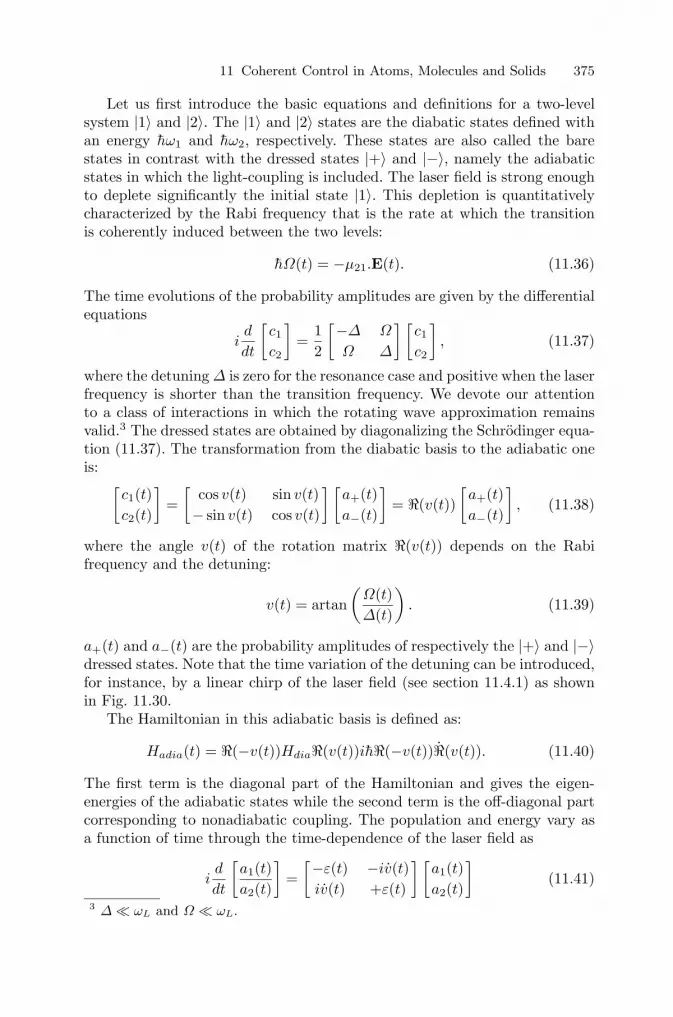
11 Coherent Control in Atoms, Molecules and Solids 375

Let us first introduce the basic equations and definitions for a two-levelsystem |1〉 and |2〉. The |1〉 and |2〉 states are the diabatic states defined withan energy hω1 and hω2, respectively. These states are also called the barestates in contrast with the dressed states |+〉 and |−〉, namely the adiabaticstates in which the light-coupling is included. The laser field is strong enoughto deplete significantly the initial state |1〉. This depletion is quantitativelycharacterized by the Rabi frequency that is the rate at which the transitionis coherently induced between the two levels:

hΩ(t) = −μ21.E(t). (11.36)

The time evolutions of the probability amplitudes are given by the differentialequations

id

dt

[c1

c2

]=

12

[−Δ

Ω

Ω

Δ

] [c1

c2

], (11.37)

where the detuning Δ is zero for the resonance case and positive when the laserfrequency is shorter than the transition frequency. We devote our attentionto a class of interactions in which the rotating wave approximation remainsvalid.3 The dressed states are obtained by diagonalizing the Schrodinger equa-tion (11.37). The transformation from the diabatic basis to the adiabatic oneis: [

c1(t)c2(t)

]=[

cos v(t)− sin v(t)

sin v(t)cos v(t)

] [a+(t)a−(t)

]= �(v(t))

[a+(t)a−(t)

], (11.38)

where the angle v(t) of the rotation matrix �(v(t)) depends on the Rabifrequency and the detuning:

v(t) = artan(

Ω(t)Δ(t)

). (11.39)

a+(t) and a−(t) are the probability amplitudes of respectively the |+〉 and |−〉dressed states. Note that the time variation of the detuning can be introduced,for instance, by a linear chirp of the laser field (see section 11.4.1) as shownin Fig. 11.30.

The Hamiltonian in this adiabatic basis is defined as:

Hadia(t) = �(−v(t))Hdia�(v(t))ih�(−v(t))�(v(t)). (11.40)

The first term is the diagonal part of the Hamiltonian and gives the eigen-energies of the adiabatic states while the second term is the off-diagonal partcorresponding to nonadiabatic coupling. The population and energy vary asa function of time through the time-dependence of the laser field as

id

dt

[a1(t)a2(t)

]=[−ε(t)

iv(t)−iv(t)+ε(t)

] [a1(t)a2(t)

](11.41)

3 Δ ωL and Ω ωL.

376 T. Amand, V. Blanchet, B. Girard and X. Marie

Fig. 11.29. AC-stark shift induced by a FWHM = 160 fs and 108 V/cm linearlypolarized electric field on the two-level system |1〉 adn |2〉. In the case of a positivedetuning (top), the energy difference of the adiabatic states |+〉 and |−〉 increaseswith the intensity, while it decreases for a negative detuning (bottom)

with the following expression for the eigenenergy ε(t):

ε(t) =h

2

√Ω2(t) + Δ2(t). (11.42)

For instance, a one-photon resonant laser pulse with EL = 108V/cm, linearlypolarized and parallel to a dipole moment μ21 of ∼ 1.10−30C.m. induces amaximum light-coupling strength of hΩ(t). The ac Stark shift of the twolevels will reach a maximum of Ω/2 = 500cm−1.

As shown in Fig. 11.29, the splitting of the adiabatic states increases ordecreases for a positive (Fig. 11.29-top) or negative (Fig. 11-29 bottom) de-tuning. In the dressed state picture (Fig. 11.30), the coupling results alwaysin a repulsion between the |1, (n+1)〉 and |2, n〉 states. Without any pulse (inFigs. 11.29 and 11.30 for |t| > 250 fs), the adiabatic states |+〉 and |−〉 cor-respond to the diabatic states |1, (n + 1)〉 and |2, n〉. As shown in Figs. 11.29and 11.30-top, for the off-resonance cases with no chirp of the laser pulse, theprobability transition from |1〉 to |2〉 is zero: each adiabatic state |+〉 or |−〉is correlated to the same diabatic state before and after the laser pulse inter-action. Once the instantaneous pulse frequency is scanned as shown in Fig.11.30 (middle and bottom), this probability transition becomes significant;

11 Coherent Control in Atoms, Molecules and Solids 377

Fig. 11.30. AC-stark shift indeced by (top) a Fourier limited pulse in a two-levelssystem characterized by a +200-cm−1 detuning; the same laser pulse characteristics(160 fs, 108 V/cm) and the same energy scheme as Fig. 11.29 top; (middle) a pulsepositively chirped from 160 fs to 400 fs in resonance and with the same energy/pulseand focalization length used in Fig. 11.29; (bottom) a pulse negatively chirped from160 fs to 400 fs off-resonance by +200 cm−1 and with the same energy/pulse andfocalization length used in Fig. 11.29.

each adiabatic state is correlated to different diabatic states before and afterthe laser pulse interaction. The dipole coupling lifts the degeneracy betweenthe diabatic states at their crossing. Therefore this crossing becomes more orless avoided as a function of the laser intensity, guiding the population fromthe initial state |1〉 to the excited state |2〉. The efficiency of this transition pro-cess [11.136] might reach 100% once the adiabaticity criterion is fulfilled in theSchrodinger equation (11.41). Concretely, this means the population evolutionfollows the building of the adiabatic eigenstates with negligible nonadiabaticcouplings (the off-diagonal terms of Eq. (11.41):

378 T. Amand, V. Blanchet, B. Girard and X. Marie

|v(t)| � ε(t). (11.43)

Taking into account Eqs. (11.39) and (11.42), the adiabaticity is encounteredonce:

|Ω(t)Δ(t) − Ω(t)Δ(t)(t)| � (Ω2(t) + Δ2(t))3/2. (11.44)

This latter inequality is achieved with a smooth pulse envelope and a slowfrequency sweep to minimize Ω(t) and Δ(t), respectively. A large field intensityand a large detuning can also lead to adiabatic evolution. In the case of apartial adiabaticity, the system ends up in a coherent superposition of diabaticstates. This interplay of the diabatic states has been observed as a functionof the detuning as well as the laser field duration [11.137] on a two-photonionization.

The main advantage of this adiabatic control is its generality and its ro-bustness with respect to intensity or frequency fluctuations, once the laserfield is high enough to achieve the adiabatic criterion (Eq. (11.44)). However,the main difficulty in this kind of control is to take into account all the energylevels involved, and more specifically the losses toward the dissociative andionization continua. Indeed, there is always the possibility that other neigh-boring levels in the dressed state picture complicate the control scheme. Arecent development is to implement a learning control strategy, controllingthe intense pulse shape in order to achieve the control task [11.106,130] (seesection 11.4.3.2).

After the first experiments realized at this intensity range, the idea ofusing the time-dependency of the laser intensity to shape the potentials hasbeen introduced. For instance, a Rydberg radial wave packet has been tailoredby depleting more or less differently the Rydberg levels composing this wavepacket [11.138]. However, the state density is too high to get insight of thepopulation redistribution as clearly as the freezing of a spin orbit wave packetin a three-level system [11.45].

In molecules, various ionization and dissociation multiphoton pathwayscoexist when exposed at this intensity range [11.139]. Their interplay, beingat the same time a key point in the realization of new control schemes, havestrongly impeded any conclusive identification of the phenomena. Experimen-tally, it is through the preparation of the initial state distribution [11.140]or via a differential detection [11.141–143] that unambiguous experimentalevidences of these intense field effects have been obtained.

We illustrate the principles of wave packet tailoring via light-induced defor-mation of potential through the well-known work of Garraway and Suominen[11.144–147] on the mere sodium dimer. The three diabatic electronic statesare represented in Fig. 11.31. In the dressed state picture, the optical reso-nances appear as curve crossings (Fig. 11.31(b)). The time evolution of themolecular system consists of a nontrivial balance between adiabatic followingof the vibrational eigenstates and nonadiabatic transfers between them at theavoided crossings. The evolution of the three electronic state wave functionsΨi=X,A,Π(R, t) is governed by the Schrodinger equation with the Hamiltonian

11 Coherent Control in Atoms, Molecules and Solids 379

Fig. 11.31. (a) The three different diabatic electronic states used in the calculationof Garraway and Suominen [11.144–48] as well as the energy of the two laser pulses;(b) the shifted potentials by applying the rotating wave approximation, Δ = Δ1 =−Δ2 = 2000 cm−1 is the detuning of the two pulses from the well bottoms of (a).

for the vibrational motion of the molecule written as

H = − h2

2m

∂2

∂R2 I + U(R, t), (11.45)

where I is the identity matrix, R the internuclear distance and m the reducedmass. The matrix U(R, t) includes the electronic potentials and light-coupling:

U(R, t) =

⎡⎣ Ux(R) hΩ1(t) 0

hΩ1(t) UA(R) + hΔ1 hΩ1(t)0 hΩ2(t) UΠ(R) + h(Δ2 + Δ1)

⎤⎦ , (11.46)

where Ui(R) are the three electronic potentials; Δ1 and Δ2 are the constantdetunings for A ← X and Π ← A bottom-bottom transitions, respectively.Eventually, Ω1(t) = hμA←XE1(t) and Ω2(t) = hμΠ←AE2(t) are the two Rabifrequencies, independent of R for simplicity and function of time through theGaussian pulse envelope such that

Ωj=1,2(t) = Ω exp(−[(t − tj)/T ]2), (11.47)

with tj the arrival time of the laser pulse j. To simplify, the light-couplingstrength Ω (= 3000 cm−1) and the pulse duration T (= 5.42 ps) are identicalfor both pulses and the detunings are such that Δ = Δ1 = −Δ2 (= −2200

380 T. Amand, V. Blanchet, B. Girard and X. Marie

Fig. 11.32. Space and time dependence of the light-induced potential responsiblefor the dynamics of the wave packet in Fig. 11.31. The active light-induced potentialis the one with its minima always closest to the zero point energy in the dressedstate picture [11.144].

cm−1), ensuring two-photon resonance. The light-induced potentials are ob-tained by diagonalizing the matrix U(R, t).

When the laser pulses are applied in a counterintuitive way (t1 > t2) asshown in Fig. 11.32, with a constant negative detuning Δ (Δ2 > 0), the firstlight-induced shifting is the repulsion of the A-Π. When the electric fieldE2(t) increases (maximum at t2 = 10.8 ps), the right-well of the double-wellstructure seen at t = 0 becomes progressively shallower and disappears. OnceE1(t) is turned on (t1 = 16.3 ps), the X and A states attract each other,broadening and displacing the bottom of the active light-induced potentialto the right side, corresponding also to the minimum of the Π state. At thisstage of the dynamics, there is a diabatic coupling from the X state onto theΠ one. Indeed there is no crossing of the diabatic vibrational levels of theX and Π states, as observed in Fig. 11.30, so the population can never betransferred adiabatically from the X state onto the Π one. As shown in Fig.11.33, the X and Π states exchange their population, while the population of

11 Coherent Control in Atoms, Molecules and Solids 381

Fig. 11.33. The wave packet dynamics on (a) the X ground state and (b) the Πtarget state. The ground state population disappears when the two pulses arriveat t2 = 10.8 ps and t1 = 16.3 ps (a), while it appears slowly in the Π state (b).T = 5.42 ps. The adiabatic transition is from the X (ν = 0) state onto the Π (ν = 0)state [11.137]

the A state remains very low at any time since there is never a crossing of theA state with the active light-induced potential.

The signature of the diabatic coupling is the smooth positional shifting ofthe wave packet observed in Fig. 11.33. The not-perfect adiabatic following isthe key point of this control and is achieved differently as a function of thelaser intensity, detuning and chirp rate [11.147]. The overall control appearsas a violation of the Franck-Condon principle, however the manipulation ofthe molecular states is achieved on a time scale longer than the vibrationalperiod, allowing the displacement over a large distance. Control schemes ma-nipulating excited vibrational levels [11.145], dissociative states [11.148] orefficient transfer to a dark molecular state [11.146] have also been proposed.

The goal of these previous examples was to control the population in theelectronic excited states or the internal degrees of freedom of the moleculesby playing on the laser-induced resonances and the electric dipole moment.Another main field of control is achieved on the external degrees of freedom.The rotation of molecules can be controlled and even stopped, thus creating

382 T. Amand, V. Blanchet, B. Girard and X. Marie

(static or dynamic) alignment or orientation. Beam acceleration, decelera-tion or deflection has also been achieved by acting on the center of massmotion [11.149]. A nonresonant intense laser pulse induces a dipole momentin a molecular ground state. The interaction Hamiltonian involves thus thepermanent dipole moment μ and the dynamic polarizability tensor α:

Hind(t) = −12

∑i,j=x,y,z

Ei(t)αijEj(t) cos2(ωLt) − μ.E(t) cos(ωLt) (11.48)

Here, (x, y, z) denotes the space-fixed Cartesian coordinates. For a linear orsymmetric top molecule with a quantization axis chosen along the body-fixedZ-axis, the polarizability tensor in the molecular frame is reduced to twocomponents: α‖ = αZ and α⊥ = αX = αY . Therefore, for a linearly polarizedlaser field along the Oz-axis, the laser-induced Hamiltonian of Eq. (11.48) isdependent only on the polar Euler angle θ between the laser polarization Ozand the molecular symmetry axis OZ with the following expression:

Hind(t) = −12E2(t) cos2(ωLt)

[α‖ cos2 θ + α⊥ sin2 θ

]− μE(t) cos(ωLt) cos θ.

(11.49)Taking into account that the laser period varies rapidly compared to the

envelope of the laser electric field E(t) and that the laser is nonresonant,the laser interaction with the permanent dipole moment is quenched. Thelaser-induced dipole moment can be averaged over a laser period to give thefollowing expressions:

μind(t) = 14E(t) cos(θ)αeff

Hind(t) = −μindE(t) cos(θ)(11.50)

with the effective polarization defined as αeff = α‖ − α⊥. This laser-inducedHamiltonian adds to the rotation Hamiltonian in the ground electronic state,written for a rigid molecule as

Hrot =∑

n

J2n

2In,

where n is the principle of axis inertia, I the inertia moment and J the angularmomentum operator. The orientation and alignment of the molecular axis aregiven by the average values of M/J and (M2−J(J+1))/(J(J+1), respectively(M is the projection of J on the laser polarization axis). For a statistical Mdistribution, no net alignment or orientation is observed. The intense laser fieldinduces Raman excitations in the ground electronic state (ΔJ = ±2) resultingin rotational excitation corresponding to a rotational wave packet. Since M isconserved with linear polarization, one obtains, on average, Jh|M |, leading toa strong alignment. Thus the molecule might align parallel or perpendicularto the polarization plane, depending on the sign of its effective polarizability.

11 Coherent Control in Atoms, Molecules and Solids 383

Fig. 11.34. Final angles reached by molecules with initial angles of 20◦ (squares),40◦ (circles), 60◦ (up triangles) and 80◦ (down triangles) as a function of laserintensity [11.151].

Classical models have been derived to describe the angular motion of themolecule in the laser field. From the Lagrangian for a rigid molecule:

L =12Iθ2 − Hind (11.51)

(moment of inertia I = mr2(t)/2) leads to the classical equation of motion:

θ =αeff

2IE2(t) sin(2θ) − 2

r

rθ. (11.52)

The first term of the angular acceleration causes the alignment, while thesecond term is a damping term that reduces the angular acceleration oncethe molecules dissociate. The mass of the molecule has two counteractingeffects in this dynamics; a light molecule is easy to accelerate. However, at thesame time, the internuclear distance is increasing quickly, leading to a largermoment of inertia, such that the damping term might become significant whilethe laser field is still on. As seen through Eq. (11.52), the angular accelerationdepends on the time-dependency of the electric field as well as its intensity[11.150]. Figure 11.34 [11.151] shows the final angles of diatomic moleculeswith initial angles of 20◦, 40◦, 60◦ and 80◦ as a function of laser intensity.The molecules irradiated with the lowest-intensity laser pulses undergo thelargest rotation. With the Gaussian laser pulses used in these calculations,molecules that experience higher intensities can end up less aligned. At fixedintensity, the width of the angular distribution decreases with increasing pulseduration, indicating that dynamic alignment occurs. For example, for a pulseenergy of 3 mJ, the FWHM of the angular distribution of the I2 moleculesdecreases from 64.4±2. to 25.2±0.8. when the duration is stretched from 500 fs

384 T. Amand, V. Blanchet, B. Girard and X. Marie

to 3ps (with an intensity reduced from 1.6×1014 W/cm2 to 2.65×1013 W/cm2

[11.152].This laser-induced alignment has been observed in many diatomic molecules

[11.153–156] as well as on polyatomic molecules in which the laser polariza-tion is chosen elliptic to force three molecular axes into the alignment [11.157].The molecular alignment reached is truly significant [11.152] such that furtherperpendicular transitions are enhanced and parallel transitions suppressed (orvice versa). This macroscopic control of the orientation of the molecules al-lows, for instance, control of the branching ratio of further photodissociationprocesses [11.158].

Rotating the laser polarization during the alignment causes the alignedmolecule to rotate. Two counterrotating circularly polarized fields, identical inintensity and spectrum, can be combined to produce this rotating polarization.This rotation of the polarization can be accelerated by chirping the two laserpulses with opposite signs, such that the rate of rotation increases from 0to 6THz in 50 ps [11.159]. Molecular rotation is thus strongly acceleratedup to values of several hundreds, where the molecular bond is broken bythe centrifugal force [11.160]. This control of the dissociation is done in lessthan one ground state rotational period and very efficiently, since each of thehundred successive Raman transitions has nearly 100% probability.

In solid-state physics, the carrier densities are typically of 1018 to 1019

electrons/cm3, involving large dipole moments between the band states. Thethreshold of strong field effects is lowered, typically around GW/cm2 com-pared to the molecular physics case. In semiconductors, the dephasing in-creases with larger carrier density due to the elevated scattering processes.The main effect of the strong field interaction is the Rabi flopping of the opti-cally induced excitation density. The first Rabi oscillations has been observedin the absorption continuum of a semiconductor off-resonance [11.161] or on-resonance [11.162]. Since then, many other works have been published on Rabioscillations in semiconductors [11.163,164], as well as in microwave-irradiatedJosephson-Junction circuit [11.165].

In semiconductor quantum wells, the dynamical Stark effect has recentlybeen observed in quantum wells embedded in semiconductor microcavities[11.166]; the exciton states are dressed by the enhanced electromagnetic fieldwithin the cavity. Two sidebands appear in pump-probe experiments, whosespectral distance increases as the square root of the light intensity, as ex-pected. These sidebands are reminiscent of the Mollow absorption spectrumoccurring in two-level system [11.167,168] and observed in atomic systems asStark effect excited by a CW laser [11.169]. More recently, the same effectcould be observed in bare quantum wells [11.170]. Here, a strong interactionpicture prevails against the perturbative description as soon as the excitondipole interaction with the laser field becomes stronger than the exciton col-lision broadening.

For high pulse intensities, nearly full-state occupation occurs in an energyregion substantially wider than the excitation bandwidth of the laser field of

11 Coherent Control in Atoms, Molecules and Solids 385

120 fs. Hence scattering into these states is increasingly hindered by the Pauliprinciple resulting in lower dephasing rates [11.171]. Consequently, the quan-tum kinetic buildup of screening will tend to reduce carrier–carrier dephasingand allow for coherent dynamics in the later stages of the dynamics. Rabioscillations have also been observed in semiconductor quantum dots [11.172].In these artificial atoms, excitonic excitation from the ground state might beseen as a two-level system where the complete inversion induced by π-pulseis the deterministic creation of one electron-hole. A single quantum dot in aphotodiode, once irradiated by a π-pulse, corresponds to a source of singleelectron delivered at the laser repetition rate [11.173].

Moreover, the interplay between Rabi oscillations and quantum interfer-ence in a temporal coherent control scheme has been observed [11.174,175].The exciton dressed state in quantum dots have been evidenced, together withthe state splitting under intense electromagnetic field [11.174], in analogy withthe occurrence of Mollow triplet in atomic stimulated emission under intenselight excitation [11.167,168].

11.6 Conclusion

The applications of coherent control or optimal control have reached wider andwider fields. As significant examples, we describe several cases of optimizationof the generation of high-order harmonics, applications to information storageand the search for control of molecular chirality (several theoretical schemesbased on frequency domain coherent control [11.176,177]).

The generation of coherent vacuum ultraviolet (VUV), extreme ultraviolet(XUV) or X-ray radiation is an emerging field that will open the route to awealth of new applications and has attracted strong interest. Two examplesare the possibility of carrying ultrafast X-ray diffraction of biological samples[11.178], or the generation of “attosecond” pulses [11.179–182]. The variousapproaches described in this chapter have been used to modify and controlthe efficiency of harmonic generation: chirped pulses [11.183], shaped pulses[11.129,182,184,185] (see Fig 11.35), or wave packet interferences in Ramsey-type spectroscopy [11.186].

Quantum information is also an exploding field in which coherent controlschemes have been demonstrated in simple cases. A set of atomic Rydbergstates have been used as quantum data register [11.187]. Wave packet inter-ferences produced by a transform limited pulse and a shaped pulse are used tostore and restore information [11.188]. Another possibility is to use half-cycleTerahertz pulses [11.189]. These schemes can be used to implement Grover’ssearch algorithm [11.190,191]. Molecular Rydberg states have been used toachieve a multiple input AND gate [11.192]. Other quantum logic gates havebeen implemented in molecular vibrational levels [11.193,194].

Finally, an intense research activity started in solid-state systems, whichaims to implement quantum logic gates based on the control of quantum states

386 T. Amand, V. Blanchet, B. Girard and X. Marie

Fig. 11.35. Closed-loop scheme applied to enhance harmonic generation [11.182]:(a) Experimental setup: The intensity of the various harmonics numbers is recordedon the x-ray CCD in the x-ray spectrometer. Each harmonic number can be inde-pendently optimized; (b) result of the optimization of the 27th harmonic. The x-rayspectrum is presented as a function of the iteration number. An improvement by afactor of 8 is achieved; (c) maximal enhancement factor for each harmonic number.

11 Coherent Control in Atoms, Molecules and Solids 387

by light pulses. (This effort is motivated by the integration and scalability po-tentialities provided by solid-state devices.) Two strategies are currently underinvestigation. The first consists of controlling charge states in quantum dots:exciton and exciton-molecule coherent dynamics within one single dot usingshaped pulses [11.195–197], or charge manipulations in electronically coupledquantum dots [11.198,199]. All these proposals rely on electronic correlationsin multicharged dots. The resulting coherent polarization dynamics allows usto build conditional operations. The second approach is based on coherent ma-nipulations of localized spin states in separate quantum dots with light pulses.The interest of this approach relies on the fact that spin states are more ro-bust against decoherence than charge states. In one proposed scheme [11.200],the long-range interaction between two spin eigenstates is obtained by Ramancoupling via strong laser fields, mediated by the vacuum field of a high finessemicrocavity. In another scheme, spin interaction is generated by an opticalpulse via virtual excitation of delocalized excitons of the semiconductor ma-trix [11.201]. This effect is analogous to the Rudemann-Kittel-Kasuya-Yoshidainteraction between two magnetic impurities, which is mediated by delocalizedconduction electrons or excitons in magnetic materials, except that the inter-mediate electron-hole pair is produced here by external light. The quantummanipulation can be achieved in the adiabatic limit and is robust against de-coherence by spontaneous emission. This leads to some effective light-inducedexchange interaction, allowing us to generate and control the entanglement ofspin states in two neighboring quantum dots.

References

[11.1] E.A. Manykin, A.M. Alfanasev: Sov. Phys. JETP 25, 828 (1967)[11.2] M. Shapiro, P. Brumer: Int. Rev. Phys. Chem. 13, 187 (1994)[11.3] R.J. Gordon, S.A. Rice: Ann. Rev. Phys. Chem. 48, 601 (1997)[11.4] P. Brumer, M. Shapiro: Structure and Dynamics of Electronic Excited

States, Springer, Berlin, (1999)[11.5] W. Potz, W.A. Schroeder: Coherent Control in Atoms, Molecules and

Semiconductors Kluwer Academic (1999)[11.6] S.A. Rice, M.S. Zhao: Optical Control of Molecular Dynamics, Wiley, New

York (2000)[11.7] T. Brixner, N.H. Damrauer, G. Gerber: Advances in Atomic, Molecular,

and Optical Physics, 46, (2001)[11.8] D.J. Tannor, S.A. Rice: J. Chem. Phys. 83, 5013 (1985)[11.9] R. Kosloff, S.A. Rice, P. Gaspard, S. Tersigni, D.J. Tannor: Chem. Phys.

139, 201 (1989)[11.10] E.D. Potter, J.L. Herek, S. Pedersen, Q. Liu, A.H. Zewail, Nature 355, 66

(1992)[11.11] J.L. Herek, A. Materny, A.H. Zewail: Chem. Phys. Lett. 228, 15 (1994)[11.12] U. Gaubatz, P. Rudecki, S. Schiemann, K. Bergmann: J. Chem. Phys. 92,

5363 (1990)

388 T. Amand, V. Blanchet, B. Girard and X. Marie

[11.13] N.V. Vitanov, T. Halfmann, B.W. Shore, K. Bergmann: Ann. Rev. Phys.Chem. 52, 763 (2001)

[11.14] N.V. Vitanov, M. Fleischhauer, B.W. Shore, K. Bergmann: Advances inAtomic, Molecular, and Optical Physics, 46 (2001)

[11.15] M. Shapiro, J.W. Hepburn, P. Brumer, Chem. Phys. Lett. 149, 451 (1988).[11.16] C. Chen, Y.-Y. Yin, D.S. Elliott: Phys. Rev. Lett. 64, 507 (1990)[11.17] S.M. Park, S.P. Lu, R.J. Gordon: J. Chem. Phys. 94, 8622 (1991)[11.18] S.P. Lu, S.M. Park, Y. Xie, R.J. Gordon: J. Chem. Phys. 96, 6613 (1992)[11.19] L. Zhu, V.D. Kleiman, X. Li, S.P. Lu, K. Trentelman, R.J. Gordon, Science

270, 77 (1995)[11.20] L. Zhu, K. Suto, J.A. Fiss, R. Wada, T. Seideman, R.J. Gordon: Phys.

Rev. Lett. 79, 4108 (1997)[11.21] J.A. Fiss, L. Zhu, R.J. Gordon, T. Seideman: Phys. Rev. Lett. 82, 65 (1999)[11.22] V.D. Kleiman, L. Zhu, J. Allen, R.J. Gordon: J. Chem. Phys. 103, 10800

(1995)[11.23] G. Xing, X. Wang, X. Huang, R. Bersohn, B. Katz: J. Chem. Phys. 104,

826 (1996)[11.24] X. Wang, R. Bersohn, K. Takahashi, M. Kawasaki, H.L. Kim: J. Chem.

Phys. 105, 2992 (1996)[11.25] H. Lefebvre Brion, T. Seideman, R.J. Gordon: J. Chem. Phys. 114, 9402

(2001)[11.26] H.G. Muller, P.H. Bucksbaum, D.W. Schumacher, A. Zavriyev: J. Phys.

B 23, 2761 (1990)[11.27] Y.-Y. Yin, C. Chen, D.S. Elliott, A.V. Smith: Phys. Rev. Lett. 69, 2353

(1992)[11.28] N.B. Baranova, A.N. Chudinov, B.Y. Zel’dovich: Opt. Commun. 79, 116

(1990)[11.29] E. Charron, A. Giusti-Suzor, F.H. Mies: Phys. Rev. Lett. 75, 2815 (1995)[11.30] B. Sheehy, B. Walker, L.F. DiMauro: Phys. Rev. Lett. 74, 4799 (1995)[11.31] E. Dupont, P.B. Corkum, H.C. Liu, M. Buchanan, Z.R. Wasilewski: Phys.

Rev. Lett. 74, 3596 (1995)[11.32] R. Atanasov, A. Hache, J.L.P. Hughes, H.M. van Driel, J.E. Sipe: Phys.

Rev. Lett. 76, 1703 (1996)[11.33] E. Charron, A. Giusti-Suzor, F.H. Mies: Phys. Rev. Lett. 71, 692 (1993)[11.34] T. Zuo, A.D. Bandrauk: Phys. Rev. A 54, 3254 (1996)[11.35] G. Kurizki, M. Shapiro, P. Brumer: Phys. Rev. B 39, 3435 (1989)[11.36] A. Hache, Y. Kostoulas, R. Atanasov, J.L.P. Hughes, J.E. Sipe, H.M. van

Driel: Phys. Rev. Lett. 78, 306 (1997)[11.37] F. Wang, C. Chen, D.S. Elliott: Phys. Rev. Lett. 77, 2416 (1996)[11.38] E. Luc Koenig, M. Aymar, M. Millet, J.M. Lecomte, A. Lyras: Eur. Phys.

J.D 10, 205 (2000)[11.39] M.A. Bouchene, V. Blanchet, C. Nicole, N. Melikechi, B. Girard, H. Ruppe,

S. Rutz, E. Schreiber, L. Woste: Eur. Phys. J.D 2, 131 (1998)[11.40] N.F. Scherer, A.J. Ruggiero, M. Du, G.R. Fleming: J. Chem. Phys. 93,

856 (1990)[11.41] N.F. Scherer, R.J. Carlson, A. Matro, M. Du, A.J. Ruggiero, V. Romero-

rochin, J.A. Cina, G.R. Fleming, S.A. Rice, J. Chem. Phys. 95, 1487 (1991)[11.42] V. Blanchet, M.A. Bouchene, B. Girard: J. Chem. Phys. 108, 4862 (1998)[11.43] V. Blanchet, C. Nicole, M.A. Bouchene, B. Girard: Phys. Rev. Lett. 78,

2716 (1997)

11 Coherent Control in Atoms, Molecules and Solids 389

[11.44] C. Nicole, M.A. Bouchene, S. Zamith, N. Melikechi, B. Girard, Phys. Rev.A 60, R1755 (1999)

[11.45] C. Nicole, M.A. Bouchene, B. Girard: J. Mod. Optics 49, 183 (2002)[11.46] J.F. Christian, B. Broers, J.H. Hoogenraad, W.J. Van der Zande, L.D.

Noordam: Opt. Commun. 103, 79 (1993)[11.47] O. Kinrot, I.S. Averbukh, Y. Prior: Phys. Rev. Lett. 75, 3822 (1995)[11.48] M.A. Bouchene, C. Nicole, B. Girard: Opt. Commun. 181, 327 (2000)[11.49] A.P. Heberle, J.J. Baumberg, K. Kohler: Phys. Rev. Lett. 75, 2598 (1995)[11.50] M. Woerner, J. Shah: Phys. Rev. Lett. 81, 4208 (1998)[11.51] S. Haacke, R.A. Taylor, R. Zimmermann, I. Bar-Joseph, B. Deveaud: Phys.

Rev. Lett. 78, 2228 (1997)[11.52] N. Garro, S.P. Kennedy, A.P. Heberle, R.T. Phillips: Phys. Stat. Sol. B

221, 385 (2000)[11.53] A.P. Heberle, J.J. Baumberg, E. Binder, T. Kuhn, K. Kohler, K.H. Ploog:

IEEE J. Quantum Elect. 2, 769 (1996)[11.54] X. Marie, P. Le Jeune, T. Amand, M. Brousseau, J. Barrau, M. Paillard,

R. Planel: Phys. Rev. Lett. 78, 3222 (1997)[11.55] X. Marie, P. Renucci, S. Dubourg, T. Amand, P. Le Jeune, J. Barrau, J.

Bloch, R. Planel: Phys. Rev. B 59, R2494 (1999)[11.56] P.C.M. Planken, I. Brener, M.C. Nuss, M.S.C. Luo, S.L. Chuang: Phys.

Rev. B 48, 4903 (1993)[11.57] M.U. Wehner, M.H. Ulm, D.S. Chemla, M. Wegener: Phys. Stat. Sol. B

206, 281 (1998)[11.58] M.U. Wehner, M.H. Ulm, D.S. Chemla, M. Wegener: Phys. Rev. Lett. 80,

1992 (1998)[11.59] C.-K. Sun, Y.-K. Huang, J.-C. Liang, A. Abare, S.P. DenBaars: Appl.

Phys. Lett. 78, 1201 (2001)[11.60] U. Ozgur, L. Chang Won, H.O. Everitt: Phys. Rev. Lett. 86, 5604 (2001)[11.61] S.P. Kennedy, N. Garro, R.T. Phillips; Phys. Rev. Lett. 86, 4148 (2001)[11.62] S. Ogawa, H. Nagano, H. Petek, A.P. Heberle: Phys. Rev. Lett. 78, 1339

(1997)[11.63] H. Petek, A.P. Heberle, W. Nessler, H. Nagano, S. Kubota, S. Matsunami,

N. Moriya, S. Ogawa: Phys. Rev. Lett. 79, 4649 (1997)[11.64] R.S. Judson, H. Rabitz: Phys. Rev. Lett. 68, 1500 (1992)[11.65] W.S. Warren, H. Rabitz, M. Dahleh: Science 259, 1581 (1993)[11.66] A.M. Weiner: Rev. Sci. Instr. 71, 1929 (2000)[11.67] T. Brixner, G. Gerber: Opt. Lett. 26, 557 (2001)[11.68] M.A. Dugan, J.X. Tull, W.S. Warren: J. Opt. Soc. Am. B 14, 2348 (1997)[11.69] E. Zeek, K. Maginnis, S. Backus, U. Russek, M. Murnane, G. Mourou, H.

Kapteyn, G. Vdovin: Opt. Lett. 24, 493 (1999)[11.70] F. Verluise, V. Laude, Z. Cheng, C. Spielmann, P. Tournois: Opt. Lett. 25,

575 (2000)[11.71] G. Stobrawa, M. Hacker, T. Feurer, D. Zeidler, M. Motzkus, F. Reichel,

Appl. Phys. B 72, 627 (2001)[11.72] R. Trebino, K.W. DeLong, D.N. Fittinghoff, J.N. Sweetser, M.A.

Krumbugel, B.A. Richman, D.J. Kane: Rev. Sci. Instr. 68, 3227 (1997)[11.73] C. Dorrer, B. de Beauvoir, C. Le Blanc, J.-P. Rousseau, S. Ranc, P.

Rousseau, J.-P. Chambaret, F. Salin: Appl. Phys. B 70, S77 (2000)[11.74] L. Lepetit, G. Cheriaux, M. Joffre: J. Opt. Soc. Am. B 12, 2467 (1995)

390 T. Amand, V. Blanchet, B. Girard and X. Marie

[11.75] M. Wefers, K. Nelson: IEEE J. Quantum Elect. 32, 161 (1996)[11.76] J.C. Vaughan, T. Feurer, K.A. Nelson: J. Opt. Soc. Amer. B 19, 2489

(2002)[11.77] R.M. Koehl, S. Adachi, K.A. Nelson: J. Chem. Phys. 110, 1317 (1999)[11.78] R.M. Koehl, K.A. Nelson: J. Chem. Phys. 114, 1443 (2001)[11.79] N.S. Stoyanov, D.W. Ward, T. Feurer, K.A. Nelson: J. Chem. Phys. 117,

2897 (2002)[11.80] B. Kohler, V.V. Yakovlev, J. Che, J.L. Krause, M. Messina, K.R. Wilson,

N. Schwentner, R.M. Whitnell, Y. Yan: Phys. Rev. Lett. 74, 3360 (1995)[11.81] C.J. Bardeen, Q. Wang, C.V. Shank: Phys. Rev. Lett. 75, 3410 (1995)[11.82] A. Assion, T. Baumert, J. Helbing, V. Seyfried, G. Gerber: Chem. Phys.

Lett. 259, 488 (1996)[11.83] J.S. Melinger, A. Hariharan, S.R. Gandhi, W.S. Warren: J. Chem. Phys.

95, 2210 (1991)[11.84] D.J. Maas, C.W. Rella, P. Antoine, E.S. Toma, L.D. Noordam: Phys. Rev.

A 59, 1374 (1999)[11.85] G. Cerullo, C.J. Bardeen, Q. Wang, C.V. Shank: Chem. Phys. Lett. 262,

362 (1996)[11.86] C.J. Bardeen, V.V. Yakovlev, J.A. Squier, K.R. Wilson: J. Am. Chem.

Soc. 120, 13023 (1998)[11.87] C.J. Bardeen, J.S. Cao, F.L.H. Brown, K.R. Wilson: Chem. Phys. Lett.

302, 405 (1999)[11.88] A.H. Buist, M. Muller, R.I. Ghauharali, G.J. Brakenhoff, J.A. Squier, C.J.

Bardeen, V.V. Yakovlev, K.R. Wilson: Opt. Lett. 24, 244 (1999)[11.89] B. Broers, H.B. van Linden van den Heuvell, L.D. Noordam: Phys. Rev.

Lett. 69, 2062 (1992)[11.90] P. Balling, D.J. Maas, L.D. Noordam: Phys. Rev. A 50, 4276 (1994)[11.91] B. Chatel, J. Degert, S. Stock, B. Girard: Phys. Rev. A, 68, 041402(R)

(2003)[11.92] S. Zamith, J. Degert, S. Stock, B. De Beauvoir, V. Blanchet, M.A. Bouch-

ene, B. Girard: Phys. Rev. Lett. 87, 033001 (2001)[11.93] D. Meshulach, Y. Silberberg: Nature 396, 239 (1998)[11.94] D. Meshulach, Y. Silberberg: Phys. Rev. A 60, 1287 (1999)[11.95] N. Dudovich, B. Dayan, S.H.G. Faeder, Y. Silberberg, Phys. Rev. Lett. 86,

47 (2001)[11.96] N. Dudovich, D. Oron, Y. Silberberg: Phys. Rev. Lett. 88, 123004 (2002)[11.97] J. Degert, W. Wohlleben, B. Chatel, M. Motzkus, B. Girard: Phys. Rev.

Lett. 89, 203003 (2002)[11.98] W. Wohlleben, J. Degert, A. Monmayrant, B. Chatel, M. Motzkus, B.

Girard: Appl. Phys. B accepted (2004)[11.99] D. Oron, N. Dudovich, D. Yelin, Y. Silberberg, Phys. Rev. Lett. 88, 063004

(2002)[11.100] N. Dudovich, D. Oron, Y. Silberberg: Nature 418, 512 (2002)[11.101] T. Baumert, T. Brixner, V. Seyfried, M. Strehle, G. Gerber: Appl. Phy. B

65, 779 (1997)[11.102] A. Assion, T. Baumert, M. Bergt, T. Brixner, B. Kiefer, V. Seyfried, M.

Strehle, G. Gerber: Science 282, 919 (1998)[11.103] S. Vajda, A. Bartelt, E.-C. Kaposta, T. Leisner, C. Lupulescu, S.

Minemoto, P. Rosendo-Francisco, L. Woste: Chem. Phys. 267, 231 (2001)

11 Coherent Control in Atoms, Molecules and Solids 391

[11.104] C. Daniel, J. Full, L. Gonzalez et al., Chem. Phys. 267, 247 (2001)[11.105] T. Brixner, B. Kiefer, G. Gerber: Chem. Phys. 267, 241 (2001)[11.106] R.J. Levis, G.M. Menkir, H. Rabitz: Science 292, 709 (2001)[11.107] C.J. Bardeen, V.V. Yakovlev, K.R. Wilson, S.D. Carpenter, P.M. Weber,

W.S. Warren, Chem. Phys. Lett. 280, 151 (1997)[11.108] T. Brixner, N.H. Damrauer, P. Niklaus, G. Gerber: Nature 414, 57 (2001)[11.109] R.A. Bartels, T.C. Weinacht, S.R. Leone, C. Kapteyn, M.M. Murnane:

Phys. Rev. Lett. 88, 033001 (2002)[11.110] J.L. Herek, W. Wohlleben, R.J. Cogdell, D. Zeidler, M. Motzkus: Nature

417, 533 (2002)[11.111] T. Hornung, R. Meier, M. Motzkus: Chem. Phys. Lett. 326, 445 (2000)[11.112] J.A. Nelder, R. Mead: Comp. J. 7, 308 (1965)[11.113] N.A. Gershenfeld: The Nature of Mathematical Modeling, Cambridge Uni-

versity Press (1999)[11.114] M. Hacker, G. Strobrawa, T. Feurer: Opt. Exp. 9, 191 (2001)[11.115] S. Kirkpatrick, C.D. Gelatt, M.P. Vecchi: Science 220, 671 (1983)[11.116] J.H. Holland: Adaptation in Natural and Artificial Systems, Ann Arbor

(1975)[11.117] D.B. Fogel, A.J. Owens, M.J. Walsh: Artificial Intelligence through Simu-

lated Evolution, New York (1966)[11.118] T. Back and H.-P. Schwefel: Evol. Comp. 1, 1 (1993)[11.119] B.J. Pearson, J.L. White, T.C. Weinacht, P.H. Bucksbaum: Phys. Rev. A

63, 063412 (2001)[11.120] D. Zeidler, S. Frey, K.-L. Kompa, M. Motzkus: Phys. Rev. A 64, 023420

(2001)[11.121] D.A. Stariolo, C. Tsallis, Annu. Rev. Comp. Physic. (1995).[11.122] B. Amstrup, J.D. Doll, R.A. Sauerbrey, G. Szabo, A. Lorincz: Phys. Rev.

A 48, 3830 (1993)[11.123] A. Glass, T. Rozgonyi, T. Feurer, R. Sauerbrey, G. Szabo: Appl. Phys. B

71, 262 (2000)[11.124] D. Meshulach, D. Yelin, Y. Silberberg: Opt. Commun. 138, 345 (1997)[11.125] L. Chambers: Practical Handbook of Genetic Algorithm: New Frontiers,

CRC Press, New York (1995)[11.126] U. Siegner, M. Haiml, J. Kunde, U. Keller: Opt. Lett. 27, 315 (2002)[11.127] T. Hornung, R. Meier, D. Zeidler, K.-L. Kompa, D. Proch, M. Motzkus:

Appl. Phys. B 71, 277 (2000)[11.128] D. Zeidler, T. Hornung, D. Proch, M. Motzkus: Appl. Phys. B 70, S125

(2001)[11.129] R. Bartels, S. Backus, E. Zeek, L. Misoguti, G. Vdovin, I.P. Christov, M.M.

Murnane, C. Kapteyn: Nature 406, 164 (2000)[11.130] T.C. Weinacht, J.L. White, P.H. Bucksbaum: J. Phys. Chem. A 103, 10166

(1999)[11.131] D. Zeidler, S. Frey, W. Wohlleben, M. Motzkus, F. Busch, T. Chen, W.

Kiefer, A. Materny: J. Chem. Phys. 116, 5231 (2002)[11.132] H. Rabitz, R. de Vivie-Riedle, M. Motzkus, K. Kompa: Science 288, 824

(2000)[11.133] D. Goswami, M.R. Fetterman, W.S. Warren, W. Yang: J. Opt. Comm. 21,

694 (2001)[11.134] Z.M. Lu, H. Rabitz: J. Phys. Chem. 99, 13731 (1995)

392 T. Amand, V. Blanchet, B. Girard and X. Marie

[11.135] C. Daniel, J. Full, L. Gonzalez, C. Lupulescu, J. Manz, A. Merli, S. Vajda,L. Woste: Science 299, 536 (2003)

[11.136] N.V. Vitanov: Phys. Rev. A 59, 988 (1999)[11.137] J.G. Story, D.I. Duncan, T.F. Gallagher: Phys. Rev. Lett. 70, 3012 (1993)[11.138] R.R. Jones, C.S. Raman, D.W. Schumacher, P.H. Bucksbaum: Phys. Rev.

Lett. 71, 2575 (1993)[11.139] P. Dietrich, P. Corkum: J. Chem. Phys. 97, 3187 (1992)[11.140] C. Wunderlich, H. Figger, T.W. Hansch: Chem. Phys. Lett. 256, 43 (1996)[11.141] P.H. Bucksbaum, A. Zavriyev, H.G. Muller, D.W. Schumacher: Phys. Rev.

Lett. 64, 1883 (1990)[11.142] V. Schyja, T. Lang, H. Helm: Phys. Rev. A 57 (1998)[11.143] R.B. Vrijen, J.H. Hoogenraad, H.G. Muller, L.D. Noordam: Phys. Rev.

Lett. 70, 3016 (1993)[11.144] B.M. Garraway, K.-A. Suominen: Phys. Rev. Lett. 80, 932 (1998)[11.145] M. Rodriguez, K.-A. Suominen, B.M. Garraway: Phys. Rev. A 62, 053413

(2000)[11.146] V.S. Malinovsky, J.L. Krause: Chem. Phys. 267, 47 (2001)[11.147] V.S. Malinovsky, J.L. Krause: Phys. Rev. A 63, 043415 (2001)[11.148] K. Suominen, B.M. Garraway, S. Stenholm: Phys. Rev. A 45, 3060 (1992)[11.149] H. Stapelfeldt, H. Sakai, E. Constant, P.B. Corkum: Phys. Rev. Lett. 79,

2787 (1997)[11.150] S. Banerjee, D. Mathur, G. Ravindra Kumar: Phys. Rev. A 63, 045401

(2001)[11.151] E. Springate, F. Rosca-Pruna, H.L. Offerhaus, M. Krishnamurthy, M. J.J.

Vrakking: J. Phys. B 34, 4939 (2001)[11.152] F. Rosca-Pruna, M.J.J. Vrakking: Phys. Rev. Lett. 87, 153902 (2001)[11.153] D. Normand, L.A. Lompre, C. Cornaggia: J. Phys. B 25, L497 (1992)[11.154] B. Friedrich, D. Herschbach: Phys. Rev. Lett. 74, 4623 (1995)[11.155] J.H. Posthumus, J. Plumridge, M.K. Thomas, K. Codling, L.J. Frasinski,

A.J. Langley, P.F. Taday: J. Phys. B 31, L553 (1998)[11.156] C. Ellert, P.B. Corkum: Phys. Rev. A 59, R3170 (1999)[11.157] J.J. Larsen, K. Hald, N. Bjerre, H. Stapelfeldt: Phys. Rev. Lett. 85, 2470

(2000)[11.158] J.J. Larsen, I. Wendt-Larsen, H. Stapelfeldt: Phys. Rev. Lett. 83, 1123

(1999)[11.159] D.M. Villeneuve, S.A. Aseyev, P. Dietrich, M. Spanner, M.Y. Ivanov, P.B.

Corkum: Phys. Rev. Lett. 85, 542 (2000)[11.160] J. Karczmarek, J. Wright, P. Corkum, M. Ivanov: Phys. Rev. Lett. 82,

3420 (1999)[11.161] S.T. Cundiff, A. Knorr, J. Feldmann, S.W. Koch, E.O. Gobel, H. Nickel:

Phys. Rev. Lett. 73, 1178 (1994)[11.162] C. Furst, A. Leitenstorfer, A. Nutsch, G. Trankle, A. Zrenner: Physica

status solidi (b) 204, 20 (1997)[11.163] O.D. Mucke, T. Tritschler, M. Wegener, U. Morgner, F.X. Kartner, Phys.

Rev. Lett. 87, 057401 (2001)[11.164] A. Schulzgen, R. Binder, M.E. Donovan, M. Lindberg, K. Wundke, H.M.

Gibbs, G. Khitrova, N. Peyghambarian: Phys. Rev. Lett. 82, 2346 (1999)[11.165] Y. Nakamura, Y.A. Pashkin, J.S. Tsai: Phys. Rev. Lett. 87, 246601 (2001)[11.166] F. Quochi, G. Bongiovanni, A. Mura, J.L. Staehli, B. Deveaud, R.P. Stan-

ley, U. Oesterle, R. Houdre: Phys. Rev. Lett. 80, 4733 (1998)

11 Coherent Control in Atoms, Molecules and Solids 393

[11.167] B.R. Mollow: Phys. Rev. 188, 1969 (1969)[11.168] B.R. Mollow: Phys. Rev. A 5, 2217 (1972)[11.169] F.Y. Wu, S. Ezekiel, M. Ducloy, B.R. Mollow: Phys. Rev. Lett. 38, 1077

(1977)[11.170] M. Saba, F. Quochi, C. Ciuti, D. Martin, J.L. Staehli, B. Deveaud, A.

Mura, G. Bongiovanni: Phys. Rev. B 62, R16322 (2000)[11.171] L. Banyai, Q.T. Vu, B. Mieck, H. Haug: Phys. Rev. Lett. 81, 882 (1998)[11.172] T.H. Stievater, X. Li, D.G. Steel, D. Gammon, D.S. Katzer, D. Park, C.

Piermarocchi, L.J. Sham: Phys. Rev. Lett. 87, 133603 (2001)[11.173] A. Zrenner, E. Beham, S. Stufler, F. Findeis, M. Bichler, G. Abstreiter:

Nature 418, 612 (2002)[11.174] H. Kamada, H. Gotoh, J. Temmyo, T. Takagahara, H. Ando: Phys. Rev.

Lett. 87, 246401 (2001)[11.175] H. Htoon, T. Takagahara, D. Kulik, O. Baklenov, A.L. Holmes, Jr., C.K.

Shih: Phys. Rev. Lett. 88, 1 (2002)[11.176] M. Shapiro, E. Frishman, P. Brumer: Phys. Rev. Lett. 84, 1669 (2000)[11.177] P. Kral, M. Shapiro: Phys. Rev. Lett. 87, 1 (2001)[11.178] C. Zenghu, A. Rundquist, W. Haiwen, M.M. Murnane, H.C. Kapteyn:

Phys. Rev. Lett. 79, 2967 (1997)[11.179] M. Hentschel, R. Kienberger, C. Spielmann, G. Reider, A.N. Milosevic, T.

Brabec, P. Corkum, U. Heinzmann, M. Drescher, F. Krausz: Nature 414,509 (2001)

[11.180] I.P. Christov, R. Bartels, H.C. Kapteyn, M.M. Murnane: Phys. Rev. Lett.86, 5458 (2001)

[11.181] I.P. Christov: J. Opt. Soc. Am. B 18, 1877 (2001)[11.182] R. Bartels, S. Backus, I. Christov, H. Kapteyn, M. Murnane: Chem. Phys.

267, 277 (2001)[11.183] D.G. Lee, J.-H. Kim, K.-H. Hong, C.H. Nam: Phys. Rev. Lett. 87, 243902

(2001)[11.184] C. Xi, I.C. Shih: Phys. Rev. A 64, 021403 (2001)[11.185] P. Balcou, R. Haroutunian, S. Sebban et al., Appl. Phys. B 6, 509 (2002)[11.186] S. Cavalieri, R. Eramo, M. Materazzi, C. Corsi, M. Bellini: Phys. Rev. Lett.

89, 133002 (2002)[11.187] T.C. Weinacht, J. Ahn, P.H. Bucksbaum, Phys. Rev. Lett. 80, 5508 (1998)[11.188] J. Ahn, T.C. Weinacht, P.H. Bucksbaum: Science 287, 463 (2000)[11.189] J. Ahn, D.N. Hutchinson, C. Rangan, P.H. Bucksbaum: Phys. Rev. Lett.

86, 1179 (2001)[11.190] L.K. Grover: Phys. Rev. Lett. 79, 325 (1997)[11.191] L.K. Grover: Phys. Rev. Lett. 79, 4709 (1997)[11.192] Z. Amitay, R. Kosloff, S.R. Leone: Chem. Phys. Lett. 359, 8 (2002)[11.193] V.V. Lozovoy, M. Dantus: Chem. Phys. Lett. 351, 213 (2002)[11.194] C.M. Tesch, R.de Vivie-Riedle: Phys. Rev. Lett. 89, 157901 (2002)[11.195] F. Troiani, U. Hohenester, E. Molinari: Phys. Rev. B 62, R2263 (2000)[11.196] P.-C., C. Piermarocchi, L.J. Sham: Phys. Rev. Lett. 87, 067401 (2001)[11.197] G. Chen, T.H. Stievater, E.T. Batteh, Xiaoqin-Li, D.G. Steel, D. Gammon,

D.S. Katzer, D. Park, L.J. Sham: Phys. Rev. Lett. 88, 117901 (2002)[11.198] E. Biolatti, R.C. Iotti, P. Zanardi, F. Rossi: Phys. Rev. Lett. 85, 5647

(2000)[11.199] M. Bayer, P. Hawrylak, K. Hinzer, S. Fafard, M. Korkusinski, Z.R.

Wasilewski, O. Stern, A. Forchel: Science 291, 451 (2001)

394 T. Amand, V. Blanchet, B. Girard and X. Marie

[11.200] A. Imamoglu, D.D. Awschalom, G. Burkard, D.P. DiVincenzo, D. Loss,M. Sherwin, A. Small: Phys. Rev. Lett. 83, 4204 (1999)

[11.201] C. Piermarocchi, C. Pochung, L.J. Sham, D.G. Steel: Phys. Rev. Lett. 89,167402 (2002)

12

Attosecond Pulses

E. Constant and E. Mevel

With 17 figures

12.1 Introduction

It is now possible to generate optical pulses with a duration corresponding toonly a few optical cycles of the electromagnetic radiation in a wide spectralrange. The generation of such short pulses is usually performed in two ways.

Low-energy pulses can be obtained directly from femtosecond oscillatorand the minimum pulse duration supported by broadband gain media, suchas the titanium-doped sapphire (Ti:Sa), is currently around 10 fs. Carefulintracavity gain shaping allows ultimate pulse duration below 5 fs in Ti:Saoscillators [12.1,2]. However amplification of these pulses results in a spectralnarrowing, and the shortest pulses obtained until now above the mJ level are17.5 fs long [12.3].

Those amplified pulses can then be further shortened by postcompressiontechniques and the shortest high-energy visible pulses obtained by these tech-niques have a duration of ∼ 5 fs [12.4,5], which corresponds to only 2 opticalcycles of the central wavelength and could not be significantly shortened inthis wavelength range.

The possibility to generate and use such short pulses allowed many fas-cinating applications in the time domain through pump-probe techniques.However, many events occur on a subfemtosecond time scale, and their studyrequires shorter pulses. This includes, for instance, most of the electronic mo-tion, the evolution of molecules in highly excited states or even the evolutionof molecular hydrogen, which is one of the best-known systems in theory butstill cannot be experimentally studied in the time domain. Obtaining pulsesshorter than 1 fs and entering the attosecond domain (1 as = 10−18 s) willtherefore open new applications in physics.

As for femtosecond pulses generated in mode-locked oscillators, attosecondpulses require phase-locked frequencies over an even larger bandwidth. Thereare two known processes that provide a coherent spectra over a bandwidthbroad enough to support attosecond emission. A first one is based on stimu-lated Raman scattering [12.6–8]. A subsequent spectral broadening of a UV

396 E. Constant and E. Mevel

pulse is obtained through phase modulation by impulsively exciting coherentvibration of molecules [12.9,10]. This method promises subfemtosecond sub-cycle pulse generation. So far, experimental tests have demonstrated emissionof a periodic train of 6 fs pulses [12.11] and generation of a single 4 fs pulse[12.12], both at 400 nm. Here, we will focus on the second process, which allowsattosecond emission in the XUV spectral range. This process relies on high-order harmonic generation (HHG), which was discovered in 1987 [12.13,14].The light emitted through high-order harmonic generation consists of a combof many VUV lines (equally spaced and of approximately equal amplitudes) ina spectral range that can be broader than 100 eV. Shortly after the discoveryof this process, it was understood that the emitted spectrum was large enoughto support trains of attosecond pulses [12.15–17] The theoretical understand-ing of high-order harmonic generation [12.18–21] even quickly revealed thatthese harmonics can be phase-locked [12.22] and that an isolated attosecondpulse can be created through high-order harmonic generation [12.23,24].

To illustrate how this can be done, we first present the process of high-order harmonic generation and its main characteristics. Although this processis now very well simulated with quantum models, we will present a simplesemiclassical model [12.18,19] for understanding how the response of an atomexcited by a strong laser field can lead to high-order harmonic generation.Historically, this model allowed the understanding of this process. Althoughthis model may appear oversimplified, it contains the essence of high-orderharmonic generation.

Being a coherent process, high-order harmonic generation not only relies onthe single-atom response but also on collective effects such as phase matching(for instance, see [12.25] and references therein), which will only be brieflymentioned in this chapter.

After this presentation, we describe how high-order harmonic generationcan be considered as a source of train of attosecond pulses and how a singleattosecond pulse can be extracted from this train. Then we present sometechniques for measuring harmonic pulses or attosecond pulses, and finally wepresent possible applications of attosecond pulses.

12.2 High-Order Harmonic Generation: A Coherent,Short-Pulse XUV Source

High-order harmonic generation occurs when an ultrashort intense laser fieldis focused onto an atomic gas target. The typical experimental setup, depictedin Fig. 12.1 consists of a short-pulse laser focused by a lens (or mirror) onto agas medium located in a vacuum chamber where the emitted VUV light canpropagate.

High-order harmonics are produced by focusing short laser pulses in agas medium at intensities where substantial ionization of the gas can occur.

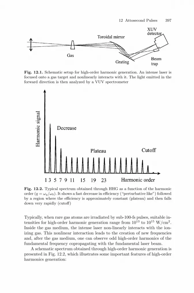
12 Attosecond Pulses 397

Fig. 12.1. Schematic setup for high-order harmonic generation. An intense laser isfocused onto a gas target and nonlinearly interacts with it. The light emitted in theforward direction is then analyzed by a VUV spectrometer

Fig. 12.2. Typical spectrum obtained through HHG as a function of the harmonicorder (q = ωq/ω0). It shows a fast decrease in efficiency (“perturbative like”) followedby a region where the efficiency is approximately constant (plateau) and then fallsdown very rapidly (cutoff)

Typically, when rare gas atoms are irradiated by sub-100-fs pulses, suitable in-tensities for high-order harmonic generation range from 1013 to 1015 W/cm2.Inside the gas medium, the intense laser non-linearly interacts with the ion-izing gas. This nonlinear interaction leads to the creation of new frequenciesand, after the gas medium, one can observe odd high-order harmonics of thefundamental frequency copropagating with the fundamental laser beam.

A schematic spectrum obtained through high-order harmonic generation ispresented in Fig. 12.2, which illustrates some important features of high-orderharmonics generation:

398 E. Constant and E. Mevel

• The spectrum consists of lines separated by twice the frequency of thefundamental laser field (ω0) and only odd harmonics are present (ωq =qω0 = (2n + 1)ω0).

• After a fast decrease in efficiency for the low-order harmonics (the effi-ciency being defined as the ratio of the energy contained in a given har-monic peak to the initial energy of the fundamental pulse), the high-orderharmonics all have roughly the same amplitude (presence of a plateau) andthen abruptly disappear for frequencies higher than the cutoff frequency,ωc. Although the initial decrease is typical of perturbative interactions, thepresence of such a plateau is the signature of a nonperturbative interactionregime.

The efficiency of high-order harmonic generation and its spectral extensiondepends a lot on the gas (mainly through its ionization potential Ip) and onthe fundamental laser characteristics (mainly through its frequency ω0, peakintensity Imax, pulse duration τ , and polarization state). Generally, one canobserve that:

• The higher Ip, the higher the cutoff frequency.• The smaller ω0, the higher the cutoff frequency.• The shorter τ , the higher the cutoff frequency.• For a given VUV wavelength of the plateau and a given atomic species,

the smaller ω0, the lower the efficiency.• For high harmonics, the efficiency is maximal when the fundamental field

is linearly polarized and quickly decreases when the ellipticity is increasing.• When the intensity of the fundamental pulse is increased, the high-order

harmonic generation efficiency first increases quickly and then saturatesor remains roughly constant when the peak intensity exceeds the so-calledsaturation intensity (at which all atoms are ionized).

As will be seen in the next paragraph, all these characteristics arise fromthe single-atom response to the strong field excitation.

HHG is also a coherent process and many of the VUV beam propertiesdepend on collective effects. For instance the efficiency depends nonlinearly onthe gas pressure [12.26], which implies that the radiation emitted by differentatoms can interfere constructively. The emitted harmonic beam is a coherentbeam that can be very well collimated with a divergence similar to the one ofthe fundamental beam [12.27–29].

12.3 Semiclassical Picture of HHG

High-order harmonic generation is now very well understood theoretically andquantum calculation (resolution of the time-dependent Schrodinger equation,

12 Attosecond Pulses 399

TDSE) [12.30,31] or even approximate quantum calculations (Strong field ap-proximation, SFA) [12.20,21] associated with propagation codes can simulatevery nicely most of the experimental results.

In this chapter we will present a much simpler theory, so called semiclassi-cal theory (or the simple man model), which also reproduces reasonably wellthe experimental findings and provides a clear understanding of the high-order harmonic generation process. Strictly speaking, this semiclassical modelis valid only in the so-called tunnel regime defined by

hω0 � Ip � Up, (12.1)

where Ip is the ionization potential of the atom and Up is the so-called pon-deromotive energy that corresponds to the average kinetic energy of a freeelectron oscillating in the laser field (of frequency ω0 and intensity I). It alsorepresents the typical energy that the intense laser can provide to an elec-tron and scales as I/ω2

0 . For a short pulse centered at a wavelength of 800nm (Ti:Sa), Up (in eV) is equal to 6I (with I in units of 1014 W/cm2). Thedescription of this semiclassical model for high-order harmonic generation re-quires some prerequisite knowledge about atomic ionization and about intenselaser-electron interaction.

12.3.1 Atomic Ionization in the Tunnel Domain

In this tunnel domain, the condition hω0 � Ip implies that the absorption ofmany photons is necessary to ionize an atom. An accurate description of theionization mechanisms requires therefore many simulations, and nonpertur-bative methods are necessary. However, in this domain the photonic characterof the laser field can be partly neglected and quasistatic approximate modelshave been successfully developed to simulate strong field-atom ionization viatunnel ionization.

According to these models, an atom is described as an ionic core and anelectron. The ionic core creates a Coulomb potential in which the electronevolves. The intense laser field is simply considered as a slowly oscillatingelectric field E(t) = E0(t) cos(ω0t). When an atom is irradiated by the stronglaser field, the total potential is the sum of the ionic core potential and theelectric interaction potential qE.r . It results in a potential barrier in the di-rection of the laser electric field. Therefore, when this field is very strong theelectron has some probability to escape the ionic core by tunneling throughthe potential barrier. This is illustrated in Fig. 12.3, where one can see the po-tential created by the ionic core only (left) and the total potential in presenceof the field (right).

The probability for an electron to tunnel through a potential barrier is wellknown and depends on the initial energy level (Ip for an atom initially in itsground state) and on the width of the barrier (defined by the field strength,E = (2I/ε0c)1/2). A general formula to describe tunnel ionization of the atom

400 E. Constant and E. Mevel

Fig. 12.3. Schematic of the potential created by the ionic core only (left) and bythe strong field + ionic core (right). When the field is strong enough, the electroncan escape the core attraction and reach the continuum by tunneling through thepotential barrier

was derived by Ammossov, Delone and Krainov [12.32]. This instantaneousionization rate Wdc (in s−1) is given by

Wdc = ωs|Cn∗l∗ |2Glm(4ωs/ωt)2n∗−m−1 exp(−4ωs/3ωt), (12.2)

where ωs = Ih/h, (with Ih being the ionization potential of hydrogen),ωt = qE/(2meIp)1/2, (with Ip the ionization potential of the atom, me andq being, respectively, the mass and charge of the electron, Z, the charge ofthe final ion, and E the laser electric field), n∗ = Z(Ih/Ip)1/2, Glm = (2l +1)(l + |m|)!(2−|m|)/|m|!(l − |m|)! (l and m being the azimuthal and magneticquantum numbers, respectively), |Cn∗l∗ |2 = 22n∗

[n∗Γ (n∗+l∗+1)Γ (n∗−l∗)]−1

with l∗ = 0 for l � n or l∗ = n∗ − 1 otherwise.For a slowly varying pulse envelope, this rate can be averaged over one

optical period of the laser field and leads to

Wac(in s−1) = (3ωt/2πωs)1/2Wdc. (12.3)

This rate agrees well with experimentally observed ionization in the tunneldomain [12.33], and this simple formula is therefore widely used. Moreover, therelative crudity of the model (classical field, one discrete state, a continuum)is validated by the structureless photoelectron spectra detected in this regime[12.34].

12.3.2 Electronic Motion in an Electric Field

When an atom is ionized, an electron is released in a strong electric field, andthe corresponding electric force will impose its motion. Even by neglecting thecore attraction and considering a free electron, the electron motion is stronglyinfluenced by the time of ionization, ti. Its classical motion is defined by:

m∂2r∂t2

= qE cos(ω0t). (12.4)

12 Attosecond Pulses 401

Fig. 12.4. Kinetic energy of the electrons, released with no kinetic energy at theirfirst return at their initial position (x = 0) as a function of the phase at ionization

For a linearly polarized field (along x), we have

m∂2x

∂t2= qE cos(ω0t). (12.5)

from which we can find the electron velocity:

V (t) = [qE/(mω0)](sinω0t − sinω0ti) + V0 (12.6)

(V0 being the initial velocity) in the slowly varying envelope approximation(E(t) ≈ cte during one optical cycle). For a zero initial kinetic energy, itsaverage kinetic energy (ponderomotive energy) is then:

Up = q2E2/(4mω20). (12.7)

Again, this ponderomotive energy is a very important parameter in the tunnelregime in which we can consider that an electron mainly interacts with theelectric field of the laser. It can provide to the electron an energy that is onthe order of Up.

For the specific case where the electron is released in the continuum with-out any kinetic energy (V0 = 0), the kinetic energy of the electron when itcomes back at its initial position (x = 0) is simply defined by the ionizationtime, ti, as shown in Fig. 12.4. One can see, in this figure, that the maximumkinetic energy of the electrons coming back at their initial position, x = 0, is3.17Up and is achieved for an ionization phase ω0ti = 18◦.

High-order harmonic generation usually occurs at the limit of this tunnelregime (hω0 ≤ Ip ≈ Up), but it was quickly discovered that Up is a keyparameter for this process. Indeed, the cutoff frequency, ωc, is linked to Up

by:hωc = Ip + 3.17Up (12.8)

402 E. Constant and E. Mevel

Fig. 12.5. Schematic of the three steps of HHG: (1) Ionization, (2) acceleration bythe laser electric field, (3) radiative recombination

12.3.3 Semiclassical View of HHG

In the “simple man model,” high-order harmonic generation consists of athree-step phenomena; the steps are illustrated in Fig. 12.5.

1. An atom irradiated by a strong laser field can be ionized at a time ti,creating an ion (the parent ion) and a free electron with no initial kineticenergy.

2. The electron is accelerated by the laser electric field. When the electricfield changes its sign, it may (or not) drive back the electron in the vicinityof the parent ion.

3. If the electron collides with the parent ion, the ion and electron can thenrecombine and the total extra energy (i.e., kinetic energy, Ec, of the elec-tron plus the binding energy of the atom (i.e., Ip)) is released by emittinga photon of energy hω = Ec + Ip.

This model allows us to understand the cutoff law hωc = Ip + 3.17Up.Indeed, an electron released (with zero initial velocity) at a given time, accel-erated and driven back to its initial position, has a maximum kinetic energyof 3.17Up (Fig. 12.4) when the collision occurs. Therefore the emitted pho-ton energy cannot exceed Ip +3.17Up. This cutoff law was discovered throughnumerical simulations [12.35], interpreted with the semiclassical model as pre-sented earlier [12.18,36] and confirmed experimentally [12.37].

It should then be understood that this process is probabilistic and onecannot say whether the atom is ionized or not but rather that at some time theatom has a probability to get ionized. These three processes can therefore leadto the emission of a VUV photon (or more precisely, to the emission of VUVradiation) every time that the atom has a strong probability to be ionized(first step). This occurs when the electric field is maximum and thereforewith a periodicity of half an optical cycle of the fundamental. A single atomtherefore has some probability to emit XUV photons periodically.

12 Attosecond Pulses 403

Furthermore, one should not consider the electron as a classical particlebut rather as a quantum wave packet that oscillates with its own phase. Interms of waves, the three steps correspond to a transition from the initial wavefunction (ground state of the atom) to the continuum, then an evolution ofthe wave packet in the continuum and finally a transition from the continuumback to the initial wave function associated with the emission of a radiation[12.20]. The phase of this radiation is therefore imposed by the evolution ofthe wave packet phase in the continuum (which is imposed by the fundamentalfield) and linked to the phase of the fundamental. As will be stressed later,one finds that this phase accumulated by the wave packet evolution in thecontinuum is proportional to the laser intensity ϕq = αqI [12.39,40]. Theimportant point is that the phases of the XUV radiation are linked to thefundamental laser phase. These harmonics are therefore phase locked withthe fundamental laser [12.41].

The fact that the XUV phase is linked to the laser phase makes the pro-cess coherent. This implies that not only the XUV energy bursts are emittedperiodically but also that the associated XUV field is emitted periodically inphase.

With this model, one can see high-order harmonic generation as a periodicemission of coherent radiation (note that this picture is valid, provided thefield strength is constant and the atomic ground state is not significantlydepleted by ionization). The symmetry of the ion potential ensures that theperiodicity of the XUV emission is T0/2 and that the phase of the emittedXUV light is locked to the phase of the fundamental in the same way at eachhalf optical period. However, the sign of the fundamental field changes at eachhalf optical period, and therefore does the XUV field. The real periodicity ofthe emission is therefore T0 with an antiperiodicity of T0/2 (periodicity of T0/2in intensity). The total XUV emitted field, at a frequency ωq, is therefore:

Eωq =∫

Aωq exp−i(ωqt + ϕq). (12.9)

Or by considering the periodicity of the process and summing over many halfoptical period (with index n):

Eωq =∑

Aωq(−1)n exp−i(ωq(t + nT0/2) + ϕq) (12.10a)

Eωq = Aωq exp−i(ωqt + ϕq)∑

exp−i(ωqnT0/2 − nπ). (12.10b)

The first term (Aωq exp−i(ωqt + ϕq)) corresponds to a wave oscillating atthe frequency ωq, and the second term (

∑exp−i(ωqnT0/2 − nπ)) defines its

amplitude. For a large number of half optical periods (n � 1), this amplitudeis∑

exp−i(ωqnT0/2−nπ)=(1−exp−ni(ωqT0/2−π))/(1−exp−i(ωqT0/2−π)),(12.11)

404 E. Constant and E. Mevel

which is large (and independent on n) only for (1 − exp−i(ωqT0/2 − π)) = 0which implies ωq = (2n + 1)ω0. This periodicity and the coherence of theprocess ensure therefore that the emitted spectrum will be composed only ofpeaks at frequencies ωq that are odd multiples of the fundamental frequency,ωq = qω0 = (2n + 1)ω0, as observed experimentally.

The fact that the atomic response is imposed (in amplitude and phase)by the fundamental laser field also has some important consequences in thespatial domain since the spatial coherence of the fundamental laser beamis partly transferred to the harmonic beam. Indeed, all atoms irradiated bythe same field will emit the same radiation. This makes the process of high-order harmonic generation a (spatially) coherent process and to compute thetotal field emitted by a macroscopic medium, one therefore needs to sum theamplitudes of the fields emitted by the different atoms. The total emittedintensity is then obtained by squaring the total amplitude, and this coherenceimplies that the net efficiency of high-order harmonic generation is imposednot only by the single-atom response but also by collective effects such asphase matching [12.25] and reabsorption of the harmonics [12.42,43]. Thesecollective effects are only briefly mentioned here for the sake of simplicity.

The coherence of high-order harmonic generation implies that in order tomaximize the total number of XUV photons emitted in a given direction,phase matching should be obtained. In other words, the radiation emitted byseveral atoms must interfere constructively (Fig. 12.6). This is well known instandard nonlinear optics where the phase-matching condition states that allradiation emitted in different part of the medium must exit the medium withthe same phase to interfere constructively. This implies that

ΔK = 0 (12.12)

for perfect phase matching, or

ΔKLmed < π (12.13)

for approximate phase matching in a medium of length Lmed, where ΔK =kq − qk0 being the wave-vector mismatch between the fundamental wave (ofwave-vector k0) and the harmonic wave (wave-vector kq).

Similar notation can be extrapolated for HHG, provided that one considersthat the phase of the emitted radiation also depends on the intensity of thefundamental beam at the place of emission via ϕq = αqI. One therefore needsto include an additional wave-vector kI = −∇αI to obtain the generalizedphase-matching condition [12.25]:

ΔK = kq + kI − qk0 = 0. (12.14)

Once phase matching is achieved, the total emitted field should scale as thenumber of irradiated atoms (proportional to the gas pressure) and the num-ber of XUV photons emitted in a given direction should scale with the square

12 Attosecond Pulses 405

Fig. 12.6. Phase matching and absorption effect in HHG

of the pressure. This implies that optimizing high-order harmonic generationrequires use of high pressures. However, high-order harmonics can also bereabsorbed by the emitting medium and this absorption increases with thegas pressure. When phase matching is achieved and absorption becomes im-portant, the number of emitted XUV photons gets roughly independent ofthe gas pressure and optimization of the single-atom response, and increas-ing the emitting volume allows the optimization of the high-order harmonicgeneration efficiency [12.42].

12.4 High-Order Harmonic Generation as an AttosecondPulse Source

The typical shape of harmonic spectra (constituted on peaks of constant am-plitude and spaced by 2hω0) associated with the coherence of this XUV radia-tion indicates that this emission is the result of a periodic light emission witha periodicity of T0/2. Furthermore, for an event to be periodic, its naturaltime scale needs to be smaller than the period. This implies that the time ofemission of these XUV photons occurs at well-defined times within each halfoptical cycle of the fundamental. For the typical case of Ti: Sapphire funda-mental laser beams (centered at 800 nm, T0 = 2.66 fs) the typical time scaleof the XUV emission is therefore well defined compared to 1.33 fs and is inthe attosecond range.

As will be seen, the high-order harmonic generation can indeed be seen asthe emission of a train of attosecond pulses (after spectral filtering). In thespectral domain, this implies a well-defined phase relation all the frequencies,which is not always clearly visible in calculations (this phase relation will bediscussed at the end of this chapter). In the following, we will mainly considerthis problem in the time domain which turns out to be much simpler to use tofigure out how high-order harmonic generation can be seen as an emission ofa train of attosecond pulses and how this emission can be confined to generatea single isolated attosecond pulse.

406 E. Constant and E. Mevel

Fig. 12.7. (top) Energy (in Up units) of the recolliding electron as a function ofthe recollision time, tr; (bottom) schematic of the corresponding XUV emission (seetext) after selection of the cutoff harmonics (peak centered at around tr = 0.7T0,i.e., ωtr = 252◦) or of some plateau harmonics (peaks around tr = 0.53T0, i.e.,ωtr = 192◦ and tr = 0.85T0, i.e., ωtr = 306◦). (In both cases, only electron releasedfor 0 < ti < T0/2 are considered)

According to the quasiclassical model of HHG, the energy of the XUVphoton emitted during recollision is simply defined by the fundamental fieldintensity and by the phase, ω0ti (or the “birth time,” ti), at which the electronis released in the continuum. Equivalently, one can draw as a function of therecombination time, tr, the energy of the emitted XUV photons as shown inFig. 12.7.

In this figure, one can clearly see that the photons with the highest energy(cutoff photons with energy close to Ip + 3.2Up) are emitted only around thetime tr = 0.7T0. Using a spectral filter that transmit-only frequencies higherthan Ip + 3Up, only the photons emitted around ωtr = 0.7T0 (modulo T0/2)would be transmitted. The transmitted light would therefore consist of veryshort bursts of light (attosecond pulses) separated by T0/2.

In Fig. 12.7, one can also see that for the photons with energy smallerthan the cutoff frequency (for instance, Ip + Up < hωq < Ip + 2Up), thereare two possible times of emission within each half optical cycle of the fun-damental. These two times of emission correspond to two different electrontrajectories (often referred to as the two quantum paths), which end at thetime of recollision with the same kinetic energy. In the temporal domain, thesetwo trajectories still give rise to light emission at well-defined times and after

12 Attosecond Pulses 407

Fig. 12.8. High-order harmonic generation seen in the temporal domain after se-lection of the cutoff harmonics by spectral filtering. (from [12.23])

spectral filtering (for instance, transmission of light having frequencies be-tween Ip + Up and Ip + 2Up), each of them should lead to a subfemtosecondemission of XUV light. The total emission should therefore consist of a trainof two sets of attosecond peaks with a periodicity of T0/2 with two attosecondpulses every half optical cycle of the fundamental [12.22].

Figure 12.8 shows the results of semiclassical calculations performed underrealistic conditions (harmonics generated in neon with a 25-fs pulse at a peakintensity of 6×1014 W/cm2 resulting in a cutoff energy of 140 eV) and wherethe spectral filtering is performed by a 200 nm thick silver filter that transmitsonly photons with energy larger than 100 eV.

This basic approach for attosecond pulse generation is valid only for thesingle-atom response; it gets more complex when propagation effects or evendistribution of peak intensities (due to the spatial profile of the fundamentallaser beam in the gas medium) are taken into account. Surprisingly enough, itwas found that under certain conditions phase matching may help to clean upthe pulse train. In this case, the simple picture of the attosecond pulse trainemission can still be valid after propagation in a macroscopic gas medium, aswas simulated in [12.22].

When the plateau harmonics are considered in the spectral domain, thephase of the harmonics changes a lot from one to the next [12.22]. This couldimply that no phase relation exists between neighbor harmonics. However,this arises only because in quantum single-atom response simulations, thetwo quantum paths are considered simultaneously and the interference be-tween them leads to an almost chaotic phase [12.40,44]. When these two

408 E. Constant and E. Mevel

quantum paths are considered separately, a clear phase relation between neigh-bor harmonics appears as requested to generate a train of attosecond pulses[12.22]. The artificial separation of these two paths is justified [12.45] becauseof their very different emission characteristics, which lead, after propagationin a macroscopic medium, to very different spatial characteristics (generally awell-centered beam for the short quantum path and a much larger one, or evenan annular beam, for the long quantum path) [12.39]. Indeed, phase matchingitself can fully destroy one of the quantum path emission while optimizing theemission arising from the other. This was clearly observed in [12.22], wherethe temporal shape of the harmonic emission was obtained by quantum calcu-lations associated with a propagation code. Therefore, for plateau harmonics,a proper spectral filtering associated with specific interaction geometry in amacroscopic medium can lead to emission of a train of attosecond pulses.

12.4.1 Emission of an Isolated Attosecond Pulse

The basic idea to extract a single attosecond pulse out of this pulse trainis simply to prevent the harmonic emission during most of the fundamentalpulse and to confine the emission to a time shorter than half an optical cycle ofthe fundamental. Preventing the harmonic emission is relatively easy; severaltechniques have been proposed.

The simplest one is to use an extremely short fundamental pulse (5–7 fs)to generate the harmonics. Simply because Up changes with time, the highestharmonics with energy Ip + 3.2Umax

p (where Umaxp is the maximum pondero-

motive energy) can only be emitted at a very well-defined time [12.46]. Thiscould lead to the emission of a single attosecond pulse, as was recently claimed[12.47], although the harmonic selection should be very careful. Indeed, evenwithout shot-to-shot intensity fluctuations, the cutoff position can change alot because of changes in the absolute phase of the fundamental pulse (evenwith the same envelope, two pulses oscillating as either a cosine or a sine wouldlead to very different harmonic spectra with such short pulses) [12.48,49]. Theprice to pay for the simplicity of the technique is therefore that it can only beused with intense extremely short pulses, only for the cutoff harmonics andonly after the rejection of most of the laser shots.

The second technique [12.23,24] relies on the extreme sensitivity of high-order harmonic generation on the ellipticity of the fundamental pulse [12.50–53]. Indeed, as soon as this pulse is slightly elliptically polarized, high-orderharmonic generation is strongly suppressed. As illustrated in Fig. 12.9, mod-ulating temporally the ellipticity of the fundamental pulse is a way to confinehigh-order harmonic generation in a well-defined temporal gate.

The reason of the strong influence of the fundamental polarization onthe high-order harmonic generation efficiency can be understood with thesemiclassical model and is illustrated in Fig. 12.10. A slight ellipticity of thefundamental does not strongly affect the ionization process (step 1 of HHG),but when the free electron is accelerated by an elliptic field, it evolves in the

12 Attosecond Pulses 409

Fig. 12.9. Temporal profile and polarization state of the fundamental pulse (left)and the corresponding harmonic emission with (top) a linearly polarized fundamen-tal pulse (bottom) a fundamental pulse where polarization evolves temporally andis linear around the maximum of the pulse

Fig. 12.10. The three-steps process of high-order harmonic generation in an ellip-tically polarized fundamental field

continuum on a curve that will always drive it away from the parent ion.Therefore, the probability of recollision is strongly reduced, as is the emissionof XUV photons.

This sensitivity of high-order harmonic generation on the ellipticity of thefundamental pulse was studied in [12.50–53] and for very high-order harmon-ics the emission efficiency is typically reduced by a factor of 2 for an ellipticityof 10% (this ellipticity being defined as the ratio between the fields Ex andEy oscillating with a π/2 dephasing). Modulating the ellipticity of the fun-damental field in such a way that it remains smaller than 0.1 for less thanone optical period of the fundamental field would therefore confine the XUVphoton emission to less than an optical cycle of the fundamental. After properspectral filtering, this implies the emission of a single XUV attosecond pulse aswas theoretically observed in the first paper proposing this technique [12.23]and recently corroborated by calculations [12.54].

410 E. Constant and E. Mevel

Fig. 12.11. Experimental setup for modulating the polarization state of a shortpulse (top) and the corresponding polarization of the pulse (bottom)

Several methods have been proposed to modulate temporally the elliptic-ity of the fundamental pulse [12.23,24,54,55]. A first technique derived from[12.23,24] was experimentally investigated in [12.56]. It demonstrated that atemporal gate for harmonic generation could be obtained. Nevertheless, themethod was found impractical to vary the width and position of the gate rel-ative to the pulse envelope. Essentially, the experiment resulted in a spectralnarrowing of harmonics compatible with a reduction of the frequency chirpinduced by the intensity-dependent intrinsic atomic phase [12.38,39]. The twotechniques proposed in [12.54] and [12.55], respectively, were recently testedexperimentally for high-order harmonic generation. Here, the width and po-sition of the gate relative to the pulse envelope could be varied. In contrastto [12.56], the contribution of the frequency chirp was overcome and a spec-tral broadening of harmonics consistent with an effective confinement of theharmonic emission was observed [12.57,58].

This technique of polarization control [12.55] (Fig. 12.11) relies on theuse of birefringent plates, which naturally have two different axes along twoperpendicular directions. When a linearly polarized pulse is sent through thisplate with an initial polarization at 45◦ of the plate axis, two delayed andperpendicularly polarized pulses exit the plate. Choosing the thickness of theplate allows us to control the delay between the two pulses and the phase dif-ference between these pulses. For instance, a 1-mm-thick quartz plate inducesa delay of 30 fs when a pulse centered at 800 nm crosses it. When a 30-fspulse crosses this plate, the output pulse is first linearly polarized along thefast axis and at the end of the pulse the polarization is also linear along theslow axis. Between these two extremes, there is a time interval when the two

12 Attosecond Pulses 411

Fig. 12.12. Time-dependent ellipticity and resulting pulse shape after sending ashort pulse through a multiple-order quarter wave plate (with thickness inducing adelay equals s to the initial pulse duration) and a zero order quarter wave plate

pulses have the same amplitude and the dephasing is chosen to be π/2: thetotal field is then circularly polarized.

Simply using a 1-mm-thick quartz quarter wave plate to transmit a 30-fspulse makes it possible therefore to create a pulse having a polarization thatevolves from linear to circular and back to linear. An additional zero orderquarter wave plate can then change a circular polarization in linear and alinear polarization in circular. Using a multiple-order wave plate associatedwith a zero-order wave plate allows us therefore to change a linearly polar-ized pulse in a pulse with a temporally modulated polarization suitable forconfining high-order harmonic generation.

The evolution of the ellipticity of the pulse (shown in Fig. 12.12) dependsonly on the initial pulse duration and the time during which the ellipticityis smaller than 10% is set to τ/8 where τ is the initial pulse duration. Ifone considers that the efficiency of high-order harmonic generation is reducedby 50% for an ellipticity of 10% [12.50], this polarization modulation shouldcreate a temporal gate of width τ/8 where high-order harmonic generation isconfined. Using 15-fs pulses would therefore makes it possible to confine thehigh-order harmonic generation to less than one optical cycle and thereforeto obtain an isolated attosecond pulse.

412 E. Constant and E. Mevel

Fig. 12.13. Typical setup for cross correlation of a harmonic pulse with an infraredpulse

Furthermore, with this simple setup, one can tune the width of the gatesimply by rotating the zero-order wave plate. This rotation does not affect thecentral part of the pulse (a circular polarization is changed in linear for allangles, θ2, of the zero-order wave plate) but changes the maximum ellipticity.Indeed, when the orientation of the second plate axis is identical to the oneof the first plate (θ2 = 0), the output field is always linearly polarized (gateof infinite width). Such an experiment was performed with a 30-fs input pulseand, although no temporal measurement was performed, the spectral broad-ening due to the temporal gating was consistent with a harmonic emissionconfined to ∼ 5 fs [12.57].

12.5 Techniques for Measurement of Attosecond Pulses

Although several techniques exist to generate isolated subfemtosecond pulses,the main problem lies in the measurement of these pulses. Three possibletechniques will be outlined in this chapter: the cross correlation, laser streakingand autocorrelation. Other techniques are now appearing [12.59–61] and somehave even already led to the observation of “attosecond localization of light”[12.59], but the complexity of these techniques or of the full analysis of theresults puts their presentation beyond the scope of this chapter.

12.5.1 Cross Correlation

This technique relies on the observation of photo-electrons created by ioniza-tion of atoms in the combined field of an XUV pulse and an IR pulse (Fig.12.13).

12 Attosecond Pulses 413

Fig. 12.14. Attosecond pulse train reconstructed by measuring the relative phaseof several harmonics (from [12.64])

When atoms are ionized by an XUV harmonic pulse, the energies of thephoto-electrons, Ec, are given by the energy of the XUV photons, hωq, minusthe ionization potential Ip (Ec = hωq−Ip). The photo-electrons spectra consisttherefore in peaks separated by 2hω0. When this ionization takes place inpresence of a weak IR field (with photon energy hω0), the atom can absorb (oremit) extra IR photons during ionization, and this extra energy is given to thephoto-electron. The photo-electron spectra then consist in peaks separated by2hω0 and some extra peaks in between called side bands [12.62]. This extraabsorption (or emission) of an IR photon can only occur if the XUV andIR fields are temporally overlapped (if the IR photon arrives after the XUVionization, the photo-electron energy is not modified because a free electroncannot absorb photons). The amplitude of the side bands changes with thetemporal overlap of the XUV pulse and the dressing IR pulse. Recording theamplitude of the side bands as a function of the delay between the IR and XUVpulses provides the cross correlation between the two pulses. The resolutionof the cross correlation is limited by the accuracy with which one knows theIR pulse shape and can be on the order of a few fs.

This technique can be extended to multiphoton IR absorption (which re-sults in a shift of the ionization potential [12.63]). It can also be used withinterferometric stability (as compared to the fundamental wavelength) to ob-serve the amplitude modulation of side bands as a function of the delay be-tween the XUV pulse and the IR pulse. This experiment was recently per-formed and led to the observation of a modulation of the side band amplitudewhen the delay was changed by a fraction of the fundamental wavelength. Thisshows that the XUV pulse positions are well locked to the phase of the fun-damental laser, as theoretically expected. Recording this evolution of the sideband amplitude for several harmonics also allowed the authors to estimate therelative dephasing between neighbor harmonics. Under the assumption that allthe frequencies of a given harmonic have the same phase, the temporal shapeof the XUV pulse was estimated (Fig. 12.14) and the authors confirm thathigh-order harmonic generation consists trains of attosecond pulses [12.64].

414 E. Constant and E. Mevel

With these cross-correlation techniques, one needs to resolve the side bandsand therefore to observe well-defined harmonics. This prevents its use forisolated attosecond pulses for which the XUV spectra should be continuous.

12.5.2 Laser Streaking

A second technique for characterizing the XUV pulse relies on a similar prin-ciple except that many IR photons are absorbed instead of one. The basicprinciple is then that the XUV photon triggers the ionization in the presenceof a strong IR field (the deflecting field). According to classical calculations,the effect of the IR field on the photoelectron depends on the exact time atwhich the electron is released (ti) and can affect it through its energy or thedirection at which the electron is detected. When a far infrared intense field(for instance, the laser field from a CO2 laser) is used as the deflecting field, itcan provide such a large kinetic energy to the photo-electrons that the initialkinetic energy is negligible and the photo-electron spectra is only determinedby the time of ionization [12.65]. This technique can then have a subfemtosec-ond resolution. However, it is very difficult to synchronize an intense far IRlaser with an XUV pulse, preventing to use this technique as a routine.

An alternative laser streaking technique was recently implemented in aclever way that allowed the authors to use directly the fundamental IR fieldto deflect photo-electrons released by a short XUV pulse. The initial kineticenergy of the photons released by the XUV field was then comparable tothe energy provided by the deflecting field and the final energy of the photo-electron depends on both the XUV energy and the dressing IR field. A carefulchoice of the studied system still allowed the authors to get a very goodtemporal resolution.

The basic principle of the technique, outlined in Fig. 12.15, is that anXUV pulse ionizes atoms in the presence of an intense IR pulse (both lin-early polarized) and photo-electrons are detected in a well-defined directionperpendicular to the laser polarization.

In this experiment, the electron time of flight is measured and providesthe electron velocity and its kinetic energy. When ionization is triggered bythe XUV pulse only, the photo-electron energy distribution corresponds to theXUV spectrum. When ionization takes place in the presence of the IR pulsethat deflects the electrons perpendicularly to the time-of-flight axis (V2 in Fig.12.15), the net velocity of the electrons along the time-of-flight axis appearssmaller than without the IR field. According to the simple man model, thisextra transverse velocity

V2 = qE(ti) sin(ω0ti)/mω0 (12.15)

depends on the exact time of ionization and changes within one quarter of theoptical cycle of the fundamental. When the delay is averaged over all phases,only the infra-red pulse envelope, E(t), will determine the shift and spread in

12 Attosecond Pulses 415

Fig. 12.15. Schematic setup for subcycle laser streaking

the flight velocity of the photo-electrons. Changes in this energy as a functionof the XUV and IR pulse delays allows us to estimate the XUV pulse durationand an XUV duration smaller than 2.66 fs was obtained [12.66] by generatingthe harmonics and probing them with a 7-fs IR pulse. The accuracy of themethod is then limited by the measure of the probe pulse duration.

When the IR-XUV delay is controlled with an interferometric accuracy[12.47], the velocity V2 changes within half an optical cycle of the fundamentalpulse. It is therefore very well suited to measure XUV pulses shorter than halfof the optical cycle of the deflecting pulse. However, the measurement cannotdiscriminate between the measurement of a single isolated pulse or two (ormore) pulses separated by half an optical cycle of the fundamental pulse andcan only be used once it is proven that a single attosecond pulse is generated.It is therefore clear that the method offers a subfemtosecond accuracy andenables the measure of ultrashort XUV pulse duration shorter than half anoptical cycle of the fundamental.

12.5.3 Autocorrelation

In the visible domain, the standard technique to measure ultrashort pulses isautocorrelation. It relies on splitting a pulse in two identical pulses, recom-bining them after a control of their relative delay and measuring the efficiencyof a nonlinear process as a function of this delay (see Chapter 7).

While an XUV autocorrelation was already performed with low-order har-monics [12.67,68], several problems remain to extend this technique to veryhigh-order harmonics. These problems are the observation of an XUV-inducednonlinear process and the splitting/recombination and delay control betweenXUV pulses.

416 E. Constant and E. Mevel

Fig. 12.16. A nondispersive quasi-interferometric autocorrelator

12.5.4 XUV-induced Nonlinear Processes

According to simulations and measurement, the achievable intensities in theXUV domain are very high with high-order harmonic generation. Indeed 109

photons per pulse, focused on a spot of few microns [12.69] and associated witha duration of 10 fs would lead to intensities higher than 1010 W/cm2, whichare sufficient to observe a nonlinear process such as two photon ionization ofatoms [12.67,68,70,71].

12.5.5 Splitting, Delay Control and Recombination of AttosecondPulses

In order to perform an autocorrelation, one also needs to spatially recombinetwo identical pulses while controlling the delay between them. So far, twoalternatives have been pursued:

• generation of two identical XUV pulses using two identical fundamentalbeams and controlling their relative delay [12.67,68].

• generation of a single XUV pulse and subsequent splitting and recombi-nation [12.72,73]

Generating two independent XUV sources has the great advantage of sim-plicity for the delay control because it only requires to control the relativedelay between two identical infrared pulses. The main drawback is that thetwo harmonic sources need to be identical, which is quite difficult to achieve.This technique already gave promising results and allowed several teams tostudy the intercoherence [12.41,74,75] of two XUV sources or even to performthe autocorrelation of low-order harmonic pulses [12.67,68].

Splitting a single harmonic beam in two and recombining them after con-trolling their relative delay remains difficult mainly because the XUV lightis highly absorbed by the optics, and very few optics, such as beam split-ters, have been developed so far. This limits the number of optics to theminimum and prevents the use of a standard Michelson geometry. However,

12 Attosecond Pulses 417

alternative techniques are under development and it was recently shown thatquasi-interferometric autocorrelation could be obtained (in the infrared) byusing an interferometer relying on the wave front division rather than on theamplitude division [12.73].

Indeed, focusing an XUV beam with a spherical mirror gets a single focusedbeam, but simply by cutting the mirror in two one can get a splitting of thebeam and recombine them at focus (Fig. 12.16). Moving one of the mirrorsthen allows the control of the relative delay between the two pulses for smalldelays [12.73]; it does not change the spatial overlap of the two beams. Thisnondispersive technique has the advantage of using only a single XUV sourceand a single optic thereby enhancing the throughput, but it has not yet ledto any autocorrelation in the XUV domain. This technique is also usable toperform pump probe experiments with attosecond pulses with an attosecondresolution.

An alternative technique was recently developed for a dispersionless XUVautocorrelator and offers an attosecond resolution. Although it requires severalreflections, this technique has the great advantage to allow a control of thespectral content of the studied harmonic pulse [12.72].

12.6 Applications of Attosecond Pulses

Because attophysics is a new domain, the applications of attosecond pulsesare only starting to emerge, and they mainly concern the ultrafast evolutionof electronic motion [12.43,47,76,77]. For instance, XUV attosecond pulsesseem particularly suitable for time-resolved inner-shell spectroscopy. Typi-cally, when an inner-shell electron is kicked out, the resulting vacancy is re-filled by an electron from an outer shell within a time scale ranging from afew femtosecond to hundreds of attoseconds, depending on the binding energyof the released electron. The energy released by the inner shell transition canliberate a second, so-called Auger electron. A method derived from subcyclelaser streaking has been proposed to measure the duration of such an Augertransition [12.43,47,77]. It was also suggested that attosecond pulses may timeresolve the process of electron valency, for instance, in H2

+ and in benzenestructures [12.78].

The motion of heavier particles such as atoms in molecules is usually acces-sible with femtosecond pulses. However, highly excited states are still poorlyknown because of their short lifetimes and fast evolution. Also, even if thehydrogen molecule is perfectly known on a theoretical basis, the temporalevolution is still inaccessible experimentally because of its very fast evolution[12.79]. This is also the case for most of the hydrogenated molecules in whichthe proton motions are very fast.

Here, we present a possible application of attosecond pulses for studyingthe vibrational dynamic of the H2

+ molecule (Fig. 12.17), which has a vibra-tional period on the order of 14 fs. Although this molecular ion is perfectly well

418 E. Constant and E. Mevel

Fig. 12.17. Schematic of a pump probe experiment using attosecond pulses toimage vibrational wave functions in H2

+

known in theory, its quick evolution has so far put it beyond our experimentalcapabilities for time-resolved studies.

For this experiment, two XUV pulses need to be synchronized and focusedonto the same spot; this can be performed with the dispersionless autocor-relator. The first pump pulse would induce a transition from the H2 groundstate to the H2

+ ground state by ionizing the hydrogen molecule. In order toselectively excite this transition, the XUV pulse spectra can range from 15.5to 30 eV, which can be achieved by generating harmonics with a Ti:Sapphirelaser in Xenon or Krypton (cutoff close to the 19th harmonic, which has anenergy of 29.5 eV) and spectrally filtering with an aluminium filter (transmis-sion above ∼ 15 eV). This attosecond pump pulse would create a vibrationalwave packet in H2

+, which can evolve from the initial internuclear distanceof ∼ 0.8 to 2–3 A in approximately 7 fs. A second pulse (probe) could then

12 Attosecond Pulses 419

ionize H2+ and thereby create two protons. These two protons then repel each

other via Coulomb repulsion, and this Coulomb energy is transferred to theprotons as kinetic energy (Coulomb explosion). A measurement of the kineticenergy of the protons then provides the internuclear separation of H2

+ at thetime of second ionization and the distribution of kinetic energies provides animage of the distribution of internuclear distances at that time, i.e., an imageof the vibrational wave packet of H2

+ [12.79]. Because the kinetic energy ofthe fragments change with the internuclear distance (the energy of each frag-ment being Ec (eV) = 7.7/R where R is the internuclear distance in A) andshould peak around 10 eV at t = 0 (R0 ∼ 0.77 A) and 3.8 eV at t = 7 fs,following the kinetic energy distribution of the fragments should allow us tofollow the evolution of one of the fastest molecular vibrational wave packets.To get the full image of the wave packet, the probe pulse should have a spec-trum extending from 35 to 15 eV and should therefore be slightly broaderthan the first pump pulse but even with two identical pulses (ranging from15.5 to 30 eV), one should be able to image the wave packet between 1 A andlarge internuclear distances.

12.7 Conclusion

This paper presents an overview of the main basic aspects of high-order har-monic generation and how this process can be used to generate attosecondpulse trains or an isolated attosecond pulse. It also introduces few basic tech-niques for the measurement of XUV subfemtosecond pulses and some possibleapplications of these ultrashort XUV pulses.

Acknowledgments

Part of the work presented here was supported by the EC in the frame ofthe ATTO network (contract n◦HPRN-2000-00133). We also acknowledge the“Region Aquitaine” for its partial support.

References

[12.1] D.H. Sutter, G. Steinmeyer, L. Gallmann, N. Matuschek, F. Morier-Genoud,U. Keller, V. Scheuer, G. Angelow, T. Tschudi: Opt. Lett. 24, 631 (1999)

[12.2] U. Morgner, F.X. Kartner, S.H. Cho, Y. Chen, H.A. Haus, J.G. Fujimoto,E.P. Ippen, V. Scheurer, G. Angelow, T. Tschudi: Opt. Lett. 23, 411 (1999)

[12.3] Z. Cheng, F. Krausz, C. Spielmann: Opt. Comm. 201, 145 (2002)[12.4] M. Nisoli, S. De Silvestri, O. Svelto: Appl. Phys. Lett. 68, 2793 (1996)[12.5] S. Sartania, Z. Cheng, M. Lenzner, G. Tempea, C. Spielmann, F. Krausz:

Opt. Lett. 22 1562 (1997)[12.6] A.E. Kaplan: Phys. Rev. Lett. 73, 1243 (1994)

420 E. Constant and E. Mevel

[12.7] S.E. Harris, A.V. Sokolov: Phys. Rev. Lett. 81, 2894 (1998) ‘[12.8] A. Nazarkin, G. Korn, T. Elsaesser: Opt. Comm. 203, 403 (2002)[12.9] A.V. Sokolov, D.R. Walker, D.D. Yavuz, G.Y. Yin, S.E. Harris: Phys. Rev.

Lett. 85, 562 (2000)[12.10] A. Nazarkin, G. Korn, M. Wittmann, T. Elsaesser: Phys. Rev. Lett. 83,

2560 (1999)[12.11] M. Wittmann, A. Nazarkin, G. Korn: Opt. Lett. 26, 298 (2001)[12.12] N. Zhavoronkov, G. Korn: Phys. Rev. Lett. 88, 203901 (2002)[12.13] A. McPherson, G. Gibson, H. Jara, U. Johann, T.S. Luk, I. McIntyre, K.

Boyer, C.K. Rhodes: J. Opt. Soc. Am. B 4, 595 (1987)[12.14] M. Ferray, A. L’Huillier, K.F. Li, L.A. Lompre, G. Mainfray, C. Manus: J.

Phys. B 21, L31 (1988)[12.15] S. Gladkov, N. Koroteev: Sov. Phys. Usp. 33, 554 (1990)[12.16] G. Farkas, C. Toth: Phys. Lett. A 168, 447 (1992)[12.17] S.E. Harris, J.J. Macklin, T.W. Hansch: Opt. Comm. 100, 487 (1993)[12.18] P.B. Corkum: Phys. Rev. Lett. 71, 1994 (1993)[12.19] K.J. Schafer, B. Yang, L.F. DiMauro, K.C. Kulander: Phys. Rev. Lett. 70,

1599 (1993)[12.20] M. Lewenstein, P. Balcou, M. Yu. Ivanov, A. L’Huillier, P.B. Corkum, Phys.

Rev. A 49, 2117 (1994)[12.21] W. Becker, S. Long, J.K. McIver: Phys. Rev. A 50, 1540 (1994)[12.22] P. Antoine, A. L’Huillier, M. Lewenstein: Phys. Rev. Lett. 77, 1234 (1996)[12.23] P.B. Corkum, N.H. Burnett, M.Y. Ivanov: Opt. Lett. 19, 1870 (1994)[12.24] M.Y. Ivanov, P.B. Corkum, T. Zuo, A. Bandrauk: Phys. Rev. Lett. 74, 2933

(1995)[12.25] P. Balcou, P. Salieres, A. L’Huillier, M. Lewenstein: Phys. Rev. A 55, 3204

(1995)[12.26] C. Altucci, T. Starczewski, E. Mevel, C.G. Wahlstrom, B. Carre, A.

L’Huillier: J. Opt. Soc. Am. B 13, 148 (1996)[12.27] J.W.G. Tisch, R.A. Smith, J.E. Muffet, M. Ciarroca, J.P. Marangos, M.

H.R. Hutchinson: Phys. Rev A 49, R28 (1994)[12.28] P. Salieres, T. Ditmire, K.S. Budil, M.D. Perry, A. L’Huillier: J. Phys. B

27, L217 (1994)[12.29] J. Peatross, D.D. Meyerhofer: Phys. Rev. A 51, R906 (1995)[12.30] K.C. Kulander, K.J. Schafer, J.L. Krause: Atoms in Intense Radiation

Fields, Academic Press, New York (1992).[12.31] J.H. Eberly, Q. Su, J. Javanainen: Phys. Rev. Lett. 62, 881 (1989)[12.32] M.V. Ammosov, M.B. Delone, V.P. Kraınov: Sov. Phys. JETP 64, 1191

(1986)[12.33] T. Auguste, P. Monot, L.A. Lompre, G. Mainfray, C. Manus: J. Phys. B

25, 4181 (1992)[12.34] E. Mevel, P. Breger, R. Trainham, G. Petite, P. Agostini, A. Migus, J.P.

Chambarret, A. Antonetti: Phys. Rev. Lett. 70, 406 (1993)[12.35] J. L. Krause, K. Schafer, K.C. Kulander: Phys. Rev. Lett. 68, 3535 (1992)[12.36] K.C. Kulander, K.J. Schafer, J.L. Krause: Super Intense Laser-Atom

Physics 316 of NATO Advanced Study Institute, Series B: Physics, Plenum,New York, (1993).

[12.37] A.L’Huillier, M. Lewenstein, P. Salieres, P. Balcou, M. Yu. Ivanov, J. Lars-son, C.G. Wahlstrom: Phys. Rev. A 48, 3433 (1993).

12 Attosecond Pulses 421

[12.38] C.G. Wahlstrom, J. Larsson, A. Persson, T. Starczewski, S. Svanberg, P.Salieres, P. Balcou, A.L’Huiller: Phys. Rev. A 48, 4709 (1993)

[12.39] P. Salieres, A. L’Huillier, and M. Lewenstein: Phys. Rev. Lett. 74, 3776(1995)

[12.40] M. Lewenstein, P. Saleres, A. L’Huillier: Phys. Rev. A 52, 4747 (1995)[12.41] R. Zerne, C. Altucci, M. Bellini, M. B. Gaarde, T. W. Hansch, A. L’Huillier,

C. Lynga, C.G. Wahlstrom, Phys. Rev. Lett 79, 1006 (1997)[12.42] E. Constant, D. Garzella, E. Mevel, P. Breger, C. Dorrer, C. Le Blanc, F.

Salin, P. Agostini: Phys. Rev. Lett. 82, 1668 (1999)[12.43] M. Schnurer, Z. Cheng, M. Hentschel, G. Tempea, P. Kalman, T. Brabec,

F. Krausz: Phys. Rev. Lett. 83, 722 (1999)[12.44] C. Kan, C.E. Capjack, R. Rankin, N.H. Burnett: Phys. Rev. A 52, R4336

(1995)[12.45] M.B. Gaarde, F. Salin, E. Constant, P. Balcou, K.J. Schafer, K.C. Kulander,

A.L’Huillier: Phys. Rev. A 59, 1367 (1999)[12.46] I.P. Christov, M.M. Murnane, H.C. Kapteyn: Phys. Rev. Lett. 78, 1251

(1997)[12.47] M. Hentschel, R. Klenberger, C. Spielmann, G.A. Reider, N. Milosevic, T.

Brabec, P. Corkum, U. Heinzmann, M. Drescher, F. Krausz, Nature 414,509 (2001)

[12.48] A.de Bohan, P. Antoine, D.B. Milosevic, B. Piraux: Phys. Rev. Lett. 81,1837 (1998)

[12.49] G. Tempea, M. Geissler, T. Brabec: J. Opt. Soc. Am. B 16, 669 (1999)[12.50] K.S. Budil, P. Salieres, A. L’Huillier, T. Ditmire, M.D. Perry: Phys. Rev. A

48, R3437 (1993)[12.51] P. Dietrich, N.H. Burnett, M. Ivanov, P.B. Corkum: Phys. Rev. A 50, R3585

(1994)[12.52] N.H. Burnett, C. Kan, P.B. Corkum: Phys. Rev. A 51, R3418 (1995)[12.53] P. Antoine, A. L’Huillier, M. Lewenstein, P. Salieres, B. Carre: Phys. Rev.

A 53, 1725 (1996)[12.54] V.T. Platonenko, V.V. Strelkov: J. Opt. Soc Am. B 16, 435 (1999)[12.55] E. Constant, Ph.D. thesis[12.56] C. Altucci, C. Delfin, L. Ross, M. B. Gaarde, A. L’Huillier, I. Mercer, T.

Starczewski, C.G. Wahlstrom: Phys. Rev. A 58, 3934 (1998)[12.57] O. Tcherbakoff, E. Mevel, D. Descamps, J. Plumridge, E. Constant: Phys.

Rev. A 68, 043804 (2003)[12.58] M. Kovacev, Y. Mairesse, E. Priori, H. Merdji, O. Tcherbakoff, P.

Monchicourt, P. Breger, E. Mevel, E. Constant, P. Salieres, B. Carre, andP. Agostini: European Physics Journal D26, 79 (2003)

[12.59] N.A. Papadogiannis, B. Witzel, C. Kalpouzos, D. Charalambidis: Phys. Rev.Lett. 83, 4289 (1999)

[12.60] C. Dorrer, E. Cormier, I.A. Walmsley, L.F. DiMauro: Private communica-tion

[12.61] F. Quere, J. Itatani, G.L. Yudin, P.B. Corkum: Private communication[12.62] V. Veniard, R. Taieb, A. Maquet: Phys. Rev. Lett. 74, 4161 (1995)[12.63] E.S. Toma, H.G. Muller, P.M. Paul, P. Breger, M. Cheret, P. Agostini, C.le

Blanc, G. Mulot, G. Cheriaux: Phys. Rev. A 62, 061801 (R) (2000)[12.64] P.M. Paul, E.S. Toma, P. Berger, G. Mullot, F. Auge, P. Balcou, H.G.

Muller, P. Agostini: Science 292, 1689 (2001)

422 E. Constant and E. Mevel

[12.65] E. Constant, V.D. Taranukhin, A. Stolow, P.B. Corkum: Phys. Rev. A 56,3870 (1997)

[12.66] M. Drescher, M. Hentschel, R. Kienberger, G. Tempea, C. Spielmann, G.A. Reider, P.B. Corkum: Science 291, 1923 (2001)

[12.67] Y. Kobayashi, T. Sekikawa, Y. Nabekawa, S. Watanabe: Opt. Lett. 23, 64(1998)

[12.68] D. Descamps, L. Roos, C. Delfin, A. L’Huillier, C.-G. Wahlstrom, Phys.Rev. A 64, 031404 (R) (2001)

[12.69] L.Le Deroff, P. Salieres, B. Carre: Opt. Lett. 23, 1544 (1998)[12.70] D. Xenakis, O. Faucher, D. Charalambidis, C. Fotakis: J. Phys. B 29, L457

(1996)[12.71] E.J. McGuire: Phys. Rev. A 24, 835 (1981)[12.72] E. Goulielmakis, G. Nersisyan, N.A. Papadogiannis, D. Charalambidis, G.D.

Tsakiris, K. Witte: Appl. Phys. B 74, 197 (2002)[12.73] E. Constant, E. Mevel, V. Bagnoud, F. Salin: J. Phys. IV France 11, Pr2-

537 (2001)[12.74] M. Bellini, C. Lynga, M.B. Gaarde, T.W. Hansch, A. L’Huillier, C.G.

Wahlstrom: Phys. Rev. Lett. 81, 297 (1998)[12.75] C. Lynga, M.B. Gaarde, C. Delfin, M. Bellini, T.W. Hansch, A.L’Huillier,

C.-G. Wahlstrom: Phys. Rev. A 60, 4823 (1999)[12.76] A.H. Zewail: J. Phys. Chem. A 104, 5660 (2000)[12.77] F. Krausz: Optics & Photonics News 13, 62 (2002)[12.78] A.H. Zewail: Faraday Discuss. Chem. Soc. 91, 207 (1991)[12.79] A.D. Bandrauk, S. Chelkowski: Phys. Rev. Lett. 87, 273004-1 (2001)

Index

1,3,5-cycloheptatriene, 2391,4 diphenylbutadiene, 246

absorption modulation for Q-switching,153–157

absorption saturation, 50absorption, transient, demonstration,

275acousto-optical modulator, 68active Q-switching, 157ammonia maser, 13amplification/absorption coefficient, 129

in 2D semiconductors, 138amplitude grating, 265amplitude modulation (gain-switching

of semiconductor lasers), 146amplitude modulation for mode-locking,

68attosecond physics, 417attosecond pulses, 395Auston switch, 311autocorrelation

intensity, 207, 212interferometric, 202, 206

autocorrelation function, 202second-order, 208

autocorrelatorhigh-repetition-rate second-order,

205–213single-shot second-order, 213

beam radius, 18beam waist, 18Beer–Lambert law, 5

Bernard and Duraffourg condition, 129black-body radiation, 1Bloch equation, 284

CARSdegenerate, 244demonstration, 276electronic resonance, 249nonresonant contribution, 248

cation ejection, 231cation formation, 246chirp, in semiconductor terms, 150chirped mirror, 90chirped pulse, 32

amplification, 183coherence length, 40colliding-pulse mode-locked laser,

96–101, 168conduction band, 126confinement, optical and electronic, 132continuum generation, 104, 185, 226correlation function, 202Coulomb explosion, 419CPM, see colliding-pulse mode-locked

lasercross-correlation (populations), 260, 414cubic phase distortion, 101

decouplingdynamic, 12static, 11

degenerate CARS, 244densities of states, 127, 137dephasing rate, 285

424 Index

dephasing time, measurement, 243detector linearity in pump–probe

methods, 231DFWM, 265

decay, 267demonstration, 279dynamic response, 268

difference-frequency mixing, 190differential gain, 134diffracting Fourier transform spectrom-

eter, 317distributed-feedback semiconductor

laser, 135Doppler broadening, 92dual-beam pump–probe method, 227dye amplifier, 180

Einstein A and B coefficients, 2energy conservation, 28

CARS, 242excimer amplifier, 181excited population, second-order

coherence effects, 292

femtochemistry, 235Fermat’s principle, 27Fermi–Dirac distribution, 6, 128Feynman diagram, double-sided, 287four-level system, 8four-wave mixing, 302Fourier-transform-limited pulse, 31, 60,

66, 215Frantz–Nodvick equation, 180Franz–Keldysh effect, 154frequency doubling, 28, see second-

harmonic generationfrequency modulation for mode-locking,

69Fresnel, 25fundamental transverse mode, 16–17

gaindemonstration, 275narrowing, 182saturation, 10

gain-guiding, 133gated detection, 319Gaussian pulse, 29

graded-index separate-confinementheterostructure (GRINSCH), 139

Green function, 285group velocity, 34

dispersion, 35, 80, 85, 90, 98in pump–probe methods, 228matching, 186up-conversion, 259

harmonic mode-locking, 169heminglobin, 235high-order harmonic generation (HHG),

396hole, 127hybrid synchronously pumped dye laser,

102

ICN, 235index-guiding, 133inner shell spectroscopy, 417inverse electro-optic effect, 314ion implantation, 156, 165

Kastler, Alfred, 6Kerr lens, 46, 82, 84Kleinman relation, 249

laser streaking, 412light-emitting diode, 130

Manley–Rowe equation, 44materials for femtosecond amplifiers,

183Maupertuis’s principle, 28momentum conservation, 28

CARS, 242multimode regime, 57–66multipass amplification, 181multiple quantum well

time-resolved photoluminescence, 260myoglobin, 235

noise in pump–probe methods, 229nonlinear refraction index, 45

one-dimensional (1D) structures, 170optical confinement factor, 134optical density, 226optical parametric amplification, 44optical parametric oscillator, 45

parametric devices, 185

Index 425

parametric effects, 42passive Q-switching, 159pertubed polarization decay, 300phase grating, 265phase velocity, 34phase-matching, 40, 186, 188, 248, 276

up-conversion, 256photochemical sigmatropic shift, 239photodiode, 198photodissociation, 235photon echo, 302Planck distribution law, 1Pockels effect, 319polarization grating, 269polarization in pump–probe mehtods,

228ponderomotive force, 399population mixing, 260population relaxation rate, 285population term, 299Porter, G., 235power meter, 198pulse compression, 37

grating, 176optical fiber, 93, 176prism, 98

pulse duration of Gaussian pulse, 64pulse shapes, mathematical results, 213pulse stretcher, 183pulsed operation (gain-switching of

semiconductor lasers), 145pump–polarization coupling, 300pump–probe method, coherent effects,

297–302pyroelectric detector, 196

quantum well, wave-packet oscillation,294

quantum-confined Stark effect, 154quantum-mechanical size-effect

modulation, 158quasi-monochromatic probe pulses, 226quasi-soliton, 85, 100

regenerative amplification, 181relaxation oscillation phenomenon, 143rotating-wave approximation (RWA),

288ruby, 8, 22

satellite pulse, 73saturable absorber, 50, 74, 78, 80, 96,

165saturation fluence, 180sech2 “standard” pulse, 213, 216second-harmonic generation, 39, 44self-focusing see also Kerr lens, 47self-phase-modulation, 48semiconductor laser materials, 131separate-confinement heterostructure

(SCH), 139SESAM, 85, 86spontaneous parametric fluorescence, 44stability of optical cavity, 14–20stimulated-emission cross-section, 9streak camera, 199–202synchronous pumping, 69

by current injection, 160–162synchroscan mode (streak camera), 201

t-stilbene, 266TEM00, 17thermal grating, 269third-order nonlinear susceptibility

observation, 265, 270real and imaginary parts, 271

three-level system, 7three-pulse photon echo, 302three-wave mixing, 185threshold current, 135Ti:sapphire laser, 82, 107–109time compression, see pulse compressiontime-resolved Raman technique, 237transform-limited pulse, see Fourier-

transform-limited pulsetransverse modes, 17 see also funda-

mental transverse modetunable terahertz radiation, 322two-dimensional (2D) structures, 137two-photon absorption limitation, 172two-pulse photon echo, 302

uncertainty principle, 31unstable cavity, 19up-conversion, 43, 44

valence band, 126VCSEL (vertical-cavity surface-emitting

laser), 141

426 Index

water vapor, transmission of terahertzpulse, 325

wave-packet excitation, 293–296

XUV source, 396

zero-dimensional (0D) structures, 170

Fig. 8.38. Photograph of probe continuum as it appears on a white screen. Top:without excitation beam on sample. Bottom: with excitation beam on sample. (Forexperimental conditions, see text)

Fig. 8.42. Diffraction pattern observed on the screen in the setup shown in Fig. 8.41.Left to right : second order, first order, pulse 1, pulse 2, first order

CARS

Fig. 8.39. Experimental setup used for demonstration of CARS signal generation.“regen”: Nd3+:YAG regenerative amplifier