Population Flow on FitnessLandscapesWim Hordijkbkhordyk@cs.few.eur.nlSupervisor:Bernard ManderickAugust 1994E Erasmus University RotterdamFaculty of EconomicsDepartment of Computer Science

\We need a real theory relating the structure of rugged multipeaked�tness landscapes to the ow of a population upon those landscapes.We do not yet have such a theory."Stuart A. Kau�man

Contents1 Introduction 11.1 The goal of this thesis : : : : : : : : : : : : : : : : : : : : : : : : : : : : : 21.2 The outline of the thesis : : : : : : : : : : : : : : : : : : : : : : : : : : : : 31.3 Acknowledgements : : : : : : : : : : : : : : : : : : : : : : : : : : : : : : : 42 Fitness Landscapes 52.1 The concept of �tness : : : : : : : : : : : : : : : : : : : : : : : : : : : : : : 52.1.1 Fitness in biology : : : : : : : : : : : : : : : : : : : : : : : : : : : : 52.1.2 Fitness in problem solving : : : : : : : : : : : : : : : : : : : : : : : 62.1.3 The �tness function : : : : : : : : : : : : : : : : : : : : : : : : : : : 72.2 Fitness landscapes : : : : : : : : : : : : : : : : : : : : : : : : : : : : : : : 82.2.1 Bit strings and Hamming distance : : : : : : : : : : : : : : : : : : : 82.2.2 The genotype space : : : : : : : : : : : : : : : : : : : : : : : : : : : 82.2.3 The �tness landscape : : : : : : : : : : : : : : : : : : : : : : : : : : 92.2.4 The structure of a �tness landscape : : : : : : : : : : : : : : : : : : 92.3 The NK-model : : : : : : : : : : : : : : : : : : : : : : : : : : : : : : : : : 102.3.1 The NK-model of epistatic interactions : : : : : : : : : : : : : : : : 102.3.2 Properties of the NK-model : : : : : : : : : : : : : : : : : : : : : : 122.4 Summary : : : : : : : : : : : : : : : : : : : : : : : : : : : : : : : : : : : : 133 Search Strategies and Performance 153.1 Search strategies : : : : : : : : : : : : : : : : : : : : : : : : : : : : : : : : 153.1.1 Hillclimbing : : : : : : : : : : : : : : : : : : : : : : : : : : : : : : : 153.1.2 Long jumps : : : : : : : : : : : : : : : : : : : : : : : : : : : : : : : 183.1.3 Genetic Algorithm : : : : : : : : : : : : : : : : : : : : : : : : : : : 183.1.4 Hybrid Genetic Algorithm : : : : : : : : : : : : : : : : : : : : : : : 223.2 Performance measures : : : : : : : : : : : : : : : : : : : : : : : : : : : : : 233.2.1 On-line performance : : : : : : : : : : : : : : : : : : : : : : : : : : 233.2.2 O�-line performance : : : : : : : : : : : : : : : : : : : : : : : : : : 243.2.3 Mean Hamming distance : : : : : : : : : : : : : : : : : : : : : : : : 243.3 Summary : : : : : : : : : : : : : : : : : : : : : : : : : : : : : : : : : : : : 25i

4 The Structure of Fitness Landscapes 274.1 The correlation structure : : : : : : : : : : : : : : : : : : : : : : : : : : : : 274.1.1 Measuring correlation : : : : : : : : : : : : : : : : : : : : : : : : : : 274.1.2 Time series analysis : : : : : : : : : : : : : : : : : : : : : : : : : : : 294.1.3 Handling other operators : : : : : : : : : : : : : : : : : : : : : : : : 294.2 The Box-Jenkins approach : : : : : : : : : : : : : : : : : : : : : : : : : : : 304.3 The correlation structure of NK-Landscapes : : : : : : : : : : : : : : : : : 334.3.1 Results for point mutation : : : : : : : : : : : : : : : : : : : : : : : 344.3.2 Results for crossover : : : : : : : : : : : : : : : : : : : : : : : : : : 404.3.3 Results for long jumps : : : : : : : : : : : : : : : : : : : : : : : : : 454.4 Conclusions : : : : : : : : : : : : : : : : : : : : : : : : : : : : : : : : : : : 465 Population Flow 475.1 Experimental setup : : : : : : : : : : : : : : : : : : : : : : : : : : : : : : : 475.2 Evaluation by maximum �tness : : : : : : : : : : : : : : : : : : : : : : : : 485.2.1 Smooth landscapes: K=0 : : : : : : : : : : : : : : : : : : : : : : : 485.2.2 Rugged landscapes: K=2, 5 : : : : : : : : : : : : : : : : : : : : : : 505.2.3 Very rugged landscapes: K=25, 50 : : : : : : : : : : : : : : : : : : 515.2.4 Completely random landscapes: K=99 : : : : : : : : : : : : : : : : 515.3 Evaluation by on-line performance : : : : : : : : : : : : : : : : : : : : : : : 535.4 Evaluation by o�-line performance : : : : : : : : : : : : : : : : : : : : : : 555.5 Evaluation by mean Hamming distance : : : : : : : : : : : : : : : : : : : : 555.6 Conclusions : : : : : : : : : : : : : : : : : : : : : : : : : : : : : : : : : : : 585.6.1 General conclusions : : : : : : : : : : : : : : : : : : : : : : : : : : : 585.6.2 Time scales in adaptation : : : : : : : : : : : : : : : : : : : : : : : 595.6.3 Some implications : : : : : : : : : : : : : : : : : : : : : : : : : : : : 605.6.4 Summary : : : : : : : : : : : : : : : : : : : : : : : : : : : : : : : : 626 The Usefulness of Recombination 636.1 Crossover disruption : : : : : : : : : : : : : : : : : : : : : : : : : : : : : : 636.1.1 Experimental setup : : : : : : : : : : : : : : : : : : : : : : : : : : : 646.1.2 Results : : : : : : : : : : : : : : : : : : : : : : : : : : : : : : : : : : 646.2 Recombination and the location of optima : : : : : : : : : : : : : : : : : : 686.2.1 Experimental setup : : : : : : : : : : : : : : : : : : : : : : : : : : : 686.2.2 Results : : : : : : : : : : : : : : : : : : : : : : : : : : : : : : : : : : 696.3 Conclusions : : : : : : : : : : : : : : : : : : : : : : : : : : : : : : : : : : : 737 Conclusions and Further Research 757.1 The structure of �tness landscapes : : : : : : : : : : : : : : : : : : : : : : 757.2 Time scales in adaptation : : : : : : : : : : : : : : : : : : : : : : : : : : : 767.3 The usefulness of recombination : : : : : : : : : : : : : : : : : : : : : : : : 777.4 Directions for further research : : : : : : : : : : : : : : : : : : : : : : : : : 77ii

A A Two-Sample Test for Means 79B The Height of Peaks in a Landscape 80C Used Software 83

iii

iv

Chapter 1IntroductionThe last two or three decades, there has been an increasing interest in using an evolutionaryapproach to problem solving (see for example [BHS91, Hol92]). At the same time, biolo-gists are beginning to consider evolution more and more as a combinatorial optimizationproblem, that is, a problem with a large but �nite number of solutions. But although muchprogress is made with these new developments, evolution is still not fully understood.The �rst real theory of evolution was put forward in 1859 by Darwin. His theory is basedon variations between the members of a population, and the \preservation of favourablevariations and the rejection of injurious variations", which he called Natural Selection[Dar59]. During the following decades, the causes of these variations, unknown to Darwinhimself, were gradually laid bare. Every organism contains genetic material (the genotype)that determines the appearance of this organism (the phenotype). During reproduction,this genetic material is passed on to the o�spring, but di�erent genetic operators alterthe genetic material of the o�spring, causing it to be di�erent from that of its parent(s).These genetic operators include crossover (exchanging parts of the genetic material oftwo parents) and mutation (small changes in the genetic material, for example caused by\copying errors").The genetic material turned out to be stated in a \universal" genetic code, which wascracked a century after Darwin came up with his theory. So, an organism (the phenotype)can be represented by a genotype by means of this code. In fact, this is exactly whatis done in evolutionary biology: the evolution of a population of organisms is consideredas the evolution of a population of genotypes in a large, but �nite space of all possiblegenotypes.In the evolutionary approach to problem solving, Nature is imitated. Given a certainproblem, a coding is used to represent the possible solutions for this problem in the formof genotypes. Starting with one or more randomly chosen genotypes, new generationsof this population of genotypes are created by repeatedly applying one or more geneticoperators (for example crossover and mutation) to these genotypes, in the hope that new1

genotypes are formed that represent increasingly better solutions for the given problem.Usually, some form of selection, which tends to keep only the better solutions (or, in fact,genotypes) in the population, is also applied. This way an optimal solution is searched forby an imitation of natural evolution, also in a large, but �nite genotype space.Both in Nature and problem solving, an individual (be it an organism or a solution for aproblem) can be assigned a �tness. For now, consider this �tness as a measure of success(for example in survival or in solving a problem). So, to every possible genotype belongs acertain �tness. The distribution of these �tness values over the space of possible genotypesconstitutes a �tness landscape. Imagine this as a landscape with hills and valleys, hilltopsdenoting high �tness, valleys denoting low �tness. (The concepts of �tness and �tnesslandscapes is explained in more detail in the next chapter.)The evolution of a population of individuals (whether organisms or solutions) can now bevisualized as a population of genotypes adapting on a �tness landscape, in search for thehighest peaks. Knowing the structure of this underlying �tness landscape can help a lotin understanding, interpreting, and perhaps predicting the evolution of such a population.1.1 The goal of this thesisUntil now, little is known about how populations evolve, or adapt, on di�erent kinds of�tness landscapes. The main goal of this thesis is therefore to gain more insight into thepopulation ow on �tness landscapes, which hopefully contributes to a theory relating thestructure of a �tness landscape to the ow of a population on it. Such a theory can helpboth in biology, for a better understanding of the principles of evolution, and in problemsolving, for �nding better ways to solve a di�cult problem. Kau�man made a start in thisdirection, and a large part of this thesis depends on his work (see [Kau93]).To reach the stated goal, the (global) structure of a �tness landscape has to be known �rst.Di�erent procedures have been used to measure this structure ([Wei90, MWS91, Lip91]). Amore complete statistical procedure, based on the one introduced in [Wei90], to determineand express this global structure is proposed (and applied) here.Next, di�erent search strategies (some of which are biologically inspired) are applied todi�erent �tness landscapes, to gain some insight into population ow in general. Thestrategies are compared to each other by a couple of performance measures. Besides, thevalidity of the next statement made by Kau�man is assessed. He identi�es three naturaltime scales in adaptation on rugged �tness landscapes:1. Initially, �tter individuals (individuals having a higher �tness) are found faster bylong jumps (jumps in the landscape over a long distance) than by local search. How-ever, the waiting time to �nd such �tter individuals doubles each time one is found.2

2. Therefore, in the midterm, adaptation �nds nearby �tter individuals faster thandistant �tter individuals and hence climbs a local hill in the landscape. But the rateof �nding �tter nearby individuals �rst dwindles and then stops as a local optimum(\the top of a hill") is reached.3. On the longer time scale, the process, before it can proceed, must await a successfullong jump to a better hillside some distance away.He states that \this outline frames in the behavior of an adapting population when the rateof �nding �tter individuals is low compared with �tness di�erentials".Finally, the usefulness of recombination (exchanging parts of two genotypes to form anew one) is examined more thoroughly, and the validity of a second statement made byKau�man is assessed. He states that \recombination is useless on uncorrelated landscapesbut useful under two conditions: (1) when the high peaks are near one another and hencecarry mutual information about their joint locations in the �tness landscape and (2) whenparts of the evolving individuals are quasi-independent of one another and hence can beinterchanged with modest chances that the recombined individual has the advantage of bothparents".1.2 The outline of the thesisThe next two chapters introduce the basic concepts on which the rest of the thesis is based.First, Chapter 2 gives an introduction to the concepts of �tness and �tness landscapes, andthe biological background from which all this is derived. Furthermore, it introduces theNK-model, which is a model for general �tness landscapes. This model is used throughoutthis thesis. Chapter 3 then introduces the di�erent search strategies that are applied tolandscapes generated by the NK-model. It also introduces some performance measures bywhich the strategies are compared.In Chapter 4, a statistical procedure is proposed to determine and express the global struc-ture of �tness landscapes. The results of applying this procedure to landscapes generatedby the NK-model are also presented in this chapter. Next, Chapter 5 presents the resultsof applying the search strategies, introduced in Chapter 3, to �tness landscapes generatedby the NK-model. The results are evaluated by the performance measures also introducedin Chapter 3. Besides, the validity of Kau�man's statement about the three time scalesin adaptation, mentioned in Section 1.1, is assessed. The focus of Chapter 6 is on theusefulness of recombination. This reproduction strategy is examined more thoroughly, andKau�man's statement about the usefulness of recombination (see section 1.1) is put to thetest.Finally,Chapter 7 summarizes the major conclusions reached in the previous chapters,followed by some directions for further research.3

1.3 AcknowledgementsFirst of all I want to thank my supervisor Bernard Manderick. Without his invaluablecomments, ideas and criticisms, this thesis would have got stuck somewhere halfway upthe hillside. He made me see how important it is to always be careful in interpretingresults, and how useful the vision of an \experienced eye" is.Furthermore I want to say thanks to R�emon Sinnema for letting me use his software, forthe fruitful discussions, and for sharing many thoughts, ideas and beers. Climbing the hilltogether is much more fun than doing it all alone!Also thanks to hathi for going down only once while being pushed to the limit for morethan two months.Last, but not least, I especially want to thank my parents for smoothing, in many ways,the landscape I had to walk on for the past years.

4

Chapter 2Fitness LandscapesThe notion of �tness and �tness landscapes comes from biology, where it is used as aframework for thinking about evolution. This approach has proved to be very useful. Inthe evolutionary approach to problem solving, this paradigm has also been adopted. It hasbecome a central theme in the evolutionary sciences.This chapter �rst introduces the concepts of �tness and �tness landscapes, and the bio-logical background on which these concepts are based. Next, the NK-model is introduced.This model generates di�erent kinds of �tness landscapes, and it is used throughout thisthesis.2.1 The concept of �tness2.1.1 Fitness in biologyThe term �tness originally stems from biology: \In essence, the �tness of an individualdepends on the likelihood that one individual, relative to other individuals in the population,will contribute its genetic information to the next generation. Fitness, then, includes therelative ability of an organism to survive, to mate successfully, and to reproduce, resultingin a new organism." [WH88]. This use of the term �tness is a direct consequence of thetheory of Natural Selection, which states that better adapted individuals will on averageleave more o�spring than less adapted individuals.This de�nition implies that the �tness of an individual can only be determined afterwards.But the main point is, that the �tness of an individual somehow denotes its chances ofleaving o�spring (pass on its genetic information), and that it is a measure of \how good"the individual is, relative to the other individuals in the population.In biology, a distinction is made between the genotype and the phenotype of an organ-ism. The genotype of an organism is the genetic make-up of this organism (the genetic5

information that is stored in the form of DNA in the chromosomes of every living cell).The phenotype is the appearance of the organism | the expression of the genotype. Thismeans, the organism as it appears and interacts in the environment it �nds itself in.The genetic information is stated in a universal1 genetic code that is represented by thefour letters A, T, C and G. So, a phenotype can be represented by a genotype, which isan alternating sequence of four letters, something like ATCCGTCGAA. The exact sequence ofthese four letters determines the phenotypical expression2.In the process of reproduction, the genetic information that is passed on to the o�springis altered in some ways. Sometimes a \copying error" occurs, for example when a C isby mistake copied to a T. This is called mutation. When the reproduction is sexual, i.e.two parents are involved, the genetic information of the two parents is mingled, and a newgenotype that is di�erent from that of both parents is created. This is called crossover. Itis by means of these variations that evolution is possible. Variations that are useful to anorganism will, on average, be preserved, and variations that are harmful to an organismwill, again on average, be rejected by the process of Natural Selection.So, the �tness of an organism is assigned directly to the phenotype (according to how wellit is adapted to survive and reproduce), but the evolution itself takes place at the levelof the genotype. Genotypes that code for successful (well adapted) organisms will havea higher chance of being passed on than genotypes that code for unsuccessful (not welladapted) organisms. So, the genotypes are assigned a �tness indirectly.2.1.2 Fitness in problem solvingIn the evolutionary approach to problem solving, the distinction into genotype and phe-notype is copied. Here, the phenotype is a solution for the given problem. This can be aninteger, a graph, a permutation, or whatever. The genotype, then, is a coding for such asolution, just as the DNA of an organism is the coding for the appearance of this organism.Take for example the problem of maximizing the function f(x) = x2 over the integers inthe range [0; 31]. The integers from 0 to 31 can be coded by their binary representation.Strings of length 5 will then be needed. The string 00000 codes for the integer 0, the string00001 codes for the integer 1, and so on until 11111, which codes for the integer 31. So, inthis example a genotype is a string of length 5 consisting of 0's and 1's, and a phenotypeis an integer which is a possible solution to the given problem.Now every solution, or phenotype, can be assigned a �tness. In this case, the �tnessis a measure of \how good" the phenotype is for the given problem, relative to other1Universal means that the genetic information of every living creature on earth is stated in this code.2This is a rather simpli�ed view that can not be hold in real life. The environment also plays a majorrole in the development of an organism, but the simpli�ed view is used in modelling evolution.6

phenotypes. In the example above, the �tness of a phenotype is just its square. So, 0 hasa �tness of 02 = 0, 3 has a �tness of 32 = 9, etc. It is easy to see that the phenotype 31has the highest �tness of all possible phenotypes and thus is the optimum. Here too, thegenotypes are assigned a �tness indirectly through their corresponding phenotypes. So,the genotype 00011, which codes for the phenotype 3, has a �tness of 9.Just as in Nature, di�erent genetic operators can now be applied to the genotypes, making aform of evolution possible. The �tness of the corresponding phenotypes is used to simulateNatural Selection: high �tness means a high chance of being chosen to contribute thegenetic material to the o�spring, low �tness means a low chance of being chosen3.In the example above, it is rather straightforward what the phenotypes and genotypesare, and what their �tness is. But in general, this will not be the case. Most (real-world)problems will be more complex than the one above, and will not be solvable in an analyticalway. Furthermore, a solution for a problem can be a graph, or a permutation, or an evenmore complex data structure, instead of just an integer. In this case, it will not immediatelybe obvious what the �tness of a solution is. To handle this problem of assigning a �tnessto a solution, a �tness function is used.2.1.3 The �tness functionA �tness function is a mathematical description of a certain problem. It is used to evaluatedi�erent solutions for this problem, just as Natural Selection \evaluates" organisms inNature. The better a solution is for the given problem, relative to other solutions, thehigher its �tness will be.A �tness function takes as its input the coding (the genotype) of a possible solution,translates this genotype to the corresponding solution (the phenotype), applies this solutionto the given problem and returns a �tness value according to \how good" the solution is forthis problem. In the example above, the �tness function takes as input a string of length5 consisting of 0's and 1's, considers this as the binary representation of an integer, andreturns the square of this integer.The di�erence between Nature and the evolutionary approach to problem solving is, thatin Nature the �tness function is implicit (�tness is assigned by means of the selectionprocess), while in problem solving the �tness function is explicit (to make the simulationof a selection process possible).Now that the concepts of �tness, genotypes and phenotypes, and �tness functions areknown, the concept of a �tness landscape can be explained.3Genotypes have to be picked out and reproduced by some external force, usually a computer program,because they cannot do this themselves, of course. 7

2.2 Fitness landscapes2.2.1 Bit strings and Hamming distanceTo explain �tness landscapes, a notion of a distance between genotypes is needed. Geno-types are codings, and di�erent codings can induce di�erent distance measures. Also, oftenmore than one distance measure, or metric, can be de�ned for one and the same coding.Usually, a coding in the form of bit strings is used. Bit strings are strings consisting only of0's and 1's, like 0110100111. Bit strings have some advantages over other codings. Firstof all, genetic operators like crossover and mutation are easy to apply in such a way thatthe results are bit strings again (which, of course, is necessary). Second, bit strings canbe implemented very easily in computer programs. Third, a very natural and widely usedmetric is de�ned for bit strings: the Hamming distance.The Hamming distance between two bit strings is de�ned as the number of correspondingpositions in these bit strings where the bits have a di�erent value. So, the distance between010 and 100 is two, because the �rst and second positions have di�erent values. A normal-ized Hamming distance can be de�ned by dividing the Hamming distance between two bitstrings by the length of these bit strings. This way, the distance measure is independent ofthe length of the bit strings. A normalized Hamming distance of 0.5, for example, meansthat half the bits of two bits string have a di�erent value.Throughout this thesis, bit strings are used as a coding, and the Hamming distance is usedas metric.2.2.2 The genotype spaceIf the possible solutions for a given problem are encoded by some form of genotype, thenthe problem space (the abstract space of all possible solutions) can also be represented bya genotype space. A genotype space is the (mostly high dimensional) space in which eachpoint represents one genotype and is next to all other points that have a distance of onefrom this point (according to some appropriate metric). All the points at distance one arecalled the neighbors of this �rst point, and together they form a neighborhood. (Note thatthis genotype space is a discrete space.)The next example will make things more clear. Consider as genotypes bit strings of length3. The total number of bit strings of this length is 23 = 8. With the Hamming distance(see section 2.2.1) as metric, every bit string of length three has exactly three neighbors,namely those bit strings that di�er in one of the three bits. The corresponding genotypespace is shown in Figure 2.1 (ignore the �gures between parentheses for now). Every pointin the space represents one genotype and has exactly three neighbors, each of which di�ersin the value of one bit. 8

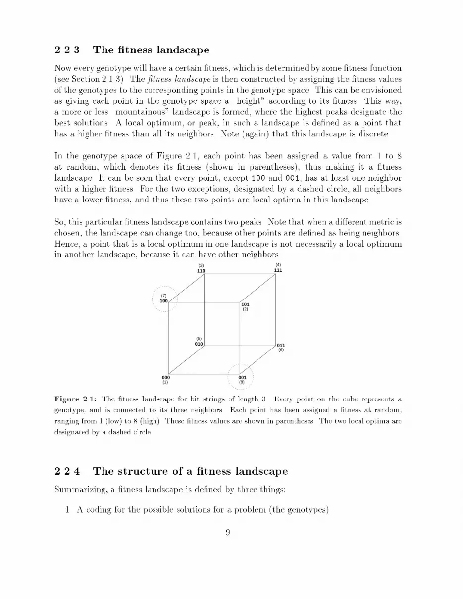
2.2.3 The �tness landscapeNow every genotype will have a certain �tness, which is determined by some �tness function(see Section 2.1.3). The �tness landscape is then constructed by assigning the �tness valuesof the genotypes to the corresponding points in the genotype space. This can be envisionedas giving each point in the genotype space a \height" according to its �tness. This way,a more or less \mountainous" landscape is formed, where the highest peaks designate thebest solutions. A local optimum, or peak, in such a landscape is de�ned as a point thathas a higher �tness than all its neighbors. Note (again) that this landscape is discrete.In the genotype space of Figure 2.1, each point has been assigned a value from 1 to 8at random, which denotes its �tness (shown in parentheses), thus making it a �tnesslandscape. It can be seen that every point, except 100 and 001, has at least one neighborwith a higher �tness. For the two exceptions, designated by a dashed circle, all neighborshave a lower �tness, and thus these two points are local optima in this landscape.So, this particular �tness landscape contains two peaks. Note that when a di�erent metric ischosen, the landscape can change too, because other points are de�ned as being neighbors.Hence, a point that is a local optimum in one landscape is not necessarily a local optimumin another landscape, because it can have other neighbors.000 001

011

111

101

010

110

100

(1) (8)

(6)

(2)

(5)

(7)

(3) (4)

Figure 2.1: The �tness landscape for bit strings of length 3. Every point on the cube represents agenotype, and is connected to its three neighbors. Each point has been assigned a �tness at random,ranging from 1 (low) to 8 (high). These �tness values are shown in parentheses. The two local optima aredesignated by a dashed circle.2.2.4 The structure of a �tness landscapeSummarizing, a �tness landscape is de�ned by three things:1. A coding for the possible solutions for a problem (the genotypes)9

2. A metric that de�nes which genotypes are neighbors3. A �tness function that de�nes the �tness of the genotypesThe �rst two items de�ne the genotype space. Adding the third item gives the �tnesslandscape. If one of these three items changes, the landscape will change as well. So, ingeneral, there is not a unique �tness landscape for a given problem, and the structure ofthe landscape depends on the above three items.The structure of a landscape incorporates many things, like the dimensionality (the numberof neighbors each point in the genotype space has), the number of peaks, the \steepness"of the hillsides, the relative height of the peaks, etc.A landscape where the average di�erence in �tness between neighboring points is relativelysmall, is called smooth. On such a landscape it will be easy to �nd good optima: localinformation about the landscape can be used e�ectively to direct the search. A landscapewith a relatively large average �tness di�erence between neighbors, is called rugged. Onsuch a landscape it will be di�cult to �nd good optima: local information becomes lessvaluable.So, the (global) structure of a landscape can range from very smooth to very rugged. Oneway to mathematically express this global structure of a landscape is by its correlationstructure. What this means and how this is measured is explained in Chapter 4.2.3 The NK-modelThe structure of a �tness landscape depends on the underlying problem. But a theory aboutpopulation ow should be independent of that. It would therefore be convenient to havea problem-independent �tness landscape. Kau�man introduced a model to generate suchlandscapes: the NK-model [Kau89]. The landscapes that result from this model (hereaftercalled NK-landscapes) can be tuned from smooth to rugged. The NK-model turned out tobe a good model for a wide range of problems. Therefore it is used throughout this thesisfor modelling general �tness landscapes.2.3.1 The NK-model of epistatic interactionsThe NK-model, of course, incorporates the three items that de�ne a �tness landscape. Asgenotypes, bit strings of length N are used. As metric, the Hamming distance is taken(see Section 2.2.1). The �tness function is more complicated, and will be explained next.Suppose every bit bi (i = 1; : : : ; N) in the bit string b is assigned a �tness of its own. The�tness of a bit, however, does not only depend on the value (0 or 1) of this speci�c bit,but also on the value of K other bits in the same bit string (0 � K � N � 1). These10

dependencies are called epistatic interactions. Thus the two main parameters of the NK-model are the number of bits, N , and the number of other bits K which epistaticallyin uence the �tness contribution of each bit.So, the �tness contribution of one bit depends on the value of K + 1 bits (itself and Kothers), giving rise to a total of 2K+1 possibilities. Since, in general, it is not known whatthe e�ects of these epistatic interactions are, they are modelled by assigning to each of the2K+1 possibilities at random a �tness value drawn from the Uniform distribution between0.0 and 1.0. Therefore, the �tness contribution wi of bit bi is speci�ed by a list of randomdecimals between 0.0 and 1.0, with 2K+1 entries. This procedure is repeated for every bitbi; i = 1; : : : ; N in the bit string b.Having assigned the �tness contributions for every bit in the string, the �tness of the entirebit string, or genotype, is now de�ned as the average of the contributions of all the bits:W = 1N NXi=1wiTable 2.1 gives an example (taken from [Kau93]) with N=3 and K=2. In this example,each bit depends on all other bits in the bit string. The �tness contributions in the fourth,�fth and sixth column are drawn at random. The total �tness of the genotype is calculatedas the average of the �tness contribution of all bits in the string, and is given in the lastcolumn. The corresponding �tness landscape is shown in Figure 2.2.value �tnessof bit contribution total �tness1 2 3 w1 w2 w3 W = 1N PNi=1 wi0 0 0 0.6 0.3 0.5 0.470 0 1 0.1 0.5 0.9 0.500 1 0 0.4 0.8 0.1 0.430 1 1 0.3 0.5 0.8 0.531 0 0 0.9 0.9 0.7 0.831 0 1 0.7 0.2 0.3 0.401 1 0 0.6 0.7 0.6 0.631 1 1 0.7 0.9 0.5 0.70Table 2.1: Assignment of �tness values to each of the three bits with random values for each of the2K+1 = 8 possible situations. The total �tness of each genotype is the average of the three �tnesscontributions. Example taken from [Kau93].One further aspect of the NK-model characterizes how the K epistatic interactions for eachbit are chosen. Generally, this is done in one of two ways.11

000 001

011

111

101

010

110

100(0.83)

(0.63)

(0.43)

(0.47) (0.50)

(0.53)

(0.70)

(0.40)Figure 2.2: The �tness landscape corresponding to the example in Table 2.1. The �tness values areshown between parentheses. There are two local optima, which are designated by a dashed circle.The �rst way is by choosing them at random from among the other N � 1 bits. This iscalled random interactions. It is important to note that no reciprocity in epistatic in uenceis assumed. This means that if the �tness of bit bi depends on bit bj, it is not necessary thatthe reverse also holds. So, the epistatic interactions for a bit are determined independentof the other bits.The second way is by choosing the K neighboring bits as epistatic interactions. The K=2bits on each side of a bit will in uence the �tness of this bit. This is called nearest neighborinteractions. To make this possible, periodic boundary conditions are taken into account.This means that the bit string is considered as being circular, so the �rst and the lastbit are each others neighbors. Note that for K=0 and K = N � 1, there is no di�erencebetween the two sorts of interactions. In the �rst case, the �tness of each bit depends onlyon its own value, and in the second case, the �tness of each bit depends on the value of allthe bits in the string.2.3.2 Properties of the NK-modelThe main property of the NK-model, the property for which the model was formulated inthe �rst place, is that the corresponding landscape can be tuned from smooth to ruggedby changing the parameter K, relative to N . In the case of K=0, there are no epistaticinteractions, and for each bit, by chance, either the value 0 or the value 1 makes thehigher �tness contribution. Therefore, there is one genotype having the �tter value ateach position which is the global optimum. Furthermore, every other genotype can besequentially changed to the global optimum by successive ipping of each bit which hasthe less favored value to the more favored value. The landscape for K=0 is very smooth:neighboring genotypes do not di�er much in their �tness values, and there is one (global)peak. 12

Increasing K introduces con icting constraints among the di�erent bits, and causes thelandscape to become more rugged, because the complexity of the model increases. Thecase of K = N � 1 corresponds to a fully random landscape. Changing the value of onlyone bit causes a change in the �tness of all bits, because the �tness of each bit depends alsoon all other bits. Each bit now has a di�erent (random) �tness, and therefore the �tnessof the entire string changes to a completely random value. So, neighboring genotypes havevery di�erent �tnesses, and the landscape will be extremely rugged.Kau�man has investigated the properties of the NK-model extensively. A summary of themost important conclusions is as follows [Kau93]:� Almost all features of the �tness landscape depend entirely on N and K, makingthe NK-model a very simple but e�ective tool for investigation. Also, according toKau�man, the features of the landscape do not depend on the type of interactions(random or nearest neighbor), nor on the type of distribution that is used to assignthe random �tness contributions to each bit.� When K is proportional to N , a complexity catastrophe sets in as N increases: at-tainable optima become ever more \mediocre", or typical of the entire landscape.When K remains small as N increases, this complexity catastrophe does not set in;hence low epistatic interactions are a su�cient \construction requirement" in com-plex systems in order to adapt on \good" �tness landscapes with high accessibleoptima.� In an adaptive search, the time to �nd a �tter individual doubles every time such anindividual is found.� When a constant mutation rate (the rate at which bits \spontaneously" change theirvalue) is assumed, an error catastrophe sets in as N increases: the ability of selectionto hold an adapting population at a local optimum ultimately fails, and the popu-lation \melts" and ows down the hillside to drift neutrally through wide regions ofthe landscape.2.4 SummaryThe evolution of a population of individuals, whether real organisms or solutions for someoptimization problem, can be modelled by an adapting population of genotypes on a �tnesslandscape. The genotype of an individual is its genetic coding, which determines thephenotype, the actual appearance of the individual. A �tness landscape, then, is the spaceof all possible genotypes with some neighborhood relation, where every genotype is assigneda �tness by means of a �tness function. The �tness of an individual denotes its relativesuccess in leaving o�spring, that is, relative to other individuals. A �tness function can beimplicit (the �tness is determined by a selection process) or explicit (the �tness is used tosimulate selection). 13

The NK-model is a useful model to generate �tness landscapes of which the global structurecan be tuned from smooth (small di�erences in �tness between neighboring genotypes) tovery rugged (large di�erences in �tness between neighboring genotypes) by changing theparameter K (the richness of epistatic interactions) relative to N (the length of the geno-types). Since Kau�man already showed what happens when N varies, given a (relative)value of K, and since the main interest in this thesis is what happens with populations onlandscapes that di�er in ruggedness, the value of N is �xed in all experiments, and K isvaried relative to N .Having introduced the concept of �tness landscapes, and a model to generates such land-scapes, there still is no evolution, or population ow. To let this happen, some kind ofsearch process has to take place on these landscapes. The next chapter introduces somesearch strategies that perform such processes on �tness landscapes.

14

Chapter 3Search Strategies and PerformanceOn the one hand, evolutionary search strategies are used more and more to solve complexproblems. On the other hand, evolution is considered more and more as a search process ina large, but �nite space of possible solutions. This chapter introduces some search strategiesthat are applied to di�erent kinds of �tness landscapes (see Chapter 2). The strategiesall perform an adaptive search on these landscapes. Comparing the performances of thedi�erent strategies can give insight into what types of strategies work well on what typesof landscapes, but also into the principles of evolution itself. Some performance measuresare introduced as well, by which the strategies are evaluated.3.1 Search strategiesThe search strategies that are applied to di�erent �tness landscapes are various implemen-tations of the following four search methods:� Hillclimbing� Long jumps� Genetic Algorithm� Hybrid Genetic AlgorithmIn this section, these four methods are introduced one by one. Their weaknesses andstrengths are discussed, and the exact implementations that are used are given as well.With all strategies, it is assumed that the points (genotypes) in the landscape to whichthese strategies are applied, are bit strings.3.1.1 HillclimbingHillclimbing is a general, local search strategy that can be applied to a multitude of prob-lems. The idea is to start at a randomly chosen point in the landscape, and walk via �tter15

neighbors to a nearby hilltop. If this procedure is repeated a couple of times, it is callediterated hillclimbing.Basically, there are three forms of hillclimbing (steepest ascent, next ascent, and randomascent), which are all variants of the following general algorithm:Hillclimbing1. Choose a bit string at random. Call this string current-hilltop.2. Choose a �tter neighboring string of current-hilltop by some criterion.3. If a �tter neighbor could be found, then set current-hilltop to this new string, andreturn to step 2 with this new current-hilltop.4. If no �tter neighbor could be found, then return the �tness of the current-hilltop.With iterated hillclimbing, this procedure is restarted every time a local optimum hasbeen found (that is, not �tter neighbor could be found), until a preset number of functionevaluations has been reached. The local optima that are found during the search are saved,and in the end the best optimum found is returned.The three forms of hillclimbing di�er in the criterion by which a �tter neighboring stringis chosen. These criteria are as follows [FM93]:Steepest ascent hillclimbing: Systematically ip all bits in the string, recording the�tnesses of the resulting strings. Choose the string that gives the highest increase in�tness.Next ascent hillclimbing: Flip single bits from left to right, until a neighbor is foundthat gives an increase in �tness. Choose this string as �tter neighbor. At the followingstep, however, continue ipping bits after the point at which the last �tness increasewas found.Random ascent hillclimbing: Flip bits at random, until a neighbor is found that givesan increase in �tness. Choose this string as �tter neighbor.Note that the �rst two algorithms can be performed in an iterated way, because the bits are ipped systematically, so it is known when a local optimum has been reached. Randomascent hillclimbing, however, just keeps ipping bits at random, so it is never knownwhether a local optimum has been reached yet.Hillclimbing is a very general search strategy that is often used as a \benchmark" for othersearch strategies. A search strategy should at least perform as well as hillclimbing. But incomparing other search strategies with hillclimbing, \it matters which type of hillclimbingalgorithm is used" [FM93]. Therefore, two di�erent hillclimbing variants will be used here.16

The �rst hillclimbing variant is based on random ascent hillclimbing. Random ascenthillclimbing appears to be a very strong algorithm for some specially designed �tness land-scapes, \but [it] will have trouble with any function with local optima" [FM93]. Therefore,an \extended version" is implemented here: Random ascent hillclimbing with memory. Thealgorithm \remembers" which bits it already has tried, and so it will know when it is ata local optimum. This way, the algorithm can be used in an iterative way too. The bitsthat are ipped are chosen at random, but without repetition (of course, every time a �tterneighbor has been found, all the bits can be chosen again). The implementation of thishillclimbing variant is as follows:Random ascent hillclimbing with memory (RAHCM)1. Set best-evaluated to 0.2. Choose a bit string at random. Call this string current-hilltop. If the �tness ofcurrent-hilltop is higher than best-evaluated, then set best-evaluated to this �tness.3. Choose a bit from current-hilltop at random, without repetition, and ip it. If thisleads to an increase in �tness, then set current-hilltop to the resulting string, oth-erwise, repeat step 3. If the �tness of the new current-hilltop is higher than best-evaluated, then set best-evaluated to this �tness. Go to step 3 with the new current-hilltop, and forget all the bits that have been ipped so far.4. If all bits of the current-hilltop have already been ipped once and no increase in�tness was found, then go to step 2.5. When a set number of function evaluations has been performed, return best-evaluated.The second hillclimbing variant combines elements of both steepest ascent and randomascent hillclimbing. Just as in steepest ascent hillclimbing, the �tness of all neighbors arecalculated and stored. But where in random ascent a bit is chosen at random, in this varianta �tter neighbor is chosen at random. This is repeated until no �tter neighbors exist, andthus a local optimum has been reached. This variant will be called Random neighbor ascenthillclimbing, to emphasize that a �tter neighbor is chosen at random instead of just a bit.The implementation of this hillclimbing variant is as follows:Random neighbor ascent hillclimbing (RNAHC)1. Set best-evaluated to 0.2. Choose a bit string at random. Call this string current-hilltop. If the �tness ofcurrent-hilltop is higher than best-evaluated, then set best-evaluated to this �tness.3. Systematically ip each bit in the string from left to right, recording the strings thatlead to an increase in �tness. 17

4. If there are strings that lead to an increase in �tness, then choose one of them atrandom and set current-hilltop to this string, otherwise go to step 2. If the �tness ofthe new current-hilltop is higher than best-evaluated, then set best-evaluated to this�tness. Go to step 3 with the new current-hilltop.5. When a set number of function evaluations has been performed, return best-evaluated.So, this algorithm is also used in an iterative way. This algorithm was used by Kau�manfor examining the properties of NK-landscapes (see Chapter 2). It is assumed that he basedhis statement about the three time scales in adaptation (see Section 1.1) on the resultsobtained with this hillclimbing variant.3.1.2 Long jumpsWith long jumps, not just one bit is ipped, but a lot of bits are ipped at one step. Thismeans that an individual jumps a long distance (in terms of Hamming distance) across the�tness landscape. Long jumps are implemented as follows:Long jumps1. Initialize a population of bit strings at random.2. For each bit string in the population, make a long jump by systematically ippingeach bit in the string with probability 0.5. If the resulting string has a higher �tness,then replace the old string with the new string, otherwise, keep the old string in thepopulation.3. Repeat step 2 for a set number of function evaluations.Since every bit in a string is ipped with probability 0.5, it comes e�ectively down to justtrying random strings to see if they are better. So, there is no direction in the searchwhatsoever. The only restriction is that only strings that are better than the previous oneare allowed to enter the population.Note that the algorithm can not be used in an iterative way, because it is never knownwhen a local optimum has been reached (the immediate neighbors of a bit string are notevaluated). Therefore, the algorithm uses a population of searchers, but never starts anew.A population size of 50 is taken for all experiments.3.1.3 Genetic AlgorithmA Genetic Algorithm (GA, see [Hol92, Gol89]) simulates natural evolution by repeatedlyapplying three operators to a population of genotypes: selection, crossover and mutation.The operators can be implemented in various ways, but here only the variants that areused are explained. 18

First, an initial population of genotypes (in the from of bit strings) is created at random.Each genotype in the population is assigned a �tness which is determined by some �tnessfunction (see section 2.1.3). Next, new generations are created by repeatedly applying thethree operators.SelectionA new population is created by selecting at random genotypes from the old population,where the relative �tness of each genotype (relative to the �tness of the other genotypesin the population) determines its probability of being selected. So, genotypes with a highrelative �tness have a higher probability of being selected than genotypes with a low relative�tness. On average, some (relatively �t) genotypes will be selected more than once, whilesome other (relatively un�t-�t) genotypes will not be selected at all. This selecting ofgenotypes is repeated until the new population is as large as the old one.The selection mechanism that is used in the experiments, is called Deterministic tourna-ment selection. This mechanism is implemented as follows:Deterministic tournament selection1. Choose s genotypes at random from the old population without repetition. s is thetournament size.2. Take the �ttest genotype of the s selected ones and place it in the new population.3. Repeat steps 1 and 2 until the new population is as large as the old one.This selection mechanism can be seen as random individuals in the population playinga tournament, and the most �t individual in this tournament wins, and is allowed tocontribute its genetic information to the next generation. The tournament size s can beused to vary the selection pressure.CrossoverStart by taking the �rst pair of genotypes from the new population as parents. With acertain chance pc (called the crossover rate) exchange some parts of the genetic informationof these two parents, thus creating two children. These children replace their parents inthe population. Repeat this procedure for every next pair in the population.The crossover rate pc is a number between 0 and 1, determining the probability that thisexchange of genetic information actually happens for a pair of parents. In practice, a ratesomewhere between 0.6 and 0.9 gives the best results [Gre86].Two di�erent types of crossover are used in the experiments: One-point crossover andUniform crossover. These types of crossover work as follows (using bit strings):19

One-point crossoverTake two bit strings as parents. Choose a crossover point (a random point somewherebetween the �rst and the last bit) and exchange the parts of the two parents after thiscrossover point. This way, two children are created, as shown in the next example.parent 1: 000|00000 child 1: 00011111parent 2: 111|11111 child 2: 11100000|crossover pointUniform crossoverTake two bit strings as parents and create two children as follows: for each bit position onthe two children, decide randomly which parent contributes its bit value to which child.Next, an example is shown:parent 1: 00000000 child 1: 00101101parent 2: 11111111 child 2: 11010010MutationStart with the �rst genotype of the new population. Successively ip each bit with a certainprobability pm (called the mutation rate). Repeat this procedure for every next genotypein the population. In practice, the mutation rate pm will be very small, in the order ofmagnitude of 0.01 to 0.001 for example. So, with bit strings, 1 bit in every 100 or 1000bits will actually be ipped.The mutation operator plays an important role in maintaining some diversity in the popu-lation. Crossover alone is not able to introduce a new value at a certain bit position whenall the individuals in the population have the same value at this bit position. So, the taskof mutation is primarily to prevent the population to converge to one speci�c point in thelandscape, and to maintain some evolvability.Now that the three operators are applied, the �tness of each genotype in the new populationis determined, and the operators are applied again. This process is repeated for a �xednumber of generations.Schema processingThe notion of a schema is central to understand how a GA works. Schemata are sets ofindividuals in the search space, and the GA is thought to work by directing the searchtowards schemata containing highly �t regions of the search space (i.e. hilltops in the�tness landscape). 20

If the GA uses bit strings of length L as genotypes, then a schema is de�ned as an elementof f0; 1; �gL. So, a schema looks something like 1**01*00*, where a * means don't care,either value (0 or 1) is allowed. A bit string b that matches the pattern of a schema s issaid to be an instance of s. Fot example, both 00 and 10 are instances of *0.In schemata, 0's and 1's are called de�ned bits. The order of a schema is the number ofde�ned bits in that schema. The de�ning length of a schema is the distance between the�rst and the last de�ned bit. For example, the schema 1**01*00* is of order 5 and hasde�ning length 7.The �tness of a schema is de�ned as the average of the �tness values of all bit strings thatare an instance of this schema. For large string lengths, this is of course impossible tocalculate for every schema, but the �tness of any bit string in the population gives someinformation about the �tness of the 2L di�erent schemata of which it is an instance. So,an explicit evaluation of a population of M individual strings is also an implicit evaluationof a much larger number of schemata.The building block hypothesis ([Hol92, Gol89]) states that a GA works well when short,low-order, highly �t schemata (so-called building blocks) are recombined to form even morehighly �t higher-order schemata. The ability to produce �tter and �tter partial solutionsby combining building blocks is believed to be the primary source of the GA's search power.According to the Schema Theorem ([Hol92, Gol89]), short, low-order, above average sche-mata receive exponentially increasing trials in subsequent generations. Above averagemeans a �tness above the average �tness of the current population. So, early on in thesearch the GA explores the search space by processing as many di�erent schemata aspossible, and later on it exploits biases that it �nds by converging to instances of the most�t schemata it has detected.This strong convergence property of the GA is both a strength and a weakness. On theone hand, the fact that the GA can identify the �ttest parts of the space very quicklyis a powerful property. On the other hand, since the GA always operates on �nite sizepopulations, there is inherently some sampling error in the search, and in some cases theGA can magnify a small sampling error, causing premature convergence.Another problem with GA's is crossover disruption. The building block hypothesis statesthat building blocks must be combined to ever �tter and longer schemata. But fromthe mathematical formula that supports the Schema Theorem ([Hol92, Gol89]), it followsthat longer, higher-order schemata are more sensitive to being disrupted by crossover thanshorter, low-order ones. So, crossover should on the one hand combine building blocks tolonger, highly �t schemata, but on the other hand avoid disrupting them again as much aspossible. 21

Both problems, premature convergence and crossover disruption, are examined in laterchapters (see Chapters 5 and 6). To do this, two di�erent GA's are applied to the �tnesslandscapes. Both GA's have the same parameter values, but the �rst one uses one-pointcrossover (GA-ONEP), while the second one uses uniform crossover (GA-UNIF). The im-plementation of the two GA's is as follows:GA-ONEPPopulation size: 50Selection: Deterministic tournament selection, s=3Crossover: One-point crossover, pc=0.75Mutation: pm=0.005GA-UNIFPopulation size: 50Selection: Deterministic tournament selection, s=3Crossover: Uniform crossover, pc=0.75Mutation: pm=0.0053.1.4 Hybrid Genetic AlgorithmA Hybrid Genetic Algorithm (HGA) is a combination of a Genetic Algorithm (a globalsearch strategy) with a local search strategy (see [Dav91]). It comes down to applying thelocal search strategy to a population of genotypes, then applying one generation of theGA, then the local search strategy again, etc. A GA can for example be combined withhillclimbing. First, let all the members of the population climb to a nearby hilltop. Next,apply crossover (and possibly mutation) to this population of local optima. Repeat thiscycle for a number of generations. The idea behind this is that the locations of local optimamay give some information about the locations of other, hopefully better, local optima.Here, a GA combined with random ascent hillclimbing with memory (see section 3.1.1)is used. In the GA, an integrated selection recombination operator is used, called ElitistRecombination. This operator works as follows [TG94]:Elitist Recombination1. Random shu�e the population2. For every mating pair(a) Generate o�spring(b) Keep the best two of each family(= 2 parents + 2 o�springs) 22

So, with this operator, children are only allowed to enter the population if they are �tterthan (one of) their parents. In the implementation that is used here, the o�spring isgenerated with one-point crossover, with a crossover rate pc of 1.0, so crossover is alwaysapplied. The exact implementation of the Hybrid Genetic Algorithm is as follows:Hybrid Genetic Algorithm (HGA)1. Initialize a random population of bit strings.2. Apply Elitist Recombination to the population using one-point crossover (c=1.0)3. Apply random ascent hillclimbing with memory to every member of the population4. Repeat steps 2 and 3 for a preset number of function evaluationsA population size of 10 is taken for all experiments.3.2 Performance measuresTo compare the di�erent search strategies that are introduced in the last section, they areevaluated by some performance measures. These measures are set out against the numberof function evaluations done by a search strategy.First of all, the maximum �tness in the population is monitored. For hillclimbing, whichdoes not use a population, the best �tness found so far is taken. However, this performancemeasure only gives a snapshot at a certain time during the search. Therefore, the on-lineand o�-line performance (see [Gol89]) are measured as well. These measures keep track ofall the function evaluations done by a strategy throughout the search.As explained in Section 3.1.3, premature convergence of a population can be a problem fora Genetic Algorithm. So, it would be of interest to monitor the diversity of a populationduring a search. The mean Hamming distance is such a measure of population diversity,and it will be used here too.In the following subsections, the on-line and o�-line performance, as well as the meanHamming distance, are explained in more detail.3.2.1 On-line performanceThe on-line (ongoing) performance is an average of all function evaluations done by asearch strategy up to and including the current evaluation T . The on-line performanceonls(T ) of strategy s is de�ned as: onls(T ) = 1T TX1 f(t)23

where f(t) is the �tness value on evaluation t. Generally speaking, if the on-line perfor-mance of a search strategy stays very low during a search, then the strategy is wasting toomuch evaluations on \bad" solutions.3.2.2 O�-line performanceThe o�-line (convergence) performance is a running average of the best �tness valuesfound by a search strategy up to a particular evaluation. The o�-line performance o�s(T )of strategy s is de�ned as: o�s(T ) = 1T TX1 f�(t)where f�(t) is the best �tness value encountered up to evaluation t. The o�-line per-formance is a measure of how quickly the search strategy �nds the optimal value (or\converges" to the optimum).If, for example, at time T = 5 �ve genotypes have been evaluated by strategy s, with �tness10, 8, 20, 2 and 15 respectively, then the on-line performance onls(5) is 10+8+20+2+155 = 11,and the o�-line performance o�s(5) is 10+10+20+20+205 = 16.3.2.3 Mean Hamming distanceThe mean Hamming distance (MHD) is a measure of population diversity. It is de�nedas the average value of the Hamming distances (see Section 2.2.1) between every twoindividuals of a population of bit strings:MHD = 10:5n(n � 1)Xi6=j HD(i; j)where n is the population size, i and j range over (di�erent) individuals of the currentpopulation, and HD(i; j) is their Hamming distance.Here, a normalized MHD is used, by taking the normalized Hamming distance betweentwo bit strings (that is, the Hamming distance divided by the length of the bit strings, seeSection 2.2.1). In this way, the MHD is independent of the length of the bit strings, and isa number between 0 and 1. A MHD of about 0.5, then, means that about half the bits oftwo arbitrary bit strings in the population di�er in their value. This will be the case whena population of bit strings is created at random. A MHD of 0 indicates that all bit stringsin the population are equal, so the population has completely converged onto one speci�cpoint in the �tness landscape. 24

3.3 SummaryIn this chapter several search strategies are introduced that are applied to di�erent �tnesslandscapes. These strategies include two types of hillclimbing (RAHCM and RNAHC),Long jumps, two Genetic Algorithms (GA-ONEP and GA-UNIF), and a Hybrid GeneticAlgorithm (HGA). All these strategies apply one or more genetic operators to the genotypesthey use during the search. Some of these operators are biologically inspired, others arepurely arti�cial. By comparing the performance of the di�erent strategies, hopefully abetter understanding can be gained in the way these operators work or how useful theyare. This can contribute to a better understanding of both problem solving and the processof evolution.The performance of the search strategies is monitored by di�erent performance measures.The �rst, and most important one, is the maximum �tness. For hillclimbing, the maxi-mum �tness found up to a certain time is monitored, while for the other search strategiesthe maximum �tness in the population is recorded. This seems not quite fair, but sincehillclimbing is usually considered as a benchmark, or \minimal performance", that worksquite well on a multitude of problems, the performance of other strategies can be comparedwith the maximum found by hillclimbing. Besides, in this thesis the interest is focused onthe population ow in general: not only how fast an optimum is found and how good thisoptimum is, but also how this optimum was reached and whether this optimum can bemaintained in a population for a longer period of time.Other performance measures are the on-line and o�-line performance, which keep track ofall the function evaluations done by a search strategy throughout a search. In case of apopulation-based strategy, the mean Hamming distance is also monitored, which gives ameasure of the diversity of a population during a search.To be able to relate the performance of a search strategy to the structure of the underlying�tness landscape, this structure has to be known �rst. Therefore, the next chapter proposesa way to express and determine the global structure of a �tness landscape.25

26

Chapter 4The Structure of Fitness LandscapesTo �nd a theory that relates the structure of a �tness landscape to the ow of a populationon it, it is desirable to have some mathematical expression for this structure. But asalready mentioned in Section 2.2.4, the structure of a �tness landscape incorporates manythings, like its dimensionality, the number and average height of local optima, etc. Oneway to mathematically express the global structure of a �tness landscape, however, is byits correlation structure.The correlation structure of a �tness landscape is determined by the �tness di�erentials be-tween neighboring points in the landscape. Small di�erences in �tness between neighboringpoints gives a highly correlated landscape, large di�erences in �tness gives an uncorrelatedlandscape, with a whole range of more or less correlated landscapes in between. Fromthis correlation structure, a correlation length can be derived, which somehow denotes thelargest \distance" between points at which the �tness of one point still provides someinformation about the expected value of the �tness of the other point.Di�erent procedures have been used to measure and express the correlation structure andcorrelation length ([Wei90, MWS91, Lip91]). This chapter �rst proposes a more completeprocedure based on the one introduced in [Wei90], and on a time series analysis knownas the Box-Jenkins approach. Next, the results of applying this procedure to di�erentNK-landscapes (see Section 2.3) are presented. Finally, some conclusions are drawn fromthese results.4.1 The correlation structure4.1.1 Measuring correlationWeinberger introduced a procedure to measure the correlation structure of �tness land-scapes [Wei90]. The idea is to generate a random walk on the landscape via neighboringpoints. In case of bit strings as genotypes and the Hamming distance as metric (see Sec-27

tion 2.2.1), this means that at every step one randomly chosen bit in the string is ipped,so-called point mutation. At each step the �tness of the genotype encountered is recorded.This way, a time series of �tness values is generated. Next, the autocorrelation function isused to determine the correlation structure of this time series.The autocorrelation function �i relates the �tness of two genotypes along the walk whichare i steps (called times lags in case of a time series) apart. The autocorrelation for timelag i of a time series yt; t = 1; ::; T is de�ned as:�i = Corr(yt; yt+i) = E[ytyt+i]�E[yt]E[yt+i]V ar(yt)where E[yt] is the expected value of yt and V ar(yt) is the variance of yt. It always holdsthat �1 � �i � 1. If j�ij is close to one, then there is much correlation between two valuesi steps apart; if it is close to zero, then there is hardly any correlation. Estimates of theseautocorrelations are: ri = PT�it=1 (yt � y)(yt+i � y)PTt=1(yt � y)2where y = 1T PTt=1 yt and T � 0.An important assumption made here is that the �tness landscape is statistically isotropic.This means that the statistics of the time series generated by a random walk via neighboringpoints are the same, regardless of the starting point. The signi�cance of statistical isotropyis that the random walk is \representative" for the entire landscape, and thus that thecorrelation structure of the time series can be regarded as the correlation structure of thelandscape.There still seems to be no agreement about an exact de�nition of the correlation length ofa �tness landscape, since everybody uses its own de�nition ([Wei90, MWS91, Lip91]). Thecorrelation length gives an indication of the largest \distance", or time lag, between twopoints at which the �tness of one point still provides some information about the expectedvalue of the �tness of the other point. In other words, the correlation length � is the largesttime lag i for which there still exists some correlation between two points i steps apart.In statistics, it is usual to compare an estimated value with its two-standard-error1 bound,to see whether the estimated value is signi�cantly di�erent from zero. For the ri, theestimates of the �i, this two-standard-error bound is �2=pT (see [J+88]). So, it is proposedhere to take as correlation length � one less than the �rst time lag i for which the estimatedautocorrelation ri falls inside the region (�2=pT;+2=pT ), and thus becomes (statistically)equal to zero. This way, the correlation length � is the largest time lag i for which thecorrelation between two points i steps apart is still statistically signi�cant.1The statistical estimation of some variable will never be exact, but contains some uncertainty. Thestandard error of an estimated value gives an indication of the amount of this uncertainty.28

4.1.2 Time series analysisThe procedure introduced in [Wei90] only calculates the autocorrelations from the obtainedtime series, and derives a correlation length from them. It is proposed here to expand thiscorrelation analysis to a more complete time series analysis. This involves identifying anappropriate model that adequately represents the data generating process (in this case therandom walk), estimating the parameters of this model, and applying statistical tests tosee how well the estimated model approximates the given data and what the explanatoryand predictive value of the model is.In other words, a model of the formyt+1 = f(yt; yt�1; � � � ; y0)is derived from the observed data, that can be used to simulate the outcome of a randomwalk on the landscape or to predict future values in a time series generated by such a walk.Di�erent landscapes can then be compared in terms of these models, which are used toexpress the correlation structure of these landscapes.Section 4.2 introduces such a complete time series analysis that is based on the estimationof the autocorrelations of a given time series. This time series analysis is known as theBox-Jenkins approach, and it will be applied here to time series that are generated by arandom walk on NK-landscapes.4.1.3 Handling other operatorsGenetic operators that give rise to steps of a distance larger than one (in terms of themetric that is used to de�ne the �tness landscape) will experience another correlationstructure. In terms of bit strings, operators other than point mutation will experienceother correlation structures on a landscape de�ned by Hamming distance. One step ofan arbitrary operator other than mutation (for example long jumps or crossover) will, ingeneral, end up in a point that has a Hamming distance of more than one from the pointthat was started from. The correlation between two points \one step apart" will thus bedi�erent for each operator. So, each operator experiences the landscape in a di�erent way.Compare this with a mountaineers-club which has a couple of camps in the Alps. Consider amountaineer walking along a route passing these camps. The only things this mountaineercan observe at every step he takes, are his coordinates and his altitude. From theseobservations he has to construct a picture of the landscape he is walking through. Now afellow mountaineer is hopping in a helicopter from one camp to another. He is also able torecord only his coordinates and altitude at every camp he lands. The picture he constructsfrom his data will be di�erent from the picture his walking fellow made earlier on, whileboth men travelled through the same landscape!29

A procedure to deal with di�erent operators is due to Manderick et al. [MWS91]. Thisprocedure involves generating a random population of genotypes (the parent population),applying the operator of interest to this population, thus creating an o�spring population,and then calculating the correlation coe�cient between the �tness values of the parents andthe o�spring. This procedure is done for the �rst generation. If the correlation coe�cientfor more generations is wanted, then this procedure can be repeated, this time with theo�spring population acting as parent population. Because no new genotypes are introducedduring this process, there is a chance that the population converges to some extent, andthis will be re ected in the calculations of the correlation coe�cient, causing a bias in theoutcome.Therefore, it is proposed here to use the procedure introduced in Section 4.1.2 for otheroperators as well. Instead of walking along neighboring points in the landscape (that is,using point mutation in case of bit string and Hamming distance), a random walk can begenerated by the operator of interest2. The complete time series analysis applied to thetime series generated in this way, gives insight into how this particular operator experiencesthe correlation structure of the landscape.In fact, calculating the autocorrelationfor the �rst time lag of such a time series is equalto calculating the correlation coe�cient for parent and o�spring populations. Insteadof creating an o�spring population and calculating the correlation between the �tness ofparents and o�spring, the correlation between the original time series and the same seriesone time lag shifted is calculated (remember that the genotype encountered at time t isthe parent of the genotype encountered at time t+ 1). Hence the term autocorrelation, orcorrelation with oneself. In the same way, the correlations for larger time lags can also becalculated with only one time series, instead of a number of populations, thus avoiding thedanger of a biased outcome due to convergence.The next section introduces the Box-Jenkins approach, which is used to perform the com-plete time series analysis based on the estimated autocorrelations of the time series.4.2 The Box-Jenkins approachThe Box-Jenkins approach [BJ70] is a very useful standard statistical method of modelbuilding, based on the analysis of a time series y1; y2; : : : ; yT , generated by a stochasticprocess. The purpose of the Box-Jenkins approach is to �nd an ARMA model that ade-quately represents this data generating process. Once an adequate model is found, it canbe used to make forecasts about future values, or to simulate a similar process as the onethat generated the original data.2Note that this gives a slight problem for binary operators (i.e. operators that use two parents insteadof one). One way to overcome this problem is by choosing a second parent at random out of all possiblegenotypes and taking one of the two children, both with an equal chance, to proceed with.30

An ARMA model represents an autoregressive moving-average process, and is obtained bycombining an autoregressive (AR) process and a moving-average (MA) process. An ARprocess of order p (AR(p)) has the formyt = �1yt�1 + � � � + �pyt�p + "twhere the stochastic variable "t is white noise, that is, E["t] = 0, V ar("t) < 1 for all t,and Cov("s; "t) = 0 for s 6= t, so all "t are independent of each other. So, each value in anAR(p) process depends on p past values and some stochastic variable "t. An MA processof order q (MA(q)) has the formyt = "t + �1"t�1 + � � �+ �q"t�qwhere "t is again white noise. So, each value in an MA(q) process is a weighted sum ofmembers of a white noise series. An ARMA(p; q) process, then, is a combination of anAR(p) and an MA(q) process:yt = �1yt�1 + � � �+ �pyt�p + "t + �1"t�1 + � � �+ �q"t�qThe mean of a time series generated by one of these three processes is zero. If this is notwanted, then a constant c can be added to the model, resulting in a non-zero mean of thetime series.In economics (and business) the Box-Jenkins approach is used frequently when a modelis needed to make forecasts about future values of some (partly) stochastic variable, forexample the price of some commodity, or the index of industrial production. The approachconsists of three stages:1. Identi�cation, in which a choice is made for one or more appropriate models, bylooking at the (partial) autocorrelations of the time series;2. Estimation, in which the parameters of the chosen model are estimated;3. Diagnostic checking, which involves applying various tests to see if the chosen modelis really adequate.The three stages of the approach are explained in more detail below.Identi�cationAt the identi�cation stage an appropriate model is speci�ed on the basis of the correlogramand the partial correlogram. The correlogram of a time series yt is a plot of the (estimated)autocorrelations (the ri as given in Section 4.1.1) of this series against the time lag i. Thepartial correlogram is the plot of the (estimated) partial autocorrelations of the time seriesagainst the time lag. It will not be explained here how to calculate the partial autocorre-lations (see [BJ70, Gra89, J+88]), but the i'th partial autocorrelation can be interpretedas the estimated correlation between yt and yt+i, after the e�ects of all intermediate y'son this correlation are taken out. The choice of model can now be made on the followingbasis: 31

� If the correlogram tapers o� to zero and the partial correlogram suddenly \cuts o�"after some point, say p, then an appropriate model is AR(p). To determine thiscut-o� point p, the partial autocorrelations are compared with a two-standard-errorbound, which is 2=pT (T being the length of the time series).� If the correlogram \cuts o�" after some point, say q, and the partial correlogramtapers o� to zero, then an appropriate model is MA(q). Here the \cut-o�" pointis also determined by comparing the autocorrelations with their two-standard-errorbound of 2=pT .� If neither diagram \cuts o�" at some point, but both taper o�, then an appropriatemodel is ARMA(p,q). The values of p and q have to be inferred from the particularpattern of the two diagrams.EstimationOnce the appropriate model is chosen, the parameters of this model can be estimated. Thisis achieved by using the estimates of the autocorrelations. From these values, estimatesfor the parameters of the model can be derived (see [BJ70, Gra89, J+88]).As a measure of signi�cance of the estimated parameters the t-statistic is used. Thisstatistic is de�ned as the estimated value of the parameter divided by its estimated standarderror. Because the estimation of a parameter will never be exact, an interval of two timesthe standard error on both sides of the estimate determines a so called 95% con�denceinterval. The probability that the real value of the parameter will fall inside this intervalis 95%. But if zero also falls inside this interval, then the parameter could just as wellbe equal to zero. For this reason, a parameter is called signi�cant (meaning signi�cantlydi�erent from zero), if the absolute value of the t-statistic of its estimate is greater thantwo, because zero will then be outside the 95% con�dence interval.As a measure of \goodness of �t" of the estimated model, the R2 is used. This value is ameasure of the proportion of the total variance in the data accounted for by the in uenceof the explanatory variables of the estimated model. A value of R2 close to one meansthat the explanatory variables can explain the observed data very well. A value of R2 closeto zero means that the stochastic component of the model plays a dominant role (or itcould be that there exist more explanatory variables than there are currently in the model;this will not be the case here, because it is assumed that in the identi�cation stage anappropriate model is already chosen).Diagnostic checkingBefore the estimated model is used, it is important to check that it is a satisfactory one.The usual test is to �t the model on the data and calculate the autocorrelations of theresiduals (the di�erence between the observed values and those predicted by the estimatedmodel). These residuals should be white noise, so all the autocorrelations should not besigni�cantly di�erent from zero. To check this, the residual autocorrelations are compared32

with a two-standard-error bound (also 2=pT ). Another test is to �t a slightly higher-ordermodel and then to see whether the extra parameters are signi�cantly di�erent from zero.So, if an AR(p) model is estimated, an AR(p+ 1) model could also be estimated and thesigni�cance of the extra parameter should be checked (it should be insigni�cant).Summarizing, the Box-Jenkins approach is used to �nd an appropriate model for a giventime series generated by some stochastic process, to make forecasts for, or simulations ofthe process that generated the original data. In the next section, the results of applyingthe Box-Jenkins approach to time series of �tness values generated by random walks onNK-landscapes are presented.4.3 The correlation structure of NK-LandscapesTo determine the correlation structure of NK-landscapes, the Box-Jenkins approach isapplied to time series of �tness values, generated by random walks on these landscapes.Since NK-landscapes are de�ned by bit strings as genotypes and the Hamming distance asmetric (see Section 2.3), at least the operator point mutation is used to generate randomwalks. This operator visits neighboring points in the NK-landscape, so the results obtainedfor this operator can be regarded as the correlation structure of the NK-landscape.Furthermore, because all search strategies introduced in Chapter 3 use at least one ofthe operators mutation, long jumps or crossover, these last two operators are also usedto generate random walks (only one-point crossover is used here; uniform crossover is notconsidered). The results obtained for these operators indicate how they experience the cor-relation structure of the NK-landscape. The three types of random walks are implementedas follows:Point mutation: At every step one bit, which is selected at random, is ipped.One-point crossover: At every step a second parent is randomly chosen out of all possiblebit strings. A crossover point is selected at random, and the parts of the parents afterthis crossover point are exchanged, creating two children. One of these two childrenis selected for the next step (each with chance 0.5).Long jumps: At every step each bit in the string is ipped with chance 0.5.The length of the random walks is 10,000 steps, and the autocorrelations for the �rst 50 timelags are estimated. NK-landscapes with the following values for N and K are considered:N=100, K=0, 2, 5, 25, 50 and 99. Both random and nearest neighbor interactions areconsidered. The Box-Jenkins approach is carried out with the statistical package TSP(Time Series Processor). The following subsections present the results for the di�erentoperators. 33

4.3.1 Results for point mutationIdenti�cationThe correlograms for the di�erent values ofK are given in Figures 4.1 (random interactions)and 4.2 (nearest neighbor interactions), together with the two-standard-error bound of2=pT , or 0.02 for T=10,000. The correlograms all taper o� to zero (except for K=99;here the autocorrelations almost immediately drop to zero), so an AR(p) or an ARMA(p,q)process should be most appropriate here. The graphs show clearly that the correlationlength decreases as K increases, and that there is not much di�erence between randominteractions and nearest neighbor interactions. Table 4.1 gives the correlation lengths (asde�ned in Section 4.1.1) for the di�erent values of K.nearestrandom neighborK interactions interactions0 >50 >502 >50 >505 49 >5025 18 1450 5 799 2 3Table 4.1: The correlation lengths for the operator point mutation on NK-landscapes for N=100 anddi�erent values of K.What is striking here is the fact that forK=99 there still is some correlation left. Accordingto Kau�man [Kau93] it should be expected that the correlation is zero in the case ofK = N � 1, because the landscape is completely random. So the time series generatedby a random walk should be white noise (i.e. completely random) around the mean ofthe series. But although the estimated correlations are very small, as the graphs show,statistically they are signi�cantly di�erent from zero. Repeating the procedure for thisvalue of K always gives the same sort of result, so it is not \just an accident".A possible explanation for these minor correlations is that for K = N � 1 the �tnessesof the local optima become very small due to the large amount of con icting constraints.All �tness values vary just slightly around the mean of 0.5. The fact that the �tnessesof di�erent points do not di�er very much, although they are completely random, mightintroduce some slight correlations, which, strictly speaking, are not actually present.To see which of the two models (AR(p) or ARMA(p,q)) is the most appropriate, the partialcorrelogram for K=0 (random interactions) is shown in Figure 4.3. This plot shows thatthe �rst partial autocorrelation is almost equal to one, and thus well outside the two-standard-error bound of 0.02. The other partial autocorrelations are all within this bound34

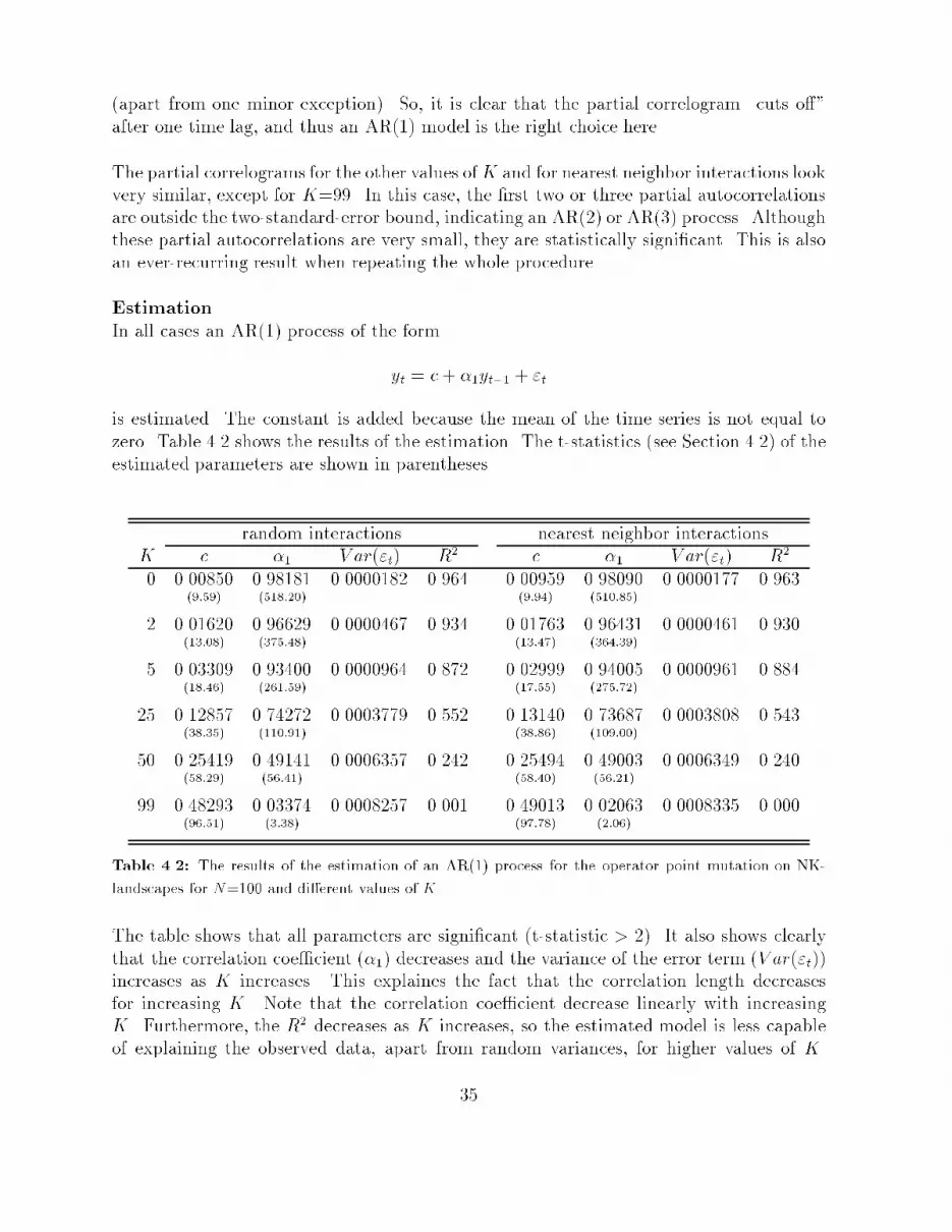
(apart from one minor exception). So, it is clear that the partial correlogram \cuts o�"after one time lag, and thus an AR(1) model is the right choice here.The partial correlograms for the other values ofK and for nearest neighbor interactions lookvery similar, except for K=99. In this case, the �rst two or three partial autocorrelationsare outside the two-standard-error bound, indicating an AR(2) or AR(3) process. Althoughthese partial autocorrelations are very small, they are statistically signi�cant. This is alsoan ever-recurring result when repeating the whole procedure.EstimationIn all cases an AR(1) process of the formyt = c+ �1yt�1 + "tis estimated. The constant is added because the mean of the time series is not equal tozero. Table 4.2 shows the results of the estimation. The t-statistics (see Section 4.2) of theestimated parameters are shown in parentheses.random interactions nearest neighbor interactionsK c �1 V ar("t) R2 c �1 V ar("t) R20 0.00850 0.98181 0.0000182 0.964 0.00959 0.98090 0.0000177 0.963(9:59) (518:20) (9:94) (510:85)2 0.01620 0.96629 0.0000467 0.934 0.01763 0.96431 0.0000461 0.930(13:08) (375:48) (13:47) (364:39)5 0.03309 0.93400 0.0000964 0.872 0.02999 0.94005 0.0000961 0.884(18:46) (261:59) (17:55) (275:72)25 0.12857 0.74272 0.0003779 0.552 0.13140 0.73687 0.0003808 0.543(38:35) (110:91) (38:86) (109:00)50 0.25419 0.49141 0.0006357 0.242 0.25494 0.49003 0.0006349 0.240(58:29) (56:41) (58:40) (56:21)99 0.48293 0.03374 0.0008257 0.001 0.49013 0.02063 0.0008335 0.000(96:51) (3:38) (97:78) (2:06)Table 4.2: The results of the estimation of an AR(1) process for the operator point mutation on NK-landscapes for N=100 and di�erent values of K.The table shows that all parameters are signi�cant (t-statistic > 2). It also shows clearlythat the correlation coe�cient (�1) decreases and the variance of the error term (V ar("t))increases as K increases. This explaines the fact that the correlation length decreasesfor increasing K. Note that the correlation coe�cient decrease linearly with increasingK. Furthermore, the R2 decreases as K increases, so the estimated model is less capableof explaining the observed data, apart from random variances, for higher values of K.35

The table, just as the correlograms, also shows no di�erence between random and nearestneighbor interactions.It appears that the estimated �1 and the R2 for K=99 are both very small. So, theestimated model for K = N � 1 is hardly any di�erent from an ordinary white noise seriesaround the mean of the series, which is, as said earlier, theoretically expected.Diagnostic checkingFigure 4.4 shows the �rst 25 residual autocorrelations for K=0 (random interactions).This plot shows that they are all well within the two-standard-error bound of 0.02 (apartfrom one minor exception). The plots for the other values of K and for nearest neighborinteractions look very similar.To make absolutely sure, an AR(2) model is estimated for all cases. The results arepresented in Table 4.3.random interactions nearest neighbor interactionsK �2 t-statistic �2 t-statistic0 0.00624 0.62 -0.00548 -0.552 -0.01104 -1.10 -0.01437 -1.445 -0.00716 -0.72 0.00642 0.6425 0.00526 0.53 0.00955 0.9650 0.00812 0.81 -0.00746 -0.7599 0.03189 3.19 0.04821 4.83Table 4.3: The results of the overestimation of the chosen model for di�erent values of K.As expected, the extra parameter is not signi�cantly di�erent from zero in all cases exceptfor K=99. This exception is not surprising, because the partial autocorrelations alreadysuggested an AR(2) or AR(3) process. But as noted above, the estimated parameters inthis model are very small (as well as the R2), and it e�ectively comes down to an ordinarywhite noise series. So, these two checks show that the chosen AR(1) model seems to beadequate in all cases, except for K=99.A �nal remark here, is that it is important to note that the time lag i between two valuesin the time series is not the same as the Hamming distance between two genotypes i stepsapart. Because a randomly chosen bit is ipped each step, the same bit can be ippedmore than once in a sequence of steps. Generating a random walk of length 10,000 withpoint mutation as operator, and calculating the average (normalized) Hamming distancebetween two genotypes i steps apart for 0 � i � 50, gives a result as shown in Figure 4.5.In this graph it can be seen that the Hamming distance increases less than linearly withthe time lag i. 36

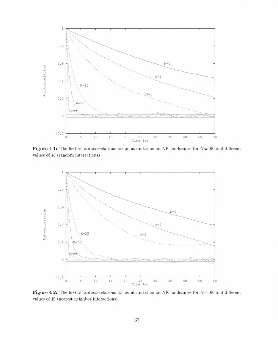
-0.2

0

0.2

0.4

0.6

0.8

1

0 5 10 15 20 25 30 35 40 45 50

Autocorrelation

Time lag

K=0

K=2

K=5

K=25

K=50

K=99Figure 4.1: The �rst 50 autocorrelations for point mutation on NK-landscapes for N=100 and di�erentvalues of K (random interactions).-0.2

0

0.2

0.4

0.6

0.8

1

0 5 10 15 20 25 30 35 40 45 50

Autocorrelation

Time lag

K=0

K=2

K=5K=25

K=50

K=99Figure 4.2: The �rst 50 autocorrelations for point mutation on NK-landscapes for N=100 and di�erentvalues of K (nearest neighbor interactions). 37

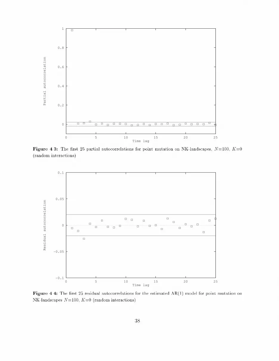
0

0.2

0.4

0.6

0.8

1

0 5 10 15 20 25

Partial autocorrelation

Time lagFigure 4.3: The �rst 25 partial autocorrelations for point mutation on NK-landscapes, N=100, K=0(random interactions).-0.1

-0.05

0

0.05

0.1

0 5 10 15 20 25

Residual autocorrelation

Time lagFigure 4.4: The �rst 25 residual autocorrelations for the estimated AR(1) model for point mutation onNK-landscapes N=100, K=0 (random interactions).38

0

0.05

0.1

0.15

0.2

0.25

0.3

0.35

0.4

0.45

0.5

0 5 10 15 20 25 30 35 40 45 50

Average Hamming distance

Number of stepsFigure 4.5: The average (normalized) Hamming distance of two genotypes i steps apart (0 � i � 50) ina random walk generated with point mutation.

39

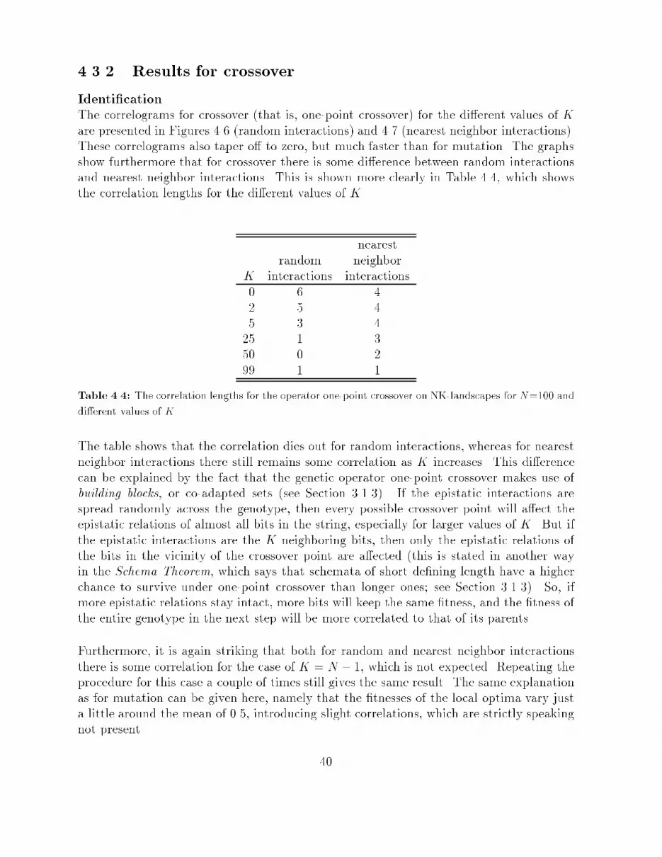
4.3.2 Results for crossoverIdenti�cationThe correlograms for crossover (that is, one-point crossover) for the di�erent values of Kare presented in Figures 4.6 (random interactions) and 4.7 (nearest neighbor interactions).These correlograms also taper o� to zero, but much faster than for mutation. The graphsshow furthermore that for crossover there is some di�erence between random interactionsand nearest neighbor interactions. This is shown more clearly in Table 4.4, which showsthe correlation lengths for the di�erent values of K.nearestrandom neighborK interactions interactions0 6 42 5 45 3 425 1 350 0 299 1 1Table 4.4: The correlation lengths for the operator one-point crossover on NK-landscapes for N=100 anddi�erent values of K.The table shows that the correlation dies out for random interactions, whereas for nearestneighbor interactions there still remains some correlation as K increases. This di�erencecan be explained by the fact that the genetic operator one-point crossover makes use ofbuilding blocks, or co-adapted sets (see Section 3.1.3). If the epistatic interactions arespread randomly across the genotype, then every possible crossover point will a�ect theepistatic relations of almost all bits in the string, especially for larger values of K. But ifthe epistatic interactions are the K neighboring bits, then only the epistatic relations ofthe bits in the vicinity of the crossover point are a�ected (this is stated in another wayin the Schema Theorem, which says that schemata of short de�ning length have a higherchance to survive under one-point crossover than longer ones; see Section 3.1.3). So, ifmore epistatic relations stay intact, more bits will keep the same �tness, and the �tness ofthe entire genotype in the next step will be more correlated to that of its parents.Furthermore, it is again striking that both for random and nearest neighbor interactionsthere is some correlation for the case of K = N � 1, which is not expected. Repeating theprocedure for this case a couple of times still gives the same result. The same explanationas for mutation can be given here, namely that the �tnesses of the local optima vary justa little around the mean of 0.5, introducing slight correlations, which are strictly speakingnot present. 40

Looking at the partial correlogram for K=0 (random interactions), as shown in Figure4.8, it can be concluded that an AR(1) process is the most appropriate model here too.The partial correlograms for the other values of K and for nearest neighbor interactionslook very similar, except for K=50, random interactions. In this case, all partial auto-correlations are within the two-standard-error bound, indicating that a white noise seriesaround the mean is the most appropriate model here. This is not surprising, because thecorrelation length is zero in this case, as Table 4.4 shows.EstimationAs with mutation, an AR(1) process with constant is estimated here. The results arepresented in Table 4.5 (t-statistics shown between parentheses).random interactions nearest neighbor interactionsK c �1 V ar("t) R2 c �1 V ar("t) R20 0.26140 0.50278 0.0003423 0.253 0.23012 0.50130 0.0003581 0.251(57:52) (58:21) (57:57) (57:93)2 0.31878 0.37191 0.0006060 0.138 0.26521 0.49274 0.0005581 0.243(67:56) (40:06) (58:21) (56:62)5 0.37223 0.26104 0.0007311 0.068 0.26929 0.45817 0.0006116 0.210(76:42) (27:04) (60:85) (51:54)25 0.47254 0.05400 0.0008388 0.003 0.35425 0.29229 0.0007491 0.085(94:56) (5:41) (73:87) (30:56)50 0.49038 0.01925 0.0008214 0.000 0.42640 0.14640 0.0008310 0.021(97:92) (1:92) (86:14) (14:80)99 0.48515 0.02921 0.0008209 0.001 0.48189 0.03048 0.0008354 0.001(96:95) (2:92) (96:84) (3:05)Table 4.5: The results of the estimation of an AR(1) process for one-point crossover on NK-landscapesfor N=100 and di�erent values of K.All parameters appear to be signi�cant, except for the �1 for K=50, random interactions(indicating again the absence of correlation in this case). The table also shows that theestimated value of �1 is larger for nearest neighbor interactions than for random interactionsfor 0 < K < N � 1 (for the two extremes of K=0 and K = N � 1 there is of course nodi�erence between random and nearest neighbor interactions, see page 12). This indicatesthat there is indeed more correlation for one-point crossover between two points one stepapart for in a landscape with nearest neighbor interactions, than in a landscape withrandom interactions. Also, the R2 is larger for nearest neighbor interactions for 0 < K <N � 1, which means that the estimated model has more explanatory and predictive valuethan it does for random interactions. For crossover too, the model for K=99 is hardlydistinguishable from ordinary white noise, considering the estimated value of �1 and R2.41

Diagnostic checkingFigure 4.9 shows the �rst 25 residual autocorrelations for K=0 (random interactions). Allare well within the two-standard-error bound. The plots for larger values of K and nearestneighbor interactions look very similar. Table 4.6 gives the results of the overestimation,the extra check on the adequacy of the chosen model. The table shows that all extraparameters are not signi�cantly di�erent from zero, indicating once more that the AR(1)model is adequate. random interactions nearest neighbor interactionsK �2 t-statistic �2 t-statistic0 0.00412 0.41 -0.00623 -0.622 0.01767 1.77 -0.00866 -0.875 0.01198 1.20 0.00613 0.6125 0.00013 0.01 0.01576 1.5850 0.00386 0.39 0.01270 1.3099 0.00284 0.28 0.00160 0.16Table 4.6: The results of the overestimation of the chosen model for crossover for di�erent values of K.The average (normalized) Hamming distance between parent and child in a random walkgenerated with one-point crossover will be 0.25. This can be argued as follows: Because asecond parent is chosen at random, on average half of the bits of the two parents will have adi�erent value. The crossover point will be, also on average, somewhere halfway, so eitherthe �rst half or the second half of the child will be equal to the �rst parent (remember thatone of the two children is selected at random). The other half of the child will come fromthe second parent, so about half the bits in this part will be di�erent from the �rst parent.As a result, about one quarter of the bits of the selected child will be di�erent from the�rst parent (which was the one used for continuing the random walk one step ago).The following simple example shows a situation where the Hamming distance between thetwo parents is 0.5, the crossover point is halfway the genotypes, and the Hamming distancebetween the child and the �rst parent is 0.25.parent 1: 0000|0000parent 2: 1010|1010---------------------child : 0000|1010Calculating the average Hamming distance between parent and child in a random walk oflength 10,000 generated with crossover, con�rms this result. Figure 4.10 gives the averageHamming distance of two genotypes i steps apart for 0 � i � 50.42

-0.2

0

0.2

0.4

0.6

0.8

1

0 1 2 3 4 5 6 7 8 9 10

Autocorrelation

Time lag

K=0

K=2

K=5

K=25K=50K=99Figure 4.6: The �rst 10 autocorrelations for crossover on NK-landscapes for N=100 and di�erent valuesof K (random interactions).

-0.2

0

0.2

0.4

0.6

0.8

1

0 1 2 3 4 5 6 7 8 9 10

Autocorrelation

Time lag

K=0

K=2

K=5

K=25K=50

K=99Figure 4.7: The �rst 10 autocorrelations for crossover on NK-landscapes for N=100 and di�erent valuesof K (nearest neighbor interactions). 43

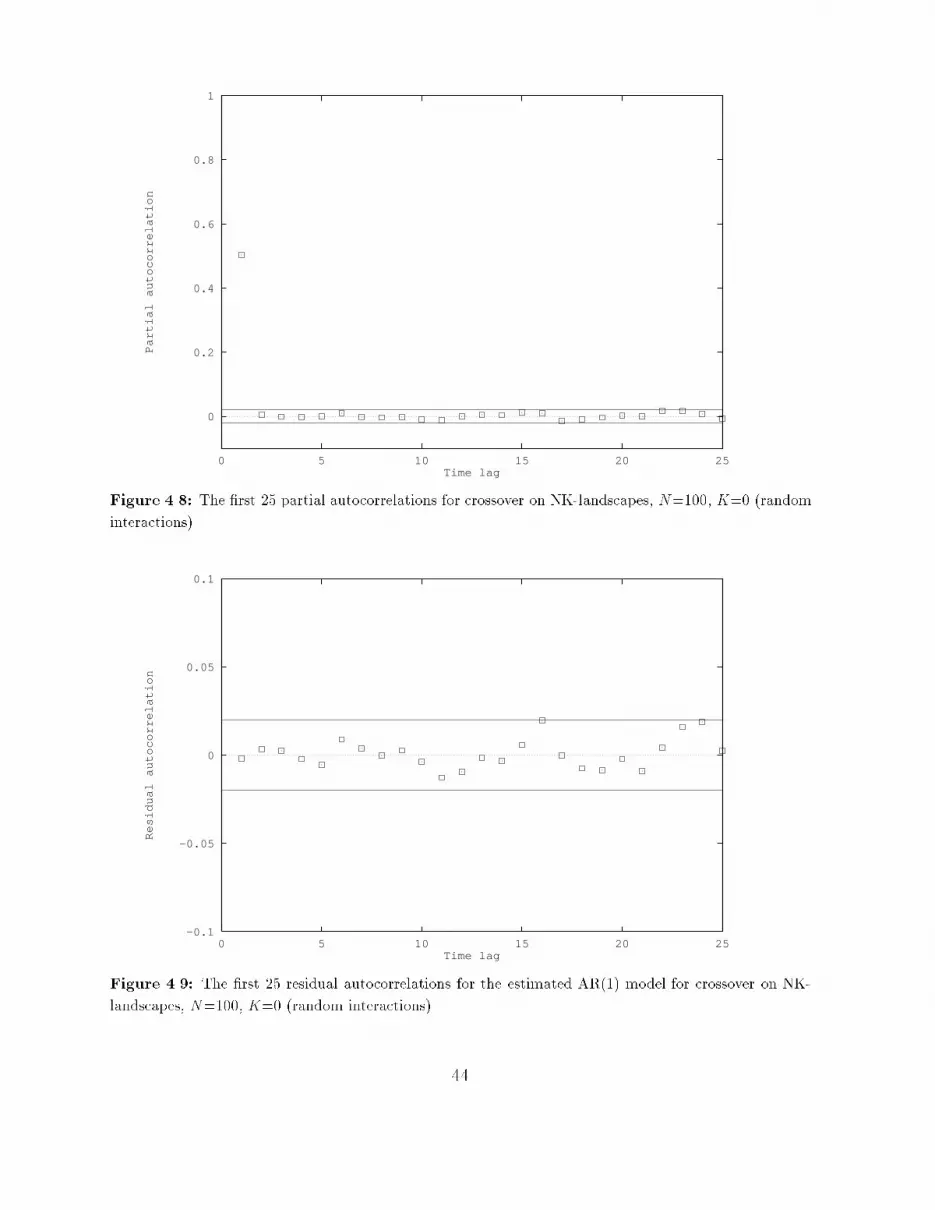
0

0.2

0.4

0.6

0.8

1

0 5 10 15 20 25

Partial autocorrelation

Time lagFigure 4.8: The �rst 25 partial autocorrelations for crossover on NK-landscapes, N=100, K=0 (randominteractions).-0.1

-0.05

0

0.05

0.1

0 5 10 15 20 25

Residual autocorrelation

Time lagFigure 4.9: The �rst 25 residual autocorrelations for the estimated AR(1) model for crossover on NK-landscapes, N=100, K=0 (random interactions). 44

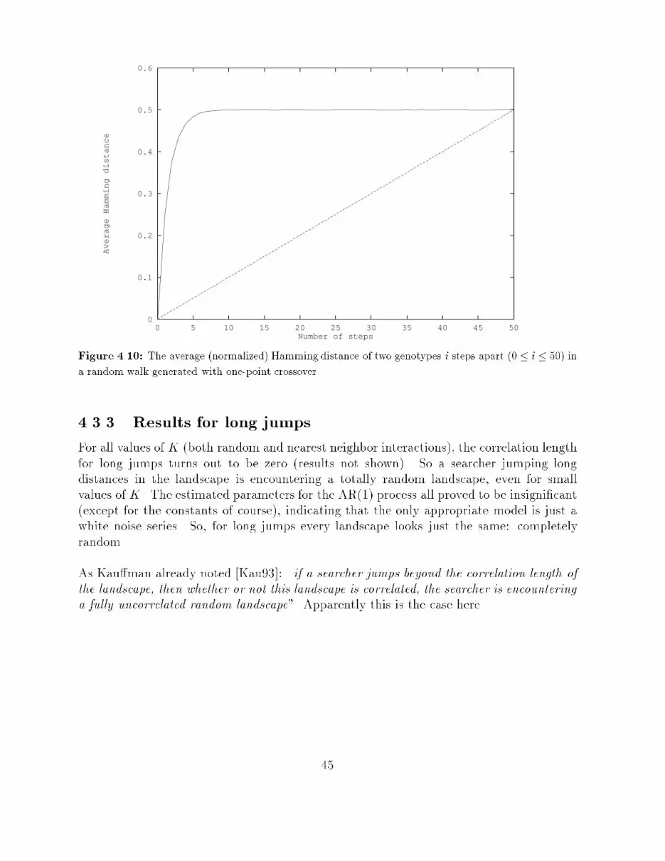
0

0.1

0.2

0.3

0.4

0.5

0.6

0 5 10 15 20 25 30 35 40 45 50

Average Hamming distance

Number of stepsFigure 4.10: The average (normalized) Hamming distance of two genotypes i steps apart (0 � i � 50) ina random walk generated with one-point crossover.4.3.3 Results for long jumpsFor all values of K (both random and nearest neighbor interactions), the correlation lengthfor long jumps turns out to be zero (results not shown). So a searcher jumping longdistances in the landscape is encountering a totally random landscape, even for smallvalues of K. The estimated parameters for the AR(1) process all proved to be insigni�cant(except for the constants of course), indicating that the only appropriate model is just awhite noise series. So, for long jumps every landscape looks just the same: completelyrandom.As Kau�man already noted [Kau93]: \if a searcher jumps beyond the correlation length ofthe landscape, then whether or not this landscape is correlated, the searcher is encounteringa fully uncorrelated random landscape". Apparently this is the case here.45

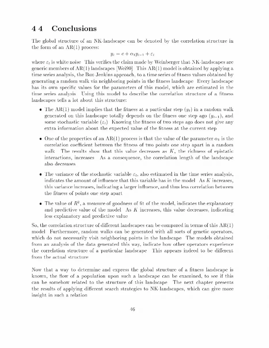
4.4 ConclusionsThe global structure of an NK-landscape can be denoted by the correlation structure inthe form of an AR(1) process: yt = c+ �1yt�1 + "twhere "t is white noise. This veri�es the claimmade by Weinberger that NK-landscapes aregeneric members of AR(1) landscapes [Wei90]. This AR(1) model is obtained by applying atime series analysis, the Box-Jenkins approach, to a time series of �tness values obtained bygenerating a random walk via neighboring points in the �tness landscape. Every landscapehas its own speci�c values for the parameters of this model, which are estimated in thetime series analysis. Using this model to describe the correlation structure of a �tnesslandscapes tells a lot about this structure:� The AR(1) model implies that the �tness at a particular step (yt) in a random walkgenerated on this landscape totally depends on the �tness one step ago (yt�1), andsome stochastic variable ("t). Knowing the �tness of two steps ago does not give anyextra information about the expected value of the �tness at the current step.� One of the properties of an AR(1) process is that the value of the parameter �1 is thecorrelation coe�cient between the �tness of two points one step apart in a randomwalk. The results show that this value decreases as K, the richness of epistaticinteractions, increases. As a consequence, the correlation length of the landscapealso decreases.� The variance of the stochastic variable "t, also estimated in the time series analysis,indicates the amount of in uence that this variable has in the model. AsK increases,this variance increases, indicating a larger in uence, and thus less correlation betweenthe �tness of points one step apart.� The value of R2, a measure of goodness of �t of the model, indicates the explanatoryand predictive value of the model. As K increases, this value decreases, indicatingless explanatory and predictive value.So, the correlation structure of di�erent landscapes can be compared in terms of this AR(1)model. Furthermore, random walks can be generated with all sorts of genetic operators,which do not necessarily visit neighboring points in the landscape. The models obtainedfrom an analysis of the data generated this way, indicate how other operators experiencethe correlation structure of a particular landscape. This appears indeed to be di�erentfrom the actual structure.Now that a way to determine and express the global structure of a �tness landscape isknown, the ow of a population upon such a landscape can be examined, to see if thiscan be somehow related to the structure of this landscape. The next chapter presentsthe results of applying di�erent search strategies to NK-landscapes, which can give moreinsight in such a relation. 46

Chapter 5Population FlowAdaptive evolution is a search process|driven by mutation, recombination, and selection|on a �tness landscape. An adapting population ows over the landscape under theseforces. So, to gain more insight into the population ow on �tness landscapes, it is usefulto apply di�erent search strategies|based on mutation, recombination, and selection|tosuch landscapes.This chapter presents the results of applying di�erent search strategies, as introduced inChapter 3, to di�erent NK-landscapes. The performance of these strategies is evaluated bythe performance measures also introduced in Chapter 3. First, the experimental setup isdescribed. Next, the strategies are evaluated by each of the performance measures. Finally,some conclusions are drawn, and the validity of Kau�man's statement about the three timescales in adaptation (see Section 1.1) is assessed.5.1 Experimental setupThe following search strategies (see Chapter 3 for the exact implementations) are appliedto di�erent NK-landscapes:� Random ascent hillclimbing with memory (RAHCM)� Random neighbor ascent hillclimbing (RNAHC)� Long jumps� Genetic Algorithm with one-point crossover (GA-ONEP)� Hybrid Genetic Algorithm (HGA)All strategies are allowed to do a total of 10,000 function evaluations. The di�erent per-formance measures are recorded every 50 function evaluations.47

NK-landscapes (see Chapter 2) with the following values for N and K are taken: N=100,K=0, 2, 5, 25, 50, and 99. In this chapter, only random interactions are considered.Furthermore, because an NK-landscape depends on randomly assigned �tness values, allresults are averaged over 100 runs, each run on a di�erent landscape but with the samevalues for N and K, to avoid statistical biases.The next four sections each evaluate the di�erent search strategies by one of the perfor-mance measures introduced in Chapter 3: maximum �tness, on-line performance, o�-lineperformance, and mean Hamming distance.5.2 Evaluation by maximum �tnessFigures 5.1 to 5.6 show the maximum�tness of the strategies plotted against the number offunction evaluations for the di�erent values of K. Note that for K=0 the Hybrid GeneticAlgorithm is not applied, because the HGA would not be di�erent from the RAHCMstrategy (remember this strategy is also applied within the HGA): all individuals willclimb to the one and only peak in the landscape, and crossover applied to a populationwith completely identical individuals makes no di�erence.In the next subsections, the results with respect to the maximum �tness are evaluated pertype of landscape.5.2.1 Smooth landscapes: K=0As Figure 5.1 shows, RAHCM �nds the (only) optimum quickly, while RNAHC takesmuch longer to �nd this optimum. This is due to the many function evaluations the latterstrategy has to do before it can step to a �tter neighbor: �rst, all neighbors are evaluated,and only then a �tter one is chosen. As the graph shows, this costs a lot of (wasted)evaluations.The strategy of Long jumps is very poor. In fact it is nothing more than just a randomsearch. Initially, it is able to �nd some �tter individuals quite quickly, but the more �tterindividuals are found, the longer it takes to �nd yet another one. Kau�man already showedthat there is a \universal law" for long jump adaptation: the waiting time to �nd a �tterindividual doubles each time one is found [Kau93]. So, it is not to be expected that thisstrategy will perform well.The maximum �tness in the GA-ONEP population increases steadily and quite fast, but itsomehow seems to be unable to catch up with the RAHCM strategy. To �nd out whetherthis is just a statistical di�erence or a real discrepancy, a two-sample test for comparingthe means of two stochastic variables is done. This test, using the mean and standarddeviation of the samples, is described in Appendix A. The mean (X) and the standard48

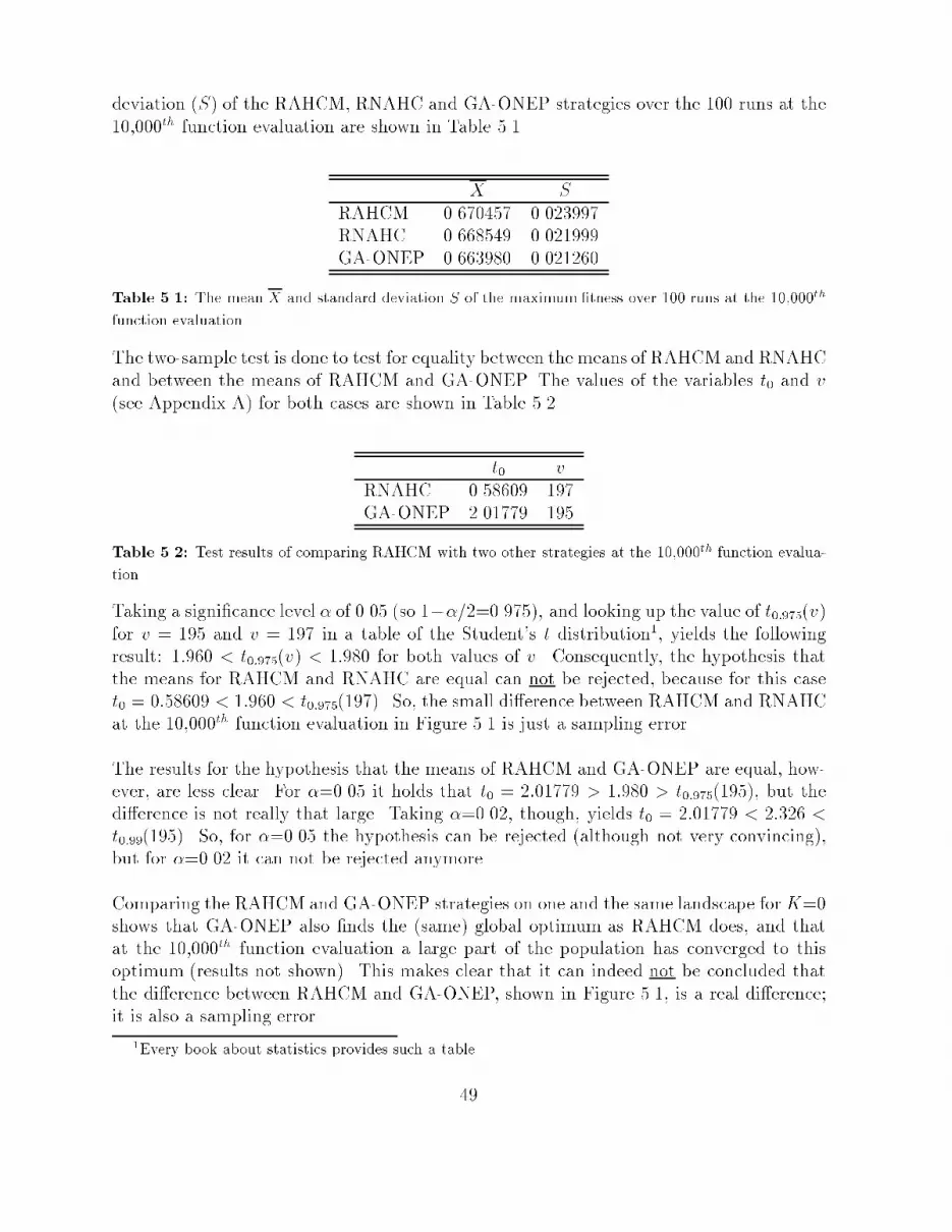
deviation (S) of the RAHCM, RNAHC and GA-ONEP strategies over the 100 runs at the10,000th function evaluation are shown in Table 5.1.X SRAHCM 0.670457 0.023997RNAHC 0.668549 0.021999GA-ONEP 0.663980 0.021260Table 5.1: The mean X and standard deviation S of the maximum �tness over 100 runs at the 10,000thfunction evaluation.The two-sample test is done to test for equality between the means of RAHCM and RNAHCand between the means of RAHCM and GA-ONEP. The values of the variables t0 and v(see Appendix A) for both cases are shown in Table 5.2.t0 vRNAHC 0.58609 197GA-ONEP 2.01779 195Table 5.2: Test results of comparing RAHCM with two other strategies at the 10,000th function evalua-tion.Taking a signi�cance level � of 0.05 (so 1��=2=0.975), and looking up the value of t0:975(v)for v = 195 and v = 197 in a table of the Student's t distribution1, yields the followingresult: 1:960 < t0:975(v) < 1:980 for both values of v. Consequently, the hypothesis thatthe means for RAHCM and RNAHC are equal can not be rejected, because for this caset0 = 0:58609 < 1:960 < t0:975(197). So, the small di�erence between RAHCM and RNAHCat the 10,000th function evaluation in Figure 5.1 is just a sampling error.The results for the hypothesis that the means of RAHCM and GA-ONEP are equal, how-ever, are less clear. For �=0.05 it holds that t0 = 2:01779 > 1:980 > t0:975(195), but thedi�erence is not really that large. Taking �=0.02, though, yields t0 = 2:01779 < 2:326 <t0:99(195). So, for �=0.05 the hypothesis can be rejected (although not very convincing),but for �=0.02 it can not be rejected anymore.Comparing the RAHCM and GA-ONEP strategies on one and the same landscape forK=0shows that GA-ONEP also �nds the (same) global optimum as RAHCM does, and thatat the 10,000th function evaluation a large part of the population has converged to thisoptimum (results not shown). This makes clear that it can indeed not be concluded thatthe di�erence between RAHCM and GA-ONEP, shown in Figure 5.1, is a real di�erence;it is also a sampling error.1Every book about statistics provides such a table49

So, GA-ONEP does indeed �nd the global optimum, but it takes longer to �nd it thanRAHCM does. On the other hand, it is much faster than RNAHC. These results, thata Genetic Algorithm is outperformed in speed by one speci�c type of hillclimbing, butis faster than other forms of hillclimbing on a smooth �tness landscape with only oneoptimum, is in accordance with results obtained in [MHF].5.2.2 Rugged landscapes: K=2, 5As Figures 5.2 and 5.3 show, it takes a little longer for RAHCM to �nd a good optimum onrugged landscapes than to �nd the global optimum on a smooth landscape, but even after10,000 function evaluations the maximum for RAHCM is still slowly increasing, so once ina while an even higher hilltop is found. The cost that RNAHC has to pay to choose a �tterneighbor is too much on rugged landscapes: after 10,000 function evaluations RNAHC isstill far behind on RAHCM. The strategy of Long jumps is again not better than just arandom search. The universal law for long jump adaptation is in force here too.The di�erence between GA-ONEP and RAHCM, compared with a smooth landscape,seems to be quite signi�cant on rugged landscapes. Testing the hypothesis that the meansover the 100 runs of these two search strategies are equal at the 10,000th function evaluation,gives the results shown in Table 5.3. t0 vK=2 3.58490 180K=5 12.42182 165Table 5.3: Test results of comparing RAHCM with GA-ONEP at the 10,000th function evaluation forK=2 and 5.Even at a signi�cance level � of 0.02, the hypothesis is rejected for both values of K. ForK=2 it holds that t0 = 3:58490 > 2:358 > t0:99(180), and for K=5 that t0 = 12:42182 >2:358 > t0:99(165). So, on rugged landscapes the di�erence is really signi�cant.It appears that GA-ONEP becomes trapped in a local region of the space where the�tnesses of the local optima are signi�cantly less than those of the highest optima in thelandscape. The crossover operator becomes less able to �nd the highest optima, becausethe correlation length for crossover is less on rugged landscapes than on smooth landscapes(see Section 4.3.2). Apparently, crossover is able to �nd a relatively good region in thelandscape initially, but it is unable to structurally �nd even better regions.The HGA, however, performs very well. It �nds good optima relatively fast, and is alsoable to hold the population there. This, of course, is due to the stringent selection, whichonly holds the best individuals in the population (see Section 3.1.4). It appears that in50

the �rst part of the search the HGA does at least as well as the RAHCM strategy, buteventually the HGA stays constant, while the RAHCM strategy keeps increasing, althoughvery slowly. Again an indication that crossover is not able to �nd better regions in thelandscape in the long run, when the population has already converged to an initially foundgood region.There is one striking feature about rugged landscapes: although the good optima are harderto �nd, they tend to be higher than the optimum in a smooth landscape. An explanationfor this is given in appendix B.5.2.3 Very rugged landscapes: K=25, 50Figures 5.4 and 5.5 show that the two hillclimbing strategies show the same trend on veryrugged landscapes as on rugged landscapes: it takes even longer to �nd good optima, and,during the rest of the search, better optima are found slowly. Also, RNAHC still has adisadvantage compared to RAHCM. Furthermore, Long jumps are again not very usefulfor �nding good optima.The GA-ONEP strategy still seems to be unable to reach better regions in the landscape inthe long run, and gets stuck in intermediate regions. Even the HGA, although keeping upwith RAHCM initially, gets stuck after a certain amount of evaluations. Crossover seemsto be unable here to �nd better hillsides in the long run, not surprisingly considering thevery low, or even absence of, correlation length for crossover on very rugged NK-landscapeswith random interactions (see Section 4.3.2).5.2.4 Completely random landscapes: K=99On a completely random landscape, as shown in Figure 5.6, RAHCM, RNAHC and Longjumps perform equally well. All three search strategies boil down to just a random search.It does not matter anymore whether small or large jumps are made, the time to �nd �tterindividuals is equally long.Crossover appears to have no use at all on completely random landscapes, considering theperformance of GA-ONEP and HGA. Information about the local structure at one place inthe landscape implies nothing about the local structure in another place. On a completelyrandom landscape, only random search is possible.51

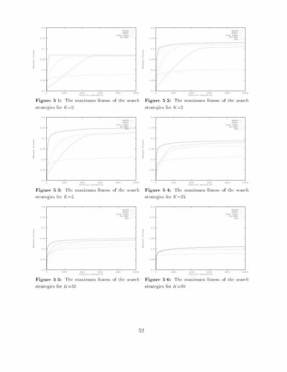
0.5

0.55

0.6

0.65

0.7

0.75

0.8

0 2000 4000 6000 8000 10000

Maximum fitness

Function evaluation

RAHCMRNAHC

Long jumpsGA-ONEP

Figure 5.1: The maximum �tness of the searchstrategies for K=0. 0.5

0.55

0.6

0.65

0.7

0.75

0.8

0 2000 4000 6000 8000 10000

Maximum fitness

Function evaluation

RAHCMRNAHC

Long jumpsGA-ONEP

HGA

Figure 5.2: The maximum �tness of the searchstrategies for K=2.0.5

0.55

0.6

0.65

0.7

0.75

0.8

0 2000 4000 6000 8000 10000

Maximum fitness

Function evaluation

RAHCMRNAHC

Long jumpsGA-ONEP

HGA

Figure 5.3: The maximum �tness of the searchstrategies for K=5. 0.5

0.55

0.6

0.65

0.7

0.75

0.8

0 2000 4000 6000 8000 10000

Maximum fitness

Function evaluation

RAHCMRNAHC

Long jumpsGA-ONEP

HGA

Figure 5.4: The maximum �tness of the searchstrategies for K=25.0.5

0.55

0.6

0.65

0.7

0.75

0.8

0 2000 4000 6000 8000 10000

Maximum fitness

Function evaluation

RAHCMRNAHC

Long jumpsGA-ONEP

HGA

Figure 5.5: The maximum �tness of the searchstrategies for K=50. 0.5

0.55

0.6

0.65

0.7

0.75

0.8

0 2000 4000 6000 8000 10000

Maximum fitness

Function evaluation

RAHCMRNAHC

Long jumpsGA-ONEP

HGA

Figure 5.6: The maximum �tness of the searchstrategies for K=99.52

5.3 Evaluation by on-line performanceThe on-line performance of a search strategy gives an overview of the average value of allfunction evaluations done by this strategy up to a certain time. A high on-line performancemeans that the strategy is evaluating mostly good individuals, while a very low on-lineperformance means that it is wasting too much time on bad individuals.On all landscapes, except the completely random one (K=99), the same sort of picturecan be seen, as Figures 5.7 to 5.11 show. RAHCM initially increases quickly, but staysconstant on an intermediate level for the rest of the search. This is due to the fact that eachtime an optimum is found, the search starts anew at a random point, and then graduallyclimbs up again. The high costs that RNAHC has to pay are shown here very clearly: theon-line performance increases very slowly and reaches only a moderate level. This showsagain that the RNAHC strategy pays too much compared to the gain in �tness it receives.That the strategy of Long jumps is really a random search, is shown by the fact that onall landscapes its on-line performance is exactly 0.5 throughout the search. So, on average,this strategy is evaluating just as much individuals that have a below-average �tness, asindividuals that have an above-average �tness. There is no direction at all in the search.A striking result is that, although GA-ONEP is not able to reach the highest peaks in(very) rugged landscapes, in the long run it outperforms all other strategies in on-lineperformance. So, it looks like GA-ONEP is a very e�cient strategy, but this may bea little misleading. More will be said about this when the strategies are evaluated bypopulation diversity.The HGA performs initially just as well as RAHCM, but after a while it suddenly starts tobecome more e�cient. This is the result of the stringent selection mechanism, which doesnot allow individuals that are less �t than the current members of the population to enterthis population. So, this HGA never \falls back" to less good regions of the landscape, asRAHCM does each time it starts the search anew at a random point.Completely random landscapes, shown in Figure 5.12, give a di�erent picture. Apparently,all strategies, except GA-ONEP, are \degraded" to just random search. Only GA-ONEPmanages to escape this fate, mainly due to its selection mechanism. The HGA strategyalso uses a (very strong) selection mechanism, but here every generation all the neighborsof each genotype in the population are evaluated by the hillclimbing part of the algorithm,which, as said in Section 5.2.4, is just a random search when the landscape is completelyrandom. 53

0.45

0.5

0.55

0.6

0.65

0.7

0.75

0.8

0 2000 4000 6000 8000 10000

On-line performance

Function evaluation

RAHCMRNAHC

Long jumpsGA-ONEP

Figure 5.7: The on-line performance of the searchstrategies for K=0. 0.45

0.5

0.55

0.6

0.65

0.7

0.75

0.8

0 2000 4000 6000 8000 10000

On-line performance

Function evaluation

RAHCMRNAHC

Long jumpsGA-ONEP

HGA

Figure 5.8: The on-line performance of the searchstrategies for K=2.0.45

0.5

0.55

0.6

0.65

0.7

0.75

0.8

0 2000 4000 6000 8000 10000

On-line performance

Function evaluation

RAHCMRNAHC

Long jumpsGA-ONEP

HGA

Figure 5.9: The on-line performance of the searchstrategies for K=5. 0.45

0.5

0.55

0.6

0.65

0.7

0.75

0.8

0 2000 4000 6000 8000 10000

On-line performance

Function evaluation

RAHCMRNAHC

Long jumpsGA-ONEP

HGA

Figure 5.10: The on-line performance of thesearch strategies for K=25.0.45

0.5

0.55

0.6

0.65

0.7

0.75

0.8

0 2000 4000 6000 8000 10000

On-line performance

Function evaluation

RAHCMRNAHC

Long jumpsGA-ONEP

HGA

Figure 5.11: The on-line performance of thesearch strategies for K=50. 0.45

0.5

0.55

0.6

0.65

0.7

0.75

0.8

0 2000 4000 6000 8000 10000

On-line performance

Function evaluation

RAHCMRNAHC

Long jumpsGA-ONEP

HGA

Figure 5.12: The on-line performance of thesearch strategies for K=99.54

5.4 Evaluation by o�-line performanceFigures 5.13 to 5.18 show the o�-line performance of the strategies on all six landscapes.In the o�-line performance, the best �tness found up to a certain time is averaged, so thisis independent of the �tness of the individuals in the population at that time.The general picture of the o�-line performance shows not much di�erence with that ofthe maximum �tness, so it does not contribute any new information. It once more showsthat RNAHC converges much too slow to an optimum, and that the Genetic Algorithmis outperformed in speed by the strong hillclimbing scheme RAHCM on smooth �tnesslandscapes.5.5 Evaluation by mean Hamming distanceTo gain more insight into the diversity of a population during the search, the mean Ham-ming distance for the population-based strategies is shown in Figures 5.19 to 5.24.The members in the population of long jumpers do not converge at all, except a little forthe smooth (K=0) landscape. In such a landscape there is only one hill, so every jump toa �tter individual brings the members of the population a little closer to the one and onlyoptimum, and thus a little closer to each other.The GA-ONEP population, however, converges rather quickly (except on a completelyrandom landscape). After some time, the members of the population di�er, on average, injust one or two bits. The population then becomes a tight cluster in the �tness landscape.This partly explains the seemingly e�cient behavior of GA-ONEP that can be observed inthe on-line performance (see Section 5.3): GA-ONEP is doing a lot of the same, \relativelygood", function evaluations, because the members of the population are stuck in a smallregion of intermediate optima in the �tness landscape. This strong convergence couldindicate that either the selection pressure is too high or that the mutation rate is too low,or maybe both.By contrast, the HGA population is hardly converging. This shows that, although crossoveris applied, all individuals are climbing di�erent hillsides. Only for K=2, the populationconverges to some extent. This is due to a special structure that appears to exist in theselandscapes, called a massif central. This feature is discussed in the next chapter.55

0.5

0.55

0.6

0.65

0.7

0.75

0.8

0 2000 4000 6000 8000 10000

Off-line performance

Function evaluation

RAHCMRNAHC

Long jumpsGA-ONEP

Figure 5.13: The o�-line performance of thesearch strategies for K=0. 0.5

0.55

0.6

0.65

0.7

0.75

0.8

0 2000 4000 6000 8000 10000

Off-line performance

Function evaluation

RAHCMRNAHC

Long jumpsGA-ONEP

HGA

Figure 5.14: The o�-line performance of thesearch strategies for K=2.0.5

0.55

0.6

0.65

0.7

0.75

0.8

0 2000 4000 6000 8000 10000

Off-line performance

Function evaluation

RAHCMRNAHC

Long jumpsGA-ONEP

HGA

Figure 5.15: The o�-line performance of thesearch strategies for K=5. 0.5

0.55

0.6

0.65

0.7

0.75

0.8

0 2000 4000 6000 8000 10000

Off-line performance

Function evaluation

RAHCMRNAHC

Long jumpsGA-ONEP

HGA

Figure 5.16: The o�-line performance of thesearch strategies for K=25.0.5

0.55

0.6

0.65

0.7

0.75

0.8

0 2000 4000 6000 8000 10000

Off-line performance

Function evaluation

RAHCMRNAHC

Long jumpsGA-ONEP

HGA

Figure 5.17: The o�-line performance of thesearch strategies for K=50. 0.5

0.55

0.6

0.65

0.7

0.75

0.8

0 2000 4000 6000 8000 10000

Off-line performance

Function evaluation

RAHCMRNAHC

Long jumpsGA-ONEP

HGA

Figure 5.18: The o�-line performance of thesearch strategies for K=99.56

0

0.1

0.2

0.3

0.4

0.5

0 1000 2000 3000 4000 5000 6000 7000 8000 9000 10000

Mean Hamming distance

Function evaluation

Long jumpsGA-ONEP

Figure 5.19: The mean Hamming distance of thesearch strategies for K=0. 0

0.1

0.2

0.3

0.4

0.5

0 1000 2000 3000 4000 5000 6000 7000 8000 9000 10000

Mean Hamming distance

Function evaluation

Long jumpsGA-ONEP

HGA

Figure 5.20: The mean Hamming distance of thesearch strategies for K=2.0

0.1

0.2

0.3

0.4

0.5

0 1000 2000 3000 4000 5000 6000 7000 8000 9000 10000

Mean Hamming distance

Function evaluation

Long jumpsGA-ONEP

HGA

Figure 5.21: The mean Hamming distance of thesearch strategies for K=5. 0

0.1

0.2

0.3

0.4

0.5

0 1000 2000 3000 4000 5000 6000 7000 8000 9000 10000

Mean Hamming distance

Function evaluation

Long jumpsGA-ONEP

HGA

Figure 5.22: The mean Hamming distance of thesearch strategies for K=25.0

0.1

0.2

0.3

0.4

0.5

0 1000 2000 3000 4000 5000 6000 7000 8000 9000 10000

Mean Hamming distance

Function evaluation

Long jumpsGA-ONEP

HGA

Figure 5.23: The mean Hamming distance of thesearch strategies for K=50. 0

0.1

0.2

0.3

0.4

0.5

0 1000 2000 3000 4000 5000 6000 7000 8000 9000 10000

Mean Hamming distance

Function evaluation

Long jumpsGA-ONEP

HGA

Figure 5.24: The mean Hamming distance of thesearch strategies for K=99.57

5.6 ConclusionsFirst, the general conclusions about population ow that can be drawn from the results aregiven. Next, the validity of Kau�man's statement about the three time scales in adaptationon rugged �tness landscapes is assessed. After that, some implications that follow fromthe conclusions are discussed. Finally, a summary of the main conclusions is given.5.6.1 General conclusionsThe �ve search strategies that are applied to NK-landscapes all show a di�erent type ofbehavior. Next, a summary of their performance is given:� As already observed in Section 3.1.1, it indeed matters which type of hillclimbing isused. RAHCM appears to work very well on all types of landscapes, from smoothto completely random. On the other hand, RNAHC is much too slow in �nding�tter individuals. Hillclimbing is not a really \e�cient" strategy, because it spendsa substantial amount of evaluations on less �t individuals, but it is able to �nd goodoptima quite fast.� Long jumps is nothing more than just a random search, which only works well oncompletely random landscapes. As Kau�man already showed, there exists a universallaw for Long jumps: the time to �nd a �tter individual doubles each time one is found.� The Genetic Algorithm is able to �nd a relatively good region in the �tness landscapeinitially, but in the long run the population converges and gets stuck in such a region,preventing still better regions to be found. It seems to be a very e�cient algorithm,but this is merely due to this strong convergence property. The more rugged alandscape becomes, the less useful crossover will be due to the lack of correlation forthis operator.� The Hybrid Genetic Algorithm performs very well on most landscapes, but eventuallygets stuck on local optima just below the highest peaks in the landscape. For thisalgorithm too, crossover becomes less useful on more rugged landscapes.Local search (like hillclimbing) is useful on all types of landscapes, but the speed at which�tter individuals are found depends on the exact implementation of the local search strat-egy. A local search strategy makes use of information from neighboring points in thelandscape to direct the search to a nearby hilltop. Since for almost all types of landscapes(except for completely random landscapes) there exists correlation between the �tness ofneighboring points (see Section 4.3.1), this strategy works very well. On completely ran-dom landscapes, the local search itself just comes down to a random search, which is theonly possibility on these types of landscapes.58

Global search (like crossover), on the other hand, appears to be most useful on smoothand not-too-rugged landscapes (K=0, 2, 5). On these landscapes, operators like one-pointcrossover experience enough correlation between the �tness of parents and o�spring (seeSection 4.3.2) to direct the search to a relatively good region in the landscape. Once sucha good region has been found, however, local search (like mutation, or hillclimbing) hasto \�ne tune" the population to the highest peaks within this region; global search likecrossover is not able to do this by itself.So, global search should always be combined with local search, but also with some formof selection, to prevent this global search to become just a random search (only the bestindividuals should be used to direct the global search). Using a form of selection, however,restricts the evolvability of a population: once a relatively good region in the landscape isfound, selection will tend to keep the population on the peaks within this region, preventingother, maybe better, regions to be found.In [Kau93] it is stated that: \Whether both evolvability and sustained �tness can be jointlyoptimized is unclear". The results obtained in this chapter for the Genetic Algorithm cannot give a positive answer to this question. The (strong) selection ensures sustained �tness,but limits evolvability. On the other hand, when the individual runs are considered, it ap-pears that sometimes a better individual is found which cannot be kept in the population(results not shown). When the selection becomes weaker, or the mutation rate becomeshigher, this will happen more often, thus threatening sustained �tness in favor of evolvabil-ity. In this case, the error catastrophe will occur (selection is not able to hold the adaptingpopulation on the highest peaks; see page 13). So, it will be di�cult, if not impossible,to �nd a good selection pressure together with a good mutation rate that avoids both theerror catastrophe and premature convergence on rugged �tness landscapes.Random search (like Long jumps) appears to work well on completely random landscapesonly. Not surprisingly considering the fact that long jump adaptation experiences nocorrelation at all on a �tness landscape, no matter what the actual correlation structure ofthis landscape is (see Section 4.3.3). Random search can probably be useful in combinationwith global search, for example when a population becomes stuck on the peaks of oneparticular region in a �tness landscape. Long jumps can then be helpful in �nding otherregions in the landscape that might contain even higher peaks.5.6.2 Time scales in adaptationKau�man identi�es three natural time scales in adaptation on rugged �tness landscapes[Kau93]:1. Initially, �tter individuals are found faster by long jumps than by local search. How-ever, the waiting time to �nd such �tter individuals doubles each time one is found.59

2. Therefore, in the midterm, adaptation �nds nearby �tter individuals faster thandistant �tter individuals and hence climbs a local hill in the landscape. But the rateof �nding �tter nearby individuals �rst dwindles and then stops as a local optimumis reached.3. On the longer time scale, the process, before it can proceed, must await a successfullong jump to a better hillside some distance away.So, Kau�man states that initially long jumps �nd �tter individuals faster than local searchdoes. He used RNAHC as local search strategy, which is indeed slower than long jumps(see Figures 5.1 to 5.6). However, it was already stated in Section 3.1.1, that in comparingother search strategies with hillclimbing, it matters which type of hillclimbing algorithm isused. This statement is clearly validated by the results obtained in this chapter. It appearsthat, taking RAHCM as local search strategy, the �rst time scale does not hold anymore.(see again Figures 5.1 to 5.6).Furthermore, there seems to be no directional search in Kau�man's �rst phase. Distantpoints are tried at random in the hope that one of them will have a higher �tness than thecurrent highest �tness in the population. But as the results in this chapter show, directedglobal search can be very useful in �nding good regions in the landscape initially.The general picture about the ow of a population on a �tness landscape that the resultsobtained in this chapter provide, looks more like a process of only two time scales, orphases, in adaptation:1. Initially, a relatively good region in the landscape is found by a (directed) globalsearch.2. On the longer time scale, local search has to \�ne tune" the adapting population by�nding the best peaks within this relatively good region.So, the results presented here do not support Kau�man's statement about three time scalesin adaptation, but imply an adjusted one that incorporates only two time scales, or phases.5.6.3 Some implicationsDi�erent implications follow from the above conclusions, depending on what point of viewis taken. From the viewpoint of problem solving, the main interest is in �nding a goodsolution for a problem as fast as possible. A strong hillclimbing algorithm appears toperform this task quite well on all types of landscapes. A global search strategy (forexample crossover) combined with a local strategy (for example hillclimbing) works welltoo, but mainly on not-too-rugged landscapes, on which there is still enough correlationexperienced by the global search operator. 60

In using a Genetic Algorithm for problem solving, a good balance has to be found betweenevolvability and sustained �tness, that is, between mutation rate and selection pressure.A mutation rate that is too low compared to the selection pressure causes prematureconvergence, while a mutation rate that is too high compared to the selection pressuregives rise to the error-catastrophe. Furthermore, a GA on its own is probably not powerfulenough to �nd the best solutions, but several studies indicate that using problem-speci�cinformation in the algorithm can enhance its performance substantially (see for example[ERR94, MHF]).From a biological viewpoint, more care has to be taken in �nding valid implications. Notall search strategies are biologically plausible. In the RAHCM strategy for example, noneighbor is evaluated more than once, while in the RNAHC strategy, all neighbors areevaluated at each step. In Nature, something in between happens: some, but not nec-essarily all, neighbors are evaluated, some of which even more than once. The GeneticAlgorithm is a rather plausible model of a real adapting population, and even the strategyof the Hybrid Genetic Algorithm occurs in Nature (see [MS93]). The Elitist Recombinationoperator, however, is rather arti�cial (usually, parents do not throw away their children ifthey appear to be less �t, whatever that means, than they are themselves).Another simpli�cation in the experiments done here, compared to Nature, is that the �tnesslandscape stays �xed during the search, or evolution. In Nature, the environment (whichdetermines the �tness landscape) is constantly changing, as a result of this evolution. Butopposed to these drawbacks, the advantage of using evolutionary models is that some basicaspects of evolution can be isolated and studied in detail, which is much more di�cult inNature itself. So, it will still be possible to derive some biologically plausible implicationsfrom the results presented in this chapter.One of these implications follows from the result that crossover is most useful on not-too-rugged landscapes. The more complex organisms in Nature, including humans, reproducesexually, which involves the crossing over of the genetic material of both parents. It shouldtherefore be expected that the �tness landscapes on which these organisms evolve arenot-too-rugged, allowing this crossover to be useful in the evolution. This means thatthe amount of epistatic interactions is relatively small, compared with the length of thegenotypes (in the order of 0.05N for example,N being the length of the genotype). On suchlandscapes, crossover still experiences enough correlation to be able to �nd good regionsin these landscapes.Another implication is, that a population or a species should keep some evolvability withinthe population or species. Otherwise, there is a danger of becoming trapped inside a smallregion of the landscape, having lost the ability to �nd other, maybe better, regions. If aspecies is no longer able to escape from such a small region in the landscape, this speciesmight become extinct. Nature seems to have found some solutions against this danger, forexample by trying to avoid inbreeding. 61

A �nal implication is, that a lot can still be learned from Nature. The models and searchstrategies, as used in this thesis, do not by a long way reach the complexity that can beseen in Nature itself. There still has to be done a lot of work for a complete understandingof the processes that drive the ow of a population on a �tness landscape.5.6.4 SummaryLocal search (like Hillclimbing) is useful on all types of landscapes, while global search (likecrossover) is most useful on smooth and not-too-rugged landscapes. Global search is ableto �nd a relatively good region in the landscape initially, but it is unable to \�ne tune" apopulation to the highest peaks within this region. Therefore, global search should alwaysbe combined with local search.The simultaneous optimization of evolvability and sustained �tness remains a problem.Selection should be strong enough to ensure sustained �tness, but not too strong, becausethis limits evolvability. The results of this chapter can not give a de�nitive answer towhether, or how, this problem can be solved.The three times scales Kau�man identi�es in an adaptive search, are not supported by theresults of this chapter. Instead, a picture of only two time scales, or phases, in an adaptivesearch emerges. First, a relatively good region in the �tness landscape is found by globalsearch. In the second phase, local search �nds the highest peaks within this region.In this chapter, only NK-landscapes with random interactions are considered, because thisis the most general case. In fact, for most operators, like mutation and long jumps, itdoes not make any di�erence whether the epistatic interactions are randomly distributedor nearby. Only for operators that make use of recombination, like crossover, there isa di�erence. Therefore, the next chapter examines more thoroughly the usefulness ofrecombination in these di�erent circumstances.62

Chapter 6The Usefulness of RecombinationIn the previos chapter it was concluded that crossover, a form of recombination, is mostuseful on not-too-rugged landscapes, that is, landscapes with low epistasis. When thelandscape becomes more rugged, the usefulness of crossover decreases. One explanationfor this, is the small, or even absence of, correlation for crossover on very rugged landscapes.In this chapter, the usefulness of recombination is examined more thoroughly. First, the re-lation between the type of recombination that is used and the type of epistatic interactionson the �tness landscape is examined. Next, the usefulness of recombination in relation tothe location of optima in the �tness landscape is examined. Finally, the conclusions thatare drawn from the examination of these two relations are summarized, and the validity ofKau�man's statement about the usefulness of recombination (see Section 1.1) is assessed.6.1 Crossover disruptionAccording to the building block hypothesis, a Genetic Algorithm works well when short,low-order, highly �t schemata (building blocks) are recombined to form even more highly�t higher-order schemata (see Section 3.1.3). So, a GA works well when crossover is ableto recombine building blocks to longer, higher-order schemata with a high �tness. On theother hand, it follows from the Schema Theorem that long, high-order schemata are morea�ected by crossover disruption than short, low-order ones (see also Section 3.1.3). So,opposed to the usefulness of crossover in constructing longer, highly �t schemata, there isthe danger of disrupting them again.To investigate this construction-disruption duality, two types of crossover, one-point anduniform (see Section 3.1.3), are compared on �tness landscapes with di�erent types ofepistatic interactions, random and nearest neighbor. Uniform crossover is believed to bemaximally disruptive, while one-point crossover is more conservative. But this dependshighly on the type of epistatic interactions within a genotype, or bit string.63

One-point crossover is more disruptive when the epistatic interactions in a genotype arerandomly distributed than when they are the nearest neighbors: with random interactionsalmost every possible crossover point will a�ect the epistatic relations of almost all bits ina bit string, while with nearest neighbor interactions only the epistatic relations of the bitsin the vicinity of the crossover point are a�ected. This is shown in Section 4.3.2 by thefact that one-point crossover has a larger correlation coe�cient on landscapes with nearestneighbor interactions than on landscapes with random interactions.With uniform crossover, however, there is a large chance that a good con�guration ofneighboring epistatically interacting bits will be disrupted. On the other hand, when theepistatic interactions are random, uniform crossover can recombine good values for theseinteracting bits, while one-point crossover is unable to do this.Next, the experimental setup for examining the relation between the type of recombinationthat is used and the type of epistatic interactions on the �tness landscape is described,after which the results of the experiments are presented.6.1.1 Experimental setupTwo Genetic Algorithms, having di�erent crossover operators, are applied to di�erent NK-landscapes (see Section 3.1.3 for the exact implementations of the GA's) :� A GA with one-point crossover (GA-ONEP)� A GA with uniform crossover (GA-UNIF)The GA's have exactly the same implementation, except for their crossover methods. BothGA's are allowed to do a total of 10,000 function evaluations. Every 50 function evaluations(that is, every generation), the maximum �tness in the population is recorded.NK-landscapes with the following values for N and K are taken: N=100, K=0, 2, 5, 25,50, and 99. Both random and nearest neighbor interactions are considered. All results areaveraged over 100 runs, each run on a di�erent landscape, but with the same values for Nand K.6.1.2 ResultsFigures 6.1 to 6.6 show the results of applying the two GA's to the di�erent NK-landscapes.The abbreviation RND stands for random interactions, while NNI stands for nearest neigh-bor interactions. So, GA-ONEP (RND) means the Genetic Algorithm with one-pointcrossover applied to an NK-landscape with random epistatic interactions. Note that forK=0 and K=99 only random interactions are considered, because nearest neighbor inter-actions is exactly the same as random interactions for these values of K (see Section 2.3.1).64

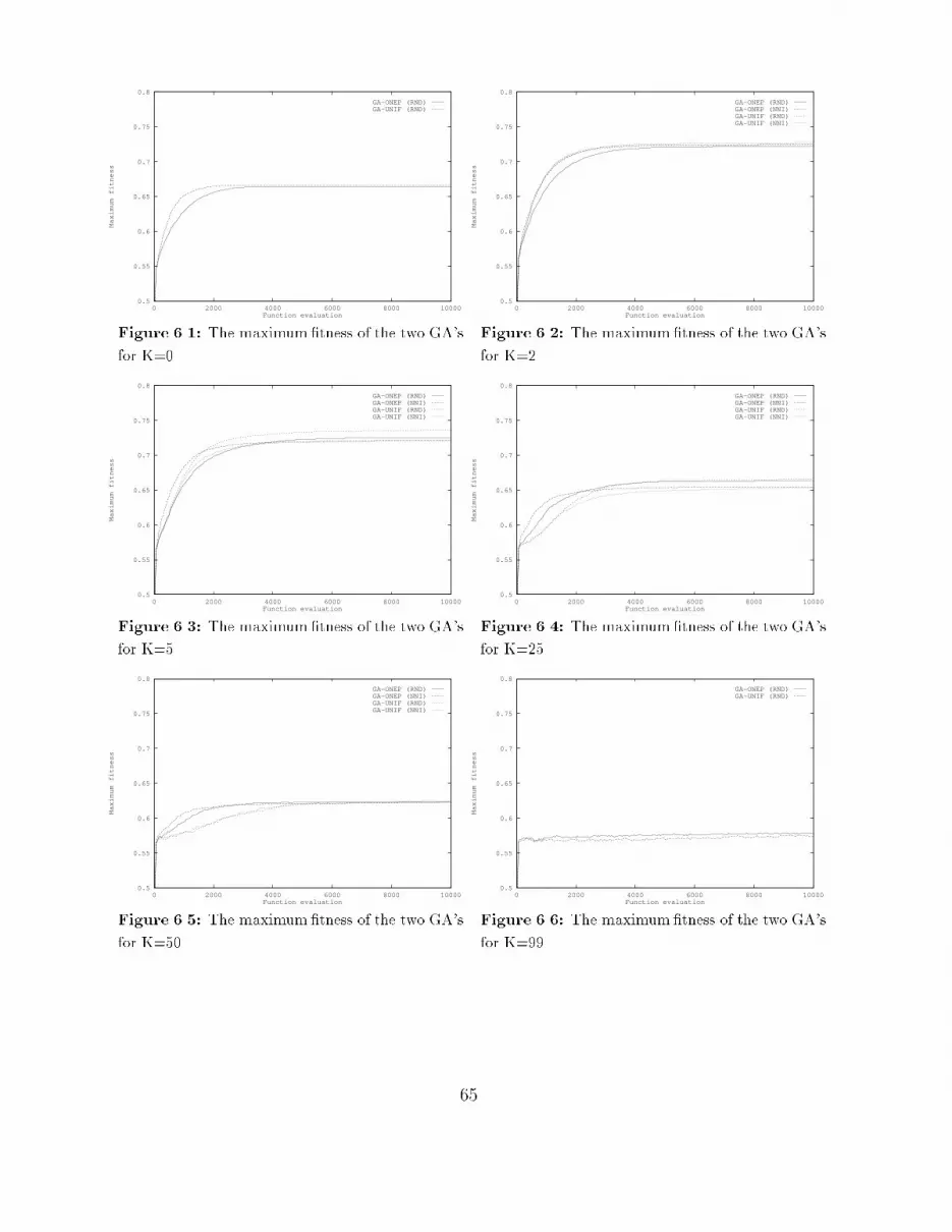
0.5

0.55

0.6

0.65

0.7

0.75

0.8

0 2000 4000 6000 8000 10000

Maximum fitness

Function evaluation

GA-ONEP (RND)GA-UNIF (RND)

Figure 6.1: The maximum�tness of the two GA'sfor K=0. 0.5

0.55

0.6

0.65

0.7

0.75

0.8

0 2000 4000 6000 8000 10000

Maximum fitness

Function evaluation

GA-ONEP (RND)GA-ONEP (NNI)GA-UNIF (RND)GA-UNIF (NNI)

Figure 6.2: The maximum�tness of the two GA'sfor K=2.0.5

0.55

0.6

0.65

0.7

0.75

0.8

0 2000 4000 6000 8000 10000

Maximum fitness

Function evaluation

GA-ONEP (RND)GA-ONEP (NNI)GA-UNIF (RND)GA-UNIF (NNI)

Figure 6.3: The maximum�tness of the two GA'sfor K=5. 0.5

0.55

0.6

0.65

0.7

0.75

0.8

0 2000 4000 6000 8000 10000

Maximum fitness

Function evaluation

GA-ONEP (RND)GA-ONEP (NNI)GA-UNIF (RND)GA-UNIF (NNI)

Figure 6.4: The maximum�tness of the two GA'sfor K=25.0.5

0.55

0.6

0.65

0.7

0.75

0.8

0 2000 4000 6000 8000 10000

Maximum fitness

Function evaluation

GA-ONEP (RND)GA-ONEP (NNI)GA-UNIF (RND)GA-UNIF (NNI)

Figure 6.5: The maximum�tness of the two GA'sfor K=50. 0.5

0.55

0.6

0.65

0.7

0.75

0.8

0 2000 4000 6000 8000 10000

Maximum fitness

Function evaluation

GA-ONEP (RND)GA-UNIF (RND)

Figure 6.6: The maximum�tness of the two GA'sfor K=99.65

The graphs clearly show the two phases in an adaptive search that are identi�ed in Chap-ter 5: the �rst phase consists of �nding a good region in the �tness landscape by globalsearch, and the second phase consists of trying to �nd the highest peaks within this regionby local search. Initially, the graphs are increasing rapidly (the �rst phase), but then theybecome gradually less steep (the second phase) until they are completely smooth, indi-cating that the highest peaks in a relatively good region are found. Only the completelyrandom landscape (K=99, Figure 6.6) does not �t into this picture, because global searchis useless on this landscape. Therefore, the case of K=99 is left out of the rest of theanalysis.Since the second phase in the search is dominated by local search, only the performance inthe �rst phase of the search is evaluated here to examine the usefulness of recombination.Di�erences in performance in the second phase are mainly a re ection of di�erences inperformance in this �rst phase. Furthermore, the results are viewed in two ways: takingone type of GA and comparing random with nearest neighbor interactions, and taking onetype of epistatic interactions and comparing GA-ONEP with GA-UNIF.Table 6.1 presents the results from the �rst viewpoint. It shows for both types of GA's onwhich type of landscape (that is, with random interactions (RND) or with nearest neighborinteractions (NNI)) they are better able to �nd a good region in the landscape in the �rstphase of the search. \Better able" means either �nding such a region faster, or �ndinga better region (that is, containing higher peaks), or sometimes both. An X means thatthere is no di�erence between the two interactions.K=0 K=2 K=5 K=25 K=50GA-ONEP - NNI NNI NNI/RND NNIGA-UNIF - X RND RND XTable 6.1: Comparison of random interactions (RND) with nearest neighbor interactions (NNI) for GA-ONEP and GA-UNIF in the �rst phase of the search. An entry RND means that the GA works betteron a landscape with random interactions than on a landscape with nearest neighbor interactions. An Xmeans that there is no di�erence.The table shows that one-point crossover (GA-ONEP) works better on a landscape withnearest neighbor interactions than on a landscape with random interactions. So, one-pointcrossover is better able to combine con�gurations of nearby interacting bits (without dis-rupting them too much again), than con�gurations of random interactions. The entryNNI/RND for K=25 re ects the fact that the graph of GA-ONEP is initially increasingfaster for landscapes with nearest neighbor interactions, but is overtaken by random inter-actions, for which it eventually �nds a better region (that is, containing higher peaks), ascan be seen in Figure 6.4. 66

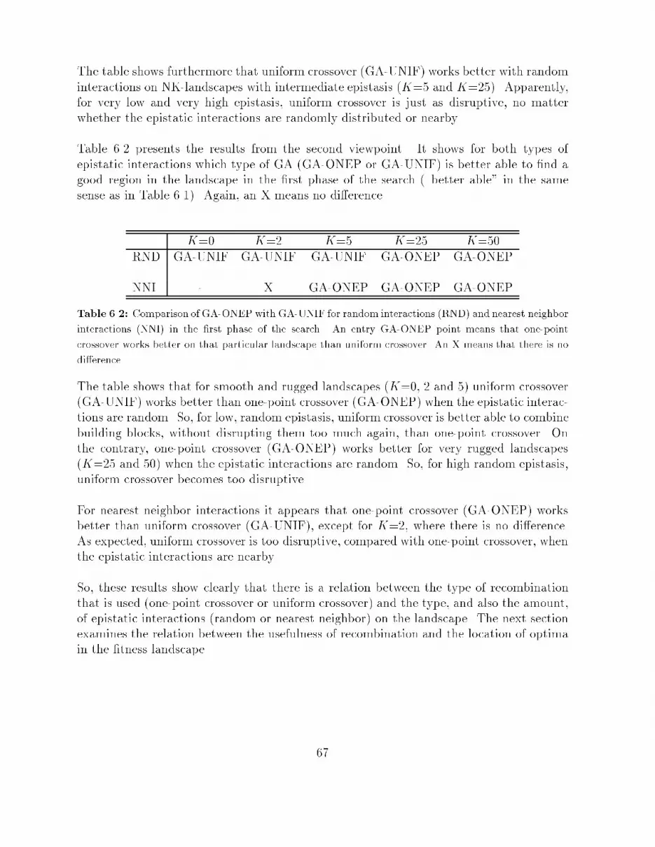
The table shows furthermore that uniform crossover (GA-UNIF) works better with randominteractions on NK-landscapes with intermediate epistasis (K=5 and K=25). Apparently,for very low and very high epistasis, uniform crossover is just as disruptive, no matterwhether the epistatic interactions are randomly distributed or nearby.Table 6.2 presents the results from the second viewpoint. It shows for both types ofepistatic interactions which type of GA (GA-ONEP or GA-UNIF) is better able to �nd agood region in the landscape in the �rst phase of the search (\better able" in the samesense as in Table 6.1). Again, an X means no di�erence.K=0 K=2 K=5 K=25 K=50RND GA-UNIF GA-UNIF GA-UNIF GA-ONEP GA-ONEPNNI - X GA-ONEP GA-ONEP GA-ONEPTable 6.2: Comparison of GA-ONEP with GA-UNIF for random interactions (RND) and nearest neighborinteractions (NNI) in the �rst phase of the search. An entry GA-ONEP point means that one-pointcrossover works better on that particular landscape than uniform crossover. An X means that there is nodi�erence.The table shows that for smooth and rugged landscapes (K=0, 2 and 5) uniform crossover(GA-UNIF) works better than one-point crossover (GA-ONEP) when the epistatic interac-tions are random. So, for low, random epistasis, uniform crossover is better able to combinebuilding blocks, without disrupting them too much again, than one-point crossover. Onthe contrary, one-point crossover (GA-ONEP) works better for very rugged landscapes(K=25 and 50) when the epistatic interactions are random. So, for high random epistasis,uniform crossover becomes too disruptive.For nearest neighbor interactions it appears that one-point crossover (GA-ONEP) worksbetter than uniform crossover (GA-UNIF), except for K=2, where there is no di�erence.As expected, uniform crossover is too disruptive, compared with one-point crossover, whenthe epistatic interactions are nearby.So, these results show clearly that there is a relation between the type of recombinationthat is used (one-point crossover or uniform crossover) and the type, and also the amount,of epistatic interactions (random or nearest neighbor) on the landscape. The next sectionexamines the relation between the usefulness of recombination and the location of optimain the �tness landscape. 67

6.2 Recombination and the location of optimaThe �rst condition that has to be met, according to Kau�man, for recombination to beuseful, is that the high peaks in the landscape are near one another and hence carry mutualinformation about their locations in the �tness landscape. To examine to what extent thiscondition holds, the two types of crossover, one-point and uniform, are compared to eachother and to a situation in which no crossover is applied. This is done on a �xed �tnesslandscape, of which the locations of local optima, relative to each other, are determined.Both random interactions and nearest neighbor interactions are considered.6.2.1 Experimental setupFirst, a �xed NK-landscape is generated for N=100 andK=2, both for random interactionsand for nearest neighbor interactions. Three forms of an iterated hillclimbing strategyare then applied to each of these two landscapes: one with one-point crossover (IHC-ONEP), one with uniform crossover (IHC-UNIF), and one without crossover (IHC). Theimplementations of these strategies are as follows: (For the implementation of randomascent hillclimbing with memory, see section 3.1.1).IHC-ONEP1. Create a population of bit strings at random2. Let all the members of the population (one after another) climb to a nearby hilltop,using random ascent hillclimbing with memory.3. Shu�e the population in a random order. Apply one-point crossover to every nextpair of parents in the population.4. Repeat steps 2 and 3 for a set number of function evaluations.IHC-UNIF1. Create a population of bit strings at random2. Let all the members of the population (one after another) climb to a nearby hilltop,using random ascent hillclimbing with memory.3. Shu�e the population in a random order. Apply uniform crossover to every nextpair of parents in the population.4. Repeat steps 2 and 3 for a set number of function evaluations.68

IHC1. Create a population of bit strings at random2. Let all the members of the population (one after another) climb to a nearby hilltop,using random ascent hillclimbing with memory.3. Repeat steps 1 and 2 for a set number of function evaluations.A population size of 10 is taken, and the crossover rate is 1.0, so crossover is always applied.The three strategies are all allowed to do 50,000 function evaluations. During the run, themaximum �tness in the population is recorded every 50 function evaluations.Furthermore, the locations of the local optima, relative to each other, are determined forboth landscapes, by applying random ascent hillclimbing with memory 10,000 times to eachlandscape. Every found local optimum is recorded, together with its �tness. The �tnessof the local optima is then plotted against the (normalized) Hamming distance from thebest found local optimum.6.2.2 ResultsFigures 6.7 and 6.8 show the results of applying the three search strategies, IHC-ONEP,IHC-UNIF, and IHC, to the �xed �tness landscape for random and nearest neighbor in-teractions, respectively. It is clear that on the landscape with random interactions bothcrossover operators are useful. If crossover is applied to the population, the maximum �t-ness in the population stays relatively high, indicating that the locations of two optima giveinformation about the locations of other optima. Also, the graphs appear to be graduallyincreasing. There is not much di�erence between one-point and uniform crossover.For nearest neighbor interactions, however, the distinction is less clear. The IHC-ONEPand IHC-UNIF strategies appear to be just a little better than the IHC strategy duringthe search, but not much. Crossover contributes just a little in �nding good regions in thelandscape. Furthermore, the graphs are certainly not increasing, but instead appear todecrease a little after a while. Again, there is not much di�erence between one-point anduniform crossover.Figures 6.9 and 6.10 show the locations of local optima, relative to the best optimum found,for the landscapes with random interactions and nearest neighbor interactions, respectively.For the landscape with random interactions 9,970 di�erent local optima were found, whilefor the landscape with nearest neighbor interaction 10,000 di�erent local optima werefound.There is a clear similarity between the two plots. The optima with a relatively higher�tness tend to be closer to the best optimum than optima with a relatively lower �tness.69

This shows a feature of the landscapes that Kau�man called a massif central: there is oneplace in the landscape where all the good optima are situated, surrounded by the less goodoptima. This feature is the cause that crossover can help in �nding a good region in thelandscape: recombining the information of two optima gives a high chance of �nding stillbetter optima.This massif central is also the explanation for the fact that the population of the HGAstrategy converges to some extent on K=2 landscapes (see Section 5.5). All individualsin the population of the HGA climb di�erent hillsides, but by applying crossover to them,they all move closer and closer to the center of this massif central, and thus to each other.In landscapes with higher values of K, the optima are more or less randomly distributed(see [Kau93]). Therefore, on these kinds of landscapes, this convergence does not happen.Besides the similarity, there is also one striking di�erence between the plots, though. Forrandom interactions, the good optima are much closer to the best optimum (and thusto each other) than for nearest neighbor interactions. The number of optima with a(normalized) Hamming distance of 0.10 or less from the best optimum is 48 for randominteractions, while it is only 2 for nearest neighbor interactions. This explains the di�erencein crossover performance (relative to no crossover) between the two landscapes. For nearestneighbor interactions, the good optima are just a little too far from the best optimum (andprobably also from each other), to give enough information about the location of the highestpeaks.Kau�man already did this landscape analysis himself, and the plots shown here are verysimilar to his plots, which also show the similarity between random and nearest neighborinteractions. But because he used di�erent scales for both plots, the striking di�erencebetween the two is much harder to detect. At least, Kau�man does not say anythingabout it.So, these results make it clear that the high peaks in the landscape indeed have to be nearone another, to make recombination really useful.70

0.5

0.55

0.6

0.65

0.7

0.75

0.8

0 5000 10000 15000 20000 25000 30000 35000 40000 45000 50000

Maximum fitness

Function evaluation

IHCIHC-ONEPIHC-UNIF

Figure 6.7: Comparison of 1-point (IHC-ONEP) and uniform (IHC-UNIF) crossover and no crossover(IHC) for K=2, random interactions.0.5

0.55

0.6

0.65

0.7

0.75

0.8

0 5000 10000 15000 20000 25000 30000 35000 40000 45000 50000

Maximum fitness

Function evaluation

IHCIHC-ONEPIHC-UNIF

Figure 6.8: Comparison of 1-point (IHC-ONEP) and uniform (IHC-UNIF) crossover and no crossover(IHC) for K=2, nearest neighbor interactions. 71

0.63

0.64

0.65

0.66

0.67

0.68

0.69

0.7

0.71

0.72

0.73

0.74

0 0.1 0.2 0.3 0.4 0.5 0.6 0.7

Fitness

Hamming distanceFigure 6.9: The correlation between the �tness of local optima and their (normalized) Hamming distancefrom the �ttest local optimum found. K=2, random interactions.0.63

0.64

0.65

0.66

0.67

0.68

0.69

0.7

0.71

0.72

0.73

0.74

0 0.1 0.2 0.3 0.4 0.5 0.6 0.7

Fitness

Hamming distanceFigure 6.10: The correlation between the �tness of local optima and their (normalized) Hamming distancefrom the �ttest local optimum found. K=2, nearest neighbor interactions.72

6.3 ConclusionsThere appears to be a clear relation between on the one hand the type of recombinationthat is used and the type and amount of epistatic interactions on the �tness landscape,and on the other hand the usefulness of recombination.In the �rst phase of a search, when a good region in the landscape is searched for byglobal search, one-point crossover works better when the epistatic interactions are nearbythan when they are randomly distributed. In the latter case, one-point crossover is toodisruptive. Uniform crossover works best on NK-landscapes with intermediate values of K(K=5,25) and with the interactions randomly distributed.On a landscape with random interactions, uniform crossover is faster than one-pointcrossover in �nding good regions when the landscape is smooth or rugged (K=0,2,5).On very rugged and completely random landscapes (K=25,50,99), however, one-pointcrossover is faster than uniform crossover. When the interactions are the nearest neigh-bors, one-point crossover is the better type in the �rst phase of the search. As expected,uniform crossover is too disruptive in this case.Furthermore, there also is clear relation between the locations of local optima in the �t-ness landscape, and the usefulness of recombination. Recombination is most useful whenrelatively high optima tend to be near each other. Recombining the information of thelocation of two optima gives a fair chance of �nding even better optima. When the highestoptima are not really close enough to each other, recombination becomes less useful.With these conclusions, the validity of the next statement made by Kau�man can beassessed: \recombination is useless on uncorrelated landscapes but useful under two condi-tions: (1) when the high peaks are near one another and hence carry mutual informationabout their joint locations in the �tness landscape and (2) when parts of the evolving indi-viduals are quasi-independent of one another and hence can be interchanged with modestchances that the recombined individual has the advantage of both parents". The secondcondition means that the epistatic interactions should be the nearest neighbors, and notrandomly distributed.That recombination is useless on uncorrelated landscapes is already validated in Chapter 5.The �rst condition is also validated, considering the conclusion above, based on the resultsof Section 6.2. The second condition, however, is not validated. As the results in Section6.1 show, the usefulness of recombination depends on the type of recombination that isused and the type and amount of epistatic interactions on the landscape. It is not alwaysnecessary that the \parts of the evolving system are quasi-independent of one another". So,the results presented here do not fully support Kau�man's statement about the usefulnessof recombination, but imply a more extensive one.73

From these conclusion, some implications can be derived again for both problem solvingand biology. From the viewpoint of problem solving, the clear relation between the type ofrecombination used and the type and amount of epistatic interactions, and the usefulness ofrecombination, is very important. Knowing the type and amount of epistatic interactionson a landscape makes it possible to choose the type of recombination that is best for this oflandscape. \Best" in a sense that it is able to �nd the best regions, that is containing thehighest peaks, or that it �nds such good regions faster than other types of recombination.From a biological viewpoint, something can be said again about the type of landscapeson which more complex organisms, using sexual reproduction, evolve. It appears that theepistatic interactions in the genetic material (the chromosomes) of organisms are randomlydistributed. Furthermore, the type of recombination that Nature uses, is n-point crossover.Multiple crossover points are randomly selected, and the genetic material between everynext pair of crossover points is exchanged. So, this type of recombination is somewhere inbetween one-point crossover and uniform crossover, in terms of ability to combine buildingblocks, and in terms of disruptiveness.For random interactions, uniform crossover works better for low epistasis (K=0, 2, 5),and one-point crossover works better for intermediate to high epistasis (K=25, 50). Sincen-point crossover is somewhere between one-point and uniform crossover, it will probablywork best for low to intermediate epistasis (K=5 to 25) when the interactions are randomlydistributed. In Chapter 5 it was already argued that the amount of epistatic interactionsis probably relatively small, compared with the length of the genotypes (in the order of0.05N for example, N being the length of the genotype). So, the conclusions drawn in thischapter seem to agree rather well with this argument.74

Chapter 7Conclusions and Further ResearchThe goal of this thesis has been to gain more insight into the population ow on �tnesslandscapes, which hopefully contributes to a theory relating the structure of �tness land-scapes to the ow of a population on it. Such a theory can help both in biology, for abetter understanding of evolution, and in problem solving, for �nding better ways to solveproblems by evolutionary search strategies.To reach this goal, a procedure to determine and express the correlation structure of �t-ness landscapes has been proposed and applied �rst (see Chapter 4). Then, di�erent searchstrategies were applied to di�erent �tness landscapes, to gain some insight into the popula-tion ow in general. Besides, the validity of Kau�man's statement about three time scalesin adaptation was assessed (see Chapter 5). Finally, the usefulness of recombination wasexamined more thoroughly, and the validity of Kau�man's statement about this usefulnesswas assessed (see Chapter 6).To conclude this thesis, the major conclusions reached in the previous chapters are sum-marized in this chapter. At the end, some directions for further research are given.7.1 The structure of �tness landscapesThe structure of a �tness landscape incorporates many features, some of which are local,others are global features. One way to denote the global structure of a �tness landscape isby its correlation structure. The correlation structure of a �tness landscape is determinedby the amount of correlation between the �tness of neighboring points in the landscape. InChapter 4 it is found that this correlation structure can be expressed by an AR(1) model,which has the form yt = c+ �1yt�1 + "tThis AR(1) model is obtained by applying a time series analysis, the Box-Jenkins approach,to a time series of �tness values obtained by generating a random walk with a geneticoperator that visits neighboring points in the �tness landscape. Every �tness landscape75

has its own speci�c values for the parameters of this model, which are estimated in thetime series analysis.The value of �1 gives the correlation coe�cient between the �tness of two points one stepapart. The parameter "t is a stochastic variable, and its variance, also estimated in thetime series analysis, indicates its amount of in uence in the model. The R2, a measure ofgoodness of �t of the estimated model, indicates the explanatory (apart from the stochasticcomponent) and predictive value of the model. Furthermore, the fact that a random walkcan be modelled by an AR(1) model, means that the �tness of the current point totallydepends on the �tness of one step ago. Knowing the �tness of the point two steps agogives no extra information about the expected �tness of the current point.Random walks can also be generated with other genetic operators, which do not necessarilyvisit neighboring points in the landscape. The models obtained from a time series analysisof the data generated this way, indicate how other operators experience the correlationstructure of a particular landscape. So, for every operator, a model can be determinedand estimated on every type of landscape. The di�erent landscapes and the performanceof the di�erent operators can then be compared in terms of these models.7.2 Time scales in adaptationKau�man identi�es three natural time scales in adaptation on rugged �tness landscapes:1. Initially, �tter individuals are found faster by long jumps than by local search. How-ever, the waiting time to �nd such �tter individuals doubles each time one is found.2. Therefore, in the midterm, adaptation �nds nearby �tter individuals faster thandistant �tter individuals and hence climbs a local hill in the landscape. But the rateof �nding �tter nearby individuals �rst dwindles and then stops as a local optimumis reached.3. On the longer time scale, the process, before it can proceed, must await a successfullong jump to a better hillside some distance away.The results of Chapter 5, however, show that the validity of the �rst time scale is highlydependent on the type of local search that is used. Instead of these three time scales, theresults imply a general picture of only two time scales, or phases, in adaptation:1. Initially, a relatively good region in the landscape is found by global search.2. On the longer time scale, local search has to \�ne tune" the adapting population by�nding the best peaks within this relatively good region.This holds, of course, provided that selection is able to hold the population within thisrelatively good region. But this sustained �tness requirement, on the other hand, limits the76

evolvability of the population. It is still unclear whether both evolvability and sustained�tness can be jointly optimized, but the results in Chapter 5 seem to give a negative answerto this question.7.3 The usefulness of recombinationKau�man makes the next statement about the usefulness of recombination: \recombinationis useless on uncorrelated landscapes but useful under two conditions: (1) when the highpeaks are near one another and hence carry mutual information about their joint locationsin the �tness landscape and (2) when parts of the evolving individuals are quasi-independentof one another and hence can be interchanged with modest chances that the recombinedindividual has the advantage of both parents".The results in Chapter 6 indicate that this statement is only partially correct. Indeed,recombination is useless on uncorrelated landscapes. Also, the �rst condition that the highpeaks in the landscape have to be near one another, must be met, as is shown in Chapter6. The second condition, however, is too restricted.There is a clear relation between on the one hand the type of recombination that is usedand the type and amount of epistatic interactions on the �tness landscape, and on theother hand the usefulness of recombination. So, it is not necessary that the epistaticinteractions are nearby and not randomly distributed, but depending on the type andamount of epistatic interactions on the landscape, a type of recombination can be chosenthat works well on such a landscape.7.4 Directions for further researchAll experiments presented in this thesis, were done on \static" landscapes, i.e. the land-scape does not change during the search. In problem solving this will be the case most ofthe time, but from a biological point of view this is only partially plausible. In Nature,landscapes change all the time because the environment changes. So, it would be moreplausible to incorporate this in the landscape models. In fact, Kau�man already did thiswith his coupled NK-landscapes. It would be interesting to look at the population owon these coupled landscapes, and how, or if, the correlation structure of these landscapeschanges during adaptation.Furthermore, the most plausible model of an adapting population, also from a biologicalpoint of view, is the Genetic Algorithm. Only one speci�c GA is used here, and it wouldbe very interesting, also from the point of view of problem solving, to do some of theexperiments with di�erent parameters for the GA. This could give some more insight intothe sustained �tness versus evolvability problem.77

Trying other hybrid strategies might also yield interesting results. For example combiningthe GA with Long jumps, when the population becomes stuck in one particular region ofthe landscape. Or maybe still other recombination methods exist that appear to be usefulin combination with some sort of epistatic interactions on the landscape.A lot still has to be done to �nd a real theory relating the structure of rugged multipeaked�tness landscapes to the ow of a population upon those landscapes. But hopefully theresearch presented in this thesis will shed some light on what such a theory might looklike. | Let There Be More Light |

78

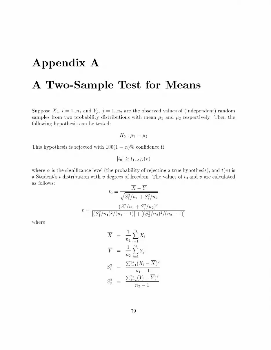
Appendix AA Two-Sample Test for MeansSuppose Xi; i = 1::n1 and Yj; j = 1::n2 are the observed values of (independent) randomsamples from two probability distributions with mean �1 and �2 respectively. Then thefollowing hypothesis can be tested: H0 : �1 = �2This hypothesis is rejected with 100(1 � �)% con�dence ifjt0j � t1��=2(v)where � is the signi�cance level (the probability of rejecting a true hypothesis), and t(v) isa Student's t distribution with v degrees of freedom. The values of t0 and v are calculatedas follows: t0 = X � YqS21=n1 + S22=n2v = (S21=n1 + S22=n2)2[(S21=n1)2=(n1 � 1)] + [(S22=n2)2=(n2 � 1)]where X = 1n1 n1Xi=1XiY = 1n2 n2Xj=1YjS21 = Pn1i=1(Xi �X)2n1 � 1S22 = Pn2j=1(Yj � Y )2n2 � 179

Appendix BThe Height of Peaks in a LandscapeIt appears that the �tness of the highest peaks in NK-landscapes for low values of K (K=2,5) is higher than the �tness of the peak in a landscape with K=0. If K increases more(K=25, 50), then the �tness of the peaks gradually decreases, and eventually becomes lessthan that of the peak for K=0. This appendix gives an explanation for this phenomenon.In the NK-model, the �tness of a bit depends on its own value and the value of K otherbits. So there are 2K+1 possible \con�gurations" for a bit, all of which are assigned arandom �tness from a UNIF(0,1) distribution. The higher the value of K, the higher thechance that some of the con�gurations of a bit are assigned a high �tness, because moredrawings from the same distribution are done.The expected values of the �tnesses that are assigned to the con�gurations of a bit canbe calculated by means of order statistics. Suppose x1; x2; :::; xn is a random sample ofsize n from some continuous probability density function1 (pdf) f(x), a � x � b. Whenthis random sample is ordered in increasing order, a set of order statistics, denoted byy1; y2; :::yn, is obtained. So y1 is the minimum of fx1; x2; :::; xng and yn is the maximum ofthis set of observed values.The pdf of the rth order statistic yr is de�ned as:gr(yr) = n!(r � 1)!(n� r)![F (yr)]r�1[1� F (yr)]n�rf(yi); a � yr � bwhere F (x) is the cumulative distribution function2 (CDF) belonging to the pdf f(x). Theexpected value of this rth order statistic yr can now be calculated as:E[yr] = Z ba ygr(y)dy1A function f(x) is a pdf for some continuous random variable X if and only if f(x) � 0 8x andR1�1 f(x)dx = 1.2The CDF F (x) denotes the chance that a random variable X will be less than or equal to the valuex. It is de�ned as F (x) = P [X � x] = R x�1 f(t)dt, where f(x) is the pdf of the random variable X.80

In the NK-model, for every bit 2K+1 drawings from a UNIF(0,1) distribution are done. Son = 2K+1; f(x) = 1, and F (x) = x, 0 � x � 1. The pdf of the rth order statistic is thengr(yr) = n!(r � 1)!(n � r)!yr�1r (1� yr)n�r � 1= n!(r � 1)!(n � r)!yr�1r n�rXi=0 n� ri ! (�1)iyir= n!(r � 1)!(n � r)! n�rXi=0 n� ri ! (�1)iyi+r�1rand the expected value of the rth order statistic becomesE[yr] = Z 10 n!y(r � 1)!(n� r)! n�rXi=0 n� ri ! (�1)iyi+r�1dy= Z 10 n!(r � 1)!(n� r)! n�rXi=0 n� ri ! (�1)iyi+rdy= " n!(r � 1)!(n� r)! n�rXi=0 1i+ r + 1 n� ri ! (�1)iyi+r+1#10= n!(r � 1)!(n � r)! n�rXi=0 n� ri ! (�1)ii+ r + 1From this result the expected value of the highest order statistic can be found by substi-tuting n for r: E[yn] = n!(n� 1)!(n� n)! n�nXi=0 n� ni ! (�1)ii+ n+ 1= n� 0Xi=0 0i! (�1)ii+ n+ 1= n� 00! 1n + 1= nn+ 1When K=0 in the NK-model, the (global) optimum can be found by taking for every bitthe value which is assigned the highest �tness (see Section 2.3). The expected value ofthis �tness is E[yn] = nn+1 = 23 (n = 20+1 = 2). But when K > 0, the optimum cannot be found in such a way because of the con icting constraints that result from theepistatic interactions. The expected value of the maximum of all the �tnesses assigned tothe con�gurations of a bit, increases with increasing K, but the con icting constraints alsobecome more stringent, so a �tness somewhere further back in the order statistics will bethe best possible for most bits. 81

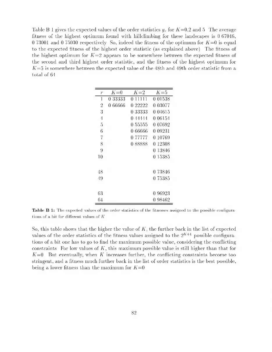
Table B.1 gives the expected values of the order statistics yr for K=0,2 and 5. The average�tness of the highest optimum found with hillclimbing for these landscapes is 0.67046,0.73001 and 0.75030 respectively. So, indeed the �tness of the optimum for K=0 is equalto the expected �tness of the highest order statistic (as explained above). The �tness ofthe highest optimum for K=2 appears to be somewhere between the expected �tness ofthe second and third highest order statistic, and the �tness of the highest optimum forK=5 is somewhere between the expected value of the 48th and 49th order statistic from atotal of 64. r K=0 K=2 K=51 0.33333 0.11111 0.015382 0.66666 0.22222 0.030773 0.33333 0.046154 0.44444 0.061545 0.55555 0.076926 0.66666 0.092317 0.77777 0.107698 0.88888 0.123089 0.1384610 0.15385... ...48 0.7384649 0.75385... ...63 0.9692364 0.98462Table B.1: The expected values of the order statistics of the �tnesses assigned to the possible con�gura-tions of a bit for di�erent values of K.So, this table shows that the higher the value of K, the further back in the list of expectedvalues of the order statistics of the �tness values assigned to the 2K+1 possible con�gura-tions of a bit one has to go to �nd the maximum possible value, considering the con ictingconstraints. For low values of K, this maximum possible value is still higher than that forK=0. But eventually, when K increases further, the con icting constraints become toostringent, and a �tness much further back in the list of order statistics is the best possible,being a lower �tness than the maximum for K=0.82

Appendix CUsed SoftwareA great deal of the software that was used for the experiments was written by myself. Thisincludes:� A �tness function for the NK-model.� A program for generating random walks on a �tness landscape.� Two hillclimbing programs.� A program for �nding and storing di�erent optima in a landscape.All this was written in C++, running under both UNIX (SunOS 4.1.3) and MS-DOS.The �tness function for the NK-model was tested by repeating an experiment, done origi-nally by Kau�man, for �nding the mean �tness of local optima and the mean walk lengthsto these local optima in NK-landscapes ([Kau93], pages 55-57). The obtained results werevery similar to those in [Kau93], indicating that the �tness function is implemented cor-rectly.R�emon Sinnema wrote a very nice toolkit for working with GA's, called EUREGA (also inC++). I added di�erent kinds of operators to this toolkit for performing the experimentswith the di�erent search strategies.The Box-Jenkins approach (Chapter 4) was carried out with the statistical package TSP(Time Series Processor). For the two-sample test for means (Appendix A), both a spread-sheet (PlanPerfect) and the statistical package SPSS were used. The order statistics inAppendix B were calculated with Maple. The graphs in this thesis were produced withGNUPLOT. For those of you who did not recognize it already, the thesis itself was writtenin LaTEX. 83

84

Bibliography[BE87] L. J. Bain and M. Engelhardt. Introduction to Probability and MathematicalStatistics. Duxbury Press, 1987.[BHS91] T. B�ack, F. Ho�meister, and H-P. Schwefel. A Survey of Evolution Strategies. InR. K. Belew and L. B. Booker, editors, Proceedings of the Fourth InternationalConference on Genetic Algorithms, pages 2{9. Morgan Kaufmann, 1991.[BJ70] G. E. P. Box and G. M. Jenkins. Time Series Analysis, Forecasting and Control.Holden Day, 1970.[Dar59] C. Darwin. The Origin of Species by Means of Natural Selection. Penguin Books,1859.[Dav91] L. Davis, editor. Handbook of Genetic Algorithms. Van Nostrand Reinhold,1991.[EJ89] M. A. Edey and D. C. Johanson. Blueprints|solving the mystery of evolution.Little, Brown and Company, 1989.[ERR94] A. E. Eiben, P-E. Rau�e, and Zs. Ruttkay. Repairing, adding constraints andlearning as a means of improving GA performance on CSPs. In J. C. Bioch andS. H. Nienhuys-Cheng, editors, Proceeding of the Fourth Belgian-Dutch Confer-ence on Machine Learning, pages 112{123, 1994.[FM] S. Forrest and M. Mitchell. What Makes a Problem Hard for a Genetic Algo-rithm? Some Anomalous Results and Their Explanation.[FM93] S. Forrest and M. Mitchell. Relative Building-Block Fitness and the Building-Block Hypothesis. In D. Whitley, editor, Foundations of Genetic Algorithms 2,pages 109{126. Morgan Kaufmann, 1993.[Gol89] D. E. Goldberg. Genetic Algorithms in Search, Optimization and MachineLearning. Addison-Wesley, 1989.[Gra89] C. W. J. Granger. Forecasting in Business and Economics. Academic Press,2nd edition, 1989. 85

[Gre86] J. J. Grefenstette. Optimization of Control Parameters for Genetic Algorithms.IEEE Transactions on Systems, Man, and Cybernetics, (1):122{128, 1986.[Hol92] J. H. Holland. Adaptation in Natural and Arti�cial Systems. MIT Press, 2ndedition, 1992.[J+88] G. G. Judge et al. Introduction to the Theory and Practice of Econometrics.John Wiley & Sons, 2nd edition, 1988.[Kau89] S. A. Kau�man. Adaptation on Rugged Fitness Landscapes. In D. Stein, editor,Lectures in the Sciences of Complexity, pages 527{618. Addison-Wesley, 1989.[Kau93] S. A. Kau�man. Origins of Order: Self-Organization and Selection in Evolution.Oxford University Press, 1993.[Lip91] M. Lipsitch. Adaptation on Rugged Landscapes Generated by Iterated LocalInteractions of Neighboring Genes. In R. K. Belew and L. B. Booker, editors,Proceedings of the Fourth International Conference on Genetic Algorithms, pages128{135. Morgan Kaufmann, 1991.[MHF] M. Mitchell, J. H. Holland, and S. Forrest. When Will a Genetic AlgorithmOutperform Hill Climbing?[MS93] J. Maynard Smith. The Theory of Evolution. Cambridge University Press, Cantoedition, 1993.[MWS91] B. Manderick, M. de Weger, and P. Spiessens. The Genetic Algorithm and theStructure of the Fitness Landscape. In R. K. Belew and L. B. Booker, editors,Proceedings of the Fourth International Conference on Genetic Algorithms, pages143{150. Morgan Kaufmann, 1991.[TG94] D. Thierens and D.E. Goldberg. Elitist recombination: an integrated selectionrecombination GA. In Proceedings of the IEEE World Gongress on Computa-tional Intelligence, pages 508{512, 1994.[Wei90] E. D. Weinberger. Correlated and Uncorrelated Fitness Landscapes and How toTell the Di�erence. Biological Cybernetics, (63):325{336, 1990.[WH88] N. K. Wessels and J. L. Hopson. Biology. Random House, Inc., 1988.86