on the construction and interpretation of fitness landscapes for
TRANSCRIPT
University of Tennessee, Knoxville University of Tennessee, Knoxville
TRACE: Tennessee Research and Creative TRACE: Tennessee Research and Creative
Exchange Exchange
Doctoral Dissertations Graduate School
8-2017
On the construction and interpretation of fitness landscapes for On the construction and interpretation of fitness landscapes for
HIV: a computational perspective HIV: a computational perspective
Elizabeth Grace Johnson University of Tennessee, Knoxville, [email protected]
Follow this and additional works at: https://trace.tennessee.edu/utk_graddiss
Part of the Bioinformatics Commons, Computational Biology Commons, and the Immunology and
Infectious Disease Commons
Recommended Citation Recommended Citation Johnson, Elizabeth Grace, "On the construction and interpretation of fitness landscapes for HIV: a computational perspective. " PhD diss., University of Tennessee, 2017. https://trace.tennessee.edu/utk_graddiss/4696
This Dissertation is brought to you for free and open access by the Graduate School at TRACE: Tennessee Research and Creative Exchange. It has been accepted for inclusion in Doctoral Dissertations by an authorized administrator of TRACE: Tennessee Research and Creative Exchange. For more information, please contact [email protected].

To the Graduate Council:
I am submitting herewith a dissertation written by Elizabeth Grace Johnson entitled "On the
construction and interpretation of fitness landscapes for HIV: a computational perspective." I
have examined the final electronic copy of this dissertation for form and content and
recommend that it be accepted in partial fulfillment of the requirements for the degree of Doctor
of Philosophy, with a major in Microbiology.
Vitaly V. Ganusov, Major Professor
We have read this dissertation and recommend its acceptance:
Elizabeth Fozo, Suzanne Lenhart, Tim Sparer, Michael Gilchrist
Accepted for the Council:
Dixie L. Thompson
Vice Provost and Dean of the Graduate School
(Original signatures are on file with official student records.)
On the construction and interpretation
of fitness landscapes for HIV: a
computational perspective
A Dissertation Presented for the
Doctor of Philosophy
Degree
The University of Tennessee, Knoxville
Elizabeth Grace Johnson
August 2017

c© by Elizabeth Grace Johnson, 2017
All Rights Reserved.
ii

To Mom, Dad
... and the 4th floor of Hesler
(I will return all your books. I promise.)
iii

I am indebted to the many professors, post-docs and graduate students who have contributed
to my growth both professionally and personally over the course of my graduate career.
My co-advisers, Vitaly Ganusov and Michael Gilchrist, have strongly influenced my attitude
towards modeling. Both have encouraged me to do the hard work of constructing practical data-
driven driven models that are mechanistic in character. I have likewise been enriched by each
advisor’s unique perspectives on model testing and validation.
I am also grateful to Yiding Yang, a mathematician and post-doc in my lab for lending me
her technical expertise and being a wonderful lab-mate who both pushed and encouraged me.
Additionally, I would like to thank everyone on the 4th floor of Hesler who enthusiastically reviewed
my proposals, advised me statistically, lent me books, and helped me resolve programming bugs
- despite the fact that I was not in their department.
I would like to extend special thanks to committee members Liz Fozo and Dr. Lenhart for
their aid and advice as I navigated my graduate career. I would also like to recognize all the
experimental members of my committee who endured all manner of equations, statistics and
computational jargon with extreme patience. I am also grateful to the Microbiology department,
the NSF IGERT SCALE-IT, UT’s SARIF program and the National Institute for Mathematical
and Biological Synthesis (NIMBioS) for the financial support they provided.
iv

“[Perfection] is the enemy of the good.”
–Orlando Pescetti
v
Abstract
To identify vulnerable viral targets to incorporate into an immunogen, fitness landscapes for
the viral proteome have been constructed. These landscapes describe the sum or synergistic
replicative cost exacted on the virus for any combination of non-synonymous mutations. Here we
attempt to assess the robustness of current computational methods for measuring the fitness cost
of HIV polymorphisms in these landscapes. We also address in the following chapters assumptions
and shortcomings that may underlie current landscape’s uneven ability to predict fitness effects.
In the first chapter, I appraise the robustness of current frame-works that derive fitness costs
from patient sequence data. In this chapter I also address the fields over-reliance on cross-
sectional data, justified by the assumptions that the viral populations can be 1) regarded as an
ideal population at equilibrium and 2) are at large unmarred by host pressures. To explore how
these problematic assumptions may undermine landscape construction, I assemble an alternate
landscape, where fitness costs were directly measured from temporal population fluxes using
a dynamical systems framework. This landscape paints a far different picture of the fitness
topography.
In the following chapter, I tackle another problematic aspect of current landscapes, their
neglect of physicochemical detail. I demonstrate that this model contrivance, leads us to under
or over estimating fitness costs at positions with highly divergent or similar physicochemical
character. In response, I adapt a population genetics model to account for the functional impact
of each residue mutation, and illustrate that it improves our ability to predict in vitro viral fitness.
Finally, in the last chapter, we employ several different metrics of fitness to determine if
the overall topography of the fitness landscape might shift over the course of early infection.
vi

Research has suggested that the replicative capacity of the virus increases over time and that
viral populations are continuously evolving in response to immune pressures. We found, that
although the protein was not mutational static at residue resolution, at the regional and protein
level it remained static due to compensating mutations.
vii
Table of Contents
1 Introduction 1
1.1 Complications in Regard to Translating in vitro Data into Fitness Maps . . . . . 3
1.2 Current Computational Approaches to Calculating Fitness Costs and Constructing
Fitness Landscapes . . . . . . . . . . . . . . . . . . . . . . . . . . . . . . . . . 5
1.3 Addressing Assumptions and Weaknesses in the Current Computational Approaches 8
2 Discordance of HIV fitness-landscapes created using cross-sectional vs longitu-
dinal data 10
Abstract . . . . . . . . . . . . . . . . . . . . . . . . . . . . . . . . . . . . . . . . . 11
2.1 Introduction . . . . . . . . . . . . . . . . . . . . . . . . . . . . . . . . . . . . 12
2.1.1 Fitness Landscapes and HIV Diversity . . . . . . . . . . . . . . . . . . . 12
2.1.2 Methods for deriving fitness landscapes from cross-sectional data . . . . 12
2.1.3 Deriving Fitness Landscapes using intra-host dynamics (Longitudinal
Data) . . . . . . . . . . . . . . . . . . . . . . . . . . . . . . . . . . . 13
2.1.4 Deriving Fitness Landscapes using physio-chemical properties of residues
(Cross-sectional Data) . . . . . . . . . . . . . . . . . . . . . . . . . . . 14
2.2 Methods . . . . . . . . . . . . . . . . . . . . . . . . . . . . . . . . . . . . . . 14
2.2.1 Cross-sectional Sequences . . . . . . . . . . . . . . . . . . . . . . . . . 14
2.2.2 Longitudnal Sequences . . . . . . . . . . . . . . . . . . . . . . . . . . . 15
2.2.3 Generating Confidence Intervals for the Longitudinal Patient Samples . . 15
2.2.4 Mathematical Models . . . . . . . . . . . . . . . . . . . . . . . . . . . 16
viii

2.3 Results and Discussion . . . . . . . . . . . . . . . . . . . . . . . . . . . . . . . 24
2.3.1 Shannon Entropy as proxy for fitness cost: considerations . . . . . . . . 27
2.3.2 Reversions as a proxy for fitness cost: considerations . . . . . . . . . . . 27
2.3.3 Confounding factors to be explored in further analysis: immune pressure
and epistasis . . . . . . . . . . . . . . . . . . . . . . . . . . . . . . . . 28
2.4 Supporting Information . . . . . . . . . . . . . . . . . . . . . . . . . . . . . . 29
2.4.1 Immune Equation Derivation . . . . . . . . . . . . . . . . . . . . . . . 30
3 Fitness Map constructed using a physico-chemical model of residue substitution 34
Abstract . . . . . . . . . . . . . . . . . . . . . . . . . . . . . . . . . . . . . . . . . 35
3.1 Introduction . . . . . . . . . . . . . . . . . . . . . . . . . . . . . . . . . . . . 36
3.1.1 Fitness Landscapes and HIV Diversity . . . . . . . . . . . . . . . . . . . 36
3.2 Methods . . . . . . . . . . . . . . . . . . . . . . . . . . . . . . . . . . . . . . 37
3.2.1 Shannon Entropy . . . . . . . . . . . . . . . . . . . . . . . . . . . . . . 37
3.2.2 Estimating Physico-chemical Sensitivities . . . . . . . . . . . . . . . . . 38
3.2.3 Model Parameterization . . . . . . . . . . . . . . . . . . . . . . . . . . 40
3.2.4 Cross-sectional Sequences . . . . . . . . . . . . . . . . . . . . . . . . . 41
3.2.5 Assessing Concordance of Physico-chemical Sensitivity with Shannon
Entropy . . . . . . . . . . . . . . . . . . . . . . . . . . . . . . . . . . 42
3.2.6 Characterizing Distribution of Sensitivities . . . . . . . . . . . . . . . . 42
3.2.7 Predicting Viral Behaviors . . . . . . . . . . . . . . . . . . . . . . . . . 43
3.3 Results and Discussion . . . . . . . . . . . . . . . . . . . . . . . . . . . . . . . 44
3.3.1 Physico-chemical selective forces vary along the poly-protein . . . . . . . 44
3.3.2 Distributions of Physico-Chemical Sensitivities . . . . . . . . . . . . . . 45
3.3.3 Assessing Concordance of Physico-chemical Sensitivity with Shannon
Entropy . . . . . . . . . . . . . . . . . . . . . . . . . . . . . . . . . . 50
3.3.4 Predictive power of physico-chemical sensitivity on fitness effects . . . . 53
3.3.5 Conclusions . . . . . . . . . . . . . . . . . . . . . . . . . . . . . . . . 55
3.4 Supporting information . . . . . . . . . . . . . . . . . . . . . . . . . . . . . . 58
ix

3.4.1 Physico-chemical weights . . . . . . . . . . . . . . . . . . . . . . . . . 58
3.4.2 Distribution of Fitness Proxy Metrics . . . . . . . . . . . . . . . . . . . 58
3.4.3 Model Comparison . . . . . . . . . . . . . . . . . . . . . . . . . . . . . 59
4 Mutational Shift of the Gag poly-protein during early and acute infection 61
Abstract . . . . . . . . . . . . . . . . . . . . . . . . . . . . . . . . . . . . . . . . . 62
4.1 Introduction . . . . . . . . . . . . . . . . . . . . . . . . . . . . . . . . . . . . 63
4.2 Methods . . . . . . . . . . . . . . . . . . . . . . . . . . . . . . . . . . . . . . 64
4.2.1 Sequences . . . . . . . . . . . . . . . . . . . . . . . . . . . . . . . . . 64
4.2.2 Calculating the Fitness of Patient Viral Populations via Hamming Distances 65
4.2.3 Estimating the Fitness of Patient Viral Populations from Global Population
Likelihoods . . . . . . . . . . . . . . . . . . . . . . . . . . . . . . . . . 67
4.2.4 Statistics On Fitness Trends . . . . . . . . . . . . . . . . . . . . . . . . 68
4.3 Results . . . . . . . . . . . . . . . . . . . . . . . . . . . . . . . . . . . . . . . 69
4.3.1 Polymorphic Approach: HIV Structural Proteins Show No Discernible
Trend of Increased Fitness Over Acute Infection . . . . . . . . . . . . . 69
4.3.2 Classification of Mutational Trends . . . . . . . . . . . . . . . . . . . . 71
4.3.3 Robustness of Detected Population Shifts . . . . . . . . . . . . . . . . . 74
4.4 Discussion . . . . . . . . . . . . . . . . . . . . . . . . . . . . . . . . . . . . . 76
4.4.1 Polymorphic Approach: Expected Fitness Increase in Viral Structural
Elements Not Observed . . . . . . . . . . . . . . . . . . . . . . . . . . 76
4.4.2 Adding Biological Detail Produced Qualitatively Different Trends . . . . 77
4.4.3 Further Work . . . . . . . . . . . . . . . . . . . . . . . . . . . . . . . . 78
4.5 Supporting information . . . . . . . . . . . . . . . . . . . . . . . . . . . . . . 79
5 Conclusions 84
Bibliography 88
Vita 104
x

List of Tables
1.1 Notable in-vitro derived fitness landscapes for RNA viruses Bellow are
shown several different empirical landscapes from the literature derived from
growth assays where stock or patient derived virus is competed in culture. . . . . 4
1.2 Models used to Infer Fitness Landscapes Shown below are computational
landscapes used to infer fitness in the HIV literature. All but one is derived from
cross-sectional sequence samples. . . . . . . . . . . . . . . . . . . . . . . . . . 6
2.1 Table of State Variables and Parameters for ODE Models The following
state variables and parameters are shared between the ordinary differential
equation models. . . . . . . . . . . . . . . . . . . . . . . . . . . . . . . . . . . 21
2.2 State Variables and Parameters The following parameters and state variables
are shared between the two ODE Models . . . . . . . . . . . . . . . . . . . . . 31
3.1 Parameters and Variables for Physico-Chemical Model The following
parameters are shared between the models used to approximate strong stabilizing
selective pressure along the protein. . . . . . . . . . . . . . . . . . . . . . . . 40
3.2 Model Selection Likelihood Ratio Test assessing single (H0) vs regional (HA)
physico-chemical weighting . . . . . . . . . . . . . . . . . . . . . . . . . . . . 44
3.3 Likelihood of PDF Models Shows likelihood of Gamma, Lognormal and Inverse
Gamma continuous probability distributions for the G′′ sensitivity values for
residues along the Gag poly-protein. . . . . . . . . . . . . . . . . . . . . . . . . 46
xi

3.4 LogNormal Fits of Physico-Chemical Sensitivities The distribution of
physico-chemical sensitivities were described by a lognormal distribution for
functional regions p17,p24,p7 p6 and all the regions collectively. The MLE for the
lognormal shape parameters (µ,σ) are displayed for each region. The estimates are
displayed with 95% confidence intervals calculated from the parameter’s likelihood
profile. . . . . . . . . . . . . . . . . . . . . . . . . . . . . . . . . . . . . . . . 48
3.5 Model Selection for Regional vs Poly-Protein Model of Sensitivity
Distributions The distribution of physico-chemical sensitivites are described via a
single lognormal probability distribution function (H0) or via a family of lognormal
distributions (HA) tailored to the proteins functional regions p17, p24, p7 and p6. 49
3.6 Primary and Secondary Structure Correlation between methods (Kendall Tau)
with primary and secondary structure. Secondary structure broken down by turn,
helix and strand . . . . . . . . . . . . . . . . . . . . . . . . . . . . . . . . . . 50
3.7 Correlation Statistics between Sensitivity and ConservationTable displaying
correlation statistics between sensitivity (G′) and conservation (1/S) for the poly-
protein and each functional region . . . . . . . . . . . . . . . . . . . . . . . . . 53
3.8 Correlation with Escape Time Table displaying correlation statistics between
epitope sensitivity (G′′) or entropy (S) and escape time . . . . . . . . . . . . . 54
3.9 Correlation between conservation and sensitivity Table displaying correlation
statistics between epitope sensitivity (G′) or entropy (1/S) and viral spreading fitness 55
3.10 Physico-chemical Weights Weights were extracted via fitting of the model to
MSA data for the entire poly-protein (All) and in individual functional regions
(p24,p17,p7,p6) The parameters (θc, θp, θv) denote the weighting terms for
composition, polarity, and molecular volume respectively . . . . . . . . . . . . . 58
3.11 Null and alternative model describing distribution of physico-chemical
sensitivities The distribution can be described using a family of parametrized
probability density functions (HA) that describe the distribution in each functional
region or this model can be simplified so that the distribution is described by a
single Lognormal pdf (H0). . . . . . . . . . . . . . . . . . . . . . . . . . . . . 58
xii
3.12 Congruity of Descriptive Distributions for Metrics This table displays how
the distributions of physico-chemical sensitivities (G”) and conservation values
(1/E) compare over the entire Gag poly-protein (All) and over specific functional
regions (p6,p7,p24,p17). . . . . . . . . . . . . . . . . . . . . . . . . . . . . . 59
4.1 Conservative and Permissive Metric vs Polymorphic Metric Two marginal
homegeneity tests were conducted to determine if metric type impacted cate-
gorization of the patients. The tests evaluated a null hypothesis where both
metrics are assumed to categorize the mutational trajectory of the patient’s viral
populations similarly. . . . . . . . . . . . . . . . . . . . . . . . . . . . . . . . . 74
4.2 Robustness of Detected Population Shifts The sequence sets amplified from
each blood sample were re-sampled 1000 times at each time-point to create 1000
re-sampled mutational trajectories for each patient. Linear fits were conducted for
all re-sampled trajectories, from the distribution of resulting slopes with p-values
the robustness of the detected shift was calculated by dividing the number of
re-sample trajectories showing a significant shift in mutational character over the
total number of trajectories. . . . . . . . . . . . . . . . . . . . . . . . . . . . . 76
4.3 Linear fits Polymorphic. False Discovery Rate (FDR) set at 0.25%. . . . . . . . 81
4.4 Linear fits Conservative metric. False Discovery Rate (FDR) set at 25%. . . . . 82
4.5 Linear Fits Permissive metric. The False Discovery Rate (FDR) tolerance set 25%. 83
xiii

List of Figures
2.1 in silico approach to assess landscape concordance . . . . . . . . . . . . . 17
2.2 Diagram of Differential Equation Models . . . . . . . . . . . . . . . . . . . . . 20
2.3 Bootstrapping Example of resampling at position 427 and 242 in two patients
experiencing a viral reversion back to the consensus residue over 250 days. The
samples at each time-point were bootstrapped 1000 times, creating 1000 new
reverting trajectories. the distributions of the data and refitting the data produces
a distribution of 1000 cost values for each position. . . . . . . . . . . . . . . . 23
2.4 Correlation between non-standard metric Absence of a strong negative
correlation between the simplified Ising / Physio-Chemical sensitivities and fitness
cost (τ=-0.18 ns and τ=-0.09 ns) for full protein respectively. Points represent
HXB2 position coordinates for which there was a reversion from which a fitness
cost could be extracted. On the x-axis we plot that HXB2 positions corresponding
sensitivity to mutation from cross-sectional sequences. On the y-axis we plot
the HXB2 positions corresponding fitness cost as extracted from the longitudinal
sequences. The concordances are displayed for all HXB2 positions along the poly-
protein (A and C) and per protein (B and D). . . . . . . . . . . . . . . . . . 24
xiv

2.5 Correlation with Entropy S ignificant positive correlation between entropy and
fitness cost using a kendall tau concordance statistic Points represent HXB2
position coordinates for which there was a reversion from which a fitness cost
could be extracted. On the x-axis we plot that HXB2 positions corresponding
entropy from cross-sectional sequences. On the y-axis we plot the HXB2 positions
corresponding fitness cost as extracted from the longitudinal sequences. The
concordances are displayed for all HXB2 positions along the poly-protein (A) and
per protein (B) . . . . . . . . . . . . . . . . . . . . . . . . . . . . . . . . . . 25
2.6 Bar Plot of Metrics The x-axis on each plot denotes our location along the set
of 1000 aligned Gag-polyprotein. The y axis describes the fitness cost (c,H,G′)
or entropy (E) associated with each location. The Gag poly-protein encoded by
these sequences is broken down into functional units by color on the plot. These
units include p17 the matrix, p24 the capsid, p7 the nucleocapsid and p6 the
nucleoprotein. (A) The fitness cost unit G is a measure of how fragile a position
is to deviations from consensus. It estimates this fragility by observing how the
position tolerates physio-chemical deviations from the consensus residue. (B)
The fitness cost unit H is also a measure of how fragile a position is to deviations
from consensus. However,it uses a purely binary metric of deviation without any
physio-chemical detail. (C) The entropy measure E is the Shannon Entropy of
each position. The Shannon Entropy is a measure of residue diversity regarded as
an inverse proxy of fitness cost in the literature. (D) The fitness cost c describes
to what degree the replication capacity of the virus has been reduced if there is a
mutant residue at that position . . . . . . . . . . . . . . . . . . . . . . . . . . 26
3.1 Distribution of physico-chemical sensitivities for Gag Polyprotein The
distributions of G′′ sensitivities are described with a Lognormal model. Regional
location µ and scale σ parameters identified via MLE. Distribution excludes spacer
regions and includes regions p17,p24,p7 and p6 (n= 370). Hyper-conserved outlier
positions (conservation value (1/E) >100) were excluded . . . . . . . . . . . . 46
xv

3.2 Distribution of physico-chemical sensitivities The distributions of G′′ sensi-
tivities are described with a Lognormal model. Regional location µ and scale σ
parameters identified via MLE. A.p17 Lognormal PDF describing distribution of
physico-chemical sensitivities for the Matrix. B.p24 Lognormal PDF describing
distribution of physico-chemical sensitivities for the Capsid. C.p7) Lognormal
PDF describing distribution of physico-chemical sensitivities for the Nucleo-capsid.
D.p6) Lognormal PDF describing the distribution of physico-chemical sensitivities
for the Nucleoprotein. . . . . . . . . . . . . . . . . . . . . . . . . . . . . . . . 47
3.3 MLE of Lognormal parameters for each region Panels display Lognormal
parameter fits for each region and all regions collectively. A. The location
parameter for the capsid’s (p24) distribution is statically higher compared to the
other regions and the nucleocapsid’s (p7) distribution is statistically lower than the
poly-protein’s (All) distribution. B. Shows location parameter σ for each region
with 95% confidence intervals estimated by likelihood profiling. The capsid (p24)
and matrix (p17) distributions have a shape parameters distinct from each-other 49
3.4 Rank correlation of each position’s estimated physico-chemical sensitivity
G′′ with it’s conservation (1/E). Positions total 520 in the Gag poly-protein
excluding spacer regions. Estimates of sensitivity G′′ and conservation 1/E
estimated and derived from 1000 sample MSA of the Gag poly-protein for HIV-1
subtype C. Sensitivity and conservation concord with each other with a significant
kendall τ of 0.567. . . . . . . . . . . . . . . . . . . . . . . . . . . . . . . . . . 51
3.5 Rank correlation of sensitivity and conservation in the four functional
regions in the Gag poly-protein A.p24) Concordance of sensitivity and
conservation in the viral capsid tau = 0.456 B.p17) Concordance of sensitivity
and conservation in the viral matrix tau = 0.625 C.p7) Weak concordance
of sensitivity and conservation in the viral nucleo-capsid tau = 0.344 D.p6)
Strong concordance of sensitivity and conservation in the viral nucleo-protein
tau = 0.791. Estimates of sensitivity G′′ and conservation 1/E estimated and
derived from a 1000 sample MSA of the Gag poly-protein for HIV-1 subtype C. 52
xvi
3.6 Correlation of entropy and sensitivity with the escape time of 24 epitopes in
the Gag poly-protein A) Correlation of the escape time of an epitope in days with
the epitope’s entropy B) Correlation of the escape time of an epitope in days with
the epitope’s physico-chemical sensitivity. . . . . . . . . . . . . . . . . . . . . 54
3.7 Correlation of entropy and sensitivity of residues with the spreading
fitness of 31 viral strains bearing mutations in the corresponding residues A)
Correlation of the assayed spreading fitness of the mutated virus in days with the
correspondingly position’s entropy B) Correlation of the assayed spreading fitness
of the mutated virus in days with the correspondingly position’s physico-chemical
sensitivity. . . . . . . . . . . . . . . . . . . . . . . . . . . . . . . . . . . . . . 56
4.1 Comparative Assessment of Viral Evolution Polymorphic, Permissive and
Conservative methods comparatively assess viral population fitness shifts over 4-12
time points. Panels display categorization of fitness shifts (neutral,less fit,more fit)
in acutely infected patient cohort (41) by method. Pol. Polymorphic Classification
Scheme gives likelihood of drawing a particular blood sample given the diversity
of database sequences(eq 4.5). Per. Permissive Classification Scheme, where
non-consensus residues categorized as unfit. (eq 4.1). Con. Conservative
Classification Scheme, where highly polymorphic sites (consensus frequency ≤
50%) effectively disregarded (eq 4.1). . . . . . . . . . . . . . . . . . . . . . . 70
4.3 Empirical Bootstrap of Viral Sequences Robustness of the four patients shifts
for the Polymorphic metric assessed by bootstrapping (n=1000) the patient blood
samples. Post bootstrapping, polymorphic fitness estimates were recalculated.
Slopes from linear regressions on the newly constructed time-courses were
categorized as significant or non-significant. Panels displays the distribution of
slopes obtained from each of the four patients. Colors denote the significant and
non-significant slopes in the empirical bootstrap. . . . . . . . . . . . . . . . . . 75
xvii

4.4 Density Plots of Fitness Metrics for Three Approaches. Pooled samples
from 41 patients A Permissive and Conservative Metric Density Plot B
Polymorphic Density Plot. Pooled samples from 41 patients. . . . . . . . . . . . 79
xviii
Chapter 1
Introduction
As an RNA virus, the human immunodeficiency virus (HIV) mutates at rates orders of
magnitude higher than DNA based pathogens (Sanjun et al., 2010). It has been observed that
HIV accumulates mutations at a rate of 1.2 × 10⁻⁵ per day per site (Zanini et al., 2016). This
rapid rate of mutation allows HIV to quickly traverse and explore its sequence space, creating
diverse intra-host populations within short time-frames. These diverse and mutable populations
are adept at escaping the adaptive immune responses, preventing long-term adaptive immune
control of the virus. (Johnston and Fauci, 2008; Walker and Burton, 2008). These same viral
traits have also frustrated attempts to create an effective prophylactic vaccine, believed to be
the best hope of curbing our current HIV pandemic (McElrath and Haynes, 2010; Korber et al.,
2001)
Fitness landscapes can be used as a tool to predict viral evolutionary dynamics, making it
easier to grasp and interpret the viruses incredible mutability and diversity. These landscapes
quantitatively describe how a mutation will impair the replicative capacity of the virus given
the specific genetic background the mutation is embedded in (Wright, 1932). In their simplest
incarnation, computationally derived landscapes will use residue conservation at a site (the inverse
Shannon entropy) as a direct proxy for fitness (Rihn et al., 2013; Ferrari et al., 2011; Liu et al.,
2012). More complex models, on the other hand, will incorporate epistatic interactions between
residues (Mann et al., 2014; Ferguson et al., 2013; Barton et al., 2016).
1
In practice, these landscapes can help predict when and where a virus will escape immune
control given a patients’ HLA profile (Barton et al., 2016). The highly polymorphic human
leukocyte antigen (HLA) genes encode for a protein complex that presents viral peptides to the
immune system. Because HLA types vary from patient to patient, particular viral peptides will
elicit a strong immune response in some patients and not in others. Studies therefore often
combine information from both the viral fitness landscape and a patient’s HLA typing (Liu et al.,
2012).
The information embedded in these fitness landscapes can also be applied to vaccine
optimization problems (Ferguson et al., 2013; Shekhar et al., 2013). While it is important to
create a vaccine immunogen that elicits a strong immune response, it is equally important to
make sure that the virus cannot easily escape said strong immune response via accessible escape
pathways (Chopera et al., 2011). Fitness landscapes can help us identify conserved elements in
the viral proteome, allowing us to quantitatively describe the fragility of each conserved element
and its propensity to escape immune control given its sequence background (Mann et al., 2014).
While using residue frequency as a proxy for fitness has been useful in some contexts (Ferguson
et al., 2013; Mann et al., 2014), there have been notable discrepancies with computationally
estimated fitness costs failing to predict a positions fragility to mutation in in vitro e.g. (Rihn
et al., 2013) or escape rate textitin vivo e.g (Barton et al., 2016). In light of these discrepancies,
we attempt to advance the field by probing the following biological assumptions made in fitness
landscapes construction in the following chapters: 1) viral frequency is a robust proxy for fitness
despite host pressures and small effective population size 2) ignoring physio-chemical detail in
our landscapes is not skewing fitness estimates 3) that the population is at steady state.
2
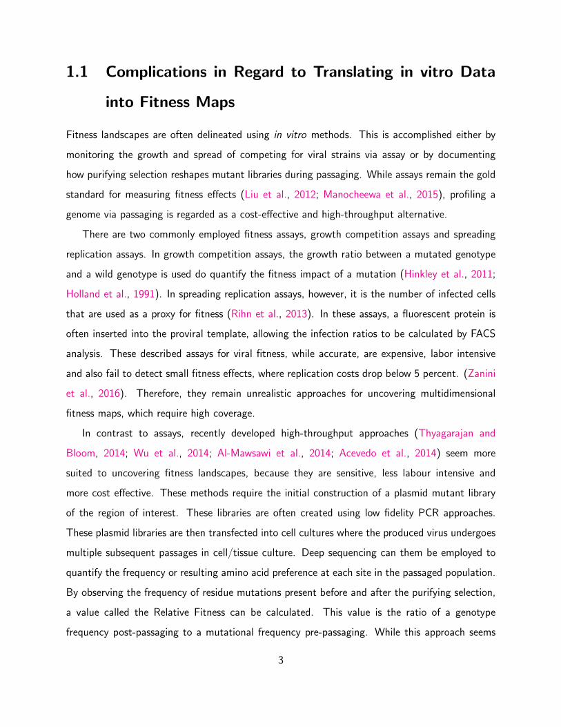
1.1 Complications in Regard to Translating in vitro Data
into Fitness Maps
Fitness landscapes are often delineated using in vitro methods. This is accomplished either by
monitoring the growth and spread of competing for viral strains via assay or by documenting
how purifying selection reshapes mutant libraries during passaging. While assays remain the gold
standard for measuring fitness effects (Liu et al., 2012; Manocheewa et al., 2015), profiling a
genome via passaging is regarded as a cost-effective and high-throughput alternative.
There are two commonly employed fitness assays, growth competition assays and spreading
replication assays. In growth competition assays, the growth ratio between a mutated genotype
and a wild genotype is used do quantify the fitness impact of a mutation (Hinkley et al., 2011;
Holland et al., 1991). In spreading replication assays, however, it is the number of infected cells
that are used as a proxy for fitness (Rihn et al., 2013). In these assays, a fluorescent protein is
often inserted into the proviral template, allowing the infection ratios to be calculated by FACS
analysis. These described assays for viral fitness, while accurate, are expensive, labor intensive
and also fail to detect small fitness effects, where replication costs drop below 5 percent. (Zanini
et al., 2016). Therefore, they remain unrealistic approaches for uncovering multidimensional
fitness maps, which require high coverage.
In contrast to assays, recently developed high-throughput approaches (Thyagarajan and
Bloom, 2014; Wu et al., 2014; Al-Mawsawi et al., 2014; Acevedo et al., 2014) seem more
suited to uncovering fitness landscapes, because they are sensitive, less labour intensive and
more cost effective. These methods require the initial construction of a plasmid mutant library
of the region of interest. These libraries are often created using low fidelity PCR approaches.
These plasmid libraries are then transfected into cell cultures where the produced virus undergoes
multiple subsequent passages in cell/tissue culture. Deep sequencing can them be employed to
quantify the frequency or resulting amino acid preference at each site in the passaged population.
By observing the frequency of residue mutations present before and after the purifying selection,
a value called the Relative Fitness can be calculated. This value is the ratio of a genotype
frequency post-passaging to a mutational frequency pre-passaging. While this approach seems
3
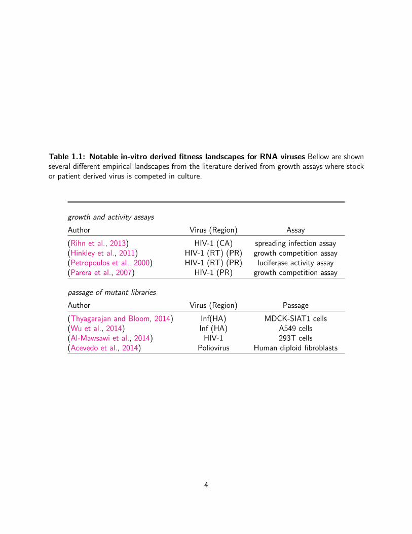
Table 1.1: Notable in-vitro derived fitness landscapes for RNA viruses Bellow are shownseveral different empirical landscapes from the literature derived from growth assays where stockor patient derived virus is competed in culture.
growth and activity assays
Author Virus (Region) Assay
(Rihn et al., 2013) HIV-1 (CA) spreading infection assay(Hinkley et al., 2011) HIV-1 (RT) (PR) growth competition assay(Petropoulos et al., 2000) HIV-1 (RT) (PR) luciferase activity assay(Parera et al., 2007) HIV-1 (PR) growth competition assay
passage of mutant libraries
Author Virus (Region) Passage
(Thyagarajan and Bloom, 2014) Inf(HA) MDCK-SIAT1 cells(Wu et al., 2014) Inf (HA) A549 cells(Al-Mawsawi et al., 2014) HIV-1 293T cells(Acevedo et al., 2014) Poliovirus Human diploid fibroblasts
4
more tractable for constructing fitness landscapes, detailed profiles of Influenza’s HA protein
conducted on two different cell lines do not seem to agree (Thyagarajan and Bloom, 2014; Wu
et al., 2014), suggesting that this method might produce very different landscapes depending on
how the virus is passaged.
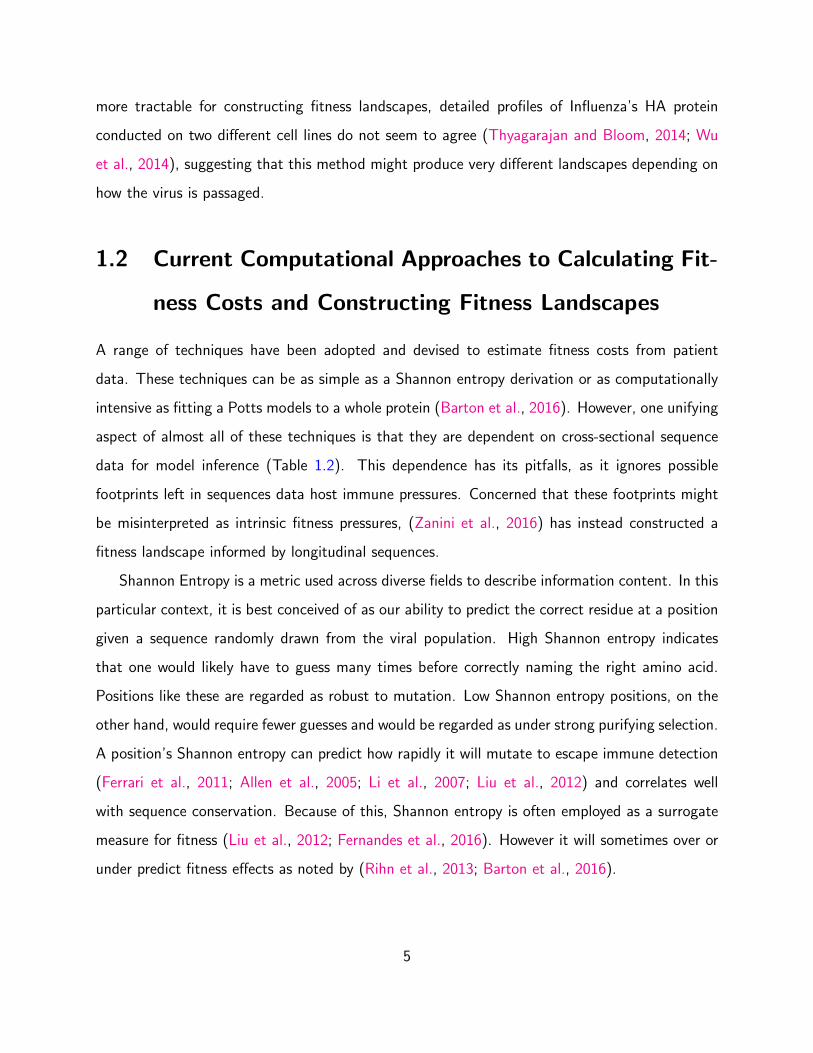
1.2 Current Computational Approaches to Calculating Fit-
ness Costs and Constructing Fitness Landscapes
A range of techniques have been adopted and devised to estimate fitness costs from patient
data. These techniques can be as simple as a Shannon entropy derivation or as computationally
intensive as fitting a Potts models to a whole protein (Barton et al., 2016). However, one unifying
aspect of almost all of these techniques is that they are dependent on cross-sectional sequence
data for model inference (Table 1.2). This dependence has its pitfalls, as it ignores possible
footprints left in sequences data host immune pressures. Concerned that these footprints might
be misinterpreted as intrinsic fitness pressures, (Zanini et al., 2016) has instead constructed a
fitness landscape informed by longitudinal sequences.
Shannon Entropy is a metric used across diverse fields to describe information content. In this
particular context, it is best conceived of as our ability to predict the correct residue at a position
given a sequence randomly drawn from the viral population. High Shannon entropy indicates
that one would likely have to guess many times before correctly naming the right amino acid.
Positions like these are regarded as robust to mutation. Low Shannon entropy positions, on the
other hand, would require fewer guesses and would be regarded as under strong purifying selection.
A position’s Shannon entropy can predict how rapidly it will mutate to escape immune detection
(Ferrari et al., 2011; Allen et al., 2005; Li et al., 2007; Liu et al., 2012) and correlates well
with sequence conservation. Because of this, Shannon entropy is often employed as a surrogate
measure for fitness (Liu et al., 2012; Fernandes et al., 2016). However it will sometimes over or
under predict fitness effects as noted by (Rihn et al., 2013; Barton et al., 2016).
5
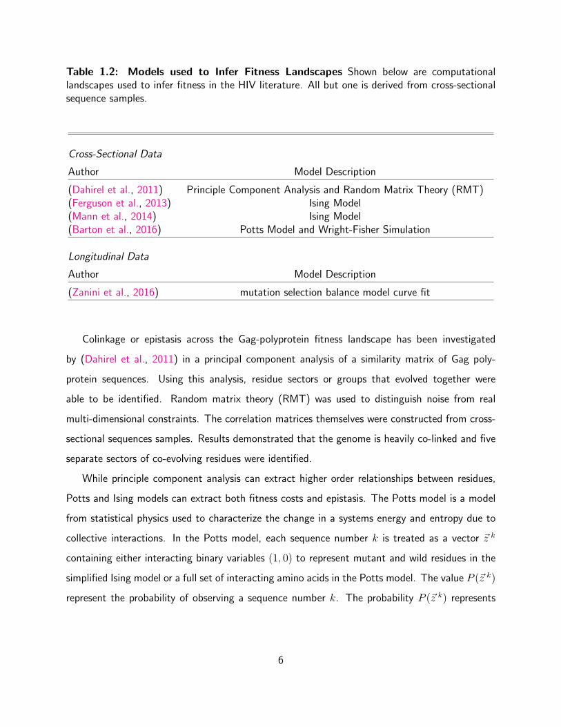
Table 1.2: Models used to Infer Fitness Landscapes Shown below are computationallandscapes used to infer fitness in the HIV literature. All but one is derived from cross-sectionalsequence samples.
Cross-Sectional Data
Author Model Description
(Dahirel et al., 2011) Principle Component Analysis and Random Matrix Theory (RMT)(Ferguson et al., 2013) Ising Model(Mann et al., 2014) Ising Model(Barton et al., 2016) Potts Model and Wright-Fisher Simulation
Longitudinal Data
Author Model Description
(Zanini et al., 2016) mutation selection balance model curve fit
Colinkage or epistasis across the Gag-polyprotein fitness landscape has been investigated
by (Dahirel et al., 2011) in a principal component analysis of a similarity matrix of Gag poly-
protein sequences. Using this analysis, residue sectors or groups that evolved together were
able to be identified. Random matrix theory (RMT) was used to distinguish noise from real
multi-dimensional constraints. The correlation matrices themselves were constructed from cross-
sectional sequences samples. Results demonstrated that the genome is heavily co-linked and five
separate sectors of co-evolving residues were identified.
While principle component analysis can extract higher order relationships between residues,
Potts and Ising models can extract both fitness costs and epistasis. The Potts model is a model
from statistical physics used to characterize the change in a systems energy and entropy due to
collective interactions. In the Potts model, each sequence number k is treated as a vector ~z k
containing either interacting binary variables (1, 0) to represent mutant and wild residues in the
simplified Ising model or a full set of interacting amino acids in the Potts model. The value P (~z k)
represent the probability of observing a sequence number k. The probability P (~z k) represents
6
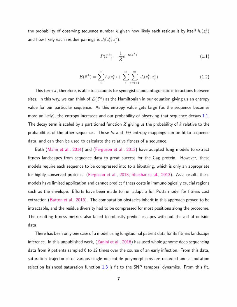
the probability of observing sequence number k given how likely each residue is by itself hi(zki )
and how likely each residue pairings is Ji(zki , z
kj ).
P (~z k) =1
Ze−E(~z k) (1.1)
E(~z k) =m∑i
hi(zki ) +
m∑i
m∑j=i+1
Ji(zki , z
kj ) (1.2)
This term J , therefore, is able to accounts for synergistic and antagonistic interactions between
sites. In this way, we can think of E(~z k) as the Hamiltonian in our equation giving us an entropy
value for our particular sequence. As this entropy value gets large (as the sequence becomes
more unlikely), the entropy increases and our probability of observing that sequence decays 1.1.
The decay term is scaled by a partitioned function Z giving us the probability of k relative to the
probabilities of the other sequences. These hi and Jij entropy mappings can be fit to sequence
data, and can then be used to calculate the relative fitness of a sequence.
Both (Mann et al., 2014) and (Ferguson et al., 2013) have adapted Ising models to extract
fitness landscapes from sequence data to great success for the Gag protein. However, these
models require each sequence to be compressed into to a bit-string, which is only an appropriate
for highly conserved proteins. (Ferguson et al., 2013; Shekhar et al., 2013). As a result, these
models have limited application and cannot predict fitness costs in immunologically crucial regions
such as the envelope. Efforts have been made to run adapt a full Potts model for fitness cost
extraction (Barton et al., 2016). The computation obstacles inherit in this approach proved to be
intractable, and the residue diversity had to be compressed for most positions along the proteome.
The resulting fitness metrics also failed to robustly predict escapes with out the aid of outside
data.
There has been only one case of a model using longitudinal patient data for its fitness landscape
inference. In this unpublished work, (Zanini et al., 2016) has used whole genome deep sequencing
data from 9 patients sampled 6 to 12 times over the course of an early infection. From this data,
saturation trajectories of various single nucleotide polymorphisms are recorded and a mutation
selection balanced saturation function 1.3 is fit to the SNP temporal dynamics. From this fit,
7
the author is able to obtain selection coefficients against the various SNPs. Using these selection
coefficients he constructs a map of the HIV genome with more than 50% percent coverage.
〈x〉 =µ
s(1− e−st) (1.3)
A function above (Eq.1.3) is used to describe the average trajectory of a single nucleotide
polymorphism (SNP). In this function µ stands for the mutation rate s for the fitness cost or
selection coefficient and t for time. In this function, the SNP frequency will saturate as time
goes on. Because mutations tend to be transitory or only semi-dominant in the population
(Novitsky et al., 2009) the SNPs trajectories taken from the data were exceedingly noisy (Zanini
et al., 2016). Due to this noise, extraction of selection coefficients was non-trivial. The process
required both extensive trajectory smoothing and averaging among patients.
1.3 Addressing Assumptions and Weaknesses in the Cur-
rent Computational Approaches
One concern with computationally generated landscapes is their over-reliance on cross-sectional
data (Mann et al., 2014; Ferguson et al., 2013; Barton et al., 2016). These cross-sectional
sequences are used to calculate the frequency of mutation in particular regions. However it is
not clear if mutations are enriched in a region because 1) that region is more structural and
functionally permissive to mutation, 2) or because this region has undergone multiple selective
sweeps by the immune system and therefore has been enriched with mutations (Zanini et al.,
2016). To address this problem, we used longitudinal data of early infections to observe rate of
fixation of viral mutations as an alternative method to obtain fitness costs. Here we attempt to
assess the robustness of current methods for measuring the fitness cost of HIV polymorphisms.
Another problematic aspect of current landscapes is that they ignore the physicochemical
nature of the residues composing the map (Mann et al., 2014). Each residue is regarded as
interchangeable with the next in terms of size, polarity and side-chain composition. In such
cases we may be under estimating fitness costs at positions hosting a diversity of residues that
8
are physicochemically uniform. Conversely, we may also be over estimating fitness costs at
positions hosting a few residues that are physicochemically divergent. From a database of HIV
sequences, we may observe that a particular position hosts a diverse set of residues. At first
glance, this diversity might suggest there is not a great deal of purifying pressure exerted on that
position. However, upon further examination, we may find that the residues at this site tend to be
quite physiochemically similar. This conservation of physiochemical characteristics alternatively
suggests that a high degree of purifying pressure is exerted on that position. Conversely, a position
may be fairly non-diverse in its residue variety; but the residues may be quite physiochemically
distinct from one another. In this situation, purifying pressure may exert much less force on that
position than one might assume from residue diversity alone.
Finally, because fitness landscapes are usually not derived from longitudinal data, it is not
clear if the fitness landscape is dynamic or static over the course of infection. By dynamic we
mean shifting in distance from the consensus virus over infection, and fundamentally changing its
character as it adapts to the host. Previous work examining ex vivo fitness of longitudinally
sampled patient virus has show that the replicative capacity of the virus seems to increase
over time (Quiones-Mateu et al., 2000; Troyer et al., 2005). This would seem to suggest the
fitness landscape is organizing itself around the consensus viral sequence. This fitness however is
measured using an exogenous replication system that does not recapitulate the host environment
with its cytokines and immune factors, in addition others have found viral replication capacity to
decrease over time in the presence of adaptive immune pressures (Arnott et al., 2010). Given that
Gag-poly protein is one of the main structural poly-proteins in the virus and the most conserved
(Li et al., 2013), we wanted to know how it evolved in regard to the consensus sequence over time.
Evidence from longitudinal data (Novitsky et al., 2009) seemed to suggest that the protein was
dominated by mutational reversion that went to fixation during early infection and by transient
forward mutations away from fit consensus residues later in infection.
9
Chapter 2
Discordance of HIV fitness-landscapes
created using cross-sectional vs
longitudinal data
10
Abstract
HIV is a genetically plastic virus, adept at evading the patient’s adaptive immune system. The
virus avoids immune recognition by mutating key residues embedded in epitopes targeted by
adaptive responses. However, these substituted residues can be structurally and functionally sub-
optimal for the virus. Fitness landscapes of the virus quantitatively describe, with residue level
resolution, the particular cost exacted on the intrinsic fitness of the virus for these mutations.
In computationally derived landscapes, residue frequency is regarded as the underlying signature
of fitness. The more fit an amino acid residue is the more often one would expect to observe it
at that particular position. We compared the robustness of methods using cross-sectional data
against each other and a fitness map extracted from longitudinal data. The temporal resolution
of the longitudinal data sets enables us to estimate fitness cost from viral population kinetics
within an individual patient. In this analysis of fitness, compartmentalization of replication and
inter-patient variation is perhaps less of a confounding factor. We find significant discrepancies
between the fitness maps derived from cross-sectional patient data and the map derived from
longitudinal data. The lack of concordance suggests that they are perhaps not actually measuring
the same phenomenon.
11
2.1 Introduction
2.1.1 Fitness Landscapes and HIV Diversity
HIV is a highly mutable and diverse virus. This inherit mutability and diversity have stymied
efforts to create the vaccine immunogens necessary to curb the ongoing pandemic. An estimated
70 million people have been infected with the retrovirus since the start of the pandemic, with
1.1 million dying from an AIDS associated illness in 2015 alone and 2.1 million new infections
detected in the same year Global Aids Response Progress Reporting (GARPR, 2016). It has been
proposed that an effective vaccine immunogen should not only elicit strong responses against
highly conserved residues but also against residues that are marginally costly for the virus to
mutate (Walker and Burton, 2008; Troyer et al., 2009). Residues that are costly to mutate
are said to have “high fitness costs” in that they exact a high price on viral replication. A
position may not be entirely deleterious to mutate but can be costly enough that it impairs the
replicative capacity of the virus. It has been shown that individuals who control the virus possess
virus that replicates poorly (Miura et al., 2010). In particular strong immune recognition of Gag
epitopes correlates well with lower viral loads during the later stage of chronic infection (Sunshine
et al., 2015). Fitness landscapes of conserved proteins like Gag, help us identify which particular
positions we want to elicit immune responses against if we wish to accrue costly mutations in
the viral population. By accruing expensive mutations, one can push the virus towards its error
threshold. These landscapes also reveal the hyper-conserved regions where there is little to no
deviation from the consensus sequence either due to strong intrinsic purifying pressures, or the
lack of any notable external selective pressures.
2.1.2 Methods for deriving fitness landscapes from cross-sectional data
Shannon Entropy calculations (Rihn et al., 2013; Liu et al., 2012; Ferrari et al., 2011) and
Entropy Maximization models (Ferguson et al., 2013; Mann et al., 2014; Shekhar et al., 2013)
have both been used to gauge fitness costs associated with escape mutations and estimate escape
times from immune responses. When employing either method, it is assumed that sequences are
12
sampled from a putatively large and rapidly mutating RNA virus population can be treated as
a homogenous idealized population at equilibrium. In these idealized populations, the frequency
landscape for HIV polymorphisms is treated as a direct proxy of the fitness landscape for these
polymorphisms (Shekhar et al., 2013). Cross-sectional patient data is pooled together to produce
these prevalence landscapes.
The degree to which natural intra-host HIV populations actually resemble a homogeneous
ideal population at equilibrium is unclear. While the census size population for HIV is quite large
(108-107) the effective population size may be quite small (104) (Shriner et al., 2004; Rouzine
and Weinberger, 2013). Also, notably, the HIV population is never at true equilibrium, but is
continually perturbed by host selective pressures and is constantly in flux. (Holmes and Moya,
2002),(Hedskog et al., 2010)(Tsibris et al., 2009). Yet more concerning, the viral population is
heavily compartmentalized spatially in the secondary lymphoid tissues (van Marle et al., 2007)
(Rozera et al., 2014) (Sturdevant et al., 2015) and seems unlikely to behave as a homogeneous
unit.
The second simplifying assumption the Shannon entropy calculation and maximum entropy
model share, is residue interchangeability. Each residue, regardless of its physio-chemical
properties is distinguished (at most) as either consensus or non consensus. However, the fitness
of a mutation does seem to be residue specific in HIV, with residues with similar R groups tending
to more readily replace each other (Grantham, 1974).
2.1.3 Deriving Fitness Landscapes using intra-host dynamics (Longitu-
dinal Data)
Gauging fitness costs from longitudinal patient data, in contrast, does not require one to assume
the viral sequences were taken from large idealized population at equilibrium. Instead of using
frequency as a proxy of fitness, the rate of fixation in the population is used as an estimate of
fitness (Davenport et al., 2008). Using differential equations that account for growth differentials
and immune pressure, one can get a more precise estimation of the fitness difference (eq. 2.14),
(Ganusov and De Boer, 2006; Fernandez et al., 2005). By applying this dynamical system
13
approach on a position by position basis, we will show it is possible to construct a fitness cost
map for a section of the HIV genome.
2.1.4 Deriving Fitness Landscapes using physio-chemical properties of
residues (Cross-sectional Data)
On cross-sectional Multiple Sequence Alignment data (MSA), we used a more complex incarnation
of the Maximum Entropy model adapted from work done by Shah and Gilchrist.(Shah and
Gilchrist, 2011; Gilchrist, 2007; Gilchrist et al., 2009). In this formulation, all mutations are
not treated as equally deleterious to the virus. Instead, the functional impact of each mutation
is taken into account. To achieve this, a physio-chemical distance measurement is employed to
gauge how different a mutant residue is from the putatively optimal residue. Physio-chemical
attributes considered in the distance measurement includes properties such as polarity, charge,
and size (Grantham, 1974).
2.2 Methods
2.2.1 Cross-sectional Sequences
We use 1058 curated sequences in the Los Alamos database for subtype C (2016) . These
sequences were filtered web alignments that provide a good example of the subtypes breadth.
Every sequence belongs to a unique patient and sequences that resemble each other too closely
had been removed. Additionally questionable sequences such as those that appear to be hyper-
mutants and synthetics have also been removed. The curated sequences were clean, containing
little ambiguous coding, few long insertions and lacked a preponderance of frame shifts. Sequences
in this curated alignment were aligned using both automation (HMMER) and manual editing.
14
2.2.2 Longitudnal Sequences
The HIV-1 Gag sequences used to construct the viral population kinetics in this analysis, came
from a primary HIV-1 subtype C infection study conducted in Botswana from 2004-2005 (Novitsky
et al., 2009). In this study, a cohort of 42 HIV-1 subtype C positive individuals had their blood
drawn at 4-6 points in a 500 day period after sero-converting. Patients were newly infected.
Of the 42 patients, 34 individuals were in Fiebig stage IV or V (20-100 days post infection)
the other 8 were still in Feibig II (˜15-20 days post infection). The accession numbers for the
sequences are as follows: GQ275380–GQ277569, GQ375107–GQ375128, GQ870874–GQ871183.
It was impossible to get a linear fit for Patient “OM” individually because the patient had only
two recorded blood samples. Therefore patient “OM” is omitted from the sample in the patient
breakdowns.
2.2.3 Generating Confidence Intervals for the Longitudinal Patient
Samples
The data points we fit in the models were binomial proportions as viral strains were categorized
in a binary fashion as either consensus or non-consensus. Because the number of samples per
time point was small n=(5-30) we elected to use a Jeffery’s prior interval (Jeffreys, 1946) to
calculate the confidence intervals around the frequency of the wild-type at each timepoint. The
Jeffreys interval is derived from the Binomial Distribution using Bayes Theorem and Jeffery’s
Prior (Brown et al., 2001). This interval uses a Beta distribution I(α, β) with shape parameters
α = 1/2 and β = 1/2 as a prior probability density function:
Prior: Ix(1/2, 1/2) (2.1)
The shape parameters are then updated with more information about the data. If we find
x consensus viral residues out of n total residues we adjust the probability density function as
follows:
15

Posterior: Ix(x+ 1/2, n− x+ 1/2) (2.2)
The confidence interval can then be written as the quantile below:
When x 6= 0 and x 6= 1 :
upper CI: I−11−α2
(x+ 1/2, n− x+ 1/2) (2.3)
lower CI: I−1α−12
+1(x+ 1/2, n− x+ 1/2) (2.4)
Boundary Cases: As the frequency tends to zero or one, we lose coverage using this
distribution. Therefore for borderline cases when x = 0 we set the the lower limit equal to
zero and when x = n we set the upper limit equal to 1 (Brown et al., 2001).
2.2.4 Mathematical Models
Four different approaches for creating fitness landscapes are detailed (Fig. 2.1) each using a
different metric as a surrogate for fitness. The Shannon Entropy Metric, Maximum Entropy
Metric, and the PhysioChemical Metric are estimated or calculated using the same cross-sectional
set of sequences. The Ordinary Differential Equation fitness metrics,however, are estimated using
longitudnally sampled set of sequences. These models do not account for epistasis between
positions, but can be extended to do so.
Model A: Shannon Entropy Metric
wij ∝xijN
(2.5)
pij =wij
20∑j=1
wij
=xijN
(2.6)
16
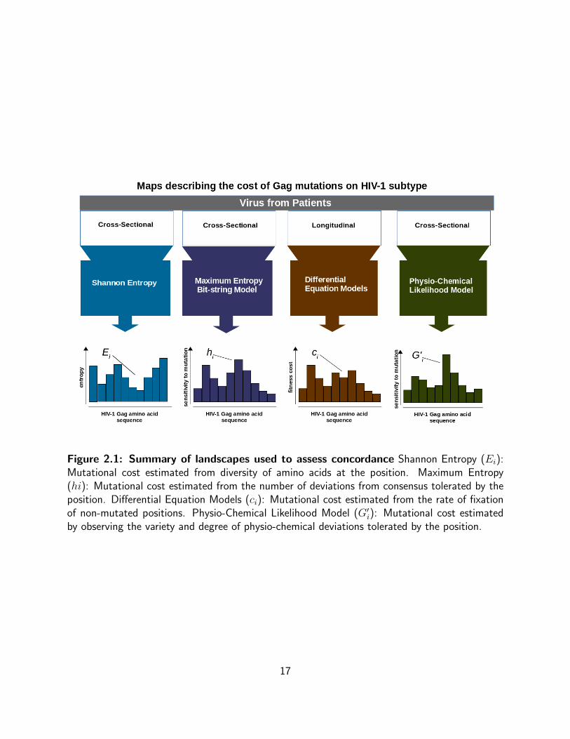
Figure 2.1: Summary of landscapes used to assess concordance Shannon Entropy (Ei):Mutational cost estimated from diversity of amino acids at the position. Maximum Entropy(hi): Mutational cost estimated from the number of deviations from consensus tolerated by theposition. Differential Equation Models (ci): Mutational cost estimated from the rate of fixationof non-mutated positions. Physio-Chemical Likelihood Model (G′i): Mutational cost estimatedby observing the variety and degree of physio-chemical deviations tolerated by the position.
17
Ei(X) = −20∑j=1
pij ln pij (2.7)
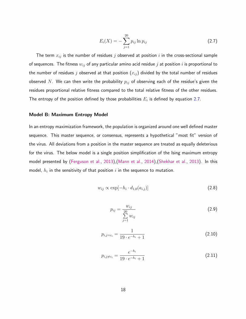
The term xij is the number of residues j observed at position i in the cross-sectional sample
of sequences. The fitness wij of any particular amino acid residue j at position i is proportional to
the number of residues j observed at that position (xij) divided by the total number of residues
observed N . We can then write the probability pij of observing each of the residue’s given the
residues proportional relative fitness compared to the total relative fitness of the other residues.
The entropy of the position defined by those probabilities Ei is defined by equation 2.7.
Model B: Maximum Entropy Model
In an entropy maximization framework, the population is organized around one well defined master
sequence. This master sequence, or consensus, represents a hypothetical ”most fit” version of
the virus. All deviations from a position in the master sequence are treated as equally deleterious
for the virus. The below model is a single position simplification of the Ising maximum entropy
model presented by (Ferguson et al., 2013),(Mann et al., 2014),(Shekhar et al., 2013). In this
model, hi in the sensitivity of that position i in the sequence to mutation.
wij ∝ exp[−hi · d1,0(ai,j)] (2.8)
pij =wij
20∑j=1
wij
(2.9)
pi,j=ci =1
19 · e−hi + 1(2.10)
pi,j 6=ci =e−hi
19 · e−hi + 1(2.11)
18

L(hi|X) =Γ(∑
j xij + 1)∏j Γ(xij + 1)
20∏j=1
pxijij (2.12)
The relative fitness (wij) of variants bearing amino acid j at position i is proportional to an
exponential term that decays depending on the distance d1,0 of the amino acid j from the putative
optimal and the degree of sensitivity of the position hi to mutation. The distance term d1,0 is
defined by astep function function where d1,0(aij) = 1 if the amino acid is not the consensus
residue and d1,0(aij) = 0 if the residue is the consensus residue. We can then write the probability
pij of observing each residue, given the residues proportional relative fitness compared to the total
relative fitness of the other residues. There will be one probability for non-consensus residues
j 6= ci and another for consenus residues j = ci. Using a maximum likelihood estimation we can
then estimate what sensitivity hi is most likely for that position given the frequency distribution
of amino acids (X) observed at that position.
Dynamical Systems Model C: Differential Equation System
By applying this differential equation system on a position by position basis, a cost map for a
section of the genome can be constructed. The parameter c in this model is the replication
penalty exacted on a position i carrying a mutation.
Below, is a set of closed form equations describing how the number of viral variants change
over time within a patient. The closed form equations were derived from a set of differential
equations one representing the change in the consensus and non-consensus variants over time
with and without an effector response. The closed form solution, describes how the frequency of
the wild variant may shift over time, given its initial starting frequency f0 and the degree c to
which the mutant variant’s replication is impaired (Fig 2.2).
fw(t) =f0
(1− f0)e−crt + f0, (2.13)
19
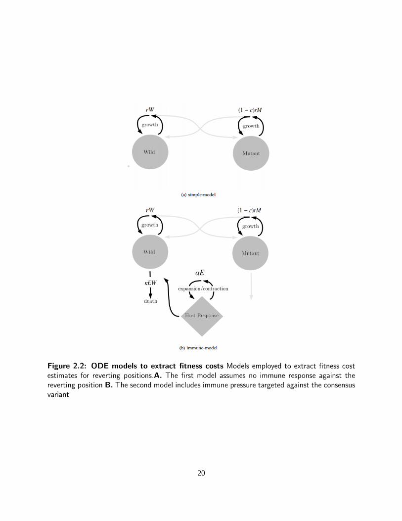
Figure 2.2: ODE models to extract fitness costs Models employed to extract fitness costestimates for reverting positions.A. The first model assumes no immune response against thereverting position B. The second model includes immune pressure targeted against the consensusvariant
20
fw(t) =f0e
λα
(1− f0)eλeαt
α−crt + f0e
λα
,
λ = κE0.
(2.14)
Table 2.1: Table of State Variables and Parameters for ODE Models The following statevariables and parameters are shared between the ordinary differential equation models.
parameters
fw frequency of wild variantf0 initial frequency of wild variantµw mutation rate of wild into mutant populationµm mutation rate of mutant into wild populationc replicative cost of mutationr growth constant of wild variantκ killing rate of effector cellsα expansion rate of effector cellsE0 initial population of effector cells
state variables
M RNA copies of mutant variant per ml of bloodW RNA copies of wild variant per ml bloodE effector response of immune system
A likelihood ratio test was used to compare how well the simple reversion model and the
immune-reversion model fit the same data set. This statistical test requires that one of the
models be a nested version of the other. It can be easily shown that our simple reversion model
is a nested version of the more complex immune model. The complex immune model can be
converted into the simple model by constraining the clearance rate κ by setting it equal to 0.
The parameters f0,c,α and λ were estimated using a binomial log likelihood fitting of the
data. In this binomial log likelihood fitting, we identified an optimal set of parameters that
described the observed residue frequencies at the different time points given the underlying
binomial distribution of the sampled data. The sampling of the virus was bernoulli like, and
there was also a significant discrepancy in sample number between the timepoints. Therefore,
21
this binomial log likelihood fitting procedure described above was preferable to a least squares
fitting procedure. The combination of parameters that produced the most probable frequencies
given the data and model were identified numerically using a downhill simplex algorithm (Nelder-
Mead) and a constrained optimization by linear approximation (COBYLA). The objective function
used in this non-linear minimization is given below (eq. 2.15):
ln(L(θ;X)) =N∑i
ln
((nixi
)fw(θ, ti)
xi(1− fw(θ, ti))n−xi
)(2.15)
The parameter θ is the vector of model parameters: f0,c,α and λ. The data term X is
the presence/absence data for the consensus residue at different timepoints in the patient. The
number ni is the number of viral sequences amplified at timepoint i while xi is the number of
viral sequences amplified at timepoint i bearing a consensus residue at the position. The value
fw is the estimated frequency of consensus residue as predicted by the model. The value ti
denotes how many days post-seroconversion the patient is at sample i with N representing the
total number of samples during the infection.
Estimating fitness cost for rapid reversions and generating parameter confidence
intervals
Reversions in Gag often happen rapidly (within 100 days or less) (Novitsky et al., 2011) and the
temporal resolution in this study is somewhat low with an average of 6 samples per 500 days.
As a result, a reversion will often occur between two sampling periods. Since the frequency
jumps from 0 to 1, it is difficult to determine the fitness cost that drove the rapid reversion
given the logistic behavior of our model. This difficulty is addressed by re-sampling the data
assuming a continuous beta distribution (the conjugate prior probability distribution for the
binomial distribution) underlies the data, refitting the re-sampled data and thereby obtaining
a distribution of possible c-values. The median of these c-values is then taken as our best guess
for c (Fig 2.3).
22
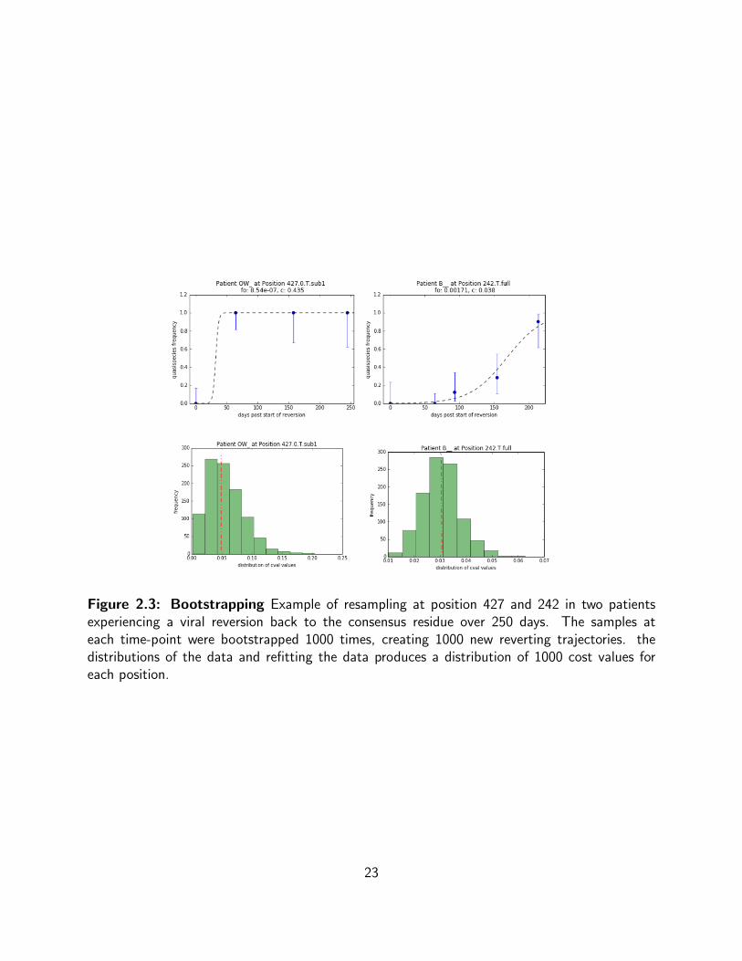
Figure 2.3: Bootstrapping Example of resampling at position 427 and 242 in two patientsexperiencing a viral reversion back to the consensus residue over 250 days. The samples ateach time-point were bootstrapped 1000 times, creating 1000 new reverting trajectories. thedistributions of the data and refitting the data produces a distribution of 1000 cost values foreach position.
23
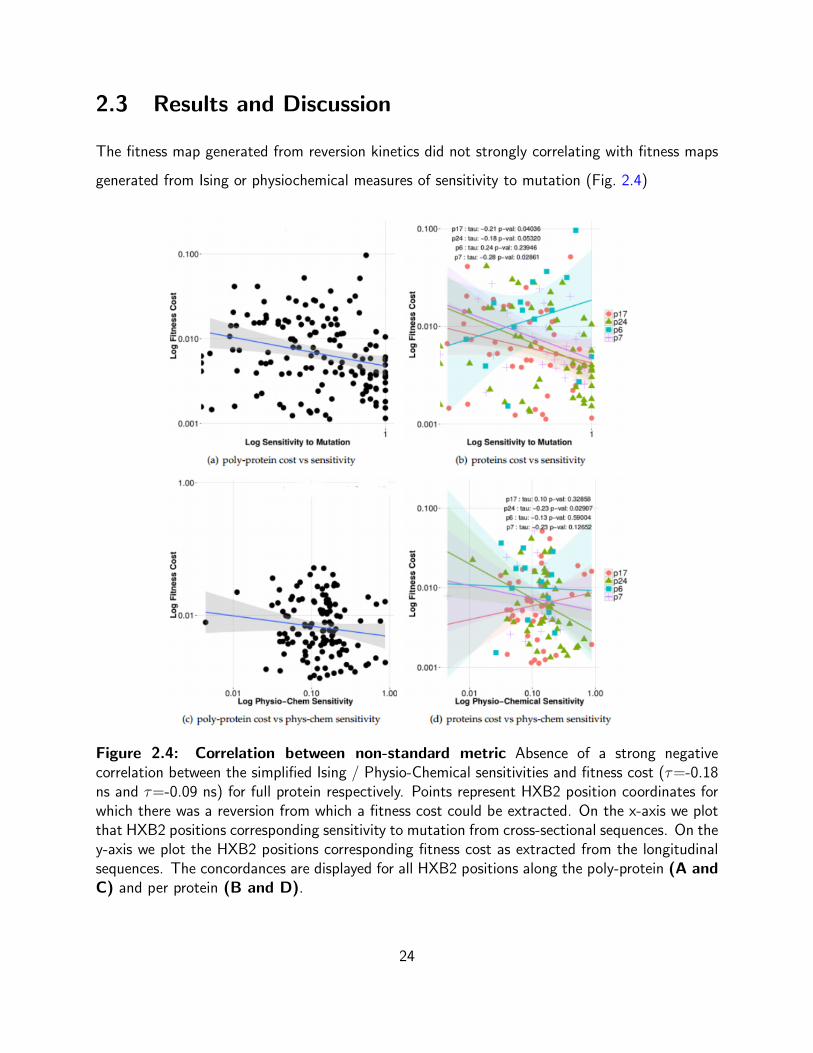
2.3 Results and Discussion
The fitness map generated from reversion kinetics did not strongly correlating with fitness maps
generated from Ising or physiochemical measures of sensitivity to mutation (Fig. 2.4)
Figure 2.4: Correlation between non-standard metric Absence of a strong negativecorrelation between the simplified Ising / Physio-Chemical sensitivities and fitness cost (τ=-0.18ns and τ=-0.09 ns) for full protein respectively. Points represent HXB2 position coordinates forwhich there was a reversion from which a fitness cost could be extracted. On the x-axis we plotthat HXB2 positions corresponding sensitivity to mutation from cross-sectional sequences. On they-axis we plot the HXB2 positions corresponding fitness cost as extracted from the longitudinalsequences. The concordances are displayed for all HXB2 positions along the poly-protein (A andC) and per protein (B and D).
24
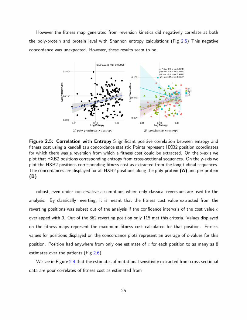
However the fitness map generated from reversion kinetics did negatively correlate at both
the poly-protein and protein level with Shannon entropy calculations (Fig 2.5) This negative
concordance was unexpected. However, these results seem to be
Figure 2.5: Correlation with Entropy S ignificant positive correlation between entropy andfitness cost using a kendall tau concordance statistic Points represent HXB2 position coordinatesfor which there was a reversion from which a fitness cost could be extracted. On the x-axis weplot that HXB2 positions corresponding entropy from cross-sectional sequences. On the y-axis weplot the HXB2 positions corresponding fitness cost as extracted from the longitudinal sequences.The concordances are displayed for all HXB2 positions along the poly-protein (A) and per protein(B)
robust, even under conservative assumptions where only classical reversions are used for the
analysis. By classically reverting, it is meant that the fitness cost value extracted from the
reverting positions was subset out of the analysis if the confidence intervals of the cost value c
overlapped with 0. Out of the 862 reverting position only 115 met this criteria. Values displayed
on the fitness maps represent the maximum fitness cost calculated for that position. Fitness
values for positions displayed on the concordance plots represent an average of c-values for this
position. Position had anywhere from only one estimate of c for each position to as many as 8
estimates over the patients (Fig 2.6).
We see in Figure 2.4 that the estimates of mutational sensitivity extracted from cross-sectional
data are poor correlates of fitness cost as estimated from
25
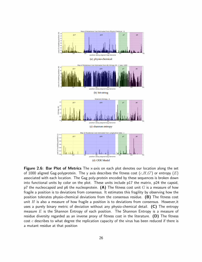
Figure 2.6: Bar Plot of Metrics The x-axis on each plot denotes our location along the setof 1000 aligned Gag-polyprotein. The y axis describes the fitness cost (c,H,G′) or entropy (E)associated with each location. The Gag poly-protein encoded by these sequences is broken downinto functional units by color on the plot. These units include p17 the matrix, p24 the capsid,p7 the nucleocapsid and p6 the nucleoprotein. (A) The fitness cost unit G is a measure of howfragile a position is to deviations from consensus. It estimates this fragility by observing how theposition tolerates physio-chemical deviations from the consensus residue. (B) The fitness costunit H is also a measure of how fragile a position is to deviations from consensus. However,ituses a purely binary metric of deviation without any physio-chemical detail. (C) The entropymeasure E is the Shannon Entropy of each position. The Shannon Entropy is a measure ofresidue diversity regarded as an inverse proxy of fitness cost in the literature. (D) The fitnesscost c describes to what degree the replication capacity of the virus has been reduced if there isa mutant residue at that position
26
reversions. Shannon entropy, in contrast, has a significant positive correlation with fitness
cost (Fig. 2.4), precisely the opposite of what one would predict. One would expect that a hyper
variable position would not be costly to mutate and we would see slow reversions at that position.
Conversely, one would expect a conserved position to revert to consensus rapidly. However, we
observe the opposite. It is the variable positions (high entropy positions) that revert rapidly and
it is the non-variable/conserved (low entropy positions) that revert slowly.
2.3.1 Shannon Entropy as proxy for fitness cost: considerations
Either Shannon entropy is a poor proxy for fitness, reversion rate is a poor proxy of fitness,
or both poorly measure fitness. There is evidence that Shannon entropy can sometimes fail
to predict fitness well in competition assays (Rihn et al., 2013) and is not necessarily a robust
measure of viral escape time from the immune response (Barton et al., 2015). The replication
of the virus is believed to be somewhat compartmentalized (van Marle et al., 2007) (Rozera
et al., 2014) (Sturdevant et al., 2015) (Heath et al., 2009) as the bulk of the replication occurs
in structured lymphoid tissues (Folkvord et al., 2005)(Hufert et al., 1997)(Schacker, 2008).
Compartmentalization creates smaller populations more susceptible to genetic drift. In these
smaller, more stochastic populations, the fittest variant would not necessarily fix in the population.
Instead, less fit variants would be able to establish locally when drift overpowers selection. In
this scenario, mutation would play an important role in generation diversity. Mutation rates
may vary over the HIV genome, due to differential rates of hyper-mutation by APOBEC (Kim
et al., 2014)(Wood et al., 2009) and reverse transcriptase’s lack of fidelity over particular stem
loop structures (Cuevas et al., 2015) (Geller et al., 2015). Shannon entropy may be detecting
differential diversity that is a signature of these uneven mutation rates. Shannon entropy may
not simply be detecting signatures of functional and structural plasticity alone.
2.3.2 Reversions as a proxy for fitness cost: considerations
Alternatively, our reversion rates could be poor proxies of fitness. This might be due to the
fact that samples were only taken post sero-conversion in the patients. A large window period
27
measuring 20-30 days occurred between the time the patient first contracted HIV and had their
blood sampled. Many highly conserved positions may have already reverted during this period.
Therefore, a large subset of rapid reversions may be absent from our estimates. If this subset is
large, we could possibly be grossly underestimating the average fitness costs at many positions.
Secondly, we only observed consensus sequences out-replicating variants carrying typically only
one residue type. The rate of reversion is likely residue dependent. However, even so it is
concerning that on average, entropy does not predict reversion rate well.
2.3.3 Confounding factors to be explored in further analysis: immune
pressure and epistasis
Two confounding factors must be taken into account when attempting to derive a fitness
landscape from intra-patient longitudinal sequence data. First a residues fitness is highly
dependent on the particular genetic background it is embedded in and second, immune pressure is
heavily shaping the evolution of our population. The disappearance of viruses’ bearing a particular
residue may not be a sign that the residue is unfavorable for the virus to carry, instead it may
indicate that the immune system more readily recognizes epitopes bearing that particular residue.
In that case, even an intrinsically favorable residue may disappear from the population. White
blood cells called T-cells play a central role in reducing viral loads during the acute portion of
HIV infection (Borrow et al., 1994) (Ogg et al., 1998).Sometimes it is unclear whether a variant
is disappearing because it is unfit, or if it is being targeted by the immune system. Immune
system clearance of a variant can often be observed in patient kinetic data, with variants peaking
in frequency during the first portion of the acute infection and then being eradicated during the
second portion (Novitsky et al., 2009) (Liu et al., 2012).However, even in the absence of immune
pressure, a residue’s fitness may be shifted or hijacked by the mutational status of surrounding
residues. In fact, simultaneous and tandem mutations are often observed within viral populations
due to shared structural and or functional constraints (Ferguson et al., 2013)(Brockman et al.,
2007)(Schneidewind et al., 2007)(Dahirel et al., 2011). Because of this, the cost of a mutation
cannot not be ascertained from simply observing how single residue mutants replicate. The
28
mutational status of the residues our position is coupled may need to be taken into account as
well. It could be that a residue mutation is normally neutral in isolation, but in the presence of
a neighboring mutation it is rendered unfit. It should be noted we have accounted for the first
confounding factor in this analysis but not the latter.
Acknowledgments
We are grateful to all members of the primary HIV-1 subtype C infection study in Botswana
(Tshedimoso Study) (Novitsky et al., 2011). We would also like to acknowledge the Theoretical
Biology and Biophysics Division at Los Alamos National Laboratory for the HIV compendium
and alignments made available by their group https://www.hiv.lanl.gov. The HIV Compendia
are funded by the Division of AIDS, National Institute of Allergy and Infectious Diseases, through
an interagency agreement with the U.S. Department of Energy. This work was supported in part
by an NSF IGERT: Scalable Computing and Leading Edge Innovative Technologies (SCALE-IT)
for Biology NSF Award Number 0801540.
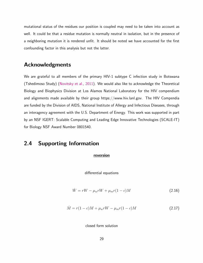
2.4 Supporting Information
reversion
differential equations
W = rW − µwrW + µmr(1− c)M (2.16)
M = r(1− c)M + µwrW − µmr(1− c)M (2.17)
closed form solution
29

fw(t) =f0
(1− f0)e−crt + f0(2.18)
reversion with effector response
differential equations
W = rW − κEW − µwrW + µmr(1− c)M (2.19)
M = r(1− c)M + µwrW − µmr(1− c)M (2.20)
E = αE (2.21)
closed form solution
fw(t) =f0e
λα
(1− f0)eλeαt
α−crt + f0e
λα
λ = κE0 (2.22)
growth constant r = ln(2)/T = 1 where T is the doubling time of the virus. The assumption
µw = µm = 0 can be make for large population sizes.
2.4.1 Immune Equation Derivation
If we assume the mutation rate has a neglible impact on our estimate of c due to large
populations sizes, we can ignoring the mutation in and out of the consensus/wild W and non-
consensus/mutant populations M , then we can write
30

Table 2.2: State Variables and Parameters The following parameters and state variables areshared between the two ODE Models
parameters
fw frequency of wild variantf0 initial frequency of wild variantµw mutation rate of wild into mutant populationµm mutation rate of mutant into wild populationc replicative cost of mutationr growth constant of wild variantκ killing rate of effector cellsα expansion rate of effector cells
state variables
M rna copies of mutant variant per ml of bloodW rna copies of wild variant per ml bloodE effector response of immune system
W = rW − κEW (2.23)
M = r(1− c)M E = αE (2.24)
If we solve the effector differential equation assuming that at E(0) = E0 we obtain the
following solution to the below equation.
E = αE (2.25)
which solves as:
E(t) = E0eαt. (2.26)
We can than write the change in W and M as:
31

W = rW − κE0eαtW (2.27)
M = r(1− c)M (2.28)
We wish to obtain a closed-form solution that describes the frequency of the variant:
fw =W
M +W(2.29)
We can rewrite fw as:
fw =WM
1 + WM
(2.30)
We can solve easily for this ratio of W to M . We will call this z(t) = W (t)M(t)
. We know that
the derivative of z is:
z′(t) =(WM
) ddt
=MW −WM
M2(2.31)
substituting in the respective differential equations we obtain
(WM
) ddt
=M(rW − κE0e
αtW)
M2−W(r(1− c)M
)M2
(2.32)
Cancel out terms and group WM
ratios
z′(t) =(r − κE0e{αt} − r(1− c)
)z(t) (2.33)
which simplifies to
z′(t) =(− κE0e{αt}+ rc
)z(t) (2.34)
We can then solve for the ratio z in this separable equation:
this gives us a solution of:
32

z(t) = z0 · e{(−κE0e
αt
α+κE0
α+ rct
)} (2.35)
The solution to fw is then:
fw(t) =z(t)
1 + z(t)(2.36)
Which when substituting z,
fw(t) =z0 · e
−κE0eαt
α+κE0α
+rct
1 + z0 · e−κE0e
αt
α+κE0α
+rct(2.37)
Writing z0 in terms of f0 we see that,
fw(t) =eκE0α
1−f0f0· e
κE0eαt
α−rct + e
κE0α
(2.38)
If we group the clearance rate κ and the initial effector population E0 we are then only fitting
four parameters (κE0 = λ).
fw(t) =f0e
λα
(1− f0)eλeαt
α−crt + f0e
λα
(2.39)
λ = κE0 (2.40)
33

Chapter 3
Fitness Map constructed using a
physico-chemical model of residue
substitution
34
Abstract
Quantifying the variation in the strength of purifying selection across a protein sequence is of
fundamental interest in both structural and evolutionary biology. Here we present a simple,
quantitative model grounded in the field of population genetics that allows one to estimate the
optimal amino acid sequence of a protein and the sensitivity of the protein’s functionality to
deviation from this optimal sequence in physicochemial space. Conceptually, our model can be
viewed as constrained version of a model describing residue conservation, where, in our model, the
link between protein sequence (genotype), protein function (phenotype), and fitness are explicitly,
rather than implicitly, modelled. We use maximum likelihood to parameterize our model using
over a 1000 different sequences of HIV subtype C’s Gag poly-protein. We evaluate its performance
by comparing our amino acid site specific sensitivity parameters to empirical in vitro and in vivo
measures of HIV fitness. To better contextualize our results, we first show how frequently used,
entropy metrics can be viewed as a generalization and fully saturated version of our model.
Second, we fit the entropy model to the same sequence data and evaluate its ability to predict
the same empirical fitness data. In terms of fitting the sequence data, AIC indicates that the
entropy model substantially outperforms our model. This result is not surprising given the entropy
model has as many parameters as categories and, by definition, the best model possible for any
categorical data set and that we fit the models using more than 50 data points per parameter.
In contrast, we find that our model’s site sensitivity parameters do a better job predicting the
empirical fitness data than the entropy model’s site specific conservation terms. Thus, while the
entropy model may fit the sequence data better, our model appears to better contextualize the
information encoded within that data. This result is also not surprising given the fact that our
model’s site specific sensitivity parameter has a direct biological interpretation while the entropy
model’s conservation term is simply a measure of mean uncertainty of the state of a site. More
importantly, unlike the entropy model, our model can be further refined and used to test more
complex hypotheses about the link between genotype, phenotype, and fitness. For example, in our
analysis we find evidence that different functional regions of the gag poly-protein have different
sensitivities to deviation from the optimal amino acid’s molecular volume.
35
3.1 Introduction
3.1.1 Fitness Landscapes and HIV Diversity
HIV exhibits a great deal of genetic plasticity (Lemey et al., 2006; Salemi, 2013; Cuevas et al.,
2015). This genetic plasticity allows the virus to effectively evade a patient’s immune response
and has accordingly aggravated attempts to create an effective vaccine immunogen (Goulder and
Watkins, 2004; Autran et al., 2008; Johnston and Fauci, 2008). While an immunogen might elicit
a strong CTL response against an HIV epitope, the virus can often avoid this immunogen elicited
recognition by mutating the targeted epitope. In a genetically plastic virus such as HIV, not every
mutation incurs a serious fitness penalty. As a consequence, mutationally robust positions along
the proteome tend to be the ones to escape immune recognition (Korber et al., 2001; Hinkley
et al., 2011). However, there are vulnerable regions along the proteome that are expensive for the
virus to mutate (Martinez-Picado et al., 2006; Rihn et al., 2013; Manocheewa et al., 2015). In
order to identify these vulnerable regions, mutational landscapes for the viral proteome have been
constructed (Deforche et al., 2008; Seifert et al., 2015; Kouyos et al., 2012; Hinkley et al., 2011;
Shekhar et al., 2013; Ferguson et al., 2013; Mann et al., 2014; Lorenzo-Redondo et al., 2014;
Moradigaravand et al., 2014; Barton et al., 2016). These mutational landscapes describe the sum
or synergistic replicative cost exacted on the virus for any combination of residue level mutations
(Michael R. Dietrich, 2012; Acevedo et al., 2014). They can be constructed using a variety of
approaches, both indirectly by computational analysis of patient sequence data (Ferguson et al.,
2013) and directly using in vitro methods such as growth competition assays (Manocheewa et al.,
2015).
Predict escapes is bench-marked on a longitudinal data set detailing viral within-host
dynamics. Using a cross-sectional MSA, we can generate a fitness landscape using a population
genetics model derived from work by Gilchrist et al. (2009); Gilchrist (2007) and Shah and
Gilchrist (2011). In this formulation, the frequency landscape of residues in the proteome informs
36
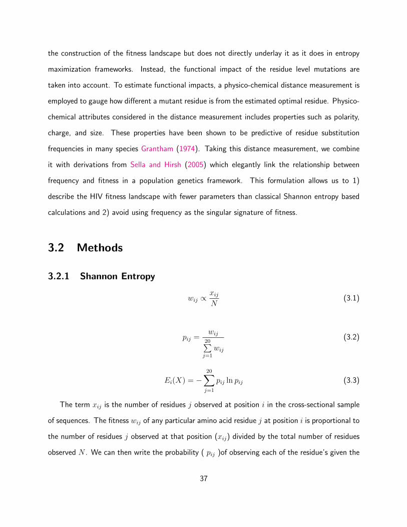
the construction of the fitness landscape but does not directly underlay it as it does in entropy
maximization frameworks. Instead, the functional impact of the residue level mutations are
taken into account. To estimate functional impacts, a physico-chemical distance measurement is
employed to gauge how different a mutant residue is from the estimated optimal residue. Physico-
chemical attributes considered in the distance measurement includes properties such as polarity,
charge, and size. These properties have been shown to be predictive of residue substitution
frequencies in many species Grantham (1974). Taking this distance measurement, we combine
it with derivations from Sella and Hirsh (2005) which elegantly link the relationship between
frequency and fitness in a population genetics framework. This formulation allows us to 1)
describe the HIV fitness landscape with fewer parameters than classical Shannon entropy based
calculations and 2) avoid using frequency as the singular signature of fitness.
3.2 Methods
3.2.1 Shannon Entropy
wij ∝xijN
(3.1)
pij =wij
20∑j=1
wij
(3.2)
Ei(X) = −20∑j=1
pij ln pij (3.3)
The term xij is the number of residues j observed at position i in the cross-sectional sample
of sequences. The fitness wij of any particular amino acid residue j at position i is proportional to
the number of residues j observed at that position (xij) divided by the total number of residues
observed N . We can then write the probability ( pij )of observing each of the residue’s given the
37

residues proportional relative fitness compared to the total relative fitness of the other residues.
The entropy of the position defined by those probabilities Ei is defined by equation 3.3.
3.2.2 Estimating Physico-chemical Sensitivities
In the model, the fitness wij of an amino acid j at position i is proportional to an exponential
decay function (eq. 3.4). This function, decays as the Physico-chemical distance Dij increases
between the amino acid aj and the consensus amino acid ai for that position (eq. 3.5). The
sensitivity parameter G′ describing how sensitive the virus is to deviations from the consensus
residue at this position.
wij ∝ exp[−G′i ·D(~θ, ai, aj)] (3.4)
Physico-chemical deviation between residues i and j are measured in terms of differences
in composition ci, polarity pi, and molecular volume vi, using the weightings θc,θp, and θv
respectively. It should be noted that these three properties are not necessarily independent
of each other. However, for the sake of simplicity, the properties of composition, polarity and
molecular volume are treated as independent and therefore orthogonal to each other in the
distance calculation for D (eq. 3.5).
D(~θ, ai, aj) = [θα(ci − cj)2 + θβ(pi − pj)2 + θγ(vi − vj)2]1/2 (3.5)
These three properties are used because residues that share one of these three properties are
more likely to be interchanged with each other according to residue substitution frequencies (RSF).
Values for these properties were taken from Grantham (Grantham, 1974) and the weighting of
each of these properties was estimated specifically for HIV using a MLE on sequence data.
We can calculate the probability of observing an amino acid by partitioning the relative
frequency of the amino acid by the sum total of all the relative amino acid frequencies for
38

the position. The relative frequency of an amino acid at a position can be expressed in terms of
fitness and population size. The value wij in (eq. 3.6) describes the fitness of amino acid i at
position j relative to other amino acids. However it is not sufficient to describe the probability
of drawing an amino acid in terms of relative fitness alone. Due to drift, we would expect the
frequency of a less fit amino acid to be higher in smaller populations and lower in larger ones.
To account for this, the value wij is modulated by the effective population size Ne to obtain a
relative amino acid frequency for the position. This model is different than the Ising model in that
it is derived from a population genetics framework, and incorporates more biological information
in order to calculate the decay term with the exponential.
pij =(wij)
Ne
20∑j=1
(wij)Ne=
exp[−Ne ·G′i ·D(~θ, ai, aj)]20∑j=1
exp[−Ne ·G′i ·D(~θ, ai, aj)]
(3.6)
We can regard the resulting formulation (eq. 3.6) as a type of Boltzmann distribution with
fitness corresponding to energy, and population size corresponding to heat. Sella and Hirsh
demonstrated in their 2005 paper Sella and Hirsh (2005) that the Boltzmann distribution, used
to describe state distributions in a thermodynamic systems, had analogous application to genotype
distributions in evolutionary systems. However, our data does not allow us to tease apart
population (Ne) and sensitivity (G′) effects. We therefore group the two terms together as
G′′, scaling mutational sensitivity by effective population size (eq. 3.7).
pij =exp[−G′′i ·D(~θ, ai, aj)]
20∑j=1
exp[−G′′i ·D(~θ, ai, aj)]
(3.7)
The likelihood function
L(G′′i ,~θ | X) =
Γ(∑
j xij + 1)∏j Γ(xij + 1)
20∏j=1
pxijij (3.8)
39
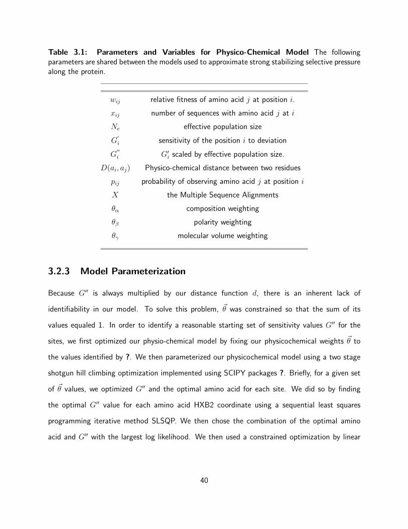
Table 3.1: Parameters and Variables for Physico-Chemical Model The followingparameters are shared between the models used to approximate strong stabilizing selective pressurealong the protein.
wij relative fitness of amino acid j at position i.
xij number of sequences with amino acid j at i
Ne effective population size
G′i sensitivity of the position i to deviation
G′′i G′i scaled by effective population size.
D(ai, aj) Physico-chemical distance between two residues
pij probability of observing amino acid j at position i
X the Multiple Sequence Alignments
θα composition weighting
θβ polarity weighting
θγ molecular volume weighting
3.2.3 Model Parameterization
Because G′′ is always multiplied by our distance function d, there is an inherent lack of
identifiability in our model. To solve this problem, ~θ was constrained so that the sum of its
values equaled 1. In order to identify a reasonable starting set of sensitivity values G′′ for the
sites, we first optimized our physio-chemical model by fixing our physicochemical weights ~θ to
the values identified by ?. We then parameterized our physicochemical model using a two stage
shotgun hill climbing optimization implemented using SCIPY packages ?. Briefly, for a given set
of ~θ values, we optimized G′′ and the optimal amino acid for each site. We did so by finding
the optimal G′′ value for each amino acid HXB2 coordinate using a sequential least squares
programming iterative method SLSQP. We then chose the combination of the optimal amino
acid and G′′ with the largest log likelihood. We then used a constrained optimization by linear
40

approximation COBYLA algorithm to optimize over ~θ space, re-optimizing G′′ and the optimal
amino acid at each step as described above.
The optimization was first initialized at >50 random weights in the physicochemical weight
space ~θ. The weight space was explored for a constrained number of optimization steps to
assess the most likely combination of weights around the initialized points. For each step in
this exploration, the G′′ sensitivities were re-optimized for that particular set of weights. After
this exploration routine, the shotgun hill climbing optimization was reinitialized for the top three
sets of physicochemical weights obtaining the highest likelihoods. The optimization algorithm
was reinitialized from these regions of physico-chemical weight space and was allowed to run
until convergence. The most likely parameter weight combination from this optimization step
was then selected. The optimization for the G′′ values was initialized as a grid search using a
vector containing a distribution of likely G′′ values. This distribution of likely G′′ values was
obtained from an optimization in which the physicochemical weights were regarded as similar to
those estimated from (Grantham, 1974) paper examining general residue substitution frequencies
across species. We regarded the maximum likelihood set of parameter weight combinations from
the convergence of these optimization to be our global optimum. In order to test whether the
same ~θ values were applicable across all sites, we compared our model fit with a single set of ~θ
values to one where ~θ was allowed to vary between the functional regions p24, p17, p7, and p6.
3.2.4 Cross-sectional Sequences
We use 1000 curated sequences in the Los Alamos database for subtype C http://www.hiv.lanl.gov/.
These sequences were filtered web alignments that provide a good example of the subtypes
breadth. Every sequence belongs to a unique patient and sequences that resemble each other
too closely had been removed. Additionally questionable sequences such as those that appear
to be hypermutants and synthetics have also been removed. The curated sequences were clean,
containing little ambiguous coding, few long insertions and lacked a preponderance of frame shifts.
41
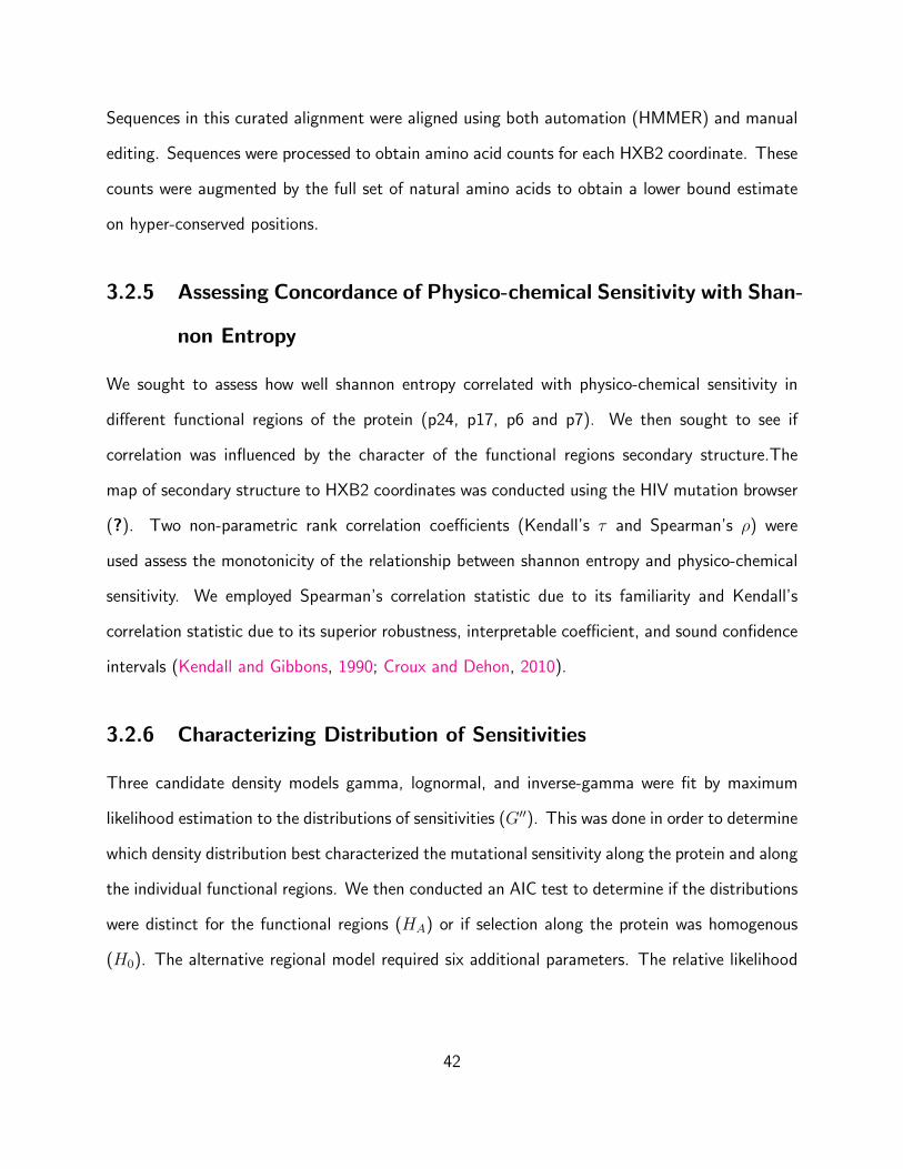
Sequences in this curated alignment were aligned using both automation (HMMER) and manual
editing. Sequences were processed to obtain amino acid counts for each HXB2 coordinate. These
counts were augmented by the full set of natural amino acids to obtain a lower bound estimate
on hyper-conserved positions.
3.2.5 Assessing Concordance of Physico-chemical Sensitivity with Shan-
non Entropy
We sought to assess how well shannon entropy correlated with physico-chemical sensitivity in
different functional regions of the protein (p24, p17, p6 and p7). We then sought to see if
correlation was influenced by the character of the functional regions secondary structure.The
map of secondary structure to HXB2 coordinates was conducted using the HIV mutation browser
(?). Two non-parametric rank correlation coefficients (Kendall’s τ and Spearman’s ρ) were
used assess the monotonicity of the relationship between shannon entropy and physico-chemical
sensitivity. We employed Spearman’s correlation statistic due to its familiarity and Kendall’s
correlation statistic due to its superior robustness, interpretable coefficient, and sound confidence
intervals (Kendall and Gibbons, 1990; Croux and Dehon, 2010).
3.2.6 Characterizing Distribution of Sensitivities
Three candidate density models gamma, lognormal, and inverse-gamma were fit by maximum
likelihood estimation to the distributions of sensitivities (G′′). This was done in order to determine
which density distribution best characterized the mutational sensitivity along the protein and along
the individual functional regions. We then conducted an AIC test to determine if the distributions
were distinct for the functional regions (HA) or if selection along the protein was homogenous
(H0). The alternative regional model required six additional parameters. The relative likelihood
42
or weight of evidence (wi) for the next best fitting model was then calculated using the below
equation where i denotes the model with the larger AIC (bur, 2002).
wi = exp[AICmin − AICi
2
](3.9)
3.2.7 Predicting Viral Behaviors
Correlation with in vivo escape times
Entropy scores can help predict how long it will take the virus to escape a CD8 T-cell response.
(Liu et al., 2012). It has been shown that high entropy epitopes can more easily escape immune
targeting while low entropy epitopes struggle to evade immune detection or escape slowly (Ferrari
et al., 2011). In this analysis, we test whether our physico-chemical sensitivity (G′′) or shannon
entropy (S) better predicts escape times. The escape times used in this analysis come from a
2012 paper by Liu et al. (2012) where viral escapes at reactive epitopes sites were characterized
in 17 HIV-1 subtype B infected patients over 3 years using serial SGA sequencing. In this analysis,
the predicted variabe escape time (t50) is defined as the number of days between detection of
the T-cell response and the time viral variants bearing that respective reactive epitope fell below
50%.
Correlation with in vitro viral spreading fitness
Entropy scores can be used to predict how a mutation will impact the replicative capacity of HIV
In this analysis, we tested whether our physico-chemical sensitivity (G′′) or shannon entropy (S)
better predicted replicative fitness costs exacted on mutants. Rihn et al. (2013) assessed the
replicative fitness of HIV virions bearing various capsid (CA)mutations via spreading replication
assays on human T-cell lines (MT4) and PBMC. The CA mutants in this study were generated
by creating a mutagenized CA library using a low fidelity PCR approach and then inserting the
43

mutated CA sequences in replication competent proviral clones. Fitness was reported as % of
the wild-type replication as recorded by the number of GFP fluorescing cells.
3.3 Results and Discussion
3.3.1 Physico-chemical selective forces vary along the poly-protein
It was unclear if the the physicochemical selective forces shaping residue evolution varied along
the Gag poly-protein. Two candidate models were compared to inspect the variation. In the
alternative model HA the physicochemical selective forces as described by the weighting vector
~θ were free to vary by region. In the null model H0, it was assumed that selective forces ~θ were
uniform over the protein. Surprisingly, even slight adjustments to the physicochemical weights on
a per-region basis (Table 3.10) significantly improved the model’s ability to describe the observed
residue frequencies in our MSA by several loglikelihood units (Table 3.2)
Table 3.2: Model Selection Likelihood Ratio Test assessing single (H0) vs regional (HA)physico-chemical weighting
Log(L) H0 Log(L) HA LRT test statistic df p-value
-69040 -63550 10980 6 <2.23e-308
This variation likely stems from differences in secondary structure composition among the
regions. It has been shown that amino acids can be clustered by alpha helices/turn and
beta sheet propensity (kawashima,2000) as each structure possesses inherently different physico-
chemical constraints. These particular properties (molecular volume, polarity and composition)
are just three among a host of side chain properties that may be similarly predictive of residue
interchangeability. This set of properties was initially chosen because they were good correlates of
residue interchangeability in organisms other than HIV (Grantham, 1974). In the previous paper
these estimates were derived from residue substitution frequencies. Finally, the inter-property
44

correlations between the side-chain traits imply that these weighting estimates are similarly not
entirely independent of each other.
Given that the traits of composition, polarity, and molecular volume may not be the principle
selective forces determining residue interchangeability and fixation, further work should pursue
identifying other traits that appreciably improve the model’s ability to describe residue frequency
in a sampled viral poplulation. Contending traits include continuous properties like hydrophobicity
or acidity and categorical traits such as the aliphatic or aromatic side chain construction.
3.3.2 Distributions of Physico-Chemical Sensitivities
Lognormal model best describes distribution of sensitivities
Out of three candidate density models (gamma, lognormal, inverse-gamma), the lognormal model
optimally described the distribution of sensitivites over the poly-protein (Table 3.3).The exception
was p7, in which the gamma fit was slightly better. The generative process underlying this
distribution is one in which many positive random independent variables act proportionally on
each other. Many biological phenomena are well described by this type of process. The parameters
of this model are readily interpretable as the logarithm of a lognormal distribution X is simply a
normal distribution. This normal distribution can be described by a location value µ where values
around µ are shifted by a standard normal random variable Z scaled by a shape parameter σ
(eq. 3.10).
X = eµ+σZ (3.10)
Character of sensitivity distributions differ between functional regions
Under this new model, it was unclear if the fitness proxy’s (G′′) distribution would retain a
distinct character from one region to the next or if the fitness proxy’s distribution would appear
45
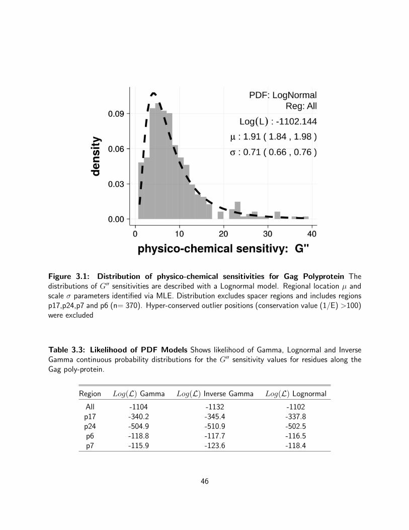
Figure 3.1: Distribution of physico-chemical sensitivities for Gag Polyprotein Thedistributions of G′′ sensitivities are described with a Lognormal model. Regional location µ andscale σ parameters identified via MLE. Distribution excludes spacer regions and includes regionsp17,p24,p7 and p6 (n= 370). Hyper-conserved outlier positions (conservation value (1/E) >100)were excluded
Table 3.3: Likelihood of PDF Models Shows likelihood of Gamma, Lognormal and InverseGamma continuous probability distributions for the G′′ sensitivity values for residues along theGag poly-protein.
Region Log(L) Gamma Log(L) Inverse Gamma Log(L) Lognormal
All -1104 -1132 -1102p17 -340.2 -345.4 -337.8p24 -504.9 -510.9 -502.5p6 -118.8 -117.7 -116.5p7 -115.9 -123.6 -118.4
46
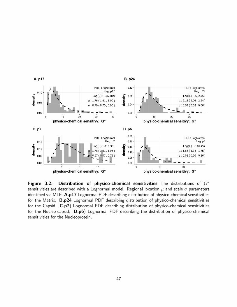
Figure 3.2: Distribution of physico-chemical sensitivities The distributions of G′′
sensitivities are described with a Lognormal model. Regional location µ and scale σ parametersidentified via MLE. A.p17 Lognormal PDF describing distribution of physico-chemical sensitivitiesfor the Matrix. B.p24 Lognormal PDF describing distribution of physico-chemical sensitivitiesfor the Capsid. C.p7) Lognormal PDF describing distribution of physico-chemical sensitivitiesfor the Nucleo-capsid. D.p6) Lognormal PDF describing the distribution of physico-chemicalsensitivities for the Nucleoprotein.
47
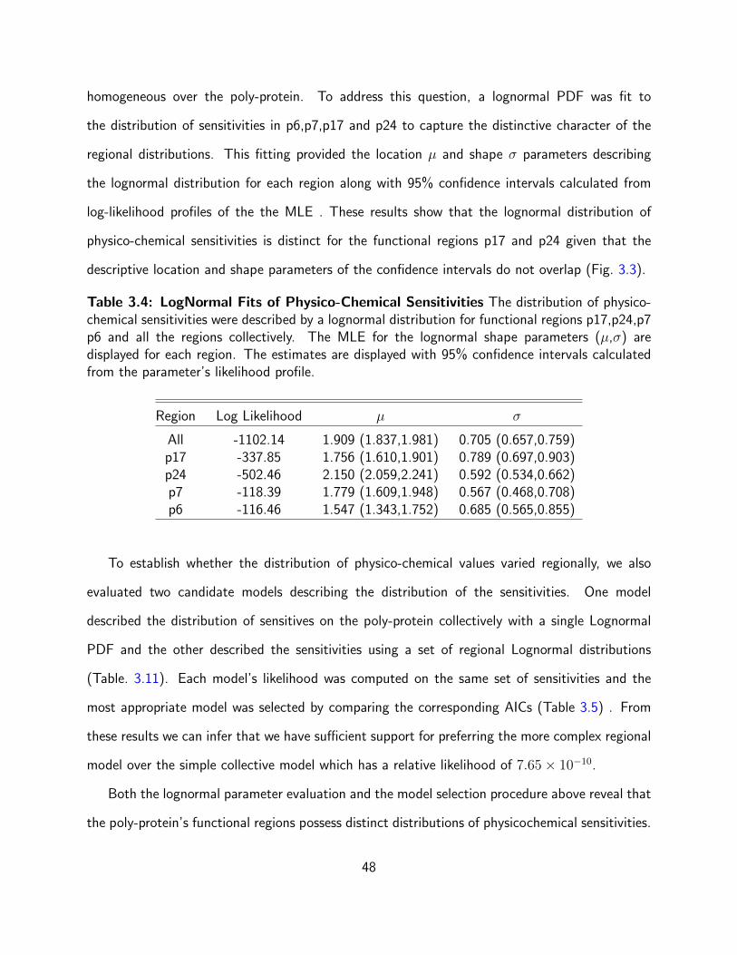
homogeneous over the poly-protein. To address this question, a lognormal PDF was fit to
the distribution of sensitivities in p6,p7,p17 and p24 to capture the distinctive character of the
regional distributions. This fitting provided the location µ and shape σ parameters describing
the lognormal distribution for each region along with 95% confidence intervals calculated from
log-likelihood profiles of the the MLE . These results show that the lognormal distribution of
physico-chemical sensitivities is distinct for the functional regions p17 and p24 given that the
descriptive location and shape parameters of the confidence intervals do not overlap (Fig. 3.3).
Table 3.4: LogNormal Fits of Physico-Chemical Sensitivities The distribution of physico-chemical sensitivities were described by a lognormal distribution for functional regions p17,p24,p7p6 and all the regions collectively. The MLE for the lognormal shape parameters (µ,σ) aredisplayed for each region. The estimates are displayed with 95% confidence intervals calculatedfrom the parameter’s likelihood profile.
Region Log Likelihood µ σ
All -1102.14 1.909 (1.837,1.981) 0.705 (0.657,0.759)p17 -337.85 1.756 (1.610,1.901) 0.789 (0.697,0.903)p24 -502.46 2.150 (2.059,2.241) 0.592 (0.534,0.662)p7 -118.39 1.779 (1.609,1.948) 0.567 (0.468,0.708)p6 -116.46 1.547 (1.343,1.752) 0.685 (0.565,0.855)
To establish whether the distribution of physico-chemical values varied regionally, we also
evaluated two candidate models describing the distribution of the sensitivities. One model
described the distribution of sensitives on the poly-protein collectively with a single Lognormal
PDF and the other described the sensitivities using a set of regional Lognormal distributions
(Table. 3.11). Each model’s likelihood was computed on the same set of sensitivities and the
most appropriate model was selected by comparing the corresponding AICs (Table 3.5) . From
these results we can infer that we have sufficient support for preferring the more complex regional
model over the simple collective model which has a relative likelihood of 7.65× 10⁻¹⁰.
Both the lognormal parameter evaluation and the model selection procedure above reveal that
the poly-protein’s functional regions possess distinct distributions of physicochemical sensitivities.
48
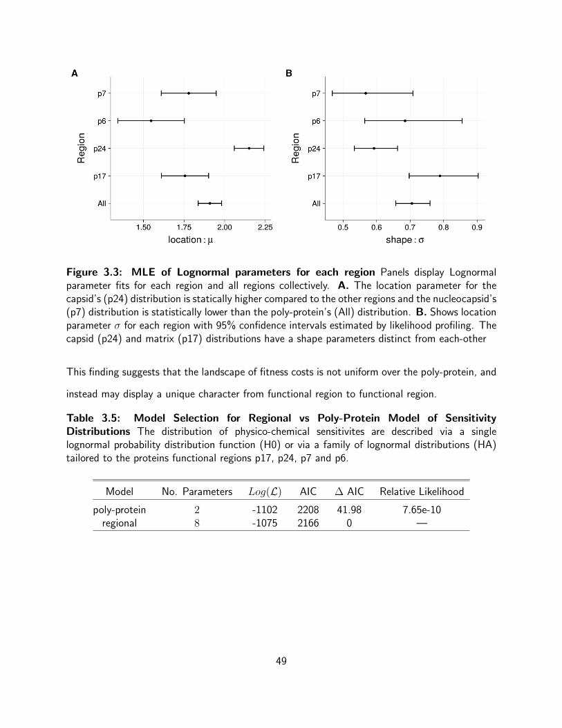
Figure 3.3: MLE of Lognormal parameters for each region Panels display Lognormalparameter fits for each region and all regions collectively. A. The location parameter for thecapsid’s (p24) distribution is statically higher compared to the other regions and the nucleocapsid’s(p7) distribution is statistically lower than the poly-protein’s (All) distribution. B. Shows locationparameter σ for each region with 95% confidence intervals estimated by likelihood profiling. Thecapsid (p24) and matrix (p17) distributions have a shape parameters distinct from each-other
This finding suggests that the landscape of fitness costs is not uniform over the poly-protein, and
instead may display a unique character from functional region to functional region.
Table 3.5: Model Selection for Regional vs Poly-Protein Model of SensitivityDistributions The distribution of physico-chemical sensitivites are described via a singlelognormal probability distribution function (H0) or via a family of lognormal distributions (HA)tailored to the proteins functional regions p17, p24, p7 and p6.
Model No. Parameters Log(L) AIC ∆ AIC Relative Likelihood
poly-protein 2 -1102 2208 41.98 7.65e-10regional 8 -1075 2166 0 —
49
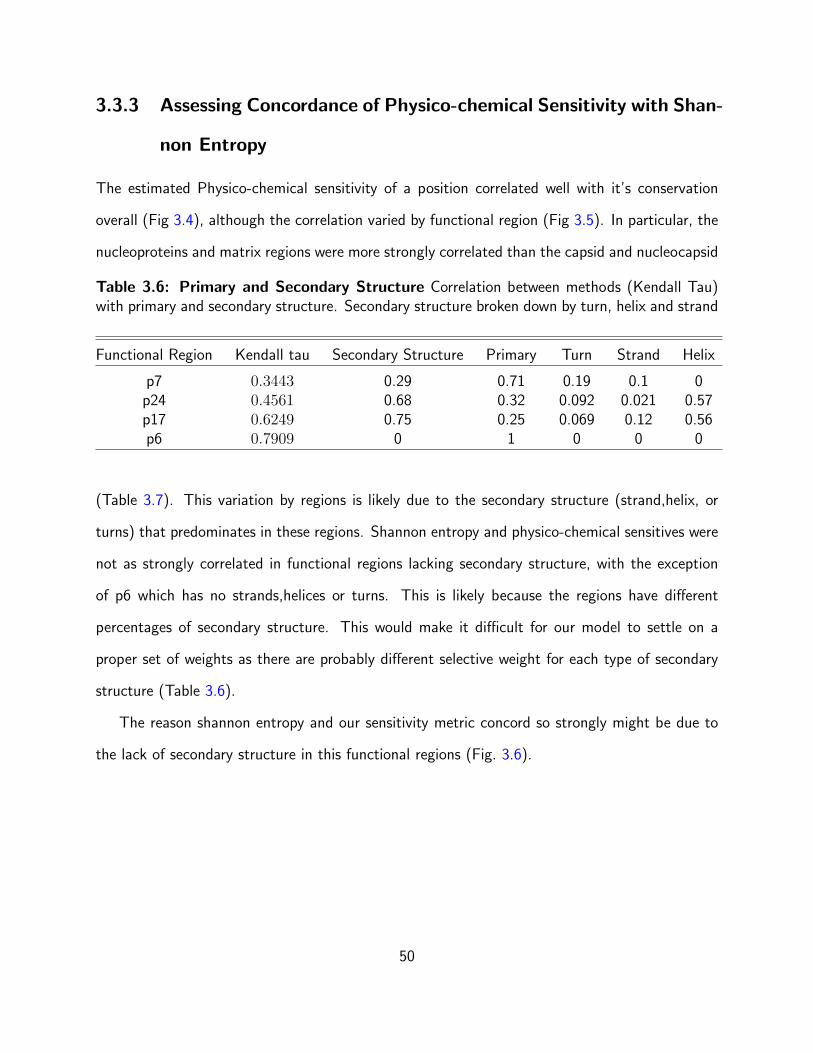
3.3.3 Assessing Concordance of Physico-chemical Sensitivity with Shan-
non Entropy
The estimated Physico-chemical sensitivity of a position correlated well with it’s conservation
overall (Fig 3.4), although the correlation varied by functional region (Fig 3.5). In particular, the
nucleoproteins and matrix regions were more strongly correlated than the capsid and nucleocapsid
Table 3.6: Primary and Secondary Structure Correlation between methods (Kendall Tau)with primary and secondary structure. Secondary structure broken down by turn, helix and strand
Functional Region Kendall tau Secondary Structure Primary Turn Strand Helix
p7 0.3443 0.29 0.71 0.19 0.1 0p24 0.4561 0.68 0.32 0.092 0.021 0.57p17 0.6249 0.75 0.25 0.069 0.12 0.56p6 0.7909 0 1 0 0 0
(Table 3.7). This variation by regions is likely due to the secondary structure (strand,helix, or
turns) that predominates in these regions. Shannon entropy and physico-chemical sensitives were
not as strongly correlated in functional regions lacking secondary structure, with the exception
of p6 which has no strands,helices or turns. This is likely because the regions have different
percentages of secondary structure. This would make it difficult for our model to settle on a
proper set of weights as there are probably different selective weight for each type of secondary
structure (Table 3.6).
The reason shannon entropy and our sensitivity metric concord so strongly might be due to
the lack of secondary structure in this functional regions (Fig. 3.6).
50
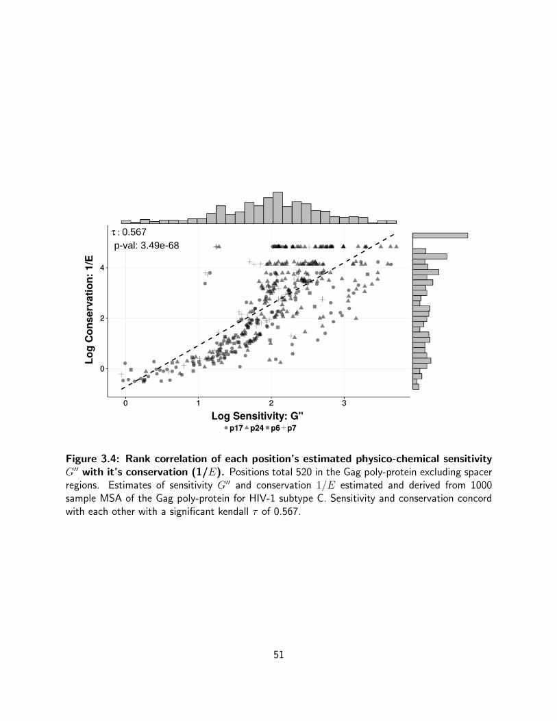
Figure 3.4: Rank correlation of each position’s estimated physico-chemical sensitivityG′′ with it’s conservation (1/E). Positions total 520 in the Gag poly-protein excluding spacerregions. Estimates of sensitivity G′′ and conservation 1/E estimated and derived from 1000sample MSA of the Gag poly-protein for HIV-1 subtype C. Sensitivity and conservation concordwith each other with a significant kendall τ of 0.567.
51
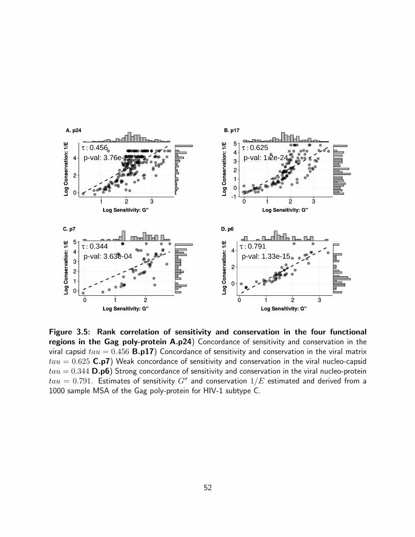
Figure 3.5: Rank correlation of sensitivity and conservation in the four functionalregions in the Gag poly-protein A.p24) Concordance of sensitivity and conservation in theviral capsid tau = 0.456 B.p17) Concordance of sensitivity and conservation in the viral matrixtau = 0.625 C.p7) Weak concordance of sensitivity and conservation in the viral nucleo-capsidtau = 0.344 D.p6) Strong concordance of sensitivity and conservation in the viral nucleo-proteintau = 0.791. Estimates of sensitivity G′′ and conservation 1/E estimated and derived from a1000 sample MSA of the Gag poly-protein for HIV-1 subtype C.
52
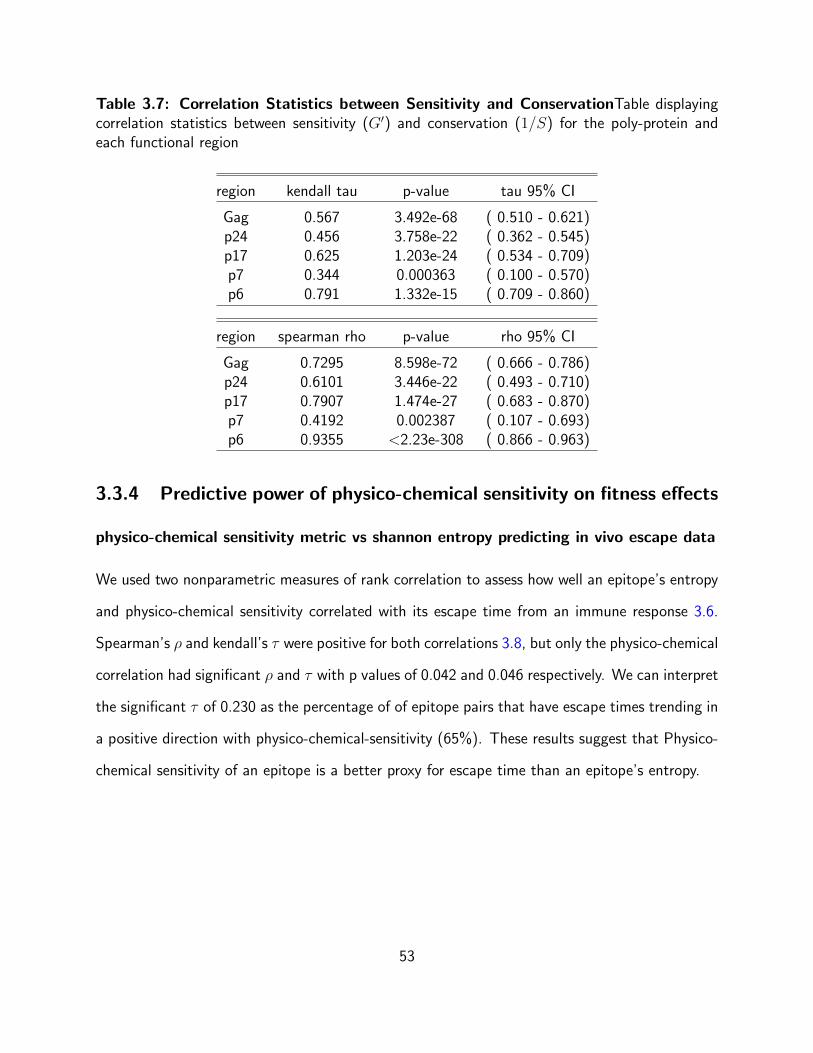
Table 3.7: Correlation Statistics between Sensitivity and ConservationTable displayingcorrelation statistics between sensitivity (G′) and conservation (1/S) for the poly-protein andeach functional region
region kendall tau p-value tau 95% CI
Gag 0.567 3.492e-68 ( 0.510 - 0.621)p24 0.456 3.758e-22 ( 0.362 - 0.545)p17 0.625 1.203e-24 ( 0.534 - 0.709)p7 0.344 0.000363 ( 0.100 - 0.570)p6 0.791 1.332e-15 ( 0.709 - 0.860)
region spearman rho p-value rho 95% CI
Gag 0.7295 8.598e-72 ( 0.666 - 0.786)p24 0.6101 3.446e-22 ( 0.493 - 0.710)p17 0.7907 1.474e-27 ( 0.683 - 0.870)p7 0.4192 0.002387 ( 0.107 - 0.693)p6 0.9355 <2.23e-308 ( 0.866 - 0.963)
3.3.4 Predictive power of physico-chemical sensitivity on fitness effects
physico-chemical sensitivity metric vs shannon entropy predicting in vivo escape data
We used two nonparametric measures of rank correlation to assess how well an epitope’s entropy
and physico-chemical sensitivity correlated with its escape time from an immune response 3.6.
Spearman’s ρ and kendall’s τ were positive for both correlations 3.8, but only the physico-chemical
correlation had significant ρ and τ with p values of 0.042 and 0.046 respectively. We can interpret
the significant τ of 0.230 as the percentage of of epitope pairs that have escape times trending in
a positive direction with physico-chemical-sensitivity (65%). These results suggest that Physico-
chemical sensitivity of an epitope is a better proxy for escape time than an epitope’s entropy.
53
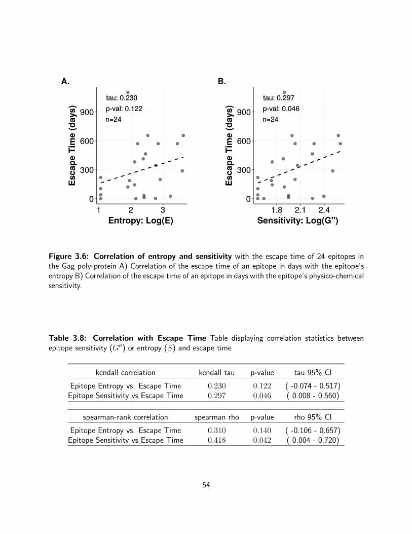
Figure 3.6: Correlation of entropy and sensitivity with the escape time of 24 epitopes inthe Gag poly-protein A) Correlation of the escape time of an epitope in days with the epitope’sentropy B) Correlation of the escape time of an epitope in days with the epitope’s physico-chemicalsensitivity.
Table 3.8: Correlation with Escape Time Table displaying correlation statistics betweenepitope sensitivity (G′′) or entropy (S) and escape time
kendall correlation kendall tau p-value tau 95% CI
Epitope Entropy vs. Escape Time 0.230 0.122 ( -0.074 - 0.517)Epitope Sensitivity vs Escape Time 0.297 0.046 ( 0.008 - 0.560)
spearman-rank correlation spearman rho p-value rho 95% CI
Epitope Entropy vs. Escape Time 0.310 0.140 ( -0.106 - 0.657)Epitope Sensitivity vs Escape Time 0.418 0.042 ( 0.004 - 0.720)
54
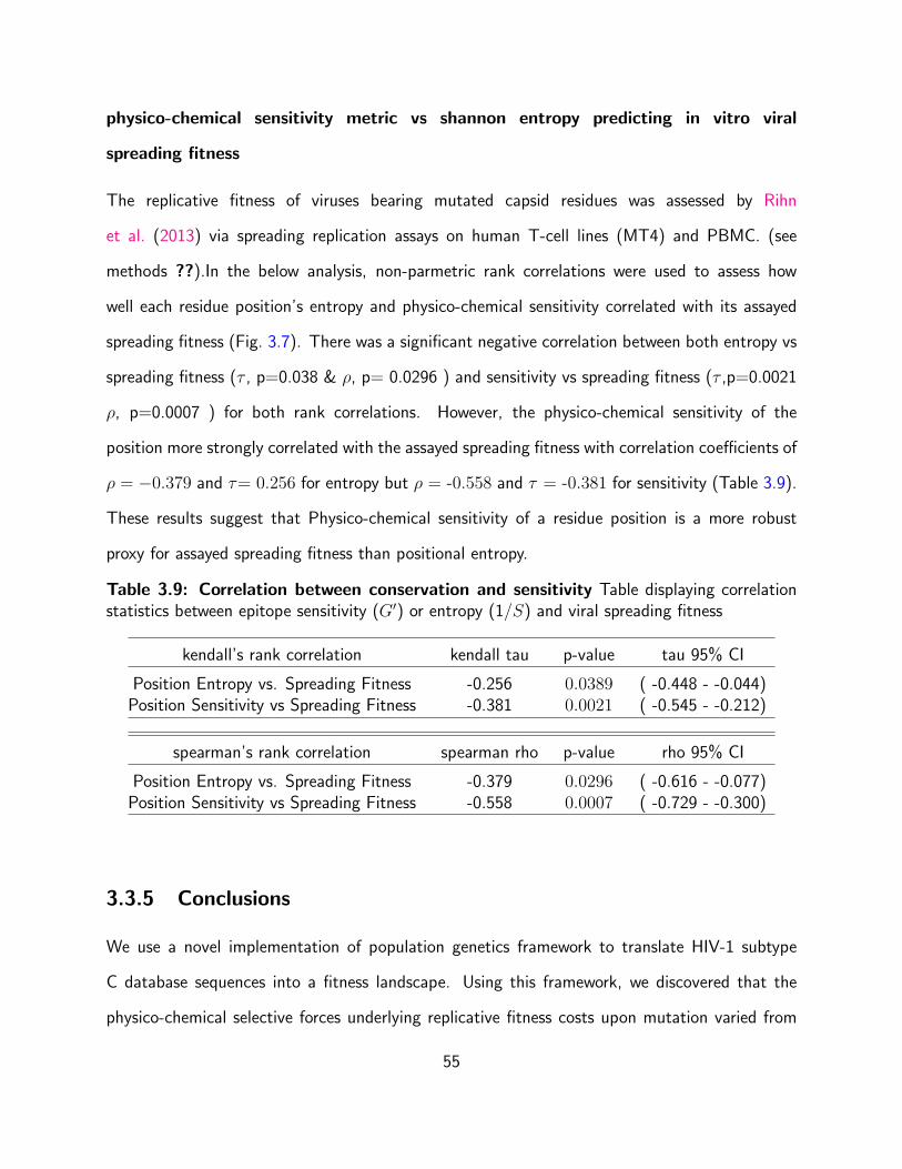
physico-chemical sensitivity metric vs shannon entropy predicting in vitro viral
spreading fitness
The replicative fitness of viruses bearing mutated capsid residues was assessed by Rihn
et al. (2013) via spreading replication assays on human T-cell lines (MT4) and PBMC. (see
methods ??).In the below analysis, non-parmetric rank correlations were used to assess how
well each residue position’s entropy and physico-chemical sensitivity correlated with its assayed
spreading fitness (Fig. 3.7). There was a significant negative correlation between both entropy vs
spreading fitness (τ , p=0.038 & ρ, p= 0.0296 ) and sensitivity vs spreading fitness (τ ,p=0.0021
ρ, p=0.0007 ) for both rank correlations. However, the physico-chemical sensitivity of the
position more strongly correlated with the assayed spreading fitness with correlation coefficients of
ρ = −0.379 and τ= 0.256 for entropy but ρ = -0.558 and τ = -0.381 for sensitivity (Table 3.9).
These results suggest that Physico-chemical sensitivity of a residue position is a more robust
proxy for assayed spreading fitness than positional entropy.
Table 3.9: Correlation between conservation and sensitivity Table displaying correlationstatistics between epitope sensitivity (G′) or entropy (1/S) and viral spreading fitness
kendall’s rank correlation kendall tau p-value tau 95% CI
Position Entropy vs. Spreading Fitness -0.256 0.0389 ( -0.448 - -0.044)Position Sensitivity vs Spreading Fitness -0.381 0.0021 ( -0.545 - -0.212)
spearman’s rank correlation spearman rho p-value rho 95% CI
Position Entropy vs. Spreading Fitness -0.379 0.0296 ( -0.616 - -0.077)Position Sensitivity vs Spreading Fitness -0.558 0.0007 ( -0.729 - -0.300)
3.3.5 Conclusions
We use a novel implementation of population genetics framework to translate HIV-1 subtype
C database sequences into a fitness landscape. Using this framework, we discovered that the
physico-chemical selective forces underlying replicative fitness costs upon mutation varied from
55
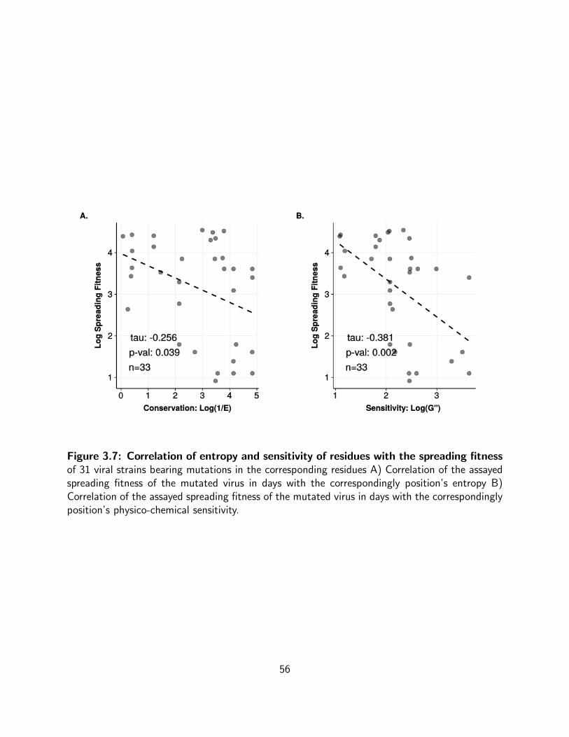
Figure 3.7: Correlation of entropy and sensitivity of residues with the spreading fitnessof 31 viral strains bearing mutations in the corresponding residues A) Correlation of the assayedspreading fitness of the mutated virus in days with the correspondingly position’s entropy B)Correlation of the assayed spreading fitness of the mutated virus in days with the correspondinglyposition’s physico-chemical sensitivity.
56

functional region to functional regions. It also became clear that the generative process underlying
the distribution of the physico-chemical sensitivities was likely one in which many positive random
independent variables were acting proportionally on one another. One biological case in which
this might occur is where residues are interacting on eachother (epistasis). It also became clear
upon analysis of the distribution of sensitivities that our proxy for fitness cost was not uniform
over the poly-protein varying in degree and distribution in different functional regions. Our proxy
of fitness cost correlated well with shannon entropy a metric often employed to predict fitness
effects in the literature. However, these physico-chemical sensitivities seemed to be a better
predictors of the rank order of these fitness effects, both in vitro and in vivo.
Acknowledgments
We would like to acknowledge the Theoretical Biology and Biophysics Division at Los Alamos
National Laboratory for the HIV compendium and alignments made available by their group
https://www.hiv.lanl.gov. The HIV Compendia are funded by the Division of AIDS, National
Institute of Allergy and Infectious Diseases, through an interagency agreement with the U.S.
Department of Energy. This work was supported by a research assistantship offered thorough the
National Institute of Mathematical and Biological Synthesis (NIMBioS). NIMBioS is sponsored
by the National Science Foundation through NSF Award DBI-1300426, with additional support
from The University of Tennessee, Knoxville.
57
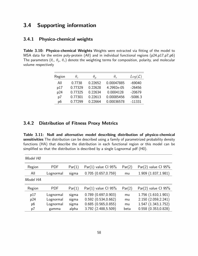
3.4 Supporting information
3.4.1 Physico-chemical weights
Table 3.10: Physico-chemical Weights Weights were extracted via fitting of the model toMSA data for the entire poly-protein (All) and in individual functional regions (p24,p17,p7,p6)The parameters (θc, θp, θv) denote the weighting terms for composition, polarity, and molecularvolume respectively
Region θc θp θv Log(L)
All 0.7738 0.22652 0.00047885 -69040p17 0.77329 0.22628 4.2992e-05 -26456p24 0.77325 0.22634 0.0004128 -20679p7 0.77301 0.22613 0.00085456 -5086.3p6 0.77299 0.22664 0.00036578 -11331
3.4.2 Distribution of Fitness Proxy Metrics
Table 3.11: Null and alternative model describing distribution of physico-chemicalsensitivities The distribution can be described using a family of parametrized probability densityfunctions (HA) that describe the distribution in each functional region or this model can besimplified so that the distribution is described by a single Lognormal pdf (H0).
Model H0
Region PDF Par(1) Par(1) value CI 95% Par(2) Par(2) value CI 95%
All Lognormal sigma 0.705 (0.657,0.759) mu 1.909 (1.837,1.981)
Model HA
Region PDF Par(1) Par(1) value CI 95% Par(2) Par(2) value CI 95%
p17 Lognormal sigma 0.789 (0.697,0.903) mu 1.756 (1.610,1.901)p24 Lognormal sigma 0.592 (0.534,0.662) mu 2.150 (2.059,2.241)p6 Lognormal sigma 0.685 (0.565,0.855) mu 1.547 (1.343,1.752)p7 gamma alpha 3.792 (2.488,5.509) beta 0.558 (0.353,0.828)
58

Table 3.12: Congruity of Descriptive Distributions for Metrics This table displays how thedistributions of physico-chemical sensitivities (G”) and conservation values (1/E) compare overthe entire Gag poly-protein (All) and over specific functional regions (p6,p7,p24,p17).
Region Descriptive PDF (G”) Descriptive PDF (1/E) Congruous
All Lognormal Lognormal Yesp17 Lognormal Lognormal Yesp24 Lognormal gamma Nop6 Lognormal inverse gamma Nop7 gamma gamma Yes
3.4.3 Model Comparison
The probability of observing the set of amino acids ~x at a position in a population where they
occur at frequency ~p is given by the following multinomial (eq. 3.11).
P (~x | ~p) =Γ(∑
j xj + 1)∏j Γ(xj + 1)
20∏j=1
pxjj (3.11)
Therefore we can express the likelihood of the model given the data as follows (eq. 3.12).
L(~p | ~x) =Γ(∑
j xj + 1)∏j Γ(xj + 1)
20∏j=1
pxjj (3.12)
The log likelihood of the observed amino acid set ~x for the position now can be written as
(eq. 3.13).
ln(L(~p | ~x)) = ln
(Γ(∑
j xj + 1)∏j Γ(xj + 1)
)+
20∑j=1
xj ln(pj) (3.13)
The shannon entropy (eq. 3.14) for the position is therefore associated with the log likelihood
of observing the set of amino acids ~x in the following way (eqs. 3.15) - 3.18]. In these equations N
is the sum of the amino acid counts represented by the vector ~x. The shannon entropy calculation
assumes that pj =xjN
.
59
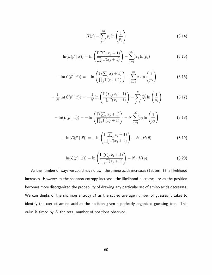
H(~p) =20∑j=1
pj ln
(1
pj
)(3.14)
ln(L(~p | ~x)) = ln
(Γ(∑
j xj + 1)∏j Γ(xj + 1)
)−
20∑j=1
xj ln(pj) (3.15)
− ln(L(~p | ~x)) = − ln
(Γ(∑
j xj + 1)∏j Γ(xj + 1)
)−
20∑j=1
xj ln
(1
pj
)(3.16)
− 1
Nln(L(~p | ~x)) = − 1
Nln
(Γ(∑
j xj + 1)∏j Γ(xj + 1)
)−
20∑j=1
xjN
ln
(1
pj
)(3.17)
− ln(L(~p | ~x)) = − ln
(Γ(∑
j xj + 1)∏j Γ(xj + 1)
)−N
20∑j=1
pj ln
(1
pj
)(3.18)
− ln(L(~p | ~x)) = − ln
(Γ(∑
j xj + 1)∏j Γ(xj + 1)
)−N ·H(~p) (3.19)
ln(L(~p | ~x)) = ln
(Γ(∑
j xj + 1)∏j Γ(xj + 1)
)+N ·H(~p) (3.20)
As the number of ways we could have drawn the amino acids increases (1st term) the likelihood
increases. However as the shannon entropy increases the likelihood decreases, or as the position
becomes more disorganized the probability of drawing any particular set of amino acids decreases.
We can thinks of the shannon entropy H as the scaled average number of guesses it takes to
identify the correct amino acid at the position given a perfectly organized guessing tree. This
value is timed by N the total number of positions observed.
60
Chapter 4
Mutational Shift of the Gag poly-protein
during early and acute infection
61
Abstract
Our findings suggest HIV structural proteins encoded by the Gag poly-protein do not substantially
move closer to the consensus strain over the early stage of infection. This analysis was conducted
by examining patient level viral evolution using two distinct measures of fitness. One measure
assessed the viral population’s likelihood given sequence diversity and the other calculated the
Hamming distance of the population from the consensus strain of HIV. Little is understood about
HIV fitness during early infection (Arnott et al., 2010); however, one study conducted by Troyer
et al. (2005) suggests viral replicative fitness in culture improves over the course of infection. We
examined fitness in HIV structural proteins via a patient cohort sampled during the Tshedimoso
study Novitsky et al. (2009). On average, 30 positions in the HIV protein Gag transitioned from
one type of amino acid residue to another during this study. Given that the Gag polyprotein
is highly functionally constrained (Rihn et al., 2013; Miura et al., 2010), we hypothesized that
this region would become more fit as the population expanded post the transmission bottleneck
(Carlson et al., 2014). Instead, we found that despite the substantial mutation, the net impact
of the mutation on the protein appeared to be neutral. This neutrality was most evident in
the metric of fitness that accounted for the differential fitness costs of the polymorphisms. It
has been suggested, that shed polymorphisms may be balanced out by milder polymorphisms
accrued elsewhere in this protein Novitsky et al. (2013). In this way, the overall mutational
distance from consensus remains the same. Our results support this idea, given the fitness of
the structural elements on a protein level were more static than one might suspect given the
number of observed mutations along the protein during this period. The number of populations
displaying increased fitness were counterbalanced by populations displaying decreases in fitness.
These findings suggest that host immune responses are rather idiosyncratic in their ability to
depress fitness in viral structural proteins, if they can at all.
62
4.1 Introduction
The Gag polyprotein is an important immune target. Its functionally and structurally constrained
cleavage products comprise over 50 % of the viral mass (Waheed and Freed, 2012; Li et al., 2010).
Elite controllers are patients who are able to control their HIV viral load. Elite controllers often
target critical epitopes within this region of the polyprotein, leading to successful and sustained
control over the virus (Honeyborne et al., 2007; Rolland et al., 2008). Consequently, HIV vaccines
typically incorporate immunogens from this region in their constructs (Li et al., 2010; Waheed
and Freed, 2012; Goulder and Watkins, 2004; Korber et al., 2009).
The first year of viral evolution is particularly critical in determining patient outcomes. There is
a well-established relationship between disease progression and viral fitness (Quiones-Mateu et al.,
2000). By the first year, the viral load’s set point for the chronic infection is well established. This
fitness setpoint is often predictive of when the patient will progress to AIDS (?). The majority
of evolution occurs during this first year as well, prior CD4 T-Cell decline (Li et al., 2007) .
During this period, the virus still enjoys an abundance of target cells and immune responses have
not yet been severely compromised. We wished to assess whether the transiently potent CTL
response managed to depress viral fitness during this critical period. Other assessments of viral
fitness (Troyer et al., 2005) have suggested in vitro replicative fitness of the virus increases over
time. Likewise, others have shown that the virus rapidly sheds unfit polymorphisms acquired in
the previous host (Carlson et al., 2014). By shed we mean that these non-consensus residues
disapear from the population. We may also expect viral fitness to increase due to the adaptive
expansion the virus is undergoing after a tightly bottlenecked transmission event. By bottleneck,
we mean that viral infection is only founded by a few viruses that are biased towards being
consensus like in nature due to the mechanics and biology of transmisson (Carlson et al., 2014).
One approach to designing a vaccine immunogen is to prime host immune responses to
push the virus over its error threshold Korber et al. (2009); Tripathi et al. (2012); ?. This
63
is accomplished by designing immunogens that elicit immune responses against a broad set of
mutationally fragile regions. Given this approach, we wanted to see if natural unprimed host
immune responses were already managing to depress viral structural fitness to any appreciable
degree. Ideally, successful natural responses could be strengthened by exposure to a vaccine
immunogen. Studies have suggested that the Gag poly-protein is tightly co-linked epistatically
(Dahirel et al., 2011), with compensating mutations rapidly arising whenever a deleterious
mutation arises in the region due to CTL pressure (Brockman et al., 2010, 2007; Burwitz et al.,
2011). Therefore, it may be difficult to depress viral fitness in this regions, much less force it
over its error threshold.
Little is understood about how viral fitness changes during the early stages of infection.
To establish whether the viral structural elements were increasing or decreasing in fitness, we
assessed fitness trends in 41 HIV-1 subtype C infected 41 patients. Changes in the viral population
structure were captured using two different metrics. In the first approach, we employed a standard
Hamming distance metric that calculated population distance from the HIV consensus stain. In
the second approach, we employed a polymorphism sensitive likelihood measure which determined
the likelihood of the viral contents of a blood sample given global subtype diversity.
4.2 Methods
4.2.1 Sequences
Longitudnal Sequences
The HIV-1 Gag sequences used to construct the viral population kinetics in this analysis, came
from a primary HIV-1 subtype C infection study conducted in Botswana from 2004-2005 (Novitsky
et al., 2011, 2009). In this study, a cohort of 42 HIV-1 subtype C positive individuals had their
blood drawn at 4-6 points in a 500 day period after sero-converting. Patients were newly infected.
64
Of the 42 patients, 34 individuals were in Fiebig stage IV or V (20-100 days post infection) the
other 8 were still in Feibig II (˜15-20 days post infection). It was impossible to get a linear fit for
Patient “OM” individually because the patient had only two recorded blood samples. Therefore
patient “OM” is omitted from the sample in the patient breakdowns.
Cross-sectional Sequences
We use 1058 curated sequences in the Los Alamos database for subtype C (2016) (see Los Alamos
HIV-1 Sequence Database). These sequences were filtered web alignments that provide a good
example of the subtypes breadth. Every sequence belongs to a unique patient and sequences that
resemble each other too closely had been removed. This was to make sure duplicate sequences
were not used. Additionally questionable sequences such as those that appear to be hypermutants
and synthetics have also been removed. The curated sequences were clean, containing little
amibuous coding, few long insertions and lacked a preponderance of frame shifts. Sequences in
this curated alignment were aligned using both automation (HMMER) and manual editing.
4.2.2 Calculating the Fitness of Patient Viral Populations via Hamming
Distances
We describe the intrinsic fitness (F ) of the virus in the blood sample (Xt) taken from the patient
at time t in terms of viral Hamming distance from the viral consensus (eq. 4.1). This measure
of sequence mutation which treats sequences as binary strings (0 non-deviation from consensus,
1 deviation from consensus) if often employed to infer viral fitness and estimate viral diversity
Ferguson et al. (2013); Pilcher et al. (2008). In this context, we define the hamming distance
as the residue distance between the sampled viral sequence and the HIV-1 subtype C consensus
sequence (see Los Alamos Consensus Alignment Database).
65
F (Xt) =
∑sj
∑ni δµ(rij)∑s
j
∑ni δ(rij)
. (4.1)
δµ(rij) =
1, if p(rij) < pmax
0, if rij ∈ {−, ∗}
0, otherwise
(4.2)
Each element rij in the HXB2 residue vector ~rj of length n represents the state (residue,
gap, stop codon) at HXB2 coordinate position i in viral sequence j. We use two Kronecker delta
functions (δµ, δ) to count the total number of HXB2 coordinates bearing mutations δmu (eq. 4.2)
and the total number of HXB2 coordinates bearing one of the 20 natural amino acid residues
δ (eq. 4.3). Because we are defining hamming distance in terms of residue differences, residue
coordinates containing gaps or stop and start codons {−, ∗} are ignored in both Kronecker delta
counts. Mutations are defined in the Kronecker delta function (δµ using prevalence map which
recorded the prevalence of each coordinate state p(rij) for a 1058 sequence sample taken from
curated alignment for HIV subtype C www.hiv.lanl.gov.The prevalence map was augmented to
account for non-observed residues, with the prevalence set at 1/1058 or 0.000945 for non-observed
residues. The Kronecker delta function δµ can either categorize a mutation conservatively or
permissively. Using the conservative definition, a residue coordinate will be classified as mutated
if the the residue it bears at that position has a prevalence of less than 0.50. In this way, any
residue at a highly polymorphic position will be automatically classed as mutated and only fitness
shifts at conserved positions will be monitored. Using a more permissive definition, the Kronecker
delta function will classify anything that has a prevalence lower than that of the consensus residue
as mutated.
66
δ(rij) =
0, if rij ∈ {−, ∗}
1, otherwise
(4.3)
pmax =
0.50, if conservative
p(ric), if permissive
(4.4)
4.2.3 Estimating the Fitness of Patient Viral Populations from Global
Population Likelihoods
Each set of viral variants sequenced from a patient’s blood sample is regarded as representative
of the larger viral population in the blood compartment. The total number of residues observed
at any HXB2 coordinate j in the blood sample is nj. The values x1,j...x20,j represent the counts
for each of the 20 natural amino acids. The value p(aij) denotes the prevalence of that amino
acid i at the sequence coordinate position.
L(θp | Xt) =520∏j=1
(nj!
x1,j! · · · x20,j!
20∏i=1
p(aij)xij
)(4.5)
j in the database. In this way we can can calculate the likelihood of sequencing a particular
set of amino acids for a position from a blood sample. By multiplying these likelihoods over the
length of the sequence. we can calculate the probability of drawing the provided blood sample
(Xt) given what we know about the prevalence of residues in the larger circulating population of
virus (θp). So every likelihood multiplied is the probability of observing the amino acid distribution
we found at that position.
67
4.2.4 Statistics On Fitness Trends
Two marginal homogeneity tests were conducted to determine if the method used to estimate
fitness impacted categorization of the patients. The tests evaluated a null hypothesis where
both metrics are assumed to categorize the mutational trajectory of the patients viral populations
similarly. Patient viral populations were either categorized as increasing in fitness or descreasing
linear regression. A contingency table was constructed where an increasing or descreasing trend
was regarded as a dichotomous viral population trait. The method used to estimating fitness was
considered the treatment for our viral populations. Marginal homegeneity of the differences in the
viral population classifications was assessed using both a standard McNemar Chi-squared Test and
Bhapkar Marginal Homogeneity Test given that is was a good extension of the Stuart-Maxwell
test with more power (Agresti, 2003).
To insure that the polymorphic fitness trends we identified were not false positives, we assessed
the robustness of the polymorphic fitness trends via bootstrapping . Sequence sets amplified
from each blood sample were re-sampled 1000 times at each time-point to create 1000 re-
sampled mutational trajectories for each patient. Linear fits were conducted for all re-sampled
trajectories, from the distribution of resulting slopes with p-values the robustness of the detected
shift was calculated by dividing the number of re-sample trajectories showing a significant shift
in mutational character over the total number of trajectories.
Method specific viral populations fitness trends were assessed with a linear regression. Estimates
of viral population fitness were generated from patient blood samples taken up to 700 days post-
seroconversion. Regressions of trends were displayed with confidence bands denoting the standard
error of respective regression. We begin by assuming there is no trend in the viral population, and
the slope of our regression is zero. The p-value we obtain represents the probability of recording
a slope that is as extreme or more extreme than the one we observed (assuming there really is
no trend). If we obtain a slope with a p-value of 0.02, this means that if we were to resample
68
the patient 100 times and rerun our regression, we would obtain a slope as extreme as this (or
more) 2 out of every 100 resamples. This 2% chance of obtaining a false positive by random
chance seems small, so we reject the notion that the null hypothesis is true and consider the
alternate hypothesis that the trend is real. Most of the time we want the probability of obtaining
a false positive (the type I error) to be below 5%. However, in some cases, we desire it to be
lower because we are running more experiments. Our chance of obtaining a false positive due
to random error increases as we look for viral population trends in more patients. We therefore
run a BenjaminiHochberg procedure with our False Discovery Rate set at a tolerance of 25%.
Patients whose viral trends remained significant are noted with asterisk.
4.3 Results
4.3.1 Polymorphic Approach: HIV Structural Proteins Show No
Discernible Trend of Increased Fitness Over Acute Infection
Figure (4.1) displays breakdowns of mutational trajectories by method. A Polymorphic, Permissive
and Conservative method were used to comparatively assess how a patient’s viral population
evolved. Specifically, the goal was to assess if a patient’s viral population became 1) more fit 2)
less fit or 3) remained static over the acute infection period. Panels in Figure (4.1) display the
break down of viral evolution in the patient cohort by method. The viral sequences sampled from
41 HIV-C acutely infected patients (4-12 timepoints), were used in the fitness calculations.
The fitness status of the current viral population was evaluated per timepoints using all
three methods (Polymorphic, Permissive, Conservative) and resulting trends were identified via
regression. In the polymorphic classification scheme, viral population fitness was interpreted in
terms of how likely one was to draw that particular blood sample given the diversity of database
sequences. (eq 4.1). In the permissive classification scheme, any non-consensus residue was
69
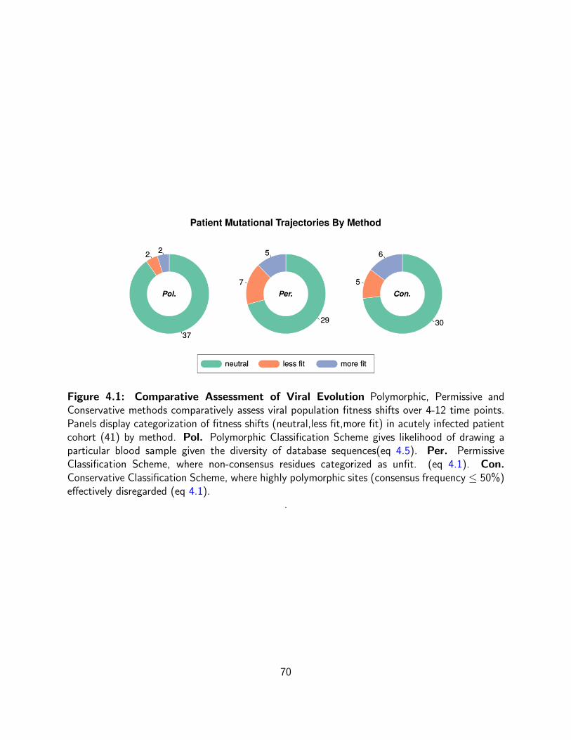
Figure 4.1: Comparative Assessment of Viral Evolution Polymorphic, Permissive andConservative methods comparatively assess viral population fitness shifts over 4-12 time points.Panels display categorization of fitness shifts (neutral,less fit,more fit) in acutely infected patientcohort (41) by method. Pol. Polymorphic Classification Scheme gives likelihood of drawing aparticular blood sample given the diversity of database sequences(eq 4.5). Per. PermissiveClassification Scheme, where non-consensus residues categorized as unfit. (eq 4.1). Con.Conservative Classification Scheme, where highly polymorphic sites (consensus frequency ≤ 50%)effectively disregarded (eq 4.1).
.
70
categorized as unfit. This rather binary estimate of fitness was overly liberal in classifying
mutations given that positions in this poly-protein can bear more than one dominant residue
(eq 4.1). In the conservative classification scheme, the metric used to categorize mutations was
conservative as to what was categorized as a mutation with changes at highly polymorphic sites
(consensus frequency ≤ 50%) being effectively disregarded (eq 4.5).
The polymorphic method of assessing fitness trends detected little to no change in the fitness
status of the virus over acute infection (Fig 4.5). The other two hamming based methods
were more liberal in their classification of mutations and did detected more fitness shifts in the
patient cohort. However, at a patient population level, the shifts in fitness followed no discernible
pattern. Some patient viral population’s became more fit in regards to their structural elements,
while an approximately equal number declined in fitness. Shifts were not detectable in pooled
blood sample estimates given the patient heterogeneity (Fig A-B S.4.5) for the conservative
and permissive measures of fitness. A shift towards fitness was detected using the polymorphic
approach on the pooled samples. However, given that this positive trend does not carry over at
the patient level, it is likely an artifact of pooling the data (Figure C S.4.5).
4.3.2 Classification of Mutational Trends
Figure (4.2) displays how intra-host viral populations evolved over acute infection using three
different approaches to appraise fitness, two in which hamming distance from the consensus
sequence was used as a measure of fitness (Permissive,Conservative) and one in which a likelihood
measure was used to estimate fitness (Polymorphic).
Each point on the graphs represents a method specific estimate of viral population fitness
at some time-point post-seroconversion. Each fitness estimate was calculated using either the
simple permissive and conservative hamming distance measures or the more complex polymorphic
measure that was based on the likelihood of drawing the blood sample. The left column presents
the patients which showed a significant increase in fitness, the right columns the patients who
71
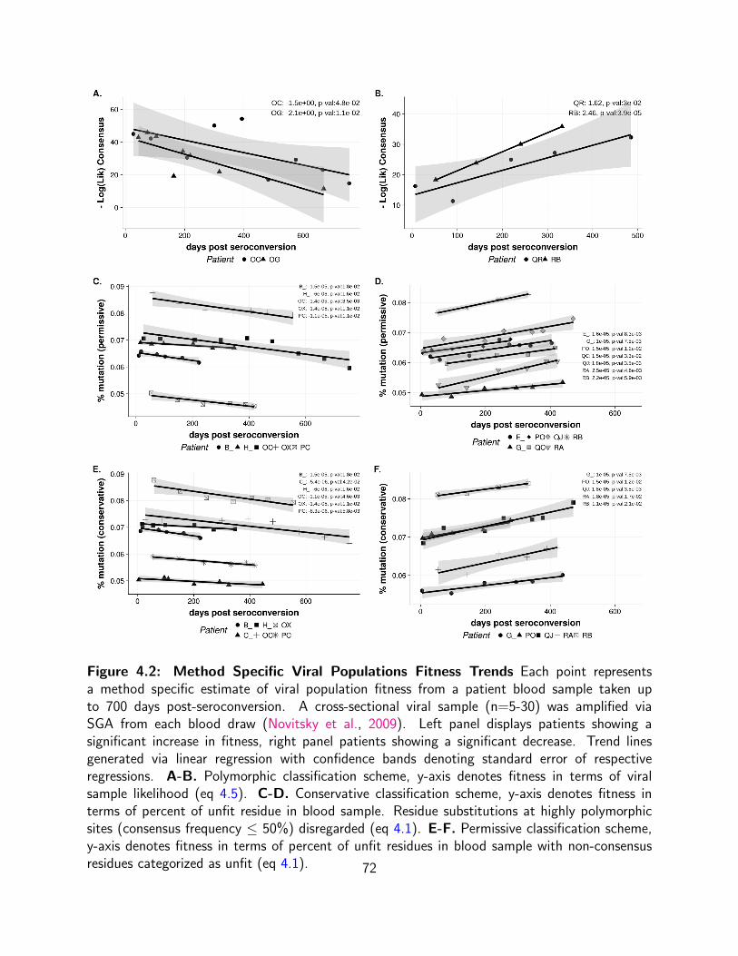
Figure 4.2: Method Specific Viral Populations Fitness Trends Each point representsa method specific estimate of viral population fitness from a patient blood sample taken upto 700 days post-seroconversion. A cross-sectional viral sample (n=5-30) was amplified viaSGA from each blood draw (Novitsky et al., 2009). Left panel displays patients showing asignificant increase in fitness, right panel patients showing a significant decrease. Trend linesgenerated via linear regression with confidence bands denoting standard error of respectiveregressions. A-B. Polymorphic classification scheme, y-axis denotes fitness in terms of viralsample likelihood (eq 4.5). C-D. Conservative classification scheme, y-axis denotes fitness interms of percent of unfit residue in blood sample. Residue substitutions at highly polymorphicsites (consensus frequency ≤ 50%) disregarded (eq 4.1). E-F. Permissive classification scheme,y-axis denotes fitness in terms of percent of unfit residues in blood sample with non-consensusresidues categorized as unfit (eq 4.1). 72
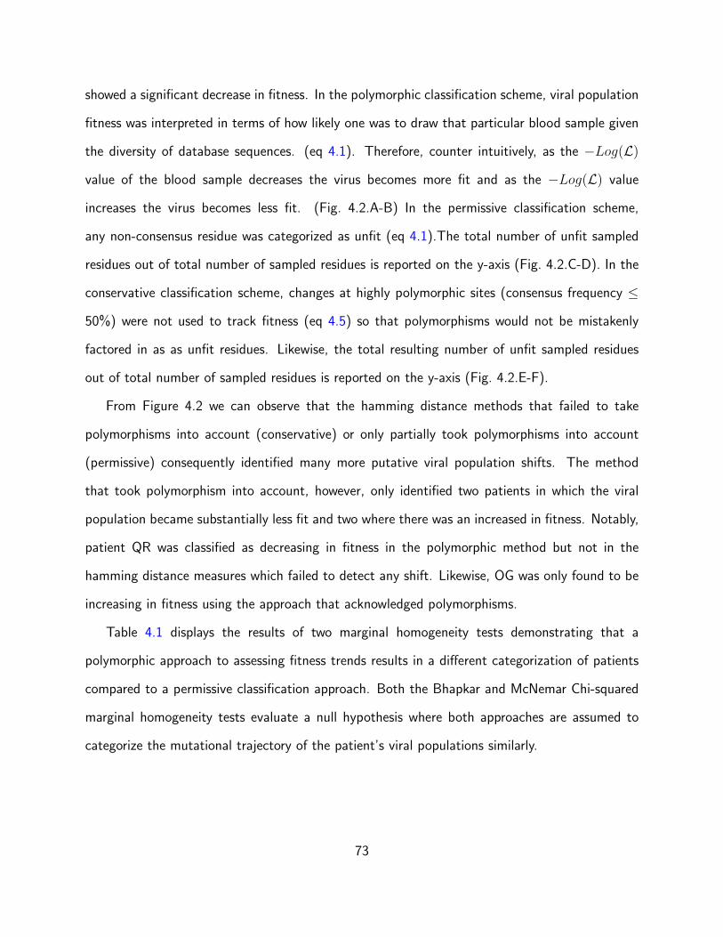
showed a significant decrease in fitness. In the polymorphic classification scheme, viral population
fitness was interpreted in terms of how likely one was to draw that particular blood sample given
the diversity of database sequences. (eq 4.1). Therefore, counter intuitively, as the −Log(L)
value of the blood sample decreases the virus becomes more fit and as the −Log(L) value
increases the virus becomes less fit. (Fig. 4.2.A-B) In the permissive classification scheme,
any non-consensus residue was categorized as unfit (eq 4.1).The total number of unfit sampled
residues out of total number of sampled residues is reported on the y-axis (Fig. 4.2.C-D). In the
conservative classification scheme, changes at highly polymorphic sites (consensus frequency ≤
50%) were not used to track fitness (eq 4.5) so that polymorphisms would not be mistakenly
factored in as as unfit residues. Likewise, the total resulting number of unfit sampled residues
out of total number of sampled residues is reported on the y-axis (Fig. 4.2.E-F).
From Figure 4.2 we can observe that the hamming distance methods that failed to take
polymorphisms into account (conservative) or only partially took polymorphisms into account
(permissive) consequently identified many more putative viral population shifts. The method
that took polymorphism into account, however, only identified two patients in which the viral
population became substantially less fit and two where there was an increased in fitness. Notably,
patient QR was classified as decreasing in fitness in the polymorphic method but not in the
hamming distance measures which failed to detect any shift. Likewise, OG was only found to be
increasing in fitness using the approach that acknowledged polymorphisms.
Table 4.1 displays the results of two marginal homogeneity tests demonstrating that a
polymorphic approach to assessing fitness trends results in a different categorization of patients
compared to a permissive classification approach. Both the Bhapkar and McNemar Chi-squared
marginal homogeneity tests evaluate a null hypothesis where both approaches are assumed to
categorize the mutational trajectory of the patient’s viral populations similarly.
73
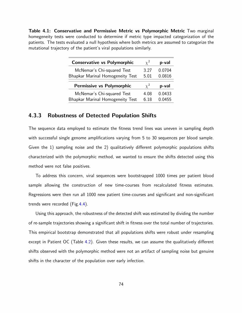
Table 4.1: Conservative and Permissive Metric vs Polymorphic Metric Two marginalhomegeneity tests were conducted to determine if metric type impacted categorization of thepatients. The tests evaluated a null hypothesis where both metrics are assumed to categorize themutational trajectory of the patient’s viral populations similarly.
Conservative vs Polymorphic χ2 p-val
McNemar’s Chi-squared Test 3.27 0.0704Bhapkar Marinal Homogeneity Test 5.01 0.0816
Permissive vs Polymorphic χ2 p-val
McNemar’s Chi-squared Test 4.08 0.0433Bhapkar Marinal Homogeneity Test 6.18 0.0455
4.3.3 Robustness of Detected Population Shifts
The sequence data employed to estimate the fitness trend lines was uneven in sampling depth
with successful single genome amplifications varying from 5 to 30 sequences per blood sample.
Given the 1) sampling noise and the 2) qualitatively different polymorphic populations shifts
characterized with the polymorphic method, we wanted to ensure the shifts detected using this
method were not false positives.
To address this concern, viral sequences were bootstrapped 1000 times per patient blood
sample allowing the construction of new time-courses from recalculated fitness estimates.
Regressions were then run all 1000 new patient time-courses and significant and non-significant
trends were recorded (Fig.4.4).
Using this approach, the robustness of the detected shift was estimated by dividing the number
of re-sample trajectories showing a significant shift in fitness over the total number of trajectories.
This empirical bootstrap demonstrated that all populations shifts were robust under resampling
except in Patient OC (Table 4.2). Given these results, we can assume the qualitatively different
shifts observed with the polymorphic method were not an artifact of sampling noise but genuine
shifts in the character of the population over early infection.
74
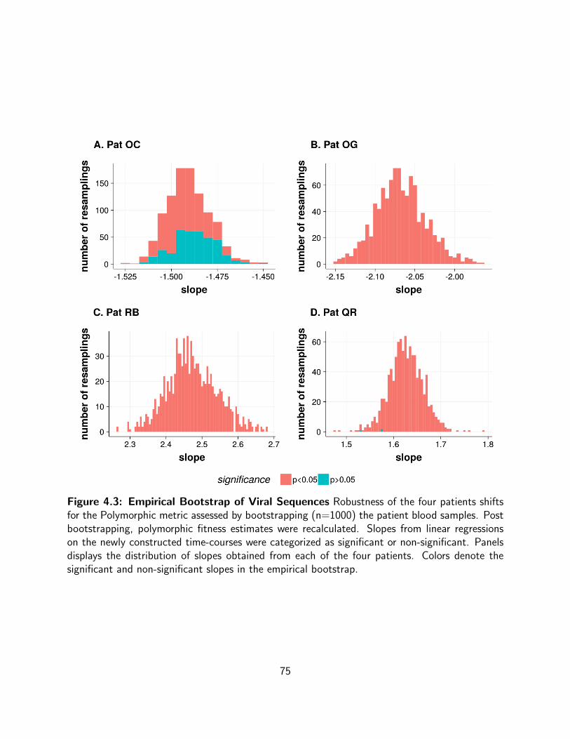
Figure 4.3: Empirical Bootstrap of Viral Sequences Robustness of the four patients shiftsfor the Polymorphic metric assessed by bootstrapping (n=1000) the patient blood samples. Postbootstrapping, polymorphic fitness estimates were recalculated. Slopes from linear regressionson the newly constructed time-courses were categorized as significant or non-significant. Panelsdisplays the distribution of slopes obtained from each of the four patients. Colors denote thesignificant and non-significant slopes in the empirical bootstrap.
75
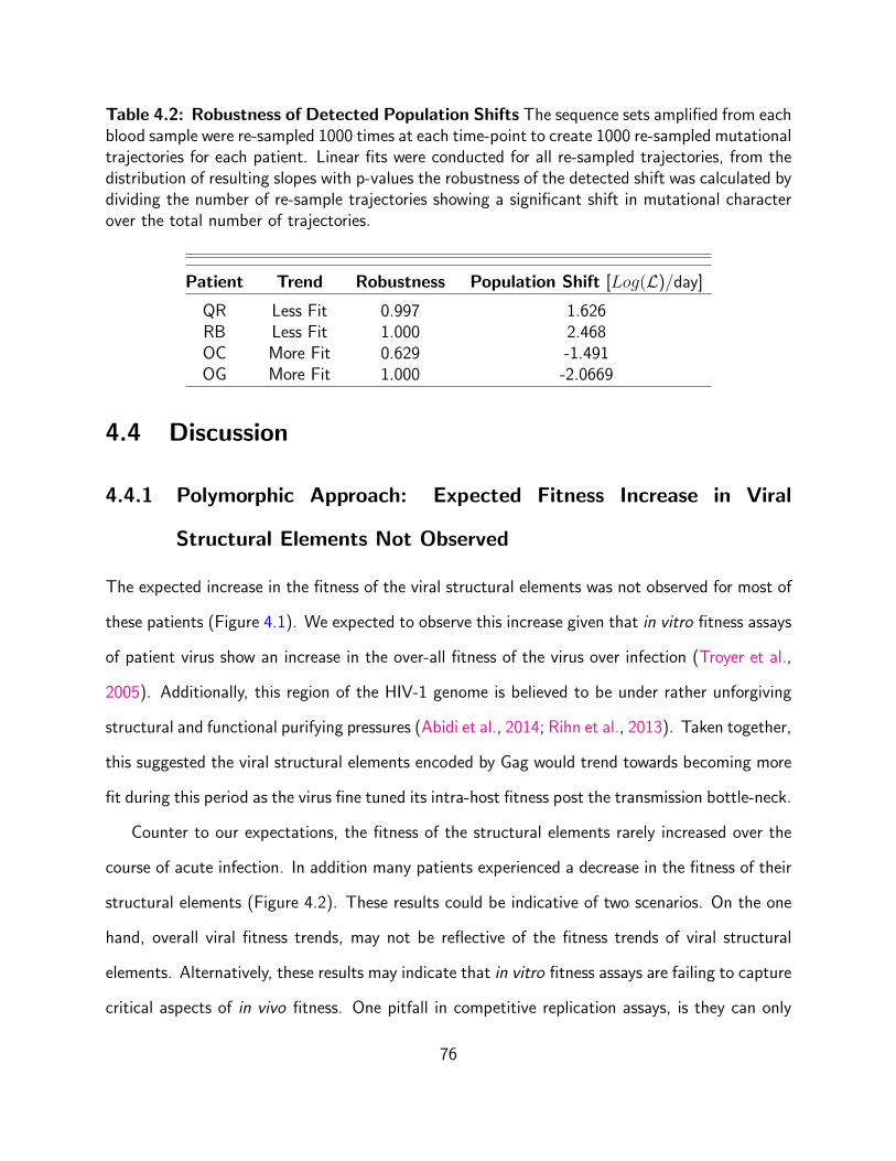
Table 4.2: Robustness of Detected Population Shifts The sequence sets amplified from eachblood sample were re-sampled 1000 times at each time-point to create 1000 re-sampled mutationaltrajectories for each patient. Linear fits were conducted for all re-sampled trajectories, from thedistribution of resulting slopes with p-values the robustness of the detected shift was calculated bydividing the number of re-sample trajectories showing a significant shift in mutational characterover the total number of trajectories.
Patient Trend Robustness Population Shift [Log(L)/day]
QR Less Fit 0.997 1.626RB Less Fit 1.000 2.468OC More Fit 0.629 -1.491OG More Fit 1.000 -2.0669
4.4 Discussion
4.4.1 Polymorphic Approach: Expected Fitness Increase in Viral
Structural Elements Not Observed
The expected increase in the fitness of the viral structural elements was not observed for most of
these patients (Figure 4.1). We expected to observe this increase given that in vitro fitness assays
of patient virus show an increase in the over-all fitness of the virus over infection (Troyer et al.,
2005). Additionally, this region of the HIV-1 genome is believed to be under rather unforgiving
structural and functional purifying pressures (Abidi et al., 2014; Rihn et al., 2013). Taken together,
this suggested the viral structural elements encoded by Gag would trend towards becoming more
fit during this period as the virus fine tuned its intra-host fitness post the transmission bottle-neck.
Counter to our expectations, the fitness of the structural elements rarely increased over the
course of acute infection. In addition many patients experienced a decrease in the fitness of their
structural elements (Figure 4.2). These results could be indicative of two scenarios. On the one
hand, overall viral fitness trends, may not be reflective of the fitness trends of viral structural
elements. Alternatively, these results may indicate that in vitro fitness assays are failing to capture
critical aspects of in vivo fitness. One pitfall in competitive replication assays, is they can only
76
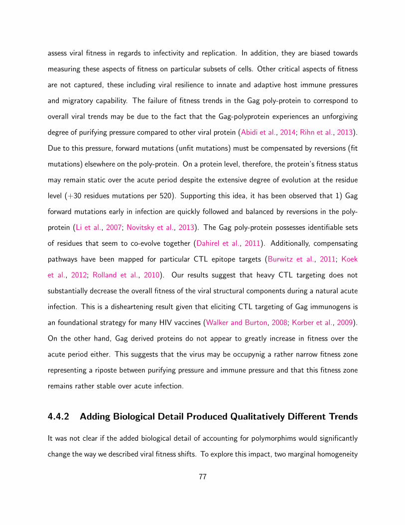
assess viral fitness in regards to infectivity and replication. In addition, they are biased towards
measuring these aspects of fitness on particular subsets of cells. Other critical aspects of fitness
are not captured, these including viral resilience to innate and adaptive host immune pressures
and migratory capability. The failure of fitness trends in the Gag poly-protein to correspond to
overall viral trends may be due to the fact that the Gag-polyprotein experiences an unforgiving
degree of purifying pressure compared to other viral protein (Abidi et al., 2014; Rihn et al., 2013).
Due to this pressure, forward mutations (unfit mutations) must be compensated by reversions (fit
mutations) elsewhere on the poly-protein. On a protein level, therefore, the protein’s fitness status
may remain static over the acute period despite the extensive degree of evolution at the residue
level (+30 residues mutations per 520). Supporting this idea, it has been observed that 1) Gag
forward mutations early in infection are quickly followed and balanced by reversions in the poly-
protein (Li et al., 2007; Novitsky et al., 2013). The Gag poly-protein possesses identifiable sets
of residues that seem to co-evolve together (Dahirel et al., 2011). Additionally, compensating
pathways have been mapped for particular CTL epitope targets (Burwitz et al., 2011; Koek
et al., 2012; Rolland et al., 2010). Our results suggest that heavy CTL targeting does not
substantially decrease the overall fitness of the viral structural components during a natural acute
infection. This is a disheartening result given that eliciting CTL targeting of Gag immunogens is
an foundational strategy for many HIV vaccines (Walker and Burton, 2008; Korber et al., 2009).
On the other hand, Gag derived proteins do not appear to greatly increase in fitness over the
acute period either. This suggests that the virus may be occupynig a rather narrow fitness zone
representing a riposte between purifying pressure and immune pressure and that this fitness zone
remains rather stable over acute infection.
4.4.2 Adding Biological Detail Produced Qualitatively Different Trends
It was not clear if the added biological detail of accounting for polymorphims would significantly
change the way we described viral fitness shifts. To explore this impact, two marginal homogeneity
77

test were conducted on patient categorizations resulting from conservative (non-polymorphic)
and polymorphic approaches. These tests allowed us to assess whether the conservative and
polymorphic approaches similarly classified viral population behavior. Both tests suggested, the
approaches were not classifying viral trends similarly. Taking into account polymorphism appeared
to fundamentally changes the putative viral fitness trends observed. Given these findings, as well
as the well acknowledged highly diverse mutant spectrum’s within hosts (Pennings et al., 2014;
Korber et al., 2001), we suggest that future models assessing in vivo fitness of virus factor
polymorphisms into their fitness assessments.
4.4.3 Further Work
More work should be done to assess viral mutational trends in the other HIV proteins. We might
fail to observe any trend towards fitness in these proteins as well. If we did, it would suggest that
the in vitro and in vivo database methods actually predict different evolutionary trajectories not
just for the structural elements but for all proteins. This would indicate that these in vitro assays
may not be capturing critical aspects of viral fitness.
Acknowledgments
We would like to acknowledge the Theoretical Biology and Biophysics Division at Los Alamos
National Laboratory for the HIV compendium and alignments made available by their group
https://www.hiv.lanl.gov. The HIV Compendia are funded by the Division of AIDS, National
Institute of Allergy and Infectious Diseases, through an interagency agreement with the U.S.
Department of Energy.
78
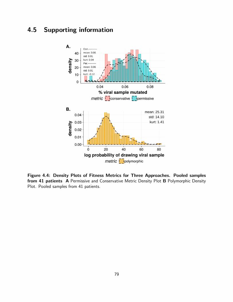
4.5 Supporting information
Figure 4.4: Density Plots of Fitness Metrics for Three Approaches. Pooled samplesfrom 41 patients A Permissive and Conservative Metric Density Plot B Polymorphic DensityPlot. Pooled samples from 41 patients.
79
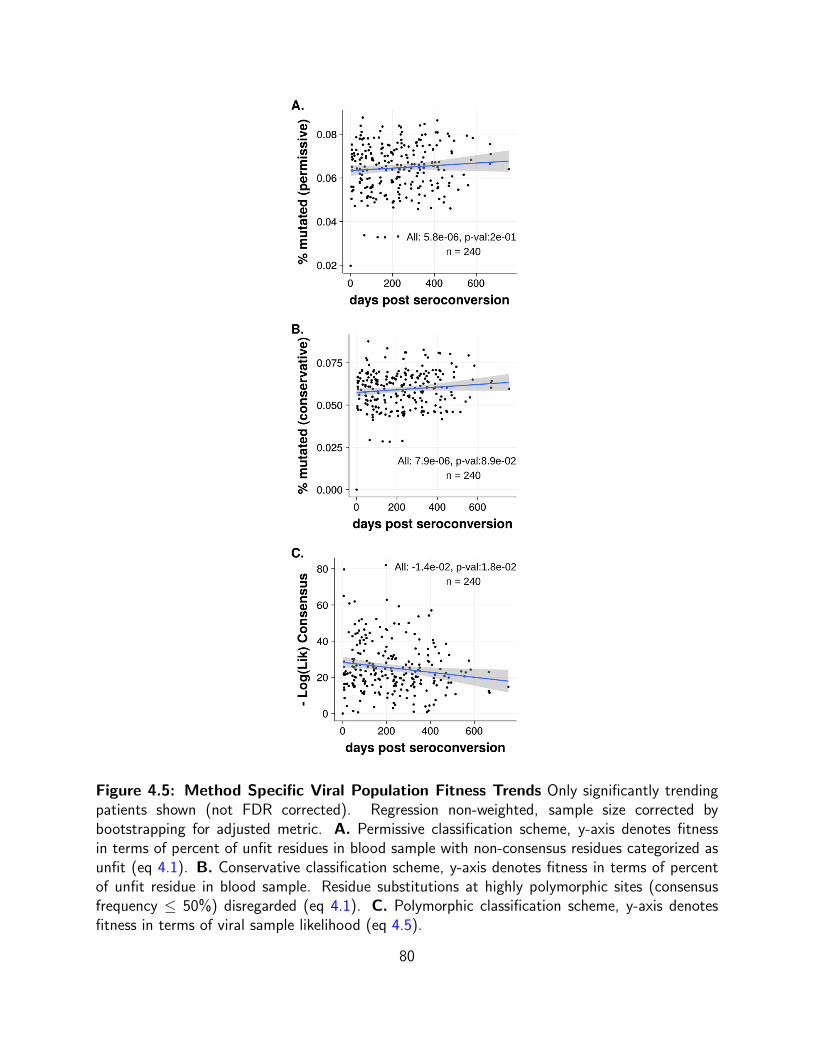
Figure 4.5: Method Specific Viral Population Fitness Trends Only significantly trendingpatients shown (not FDR corrected). Regression non-weighted, sample size corrected bybootstrapping for adjusted metric. A. Permissive classification scheme, y-axis denotes fitnessin terms of percent of unfit residues in blood sample with non-consensus residues categorized asunfit (eq 4.1). B. Conservative classification scheme, y-axis denotes fitness in terms of percentof unfit residue in blood sample. Residue substitutions at highly polymorphic sites (consensusfrequency ≤ 50%) disregarded (eq 4.1). C. Polymorphic classification scheme, y-axis denotesfitness in terms of viral sample likelihood (eq 4.5).
80
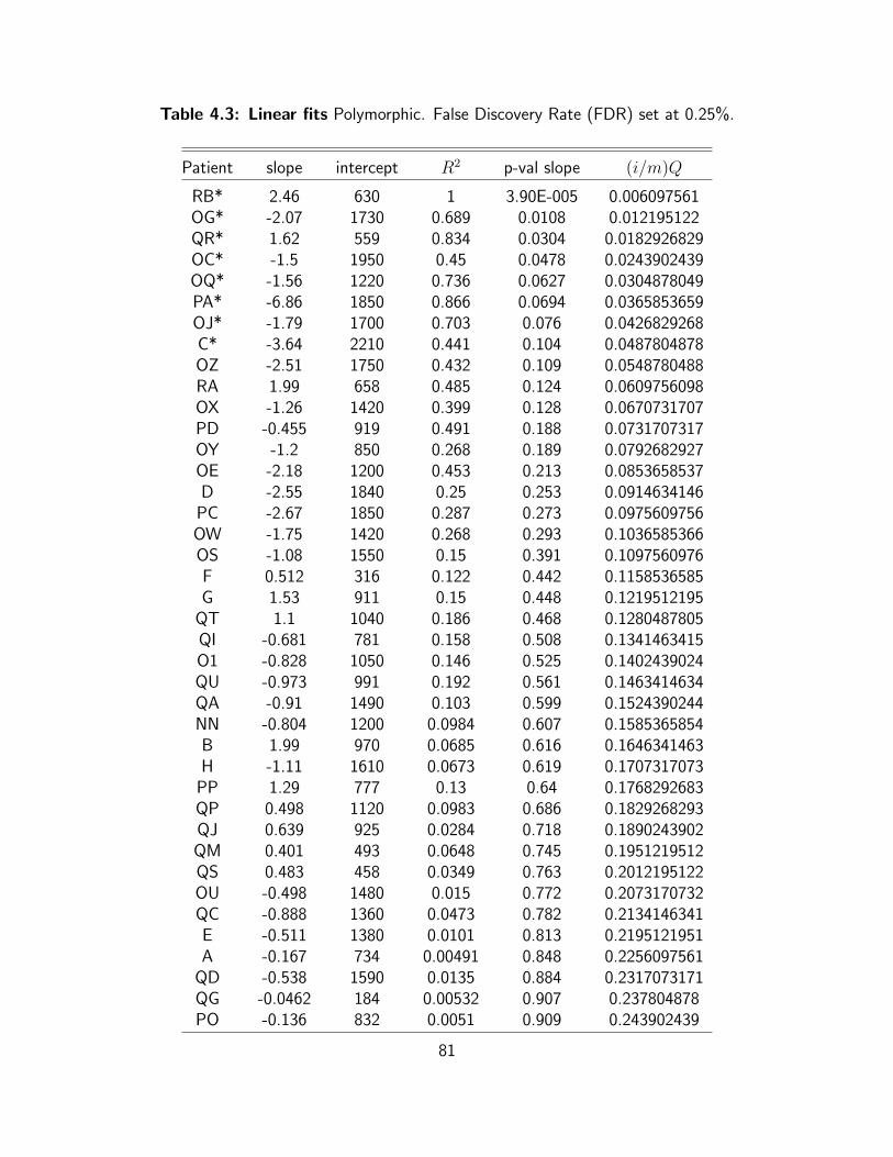
Table 4.3: Linear fits Polymorphic. False Discovery Rate (FDR) set at 0.25%.
Patient slope intercept R2 p-val slope (i/m)Q
RB* 2.46 630 1 3.90E-005 0.006097561OG* -2.07 1730 0.689 0.0108 0.012195122QR* 1.62 559 0.834 0.0304 0.0182926829OC* -1.5 1950 0.45 0.0478 0.0243902439OQ* -1.56 1220 0.736 0.0627 0.0304878049PA* -6.86 1850 0.866 0.0694 0.0365853659OJ* -1.79 1700 0.703 0.076 0.0426829268C* -3.64 2210 0.441 0.104 0.0487804878OZ -2.51 1750 0.432 0.109 0.0548780488RA 1.99 658 0.485 0.124 0.0609756098OX -1.26 1420 0.399 0.128 0.0670731707PD -0.455 919 0.491 0.188 0.0731707317OY -1.2 850 0.268 0.189 0.0792682927OE -2.18 1200 0.453 0.213 0.0853658537D -2.55 1840 0.25 0.253 0.0914634146
PC -2.67 1850 0.287 0.273 0.0975609756OW -1.75 1420 0.268 0.293 0.1036585366OS -1.08 1550 0.15 0.391 0.1097560976F 0.512 316 0.122 0.442 0.1158536585G 1.53 911 0.15 0.448 0.1219512195
QT 1.1 1040 0.186 0.468 0.1280487805QI -0.681 781 0.158 0.508 0.1341463415O1 -0.828 1050 0.146 0.525 0.1402439024QU -0.973 991 0.192 0.561 0.1463414634QA -0.91 1490 0.103 0.599 0.1524390244NN -0.804 1200 0.0984 0.607 0.1585365854B 1.99 970 0.0685 0.616 0.1646341463H -1.11 1610 0.0673 0.619 0.1707317073
PP 1.29 777 0.13 0.64 0.1768292683QP 0.498 1120 0.0983 0.686 0.1829268293QJ 0.639 925 0.0284 0.718 0.1890243902QM 0.401 493 0.0648 0.745 0.1951219512QS 0.483 458 0.0349 0.763 0.2012195122OU -0.498 1480 0.015 0.772 0.2073170732QC -0.888 1360 0.0473 0.782 0.2134146341E -0.511 1380 0.0101 0.813 0.2195121951A -0.167 734 0.00491 0.848 0.2256097561
QD -0.538 1590 0.0135 0.884 0.2317073171QG -0.0462 184 0.00532 0.907 0.237804878PO -0.136 832 0.0051 0.909 0.243902439
81
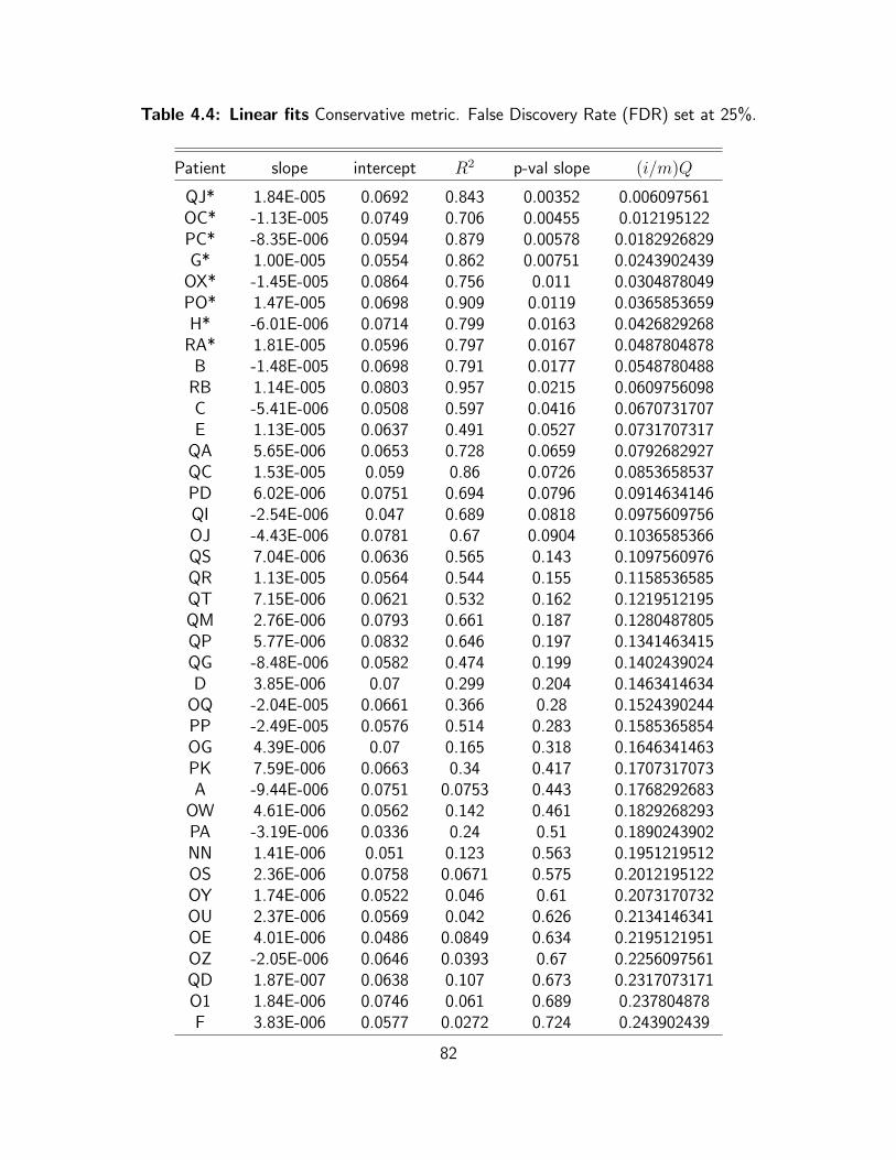
Table 4.4: Linear fits Conservative metric. False Discovery Rate (FDR) set at 25%.
Patient slope intercept R2 p-val slope (i/m)Q
QJ* 1.84E-005 0.0692 0.843 0.00352 0.006097561OC* -1.13E-005 0.0749 0.706 0.00455 0.012195122PC* -8.35E-006 0.0594 0.879 0.00578 0.0182926829G* 1.00E-005 0.0554 0.862 0.00751 0.0243902439
OX* -1.45E-005 0.0864 0.756 0.011 0.0304878049PO* 1.47E-005 0.0698 0.909 0.0119 0.0365853659H* -6.01E-006 0.0714 0.799 0.0163 0.0426829268
RA* 1.81E-005 0.0596 0.797 0.0167 0.0487804878B -1.48E-005 0.0698 0.791 0.0177 0.0548780488
RB 1.14E-005 0.0803 0.957 0.0215 0.0609756098C -5.41E-006 0.0508 0.597 0.0416 0.0670731707E 1.13E-005 0.0637 0.491 0.0527 0.0731707317
QA 5.65E-006 0.0653 0.728 0.0659 0.0792682927QC 1.53E-005 0.059 0.86 0.0726 0.0853658537PD 6.02E-006 0.0751 0.694 0.0796 0.0914634146QI -2.54E-006 0.047 0.689 0.0818 0.0975609756OJ -4.43E-006 0.0781 0.67 0.0904 0.1036585366QS 7.04E-006 0.0636 0.565 0.143 0.1097560976QR 1.13E-005 0.0564 0.544 0.155 0.1158536585QT 7.15E-006 0.0621 0.532 0.162 0.1219512195QM 2.76E-006 0.0793 0.661 0.187 0.1280487805QP 5.77E-006 0.0832 0.646 0.197 0.1341463415QG -8.48E-006 0.0582 0.474 0.199 0.1402439024D 3.85E-006 0.07 0.299 0.204 0.1463414634
OQ -2.04E-005 0.0661 0.366 0.28 0.1524390244PP -2.49E-005 0.0576 0.514 0.283 0.1585365854OG 4.39E-006 0.07 0.165 0.318 0.1646341463PK 7.59E-006 0.0663 0.34 0.417 0.1707317073A -9.44E-006 0.0751 0.0753 0.443 0.1768292683
OW 4.61E-006 0.0562 0.142 0.461 0.1829268293PA -3.19E-006 0.0336 0.24 0.51 0.1890243902NN 1.41E-006 0.051 0.123 0.563 0.1951219512OS 2.36E-006 0.0758 0.0671 0.575 0.2012195122OY 1.74E-006 0.0522 0.046 0.61 0.2073170732OU 2.37E-006 0.0569 0.042 0.626 0.2134146341OE 4.01E-006 0.0486 0.0849 0.634 0.2195121951OZ -2.05E-006 0.0646 0.0393 0.67 0.2256097561QD 1.87E-007 0.0638 0.107 0.673 0.2317073171O1 1.84E-006 0.0746 0.061 0.689 0.237804878F 3.83E-006 0.0577 0.0272 0.724 0.243902439
82
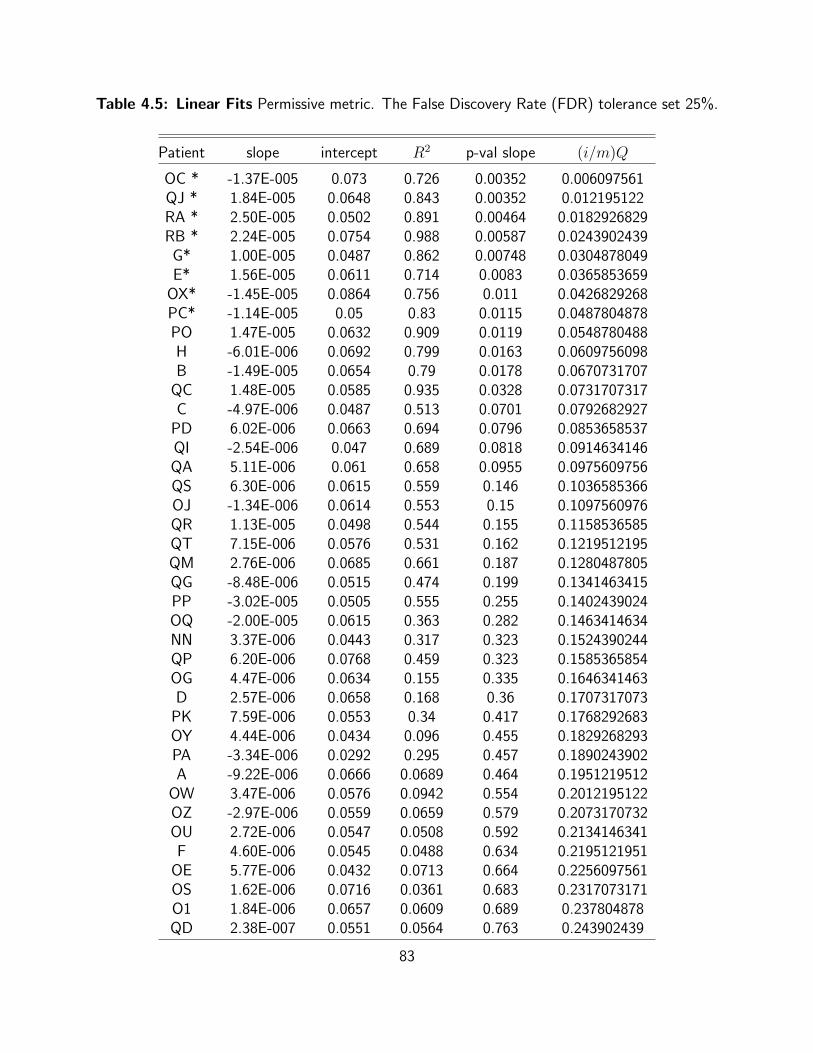
Table 4.5: Linear Fits Permissive metric. The False Discovery Rate (FDR) tolerance set 25%.
Patient slope intercept R2 p-val slope (i/m)Q
OC * -1.37E-005 0.073 0.726 0.00352 0.006097561QJ * 1.84E-005 0.0648 0.843 0.00352 0.012195122RA * 2.50E-005 0.0502 0.891 0.00464 0.0182926829RB * 2.24E-005 0.0754 0.988 0.00587 0.0243902439
G* 1.00E-005 0.0487 0.862 0.00748 0.0304878049E* 1.56E-005 0.0611 0.714 0.0083 0.0365853659
OX* -1.45E-005 0.0864 0.756 0.011 0.0426829268PC* -1.14E-005 0.05 0.83 0.0115 0.0487804878PO 1.47E-005 0.0632 0.909 0.0119 0.0548780488H -6.01E-006 0.0692 0.799 0.0163 0.0609756098B -1.49E-005 0.0654 0.79 0.0178 0.0670731707
QC 1.48E-005 0.0585 0.935 0.0328 0.0731707317C -4.97E-006 0.0487 0.513 0.0701 0.0792682927
PD 6.02E-006 0.0663 0.694 0.0796 0.0853658537QI -2.54E-006 0.047 0.689 0.0818 0.0914634146QA 5.11E-006 0.061 0.658 0.0955 0.0975609756QS 6.30E-006 0.0615 0.559 0.146 0.1036585366OJ -1.34E-006 0.0614 0.553 0.15 0.1097560976QR 1.13E-005 0.0498 0.544 0.155 0.1158536585QT 7.15E-006 0.0576 0.531 0.162 0.1219512195QM 2.76E-006 0.0685 0.661 0.187 0.1280487805QG -8.48E-006 0.0515 0.474 0.199 0.1341463415PP -3.02E-005 0.0505 0.555 0.255 0.1402439024OQ -2.00E-005 0.0615 0.363 0.282 0.1463414634NN 3.37E-006 0.0443 0.317 0.323 0.1524390244QP 6.20E-006 0.0768 0.459 0.323 0.1585365854OG 4.47E-006 0.0634 0.155 0.335 0.1646341463D 2.57E-006 0.0658 0.168 0.36 0.1707317073
PK 7.59E-006 0.0553 0.34 0.417 0.1768292683OY 4.44E-006 0.0434 0.096 0.455 0.1829268293PA -3.34E-006 0.0292 0.295 0.457 0.1890243902A -9.22E-006 0.0666 0.0689 0.464 0.1951219512
OW 3.47E-006 0.0576 0.0942 0.554 0.2012195122OZ -2.97E-006 0.0559 0.0659 0.579 0.2073170732OU 2.72E-006 0.0547 0.0508 0.592 0.2134146341F 4.60E-006 0.0545 0.0488 0.634 0.2195121951
OE 5.77E-006 0.0432 0.0713 0.664 0.2256097561OS 1.62E-006 0.0716 0.0361 0.683 0.2317073171O1 1.84E-006 0.0657 0.0609 0.689 0.237804878QD 2.38E-007 0.0551 0.0564 0.763 0.243902439
83
Chapter 5
Conclusions
It was unclear if, cross-sectionally derived HIV landscapes would concord well with HIV landscapes
derived from longitudinal sequence data. With few exceptions (Seifert et al., 2015), most
computationally derived fitness landscapes have been inferred using cross-sectionally sampled
sequences. (Rihn et al., 2013; Mann et al., 2014; Ferguson et al., 2013; Barton et al., 2015).
These models assume rank prevalence of strains is a sufficient indicator of fitness. However,
there is evidence that these models sometimes fail to well predict spreading fitness and escape
rate of viral mutants (Rihn et al., 2013; Liu et al., 2012; Barton et al., 2015). In our analysis,
we discovered that estimates of fitness costs extracted from cross-sectional data did not well
correlate with fitness costs extracted from longitudinal data. (Chapter 2 Fig 2.4). It appears that
either 1) entropy/prevalence based methods are a poor proxy for fitness, 2) our method based
on reversion rates is a poor proxy of fitness, or both fail to capture critical aspects of intra-host
fitness.
We have developed a novel technique for constructing a one dimensional fitness landscape of
HIV. This technique uses systems of differential equations to extract fitness landscape parameters
from viral population dynamics. The resulting landscape denotes how costly it is for HIV to mutate
single residues along its Gag protein ( a common vaccine target Korber et al. (2009); Currier et al.
84
(2011)). We would like to extend this framework to examine double mutations along the HIV
protein, as mutations tend to have strong interactions in HIV Bonhoeffer et al. (2004); Dahirel
et al. (2011); Koek et al. (2012); Brockman et al. (2007). Often, amino acid mutations in
combination will impact HIVs fitness differently than if they were to occur separately. These type
of interactions are called epistatic interactions Silva et al. (2010). Two dimensional fitness maps
accounting for epistatic interactions have been developed using cross-sectional database sequences
Deforche et al. (2008); Seifert et al. (2015); Ferguson et al. (2013); Mann et al. (2014) and in
vitro competitions assays Manocheewa et al. (2015); Hinkley et al. (2011); Lorenzo-Redondo
et al. (2014). Our analysis, however, avoids the confounding problem of co-inheritance found
in cross-sectional database methods Wang and Lee (2007). Also, unlike in vitro methods, this
technique could describe how epistatic interactions as they occur in real patients. We could extend
our single trajectory ODE model to fit double mutation trajectories. This will be accomplished by
linking the fitness values of the two mutations in the current model so that they are simultaneously
regarded as individual positions and as a mutating unit when a landscape parameter is extracted.
. As shown by (Zanini et al., 2016), when observing proxies for fitness cost the interior residues
tend to much more costly to mutate compared with the exterior residues. This could very well
explain the two grouped populations that emerge in both the shannon entropy metric and the
sensitivity metric. One way in which we could verify that the grouping is arising due extremity or
inferiority, is to map this information onto the metric using HXB2 coordinates for the virus and
determine if this characteristic explains the grouping.
We als wished to determine if incorporating physico-chemical residue detail into a fitness
landscape would improve its ability to predict and describe viral behaviors. We show in Chapter
3 that incorporating physico-chemical detail allowed us to better predict fitness spreading rates
(Fig. 3.7) and escape times (Fig. 3.6). Shannon entropy is currently the metric of choice for
predicting viral fitness behaviors, however, this metric has failed to always describe HIV fitness
85
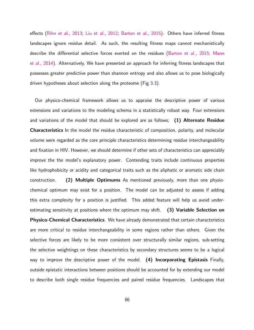
effects (Rihn et al., 2013; Liu et al., 2012; Barton et al., 2015). Others have inferred fitness
landscapes ignore residue detail. As such, the resulting fitness maps cannot mechanistically
describe the differential selective forces exerted on the residues (Barton et al., 2015; Mann
et al., 2014). Alternatively, We have presented an approach for inferring fitness landscapes that
possesses greater predictive power than shannon entropy and also allows us to pose biologically
driven hypotheses about selection along the proteome (Fig 3.3).
Our physico-chemical framework allows us to appraise the descriptive power of various
extensions and variations to the modeling schema in a statistically robust way. Four extensions
and variations of the model that should be explored are as follows; (1) Alternate Residue
Characteristics In the model the residue characteristic of composition, polarity, and molecular
volume were regarded as the core principle characteristics determining residue interchangeability
and fixation in HIV. However, we should determine if other sets of characteristics can appreciably
improve the the model’s explanatory power. Contending traits include continuous properties
like hydrophobicity or acidity and categorical traits such as the aliphatic or aromatic side chain
construction. (2) Multiple Optimums As mentioned previously, more than one physio-
chemical optimum may exist for a position. The model can be adjusted to assess if adding
this extra complexity for a position is justified. This added feature will help us avoid under-
estimating sensitivity at positions where the optimum may shift. (3) Variable Selection on
Physico-Chemical Characteristics. We have already demonstrated that certain characteristics
are more critical to residue interchangeability in some regions rather than others. Given the
selective forces are likely to be more consistent over structurally similar regions, sub-setting
the selective weightings on these characteristics by secondary structures seems to be a logical
way to improve the descriptive power of the model. (4) Incorporating Epistasis Finally,
outside epistatic interactions between positions should be accounted for by extending our model
to describe both single residue frequencies and paired residue frequencies. Landscapes that
86
incorporate interactions between all positions can be computationally expensive to fit, so using
a model selection framework to identify only those positions pairs that substantially improve the
description of the multiple sequence alignment may be preferable.
Little is known about the fitness of HIV during acute infection (Arnott et al., 2010). However
it is well established that HIV’s structural elements are under both heavy purifying pressure
and rapidly shed unfit polymorphims post transmission (Carlson et al., 2014; Novitsky et al.,
2009). Given these observations, we might expect to see fitness increase over early infection as
mutations accrued in the former patient are shed and the virus experiences an adaptive expansion
post the transmission bottleneck. We concluded from analyzing longitudinal sampled virus, that
HIV’s structural proteins showed little to no discernible increase in fitness over early infection.
Previously, an increase in overall viral replicative fitness over infection had been observed in 10
HIV-1 subtype B infected patients Troyer et al. (2005). It may be that in vitro fitness assays
do not well mirror within host selective pressures for this poly-protein. Alternatively, overall viral
fitness trends may not be reflective of the fitness trends of viral structural elements. In the future,
it may pay to employ the physicochemical metric explored in Chapter 3 as a way to describe the
structural protein’s distance from the consensus strain.
87

Bibliography
88
2002. Basic Use of the Information-Theoretic Approach. In K. P. Burnham, and D. R. Anderson,
eds., Model Selection and Multimodel Inference, pages 98–148. Springer New York. DOI:
10.1007/978-0-387-22456-5 3. 43
Abidi, S. H., M. L. Kalish, F. Abbas, S. Rowland-Jones, and S. Ali. 2014. HIV-1 Subtype A Gag
Variability and Epitope Evolution. PLoS ONE 9:e93415. doi:10.1371/journal.pone.0093415.
76, 77
Acevedo, A., L. Brodsky, and R. Andino. 2014. Mutational and fitness landscapes of an RNA
virus revealed through population sequencing. Nature 505:686–690. doi:10.1038/nature12861.
3, 4, 36
Agresti, A. 2003. Categorical Data Analysis. John Wiley & Sons. 68
Al-Mawsawi, L. Q., N. C. Wu, C. A. Olson, V. C. Shi, H. Qi, X. Zheng, T.-T. Wu, and R. Sun.
2014. High-throughput profiling of point mutations across the HIV-1 genome. Retrovirology
11:124. doi:10.1186/s12977-014-0124-6. 3, 4
Allen, T. M., M. Altfeld, S. C. Geer, E. T. Kalife, C. Moore, K. M. O’sullivan, I. Desouza, M. E.
Feeney, R. L. Eldridge, E. L. Maier, D. E. Kaufmann, M. P. Lahaie, L. Reyor, G. Tanzi, M. N.
Johnston, C. Brander, R. Draenert, J. K. Rockstroh, H. Jessen, E. S. Rosenberg, S. A. Mallal,
and B. D. Walker. 2005. Selective escape from CD8+ T-cell responses represents a major
driving force of human immunodeficiency virus type 1 (HIV-1) sequence diversity and reveals
constraints on HIV-1 evolution. Journal of Virology 79:13239–13249. doi:10.1128/JVI.79.21.
13239-13249.2005. 5
89
Arnott, A., D. Jardine, K. Wilson, P. R. Gorry, K. Merlin, P. Grey, M. G. Law, E. M. Dax, A. D.
Kelleher, D. E. Smith, D. A. McPhee, and a. t. P. S. Team. 2010. High Viral Fitness during
Acute HIV-1 Infection. PLOS ONE 5:e12631. doi:10.1371/journal.pone.0012631. 9, 62, 87
Autran, B., R. L. Murphy, D. Costagliola, R. Tubiana, B. Clotet, J. Gatell, S. Staszewski,
N. Wincker, L. Assoumou, R. El-Habib, V. Calvez, B. Walker, C. Katlama, and ORVACS Study
Group. 2008. Greater viral rebound and reduced time to resume antiretroviral therapy after
therapeutic immunization with the ALVAC-HIV vaccine (vCP1452). AIDS (London, England)
22:1313–1322. doi:10.1097/QAD.0b013e3282fdce94. 36
Barton, J. P., M. Kardar, and A. K. Chakraborty. 2015. Scaling laws describe memories of host-
pathogen riposte in the HIV population. Proceedings of the National Academy of Sciences of
the United States of America 112:1965–1970. doi:10.1073/pnas.1415386112. 27, 84, 86
Barton, J. P., N. Goonetilleke, T. C. Butler, B. D. Walker, A. J. McMichael, and A. K.
Chakraborty. 2016. Relative rate and location of intra-host HIV evolution to evade cellular
immunity are predictable. Nature Communications 7:11660. doi:10.1038/ncomms11660. 1, 2,
5, 6, 7, 8, 36
Bonhoeffer, S., C. Chappey, N. T. Parkin, J. M. Whitcomb, and C. J. Petropoulos. 2004. Evidence
for positive epistasis in HIV-1. Science (New York, N.Y.) 306:1547–1550. doi:10.1126/science.
1101786. 85
Borrow, P., H. Lewicki, B. H. Hahn, G. M. Shaw, and M. B. Oldstone. 1994. Virus-specific
CD8+ cytotoxic T-lymphocyte activity associated with control of viremia in primary human
immunodeficiency virus type 1 infection. Journal of Virology 68:6103–6110. 28
Brockman, M. A., A. Schneidewind, M. Lahaie, A. Schmidt, T. Miura, I. Desouza, F. Ryvkin, C. A.
Derdeyn, S. Allen, E. Hunter, J. Mulenga, P. A. Goepfert, B. D. Walker, and T. M. Allen. 2007.
Escape and Compensation from Early HLA-B57-Mediated Cytotoxic T-Lymphocyte Pressure
90
on Human Immunodeficiency Virus Type 1 Gag Alter Capsid Interactions with Cyclophilin A.
Journal of Virology 81:12608–12618. doi:10.1128/JVI.01369-07. 28, 64, 85
Brockman, M. A., Z. L. Brumme, C. J. Brumme, T. Miura, J. Sela, P. C. Rosato, C. M.
Kadie, J. M. Carlson, T. J. Markle, H. Streeck, A. D. Kelleher, M. Markowitz, H. Jessen,
E. Rosenberg, M. Altfeld, P. R. Harrigan, D. Heckerman, B. D. Walker, and T. M. Allen. 2010.
Early Selection in Gag by Protective HLA Alleles Contributes to Reduced HIV-1 Replication
Capacity That May Be Largely Compensated for in Chronic Infection. Journal of Virology
84:11937–11949. doi:10.1128/JVI.01086-10. 64
Brown, L. D., T. T. Cai, and A. DasGupta. 2001. Interval Estimation for a Binomial Proportion.
Statistical Science 16:101–117. ArticleType: research-article / Full publication date: May,
2001 / Copyright 2001 Institute of Mathematical Statistics. 15, 16
Burwitz, B. J., J. B. Sacha, J. S. Reed, L. P. Newman, F. A. Norante, B. N. Bimber, N. A. Wilson,
D. I. Watkins, and D. H. O’Connor. 2011. Pyrosequencing Reveals Restricted Patterns of CD8+
T Cell Escape-Associated Compensatory Mutations in Simian Immunodeficiency Virus. Journal
of Virology 85:13088–13096. doi:10.1128/JVI.05650-11. 64, 77
Carlson, J. M., M. Schaefer, D. C. Monaco, R. Batorsky, D. T. Claiborne, J. Prince,
M. J. Deymier, Z. S. Ende, N. R. Klatt, C. E. DeZiel, T.-H. Lin, J. Peng, A. M.
Seese, R. Shapiro, J. Frater, T. Ndungu, J. Tang, P. Goepfert, J. Gilmour, M. A. Price,
W. Kilembe, D. Heckerman, P. J. R. Goulder, T. M. Allen, S. Allen, and E. Hunter. 2014.
Selection bias at the heterosexual HIV-1 transmission bottleneck. Science 345:1254031. doi:
10.1126/science.1254031. 62, 63, 87
Chopera, D. R., J. K. Wright, M. A. Brockman, and Z. L. Brumme. 2011. Immune-mediated
attenuation of HIV-1. Future Virology 6:917–928. doi:10.2217/fvl.11.68. 2
91
Croux, C., and C. Dehon. 2010. Influence functions of the Spearman and Kendall correlation
measures. Statistical Methods & Applications 19:497–515. doi:10.1007/s10260-010-0142-z.
42
Cuevas, J. M., R. Geller, R. Garijo, J. Lpez-Aldeguer, and R. Sanjun. 2015. Extremely High
Mutation Rate of HIV-1 In Vivo. PLoS Biology 13. doi:10.1371/journal.pbio.1002251. 27, 36
Currier, J. R., M. L. Robb, N. L. Michael, and M. A. Marovich. 2011. Defining epitope
coverage requirements for T cell-based HIV vaccines: Theoretical considerations and practical
applications. Journal of Translational Medicine 9:212. doi:10.1186/1479-5876-9-212. 84
Dahirel, V., K. Shekhar, F. Pereyra, T. Miura, M. Artyomov, S. Talsania, T. M. Allen, M. Altfeld,
M. Carrington, D. J. Irvine, B. D. Walker, and A. K. Chakraborty. 2011. Coordinate linkage
of HIV evolution reveals regions of immunological vulnerability. Proceedings of the National
Academy of Sciences doi:10.1073/pnas.1105315108. 6, 28, 64, 77, 85
Davenport, M. P., L. Loh, J. Petravic, and S. J. Kent. 2008. Rates of HIV immune escape and
reversion: implications for vaccination. Trends in Microbiology 16:561–566. doi:10.1016/j.tim.
2008.09.001. 13
Deforche, K., R. Camacho, K. V. Laethem, P. Lemey, A. Rambaut, Y. Moreau, and A.-M.
Vandamme. 2008. Estimation of an in vivo fitness landscape experienced by HIV-1 under
drug selective pressure useful for prediction of drug resistance evolution during treatment.
Bioinformatics 24:34–41. doi:10.1093/bioinformatics/btm540. 36, 85
Ferguson, A. L., J. K. Mann, S. Omarjee, T. Ndungu, B. D. Walker, and A. K. Chakraborty. 2013.
Translating HIV sequences into quantitative fitness landscapes predicts viral vulnerabilities for
rational immunogen design. Immunity 38:606–617. doi:10.1016/j.immuni.2012.11.022. 1, 2,
6, 7, 8, 12, 18, 28, 36, 65, 84, 85
92
Fernandes, J. D., T. B. Faust, N. B. Strauli, C. Smith, D. C. Crosby, R. L. Nakamura, R. D.
Hernandez, and A. D. Frankel. 2016. Functional Segregation of Overlapping Genes in HIV.
Cell 167:1762–1773.e12. doi:10.1016/j.cell.2016.11.031. 5
Fernandez, C. S., I. Stratov, R. D. Rose, K. Walsh, C. J. Dale, M. Z. Smith, M. B. Agy, S.-
l. Hu, K. Krebs, D. I. Watkins, D. H. O’Connor, M. P. Davenport, and S. J. Kent. 2005.
Rapid Viral Escape at an Immunodominant Simian-Human Immunodeficiency Virus Cytotoxic
T-Lymphocyte Epitope Exacts a Dramatic Fitness Cost. Journal of Virology 79:5721–5731.
doi:10.1128/JVI.79.9.5721-5731.2005. 13
Ferrari, G., B. Korber, N. Goonetilleke, M. K. P. Liu, E. L. Turnbull, J. F. Salazar-Gonzalez,
N. Hawkins, S. Self, S. Watson, M. R. Betts, C. Gay, K. McGhee, P. Pellegrino, I. Williams,
G. D. Tomaras, B. F. Haynes, C. M. Gray, P. Borrow, M. Roederer, A. J. McMichael, and
K. J. Weinhold. 2011. Relationship between Functional Profile of HIV-1 Specific CD8 T Cells
and Epitope Variability with the Selection of Escape Mutants in Acute HIV-1 Infection. PLOS
Pathog 7:e1001273. doi:10.1371/journal.ppat.1001273. 1, 5, 12, 43
Folkvord, J. M., C. Armon, and E. Connick. 2005. Lymphoid follicles are sites of heightened
human immunodeficiency virus type 1 (HIV-1) replication and reduced antiretroviral effector
mechanisms. AIDS research and human retroviruses 21:363–370. doi:10.1089/aid.2005.21.363.
27
Ganusov, V. V., and R. J. De Boer. 2006. Estimating Costs and Benefits of CTL Escape Mutations
in SIV/HIV Infection. PLoS Comput Biol 2:e24. doi:10.1371/journal.pcbi.0020024. 13
GARPR. 2016. Global AIDS Update 2016. 12
Geller, R., P. Domingo-Calap, J. M. Cuevas, P. Rossolillo, M. Negroni, and R. Sanjun. 2015. The
external domains of the HIV-1 envelope are a mutational cold spot. Nature Communications
6:8571. doi:10.1038/ncomms9571. 27
93
Gilchrist, M. A. 2007. Combining Models of Protein Translation and Population Genetics to
Predict Protein Production Rates from Codon Usage Patterns. Molecular Biology and Evolution
24:2362–2372. doi:10.1093/molbev/msm169. 14, 36
Gilchrist, M. A., P. Shah, and R. Zaretzki. 2009. Measuring and Detecting Molecular Adaptation
in Codon Usage Against Nonsense Errors During Protein Translation. Genetics 183:1493–1505.
doi:10.1534/genetics.109.108209. 14, 36
Goulder, P. J. R., and D. I. Watkins. 2004. HIV and SIV CTL escape: implications for vaccine
design. Nature Reviews Immunology 4:630–640. doi:10.1038/nri1417. 36, 63
Grantham, R. 1974. Amino acid difference formula to help explain protein evolution. Science
(New York, N.Y.) 185:862–864. 13, 14, 37, 38, 41, 44
Heath, L., A. Fox, J. McClure, K. Diem, A. B. v. t. Wout, H. Zhao, D. R. Park, J. T. Schouten,
H. L. T. Iii, L. Corey, J. I. Mullins, and J. E. Mittler. 2009. Evidence for Limited Genetic
Compartmentalization of HIV-1 between Lung and Blood. PLOS ONE 4:e6949. doi:10.1371/
journal.pone.0006949. 27
Hedskog, C., M. Mild, J. Jernberg, E. Sherwood, G. Bratt, T. Leitner, J. Lundeberg,
B. Andersson, and J. Albert. 2010. Dynamics of HIV-1 Quasispecies during Antiviral Treatment
Dissected Using Ultra-Deep Pyrosequencing. PLoS ONE 5:e11345. doi:10.1371/journal.pone.
0011345. 13
Hinkley, T., J. Martins, C. Chappey, M. Haddad, E. Stawiski, J. M. Whitcomb, C. J. Petropoulos,
and S. Bonhoeffer. 2011. A systems analysis of mutational effects in HIV-1 protease and reverse
transcriptase. Nature Genetics 43:487–489. doi:10.1038/ng.795. 3, 4, 36, 85
Holland, J. J., J. C. d. l. Torre, D. K. Clarke, and E. Duarte. 1991. Quantitation of relative fitness
and great adaptability of clonal populations of RNA viruses. Journal of Virology 65:2960–2967.
3
94
Holmes, E. C., and A. Moya. 2002. Is the Quasispecies Concept Relevant to RNA Viruses?
Journal of Virology 76:460–462. doi:10.1128/JVI.76.1.460-462.2002. 13
Honeyborne, I., A. Prendergast, F. Pereyra, A. Leslie, H. Crawford, R. Payne, S. Reddy, K. Bishop,
E. Moodley, K. Nair, M. van der Stok, N. McCarthy, C. M. Rousseau, M. Addo, J. I. Mullins,
C. Brander, P. Kiepiela, B. D. Walker, and P. J. R. Goulder. 2007. Control of Human
Immunodeficiency Virus Type 1 Is Associated with HLA-B*13 and Targeting of Multiple Gag-
Specific CD8+ T-Cell Epitopes. Journal of Virology 81:3667–3672. doi:10.1128/JVI.02689-06.
63
Hufert, F. T., J. van Lunzen, G. Janossy, S. Bertram, J. Schmitz, O. Haller, P. Racz, and D. von
Laer. 1997. Germinal centre CD4+ T cells are an important site of HIV replication in vivo.
AIDS (London, England) 11:849–857. 27
Jeffreys, H. 1946. An Invariant Form for the Prior Probability in Estimation Problems. Proceedings
of the Royal Society of London A: Mathematical, Physical and Engineering Sciences 186:453–
461. doi:10.1098/rspa.1946.0056. 15
Johnston, M. I., and A. S. Fauci. 2008. An HIV Vaccine Challenges and Prospects. New England
Journal of Medicine 359:888–890. doi:10.1056/NEJMp0806162. 1, 36
Kendall, M. G., and J. D. Gibbons. 1990. Rank correlation methods. E. Arnold. Google-Books-ID:
ly4nAQAAIAAJ. 42
Kim, E.-Y., R. Lorenzo-Redondo, S. J. Little, Y.-S. Chung, P. K. Phalora, I. Maljkovic Berry,
J. Archer, S. Penugonda, W. Fischer, D. D. Richman, T. Bhattacharya, M. H. Malim, and
S. M. Wolinsky. 2014. Human APOBEC3 Induced Mutation of Human Immunodeficiency
Virus Type-1 Contributes to Adaptation and Evolution in Natural Infection. PLoS Pathogens
10. doi:10.1371/journal.ppat.1004281. 27
95
Korber, B., B. Gaschen, K. Yusim, R. Thakallapally, C. Kesmir, and V. Detours. 2001.
Evolutionary and immunological implications of contemporary HIV-1 variation. British Medical
Bulletin 58:19–42. 1, 36, 78
Korber, B. T., N. L. Letvin, and B. F. Haynes. 2009. T-Cell Vaccine Strategies for Human
Immunodeficiency Virus, the Virus with a Thousand Faces. Journal of Virology 83:8300–8314.
doi:10.1128/JVI.00114-09. 63, 77, 84
Kouyos, R. D., G. E. Leventhal, T. Hinkley, M. Haddad, J. M. Whitcomb, C. J. Petropoulos, and
S. Bonhoeffer. 2012. Exploring the Complexity of the HIV-1 Fitness Landscape. PLoS Genet
8:e1002551. doi:10.1371/journal.pgen.1002551. 36
Koek, M., S. Henke, K. G. akov, G. B. Jacobs, A. Schuch, B. Buchholz, V. Mller, H.-G. Krusslich,
P. ezov, J. Konvalinka, and J. Bodem. 2012. Mutations in HIV-1 gag and pol Compensate
for the Loss of Viral Fitness Caused by a Highly Mutated Protease. Antimicrobial Agents and
Chemotherapy 56:4320–4330. doi:10.1128/AAC.00465-12. 77, 85
Lemey, P., A. Rambaut, and O. G. Pybus. 2006. HIV evolutionary dynamics within and among
hosts. AIDS reviews 8:125–140. 36
Li, B., A. D. Gladden, M. Altfeld, J. M. Kaldor, D. A. Cooper, A. D. Kelleher, and T. M. Allen.
2007. Rapid Reversion of Sequence Polymorphisms Dominates Early Human Immunodeficiency
Virus Type 1 Evolution. Journal of Virology 81:193–201. doi:10.1128/JVI.01231-06. 5, 63,
77
Li, G., J. Verheyen, S.-Y. Rhee, A. Voet, A.-M. Vandamme, and K. Theys. 2013. Functional
conservation of HIV-1 Gag: implications for rational drug design. Retrovirology 10:126. doi:
10.1186/1742-4690-10-126. 9
Li, H., K. J. Bar, S. Wang, J. M. Decker, Y. Chen, C. Sun, J. F. Salazar-Gonzalez, M. G. Salazar,
G. H. Learn, C. J. Morgan, J. E. Schumacher, P. Hraber, E. E. Giorgi, T. Bhattacharya, B. T.
96
Korber, A. S. Perelson, J. J. Eron, M. S. Cohen, C. B. Hicks, B. F. Haynes, M. Markowitz,
B. F. Keele, B. H. Hahn, and G. M. Shaw. 2010. High Multiplicity Infection by HIV-1 in Men
Who Have Sex with Men. PLoS Pathog 6:e1000890. doi:10.1371/journal.ppat.1000890. 63
Liu, M. K., N. Hawkins, A. J. Ritchie, V. V. Ganusov, V. Whale, S. Brackenridge, H. Li, J. W.
Pavlicek, F. Cai, M. Rose-Abrahams, F. Treurnicht, P. Hraber, C. Riou, C. Gray, G. Ferrari,
R. Tanner, L.-H. Ping, J. A. Anderson, R. Swanstrom, C. C. B, M. Cohen, S. S. A. Karim,
B. Haynes, P. Borrow, A. S. Perelson, G. M. Shaw, B. H. Hahn, C. Williamson, B. T. Korber,
F. Gao, S. Self, A. McMichael, and N. Goonetilleke. 2012. Vertical T cell immunodominance
and epitope entropy determine HIV-1 escape. Journal of Clinical Investigation doi:10.1172/
JCI65330. 1, 2, 3, 5, 12, 28, 43, 84, 86
Lorenzo-Redondo, R., S. Delgado, F. Morn, and C. Lopez-Galindez. 2014. Realistic Three
Dimensional Fitness Landscapes Generated by Self Organizing Maps for the Analysis of
Experimental HIV-1 Evolution. PLoS ONE 9:e88579. doi:10.1371/journal.pone.0088579.
36, 85
Mann, J. K., J. P. Barton, A. L. Ferguson, S. Omarjee, B. D. Walker, A. Chakraborty, and
T. Ndung’u. 2014. The Fitness Landscape of HIV-1 Gag: Advanced Modeling Approaches
and Validation of Model Predictions by In Vitro Testing. PLoS Comput Biol 10:e1003776.
doi:10.1371/journal.pcbi.1003776. 1, 2, 6, 7, 8, 12, 18, 36, 84, 85, 86
Manocheewa, S., E. C. Lanxon-Cookson, Y. Liu, J. V. Swain, J. McClure, U. Rao, B. Maust,
W. Deng, J. E. Sunshine, M. Kim, M. Rolland, and J. I. Mullins. 2015. Pairwise Growth
Competition Assay for Determining the Replication Fitness of Human Immunodeficiency
Viruses. Journal of Visualized Experiments : JoVE doi:10.3791/52610. 3, 36, 85
Martinez-Picado, J., J. G. Prado, E. E. Fry, K. Pfafferott, A. Leslie, S. Chetty, C. Thobakgale,
I. Honeyborne, H. Crawford, P. Matthews, T. Pillay, C. Rousseau, J. I. Mullins, C. Brander,
97
B. D. Walker, D. I. Stuart, P. Kiepiela, and P. Goulder. 2006. Fitness cost of escape mutations
in p24 Gag in association with control of human immunodeficiency virus type 1. Journal of
virology 80:3617–3623. doi:10.1128/JVI.80.7.3617-3623.2006. 36
McElrath, M. J., and B. F. Haynes. 2010. Induction of immunity to human immunodeficiency
virus type-1 by vaccination. Immunity 33:542–554. doi:10.1016/j.immuni.2010.09.011. 1
Michael R. Dietrich, R. S. 2012. A Shifting Terrain: A Brief History of the Adaptive Landscape.
The adaptive landscape in evolutionary biology pages 3–15. 36
Miura, T., Z. L. Brumme, M. A. Brockman, P. Rosato, J. Sela, C. J. Brumme, F. Pereyra,
D. E. Kaufmann, A. Trocha, B. L. Block, E. S. Daar, E. Connick, H. Jessen, A. D. Kelleher,
E. Rosenberg, M. Markowitz, K. Schafer, F. Vaida, A. Iwamoto, S. Little, and B. D. Walker.
2010. Impaired Replication Capacity of Acute/Early Viruses in Persons Who Become HIV
Controllers. Journal of Virology 84:7581–7591. doi:10.1128/JVI.00286-10. 12, 62
Moradigaravand, D., R. Kouyos, T. Hinkley, M. Haddad, C. J. Petropoulos, J. Engelstdter, and
S. Bonhoeffer. 2014. Recombination Accelerates Adaptation on a Large-Scale Empirical Fitness
Landscape in HIV-1. PLoS Genet 10:e1004439. doi:10.1371/journal.pgen.1004439. 36
Novitsky, V., R. Wang, L. Margolin, J. Baca, L. Kebaabetswe, R. Rossenkhan, C. Bonney,
M. Herzig, D. Nkwe, S. Moyo, R. Musonda, E. Woldegabriel, E. van Widenfelt, J. Makhema,
S. Lagakos, and M. Essex. 2009. Timing Constraints of In Vivo Gag Mutations during Primary
HIV-1 Subtype C Infection. PLoS ONE 4:e7727. doi:10.1371/journal.pone.0007727. 8, 9, 15,
28, 62, 64, 72, 87
Novitsky, V., R. Wang, J. Baca, L. Margolin, M. F. McLane, S. Moyo, E. van Widenfelt,
J. Makhema, and M. Essex. 2011. Evolutionary Gamut of in vivo Gag Substitutions during
Early HIV-1 Subtype C Infection. Virology 421:119–128. doi:10.1016/j.virol.2011.09.020. 22,
29, 64
98
Novitsky, V., R. Wang, R. Rossenkhan, S. Moyo, and M. Essex. 2013. Intra-host evolutionary rates
in HIV-1c env and gag during primary infection. Infection, Genetics and Evolution 19:361–368.
doi:10.1016/j.meegid.2013.02.023. 62, 77
Ogg, G. S., X. Jin, S. Bonhoeffer, P. R. Dunbar, M. A. Nowak, S. Monard, J. P. Segal, Y. Cao,
S. L. Rowland-Jones, V. Cerundolo, A. Hurley, M. Markowitz, D. D. Ho, D. F. Nixon, and
A. J. McMichael. 1998. Quantitation of HIV-1-specific cytotoxic T lymphocytes and plasma
load of viral RNA. Science (New York, N.Y.) 279:2103–2106. 28
Parera, M., G. Fernndez, B. Clotet, and M. A. Martnez. 2007. HIV-1 Protease Catalytic Efficiency
Effects Caused by Random Single Amino Acid Substitutions. Molecular Biology and Evolution
24:382–387. doi:10.1093/molbev/msl168. 4
Pennings, P. S., S. Kryazhimskiy, and J. Wakeley. 2014. Loss and Recovery of Genetic Diversity in
Adapting Populations of HIV. PLoS Genet 10:e1004000. doi:10.1371/journal.pgen.1004000.
78
Petropoulos, C. J., N. T. Parkin, K. L. Limoli, Y. S. Lie, T. Wrin, W. Huang, H. Tian,
D. Smith, G. A. Winslow, D. J. Capon, and J. M. Whitcomb. 2000. A Novel Phenotypic
Drug Susceptibility Assay for Human Immunodeficiency Virus Type 1. Antimicrobial Agents
and Chemotherapy 44:920–928. doi:10.1128/AAC.44.4.920-928.2000. 4
Pilcher, C. D., J. K. Wong, and S. K. Pillai. 2008. Inferring HIV Transmission Dynamics from
Phylogenetic Sequence Relationships. PLoS Medicine 5. doi:10.1371/journal.pmed.0050069.
65
Quiones-Mateu, M. E., S. C. Ball, A. J. Marozsan, V. S. Torre, J. L. Albright, G. Vanham, G. v. d.
Groen, R. L. Colebunders, and E. J. Arts. 2000. A Dual Infection/Competition Assay Shows
a Correlation between Ex Vivo Human Immunodeficiency Virus Type 1 Fitness and Disease
99
Progression. Journal of Virology 74:9222–9233. doi:10.1128/JVI.74.19.9222-9233.2000. 9,
63
Rihn, S. J., S. J. Wilson, N. J. Loman, M. Alim, S. E. Bakker, D. Bhella, R. J. Gifford, F. J.
Rixon, and P. D. Bieniasz. 2013. Extreme Genetic Fragility of the HIV-1 Capsid. PLoS Pathog
9:e1003461. doi:10.1371/journal.ppat.1003461. 1, 2, 3, 4, 5, 12, 27, 36, 43, 55, 62, 76, 77,
84, 86
Rolland, M., D. Heckerman, W. Deng, C. M. Rousseau, H. Coovadia, K. Bishop, P. J. R.
Goulder, B. D. Walker, C. Brander, and J. I. Mullins. 2008. Broad and Gag-Biased HIV-
1 Epitope Repertoires Are Associated with Lower Viral Loads. PLOS ONE 3:e1424. doi:
10.1371/journal.pone.0001424. 63
Rolland, M., J. M. Carlson, S. Manocheewa, J. V. Swain, E. Lanxon-Cookson, W. Deng, C. M.
Rousseau, D. N. Raugi, G. H. Learn, B. S. Maust, H. Coovadia, T. Ndung’u, P. J. R. Goulder,
B. D. Walker, C. Brander, D. E. Heckerman, and J. I. Mullins. 2010. Amino-Acid Co-Variation
in HIV-1 Gag Subtype C: HLA-Mediated Selection Pressure and Compensatory Dynamics.
PLoS ONE 5. doi:10.1371/journal.pone.0012463. 77
Rouzine, I. M., and L. S. Weinberger. 2013. The quantitative theory of within-host viral evolution.
Journal of Statistical Mechanics: Theory and Experiment 2013:P01009. 13
Rozera, G., I. Abbate, C. Vlassi, E. Giombini, R. Lionetti, M. Selleri, P. Zaccaro, B. Bartolini,
A. Corpolongo, G. D’Offizi, A. Baiocchini, F. Del Nonno, G. Ippolito, and M. R. Capobianchi.
2014. Quasispecies tropism and compartmentalization in gut and peripheral blood during early
and chronic phases of HIV-1 infection: possible correlation with immune activation markers.
Clinical Microbiology and Infection 20:O157–O166. doi:10.1111/1469-0691.12367. 13, 27
100
Salemi, M. 2013. The Intra-Host Evolutionary and Population Dynamics of Human
Immunodeficiency Virus Type 1: A Phylogenetic Perspective. Infectious Disease Reports 5.
doi:10.4081/idr.2013.s1.e3. 36
Sanjun, R., M. R. Nebot, N. Chirico, L. M. Mansky, and R. Belshaw. 2010. Viral Mutation Rates.
Journal of Virology 84:9733–9748. doi:10.1128/JVI.00694-10. 1
Schacker, T. 2008. The role of secondary lymphatic tissue in immune deficiency of HIV infection.
AIDS (London, England) 22 Suppl 3:S13–18. doi:10.1097/01.aids.0000327511.76126.b5. 27
Schneidewind, A., M. A. Brockman, R. Yang, R. I. Adam, B. Li, S. Le Gall, C. R. Rinaldo, S. L.
Craggs, R. L. Allgaier, K. A. Power, T. Kuntzen, C.-S. Tung, M. X. LaBute, S. M. Mueller,
T. Harrer, A. J. McMichael, P. J. R. Goulder, C. Aiken, C. Brander, A. D. Kelleher, and
T. M. Allen. 2007. Escape from the dominant HLA-B27-restricted cytotoxic T-lymphocyte
response in Gag is associated with a dramatic reduction in human immunodeficiency virus type
1 replication. Journal of Virology 81:12382–12393. doi:10.1128/JVI.01543-07. 28
Seifert, D., F. D. Giallonardo, K. J. Metzner, H. F. Gnthard, and N. Beerenwinkel. 2015. A
Framework for Inferring Fitness Landscapes of Patient-Derived Viruses Using Quasispecies
Theory. Genetics 199:191–203. doi:10.1534/genetics.114.172312. 36, 84, 85
Sella, G., and A. E. Hirsh. 2005. The application of statistical physics to evolutionary biology.
Proceedings of the National Academy of Sciences of the United States of America 102:9541–
9546. doi:10.1073/pnas.0501865102. 37, 39
Shah, P., and M. A. Gilchrist. 2011. Explaining complex codon usage patterns with selection for
translational efficiency, mutation bias, and genetic drift. Proceedings of the National Academy
of Sciences 108:10231–10236. doi:10.1073/pnas.1016719108. 14, 36
Shekhar, K., C. F. Ruberman, A. L. Ferguson, J. P. Barton, M. Kardar, and A. K. Chakraborty.
2013. Spin models inferred from patient-derived viral sequence data faithfully describe HIV
101
fitness landscapes. Physical Review. E, Statistical, Nonlinear, and Soft Matter Physics
88:062705. doi:10.1103/PhysRevE.88.062705. 2, 7, 12, 13, 18, 36
Shriner, D., R. Shankarappa, M. A. Jensen, D. C. Nickle, J. E. Mittler, J. B. Margolick, and J. I.
Mullins. 2004. Influence of Random Genetic Drift on Human Immunodeficiency Virus Type 1
env Evolution During Chronic Infection. Genetics 166:1155–1164. doi:10.1534/genetics.166.
3.1155. 13
Silva, J. d., M. Coetzer, R. Nedellec, C. Pastore, and D. E. Mosier. 2010. Fitness Epistasis
and Constraints on Adaptation in a Human Immunodeficiency Virus Type 1 Protein Region.
Genetics 185:293–303. doi:10.1534/genetics.109.112458. 85
Sturdevant, C. B., S. B. Joseph, G. Schnell, R. W. Price, R. Swanstrom, and S. Spudich. 2015.
Compartmentalized Replication of R5 T Cell-Tropic HIV-1 in the Central Nervous System Early
in the Course of Infection. PLOS Pathogens 11:e1004720. doi:10.1371/journal.ppat.1004720.
13, 27
Sunshine, J. E., B. B. Larsen, B. Maust, E. Casey, W. Deng, L. Chen, D. H. Westfall, M. Kim,
H. Zhao, S. Ghorai, E. Lanxon-Cookson, M. Rolland, A. C. Collier, J. Maenza, J. I. Mullins,
and N. Frahm. 2015. Fitness-Balanced Escape Determines Resolution of Dynamic Founder
Virus Escape Processes in HIV-1 Infection. Journal of Virology 89:10303–10318. doi:10.1128/
JVI.01876-15. 12
Thyagarajan, B., and J. D. Bloom. 2014. The inherent mutational tolerance and antigenic
evolvability of influenza hemagglutinin. eLife 3:e03300. doi:10.7554/eLife.03300. 3, 4, 5
Tripathi, K., R. Balagam, N. K. Vishnoi, and N. M. Dixit. 2012. Stochastic Simulations Suggest
that HIV-1 Survives Close to Its Error Threshold. PLoS Computational Biology 8. doi:10.
1371/journal.pcbi.1002684. 63
102
Troyer, R. M., K. R. Collins, A. Abraha, E. Fraundorf, D. M. Moore, R. W. Krizan, Z. Toossi, R. L.
Colebunders, M. A. Jensen, J. I. Mullins, G. Vanham, and E. J. Arts. 2005. Changes in Human
Immunodeficiency Virus Type 1 Fitness and Genetic Diversity during Disease Progression.
Journal of Virology 79:9006–9018. doi:10.1128/JVI.79.14.9006-9018.2005. 9, 62, 63, 76,
87
Troyer, R. M., J. McNevin, Y. Liu, S. C. Zhang, R. W. Krizan, A. Abraha, D. M. Tebit, H. Zhao,
S. Avila, M. A. Lobritz, M. J. McElrath, S. Le Gall, J. I. Mullins, and E. J. Arts. 2009. Variable
Fitness Impact of HIV-1 Escape Mutations to Cytotoxic T Lymphocyte (CTL) Response. PLoS
Pathog 5:e1000365. doi:10.1371/journal.ppat.1000365. 12
Tsibris, A. M. N., B. Korber, R. Arnaout, C. Russ, C.-C. Lo, T. Leitner, B. Gaschen, J. Theiler,
R. Paredes, Z. Su, M. D. Hughes, R. M. Gulick, W. Greaves, E. Coakley, C. Flexner,
C. Nusbaum, and D. R. Kuritzkes. 2009. Quantitative Deep Sequencing Reveals Dynamic
HIV-1 Escape and Large Population Shifts during CCR5 Antagonist Therapy In Vivo. PLoS
ONE 4:e5683. doi:10.1371/journal.pone.0005683. 13
van Marle, G., M. J. Gill, D. Kolodka, L. McManus, T. Grant, and D. L. Church. 2007.
Compartmentalization of the gut viral reservoir in HIV-1 infected patients. Retrovirology 4:87.
doi:10.1186/1742-4690-4-87. 13, 27
Waheed, A. A., and E. O. Freed. 2012. HIV Type 1 Gag as a Target for Antiviral Therapy. AIDS
Research and Human Retroviruses 28:54–75. doi:10.1089/aid.2011.0230. 63
Walker, B. D., and D. R. Burton. 2008. Toward an AIDS Vaccine. Science 320:760–764. doi:
10.1126/science.1152622. 1, 12, 77
Wang, Q., and C. Lee. 2007. Distinguishing Functional Amino Acid Covariation from Background
Linkage Disequilibrium in HIV Protease and Reverse Transcriptase. PLoS ONE 2. doi:10.1371/
journal.pone.0000814. 85
103
Wood, N., T. Bhattacharya, B. F. Keele, E. Giorgi, M. Liu, B. Gaschen, M. Daniels, G. Ferrari,
B. F. Haynes, A. McMichael, G. M. Shaw, B. H. Hahn, B. Korber, and C. Seoighe. 2009. HIV
Evolution in Early Infection: Selection Pressures, Patterns of Insertion and Deletion, and the
Impact of APOBEC. PLOS Pathogens 5:e1000414. doi:10.1371/journal.ppat.1000414. 27
Wright, S. 1932. The roles of mutation, inbreeding, crossbreeding and selection in evolution.
Proceedings of the sixth international congress of genetics 6:356–366. 1
Wu, N. C., A. P. Young, L. Q. Al-Mawsawi, C. A. Olson, J. Feng, H. Qi, S.-H. Chen, I.-H. Lu,
C.-Y. Lin, R. G. Chin, H. H. Luan, N. Nguyen, S. F. Nelson, X. Li, T.-T. Wu, and R. Sun.
2014. High-throughput profiling of influenza A virus hemagglutinin gene at single-nucleotide
resolution. Scientific Reports 4:4942. doi:10.1038/srep04942. 3, 4, 5
Zanini, F., V. Puller, J. Brodin, J. Albert, and R. Neher. 2016. In-vivo mutation rates and fitness
landscape of HIV-1. bioRxiv page 045039. doi:10.1101/045039. 1, 3, 5, 6, 7, 8, 85
104

Vita
Elizabeth Johnson was born in Pittsfield, MA in 1986. In 2002 she was admitted to Appalachian
State University as a Chancellor Scholar where she graduated summa cum laude in 2006 with a
Bachelors of Science in Biology and minors in both Mathematics and Chemistry. She accepted
a graduate position at the University of Tennessee Knoxville in 2010, where she was funded by
an NSF Graduate Education and Research Fellowship for Scalable Computing in Biology and an
assistantship from the National Institute for Mathematical and Biological Synthesis (NIMBioS).
She pursued a doctorate under Vitaly Ganusov in a theoretical immunology laboratory housed in
the Microbiology Department. There, she completed her computational minor and dissertation
research on HIV fitness landscapes.
105