physicochemical problems of mineral processing
TRANSCRIPT
Physicochemical Problems
of Mineral Processing
Volume 48, Issue 2
2012
www.minproc.pwr.wroc.pl/journal
www.dbc.wroc.pl/dlibra/publication/11251
Oficyna Wydawnicza Politechniki Wrocławskiej
Wrocław 2012
Editors
Jan Drzymała editor-in-chief
Adriana Zalewska
Paweł Nowak
Editorial Board
Ashraf Amer, Wiesław Blaschke, Marian Brożek, Stanisław Chibowski, Tomasz Chmielewski,
Beata Cwalina, Janusz Girczys, Andrzej Heim, Jan Hupka, Andrzej Konieczny, Teofil Jesionowski,
Janusz Laskowski, Andrzej Łuszczkiewicz, Kazimierz Małysa, Andrzej Pomianowski,
Stanisława Sanak-Rydlewska, Jerzy Sablik, Kazimierz Sztaba, Barbara Tora, Kazimierz Tumidajski,
Zygmunt Sadowski
Production Editor
Przemysław B. Kowalczuk
The papers published in the Physicochemical Problems of Mineral Processing journal are abstracted
in BazTech, Chemical Abstracts, Coal Abstracts, EBSCO, Google Scholar, Scopus, Thomson Reuters
(Science Citation Index Expanded, Materials Science Citation Index, Journal Citation Reports)
and other sources
This publication was supported in different forms by
Komitet Górnictwa PAN (Sekcja Wykorzystania Surowców Mineralnych)
Akademia Górniczo-Hutnicza w Krakowie
Politechnika Śląska w Gliwicach
Politechnika Wrocławska
©Copyright by Oficyna Wydawnicza Politechniki Wrocławskiej, Wrocław 2012
ISSN 1643-1049 (print) previously 0137-1282
ISSN 2084-4735 (online)
OFICYNA WYDAWNICZA POLITECHNIKI WROCŁAWSKIEJ
Wybrzeże Wyspiańskiego 27, 50-370 Wrocław, Poland

CONTENTS
N. Magdalinovic, M. Trumic, M. Trumic, L. Andric, The optimal ball diameter in a mill ............... 329
I. Demir, I. Kursun, Investigation of radioactive content of Manisa-Soma and Istanbul-Agacli
coals (Turkey) ....................................................................................................................... 341
A. Ekmekyapar, M. Tanaydin, N. Demirkiran, Investigation of copper cementation kinetics by
rotating aluminum disc from the leach solutions containing copper ions ............................. 355
I. Gulgonul, Evaluation of Turkish bentonite for removal of dyes from textile wastewaters ............. 369
H. Hacifazlioglu, I. Kursun, M.Terzi, Beneficiation of low-grade feldspar ore using cyclojet
flotation cell, conventional cell and magnetic separator ....................................................... 381
W. Xia, J. Yang , Y. Zhao, B. Zhu, Y. Wang, Improving floatability of Taixi anthracite coal of
mild oxidation by grinding .................................................................................................... 393
K. Szczepanowicz, G. Para, A.M. Bouzga, C. Simon, J. Yang, P. Warszynski, Hydrolysis of silica
sources: APS and DTSACl in microencapsulation processes ............................................... 403
S.S. Ibrahim, A. Q. Selim, Heat treatment of natural diatomite ........................................................ 413
A. Mehdilo, M. Irannajad, Iron removing from titanium slag for synthetic rutile production ........... 425
C. Sarici-Ozdemir, Adsorption and desorption kinetics behaviour of Methylene Blue onto
activated carbon .................................................................................................................... 441
S.G. Ozkan, C. Gungoren, Enhancement of colemanite flotation by ultrasonic pre-treatment.......... 455
L. Klapiszewski, M. Madrawska, T. Jesionowski, Preparation and characterisation of hydrated
silica/lignin biocomposites .................................................................................................... 463
O. Sivrikaya, A.I. Arol, Evaluation of low grade iron ore deposit in Erzincan-turkey for iron ore
pellet concentrate production ................................................................................................ 475
M. Koyuncu, Colour removal from aqueous solution of Tar-Chromium Green 3G dye using
natural diatomite ................................................................................................................... 485
A. Tasdemir, Effect of autocorrelation on the process control charts in monitoring of a coal
washing plant ........................................................................................................................ 495
M. Karimi, G. Akdogan, S.M. Bradshaw, Effects of different mesh schemes and turbulence
models in CFD modelling of stirred tanks ............................................................................. 513
O. Sahbaz, U. Ercetin, B. Oteyaka, Determination of turbulence and upper size limit in Jameson
flotation cell by the use of Computational Fluid Dynamic modelling ................................... 533
J. Malewski, M. Krzeminska, Dependence of mine revenue on the grade of copper concentrate ..... 545
E. Sabah, C. Aciksoz, Flocculation performance of fine particles in travertine slime suspension .... 555
A.A.S. Seifelnassr, E.M. Moslim, A.M. Abouzeid, Effective processing of low-grade iron ore
through gravity and magnetic separation techniques ............................................................ 567
J. Szpyrka, M. Lutynski, Analysis of selected methods of beneficiating coal slurries deposited in
impoundments ....................................................................................................................... 579
A. Yorukoglu, Influence of acid activation on the ion-exchange properties of Manisa-Gordes
clinoptilolite .......................................................................................................................... 591
A. Kekki, J. Aromaa, O. Forsen, Leaching characteristics of EAF and AOD stainless steel
production dusts .................................................................................................................... 599
A.M. Didyk, Z. Sadowski, Flotation of serpentinite and quartz using biosurfactants ...................... 607
K. Szwarc-Rzepka, F. Ciesielczyk, M. Zawisza, M. Kaczmarek, M. Dutkiewicz, B. Marciniec,
H. Maciejewski, T. Jesionowski, Synthesis of hepta(isobuthyl)ethyltriethoxysilyl
octasilsesquioxane and its application as a modifier of both hydrated and emulsion silicas 619
A. Pilarska, I. Linda, M. Wysokowski, D. Paukszta, T. Jesionowski, Synthesis of Mg(OH)2 from
magnesium salts and NH4OH by direct functionalisation with poly(ethylene glycols) ......... 631
M. Kademli, O.Y. Gulsoy, The role of particle size and solid contents of feed on mica-feldspar
separation in gravity concentration ...................................................................................... 645

http://dx.doi.org/10.5277/ppmp120201
Physicochem. Probl. Miner. Process. 48(2), 2012, 329–339 Physicochemical Problems
of Mineral Processing
w w w . m i n p r o c . p w r . w r o c . p l / j o u r n a l / ISSN 1643-1049 (print)
ISSN 2084-4735 (online)
Received February 28, 2012; reviewed; accepted March 16, 2012
THE OPTIMAL BALL DIAMETER IN A MILL
Nedeljko MAGDALINOVIC*, Milan TRUMIC**, Maja TRUMIC**
Ljubisa ANDRIC***
* Megatrend University, Faculty of Management, Park suma kraljevica bb, Zajecar, Serbia
** University of Belgrade, Technical Faculty, VJ 12, Bor, Serbia, [email protected], Tel.: +381 30 421 749;
fax: +381 30 421 078
*** Institute for Technology of Nuclear and Other Mineral Raw Materials, Bulevar Franš d'Eperea 86,
Belgrade, Serbia
Abstract. This paper covers theoretical and experimental explorations for the sake of
determining the optimal ball charge in mills. In the first part of the paper, on the basis of the
theoretical analysis of the energy-geometric correlations, which are being established during
the grain comminution by ball impact, as well as on the basis of the experiment carried out on
grinding quartz and copper ore in a laboratory ball mill, there has been defined a general form
of the equation for determining: the optimal ball diameter depending on the grain size being
ground; and the parameter of the equation through which the influence of a mill is being
demonstrated; then the parameter of the grinding conditions; and the parameter of the material
characteristics being ground in relation to the ball size. In the second part of the paper, the
process of making up the optimal ball charge has been defined providing the highest grinding
efficiency, as well as its confirmation by the results of the experimental explorations.
keywords: mineral processing, optimal ball diameter, optimal ball charge, grinding
1. Introduction
The ball size in a mill has a significant influence on the mill throughput, power
consumption and ground material size (Austin et al., 1976; Fuerstenau et al., 1999;
Kotake et. al., 2004).
The basic condition, which must be met while grinding the material in a mill is that
the ball, while breaking the material grain, causes in it stress which is higher than the
grain hardness (Bond, 1962; Razumov, 1947; Supov, 1962). Therefore, for the biggest
grain size, it is necessary to have a definite number of the biggest balls in the charge,
and with the decreased grain size, the necessary ball size also decreases (Olejnik,
2010; 2011). For each grain size there is an optimal ball size (Trumic et. al., 2007).
The bigger ball in relation to the optimal one will have an excess energy, and
consequently, the smaller ball mill has less energy necessary for grinding. In both
cases, the specific power consumption increases and the grinding capacity decreases
(Concha et al. 1992; Katubilwa and Moys, 2009; Erdem and Ergun, 2009).
330 N. Magdalinovic et al.
A great number of explorers were dealing with the questions of determining the
maximal ball diameter depending on the material size being ground. A few empirical
formulae have been proposed, out of which some are recommended for industrial mills
(Bond, 1962; Razumov, 1947; Olevskij, 1948), but some of them have been defined
on the basis of investigations carried out in laboratory mills and they have not been
applied to industrial mills (Belecki, 1985; Supov, 1962).
All suggested formulae fit into the general form given by:
nb Kdd max , (1)
where: db max is the maximum ball diameter in a charge, d is the characteristic top limit
of the material size which is being ground (d95 or d80 in the formulae is recommended
for industrial mills); K and n are parameters, for which all authors say to be dependent
on the mill characteristics, grinding conditions and characteristics of the material
being ground. They are determined experimentally.
Even a simplified theoretical analysis clearly defines the influential factors on
parameters K and n. The topic of this paper is, first of all, this kind of analysis and
then the determination of the optimal ball charge model in a mill.
2. Theoretical background
Each grain size corresponds to a definite optimal ball size. The diameter of a ball is
determined by the condition that, at the moment of breaking the grain, it has energy E,
which is equal to energy E0 necessary for grain comminution:
0EE . (2)
The ball impact energy on grain is proportional to the ball diameter to the third
power:
31 bdKE . (3)
The coefficient of proportionality K1 directly depends on the mill diameter, ball
mill loading, milling rate and the type of grinding (wet/dry). None of the
characteristics of the material being ground have any influence on K1.
The ball impact energy on the grain is turned into the action of comminution,
which according to the Rittinger comminution law is directly proportional to the
newly formed grain surface while being ground. We can suppose that the grain has got
the form of a ball with diameter d and that the area of comminution occurs along the
equator cross section. Then, the comminution energy E0 is proportional to the surface
of equator circle, that is, the grain diameter to the second power:
220 dKE . (4)
It is clear that the coefficient of proportionality K2 is not influenced by any of the
characteristics of the material being ground.
The optimal ball diameter in a mill 331
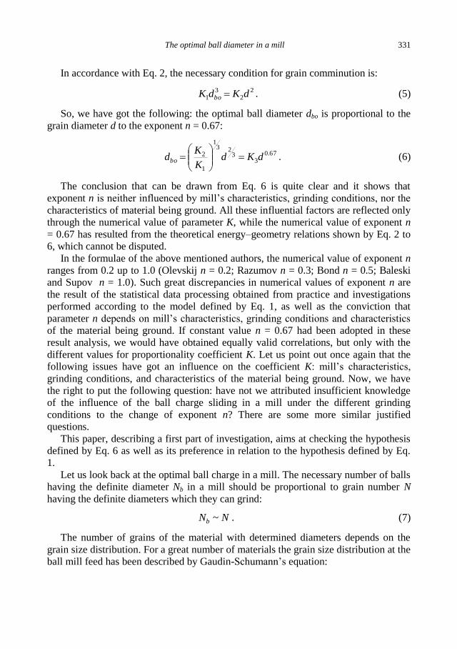
In accordance with Eq. 2, the necessary condition for grain comminution is:
22
31 dKdK bo . (5)
So, we have got the following: the optimal ball diameter dbo is proportional to the
grain diameter d to the exponent n = 0.67:
67.03
323
1
1
2 dKdK
Kdbo
. (6)
The conclusion that can be drawn from Eq. 6 is quite clear and it shows that
exponent n is neither influenced by mill’s characteristics, grinding conditions, nor the
characteristics of material being ground. All these influential factors are reflected only
through the numerical value of parameter K, while the numerical value of exponent n
= 0.67 has resulted from the theoretical energy–geometry relations shown by Eq. 2 to
6, which cannot be disputed.
In the formulae of the above mentioned authors, the numerical value of exponent n
ranges from 0.2 up to 1.0 (Olevskij n = 0.2; Razumov n = 0.3; Bond n = 0.5; Baleski
and Supov n = 1.0). Such great discrepancies in numerical values of exponent n are
the result of the statistical data processing obtained from practice and investigations
performed according to the model defined by Eq. 1, as well as the conviction that
parameter n depends on mill’s characteristics, grinding conditions and characteristics
of the material being ground. If constant value n = 0.67 had been adopted in these
result analysis, we would have obtained equally valid correlations, but only with the
different values for proportionality coefficient K. Let us point out once again that the
following issues have got an influence on the coefficient K: mill’s characteristics,
grinding conditions, and characteristics of the material being ground. Now, we have
the right to put the following question: have not we attributed insufficient knowledge
of the influence of the ball charge sliding in a mill under the different grinding
conditions to the change of exponent n? There are some more similar justified
questions.
This paper, describing a first part of investigation, aims at checking the hypothesis
defined by Eq. 6 as well as its preference in relation to the hypothesis defined by Eq.
1.
Let us look back at the optimal ball charge in a mill. The necessary number of balls
having the definite diameter Nb in a mill should be proportional to grain number N
having the definite diameters which they can grind:
NNb ~ . (7)
The number of grains of the material with determined diameters depends on the
grain size distribution. For a great number of materials the grain size distribution at the
ball mill feed has been described by Gaudin-Schumann’s equation:

332 N. Magdalinovic et al.
m
d
dd
max
* , (8)
where d* is the filling load of grains less than d, d is the grain diameter, dmax is the
maximum grain diameter, m is the exponent which characterizes the grain size
distribution.
The number of balls, having the determined diameter in a mill, depends on the ball
size distribution in the charge. Let us suppose that the ball size distribution in the
charge can also be depicted by Gaudin-Schumann’s equation:
c
b
b
d
dY
max
, dbmin<db<dbmax, (9)
where Y is the load of the balls having diameters less than db, db is the ball diameter,
dbmax is the maximum ball diameter in charge, dbmin is the minimum ball diameter
which can grind efficiently in a mill, c is the exponent which characterizes the ball
size distribution.
The condition for efficient grinding, defined by Eq. 7, will be fulfilled when the
grain size distribution and the ball size distribution are the same, which means that the
parameters of both distributions are equal in Eqs. 7 and 9:
cm . (10)
In the second part of the paper, we will investigate the hypothesis defined by Eqs.
8, 9 and 10.
3. Experimental
Investigations were carried out in a laboratory ball mill having the size of DxL =
160x200 mm with a ribbed inside surface of the drum. The mill ball loading was 40%
by volume, the rotation rate was equal to 85% of the critical speed.
Balls were made from steel: S4146, extra high quality, having hardness 62 ± 2
HRC according to Rockwell. Grinding tests were carried out with the samples of
quartz having high purity of >99% SiO2 as well as samples of copper ore consisting of
0.37% Cu, 67.48% SiO2 and 15.02% Al2O3. Bond’s working index for quartz is Wi =
14.2 kWh/t and for for copper ore Wi = 14.9 kWh/t.
The first part of this investigation has been oriented towards testing the hypothesis
defined by Eq. 5. For that purpose, there has been observed the grinding kinetics of
narrow size fractions of quartz and copper ore sizes (-0.80/+0.63 mm; -0.63/+0.50
mm; -0.50/+0.40 mm and -0.40/+0.315 mm) with the ball charge of different
diameters (Table 1). The dry mill grinding has been conducted. The volume of
grinding samples was equal to the volume of the interspaces of balls and the interstitial
gaps between the balls charge.
The optimal ball diameter in a mill 333
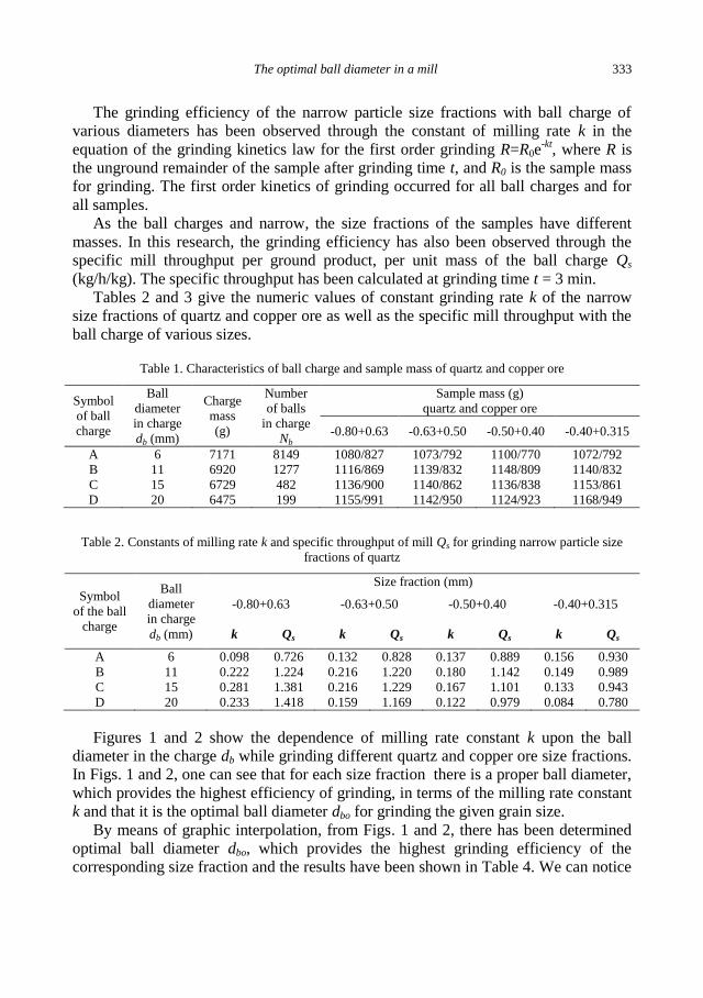
The grinding efficiency of the narrow particle size fractions with ball charge of
various diameters has been observed through the constant of milling rate k in the
equation of the grinding kinetics law for the first order grinding R=R0e-kt
, where R is
the unground remainder of the sample after grinding time t, and R0 is the sample mass
for grinding. The first order kinetics of grinding occurred for all ball charges and for
all samples.
As the ball charges and narrow, the size fractions of the samples have different
masses. In this research, the grinding efficiency has also been observed through the
specific mill throughput per ground product, per unit mass of the ball charge Qs
(kg/h/kg). The specific throughput has been calculated at grinding time t = 3 min.
Tables 2 and 3 give the numeric values of constant grinding rate k of the narrow
size fractions of quartz and copper ore as well as the specific mill throughput with the
ball charge of various sizes.
Table 1. Characteristics of ball charge and sample mass of quartz and copper ore
Symbol
of ball
charge
Ball
diameter
in charge
db (mm)
Charge
mass
(g)
Number
of balls
in charge
Nb
Sample mass (g)
quartz and copper ore
-0.80+0.63 -0.63+0.50 -0.50+0.40 -0.40+0.315
A 6 7171 8149 1080/827 1073/792 1100/770 1072/792
B 11 6920 1277 1116/869 1139/832 1148/809 1140/832
C 15 6729 482 1136/900 1140/862 1136/838 1153/861
D 20 6475 199 1155/991 1142/950 1124/923 1168/949
Table 2. Constants of milling rate k and specific throughput of mill Qs for grinding narrow particle size
fractions of quartz
Symbol
of the ball
charge
Ball
diameter
in charge
db (mm)
Size fraction (mm)
-0.80+0.63 -0.63+0.50 -0.50+0.40 -0.40+0.315
k Qs k Qs k Qs k Qs
A 6 0.098 0.726 0.132 0.828 0.137 0.889 0.156 0.930
B 11 0.222 1.224 0.216 1.220 0.180 1.142 0.149 0.989
C 15 0.281 1.381 0.216 1.229 0.167 1.101 0.133 0.943
D 20 0.233 1.418 0.159 1.169 0.122 0.979 0.084 0.780
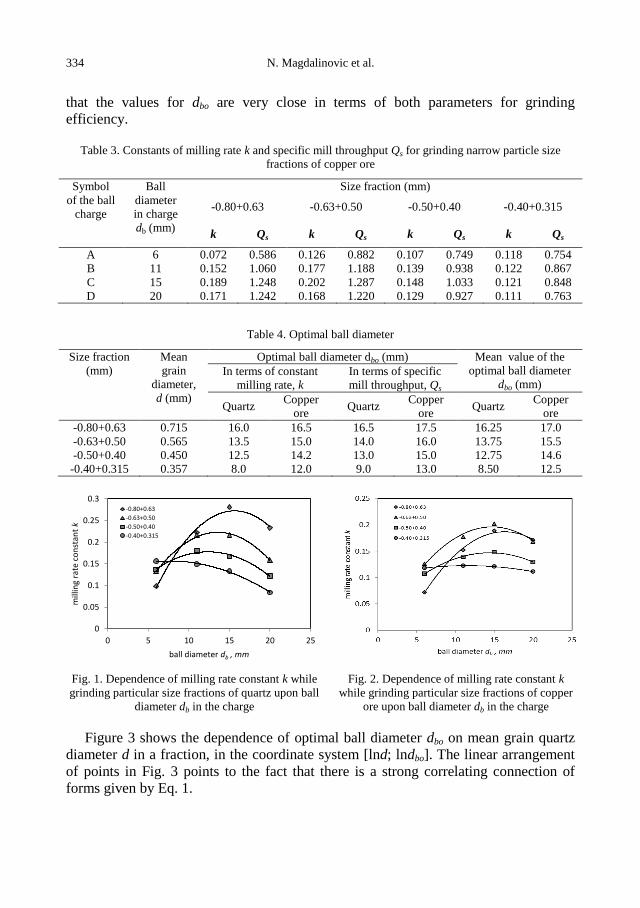
Figures 1 and 2 show the dependence of milling rate constant k upon the ball
diameter in the charge db while grinding different quartz and copper ore size fractions.
In Figs. 1 and 2, one can see that for each size fraction there is a proper ball diameter,
which provides the highest efficiency of grinding, in terms of the milling rate constant
k and that it is the optimal ball diameter dbo for grinding the given grain size.
By means of graphic interpolation, from Figs. 1 and 2, there has been determined
optimal ball diameter dbo, which provides the highest grinding efficiency of the
corresponding size fraction and the results have been shown in Table 4. We can notice
334 N. Magdalinovic et al.
that the values for dbo are very close in terms of both parameters for grinding
efficiency.
Table 3. Constants of milling rate k and specific mill throughput Qs for grinding narrow particle size
fractions of copper ore
Symbol
of the ball
charge
Ball
diameter
in charge
db (mm)
Size fraction (mm)
-0.80+0.63 -0.63+0.50 -0.50+0.40 -0.40+0.315
k Qs k Qs k Qs k Qs
A 6 0.072 0.586 0.126 0.882 0.107 0.749 0.118 0.754
B 11 0.152 1.060 0.177 1.188 0.139 0.938 0.122 0.867
C 15 0.189 1.248 0.202 1.287 0.148 1.033 0.121 0.848
D 20 0.171 1.242 0.168 1.220 0.129 0.927 0.111 0.763
Table 4. Optimal ball diameter
Size fraction
(mm)
Mean
grain
diameter,
d (mm)
Optimal ball diameter dbo (mm) Mean value of the
optimal ball diameter
dbo (mm) In terms of constant
milling rate, k
In terms of specific
mill throughput, Qs
Quartz Copper
ore Quartz
Copper
ore Quartz
Copper
ore
-0.80+0.63 0.715 16.0 16.5 16.5 17.5 16.25 17.0
-0.63+0.50 0.565 13.5 15.0 14.0 16.0 13.75 15.5
-0.50+0.40 0.450 12.5 14.2 13.0 15.0 12.75 14.6
-0.40+0.315 0.357 8.0 12.0 9.0 13.0 8.50 12.5
0
0.05
0.1
0.15
0.2
0.25
0.3
0 5 10 15 20 25
mill
ing
rate
co
nst
ant
k
ball diameter db , mm
-0.80+0.63
-0.63+0.50
-0.50+0.40
-0.40+0.315
Fig. 1. Dependence of milling rate constant k while
grinding particular size fractions of quartz upon ball
diameter db in the charge
Fig. 2. Dependence of milling rate constant k
while grinding particular size fractions of copper
ore upon ball diameter db in the charge
Figure 3 shows the dependence of optimal ball diameter dbo on mean grain quartz
diameter d in a fraction, in the coordinate system [lnd; lndbo]. The linear arrangement
of points in Fig. 3 points to the fact that there is a strong correlating connection of
forms given by Eq. 1.

The optimal ball diameter in a mill 335
By the method of the least squares, it was possible to determine the numerical
values of parameters K and n in Eq. 1, with a very high degree of correlation r, so that
they, for the conditions of our experiment, would be as follows:
quartz: 87.067.22 ddbo , r=0.95, (11)
copper ore: 42.077.19 ddbo , r=0.98. (12)
R² = 0.8864
R² = 0.9532
lnd
bo
ln d
Fig. 3. Dependence of optimal ball diameter dbo on
mean grain diameter d in a fraction
The grinding tests on all samples have been performed under identical conditions.
The only difference is in the characteristics of quartz and copper ore, in terms of
Bond’s working index. In other words, copper ore has got a higher Bond’s working
index and this should have been expressed in Eq. 12 in terms of a higher value for
coefficient K compared to the value in Eq. 11 for quartz. However, this didn’t happen.
The value of K in Eq. 12 is less than the value in Eq. 11. This happened because of the
incorrect hypothesis, which says that the exponent n depends on the characteristics of
a mill, grinding conditions and raw material characteristics. It was incorrect to
emphasize higher influence of Bond’s working index on exponent n instead on
parameter K.
In this paper, in our theoretical analysis, we have come to the concision, that
parameter n has got the constant value: n = 0.67 and that it does not depend on the
characteristics of a mill, the grinding conditions and raw material characteristics.
Thus, consequently, the optimal ball size is defined by Eq. 6.
By means of the least squares, we have determined the numerical values of
parameters K in Eq. 6, so that they, for the conditions of our experiment and with a
very high degree of correlation r, are as follows:
quartz: 67.069.19 ddbo , r=0.94, (13)
copper ore: 67.045.23 ddbo , r=0.97. (14)
Equations 13 and 14 confirm our theoretical hypothesis that exponent n has got the
constant value n = 0.67 and that the influence of the mill characteristics, grinding
conditions and raw material characteristics has been demonstrated only in terms of the
336 N. Magdalinovic et al.
numerical value of parameter K. The higher value of the Bond’s working index for
copper ore has led to the higher value of parameter K in Eq. 14 in relation to the value
of the same one in Eq. 13 for quartz, and that is the theoretically expected issue.
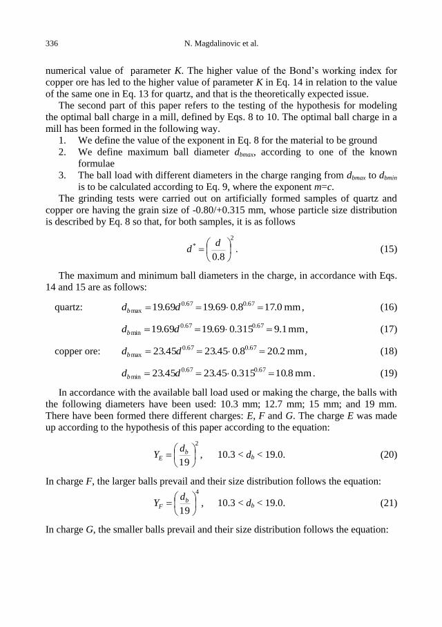
The second part of this paper refers to the testing of the hypothesis for modeling
the optimal ball charge in a mill, defined by Eqs. 8 to 10. The optimal ball charge in a
mill has been formed in the following way.
1. We define the value of the exponent in Eq. 8 for the material to be ground
2. We define maximum ball diameter dbmax, according to one of the known
formulae
3. The ball load with different diameters in the charge ranging from dbmax to dbmin
is to be calculated according to Eq. 9, where the exponent m=c.
The grinding tests were carried out on artificially formed samples of quartz and
copper ore having the grain size of -0.80/+0.315 mm, whose particle size distribution
is described by Eq. 8 so that, for both samples, it is as follows
2
*
8.0
dd . (15)
The maximum and minimum ball diameters in the charge, in accordance with Eqs.
14 and 15 are as follows:
quartz: mm0.178.069.1969.19 67.067.0max ddb , (16)
mm1.9315.069.1969.19 67.067.0min ddb , (17)
copper ore: mm2.208.045.2345.23 67.067.0max ddb , (18)
mm8.10315.045.2345.23 67.067.0min ddb . (19)
In accordance with the available ball load used or making the charge, the balls with
the following diameters have been used: 10.3 mm; 12.7 mm; 15 mm; and 19 mm.
There have been formed there different charges: E, F and G. The charge E was made
up according to the hypothesis of this paper according to the equation:
2
19
b
E
dY , 10.3 < db < 19.0. (20)
In charge F, the larger balls prevail and their size distribution follows the equation: 4
19
b
F
dY , 10.3 < db < 19.0. (21)
In charge G, the smaller balls prevail and their size distribution follows the equation:

The optimal ball diameter in a mill 337
5.1
19
b
G
dY , 10.3 < db < 19.0. (22)
In Table 5 we have given the composition of samples in the charge according to the
size distribution. The ball mill loading is 40% by volume. The quartz sample mass for
grinding is 915 g and for copper ore 787 g.
The grinding efficiency with ball charges E, F and G, has been observed in terms
of the constant milling rate of the first-order k and the specific throughput of mill Qs
per ground product per unit mass of the charge, on the controlling screen with the
mesh size of d = 0.315 mm at the grinding time of t = 3 min. The results of grinding
are shown in Table 6 and they confirm our hypothesis that the highest grinding
efficiency is provided by charge E, where the ball size distribution is identical with the
one with the grain size distribution of the material being ground.
The accomplishment of this principal in industrial mills is possible by loading the
mills with the balls of different diameters, in the proper correlation, where the value of
exponent c in Eq. 9 is brought closer to the value of the exponent m in Eq. 8.
Table 5: Composition of samples and charges according to the size distribution
Particle size
distribution,
d (mm)
Weight
W
(%)
Ball
diameter
db
(mm)
Charge E Charge F Charge G
W
(%)
M
(g)
W
(%)
M
(g)
W
(%)
M
(g)
-0.80+0.63 38 19 38 2732 58 4157 29 2090
-0.63+0.50 23 15 23 1653 21 1480 16 1159
-0.5+0.40 14 12.7 14 1006 12 853 15 1089
-0.40+0.315 25 10.3 25 1797 9 667 40 2898
100 100 7188 100 7147 100 7236
Table 6: Milling rate constant k and specific throughput of mill Qs, with different ball charges
Indicator for
the grinding
efficiency
Charge
E F G
Quartz Copper ore Quartz Copper ore Quartz Copper ore
k 0.119 0.078 0.108 0.072 0.105 0.073
Qs 0.890 1.084 0.821 1.075 0.796 1.071
4. Conclusion
All proposed formulae for determining the ball diameter, depending on the
diameter of the grain size material being ground, fit into the general form given in the
equation:
nb Kdd ,
where db is the ball diameter, d is the diameter of the grain size material being ground,
K and n are parameters, for which all authors say, depend on mill characteristics,
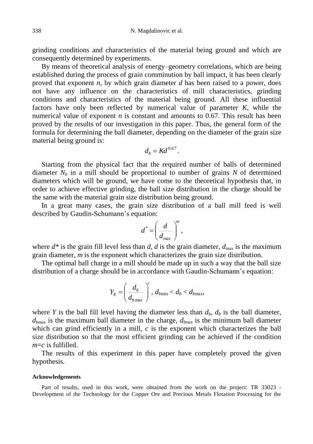
338 N. Magdalinovic et al.
grinding conditions and characteristics of the material being ground and which are
consequently determined by experiments.
By means of theoretical analysis of energy–geometry correlations, which are being
established during the process of grain comminution by ball impact, it has been clearly
proved that exponent n, by which grain diameter d has been raised to a power, does
not have any influence on the characteristics of mill characteristics, grinding
conditions and characteristics of the material being ground. All these influential
factors have only been reflected by numerical value of parameter K, while the
numerical value of exponent n is constant and amounts to 0.67. This result has been
proved by the results of our investigation in this paper. Thus, the general form of the
formula for determining the ball diameter, depending on the diameter of the grain size
material being ground is: 67.0Kddb .
Starting from the physical fact that the required number of balls of determined
diameter Nb in a mill should be proportional to number of grains N of determined
diameters which will be ground, we have come to the theoretical hypothesis that, in
order to achieve effective grinding, the ball size distribution in the charge should be
the same with the material grain size distribution being ground.
In a great many cases, the grain size distribution of a ball mill feed is well
described by Gaudin-Schumann’s equation: m
d
dd
max
* ,
where d* is the grain fill level less than d, d is the grain diameter, dmax is the maximum
grain diameter, m is the exponent which characterizes the grain size distribution.
The optimal ball charge in a mill should be made up in such a way that the ball size
distribution of a charge should be in accordance with Gaudin-Schumann’s equation:
c
b
bE
d
dY
max
, dbmin < db < dbmax,
where Y is the ball fill level having the diameter less than db, db is the ball diameter,
dbmax is the maximum ball diameter in the charge, dbmin is the minimum ball diameter
which can grind efficiently in a mill, c is the exponent which characterizes the ball
size distribution so that the most efficient grinding can be achieved if the condition
m=c is fulfilled.
The results of this experiment in this paper have completely proved the given
hypothesis.
Acknowledgements
Part of results, used in this work, were obtained from the work on the project: TR 33023 -
Development of the Technology for the Copper Ore and Precious Metals Flotation Processing for the
The optimal ball diameter in a mill 339
Sake of Achieving better Technological Results and TR 33007 - Implementation of Advanced
Technological and Ecological Solutions in Existing Product Systems of Copper Mine Bor and Copper
Mine Majdanpek, It was financed by the Ministry of Education and Science of the Republic of Serbia.
References
AUSTIN, L.G., SHOJI, K., LUCKIE, P.T., 1976, The effect of ball size on mill performance, Powder
Technol. 14 (1), 71–79.
BELECKI, E.P., 1985, Vibor razmera šarov dlja šarovih meljnic, Obogašchenie rud, 11, 40-42.
BOND, F.C., 1961, Crushing and Grinding Calculations, Allis Chalmers Tech. Pub. O7R9235B.
CONCHA, F., MAGNE, L., AUSTIN, L.G., 1992, Optimization of the make-up ball charge in a grinding
mill, Int. J. Miner. Process. 34 (3), 231–241.
ERDEM, A.S. ERGUN, S.L., 2009, The effect of ball size on breakage rate parameter in a pilot scale
ball mill, Miner. Eng. 22, 660–664
FUERSTENAU, D.W., LUTCH, J.J., DE, A., 1999, The effect of ball size on the energy efficiency of
hybrid high-pressure roll mill/ball mill grinding, Powder Technol. 105, 199–204.
KATUBILWA, F. M., MOYS, M.H., 2009, Effect of ball size distribution on milling rate, Miner. Eng.
22, 1283–1288
KOTAKE, N., DAIBO, K., YAMAMOTO, T., KANDA, Y., 2004, Experimental investigation on a
grinding rate constant of solid materials by a ball mill—effect of ball diameter and feed size, Powder
Technol. 143– 144, 196– 203
OLEJNIK, T.P., 2010, Kinetics of grinding ceramic bulk considering grinding media contact points,
Physicochem. Probl. Miner. Process. 44, 187–194.
OLEJNIK, T.P., 2011, Milling kinetics of chosen rock materials under dry conditions considering
strength and statistical properties of bed, Physicochem. Probl. Miner. Process. 46, 145–154.
OLEVSKIJ, V.A., 1948, Najvigodesni razmer šarov dlja šarovih meljnici, Gornij žurnal, 1,1–5.
RAZUMOV, K.A., 1947, Racionirovanoe pitanie meljnic šarami, Gornij žurnal 3, 31–35.
ŠUPOV, L.P., 1962, Udarnoe dejstvie šarov v meljnice, Obogašshenie rud, 4, 15–20.
TRUMIC, M., MAGDALINOVIC, N., TRUMIC, G., 2007, The model for optimal charge in the ball
mill, Journal of Mining and Metallurgy A, 43, 19–32.

340 N. Magdalinovic et al.
http://dx.doi.org/10.5277/ppmp120202
Physicochem. Probl. Miner. Process. 48(2), 2012, 341–353 Physicochemical Problems
of Mineral Processing
w w w . m i n p r o c . p w r . w r o c . p l / j o u r n a l / ISSN 1643-1049 (print)
ISSN 2084-4735 (online)
Received November 14, 2011; reviewed; accepted February 17, 2012
INVESTIGATION OF RADIOACTIVE CONTENT OF
MANISA-SOMA AND ISTANBUL-AGACLI COALS (TURKEY)
Ismail DEMIR, Ilgin KURSUN
Istanbul University Engineering Faculty Mining Engineering Department, Istanbul, Turkey,
[email protected], [email protected]
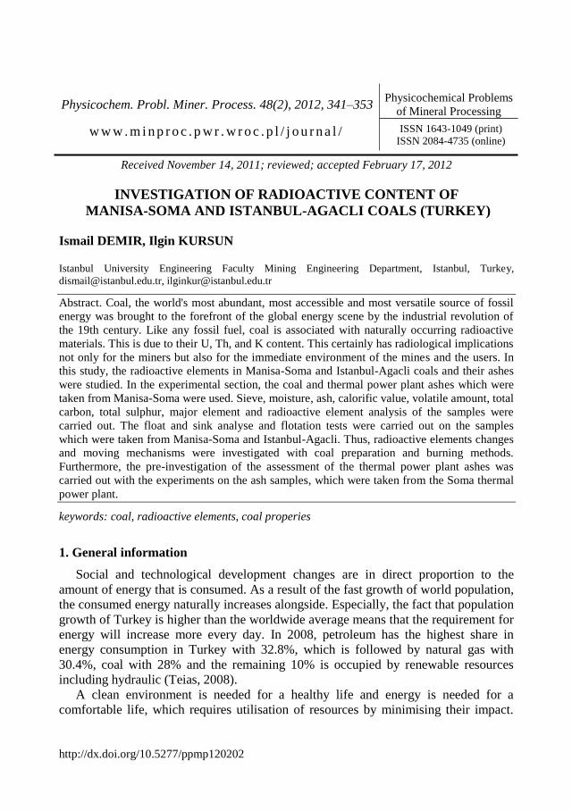
Abstract. Coal, the world's most abundant, most accessible and most versatile source of fossil
energy was brought to the forefront of the global energy scene by the industrial revolution of
the 19th century. Like any fossil fuel, coal is associated with naturally occurring radioactive
materials. This is due to their U, Th, and K content. This certainly has radiological implications
not only for the miners but also for the immediate environment of the mines and the users. In
this study, the radioactive elements in Manisa-Soma and Istanbul-Agacli coals and their ashes
were studied. In the experimental section, the coal and thermal power plant ashes which were
taken from Manisa-Soma were used. Sieve, moisture, ash, calorific value, volatile amount, total
carbon, total sulphur, major element and radioactive element analysis of the samples were
carried out. The float and sink analyse and flotation tests were carried out on the samples
which were taken from Manisa-Soma and Istanbul-Agacli. Thus, radioactive elements changes
and moving mechanisms were investigated with coal preparation and burning methods.
Furthermore, the pre-investigation of the assessment of the thermal power plant ashes was
carried out with the experiments on the ash samples, which were taken from the Soma thermal
power plant.
keywords: coal, radioactive elements, coal properies
1. General information
Social and technological development changes are in direct proportion to the
amount of energy that is consumed. As a result of the fast growth of world population,
the consumed energy naturally increases alongside. Especially, the fact that population
growth of Turkey is higher than the worldwide average means that the requirement for
energy will increase more every day. In 2008, petroleum has the highest share in
energy consumption in Turkey with 32.8%, which is followed by natural gas with
30.4%, coal with 28% and the remaining 10% is occupied by renewable resources
including hydraulic (Teias, 2008).
A clean environment is needed for a healthy life and energy is needed for a
comfortable life, which requires utilisation of resources by minimising their impact.
342 I. Demir, I. Kursun
The fact that even ashes of burned coal is usable is an important point both for
economic benefit and environmental impact, and this may only be possible due to
proper features of coal. When coal is burnt in thermal power stations, toxic trace
elements in the coal like As, Cd, Ga, Ge, Pb, Sb, Se, Sn, Mo, Ti and Zn, which have
the potential of contaminating, are transferred to the waste products (cinder, ash and
gas). Volatile ashes containing many poisonous elements may be collected in ash
collection pools under furnaces or as piles. Because soluble metal ions and compounds
may leak from the ash pools or piles, then have the potential to contaminate soil,
surface and underground water. Then, severe environmental problems may occur
(Karayiğit et al., 2000; Perçinel, 2000; Esenlik, 2005; Tuna et al., 2005).
When coal is combusted, toxic trace elements like arsenic (As), cadmium (Cd),
lead (Pb), antimony (Sb), selenium (Se), stannum (Sn) and zinc (Zn) are transferred to
waste products like cinder, ash and gases. When the waste products are disposed
contained poisonous (toxic) trace elements may be conveyed to the atmosphere, earth
surface and oceans. These elements may be seriously threatening for living organisms
by creating environmental, and health problems when the waste products are washed
with rain and these elements are carried away with underground water to the soil, and
surface and underground waters (Baba, 2001; Ateşok, 2004; Demir, 2009).
Some of the human diseases occurring near thermal power plants, due to the toxic
elements spread in the neighbourhood are given below (Perçinel, 2000):
As: Anaemia, nausea, renal symptoms, ulcer, skin and pulmonary cancer, defective
births.
Be: Malfunction of respiration and lymph, lungs, spleen and kidneys, carcinogenic
effects.
Cd: Lung emphysema and fibrosis, kidney diseases, cardiovascular effects,
carcinogenic effects.
Hg: Nervous and kidney damages, cardiovascular effects, birth problems.
Mn: Respiratory problems.
Ni: Skin and intestinal diseases, carcinogenic effects.
Pb: Anaemia, nervous and cardiovascular problems, delayed growth, gastric and
intestinal problems, carcinogenic effects, birth problems.
Se: Gastric and intestinal nausea, pulmonary and splenic damages, anaemia,
cancer, teratogenic effects.
V: Acute and chronic respiratory malfunction (Perçinel, 2000).
Radon gas forms in the area in which ashes of the thermal power plant collect (ash
chambers) reach the air. Even if these ashes are buried in soil, radon gas infiltrates
through the pores of the soil and blends in the air. Radon gas may transform into
polonium and active lead in 3.8 days. Therefore, piles of ash emit radioactivity.
Perhaps the most critical material that is disposed through the chimneys is uranium,
that is contained in lignite and released during combustion to spread around. Uranium
is also a serious problem (Özyurt, 2006).
Investigation of radioactive content of Manisa-Soma and Istanbul-Agacli coals (Turkey) 343
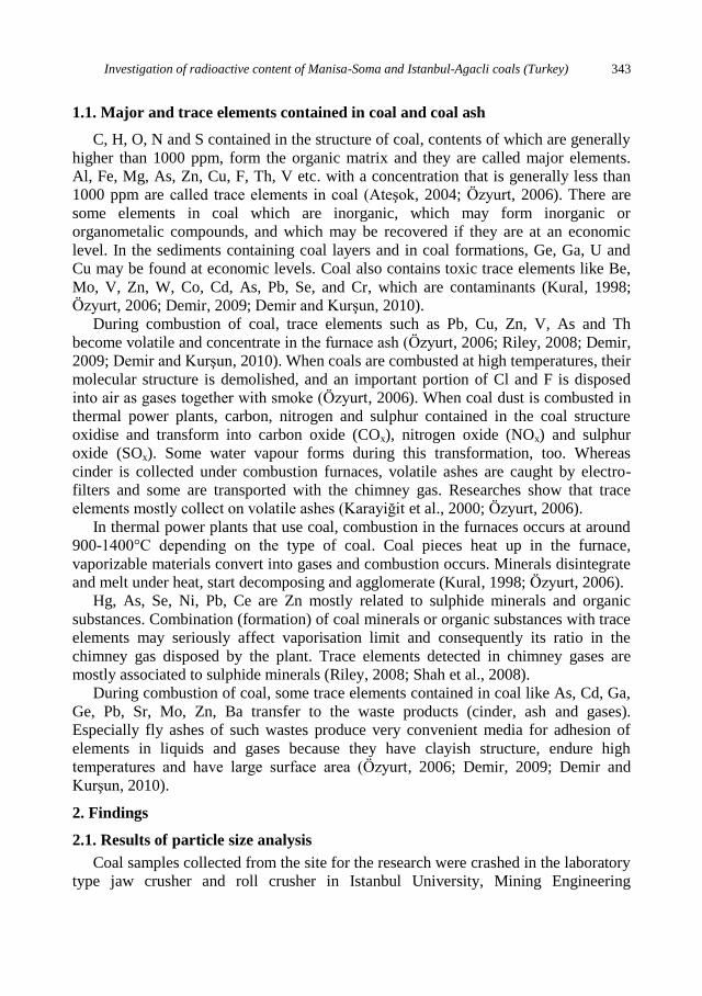
1.1. Major and trace elements contained in coal and coal ash
C, H, O, N and S contained in the structure of coal, contents of which are generally
higher than 1000 ppm, form the organic matrix and they are called major elements.
Al, Fe, Mg, As, Zn, Cu, F, Th, V etc. with a concentration that is generally less than
1000 ppm are called trace elements in coal (Ateşok, 2004; Özyurt, 2006). There are
some elements in coal which are inorganic, which may form inorganic or
organometalic compounds, and which may be recovered if they are at an economic
level. In the sediments containing coal layers and in coal formations, Ge, Ga, U and
Cu may be found at economic levels. Coal also contains toxic trace elements like Be,
Mo, V, Zn, W, Co, Cd, As, Pb, Se, and Cr, which are contaminants (Kural, 1998;
Özyurt, 2006; Demir, 2009; Demir and Kurşun, 2010).
During combustion of coal, trace elements such as Pb, Cu, Zn, V, As and Th
become volatile and concentrate in the furnace ash (Özyurt, 2006; Riley, 2008; Demir,
2009; Demir and Kurşun, 2010). When coals are combusted at high temperatures, their
molecular structure is demolished, and an important portion of Cl and F is disposed
into air as gases together with smoke (Özyurt, 2006). When coal dust is combusted in
thermal power plants, carbon, nitrogen and sulphur contained in the coal structure
oxidise and transform into carbon oxide (COx), nitrogen oxide (NOx) and sulphur
oxide (SOx). Some water vapour forms during this transformation, too. Whereas
cinder is collected under combustion furnaces, volatile ashes are caught by electro-
filters and some are transported with the chimney gas. Researches show that trace
elements mostly collect on volatile ashes (Karayiğit et al., 2000; Özyurt, 2006).
In thermal power plants that use coal, combustion in the furnaces occurs at around
900-1400°C depending on the type of coal. Coal pieces heat up in the furnace,
vaporizable materials convert into gases and combustion occurs. Minerals disintegrate
and melt under heat, start decomposing and agglomerate (Kural, 1998; Özyurt, 2006).
Hg, As, Se, Ni, Pb, Ce are Zn mostly related to sulphide minerals and organic
substances. Combination (formation) of coal minerals or organic substances with trace
elements may seriously affect vaporisation limit and consequently its ratio in the
chimney gas disposed by the plant. Trace elements detected in chimney gases are
mostly associated to sulphide minerals (Riley, 2008; Shah et al., 2008).
During combustion of coal, some trace elements contained in coal like As, Cd, Ga,
Ge, Pb, Sr, Mo, Zn, Ba transfer to the waste products (cinder, ash and gases).
Especially fly ashes of such wastes produce very convenient media for adhesion of
elements in liquids and gases because they have clayish structure, endure high
temperatures and have large surface area (Özyurt, 2006; Demir, 2009; Demir and
Kurşun, 2010).
2. Findings
2.1. Results of particle size analysis
Coal samples collected from the site for the research were crashed in the laboratory
type jaw crusher and roll crusher in Istanbul University, Mining Engineering

344 I. Demir, I. Kursun
Department, Mineral Processing Laboratory, and then applied dry particle size
analysis to study particle size distribution.
Particle size curves were drawn according to the particle size analysis performed
using 8 mm, 4 mm, 2 mm, 1 mm and 0.5 mm laboratory type Retsch brand stainless
steel sieves of square section and d80 particle dimensions were calculated.
Figure 1 shows particle size curves drawn according to the results of particle size
analysis made after crashing of coal samples collected from Manisa-Soma and
İstanbul-Agacli region in roll crusher. As the curves show, d80 of roll crusher outputs
of Manisa – Soma and Istanbul-Agacli coals are 5.4 mm and 5.9 mm, respectively.
Figure 2 shows particle size curve of the coal samples collected from Manisa-
Soma and Istanbul-Agacli Region, which were used in float and sink experiments,
according to the results of particle size analysis. The curves show that d80 of Manisa-
Soma and Istanbul-Agacli coals are 1900 µm and 2100 µm, respectively.
Fig. 1. Manisa-Soma and Istanbul-Agacli
particle size distribution after roll crushing Fig. 2. Particle size curves of “float and sink
experiments” samples of Manisa-Soma
and Istanbul-Agacli coals
2.2. Results of Proximate and Ultimate Chemical Analysis
Ash samples and coal samples collected for the study were brought to the Mineral
Processing Laboratory of Istanbul University, and humidity, ash, density, volatile
matter, total sulphur and thermal value analyses were made on these samples.
Evaluation and interpretation of the chemical analysis results of the coal and ash
samples are summarised below.
Humidity. Coal samples collected from the TKI (Turkish Coal Enterprises) Ege
Lignite Enterprises (Manisa-Soma) for the study were brought to the Mineral
Processing Laboratory of Istanbul University, and total humidity analysis was made
on these samples. Analysis was made according to standard TS 690 ISO 598 (Method-
C). Total humidity analysis was made after bringing samples to the laboratory in
closed nylon bags without losing time. Due to the high temperature at electro-filters,
humidity values of ash samples are mostly almost zero.

Investigation of radioactive content of Manisa-Soma and Istanbul-Agacli coals (Turkey) 345
Figure 3 shows the percentage curves of the humidity that is lost in time when coal
samples collected from Manisa-Soma and Istanbul-Agacli region are heated in drying
oven at 105ºC. It was calculated that coal samples collected from Manisa-Soma and
Istanbul-Agacli contain 15.49% and 31.75% humidity, respectively. The analyses
show that almost entire humidity contained in the samples may be removed in 3 hours
for Manisa-Soma coal samples and 5 hours for Istanbul-Agacli coal samples.
Fig. 3: Graphic of humidity loss (%) as a function of time (hours)
for Manisa-Soma and Istanbul-Agacli coals
Volatile Matter. It was observed that volatile matter content of ash samples is lower
than coals’. Whereas, Manisa-Soma coal sample contains 31.32% volatile matter, its
thermal power plant ashes contain 1.2% because of the unburned coal pieces. Agacli
sample contains 57.27% volatile matter.
Ash. Ash analyses of the coal samples within the study were realised in Istanbul
University, Department of Mine Engineering, Mineral Processing Laboratory.
According to the results of this analysis, coals collected from Manisa – Soma region
are coals with high ash ratio.
Theoretically, ash content of waste products formed as the result of combustion in
thermal power plants (volatile ash and bottom ash) must be 100%. However,
depending on characteristics of combusted coal and conditions of combustion systems,
it is always possible to find some unburned coal remnants in these wastes. As a matter
of fact, Manisa – Soma thermal power plant ash contains 1.2% unburned pieces.
Total Sulphur. Dry base total sulphur contents of thermal Power Plant ash and coal
samples collected for the study in air were analysed by Acme Analytical Laboratories
Ltd. in Canada. Leco carbon sulphur device was used in total sulphur analysis (Acme,
2009).
When coals used in Manisa-Soma thermal power plant and ashes formed by
combustion are examined for total sulphur contents, it is observed that a little portion
is disposed into the air by burning and the rest is concentrated in ash.
346 I. Demir, I. Kursun
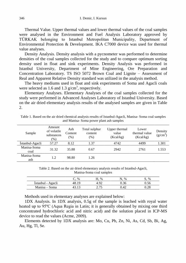
Thermal Value. Upper thermal values and lower thermal values of the coal samples
were analysed in the Environment and Fuel Analysis Laboratory approved by
TÜRKAK belonging to Istanbul Metropolitan Municipality, Department of
Environmental Protection & Development. IKA C7000 device was used for thermal
value analyses.
Density Analysis. Density analysis with a pycnometer was performed to determine
densities of the coal samples collected for the study and to compare optimum sorting
density used in float and sink experiments. Density Analysis was performed in
Istanbul University, Department of Mine Engineering, Ore Preparation and
Concentration Laboratory. TS ISO 5072 Brown Coal and Lignite – Assessment of
Real and Apparent Relative Density standard was utilized in the analysis method.
The heavy mediums used in float and sink experiments of Soma and Agacli coals
were selected as 1.6 and 1.3 g/cm3, respectively.
Elementary Analyses. Elementary Analyses of the coal samples collected for the
study were performed in Advanced Analyses Laboratory of Istanbul University. Based
on the air dried elementary analysis results of the analysed samples are given in Table
2.
Table 1. Based on the air dried chemical analysis results of Istanbul-Agacli, Manisa- Soma coal samples
and Manisa- Soma power plant ash samples
Sample
Amount
of volatile
substances
(%)
Ash
Content
(%)
Total sulphur
content
(%)
Upper thermal
value
(Kcal/kg)
Lower
thermal value
(Kcal/kg)
Density
(g/cm3)
İstanbul-Agacli 57.27 8.12 1.37 4742 4499 1.301
Manisa-Soma
coal 31.32 35.88 0.67 2942 2761 1.553
Manisa-Soma
ash 1.2 98.80 1.26
Table 2. Based on the air dried elementary analysis results of Istanbul-Agacli,
Manisa-Soma coal samples
C, % H, % N, % S, %
İstanbul - Agacli 48.19 4.92 0.36 0.56
Manisa – Soma 43.13 2.75 0.42 0.28
Methods used in elementary analyses are explained below:
1DX Analysis. In 1DX analysis, 0.5g of the sample is leached with royal water
heated up to 95ºC (Aqua Regia in Latin; it is generally obtained by mixing one third
concentrated hydrochloric acid and nitric acid) and the solution placed in ICP-MS
device to read the values (Acme, 2009).
Elements detected by 1DX analysis are: Mo, Cu, Pb, Zn, Ni, As, Cd, Sb, Bi, Ag,
Au, Hg, Tl, Se.
Investigation of radioactive content of Manisa-Soma and Istanbul-Agacli coals (Turkey) 347
Leco TOT/C and TOT/S analysis. Total C and Total S analyses are performed with
Leco carbon sulphur device (Acme, 2009).
4A Analysis. In 4A analysis, 0.2g coal and ash samples are applied lithium
metaborate/tetraborate fusion and decomposed with diluted nitric acid, and then major
oxides they contained were detected with the ICP-ES device (Acme, 2009).
Minerals that are analysed with 4A are: SiO2, Al2O3, Fe2O3, MgO, CaO, Na2O,
K2O, TiO2, P2O5, MnO, Cr2O3.
4B Analysis. In 4B analysis, 0.2g coal and ash samples are applied lithium
metaborate/tetraborate fusion and decomposed with diluted nitric acid, and then rare
soil elements and refractor elements they contained were detected with the ICP-MS
device. In addition, 0.5g samples were decomposed in royal water, and precious
metals and base metals were detected with ICP-MS (Acme, 2009).
Elements that are analysed with 4B are (nitric acid and ICP-MS): Ba, Be Co, Cs,
Ga, Hf, Nb, Rb, Sc, Sn, Sr, Ta, Th, U, V, W, Y, Zr, La, Ce, Pr, Nd, Sm, Eu, Gd, Tb,
Dy, Ho, Er, Tm, Yb, Lu.
Elements that are analysed with 4B are (Royal Water and ICP-MS): Au, Ag, As,
Bi, Cd, Cu, Hg, Mo, Ni, Pb, Sb, Se, Tl, Zn.
Combustible efficiency analysis. It is used in interpretation of combustible
efficiency washing performance. Combustible efficiency has been calculated with the
formulae as below (Ateşok, 2004):
100100
100EfficiencyeCombustibl
ctf
ftc
, (1)
where, t represents waste schist ash %, f raw coal ash %, c clean coal ash %.
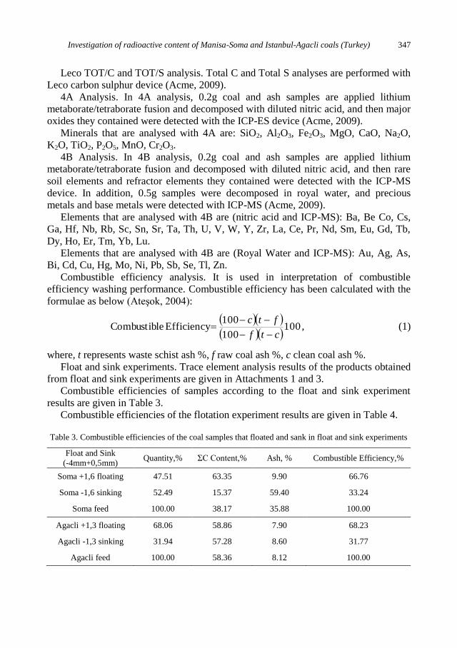
Float and sink experiments. Trace element analysis results of the products obtained
from float and sink experiments are given in Attachments 1 and 3.
Combustible efficiencies of samples according to the float and sink experiment
results are given in Table 3.
Combustible efficiencies of the flotation experiment results are given in Table 4.
Table 3. Combustible efficiencies of the coal samples that floated and sank in float and sink experiments
Float and Sink
(-4mm+0,5mm) Quantity,% ΣC Content,% Ash, % Combustible Efficiency,%
Soma +1,6 floating 47.51 63.35 9.90 66.76
Soma -1,6 sinking 52.49 15.37 59.40 33.24
Soma feed 100.00 38.17 35.88 100.00
Agacli +1,3 floating 68.06 58.86 7.90 68.23
Agacli -1,3 sinking 31.94 57.28 8.60 31.77
Agacli feed 100.00 58.36 8.12 100.00
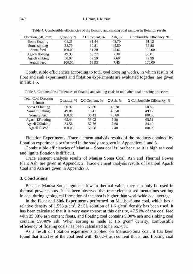
348 I. Demir, I. Kursun
Table 4. Combustible efficiencies of the floating and sinking coal samples in flotation results
Flotation, (-0,5mm) Quantity, % ΣC Content, % Ash, % Combustible Efficiency, %
Soma floating 61.21 31.44 45.70 61.12
Soma sinking 38.79 30.81 45.50 38.88
Soma feed 100.00 31.20 45.62 100.00
Agacli floating 49.93 60.27 7.30 50.01
Agacli sinking 50.07 59.59 7.60 49.99
Agacli feed 100.00 59.93 7.45 100.00
Combustible efficiencies according to total coal dressing works, in which results of
float and sink experiments and flotation experiments are evaluated together, are given
in Table 5.
Table 5. Combustible efficiencies of floating and sinking coals in total after coal dressing processes
Total Coal Dressing
(-4mm) Quantity, % ΣC Content, % Σ Ash, % Σ Combustible Efficiency, %
Soma ΣFloating 50.92 53.80 45.70 50.83
Soma ΣSinking 49.08 18.41 45.50 49.17
Soma ΣFeed 100.00 36.43 45.60 100.00
Agacli ΣFloating 65.44 59.02 7.30 65.51
Agacli ΣSinking 34.56 57.76 7.60 34.49
Agacli ΣFeed 100.00 58.58 7.40 100.00
Flotation Experiments. Trace element analysis results of the products obtained by
flotation experiments performed in the study are given in Appendices 1 and 3.
Combustible efficiencies of Manisa – Soma coal is low because it is high ash coal
and lignite flotation is difficult.
Trace element analysis results of Manisa Soma Coal, Ash and Thermal Power
Plant Ash, are given in Appendix 2. Trace element analysis results of İstanbul Agacli
Coal and Ash are given in Appendix 3.
3. Conclusions
Because Manisa-Soma lignite is low in thermal value, they can only be used in
thermal power plants. It has been observed that trace element sedimentations settling
in coal during geological formation of the area is higher than worldwide coal average.
In the Float and Sink Experiments performed on Manisa-Soma coal, which has a
relative density of 1.553 g/cm3, ZnCl2 solution of 1.6 g/cm
3 density has been used. It
has been calculated that it is very easy to sort at this density, 47.51% of the coal feed
with 35.88% ash content floats, and floating coal contains 9.90% ash and sinking coal
contains 59.40% ash. When sorting is made at 1.6 g/cm3 density, combustible
efficiency of floating coals has been calculated to be 66.76%.
As a result of flotation experiments applied on Manisa-Soma coal, it has been
found that 61.21% of the coal feed with 45.62% ash content floats, and floating coal
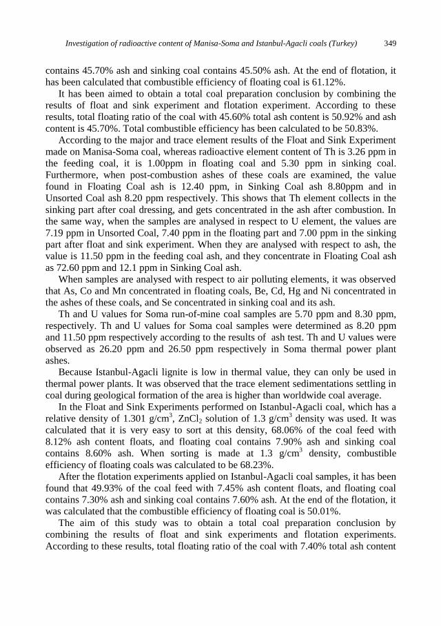
Investigation of radioactive content of Manisa-Soma and Istanbul-Agacli coals (Turkey) 349
contains 45.70% ash and sinking coal contains 45.50% ash. At the end of flotation, it
has been calculated that combustible efficiency of floating coal is 61.12%.
It has been aimed to obtain a total coal preparation conclusion by combining the
results of float and sink experiment and flotation experiment. According to these
results, total floating ratio of the coal with 45.60% total ash content is 50.92% and ash
content is 45.70%. Total combustible efficiency has been calculated to be 50.83%.
According to the major and trace element results of the Float and Sink Experiment
made on Manisa-Soma coal, whereas radioactive element content of Th is 3.26 ppm in
the feeding coal, it is 1.00ppm in floating coal and 5.30 ppm in sinking coal.
Furthermore, when post-combustion ashes of these coals are examined, the value
found in Floating Coal ash is 12.40 ppm, in Sinking Coal ash 8.80ppm and in
Unsorted Coal ash 8.20 ppm respectively. This shows that Th element collects in the
sinking part after coal dressing, and gets concentrated in the ash after combustion. In
the same way, when the samples are analysed in respect to U element, the values are
7.19 ppm in Unsorted Coal, 7.40 ppm in the floating part and 7.00 ppm in the sinking
part after float and sink experiment. When they are analysed with respect to ash, the
value is 11.50 ppm in the feeding coal ash, and they concentrate in Floating Coal ash
as 72.60 ppm and 12.1 ppm in Sinking Coal ash.
When samples are analysed with respect to air polluting elements, it was observed
that As, Co and Mn concentrated in floating coals, Be, Cd, Hg and Ni concentrated in
the ashes of these coals, and Se concentrated in sinking coal and its ash.
Th and U values for Soma run-of-mine coal samples are 5.70 ppm and 8.30 ppm,
respectively. Th and U values for Soma coal samples were determined as 8.20 ppm
and 11.50 ppm respectively according to the results of ash test. Th and U values were
observed as 26.20 ppm and 26.50 ppm respectively in Soma thermal power plant
ashes.
Because Istanbul-Agacli lignite is low in thermal value, they can only be used in
thermal power plants. It was observed that the trace element sedimentations settling in
coal during geological formation of the area is higher than worldwide coal average.
In the Float and Sink Experiments performed on Istanbul-Agacli coal, which has a
relative density of 1.301 g/cm3, ZnCl2 solution of 1.3 g/cm
3 density was used. It was
calculated that it is very easy to sort at this density, 68.06% of the coal feed with
8.12% ash content floats, and floating coal contains 7.90% ash and sinking coal
contains 8.60% ash. When sorting is made at 1.3 g/cm3 density, combustible
efficiency of floating coals was calculated to be 68.23%.
After the flotation experiments applied on Istanbul-Agacli coal samples, it has been
found that 49.93% of the coal feed with 7.45% ash content floats, and floating coal
contains 7.30% ash and sinking coal contains 7.60% ash. At the end of the flotation, it
was calculated that the combustible efficiency of floating coal is 50.01%.
The aim of this study was to obtain a total coal preparation conclusion by
combining the results of float and sink experiments and flotation experiments.
According to these results, total floating ratio of the coal with 7.40% total ash content
350 I. Demir, I. Kursun
is 64.44% and ash content is 7.30%. Total combustible efficiency was calculated as
65.51%.
According to the major and trace element results of the Float and Sink Experiment
made on Istanbul-Agacli coal, whereas the radioactive element content of Th is 3.05
ppm in the feeding coal, it is 2.60 ppm in floating coal and 4.00ppm in sinking coal.
Furthermore, when post-combustion ashes of these coals are examined, the value
found in Floating Coal ash is 32.30 ppm, in Sinking Coal ash 36.00 ppm and in
Unsorted Coal ash 43.40 ppm. This shows that Th element collects in the sinking part
after coal dressing, and gets concentrated in the ash after combustion. In the same
way, when the samples are analysed in respect to U element, the values are1.16 ppm
in Unsorted Coal, 0.90 ppm in the floating part and 1.70 ppm in the sinking part after
float and sink experiment. When they are analysed with respect to ash, the value is
11.60 ppm in the feeding coal ash, and they concentrate in Floating Coal ash as 13.70
ppm and 13.4 ppm in Sinking Coal ash.
When samples were analysed with respect to air polluting elements, it was
observed that As, Co and Mn were concentrated in floating coals, Be, Cd, Hg and Ni
were concentrated in the ashes of these coals, and Se was concentrated in sinking coal
and its ash.
Acknowledgement
A part of this work was supported by Scientific Research Projects Coordination Unit of Istanbul
University under the project number T-2324.
References
ACME, 2009, Acme Labs Schedule of Services & Fees.
ATEŞOK, G., 2004, Coal preparation and technology, Publications of the Foundation for Development
of Mining, ISBN-975-7946-22-2, İstanbul, Turkey.
BABA, A., 2001, Effect of Yatağan (Muğla) thermal power plant waste product storage area on
underground water, Dokuz Eylül University Journal of Geology Engineering 25 (2), İzmir, Turkey.
DEMIR, İ., 2009, Investigation of evaluation possibilities of Turkish Coals in terms of their trace element
contents by use of coal preparation methods. Istanbul University, Institute of Science, Mining
Engineering Department, Master’s Thesis, İstanbul, Turkey.
DEMIR, İ., KURŞUN, İ., 2010, An investigation of trace element content of the Zonguldak-Kozlu coal
washery plant’s feed coal, Proceedings of the 17th Coal Congress of Turkey, June 02-04, 2010
Zonguldak, Turkey, 415–429.
ESENLIK, S., 2005, Mineralogy, petrography and element contents of coal combusted in Orhaneli
thermal power plant and waste Products, Bursa, Turkey. Hacettepe University, Institute of Sciences,
Geological Engineering Department, Master’s Thesis, Ankara, Turkey.
KARAYIĞIT, A.I., GAYER, R.A., QUEROL, X., ONACAK, T., 2000, Contents of major and trace
elements in feed coals from Turkish coal-fired power plants, Int. J. Coal Geol., 44, 169‒184.
KURAL, O., (Ed.) 1998, Properties, technology and environmental impacts of coal. ITU Faculty of
Mining, İstanbul, Turkey.
ÖZYURT, Z., 2006, Environmental effect of the trace elements in thermal power plants’ waste products,
Eskişehir Osmangazi University, Mining Engineering Department, Master’s Thesis, Eskişehir,
Turkey.
Investigation of radioactive content of Manisa-Soma and Istanbul-Agacli coals (Turkey) 351
PERÇINEL, S., 2000, Effect of coal use in thermal power plants on human health, Proceedings of the 12th
Turkish Coal Congress, 23-26 May 2000, Zonguldak, Turkey.
RILEY, K., 2008, Analysing for trace elements, http://www.ccsd.biz/products/traceelementdb.cfm.
SHAH, P., STREZOV, V., PRINCE, K., NELSON, P. F., 2008, Speciation of As. Cr. Se and Hg under
coal fired power station conditions, Elsevier Fuel 87, 1859‒1869.
SWAINE, D.J., 1990, Trace elements in coal, Butterwarh, London.
TEIAS, 2008, Web page of Turkish Electricity Transmission Co. (Türkiye Elektrik İletim A.Ş.)
http://www.teias.gov.tr/ (visiting date: 12.09.2008).
TSE, 1992, TS 10091/April 1992, Mineral coal foamy flotation experiment, section 1, laboratory process,
Turkish Standards Institute, Ankara, Turkey.
TSE, 1999, TS ISO 5072/April 1999, Brown coal and lignite – assessment of real and apparent relative
density, Turkish Standards Institute, Ankara, Turkey.
TSE, 2002a, TS 690 ISO 589/March 2002, Assessment of total humidity in mineral coal, Turkish
Standards Institute, Ankara, Turkey.
TSE. 2002b, TS 711 ISO 562/March 2002, Assessment of volatile substances in mineral coal and coke,
Turkish Standards Institute, Ankara, Turkey.
TSE. 2003, TS 3037 ISO 7936/March 2003, Definition and display of mineral coal float and sink
experiment requirements, general definitions for device and processes, Turkish Standards Institute,
Ankara, Turkey.
TSE, 2006, TS ISO 1171+Tech Cor 1/November 2006, Solid mineral fuels – quantity of ash, Turkish
Standards Institute, Ankara, Turkey.
TUNA, A. L., YAĞMUR, B., HAKERLERLER, H., KILINÇ. R., YOKAŞ, İ., BÜRÜN, B., 2005,
Research on pollution caused by the thermal power plants in Muğla region, Muğla University,
Scientific Research Projects Final Report, Muğla, Turkey.
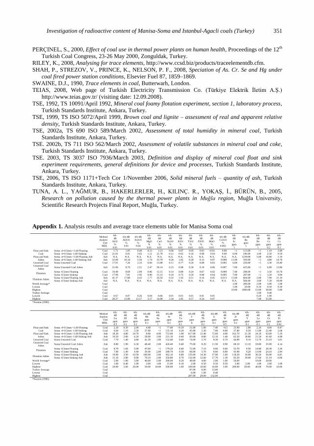
Appendix 1. Analysis results and average trace elements table for Manisa Soma coal
Method
Analyte
Unit
MDL
4A-
4B
SiO2
%
0.01
4A-4B
AI2O3
%
0.01
4A-4B
Fe2O3
%
0.04
4A-
4B
MgO
%
0.01
4A-
4B
CaO
%
0.01
4A-
4B
Na2O
%
0.01
4A-
4B
K2O
%
0.01
4A-
4B
TiO2
%
0.01
4A-
4B
P2O5
%
0.01
4A-
4B
MnO
%
0.01
4A-4B
Cr2O3
%
0.002
4A-
4B
Sc
ppm
1
4A-4B
Ba
ppm
1
4A-
4B
Be
ppm
1
4A-
4B
Co
ppm
0.2
4A-
4B
Cs
ppm
0.1
Float and Sink
Coal
Soma -4+0.5mm +1.60 Floating Coal 1.71 1.05 0.49 0.23 3.23 0.06 0.07 0.05 0.03 <0.01 0.00 <1 113.00 <1 1.10 2.80
Soma -4+0.5mm -1.60 Sinking Coal 21.81 6.01 3.02 1.11 21.78 0.11 0.65 0.16 0.08 0.04 0.00 6.00 196.00 1.00 2.50 9.50
Float and Sink
Ashes
Soma -4+0.5mm +1.60 Floating Ash Ash N.A. N.A. N.A. N.A. N.A. N.A. N.A. N.A. N.A. N.A. N.A. N.A. 1239.00 5.00 16.80 5.10
Soma -4+0.5mm -1.60 Sinking Ash Ash 32.00 10.34 5.56 1.74 33.79 0.26 1.02 0.28 0.13 0.07 0.008 11.00 350.00 <1 4.80 14.70
Unsorted Coal Soma Unsorted Coal Coal 17.91 7.26 2.33 0.84 13.08 0.11 0.77 0.20 0.08 0.03 0.005 6.00 250.00 <1 3.30 10.40
Unsorted Coal
Ashes Soma Unsorted Coal Ashes Ash 21.06 8.70 2.51 2.47 58.14 0.23 0.98 0.30 0.19 0.06 0.007 7.00 425.00 <1 6.80 13.80
Flotation Soma -0.5mm Floating Coal 19.49 8.69 2.09 0.86 13.15 0.14 0.89 0.24 0.07 0.02 0.009 7.00 298.00 <1 3.50 10.70
Soma -0.5mm Sinking Coal 17.99 7.01 2.95 0.90 15.33 0.18 0.73 0.20 0.08 0.04 0.005 7.00 287.00 <1 3.20 9.00
Flotation Ashes Soma -0.5mm Floating Ash Ash 41.37 17.88 4.43 1.77 26.50 0.32 1.93 0.51 0.16 0.05 0.013 15.00 604.00 2.00 7.90 21.10
Soma -0.5mm Sinking Ash Ash N.A. N.A. N.A. N.A. N.A. N.A. N.A. N.A. N.A. N.A. N.A. N.A. 584.00 3.00 7.20 18.90
World Average* Coal 1.00 200.00 2.00 5.00 1.00
Lowest Coal 1.00 20.00 0.10 0.50 0.30
Highest Coal 10.00 1000.00 15.00 30.00 5.00
Turkey Average Coal 1.00 9.40
Lowest Coal 0.67 0.07 0.26 0.04 0.06 0.01 0.01 0.01 0.01 0.01 0.20 1.00
Highest Coal 28.27 12.00 12.57 3.17 14.08 2.34 1.85 0.57 0.24 0.07 7.00 55.00
*Swaine (1990)
Method
Analyte
Unit
MDL
4A-
4B
Ga
ppm
0.5
4A-
4B
Hf
ppm
0.1
4A-
4B
Nb
ppm
0.1
4A-4B
Rb
ppm
0.1
4A-
4B
Sn
ppm
1
4A-4B
Sr
ppm
0.5
4A-
4B
Ta
ppm
0.1
4A-4B
V
ppm
8
4A-
4B
Th
ppm
0.2
4A-4B
U
ppm
0.1
4A-
4B
W
ppm
0.5
4A-4B
Zr
ppm
0.1
4A-
4B
Y
ppm
0.1
4A-
4B
La
ppm
0.1
4A-
4B
Ce
ppm
0.1
4A-
4B
Pr
ppm
0.02
Float and Sink
Coal
Soma -4+0.5mm +1.60 Floating Coal 2.10 0.30 2.00 4.40 <1 77.40 <0.10 51.00 1.00 7.40 <0.5 13.90 1.80 2.10 4.00 0.47
Soma -4+0.5mm -1.60 Sinking Coal 6.60 1.10 3.30 37.90 <1 135.10 0.20 45.00 5.30 7.00 0.80 37.80 9.50 11.80 22.40 2.68
Float and Sink
Ashes
Soma -4+0.5mm +1.60 Floating Ash Ash 18.30 4.80 24.70 8.90 4.00 753.00 1.00 617.00 12.40 72.60 4.90 163.70 21.30 24.10 43.00 5.19
Soma -4+0.5mm -1.60 Sinking Ash Ash 10.50 2.00 6.20 58.90 3.00 231.10 0.40 83.00 8.80 12.10 1.40 65.50 18.80 21.50 41.60 4.98
Unsorted Coal Soma Unsorted Coal Coal 7.70 1.40 4.80 41.20 1.00 152.40 0.40 74.00 5.70 8.30 0.70 44.90 9.10 13.70 25.10 3.01
Unsorted Coal
Ashes Soma Unsorted Coal Ashes Ash 8.80 1.90 6.30 48.40 2.00 426.40 0.40 75.00 8.20 11.50 0.90 68.10 13.10 18.80 35.00 4.14
Flotation Soma -0.5mm Floating Coal 8.70 1.60 5.00 47.60 <1 179.20 0.40 72.00 7.10 9.00 0.60 53.70 9.50 14.80 28.30 3.36
Soma -0.5mm Sinking Coal 7.90 1.40 4.40 39.40 2.00 180.70 0.30 66.00 5.70 8.60 0.80 43.90 9.20 13.00 24.10 2.94
Flotation Ashes Soma -0.5mm Floating Ash Ash 19.00 3.50 10.50 100.90 3.00 362.10 0.80 155.00 14.30 17.90 1.60 118.20 19.90 30.20 56.90 6.81
Soma -0.5mm Sinking Ash Ash 15.10 2.80 8.90 79.10 2.00 350.80 0.70 132.00 12.60 17.70 1.30 93.20 19.00 27.60 51.10 6.06
World Average* Coal 5.00 1.00 5.00 40.00 2.00 200.00 0.20 40.00 4.00 2.00 1.00 50.00 10.00 20.00
Lowest Coal 1.00 0.40 1.00 2.00 1.00 15.00 0.10 2.00 0.50 0.50 0.50 5.00 2.00 1.00 2.00 1.00
Highest Coal 20.00 5.00 20.00 50.00 10.00 500.00 1.00 100.00 10.00 10.00 5.00 200.00 50.00 40.00 70.00 10.00
Turkey Average Coal 87.00 6.00 13.00
Lowest Coal 6.00 1.00 0.40
Highest Coal 287.00 29.00 132.00
*Swaine (1990)
352 I. Demir, I. Kursun
Method
Analyte
Unit
MDL
4A-
4B
Nd
ppm
0.3
4A-
4B
Sm
ppm
0.05
4A-
4B
Eu
ppm
0.02
4A-
4B
Gd
ppm
0.05
4A-
4B
Tb
ppm
0.01
4A-
4B
Dy
ppm
0.05
4A-
4B
Ho
ppm
0.02
4A-
4B
Er
ppm
0.03
4A-
4B
Tm
ppm
0.01
4A-
4B
Yb
ppm
0.05
4A-
4B
Lu
ppm
0.01
2A
Leco
TOT/C
%
0.02
2ALeco
TOT/S
%
0.02
4A-4B
LOI
%
-5.1
4A-
4B
Sum
%
0.01
Float and Sink
Coal
Soma -4+0.5mm +1.60 Floating Coal 1.80 0.32 0.07 0.31 0.06 0.27 0.07 0.18 0.03 0.21 0.03 63.35 0.70 90.10 97.00
Soma -4+0.5mm -1.60 Sinking Coal 10.00 2.02 0.48 1.83 0.28 1.50 0.31 0.85 0.14 0.96 0.15 15.37 0.65 40.60 95.41
Float and Sink
Ashes
Soma -4+0.5mm +1.60 Floating Ash Ash 20.40 3.78 0.92 3.72 0.63 3.54 0.65 2.12 0.27 2.13 0.36 N.A. N.A. N.A. N.A.
Soma -4+0.5mm -1.60 Sinking Ash Ash 20.00 3.76 0.89 3.29 0.55 3.02 0.62 1.81 0.30 1.82 0.28 0.22 1.18 7.30 92.48
Unsorted Coal Soma Unsorted Coal Coal 11.60 2.07 0.47 1.67 0.28 1.48 0.30 0.93 0.14 0.95 0.15 33.93 0.75 57.30 99.89
Unsorted Coal
Ashes Soma Unsorted Coal Ashes Ash 16.40 2.85 0.62 2.33 0.39 2.16 0.43 1.32 0.20 1.34 0.19 0.97 0.73 5.20 99.81
Flotation Soma -0.5mm Floating Coal 12.40 2.08 0.49 1.84 0.30 1.64 0.33 0.99 0.16 1.00 0.16 31.44 0.76 54.30 99.90
Soma -0.5mm Sinking Coal 10.50 1.91 0.46 1.63 0.27 1.57 0.31 0.98 0.15 0.93 0.15 30.81 0.81 54.50 99.88
Flotation Ashes Soma -0.5mm Floating Ash Ash 25.00 4.64 0.99 3.77 0.61 3.49 0.67 2.12 0.32 2.18 0.33 1.49 1.52 4.80 99.77
Soma -0.5mm Sinking Ash Ash 23.20 4.25 0.99 3.67 0.57 3.31 0.63 1.97 0.31 2.03 0.30 N.A. N.A. N.A. N.A.
World Average* Coal 10.00 2.00 0.50 1.00
Lowest Coal 3.00 0.50 0.10 0.40 0.10 0.50 0.10 0.50 0.50 0.30 0.03
Highest Coal 30.00 6.00 2.00 4.00 1.00 4.00 2.00 3.00 3.00 3.00 1.00
Turkey Average Coal
Lowest Coal
Highest Coal
*Swaine (1990)
Method
Analyte
Unit
MDL
1DX
Mo
ppm
0.1
1DX
Cu
ppm
0.1
1DX
Pb
ppm
0.1
1DX
As
ppm
0.5
1DX
Cd
ppm
0.1
1DX
Sb
ppm
0.1
1DX
Bi
ppm
0.1
1DX
Ag
ppm
0.1
1DX
Au
ppb
0.5
1DX
Hg
ppm
0.01
1DX
Tl
ppm
0.1
1DX
Se
ppm
0.5
1DX
Ni
ppm
0.1
Float and Sink Coal Soma -4+0.5mm +1.60 Floating Coal 0.70 9.50 3.90 20.90 0.10 0.10 <0.10 <0.10 <0.50 0.06 0.70 0.80 7.60
Soma -4+0.5mm -1.60 Sinking Coal 0.50 15.00 8.90 66.60 0.30 <0.10 0.10 <0.10 0.70 0.06 0.90 2.80 7.10
Float and Sink
Ashes
Soma -4+0.5mm +1.60 Floating Ash Ash 12.00 61.00 5.50 219.00 0.90 1.70 0.40 <0.10 8.30 <0.01 <0.10 2.10 54.20
Soma -4+0.5mm -1.60 Sinking Ash Ash 1.40 21.80 10.40 102.30 0.50 0.20 0.30 <0.10 <0.50 <0.01 0.10 3.10 15.20
Unsorted Coal Soma Unsorted Coal Coal 0.60 18.90 8.60 52.00 0.20 0.20 0.20 <0.10 <0.50 0.07 <0.10 0.70 9.40
Unsorted Coal
Ashes Soma Unsorted Coal Ashes Ash 1.60 20.80 16.40 58.90 0.30 0.10 0.20 <0.10 1.00 <0.01 0.20 1.10 21.50
Flotation Soma -0.5mm Floating Coal 0.70 21.90 10.60 46.90 0.30 0.20 0.20 <0.10 <0.50 0.08 <0.10 0.60 12.10
Soma -0.5mm Sinking Coal 0.90 21.10 10.40 56.10 0.20 0.20 0.20 <0.10 <0.50 0.10 <0.10 0.60 13.20
Flotation Ashes Soma -0.5mm Floating Ash Ash 2.10 45.50 16.80 99.50 <0.10 0.30 <0.10 <0.10 0.90 <0.01 0.50 1.70 29.70
Soma -0.5mm Sinking Ash Ash 2.20 42.20 16.90 114.40 0.10 0.30 <0.10 <0.10 <0.50 <0.01 0.30 1.50 25.30
World Average* Coal 3.00 15.00 20.00 10.00 0.50 1.50 1.00 20.00
Lowest Coal 0.10 0.50 2.00 0.50 0.10 0.10 2.00 0.02 0.20 0.20 0.50
Highest Coal 10.00 50.00 80.00 80.00 3.00 10.00 20.00 1.00 1.00 10 50.00
Turkey Average Coal 12.00 53.00 1.00 0.10 2.00 126.00
Lowest Coal 0.10 2.00 0.01 0.03 0.10 3.00
Highest Coal 286.00 686.00 45.00 0.70 26.00 1700.00
*Swaine (1990)
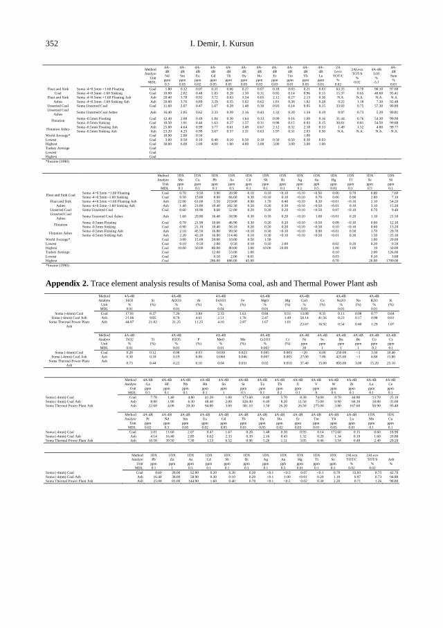
Appendix 2. Trace element analysis results of Manisa Soma coal, ash and Thermal Power Plant ash
Method
Analyte
Unit
MDL
4A-4B
SiO2
%
0.01
Si
(%)
4A-4B
Al2O3
%
0.01
Al
(%)
4A-4B
Fe2O3
%
0.04
Fe
(%)
4A-4B
MgO
%
0.01
Mg
(%)
4A-4B
CaO
%
0.01
Ca
(%)
4A-4B
Na2O
%
0.01
Na
(%)
4A-4B
K2O
%
0.01
K
(%)
Soma (-4mm) Coal Coal 17.91 8.37 7.26 3.84 2.33 1.63 0.84 0.51 13.08 9.35 0.11 0.08 0.77 0.64
Soma (-4mm) Coal Ash Ash 21.06 9.85 8.70 4.61 2.51 1.76 2.47 1.49 58.14 41.56 0.23 0.17 0.98 0.81
Soma Thermal Power Plant
Ash
Ash 44.97 21.02 21.25 11.25 4.10 2.87 1.67 1.01 23.67 16.92 0.54 0.40 1.29 1.07
Method
Analyte
Unit
MDL
4A-4B
TiO2
%
0.01
Ti
(%)
4A-4B
P2O5
%
0.01
P
(%)
4A-4B
MnO
%
0.01
Mn
(%)
4A-4B
Cr2O3
%
0.002
Cr
(%)
4A-4B
Ni
ppm
20
4A-4B
Sc
ppm
1
4A-4B
Ba
ppm
1
4A-4B
Be
ppm
1
4A-4B
Co
ppm
0.2
4A-4B
Cs
ppm
0.1
Soma (-4mm) Coal Coal 0.20 0.12 0.08 0.03 0.030 0.023 0.005 0.003 <20 6.00 250.00 <1 3.30 10.40
Soma (-4mm) Coal Ash Ash 0.30 0.18 0.19 0.08 0.060 0.046 0.007 0.005 27.00 7.00 425.00 <1 6.80 13.80
Soma Thermal Power Plant
Ash
Ash 0.73 0.44 0.22 0.10 0.04 0.031 0.02 0.010 37.40 15.00 893.00 3.00 15.20 25.10
Method
Analyte
Unit
MDL
4A-4B
Ga
ppm
0.5
4A-4B
Hf
ppm
0.1
4A-4B
Nb
ppm
0.1
4A-4B
Rb
ppm
0.1
4A-4B
Sn
ppm
1
4A-4B
Sr
ppm
0.5
4A-4B
Ta
ppm
0.1
4A-4B
Th
ppm
0.2
4A-4B
U
ppm
0.1
4A-4B
V
ppm
8
4A-4B
W
ppm
0.5
4A-4B
Zr
ppm
0.1
4A-4B
La
ppm
0.1
4A-4B
Ce
ppm
0.1
Soma (-4mm) Coal Coal 7.70 1.40 4.80 41.20 1.00 173.60 0.40 5.70 8.30 74.00 0.70 44.90 13.70 25.10
Soma (-4mm) Coal Ash Ash 8.80 1.90 6.30 48.40 2.00 426.40 0.40 8.20 11.50 75.00 0.90 68.10 18.80 35.00
Soma Thermal Power Plant Ash Ash 22.60 4.00 20.30 94.80 3.00 381.10 1.50 26.20 26.50 275.00 3.80 167.60 50.90 95.40
Method
Analyte
Unit
MDL
4A-4B
Pr
ppm
0.02
4A-4B
Nd
ppm
0.3
4A-4B
Sm
ppm
0.05
4A-4B
Eu
ppm
0.02
4A-4B
Gd
ppm
0.05
4A-4B
Tb
ppm
0.01
4A-4B
Dy
ppm
0.05
4A-4B
Ho
ppm
0.02
4A-4B
Er
ppm
0.03
4A-4B
Tm
ppm
0.01
4A-4B
Yb
ppm
0.05
4A-4B
Lu
ppm
0.01
1DX
Mo
ppm
0.1
1DX
Cu
ppm
0.1
Soma (-4mm) Coal Coal 3.01 11.60 2.07 0.47 1.67 0.28 1.48 0.30 0.93 0.14 173.60 0.15 0.60 18.90
Soma (-4mm) Coal Ash Ash 4.14 16.40 2.85 0.62 2.33 0.39 2.16 0.43 1.32 0.20 1.34 0.19 1.60 20.80
Soma Thermal Power Plant Ash Ash 10.58 39.50 7.30 1.53 6.52 0.96 5.26 1.11 3.05 0.46 3.34 0.48 2.40 29.20
Method
Analyte
Unit
MDL
1DX
Pb
ppm
0.1
1DX
Zn
ppm
1
1DX
As
ppm
0.5
1DX
Cd
ppm
0.1
1DX
Sb
ppm
0.1
1DX
Bi
ppm
0.1
1DX
Ag
ppm
0.1
1DX
Au
ppb
0.5
1DX
Hg
ppm
0.01
1DX
Tl
ppm
0.1
1DX
Se
ppm
0.5
2ALeco
TOT/C
%
0.02
2ALeco
TOT/S
%
0.02
Ash
%
Soma (-4mm) Coal Coal 8.60 28.00 52.00 0.20 0.20 0.20 <0.1 <0.5 0.07 <0.1 0.70 33.93 0.75 42.70
Soma (-4mm) Coal Ash Ash 16.40 38.00 58.90 0.30 0.10 0.20 <0.1 1.00 <0.01 0.20 1.10 0.97 0.73 94.80
Soma Thermal Power Plant Ash Ash 25.00 81.00 144.90 1.60 0.40 0.70 <0.1 <0.5 0.02 0.30 2.20 0.71 1.26 98.80
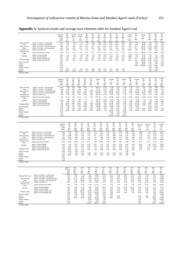
Investigation of radioactive content of Manisa-Soma and Istanbul-Agacli coals (Turkey) 353
Appendix 3. Analysis results and average trace elements table for Istanbul Agacli coal
Method
Analyte
Unit
MDL
4A-
4B
SiO2
%
0,01
4A-4B
AI2O3
%
0,01
4A-4B
Fe2O3
%
0,04
4A-
4B
MgO
%
0,01
4A-
4B
CaO
%
0,01
4A-
4B
Na2O
%
0,01
4A-
4B
K2O
%
0,01
4A-
4B
TiO2
%
0,01
4A-
4B
P2O5
%
0,01
4A-
4B
MnO
%
0,01
4A-4B
Cr2O3
%
0,002
4A-
4B
Sc
ppm
1
4A-4B
Ba
ppm
1
4A-
4B
Be
ppm
1
4A-
4B
Co
ppm
0,2
4A-
4B
Cs
ppm
0,1
Float and Sink
Coal
Agacli -4+0.5mm +1.30 Floating Coal 0.42 0.70 1.10 0.28 2.08 0.08 0.01 <0,01 <0,01 <0,01 0.00 1.00 47.00 2.00 2.10 <0.10
Agacli -4+0.5mm -1.30 Sinking Coal 1.35 1.20 1.33 0.25 1.82 0.09 0.05 0.04 <0,01 <0,01 0.00 2.00 46.00 2.00 1.80 0.30
Float and Sink
Ashes
Agacli -4+0.5mm +1.30 Floating Ash Ash N.A. N.A. N.A. N.A. N.A. N.A. N.A. N.A. N.A. N.A. N.A. N.A. 610.00 21.00 34.60 0.30
Agacli -4+0.5mm -1.30 Sinking Ash Ash N.A. N.A. N.A. N.A. N.A. N.A. N.A. N.A. N.A. N.A. N.A. N.A. 460.00 10.00 19.70 1.20
Unsorted Coal Agacli Unsorted Coal Coal 0.87 0.94 1.22 0.31 2.17 0.09 0.02 0.02 0.04 0.01 <0.002 2.00 57.00 2.00 2.60 0.20
Unsorted Coal
Ashes Agacli Unsorted Coal Ashes Ash N.A. N.A. N.A. N.A. N.A. N.A. N.A. N.A. N.A. N.A. N.A. N.A. 609.00 17.00 36.60 0.90
Flotation Agacli -0.5mm Floating Coal 1.28 1.26 1.56 0.34 2.56 0.09 0.04 0.03 0.01 0.01 0.002 3.00 63.00 2.00 2.70 0.30
Agacli -0.5mm Sinking Coal 1.20 1.15 1.41 0.31 2.38 0.11 0.03 0.03 0.04 0.01 0.004 3.00 61.00 2.00 2.30 0.20
Flotation Ashes Agacli -0.5mm Floating Ash Ash N.A. N.A. N.A. N.A. N.A. N.A. N.A. N.A. N.A. N.A. N.A. N.A. 654.00 15.00 27.70 2.00
Agacli -0.5mm Sinking Ash Ash N.A. N.A. N.A. N.A. N.A. N.A. N.A. N.A. N.A. N.A. N.A. N.A. 659.00 13.00 26.30 2.30
World Average* Coal 1.00 200.00 2.00 5.00 1.00
Lowest Coal 1.00 20.00 0.10 0.50 0.30
Highest Coal 10.00 1000.00 15.00 30.00 5.00
Turkey Average Coal 1.00 9.40
Lowest Coal 0.67 0.07 0.26 0.04 0.06 0.01 0.01 0.01 0.01 0.01 0.20 1.00
Highest Coal 28.27 12.00 12.57 3.17 14.08 2.34 1.85 0.57 0.24 0.07 7.00 55.00
*Swaine (1990)
Method
Analyte
Unit
MDL
4A-
4B
Ga
ppm
0,5
4A-
4B
Hf
ppm
0,1
4A-
4B
Nb
ppm
0,1
4A-
4B
Rb
ppm
0,1
4A-
4B
Sn
ppm
1
4A-4B
Sr
ppm
0,5
4A-
4B
Ta
ppm
0,1
4A-4B
V
ppm
8
4A-
4B
Th
ppm
0,2
4A-4B
U
ppm
0,1
4A-
4B
W
ppm
0,5
4A-4B
Zr
ppm
0,1
4A-
4B
Y
ppm
0,1
4A-
4B
La
ppm
0,1
4A-
4B
Ce
ppm
0,1
4A-
4B
Pr
ppm
0,02
Float and Sink
Coal
Agacli -4+0.5mm +1.30 Floating Coal 2.60 0.30 0.80 0.10 <1 462.70 <0.10 11.00 2.60 0.90 1.20 9.70 6.50 1.90 4.80 0.55
Agacli -4+0.5mm -1.30 Sinking Coal 3.30 0.40 2.50 1.90 <1 373.10 <0.10 16.00 4.00 1.70 1.30 14.60 7.20 4.10 9.00 1.01
Float and Sink
Ashes
Agacli -4+0.5mm +1.30 Floating Ash Ash 27.10 3.20 13.90 2.10 12.00 5672.00 0.40 259.00 32.30 13.70 14.40 113.00 91.90 24.90 56.90 7.42
Agacli -4+0.5mm -1.30 Sinking Ash Ash 28.00 4.40 20.50 10.00 3.00 3435.00 1.00 202.00 36.00 13.40 11.90 148.80 60.30 32.10 71.30 7.89
Unsorted Coal Agacli Unsorted Coal Coal 2.60 0.30 1.60 0.90 1.00 445.50 <0.10 47.00 3.60 1.30 1.10 11.00 6.80 3.10 6.20 0.81
Unsorted Coal
Ashes Agacli Unsorted Coal Ashes Ash 22.10 3.70 11.10 7.20 7.00 5792.00 0.70 227.00 43.40 11.60 10.50 140.60 91.80 43.30 95.60 11.03
Flotation Agacli -0.5mm Floating Coal 2.80 0.40 2.00 1.10 <1 491.40 <0.10 21.00 4.00 1.50 1.10 14.50 7.70 3.70 7.90 0.95
Agacli -0.5mm Sinking Coal 2.50 0.40 1.80 1.10 <1 476.70 <0.10 35.00 3.90 1.30 0.90 13.80 7.10 3.50 7.50 0.88
Flotation Ashes Agacli -0.5mm Floating Ash Ash 28.40 4.80 18.60 8.40 2.00 4744.00 0.80 219.00 38.60 15.40 11.10 153.30 79.60 35.80 78.50 9.18
Agacli -0.5mm Sinking Ash Ash 28.90 4.20 19.00 8.80 2.00 4746.00 0.80 225.00 36.80 15.70 10.90 147.90 78.80 35.70 77.40 8.93
World Average* Coal 5.00 1.00 5.00 40.00 2.00 200.00 0.20 40.00 4.00 2.00 1.00 50.00 10.00 20.00
Lowest Coal 1.00 0.40 1.00 2.00 1.00 15.00 0.10 2.00 0.50 0.50 0.50 5.00 2.00 1.00 2.00 1.00
Highest Coal 20.00 5.00 20.00 50.00 10.00 500.00 1.00 100.00 10.00 10.00 5.00 200.00 50.00 40.00 70.00 10.00
Turkey Average Coal 87.00 6.00 13.00
Lowest Coal 6.00 1.00 0.40
Highest Coal 287.00 29.00 132.00
*Swaine (1990)
Method
Analyte
Unit
MDL
4A-
4B
Nd
ppm
0,3
4A-
4B
Sm
ppm
0,05
4A-
4B
Eu
ppm
0,02
4A-
4B
Gd
ppm
0,05
4A-
4B
Tb
ppm
0,01
4A-
4B
Dy
ppm
0,05
4A-
4B
Ho
ppm
0,02
4A-
4B
Er
ppm
0,03
4A-
4B
Tm
ppm
0,01
4A-
4B
Yb
ppm
0,05
4A-
4B
Lu
ppm
0,01
2A Leco
TOT/C
%
0,02
2ALeco
TOT/S
%
0,02
4A-
4B
LOI
%
-5,1
4A-4B
Sum
%
0,01
Float and Sink
Coal
Agacli -4+0.5mm +1.30 Floating Coal 2.60 0.58 0.19 0.78 0.13 0.79 0.18 0.51 0.07 0.49 0.07 58.86 1.18 92.10 96.75
Agacli -4+0.5mm -1.30 Sinking Coal 3.60 0.95 0.22 0.95 0.15 0.93 0.22 0.60 0.10 0.54 0.09 57.28 1.77 91.40 97.56
Float and Sink
Ashes
Agacli -4+0.5mm +1.30 Floating Ash Ash 32.80 7.99 2.48 9.72 1.81 10.52 2.46 6.80 1.00 6.33 1.09 N.A. N.A. N.A. N.A.
Agacli -4+0.5mm -1.30 Sinking Ash Ash 32.20 6.64 1.81 7.13 1.21 6.94 1.58 4.80 0.72 4.41 0.64 N.A. N.A. N.A. N.A.
Unsorted Coal Agacli Unsorted Coal Coal 2.80 0.67 0.28 0.90 0.21 0.86 0.21 0.63 0.14 0.58 0.14 59.36 1.19 93.20 98.91
Unsorted Coal
Ashes Agacli Unsorted Coal Ashes Ash 45.30 10.02 2.72 11.12 1.85 10.92 2.39 6.60 0.87 5.84 0.89 N.A. N.A. N.A. N.A.
Flotation Agacli -0.5mm Floating Coal 4.10 0.87 0.23 0.93 0.16 1.05 0.22 0.62 0.09 0.58 0.08 60.27 1.18 92.70 99.92
Agacli -0.5mm Sinking Coal 3.80 0.85 0.21 0.94 0.15 1.04 0.21 0.62 0.09 0.51 0.07 59.59 1.49 92.40 99.06
Flotation Ashes Agacli -0.5mm Floating Ash Ash 38.60 8.47 2.33 9.41 1.55 9.66 2.07 6.53 0.92 5.54 0.83 N.A. N.A. N.A. N.A.
Agacli -0.5mm Sinking Ash Ash 37.40 8.26 2.31 9.26 1.54 9.36 2.06 6.23 0.92 5.48 0.82 N.A. N.A. N.A. N.A.
World Average* Coal 10.00 2.00 0.50 1.00
Lowest Coal 3.00 0.50 0.10 0.40 0.10 0.50 0.10 0.50 0.50 0.30 0.03
Highest Coal 30.00 6.00 2.00 4.00 1.00 4.00 2.00 3.00 3.00 3.00 1.00
Turkey Average Coal
Lowest Coal
Highest Coal
*Swaine (1990)
Method
Analyte
Unit
MDL
1DX
Mo
ppm
0,1
1DX
Cu
ppm
0,1
1DX
Pb
ppm
0,1
1DX
As
ppm
0,5
1DX
Cd
ppm
0,1
1DX
Sb
ppm
0,1
1DX
Bi
ppm
0,1
1DX
Ag
ppm
0,1
1DX
Au
ppb
0,5
1DX
Hg
ppm
0,01
1DX
Tl
ppm
0,1
1DX
Se
ppm
0,5
1DX
Ni
ppm
0,1
Float and Sink Coal Agacli -4+0.5mm +1.30 Floating Coal 0.50 7.10 3.00 28.90 <0.10 0.10 <0.10 <0.10 <0.50 0.04 2.40 1.20 12.80
Agacli -4+0.5mm -1.30 Sinking Coal 0.70 10.20 6.80 32.50 <0.10 0.20 0.10 <0.10 <0.50 0.05 2.70 1.50 13.40
Float and Sink
Ashes
Agacli -4+0.5mm +1.30 Floating Ash Ash 10.70 82.70 0.60 307.20 <0.10 2.10 <0.10 0.10 8.10 <0.01 <0.10 2.70 119.80
Agacli -4+0.5mm -1.30 Sinking Ash Ash 7.40 105.30 5.90 235.60 0.50 1.50 <0.10 0.10 <0.50 <0.01 <0.10 4.90 94.30
Unsorted Coal Agacli Unsorted Coal Coal 0.50 10.70 5.30 30.90 <0.10 0.20 0.10 <0.10 0.60 0.05 <0.10 1.00 14.00
Unsorted Coal
Ashes Agacli Unsorted Coal Ashes Ash 7.60 75.10 27.40 311.70 0.10 1.30 0.30 0.20 2.50 <0.01 <0.10 0.90 130.40
Flotation Agacli -0.5mm Floating Coal 0.60 15.20 6.60 30.30 <0.10 0.20 0.10 <0.10 <0.50 0.05 <0.10 1.10 16.20
Agacli -0.5mm Sinking Coal 0.50 14.00 7.40 29.00 <0.10 0.20 0.10 <0.10 <0.50 0.06 0.10 0.90 15.20
Flotation Ashes Agacli -0.5mm Floating Ash Ash 10.00 162.00 22.60 312.80 <0.10 2.40 <0.10 0.30 3.20 <0.01 0.50 3.50 136.70
Agacli -0.5mm Sinking Ash Ash 9.90 135.10 21.80 310.60 0.40 2.60 <0.10 0.30 1.10 <0.01 0.40 3.90 136.60
World Average* Coal 3.00 15.00 20.00 10.00 0.50 1.50 1.00 20.00
Lowest Coal 0.10 0.50 2.00 0.50 0.10 0.10 2.00 0.02 0,20 0.20 0.50
Highest Coal 10.00 50.00 80.00 80.00 3.00 10.00 20.00 1.00 1.00 10.00 50.00
Turkey Average Coal 12.00 53.00 1.00 0.10 2.00 126.00
Lowest Coal 0.10 2.00 0.01 0.03 0.10 3.00
Highest Coal 286.00 686.00 45.00 0.70 26.00 1700.00
*Swaine (1990)

354 I. Demir, I. Kursun

http://dx.doi.org/10.5277/ppmp120203
Physicochem. Probl. Miner. Process. 48(2), 2012, 355−367 Physicochemical Problems
of Mineral Processing
w w w . m i n p r o c . p w r . w r o c . p l / j o u r n a l / ISSN 1643-1049 (print)
ISSN 2084-4735 (online)
Received November 12, 2011; reviewed; accepted January 27, 2012
INVESTIGATION OF COPPER CEMENTATION KINETICS BY
ROTATING ALUMINUM DISC FROM THE LEACH SOLUTIONS
CONTAINING COPPER IONS
Ahmet EKMEKYAPAR*, Mehmet TANAYDIN**, Nizamettin DEMIRKIRAN*
* Chemical Engineering Department, Faculty of Engineering, Inonu University, 44280, Malatya, Turkey,
** Chemical Engineering Department, Faculty of Engineering, Tunceli University, 62000, Tunceli, Turkey
Abstract. Recovery of metallic copper from the leach solution containing copper (II) ions by
cementation process using aluminum disc has been examined. Solutions obtained from the
leaching of malachite in aqueous acetic acid solutions were used in the study. It was
determined that the cementation rate increased with increasing solution concentration,
temperature and rotating speed, and decreasing solution pH. The reaction rate fits to the first
order pseudo homogeneous reaction model and is controlled by diffusion. The activation
energy of this process was calculated to be 32.6 kJ/mol.
keywords: copper cementation, leaching, malachite, activation energy
1. Introduction
Most of metals are found in nature as complex mixtures of their sulfides, oxides,
carbonates, silicates etc. Metals are generally produced after being extracted from an
ore or its concentrates. The extraction of metals from the metal sources is carried out
either by pyrometallurgy or hydrometallurgy (Venkatachalam, 1998; Gupta and
Murkherjee, 1990). Hydrometallurgical methods in processing ores, concentrates, and
secondary metal sources (various industrial wastes) have gained recently increasing
importance in the extraction of nonferrous metals from ores.
Hydrometallurgy is essentially concerned with methods whereby metals, metal
salts, or other metal compounds are produced by means of chemical reactions
involving aqueous and organic solutions (Gupta and Murkherjee, 1990). It covers a
large variety of processes ranging from the leaching of metal values in an aqueous
solvent through the purification of the solutions to the recovery of the metals or their
compounds by chemical or electrochemical precipitation (Venkatachalam, 1998;
Rosenqvist, 2004).
Leaching is the first step of any hydrometallurgical process. Leaching is the term
applied to the process of recovering a metal from the metal source by a solvent or
lixiviant. The metallic value in a metal source passes into the solution by dissolving in

356 A. Ekmekyapar et al.
the leaching step. During this step, in addition to the desired metal, other metals
present in the ore matrix may also pass into the solution. Therefore, before the final
recovery of the desired metal, purification processes are applied to remove the
impurities from the leach liquor. There are many ways to achieve this goal
(Venkatachalam, 1998; Gupta and Murkherjee, 1990; Han, 2002). Metal value can be
directly obtained from the leach liquor without purification in some cases.
The final part of a hydrometallurgical flow sheet concerns the recovery process.
The acquired product is either the elemental metal or its suitable compound. The
various techniques available for the recovery of a metal from the leach liquors with or
without purification are crystallization, ionic precipitation, reduction with a gas,
electrochemical reduction (cementation), and electrolytic reduction (Gupta and
Murkherjee, 1990).
Among the metal gaining processes, cementation, which is basically an
electrochemical reduction process, is one of the most effective and economic methods
applied successfully for obtaining of valuable metals from industrial solutions. The
advantages of this technique are its relative simplicity, ease of control, and low energy
consumption (Venkatachalam, 1998; Gupta and Murkherjee, 1990; Naubactep, 2010;
Kuntyi et al., 2011). That process involves the chemical reduction of metal ions by
galvanic interaction between noble metal ions and a more active metal in an aqueous
solution medium. (Venkatachalam, 1998; Gupta and Murkherjee, 1990). For any
cementation reaction the overall reaction equation can be written as follows
Nn+
+ M0 ⟶ N
0 + M
m+ (1)
where, N is the noble or precipitating metal, M is the reductant metal.
Copper is among the most intensively applied and valuable metals used by
industry. It is used mostly in the electrical and electronics industries because of its
high electrical conductivity. In addition, copper and its alloys are utilized in the
engine, communication, and aviation industries, for electricity production and
distribution, in measuring devices, in chemical industry etc. (Dib and Makhloufi,
2004; Arzutug et al., 2004).
Copper generally is found in nature in the form of sulfide and oxide minerals, such
as azurite, malachite, tenorite, chrysocolla, bornite, brochantite, enargite, chalcopyrite,
chalcocite, covellite (Akçıl, 2002; Arzutug et al., 2004; Bingöl et al., 2005). Metallic
copper is produced from these ores by pyrometallurgical and hydrometallurgical
methods. In production of copper from low-grade oxidized copper ores,
hydrometallurgical methods are commonly preferred because pyrometallurgy is not
feasible for these type ores.
Among the oxidized copper ores, malachite is the most popular. The leaching and
kinetics of malachite has been investigated by various researchers (Oudenne and
Olson, 1983; Künkül et al., 1994; Yartaşı and Çopur, 1996; Ekmekyapar et al., 2003;
Bingöl and Canbazoğlu, 2004; Arzutuğ, 2004; Bingöl et al. 2005; Lui et al., 2010).
Malachite ore can be used to produce metallic copper and copper compounds by
Investigation of copper cementation kinetics by rotating aluminum disc from the leach solutions… 357
hydrometallurgical techniques. After leaching of malachite with a convenient lixiviant,
copper in the purified leach solution can be precipitated by cementation, deposited by
direct electrowinning or solvent extraction-electrowinning methods. In cementation
and direct electrowinning methods copper is obtained in metallic state, while in
solvent extraction-electrowinning method, copper is first selectively recovered from
the solution by chelating Cu2+
and dissolving in an organic solvent, and then the
solvent is stripped off from the chelat by a strong acid to give a solution to be
amenable to electrowinning process (Ekmekyapar et al., 2003; Elamari et al., 2006).
In the recovery of copper from the leach solution by cementation process, when
aluminum is used as reductant metal, copper ions are easily reduced to its metallic
state due to the difference between the electrode potentials of these two metals. The
standard reduction potentials of copper and aluminum are 0.34 and -1.67 V,
respectively. During the cementation process, the half-cell reactions occurring are:
Cu2+
+ 2e- ⇆ Cu
o (reduction reaction) E
o = 0.34 V (2)
Alo ⇆ Al
3+ + 3e
- (oxidation reaction) E
o = -1.67 V (3)
Thus, the whole cementation reaction of copper ions onto aluminum disc may be
expressed by the following reaction equation:
3Cu2+
+ 2Alo ⟶ 3Cu
o + 2Al
3+ 𝛥E
o = 2.01 V (4)
As can be seen from Equation (4), the potential of this cementation reaction is
positive, and the standard free energy, 𝛥Go, is negative (𝛥G
o= -nF𝛥E
o). The negative
value of the standard free energy indicates that this process is favorable
thermodynamically, and thus a spontaneous heterogeneous reaction takes place in the
galvanic cell.
Recovery of copper from various solutions containing copper (II) ions by
cementation reaction has been studied by many researchers. In these studies related to
copper cementation iron has been generally used as sacrificial metal because of its
cheapness. However, zinc and aluminum have been also used as precipitant or
reductant metals (MacKinnon and Ingraham, 1970; MacKinnon and Ingraham, 1971;
MacKinnon et al., 1971; Annamalai et al., 1978; Annamalai and Murr, 1978; Chen
and Lee, 1994; Wei et al., 1994; Masse and Piron, 1994; Djokic, 1996; Stefanowicz et
al., 1997; Dönmez et al., 1999; Kanungo et al., 2001; Stankoviç et al., 2004; Dib and
Makhloufi, 2004; Kanungo et al., 2003; Karavasteva, 2005; Fouad and Abdel Basir,
2005; Hung et al., 2005; Demirkıran et al., 2007; Amin and El-Ashtoukhy, 2011).
In most of works in the literature copper cementation with a reductant metal has
been mostly carried out using synthetic pure solutions containing copper ions. In the
present study, metallic copper was recovered by using the actual solution which is
derived from after the leaching of malachite ore in acetic acid solution. For the
recovery of copper a rotating aluminum disc was used as the reductant metal. In the
experiments the influence of copper ion concentration, reaction temperature, solution
pH, and disc rotation speed on copper cementation were investigated. The kinetics of
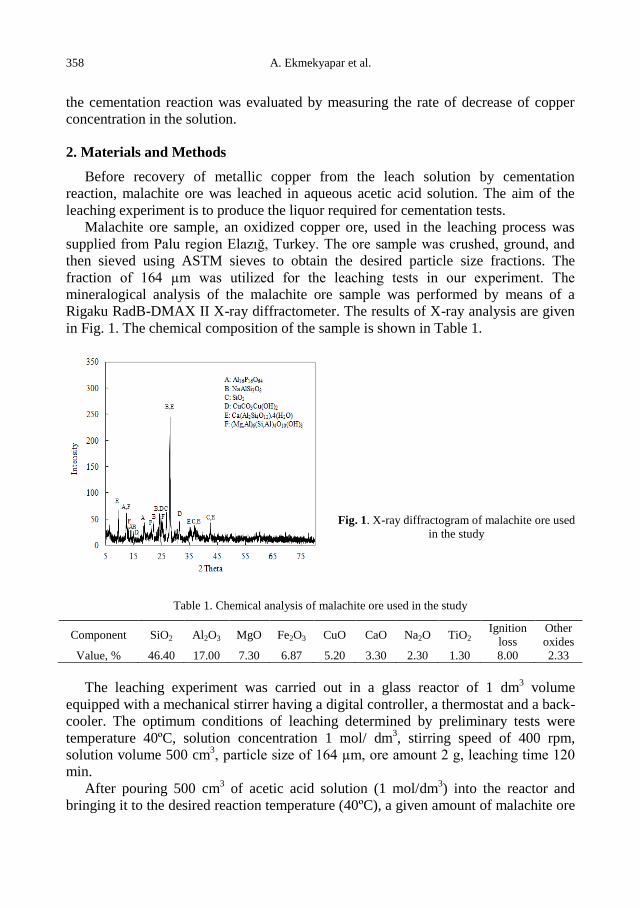
358 A. Ekmekyapar et al.
the cementation reaction was evaluated by measuring the rate of decrease of copper
concentration in the solution.
2. Materials and Methods
Before recovery of metallic copper from the leach solution by cementation
reaction, malachite ore was leached in aqueous acetic acid solution. The aim of the
leaching experiment is to produce the liquor required for cementation tests.
Malachite ore sample, an oxidized copper ore, used in the leaching process was
supplied from Palu region Elazığ, Turkey. The ore sample was crushed, ground, and
then sieved using ASTM sieves to obtain the desired particle size fractions. The
fraction of 164 µm was utilized for the leaching tests in our experiment. The
mineralogical analysis of the malachite ore sample was performed by means of a
Rigaku RadB-DMAX II X-ray diffractometer. The results of X-ray analysis are given
in Fig. 1. The chemical composition of the sample is shown in Table 1.
Fig. 1. X-ray diffractogram of malachite ore used
in the study
Table 1. Chemical analysis of malachite ore used in the study
Component SiO2 Al2O3 MgO Fe2O3 CuO CaO Na2O TiO2 Ignition
loss
Other
oxides
Value, % 46.40 17.00 7.30 6.87 5.20 3.30 2.30 1.30 8.00 2.33
The leaching experiment was carried out in a glass reactor of 1 dm3 volume
equipped with a mechanical stirrer having a digital controller, a thermostat and a back-
cooler. The optimum conditions of leaching determined by preliminary tests were
temperature 40ºC, solution concentration 1 mol/ dm3, stirring speed of 400 rpm,
solution volume 500 cm3, particle size of 164 µm, ore amount 2 g, leaching time 120
min.
After pouring 500 cm3 of acetic acid solution (1 mol/dm
3) into the reactor and
bringing it to the desired reaction temperature (40ºC), a given amount of malachite ore
Investigation of copper cementation kinetics by rotating aluminum disc from the leach solutions… 359
(2 g) was added to the solution, and the stirring speed was set to 400 rpm. The
leaching process was carried out for 120 min of reaction time. At the end of this
operation the content of the reactor was immediately filtered. The amount of copper
(II) ion in the filtrate was determined by complexometric titration using EDTA as a
titrant and murexide as an indicator. The amount of extracted copper from the ore after
120 min of leaching time was calculated as 1.58 g/dm3. The solution attained in the
leaching step was considered as the mother liquid and it was diluted by adding
distilled water to reach the desired concentration of copper(II) ion for utilization in the
cementation stage. Process variables chosen for cementation process are given in
Table 2. Cementation studies were performed in a 1 dm3 glass reactor equipped with a
mechanical stirrer, a reaction temperature control unit, and a cooler to avoid loss of
solution by evaporation. The leach solution containing copper(II) ion of 500 cm3
volume was added into the reaction vessel. The pH of the solution was adjusted to the
desired value by diluted sulfuric acid solution. When the reactor content reached the
desired reaction temperature, aluminum disc (height of 0.005 m, diameter of 0.05 m,
working surface area 1.7310-2
m2)
was immersed in the solution. The disc was
screwed onto the end of a thin stainless steel rod which was attached to the mechanical
stirrer. The disc was rotated at controlled speeds in the solution. The progress of the
cementation reaction was followed by measuring the concentration of copper ions in
the solution. Aliquots of 5 cm3 each were withdrawn at regular intervals during the
reaction and immediately filtered using filter paper. The filtered samples were
analyzed for copper ion content by titrating with EDTA in the presence of murexide
indicator. The amount of deposited copper was calculated according to difference
between the initial and final copper concentrations of the solution. The fraction of
cemented copper was calculated as follows:
x = initial copper concentration/copper concentration at time t.
Table 2. Parameters and their ranges used in the experiments
Parameter Value
Concentration, mol/dm3 0.0025, 0.005, 0.010, 0.020
Temperature, ºC 20, 30, 40, 50, 60
Rotating speed, rpm 200, 300, 400, 500
pH 1.0, 1.5, 2.0, 2.5, 3.26
3. Results and Discussion
In order to observe the effect of rotation speed of Al disc on the cementation rate of
copper the experiments were carried out at different rotation speeds in the range of
200 to 500 rpm. The results obtained from these tests showed that the cemented
copper fraction increased with increasing the disc rotation speed. This result indicates
that the copper cementation rate is probably the diffusion controlled under these
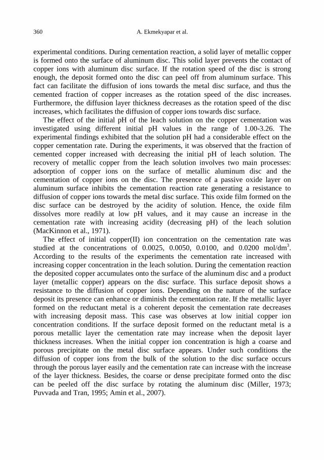
360 A. Ekmekyapar et al.
experimental conditions. During cementation reaction, a solid layer of metallic copper
is formed onto the surface of aluminum disc. This solid layer prevents the contact of
copper ions with aluminum disc surface. If the rotation speed of the disc is strong
enough, the deposit formed onto the disc can peel off from aluminum surface. This
fact can facilitate the diffusion of ions towards the metal disc surface, and thus the
cemented fraction of copper increases as the rotation speed of the disc increases.
Furthermore, the diffusion layer thickness decreases as the rotation speed of the disc
increases, which facilitates the diffusion of copper ions towards disc surface.
The effect of the initial pH of the leach solution on the copper cementation was
investigated using different initial pH values in the range of 1.00-3.26. The
experimental findings exhibited that the solution pH had a considerable effect on the
copper cementation rate. During the experiments, it was observed that the fraction of
cemented copper increased with decreasing the initial pH of leach solution. The
recovery of metallic copper from the leach solution involves two main processes:
adsorption of copper ions on the surface of metallic aluminum disc and the
cementation of copper ions on the disc. The presence of a passive oxide layer on
aluminum surface inhibits the cementation reaction rate generating a resistance to
diffusion of copper ions towards the metal disc surface. This oxide film formed on the
disc surface can be destroyed by the acidity of solution. Hence, the oxide film
dissolves more readily at low pH values, and it may cause an increase in the
cementation rate with increasing acidity (decreasing pH) of the leach solution
(MacKinnon et al., 1971).
The effect of initial copper(II) ion concentration on the cementation rate was
studied at the concentrations of 0.0025, 0.0050, 0.0100, and 0.0200 mol/dm3.
According to the results of the experiments the cementation rate increased with
increasing copper concentration in the leach solution. During the cementation reaction
the deposited copper accumulates onto the surface of the aluminum disc and a product
layer (metallic copper) appears on the disc surface. This surface deposit shows a
resistance to the diffusion of copper ions. Depending on the nature of the surface
deposit its presence can enhance or diminish the cementation rate. If the metallic layer
formed on the reductant metal is a coherent deposit the cementation rate decreases
with increasing deposit mass. This case was observes at low initial copper ion
concentration conditions. If the surface deposit formed on the reductant metal is a
porous metallic layer the cementation rate may increase when the deposit layer
thickness increases. When the initial copper ion concentration is high a coarse and
porous precipitate on the metal disc surface appears. Under such conditions the
diffusion of copper ions from the bulk of the solution to the disc surface occurs
through the porous layer easily and the cementation rate can increase with the increase
of the layer thickness. Besides, the coarse or dense precipitate formed onto the disc
can be peeled off the disc surface by rotating the aluminum disc (Miller, 1973;
Puvvada and Tran, 1995; Amin et al., 2007).
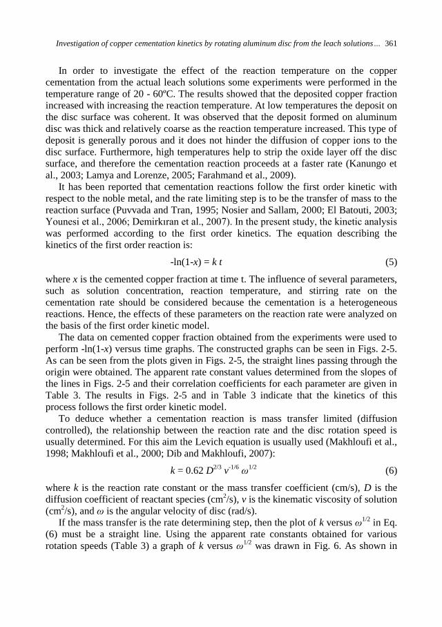
Investigation of copper cementation kinetics by rotating aluminum disc from the leach solutions… 361
In order to investigate the effect of the reaction temperature on the copper
cementation from the actual leach solutions some experiments were performed in the
temperature range of 20 - 60ºC. The results showed that the deposited copper fraction
increased with increasing the reaction temperature. At low temperatures the deposit on
the disc surface was coherent. It was observed that the deposit formed on aluminum
disc was thick and relatively coarse as the reaction temperature increased. This type of
deposit is generally porous and it does not hinder the diffusion of copper ions to the
disc surface. Furthermore, high temperatures help to strip the oxide layer off the disc
surface, and therefore the cementation reaction proceeds at a faster rate (Kanungo et
al., 2003; Lamya and Lorenze, 2005; Farahmand et al., 2009).
It has been reported that cementation reactions follow the first order kinetic with
respect to the noble metal, and the rate limiting step is to be the transfer of mass to the
reaction surface (Puvvada and Tran, 1995; Nosier and Sallam, 2000; El Batouti, 2003;
Younesi et al., 2006; Demirkıran et al., 2007). In the present study, the kinetic analysis
was performed according to the first order kinetics. The equation describing the
kinetics of the first order reaction is:
-ln(1-x) = k t (5)
where x is the cemented copper fraction at time t. The influence of several parameters,
such as solution concentration, reaction temperature, and stirring rate on the
cementation rate should be considered because the cementation is a heterogeneous
reactions. Hence, the effects of these parameters on the reaction rate were analyzed on
the basis of the first order kinetic model.
The data on cemented copper fraction obtained from the experiments were used to
perform -ln(1-x) versus time graphs. The constructed graphs can be seen in Figs. 2-5.
As can be seen from the plots given in Figs. 2-5, the straight lines passing through the
origin were obtained. The apparent rate constant values determined from the slopes of
the lines in Figs. 2-5 and their correlation coefficients for each parameter are given in
Table 3. The results in Figs. 2-5 and in Table 3 indicate that the kinetics of this
process follows the first order kinetic model.
To deduce whether a cementation reaction is mass transfer limited (diffusion
controlled), the relationship between the reaction rate and the disc rotation speed is
usually determined. For this aim the Levich equation is usually used (Makhloufi et al.,
1998; Makhloufi et al., 2000; Dib and Makhloufi, 2007):
k = 0.62 D2/3
v-1/6
ω1/2
(6)
where k is the reaction rate constant or the mass transfer coefficient (cm/s), D is the
diffusion coefficient of reactant species (cm2/s), v is the kinematic viscosity of solution
(cm2/s), and ω is the angular velocity of disc (rad/s).
If the mass transfer is the rate determining step, then the plot of k versus ω1/2
in Eq.
(6) must be a straight line. Using the apparent rate constants obtained for various
rotation speeds (Table 3) a graph of k versus ω1/2
was drawn in Fig. 6. As shown in
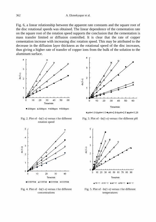
362 A. Ekmekyapar et al.
Fig. 6, a linear relationship between the apparent rate constants and the square root of
the disc rotational speeds was obtained. The linear dependence of the cementation rate
on the square root of the rotation speed supports the conclusion that the cementation is
mass transfer limited or diffusion controlled. It is clear that the rate of copper
cementation increase with increasing disc rotation speed. This may be attributed to the
decrease in the diffusion layer thickness as the rotational speed of the disc increases,
thus giving a higher rate of transfer of copper ions from the bulk of the solution to the
aluminum surface.
Fig. 2. Plot of –ln(1-x) versus t for different
rotation speed Fig. 3. Plot of –ln(1-x) versus t for different pH
Fig. 4. Plot of –ln(1-x) versus t for different
concentrations Fig. 5. Plot of –ln(1-x) versus t for different
temperatures
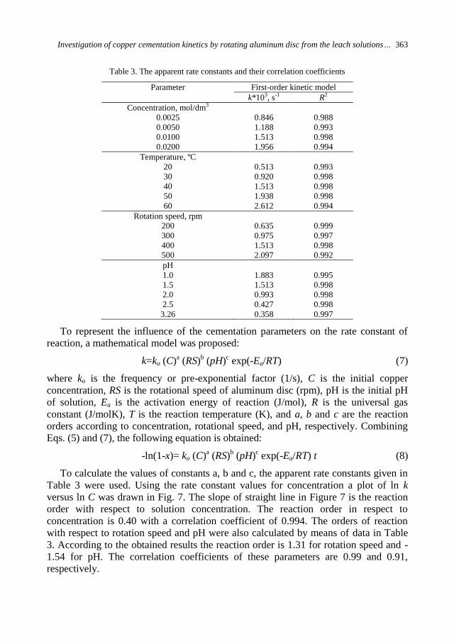
Investigation of copper cementation kinetics by rotating aluminum disc from the leach solutions… 363
Table 3. The apparent rate constants and their correlation coefficients
Parameter First-order kinetic model
k*103, s-1 R2
Concentration, mol/dm3
0.0025
0.0050
0.0100
0.0200
0.846
1.188
1.513
1.956
0.988
0.993
0.998
0.994
Temperature, ºC
20
30
40
50
60
0.513
0.920
1.513
1.938
2.612
0.993
0.998
0.998
0.998
0.994
Rotation speed, rpm
200
300
400
500
0.635
0.975
1.513
2.097
0.999
0.997
0.998
0.992
pH
1.0
1.5
2.0
2.5
3.26
1.883
1.513
0.993
0.427
0.358
0.995
0.998
0.998
0.998
0.997
To represent the influence of the cementation parameters on the rate constant of
reaction, a mathematical model was proposed:
k=ko (C)a (RS)
b (pH)
c exp(-Ea/RT) (7)
where ko is the frequency or pre-exponential factor (1/s), C is the initial copper
concentration, RS is the rotational speed of aluminum disc (rpm), pH is the initial pH
of solution, Ea is the activation energy of reaction (J/mol), R is the universal gas
constant (J/molK), T is the reaction temperature (K), and a, b and c are the reaction
orders according to concentration, rotational speed, and pH, respectively. Combining
Eqs. (5) and (7), the following equation is obtained:
-ln(1-x)= ko (C)a (RS)
b (pH)
c exp(-Ea/RT) t (8)
To calculate the values of constants a, b and c, the apparent rate constants given in
Table 3 were used. Using the rate constant values for concentration a plot of ln k
versus ln C was drawn in Fig. 7. The slope of straight line in Figure 7 is the reaction
order with respect to solution concentration. The reaction order in respect to
concentration is 0.40 with a correlation coefficient of 0.994. The orders of reaction
with respect to rotation speed and pH were also calculated by means of data in Table
3. According to the obtained results the reaction order is 1.31 for rotation speed and -
1.54 for pH. The correlation coefficients of these parameters are 0.99 and 0.91,
respectively.
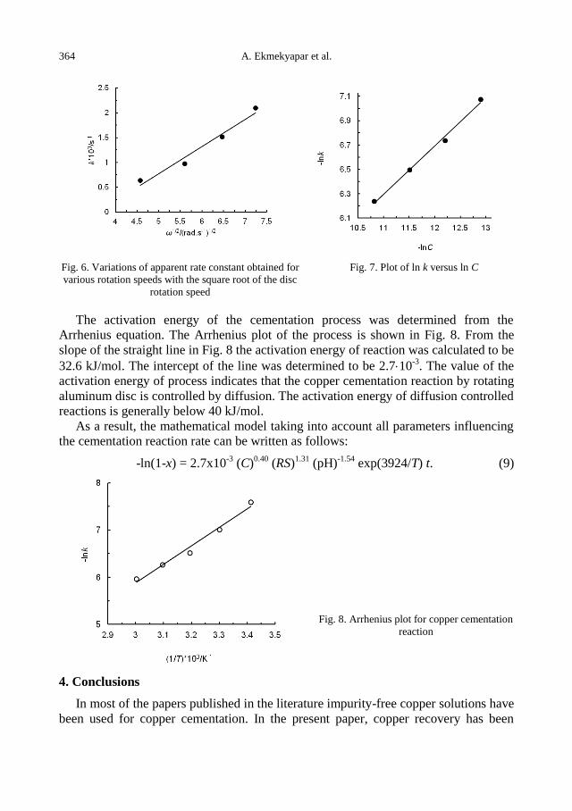
364 A. Ekmekyapar et al.
Fig. 6. Variations of apparent rate constant obtained for
various rotation speeds with the square root of the disc
rotation speed
Fig. 7. Plot of ln k versus ln C
The activation energy of the cementation process was determined from the
Arrhenius equation. The Arrhenius plot of the process is shown in Fig. 8. From the
slope of the straight line in Fig. 8 the activation energy of reaction was calculated to be
32.6 kJ/mol. The intercept of the line was determined to be 2.710-3
. The value of the
activation energy of process indicates that the copper cementation reaction by rotating
aluminum disc is controlled by diffusion. The activation energy of diffusion controlled
reactions is generally below 40 kJ/mol.
As a result, the mathematical model taking into account all parameters influencing
the cementation reaction rate can be written as follows:
-ln(1-x) = 2.7x10⁻³
(C)0.40
(RS)1.31
(pH)-1.54
exp(3924/T) t. (9)
Fig. 8. Arrhenius plot for copper cementation
reaction
4. Conclusions
In most of the papers published in the literature impurity-free copper solutions have
been used for copper cementation. In the present paper, copper recovery has been
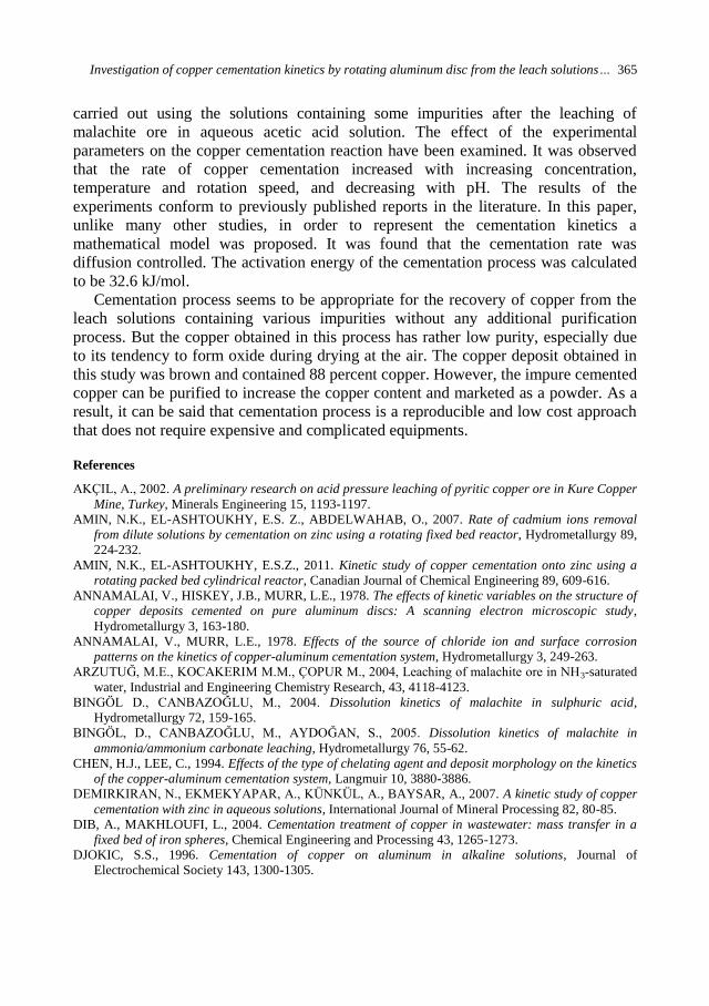
Investigation of copper cementation kinetics by rotating aluminum disc from the leach solutions… 365
carried out using the solutions containing some impurities after the leaching of
malachite ore in aqueous acetic acid solution. The effect of the experimental
parameters on the copper cementation reaction have been examined. It was observed
that the rate of copper cementation increased with increasing concentration,
temperature and rotation speed, and decreasing with pH. The results of the
experiments conform to previously published reports in the literature. In this paper,
unlike many other studies, in order to represent the cementation kinetics a
mathematical model was proposed. It was found that the cementation rate was
diffusion controlled. The activation energy of the cementation process was calculated
to be 32.6 kJ/mol.
Cementation process seems to be appropriate for the recovery of copper from the
leach solutions containing various impurities without any additional purification
process. But the copper obtained in this process has rather low purity, especially due
to its tendency to form oxide during drying at the air. The copper deposit obtained in
this study was brown and contained 88 percent copper. However, the impure cemented
copper can be purified to increase the copper content and marketed as a powder. As a
result, it can be said that cementation process is a reproducible and low cost approach
that does not require expensive and complicated equipments.
References
AKÇIL, A., 2002. A preliminary research on acid pressure leaching of pyritic copper ore in Kure Copper
Mine, Turkey, Minerals Engineering 15, 1193-1197.
AMIN, N.K., EL-ASHTOUKHY, E.S. Z., ABDELWAHAB, O., 2007. Rate of cadmium ions removal
from dilute solutions by cementation on zinc using a rotating fixed bed reactor, Hydrometallurgy 89,
224-232.
AMIN, N.K., EL-ASHTOUKHY, E.S.Z., 2011. Kinetic study of copper cementation onto zinc using a
rotating packed bed cylindrical reactor, Canadian Journal of Chemical Engineering 89, 609-616.
ANNAMALAI, V., HISKEY, J.B., MURR, L.E., 1978. The effects of kinetic variables on the structure of
copper deposits cemented on pure aluminum discs: A scanning electron microscopic study,
Hydrometallurgy 3, 163-180.
ANNAMALAI, V., MURR, L.E., 1978. Effects of the source of chloride ion and surface corrosion
patterns on the kinetics of copper-aluminum cementation system, Hydrometallurgy 3, 249-263.
ARZUTUĞ, M.E., KOCAKERIM M.M., ÇOPUR M., 2004, Leaching of malachite ore in NH3-saturated
water, Industrial and Engineering Chemistry Research, 43, 4118-4123.
BINGÖL D., CANBAZOĞLU, M., 2004. Dissolution kinetics of malachite in sulphuric acid,
Hydrometallurgy 72, 159-165.
BINGÖL, D., CANBAZOĞLU, M., AYDOĞAN, S., 2005. Dissolution kinetics of malachite in
ammonia/ammonium carbonate leaching, Hydrometallurgy 76, 55-62.
CHEN, H.J., LEE, C., 1994. Effects of the type of chelating agent and deposit morphology on the kinetics
of the copper-aluminum cementation system, Langmuir 10, 3880-3886.
DEMIRKIRAN, N., EKMEKYAPAR, A., KÜNKÜL, A., BAYSAR, A., 2007. A kinetic study of copper
cementation with zinc in aqueous solutions, International Journal of Mineral Processing 82, 80-85.
DIB, A., MAKHLOUFI, L., 2004. Cementation treatment of copper in wastewater: mass transfer in a
fixed bed of iron spheres, Chemical Engineering and Processing 43, 1265-1273.
DJOKIC, S.S., 1996. Cementation of copper on aluminum in alkaline solutions, Journal of
Electrochemical Society 143, 1300-1305.
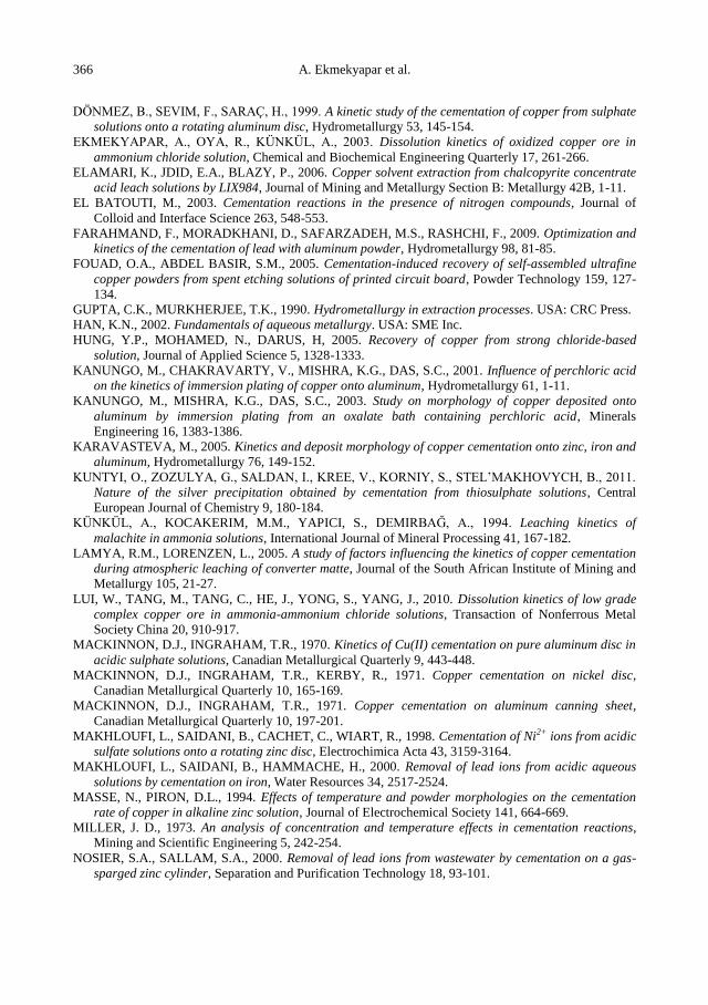
366 A. Ekmekyapar et al.
DÖNMEZ, B., SEVIM, F., SARAÇ, H., 1999. A kinetic study of the cementation of copper from sulphate
solutions onto a rotating aluminum disc, Hydrometallurgy 53, 145-154.
EKMEKYAPAR, A., OYA, R., KÜNKÜL, A., 2003. Dissolution kinetics of oxidized copper ore in
ammonium chloride solution, Chemical and Biochemical Engineering Quarterly 17, 261-266.
ELAMARI, K., JDID, E.A., BLAZY, P., 2006. Copper solvent extraction from chalcopyrite concentrate
acid leach solutions by LIX984, Journal of Mining and Metallurgy Section B: Metallurgy 42B, 1-11.
EL BATOUTI, M., 2003. Cementation reactions in the presence of nitrogen compounds, Journal of
Colloid and Interface Science 263, 548-553.
FARAHMAND, F., MORADKHANI, D., SAFARZADEH, M.S., RASHCHI, F., 2009. Optimization and
kinetics of the cementation of lead with aluminum powder, Hydrometallurgy 98, 81-85.
FOUAD, O.A., ABDEL BASIR, S.M., 2005. Cementation-induced recovery of self-assembled ultrafine
copper powders from spent etching solutions of printed circuit board, Powder Technology 159, 127-
134.
GUPTA, C.K., MURKHERJEE, T.K., 1990. Hydrometallurgy in extraction processes. USA: CRC Press.
HAN, K.N., 2002. Fundamentals of aqueous metallurgy. USA: SME Inc.
HUNG, Y.P., MOHAMED, N., DARUS, H, 2005. Recovery of copper from strong chloride-based
solution, Journal of Applied Science 5, 1328-1333.
KANUNGO, M., CHAKRAVARTY, V., MISHRA, K.G., DAS, S.C., 2001. Influence of perchloric acid
on the kinetics of immersion plating of copper onto aluminum, Hydrometallurgy 61, 1-11.
KANUNGO, M., MISHRA, K.G., DAS, S.C., 2003. Study on morphology of copper deposited onto
aluminum by immersion plating from an oxalate bath containing perchloric acid, Minerals
Engineering 16, 1383-1386.
KARAVASTEVA, M., 2005. Kinetics and deposit morphology of copper cementation onto zinc, iron and
aluminum, Hydrometallurgy 76, 149-152.
KUNTYI, O., ZOZULYA, G., SALDAN, I., KREE, V., KORNIY, S., STEL’MAKHOVYCH, B., 2011.
Nature of the silver precipitation obtained by cementation from thiosulphate solutions, Central
European Journal of Chemistry 9, 180-184.
KÜNKÜL, A., KOCAKERIM, M.M., YAPICI, S., DEMIRBAĞ, A., 1994. Leaching kinetics of
malachite in ammonia solutions, International Journal of Mineral Processing 41, 167-182.
LAMYA, R.M., LORENZEN, L., 2005. A study of factors influencing the kinetics of copper cementation
during atmospheric leaching of converter matte, Journal of the South African Institute of Mining and
Metallurgy 105, 21-27.
LUI, W., TANG, M., TANG, C., HE, J., YONG, S., YANG, J., 2010. Dissolution kinetics of low grade
complex copper ore in ammonia-ammonium chloride solutions, Transaction of Nonferrous Metal
Society China 20, 910-917.
MACKINNON, D.J., INGRAHAM, T.R., 1970. Kinetics of Cu(II) cementation on pure aluminum disc in
acidic sulphate solutions, Canadian Metallurgical Quarterly 9, 443-448.
MACKINNON, D.J., INGRAHAM, T.R., KERBY, R., 1971. Copper cementation on nickel disc,
Canadian Metallurgical Quarterly 10, 165-169.
MACKINNON, D.J., INGRAHAM, T.R., 1971. Copper cementation on aluminum canning sheet,
Canadian Metallurgical Quarterly 10, 197-201.
MAKHLOUFI, L., SAIDANI, B., CACHET, C., WIART, R., 1998. Cementation of Ni2+ ions from acidic
sulfate solutions onto a rotating zinc disc, Electrochimica Acta 43, 3159-3164.
MAKHLOUFI, L., SAIDANI, B., HAMMACHE, H., 2000. Removal of lead ions from acidic aqueous
solutions by cementation on iron, Water Resources 34, 2517-2524.
MASSE, N., PIRON, D.L., 1994. Effects of temperature and powder morphologies on the cementation
rate of copper in alkaline zinc solution, Journal of Electrochemical Society 141, 664-669.
MILLER, J. D., 1973. An analysis of concentration and temperature effects in cementation reactions,
Mining and Scientific Engineering 5, 242-254.
NOSIER, S.A., SALLAM, S.A., 2000. Removal of lead ions from wastewater by cementation on a gas-
sparged zinc cylinder, Separation and Purification Technology 18, 93-101.
Investigation of copper cementation kinetics by rotating aluminum disc from the leach solutions… 367
NOUBACTEP, C., 2010. Elemental metals for environmental remediation: Learning from cementation
process, Journal of Hazardous Materials 181, 1170-1174.
OUDENNE, P.D., OLSON, F.A., 1983. Leaching kinetics of malachite in ammonium carbonate
solutions, Metallurgical Transactions B 14B, 33-40.
PUVVADA, G., TRAN, T., 1995. The cementation of Ag(I) ions from sodium chloride solutions onto a
rotating copper disc, Hydrometallurgy 37, 193-206.
ROSENQVIST, T., 2004. Principles of extractive metallurgy, USA: Tapir Academic Press.
STANKOVIÇ, V., SERBULA, S., JANCEVA, B., 2004. Cementation of copper onto brass particles in a
packed bed, Journal of Mining and Metallurgy Section B: Metallurgy 40B, 21-39.
STEFANOWICZ, T., OSINSKA, M., STEFANIA N.Z., 1997. Copper recovery by the cementation
method, Hydrometallurgy 47, 69-90.
VENKATACHALAM, S., 1998. Hydrometallurgy, India: Narosa Publishing House.
WEI, W.Y., LEE, C., CHEN, H.J., 1994. Modeling and analysis of the cementation process on a rotating
disk, 10, 1980-1986.
YARTAŞI, A., ÇOPUR, M., 1996. Dissolution kinetics of copper (II) oxide in ammonium chloride
solutions, Minerals Engineering 9, 693-698.
YOUNESI, S.R., ALIMADADI, H., ALAMDARI, E.K., MARASHI, S.P.H., 2006. Kinetic mechanism of
cementation of cadmium ions by zinc powder from sulphate solutions, Hydrometallurgy 84, 155-164.

368 A. Ekmekyapar et al.
http://dx.doi.org/10.5277/ppmp120204
Physicochem. Probl. Miner. Process. 48(2), 2012, 369−380 Physicochemical Problems
of Mineral Processing
w w w . m i n p r o c . p w r . w r o c . p l / j o u r n a l / ISSN 1643-1049 (print)
ISSN 2084-4735 (online)
Received October 5, 2011; reviewed; accepted February 27, 2012
EVALUATION OF TURKISH BENTONITE FOR REMOVAL OF DYES
FROM TEXTILE WASTEWATERS
Ilhan GULGONUL
Balikesir University, Mining Department, Cagis Yerleskesi, Balikesir, 10145, Turkey [email protected]
Abstract. Removal of reactive dyes from textile industry wastewaters is a great economic and
environmental challenge. In this study, systematic adsorption tests were carried out using
natural and modified bentonites to remove a textile dye, Procion Navy HEXL. The results
indicated an optimum at 0.1% solids concentration and 4 h of mixing time. The modified
bentonite (hexadecyltrimethylammonium bromide, HTAB) had a 12-fold increase in the
adsorption capacity compared to the natural bentonite. The zeta potential experiments revealed
that the negative surface charge of natural bentonite at all pH values became positive upon
modification with HTAB. These results clearly indicated that the negatively charged dye can
adsorb onto bentonite surface via electrostatic attraction. In addition, adsorption isotherm
models (Langmuir, Freundlich and Dubinin–Radushkevich) were used to analyze the
adsorption in the dye-bentonite system. It is concluded that bentonite after surface modification
can be conveniently used in the abatement of reactive azo dyes in textile wastewaters.
keywords: textile wastewater, dye, Procion Navy HEXL, bentonite, adsorption
1. Introduction
Wastewaters from textile industry cause considerable environmental pollution in
the world. Particularly, wastewaters containing soluble dyes must be cleaned before
they are discharged to nature. Therefore, textiles dyeing processes as well as the
chemical content of dyeing components are very important. The dyed wastewaters
consist of generally acids, bases, dissolved solid toxic compounds, and considerable
colored pollutants (Armagan et al., 2004). Moreover, many dyes are toxic, and
obstruct catalytic effects and also cause severe damages to the human bodies
(Baskaralingam et al., 2006; Ozcan et al., 2007). While reactive dyes are fairly soluble
in water, their removal from wastewater by conventional coagulation and activated
sludge process is rather difficult (Ozdemir et al., 2004).
Oxidation and adsorption are two basic techniques used in the treatment of textile
industry wastewater. UV/o zone and UV/H2O2 oxidation methods are used to make
wastewater colorless (Espantaleόn et al., 2003; Baskaralingam et al., 2006; Ozcan et
al., 2007; Eren and Afsin, 2008; Turabik, 2008). Adsorption is an important method
commonly used for cleaning of wastewater for treatment and separation of colorants in
370 I. Gulgonul
industrial processes (McKay, 1982). It is claimed that activated carbon and polymer
resin are good but relatively expensive for the removal of chemicals from wastewater
(McKay, 1982; Ozcan et al., 2007; Turabik, 2008).
Activated carbon is known to have a fairly low adsorption capacity for some
reactive dyes (Juang et al., 1997). There are also a number of studies on decolorization
of wastewater using cost-effective adsorbent systems, chitosan/reactive (Juang et al.,
1997), montmorillonite and sepiolite/methylgreen (Rytwo et al., 2000),
sepiolite/rhodamine (Arbeloa et al., 1997), and natural zeolite/basic dye (Armagan et
al., 2004; Ozdemir et al., 2004; Benkli et al., 2005; Ozcan et al., 2007; Turabik, 2008).
In recent years, since activated carbon adsorbent is expensive, low-cost natural clays
such as sepiolite (Espantaleόn et al., 2003; Ozdemir et al., 2004; Alkan et al., 2007),
bentonite (Espantaleόn et al., 2003; Baskaralingam et al., 2006; Ozcan et al., 2007;
Eren and Afsin, 2008; Turabik, 2008), zeolite (Espantaleόn et al., 2003;
Baskaralingam et al., 2006; Ozcan et al., 2007; Eren and Afsin, 2008; Turabik, 2008),
and montmorillonite (Wang et al., 2004) have been used directly or modified for
cleaning of textile industry wastewater.
Meanwhile, the adsorption isotherm is one of the most important data to
understand the mechanism of the adsorption systems. For this purpose, several
isotherm models have been widely used for the systems (Espantaleόn et al., 2003;
Baskaralingam et al., 2006; Ozcan et al., 2007; Eren and Afsin, 2008; Turabik, 2008).
For example, in our study, three important adsorption models, namely Freundlich
(Freundlich, 1906), Langmuir (Langmuir, 1918), and Dubinin–Radushkevich (D-R)
(Dubinin and Radushkevich, 1947) were used in the analysis of adsorption data.
The aim of this study is to examine the adsorption mechanism of reactive Procion
Navy HEXL dye by natural and modified bentonites, and find out their applicability to
textile waste waters. The effects of parameters such as solids concentration, mixing
time, and dye concentration on the adsorption capacity of bentonite were
systematically investigated. Additionally, the adsorption isotherms, Langmuir,
Freundlich, and D-R, were used to find the best-fitted model for the adsorption results.
The results will help provide a basis for removal of colorants through the use of
bentonite.
2. Materials and methods
2.1. Materials
The bentonite sample, Na-bentonite, used for the experiments was obtained from
Samaş Bentonite Company in Reşadiye-Tokat region of Turkey. The chemical
analysis of Na-bentonite sample (<63 μm) was performed by inductively coupled
plasma (ICP, Perkin Elmer Model 3800). The mineralogical composition of the
sample was identified by XRD technique using air-dried and ethylene-glycol treated
samples (Rigakudiffractometer with Cu(Kα) radiation). The chemical and
mineralogical composition of Na-bentonite was given elsewhere (Bulut et al., 2009).
Evaluation of Turkish bentonite for removal of dyes from textile wastewaters 371
The bentonite sample has an average particle size (d50) of 3 μm as determined by
Fritsch Particle Sizer. The raw bentonite has a cation exchange capacity (CEC) of
76.45 meq/100 g whereas the purified bentonite was found to have a CEC of 99.2
meq/100 g.
A quaternary amine, hexadecyltrimethylammonium bromide (HTAB, C19H42BrN,
99% purity), purchased from SIGMA, was used for modifying the surface of
bentonite. The chemical structure of HTAB and the procedure for the preparation of
modified bentonite are given elsewhere (Sabah, 1998). Briefly, the modification
process involves mixing of 3% solids with 310-2
M HTAB followed by solid–liquid
separation and drying. When the surface of bentonite was modified with HTAB, the
clay surface was converted from polar to nonpolar properties. First, 3% bentonite was
conditioned at 60ºC for 1 h in water and then treated with HTAB at 25ºC for 2 h.
Distilled and deionized water with a conductivity value of 210-6
mohms/cm was used
in all experiments.
A commercial dye, Procion Navy HEXL with reactive azo group and
aminochlorotriazine was used for the adsorption experiments. It contains an anionic
sulfonate group. This dye is a commercial sample, and its structure is not given in the
Color Index.
2.2. Methods
2.2.1. Zeta potential experiments
The zeta potential measurements of the bentonite samples were carried out with the
Zeta Meter 3.0 equipped with a microprocessor unit, which automatically calculates
the electrophoretic mobility of particles, and then converts it to zeta potential. First,
a bentonite sample of 0.1 g was conditioned in 100 cm3 of distilled water for 10 min.
Then, the suspension was kept for 5 min to allow the large particles to settle down.
Finally, the zeta potential measurements were carried out with the natural and
modified bentonite samples. Each data point was taken as an average of approximately
10 measurements. All measurements were made at room temperature (22.5±1ºC).
2.2.2. Adsorption experiments
The adsorption tests were carried out using the natural and modified bentonite
samples in 20 cm3 glass vials at 0.1% solids concentration. The vials were shaken at
400 rpm using an orbital shaker (Edmund Buhler KL-2) for 4 h followed by
centrifugation for 10 min. The equilibrium concentration of the dye Procion Navy
HEXL was determined by UV automatic spectrophotometer (UV-2000). The samples
for UV analysis were filtered to remove the suspended matters. The adsorption density
was calculated by the following formula:
372 I. Gulgonul
1000m
VCCΓ ei , (1)
where is the amount of dye adsorbed per g of adsorbent in mg/g, Ci is the initial dye
concentration in mg/dm3, Ce is the equilibrium (residual) dye concentration in mg/dm
3,
V is the volume of the solution in dm3, m is the mass of adsorbent (g).
2.2.3. Adsorption models
Langmuir, Freundlich, and D-R isotherm models, which are two-parameter
equations, were used to identify the adsorption mechanism of dye-bentonite system.
The Langmuir isotherm is represented as below (Espantaleόn et al., 2003;
Baskaralingam et al., 2006; Ozcan et al., 2007; Eren and Afsin, 2008; Turabik, 2008):
eL
eLLe
Ca
Caq
1
K (2)
where KL is the constant of the Langmuir model related to the adsorption capacity, aL
is the constant of the Langmuir model related to the energy of adsorption.
The theoretical maximum monolayer adsorption capacity qm (mg/g) is numerically
equal to (KL/aL). Freundlich equation is based on the equation (Espantaleόn et al.,
2003; Baskaralingam et al., 2006; Ozcan et al., 2007; Eren and Afsin, 2008; Turabik,
2008):
n1
K efe Cq (3)
where Kf is Freundlich constant with indicators of adsorption capacity, n is Freundlich
constant with indicators of adsorption intensity.
D–R isotherm is expressed as follows (Espantaleόn et al., 2003; Baskaralingam et
al., 2006; Ozcan et al., 2007; Eren and Afsin, 2008; Turabik, 2008):
2
2
2
11ln
expE
CRT
qqe
me (4)
where qm is the maximum adsorption capacity (mg/g), E is the energy of adsorption
(kJ/mole).
In addition, nonlinear regression technique was performed to optimize the isotherm
parameters of reactive Procion Navy HEXL dye adsorption on bentonite surface. The
solver add-in function of the Microsoft Excel was used for nonlinear regression
method (Corporation, 2002).
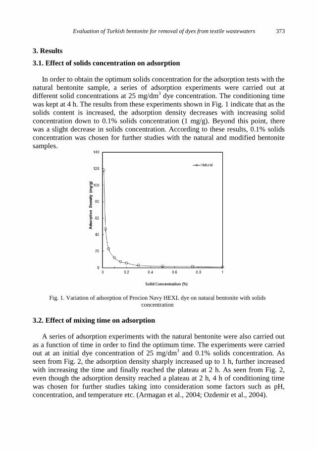
Evaluation of Turkish bentonite for removal of dyes from textile wastewaters 373
3. Results
3.1. Effect of solids concentration on adsorption
In order to obtain the optimum solids concentration for the adsorption tests with the
natural bentonite sample, a series of adsorption experiments were carried out at
different solid concentrations at 25 mg/dm3 dye concentration. The conditioning time
was kept at 4 h. The results from these experiments shown in Fig. 1 indicate that as the
solids content is increased, the adsorption density decreases with increasing solid
concentration down to 0.1% solids concentration (1 mg/g). Beyond this point, there
was a slight decrease in solids concentration. According to these results, 0.1% solids
concentration was chosen for further studies with the natural and modified bentonite
samples.
Fig. 1. Variation of adsorption of Procion Navy HEXL dye on natural bentonite with solids
concentration
3.2. Effect of mixing time on adsorption
A series of adsorption experiments with the natural bentonite were also carried out
as a function of time in order to find the optimum time. The experiments were carried
out at an initial dye concentration of 25 mg/dm3 and 0.1% solids concentration. As
seen from Fig. 2, the adsorption density sharply increased up to 1 h, further increased
with increasing the time and finally reached the plateau at 2 h. As seen from Fig. 2,
even though the adsorption density reached a plateau at 2 h, 4 h of conditioning time
was chosen for further studies taking into consideration some factors such as pH,
concentration, and temperature etc. (Armagan et al., 2004; Ozdemir et al., 2004).
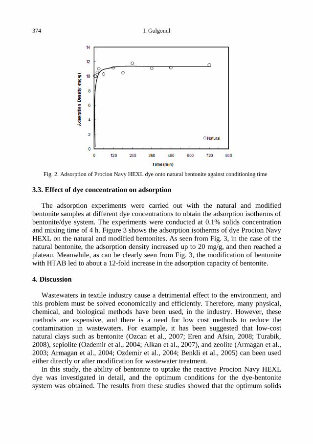
374 I. Gulgonul
Fig. 2. Adsorption of Procion Navy HEXL dye onto natural bentonite against conditioning time
3.3. Effect of dye concentration on adsorption
The adsorption experiments were carried out with the natural and modified
bentonite samples at different dye concentrations to obtain the adsorption isotherms of
bentonite/dye system. The experiments were conducted at 0.1% solids concentration
and mixing time of 4 h. Figure 3 shows the adsorption isotherms of dye Procion Navy
HEXL on the natural and modified bentonites. As seen from Fig. 3, in the case of the
natural bentonite, the adsorption density increased up to 20 mg/g, and then reached a
plateau. Meanwhile, as can be clearly seen from Fig. 3, the modification of bentonite
with HTAB led to about a 12-fold increase in the adsorption capacity of bentonite.
4. Discussion
Wastewaters in textile industry cause a detrimental effect to the environment, and
this problem must be solved economically and efficiently. Therefore, many physical,
chemical, and biological methods have been used, in the industry. However, these
methods are expensive, and there is a need for low cost methods to reduce the
contamination in wastewaters. For example, it has been suggested that low-cost
natural clays such as bentonite (Ozcan et al., 2007; Eren and Afsin, 2008; Turabik,
2008), sepiolite (Ozdemir et al., 2004; Alkan et al., 2007), and zeolite (Armagan et al.,
2003; Armagan et al., 2004; Ozdemir et al., 2004; Benkli et al., 2005) can been used
either directly or after modification for wastewater treatment.
In this study, the ability of bentonite to uptake the reactive Procion Navy HEXL
dye was investigated in detail, and the optimum conditions for the dye-bentonite
system was obtained. The results from these studies showed that the optimum solids
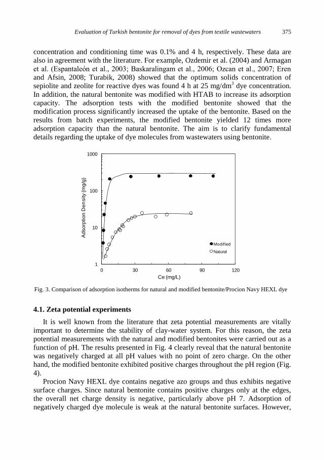
Evaluation of Turkish bentonite for removal of dyes from textile wastewaters 375
concentration and conditioning time was 0.1% and 4 h, respectively. These data are
also in agreement with the literature. For example, Ozdemir et al. (2004) and Armagan
et al. (Espantaleόn et al., 2003; Baskaralingam et al., 2006; Ozcan et al., 2007; Eren
and Afsin, 2008; Turabik, 2008) showed that the optimum solids concentration of
sepiolite and zeolite for reactive dyes was found 4 h at 25 mg/dm3 dye concentration.
In addition, the natural bentonite was modified with HTAB to increase its adsorption
capacity. The adsorption tests with the modified bentonite showed that the
modification process significantly increased the uptake of the bentonite. Based on the
results from batch experiments, the modified bentonite yielded 12 times more
adsorption capacity than the natural bentonite. The aim is to clarify fundamental
details regarding the uptake of dye molecules from wastewaters using bentonite.
Fig. 3. Comparison of adsorption isotherms for natural and modified bentonite/Procion Navy HEXL dye
4.1. Zeta potential experiments
It is well known from the literature that zeta potential measurements are vitally
important to determine the stability of clay-water system. For this reason, the zeta
potential measurements with the natural and modified bentonites were carried out as a
function of pH. The results presented in Fig. 4 clearly reveal that the natural bentonite
was negatively charged at all pH values with no point of zero charge. On the other
hand, the modified bentonite exhibited positive charges throughout the pH region (Fig.
4).
Procion Navy HEXL dye contains negative azo groups and thus exhibits negative
surface charges. Since natural bentonite contains positive charges only at the edges,
the overall net charge density is negative, particularly above pH 7. Adsorption of
negatively charged dye molecule is weak at the natural bentonite surfaces. However,
1
10
100
1000
0 30 60 90 120
Ad
so
rptio
n D
en
sity (m
g/g
)
Ce (mg/L)
Modif ied
Natural
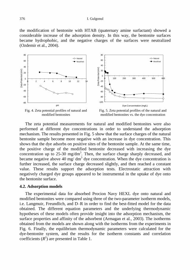
376 I. Gulgonul
the modification of bentonite with HTAB (quaternary amine surfactant) showed a
considerable increase of the adsorption density. In this way, the bentonite surfaces
became hydrophobic, and the negative charges of the surfaces were neutralized
(Ozdemir et al., 2004).
Fig. 4. Zeta potential profiles of natural and
modified bentonites Fig. 5. Zeta potential profiles of the natural and
modified bentonites vs. the dye concentration
The zeta potential measurements for natural and modified bentonites were also
performed at different dye concentrations in order to understand the adsorption
mechanism. The results presented in Fig. 5 show that the surface charges of the natural
bentonite sample become more negative with an increase in dye concentration. This
shows that the dye adsorbs on positive sites of the bentonite sample. At the same time,
the positive charge of the modified bentonite decreased with increasing the dye
concentration up to 25-30 mg/dm3. Then, the surface charge sharply decreased, and
became negative above 40 mg/ dm3 dye concentration. When the dye concentration is
further increased, the surface charge decreased slightly, and then reached a constant
value. These results support the adsorption tests. Electrostatic attraction with
negatively charged dye groups appeared to be instrumental in the uptake of dye onto
the bentonite surface.
4.2. Adsorption models
The experimental data for absorbed Procion Navy HEXL dye onto natural and
modified bentonites were compared using three of the two-parameter isotherm models,
i.e. Langmuir, Freundlich, and D–R in order to find the best-fitted model for the data
obtained. The different equation parameters and the underlying thermodynamic
hypotheses of these models often provide insight into the adsorption mechanism, the
surface properties and affinity of the adsorbent (Armagan et al., 2003). The isotherms
obtained from the models are shown along with the isotherms from the experiments in
Fig. 6. Finally, the equilibrium thermodynamic parameters were calculated for the
dye-bentonite system, and the results for the isotherm constants and correlation
coefficients (R2) are presented in Table 1.
-80
-60
-40
-20
0
20
40
60
80
0 2 4 6 8 10 12 14
Ze
ta P
ote
ntia
l (m
V)
pH
Natural
Modif ied
-100
-80
-60
-40
-20
0
20
40
60
80
0 100 200 300 400 500 600
Ze
ta P
ote
ntia
l (m
V)
Dye Concentration (mg/L)
Natural
Modif ied
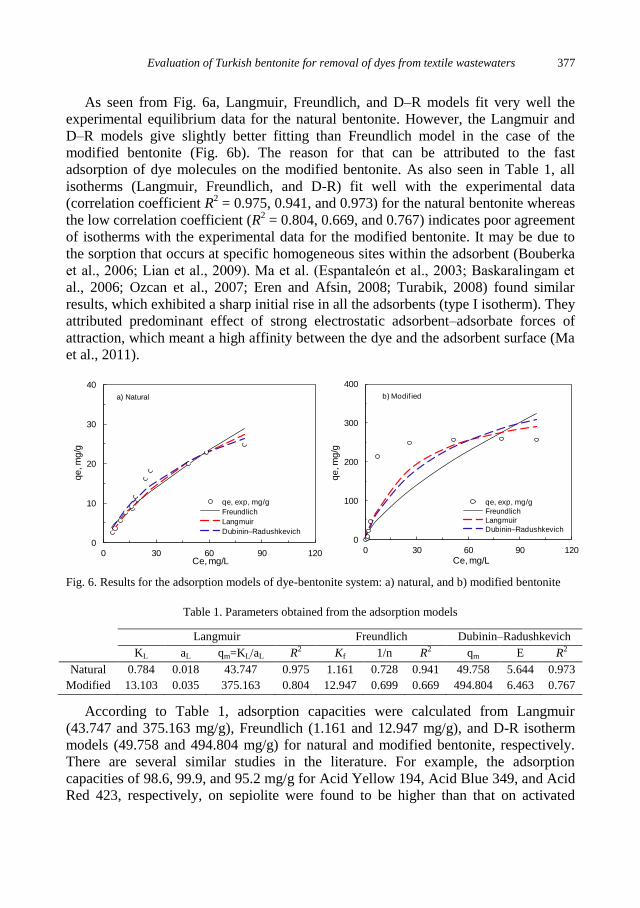
Evaluation of Turkish bentonite for removal of dyes from textile wastewaters 377
As seen from Fig. 6a, Langmuir, Freundlich, and D–R models fit very well the
experimental equilibrium data for the natural bentonite. However, the Langmuir and
D–R models give slightly better fitting than Freundlich model in the case of the
modified bentonite (Fig. 6b). The reason for that can be attributed to the fast
adsorption of dye molecules on the modified bentonite. As also seen in Table 1, all
isotherms (Langmuir, Freundlich, and D-R) fit well with the experimental data
(correlation coefficient R2 = 0.975, 0.941, and 0.973) for the natural bentonite whereas
the low correlation coefficient (R2 = 0.804, 0.669, and 0.767) indicates poor agreement
of isotherms with the experimental data for the modified bentonite. It may be due to
the sorption that occurs at specific homogeneous sites within the adsorbent (Bouberka
et al., 2006; Lian et al., 2009). Ma et al. (Espantaleόn et al., 2003; Baskaralingam et
al., 2006; Ozcan et al., 2007; Eren and Afsin, 2008; Turabik, 2008) found similar
results, which exhibited a sharp initial rise in all the adsorbents (type I isotherm). They
attributed predominant effect of strong electrostatic adsorbent–adsorbate forces of
attraction, which meant a high affinity between the dye and the adsorbent surface (Ma
et al., 2011).
Fig. 6. Results for the adsorption models of dye-bentonite system: a) natural, and b) modified bentonite
Table 1. Parameters obtained from the adsorption models
Langmuir Freundlich Dubinin–Radushkevich
KL aL qm=KL/aL R2 Kf 1/n R2 qm E R2
Natural 0.784 0.018 43.747 0.975 1.161 0.728 0.941 49.758 5.644 0.973
Modified 13.103 0.035 375.163 0.804 12.947 0.699 0.669 494.804 6.463 0.767
According to Table 1, adsorption capacities were calculated from Langmuir
(43.747 and 375.163 mg/g), Freundlich (1.161 and 12.947 mg/g), and D-R isotherm
models (49.758 and 494.804 mg/g) for natural and modified bentonite, respectively.
There are several similar studies in the literature. For example, the adsorption
capacities of 98.6, 99.9, and 95.2 mg/g for Acid Yellow 194, Acid Blue 349, and Acid
Red 423, respectively, on sepiolite were found to be higher than that on activated
0
10
20
30
40
0 30 60 90 120
qe
, m
g/g
Ce, mg/L
qe, exp, mg/g
Freundlich
Langmuir
Dubinin–Radushkevich
Two-parameter izotherms
a) Natural
0
100
200
300
400
0 30 60 90 120
qe
, m
g/g
Ce, mg/L
qe, exp, mg/g
Freundlich
Langmuir
Dubinin–Radushkevich
b) Modif ied
378 I. Gulgonul
carbon (49.2, 68.2, and 26.3 mg/g) but similar to that on natural bentonite (24.9, 92.7,
and 29.1 mg/g) (Espantaleόn et al., 2003; Baskaralingam et al., 2006; Ozcan et al.,
2007; Eren and Afsin, 2008; Turabik, 2008).
Qiao et al. (2009) measured single dye adsorption equilibrium and analyzed the
experimental data with the Langmuir, Freundlich and Redlich-Peterson isotherms.
Their results fit well Redlich-Peterson model and provided the best correlation of the
experimental data and also the adsorption capacities estimated from the Langmuir
model for AR18 and AY23 were at 69.8 and 75.4 mg/g, respectively. Ozcan et al.
(Ozcan et al., 2004) compared the results of natural and modified bentonite using
dodecyl trimethylammonium bromide (DTMA) for the removal of acid blue 193. The
adsorption capacity of DTMA-bentonite (740.5 mg/g) was found to be about 11-fold
higher than that of Na-bentonite (67.1 mg/g) at 20C. Ozcan et al. (2007) also found
out that adsorption capacity was 206.58 mg/g for DTMA-bentonite in acidic solutions
for the removal of reactive Blue 19, and adsorption isotherm data were fitted to the
Langmuir model.
Ma et al. (2011) emphasized that the adsorption capacity of organobentonite was
affected by the surfactant alkyl chain length. The longer chain surfactant of modified
bentonite shows higher adsorption capacity. As the surfactant carbon chain length
decreased from C16 to C8, the adsorption capacities of Orange II decreased from
298.39 mg/g to 144.08 mg/g. The adsorption capacities of Orange G showed the same
tendency (from 170.46 to 94.72 mg/g). Eren (Eren, 2009) showed that Langmuir
monolayer adsorption capacities of raw and manganese oxide modified bentonite as
131 and 457 mg/g, respectively. The Langmuir model with the maximum adsorption
capacity of 227.27 mg/g agreed very well with experimental data whereas Freundlich
model yielded 119.40 mg/g adsorption capacity (Lian et al., 2009).
For the D-R isotherm, E (kJ/mole) gives information about the type of adsorption
(physical, chemical, and ion exchange). The energy of adsorption refers to transfer of
one mole of ion from the bulk to the interface. When this value of free energy is in the
range of 1-8 kJ/mole, the adsorption type can be classified as physical (Helferrich,
1962). An energy range between 8 and 16 kJ/mole indicates ion exchange (Cestari et
al., 2007) and when the energy is more than 16 kJ/mole the type of adsorption can be
stated as chemical adsorption (Basar, 2006; Tahir and Rauf, 2006). Because the
magnitude of E calculated from the D-R isotherm is lower than 8 kJ/mole for both
natural and modified bentonites, the adsorption mechanism of dye onto bentonite can
be described by physical interactions. Tahir and Rauf (2006) found that the adsorption
free energy from D-R isotherm for uptake of Malachite Green oxalate dye on
bentonite at different temperatures were between 1.00 and 1.13 kJ/mole corresponding
to physical adsorption. On the other hand Eren (2009) found that adsorption energy
from D-R isotherm for Crystal Violet onto raw and modified bentonite were 11.47 and
19.55 kJ/mole, the adsorption type can be explained based on ion exchange and
chemical adsorption, respectively.
Evaluation of Turkish bentonite for removal of dyes from textile wastewaters 379
5. Conclusions
The adsorption of Procion Navy HEXL on the bentonite sample was systematically
investigated. The results showed that while the natural bentonite has an adsorption
capacity of about 20 mg/g, bentonite modified with quaternary amines significantly
increased its capacity (about 12 times, 250 mg/g). The zeta potential experiments
indicated that the adsorption mechanism of dye on the modified bentonite is governed
by electrostatic attraction of negatively charged dye groups on the positively charged
surface. Finally, the adsorption data obtained from the experiments were analyzed
using the adsorption models, i.e. Langmuir, Freundlich, and D–R. The results indicate
that while all three models demonstrated a good correlation for the adsorption of dye
molecules on the natural bentonite, it was not so good on modified bentonite.
These results clearly showed that modified bentonite could be used for the removal
of dyes in textile wastewaters due to its low cost and high yield. This will be not only
a good alternative to high cost absorbents such as activated carbon and polymer resins,
but also help solve environmental problems.
References
ALKAN, M., DEMIRBAS, O., DOĞAN, M., 2007, Adsorption kinetics and thermodynamics of an
anionic dye onto sepiolite, Micropor. Mesopor. Mat., 101(3), 388–396.
ARBELOA, F.L., ARBELOA, T.L., ARBELOA, I.L., 1997, Spectroscopy of rhodamine 6G adsorbed on
sepiolite aqueous suspensions, J. Colloid Interf. Sci., 187(1), 105–112.
ARMAGAN, B., OZDEMIR, O., TURAN, M., CELIK, M.S., 2003, Adsorption of negatively charged
azo dyes onto surfactant-modified sepiolite, J. Environ. Eng., 129(8), 709–715.
ARMAGAN, B., OZDEMIR, O., TURAN, M., CELIK, M.S., 2003, The removal of reactive azo dyes by
natural and modified zeolities, J. Chem. Technol. Biot., 78(7), 725–732.
ARMAGAN, B., TURAN, M., ÇELIK, M.S., 2004, Equilibrium studies on the adsorption of reactive azo
dyes into zeolite, Desalination, 170(1), 33–39.
BASAR, C.A., 2006, Applicability of the various adsorption models of three dyes adsorption onto
activated carbon prepared waste apricot, J. Hazard. Mater. B, 135, 232–241.
BASKARALINGAM, P., PULIKESI, M., ELANGO, D., RAMAMURTHI, V., SIVANESAN, S., 2006,
Adsorption of acid dye onto organobentonite, J. Hazard. Mater., 128(2–3), 138–144.
BENKLI, Y.E., CAN, M.F., TURAN, M., CELIK, M.S., 2005, Modification of organo-zeolit surface for
the removal of reactive azo dyes in fixed-bed reactors, Water Res., 39(2–3), 487–493.
BOUBERKA, Z., KHENIFI, A., BENDERDOUCHE, N., DERRICHE, Z., 2006, Removal of Supranol
Yellow 4GL by adsorption onto Cr-intercalated montmorillonite, J. Hazard. Mater., 133(1–3), 154–
161.
BULUT, G., CHIMEDDORJ, M., ESENLI, F., CELIK, M.S., 2009, Production of desiccants
fromTurkish Bentonites, Appl. Clay Sci., 46, 141–147.
CESTARI, A.R., VIEIRA, E.F.S., VIEIRA, G.S., ALMEIDA, L.E., 2007, Aggregation and adsorption of
reactive dyes in the presence of an anionic surfactant on mesoporous aminopropyl silica, J. Colloid
Interf. Sci., 309(2), 402–411.
CORPORATION, M., 2002, User’s guide Microsoft Excel Version.
DUBININ, M.M., RADUSHKEVICH, L.V., 1947, Equation of the characteristic curve of activated
charcoal, Chem. Zentr., 1875.
EREN, B., AFSIN, B., 2008, Investigation of a basic dye adsorption from aqueous solution onto raw and
pre-treated bentonite surfaces, Dyes Pigments., 76(1), 220–225.
380 I. Gulgonul
EREN, E., 2009, Removal of basic dye by modified Unye bentonite, Turkey, J. Hazard. Mater., 162(2–3),
1355–1363.
ESPANTALEΌN, A.G., NIETO, J.A., FERNÁNDEZ, M., MARSAL, A., 2003, Use of activated clays in
the removal of dyes and surfactants from tannery waste waters, Appl. Clay Sci., 24(1), 105–110.
FREUNDLICH, H.M.F., 1906, Over the adsorption in solution, J. Phys. Chem., 57, 385–470.
HELFERRICH, F., 1962, Ion-exchange, McGraw Hill, New York, NY,
JUANG, R.S., TSENG, R.L., WU, F.C., LEE, S.H., 1997, Adsorption behavior of reactive dyes from
aqueous solutions on chitosan, J. Chem. Technol. Biot., 70(4), 391–399.
LANGMUIR, I., 1918, Adsorption of gases on plane surfaces of glass, mica and platinum, J. Am. Chem.
Soc. , 40, 1361–1403.
LIAN, L., GUO, L., WANG, A., 2009, Use of CaCl2 modified bentonite for removal of Congo red dye
from aqueous solutions, Desalination, 249(2), 797–801.
MA, J., CUIA, B., DAIB, J., LI, D., 2011, Mechanism of adsorption of anionic dye from aqueous
solutions onto organobentonite, J. Hazard. Mater., 186 (2–3), 1758–1765.
MCKAY, G., 1982, Adsorption of dyestuffs from aqueous solutions with activated carbon I: equilibrium
and batch contact-time studies, J. Chem. Technol. Biot., 32, 759–772.
OZCAN, A., OMEROGLU, C., ERDOGAN, Y., OZCAN, A.S., 2007, Modification of bentonite with a
cationic surfactant: an adsorption study of textile dye Reactive Blue 19, J. Hazard. Mater., 140(1–2),
173–179.
OZCAN, A.S., ERDEM, B., OZCAN, A., 2004, Adsorption of acid blue 193 from aqueous solutions onto
Na-bentonite and DTMA-bentonite, J. Colloid Interf. Sci., 280(1), 44–54.
OZDEMIR, O., ARMAGAN, B., TURAN, M., CELIK, M.S., 2004, Comparison of adsorption
characteristic of azo-reactive dyes on mezoporous minerals, Dyes and Pigments, 62(1), 49–60.
QIAOA, S., HUA, Q., HAGHSERESHTA, F., HUB, X., LUA, G.Q.M., 2009, An investigation on the
adsorption of acid dyes on bentonite based composite adsorbent, Sep. Purif. Technol., 67, 218–225.
RYTWO, G., NIR, S., CREPSIN, M., MARGULIES, L., 2000, Adsorption and interactions of methyl
green with montmorillonite and sepiolite, J. Colloid Interf. Sci., 222(1), 12–19.
SABAH, E., 1998, Adsorption mechanism of various amines onto sepiolite, Ph.D. Thesis, Osmangazi
University, Eskisehir,
TAHIR, S.S., RAUF, N., 2006, Removal of a cationic dye from aqueous solutions by adsorption onto
bentonite clay, Chemosphere, 63(11), 1842–1848.
TURABIK, M., 2008, Adsorption of basic dyes from single and binary component systems onto
bentonite: simultaneous analysis of Basic Red 46 and Basic Yellow 28 by first order derivative
spectrophotometric analysis methods, J. Hazard. Mater., 158(1), 52–64.
WANG, C.C., JUANG, L.C., HSU, T.C., LEE, C.K., LEE, J.F., HUANG, F.C., 2004, Adsorption of basic
dyes onto montmorillonite, J. Colloid Interf. Sci., 273(1), 80–86
http://dx.doi.org/10.5277/ppmp120205
Physicochem. Probl. Miner. Process. 48(2), 2012, 381−392 Physicochemical Problems
of Mineral Processing
w w w . m i n p r o c . p w r . w r o c . p l / j o u r n a l / ISSN 1643-1049 (print)
ISSN 2084-4735 (online)
Received December 10, 2011; reviewed; accepted February 8, 2012
BENEFICIATION OF LOW-GRADE FELDSPAR ORE USING
CYCLOJET FLOTATION CELL, CONVENTIONAL CELL AND
MAGNETIC SEPARATOR
Hasan HACIFAZLIOGLU, Ilgin KURSUN, Mert TERZI
Istanbul University, Engineering Faculty, Mining Engineering Department, Avcılar, Istanbul,
Abstract. In order to increase the quality of feldspar ore and to obtain sellable feldspar
concentrate, it is necessary to remove coloring impurities such as iron and titanium contained
in it. For the removal of coloring minerals from feldspar ore the most widely used method is
reverse flotation method. Reverse flotation process is generally carried out in conventional
mechanical cells. In this study, it was aimed to enrich low-grade feldspar by using cyclojet
flotation cell which was developed as an alternative to conventional cell. Then, experiments
were performed by using conventional cell and wet magnetic separator and the results were
compared with the flotation results obtained by using cyclojet cell. In experimental studies, 200
micrometer grain sized feldspar (albite) ore obtained from Muğla province at the west side of
Turkey was used. It was detected that the sample was containing 0.100% Fe2O3 and 0.360%
TiO2 as coloring minerals. Cyclojet cell, conventional cell and magnetic separator reduced the
Fe2O3 content down to 0.010%, but TiO2 content was different in the concentrates obtained by
different devices. There was almost no reduction in TiO2 content by magnetic separation
method. Cyclojet cell reduced TiO2 content down to 0.030% and mechanical cell reduced TiO2
content down to 0.020%. The weights of the concentrate were detected as the highest (92.70%)
in magnetic separator and as the lowest (75.40%) in cyclojet cell. Therefore, it is possible to
say that cyclojet cell can compete with mechanical cell and removal of TiO2 in cyclojet cell is
much better than the removal of TiO2 in magnetic separator. Generally, in the flotation process
performed by using a reagent of Aero801 and Aero825 mixture in natural pH medium, both
Fe2O3 and TiO2 can be removed at a rate of up to 90%, but magnetic separator can only remove
Fe2O3 mineral.
keywords: feldspar, separation, flotation
1. Introduction
Feldspar is an important industrial raw material used in ceramic, porcelain and
glass industries. Sixty percent of the World feldspar production is used in ceramic
industry, 35% is used in glass industry, and 5% is used in welding electrode, rubber,
plastic and paint industry as filling material. It is known that total feldspar reserves of
the World is 1.740106
Mg and a large part of this reserve is located in Asia. Turkey

382 H. Hacifazlioglu et al.
has a reserve of 240106 Mg which is 14% of the World feldspar reserves and it has the
largest Na-feldspar reserves among other countries in the World (Bayraktar et al.,
1998; Kangal and Guney, 2002; Anonymous, 2010). Commercial and the most
important ones of feldspar group minerals are albite (NaAlSi3O8), orthoclase
(KAISi3O8) and anorthite (CaAl2Si2O8) which are named according to the Na, K, and
Ca contents in their structures. Since there are not many commercial anorthite deposits
in the World, feldspar production mainly depends on albite and orthoclase minerals
(Bayraktar et al., 2001; Karaguzel and Çobanoğlu, 2010).
Iron and titanium minerals existing in mineralogical structures of feldspar are
known as unwanted impurities because of their coloring properties. Therefore, Fe2O3
and TiO2 contents of 0.50% or below are required in feldspar. The main impurity
minerals observed in feldspar ores are rutile and sphene for titanium, mica minerals
and minerals such as garnet, hematite, hornblende, tourmaline, biotite, and muscovite
for iron oxides. In case that the amounts of these minerals are higher than the specific
values, the quality of glass and ceramic decreases and the color changes accordingly.
Therefore, the main goal in enrichment of feldspars is based on removal of the
coloring minerals from the ore. Magnetic separation appears to be the most
appropriate method for enrichment of feldspars in terms of cost and simplicity.
However, flotation method is generally preferred according to the mineralogical
property because magnetic susceptibilities of titanium minerals such as sphene and
rutile are very low and also magnetic separators used in this area can perform efficient
separation down to a specific grain size. Conventional reverse flotation method is still
the most widely used method in the World for the removal of the impurities in
feldspars. On the other hand, chemical and biological methods also can be used for the
removal of impurities. In chemical method, feldspar is leached by organic and
inorganic acids and in biological method, microorganisms are used instead of
chemicals (Styriakovaa et al., 2006; El-Rehiem and Abd El-Rahman, 2008).
Agglomeration or selective flocculation methods are also used for enrichment of
feldspar (Doğu and Arol, 2004).
In this study, Na-feldspar ore obtained from Muğla province (Turkey) was enriched
by cyclojet cell which is an alternative jet flotation technique, conventional cell and
magnetic separator and the results obtained from the devices were compared.
2. Experimental studies
2.1. Cyclojet flotation cell
Cyclojet cell is a high density jet flotation cell developed in Turkey in 2006 for the
enrichment of coal slimes. In the previous studies, outstanding success of cyclojet for
the enrichment of coal slime has been proven by many researches. It was observed that
clean coals containing ash between 7% and 15% were obtained from coal slime having
ash contents of about 45-55% fed into cyclojet cell (Hacıfazlıoğlu, 2009;
Hacıfazlıoglu and Toroğlu, 2008). This device, which is effective in enrichment of
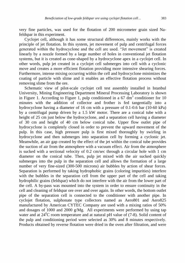
Beneficiation of low-grade feldspar ore using cyclojet flotation cell… 383
very fine particles, was used for the flotation of 200 micrometer grain sized Na-
feldspar in this experiment.
Cyclojet cell, although it has some structural differences, mainly works with the
principle of jet flotation. In this system, jet movement of pulp and centrifugal forces
generated within the hydrocyclone and the cell are used. “Jet movement” is created
linearly by a nozzle formed by a large number of holes in conventional jet flotation
systems, but it is created as cone-shaped by a hydrocyclone apex in a cyclojet cell. In
other words, pulp jet created in a cyclojet cell submerges into cell with a cyclonic
move and creates a more efficient flotation providing more intensive shearing forces.
Furthermore, intense mixing occurring within the cell and hydrocyclone minimizes the
coating of particle with slime and it enables an effective flotation process without
removing slime from the ore.
Schematic view of pilot-scale cyclojet cell test assembly installed in Istanbul
University, Mining Engineering Department Mineral Processing Laboratory is shown
in Figure 1. According to Figure 1, pulp conditioned in a 67 dm3 conditioner for 10
minutes with the addition of collector and frother is fed tangentially into a
hydrocyclone having a diameter of 16 cm with a pressure of 0.1-0.6 bar (10-60 kPa)
by a centrifugal pump driven by a 1.5 kW motor. There are a conical tube with a
height of 25 cm just below the hydrocyclone, and a separation cell having a diameter
of 30 cm and height of 40 cm below conical tube. Upper flow outlet pipe of
hydrocyclone is completely closed in order to prevent the upward movement of the
pulp. In this case, high pressure pulp is first mixed thoroughly by swirling in
hydrocyclone and then submerges into separation cell by forming a cyclonic jet.
Meanwhile, an air gap created by the effect of the jet within the conical tube provides
the suction of air from the atmosphere with a vacuum effect. Air from the atmosphere
is sucked with a sectional velocity of 0.2 cm/sec through a circular hole with 1 cm
diameter on the conical tube. Then, pulp jet mixed with the air sucked quickly
submerges into the pulp in the separation cell and allows the formation of a large
number of very fine-sized (300-500 microns) air bubbles by action of shear forces.
Separation is performed by taking hydrophobic grains (coloring impurities) interfere
with the bubbles in the separation cell from the upper part of the cell and taking
hydrophilic grains (feldspar) which do not interfere with the air from the lower part of
the cell. A by-pass was mounted into the system in order to ensure continuity in the
cell and cleaning of feldspar ore over and over again. In other words, the bottom outlet
pipe of the separation cell is connected to the conditioner with another pipe. In
cyclojet flotation, sulphonate type collectors named as Aero801 and Aero825
manufactured by American CYTEC Company are used with a mixing ratios of 50%
and dosages of 1000 and 2000 g/Mg. All experiments were performed by using tap
water and at 240C room temperature and at natural pH value of (7-8). Solid content of
the pulp and conditioning period were selected as 30% and 8 minutes respectively.
Products obtained by reverse flotation were dried in the oven after filtration, and were
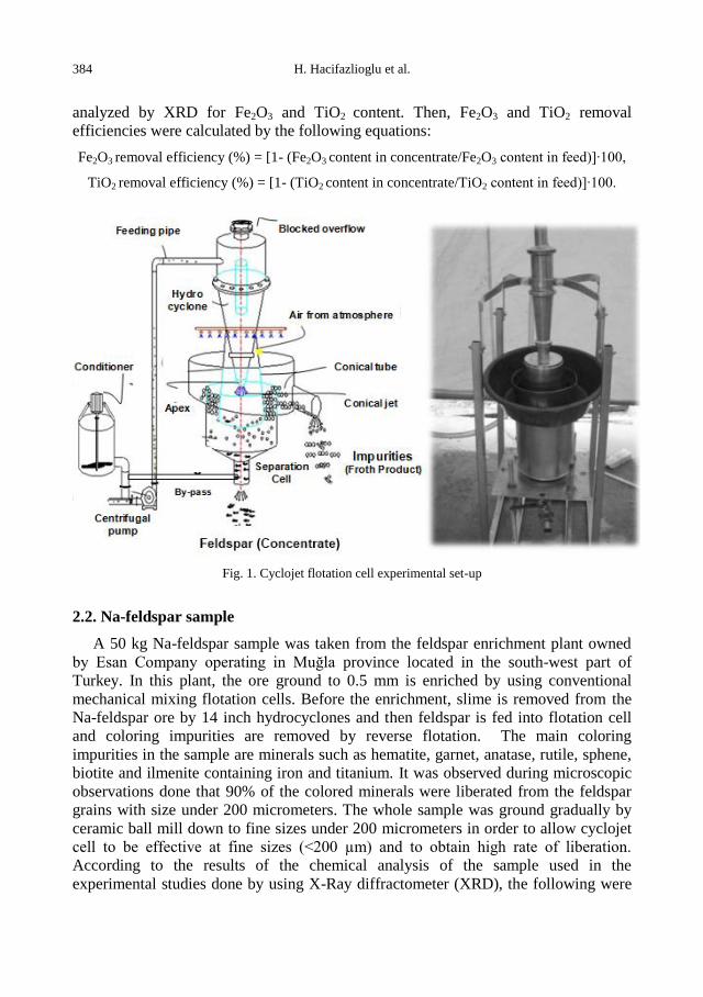
384 H. Hacifazlioglu et al.
analyzed by XRD for Fe2O3 and TiO2 content. Then, Fe2O3 and TiO2 removal
efficiencies were calculated by the following equations:
Fe2O3 removal efficiency (%) = [1- (Fe2O3 content in concentrate/Fe2O3 content in feed)]∙100,
TiO2 removal efficiency (%) = [1- (TiO2 content in concentrate/TiO2 content in feed)]∙100.
Fig. 1. Cyclojet flotation cell experimental set-up
2.2. Na-feldspar sample
A 50 kg Na-feldspar sample was taken from the feldspar enrichment plant owned
by Esan Company operating in Muğla province located in the south-west part of
Turkey. In this plant, the ore ground to 0.5 mm is enriched by using conventional
mechanical mixing flotation cells. Before the enrichment, slime is removed from the
Na-feldspar ore by 14 inch hydrocyclones and then feldspar is fed into flotation cell
and coloring impurities are removed by reverse flotation. The main coloring
impurities in the sample are minerals such as hematite, garnet, anatase, rutile, sphene,
biotite and ilmenite containing iron and titanium. It was observed during microscopic
observations done that 90% of the colored minerals were liberated from the feldspar
grains with size under 200 micrometers. The whole sample was ground gradually by
ceramic ball mill down to fine sizes under 200 micrometers in order to allow cyclojet
cell to be effective at fine sizes (<200 µm) and to obtain high rate of liberation.
According to the results of the chemical analysis of the sample used in the
experimental studies done by using X-Ray diffractometer (XRD), the following were
Beneficiation of low-grade feldspar ore using cyclojet flotation cell… 385
detected: SiO2 67.38%; Al2O3 19.28%, Fe2O3 0.10%, TiO2 0.36%, MgO 0.25%, CaO
1.08%, K2O 0.43% and Na2O 10.07%.
3. Results and discussion
3.1. Optimization of cyclojet operation parameters
Some of the parameters of the study should be optimized in order to allow cyclojet
cell to be effective in feldspar flotation. The most important ones are amount of
reagent, pulp pressure, conical jet length and conical tube submerging depth. In the
experiments performed to find the effect of the amount of reagent (collector), feeding
pressure, conical jet height and conical tube submerging depth, solid concentration
were set to 40 kPa, 10 cm, 30% respectively. In all experiments, total conditioning
time was set to 8 minutes and total flotation time (froth removal time) was set to 10
minutes. Any additional frother or any chemical for pH adjustment were not used in
the experiments since the Aero 801 and Aero 825 collectors have frothing
characteristics. All experiments were performed by using tap water and at natural pH
value of 7-8. The effects of various parameters on concentrate and waste
characteristics during cyclojet flotation are given in Table 1. Every optimum
parameter obtained was used in the next experiment.
Table 1. The effects of various parameters on concentrate and waste characteristics during cyclojet
flotation
Parameters Values Concentrate
(Feldspar)
Reject
(impurities)
Fe2O3
content(%)
TiO2
content(%)
Wt.
(%)
Fe2O3
content(%)
TiO2
content(%)
Wt.
(%)
Reagent
Aero801+825
(g/Mg)
750 0.070 0.230 76.600 0.198 0.786 23.400
1500 0.020 0.040 67.200 0.264 1.016 32.800
Feed pressure
(kPa)
10 0.090 0.270 82.200 0.146 0.776 17.800
40 0.010 0.040 65.400 0.270 0.965 34.600
Conical
jet lenght
(cm)
10 0.010 0.030 66.100 0.275 1.003 33.900
20 0.060 0.190 70.100 0.194 0.759 29.900
Conical tube
submerging
depth
(cm)
10 0.010 0.030 67.000 0.283 91.667 33.000
20 0.050 0.150 74.000 0.242 58.333 26.000
As shown in Table 1, removal of both Fe2O3 and TiO2 increased with the increase
in reagent amount. By increasing the reagent amount from a dosage of 750 g/Mg to a
dosage of 1500 g/Mg, the Fe2O3 content in the concentrate was decreasing from
0.070% to 0.020%, while TiO2 content decreased from 0,230% to 0,040%. Increase in
the reagents amount provided flotation of greater amounts of impurities. On the other
hand, with a fixed reagents dosage (1500 g/Mg), the Fe2O3 content in the concentrate
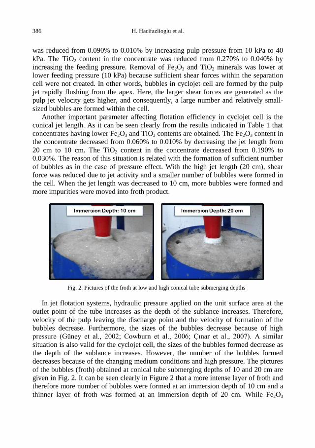
386 H. Hacifazlioglu et al.
was reduced from 0.090% to 0.010% by increasing pulp pressure from 10 kPa to 40
kPa. The TiO2 content in the concentrate was reduced from 0.270% to 0.040% by
increasing the feeding pressure. Removal of Fe2O3 and TiO2 minerals was lower at
lower feeding pressure (10 kPa) because sufficient shear forces within the separation
cell were not created. In other words, bubbles in cyclojet cell are formed by the pulp
jet rapidly flushing from the apex. Here, the larger shear forces are generated as the
pulp jet velocity gets higher, and consequently, a large number and relatively small-
sized bubbles are formed within the cell.
Another important parameter affecting flotation efficiency in cyclojet cell is the
conical jet length. As it can be seen clearly from the results indicated in Table 1 that
concentrates having lower Fe2O3 and TiO2 contents are obtained. The Fe2O3 content in
the concentrate decreased from 0.060% to 0.010% by decreasing the jet length from
20 cm to 10 cm. The TiO2 content in the concentrate decreased from 0.190% to
0.030%. The reason of this situation is related with the formation of sufficient number
of bubbles as in the case of pressure effect. With the high jet length (20 cm), shear
force was reduced due to jet activity and a smaller number of bubbles were formed in
the cell. When the jet length was decreased to 10 cm, more bubbles were formed and
more impurities were moved into froth product.
Fig. 2. Pictures of the froth at low and high conical tube submerging depths
In jet flotation systems, hydraulic pressure applied on the unit surface area at the
outlet point of the tube increases as the depth of the sublance increases. Therefore,
velocity of the pulp leaving the discharge point and the velocity of formation of the
bubbles decrease. Furthermore, the sizes of the bubbles decrease because of high
pressure (Güney et al., 2002; Cowburn et al., 2006; Çınar et al., 2007). A similar
situation is also valid for the cyclojet cell, the sizes of the bubbles formed decrease as
the depth of the sublance increases. However, the number of the bubbles formed
decreases because of the changing medium conditions and high pressure. The pictures
of the bubbles (froth) obtained at conical tube submerging depths of 10 and 20 cm are
given in Fig. 2. It can be seen clearly in Figure 2 that a more intense layer of froth and
therefore more number of bubbles were formed at an immersion depth of 10 cm and a
thinner layer of froth was formed at an immersion depth of 20 cm. While Fe2O3
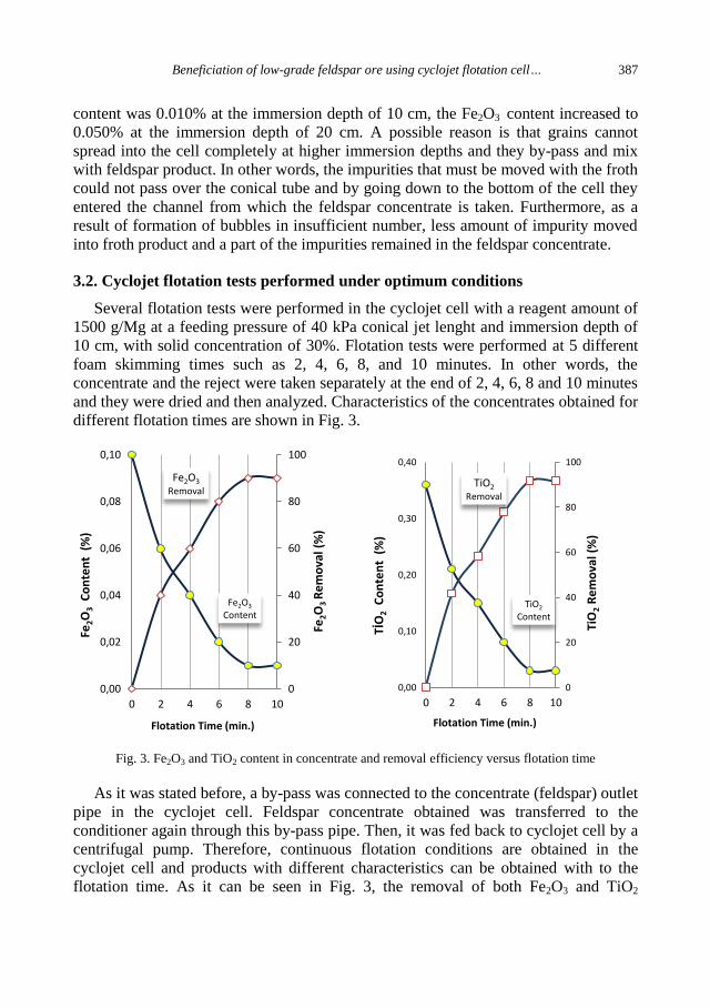
Beneficiation of low-grade feldspar ore using cyclojet flotation cell… 387
content was 0.010% at the immersion depth of 10 cm, the Fe2O3 content increased to
0.050% at the immersion depth of 20 cm. A possible reason is that grains cannot
spread into the cell completely at higher immersion depths and they by-pass and mix
with feldspar product. In other words, the impurities that must be moved with the froth
could not pass over the conical tube and by going down to the bottom of the cell they
entered the channel from which the feldspar concentrate is taken. Furthermore, as a
result of formation of bubbles in insufficient number, less amount of impurity moved
into froth product and a part of the impurities remained in the feldspar concentrate.
3.2. Cyclojet flotation tests performed under optimum conditions
Several flotation tests were performed in the cyclojet cell with a reagent amount of
1500 g/Mg at a feeding pressure of 40 kPa conical jet lenght and immersion depth of
10 cm, with solid concentration of 30%. Flotation tests were performed at 5 different
foam skimming times such as 2, 4, 6, 8, and 10 minutes. In other words, the
concentrate and the reject were taken separately at the end of 2, 4, 6, 8 and 10 minutes
and they were dried and then analyzed. Characteristics of the concentrates obtained for
different flotation times are shown in Fig. 3.
Fig. 3. Fe2O3 and TiO2 content in concentrate and removal efficiency versus flotation time
As it was stated before, a by-pass was connected to the concentrate (feldspar) outlet
pipe in the cyclojet cell. Feldspar concentrate obtained was transferred to the
conditioner again through this by-pass pipe. Then, it was fed back to cyclojet cell by a
centrifugal pump. Therefore, continuous flotation conditions are obtained in the
cyclojet cell and products with different characteristics can be obtained with to the
flotation time. As it can be seen in Fig. 3, the removal of both Fe2O3 and TiO2
Fe2O3 Removal
Fe2O3
Content
0
20
40
60
80
100
0,00
0,02
0,04
0,06
0,08
0,10
0 2 4 6 8 10
Fe2O
3 C
on
ten
t (
%)
Flotation Time (min.)
Fe2O
3 R
em
ova
l (%
)
TiO2 Removal
TiO2
Content
0
20
40
60
80
100
0,00
0,10
0,20
0,30
0,40
0 2 4 6 8 10
TİO
2 C
on
ten
t (
%)
Flotation Time (min.)
TiO
2 R
em
ova
l (%
)
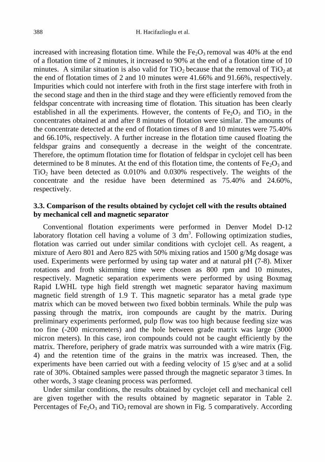
388 H. Hacifazlioglu et al.
increased with increasing flotation time. While the Fe2O3 removal was 40% at the end
of a flotation time of 2 minutes, it increased to 90% at the end of a flotation time of 10
minutes. A similar situation is also valid for TiO2 because that the removal of TiO2 at
the end of flotation times of 2 and 10 minutes were 41.66% and 91.66%, respectively.
Impurities which could not interfere with froth in the first stage interfere with froth in
the second stage and then in the third stage and they were efficiently removed from the
feldspar concentrate with increasing time of flotation. This situation has been clearly
established in all the experiments. However, the contents of Fe2O3 and TiO2 in the
concentrates obtained at and after 8 minutes of flotation were similar. The amounts of
the concentrate detected at the end of flotation times of 8 and 10 minutes were 75.40%
and 66.10%, respectively. A further increase in the flotation time caused floating the
feldspar grains and consequently a decrease in the weight of the concentrate.
Therefore, the optimum flotation time for flotation of feldspar in cyclojet cell has been
determined to be 8 minutes. At the end of this flotation time, the contents of Fe2O3 and
TiO2 have been detected as 0.010% and 0.030% respectively. The weights of the
concentrate and the residue have been determined as 75.40% and 24.60%,
respectively.
3.3. Comparison of the results obtained by cyclojet cell with the results obtained
by mechanical cell and magnetic separator
Conventional flotation experiments were performed in Denver Model D-12
laboratory flotation cell having a volume of 3 dm3. Following optimization studies,
flotation was carried out under similar conditions with cyclojet cell. As reagent, a
mixture of Aero 801 and Aero 825 with 50% mixing ratios and 1500 g/Mg dosage was
used. Experiments were performed by using tap water and at natural pH (7-8). Mixer
rotations and froth skimming time were chosen as 800 rpm and 10 minutes,
respectively. Magnetic separation experiments were performed by using Boxmag
Rapid LWHL type high field strength wet magnetic separator having maximum
magnetic field strength of 1.9 T. This magnetic separator has a metal grade type
matrix which can be moved between two fixed bobbin terminals. While the pulp was
passing through the matrix, iron compounds are caught by the matrix. During
preliminary experiments performed, pulp flow was too high because feeding size was
too fine (-200 micrometers) and the hole between grade matrix was large (3000
micron meters). In this case, iron compounds could not be caught efficiently by the
matrix. Therefore, periphery of grade matrix was surrounded with a wire matrix (Fig.
4) and the retention time of the grains in the matrix was increased. Then, the
experiments have been carried out with a feeding velocity of 15 g/sec and at a solid
rate of 30%. Obtained samples were passed through the magnetic separator 3 times. In
other words, 3 stage cleaning process was performed.
Under similar conditions, the results obtained by cyclojet cell and mechanical cell
are given together with the results obtained by magnetic separator in Table 2.
Percentages of Fe2O3 and TiO2 removal are shown in Fig. 5 comparatively. According
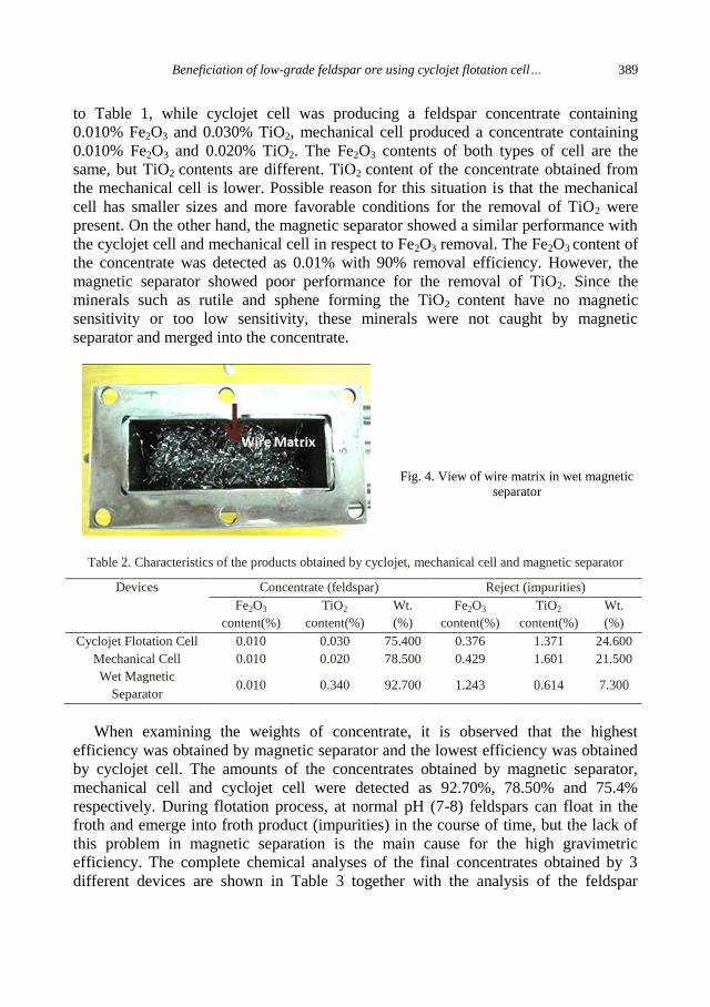
Beneficiation of low-grade feldspar ore using cyclojet flotation cell… 389
to Table 1, while cyclojet cell was producing a feldspar concentrate containing
0.010% Fe2O3 and 0.030% TiO2, mechanical cell produced a concentrate containing
0.010% Fe2O3 and 0.020% TiO2. The Fe2O3 contents of both types of cell are the
same, but TiO2 contents are different. TiO2 content of the concentrate obtained from
the mechanical cell is lower. Possible reason for this situation is that the mechanical
cell has smaller sizes and more favorable conditions for the removal of TiO2 were
present. On the other hand, the magnetic separator showed a similar performance with
the cyclojet cell and mechanical cell in respect to Fe2O3 removal. The Fe2O3 content of
the concentrate was detected as 0.01% with 90% removal efficiency. However, the
magnetic separator showed poor performance for the removal of TiO2. Since the
minerals such as rutile and sphene forming the TiO2 content have no magnetic
sensitivity or too low sensitivity, these minerals were not caught by magnetic
separator and merged into the concentrate.
Fig. 4. View of wire matrix in wet magnetic
separator
Table 2. Characteristics of the products obtained by cyclojet, mechanical cell and magnetic separator
Devices Concentrate (feldspar) Reject (impurities)
Fe2O3
content(%)
TiO2
content(%)
Wt.
(%)
Fe2O3
content(%)
TiO2
content(%)
Wt.
(%)
Cyclojet Flotation Cell 0.010 0.030 75.400 0.376 1.371 24.600
Mechanical Cell 0.010 0.020 78.500 0.429 1.601 21.500
Wet Magnetic
Separator 0.010 0.340 92.700 1.243 0.614 7.300
When examining the weights of concentrate, it is observed that the highest
efficiency was obtained by magnetic separator and the lowest efficiency was obtained
by cyclojet cell. The amounts of the concentrates obtained by magnetic separator,
mechanical cell and cyclojet cell were detected as 92.70%, 78.50% and 75.4%
respectively. During flotation process, at normal pH (7-8) feldspars can float in the
froth and emerge into froth product (impurities) in the course of time, but the lack of
this problem in magnetic separation is the main cause for the high gravimetric
efficiency. The complete chemical analyses of the final concentrates obtained by 3
different devices are shown in Table 3 together with the analysis of the feldspar
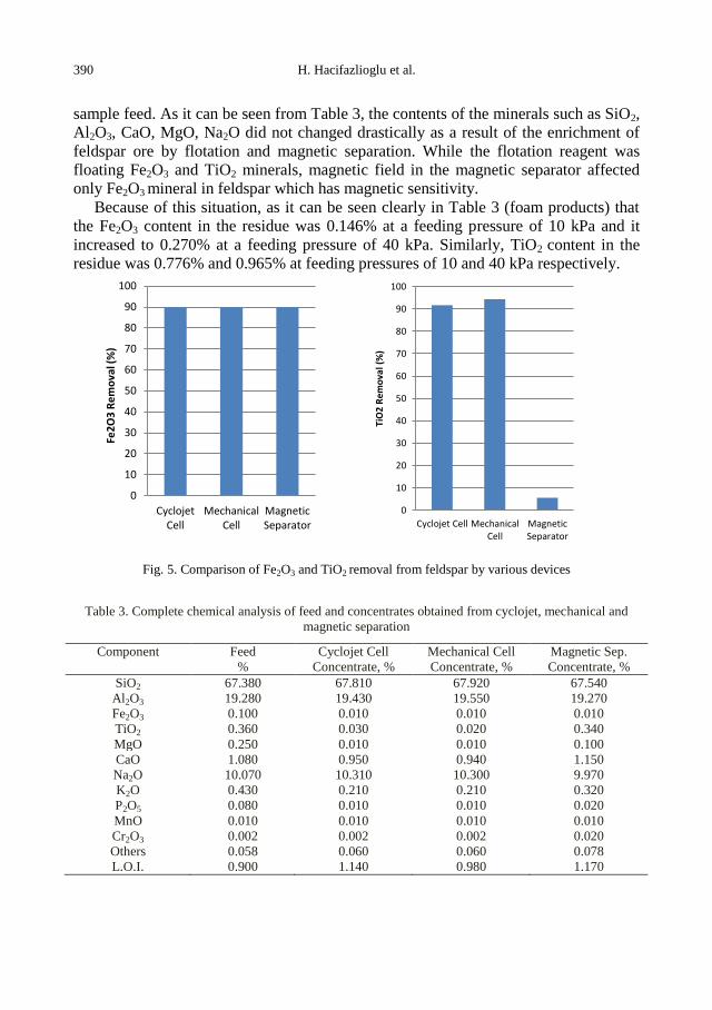
390 H. Hacifazlioglu et al.
sample feed. As it can be seen from Table 3, the contents of the minerals such as SiO2,
Al2O3, CaO, MgO, Na2O did not changed drastically as a result of the enrichment of
feldspar ore by flotation and magnetic separation. While the flotation reagent was
floating Fe2O3 and TiO2 minerals, magnetic field in the magnetic separator affected
only Fe2O3 mineral in feldspar which has magnetic sensitivity.
Because of this situation, as it can be seen clearly in Table 3 (foam products) that
the Fe2O3 content in the residue was 0.146% at a feeding pressure of 10 kPa and it
increased to 0.270% at a feeding pressure of 40 kPa. Similarly, TiO2 content in the
residue was 0.776% and 0.965% at feeding pressures of 10 and 40 kPa respectively.
Fig. 5. Comparison of Fe2O3 and TiO2 removal from feldspar by various devices
Table 3. Complete chemical analysis of feed and concentrates obtained from cyclojet, mechanical and
magnetic separation
Component Feed
%
Cyclojet Cell
Concentrate, %
Mechanical Cell
Concentrate, %
Magnetic Sep.
Concentrate, %
SiO2 67.380 67.810 67.920 67.540
Al2O3 19.280 19.430 19.550 19.270
Fe2O3 0.100 0.010 0.010 0.010
TiO2 0.360 0.030 0.020 0.340
MgO 0.250 0.010 0.010 0.100
CaO 1.080 0.950 0.940 1.150
Na2O 10.070 10.310 10.300 9.970
K2O 0.430 0.210 0.210 0.320
P2O5 0.080 0.010 0.010 0.020
MnO 0.010 0.010 0.010 0.010
Cr2O3 0.002 0.002 0.002 0.020
Others 0.058 0.060 0.060 0.078
L.O.I. 0.900 1.140 0.980 1.170
0
10
20
30
40
50
60
70
80
90
100
CyclojetCell
MechanicalCell
MagneticSeparator
Fe2
O3
Re
mo
val (
%)
0
10
20
30
40
50
60
70
80
90
100
Cyclojet Cell MechanicalCell
MagneticSeparator
TiO
2 R
emo
val (
%)
Beneficiation of low-grade feldspar ore using cyclojet flotation cell… 391
4. Conclusion
It is known that the coloring minerals found in feldspar ore can be removed
by various methods. It has been observed that 90% of Fe2O3 can be removed by
the performed flotation and magnetic separation processes, but TiO2 content
can only be removed by flotation. As a result of cyclojet flotation experiments
TiO2 content was reduced from 0.360% to 0.030%, and by magnetic separation
TiO2 content was reduced in a negligible amount down to 0.34%. Similarly,
TiO2 content was reduced down to 0.020% by the conventional flotation cell.
On the other hand, all 3 devices showed similar performances in respect to
Fe2O3 removal. The reason of this situation is that Fe2O3 mineral has magnetic
sensitivity, but TiO2 mineral have no magnetic sensitivity or low magnetic
sensitivity. It is clearly seen from the results of this study that for the ores
containing small amounts of TİO2 only magnetic separation is sufficient, but
for the ores containing high amount of TiO2 cyclojet or mechanical cell can be
used.
Acknowledgement
The authors would like to give a special thanks to Esan Inc. for the supply of the samples and XRD
analyses.
References
ANONYMOUS, 2010, Feldspar Report, TMMOB Chamber of Mining Engineers. No.169; ISBN:978-
99444-89-905-5.
BAYRAKTAR, I., ERSAYIN, S., GÜLSOY, O.Y., 1998, Magnetic separation and flotation of albite,
Innovations in Mineral Processing, Atak, Önal & Çelik (eds), Balkema, Rotterdam, ISBN:90-5809-
013-2.
BAYRAKTAR, L., ERSAYIN, S., GÜLSOY, Ö.Y., 1997, Upgrading titanium bearing Na-feldspar by
flotation using sulphonates, succinamate and soaps of vegetable oils, Miner. Eng. 12(1), 1363‒1374.
COWBURN, J., HARBORT, G., MANLAPIG, E., POKRAJCIC, Z., 2006, Improving the recovery of
coarse coal particles in a Jameson cell, Miner. Eng., 19 (6-8), 609‒618.
ÇINAR, F., ŞAHBAZ, O., ÇINAR, M., ÖTEKAYA, B.,KELEBEK, Ş., 2007, A parametric study on
Jameson cell flotation of quartz, XII Balkan Mineral Processing Congress, 10-14 June, Delphi,
Greece, 251‒256.
DOĞU, I., AROL, A.I., 2004, Separation of dark-colored minerals from feldspar by selective flocculation
using starch, Powder Technol. 139, 258‒263.
El-REHIEM, F.H., ABD EL-RAHMAN, M. K., 2008, Removal of coloring materials from Egyptian
albite ore, Trans. Inst. Min. Metall., Sect. C. 117(3), 171‒174.
GÜNEY, A., ÖNAL, G., ERGUT, Ö., 2002, Benefication of fine coal by using the free jet flotation
system, Fuel Process. Technol. 15, 141‒150.
HACIFAZLIOGLU, H., 2009, Development of a new flotation machine (cyclojet cell) for flotation of fine
coals, Ph.D.Thesis, Karaelmas University, Zonguldak, Turkey.
HACIFAZLIOGLU, H., TOROĞLU, I., 2008, Flotation of Bituminous Coal Slimes in the Cyclojet Cell
and a Comparison of Cyclojet Cell and Jameson Cell in Terms of Their Flotation Performance, Min.
J. 47(1), 3–12.

392 H. Hacifazlioglu et al.
KARAGÜZEL, C., ÇOBANOĞLU, G., 2010, Stage-wise flotation for the removal of colored minerals
from feldispathic slimes using laboratory scale Jameson cell, Sep. Purif. Technol. 74, 100–107.
KANGAL, O., GUNEY, A., 2002, Beneficiation of low-grade feldispars using free jet flotation, Miner.
Process. Extr. Metall. Rev. 23(3-4), 129‒140.
STYRIAKOVAA, I., STYRIAK,I., MALACHOVSKY, P., LOVASA, M., 2006, Biological, chemical
and electromagnetic treatment of three types of feldspar raw materials, Miner. Eng. 19(4), 348–354.
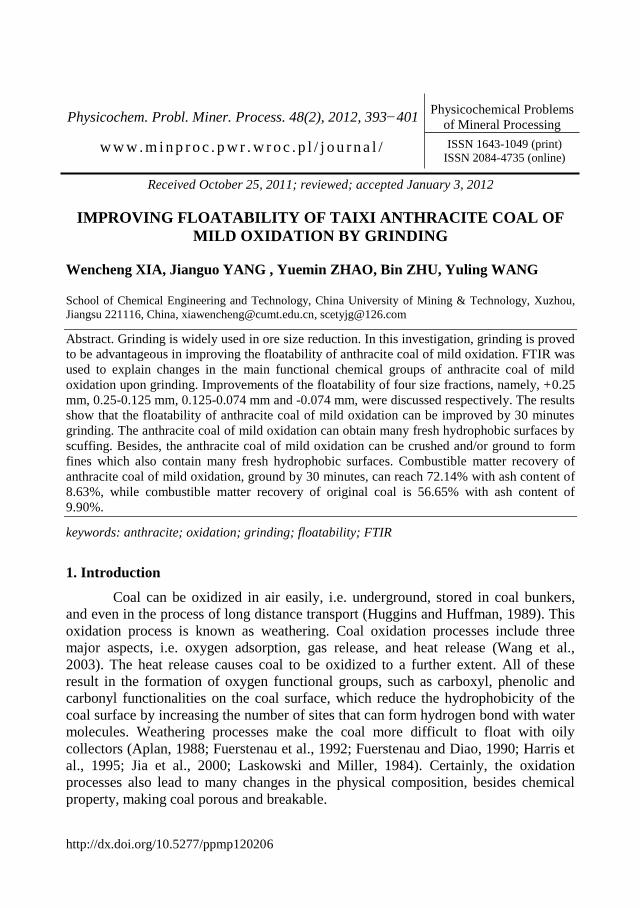
http://dx.doi.org/10.5277/ppmp120206
Physicochem. Probl. Miner. Process. 48(2), 2012, 393−401 Physicochemical Problems
of Mineral Processing
w w w . m i n p r o c . p w r . w r o c . p l / j o u r n a l / ISSN 1643-1049 (print)
ISSN 2084-4735 (online)
Received October 25, 2011; reviewed; accepted January 3, 2012
IMPROVING FLOATABILITY OF TAIXI ANTHRACITE COAL OF
MILD OXIDATION BY GRINDING
Wencheng XIA, Jianguo YANG , Yuemin ZHAO, Bin ZHU, Yuling WANG
School of Chemical Engineering and Technology, China University of Mining & Technology, Xuzhou,
Jiangsu 221116, China, [email protected], [email protected]
Abstract. Grinding is widely used in ore size reduction. In this investigation, grinding is proved
to be advantageous in improving the floatability of anthracite coal of mild oxidation. FTIR was
used to explain changes in the main functional chemical groups of anthracite coal of mild
oxidation upon grinding. Improvements of the floatability of four size fractions, namely, +0.25
mm, 0.25-0.125 mm, 0.125-0.074 mm and -0.074 mm, were discussed respectively. The results
show that the floatability of anthracite coal of mild oxidation can be improved by 30 minutes
grinding. The anthracite coal of mild oxidation can obtain many fresh hydrophobic surfaces by
scuffing. Besides, the anthracite coal of mild oxidation can be crushed and/or ground to form
fines which also contain many fresh hydrophobic surfaces. Combustible matter recovery of
anthracite coal of mild oxidation, ground by 30 minutes, can reach 72.14% with ash content of
8.63%, while combustible matter recovery of original coal is 56.65% with ash content of
9.90%.
keywords: anthracite; oxidation; grinding; floatability; FTIR
1. Introduction
Coal can be oxidized in air easily, i.e. underground, stored in coal bunkers,
and even in the process of long distance transport (Huggins and Huffman, 1989). This
oxidation process is known as weathering. Coal oxidation processes include three
major aspects, i.e. oxygen adsorption, gas release, and heat release (Wang et al.,
2003). The heat release causes coal to be oxidized to a further extent. All of these
result in the formation of oxygen functional groups, such as carboxyl, phenolic and
carbonyl functionalities on the coal surface, which reduce the hydrophobicity of the
coal surface by increasing the number of sites that can form hydrogen bond with water
molecules. Weathering processes make the coal more difficult to float with oily
collectors (Aplan, 1988; Fuerstenau et al., 1992; Fuerstenau and Diao, 1990; Harris et
al., 1995; Jia et al., 2000; Laskowski and Miller, 1984). Certainly, the oxidation
processes also lead to many changes in the physical composition, besides chemical
property, making coal porous and breakable.

394 W. Xia et al.
Previous studies were focused on the oxidation mechanism by simulating the
oxidation processes and show that the coal oxidation processes are concerned with
oxidation temperature, coal particle size, and coal moisture (Chen, 1993; Coward,
1957; Sun, 1954). Oxidation rate decreases with the coal particle size and increases
with the coal specific surface (Akgun and Arisoy, 1994; Carras and Young, 1994).
The oxidation processes generally occur on the coal particle surface. Therefore, the
physical composition and chemical property inside the coal particle change less
(Somasundaran et al., 2000). It is generally acknowledged that the oxidation rate is
inversely proportional to the degree of coalification (Diao and Fuerstenau, 1992;
Schmal, 1989). Flotation tests of difficult-to-float oxidized coal were successfully
accomplished by applying a direct coal and flotation reagents contact procedure with
appropriate reagents (Ahmed and Drzymala, 2004). Coal stored at coarse size and then
ground to fine size before flotation exhibits a higher flotation yield than that stored as
fines (Fuerstenau et al., 1994). Recently, attrition has been used in improving the
floatability of oxidized surface of anthracite waste coal (Sokolovic et al., 2012).
Evidently, grinding generates sufficient fresh surface that minimizes the effects of the
external oxidized surface, but grinding process may produce more ultra-fine coal
particles, whose sizes are less than 10 micrometers, which are difficult to float
(Forbes, 2011). Simultaneously, the ultra-fine coal particles need more flotation agent
and the ultra-fine gangue particles adsorb on the coal surface leading to a more
hydrophilic coal surface (Huynh et al., 2000; Oats et al., 2010). Optimal grinding time
will be determined in this study. Coal particles of different sizes have different
flotabilities which change through grinding. In this paper four size fractions, i.e. +0.25
mm, 0.25-0.125 mm, 0.125-0.074 mm and -0.074 mm of floatation concentrates will
be compared for ground and original coal. In this regard, the paper investigates the
flotation behavior and hydrophobicity of anthracite coal of mild oxidation before and
after grinding using flotation. In addition, the Fourier Transform Infrared
Spectroscopy (FTIR) analysis is used to explain the changes in the main functional
chemical groups of anthracite coal of mild oxidation upon grinding.
2. Experimental method and procedure
In this investigation, dodecane was used as the oily collector and 2-octanol was
used as the frother. Coal samples were provided by Taixi Coal Preparation Plant in
China. Coal in this plant is stored outside and oxidizes mildly under the air, rain and
sunshine. Coal samples were screened to pass 0.5 mm. The flotation tests were
conducted in a 1.5 dm3 XFG flotation cell using 100 g of coal at a pulp density of
6.25% solids. The impeller speed of the flotation machine was 1910 rpm and the
airflow rate was 2 dm3/min. Dodecane collector dose was 5 kg/Mg and 2-octanol
frother 1 kg/Mg of coal. In each flotation test, the pulp was first agitated in the
flotation cell for 3 min, after which dodecane collector (5 kg/Mg) was added and the
pulp conditioned for an additional period of 3-min. 2-octanol frother (1 kg/Mg) was
then added and the pulp was conditioned for an additional one minute.

Improving floatability of Taixi anthracite coal of mild oxidation by grinding 395
The FTIR spectrum was obtained with KBr pellets prepared with 0.125-0.074 mm
anthracite coal of mild oxidation samples (original coal) and the same anthracite coal
of mild oxidation samples ground with KBr for an additional time in a mortar. For the
FTIR analyses a Perkin Elmer Spectrum 2000 model spectrometer was used and the
spectrum was obtained at 2 cm-1
resolution, between 4000 and 400 cm-1
. It is worth
emphasizing that ash content influences the FTIR spectrum. The 0.125-0.074 mm
anthracite coal of mild oxidation samples were separated by density separation using a
centrifugal extractor with the density fraction of 1.4 kg/dm3.
Grinding was conducted in a laboratory dry rod mill. Grinding times were 5 min,
10 min, 20 min and 30 min, respectively. The grinding products and flotation
concentrate were screened to get four size fractions: +0.25 mm, 0.25-0.125 mm,
0.125-0.074 mm and -0.074 mm. Every size fraction was analyzed to determine
parameters such as ash content, combustible matter recovery and yield. Eq. (1) was
used to calculate the combustible matter recovery of the flotation experiments:
100)]100(/)100([(%)recoverymattereCombustabl xAMAM FFcc , (1)
where MC is weight of the concentrate (%), MF is weight of the feed (%), AC is the ash
content of the concentrate (%), and AF is the ash content of the feed (%).
3. Results and discussion
3.1. FTIR spectrum
The FTIR spectra of original and ground coal are showed in Fig. 1. After grinding,
the FTIR spectrum shows five main functional chemical groups more than the original
coal. The five main functional chemical groups are: 3030 cm-1
, 2910 cm-1
, 867 cm-1
,
797 cm-1
and 736 cm-1
. Among the five functional chemical groups, 3030 cm-1
and
2910 cm-1
are aliphatic hydrocarbons which are hydrophobic. Another three functional
chemical groups 867 cm-1
, 797 cm-1
and 736 cm-1
indicate the presence of benzene
rings which also are more hydrophobic than the oxygen functional groups. Oxygen
functional groups detected at 3440 cm-1
and 1630 cm-1
are shown in Fig. 1. The FTIR
image shows that grinding leads to more fresh surface and hydrophobic functional
chemical groups on the surface of anthracite coal of mild oxidation than that of
original coal. The absorbances of functional chemical groups are widely used for
quantitative analysis (Jena et al., 2008; Yuh and Wolt, 1983). The absorbance is
concerned with the functional chemical groups’ content. Low absorbance is
considered as a result of low functional chemical group content. After grinding, the
anthracite coal of mild oxidation has low absorbance of the oxygen functional groups
(3440 cm-1
and 1630 cm-1
). Thus, grinding causes anthracite coal of mild oxidation to
be more hydrophobic than the original coal.
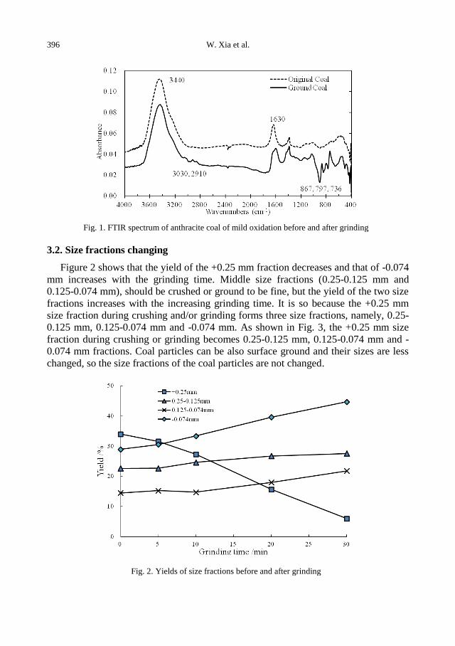
396 W. Xia et al.
Fig. 1. FTIR spectrum of anthracite coal of mild oxidation before and after grinding
3.2. Size fractions changing
Figure 2 shows that the yield of the +0.25 mm fraction decreases and that of -0.074
mm increases with the grinding time. Middle size fractions (0.25-0.125 mm and
0.125-0.074 mm), should be crushed or ground to be fine, but the yield of the two size
fractions increases with the increasing grinding time. It is so because the +0.25 mm
size fraction during crushing and/or grinding forms three size fractions, namely, 0.25-
0.125 mm, 0.125-0.074 mm and -0.074 mm. As shown in Fig. 3, the +0.25 mm size
fraction during crushing or grinding becomes 0.25-0.125 mm, 0.125-0.074 mm and -
0.074 mm fractions. Coal particles can be also surface ground and their sizes are less
changed, so the size fractions of the coal particles are not changed.
Fig. 2. Yields of size fractions before and after grinding
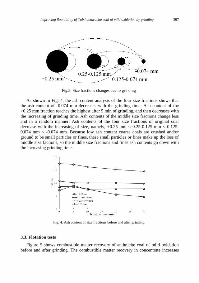
Improving floatability of Taixi anthracite coal of mild oxidation by grinding 397
Fig.3. Size fractions changes due to grinding
As shown in Fig. 4, the ash content analysis of the four size fractions shows that
the ash content of -0.074 mm decreases with the grinding time. Ash content of the
+0.25 mm fraction reaches the highest after 5 min of grinding, and then decreases with
the increasing of grinding time. Ash contents of the middle size fractions change less
and in a random manner. Ash contents of the four size fractions of original coal
decrease with the increasing of size, namely, +0.25 mm < 0.25-0.125 mm < 0.125-
0.074 mm < -0.074 mm. Because low ash content coarse coals are crushed and/or
ground to be small particles or fines, these small particles or fines make up the loss of
middle size factions, so the middle size fractions and fines ash contents go down with
the increasing grinding time.
Fig. 4. Ash content of size fractions before and after grinding
3.3. Flotation tests
Figure 5 shows combustible matter recovery of anthracite coal of mild oxidation
before and after grinding. The combustible matter recovery in concentrate increases

398 W. Xia et al.
with the increasing grinding time for grinding time of 20 min and 30 min. The
combustible matter recovery of +0.25 mm size fraction reaches the highest value after
20 min of grinding, and recovery after 30 min of grinding is smaller, but both are
higher than these after 5 min or 10 min of grinding. The combustible matter recovery
of different size fractions, namely, 0.25-0.125 mm, 0.125-0.074 mm and -0.074 mm,
increases with the grinding time and is similar when the grinding time is either 20 min
or 30 min. From the original coal flotation results, it can be seen that the size fractions,
namely, 0.25-0.125 mm, 0.125-0.074 mm and -0.074 mm, have a similar combustible
matter recovery, therefore, the size fraction has less effect on the floatability of
anthracite coal of mild oxidation particles when the particles size is less than -0.25
mm. However, the combustible matter recovery of the 0.25-0.125 mm, 0.125-0.074
mm and -0.074 mm size fractions is different and becomes higher after grinding. All
of these prove that grinding can improve floatability of anthracite coal of mild
oxidation.
Fig. 5. Combustible matter recovery of size fractions before and after grinding
Figure 5 shows that anthracite coal of mild oxidation after 20 min or 30 min
grinding time has higher combustible matter recovery and similar ash content.
However, the combustible matter recovery of +0.25 mm size fraction decreases when
the grinding time is more than 20 min. It may be explained that long time grinding
produces many fines and ultra-fine coal particles which need more flotation agent
dose. Ultra-fine gangue particles also adsorb on the coal surface causing the coal
surface to be hydrophilic. Coarse coals need more hydrophobic surface for flotation
than the middle size particles or fines because greater mass.
Figure 5 shows that the combustible matter recovery of different size fractions,
namely, 0.25-0.125 mm, 0.125-0.074 mm and -0.074 mm, are higher than +0.25 mm.
This phenomenon proves that the size fraction has a great effect on coal particles
flotation, even though the coarse coals have been surface ground. In addition, the
combustible matter recovery of size fractions, namely, 0.25-0.125 mm and 0.125-
0.074 mm, is higher than -0.074 mm. It proves that fines from the surface of anthracite
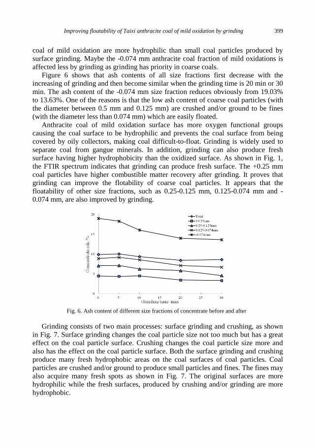
Improving floatability of Taixi anthracite coal of mild oxidation by grinding 399
coal of mild oxidation are more hydrophilic than small coal particles produced by
surface grinding. Maybe the -0.074 mm anthracite coal fraction of mild oxidations is
affected less by grinding as grinding has priority in coarse coals.
Figure 6 shows that ash contents of all size fractions first decrease with the
increasing of grinding and then become similar when the grinding time is 20 min or 30
min. The ash content of the -0.074 mm size fraction reduces obviously from 19.03%
to 13.63%. One of the reasons is that the low ash content of coarse coal particles (with
the diameter between 0.5 mm and 0.125 mm) are crushed and/or ground to be fines
(with the diameter less than 0.074 mm) which are easily floated.
Anthracite coal of mild oxidation surface has more oxygen functional groups
causing the coal surface to be hydrophilic and prevents the coal surface from being
covered by oily collectors, making coal difficult-to-float. Grinding is widely used to
separate coal from gangue minerals. In addition, grinding can also produce fresh
surface having higher hydrophobicity than the oxidized surface. As shown in Fig. 1,
the FTIR spectrum indicates that grinding can produce fresh surface. The +0.25 mm
coal particles have higher combustible matter recovery after grinding. It proves that
grinding can improve the flotability of coarse coal particles. It appears that the
floatability of other size fractions, such as 0.25-0.125 mm, 0.125-0.074 mm and -
0.074 mm, are also improved by grinding.
Fig. 6. Ash content of different size fractions of concentrate before and after
Grinding consists of two main processes: surface grinding and crushing, as shown
in Fig. 7. Surface grinding changes the coal particle size not too much but has a great
effect on the coal particle surface. Crushing changes the coal particle size more and
also has the effect on the coal particle surface. Both the surface grinding and crushing
produce many fresh hydrophobic areas on the coal surfaces of coal particles. Coal
particles are crushed and/or ground to produce small particles and fines. The fines may
also acquire many fresh spots as shown in Fig. 7. The original surfaces are more
hydrophilic while the fresh surfaces, produced by crushing and/or grinding are more
hydrophobic.
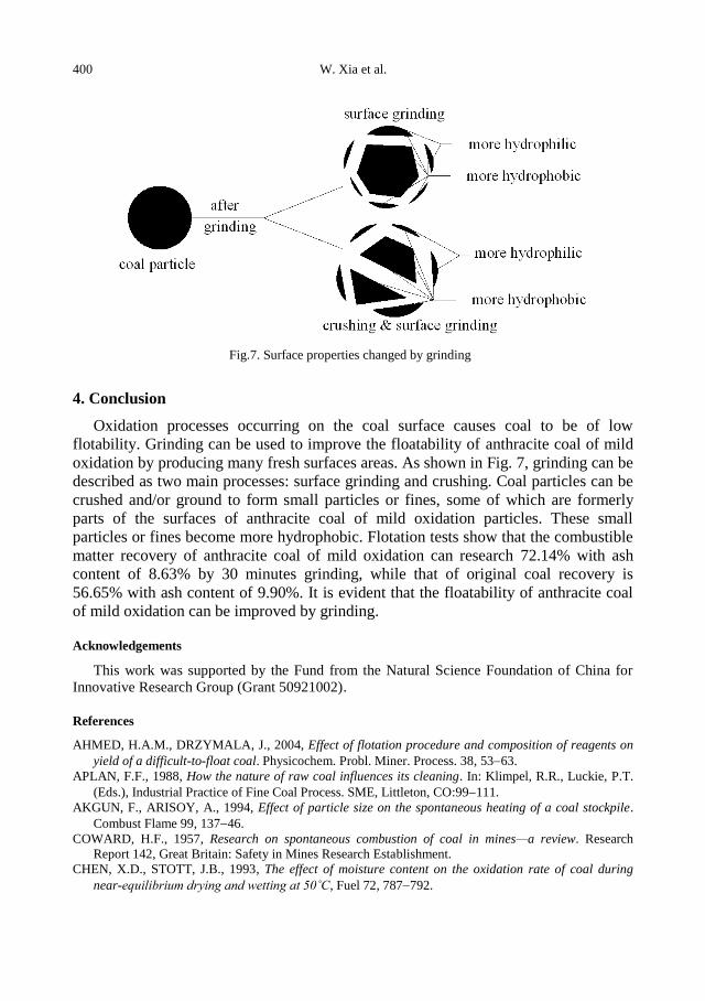
400 W. Xia et al.
Fig.7. Surface properties changed by grinding
4. Conclusion
Oxidation processes occurring on the coal surface causes coal to be of low
flotability. Grinding can be used to improve the floatability of anthracite coal of mild
oxidation by producing many fresh surfaces areas. As shown in Fig. 7, grinding can be
described as two main processes: surface grinding and crushing. Coal particles can be
crushed and/or ground to form small particles or fines, some of which are formerly
parts of the surfaces of anthracite coal of mild oxidation particles. These small
particles or fines become more hydrophobic. Flotation tests show that the combustible
matter recovery of anthracite coal of mild oxidation can research 72.14% with ash
content of 8.63% by 30 minutes grinding, while that of original coal recovery is
56.65% with ash content of 9.90%. It is evident that the floatability of anthracite coal
of mild oxidation can be improved by grinding.
Acknowledgements
This work was supported by the Fund from the Natural Science Foundation of China for
Innovative Research Group (Grant 50921002).
References
AHMED, H.A.M., DRZYMALA, J., 2004, Effect of flotation procedure and composition of reagents on
yield of a difficult-to-float coal. Physicochem. Probl. Miner. Process. 38, 5363.
APLAN, F.F., 1988, How the nature of raw coal influences its cleaning. In: Klimpel, R.R., Luckie, P.T.
(Eds.), Industrial Practice of Fine Coal Process. SME, Littleton, CO:99111.
AKGUN, F., ARISOY, A., 1994, Effect of particle size on the spontaneous heating of a coal stockpile.
Combust Flame 99, 13746.
COWARD, H.F., 1957, Research on spontaneous combustion of coal in mines—a review. Research
Report 142, Great Britain: Safety in Mines Research Establishment.
CHEN, X.D., STOTT, J.B., 1993, The effect of moisture content on the oxidation rate of coal during
near-equilibrium drying and wetting at 50˚С, Fuel 72, 787792.
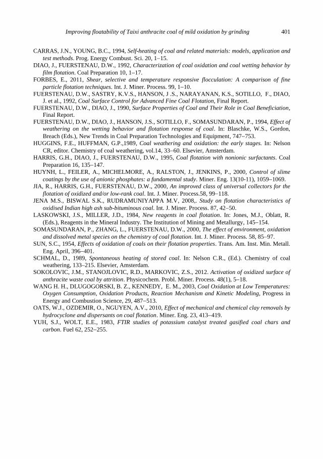
Improving floatability of Taixi anthracite coal of mild oxidation by grinding 401
CARRAS, J.N., YOUNG, B.C., 1994, Self-heating of coal and related materials: models, application and
test methods. Prog. Energy Combust. Sci. 20, 115.
DIAO, J., FUERSTENAU, D.W., 1992, Characterization of coal oxidation and coal wetting behavior by
film flotation. Coal Preparation 10, 117.
FORBES, E., 2011, Shear, selective and temperature responsive flocculation: A comparison of fine
particle flotation techniques. Int. J. Miner. Process. 99, 110.
FUERSTENAU, D.W., SASTRY, K.V.S., HANSON, J .S., NARAYANAN, K.S., SOTILLO, F., DIAO,
J. et al., 1992, Coal Surface Control for Advanced Fine Coal Flotation, Final Report.
FUERSTENAU, D.W., DIAO, J., 1990, Surface Properties of Coal and Their Role in Coal Beneficiation,
Final Report.
FUERSTENAU, D.W., DIAO, J., HANSON, J.S., SOTILLO, F., SOMASUNDARAN, P., 1994, Effect of
weathering on the wetting behavior and flotation response of coal. In: Blaschke, W.S., Gordon,
Breach (Eds.), New Trends in Coal Preparation Technologies and Equipment, 747753.
HUGGINS, F.E., HUFFMAN, G.P.,1989, Coal weathering and oxidation: the early stages. In: Nelson
CR, editor. Chemistry of coal weathering, vol.14, 3360. Elsevier, Amsterdam.
HARRIS, G.H., DIAO, J., FUERSTENAU, D.W., 1995, Coal flotation with nonionic surfactants. Coal
Preparation 16, 135147.
HUYNH, L., FEILER, A., MICHELMORE, A., RALSTON, J., JENKINS, P., 2000, Control of slime
coatings by the use of anionic phosphates: a fundamental study. Miner. Eng. 13(10-11), 10591069.
JIA, R., HARRIS, G.H., FUERSTENAU, D.W., 2000, An improved class of universal collectors for the
flotation of oxidized and/or low-rank coal. Int. J. Miner. Process.58, 99118.
JENA M.S., BISWAL S.K., RUDRAMUNIYAPPA M.V, 2008,. Study on flotation characteristics of
oxidised Indian high ash sub-bituminous coal. Int. J. Miner. Process. 87, 4250.
LASKOWSKI, J.S., MILLER, J.D., 1984, New reagents in coal flotation. In: Jones, M.J., Oblatt, R.
(Eds.), Reagents in the Mineral Industry. The Institution of Mining and Metallurgy, 145154.
SOMASUNDARAN, P., ZHANG, L., FUERSTENAU, D.W., 2000, The effect of environment, oxidation
and dissolved metal species on the chemistry of coal flotation. Int. J. Miner. Process. 58, 8597.
SUN, S.C., 1954, Effects of oxidation of coals on their flotation properties. Trans. Am. Inst. Min. Metall.
Eng. April, 396401.
SCHMAL, D., 1989, Spontaneous heating of stored coal. In: Nelson C.R., (Ed.). Chemistry of coal
weathering, 133–215. Elsevier, Amsterdam.
SOKOLOVIC, J.M., STANOJLOVIC, R.D., MARKOVIC, Z.S., 2012. Activation of oxidized surface of
anthracite waste coal by attrition. Physicochem. Probl. Miner. Process. 48(1), 518.
WANG H. H., DLUGOGORSKI, B. Z., KENNEDY, E. M., 2003, Coal Oxidation at Low Temperatures:
Oxygen Consumption, Oxidation Products, Reaction Mechanism and Kinetic Modeling, Progress in
Energy and Combustion Science, 29, 487513.
OATS, W.J., OZDEMIR, O., NGUYEN, A.V., 2010, Effect of mechanical and chemical clay removals by
hydrocyclone and dispersants on coal flotation. Miner. Eng. 23, 413419.
YUH, S.J., WOLT, E.E., 1983, FTIR studies of potassium catalyst treated gasified coal chars and
carbon. Fuel 62, 252255.

402 W. Xia et al.
http://dx.doi.org/10.5277/ppmp120207
Physicochem. Probl. Miner. Process. 48(2), 2012, 403−412 Physicochemical Problems
of Mineral Processing
w w w . m i n p r o c . p w r . w r o c . p l / j o u r n a l / ISSN 1643-1049 (print)
ISSN 2084-4735 (online)
Received July 29, 2011; reviewed; accepted October 15, 2011
HYDROLYSIS OF SILICA SOURCES: APS AND DTSACl IN
MICROENCAPSULATION PROCESSES
Krzysztof SZCZEPANOWICZ* , Grazyna PARA*, Aud M. BOUZGA**,
Christian SIMON**, Juan YANG**, Piotr WARSZYNSKI*
* Jerzy Haber Institute of Catalysis and Surface Chemistry, Polish Academy of Sciences, Niezpominajek
st. 8, Krakow 30-239, Poland, [email protected]
** SINTEF Material and Chemistry, Forskningsveien 1, NO-0314 Oslo, Norway
Abstract. The process of formation of silica shells around emulsion droplets was investigated.
The 1H-NMR spectroscopy was applied to follow the silica shell formation around emulsion
droplets by hydrolysis and condensation of selected silanes in the emulsion system.
(3- aminopropyl) triethoxysilane (APS) and dimethyloctadecyl [3-(trimethoxysilyl) propyl]
ammonium chloride (DTSACl) were used as silica sources in microencapsulation process. The
NMR analysis revealed strong dependence of the hydrolysis reaction rate on pH. Obtained
information allowed selecting the optimal conditions for the formation of the capsules with
silica shells. The obtained capsules’ suspensions were stable for several weeks.
keywords: encapsulation, emulsions, silica shells, capsules, 1H -NMR
1. Introduction
Microencapsulation can be defined as a process in which colloidal particles or
droplets are being enclosed in inert shells of various materials to obtain capsules
(Swapan, 2006). Encapsulation has a potential to improve the compatibility of
lipophilic, poorly water-soluble or even water-insoluble compounds with aqueous
media and it can protect active molecules from the negative effect of external
environment. The development of the microencapsulation technology started with
introduction of capsules containing dyes, which were incorporated into paper for
copying purposes and replaced carbon paper (Schleicher and Green, 1956). Since then
the number of processes used to produce microcapsules has continued to grow and the
development of functional micro or nano-containers is currently one of the main topics
in pharmaceutical research. In particular, nanocapsules can be used in specific drug
delivery system as they can penetrate the cell membrane. Moreover they can be
functionalized to achieve “intelligent targeting”, i.e. delivery to the specific cells or
organs (Donath and Moya, 2002; Radtchenko and Giersig, 2002; Shchukin and
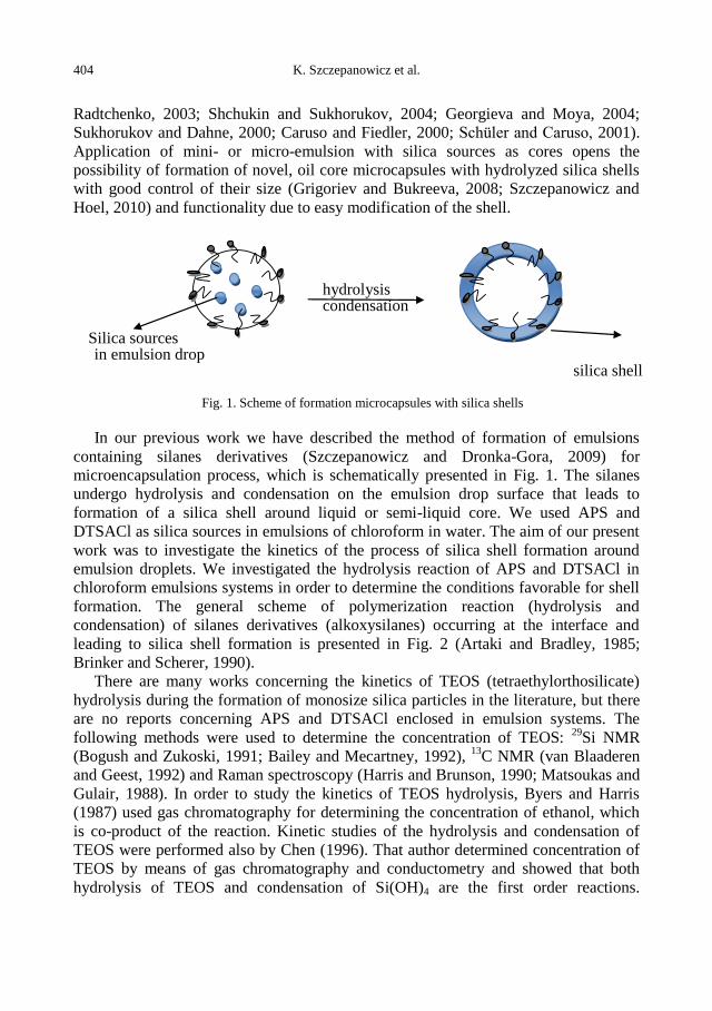
404 K. Szczepanowicz et al.
Radtchenko, 2003; Shchukin and Sukhorukov, 2004; Georgieva and Moya, 2004;
Sukhorukov and Dahne, 2000; Caruso and Fiedler, 2000; Schüler and Caruso, 2001).
Application of mini- or micro-emulsion with silica sources as cores opens the
possibility of formation of novel, oil core microcapsules with hydrolyzed silica shells
with good control of their size (Grigoriev and Bukreeva, 2008; Szczepanowicz and
Hoel, 2010) and functionality due to easy modification of the shell.
hydrolysis condensation
Silica sources in emulsion drop
silica shell
Fig. 1. Scheme of formation microcapsules with silica shells
In our previous work we have described the method of formation of emulsions
containing silanes derivatives (Szczepanowicz and Dronka-Gora, 2009) for
microencapsulation process, which is schematically presented in Fig. 1. The silanes
undergo hydrolysis and condensation on the emulsion drop surface that leads to
formation of a silica shell around liquid or semi-liquid core. We used APS and
DTSACl as silica sources in emulsions of chloroform in water. The aim of our present
work was to investigate the kinetics of the process of silica shell formation around
emulsion droplets. We investigated the hydrolysis reaction of APS and DTSACl in
chloroform emulsions systems in order to determine the conditions favorable for shell
formation. The general scheme of polymerization reaction (hydrolysis and
condensation) of silanes derivatives (alkoxysilanes) occurring at the interface and
leading to silica shell formation is presented in Fig. 2 (Artaki and Bradley, 1985;
Brinker and Scherer, 1990).
There are many works concerning the kinetics of TEOS (tetraethylorthosilicate)
hydrolysis during the formation of monosize silica particles in the literature, but there
are no reports concerning APS and DTSACl enclosed in emulsion systems. The
following methods were used to determine the concentration of TEOS: 29
Si NMR
(Bogush and Zukoski, 1991; Bailey and Mecartney, 1992), 13
C NMR (van Blaaderen
and Geest, 1992) and Raman spectroscopy (Harris and Brunson, 1990; Matsoukas and
Gulair, 1988). In order to study the kinetics of TEOS hydrolysis, Byers and Harris
(1987) used gas chromatography for determining the concentration of ethanol, which
is co-product of the reaction. Kinetic studies of the hydrolysis and condensation of
TEOS were performed also by Chen (1996). That author determined concentration of
TEOS by means of gas chromatography and conductometry and showed that both
hydrolysis of TEOS and condensation of Si(OH)4 are the first order reactions.
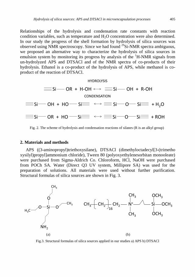
Hydrolysis of silica sources: APS and DTSACl in microencapsulation processes 405
Relationships of the hydrolysis and condensation rate constants with reaction
condition variables, such as temperature and H2O concentration were also determined.
In our study the progress of the shell formation by hydrolysis of silica sources was
observed using NMR spectroscopy. Since we had found 29
Si-NMR spectra ambiguous,
we proposed an alternative way to characterize the hydrolysis of silica sources in
emulsion system by monitoring its progress by analysis of the 1H-NMR signals from
un-hydrolyzed APS and DTSACl and of the NMR spectra of co-products of their
hydrolysis. Ethanol is a co-product of the hydrolysis of APS, while methanol is co-
product of the reaction of DTSACl.
Si OR + H-OH Si OH + R-OH
Si OR + HO Si Si O Si + ROH
Si OH + HO Si Si O Si + H2O
HYDROLYSIS
CONDENSATION
Fig. 2. The scheme of hydrolysis and condensation reactions of silanes (R is an alkyl group)
2. Materials and methods
APS ((3-aminopropyl)triethoxysilane), DTSACl (dimethyloctadecyl[3-(trimetho
xysilyl)propyl]ammonium chloride), Tween 80 (polyoxyethylenesorbitan monooleate)
were purchased from Sigma-Aldrich Co. Chloroform, HCl, NaOH were purchased
from POCh SA. Water (Direct Q3 UV system, Millipore SA) was used for the
preparation of solutions. All materials were used without further purification.
Structural formulas of silica sources are shown in Fig. 3.
Si OO
O
NH2
CH3
H3C
CH3
CH3 CH2 CH2 N+ Si OCH3
OCH3
OCH3
16
CH3
CH3
(a) (b)
Fig.3. Structural formulas of silica sources applied in our studies a) APS b) DTSACl
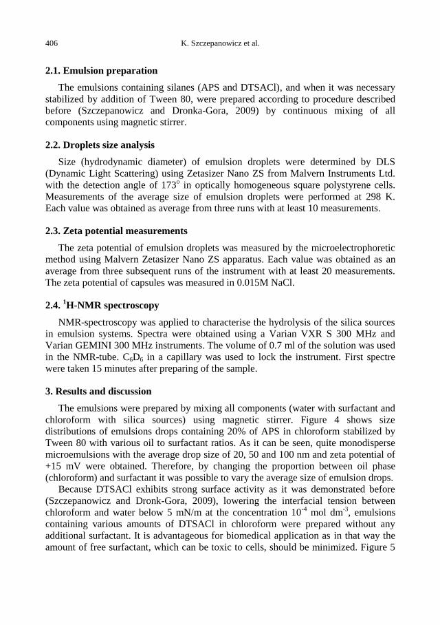
406 K. Szczepanowicz et al.
2.1. Emulsion preparation
The emulsions containing silanes (APS and DTSACl), and when it was necessary
stabilized by addition of Tween 80, were prepared according to procedure described
before (Szczepanowicz and Dronka-Gora, 2009) by continuous mixing of all
components using magnetic stirrer.
2.2. Droplets size analysis
Size (hydrodynamic diameter) of emulsion droplets were determined by DLS
(Dynamic Light Scattering) using Zetasizer Nano ZS from Malvern Instruments Ltd.
with the detection angle of 173o in optically homogeneous square polystyrene cells.
Measurements of the average size of emulsion droplets were performed at 298 K.
Each value was obtained as average from three runs with at least 10 measurements.
2.3. Zeta potential measurements
The zeta potential of emulsion droplets was measured by the microelectrophoretic
method using Malvern Zetasizer Nano ZS apparatus. Each value was obtained as an
average from three subsequent runs of the instrument with at least 20 measurements.
The zeta potential of capsules was measured in 0.015M NaCl.
2.4. 1H-NMR spectroscopy
NMR-spectroscopy was applied to characterise the hydrolysis of the silica sources
in emulsion systems. Spectra were obtained using a Varian VXR S 300 MHz and
Varian GEMINI 300 MHz instruments. The volume of 0.7 ml of the solution was used
in the NMR-tube. C6D6 in a capillary was used to lock the instrument. First spectre
were taken 15 minutes after preparing of the sample.
3. Results and discussion
The emulsions were prepared by mixing all components (water with surfactant and
chloroform with silica sources) using magnetic stirrer. Figure 4 shows size
distributions of emulsions drops containing 20% of APS in chloroform stabilized by
Tween 80 with various oil to surfactant ratios. As it can be seen, quite monodisperse
microemulsions with the average drop size of 20, 50 and 100 nm and zeta potential of
+15 mV were obtained. Therefore, by changing the proportion between oil phase
(chloroform) and surfactant it was possible to vary the average size of emulsion drops.
Because DTSACl exhibits strong surface activity as it was demonstrated before
(Szczepanowicz and Dronk-Gora, 2009), lowering the interfacial tension between
chloroform and water below 5 mN/m at the concentration 10-4
mol dm-3
, emulsions
containing various amounts of DTSACl in chloroform were prepared without any
additional surfactant. It is advantageous for biomedical application as in that way the
amount of free surfactant, which can be toxic to cells, should be minimized. Figure 5
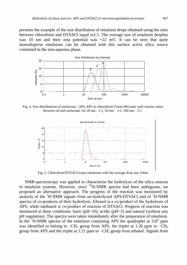
Hydrolysis of silica sources: APS and DTSACl in microencapsulation processes 407
presents the example of the size distribution of emulsion drops obtained using the ratio
between chloroform and DTSACl equal to1:1. The average size of emulsion droplets
was 10 nm and their zeta potential was +22 mV. It can be seen that quite
monodisperse emulsions can be obtained with this surface active silica source
contained in the non-aqueous phase.
0
5
10
15
20
0.1 1 10 100 1000 10000
Inte
nsity (
%)
Size (d.nm)
Size Distribution by Intensity
1
1
2 3
Fig. 4. Size distributions of emulsions - 20% APS in chloroform/Tween 80/water with various ratios
between oil and surfactant: for 20 nm - 1:1, 50 nm – 3:1, 100 nm – 5:1.
Fig. 5. Chloroform/DTSACl/water emulsions with the average drop size 10nm
NMR-spectroscopy was applied to characterise the hydrolysis of the silica sources
in emulsion systems. However, since 29
Si-NMR spectra had been ambiguous, we
proposed an alternative approach. The progress of the reaction was monitored by
analysis of the 1H-NMR signals from un-hydrolyzed APS/DTSACl and of
1H-NMR
spectra of co-products of their hydrolysis. Ethanol is a co-product of the hydrolysis of
APS, while methanol is co-product of reaction of DTSACl. Progress of reaction was
monitored at three conditions: basic (pH~10), acidic (pH~3) and natural (without any
pH regulation). The spectra were taken immediately after the preparation of emulsion.
In the 1H-NMR spectra of the emulsion containing APS the quadruplet at 3.87 ppm
was identified to belong to –CH3 group from APS, the triplet at 1.26 ppm to –CH2
group from APS and the triplet at 1.21 ppm to –CH2 group from ethanol. Signals from

408 K. Szczepanowicz et al.
unhydrolyzed APS were missing in spectra regardless of hydrolysis conditions,
whereas ones corresponding to the ethanol were visible for all conditions studied,
which means that hydrolysis of APS in the emulsion system was very fast (Fig. 6).
The time needed to prepare emulsions was always longer than time of the hydrolysis
reaction so APS was fully hydrolyzed.
Fig. 6. The 1H-NMR spectra of emulsions containing APS. From the top: basic, natural, acidic
Fig. 7. The 1H -NMR spectra of emulsions containing DTSACl. From the top: acidic, natural, basic
In the case of DTSACl a convenient way to characterize the progress of hydrolysis
was the analysis of the 1H-NMR peak at 3.6 ppm from –O-CH3 groups in DTSACl
and the peak at 3.4 ppm of –CH3 group from methanol. During the course of
hydrolysis reaction the integrals of peaks from –O-CH3 group in DTSACl decreased
and integrals of methanol peaks increased. The kinetics of the reaction revealed strong
dependence of its rate on pH of the emulsion. In the basic conditions (pH 10)
hydrolysis was very fast, since the signal from DTSACl was not visible in the first
spectra taken just after the sample preparation. In the natural and acidic conditions
hydrolysis reaction was much slower (Fig. 7). In the acidic conditions (pH 3) no
changes in spectra were observed even after 18 hours after sample preparation (see
Fig. 8). Results obtained from NMR measurements of hydrolysis rate are collected in
Table 1. This information allows selecting the optimal conditions for the formation of
capsules with silica shells, in which hydrolysis of selected organosilanes is favorable.
On the other hand it was found that DTSACl under the natural conditions (pH 6) was
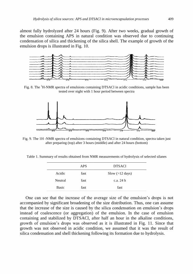
Hydrolysis of silica sources: APS and DTSACl in microencapsulation processes 409
almost fully hydrolyzed after 24 hours (Fig. 9). After two weeks, gradual growth of
the emulsion containing APS in natural condition was observed due to continuing
condensation of silica and thickening of the silica shell. The example of growth of the
emulsion drops is illustrated in Fig. 10.
Fig. 8. The 1H-NMR spectra of emulsions containing DTSACl in acidic conditions, sample has been
tested over night with 1 hour period between spectra
Fig. 9. The 1H -NMR spectra of emulsions containing DTSACl in natural condition, spectra taken just
after preparing (top) after 3 hours (middle) and after 24 hours (bottom)
Table 1. Summary of results obtained from NMR measurements of hydrolysis of selected silanes
One can see that the increase of the average size of the emulsion’s drops is not
accompanied by significant broadening of the size distribution. Thus, one can assume
that the increase of the size is caused by the silica condensation on emulsion’s drops
instead of coalescence (or aggregation) of the emulsion. In the case of emulsion
containing and stabilized by DTSACl, after half an hour in the alkaline conditions,
growth of emulsion’s drops was observed as it is illustrated in Fig. 11. Since that
growth was not observed in acidic condition, we assumed that it was the result of
silica condensation and shell thickening following its formation due to hydrolysis.
APS DTSACl
Acidic fast Slow (>12 days)
Neutral fast c.a. 24 h
Basic fast fast

410 K. Szczepanowicz et al.
0
2
4
6
8
10
12
14
0.1 1 10 100 1000 10000
Inte
nsity (
%)
Size (d.nm)
Size Distribution by Intensity
(a)
0
2
4
6
8
10
12
0.1 1 10 100 1000 10000
Inte
nsity (
%)
Size (d.nm)
Size Distribution by Intensity
(b)
Fig. 10. Size distributions of emulsions - 20% APS in chloroform/Tween 80/water: (a) before and (b)
after hydrolysis and condensation
Fig. 11. Size distribution of emulsions - chloroform/DTSACl/water a) before (green line) and b) after
hydrolysis and condensation (red line)
Hydrolysis of silica sources: APS and DTSACl in microencapsulation processes 411
4. Conclusions
Chloroform solutions of silane derivatives APS or DTSACl were used as oil phase
to prepare microemulsions, which play the role of cores for nanocapsules with silica
shells. The size of obtained emulsion droplets ranged from 10 to 100 nm. The 1H-
NMR spectroscopy was applied to follow the silica shell formation around obtained
emulsion droplets by the hydrolysis of silanes. The results revealed some dependence
of the hydrolysis reaction rate on pH. In the case of the emulsion containing APS and
stabilized by Tween 80, the rate was fast in all pH conditions studied, i.e., APS was
fully hydrolyzed. On the other hand in the case of emulsion containing surface active
DTSACl, the rate of its hydrolysis was strongly pH dependent - fast in the alkaline
conditions, slow in acidic ones. The obtained information concerning the hydrolysis
rate allows selecting the optimal conditions for the formation of capsules with silica
shells. Gradual growth of the emulsion drop size observed under the conditions of fast
hydrolysis, which was not accompanied by significant broadening of the size
distribution by coalescence (or aggregation), was attributed to the silica condensation
on emulsion’s drops surface and shell thickening. Obtained nanocapsules with silica
shells can be used for encapsulation and further surface modification (e.g. by layer-by-
layer adsorption of polyelectrolytes).
Acknowledgements
The work was financed by MNiSW ‘JUVENTUS’ grant.
References
ARTAKI, F., BRADLEY, M., ZERDA, T.W., JONAS, J., 1985, NMR and Raman study of the hydrolysis
reaction in sol-gel process. J. Phys. Chem. 89, 4399−4404.
BAILEY, J.K., MECARTNEY, M.L., 1992, Formation of colloidal silica particles from alkoxides.
Colloids Surf. 63, 151−161.
BOGUSH, G.H., ZUKOSKI, I.V., 1991, Studies of the kinetics of the precipitation of uniform silica
particles through the hydrolysis and condensation of silicon alkoxides. J. Colloid Interface Sci. 142,
1−18.
BRINKER, C.J., SCHERER, G.W., 1990, Eds. Sol-Gel Science; Academic Press: San Diego, p 108.
BYERS, C.H., HARRIS M.T., 1987, Controlled microcrystalline growth studies by dynamic laser-light-
scattering methods. Ind. Eng. Chem. Res., 26, 1916−1923.
CARUSO, F., FIEDLER, H., 2000, Assembly of Beta-Glucosidase Multilayers on Spherical Colloidal
Particles and Their use as Active Catalysts. Colloids Surfaces A: Physicochem. Eng. Aspects 169,
287−293.
DONATH, E., MOYA, S., 2002, Hollow polymer shells from biological templates: Fabrication and
potential applications. Chem-Eur I vol. 8, (23) 5481−5485.
GEORGIEVA, R., MOYA, S.E., 2004, Permeability and Conductivity of Red Blood Cell Templated
polyelectrolyte Capsules Coated with Supplementary Layers. Langmuir 20,1895−1900.
GRIGORIEV, D.O., BUKREEVA, T., 2008, New method for fabrication of loaded micro- and
nanocontainers: Emulsion encapsulation by polyelectrolyte layer-by-layer deposition on the liquid
core. Langmuir 24, 999−1004.
HARRIS, M.T., BRUNSON, R.R., 1990, The base-catalyzed hydrolysis and condensation reaction of
dilute and concentration TEOS solutions. J. Non-Cryst. Solids 121, 397−403.
412 K. Szczepanowicz et al.
MATSOUKAS, T., GULAIR, E., 1988, Dynamics of growth of silica particles from ammonia-catalyzed
hydrolysis of tetraethylorthosilicate. J. Colloid Interface Sci. 124(1), 252−261.
RADTCHENKO, I.L., GIERSIG, M., 2002, Inorganic particle synthesis in confined micron-sized
polyelectrolyte capsules. Langmuir vol. 18, (21) 8204−8208
SCHLEICHER, L., GREEN, B.K., 1956. US Patent 2730456
SCHÜLER, C., CARUSO, F., 2001, Decomposable Hollow Biopolymer Capsules. Biomacromolecules,
2, 921−926
SHCHUKİN, D.G., RADTCHENKO, I.L., 2003, Synthesis of nanosized magnetic ferrite particles inside
hollow polyelectrolyte capsules. J. Phys. Chem. B. 107(1), 86−90
SHCHUKIN, D.G., SUKHORUKOV, G.B., 2004, Fabrication of fluorescent rare earth phosphates in
confined media of polyelectrolyte microcapsules. J. Phys. Chem. B. 108 (50), 19109−19113.
SHENG-LI, CHEN, 1996, Kinetics of Formation of Monodisperse Colloidal Silica Particles through the
Hydrolysis and Condensation of Tetraethylorthosilicate. Ind. Eng. Chem. Res. 35, 4487−4493.
SUKHORUKOV, G., DAHNE, L., 2000, Controlled precipitation of dyes into hollow polyelectrolyte
capsules based on colloids and biocolloids. Adv mater 12(2), 112−115.
SWAPAN K.G., 2006, Functional Coatings by Polymer Microencapsulation. Wiley-vch Verlag GmbH &
Co. KGaA, Weinheim
SZCZEPANOWICZ, K., DRONKA-GORA, D., 2009, Chloroform Emulsions Containing TEOS, APS
and DTSACl as Cores for Microencapsulation. Procedia Chem. 1, 1576−1583.
SZCZEPANOWICZ, K., HOEL, H.J., 2010, Formation of Biocompatible Nanocapsules with Emulsion
Core and Pegylated Shell by Polyelectrolyte Multilayer Adsorption. Langmuir, 26(15), 12592–12597.
VAN BLAADEREN, A., VAN GEEST, J., 1992, Monodisperse colloidal silica spheres from
tetraalkoxysilanes: Particle formation and growth mechanism. J. Colloid Interface Sci, 154(2),
481−501.

http://dx.doi.org/10.5277/ppmp120208
Physicochem. Probl. Miner. Process. 48(2), 2012, 413−424 Physicochemical Problems
of Mineral Processing
w w w . m i n p r o c . p w r . w r o c . p l / j o u r n a l / ISSN 1643-1049 (print)
ISSN 2084-4735 (online)
Received January 5, 2012; reviewed; accepted March 1, 2012
HEAT TREATMENT OF NATURAL DIATOMITE
Suzan S. IBRAHIM*, Ali Q. SELIM**
*Central Metallurgical R&D Institute CMRDI, P.O. Box 87, Helwan, Egypt, [email protected]
** Geology Dept., Faculty of Science, Beni Suif Univ., Egypt
Abstract. Heat treatment of an Egyptian natural diatomite was performed at different
temperatures (600, 900, 1000, 1100, and 1200ºC). The samples were heated from room
temperature 23±1ºC to the appointed temperature at a rate of 20oC/ min, and kept at that
temperature for 5 hour. The heat treated samples were examined by X-ray diffraction, scan-
electro-microscopy, and other physical characters like sample color, texture, and weight
reduction. Results showed that heat treatment of natural diatomite caused different forms of
mineral modification and transformation to another mineral. At 1200ºC a new nano-metric
silicate material was formed. These changes were mainly depending upon the treated
temperature, diatomite genera, and the accompanied gangue minerals as well.
keywords: natural diatomite, heat treatment, porous structure
1. Introduction
Diatoms are belonging to the diploid eukaryotic unicellular algae (Bacillariophyta)
with wide ranges of structures and shapes. Each of these has its own distinct shape and
size (Sterrenburg et al., 2007). The outstanding feature of diatoms is their siliceous
“shell” or frustule, which can be preserved for millions of years. In this manner, fossil
deposits of microscopic diatom shells were built up as thick layers of “diatomaceous
earth” or diatomite which could be extending over several miles (Sterrenburg et al.,
2007).
Diatomite is formed by the closest packing of hydrous SiO2 spheres and is
classified as opal-A. Opaline minerals have been categorized into three general
groups, including Opal-A, Opal-C, and Opal-CT, according to crystallinity and crystal
structure (Jones and Segnit, 1971). Opal-A is predominantly amorphous. Opal-CT is
semi-crystalline comprising of crystalline regions of cristobalite and tridymite, where
opal-C is a well-ordered form of the silicate predominantly in the cristobalite form
(Jones and Segnit, 1971). Diatomaceous silica, the amorphous silica with opal-A
structure, exists in the form of frustule in the natural mineral assemblage of diatomite.
Since the diatomaceous silica has properties such as high porosity with strong
absorbability and excellent thermal resistance, diatomite has been widely used as filter
aid, catalytic support, biological support, functional filler, and adsorbent, etc.
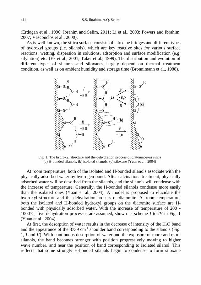
414 S.S. Ibrahim, A.Q. Selim
(Erdogan et al., 1996; Ibrahim and Selim, 2011; Li et al., 2003; Powers and Ibrahim,
2007; Vasconclos et al., 2000).
As is well known, the silica surface consists of siloxane bridges and different types
of hydroxyl groups (i.e. silanols), which are key reactive sites for various surface
reactions: wetting, dispersion in solutions, adsorption and surface modification (e.g.
silylation) etc. (Ek et al., 2001; Takei et al., 1999). The distribution and evolution of
different types of silanols and siloxanes largely depend on thermal treatment
condition, as well as on ambient humidity and storage time (Bronnimann et al., 1988).
Fig. 1. The hydroxyl structure and the dehydration process of diatomaceous silica
(a) H-bonded silanols, (b) isolated silanols, (c) siloxane (Yuan et al., 2004)
At room temperature, both of the isolated and H-bonded silanols associate with the
physically adsorbed water by hydrogen bond. After calcinations treatment, physically
adsorbed water will be desorbed from the silanols, and the silanols will condense with
the increase of temperature. Generally, the H-bonded silanols condense more easily
than the isolated ones (Yuan et al., 2004). A model is proposed to elucidate the
hydroxyl structure and the dehydration process of diatomite. At room temperature,
both the isolated and H-bonded hydroxyl groups on the diatomite surface are H-
bonded with physically adsorbed water. With the increase of temperature of 200 -
1000ºC, five dehydration processes are assumed, shown as scheme I to IV in Fig. 1
(Yuan et al., 2004).
At first, the desorption of water results in the decrease of intensity of the H2O band
and the appearance of the 3739 cm-1
shoulder band corresponding to the silanols (Fig.
1, I and II). With continuous desorption of water and the exposure of more and more
silanols, the band becomes stronger with position progressively moving to higher
wave number, and near the position of band corresponding to isolated silanol. This
reflects that some strongly H-bonded silanols begin to condense to form siloxane
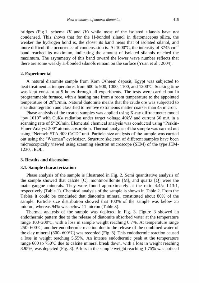
Heat treatment of natural diatomite 415
bridges (Fig.1, scheme III and IV) while most of the isolated silanols have not
condensed. This shows that for the H-bonded silanol in diatomaceous silica, the
weaker the hydrogen bond is, the closer its band nears that of isolated silanol, and
more difficult the occurrence of condensation is. At 1000ºC, the intensity of 3745 cm-1
band reached its maximum, indicating the amount of isolated silanols reached the
maximum. The asymmetry of this band toward the lower wave number reflects that
there are some weakly H-bonded silanols remain on the surface (Yuan et al., 2004).
2. Experimental
A natural diatomite sample from Kom Osheem deposit, Egypt was subjected to
heat treatment at temperatures from 600 to 900, 1000, 1100, and 1200ºC. Soaking time
was kept constant at 5 hours through all experiments. The tests were carried out in
programmable furnace, with a heating rate from a room temperature to the appointed
temperature of 20oC/min. Natural diatomite means that the crude ore was subjected to
size disintegration and classified to remove extraneous matter coarser than 45 micron.
Phase analysis of the treated samples was applied using X-ray diffractmeter model
“pw 1010” with CuKα radiation under target voltage 40kV and current 30 mA in a
scanning rate of 5º 2θ/min. Elemental chemical analysis was conducted using “Perkin-
Elmer Analyst 200” atomic absorption. Thermal analysis of the sample was carried out
using “Netzsch STA 409 C/CD” unit. Particle size analysis of the sample was carried
out using the ‘Warman” cyclosizer. Structure skeleton of different samples have been
microscopically viewed using scanning electron microscope (SEM) of the type JEM-
1230, JEOL.
3. Results and discussion
3.1. Sample characterization
Phase analysis of the sample is illustrated in Fig. 2. Semi quantitative analysis of
the sample showed that calcite [C], montmorillonite [M], and quartz [Q] were the
main gangue minerals. They were found approximately at the ratio 4.45: 1.13:1,
respectively (Table 1). Chemical analysis of the sample is shown in Table 2. From the
Tables it could be concluded that diatomite mineral constituted about 80% of the
sample. Particle size distribution showed that 100% of the sample was below 35
micron, whereas 94% was below 11 micron (Table 3).
Thermal analysis of the sample was depicted in Fig. 3. Figure 3 showed an
endothermic pattern due to the release of diatomite absorbed water at the temperature
range 100–200ºC, with a loss in sample weight reaching 0.7%. At temperature range
250- 600ºC, another endothermic reaction due to the release of the combined water of
the clay mineral (300- 600°C) was recorded (Fig. 3). This endothermic reaction caused
a loss in weight reaching 5.55%. An intense endothermic peak at the temperature
range 600 to 750ºC due to calcite mineral break down, with a loss in weight reaching
8.95%, was depicted (Fig. 3). A loss in the sample weight reaching 1.75% was noticed
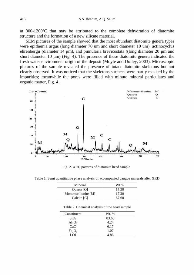
416 S.S. Ibrahim, A.Q. Selim
at 900-1200ºC that may be attributed to the complete dehydration of diatomite
structure and the formation of a new silicate material.
SEM pictures of the sample showed that the most abundant diatomite genera types
were epithemia argus (long diameter 70 um and short diameter 10 um), actinocyclus
ehrenbergii (diameter 14 μm), and pinnularia brevicostata ((long diameter 20 μm and
short diameter 10 μm) (Fig. 4). The presence of these diatomite genera indicated the
fresh water environment origin of the deposit (Moyle and Dolley, 2003). Microscopic
pictures of the sample revealed the presence of intact diatomite skeletons but not
clearly observed. It was noticed that the skeletons surfaces were partly masked by the
impurities; meanwhile the pores were filled with minute mineral particulates and
organic matter, Fig. 4.
Fig. 2. XRD patterns of diatomite head sample
Table 1. Semi quantitative phase analysis of accompanied gangue minerals after XRD
Mineral Wt.%
Quartz [Q]
Montmorillonite [M]
Calcite [C]
15.20
17.20
67.60
Table 2. Chemical analysis of the head sample
Constituent Wt. % SiO2 83.60 Al2O3 4.24 CaO 6.17
Fe2O3 1.07 LOI 4.86
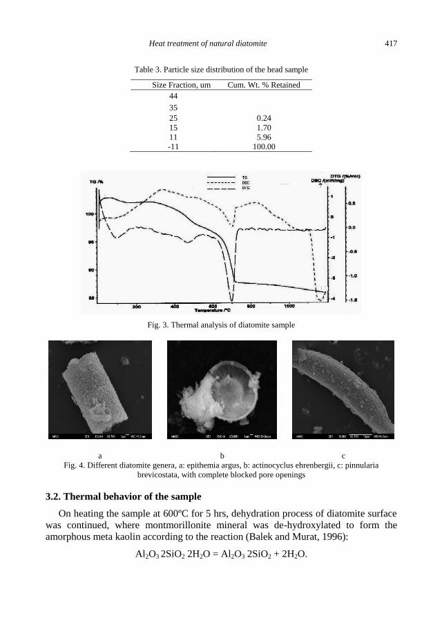
Heat treatment of natural diatomite 417
Table 3. Particle size distribution of the head sample
Size Fraction, um Cum. Wt. % Retained 44 35 25 0.24 15 1.70 11 5.96 -11 100.00
Fig. 3. Thermal analysis of diatomite sample
a b c
Fig. 4. Different diatomite genera, a: epithemia argus, b: actinocyclus ehrenbergii, c: pinnularia
brevicostata, with complete blocked pore openings
3.2. Thermal behavior of the sample
On heating the sample at 600ºC for 5 hrs, dehydration process of diatomite surface
was continued, where montmorillonite mineral was de-hydroxylated to form the
amorphous meta kaolin according to the reaction (Balek and Murat, 1996):
Al2O3 2SiO2 2H2O = Al2O3 2SiO2 + 2H2O.
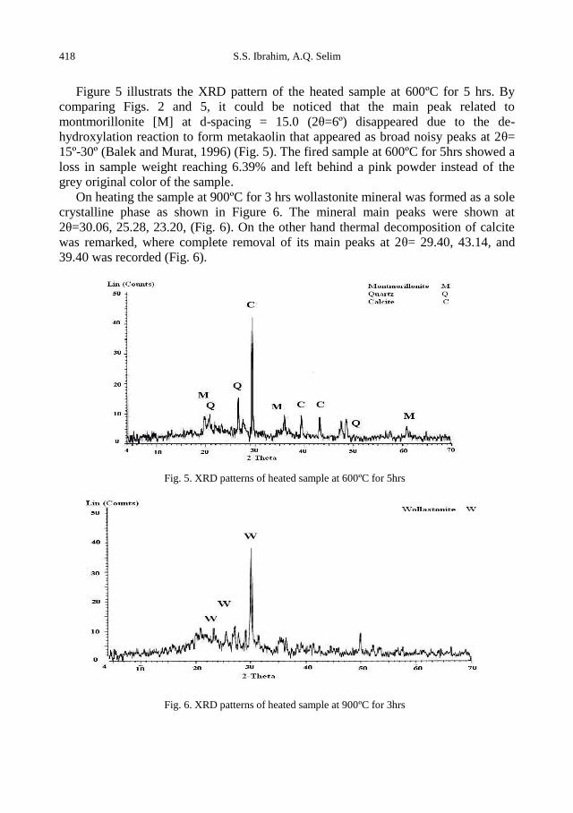
418 S.S. Ibrahim, A.Q. Selim
Figure 5 illustrats the XRD pattern of the heated sample at 600ºC for 5 hrs. By
comparing Figs. 2 and 5, it could be noticed that the main peak related to
montmorillonite [M] at d-spacing = 15.0 (2θ=6º) disappeared due to the de-
hydroxylation reaction to form metakaolin that appeared as broad noisy peaks at 2θ=
15º-30º (Balek and Murat, 1996) (Fig. 5). The fired sample at 600ºC for 5hrs showed a
loss in sample weight reaching 6.39% and left behind a pink powder instead of the
grey original color of the sample.
On heating the sample at 900ºC for 3 hrs wollastonite mineral was formed as a sole
crystalline phase as shown in Figure 6. The mineral main peaks were shown at
2θ=30.06, 25.28, 23.20, (Fig. 6). On the other hand thermal decomposition of calcite
was remarked, where complete removal of its main peaks at 2θ= 29.40, 43.14, and
39.40 was recorded (Fig. 6).
Fig. 5. XRD patterns of heated sample at 600ºC for 5hrs
Fig. 6. XRD patterns of heated sample at 900ºC for 3hrs
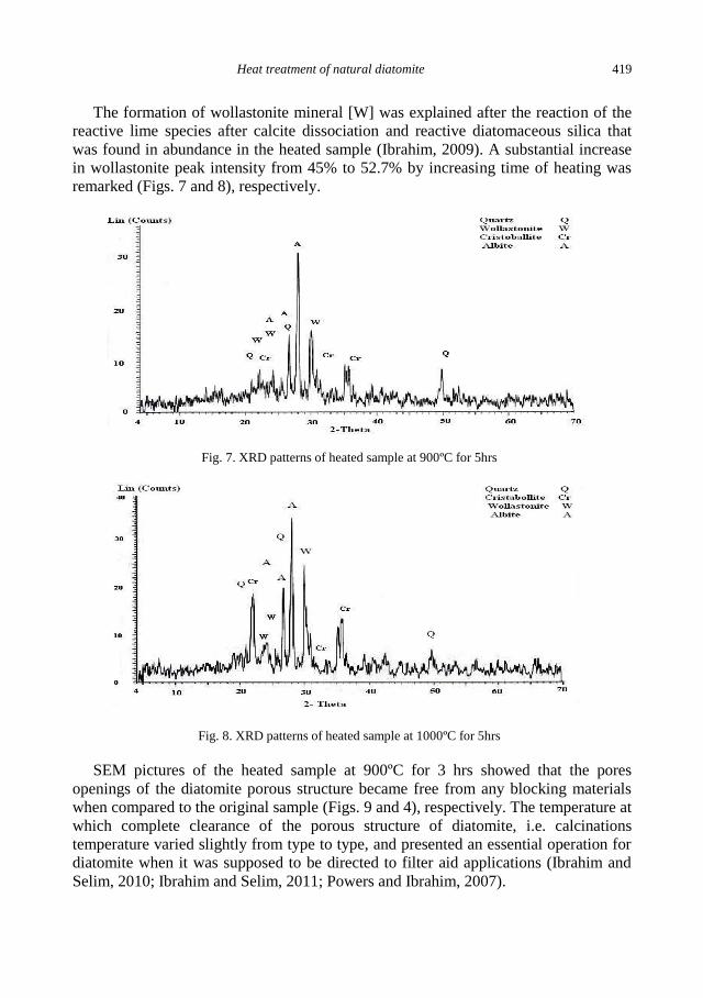
Heat treatment of natural diatomite 419
The formation of wollastonite mineral [W] was explained after the reaction of the
reactive lime species after calcite dissociation and reactive diatomaceous silica that
was found in abundance in the heated sample (Ibrahim, 2009). A substantial increase
in wollastonite peak intensity from 45% to 52.7% by increasing time of heating was
remarked (Figs. 7 and 8), respectively.
Fig. 7. XRD patterns of heated sample at 900ºC for 5hrs
Fig. 8. XRD patterns of heated sample at 1000ºC for 5hrs
SEM pictures of the heated sample at 900ºC for 3 hrs showed that the pores
openings of the diatomite porous structure became free from any blocking materials
when compared to the original sample (Figs. 9 and 4), respectively. The temperature at
which complete clearance of the porous structure of diatomite, i.e. calcinations
temperature varied slightly from type to type, and presented an essential operation for
diatomite when it was supposed to be directed to filter aid applications (Ibrahim and
Selim, 2010; Ibrahim and Selim, 2011; Powers and Ibrahim, 2007).
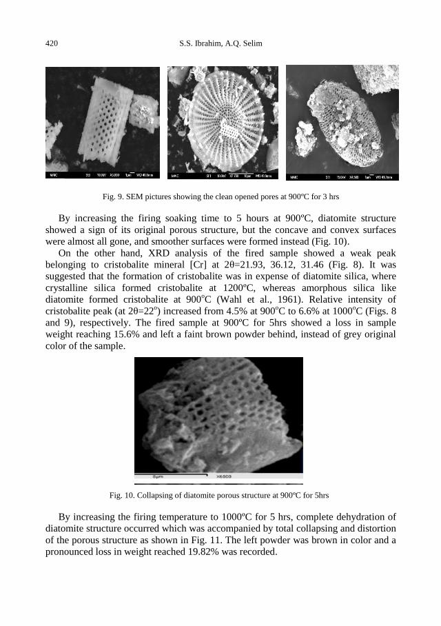
420 S.S. Ibrahim, A.Q. Selim
Fig. 9. SEM pictures showing the clean opened pores at 900ºC for 3 hrs
By increasing the firing soaking time to 5 hours at 900ºC, diatomite structure
showed a sign of its original porous structure, but the concave and convex surfaces
were almost all gone, and smoother surfaces were formed instead (Fig. 10).
On the other hand, XRD analysis of the fired sample showed a weak peak
belonging to cristobalite mineral [Cr] at 2θ=21.93, 36.12, 31.46 (Fig. 8). It was
suggested that the formation of cristobalite was in expense of diatomite silica, where
crystalline silica formed cristobalite at 1200ºC, whereas amorphous silica like
diatomite formed cristobalite at 900oC (Wahl et al., 1961). Relative intensity of
cristobalite peak (at 2θ=22o) increased from 4.5% at 900
oC to 6.6% at 1000
oC (Figs. 8
and 9), respectively. The fired sample at 900ºC for 5hrs showed a loss in sample
weight reaching 15.6% and left a faint brown powder behind, instead of grey original
color of the sample.
Fig. 10. Collapsing of diatomite porous structure at 900ºC for 5hrs
By increasing the firing temperature to 1000ºC for 5 hrs, complete dehydration of
diatomite structure occurred which was accompanied by total collapsing and distortion
of the porous structure as shown in Fig. 11. The left powder was brown in color and a
pronounced loss in weight reached 19.82% was recorded.

Heat treatment of natural diatomite 421
By heating the sample at 1100ºC for 5 hrs, an olive green colored material was
formed. The main XRD peaks of the product appeared at 2θ=21.93, 29.85, 35.48, and
30.88, that belonged to calcium alkali silicate mineral called diopside, (Fig. 12).
Diopside is an inosilicate mineral composed of single chains of silica tetrahedra and
belonging to pyroxene group. Pyroxenes have the general formula XY(Si, Al)2O6
(where X represents calcium, sodium, Fe+2
and magnesium and more rarely zinc,
manganese and lithium and Y represents ions of smaller size, such as chromium,
aluminium, iron (III), magnesium, manganese, scandium, titanium, vanadium and
even iron (II). Although aluminium substitutes extensively for silicon in silicates such
as feldspars and amphiboles, the substitution occurs only to a limited extent in most
pyroxenes (Morimoto et al., 1989). The formed product showed loss on sample weight
that reached 23.08% with a hard vitreous texture.
Fig. 11. Complete destroying of diatomite porous structure at 1000ºC
Fig. 12. XRD patterns of heated sample at 1100ºC for 5hrs

422 S.S. Ibrahim, A.Q. Selim
Figure 13 illustrates the XRD pattern of the sample after heating at 1200ºC for 5
hrs. The formed sample was a nano-metric vitreous glassy material (Fig. 14) that
showed remarkable reduction in volume compared to the sample heated at 900ºC for 5
hrs (Fig. 15).
Fig. 13. XRD patterns of heated sample at 1200ºC for 5hrs
Fig. 14. SEM picture of the new material formed at 1200ºC
4. Conclusions
Natural diatomite sample from Kom Osheem Localiy, El-Fayoum Depression,
Egypt was subjected to heat treatment. The main accompanied minerals were calcite,
montmorillonite and quartz. The sample was soaked for 5 hrs at temperatures of 600,
900, 1000, 1100, and 1200ºC. Characterization of the heated samples was followed up
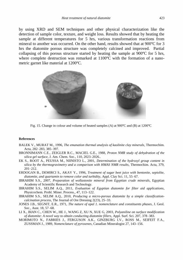
Heat treatment of natural diatomite 423
by using XRD and SEM techniques and other physical characterization like the
detection of sample color, texture, and weight loss. Results showed that by heating the
sample at different temperatures for 5 hrs, various transformation reactions from
mineral to another was occurred. On the other hand, results showed that at 900ºC for 3
hrs the diatomite porous structure was completely calcined and improved. Partial
collapsing of this porous structure started by heating the sample at 900ºC for 5 hrs,
where complete destruction was remarked at 1100ºC with the formation of a nano-
metric garnet like material at 1200ºC.
Fig. 15. Change in colour and volume of heated samples (A) at 900ºC and (B) at 1200ºC
References
BALEK V., MURAT M., 1996, The emanation thermal analysis of kaolinite clay minerals, Thermochim.
Acta, 282–283, 385–397.
BRONNIMANN C.E., ZEIGLER R.C., MACIEL G.E., 1988, Proton NMR study of dehydration of the
silica gel surface, J. Am. Chem. Soc., 110, 2023–2026..
EK S., ROOT A., PEUSSA M., NIINISTO L., 2001, Determination of the hydroxyl group content in
silica by the thermogravimetry and a comparison with HMAS NMR results, Thermochim. Acta, 379,
201–212.
ERDOGAN B., DEMIRCI S., AKAY Y., 1996, Treatment of sugar beet juice with bentonite, sepiolite,
diatomite, and quartamin to remove color and turbidity, Appl. Clay Sci. 11, 55–67.
IBRAHIM S.S., 2007, Preparation of wollastonite mineral from Egyptian crude minerals, Egyptian
Academy of Scientific Research and Technology.
IBRAHIM S.S., SELIM A.Q., 2011, Evaluation of Egyptian diatomite for filter aid applications,
Physicochem. Probl. Miner. Process., 47, 113–122.
IBRAHIM S.S., SELIM A.Q., 2010, Producing a micro-porous diatomite by a simple classification-
calcination process, The Journal of Ore Dressing 2(23), 25–33.
JONES J.B., SEGNIT, E.R., 1971, The nature of opal 1. nomenclature and constituents phases, J. Geol.
Soc., Aust. 18, 57–68.
LI X., BIAN C., CHEN W., HE J., WANG Z, XU N, XUE G, 2003, Polyaniline on surface modification
of diatomite: A novel way to obtain conducting diatomite fillers, Appl. Surf. Sci. 207, 378–383.
MORIMOTO N., FABRIES J., FERGUSON A.K., GINZBURG I.V., ROSS M., SEIFEIT F.A.,
ZUSSMAN J., 1989, Nomenclature of pyroxenes, Canadian Mineralogist 27, 143–156.
424 S.S. Ibrahim, A.Q. Selim
MOYLE P.R., DOLLEY T.P., 2003, A comparison of marine and continental-lacustrine diatomite
deposits, Industrial-Minerals Research.
POWERS K., IBRAHIM S.S., 2009, Preparation of different diatomite concentrates for various
industrial applications, International Science and Engineering, NSF, USA.
STERRENBURG F., GORDON RJ., TIFFANY M.A., NAGY S.S., 2007, Algae and cyan-bacteria in
extreme environments, Springer, 141–172.
TAKEI T., KATO K., MEGURO A., CHIKAZAWA M., 1999, Infrared Spectra of Geminal and Novel
Triple Hydroxyl Groups on Silica Surfaces, Colloids and Surfaces, A: Physicochemical and
Engineering Aspects, Vol. 150, No. 1, 77–84.
VASCONCELOS P.V., LABRINCHA J.A., FERREIRA J.M.F., 2000, Permeability of diatomite layers
processed by different colloidal techniques, J. Eur. Ceram. Soc. 20, 201–207.
WAHL F.M., GRIM R.E., GRAF R.B., 1961, Phase Transformations in Silica as Examined by
Continuous X-ray Diffraction, The American Mineralogist, 46, 1064–1076.
YUAN P., WU D.Q., HE H.P., LIN Z.Y., 2004, The hydroxyl species and acid sites on diatomite surface:
A combined IR and Raman study, Applied Surface Science, 227, 30–39.
http://dx.doi.org/10.5277/ppmp120209
Physicochem. Probl. Miner. Process. 48(2), 2012, 425−439 Physicochemical Problems
of Mineral Processing
w w w . m i n p r o c . p w r . w r o c . p l / j o u r n a l / ISSN 1643-1049 (print)
ISSN 2084-4735 (online)
Received July 11, 2011; reviewed; accepted December 24, 2011
IRON REMOVING FROM TITANIUM SLAG FOR SYNTHETIC
RUTILE PRODUCTION
Akbar MEHDILO, Mehdi IRANNAJAD
Department of Mining and Metallurgical Eng., Amirkabir University of Technology, Tehran, Iran,
[email protected], Phone: 0098-21-66419729, Fax: 0098-21-66405846
Abstract. Leaching with sulfuric and hydrochloric acids for upgrading titanium slag obtained
from the Qara-aghaj ilmenite concentrate to a high grade titanium dioxide (TiO2) was studied.
The titanium slag containing 72.7% TiO2 and 7.8% Fe2O3 was leached at varying solid/liquid
(S/L) ratio, particle size, leaching time and acid concentration. The optimum amount of S/L
ratio, particle size, acid concentration and leaching time using both acids were determined as
1:4, -100 m, 8% and 2 h. Under optimum conditions, by using sulfuric acid, a titanium
dioxide concentrate with 86.8% TiO2 and 1.87% Fe2O3 was produced, while employing
hydrochloric acid resulted in a concentrate containing 91% TiO2 and 0.61% Fe2O3. The
titanium dioxide concentrate prepared with hydrochloric acid, having acicular texture and by
means of elongated separate particles; has less impurities than the one produced by sulfuric
acid. The results demonstrate that hydrochloric acid dissolution of titanium slag and removing
some impurities such as SiO2 and MgO provide a product with good quality is prepared which
is suitable as raw material for TiO2 pigment production through the chloride process.
keywords: titanium slag, synthetic rutile, chloride process, sulfate process, acid leaching, TiO2
pigment
1. Introduction
Titanium is relatively abundant in the earth’s crust, which is usually found in
igneous and metamorphic rocks as ilmenite (FeTiO3), rutile (TiO2) and
titanomagnetite (Fe2TiO4–Fe2O4). A survey on the use of titanium in its various forms
indicates that almost 95% is for the production of white TiO2 pigment which has
extensive application in paint, plastic and paper industries (Nayl et al., 2009; Nayl et
al., 2009). Titanium dioxide also has high potential applications in environmental
purification, gas sensors, and in photovoltaic cells due to its unique characteristics
(Zang et al., 2009). Relatively minor quantities are used to produce metal and titanium
chemicals (Lasheen, 2004).
Natural rutile, owing to its high titanium content and low levels of impurities, has
traditionally been preferred as a feed stock for the production of titanium dioxide

426 A. Mehdilo, M. Irannajad
pigment. Natural rutile is becoming scarcer and consequently more costly and
alternative methods that use ilmenite are being favored. Ilmenite concentrates have
relatively low titanium content (usually about 50% titanium dioxide compared to
about 96% in the case of rutile) but have Fe as their major impurity and thus pose
problems for pigment production. Nevertheless, ilmenite has been used as an alternate
feed material for production of pigment through chemical routes (Samala et al., 2009).
Commercial production of TiO2 pigment uses either the sulfate process or chloride
process. In the former process, relatively low grade feedstock can be used, but it gives
a higher volume of waste product that requires proper treatment and disposal. It is
more preferable to use the chloride process which utilizes a feedstock of high TiO2
grade as natural rutile mineral (94-98% TiO2), synthetic rutile (92-95% TiO2), anatase
(90-95% TiO2), leucoxene (>68% TiO2), or titanium slag (80-90% TiO2) as raw
materials (Samala et al., 2009; El-Hazek et al., 2007; Lasheen, 2008, Zhang and Nicol,
2010; Nayl et al., 2009). The chloride process offers several advantages such as the
yield of high quality products, a more eco-friendly process and the generation of a
smaller amount of waste products (Zhang and Nicol, 2010).
The shortage of natural rutile and the need for higher grade titanium feedstocks has
encouraged ilmenite upgrading by removing iron oxide and other impurities from the
grain lattice, thus converting ilmenite into synthetic rutile for the chlorination process
(El-Hazek et al., 2007; Mahmoud et al. 2004; Lasheen, 2009). There are several
processes for the production of synthetic rutile from ilmenite and some of them were
commercially applied. The most important of these processes are (Lasheen, 2004; El-
Hazek et al., 2007; Mahmoud et al. 2004; Lasheen, 2009; Chun et al., 2008; Zhang
and Nicol, 2009; Sasikumar et al. 2007; Kamala, 2006) given below.
(1) Smelting processes, where the iron part of the ilmenite is reduced and melted to
separate iron from titanium. The titanium slag is then leached with sulfuric acid or
with hydrochloric acid at elevated temperatures.
(2) Reduction of ilmenite to convert ferric iron partially to the ferrous form or
completely to the metallic iron form followed by acid leaching.
(3) Reduction of the iron content of the ilmenite to the metallic iron followed by
corrosion with oxygen and ammonium chloride.
(4) Oxidation and reduction of ilmenite followed by hydrochloric acid leaching
(MURSO process).
(5) Roasting and magnetic separation followed by hydrochloric acid leaching
(ERMS process).
In the first method, ilmenite ore can be smelted in the presence of carbonaceous
reducing agents in an electric furnace where good quality pig iron is obtained together
with titanium-rich slag which is chemically and mineralogically different than ilmenite
(Nayl et al., 2009). In spite of high power consumption, smelting of ilmenite or
titanium-bearing ore has several advantages over the synthetic rutile route by chemical
process. The major advantages of the slag technology are: high titanium content, low
waste generation, being suitable for sulphate and chloride processes, low chemicals
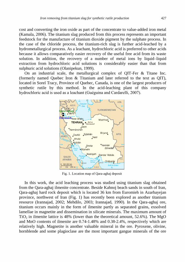
Iron removing from titanium slag for synthetic rutile production 427
cost and converting the iron oxide as part of the concentrate to value-added iron metal
(Kamala, 2006). The titanium slag produced from this process represents an important
feedstock for the manufacture of titanium dioxide pigment by the sulphate process. In
the case of the chloride process, the titanium-rich slag is further acid-leached by a
hydrometallurgical process. As a leachant, hydrochloric acid is preferred to other acids
because it allows comparatively easier recovery of the useful free acid from its waste
solution. In addition, the recovery of a number of metal ions by liquid–liquid
extraction from hydrochloric acid solutions is considerably easier than that from
sulphuric acid solutions (Olanipekun, 1999).
On an industrial scale, the metallurgical complex of QIT-Fer & Titane Inc.
(formerly named Quebec Iron & Titanium and later referred to the text as QIT),
located in Sorel Tracy, Province of Quebec, Canada, is one of the largest producers of
synthetic rutile by this method. In the acid-leaching plant of this company
hydrochloric acid is used as a leachant (Guéguina and Cardarelli, 2007).
Fig. 1. Location map of Qara-aghaj deposit
In this work, the acid leaching process was studied using titanium slag obtained
from the Qara-aghaj ilmenite concentrate. Beside Kahnoj beach sands in south of Iran,
Qara-aghaj hard rock deposit which is located 36 km from Euromieh in Azarbayejan
province, northwest of Iran (Fig. 1) has recently been explored as another titanium
resource (Irannajad, 2002; Mehdilo, 2003; Irannajad, 1990). In the Qara-aghaj ore,
titanium occurs mainly in the form of ilmenite partly as separated grains, exsolved
lamellae in magnetite and dissemination in silicate minerals. The maximum amount of
TiO2 in ilmenite lattice is 48% (lower than the theoretical amount, 52.6%). The MgO
and MnO contents of ilmenite are 0.74-1.48% and 0.38-2.4%, respectively which are
relatively high. Magnetite is another valuable mineral in the ore. Pyroxene, olivine,
hornblende and some plagioclase are the most important gangue minerals of the ore
Qara-aghaj
Euromieh ● ▪
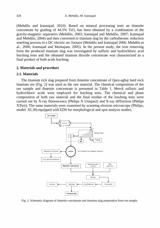
428 A. Mehdilo, M. Irannajad
(Mehdilo and Irannajad, 2010). Based on mineral processing tests an ilmenite
concentrate by grading of 44.5% TiO2 has been obtained by a combination of the
gravity-magnetic separators (Mehdilo, 2003; Irannajad and Mehdilo, 2007; Irannajad
and Mehdilo, 2004) and then converted to titanium slag by the carbothermic reduction
smelting process in a DC electric arc furnace (Mehdilo and Irannajad 2006; Mehdilo et
al., 2006; Irannajad and Montajam, 2005). In the present study, the iron removing
from the produced titanium slag was investigated by sulfuric and hydrochloric acid
leaching tests and the obtained titanium dioxide concentrate was characterized as a
final product of both acids leaching.
2. Materials and procedure
2.1. Materials
The titanium rich slag prepared from ilmenite concentrate of Qara-aghaj hard rock
titanium ore (Fig. 2) was used as the raw material. The chemical composition of the
ore sample and ilmenite concentrate is presented in Table 1. Merck sulfuric and
hydrochloric acids were employed for leaching tests. The chemical and phase
composition of both raw material and the final residue of the leaching tests were
carried out by X-ray fluorescence (Philips X Unique2) and X-ray diffraction (Philips
X'Pert). The same materials were examined by scanning electron microscopy (Philips,
model: XL30) equipped with EDS for morphological and spot analysis studies.
LIWMS
Ore Sample
Magnetite Concentrate
V2O5 and iron production
Ilmenite Concentrate
F
Mixing
C
Tailing M
Rod mill
Reductant agent
(Cock)
Flux
(Na2CO3)
Calcination Iron Reduction Smelting
Titanium Slag
Cast Iron
Low Intensity Wet Magnetic Separator
Shaking Table
Fig. 2. Schematic diagram of ilmenite concentrate and titanium slag preparation from ore sample
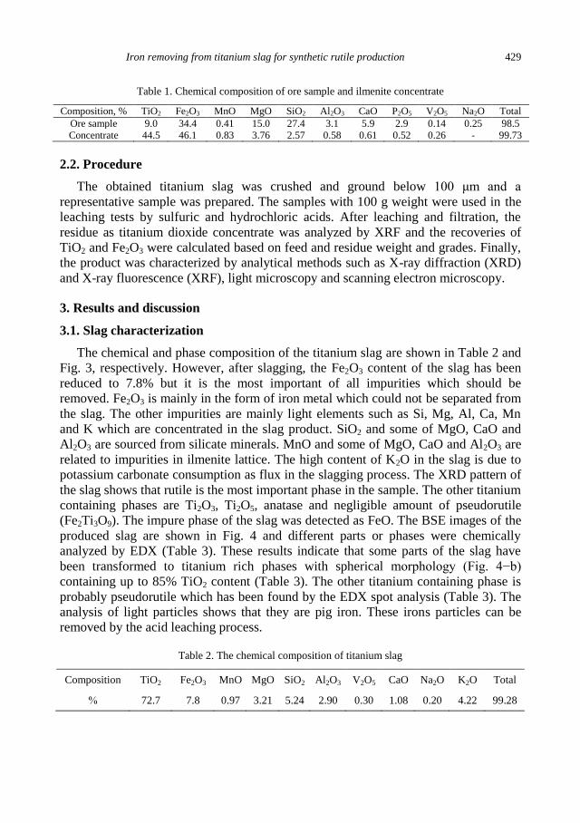
Iron removing from titanium slag for synthetic rutile production 429
Table 1. Chemical composition of ore sample and ilmenite concentrate
Composition, % TiO2 Fe2O3 MnO MgO SiO2 Al2O3 CaO P2O5 V2O5 Na2O Total
Ore sample 9.0 34.4 0.41 15.0 27.4 3.1 5.9 2.9 0.14 0.25 98.5
Concentrate 44.5 46.1 0.83 3.76 2.57 0.58 0.61 0.52 0.26 - 99.73
2.2. Procedure
The obtained titanium slag was crushed and ground below 100 μm and a
representative sample was prepared. The samples with 100 g weight were used in the
leaching tests by sulfuric and hydrochloric acids. After leaching and filtration, the
residue as titanium dioxide concentrate was analyzed by XRF and the recoveries of
TiO2 and Fe2O3 were calculated based on feed and residue weight and grades. Finally,
the product was characterized by analytical methods such as X-ray diffraction (XRD)
and X-ray fluorescence (XRF), light microscopy and scanning electron microscopy.
3. Results and discussion
3.1. Slag characterization
The chemical and phase composition of the titanium slag are shown in Table 2 and
Fig. 3, respectively. However, after slagging, the Fe2O3 content of the slag has been
reduced to 7.8% but it is the most important of all impurities which should be
removed. Fe2O3 is mainly in the form of iron metal which could not be separated from
the slag. The other impurities are mainly light elements such as Si, Mg, Al, Ca, Mn
and K which are concentrated in the slag product. SiO2 and some of MgO, CaO and
Al2O3 are sourced from silicate minerals. MnO and some of MgO, CaO and Al2O3 are
related to impurities in ilmenite lattice. The high content of K2O in the slag is due to
potassium carbonate consumption as flux in the slagging process. The XRD pattern of
the slag shows that rutile is the most important phase in the sample. The other titanium
containing phases are Ti2O3, Ti2O5, anatase and negligible amount of pseudorutile
(Fe2Ti3O9). The impure phase of the slag was detected as FeO. The BSE images of the
produced slag are shown in Fig. 4 and different parts or phases were chemically
analyzed by EDX (Table 3). These results indicate that some parts of the slag have
been transformed to titanium rich phases with spherical morphology (Fig. 4−b)
containing up to 85% TiO2 content (Table 3). The other titanium containing phase is
probably pseudorutile which has been found by the EDX spot analysis (Table 3). The
analysis of light particles shows that they are pig iron. These irons particles can be
removed by the acid leaching process.
Table 2. The chemical composition of titanium slag
Composition TiO2 Fe2O3 MnO MgO SiO2 Al2O3 V2O5 CaO Na2O K2O Total
% 72.7 7.8 0.97 3.21 5.24 2.90 0.30 1.08 0.20 4.22 99.28
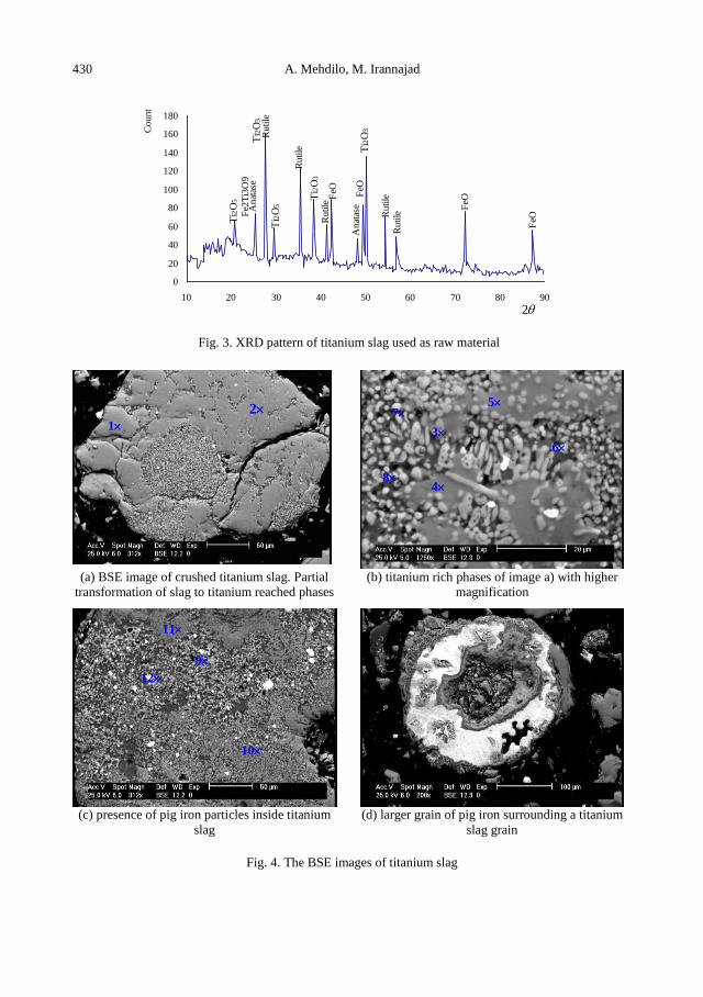
430 A. Mehdilo, M. Irannajad
0
20
40
60
80
100
120
140
160
180
10 20 30 40 50 60 70 80 90
Count
Rutile
FeO
FeO
FeO
Rutile
Rutile
Rutile
Rutile
Anat
ase
FeO
Anat
ase
Ti2
O3
Ti2
O3
Ti2
O5
Ti2
O5
Fe2
Ti3
O9
Ti2
O3
2
Fig. 3. XRD pattern of titanium slag used as raw material
(a) BSE image of crushed titanium slag. Partial
transformation of slag to titanium reached phases
(b) titanium rich phases of image a) with higher
magnification
(c) presence of pig iron particles inside titanium
slag
(d) larger grain of pig iron surrounding a titanium
slag grain
Fig. 4. The BSE images of titanium slag
3
4
5
11
12
10
9
7
6
8
2
1
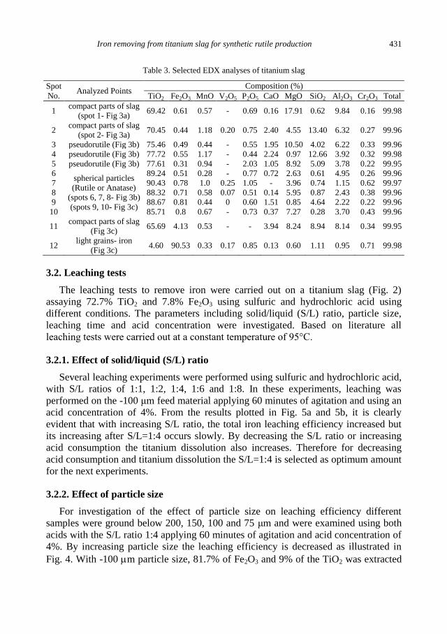
Iron removing from titanium slag for synthetic rutile production 431
Table 3. Selected EDX analyses of titanium slag
Spot
No. Analyzed Points
Composition (%)
TiO2 Fe2O3 MnO V2O5 P2O5 CaO MgO SiO2 Al2O3 Cr2O3 Total
1 compact parts of slag
(spot 1- Fig 3a) 69.42 0.61 0.57 - 0.69 0.16 17.91 0.62 9.84 0.16 99.98
2 compact parts of slag
(spot 2- Fig 3a) 70.45 0.44 1.18 0.20 0.75 2.40 4.55 13.40 6.32 0.27 99.96
3 pseudorutile (Fig 3b) 75.46 0.49 0.44 - 0.55 1.95 10.50 4.02 6.22 0.33 99.96
4 pseudorutile (Fig 3b) 77.72 0.55 1.17 - 0.44 2.24 0.97 12.66 3.92 0.32 99.98
5 pseudorutile (Fig 3b) 77.61 0.31 0.94 - 2.03 1.05 8.92 5.09 3.78 0.22 99.95
6 spherical particles
(Rutile or Anatase)
(spots 6, 7, 8- Fig 3b)
(spots 9, 10- Fig 3c)
89.24 0.51 0.28 - 0.77 0.72 2.63 0.61 4.95 0.26 99.96
7 90.43 0.78 1.0 0.25 1.05 - 3.96 0.74 1.15 0.62 99.97
8 88.32 0.71 0.58 0.07 0.51 0.14 5.95 0.87 2.43 0.38 99.96
9 88.67 0.81 0.44 0 0.60 1.51 0.85 4.64 2.22 0.22 99.96
10 85.71 0.8 0.67 - 0.73 0.37 7.27 0.28 3.70 0.43 99.96
11 compact parts of slag
(Fig 3c) 65.69 4.13 0.53 - - 3.94 8.24 8.94 8.14 0.34 99.95
12 light grains- iron
(Fig 3c) 4.60 90.53 0.33 0.17 0.85 0.13 0.60 1.11 0.95 0.71 99.98
3.2. Leaching tests
The leaching tests to remove iron were carried out on a titanium slag (Fig. 2)
assaying 72.7% TiO2 and 7.8% Fe2O3 using sulfuric and hydrochloric acid using
different conditions. The parameters including solid/liquid (S/L) ratio, particle size,
leaching time and acid concentration were investigated. Based on literature all
leaching tests were carried out at a constant temperature of 95°C.
3.2.1. Effect of solid/liquid (S/L) ratio
Several leaching experiments were performed using sulfuric and hydrochloric acid,
with S/L ratios of 1:1, 1:2, 1:4, 1:6 and 1:8. In these experiments, leaching was
performed on the -100 μm feed material applying 60 minutes of agitation and using an
acid concentration of 4%. From the results plotted in Fig. 5a and 5b, it is clearly
evident that with increasing S/L ratio, the total iron leaching efficiency increased but
its increasing after S/L=1:4 occurs slowly. By decreasing the S/L ratio or increasing
acid consumption the titanium dissolution also increases. Therefore for decreasing
acid consumption and titanium dissolution the S/L=1:4 is selected as optimum amount
for the next experiments.
3.2.2. Effect of particle size
For investigation of the effect of particle size on leaching efficiency different
samples were ground below 200, 150, 100 and 75 μm and were examined using both
acids with the S/L ratio 1:4 applying 60 minutes of agitation and acid concentration of
4%. By increasing particle size the leaching efficiency is decreased as illustrated in
Fig. 4. With -100 m particle size, 81.7% of Fe2O3 and 9% of the TiO2 was extracted
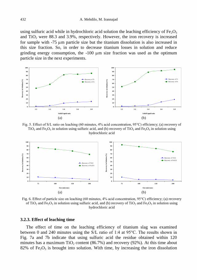
432 A. Mehdilo, M. Irannajad
using sulfuric acid while in hydrochloric acid solution the leaching efficiency of Fe2O3
and TiO2 were 88.3 and 3.9%, respectively. However, the iron recovery is increased
for sample with -75 m particle size but the titanium dissolution is also increased in
this size fraction. So, in order to decrease titanium losses in solution and reduce
grinding energy consumption, the -100 m size fraction was used as the optimum
particle size in the next experiments.
0
10
20
30
40
50
60
70
80
90
100
1:1 1:2 1:4 1:6 1:8
Solid/Liquid ratio
Reco
very
in
So
luti
on
(%
)
Recovery of Ti
Recovery of Fe
0
10
20
30
40
50
60
70
80
90
100
1:1 1:2 1:4 1:6 1:8
Solid/Liquid ratio
Reco
very
in
So
luti
on
(%
)
Recovery of Ti
Recovery of Fe
(a) (b)
Fig. 5. Effect of S/L ratio on leaching (60 minutes, 4% acid concentration, 95°C) efficiency; (a) recovery of
TiO2 and Fe2O3 in solution using sulfuric acid, and (b) recovery of TiO2 and Fe2O3 in solution using
hydrochloric acid
0
10
20
30
40
50
60
70
80
90
100
75 100 150 200
Size (microns)
Reco
very
in
So
luti
on
(%
)
Recovery of TiO2
Recovery of Fe2O3
0
10
20
30
40
50
60
70
80
90
100
75 100 150 200
Size (microns)
Reco
very
in
So
luti
on
(%
)
Recovery of TiO2
Recovery of Fe2O3
(a) (b)
Fig. 6. Effect of particle size on leaching (60 minutes, 4% acid concentration, 95°C) efficiency; (a) recovery
of TiO2 and Fe2O3 in solution using sulfuric acid, and (b) recovery of TiO2 and Fe2O3 in solution using
hydrochloric acid
3.2.3. Effect of leaching time
The effect of time on the leaching efficiency of titanium slag was examined
between 0 and 240 minutes using the S/L ratio of 1:4 at 95°C. The results shown in
Fig. 7a and 7b indicate that using sulfuric acid the residue obtained within 120
minutes has a maximum TiO2 content (86.7%) and recovery (92%). At this time about
82% of Fe2O3 is brought into solution. With time, by increasing the iron dissolution

Iron removing from titanium slag for synthetic rutile production 433
efficiency, the recovery of TiO2 in the residue as titanium dioxide concentrate
decreases from 92% to 88.5% by increasing the leaching time from 0 to 240 minutes.
In the case of hydrochloric acid, the results presented in Fig. 8a and 8b indicate that
the TiO2 content in the residue (synthetic rutile) is greater than that produced by
sulfuric acid leaching. This is due to higher solubility of iron in hydrochloric acid.
With time, with increasing TiO2 content in the residue from 88.7 to 91.3% the Fe2O3
content is decreased from 1.51% to 0.42%. The increase in leaching time results in the
increase of titanium dissolution and decrease of titanium recovery in produced
synthetic rutile. At 120 minutes leaching time, the Fe2O3 dissolution efficiency is
about 94% and 95% of TiO2 is recovered in the leaching residue as titanium dioxide
concentrate.
0
10
20
30
40
50
60
70
80
90
100
0 30 60 90 120 150 180 210 240 270
Time (min)
Gra
de a
nd
reco
very
in
resi
du
e (
%)
TiO2 % Recovery of TiO2
Fe2O3 % Recovery of Fe2O3
0
10
20
30
40
50
60
70
80
90
100
0 30 60 90 120 150 180 210 240 270
Time (min)
Reco
very
in
so
luti
on
(%
)
Recovery of TiO2
Recovery of Fe2O3
(a) (b)
Fig. 7. (a) Effect of time on TiO2 and Fe2O3 contents and on their recoveries in residue, (b) Effect of time
on recovery of TiO2 and Fe2O3 in solution during sulfuric acid leaching (S/L ratio 1:4, 95°C)
0
10
20
30
40
50
60
70
80
90
100
0 30 60 90 120 150 180 210 240 270
Time (min)
Gra
de a
nd
reco
very
in
resi
du
e (
%)
TiO2 % Recovery of TiO2Fe2O3 % Recovery of Fe2O3
0
10
20
30
40
50
60
70
80
90
100
0 30 60 90 120 150 180 210 240 270
Time (min)
reco
very
in
so
luti
on
(%
)
Recovery of TiO2
Recovery of Fe2O3
(a) (b)
Fig. 8. (a) Effect of time on TiO2 and Fe2O3 contents and on their recoveries in residue, (b) Effect of time
on recovery of TiO2 and Fe2O3 in solution during hydrochloric acid leaching (S/L ratio 1:4, 95°C)
3.2.4. Effect of acid concentration
Several experiments were carried out using sulfuric and hydrochloric acid
concentrations varying from 4 to 18% at 2 h leaching time and 95°C. From the results
plotted in Figs. 9a and 9b it is clearly evident that, with increasing sulfuric acid
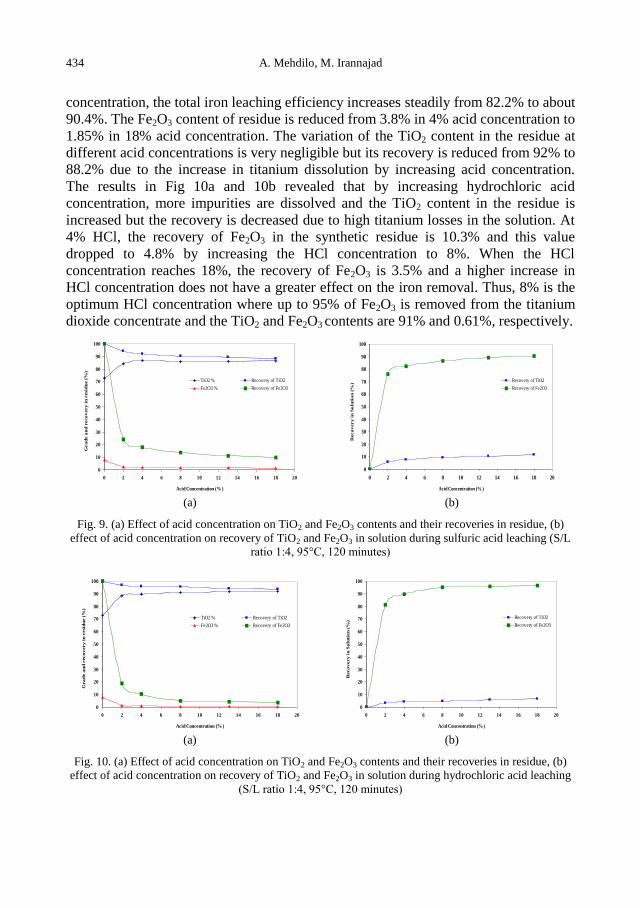
434 A. Mehdilo, M. Irannajad
concentration, the total iron leaching efficiency increases steadily from 82.2% to about
90.4%. The Fe2O3 content of residue is reduced from 3.8% in 4% acid concentration to
1.85% in 18% acid concentration. The variation of the TiO2 content in the residue at
different acid concentrations is very negligible but its recovery is reduced from 92% to
88.2% due to the increase in titanium dissolution by increasing acid concentration.
The results in Fig 10a and 10b revealed that by increasing hydrochloric acid
concentration, more impurities are dissolved and the TiO2 content in the residue is
increased but the recovery is decreased due to high titanium losses in the solution. At
4% HCl, the recovery of Fe2O3 in the synthetic residue is 10.3% and this value
dropped to 4.8% by increasing the HCl concentration to 8%. When the HCl
concentration reaches 18%, the recovery of Fe2O3 is 3.5% and a higher increase in
HCl concentration does not have a greater effect on the iron removal. Thus, 8% is the
optimum HCl concentration where up to 95% of Fe2O3 is removed from the titanium
dioxide concentrate and the TiO2 and Fe2O3 contents are 91% and 0.61%, respectively.
0
10
20
30
40
50
60
70
80
90
100
0 2 4 6 8 10 12 14 16 18 20
Acid Concentration (% )
Gra
de a
nd
reco
very
in
resi
du
e (
%)
TiO2 % Recovery of TiO2
Fe2O3 % Recovery of Fe2O3
0
10
20
30
40
50
60
70
80
90
100
0 2 4 6 8 10 12 14 16 18 20
Acid Concentration (% )
Reco
very
in
So
luti
on
(%
)
Recovery of TiO2
Recovery of Fe2O3
(a) (b)
Fig. 9. (a) Effect of acid concentration on TiO2 and Fe2O3 contents and their recoveries in residue, (b)
effect of acid concentration on recovery of TiO2 and Fe2O3 in solution during sulfuric acid leaching (S/L
ratio 1:4, 95°C, 120 minutes)
0
10
20
30
40
50
60
70
80
90
100
0 2 4 6 8 10 12 14 16 18 20
Acid Concentration (% )
Gra
de a
nd
reco
very
in
resi
du
e (
%)
TiO2 % Recovery of TiO2
Fe2O3 % Recovery of Fe2O3
0
10
20
30
40
50
60
70
80
90
100
0 2 4 6 8 10 12 14 16 18 20
Acid Concentration (% )
Reco
very
in
So
luti
on
(%
)
Recovery of TiO2
Recovery of Fe2O3
(a) (b)
Fig. 10. (a) Effect of acid concentration on TiO2 and Fe2O3 contents and their recoveries in residue, (b)
effect of acid concentration on recovery of TiO2 and Fe2O3 in solution during hydrochloric acid leaching
(S/L ratio 1:4, 95°C, 120 minutes)

Iron removing from titanium slag for synthetic rutile production 435
3.3. Characterization of titanium dioxide concentrate
The produced titanium dioxide concentrate at the optimum conditions was washed
and dried. In this concentrate rutile is the dominant phase but Ti2O3, anatase and iron
oxide phases were also found. The chemical analysis of the dried product obtained
under optimum conditions is presented in Table 4. The product of HCl leaching
contains about 91% TiO2 and only 0.6% iron as Fe2O3 while their content in the
titanium dioxide concentrate obtained by H2SO4 leaching are 86.8 and 1.87,
respectively. The contents of most impurities in the product of H2SO4 leaching are a
little greater than the HCl leaching product. The BSE images of titanium dioxide
concentrate produced by sulfuric and hydrochloric acid are compared in Fig. 11. These
images indicate that the texture and morphology of the product obtained by HCl and
H2SO4 are very different. The morphology of titanium dioxide produced by HCl
leaching is more granular than that prepared by H2SO4 leaching (Fig. 11a and 11b). In
the product of HCl leaching, the grains are mostly elongated with a clear and sharp
boundary while the product of the H2SO4 process has grains with less elongation and
unclear boundaries (Fig. 11c and 11d). Most of the particles produced by HCl leaching
are needle-like crystals but the acicular texture is observed scarcely in the product of
H2SO4 leaching (Fig. 11e and 11f). The particle size of the titanium dioxide
concentrates produced by H2SO4 and HCl leaching was also determined by the image
analysis method using a Clemex software. The cumulative percent of particles as a
function of circular and spherical diameter is shown in Fig. 12 and 13. The
information about size distribution of both products is presented in Table 6. The
results indicate that the mean size of particles obtained from HCl leaching is a little
smaller than that produced with H2SO4 leaching. Some of the particles shown in Fig.
11 were analyzed by EDX (Table 5). The chemical compositions of titanium dioxide
particles produced by different acids leaching are closely similar. The maximum
content of TiO2 is 93% and the minimum content of iron as Fe2O3 is 0.48%. Among
the coloring metals, the content of V2O5 and Cr2O3 in the produced material does not
exceed 0.12% and 0.3%, respectively but the quantity of MnO2 sourced from ilmenite
lattice varies from 0.88 to 1.31% and could negatively affect the chlorination process.
The content of other impurities (MgO, SiO2, Al2O3, CaO and P2O5) is relatively high.
Silica is not a major problem in the chloride process and could be removed with
alkaline leaching (Nayl et al., 2009) but other impurities (MgO, Al2O3, CaO and P2O5)
are the chlorine consuming components and should be removed before using this
process.
Table 4. The chemical composition of produced titanium dioxide
% TiO2 Fe2O3 MnO MgO SiO2 Al2O3 V2O5 CaO K2O SO3 Cl Total
H2SO4 86.8 1.87 0.57 2.79 4.6 1.02 0.22 1.04 0.21 0.51 - 99.63
HCl 91.0 0.61 0.62 2.11 3.28 0.86 0.18 0.58 0.09 - 0.38 99.51
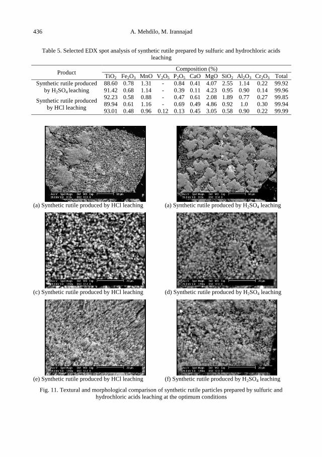
436 A. Mehdilo, M. Irannajad
Table 5. Selected EDX spot analysis of synthetic rutile prepared by sulfuric and hydrochloric acids
leaching
Product Composition (%)
TiO2 Fe2O3 MnO V2O5 P2O5 CaO MgO SiO2 Al2O3 Cr2O3 Total
Synthetic rutile produced
by H2SO4 leaching
88.60 0.78 1.31 - 0.84 0.41 4.07 2.55 1.14 0.22 99.92
91.42 0.68 1.14 - 0.39 0.11 4.23 0.95 0.90 0.14 99.96
Synthetic rutile produced
by HCl leaching
92.23 0.58 0.88 - 0.47 0.61 2.08 1.89 0.77 0.27 99.85
89.94 0.61 1.16 - 0.69 0.49 4.86 0.92 1.0 0.30 99.94
93.01 0.48 0.96 0.12 0.13 0.45 3.05 0.58 0.90 0.22 99.99
(a) Synthetic rutile produced by HCl leaching (a) Synthetic rutile produced by H2SO4 leaching
(c) Synthetic rutile produced by HCl leaching (d) Synthetic rutile produced by H2SO4 leaching
(e) Synthetic rutile produced by HCl leaching (f) Synthetic rutile produced by H2SO4 leaching
Fig. 11. Textural and morphological comparison of synthetic rutile particles prepared by sulfuric and
hydrochloric acids leaching at the optimum conditions
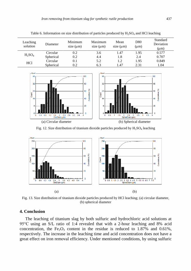
Iron removing from titanium slag for synthetic rutile production 437
Table 6. Information on size distribution of particles produced by H2SO4 and HCl leaching
Leaching
solution Diameter
Minimum
size (m)
Maximum
size (m)
Mean
size (m)
D80
(m)
Standard
Deviation
(m)
H2SO4 Circular 0.2 3.6 1.47 1.95 0.577
Spherical 0.2 4.4 1.8 2.4 0.707
HCl Circular 0.1 5.2 1.2 1.95 0.849
Spherical 0.2 6.3 1.47 2.31 1.04
(a) Circular diameter (b) Spherical diameter
Fig. 12. Size distribution of titanium dioxide particles produced by H2SO4 leaching
(a) (b)
Fig. 13. Size distribution of titanium dioxide particles produced by HCl leaching; (a) circular diameter,
(b) spherical diameter
4. Conclusion
The leaching of titanium slag by both sulfuric and hydrochloric acid solutions at
95°C using an S/L ratio of 1:4 revealed that with a 2-hour leaching and 8% acid
concentration, the Fe2O3 content in the residue is reduced to 1.87% and 0.61%,
respectively. The increase in the leaching time and acid concentration does not have a
great effect on iron removal efficiency. Under mentioned conditions, by using sulfuric
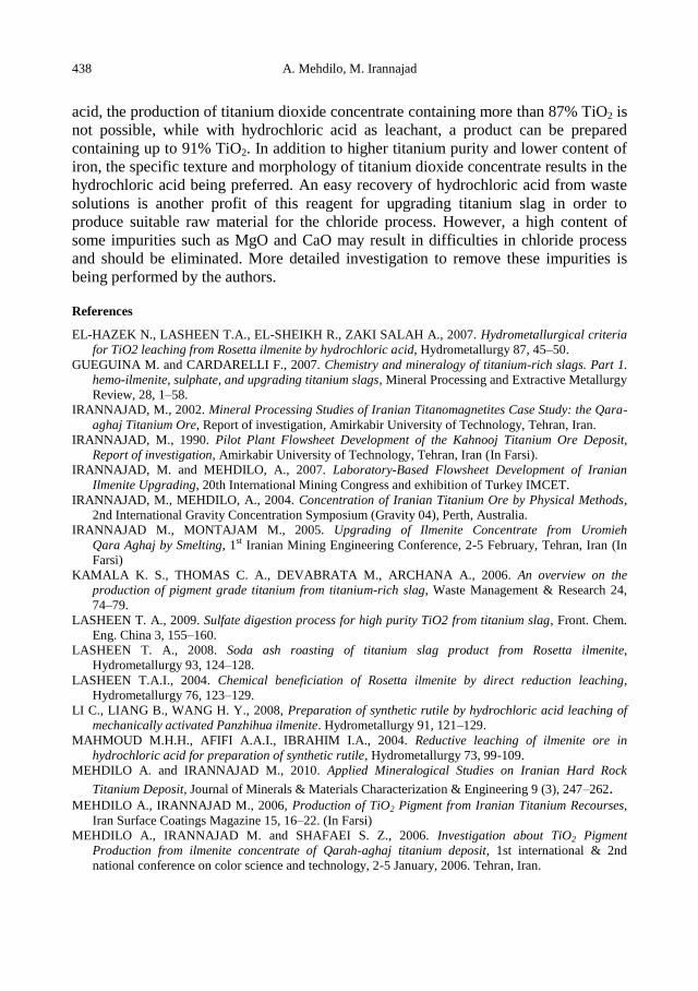
438 A. Mehdilo, M. Irannajad
acid, the production of titanium dioxide concentrate containing more than 87% TiO2 is
not possible, while with hydrochloric acid as leachant, a product can be prepared
containing up to 91% TiO2. In addition to higher titanium purity and lower content of
iron, the specific texture and morphology of titanium dioxide concentrate results in the
hydrochloric acid being preferred. An easy recovery of hydrochloric acid from waste
solutions is another profit of this reagent for upgrading titanium slag in order to
produce suitable raw material for the chloride process. However, a high content of
some impurities such as MgO and CaO may result in difficulties in chloride process
and should be eliminated. More detailed investigation to remove these impurities is
being performed by the authors.
References
EL-HAZEK N., LASHEEN T.A., EL-SHEIKH R., ZAKI SALAH A., 2007. Hydrometallurgical criteria
for TiO2 leaching from Rosetta ilmenite by hydrochloric acid, Hydrometallurgy 87, 45–50.
GUEGUINA M. and CARDARELLI F., 2007. Chemistry and mineralogy of titanium-rich slags. Part 1.
hemo-ilmenite, sulphate, and upgrading titanium slags, Mineral Processing and Extractive Metallurgy
Review, 28, 1–58.
IRANNAJAD, M., 2002. Mineral Processing Studies of Iranian Titanomagnetites Case Study: the Qara-
aghaj Titanium Ore, Report of investigation, Amirkabir University of Technology, Tehran, Iran.
IRANNAJAD, M., 1990. Pilot Plant Flowsheet Development of the Kahnooj Titanium Ore Deposit,
Report of investigation, Amirkabir University of Technology, Tehran, Iran (In Farsi).
IRANNAJAD, M. and MEHDILO, A., 2007. Laboratory-Based Flowsheet Development of Iranian
Ilmenite Upgrading, 20th International Mining Congress and exhibition of Turkey IMCET.
IRANNAJAD, M., MEHDILO, A., 2004. Concentration of Iranian Titanium Ore by Physical Methods,
2nd International Gravity Concentration Symposium (Gravity 04), Perth, Australia.
IRANNAJAD M., MONTAJAM M., 2005. Upgrading of Ilmenite Concentrate from Uromieh
Qara Aghaj by Smelting, 1st Iranian Mining Engineering Conference, 2-5 February, Tehran, Iran (In
Farsi)
KAMALA K. S., THOMAS C. A., DEVABRATA M., ARCHANA A., 2006. An overview on the
production of pigment grade titanium from titanium-rich slag, Waste Management & Research 24,
74–79.
LASHEEN T. A., 2009. Sulfate digestion process for high purity TiO2 from titanium slag, Front. Chem.
Eng. China 3, 155–160.
LASHEEN T. A., 2008. Soda ash roasting of titanium slag product from Rosetta ilmenite,
Hydrometallurgy 93, 124–128.
LASHEEN T.A.I., 2004. Chemical beneficiation of Rosetta ilmenite by direct reduction leaching,
Hydrometallurgy 76, 123–129.
LI C., LIANG B., WANG H. Y., 2008, Preparation of synthetic rutile by hydrochloric acid leaching of
mechanically activated Panzhihua ilmenite. Hydrometallurgy 91, 121–129.
MAHMOUD M.H.H., AFIFI A.A.I., IBRAHIM I.A., 2004. Reductive leaching of ilmenite ore in
hydrochloric acid for preparation of synthetic rutile, Hydrometallurgy 73, 99-109.
MEHDILO A. and IRANNAJAD M., 2010. Applied Mineralogical Studies on Iranian Hard Rock
Titanium Deposit, Journal of Minerals & Materials Characterization & Engineering 9 (3), 247–262. MEHDILO A., IRANNAJAD M., 2006, Production of TiO2 Pigment from Iranian Titanium Recourses,
Iran Surface Coatings Magazine 15, 16–22. (In Farsi)
MEHDILO A., IRANNAJAD M. and SHAFAEI S. Z., 2006. Investigation about TiO2 Pigment
Production from ilmenite concentrate of Qarah-aghaj titanium deposit, 1st international & 2nd
national conference on color science and technology, 2-5 January, 2006. Tehran, Iran.
Iron removing from titanium slag for synthetic rutile production 439
MEHDILO, A., 2003. Mineral Processing Studies of the Qara-aghaj Titanium Ore by Physical Methods,
MSc Thesis, Amirkabir University of Technology, Tehran, Iran. (In Farsi)
NAYL A.A., AWWARD N.S., ALY H.F., 2009a. Kinetics of acid leaching of ilmenite decomposed by
KOH Part 2. Leaching by H2SO4 and C2H2O4, Journal of Hazardous Materials168, 793–799.
NAYL A.A., ISMAIL I.M. and ALY H.F., 2009b. Ammonium hydroxide decomposition of ilmenite slag,
Hydrometallurgy 98, 196–200.
OLANIPEKUN E., 1999, A kinetic study of the leaching of a Nigerian ilmenite ore by hydrochloric acid,
Hydrometallurgy, 53, 1–10.
SAMALA S., MOHAPATRA B.K., MUKHERJEE P.S. and CHATTERJEE S.K., 2009. Integrated XRD,
EPMA and XRF study of ilmenite and titanium slag used in pigment production, Journal of Alloys
and Compounds 474, 484–489.
SASIKUMAR C., RAO D.S., SRIKANTH S., MUKHOPADHYAY N.K., MEHROTRA S.P., 2007.
Dissolution studies of mechanically activated manavalakurichi ilmenite with HCl and H2SO4,
Hydrometallurgy 88, 154–169.
ZHANG S. and NICOL M. J., 2009. An electrochemical study of the reduction and dissolution of ilmenite
in sulfuric acid solutions, Hydrometallurgy, 97, 146–152.
ZHANG S. and NICOL M. J., 2010. Kinetics of the dissolution of ilmenite in sulfuric acid solutions under
reducing conditions, Hydrometallurgy 103, 196–204.
ZHANG Y., TAO Q., ZHANG Y., 2009. A novel preparation of titanium dioxide from titanium slag,
Hydrometallurgy, 96, 52–56.

440 A. Mehdilo, M. Irannajad
http://dx.doi.org/10.5277/ppmp120210
Physicochem. Probl. Miner. Process. 48(2), 2012, 441−454 Physicochemical Problems
of Mineral Processing
w w w . m i n p r o c . p w r . w r o c . p l / j o u r n a l / ISSN 1643-1049 (print)
ISSN 2084-4735 (online)
Received January 5, 2012; reviewed; accepted February 28, 2012
ADSORPTION AND DESORPTION KINETICS BEHAVIOUR
OF METHYLENE BLUE ONTO ACTIVATED CARBON
Cigdem SARICI-OZDEMIR
Inonu University, Faculty of Engineering, Department of Chemical Engineering, 44280, Malatya, Turkey,
Tel. : +90 422 3410010–4757, Fax: +90 422 3410046, [email protected]
Abstract. In the present work investigations on a potential use of activated carbon for the
removal of Methylene Blue (MB) from wastewater are presented. Adsorption kinetics of
methylene blue has been studied using reaction-based and diffusion-based models. Three
kinetic models, namely, pseudo-first-order, pseudo-second-order and the Elovich are analyzed
at the temperature of 298 K for the reaction-based model. The kinetic studies showed that the
data were well described by the pseudo-second-order kinetic model. Intraparticle diffusion,
external-film diffusion, and internal-pore diffusion models characterizing MB were obtained.
The results suggested that the activated carbon has a high potential to be used as an effective
adsorbent for methylene blue adsorption. Pseudo first-order, pseudo second-order and the
Elovich models were employed to describe the desorption mechanism. The experimental
results showed that the pseudo second-order equation is the best model. About 99% of
activated carbon has been regenerated by desorption.
keywords: activated carbon, adsorption, desorption, kinetic studies, methylene blue
1. Introduction
Environmental pollution is a problem both in developed and devoloping countries.
Factors such as population growth, and urbanization, invariably place greater demands
on the world. Industrial revolution brought, with technological progress such as
discovery of how to make synthetic dye, virtually universal use by different industries.
Cheaper to produce, more brighter color, fast and easy to apply to fabric, the new dyes
changed world. The chemicals used to produce dyes today are often highly toxic,
carcinogenic, or even explosive. Harmful chemicals are used in the dying process,
including aniline, dioxin, toxic heavy metals (such as chrome, copper, zinc,
formaldehyde). Almost all industrial dye processes involve a solution of a dye in water
in which the fabrics are soak. So, the textile factories across the world are dumping
millions of Mg of dye effluent into rivers. Therefore, it is necessary to remove them
from the wastewater before discharging. For the removal of these materials, several
methods such as physical, chemical and biological have been investigated. Among the
methods, removal of dyes by adsorption is regarded as one of the competitive methods

442 C. Sarici-Ozdemir
because of high efficiency, economic feasibility and simplicity of design/operation
(Chen et al., 2010; Rafatullah et al., 2010; Haque et al., 2011). Activated carbons,
because of their large surface area and relatively high sorption capacity, for a wide
variety of dyes, have become the most promising and effective adsorbent.
Nevertheless, their applications are restricted, because activated carbons are prepared
from natural materials such as wood or coal, which are expensive. Recently, low cost
and easily available other carbonaceous materials have been used, for example apricot
stone, almand barks, coffee seeds, tea waste, rice husk etc.) (Diao et al., 2001; Wei-
Lung et al., 2011). Textile waste containing cotton, nylon and polymers creates a
problem in the world. Activated carbon prepared from these wastes could be important
for the regional economy. Because high value products are obtained from low cost
materials, they simultaneously bring solution to the problem of wastes (Altenor et al.
2009).
Methylene blue (MB) is one of the well known basic/cationic dyes and has been
widely used in wood, silk, cotton, pharmaceutical industries. In this work, activated
carbon has been prepared from a mixture of textural waste by chemical activation with
ZnCl2 in the flow of N2 at 500°C. The prepared activated carbon is used as an
adsorbent to remove methylene blue from aqueous solutions. The kinetics and
diffusion parameters of the adsorption and desorption processes have been
investigated.
2. Materials and methods
2.1. Materials
The solute selected for this work was MB (chemical formula = C16H18N3SCl, MW
=320 g/mol). A stock solution of 1000 mg/dm3 was prepared by dissolving the
required amount of methylene blue in distilled water. The spectrophotometric
determination of MB was carried out using a Shimadzu UV/Vis spectrophotometer at
662 nm (model UV-2100S, Japan).
2.2. Preparation of activated carbon (WZ)
Textural waste, provided by different textile fabrics in Malatya, Turkey, was used
in this study as a source of activated carbon. The raw material was subjected to two
steps of activation as follows.
a) The raw material was mixed with ZnCl2 (ZnCl2: waste=0.5/1), and the mixture
was kneaded by adding distilled water. The mixture was then dried at 110°C to
prepare the impregnated sample.
b) The impregnated sample was placed on a quartz dish, which was then inserted
within a quartz tube (internal diameter = 60 mm). The impregnated sample was heated
at the rate of 10°C/min up to the activation temparature (500°C) under N2 flow (100
cm3/min) and held at the activation temperature for 1 h. After activation, the sample
was cooled under N2 flow. The sample was washed sequentially several times with hot

Adsorption and desorption kinetics behaviour of methylene blue onto activated carbon 443
distilled water to remove any residual chemical and until a pH of 7 was reached. The
washed sample was dried at 110°C to prepare activated carbon.
2.3. Adsorption experiments
MB solutions were prepared in distilled water at the desired concentrations.
Adsorption experiments were carried out by agitating 0.1 g of WZ with 50 cm3
solutions of the desired concentration (50, 75 and 100 mg/dm3) at different values of
time (1 to 60 min) and 25ºC in a thermostatic bath operating at 400 rpm. The amount
of MB adsorbed onto WZ, qt (mg/g), was calculated by the mass balance relationship
represented by equation:
W
VCCq tt )( 0 , (1)
where C0 and Ct are the initial and final (at time t) liquid and phase concentrations of
MB (mg/dm3), respectively, V is the volume of the solution (dm
3), and W is the weight
of the dry WZ used (g).
The normalized standard deviation qe (%) was calculated using Eq. (2):
1
/100(%)
2
exp,,exp,
N
qqqq
ecalee
e , (2)
where N is the number of data points, q e,exp and q e,cal (mg/g) are the experimental and
calculated equilibrium adsorption capacities value, respectively.
2.4. Desorption experiments
For the desorption study, 0.5 g of activated carbon was added to 250 cm3 of MB
solutions (50, 75 and 100 mg/dm3) and the mixture was stirred at 60 min. After
mixing, the supernatant MB solution was discarded and the activated carbon alone
was separated. Then, the MB-adsorbed activated carbon was added into 250 cm3 of
ethanol mixture (v/v, ethanol/water= 10/100). Ethanol and activated carbon (saturated
with MB) solution samples were taken at specific time intervals (3, 5, 10, 60 min).
The amount of MB desorbed from WZ, qt (mg/g), was calculated at different values of
time (1 to 60 min) and all concentrations and temperature of 25oC by the Eq. (1).
3. Results and discussion
3.1. Effect of initial concentration of methylene blue
Initial dye concentration provides an important driving force to overcome the mass
transfer resistance of dye between the aqueous solution and activated carbon surface.
Adsorption kinetic studies were performed by measuring methylene blue
concentration and the results are illustrated in Fig. 1. The adsorption capacity
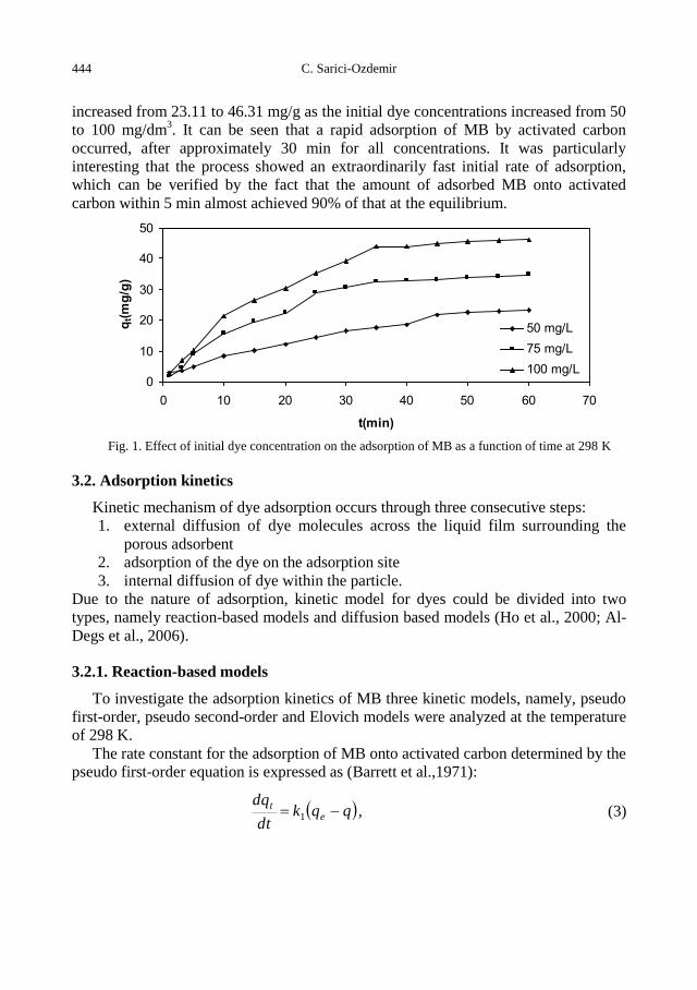
444 C. Sarici-Ozdemir
increased from 23.11 to 46.31 mg/g as the initial dye concentrations increased from 50
to 100 mg/dm3. It can be seen that a rapid adsorption of MB by activated carbon
occurred, after approximately 30 min for all concentrations. It was particularly
interesting that the process showed an extraordinarily fast initial rate of adsorption,
which can be verified by the fact that the amount of adsorbed MB onto activated
carbon within 5 min almost achieved 90% of that at the equilibrium.
Fig. 1. Effect of initial dye concentration on the adsorption of MB as a function of time at 298 K
3.2. Adsorption kinetics
Kinetic mechanism of dye adsorption occurs through three consecutive steps:
1. external diffusion of dye molecules across the liquid film surrounding the
porous adsorbent
2. adsorption of the dye on the adsorption site
3. internal diffusion of dye within the particle.
Due to the nature of adsorption, kinetic model for dyes could be divided into two
types, namely reaction-based models and diffusion based models (Ho et al., 2000; Al-
Degs et al., 2006).
3.2.1. Reaction-based models
To investigate the adsorption kinetics of MB three kinetic models, namely, pseudo
first-order, pseudo second-order and Elovich models were analyzed at the temperature
of 298 K.
The rate constant for the adsorption of MB onto activated carbon determined by the
pseudo first-order equation is expressed as (Barrett et al.,1971):
qqkdt
dqe
t 1 , (3)
0
10
20
30
40
50
0 10 20 30 40 50 60 70
t(min)
qt(m
g/g
)
50 mg/L
75 mg/L
100 mg/L
Adsorption and desorption kinetics behaviour of methylene blue onto activated carbon 445
where k1 (min–1
) is the pseudo first-order rate constant. Integrating Eq. (3) with respect
to the integration conditions q = 0 to q = qt at t = 0 to t = t, the kinetic rate expression
becomes:
tk
qqq ete303.2
log)log( 1 , (4)
where qe and qt are the amounts of MB adsorbed (mg/g) at equilibrium and time t
(min), respectively.
The adsorption kinetics have also been determined by the pseudo second-order
model using equation (Ho and McKay, 1998):
eet q
t
qkq
t
22
1, (5)
where k2 is the second order-rate constantn, g/(mgmin); and h = k2qe2, where h is the
initial adsorption rate, mg/(gmin).
The Elovich model equation is generally expressed as (Low, 1960):
tt q
dt
dq exp . (6)
To simplify the the Elovich equation, Chian and Clayton (1980) assumed that αβt>>t
and by applying boundary conditions t=0 to t=t and qt=0 to qt=q0. Then, Eq. (6)
becomes (Chien and Clayton, 1980):
tqt ln1
ln1
. (7)
where α is the initial adsorption rate, mg/(gmin) and β is the desorption constant
(g/mg).
The plot of log (qe-qt) versus t should give a linear relationship, from which k1 and
qe can be obtained from the slope and intercept of the plot, respectively. The k1 values,
calculated qe values, and correlation coefficients are provided in Table 1. The
coefficient of correlation for the pseudo first-order kinetic model is not high for all
concentrations. Moreover, the determined values of qe calculated from the equation
differ from the experimental values showing that adsorption of methylene blue onto
WZ is not a first-order reaction and had low correlation coefficients (R2<0.88).
The plot of (t/qt) versus t of Eq. (5) should give a linear relationship, from which qe
and k2 can be determined from the slope and intercept of the plot, respectively. The
results are illustrated in Table 1. The experimental results were applied to the pseudo-
second order model straight lines with high correlation coefficients (R2=0.982). They
indicate that adsorption of MB follows the pseudo-second order kinetic model. From
the analysis of all kinetic models one can predict experimental behaviour of the MB-
WZ system.

446 C. Sarici-Ozdemir
Table 1. Kinetic paramaters of adsorption
Concentration (mg/dm3) 50 75 100
qe,exp (mg/g) 32.11 43.56 64.30
Pseudo-first order
qe,cal (mg/g) 34.84 72.45 111.55
k1 (min-1) 0.072 0.080 0.091
R2 0.839 0.858 0.878
qe (%) 40.2 31.1 28.0
Pseudo-second order
qe,cal (mg/g) 32.36 42.63 68.49
k2 (gmg-1min-1) 0.00081 0.00078 0.00072
h (mgg-1min-1) 0.848 1.417 3.377
R2 0.915 0.962 0.982
qe (%) 11.1 9.90 5.69
Elovich
α ( mgg-1min-1) 3.947 6.537 8.864
β (g.mg-1) 0.178 0.106 0.079
R2 0.900 0.953 0.958
qe (%) 28.8 26.1 18.2
A comparison of the three kinetic models with experimental values for all
concentrations can be seen in Figs. 2a-c. The normalized standard deviations qe (%)
are used to see the fit between the experimental data and theoretical values of MB onto
activated carbon. It is clear from the figures and standard deviations (<11.10 %) that
for pseudo-second-order (Table 1), there is a good agreement between the
experimental and predicted values.
3.2.2. Diffusion-based models
Various diffusion models can be used to describe adsorption. These diffusion
models have been developed to predict the dynamic character of adsorption. This work
used the intraparticle diffusion, external-film diffusion, and internal-pore diffusion
models to characterize adsorption of MB.
The intraparticle diffusion equation (Srivastova et al., 1989; Weber et al., 1973)
can be written as follows:
ctkqt 2/1int , (8)
where c is the intercept of the line, which is proportional to the thickness of the
boundary layer and kint is the intraparticle diffusion rate constant, mg/(gmin–1/2
). The
intraparticle diffusion model rate constant, kint, is obtained from the slope of the
straight line of qt versus t1/2
(Fig. 3).
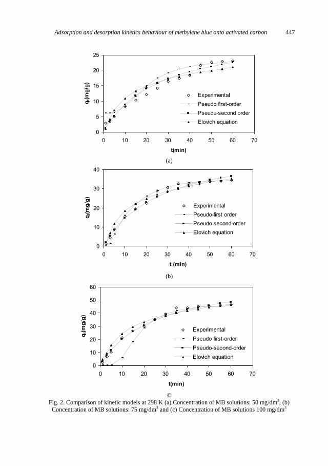
Adsorption and desorption kinetics behaviour of methylene blue onto activated carbon 447
(a)
(b)
©
Fig. 2. Comparison of kinetic models at 298 K (a) Concentration of MB solutions: 50 mg/dm3, (b)
Concentration of MB solutions: 75 mg/dm3 and (c) Concentration of MB solutions 100 mg/dm3
0
5
10
15
20
25
0 10 20 30 40 50 60 70
t(min)
qt(m
g/g
)
Experimental
Pseudo first-order
Pseudu-second order
Elovich equation
0
10
20
30
40
0 10 20 30 40 50 60 70
t (min)
qt(m
g/g
)
Experimental
Pseudo-first order
Pseudo second-order
Elovich equation
0
10
20
30
40
50
60
0 10 20 30 40 50 60 70
t(min)
qt(m
g/g
)
Experimental
Pseudo first-order
Pseudo-second-order
Elovich equation
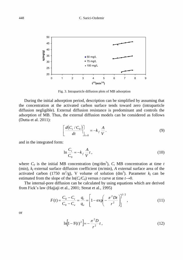
448 C. Sarici-Ozdemir
Fig. 3. Intraparticle diffusion plots of MB adsorption
During the initial adsorption period, description can be simplified by assuming that
the concentration at the activated carbon surface tends toward zero (intraparticle
diffusion negligible). External diffusion resistance is predominant and controls the
adsorption of MB. Thus, the external diffusion models can be considered as follows
(Dutta et al. 2011):
V
Ak
dt
CCdf
t
t
0
0/. (9)
and in the integrated form:
tV
Ak
C
Cf
t 0
ln , (10)
where C0 is the initial MB concentration (mg/dm3), Ct MB concentration at time t
(min), kf external surface diffusion coefficient (m/min), A external surface area of the
activated carbon (1750 m2/g), V volume of solution (dm
3). Parameter kf can be
estimated from the slope of the ln(Ct/C0) versus t curve at time t→0.
The internal-pore diffusion can be calculated by using equations which are derived
from Fick’s law (Hajjaji et al., 2001; Streat et al., 1995)
2/1
2
2
0
0 exp1)(
r
Dt
q
q
CC
CCtF
e
t
e
t , (11)
or
tr
Dt
2
22)F(1ln
, (12)
20
25
30
35
40
45
50
0 1 2 3 4 5 6 7 8 9
t1/2(min1/2)
qt(m
g/g
)
50 mg/L
75 mg/L
100 mg/L
Adsorption and desorption kinetics behaviour of methylene blue onto activated carbon 449
where Ce is the MB equilibrium concentration (mg/dm3), D is the internal-pore
diffusion coefficient (m2/min) and r is the particle radius assuming spherical geometry
(2.10-6
m). A plot of ln[1-F(t)2] versus time t should be linear with a slop of -
2D/r
2,
which is commonly known as the diffusional rate constant.
Table 2 shows that the intraparticle diffusion model rate constant, kint, which
increases as the initial MB concentration increases. This could be attributed to the
driving force of diffusion. The driving force changes with the MB concentration in the
solution. The linear plots at various concentration do not pass through the origin,
which shows that the intraparticle diffusion is not the only rate-controlling step (Fig.
3). If the plot is straight line passing through the origin, then the adsorption rate is
governed by particle diffusion mechanism. Otherwise, it is governed by the film
diffusion (Sarkar et al., 2003). The values of c are related to the boundary layer
resistance. It is relatively high, and the greater is the contribution of the surface
adsorption in the rate limiting step.
The values of external diffusion coefficient, kf, increase by the increasing initial
MB concentration (Table 2). The change in kf, depends on the surface area and pore
distribution of activated carbon. The activated carbon has micropores and external
diffusion is more diffucult with the increasing initial concentration of MB.
The internal pore diffusivities were determined using Eq. (12). The adsorption data
in Table 2 show that the internal pore diffusion coefficients is increasing with the
increasing initial dye concentration.
A comparison of the adsorption capacities of MB adsorption estimated from the
kinetic studies on various adsorbents is presented in Table 3. The variation in
adsorption capacities and affinities can be mainly attributed to the differences in
experimental condition and properties of the adsorbent. From Table 3, it can be
observed, that the values of qe of WZ for MB adsorption for the same initial
concentration were higher than that for agricultural by-products (wood sawdust,
rejected tea, carrot powder etc), zeolite, and activated carbon. The results
demonstrated that WZ’s could be employed as promising adsorbents.
Table 2. Diffusion parameters of adsorption
Concentration (mg/dm3) 50 75 100
İntraparticle diffusion
kint (mgg–1min–1/2). 1.12 1.18 1.42
c 12.29 25.46 35.42
R2 0.898 0.970 0.989
External-film diffusion
kf108 (m/min) 13.10 14.50 15.10
R2 0.976 0.980 0.993
Internal-pore diffusion
D1015(m2/min) 22.31 27.18 28.27
R2 0.893 0.963 0.939
450 C. Sarici-Ozdemir
Table 3. Adsorption capacities of MB for adsorbents
Adsorbent Co (mg/dm3) qe (mg/g) Ref.
Wood sawdust 120 16.21 (Ofomaja, 2008)
Cotton stalk 475 825
104.82 211.35
(Deng et al., 20011)
Cotton stalk
(with H2SO4)
950
1415
240.96
381.68
(Deng et al., 20011)
Cotton stalk
(with H3PO4)
950
1415
173.01
242.13
(Deng et al., 20011)
Rejected tea 50 100
200
20.80 40.50
80.00
(Nasuha et al., 2010)
Kenaf care fibers 50
100
150
44.84
96.15
142.80
(Sajab et al., 2011)
Activated carbon (from posidonia oceonica)
250 500
750
50.09 101.40
153.55
(Durala et al., 2011)
Wheat straw 100 96.40 (Han et al., 2010) Palm kernel fiber 20
40
80 160
7.67
7.22
27.22 31.26
(El-Sayed et al., 2011)
Peanut husk 80 35.52 (Song et al., 2011)
Carrot leaves powder 10 4.10 (Kushwaha et al., 2011) Carrot stem powder 10 4.34 (Kushwaha et al., 2011)
J. curcas cake residue 200
500
160.85
282.31
(Kurniawan et al. 2011)
Titanate nanotubes 50
100
94.15
129.17
(Xionga et al. 2010)
NaOH-modified rejected tea
50 100
200
300
2.44 3.99
19.80
71.42
(Nasuha et al. 2011)
Lotus leaf powder 50
100
46.00
91.00
(Han et al., 2011)
Zeolite 30 55
113
4.81 8.27
14.90
(Han et al., 2009)
Jack fruit peel 35
80
130
10.58
25.48
40.70
(Hameed, 2009)
Tea waste 50 24.76 (Udin et al., 2009)
Activated carbon
(from textural waste)
50
75 100
32.36
42.63 68.49
This work
3.3 Desorption kinetics
Desorption characteristics or regeneration of spent activated carbon is extremely
important. Desorption experiments were carried out using activated carbon at 25oC
and initial concentration of 50, 75 and 100 mg/dm3. As shown in Fig. 4 the desorption
capacity at equilibrium of MB desorption increased from 0.08 to 0.23 mg/dm3 with an
increase in the initial dye concentration. The desorption reaches equilibrium with solid
phase concentration of qt at the shortest time of about 6 min. On the other hand, the
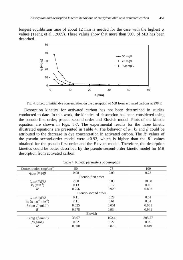
Adsorption and desorption kinetics behaviour of methylene blue onto activated carbon 451
longest equilibrium time of about 12 min is needed for the case with the highest qt
values (Tseng et al., 2009). These values show that more than 99% of MB has been
desorbed.
Fig. 4. Effect of initial dye concentration on the desorption of MB from activated carbons at 298 K
Desorption kinetics for activated carbon has not been determined in studies
conducted to date. In this work, the kinetics of desorption has been considered using
the pseudo-first order, pseudo-second order and Elovich model. Plots of the kinetic
equation are shown in Figs. 5-7. The experimental results for the three kinetic
illustrated equations are presented in Table 4. The behavior of k1, k2 and β could be
attributed to the decrease in dye concentration in activated carbon. The R2 values of
the pseudo second-order model were >0.93, which is higher than the R2 values
obtained for the pseudo-first-order and the Elovich model. Therefore, the desorption
kinetics could be better described by the pseudo-second-order kinetic model for MB
desorption from activated carbon.
Table 4. Kinetic parameters of desorption
Concentration (mg/dm3) 50 75 100
qe,exp (mg/g) 0.08 0.09 0.23
Pseudo-first order
qe,cal (mg/g) 2.00 8.03 18.88
k1 (min-1) 0.13 0.12 0.10
R2 0.756 0.929 0.892
Pseudo-second order
qe,cal (mg/g) 0.11 0.29 0.51
k2 (gmg-1min-1) 2.11 0.61 0.31
h (mgg-1min-1) 0.025 0.051 0.081
R2 0.978 0.934 0.941
Elovich
α (mgg-1min-1) 38.67 102.4 305.27
β (g/mg) 0.32 0.22 0.09
R2 0.800 0.875 0.849
0
10
20
30
40
50
0 10 20 30 40 50
t (min)
qt (m
g/g
)
50 mg/L
75 mg/L
100 mg/L
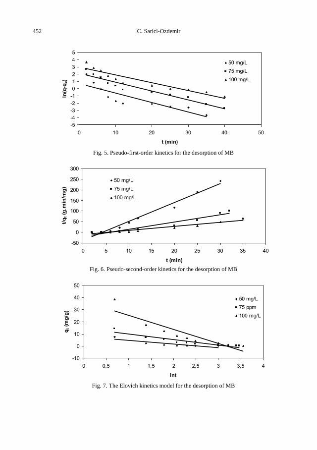
452 C. Sarici-Ozdemir
Fig. 5. Pseudo-first-order kinetics for the desorption of MB
Fig. 6. Pseudo-second-order kinetics for the desorption of MB
Fig. 7. The Elovich kinetics model for the desorption of MB
-5
-4
-3
-2
-1
0
1
2
3
4
5
0 10 20 30 40 50
t (min)
ln(q
-qe)
50 mg/L
75 mg/L
100 mg/L
-50
0
50
100
150
200
250
300
0 5 10 15 20 25 30 35 40
t (min)
t/q
t (g
.min
/mg
)
50 mg/L
75 mg/L
100 mg/L
-10
0
10
20
30
40
50
0 0,5 1 1,5 2 2,5 3 3,5 4
lnt
qt (m
g/g
)
50 mg/L
75 ppm
100 mg/L
Adsorption and desorption kinetics behaviour of methylene blue onto activated carbon 453
4. Conclusion
Activated carbon (WZ) can be used as adsorbent for removal of MB from its
aqueous solution.
The kinetics of MB adsorption onto activated carbon was examined using the
pseudo-first-order, pseudo-second-order and Elovich kinetics models. The adsorption
kinetics followed the pseudo-second-order kinetic model.
The adsorption of MB onto activated carbon was controlled by external diffusion.
The rate of adsorption of MB was very high during the first ten minutes. This was
followed by a slower rate, and gradually approached a plateau.
Regeneration efficiency of activated carbon (or desorption of MB) was calculated
to be 99%. The desorption kinetics followed the pseudo-second-order kinetic model.
References
AL-DEGS, Y.S., EL-BARGHOUTHİ, M.I., ISSA, A.A., KHRAİSHEH, M.A., WALKER, G.M., 2006,
Sorption of Zn(II), Pb(II) and Co(II) using natural sorbents: equilibrium and kinetic studies, Water
Res. 40, 2645–2658.
ALTENOR, S., CARENE, B., EMMANUEL, E., LAMBERT, J., EHRHARDT, J., GASPARD, S., 2009,
Adsorption studies of methylene blue and phenol onto vetiver roots activated carbon prepared by
chemical activation J. Hazard. Mater. 165, 1029–1039.
BARRETT, P.E.P, JOYNER, L.G., HALENDA, P.P. 1951, The determination of pore volume and area
distribution in porous substance. I. Computations from nitrogen isotherms, J.Am. Chem. Soc. 73,
373–380.
CHEN, S., ZHANG, J., ZHANG, C., YUE, Q., Lİ, Y., Lİ, C. 2010, Equilibrium and kinetic studies of
methyl orange and methyl violet adsorption on activated carbon derived from Phragmites austries,
Desalination 252, 149–156.
CHİEN,S.H., CLAYTON, W.R., 1980, Application of Elovich equation to the kinetics of phosphate
release and sorption on soils, Soil Sci. Soc. Am. J. 44, 265–268.
DENG, H., LU, J., Lİ, G., ZHANG, G., WANG, X. 2011, Adsorption of methylene blue on adsorbent
materials produced from cotton stalk, Chemical Engineering Journal 172, 326–334.
DİAO, Y., WALAWENDER, W.P., FAN, L.T. 2002, Activated carbons prepared from phosphoric acid
activation of grain sorghum, Bioresource Technology 81, 45-52.
DURALA, M.U., CAVASA, L., PAPAGEORGİOUC, S.K., KATSAROSC, F.K. 2011, Ethylene blue
adsorption on activated carbon prepared from Posidonia oceanica (L.) dead leaves: Kinetics and
equilibrium studies, Chemical Engineering Journal 168, 77-85.
DUTTA, S., BASU, J.K., GHAR, R.N. 2001, Studies on adsorption of p-nitrophenol on charred saw-
dust, Sep. Purif. Technol. 21, 227–235.
EL-SAYED, G.O. 2011, Removal of methylene blue and crystal violet from aqueous solutions by palm
kernel fiber, Desalination 272, 225–232.
HAJJAJI, M., KACIM, S., ALAMI, A., EL-BOUADILI, A., EL-MOUNTASSIR, M. 2001, Chemical
and mineralogical characterisation of a clay taken from the Moroccan meseta and a study of the
interaction between its fine friction and methylene blue. Applied Clay Science 20 1–12.
HAMEED, B.H., 2009, Removal of cationic dye from aqueous solution using jackfruit peel non-
conventional low-cost adsorbent, Journal of Hazardous Materials 162, 344–350.
HAN, X., WANG, W., MA, X., 2011, Adsorption characteristics of methylene blue onto low cost
biomass material lotus leaf, Chemical Engineering Journal 171, 1–8.
HAN, R., ZHANG, J., HAN, P., WANG, Y., ZHAO, Z., TANGA M., 2009, Study of equilibrium, kinetic
and thermodynamic parameters about methylene blue adsorption onto natural zeolite, Chemical
Engineering Journal 145 496–504.
454 C. Sarici-Ozdemir
HAN, R., ZHANG L., SONG C., ZHANG M., ZHU H., ZHANG L., 2010, Characterization of modified
wheat straw, kinetic and equilibrium study about copper ion and methylene blue adsorption in batch
mode, Carbohydrate Polymers 79, 1140–1149.
HAQUE, E., JUN, J.W., JHUNG, S.H. 2011, Adsorptive removal of methyl orange and methylene blue
from aqueous solution with a metal-organic framework material, iron terephthalate (MOF-235). J.
Hazard. Mater. 185, 507–511.
HO, Y.S., MCKAY, G. 1998, Sorption of dye from aqueous solution by peat, Chem. Eng. J. 70, 115–124.
HO, Y.S., NG, J.C.Y., MCKAY, G. 2000, Kinetics of pollutant sorption by biosorbents: a review. Sep.
Purif. Methods 29, 189–232.
KURNİAWAN, A., ISMADJİ, S., 2011, Potential utilizationof Jatropha curcas L. press-cake residue as
new precursor for activated carbon preparation:Application methylene blue removal from aqueous
solution, Journal of the Taiwan Institute of Chemical Engineers, in press.
KUSHWAHA, A.K., GUPTA, N., CHATTOPADHYAYA, M.C., 2011, Removal of cationic methylene
blue and malachite gren dyes from aqueous solution by waste materials of Daucus carota, Journal of
Saudi Chemical Society, in press.
LOW, M.J.D. 1960, Kinetics of chemisorption of gases on solids, Chem. Rev. 60, 267–317.
NASUHA N., HAMEED B.H., DİN A.T. 2010, Rejected tea as a potential low-cost adsorbent for the
removal of methylene blue, Journal Hazard. Mater. 175, 126–132.
NASUHA, N., HAMEED, B.H., 2011, Adsorption of methylene blue from aqueous solution onto NaOH-
modified rejected tea, Chemical Engineering Journal 166, 783–786.
OFOMAJA, A.E., 2008, Kinetic study and sorption mechanism of methylene blue and methyl violet onto
mansonia (Mansonia altissima) wood sawdust, Chemical Engineering Journal 143, 85–95.
RAFATULLAH, M., SULAİMAN, O., HASHİM, R., AHMAD, A. 2010, Adsorption of methylene blue
on low-cost adsorbents: A review, J. Hazard. Mater. 177, 70–80.
SAJAB, M.S., CHİA, C.H., ZAKARİA, S., JANİ, S.M., AYOB, M.K. 2011, Citric acid modified kenaf
core fibres for removal of methylene blue from aqueous solution, Bioresource Technology 102, 7237–
7243.
SARKAR M., KUMARACHARYA P., BHATTACHARYA B., 2003, Modeling the adsorption kinetics
of some priority organic pollutants in water from diffusion and activation energy parameters, J.
Colloid Interf. Sci. 266, 28-32.
SRIVASTOVA, S.K., TYAGI, R., PANT, N. 1989, Adsorption of heavy metal ions on carbonaceous
material developed from the waste slurry generated in local fertilizer plants, Water Research 23,
1161–1165.
STREAT, M., PATRICK, J.W., CAMPORRO PEREZ, M.J. 1995, Sorption of phenol and
parachlorophenol from water using conventional and novel activated carbons, Water Research 29,
467–472.
SONG, J., ZOU, W., BİAN, Y., SU, F., HAN, R., 2011, Adsorption characteristics of methylene blue by
peanut husk in batch and column models, Desalination 265, 119–125.
TSENG J., CHANG C., CHANG C., CHEN Y., CHANG C., Jİ D., C. CHİU,P. CHİANG, 2009, Kinetics
and equilibrium of desorption removal of copper from magnetic polymer adsorbent, Journal of
Hazard. Mater. 171, 370–377.
UDİN, T., ISLAM, A., MAHMUD, S., RUKANUZZAMAN M., 2009, Adsorptive removal of methylene
blue by tea waste, Journal of Hazardous Materials 164, 53–60.
WEBER, W.J., ASCE, J.M., MORRIS, J.C. 1963, Kinetics of adsorption on carbon from solution in:
Proceedings of the American Society of Civil Engineers, J. Senit Eng. Div. 89, 31–59.
WEİ-LUNG C., Lİ-SHİEN C.,YEN-HSİANG H., CHİH-YANG H., 2011, Effect of process parameters
on the removal of indium ions from aqueous solutions by adsorption onto tea waste, Fresenius
Environmental Bulletin.
XİONGA, L., YANG, Y., MAİA, J., SUNA, W., ZHANG, C., WEİ, D., CHEN, Q., Nİ J., 2010,
Adsorption behavior of methylene blue onto titanate nanotubes, Chemical Engineering Journal 156,
313–320.

http://dx.doi.org/10.5277/ppmp120211
Physicochem. Probl. Miner. Process. 48(2), 2012, 455−462 Physicochemical Problems
of Mineral Processing
w w w . m i n p r o c . p w r . w r o c . p l / j o u r n a l / ISSN 1643-1049 (print)
ISSN 2084-4735 (online)
Received October 31, 2011; reviewed; accepted February 17, 2012
ENHANCEMENT OF COLEMANITE FLOTATION BY ULTRASONIC
PRE-TREATMENT
Safak G. OZKAN, Can GUNGOREN
Istanbul University, Eng. Faculty, Mining Eng. Dept., 34320, Avcilar, Istanbul, Turkey
Abstract. Ultrasonic treatment methods are widely used for surface cleaning purposes prior to
application of flotation. In this study, enhancement possibility for colemanite recovery was
investigated with use of an ultrasonic bath prior to flotation. Representative colemanite ore
samples from Hisarcik and Espey open pit mines, located in Emet, Turkey were used for this
purpose. Ultrasonic flotation experiments were carried out by using circularly shaped RK-106
model of ultrasonic bath with constant frequency and power, manufactured by Bandelin GmbH
in Germany and Denver Sub-2A type flotation machine with an impeller speed of 1200 rpm
and 1 cubic decimeter capacity. The reagent for colemanite flotation was Cytec-R825 with
variable dosages during conventional and ultrasonic flotation experiments. The results showed
that ultrasonic pre-treatment helps desliming and hence yields more borate recovery in floated
part with lower borate content in tailing than under conventional flotation conditions by using
similar reagent dosages.
keywords: colemanite flotation, ultrasound, ultrasonic pre-treatment, desliming, borates
1. Introduction
Froth flotation process can be influenced by a large number of material, chemical,
equipment and operational variables. Changing one of these variables certainly affects
the results of flotation, such as grade and recovery significantly. Ultrasound is one of
the important treatment methods used to advance the flotation process (Stoev, 1992;
Ozkan and Gungoren, 2010).
Chemical effects of ultrasonic treatment in a flotation system are characterized by
cavitation and are accompanied by a local increase in pressure and temperature. As
solid/liquid interactions are weaker than liquid cohesion forces, solid/liquid interfaces
are more amenable to the formation of cavitation. The unsettled conditions occurred at
a solid/liquid interface can modify the surface properties of minerals, leading to
changes in the adsorption of collectors on minerals and accordingly in their flotation
responses. However, dispersive effects occur when ultrasound is applied to a pulp
containing a stabilizer such as a surfactant. This phenomenon ends with the formation
of an emulsion. Ultrasonic treatment can improve the effectiveness of a reagent due to
more uniform distribution in the suspension and also in enhancement of the activity of
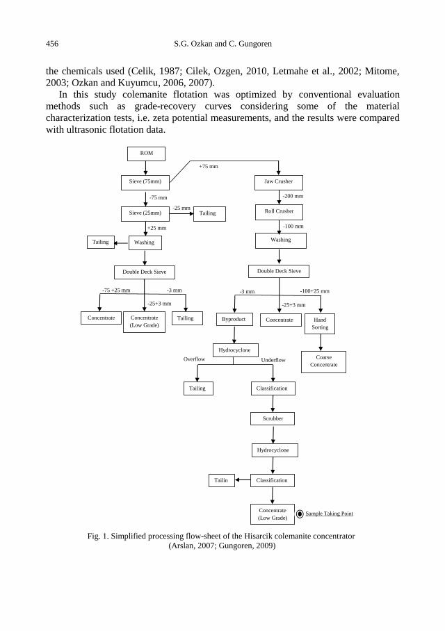
456 S.G. Ozkan and C. Gungoren
the chemicals used (Celik, 1987; Cilek, Ozgen, 2010, Letmahe et al., 2002; Mitome,
2003; Ozkan and Kuyumcu, 2006, 2007).
In this study colemanite flotation was optimized by conventional evaluation
methods such as grade-recovery curves considering some of the material
characterization tests, i.e. zeta potential measurements, and the results were compared
with ultrasonic flotation data.
Concentrate
Coarse
Concentrate
-200 mm
-100 mm
Byproduct
-100+25 mm
Concentrate Hand
Sorting
+75 mm
ROM
Sieve (75mm)
Sieve (25mm)
-75 mm
-25 mm
-25+3 mm
+25 mm
Washing
Tailing
Tailing
-75 +25 mm -3 mm
Concentrate
(Low Grade)
Tailing
Jaw Crusher
Roll Crusher
Double Deck Sieve
Washing
-3 mm
-25+3 mm
Hydrocyclone
Tailing
Overflow Underflow
Classification
Scrubber
Hydrocyclone
Classification Tailin
g
Concentrate
(Low Grade)
Double Deck Sieve
Sample Taking Point
Fig. 1. Simplified processing flow-sheet of the Hisarcik colemanite concentrator
(Arslan, 2007; Gungoren, 2009)
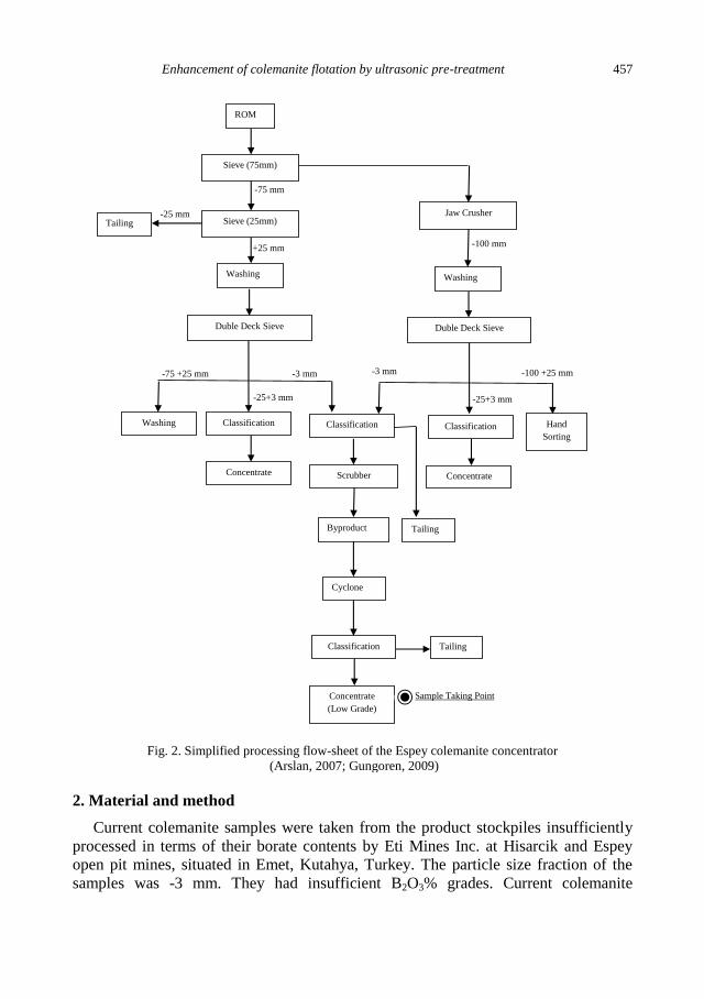
Enhancement of colemanite flotation by ultrasonic pre-treatment 457
ROM
Sieve (75mm)
-75 mm
Sieve (25mm) -25 mm
Tailing
+25 mm
Washing
Duble Deck Sieve
-75 +25 mm -3 mm
-25+3 mm
Washing
Concentrate
Classification
Jaw Crusher
Washing
-100 mm
Classification
Scrubber
Byproduct
Cyclone
Classification
Concentrate
(Low Grade)
-3 mm
-25+3 mm
-100 +25 mm
Hand
Sorting Classification
Concentrate
Tailing
Tailing
Sample Taking Point
Duble Deck Sieve
Fig. 2. Simplified processing flow-sheet of the Espey colemanite concentrator
(Arslan, 2007; Gungoren, 2009)
2. Material and method
Current colemanite samples were taken from the product stockpiles insufficiently
processed in terms of their borate contents by Eti Mines Inc. at Hisarcik and Espey
open pit mines, situated in Emet, Kutahya, Turkey. The particle size fraction of the
samples was -3 mm. They had insufficient B2O3% grades. Current colemanite
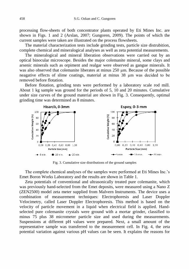
458 S.G. Ozkan and C. Gungoren
processing flow-sheets of both concentrator plants operated by Eti Mines Inc. are
shown in Figs. 1 and 2 (Arslan, 2007; Gungoren, 2009). The points of which the
current samples were taken are illustrated on the process flowsheets.
The material characterization tests include grinding tests, particle size distrubition,
complete chemical and mineralogical analyses as well as zeta potential measurements.
The mineralogical and mineral liberation observations were carried out by an
optical binocular microscope. Besides the major colemanite mineral, some clays and
arsenic minerals such as orpiment and realgar were observed as gangue minerals. It
was also observed that colemanite liberates at minus 250 µm. Because of the possible
neagative effects of slime coatings, material at minus 38 µm was decided to be
removed before flotation.
Before flotation, grinding tests were performed by a laboratory scale rod mill.
About 1 kg sample was ground for the periods of 5, 10 and 20 minutes. Cumulative
under size curves of the ground material are shown in Fig. 3. Consequently, optimal
grinding time was determined as 8 minutes.
Fig. 3. Cumulative size distributions of the ground samples
The complete chemical analyses of the samples were performed at Eti Mines Inc.’s
Emet Boron Works Laboratory and the results are shown in Table 1.
Zeta potentials of conventional and ultrasonically treated pure colemanite, which
was previously hand-selected from the Emet deposits, were measured using a Nano Z
(ZEN2500) model zeta meter supplied from Malvern Instruments. The device uses a
combination of measurement techniques: Electrophoresis and Laser Doppler
Velocimetry, called Laser Doppler Electrophoresis. This method is based on the
velocity of particle movement in a liquid when electrical field is applied. Hand-
selected pure colemanite crystals were ground with a mortar grinder, classified to
minus 75 plus 38 micrometer particle size and used during the measurements.
Suspensions at different pH values were prepared. Next, a small amount of the
representative sample was transferred to the measurement cell. In Fig. 4, the zeta
potential variation against various pH values can be seen. It explains the reasons for
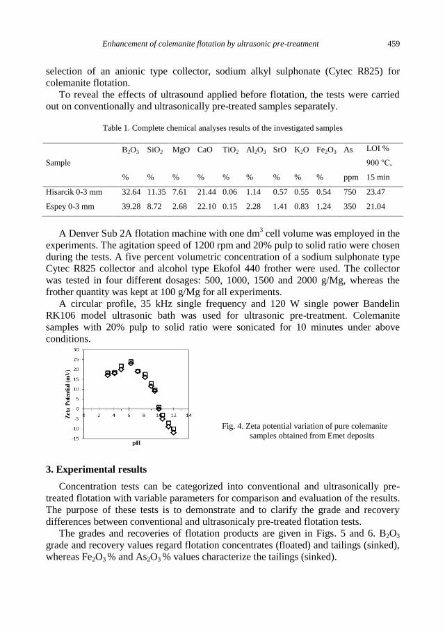
Enhancement of colemanite flotation by ultrasonic pre-treatment 459
selection of an anionic type collector, sodium alkyl sulphonate (Cytec R825) for
colemanite flotation.
To reveal the effects of ultrasound applied before flotation, the tests were carried
out on conventionally and ultrasonically pre-treated samples separately.
Table 1. Complete chemical analyses results of the investigated samples
Sample
B2O3 SiO2 MgO CaO TiO2 Al2O3 SrO K2O Fe2O3 As LOI %
900 °C,
15 min % % % % % % % % % ppm
Hisarcik 0-3 mm 32.64 11.35 7.61 21.44 0.06 1.14 0.57 0.55 0.54 750 23.47
Espey 0-3 mm 39.28 8.72 2.68 22.10 0.15 2.28 1.41 0.83 1.24 350 21.04
A Denver Sub 2A flotation machine with one dm3 cell volume was employed in the
experiments. The agitation speed of 1200 rpm and 20% pulp to solid ratio were chosen
during the tests. A five percent volumetric concentration of a sodium sulphonate type
Cytec R825 collector and alcohol type Ekofol 440 frother were used. The collector
was tested in four different dosages: 500, 1000, 1500 and 2000 g/Mg, whereas the
frother quantity was kept at 100 g/Mg for all experiments.
A circular profile, 35 kHz single frequency and 120 W single power Bandelin
RK106 model ultrasonic bath was used for ultrasonic pre-treatment. Colemanite
samples with 20% pulp to solid ratio were sonicated for 10 minutes under above
conditions.
Fig. 4. Zeta potential variation of pure colemanite
samples obtained from Emet deposits
3. Experimental results
Concentration tests can be categorized into conventional and ultrasonically pre-
treated flotation with variable parameters for comparison and evaluation of the results.
The purpose of these tests is to demonstrate and to clarify the grade and recovery
differences between conventional and ultrasonicaly pre-treated flotation tests.
The grades and recoveries of flotation products are given in Figs. 5 and 6. B2O3
grade and recovery values regard flotation concentrates (floated) and tailings (sinked),
whereas Fe2O3 % and As2O3 % values characterize the tailings (sinked).
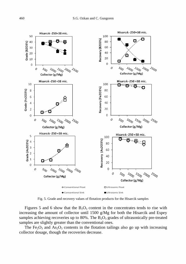
460 S.G. Ozkan and C. Gungoren
Fig. 5. Grade and recovery values of flotation products for the Hisarcik samples
Figures 5 and 6 show that the B2O3 content in the concentrates tends to rise with
increasing the amount of collector until 1500 g/Mg for both the Hisarcik and Espey
samples achieving recoveries up to 80%. The B2O3 grades of ultrasonically pre-treated
samples are slightly greater than the conventional ones.
The Fe2O3 and As2O3 contents in the flotation tailings also go up with increasing
collector dosage, though the recoveries decrease.
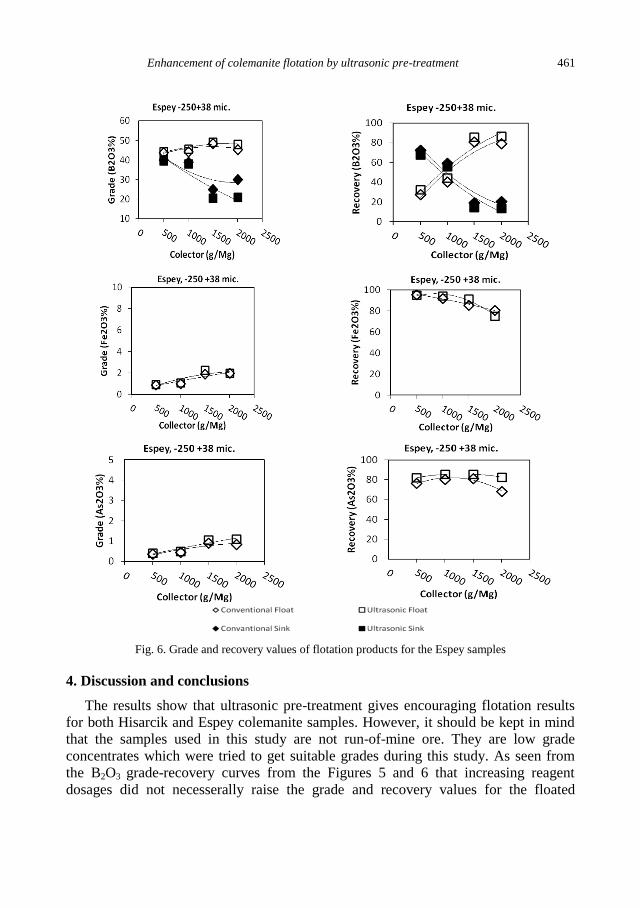
Enhancement of colemanite flotation by ultrasonic pre-treatment 461
Fig. 6. Grade and recovery values of flotation products for the Espey samples
4. Discussion and conclusions
The results show that ultrasonic pre-treatment gives encouraging flotation results
for both Hisarcik and Espey colemanite samples. However, it should be kept in mind
that the samples used in this study are not run-of-mine ore. They are low grade
concentrates which were tried to get suitable grades during this study. As seen from
the B2O3 grade-recovery curves from the Figures 5 and 6 that increasing reagent
dosages did not necesserally raise the grade and recovery values for the floated
462 S.G. Ozkan and C. Gungoren
colemanite. Approximately 41% B2O3 grade value was reached by desliming only for
both samples for particle size of -250+38 µm. In addition, the B2O3 % grade value
could be increased upto 49% by ultrasonically pre-treated flotation with a recovery of
above 80%. Besides, the B2O3 grade of the tailings was decreased to around 20% B2O3
agaisnt the feed grade B2O3 grade of 33% for Hisarcik and 39% for Espey
respectively. The optimal results were reached with use of 1500 g/Mg collector
dosage.
During flotation, the Fe2O3 and As2O3 contents of the samples were also
investigated. As seen from the Fe2O3 and As2O3 grade-recovery curves in Figs. 5 and 6
the increasing reagent dosages did not significantly affect the grade and recovery
values for sinked tailings. In the concentrates, 0.10% Fe2O3 grade could be reached
when the feed grade was between 0.70-1.00 % while As2O3 grade could be decreased
from 0.35% to 0.10%.
It is believed that better results in the ultrasonically pre-treated flotation, than in the
conventional flotation, were caused by a cavitation effect of ultrasounds. It is also
assumed that the high speed water jets at high pressure and temperature during the
sonication remove the clay and slime coatings on the surface of colemanite which
obstruct reagent adsorption. Due to the ultrasounds the reagents can absorb more
effectively on the surface of colemanite and increase their hydrophobicity.
Acknowledgement
The present work was supported by the Research Fund of Istanbul University, Project No: ACIP-
3609, T-2276 and UDP-13658.
References
ARSLAN, M., 2007, Emet borik asit urununun uretim surecinin iyilestirme analizi, Afyon Kocatepe
University. M.Sc. Thesis, Turkey, (in Turkish).
CELIK, M.S., 1987, Effect of ultrasonic treatment on the floability of coal and galena, Sep. Sci. Technol.
24(14), 1159–1166.
CILEK, E.C., OZGEN, S., 2010, Improvement of the flotation selectivity in a mechanical flotation cell by
ultrasound, Sep. Sci. Technol. 45: 572–579.
GUNGOREN, C., 2009, Ultrasonik ve mikrodalga enerjilerinin kolemanit flotasyonunda on islem olarak
kullanma olanaklarinin arastirilmasi, Istanbul University, M.Sc. Thesis, Turkey, (in Turkish).
LETMAHE, C., BENKER, B., GUNTHER, L., 2002, Intensivierung der schaumflotation durch einsatz
von ultraschall. Aufbereitungs Technik 43, 32–40.
MITOME, H., 2003, Action of ultrasound on particles and cavitation bubbles, In: Proc. World Congress
on Ultrasonics, Paris, 2003, 2342-2346.
OZKAN, S.G., GUNGOREN, C., 2010, Investigation of ultrasonics use for colemanite flotation,
Conference Proceedings of 10th International Multidisciplinary Scientific Geoconference – SGEM,
20-26 June, Bulgaria, vol. 1, 661–668.
OZKAN, S.G., KUYUMCU, H.Z., 2007, Design of a flotation cell equipped with ultrasound transducers
to enhance coal flotation, Ultrason. Sonochem. 14(2), 524–529.
OZKAN, S.G., KUYUMCU, H.Z., 2006, Investigation of mechanism of ultrasound on coal flotation, Int.
J. Miner. Process., 81(3), 201–203.
STOEV, S.M., 1992, Vibroacoustic improvements of froth flotation, Innovations in flotation technology,
NATO ASI, the Netherlands, series vol. 208, 383–407.
http://dx.doi.org/10.5277/ppmp120212
Physicochem. Probl. Miner. Process. 48(2), 2012, 463−473 Physicochemical Problems
of Mineral Processing
w w w . m i n p r o c . p w r . w r o c . p l / j o u r n a l / ISSN 1643-1049 (print)
ISSN 2084-4735 (online)
Received March 9, 2011; reviewed; accepted April 1, 2012
PREPARATION AND CHARACTERISATION OF HYDRATED
SILICA/LIGNIN BIOCOMPOSITES
Lukasz KLAPISZEWSKI, Magda MADRAWSKA, Teofil JESIONOWSKI
Poznan University of Technology, Institute of Chemical Technology and Engineering, M. Sklodowskiej–Curie
2, PL-60965 Poznan, Poland, [email protected], phone: +48(61)6653720, fax: +48(61)6653649
Abstract. Silica/lignin biocomposites were obtained by a new method proposed and fully
characterised. Silica was precipitated from aqueous solution of sodium silicate (as an SiO2
precursor) and sulphuric acid (as a precipitating agent). The support obtained was subjected to
surface functionalisation with aminosilane and then modified with Kraft lignin preliminary
activated with sodium periodate solution. The products were characterised by elemental (N, C,
H, S) and colorimetric analyses. Adsorption properties of the products were evaluated on the
basis of determination of specific surface area, pore volume and pore diameter. The influence
of the amount of lignin incorporated into the silica matrix on the physicochemical properties of
the biocomposites was proved to be significant. The materials obtained can be used as selective
adsorbents of heavy metals or pro-ecological polymer fillers.
keywords: silica/lignin biocomposites, silica, Kraft lignin, modification, physicochemical
properties
1. Introduction
Dynamic development of production technologies of new materials has been
focused on getting products of specific target properties. A large group of such new
materials is based on silica and show a large variety of morphological features.
Particularly interesting is production of composites with an addition of organic origin
polymer such as for instance lignin. The use of biodegradable materials such as lignin
in an inorganic matrix offers a possibility of obtaining a new generation of highly
functional biocomposites of prospective economic importance.
Silica belongs to the most abundant natural materials. The most often used methods
of its production include: hydrolysis and condensation of tetraalkoxysilanes according
to the Stöber method (Stöber, 1968; Ibrahim, 2010), precipitation from sodium
metasilicate aqueous solution in polar and nonpolar systems (Jesionowski, 2001,
2002) and high-temperature combustion of silicon halogens in the gas phase (Wypych,
2010). Because of a number of valuable physicochemical properties such as large
surface area, high hardness, chemical resistance and high mechanical resistance, silica
has been widely used in many branches of industry and in everyday use products.
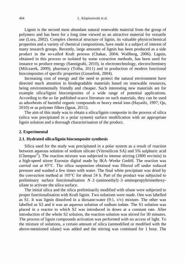
464 L. Klapiszewski et al.
Lignin is the second most abundant natural renewable material from the group of
polymers and has been for a long time viewed as an attractive material for versatile
use (Lora, 2002). Complex chemical structure of lignin, its valuable physicochemical
properties and a variety of chemical compositions, have made it a subject of interest of
many research groups. Recently, large amounts of lignin has been produced as a side
product in the so-called Kraft process (Chakar, 2004; Wallberg, 2006). Lignin,
obtained in this process or isolated by some extraction methods, has been used for
instance to produce energy (Sannigrahi, 2010), in electrotechnology, electrochemistry
(Milczarek, 2009), pharmacy (Tolba, 2011) and in production of modern functional
biocomposites of specific properties (Gosselink, 2004).
Increasing cost of energy and the need to protect the natural environment have
directed much attention to biodegradable materials based on renewable resources,
being environmentally friendly and cheaper. Such interesting new materials are for
example silica/lignin biocomposites of a wide range of potential applications.
According to the so far published scarce literature on such materials, they can be used
as adsorbents of harmful organic compounds or heavy metal ions (Hayashi, 1997; Qu,
2010) or as polymer fillers (Ignat, 2011).
The aim of this study was to obtain a silica/lignin composite in the process of silica
(silica was precipitated in a polar system) surface modification with an appropriate
lignin solution and a thorough characterisation of the product.
2. Experimental
2.1. Hydrated silica/lignin biocomposite synthesis
Silica used for the study was precipitated in a polar system as a result of reaction
between aqueous solution of sodium silicate (Vitrosilicon SA) and 5% sulphuric acid
(Chempur®). The reaction mixture was subjected to intense stirring (1800 rev/min) in
a high-speed stirrer Eurostar digital made by IKA–Werke GmbH. The reaction was
carried out at 85°C. The silica suspension obtained was filtered off under reduced
pressure and washed a few times with water. The final white precipitate was dried by
the convection method at 105°C for about 24 h. Part of the product was subjected to
preliminary surface functionalisation N–2–(aminoethyl)–3–aminopropyltrimethoxy-
silane to activate the silica surface.
The initial silica and the silica preliminarily modified with silane were subjected to
proper functionalisation with Kraft lignin. Two solutions were made. One was labelled
as S1. It was lignin dissolved in a dioxane:water (9:1, v/v) mixture. The other was
labelled as S2 and it was an aqueous solution of sodium iodate. The S1 solution was
placed in a reactor to which S2 was introduced in doses at a constant rate. After
introduction of the whole S2 solution, the reaction solution was stirred for 30 minutes.
The process of lignin compounds activation was performed with no access of light. To
the mixture of solutions, a certain amount of silica (unmodified or modified with the
above-mentioned silane) was added and the stirring was continued for 1 hour. The
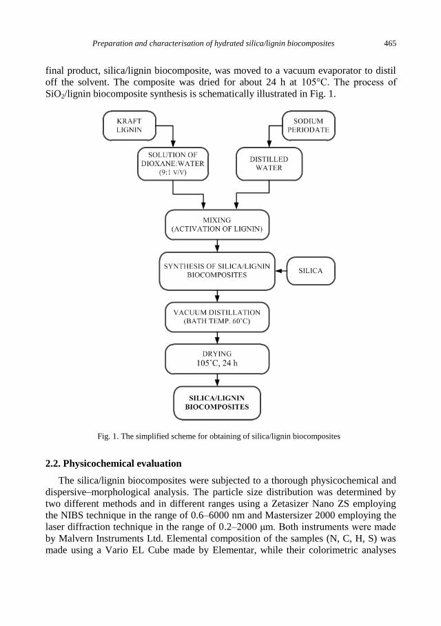
Preparation and characterisation of hydrated silica/lignin biocomposites 465
final product, silica/lignin biocomposite, was moved to a vacuum evaporator to distil
off the solvent. The composite was dried for about 24 h at 105°C. The process of
SiO2/lignin biocomposite synthesis is schematically illustrated in Fig. 1.
Fig. 1. The simplified scheme for obtaining of silica/lignin biocomposites
2.2. Physicochemical evaluation
The silica/lignin biocomposites were subjected to a thorough physicochemical and
dispersive–morphological analysis. The particle size distribution was determined by
two different methods and in different ranges using a Zetasizer Nano ZS employing
the NIBS technique in the range of 0.6–6000 nm and Mastersizer 2000 employing the
laser diffraction technique in the range of 0.2–2000 μm. Both instruments were made
by Malvern Instruments Ltd. Elemental composition of the samples (N, C, H, S) was
made using a Vario EL Cube made by Elementar, while their colorimetric analyses
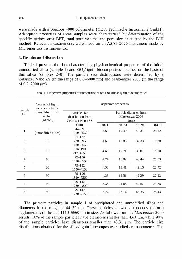
466 L. Klapiszewski et al.
were made with a Specbos 4000 colorimeter (YETI Technische Instrumente GmbH).
Adsorption properties of some samples were characterised by determination of the
specific surface area BET, total pore volume and pore size calculated by the BJH
method. Relevant measurements were made on an ASAP 2020 instrument made by
Micromeritics Instrument Co.
3. Results and discussion
Table 1 presents the data characterising physicochemical properties of the initial
unmodified silica (sample 1) and SiO2/lignin biocomposites obtained on the basis of
this silica (samples 2–8). The particle size distributions were determined by a
Zetasizer Nano ZS (in the range of 0.6–6000 nm) and Mastersizer 2000 (in the range
of 0.2–2000 μm).
Table 1. Dispersive properties of unmodified silica and silica/lignin biocomposites
Sample
No.
Content of lignin
in relation to the
unmodified silica
matrix
(wt./wt.)
Dispersive properties
Particle size
distribution from
Zetasizer Nano ZS
(nm)
Particle diameter from
Mastersizer 2000
(μm)
d(0.1) d(0.5) d(0.9) D[4.3]
1 0
(unmodified silica)
44–59
1110–5560 4.63 19.40 43.31 25.12
2 3
91–122
220–295
1480–5560
4.60 16.85 37.33 19.20
3 5 106–190
712–4150 4.60 17.71 38.01 19.80
4 10 79–106
1990–5560 4.74 18.82 40.44 21.03
5 20 79–122
1720–4150 4.50 19.41 42.16 22.72
6 30 79–106
1990–5560 4.33 19.51 42.29 22.92
7 40 79–142
1280–4800 5.38 21.63 44.57 23.75
8 50 79–142
1280–4150 5.24 23.14 48.35 25.43
The primary particles in sample 1 of precipitated and unmodified silica had
diameters in the range of 44–59 nm. These particles showed a tendency to form
agglomerates of the size 1110–5560 nm in size. As follows from the Mastersizer 2000
results, 10% of the sample particles have diameters smaller than 4.63 μm, while 90%
of the sample particles have diameters smaller than 43.31 μm. The particle size
distributions obtained for the silica/lignin biocomposites studied are nanometric. The
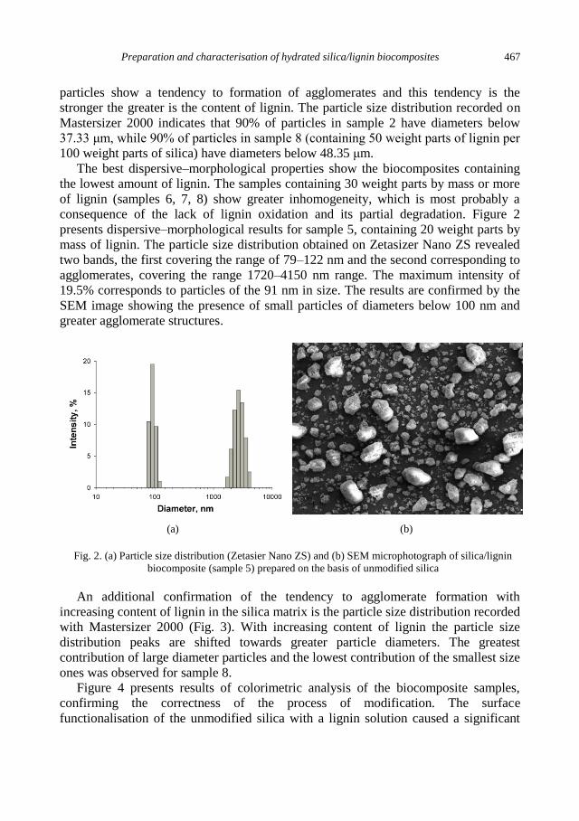
Preparation and characterisation of hydrated silica/lignin biocomposites 467
particles show a tendency to formation of agglomerates and this tendency is the
stronger the greater is the content of lignin. The particle size distribution recorded on
Mastersizer 2000 indicates that 90% of particles in sample 2 have diameters below
37.33 μm, while 90% of particles in sample 8 (containing 50 weight parts of lignin per
100 weight parts of silica) have diameters below 48.35 μm.
The best dispersive–morphological properties show the biocomposites containing
the lowest amount of lignin. The samples containing 30 weight parts by mass or more
of lignin (samples 6, 7, 8) show greater inhomogeneity, which is most probably a
consequence of the lack of lignin oxidation and its partial degradation. Figure 2
presents dispersive–morphological results for sample 5, containing 20 weight parts by
mass of lignin. The particle size distribution obtained on Zetasizer Nano ZS revealed
two bands, the first covering the range of 79–122 nm and the second corresponding to
agglomerates, covering the range 1720–4150 nm range. The maximum intensity of
19.5% corresponds to particles of the 91 nm in size. The results are confirmed by the
SEM image showing the presence of small particles of diameters below 100 nm and
greater agglomerate structures.
(a) (b)
Fig. 2. (a) Particle size distribution (Zetasier Nano ZS) and (b) SEM microphotograph of silica/lignin
biocomposite (sample 5) prepared on the basis of unmodified silica
An additional confirmation of the tendency to agglomerate formation with
increasing content of lignin in the silica matrix is the particle size distribution recorded
with Mastersizer 2000 (Fig. 3). With increasing content of lignin the particle size
distribution peaks are shifted towards greater particle diameters. The greatest
contribution of large diameter particles and the lowest contribution of the smallest size
ones was observed for sample 8.
Figure 4 presents results of colorimetric analysis of the biocomposite samples,
confirming the correctness of the process of modification. The surface
functionalisation of the unmodified silica with a lignin solution caused a significant
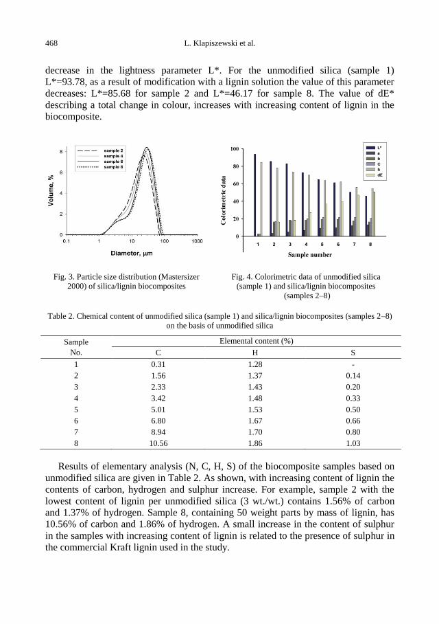
468 L. Klapiszewski et al.
decrease in the lightness parameter L*. For the unmodified silica (sample 1)
L*=93.78, as a result of modification with a lignin solution the value of this parameter
decreases: L*=85.68 for sample 2 and L*=46.17 for sample 8. The value of dE*
describing a total change in colour, increases with increasing content of lignin in the
biocomposite.
Fig. 3. Particle size distribution (Mastersizer
2000) of silica/lignin biocomposites
Fig. 4. Colorimetric data of unmodified silica
(sample 1) and silica/lignin biocomposites
(samples 2–8)
Table 2. Chemical content of unmodified silica (sample 1) and silica/lignin biocomposites (samples 2–8)
on the basis of unmodified silica
Sample
No.
Elemental content (%)
C H S
1 0.31 1.28 -
2 1.56 1.37 0.14
3 2.33 1.43 0.20
4 3.42 1.48 0.33
5 5.01 1.53 0.50
6 6.80 1.67 0.66
7 8.94 1.70 0.80
8 10.56 1.86 1.03
Results of elementary analysis (N, C, H, S) of the biocomposite samples based on
unmodified silica are given in Table 2. As shown, with increasing content of lignin the
contents of carbon, hydrogen and sulphur increase. For example, sample 2 with the
lowest content of lignin per unmodified silica (3 wt./wt.) contains 1.56% of carbon
and 1.37% of hydrogen. Sample 8, containing 50 weight parts by mass of lignin, has
10.56% of carbon and 1.86% of hydrogen. A small increase in the content of sulphur
in the samples with increasing content of lignin is related to the presence of sulphur in
the commercial Kraft lignin used in the study.
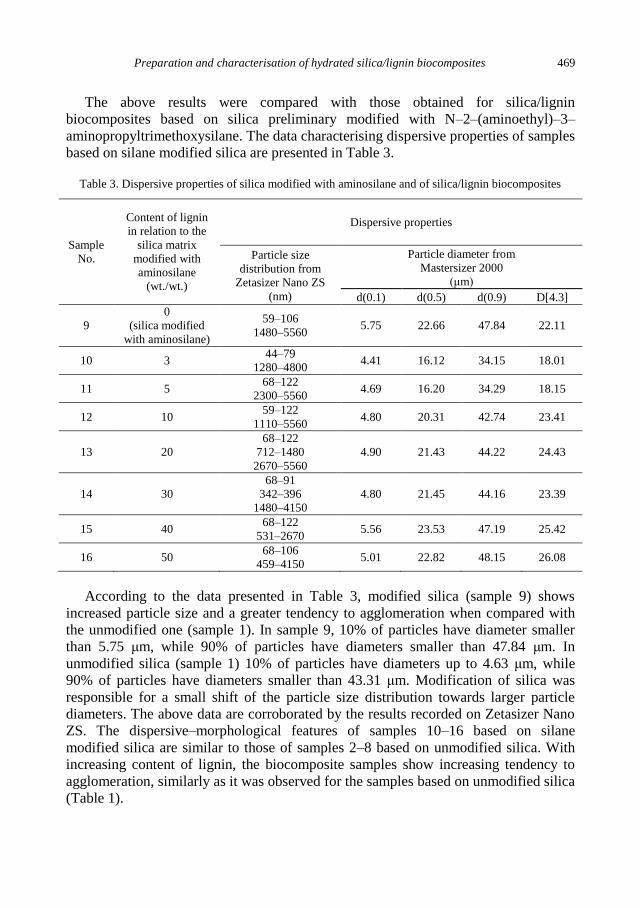
Preparation and characterisation of hydrated silica/lignin biocomposites 469
The above results were compared with those obtained for silica/lignin
biocomposites based on silica preliminary modified with N–2–(aminoethyl)–3–
aminopropyltrimethoxysilane. The data characterising dispersive properties of samples
based on silane modified silica are presented in Table 3.
Table 3. Dispersive properties of silica modified with aminosilane and of silica/lignin biocomposites
Sample
No.
Content of lignin
in relation to the
silica matrix
modified with
aminosilane
(wt./wt.)
Dispersive properties
Particle size
distribution from
Zetasizer Nano ZS
(nm)
Particle diameter from
Mastersizer 2000
(μm)
d(0.1) d(0.5) d(0.9) D[4.3]
9
0
(silica modified
with aminosilane)
59–106
1480–5560 5.75 22.66 47.84 22.11
10 3 44–79
1280–4800 4.41 16.12 34.15 18.01
11 5 68–122
2300–5560 4.69 16.20 34.29 18.15
12 10 59–122
1110–5560 4.80 20.31 42.74 23.41
13 20
68–122
712–1480
2670–5560
4.90 21.43 44.22 24.43
14 30
68–91
342–396
1480–4150
4.80 21.45 44.16 23.39
15 40 68–122
531–2670 5.56 23.53 47.19 25.42
16 50 68–106
459–4150 5.01 22.82 48.15 26.08
According to the data presented in Table 3, modified silica (sample 9) shows
increased particle size and a greater tendency to agglomeration when compared with
the unmodified one (sample 1). In sample 9, 10% of particles have diameter smaller
than 5.75 μm, while 90% of particles have diameters smaller than 47.84 μm. In
unmodified silica (sample 1) 10% of particles have diameters up to 4.63 μm, while
90% of particles have diameters smaller than 43.31 μm. Modification of silica was
responsible for a small shift of the particle size distribution towards larger particle
diameters. The above data are corroborated by the results recorded on Zetasizer Nano
ZS. The dispersive–morphological features of samples 10–16 based on silane
modified silica are similar to those of samples 2–8 based on unmodified silica. With
increasing content of lignin, the biocomposite samples show increasing tendency to
agglomeration, similarly as it was observed for the samples based on unmodified silica
(Table 1).

470 L. Klapiszewski et al.
Figure 5 presents the particle size distribution recorded in the Zetasizer Nano ZS
and SEM image of sample 13 (20 weight parts by mass of lignin in relation to silane–
grafted silica). Three peaks are obtained: the first corresponds to primary particles and
covers the range of 68–122 nm, the second corresponds to aggregations and covers the
range of 712–1480 nm and the third in the range of 2670–5560 nm corresponds to
agglomerates. The results are confirmed by the SEM image (Fig. 5b) showing the
presence of small particles and larger agglomerate clusters. No significant differences
in dispersive and morphological properties were found between the samples based on
unmodified and silane modified silica. This conclusion is confirmed by the results
obtained with Mastersizer 2000 (Fig. 6) showing that with increasing content of lignin
the contribution of greater size particles increases.
(a) (b)
Fig. 5. (a) Particle size distribution (Zetasier Nano ZS) and (b) SEM microphotograph of silica/lignin
biocomposite (sample 13) prepared on the basis of silica modified with aminosilane
As follows from the colorimetric analysis (Fig. 7) with increasing content of lignin
in the samples based on modified silica, the lightness L* decreases while the total
colour change dE* increases. A comparison of colorimetric results obtained for
unmodified and silane modified silica has shown that the silane modification leads
first of all to reduction in the lightness L*. For example the lightness of samples 6
(unmodified silica) and 13 (modified silica) containing 20 weight parts by mass of
lignin was L*=64.75 and L*=60.19, respectively. This results indicates an increase in
the silica affinity to lignin as a result of preliminary silane functionalisation of the
former.
Data on the chemical composition of silane modified silica (sample 9) and
biocomposites based on modified silica (samples 10–16) are given in Table 4.
As follows from the data, the effect of the preliminary silane modification was an
increase in the nitrogen content to 0.61%. Analysis of the data for samples 10–16 has
shown an increase in the content of carbon, hydrogen and sulphur with increasing
content of lignin. The results are consistent with expectations. Moreover, greater

Preparation and characterisation of hydrated silica/lignin biocomposites 471
contents of N, C, H and S in the samples based on silane modified silica illustrates the
significance of changes caused by the silane applied.
Fig. 6. Particle size distribution
(Mastersizer 2000) of silica/lignin
biocomposites
Fig. 7. Colorimetric data of silica modified with
aminosilane (sample 9) and silica/lignin
biocomposites (samples 10–16)
Table 4. Chemical content of silica modified with aminosilane (sample 9) and silica/lignin biocomposites
(samples 10–16) on the basis of silica modified with aminosilane
Sample
No.
Elemental content (%)
N C H S
9 0.61 1.44 1.48 -
10 0.44 2.60 1.47 0.18
11 0.49 3.45 1.53 0.23
12 0.42 5.04 1.67 0.39
13 0.40 6.70 1.75 0.57
14 0.40 7.97 1.81 0.70
15 0.36 10.15 1.88 0.87
16 0.31 11.33 1.93 1.03
Table 5 presents the data characterising adsorption properties of unmodified silica
(sample 1), preliminary silane modified silica (sample 9) and selected silica/lignin
biocomposites (samples 4, 8, 12, 16). The specific surface area of these products
varies from 108 to 131 m2/g. Preliminary modification with silane leads to a small
increase in the surface area relative to the unmodified silane sample. The mean pore
size for all samples are similar and vary from 3.55 to 3.61 nm, which confirms their
mesoporous character. Surface functionalisation of silica, either unmodified or
modified, with Kraft lignin solution did not affect significantly the adsorption
properties of the materials studied
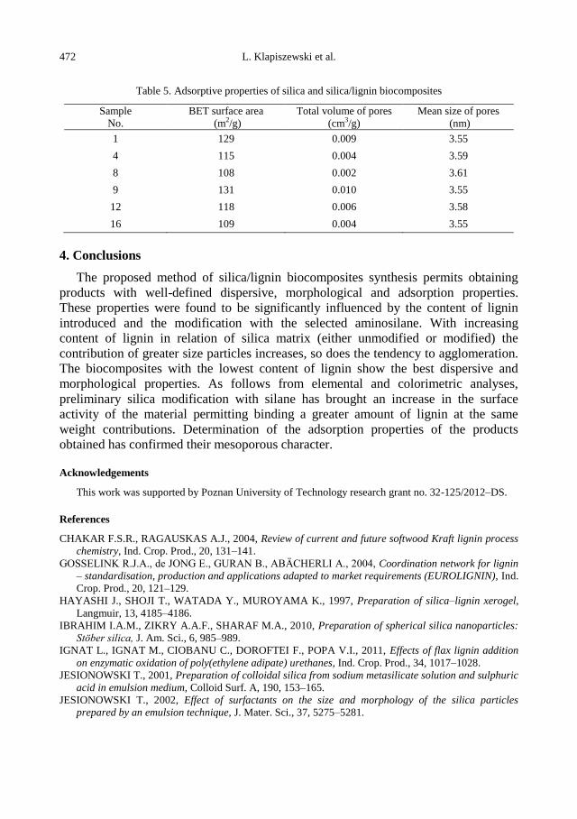
472 L. Klapiszewski et al.
Table 5. Adsorptive properties of silica and silica/lignin biocomposites
Sample
No.
BET surface area
(m2/g)
Total volume of pores
(cm3/g)
Mean size of pores
(nm)
1 129 0.009 3.55
4 115 0.004 3.59
8 108 0.002 3.61
9 131 0.010 3.55
12 118 0.006 3.58
16 109 0.004 3.55
4. Conclusions
The proposed method of silica/lignin biocomposites synthesis permits obtaining
products with well-defined dispersive, morphological and adsorption properties.
These properties were found to be significantly influenced by the content of lignin
introduced and the modification with the selected aminosilane. With increasing
content of lignin in relation of silica matrix (either unmodified or modified) the
contribution of greater size particles increases, so does the tendency to agglomeration.
The biocomposites with the lowest content of lignin show the best dispersive and
morphological properties. As follows from elemental and colorimetric analyses,
preliminary silica modification with silane has brought an increase in the surface
activity of the material permitting binding a greater amount of lignin at the same
weight contributions. Determination of the adsorption properties of the products
obtained has confirmed their mesoporous character.
Acknowledgements
This work was supported by Poznan University of Technology research grant no. 32-125/2012–DS.
References
CHAKAR F.S.R., RAGAUSKAS A.J., 2004, Review of current and future softwood Kraft lignin process
chemistry, Ind. Crop. Prod., 20, 131–141.
GOSSELINK R.J.A., de JONG E., GURAN B., ABÄCHERLI A., 2004, Coordination network for lignin
– standardisation, production and applications adapted to market requirements (EUROLIGNIN), Ind.
Crop. Prod., 20, 121–129.
HAYASHI J., SHOJI T., WATADA Y., MUROYAMA K., 1997, Preparation of silica–lignin xerogel,
Langmuir, 13, 4185–4186.
IBRAHIM I.A.M., ZIKRY A.A.F., SHARAF M.A., 2010, Preparation of spherical silica nanoparticles:
Stöber silica, J. Am. Sci., 6, 985–989.
IGNAT L., IGNAT M., CIOBANU C., DOROFTEI F., POPA V.I., 2011, Effects of flax lignin addition
on enzymatic oxidation of poly(ethylene adipate) urethanes, Ind. Crop. Prod., 34, 1017–1028.
JESIONOWSKI T., 2001, Preparation of colloidal silica from sodium metasilicate solution and sulphuric
acid in emulsion medium, Colloid Surf. A, 190, 153–165.
JESIONOWSKI T., 2002, Effect of surfactants on the size and morphology of the silica particles
prepared by an emulsion technique, J. Mater. Sci., 37, 5275–5281.

Preparation and characterisation of hydrated silica/lignin biocomposites 473
LORA J.H., GLASSER W.G., 2002, Recent industrial applications of lignin: a sustainable alternative to
nonrenewable materiale, J. Polym. Environ., 10, 39–48.
MILCZAREK G., 2009, Preparation, characterization and electrocatalytic properties of an iodine
lignin–modified gold electrode, Electrochim. Acta, 54, 3199–3205.
QU Y., TIAN Y., ZOU B., ZHANG J., ZHENG Y., WANG L., LI Y., RONG C., WANG Z., 2010, A
novel mesoporous lignin/silica hybrid from rice husk produced by a sol–gel method, Bioresource
Technol., 101, 8402–8405.
SANNIGRAHI P., PU Y., RAGAUSKAS A., 2010, Cellulosic biorafineries – unleashing lignin
opportunities, Curr. Opin. Environ. Sustain., 2, 383–393.
STÖBER W., FINK A., BOHN E., 1968, Controlled growth of monodisperse silica spheres in the micron
size range, J. Colloid Interf. Sci., 26, 62–69.
TOLBA R., WU G., CHEN A., 2011, Adsorption of dietary oils onto lignin for promising pharmaceutical
and nutritional applications, BioResources, 6, 1322–1335.
WALLBERG O., LINDE M., JÖNSSON A.S., 2006, Extraction of lignin and hemicelluloses from Kraft
black liquor, Desalination, 199, 413–414.
WYPYCH G., 2010, Handbook of Fillers, ChemTec Publishing, Toronto 2010.

474 L. Klapiszewski et al.

http://dx.doi.org/10.5277/ppmp120213
Physicochem. Probl. Miner. Process. 48(2), 2012, 475−484 Physicochemical Problems
of Mineral Processing
w w w . m i n p r o c . p w r . w r o c . p l / j o u r n a l / ISSN 1643-1049 (print)
ISSN 2084-4735 (online)
Received December 8, 2011; reviewed; accepted February 9, 2012
EVALUATION OF LOW GRADE IRON ORE DEPOSIT IN
ERZINCAN-TURKEY FOR IRON ORE PELLET CONCENTRATE
PRODUCTION
Osman SIVRIKAYA*,**, Ali Ihsan AROL*
* Selçuk University, Mining Engineering Department, 42075 Konya, Turkey, [email protected]
** Middle East Technical University, Mining Engineering Department, Ankara, Turkey, [email protected]
Abstract. In this study the separation possibility of gangue minerals from a low grade
magnetite ore with 45% Fe from an iron ore deposit located near Erzincan-Turkey was
investigated. The iron ore deposit consists of mainly magnetite mineral. Hematite is the second
iron oxide found in the deposit. The gangue minerals contain mainly SiO2 and Al2O3
impurities. The main object of the research is to investigate the production of a concentrate
suitable for iron ore pellet production. The concentrate for pellet production should have at
least 65% Fe with reasonable gangue contents (SiO2 <6.0% and Al2O3 <1.0%). The Davis tube
and low intensity drum type wet magnetic separators were used for upgrading the Fe content
and separation of gangue impurities from the iron ore. The results showed that, in order to
produce a concentrate with sufficient Fe grade (>65% Fe), the iron ore should be ground to get
45% of material by weight to be finer than 45 m. The concentrate with over 65% Fe and 90%
Fe recovery could be produced with 45% Fe content from the feed material by crushing,
grinding and magnetic separation operations.
keywords: iron ore, magnetite, magnetic separation, iron ore pellet
1. Introduction
The main raw material for iron production in the iron-steel industry is iron oxide
ore. Natural iron oxide ores can be typically classified as high grade (>65% Fe),
medium grade (<65 and >62% Fe) and low grade (<62% Fe) in terms of their Fe
contents. The high grade iron ores, which can be used directly in the blast furnace to
produce metallic iron, are not abundant in earth’s crust to supply the need of iron-steel
industry. The exploitation of low grade iron ores is possible after enrichment. The low
grade iron ores with considerable amount of gangue minerals, e.g. silica, alumina,
calcium and magnesium compounds, require concentration. For concentration, iron
ore is crushed and ground for liberation before the implementation of separation
techniques. Liberation can mostly be achieved at a very fine particle size and, hence,
the concentrate obtained is not suitable to be charged directly into the blast furnace or
the DR-plant without converting it into suitably sized agglomerates. The most
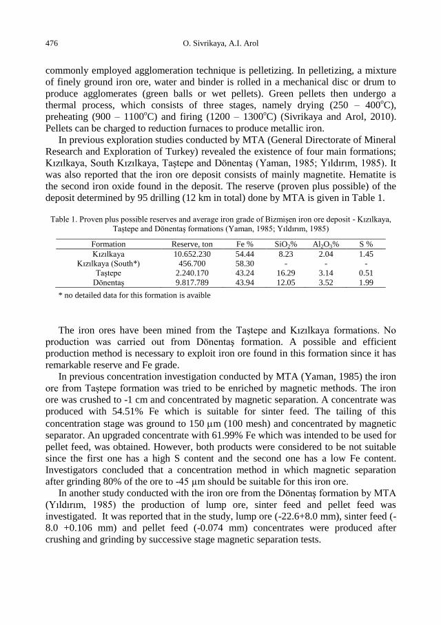
476 O. Sivrikaya, A.I. Arol
commonly employed agglomeration technique is pelletizing. In pelletizing, a mixture
of finely ground iron ore, water and binder is rolled in a mechanical disc or drum to
produce agglomerates (green balls or wet pellets). Green pellets then undergo a
thermal process, which consists of three stages, namely drying (250 – 400oC),
preheating (900 – 1100oC) and firing (1200 – 1300
oC) (Sivrikaya and Arol, 2010).
Pellets can be charged to reduction furnaces to produce metallic iron.
In previous exploration studies conducted by MTA (General Directorate of Mineral
Research and Exploration of Turkey) revealed the existence of four main formations;
Kızılkaya, South Kızılkaya, Taştepe and Dönentaş (Yaman, 1985; Yıldırım, 1985). It
was also reported that the iron ore deposit consists of mainly magnetite. Hematite is
the second iron oxide found in the deposit. The reserve (proven plus possible) of the
deposit determined by 95 drilling (12 km in total) done by MTA is given in Table 1.
Table 1. Proven plus possible reserves and average iron grade of Bizmişen iron ore deposit - Kızılkaya,
Taştepe and Dönentaş formations (Yaman, 1985; Yıldırım, 1985)
Formation Reserve, ton Fe % SiO2% Al2O3% S %
Kızılkaya 10.652.230 54.44 8.23 2.04 1.45
Kızılkaya (South*) 456.700 58.30 - - -
Taştepe 2.240.170 43.24 16.29 3.14 0.51
Dönentaş 9.817.789 43.94 12.05 3.52 1.99
* no detailed data for this formation is avaible
The iron ores have been mined from the Taştepe and Kızılkaya formations. No
production was carried out from Dönentaş formation. A possible and efficient
production method is necessary to exploit iron ore found in this formation since it has
remarkable reserve and Fe grade.
In previous concentration investigation conducted by MTA (Yaman, 1985) the iron
ore from Taştepe formation was tried to be enriched by magnetic methods. The iron
ore was crushed to -1 cm and concentrated by magnetic separation. A concentrate was
produced with 54.51% Fe which is suitable for sinter feed. The tailing of this
concentration stage was ground to 150 m (100 mesh) and concentrated by magnetic
separator. An upgraded concentrate with 61.99% Fe which was intended to be used for
pellet feed, was obtained. However, both products were considered to be not suitable
since the first one has a high S content and the second one has a low Fe content.
Investigators concluded that a concentration method in which magnetic separation
after grinding 80% of the ore to -45 µm should be suitable for this iron ore.
In another study conducted with the iron ore from the Dönentaş formation by MTA
(Yıldırım, 1985) the production of lump ore, sinter feed and pellet feed was
investigated. It was reported that in the study, lump ore (-22.6+8.0 mm), sinter feed (-
8.0 +0.106 mm) and pellet feed (-0.074 mm) concentrates were produced after
crushing and grinding by successive stage magnetic separation tests.
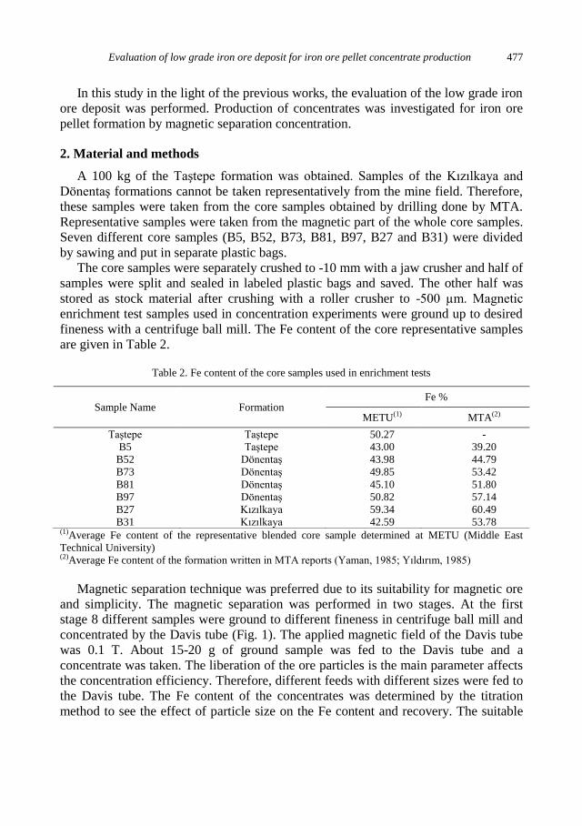
Evaluation of low grade iron ore deposit for iron ore pellet concentrate production 477
In this study in the light of the previous works, the evaluation of the low grade iron
ore deposit was performed. Production of concentrates was investigated for iron ore
pellet formation by magnetic separation concentration.
2. Material and methods
A 100 kg of the Taştepe formation was obtained. Samples of the Kızılkaya and
Dönentaş formations cannot be taken representatively from the mine field. Therefore,
these samples were taken from the core samples obtained by drilling done by MTA.
Representative samples were taken from the magnetic part of the whole core samples.
Seven different core samples (B5, B52, B73, B81, B97, B27 and B31) were divided
by sawing and put in separate plastic bags.
The core samples were separately crushed to -10 mm with a jaw crusher and half of
samples were split and sealed in labeled plastic bags and saved. The other half was
stored as stock material after crushing with a roller crusher to -500 µm. Magnetic
enrichment test samples used in concentration experiments were ground up to desired
fineness with a centrifuge ball mill. The Fe content of the core representative samples
are given in Table 2.
Table 2. Fe content of the core samples used in enrichment tests
(1)Average Fe content of the representative blended core sample determined at METU (Middle East
Technical University) (2)Average Fe content of the formation written in MTA reports (Yaman, 1985; Yıldırım, 1985)
Magnetic separation technique was preferred due to its suitability for magnetic ore
and simplicity. The magnetic separation was performed in two stages. At the first
stage 8 different samples were ground to different fineness in centrifuge ball mill and
concentrated by the Davis tube (Fig. 1). The applied magnetic field of the Davis tube
was 0.1 T. About 15-20 g of ground sample was fed to the Davis tube and a
concentrate was taken. The liberation of the ore particles is the main parameter affects
the concentration efficiency. Therefore, different feeds with different sizes were fed to
the Davis tube. The Fe content of the concentrates was determined by the titration
method to see the effect of particle size on the Fe content and recovery. The suitable
Sample Name Formation Fe %
METU(1) MTA(2)
Taştepe Taştepe 50.27 -
B5 Taştepe 43.00 39.20
B52 Dönentaş 43.98 44.79
B73 Dönentaş 49.85 53.42
B81 Dönentaş 45.10 51.80
B97 Dönentaş 50.82 57.14
B27 Kızılkaya 59.34 60.49
B31 Kızılkaya 42.59 53.78
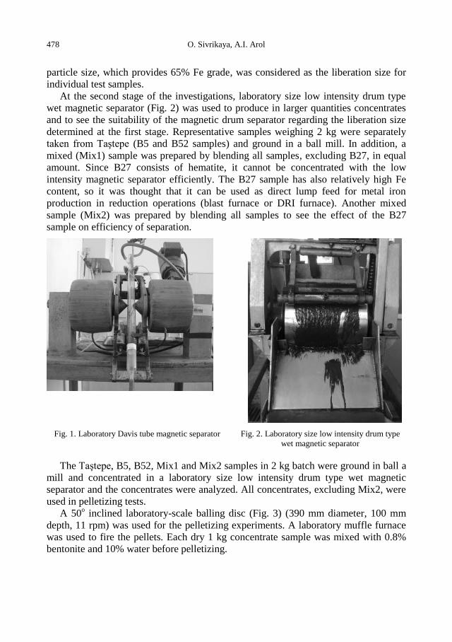
478 O. Sivrikaya, A.I. Arol
particle size, which provides 65% Fe grade, was considered as the liberation size for
individual test samples.
At the second stage of the investigations, laboratory size low intensity drum type
wet magnetic separator (Fig. 2) was used to produce in larger quantities concentrates
and to see the suitability of the magnetic drum separator regarding the liberation size
determined at the first stage. Representative samples weighing 2 kg were separately
taken from Taştepe (B5 and B52 samples) and ground in a ball mill. In addition, a
mixed (Mix1) sample was prepared by blending all samples, excluding B27, in equal
amount. Since B27 consists of hematite, it cannot be concentrated with the low
intensity magnetic separator efficiently. The B27 sample has also relatively high Fe
content, so it was thought that it can be used as direct lump feed for metal iron
production in reduction operations (blast furnace or DRI furnace). Another mixed
sample (Mix2) was prepared by blending all samples to see the effect of the B27
sample on efficiency of separation.
Fig. 1. Laboratory Davis tube magnetic separator Fig. 2. Laboratory size low intensity drum type
wet magnetic separator
The Taştepe, B5, B52, Mix1 and Mix2 samples in 2 kg batch were ground in ball a
mill and concentrated in a laboratory size low intensity drum type wet magnetic
separator and the concentrates were analyzed. All concentrates, excluding Mix2, were
used in pelletizing tests.
A 50o inclined laboratory-scale balling disc (Fig. 3) (390 mm diameter, 100 mm
depth, 11 rpm) was used for the pelletizing experiments. A laboratory muffle furnace
was used to fire the pellets. Each dry 1 kg concentrate sample was mixed with 0.8%
bentonite and 10% water before pelletizing.

Evaluation of low grade iron ore deposit for iron ore pellet concentrate production 479
The detailed pelletizing procedure was explained in our previous publication
(Sivrikaya and Arol, 2011). The green pellets were air-dried overnight and then fired
at 1200oC for 2 hours in a muffle furnace at a heating rate of 5
oC/min.
Fig. 3. Laboratory size pelletizing disc to produce
iron ore pellets
3. Results and discussion
3.1. Magnetic separation test with the Davis Tube
The production of a concentrate with 65% Fe was aimed during the magnetic
separation experiments. In the light of the previous results, the liberation was assumed
to be at finer particle sizes. In addition, the reference particle size (80% -45 µm) for
industrial pellet feed was accepted. Therefore, the enrichment possibility of samples
was investigated according to their fineness (-45 m). The results are given in Figs.
4-6. The results are grouped according to their formation taken from.
The Davis tube enrichment results for the Taştepe and B5 core samples which
represent the Taştepe formation are given in Fig. 4. As can be seen from Fig. 4, when
the sample is ground to 45%, by weight of -45 m particles, the Fe grade of
concentrate is over 65% Fe.
The B52, B73, B81 and B97 core samples represent the Dönentaş formation. The
Davis tube enrichment results for these samples are given in Fig. 5. The results
showed that a concentrate with over 65% Fe can be produced if the feed is ground 38-
53% by weight -45 µm.
Different results were obtained with B27 and B31 core samples representing the
Kızılkaya formation (Fig. 6). A concentrate with over 65% Fe can be produced when
the B27 core sample feed is ground to 25% by weight of the -45 m size fraction. A
further grinding (60% -45 m) increased the grade of the concentrate up to around
68.5% Fe. The B27 core sample consists of hematite and due to oxidation of hematite,
this sample gets loose structure and could be ground easily. A direct use of the lump
ore is more appropriate since the grade of the B27 sample feed is high (59.34% Fe)
and the loses (Table 5) would occur during low intensity magnetic separation for this
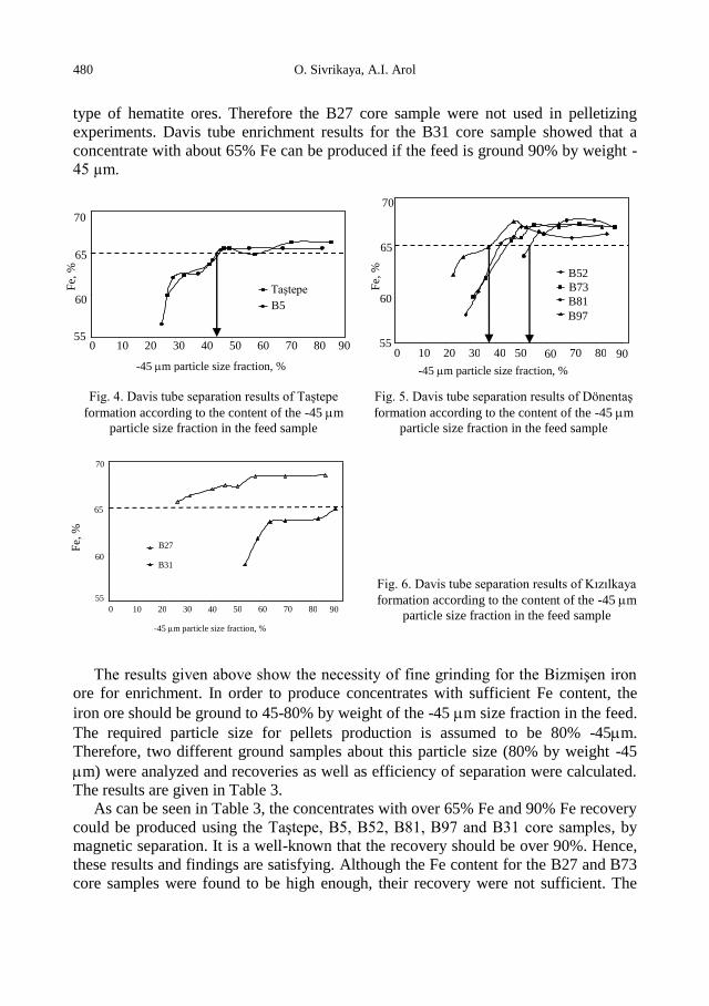
480 O. Sivrikaya, A.I. Arol
type of hematite ores. Therefore the B27 core sample were not used in pelletizing
experiments. Davis tube enrichment results for the B31 core sample showed that a
concentrate with about 65% Fe can be produced if the feed is ground 90% by weight -
45 µm.
Fig. 4. Davis tube separation results of Taştepe
formation according to the content of the -45 m
particle size fraction in the feed sample
Fig. 5. Davis tube separation results of Dönentaş
formation according to the content of the -45 m
particle size fraction in the feed sample
Fig. 6. Davis tube separation results of Kızılkaya
formation according to the content of the -45 m
particle size fraction in the feed sample
The results given above show the necessity of fine grinding for the Bizmişen iron
ore for enrichment. In order to produce concentrates with sufficient Fe content, the
iron ore should be ground to 45-80% by weight of the -45 m size fraction in the feed.
The required particle size for pellets production is assumed to be 80% -45m.
Therefore, two different ground samples about this particle size (80% by weight -45
m) were analyzed and recoveries as well as efficiency of separation were calculated.
The results are given in Table 3.
As can be seen in Table 3, the concentrates with over 65% Fe and 90% Fe recovery
could be produced using the Taştepe, B5, B52, B81, B97 and B31 core samples, by
magnetic separation. It is a well-known that the recovery should be over 90%. Hence,
these results and findings are satisfying. Although the Fe content for the B27 and B73
core samples were found to be high enough, their recovery were not sufficient. The
55
60
65
0 10 20 30 40 50 60 70 80 90
Taştepe
B5
70
55
60
65
70
0 10 20 30 40 50 60 70 80 90
B52
B97
B73
B81
-45 m particle size fraction, %
55
60
65
70
0 10 20 30 40 50 60 70 80 90
B31
B27
-45 m particle size fraction, %
Fe,
%
-45 m particle size fraction, % F
e, %
Fe,
%

Evaluation of low grade iron ore deposit for iron ore pellet concentrate production 481
reason of this is believed to be due to a low magnetic susceptibility of the minerals
(hematite and pyrite) present in the two samples. The relatively lower magnetic
susceptibility of these minerals leads to loses during low intensity magnetic
separation.
Table 3. Grade and recoveries of concentrates produced with Davis tube according to the particle size of
feed sample
3.2. Magnetic separation tests with magnetic drum concentrator and pelletizing
experiments
The Davis tube experiments showed that the enrichment of the Bizmişen iron ore is
possible and the produced concentrates with a sufficient amount of Fe (over 65% Fe).
In order to achieve this target the ore should be ground to finer sizes. Since the desired
particle size for pellet production is minimum 80% -45 m, the feed was ground to
this fineness and fed to the laboratory size low intensity drum type wet magnetic
separator. Different particle sizes were not using the drum separator due to a lack of
enough samples.
Five different samples namely Taştepe, B5, B52, Mix1 and Mix2, were used during
the drum separator tests. The first three samples were ground and concentrated
separately. The latter two were formed by blending all samples Taştepe, B5, B52,
B73, B81, B97 and B27 and B31 (14.29% from each samples excluding B27 for
Mix1, 12.5% from each for Mix2). All five samples were concentrated separately with
the low intensity magnetic separator. Different concentrates and tailings were analyzed
Formation Sample
name
Particle
Size
(-45 m),
%
Grade of Fe, % Recovery
by weight, % Recovery of Fe, %
Feed Concentrate Tailing Concentrate Tailing Concentrate Tailing
Taştepe
Taştepe 71.0 50.3 66.3 10.5 71.3 28.7 94.0 6.0
85.0 50.3 66.3 11.0 71.0 29.0 93.6 6.4
B5 68.0 43.0 65.6 7.5 61.1 38.9 93.2 6.8
82.0 43.0 65.6 8.7 60.3 39.7 92.0 8.0
Dönentaş
B52 70.0 44.0 65.9 7.8 62.3 37.7 93.3 6.7
84.0 44.0 66.3 8.5 61.4 38.6 92.5 7.5
B73 73.0 49.8 67.3 16.1 65.9 34.1 89.0 11.0
87.0 49.9 67.0 17.5 65.4 34.6 87.9 12.1
B81 79.0 45.1 67.7 7.7 62.3 37.7 93.6 6.4
87.0 45.1 67.0 10.9 61.0 39.0 90.6 9.4
B97 65.0 50.8 67.3 9.5 71.5 28.5 94.7 5.3
82.0 50.8 67.0 10.1 71.6 28.4 94.4 5.6
Kızılkaya
B27 70.0 59.3 68.4 39.1 69.1 30.9 79.6 20.4
86.0 59.3 68.5 44.7 61.5 38.5 71.0 29.0
B31 83.0 42.6 63.8 7.7 62.2 37.8 93.2 6.8
90.0 42.6 64.9 10.9 58.7 41.3 89.4 10.6
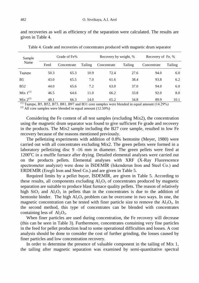
482 O. Sivrikaya, A.I. Arol
and recoveries as well as efficiency of the separation were calculated. The results are
given in Table 4.
Table 4. Grade and recoveries of concentrates produced with magnetic drum separator
(1) Taştepe, B5, B52, B73, B81, B97 and B31 core samples were blended in equal amount (14.29%) (2) All core samples were blended in equal amount (12.50%)
Considering the Fe content of all test samples (excluding Mix2), the concentration
using the magnetic drum separator was found to give sufficient Fe grade and recovery
in the products. The Mix2 sample including the B27 core sample, resulted in low Fe
recovery because of the reasons mentioned previously.
The pelletizing experiments with addition of 0.8% bentonite (Meyer, 1980) were
carried out with all concentrates excluding Mix2. The green pellets were formed in a
laboratory pelletizing disc 9 -16 mm in diameter. The green pellets were fired at
1200oC in a muffle furnace after drying. Detailed elemental analyses were carried out
on the products pellets. Elemental analyses with XRF (X-Ray Fluorescence
spectrometer analyzer) were done in İSDEMİR (Iskenderun Iron and Steel Co.) and
ERDEMİR (Eregli Iron and Steel Co.) and are given in Table 5.
Required limits by a pellet buyer, İSDEMİR, are given in Table 5. According to
these results, all components excluding Al2O3 of concentrates produced by magnetic
separation are suitable to produce blast furnace quality pellets. The reason of relatively
high SiO2 and Al2O3 in pellets than in the concentrates is due to the addition of
bentonite binder. The high Al2O3 problem can be overcome in two ways. In one, the
magnetic concentration can be tested with finer particle size to remove the Al2O3. In
the second method, this type of concentrates can be blended with concentrates
containing less of Al2O3.
When finer particles are used during concentration, the Fe recovery will decrease
(this can be seen in Table 3). Furthermore, concentrates containing very fine particles
in the feed for pellet production lead to some operational difficulties and losses. A cost
analysis should be done to consider the cost of further grinding, the losses caused by
finer particles and low concentration recovery.
In order to determine the presence of valuable component in the tailing of Mix 1,
the tailing after magnetic separation was examined by semi-quantitative spectral
Sample
Name
Grade of Fe% Recovery by weight, % Recovery of Fe, %
Feed Concentrate Tailing Concentrate Tailing Concentrate Tailing
Taştepe 50.3 65.3 10.9 72.4 27.6 94.0 6.0
B5 43.0 65.5 7.0 61.6 38.4 93.8 6.2
B52 44.0 65.6 7.2 63.0 37.0 94.0 6.0
Mix 1(1) 46.5 64.6 11.0 66.2 33.8 92.0 8.0
Mix 2(2) 48.1 66.3 14.0 65.2 34.8 89.9 10.1
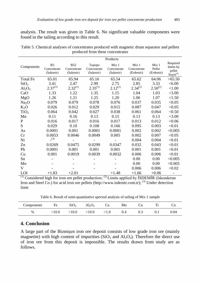
Evaluation of low grade iron ore deposit for iron ore pellet concentrate production 483
analysis. The result was given in Table 6. No significant valuable components were
found in the tailing according to this result.
Table 5. Chemical analyses of concentrates produced with magnetic drum separator and pellets
produced from these concentrates
Components
Products
B5
Concentrate (İsdemir)
B52
Concentrate (İsdemir)
Taştepe
Concentrate (İsdemir)
Mix 1
Concentrate (İsdemir)
Mix 1
Concentrate (Erdemir)
Mix 1
Pellet (Erdemir)
Required limits by
pellet
buyer(2)
Total Fe 65.01 65.94 65.16 65.54 65.62 64.06 >65.50 SiO2 3.41 2.47 2.99 2.75 2.85 3.33 <6.00
Al2O3 2.37(1)
2.32(1)
2.35(1)
2.12(1)
2.34(1)
2.50(1)
<1.00 CaO 1.33 1.22 1.35 1.15 1.04 1.03 <3.00
MgO 1.26 1.21 1.25 1.20 1.06 1.07 <1.50 Na2O 0.079 0.079 0.078 0.076 0.037 0.035 <0.05
K2O 0.026 0.012 0.029 0.015 0.087 0.047 <0.05 TiO2 0.064 0.042 0.027 0.038 0.061 0.064 <0.50
Mn 0.11 0.16 0.13 0.15 0.13 0.13 <3.00
P 0.016 0.017 0.016 0.017 0.013 0.012 <0.06 S 0.029 0.10 0.108 0.166 0.095 0.003 <0.01
As 0.0001 0.001 0.0001 0.0001 0.002 0.002 <0.005 Cr 0.0053 0.0046 0.0049 0.005 0.002 0.007 <0.05
Ni -(3)
- - - 0.004 0.004 <0.01
Zn 0.0269 0.0475 0.0299 0.0347 0.032 0.043 <0.01 Pb 0.0001 0.001 0.001 0.001 0.001 0.001 <0.01
Cu 0.001 0.0019 0.0039 0.0032 0.006 0.006 <0.01 Sn - - - - 0.00 0.00 <0.005
Mo - - - - 0.00 0.00 <0.005 V - - - - 0.006 0.006 <0.02
LOI +1.83 +2.01 +1.48 +1.66 +0.06 - (1)
Considered high for iron ore pellet production; (2)
Limits applied by İSDEMİR (Iskenderun
Iron and Steel Co.) for acid iron ore pellets (http://www.isdemir.com.tr); (3)
Under detection
limit
Table 6. Result of semi-quantitative spectral analysis of tailing of Mix 1 sample
Components Fe SiO2 Al2O3 Ca Mn Cu Ti Co
% >10.0 >10.0 >10.0 >1.0 0.4 0.3 0.1 0.04
4. Conclusion
A large part of the Bizmişen iron ore deposit consists of low grade iron ore (mainly
magnetite) with high content of impurities (SiO2 and Al2O3). Therefore the direct use
of iron ore from this deposit is impossible. The results drawn from study are as
follows.

484 O. Sivrikaya, A.I. Arol
The liberation size of this low grade iron ore was found to be about 45 µm for the
production of concentrates with over 65% Fe content by magnetic separation.
The concentrates produced cannot be used directly due to their fine particles.
Agglomeration process is necessary to produce reduction furnace feed. The
concentrate meets the requirements for iron ore pellet production.
The pelletizing results showed that all components excluding Al2O3 of concentrate
produced by magnetic separation are suitable to produce blast furnace quality
pellets.
The problem of high content of Al2O3 can be overcome by either further grinding
applied to achieve better liberation and thus to produce a concentrate with
acceptable Al2O3 content, or blending with low Al2O3 concentrates.
Acknowledgement
The authors would like to thank to Bilfer Mining Inc.-Turkey for financial support for the research.
References
SİVRİKAYA, O., AROL, A.İ., 2010, Use of Boron Compounds as Binders in Iron ore Pelletization, The
Open Mineral Processing Journal (3), 25‒35.
YAMAN, M., 1985, Pre-concentration Studies of Erzincan-Kemaliye-Taştepe Iron Ore, MTA Report,
Turkey.
YILDIRIM, M., 1985, Pre-concentration Studies of Erzincan-Kemaliye-Dönentaş Iron Ore, MTA
Report, Turkey .
SİVRİKAYA, O., AROL, A.İ., 2011, Pelletization of Magnetite ore with Colemanite Added Organic
Binders, Powder Technology 210(1), 23‒28.
MEYER, K., 1980, Pelletizing of Iron Ores, Springer-Verlag Berlin Heidelberg New York Verlag
Stahleisen GmbH, Düsseldorf.
http://dx.doi.org/10.5277/ppmp120214
Physicochem. Probl. Miner. Process. 48(2), 2012, 485−494 Physicochemical Problems
of Mineral Processing
w w w . m i n p r o c . p w r . w r o c . p l / j o u r n a l / ISSN 1643-1049 (print)
ISSN 2084-4735 (online)
Received August 4, 2011; reviewed; accepted January 31, 2012
COLOUR REMOVAL FROM AQUEOUS SOLUTION OF TAR-
CHROMIUM GREEN 3G DYE USING NATURAL DIATOMITE
Menderes KOYUNCU
Yuzuncu Yil University, Van Vocational Higher School, Department of Textile, Van, Turkey, Tel.: +90 432
2251414; fax: +90 432 2251415, [email protected],
Abstract. Removal of Tar-Chromium Green 3G dye from aqueous solution at different dye
concentrations, different temperatures and adsorbent doses has been studied. It was seen that
the maximum of 88% adsorption has been achieved from the wastewater using 3.0 g material at
30ºC temperature for shaking time of 60 min.The adsortion isotherms are described by means
of the Langmuir and Freudlich isotherms at different temperatures of 25, 30 and 35ºC, and the
results were discussed. The equilibrium data satisfied both the Langmuir and Freundlich
models. Moreover, thermodynamic parameters such as ∆H, ∆S and ∆G were also studied. It
was found that the values of standard free energy (∆G) and the values of standard enthalpy
(∆H) were negative and entropy (∆S) was found to be positive. Thermodynamic studies
showed that the reaction for uptake by diatomite is exohtermic in nature.The results of this
study showed that diatomite could be employed as effective and low-cost materials for the
removal of the dye from aqueous solution.
keywords: chromium dyes, adsorption, diatomite, Langmuir and Freundlich model,
thermodynamics
1. Introduction
Dyes and pigments from several industrial branches can be emitted into water
systems. The presence of dyes in water is highly visible and affects water transparency
(Wang and Huiting, 2005). Coloured wastewater is a consequence of batch processes
both in the dye manufacturing industries and in the dye-consuming industries. Two
percent of dyes that are produced are discharged directly in aqueous effluent, and 10%
are subsequently lost during the textile coloration process (Easton, 1995). An
indication of the scale of the problem is given by the observation that the annual
market for dyes is more than 7105 Mg per year (Robinsonet al., 2001). The main
reason for dye loss is the incomplete exhaustion of dyes on to the fibre. The amount of
dye lost is dependent upon dyestuff type, the application route and the depth of shade
required (Pearce et al., 2003). Untreated disposal of the coloured water into the
receiving water body not only causes damage to aquatic life, but also to human beings
by mutagenic and/or carcinogenic effect. It can cause severe damage to the
486 M. Koyuncu
reproductive system, liver,brain and dysfunction of kidneys. and cause damage to the
aesthetic nature of the environment (Baskaralingram et al., 2006). Therefore, the
undesirable dye pollutions are required to be removed from wastewaters before being
discharged to the environment.
During the past three decades, several physical, chemical and biological
decolorization methods such as aerobic and anaerobic microbial degradation,
coagulation and chemical oxidation, membrane separation process, electrochemical,
dilution, filtration, flotation, softening and reverse osmosis have been proposed (Singh
et al., 2003). However, all of these methods suffered with one or another limitation,
and none of these were succesful in removing color from the wastewater completely
(Dogan et al., 2009).
Amongst the numerous techniques of dye removal, the adsorption process is one of
the effective techniques that have been widely used to remove certain classes of
pollutants from wastewaters, especially those that are not easily biodegradable. A
desired adsorbent should have sufficient adsorption capacity, high thermal and
chemical stability, low cost and low environmental impact. The successful
implementation of solid-liquid phase dye adsorption requires stable and effective
adsorbents from wastewater (Chiou et al., 2004).
For this purpose, recently, some researchers have focused on the use of low cost
sorbents. Some low cost materials used as sorbent for dye sorption from wastewaters
were as follows, bentonite (Koyuncu, 2009; Tahir and Nassem, 2007), natural and
modified diatomite (Yuan et al., 2010; Al-Ghouti et al., 2009; Er et al., 2009; Koyuncu
and Kul, 2011), silica (Qiu et al., 2011; Blitz et al., 2007) fly ash (Eren and Acar,
2006), chitosan (Uzun, 2006), and others (Malkoç and Nuhoğlu, 2006; Parap et al.,
2006; Marungrueng and Pavasant, 2007).
Diatomite may be thought as other inexpensive materials which can be used as
sorbents. Diatomite (SiO2. nH2O) is a soft, light colour sedimentary rock formed from
accumulation of siliceous crusts of diatoms, which are aquatic organism from algae,
and have fosil characteristics. It has a unique combination of physical and chemical
properties, which make it applicable as a substrate for adsorption of organic pollutants
as filtration medium in a number of industrial uses. Its high permeability and high
porosity make it a cheap alternative to activated carbon. The feasibility of using
diatomite for removal of color from textile wastewaters was attempted by Erdem et al.
(2005) and Hameed (2008).
The aim of the present study is to investigate the effect of initial dye concentration,
temperature, and adsorbent dosage on the adsorption of Tar-Chromium Green 3G, the
adsorption isotherm and thermodynamics were studied in detail.
2. Materials and methods
2.1. Materials
Diatomite (230 mesh in size) with surface area of 49.040 m2/g from Çaldıran
(Van/Turkey) was used as an adsorbent and the chemical composition of the adsorbent
Colour removal from aqueous solution of Tar-Chromium Green 3G dye using natural diatomite 487
was obtained with a XRD instrument. According to XRD it contained 76.50% SiO2,
7.25% Al2O3, 3,85% Fe2O3, 0.50% TiO3, 0.45% Na2O, 0.85% K2O and 0.43% loss on
ignition
The dye was provided by Van Textile Fabrics (Van/Turkey). The molecular
structure and formula of Tar-Chromium Green 3G was not provided for commerical
reasons. It represents a basic dye.
2.2. Adsorption studies
The adsorption experiment was carried out at natural pH of solutions. Each of 50
cm3 5mg/dm
3 of dyes solutions was put in five 100 cm
3 erlenmeyer flasks and
diatomite adsorbent was added to each of other five erlenmeyers in different adsorbent
doses (0.5-5g). Samples of 50 cm3 of each dyes solutions were shaken with a shaker
(New Bounswick Scentific G.24). Working conditions were: 30ºC, 195 rpm for 300
min. The 30ºC, 195 rpm shaking rate was kept as contant and the time variable was
15, 30, 60, 180 and 300 min. The samples were filtrated and analyzed by a UV- vis
spectrophotometer(Cintra 202 Duble Beam) set at a wavelength of 480 nm, providing
maximum absorbance. The effect of temperature and time variable on adsorption at
recorded experimental conditions were also studied. At the end of the each
experiment, supernatants were analyzed by UV- vis spectrophotometer (Cintra 202
Duble Beam) set at a wave-length of 480 nm.
The amount of dye adsorbed by diatomite qe (mg/g), was calculated by the
following mass balance relationship
W
VCCq eo
e
, (1)
where qe is the amount of dye adsorbed (mg/g). Co and Ce are the initial and
equilibrium solution concentrations of dye respectively. V is the volume of the
solution, and W is the weight of the adsorbent used.
3. Results and discussion
3.1.Effect of initial dye concentration
The adsorption of Tar-Chromium Green 3G dyes on natural diatomite as a function
of concentration was studied at 30ºC by varying concentrations from 5 to 75 mg/dm3,
while keeping all other parameters constant. The adsorption result for the dye is shown
in Fig. 1.The results show that the colour removal of Tar-Chromium Green 3G was
decreased when the initial dye concentration was inceased. At low concentrations,
adsorption sites took more the available dye more quickly. However, at higher
concentrations, dye has to migrate to the adsorbent surface by intraparticle diffusion.
The percentage of dye removal increased from 5 mg/dm3 to 45 mg/dm
3 when the
initial concentration of dye was from 5 to 75 mg/dm3 for 3g of adsorbent at
equilibrium contact time of 60 min. It indicates that the initial concentration provided

488 M. Koyuncu
a powerful driving force to overcome the mass transfer resistance between the aqueous
and solid phases. Similar observation has been reported by Dogan et al. (2009), and a
similar trend was reported for the Cr(VI) removal using Bael Fruit (Anandkumar and
Mandal, 2009), a basic dyes, onto live activated sludge (Basıbuyuk and Foster, 2003).
Figure 2 shows that the removal efficiency was increasing sharply in 60 minutes
time. The removal of dye is decreasing over next 60 minutes treatment time. The
decrease can be explained by a reaching maximum specific holding capacity of
diatomite for a system being in the state of adsorption equilibrium between solution
and the surface area. Similar adsorption behaviour was reported in the kinetic
experiments with trivalent chromium by Gürü et al. (2008) using Tar-Chromium Red-
B (Koyuncu and Kul, 2011).
Fig.1. Effect of initial dye concentration on diatomite
Fig. 2. Removal of Tar-Chromium Green 3G on diatomite for different times,
3 g diatomite, 30ºC, 195 rpm
3.2. Effect of adsorbent mass
Figure 2 shows the removal of Tar-Chromium Green 3G by diatomite at different
adsorbent doses (0.5-5g) for the 50 cm3 of 5 mg/dm
3 of the dye solution. It is evident
from the figure that as the mass of the adsorbent dose increases, the percentage of dye
removal also increases. This is due to increase in the surface area with a high dosage
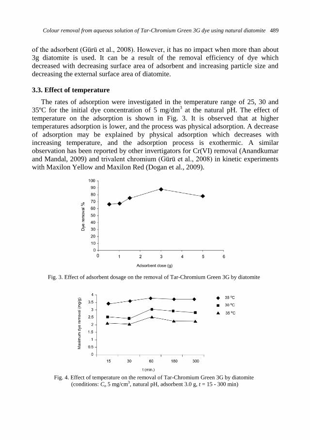
Colour removal from aqueous solution of Tar-Chromium Green 3G dye using natural diatomite 489
of the adsorbent (Gürü et al., 2008). However, it has no impact when more than about
3g diatomite is used. It can be a result of the removal efficiency of dye which
decreased with decreasing surface area of adsorbent and increasing particle size and
decreasing the external surface area of diatomite.
3.3. Effect of temperature
The rates of adsorption were investigated in the temperature range of 25, 30 and
35ºC for the initial dye concentration of 5 mg/dm3 at the natural pH. The effect of
temperature on the adsorption is shown in Fig. 3. It is observed that at higher
temperatures adsorption is lower, and the process was physical adsorption. A decrease
of adsorption may be explained by physical adsorption which decreases with
increasing temperature, and the adsorption process is exothermic. A similar
observation has been reported by other invertigators for Cr(VI) removal (Anandkumar
and Mandal, 2009) and trivalent chromium (Gürü et al., 2008) in kinetic experiments
with Maxilon Yellow and Maxilon Red (Dogan et al., 2009).
Fig. 3. Effect of adsorbent dosage on the removal of Tar-Chromium Green 3G by diatomite
Fig. 4. Effect of temperature on the removal of Tar-Chromium Green 3G by diatomite
(conditions: Co 5 mg/cm3, natural pH, adsorbent 3.0 g, t = 15 - 300 min)

490 M. Koyuncu
3.4. Isotherm study
The isotherm analysis of adsorption process were carried out using the Langmuir
and Freundlich models at different temperatures.
The Langmuir and Freundlich isotherm parameters were determined for their linear
forms. In the case of the Freundlich isoterm:
nee kCq1
Freundlich isotherm, (2)
ee Cn
kq ln1
lnln Freundlich isotherm (linear form), (3)
where qe is the amount of dye adsorbed at equilibrium time (mg/g), Ce is the
equilibrium concentration of the dye in solution (mg/dm3), k and n are isotherm
constants which indicate the capacity and intensity of the adsorption, respectively.
Figure 4 presents the plots of ln qe against ln Ce for the adsorption of dye onto
diatomite in the range from 25, 30 to 35ºC at natural pH, respectively. Figure 4 shows
that the plots for diatomite provide the Freundlich isotherm correlation coefficients
0.980, 0.976 and, 0.973 respectively. On the other hand, the values of n between 2 and
10 show good adsorption (Gürü et al., 2008; Erdem et al., 2005). The values of k and
n were calculated from the incercept and slope of the plot of ln qe versus ln Ce,
respectively. Therefore, the adsorption of Tar-Chromium Green 3G onto diatomite fits
well with the Freundlich models. These constants are given in Table 1. The Freundlich
equation frequently gives an adequate description of adsorption data over a restricted
range of concentration. The Freundlich equation is suitable for a highly heterogonous
surface and adsorption isotherm lacking a plateau, indicating a multi-layer adsorption.
The Langmuir model is as follows:
e
eoe
bC
bCQq
1 Langmuir isotherm, (4)
o
e
oe
e
Q
C
bQq
C
1 Langmuir isotherm (linear form), (5)
where Qo and b are Langmuir constants, which indicate the adsorption capacity (mg/g)
and energy of adsorption, respectively.
Figure 5 shows the plots obtained for diatomite with the Langmuir isotherm
correlation coefficients at 25, 30 and 35ºC, 0.998, 0.961 and, 0.935 respectively. The
values of Qo and b are found from the slope and intercept of the plot of Ce/qe versus
Ce, respectively. The constants Qo, b determined at different temperatures are given in
Table 1.
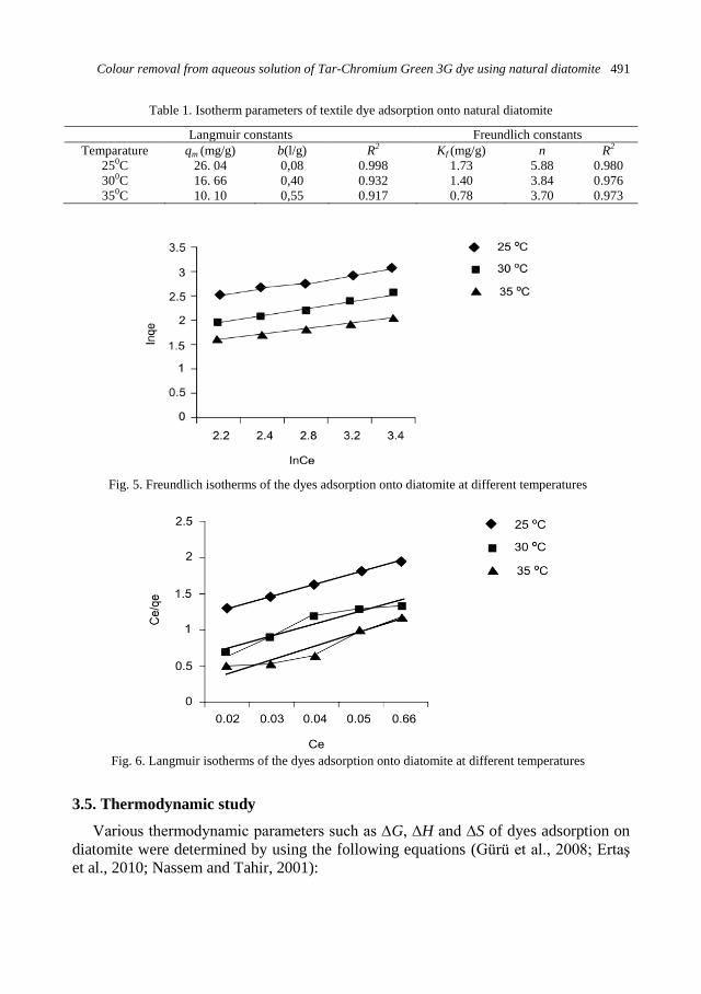
Colour removal from aqueous solution of Tar-Chromium Green 3G dye using natural diatomite 491
Table 1. Isotherm parameters of textile dye adsorption onto natural diatomite
Langmuir constants Freundlich constants
Temparature qm (mg/g) b(l/g) R2 Kf (mg/g) n R2
250C 26. 04 0,08 0.998 1.73 5.88 0.980
300C 16. 66 0,40 0.932 1.40 3.84 0.976
350C 10. 10 0,55 0.917 0.78 3.70 0.973
Fig. 5. Freundlich isotherms of the dyes adsorption onto diatomite at different temperatures
Fig. 6. Langmuir isotherms of the dyes adsorption onto diatomite at different temperatures
3.5. Thermodynamic study
Various thermodynamic parameters such as ∆G, ∆H and ∆S of dyes adsorption on
diatomite were determined by using the following equations (Gürü et al., 2008; Ertaş
et al., 2010; Nassem and Tahir, 2001):
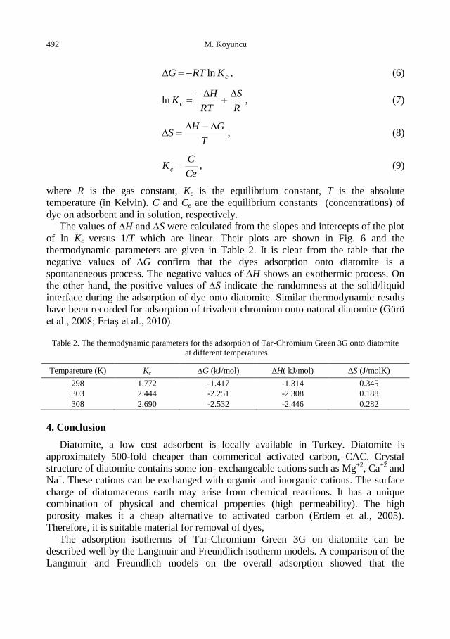
492 M. Koyuncu
cKRTG ln , (6)
R
S
RT
HKc
ln , (7)
T
GHS
, (8)
Ce
CK c , (9)
where R is the gas constant, Kc is the equilibrium constant, T is the absolute
temperature (in Kelvin). C and Ce are the equilibrium constants (concentrations) of
dye on adsorbent and in solution, respectively.
The values of ∆H and ∆S were calculated from the slopes and intercepts of the plot
of ln Kc versus 1/T which are linear. Their plots are shown in Fig. 6 and the
thermodynamic parameters are given in Table 2. It is clear from the table that the
negative values of ∆G confirm that the dyes adsorption onto diatomite is a
spontaneneous process. The negative values of ∆H shows an exothermic process. On
the other hand, the positive values of ∆S indicate the randomness at the solid/liquid
interface during the adsorption of dye onto diatomite. Similar thermodynamic results
have been recorded for adsorption of trivalent chromium onto natural diatomite (Gürü
et al., 2008; Ertaş et al., 2010).
Table 2. The thermodynamic parameters for the adsorption of Tar-Chromium Green 3G onto diatomite
at different temperatures
Tempareture (K) Kc ∆G (kJ/mol) ∆H( kJ/mol) ∆S (J/molK)
298 1.772 -1.417 -1.314 0.345
303 2.444 -2.251 -2.308 0.188
308 2.690 -2.532 -2.446 0.282
4. Conclusion
Diatomite, a low cost adsorbent is locally available in Turkey. Diatomite is
approximately 500-fold cheaper than commerical activated carbon, CAC. Crystal
structure of diatomite contains some ion- exchangeable cations such as Mg+2
, Ca+2
and
Na+. These cations can be exchanged with organic and inorganic cations. The surface
charge of diatomaceous earth may arise from chemical reactions. It has a unique
combination of physical and chemical properties (high permeability). The high
porosity makes it a cheap alternative to activated carbon (Erdem et al., 2005).
Therefore, it is suitable material for removal of dyes,
The adsorption isotherms of Tar-Chromium Green 3G on diatomite can be
described well by the Langmuir and Freundlich isotherm models. A comparison of the
Langmuir and Freundlich models on the overall adsorption showed that the
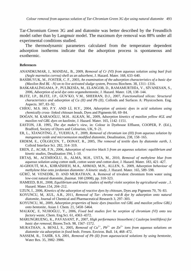
Colour removal from aqueous solution of Tar-Chromium Green 3G dye using natural diatomite 493
Tar-Chromium Green 3G and and diatomite was better described by the Freundlich
model rather than by Langmuir model. The maximum dye removal was 88% under all
experimental conditions studied.
The thermodynamic parameters calculated from the temperature dependent
adsorption isotherms indicate that the adsorption process is spontaneous and
exothermic.
References
ANANDKUMAR, J., MANDAL, B., 2009, Removal of Cr (VI) from aqueous solution using bael fruit
(Aegle marmelos correa) shell as an adsorbent, J. Hazard. Mater. 168, 633–640.
BASİBUYUK, M., FOSTER, C. F., 2003, An examination of the adsorption characteristics of a basic dye
(Maxilon Red BL –N) on to live activated sludge system, Process Biochem. 38, 1311–1316.
BASKARALİNGAMA, P., PULİKESİA, M., ELANGOB, D., RAMAMURTHİA, V., SİVANESAN, S.,
2006, Adsorption of acid dye onto organobentonite, J. Hazard. Mater. 128, 138–144.
BLITZ, I.P., BLITZ, J.P., GUN’KO, V.M., SHEERAN, D.J., 2007, Functionalized silicas: Structural
characteristics and adsorption of Cu (II) and Pb (II), Colloids and Surfaces A: Physicochem. Eng.
Aspects. 307, 83–92.
CHİOU, M.S. HO, P.Y. AND Lİ, H.Y., 2004, Adsorption of anionic dyes in acid solutions using
chemically cross- linked chitosan beads, Dyes and Pigments 60, 69–84.
DOĞAN, M. KARAOĞLU, M.H.. ALKAN, M., 2009, Adsorption kinetics of maxilon yellow 4GL and
maxilon red GRL dyes on kaolinite, J. Hazard. Mater. 165, 1142–1151.
EASTON, J.R. 1995, The dye maker's view, in: Colour in Dyehouse Effluent, COOPER, P. (Ed.),
Bradford, Society of Dyers and Colourists, UK, 9–21.
ER, L., XİANGYİNG, Z., YUEHUA, F., 2009, Removal of chromium ion (III) from aqueous solution by
manganese oxide and microemusion modified diatomite, Desalination, 238, 158–165.
ERDEM, E., ÇÖLGEÇEN, T., DONAT, R., 2005, The removal of textile dyes by diatomite earth, J.
Colloid Interface Sci. 282, 314–319.
EREN, Z., ACAR, F.N., 2006, Adsorption of reactive black 5 from an aqueous solution: equilibrium and
kinetic studies, Desalination 194, 1–10.
ERTAŞ, M., ACEMİOĞLU, B., ALMA, M.H., USTA, M., 2010, Removal of methylene blue from
aqueous solution using cotton stalk, cotton waste and cotton dust, J. Hazard. Mater. 183, 421–427.
Al-GHOUTİ, M.A., KHRAİSHEH, M.A., AHMAD, M.N., ALLEN, S.. 2009, Adsorption behaviour of
methylene blue onto jordanian diatomite: A kinetic study, J. Hazard. Mater. 165, 589–598.
GÜRÜ, M. VENEDİK, D. AND MURATHAN, A. Removal of trivalent chromium from water using
low-cost natural diatomite, jhazmat. 160 (2008), pp. 318-323.
HAMEED, B.H., 2008, Equilibrium and kinetic studies of methyl violet sorption by agricultural waste , J.
Hazard. Mater.154, 204–212.
UZUN, İ., 2006, Kinetics of the adsorption of reactive dyes by chitosan, Dyes anp Pigments 70, 76–83.
KOYUNCU, M, .KUL, A.R., 2011, Removal of Tar- chrome red-B dye by adsorption onto natural
diatomite, Journal of Chemical and Pharmaceutical Research 3, 297–303.
KOYUNCU, M., 2009, Adsorption properties of basic dyes (maxilon red GRL and maxilon yellow GRL)
onto bentonite, Asian J. Chem. 21, 5458–5464.
MALKOÇ, E, NUHOĞLU, Y., 2006, Fixed bed studies fort he sorption of chromium (VI) onto tea
factory waste, Chem. Eng.Sci. 61, 4363–4372.
MARUNGRUENG, K., PAVASANT, P., 2007, High performance biosorbent ( Caulerpa lentillifera) for
basic dye removal, Biores.Tech. 98, 1567–1572.
MURATHAN, A. BENLİ, S., 2005, Removal of Cu2+, Pb2+ an Zn2+ ions from aqueous solutions on
diatomite via adsorption in fixed beds. Fresen. Environ. Bull. 14, 468–472.
NASSEM, R., TAHİR, S.S, 2001, Removal of Pb (II) from aqueous/acid solutions by using bentonite,
Water Res. 35, 3982–3986.
494 M. Koyuncu
PARAB, H., JOSHI, S.; SHENOY, N., LALI, A.; SARMA, U.S.; SUDERSANAN, M.; 2006,
Detemination of kinetic and equilibrium parameters of the batch adsorption of Co (II) Cr(III) and
Ni(II) onto coir pith, Process Biochem. 41, 609–615.
PEARCE, C.I., LLOYD, J.R., GUTHRİE, J.T., 2003, The removal of colour from textile waste water
using whole bacterial cells. A review, Dyes and Pigments 58, 179–196.
QİU, J., WANG, Z., Lİ, H., XU, L., PENG, J., ZHAİ, M., YANG, C., Lİ, J., WEİ, G., 2009, Adsorption
of Cr(VI) using silica- based adsorbent prepared by radiation-induced grafting, J. Hazard. Mater.
166, 270–276.
ROBİNSON, T., MULLAN, G., MARCHANT, R., NİGAM, P., 2001, Remediation of dyes in textile
effluenta critical on current treatment technologies with a proposed alternative, Bioresour. Technol.,
77, 247–254.
SİNGH, K.P.,MOHAN, D., SİNHA, S., TONDON, G.S., GOSH, D., 2003, Color removal from
wastewater using low-cost activated carbon derived from agricultural waste material, Ind. Eng.
Chem. Res. 42, 1965–1976.
TAHİR, S.S., NASSEM, R., 2007, Removal of Cr (III) from tannery wastewater by adsorption onto
bentonite clay, Sep. Purif. Technol. 53, 312–321.
WANG, S., HUİTİNG, L., 2005, Dye adsorption on unburned carbon: Kinetics and equilibrium, J.
Hazard. Mater. 26, 71–77.
YUAN, P., LİU, D., FAN, M., YANG, D., ZHU, R., GE, F., ZHU, J., HE, H., 2010, Removal of
hexavalent chromium [Cr(VI)] from aqueous solutions by the diatomite supported/unsupported
magnetite nano particles, J. Hazard. Mater. 173, 614–621.
http://dx.doi.org/10.5277/ppmp120215
Physicochem. Probl. Miner. Process. 48(2), 2012, 495−512 Physicochemical Problems
of Mineral Processing
w w w . m i n p r o c . p w r . w r o c . p l / j o u r n a l / ISSN 1643-1049 (print)
ISSN 2084-4735 (online)
Received April 3, 2012; reviewed; accepted May 1, 2012
EFFECT OF AUTOCORRELATION ON THE PROCESS CONTROL
CHARTS IN MONITORING OF A COAL WASHING PLANT
Adem TASDEMIR
Department of Mining Engineering, Division of Mineral Processing, Eskişehir Osmangazi University, 26480,
Eskişehir, Turkey, [email protected], Tel: +90 222 239 37 50 Ext: 3438
Abstract. Traditional statistical process control charts assume that generated process data are
normally and independently distributed, i.e. uncorrelated. This research presents the effect of
autocorrelation on process control charts to monitor the two quality characteristics of fine coals
produced in a coal washing plant for power plant, namely moisture content and ash content.
Individual (X) and moving range charts (MR) were constructed to monitor 10 months data. It
was determined that even though both data values obey the normal distribution, there is a
moderate autocorrelation between their observations. For simulating the autocorrelated data,
ARIMA time-series models were used. It was found that X/MR charts showed many false
alarms due to the autocorrelation. The ARIMA (1, 0, 1) for moisture content and ARIMA (0, 1,
2) for ash content were determined to be the best models to remove autocorrelation. Compared
to large number of false alarms on conventional X/MR charts and on charts applying the
Western Electric rules, which assume the data independence, there were much less unusual
points on the X/MR charts of residuals (Special Cause Charts). Usage of residual based control
charts is suggested when the data are autocorrelated.
keywords: coal, autocorrelation, statistical control charts, special cause charts, ARIMA
models
1. Introduction
Statistical process control (SPC) has been proposed firstly by Dr. Shewhart in 1931
and then, many SPC charts have been developed and improved to use for different
process data. In its basics form, a control chart compares process observations with a
pair of control limits (Karaoğlan and Bayhan, 2011). One of the essentials of
producing high quality low cost product is to adopt and apply the SPC correctly. SPC
is a tool for achieving and improving quality standards. The most important and
sophisticated tool of SPC is control charts.
SPC is widely used to monitor, control and improve quality in many industrial
processes (MacCharty and Wasusri, 2002). The SPC has been also used in mining and
mineral processing field to monitor the grade variations and to ensure the product
specifications. In a review study, MacCharty and Wasusri (2002) summarize the usage
of non-standard applications of statistical process control charts. Some application
496 A. Tasdemir
examples of SPC can be given from the literature for mining/mineral processing
industry (Ankara and Bilir, 1995; İpek et al., 1999; Bhattacherjee and Samanta, 2002;
Bayat and Arslan, 2004; Aykul et al., 2005; Vapur et al., 2005; Elevli and Behdioğlu,
2006; Ankara and Yerel, 2008; Vapur, 2009; Elevli, 2009; Aykul et al., 2010; Yerel
and Ankara, 2011). However, the information related to the application of SPC in
mineral industry is still limited when compared to other industrial areas.
Traditional SPC techniques are based on the assumption that generated data
generated are normally and independently distributed. However, the independency
assumption is not realistic in practice (Demirkol, 2008). Therefore, the assumption of
normality and indepence of data must be satisfied in order to apply SPC for a process
(Bhattacherjee and Samanta, 2002).
In the continuous industries processes most data are autocorrelated (Le, 1998).
Since observations for many processes exhibit autocorrelation that may be the result of
dynamics that are inherent to the process, the autocorrelation is more likely to be
observed in processes when observations are closely spaced in time (Lu and Reynolds,
2001). Such autocorrelations can occur for a number of reasons. One reason is
because of current automated measurement and recording technology, subgroup
samples may be taken with a high frequency, with consecutive samples being similar
in nature and hence statistically correlated. Other samples of correlated subgroups
occur when items made by a worker exhibit similar characteristics due to the way the
machine is handled, the process shows seasonal patterns due to materials or weather,
or the alertness of a worker changes over time (Le, 1998).
The effect of autocorrelation on the performance of process control charts have
been shown by many researhers (Alwan and Roberts, 1998; Lu and Reynolds, 1999;
Montgomery and Mastrangeko, 1991; Atienza et al., 1997; Reynolds and Lu, 1997;
Zhang, 1997). Results of these studies have shown that traditional SPC methods are
strongly affected by data autocorrelation. Under autocorrelation conditions, the
traditional control charts will become ineffective and many false alarms may occur on
the charts. Consequently, there has been considerable research in recent years on
designing SPC procedures suitable for autocorrelated processes.
In the case of autocorrelation, a very high false alarm rate will cause process
personnel to waste effort in unproductive searches for special causes. This can lead to
a loss of confidence in the control chart, and even to process monitoring being
discontinued. Thus, autocorrelation should not be ignored when designing control
charts, because failure to properly account for autocorrelation can greatly reduce or
eliminate the effectiveness of control charts (Lu and Reynolds, 2001).
For these reasons, some modifications for traditional control charts are necessary.
As an alternative to traditional control charts which plot the original observations, a
number of papers have suggested fitting a time series model (Alwan and Roberts,
1988; Reynolds and Lu, 1997; Lu and Reynolds, 1999; Lu and Reynolds, 2001). The
residuals obtained from time series model are then plotted on standard control charts.
Effect of autocorrelation on the process control charts in monitoring … 497
To apply these methods, a time series model of the process is required (Apley and Lee,
2003).
Alwan and Roberts (1988) introduced the first residual control chart, namely
special cause chart (SCC). A residual Shewhart chart was developed by them and it is
called as the special control chart (SCC). The SCC is an individual control chart
(individual control chart is constructed by plotting single observations and setting
control limits on these observations) applied to the residuals. Therefore, the SCC is
also known as the X residual chart in the literature. In residual charts, an appropriate
time series model is fitted to the autocorrelated observations and the residuals are
plotted in a control chart (Demirkol, 2008).
Even though the assumptions required for the applicability of SPC methods are
known to be essential, their existence may questionable in mining industry
(Bhattacherjee and Samanta, 2001). When the literature is reviewed, the impact of
autocorrelation on SPC have been considered in mineral applications by only few
studies (Samanta and Bhattacherjee, 2001; Bhattacherjee and Samanta, 2002;
Samanta, 2002; Elevli et al., 2009). Indeeed, the observations in these studies are
assumed to normally distributed and independent that is uncorrelated.
Turkey has 8.3 billion tons of lignite coal reserves (Arslan, 2006). Since 80% of
Turkish lignite coal reserves has a heating value of below 2500 kcal/kg, large amount
of them are used in power plants. Moisture and ash contents of coals are the two
important quality characteristics that determine properties of coals burning in power
plants. Substantial amount of low quality coals which have high ash and moisture
contents are transformed into energy by burning them in power plants (Tekir et al.,
2009). In a power plats that burns lignites, moisture and ash contents are the key
quality indicators monitored. Therefore, lowering the ash contents of lignites to the
desired levels is an essential entity to reduce problems and costs associated with the
ash. Coals having high ash and moisture contents cause serious problems such as
incrasing the costs of operation, transportation and burning of coal together with
disposing the ash to dams in power plants (Tekir et al., 2009). For these reasons, coal
fines produced in a coal washing plant should have desired moisture and ash content
limits in order to be used as feeding material for a power plant. To control the coal
qualities produced in washing plants, it is necessary to monitor the coal characteristics
by applying an effective method such as statistical process control.
The aim of this paper is to investigate individual X control charts based on the
original observations or on residuals obtained by the time series of ARIMA models for
moisture and ash contents of fine coal products that are produced for power plant as a
feeding material in Tunçbilek washing plant. Autocorrelated observations were
characterized by ARIMA models and special control charts (SCC) were utilized to
monitor the residuals, based on the ARIMA model forecast values. The performance
of the standard Shewhart chart, which ignores subgroup correlations for the two coal
quality variables, is compared with the X charts of residuals.
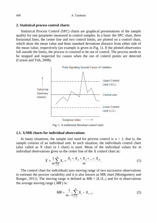
498 A. Tasdemir
2. Statistical process control charts
Statistical Process Control (SPC) charts are graphical presentations of the sample
quality for one parameter measured in control samples. In a basic the SPC chart, three
horizontal lines, the center line and two control limits, are plotted on a control chart,
which show the mean value and three standard deviations distance from either side of
the mean value, respectively (an example is given in Fig. 1). If the plotted observatios
fall outside the limits, the process is consired to be out of control. The process needs to
be stopped and inspected for causes when the out of control points are detected
(Carson and Yeh, 2008).
Fig. 1. A traditional Shewhart control chart
2.1. X/MR charts for individual observations
In many situations, the sample size used for process control is n = 1; that is, the
sample consists of an individual unit. In such situation, the individuals control chart
(also called as X chart or I chart) is used. Mean of the individual values for m
individual observations gives us the center line of the X control chart as:
m
i
mi
m
XXXXX
mX
1
321 ...1. (1)
The control chart for individuals uses moving range of two successive observations
to estimate the process variability and it is also known as MR chart (Montgomery and
Runger, 2011). The moving range is defined as MRi = |Xi-Xi-1| and for m observations
the average moving range ( MR ) is:
m
i
ii XXm
MR2
21
1. (2)
Effect of autocorrelation on the process control charts in monitoring … 499
An estimate of standard deviation (σ) is:
128.12
MR
d
MR . (3)
Here, d2 is a constant depending on the sample size, n, (Montgomery and Runger,
2011). It is 1.128 for n = 2.
The center line (CLX) and upper control limit (UCLX) and lower control limit
(LCLX) for a control chart for individuals is (Montgomery and Runger, 2011):
MRXMR
Xd
MRXUCLX 66.2
128.133
2
, (4)
XCLX , (5)
MRXMR
Xd
MRXLCLX 66.2
128.133
2
. (6)
Since each moving range is the range between two consecutive observations. It
should be noted that there are only m-1 moving ranges. The parameters for a control
chart of moving range are defined as follows:
MRMRDUCLMR 267.34 , (7)
MRCLMR , (8)
03 MRDLCLMR . (9)
D3 and D4 are constants depending on the sample size, n. It is possible to establish
a control chart on the MR using D3 and D4 for n = 2 (Montgomery and Runger, 2011).
The LCLMR for this moving range chart is always zero because D3 = 0 for n = 2. The
D4 equals to 3.267 for n = 2 while determining the UCLMR .
For a simple control chart in Fig. 1 control limits were plotted as warning lines
from the action limits of 3σ. In this figure, only measurements that are plotted further
than 3σ from the central line indicate an out-of-control process. However, additional
warning limits in Shewhart charts are commonly used in practice, since they help the
analyst to recognize possible changes in the process before it shifts out of 3σ (Carson
and Yeh, 2008). For example, when two consecutive out of 2σ samples are detected,
this can indicate some changes in the process. Therefore, it is advisable to perform
some rechecks of the process at this point.
It is known that the Shewhart control chart is insensitive to small shifts in the
process parameter. To enhance the ability for the chart to detect small shifts more
quickly, one way is to add sensitive rules in the chart (Chang and Wu, 2011). Several
frequently used rules suggested by the Western Electric (1956) are (Montgomery and
Runger, 2011):
500 A. Tasdemir
1. One or more points fall outside the 3σ control limits,
2. Two of three consecutive points fall outside the 2σ warning limits,
3. Four of five consecutive points fall beyond the 1σ limits,
4. Eight points in a row fall one side of the center line.
The above rules are always referred to runs rules. In the sequel, a control chart that
uses several rules simultaneously is referred to a compound control chart. It should be
noted that rule 1 in included in all compound control charts. Also note that these rules
can only be applied to one side of the center line. There are more rules for detecting
small shifts and these can be added to control.
In this study, the four rules listed above were used when considering additional
warning limits by Western electric rules. These plots searches and identifies any
unusual patterns in the data. This is often helpful in detecting processes which are
slowly drifting away from target, even though no points may fall outside the control
limits.
3. Time series models
The methodology of ARIMA estimation and model selection is a classical topic
covered in most textbooks on time series analysis such as Montgomery et al. (2008).
Therefore, we will not duplicate the descriptions of already well documented
methodologies. We will give only practical information in this context to the models.
3.1. Autoregressive Process (AR)
Most time series consist of elements that are serially dependent in the sense that
one can estimate a coefficient or a set of coefficients that describe consecutive
elements of the series from specific, time-lagged (previous) elements. This can be
summarized in the following Eq. 10:
tptpttt XXXX ...2211 , (10)
where Xt is response (dependent) variable at time t; Xt-1, Xt-2, Xt-p response variable at
time lags t-1, t-2,…t-p, respectively; ϕ1, ϕ2, ϕp, denote estimated coefficients, εt is an
error term at time t, and
p
i
i
1
1 with μ denotes the process mean.
It should be noted that an autoregressive process will only be stable if the
parameters are within a certain range for example, if there is only one autoregressive
parameter, then it must fall within the interval of -1<ϕ1<+1. Otherwise, past effects
would accumulate and the values of successive Xt's would move towards infinity, that
is, the series would not be stationary. If there is more than one autoregressive
parameter, similar (general) restrictions on the parameter values can be defined
(Montgomery et al., 2008).
Effect of autocorrelation on the process control charts in monitoring … 501
3.2. Moving Average process (MA)
Independent from the autoregressive process, each element in the series can also be
affected by the past error (or random shock) that cannot be accounted for by the
autoregressive component, that is:
qtqttttX ...2211 , (11)
where Xt is the time series, μ is the mean of the series, εt-I denotes random noise term
with mean 0 and variance σε2 at time t. θ1, θ2, θq, are the moving average model
parameters. The value of q is called the order of the MA model.
3.3 Autoregressive Moving Average model (ARIMA)
The ARIMA model which combines the autoregressive and moving average
parameters and includes differencing in the model was introduced by Box and Jenkins
(1976) (Montgomery et al., 2008). This equation was used to forecast one-step ahead
disturbances, according to data characteristics of stationary or non-stationary as shown
in Eq. 12.
qtqttptdptdtdtd XXXX ...... 112211 , (12)
Three types of parameters in the model are: the autoregressive parameters (p), the
number of differencing passes (d), and moving average parameters (q). The Box and
Jenkins models are summarized as the ARIMA (p, d, q); so, for example, a model
described as (0, 1, 2) means that it contains 0 (zero) autoregressive (p) parameters and
2 moving average (q) parameters which were computed for the series after it was
differenced once (documentation.statsoft.com).
The input series needs to be stationary for ARIMA. It should have a constant mean,
variance, and autocorrelation through time. Therefore, the series are first differentiated
until they are stationary. Sometimes the series also require log transformation of data
to stabilize the variance. The d parameter indicates the number of times the series
needs to be differenced to achieve stationarity (documentation.statsoft.com). The
necessary level of differencing is determined by examining the plot of the data and
autocorrelogram. Significant changes in level (strong upward or downward changes)
usually require first order non seasonal (lag=1) differencing; strong changes of slope
usually require second order non seasonal differencing. When the estimated
autocorrelation coefficients decline slowly at longer lags, first order differencing is
usually needed (documentation.statsoft.com). Some time series may require little or no
differencing, and over differenced series produce less stable coefficient estimates It is
needed to decide how many autoregressive (p) and moving average (q) parameters are
necessary to yield an effective but has the fewest parameters and greatest number of
degrees of freedom among all models that fit the data model of the process. The
number of p or q parameters very rarely need to be greater than 2 in practice
(documentation.statsoft.com).
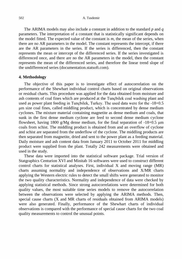
502 A. Tasdemir
The ARIMA models may also include a constant in addition to the standard p and q
parameters. The interpretation of a constant that is statistically significant depends on
the model fitted. The expected value of the constant is m, the mean of the series, when
there are no AR parameters in the model. The constant represents the intercept, if there
are the AR parameters in the series. If the series is differenced, then the constant
represents the mean or intercept of the differenced series. If the series investigated is
differenced once, and there are no the AR parameters in the model, then the constant
represents the mean of the differenced series, and therefore the linear trend slope of
the undifferenced series (documentation.statsoft.com).
4. Methodology
The objective of this paper is to investigate effect of autocorrelation on the
performance of the Shewhart individual control charts based on original observations
or residual charts. This procedure was applied for the data obtained from moisture and
ash contents of coal fines which are produced at the Tunçbilek coal washing plant and
used as power plant feeding in Tunçbilek, Turkey. The used data were for the -18+0.5
μm size coal fines, called middling product, which is concentrated by dense medium
cyclones. The mixture material containing magnetite as dense medium and coals, that
sunk in the first dense medium cyclone are feed to second dense medium cyclone
flowsheet, having 1800 g/Mg dense medium, for the final separation of -18+0.5 μm
coals from schist. The middling product is obtained from and an overflow of cyclone
and schist are separated from the underflow of the cyclone. The middling products are
then separated from magnetite, dried and sent to the power plant as a feeding material.
Daily moisture and ash content data from January 2011 to October 2011 for middling
product were supplied from the plant. Totally 242 measurements were obtained and
used in the study.
These data were imported into the statistical software package. Trial version of
Statgraphics Centurion XVI and Minitab 16 softwares were used to construct different
control charts for statistical analyses. First, individual X and moving range (MR)
charts assuming normality and independence of observations and X/MR charts
applying the Western electric rules to detect the small shifts were generated to monitor
the two quality characteristics. Normality and independence of data were checked by
applying statistical methods. Since strong autocorrelations were determined for both
quality values, the most suitable time series models to remove the autocorrelation
between the observations were selected by applying the ARIMA methods. Then,
special cause charts (X and MR charts of residuals obtained from ARIMA models)
were also generated. Finally, performance of the Shewhart charts of individual
observations is compared with the performance of special cause charts for the two coal
quality measurements to control the unusual points.
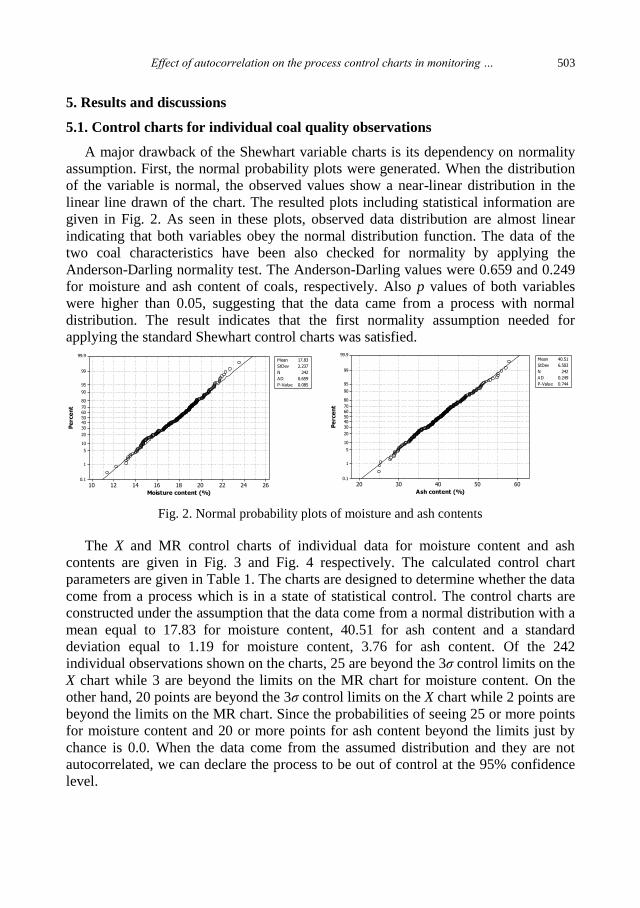
Effect of autocorrelation on the process control charts in monitoring … 503
5. Results and discussions
5.1. Control charts for individual coal quality observations
A major drawback of the Shewhart variable charts is its dependency on normality
assumption. First, the normal probability plots were generated. When the distribution
of the variable is normal, the observed values show a near-linear distribution in the
linear line drawn of the chart. The resulted plots including statistical information are
given in Fig. 2. As seen in these plots, observed data distribution are almost linear
indicating that both variables obey the normal distribution function. The data of the
two coal characteristics have been also checked for normality by applying the
Anderson-Darling normality test. The Anderson-Darling values were 0.659 and 0.249
for moisture and ash content of coals, respectively. Also p values of both variables
were higher than 0.05, suggesting that the data came from a process with normal
distribution. The result indicates that the first normality assumption needed for
applying the standard Shewhart control charts was satisfied.
262422201816141210
99.9
99
95
90
80
7060504030
20
10
5
1
0.1
Moisture content (%)
Pe
rce
nt
Mean 17.83
StDev 2.237
N 242
AD 0.659
P-Value 0.085
Probability Plot of Moisture Content
6050403020
99.9
99
95
90
80
7060504030
20
10
5
1
0.1
Ash content (%)
Pe
rce
nt
Mean 40.51
StDev 6.503
N 242
AD 0.249
P-Value 0.744
Probability Plot of Ash Content
Fig. 2. Normal probability plots of moisture and ash contents
The X and MR control charts of individual data for moisture content and ash
contents are given in Fig. 3 and Fig. 4 respectively. The calculated control chart
parameters are given in Table 1. The charts are designed to determine whether the data
come from a process which is in a state of statistical control. The control charts are
constructed under the assumption that the data come from a normal distribution with a
mean equal to 17.83 for moisture content, 40.51 for ash content and a standard
deviation equal to 1.19 for moisture content, 3.76 for ash content. Of the 242
individual observations shown on the charts, 25 are beyond the 3σ control limits on the
X chart while 3 are beyond the limits on the MR chart for moisture content. On the
other hand, 20 points are beyond the 3σ control limits on the X chart while 2 points are
beyond the limits on the MR chart. Since the probabilities of seeing 25 or more points
for moisture content and 20 or more points for ash content beyond the limits just by
chance is 0.0. When the data come from the assumed distribution and they are not
autocorrelated, we can declare the process to be out of control at the 95% confidence
level.
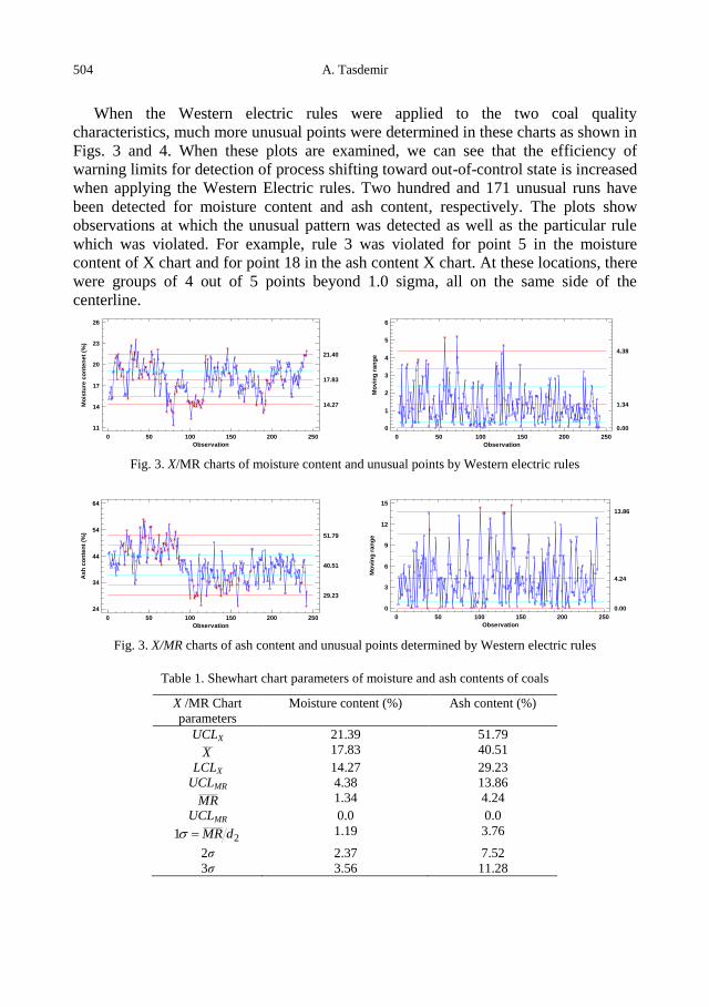
504 A. Tasdemir
When the Western electric rules were applied to the two coal quality
characteristics, much more unusual points were determined in these charts as shown in
Figs. 3 and 4. When these plots are examined, we can see that the efficiency of
warning limits for detection of process shifting toward out-of-control state is increased
when applying the Western Electric rules. Two hundred and 171 unusual runs have
been detected for moisture content and ash content, respectively. The plots show
observations at which the unusual pattern was detected as well as the particular rule
which was violated. For example, rule 3 was violated for point 5 in the moisture
content of X chart and for point 18 in the ash content X chart. At these locations, there
were groups of 4 out of 5 points beyond 1.0 sigma, all on the same side of the
centerline.
Mo
istu
re c
on
ten
et
(%)
21.40
X Chart for Col_1
0 50 100 150 200 250
Observation
11
14
17
20
23
26
17.83
14.27
Mo
vin
g r
an
ge
4.38
MR(2) Chart for Col_1
0 50 100 150 200 250
Observation
0
1
2
3
4
5
6
1.34
0.00
Fig. 3. X/MR charts of moisture content and unusual points by Western electric rules
Ash
co
nte
nt
(%)
51.79
X Chart for Col_2
0 50 100 150 200 250
Observation
24
34
44
54
64
40.51
29.23
Mo
vin
g r
an
ge
13.86
MR(2) Chart for Col_2
0 50 100 150 200 250
Observation
0
3
6
9
12
15
4.24
0.00
Fig. 3. X/MR charts of ash content and unusual points determined by Western electric rules
Table 1. Shewhart chart parameters of moisture and ash contents of coals
X /MR Chart
parameters
Moisture content (%) Ash content (%)
UCLX 21.39 51.79
X 17.83 40.51
LCLX 14.27 29.23
UCLMR 4.38 13.86
MR 1.34 4.24
UCLMR 0.0 0.0
21 dMR 1.19 3.76
2σ 2.37 7.52
3σ 3.56 11.28
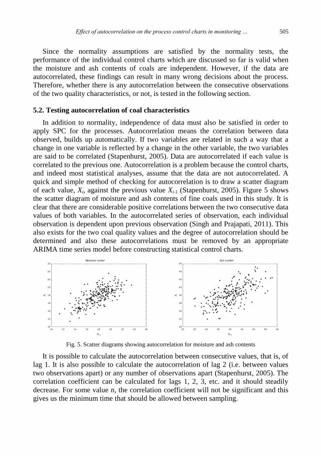
Effect of autocorrelation on the process control charts in monitoring … 505
Since the normality assumptions are satisfied by the normality tests, the
performance of the individual control charts which are discussed so far is valid when
the moisture and ash contents of coals are independent. However, if the data are
autocorrelated, these findings can result in many wrong decisions about the process.
Therefore, whether there is any autocorrelation between the consecutive observations
of the two quality characteristics, or not, is tested in the following section.
5.2. Testing autocorrelation of coal characteristics
In addition to normality, independence of data must also be satisfied in order to
apply SPC for the processes. Autocorrelation means the correlation between data
observed, builds up automatically. If two variables are related in such a way that a
change in one variable is reflected by a change in the other variable, the two variables
are said to be correlated (Stapenhurst, 2005). Data are autocorrelated if each value is
correlated to the previous one. Autocorrelation is a problem because the control charts,
and indeed most statistical analyses, assume that the data are not autocorrelated. A
quick and simple method of checking for autocorrelation is to draw a scatter diagram
of each value, Xi, against the previous value Xi-1 (Stapenhurst, 2005). Figure 5 shows
the scatter diagram of moisture and ash contents of fine coals used in this study. It is
clear that there are considerable positive correlations between the two consecutive data
values of both variables. In the autocorrelated series of observation, each individual
observation is dependent upon previous observation (Singh and Prajapati, 2011). This
also exists for the two coal quality values and the degree of autocorrelation should be
determined and also these autocorrelations must be removed by an appropriate
ARIMA time series model before constructing statistical control charts.
Moisture content
10 12 14 16 18 20 22 24 26
Xi-1
10
12
14
16
18
20
22
24
26
Xi
Ash content
20 25 30 35 40 45 50 55 60
Xi-1
20
25
30
35
40
45
50
55
60
Xi
Fig. 5. Scatter diagrams showing autocorrelation for moisture and ash contents
It is possible to calculate the autocorrelation between consecutive values, that is, of
lag 1. It is also possible to calculate the autocorrelation of lag 2 (i.e. between values
two observations apart) or any number of observations apart (Stapenhurst, 2005). The
correlation coefficient can be calculated for lags 1, 2, 3, etc. and it should steadily
decrease. For some value n, the correlation coefficient will not be significant and this
gives us the minimum time that should be allowed between sampling.
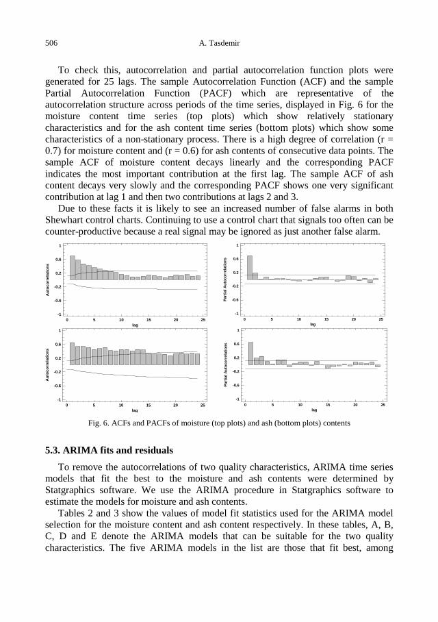
506 A. Tasdemir
To check this, autocorrelation and partial autocorrelation function plots were
generated for 25 lags. The sample Autocorrelation Function (ACF) and the sample
Partial Autocorrelation Function (PACF) which are representative of the
autocorrelation structure across periods of the time series, displayed in Fig. 6 for the
moisture content time series (top plots) which show relatively stationary
characteristics and for the ash content time series (bottom plots) which show some
characteristics of a non-stationary process. There is a high degree of correlation (r =
0.7) for moisture content and (r = 0.6) for ash contents of consecutive data points. The
sample ACF of moisture content decays linearly and the corresponding PACF
indicates the most important contribution at the first lag. The sample ACF of ash
content decays very slowly and the corresponding PACF shows one very significant
contribution at lag 1 and then two contributions at lags 2 and 3.
Due to these facts it is likely to see an increased number of false alarms in both
Shewhart control charts. Continuing to use a control chart that signals too often can be
counter-productive because a real signal may be ignored as just another false alarm. Estimated Autocorrelations for Col_1
0 5 10 15 20 25
lag
-1
-0.6
-0.2
0.2
0.6
1
Au
toco
rrela
tio
ns
Estimated Partial Autocorrelations for Col_1
0 5 10 15 20 25
lag
-1
-0.6
-0.2
0.2
0.6
1
Part
ial
Au
toco
rrela
tio
ns
Estimated Autocorrelations for Col_2
0 5 10 15 20 25
lag
-1
-0.6
-0.2
0.2
0.6
1
Au
toco
rrela
tio
ns
Estimated Partial Autocorrelations for Col_2
0 5 10 15 20 25
lag
-1
-0.6
-0.2
0.2
0.6
1
Part
ial
Au
toco
rrela
tio
ns
Fig. 6. ACFs and PACFs of moisture (top plots) and ash (bottom plots) contents
5.3. ARIMA fits and residuals
To remove the autocorrelations of two quality characteristics, ARIMA time series
models that fit the best to the moisture and ash contents were determined by
Statgraphics software. We use the ARIMA procedure in Statgraphics software to
estimate the models for moisture and ash contents.
Tables 2 and 3 show the values of model fit statistics used for the ARIMA model
selection for the moisture content and ash content respectively. In these tables, A, B,
C, D and E denote the ARIMA models that can be suitable for the two quality
characteristics. The five ARIMA models in the list are those that fit best, among

Effect of autocorrelation on the process control charts in monitoring … 507
dozens that were fit. The most suitable model between them was selected by applying
the selection criteria. The procedure fits each of the models indicated and selects the
models that give the smallest value of the selected criterion. There are six criteria to
choose from: (1) the root mean squared error (RMSE), (2) the mean absolute error
(MAE), (3) the mean absolute percentage error (MAPE), (4) the mean error (ME), (5)
the mean percentage error (MPE), (6) the Akaike Information Criterion (AIC).
Each of the statistics is based on the one-ahead forecast errors, which are the
differences between the data value at time t and the forecast of that value made at time
t-1. The first three statistics measure the magnitude of the errors. A better model will
give a smaller value. The last two statistics measure bias. A better model will give a
value close to 0. This table compares the results of fitting different models to the data.
The model with the lowest value of the Akaike Information Criterion (AIC) was
chosen as the best describing model in this study. The AIC is calculated from:
ncRSMEAIC 2ln2 , (13)
where RSME is the root mean squared error during the estimation period, c the number
of estimated coefficients in the fitted model, and n the sample size used to fit the
model. The AIC is a function of the variance of the model residuals, penalized by the
number of estimated parameters. In general, the model will be selected that minimizes
the mean squared error without using too many coefficients (relative to the amount of
data available).
The models with the lowest value of AIC are ARIMA (1,0,1) with a constant for
the moisture content and ARIMA (0,1,2) for ash content though several other models
are very similar, as presented in Table 2 and Table 3. Therefore, the ARIMA models
are preferred for our data in this research.
Table 2. ARIMA model fit statistics for moisture content
A: ARIMA(1,0,1) with constant; B: ARIMA(2,0,0) with constant; C: ARIMA(1,0,2) with constant;
D: ARIMA(2,0,1) with constant; E: ARIMA(2,1,1)
Table 3. ARIMA model fit statistics for ash content
Model RMSE MAE MAPE ME MPE AIC
(A) 4.62662 3.67199 9.47837 -0.168696 -1.69922 3.08018
(B) 4.63186 3.67325 9.5009 -0.178473 -1.74001 3.08245
(C) 4.63362 3.66381 9.425 -0.00738307 -1.29087 3.09147
(D) 4.618 3.61403 9.35612 -0.10959 -1.65678 3.09298
(E) 4.63713 3.66895 9.46142 -0.16297 -1.67918 3.09299 A: ARIMA(0,1,2); B: ARIMA(1,1,1); C: ARIMA(0,1,2) with constant; D: ARIMA(1,0,2) with constant;
E: ARIMA(1,1,2)
Model RMSE MAE MAPE ME MPE AIC
(A) 1.56223 1.24302 7.09856 0.0137352 -0.713845 0.917022
(B) 1.5634 1.24791 7.1247 0.0160021 -0.705291 0.91852
(C) 1.56514 1.24187 7.09152 0.0129439 -0.715767 0.929005
(D) 1.56633 1.24641 7.11658 0.0119596 -0.722733 0.930528
(E) 1.57798 1.23127 6.99972 0.0646808 -0.372863 0.937088
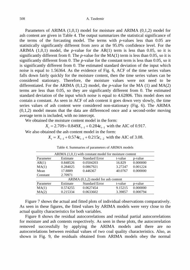
508 A. Tasdemir
Parameters of ARIMA (1,0,1) model for moisture and ARIMA (0,1,2) model for
ash content are given in Table 4. The output summarizes the statistical significance of
the terms of the forcasting model. The terms with p-values less than 0.05 are
statistically significantly different from zero at the 95.0% confidence level. For the
ARIMA (1,0,1) model, the p-value for the AR(1) term is less than 0.05, so it is
significantly different from 0. The p-value for the MA(1) term is less than 0.05, so it is
significantly different from 0. The p-value for the constant term is less than 0.05, so it
is significantly different from 0. The estimated standard deviation of the input which
noise is equal to 1.56364. As the evidence of Fig. 6, ACF of the time series values
falls down fairly quickly for the moisture content, then the time series values can be
considered stationary. Therefore, the moisture values were not need to be
differentiated. For the ARIMA (0,1,2) model, the p-value for the MA (1) and MA(2)
terms are less than 0.05, so they are significantly different from 0. The estimated
standard deviation of the input which noise is equal to 4.62806. This model does not
contain a constant. As seen in ACF of ash content it goes down very slowly, the time
series values of ash content were considered non-stationary (Fig. 6). The ARIMA
(0,1,2) model means that the data are differenced once and a second-order moving
average term is included, with no intercept.
We obtained the moisture content model in the form:
11 284.0849.0709.2 ttt XX with the AIC of 0.917.
We also obtained the ash content model in the form:
211 215.0574.0 tttt XX with the AIC of 3.08.
Table 4. Summaries of parameters of ARIMA models
ARIMA (1,0,1) with constant model for moisture content
Parameter Estimate Standard Error t-value p-value
AR(1) 0.848526 0.0504203 16.829 0.000000
MA(1) 0.284025 0.0867921 3.27247 0.001224
Mean 17.8889 0.446367 40.0767 0.000000
Constant 2.70971
ARIMA (0,1,2) model for ash content
Parameter Estimate Standard Error t-value p-value
MA(1) 0.574255 0.0627454 9.15215 0.000000
MA(2) 0.215334 0.0633602 3.39857 0.000794
Figure 7 shows the actual and fitted plots of individual observations comparatively.
As seen in these figures, the fitted values by ARIMA models were very close to the
actual quality characteristics for both variables.
Figure 8 shows the residual autocorrelations and residual partial autocorrelations
for moisture and ash contents respectively. As seen in these plots, the autocorrelation
removed successfully by applying the ARIMA models and there are no
autocorrelations between residual values of two coal quality characteristics. Also, as
shown in Fig. 9, the residuals obtained from ARIMA models obey the normal

Effect of autocorrelation on the process control charts in monitoring … 509
distribution very well. Since the normality and independence assumptions were
satisfied by the ARIMA model residuals, the standard Shewhart charts can be applied
conveniently to monitor the moisture and ash contents.
240216192168144120967248241
24
22
20
18
16
14
12
10
Days
Mo
istu
re c
on
ten
t (%
)
Actual
Fits
240216192168144120967248241
60
50
40
30
20
Days
Ash
co
nte
nt
(%)
Actual
Fits
Fig. 7. Actual and fitted moisture contents by ARIMA (1, 0, 1) with constant model and ash contents by
ARIMA (0,1,2) model
Residual Autocorrelations for Col_1
ARIMA(1,0,1) with constant
0 5 10 15 20 25
lag
-1
-0.6
-0.2
0.2
0.6
1
Au
toco
rrela
tio
ns
Residual Partial Autocorrelations for Col_1
ARIMA(1,0,1) with constant
0 5 10 15 20 25
lag
-1
-0.6
-0.2
0.2
0.6
1
Part
ial
Au
toco
rrela
tio
ns
Residual Autocorrelations for Col_2
ARIMA(0,1,2)
0 5 10 15 20 25
lag
-1
-0.6
-0.2
0.2
0.6
1
Au
toco
rrela
tio
ns
Residual Partial Autocorrelations for Col_2
ARIMA(0,1,2)
0 5 10 15 20 25
lag
-1
-0.6
-0.2
0.2
0.6
1
Part
ial
Au
toco
rrela
tio
ns
Fig. 8. ACFs and PACFs of residuals for moisture content by ARIMA (1,0,1) with constant model and for
ash content by ARIMA (0,1,2)
5.4. X/MR Charts for monitoring forecast residuals
Figure 10 shows the X and MR charts of residuals for individual moisture and ash
contents. Even applying the Western electric rules, the number of out-of control points
signaficantly reduced the false alarms. There are only 5 and 6 unusual points in X
charts of moisture and ash contents, respectively. There is only one point exceeding 3σ
limits for moisture and no out-of control point for ash content. On the other hand these
numbers are 2 and 3 on the MR charts for the moisture and ash contents, respectively.
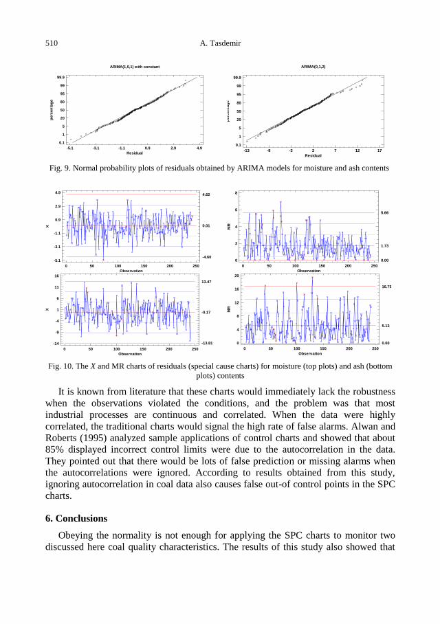
510 A. Tasdemir
Residual Normal Probability Plot
ARIMA(1,0,1) with constant
-5.1 -3.1 -1.1 0.9 2.9 4.9
Residual
0.1
1
5
20
50
80
95
99
99.9
perc
en
tag
e
Residual Normal Probability Plot
ARIMA(0,1,2)
-13 -8 -3 2 7 12 17
Residual
0.1
1
5
20
50
80
95
99
99.9
perc
en
tag
e
Fig. 9. Normal probability plots of residuals obtained by ARIMA models for moisture and ash contents
4.62
X Chart for residuals of moisture content
0 50 100 150 200 250
Observation
-5.1
-3.1
-1.1
0.9
2.9
4.9
X 0.01
-4.60
5.66
MR Chart for residuals of moisture content
MR
0 50 100 150 200 250
Observation
0
2
4
6
8
1.73
0.00
13.47
X Chart for residulas of ash content
0 50 100 150 200 250
Observation
-14
-9
-4
1
6
11
16
X
-0.17
-13.81
16.75
MR Chart for residuals of ash content
MR
0 50 100 150 200 250
Observation
0
4
8
12
16
20
5.13
0.00
Fig. 10. The X and MR charts of residuals (special cause charts) for moisture (top plots) and ash (bottom
plots) contents
It is known from literature that these charts would immediately lack the robustness
when the observations violated the conditions, and the problem was that most
industrial processes are continuous and correlated. When the data were highly
correlated, the traditional charts would signal the high rate of false alarms. Alwan and
Roberts (1995) analyzed sample applications of control charts and showed that about
85% displayed incorrect control limits were due to the autocorrelation in the data.
They pointed out that there would be lots of false prediction or missing alarms when
the autocorrelations were ignored. According to results obtained from this study,
ignoring autocorrelation in coal data also causes false out-of control points in the SPC
charts.
6. Conclusions
Obeying the normality is not enough for applying the SPC charts to monitor two
discussed here coal quality characteristics. The results of this study also showed that

Effect of autocorrelation on the process control charts in monitoring … 511
autocorrelation strongly affected performance of the SPC charts in case of coal
washing data. It was determined that the data of daily moisture and ash contents of the
coal washing plant were moderately autocorrelated. For this reason, much more out-of
control points on the traditional Shewhart charts, which assumes the independence of
observations with normaly distributed data, were detected for both variables.
The series of daily values of moisture contents are best described by ARIMA
(1,0,1), with a constant model. The ARIMA (0,1,2) model is recommended to be used
for generating time series of ash contents. Reduced number of out-of control points in
the residual control charts showed us the importance of autocorrelation in coal
industry and this autocorrelation should be removed before constructing a control
chart to monitor the quality characteristics. It is also shown that the Shewhart control
charts of residuals which are independent and normally distributed and obtained from
ARIMA models are more appropriate to find the true unusual points otherwise huge
amount of wrong out-of control points are recorded. These situations might cause
wrong decisions to monitor the process since most of the data points which are in
control actually detected as out-of control. Therefore, usage of uncorrelated data may
cause misleading results about the process.
It may also possible to make make preventive and corrective actions for the quality
characteristics of coal by the ARIMA models since these models can forecast for the
future using past data of the processes.
Acknowledgements
The author greatefully acknowledges the Tunçbilek coal washing plant for supplying the data used in
this research.
References
ALWAN, L.C., ROBERTS, H.V., 1988, Time-series modeling for statistical process control, Journal of
Business and Economic Statistics 6, 86‒95.
ALWAN, L.C., ROBERTS, H.V., 1995, The problem of misplaced control limits, Journal of Royal
Statistical Societyi Series C 44(3), 269‒278.
ANKARA, H., BİLİR, K., 1995; Kriblaj tesisinde kalite denetimi, Madencilikte Bilgisayar Uygulamaları
Sempozyumu, 235‒240 (in Turkish).
ANKARA, H., YEREL, S., 2008, Use of range control charts in determination of variability in surface
parallelisms of plates, Journal of Scientific & Industrial Research 67, 1078‒1082.
APLEY, D.W., LEE, H.C., 2003, Design of exponentially weighted moving average control charts for
autocorrelated processes with model uncertainty, Technometrics 45(3), 187‒198.
ARSLAN, V., 2006, Dry coal cleaning methods, Madencilik 45(3): 9‒18 (in Turkish).
AYKUL, H., AKÇAKOCA, H., EDİZ, G.,TAKSUK, M., 2005, Garp linyitleri işletmesi termik santral
kömürleri için istatistiksel süreç kontrol analizi, Türkiye 19, Uluslararası Madencilik Kongresi,
313‒321 (in Turkish).
AYKUL, H., EDİZ, İ. G., AKÇAKOCA, H., ERARSLAN, K., TAKSUK, M., DİXON-HARDY, D. W.,
2010, Statitistical process control for coal fired power plant system, Journal of the Energy Institute
83, 41‒47.
BAYAT, O., ARSLAN, V., 2004, Statistical analysis in Turkish chromite mining, Scandinavian Journal
of Metallurgy 33, 322‒327.
512 A. Tasdemir
BHATTACHERJEE, A., SAMANTA, B., 2002, Practical issues in the consruction of control charts in
mining applications, The Journal of The South African Institute of Mining and Metalllurgy, 173‒180.
CARSON, P. K., YEH, A. B., 2008, Exponentially weighted moving average (EWMA) control charts for
monitoring an analytical process, Ind. Eng. Chem. Res. 47, 405‒411.
CHANG, Y. M., WU, T. L., 2011, On average run length of control charts for autocorrelated processes,
Methodol. Comput. Appl. Probab. 13, 419‒431.
DEMİRKOL, Ş., 2008, Comparison of control charts for autocorrelated data, Master Thesis, Graduate
School of Natural and Applied Sciences of Dokuz Eylül University.
ELEVLİ, S., BEHDİOĞLU, S., 2006, İstatistiksel Proses Kontrolü Teknikleri İle Kömür Kalitesindeki
Değişkenliğin Belirlenmesi, Madencilik 45(3), 19‒26 (in Turkish).
ELEVLİ, S., 2006, Coal quality control with control charts, Coal Preparation 26(4), 181‒199.
ELEVLİ, S., 2009, Control charts for autocorrelated colemanite data, Journal of Scientific & Industrial
Research 68, 11‒17.
HTTP://DOCUMENTATION.STATSOFT.COM/STATISTICAHelp.aspx?path=TimeSeries/TimeSeries/
Overview/Arima/ARIMAARIMAMethodology.
İPEK, H., ANKARA, H., ÖZDAĞ, H., The application of statistical process control, Minerals
Engineering 12(7): 827-835.
KARAOĞLAN, A.D., BAYHAN, G.M., 2011, Performance comparison of residual control charts for
trend stationary first order autoregressive processes, Gazi University Journal of Science 24(2),
329‒33.
LE, K.H., 1998, A statistical control chart for process with correlated subgroups, The Korean
Communications in Statistics 5(2), 373‒381.
LU, C.W., REYNOLDS, M.R., 2001, CUSUM charts for monitoring an autocorrelated process, Journal
of Quality Technology 33, 316‒334.
MACCHARTY, B.L., WASUSRI, T., 2002, A review of non-standard applications of statistical process
control (SPC) charts, International Journal of Quality & Reliability Management 19(3), 295‒320.
MONTGOMERY, D.C., JENNINGS, C.L., KULAHÇI, M., 2008, Introduction to time series analysis
and forecasting, Wiley Sries in Probability and Statistics.
MONTGOMERY, D. C., RUNGER, G.C., 2011, Applied statistics and probability for engineers, Fifth
Edition, John Wiley&Sons, Inc.
SAMANTA, B., BHATTACHERJEE, A., 2001, An investigation of quality control charts for
autocorrelated data, Mineral Resources Engineering 10, 53‒69.
SAMANTA, B., 2002, Multivariate control charts for grade control using principal-component analysis
and time series modelling, Trans. Inst. Min. Metall. (Sect A: Min Technol) 307, 149‒157.
SCHMID, W., SCHÖNE, A., 1997, Some properties of the EWMA control chart in the presence of
autocorrelation, The Annals of Statistics 25(3): 1277‒1283.
STAPENHURST, T., 2005, Mastering statistical process control, A handbook for performance
improvement using cases, Elsevier.
TEKİR, U., ARSLAN, V., AKAR, G., 2009, Dry beneficiation of fine coals from soma basin with
pneumatic air table, The Jornal of Ore Dressing 11(22), 33‒38.
VAPUR, H., BAYAT, O., AKYOL, F., 2005, Eti Gümüş A.Ş. Liç Prosesinde İstatistiksel Proses
Kontrolü Uygulaması, Türkiye 19. Uluslararası Madencilik Kongresi, 347-356 (in Turkish).
VAPUR, H., 2009, Applicability of statistical process control for flotation of metals complex, Asian
Journal of Chemistry 21(1), 655‒665.
YEREL, S., ANKARA, H., KONUK, A., ÖZDAĞ, H., 2007, Preventive maintance policy supported by a
quality control chart and Kolmogorov-Smirnov tests: Emet colemanite mineral processing plant,
Turkey, Minerals & Metallurgical Process 24, 152‒156.
YEREL, S., ANKARA, H., 2011, Process control for a coal washing plant using a range control chart
and multidimensional, scaling analysis, Energy Sources, Part A 33, 1028‒1034.
http://dx.doi.org/10.5277/ppmp120216
Physicochem. Probl. Miner. Process. 48(2), 2012, 513−531 Physicochemical Problems
of Mineral Processing
w w w . m i n p r o c . p w r . w r o c . p l / j o u r n a l / ISSN 1643-1049 (print)
ISSN 2084-4735 (online)
Received April 13, 2011; reviewed; accepted May 10 , 2012
EFFECTS OF DIFFERENT MESH SCHEMES AND TURBULENCE
MODELS IN CFD MODELLING OF STIRRED TANKS
Mohsen KARIMI, Guven AKDOGAN, Steven M. BRADSHAW
Department of Process Engineering, Stellenbosch University, Private Bag X1, Matieland 7602, Stellenbosch,
South Africa. Tel: +27 21 808 3860, Fax: +27 21 808 2059; Email: [email protected]
Abstract. This paper focuses on the effects of grid schemes and turbulence models on the CFD
modelling of stirred tanks. The economical grid was determined by examining the
dimensionless wall distance and the skewness of elements. The grid independency study
ensured that the independency of numerical predictions. Also, three categories of turbulence
models were compared for prediction of flow pattern. The grid sensitivity study highlighted
that the quality of control volumes in the bulk and near the wall regions are significant for
obtaining the consistent solutions. It was also found that for the prediction of velocity
components and the turbulent quantity the RANS based models are more efficient.
keywords: stirred tank, computational fluid dynamics, turbulence models, grid sensitivity
1. Introduction
Mechanically stirred vessels are broadly used in a wide range of unit operations
such as flotation cells in mineral processing plants, blending of liquids and
crystallization in chemical engineering reactors. Owing to their extensive range of use,
a reliable method of simulating the hydrodynamics of flow instead of correlating the
overall performance to the operational and geometrical conditions would be beneficial
for the industries.
Computational Fluid Dynamics (CFD) provides a numerical method in which
thorough information on the hydrodynamics of fluid flow can be extracted. The flow
pattern is then used to understand the details of the process itself. Thus, it would be
expected that an accurate CFD simulation of the fluid flow leads to improved
understanding of the mixing sub-processes occurring in mechanically stirred vessels.
Since the unsteady nature of turbulent flow inside stirred tanks is affected by many
parameters such as the geometry of rotational system, the local vortices, the gas
dispersion and so on, an accurate simulation of the flow pattern is rather complex. To
tackle this intricate problem one may investigate the factors such as the grid
resolution, the discretization scheme, the impeller rotation modelling method, and the
turbulence models. At the same time, the enhancement of CFD packages is an on-
going progress, and each new version of solvers is equipped with more features aimed
514 M. Karimi et al.
at accurately capturing more details of the fluid flow behaviour. As a consequence, a
computationally efficient and accurate CFD model for a stirred tank must be updated
to assess the effects of new options encompassed in recent CFD solvers. In the insight
of previous works that considered different aspects of CFD modelling of a stirred tank,
this research is scoped to update and optimize the CFD methodology for stirred tanks
as realistic as possible, while it should be computationally inexpensive.
The potential of CFD for modelling of unbaffled stirred tanks has been reported in
several papers. The applicability of numerical modelling was demonstrated by
comparison of the simulated results with the laser-Doppler velocimeter data
(Armenante et al., 1997; Dong et al., 1994a, b). In these early papers, the standard k-ε
and the Algebraic Stress Model (ASM) were used as turbulence models and the
rotation of impeller was modelled by either adapting the LDV measurements or by the
Multiple Reference Frames (MRF) method.
Oshinowo et al. (2000) showed that MRF is an efficient choice for the modelling of
impellers in the baffled stirred tanks. The sensitivity of the solution to the different
grids was also investigated. They compared the predicted tangential velocities with the
three turbulence models including the standard k-ε, the RNG k-ε and RSM. They
concluded that the steady-state modelling with the MRF is a valuable tool in the
analysis and design of stirred tanks when the single phase turbulent flow occurs.
Bakker (Bakker and Oshinowo, 2004; Bakker et al., 2000) investigated whether the
Large Eddy Simulation (LES) can predict the large-scale chaotic structures in stirred
tanks. A single radial pumping impeller and a single axial pumping pitched blade
turbine were simulated. The results showed that both impeller configurations had
qualitatively good agreement with the experimental data (Myers et al., 1997).
Another approach for modelling of impellers, the Sliding Mesh method (SM), was
compared with the MRF by Lane et al. (2000). The computational time, accuracy of
mean velocities and the turbulence parameters were the main variables of comparison.
A half slice model of a 294 mm diameter baffled stirred tank was discretized by 48, 39
and 60 cells in the axial, radial and azimuthal directions. An important finding was
that the MRF method was more computationally efficient than the SM. They also
found that both methods had similar results for the prediction of the velocities. For
turbulence characterizations, the MRF provided an improvement in the predictions.
Yoon et al. (2001) modelled the motion of impellers using Particle Image
Velocimetry (PIV) data as boundary conditions around the impeller. A 3D grid of
51,840 cells for 60◦ sector of a 145 mm diameter cell was used to compute the flow.
They provide a method to describe the impeller-induced flow in the stirred tank.
Influences of different impeller modelling methods, discretization schemes, and
turbulence models on the CFD modelling of stirred tanks were investigated by Aubin
et al. (2004). The mean axial and radial flow patterns were slightly affected by the
choice of SM or MRF for modelling of the impeller. The higher order of discretization
schemes were recommended for the simulation of turbulent flow inside the stirred
tank. Applying the Reynolds Stress Model (RSM) as the turbulence model led to a
Effects of different mesh schemes and turbulence models in CFD modelling of stirred tanks 515
diverged solution. The Standard and the Renormalization-group k-ε models did not
show significant differences in predicting the mean radial and axial velocity fields.
The authors suggested that correct prediction of the single phase flow quantities is
necessary for an accurate multiphase modelling of stirred tanks.
Deglon and Meyer (2006) used the MRF for modelling of the impeller rotation in
conjunction with the standard k-ε turbulence model for studying the turbulence
effects. The flow pattern in a half of a cylindrical tank agitated with a standard six-
blade Rushton turbine was simulated over four different grids using the QUICK
discretization scheme. A range of impeller speeds corresponding to the laminar and
turbulent flow regimes were tested. They showed that although the flow field can be
predicted with a coarse mesh, an accurate prediction of turbulence in stirred vessels is
computationally intensive and needs both fine grid resolution and a high-order
discretization method.
One of the recent work addressing numerical issues in the CFD simulation of the
fluid flow in stirred tanks was performed by Coronoe (2010). This work aimed at
verifying the effect of numerical issues on the RANS-based predictions of the single
phase flow in stirred tanks. The effects of grid sizes and discretization schemes were
considered for modelling of the mean velocity, the turbulent dissipation, and the
homogenization with the standard k-ε turbulence model and the MRF method. This
work revealed that the effect of numerical uncertainties may be minimized with
sufficiently fine grid resolution. They argued that due to the limitation of the
turbulence model the detailed explanation of turbulence quantities cannot be achieved.
They also mentioned that the effects of the numerical inaccuracies would be more
important in the multiphase modelling of stirred tanks.
Reviewing the previous literature revealed that the standard k-ε is a
computationally affordable turbulence model and it is generally accepted for the
modelling of stirred tanks. The Multiple Reference Frames (MRF) yields better results
than the Sliding Mesh method to model the impeller motion in terms of both
computational time and agreement with the experimental data. Although the previous
works shed some light on how to deal with the common aspects of the numerical
issues on the CFD modelling of stirred tanks, CFD solver developments led to the
question of whether the available methodology of numerical simulation of the stirred
vessel is still reliable or it should be updated. Thus, this paper is intended to fill this
gap. To accomplish this goal, the optimized mesh was selected through different
criteria including the value of y+ on the problematic regions near the walls to capture
the small eddies, skewness of elements, and the grid independence study. Then,
turbulence models were categorized into three different groups. The performance of
each category was compared with the experimental data.
2. Methodology
The Reynolds averaged continuity and the Reynolds averaged Navier-Stokes
equations (RANS) have been resolved in this work to model the highly turbulent flow
inside the agitated vessel. They can be written as follow:
516 M. Karimi et al.
0
i
i
x
u
t
, (1)
iij
jj
i
jij
jiig
xx
u
xx
p
x
uu
t
u
Re , (2)
where u is the velocity component, is the liquid density, p is the pressure, μ is the
fluid viscosity, and g is the gravitational acceleration. The term τijRe
denotes the
Reynolds stress and signifies the effects of turbulent velocity fluctuations on the mean
flow. To close Eqs. (1) and (2) the Reynolds stress must be modelled. There are
different turbulence models to achieve closure for the above partial differential
equations. In the following sections the fundamentals of these models are briefly
explained and referenced.
2.1. RANS based turbulence mode
The RANS-based turbulence models are recommended (ANSYS Inc, 2009) to
reduce the required computational effort and resource. They are divided into the four
different categories including: one-equation model, two-equation models, three-
equation models, and Reynolds Stress Model (RSM). Except the latter, the other
RANS-based turbulence models apply the Boussinesq hypothesis (Hinze, 1975) that
relates the Reynolds stresses to the mean velocity gradients:
ij
k
kt
j
j
j
itij
x
uk
x
u
x
uu
3
2Re . (3)
In this equation μt is the turbulent viscosity, k is the turbulent kinetic energy and δij
is the Kronecker delta. The Boussinesq theory assumes the turbulent viscosity is an
isotropic scalar.
The RANS-based turbulence models have been divided according to the number of
additional transport equations essential to resolve the flow field.
2.1.1. One-equation model
The Spalart-Allmaras is a relatively simple one-equation model that solves one
transport equation for the turbulent kinematic viscosity. The details of equations of
this model are explained by Spalart and Allmaras (1992).
2.1.2. Two-equation models
This group of turbulence models has become the standard approach for industrial
applications and is of particular interest for engineering problems where turbulence
effects are significant such as stirred vessels. As the definition states, to capture the

Effects of different mesh schemes and turbulence models in CFD modelling of stirred tanks 517
turbulence effects, two extra transport equations must be solved for this type of
turbulence model. Models such as the k- ε and its variants and the k- model and its
variant fall into this class. From two additional transport equations, one of the
variables is turbulent kinetic energy, k. The second one depends on what type of two-
equation turbulence models is used. The second transported variable can be thought of
as the determination factor of turbulence. The common options for the two-equation
models are the turbulent dissipation, ε, or the specific dissipation, .
Standard k-ε model
The advantages of using the Standard k-ε model such as robustness and reasonable
accuracy account for the numerous applications of this model in the simulation of
stirred tanks. The standard k-ε model is a semi-empirical model that solves the
turbulent kinetic energy (k) and its turbulent dissipation (ε) for fully turbulent flow.
The details of the transport equations were explained by Launder and Spalding (1972).
RNG k-ε model
The RNG k-ε model is derived from the standard k-ε model carrying out a
mathematical technique called “renormalization group” (RNG). In this turbulence
model some refinements for accurate results have been outlined. Adding an extra term
in the “ε” equation improves the accuracy for rapidly strained flows. Besides, the
effects of swirl on the turbulence are included in the RNG k-εmodel, enhancing the
precision for swirling flow. Orszag et al. (1993) have documented a complete
application of the RNG concept for turbulence modelling.
Realizable k-ε model
This turbulence model is a relatively new approach to resolve the Reynolds stresses
(Shih et al., 1995). Its differences from the standard k-ε model are twofold: a new
formulation for the turbulent viscosity and a vorticity-based new transport equation for
the turbulent dissipation, ε. These modifications are reported to provide superior
performance for swirling flow.
Standard k- model
The standard k- model used in this paper is based on the Wilcox k- model
(Wilcox, 1998). Wilcox has derived this empirical turbulence model based on the
transport equations for turbulence kinetic energy (k) and the specific turbulent
dissipation ().
Shear-Stress Transport (SST) k- model
Blending the robust formulation of the k- model in the inner parts of boundary
layer with the applicability of the k- model in the bulk flow is the backbone of this
model. The SST k- turbulence model was developed by Menter (1994).
Transition SST model
The transition SST model is another derivative of the k- model taking advantage
of two more transport equations, one for intermittency and one for the transition onset
criteria.
518 M. Karimi et al.
2.1.3. Three-equation model
k-kl- transition model
Since the k-kl- model has three transport equations for the turbulent kinetic
energy, the laminar kinetic energy, and the inverse turbulent time scale (), it is
considered as a three-equation model. This model benefits from predicting the
boundary layer development and the calculating transition onset. Using this model one
can effectively address the evolution from laminar flow to turbulence in the boundary
layer.
2.2. Large Eddy Simulation (LES)
The entire concept of the Large Eddy Simulation (LES) model is based on eddies
that are the main characteristics of the turbulent flow. In this model, the motion of
large eddies is resolved directly, while the small eddies are implicitly modelled using a
sub-grid scale model. Thus, a filtering operation should be conducted to separate the
velocity field into two resolved parts; large eddies and a sub-grid part. Filtering the
time-dependent Navier-Stokes equations results in a set of the solved part (large scale)
and the residuals (small scale). The filtered equations are expressed as:
0
i
i
x
u
t
, (4)
i
j
sgsij
j
i
jtj
jii gxx
u
xx
p
x
uu
t
u
1, (5)
τijsgs
is the stress tensor composed of all the information about small scales. It can be
related to the eddy viscosity by the following equation:
i
j
j
it
sgsij
x
u
x
u . (6)
In this research, solving the eddy viscosity, μt, has been conducted by three
different methods: Smagorinsky-Lilly (Smagorinsky, 1963), WALE model (Nicoud
and Ducros, 1999), and dynamic kinetic energy (Kim and Menon, 1997).
2.3. Detached Eddy Simulation
The DES model is a hybrid turbulence model that applies the RANS model to solve
the flow near the wall, and other regions far from the walls are computed by the LES
approach. In the modelling of stirred tanks in this study three combinations of RANS
models with the LES have been considered including the Spalart-Allmaras, realizable
k-ε and the SST k-(Shur et al., 1999). It should be noted here that computational
Effects of different mesh schemes and turbulence models in CFD modelling of stirred tanks 519
cost of using DES model is greater than the RANS computational cost, but less than
the LES.
3. Numerical approach
The 3D unsteady flow of water inside a 293 mm diameter unbaffled tank agitated
by a six-blade impeller with 73 mm clearance (Fig. 1) was simulated using CFD
package ANSYS FLUENT 12.1. Since the finite volume method is implemented in
this solver, the computational domain, adopted from (Armenante et al., 1997), was
discretized into different cells. To conduct the MRF method for modelling of impeller
motion, recommended by Lane et al. (2000) and Deglon and Meyer (2006), the entire
vessel was divided into the bulk flow region and the rotational zone. In this way,
governing equations are solved in a rotating reference frame to handle the impeller
rotation, while in the rest of the vessel the flow is calculated by solving the RANS
equations in a stationary reference frame. The SIMPLE algorithm coupled the
continuity and momentum equations to derive the pressure field inside the tank, and
the momentum discretization was computed by a second-order upwind method. It
should be mentioned that to perform the LES and DES turbulence models the
discretization scheme was altered to the bounded central differencing method. In this
study, the impeller speed was 450 rpm. A 45◦ sector of vessel was simulated using
periodic boundary conditions.
Different time steps corresponding to 5, 10, 12 and 15 degrees of rotational angle
of the impeller have been simulated. Each simulation was initialized with the standard
k-ε turbulence model for 10 revolutions of the impeller. All the simulations were
performed on an Intel Corei7 CPU 1.6 GHz workstation in this study.
One of the main issues that have been considered in this article is how sensitive the
CFD results are to the various mesh schemes. The grid density should be dense
enough to embody all the underlying flow features. To explain this effect, different
grids have been built up. In each case, different numbers of elements in the two
separate regions, the bulk flow and the rotational zone, have been distinguished. The
details of each structured hexagonal mesh are described in Table 1. The number of
elements in the three directions of cylindrical coordinate system is shown in Table 1.
In order to capture the time-dependent fluctuations of turbulence inside the
boundary layer, y+ value was taken into account. These parameters are defined as the
dimensionless distance from the wall to the first grid point. The value of y+ is
computed for the boundary cells on the specified wall zones. Then, those cells with the
y+ values within a specified range will be marked for refinement during the solution
process. The y+ can be computed by the following equation:
v
yuy
* , (7)
where u*, the friction velocity can be defined by Eq. (8), y is the distance to the wall
and is the kinematic viscosity:

520 M. Karimi et al.
wu * , (7)
where τw is the wall shear stress and is the fluid density at the wall.
Skewness has also been used in this study to investigate the quality of each control
volume. As is shown in Table 1, even the maximum skewness is in the excellent range
of commonly used for the mesh quality (ANSYS Inc, 2009).
Fig. 1. Schematic of the whole vessel adapted from Armenante et al. (1997)
Table 1. Properties of the mesh schemes used in this article
Case# Bulk flow Rotational zone No. Cells Skewness
z z Original Adapted Min Max Ave
C1 31 20 65 11 20 5 40,300 59,375 0.0125 0.1086 0.0242
C2 40 24 78 14 24 6 74,880 110,762 0.0104 0.1429 0.0190
C3 48 29 94 17 29 8 130,848 176,306 0.0050 0.0990 0.0211
C4 58 35 113 20 35 10 229,390 296,478 0.0041 0.1077 0.0168
C5 70 42 126 24 42 12 370,440 472,129 0.0034 0.1260 0.0210
C6 84 50 139 29 50 14 583,800 704,818 0.0029 0.1436 0.0208
C7 92 60 154 35 60 17 850,080 1,024,317 0.0015 0.1606 0.0309
* the numbers in the ,, and z columns represent the number of elements in each direction of cylindrical coordinate system
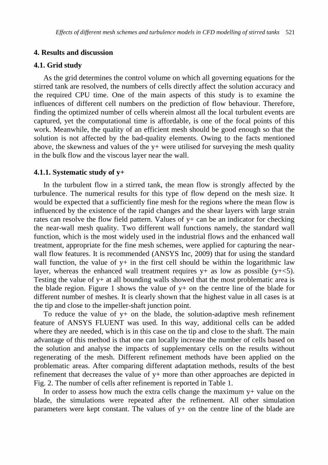
Effects of different mesh schemes and turbulence models in CFD modelling of stirred tanks 521
4. Results and discussion
4.1. Grid study
As the grid determines the control volume on which all governing equations for the
stirred tank are resolved, the numbers of cells directly affect the solution accuracy and
the required CPU time. One of the main aspects of this study is to examine the
influences of different cell numbers on the prediction of flow behaviour. Therefore,
finding the optimized number of cells wherein almost all the local turbulent events are
captured, yet the computational time is affordable, is one of the focal points of this
work. Meanwhile, the quality of an efficient mesh should be good enough so that the
solution is not affected by the bad-quality elements. Owing to the facts mentioned
above, the skewness and values of the y+ were utilised for surveying the mesh quality
in the bulk flow and the viscous layer near the wall.
4.1.1. Systematic study of y+
In the turbulent flow in a stirred tank, the mean flow is strongly affected by the
turbulence. The numerical results for this type of flow depend on the mesh size. It
would be expected that a sufficiently fine mesh for the regions where the mean flow is
influenced by the existence of the rapid changes and the shear layers with large strain
rates can resolve the flow field pattern. Values of y+ can be an indicator for checking
the near-wall mesh quality. Two different wall functions namely, the standard wall
function, which is the most widely used in the industrial flows and the enhanced wall
treatment, appropriate for the fine mesh schemes, were applied for capturing the near-
wall flow features. It is recommended (ANSYS Inc, 2009) that for using the standard
wall function, the value of y+ in the first cell should be within the logarithmic law
layer, whereas the enhanced wall treatment requires y+ as low as possible (y+<5).
Testing the value of y+ at all bounding walls showed that the most problematic area is
the blade region. Figure 1 shows the value of y+ on the centre line of the blade for
different number of meshes. It is clearly shown that the highest value in all cases is at
the tip and close to the impeller-shaft junction point.
To reduce the value of y+ on the blade, the solution-adaptive mesh refinement
feature of ANSYS FLUENT was used. In this way, additional cells can be added
where they are needed, which is in this case on the tip and close to the shaft. The main
advantage of this method is that one can locally increase the number of cells based on
the solution and analyse the impacts of supplementary cells on the results without
regenerating of the mesh. Different refinement methods have been applied on the
problematic areas. After comparing different adaptation methods, results of the best
refinement that decreases the value of y+ more than other approaches are depicted in
Fig. 2. The number of cells after refinement is reported in Table 1.
In order to assess how much the extra cells change the maximum y+ value on the
blade, the simulations were repeated after the refinement. All other simulation
parameters were kept constant. The values of y+ on the centre line of the blade are
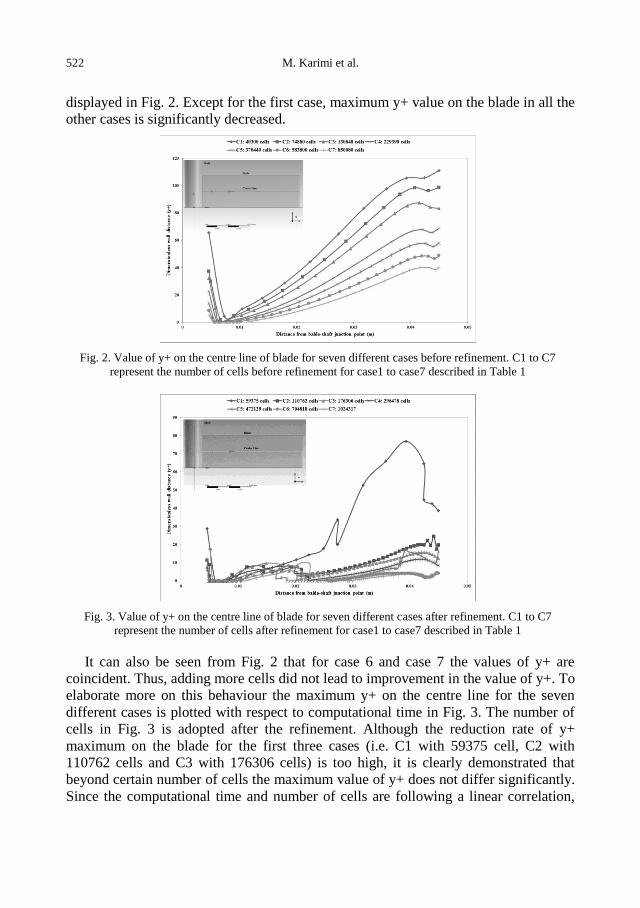
522 M. Karimi et al.
displayed in Fig. 2. Except for the first case, maximum y+ value on the blade in all the
other cases is significantly decreased.
Fig. 2. Value of y+ on the centre line of blade for seven different cases before refinement. C1 to C7
represent the number of cells before refinement for case1 to case7 described in Table 1
Fig. 3. Value of y+ on the centre line of blade for seven different cases after refinement. C1 to C7
represent the number of cells after refinement for case1 to case7 described in Table 1
It can also be seen from Fig. 2 that for case 6 and case 7 the values of y+ are
coincident. Thus, adding more cells did not lead to improvement in the value of y+. To
elaborate more on this behaviour the maximum y+ on the centre line for the seven
different cases is plotted with respect to computational time in Fig. 3. The number of
cells in Fig. 3 is adopted after the refinement. Although the reduction rate of y+
maximum on the blade for the first three cases (i.e. C1 with 59375 cell, C2 with
110762 cells and C3 with 176306 cells) is too high, it is clearly demonstrated that
beyond certain number of cells the maximum value of y+ does not differ significantly.
Since the computational time and number of cells are following a linear correlation,
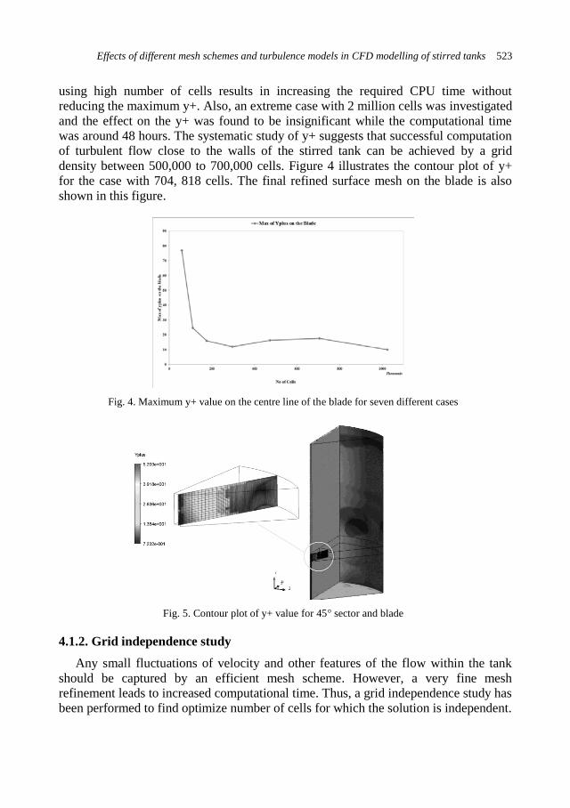
Effects of different mesh schemes and turbulence models in CFD modelling of stirred tanks 523
using high number of cells results in increasing the required CPU time without
reducing the maximum y+. Also, an extreme case with 2 million cells was investigated
and the effect on the y+ was found to be insignificant while the computational time
was around 48 hours. The systematic study of y+ suggests that successful computation
of turbulent flow close to the walls of the stirred tank can be achieved by a grid
density between 500,000 to 700,000 cells. Figure 4 illustrates the contour plot of y+
for the case with 704, 818 cells. The final refined surface mesh on the blade is also
shown in this figure.
Fig. 4. Maximum y+ value on the centre line of the blade for seven different cases
Fig. 5. Contour plot of y+ value for 45° sector and blade
4.1.2. Grid independence study
Any small fluctuations of velocity and other features of the flow within the tank
should be captured by an efficient mesh scheme. However, a very fine mesh
refinement leads to increased computational time. Thus, a grid independence study has
been performed to find optimize number of cells for which the solution is independent.
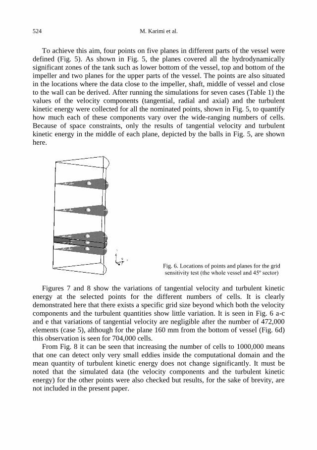
524 M. Karimi et al.
To achieve this aim, four points on five planes in different parts of the vessel were
defined (Fig. 5). As shown in Fig. 5, the planes covered all the hydrodynamically
significant zones of the tank such as lower bottom of the vessel, top and bottom of the
impeller and two planes for the upper parts of the vessel. The points are also situated
in the locations where the data close to the impeller, shaft, middle of vessel and close
to the wall can be derived. After running the simulations for seven cases (Table 1) the
values of the velocity components (tangential, radial and axial) and the turbulent
kinetic energy were collected for all the nominated points, shown in Fig. 5, to quantify
how much each of these components vary over the wide-ranging numbers of cells.
Because of space constraints, only the results of tangential velocity and turbulent
kinetic energy in the middle of each plane, depicted by the balls in Fig. 5, are shown
here.
Fig. 6. Locations of points and planes for the grid
sensitivity test (the whole vessel and 45º sector)
Figures 7 and 8 show the variations of tangential velocity and turbulent kinetic
energy at the selected points for the different numbers of cells. It is clearly
demonstrated here that there exists a specific grid size beyond which both the velocity
components and the turbulent quantities show little variation. It is seen in Fig. 6 a-c
and e that variations of tangential velocity are negligible after the number of 472,000
elements (case 5), although for the plane 160 mm from the bottom of vessel (Fig. 6d)
this observation is seen for 704,000 cells.
From Fig. 8 it can be seen that increasing the number of cells to 1000,000 means
that one can detect only very small eddies inside the computational domain and the
mean quantity of turbulent kinetic energy does not change significantly. It must be
noted that the simulated data (the velocity components and the turbulent kinetic
energy) for the other points were also checked but results, for the sake of brevity, are
not included in the present paper.
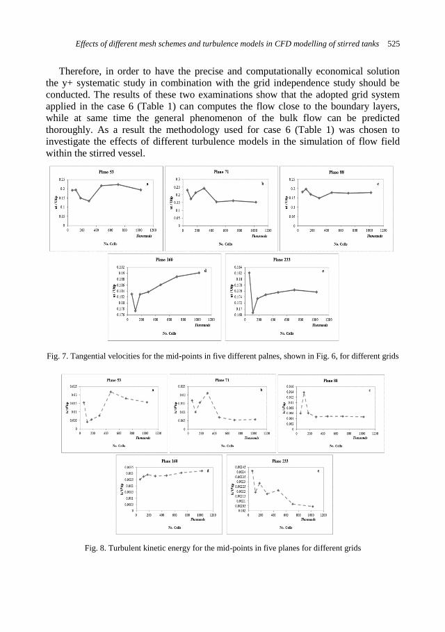
Effects of different mesh schemes and turbulence models in CFD modelling of stirred tanks 525
Therefore, in order to have the precise and computationally economical solution
the y+ systematic study in combination with the grid independence study should be
conducted. The results of these two examinations show that the adopted grid system
applied in the case 6 (Table 1) can computes the flow close to the boundary layers,
while at same time the general phenomenon of the bulk flow can be predicted
thoroughly. As a result the methodology used for case 6 (Table 1) was chosen to
investigate the effects of different turbulence models in the simulation of flow field
within the stirred vessel.
Fig. 7. Tangential velocities for the mid-points in five different palnes, shown in Fig. 6, for different grids
Fig. 8. Turbulent kinetic energy for the mid-points in five planes for different grids
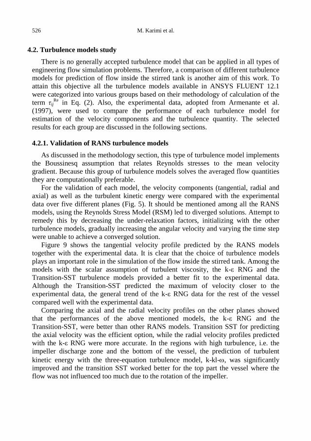
526 M. Karimi et al.
4.2. Turbulence models study
There is no generally accepted turbulence model that can be applied in all types of
engineering flow simulation problems. Therefore, a comparison of different turbulence
models for prediction of flow inside the stirred tank is another aim of this work. To
attain this objective all the turbulence models available in ANSYS FLUENT 12.1
were categorized into various groups based on their methodology of calculation of the
term τijRe
in Eq. (2). Also, the experimental data, adopted from Armenante et al.
(1997), were used to compare the performance of each turbulence model for
estimation of the velocity components and the turbulence quantity. The selected
results for each group are discussed in the following sections.
4.2.1. Validation of RANS turbulence models
As discussed in the methodology section, this type of turbulence model implements
the Boussinesq assumption that relates Reynolds stresses to the mean velocity
gradient. Because this group of turbulence models solves the averaged flow quantities
they are computationally preferable.
For the validation of each model, the velocity components (tangential, radial and
axial) as well as the turbulent kinetic energy were compared with the experimental
data over five different planes (Fig. 5). It should be mentioned among all the RANS
models, using the Reynolds Stress Model (RSM) led to diverged solutions. Attempt to
remedy this by decreasing the under-relaxation factors, initializing with the other
turbulence models, gradually increasing the angular velocity and varying the time step
were unable to achieve a converged solution.
Figure 9 shows the tangential velocity profile predicted by the RANS models
together with the experimental data. It is clear that the choice of turbulence models
plays an important role in the simulation of the flow inside the stirred tank. Among the
models with the scalar assumption of turbulent viscosity, the k-ε RNG and the
Transition-SST turbulence models provided a better fit to the experimental data.
Although the Transition-SST predicted the maximum of velocity closer to the
experimental data, the general trend of the k-ε RNG data for the rest of the vessel
compared well with the experimental data.
Comparing the axial and the radial velocity profiles on the other planes showed
that the performances of the above mentioned models, the k-ε RNG and the
Transition-SST, were better than other RANS models. Transition SST for predicting
the axial velocity was the efficient option, while the radial velocity profiles predicted
with the k-ε RNG were more accurate. In the regions with high turbulence, i.e. the
impeller discharge zone and the bottom of the vessel, the prediction of turbulent
kinetic energy with the three-equation turbulence model, k-kl-, was significantly
improved and the transition SST worked better for the top part the vessel where the
flow was not influenced too much due to the rotation of the impeller.
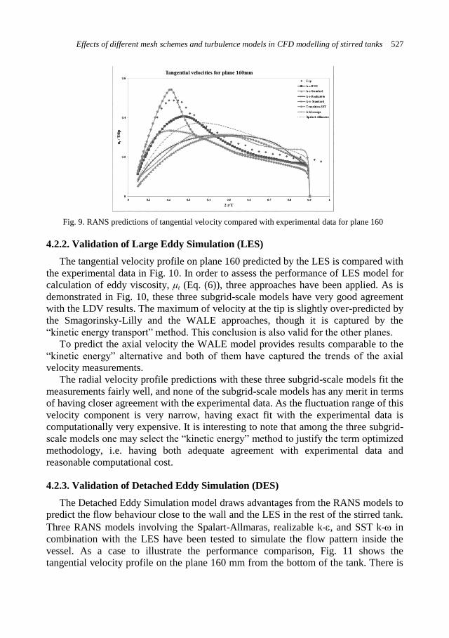
Effects of different mesh schemes and turbulence models in CFD modelling of stirred tanks 527
Fig. 9. RANS predictions of tangential velocity compared with experimental data for plane 160
4.2.2. Validation of Large Eddy Simulation (LES)
The tangential velocity profile on plane 160 predicted by the LES is compared with
the experimental data in Fig. 10. In order to assess the performance of LES model for
calculation of eddy viscosity, μt (Eq. (6)), three approaches have been applied. As is
demonstrated in Fig. 10, these three subgrid-scale models have very good agreement
with the LDV results. The maximum of velocity at the tip is slightly over-predicted by
the Smagorinsky-Lilly and the WALE approaches, though it is captured by the
“kinetic energy transport” method. This conclusion is also valid for the other planes.
To predict the axial velocity the WALE model provides results comparable to the
“kinetic energy” alternative and both of them have captured the trends of the axial
velocity measurements.
The radial velocity profile predictions with these three subgrid-scale models fit the
measurements fairly well, and none of the subgrid-scale models has any merit in terms
of having closer agreement with the experimental data. As the fluctuation range of this
velocity component is very narrow, having exact fit with the experimental data is
computationally very expensive. It is interesting to note that among the three subgrid-
scale models one may select the “kinetic energy” method to justify the term optimized
methodology, i.e. having both adequate agreement with experimental data and
reasonable computational cost.
4.2.3. Validation of Detached Eddy Simulation (DES)
The Detached Eddy Simulation model draws advantages from the RANS models to
predict the flow behaviour close to the wall and the LES in the rest of the stirred tank.
Three RANS models involving the Spalart-Allmaras, realizable k-, and SST k- in
combination with the LES have been tested to simulate the flow pattern inside the
vessel. As a case to illustrate the performance comparison, Fig. 11 shows the
tangential velocity profile on the plane 160 mm from the bottom of the tank. There is
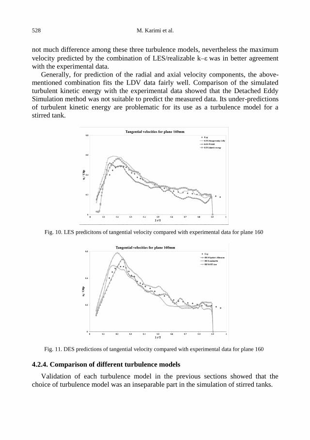
528 M. Karimi et al.
not much difference among these three turbulence models, nevertheless the maximum
velocity predicted by the combination of LES/realizable k‒εwas in better agreement
with the experimental data.
Generally, for prediction of the radial and axial velocity components, the above-
mentioned combination fits the LDV data fairly well. Comparison of the simulated
turbulent kinetic energy with the experimental data showed that the Detached Eddy
Simulation method was not suitable to predict the measured data. Its under-predictions
of turbulent kinetic energy are problematic for its use as a turbulence model for a
stirred tank.
Fig. 10. LES predicitons of tangential velocity compared with experimental data for plane 160
Fig. 11. DES predictions of tangential velocity compared with experimental data for plane 160
4.2.4. Comparison of different turbulence models
Validation of each turbulence model in the previous sections showed that the
choice of turbulence model was an inseparable part in the simulation of stirred tanks.
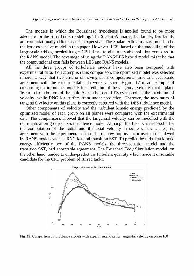
Effects of different mesh schemes and turbulence models in CFD modelling of stirred tanks 529
The models in which the Boussinesq hypothesis is applied found to be more
adequate for the stirred tank modelling. The Spalart-Allmaras, k-ε family, k- family
are computationally efficient and inexpensive. The Spalart-Allmaras was found to be
the least expensive model in this paper. However, LES, based on the modelling of the
large-scale eddies, needed longer CPU times to obtain a stable solution compared to
the RANS model. The advantage of using the RANS/LES hybrid model might be that
the computational cost falls between LES and RANS models.
All the three groups of turbulence models have also been compared with
experimental data. To accomplish this comparison, the optimized model was selected
in such a way that two criteria of having short computational time and acceptable
agreement with the experimental data were satisfied. Figure 12 is an example of
comparing the turbulence models for prediction of the tangential velocity on the plane
160 mm from bottom of the tank. As can be seen, LES over-predicts the maximum of
velocity, while RNG k-ε suffers from under-prediction. However, the maximum of
tangential velocity on this plane is correctly captured with the DES turbulence model.
Other components of velocity and the turbulent kinetic energy predicted by the
optimized model of each group on all planes were compared with the experimental
data. The comparisons showed that the tangential velocity can be modelled with the
renormalization group of k-ε turbulence model. Although the LES was successful for
the computation of the radial and the axial velocity in some of the planes, its
agreement with the experimental data did not show improvement over that achieved
by RANS models such as RNG k-ε and transition SST. To predict the turbulent kinetic
energy efficiently two of the RANS models, the three-equation model and the
transition SST, had acceptable agreement. The Detached Eddy Simulation model, on
the other hand, tended to under-predict the turbulent quantity which made it unsuitable
candidate for the CFD problem of stirred tanks.
Fig. 12. Comparison of turbulence models with experimental data for tangential velocity on plane 160

530 M. Karimi et al.
5. Conclusion
Two underlying aspects of the numerical simulation of stirred tanks, namely the
efficient grid scheme and the choice of suitable turbulence models, have been
investigated. Through various criteria we have established the meshing methodology
which ensures both results’ independency and adequate agreement with experimental
data. The widely used skewness factor was also tested to understand the optimal cell
size in the bulk flow. The value of the y+ showed the problematic elements near the
wall boundary conditions. Solving the problematic elements was carried out using
different refinement methods to locally increase the number of cells. The grid
independence study suggested that the solutions tend to converge at around 700,000
cells by which most characteristics of the turbulent flow can be captured.
In this study, the performances of RANS, LES and DES turbulence models for
prediction of velocity components and turbulent kinetic energy have been investigated
and compared with experimental data.
It was found that the RNG k-ε and the transition SST turbulence model produced
better agreement for both velocity components and turbulent quantity. Likewise, the
LES turbulence model in conjunction with the “kinetic energy” as subgrid-scale model
was found to capture the trends of velocity components. However, the required CPU
time for having converged solution made this model computationally intensive.
Application of DES as the turbulence model for the stirred tank also gave accurate
results for all the velocity components. It should be noted that the turbulent kinetic
energy was under predicted.
Overall, this study demonstrated that for the consistent solution one needs to
investigate the quality of mesh near the walls and the independency of the results from
the number of cells. In addition, RANS turbulence models which implemented the
Boussinesq hypothesis such as RNG k-ε and transition SST yielded better simulation
of the flow behaviour inside the stirred tank. These recommendations might also be
useful for the multiphase modelling of stirred tanks.
References
ANSYS Inc, 2009, ANSYS FLUENT 12.0 Theory Guide. ANSYS Inc,.
ARMENANTE, P.M., LUO, C., CHOU, C.-C., FORT, I., MEDEK, J., 1997, Velocity profiles in a closed,
unbaffled vessel: comparison between experimental LDV data and numerical CFD predictions,
Chemical Engineering Science 52(20), 3483‒3492.
AUBIN, J., FLETCHER, D.F., XUEREB, C., 2004, Modeling turbulent flow in stirred tanks with CFD:
the influence of the modeling approach, turbulence model and numerical scheme, Experimental
Thermal and Fluid Science 28(5), 431‒445.
BAKKER, A., OSHINOWO, L.M., 2004, Modelling of Turbulence in Stirred Vessels Using Large Eddy
Simulation, Chemical Engineering Research and Design 82(9), 1169‒1178.
BAKKER, A., OSHINOWO, L.M., MARSHALL, E., 2000, The use of Large Eddy Simulation to study
stirred vessel hydrodynamics, In 10th European Conference on Mixing, 247‒254.
CORONEO, M., MONTANTE, G., PAGLIANTI, A., MAGELLI, F., 2011, CFD prediction of fluid flow
and mixing in stirred tanks: numerical issues about RANS simulation,Computer & Chemical
Engineering 35(10), 1959‒1968.
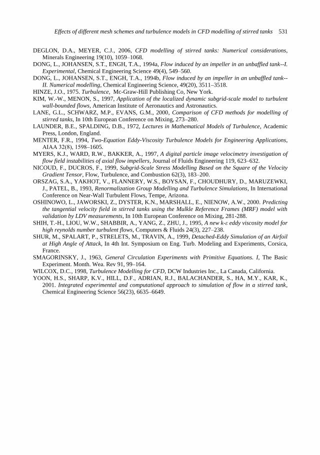
Effects of different mesh schemes and turbulence models in CFD modelling of stirred tanks 531
DEGLON, D.A., MEYER, C.J., 2006, CFD modelling of stirred tanks: Numerical considerations,
Minerals Engineering 19(10), 1059‒1068.
DONG, L., JOHANSEN, S.T., ENGH, T.A., 1994a, Flow induced by an impeller in an unbaffled tank--I.
Experimental, Chemical Engineering Science 49(4), 549‒560.
DONG, L., JOHANSEN, S.T., ENGH, T.A., 1994b, Flow induced by an impeller in an unbaffled tank--
II. Numerical modelling, Chemical Engineering Science, 49(20), 3511‒3518.
HINZE, J.O., 1975. Turbulence, Mc-Graw-Hill Publishing Co, New York.
KIM, W.-W., MENON, S., 1997, Application of the localized dynamic subgrid-scale model to turbulent
wall-bounded flows, American Institute of Aeronautics and Astronautics.
LANE, G.L., SCHWARZ, M.P., EVANS, G.M., 2000, Comparison of CFD methods for modelling of
stirred tanks, In 10th European Conference on Mixing, 273‒280.
LAUNDER, B.E., SPALDING, D.B., 1972, Lectures in Mathematical Models of Turbulence, Academic
Press, London, England.
MENTER, F.R., 1994, Two-Equation Eddy-Viscosity Turbulence Models for Engineering Applications,
AIAA 32(8), 1598‒1605.
MYERS, K.J., WARD, R.W., BAKKER, A., 1997, A digital particle image velocimetry investigation of
flow field instabilities of axial flow impellers, Journal of Fluids Engineering 119, 623‒632.
NICOUD, F., DUCROS, F., 1999, Subgrid-Scale Stress Modelling Based on the Square of the Velocity
Gradient Tensor, Flow, Turbulence, and Combustion 62(3), 183‒200.
ORSZAG, S.A., YAKHOT, V., FLANNERY, W.S., BOYSAN, F., CHOUDHURY, D., MARUZEWKI,
J., PATEL, B., 1993, Renormalization Group Modelling and Turbulence Simulations, In International
Conference on Near-Wall Turbulent Flows, Tempe, Arizona.
OSHINOWO, L., JAWORSKI, Z., DYSTER, K.N., MARSHALL, E., NIENOW, A.W., 2000. Predicting
the tangential velocity field in stirred tanks using the Mulkle Reference Frames (MRF) model with
validation by LDV measurements, In 10th European Conference on Mixing, 281-288.
SHIH, T.-H., LIOU, W.W., SHABBIR, A., YANG, Z., ZHU, J., 1995, A new k-ε eddy viscosity model for
high reynolds number turbulent flows, Computers & Fluids 24(3), 227‒238.
SHUR, M., SPALART, P., STRELETS, M., TRAVIN, A., 1999, Detached-Eddy Simulation of an Airfoil
at High Angle of Attack, In 4th Int. Symposium on Eng. Turb. Modeling and Experiments, Corsica,
France.
SMAGORINSKY, J., 1963, General Circulation Experiments with Primitive Equations. I, The Basic
Experiment. Month. Wea. Rev 91, 99‒164.
WILCOX, D.C., 1998, Turbulence Modelling for CFD, DCW Industries Inc., La Canada, California.
YOON, H.S., SHARP, K.V., HILL, D.F., ADRIAN, R.J., BALACHANDER, S., HA, M.Y., KAR, K.,
2001. Integrated experimental and computational approach to simulation of flow in a stirred tank,
Chemical Engineering Science 56(23), 6635‒6649.

532 M. Karimi et al.
http://dx.doi.org/10.5277/ppmp120217
Physicochem. Probl. Miner. Process. 48(2), 2012, 533−544 Physicochemical Problems
of Mineral Processing
w w w . m i n p r o c . p w r . w r o c . p l / j o u r n a l / ISSN 1643-1049 (print)
ISSN 2084-4735 (online)
Received January30, 2012; reviewed; accepted May 4, 2012
DETERMINATION OF TURBULENCE AND UPPER SIZE LIMIT IN
JAMESON FLOTATION CELL BY THE USE OF COMPUTATIONAL
FLUID DYNAMIC MODELLING
Oktay SAHBAZ*, Umran ERCETIN**, Bahri OTEYAKA***
*Dumlupinar University, Department of Mining Engineering, Kutahya, Turkey, Tel.: +90 537 3862002;
Fax.: +90 274 2652066; [email protected]
**Dumlupinar University, Department of Mechanical Engineering, Kutahya, Turkey
***Osmangazi University, Department of Mining Engineering, Eskişehir, Turkey
Abstract. In the coarse particle flotation, turbulence which can be treated as energy dissipation
rate, is one of the most significant parameters effecting the recovery and grade. Therefore,
determination of energy dissipation rate is very beneficial for delineation of coarse particle
flotation and determining the maximum floatable particle size in any cell. In this study,
Computational Fluid Dynamic (CFD) modelling for the Jameson cell has been carried out to
determine the high turbulent regions and the effect on the upper floatable size limit. The CFD
modelling has been utilized for determining the flow characteristics and hydrodynamic
behaviour of the Jameson flotation cell. In parallel with this purpose the turbulence map of the
cell has been determined and energy dissipation rate determined by using the CFD modelling.
According to the result acquired from the CFD modelling, there are two main turbulent regions
which are mixing zone in the upper part of the downcomer and critical region at the separation
tank. While the high turbulence at the mixing zone supplies fine bubbles and fast collection of
particles, the turbulence at the separation tank causes the main detachment of the bubble-
particle aggregate. Then, the increase in turbulence in the tank causes the decrease of the
maximum floatable size of particles. In addition, the average energy dissipation rate in the
critical region has been determined and used for estimation of the maximum floatable particle
size in the Jameson cell. Moreover, the effect of hydrophobicity has been discussed.
keywords: Jameson cell, coarse particle flotation, turbulence, CFD modelling
1. Introduction
Flotation is a dynamic process used for separation of hydrophobic minerals from
hydrophilic ones. The size of particles is one of the most important parameters in
flotation. While the flotation recovery of intermediate particles is high, the recovery
of both fine and coarse particles is usually remarkably low (Trahar, 1981). Thus,
particle size versus recovery figures leads to the inverted U-shape curves (Trahar,
1981; Nguyen, 2003). The reason of low recovery of coarse particle is mostly the
turbulence within the cells (Schulze, 1982; Oteyaka and Soto, 1995; Drzymala,
534 O. Sahbaz et al.
1994a). Even though particles may have high hydrophobicity, they cannot be reported
as a “float” due to the instability of the aggregate as a result of high turbulence. On the
other hand, the low recovery of fine particles can be attributed to low collision
probability of fine particles (Schulze, 1989; Çinar et al., 2007). Therefore, new and
modified conventional technologies are under investigations to increase flotation
performance of fine and coarse particles (Rodrigues and Rubio, 2007; Uçurum and
Bayat, 2007; Jameson, 2010; Şahbaz, 2010;). Moreover, determination of particle size
limits in flotation cells is prepossessed (Nguyen, 2003; Gonjito et al., 2007;
Kowalczuk et al., 2011).
The Jameson cell is relatively new flotation device used especially in the flotation
of fine particles (<100 µm) with a high performance (Evans et al., 1995; Cowburn et
al., 2006; Cinar et al., 2007). However, the collision probability of fine particles
increase in the Jameson cell due to the fine bubble (400-700 µm) generation in the
upper part of the downcomer, called the mixing zone, which is one of the main parts
of the cell and primary contacting zone of bubble and particle (Evans et al., 1995). On
the contrary, the performance of the Jameson cell shows tendency to decrease with the
increase of particle size due to turbulence (Cowburn et al., 2006; Cinar et al., 2007).
However; due to operational and maintenance issues, it is becoming necessary to
recover the coarse particle by using the Jameson cell in existing mineral processing
plants (Cowburn et al., 2006). In some applications of coal flotation the feed size can
be greater than 500 µm for the Jameson cell (Cowburn et al., 2006). Therefore, the
turbulent region causing the detachment should be determined and maximum floatable
particle size should be ascertained in the cell.
Computational fluid dynamic (CFD) modelling, which has been recently applied to
flotation cells to elucidate complexity of the hydrodynamic characteristics of cells,
has been used in flotation science by Koh et al. (2000), Koh and Schwarz (2003 and
2006), Lane et al. (2002), Liu and Schwarz (2009), Sahbaz (2010) etc. In CFD
modelling, a flotation cell is discretized into particular finite volumes where local
values of flow fields are calculated. The detailed understanding of flows using this
approach allows determination of flow characteristics by means of velocity magnitude,
pressure changes, turbulence dissipation rate etc. Also this information provides the
possibility for investigating where the attachment and detachment occur (Koh et al.,
2000; Koh and Schwarz, 2003; 2006). The CFD modelling has become a popular
method as it yields informative results and insights to mechanisms, and because of the
relatively low labour and equipment costs involved as a result of ever-increasing
computer speed and capacity (Liu and Schwarz, 2009). Finally, the CFD modelling
seems to be a very useful tool for determination of turbulence, resulting from energy
dissipation rate, and related particle size limits in flotation.
In the present study, the turbulence has been quantitatively determined and its
effect on the upper particle size limits in the Jameson flotation cell has been
ascertained by using the CFD modelling. Furthermore, the effect of particle
hydrophobicity on maximum floatable particle size has been elucidated.
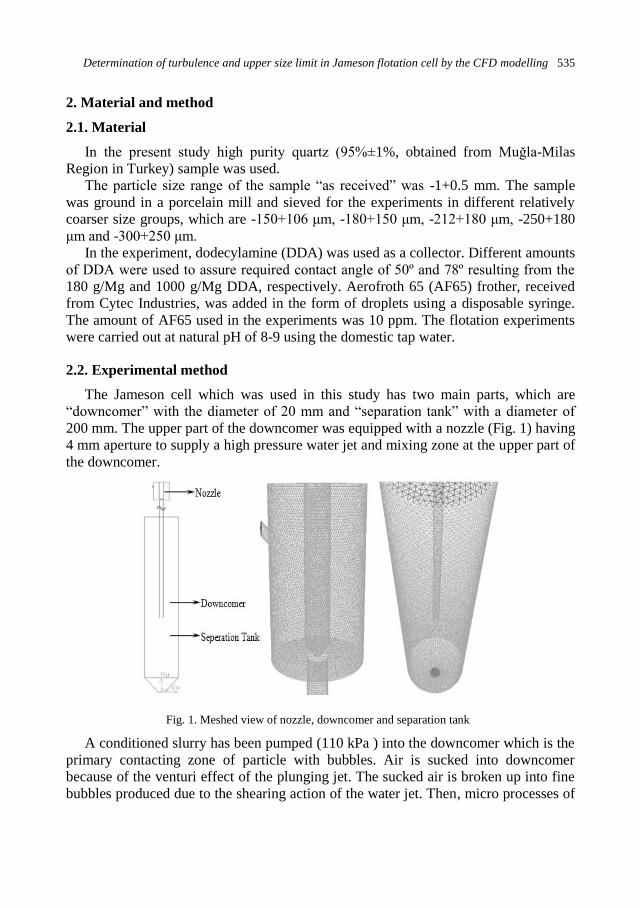
Determination of turbulence and upper size limit in Jameson flotation cell by the CFD modelling 535
2. Material and method
2.1. Material
In the present study high purity quartz (95%±1%, obtained from Muğla-Milas
Region in Turkey) sample was used.
The particle size range of the sample “as received” was -1+0.5 mm. The sample
was ground in a porcelain mill and sieved for the experiments in different relatively
coarser size groups, which are -150+106 μm, -180+150 μm, -212+180 μm, -250+180
μm and -300+250 μm.
In the experiment, dodecylamine (DDA) was used as a collector. Different amounts
of DDA were used to assure required contact angle of 50º and 78º resulting from the
180 g/Mg and 1000 g/Mg DDA, respectively. Aerofroth 65 (AF65) frother, received
from Cytec Industries, was added in the form of droplets using a disposable syringe.
The amount of AF65 used in the experiments was 10 ppm. The flotation experiments
were carried out at natural pH of 8-9 using the domestic tap water.
2.2. Experimental method
The Jameson cell which was used in this study has two main parts, which are
“downcomer” with the diameter of 20 mm and “separation tank” with a diameter of
200 mm. The upper part of the downcomer was equipped with a nozzle (Fig. 1) having
4 mm aperture to supply a high pressure water jet and mixing zone at the upper part of
the downcomer.
Fig. 1. Meshed view of nozzle, downcomer and separation tank
A conditioned slurry has been pumped (110 kPa ) into the downcomer which is the
primary contacting zone of particle with bubbles. Air is sucked into downcomer
because of the venturi effect of the plunging jet. The sucked air is broken up into fine
bubbles produced due to the shearing action of the water jet. Then, micro processes of

536 O. Sahbaz et al.
flotation, which are encountering, collision, attachment and detachment, start and
turbulent region with a high rate occurs at the tip of the nozzle. The three phase
mixture is transported into the separation tank due to the gravity flow under high
pressure. The second turbulent region occurs at the exit of the downcomer during
transportation. This turbulence can be accepted as the turbulence causing the majority
of detachment. Therefore, the turbulence, which occurs during the operation must be
satisfactorily understood to describe the flotation of coarse particles in the Jameson
cell.
During the study all parameters of experiments, such as feeding velocity, solid
ratio, air to pulp ratio, have been tried to be kept at optimum conditions considering
the previous studies carried out by Evans et al. (1995), Harbort et al. (2002), Çınar et
al. (2007), and Sahbaz et al. (2008; 2010).
3. Theory
3.1. The maximum floatable particle size
Flotation of particle depends on the balance of forces acting on bubble-particle
aggregate. These forces are the attachment forces between bubble and particle in
relation to detachment forces in the environment (Ralston et al., 1999; Pyke et al.,
2003; Kowalczuk et al., 2011). The main forces operating at the moment of spherical
particle – gas phase rupture are given in Table 1 (Drzymala, 1994b; Pyke et al., 2003;
Kowalczuk et al., 2011).
The more realistic force balance for a spherical particle in the liquid/gas interface
can be written as in Eq.1 (Kowalczuk et al, 2011):
0max agphbc FFFFFF , (1)
The sum of the forces is zero at equilibrium. At the equilibrium, particle has the
same chance to sink or float. If attachment forces are greater than the detaching forces,
particles can float. Therefore; maximum floatable particle size in flotation can be
determined by the ratio of the attachment and detachment forces. The probability of
stabilisation or destabilisation of the bubble–particle aggregate is based on the Bond
number, Bo (Schulze, 1993):
att
deto
F
FB , (2)
In this equation, the parameter “a”, which is used to determine the inertia force, is
hard to determine. Additional acceleration, a, determines the detachment forces and
depend on the structure and intensity of the turbulent flow field, therewithal on the
energy dissipation in a given volume of apparatus (Schulze, 1993). It can be calculated
by using the maximum energy dissipation (ε) and aggregate size (Dagr) (Pyke et al,
2003):

Determination of turbulence and upper size limit in Jameson flotation cell by the CFD modelling 537
31
32
6.29
agrDa
, (3)
where aggregate size is
pbagr ddD . (4)
Thus, the final equation (5) is obtained to determine the additional acceleration by
using Eq. (3) and Eq.(4):
31
32
6.29
pb dda
. (5)
In addition, the detachment contact angle, θd, in the equations (Table 1) refers to
experimental (advancing) contact angle (Kowalczuk et al, 2011).
The maximum floatable size of any particle can be found by using the Bond
number calculating the values of forces acting on bubble-particle aggregate by
iteration. All terms can be found easily, except for energy dissipation rate, ε, in the
cells. The CFD study is one of the useful methods to determine the energy dissipation
rate in the flotation cells.
Table 1. Main forces acting on aggregate
Symbol Force Equation and Explanation Effect of force
Fcmax The maximum
capillary force
)cos1(π2
1maxmax dc dF
where dmax is a maximum floatable particle size,
θd is a detachment contact angle, and σ is a surface
tension
Attachment
Fb Buoyancy force
2cos
31
2cos
32π
81 33
maxdd
lb gdF
where ρl is a liquid density, g is a gravity constant
Attachment
Fh Hydrostatic
pressure force
gRdF ldh cos1π4
1 2max
where R is a bubble radius
Attachment
Fp Pressure in the gas
bubble force
RdF dp
cos1π
41 2
max Detachment
Fg Gravity force pg dF 3maxπ
61
where ρp is a particle density
Detachment
Fa Inertia force
maFa
adF pa 3maxπ
61
where a is an additional acceleration
Detachment

538 O. Sahbaz et al.
3.2. CFD modelling
The required simulation results for the Jameson flotation system has been
numerically modelled using the commercial the CFD code of Fluent. The geometry of
the Jameson cell has been defined and a grid has been generated using Gambit 2.4.6
which is the pre-processor for geometry modelling and mesh generation. For all cases
studied in this paper, mixtures of triangular and quadrilateral elements have been
generated. The computational domain and grid structure in 3D flow field is shown in
Fig. 1. The Fluent 6.3.26 commercial computer program for modelling fluid flow, has
been used to carry out the modelling of the experimental process. Computations have
been performed using Eulerian multiphase approach, for turbulent flows depending on
water and air inlet velocity in thr 3D space. The CFD simulations have been
performed using a pressure based steady-state segregated implicit solver. A standard
k- mixture model has been employed for flow simulation. Pressure based implicit
solver with green-gauss node based has been used. The relationship between velocity
and pressure corrections has been calculated using a simple algorithm. A second order
upwind discretization scheme has been employed for momentum, turbulent kinetic
energy, turbulent dissipation rate and for volume fraction. Gravitational acceleration
has been included in the computation and the governing equations for flow and
turbulence have been solved iteratively until convergence has been obtained. The inlet
velocities of air and water have been entered as 1.4 m/s, volume fraction of air has
been set as 43.75%. Outlets have been adjusted as outflow and ratio of the outlets are
20% at mixing outlet and 80% at water outlet. The simulation has been converged
after more than 2500 iterations. Grid independence tests for different mesh sizes have
been carried out. It was found that the solution has not been affected by the mesh
quantity.
4. Results and discussion
The CFD predictions have helped to figure out a complex flow field within the
Jameson cell. It has been used to visualize the main turbulent regions within the cell.
In addition, values of energy dissipation rates have been determined by the use of the
the CFD modelling. Thus, the maximum floatable sizes of particles having contact
angles of 50⁰ and 78⁰ have been revealed by the use of the CFD results and the force
balance.
The CFD results include turbulence intensity values which indicate that there are
two main turbulent regions in the Jameson cell (Fig. 2). It is seen in Fig. 2 that these
regions arise from the upper part of the downcomer and at the exit of the downcomer.
The turbulence intensity of 1% or less can be considered as low, while the turbulence
value greater than 10% can be considered as high (Fluent 6.3 User’s Guide). The
turbulence intensity at the tip of the nozzle (mixing zone) and downcomer has
exceeded the scale and was more than 10% in Fig. 2. But this turbulence may not
cause the main detachment because of the compact design and nature of the system.
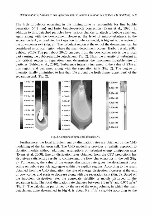
Determination of turbulence and upper size limit in Jameson flotation cell by the CFD modelling 539
The high turbulence occurring in the mixing zone is responsible for fine bubble
generation (< 1 mm) and faster bubble-particle connection (Evans et al., 1995). In
addition to this, detached particles have various chances to attach to bubble again and
again along with the downcomer. However, the level of micro-turbulence in the
separation tank, as predicted by k-epsilon turbulence model, is highest at the region of
the downcomer exit (Fig. 2.). The turbulent region at the exit of the downcomer can be
considered as critical region where the main detachment occurs (Harbort et al., 2002;
Sahbaz, 2010). The part about 20-25 cm deep from the downcomer exit is the critical
part causing the bubble-particle detachment (Fig. 2). Thus, the intensity of turbulent in
this critical region in separation tank determines the maximum floatable size of
particles (Sahbaz et al., 2010). Turbulence intensity increased to the value of 23% at
this region and decreased along with the separation tank (Fig. 2). The degree of
intensity finally diminished to less than 1% around the froth phase (upper part) of the
separation tank (Fig. 2).
Fig. 2. Contours of turbulence intensity, %
Furthermore, the local turbulent energy dissipation rates are obtained by the CFD
modelling of the Jameson cell. The CFD modelling provides a realistic approach to
flotation models without additional assumptions on turbulent energy dissipation rates
(Evans et al, 2008). Energy dissipation rates obtained from the CFD predictions has
also given satisfactory results to comprehend the flow characteristics in the cell (Fig.
3). Furthermore, the value of the energy dissipation rate gives the detachment force
acting on bubble particle aggregate within the explicit regions. According to the result
obtained from the CFD simulation, the rate of energy dissipation increases at the exit
of downcomer and starts to decrease along with the separation tank (Fig. 3). Based on
the turbulent dissipation rate, the aggregate stability is mostly disturbed in the
separation tank. The local dissipation rate changes between 2.1 m2/s
3 and 0.075 m
2/s
3
(Fig 3). The calculation performed by the use of the exact volume, in which the main
detachment zone determined in Fig 4. is about 0.9 m2/s
3 (Fig.4-b) according to the
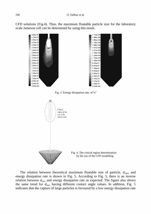
540 O. Sahbaz et al.
CFD solutions (Fig.4). Thus, the maximum floatable particle size for the laboratory
scale Jameson cell can be determined by using this result.
Fig. 3. Energy dissipation rate, m2/s3
Fig. 4. The critical region determination
by the use of the CFD modelling
The relation between theoretical maximum floatable size of particle, dmax, and
energy dissipation rate is shown in Fig. 5. According to Fig. 5, there is an inverse
relation between dmax and energy dissipation rate as expected. The figure also shows
the same trend for dmax having different contact angle values. In addition, Fig. 5
indicates that the capture of large particles is favoured by a low energy dissipation rate
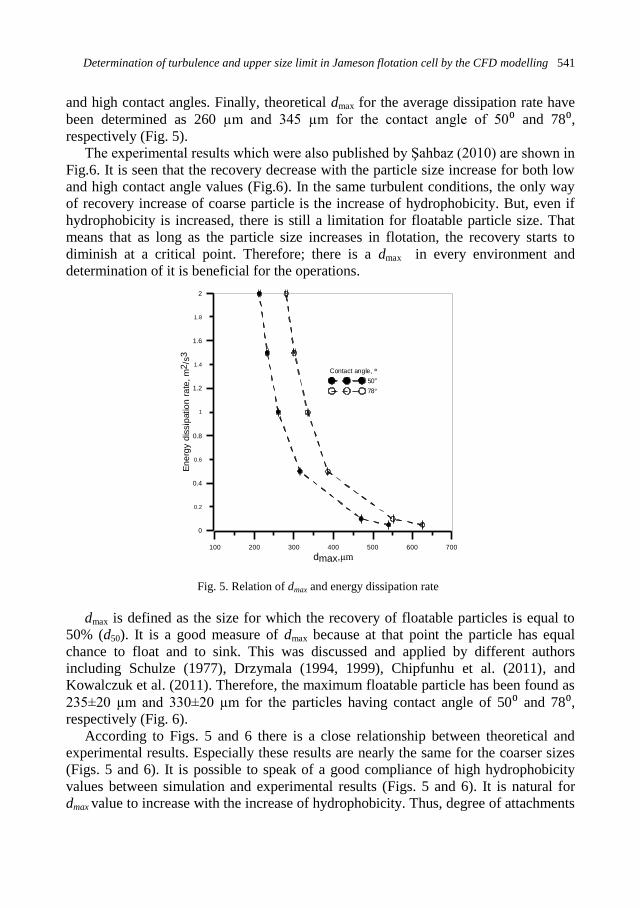
Determination of turbulence and upper size limit in Jameson flotation cell by the CFD modelling 541
and high contact angles. Finally, theoretical dmax for the average dissipation rate have
been determined as 260 µm and 345 µm for the contact angle of 50⁰ and 78⁰, respectively (Fig. 5).
The experimental results which were also published by Şahbaz (2010) are shown in
Fig.6. It is seen that the recovery decrease with the particle size increase for both low
and high contact angle values (Fig.6). In the same turbulent conditions, the only way
of recovery increase of coarse particle is the increase of hydrophobicity. But, even if
hydrophobicity is increased, there is still a limitation for floatable particle size. That
means that as long as the particle size increases in flotation, the recovery starts to
diminish at a critical point. Therefore; there is a dmax in every environment and
determination of it is beneficial for the operations.
100 200 300 400 500 600 700
dmax,µm
0
0.4
0.8
1.2
1.6
2
0.2
0.6
1
1.4
1.8
En
erg
yd
issip
atio
nra
te,
m2
/s3
Contact angle, °
50º
78º
Fig. 5. Relation of dmax and energy dissipation rate
dmax is defined as the size for which the recovery of floatable particles is equal to
50% (d50). It is a good measure of dmax because at that point the particle has equal
chance to float and to sink. This was discussed and applied by different authors
including Schulze (1977), Drzymala (1994, 1999), Chipfunhu et al. (2011), and
Kowalczuk et al. (2011). Therefore, the maximum floatable particle has been found as
235±20 µm and 330±20 µm for the particles having contact angle of 50⁰ and 78⁰, respectively (Fig. 6).
According to Figs. 5 and 6 there is a close relationship between theoretical and
experimental results. Especially these results are nearly the same for the coarser sizes
(Figs. 5 and 6). It is possible to speak of a good compliance of high hydrophobicity
values between simulation and experimental results (Figs. 5 and 6). It is natural for
dmax value to increase with the increase of hydrophobicity. Thus, degree of attachments
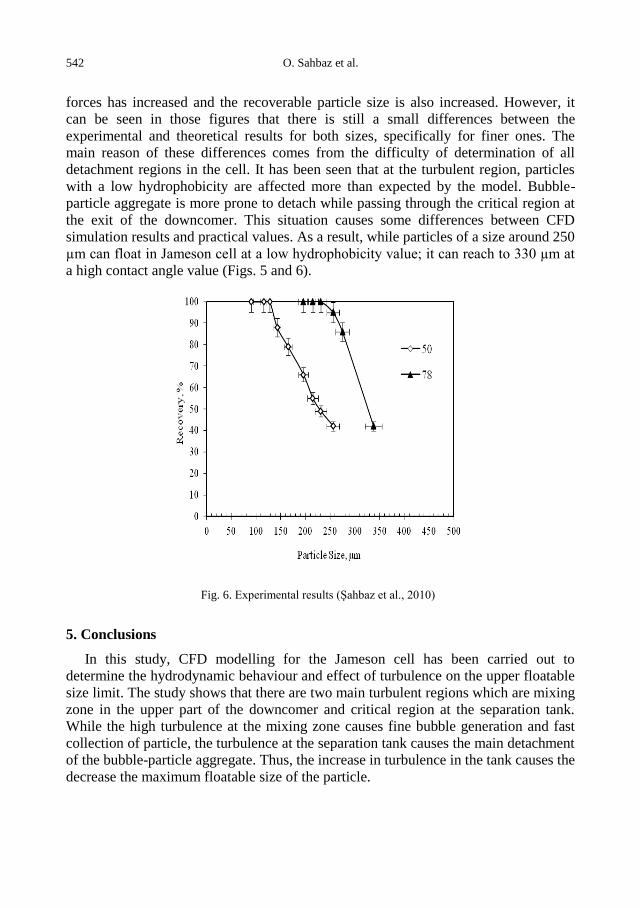
542 O. Sahbaz et al.
forces has increased and the recoverable particle size is also increased. However, it
can be seen in those figures that there is still a small differences between the
experimental and theoretical results for both sizes, specifically for finer ones. The
main reason of these differences comes from the difficulty of determination of all
detachment regions in the cell. It has been seen that at the turbulent region, particles
with a low hydrophobicity are affected more than expected by the model. Bubble-
particle aggregate is more prone to detach while passing through the critical region at
the exit of the downcomer. This situation causes some differences between CFD
simulation results and practical values. As a result, while particles of a size around 250
µm can float in Jameson cell at a low hydrophobicity value; it can reach to 330 µm at
a high contact angle value (Figs. 5 and 6).
Fig. 6. Experimental results (Şahbaz et al., 2010)
5. Conclusions
In this study, CFD modelling for the Jameson cell has been carried out to
determine the hydrodynamic behaviour and effect of turbulence on the upper floatable
size limit. The study shows that there are two main turbulent regions which are mixing
zone in the upper part of the downcomer and critical region at the separation tank.
While the high turbulence at the mixing zone causes fine bubble generation and fast
collection of particle, the turbulence at the separation tank causes the main detachment
of the bubble-particle aggregate. Thus, the increase in turbulence in the tank causes the
decrease the maximum floatable size of the particle.
Determination of turbulence and upper size limit in Jameson flotation cell by the CFD modelling 543
According to the CFD simulation the turbulence intensity is higher at the exit of the
downcomer than in the whole separation tank. Value of energy dissipation rate within
the cell changes between 2.5 m2/s
3 and 0,025 m
2/s
3. In addition to this, the local energy
dissipation rate within the critical region is around 0.9 m2/s
3. This means that the
maximum floatable particle size within the cell is approximately 250 µm and 350 µm
for the contact angle rate of 50⁰ and 78⁰, respectively. The experimental results have
been confirmed by the theoretical results.
Acknowledgement
The authors are thankful to Prof. Dr. Greame J. Jameson for his great support during the design of
laboratory scale Jameson cell. And we are also thankful to Dr. Ali Ucar for his advices during the
experimental part of this study.
References
CHIPFUNHU, D., ZANIN, M., GRANO,S., 2011, Flotation behaviour of fine particles with respect to
contact angle, Chemical Engineering Research and Design, 2011, Article in Press.
ÇINAR, M., ŞAHBAZ, O., ÇINAR, F., KELEBEK, Ş. AND ÖTEYAKA, B., 2007, Effect of Jameson
cell operating variables and design characteristics on quartz-dodecylamine flotation system, Minerals
Engineering, 20, 1391‒1396.
COWBURN, J., HARBORT, G., MANLAPIG, E. POKRAJCIC, Z., 2006, Improving the recovery of
coarse coal particles in Jameson cell, Minerals Engineering, 19, 609‒618.
DRZYMALA, J., 1994a, Characterization of materials by Hallimond tube flotation, Part 1. Maximum
size of entrained particles, Int. J. Miner. Process, 42, 139–152.
DRZYMALA, J., 1994b, Hydrophobicity and collectorless flotation of inorganic materials, Adv. Colloid
Interface Sci., 50, 143–185.
EVANS, G.M., ATKINSON, B., JAMESON, G.J., 1995, The Jameson Cell. Flotation Science and
Engineering, ed. Matis K.A., Marcel Dekker Inc., 331‒363.
EVANS, G.M., DOROODCHI, E., LANE, G.L., KOH, P.T.L., SCHWARZ, M.P., 2008, Mixing and gas
dispersion in mineral flotation cells, Chemical Engineering Research and Design, 86, 1350–1362.
FLUENT 6.3 User’s Guide, Fluent Inc., Centerra Resource Park, 10 Cavendish Court, Lebanon, NH
03766, USA, 2006.
GAMBIT User’s Guide, Fluent Inc., Centerra Resource Park, 10 Cavendish Court, Lebanon, NH 03766,
USA, 2006.
GONJITO, F.C., Fornasiero, D., Ralston, J., 2007, The limits of fine and coarse particle flotation, The
Canadian Journal of Chemical Engineering, 85, 739‒747.
HARBORT, G.J., MANLAPIG, E.V. ve DEBONO, S.K., 2002, Particle collection within the Jameson
cell downcomer, Trans. IMM Section C, 111/Proc. Australas IMM, V. 307.
JAMESON, G.J., 2010, New directions in flotation machine design, Minerals Engineering, 23(11‒13),
835‒841.
KOH, P.T.L., MANICKAM, M., M.P. SCHWARZ, 2000, CFD simulation of bubble- partıcle collisions
in mıneral flotation cells, Minerals Engineering, 13, 1455‒1463.
KOH, P.T.L., SCHWARZ, M.P., 2003, CFD modelling of bubble-particle collision rates and efficiencies
in a flotation cell, Minerals Engineering, 16, 1055‒1059.
KOH, P.T.L., M.P. SCHWARZ, 2006, CFD modelling of bubble–particle attachments in flotation cells,
Minerals Engineering, 19, 619–626.
KOWALCZUK, P., SAHBAZ, O., DRZYMALA, J., 2011, Maximum size of floating particles in
different flotation cells, Minerals Engineering, 24, 766‒771.
LANE, G.L., SCHWARZ, M.P., EVANS, G.M., 2002, Predicting gas–liquid flow in a mechanically
stirred tank, Applied Mathematical Modelling, 26, 223–235.
544 O. Sahbaz et al.
LUI, T.Y. SCHWARZ, M.P., 2009, CFD based modelling of bubble particle collision efficiency with
mobile bubble surface in a turbulent environment, International Journal of Mineral Processing, 90,
45–55.
NGUYEN, A.V., 2003, New method and equations for determining attachment tenacity and particle size
limit in flotation, International Journal of Mineral Processing, 68, 167‒182.
ÖTEYAKA, B., SOTO, H., 1995, Modelling of negative bias column for coarse particles flotation,
Minerals Engineering, 8, 91‒100.
ÖTEYAKA, B., 1993, Modelisation D’une Colonne De Flottation Sans Zone D’ecume Pour La
Separation Des Particules Grossieres, PhD Thesis, Universite Laval, Quebec, Canada, 1993.
PYKE, B., FORNASIERO, D., RALSTON, J., 2003, Bubble particle heterocoagulation under turbulent
conditions, Journal of Colloid and Interface Science, 265, 141–151.
RALSTON, J., FORNASIERO, D. HAYES, R., 1999, Bubble-particle attachment and detachment in
flotation, International Journal of Mineral Processing, 56, 133-164.
RODRIGUES, R.T., RUBIO, J., 2007, DAF–dissolved air flotation: Potential applicationsin the mining
and mineral processing industry, International Journal of Mineral Processing, 82,1–13.
ŞAHBAZ, O., ÖTEYAKA, B., KELEBEK, Ş., UÇAR A. ve DEMIR, U., 2008, Separation of unburned
carbonaceous matter in bottom ash using Jameson cell, Separation and Purification Technology, 62,
103‒109.
SAHBAZ, O., 2010, Modification of downcomer in Jameson Cell and its effect on performance. Ph.D.
Thesis, Dumlupinar University, Department of Mining Engineering, Turkey, 2010.
SCHUBERT, H., 1999, On the turbulence-controlled microprocesses in flotation machines, International
Journal of Mineral Processing, 56, 257‒276.
SCHULZE, H.J., 1977, New theoretical and experimental investigations on stability of bubble/particle
aggregates in flotation: a theory on the upper particle size of floatability, International Journal of
Mineral Processing, 4, 241‒259.
SCHULZE, H.J., 1982, Dimensionless number and approximate calculation of the upper particle size of
floatability in flotation machines, International Journal of Mineral Processing, 9, 321‒328.
SCHULZE, H.J., 1989, Determination of adhesive strength of praticles within the liquid/gas interface in
flotation by means of a centrifuge method, Journal of Colloidal and Interface Science, 128(1).
SCHULZE, J.H., 1993, Flotation as a heterocoagulation process: possibilities of calculating the
probability of flotation. Coagulation and Flocculation and Applications. Dekker, New York, ed.
Dobias, B., 1993, 321‒353.
TRAHAR, W.J., 1981, A rational interpretation of the role of particle size in flotation, International
Journal of Mineral Processing, 1981, 8, 289‒327.
UÇURUM, M., BAYAT O., 2007, Effects of operating variables on modified flotation parameters in the
mineral separation, Separation and Purification Technology, 55 (2), 173‒181.

http://dx.doi.org/10.5277/ppmp120218
Physicochem. Probl. Miner. Process. 48(2), 2012, 545−554 Physicochemical Problems
of Mineral Processing
w w w . m i n p r o c . p w r . w r o c . p l / j o u r n a l / ISSN 1643-1049 (print)
ISSN 2084-4735 (online)
Received April 7, 2012; reviewed; accepted May 5, 2012
DEPENDENCE OF MINE REVENUE
ON THE GRADE OF COPPER CONCENTRATE
Jerzy MALEWSKI*, Malgorzata KRZEMINSKA**
* Wroclaw University of Technology, Wyb. Wyspianskiego 27, 50-370 Wroclaw, [email protected]
** KGHM Polska Miedź S.A. Oddział Zakłady Wzbogacania Rud, Polkowice
Abstract. The paper presents a method of calculating the Net Smelter Return or Revenue
(NSR) formula for copper ore mines based on heuristic models of functional relationships
between concentration of metals in ore and copper concentrates, the operational efficiency, and
the metal prices in the global markets. A method has been proposed to identify these
relationships as well as a way of estimating their parameters. The NSR optimization
calculations have been performed for the data coming from the mining and smelting practise of
KGHM Polska Miedź S.A., which demonstrate its practical usefulness in assessing the
efficiency of production based on the current quality of ore, the efficiency of its beneficiation,
and the market prices of metals.
keywords: NSR, copper grading, recovery, costs, revenue, modelling
1. Introduction
The Net Smelter Return or Revenue (NSR) method is commonly used to analyse
the economic impact of the degree of concentration of enriched minerals in light of
processing costs and metal market prices (Czeczott, 1937; Paulo and Strzelska-
Smakowska, 2000; Wills, 2006). It involves calculating the profits achievable from the
sale of the main product of the mine, i.e. the concentrate after deducting the processing
costs. It is an important piece of information for the mine, which may be a criterion for
optimizing extraction and beneficiation of ore according to the quality of the
concentrates. This method also provides the basis for the structure of settlement
contracts between the mine and the smelter, but it can also be used as a tool for
studying the efficiency of investment projects (Płaneta et al., 2000) or optimization
projects (Krzemińska, 2012).
In such a settings the mine, i.e. mining units and the processing plant taken
together represent one side of the settlements, while the smelter is on the other side.
Combining ore excavation and beneficiation into one technological body is due to the
fact that shipment of ore over great distances to the processing plant and then to the
smelter without beneficiation would be, for obvious reasons, completely
uneconomical. Therefore, the processing plant is usually an integral part of the mine,

546 J. Malewski and M. Krzeminska
whereas smelters can be located anywhere in the world because they are not dependent
on a specific mine and can operate safely through the concentrates markets or by
entering into direct contracts with specific providers. The global mining practise is
such that about half of that industry operates without processing while the other half
operates in the form of mining and smelting groups (Fig. 1).
In the Polish copper industry metal production is organized in terms of technology
and management as a mining and smelting group, which is functionally divided into
extraction, ore beneficiation, and smelting divisions (Monografia KGHM, 2007). The
divisions settle their mutual accounts according to the volume and quality of the main
product, but not financially. Consequently, it is interesting to determine what
maximum revenue can be achieved by the mine (extraction + ore beneficiation plant)
from mining production (quality of the ore and concentrate) considering the
processing costs and the price movements on the global market of non-ferrous metals.
For this purpose we will use own structure of the NSR settlement formula built on
relationships between the quality of ore, quality and yield of the concentrates,
processing costs, and finally, metal prices in the open market.
Fig. 1. The structure of production of the 10 largest producers of raw materials. Source: MMSD, CRUI
report 2001
Figure 2 shows the revenue limits at each stage of production. In this article we
will confine ourselves to the analysis of the cost and quality relationships between the
mine and the Ore Beneficiation Plant (OBP) on one hand and the smelter on the other
hand. However, it is also possible to put extraction on the one side and the OBP with
the smelter on the other side, where the potential revenue of mining would be called
Net Smelting & Processing Revenue (NSPR).
The final beneficiary of the mining and smelting production is the investor, whose
expected benefit from the investment is the revenue after deducting total production
costs, i.e. Net Smelting & Processing & Mining Revenue (NSPMR). The volume
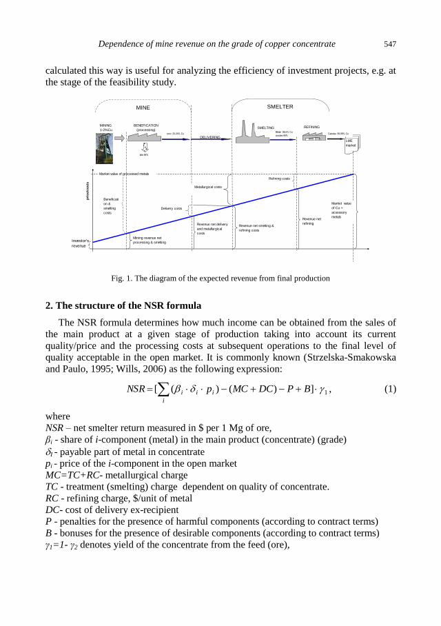
Dependence of mine revenue on the grade of copper concentrate 547
calculated this way is useful for analyzing the efficiency of investment projects, e.g. at
the stage of the feasibility study.
MINE SMELTER
BENEFICATION
(processing)REFINING
LME
market
MINING
1-2%Cu
Investor's
revenue
Market value of processed metals
SMELTING
DELIVERING
Mining revenue net
processing & smelting
Beneficati
on &
smelting
costs
Revenue net delivery
and metallurgical
costs
Revenue net smelting &
refining costs
Revenue net
refining
Metallurgical costs
Market value
of Cu +
acsessory
metals
Refining costs
conc. 20-35% CuBlister 98.5% Cu
anodes 99%Catodes 99.99% Cu
pri
ce/c
osts
tails 98%
Delivery costs
Fig. 1. The diagram of the expected revenue from final production
2. The structure of the NSR formula
The NSR formula determines how much income can be obtained from the sales of
the main product at a given stage of production taking into account its current
quality/price and the processing costs at subsequent operations to the final level of
quality acceptable in the open market. It is commonly known (Strzelska-Smakowska
and Paulo, 1995; Wills, 2006) as the following expression:
1])()([ BPDCMCpNSR i
i
ii , (1)
where
NSR – net smelter return measured in $ per 1 Mg of ore,
βi - share of i-component (metal) in the main product (concentrate) (grade)
I - payable part of metal in concentrate
pi - price of the i-component in the open market
MC=TC+RC- metallurgical charge
TC - treatment (smelting) charge dependent on quality of concentrate.
RC - refining charge, $/unit of metal
DC- cost of delivery ex-recipient
P - penalties for the presence of harmful components (according to contract terms)
B - bonuses for the presence of desirable components (according to contract terms)
γ1=1- γ2 denotes yield of the concentrate from the feed (ore),

548 J. Malewski and M. Krzeminska
where γ2- yield of tailings, and γ0=1 - amount (unit) of feed (ore).
Formula (1) may additionally introduce costs of chemical analyses of quality
testing, and other contractual limitations.
3. Concept of calculation
In the optimization analyses the basic problem is to identify the relationship
between the efficiency of beneficiation operations (recovery) () and the concentration
of the enriched minerals. In the case of complex ores the producer may be interested in
any one component (metal, mineral), but not each one is the subject of beneficiation
even though it will be recovered in subsequent smelting operations. This is precisely
the case that will be considered in this work on the example of copper production
technology at KGHM Polska Miedź S.A.
Under the qualitative and quantitative calculations of the yield of the main
component (Cu) depending on the efficiency of the beneficiation operations we use a
relationship that is well-known in the processing, which is derived from the mass
balance of the processing operation (Drzymala, 2007):
1
, (2)
where is a metal (Cu) content in the feed (ore) or concentrate, β is a metal (Cu)
content in the concentrate.
The second relationship useful for further calculations will be the empirical
hypothesis (Malewski, 2008) of a relationship between Cu recovery and the desired
concentration of that metal in the concentrate which we will write down as follows:
A
max
1 , (3)
where:
A=f(π,z,t) is a function of current values of the operation parameters {π},
environmental variables{z} and duration of the beneficiation operation t,.
βmax – limit of the metal (Cu) content in processed minerals,
, β – as in (2); γ1 as in (1).
So, from (3) we can determine recovery for a given quality of concentrate and then
from (2) calculate actual concentrate yield, or after appropriate transformations we
obtain a formula for yield of the main component in the concentrates as follows
max
max
1 ,1
A
. (4)
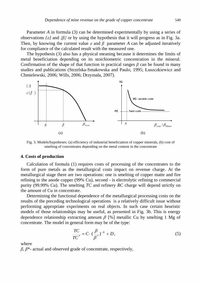
Dependence of mine revenue on the grade of copper concentrate 549
Parameter A in formula (3) can be determined experimentally by using a series of
observations {} and {β} or by using the hypothesis that it will progress as in Fig. 3a.
Then, by knowing the current value and β parameter A can be adjusted iteratively
for compliance of the calculated result with the measured one.
The hypothesis (3) also has a physical meaning because it determines the limits of
metal beneficiation depending on its stoichiometric concentration in the mineral.
Confirmation of the shape of that function in practical ranges β can be found in many
studies and publications (Strzelska-Smakowska and Paulo, 1995; Łuszczkiewicz and
Chmielewski, 2006; Wills, 2006; Drzymała, 2007).
)(
0.1
max
(a)
blisterconc /
TC
fixed costs
VC- variable costs
FC
(b)
Fig. 3. Models/hypotheses: (a) efficiency of industrial beneficiation of copper minerals, (b) cost of
smelting of concentrates depending on the metal content in the concentrate
4. Costs of production
Calculation of formula (1) requires costs of processing of the concentrates to the
form of pure metals as the metallurgical costs impact on revenue charge. At the
metallurgical stage there are two operations: one is smelting of copper matte and fire
refining to the anode copper (99% Cu), second - is electrolytic refining to commercial
purity (99.99% Cu). The smelting TC and refinery RC charge will depend strictly on
the amount of Cu in concentrate.
Determining the functional dependence of the metallurgical processing costs on the
results of the preceding technological operations is a relatively difficult issue without
performing appropriate experiments on real objects. In such case certain heuristic
models of those relationships may be useful, as presented in Fig. 3b. This is energy
dependence relationship extracting amount [%] metallic Cu by smelting 1 Mg of
concentrate. The model in general form may be of the type:
DCTC
TC k )(**
, (5)
where
β, β*- actual and observed grade of concentrate, respectively,
550 J. Malewski and M. Krzeminska
C=VC*/TC
* – constant, representing relative variable treatment costs,
D=FC/TC*– constant, representing relative fixed treatment cost,
TC* – observed treatment costs
k –curve form factor determined experimentally by iteration in a way similar to how it
was described in the case of formula (3).
If β=β* and TC=TC
* then from formula (5) we have C+D=1.
The metallurgical costs, however, depend on the presence of components harmful
to the refining technology or the environment. Therefore, the formula (1) introduces
optionally the penalty component (P ) for the presence of undesirable components in
the concentrate.
Content and recovery of precious metals from refining tailings is usually beyond
the control of concentrates production but could theoretically be the subject of
considering more sophisticated technology for this aim on the stages of deposit
exploitation or ore beneficiation.
The content of accessory metals will be taken into account in our NSR equation in a
simplified manner from the relationship:
**Cu
CuCu
i
i b
. (6)
Thus, βi≈bCuβi* is a current grade βi of i-component proportionally to the relative
change of copper grade of concentrate.
The same approach is applied to calculate the i-component of ore for the need of
current ore value calculation, i.g. αi≈aCuαi*.
5. Sample calculations
Now, we will perform calculations to optimize the quality of the concentrate for the
content of copper and/or accessory metals using the previously derived relationships.
We will use industrial data of metals content in the operations streams throughout the
copper production cycle. Input data for calculations are presented in Table 1.
Treating the data in Table 1 as empirical (αi*, βi*), we will calculate the relative
yield of the concentrate γ1. Taking αCu*=1.67%, βCu*=25.76, εCu*=88% and assuming
metal content in the mineral βmax*=70% applying iterative method we will assess the
parameters of the function (3) that it crosses the empirical point as shown in Fig. 4.
Knowing the relationship as described above and comparing it to (4) we will
calculate the yields γCu=f(aCuβCu) for the current values of copper grading in the
concentrate and in the ore.
The next task is the estimation of smelting costs. Using approximation method as
above for the parameters as in Table 2 we will obtain the result presented in Fig. 4.
When we have the dependence models and assessment of their parameters, we can
simulate revenue limits from production of concentrates for the mine and processing
plant complex. Figures 6-7 show the results of such calculations for a practical scope
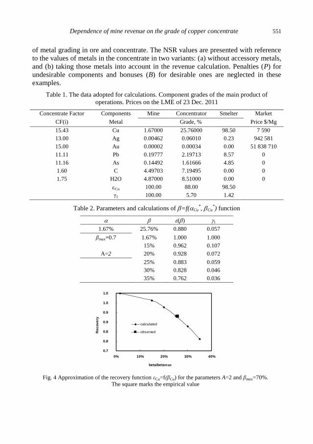
Dependence of mine revenue on the grade of copper concentrate 551
of metal grading in ore and concentrate. The NSR values are presented with reference
to the values of metals in the concentrate in two variants: (a) without accessory metals,
and (b) taking those metals into account in the revenue calculation. Penalties (P) for
undesirable components and bonuses (B) for desirable ones are neglected in these
examples.
Table 1. The data adopted for calculations. Component grades of the main product of
operations. Prices on the LME of 23 Dec. 2011
Concentrate Factor Components Mine Concentrator Smelter Market
CF(i) Metal Grade, % Price $/Mg
15.43 Cu 1.67000 25.76000 98.50 7 590
13.00 Ag 0.00462 0.06010 0.23 942 581
15.00 Au 0.00002 0.00034 0.00 51 838 710
11.11 Pb 0.19777 2.19713 8.57 0
11.16 As 0.14492 1.61666 4.85 0
1.60 C 4.49703 7.19495 0.00 0
1.75 H2O 4.87000 8.51000 0.00 0
Cu 100.00 88.00 98.50
γ1 100.00 5.70 1.42
Table 2. Parameters and calculations of =f(Cu*, Cu
*) function
() 1
1.67% 25.76% 0.880 0.057
βmax=0.7 1.67% 1.000 1.000
15% 0.962 0.107
A=2 20% 0.928 0.072
25% 0.883 0.059
30% 0.828 0.046
35% 0.762 0.036
0.7
0.8
0.8
0.9
0.9
1.0
1.0
0% 10% 20% 30% 40%
beta/betamax
Re
co
ve
ry
calculated
observed
Fig. 4 Approximation of the recovery function εCu=f(βCu) for the parameters A=2 and βmax=70%.
The square marks the empirical value
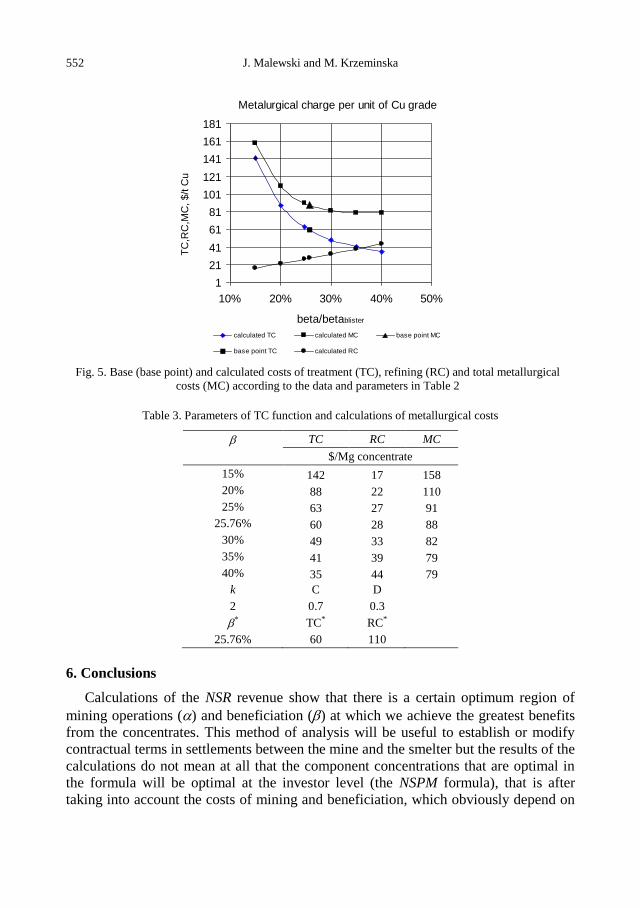
552 J. Malewski and M. Krzeminska
Metalurgical charge per unit of Cu grade
1
21
41
61
81
101
121
141
161
181
10% 20% 30% 40% 50%
beta/betablister
TC
,RC
,MC
, $
/t C
u
calculated TC calculated MC base point MC
base point TC calculated RC
Fig. 5. Base (base point) and calculated costs of treatment (TC), refining (RC) and total metallurgical
costs (MC) according to the data and parameters in Table 2
Table 3. Parameters of TC function and calculations of metallurgical costs
TC RC MC
$/Mg concentrate
15% 142 17 158
20% 88 22 110
25% 63 27 91
25.76% 60 28 88
30% 49 33 82
35% 41 39 79
40% 35 44 79
k C D
2 0.7 0.3
* TC* RC*
25.76% 60 110
6. Conclusions
Calculations of the NSR revenue show that there is a certain optimum region of
mining operations () and beneficiation () at which we achieve the greatest benefits
from the concentrates. This method of analysis will be useful to establish or modify
contractual terms in settlements between the mine and the smelter but the results of the
calculations do not mean at all that the component concentrations that are optimal in
the formula will be optimal at the investor level (the NSPM formula), that is after
taking into account the costs of mining and beneficiation, which obviously depend on
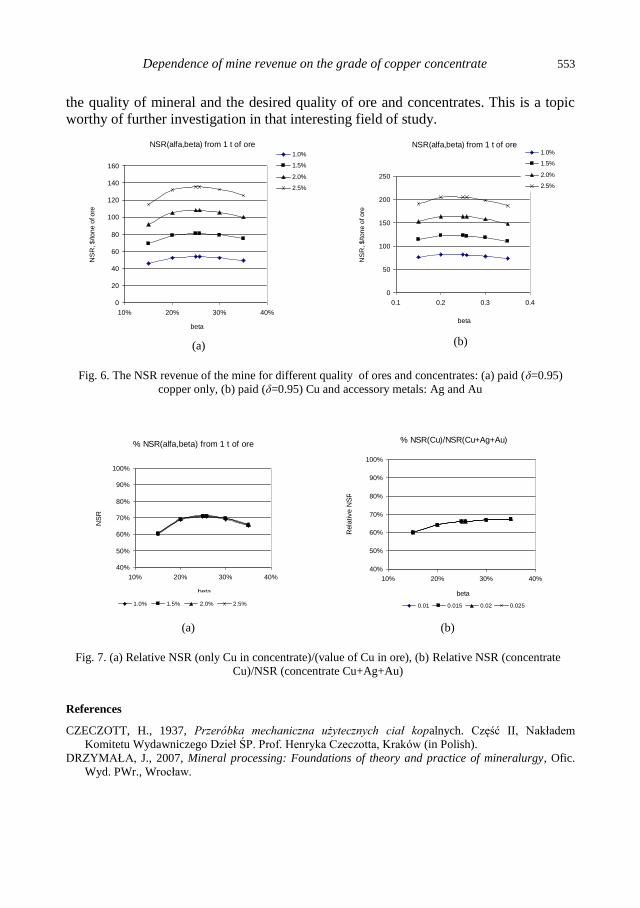
Dependence of mine revenue on the grade of copper concentrate 553
the quality of mineral and the desired quality of ore and concentrates. This is a topic
worthy of further investigation in that interesting field of study.
NSR(alfa,beta) from 1 t of ore
0
20
40
60
80
100
120
140
160
10% 20% 30% 40%
beta
NS
R, $
/to
ne
of o
re
1.0%
1.5%
2.0%
2.5%
(a)
NSR(alfa,beta) from 1 t of ore
0
50
100
150
200
250
0.1 0.2 0.3 0.4
beta
NS
R, $
/to
ne
of o
re
1.0%
1.5%
2.0%
2.5%
(b)
Fig. 6. The NSR revenue of the mine for different quality of ores and concentrates: (a) paid (δ=0.95)
copper only, (b) paid (δ=0.95) Cu and accessory metals: Ag and Au
% NSR(alfa,beta) from 1 t of ore
40%
50%
60%
70%
80%
90%
100%
10% 20% 30% 40%
beta
NS
R
1.0% 1.5% 2.0% 2.5%
(a)
% NSR(Cu)/NSR(Cu+Ag+Au)
40%
50%
60%
70%
80%
90%
100%
10% 20% 30% 40%
beta
Rela
tive N
SR
0.01 0.015 0.02 0.025
(b)
Fig. 7. (a) Relative NSR (only Cu in concentrate)/(value of Cu in ore), (b) Relative NSR (concentrate
Cu)/NSR (concentrate Cu+Ag+Au)
References
CZECZOTT, H., 1937, Przeróbka mechaniczna użytecznych ciał kopalnych. Część II, Nakładem
Komitetu Wydawniczego Dzieł ŚP. Prof. Henryka Czeczotta, Kraków (in Polish).
DRZYMAŁA, J., 2007, Mineral processing: Foundations of theory and practice of mineralurgy, Ofic.
Wyd. PWr., Wrocław.
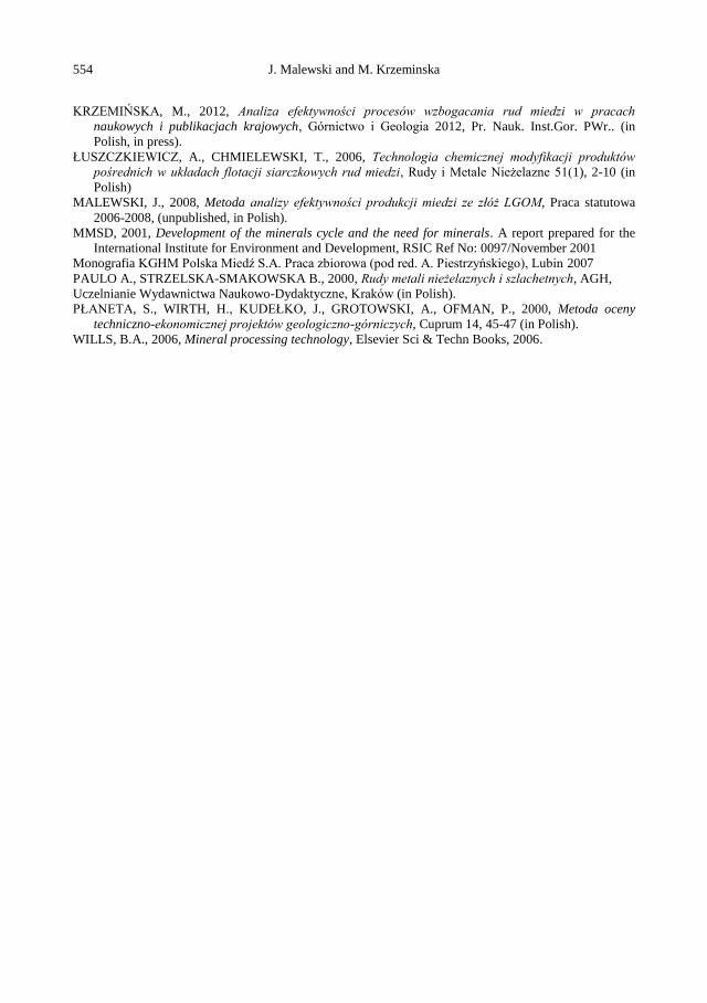
554 J. Malewski and M. Krzeminska
KRZEMIŃSKA, M., 2012, Analiza efektywności procesów wzbogacania rud miedzi w pracach
naukowych i publikacjach krajowych, Górnictwo i Geologia 2012, Pr. Nauk. Inst.Gor. PWr.. (in
Polish, in press).
ŁUSZCZKIEWICZ, A., CHMIELEWSKI, T., 2006, Technologia chemicznej modyfikacji produktów
pośrednich w układach flotacji siarczkowych rud miedzi, Rudy i Metale Nieżelazne 51(1), 2-10 (in
Polish)
MALEWSKI, J., 2008, Metoda analizy efektywności produkcji miedzi ze złóż LGOM, Praca statutowa
2006-2008, (unpublished, in Polish).
MMSD, 2001, Development of the minerals cycle and the need for minerals. A report prepared for the
International Institute for Environment and Development, RSIC Ref No: 0097/November 2001
Monografia KGHM Polska Miedź S.A. Praca zbiorowa (pod red. A. Piestrzyńskiego), Lubin 2007
PAULO A., STRZELSKA-SMAKOWSKA B., 2000, Rudy metali nieżelaznych i szlachetnych, AGH,
Uczelnianie Wydawnictwa Naukowo-Dydaktyczne, Kraków (in Polish).
PŁANETA, S., WIRTH, H., KUDEŁKO, J., GROTOWSKI, A., OFMAN, P., 2000, Metoda oceny
techniczno-ekonomicznej projektów geologiczno-górniczych, Cuprum 14, 45-47 (in Polish).
WILLS, B.A., 2006, Mineral processing technology, Elsevier Sci & Techn Books, 2006.
http://dx.doi.org/10.5277/ppmp120219
Physicochem. Probl. Miner. Process. 48(2), 2012, 555−566 Physicochemical Problems
of Mineral Processing
w w w . m i n p r o c . p w r . w r o c . p l / j o u r n a l / ISSN 1643-1049 (print)
ISSN 2084-4735 (online)
Received December 17, 2011; reviewed; accepted May 10, 2012
FLOCCULATION PERFORMANCE OF FINE PARTICLES
IN TRAVERTINE SLIME SUSPENSION
Eyup SABAH, Ceyhun ACIKSOZ
Afyon Kocatepe University, Engineering Faculty, Department of Mining Engineering, 03200 Afyonkarahisar,
Turkey, Tel.: +90 272 228 14 23/1320; Fax:+90 272 228 14 22, [email protected]
Abstract. The flocculation performance of new generation of flocculants (Magnafloc 5250 and
6250) possessing unique molecular architecture (UMA) and conventional polyacrylamide
based SB 1836 was investigated for the solid-liquid separation of travertine processing
wastewater. The settling rate and turbidity values were considered as the performance criteria.
Based on the settling rate and turbidity values the anionic UMA flocculant 6260 showed better
performance compared to the other anionic flocculants, SB 1836, which is currently used in the
travertine processing plant, and the UMA flocculant 5250. The results obtained from this study
clearly indicated that the type of the flocculants showed no significant effect on the adsorption
of the polymers on the travertine particles at natural pH. The settling rates of the travertine
particles and the turbidity of the suspensions were greatly affected by the surface charge of the
flocculants at high and low pH regimes. The flocculation tests results with the medium charge
flocculants (Magnafloc 5250 and SB 1836) were slightly affected by pH, and resulted in poor
performance in terms of turbidity.
keywords: travertine processing, wastewater, flocculation, settling rate, turbidity
1. Introduction
The use of natural stones such as marble and travertine in construction industry has
been growing rapidly during the last few years. Particularly, there is a significant
increase in production level for both domestic consumption and export markets in
Turkey. However, processing of marble and travertine for the end use generates fine
dust. In addition, a significant amount of water is used for cutting, shaping, and
polishing operations. For this reason recovery and reuse of water from these processes
has become an important topic of interest from both environmental and a dust
suppression point of view.
Although thickeners may be utilized to settle and remove particles less than 75 µm,
some colloidal particles (<1 µm) may still remain in water which adversely affects
surface polishing and cause plugging in pipes (Acar, 2001; Önenç, 2001).
Sedimentation, another method used to dewater travertine processing wastes is often
applied with addition of water soluble polymers which accelerate the settling of
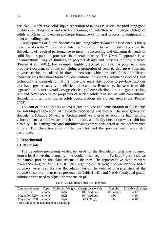
556 E. Sabah and C. Aciksoz
particles. An effective solid–liquid separation of tailings is crucial for producing good
quality circulating water and also for obtaining an underflow with high percentage of
solids which in turns enhances the performance of mineral processing equipment in
plant and tailing dam.
Developments of future flocculants including polyacrylamide-based ones is likely
to be based on the “molecular architecture” concept. That will enable to produce the
flocculants of required performance to meet the increasing and changing demands of
solid–liquid separation processes in mineral industry. The UMATM
approach is an
unconventional way of thinking in polymer design and presents multiple pictures
(Pearse et al., 2001). For example, highly branched and reactive polymer chains
produce flocculant solutions containing a proportion of semi-particulate entities and
polymer chains reticulated in three dimensions which produce flocs of different
characteristics than those formed by conventional flocculants. Another aspect of UMA
technology is manipulation of the molecular mass distribution to produce fractions
that have greater activity in efficient flocculation. Benefits to be seen from this
approach are better overall dosage efficiency, better clarification at a given settling
rate and better rheological properties of settled solids than shown with conventional
flocculants in terms of higher solids concentrations for a given yield stress (Pearse,
2003).
The aim of this study was to investigate the type and concentration of flocculants
for solid-liquid separation of travertine processing wastewater. The new generation
flocculants (Unique Molecular Architecture) were used to obtain a high settling
velocity, hence a solid waste at high solid ratio, and finally circulation water with low
turbidity. The settling rate and turbidity values were considered as the performance
criteria. The characterization of the particles and the process water were also
performed.
2. Experimental
2.1. Materials
The travertine processing wastewater used for the flocculation tests was obtained
from a local travertine company in Afyonkarahisar region in Turkey. Figure 1 shows
the sample port on the plant schematic diagram. The representative samples were
taken according to TSE 5667-10. Three high molecular weight polyacrylamide based
polymers were used for the flocculation tests. The detailed characteristics of the
polymers used for the tests are presented in Table 1. HCl and NaOH (analytical grade)
solutions were used to adjust the suspension pH.
Table 1. Basic characteristics of polymers
Commercial name Type Molecular Weight Charge density (%) Supplier Effective pH range
SB 1836 anionic high 40* (medium) Snf Floerger 4-12*
Magnafloc 5250 anionic high 30* (medium) Ciba 4-10*
Magnafloc 6260 anionic high 49.4* (high) Ciba 4-10*
* According to the manufacturer description
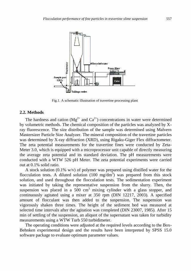
Flocculation performance of fine particles in travertine slime suspension 557
Fig.1. A schematic illustration of travertine processing plant
2.2. Methods
The hardness and cation (Mg2+
and Ca2+
) concentrations in water were determined
by volumetric methods. The chemical composition of the particles was analyzed by X-
ray fluorescence. The size distribution of the sample was determined using Malvern
Mastersizer Particle Size Analyzer. The mineral composition of the travertine particles
was determined by X-ray diffraction (XRD), using Rigaku-Giger Flex diffractometer.
The zeta potential measurements for the travertine fines were conducted by Zeta-
Meter 3.0, which is equipped with a microprocessor unit capable of directly measuring
the average zeta potential and its standard deviation. The pH measurements were
conducted with a WTW 526 pH Meter. The zeta potential experiments were carried
out at 0.1% solid ratio.
A stock solution (0.1% w/v) of polymer was prepared using distilled water for the
flocculation tests. A diluted solution (100 mg/dm3) was prepared from this stock
solution, and used throughout the flocculation tests. The sedimentation experiment
was initiated by taking the representative suspension from the slurry. Then, the
suspension was placed in a 500 cm3 mixing cylinder with a glass stopper, and
continuously agitated using a mixer at 350 rpm (DIN 12217, 2003). A specified
amount of flocculant was then added to the suspension. The suspension was
vigorously shaken three times. The height of the sediment bed was measured at
selected time intervals after the agitation was completed (DIN 23007, 1985). After 15
min of settling of the suspension, an aliquot of the supernatant was taken for turbidity
measurements using a WTW Turb 550 turbidimeter.
The operating conditions were adjusted at the required levels according to the Box-
Behnken experimental design and the results have been interpreted by SPSS 15.0
software package to evaluate optimum parameter values.
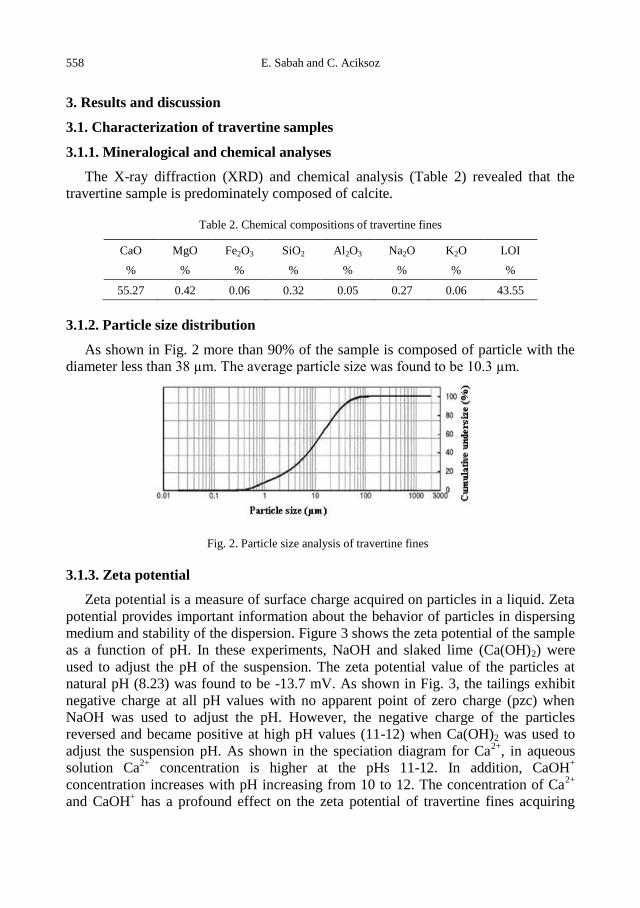
558 E. Sabah and C. Aciksoz
3. Results and discussion
3.1. Characterization of travertine samples
3.1.1. Mineralogical and chemical analyses
The X-ray diffraction (XRD) and chemical analysis (Table 2) revealed that the
travertine sample is predominately composed of calcite.
Table 2. Chemical compositions of travertine fines
CaO MgO Fe2O3 SiO2 Al2O3 Na2O K2O LOI
% % % % % % % %
55.27 0.42 0.06 0.32 0.05 0.27 0.06 43.55
3.1.2. Particle size distribution
As shown in Fig. 2 more than 90% of the sample is composed of particle with the
diameter less than 38 µm. The average particle size was found to be 10.3 µm.
Fig. 2. Particle size analysis of travertine fines
3.1.3. Zeta potential
Zeta potential is a measure of surface charge acquired on particles in a liquid. Zeta
potential provides important information about the behavior of particles in dispersing
medium and stability of the dispersion. Figure 3 shows the zeta potential of the sample
as a function of pH. In these experiments, NaOH and slaked lime (Ca(OH)2) were
used to adjust the pH of the suspension. The zeta potential value of the particles at
natural pH (8.23) was found to be -13.7 mV. As shown in Fig. 3, the tailings exhibit
negative charge at all pH values with no apparent point of zero charge (pzc) when
NaOH was used to adjust the pH. However, the negative charge of the particles
reversed and became positive at high pH values (11-12) when Ca(OH)2 was used to
adjust the suspension pH. As shown in the speciation diagram for Ca2+
, in aqueous
solution Ca2+
concentration is higher at the pHs 11-12. In addition, CaOH+
concentration increases with pH increasing from 10 to 12. The concentration of Ca2+
and CaOH+ has a profound effect on the zeta potential of travertine fines acquiring
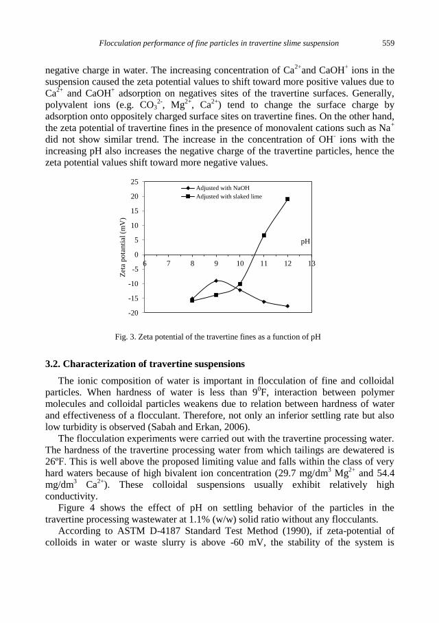
Flocculation performance of fine particles in travertine slime suspension 559
negative charge in water. The increasing concentration of Ca2+
and CaOH+ ions in the
suspension caused the zeta potential values to shift toward more positive values due to
Ca2+
and CaOH+ adsorption on negatives sites of the travertine surfaces. Generally,
polyvalent ions (e.g. CO32-
, Mg2+
, Ca2+
) tend to change the surface charge by
adsorption onto oppositely charged surface sites on travertine fines. On the other hand,
the zeta potential of travertine fines in the presence of monovalent cations such as Na+
did not show similar trend. The increase in the concentration of OH- ions with the
increasing pH also increases the negative charge of the travertine particles, hence the
zeta potential values shift toward more negative values.
-20
-15
-10
-5
0
5
10
15
20
25
6 7 8 9 10 11 12 13
Zet
a pota
nti
al (
mV
)
pH
Adjusted with NaOH
Adjusted with slaked lime
Fig. 3. Zeta potential of the travertine fines as a function of pH
3.2. Characterization of travertine suspensions
The ionic composition of water is important in flocculation of fine and colloidal
particles. When hardness of water is less than 90F, interaction between polymer
molecules and colloidal particles weakens due to relation between hardness of water
and effectiveness of a flocculant. Therefore, not only an inferior settling rate but also
low turbidity is observed (Sabah and Erkan, 2006).
The flocculation experiments were carried out with the travertine processing water.
The hardness of the travertine processing water from which tailings are dewatered is
26ºF. This is well above the proposed limiting value and falls within the class of very
hard waters because of high bivalent ion concentration (29.7 mg/dm3 Mg
2+ and 54.4
mg/dm3 Ca
2+). These colloidal suspensions usually exhibit relatively high
conductivity.
Figure 4 shows the effect of pH on settling behavior of the particles in the
travertine processing wastewater at 1.1% (w/w) solid ratio without any flocculants.
According to ASTM D-4187 Standard Test Method (1990), if zeta-potential of
colloids in water or waste slurry is above -60 mV, the stability of the system is
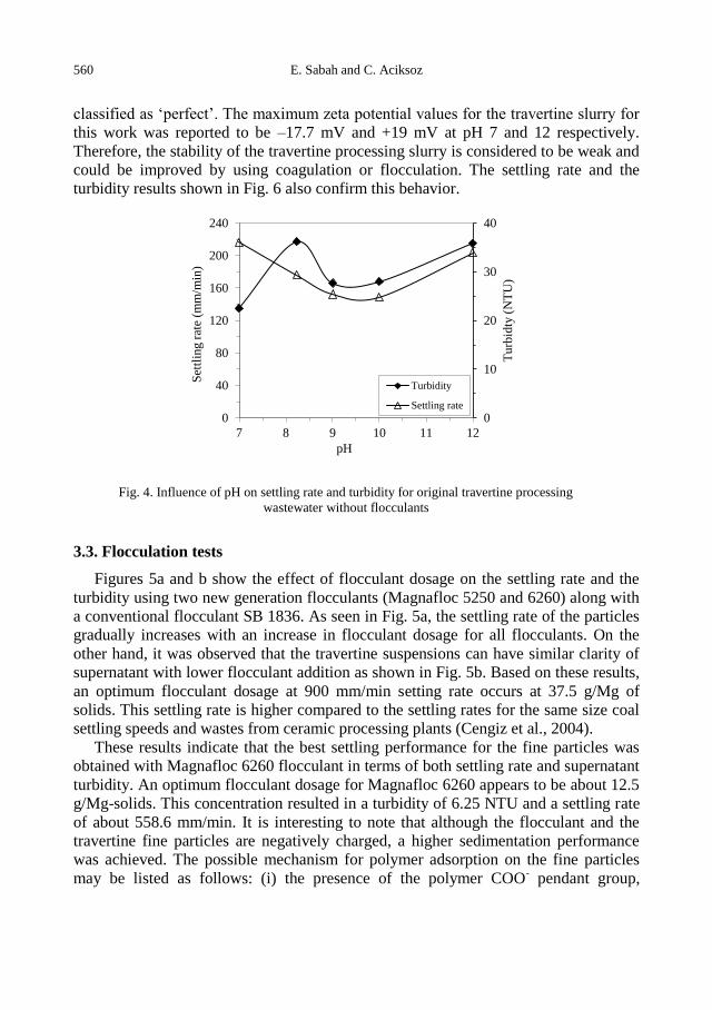
560 E. Sabah and C. Aciksoz
classified as ‘perfect’. The maximum zeta potential values for the travertine slurry for
this work was reported to be –17.7 mV and +19 mV at pH 7 and 12 respectively.
Therefore, the stability of the travertine processing slurry is considered to be weak and
could be improved by using coagulation or flocculation. The settling rate and the
turbidity results shown in Fig. 6 also confirm this behavior.
0
10
20
30
40
0
40
80
120
160
200
240
7 8 9 10 11 12
Tu
rbid
ty (
NT
U)
Set
tlin
g r
ate
(mm
/min
)
pH
Turbidity
Settling rate
Fig. 4. Influence of pH on settling rate and turbidity for original travertine processing
wastewater without flocculants
3.3. Flocculation tests
Figures 5a and b show the effect of flocculant dosage on the settling rate and the
turbidity using two new generation flocculants (Magnafloc 5250 and 6260) along with
a conventional flocculant SB 1836. As seen in Fig. 5a, the settling rate of the particles
gradually increases with an increase in flocculant dosage for all flocculants. On the
other hand, it was observed that the travertine suspensions can have similar clarity of
supernatant with lower flocculant addition as shown in Fig. 5b. Based on these results,
an optimum flocculant dosage at 900 mm/min setting rate occurs at 37.5 g/Mg of
solids. This settling rate is higher compared to the settling rates for the same size coal
settling speeds and wastes from ceramic processing plants (Cengiz et al., 2004).
These results indicate that the best settling performance for the fine particles was
obtained with Magnafloc 6260 flocculant in terms of both settling rate and supernatant
turbidity. An optimum flocculant dosage for Magnafloc 6260 appears to be about 12.5
g/Mg-solids. This concentration resulted in a turbidity of 6.25 NTU and a settling rate
of about 558.6 mm/min. It is interesting to note that although the flocculant and the
travertine fine particles are negatively charged, a higher sedimentation performance
was achieved. The possible mechanism for polymer adsorption on the fine particles
may be listed as follows: (i) the presence of the polymer COO- pendant group,
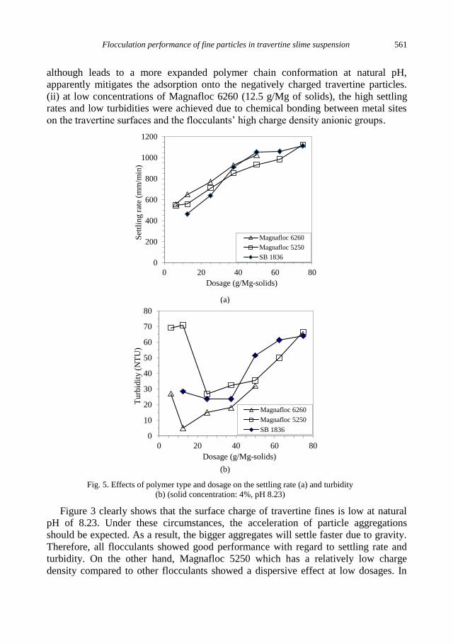
Flocculation performance of fine particles in travertine slime suspension 561
although leads to a more expanded polymer chain conformation at natural pH,
apparently mitigates the adsorption onto the negatively charged travertine particles.
(ii) at low concentrations of Magnafloc 6260 (12.5 g/Mg of solids), the high settling
rates and low turbidities were achieved due to chemical bonding between metal sites
on the travertine surfaces and the flocculants’ high charge density anionic groups.
0
200
400
600
800
1000
1200
0 20 40 60 80
Set
tlin
g r
ate
(mm
/min
)
Dosage (g/Mg-solids)
Magnafloc 6260
Magnafloc 5250
SB 1836
(a)
0
10
20
30
40
50
60
70
80
0 20 40 60 80
Tu
rbid
ity (
NT
U)
Dosage (g/Mg-solids)
Magnafloc 6260
Magnafloc 5250
SB 1836
(b)
Fig. 5. Effects of polymer type and dosage on the settling rate (a) and turbidity
(b) (solid concentration: 4%, pH 8.23)
Figure 3 clearly shows that the surface charge of travertine fines is low at natural
pH of 8.23. Under these circumstances, the acceleration of particle aggregations
should be expected. As a result, the bigger aggregates will settle faster due to gravity.
Therefore, all flocculants showed good performance with regard to settling rate and
turbidity. On the other hand, Magnafloc 5250 which has a relatively low charge
density compared to other flocculants showed a dispersive effect at low dosages. In
562 E. Sabah and C. Aciksoz
such systems, with negatively charged particles, this is an expected behavior with
polymers of high molecular weight and low to high charge density. At low
concentrations of Magnafloc 6260 (12.5 g/Mg of solids), the high settling rates and
low turbidities were achieved due to chemical bonding between metal sites on the
surface of the travertine fines and the flocculants’ high charge density anionic groups.
The type of the flocculant showed significant effect on the adsorption of the
flocculants on the travertine particles at natural pH, as seen in Fig. 6a and b. However
at pH values lower or higher than the natural pH these flocculants show different
performance in terms of settling rates and turbidity. This behavior is understandable
since each polymer has different chemical structure and different affinity for a given
particle surface.
The settling rate and the turbidity of the travertine fine particles was significantly
affected by the charge density of the flocculants at high and low pH values. The
suspensions with low turbidities were obtained at low and high pH values with the use
of high surface charge density Magnafloc 6260 floculant. The flocculation tests with
Magnafloc 5250 (medium charge density) were slightly affected by pH, and hence
exhibited a poor sedimentation performance in terms of turbidity. However, the
flocculation tests with the conventional flocculant SB 1836 (medium charge density)
showed an unstable behavior with a pH dependent flocculation of colloidal particles.
The high charge density Magnafloc 6260 formed small and compact flocs in the
travertine process water at natural pH. This caused a decrease in the settling rate of the
travertine fine particles with a clear supernatant. The decrease in the settling rate is
due to the decrease in the number of carboxyl groups of the anionic polymer which
can be hydrolyzed in the acidic pH. It is plausible that the intra molecular bonds
between carboxyl groups may cause the polymer molecule to form a ring shape and
thus weakening the bridge formation. The suspension pH can change charge
characteristics of polymer chain and their conformation in solution and thus may
directly affect the flocculation power of polymer (Foshee et al., 1982; Reuter and
Hartan, 1986). The flocculation power of anionic polymers by bridging decreases as
the polymer molecules are in a random coil conformation in sections, whereas at
relatively high pH the configurations of the polymer extends due to electrostatic
repulsion between the charged groups on the polymer chain. Taylor et al. (2002) and
Sworska et al. (2000) reported that the addition of Ca2+
and Mg2+
ions prior to the
addition of the flocculant improves the clarity of the supernatant in alkaline
environment in the presence of stable clay suspensions.
Obtaining a fairly clear supernatant (with low turbidity) is important since water
used in cutting and polishing operation is generally recycled. In order to achieve a
suspension with a lower turbidity, the suspension pH was adjusted using slaked lime.
The tests results with Magnafloc 6260 indicated that the best flocculant performance
can be achieved by utilizing lime for the adjustment of the suspension pH. The lime
resulted in much lower turbidity (0.33 NTU) and also reduced the required flocculant
dosage (25 g/ton-solids). However, the settling rate decreased to 371 mm/min which is

Flocculation performance of fine particles in travertine slime suspension 563
tolerable level. These results indicate that Ca2+
adsorption at the travertine-H2O
interface involves the transfer of Ca2+
ions into Stern plane without the release of an
equivalent number of protons into the diffuse layer and bulk solution. The subsequent
decrease in the zeta-potential due to adsorption of Ca2+
ions may be related to unstable
colloidal suspension and very small, dispersed floc particles in the presence of Ca2+
solutions when lime was used as pH modifier. This may imply that if lime solutions
were to be added to the travertine slime suspension prior to Magnafloc 6260 addition,
there is a good probability that the flocculation would be “activated” because of the
presence of Ca2+
ions in the system. In addition, Ca2+
ions may also act as bridges
between the anionic sites on the ionized polymer chain and travertine fines at pH 9 as
shown in Fig. 7
600
700
800
900
1000
1100
1200
6 7 8 9 10 11 12 13 14
Set
tlin
g r
ate
(mm
/min
)
pH
Magnafloc 6260
Magnafloc 5250
SB 1836
(a)
0
10
20
30
40
50
60
70
6 7 8 9 10 11 12 13 14
Tu
rbid
ity (
NT
U)
pH
Magnafloc 6260
Magnafloc 5250
SB 1836
(b)
Fig. 6. Effect of suspension pH on settling rate (a) and turbidity (b) at optimum
polymer dosages (solids concentration: 4%, pH 8.23, dosage 37.5 g/Mg of solids)

564 E. Sabah and C. Aciksoz
Fig. 7. Schematic illustration of Ca2+ activation on adsorption of high molecular weight anionic
flocculant onto a negatively charged suspended travertine fines
3.4. Modeling of settling rate and turbidity
The regression analysis was chosen to determine the relationship between the
response functions (settling rate and the turbidity) and the operating conditions
(dosage and pH). A two factor matrix three level Box-Behnken design was used to
determine the response (settling rate and turbidity). Two significant variables of
flocculation performance are flocculant dosage and pH. When the number of tests at
the central points is three, the total number of tests required for the two variables
comes out to be 32+2+2=13 for the Box-Behnken design (Souzaa et al., 2005). The
variables and their levels used in this study are shown in Table 3.
Table 3. The level of variables chosen for the Box-Behnken design.
Variable
Variable level
Low Center High
-1 0 +1
Dosage, g/Mg of solids x1 6,25 37,5 75
pH x2 7 9 12
For the three-level two-factorial Box-Behnken experimental design, a total of 13
experimental runs are needed. Using the relationships in Table 3, the levels of the
variables for each of the experiments in the design matrix were calculated as given in
Table 4.
For the settling rate of travertine:
SRSB 1836= 77 + 10.3D + 44.3pH; R2 = 0.832
SRMG 5250= 579 + 8.41D - 4.5pH; R2 = 0.778
SRMG 6260= 182 + 8.35D + 31.3pH; R2 = 0.702.
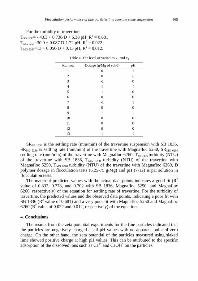
Flocculation performance of fine particles in travertine slime suspension 565
For the turbidity of travertine:
TSB 1836= - 43.3 + 0.738D + 6.38pH; R2 = 0.681
TMG 5250=30.9 + 0.087D-1.72pH; R2 = 0.022
TMG 6260=13 + 0.056D + 0.13pH; R2 = 0.012.
Table 4. The level of variables x1 and x2
Run no. Dosage (g/Mg of solid) pH
1 0 1
2 0 -1
3 -1 0
4 1 -1
5 1 0
6 0 0
7 -1 1
8 0 0
9 -1 -1
10 0 0
11 0 0
12 0 0
13 1 1
SRSB 1836 is the settling rate (mm/min) of the travertine suspension with SB 1836,
SRMG 5250 is settling rate (mm/min) of the travertine with Magnafloc 5250, SRMG 6260
settling rate (mm/min) of the travertine with Magnafloc 6260, TSB 1836 turbidity (NTU)
of the travertine with SB 1836, TMG 5250 turbidity (NTU) of the travertine with
Magnafloc 5250, TMG 6260 turbidity (NTU) of the travertine with Magnafloc 6260, D
polymer dosage in flocculation tests (6.25-75 g/Mg) and pH (7-12) is pH solution in
flocculation tests.
The match of predicted values with the actual data points indicates a good fit (R2
value of 0.832, 0.778, and 0.702 with SB 1836, Magnafloc 5250, and Magnafloc
6260, respectively) of the equation for settling rate of travertine. For the turbidity of
travertine, the predicted values and the observed data points, indicating a poor fit with
SB 1836 (R2 value of 0.681) and a very poor fit with Magnafloc 5250 and Magnafloc
6260 (R2 value of 0.022 and 0.012, respectively) of the equations.
4. Conclusions
The results from the zeta potential experiments for the fine particles indicated that
the particles are negatively charged at all pH values with no apparent point of zero
charge. On the other hand, the zeta potential of the particles measured using slaked
lime showed positive charge at high pH values. This can be attributed to the specific
adsorption of the dissolved ions such as Ca2+
and CaOH+ on the particles.
566 E. Sabah and C. Aciksoz
In terms of the settling rate and turbidity, the UMA Magnafloc 6260 anionic
polymer showed a better flocculation performance compared to UMA Magnafloc
5250 and conventional SB 1816 at natural pH of travertine suspension.
The polymer charge density at high and low pH regimes played a crucial role in the
flocculation of the travertine particles. On the other hand, the medium charge density
polymers (Magnafloc 5250 and SB 1836) were slightly affected by pH, and exhibited
a very bad performance in terms of the turbidity. In the case of the pH dependant
flocculation of colloidal particles, conventional flocculant SB 1836 presented an
unstable behavior.
The decrease in the polymer dosage and turbidity (0.33 NTU) can be achieved by
Magnafloc 6260 when slaked lime is used to adjust the suspension pH due to the
presence of Ca2+
ions in the system.
Acknowledgements
The financial support of Scientific Research Commission (BAPK) of Afyon Kocatepe University is
greatly acknowledged.
References
ACAR, H., 2001, Particular points in construction and operation of the water recycling system for
marble processing plant, 3th Marble Symposium, Afyonkarahisar-Turkey, 289-296.
ASTM D4187-82, 1990, Methods of Test for Zeta Potential of Colloids in Water and Waste Water.
CENGIZ, İ., SABAH, E., ERKAN, Z.E., 2004, A Study on the Flocculation Performance of Conventional
and UMA (Unique Molecular Architecture) Technology Polymers, Madencilik. 43(1), 15–23.
DIN 23007, 1985, The German Institute for Standardization. Flocculants for Process Water, Beuth-
Vertrieb GmbH, Berlin.
DIN 12217, 2003, The German Institute for Standardization. Doors - Operating Forces - Requirements
and Classification, Beuth-Vertrieb GmbH, Berlin.
FOSHEE, W.C., SWAN, W.J., KLİMPEL, R.R., 1982, Improvement in Coal Preparation. Water
Classification Through Polymer Flocculation, Miner. Eng. 34, 93–97.
ÖNENÇ, D. İ., 2001, The Blocks Becoming Powder and The Hopes, Marble. 7 (30), 66–68.
PEARSE, M.J., WEIR, S., ADKINS, S.J., MOODY, G.M., 2001, Advances in Mineral Flocculation,
Miner. Eng. 14 (11), 1505–1511.
PEARSE, M. J., 2003, Historical Use and Future Development of Chemicals for Solid–Liquid Separation
in the Mineral Processing Industry, Miner. Eng. 16, 103–108.
REUTER, J.M., HARTAN, H.G., 1986, Structure and Reaction Kinetics of Polyelectrolytes and Their
Use in Solid–Liquid Processing, Aufbereitungs-Technik. 11, 598–606.
SABAH, E., ERKAN, Z.E. 2006, Interaction Mechanism of Flocculants with Coal Waste Slurry, Fuel.
85, 350–359.
SOUZAA, A.S., WALTER, N.L., SERGIO FERRIA, L.C., 2005, Application of Box–Behnken design in
the optimization of an on-line pre-concentration system using knotted reactor for cadmium
determination by flame atomic absorption spectrometry, Spectrochim. Acta B. 60, 737–742.
SWORSKA, A., LASKOWSKI, J.S., CYMERMAN, G., 2000, Flocculation of the Syncrude Fine
Tailings: Part I. Effect of pH, Polymer Dosage and Mg2+ and Ca2+ Cation, Int. J. Miner. Process. 60,
143–152.
TAYLOR, M.L., MORRİS, G.E., SELF, P.G., SMART, R.C., 2002, Kinetics of Adsorption of High
Molecular Weight Anionic Polyacrylamide onto Kaolinite. J. Colloid. Interf. Sci. 250, 28–36.
TS 5667-10, 2002. Sampling methods of wastewater, Turkish Standard Institution.
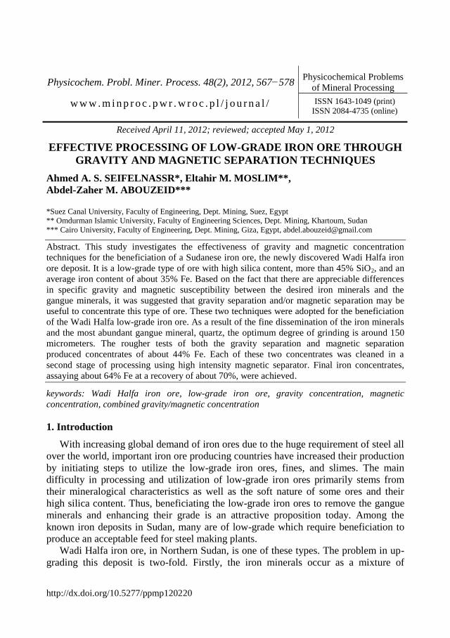
http://dx.doi.org/10.5277/ppmp120220
Physicochem. Probl. Miner. Process. 48(2), 2012, 567−578 Physicochemical Problems
of Mineral Processing
w w w . m i n p r o c . p w r . w r o c . p l / j o u r n a l / ISSN 1643-1049 (print)
ISSN 2084-4735 (online)
Received April 11, 2012; reviewed; accepted May 1, 2012
EFFECTIVE PROCESSING OF LOW-GRADE IRON ORE THROUGH
GRAVITY AND MAGNETIC SEPARATION TECHNIQUES
Ahmed A. S. SEIFELNASSR*, Eltahir M. MOSLIM**,
Abdel-Zaher M. ABOUZEID***
*Suez Canal University, Faculty of Engineering, Dept. Mining, Suez, Egypt
** Omdurman Islamic University, Faculty of Engineering Sciences, Dept. Mining, Khartoum, Sudan
*** Cairo University, Faculty of Engineering, Dept. Mining, Giza, Egypt, [email protected]
Abstract. This study investigates the effectiveness of gravity and magnetic concentration
techniques for the beneficiation of a Sudanese iron ore, the newly discovered Wadi Halfa iron
ore deposit. It is a low-grade type of ore with high silica content, more than 45% SiO2, and an
average iron content of about 35% Fe. Based on the fact that there are appreciable differences
in specific gravity and magnetic susceptibility between the desired iron minerals and the
gangue minerals, it was suggested that gravity separation and/or magnetic separation may be
useful to concentrate this type of ore. These two techniques were adopted for the beneficiation
of the Wadi Halfa low-grade iron ore. As a result of the fine dissemination of the iron minerals
and the most abundant gangue mineral, quartz, the optimum degree of grinding is around 150
micrometers. The rougher tests of both the gravity separation and magnetic separation
produced concentrates of about 44% Fe. Each of these two concentrates was cleaned in a
second stage of processing using high intensity magnetic separator. Final iron concentrates,
assaying about 64% Fe at a recovery of about 70%, were achieved.
keywords: Wadi Halfa iron ore, low-grade iron ore, gravity concentration, magnetic
concentration, combined gravity/magnetic concentration
1. Introduction
With increasing global demand of iron ores due to the huge requirement of steel all
over the world, important iron ore producing countries have increased their production
by initiating steps to utilize the low-grade iron ores, fines, and slimes. The main
difficulty in processing and utilization of low-grade iron ores primarily stems from
their mineralogical characteristics as well as the soft nature of some ores and their
high silica content. Thus, beneficiating the low-grade iron ores to remove the gangue
minerals and enhancing their grade is an attractive proposition today. Among the
known iron deposits in Sudan, many are of low-grade which require beneficiation to
produce an acceptable feed for steel making plants.
Wadi Halfa iron ore, in Northern Sudan, is one of these types. The problem in up-
grading this deposit is two-fold. Firstly, the iron minerals occur as a mixture of
568 A.A.S. Seifelnassr et al.
goethite and hematite in an oolitic pisolitic texture. Secondly, the iron minerals are
finely disseminated in silica and silicates. This requires fine grinding to obtain
adequate degree of liberation of the desired iron mineral and the gangue constituents.
The location of Wadi Halfa iron ore deposit, in the Northern State, is bounded by
latitude 21º 45' and 22º 00' N and longitudes 31º 15' and 31º 45' E. The iron ore
deposits of this area are located on both sides of Lake Nasser. The ore exists in
several layers in stratified succession. The iron ore tonnage is estimated for only one
layer of the deposit to be about 400-800 Tg (teragrams or million tons) at an average
assay of 36% Fe. Since the ore is multi-layered, the tonnage given could be an
underestimation of the whole reserves. In addition, the western part of the area is not
yet assessed but it could add some additional reserves (Ali et al., 2004; Moslim, 2010).
The processing of this particular iron ore is worthy to be considered for many
reasons. It’s occurrence beside the Nile River; hence water will be available in terms
of quantity and quality. Electricity is underway in the near future when the national
grid reaches Halfa from Merawe Dam. Railway line connects Halfa to the rest of the
country. Skilled labor is available in the area.
The most commonly used beneficiation methods for iron ores are the gravity and
magnetic separation methods. Recovery of valuables from natural ores by gravity
concentration process is one of the oldest and most economic techniques (Brut, 1999).
Although in the twentieth century gravity concentration has been partially replaced by
other techniques, notably, flotation and magnetic separation, they have not made it
obsolete. Gravity separation techniques are widely used in mineral beneficiation
practices for its low-cost, ease of operation, and eco-friendly nature. They are based
on the differential settling velocities of the constituting particle of the ore.
The settling velocity of particles is governed jointly by weight (volume and
density), buoyancy, and drag forces. The most commonly used gravity techniques for
beneficiation of iron ores are shaking tables, jigs (Roy, 2009) and spirals. Upgrading
iron ores by jigging has been an emerging trend (Mukherjee, 2006). Flowing film
gravity concentration using Wilfley table is a powerful technique for the recovery of
fine iron minerals. Many theoretical and experimental investigations of Wilfley table
performance have been reported (Gaudin, 1987; Mansar, et al., 1999; Shivamohan,
and Forssberg, 1985). Tabling efficiency is quite high when the specific gravity
difference between valuable and gangue minerals is high (Samykina et al., 2005). In
addition, for upgrading iron ores, magnetic separation may be preferred solely or in
combination with gravity separation, depending on the ore characteristics (Svoboda,
and Ross, 1989; Svoboda, 1994; Svoboda and Fujita, 2003).
Beneficiation of Camdag iron (oolitic) hematite ore containing limonite-hematite
or goethite-limonite using gravity separation and high intensity magnetic separation,
increases the grade of ore about 5-7% in concentrates with about 60% recovery by
both methods (Guney et al., 2000). Abouzeid (1967) studied the possibility of using
high intensity magnetic separator for the beneficiation of El-Gedida iron ore. An ore
sample containing 51.6% Fe, 8.76% SiO2 and 3.06% BaO was used for the study. He
Effective processing of low-grade iron ore through separation techniques 569
found that high intensity magnetic separator tests were limited to very close range of
sizes between 2 and 0.125 mm. The final magnetic product assayed 61% Fe at an iron
recovery of 90.3%. However, 5% by weight was obtained as middling assaying
31.4% Fe. These middling products, together with the fine fraction minus 0.125mm
which constitute 35% by weight of the whole sample, were not possible to be
upgraded by magnetic separation. The barite-riche iron ore of the same deposit was
treated by anionic flotation using Na-DDS as a collector for floating barium sulfate,
and sodium silicate as a depressant for iron minerals (Mossallam, 2004). The feed size
fraction for the flotation cell was -250+80 μm assaying 36.5% Fe and 23% BaO. After
several cleaning stages by flotation, an iron concentrate assaying 62% Fe with less
than 2% BaO at a recovery of 71.3% was obtained.
Rowayshed (1983) studied the possibility of using high intensity magnetic
separator for beneficiation of El-Gedida. He found that high intensity magnetic
separator is limited by a much-closed range of sizes less than 2 mm, neither the coarse
nor the very fine sizes can be treated by this method. The dominant iron minerals
present in this ore are the hydrated minerals, goethite and hydro-goethite, which are
difficult to treat through the high intensity magnetic separator.
Fatma et al. (1999) studied the beneficiation of an iron ore sample containing 44%
Fe, 1.59% SiO2 and 20% BaO. By magnetic separation, two products of iron ore and
barite concentrates were obtained by using a high intensity magnetic separator. The
fine fraction (-0.125 mm) is about 20% by weight assaying 54.6% Fe, and 3.91%
BaO, which needs further cleaning to reduce the barite content to meet the smelter
specifications (52% Fe, and 2% BaO). The size (0.74 +0.106 mm) fraction, after
concentration by H.I.M.S., still contains 41.9% Fe and 11.55% BaO. After cleaning
several times using H.I.M.S, an iron concentrate assaying 58.48% Fe, and 0.73% BaO
is obtained. Final iron concentrate was obtained assaying 64.2% Fe, and 0.24% BaO.
Faraghaly (2002) studied an iron ore containing 23.5% Fe and 34% BaO using a
dry high intensity magnetic separator for the processing of a feed size fraction of -
1+0.125 mm (about 69% by weight of the original feed size). A concentrate
containing 56.78% Fe and 1.61% BaO at a recovery of 82.76% was obtained.
Reduction roasting process was carried out on the fine fraction (-0.125mm) which
represents about 31% by weight of the head sample. A concentrate assaying
56.78%Fe, and 1.61%BaO, with recovery of 82.76% was obtained.
The iron ore at Wadi Halfa is intercalated with Nubian sedimentary rock faces and
overlies these rocks. The stratigraphy of the area from bottom to top is composed of
whitish to violet clayey sandstone, followed by iron-bearing rocks (usually varied in
thickness), conglomerates, and then ferruginous layes intercalated with Nubian
sandstone, which is usually capped with oolitic ironstone. The stratigraphy is
repetitive in nature indicating several or multiple depositional sedimentary cycles.
Chemically and structurally, the oolitic iron ore of Wadi Halfa can be classified into
three types. These are: 1) hematitic oolitic type is red in color because hematite is
domination in the ore. It is fine grained and is always found at the base of the iron
570 A.A.S. Seifelnassr et al.
oolitic form colony, 2) oolitic goethitic iron ore which is black in color indicates
supergene sedimentary conditions associated with the precipitation of the iron ore, 3)
brown oolitic iron formation is an intermediate species between the above two
mentioned types in terms of composition and color (Ali et al., 2003).
It is worth mentioning that the Wadi Halfa iron ore deposit was discovered recently
by the Geological Research Authority of Sudan (GRAS) (Ali et al., 2004). No
beneficiation studies have been reported concerning this deposit until now.
The main objective of this study is to investigate the amenability of Wadi Halfa
(Northern Sudan) low-grade iron ore for upgrading by gravity and magnetic separation
techniques. The main parameters affecting the effectiveness of a shaking table
(exploiting the difference in specific gravity of the main ore constituents), and a high
intensity magnetic separator (exploiting the differences in magnetic susceptibility of
the ore constituents) were investigated
2. Experimental
Ore sample. A composite sample of about 200 kg was collected from the iron ore
deposit at Wadi Halfa area. The sample was collected from different pits in the deposit
area to represent, to some extent, the actual deposit. It was crushed, well mixed, and
quartered to small samples of about 1 kg each. Representative samples were prepared
for chemical analysis and mineralogical studies.
Feed preparation. Some of the samples were ground in a ball mill to different
degrees of fineness: -500 μm, -350 μm, and -150 μm to be used in the beneficiation
experiments. These fractions were deslimed using a hydro-cyclone at a cut size of 20
μm, which made the feed fractions to be: -500+20 μm, -350+20 μm, and -150+20 μm.
Beneficiation techniques. A laboratory shaking table of dimensions 50 cm x 120
cm was used to exploit the difference in specific gravity between the iron minerals and
the gangue minerals. Also, as a result of the significant difference in magnetic
susceptibility between the desired and no desired minerals, a High Intensity Magnetic
Separator (H. T. Readings, PTY LTD, Series No. 88.1) was used as an alternative
technique for upgrading this type of iron ore.
3. Results and discussion
3.1. Characterization of the ore
Mineralogy of the ore. Using X-Ray Differential Analysis, it was found that the
iron ore sample consisted of goethite, hematite, quartz, calcite kaolin, and feldspar.
The major constituents were goethite as an iron mineral and quartz as a gangue
mineral, and the rest were minor minerals. Under the optical microscope, it was
observed that the iron minerals and quartz are finely disseminated. The ore exists in
the form of oolitic and pesolitic texture.
Chemical analysis. Table 1 gives the chemical analysis of the iron ore sample used
in this research work. It is clear that the iron content is relatively low, in the range of
Effective processing of low-grade iron ore through separation techniques 571
36% Fe, and the major gangue mineral is quartz, in the range of 48% SiO2. The rest of
the undesired constituents is less than 2% each.
Table 1. Chemical analysis of Wadi Halfa iron ore sample
Constituent Fe2 O3 Fe (Total) SiO2 CaO MgO MnO Al2 O3 SO4 P2 O5
Percent 45.3 36.1 47.5 1.6 0.3 0.3 1.8 nil 0.1
Desliming of the ore sample. The three ball mill products: -500 μm, -350 μm, and -
150 μm were deslimed using a hydro-cyclone to remove the -20 μm particles. Table 2
shows the results of the desliming tests. The slimes fraction ranges from 6% by weight
in the coarse size fraction, -500 μm, to 10% by weight in the fine size fraction, -150
μm, with rejected amounts of 2.5% Fe and 8.0% Fe, respectively.
Table 2. Classification of the feed fractions
Size fraction, μm Fraction weight, % Assay, Fe % Metal distribution, %
-500+20
-20
Total
94.3
5.7
100.0
36.7
34.7
36.6
97.5
02.5
100.0
-350+20
-20
Total
92.4
7.6
100
37.0
31.9
36.6
94.7
5.3
100
-150+20
-20
Total
90.5
9.5
100
37.7
30.0
36.9
92.0
08.0
100
Liberation study. The degree of liberation of the iron minerals was studied by the
point counting technique. Polished sections of the different size fractions were
prepared and studied under the microscope in reflected light mode. Both the free
particles of iron minerals and the grains of iron minerals locked with gangue minerals
in the microscope view were counted, and the percentage of free iron minerals grains
relative to the sum of the two types of particles was calculated. Table 3 gives the
counting results and the degree of liberation of the iron minerals
Table 3. Degree of liberation of Wadi Halfa iron ore as a function of size fraction
Size fraction, μm No. of free iron
minerals grains
No. of locked
grains
Total number
(free +locked)
Degree of
liberation, %
-500+20 2957 2254 5211 56.7
-350+20 3053 960 4013 76.1
-150+20 2396 235 2631 91.1
-105+20 2408 105 2513 95.8
The above counts suggest that the degree of liberation increases as the grain size
gets finer, which is obvious.
Concentration of the Wadi Halfa iron ore. Gravity and magnetic separation
techniques seem to be two suitable candidates for upgrading this type of iron ore due

572 A.A.S. Seifelnassr et al.
to the significant differences in specific gravity and magnetic susceptibility between
the desired and no desired constituents in the ore. The important parameters in both of
these techniques were investigated to find out if one of them or both could be applied
to concentrate the Wadi Halfa iron ore. The following is a brief discussion of the
results obtained throughout this study.
3.2. Gravity separation
Effects of the two important operating parameters of the shaking table,-feed size
range and table tilt were investigated. The following summarizes the obtained results.
Effect of feed size range. The feed size ranges used in this study were +500-20 μm,
-350+20 μm, and -150+20 μm. Table 4 summarizes the effect of the feed size fraction
to the table on the assay and metal distribution of the iron concentrate.
Table 4. Effect of feed size fraction on the efficiency of tabling (table tilt is 5 degrees)
Size fraction, μm Product Product
weight, % Assay, Fe %
Metal
distribution
%
Metal distribution
relative to original
sample, %
-500+20
Concentrate
Tailing
Total
70.0
30.0
100
38.8
31.4
36.7
74.3
25.7
100.0
72.5
25.1
97.6
-350+20
Concentrate
Tailing
Total
72.6
27.4
100.0
41.5
23.6
36.5
82.3
17.7
100.0
77.9
16.8
94.7
-150+20
Concentrate
Tailing
Total
72.5
27.5
100
44.9
18.2
37.6
86.7
13.3
100.0
79.9
12.1
92.0
The assay of the concentrate obtained using the coarse feed is not significantly
different from that of the feed. The assay of the concentrate as well as the metal
recovery continued to increase as the feed size fraction decreased. The assay increased
from 38.8% Fe to 44.9% Fe and the recovery increased from 74.3% to 86.7% as the
feed size fraction decreased from -500+20 to -150+20 μm, respectively. These effects
are logical because the degree of liberation increases as the size fraction decreases
(Fig. 1).
Effect of angle of table inclination (table tilt). The tilt angle was changed between
3º and 5º. Table 5 presented the results as a function of the table tilt angle.
The optimum tilt angle is 5º. At 5º table inclination large amount of middling
particles are driven towards the concentration end of the table, which increased the
recovery and decreased the assay. At higher tilt angle, the wash water washes away
large amounts of the iron-bearing particles towards the tailing section of the table (Fig.
2).
The above results show that the optimum parameter values for using the shaking
table as a roughing stage for concentrating this type of iron ore are: feed size fraction
of -150+20 μm when the table tilt angle was 5º. At these parameter values, the
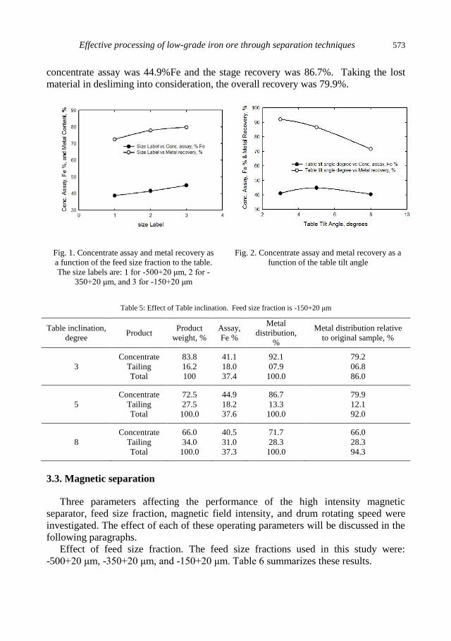
Effective processing of low-grade iron ore through separation techniques 573
concentrate assay was 44.9%Fe and the stage recovery was 86.7%. Taking the lost
material in desliming into consideration, the overall recovery was 79.9%.
Fig. 1. Concentrate assay and metal recovery as
a function of the feed size fraction to the table.
The size labels are: 1 for -500+20 μm, 2 for -
350+20 μm, and 3 for -150+20 μm
Fig. 2. Concentrate assay and metal recovery as a
function of the table tilt angle
Table 5: Effect of Table inclination. Feed size fraction is -150+20 μm
Table inclination,
degree Product
Product
weight, %
Assay,
Fe %
Metal
distribution,
%
Metal distribution relative
to original sample, %
3
Concentrate
Tailing
Total
83.8
16.2
100
41.1
18.0
37.4
92.1
07.9
100.0
79.2
06.8
86.0
5
Concentrate
Tailing
Total
72.5
27.5
100.0
44.9
18.2
37.6
86.7
13.3
100.0
79.9
12.1
92.0
8
Concentrate
Tailing
Total
66.0
34.0
100.0
40.5
31.0
37.3
71.7
28.3
100.0
66.0
28.3
94.3
3.3. Magnetic separation
Three parameters affecting the performance of the high intensity magnetic
separator, feed size fraction, magnetic field intensity, and drum rotating speed were
investigated. The effect of each of these operating parameters will be discussed in the
following paragraphs.
Effect of feed size fraction. The feed size fractions used in this study were:
-500+20 μm, -350+20 μm, and -150+20 μm. Table 6 summarizes these results.

574 A.A.S. Seifelnassr et al.
Table 6: Effect of feed size fraction on efficiency of magnetic separation at 0.3 Ampere and 100 rpm
Size fraction
μm Product
Product
weight, %
Assay
Fe %
Metal
distribution, %
Metal distribution relative
to original sample, %
-500+20
Magnetic
Non-magnetic
Total
65.1
34.9
100
38.8
31.4
36.7
74.3
25.7
100.0
72.5
25.1
97.6
-350+20
Magnetic
N0n-magnetic
Total
75.3
24.7
100.0
41.5
23.6
36.5
82.3
17.7
100.0
77.9
16.8
94.7
-150+20
Magnetic
Non-magnetic
Total
81.5
18.5
100.0
42.4
16.0
36.5
92.4
7.8
100
84.9
7.1
92.0
As it was observed in the gravity separation, the optimum results were obtained at
feed size fraction of -150+20 μm, where the iron assay of the concentrate was 42.4%
Fe at a recovery of 92.2%. Again, this is because the finer the size fraction, the more
is the liberation of the desired minerals from the gangue minerals (Fig. 3). However,
the selectivity was low because of the high percentage of silica.
Fig. 3. Effect of feed size fraction on the
concentrate assay and metal recovery
using high intensity magnetic separator.
The size labels are: 1 for -500+20 μm, 2
for -350+20 μm, and 3 for -150+20 μm
Effect of electric current intensity to the electromagnetic coil. The current intensity
to the coil is an indication to the magnetic field intensity, as the current increases the
field intensity increases. The range of the current variation in the magnetic separator
that was used is from 0.1 to 0.5 Amperes. Table 7 and Figure 4 give the results of the
effect of the current intensity on the assay and recovery of the concentrate.
From Table 7, it can be seen that the assay of the concentrate decreases with
increasing the magnetic field intensity. This result is due to the degree of selectivity as
a function of the field intensity. At low field intensity only the high magnetically
susceptible particles are picked up by the rotating drum, which produces a relatively
high grade concentrate (45.0% Fe) at low recovery (79.6%). The low recovery is due
to the fact that a large portion of the locked particles goes with the non-magnetic
fraction. The optimum result was obtained at a current intensity of 0.3 Ampere.

Effective processing of low-grade iron ore through separation techniques 575
Table 7. Effect of magnetic field intensity. The magnet drum runs at 100 rpm
Current
Ampere Product
Product
weight, %
Assay
Fe %
Metal
distribution, %
Metal distribution relative to
original sample, %
0.1
Magnetic
Non-magnetic
Total
66.0
34.0
100.0
45.0
22.5
37.4
79.6
20.4
100.0
73.2
18.8
92.0
0.2
Magnetic
Non-magnetic
Total
76.5
23.5
100.0
42.7
20.2
37.4
87.3
12.7
100.0
80.3
11.7
92.0
0.3
Magnetic
Non-magnetic
Total
81.5
18.5
100.0
42.4
16.0
37.5
92.2
07.8
100.0
84.8
07.2
92.0
0.4
Magnetic
Non-magnetic
Total
82.0
18.0
100.0
41.9
17.0
37.4
91.8
08.2
100.0
84.4
07.6
92.0
0.5
Magnetic
Non-magnetic
Total
83.0
17.0
100
41.2
18.3
37.3
91.7
08.3
100.0
84.3
07.7
92.0
Fig. 4. Iron assay and metal recovery of the
concentrate as a function of current intensity to
the electromagnetic coil at this current intensity,
the magnetic intensity
Effect of the drum rotational speed. The drum rotational speed was varied from 60
to 220 rpm. The main effect of the drum rotational speed is the induced centrifugal
force to the flowing particles which is a function of the particle mass. However,
because of the nature of the main ore constituents, iron minerals and quartz, during
size reduction, the quartz particles are coarser than the iron minerals particles although
less in density than the iron minerals. Also the particle weight (density multiplied by
volume) is a main parameter in this case because of the gravitational force acting on
the individual particles. This means that there are several forces which act on the
flowing particles, namely, centrifugal force, gravitational force, and magnetic force. A
combined effect of these acting forces determines the optimum operating conditions in
this case. As a result of this combination of forces, the optimum result, as represented
by the concentrate assay and recovery, was obtained at drum revolution of 100 rpm
(Table 8 and Fig. 5).
The above results show that the conditions under which the optimum concentrate
was obtained, using the high intensity magnetic separator, are feed particle size of -
150+20 m, electric current intensity of 0.3 A, and 100 rpm drum rotational speed.
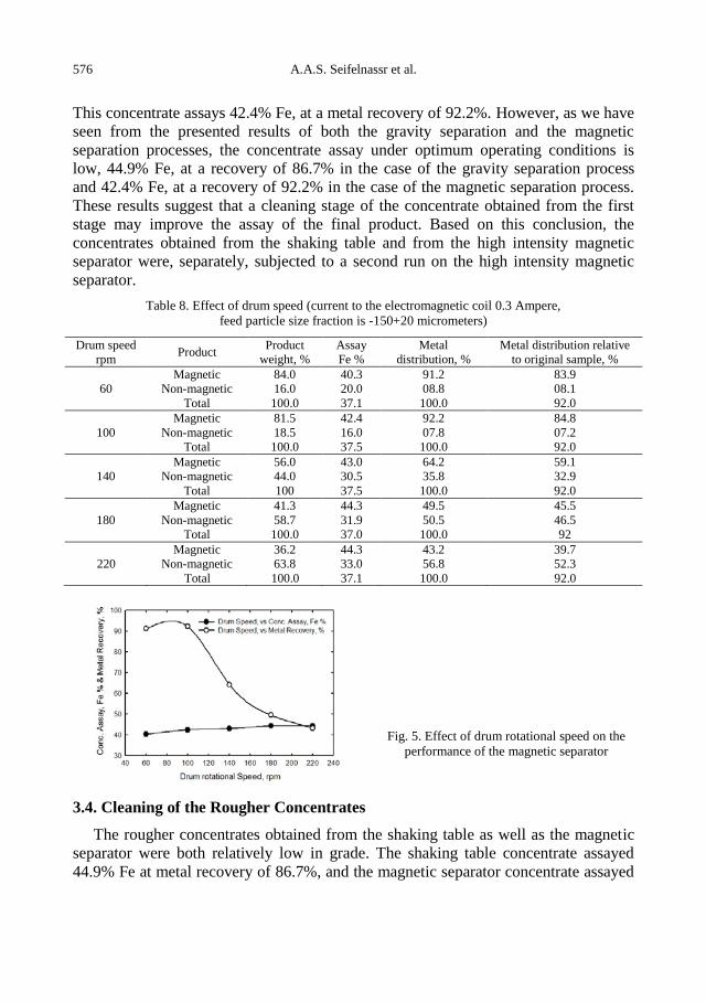
576 A.A.S. Seifelnassr et al.
This concentrate assays 42.4% Fe, at a metal recovery of 92.2%. However, as we have
seen from the presented results of both the gravity separation and the magnetic
separation processes, the concentrate assay under optimum operating conditions is
low, 44.9% Fe, at a recovery of 86.7% in the case of the gravity separation process
and 42.4% Fe, at a recovery of 92.2% in the case of the magnetic separation process.
These results suggest that a cleaning stage of the concentrate obtained from the first
stage may improve the assay of the final product. Based on this conclusion, the
concentrates obtained from the shaking table and from the high intensity magnetic
separator were, separately, subjected to a second run on the high intensity magnetic
separator.
Table 8. Effect of drum speed (current to the electromagnetic coil 0.3 Ampere,
feed particle size fraction is -150+20 micrometers)
Drum speed
rpm Product
Product
weight, %
Assay
Fe %
Metal
distribution, %
Metal distribution relative
to original sample, %
60
Magnetic
Non-magnetic
Total
84.0
16.0
100.0
40.3
20.0
37.1
91.2
08.8
100.0
83.9
08.1
92.0
100
Magnetic
Non-magnetic
Total
81.5
18.5
100.0
42.4
16.0
37.5
92.2
07.8
100.0
84.8
07.2
92.0
140
Magnetic
Non-magnetic
Total
56.0
44.0
100
43.0
30.5
37.5
64.2
35.8
100.0
59.1
32.9
92.0
180
Magnetic
Non-magnetic
Total
41.3
58.7
100.0
44.3
31.9
37.0
49.5
50.5
100.0
45.5
46.5
92
220
Magnetic
Non-magnetic
Total
36.2
63.8
100.0
44.3
33.0
37.1
43.2
56.8
100.0
39.7
52.3
92.0
Fig. 5. Effect of drum rotational speed on the
performance of the magnetic separator
3.4. Cleaning of the Rougher Concentrates
The rougher concentrates obtained from the shaking table as well as the magnetic
separator were both relatively low in grade. The shaking table concentrate assayed
44.9% Fe at metal recovery of 86.7%, and the magnetic separator concentrate assayed

Effective processing of low-grade iron ore through separation techniques 577
42.4% Fe at metal recovery of 92.2%. These two rougher concentrates were passed
through the high intensity magnetic separator, at its optimum operating conditions
(current to the coil is 0.3 Ampere, drum rotation speed 100 rpm), for cleaning. Table 9
presents the results of the cleaning stage of the shaking table concentrate. The final
assay of the concentrate is 65.4% Fe, at an overall metal recovery of 69%.
The rougher concentrate from the magnetic separator was passed again on the high
intensity magnetic separator, at its optimum operating conditions, for cleaning. The
cleaned concentrate assayed 63.5% Fe at an overall metal recovery of 67.7%. Table 10
shows the results of the cleaning stage for the magnetic separator rougher concentrate.
Table 9. Cleaning of the table concentrate using the high intensity magnetic separator
(magnetic field intensity is at 0.3 A, drum speed 100 rpm)
Product Product
wt. %
Assay
Fe % Metal distribution, %
Metal distribution relative to
original sample, %
Magnetic 60.1 65.4 87.2 69.0
Non-magnetic 39.9 14.5 12.8 10.2
Total 100 45.0 100 79.2
Table 10. Cleaning of the magnetic rougher concentrate
(magnetic field intensity at 0.3 A, drum speed 100 rpm)
Product Product
wt. %
Assay
Fe % Metal distribution,%
Metal distribution relative to
original sample, %
Concentrate
Tailing
Total
53.2
46.8
100.0
63.5
18.4
42.4
79.7
20.3
100.0
67.7
17.3
85.0
4. Conclusions
The low-grade iron ore sample obtained from the Wadi Halfa iron ore deposit,
North of Sudan, was analyzed mineralogically and chemically. The major mineral
constituents were hydrated iron minerals and quartz. The trace constituents were
calcium, magnesium, aluminum, manganese, and phosphorus oxides. The average iron
assay was about 36% Fe, and the silica content was about 57% SiO2. Three samples
were ground such that the first sample passed 500 μm, the second passed 350 μm, and
the third passed 150 μm. Each of the three samples were deslimed to remove the -20
μm fraction, such that the feed size ranges to be tested were -500+20 μm, -350+20 μm,
and -150+20μm. The ore was beneficiated using the shaking table and the high
intensity magnetic separator. The beneficiation took place in two stages: roughing and
cleaning. The optimum operating conditions for the table were: feed size fraction of -
150+20 μm and table tilt angle of 5ο, and those of the magnetic separator were: feed
size fraction of -150+20 μm, 0.3 Ampere, and drum rotational speed of 100 rpm. The
rougher concentrates from both the gravity separation and the magnetic separation
were, separately, subjected to the second stage of concentration, the cleaning stage. In
the cleaning stage, the rougher concentrates were passed on the high intensity
magnetic separator at its optimum operating conditions: 0.3 Ampere and 100 rpm
578 A.A.S. Seifelnassr et al.
drum speed. The cleaned concentrate obtained by using the shaking table followed by
magnetic separator assayed 65.5% Fe, at a recovery of 69.0%, and the cleaned
concentrate obtained by passing the ore twice on the magnetic separator assayed
63.5% Fe, at a recovery of 67.7%. The obtained results suggest that the Wadi Halfa
iron ore could be beneficiated using either of the two routes: gravity separation
(shaking tables) followed by high intensity magnetic separation, or two stage high
intensity magnetic separation.
References
ABU-ZEID, A.M., 1967, A contribution to the beneficiation of El-Gedida iron ore, Bahariya Oases,
Egypt, M.Sc. Thesis, Faculty of Engineering, Cairo University.
ALI, M.N.W., et al., 2004, A study on the Oolitic Iron Ore Mineralization of Wadi Halfa, Arab Mining
Conference, University of Amman, Jorden.
ALI, M.N.W., BABIKER, M. E., ELTAYEB, H., HAROUN, A., 2003, A study on the oolitic iron ore
mineralization of Wadi Halfa, Geolocal Rasearch Authority of Sudan, Report.
BURT.R, 1999, The role of gravity concentration in modern processing plants, Minerals Engineering 12,
1291‒1300.
FARAGHALY, M.G., 2002, Beneficiation of El-Gedida Barite Iron Ore, Journal of Engineering Science
30, 779‒812.
FATMA, H.A., ARAFA, M.A., 1999, Concentrate from an Egyptian baritic iron ore. Proceedings of the
6th international conference on Mining, Petroleum, and Metallurgy, Faculty of Engineering, Cairo
University, Feb. 1999.
GAUDIN, A.M., 1987, Principles of Mineral Dressing, New Delhi, Tata McGraw-Hill Publishing
Company Limited, Mohan Makhijani at Rekha Printers Pvt. Ltd.
GUNEY, A. et al., 2000, The Beneficiation of Camdag Iron Ore . ITU Mining Faculty ,Mining Eng. Dep.
Min and Coal proc. Section ,80626, Maslak, Istanbul, Turkey.
MOSLIM, E. M., 2010, Beneficiation Studies on low grade iron ore, Wadi Halfa area, Northern Sudan.
Ph.D. Thesis, Faculty of Engineering Sciences, Omdurman University, Sudan.
MANSAR, R.J., BARLEY, R.W., WILLS, B.A., 1991, The shaking table concentrator — The influence
of operating conditions and table parameters on mineral separation — The development of a
mathematical model for normal operating conditions, Minerals Engineering 4, 369–381.
MUSSALLAM, F. K., 2004, Fundamental Studies on Upgrading Iron Ores in Egypt, M Sc Thesis,
Faculty of Petroleum and Mining Engineering, Suez Canal University.
MUKHERJEE, A.K. BHATTACHARJEE, D., MISHRA, B.K., 2006, Role of water velocity for efficient
jigging of iron ore, Minerals Engineering 19, 952‒959.
ROY, S., 2009, Recovery improvement of fine iron ore particles by multigravity separation. The Open
Mineral Processing Journal 2, 17‒30.
ROWAYSHED .S.A., 1983, Beneficiation of El-Bahariya Oasis Low grade Iron Ores, M.Sc. Thesis,
Faculty of Engineering, Al-Azhar University, Cairo, p.103
SAMYKINA, E., SURKOV, A., EPPELBAUM, L., SEMENOV, S., 2005, Do old spoils contain large
amounts of economic minerals? Minerals Engineering, 18, 643‒645.
SHIVAMOHAN, R., FORSSBERG, E., 1985, Principles of tabling, International Journal of Mineral
Processing 15, 281‒295.
SVOBODA, J., ROSS, V.E., 1989, Particle capture in the matrix of magnetic separator, International
Journal of Mineral Processing 27, 75‒94.
SVOBODA, J., 1994, The effect of magnetic field strength on the efficiency of magnetic separation,
Mineral Engineering 7, 747‒757.
SVOBODA, J., FUJITA, T., 2003, Recent developments in magnetic methods of material separation,
Minerals Engineering 16, 785‒793.
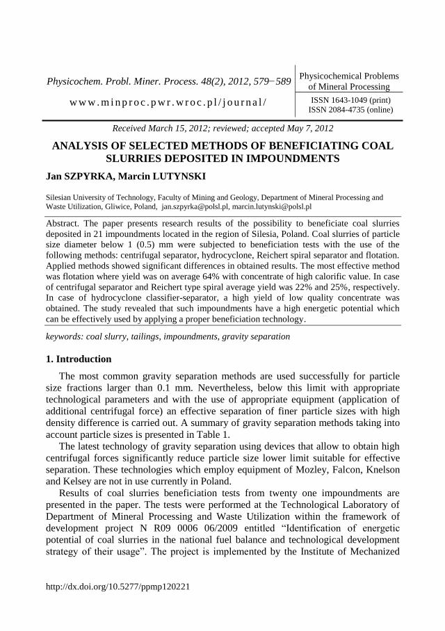
http://dx.doi.org/10.5277/ppmp120221
Physicochem. Probl. Miner. Process. 48(2), 2012, 579−589 Physicochemical Problems
of Mineral Processing
w w w . m i n p r o c . p w r . w r o c . p l / j o u r n a l / ISSN 1643-1049 (print)
ISSN 2084-4735 (online)
Received March 15, 2012; reviewed; accepted May 7, 2012
ANALYSIS OF SELECTED METHODS OF BENEFICIATING COAL
SLURRIES DEPOSITED IN IMPOUNDMENTS
Jan SZPYRKA, Marcin LUTYNSKI
Silesian University of Technology, Faculty of Mining and Geology, Department of Mineral Processing and
Waste Utilization, Gliwice, Poland, [email protected], [email protected]
Abstract. The paper presents research results of the possibility to beneficiate coal slurries
deposited in 21 impoundments located in the region of Silesia, Poland. Coal slurries of particle
size diameter below 1 (0.5) mm were subjected to beneficiation tests with the use of the
following methods: centrifugal separator, hydrocyclone, Reichert spiral separator and flotation.
Applied methods showed significant differences in obtained results. The most effective method
was flotation where yield was on average 64% with concentrate of high calorific value. In case
of centrifugal separator and Reichert type spiral average yield was 22% and 25%, respectively.
In case of hydrocyclone classifier-separator, a high yield of low quality concentrate was
obtained. The study revealed that such impoundments have a high energetic potential which
can be effectively used by applying a proper beneficiation technology.
keywords: coal slurry, tailings, impoundments, gravity separation
1. Introduction
The most common gravity separation methods are used successfully for particle
size fractions larger than 0.1 mm. Nevertheless, below this limit with appropriate
technological parameters and with the use of appropriate equipment (application of
additional centrifugal force) an effective separation of finer particle sizes with high
density difference is carried out. A summary of gravity separation methods taking into
account particle sizes is presented in Table 1.
The latest technology of gravity separation using devices that allow to obtain high
centrifugal forces significantly reduce particle size lower limit suitable for effective
separation. These technologies which employ equipment of Mozley, Falcon, Knelson
and Kelsey are not in use currently in Poland.
Results of coal slurries beneficiation tests from twenty one impoundments are
presented in the paper. The tests were performed at the Technological Laboratory of
Department of Mineral Processing and Waste Utilization within the framework of
development project N R09 0006 06/2009 entitled “Identification of energetic
potential of coal slurries in the national fuel balance and technological development
strategy of their usage”. The project is implemented by the Institute of Mechanized
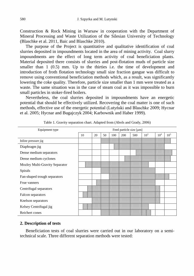
580 J. Szpyrka and M. Lutynski
Construction & Rock Mining in Warsaw in cooperation with the Department of
Mineral Processing and Waste Utilization of the Silesian University of Technology
(Blaschke et al. 2011, Baic and Blaschke 2010).
The purpose of the Project is quantitative and qualitative identification of coal
slurries deposited in impoundments located in the area of mining activity. Coal slurry
impoundments are the effect of long term activity of coal beneficiation plants.
Material deposited there consists of slurries and post-flotation muds of particle size
smaller than 1 (0.5) mm. Up to the thirties i.e. the time of development and
introduction of froth flotation technology small size fraction gangue was difficult to
remove using conventional beneficiation methods which, as a result, was significantly
lowering the coke quality. Therefore, particle size smaller than 1 mm were treated as a
waste. The same situation was in the case of steam coal as it was impossible to burn
small particles in stoker-fired boilers.
Nevertheless, the coal slurries deposited in impoundments have an energetic
potential that should be effectively utilized. Recovering the coal matter is one of such
methods, effective use of the energetic potential (Lutyński and Blaschke 2009; Hycnar
et al. 2005; Hycnar and Bugajczyk 2004; Karbownik and Haber 1999).
Table 1. Gravity separation chart. Adapted from (Abols and Grady, 2006)
Equipment type Feed particle size [μm]
10 20 50 100 200 500 103 104 105
Inline pressure jig
Diaphragm jig
Dense medium separators
Dense medium cyclones
Mozley Multi-Gravity Separator
Spirals
Fan-shaped trough separators
Frue vanners
Centrifugal separators
Falcon separators
Knelson separators
Kelsey Centrifugal jig
Reichert cones
2. Description of tests
Beneficiation tests of coal slurries were carried out in our laboratory on a semi-
technical scale. Three different separation methods were tested:
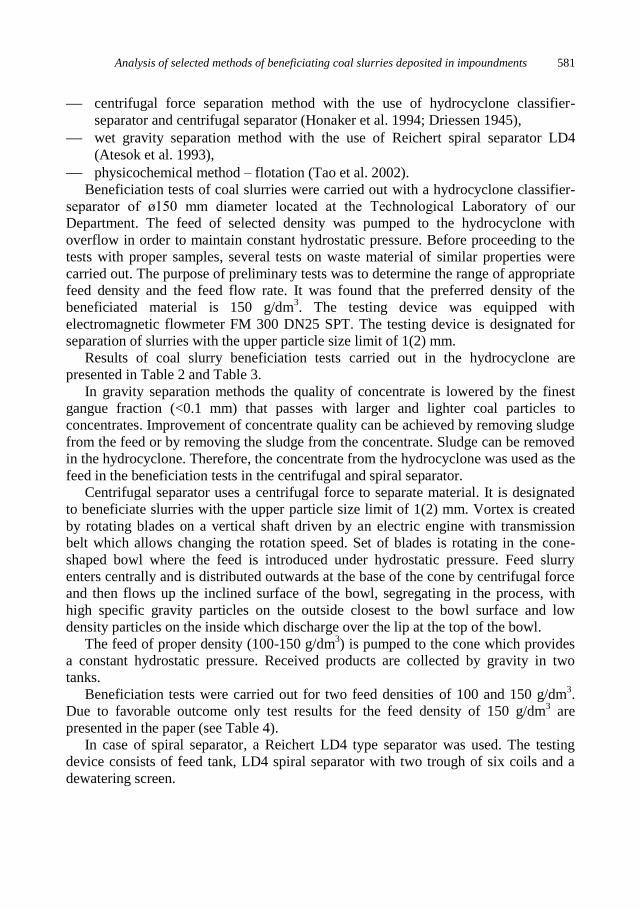
Analysis of selected methods of beneficiating coal slurries deposited in impoundments 581
centrifugal force separation method with the use of hydrocyclone classifier-
separator and centrifugal separator (Honaker et al. 1994; Driessen 1945),
wet gravity separation method with the use of Reichert spiral separator LD4
(Atesok et al. 1993),
physicochemical method – flotation (Tao et al. 2002).
Beneficiation tests of coal slurries were carried out with a hydrocyclone classifier-
separator of ø150 mm diameter located at the Technological Laboratory of our
Department. The feed of selected density was pumped to the hydrocyclone with
overflow in order to maintain constant hydrostatic pressure. Before proceeding to the
tests with proper samples, several tests on waste material of similar properties were
carried out. The purpose of preliminary tests was to determine the range of appropriate
feed density and the feed flow rate. It was found that the preferred density of the
beneficiated material is 150 g/dm3. The testing device was equipped with
electromagnetic flowmeter FM 300 DN25 SPT. The testing device is designated for
separation of slurries with the upper particle size limit of 1(2) mm.
Results of coal slurry beneficiation tests carried out in the hydrocyclone are
presented in Table 2 and Table 3.
In gravity separation methods the quality of concentrate is lowered by the finest
gangue fraction (<0.1 mm) that passes with larger and lighter coal particles to
concentrates. Improvement of concentrate quality can be achieved by removing sludge
from the feed or by removing the sludge from the concentrate. Sludge can be removed
in the hydrocyclone. Therefore, the concentrate from the hydrocyclone was used as the
feed in the beneficiation tests in the centrifugal and spiral separator.
Centrifugal separator uses a centrifugal force to separate material. It is designated
to beneficiate slurries with the upper particle size limit of 1(2) mm. Vortex is created
by rotating blades on a vertical shaft driven by an electric engine with transmission
belt which allows changing the rotation speed. Set of blades is rotating in the cone-
shaped bowl where the feed is introduced under hydrostatic pressure. Feed slurry
enters centrally and is distributed outwards at the base of the cone by centrifugal force
and then flows up the inclined surface of the bowl, segregating in the process, with
high specific gravity particles on the outside closest to the bowl surface and low
density particles on the inside which discharge over the lip at the top of the bowl.
The feed of proper density (100-150 g/dm3) is pumped to the cone which provides
a constant hydrostatic pressure. Received products are collected by gravity in two
tanks.
Beneficiation tests were carried out for two feed densities of 100 and 150 g/dm3.
Due to favorable outcome only test results for the feed density of 150 g/dm3 are
presented in the paper (see Table 4).
In case of spiral separator, a Reichert LD4 type separator was used. The testing
device consists of feed tank, LD4 spiral separator with two trough of six coils and a
dewatering screen.
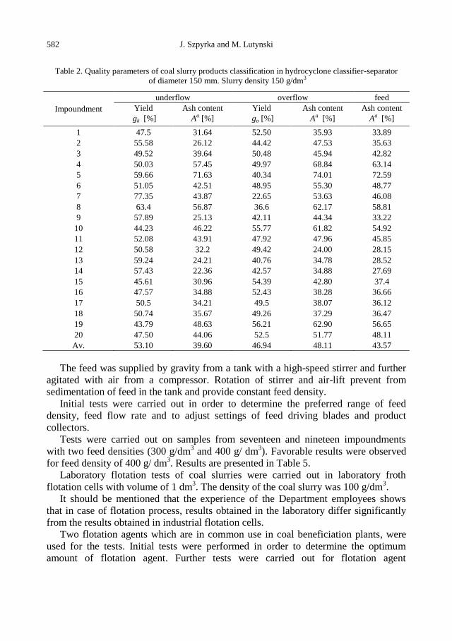
582 J. Szpyrka and M. Lutynski
Table 2. Quality parameters of coal slurry products classification in hydrocyclone classifier-separator
of diameter 150 mm. Slurry density 150 g/dm3
Impoundment
underflow overflow feed
Yield Ash content Yield Ash content Ash content
gk [%] Aa [%] go [%] Aa [%] Aa [%]
1 47.5 31.64 52.50 35.93 33.89
2 55.58 26.12 44.42 47.53 35.63
3 49.52 39.64 50.48 45.94 42.82
4 50.03 57.45 49.97 68.84 63.14
5 59.66 71.63 40.34 74.01 72.59
6 51.05 42.51 48.95 55.30 48.77
7 77.35 43.87 22.65 53.63 46.08
8 63.4 56.87 36.6 62.17 58.81
9 57.89 25.13 42.11 44.34 33.22
10 44.23 46.22 55.77 61.82 54.92
11 52.08 43.91 47.92 47.96 45.85
12 50.58 32.2 49.42 24.00 28.15
13 59.24 24.21 40.76 34.78 28.52
14 57.43 22.36 42.57 34.88 27.69
15 45.61 30.96 54.39 42.80 37.4
16 47.57 34.88 52.43 38.28 36.66
17 50.5 34.21 49.5 38.07 36.12
18 50.74 35.67 49.26 37.29 36.47
19 43.79 48.63 56.21 62.90 56.65
20 47.50 44.06 52.5 51.77 48.11
Av. 53.10 39.60 46.94 48.11 43.57
The feed was supplied by gravity from a tank with a high-speed stirrer and further
agitated with air from a compressor. Rotation of stirrer and air-lift prevent from
sedimentation of feed in the tank and provide constant feed density.
Initial tests were carried out in order to determine the preferred range of feed
density, feed flow rate and to adjust settings of feed driving blades and product
collectors.
Tests were carried out on samples from seventeen and nineteen impoundments
with two feed densities (300 g/dm3 and 400 g/ dm
3). Favorable results were observed
for feed density of 400 g/ dm3. Results are presented in Table 5.
Laboratory flotation tests of coal slurries were carried out in laboratory froth
flotation cells with volume of 1 dm3. The density of the coal slurry was 100 g/dm
3.
It should be mentioned that the experience of the Department employees shows
that in case of flotation process, results obtained in the laboratory differ significantly
from the results obtained in industrial flotation cells.
Two flotation agents which are in common use in coal beneficiation plants, were
used for the tests. Initial tests were performed in order to determine the optimum
amount of flotation agent. Further tests were carried out for flotation agent

Analysis of selected methods of beneficiating coal slurries deposited in impoundments 583
concentration of 0.4, 0.5 and 0.6 kg per Mg of dry material. Best results were obtained
for the concentration of flotation agent of 0.6 kg per Mg of dry material.
Table 3. Quality parameters of concentrate (underflow from hydrocyclone classifier-separator)
obtained for classification of 0.1 mm sorted particle size
Impoundment
Concentrate (underflow)
Yield Ash content Hydroscopic moisture Sulfur content Calorific value
k Aa [%] Wex [%] Sca [%] Qa [%]
1 47.50 31.64 6.65 1.34 18121
2 55.58 26.12 6.43 0.76 20362
3 49.52 39.64 5.30 1.02 17281
4 50.03 57.45 4.41 0.58 9295
5 59.66 71.63 4.59 0.66 8576
6 51.05 42.51 5.32 0.96 15990
7 77.35 43.87 1.33 3.42 16277
8 63.40 56.87 1.22 2.04 12027
9 57.89 25.13 2.89 0.70 24234
10 44.23 46.22 4.09 1.09 13444
11 52.08 43.91 1.50 1.05 17972
12 50.58 32.2 2.19 0.35 24363
13 59.24 24.21 1.99 0.61 24,557
14 57.43 22.36 2.02 0.83 25501
15 45.61 30.96 1.88 0.86 21415
16 47.57 34.88 2.21 0.85 21085
17 50.50 34.21 1.69 1.12 21161
18 50.74 35.67 2.22 1.06 21844
19 43.79 48.63 3.30 0.82 12008
20 47.50 44.06 2.12 0.74 18022
Av. 53.10 39.60 3.16 1.04 16950
Tests were conducted on samples from all impoundments. A positive flotation test
result was assumed when 80% of the samples had a positive flotation effect. In case of
samples from one impoundment a positive test was considered when 66% of the
samples had a yield greater than 30% and the ash content in concentrate was lower
than 25%. These criteria were fulfilled for the samples from 12 impoundments.
Results of tests for the flotation agent 2 which was considered as preferable are
presented in Table 6.
3. Results of investigation
Results of tests carried out were summarized in Tables 2 to 8. In Tables 7 and 8 a
comparison of selected results from different separation methods is shown. Presented
results are both for concentrate and tailings. It seems that obtained results indicate the
efficiency of selected method (Fig. 1). In Figures 2 and 3 washability curves for the
two most favorable results of hydrocyclone separation are presented.
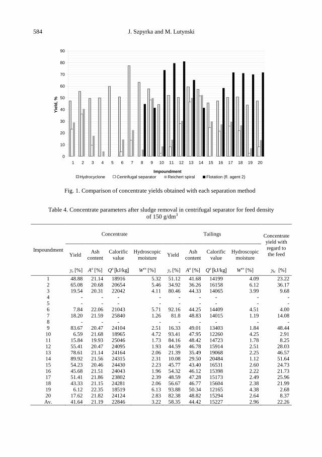
584 J. Szpyrka and M. Lutynski
0
10
20
30
40
50
60
70
80
90
1 2 3 4 5 6 7 8 9 10 11 12 13 14 15 16 17 18 19 20
Impoundment
Yie
ld,
%
Hydrocyclone Centrifugal separator Reichert spiral Flotation (fl. agent 2)
Fig. 1. Comparison of concentrate yields obtained with each separation method
Table 4. Concentrate parameters after sludge removal in centrifugal separator for feed density
of 150 g/dm3
Impoundment
Concentrate Tailings Concentrate yield with
regard to
the feed Yield Ash
content
Calorific
value
Hydroscopic
moisture Yield
Ash
content
Calorific
value
Hydroscopic
moisture
o [%] Aa [%] Qa [kJ/kg] Wex [%] o [%] Aa [%] Qa
[kJ/kg] Wex [%] kc [%]
1 48.88 21.14 18916 5.32 51.12 41.68 14199 4.09 23.22
2 65.08 20.68 20654 5.46 34.92 36.26 16158 6.12 36.17 3 19.54 20.31 22042 4.11 80.46 44.33 14065 3.99 9.68
4 - - - - - - - - -
5 - - - - - - - - - 6 7.84 22.06 21043 5.71 92.16 44.25 14409 4.51 4.00
7 18.20 21.59 25840 1.26 81.8 48.83 14015 1.19 14.08
8 - - - - - - - - - 9 83.67 20.47 24104 2.51 16.33 49.01 13403 1.84 48.44
10 6.59 21.68 18965 4.72 93.41 47.95 12260 4.25 2.91 11 15.84 19.93 25046 1.73 84.16 48.42 14723 1.78 8.25
12 55.41 20.47 24095 1.93 44.59 46.78 15914 2.51 28.03
13 78.61 21.14 24164 2.06 21.39 35.49 19068 2.25 46.57 14 89.92 21.56 24315 2.31 10.08 29.50 20484 1.12 51.64
15 54.23 20.46 24430 2.23 45.77 43.40 16531 2.60 24.73
16 45.68 21.51 24043 1.96 54.32 46.12 15398 2.22 21.73 17 51.41 21.86 23802 2.39 48.59 47.28 15173 2.49 25.96
18 43.33 21.15 24281 2.06 56.67 46.77 15604 2.38 21.99
19 6.12 22.35 18519 6.13 93.88 50.34 12165 4.38 2.68 20 17.62 21.82 24124 2.83 82.38 48.82 15294 2.64 8.37
Av. 41.64 21.19 22846 3.22 58.35 44.42 15227 2.96 22.26
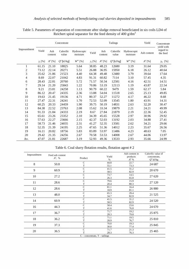
Analysis of selected methods of beneficiating coal slurries deposited in impoundments 585
Table 5. Parameters of separation of concentrate after sludge removal beneficiated in six coils LD4 of
Reichert spiral separator for the feed density of 400 g/dm3
Impoundment
Concentrate Tailings Yield Concentrate
yield with
regard to
the feed Yield Ash
content
Calorific
value
Hydroscopic
moisture Yield
Ash
content
Calorific
value
Hydroscopic
moisture Ash content
o [%] Aa [%] Qa [kJ/kg] Wex [%] o [%] Aa [%] Qa
[kJ/kg] Wex [%] Aa [%] kc [%]
1 61.15 21.10 18825 5.64 38.85 48.23 12680 3.19 31.64 29.05
2 73.12 22.14 20271 5.51 26.88 36.95 15950 6.18 26.12 40.64
3 35.62 21.86 21523 4.40 64.38 49.48 12480 3.79 39.64 17.64
4 8.69 22.07 21042 4.83 91.31 60.82 7114 3.10 57.45 4.35
6 28.43 22.81 20760 5.72 71.57 50.34 12581 4.16 42.51 14.51
7 29.14 21.20 25843 1.22 70.86 53.19 12113 1.19 43.87 22.54
8 9.21 23.81 24258 1.13 90.79 60.22 9479 1.59 62.17 5.84
9 86.12 20.47 24335 2.36 13.88 54.04 11518 2.65 25.13 49.85
10 19.63 21.45 19136 4.71 80.37 52.27 11272 4.17 46.22 8.68
11 27.47 22.31 24241 1.70 72.53 52.09 13545 1.80 43.91 14.31
12 60.25 20.33 24459 1.90 39.75 50.19 14831 2.63 32.20 30.47
13 84.38 22.52 23763 2.08 15.62 33.34 19879 2.21 24.21 49.99
14 91.33 21.84 24333 2.19 8.67 27.84 21879 2.19 22.36 52.45
15 65.61 23.26 23352 2.10 34.39 45.65 15528 2.97 30.96 29.92
16 57.63 22.27 23666 2.15 42.37 52.03 13192 2.03 34.88 27.41
17 58.73 21.46 24035 2.31 41.27 52.35 13581 2.62 34.21 29.66
18 52.35 21.39 24195 2.25 47.65 51.36 14012 2.23 35.67 26.56
19 16.11 20.82 18756 5.83 83.89 53.97 11486 4.23 48.63 7.05
20 29.42 21.35 24256 2.67 70.58 53.53 14008 2.67 44.06 13.97
Av. 47.07 21.81 22687 3.19 52.93 49.36 13533 2.93 35.66 24.99
Table 6. Coal slurry flotation results, flotation agent # 2
Impoundment Feed ash content
Aa, %
Product
Yield
%
Ash content in
products
Aa %
Calorific value of
concentrate,
Qa kJ/kg
8 50.8 C
T
44.8
55.1
22.7
73.3 24 687
9 60.9 C
T
41.5
58.5
31.2
82.9 20 670
10 27.2 C
T
73.7
26.3
14.5
65.8 27 620
11 28.6 C
T
79.6
20.4
15.9
80.3 27 120
12 28.6 C
T
81.1
18.9
16.4
81.1 26 880
13 48.0 C
T
65.3
34.7
29.4
82.9 21 525
14 60.9 C
T
41.5
58.5
31.2
82.9 24 520
16 44.3 C
T
58.4
41.6
23.6
76.8 24 670
17 36.7 C
T
71.7
28.3
19.2
79.8 25 875
18 36.2 C
T
71.1
28.9
19.5
76.7 25 810
19 37.3 C
T
70.0
30.0
19.3
77.4 25 845
20 36.5 C
T
71.7
28.3
21.3
76.3 25 465
C – concentrate, T – tailings
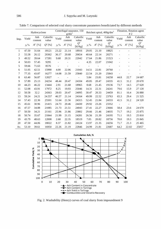
586 J. Szpyrka and M. Lutynski
Table 7. Comparison of selected coal slurry concentrate parameters beneficiated by different methods
Imp.
Hydrocyclone Centrifugal separator, 150
g/dm3 Reichert spiral, 400g/dm3
Flotation, flotation agent
# 2
Yield Ash
content Calorific
value Yield
Ash content
Calorific value
Yield Ash
content Calorific
value Yield
Ash content
Calorific value
k Aa Qa [%] k AaQa
[kJ/kg] k Aa
Qa
[kJ/kg] k Aa
Qa
[kJ/kg]
1 47.50 31.64 18121 23.22 21.14 18916 29.05 21.10 18825 - - -
2 55.58 26.12 20362 36.17 20.68 20654 40.64 22.14 20271 - - -
3 49.52 39.64 17281 9.68 20.31 22042 17.64 21.86 21523 - - -
4 50.03 57.45 9295 - - - 4.35 22.07 21042 - - -
5 59.66 71.63 8576 - - - - - - - - -
6 51.05 42.51 15990 4.00 22.06 21043 14.51 22.81 20760 - - -
7 77.35 43.87 16277 14.08 21.59 25840 22.54 21.20 25843 - - -
8 63.40 56.87 12027 - - - 5.84 23.81 24258 44.8 22.7 24 687
9 57.89 25.13 24234 48.44 20.47 24104 49.85 20.47 24335 41.5 31.2 20 670
10 44.23 46.22 13444 2.91 21.68 18965 8.68 21.45 19136 73.7 14.5 27 620
11 52.08 43.91 17972 8.25 19.93 25046 14.31 22.31 24241 79.6 15.9 27 120
12 50.58 32.2 24363 28.03 20.47 24095 30.47 20.33 24459 81.1 16.4 26 880
13 59.24 24.21 24.557 46.57 21.14 24164 49.99 22.52 23763 65.3 29.4 21 525
14 57.43 22.36 25501 51.64 21.56 24315 52.45 21.84 24333 41.5 31.2 24 520
15 45.61 30.96 21415 24.73 20.46 24430 29.92 23.26 23352 - - -
16 47.57 34.88 21085 21.73 21.51 24043 27.41 22.27 23666 58.4 23.6 24 670
17 50.50 34.21 21161 25.96 21.86 23802 29.66 21.46 24035 71.7 19.2 25 875
18 50.74 35.67 21844 21.99 21.15 24281 26.56 21.39 24195 71.1 19.5 25 810
19 43.79 48.63 12008 2.68 22.35 18519 7.05 20.82 18756 70.0 19.3 25 845
20 47.50 44.06 18022 8.37 21.82 24124 13.97 21.35 24256 71.7 21.3 25 465
Av. 53.10 39.61 16950 22.26 21.19 22846 24.99 21.81 22687 64.2 22.02 25057
0
10
20
30
40
50
60
70
80
90
100
0 10 20 30 40 50 60 70 80 90 100
Cumulative Ash, %
Cu
mu
lati
ve Y
ield
, %
Ash Content in ConcentrateAsh Content in TailingsAsh Yield in TailingsCombustible and Volatile Recovery
Fig. 2. Washability (Henry) curves of coal slurry from impoundment 9
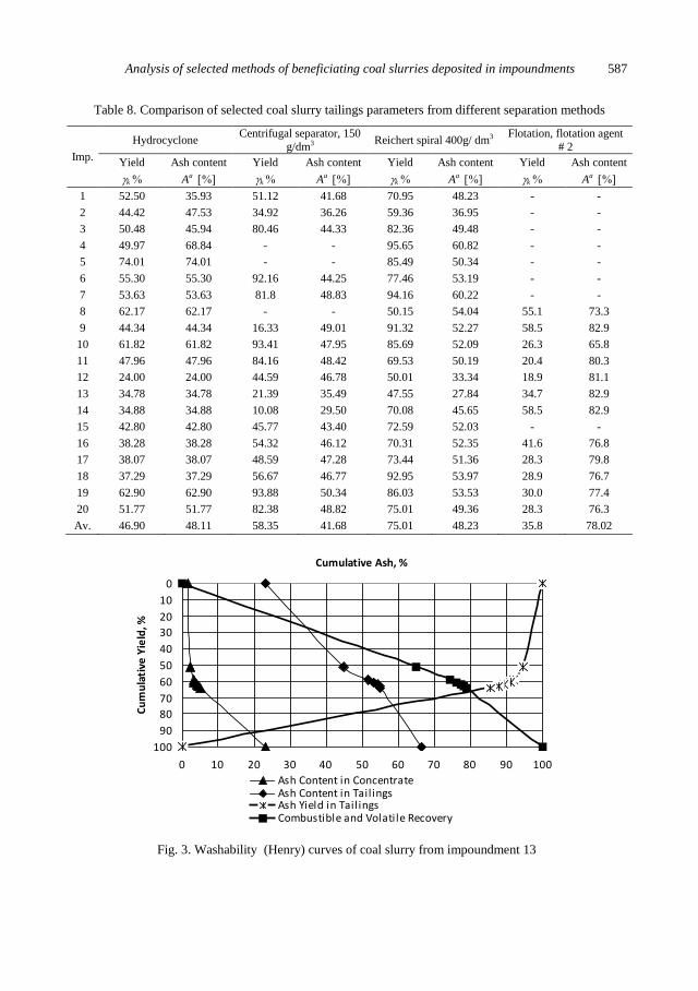
Analysis of selected methods of beneficiating coal slurries deposited in impoundments 587
Table 8. Comparison of selected coal slurry tailings parameters from different separation methods
Imp.
Hydrocyclone Centrifugal separator, 150
g/dm3 Reichert spiral 400g/ dm3
Flotation, flotation agent
# 2
Yield Ash content Yield Ash content Yield Ash content Yield Ash content
k Aa k Aa k Aa k Aa
1 52.50 35.93 51.12 41.68 70.95 48.23 - -
2 44.42 47.53 34.92 36.26 59.36 36.95 - -
3 50.48 45.94 80.46 44.33 82.36 49.48 - -
4 49.97 68.84 - - 95.65 60.82 - -
5 74.01 74.01 - - 85.49 50.34 - -
6 55.30 55.30 92.16 44.25 77.46 53.19 - -
7 53.63 53.63 81.8 48.83 94.16 60.22 - -
8 62.17 62.17 - - 50.15 54.04 55.1 73.3
9 44.34 44.34 16.33 49.01 91.32 52.27 58.5 82.9
10 61.82 61.82 93.41 47.95 85.69 52.09 26.3 65.8
11 47.96 47.96 84.16 48.42 69.53 50.19 20.4 80.3
12 24.00 24.00 44.59 46.78 50.01 33.34 18.9 81.1
13 34.78 34.78 21.39 35.49 47.55 27.84 34.7 82.9
14 34.88 34.88 10.08 29.50 70.08 45.65 58.5 82.9
15 42.80 42.80 45.77 43.40 72.59 52.03 - -
16 38.28 38.28 54.32 46.12 70.31 52.35 41.6 76.8
17 38.07 38.07 48.59 47.28 73.44 51.36 28.3 79.8
18 37.29 37.29 56.67 46.77 92.95 53.97 28.9 76.7
19 62.90 62.90 93.88 50.34 86.03 53.53 30.0 77.4
20 51.77 51.77 82.38 48.82 75.01 49.36 28.3 76.3
Av. 46.90 48.11 58.35 41.68 75.01 48.23 35.8 78.02
0
10
20
30
40
50
60
70
80
90
100
0 10 20 30 40 50 60 70 80 90 100
Cumulative Ash, %
Cu
mu
lati
ve Y
ield
, %
Ash Content in ConcentrateAsh Content in TailingsAsh Yield in TailingsCombustible and Volatile Recovery
Fig. 3. Washability (Henry) curves of coal slurry from impoundment 13

588 J. Szpyrka and M. Lutynski
4. Conclusions
Four separation methods presented in the paper show significant differences in
results. The most effective method is the froth flotation where yield was on average
64%, calorific value of the concentrate was approximately 25 MJ/kg and the ash
content approximately 22%. Moreover, tailings showed high ash content. Performed
tests reported that due to flotation agent used this method cannot be applied to all
tested coal slurries. Thus, if this method is to be applied for fine particle size coal
tailings, other more efficient flotation agents must be applied (Laskowski 2004).
Much less favorable results were obtained with the centrifugal separator and
Reichert type LD4 spiral separator. In material used in these types of separators
particle size below 0.1 mm was initially separated in the hydrocyclone. The average
yield for the Reichert spiral was 25% and for the centrifugal separator 22%. The
calorific value of the concentrate was 22.687 MJ/kg and 22.846 MJ/kg, respectively,
and ash content 25% and 22%, respectively. Low ash content was observed in tailings
which was approximately 48% and 58% for the Reichert spiral and centrifugal
separator respectively.
In case of hydrocyclone separation of particle below 0.1 mm in size, a significant
yield (53%) was obtained, while the quality was low. The concentrate had a high ash
content (39.6%) and low calorific value (16.95 MJ/kg) whereas tailings had low ash
content (48.11%). Thus, the separation was inefficient due to the fact that the
concentrate had approximately 38% particles smaller than 0.1 mm fraction and
according to the study of Szpyrka and Lutyński (2012) these particle have a high ash
content.
In conclusion, it should be noted that there is a possibility to upgrade fine coal
particles. This process is of great importance because of considerable amount of coal
deposited in impoundments. An alternative for fine coal beneficiation is a direct
combustion in fluidized bed furnaces. Such furnaces are designed and manufactured
taking into account individual characteristics of the fuel, i.e. particle size and quality
parameters. Some of the materials tested fulfill these criteria (Blaschke 2005,
Grudziński 2005).
References
ABOLS, J.A., GRADY, P.M., 2006, Maximizing Gravity Recovery through the application of multiple
gravity devices. Vancouver, Gekko Systems.
ATESOK, G., YILDIRIM, I., CELIK, M.S., 1993, Applicability of the Reichert spiral for cleaning
bituminous and lignitic coals, a pilot scale study,Int. J. Miner. Process.40(1–2), 33–44.
BAIC, I., BLASCHKE, W., 2010, Identyfikacja mułów węglowych i strategia rozwoju technologicznego
w zakresie ich gospodarczego wykorzystania. Paliwo-bezpieczeństwo środowisko. Innowacyjne
Techniki i Technologie Instytut Techniki Górniczej KOMAG. Gliwice.
BLASCHKE, W., RÓG, L., OSTATKIEWICZ, A., 2011, Jakość produktów odpadowych wydzielanych w
procesach wzbogacania energetycznego węgla kamiennego. Przegląd Górniczy 5, 42‒46.
BLASCHKE, W., 2005, Określenie wartości mułów węglowych zdeponowanych w osadnikach ziemnych.
Materiały VII Ogólnopolskiej Konferencji Naukowej pt. Kompleksowe i szczegółowe problemy
inżynierii środowiska. Politechnika Koszalińska. Koszalin.
Analysis of selected methods of beneficiating coal slurries deposited in impoundments 589
DRIESSEN, M.G., 1945, The use of centrifugal force for cleaning fine coal in heavy liquids and
suspensions with special reference to the cyclone washer, Journal Institute Fuel.
GRUDZIŃSKI, Z., 2005, Analiza porównawcza jakości mułów węgla kamiennego pochodzących z
bieżącej produkcji i zdeponowanych w osadnikach ziemnych. Materiały VII Ogólnopolskiej
Konferencji Naukowej pt. Kompleksowe i szczegółowe problemy inżynierii środowiska. Politechnika
Koszalińska. Koszalin.
HONAKER, R.Q., PAUL, B.C., WANG, D., HUANG, M., 1994, The Application of Centrifugal
Washing for Fine Coal Cleaning, Preprint, SME Meeting, Albuquerque, New Mexico, February 14-
17, 94‒259.
HYCNAR, J.J., FOLTYN, R., OKULSKI, T., BLASCHKE, S.A., 2005, Kierunki energetycznego
wykorzystania drobnoziarnistych odpadów z wydobycia i wzbogacania węgla kamiennego. VII
Konferencja Naukowa Kompleksowe i szczegółowe problemy inżynierii środowiska. Politechnika
Koszalińska. Koszalin - Ustronie Morskie.
HYCNAR, J.J., BUGAJCZYK, M.,, 2004, Kierunki racjonalnego zagospodarowania drobnoziarnistych
odpadów węglowych. Polityka Energetyczna. Wydawnictwo IGSMiE PAN. Tom 7. Zeszyt Specjalny.
Kraków.
KARBOWNIK, A., HABER, M., 1994, Wykorzystanie mułów węglowych a ochrona środowiska. Karbo
10.
Laskowski J. S., Testing flotation frothers, Physicochemical Problems of Mineral Processing, 38 (2004)
13-22
LUTYŃSKI, A., BLASCHKE, W., 2009, Aktualne kierunki zagospodarowania odpadów przeróbczych
węgla kamiennego. Przegląd Górniczy 10, 33‒35.
SZPYRKA, J., LUTYŃSKI, A., 2012, Właściwości fizyko-chemiczne mułów węglowych zdeponowanych
w osadnikach ziemnych. Innowacyjne i przyjazne dla środowiska techniki i technologie przeróbki
surowców mineralnych. Bezpieczeństwo – jakość – efektywność. Instytut Techniki Górniczej
KOMAG. ISBN 978-83-60708-59-0. Gliwice, 259‒274.
TAO D., LI B, JOHNSON S., PAREKH B.K., 2002, A flotation study of refuse pond coal slurry. Fuel
Processing Technology 76(3), 201–210.

590 J. Szpyrka and M. Lutynski
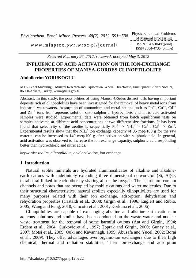
http://dx.doi.org/10.5277/ppmp120222
Physicochem. Probl. Miner. Process. 48(2), 2012, 591−598 Physicochemical Problems
of Mineral Processing
w w w . m i n p r o c . p w r . w r o c . p l / j o u r n a l / ISSN 1643-1049 (print)
ISSN 2084-4735 (online)
Received February 26, 2012; reviewed; accepted May 3, 2012
INFLUENCE OF ACID ACTIVATION ON THE ION-EXCHANGE
PROPERTIES OF MANISA-GORDES CLINOPTILOLITE
Abdulkerim YORUKOGLU
MTA Genel Mudurlugu, Mineral Research and Exploration General Directorate, Dumlupinar Bulvari No:139,
06800-Ankara, Turkey, [email protected]
Abstract. In this study, the possibilities of using Manisa-Gördes district tuffs having important
deposits rich of clinoptilolites have been investigated for the removal of heavy metal ions from
industrial wastewaters. Adsorption of ammonium and metal cations such as Pb++
, Cu++
, Cd++
and Zn++
ions from aqueous solution onto sulphuric, hydrochloric and nitric acid activated
samples were studied. Experimental data were obtained from batch equilibrium tests on
samples activated at different acid concentrations at two different size fractions. It has been
found that selectivity of the zeolite is sequentially Pb++
> NH4+ > Cu
++, Cd
++ > Zn
++.
Experimental results show that the NH4+ ion exchange capacity of 95 meq/100 g for the raw
material can be increased to 140 meq/100 g after activation with sulphuric acid. In general,
acid activation was observed to increase the ion exchange capacity, sulphuric acid responding
better than hydrochloric and nitric acids.
keywords: zeolite, clinoptilolite, acid activation, ion exchange
1. Introduction
Natural zeolite minerals are hydrated aluminosilicates of alkaline and alkaline-
earth cations with indefinitely extending three dimensional network of (Si, Al)O4
tetrahedral linked to each other by sharing all of the oxygen. Their structure contain
channels and pores that are occupied by mobile cations and water molecules. Due to
their structural characteristics, natural zeolites especially clinoptilolites are used for
many purposes related with their ion exchange, adsorption, dehydration and
rehydration properties (Castaldi et al., 2008; Girgin et al., 1996; Englert and Rubio,
2005; Wang and Peng, 2010, Cincotti et al., 2001; Korkuna et al., 2006).
Clinoptilolites are capable of exchanging alkaline and alkaline-earth cations in
aqueous solutions and studies have been conducted on the waste water and nuclear
waste treatment for the removal of some harmful cations (Ata and Girgin, 1994;
Erdem et al., 2004; Curkovic et al., 1997; Toprak and Girgin, 2000; Gunay et al.,
2007; Motsi et al., 2009; Ouki and Kavannagh, 1999; Abusafa and Yucel, 2002; Borai
et al., 2009). They offer advantages over organic-ion exchangers due to their high
chemical, thermal and radiation stabilities. Their ion-exchange and adsorption
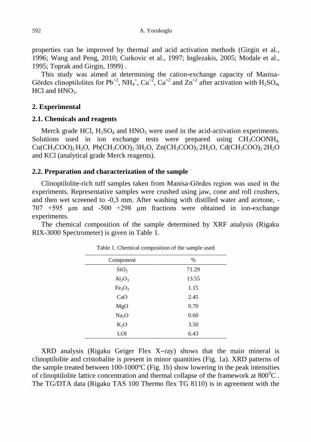
592 A. Yorukoglu
properties can be improved by thermal and acid activation methods (Girgin et al.,
1996; Wang and Peng, 2010; Curkovic et al., 1997; Inglezakis, 2005; Modale et al.,
1995; Toprak and Girgin, 1999) .
This study was aimed at determining the cation-exchange capacity of Manisa-
Gördes clinoptilolites for Pb+2
, NH4+, Cu
+2, Ca
+2 and Zn
+2 after activation with H2SO4,
HCl and HNO3.
2. Experimental
2.1. Chemicals and reagents
Merck grade HCl, H2SO4 and HNO3 were used in the acid-activation experiments.
Solutions used in ion exchange tests were prepared using CH3COONH4,
Cu(CH3COO)2.H2O, Pb(CH3COO)2
.3H2O, Zn(CH3COO)2
.2H2O, Cd(CH3COO)2
.2H2O
and KCl (analytical grade Merck reagents).
2.2. Preparation and characterization of the sample
Clinoptilolite-rich tuff samples taken from Manisa-Gördes region was used in the
experiments. Representative samples were crushed using jaw, cone and roll crushers,
and then wet screened to -0,3 mm. After washing with distilled water and acetone, -
707 +595 µm and -500 +298 µm fractions were obtained in ion-exchange
experiments.
The chemical composition of the sample determined by XRF analysis (Rigaku
RIX-3000 Spectrometer) is given in Table 1.
Table 1. Chemical composition of the sample used
Component %
SiO2 71.29
Al2O3 13.55
Fe2O3 1.15
CaO 2.45
MgO 0.70
Na2O 0.60
K2O 3.50
LOI 6.43
XRD analysis (Rigaku Geiger Flex X ray) shows that the main mineral is
clinoptilolite and cristobalite is present in minor quantities (Fig. 1a). XRD patterns of
the sample treated between 100-1000ºC (Fig. 1b) show lowering in the peak intensities
of clinoptilolite lattice concentration and thermal collapse of the framework at 8000C .
The TG/DTA data (Rigaku TAS 100 Thermo flex TG 8110) is in agreement with the

Influence of acid activation on the ion-exchange properties of Manisa-Gordes clinoptilolite 593
XRD results showing continuous hydration up to 7000C with release of water and an exothermic event at around 924ºC due to the collapse of the structure (Fig. 2).
Considering the K, Na, Ca, Mg contents of the sample, theoretical cation exchange capacity was calculated as 120.74 meq/100g. Also, specific surface area, pore diameter, pore volume and the density (Quantachrome Nova 2000) of the sample were determined as 43.91 m2/g, 0.018 μm, 0.1717 cm3/gr, 2.12 g/cm3, respectively.
Figure 3 shows the electronmicroscopic view of the sample (FEI Qanta 400 MK2 electronmicroscope) where macro and micropores can clearly be seen between the clinoptilolite crystals (Fig. 3d).
(a) (b)
Fig. 1. a)XRD pattern of the sample b) XRD patterns of the sample between 100−1000ºC
Fig. 2. TG/DTA curves of the sample
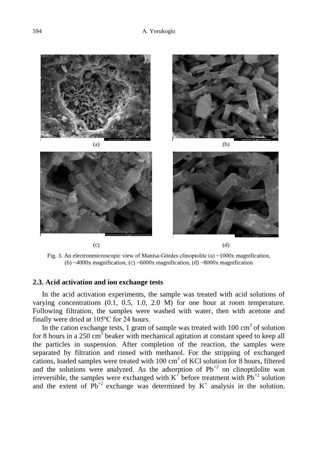
594 A. Yorukoglu
(a)
(b)
(c)
(d)
Fig. 3. An electronmicroscopic view of Manisa-Gördes clinoptolite (a) ~1000x magnification,
(b) ~4000x magnification, (c) ~6000x magnification, (d) ~8000x magnification
2.3. Acid activation and ion exchange tests
In the acid activation experiments, the sample was treated with acid solutions of
varying concentrations (0.1, 0.5, 1.0, 2.0 M) for one hour at room temperature.
Following filtration, the samples were washed with water, then with acetone and
finally were dried at 105ºC for 24 hours.
In the cation exchange tests, 1 gram of sample was treated with 100 cm3 of solution
for 8 hours in a 250 cm3 beaker with mechanical agitation at constant speed to keep all
the particles in suspension. After completion of the reaction, the samples were
separated by filtration and rinsed with methanol. For the stripping of exchanged
cations, loaded samples were treated with 100 cm3 of KCl solution for 8 hours, filtered
and the solutions were analyzed. As the adsorption of Pb+2
on clinoptilolite was
irreversible, the samples were exchanged with K+ before treatment with Pb
+2 solution
and the extent of Pb+2
exchange was determined by K+ analysis in the solution.

Influence of acid activation on the ion-exchange properties of Manisa-Gordes clinoptilolite 595
Ammonium ion was determined by colorimetric method and the other ions were
analyzed using the atomic absorption spectrophotometric method.
The batch technique was used for measurement of cation exchange capacity of
samples (Sub-Committee, 1994) and the cation exchange capacities (CEC) in
meq/100g were determined using equation:
CEC (meq/100g) = (milimoles of sorbed ion / 100g sample) (cation valence).
3. Results and discussion
The NH4+
exchange capacities for the raw sample were determined as 94 meq/100g
and 100 meq/100 g for sample sizes of +595 m and +298 m, respectively. The
effect of particle size and acid concentration were considered in the ion exchange
experiments and the results for acid activated samples are given in Fig. 4.
50
75
100
125
150
50
75
100
125
150
0 0,5 1 1,5 2
CE
C, m
eq/1
00gr
CE
C, m
eq/1
00gr
Acid Concenration, M
HCl
H2SO4
HNO3
+595 m +298 m
0
5
10
15
0
5
10
15
0 0,5 1 1,5 2
CE
C, m
eq/1
00gr
CE
C, m
eq/1
00gr
Acid Concenration, M
HCl
H2SO4
HNO3
+595 m +298 m+595 m +298 m
Fig. 4. NH4
+ exchange capacity of the acid
activated samples
Fig. 5. Zn2+ exchange capacity of the acid
activated samples
Although HCl does not have a significant effect on the ion exchange capacity for
+595 m sample, ion exchange capacity decreases from 93.4 meq/100 g to 78.3
meq/100 g for +298 m sized sample. The highest value obtained for 0.1 M HCl
activated sample for both sizes was determined as 98.5 meq/100 g. Ion exchange
capacity values for +595 m sample activated with 0.1 and 0.5 M HNO3 were reached
to 107.6 meq/100 g and 111 meq/100 g, respectively. But, upon increase of the acid
concentration in the activation, ion exchange capacities were decreased considerably.
Compared to others, better results were obtained with the sample activated using 1 M
H2SO4 and the CEC value was reached to 140.8 meq/100 g for both sizes.
Zn++
exchange capacity of the raw sample for both sizes were quite close to each
other being around 7 meq/100 g. Considering the Zn++
exchange capacities for acid
activated samples (Fig. 5) HCl and HNO3 activated samples showed slight increases in
the exchange capacities. Best results again were obtained with H2SO4 activated sample
and the highest value reached was 11.5 meq/100 g for +595 m size when the
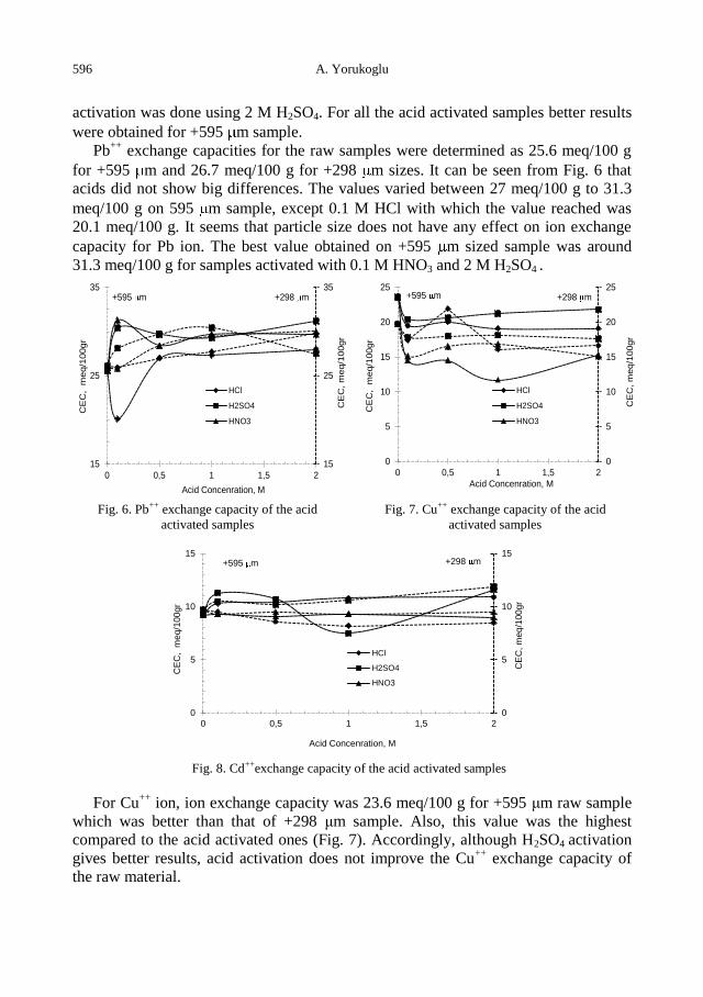
596 A. Yorukoglu
activation was done using 2 M H2SO4. For all the acid activated samples better results
were obtained for +595 m sample.
Pb++
exchange capacities for the raw samples were determined as 25.6 meq/100 g
for +595 m and 26.7 meq/100 g for +298 m sizes. It can be seen from Fig. 6 that
acids did not show big differences. The values varied between 27 meq/100 g to 31.3
meq/100 g on 595 m sample, except 0.1 M HCl with which the value reached was
20.1 meq/100 g. It seems that particle size does not have any effect on ion exchange
capacity for Pb ion. The best value obtained on +595 m sized sample was around
31.3 meq/100 g for samples activated with 0.1 M HNO3 and 2 M H2SO4 .
15
25
35
15
25
35
0 0,5 1 1,5 2
CE
C, m
eq/1
00gr
CE
C, m
eq/1
00gr
Acid Concenration, M
HCl
H2SO4
HNO3
+595 m +298 m
0
5
10
15
20
25
0
5
10
15
20
25
0 0,5 1 1,5 2
CE
C, m
eq/1
00gr
CE
C, m
eq/1
00gr
Acid Concenration, M
HCl
H2SO4
HNO3
+595 m +298 m
Fig. 6. Pb++ exchange capacity of the acid
activated samples
Fig. 7. Cu++ exchange capacity of the acid
activated samples
0
5
10
15
0
5
10
15
0 0,5 1 1,5 2
CE
C, m
eq/1
00gr
CE
C, m
eq/1
00gr
Acid Concenration, M
HCl
H2SO4
HNO3
+595 m +298 m
Fig. 8. Cd++exchange capacity of the acid activated samples
For Cu++
ion, ion exchange capacity was 23.6 meq/100 g for +595 μm raw sample
which was better than that of +298 μm sample. Also, this value was the highest
compared to the acid activated ones (Fig. 7). Accordingly, although H2SO4 activation
gives better results, acid activation does not improve the Cu++
exchange capacity of
the raw material.
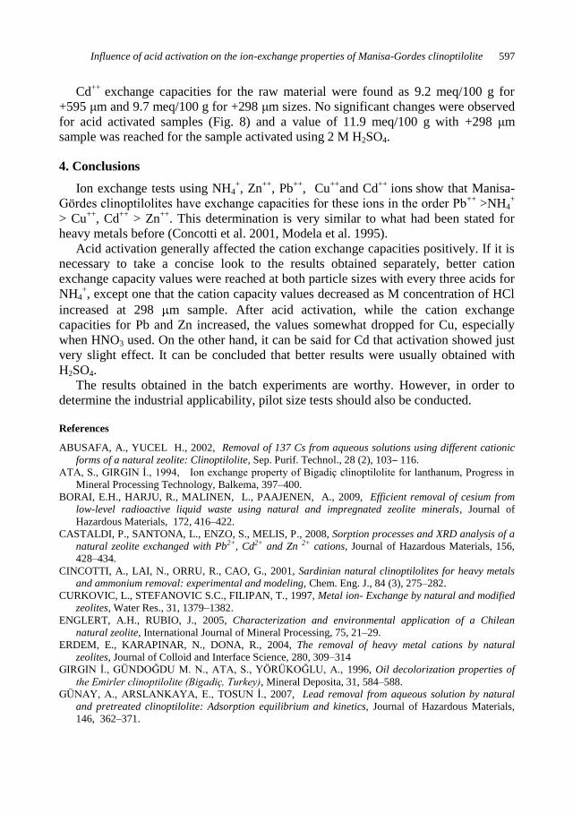
Influence of acid activation on the ion-exchange properties of Manisa-Gordes clinoptilolite 597
Cd++
exchange capacities for the raw material were found as 9.2 meq/100 g for
+595 μm and 9.7 meq/100 g for +298 μm sizes. No significant changes were observed
for acid activated samples (Fig. 8) and a value of 11.9 meq/100 g with +298 μm
sample was reached for the sample activated using 2 M H2SO4.
4. Conclusions
Ion exchange tests using NH4+, Zn
++, Pb
++, Cu
++and Cd
++ ions
show that Manisa-
Gördes clinoptilolites have exchange capacities for these ions in the order Pb++
>NH4+
> Cu++
, Cd++
> Zn++
. This determination is very similar to what had been stated for
heavy metals before (Concotti et al. 2001, Modela et al. 1995).
Acid activation generally affected the cation exchange capacities positively. If it is
necessary to take a concise look to the results obtained separately, better cation
exchange capacity values were reached at both particle sizes with every three acids for
NH4+, except one that the cation capacity values decreased as M concentration of HCl
increased at 298 m sample. After acid activation, while the cation exchange
capacities for Pb and Zn increased, the values somewhat dropped for Cu, especially
when HNO3 used. On the other hand, it can be said for Cd that activation showed just
very slight effect. It can be concluded that better results were usually obtained with
H2SO4.
The results obtained in the batch experiments are worthy. However, in order to
determine the industrial applicability, pilot size tests should also be conducted.
References
ABUSAFA, A., YUCEL H., 2002, Removal of 137 Cs from aqueous solutions using different cationic
forms of a natural zeolite: Clinoptilolite, Sep. Purif. Technol., 28 (2), 103‒ 116.
ATA, S., GIRGIN İ., 1994, Ion exchange property of Bigadiç clinoptilolite for lanthanum, Progress in
Mineral Processing Technology, Balkema, 397–400.
BORAI, E.H., HARJU, R., MALINEN, L., PAAJENEN, A., 2009, Efficient removal of cesium from
low-level radioactive liquid waste using natural and impregnated zeolite minerals, Journal of
Hazardous Materials, 172, 416–422.
CASTALDI, P., SANTONA, L., ENZO, S., MELIS, P., 2008, Sorption processes and XRD analysis of a
natural zeolite exchanged with Pb2+, Cd2+ and Zn 2+ cations, Journal of Hazardous Materials, 156,
428–434.
CINCOTTI, A., LAI, N., ORRU, R., CAO, G., 2001, Sardinian natural clinoptilolites for heavy metals
and ammonium removal: experimental and modeling, Chem. Eng. J., 84 (3), 275–282.
CURKOVIC, L., STEFANOVIC S.C., FILIPAN, T., 1997, Metal ion- Exchange by natural and modified
zeolites, Water Res., 31, 1379–1382.
ENGLERT, A.H., RUBIO, J., 2005, Characterization and environmental application of a Chilean
natural zeolite, International Journal of Mineral Processing, 75, 21–29.
ERDEM, E., KARAPINAR, N., DONA, R., 2004, The removal of heavy metal cations by natural
zeolites, Journal of Colloid and Interface Science, 280, 309–314
GIRGIN İ., GÜNDOĞDU M. N., ATA, S., YÖRÜKOĞLU, A., 1996, Oil decolorization properties of
the Emirler clinoptilolite (Bigadiç, Turkey), Mineral Deposita, 31, 584–588.
GÜNAY, A., ARSLANKAYA, E., TOSUN İ., 2007, Lead removal from aqueous solution by natural
and pretreated clinoptilolite: Adsorption equilibrium and kinetics, Journal of Hazardous Materials,
146, 362–371.
598 A. Yorukoglu
INGLEZAKIS, V.J., 2005, The concept of “capacity” in zeolite ion-exchange systems, Journal of Colloid
and Interface Science 281, 68–79.
KORKUNA, O., LEBODA, R., SKUBISZEWSKA-ZEEBA, J., VRUBLEVS’KA, T., GUN’KO, V.M.,
RYCZKOWSKI, J., 2006, Structural and physicochemical properties of natural zeolites:
clinoptilolite and mordenite, Microporous and Mesoporous Materials 84, 243–254.
MONDALE, K.D., CARLAND, R.M., APLAN, F.F., 1995, The comparative ion exchange capacities of
natural sedimentary and synthetic zeolites, Minerals Engineering 8, 535–548.
Motsi, T., Rowson N.A., Simmons M.J.H., 2009, Adsorption of heavy metals from acid mine drainage by
natural Zeolite, International Journal of Mineral processing 92, 42–48.
OUKI, S.K., KAVANNAGH M., 1999, Treatment of metals-contaminated wastewaters by use of natural
zeolites, Wat.Sci.Tech., 39, 115‒ 122.
SUB-COMMITTEE MEMBER from Okutama Kogyo Co Ltd., Tokyo Japan., 1994, Method for
Measurements of Cation Exchange Capacity (CEC), “Natural Zeolite and its Utilization” Edit
No:111 committee CSPTS Jacarta SPS, 319–325.
TOPRAK R., GIRGIN İ., 2000, Aktifleştirilmiş klinoploliteile deri sanayi atık sularından kromun
giderilmesi, Turk J. Engin. Environ. Sci., 24, 343–351.
TOPRAK, R., GIRGIN, İ., 1999, Balıkesir – Bigadiç klinoptilolitlerinin adsorplama özelliklerinin
iyileştirilmesi için anorganik asitlerle aktivasyonu, Yerbilimleri, 21, 201–209.
WANG, S.,PENG, Y., 2010, Natural zeolites as effective adsorbents in water and wastewater treatment,
Chemical Engineering Journal, 156, 11–24.

http://dx.doi.org/10.5277/ppmp120223
Physicochem. Probl. Miner. Process. 48(2), 2012, 599−606 Physicochemical Problems
of Mineral Processing
w w w . m i n p r o c . p w r . w r o c . p l / j o u r n a l / ISSN 1643-1049 (print)
ISSN 2084-4735 (online)
Received April 13, 2012; reviewed; accepted May 4, 2012
LEACHING CHARACTERISTICS OF EAF AND AOD STAINLESS
STEEL PRODUCTION DUSTS
Antti KEKKI, Jari AROMAA, Olof FORSEN
Aalto University, Department of Materials Science and Engineering, PO Box 16200, FI-0076, Aalto, Finland,
email: [email protected]
Abstract. In this paper sulfuric acid leaching of four different stainless steel production flue
dusts is studied. The main objective is to study and compare the valuable metal Zn, Cr, Ni, Fe,
Mo dissolution present in the EAF 1&2 (electric arc furnace) and AOD 1&2 (argon oxygen
decarburization converter) dusts. The effect of sulfuric acid concentration, temperature and
liquid-to-solid ratio are tested for maximum and selective Zn leaching into solution for
recycling purposes. Leaching tests were done in 0.1 M, 0.5 M and 1.5 M sulfuric acid, at
temperatures of 30ºC, 60ºC and 90ºC with liquid-to-solid ratios L:S = 10 and 20 under 1 bar
pressure for 120 minutes. Maximum Zn dissolution yield was achieved with 1.5M, 90ºC, L:S =
10 where the Zn dissolution yield varied from 65% to almost 100%, depending on the dust type
(AOD, EAF) and production line (1 or 2). At the same time Cr was leached 7 – 17%, Ni 37 –
48%, Fe 48 – 89% and Mo 82 – 100%. The best zinc selectivity vs. Cr, Ni, Fe, Mo was
achieved with 0.5 M, 30ºC and L:S 10. The Zn dissolution varied between 33 – 72%, Cr 2 –
4%, Ni 6 – 9%, Fe 2 – 9% and Mo 1 – 55%. Higher temperature and acid concentration
resulted in faster dissolution of metals. AOD dust in both lines 1 and 2 has better valuable
metal recycling possibilities than EAF dust due to better maximum Zn dissolution and better
selective dissolution of Zn vs. Cr, Ni, Fe, Mo.
keywords: stainless steel dust leaching, EAF, electric arc furnace AOD, argon oxygen
decarburization converter, hydrometallurgy, recycling
1. Introduction
Various amounts of wide range metal containing dusts are generated in separate
parts of stainless steel process. In electric arc furnace (EAF), for example, about 1-2%
of the charge is turned into dust (Steinlechner and Antrekowitsch, 2010; Tsakiridis
and Oustadakis, 2010). Both the EAF and AOD dusts contains various amounts of
chromium, nickel, iron, zinc and other heavy metal oxides and the weight percent of
these elements usually varies from batch to batch basis (Nyirenda, 1991; Machado and
Brehm, 2006; Tsakiridis and Oustadakis, 2010). Due to stricter environmental
regulation laws and high price of stainless alloying elements, the valuable segment
(Cr, Ni, Mo) of the stainless steel dusts are in the interest to be recycled back to
600 A. Kekki et al.
process, and the rest, small part of the harmful materials that are now landfilled, to be
neutralized or minimized.
Today, most part of the carbon steel and stainless steel dusts are treated in separate
plants mainly by pyrometallurgical methods to recover majority of the valuable
materials (Zn, Cr, Ni, Mo) for re-use. However, some part of the flue dusts are still
stored as landfill, mainly in developing countries (Nasmyth and Cooper, 2010;
Ruetten 2010; Steinlechner and Antrekowitsch, 2010).
Hydrometallurgical methods instead of pyrometallurgical ones can offer energy
savings and lower CO2 emissions. Still, many hydrometallurgical processes have been
investigated in the past three decades but virtually none of them have passed to wider
industrial scale use. The main problem in steel dust leaching is the low yield and
separability of zinc. Usually over 50% of Zn in the dusts exists in zinc ferrite structure
ZnFe2O4 (franklinite) which makes the selective leaching of Zn without Fe difficult,
whereas ZnO (zincite) phase does not cause problems and dissolves easily (LeClerc et
al., 2003; Havlik et al., 2005; Havlik et al., 2006; Langová and Matýsek, 2010).
Depending on its current price, the recovery method and amount in the dust, zinc is a
valuable material resource for recycling to primary zinc production but a major
impurity if recycled back to stainless steel process with Cr, Ni, Mo and Fe. Zinc is a
volatile component which recirculates and adds up in the furnace and ventilation
system (Nyirenda, 1991). In hydrometallurgical research, Zn - Fe separation and zinc
recovery especially from carbon steel dusts, mainly from EAF dusts, has been the
most researched topic. However, very few research projects have been focused on
other types of dusts, i.e. AOD dust, or in general, on stainless steel dusts to recover Cr,
Ni, Mo and Fe. Thus, a developed method to recover these valuable elements by
hydrometallurgical means is relatively unknown. This might be due to the fact that
stainless steel dust recycling by pyrometallurgical methods is well established and the
value and concentration of the recovered elements has been sufficiently high to offset
the high-energy consumption, the generation of worthless residues to landfill and high
CO2 emissions (Nyirenda, 1991; Tsakiridis and Oustadakis, 2010).
There are numerous reports of EAF carbon steel dust leaching and treatment
experiments in atmospheric pressure with sulfuric acid but the results vary greatly
depending on the dust composition and leaching conditions (Nyirenda, 1991; Cruells
et al., 1992; Strobos and Friend, 2004; Havlik et al., 2005; Shawabkeh, 2010;
Tsakiridis and Oustadakis, 2010). Hydrochloric acid is found to be a quite effective
lixiviant for the steel dusts zinc ferrite spinel (Baik and Fray, 2000). Jha et al. (2001)
have done a review of different hydrometallurgical dust treatment processes for zinc
recovery from industrial wastes. Havlik et al. (2004), Nyirenda (1991) and Zunkel
(2001) discuss generally hydrometallurgical methods and problems encountered in
carbon steel (EAF) dust treatment. For example, it is known fact that Cl and F are
detrimental elements with very small ppm level amounts in the liquid phase if
considering recycling zinc back to Zn primary metallurgy. The same problems and
methods apply to some extent also in stainless steel dust treatment, for example
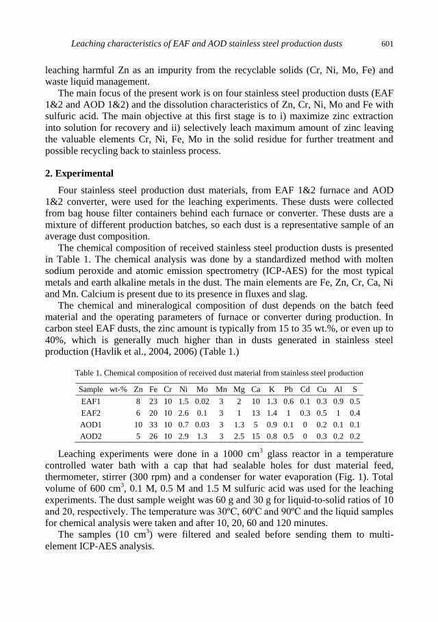
Leaching characteristics of EAF and AOD stainless steel production dusts 601
leaching harmful Zn as an impurity from the recyclable solids (Cr, Ni, Mo, Fe) and
waste liquid management.
The main focus of the present work is on four stainless steel production dusts (EAF
1&2 and AOD 1&2) and the dissolution characteristics of Zn, Cr, Ni, Mo and Fe with
sulfuric acid. The main objective at this first stage is to i) maximize zinc extraction
into solution for recovery and ii) selectively leach maximum amount of zinc leaving
the valuable elements Cr, Ni, Fe, Mo in the solid residue for further treatment and
possible recycling back to stainless process.
2. Experimental
Four stainless steel production dust materials, from EAF 1&2 furnace and AOD
1&2 converter, were used for the leaching experiments. These dusts were collected
from bag house filter containers behind each furnace or converter. These dusts are a
mixture of different production batches, so each dust is a representative sample of an
average dust composition.
The chemical composition of received stainless steel production dusts is presented
in Table 1. The chemical analysis was done by a standardized method with molten
sodium peroxide and atomic emission spectrometry (ICP-AES) for the most typical
metals and earth alkaline metals in the dust. The main elements are Fe, Zn, Cr, Ca, Ni
and Mn. Calcium is present due to its presence in fluxes and slag.
The chemical and mineralogical composition of dust depends on the batch feed
material and the operating parameters of furnace or converter during production. In
carbon steel EAF dusts, the zinc amount is typically from 15 to 35 wt.%, or even up to
40%, which is generally much higher than in dusts generated in stainless steel
production (Havlik et al., 2004, 2006) (Table 1.)
Table 1. Chemical composition of received dust material from stainless steel production
Sample wt-% Zn Fe Cr Ni Mo Mn Mg Ca K Pb Cd Cu Al S
EAF1 8 23 10 1.5 0.02 3 2 10 1.3 0.6 0.1 0.3 0.9 0.5
EAF2 6 20 10 2.6 0.1 3 1 13 1.4 1 0.3 0.5 1 0.4
AOD1 10 33 10 0.7 0.03 3 1.3 5 0.9 0.1 0 0.2 0.1 0.1
AOD2 5 26 10 2.9 1.3 3 2.5 15 0.8 0.5 0 0.3 0.2 0.2
Leaching experiments were done in a 1000 cm3 glass reactor in a temperature
controlled water bath with a cap that had sealable holes for dust material feed,
thermometer, stirrer (300 rpm) and a condenser for water evaporation (Fig. 1). Total
volume of 600 cm3, 0.1 M, 0.5 M and 1.5 M sulfuric acid was used for the leaching
experiments. The dust sample weight was 60 g and 30 g for liquid-to-solid ratios of 10
and 20, respectively. The temperature was 30ºC, 60ºC and 90ºC and the liquid samples
for chemical analysis were taken and after 10, 20, 60 and 120 minutes.
The samples (10 cm3) were filtered and sealed before sending them to multi-
element ICP-AES analysis.
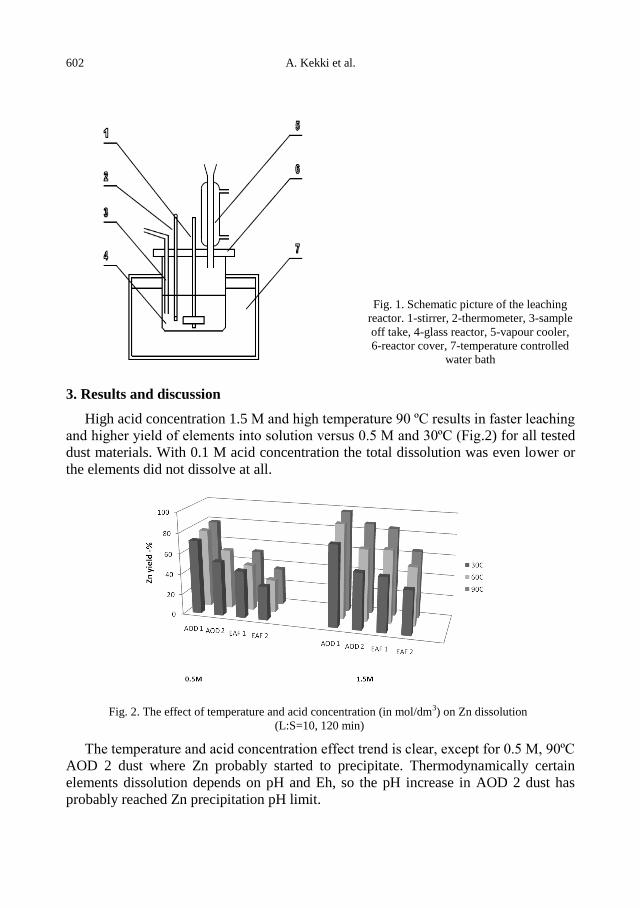
602 A. Kekki et al.
Fig. 1. Schematic picture of the leaching
reactor. 1-stirrer, 2-thermometer, 3-sample
off take, 4-glass reactor, 5-vapour cooler,
6-reactor cover, 7-temperature controlled
water bath
3. Results and discussion
High acid concentration 1.5 M and high temperature 90 ºC results in faster leaching
and higher yield of elements into solution versus 0.5 M and 30ºC (Fig.2) for all tested
dust materials. With 0.1 M acid concentration the total dissolution was even lower or
the elements did not dissolve at all.
Fig. 2. The effect of temperature and acid concentration (in mol/dm3) on Zn dissolution
(L:S=10, 120 min)
The temperature and acid concentration effect trend is clear, except for 0.5 M, 90ºC
AOD 2 dust where Zn probably started to precipitate. Thermodynamically certain
elements dissolution depends on pH and Eh, so the pH increase in AOD 2 dust has
probably reached Zn precipitation pH limit.
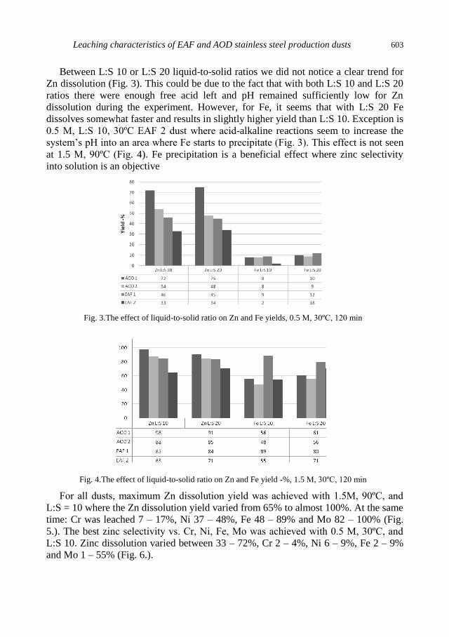
Leaching characteristics of EAF and AOD stainless steel production dusts 603
Between L:S 10 or L:S 20 liquid-to-solid ratios we did not notice a clear trend for
Zn dissolution (Fig. 3). This could be due to the fact that with both L:S 10 and L:S 20
ratios there were enough free acid left and pH remained sufficiently low for Zn
dissolution during the experiment. However, for Fe, it seems that with L:S 20 Fe
dissolves somewhat faster and results in slightly higher yield than L:S 10. Exception is
0.5 M, L:S 10, 30ºC EAF 2 dust where acid-alkaline reactions seem to increase the
system’s pH into an area where Fe starts to precipitate (Fig. 3). This effect is not seen
at 1.5 M, 90ºC (Fig. 4). Fe precipitation is a beneficial effect where zinc selectivity
into solution is an objective
Fig. 3.The effect of liquid-to-solid ratio on Zn and Fe yields, 0.5 M, 30ºC, 120 min
Fig. 4.The effect of liquid-to-solid ratio on Zn and Fe yield -%, 1.5 M, 30ºC, 120 min
For all dusts, maximum Zn dissolution yield was achieved with 1.5M, 90ºC, and
L:S = 10 where the Zn dissolution yield varied from 65% to almost 100%. At the same
time: Cr was leached 7 – 17%, Ni 37 – 48%, Fe 48 – 89% and Mo 82 – 100% (Fig.
5.). The best zinc selectivity vs. Cr, Ni, Fe, Mo was achieved with 0.5 M, 30ºC, and
L:S 10. Zinc dissolution varied between 33 – 72%, Cr 2 – 4%, Ni 6 – 9%, Fe 2 – 9%
and Mo 1 – 55% (Fig. 6.).
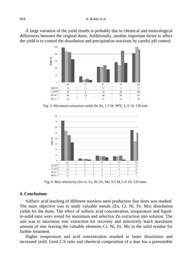
604 A. Kekki et al.
A large variation of the yield results is probably due to chemical and mineralogical
differences between the original dusts. Additionally, another important factor to affect
the yield is to control the dissolution and precipitation reactions by careful pH control.
Fig. 5. Maximum extraction yields for Zn, 1.5 M, 90ºC, L:S 10, 120 min
Fig. 6. Best selectivity (Zn vs. Cr, Ni, Fe, Mo, 0.5 M, L:S 10, 120 min)
4. Conclusions
Sulfuric acid leaching of different stainless steel production flue dusts was studied.
The main objective was to study valuable metals (Zn, Cr, Ni, Fe, Mo) dissolution
yields for the dusts. The effect of sulfuric acid concentration, temperature and liquid-
to-solid ratio were tested for maximum and selective Zn extraction into solution. The
aim was to maximize zinc extraction for recovery and selectively leach maximum
amount of zinc leaving the valuable elements Cr, Ni, Fe, Mo in the solid residue for
further treatment.
Higher temperature and acid concentration resulted in faster dissolution and
increased yield. Used L:S ratio and chemical composition of a dust has a presumable
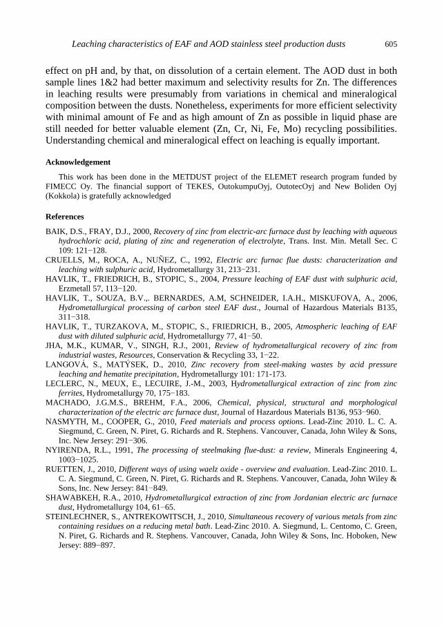
Leaching characteristics of EAF and AOD stainless steel production dusts 605
effect on pH and, by that, on dissolution of a certain element. The AOD dust in both
sample lines 1&2 had better maximum and selectivity results for Zn. The differences
in leaching results were presumably from variations in chemical and mineralogical
composition between the dusts. Nonetheless, experiments for more efficient selectivity
with minimal amount of Fe and as high amount of Zn as possible in liquid phase are
still needed for better valuable element (Zn, Cr, Ni, Fe, Mo) recycling possibilities.
Understanding chemical and mineralogical effect on leaching is equally important.
Acknowledgement
This work has been done in the METDUST project of the ELEMET research program funded by
FIMECC Oy. The financial support of TEKES, OutokumpuOyj, OutotecOyj and New Boliden Oyj
(Kokkola) is gratefully acknowledged
References
BAIK, D.S., FRAY, D.J., 2000, Recovery of zinc from electric-arc furnace dust by leaching with aqueous
hydrochloric acid, plating of zinc and regeneration of electrolyte, Trans. Inst. Min. Metall Sec. C
109: 121−128.
CRUELLS, M., ROCA, A., NUÑEZ, C., 1992, Electric arc furnac flue dusts: characterization and
leaching with sulphuric acid, Hydrometallurgy 31, 213−231.
HAVLIK, T., FRIEDRICH, B., STOPIC, S., 2004, Pressure leaching of EAF dust with sulphuric acid,
Erzmetall 57, 113−120.
HAVLIK, T., SOUZA, B.V.,. BERNARDES, A.M, SCHNEIDER, I.A.H., MISKUFOVA, A., 2006,
Hydrometallurgical processing of carbon steel EAF dust., Journal of Hazardous Materials B135,
311−318.
HAVLIK, T., TURZAKOVA, M., STOPIC, S., FRIEDRICH, B., 2005, Atmospheric leaching of EAF
dust with diluted sulphuric acid, Hydrometallurgy 77, 41−50.
JHA, M.K., KUMAR, V., SINGH, R.J., 2001, Review of hydrometallurgical recovery of zinc from
industrial wastes, Resources, Conservation & Recycling 33, 1−22.
LANGOVÁ, S., MATÝSEK, D., 2010, Zinc recovery from steel-making wastes by acid pressure
leaching and hematite precipitation, Hydrometallurgy 101: 171-173.
LECLERC, N., MEUX, E., LECUIRE, J.-M., 2003, Hydrometallurgical extraction of zinc from zinc
ferrites, Hydrometallurgy 70, 175−183.
MACHADO, J.G.M.S., BREHM, F.A., 2006, Chemical, physical, structural and morphological
characterization of the electric arc furnace dust, Journal of Hazardous Materials B136, 953−960.
NASMYTH, M., COOPER, G., 2010, Feed materials and process options. Lead-Zinc 2010. L. C. A.
Siegmund, C. Green, N. Piret, G. Richards and R. Stephens. Vancouver, Canada, John Wiley & Sons,
Inc. New Jersey: 291−306.
NYIRENDA, R.L., 1991, The processing of steelmaking flue-dust: a review, Minerals Engineering 4,
1003−1025.
RUETTEN, J., 2010, Different ways of using waelz oxide - overview and evaluation. Lead-Zinc 2010. L.
C. A. Siegmund, C. Green, N. Piret, G. Richards and R. Stephens. Vancouver, Canada, John Wiley &
Sons, Inc. New Jersey: 841−849.
SHAWABKEH, R.A., 2010, Hydrometallurgical extraction of zinc from Jordanian electric arc furnace
dust, Hydrometallurgy 104, 61−65.
STEINLECHNER, S., ANTREKOWITSCH, J., 2010, Simultaneous recovery of various metals from zinc
containing residues on a reducing metal bath. Lead-Zinc 2010. A. Siegmund, L. Centomo, C. Green,
N. Piret, G. Richards and R. Stephens. Vancouver, Canada, John Wiley & Sons, Inc. Hoboken, New
Jersey: 889−897.

606 A. Kekki et al.
STROBOS, JG., FRIEND, J.F.C., 2004, Zinc recovery from baghouse dust generated at ferrochrome
foundries, Hydrometallurgy 74, 165−171.
TSAKIRIDIS, P.E., OUSTADAKIS, P., 2010, Hydrometallurgical process for zinc recovery from
electric arc furnace dust (EAFD), Part I: Characterization and leaching by diluted sulphuric acid,
Journal of Hazardous Materials 179(1−3), 1−7.
ZUNKEL, D.A.D., 2001, Recovering zinc and lead from electric arc furnace dust: A 2001 processing and
technology status update. European Metallurgical Conference, Friedrichshafen, Germany, GDMB.
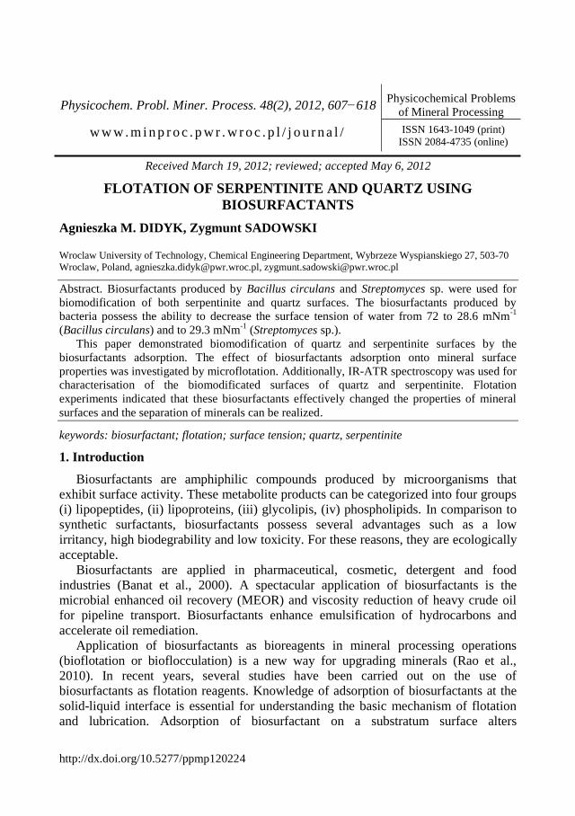
http://dx.doi.org/10.5277/ppmp120224
Physicochem. Probl. Miner. Process. 48(2), 2012, 607−618 Physicochemical Problems
of Mineral Processing
w w w . m i n p r o c . p w r . w r o c . p l / j o u r n a l / ISSN 1643-1049 (print)
ISSN 2084-4735 (online)
Received March 19, 2012; reviewed; accepted May 6, 2012
FLOTATION OF SERPENTINITE AND QUARTZ USING
BIOSURFACTANTS
Agnieszka M. DIDYK, Zygmunt SADOWSKI
Wroclaw University of Technology, Chemical Engineering Department, Wybrzeze Wyspianskiego 27, 503-70
Wroclaw, Poland, [email protected], [email protected]
Abstract. Biosurfactants produced by Bacillus circulans and Streptomyces sp. were used for
biomodification of both serpentinite and quartz surfaces. The biosurfactants produced by
bacteria possess the ability to decrease the surface tension of water from 72 to 28.6 mNm-1
(Bacillus circulans) and to 29.3 mNm-1
(Streptomyces sp.).
This paper demonstrated biomodification of quartz and serpentinite surfaces by the
biosurfactants adsorption. The effect of biosurfactants adsorption onto mineral surface
properties was investigated by microflotation. Additionally, IR-ATR spectroscopy was used for
characterisation of the biomodificated surfaces of quartz and serpentinite. Flotation
experiments indicated that these biosurfactants effectively changed the properties of mineral
surfaces and the separation of minerals can be realized.
keywords: biosurfactant; flotation; surface tension; quartz, serpentinite
1. Introduction
Biosurfactants are amphiphilic compounds produced by microorganisms that
exhibit surface activity. These metabolite products can be categorized into four groups
(i) lipopeptides, (ii) lipoproteins, (iii) glycolipis, (iv) phospholipids. In comparison to
synthetic surfactants, biosurfactants possess several advantages such as a low
irritancy, high biodegrability and low toxicity. For these reasons, they are ecologically
acceptable.
Biosurfactants are applied in pharmaceutical, cosmetic, detergent and food
industries (Banat et al., 2000). A spectacular application of biosurfactants is the
microbial enhanced oil recovery (MEOR) and viscosity reduction of heavy crude oil
for pipeline transport. Biosurfactants enhance emulsification of hydrocarbons and
accelerate oil remediation.
Application of biosurfactants as bioreagents in mineral processing operations
(bioflotation or bioflocculation) is a new way for upgrading minerals (Rao et al.,
2010). In recent years, several studies have been carried out on the use of
biosurfactants as flotation reagents. Knowledge of adsorption of biosurfactants at the
solid-liquid interface is essential for understanding the basic mechanism of flotation
and lubrication. Adsorption of biosurfactant on a substratum surface alters

608 A.M. Didyk and Z. Sadowski
hydrophobicity of the surface and causes a facilitation of microbial adhesion. For
mineral processing, bioflotation is very important to understand the role of metabolic
products in biomodification of the mineral surface.
Chemoautotrophic bacteria such as Acidithiobacillus ferrooxidans,
Acidithiobacillus thiooxidans, and Leptospirillum ferrooxidans, which usually live in
aqueous acid solution in mines, are able to depress sulfide minerals. It is a result of
surface oxidation. Selective flotation of complex sulfide ores, particularly
chalcopyrite, sphalerite, and pyrrotite using xanthate as collector, needs application of
bioreagents (Pecina et al., 2009).
Bacteria attach to the surface by a complex of exopolysaccharides, called
glycocalyx, forming a biofilm. The colonization of the surface by bacteria can lead to
modification of the surface property (Das et al., 2009).
Magnesium silicate can be used for storage of CO2 by mineral carbonation.
Dissolution of natural serpentinite in acids and precipitation of magnesium carbonate
require quartz to be removed. Carbonation of natural serpentinite seems to be an
interesting alternative to geological reservoirs for storage of CO2 (Teir et al., 2009).
Serpentinite can be used as a conventional raw material in the ceramic industry.
Mechanical resistance of serpentinite depends on the quantity of quartz in the raw
materials (Diaz, Torrecillas 2007).
The aim of this paper was to investigate flotation of quartz and serpentinite in the
presence of biosurfactants and nickel ions as an activator.
2. Materials and methods
2.1. Microorganisms and biosurfactant production
Bacteria were isolated from soil samples. Soil samples were collected from a gas
station soil. The samples were collected in sterilized glass bottles. The isolation
procedure was carried out using the serial dilution-agar plating technique. Two pure
cultures (Bacillus circulans and Streptomyces sp.) were selected. The strains were
grown on a liquid mineral salt medium consisting of K2HPO4 (7 g/dm3), KH2PO4 (3
g/dm3), MgSO4·7H2O (0.1 g/dm
3) (NH4)2SO4 (1 g/dm
3), Yeast extract (0.5 g/dm
3),
saccharose (10 g/dm3) and glycerin. Microorganisms were cultures in 500 cm
3 shake
flasks containing 250 dm3 of medium. The cultures were incubated in a rotary shaker
at the temperature of 26 °C. The cell growth and surface tension were monitored with
respect to time. The cultures from the end of exponential growth phase were
centrifuged (3500 rpm for 25 min) and the cell-free culture broth was used as the broth
for flotation experiments. The cell concentration was determined by the optical density
measurements at wavelength 550 nm (OD550) using a spectrophotometer.
2.2. Mineral samples
Mineral samples of quartz and serpentinite (Mg3(Si2O5)OH4) were obtained from
Osiecznica mine and Grochow mine, respectively. Both mines are located in Lower
Silesia (Poland).
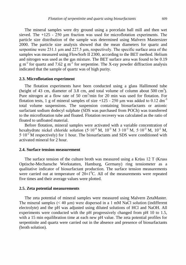
Flotation of serpentinite and quartz using biosurfactants 609
The mineral samples were dry ground using a porcelain ball mill and then wet
sieved. The +125 - 250 µm fraction was used for microflotation experiments. The
particle size distribution of the sample was determined using Malvern Mastersizer
2000. The particle size analysis showed that the mean diameters for quartz and
serpentine were 231.1 µm and 227.5 µm, respectively. The specific surface area of the
samples was measured using FlowSorb II 2300, according to the BET method. Helium
and nitrogen was used as the gas mixture. The BET surface area was found to be 0.19
g m-2
for quartz and 7.62 g m-2
for serpentine. The X-ray powder diffraction analysis
indicated that the sample of quartz was of high purity.
2.3. Microflotation experiment
The flotation experiments have been conducted using a glass Hallimond tube
(height of 43 cm, diameter of 3.8 cm, and total volume of column about 500 cm3).
Pure nitrogen at a flow rate of 50 cm3/min for 20 min was used for flotation. For
flotation tests, 1 g of mineral samples of size +125 - 250 µm was added to 0.12 dm-3
total volume suspensions. The suspension containing biosurfactants or anionic
surfactant sodium dodecyl sulphate (SDS was purchased from POCh) was transferred
to the microflotation tube and floated. Flotation recovery was calculated as the ratio of
floated to unfloated material.
Before flotation, mineral samples were activated with a variable concentration of
hexahydrate nickel chloride solution (5·10-4
M, 10-3
M 3·10-3
M, 5·10-3
M, 10-2
M,
5·10-2
M respectively) for 1 hour. The biosurfactants and SDS were conditioned with
activated mineral for 2 hour.
2.4. Surface tension measurement
The surface tension of the culture broth was measured using a Krüss 12 T (Kruss
Optische-Mechansche Werkstatten, Hamburg, Germany) ring tensiometer as a
qualitative indicator of biosurfactant production. The surface tension measurements
were carried out at temperature of 20±10C. All of the measurements were repeated
five times and their average values were plotted.
2.5. Zeta potential measurements
The zeta potential of mineral samples were measured using Malvern ZetaMaster.
The mineral samples (< 40 µm) were dispersed in a 1 mM NaCl solution (indifferent
electrolyte) and the pH was adjusted using diluted solutions of HCl and NaOH. All
experiments were conducted with the pH progressively changed from pH 10 to 1.5,
with a 15 min equilibration time at each new pH value. The zeta potential profiles for
serpentinite and quartz were carried out in the absence and presence of biosurfactants
(broth solution).
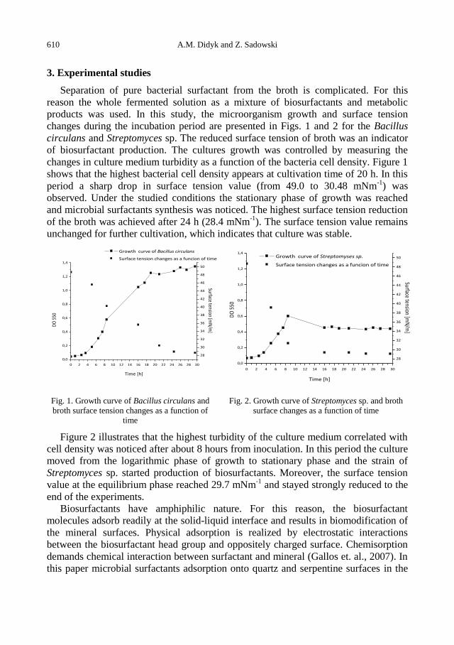
610 A.M. Didyk and Z. Sadowski
3. Experimental studies
Separation of pure bacterial surfactant from the broth is complicated. For this
reason the whole fermented solution as a mixture of biosurfactants and metabolic
products was used. In this study, the microorganism growth and surface tension
changes during the incubation period are presented in Figs. 1 and 2 for the Bacillus
circulans and Streptomyces sp. The reduced surface tension of broth was an indicator
of biosurfactant production. The cultures growth was controlled by measuring the
changes in culture medium turbidity as a function of the bacteria cell density. Figure 1
shows that the highest bacterial cell density appears at cultivation time of 20 h. In this
period a sharp drop in surface tension value (from 49.0 to 30.48 mNm-1
) was
observed. Under the studied conditions the stationary phase of growth was reached
and microbial surfactants synthesis was noticed. The highest surface tension reduction
of the broth was achieved after 24 h (28.4 mNm-1
). The surface tension value remains
unchanged for further cultivation, which indicates that culture was stable.
0 2 4 6 8 10 12 14 16 18 20 22 24 26 28 30
0,0
0,2
0,4
0,6
0,8
1,0
1,2
1,4
Growth curve of Bacillus circulans
Surface tension changes as a funcion of time
Time [h]
DO
550
28
30
32
34
36
38
40
42
44
46
48
50
Surface tension [mN
/m]
0 2 4 6 8 10 12 14 16 18 20 22 24 26 28 30
0,0
0,2
0,4
0,6
0,8
1,0
1,2
1,4 Growth curve of Streptomyses sp.
Surface tension changes as a funcion of time
Time [h]
DO
550
28
30
32
34
36
38
40
42
44
46
48
50
Surface tension [mN
/m]
Fig. 1. Growth curve of Bacillus circulans and
broth surface tension changes as a function of
time
Fig. 2. Growth curve of Streptomyces sp. and broth
surface changes as a function of time
Figure 2 illustrates that the highest turbidity of the culture medium correlated with
cell density was noticed after about 8 hours from inoculation. In this period the culture
moved from the logarithmic phase of growth to stationary phase and the strain of
Streptomyces sp. started production of biosurfactants. Moreover, the surface tension
value at the equilibrium phase reached 29.7 mNm-1
and stayed strongly reduced to the
end of the experiments.
Biosurfactants have amphiphilic nature. For this reason, the biosurfactant
molecules adsorb readily at the solid-liquid interface and results in biomodification of
the mineral surfaces. Physical adsorption is realized by electrostatic interactions
between the biosurfactant head group and oppositely charged surface. Chemisorption
demands chemical interaction between surfactant and mineral (Gallos et. al., 2007). In
this paper microbial surfactants adsorption onto quartz and serpentine surfaces in the
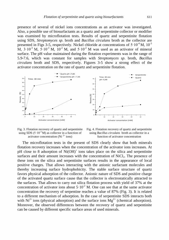
Flotation of serpentinite and quartz using biosurfactants 611
presence of several of nickel ions concentrations as an activator was investigated.
Also, a possible use of biosurfactants as a quartz and serpentinite collector or modifier
was examined by microflotation tests. Results of quartz and serpentinite flotation
using SDS, Streptomyces sp. broth and Bacillus circulans broth as the collector are
presented in Figs 3-5, respectively. Nickel chloride at concentrations of 5·10-4
M, 10-3
M, 3·10-3
M, 5·10-3
M, 10-2
M, and 5·10-2
M was used as an activator of mineral
surface. The pH value maintained during the flotation experiments was in the range of
5.9-7.6, which was constant for samples with Streptomyces sp. broth, Bacillus
circulans broth and SDS, respectively. Figures 3-5 show a strong effect of the
activator concentration on the rate of quartz and serpentinite flotation.
0 10 20 30 40 50
0
10
20
30
40
50
60
70
80
90
Quartz pH =7,60
Serpentinite pH = 7,35
Rec
over
y [%
]
Activator concentration [mM]
Time: 30 min
10 20 30 40 50
0
10
20
30
40
50
60
70pH =5,90
Serpentinite
Quartz
Reco
very
[%]
Activator concentation [mM]
Time: 30 min
Fig. 3. Flotation recovery of quartz and serpentinite
using SDS (5·10-3 M) as collector in a function of
activator concentration (Ni 2+ ions)
Fig. 4. Flotation recovery of quartz and serpentinite
using Bacillus circulans broth as collector in a
function of activator concentration
The microflotation tests in the present of SDS clearly show that both minerals
flotation recovery increases when the concentration of the activator ions increases. At
pH close to 8 adsorption of Ni(OH)+ ions takes place on the silica and serpentinite
surfaces and their amount increases with the concentration of NiCl2. The presence of
these ions on the silica and serpentinite surfaces results in the appearance of local
positive charges. That allows interacting with the anionic surfactant molecules and
thereby increasing surface hydrophobicity. The stable surface structure of quartz
favors physical adsorption of the collector. Anionic nature of SDS and positive charge
of the activated quartz surface cause that the collector is electrostatically attracted to
the surfaces. That allows to carry out silica flotation process with yield of 37% at the
concentration of activator ions about 5·10-2
M. One can see that at the same activator
concentration the recovery of serpentine reaches a value of 87% (Fig. 3). It is related
to a different mechanism of adsorption. In the case of serpentinite SDS interacts both
with Ni2+
ions (physical adsorption) and the surface ions Mg2+
(chemical adsorption).
Moreover, the observed differences between the recovery of quartz and serpentinite
can be caused by different specific surface areas of used minerals.

612 A.M. Didyk and Z. Sadowski
An analysis of experimental results of activated silica and serpentinite (Fig. 4-5)
flotation indicates that for both medium broths the flotation yield increases with
increasing activation ions concentration. The flotation profile is similar to the flotation
using anionic collector. It can be concluded, according to the previous assumptions,
that the two cultivation media contain anionic biosurfactants in their composition.
Biomolecules were able to adsorb onto mineral surfaces, causing their modification. In
the case of culture medium derived from Bacillus circulans, the flotation recovery of
silica reached a high value of 68%, while the yield of the silica flotation using the
broth from Streptomyces sp. is more than twice lower (30%).
0 10 20 30 40 50
0
5
10
15
20
25
30
35
Serpentinite
Quartz
Reco
very
[%]
Activator concentration [mM]
pH = 6,6
Time: 30 min
1 2 3 4 5 6 7 8 9 10 11
-30
-20
-10
0
10
20
30
Activator concentration [M]:
zeta
pot
entia
l [m
V]
pH
Pure serpentine
5*10-4
2,5*10-3
2,5*10-2
5*10-2
Fig. 5. Flotation recovery of quartz and serpentinite
using Streptomyces sp. broth. as collector as a
function of activator concentration
Fig. 6. Zeta potential of activated quartz and pure
serpentinite as a function of pH (indifferent
electrolyte 1 mM NaCl solution)
Figures 4 and 5 show the results of flotation experiments using activated
serpentinite. As for silica, we are dealing with biomodification of mineral surface.
However, in this case, the flotation recovery is much lower. The analysis of the results
indicates that serpentinite flotation using culture medium from Bacillus circulans gave
flotation yield about 18%, while flotation testes carried out after the interaction with
broth solution from Streptomyces sp. made it possible to obtain only 5% recovery. As
one can see, there are large differences in the flotation recoveries of both minerals.
Therefore, it seems possible to selectively float quartz from serpentinite. The obtained
lower bioflotation results, when compared to the flotation test with SDS, can be
attributed to the fact that broths containing polysaccharides, proteins and organic acids
make the surface of serpentine and quartz more hydrophilic. Moreover, large yields
differences between quartz and serpentinite flotation for the same medium broth result
from differences in interacting of broth compounds with activated mineral surfaces
(interaction and complex formation between Mg2+
and broth compounds could occur),
and consequently from the different adsorption degrees of these elements on both
mineral surfaces.
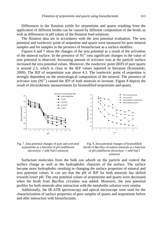
Flotation of serpentinite and quartz using biosurfactants 613
Differences in the flotation yields for serpentinite and quartz resulting from the
application of different broths can be caused by different composition of the broth, as
well as differences in pH values of the flotation feed solutions.
The flotation data are in accordance with the zeta potential evaluation. The zeta
potential and isoelectric point of serpentine and quartz were measured for pure mineral
samples and for samples in the presence of biosurfactant as a surface modifier.
Figures 6 and 7 show the changes of the zeta potential as a result of the activation
of the mineral surface. In the presence of Ni2+
ions significant changes in the value of
zeta potential is observed. Increasing amount of activator ions at the particle surface
increased the zeta potential values. Moreover, the isoelectric point (IEP) of pure quartz
is around 2.5, which is close to the IEP values reported in literature (Kosmulski,
2009). The IEP of serpentinite was above 4.3. The isoelectric point of serpentine is
strongly dependent on the mineralogical composition of the mineral. The presence of
activator ions (Ni2+
) caused the IEP of both minerals to increase. Figure 8 depicts the
result of electrokinetic measurements for biomodified serpentinite and quartz.
1 2 3 4 5 6 7 8 9 10 11
-30
-20
-10
0
10
20
30
Activator concentration [M]:
Zeta
po
ten
tial
[m
V]
pH
pure serpentine
5*10-4
2,5*10-3
2,5*10-2
5*10-2
0 2 4 6 8 10
-60
-50
-40
-30
-20
-10
0
10
20 Pure serpenttinite
Pure quartz
Biomodified serpentinite
Biomodified quartz
Zeta
pot
entia
l [m
V]
pH
Fig. 7. Zeta potential changes of pure and activated
serpentinite as a function of pH (indifferent
electrolyte: 1 mM NaCl solution)
Fig. 8. Zeta potential changes of biomodified
(broth of Bacillus circulans) minerals as a function
of pH (indifferent electrolyte: 1 mM NaCl
solution)
Surfactant molecules from the bulk can adsorb on the particle and control the
surface charge as well as the hydrophobic character of the surface. The surface
became more hydrophobic resulting in changing the surface properties of mineral and
zeta potential values. It can see that the pH of IEP for both minerals has shifted
towards lower pH. The zeta potential values of serpentinite and quartz were decreased
when the broth from Bacillus circulans was added. Moreover, the zeta potential
profiles for both minerals after interaction with the metabolite solution were similar.
Additionally, the IR-ATR spectroscopy and optical microscope were used for the
characterization of surface properties of pure samples of quartz and serpentinite before
and after interaction with biosurfactants.
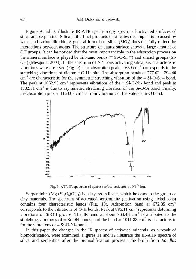
614 A.M. Didyk and Z. Sadowski
Figure 9 and 10 illustrate IR-ATR spectroscopy spectra of activated surfaces of
silica and serpentine. Silica is the final products of silicates decomposition caused by
water and carbon dioxide. A general formula of silica (SiO2) does not fully reflect the
interactions between atoms. The structure of quartz surface shows a large amount of
OH groups. It can be noticed that the most important role in the adsorption process on
the mineral surface is played by siloxane bonds (≡ Si-O-Si ≡) and silanol groups (Si-
OH) (Mesquita, 2003). In the spectrum of Ni2+
ions activating silica, six characteristic
vibrations were observed (Fig. 9). The absorption peak at 650 cm-1
corresponds to the
stretching vibrations of diatomic O-H units. The absorption bands at 777.62 - 794.40
cm-1
are characteristic for the symmetric stretching vibration of the ≡ Si-O-Si ≡ bond.
The peak at 1062.93 cm-1
represents vibrations of the ≡ Si-O-Ni- bond and peak at
1082.51 cm-1
is due to asymmetric stretching vibration of the Si-O-Si bond. Finally,
the absorption pick at 1163.63 cm-1
is from vibrations of the valence Si-O bond.
Fig. 9. ATR-IR spectrum of quartz surface activated by Ni 2+ ions
Serpentinite (Mg3(Si2O5)OH4) is a layered silicate, which belongs to the group of
clay materials. The spectrum of activated serpentinite (activation using nickel ions)
contains four characteristic bands (Fig. 10). Adsorption band at 672.35 cm-1
corresponds to the vibrations of O-H bonds. Peak at 885.11 cm-1
represents deforming
vibrations of Si-OH groups. The IR band at about 963.48 cm-1
is attributed to the
stretching vibrations of ≡ Si-OH bonds, and the band at 1011.88 cm-1
is characteristic
for the vibrations of ≡ Si-O-Ni- bond.
In this paper the changes in the IR spectra of activated minerals, as a result of
biomodification, were examined. Figures 11 and 12 illustrate the IR-ATR spectra of
silica and serpentine after the biomodification process. The broth from Bacillus
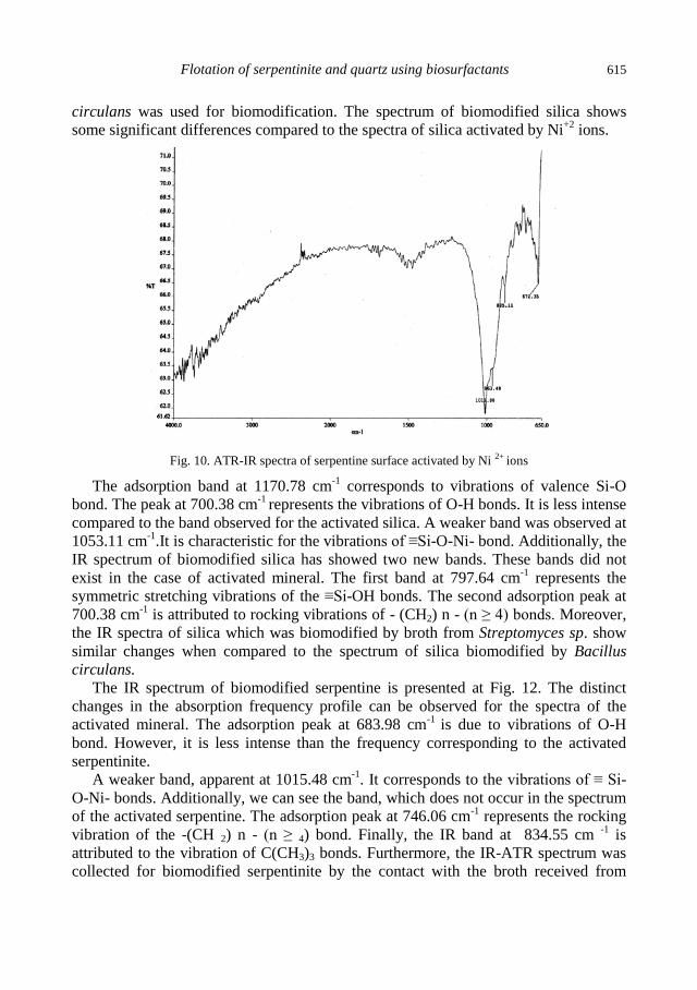
Flotation of serpentinite and quartz using biosurfactants 615
circulans was used for biomodification. The spectrum of biomodified silica shows
some significant differences compared to the spectra of silica activated by Ni+2
ions.
Fig. 10. ATR-IR spectra of serpentine surface activated by Ni 2+ ions
The adsorption band at 1170.78 cm-1
corresponds to vibrations of valence Si-O
bond. The peak at 700.38 cm-1
represents the vibrations of O-H bonds. It is less intense
compared to the band observed for the activated silica. A weaker band was observed at
1053.11 cm-1
.It is characteristic for the vibrations of ≡Si-O-Ni- bond. Additionally, the
IR spectrum of biomodified silica has showed two new bands. These bands did not
exist in the case of activated mineral. The first band at 797.64 cm-1
represents the
symmetric stretching vibrations of the ≡Si-OH bonds. The second adsorption peak at
700.38 cm-1
is attributed to rocking vibrations of - (CH2) n - (n ≥ 4) bonds. Moreover,
the IR spectra of silica which was biomodified by broth from Streptomyces sp. show
similar changes when compared to the spectrum of silica biomodified by Bacillus
circulans.
The IR spectrum of biomodified serpentine is presented at Fig. 12. The distinct
changes in the absorption frequency profile can be observed for the spectra of the
activated mineral. The adsorption peak at 683.98 cm-1
is due to vibrations of O-H
bond. However, it is less intense than the frequency corresponding to the activated
serpentinite.
A weaker band, apparent at 1015.48 cm-1
. It corresponds to the vibrations of ≡ Si-
O-Ni- bonds. Additionally, we can see the band, which does not occur in the spectrum
of the activated serpentine. The adsorption peak at 746.06 cm-1
represents the rocking
vibration of the -(CH 2) n - (n ≥ 4) bond. Finally, the IR band at 834.55 cm -1
is
attributed to the vibration of C(CH3)3 bonds. Furthermore, the IR-ATR spectrum was
collected for biomodified serpentinite by the contact with the broth received from
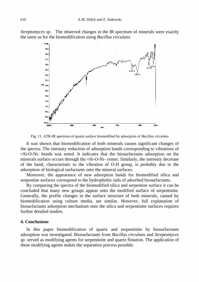
616 A.M. Didyk and Z. Sadowski
Streptomyces sp. The observed changes in the IR spectrum of minerals were exactly
the same as for the biomodification using Bacillus circulans.
Fig. 11. ATR-IR spectrum of quartz surface biomodified by adsorption of Bacillus circulans
It was shown that biomodification of both minerals causes significant changes of
the spectra. The intensity reduction of adsorption bands corresponding to vibrations of
≡Si-O-Ni- bonds was noted. It indicates that the biosurfactants adsorption on the
minerals surface occurs through the ≡Si-O-Ni- center. Similarly, the intensity decrease
of the band, characteristic to the vibration of O-H group, is probably due to the
adsorption of biological surfactants onto the mineral surfaces.
Moreover, the appearance of new adsorption bands for biomodified silica and
serpentine surfaces correspond to the hydrophobic tails of adsorbed biosurfactants.
By comparing the spectra of the biomodified silica and serpentine surface it can be
concluded that many new groups appear onto the modified surface of serpentinite.
Generally, the profile changes in the surface structure of both minerals, caused by
biomodification using culture media, are similar. However, full explanation of
biosurfactants adsorption mechanism onto the silica and serpentinite surfaces requires
further detailed studies.
4. Conclusions
In this paper biomodification of quartz and serpentinite by biosurfactants
adsorption was investigated. Biosurfactants from Bacillus circulans and Streptomyces
sp. served as modifying agents for serpentinite and quartz flotation. The application of
these modifying agents makes the separation process possible.
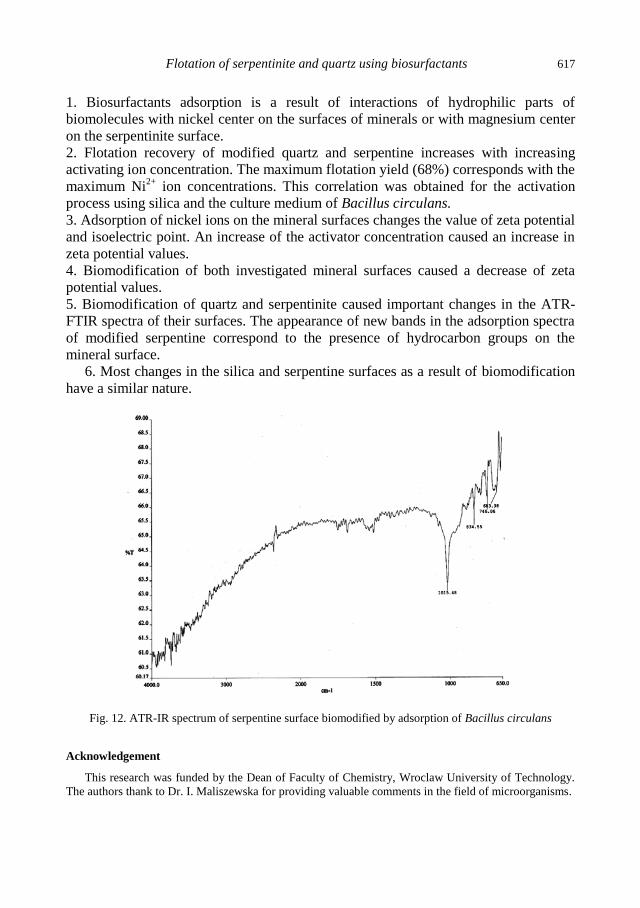
Flotation of serpentinite and quartz using biosurfactants 617
1. Biosurfactants adsorption is a result of interactions of hydrophilic parts of
biomolecules with nickel center on the surfaces of minerals or with magnesium center
on the serpentinite surface.
2. Flotation recovery of modified quartz and serpentine increases with increasing
activating ion concentration. The maximum flotation yield (68%) corresponds with the
maximum Ni2+
ion concentrations. This correlation was obtained for the activation
process using silica and the culture medium of Bacillus circulans.
3. Adsorption of nickel ions on the mineral surfaces changes the value of zeta potential
and isoelectric point. An increase of the activator concentration caused an increase in
zeta potential values.
4. Biomodification of both investigated mineral surfaces caused a decrease of zeta
potential values.
5. Biomodification of quartz and serpentinite caused important changes in the ATR-
FTIR spectra of their surfaces. The appearance of new bands in the adsorption spectra
of modified serpentine correspond to the presence of hydrocarbon groups on the
mineral surface.
6. Most changes in the silica and serpentine surfaces as a result of biomodification
have a similar nature.
Fig. 12. ATR-IR spectrum of serpentine surface biomodified by adsorption of Bacillus circulans
Acknowledgement
This research was funded by the Dean of Faculty of Chemistry, Wroclaw University of Technology.
The authors thank to Dr. I. Maliszewska for providing valuable comments in the field of microorganisms.

618 A.M. Didyk and Z. Sadowski
References
BANAT, M.I., MAKKAR S.R., CAMEOTRA S.S., 2000, Potential commercial application of microbial
surfactantas, Appl. Microbial Biotechnol., 53,495−508.
CASAS BOTERO E.A., TOREM L.M., SOUZA DE MESQUITA M.L., 2007, Fundamental studies of
Rhodococcus opacus a as a biocollector of calcite and magnesite, Minerals Engineering, 20,
1026−1032.
DAS P., MUKHERJEE S., SEN R., 2009, Antiadhesive action of a marine microbial surfactant, Colloids
Surfaces B: Biointerfaces, 71, 183−186.
De MESQUITA S.M.L., LINS F.F., TOREM L.M., 2003, Interaction of a hydrophobic bacterium strain
in a hematite-quartz flotation system, Int. J. Miner. Process. 71, 31−44.
DIAZ A.L., TORRECILLAS R., 2007, Porcelain stoneware obtained from the residual muds of
serpentinite raw materials, J. European Ceramic Society, 27, 2341−2345.
GALLIOS G.P., DELIYANNI E.A., PELEKA E.N., K.A. MATIS, 2007, Flotation of chromite and
serpentine, Separation and Purification Technology, 55, 232−237.
KOSMULSKI M., 2009, Complication of PZC and IEP of sparingly soluble metal oxides and hydroxides
from literature, Advances Colloid Inter. Sci., 152, 14−25.
PECINA T.E., RODRIGUEZ M., CASTILLO P., DIAZ V., ORRANTIA E., 2009, Effect of
Leptospirillum ferrooxidans on the flotation kinetics of sulphide ores, Minerals Engineering 22,
462−468.
RAO H.K., VILINSKA A., CHERNYSHOVA V.I., 2010, Minerals bioprocessing: R and D needs in
mineral biobeneficiation, Hydrometallurgy, 104, 465−470.
TEIR S., ELONEVA S., FOGELHOLM C-J., ZAVENHOVEN R., 2009, Fixation of carbon dioxide by
producing hydromagnesite from serpentinite, Applied Energy, 86, 214−218.

http://dx.doi.org/10.5277/ppmp120225
Physicochem. Probl. Miner. Process. 48(2), 2012, 619−630 Physicochemical Problems
of Mineral Processing
w w w . m i n p r o c . p w r . w r o c . p l / j o u r n a l / ISSN 1643-1049 (print)
ISSN 2084-4735 (online)
Received March 21, 2012; reviewed; accepted April 23, 2012
SYNTHESIS OF HEPTA(ISOBUTHYL)ETHYLTRIETHOXYSILYL-
OCTASILSESQUIOXANE AND ITS APPLICATION AS A MODIFIER
OF BOTH HYDRATED AND EMULSION SILICAS
Karolina SZWARC-RZEPKA*, Filip CIESIELCZYK*, Monika ZAWISZA*,
Michał KACZMAREK*, Michał DUTKIEWICZ**, Bogdan MARCINIEC**,
Hieronim MACIEJEWSKI***, Teofil JESIONOWSKI*
* Poznan University of Technology, Faculty of Chemical Technology, Institute of Chemical Technology and
Engineering, M. Skłodowskiej–Curie 2, PL-60965, Poznan, Poland, E–mail: [email protected],
phone: +48(61)6653720, fax: +48(61)6653649
** Adam Mickiewicz University, Faculty of Chemistry, Department of Organometallic Chemistry, PL-60780,
Grunwaldzka 6, Poznan, Poland
*** Poznan Science and Technology Park, Rubież 46, PL-61612 Poznan, Poland
Abstract. Hepta(isobuthyl)ethyltriethoxysilyloctasilsesquioxane was synthesized by hydro-
silylation of hepta(isobuthyl)vinyloctasilsesquioxane with triethoxysilane, over Karstedt
catalyst and tetrahydrofuran. Hybrid systems of silica and monofunctional silsesquioxane
(SiO2/POSS) were obtained by solvent evaporation, using emulsion silica (ES) and hydrated
silica (HS), obtained by precipitation in emulsion or water media. For their surface
modification hepta(isobuthyl)ethyltriethoxysilyloctasilsesquioxane was used. The hybrids were
characterized by dispersion analysis (NIBS method and laser diffraction technique) and
morphological analysis (transmission electron microscopy) as well as wettability profiles in an
aqueous system. The adsorptive properties of the hybrids were evaluated on the basis of
surface area BET, pore volume and size. The effectiveness of modification of the hybrid fillers
was tested by FTIR and 29
Si CP MAS NMR.
keywords: silica, surface modification, silsesquioxanes cage, hybrid nanofillers
1. Introduction
Polyhedral Oligomeric Silsesquioxanes or POSS make an important group of
organic-inorganic hybrid materials. They occur in many varieties differing in the size
of cages, the number and type of side groups (Iyer, 2007). Particularly stable is T8
silsesquioxane in which the organic groups R are attached to the inorganic fragments
of each vertex of a silsesquioxane cage containing Si–O–Si group (Wallace, 2000).
The chemistry of silsesquioxanes is dominated by the chemistry of T8 and its
derivatives, which is related to its easy synthesis, easy isolation from the reaction
mixture and high yields of the processes in which it is involved when compared to
those of the other POSS (Janowski, 2008). POSS show many interesting properties

620 K. Szwarc-Rzepka et al.
such as thermal stability, easy chemical modification and tendency to formation of
nanometric size particles (Madhavan, 2009).
POSS containing 8 silicon atoms in its molecule (T8) is most often used in
synthesis of polymers (Tang, 2009; Lin, 2009), in dentistry (Wu, 2009),
microelectronics and optics (Matisons, 2010). Silicas modified with cage POSS have
been so far used only for determination of catalytic properties of metallocenes
(Bianchini, 2005).
The main aim of this work was the synthesis of hepta(isobuthyl)-
ethyltriethoxysilyloctasilsesquioxane and its application as a modifier of hydrated and
emulsion silicas. Moreover, the influence of such modification process on the
physicochemical properties of hybrid fillers obtained was evaluated.
2. Experimental
2.1. Synthesis of hepta(isobuthyl)ethyltriethoxysilyloctasilsesquioxane
Hepta(isobuthyl)ethyltriethoxysilyloctasilsesquioxane (K-POSS) was synthesized
in the hydrosilylation reaction of previously synthesized hepta(isobuthyl)-
vinyloctasilsesquioxane (Żak, 2009) with triethoxysilane (Fig. 1). The process was
carried out in the presence of a Karstedt catalyst and THF as a solvent.
Hepta(isobuthyl)vinyloctasilsesquioxane (5 g, 5.9 mmol), triethoxysilane with 10%
excess (1.1 g, 6.7 mmol) together with 100 cm3 of THF as a solvent were placed in a
three necked, round bottom flask equipped with a thermometer, condenser and
magnetic bar. The Karstedt catalyst (3.7 mg, 4.0710-7
mol Pt) was added at room
temperature and the solution was heated to 60°C and kept at this temperature
overnight. Then, the solvent and the excess of triethoxysilane were evaporated under
vacuum to give the product as white powder (5.8 g, 98% of theoretical yield).
To control the course of synthesis and to verify the products structure the spectra: 1H NMR (300 MHz),
13C NMR (75 MHz) and
29Si NNR (59 MHz) were recorded on a
Varian XL 300 spectrometer at room temperature using C6D6 as solvent. All chemicals
were used as received from suppliers without any further purification.
Fig. 1. Synthesis of hepta(isobuthyl)ethyltriethoxysilyloctasilsesquioxane (K-POSS)

Synthesis of hepta(isobuthyl)ethyltriethoxysilyloctasilsesquioxane and its application as a modifier 621
2.2. SiO2/POSS hybryd synthesis
The process was begun with production of silicas on a large laboratory scale. Two
types of silica were prepared, obtained in the emulsion (ES) or in the aqueous (HS)
system. The idea of production of silica fillers was presented in detail by Jesionowski
(2003, 2009). The SiO2/POSS hybrids were obtained by solvent evaporation. At first a
fraction of ES or HS silica was introduced into the reactor and then on the silica
surface a mixture made of a monosubstituted silsesquixane cage and 30 cm3 toluene
was introduced in doses by the atomization method. The modifying substance was
introduced in the amounts of 3, 5 or 10 weight parts by mass of SiO2. After
introduction of the whole portion of the mixture, the contents were moved into a flask
of 500 cm3 in capacity and placed in a vacuum evaporator Rotavapor RII made by
Büchi Labortechnik AG to perform the modification and to evaporate the solvent.
Finally the product was subjected to convection drying at 120C for 48h (chamber
drier SEL–I3, made by Memmert). The idea of synthesis of hybrid fillers is
schematically presented in Fig. 2.
Fig. 2. A scheme of synthesis of SiO2/POSS hybrids
The final product was characterized by a number of methods. The particle size
distributions of the samples were measured using Zetasizer Nano ZS and Mastersizer
2000, both made by Malvern Instruments Ltd., enabling measurements in the range
0.6–6000 nm (NIBS method) and 0.2–2000 μm (laser diffraction technique).
Microstructure of the samples was analyzed by using the transmission electron
microscopy images (Joel 1200 EX II). The wettability with water was measured by a
tensiometer K100 made by Krüss equipped with necessary attachments. For selected
hybrid systems the nitrogen adsorption/desorption isotherms were recorded using an
ASAP 2020 analyzer, made by Micromeritics Instrument Co. On the basis of the
isotherms the specific surface area BET (SBET) was calculated and the pore size (SP)
and volume (VP) were found from BJH equation. The effectiveness and degree of
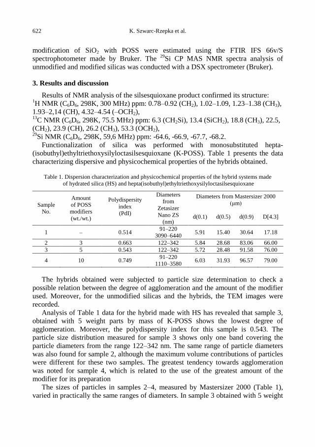
622 K. Szwarc-Rzepka et al.
modification of SiO2 with POSS were estimated using the FTIR IFS 66v/S
spectrophotometer made by Bruker. The 29
Si CP MAS NMR spectra analysis of
unmodified and modified silicas was conducted with a DSX spectrometer (Bruker).
3. Results and discussion
Results of NMR analysis of the silsesquioxane product confirmed its structure: 1H NMR (C6D6, 298K, 300 MHz) ppm: 0.78–0.92 (CH2), 1.02–1.09, 1.23–1.38 (CH3),
1.93–2,14 (CH), 4.32–4.54 (–OCH2), 13
C NMR (C6D6, 298K, 75.5 MHz) ppm: 6.3 (CH2Si), 13.4 (SiCH2), 18.8 (CH3), 22.5,
(CH2), 23.9 (CH), 26.2 (CH3), 53.3 (OCH2), 29
Si NMR (C6D6, 298K, 59,6 MHz) ppm: -64.6, -66.9, -67.7, -68.2.
Functionalization of silica was performed with monosubstituted hepta-
(isobuthyl)ethyltriethoxysilyloctasilsesquioxane (K-POSS). Table 1 presents the data
characterizing dispersive and physicochemical properties of the hybrids obtained.
Table 1. Dispersion characterization and physicochemical properties of the hybrid systems made
of hydrated silica (HS) and hepta(isobuthyl)ethyltriethoxysilyloctasilsesquioxane
Sample
No.
Amount
of POSS
modifiers
(wt./wt.)
Polydispersity
index
(PdI)
Diameters
from
Zetasizer
Nano ZS
(nm)
Diameters from Mastersizer 2000
(μm)
d(0.1) d(0.5) d(0.9) D[4.3]
1 0.514 91–220
3090–6440 5.91 15.40 30.64 17.18
2 3 0.663 122–342 5.84 28.68 83.06 66.00
3 5 0.543 122–342 5.72 28.48 91.58 76.00
4 10 0.749 91–220
1110–3580 6.03 31.93 96.57 79.00
The hybrids obtained were subjected to particle size determination to check a
possible relation between the degree of agglomeration and the amount of the modifier
used. Moreover, for the unmodified silicas and the hybrids, the TEM images were
recorded.
Analysis of Table 1 data for the hybrid made with HS has revealed that sample 3,
obtained with 5 weight parts by mass of K-POSS shows the lowest degree of
agglomeration. Moreover, the polydispersity index for this sample is 0.543. The
particle size distribution measured for sample 3 shows only one band covering the
particle diameters from the range 122–342 nm. The same range of particle diameters
was also found for sample 2, although the maximum volume contributions of particles
were different for these two samples. The greatest tendency towards agglomeration
was noted for sample 4, which is related to the use of the greatest amount of the
modifier for its preparation
The sizes of particles in samples 2–4, measured by Mastersizer 2000 (Table 1),
varied in practically the same ranges of diameters. In sample 3 obtained with 5 weight
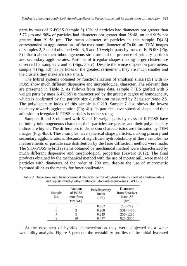
Synthesis of hepta(isobuthyl)ethyltriethoxysilyloctasilsesquioxane and its application as a modifier 623
parts by mass of K-POSS (sample 3) 10% of particles had diameters not greater than
5.72 μm and 50% of particles had diameters not greater than 28.48 μm and 90% not
greater than 91.58 μm. The mean diameter of particles in this sample D[4.3]
corresponded to agglomerations of the maximum diameter of 76.00 μm. TEM images
of samples 2, 3 and 4 obtained with 3, 5 and 10 weight parts by mass of K-POSS (Fig.
3) inform about their inhomogeneous structure and the presence of primary particles
and secondary agglomerates. Particles of irregular shapes making larger clusters are
observed for samples 2 and 3, (Figs. 3b, c). Despite the worse dispersion parameters,
sample 4 (Fig. 3d) has particles of the greatest refinement, they are much smaller and
the clusters they make are also small.
The hybrid systems obtained by functionalization of emulsion silica (ES) with K-
POSS show much different dispersive and morphological character. The relevant data
are presented in Table 2. As follows from these data, sample 7 (ES grafted with 5
weight parts by mass K-POSS) is characterised by the greatest degree of homogeneity,
which is confirmed by the particle size distribution measured by Zetasizer Nano ZS.
The polydispersity index of this sample is 0.219. Sample 7 also shows the lowest
tendency towards agglomeration (Fig. 4b). Its particles have spherical shape and their
adhesion to irregular K-POSS particles is rather strong.
Samples 6 and 8 obtained with 3 and 10 weight parts by mass of K-POSS have
definitely inhomogeneous character, their particles are greater and their polydispersity
indices are higher. The differences in dispersion characteristics are illustrated by TEM
images (Fig. 4b,d). These samples have spherical shape particles, making primary and
secondary agglomerations. Because of significant hydrophobicity of these samples, no
measurements of particle size distribution by the laser diffraction method were made.
The SiO2/POSS hybrid systems obtained by mechanical method were characterized by
much different dispersive and morphological properties (Szwarc 2012). The final
products obtained by the mechanical method with the use of mortar mill, were made of
particles with diameters of the order of 200 nm, despite the use of micrometric
hydrated silica as the matrix for functionalization.
Table 2. Dispersion and physicochemical characterization of hybrid systems made of emulsion silica
and hepta(isobuthyl)ethyltriethoxysilyloctasilsesquioxane (K-POSS)
Sample
No.
Amount
of POSS
modifiers
(wt./wt.)
Polydispersity
index
(PdI)
Diameters
from Zetasizer
Nano ZS
(nm)
5 0.252 255–712
6 3 0.268 531–1480
7 5 0.219 255–1280
8 10 0.447 825–2300
At the next step of hybrids characterization they were subjected to a water
wettability analysis. Figure 5 presents the wettability profiles of the initial hydrated

624 K. Szwarc-Rzepka et al.
silica and the hybrids based on HS obtained with the use of 3, 5 and 10 weight parts
by mass of K-POSS (samples 1–4), while Fig. 6 shows the wettability profiles of ES
and the hybrids made of ES and K-POSS (samples 5–8). The greatest tendency to
water absorption was found for sample 1, while the lowest amount of water was
absorbed by sample 4, modified with 10 wt./wt. of K-POSS. The character of the
wettability profiles indicates that with increasing amount of the modifying
monofunctional POSS, the hydrophobic character of the product increases
(a)
(b)
(c)
(d)
Fig. 3. TEM microphotographs of (a) pure hydrated silica and hybrid modified with (b) 3, (b) 5, and
(d) 10 weight parts by mass of hepta(isobuthyl)ethyltriethoxysilyloctasilsesquioxane (K-POSS)

Synthesis of hepta(isobuthyl)ethyltriethoxysilyloctasilsesquioxane and its application as a modifier 625
(a) (b)
(c) (d)
Fig. 4. TEM microphotographs of (a) pure emulsion silica and hybrid modified with (b) 3, (b) 5, and
(d) 10 weight parts by mass of hepta(isobuthyl)ethyltriethoxysilyloctasilsesquioxane (K-POSS)
The hybrids with K-POSS based on silica precipitated from the emulsion system
show similar tendencies to water absorption, although sample 5 has the highest
sorption capacity expressed by a mass increase of 0.32 g. The smallest mass increase
was noted for sample 8, obtained with the use of 10 wt./wt. of K-POSS. It should be
emphasised that the initial silicas differed significantly in hydrophilic character.
Hydrated silica absorbed about 50% more water than emulsion silica.

626 K. Szwarc-Rzepka et al.
Fig. 5. Wettability profiles obtained for hydrated
silica (HS) and selected SiO2/POSS hybrids
Fig. 6. Wettability profiles obtained for emulsion
silica (ES) and selected SiO2/POSS hybrids
(a) (b)
Fig. 7. Nitrogen adsorption/desorption isotherms and adsorptive properties for: (a) unmodified HS
(sample 1), (b) unmodified ES (sample 5) and silicas modified with 3, 5 or 10 weight parts by mass
of hepta(isobuthyl)ethyltriethoxysilyloctasilsesquioxane (K-POSS)
To evaluate the adsorptive properties of the samples studied, they were subjected to
determination of nitrogen adsorption/desorption isotherms. Analysis of the isotherms
permitted determination of the surface area as well as pore volume and diameters (see
Fig. 7). Figure 7 presents the nitrogen adsorption/desorption isotherms for the
unmodified hydrated silica (HS) and emulsion silica (ES) samples and for the hybrids
modified with 3, 5 or 10 wt./wt. of K-POSS. The isotherms show a systematic increase
in the volume of adsorbed nitrogen with increasing relative pressure till reaching a
maximum value of 240 cm3/g for sample 1 at p/p0=1 (Fig. 7a). For hybrids the
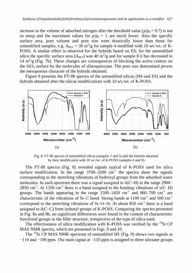
Synthesis of hepta(isobuthyl)ethyltriethoxysilyloctasilsesquioxane and its application as a modifier 627
increase in the volume of adsorbed nitrogen after the threshold value (p/p0 = 0.7) is not
so steep and the maximum values for p/p0 = 1 are much lower. Also the specific
surface area, pore volume and pore size were drastically lower than those for
unmodified samples, e.g. ABET = 30 m2/g for sample 4 modified with 10 wt./wt. of K-
POSS. A similar effect is observed for the hybrids based on ES; for the unmodified
silica the specific surface area (ABET) was 40 m2/g and for sample 8 it has decreased to
14 m2/g (Fig. 7b). These changes are consequences of blocking the active centres on
the SiO2 surface by the molecules of silsesquioxane. The pore size determined proves
the mesoporous character of the hybrids obtained.
Figure 8 presents the FT-IR spectra of the unmodified silicas (HS and ES) and the
hybrids obtained after the silicas modifications with 10 wt./wt. of K-POSS.
(a) (b)
Fig. 8. FT-IR spectra of unmodified silicas (samples 1 and 5) and the hybrids obtained
by their modification with 10 wt./wt. of K-POSS (samples 4 and 8)
The FT-IR spectra (Fig. 8) revealed signals typical of K-POSS used for silica
surface modification. In the range 3700–3200 cm-1
the spectra show the signals
corresponding to the stretching vibrations of hydroxyl groups from the adsorbed water
molecules. In each spectrum there was a signal assigned to δ(CH) in the range 2900–
2850 cm-1
. At 1350 cm-1
there is a band assigned to the bending vibrations of γ(C–H)
groups. The bands appearing in the range 1500–1450 cm-1
and 860–700 cm-1
are
characteristic of the vibrations of SiC bond. Strong bands at 1100 cm-1
and 500 cm-1
correspond to the stretching vibrations of SiOSi. At about 850 cm-1
there is a band
assigned to δ(CC) from isobutyl groups of K-POSS. Comparing the spectra presented
in Fig. 8a and 8b, no significant differences were found in the content of characteristic
functional groups in the filler structure, irrespective of the type of silica used.
The effectiveness of silica modification with K-POSS was verified by the 29
Si CP
MAS NMR spectra, which are presented in Figs. 9 and 10.
The 29
Si CP MAS NMR spectrum of unmodified HS (Fig. 9) shows two signals at
−110 and −100 ppm. The main signal at 110 ppm is assigned to three siloxane groups

628 K. Szwarc-Rzepka et al.
and one silanol group (Q3), while the signal at 100 ppm corresponds to four siloxane
bridges (Q4, SiOSi). The spectra of samples modified with K-POSS besides the
Q3 and Q
4 signals also have a band assigned to T
3 group at −67 ppm. Although the
presence of T2 and T
3 structures testifies to the chemical modification of SiO2 surface,
we cannot draw such conclusions as no changes in the intensities of Q3 and Q
4 signals
were observed as a result of functionalization with K-POSS.
Fig. 9. 29Si CP MAS NMR spectra of unmodified HS (Sample 1) and silica functionalized
with 5 wt./wt. K-POSS (Sample 3)
Fig. 10. 29Si CP MAS NMR spectra of unmodified ES (sample 5) and silica functionalized
with 5 wt./wt. of K-POSS (sample 7)
The spectrum of unmodified ES (sample 5) reveals three characteristic signals at
110, 100 and 99 ppm. The latter small signal is assigned to the double silanol
groups, to the so-called silicon site Q2. The spectrum of sample 7 shows additionally
the T3
structure (67 ppm), characteristic of condensation of the modifier (K-POSS)
with the silica support. As a result of silica functionalization, a change in the intensity
Synthesis of hepta(isobuthyl)ethyltriethoxysilyloctasilsesquioxane and its application as a modifier 629
of signals corresponding to the silanol (Q3 100 ppm) and siloxane (Q
4, 110 ppm)
groups, which could indicate that chemical adsorption have taken place. However,
because of the lack of T2
structure, we can conclude only about the adhesion of cage
POSS to the silica surface.
Recently, the interest in the hybrid systems has been increasing. A combination of
inorganic matrix with organic-inorganic cage POSS gave products showing a number
of interesting physicochemical and dispersive-morphological properties.
Modification of silica supports gives changes in the dispersive and morphological
properties and enhances the hydrophobic character of the products. The process of
silica modification with K-POSS proved effective as evidenced by the results of FTIR,
NMR analysis and adsorption parameters. Functionalization of silica with selected
POSS compounds permits controlling of the physicochemical properties of the
products to meet specific target demands.
4. Conclusions
The proposed method of silica modification involving solvent evaporation has
brought products of homogeneity lower than that of the initial silicas.
Functionalization of the silica surface with hepta(isobuthyl)ethyltriethoxy
silyloctasilsesquioxane (K-POSS) gave products containing greater size particles,
showing a tendency to formation of primary and secondary agglomerates. Much better
dispersive properties were obtained for the products based on the amorphous hydrated
silica.
With increasing amount of the monosubstituted POSS used for functionalization,
the products obtained showed increasingly higher hydrophobic character.
The functionalization with K-POSS also resulted in a significant reduction of the
surface area BET, e.g. from 110 m2/g for the unmodified hydrated silica to 30 m
2/g for
the hybrid filler (sample 4). The same tendency was noted for the emulsion silica. The
other parameters characterizing adsorptive properties such as the pore diameters and
pore volume as well as the amount of nitrogen adsorbed, were also much decreased.
The proposed method of silica modification with K-POSS had advantageous effect
on the physicochemical parameters as evidenced by the FT-IR results.
Analysis of 29
Si CP MAS NMR spectra confirmed no chemical interactions
between the silica support and the K-POSS modifier. The results indicated the
condensation phenomenon and strong adhesion of the modifier to the support.
Acknowledgement
The study was realized within the Development Project POIG 01.03.01-30-173/09 Nanosil from the
European Fund of Regional Development within the operation programme Innovative Economy.
References
BIANCHINI D., GALLAND G.B., DOS SANTOS J.H.Z., WILLIAMS R.J.J., FASCE D.P.,
DELL’ERBA I.E., QUIJADA R., PEREZ M., 2005, Metallocene supported on a Polyhedral

630 K. Szwarc-Rzepka et al.
Oligomeric Silsesquioxane‒modified silica with high catalytic activity for ethylene polymerization,
Journal of Polymer Science: Part A: Polymer Chemistry, 43, 5465‒5476.
IYER S., ABU‒ALI A., DETWILER A., SEHIRALDI A., 2007, Transparent polymer – Polyhedral
Oligomeric Silsesquioxane composities, ACS Symposium Series (Science and Technology of
Silicones and Silicone‒Modified Materials), Cleveland, 964, 313‒325.
JANOWSKI B., PIELICHOWSKI K., 2008, Polimery nanohybrydowe zawierające poliedryczne
oligosilseskwioksany, Polimery, 53, 87‒98.
JESIONOWSKI T., 2009, Preparation of spherical silica in emulsion systems using the co‒precipitation
technique, Materials Chemistry and Physics, 113, 839‒849
JESIONOWSKI T., ŻURAWSKA J., KRYSZTAFKIEWICZ A., POKORA M., WASZAK D., TYTUS
W., 2003, Physicochemical and morphological properties of hydrated silicas precipitated following
alkoxysilane surface modification, Applied Surface Science 205, 212‒224.
LIN P., KHARE R., 2009, Molecular simulation of cross‒linked epoxy and epoxy‒POSS nanocomposite,
Macromolecules, 42, 4319‒4327.
MADHAVAN K., GNANASEKARAN D., REDDY B.S.R., 2009, Synthesis and characterization of
poly(dimethylsiloxane‒urethane) nanocomposites: Effect of (in)completely condensed silsesquioxanes
on thermal, morphological, and mechanical properties, Journal of Applied Polymer Science, 114,
3659‒3667.
MATISONS J., 2010, Applications of Polyhedral Oligomeric Silsesquioxanes, Springer, New York.
SZWARC K., SIWINSKA‒STEFANSKA K., MARCINIEC B., JESIONOWSKI T., 2012, Synthesis and
characterisation of SiO2/POSS hybrid systems obtained using the mechanical method,
Physicochemical Problems of Mineral Processing, 48, 181‒192.
TANG Y., LEWIN M., 2009, Migration and surface modification In polypropylene (PP)/polyhedral
oligomeric silsequioxane (POSS) nanocomposites, Polymers Advanced Technologies, 20, 1‒15.
WALLACE W.E., GUTTMAN C.M., ANTONUCCI J.M., 2000, Polymeric silsesquioxanes:
degree‒of‒intramolecular‒condensation measured by mass spectrometry, Polymer 41,2219‒2226.
WU J., MATHER P.T., 2009, POSS Polymers: Physical properties and biomaterials applications,
Journal of Macromolecular Science, Part C: Polymer Reviews, 49, 25‒63.
ŻAK P., PIETRASZUK C., MARCINIEC B., SPÓLNIK G., DANIKIEWICZ W., 2009, Efficient
functionalisation of cubic monovinylsilsesquioxanes via cross‒metathesis and silylative coupling with
olefins in the presence of ruthenium complexes, Advanced Synthesis and Catalysis, 351, 2675‒2682.
http://dx.doi.org/10.5277/ppmp120226
Physicochem. Probl. Miner. Process. 48(2), 2012, 631−643 Physicochemical Problems
of Mineral Processing
w w w . m i n p r o c . p w r . w r o c . p l / j o u r n a l / ISSN 1643-1049 (print)
ISSN 2084-4735 (online)
Received April 2, 2012; reviewed; accepted April 16, 2012
SYNTHESIS OF Mg(OH)2 FROM MAGNESIUM SALTS AND NH4OH
BY DIRECT FUNCTIONALISATION WITH POLY(ETHYLENE
GLYCOLS)
Agnieszka PILARSKA, Iwona LINDA, Marcin WYSOKOWSKI
Dominik PAUKSZTA, Teofil JESIONOWSKI
Poznan University of Technology, Faculty of Chemical Technology, Institute of Chemical Technology and
Engineering, M. Sklodowskiej-Curie 2, PL-60965 Poznan, Poland, [email protected],
phone: +48(61)6653720, fax: +48(61)6653649
Abstract. Synthesis of magnesium hydroxide using different magnesium salts and ammonium
hydroxide is described. The reaction was performed in the presence of non-ionic compounds
representing the group of poly(ethylene glycols) as modifiers. Dispersive properties of the
products were characterised by polydispersity index, particle size, as well as SEM and TEM
images. Adsorptive properties of the products were evaluated on the basis of their specific
surface area, pore volume and diameter determination. Physicochemical characterisation of the
products was extended by the degrees of their surface coverage with PEG, calculated on the
basis of elemental analysis and specific surface area BET. Crystalline structures of the products
were determined by the WAXS method and then using the Scherrer formula the crystallite size
was calculated for selected samples. Wettability profiles in aqueous systems were measured
and selected samples were subjected to TG/DTA analyses. The properties of the products were
found to be significantly dependent on the molecular mass of PEG and type of magnesium salt
used.
keywords: Mg(OH)2, poly(ethylene glycols), particle size distribution, surface morphology,
adsorptive properties, crystal structure, elemental analysis, TG/DTA analysis
1. Introduction
Magnesium hydroxide is a very attractive compound because of a wide range of its
important applications. Besides, Mg(OH)2 is one of the most important precursors of
magnesium oxide. It is used as a neutraliser of acidic pollutants of water and gases,
filler in paper industry, antibacterial agent, and fertiliser additive (Dziubek, 1984;
Giorgi, 2005; Dong, 2010). One of its interesting properties is the diversity of its
microstructure. It crystallises as needles, plates, rods, tubes and flowers (Yan, 2005;
Wang, 2011;Song, 2011). Its non-toxic character and high thermal stability make it an
attractive additive to polymers used to restrict polymers flammability. The appearance
of many papers on Mg(OH)2 indicate increasing interest in this inorganic filler. The
main subject of these papers are new methods of synthesis of nano-Mg(OH)2 and ways
632 A. Pilarska et al.
of modification of the Mg(OH)2–polymer system aimed at improvement its
compatibility (Lv, 2007; Chen, 2009; Jurkowski, 2010; Gul, 2011).
Recently, much attention has been paid to the methods of synthesis of
nanomolecular Mg(OH)2. The methods proposed include: precipitation, solvo- and
hydrothermal, microwave, electrochemical, sol-gel and the method based on watering
of the commercial MgO with the use of dolomite and sea water (Ding, 2001; Du 2009;
Yildirim, 2010; Bae, 2011; Pilarska, 2011). The above-mentioned methods, except
precipitation, need a long time, complex and expensive equipment, which means that
the process of magnesium hydroxide production becomes economically unattractive.
The method based on precipitation is easy to conduct also on an industrial scale. It
permits control of the particle size and is rather inexpensive. No wonder that it has
been intensely studied in a number of research groups (Jiang, 2009; Meshkani, 2009;
Meshkani, 2010).
According to the recent literature reports, the properties of the final product, in
particular its morphology, are closely related to the type of precursor and the
precipitating agent. Much interest is devoted to the use of modifiers. Modification of
the reaction system, understood as direct participation of an additional organic or
inorganic chemical substance in the process of synthesis, is undertaken to modify the
original properties of the product, including its surface properties. Modifications of
this type are most often applied upon precipitation of magnesium hydroxide (Wang,
2007; Huang, 2008; Wang, 2009; Pilarska, 2011). Functionalisation of the surface of
fillers is aimed first of all at control of the shape and size of particles and at making
the product more hydrophobic to permit binding of inorganic fillers with organic
polymer matrices (Rothon, 2003).
This paper reports the synthesis of Mg(OH)2 of plate morphology realised by the
method of precipitation with the use of magnesium salts, ammonium hydroxide and
non-ionic compounds from the group of poly(ethylene glycols) as modifiers. The
influence of molecular weight and type of magnesium precursor on the dispersive-
morphological and physicochemical properties of the products has been mainly
analysed.
2. Experimental
The substrates used for the synthesis of magnesium hydroxide were: hydrated
magnesium sulfate (MgSO4·7H2O, analytical grade), magnesium chloride
(MgCl2·6H2O), magnesium nitrate (Mg(NO3)2∙6H2O, analytical grade), ammonium
hydroxide (NH4OH, analytical grade) as a precipitation agent (all made by POCh SA.)
and non-ionic compounds from the group of poly(ethylene glycols): PEG 200, PEG
400, PEG 8000 and PEG 20000 (purchased from Sigma-Aldrich), as solutions
of appropriate concentration. Magnesium hydroxide was obtained from a 5 % solution
of a given magnesium salt and a solution of ammonium hydroxide prepared to
maintain the stoichiometric amount of reagents. Precipitation was carried out at 60°C.
A technological scheme of the process is shown in Fig. 1.
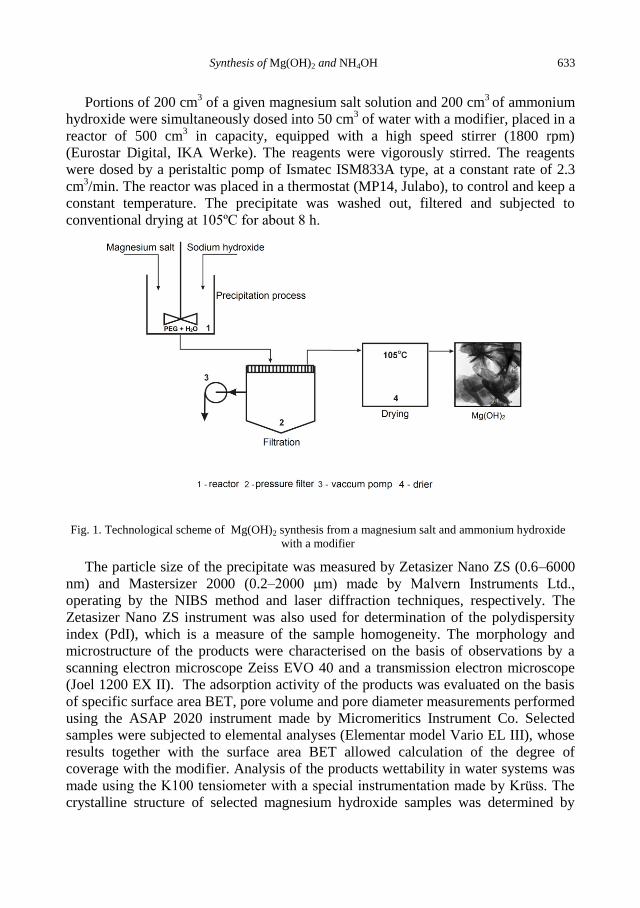
Synthesis of Mg(OH)2 and NH4OH 633
Portions of 200 cm3 of a given magnesium salt solution and 200 cm
3 of ammonium
hydroxide were simultaneously dosed into 50 cm3 of water with a modifier, placed in a
reactor of 500 cm3 in capacity, equipped with a high speed stirrer (1800 rpm)
(Eurostar Digital, IKA Werke). The reagents were vigorously stirred. The reagents
were dosed by a peristaltic pomp of Ismatec ISM833A type, at a constant rate of 2.3
cm3/min. The reactor was placed in a thermostat (MP14, Julabo), to control and keep a
constant temperature. The precipitate was washed out, filtered and subjected to
conventional drying at 105ºC for about 8 h.
Fig. 1. Technological scheme of Mg(OH)2 synthesis from a magnesium salt and ammonium hydroxide
with a modifier
The particle size of the precipitate was measured by Zetasizer Nano ZS (0.6–6000
nm) and Mastersizer 2000 (0.2–2000 μm) made by Malvern Instruments Ltd.,
operating by the NIBS method and laser diffraction techniques, respectively. The
Zetasizer Nano ZS instrument was also used for determination of the polydispersity
index (PdI), which is a measure of the sample homogeneity. The morphology and
microstructure of the products were characterised on the basis of observations by a
scanning electron microscope Zeiss EVO 40 and a transmission electron microscope
(Joel 1200 EX II). The adsorption activity of the products was evaluated on the basis
of specific surface area BET, pore volume and pore diameter measurements performed
using the ASAP 2020 instrument made by Micromeritics Instrument Co. Selected
samples were subjected to elemental analyses (Elementar model Vario EL III), whose
results together with the surface area BET allowed calculation of the degree of
coverage with the modifier. Analysis of the products wettability in water systems was
made using the K100 tensiometer with a special instrumentation made by Krüss. The
crystalline structure of selected magnesium hydroxide samples was determined by
634 A. Pilarska et al.
WAXS. The X-ray diffractograms were recorded by a computer-controlled horizontal
diffractometer, equipped with a HZG-3 type goniometer. From the Scherrer formula
the crystallite size in the samples was calculated. Selected samples of the products
were also subjected to thermal analyses TG/DTA (Jupiter STA 449F3 – Netzsch).
3. Results and discussion
Table 1 presents the dispersive and adsorptive properties of magnesium hydroxide
samples precipitated during a simultaneous dosing of reagents prepared in
stoichiometric amounts into the aqueous system at the rate of 2.3 cm3/min at 60°C.
Table 1. Physicochemical properties of magnesium hydroxide precipitated with the use of 5% solution of
a magnesium salts, ammonium hydroxide in stoichiometric amount and a 2% solution of one of the
following non-ionic compounds PEG 200, 400, 8000, 20000
Sample
No.
Precipitation process
conditions
Dispersive properties Adsorptive properties
Type
of salt
Mean
molecular
weight of
PEG
PdI
Particle
diameter
from Zetasizer
Nano ZS
(nm)
BET
surface
area
(m2/g)
Total
volume
of pore
(cm3/g)
Mean
size of
pore
(nm)
S_unmod.
magnesium
sulfate
─ 0.225 21 – 106 21 0.01 2.7
1S_mod. 200 0.688 59 – 220 28 0.01 2.6
2S_mod. 400 0.346 59 – 142 42 0.22 28.2
3S_mod. 8000 0.435 68 – 459 30 0.01 2.6
4S_mod. 20000 0.387 79 – 255 32 0.01 2.7
Cl_unmod.
magnesium
chloride
─ 0.196 220 – 396 3.3 0.02 2.8
1Cl_mod. 200 0.287 51 – 459 10 0.01 3.5
2Cl_mod. 400 0.312 122 – 459 8 0.01 3.5
3Cl_mod. 8000 0.571 68 – 2670 12 0.02 3.6
4Cl_mod. 20000 0.496 59 – 342 6 0.01 3.1
N_unmod.
magnesium
nitrate
─ 0.365 106–255;
1110–1990 3 0.01 1.5
1N_mod. 200 0.380 33 – 396 4 0.01 2.2
2N_mod. 400 0.428 51 – 825 4.5 0.01 2.6
3N_mod. 8000 0.520 79 – 3090 7 0.01 2.5
4N_mod. 20000 0.321 68 – 190 6 0.01 2.1
The following magnesium salts, in 5% solutions, were used: magnesium sulfate
(samples S_unmod., 4S_mod.), magnesium chloride (samples Cl_unmod., 4Cl_mod.)
and magnesium nitrate (samples N_unmod., 4N_mod.) with an addition of a 2%
solution of a modifier of different molecular mass PEG 200, 400, 8000, 20000 – for
each salt. The modification was performed to obtain the products with particles of
smaller size than that of unmodified sample, hydrophobic character and larger surface
areas.
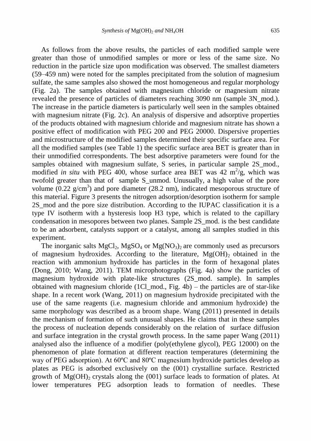
Synthesis of Mg(OH)2 and NH4OH 635
As follows from the above results, the particles of each modified sample were
greater than those of unmodified samples or more or less of the same size. No
reduction in the particle size upon modification was observed. The smallest diameters
(59–459 nm) were noted for the samples precipitated from the solution of magnesium
sulfate, the same samples also showed the most homogeneous and regular morphology
(Fig. 2a). The samples obtained with magnesium chloride or magnesium nitrate
revealed the presence of particles of diameters reaching 3090 nm (sample 3N_mod.).
The increase in the particle diameters is particularly well seen in the samples obtained
with magnesium nitrate (Fig. 2c). An analysis of dispersive and adsorptive properties
of the products obtained with magnesium chloride and magnesium nitrate has shown a
positive effect of modification with PEG 200 and PEG 20000. Dispersive properties
and microstructure of the modified samples determined their specific surface area. For
all the modified samples (see Table 1) the specific surface area BET is greater than in
their unmodified correspondents. The best adsorptive parameters were found for the
samples obtained with magnesium sulfate, S series, in particular sample 2S_mod.,
modified in situ with PEG 400, whose surface area BET was 42 m2/g, which was
twofold greater than that of sample S_unmod. Unusually, a high value of the pore
volume (0.22 g/cm3) and pore diameter (28.2 nm), indicated mesoporous structure of
this material. Figure 3 presents the nitrogen adsorption/desorption isotherm for sample
2S_mod and the pore size distribution. According to the IUPAC classification it is a
type IV isotherm with a hysteresis loop H3 type, which is related to the capillary
condensation in mesopores between two planes. Sample 2S_mod. is the best candidate
to be an adsorbent, catalysts support or a catalyst, among all samples studied in this
experiment.
The inorganic salts MgCl2, MgSO4 or Mg(NO3)2 are commonly used as precursors
of magnesium hydroxides. According to the literature, Mg(OH)2 obtained in the
reaction with ammonium hydroxide has particles in the form of hexagonal plates
(Dong, 2010; Wang, 2011). TEM microphotographs (Fig. 4a) show the particles of
magnesium hydroxide with plate-like structures (2S_mod. sample). In samples
obtained with magnesium chloride (1Cl_mod., Fig. 4b) – the particles are of star-like
shape. In a recent work (Wang, 2011) on magnesium hydroxide precipitated with the
use of the same reagents (i.e. magnesium chloride and ammonium hydroxide) the
same morphology was described as a broom shape. Wang (2011) presented in details
the mechanism of formation of such unusual shapes. He claims that in these samples
the process of nucleation depends considerably on the relation of surface diffusion
and surface integration in the crystal growth process. In the same paper Wang (2011)
analysed also the influence of a modifier (poly(ethylene glycol), PEG 12000) on the
phenomenon of plate formation at different reaction temperatures (determining the
way of PEG adsorption). At 60ºC and 80ºC magnesium hydroxide particles develop as
plates as PEG is adsorbed exclusively on the (001) crystalline surface. Restricted
growth of Mg(OH)2 crystals along the (001) surface leads to formation of plates. At
lower temperatures PEG adsorption leads to formation of needles. These
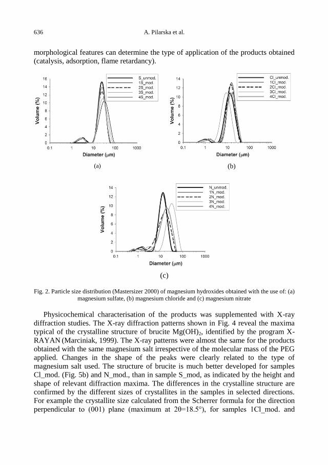
636 A. Pilarska et al.
morphological features can determine the type of application of the products obtained
(catalysis, adsorption, flame retardancy).
(a)
(b)
(c)
Fig. 2. Particle size distribution (Mastersizer 2000) of magnesium hydroxides obtained with the use of: (a)
magnesium sulfate, (b) magnesium chloride and (c) magnesium nitrate
Physicochemical characterisation of the products was supplemented with X-ray
diffraction studies. The X-ray diffraction patterns shown in Fig. 4 reveal the maxima
typical of the crystalline structure of brucite Mg(OH)2, identified by the program X-
RAYAN (Marciniak, 1999). The X-ray patterns were almost the same for the products
obtained with the same magnesium salt irrespective of the molecular mass of the PEG
applied. Changes in the shape of the peaks were clearly related to the type of
magnesium salt used. The structure of brucite is much better developed for samples
Cl_mod. (Fig. 5b) and N_mod., than in sample S_mod, as indicated by the height and
shape of relevant diffraction maxima. The differences in the crystalline structure are
confirmed by the different sizes of crystallites in the samples in selected directions.
For example the crystallite size calculated from the Scherrer formula for the direction
perpendicular to (001) plane (maximum at 2θ=18.5°), for samples 1Cl_mod. and
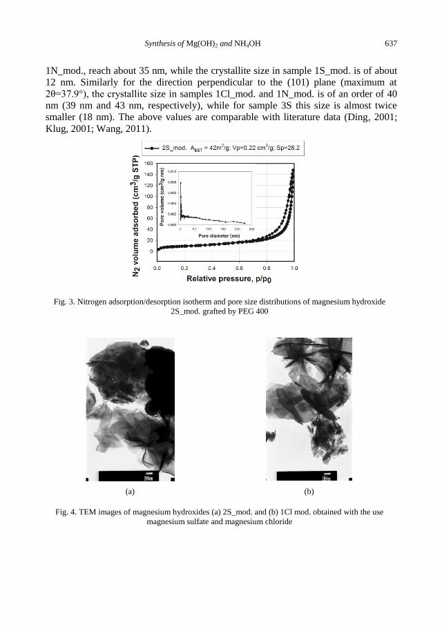
Synthesis of Mg(OH)2 and NH4OH 637
1N_mod., reach about 35 nm, while the crystallite size in sample 1S_mod. is of about
12 nm. Similarly for the direction perpendicular to the (101) plane (maximum at
2θ=37.9°), the crystallite size in samples 1Cl_mod. and 1N_mod. is of an order of 40
nm (39 nm and 43 nm, respectively), while for sample 3S this size is almost twice
smaller (18 nm). The above values are comparable with literature data (Ding, 2001;
Klug, 2001; Wang, 2011).
Fig. 3. Nitrogen adsorption/desorption isotherm and pore size distributions of magnesium hydroxide
2S_mod. grafted by PEG 400
(a)
(b)
Fig. 4. TEM images of magnesium hydroxides (a) 2S_mod. and (b) 1Cl mod. obtained with the use
magnesium sulfate and magnesium chloride
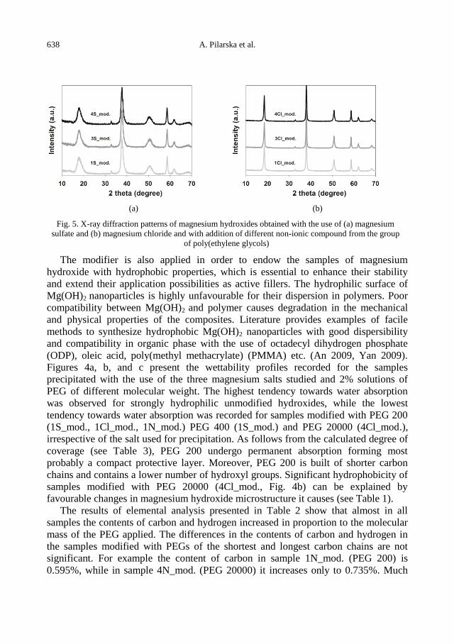
638 A. Pilarska et al.
(a)
(b)
Fig. 5. X-ray diffraction patterns of magnesium hydroxides obtained with the use of (a) magnesium
sulfate and (b) magnesium chloride and with addition of different non-ionic compound from the group
of poly(ethylene glycols)
The modifier is also applied in order to endow the samples of magnesium
hydroxide with hydrophobic properties, which is essential to enhance their stability
and extend their application possibilities as active fillers. The hydrophilic surface of
Mg(OH)2 nanoparticles is highly unfavourable for their dispersion in polymers. Poor
compatibility between Mg(OH)2 and polymer causes degradation in the mechanical
and physical properties of the composites. Literature provides examples of facile
methods to synthesize hydrophobic Mg(OH)2 nanoparticles with good dispersibility
and compatibility in organic phase with the use of octadecyl dihydrogen phosphate
(ODP), oleic acid, poly(methyl methacrylate) (PMMA) etc. (An 2009, Yan 2009).
Figures 4a, b, and c present the wettability profiles recorded for the samples
precipitated with the use of the three magnesium salts studied and 2% solutions of
PEG of different molecular weight. The highest tendency towards water absorption
was observed for strongly hydrophilic unmodified hydroxides, while the lowest
tendency towards water absorption was recorded for samples modified with PEG 200
(1S_mod., 1Cl_mod., 1N_mod.) PEG 400 (1S_mod.) and PEG 20000 (4Cl_mod.),
irrespective of the salt used for precipitation. As follows from the calculated degree of
coverage (see Table 3), PEG 200 undergo permanent absorption forming most
probably a compact protective layer. Moreover, PEG 200 is built of shorter carbon
chains and contains a lower number of hydroxyl groups. Significant hydrophobicity of
samples modified with PEG 20000 (4Cl_mod., Fig. 4b) can be explained by
favourable changes in magnesium hydroxide microstructure it causes (see Table 1).
The results of elemental analysis presented in Table 2 show that almost in all
samples the contents of carbon and hydrogen increased in proportion to the molecular
mass of the PEG applied. The differences in the contents of carbon and hydrogen in
the samples modified with PEGs of the shortest and longest carbon chains are not
significant. For example the content of carbon in sample 1N_mod. (PEG 200) is
0.595%, while in sample 4N_mod. (PEG 20000) it increases only to 0.735%. Much
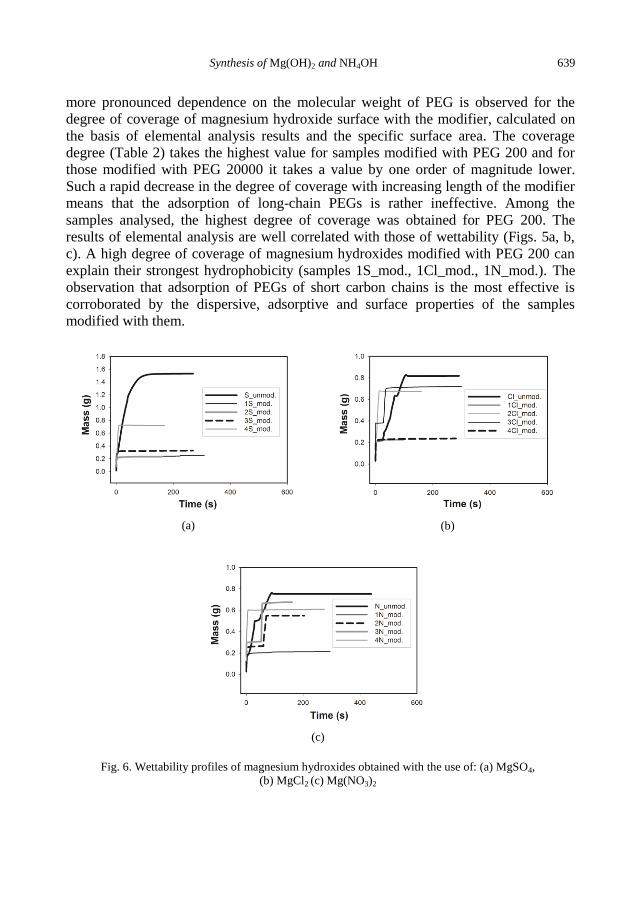
Synthesis of Mg(OH)2 and NH4OH 639
more pronounced dependence on the molecular weight of PEG is observed for the
degree of coverage of magnesium hydroxide surface with the modifier, calculated on
the basis of elemental analysis results and the specific surface area. The coverage
degree (Table 2) takes the highest value for samples modified with PEG 200 and for
those modified with PEG 20000 it takes a value by one order of magnitude lower.
Such a rapid decrease in the degree of coverage with increasing length of the modifier
means that the adsorption of long-chain PEGs is rather ineffective. Among the
samples analysed, the highest degree of coverage was obtained for PEG 200. The
results of elemental analysis are well correlated with those of wettability (Figs. 5a, b,
c). A high degree of coverage of magnesium hydroxides modified with PEG 200 can
explain their strongest hydrophobicity (samples 1S_mod., 1Cl_mod., 1N_mod.). The
observation that adsorption of PEGs of short carbon chains is the most effective is
corroborated by the dispersive, adsorptive and surface properties of the samples
modified with them.
(a)
(b)
(c)
Fig. 6. Wettability profiles of magnesium hydroxides obtained with the use of: (a) MgSO4,
(b) MgCl2 (c) Mg(NO3)2

640 A. Pilarska et al.
Another interesting observation was that the highest degree of coverage was
calculated for the samples precipitated with the use of magnesium chloride and
magnesium nitrate, which is related to small surface area BET of these samples. The
degree of coverage found for the sample precipitated with magnesium sulfate having
smaller surface area is considerably lower.
Table 2. Elemental content of carbon and hydrogen in modified samples of magnesium hydroxide
precipitated with the use of magnesium sulfate and magnesium chloride and the calculated degree of their
coverage with PEG compounds
Sample
No.
Elemental content
(%)
Coverage degree
(µmol/m2)
C H
S_unmod. ─ ─ ─
1S_mod. 1.177 6.135 7.467
2S_mod. 1.276 6.335 4.091
3S_mod. 1.480 6.675 3.683
4S_mod. 1.613 6.878 0.106
Cl_unmod. ─ ─ ─
1Cl_mod. 0.784 2.825 31.325
2Cl_mod. 0.919 2.893 18.426
3Cl_mod. 0.821 2.924 10.194
4Cl_mod. 1.107 3.056 0.446
N_unmod. ─ ─ ─
1N_mod. 0.595 2.568 26.023
2N_mod. 0.645 2.825 14.124
3N_mod. 0.690 2.937 9.036
4N_mod. 0.735 2.989 0.323
Fig. 7. TG/DTA curves of magnesium hydroxides S_unmod. and 2S_mod.
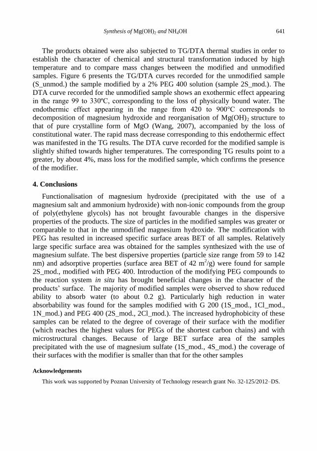
Synthesis of Mg(OH)2 and NH4OH 641
The products obtained were also subjected to TG/DTA thermal studies in order to
establish the character of chemical and structural transformation induced by high
temperature and to compare mass changes between the modified and unmodified
samples. Figure 6 presents the TG/DTA curves recorded for the unmodified sample
(S_unmod.) the sample modified by a 2% PEG 400 solution (sample 2S_mod.). The
DTA curve recorded for the unmodified sample shows an exothermic effect appearing
in the range 99 to 330ºC, corresponding to the loss of physically bound water. The
endothermic effect appearing in the range from 420 to 900°C corresponds to
decomposition of magnesium hydroxide and reorganisation of Mg(OH)2 structure to
that of pure crystalline form of MgO (Wang, 2007), accompanied by the loss of
constitutional water. The rapid mass decrease corresponding to this endothermic effect
was manifested in the TG results. The DTA curve recorded for the modified sample is
slightly shifted towards higher temperatures. The corresponding TG results point to a
greater, by about 4%, mass loss for the modified sample, which confirms the presence
of the modifier.
4. Conclusions
Functionalisation of magnesium hydroxide (precipitated with the use of a
magnesium salt and ammonium hydroxide) with non-ionic compounds from the group
of poly(ethylene glycols) has not brought favourable changes in the dispersive
properties of the products. The size of particles in the modified samples was greater or
comparable to that in the unmodified magnesium hydroxide. The modification with
PEG has resulted in increased specific surface areas BET of all samples. Relatively
large specific surface area was obtained for the samples synthesized with the use of
magnesium sulfate. The best dispersive properties (particle size range from 59 to 142
nm) and adsorptive properties (surface area BET of 42 m2/g) were found for sample
2S_mod., modified with PEG 400. Introduction of the modifying PEG compounds to
the reaction system in situ has brought beneficial changes in the character of the
products’ surface. The majority of modified samples were observed to show reduced
ability to absorb water (to about 0.2 g). Particularly high reduction in water
absorbability was found for the samples modified with G 200 (1S_mod., 1Cl_mod.,
1N_mod.) and PEG 400 (2S_mod., 2Cl_mod.). The increased hydrophobicity of these
samples can be related to the degree of coverage of their surface with the modifier
(which reaches the highest values for PEGs of the shortest carbon chains) and with
microstructural changes. Because of large BET surface area of the samples
precipitated with the use of magnesium sulfate (1S_mod., 4S_mod.) the coverage of
their surfaces with the modifier is smaller than that for the other samples
Acknowledgements
This work was supported by Poznan University of Technology research grant No. 32-125/2012‒DS.
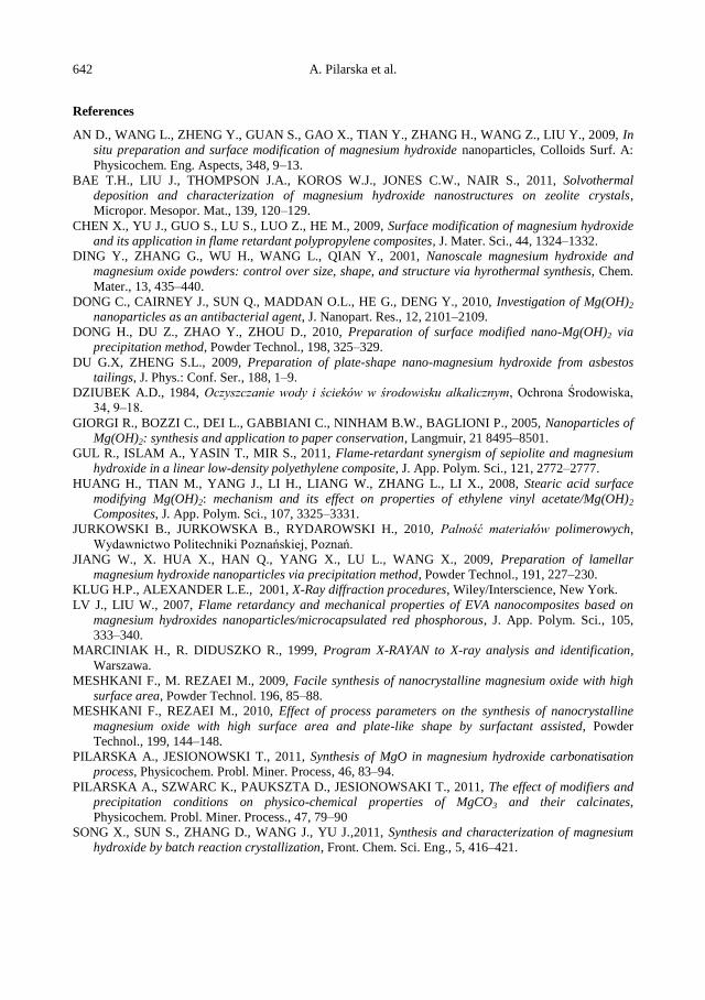
642 A. Pilarska et al.
References
AN D., WANG L., ZHENG Y., GUAN S., GAO X., TIAN Y., ZHANG H., WANG Z., LIU Y., 2009, In
situ preparation and surface modification of magnesium hydroxide nanoparticles, Colloids Surf. A:
Physicochem. Eng. Aspects, 348, 9‒13.
BAE T.H., LIU J., THOMPSON J.A., KOROS W.J., JONES C.W., NAIR S., 2011, Solvothermal
deposition and characterization of magnesium hydroxide nanostructures on zeolite crystals,
Micropor. Mesopor. Mat., 139, 120‒129.
CHEN X., YU J., GUO S., LU S., LUO Z., HE M., 2009, Surface modification of magnesium hydroxide
and its application in flame retardant polypropylene composites, J. Mater. Sci., 44, 1324‒1332.
DING Y., ZHANG G., WU H., WANG L., QIAN Y., 2001, Nanoscale magnesium hydroxide and
magnesium oxide powders: control over size, shape, and structure via hyrothermal synthesis, Chem.
Mater., 13, 435‒440.
DONG C., CAIRNEY J., SUN Q., MADDAN O.L., HE G., DENG Y., 2010, Investigation of Mg(OH)2
nanoparticles as an antibacterial agent, J. Nanopart. Res., 12, 2101‒2109.
DONG H., DU Z., ZHAO Y., ZHOU D., 2010, Preparation of surface modified nano-Mg(OH)2 via
precipitation method, Powder Technol., 198, 325–329.
DU G.X, ZHENG S.L., 2009, Preparation of plate-shape nano-magnesium hydroxide from asbestos
tailings, J. Phys.: Conf. Ser., 188, 1‒9.
DZIUBEK A.D., 1984, Oczyszczanie wody i ścieków w środowisku alkalicznym, Ochrona Środowiska,
34, 9‒18.
GIORGI R., BOZZI C., DEI L., GABBIANI C., NINHAM B.W., BAGLIONI P., 2005, Nanoparticles of
Mg(OH)2: synthesis and application to paper conservation, Langmuir, 21 8495‒8501.
GUL R., ISLAM A., YASIN T., MIR S., 2011, Flame-retardant synergism of sepiolite and magnesium
hydroxide in a linear low-density polyethylene composite, J. App. Polym. Sci., 121, 2772‒2777.
HUANG H., TIAN M., YANG J., LI H., LIANG W., ZHANG L., LI X., 2008, Stearic acid surface
modifying Mg(OH)2: mechanism and its effect on properties of ethylene vinyl acetate/Mg(OH)2
Composites, J. App. Polym. Sci., 107, 3325‒3331.
JURKOWSKI B., JURKOWSKA B., RYDAROWSKI H., 2010, Palność materiałów polimerowych,
Wydawnictwo Politechniki Poznańskiej, Poznań.
JIANG W., X. HUA X., HAN Q., YANG X., LU L., WANG X., 2009, Preparation of lamellar
magnesium hydroxide nanoparticles via precipitation method, Powder Technol., 191, 227‒230.
KLUG H.P., ALEXANDER L.E., 2001, X-Ray diffraction procedures, Wiley/Interscience, New York.
LV J., LIU W., 2007, Flame retardancy and mechanical properties of EVA nanocomposites based on
magnesium hydroxides nanoparticles/microcapsulated red phosphorous, J. App. Polym. Sci., 105,
333‒340.
MARCINIAK H., R. DIDUSZKO R., 1999, Program X-RAYAN to X-ray analysis and identification,
Warszawa.
MESHKANI F., M. REZAEI M., 2009, Facile synthesis of nanocrystalline magnesium oxide with high
surface area, Powder Technol. 196, 85‒88.
MESHKANI F., REZAEI M., 2010, Effect of process parameters on the synthesis of nanocrystalline
magnesium oxide with high surface area and plate-like shape by surfactant assisted, Powder
Technol., 199, 144‒148.
PILARSKA A., JESIONOWSKI T., 2011, Synthesis of MgO in magnesium hydroxide carbonatisation
process, Physicochem. Probl. Miner. Process, 46, 83‒94.
PILARSKA A., SZWARC K., PAUKSZTA D., JESIONOWSAKI T., 2011, The effect of modifiers and
precipitation conditions on physico-chemical properties of MgCO3 and their calcinates,
Physicochem. Probl. Miner. Process., 47, 79‒90
SONG X., SUN S., ZHANG D., WANG J., YU J.,2011, Synthesis and characterization of magnesium
hydroxide by batch reaction crystallization, Front. Chem. Sci. Eng., 5, 416‒421.

Synthesis of Mg(OH)2 and NH4OH 643
WANG D.A, ZHENG Y, GUAN S., GAO X., TIAN Y., ZHANG H., WANG Z., LIU Y., 2009, In situ
preparation and surface modification of Mg(OH)2 nanoparticles, Colloids Surf. A: Physicochem.
Eng. Aspects, 348, 9‒13.
WANG P., LI C., GONG H., WANG H., LIU J., 2011, Morphology control and growth mechanism of
magnesium hydroxide nanoparticles via a simple wet precipitation method, Ceram. Int., 37,
2061‒2066.
WANG W., QIAO X., CHEN J., LI H., 2007, Facile synthesis of magnesium oxide nanoplates via
chemical precipitation, Mater. Lett., 61, 3218‒3220.
YAN C., XUE G., ZOU L., YAN X., WANG W., 2005, Preparation of magnesium hydroxide
nanoflowers, J. Cryst. Growth, 282, 448‒454.
YAN H., ZHANG X., WEI L., LIU X., XU B., 2009, Hydrophobic magnesium hydroxide nanoparticles
via oleic acid and poly(methyl methacrylate) – grafting surface modification, Powder Technol.,
193,125‒129.
YILDRIM M., AKARSU H., 2010, Preparation of magnesium oxide (MgO) from dolomite by leach –
precipitation – pyrohydrolysis process, Physicochem. Probl. Miner. Process, 44, 257‒272.

644 A. Pilarska et al.

http://dx.doi.org/10.5277/ppmp120227
Physicochem. Probl. Miner. Process. 48(2), 2012, 645−654 Physicochemical Problems
of Mineral Processing
w w w . m i n p r o c . p w r . w r o c . p l / j o u r n a l / ISSN 1643-1049 (print)
ISSN 2084-4735 (online)
Received April 15, 2012; reviewed; accepted May 10, 2012
THE ROLE OF PARTICLE SIZE AND SOLID CONTENTS OF FEED
ON MICA-FELDSPAR SEPARATION IN GRAVITY
CONCENTRATION
Murat KADEMLI*, Ozcan Y. GULSOY
**
* Hacettepe University, Hacettepe Vocational School of Higher Education, [email protected]
** Hacettepe University, Department of Mining Engineering
Abstract. In the present study, the role of particle size of mica with flaky shape on the
separation efficiency of mica from feldspar by the shaking table and Reichert spiral (Model
HG7) concentrators were investigated. An albite ore containing mica from the Cine region of
Turkey was treated under various test conditions. During the study, particle size distribution,
solids content of the feed and flow rate of the feed were changed in the spiral tests. Then, the
flow rate of the feed was kept constant as 1 dm3/s in the shaking table tests. It was observed
that mica could be separated from feldspar, owing to its laminar morphology. Accordingly, the
particle size, directly related to the laminar morphology of mica, is the most effective
parameter in the separation process. The best results were obtained with spiral concentrators,
which met the requirements of the glass industry.
keywords: shaking table, spiral, mica, shape factor, gravity concentration
1. Introduction
Mica is the primary source of iron in feldspar minerals, which causes colouring in
ceramic and glass. The most common method for separating mica from feldspar is
flotation. Nevertheless, flotation has some disadvantages such as detrimental effects
on the environment because of chemical use, high investments and operation costs
(Akar, 1994; Bayraktar et al., 1999; 2002; Celik et al., 1998; 2001). The separation
does not always take place under conditions which are convenient for the
concentration criterion. In order to allow for the differences in the particle shape, the
concentration criterion must be multiplied by the shape ratio factor (Burt, 1984).
When there is a marked difference in particle shape, the concentration criterion, which
is the density of the heavy species minus the density of suspending fluid, divided the
density of light species minus density of suspending fluid, approaches 1.0. Typical of
this is the separation of mica from quartz and feldspar (Browning, 1973).
Mica and feldspar are close to each other in respect to their density. The densities
of feldspar and mica minerals are approximately 2.65 and 2.7-3.4 g/cm3, respectively
(Ipekoglu and Asmatulu, 1996). As mentioned by Iverson (1932) the difference
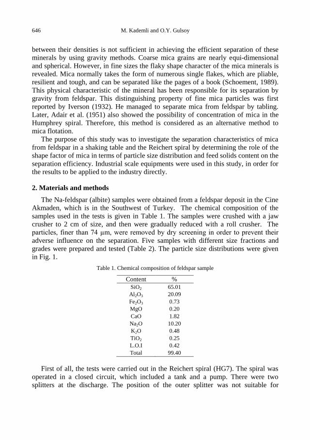
646 M. Kademli and O.Y. Gulsoy
between their densities is not sufficient in achieving the efficient separation of these
minerals by using gravity methods. Coarse mica grains are nearly equi-dimensional
and spherical. However, in fine sizes the flaky shape character of the mica minerals is
revealed. Mica normally takes the form of numerous single flakes, which are pliable,
resilient and tough, and can be separated like the pages of a book (Schoement, 1989).
This physical characteristic of the mineral has been responsible for its separation by
gravity from feldspar. This distinguishing property of fine mica particles was first
reported by Iverson (1932). He managed to separate mica from feldspar by tabling.
Later, Adair et al. (1951) also showed the possibility of concentration of mica in the
Humphrey spiral. Therefore, this method is considered as an alternative method to
mica flotation.
The purpose of this study was to investigate the separation characteristics of mica
from feldspar in a shaking table and the Reichert spiral by determining the role of the
shape factor of mica in terms of particle size distribution and feed solids content on the
separation efficiency. Industrial scale equipments were used in this study, in order for
the results to be applied to the industry directly.
2. Materials and methods
The Na-feldspar (albite) samples were obtained from a feldspar deposit in the Cine
Akmaden, which is in the Southwest of Turkey. The chemical composition of the
samples used in the tests is given in Table 1. The samples were crushed with a jaw
crusher to 2 cm of size, and then were gradually reduced with a roll crusher. The
particles, finer than 74 µm, were removed by dry screening in order to prevent their
adverse influence on the separation. Five samples with different size fractions and
grades were prepared and tested (Table 2). The particle size distributions were given
in Fig. 1.
Table 1. Chemical composition of feldspar sample
Content %
SiO2 65.01
Al2O3 20.09
Fe2O3 0.73
MgO 0.20
CaO 1.82
Na2O 10.20
K2O 0.48
TiO2 0.25
L.O.I 0.42
Total 99.40
First of all, the tests were carried out in the Reichert spiral (HG7). The spiral was
operated in a closed circuit, which included a tank and a pump. There were two
splitters at the discharge. The position of the outer splitter was not suitable for
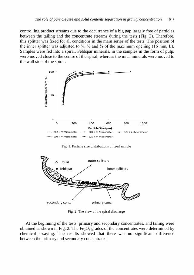
The role of particle size and solid contents separation in gravity concentration 647
controlling product streams due to the occurrence of a big gap largely free of particles
between the tailing and the concentrate streams during the tests (Fig. 2). Therefore,
this splitter was fixed for all conditions in the main series of the tests. The position of
the inner splitter was adjusted to ¼, ½ and ¾ of the maximum opening (16 mm, L).
Samples were fed into a spiral. Feldspar minerals, in the samples in the form of pulp,
were moved close to the centre of the spiral, whereas the mica minerals were moved to
the wall side of the spiral.
1
10
100
0 200 400 600 800 1000
Cum
ulat
ive
Und
ersi
ze (%
)
Particle Size (µm)
- 212 + 74 Micrometer - 300 + 74 Micrometer - 425 + 74 Micrometer
- 600 + 74 Micrometer - 825 + 74 Micrometer
Fig. 1. Particle size distributions of feed sample
L
mica
feldspar
secondary conc.
inner splitters
outer splitters
primary conc.
Fig. 2. The view of the spiral discharge
At the beginning of the tests, primary and secondary concentrates, and tailing were
obtained as shown in Fig. 2. The Fe2O3 grades of the concentrates were determined by
chemical assaying. The results showed that there was no significant difference
between the primary and secondary concentrates.
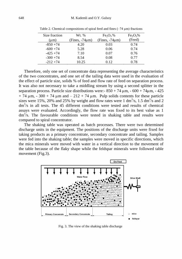
648 M. Kademli and O.Y. Gulsoy
Table 2. Chemical compositions of spiral feed and fines (–74 µm) fractions
Size fraction
(m)
Wt. %
(Fines, -74m)
Fe2O3 %
(Fines, -74m)
Fe2O3%
(Feed)
-850 +74 4.20 0.03 0.74
-600 +74 5.28 0.06 0.74
-425 +74 7.10 0.07 0.76
-300 +74 8.54 0.08 0.77
-212 +74 10.25 0.12 0.78
Therefore, only one set of concentrate data representing the average characteristics
of the two concentrates, and one set of the tailing data were used in the evaluation of
the effect of particle size, solids % of feed and flow rate of feed on separation process.
It was also not necessary to take a middling stream by using a second splitter in the
separation process. Particle size distributions were:- 850 + 74 m, - 600 + 74m, - 425
+ 74 m, - 300 + 74 m and – 212 + 74 m. Pulp solids contents for these particle
sizes were 15%, 20% and 25% by weight and flow rates were 1 dm3/s, 1.5 dm
3/s and 2
dm3/s in all tests. The 45 different conditions were tested and results of chemical
assays were evaluated. Accordingly, the flow rate was fixed to its best value as 1
dm3/s. The favourable conditions were tested in shaking table and results were
compared to spiral concentrator.
The shaking table was operated as batch processes. There were two determined
discharge units in the equipment. The positions of the discharge units were fixed for
taking products as a primary concentrate, secondary concentrate and tailing. Samples
were fed into the shaking table; the samples were moved in specific directions, which
the mica minerals were moved with water in a vertical direction to the movement of
the table because of the flaky shape while the feldspar minerals were followed table
movement (Fig.3).
Fig. 3. The view of the shaking table discharge
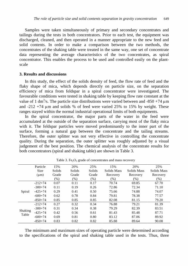
The role of particle size and solid contents separation in gravity concentration 649
Samples were taken simultaneously of primary and secondary concentrates and
tailings during the tests in both concentrators. Prior to each test, the equipment was
discharged, cleaned, and then operated in a manner appropriate to the new feed and
solid contents. In order to make a comparison between the two methods, the
concentrates of the shaking table were treated in the same way, one set of concentrate
data representing the average characteristics of the two concentrates, as spiral
concentrator. This enables the process to be used and controlled easily on the plant-
scale
3. Results and discussions
In this study, the effect of the solids density of feed, the flow rate of feed and the
flaky shape of mica, which depends directly on particle size, on the separation
efficiency of mica from feldspar in a spiral concentrator were investigated. The
favourable conditions were tested in shaking table by keeping flow rate constant at the
value of 1 dm3/s. The particle size distributions were varied between and -850 +74 m
and -212 +74 m and solids % of feed were varied 25% to 15% by weight. These
ranges stayed within the normal industrial operational limits of both equipments.
In the spiral concentrator, the major parts of the water in the feed were
accumulated at the outside of the separation surface, carrying most of the flaky mica
with it. The feldspar particles were moved predominantly to the inner part of the
surface, forming a natural gap between the concentrate and the tailing streams.
Therefore, the outer splitter was not very effective in controlling the concentrate
quality. During the separation, the outer splitter was roughly adjusted by a visual
judgement of the best position. The chemical analysis of the concentrate results for
both concentrators (spiral and shaking table) are shown in Table 3.
Table 3. Fe2O3 grade of concentrates and mass recovery
Particle
Size
(µm)
15%
Solids
Grade
(%)
20%
Solids
Grade
(%)
25%
Solids
Grade
(%)
15%
Solids Mass
Recovery
(%)
20%
Solids Mass
Recovery
(%)
25%
Solids Mass
Recovery
(%)
Spiral
-212+74 0.07 0.11 0.17 70.74 69.85 67.70
-300+74 0.11 0.19 0.26 72.86 72.34 71.10
-425+74 0.29 0.41 0.50 75.66 74.88 74.07
-600+74 0.62 0.78 0.84 79.81 78.38 77.57
-850+74 0.85 0.85 0.85 82.08 81.15 79.20
Shaking
Table
-212+74 0.27 0.32 0.34 76.88 79.21 81.39
-300+74 0.31 0.34 0.38 79.29 82.39 83.51
-425+74 0.42 0.56 0.61 81.43 85.48 87.71
-600+74 0.69 0.81 0.80 83.12 87.06 89.92
-850+74 0.83 0.82 0.82 85.88 89.64 90.08
The minimum and maximum sizes of operating particle were determined according
to the specifications of the spiral and shaking table used in the tests. Thus, three

650 M. Kademli and O.Y. Gulsoy
different solid contents that were 15%, 20% and 25% by weight, were selected and
performed. The effects of the solid content on the Fe2O3 grade of concentrate, Fe2O3
removal, and the mass recovery were investigated for each feed size. The results are
shown in Figs. 4–6 for the spiral concentrator and Fig. 7 for the shaking table.
0
10
20
30
40
50
60
70
80
90
100
0.00
0.10
0.20
0.30
0.40
0.50
0.60
0.70
0.80
0.90
1.00
0 200 400 600 800
Re
mo
va
l Re
cov
ery
(%)
Gra
de
(%
)
Maximum Particle Size (µm)
Grade of 15% Solids Grade of 20% Solids Grade of 25% SolidsRecovery of 15% Solids Recovery of 20% Solids Recovery of 25% Solids
Fig. 4. A relationship between grade, recovery and maximum particle size in spiral concentrator
at 1 dm3/s flow rate
0
10
20
30
40
50
60
70
80
90
100
0.00
0.10
0.20
0.30
0.40
0.50
0.60
0.70
0.80
0.90
1.00
0 200 400 600 800
Re
mo
va
l Re
cov
ery
(%
)
Gra
de
(%
)
Maximum Particle Size (µm)
Grade of 15% Solids Grade of 20% Solids Grade of 25% SolidsRecovery of 15% Solids Recovery of 20% Solids Recovery of 25% Solids
Fig. 5. A relationship between grade, recovery and maximum particle size in spiral concentrator
at 1.5 dm3/s flow rate

The role of particle size and solid contents separation in gravity concentration 651
0
10
20
30
40
50
60
70
80
90
100
0.00
0.10
0.20
0.30
0.40
0.50
0.60
0.70
0.80
0.90
1.00
0 200 400 600 800
Re
mo
va
l Re
cov
ery
(%
)
Gra
de
(%)
Maximum Particle Size (µm)
Grade of 15% Solids Grade of 20% Solids Grade of 25% SolidsRecovery of 15% Solids Recovery of 20% Solids Recovery of 25% Solids
Fig. 6. A relationship between grade, recovery and maximum particle size in spiral concentrator
at 2 dm3/s flow rate
0
10
20
30
40
50
60
70
80
90
100
0.00
0.10
0.20
0.30
0.40
0.50
0.60
0.70
0.80
0.90
1.00
0 200 400 600 800
Re
mo
val R
eco
very
(%)
Gra
de
(%)
Maximum Particle Size (µm)
Grade of 15% Solids Grade of 20% Solids Grade of 25% Solids
Recovery of 15% Solids Recovery of 20% Solids Recovery of 25% Solids
Fig. 7. A relationship between grade, recovery and maximum particle size in shaking table
at 1 dm3/s flow rate
From Figs. 4-7 it can be seen that the particle size distribution is the most effective
parameter in the separation in both methods. In general, the separation efficiency of
the gravity concentration methods is better for coarse particles than fine particles
because the gravity force is more effective on coarse particles. However, the coarse
652 M. Kademli and O.Y. Gulsoy
mica grains are nearly equi-dimensional, and the difference in the specific gravity is
not sufficient to make the separation of these minerals possible in this case. On the
other hand, the flaky shape character of the smaller mica particles made the separation
of the mica from the feldspar possible in the fine particle sizes. This situation is not
related to the differences in the degree of liberation since mica was in the form of
liberated particles even in the coarse fractions.
The Fe2O3 grade of the concentrate and the Fe2O3 removal and recovery of the
feldspar were directly related to the change in the particle size. An increase in the
particle size occurs with the Fe2O3 grade of the concentrate (Table 3) and decreases
with the Fe2O3 removal. The removal recovery was calculated from equation:
1001
f
c
F
CRR , (1)
where RR is removal recovery (%), C mass of concentrate (kg), F mass of feed (kg), c
Fe2O3 content in concentrate (%), f Fe2O3 content in feed (%).
The mass recovery decreased slightly with the finer particle size since the amount
of particles carried by water to the tailings stream increased. This behaviour was
observed in both concentrators. According to Table 3, increasing the solids % of the
feed increased the Fe2O3 grade of the concentrate and decreased the mass recovery,
except for the feed top size fraction of - 850 m + 74 m. As well as reducing the
separation efficiency, an increase in the solids content slightly reduced the amount of
concentrate.
In classical gravity concentration, the purpose of separation is to get maximum
grade of metallic ore with maximum possible mass recovery. In this case, most
important terms are Fe2O3 content of concentrate, removal recovery and mass
recovery. That is why the purpose of separation is to remove Fe2O3 from the feldspar
minerals and to get the minimum Fe2O3 contents, the best Fe2O3 removal and mass
recovery values in order to meet the glass industry requirements. So, the lower Fe2O3
content is favourable for this kind of separation. The spiral concentrate has 0.07%
Fe2O3 content with a 93% Fe2O3 removal recovery and approximately 70% mass
recovery, whereas the shaking table concentrate has 0.27% Fe2O3 content with a 72%
Fe2O3 removal recovery and approximately 76% yield. Although the mass recovery of
shaking table is higher than spiral concentrator, % Fe2O3 content and Fe2O3 removal
recovery do not meet the desired specifications of glass industry.
The results showed that the spiral concentrator is more favourable than the shaking
table for this kind of separation process. According to the concentrators operating
principles, the spiral concentrator has a very significant advantage such as the
centrifugal force contribution. The most favourable results of both concentrators are
given in Fig. 8.

The role of particle size and solid contents separation in gravity concentration 653
0
10
20
30
40
50
60
70
80
90
100
0.00
0.10
0.20
0.30
0.40
0.50
0.60
0.70
0.80
0.90
1.00
0 200 400 600 800 1000
Re
mo
val R
eco
very
(%)
Gra
de
(%)
Maximum Particle Size (µm)
Grade of 15% Solids in Spiral Grade of 15% Solids in Shaking Table
Recovery of 15% Solids in Spiral Recovery of 15% Solids in Shaking Table
Fig. 8. Comparison of both concentrators in their best conditions
4. Conclusions
In this investigation, the role of mica flaky shape characteristics, which is achieved
by decreasing the particle size of the feed, flow rate and the effect of the solids % in
the feed on the mica separation from feldspar mineral, were examined. The results
revealed that the increasing in particle size had an extreme effect on separation
efficiency. Separation was not possible when the particle sizes were - 850 m + 74
m or - 600 m + 74 m.
The separation efficiency of the mica removal increased as the particle size
distribution got finer, the most suitable particle size fraction being - 212 m + 74 m
in both concentrators. In the spiral, the Fe2O3 content of the concentrate was reduced
from 0.73% to 0.07% with 93% removal of the Fe2O3 and mass recovery of
approximately 70%, whereas the Fe2O3 content of the concentrate was reduced from
0.73% to 0.27% with a 72% removal of the Fe2O3 and a mass recovery of
approximately 76% in the shaking table concentrator.
The most favourable results were obtained in the spiral concentrator. There was a
certain separation occurring in the shaking table, but the values did not meet the
required specifications for the glass industry. On the other hand, the iron content,
which was obtained in the spiral tests, met these specifications. Firing buttons with a
pale pink colour confirmed these results.
It appeared that the particle size needed to be reduced to minus 212 µm in order to
ensure that the mica had a flaky shape characteristic, which had the desired distinctive
behaviour in these concentration processes.
654 M. Kademli and O.Y. Gulsoy
Although the effect on the separation efficiency of the solids in the feed was less
pronounced than that of the particle size, the increasing solids significantly reduced
the separation efficiency. Only the concentrate obtained with the minimum solids
(15%) met the desired specification.
References
ADAIR, R., MC DANIEL, W.T., HUDSPETH, W.R.,1951, A new method for recovery of flake mica,
Min. Eng. 3, 252- 254.
AKAR, A., 1994. Evaluation of Gördes Köprübaşı district feldspar industrial raw material deposits, in:
5th Progress in Mineral Processing Technology Symposium, ed. H. Demirel and S. Ersayın. Balkema
Inc., Rotterdam 243-249.
BAYRAKTAR, I., ERSAYIN, S., GULSOY, O.Y., EKMEKCİ, Z., CAN, N.M.,1999. Temel seramik ve
cam hammaddelerimizdeki (feldispat, kuvars ve kaolin) kalite sorunlari ve cozum onerileri, in: 3rd.
Industrial Mineral Symposium. Izmir, Turkey 22-33.
BAYRAKTAR, I., GULSOY, O.Y., CAN N.M., ORHAN, E.C., 2002. Feldispatlarin zenginlestirilmesi,
in : 4th Industrial Mineral Symposium, Izmir, Turkey 97-105.
BROWNING, J.S.,1973, Mica Benefication, U.S. Bureau of Mines Bulletin, 662, 21 – 22.
BURT, O.R., 1984. Gravity Concentration Technology, Elsevier Science Publishers, Amsterdam, Chap.
13.
CELIK, M.S., CAN, I., EREN R.H.,1998. Removal of titanium impurities from feldspar ores by new
flotation collectors, Miner. Eng. 12, 1201-1208.
CELIK, M.S., PEHLIVANOGLU, B., ASLANBAS, A., ASMATULU, R., 2001, Flotation of coloured
impurities from feldspar ores, Miner. and Metall. Proces. 18, 101-105.
IPEKOĞLU, B., ASMATÜLÜ, R., 1996.The recovery studies of pure mica for paint industry, in:
Changing Scopes in Mineral Processing, Balkema Inc.,Roterdam 415-420.
IVERSON, H.G.,1932, Separation of feldspar from quartz, Eng. and Min. J., April, 227-229.
SCHOEMENT,J.J.,1989, Mica and Vermiculite in South Africa, J.S. Afr. Inst. Metall., 89, 1-12.