photogrammetry and image processing techniques for beach
TRANSCRIPT


Photogrammetry and image processing
techniques for beach monitoring
Elena Sánchez García
Advisors: Josep Eliseu Pardo Pascual
Ángel Antonio Balaguer Beser
Geo-Environmental Cartography and Remote Sensing Group
Department of Cartographic engineering, Geodesy and
Photogrammetry
Universitat Politècnica de València
PhD in Mathematics; Code No. 2209
Valencia, April 2019


“Unbeatable …”
Perquè juntes som la pera llimonera!

Acknowledgments
…Una es consciente de todo lo que debe y, sin embargo, nunca parece haber
tiempo para agradecerlo… así que, allá vamos!
Sin duda, soy afortunada por tanto y a tantos/as a los que agradecer
durante esta etapa de mi vida. No ha sido fácil, y no habría sido posible sin
vosotros/as, así que “miles de gracias” por aguantarme, por quererme y por estar
siempre ahí, a mi lado.
Como estoy algo perdida, supongo que empezaré con aquella persona a la
que suelo acudir para encontrarme. Eres mi ejemplo a seguir, mi compañera de
viaje y de vida, y no hay nadie más buena y bonita que tú. Juntas somos
invencibles. Por favor, no te separes nunca de mí. A mis papis por ser los pilares
de todo a nuestro alrededor. Nunca podré devolveros y agradeceros ni siquiera un
poco de todo lo que os merecéis. Mamá, creo que soy tan fuerte a la par que
blandita como tú, pero me encanta si es así. Papá, no seas tan cabezota y
organizado que cada vez somos más iguales :P. Lo siento de verdad por mis
contestaciones y mi carácter tan estúpido a veces. Os quiero infinito. A mis tíos y
mis primitos Javier y Carmen, la nueva alegría de la casa. A todos y cada uno de
mis viejitos: yaya rosa pronto voy a tener tiempo para aprender a coser. Delia…qué
injusto y sin embargo cuánta bondad y amor sigue ofreciendo tu sonrisa. A mis
yayos/as y tíos/as que nunca os deberíais haber ido, José, Mina, Benito, Lucía,
Queru, Diego...os echo mucho, muchísimo de menos. Sé que estaríais muy
contentos de poder ver donde han llegado vuestras pequeñas. Os pido perdón por
no haberos dedicado el tiempo que os merecíais y vosotros sí nos dedicásteis.
Gracias por tantas tortillas de patata, trocitos de pan con chocolate, deliciosas
paellas; gracias por recogernos en el cole, por vuestro cariño, las ganas de reír y
luchar, la paciencia y dedicación, e incluso las regañinas…gracias por todo.
Quiero agradecer especialmente a mis directores de tesis, Angel y Josep.
Gracias por brindarme la oportunidad de trabajar con vosotros, por apoyarme,
hacer que aprendiera a valorarme, y guiarme por las diferentes etapas de este viaje.
Espero haber sabido estar a la altura.

De mi casa en la UPV, también gracias a cada una de las personas que
forman parte de la familia CGAT. A todos: Luis Ángel, Jorge, Alfonso, Jesús P.,
Jaime, JP, Sol, Jesús T., Carlos, Marta y Pabi, gracias por vuestra ayuda y hacer de
este departamento un lugar tan agradable para trabajar. Nunca fuisteis compañeros
sino grandes amigos que me llevo conmigo. Pabi, gracias por esa luna de miel a
Sudáfrica. Marta, gracias por estar siempre, por y para todo.
Del IH Cantabria quiero empezar por recordar mi acogida con Raúl
Medina y Mauricio González tras acabar cubierta de lágrimas. Realmente os doy
miles de gracias por hacerme ver que algo no iba bien en mi camino. Gracias por
vuestros consejos y facilidades. También a Paula Gómes, Jara, June, Felipe,
Alfonso, Erica, José Manuel, Tamara, Laura, Paula Núnez, Camilo y Albert, gracias
por acogerme como una más, hacerme probar el cachopo, cantar “la bicicleta” bajo
la lluvia santanderina, y hacerme sentir tan a gusto con vosotros. Aquí os espero.
De la Faculdade de Ciências da Universidade de Lisboa gracias a Rui
Taborda por acogerme, creer en mí y decirme tantas veces que no dejara de
sonreír. A Cristina, Ana, Ivana, Mafalda, João, Mónica y Tanya por vuestro cariño
y esa maravillosa fiesta de cumpleaños que me organizasteis. Gracias también a mi
galleguiña Rita por llevarme por aquellos escondites portugueses, y a mí
compañero de batalla Umberto con quién entre diferentes campañas de campo,
normalmente accidentadas, aprendí a valorar lo que era el buen vino . Cómo me
encanta recordar.
Del Water Research Laboratory de Sydney, I want to thank deeply Mitch
Harley for receiving me with the most amazing kindness and to give me the
opportunity to work on his latest initiative (CoastSnap). Also thanks to William
Glamore, Ian Coghlan and Ron Cox for the great time we had at the NSW Coastal
Conference in Port Stephens. Turner and Splinter many thanks to you too for your
advice, and to all the WRL members in general for the warm welcome in each
Monday morning meeting, in each field campaign with its corresponding meat
pies, goannas and lizards, and for considering me for the unforgettable beach
Christmas party with you all. Laura, qué suerte tuve de encontrarte como
compañera de trabajo. A ti en particular, gracias.
Del grupo Hémera de Santiago de Chile muchísimas gracias a todos por la
fantástica oportunidad que me brindasteis de colaborar con vosotros. Waldo,
Paulina y Idania, ‘ya poh’ gracias por ser tan grandes personas.
A mi grupo de amigos perroflautas que tan feliz me hacen y con quien tan
a gustito estoy. Xato, Carlos, Pabi, Marta, Pau, Inés (algunos ya van repe), gracias
por ser mis amigos.
A mis amigas de siempre con las que “crecí”, o lo intenté al menos. Gloria,
Marta, Agnes, Laura, gracias por vuestra paciencia, por quererme y por no cesar en
que nunca se estropee nuestra amistad.
No quiero olvidarme de dar las gracias al departamento de Matemática
Aplicada de la UPV por permitirme impartir docencia en diferentes asignaturas y
grados durante mi periodo de formación predoctoral. Sin lugar a dudas, es una de
las experiencias más enriquecedoras que me llevo. Gracias Genoveva Vizcarro por
tu ayuda y cariño cuando más lo necesité.
Agradecer al Ministerio de Educación, Cultura y Deporte del Gobierno de
España por la beca predoctoral FPU, y por las ayudas de movilidad concedidas,
que han permitido que esta Tesis Doctoral fuera una realidad. También a los
proyectos AICO/2015/098 y CGL2015-69906-R financiados respectivamente por
la Generalitat Valenciana y por el Ministerio de Economía y Competitividad. Por
último, agradecer también a las instituciones de educación superior y/o
investigación siguientes: la Universitat Politècnica de València, el Instituto de
Hidráulica Ambiental de la Universidad de Cantabria, la Universidad de Lisboa, el
WRL de la University of New South Wales, y la Universidad Mayor de Santiago de
Chile.
…a tod@s gracias. Jamás hubiera llegado hasta aquí sola. Un pasito más.
Elena Sánchez García
València, 2019

DEPARTMENT OF CARTOGRAPHIC ENGINEERING, GEODESY AND
PHOTOGRAMMETRY, UNIVERSITAT POLITÈCNICA DE VALÈNCIA
PHOTOGRAMMETRY AND IMAGE PROCESSING
TECHNIQUES FOR BEACH MONITORING
PhD dissertation presented by Elena Sánchez García, and directed by Dr. Josep E.
Pardo Pascual (Deptartment of Cartographic Engineering, Geodesy and
Photogrammetry; UPV) and Dr. Angel A. Balaguer Beser (Dept. of applied
mathematics; UPV), to obtain a PhD degree in mathematics. This doctoral thesis
has been carried out within the inter-university doctoral programme with quality
certification from the Universitat Politècnica de València and the Universitat de
València and within the Geoenvironmental Cartography and Remote Sensing
research group.
The thesis period has been directly financed for four years by a
predoctoral fellowship “Subprograma de formación de profesorado universitario;
FPU13/05877” from the Spanish Ministry of Education, Culture and Sport
(MECD). Additionally, the PhD student has been supported with two travel and
accommodation grants for carrying out a PhD stay in a foreign institution
(EST16/00907, EST15/00313) also from the MECD, and another from the
Erasmus+ internship program of the UPV (SMT 15-16 program). In addition, an
invitation was received from the Universidad Mayor de Santiago de Chile (Código
I-20018003 “Espacios Litorales”) to make a short stay as a PhD researcher. The
predoctoral student also received a grant to participate in the “36th ISRSE”
congress supported by the German Aerospace Center (DLR); and a grant to attend
the OPTIMISE training school and the associated CSIC Workshop supported by
COST Actions (European Cooperation in Science and Technology).
The PhD studies have been done within the projects “Development of high-
order numerical schemes and validation by experimental contrast to anayze sediment transport in
river bridges with protected riverbeds” AICO/2015/098 (IP: Dr. Ángel A. Balaguer)
supported by the Valencian government, and “Monitoring coastal changes using remote

sensing to mitigate the impacts of climate change” CGL2015-69906-R (IP: Dr. Josep E.
Pardo) supported by the Spanish Ministry of Economy and Competitiveness.
The candidate has taught a total of 180 hours in various bacherlor’s
degrees within the Department of Applied Mathematics at the UPV.
Elena Sánchez García
Valencia, 2019


i
CONTENTS Abstract vii
Resumen xi Resum xv
1. Introduction 19
1.1. Background and research justification
21
1.2. Aims and objectives 26 1.3. Document structure 27
2. Photogrammetric solution 35
2.1. Introduction
37
2.2. Horizon constraint 39 2.2.1. Image orientation using the horizon 39 2.2.2. Obtaining the horizon constraint 46
2.2.3. Obtaining from the horizon an initial solution of the camera orientation parameters
47
2.3. Methodology 48 2.3.1. A photogrammetric system 48
2.3.1.1. Camera calibration and image correction 49 2.3.1.2. Camera repositioning 49 2.3.1.3. Image rectification and data extraction 54
2.3.2. Practical implementation of C-Pro 55 2.4. Testing of the horizon constraint 56
2.4.1. Data and study area 57 2.4.2. Improvement of camera positioning 61 2.4.3. Different horizon approximations 65 2.4.4. Analysis of errors after image rectification 67
2.5. Discussion and conclusions 73
3. Novel sub-pixel shoreline solution from satellite images 77 3.1. Introduction
79
3.2. Data of the study areas 83 3.3. New sub-pixel methodological solution 84
3.3.1. A new method to define an adaptive window for shoreline location using divided differences
85
3.3.2. Definition of the polynomial surface in Lagrange form 90 3.3.3. Process to obtain the sub-pixel inflexion line 93

ii
3.4. Testing the new solution. Comparison with other interpolation techniques
95
3.5. Results 97 3.5.1. Adaptive versus fixed search window 97 3.5.2. Benefits of the complete solution through the Lagrange
interpolator polynomial 99
3.5.3. Resistance of the methodology against not accurate initial shoreline
101
3.6. Discussion 103 3.7. Conclusions 108
4. Validating the Shoreline Extraction system 111
4.1. Evaluation of annual mean shoreline position deduced from Landsat imagery as a mid-term coastal evolution indicator.
117
4.1.1. Introduction 117 4.1.2. Evaluation area 120 4.1.3. Data 120
4.1.3.1. Shoreline acquisition 121 4.1.3.2. Extraction of the mean annual shorelines 124
4.1.4. Results and discussion 126 4.1.4.1. Estimating precision of Landsat shorelines on natural
beaches 126
4.1.4.2. Using Landsat annual mean shoreline versus all shoreline Landsat data
127
4.1.4.3. Taking into account changes in sea-level 128 4.1.4.4. Main controls of the intra-annual variability of the
shoreline position 132
4.1.4.5. Similarity between different high precision shorelines and Landsat annual mean shorelines
133
4.1.5. Conclusions 135
4.2. Assessing the accuracy of extracted shorelines on microtidal beaches from L7, L8 & Sentinel-2 imagery.
139
4.2.1. Introduction 139 4.2.2. Study areas 144 4.2.3. Materials and methods 145
4.2.3.1. Shoreline extraction from mid-resolution satellite imagery
145
4.2.3.2. Reference data for high precision shorelines 147 4.2.3.3. Shoreline accuracy assessment methodology 148
4.2.4. Results 148 4.2.4.1. Assessing how PRC is working on sandy beaches 149
iii
4.2.4.2. Shoreline errors by sensor and date 149 4.2.5. Discussion 154 4.2.6. Conclusions 160
4.3. An efficient protocol for accurate and massive shoreline definition from mid-resolution satellite imagery.
163
4.3.1. Introduction 163 4.3.2. Study area 167 4.3.3. Materials and methods 168
4.3.3.1. Reference data from video-monitoring 168 4.3.3.2. Shoreline definition from Landsat 8 and Sentinel 2
imagery 172
4.3.3.3. Accuracy tests 174 4.3.4. Results 176
4.3.4.1. Combination of different kernels, polynomial degree and input bands
176
4.3.4.2. Synthetic displacement of the approximate line 177 4.3.4.3. Iterative extraction procedure 179
4.3.5. Discussion 181 4.3.6. Conclusions 186
4.4. Overall chapter discussions and conclusions 189
5. Other photogrammetric applications & techniques 195
5.1. Operational use of surfcam online streaming images for coastal morphodynamic studies
201
5.1.1. Introduction 201 5.1.1.1. Standard image rectification procedure 203 5.1.1.2. Coastal video monitoring applications 205 5.1.1.3. Surfcam images 206
5.1.2. Study site 207 5.1.3. Methods 207
5.1.3.1. Surfcam case study 208 5.1.3.2. Water level 208 5.1.3.3. Method 1: In situ acquisition of GCPs 209 5.1.3.4. Method 2: Remote acquisition of GCPs 209 5.1.3.5. Method 2: Camera position from web tool 213 5.1.3.6. Practical implementation of C-Pro 213
- Procedure 1 214
- Procedure 2 214
5.1.4. Results 216 5.1.4.1. Surfcam case study 216 5.1.4.2. Projection error 217
iv
5.1.4.3. Camera parameters 218 5.1.5. Discussion 219 5.1.6. Conclusions 223 5.1.7. Annexed work: an application of C-Pro and online streaming
surfcam data for measuring wave runup and intertidal beach topography
223
5.1.7.1. Surfcam images rectification 224 5.1.7.2. Wave runup measurements 224 5.1.7.3. Intertidal beach topography 226
5.2. Shoreline change mapping using crowd-sourced smartphone
images 231
5.2.1. Introduction 231 5.2.2. Methods 234
5.2.2.1. Crowd-sourced coastal imaging stations 234 5.2.2.2. Shoreline change mapping 239
- Image georectification 240 - Shoreline edge detection 242 - Tidal correction 243
5.2.2.3. Validation of smartphone-derived shoreline measurements
244
5.2.3. Results 247 5.2.3.1. Accuracy of smartphone-derived shoreline
measurements 247
5.2.3.2. Time-series of shoreline change over study period 251 5.2.3.3. Beachface slope estimates 253
5.2.4. Discussion 254 5.2.5. Conclusions 258
5.3. Modelling morphodynamics by terrestrial photogrammetry 261 5.3.1. Introduction 261 5.3.2. Data and study area 262 5.3.3. Methodology 264 5.3.4. Results 266
5.3.4.1. Assessing the photogrammetric SfM-DEMs from El Saler beach
266
5.3.4.2. Assessing the photogrammetric SfM-DEMs from Praia da Rainha
269
5.3.4.3. Application of SfM photogrammetry in a pilot channel
272
5.3.5. Conclusions 274
5.4. Overall chapter conclusions 277

v
6. Conclusions 281 6.1. Answers to the original research questions 283 6.2. Further research 285
Bibliography 293 Research activity 321

vi
vii
Abstract
Beaches are extremely valuable ecological spaces where terrestrial and marine
environments converge along a fragile transition strip. During the last century, the
development of tourism has turned these coastal areas into a social and economic
resource on a global scale. An improvement in our understanding of the physical
processes that occur in the coastal zone has become increasingly important. To
approach a coherent planning of coastal management it is necessary to consider
the dynamism of the various morphological changes that characterize these
environments. Therefore, measuring coastal evolutionary trends is essential for
understanding the complexity of the phenomena that occurs on beaches at
different spatial and temporal scales. Various analyses with an appropriate degree
of precision enable detailing the types of change, as well as recognizing
conditioning factors, and evaluating the environmental and socioeconomic
consequences.
The land-water boundary varies according to the sea level and the shape of
a beach profile that is continuously modelled by incident waves. Attempting to
model the response of a landscape as geomorphologically volatile as beaches
requires multiple precise measurements to recognize responses to the actions of
various geomorphic agents. It is therefore essential to have monitoring systems
capable of systematically recording the shoreline accurately and effectively. New
methods and tools are required to efficiently capture, characterize, and analyze
information – and so obtain geomorphologically significant indicators. This is the
aim of the doctoral thesis, focusing on the development of tools and procedures
for coastal monitoring using satellite images and terrestrial photographs.
On the one hand, the equations and implementation process of a versatile
new photogrammetric methodology called C-Pro (Coastal Projector) are described.
This system enables images from any video monitoring system to be
georeferenced: so avoiding the rigid photogrammetric requirements that many of
these known systems demand. The rigorous process of camera spatial resection is
achieved by including the geometrical condition of the horizon line in the
collinearity system, and then projecting the image on a georeferenced plane (RMSE
estimated at less than 1.54 m for georectified images). The inclusion of these
equations in the system offers security and a greater margin of action for the
degrees of freedom of the adjustment and depending on the estimated parameters.
The accuracy of C-Pro is evaluated on various beaches by comparing the shoreline
with other lines simultaneously obtained using more precise instruments such as
GPS-RTK. The average error obtained and its standard deviation is 0.15 ±1.05 m.
viii
Other objectives derive from the photogrammetric work and include
analyzing new methods and procedural solutions for obtaining beach information
from terrestrial photos. An approach with C-Pro is presented that converts images
from recreational video cameras into quantitative coastal data of great utility for
extracting the hydrodynamic characteristics of the incident waves on a specific
beach and for morphodynamic studies. A methodological solution that formalizes
a coastal monitoring project that uses citizen participation is also investigated and
proposed. Despite the challenges of working with photos acquired with different
mobile phones, the results obtained faithfully recreate the sedimentary changes on
the analyzed beaches (RMSE less than 1.4 m in the camera nearfield – and ranging
between 2.6-3.9 m on coastal stretches spanning up to 1 km). Other image
processing techniques for obtaining 3D information from the beach intertidal zone
are also analyzed.
On the other hand, the evaluation and improvement of various
methodological procedures that efficiently obtain the shoreline with sub-pixel
accuracy from medium resolution satellite images are discussed. Overcoming the
spatial resolution limitation (20-30 m) of the images captured by Landsat (5, 7 and
8) and Sentinel 2 satellites opens a new scenario by enabling the use of this huge
database of free images that are available worldwide for multiple studies and at
different scales (depending on the magnitude of the phenomenon or change
studied). With regard to coastal monitoring, all the evaluations start by asking
whether the shoreline deduced from the satellite images on a natural beach is
coincident with the water line measured in the field or identified in a high
resolution photograph. It is at this point where synergy with the C-Pro
photogrammetric tool has enabled a rigorous evaluation of the sub-pixel extraction
methodology (described in previous works by the same research group in which
this doctoral thesis has been developed) and the consequent implementation of
improvements addressing the weaknesses found.
One of these weaknesses derives from the significant effect that the
location of the initial approximated shoreline at pixel level has on the algorithm.
To solve the problem, a new algorithmic solution is presented which, unlike the
previous solution, seeks the sub-pixel shoreline detection by adjusting a two-
dimensional polynomial function defined on a set of pixels that adapts according
to the type of radiometric image change. An evaluation of the precision of this new
methodology shows a clear improvement compared to the original solution.
Likewise, the use of C-Pro and dozens of video-derived shorelines as precise
reference data has enabled testing the traditional algorithmic solution by applying
parameters that modify the size of the analyzed kernel, the polynomial degree of
the adjustment, or the spectral range of the analyzed image. This has made it
possible to define an optimal application solution with much more accurate results

ix
(3.57 m and 3.01 m for Landsat 8 and Sentinel 2, respectively) than those described
until now. Once an optimal solution is found, an action protocol is proposed for
this algorithmic basis − developed within a system called SHOREX (Shoreline
Extraction) – that automatically extracts shorelines on a massive scale and ensures
the operability of the developed processes.
This work brings satellite image processing and photogrammetric
solutions to scientists, engineers, and coastal managers by providing results that
demonstrate the usefulness of these viable and low-cost techniques for coastal
monitoring. Existing and freely accessible public information (satellite images,
video-derived data, or crowd-sourced photographs) can be converted into high
quality data for monitoring morphological changes on beaches and thus help
achieve a sustainable management of coastal resources.

x
xi
Resumen
Las playas son ambientes ecológicos sumamente valiosos donde a lo largo de una
frágil franja de transición converge el entorno terrestre y el medio marino. Durante
el último siglo, el desarrollo de la industria turística ha convertido estos espacios
costeros en un recurso social y económico prácticamente a escala global. Desde
entonces y cada vez más, la mejora en la comprensión de los procesos físicos que
ocurren en la zona costera es un asunto de máxima importancia. Para abordar una
planificación coherente de la gestión costera se requiere tomar en consideración el
dinamismo de los diferentes cambios morfológicos que caracterizan estos
ambientes. Por ello, conocer y cuantificar las tendencias evolutivas costeras es
esencial para comprender la complejidad de los fenómenos que allí se producen a
distintas escalas espaciales y temporales. Diversos análisis evolutivos, y con un
grado apropiado de precisión, permitirán detallar el tipo de cambio, reconocer sus
factores condicionantes, y evaluar sus consecuencias ambientales y
socioeconómicas.
El límite tierra-agua varía en función de la posición del nivel del mar y de
la forma del perfil de playa que continuamente queda modelado por las olas
incidentes. Intentar modelizar la respuesta de un paisaje tan voluble
geomorfológicamente como las playas requiere disponer de múltiples medidas
registradas con suficiente precisión para poder reconocer su respuesta frente a la
acción de los distintos agentes geomórficos. Para ello resulta esencial disponer de
diferentes sistemas de monitorización capaces de registrar de forma sistemática la
línea de costa con exactitud y efectividad. Se requieren nuevos métodos y
herramientas informáticas que permitan capturar, caracterizar y analizar
eficientemente la información con el objeto de obtener indicadores con
significación geomorfológica de calidad. En esto radica el objetivo de la presente
tesis doctoral, centrándose en el desarrollo de herramientas y procedimientos
eficientes para la monitorización costera mediante el uso de imágenes satelitales y
fotografías terrestres.
Por un lado, se describen las ecuaciones y el proceso de implementación
de una nueva metodología fotogramétrica versátil denominada C-Pro (Coastal
Projector). Con ella se podrán georreferenciar imágenes provenientes de cualquier
sistema de video monitorización salvando los rígidos requerimientos
fotogramétricos que muchos de estos conocidos sistemas exigen para funcionar. El
riguroso proceso de resección espacial de la cámara se logra incluyendo en el
sistema de colinealidad la condición geométrica de la línea del horizonte, para
posteriormente realizar la proyección de la imagen sobre un plano
georreferenciado (RMSE inferior a 1,54 m estimado para las imágenes
xii
georectificadas). La inclusión de estas ecuaciones en el sistema ofrece seguridad y
un margen mayor de actuación referente a los grados de libertad del ajuste y en
función de los parámetros a estimar. La exactitud de C-Pro se evalúa en diferentes
playas, comparando la línea de costa obtenida frente a otras líneas medidas
simultáneamente con instrumental más preciso como el GPS-RTK. El error medio
obtenido y su desviación típica es de 0,15 ±1,05 m.
Otros objetivos particulares se derivan del trabajo fotogramétrico,
analizando nuevos métodos y soluciones procedimentales para obtener
información de playas a partir de fotos terrestres. Inicialmente se presenta el modo
de proceder con C-Pro para convertir imágenes de videocámaras recreativas en
datos costeros cuantitativos de gran utilidad para extraer las características
hidrodinámicas del oleaje incidente en una playa concreta y hacer frente a estudios
morfodinámicos. También se investiga y propone una solución metodológica que
formaliza un proyecto de monitorización costera mediante participación ciudadana.
Haciendo frente a los desafíos propios de trabajar con fotos adquiridas con
diferentes teléfonos móviles, los resultados obtenidos fielmente reconstruyen los
cambios sedimentarios acaecidos en las playas analizadas (RMSE inferior a 1,4 m
en campo cercano, y oscilando entre 2,6 y 3,9 m en tramos costeros de hasta 1 km
de longitud). Otras técnicas de procesamiento de imagen son analizadas para
obtener información 3D de la zona intermareal de la playa.
Por otro lado, se muestra la evaluación y mejora de diferentes
procedimientos metodológicos que logran obtener eficientemente la línea de costa
con precisión sub-píxel, a partir de imágenes de satélite de media resolución.
Conseguir superar la limitación de la resolución espacial (20-30 m) que presentan
las imágenes capturadas por los satélites Landsat (5, 7 y 8) y Sentinel 2 abrirá, sin
lugar a dudas, un nuevo escenario que permitirá utilizar esta ingente base de datos
de imágenes gratuitas y disponibles a nivel mundial para múltiples estudios y a
diferentes escalas −según la magnitud del fenómeno o el cambio a analizar.
Respecto a la monitorización costera, todas las evaluaciones realizadas parten de
preguntarse si la línea de costa deducida de las imágenes satelitales sobre una playa
natural es o no coincidente con la línea de agua que pueda ser medida en campo o
identificada en una fotografía de mayor resolución. Es en este punto donde la
sinergia con la herramienta fotogramétrica C-Pro ha permitido una evaluación
rigurosa de la metodología de extracción sub-píxel (descrita en trabajos anteriores
por el mismo grupo de investigación en el que se desarrolla esta tesis doctoral), y la
consecuente implementación de mejoras para subsanar las debilidades encontradas.
Una de ellas se deriva de la significativa afección que supone para el
algoritmo la localización de la línea de costa a nivel pixel utilizada como
aproximación inicial. Para resolver este problema se presenta una solución
xiii
algorítmica nueva que, a diferencia de la solución anterior, busca la detección de la
línea de costa sub-píxel mediante el ajuste de una función polinómica
bidimensional definida sobre un soporte de píxeles adaptable al tipo de cambio
radiométrico de la imagen. La evaluación de las precisiones con esta nueva
metodología evidencia una clara mejora frente a la solución original. Asimismo,
disponer de decenas de líneas de costa derivadas de video monitorización como
datos precisos de referencia, y gracias a disponer de C-Pro, ha permitido testear la
solución algorítmica tradicional mediante la aplicación de diferentes parámetros –
modificando el tamaño del vecindario de análisis, el grado de ajuste del polinomio
o el rango espectral de la imagen analizada. Con esto se ha podido definir una
solución óptima de aplicación con resultados sustancialmente más precisos (3,57 m
y 3,01 m para Landsat 8 y Sentinel 2 respectivamente) que los descritos hasta
ahora. Una vez hallada una solución óptima, sobre esta base algorítmica se
propone un protocolo de actuación −desarrollado dentro de un sistema completo
que se denomina SHOREX (Shoreline Extraction)− el cual está en disposición de
extraer automáticamente líneas de costa de forma masiva, asegurando así la
operatividad de los procesos desarrollados.
El presente trabajo aporta soluciones de procesamiento de imágenes de
satélite y fotogramétricas a científicos, ingenieros y gestores costeros,
proporcionando resultados que evidencian la gran utilidad de estas técnicas viables
y de bajo coste para la monitorización costera. Mediante ellas se puede convertir
información pública existente y de libre acceso (imágenes satelitales, datos de video
cámaras o fotografías de la ciudadanía) en datos de alta calidad para el monitoreo
de los cambios morfológicos de las playas, y lograr así una consiguiente gestión
sostenible de los recursos costeros.

xiv
xv
Resum
Les platges són ambients ecològics summament valuosos on al llarg d'una feble
franja de transició convergeix l'entorn terrestre i el medi marí. En l'últim segle, el
desenvolupament de la indústria turística ha convertit aquests espais costaners en
un recurs social i econòmic pràcticament a escala global. Des de llavors i cada
vegada més, la millora en la comprensió dels processos físics que ocorren en la
zona costanera és un assumpte de màxima importància. Per a abordar una
planificació coherent de la gestió costanera es requereix prendre en consideració el
dinamisme dels diferents canvis morfològics que caracteritzen aquests ambients.
Per això, conèixer i quantificar les tendències evolutives costaneres és essencial per
a comprendre la complexitat dels fenòmens que allí es produeixen a diferents
escales espacials i temporals. Diverses anàlisis evolutives, i amb un grau apropiat de
precisió, permetran detallar el tipus de canvi, reconèixer els seus factors
condicionants, i avaluar les seues conseqüències ambientals i socioeconòmiques.
El límit terra-aigua varia en funció de la posició del nivell del mar i de la
forma del perfil de platja que contínuament queda modelat per les ones incidents.
Intentar modelitzar la resposta d'un paisatge tan voluble geomorfològicament com
les platges requereix disposar de múltiples mesures registrades amb suficient
precisió per poder reconèixer la seua resposta enfront de l'acció dels diferents
agents geomòrfics. Per tant, resulta essencial disposar de diferents sistemes de
monitoratge capaços de registrar de forma sistemàtica la línia de costa amb
exactitud i efectivitat. Es requereixen nous mètodes i eines informàtiques que
permeten capturar, caracteritzar i analitzar eficientment la informació a fi
d'obtindre indicadors amb significació geomorfològica de qualitat. En això radica
l'objectiu de la present tesi doctoral, que es centra en el desenvolupament d'eines i
procediments eficients per al monitoratge costaner mitjançant l'ús d'imatges de
satèl·lit i fotografies terrestres.
D'una banda, es descriuen les equacions i el procés d'implementació d'una
nova metodologia fotogramètrica versàtil denominada C-Pro (Coastal Projector).
Amb ella es podran georeferenciar imatges provinents de qualsevol sistema de
videomonitorització salvant els rígids requeriments fotogramètrics que molts
d’aquests coneguts sistemes exigeixen per funcionar. El rigorós procés de resecció
espacial de la càmera s'aconsegueix incloent en el sistema de colinearitat la condició
geomètrica de la línia de l'horitzó, per a posteriorment realitzar la projecció de la
imatge sobre un pla georeferenciat (RMSE inferior a 1,54 m estimat per a les
imatges georectificades). La inclusió d'aquestes equacions en el sistema ofereix
seguretat i un marge major d'actuació referent als graus de llibertat de l'ajust i en
funció dels paràmetres a estimar. L’exactitud de C-Pro s'avalua en diferents platges,
comparant la línia de costa obtinguda enfront d'altres línies mesurades
xvi
simultàniament amb instrumental de major precisió com el GPS-RTK. L'error
mitjà obtingut i la seua desviació típica és de 0,15 ±1,05 m.
Altres objectius particulars es deriven del treball fotogramètric, analitzant
nous mètodes i solucions procedimentals per obtindre informació de platges a
partir de fotos terrestres. Inicialment es presenta la forma de procedir amb C-Pro
per a convertir imatges de vídeo amb càmeres recreatives en dades costaneres
quantitatives de gran utilitat per a extraure les característiques hidrodinàmiques de
l'onatge incident en una platja concreta i fer front a estudis morfodinàmics. També
s'investiga i proposa una solució metodològica que formalitza un projecte de
monitorització costaner mitjançant participació ciutadana. Fent front als reptes
propis de treballar amb fotos adquirides amb diferents telèfons mòbils, els resultats
obtinguts fidelment reconstrueixen els canvis sedimentaris esdevinguts a les platges
analitzades (RMSE inferior a 1,4 m en proximitat, i oscil·lant entre 2,6 i 3,9 m en
trams costaners de fins a 1 km de longitud). Altres tècniques de processament
d'imatge són analitzades per a obtindre informació 3D de la zona intermareal de la
platja.
D'altra banda, es mostra l'avaluació i la millora de diferents procediments
metodològics que aconsegueixen obtindre eficientment la línia de costa amb
precisió subpíxel, a partir d'imatges de satèl·lit de mitjana resolució. Aconseguir
superar la limitació de la resolució espacial (20-30 m) que presenten les imatges
capturades pels satèl·lits Landsat (5, 7 i 8) i Sentinel 2 obrirà, sens cap dubte, un
nou escenari que permetrà utilitzar aquesta ingent base de dades d'imatges gratuïtes
i disponibles a nivell mundial per a múltiples estudis i a diferents nivells escalars
−segons la magnitud del fenomen o el canvi a analitzar. A nivell de monitoratge
costaner, totes les avaluacions realitzades parteixen de preguntar-se si la línia de
costa deduïda de les imatges de satèl·lit sobre una platja natural és o no coincident
amb la línia d'aigua que puga ser mesurada en camp o identificada en una
fotografia de major resolució. És en aquest punt on la sinergia amb l'eina
fotogramètrica C-Pro ha permés una avaluació rigorosa de la metodologia
d'extracció subpíxel (descrita en treballs anteriors pel mateix grup d'investigació en
el qual es desenvolupa aquesta tesi doctoral), i la conseqüent implementació de
millores per a esmenar les debilitats trobades.
Una d'elles es deriva de la significativa afecció que suposa per a l'algoritme
la localització de la línia de costa a nivell píxel utilitzada com a aproximació inicial.
Per a resoldre aquest problema es presenta una solució algorítmica nova que, a
diferència de la solució anterior, busca la detecció de la línia de costa subpíxel
mitjançant l'ajust d'una funció polinòmica bidimensional definida sobre un suport
de píxels adaptable al tipus de variació radiomètrica de la imatge. L'avaluació de les
precisions amb aquesta nova metodologia evidència una clara millora enfront de la
xvii
solució original. Així mateix, disposar de desenes de línies de costa derivades de
videomonitorització com a dades precises de referència, i gràcies a disposar de C-
Pro, ha permés testar la solució algorítmica tradicional mitjançant l'aplicació de
diferents paràmetres –modificant la grandària del veïnat d'anàlisi, el grau d'ajust del
polinomi o el rang espectral de la imatge analitzada. Amb això s'ha pogut definir
una solució òptima d'aplicació amb resultats substancialment més precisos (3,57 m
i 3,01 m per a Landsat 8 i Sentinel 2, respectivament) que els descrits fins ara. Una
vegada trobada la solució òptima, sobre aquesta base algorítmica es proposa un
protocol d'actuació −desenvolupat dins d'un sistema complet que es denomina
SHOREX (Shoreline Extraction)− el qual es troba en disposició d'extraure
automàticament línies de costa de forma massiva, assegurant així l'operativitat dels
processos desenvolupats.
El present treball aporta solucions de processament d’imatges de satèl·lit i
fotogramètriques a científics, enginyers, polítics i gestors costaners, proporcionant
resultats que evidencien la gran utilitat d’aquestes tècniques factibles i de baix cost
per a la monitorització costanera. Mitjançant aquestes es pot convertir informació
pública existent i de lliure accés (imatges de satèl·lit, dades de videocàmeres o
fotografies de la ciutadania) en dades d'alta qualitat per al monitoratge dels canvis
morfològics de les platges, i aconseguir així una consegüent gestió sostenible dels
recursos costaners.

Cover photo of Chapter 1: Whitehaven Beach, Whitsunday Island, Australia (taken Sept. 2017)

INTRODUCTION
21
1.1. BACKGROUND AND RESEARCH JUSTIFICATION
Coastal areas have been occupied and used by humans since ancient times. These narrow transition areas that connect terrestrial and marine environments are our planet’s most productive and valued ecosystems (Crossland et al., 2005). Only the 8% of the earth's surface corresponds to coastal areas, but 40% of the world population live within 100 km of a coastal zone, and 60% of the world’s major cities are located there (Nicholls et al., 2007).
Within coastal areas, the close relationships between humans and coastal resources intensifies the urgent questions of limits and equilibrium, sustainability, and development (Baztan et al., 2015). Beaches began to be the subject of global economic exploitation in the last century, both from an urban point of view and from the generation of economic resources, mainly due to the development of tourism. Turism now accounts for approximately 14.9% of the gross domestic
product (GDP) in Spain, with more than 82 million visitors in 2017 −according to the annual report of the World Travel & Tourism Council.
It is therefore essential to improve our understanding of the physical processes occurring in coastal zones. Understanding the response of beaches to different spatial and time scales is a priority for the proper management of this essential resource. Multiple efforts have faced the inherent problems of the shoreline by establishing the rates of erosion or accretion during a limited time interval by analyzing conditioning factors and evaluating the environmental and socioeconomic consequences of changes.
Coastal changes are qualified as problematic when they have negative implications on the resources and uses of coastal space and affect socio-economic interests and natural values. Retrospective studies aimed at trend and evolutionary analysis of coasts may be of great importance for competently facing the imminent threat of climate change. An average rise in sea level (relative to 1986-2005) of between 26 and 77 cm is estimated by the end of the 21st century (IPCC, 2018). Moreover, multiple challenges and problems on the coast are associated with human interventions that are affecting littoral dynamics and fluvial systems as these are the main sources of sediment discharge (Sanjaume and Pardo-Pascual, 2005).
Modeling the response of the shoreline to the effects of waves and sea level variation, especially on unstable coasts such as sedimentary beaches, enables an evaluation of coastal recession and migration from the shoreline to the continent in broad time scales. However, the complexity of the phenomena and processes that interact on the land-sea interface (atmospheric, hydrodynamic and
Photogrammetry and image processing techniques for beach monitoring
22
sedimentary processes) make it an oscillating event that produces both advances and setbacks in the position of this line. The land-water limit varies depending on the position of the sea level and the shape of the beach profile as continuously modeled by incident waves. Therefore, since the beach is a space that is profoundly dynamic, it is necessary to discern between those changes related to meteorological processes − with seasonal or oscillating rhythms throughout the year or a more random behavior – and those changes that show a tendency of progressive or continuous change lasting over time (Kraus et al., 1991).
The first occurs in the short-term at a monthly scale (Jiménez et al., 1997). These are the result of storms and make it possible to recognize the usual functioning of the coastal system (meaning the morphological beach response to wave forcing). The imbalance of masses caused by the different types of breakers when the waves dissipate their energy in the coastal area can be seen in the enormous wear and remobilizing of sediments to which beaches are exposed. These areas shape flexible systems capable of adapting to changing energy situations by natural modification of their morphology. Coastal storms are paradigmatic: precise information is required to verify storm magnitude and its impact on beaches in order to manage these spaces. The amplitude of the affected areas and the changing conditions of the sea in time and space require tools to capture accurate information in multiple places and varying times. Determining and geopositioning the real scope of waves during storms must be part of the basic support in determining the limit of the maritime-terrestrial domain according to the provisions of the Spanish Royal Decree 876/2014 of 10 October.
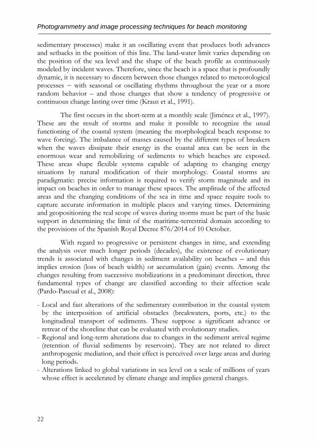
With regard to progressive or persistent changes in time, and extending the analysis over much longer periods (decades), the existence of evolutionary trends is associated with changes in sediment availability on beaches – and this implies erosion (loss of beach width) or accumulation (gain) events. Among the changes resulting from successive mobilizations in a predominant direction, three fundamental types of change are classified according to their affection scale (Pardo-Pascual et al., 2008):
- Local and fast alterations of the sedimentary contribution in the coastal system by the interposition of artificial obstacles (breakwaters, ports, etc.) to the longitudinal transport of sediments. These suppose a significant advance or retreat of the shoreline that can be evaluated with evolutionary studies.
- Regional and long-term alterations due to changes in the sediment arrival regime (retention of fluvial sediments by reservoirs). They are not related to direct anthropogenic mediation, and their effect is perceived over large areas and during long periods.
- Alterations linked to global variations in sea level on a scale of millions of years whose effect is accelerated by climate change and implies general changes.
INTRODUCTION
23
Security and coherence in coastal management is complicated by the confluence of different complex processes. For this reason, understanding and quantifying coastal trends is essential for detecting their magnitude and causes – and offering real solutions. To detail the type of change and its causes, evolutionary analysis at different spatial and temporal scales and with an appropriate degree of precision is necessary (Carter, 1988; Kraus et al., 1991; Cowell & Thom, 1994; Pye & Blott, 2008).
A deepening at different levels of the evolutionary analysis of a landscape as geomorphologically voluble as coastal areas is obviously important. Technical advances play a decisive role by enabling the definition of the changes with precision and effectiveness. For many years, there was no a specific and valid methodology to facilitate the arduous task of defining the shoreline, obviating the technical limitations and avoiding the assumption of futile simplifications.
Advances in the acquisition methods of topographic data offer new tools for the automated and precise extraction of the coastline and the carrying out monitoring work at different times. Improvements in the global positioning systems in kinematic mode and real time (RTK-GPS), LIDAR (light detection and wanging) and terrestrial laser scanner have been decisive. However, these methods present a drawback: they are very expensive when used for analyzing long coastal sectors with high temporal resolution.
Fortunately, the use of satellite imagery overcomes this problem as these platforms cover wide areas of land with a relatively high temporal frequency (Palomar-Vázquez et al., 2018a). We can cite the case of a Landsat platform operating since March 1984. Over 30 million images have been downloaded since 2008 and these systems have contributed enormously to developing several fields of research, such as natural resource management, forestry, ecology, or climate change (Hermosilla et al., 2019; Luijendijk et al., 2018; Pekel et al., 2016). Recently, in 2015, the European Space Agency (ESA) launched the Sentinel program, which offers free images covering the all of the Earth at 20 m resolution (Sentinel-2). If both Landsat and Sentinel missions are joined, we can analyze long sectors of the coast with a high combined revisit time (16 days with Landsat and 10 or 5 days with Sentinel-2). This is, without doubt, the world’s main territorial image database, and means a real revolution in terms of availability of information on the Earth’s surface. However, a weakness is that their coarse spatial resolutions (20-30 m) make it necessary to solve the problem of determining with sufficient precision the position of the shore. The working precisions must be in accordance with the magnitude of the change to be detected.
An algorithm developed by the CGAT-UPV research group extracts the shoreline from mid-resolution images at sub-pixel level (Ruiz et al., 2007, Pardo-Pascual et al., 2012, Almonacid-Caballer, 2014). Based on the different spectral responses in the infrared band of water and land, the method starts with the initial extraction of an approximate shoreline at pixel level and continues searching for
Photogrammetry and image processing techniques for beach monitoring
24
the sub-pixel shoreline in the surroundings of this first line. The algorithm carries out a resampling of the satellite image to work at sub-pixel level. In a given neighborhood of the new resampled image on the initial approximate shore, a fifth-degree polynomial is adjusted and the shoreline position is found where the Laplacian of this fitted polynomial is null and the gradient maximum (Rodríguez et al., 2009). Repeating successively the process along the initial shore, the shoreline is defined at sub-pixel level with an average error (assessed in breakwaters) of approximately 5 m. To reach these accuracies it is important to first guarantee a correct sub-pixel georeferencing of the satellite images by applying a local upsampling of the Fourier transform around the correlation peak, named LUFT (Guizar-Sicairos et al., 2008; Wang et al., 2011). Almonacid-Caballer et al. (2017) proved the effectiveness of this approach by considerably improving the accuracy of shoreline definition in 47 images from Landsat 7. These shoreline extraction and registration procedures constituted the joint workflow referred to in Pardo-Pascual et al., 2012 and Almonacid-Caballer, 2014.
Knowing the potential of using satellite images for beach monitoring at large temporal and spatial scales, the current doctoral thesis − within the CGAT research group − has been assessing the former algorithm in various natural beaches along the Valencian and Balearic coasts, and exploring and developing new methodological and procedural solutions to achieve the highest possible accuracy and efficiency. The challenge of evaluating the algorithm in natural beaches instead of fixed breakwaters lies in the complexity itself of the shoreline phenomenon. Therefore, other assessments approaches had to be analyzed.
Shore-based coastal video monitoring has been proven over the last three decades as a cost-efficient and high-quality data collection tool to support coastal scientists and engineers (Holman et al., 1993, Holman & Stanley, 2007). Despite the lower spatial coverage, video monitoring technique enable a high-frequency analysis of hydro- and mophodynamic processes on beaches. Different video monitoring solutions such as the ARGUS (Davidson et al., 2007), SIRENA (Nieto et al., 2010) and COSMOS (Taborda & Silva, 2012) systems systematically and continuously record numerous actions happening in a specific coastal segment, analyzing and quantifying their evolution. However, the functional application of dedicated video systems and related infrastructures is limited by installation-related issues.
The development of versatile and portable photogrammetric tools that, in a simple way and using conventional cameras (not necessarily mounted on fixed systems nor intended for that purpose), accurately recreate the shoreline position at the instant when the photograph was captured is essential. Such tools would easily allow an accurate recording of the shoreline position at a coastal segment (and at the time of interest) by taking advantage of the numerous touristic or recreational webcams operating along the coast. Only in Spain, we find many of them (https://www.skylinewebcams.com/es/webcam/espana and
INTRODUCTION
25
https://valenciasurf.com/webcams-surf). In this way, it would be possible to exploit existing data acquisition infrastructures for quantitative coastal studies. These online cameras remotely provide visual information of sea state to surf users and stream coastal images worldwide daily. Their exploitation would be an attractive solution for supporting coastal monitoring and coastal management (Andriolo, 2018). Alternatively, the growth of smartphone technology means that mobile camera lenses are now offer sufficient resolution and quality for coastal imaging applications. Community beach monitoring programs based entirely on smartphone images contributed by citizens are also making their way into the field of beach monitoring. The availabily of photogrammetric solutions adaptable to different devices opens possibilities for monitoring coastal dynamics. In addition, it makes it possible to acquire accurate shorelines to use as reference data for the evaluation of other shorelines obtained from satellite images.
The joint use of accurate shorelines obtained from video and satellite data opens a key scenario to advance the algorithmic solutions proposed until now in the inner algorithm and its procedural application. The algorithmic basis of Pardo-Pascual et al. (2012) and Almonacid-Caballer (2014) is interesting, but new possibilities that minimize its weaknesses must be explored and its real utility in natural environments, such as beaches where the shoreline is seen as a blurred border, must be evaluated. It is essential to know to what extent the type of land-water boundary influences image radiometry, and consequently, the accuracy of the shoreline definition. While in the breakwaters − where the former algorithm was developed − the border falls suddenly from the surface up to more than 2 m depth, in natural beaches it follows a gentle gradient seaward. Additionally, in sedimentary beaches, the sand is wetted by the waves and this can introduce substantial doubts in the shoreline definition. Foam in the breaking zone can add further doubts.
The possibility of using all of this shoreline data (including mid-resolution satellite images, video or standard cameras, and smartphones) enables addressing the morphodynamic characterization of the beaches and short, medium, and long-term evolutionary analysis from a new perspective. Likewise, this will contribute to the modelling of the beach responses to the action of the natural agents that control it and open a linkage with well-known shoreline evolution models widely used in coastal engineering to anticipate future scenarios.
Until now, cross-shore evolution model applications have been reduced to target study sites where high-resolution data (needed for calibration and validation) is available. However, new photogrammetry and image processing techniques to obtain multiple high accuracy shoreline data – such as those explored in the current doctoral thesis – can offer a promising future for beach monitoring.
Highlighting the challenges facing seashore zones around the world will facilitate the proposal of goals for the sustainable management of coastal resources.
Photogrammetry and image processing techniques for beach monitoring
26
1.2. AIMS AND OBJECTIVES
The general objective of the research presented in this thesis is the development of effective tools and procedures for coastal monitoring using satellite images and terrestrial photography. This objective is part of the research experience of the group in which the doctoral candidate forms part and partly emerges from a previous thesis (Almonacid-Caballer, 2014) that developed an algorithm to obtain the shoreline with sub-pixel accuracy from Landsat images (as mentioned in the previous section). The objective of the present thesis arises from the need to evaluate and improve this algorithm in natural sedimentary beaches and adapt it for use with images from new satellites such as Sentinel-2, as well as to create a coastal monitoring procedure using low-cost photogrammetric techniques.
Since this is the first large methodological block of the doctoral thesis, the development of a photogrammetric tool (C-Pro) capable of georeferencing images from any type of video-monitoring system to obtain the shoreline accurately and effectively was required (Chapter 2). The simultaneous work between the shorelines obtained from the satellite and those derived from the photographs (Chapter 4) was indispensable for evaluating the accuracy of the satellite extraction algorithm (Almonacid-Caballer, 2014), and the subsequent planning and development of improvements in its sub-pixel methodology for the second block of the thesis. Chapter 3 presents an improvement focused on the inner core of the sub-pixel algorithm while Section 4.3 discusses an improvement more geared towards tool efficiency and the robustness of the entire workflow.
Simultaneously with the design of new methodologies, the sub-pixel detection tool (first termed SHOREX in Palomar-Vázquez et al. 2018a) has continued to be evaluated and calibrated in other environments in works that demonstrated the potential of these satellite-derived shorelines (SDS) for improving our understanding of physical coastal processes (Chapter 4). Likewise, Section 4.4 exemplifies how SDS data can also be used to calibrate and validate an equilibrium shoreline evolution model that describes beach response according to wave forcing and coastal morphodynamics and predicts upcoming situations.
Concurrently, other objectives have been derived from the photogrammetric work such as: the operational use of online streaming video cameras as coastal research tools for hydrodynamic characterisation and morphodynamic studies; the development of citizen beach monitoring programmes using smartphones; and the establishment of a procedure to acquire SfM-3D models of the intertidal beach zone (Chapter 5).
The following hypotheses and their associated working objectives are proposed:
INTRODUCTION
27
Hypothesis 1: Photogrammetry can deliver shoreline positions with sufficient accuracy even when photogrammetric requirements are not optimal or available. Objective 1: Development of a tool capable of precisely projecting a coastal photograph regardless of the difficulties to facilitate applicability on beaches. Hypothesis 2: The importance of coastal monitoring at large temporal and spatial scales using satellite imagery is leading to constant improvements in the accuracy and efficiency of shoreline detection algorithms at sub-pixel level. Therefore, potential improvements in the intrinsic of Almonacid-Caballer (2014) methodology should be investigated. Objective 2: Design a method to untie the algorithm from input line inaccuracies and external factors so that its reliability does not depend on them. Objective 3: Design a method that works with mathematical interpolators without altering the original data. Hypothesis 3: Some coastal monitoring analyses are being carried out from mid-
resolution satellite imagery and using the SHOREX system. However, on natural
beaches, establishing the accuracy of the obtained shoreline is not a trivial matter
and requires reliable reference data against which to make an evaluation. A
profound assessment is needed.
Objective 4: Assess the potential of SDS as coastal evolution indicators.
Objective 5: Evaluate SDS accuracy against high-precision data obtained at the
specific moment of satellite passage.
Objective 6: Develop a robust protocol for obtaining accurate SDS on large
temporal and spatial scales with the necessary algorithmic improvements.
Hypothesis 4: Video monitoring devices record multiple images of the beach from
which coastal information can be obtained.
Objective 7: Obtain metrics and coastal indicators from the efficient processing of
surfcam images that capture and transmit information live on the internet.
Objective 8: Obtain precise shoreline data using photographs acquired by citizens
and through social networks.
Objective 9: Obtain 3D models that recreate beach morphodynamics.
1.3. DOCUMENT STRUCTURE
This document is divided into six chapters, the present one being an introduction to the state of the art and a presentation of the topics discussed in detail in the following four chapters (from 2 to 5). These are composed of edited versions of seven international scientific publications (four published, one accepted and two under review) and one published conference paper, including results obtained and their interpretation. Finally, Chapter 6 contains the overall conclusions of the thesis and different lines of future research derived from the work carried out.
Photogrammetry and image processing techniques for beach monitoring
28
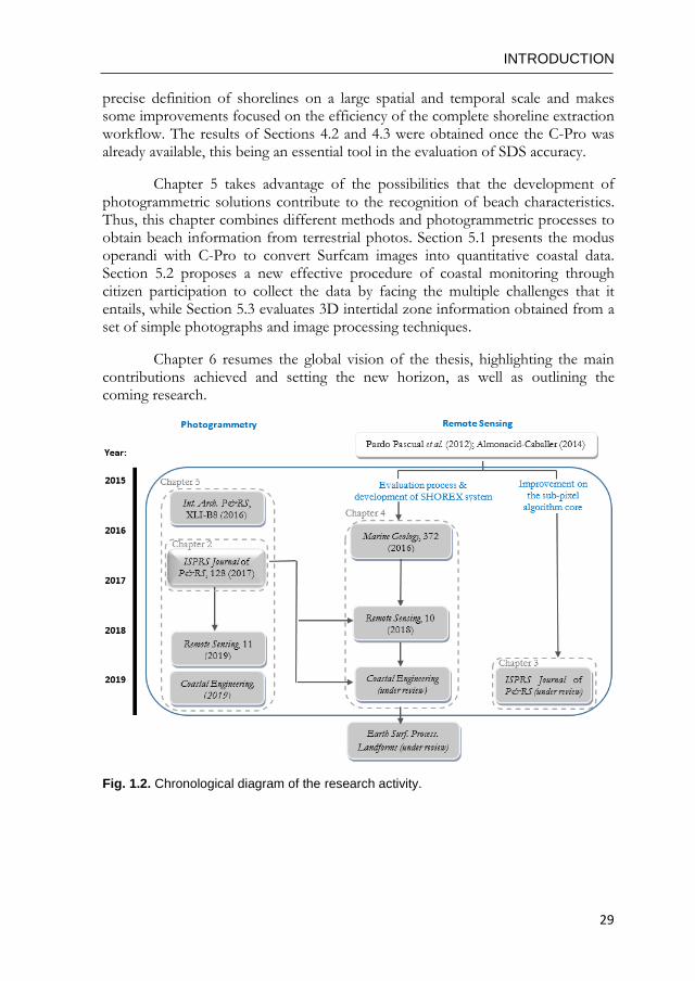
Figure 1.2 summarizes the structure of the thesis. As Section 1.1 has already mentioned, the current thesis is preceded by Almonacid-Caballer, 2014 − another thesis developed within the same research group. However, the thesis concerning us is based on two clearly differentiated but interacting groups of techniques for beach monitoring in the area of photogrammetry and remote sensing (image processing). Following the planned objectives, the advance has been synchronous throughout and both branches obtain partial results in publications as shown by Fig. 1.2. The thesis structure is organized with the aim of presenting first in Chapters 2 and 3 the new algorithmic solutions for both photogrammetry (Chapter 2) and remote sensing (Chapter 3) subject areas. These are two core contributions developed essentially by the doctoral candidate with the supervision of her advisors.
Chapter 2 describes a methodological protocol to project a terrestrial photograph of a coastal area – or whatever indicator is contained on it – in a georeferenced plane taking advantage of the terrestrial horizon as a geometric key within the collinearity adjustment system. The procedure is implemented in a tool called the Coastal Projector (C-Pro) whose versatility enables the efficient use of recreational cameras for obtaining quantitative coastline data.
Chapter 3 presents a new procedure for the detection of the instantaneous shoreline at sub-pixel level from mid-resolution satellite images. The potential of the methodology lies in the iterative selection of a set of pixels with maximum radiometric variation, and the adjustment of an interpolator polynomial that models this land-water surface. This was an improvement derived from the resulting assessments of the Almonacid-Caballer (2014) algorithm in natural beaches – which are discussed in Sections 4.1 and 4.2. While this improvement was being developed, the need to continue obtaining SDS in a massive an efficient way led the research group to continue testing other approaches and eventually led to the work in Section 4.3 (refer below to the sequential diagram for a better understanding).
Chapter 4 focuses on the evaluation of using the Pardo-Pascual et al., (2012) and Almonacid-Caballer (2014) algorithmic solution on beaches. Consequently, its improvement and development as a broad tool capable of being used massively and efficiently has been gradually shown. Therefore, this chapter is a chronological overview through the various evaluations carried out of the former algorithm (Sections 4.1 and 4.2) and the consequent improvements that led to the current SHOREX system (Section 4.3). The chapter starts with Section 4.1 evaluating – with high-precision data – the potential of a set of SDS from Landsat images to characterise the evolution of beaches in the medium and long-term. Therefore, the concept of annual mean shoreline was presented as an indicator of coastal evolution in the medium term. Section 4.2 examines other extracted SDS, this time evaluating their precision as instantaneous lines in another temporary period. Following this line of analysis, Section 4.3 presents a protocol for the
INTRODUCTION
29
precise definition of shorelines on a large spatial and temporal scale and makes some improvements focused on the efficiency of the complete shoreline extraction workflow. The results of Sections 4.2 and 4.3 were obtained once the C-Pro was already available, this being an essential tool in the evaluation of SDS accuracy.
Chapter 5 takes advantage of the possibilities that the development of photogrammetric solutions contribute to the recognition of beach characteristics. Thus, this chapter combines different methods and photogrammetric processes to obtain beach information from terrestrial photos. Section 5.1 presents the modus operandi with C-Pro to convert Surfcam images into quantitative coastal data. Section 5.2 proposes a new effective procedure of coastal monitoring through citizen participation to collect the data by facing the multiple challenges that it entails, while Section 5.3 evaluates 3D intertidal zone information obtained from a set of simple photographs and image processing techniques.
Chapter 6 resumes the global vision of the thesis, highlighting the main contributions achieved and setting the new horizon, as well as outlining the coming research.
Fig. 1.2. Chronological diagram of the research activity.
Photogrammetry and image processing techniques for beach monitoring
30
© copyright disclaimer
The present PhD dissertation is an edited compilation from the papers listed below with the approval of co-authors. This compilation satisfies the PhD requirements of the Universitat Politècnica de València, Spain. Chapter 2:
Sánchez-García, E., Balaguer-Beser, A., Pardo-Pascual, J.E. (2017). C-Pro: A Coastal Projector monitoring system using terrestrial photogrammetry with a geometric horizon constraint. ISPRS Journal of Photogrammetry & Remote Sensing, 128: 255-273, https://doi.org/10.1016/j.isprsjprs.2017.03.023 (Impact factor 2017: 5.994).
Chapter 3:
Sánchez-García, E., Balaguer-Beser, A., Almonacid-Caballer, J., Pardo-Pascual, J.E. (under review in ISPRS Journal of Photogrammetry & Remote Sensing). A new adaptive image interpolation method to define the shoreline at sub-pixel level.
These two previous works are core contributions of the thesis developed essentially by the doctoral candidate and supervised by her advisors. Dr. Almonacid also contributed in the second work with a critical review. Chapter 4:
Almonacid-Caballer, J., Sánchez-García, E., Pardo-Pascual, J.E., Balaguer-Beser, A., Palomar-Vázquez, J. (2016). Evaluation of annual mean shoreline position deduced from Landsat imagery as a mid-term coastal evolution indicator. Marine Geology, 372: 79-88, https://doi.org/10.1016/j.margeo.2015.12.015 (Impact factor 2016: 3.572). This consists of the first evaluation work of the SDS product carried out on natural beaches by the CGAT group. The PhD was responsible for data analysis by making comparisons with a set of highly accurate shorelines and took part in the writing of the research contribution.
Pardo-Pascual, J.E., Sánchez-García, E., Almonacid-Caballer, J., Palomar-Vázquez, J., Priego de los Santos, E., Fernández-Sarría, A., Balaguer-Beser, A. (2018). Assessing the accuracy of automatically extracted shorelines on microtidal beaches from Landsat 7, Landsat 8 and Sentinel-2 imagery. Remote Sensing, 10 (2), 326, https://doi.org/10.3390/rs10020326 (Impact factor 2017: 3.406).
INTRODUCTION
31
Second evaluation of the SDS product on natural beaches but this time discussing instantaneousness value in greater depth by comparing coincident reference data. The enormous potential of C-Pro was clearly appreciated through this work by recognizing not only the shoreline border, but also offering useful information of the sea state and beach characteristics when the satellite image was captured. For this contribution, the PhD was in charge of the entire photogrammetric procedure to accurately obtain the reference photo-derived shorelines with C-Pro. She also participated in the fieldwork campaigns, the validation analysis, and writing and review of the final document.
Sánchez-García, E., Palomar-Vázquez, J., Pardo-Pascual, J.E., Almonacid-Caballer, J., Cabezas-Rabadán, C., Gómez-Pujol, L. (under review in Coastal Engineering). An efficient protocol for accurate and massive shoreline definition from mid-resolution satellite imagery.
Third evaluation of the SDS algorithm together with the presentation of a new procedural solution to improve accuracy and effectiveness. The assessment was made in a different sedimentary beach where the existence of a fixed video camara enabled obtaining valuable reference data (again with C-Pro). Several researchers developed this work and the PhD candidate carried out the basic management and was responsible for the final draft. Chapter 5:
Andriolo, U., Sánchez-García, E., Taborda, R. (2019). Operational use of surfcam online streaming images for coastal morphodynamic studies. Remote Sensing, 11 (1), 78, https://doi.org/10.3390/rs11010078 (Impact factor 2017: 3.406). This work derives directly from the first PhD stay in Lisbon (09-12/2015) where Rui Taborda was responsible at the host institution. The collaboration was very important in the completion of Andriolo’s thesis. The candidate’s PhD work consisted in applying her knowledge about photogrammetric techniques and applying C-Pro to multiple surfcam images and on a miscellany of situations and requirements. Later, different coastal indicators would be derived from the georectified images for coastal morphodynamic studies as Andriolo, 2018 showed. She participated together with Andriolo in the development of the analyses, the writing and the review of the derived contribution. See the “Research Activity” section –at the end of the current document– for other conference papers derived from this close collaboration.
Harley, M., Kinsela, M., Sánchez-García, E., Vos, K. (2019). Shoreline change mapping using crowd-sourced smartphone images. Coastal Engineering.
Photogrammetry and image processing techniques for beach monitoring
32
This work arises from the third PhD stay in Sydney (09-12/2017) where Mitch Harley was responsible at the host institution. The PhD student joined the new CoastSnap team –a citizen science initiative for beach monitoring that had been started only few months earlier by Dr. Harley and Dr. Kinsela. The PhD candidate was responsible for carrying out the entire image processing analyses and procedural tests with the set of smartphone images acquired from community participation. The derived results enabled establishing the more appropriate CoastSnap protocol to follow henceforth. Additionally, the contribution was also essential in the writing and the review of the manuscript.
Sánchez-García, E., Balaguer-Beser, A., Taborda, R., Pardo-Pascual, J.E, (2016). Modelling landscape morphodynamics by terrestrial photogrammetry: an application to beach and fluvial systems. International Archives of the Photogrammetry, Remote Sensing and Spatial Information Sciences, XLI-B8: 1175-1182, https://doi.org/10.5194/isprs-archives-XLI-B8-1175-2016. This work is a contribution to the thesis developed by the doctoral candidate and supervised by her advisors and Dr. Rui Taborda (since some data comes from the PhD stay in Lisbon).


Cover photo of Chapter 2: Praia da Rainha, Cascais, Lisbon (taken Oct. 2015)

PHOTOGRAMMETRIC SOLUTION: A Coastal Projector monitoring system
37
This chapter describes a methodological protocol to project a terrestrial photograph of a coastal area – or whatever indicator is contained on it – in a georeferenced plane considering the terrestrial horizon as a geometric key. This feature, which appears in many beach photos, helps in camera repositioning and serves as a constraint in collinearity adjustment. This procedure is implemented in a tool called the Coastal Projector (C-Pro) that is based on Matlab and adapts its methodology in accordance with the input data and the available parameters of the acquisition system. The method has been tested in three coastal areas to assess the influence that the horizon constraint presents in the results by comparing the obtained shoreline against other lines measured using RTK-GPS. The proposed methodology increases the reliability and efficient use of existing recreational cameras (with non-optimal requirements, unknown image calibration, and at elevations lower than 7 m) to provide quantitative coastal data.
The applicability of C-Pro has been a key issue in carrying out most of the processes that shape the present doctoral thesis. Its application as an evaluator tool for other less precise data is implicit in Chapter 4. However, its use as a coastal monitoring tool per se to derive morphodynamic and coastal hydrodynamic indicators from images is discussed in Chapter 5. 2.1. INTRODUCTION
A proper management and planning of coastal areas is governed by an accurate understanding of these fragile and dynamic environments at different spatial and temporal scales. Modelling the coastline response to the effect of waves and sea level variation, especially in significantly unstable coasts such as sedimentary beaches, enables the evaluation of coastal retreat and coastline migration on large temporal scales. However, the complexity of the phenomena and processes that interact on the land-sea interface, makes this a deeply dynamic space in its form and arrangement (Boak and Turner, 2005). It is necessary to distinguish between oscillatory short-term effects and other long-term changes – and so monitoring changes at different temporal scales is helpful in a decision-making process involving environmental values and socioeconomic interests.
The spatial resolution and high temporal frequency achieved by terrestrial photogrammetric techniques have overcome the accuracy of other techniques in the field of monitoring. Techniques such as Airborne Light Detection and Ranging (LiDAR), Terrestrial Laser Scanner (TLS) and Global Positioning Systems in Real-Time Kinematic (RTK-GPS) define the shoreline and model the beach area with accuracy and reliability despite tedious fieldwork and costs. However, the high periodicity required to monitor dynamics in natural spaces is causing these techniques to be set aside. Conversely, remote sensing techniques are being used to establish and quantify erosion or accretion rates on beaches and the results are sufficiently accurate – in the order of several meters – to help in our understanding and prediction of long-term worldwide coastal evolution (Almonacid-Caballer et
Photogrammetry and image processing techniques for beach monitoring
38
al., 2016). Nevertheless, its potential is reduced for local studies and short-term changes where video monitoring systems are consolidated as the current benchmark.
Terrestrial photogrammetric systems enable a systematic and continuous recording of the different actions that take place in a specific coastal area. For instance, the local and rapid changes that occur during storms. Some institutions have realized the need to establish a proper and integrated coastal zone management and various video monitoring systems have been installed. The Argus system was the first developed for coastal research (Holman et al., 1993) and was validated and widely used worldwide (Holman and Stanley, 2007). Following the same principles, other coastal imaging systems were implemented. Archetti et al. (2008) made a comparative study of four fixed-camera systems: Erdman (1998); Kosta (2006); Horus (2007); and Beachkeeper (Brignone et al., 2012). Moreover, various works (Jiménez et al., 2007; Davidson et al., 2007; Aarninkhof et al., 2003) widely recognize the success of video systems for coastal research and shoreline monitoring through video-derived coastal indicators. Recent developments have emerged that access the digital image data from non-expert systems and regardless of the camera technology (e.g., Taborda & Silva, 2012; Kim et al., 2013).
Existing coastal imaging systems are ready focused and dedicated for a specific application and this leads to some economic and positioning limitations. The accurate measurement of shorelines, sand bars, beach widths, and many other indicators is easy to accomplish using fixed cameras covering wide fields of view and located on high elevation beach-front buildings. However, these optimal requirements are unusual on most beaches around the world and so other approaches are being investigated.
Many recreational video-cameras are currently operating on the coastline and sending considerable data over the internet - as well as a small number of systems designed by coastal managers in specific areas to control storm events. Most of this data is captured by Surfcam stations whose main qualitative objective is to observe breaking waves. As expected, the camera requirements are not optimal for quantitative measurements as they are low-angle and single cameras mounted on low beachfront buildings and pointing nearly horizontal toward the waves. Making the most of all the data from such shoreline monitoring cameras is the challenge tackled in this chapter and complementing other works (Bracs et al., 2016) where the potential of Surfcam data has already been proven through applying various solutions.
We propose a rigorous methodology – implemented in a coastal projector tool known as C-Pro – that overcomes the photogrammetric difficulties and non-optimal conditions that are sometimes found in beach photographs. The main goal is to use the terrestrial horizon as a photogrammetric constraint included in the collinearity system to achieve a precise repositioning of the camera (Sánchez-
PHOTOGRAMMETRIC SOLUTION: A Coastal Projector monitoring system
39
García et al., 2015b). Van Den Heuvel (1998) already advanced the benefits of using geometric constraints for object reconstruction. When using a simple non-metric camera looking horizontally towards the coastline and from any elevation –even from the ground where there is no other option– the horizon constraint helps the image spatial resection system to converge on a precise solution that is valid for coastal monitoring. Moreover, because of the field of view, most of the photos only show sand and water, and this makes it difficult to acquire ground control points (GCP) with a suitable distribution to transform image information into real world coordinates. Reducing the number of initial unknown parameters by adding horizon equations would be a great advantage in providing stability to the mathematical system (Oreifej et al., 2011).
Some works that use Surfcam online streaming images for measuring wave runup and intertidal beach topography (Andriolo et al., 2016a-b; Andriolo, 2018) are already taking advantage of C-Pro rectification methodology as the horizon constraint is the key to achieving image calibration and a precise repositioning of the camera.
In this chapter, Section 2.2 describes the mathematical formulas necessary to incorporate horizon information in a monitoring system using terrestrial photogrammetry. Section 2.3 presents the different methodological steps depending on the number of parameters initially known, access to camera calibration, knowledge of the initial location of the camera, or number of available GCPs. Finally, Section 2.4 shows the results obtained after camera repositioning and image rectification processes and shows the considerable advantages of incorporating the horizon constraint.
2.2. HORIZON CONSTRAINT
The methodology of terrestrial photogrammetry described in this chapter is designed for use in coastal imaging systems where the horizon is an element of the photo (meaning the separation between sea and sky). This section describes some mathematical tools that take advantage of the information provided by the horizon line and are useful for the new coastal projector monitoring system (C-Pro), explained in Section 2.3.
2.2.1. Image orientation using the horizon
The calculation of the image orientation with respect to the object space is made
through three rotations and three corresponding angles that transform image data
into real-world coordinates: 𝜔 ∈ [−𝜋, 𝜋], 𝜑 ∈ [−𝜋/2, 𝜋/2], 𝜅 ∈ [−𝜋, 𝜋]. By means of
this procedure, the vectors of the reference system in the object space become
these same vectors in the image space. The following matrix defines this process:
Photogrammetry and image processing techniques for beach monitoring
40
𝑅𝜅𝜑𝜔 = 𝑅𝜅𝑅𝜑𝑅𝜔 = (𝑐𝑜𝑠𝜅𝑠𝑖𝑛𝜅0 −𝑠𝑖𝑛𝜅𝑐𝑜𝑠𝜅0
001)(
𝑐𝑜𝑠𝜑0
−𝑠𝑖𝑛𝜑 010
𝑠𝑖𝑛𝜑0
𝑐𝑜𝑠𝜑)(
100 0
𝑐𝑜𝑠𝜔𝑠𝑖𝑛𝜔
0
−𝑠𝑖𝑛𝜔𝑐𝑜𝑠𝜔
) (2.1)
𝑅𝜅𝜑𝜔 consists of the product between an initial rotation matrix in the Z axis, later
in Y axis, and finally in the X axis. Thus, (X, Y, Z) coordinates of a point in the
object reference system focused on the main point of the image can be calculated
by knowing its associated coordinates (x, y, z) in the image reference system
through these equations:
(𝑋𝑌𝑍) = 𝑅𝜅𝜑𝜔 (
𝑥𝑦𝑧) → (
𝑋𝑌𝑍) =
(
𝑐𝑜𝑠𝜅 𝑐𝑜𝑠𝜑 𝑐𝑜𝑠𝜅 𝑠𝑖𝑛𝜔 𝑠𝑖𝑛𝜑 − 𝑠𝑖𝑛𝜅 𝑐𝑜𝑠𝜔 𝑐𝑜𝑠𝜅 𝑐𝑜𝑠𝜔 𝑠𝑖𝑛𝜑 + 𝑠𝑖𝑛𝜅 𝑠𝑖𝑛𝜔𝑠𝑖𝑛𝜅 𝑐𝑜𝑠𝜑 𝑠𝑖𝑛𝜅 𝑠𝑖𝑛𝜔 𝑠𝑖𝑛𝜑 + 𝑐𝑜𝑠𝜅 cos𝜔 𝑠𝑖𝑛𝜅 𝑐𝑜𝑠𝜔 𝑠𝑖𝑛𝜑 − 𝑐𝑜𝑠𝜅 𝑠𝑖𝑛𝜔−𝑠𝑖𝑛𝜑 𝑐𝑜𝑠𝜑 𝑠𝑖𝑛𝜔 𝑐𝑜𝑠𝜑 𝑐𝑜𝑠𝜔
) (𝑥𝑦𝑧) (2.2)
In the following paragraphs the (x, y, z) coordinates in the image space are referred
to as the principal point 𝑜 = (𝑥0, 𝑦0) and to simplify formulas in this section, its
coordinates are assumed as zero 𝑜 = (0,0). To develop (2.2), both the object coordinates and the image coordinates – originally defined from the upper left corner of the image – are translated by establishing its origin in the principal point. However, there are other rotational angles relating both image and object coordinates such as described by Dai et al., 2011 and Rodríguez et al., 2008. We are going to use several of these ideas to define the equations of change between reference systems (2.2) through new angles defining that matrix.
The definition of these angles is based on the approximation of the Earth’s curved horizon as a straight line in the image plane. Two alternatives for the determination of that straight line are proposed in this chapter by marking two vanishing points in the image that are as distant as possible; A = (xa, ya), B = (xb, yb), and fulfil that xa < xb. In this chapter, the horizon points have been marked manually to ensure that they do not become an added source of error in the methodological assessment.
Case a) (two points) The horizon curve is approximated through the line joining both A and B points (colored red in Fig. 2.1B).
Case b) (three points) If A and B points are far enough apart, it is possible to find a third point C = (xc, yc). These three points define a circumference and we compute P as the point where the minimum distance is reached between the circumference and the principal point of the image plane. The tangent line to the circumference at such point P then approximates the real curved horizon (shown in green in Fig. 2.1B).
Note that the horizon approximation with three points is the most realistic. However, it is very sensitive and strongly dependent on the horizon extension seen
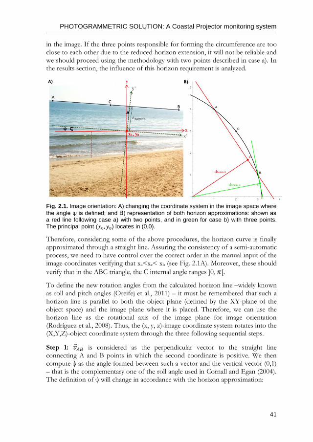
PHOTOGRAMMETRIC SOLUTION: A Coastal Projector monitoring system
41
in the image. If the three points responsible for forming the circumference are too close to each other due to the reduced horizon extension, it will not be reliable and we should proceed using the methodology with two points described in case a). In the results section, the influence of this horizon requirement is analyzed.
Fig. 2.1. Image orientation: A) changing the coordinate system in the image space where
the angle ψ is defined; and B) representation of both horizon approximations: shown as a red line following case a) with two points, and in green for case b) with three points. The principal point (𝑥0, 𝑦0) locates in (0,0).
Therefore, considering some of the above procedures, the horizon curve is finally approximated through a straight line. Assuring the consistency of a semi-automatic process, we need to have control over the correct order in the manual input of the image coordinates verifying that xa<xc< xb (see Fig. 2.1A). Moreover, these should
verify that in the ABC triangle, the C internal angle ranges ]0, 𝜋[.
To define the new rotation angles from the calculated horizon line –widely known as roll and pitch angles (Oreifej et al., 2011) – it must be remembered that such a horizon line is parallel to both the object plane (defined by the XY-plane of the object space) and the image plane where it is placed. Therefore, we can use the horizon line as the rotational axis of the image plane for image orientation (Rodríguez et al., 2008). Thus, the (x, y, z)-image coordinate system rotates into the (X,Y,Z)-object coordinate system through the three following sequential steps.
Step 1: �⃗�𝐴𝐵 is considered as the perpendicular vector to the straight line connecting A and B points in which the second coordinate is positive. We then compute ψ as the angle formed between such a vector and the vertical vector (0,1) – that is the complementary one of the roll angle used in Cornall and Egan (2004). The definition of ψ will change in accordance with the horizon approximation:
Photogrammetry and image processing techniques for beach monitoring
42
Case a) (two points) Being the horizon the straight line defined by the points A and B then �⃗�𝐴𝐵 = (𝑦𝑎 − 𝑦𝑏 , 𝑥𝑏 − 𝑥𝑎), and the angle ψ may be defined as:
ψ = arctan((𝑦𝑎 − 𝑦𝑏)/(𝑥𝑏 − 𝑥𝑎)) ∈ ] −𝜋/2, 𝜋/2[, being xa < xb (2.3)
Case b) (three points) approaching the horizon through the tangent line to
the circumference passing through the points A, B and C then �⃗�𝐴𝐵 is the direction of the line which connects the center of this circumference with the principal point
𝑜 = (0,0) of the image plane. Consequently, �⃗�𝐴𝐵 = (cx, cy) if cy > 0 or �⃗�𝐴𝐵 =
(−cx, −cy) if cy < 0, where (cx, cy) are the coordinates of the circumference center
in the image plane with respect to the principal point. This center is previously obtained as the intersection point between the line perpendicular to the segment AC that passes through its midpoint and the line perpendicular to the segment CB through its midpoint. Finally, the angle ψ is defined as:
ψ = arctan(−cx/−cy) = arctan(cx/cy) ∈ ] −𝜋/2, 𝜋/2[, 𝑖𝑓 𝑐𝑦 ≠ 0 (2.4)
In formula (2.4) it is assumed that the principal point is closer to the horizon than
the ABC circumference center. Moreover, ψ has the following definition in the
cases in which cy could be equal to 0:
{ 𝑖𝑓 cy = 0 𝑎𝑛𝑑 cx < 0 → ψ = 𝜋/2
𝑖𝑓 cy = 0 𝑎𝑛𝑑 cx > 0 → ψ = −𝜋/2 (2.5)
The xyz-system rotates a clockwise angle (−ψ) in the plane z=0, so the new x’ axis will be parallel to the horizon line (see Fig. 2.1A). The coordinates of any point in the xyz-system are related with the x’y’z’-system by:
(𝑥𝑦𝑧) = (
cos (−ψ)
sin (−ψ)
0
– 𝑠𝑖𝑛(−ψ)
cos (−ψ)
0
001)(
𝑥′
𝑦′
𝑧′) = (
cos (ψ)
−sin (ψ)
0
𝑠𝑖𝑛(ψ)
cos (ψ)
0
001)(
𝑥′
𝑦′
𝑧′) = 𝑅ψ (
𝑥′
𝑦′
𝑧′) (2.6)
In this first step the rotation angle (−ψ) does not consider the position of the horizon line with respect to the x-axis. Formulas (2.3), (2.4) and (2.5) only take into account the orientation of the vector perpendicular to the horizon line with respect to the y-vector direction. For this reason, in the next step we will consider the dhorizon sign, which represents the minimal distance in the image plane from the principal point to the approached horizon line. Thus, dhorizon could have a negative sign if the closest point of the horizon line to the principal point has a negative y-coordinate. Again, as expected, calculation of dhorizon depends on the horizon approximation as follows:
Case a) (two points) Following this first approximation, the minimal distance between the principal point and the horizon line is:
dℎ𝑜𝑟𝑖𝑧𝑜𝑛 =𝑦𝑎 𝑥𝑏 − 𝑦𝑏 𝑥𝑎
√(𝑥𝑏 − 𝑥𝑎 )2 + (𝑦𝑏 − 𝑦𝑎)
2 (2.7)
PHOTOGRAMMETRIC SOLUTION: A Coastal Projector monitoring system
43
Case b) (three points) However, in this other case, the minimal distance will be
calculated as: |𝑑ℎ𝑜𝑟𝑖𝑧𝑜𝑛| = r − √cx2 + cy2 , being r the radius of the ABC horizon
circumference. It should be remembered that given the characteristics of the horizon, we can assume – without loss of generality – that the principal point is
within the circumference. Therefore, the sign of 𝑑ℎ𝑜𝑟𝑖𝑧𝑜𝑛 is calculated as follows:
{
𝑑ℎ𝑜𝑟𝑖𝑧𝑜𝑛 = r − √cx2 + cy
2 > 0 𝑖𝑓 cy < 0
𝑑ℎ𝑜𝑟𝑖𝑧𝑜𝑛 = √cx2 + cy
2 − 𝑟 < 0 𝑖𝑓 cy > 0
(2.8)
In cases where cy = 0 then:
{ 𝑖𝑓 cy = 0 𝑎𝑛𝑑 cx < 0 → 𝑑ℎ𝑜𝑟𝑖𝑧𝑜𝑛 = r − |cx| > 0
𝑖𝑓 cy = 0 𝑎𝑛𝑑 cx > 0 → 𝑑ℎ𝑜𝑟𝑖𝑧𝑜𝑛 = |cx| − 𝑟 < 0 (2.9)
Moreover, both procedures enable calculating the coordinates of the horizon point
P (xP, yP) in the image plane (see Fig. 2.1B) centered at principal point 𝑜 = (0,0) as:
{𝑥𝑃 = 𝑑ℎ𝑜𝑟𝑖𝑧𝑜𝑛 ∗ sin(ψ)
𝑦𝑃 = 𝑑ℎ𝑜𝑟𝑖𝑧𝑜𝑛 ∗ cos(ψ) (2.10)
It is necessary to consider in (2.10) the appropriate sign of 𝑑ℎ𝑜𝑟𝑖𝑧𝑜𝑛 as explained above. The observed horizon line could then be indicated in the photos as Fig. 2.1A shows.
Step 2: Once the x’ axis is positioned parallel to the horizon line, the image plane must be oriented parallel to the object plane by means of another rotation
angle (– ξ) – that is the complementary one of the pitch angle defined in
Schwendeman and Thomson (2015). The x’y’z’-coordinate system rotates a
clockwise angle (– ξ) to generate an x’’y’’z’’-coordinate system, being x’’=x’ and z’’=Z (the elevation coordinate). Thus, in this step the image orients around the x’ axis, keeping this parallel to the horizon line and positioning the y’-axis on a plane which passes through the principal point and is parallel to the object plane (XY)
(see Fig. 2.2). In this way, (-ξ) coincides with the angle formed between y*’ axis
(whose origin is 𝐶𝑐 and is parallel to y’) and a plane parallel to the terrain pointing to infinity (y*’’).
We consider the vector �⃗� perpendicular to the object plane whose origin is the
optical center of the camera. The ξ angle (represented in Fig. 2.2) then coincides
with the angle formed between such vector �⃗� and the vector perpendicular to the
y’-axis that goes from the camera’s centre 𝐶𝑐 to the principal point o.
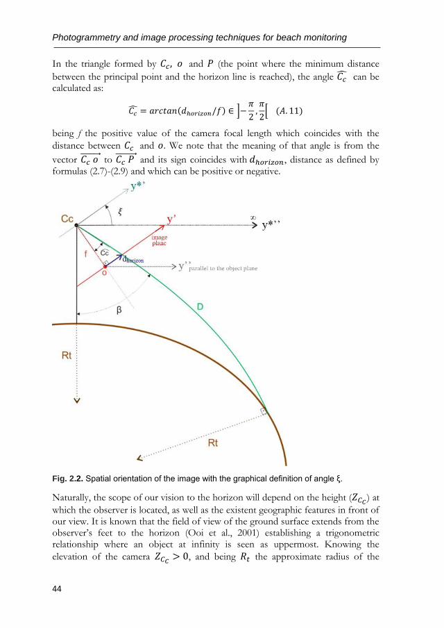
Photogrammetry and image processing techniques for beach monitoring
44
In the triangle formed by 𝐶𝑐, 𝑜 and 𝑃 (the point where the minimum distance
between the principal point and the horizon line is reached), the angle 𝐶�̂� can be calculated as:
𝐶�̂� = 𝑎𝑟𝑐𝑡𝑎𝑛(𝑑ℎ𝑜𝑟𝑖𝑧𝑜𝑛/𝑓) ∈ ]−𝜋
2,𝜋
2[ (𝐴. 11)
being f the positive value of the camera focal length which coincides with the
distance between 𝐶𝑐 and 𝑜. We note that the meaning of that angle is from the
vector 𝐶𝑐 𝑜 ⃗⃗⃗⃗ ⃗⃗ ⃗⃗ ⃗⃗ to 𝐶𝑐 𝑃 ⃗⃗ ⃗⃗ ⃗⃗ ⃗⃗ ⃗⃗ and its sign coincides with 𝑑ℎ𝑜𝑟𝑖𝑧𝑜𝑛, distance as defined by formulas (2.7)-(2.9) and which can be positive or negative.
Fig. 2.2. Spatial orientation of the image with the graphical definition of angle ξ.
Naturally, the scope of our vision to the horizon will depend on the height (𝑍𝐶𝐶 ) at
which the observer is located, as well as the existent geographic features in front of our view. It is known that the field of view of the ground surface extends from the observer’s feet to the horizon (Ooi et al., 2001) establishing a trigonometric relationship where an object at infinity is seen as uppermost. Knowing the
elevation of the camera 𝑍𝐶𝐶 > 0, and being 𝑅𝑡 the approximate radius of the

PHOTOGRAMMETRIC SOLUTION: A Coastal Projector monitoring system
45
Earth (6371 Km), we can then compute an approximation to the geographical distance D between the observer and the horizon by means of the formula:
𝐷 = +√(𝑍𝐶𝐶 + 𝑅𝑡)2− 𝑅𝑡
2 > 0 (2.12)
When sitting on the beach, facing the sea, and looking one-meter above the water, the horizon will be distinguished within D=3.57 km. However, this observed distance will increase - although disproportionally – as height increases.
The next step is to compute the angle 𝛽 between �⃗� vector and the line between the observer and the horizon. To achieve this we take into account the refraction and terrestrial sphericity correction (1 mm of error in 100 m of distance). However, sometimes when the observer’s elevation is low, this correction becomes irrelevant.
The formula to calculate angle 𝛽 is:
𝛽 = 𝑎𝑟𝑐𝑐𝑜 𝑠 (𝑍𝐶𝐶 + 0.42 ∗ 𝐷
2/𝑅𝑡
𝐷) ∈ ]0,
𝜋
2[ (2.13)
Therefore:
ξ = 𝛽 − 𝐶�̂� = 𝑎𝑟𝑐𝑐𝑜 𝑠 (𝑍𝐶𝐶 + 0.42 ∗
𝐷2
𝑅𝑡𝐷
) − 𝑎𝑟𝑐𝑡𝑎𝑛 (𝑑ℎ𝑜𝑟𝑖𝑧𝑜𝑛
𝑓) (2.14)
If 𝐶�̂� > 0, ξ definition must be ξ = (𝛽 − 𝐶�̂�) > 0, verifying ξ ∈ ]0, 𝜋[. The
extreme interval values (ξ = 0 & ξ = π) are impossible values because the image plane would be parallel to the object plane – as happens in a vertical photo – where the horizon cannot be seen.
After computing ξ by means of (2.14), the x’y’z’-system rotates the clockwise
angle(−ξ) about the x’ axis to generate an x’’y’’z’’-coordinate system. The coordinates of any point in the x’y’z’-system can be calculated from the x’’y’’z’’-system by:
(𝑥′
𝑦′
𝑧′) = (
100
0cos (−ξ)
sin (−ξ)
0– 𝑠𝑖𝑛(−ξ)
cos (−ξ))(
𝑥′′
𝑦′′
𝑧′′
)
= (100
0cos (ξ)
−sin (ξ)
0𝑠𝑖𝑛(ξ)
cos (ξ))(
𝑥′′
𝑦′′
𝑧′′) = 𝑅ξ (
𝑥′′
𝑦′′
𝑧′′) (2.15)
Step 3: The third and last angle (𝜆) of the Euler triad is the azimuth and this positions the coordinate axis (x’’, y’’, z’’) regarding the real terrain coordinates and around the z’’=Z axis.
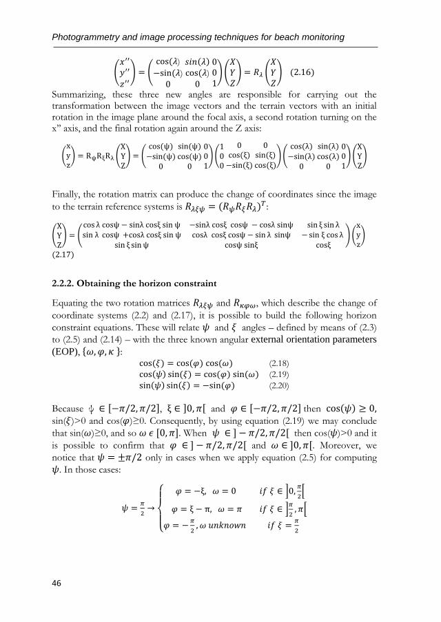
Photogrammetry and image processing techniques for beach monitoring
46
(𝑥′′
𝑦′′
𝑧′′) = (
cos (𝜆)
−sin (𝜆)
0
𝑠𝑖𝑛(𝜆)
cos (𝜆)
0
001)(
𝑋𝑌𝑍) = 𝑅𝜆 (
𝑋𝑌𝑍) (2.16)
Summarizing, these three new angles are responsible for carrying out the transformation between the image vectors and the terrain vectors with an initial rotation in the image plane around the focal axis, a second rotation turning on the x’’ axis, and the final rotation again around the Z axis:
(xyz) = RψRξRλ (
XYZ) = (
cos (ψ)−sin(ψ)
0
sin(ψ)cos (ψ)0
001)(
100
0cos (ξ)−sin(ξ)
0sin(ξ)cos (ξ)
)(cos (λ)−sin(λ)
0
sin(λ)cos (λ)0
001)(
XYZ)
Finally, the rotation matrix can produce the change of coordinates since the image
to the terrain reference systems is 𝑅𝜆𝜉𝜓 = (𝑅𝜓𝑅𝜉𝑅𝜆)𝑇:
(XYZ) = (
cos λ cosψ − sinλ cosξ sin ψ −sinλ cosξ cosψ − cosλ sinψ sin ξ sin λsin λ cosψ +cosλ cosξ sin ψ cosλ cosξ cosψ − sin λ sinψ −sin ξ cos λ
sin ξ sin ψ cosψ sinξ cosξ) (xyz)
(2.17)
2.2.2. Obtaining the horizon constraint
Equating the two rotation matrices 𝑅𝜆𝜉𝜓 and 𝑅𝜅𝜑𝜔, which describe the change of
coordinate systems (2.2) and (2.17), it is possible to build the following horizon
constraint equations. These will relate 𝜓 and 𝜉 angles – defined by means of (2.3)
to (2.5) and (2.14) – with the three known angular external orientation parameters
(EOP), {𝜔, 𝜑, 𝜅 }: cos (𝜉) = cos(𝜑) cos(𝜔) (2.18)
cos(𝜓) sin (𝜉) = cos(𝜑) sin(𝜔) (2.19)
sin(𝜓) sin(𝜉) = −sin (𝜑) (2.20)
Because ψ ∈ [−𝜋/2, 𝜋/2], ξ ∈ ]0, 𝜋[ and 𝜑 ∈ [−𝜋/2, 𝜋/2] then cos(𝜓) ≥ 0, sin(𝜉)>0 and cos(𝜑)≥0. Consequently, by using equation (2.19) we may conclude
that sin(𝜔)≥0, and so 𝜔 𝜖 [0, 𝜋]. When 𝜓 ∈ ] − 𝜋/2, 𝜋/2[ then cos(𝜓)>0 and it
is possible to confirm that 𝜑 ∈ ] − 𝜋/2, 𝜋/2[ and 𝜔 ∈ ]0, 𝜋[. Moreover, we
notice that 𝜓 = ±𝜋/2 only in cases when we apply equation (2.5) for computing
𝜓. In those cases:
𝜓 =𝜋
2→
{
𝜑 = −ξ, 𝜔 = 0 𝑖𝑓 𝜉 ∈ ]0,
𝜋
2[
𝜑 = ξ − π, 𝜔 = 𝜋 𝑖𝑓 𝜉 ∈ ]𝜋
2, 𝜋[
𝜑 = −𝜋
2, 𝜔 𝑢𝑛𝑘𝑛𝑜𝑤𝑛 𝑖𝑓 𝜉 =
𝜋
2
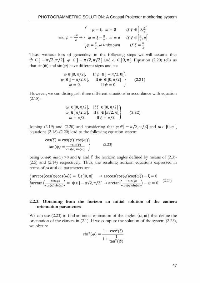
PHOTOGRAMMETRIC SOLUTION: A Coastal Projector monitoring system
47
and 𝜓 =−𝜋
2→
{
𝜑 = ξ, 𝜔 = 0 𝑖𝑓 𝜉 ∈ ]0,
𝜋
2[
𝜑 = ξ −π
2, 𝜔 = 𝜋 𝑖𝑓 𝜉 ∈ ]
𝜋
2, 𝜋[
𝜑 =𝜋
2, 𝜔 𝑢𝑛𝑘𝑛𝑜𝑤𝑛 𝑖𝑓 𝜉 =
𝜋
2
Thus, without loss of generality, in the following steps we will assume that
𝜓 ∈ ] − 𝜋/2, 𝜋/2[, 𝜑 ∈ ] − 𝜋/2, 𝜋/2[ and 𝜔 ∈ ]0, 𝜋[. Equation (2.20) tells us
that sin(𝜓) and sin(𝜑) have different signs and so:
𝜑 ∈ ]0, 𝜋/2[, If 𝜓 ∈ ] − 𝜋/2, 0[
𝜑 ∈ ] − 𝜋/2, 0[, If 𝜓 ∈ ]0, 𝜋/2[
𝜑 = 0, If 𝜓 = 0} (2.21)
However, we can distinguish three different situations in accordance with equation (2.18):
𝜔 ∈ ]0, 𝜋/2[, If 𝜉 ∈ ]0, 𝜋/2[
𝜔 ∈ ]𝜋/2, 𝜋[, If 𝜉 ∈ ]𝜋/2, 𝜋[
𝜔 = 𝜋/2, If 𝜉 = 𝜋/2 } (2.22)
Joining (2.19) and (2.20) and considering that 𝜑 ∈] − 𝜋/2, 𝜋/2[ and 𝜔 𝜖 ]0, 𝜋[, equations (2.18)-(2.20) lead to the following equation system:
cos (𝜉) = cos(𝜑) cos(𝜔)
tan(𝜓) =−sin (𝜑)
cos(𝜑)sin (𝜔)
} (2.23)
being cos(𝜑) sin(𝜔) >0 and 𝜓 and 𝜉 the horizon angles defined by means of (2.3)-(2.5) and (2.14) respectively. Thus, the resulting horizon equations expressed in
terms of ω and φ parameters are:
{arccos(cos (φ)cos(ω)) = ξ ϵ ]0, π[ → arccos(cos (φ)cos(ω)) − ξ = 0
arctan (−sin (φ)
cos (φ)sin(ω)) = ψ ϵ ] − 𝜋/2, 𝜋/2[ → arctan (
−sin (φ)
cos (φ)sin(ω)) − ψ = 0
(2.24)
2.2.3. Obtaining from the horizon an initial solution of the camera orientation parameters
We can use (2.23) to find an initial estimation of the angles {ω, 𝜑} that define the orientation of the càmera in (2.1). If we compute the solution of the system (2.23), we obtain:
𝑠𝑖𝑛2(𝜑) =1 − cos2(ξ)
1 +1
tan2(𝜓)
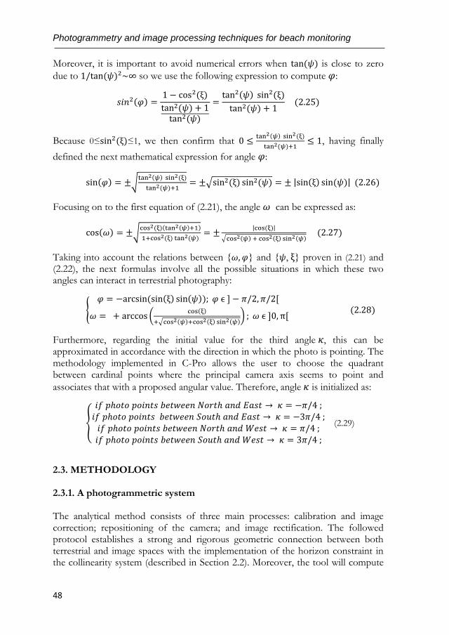
Photogrammetry and image processing techniques for beach monitoring
48
Moreover, it is important to avoid numerical errors when tan(𝜓) is close to zero
due to 1/tan (𝜓)2~∞ so we use the following expression to compute 𝜑:
𝑠𝑖𝑛2(𝜑) =1 − cos2(ξ)
tan2(𝜓) + 1tan2(𝜓)
=tan2(𝜓) sin2(ξ)
tan2(𝜓) + 1 (2.25)
Because 0≤sin2(ξ)≤1, we then confirm that 0 ≤tan2(𝜓) sin2(ξ)
tan2(𝜓)+1≤ 1, having finally
defined the next mathematical expression for angle 𝜑:
sin(𝜑) = ±√tan2(𝜓) sin2(ξ)
tan2(𝜓)+1= ±√sin2(ξ) sin2(𝜓) = ± |sin(ξ) sin (𝜓)| (2.26)
Focusing on to the first equation of (2.21), the angle 𝜔 can be expressed as:
cos(𝜔) = ±√cos2(ξ)(tan2(𝜓)+1)
1+cos2(ξ) tan2(𝜓)= ±
|cos (ξ)|
√cos2(𝜓) + cos2(ξ) sin2(𝜓) (2.27)
Taking into account the relations between {𝜔,𝜑} and {𝜓, ξ} proven in (2.21) and (2.22), the next formulas involve all the possible situations in which these two angles can interact in terrestrial photography:
{𝜑 = −arcsin (sin(ξ) sin(𝜓)); 𝜑 ϵ ] − 𝜋/2, 𝜋/2[
𝜔 = + arccos (cos(ξ)
+√cos2(𝜓)+cos2(ξ) sin2(𝜓)) ; 𝜔 ϵ ]0, π[
(2.28)
Furthermore, regarding the initial value for the third angle 𝜅, this can be approximated in accordance with the direction in which the photo is pointing. The methodology implemented in C-Pro allows the user to choose the quadrant between cardinal points where the principal camera axis seems to point and
associates that with a proposed angular value. Therefore, angle 𝜅 is initialized as:
{
𝑖𝑓 𝑝ℎ𝑜𝑡𝑜 𝑝𝑜𝑖𝑛𝑡𝑠 𝑏𝑒𝑡𝑤𝑒𝑒𝑛 𝑁𝑜𝑟𝑡ℎ 𝑎𝑛𝑑 𝐸𝑎𝑠𝑡 → 𝜅 = −𝜋/4 ; 𝑖𝑓 𝑝ℎ𝑜𝑡𝑜 𝑝𝑜𝑖𝑛𝑡𝑠 𝑏𝑒𝑡𝑤𝑒𝑒𝑛 𝑆𝑜𝑢𝑡ℎ 𝑎𝑛𝑑 𝐸𝑎𝑠𝑡 → 𝜅 = −3𝜋/4 ; 𝑖𝑓 𝑝ℎ𝑜𝑡𝑜 𝑝𝑜𝑖𝑛𝑡𝑠 𝑏𝑒𝑡𝑤𝑒𝑒𝑛 𝑁𝑜𝑟𝑡ℎ 𝑎𝑛𝑑 𝑊𝑒𝑠𝑡 → 𝜅 = 𝜋/4 ; 𝑖𝑓 𝑝ℎ𝑜𝑡𝑜 𝑝𝑜𝑖𝑛𝑡𝑠 𝑏𝑒𝑡𝑤𝑒𝑒𝑛 𝑆𝑜𝑢𝑡ℎ 𝑎𝑛𝑑 𝑊𝑒𝑠𝑡 → 𝜅 = 3𝜋/4 ;
(2.29)
2.3. METHODOLOGY 2.3.1. A photogrammetric system The analytical method consists of three main processes: calibration and image correction; repositioning of the camera; and image rectification. The followed protocol establishes a strong and rigorous geometric connection between both terrestrial and image spaces with the implementation of the horizon constraint in the collinearity system (described in Section 2.2). Moreover, the tool will compute
PHOTOGRAMMETRIC SOLUTION: A Coastal Projector monitoring system
49
the adjustment adapting to different situations depending on the number of initially known and unknown external and internal orientation parameters. 2.3.1.1. Camera calibration and image correction In photogrammetry, the extraction of metric information requires a precise knowledge of the internal orientation parameters (IOP) –principal point
coordinates o=(𝑥0, 𝑦0) and focal length (f)– and the distortion coefficients of the non-metric camera lens (assuming rectangular pixels skew factor is generally negligible). A camera acquires images composed of pixels where each pixel captures light traveling along the projection of a 3D ray. The projection rays in principle can be placed arbitrarily assuming the absence of a functional relationship between the projection rays and the pixels directed by the intrinsic parameters. Thus, the calibration is described in accordance with the coordinates of these rays (given in the local coordinate system) and the correspondence between the rays and pixels. After such calibration, each ray of the bundle passes correctly through the optical center. In the present work, as we had access to the cameras, an a-priori laboratory study of the acquisition system itself was made. It is known that self-calibration can improve the accuracy of non-metric cameras (Chandler et al., 2005). This shows the potential that cheap cameras have for measuring surfaces when the lens model has been considered and a correct calibration of the intrinsic camera parameters has been made. The calibration involves applying the Matlab camera calibration toolbox of Bouguet (2015). This calibration tool works with a series of images on a pattern like a checkerboard with the camera focused to infinity and taking the photos from different points of view and changing orientation and position. The IOP are estimated by an initial approach linearizing the equations and a least squares adjustment. These parameters are generally invariant and unique for each camera under similar conditions (Holland et al., 1997). Removing the induced effects of these intrinsic camera parameters, the image is corrected and undistorted by the empirical inverse model for compensating lens distortions proposed by Heikkila and Silvén, 1997. After the image correction, a correct geometric relation between the image and terrain systems will exist and the center of the undistorted image will coincide with the center of the original image – and will be consistent with the formulas shown in the following sections.
2.3.1.2. Camera repositioning
The process of determining the orientation parameters is understood as spatial resection and is considered as a particularization of a photogrammetric triangulation for a simple image. The six EOP recreates the moment in which a
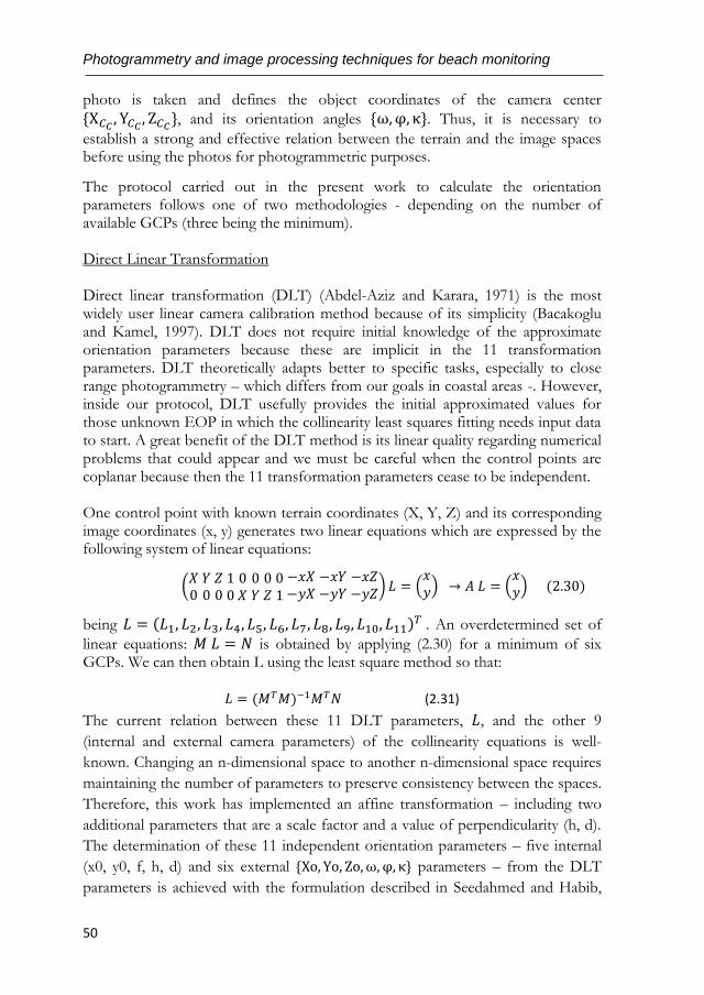
Photogrammetry and image processing techniques for beach monitoring
50
photo is taken and defines the object coordinates of the camera center
{X𝐶𝐶 , Y𝐶𝐶 , Z𝐶𝐶}, and its orientation angles {ω,φ, κ}. Thus, it is necessary to
establish a strong and effective relation between the terrain and the image spaces before using the photos for photogrammetric purposes.
The protocol carried out in the present work to calculate the orientation parameters follows one of two methodologies - depending on the number of available GCPs (three being the minimum). Direct Linear Transformation Direct linear transformation (DLT) (Abdel-Aziz and Karara, 1971) is the most widely user linear camera calibration method because of its simplicity (Bacakoglu and Kamel, 1997). DLT does not require initial knowledge of the approximate orientation parameters because these are implicit in the 11 transformation parameters. DLT theoretically adapts better to specific tasks, especially to close range photogrammetry – which differs from our goals in coastal areas -. However, inside our protocol, DLT usefully provides the initial approximated values for those unknown EOP in which the collinearity least squares fitting needs input data to start. A great benefit of the DLT method is its linear quality regarding numerical problems that could appear and we must be careful when the control points are coplanar because then the 11 transformation parameters cease to be independent. One control point with known terrain coordinates (X, Y, Z) and its corresponding image coordinates (x, y) generates two linear equations which are expressed by the following system of linear equations:
(𝑋0 𝑌0 𝑍0 1 0 0𝑋 0𝑌 0𝑍 01 −𝑥𝑋−𝑦𝑋
−𝑥𝑌−𝑦𝑌
−𝑥𝑍−𝑦𝑍
) 𝐿 = (𝑥𝑦) → 𝐴 𝐿 = (
𝑥𝑦) (2.30)
being 𝐿 = (𝐿1, 𝐿2, 𝐿3, 𝐿4, 𝐿5, 𝐿6, 𝐿7, 𝐿8, 𝐿9, 𝐿10, 𝐿11)𝑇 . An overdetermined set of
linear equations: 𝑀 𝐿 = 𝑁 is obtained by applying (2.30) for a minimum of six GCPs. We can then obtain L using the least square method so that:
𝐿 = (𝑀𝑇𝑀)−1𝑀𝑇𝑁 (2.31)
The current relation between these 11 DLT parameters, 𝐿, and the other 9
(internal and external camera parameters) of the collinearity equations is well-
known. Changing an n-dimensional space to another n-dimensional space requires
maintaining the number of parameters to preserve consistency between the spaces.
Therefore, this work has implemented an affine transformation – including two
additional parameters that are a scale factor and a value of perpendicularity (h, d).
The determination of these 11 independent orientation parameters – five internal
(x0, y0, f, h, d) and six external {Xo, Yo, Zo, ω, φ, κ} parameters – from the DLT
parameters is achieved with the formulation described in Seedahmed and Habib,
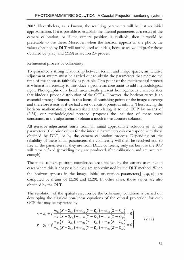
PHOTOGRAMMETRIC SOLUTION: A Coastal Projector monitoring system
51
2002. Nevertheless, as is known, the resulting parameters will be just an initial
approximation. If it is possible to establish the internal parameters as a result of the
camera calibration, or if the camera position is available, then it would be
preferable to use these. Moreover, when the horizon appears in the photo, the
values obtained by DLT will not be used as initials, because we would prefer those
obtained by (2.28) and (2.29) as section 2.4 proves.
Refinement process by collinearity
To guarantee a strong relationship between terrain and image spaces, an iterative adjustment system must be carried out to obtain the parameters that recreate the time of the shoot as faithfully as possible. This point of the mathematical process is where it is necessary to introduce a geometric constraint to add methodological rigor. Photographs of a beach area usually present homogeneous characteristics that hinder a proper distribution of the GCPs. However, the horizon curve is an essential strategic element. In this locus, all vanishing points of the image converge and therefore it acts as if we had a set of control points at infinity. Thus, having the horizon mathematically characterized and relating it to the EOP by means of (2.24), our methodological protocol proposes the inclusion of these novel constraints in the adjustment to obtain a much more accurate solution.
All iterative adjustment starts from an initial approximate solution of all the parameters. The prior values for the internal parameters can correspond with those obtained by DLT, or by the camera calibration process. Depending on the reliability of these initial parameters, the collinearity will then be resolved and so free all the parameters if they are from DLT, or freeing only six because the IOP will remain fixed (providing they are produced after calibration and are accurate enough).
The initial camera position coordinates are obtained by the camera user, but in
cases where this is not possible they are approximated by the DLT method. When
the horizon appears in the image, initial orientation parameters,{ω,φ, κ}, are
computed by means of (2.28) and (2.29). In other cases, those values are also
obtained by the DLT.
The resolution of the spatial resection by the collinearity condition is carried out developing the classical non-linear equations of the central projection for each GCP that may be expressed by:
𝑥 − 𝑥0 + 𝑓𝑚11(𝑋 − X𝐶𝐶) +𝑚12(𝑌 − 𝑌𝐶𝐶) + 𝑚13(𝑍 − Z𝐶𝐶)
𝑚31(𝑋 − X𝐶𝐶) + 𝑚32(𝑌 − 𝑌𝐶𝐶) + 𝑚33(𝑍 − Z𝐶𝐶)= 0
𝑦 − 𝑦0 + 𝑓𝑚21(𝑋 − X𝐶𝐶) +𝑚22(𝑌 − 𝑌𝐶𝐶) + 𝑚23(𝑍 − Z𝐶𝐶)
𝑚31(𝑋 − X𝐶𝐶) +𝑚32(𝑌 − 𝑌𝐶𝐶) + 𝑚33(𝑍 − Z𝐶𝐶)= 0
}
(2.32)
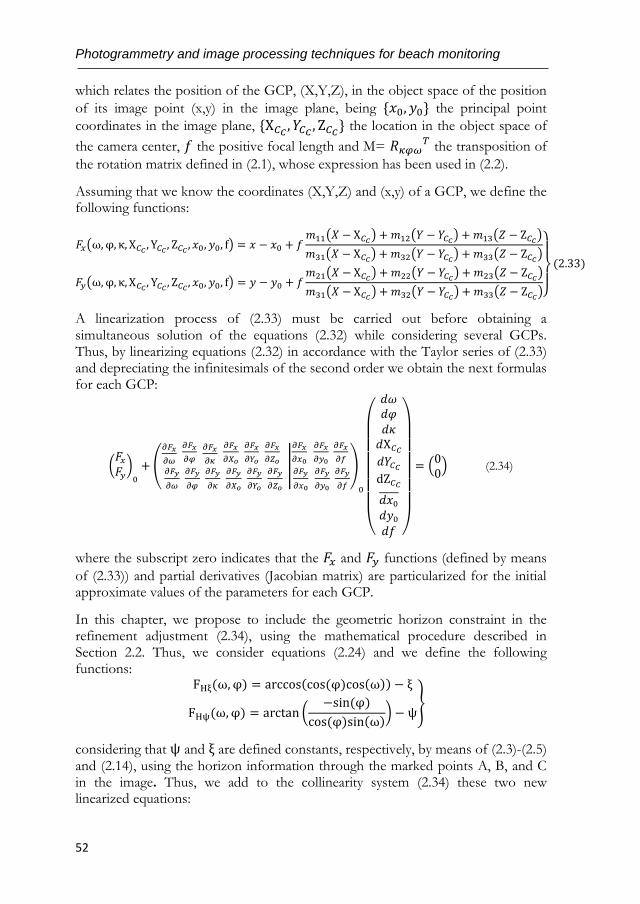
Photogrammetry and image processing techniques for beach monitoring
52
which relates the position of the GCP, (X,Y,Z), in the object space of the position
of its image point (x,y) in the image plane, being {𝑥0, 𝑦0} the principal point
coordinates in the image plane, {X𝐶𝐶 , 𝑌𝐶𝐶 , Z𝐶𝐶} the location in the object space of
the camera center, 𝑓 the positive focal length and M= 𝑅𝜅𝜑𝜔𝑇 the transposition of
the rotation matrix defined in (2.1), whose expression has been used in (2.2).
Assuming that we know the coordinates (X,Y,Z) and (x,y) of a GCP, we define the following functions:
𝐹𝑥(ω, φ, κ, X𝐶𝐶 , Y𝐶𝐶 , Z𝐶𝐶 , 𝑥0, 𝑦0, f) = 𝑥 − 𝑥0 + 𝑓𝑚11(𝑋 − X𝐶𝐶) + 𝑚12(𝑌 − 𝑌𝐶𝐶) + 𝑚13(𝑍 − Z𝐶𝐶)
𝑚31(𝑋 − X𝐶𝐶) + 𝑚32(𝑌 − 𝑌𝐶𝐶) + 𝑚33(𝑍 − Z𝐶𝐶)
𝐹𝑦(ω, φ, κ, X𝐶𝐶 , Y𝐶𝐶 , Z𝐶𝐶 , 𝑥0, 𝑦0, f) = 𝑦 − 𝑦0 + 𝑓𝑚21(𝑋 − X𝐶𝐶) + 𝑚22(𝑌 − 𝑌𝐶𝐶) + 𝑚23(𝑍 − Z𝐶𝐶)
𝑚31(𝑋 − X𝐶𝐶) + 𝑚32(𝑌 − 𝑌𝐶𝐶) + 𝑚33(𝑍 − Z𝐶𝐶)}
(2.33)
A linearization process of (2.33) must be carried out before obtaining a simultaneous solution of the equations (2.32) while considering several GCPs. Thus, by linearizing equations (2.32) in accordance with the Taylor series of (2.33) and depreciating the infinitesimals of the second order we obtain the next formulas for each GCP:
(𝐹𝑥𝐹𝑦)0
+ (
𝜕𝐹𝑥
𝜕𝜔
𝜕𝐹𝑦
𝜕𝜔
𝜕𝐹𝑥
𝜕𝜑
𝜕𝐹𝑦
𝜕𝜑
𝜕𝐹𝑥
𝜕𝜅
𝜕𝐹𝑦
𝜕𝜅
𝜕𝐹𝑥
𝜕𝑋𝑜
𝜕𝐹𝑦
𝜕𝑋𝑜
𝜕𝐹𝑥
𝜕𝑌𝑜
𝜕𝐹𝑦
𝜕𝑌𝑜
𝜕𝐹𝑥
𝜕𝑍𝑜
𝜕𝐹𝑦
𝜕𝑍𝑜
|
𝜕𝐹𝑥
𝜕𝑥0
𝜕𝐹𝑦
𝜕𝑥0
𝜕𝐹𝑥
𝜕𝑦0 𝜕𝐹𝑥
𝜕𝑓
𝜕𝐹𝑦
𝜕𝑦0 𝜕𝐹𝑦
𝜕𝑓
)
0
(
𝑑𝜔𝑑𝜑𝑑𝜅𝑑X𝐶𝐶𝑑𝑌𝐶𝐶dZ𝐶𝐶
𝑑𝑥0𝑑𝑦0𝑑𝑓 )
= (00) (2.34)
where the subscript zero indicates that the 𝐹𝑥 and 𝐹𝑦 functions (defined by means
of (2.33)) and partial derivatives (Jacobian matrix) are particularized for the initial approximate values of the parameters for each GCP.
In this chapter, we propose to include the geometric horizon constraint in the refinement adjustment (2.34), using the mathematical procedure described in Section 2.2. Thus, we consider equations (2.24) and we define the following functions:
FHξ(ω, φ) = arccos(cos (φ)cos(ω)) − ξ
FHψ(ω, φ) = arctan (−sin (φ)
cos (φ)sin(ω)) − ψ
}
considering that ψ and ξ are defined constants, respectively, by means of (2.3)-(2.5) and (2.14), using the horizon information through the marked points A, B, and C in the image. Thus, we add to the collinearity system (2.34) these two new linearized equations:
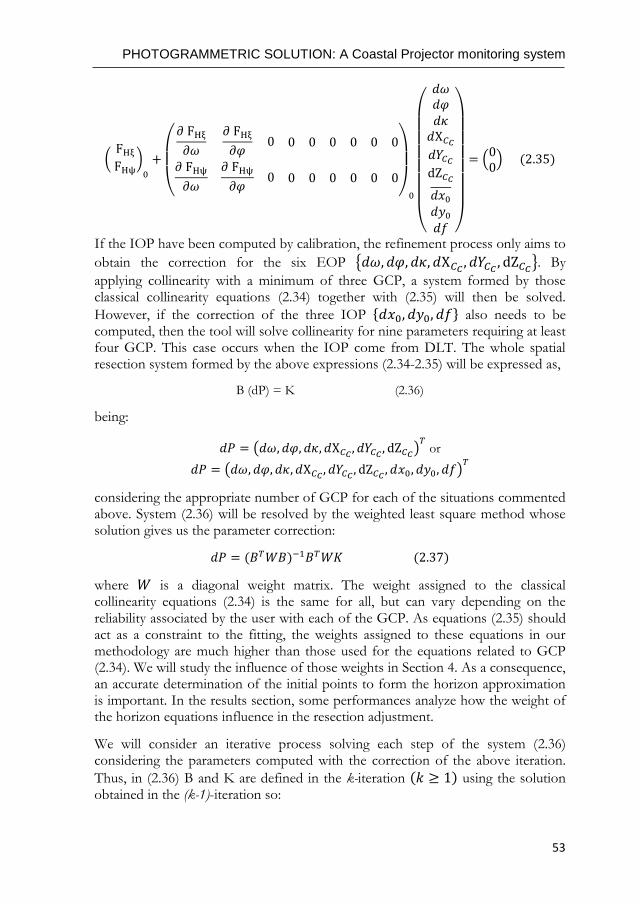
PHOTOGRAMMETRIC SOLUTION: A Coastal Projector monitoring system
53
( FHξ FHψ
)0
+
(
𝜕 FHξ
𝜕𝜔
𝜕 FHξ
𝜕𝜑0 0 0 0 0 0 0
𝜕 FHψ
𝜕𝜔
𝜕 FHψ
𝜕𝜑0 0 0 0 0 0 0
)
0
(
𝑑𝜔𝑑𝜑𝑑𝜅𝑑X𝐶𝐶𝑑𝑌𝐶𝐶dZ𝐶𝐶
𝑑𝑥0𝑑𝑦0𝑑𝑓 )
= (00) (2.35)
If the IOP have been computed by calibration, the refinement process only aims to
obtain the correction for the six EOP {𝑑𝜔, 𝑑𝜑, 𝑑𝜅, 𝑑X𝐶𝐶 , 𝑑𝑌𝐶𝐶 , dZ𝐶𝐶}. By
applying collinearity with a minimum of three GCP, a system formed by those classical collinearity equations (2.34) together with (2.35) will then be solved.
However, if the correction of the three IOP {𝑑𝑥0, 𝑑𝑦0, 𝑑𝑓} also needs to be computed, then the tool will solve collinearity for nine parameters requiring at least four GCP. This case occurs when the IOP come from DLT. The whole spatial resection system formed by the above expressions (2.34-2.35) will be expressed as,
B (dP) = K (2.36)
being:
𝑑𝑃 = (𝑑𝜔, 𝑑𝜑, 𝑑𝜅, 𝑑X𝐶𝐶 , 𝑑𝑌𝐶𝐶 , dZ𝐶𝐶)𝑇 or
𝑑𝑃 = (𝑑𝜔, 𝑑𝜑, 𝑑𝜅, 𝑑X𝐶𝐶 , 𝑑𝑌𝐶𝐶 , dZ𝐶𝐶 , 𝑑𝑥0, 𝑑𝑦0, 𝑑𝑓)𝑇
considering the appropriate number of GCP for each of the situations commented above. System (2.36) will be resolved by the weighted least square method whose solution gives us the parameter correction:
𝑑𝑃 = (𝐵𝑇𝑊𝐵)−1𝐵𝑇𝑊𝐾 (2.37)
where 𝑊 is a diagonal weight matrix. The weight assigned to the classical collinearity equations (2.34) is the same for all, but can vary depending on the reliability associated by the user with each of the GCP. As equations (2.35) should act as a constraint to the fitting, the weights assigned to these equations in our methodology are much higher than those used for the equations related to GCP (2.34). We will study the influence of those weights in Section 4. As a consequence, an accurate determination of the initial points to form the horizon approximation is important. In the results section, some performances analyze how the weight of the horizon equations influence in the resection adjustment.
We will consider an iterative process solving each step of the system (2.36) considering the parameters computed with the correction of the above iteration.
Thus, in (2.36) B and K are defined in the k-iteration (𝑘 ≥ 1) using the solution obtained in the (k-1)-iteration so:

Photogrammetry and image processing techniques for beach monitoring
54
(𝜔𝑘 , 𝜑𝑘 , 𝜅𝑘, 𝑋𝐶𝐶𝑘, 𝑌𝐶𝐶
𝑘, 𝑍𝐶𝐶𝑘, 𝑥0
𝑘, 𝑦0𝑘, 𝑓𝑘)=
(𝜔𝑘−1 + 𝑑𝜔𝑘−1, 𝜑𝑘−1 + 𝑑𝜑𝑘−1, 𝜅𝑘−1 + 𝑑𝜅𝑘−1, 𝑋𝐶𝐶
𝑘−1 + 𝑑𝑋𝐶𝐶𝑘−1, 𝑌𝐶𝐶
𝑘−1 + 𝑑𝑌𝐶𝐶𝑘−1,
𝑍𝐶𝐶𝑘−1 + 𝑑𝑍𝐶𝐶
𝑘−1, 𝑥0𝑘−1 + 𝑑𝑥0
𝑘−1, 𝑦0𝑘−1 + 𝑑𝑦0
𝑘−1, 𝑓𝑘−1 + 𝑑𝑓𝑘−1)
(2.38)
That process finishes when each of the correction parameters becomes insignificant (the established threshold is equal to 10−10).
To establish the convergence of the system, at the beginning of the k-iteration,
(𝑘 ≥ 1), the C-Pro tool will color in green the calculated image coordinates of the GCP by computing (x,y) by means of the collinearity equations (2.32), considering the parameters obtained using (2.38) and the (X,Y) coordinates of each GCP. Moreover, the horizon line will be approximated using the following equation:
𝑦 = 𝑦0𝑘 + 𝑑ℎ𝑜𝑟𝑖𝑧𝑜𝑛
𝑘 cos(ψ𝑐𝑎𝑙𝑐k ) − tan(ψ𝑐𝑎𝑙𝑐
k ) (𝑥 − 𝑥0𝑘−𝑑ℎ𝑜𝑟𝑖𝑧𝑜𝑛
𝑘 sin(ψ𝑐𝑎𝑙𝑐k )) (2.39)
where:
𝑑ℎ𝑜𝑟𝑖𝑧𝑜𝑛𝑘 = −𝑓𝑘 ∗ 𝑡𝑎𝑛 (𝑎𝑟𝑐𝑐𝑜𝑠(𝑐𝑜𝑠(𝜑𝑘) 𝑐𝑜𝑠(𝜔𝑘)) − 𝑎𝑟𝑐𝑐𝑜𝑠 (
𝑍𝐶𝐶𝑘+0.42∗
(𝐷𝑘)2
𝑅𝑡
𝐷𝑘) ) (2.40)
being 𝐷𝑘 defined by means of (2.12) and Z𝐶𝐶k defined by (2.38); and:
ψ𝑐𝑎𝑙𝑐k = arctan (
−sin (φk)
cos (φk)sin(ωk)) (2.41)
Thus, the horizon line is recomputed in each iteration with the newest parameters until the adjustment process ends.
2.3.1.3. Image rectification and data extraction
Once the repositioning camera has been fruitfully achieved, the rectification process can be done. In our tool, the user can choose whether to project a piece of the image or just an element contained therein over a specific plane with a known ZT value. Choosing the first option, the tool detects the image limits in terrain coordinates and a georeferenced grid is created for a specific pixel size on the specific ZT. Each pixel is then filled by an image intensity value through inverse mapping techniques and using the nearest neighbor interpolation method. In this case, the final product is a rectified georeferenced image (Tiff World File) used by standard GIS applications. Nevertheless, by following the second option, the user can digitalize a specific feature of interest as a coastal indicator – such as an established shoreline, the landward edge, the foredune toe, the cliff top – or just upload a file with the image
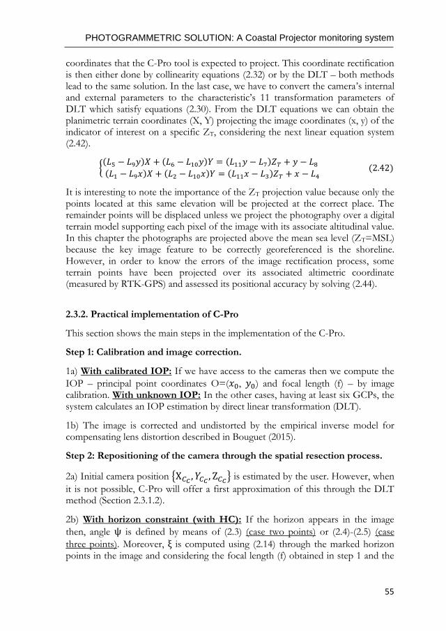
PHOTOGRAMMETRIC SOLUTION: A Coastal Projector monitoring system
55
coordinates that the C-Pro tool is expected to project. This coordinate rectification is then either done by collinearity equations (2.32) or by the DLT – both methods lead to the same solution. In the last case, we have to convert the camera’s internal and external parameters to the characteristic’s 11 transformation parameters of DLT which satisfy equations (2.30). From the DLT equations we can obtain the planimetric terrain coordinates (X, Y) projecting the image coordinates (x, y) of the indicator of interest on a specific ZT, considering the next linear equation system (2.42).
{(𝐿5 − 𝐿9𝑦)𝑋 + (𝐿6 − 𝐿10𝑦)𝑌 = (𝐿11𝑦 − 𝐿7)𝑍𝑇 + 𝑦 − 𝐿8
(𝐿1 − 𝐿9𝑥)𝑋 + (𝐿2 − 𝐿10𝑥)𝑌 = (𝐿11𝑥 − 𝐿3)𝑍𝑇 + 𝑥 − 𝐿4 (2.42)
It is interesting to note the importance of the ZT projection value because only the points located at this same elevation will be projected at the correct place. The remainder points will be displaced unless we project the photography over a digital terrain model supporting each pixel of the image with its associate altitudinal value. In this chapter the photographs are projected above the mean sea level (ZT=MSL) because the key image feature to be correctly georeferenced is the shoreline. However, in order to know the errors of the image rectification process, some terrain points have been projected over its associated altimetric coordinate (measured by RTK-GPS) and assessed its positional accuracy by solving (2.44).
2.3.2. Practical implementation of C-Pro
This section shows the main steps in the implementation of the C-Pro.
Step 1: Calibration and image correction.
1a) With calibrated IOP: If we have access to the cameras then we compute the
IOP – principal point coordinates O=(𝑥0, 𝑦0) and focal length (f) – by image calibration. With unknown IOP: In the other cases, having at least six GCPs, the system calculates an IOP estimation by direct linear transformation (DLT).
1b) The image is corrected and undistorted by the empirical inverse model for compensating lens distortion described in Bouguet (2015).
Step 2: Repositioning of the camera through the spatial resection process.
2a) Initial camera position {X𝐶𝐶 , 𝑌𝐶𝐶 , Z𝐶𝐶} is estimated by the user. However, when
it is not possible, C-Pro will offer a first approximation of this through the DLT method (Section 2.3.1.2).
2b) With horizon constraint (with HC): If the horizon appears in the image
then, angle ψ is defined by means of (2.3) (case two points) or (2.4)-(2.5) (case
three points). Moreover, ξ is computed using (2.14) through the marked horizon points in the image and considering the focal length (f) obtained in step 1 and the
Photogrammetry and image processing techniques for beach monitoring
56
camera center elevation Z𝐶𝐶 defined in 2a). {ω,φ, κ} are then computed by means
of (2.28) and (2.29). Without horizon constraint (without HC): in cases where
the horizon equation is not available, {ω,φ, κ} are estimated by the DLT.
2c) C-Pro calculates the final EOP through an iterative weighted least squares fitting (2.37) over the linearized collinearity equations (2.34) (two equations for each GCP), which starts with the parameters defined in 2b) and finishes when each
of the correction parameters become less than 10−10. The weight assigned to those equations is equal to 1, but can vary depending on the reliability associated by the user to each of the GCP. Moreover, in the cases with horizon constraint, the linearized horizon equations (2.35) are added with an associated weight of
1012 to solve the photo geometry (2.34). The system will be resolved and freeing all parameters if the IOP in step 1 proceeds from DLT (with unknown IOP), or freeing only six of them when the IOP remains fixed by considering that they are computed in step 1 (with calibrated IOP).
2d) To discover how the convergence of the system is progressing, C-Pro colors green (at the end of each iteration) the calculated image coordinates of the GCP by computing (x,y) by means of the collinearity equations (2.32) and considering the parameters obtained using (2.38). Moreover, the horizon line is also colored in green considering equation (2.39).
Step 3: Image rectification
3a) To project a piece of the image on a specific plane with a known ZT value, a georeferenced grid is created and each pixel is filled with an image intensity value through inverse mapping techniques and using the nearest neighbor interpolation method.
3b) Collinearity equations (2.32) or the DLT equations given in (2.42) will be used to project an element contained in the image on a plane with a constant ZT coordinate. In the case of shoreline rectification, the MSL value is used as ZT. 2.4. TESTING OF THE HORIZON CONSTRAINT AND C-PRO SOFTWARE
Assessing the protocol proposed in this chapter, the following subsections show the benefits achieved by including the horizon constraint in the spatial resection process.
The analyses are carried out in the three coastal areas described in this section and working with specific photogrammetry conditions that must be solved. The tests are made with non-fixed cameras. Therefore, in the first step of C-Pro, the IOP of the acquisition system were obtained through image calibration (Bouguet, 2015). However, some of the results of this section will be obtained when considering the IOP as unknown to prove that C-Pro also works accurately in such cases.
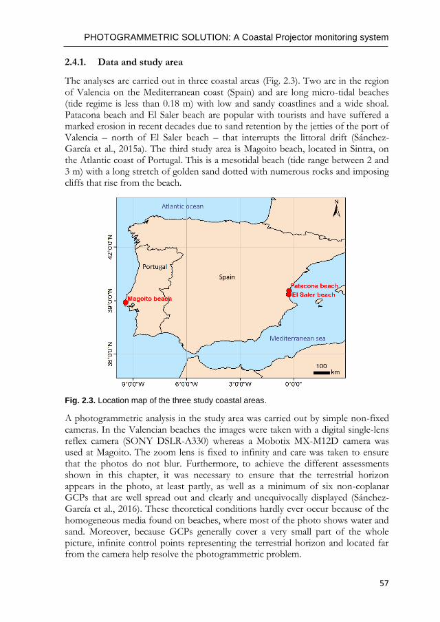
PHOTOGRAMMETRIC SOLUTION: A Coastal Projector monitoring system
57
2.4.1. Data and study area
The analyses are carried out in three coastal areas (Fig. 2.3). Two are in the region of Valencia on the Mediterranean coast (Spain) and are long micro-tidal beaches (tide regime is less than 0.18 m) with low and sandy coastlines and a wide shoal. Patacona beach and El Saler beach are popular with tourists and have suffered a marked erosion in recent decades due to sand retention by the jetties of the port of Valencia – north of El Saler beach – that interrupts the littoral drift (Sánchez-García et al., 2015a). The third study area is Magoito beach, located in Sintra, on the Atlantic coast of Portugal. This is a mesotidal beach (tide range between 2 and 3 m) with a long stretch of golden sand dotted with numerous rocks and imposing cliffs that rise from the beach.
Fig. 2.3. Location map of the three study coastal areas.
A photogrammetric analysis in the study area was carried out by simple non-fixed cameras. In the Valencian beaches the images were taken with a digital single-lens reflex camera (SONY DSLR-A330) whereas a Mobotix MX-M12D camera was used at Magoito. The zoom lens is fixed to infinity and care was taken to ensure that the photos do not blur. Furthermore, to achieve the different assessments shown in this chapter, it was necessary to ensure that the terrestrial horizon appears in the photo, at least partly, as well as a minimum of six non-coplanar GCPs that are well spread out and clearly and unequivocally displayed (Sánchez-García et al., 2016). These theoretical conditions hardly ever occur because of the homogeneous media found on beaches, where most of the photo shows water and sand. Moreover, because GCPs generally cover a very small part of the whole picture, infinite control points representing the terrestrial horizon and located far from the camera help resolve the photogrammetric problem.
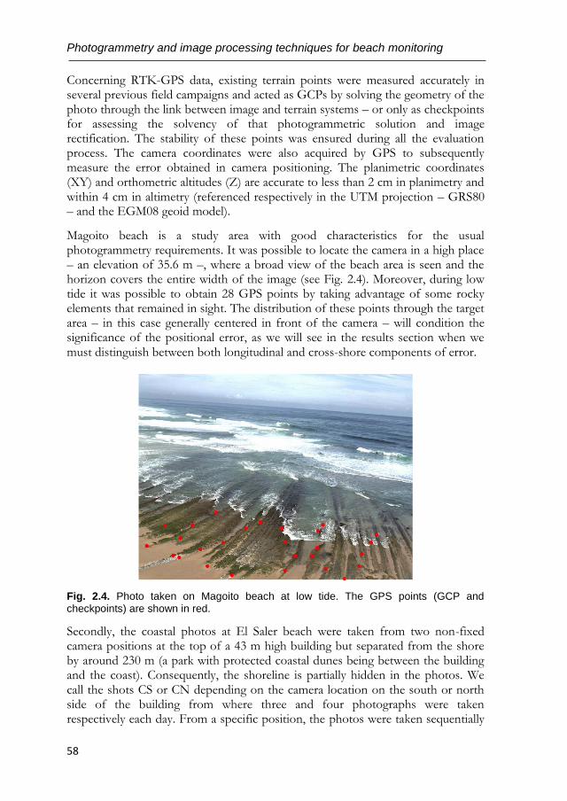
Photogrammetry and image processing techniques for beach monitoring
58
Concerning RTK-GPS data, existing terrain points were measured accurately in several previous field campaigns and acted as GCPs by solving the geometry of the photo through the link between image and terrain systems – or only as checkpoints for assessing the solvency of that photogrammetric solution and image rectification. The stability of these points was ensured during all the evaluation process. The camera coordinates were also acquired by GPS to subsequently measure the error obtained in camera positioning. The planimetric coordinates (XY) and orthometric altitudes (Z) are accurate to less than 2 cm in planimetry and within 4 cm in altimetry (referenced respectively in the UTM projection – GRS80 – and the EGM08 geoid model).
Magoito beach is a study area with good characteristics for the usual photogrammetry requirements. It was possible to locate the camera in a high place – an elevation of 35.6 m –, where a broad view of the beach area is seen and the horizon covers the entire width of the image (see Fig. 2.4). Moreover, during low tide it was possible to obtain 28 GPS points by taking advantage of some rocky elements that remained in sight. The distribution of these points through the target area – in this case generally centered in front of the camera – will condition the significance of the positional error, as we will see in the results section when we must distinguish between both longitudinal and cross-shore components of error.
Fig. 2.4. Photo taken on Magoito beach at low tide. The GPS points (GCP and checkpoints) are shown in red.
Secondly, the coastal photos at El Saler beach were taken from two non-fixed camera positions at the top of a 43 m high building but separated from the shore by around 230 m (a park with protected coastal dunes being between the building and the coast). Consequently, the shoreline is partially hidden in the photos. We call the shots CS or CN depending on the camera location on the south or north side of the building from where three and four photographs were taken respectively each day. From a specific position, the photos were taken sequentially
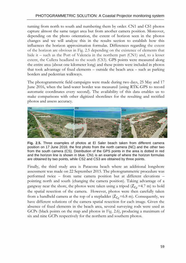
PHOTOGRAMMETRIC SOLUTION: A Coastal Projector monitoring system
59
turning from north to south and numbering them by order. CN1 and CS1 photos capture almost the same target area but from another camera position. Moreover, depending on the photo orientation, the extent of horizon seen in the photos changes and we will analyze this in the results section to establish how this influences the horizon approximation formulas. Differences regarding the extent of the horizon are obvious in Fig. 2.5 depending on the existence of elements that hide it – such as the Port of Valencia in the northern part (CN1) and, to a lesser extent, the Cullera headland to the south (CS3). GPS points were measured along the entire area (about one kilometer long) and these points were included in photos that took advantage of fixed elements – outside the beach area – such as parking borders and pedestrian walkways.
The photogrammetric field campaigns were made during two days, 25 May and 17 June 2016, when the land-water border was measured (using RTK-GPS to record automatic coordinates every second). The availability of this data enables us to make comparisons with other digitized shorelines for the resulting and rectified photos and assess accuracy.
Fig. 2.5. Three examples of photos at El Saler beach taken from different camera
position on 17 June 2016; the first photo from the north camera (NC) and the other two from the south camera (CS). Distribution of the GPS points in the area is dotted in red and the horizon line is shown in blue. CN1 is an example of where the horizon formulas are obtained by two points, while CS2 and CS3 are obtained by three points.
Finally, the third study area is Patacona beach where an additional longshore assessment was made on 22 September 2015. The photogrammetric procedure was performed twice – from same camera position but at different elevations – pointing north and south (changing the camera position). Taking advantage of a
gangway near the shore, the photos were taken using a tripod (𝑍𝐶𝐶=4.7 m) to hold
the spatial resection of the camera. However, photos were then carefully taken
from a handheld camera at the top of a stepladder (𝑍𝐶𝐶=6.8 m). Consequently, we
have different solutions of the camera spatial resection for each image. Given the absence of fixed elements in the beach area, several surveying rods were used as GCPs (black points on the map and photos in Fig. 2.6), producing a maximum of six and nine GCPs respectively for the northern and southern photos.
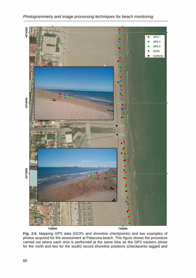
Photogrammetry and image processing techniques for beach monitoring
60
Fig. 2.6. Mapping GPS data (GCPs and shoreline checkpoints) and two examples of
photos acquired for the assessment at Patacona beach. This figure shows the procedure carried out where each shot is performed at the same time as the GPS trackers (three for the north and two for the south) record shoreline positions (checkpoints tagged and
PHOTOGRAMMETRIC SOLUTION: A Coastal Projector monitoring system
61
numbered) and subsequently evaluated on the rectified photos. The extension of a usable horizon is marked with a blue line. Grid coordinates: GCS_ETRS89 UTM30N.
The main goal of the experiment carried out in this area was to understand the functioning of our methodology when camera elevation is reduced. Moreover, to measure the longshore error after image rectification, a field campaign took a set of photos coincident in time with the data acquisition every 20 m for two or three GPS trackers. These devices were separated some 2 m apart and measured moving checkpoints for a distance of 280 m from the camera. We had to establish a distance limit because of the subsequent difficulties in the detection of those checkpoints in the image. Fig. 2.6 exemplifies the experiment performed showing a photo of the north beach and of the south beach where respectively the positions (checkpoints) of three and two GPS trackers are detected. We can also see that the horizon appears in less than half the image and so the horizon approximation formula uses two points.
2.4.2. Improvement of camera positioning by adding the horizon constraint regardless of whether IOP is known or not
The aim of this subsection is to establish the improvements and differences achieved by the influence of the horizon constraint in the spatial resection procedure (results of step 2c). For this reason, the resulting performances are achieved by applying C-Pro in various ways, that is, setting and not setting the IOP (depending on whether these are considered as unknown or known) and with and without including the horizon equations in the fitting.
Validating the final EOP for each test at Magoito and Patacona beaches, Table 2.1 summarizes the differences between these resulting camera coordinates against those accurately measured by GPS. To clarify, the camera positioning error (CPE) is:
𝐶𝑃𝐸 = √(𝑋𝐶𝑐𝐺𝑃𝑆 − 𝑋𝐶𝑐)2+ (𝑌𝐶𝑐𝐺𝑃𝑆 − 𝑌𝐶𝑐)
2+ (𝑍𝐶𝑐𝐺𝑃𝑆 − 𝑍𝐶𝑐)
2 (2.43)
being {X𝐶𝐶 , 𝑌𝐶𝐶 , Z𝐶𝐶} and {𝑋𝐶𝑐𝐺𝑃𝑆 , 𝑌𝐶𝑐𝐺𝑃𝑆 , 𝑍𝐶𝑐𝐺𝑃𝑆} the camera position coordinates
obtained by C-Pro and RTK-GPS techniques respectively.
It is observed that when the camera elevation is higher – as occurs in Magoito with a camera elevation of 35.6 m in comparison with the elevation of Patacona that ranges from 4.7 or 6.8 m – the uncertainty of the IOP causes system inconsistency and overstated positioning error. Results of Table 2.1 reveal the usefulness of the horizon constraint in step 2 of C-Pro. For both cases, with calibrated and unknown IOP, the horizon improves the convergence. However, it is in this last case when it becomes even more necessary to use the horizon to obtain a usable camera position. Regarding the differences between both horizon approximations, the Magoito beach image has a full view of the horizon (Fig. 2.4) and the approximation achieved by three points forming a circumference leads to slightly
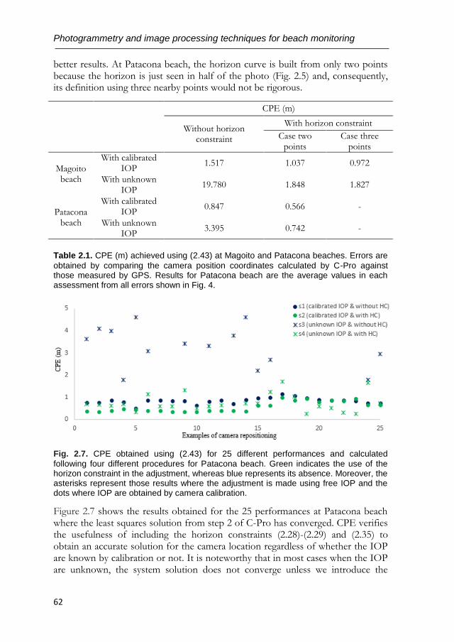
Photogrammetry and image processing techniques for beach monitoring
62
better results. At Patacona beach, the horizon curve is built from only two points because the horizon is just seen in half of the photo (Fig. 2.5) and, consequently, its definition using three nearby points would not be rigorous.
CPE (m)
Without horizon
constraint
With horizon constraint
Case two
points Case three
points
Magoito beach
With calibrated IOP
1.517 1.037 0.972
With unknown IOP
19.780 1.848 1.827
Patacona beach
With calibrated IOP
0.847 0.566 -
With unknown IOP
3.395 0.742 -
Table 2.1. CPE (m) achieved using (2.43) at Magoito and Patacona beaches. Errors are
obtained by comparing the camera position coordinates calculated by C-Pro against those measured by GPS. Results for Patacona beach are the average values in each assessment from all errors shown in Fig. 4.
Fig. 2.7. CPE obtained using (2.43) for 25 different performances and calculated
following four different procedures for Patacona beach. Green indicates the use of the horizon constraint in the adjustment, whereas blue represents its absence. Moreover, the asterisks represent those results where the adjustment is made using free IOP and the dots where IOP are obtained by camera calibration.
Figure 2.7 shows the results obtained for the 25 performances at Patacona beach where the least squares solution from step 2 of C-Pro has converged. CPE verifies the usefulness of including the horizon constraints (2.28)-(2.29) and (2.35) to obtain an accurate solution for the camera location regardless of whether the IOP are known by calibration or not. It is noteworthy that in most cases when the IOP are unknown, the system solution does not converge unless we introduce the
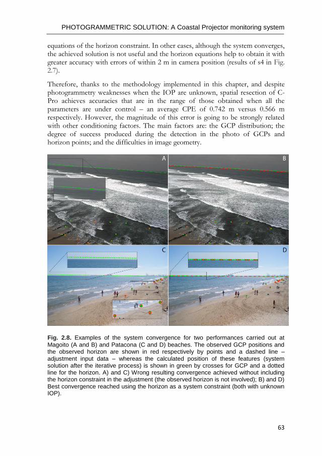
PHOTOGRAMMETRIC SOLUTION: A Coastal Projector monitoring system
63
equations of the horizon constraint. In other cases, although the system converges, the achieved solution is not useful and the horizon equations help to obtain it with greater accuracy with errors of within 2 m in camera position (results of s4 in Fig. 2.7).
Therefore, thanks to the methodology implemented in this chapter, and despite photogrammetry weaknesses when the IOP are unknown, spatial resection of C-Pro achieves accuracies that are in the range of those obtained when all the parameters are under control – an average CPE of 0.742 m versus 0.566 m respectively. However, the magnitude of this error is going to be strongly related with other conditioning factors. The main factors are: the GCP distribution; the degree of success produced during the detection in the photo of GCPs and horizon points; and the difficulties in image geometry.
Fig. 2.8. Examples of the system convergence for two performances carried out at
Magoito (A and B) and Patacona (C and D) beaches. The observed GCP positions and the observed horizon are shown in red respectively by points and a dashed line – adjustment input data – whereas the calculated position of these features (system solution after the iterative process) is shown in green by crosses for GCP and a dotted line for the horizon. A) and C) Wrong resulting convergence achieved without including the horizon constraint in the adjustment (the observed horizon is not involved); B) and D) Best convergence reached using the horizon as a system constraint (both with unknown IOP).
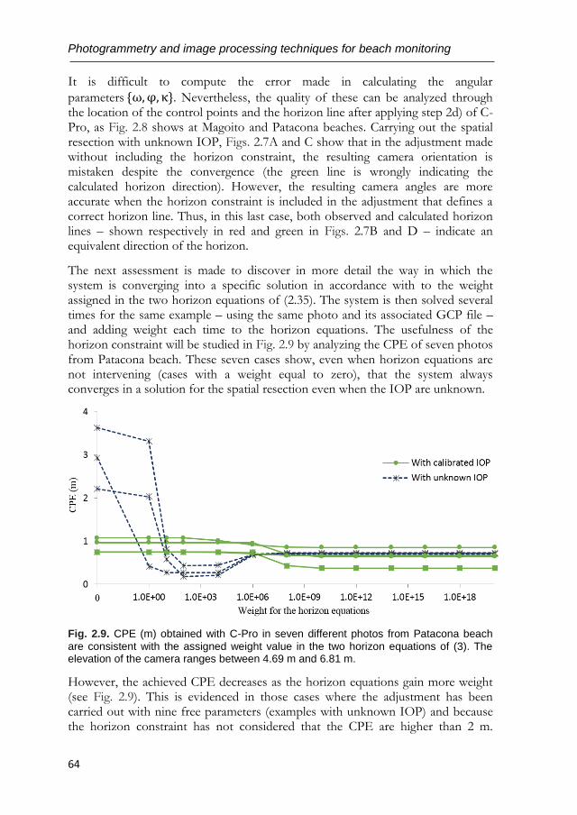
Photogrammetry and image processing techniques for beach monitoring
64
It is difficult to compute the error made in calculating the angular
parameters {ω,φ, κ}. Nevertheless, the quality of these can be analyzed through the location of the control points and the horizon line after applying step 2d) of C-Pro, as Fig. 2.8 shows at Magoito and Patacona beaches. Carrying out the spatial resection with unknown IOP, Figs. 2.7A and C show that in the adjustment made without including the horizon constraint, the resulting camera orientation is mistaken despite the convergence (the green line is wrongly indicating the calculated horizon direction). However, the resulting camera angles are more accurate when the horizon constraint is included in the adjustment that defines a correct horizon line. Thus, in this last case, both observed and calculated horizon lines – shown respectively in red and green in Figs. 2.7B and D – indicate an equivalent direction of the horizon.
The next assessment is made to discover in more detail the way in which the system is converging into a specific solution in accordance with to the weight assigned in the two horizon equations of (2.35). The system is then solved several times for the same example – using the same photo and its associated GCP file – and adding weight each time to the horizon equations. The usefulness of the horizon constraint will be studied in Fig. 2.9 by analyzing the CPE of seven photos from Patacona beach. These seven cases show, even when horizon equations are not intervening (cases with a weight equal to zero), that the system always converges in a solution for the spatial resection even when the IOP are unknown.
Fig. 2.9. CPE (m) obtained with C-Pro in seven different photos from Patacona beach
are consistent with the assigned weight value in the two horizon equations of (3). The elevation of the camera ranges between 4.69 m and 6.81 m.
However, the achieved CPE decreases as the horizon equations gain more weight (see Fig. 2.9). This is evidenced in those cases where the adjustment has been carried out with nine free parameters (examples with unknown IOP) and because the horizon constraint has not considered that the CPE are higher than 2 m.
PHOTOGRAMMETRIC SOLUTION: A Coastal Projector monitoring system
65
Additionally, in these cases it is interesting to note that the minor CPE occurs for horizon weights equal to 102 and 104. This improvement in the accuracy of the camera coordinates happens while the solution for the rest of the parameters (three camera angles and IOP) worsens. The system is less stable when the IOP are unknown and cannot find a valid solution for the entire set of parameters until the weight of the horizon increases.
The CPE remains unchangeable from a weight equal to 1012 for both horizon equations although it is almost stabilized from using a weight equal to 108. Thus, horizon equations will be added in the adjustment in step 2c) of C-Pro with a designated weight equal to 1012 and can be modified by the user. 2.4.3. Usefulness and differences between both horizon approximations
After checking the improvement achieved by introducing the horizon constraint in the spatial resection process, it is important to establish the quality of the two horizon approaches developed in this chapter. Therefore, this section analyzes their potential and limitations when these geometric equations are constraining the fitting. With regards to the definition of the horizon equations, it is expected that the correct choice of one or another approach (with two or three points) was conditioned by the percentage of horizon that appears in the photo.
The acquisition of a large set of photos for two days at El Saler beach with different percentages of horizon contained on the photographs enables us to analyze the error achieved in the spatial resection solution depending on the horizon approximation used during the process. Assessments are made by following the methodological protocol considering the IOP as unknown. Summarizing the results (see Table 2.2), we observe unacceptable results regardless of the camera location, and regardless of whether the camera is pointing north (CNi) or south (CSi), when the horizon constraint is not considered because the fitting does not converge (or it converges on a wrong solution).
The errors in the camera repositioning for both days indicate that the horizon approach obtained by three points leads to better results unless the horizon covers less than 62% of the photo area – as occurred in both CN1 and CS1 photos where the horizon remain partially hidden by the Port of Valencia (see example in Fig. 2.5). Predictably, the horizon approach calculated by three points is more realistic, but is also more sensitive and requires a significant distance between points to define a descriptive horizon circumference. In general, when the horizon just appears in a proportion less than 75% of the photo, the approximation must be defined by two points.
Representing the results graphically in Fig. 2.10, the pattern followed by the CPE repeats for both studied days. The most rigorous solutions for the spatial resection process are achieved by using the horizon approximation with three points, with smaller errors in the camera positioning until the percentage of the apparent
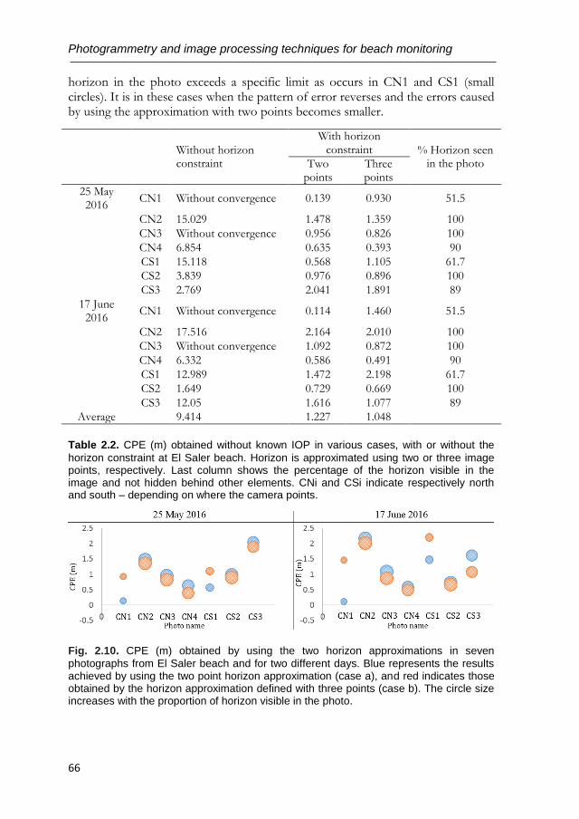
Photogrammetry and image processing techniques for beach monitoring
66
horizon in the photo exceeds a specific limit as occurs in CN1 and CS1 (small circles). It is in these cases when the pattern of error reverses and the errors caused by using the approximation with two points becomes smaller.
Without horizon constraint
With horizon constraint % Horizon seen
in the photo
Two points
Three points
25 May 2016
CN1 Without convergence 0.139 0.930 51.5
CN2 15.029 1.478 1.359 100
CN3 Without convergence 0.956 0.826 100
CN4 6.854 0.635 0.393 90
CS1 15.118 0.568 1.105 61.7
CS2 3.839 0.976 0.896 100
CS3 2.769 2.041 1.891 89
17 June 2016
CN1 Without convergence 0.114 1.460 51.5
CN2 17.516 2.164 2.010 100
CN3 Without convergence 1.092 0.872 100
CN4 6.332 0.586 0.491 90
CS1 12.989 1.472 2.198 61.7
CS2 1.649 0.729 0.669 100
CS3 12.05 1.616 1.077 89
Average 9.414 1.227 1.048
Table 2.2. CPE (m) obtained without known IOP in various cases, with or without the
horizon constraint at El Saler beach. Horizon is approximated using two or three image points, respectively. Last column shows the percentage of the horizon visible in the image and not hidden behind other elements. CNi and CSi indicate respectively north and south – depending on where the camera points.
Fig. 2.10. CPE (m) obtained by using the two horizon approximations in seven
photographs from El Saler beach and for two different days. Blue represents the results achieved by using the two point horizon approximation (case a), and red indicates those obtained by the horizon approximation defined with three points (case b). The circle size increases with the proportion of horizon visible in the photo.
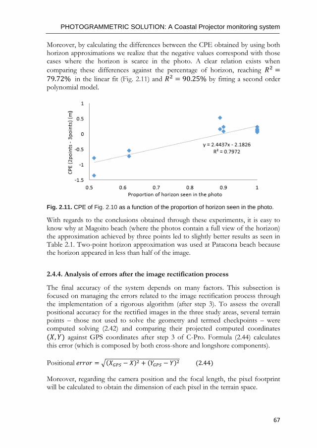
PHOTOGRAMMETRIC SOLUTION: A Coastal Projector monitoring system
67
Moreover, by calculating the differences between the CPE obtained by using both horizon approximations we realize that the negative values correspond with those cases where the horizon is scarce in the photo. A clear relation exists when
comparing these differences against the percentage of horizon, reaching 𝑅2 =79.72% in the linear fit (Fig. 2.11) and 𝑅2 = 90.25% by fitting a second order polynomial model.
Fig. 2.11. CPE of Fig. 2.10 as a function of the proportion of horizon seen in the photo.
With regards to the conclusions obtained through these experiments, it is easy to know why at Magoito beach (where the photos contain a full view of the horizon) the approximation achieved by three points led to slightly better results as seen in Table 2.1. Two-point horizon approximation was used at Patacona beach because the horizon appeared in less than half of the image.
2.4.4. Analysis of errors after the image rectification process
The final accuracy of the system depends on many factors. This subsection is focused on managing the errors related to the image rectification process through the implementation of a rigorous algorithm (after step 3). To assess the overall positional accuracy for the rectified images in the three study areas, several terrain points – those not used to solve the geometry and termed checkpoints – were computed solving (2.42) and comparing their projected computed coordinates
(𝑋, 𝑌) against GPS coordinates after step 3 of C-Pro. Formula (2.44) calculates this error (which is composed by both cross-shore and longshore components).
Positional 𝑒𝑟𝑟𝑜𝑟 = √(𝑋𝐺𝑃𝑆 − 𝑋)2 + (𝑌𝐺𝑃𝑆 − 𝑌)2 (2.44)
Moreover, regarding the camera position and the focal length, the pixel footprint will be calculated to obtain the dimension of each pixel in the terrain space.
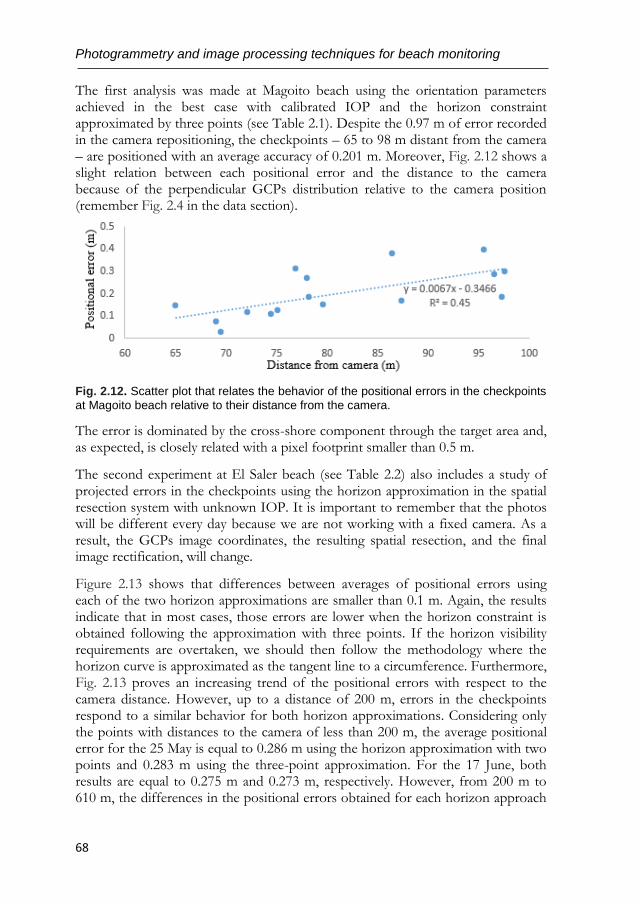
Photogrammetry and image processing techniques for beach monitoring
68
The first analysis was made at Magoito beach using the orientation parameters achieved in the best case with calibrated IOP and the horizon constraint approximated by three points (see Table 2.1). Despite the 0.97 m of error recorded in the camera repositioning, the checkpoints – 65 to 98 m distant from the camera – are positioned with an average accuracy of 0.201 m. Moreover, Fig. 2.12 shows a slight relation between each positional error and the distance to the camera because of the perpendicular GCPs distribution relative to the camera position (remember Fig. 2.4 in the data section).
Fig. 2.12. Scatter plot that relates the behavior of the positional errors in the checkpoints
at Magoito beach relative to their distance from the camera.
The error is dominated by the cross-shore component through the target area and, as expected, is closely related with a pixel footprint smaller than 0.5 m.
The second experiment at El Saler beach (see Table 2.2) also includes a study of projected errors in the checkpoints using the horizon approximation in the spatial resection system with unknown IOP. It is important to remember that the photos will be different every day because we are not working with a fixed camera. As a result, the GCPs image coordinates, the resulting spatial resection, and the final image rectification, will change.
Figure 2.13 shows that differences between averages of positional errors using each of the two horizon approximations are smaller than 0.1 m. Again, the results indicate that in most cases, those errors are lower when the horizon constraint is obtained following the approximation with three points. If the horizon visibility requirements are overtaken, we should then follow the methodology where the horizon curve is approximated as the tangent line to a circumference. Furthermore, Fig. 2.13 proves an increasing trend of the positional errors with respect to the camera distance. However, up to a distance of 200 m, errors in the checkpoints respond to a similar behavior for both horizon approximations. Considering only the points with distances to the camera of less than 200 m, the average positional error for the 25 May is equal to 0.286 m using the horizon approximation with two points and 0.283 m using the three-point approximation. For the 17 June, both results are equal to 0.275 m and 0.273 m, respectively. However, from 200 m to 610 m, the differences in the positional errors obtained for each horizon approach
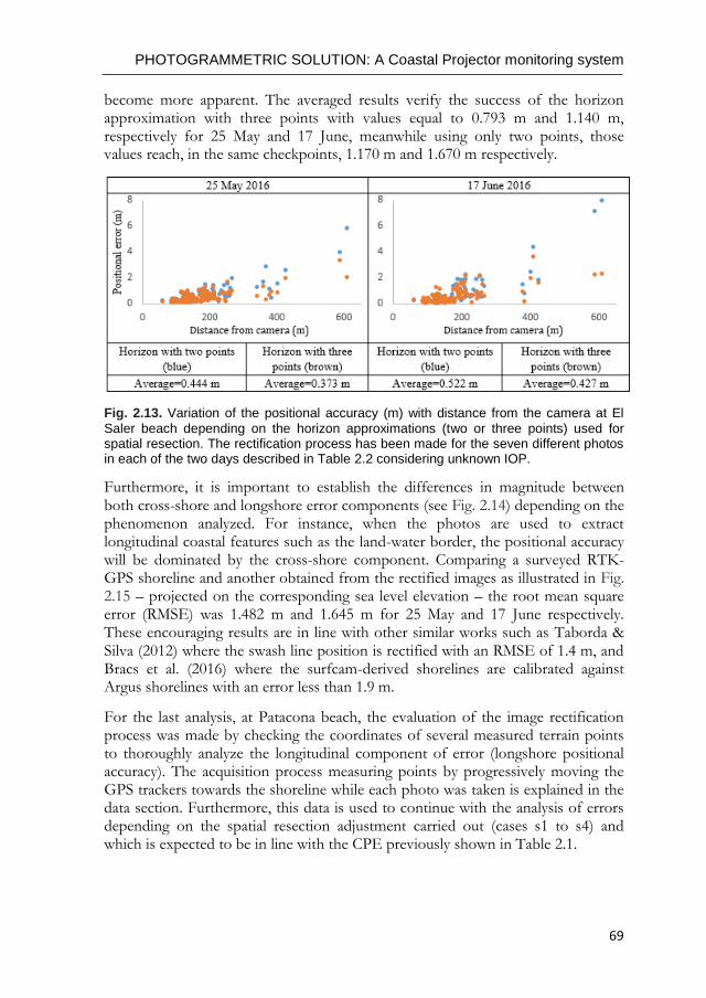
PHOTOGRAMMETRIC SOLUTION: A Coastal Projector monitoring system
69
become more apparent. The averaged results verify the success of the horizon approximation with three points with values equal to 0.793 m and 1.140 m, respectively for 25 May and 17 June, meanwhile using only two points, those values reach, in the same checkpoints, 1.170 m and 1.670 m respectively.
Fig. 2.13. Variation of the positional accuracy (m) with distance from the camera at El
Saler beach depending on the horizon approximations (two or three points) used for spatial resection. The rectification process has been made for the seven different photos in each of the two days described in Table 2.2 considering unknown IOP.
Furthermore, it is important to establish the differences in magnitude between both cross-shore and longshore error components (see Fig. 2.14) depending on the phenomenon analyzed. For instance, when the photos are used to extract longitudinal coastal features such as the land-water border, the positional accuracy will be dominated by the cross-shore component. Comparing a surveyed RTK-GPS shoreline and another obtained from the rectified images as illustrated in Fig. 2.15 – projected on the corresponding sea level elevation – the root mean square error (RMSE) was 1.482 m and 1.645 m for 25 May and 17 June respectively. These encouraging results are in line with other similar works such as Taborda & Silva (2012) where the swash line position is rectified with an RMSE of 1.4 m, and Bracs et al. (2016) where the surfcam-derived shorelines are calibrated against Argus shorelines with an error less than 1.9 m.
For the last analysis, at Patacona beach, the evaluation of the image rectification process was made by checking the coordinates of several measured terrain points to thoroughly analyze the longitudinal component of error (longshore positional accuracy). The acquisition process measuring points by progressively moving the GPS trackers towards the shoreline while each photo was taken is explained in the data section. Furthermore, this data is used to continue with the analysis of errors depending on the spatial resection adjustment carried out (cases s1 to s4) and which is expected to be in line with the CPE previously shown in Table 2.1.
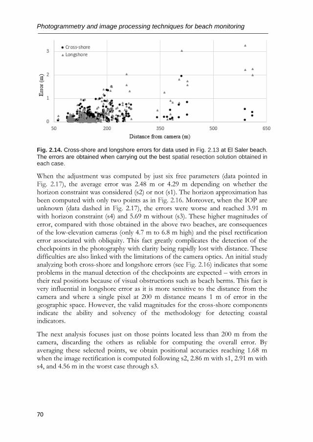
Photogrammetry and image processing techniques for beach monitoring
70
Fig. 2.14. Cross-shore and longshore errors for data used in Fig. 2.13 at El Saler beach.
The errors are obtained when carrying out the best spatial resection solution obtained in each case.
When the adjustment was computed by just six free parameters (data pointed in Fig. 2.17), the average error was 2.48 m or 4.29 m depending on whether the horizon constraint was considered (s2) or not (s1). The horizon approximation has been computed with only two points as in Fig. 2.16. Moreover, when the IOP are unknown (data dashed in Fig. 2.17), the errors were worse and reached 3.91 m with horizon constraint (s4) and 5.69 m without (s3). These higher magnitudes of error, compared with those obtained in the above two beaches, are consequences of the low-elevation cameras (only 4.7 m to 6.8 m high) and the pixel rectification error associated with obliquity. This fact greatly complicates the detection of the checkpoints in the photography with clarity being rapidly lost with distance. These difficulties are also linked with the limitations of the camera optics. An initial study analyzing both cross-shore and longshore errors (see Fig. 2.16) indicates that some problems in the manual detection of the checkpoints are expected – with errors in their real positions because of visual obstructions such as beach berms. This fact is very influential in longshore error as it is more sensitive to the distance from the camera and where a single pixel at 200 m distance means 1 m of error in the geographic space. However, the valid magnitudes for the cross-shore components indicate the ability and solvency of the methodology for detecting coastal indicators.
The next analysis focuses just on those points located less than 200 m from the camera, discarding the others as reliable for computing the overall error. By averaging these selected points, we obtain positional accuracies reaching 1.68 m when the image rectification is computed following s2, 2.86 m with s1, 2.91 m with s4, and 4.56 m in the worst case through s3.
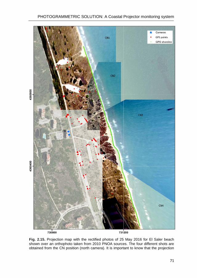
PHOTOGRAMMETRIC SOLUTION: A Coastal Projector monitoring system
71
Fig. 2.15. Projection map with the rectified photos of 25 May 2016 for El Saler beach
shown over an orthophoto taken from 2010 PNOA sources. The four different shots are obtained from the CN position (north camera). It is important to know that the projection
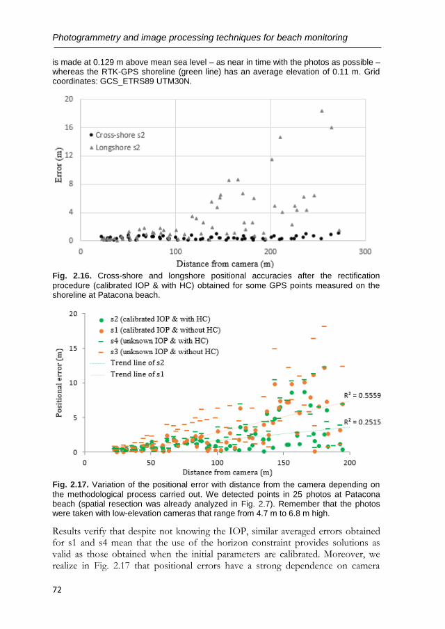
Photogrammetry and image processing techniques for beach monitoring
72
is made at 0.129 m above mean sea level – as near in time with the photos as possible – whereas the RTK-GPS shoreline (green line) has an average elevation of 0.11 m. Grid coordinates: GCS_ETRS89 UTM30N.
Fig. 2.16. Cross-shore and longshore positional accuracies after the rectification
procedure (calibrated IOP & with HC) obtained for some GPS points measured on the shoreline at Patacona beach.
Fig. 2.17. Variation of the positional error with distance from the camera depending on
the methodological process carried out. We detected points in 25 photos at Patacona beach (spatial resection was already analyzed in Fig. 2.7). Remember that the photos were taken with low-elevation cameras that range from 4.7 m to 6.8 m high.
Results verify that despite not knowing the IOP, similar averaged errors obtained for s1 and s4 mean that the use of the horizon constraint provides solutions as valid as those obtained when the initial parameters are calibrated. Moreover, we realize in Fig. 2.17 that positional errors have a strong dependence on camera
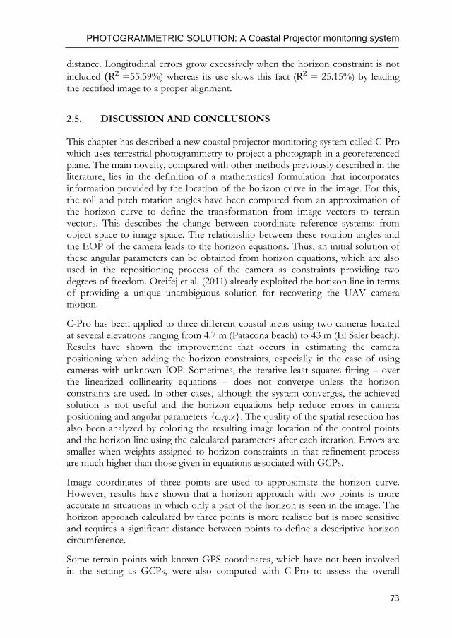
PHOTOGRAMMETRIC SOLUTION: A Coastal Projector monitoring system
73
distance. Longitudinal errors grow excessively when the horizon constraint is not
included (R2 =55.59%) whereas its use slows this fact (R2 = 25.15%) by leading the rectified image to a proper alignment.
2.5. DISCUSSION AND CONCLUSIONS
This chapter has described a new coastal projector monitoring system called C-Pro which uses terrestrial photogrammetry to project a photograph in a georeferenced plane. The main novelty, compared with other methods previously described in the literature, lies in the definition of a mathematical formulation that incorporates information provided by the location of the horizon curve in the image. For this, the roll and pitch rotation angles have been computed from an approximation of the horizon curve to define the transformation from image vectors to terrain vectors. This describes the change between coordinate reference systems: from object space to image space. The relationship between these rotation angles and the EOP of the camera leads to the horizon equations. Thus, an initial solution of these angular parameters can be obtained from horizon equations, which are also used in the repositioning process of the camera as constraints providing two degrees of freedom. Oreifej et al. (2011) already exploited the horizon line in terms of providing a unique unambiguous solution for recovering the UAV camera motion.
C-Pro has been applied to three different coastal areas using two cameras located at several elevations ranging from 4.7 m (Patacona beach) to 43 m (El Saler beach). Results have shown the improvement that occurs in estimating the camera positioning when adding the horizon constraints, especially in the case of using cameras with unknown IOP. Sometimes, the iterative least squares fitting – over the linearized collinearity equations – does not converge unless the horizon constraints are used. In other cases, although the system converges, the achieved solution is not useful and the horizon equations help reduce errors in camera positioning and angular parameters {ω,φ,κ}. The quality of the spatial resection has also been analyzed by coloring the resulting image location of the control points and the horizon line using the calculated parameters after each iteration. Errors are smaller when weights assigned to horizon constraints in that refinement process are much higher than those given in equations associated with GCPs.
Image coordinates of three points are used to approximate the horizon curve. However, results have shown that a horizon approach with two points is more accurate in situations in which only a part of the horizon is seen in the image. The horizon approach calculated by three points is more realistic but is more sensitive and requires a significant distance between points to define a descriptive horizon circumference.
Some terrain points with known GPS coordinates, which have not been involved in the setting as GCPs, were also computed with C-Pro to assess the overall
Photogrammetry and image processing techniques for beach monitoring
74
positional accuracy over the rectified images in the three coastal areas. At Magoito beach, the checkpoints situated less than 65 m from the camera were positioned with an averaged accuracy of 0.2007 m. Moreover, errors were less than 0.5 m for points located within 100 m of the camera. Those errors of projection were obtained after placing the camera with an elevation of 35.6 m, using C-Pro with calibrated IOP, and approximating the horizon constraint with three points.
Errors at checkpoints increase slightly when the IOP are unknown as is assessed in El Saler beach where the camera was located at the top of a building 43 m high. However, acceptable results are obtained by considering the horizon approximation in the spatial resection system, computed following the approximation with three points. Those results have been obtained with a non-fixed camera taking 14 photos in two days. Consequently, as the GCPs image coordinates will change, the resulting spatial resection will also differ for every photo. Considering the checkpoints whose distances to the camera were less than 200 m, the average error was equal to 0.283 m on the first day and 0.273 m on the second day.
At Patacona beach, the camera is located at an elevation ranging between 4.7 and 6.8 m. In this case, we analyze the longshore error through an experiment measuring shoreline points until a distance of less than 200 m from the camera is found that is considered as reliable for computing that error. Positional accuracies reached an average positional error equal to 1.68 m when the image rectification was computed using calibrated IOP and 2.91 m when considering unknown IOP. The horizon approximation with two points was used in these cases because the horizon appeared in less than half of the image. Thus, the use of the horizon constraint has enabled us to obtain valid solutions even in cases when it is not possible to obtain the IOP by camera calibration (or other complicated photogrammetric conditions such as low camera elevations were present).
The methodology developed in this work enables accurately projecting a coastal photograph – or any element detected in it – on a georeferenced plane, even if the photo was taken by a camera with unknown IOP and located at a less than 7 m high. Encouraging results (similar to those obtained by Taborda & Silva, 2012) which are able to define the shoreline with an RMSE of less than 1.5 m. Its implementation in C-Pro, through formulas detailed in this chapter, makes it a robust and low-cost tool that can work with any photograph taken by a conventional camera of a coastal segment with the horizon included. In this chapter, the horizon points have been marked manually but future works applying C-Pro may use techniques that automatically track the horizon (Bracs et al., 2016; Oreifej et al., 2011).
The application of C-Pro will produce valuable scientific information from numerous cameras and video cameras located along coastlines worldwide. Although in principle these recreational cameras were set for other non-metric

PHOTOGRAMMETRIC SOLUTION: A Coastal Projector monitoring system
75
goals (refer to Section 5.1), they can now also be useful for measuring beach indicators for better planning and managing coastal resources.

Cover photo of Chapter 3: Praia da Nazaré, Nazaré, Lisbon (taken Dec. 2015)

NOVEL SUB-PIXEL SHORELINE SOLUTION FROM SATELLITE IMAGES
79
This chapter presents a new methodological process for detecting the instantaneous land-water border at sub-pixel level from mid-resolution satellite images (30 m/pixel) that are freely available worldwide. The new method is based on using an iterative procedure to compute Laplacian roots of a polynomial surface that represents the radiometric response of a set of pixels. The method uses a first approximation of the shoreline at pixel level (initial pixels) and selects a set of neighboring pixels to be part of the analysis window. This adaptive window collects those stencils in which the maximum radiometric variations are found by using the information given by divided differences. Therefore, the land-water surface is computed by a piecewise interpolating polynomial that models the strong radiometric changes between both interfaces. The assessment is tested on two coastal areas to analyze how their inherent differences may affect the method. A total of 17 Landsat 7 and 8 imagery (L7 and L8) were used to extract the shorelines and compare them against other highly accurate lines that act as references. Accurate quantitative coastal data from the satellite images is obtained with a mean horizontal error of 4.38±5.66 m and 1.79±2.78 m respectively for L7 and L8. Prior methodologies to reach the sub-pixel shoreline are analyzed and the results verify the solvency of the one proposed.
3.1. INTRODUCTION
Coastal areas are a point of interest from several perspectives. Environmentally, these are the main spaces in which land, sea, and air interact. Socially, these are places of settlement, leisure, and economic activity. Obviously, the sustainable and safe use of these spaces requires knowledge of their natural functioning. Acquiring this knowledge from biologists, geomorphologists, engineers, and managers involves the acquisition of information that requires coastal mapping techniques (Graham et al., 2003). The type of data and processing reflects the purpose (Szmytkiewicz et al., 2000). In coastal mapping there is a clear distinction between three-dimensional and two-dimensional information. Three-dimensional information is usually obtained via GNSS or LiDAR techniques and enables the analysis of changes in shape and volume on beaches. These techniques offer high precision but are expensive and so they are only used when the need is great. Two-dimensional information is less complete (Moore et al., 2006). However, as the most widespread recent mapping techniques are focused on those that minimize acquisition costs, video monitoring and the use of satellite images remain as useful resources for mapping shorelines in planimetry. Video monitoring cameras offer a high temporal resolution and are widely used for coastal research and video-derived coastal indicators (Davidson et al., 2007; Aarninkhof et al., 2003) in a limited space (Andriolo et al., 2019; Sánchez-García et al., 2017; Holman and Stanley, 2007). Satellite images offer wide geographical coverage with a specific temporal and spatial resolution for each sensor (Sagar et al., 2017; Luijendijk et al., 2018). The turning point came when the
Photogrammetry and image processing techniques for beach monitoring
80
United States Geological Service released its archive of Landsat scenes (USGS, 2008). The European Space Agency (ESA) followed the same policy and offers the Sentinel-2 scenes free of charge. Landsat and Sentinel-2 make up a synergistic system of global monitoring in which every place on the planet is revisited each 2.9 days on average (Li and Roy, 2017). 2D and 3D techniques are not exclusionary and using 2D high-frequency data to decide the most efficient moment to take the 3D data may be a clear case of synergy. Boak and Turner (2005) describe 44 different interpretations of the concept of “shoreline” in relation with different fields of study. In the present chapter, we focus on mapping shorelines from satellite imagery (concretely from Landsat data) so the indicator chosen is the instantaneous water line for each satellite capture moment. In addition, two technical questions may be mentioned: the inherent limitation of Landsat spatial resolution since working at pixel level beach changes can only be detected if they exceed the pixel size (Gens, 2010), and the importance of a clear and efficient workflow to manage a big amount of data. Overcoming the problem of the pixel geometric resolution is the main but not the only technical problem when creating a complete workflow from the image acquisition and the final shoreline. Liu et al. (2011) made a homogenization of the studies by compiling a set of shoreline extraction strategies applied to different resources (LiDAR, radar, aerial and satellite images) and created an adaptable software for deducing the shore position (an extension for ArcGIS named “ShorelineExtractor”). This work created a framework in which, technical researches could be implemented to update different internal processes while the own tool can be applied for any other final-user intention (coastal management, geomorphology, etc.). The present chapter is based on a similar framework and background. Almonacid-Caballer (2014) developed a workflow, initially described in Ruiz et al. (2007) and Pardo-Pascual et al. (2012), to obtain sub-pixel precision shorelines from Landsat images. This last procedure has been used for some applied studies, using two different software implementations. During the first implementation, this was used to map the impact of a storm along 100 km of beaches in the Gulf of Valencia and the subsequent recovery (Pardo-Pascual et al., 2014). Obtaining accurate shorelines is crucial in the use of the Landsat series for mapping the past with a coastal evolution indicator (Almonacid-Caballer et al., 2016; Sánchez-García et al., 2015). While the initial implementation of that methodology (Pardo-Pascual et al., 2012, Almonacid-Caballer, 2014) was evaluated on some rigid seawalls, in Pardo-Pascual et al. (2018) the same methodology was assessed on natural beaches −since the goal is having a tool to obtain satellite-derived shorelines (SDS) for subsequent geomorphological and management works. Along the publications in which this workflow has been used, the implementation of the workflow has changed from Matlab and IDL to Python as presented in Palomar-Vázquez et al. (2018). This last complete shoreline extraction and management tool compiles the improvements
NOVEL SUB-PIXEL SHORELINE SOLUTION FROM SATELLITE IMAGES
81
required along the mentioned studies and includes: (1) management processes such as downloading the images, project structure and data storage; (2) the intrinsic technical core (discussed in Almonacid-Caballer, 2014) which includes (a) obtaining the initial shoreline (through threshold or external shoreline), (b) the sub-pixel geo-registration that ensures no more than 3 meters of misalignment between images (Almonacid-Caballer et al, 2017), and (c) the sub-pixel shoreline definition itself; finally (3) different filtering techniques to obtain a neat final shoreline. All these modifications have sought to improve efficiency but have not focused on solving some of the limitations that the basis of the shoreline extraction algorithm presents. In this regard, the current work focus on (2)(c), defining a new methodological improvement in the sub-pixel refinement (within the mentioned intrinsic technical core) carried out around an initial pixel-level shoreline. To overcome the restriction of coarse spatial resolution, different procedures have sought to increase accuracy at sub-pixel level (Liu et al., 2016). Liu et al. (2017a) compared three main processing options in which an original Landsat 8 (L8) was processed (30 m/pixel) by being pansharpened with its panchromatic band (15 m/pixel) and then with the same band upsampled to 7.5 m/pixel. Liu et al. (2017b) pansharpened Landsat 7 (L7) and L8 multispectral bands and, after several segmentation steps, looked for the sub-pixel shoreline using a variation of marching squares with a linear interpolation (MSI) approach as proposed by Cipolletti et al. (2012). In Pardo-Pascual et al. (2012) an infra-red Landsat band was binarized for land-water surfaces by analyzing the histogram of each scene. The edge-pixels between both areas were considered for the pixel-level shoreline and, around each of these pixels, a kernel of 7x7 pixels was used to reach the sub-pixel. The shoreline was then obtained as the Laplacian roots of an interpolation surface defined over such kernel. The justification for the kernel size is found in Almonacid-Caballer (2014) where it is shown that large kernels are necessary to ensure that the real shoreline position is inside. To start the process, obtaining the initial pixel-level shoreline using a single threshold for a complete scene may be a weakness. Liu and Jezek (2004) discuss that the gradient between land and water can substantially affect edge detection when thresholding detection is used. A single threshold for the whole image is a problem and they propose an adaptive thresholding technique. Moreover, Almonacid-Caballer (2014) proved that an automatic threshold obtained by intersection of Gaussian curves in bimodal histograms does not match with those photo-interpreted manually. Of course, if the study area is small and homogenous, this is not significant –as is remarked in Liu et al. (2017b). Following the analyzed sub-pixel methodology in Almonacid-Caballer (2014), the digital numbers (DN) of the 7x7 kernel around each pixel of the pixel-level shoreline were fitted with a 2D polynomial expression. The polynomial expression was introduced as a complete fifth-degree polynomial whose terms reach all the combinations of x5 and y5 and imply fitting 36 polynomial parameters. Although 49
Photogrammetry and image processing techniques for beach monitoring
82
equations could be enough, the polynomial was sometimes unstable and produced shapes that were too irregular. Fewer degrees may have been more robust –but a third-degree for the 7x7 kernel produced a surface that was too smooth and inaccurate for drawing the land-water inflection. To add robustness, the kernel was upsampled x4 to 28x28 pixels and each was given an equation for the least squares adjustment. In subsequent applications of this methodology, some shoreline points had to be filtered because the size of the kernel caused some inflections far from the reference shoreline (Pardo-Pascual et al., 2014). At the same time, given the size of the kernel, long beaches with a small curvature were necessary to achieve good results. This may be a limiting factor when working near the gaps in L7 images (Almonacid-Caballer et al., 2013). Moreover, changes in the DN on the land zone produced small displacements in the resultant shorelines –as was analyzed in Pardo-Pascual et al. (2012). Particularly, this limited when the algorithm applied to beaches embedded between natural or artificial structures as groins. Hermosilla et al. (2008) described a super-resolution/hyper-resolution process or sub-pixel edge detection through an image interpolation operator to obtain a finer grid of pixels. While Almonacid-Caballer (2014) worked with a 7x7 kernel upsampled by cubic convolution, Hermosilla et al. (2008) showed that the centered cubic interpolation method produced well defined edges but geometrically displaced with respect to their position in the reference image. To solve this problem a fourth-order non-linear interpolation procedure based on an essentially non-oscillatory (ENO) methodology was discussed. Harten et al. (1987) had already introduced this in fluid dynamic applications to avoid non-physical oscillations in the simulation of convection-dominated flows. Shu and Osher (1988) made it more efficient and used it for sub-pixel interpolation in curve evolution problems. The ENO interpolation method selects the polynomial stencils according to the DN variation around each pixel by using the divided differences of the data as a measure of smoothness. An adaptive window around each pixel is used to define a support window for the 2D piecewise reconstruction of point values that avoids high gradient regions whenever possible (Capilla and Balaguer, 2013; Balaguer and Conde, 2005). The reconstruction scheme selects an interpolating support window whose solution is the smoothest in the sense of divided differences. After an image interpolation to obtain a finer grid of pixels, the Canny edge detection algorithm is applied to obtain edges at a sub-pixel level. The current chapter looks for the opposite of the ENO method to detect the shoreline because edges are calculated using the Laplacian of the interpolation surface. Thus, the support window of that polynomial must contain the zone with the maximum gradient of the solution and this is chosen by an automatic process. The first novelty of the proposed method with respect to Pardo-Pascual et al. (2012) and Almonacid-Caballer (2014) focuses on the procedure for exploring the initial pixels and finding the optimal pixel neighbors for the 2D surface adjustment.
NOVEL SUB-PIXEL SHORELINE SOLUTION FROM SATELLITE IMAGES
83
This sweep enables the algorithm to fix a lack of precision on the initial pixel-level shoreline. In addition, it expects to solve part of the limitations described by Pardo-Pascual et al. (2012) on beaches segmented by groins. Secondly, Lagrange interpolation is used to recreate the land-water surface instead of the known least squares method (LSM). However, both polynomial functions are compared by using different degree and support windows (the selection of pixels to be used in the adjustment). Finally, no upsampling technique is applied on the initial image. Using the Lagrange solution, it is not necessary to increase the number of equations and the surface is formed with the raw DN. Therefore, the objective of this chapter is to propose a new image interpolation method to define the shoreline at sub-pixel level –an issue of great value for coastal management. Adding this to the refinement step inside the whole shoreline extraction workflow implemented by Palomar-Vázquez et al. (2018), will lead to a more robust solution in the definition of the sub-pixel shoreline. Unlike the original solution, the concept of kernel is changed now to an adaptive window that locally finds the position of the maximum land-water change. From that position, smaller windows are used and evaluated. While upsampling is avoided, the Lagrange polynomial (Lgr) is used to gain robustness using a non-homogeneous system with a single solution and raw pixel data. In this chapter, Section 3.2 presents the data of the study areas used to carry out the assessments and comparisons of the shoreline sub-pixel methodologies. Section 3.3 explains in detail the methodological steps of the new proposed sub-pixel shoreline solution. Section 3.4 describes the fundamentals of other methodologies used in the chapter to compare. Section 3.5 shows the results obtained by the various methodologies and the advantages achieved in the accurate detection of the shoreline with the proposed solution. Finally, discussion and conclusions are presented respectively in Sections 3.6 and 3.7.
3.2. DATA OF THE STUDY AREAS A set of 17 sub-pixel shorelines and their respective highly accurate reference lines (measured –depending on the study site– by GPS techniques or digitalizing) has served to evaluate the different sub-pixel techniques from Landsat images. Both types of data represent the instantaneous water line in the same space-time. The procedure to assess our final sub-pixel shorelines consists in calculating the minimum distance between the solution of each shoreline point and the closest respective point of the reference shoreline for each date. The computed distances are a measure of the error committed in each extracted shoreline given that the reference lines accurately describe the ground truth at the study sites. Positive and negative distances indicate that the resulting sub-pixel shoreline is biased seaward or landward respectively.
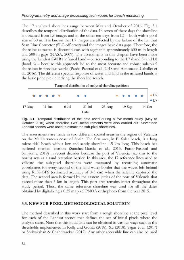
Photogrammetry and image processing techniques for beach monitoring
84
The 17 analyzed shorelines range between May and October of 2016. Fig. 3.1 describes the temporal distribution of the data. In seven of these days the shoreline is obtained from L8 images and in the other ten days from L7 – both with a pixel size of 30 m. It is known that L7 images are affected by the failure of the Landsat Scan Line Corrector (SLC-off error) and the images have data gaps. Therefore, the shoreline extracted is discontinuous with segments approximately 600 m in length and 500 m gaps (NASA, 2009). The assessments in this chapter have been made using the Landsat SWIR1 infrared band – corresponding to the L7 (band 5) and L8 (band 6) – because this approach led to the most accurate and robust sub-pixel shorelines in previous works (Pardo-Pascual et al., 2018 and Almonacid-Caballer et al., 2016). The different spectral response of water and land in the infrared bands is the basic principle underlying the shoreline search.
Fig. 3.1. Temporal distribution of the data used during a five-month study (May to
October 2016) when shoreline GPS measurements were also carried out. Seventeen Landsat scenes were used to extract the sub-pixel shorelines.
The assessments are made in two different coastal areas in the region of Valencia on the Mediterranean coast of Spain. The first area, in El Saler beach, is a long micro-tidal beach with a low and sandy shoreline 1.5 km long. This beach has suffered marked erosion (Sánchez-García et al., 2015; Pardo-Pascual and Sanjaume, 2019) in recent decades because the port of Valencia (six kms to the north) acts as a sand retention barrier. In this area, the 17 reference lines used to validate the sub-pixel shorelines were measured by recording automatic coordinates for every second of the land-water border that the waves left behind using RTK-GPS (estimated accuracy of 3-5 cm) when the satellite captured the data. The second area is formed by the eastern jetties of the port of Valencia that exceed more than 3 km in length. This port area remains intact throughout the study period. Thus, the same reference shoreline was used for all the dates obtained by digitalizing a 0.25 m/pixel PNOA orthophoto from the year 2015.
3.3. NEW SUB-PIXEL METHODOLOGICAL SOLUTION The method described in this work start from a rough shoreline at the pixel level for each of the Landsat scenes that defines the set of initial pixels where the analysis starts. Note that this initial line can be obtained in various ways such as the thresholds implemented in Kelly and Gontz (2018), Xu (2018), Sagar et al. (2017) or Shrivakshan & Chandrasekar (2012). Any other accessible line can also be used
NOVEL SUB-PIXEL SHORELINE SOLUTION FROM SATELLITE IMAGES
85
(such as the shoreline provided by the Instituto Hidrográfico de la Marina for the Spanish territory) but usually these are biased in a magnitude about one Landsat pixel (25 - 35 m). Hence working with adaptable neighborhoods may be very useful.
In this chapter, a thresholding initial shoreline is used following the bimodal nature of the histogram of an infrared band when water and land are both present (Almonacid-Caballer, 2014). The chosen threshold is unique for the whole scene and the line may displace seaward or landward depending on the selection process. This vagueness is irrelevant because the proposed sub-pixel method is intended to manage this effect. In fact, to enhance this, an experiment deliberately biases the initial line by using a wrong initial shore to show the robustness of the methodology.
Moreover, it is important to note that the satellite imagery has a potential error in its georeferencing that will directly affect the positioning of the shoreline when comparing these against the GPS lines (as shown in Almonacid-Caballer et al., 2017). Thus, a preliminary process has been implemented to georeference the Landsat images by computing the Fourier cross-correlation through a PNOA orthophoto of the study site. Once this error has been minimized to less than 0.1 pixels, we consider it as negligible.
3.3.1. A new method to define an adaptive window for shoreline location using divided differences
Given a pixel that contains a part of the initial shoreline and whose center has the
coordinates (𝑥𝑖, 𝑦𝑗), the sub-pixel shoreline is calculated through a curve that
approaches around that pixel. Moreover, the method has to be sufficiently robust that if the true shoreline does not pass within that pixel and it passes through neighboring pixels then it will be able to calculate the sub-pixel shoreline where appropriate. Therefore, the potential shoreline solution can be found in the pixel
(𝑥𝑖, 𝑦𝑗) and the analysis window around that pixel. The method described
hereafter computes a two-dimensional polynomial expression around each pixel-level shoreline. From this expression, the shoreline is assumed to be on the inflexion line with the largest gradient. As it is obtained mathematically, so a sub-pixel precision is reached. This involves creating a window around each pixel that contains the shoreline and, the divided differences are used for that purpose.
Divided differences are normally linked to the Newton interpolation method. Given a set of “d+1” points (xi, gi) from i=0 to i=d, it is known that there is only one polynomial of degree less than or equal to “d” that passes through those points. Newton proposed a method in which the polynomial had the following form:
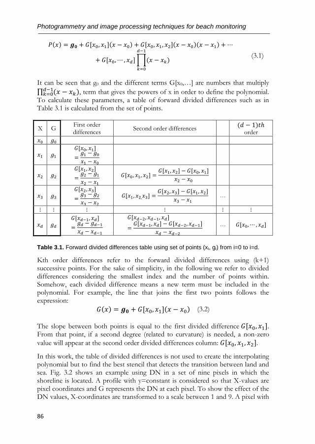
Photogrammetry and image processing techniques for beach monitoring
86
𝑃(𝑥) = 𝒈𝟎 + 𝐺[𝑥0, 𝑥1](𝑥 − 𝑥0) + 𝐺[𝑥0, 𝑥1, 𝑥2](𝑥 − 𝑥0)(𝑥 − 𝑥1) + ⋯
+ 𝐺[𝑥0, ⋯ , 𝑥𝑑]∏(𝑥 − 𝑥𝑘)
𝑑−1
𝑘=0
(3.1)
It can be seen that g0 and the different terms G[x0,…] are numbers that multiply
∏ (𝑥 − 𝑥𝑘)𝑑−1𝑘=0 , term that gives the powers of x in order to define the polynomial.
To calculate these parameters, a table of forward divided differences such as in Table 3.1 is calculated from the set of points.
X G First order differences
Second order differences (𝑑 − 1)𝑡ℎ
order
𝑥0 𝑔0
𝑥1 𝑔1 𝐺[𝑥0, 𝑥1]
=𝑔1 − 𝑔0𝑥1 − 𝑥0
𝑥2 𝑔2 𝐺[𝑥1, 𝑥2]
=𝑔2 − 𝑔1𝑥2 − 𝑥1
𝐺[𝑥0, 𝑥1, 𝑥2] =
𝐺[𝑥1, 𝑥2] − 𝐺[𝑥0, 𝑥1]
𝑥2 − 𝑥0
𝑥3 𝑔3 𝐺[𝑥2, 𝑥3]
=𝑔3 − 𝑔2𝑥3 − 𝑥2
𝐺[𝑥1, 𝑥2,𝑥3] =
𝐺[𝑥2, 𝑥3] − 𝐺[𝑥1, 𝑥2]
𝑥3 − 𝑥1 …
⋮ ⋮ ⋮ ⋮ ⋮ ⋮
𝑥𝑑 𝑔𝑑 𝐺[𝑥𝑑−1, 𝑥𝑑]
=𝑔𝑑 − 𝑔𝑑−1𝑥𝑑 − 𝑥𝑑−1
𝐺[𝑥𝑑−2, 𝑥𝑑−1, 𝑥𝑑]
=𝐺[𝑥𝑑−1, 𝑥𝑑] − 𝐺[𝑥𝑑−2, 𝑥𝑑−1]
𝑥𝑑 − 𝑥𝑑−2
… 𝐺[𝑥0, ⋯ , 𝑥𝑑]
Table 3.1. Forward divided differences table using set of points (xi, gi) from i=0 to i=d.
Kth order differences refer to the forward divided differences using (k+1) successive points. For the sake of simplicity, in the following we refer to divided differences considering the smallest index and the number of points within. Somehow, each divided difference means a new term must be included in the polynomial. For example, the line that joins the first two points follows the expression:
𝐺(𝑥) = 𝒈𝟎 + 𝐺[𝑥0, 𝑥1](𝑥 − 𝑥0) (3.2)
The slope between both points is equal to the first divided difference 𝐺[𝑥0, 𝑥1]. From that point, if a second degree (related to curvature) is needed, a non-zero
value will appear at the second order divided differences column: 𝐺[𝑥0, 𝑥1, 𝑥2].
In this work, the table of divided differences is not used to create the interpolating polynomial but to find the best stencil that detects the transition between land and sea. Fig. 3.2 shows an example using DN in a set of nine pixels in which the shoreline is located. A profile with y=constant is considered so that X-values are pixel coordinates and G represents the DN at each pixel. To show the effect of the DN values, X-coordinates are transformed to a scale between 1 and 9. A pixel with
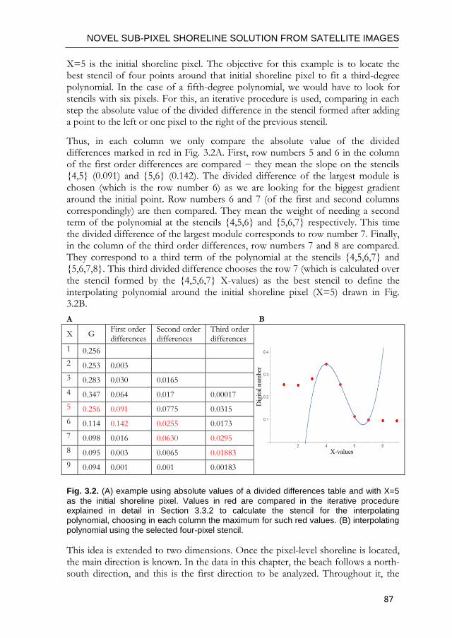
NOVEL SUB-PIXEL SHORELINE SOLUTION FROM SATELLITE IMAGES
87
X=5 is the initial shoreline pixel. The objective for this example is to locate the best stencil of four points around that initial shoreline pixel to fit a third-degree polynomial. In the case of a fifth-degree polynomial, we would have to look for stencils with six pixels. For this, an iterative procedure is used, comparing in each step the absolute value of the divided difference in the stencil formed after adding a point to the left or one pixel to the right of the previous stencil.
Thus, in each column we only compare the absolute value of the divided differences marked in red in Fig. 3.2A. First, row numbers 5 and 6 in the column of the first order differences are compared − they mean the slope on the stencils {4,5} (0.091) and {5,6} (0.142). The divided difference of the largest module is chosen (which is the row number 6) as we are looking for the biggest gradient around the initial point. Row numbers 6 and 7 (of the first and second columns correspondingly) are then compared. They mean the weight of needing a second term of the polynomial at the stencils {4,5,6} and {5,6,7} respectively. This time the divided difference of the largest module corresponds to row number 7. Finally, in the column of the third order differences, row numbers 7 and 8 are compared. They correspond to a third term of the polynomial at the stencils {4,5,6,7} and {5,6,7,8}. This third divided difference chooses the row 7 (which is calculated over the stencil formed by the {4,5,6,7} X-values) as the best stencil to define the interpolating polynomial around the initial shoreline pixel (X=5) drawn in Fig. 3.2B.
A B
X G First order differences
Second order differences
Third order differences
1 0.256
2 0.253 0.003
3 0.283 0.030 0.0165
4 0.347 0.064 0.017 0.00017
5 0.256 0.091 0.0775 0.0315
6 0.114 0.142 0.0255 0.0173
7 0.098 0.016 0.0630 0.0295
8 0.095 0.003 0.0065 0.01883
9 0.094 0.001 0.001 0.00183
Fig. 3.2. (A) example using absolute values of a divided differences table and with X=5
as the initial shoreline pixel. Values in red are compared in the iterative procedure explained in detail in Section 3.3.2 to calculate the stencil for the interpolating polynomial, choosing in each column the maximum for such red values. (B) interpolating polynomial using the selected four-pixel stencil.
This idea is extended to two dimensions. Once the pixel-level shoreline is located, the main direction is known. In the data in this chapter, the beach follows a north-south direction, and this is the first direction to be analyzed. Throughout it, the
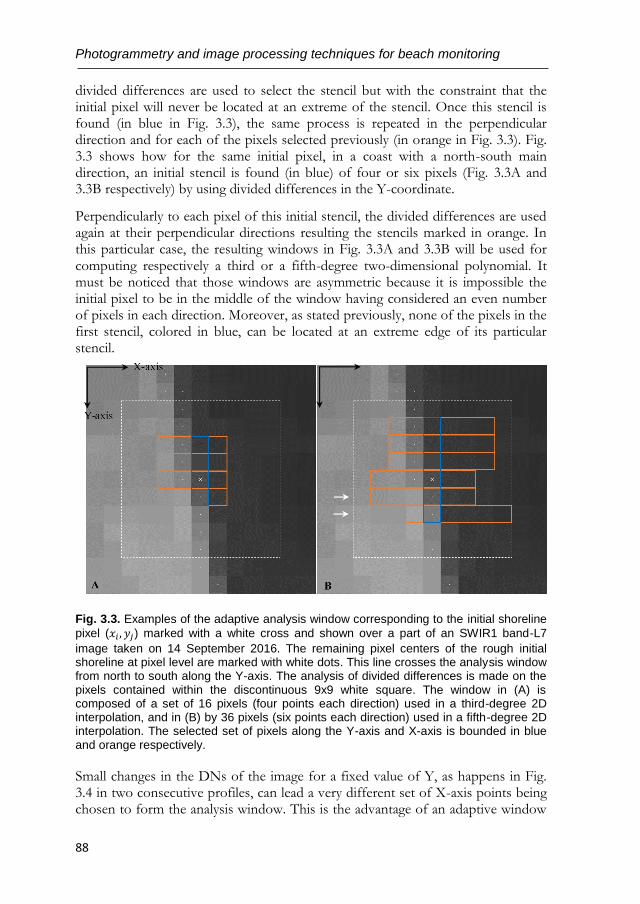
Photogrammetry and image processing techniques for beach monitoring
88
divided differences are used to select the stencil but with the constraint that the initial pixel will never be located at an extreme of the stencil. Once this stencil is found (in blue in Fig. 3.3), the same process is repeated in the perpendicular direction and for each of the pixels selected previously (in orange in Fig. 3.3). Fig. 3.3 shows how for the same initial pixel, in a coast with a north-south main direction, an initial stencil is found (in blue) of four or six pixels (Fig. 3.3A and 3.3B respectively) by using divided differences in the Y-coordinate.
Perpendicularly to each pixel of this initial stencil, the divided differences are used again at their perpendicular directions resulting the stencils marked in orange. In this particular case, the resulting windows in Fig. 3.3A and 3.3B will be used for computing respectively a third or a fifth-degree two-dimensional polynomial. It must be noticed that those windows are asymmetric because it is impossible the initial pixel to be in the middle of the window having considered an even number of pixels in each direction. Moreover, as stated previously, none of the pixels in the first stencil, colored in blue, can be located at an extreme edge of its particular stencil.
Fig. 3.3. Examples of the adaptive analysis window corresponding to the initial shoreline
pixel (𝑥𝑖 , 𝑦𝑗) marked with a white cross and shown over a part of an SWIR1 band-L7
image taken on 14 September 2016. The remaining pixel centers of the rough initial shoreline at pixel level are marked with white dots. This line crosses the analysis window from north to south along the Y-axis. The analysis of divided differences is made on the pixels contained within the discontinuous 9x9 white square. The window in (A) is composed of a set of 16 pixels (four points each direction) used in a third-degree 2D interpolation, and in (B) by 36 pixels (six points each direction) used in a fifth-degree 2D interpolation. The selected set of pixels along the Y-axis and X-axis is bounded in blue and orange respectively.
Small changes in the DNs of the image for a fixed value of Y, as happens in Fig. 3.4 in two consecutive profiles, can lead a very different set of X-axis points being chosen to form the analysis window. This is the advantage of an adaptive window
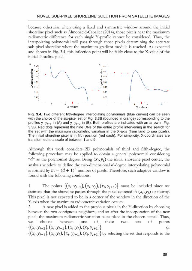
NOVEL SUB-PIXEL SHORELINE SOLUTION FROM SATELLITE IMAGES
89
because otherwise when using a fixed and symmetric window around the initial shoreline pixel such as Almonacid-Caballer (2014), those pixels near the maximum radiometric difference for each single Y-profile cannot be considered. Thus, the interpolating polynomial will pass through those pixels determining the accurate sub-pixel shoreline where the maximum gradient module is reached. As expected and shown in Fig. 3.4, this inflection point will be fairly close to the X-value of the initial shoreline pixel.
Fig. 3.4. Two different fifth-degree interpolating polynomials (blue curves) can be seen
with the choice of the six-pixel set of Fig. 3.3B (bounded in orange) corresponding to the profiles y=𝑦𝑗+1 in (A) and y=𝑦𝑗+2 in (B). Both profiles are indicated with an arrow in Fig.
3.3B. Red dots represent the nine DNs of the entire profile intervening in the search for the set with the maximum radiometric variation in the X-axis (from land to sea pixels). The initial shoreline pixel is in fifth position (red dash). For simplicity, X-coordinates are transformed to a scale of between 1 and 9.
Although this work considers 2D polynomials of third and fifth-degree, the following procedure may be applied to obtain a general polynomial considering
“𝑑” as the polynomial degree. Being (𝑥𝑖, 𝑦𝑗) the initial shoreline pixel center, the
analysis window to define the two-dimensional 𝑑-degree interpolating polynomial
is formed by 𝑚 = (𝑑 + 1)2 number of pixels. Therefore, such adaptive window is found with the following conditions:
1. The points {(𝑥𝑖, 𝑦𝑗−1), (𝑥𝑖, 𝑦𝑗), (𝑥𝑖, 𝑦𝑗+1)} must be included since we
estimate that the shoreline passes through the pixel centered in (𝑥𝑖 , 𝑦𝑗) or nearby.
This pixel is not expected to be in a corner of the window in the direction of the Y-axis when the maximum radiometric variation occurs. 2. A new pixel is added to the previous pixels in the Y-direction by choosing between the two contiguous neighbors, and so after the incorporation of the new pixel, the maximum radiometric variation takes place in the chosen stencil. Thus, we choose between one of these two sets of points
{(𝑥𝑖, 𝑦𝑗−2), (𝑥𝑖 , 𝑦𝑗−1), (𝑥𝑖, 𝑦𝑗), (𝑥𝑖, 𝑦𝑗+1)} or
{(𝑥𝑖, 𝑦𝑗−1), (𝑥𝑖 , 𝑦𝑗), (𝑥𝑖, 𝑦𝑗+1), (𝑥𝑖, 𝑦𝑗+2)} by selecting the set that responds to the

Photogrammetry and image processing techniques for beach monitoring
90
maximum fourth-order divided difference in absolute values. We then denote by
𝑗𝑚𝑖𝑛 ∈ {𝑗 − 2, 𝑗 − 1} the smallest index of the Y-coordinate.
3. A similar procedure is applied with higher interpolation orders. If 𝑑 > 3 then the stencil is formed by an iterative process that begins with these points
{(𝑥𝑖, 𝑦𝑗𝑚𝑖𝑛), (𝑥𝑖, 𝑦𝑗𝑚𝑖𝑛+1), (𝑥𝑖, 𝑦𝑗𝑚𝑖𝑛+2), (𝑥𝑖, 𝑦𝑗𝑚𝑖𝑛+3)}. A new one is then added
to the stencil (until reaching the 𝑑 + 1 set of points) by choosing between the two contiguous neighbors, so that the new stencil leads to the maximum variation linked to the maximum divided difference absolute value.
4. For each fixed value of 𝑦 = 𝑦𝑚 ∈ {𝑦𝑗𝑚𝑖𝑛 , 𝑦𝑗𝑚𝑖𝑛+1, 𝑦𝑗𝑚𝑖𝑛+2, ⋯ , 𝑦𝑗𝑚𝑖𝑛+𝑑}, the stencil now has to be constructed in the X-direction through an iterative
process starting with the point (𝑥𝑖, 𝑦𝑚) and until reaching the 𝑑 + 1 set of points. The choice is made again between the two contiguous neighbors when looking for the maximum divided difference absolute value.
3.3.2. Definition of the polynomial surface in Lagrange form
Considering “𝑑” as the polynomial degree, once each adaptive window is found around each initial pixel, the two-dimensional polynomial that fits the DN values must be found – being the polynomial degree greater than two (d>2). This polynomial, with (d+1)2 number of terms, will follow the next form:
𝑅𝑑,𝑖,𝑗(𝑥, 𝑦; 𝐺) = 𝒄𝟎,𝟎 + 𝒄𝟏,𝟎𝑥 + 𝒄𝟎,𝟏𝑦 + 𝒄𝟐,𝟎𝑥2 + 𝒄𝟎,𝟐𝑦
2 + 𝒄𝟏,𝟏𝑥𝑦 + ⋯+ 𝒄𝒅,𝒅𝑥𝑑𝑦𝑑 (3.3)
where the DN of each pixel (G) is function of the pixel coordinates (x,y). The Lagrange solution follows a similar approach as when obtaining the window in Section 3.3.1 because it is close to its definition. It is made in two steps that give two parts of the polynomial. When looking for the window, the process began by obtaining the initial stencil at the main direction of the initial shoreline (blue stencil in Fig. 3.3). In the given examples it was along Y-axis – assuming that the beach follows a north-south direction. That stencil is used to create the first part of the Lagrange polynomial as follows: (A) Interpolation in the Y-coordinate (A1) Initially, given the set of discrete values {𝐺(𝑥𝑖 , 𝑦𝑚): 𝑗 − 1 ≤ 𝑚 ≤ 𝑗 + 1} that
represent the DN values in the set of three pixels{(𝑥𝑖 , 𝑦𝑗−1), (𝑥𝑖 , 𝑦𝑗), (𝑥𝑖 , 𝑦𝑗+1)}, we define
𝑗𝑚𝑖𝑛(2)
= 𝑗 − 1.
(A2) The two following third-order divided differences of the function 𝐺(𝑥𝑖 , 𝑦𝑚) are
computed considering that 𝑥 = 𝑥𝑖 :
𝑎𝑖,𝑗(3)= 𝐺 [𝑦
𝑗𝑚𝑖𝑛(2) , ⋯ , 𝑦
𝑗𝑚𝑖𝑛(2)
+3]|𝑥=𝑥𝑖
, 𝑏𝑖,𝑗(3)= 𝐺 [𝑦
𝑗𝑚𝑖𝑛(2)
−1, ⋯ , 𝑦
𝑗𝑚𝑖𝑛(2)
+2]|𝑥=𝑥𝑖
NOVEL SUB-PIXEL SHORELINE SOLUTION FROM SATELLITE IMAGES
91
From the two possible candidate points, the point with the highest divided difference value
will be added to the stencil and used to create the interpolating polynomial of degree 𝑑 =3. In this way:
(a) If |𝑎𝑖,𝑗(3)| ≤ |𝑏𝑖,𝑗
(3)|, then: 𝑗𝑚𝑖𝑛
(3)= 𝑗𝑚𝑖𝑛
(2)− 1 = 𝑗 − 2
(b) If |𝑎𝑖,𝑗(3)| > |𝑏𝑖,𝑗
(3)|, then: 𝑗𝑚𝑖𝑛
(3)= 𝑗𝑚𝑖𝑛
(2)= 𝑗 − 1
The choice will then be made between the following two sets of values from the Landsat
image: {{𝑔𝑖,𝑗−2, 𝑔𝑖,𝑗−1, 𝑔𝑖,𝑗, 𝑔𝑖,𝑗+1}, {𝑔𝑖,𝑗−1, 𝑔𝑖,𝑗 , 𝑔𝑖,𝑗+1, 𝑔𝑖,𝑗+2}}
(A3) If 𝑑 > 3 or each 𝑛 ∈ {4,⋯ , 𝑑}, the following two nth-order divided differences of
the function 𝐺(𝑥𝑖 , 𝑦𝑚) are computed:
𝑎𝑖,𝑗(𝑛)
= 𝐺 [𝑦𝑗𝑚𝑖𝑛(𝑛−1) , ⋯ , 𝑦
𝑗𝑚𝑖𝑛(𝑛−1)
+𝑛]|𝑥=𝑥𝑖
, 𝑏𝑖,𝑗(𝑛)= 𝐺 [𝑦
𝑗𝑚𝑖𝑛(𝑛−1)
−1, ⋯ , 𝑦
𝑗𝑚𝑖𝑛(𝑛−1)
+𝑛−1]|𝑥=𝑥𝑖
In this way:
(a) If |𝑎𝑖,𝑗(𝑛)| ≤ |𝑏𝑖,𝑗
(𝑛)|, then 𝑗𝑚𝑖𝑛
(𝑛)= 𝑗𝑚𝑖𝑛
(𝑛−1)− 1
(b) If |𝑎𝑖,𝑗(𝑛)| > |𝑏𝑖,𝑗
(𝑛)|, then 𝑗𝑚𝑖𝑛
(𝑛)= 𝑗𝑚𝑖𝑛
(𝑛−1)
In the end: 𝑗𝑚𝑖𝑛 = 𝑗𝑚𝑖𝑛(𝑑) 𝑎𝑛𝑑 polynomial 𝑃𝑖,𝑗(𝑦; 𝐺) may be expressed in a Lagrange form
as:
𝑃𝑖,𝑗(𝑦; 𝐺) = ∑ 𝑔𝑖,𝑚 ( ∏(𝑦 − 𝑦𝑙)
(𝑦𝑚 − 𝑦𝑙)
𝑗𝑚𝑖𝑛+𝑑
𝑙=𝑗𝑚𝑖𝑛 ,𝑙≠𝑚
)
𝑗𝑚𝑖𝑛+𝑑
𝑚=𝑗𝑚𝑖𝑛
(3.4)
For example if 𝑑 = 5 then 𝑗𝑚𝑖𝑛 ∈ {𝑗 − 4, 𝑗 − 3, 𝑗 − 2, 𝑗 − 1} and in the Y-direction we choose one set of DNs between the following:
{
{𝑔𝑖,𝑗−4, 𝑔𝑖,𝑗−3, 𝑔𝑖,𝑗−2, 𝑔𝑖,𝑗−1, 𝑔𝑖,𝑗 , 𝑔𝑖,𝑗+1}, {𝑔𝑖,𝑗−3, 𝑔𝑖,𝑗−2, 𝑔𝑖,𝑗−1, 𝑔𝑖,𝑗 , 𝑔𝑖,𝑗+1, 𝑔𝑖,𝑗+2},
{𝑔𝑖,𝑗−2, 𝑔𝑖,𝑗−1, 𝑔𝑖,𝑗, 𝑔𝑖,𝑗+1, 𝑔𝑖,𝑗+2, 𝑔𝑖,𝑗+3},
{𝑔𝑖,𝑗−1, 𝑔𝑖,𝑗, 𝑔𝑖,𝑗+1, 𝑔𝑖,𝑗+2, 𝑔𝑖,𝑗+3, 𝑔𝑖,𝑗+4}
}
The value of each DN is given by means of 𝑔𝑖,𝑚 in (3.4). In this case, as the initial
stencil takes only values of an specified column i, it remains constant and m moves
along the column coordinates from the minimum row 𝑗𝑚𝑖𝑛 near to j (the initial
row of the stencil) to 𝑗𝑚𝑖𝑛 + 𝑑, in order to get the degree of the wanted
polynomial that decides the size of the window. It means l from 𝑗𝑚𝑖𝑛 to 𝑗𝑚𝑖𝑛 + 𝑑
are the rows values of the stencil and 𝑦𝑙 are their coordinates. Then, 𝑃𝑖,𝑗(𝑦; 𝐺) defined in (3.4) gives a polynomial only dependent on y.
Photogrammetry and image processing techniques for beach monitoring
92
The same way as each horizontal stencil was obtained around the initial vertical stencil (Fig. 3.3). Each one of those stencils (reliant on the y=ym profile considered) can give a new Lagrange polynomial only dependent on x as follows: (B) Interpolation in the X-coordinate
Considering a fixed value of 𝑦 = 𝑦𝑚 ∈ {𝑦𝑗𝑚𝑖𝑛 , 𝑦𝑗𝑚𝑖𝑛+1, 𝑦𝑗𝑚𝑖𝑛+2,⋯ , 𝑦𝑗𝑚𝑖𝑛+𝑑} we
define the minimum index in the X-coordinate, 𝑖𝑚𝑖𝑛,𝑚, using the following
iterative process: (B1)
(B1.1) If 𝑑 = 3 then initially, 𝑖𝑚𝑖𝑛,𝑚(0)
= 𝑖 is considered. In this case, the pixel (𝑥𝑖 , 𝑦𝑗)
may be at the end of the window in the direction of the X-axis if it this where the maximum variation of the shoreline occurs. This assumption ensures that the sub-pixel shoreline can be correctly defined despite the initial shoreline pixel –around which the analysis is being made− being displaced towards the sea or land by up to three pixels (an equivalent distance of 90 m when working with Landsat images).
For 𝑛 ∈ {1,2}, 𝑖𝑚𝑖𝑛,𝑚(𝑛−1)
is supposed to be known. The two following nth-order divided
differences are then computed:
𝑎𝑖,𝑚(𝑛)
= 𝐺 [𝑥𝑖𝑚𝑖𝑛,𝑚(𝑛−1) , ⋯ , 𝑥
𝑖𝑚𝑖𝑛,𝑚(𝑛−1)
+𝑛]|𝑦=𝑦𝑚
, 𝑏𝑖,𝑚(𝑛)= 𝐺 [𝑥
𝑖𝑚𝑖𝑛,𝑚(𝑛−1)
−1, ⋯ , 𝑥
𝑖𝑚𝑖𝑛,𝑚(𝑛−1)
+𝑛−1]|𝑦=𝑦𝑚
(a) If |𝑎𝑖,𝑚(𝑛)| ≤ |𝑏𝑖,𝑚
(𝑛)|, then: 𝑖𝑚𝑖𝑛,𝑚
(𝑛)= 𝑖𝑚𝑖𝑛,𝑚
(𝑛−1)− 1
(b) If |𝑎𝑖,𝑚(𝑛)| > |𝑏𝑖,𝑚
(𝑛)|, then: 𝑖𝑚𝑖𝑛,𝑚
(𝑛)= 𝑖𝑚𝑖𝑛,𝑚
(𝑛−1)
(B1.2) If 𝑑 > 3 then 𝑖𝑚𝑖𝑛,𝑚(2)
= 𝑖 − 1, considering the following pixels
{(𝑥𝑖−1, 𝑦𝑚), (𝑥𝑖 , 𝑦𝑚), (𝑥𝑖+1, 𝑦𝑚)}
(B2) For each 𝑛 ∈ {3,⋯ , 𝑑}, 𝑖𝑚𝑖𝑛,𝑚(𝑛−1)
is supposed to be known and the two following nth-
order divided differences are then computed:
𝑎𝑖,𝑚(𝑛)
= 𝐺 [𝑥𝑖𝑚𝑖𝑛,𝑚(𝑛−1) , ⋯ , 𝑥
𝑖𝑚𝑖𝑛,𝑚(𝑛−1)
+𝑛]|𝑦=𝑦𝑚
, 𝑏𝑖,𝑚(𝑛)
= 𝐺 [𝑥𝑖𝑚𝑖𝑛,𝑚(𝑛−1)
−1, ⋯ , 𝑥
𝑖𝑚𝑖𝑛,𝑚(𝑛−1)
+𝑛−1]|𝑦=𝑦𝑚
(a) If |𝑎𝑖,𝑚(𝑛)| ≤ |𝑏𝑖,𝑚
(𝑛)|, then: 𝑖𝑚𝑖𝑛,𝑚
(𝑛)= 𝑖𝑚𝑖𝑛,𝑚
(𝑛−1)− 1
(b) If |𝑎𝑖,𝑚(𝑛)| > |𝑏𝑖,𝑚
(𝑛)|, then: 𝑖𝑚𝑖𝑛,𝑚
(𝑛)= 𝑖𝑚𝑖𝑛,𝑚
(𝑛−1)
In the end: 𝑖𝑚𝑖𝑛,𝑚 = 𝑖𝑚𝑖𝑛,𝑚(𝑑)
. For each y= 𝑦𝑚 ∈ {𝑦𝑗𝑚𝑖𝑛 , 𝑦𝑗𝑚𝑖𝑛+1, 𝑦𝑗𝑚𝑖𝑛+2, 𝑦𝑗𝑚𝑖𝑛+𝑑} we
define the following d-degree interpolating polynomial that interpolates along the X-axis
considering the stencil { 𝑥𝑖𝑚𝑖𝑛,𝑚 , ⋯ , 𝑥𝑖𝑚𝑖𝑛,𝑚+𝑑}:

NOVEL SUB-PIXEL SHORELINE SOLUTION FROM SATELLITE IMAGES
93
𝑄𝑖,𝑚(𝑥; 𝐺) = ∑ 𝑔𝑘,𝑚 ( ∏(𝑥 − 𝑥𝑛)
(𝑥𝑘 − 𝑥𝑛)
𝑖𝑚𝑖𝑛,𝑚+𝑑
𝑛=𝑖𝑚𝑖𝑛,𝑚,𝑛≠𝑘
)
𝑖𝑚𝑖𝑛,𝑚+𝑑
𝑘=𝑖𝑚𝑖𝑛,𝑚
(3.5)
𝑄𝑖,𝑚(𝑥; 𝐺) is the unique one-dimensional d-degree polynomial that interpolates the
function 𝐺(𝑥, 𝑦𝑚) at point 𝑥, using the stencil {𝑥𝑖𝑚𝑖𝑛,𝑚 , ⋯ , 𝑥𝑖𝑚𝑖𝑛,𝑚+𝑑} formed by (𝑑 + 1)
successive points that include 𝑥𝑖 . An example of such an adaptive window is shown in Fig. 3.4A and 3.4B where for each Y-line a different set of X-coordinates has been selected.
Combining the one-dimensional polynomials defined by (3.4) and (3.5) we obtain the following two-dimensional polynomial (Balaguer et al., 2001):
𝑅𝑑,𝑖,𝑗(𝑥, 𝑦; 𝐺) = (𝑃 ⊗ 𝑄)𝑖,𝑗(𝑥, 𝑦; 𝐺) = 𝑃𝑖,𝑗 (𝑦; 𝑄𝑖,𝑚(𝑥; 𝐺))
= ∑ ∑ 𝑔𝑘,𝑚 ( ∏(𝑥 − 𝑥𝑛)
(𝑥𝑘 − 𝑥𝑛)
𝑖𝑚𝑖𝑛,𝑚+𝑑
𝑛=𝑖𝑚𝑖𝑛,𝑚,𝑛≠𝑘
)
𝑖𝑚𝑖𝑛,𝑚+𝑑
𝑘=𝑖𝑚𝑖𝑛,𝑚
( ∏(𝑦 − 𝑦𝑙)
(𝑦𝑚 − 𝑦𝑙)
𝑗𝑚𝑖𝑛+𝑑
𝑙=𝑗𝑚𝑖𝑛 ,𝑙≠𝑚
)
𝑗𝑚𝑖𝑛+𝑑
𝑚=𝑗𝑚𝑖𝑛
(3.6)
This polynomial 𝑅𝑑,𝑖,𝑗(𝑥, 𝑦; 𝐺) may be applied in the adaptive window defined by
pixels whose centers are:
{(𝑥𝑘 , 𝑦𝑚): 𝑚 ∈ {𝑗𝑚𝑖𝑛 , ⋯ , 𝑗𝑚𝑖𝑛 + 𝑑}, 𝑘 ∈ {𝑖𝑚𝑖𝑛,𝑚, ⋯ , 𝑖𝑚𝑖𝑛,𝑚 + 𝑑}} (3.7)
It can be seen that the value of 𝑗𝑚𝑖𝑛 only depends on the 𝑗 value of the initial pixel;
while the values of 𝑖𝑚𝑖𝑛,𝑚 depend on the 𝑦𝑚 line.
3.3.3. Process to obtain the sub-pixel inflexion line
Starting from the Lagrange 2D interpolating polynomials 𝑅3,𝑖,𝑗(𝑥, 𝑦; 𝐺) or
𝑅5,𝑖,𝑗(𝑥, 𝑦; 𝐺) (3.6) considering that d=3 or d=5, then the sub-pixel shoreline is
calculated using the roots of the Laplacian of these polynomials:
∇2𝑅𝑑,𝑖,𝑗(𝑥, 𝑦; 𝐺) =𝜕2𝑅𝑑,𝑖,𝑗(𝑥, 𝑦; 𝐺)
𝜕𝑥2+𝜕2𝑅𝑑,𝑖,𝑗(𝑥, 𝑦; 𝐺)
𝜕𝑦2, 𝑓𝑜𝑟 𝑑 = 3, 𝑜𝑟 𝑑 = 5 (3.8)
And so shorelines are computed by solving the equation (Laplacian equal to cero):
∇2𝑅𝑑,𝑖,𝑗(𝑥, 𝑦; 𝐺) = 0 (3.9)
The intersection between the Laplacian and the plane z = 0 within each analysis window offers different candidate curves as a solution. Given a constant Y-value, there are several values of X for which equation (3.9) is fulfilled as Fig. 3.5 shows. The candidate whose polynomial gradient module is maximum (3.10) will define the sub-pixel shoreline position for each Y-profile.
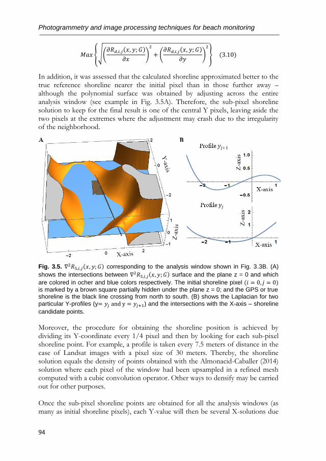
Photogrammetry and image processing techniques for beach monitoring
94
𝑀𝑎𝑥 {√(𝜕𝑅𝑑,𝑖,𝑗(𝑥, 𝑦; 𝐺)
𝜕𝑥)
2
+ (𝜕𝑅𝑑,𝑖,𝑗(𝑥, 𝑦; 𝐺)
𝜕𝑦)
2
} (3.10)
In addition, it was assessed that the calculated shoreline approximated better to the true reference shoreline nearer the initial pixel than in those further away – although the polynomial surface was obtained by adjusting across the entire analysis window (see example in Fig. 3.5A). Therefore, the sub-pixel shoreline solution to keep for the final result is one of the central Y pixels, leaving aside the two pixels at the extremes where the adjustment may crash due to the irregularity of the neighborhood.
Fig. 3.5. ∇2𝑅5,𝑖,𝑗(𝑥, 𝑦; 𝐺) corresponding to the analysis window shown in Fig. 3.3B. (A)
shows the intersections between ∇2𝑅5,𝑖,𝑗(𝑥, 𝑦; 𝐺) surface and the plane z = 0 and which
are colored in ocher and blue colors respectively. The initial shoreline pixel (𝑖 = 0, 𝑗 = 0) is marked by a brown square partially hidden under the plane z = 0; and the GPS or true shoreline is the black line crossing from north to south. (B) shows the Laplacian for two
particular Y-profiles (y= 𝑦𝑗 and y = 𝑦𝑗+1) and the intersections with the X-axis – shoreline
candidate points.
Moreover, the procedure for obtaining the shoreline position is achieved by dividing its Y-coordinate every 1/4 pixel and then by looking for each sub-pixel shoreline point. For example, a profile is taken every 7.5 meters of distance in the case of Landsat images with a pixel size of 30 meters. Thereby, the shoreline solution equals the density of points obtained with the Almonacid-Caballer (2014) solution where each pixel of the window had been upsampled in a refined mesh computed with a cubic convolution operator. Other ways to densify may be carried out for other purposes. Once the sub-pixel shoreline points are obtained for all the analysis windows (as many as initial shoreline pixels), each Y-value will then be several X-solutions due
NOVEL SUB-PIXEL SHORELINE SOLUTION FROM SATELLITE IMAGES
95
to the overlap between windows. For example, the window that serves as the
support for the stencil of the interpolating polynomial 𝑅5,𝑖,𝑗(𝑥, 𝑦; 𝐺) overlaps with
the window of 𝑅5,𝑖,𝑗−1(𝑥, 𝑦; 𝐺). Therefore, the final solution for each fixed Y-
value is calculated as the average of all the approximate sub-pixel shoreline points obtained through the different initial pixels. Other works such as Pardo-Pascual et al. (2018), calculate this average by weighing each solution point according to its distance from the initial pixel (which consequently reduces the RMSE). However, the current work does not deal with this question as it is focused on assessing exclusively the inner technical core of the sub-pixel methodology (step 2 (c) exposed in Section 3.1). So, once tested the improvement in the raw results achieved with the new methodology, subsequent procedures of filtering could be added as in former works to gain precision. At this point, we have a set of unique
points (𝑥𝑘 , 𝑦𝑚) that define the position of the shoreline. The use of an adaptive window in which the initial shoreline pixel is not in the center of the same may cause an excessive curvature in the calculated shoreline as seen in Fig. 3.6A which oscillates around the true shoreline. This happens to a lesser extent in the case of applying the Almonacid-Caballer (2014) solution which uses the LSM on a 7x7 upsampled window centered in the initial pixel, as we can see in Fig. 3.6B. For this reason, at the end of the sub-pixel calculation process described in this chapter (termed aLgr), a smoothening is applied to the set of sub-
pixel shoreline points (𝑥𝑘 , 𝑦𝑚) by using the RLOESS technique (Press and Teukolsky, 1990) in function of the percentage of solution points per window.
3.4. TESTING THE NEW SOLUTION. COMPARISON WITH OTHER INTERPOLATION TECHNIQUES Pardo-Pascual et al. 2018 −coming from Almonacid-Caballer, 2014 methodology− uses a fifth-degree polynomial expression computed using the LSM and a stencil formed with an upsampled 7x7 fixed and symmetric window around the initial shoreline pixel (see Fig. 3.6B). Conversely, the great novelty of this chapter is in changing the concept of kernel through the implementation of a smaller adaptive window defined on the pixel-level shoreline that can collect combinations of 16 or 36 pixels (stencils of four or six pixels in each direction) with greater radiometric variations. An adaptive window may select the stencils with which it is constructed to search for the land-water line. This idea assumes that the separation between water and land occurs where the infrared intensity gradient is maximum. Therefore, the shape of the window (see Fig. 3.6A or 3.3B) may be completely irregular, or even square, if the choice defines it (Fig. 3.3A), but it cannot be centered and symmetric with respect to the initial pixel using an even number of pixels.
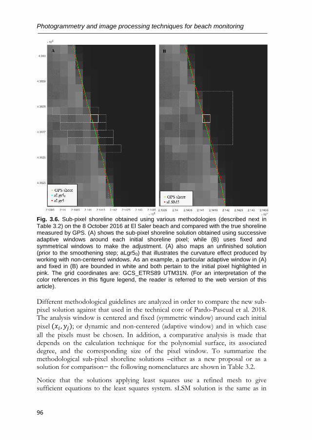
Photogrammetry and image processing techniques for beach monitoring
96
Fig. 3.6. Sub-pixel shoreline obtained using various methodologies (described next in
Table 3.2) on the 8 October 2016 at El Saler beach and compared with the true shoreline measured by GPS. (A) shows the sub-pixel shoreline solution obtained using successive adaptive windows around each initial shoreline pixel; while (B) uses fixed and symmetrical windows to make the adjustment. (A) also maps an unfinished solution (prior to the smoothening step; aLgr50) that illustrates the curvature effect produced by working with non-centered windows. As an example, a particular adaptive window in (A) and fixed in (B) are bounded in white and both pertain to the initial pixel highlighted in pink. The grid coordinates are: GCS_ETRS89 UTM31N. (For an interpretation of the color references in this figure legend, the reader is referred to the web version of this article). Different methodological guidelines are analyzed in order to compare the new sub-pixel solution against that used in the technical core of Pardo-Pascual et al. 2018. The analysis window is centered and fixed (symmetric window) around each initial
pixel (𝑥𝑖 , 𝑦𝑗); or dynamic and non-centered (adaptive window) and in which case
all the pixels must be chosen. In addition, a comparative analysis is made that depends on the calculation technique for the polynomial surface, its associated degree, and the corresponding size of the pixel window. To summarize the methodological sub-pixel shoreline solutions –either as a new proposal or as a solution for comparison− the following nomenclatures are shown in Table 3.2.
Notice that the solutions applying least squares use a refined mesh to give sufficient equations to the least squares system. sLSM solution is the same as in
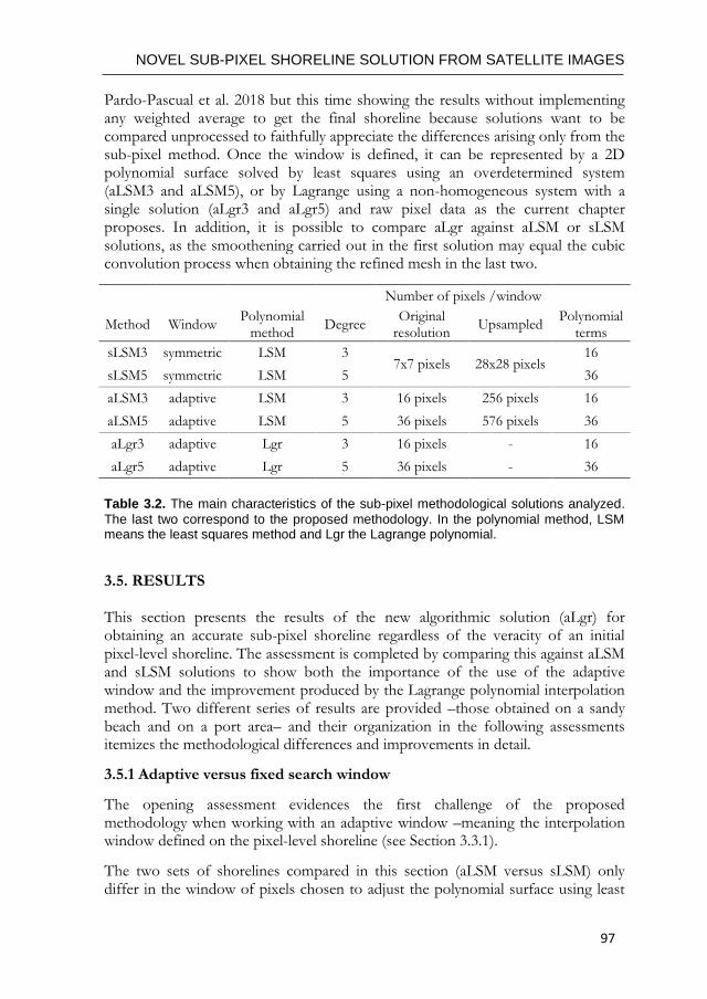
NOVEL SUB-PIXEL SHORELINE SOLUTION FROM SATELLITE IMAGES
97
Pardo-Pascual et al. 2018 but this time showing the results without implementing any weighted average to get the final shoreline because solutions want to be compared unprocessed to faithfully appreciate the differences arising only from the sub-pixel method. Once the window is defined, it can be represented by a 2D polynomial surface solved by least squares using an overdetermined system (aLSM3 and aLSM5), or by Lagrange using a non-homogeneous system with a single solution (aLgr3 and aLgr5) and raw pixel data as the current chapter proposes. In addition, it is possible to compare aLgr against aLSM or sLSM solutions, as the smoothening carried out in the first solution may equal the cubic convolution process when obtaining the refined mesh in the last two.
Number of pixels /window
Method Window Polynomial
method Degree
Original resolution
Upsampled Polynomial
terms
sLSM3 symmetric LSM 3 7x7 pixels 28x28 pixels
16
sLSM5 symmetric LSM 5 36
aLSM3 adaptive LSM 3 16 pixels 256 pixels 16
aLSM5 adaptive LSM 5 36 pixels 576 pixels 36
aLgr3 adaptive Lgr 3 16 pixels - 16
aLgr5 adaptive Lgr 5 36 pixels - 36
Table 3.2. The main characteristics of the sub-pixel methodological solutions analyzed.
The last two correspond to the proposed methodology. In the polynomial method, LSM means the least squares method and Lgr the Lagrange polynomial.
3.5. RESULTS This section presents the results of the new algorithmic solution (aLgr) for obtaining an accurate sub-pixel shoreline regardless of the veracity of an initial pixel-level shoreline. The assessment is completed by comparing this against aLSM and sLSM solutions to show both the importance of the use of the adaptive window and the improvement produced by the Lagrange polynomial interpolation method. Two different series of results are provided –those obtained on a sandy beach and on a port area– and their organization in the following assessments itemizes the methodological differences and improvements in detail.
3.5.1 Adaptive versus fixed search window
The opening assessment evidences the first challenge of the proposed methodology when working with an adaptive window –meaning the interpolation window defined on the pixel-level shoreline (see Section 3.3.1).
The two sets of shorelines compared in this section (aLSM versus sLSM) only differ in the window of pixels chosen to adjust the polynomial surface using least
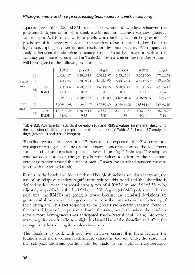
Photogrammetry and image processing techniques for beach monitoring
98
squares (see Table 3.2). sLSM uses a 7x7 symmetric window whatever the polynomial degree (3 or 5) is used. aLSM uses an adaptive window (defined according to A.4 formula) with 16 pixels when looking for third-degree and 36 pixels for fifth-degree. Whatever is the window these solutions follow the same logic: upsampling the kernel and resolution by least squares. A comparative analysis between the shorelines obtained from L7 and L8 images as well as the accuracy per zone is summarized in Table 3.3 –results concerning the aLgr solution will be analyzed in the following Section 3.5.2.
sLSM3 aLSM3 aLgr3 sLSM5 aLSM5 aLgr5
Beach
area
L8 8.63±4.17 3.48±3.19 2.01±2.87 5.35±3.80 5.26±3.38 1.79±2.78
L7 9.09±8.25 5.79±9.98 4.46±5.06 6.83±6.58 6.18±6.52 4.38±5.66
All µ±σ: 8.89±7.04 4.50±7.60 3.45±4.16 6.00±6.17 5.98±5.53 3.31±4.47
RMSE: 11.33 8.83 5.40 8.60 8.14 5.56
Port
area
L8 0.19±13.73 1.58±7.58 0.75±6.09 0.16±10.56 -1.06±9.54 1.23±5.62
L7 3.29±14.98 1.42±11.07 2.77±7.89 0.95±12.78 0.83±11.46 2.05±8.16
All µ±σ: 1.74±14.39 1.96±9.12 1.75±7.11 0.71±11.57 -1.22±10.3 1.62±6.97
RMSE: 14.49 9.32 7.32 11.59 10.40 7.16
Table 3.3. Average (µ), standard deviation (σ) and RMSE values (in meters) describing
the precision of different sub-pixel shoreline solutions (of Table 3.2) for the 17 analyzed days (seven L8 and ten L7 images).
Shoreline errors are larger for L7 because, as expected, the SLC-error and consequent data gaps existing on these images sometimes confuse the adjustment surface and cause unrealistic spikes at the ends (as Fig. 3.7 shows). The adaptive window does not have enough pixels with values to adapt to the maximum gradient direction around the ends of each L7 shoreline stretched between the gaps (even with the refined mesh).
Results in the beach area indicate that although shorelines are biased seaward, the use of an adaptive window significantly reduces this trend and the shoreline is defined with a mean horizontal error (µ±σ) of 4.50±7.6 m and 5.98±5.53 m by adjusting respectively a third (aLSM3) or fifth-degree (aLSM5) polynomial. In the port area, the RMSEs are generally worse because the standard deviations are greater and show a very heterogeneous error distribution that causes a flattening of their histogram. This fact responds to the greater radiometric variation found in the terrestrial part of the port area than in the sandy beach site where the numbers remain more homogeneous –as anticipated Pardo-Pascual et al. (2018). Moreover, many negative errors indicate a slight landward bias of the shoreline and affect the average error by reducing it to values near zero.
The freedom to work with adaptive windows ensure that these recreate the location with the maximum radiometric variations. Consequently, the search for the sub-pixel shoreline position will be made in the optimal neighborhood,
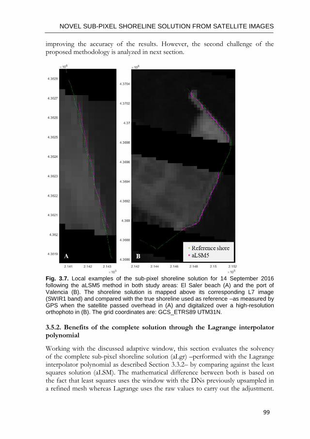
NOVEL SUB-PIXEL SHORELINE SOLUTION FROM SATELLITE IMAGES
99
improving the accuracy of the results. However, the second challenge of the proposed methodology is analyzed in next section.
Fig. 3.7. Local examples of the sub-pixel shoreline solution for 14 September 2016
following the aLSM5 method in both study areas: El Saler beach (A) and the port of Valencia (B). The shoreline solution is mapped above its corresponding L7 image (SWIR1 band) and compared with the true shoreline used as reference –as measured by GPS when the satellite passed overhead in (A) and digitalized over a high-resolution orthophoto in (B). The grid coordinates are: GCS_ETRS89 UTM31N.
3.5.2. Benefits of the complete solution through the Lagrange interpolator polynomial
Working with the discussed adaptive window, this section evaluates the solvency of the complete sub-pixel shoreline solution (aLgr) –performed with the Lagrange interpolator polynomial as described Section 3.3.2– by comparing against the least squares solution (aLSM). The mathematical difference between both is based on the fact that least squares uses the window with the DNs previously upsampled in a refined mesh whereas Lagrange uses the raw values to carry out the adjustment.
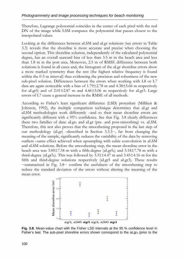
Photogrammetry and image processing techniques for beach monitoring
100
Therefore, Lagrange polynomial coincides in the center of each pixel with the real DN of the image while LSM computes the polynomial that passes closest to the interpolated values.
Looking at the differences between aLSM and aLgr solutions (see errors in Table 3.3) reveals that the shoreline is more accurate and precise when choosing the second option. This shoreline solution, independently of the calculated polynomial degree, has an overall seaward bias of less than 3.5 m in the beach area and less than 1.8 m in the port area. Moreover, 2.5 m of RMSE difference between both solutions is found in all cases and, the histogram of the aLgr shoreline errors show a more marked symmetry than the rest (the highest relative frequency is found within the 0-5 m interval) thus evidencing the precision and robustness of the new sub-pixel solution. Differences between the errors when working with L8 or L7 data are again noticeable with a bias of 1.79±2.78 m and 4.38±5.66 m respectively for aLgr5; and of 2.01±2.87 m and 4.46±5.06 m respectively for aLgr3. Large errors of L7 cause a general increase in the RMSE of all methods.
According to Fisher’s least significant difference (LSD) procedure (Milliken & Johnson, 1992), the multiple comparison technique determines that aLgr and aLSM methodologies work differently –and so their mean shoreline errors are significantly different with a 95% confidence. See that Fig. 3.8 clearly differences these two families of data: aLgr0 and aLgr (pre- and post-smoothing) vs. aLSM. Therefore, this test also proves that the smoothening proposed in the last step of our methodology (aLgr) –described in Section 3.3.3−, far from changing the meaning of the sample, significantly reduces the variability of the data by removing outliers –same effect achieved when upsampling with cubic convolution in aLSM and sLSM solutions. Before the smoothening step, the mean shoreline error in the beach area was 3.00±7.34 m with a fifth-degree (aLgr50) and 3.18±7.78 m with a third-degree (aLgr30). This was followed by 3.31±4.47 m and 3.45±4.16 m for the fifth and third-degree solutions respectively (aLgr5 and aLgr3). These results −summarized in Fig. 3.8− confirm the usefulness of the smoothening step to reduce the standard deviation of the errors without altering the meaning of the mean error.
Fig. 3.8. Mean-value chart with the Fisher LSD intervals at the 95 % confidence level in
Fisher’s test. The sub-pixel shoreline errors shown correspond to the aLgr0 (prior to the
aLgr50 aLSM5 aLgr5 aLgr30 aLSM3 aLgr3
Mea
n s
ho
relin
e er
ror
(m)
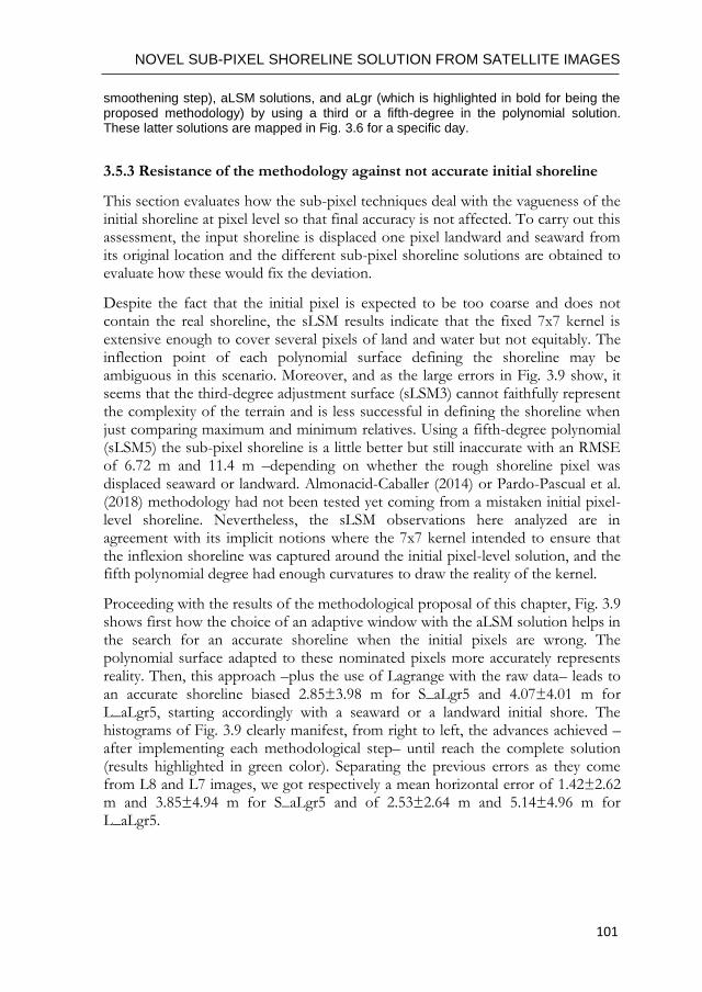
NOVEL SUB-PIXEL SHORELINE SOLUTION FROM SATELLITE IMAGES
101
smoothening step), aLSM solutions, and aLgr (which is highlighted in bold for being the proposed methodology) by using a third or a fifth-degree in the polynomial solution. These latter solutions are mapped in Fig. 3.6 for a specific day.
3.5.3 Resistance of the methodology against not accurate initial shoreline
This section evaluates how the sub-pixel techniques deal with the vagueness of the initial shoreline at pixel level so that final accuracy is not affected. To carry out this assessment, the input shoreline is displaced one pixel landward and seaward from its original location and the different sub-pixel shoreline solutions are obtained to evaluate how these would fix the deviation.
Despite the fact that the initial pixel is expected to be too coarse and does not contain the real shoreline, the sLSM results indicate that the fixed 7x7 kernel is extensive enough to cover several pixels of land and water but not equitably. The inflection point of each polynomial surface defining the shoreline may be ambiguous in this scenario. Moreover, and as the large errors in Fig. 3.9 show, it seems that the third-degree adjustment surface (sLSM3) cannot faithfully represent the complexity of the terrain and is less successful in defining the shoreline when just comparing maximum and minimum relatives. Using a fifth-degree polynomial (sLSM5) the sub-pixel shoreline is a little better but still inaccurate with an RMSE of 6.72 m and 11.4 m –depending on whether the rough shoreline pixel was displaced seaward or landward. Almonacid-Caballer (2014) or Pardo-Pascual et al. (2018) methodology had not been tested yet coming from a mistaken initial pixel-level shoreline. Nevertheless, the sLSM observations here analyzed are in agreement with its implicit notions where the 7x7 kernel intended to ensure that the inflexion shoreline was captured around the initial pixel-level solution, and the fifth polynomial degree had enough curvatures to draw the reality of the kernel.
Proceeding with the results of the methodological proposal of this chapter, Fig. 3.9 shows first how the choice of an adaptive window with the aLSM solution helps in the search for an accurate shoreline when the initial pixels are wrong. The polynomial surface adapted to these nominated pixels more accurately represents reality. Then, this approach –plus the use of Lagrange with the raw data– leads to an accurate shoreline biased 2.85±3.98 m for S_aLgr5 and 4.07±4.01 m for L_aLgr5, starting accordingly with a seaward or a landward initial shore. The histograms of Fig. 3.9 clearly manifest, from right to left, the advances achieved –after implementing each methodological step– until reach the complete solution (results highlighted in green color). Separating the previous errors as they come from L8 and L7 images, we got respectively a mean horizontal error of 1.42±2.62 m and 3.85±4.94 m for S_aLgr5 and of 2.53±2.64 m and 5.14±4.96 m for L_aLgr5.
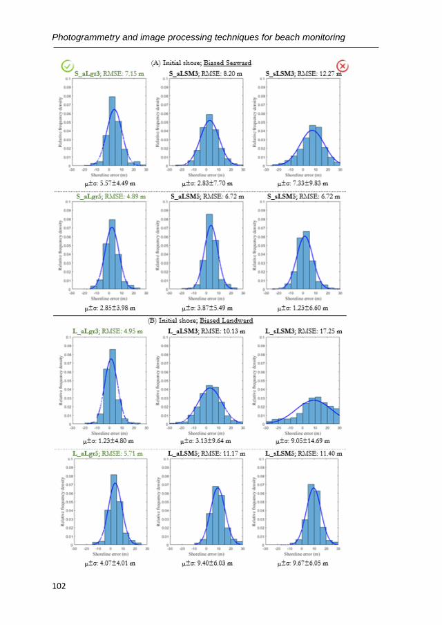
Photogrammetry and image processing techniques for beach monitoring
102
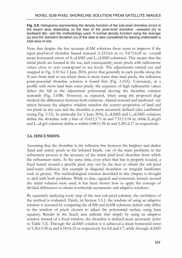
NOVEL SUB-PIXEL SHORELINE SOLUTION FROM SATELLITE IMAGES
103
Fig. 3.9. Histograms representing the density function of the sub-pixel shoreline errors in
the beach area depending on the bias of the pixel-level shoreline –seaward (A) or landward (B)– and the methodology used. A normal density function using the average (µ) and the standard deviation (σ) of the data is also considered by leaving underneath a total area of one.
Note that despite the less accurate sLSM solutions these seem to improve if the input pixel-level shoreline biased seaward (1.23±6.6 m vs. 9.67±6.05 m –overall mean horizontal errors of S_sLSM5 and L_sLSM5 solutions). This means that the initial pixels are located in the sea, and consequently, more pixels with radiometric values close to zero correspond to sea levels. The adjustments carried out and mapped in Fig. 3.10 for 2 June 2016, prove that generally in each profile along the X-axis from land to sea where there is more water than land pixels, the inflection point-potential shoreline solution is found first (Fig. 3.10A). Conversely, in a profile with more land than water pixels, the sequence of high radiometric values delays the fall in the adjustment polynomial moving the shoreline solution seawards (Fig. 3.10B). However, as expected, when using the proposed aLgr method the differences between both solutions –biased seaward and landward– are minor because the adaptive window matches the correct proportion of land and sea pixels in any case and the shoreline is more accurately defined (also confirmed seeing Fig. 3.12). In particular for 2 June 2016, S_sLSM5 and L_sLSM5 solutions define the shoreline with a bias of -0.65±3.71 m and 7.51±3.54 m; while S_aLgr5 and L_aLgr5 solutions define it within 0.88±1.96 m and 2.28±2.17 m respectively.
3.6. DISCUSSION Assuming that the shoreline is the inflexion line between the brighter and darker (land and water) pixels in the infrared bands, one of the main problems in the refinement process is the accuracy of the initial pixel-level shoreline from which the refinement starts. At the same time, even when that line is properly located, a fixed kernel around a specific pixel may not be the best to obtain the sub-pixel land-water inflexion (for example in diagonal shorelines or irregular landforms such as groins). The methodological solution described in this chapter is thought to deal with both problems. While to date, squared and symmetric kernels around the initial solution were used, it has been shown how to apply the concept of divided differences to obtain worthwhile asymmetric and adaptive windows.
By separately analyzing every step of the new sub-pixel solution, the usefulness of the method is evaluated. Firstly, in Section 3.5.1, the wisdom of using an adaptive window is assessed by comparing the aLSM and sLSM solutions (which only differ in the window of pixels chosen to adjust the polynomial surface using least squares). Results in the beach area indicate that simply by using an adaptive window instead of a fixed window, the shoreline is defined more accurately (refer to Table 3.3). Through the aLSM5 solution it is achieved a mean horizontal error of 5.26±3.38 m and 6.18±6.52 m respectively for L8 and L7; while through sLSM5
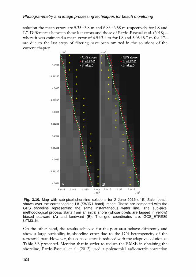
Photogrammetry and image processing techniques for beach monitoring
104
solution the mean errors are 5.35±3.8 m and 6.83±6.58 m respectively for L8 and L7. Differences between these last errors and those of Pardo-Pascual et al. (2018) –where it was estimated a mean error of 6.5±3.1 m for L8 and 5.05±5.7 m for L7– are due to the last steps of filtering have been omitted in the solutions of the current chapter.
Fig. 3.10. Map with sub-pixel shoreline solutions for 2 June 2016 of El Saler beach
shown over the corresponding L8 (SWIR1 band) image. These are compared with the GPS shoreline representing the same instantaneous water line. The sub-pixel methodological process starts from an initial shore (whose pixels are tagged in yellow) biased seaward (A) and landward (B). The grid coordinates are: GCS_ETRS89 UTM31N.
On the other hand, the results achieved for the port area behave differently and show a large variability in shoreline error due to the DN heterogeneity of the terrestrial part. However, this consequence is reduced with the adaptive solution as Table 3.3 presented. Mention that in order to reduce the RMSE in obtaining the shoreline, Pardo-Pascual et al. (2012) used a polynomial radiometric correction
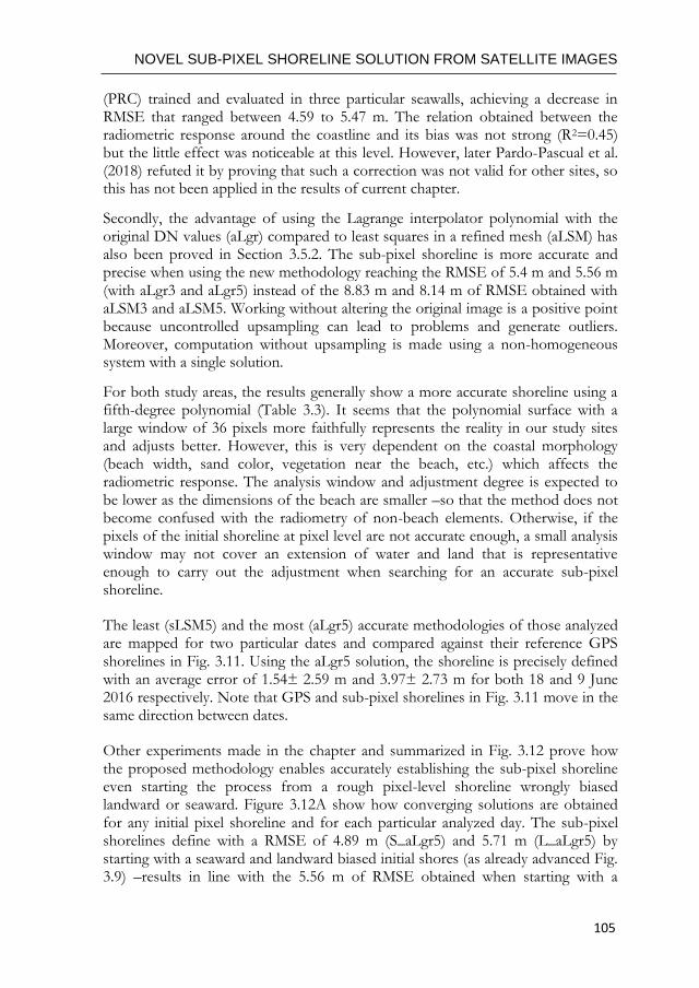
NOVEL SUB-PIXEL SHORELINE SOLUTION FROM SATELLITE IMAGES
105
(PRC) trained and evaluated in three particular seawalls, achieving a decrease in RMSE that ranged between 4.59 to 5.47 m. The relation obtained between the radiometric response around the coastline and its bias was not strong (R2=0.45) but the little effect was noticeable at this level. However, later Pardo-Pascual et al. (2018) refuted it by proving that such a correction was not valid for other sites, so this has not been applied in the results of current chapter.
Secondly, the advantage of using the Lagrange interpolator polynomial with the original DN values (aLgr) compared to least squares in a refined mesh (aLSM) has also been proved in Section 3.5.2. The sub-pixel shoreline is more accurate and precise when using the new methodology reaching the RMSE of 5.4 m and 5.56 m (with aLgr3 and aLgr5) instead of the 8.83 m and 8.14 m of RMSE obtained with aLSM3 and aLSM5. Working without altering the original image is a positive point because uncontrolled upsampling can lead to problems and generate outliers. Moreover, computation without upsampling is made using a non-homogeneous system with a single solution.
For both study areas, the results generally show a more accurate shoreline using a fifth-degree polynomial (Table 3.3). It seems that the polynomial surface with a large window of 36 pixels more faithfully represents the reality in our study sites and adjusts better. However, this is very dependent on the coastal morphology (beach width, sand color, vegetation near the beach, etc.) which affects the radiometric response. The analysis window and adjustment degree is expected to be lower as the dimensions of the beach are smaller –so that the method does not become confused with the radiometry of non-beach elements. Otherwise, if the pixels of the initial shoreline at pixel level are not accurate enough, a small analysis window may not cover an extension of water and land that is representative enough to carry out the adjustment when searching for an accurate sub-pixel shoreline.
The least (sLSM5) and the most (aLgr5) accurate methodologies of those analyzed are mapped for two particular dates and compared against their reference GPS shorelines in Fig. 3.11. Using the aLgr5 solution, the shoreline is precisely defined with an average error of 1.54± 2.59 m and 3.97± 2.73 m for both 18 and 9 June 2016 respectively. Note that GPS and sub-pixel shorelines in Fig. 3.11 move in the same direction between dates.
Other experiments made in the chapter and summarized in Fig. 3.12 prove how the proposed methodology enables accurately establishing the sub-pixel shoreline even starting the process from a rough pixel-level shoreline wrongly biased landward or seaward. Figure 3.12A show how converging solutions are obtained for any initial pixel shoreline and for each particular analyzed day. The sub-pixel shorelines define with a RMSE of 4.89 m (S_aLgr5) and 5.71 m (L_aLgr5) by starting with a seaward and landward biased initial shores (as already advanced Fig. 3.9) –results in line with the 5.56 m of RMSE obtained when starting with a
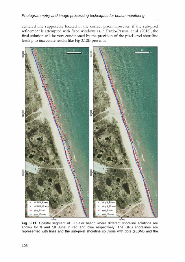
Photogrammetry and image processing techniques for beach monitoring
106
centered line supposedly located in the correct place. However, if the sub-pixel refinement is attempted with fixed windows as in Pardo-Pascual et al. (2018), the final solution will be very conditioned by the precision of the pixel-level shoreline leading to inaccurate results like Fig 3.12B presents.
Fig. 3.11. Coastal segment of El Saler beach where different shoreline solutions are
shown for 9 and 18 June in red and blue respectively. The GPS shorelines are represented with lines and the sub-pixel shoreline solutions with dots (sLSM5 and the
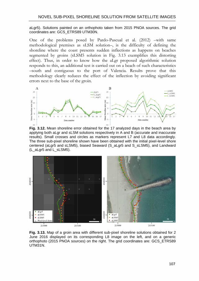
NOVEL SUB-PIXEL SHORELINE SOLUTION FROM SATELLITE IMAGES
107
aLgr5). Solutions painted on an orthophoto taken from 2015 PNOA sources. The grid coordinates are: GCS_ETRS89 UTM30N.
One of the problems posed by Pardo-Pascual et al. (2012) –with same methodological premises as sLSM solution–, is the difficulty of defining the shoreline where the coast presents sudden inflections as happens on beaches segmented by groins (sLSM5 solution in Fig. 3.13 exemplifies this distorting effect). Thus, in order to know how the aLgr proposed algorithmic solution responds to this, an additional test is carried out on a beach of such characteristics –south and contiguous to the port of Valencia. Results prove that this methodology clearly reduces the effect of the inflection by avoiding significant errors next to the base of the groin.
Fig. 3.12. Mean shoreline error obtained for the 17 analyzed days in the beach area by
applying both aLgr and sLSM solutions respectively in A and B (accurate and inaccurate results). Small crosses and circles as markers represent L7 and L8 data accordingly. The three sub-pixel shoreline shown have been obtained with the initial pixel-level shore centered (aLgr5 and sLSM5), biased Seaward (S_aLgr5 and S_sLSM5), and Landward (L_aLgr5 and L_sLSM5).
Fig. 3.13. Map of a groin area with different sub-pixel shoreline solutions obtained for 2
June 2016 displayed on its corresponding L8 image on the left, and on a generic orthophoto (2015 PNOA sources) on the right. The grid coordinates are: GCS_ETRS89 UTM31N.
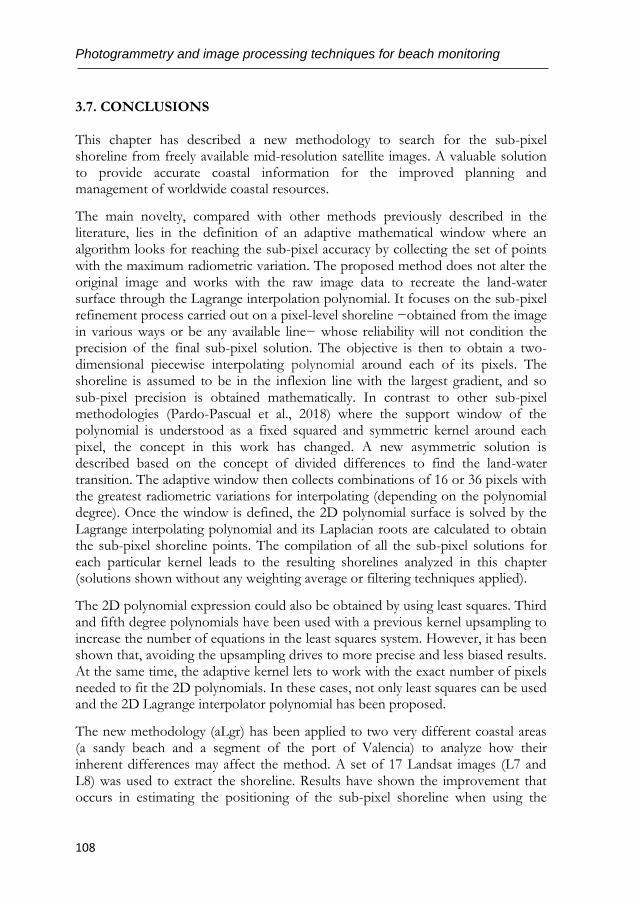
Photogrammetry and image processing techniques for beach monitoring
108
3.7. CONCLUSIONS This chapter has described a new methodology to search for the sub-pixel shoreline from freely available mid-resolution satellite images. A valuable solution to provide accurate coastal information for the improved planning and management of worldwide coastal resources.
The main novelty, compared with other methods previously described in the literature, lies in the definition of an adaptive mathematical window where an algorithm looks for reaching the sub-pixel accuracy by collecting the set of points with the maximum radiometric variation. The proposed method does not alter the original image and works with the raw image data to recreate the land-water surface through the Lagrange interpolation polynomial. It focuses on the sub-pixel refinement process carried out on a pixel-level shoreline −obtained from the image in various ways or be any available line− whose reliability will not condition the precision of the final sub-pixel solution. The objective is then to obtain a two-dimensional piecewise interpolating polynomial around each of its pixels. The shoreline is assumed to be in the inflexion line with the largest gradient, and so sub-pixel precision is obtained mathematically. In contrast to other sub-pixel methodologies (Pardo-Pascual et al., 2018) where the support window of the polynomial is understood as a fixed squared and symmetric kernel around each pixel, the concept in this work has changed. A new asymmetric solution is described based on the concept of divided differences to find the land-water transition. The adaptive window then collects combinations of 16 or 36 pixels with the greatest radiometric variations for interpolating (depending on the polynomial degree). Once the window is defined, the 2D polynomial surface is solved by the Lagrange interpolating polynomial and its Laplacian roots are calculated to obtain the sub-pixel shoreline points. The compilation of all the sub-pixel solutions for each particular kernel leads to the resulting shorelines analyzed in this chapter (solutions shown without any weighting average or filtering techniques applied).
The 2D polynomial expression could also be obtained by using least squares. Third and fifth degree polynomials have been used with a previous kernel upsampling to increase the number of equations in the least squares system. However, it has been shown that, avoiding the upsampling drives to more precise and less biased results. At the same time, the adaptive kernel lets to work with the exact number of pixels needed to fit the 2D polynomials. In these cases, not only least squares can be used and the 2D Lagrange interpolator polynomial has been proposed.
The new methodology (aLgr) has been applied to two very different coastal areas (a sandy beach and a segment of the port of Valencia) to analyze how their inherent differences may affect the method. A set of 17 Landsat images (L7 and L8) was used to extract the shoreline. Results have shown the improvement that occurs in estimating the positioning of the sub-pixel shoreline when using the
NOVEL SUB-PIXEL SHORELINE SOLUTION FROM SATELLITE IMAGES
109
proposed solution, especially in the challenging case of starting with a biased initial pixel-level shoreline. Using the ideas of former methodologies −through the sLSM5 solution− the shoreline was defined with a mean horizontal error not better than 6.0±6.17 m for the beach and 0.71±11.57 m for the port. However, better accuracies are achieved applying the proposed methodology with errors of 3.31±4.47 m and 1.62±6.97 m in those same sites respectively. In particular, and disaggregating these last results for L8 and L7, the error is respectively 1.79±2.78 m and 4.38±5.66 m in the beach area, and 1.23±5.62 m and 2.05±8.16 m in the port area. Even more, differences between methodologies exaggerate when the sub-pixel search starts from an initial biased pixel-level shoreline. In these cases, the sLSM5 method is unable to reach a RMSE below the 6.72 m, while the aLgr5 method defines the shoreline with a RMSE of 5.71 m (3.65 m for L8 and 7.14 m for L7) and 4.89 m (2.98 m for L8 and 6.26 m for L7) depending on whether the initial shore was landward or seaward biased.

Cover photo of Chapter 4: Jervis Bay, Australia (taken Dec. 2017)
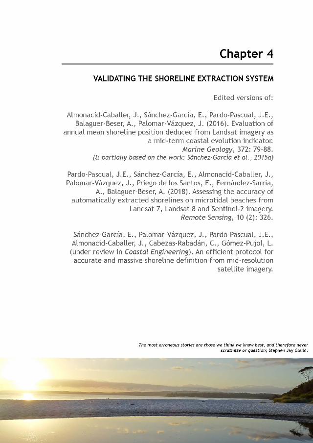

VALIDATING THE SHORELINE EXTRACTION SYSTEM
113
This chapter summarizes the complete journey through the research history of the doctoral student and CGAT research group to which she belongs.
Within the research background of the CGAT group and within the
project entitled “Monitoring coastal changes using remote sensing to mitigate the impacts of
climate change” the doctoral student has been working in recent years on the search
for solutions and techniques to further improve shoreline detection from satellite
imagery. The algorithm of shoreline extration presented in Pardo-Pascual et al.
(2012) and thoroughly described in Almonacid-Caballer 2014 needed to be tested
in other environments outside the comfort area (as were the breakwaters).
However, assessing the algorithm in other coastal areas such as beaches led to
many challenges. In dynamic environments such as beaches, the definition of a
border as the shoreline was not a trivial issue and even less so when working from
mid-resolution satellite images. However, its achievement would be very promising
for coastal monitoring and planning.
The first issue to solve when evaluating the algorithm is to establish which real phenomenon is being detected as a shoreline within the transition zone between land and sea (Do et al., 2019). Pardo-Pascual et al. (2012) analyzed the results of some 45 images in different artificially stabilized coastal segments. In these places, the impact of wave runup is null because the land-water limit and the wet line are coincident, which is not true in the case of the beaches. Therefore, it is pertinent to ask whether the deduced waterfront from Landsat images for sedimentary beaches is coincident with a shoreline measured in the field or from high-resolution images – and if its use provides information with the same validity for describing medium and long-term evolutionary trends (Sánchez-García et al., 2015a).
Achieving this, and given that reference data simultaneous with Landsat (5, 7 and 8) images was not initially available, the first study in Section 4.1 (published in Marine Geology, 2016) focused on the comparison of an annual mean shoreline with the two sources of data (high precision and Landsat imagery between the years 2005 and 2010) over an area with almost no tides. The basic assumption underlying this proposal is that as a generic rule, intra-annual shoreline variations oscillate around an average position that would be the most significant when trying to set trends. Oscillations around that average shoreline are then understood as the effect of short-term changes, while alterations obey changes in the global sedimentary balance of the analyzed beach segment. By testing the accuracy from these extracted annual mean shorelines, the potential of using Landsat imagery as a new source for describing decadal or mid-term changes in beaches was verified. A previous work (Sánchez-García et al., 2015a) had already tested the grade of similarity between these Landsat and high-precision data. Several statistical tests indicated that both sources provided similar information regarding annual mean shorelines.
Photogrammetry and image processing techniques for beach monitoring
114
Continuing with the evaluation but now aiming at the instantaneousness of the shoreline, the work presented in Section 4.2 was performed (published in Remote Sensing, 2018). Some field campaigns were carried out and accurate records were registered describing the state of the sea at the same instant as the Landsat (7 and 8) and Sentinel 2 images were acquired. The reference data was obtained using differential GNSS surveys and terrestrial photogrammetry techniques through the C-Pro monitoring system described in Chapter 2. A set of 21 sub-pixel shorelines and their respective high precision lines served for a six-month evaluation in 2016. Sentinel 2 was launched in 2015 and some of its images were added to the shoreline extraction process for this work. Therefore, this is the first evalution of the Pardo-Pascual et al., 2012 and Almonacid-Caballer, 2014 shoreline extraction algorithm on natural beaches. The derived results enabled testing this initial methodology and analyzing the factors that were affecting the accuracy of the extracted shoreline.
At this point, the potential of the satellite-derived shorelines (SDS) had been already asessed in microtidal areas, but this research focussed on the efficiency of the tool when applied to a massive set of images and with the future goal of being useful on a large spatial scale and with various tidal regimes.
An integrated shoreline extraction system called SHOREX − already referenced in Chapter 3 − was able to include all the phases within a production pipeline (Palomar-Vázquez et al., 2018a). The work presented in Section 4.3 (recently finished; Sánchez-García et al., under review) continues being an evaluation of 91 SDS with other high-resolution shorelines obtained simultaneously through video monitoring on a different sedimentary beach. However, this time, the main objective is to identify the combination of parameters under which the algorithm produces the best results and define an automatic shoreline extraction protocol. To increase the efficiency of the process, the idea of producing the initial pixel-level shoreline (around which is performed the search for the sub-pixel) has changed. Despite using an initial rough shoreline for each satellite image using threshold techniques − as in Pardo-Pascual et al. (2012) to Pardo-Pascual et al. (2018) − the idea now is to use a unique digitalized or available pixel-level shoreline for the whole set of temporal images of an area. The main goal consists in releasing the sub-pixel accuracy of the final shoreline from the inaccuracy of the initial pixel-level shoreline.
In this regards, Section 4.3 presents an efficient self-contained workflow ensuring a suitable kernel (neighborhood) to represent the land-water interface, and then defining the shoreline with the maximum precision through a smaller kernel. The different evaluations carried out in the study area have shown that by working with small neighborhoods, the algorithm is generally less confused with the remaining elements of the terrain and produces better shoreline accuracies. However, small neighborhoods first require guaranteeing that the searched transition zone between land and sea is correctly located within them.

VALIDATING THE SHORELINE EXTRACTION SYSTEM
115
The various improvements developed in the intrinsics of the SHOREX algorithm focused on offering a solution through a dynamic and adaptive neighborhood as described in Chapter 3, and with the performance of an iterative solution with the most suitable parameters as presented in Section 4.3 (within Chapter 4). Both solutions have been explored separately throughout this document to test how each contributes to SDS accuracy.

Photogrammetry and image processing techniques for beach monitoring
116
VALIDATING THE SHORELINE EXTRACTION SYSTEM
117
4.1. EVALUATION OF ANNUAL MEAN SHORELINE POSITION
DEDUCED FROM LANDSAT IMAGERY AS A MID-TERM COASTAL EVOLUTION INDICATOR
The shoreline is a useful indicator of mid-term coastal evolution. Every shoreline is affected by instantaneous sea-level, the length of the runup, and beach profile changes. In this work, annual mean shorelines are evaluated in a manner that avoids these effects by averaging the instantaneous shoreline positions registered during the same year. A set of 270 shorelines obtained from Landsat imagery between 2000 and 2014, using the method described in Pardo-Pascual et al. (2012), have been used. It has been shown that the use of annual mean shorelines enables the same rate of change to be obtained as when using all the shorelines, but that the data is simpler to manage and more useful when visualising local changes. It has also been shown that annual mean shorelines largely remove the short-term variability, and are therefore useful for analyzing mid-term trend quantifications. In addition, we propose a methodology for annual mean shorelines, obtained from Landsat imagery, that minimises the effects of sea-level variation on the shoreline positions. Both shorelines –instantaneous and mean annual– appear to be about 4 or 5 m seaward from those obtained using more precise sources.
4.1.1. Introduction
Decadal or mid-term beach changes – decades to centuries – are strongly related to variations in storm intensities, longshore sediment transport patterns, as well as changes in beach and dune sediment budgets (Carter, 1988; Kraus et al., 1991; Cowell and Thom, 1994; Sanjaume and Pardo-Pascual, 2001; Davidson-Arnott, 2010). However, these changes are often difficult to quantify using changes in the shoreline because there are too many short-term variations related with water level variation, runup dimensions, and seasonal beach profile variations (Moore, 2000; Boak and Tunner, 2005). Even in microtidal coasts, the shoreline position obtained using various tools (such as aerial photographs, satellite imagery, RTK-GPS, video-monitoring, and LiDAR) is not necessarily the most representative for measuring mid-term evolution. Trend evolution during decades is often masked by considerable variability that follows a cyclical dynamic (annual, or storm/calm periods). To correctly define the mid-term trend it is necessary to obtain sufficient samples of shorelines during a sufficient number of years. This task is usually difficult because there are insufficient sets of aerial photographs or other surveys. The use of mid-resolution satellite images with high frequency revisit times could be a good solution; however, excessively coarse pixels prevent the accurate definition of shoreline positions when quantifying beach changes (Gens, 2010). Pardo-Pascual et al. (2012) and Almonacid-Caballer (2014) proposed a methodology to extract shoreline positions from Landsat (5, 7 and 8) imagery (30 m/pixel) with RMSE values of about 5 m. This accuracy has been tested comparing 116 Landsat extracted shorelines with two shoreline segments on
Photogrammetry and image processing techniques for beach monitoring
118
seawalls in the Spanish Mediterranean (a micro-tidal area). In this case, it was easy to define the shoreline position because the coastlines do not change over time.
However, on natural beaches, the wet zone can be several metres wide and thus the Landsat shoreline precision for seawalls is not necessarily the same as for beaches. Moreover, on seawall coastal segments, the water depth suddenly falls near the shoreline, whereas on natural beaches the depth drops more gradually. As a consequence of deep water near to the coast, there is a foam fringe associated with the breaker zone which is close to the coastline and narrower in seawall zones than in natural beaches. Unfortunately, no accurate surveying measurements were made when the Landsat images were registered. Thus on natural beaches, we could only check several Landsat shorelines with other nearly co-incident (in time) high precision shorelines.
Another question regards shoreline validity as a trend indicator. Shorelines – understood as waterline borders – are inaccurate indicators of coastal changes because they are strongly influenced by sea-level variations (Moore, 2000; Boak and Turner, 2005; Del Rio and Gracia, 2013). Some authors (Stockdon et al., 2002; Ruggiero et al., 2005, Moore et al., 2006; List et al., 2006) suggest that a good solution could be to define a datum-based shoreline, taking 3D data as a basic topographic source and using the contour line that defines the local position of mean high water as a reference. Farris and List (2007) and Psuty and Silveira (2011) used this solution to successfully monitor coastal changes. However, when using shorelines extracted from Landsat imagery it is not possible to obtain this datum-based shoreline because no 3D data coincides with the captured images. This fact means that the shoreline variation between nearby dates was sometimes very large due to small water level changes after the beach profile was flattened by storm waves (Pardo-Pascual et al., 2014). Some works (Robertson et al., 2007) demonstrate that a shoreline change (even working with datum-based shorelines) is sometimes due to small changes in the nearshore microforms rather than real sedimentary changes. Therefore, it seems clear that we cannot guarantee a correct definition of mid-term beach evolution unless we use a sufficient number of shoreline positions.
Taking all these appreciations into account, we can ask if the shorelines extracted from Landsat imagery are useful for quantifying the evolution of beaches on a mid-term scale. This could be important because, in contrast to other data sources, using Landsat data it is possible to obtain many shorelines for each year from 1984 to the present.
The availability of many shoreline positions during one year reduces the risk that the position set is unduly biased by the factors affecting the intra-annual variability. However, it is difficult to perform evolutionary analyses using many lines because it is difficult to recognise the magnitude of the changes when using the traditional techniques of map line overlays (Fig. 4.1). To improve the efficiency of the
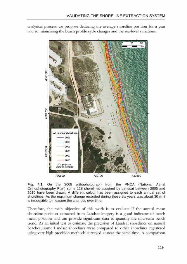
VALIDATING THE SHORELINE EXTRACTION SYSTEM
119
analytical process we propose deducing the average shoreline position for a year and so minimising the beach profile cycle changes and the sea-level variations.
Fig. 4.1. On the 2008 orthophotograph from the PNOA (National Aerial
Orthophotography Plan) some 118 shorelines acquired by Landsat between 2005 and 2010 have been drawn. A different colour has been assigned to each annual set of shorelines. As the maximum change recorded during these six years was about 30 m it is impossible to measure the changes over time.
Therefore, the main objective of this work is to evaluate if the annual mean shoreline position extracted from Landsat imagery is a good indicator of beach mean position and can provide significant data to quantify the mid-term beach trend. As an initial test to estimate the precision of Landsat shorelines on natural beaches, some Landsat shorelines were compared to other shorelines registered using very high precision methods surveyed at near the same time. A comparison
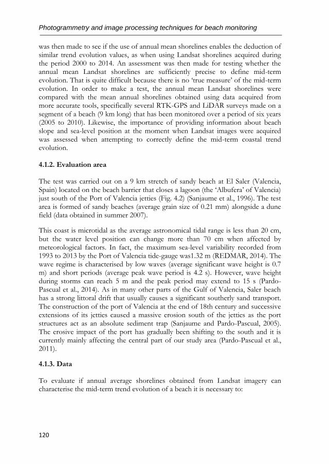
Photogrammetry and image processing techniques for beach monitoring
120
was then made to see if the use of annual mean shorelines enables the deduction of similar trend evolution values, as when using Landsat shorelines acquired during the period 2000 to 2014. An assessment was then made for testing whether the annual mean Landsat shorelines are sufficiently precise to define mid-term evolution. That is quite difficult because there is no ‘true measure’ of the mid-term evolution. In order to make a test, the annual mean Landsat shorelines were compared with the mean annual shorelines obtained using data acquired from more accurate tools, specifically several RTK-GPS and LiDAR surveys made on a segment of a beach (9 km long) that has been monitored over a period of six years (2005 to 2010). Likewise, the importance of providing information about beach slope and sea-level position at the moment when Landsat images were acquired was assessed when attempting to correctly define the mid-term coastal trend evolution. 4.1.2. Evaluation area
The test was carried out on a 9 km stretch of sandy beach at El Saler (Valencia, Spain) located on the beach barrier that closes a lagoon (the ‘Albufera’ of Valencia) just south of the Port of Valencia jetties (Fig. 4.2) (Sanjaume et al., 1996). The test area is formed of sandy beaches (average grain size of 0.21 mm) alongside a dune field (data obtained in summer 2007).
This coast is microtidal as the average astronomical tidal range is less than 20 cm, but the water level position can change more than 70 cm when affected by meteorological factors. In fact, the maximum sea-level variability recorded from 1993 to 2013 by the Port of Valencia tide-gauge was1.32 m (REDMAR, 2014). The wave regime is characterised by low waves (average significant wave height is 0.7 m) and short periods (average peak wave period is 4.2 s). However, wave height during storms can reach 5 m and the peak period may extend to 15 s (Pardo-Pascual et al., 2014). As in many other parts of the Gulf of Valencia, Saler beach has a strong littoral drift that usually causes a significant southerly sand transport. The construction of the port of Valencia at the end of 18th century and successive extensions of its jetties caused a massive erosion south of the jetties as the port structures act as an absolute sediment trap (Sanjaume and Pardo-Pascual, 2005). The erosive impact of the port has gradually been shifting to the south and it is currently mainly affecting the central part of our study area (Pardo-Pascual et al., 2011).
4.1.3. Data
To evaluate if annual average shorelines obtained from Landsat imagery can characterise the mid-term trend evolution of a beach it is necessary to:
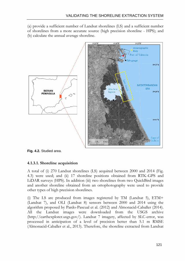
VALIDATING THE SHORELINE EXTRACTION SYSTEM
121
(a) provide a sufficient number of Landsat shorelines (LS) and a sufficient number of shorelines from a more accurate source (high precision shoreline - HPS); and (b) calculate the annual average shoreline.
Fig. 4.2. Studied area.
4.1.3.1. Shoreline acquisition
A total of (i) 270 Landsat shorelines (LS) acquired between 2000 and 2014 (Fig. 4.3) were used; and (ii) 17 shoreline positions obtained from RTK-GPS and LiDAR surveys (HPS). In addition (iii) two shorelines from two QuickBird images and another shoreline obtained from an ortophotography were used to provide other types of high precision shorelines.
(i) The LS are produced from images registered by TM (Landsat 5), ETM+ (Landsat 7), and OLI (Landsat 8) sensors between 2000 and 2014 using the algorithm proposed by Pardo-Pascual et al. (2012) and Almonacid-Caballer (2014). All the Landsat images were downloaded from the USGS archive (http://earthexplorer.usgs.gov/). Landsat 7 imagery, affected by SLC-error, was processed in anticipation of a level of precision better than 5.1 m RMSE (Almonacid-Caballer et al., 2013). Therefore, the shoreline extracted from Landsat
Photogrammetry and image processing techniques for beach monitoring
122
7 is not a continuous line and is formed of segments approximately 600 m in length with 500 m gaps.
Fig. 4.3. Bars indicate the number of shorelines extracted from Landsat images. Landsat
5 and 7 were used until 2011, but in November 2011 Landsat 5 failed and only Landsat 7 remained available. Landsat 8 was successfully launched in February 2013 and since then images acquired from Landsat 7 and 8 were used.
(ii) HPS were obtained between 2005 and 2010 as a part of a programme of morphodynamic beach monitoring at Saler (Pardo-Pascual, et al., 2011) using RTK-GPS and LiDAR surveys. The RTK-GPS surveys were performed using an all-terrain vehicle that moves over the beach (Pardo-Pascual et al., 2005). Three surveys were derived from LiDAR surveys (June 2005, December 2007, and August 2009). A semi-regular schedule followed (middle winter, spring, and autumn) and only one survey was registered during the summer (August 2009). Every survey datum was recorded on the ETRS89 reference system, in UTM projection coordinates, and the altitudes referenced to EGM08-REDNAP, the Spanish official datum.
The waterline (WL-HPS) obtained from the RTK-GPS surveys was defined as the sea beach boundary and was established during fieldwork by the coordinates acquired with the location of the waterline. In the LiDAR survey, the waterline was described by finding the lowest contour line in a generated DEM from LiDAR data that followed a clear alongshore direction (i.e. a line that did not close on itself). Fig. 4.4 enables a comparison of the temporal distribution of different types of managed shorelines acquired between 2005 and 2010 – and the data is analyzed below.
(iii) To evaluate the similarity between the shorelines obtained from Landsat imagery and those from very high resolution sources, it has been used an orthophotography (0.5 m resolution) was taken (20 June 2008) six days after a
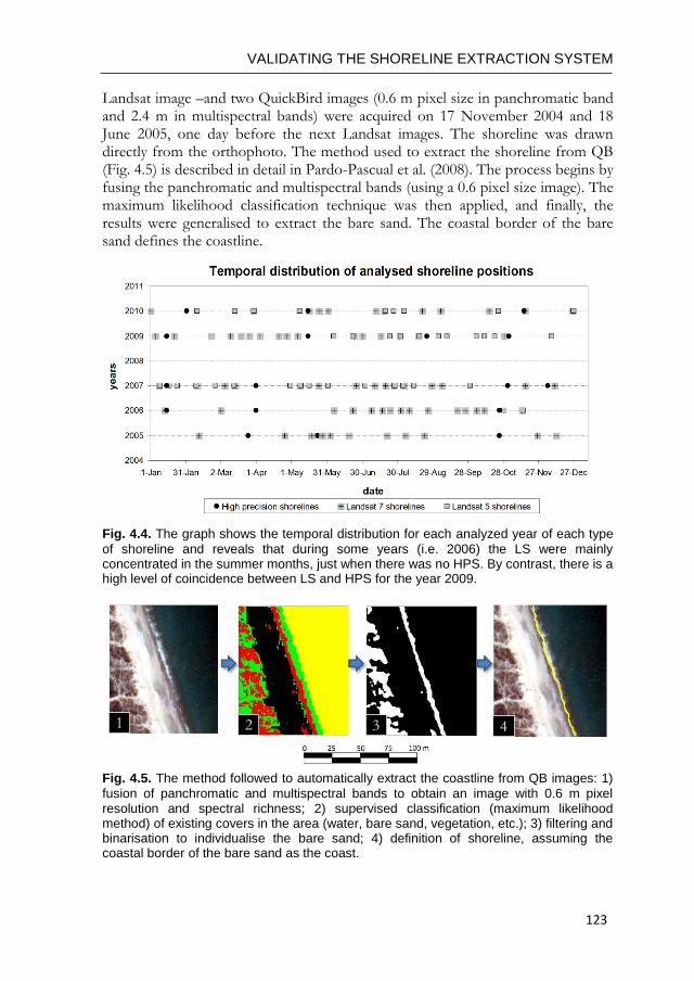
VALIDATING THE SHORELINE EXTRACTION SYSTEM
123
Landsat image –and two QuickBird images (0.6 m pixel size in panchromatic band and 2.4 m in multispectral bands) were acquired on 17 November 2004 and 18 June 2005, one day before the next Landsat images. The shoreline was drawn directly from the orthophoto. The method used to extract the shoreline from QB (Fig. 4.5) is described in detail in Pardo-Pascual et al. (2008). The process begins by fusing the panchromatic and multispectral bands (using a 0.6 pixel size image). The maximum likelihood classification technique was then applied, and finally, the results were generalised to extract the bare sand. The coastal border of the bare sand defines the coastline.
Fig. 4.4. The graph shows the temporal distribution for each analyzed year of each type
of shoreline and reveals that during some years (i.e. 2006) the LS were mainly concentrated in the summer months, just when there was no HPS. By contrast, there is a high level of coincidence between LS and HPS for the year 2009.
Fig. 4.5. The method followed to automatically extract the coastline from QB images: 1)
fusion of panchromatic and multispectral bands to obtain an image with 0.6 m pixel resolution and spectral richness; 2) supervised classification (maximum likelihood method) of existing covers in the area (water, bare sand, vegetation, etc.); 3) filtering and binarisation to individualise the bare sand; 4) definition of shoreline, assuming the coastal border of the bare sand as the coast.
1 2 3 4
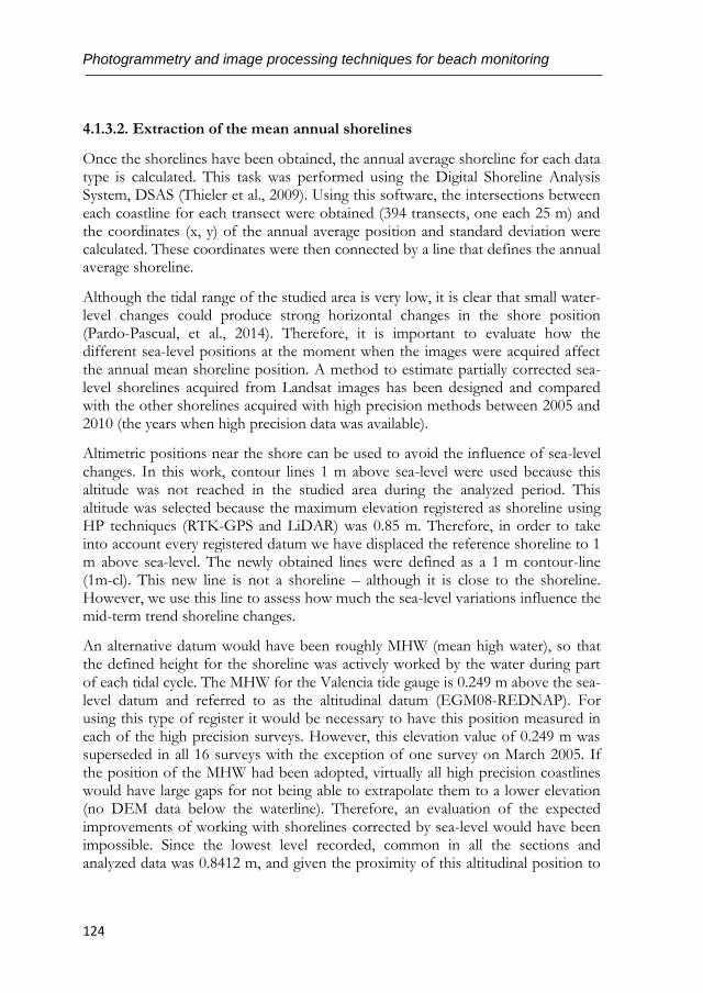
Photogrammetry and image processing techniques for beach monitoring
124
4.1.3.2. Extraction of the mean annual shorelines
Once the shorelines have been obtained, the annual average shoreline for each data type is calculated. This task was performed using the Digital Shoreline Analysis System, DSAS (Thieler et al., 2009). Using this software, the intersections between each coastline for each transect were obtained (394 transects, one each 25 m) and the coordinates (x, y) of the annual average position and standard deviation were calculated. These coordinates were then connected by a line that defines the annual average shoreline.
Although the tidal range of the studied area is very low, it is clear that small water-level changes could produce strong horizontal changes in the shore position (Pardo-Pascual, et al., 2014). Therefore, it is important to evaluate how the different sea-level positions at the moment when the images were acquired affect the annual mean shoreline position. A method to estimate partially corrected sea-level shorelines acquired from Landsat images has been designed and compared with the other shorelines acquired with high precision methods between 2005 and 2010 (the years when high precision data was available).
Altimetric positions near the shore can be used to avoid the influence of sea-level changes. In this work, contour lines 1 m above sea-level were used because this altitude was not reached in the studied area during the analyzed period. This altitude was selected because the maximum elevation registered as shoreline using HP techniques (RTK-GPS and LiDAR) was 0.85 m. Therefore, in order to take into account every registered datum we have displaced the reference shoreline to 1 m above sea-level. The newly obtained lines were defined as a 1 m contour-line (1m-cl). This new line is not a shoreline – although it is close to the shoreline. However, we use this line to assess how much the sea-level variations influence the mid-term trend shoreline changes.
An alternative datum would have been roughly MHW (mean high water), so that the defined height for the shoreline was actively worked by the water during part of each tidal cycle. The MHW for the Valencia tide gauge is 0.249 m above the sea-level datum and referred to as the altitudinal datum (EGM08-REDNAP). For using this type of register it would be necessary to have this position measured in each of the high precision surveys. However, this elevation value of 0.249 m was superseded in all 16 surveys with the exception of one survey on March 2005. If the position of the MHW had been adopted, virtually all high precision coastlines would have large gaps for not being able to extrapolate them to a lower elevation (no DEM data below the waterline). Therefore, an evaluation of the expected improvements of working with shorelines corrected by sea-level would have been impossible. Since the lowest level recorded, common in all the sections and analyzed data was 0.8412 m, and given the proximity of this altitudinal position to
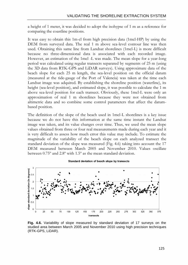
VALIDATING THE SHORELINE EXTRACTION SYSTEM
125
a height of 1 meter, it was decided to adopt the isohypse of 1 m as a reference for comparing the coastline positions.
It was easy to obtain this 1m-cl from high precision data (1mcl-HP) by using the DEM from surveyed data. The real 1 m above sea-level contour line was then used. Obtaining this same line from Landsat shorelines (1mcl-L) is more difficult because no three-dimensional data is associated with each recorded image. However, an estimation of the 1mcl -L was made. The mean slope for a year-long period was calculated using regular transects separated by segments of 25 m (using the 3D data from RTK-GPS and LiDAR surveys). Using approximate data of the beach slope for each 25 m length, the sea-level position on the official datum (measured at the tide-gauge of the Port of Valencia) was taken at the time each Landsat image was adquired. By establishing the shoreline position (waterline), its height (sea-level position), and estimated slope, it was possible to calculate the 1 m above sea-level position for each transect. Obviously, these 1mcl-L were only an approximation of real 1 m shorelines because they were not obtained from altimetric data and so combine some control parameters that affect the datum-based position.
The definition of the slope of the beach used in 1mcl-L shorelines is a key issue because we do not have this information at the same time instant the Landsat image was taken, and its value changes over time. Thus, we used the mean slope values obtained from three or four real measurements made during each year and it is very difficult to assess how much error this value may include. To estimate the magnitude of the variability of the beach slope on each analyzed transect the standard deviation of the slope was measured (Fig. 4.6) taking into account the 17 DEM measured between March 2005 and November 2010. Values oscillate between 0.75º and 2.8º with 1.5º as the mean standard deviation.
Fig. 4.6. Variability of slope measured by standard deviation of 17 surveys on the
studied area between March 2005 and November 2010 using high precision techniques (RTK-GPS, LiDAR).
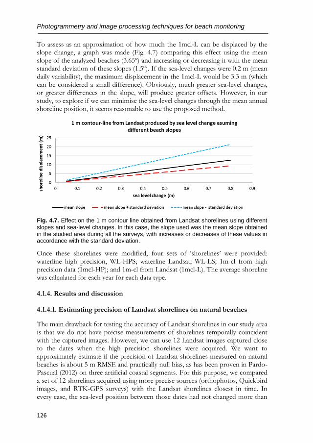
Photogrammetry and image processing techniques for beach monitoring
126
To assess as an approximation of how much the 1mcl-L can be displaced by the slope change, a graph was made (Fig. 4.7) comparing this effect using the mean slope of the analyzed beaches (3.65º) and increasing or decreasing it with the mean standard deviation of these slopes (1.5º). If the sea-level changes were 0.2 m (mean daily variability), the maximum displacement in the 1mcl-L would be 3.3 m (which can be considered a small difference). Obviously, much greater sea-level changes, or greater differences in the slope, will produce greater offsets. However, in our study, to explore if we can minimise the sea-level changes through the mean annual shoreline position, it seems reasonable to use the proposed method.
Fig. 4.7. Effect on the 1 m contour line obtained from Landsat shorelines using different
slopes and sea-level changes. In this case, the slope used was the mean slope obtained in the studied area during all the surveys, with increases or decreases of these values in accordance with the standard deviation.
Once these shorelines were modified, four sets of ‘shorelines’ were provided: waterline high precision, WL-HPS; waterline Landsat, WL-LS; 1m-cl from high precision data (1mcl-HP); and 1m-cl from Landsat (1mcl-L). The average shoreline was calculated for each year for each data type. 4.1.4. Results and discussion
4.1.4.1. Estimating precision of Landsat shorelines on natural beaches
The main drawback for testing the accuracy of Landsat shorelines in our study area is that we do not have precise measurements of shorelines temporally coincident with the captured images. However, we can use 12 Landsat images captured close to the dates when the high precision shorelines were acquired. We want to approximately estimate if the precision of Landsat shorelines measured on natural beaches is about 5 m RMSE and practically null bias, as has been proven in Pardo-Pascual (2012) on three artificial coastal segments. For this purpose, we compared a set of 12 shorelines acquired using more precise sources (orthophotos, Quickbird images, and RTK-GPS surveys) with the Landsat shorelines closest in time. In every case, the sea-level position between those dates had not changed more than
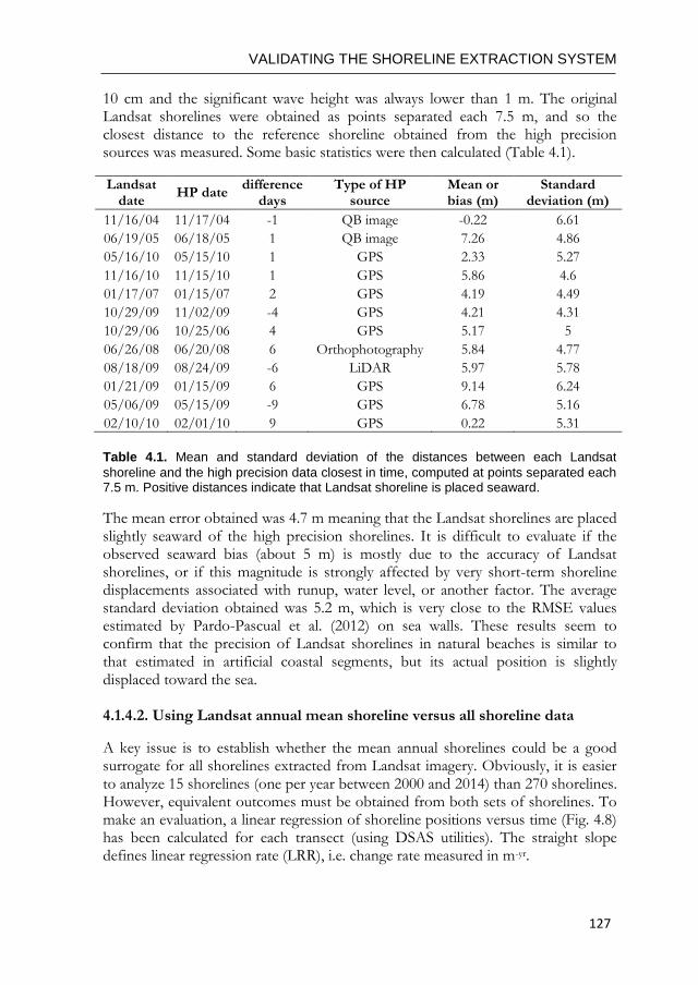
VALIDATING THE SHORELINE EXTRACTION SYSTEM
127
10 cm and the significant wave height was always lower than 1 m. The original Landsat shorelines were obtained as points separated each 7.5 m, and so the closest distance to the reference shoreline obtained from the high precision sources was measured. Some basic statistics were then calculated (Table 4.1).
Landsat date
HP date difference
days Type of HP
source Mean or bias (m)
Standard deviation (m)
11/16/04 11/17/04 -1 QB image -0.22 6.61
06/19/05 06/18/05 1 QB image 7.26 4.86
05/16/10 05/15/10 1 GPS 2.33 5.27
11/16/10 11/15/10 1 GPS 5.86 4.6
01/17/07 01/15/07 2 GPS 4.19 4.49
10/29/09 11/02/09 -4 GPS 4.21 4.31
10/29/06 10/25/06 4 GPS 5.17 5
06/26/08 06/20/08 6 Orthophotography 5.84 4.77
08/18/09 08/24/09 -6 LiDAR 5.97 5.78
01/21/09 01/15/09 6 GPS 9.14 6.24
05/06/09 05/15/09 -9 GPS 6.78 5.16
02/10/10 02/01/10 9 GPS 0.22 5.31
Table 4.1. Mean and standard deviation of the distances between each Landsat
shoreline and the high precision data closest in time, computed at points separated each 7.5 m. Positive distances indicate that Landsat shoreline is placed seaward.
The mean error obtained was 4.7 m meaning that the Landsat shorelines are placed slightly seaward of the high precision shorelines. It is difficult to evaluate if the observed seaward bias (about 5 m) is mostly due to the accuracy of Landsat shorelines, or if this magnitude is strongly affected by very short-term shoreline displacements associated with runup, water level, or another factor. The average standard deviation obtained was 5.2 m, which is very close to the RMSE values estimated by Pardo-Pascual et al. (2012) on sea walls. These results seem to confirm that the precision of Landsat shorelines in natural beaches is similar to that estimated in artificial coastal segments, but its actual position is slightly displaced toward the sea. 4.1.4.2. Using Landsat annual mean shoreline versus all shoreline data
A key issue is to establish whether the mean annual shorelines could be a good surrogate for all shorelines extracted from Landsat imagery. Obviously, it is easier to analyze 15 shorelines (one per year between 2000 and 2014) than 270 shorelines. However, equivalent outcomes must be obtained from both sets of shorelines. To make an evaluation, a linear regression of shoreline positions versus time (Fig. 4.8) has been calculated for each transect (using DSAS utilities). The straight slope defines linear regression rate (LRR), i.e. change rate measured in m-yr.
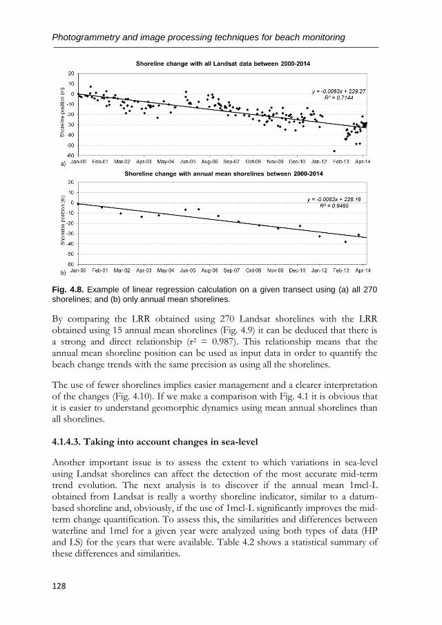
Photogrammetry and image processing techniques for beach monitoring
128
Fig. 4.8. Example of linear regression calculation on a given transect using (a) all 270
shorelines; and (b) only annual mean shorelines.
By comparing the LRR obtained using 270 Landsat shorelines with the LRR obtained using 15 annual mean shorelines (Fig. 4.9) it can be deduced that there is a strong and direct relationship (r2 = 0.987). This relationship means that the annual mean shoreline position can be used as input data in order to quantify the beach change trends with the same precision as using all the shorelines.
The use of fewer shorelines implies easier management and a clearer interpretation of the changes (Fig. 4.10). If we make a comparison with Fig. 4.1 it is obvious that it is easier to understand geomorphic dynamics using mean annual shorelines than all shorelines. 4.1.4.3. Taking into account changes in sea-level
Another important issue is to assess the extent to which variations in sea-level using Landsat shorelines can affect the detection of the most accurate mid-term trend evolution. The next analysis is to discover if the annual mean 1mcl-L obtained from Landsat is really a worthy shoreline indicator, similar to a datum-based shoreline and, obviously, if the use of 1mcl-L significantly improves the mid-term change quantification. To assess this, the similarities and differences between waterline and 1mcl for a given year were analyzed using both types of data (HP and LS) for the years that were available. Table 4.2 shows a statistical summary of these differences and similarities.
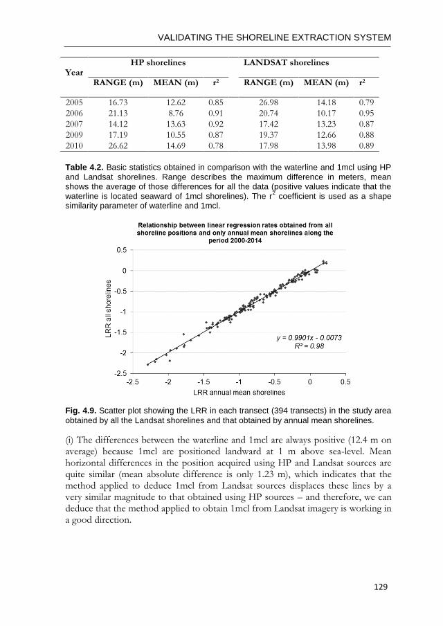
VALIDATING THE SHORELINE EXTRACTION SYSTEM
129
Year HP shorelines
LANDSAT shorelines
RANGE (m) MEAN (m) r2 RANGE (m) MEAN (m) r2
2005 16.73 12.62 0.85 26.98 14.18 0.79
2006 21.13 8.76 0.91 20.74 10.17 0.95
2007 14.12 13.63 0.92 17.42 13.23 0.87
2009 17.19 10.55 0.87 19.37 12.66 0.88
2010 26.62 14.69 0.78 17.98 13.98 0.89
Table 4.2. Basic statistics obtained in comparison with the waterline and 1mcl using HP
and Landsat shorelines. Range describes the maximum difference in meters, mean shows the average of those differences for all the data (positive values indicate that the waterline is located seaward of 1mcl shorelines). The r
2 coefficient is used as a shape
similarity parameter of waterline and 1mcl.
Fig. 4.9. Scatter plot showing the LRR in each transect (394 transects) in the study area
obtained by all the Landsat shorelines and that obtained by annual mean shorelines.
(i) The differences between the waterline and 1mcl are always positive (12.4 m on average) because 1mcl are positioned landward at 1 m above sea-level. Mean horizontal differences in the position acquired using HP and Landsat sources are quite similar (mean absolute difference is only 1.23 m), which indicates that the method applied to deduce 1mcl from Landsat sources displaces these lines by a very similar magnitude to that obtained using HP sources – and therefore, we can deduce that the method applied to obtain 1mcl from Landsat imagery is working in a good direction.
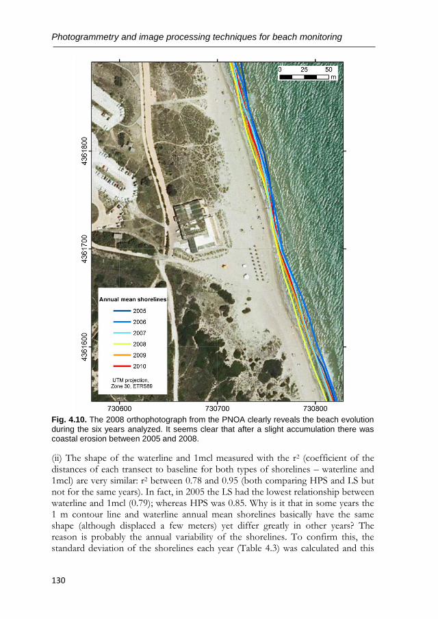
Photogrammetry and image processing techniques for beach monitoring
130
Fig. 4.10. The 2008 orthophotograph from the PNOA clearly reveals the beach evolution
during the six years analyzed. It seems clear that after a slight accumulation there was coastal erosion between 2005 and 2008.
(ii) The shape of the waterline and 1mcl measured with the r2 (coefficient of the distances of each transect to baseline for both types of shorelines – waterline and 1mcl) are very similar: r2 between 0.78 and 0.95 (both comparing HPS and LS but not for the same years). In fact, in 2005 the LS had the lowest relationship between waterline and 1mcl (0.79); whereas HPS was 0.85. Why is it that in some years the 1 m contour line and waterline annual mean shorelines basically have the same shape (although displaced a few meters) yet differ greatly in other years? The reason is probably the annual variability of the shorelines. To confirm this, the standard deviation of the shorelines each year (Table 4.3) was calculated and this
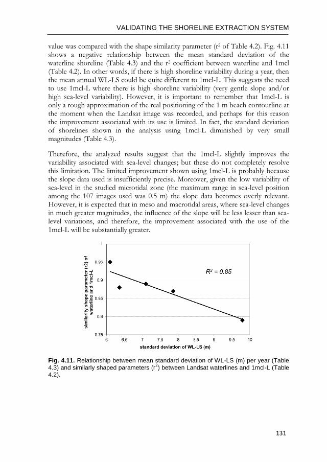
VALIDATING THE SHORELINE EXTRACTION SYSTEM
131
value was compared with the shape similarity parameter (r2 of Table 4.2). Fig. 4.11 shows a negative relationship between the mean standard deviation of the waterline shoreline (Table 4.3) and the r2 coefficient between waterline and 1mcl (Table 4.2). In other words, if there is high shoreline variability during a year, then the mean annual WL-LS could be quite different to 1mcl-L. This suggests the need to use 1mcl-L where there is high shoreline variability (very gentle slope and/or high sea-level variability). However, it is important to remember that 1mcl-L is only a rough approximation of the real positioning of the 1 m beach contourline at the moment when the Landsat image was recorded, and perhaps for this reason the improvement associated with its use is limited. In fact, the standard deviation of shorelines shown in the analysis using 1mcl-L diminished by very small magnitudes (Table 4.3).
Therefore, the analyzed results suggest that the 1mcl-L slightly improves the variability associated with sea-level changes; but these do not completely resolve this limitation. The limited improvement shown using 1mcl-L is probably because the slope data used is insufficiently precise. Moreover, given the low variability of sea-level in the studied microtidal zone (the maximum range in sea-level position among the 107 images used was 0.5 m) the slope data becomes overly relevant. However, it is expected that in meso and macrotidal areas, where sea-level changes in much greater magnitudes, the influence of the slope will be less lesser than sea-level variations, and therefore, the improvement associated with the use of the 1mcl-L will be substantially greater.
Fig. 4.11. Relationship between mean standard deviation of WL-LS (m) per year (Table
4.3) and similarly shaped parameters (r2) between Landsat waterlines and 1mcl-L (Table
4.2).
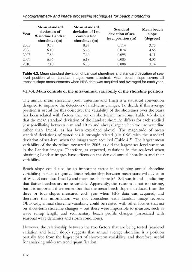
Photogrammetry and image processing techniques for beach monitoring
132
Year
Mean standard deviation of
Waterline Landsat shorelines (m)
Mean standard deviation of 1 m
contour line shorelines (m)
Standard deviation of sea
level position (m)
Mean beach slope
(degrees)
2005 9.79 8.87 0.114 3.75
2006 6.10 5.76 0.074 4.66
2007 7.86 7.66 0.095 4.11
2009 6.36 6.18 0.085 4.06
2010 7.10 6.75 0.088 3.74
Table 4.3. Mean standard deviation of Landsat shorelines and standard deviation of sea-
level position when Landsat images were acquired. Mean beach slope covers all transect slope measurements when HPS data was acquired and averaged for each year.
4.1.4.4. Main controls of the intra-annual variability of the shoreline position
The annual mean shoreline (both waterline and 1mcl) is a statistical convention designed to improve the detection of mid-term changes. To decide if this average position is useful for this objective, the variability of the shorelines over the years has been related with factors that act on short-term variations. Table 4.3 shows that the mean standard deviation of the Landsat shoreline differs for each studied year (oscillating between 6 m and 10 m and always larger when we use waterline rather than 1mcl-L, as has been explained above). The magnitude of mean standard deviations of waterlines is strongly related (r2= 0.96) with the standard deviation of sea-level when the images were acquired (Table 4.3). The largest mean variability of the shorelines occurred in 2005, as did the largest sea-level variation in the Landsat images. Therefore, as expected, variations in the sea-level when obtaining Landsat images have effects on the derived annual shorelines and their variability.
Beach slope could also be an important factor in explaining annual shoreline variability; in fact, a negative linear relationship between mean standard deviation of WL-LS (and also 1mcl-L) and mean beach slope (r2=0.4) was found – indicating that flatter beaches are more variable. Apparently, this relation is not too strong, but it is important if we remember that the mean beach slope is deduced from the three or four slopes measured each year when HPS data was acquired, and therefore this information was not coincident with Landsat image records. Obviously, annual shoreline variability could be related with other factors that act on short-term shoreline changes – but these were impossible to measure, such as wave runup length, and sedimentary beach profile changes (associated with seasonal wave dynamics and storm conditions).
However, the relationship between the two factors that are being tested (sea-level variation and beach slope) suggests that annual average shoreline is a position partially free from the largest part of short-term variability, and therefore, useful for analyzing mid-term trend quantification.
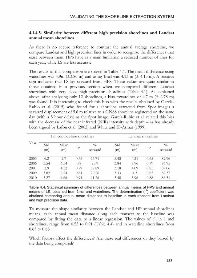
VALIDATING THE SHORELINE EXTRACTION SYSTEM
133
4.1.4.5. Similarity between different high precision shorelines and Landsat annual mean shorelines
As there is no secure reference to contrast the annual average shoreline, we compare Landsat and high precision lines in order to recognise the differences that exist between them. HPS have as a main limitation a reduced number of lines for each year, while LS are less accurate.
The results of this comparison are shown in Table 4.4. The mean difference using waterlines was 4.9m (±3.86 m) and using 1mcl was 4.13 m (± 4.15 m). A positive sign indicates that LS lay seaward from HPS. These values are quite similar to those obtained in a previous section when we compared different Landsat shorelines with very close high precision shorelines (Table 4.1). As explained above, after analyzing only 12 shorelines, a bias toward sea of 4.7 m (± 2.78 m) was found. It is interesting to check this bias with the results obtained by García-Rubio et al. (2015) who found for a shoreline extracted from Spot images a seaward displacement of 5.6 m relative to a GNSS shoreline registered on the same day (with a 5 hour delay) as the Spot image. García-Rubio et al. related this bias with the decrease of the near infrared (NIR) intensity with depth – as has already been argued by Lafon et al. (2002) and White and El-Asmar (1999).
Year
1 m contour-line shorelines Landsat shorelines
Std (m)
Mean (m)
r2 %
seaward
Std (m)
Mean (m)
r2 %
seaward
2005 6.2 2.7 0.55 73.71 5.48 4.21 0.65 82.96
2006 3.54 6.54 0.8 95.9 3.84 7.96 0.79 96.95
2007 3.9 4.52 0.79 87.89 3.18 4.09 0.85 89.06
2009 3.82 2.24 0.81 70.26 3.33 4.3 0.85 89.37
2010 3.27 4.66 0.91 91.26 3.48 3.96 0.88 86.51
Table 4.4. Statistical summary of differences between annual means of HPS and annual
means of LS, obtained from 1mcl and waterlines. The determination (r2) coefficient was
obtained comparing annual mean distances to baseline in each transect from Landsat and high precision data.
To measure the shape similarity between the Landsat and HP annual shorelines means, each annual mean distance along each transect to the baseline was compared by fitting the data to a linear regression. The values of r2, in 1 mcl shorelines, range from 0.55 to 0.91 (Table 4.4) and in waterline shorelines from 0.65 to 0.88.
Which factors affect the differences? Are these real differences or they biased by the data being compared?
Photogrammetry and image processing techniques for beach monitoring
134
(i) Partial differences could be related with the accuracy of the Landsat shoreline extraction method (5 m RMSE). However, this cannot explain mean bias toward the sea.
(ii) The beach slope seems to influence these differences. Fig. 4.12 shows the measured differences between the annual average 1mcl-HP and 1mcl-L and the beach slope in each transect. To detect more clearly this relationship, the mean slope was calculated for sets of data grouped in bins defined by 1 m differences between the 1mcl-HP and the 1mcl-L shown as large points (Fig. 4.12). There is a weak relation in which seaward displacement of Landsat shorelines increases when the beach slope increases. What could be the reason for this response? Probably, shorelines in flatter beach segments are more variable during the year than steeper segments (Fig. 4.13). Moreover, as many more LS than HP have been used, it is therefore more likely that seaward shoreline positions will be found.
(iii) The HPS were not registered during the summer (with one exception – August 2009) while 36% of LS were captured during the summer. A previous study carried out in the study zone indicates that these beaches increase the volume of sand during summer (Pardo-Pascual, et al., 2011). Therefore, it is likely that the HP annual mean shorelines (without summer registers) will be landward of the real annual average shoreline position.
The measured bias toward the sea when comparing the HPS and LS should be tempered by the fact that the effect that produces the bulk of the HPS did not include summer data. However, the predominance of this bias, even in data from 2009 (which includes summer HP) and the coincidence with the analysis of individual shorelines, and with observations by other authors (García-Rubio et al., 2015), suggests that the bias is real and that shorelines extracted from Landsat are between 4 and 5 m offshore from the line defined as the water’s edge. Therefore, as mean annual Landsat shorelines are arranged very near to those obtained by more accurate surveying methods, is clear that they can be used as source data to perform an analysis of mid-term evolution.
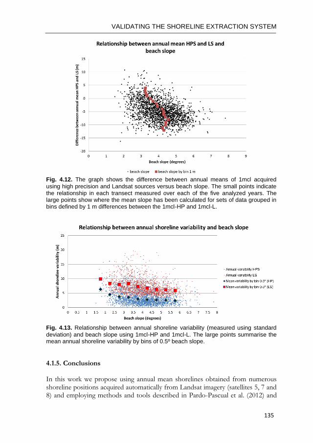
VALIDATING THE SHORELINE EXTRACTION SYSTEM
135
Fig. 4.12. The graph shows the difference between annual means of 1mcl acquired
using high precision and Landsat sources versus beach slope. The small points indicate the relationship in each transect measured over each of the five analyzed years. The large points show where the mean slope has been calculated for sets of data grouped in bins defined by 1 m differences between the 1mcl-HP and 1mcl-L.
Fig. 4.13. Relationship between annual shoreline variability (measured using standard
deviation) and beach slope using 1mcl-HP and 1mcl-L. The large points summarise the mean annual shoreline variability by bins of 0.5º beach slope.
4.1.5. Conclusions
In this work we propose using annual mean shorelines obtained from numerous shoreline positions acquired automatically from Landsat imagery (satellites 5, 7 and 8) and employing methods and tools described in Pardo-Pascual et al. (2012) and
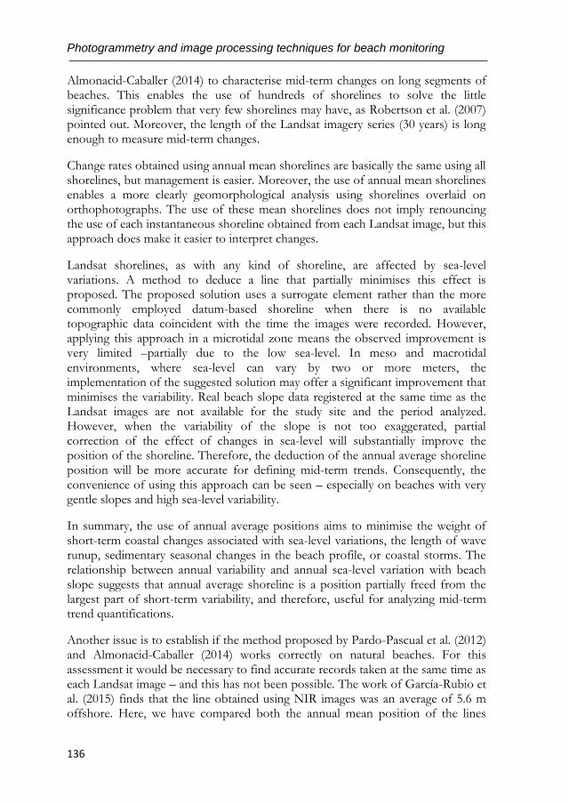
Photogrammetry and image processing techniques for beach monitoring
136
Almonacid-Caballer (2014) to characterise mid-term changes on long segments of beaches. This enables the use of hundreds of shorelines to solve the little significance problem that very few shorelines may have, as Robertson et al. (2007) pointed out. Moreover, the length of the Landsat imagery series (30 years) is long enough to measure mid-term changes.
Change rates obtained using annual mean shorelines are basically the same using all shorelines, but management is easier. Moreover, the use of annual mean shorelines enables a more clearly geomorphological analysis using shorelines overlaid on orthophotographs. The use of these mean shorelines does not imply renouncing the use of each instantaneous shoreline obtained from each Landsat image, but this approach does make it easier to interpret changes.
Landsat shorelines, as with any kind of shoreline, are affected by sea-level variations. A method to deduce a line that partially minimises this effect is proposed. The proposed solution uses a surrogate element rather than the more commonly employed datum-based shoreline when there is no available topographic data coincident with the time the images were recorded. However, applying this approach in a microtidal zone means the observed improvement is very limited –partially due to the low sea-level. In meso and macrotidal environments, where sea-level can vary by two or more meters, the implementation of the suggested solution may offer a significant improvement that minimises the variability. Real beach slope data registered at the same time as the Landsat images are not available for the study site and the period analyzed. However, when the variability of the slope is not too exaggerated, partial correction of the effect of changes in sea-level will substantially improve the position of the shoreline. Therefore, the deduction of the annual average shoreline position will be more accurate for defining mid-term trends. Consequently, the convenience of using this approach can be seen – especially on beaches with very gentle slopes and high sea-level variability.
In summary, the use of annual average positions aims to minimise the weight of short-term coastal changes associated with sea-level variations, the length of wave runup, sedimentary seasonal changes in the beach profile, or coastal storms. The relationship between annual variability and annual sea-level variation with beach slope suggests that annual average shoreline is a position partially freed from the largest part of short-term variability, and therefore, useful for analyzing mid-term trend quantifications.
Another issue is to establish if the method proposed by Pardo-Pascual et al. (2012) and Almonacid-Caballer (2014) works correctly on natural beaches. For this assessment it would be necessary to find accurate records taken at the same time as each Landsat image – and this has not been possible. The work of García-Rubio et al. (2015) finds that the line obtained using NIR images was an average of 5.6 m offshore. Here, we have compared both the annual mean position of the lines

VALIDATING THE SHORELINE EXTRACTION SYSTEM
137
acquired from Landsat imagery against the annual mean shorelines obtained using more accurate systems – as well as instantaneous shorelines obtained from Landsat and, others acquired with more precise techniques a few days before or later. In both cases, the Landsat shorelines are biased from HPS towards the sea by around 4 to 5 m: 4.7 meters for instantaneous shorelines and 4.9 m for mean annual shorelines (4.1 m using the 1 m contour line position). However, part of these deviations may be explained by the seasonal variation of the analyzed beaches (usually being wider in the summer). As 36% of the Landsat shorelines were acquired in summer and only one of the HPS, it is possible that the deviation may be something less than 4 m. In any case, the offshore displacement of the water's edge is less than the expected deviation using the method applied for the coastline extraction (about 5 m).
Hence, the results obtained suggest the possibility of using Landsat imagery as a new source for describing mid-term changes in beaches – and being much more useful if this analysis is performed using annual mean shorelines obtained by tens of Landsat shorelines acquired in the same year.

Photogrammetry and image processing techniques for beach monitoring
138
VALIDATING THE SHORELINE EXTRACTION SYSTEM
139
4.2. ASSESSING THE ACCURACY OF AUTOMATICALLY
EXTRACTED SHORELINES ON MICROTIDAL BEACHES FROM LANDSAT 7, LANDSAT 8 & SENTINEL-2 IMAGERY
This work evaluates the accuracy of shoreline positions obtained from the infrared (IR) bands of Landsat 7, Landsat 8, and Sentinel-2 imagery on natural beaches. A workflow for sub-pixel shoreline extraction, already tested on seawalls, is used. The present work analyzes the behavior of that workflow and resultant shorelines on a micro-tidal (<20cm) sandy beach and makes a comparison with other more accurate sets of shorelines. These other sets were obtained using differential GNSS surveys and terrestrial photogrammetry techniques through the C-Pro monitoring system. A set of 21 sub-pixel shorelines and their respective high precision lines served for the evaluation. The results prove that NIR bands can easily confuse the shoreline with whitewater, whereas SWIR bands are more reliable in this respect. Moreover, it verifies that shorelines obtained from bands 11 and 12 of Sentinel-2 are very similar to those obtained with bands 6 and 7 of Landsat 8 (-0.75 ±2.5 m, negative sign indicate landward bias). The variability of the brightness in the terrestrial zone influences shoreline detection: brighter zones cause a small landward bias. A relation between the swell and shoreline accuracy is found, mainly identified in images obtained from Landsat 8 and Sentinel-2. On natural beaches, the mean shoreline error varies with the type of image used. After analyzing the whole set of shorelines detected from Landsat 7, we conclude that the mean horizontal error is 4.63 m (±6.55 m) and 5.50 m (±4.86 m), respectively, for high and low gain images. For the Landsat 8 and Sentinel-2 shorelines, the mean error reaches 3.06 m (±5.79 m).
4.2.1. Introduction
The shoreline is a morphological feature that is often used to understand how beach systems work and how their development is affected by mid-long-term processes. However, the definition of shoreline may be difficult as many different indicators are used in the bibliography, especially in macro-tidal coasts (Boak & Turner, 2005). While the land-water line has been used in micro-tidal zones, the dry/wet sand line has been used in the macro-tidal area (understanding it as the shoreline for the last highest tidal position). Traditionally, the main data source for shoreline acquisition has been aerial imagery (Ford, 2013; Jones et al., 2009; Morton et al., 2004). However, some authors (Stockdon et al., 2002; Ruggiero et al., 2005; Moore et al., 2006; List et al., 2006) have criticized this shoreline because it may be affected by the sea level. They prefer to use the ishohypse at the highest tidal position (datum based shoreline) as it would be more reliable for beach profile changes. This 3D information is normally obtained by GNSS mapping (Global Navigation Satellite System) (Pardo-Pascual et al., 2005; Psuty & Silvera, 2011), LiDAR (White & Wang, 2003; Shrestha et al., 2005; Gares et al., 2006; Smeeckaert et al., 2013) or TLS (Terrestrial Laser Scanner) (Hobbs et al., 2010). These 3D
Photogrammetry and image processing techniques for beach monitoring
140
resources may offer high accuracy data: up to 5 cm (horizontal and vertical) on differential GNSS surveys; and up to 10 cm (horizontal) and 20 cm (vertical) depending on each LiDAR flight demands. Nevertheless, mapping hundreds of kilometers at a high frequency may be difficult.
Although 3D data offers more complete information, other works show that 2D sources are also useful. Video-monitoring techniques (Holman & Stanley, 2007; Davidson et al., 2007; Archetti et al., 2008), given that they can record the shoreline with high frequency, are useful in dynamic areas such as sandy beaches (the variability of the beach and the most landward shoreline position during a storm can be obtained almost in real time). The mean shoreline position may be calculated on an hourly, daily, or weekly bases for trend studies. The main constraint for video-monitorization is that it only works with very limited spaces, normally urban beaches where a camera can be installed on a building. To cover wider areas (hundreds of kilometers), both optical (Maiti & Bhattacharya, 2009; Vandebroek et al., 2017) and radar (Mann & Westphal, 2014) satellite imagery are used – but these techniques remain limited by the temporal frequency of satellite observations. This lack of frequency may cause problems when measuring natural beaches, as the shoreline position may be so affected by the sea level that its position loses geomorphological meaning. However, compiling tens of instantaneous shorelines during a specific time period may be useful for estimating mean shoreline positions and trends during the medium and long-term (Almonacid-Caballer et al., 2016).
Landsat is one of the most used satellite imagery options, especially since the USGS announced in 2008 that the images would be freely available. New research became possible as, through Landsat 5, 7 and 8 (with a revisit period of 16 days), dozens of images may be obtained for the same place during a year. Furthermore, historical series are available as Landsat 5 has been recording data from 1984 to 2011, Landsat 7 from 1999, and Landsat 8 from 2013. Following the same free availability criteria, since June 2015, the ESA (European Space Agency) satellite Sentinel-2A has been capturing images with a higher spatial and temporal resolution than Landsat 8. Working together with its newest twin Sentinel-2B – launched in March 2017 – the frequency of Sentinel-2 image registration has increased to five days (and even two or three days in medium latitudes). The combination of Landsat 8, Sentinel-2A, and Sentinel-2B provides a global median average revisit interval of 2.9 days (Li & Roy, 2017).
Figure 4.14 shows a comparison between Landsat (7 and 8) and Sentinel-2. Specifically, it shows the spectral and spatial information of ETM+ (Enhanced Thematic Mapper Plus), OLI (Operational Land Imager), and MSI (MultiSpectral Instrument) sensors, belonging to Landsat 7, Landsat 8, and Sentinel-2A satellites, respectively. The NIR (near infrared) region between Landsat 8 (band 5) and Sentinel-2A (band 8A) are similar, but differ significantly to band 4 in Landsat 7 (with a very much greater bandwidth). The same occurs in SWIR (short wave
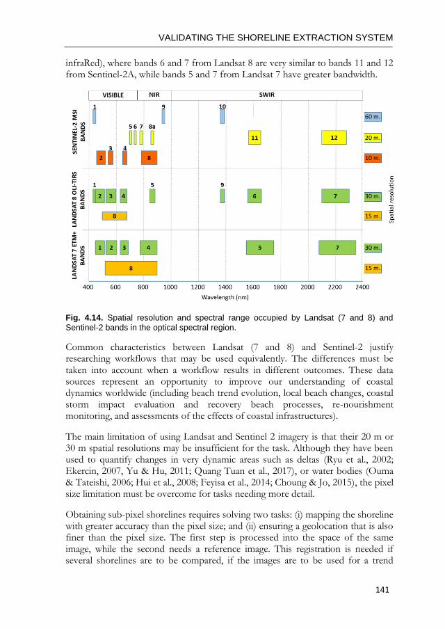
VALIDATING THE SHORELINE EXTRACTION SYSTEM
141
infraRed), where bands 6 and 7 from Landsat 8 are very similar to bands 11 and 12 from Sentinel-2A, while bands 5 and 7 from Landsat 7 have greater bandwidth.
Fig. 4.14. Spatial resolution and spectral range occupied by Landsat (7 and 8) and
Sentinel-2 bands in the optical spectral region.
Common characteristics between Landsat (7 and 8) and Sentinel-2 justify researching workflows that may be used equivalently. The differences must be taken into account when a workflow results in different outcomes. These data sources represent an opportunity to improve our understanding of coastal dynamics worldwide (including beach trend evolution, local beach changes, coastal storm impact evaluation and recovery beach processes, re-nourishment monitoring, and assessments of the effects of coastal infrastructures).
The main limitation of using Landsat and Sentinel 2 imagery is that their 20 m or 30 m spatial resolutions may be insufficient for the task. Although they have been used to quantify changes in very dynamic areas such as deltas (Ryu et al., 2002; Ekercin, 2007, Yu & Hu, 2011; Quang Tuan et al., 2017), or water bodies (Ouma & Tateishi, 2006; Hui et al., 2008; Feyisa et al., 2014; Choung & Jo, 2015), the pixel size limitation must be overcome for tasks needing more detail.
Obtaining sub-pixel shorelines requires solving two tasks: (i) mapping the shoreline with greater accuracy than the pixel size; and (ii) ensuring a geolocation that is also finer than the pixel size. The first step is processed into the space of the same image, while the second needs a reference image. This registration is needed if several shorelines are to be compared, if the images are to be used for a trend
Photogrammetry and image processing techniques for beach monitoring
142
study, or if a shoreline must be evaluated with a reference line mapped using more accurate techniques.
The most common extraction techniques for sub-pixel shorelines involve soft classification and super-resolution mapping (Foody et al., 2005; Muslim et al., 2006; Liu et al., 2016). These techniques try to discover the land-water edge within each pixel but have some constraints derived from the level of resampling which could cause problems in connections and a lack of smoothness in the final delineated line. Li et al. (2015) propose integrating back-propagation neural networks and genetic algorithms to achieve a super-resolution mapping of flooded wetland. Li et al. (2016) describe a multiple super-resolution mapping method, obtaining results that are more accurate than those obtained using an individual method. Shi et al. (2017) propose a method that combines multiple super-resolution realizations obtained using the indicator-geostatistics based method. Liu et al. (2017b) propose a method to obtain a super-resolution shoreline based on a segmentation method previously proposed by Cipolleti et al. (2012). In this method, after obtaining an initial shoreline by applying a thresholding classification, the most probable line position within a 2x2 kernel is assessed. A similar proposal was applied by Ruiz et al. (2007) being later modified and assessed by Pardo-Pascual et al. (2012), as well as being improved by Almonacid-Caballer (2014). The algorithm starts with the detection of a pixel level shoreline and, by fitting a 5th-degree polynomial function around each of these pixels, detects the inflexion line where the shoreline is expected to be. This is the methodology followed in this work.
Although both Landsat and Sentinel-2 scenes are georeferenced, small inconsistencies in the geolocation of the processed images from USGS and ESA can worsen the accuracy of results. The quality requirements of L1T Landsat 8 data include a geolocation uncertainty of less than 12 m of circular error for the OLI spectral bands (Iron et al., 2012). These products have improved their geometric accuracy with respect to previous products because the Landsat 8 sensor has a fully operational onboard global positioning system (GPS) for directly measuring exterior orientation, rather than inferring it from ground control systems – as happened with previous Landsat geolocation algorithms (Roy et al., 2014). For Sentinel-2, the geolocation accuracy regarding multi-temporal registration has been established at 1.2 pixels (Clerc, 2017). Almonacid-Caballer et al. (2017) demonstrate that the sub-pixel registration improves the final location of each shoreline: 47 shorelines from Landsat 7 were analyzed, starting from an initial mean error of 12.9 (±15.33) m to 3.75 (±7.01) m after sub-pixel georeferencing. For image registration, a local upsampling of the Fourier transform is followed around the correlation peak, named LUFT (Guizar-Sicairos et al., 2008; Wang et al., 2011). It is demonstrated that applying LUFT on 30 m/pixel images leads to a maximum of 3 m of registration error when each satellite image is matched with a high-resolution orthophotoimage (0.5m/pixel).
VALIDATING THE SHORELINE EXTRACTION SYSTEM
143
The shoreline extraction and registration joint workflow (Pardo-Pascual et al., 2012; Almonacid-Caballer, 2014) was assessed on fixed line sections of several seawalls along the coast. These studies revealed that the land cover distribution was affecting the final shoreline position by biasing it. This bias or error was modeled using least squares in function of the mean and standard deviation of the pixel values surrounding each point of the shoreline. Using these model (polynomial radiometric correction or PRC), a given point of the shoreline could be refined in function of the digital values of its neighboring pixels. A final evaluation relative to the seawalls (Almonacid-Caballer, 2014) shows that the standard deviations were: Landsat 5: 5.68 m (NIR) 5.39 m (SWIR1) and 6.08 m (SWIR2); Landsat 7: 5.20 m (NIR), 5.13 m (SWIR1) and 5.37 m (SWIR2); and Landsat 8: 4.77 m (NIR), 4.80 m (SWIR1) and 5.18 m (SWIR2).
As mentioned earlier, the main goal of this type of work is the study of beach dynamics. The three-step workflow described (sub-pixel extraction, LUFT georeferencing, and PRC) has already been used in several tasks: storm impact on beach studies (Pardo-Pascual et al., 2014); coastal evolution studies (Sánchez-García et al., 2015); or annual mean shoreline extraction (Almonacid-Caballer et al., 2016). These studies characterize beach trends on a specific micro-tidal (up to 20 cm) area. While these studies assume the standard deviation already assessed in previous works, the same behavior of the shorelines on seawalls and natural beaches cannot be expected. An evaluation on sandy beaches is therefore needed. While the line along a seawall remains constant, the accuracy of shorelines on natural beaches may be affected by the circumstances of that instant: (i) the slope in natural beaches is lower than for seawalls; (ii) the water is shallower in beaches and deeper in seawalls; (iii) a slight beach slope along with energetic conditions can cause a wide surf zone where we often find water with rough patterns or even whitewater; and (iv) a wide wet zone may also affect the outcome of the workflow as it defines a different wet/dry line. Assessing instantaneous shorelines requires knowing the exact position of the shore, the wave conditions, and the appearance of the beach when each satellite captures an image. This implies the need to measure the land-water line in detail using sufficiently precise techniques, and having a system for visualizing the coast. Photographing the shoreline when the satellite is passing overhead enables the state of the sea to be registered (swell, whitewater, wet surface on the beach) and provides sufficient detail on the state of the coast at that moment.
The main goal of this work is to assess the accuracy of instantaneous shorelines – understood as the land-water boundary— on natural sandy beaches from satellite images produced by Landsat 7, Landsat 8, and Sentinel-2. A reference area along the dike of the port of Valencia is taken as a fixed reference for each date to corroborate the accuracy reached on seawalls in previous evaluations (Almonacid-Caballer, 2014). Once it is ensured, the behavior on a natural beach will be used to analyze the instantaneous factors that may affect shoreline accuracy. Specific points to analyze are the differing behaviors of each sensor/band, and the factors
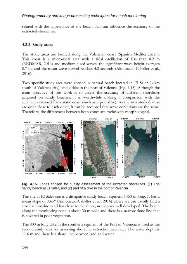
Photogrammetry and image processing techniques for beach monitoring
144
related with the appearance of the beach that can influence the accuracy of the extracted shorelines.
4.2.2. Study areas
The study areas are located along the Valencian coast (Spanish Mediterranean). This coast is a micro-tidal area with a tidal oscillation of less than 0.2 m (REDMAR, 2014) and medium-sized waves: the significant wave height averages 0.7 m, and the mean wave period reaches 4.2 seconds (Almonacid-Caballer et al., 2016).
Two specific study area were chosen: a natural beach located in El Saler (6 km south of Valencia city); and a dike in the port of Valencia (Fig. 4.15). Although the main objective of this work is to assess the accuracy of different shorelines acquired on sandy beaches, it is worthwhile making a comparison with the accuracy obtained for a static coast (such as a port dike). As the two studied areas are quite close to each other, it can be accepted that wave conditions are the same. Therefore, the differences between both zones are exclusively morphological.
Fig. 4.15. Zones chosen for quality assessment of the extracted shorelines. (1) The
sandy beach at El Saler, and (2) part of a dike in the port of Valencia.
The site at El Saler site is a dissipative sandy beach segment 1450 m long. It has a mean slope of 3.65° (Almonacid-Caballer et al., 2016) where we can usually find a small submarine sand bar close to the shore, not always well developed. The beach along the monitoring zone is about 30 m wide and there is a narrow dune line that is covered in poor vegetation.
The 800 m long dike in the southern segment of the Port of Valencia is used as the second study area for assessing shoreline extraction accuracy. The water depth is 11.6 m and there is a sharp line between land and water.
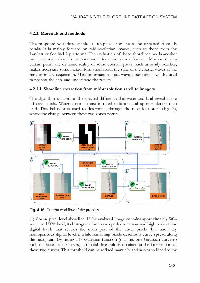
VALIDATING THE SHORELINE EXTRACTION SYSTEM
145
4.2.3. Materials and methods
The proposed workflow enables a sub-pixel shoreline to be obtained from IR bands. It is mainly focused on mid-resolution images, such as those from the Landsat or Sentinel-2 platforms. The evaluation of those shorelines needs another more accurate shoreline measurement to serve as a reference. Moreover, at a certain point, the dynamic reality of some coastal spaces, such as sandy beaches, makes necessary some meta-information about the state of the coastal waves at the time of image acquisition. Meta-information – sea wave conditions – will be used to process the data and understand the results.
4.2.3.1. Shoreline extraction from mid-resolution satellite imagery
The algorithm is based on the spectral difference that water and land reveal in the infrared bands. Water absorbs most infrared radiation and appears darker than land. This behavior is used to determine, through the next four steps (Fig. 3), where the change between these two zones occurs.
Fig. 4.16. Current workflow of the process.
(1) Coarse pixel-level shoreline. If the analyzed image contains approximately 50% water and 50% land, its histogram shows two peaks: a narrow and high peak at low digital levels that reveals the main part of the water pixels (low and very homogeneous digital levels); while remaining pixels describe a curve spread along the histogram. By fitting a bi-Gaussian function (that fits one Gaussian curve to each of those peaks/curves), an initial threshold is obtained at the intersection of these two curves. This threshold can be refined manually and serves to binarize the
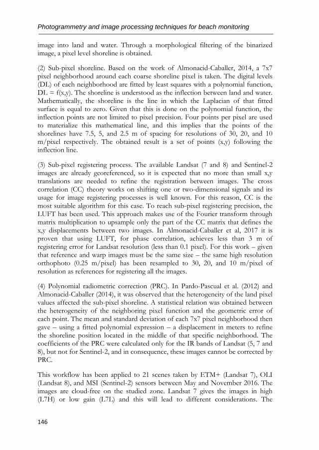
Photogrammetry and image processing techniques for beach monitoring
146
image into land and water. Through a morphological filtering of the binarized image, a pixel level shoreline is obtained.
(2) Sub-pixel shoreline. Based on the work of Almonacid-Caballer, 2014, a 7x7 pixel neighborhood around each coarse shoreline pixel is taken. The digital levels (DL) of each neighborhood are fitted by least squares with a polynomial function, DL = f(x,y). The shoreline is understood as the inflection between land and water. Mathematically, the shoreline is the line in which the Laplacian of that fitted surface is equal to zero. Given that this is done on the polynomial function, the inflection points are not limited to pixel precision. Four points per pixel are used to materialize this mathematical line, and this implies that the points of the shorelines have 7.5, 5, and 2.5 m of spacing for resolutions of 30, 20, and 10 m/pixel respectively. The obtained result is a set of points (x,y) following the inflection line.
(3) Sub-pixel registering process. The available Landsat (7 and 8) and Sentinel-2 images are already georeferenced, so it is expected that no more than small x,y translations are needed to refine the registration between images. The cross correlation (CC) theory works on shifting one or two-dimensional signals and its usage for image registering processes is well known. For this reason, CC is the most suitable algorithm for this case. To reach sub-pixel registering precision, the LUFT has been used. This approach makes use of the Fourier transform through matrix multiplication to upsample only the part of the CC matrix that defines the x,y displacements between two images. In Almonacid-Caballer et al, 2017 it is proven that using LUFT, for phase correlation, achieves less than 3 m of registering error for Landsat resolution (less than 0.1 pixel). For this work – given that reference and warp images must be the same size – the same high resolution orthophoto (0.25 m/pixel) has been resampled to 30, 20, and 10 m/pixel of resolution as references for registering all the images.
(4) Polynomial radiometric correction (PRC). In Pardo-Pascual et al. (2012) and Almonacid-Caballer (2014), it was observed that the heterogeneity of the land pixel values affected the sub-pixel shoreline. A statistical relation was obtained between the heterogeneity of the neighboring pixel function and the geometric error of each point. The mean and standard deviation of each 7x7 pixel neighborhood then gave – using a fitted polynomial expression – a displacement in meters to refine the shoreline position located in the middle of that specific neighborhood. The coefficients of the PRC were calculated only for the IR bands of Landsat (5, 7 and 8), but not for Sentinel-2, and in consequence, these images cannot be corrected by PRC.
This workflow has been applied to 21 scenes taken by ETM+ (Landsat 7), OLI (Landsat 8), and MSI (Sentinel-2) sensors between May and November 2016. The images are cloud-free on the studied zone. Landsat 7 gives the images in high (L7H) or low gain (L7L) and this will lead to different considerations. The
VALIDATING THE SHORELINE EXTRACTION SYSTEM
147
shorelines have been extracted from the available near and short-wave infrared bands, NIR, SWIR 1 and SWIR 2 (Fig. 4.14).
The images were taken around summer 2016 (Fig. 4.17). Most of the Landsat 8 images were taken before the summer, while all the Sentinel-2 images were taken afterwards. Landsat 7 images are more randomly distributed. Analyzing the metadata, the satellite acquisition can be scheduled. The start-stop acquisition time of Landsat 8 and Landsat 7 scenes are 10:43:20–10:43:52 a.m. and 10:45:22–10:45:49 a.m. (UTC time). This interval moves slightly some seconds. The acquisition time for Sentinel is less clear as start-stop acquisition time is 10:54:28–11:07:02 a.m. However, in our beaches, this interval does not imply any tidal effect.
Fig. 4.17. Temporal distribution of the 21 scenes acquired from three satellite platforms.
Note that on 8 October 2016 the study zones were registered both by Landsat 8 and Sentinel-2 with only 18 minutes of difference.
4.2.3.2. Reference data for high precision shorelines
The reference data is crucial. In stable zones, such as ports or seawalls, this is not a problem because the shoreline is not expected to move and the same reference line (in this case, a shoreline digitized in a 0.25 m/pixel orthophotograph) can be used for all the dates. However, this becomes more difficult in unstable zones such as sandy beaches. The shorelines in natural spaces are constantly moving, and this forces the field reference shoreline to be taken at the same time as the satellite image. This frees the shorelines evaluation from any tidal influence.
For this research, the reference shorelines are located on El Saler beach using two methodologies:
(i) Accurate topographic differential GNSS measurements were taken. The land-water boundary is measured by storing coordinates every second with an estimated accuracy of 3-5 cm (Prochniewicz et al., 2016; Paziewski & Wielgosz, 2017).
(ii) A terrestrial photogrammetric perspective was used and photographs were taken from a building near the reference area. The photos were taken with a digital reflex camera (SONY DSLR-A330) and processed with C-Pro, a coastal projector monitoring system (Sánchez-García et al., 2017). C-Pro uses GCPs and the horizon constraint to compute the photo resection process. The image can then be
Temporal distribution of used satellite images
20/May 9/Jun 29/Jun 19/Jul 8/Aug 28/Aug 17/Sep 7/Oct 27/Oct 16/Nov
Landsat 7-H Landsat 7-L Landsat 8 Sentinel 2
Photogrammetry and image processing techniques for beach monitoring
148
projected on a digital elevation model (DEM) or a specific plane. For this work, the mean sea level (MSL) is obtained instantaneously from the sea level gauge in the port of Valencia, located 8.5 km from the study area. This level has been used to establish the specific elevation value to project each image and resolve the instantaneous shoreline.
Both sets of data are useful in a synergistic way. The terrestrial photographs were taken at the moment when it was expected that the satellites acquired the image – although both moments may not be perfectly coincident. The GPS-shoreline is measured at a moment near the satellite image acquisition. Each GPS point is taken at the instantaneous land-water limit (which is constantly moving as it is a natural beach). Horizontally, the difference between these photographic and GPS- shorelines was measured and a mean error of 0.15 (±1.05) m was obtained. Vertically, comparing the mean elevation value of the GPS-shoreline and the MSL value, we computed a mean difference (|ZMSL- ZGPS-line|) of 0.067 m for all days. In consequence, photographic and GPS shorelines can be considered coincident, while the very small distance between them serves to indicate the magnitude of the natural shoreline movement for each date. Moreover, the terrestrial images offer additional environmental information (for example, the existence of whitewater that can affect the shorelines obtained).
Therefore, for the analysis carried out in the present work, the satellite shorelines were compared with either GPS-shorelines or photo-shorelines. We chose to use the GPS-shoreline except when this information was unavailable – and we then used the digitized shoreline from rectified photos (Fig. 4.18).
In addition, some meta-data (such as significant wave height and peak wave period) was taken from the oceanographic buoy in front of the Port of Valencia.
4.2.3.3. Shoreline accuracy assessment methodology
As each sub-pixel shoreline is integrated by points, the distance from those points to their respective reference line is a measure of the error committed. The distances have been stipulated positive seawards and negative landwards. The mean error indicates the bias of the satellite shorelines, while the standard deviation must be understood as the variability of the shoreline at the image registration moment. As mentioned before, the reference line is taken at the time when the satellite is expected to register the scene and so avoids the effect of the tide in our study.
4.2.4. Results
Subsequently, the PRC (polynomial radiometric correction) effect and accuracies per date and sensors are shown. Within each, the accuracies on the beach shorelines are compared with those obtained at the dike of the port of Valencia. The differences in the errors observed on the beach compared with those
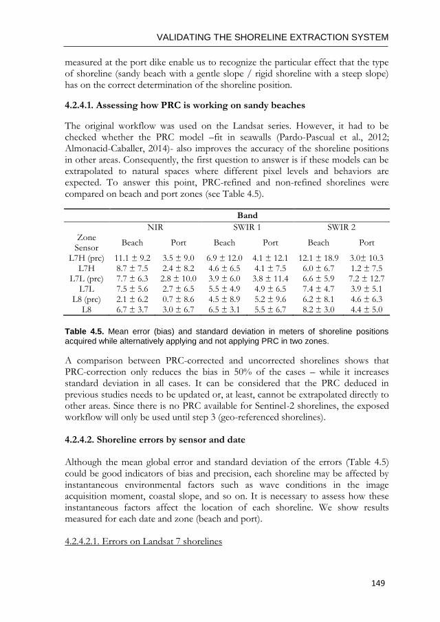
VALIDATING THE SHORELINE EXTRACTION SYSTEM
149
measured at the port dike enable us to recognize the particular effect that the type of shoreline (sandy beach with a gentle slope / rigid shoreline with a steep slope) has on the correct determination of the shoreline position.
4.2.4.1. Assessing how PRC is working on sandy beaches
The original workflow was used on the Landsat series. However, it had to be checked whether the PRC model –fit in seawalls (Pardo-Pascual et al., 2012; Almonacid-Caballer, 2014)- also improves the accuracy of the shoreline positions in other areas. Consequently, the first question to answer is if these models can be extrapolated to natural spaces where different pixel levels and behaviors are expected. To answer this point, PRC-refined and non-refined shorelines were compared on beach and port zones (see Table 4.5).
Band
NIR SWIR 1 SWIR 2 Zone
Sensor Beach Port Beach Port Beach Port
L7H (prc) 11.1 ± 9.2 3.5 ± 9.0 6.9 ± 12.0 4.1 ± 12.1 12.1 ± 18.9 3.0± 10.3 L7H 8.7 ± 7.5 2.4 ± 8.2 4.6 ± 6.5 4.1 ± 7.5 6.0 ± 6.7 1.2 ± 7.5
L7L (prc) 7.7 ± 6.3 2.8 ± 10.0 3.9 ± 6.0 3.8 ± 11.4 6.6 ± 5.9 7.2 ± 12.7 L7L 7.5 ± 5.6 2.7 ± 6.5 5.5 ± 4.9 4.9 ± 6.5 7.4 ± 4.7 3.9 ± 5.1
L8 (prc) 2.1 ± 6.2 0.7 ± 8.6 4.5 ± 8.9 5.2 ± 9.6 6.2 ± 8.1 4.6 ± 6.3 L8 6.7 ± 3.7 3.0 ± 6.7 6.5 ± 3.1 5.5 ± 6.7 8.2 ± 3.0 4.4 ± 5.0
Table 4.5. Mean error (bias) and standard deviation in meters of shoreline positions
acquired while alternatively applying and not applying PRC in two zones.
A comparison between PRC-corrected and uncorrected shorelines shows that PRC-correction only reduces the bias in 50% of the cases – while it increases standard deviation in all cases. It can be considered that the PRC deduced in previous studies needs to be updated or, at least, cannot be extrapolated directly to other areas. Since there is no PRC available for Sentinel-2 shorelines, the exposed workflow will only be used until step 3 (geo-referenced shorelines). 4.2.4.2. Shoreline errors by sensor and date
Although the mean global error and standard deviation of the errors (Table 4.5) could be good indicators of bias and precision, each shoreline may be affected by instantaneous environmental factors such as wave conditions in the image acquisition moment, coastal slope, and so on. It is necessary to assess how these instantaneous factors affect the location of each shoreline. We show results measured for each date and zone (beach and port). 4.2.4.2.1. Errors on Landsat 7 shorelines
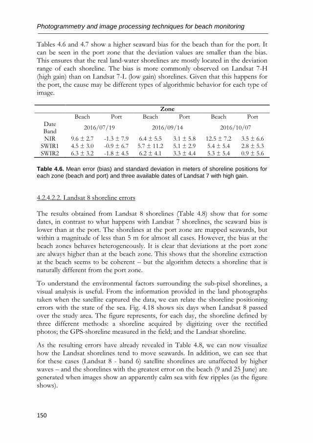
Photogrammetry and image processing techniques for beach monitoring
150
Tables 4.6 and 4.7 show a higher seaward bias for the beach than for the port. It can be seen in the port zone that the deviation values are smaller than the bias. This ensures that the real land-water shorelines are mostly located in the deviation range of each shoreline. The bias is more commonly observed on Landsat 7-H (high gain) than on Landsat 7-L (low gain) shorelines. Given that this happens for the port, the cause may be different types of algorithmic behavior for each type of image.
Zone
Beach Port Beach Port Beach Port Date Band
2016/07/19 2016/09/14 2016/10/07
NIR 9.6 ± 2.7 -1.3 ± 7.9 6.4 ± 5.5 3.1 ± 5.8 12.5 ± 7.2 3.5 ± 6.6 SWIR1 4.5 ± 3.0 -0.9 ± 6.7 5.7 ± 11.2 5.1 ± 2.9 5.4 ± 5.4 2.8 ± 5.3 SWIR2 6.3 ± 3.2 -1.8 ± 4.5 6.2 ± 4.1 3.3 ± 4.4 5.3 ± 5.4 0.9 ± 5.6
Table 4.6. Mean error (bias) and standard deviation in meters of shoreline positions for
each zone (beach and port) and three available dates of Landsat 7 with high gain.
4.2.4.2.2. Landsat 8 shoreline errors
The results obtained from Landsat 8 shorelines (Table 4.8) show that for some dates, in contrast to what happens with Landsat 7 shorelines, the seaward bias is lower than at the port. The shorelines at the port zone are mapped seawards, but within a magnitude of less than 5 m for almost all cases. However, the bias at the beach zones behaves heterogeneously. It is clear that deviations at the port zone are always higher than at the beach zone. This shows that the shoreline extraction at the beach seems to be coherent – but the algorithm detects a shoreline that is naturally different from the port zone.
To understand the environmental factors surrounding the sub-pixel shorelines, a visual analysis is useful. From the information provided in the land photographs taken when the satellite captured the data, we can relate the shoreline positioning errors with the state of the sea. Fig. 4.18 shows six days when Landsat 8 passed over the study area. The figure represents, for each day, the shoreline defined by three different methods: a shoreline acquired by digitizing over the rectified photos; the GPS-shoreline measured in the field; and the Landsat shoreline.
As the resulting errors have already revealed in Table 4.8, we can now visualize how the Landsat shorelines tend to move seawards. In addition, we can see that for these cases (Landsat 8 - band 6) satellite shorelines are unaffected by higher waves – and the shorelines with the greatest error on the beach (9 and 25 June) are generated when images show an apparently calm sea with few ripples (as the figure shows).
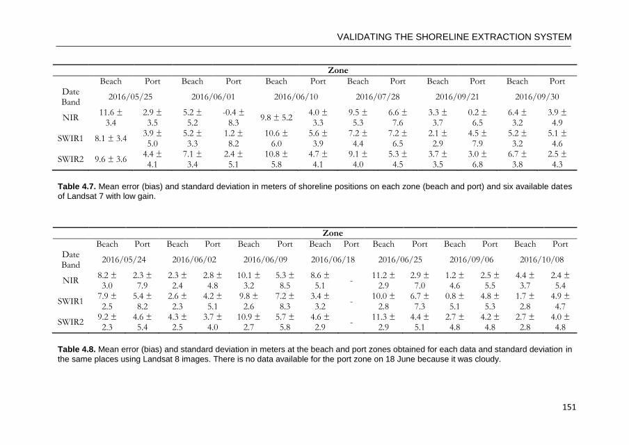
VALIDATING THE SHORELINE EXTRACTION SYSTEM
151
Zone
Beach Port Beach Port Beach Port Beach Port Beach Port Beach Port Date Band
2016/05/25 2016/06/01 2016/06/10 2016/07/28 2016/09/21 2016/09/30
NIR 11.6 ±
3.4 2.9 ± 3.5
5.2 ± 5.2
-0.4 ± 8.3
9.8 ± 5.2 4.0 ± 3.3
9.5 ± 5.3
6.6 ± 7.6
3.3 ± 3.7
0.2 ± 6.5
6.4 ± 3.2
3.9 ± 4.9
SWIR1 8.1 ± 3.4 3.9 ± 5.0
5.2 ± 3.3
1.2 ± 8.2
10.6 ± 6.0
5.6 ± 3.9
7.2 ± 4.4
7.2 ± 6.5
2.1 ± 2.9
4.5 ± 7.9
5.2 ± 3.2
5.1 ± 4.6
SWIR2 9.6 ± 3.6 4.4 ± 4.1
7.1 ± 3.4
2.4 ± 5.1
10.8 ± 5.8
4.7 ± 4.1
9.1 ± 4.0
5.3 ± 4.5
3.7 ± 3.5
3.0 ± 6.8
6.7 ± 3.8
2.5 ± 4.3
Table 4.7. Mean error (bias) and standard deviation in meters of shoreline positions on each zone (beach and port) and six available dates of Landsat 7 with low gain.
Zone
Beach Port Beach Port Beach Port Beach Port Beach Port Beach Port Beach Port Date Band
2016/05/24 2016/06/02 2016/06/09 2016/06/18 2016/06/25 2016/09/06 2016/10/08
NIR 8.2 ± 3.0
2.3 ± 7.9
2.3 ± 2.4
2.8 ± 4.8
10.1 ± 3.2
5.3 ± 8.5
8.6 ± 5.1
- 11.2 ±
2.9 2.9 ± 7.0
1.2 ± 4.6
2.5 ± 5.5
4.4 ± 3.7
2.4 ± 5.4
SWIR1 7.9 ± 2.5
5.4 ± 8.2
2.6 ± 2.3
4.2 ± 5.1
9.8 ± 2.6
7.2 ± 8.3
3.4 ± 3.2
- 10.0 ±
2.8 6.7 ± 7.3
0.8 ± 5.1
4.8 ± 5.3
1.7 ± 2.8
4.9 ± 4.7
SWIR2 9.2 ± 2.3
4.6 ± 5.4
4.3 ± 2.5
3.7 ± 4.0
10.9 ± 2.7
5.7 ± 5.8
4.6 ± 2.9
- 11.3 ±
2.9 4.4 ± 5.1
2.7 ± 4.8
4.2 ± 4.8
2.7 ± 2.8
4.0 ± 4.8
Table 4.8. Mean error (bias) and standard deviation in meters at the beach and port zones obtained for each data and standard deviation in
the same places using Landsat 8 images. There is no data available for the port zone on 18 June because it was cloudy.
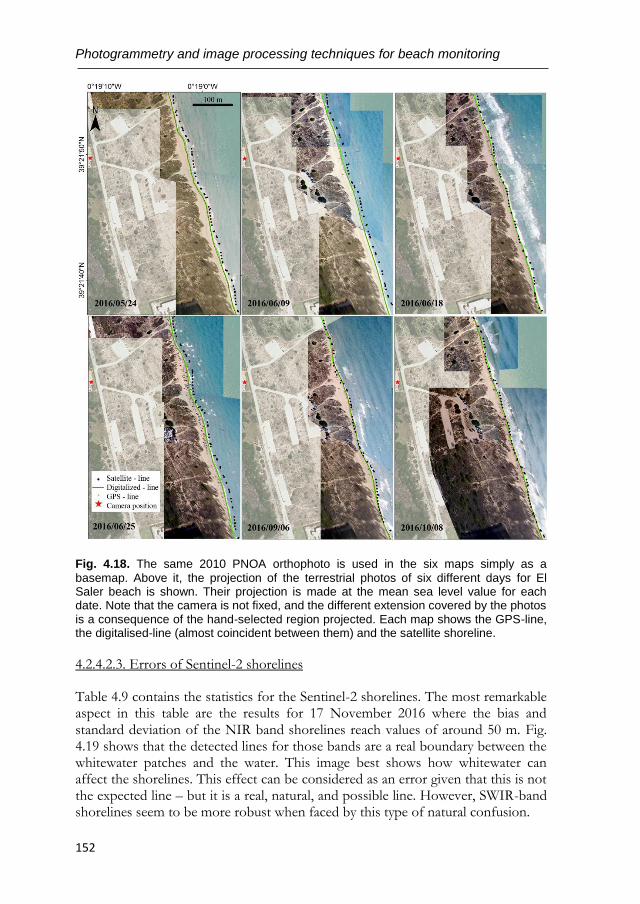
Photogrammetry and image processing techniques for beach monitoring
152
Fig. 4.18. The same 2010 PNOA orthophoto is used in the six maps simply as a
basemap. Above it, the projection of the terrestrial photos of six different days for El Saler beach is shown. Their projection is made at the mean sea level value for each date. Note that the camera is not fixed, and the different extension covered by the photos is a consequence of the hand-selected region projected. Each map shows the GPS-line, the digitalised-line (almost coincident between them) and the satellite shoreline.
4.2.4.2.3. Errors of Sentinel-2 shorelines
Table 4.9 contains the statistics for the Sentinel-2 shorelines. The most remarkable aspect in this table are the results for 17 November 2016 where the bias and standard deviation of the NIR band shorelines reach values of around 50 m. Fig. 4.19 shows that the detected lines for those bands are a real boundary between the whitewater patches and the water. This image best shows how whitewater can affect the shorelines. This effect can be considered as an error given that this is not the expected line – but it is a real, natural, and possible line. However, SWIR-band shorelines seem to be more robust when faced by this type of natural confusion.
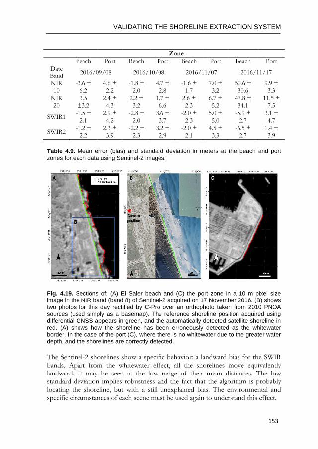
VALIDATING THE SHORELINE EXTRACTION SYSTEM
153
Zone
Beach Port Beach Port Beach Port Beach Port Date Band
2016/09/08 2016/10/08 2016/11/07 2016/11/17
NIR 10
-3.6 ± 6.2
4.6 ± 2.2
-1.8 ± 2.0
4.7 ± 2.8
-1.6 ± 1.7
7.0 ± 3.2
50.6 ± 30.6
9.9 ± 3.3
NIR 20
3.5 ±3.2
2.4 ± 4.3
2.2 ± 3.2
1.7 ± 6.6
2.6 ± 2.3
6.7 ± 5.2
47.8 ± 34.1
11.5 ± 7.5
SWIR1 -1.5 ±
2.1 2.9 ± 4.2
-2.8 ± 2.0
3.6 ± 3.7
-2.0 ± 2.3
5.0 ± 5.0
-5.9 ± 2.7
3.1 ± 4.7
SWIR2 -1.2 ±
2.2 2.3 ± 3.9
-2.2 ± 2.3
3.2 ± 2.9
-2.0 ± 2.1
4.5 ± 3.3
-6.5 ± 2.7
1.4 ± 3.9
Table 4.9. Mean error (bias) and standard deviation in meters at the beach and port
zones for each data using Sentinel-2 images.
Fig. 4.19. Sections of: (A) El Saler beach and (C) the port zone in a 10 m pixel size
image in the NIR band (band 8) of Sentinel-2 acquired on 17 November 2016. (B) shows two photos for this day rectified by C-Pro over an orthophoto taken from 2010 PNOA sources (used simply as a basemap). The reference shoreline position acquired using differential GNSS appears in green, and the automatically detected satellite shoreline in red. (A) shows how the shoreline has been erroneously detected as the whitewater border. In the case of the port (C), where there is no whitewater due to the greater water depth, and the shorelines are correctly detected.
The Sentinel-2 shorelines show a specific behavior: a landward bias for the SWIR bands. Apart from the whitewater effect, all the shorelines move equivalently landward. It may be seen at the low range of their mean distances. The low standard deviation implies robustness and the fact that the algorithm is probably locating the shoreline, but with a still unexplained bias. The environmental and specific circumstances of each scene must be used again to understand this effect.
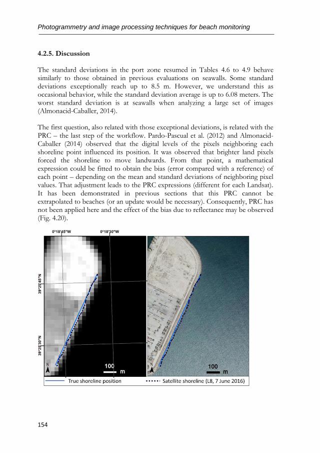
Photogrammetry and image processing techniques for beach monitoring
154
4.2.5. Discussion
The standard deviations in the port zone resumed in Tables 4.6 to 4.9 behave similarly to those obtained in previous evaluations on seawalls. Some standard deviations exceptionally reach up to 8.5 m. However, we understand this as occasional behavior, while the standard deviation average is up to 6.08 meters. The worst standard deviation is at seawalls when analyzing a large set of images (Almonacid-Caballer, 2014).
The first question, also related with those exceptional deviations, is related with the PRC – the last step of the workflow. Pardo-Pascual et al. (2012) and Almonacid-Caballer (2014) observed that the digital levels of the pixels neighboring each shoreline point influenced its position. It was observed that brighter land pixels forced the shoreline to move landwards. From that point, a mathematical expression could be fitted to obtain the bias (error compared with a reference) of each point – depending on the mean and standard deviations of neighboring pixel values. That adjustment leads to the PRC expressions (different for each Landsat). It has been demonstrated in previous sections that this PRC cannot be extrapolated to beaches (or an update would be necessary). Consequently, PRC has not been applied here and the effect of the bias due to reflectance may be observed (Fig. 4.20).
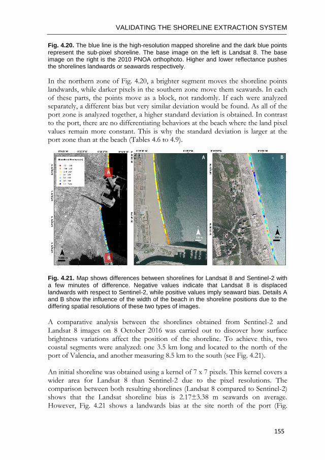
VALIDATING THE SHORELINE EXTRACTION SYSTEM
155
Fig. 4.20. The blue line is the high-resolution mapped shoreline and the dark blue points
represent the sub-pixel shoreline. The base image on the left is Landsat 8. The base image on the right is the 2010 PNOA orthophoto. Higher and lower reflectance pushes the shorelines landwards or seawards respectively.
In the northern zone of Fig. 4.20, a brighter segment moves the shoreline points landwards, while darker pixels in the southern zone move them seawards. In each of these parts, the points move as a block, not randomly. If each were analyzed separately, a different bias but very similar deviation would be found. As all of the port zone is analyzed together, a higher standard deviation is obtained. In contrast to the port, there are no differentiating behaviors at the beach where the land pixel values remain more constant. This is why the standard deviation is larger at the port zone than at the beach (Tables 4.6 to 4.9).
Fig. 4.21. Map shows differences between shorelines for Landsat 8 and Sentinel-2 with
a few minutes of difference. Negative values indicate that Landsat 8 is displaced landwards with respect to Sentinel-2, while positive values imply seaward bias. Details A and B show the influence of the width of the beach in the shoreline positions due to the differing spatial resolutions of these two types of images.
A comparative analysis between the shorelines obtained from Sentinel-2 and Landsat 8 images on 8 October 2016 was carried out to discover how surface brightness variations affect the position of the shoreline. To achieve this, two coastal segments were analyzed: one 3.5 km long and located to the north of the port of Valencia, and another measuring 8.5 km to the south (see Fig. 4.21).
An initial shoreline was obtained using a kernel of 7 x 7 pixels. This kernel covers a wider area for Landsat 8 than Sentinel-2 due to the pixel resolutions. The comparison between both resulting shorelines (Landsat 8 compared to Sentinel-2) shows that the Landsat shoreline bias is 2.17±3.38 m seawards on average. However, Fig. 4.21 shows a landwards bias at the site north of the port (Fig.
Photogrammetry and image processing techniques for beach monitoring
156
4.21A) and seawards at the southern site (Fig. 4.21B). The main difference between both zones is the beach width. The northern site is a very wide beach, and consequently, the analyzed kernel will contain very bright pixels corresponding to the beach sand. The beach at the southern site is about 30 m wide with a dune strip covered in spots of vegetation. Given that Landsat 8 covers a wider area of analysis than Sentinel-2, it captures more vegetation surface (darker than the beach response). This fact supports the idea that when a darker neighborhood is analyzed, it displaces the shoreline offshore.
A second analysis was carried out to examine a neighborhood that covers the same zone (swath) for both types of satellite images. Thus, a 7 x 7 pixel kernel was used for Sentinel 2 images (covering a 140 m swath) and 5 x 5 pixel for Landsat 8 images (covering 150 m). The shoreline differences in this case decrease to -0.75 ±2.5 m, and reinforce the idea that differing pixel brightnesses in the terrestrial zone influence the location of the shoreline. Although Landsat 8 and Sentinel-2 have different relative spectral response functions (RSRF) (Mandanici & Bitelli, 2016), the small differences found between their shorelines suggest that they are equivalent and can be used together in subsequent analyzes.
Other aspects may affect shoreline extraction. One of these aspects may be the resampling with which Landsat and Sentinel-2 pixels are interpolated during the terrain correction. Cubic convolution is currently used by USGS and ESA, and as a result, each pixel may be ‘contaminated’ by neighboring pixels. However, using other interpolation methods such as nearest neighbor, produces worse shorelines because they cause unrealistic jumps and toothed forms.
The distances of the satellite shoreline points compared with their references at the beach zone show low standard deviations. This means that each shoreline moves as a block from the reference. The reference shoreline is representing the land-water boundary, but the satellite sub-pixel shoreline is not identifying exactly the same line (depending on the environmental situation). Table 4.10 joins the mean errors (by date) and some variables of the state of the sea, such as significant wave height (H1/3), peak wave period (Tp), and the runup value (R2%) calculated by the Stockdon et al., 2006 formula:
2
004.0563.035.01.1
2/122/1
%2
f
f
HLHLR
,
Where the wavelength has been calculated by L=(gTp2)/2π and the slope (βf) has been estimated as a constant, 0.063. The mean slope value of the zone is deduced in Almonacid-Caballer et al., 2016.
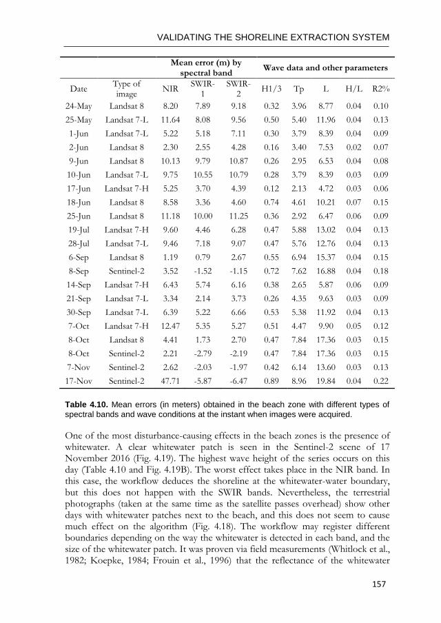
VALIDATING THE SHORELINE EXTRACTION SYSTEM
157
Mean error (m) by
spectral band Wave data and other parameters
Date Type of image
NIR SWIR-
1 SWIR-
2 H1/3 Tp L H/L R2%
24-May Landsat 8 8.20 7.89 9.18 0.32 3.96 8.77 0.04 0.10
25-May Landsat 7-L 11.64 8.08 9.56 0.50 5.40 11.96 0.04 0.13
1-Jun Landsat 7-L 5.22 5.18 7.11 0.30 3.79 8.39 0.04 0.09
2-Jun Landsat 8 2.30 2.55 4.28 0.16 3.40 7.53 0.02 0.07
9-Jun Landsat 8 10.13 9.79 10.87 0.26 2.95 6.53 0.04 0.08
10-Jun Landsat 7-L 9.75 10.55 10.79 0.28 3.79 8.39 0.03 0.09
17-Jun Landsat 7-H 5.25 3.70 4.39 0.12 2.13 4.72 0.03 0.06
18-Jun Landsat 8 8.58 3.36 4.60 0.74 4.61 10.21 0.07 0.15
25-Jun Landsat 8 11.18 10.00 11.25 0.36 2.92 6.47 0.06 0.09
19-Jul Landsat 7-H 9.60 4.46 6.28 0.47 5.88 13.02 0.04 0.13
28-Jul Landsat 7-L 9.46 7.18 9.07 0.47 5.76 12.76 0.04 0.13
6-Sep Landsat 8 1.19 0.79 2.67 0.55 6.94 15.37 0.04 0.15
8-Sep Sentinel-2 3.52 -1.52 -1.15 0.72 7.62 16.88 0.04 0.18
14-Sep Landsat 7-H 6.43 5.74 6.16 0.38 2.65 5.87 0.06 0.09
21-Sep Landsat 7-L 3.34 2.14 3.73 0.26 4.35 9.63 0.03 0.09
30-Sep Landsat 7-L 6.39 5.22 6.66 0.53 5.38 11.92 0.04 0.13
7-Oct Landsat 7-H 12.47 5.35 5.27 0.51 4.47 9.90 0.05 0.12
8-Oct Landsat 8 4.41 1.73 2.70 0.47 7.84 17.36 0.03 0.15
8-Oct Sentinel-2 2.21 -2.79 -2.19 0.47 7.84 17.36 0.03 0.15
7-Nov Sentinel-2 2.62 -2.03 -1.97 0.42 6.14 13.60 0.03 0.13
17-Nov Sentinel-2 47.71 -5.87 -6.47 0.89 8.96 19.84 0.04 0.22
Table 4.10. Mean errors (in meters) obtained in the beach zone with different types of
spectral bands and wave conditions at the instant when images were acquired.
One of the most disturbance-causing effects in the beach zones is the presence of whitewater. A clear whitewater patch is seen in the Sentinel-2 scene of 17 November 2016 (Fig. 4.19). The highest wave height of the series occurs on this day (Table 4.10 and Fig. 4.19B). The worst effect takes place in the NIR band. In this case, the workflow deduces the shoreline at the whitewater-water boundary, but this does not happen with the SWIR bands. Nevertheless, the terrestrial photographs (taken at the same time as the satellite passes overhead) show other days with whitewater patches next to the beach, and this does not seem to cause much effect on the algorithm (Fig. 4.18). The workflow may register different boundaries depending on the way the whitewater is detected in each band, and the size of the whitewater patch. It was proven via field measurements (Whitlock et al., 1982; Koepke, 1984; Frouin et al., 1996) that the reflectance of the whitewater
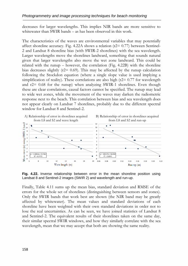
Photogrammetry and image processing techniques for beach monitoring
158
decreases for larger wavelengths. This implies NIR bands are more sensitive to whitewater than SWIR bands – as has been observed in this work.
The characteristics of the waves are environmental variables that may potentially affect shoreline accuracy. Fig. 4.22A shows a relation (r2= 0.77) between Sentinel-2 and Landsat 8 shoreline bias (with SWIR-2 shorelines) with the sea wavelength. Larger wavelengths move the shorelines landward, something that sounds natural given that larger wavelengths also move the wet zone landward. This could be related with the runup – however, the correlation (Fig. 4.22B) with the shoreline bias decreases slightly (r2= 0.69). This may be affected by the runup calculation following the Stockdon equation (where a single slope value is used implying a simplification of reality). These correlations are also high (r2= 0.77 for wavelength and r2= 0.68 for the runup) when analyzing SWIR-1 shorelines. Even though these are clear correlations, causal factors cannot be specified. The runup may lead to wide wet zones, while the movement of the waves may darken the radiometric response next to the beach. This correlation between bias and sea wavelength does not appear clearly on Landsat 7 shorelines, probably due to the different spectral window for Landsat 8 and Sentinel-2.
A) Relationship of error in shorelines acquired from L8 and S2 and wave length
B) Relationship of error in shorelines acquired from L8 and S2 and run-up
Fig. 4.22. Inverse relationship between error in the mean shoreline position using Landsat 8 and Sentinel-2 images (SWIR 2) and wavelength and run-up.
Finally, Table 4.11 sums up the mean bias, standard deviation and RMSE of the errors for the whole set of shorelines (distinguishing between sensors and zones). Only the SWIR bands that work best are shown (the NIR band may be greatly affected by whitewater). The mean values and standard deviations of each shoreline have been weighted with their own standard deviations in order not to lose the real uncertainties. As can be seen, we have joined statistics of Landsat 8 and Sentinel-2. The equivalent results of their shorelines taken on the same day, their similar spectral SWIR windows, and how they similarly correlate with the sea wavelength, mean that we may accept that both are showing the same reality.
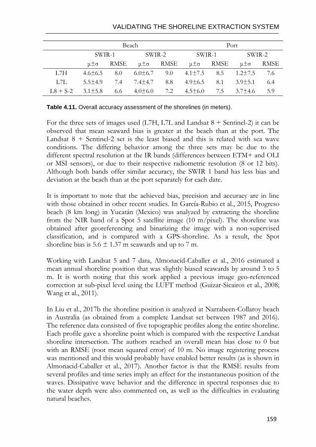
VALIDATING THE SHORELINE EXTRACTION SYSTEM
159
Beach Port
SWIR-1 SWIR-2 SWIR-1 SWIR-2
μ±σ RMSE μ±σ RMSE μ±σ RMSE μ±σ RMSE
L7H 4.6±6.5 8.0 6.0±6.7 9.0 4.1±7.5 8.5 1.2±7.5 7.6
L7L 5.5±4.9 7.4 7.4±4.7 8.8 4.9±6.5 8.1 3.9±5.1 6.4
L8 + S-2 3.1±5.8 6.6 4.0±6.0 7.2 4.5±6.0 7.5 3.7±4.6 5.9
Table 4.11. Overall accuracy assessment of the shorelines (in meters).
For the three sets of images used (L7H, L7L and Landsat 8 + Sentinel-2) it can be observed that mean seaward bias is greater at the beach than at the port. The Landsat 8 + Sentinel-2 set is the least biased and this is related with sea wave conditions. The differing behavior among the three sets may be due to the different spectral resolution at the IR bands (differences between ETM+ and OLI or MSI sensors), or due to their respective radiometric resolution (8 or 12 bits). Although both bands offer similar accuracy, the SWIR 1 band has less bias and deviation at the beach than at the port separately for each date.
It is important to note that the achieved bias, precision and accuracy are in line with those obtained in other recent studies. In García-Rubio et al., 2015, Progreso beach (8 km long) in Yucatán (Mexico) was analyzed by extracting the shoreline from the NIR band of a Spot 5 satellite image (10 m/pixel). The shoreline was obtained after georeferencing and binarizing the image with a non-supervised classification, and is compared with a GPS-shoreline. As a result, the Spot shoreline bias is 5.6 ± 1.37 m seawards and up to 7 m.
Working with Landsat 5 and 7 data, Almonacid-Caballer et al., 2016 estimated a mean annual shoreline position that was slightly biased seawards by around 3 to 5 m. It is worth noting that this work applied a previous image geo-referenced correction at sub-pixel level using the LUFT method (Guizar-Sicairos et al., 2008; Wang et al., 2011).
In Liu et al., 2017b the shoreline position is analyzed at Narrabeen-Collaroy beach in Australia (as obtained from a complete Landsat set between 1987 and 2016). The reference data consisted of five topographic profiles along the entire shoreline. Each profile gave a shoreline point which is compared with the respective Landsat shoreline intersection. The authors reached an overall mean bias close to 0 but with an RMSE (root mean squared error) of 10 m. No image registering process was mentioned and this would probably have enabled better results (as is shown in Almonacid-Caballer et al., 2017). Another factor is that the RMSE results from several profiles and time series imply an effect for the instantaneous position of the waves. Dissipative wave behavior and the difference in spectral responses due to the water depth were also commented on, as well as the difficulties in evaluating natural beaches.
Photogrammetry and image processing techniques for beach monitoring
160
Consequently, despite being affected by all the analyzed factors, the sub-pixel shorelines obtained in the present work behave equally, or better, than in other studies. However, each individual shoreline of dynamic spaces showed higher deviations and, in agreement with the references, may be affected by the described environmental factors, and perhaps by other factors still undiscovered. More assorted analyses in other beaches, and under differing environmental conditions, would be useful for a reevaluation. 4.2.6. Conclusions
The accuracy of the sub-pixel shorelines on natural beaches obtained by the proposed workflow was analyzed. It must be first mentioned that the original workflow (Pardo-Pascual et al., 2012; Almonacid-Caballer, 2014) was slightly modified. Images and shorelines were registered and extracted at sub-pixel level –but not corrected by the influence of various bright land pixels along the shoreline. To assess them, a comparison for land-water shorelines (measured via terrestrial photogrammetry and GNSS) was made. This comparison confirms that satellite shorelines define the land-water boundary with sub-pixel accuracy (Table 4.11). The main conclusions are:
- SWIR-1 bands, in all satellite sensor systems, offer the most accurate and robust sub-pixel shorelines on our study area. This result is a starting point that can be extrapolated to other similar areas and studies.
- Shorelines obtained from the NIR band have usually been accurate, but have shown to be more affected by whitewater and foam.
- Shorelines extracted from Landsat 8 and Sentinel 2 show similar disturbances for environmental factors, brightness of the land zone, and wavelength of the incident waves.
- The brightness of the land pixels surrounding the shoreline seems to affect the detected shoreline moving it landwards as the brightness of the pixels increase. This behavior appears clearer at the port area. It was seen in previous publications although modelling it has not been possible.
- A relationship between the bias of the shorelines—obtained from the SWIR-1 band of Landsat 8 and Sentinel-2—and the wavelengths of the sea waves is found. It suggests, even with the scarcity of data, that the state of the sea affects the extracted sub-pixel shorelines.

VALIDATING THE SHORELINE EXTRACTION SYSTEM
161

Photogrammetry and image processing techniques for beach monitoring
162
VALIDATING THE SHORELINE EXTRACTION SYSTEM
163
4.3. AN EFFICIENT PROTOCOL FOR ACCURATE AND MASSIVE
SHORELINE DEFINITION FROM MID-RESOLUTION SATELLITE IMAGERY
Satellite images can constitute a useful source of information for coastal monitoring as long as it is possible to manage them in an efficient way and derive precise indicators of the state of the beaches. In the present work, SHOREX system is employed for managing and processing Landsat 8 and Sentinel 2 images to automatically define the instantaneous shoreline position at sub-pixel level. Between the years 2013 and 2017, 91 satellite-derived shorelines (SDS) were assessed by comparing with other high-resolution shorelines obtained simultaneously through video-monitoring. The analysis allowed identifying the combination of parameters to perform the extraction algorithm with the highest accuracy. Furthermore, an efficient self-contained workflow is proposed untying the accuracy of the final shoreline from input line inaccuracies and external factors. Through an iterative procedure, it ensures firstly a suitable kernel of analysis representing the land-water interface to get, afterward, the definition of the shoreline with high precision below the 3 m of RMSE.
4.3.1. Introduction
Beaches are spaces of great environmental and recreational importance for coastal societies. The knowledge of their state and morphological changes, such as shoreline monitoring, is of special interest for the subsequent management of the coast (Mills et al., 2005, Esteves et al., 2009, Addo et al., 2011, Alharbi et al., 2017). In order to meet control and management needs, data collection must offer enough accuracy and frequency. Among the methods traditionally used, photointerpretation is limited to provide data at specific times (Ford, 2013; Jones et al., 2009; Morton et al., 2004; Pajak & Leatherman, 2002). Similarly, more modern and continuous video-based techniques are limited to a local scale (Aarninkhof et al., 2003; Davidson et al., 2007; Taborda & Silva, 2012; Brignone et al., 2012; Simarro et al., 2017; Sánchez-García et al., 2017), while DGPS requires arduous in situ data acquisition (Pardo-Pascual et al., 2005; Psuty & Silveira, 2011).
Alternatively, satellite images can provide information of the entire planet with a high temporal frequency. In 2008, NASA released the images of the Landsat platform (16 days of revisit time) free of charge. Similarly, the European Spatial Agency (ESA) is providing the Sentinel-2 satellite images (5 to 10 days of revisit time). Nowadays, considering both platforms together, there is a global average revisit interval of 2.9 days (Li & Roy, 2017). Thus, there is a new scenario where the shoreline position may potentially be defined in tens of different dates throughout the year in broad coastal segments. This type of data would make it possible to characterize short-term coastal processes such as the effect of storms and their subsequent recovery over time, or the impact of artificial beach
Photogrammetry and image processing techniques for beach monitoring
164
nourishments (Cabezas-Rabadán et al., 2018). However, in order to take advantage of these images it is necessary to: (i) define the shoreline position with enough accuracy for recognizing subtle changes, and (ii) have a sufficiently efficient and automated system to define the shorelines of all the images acquired by the satellites in a low time consumption process.
Near and medium infrared bands have been commonly used to detect the interface between water and land (Frazier & Page, 2000; Ryu et al., 2002; Yamano et al., 2006; Maiti & Bhattacharya, 2009). Similarly, alternative strategies have been proposed such as combining bands for obtaining indexes (Ouma & Tateishi, 2006, Choung & Jo, 2015). Among these indexes, the first and most used is the Normalized Difference Water Index (NDWI) that combines the green band with the near-infrared band using the zero value as a threshold for the difference between the dry sand and wet ocean surface (McFeeters, 1996). Xu (2018) proposed the Modified Normalized Difference Water Index (MNDWI), which replaces the near infrared band with the SWIR 1. Subsequently, new proposals have appeared such as the Automated Water Extraction Index (AWEI), which combines different bands of the visible and near and medium infrared but applying different weights to each band (Feyisa et al., 2014). These automatic water classifications have always encountered problems according to the index employed, as well as to the specific threshold chosen that varies with the different scenes and places (Ji et al., 2009). On the other hand, these indexes often confuse water zones with low albedo covers (Feyisa et al., 2014). Therefore, there is no clear consensus on which index works best as most authors focus on the correct performance of the index in their area of study. Rokni et al. (2014) evaluated multiple indexes to estimate surface changes in Lake Urmia (Iran) and found that the best solution came from a new approach based on the main components of NDWI. More recently, Hagenaars et al. (2018) used the NDWI to automate the shoreline definition, although in this case, grouping the water spots into a single large unit associated with the sea and separating it from the land.
In the attempt to automatically define the shoreline from mid-resolution satellite images using the raw infrared bands, the strategies appear divided in those working on a pixel scale, and those trying to improve the precision beyond the pixel size (sub-pixel or super-resolution). In the first case, the location of the shoreline is determined by an optimal threshold (Aedla et al., 2015; Quang Tuan et al., 2017), as well as by the selection of optimal bands and a subsequent classification (Li & Damen, 2010; García-Rubio et al., 2015). However, detailed coastal analyses would require the definition of the shoreline at sub-pixel level, improving the excessively coarse spatial resolution of the input satellite images. A few works have proposed algorithms in order to overcome that restriction (Foody et al., 2005; Zhang & Chen, 2010; Li & Gong, 2016, Li et al., 2015; Liu et al., 2017a). Nevertheless, most of these solutions focus on the algorithm basics, but without proposing any specific method to ensure a sufficiently robust georeferencing. This is a key issue
VALIDATING THE SHORELINE EXTRACTION SYSTEM
165
considering that NASA and ESA images show an excessive uncertainty in geolocation. Landsat 8 L1T products require an uncertainty lower than 12 m (Iron et al., 2012) while with regard to the multi-temporal registration, the geolocation accuracy has been previously established in 1.2 pixels, i.e. 24 m (Clerc, 2017). Hence, automatic co-registration methods appear as necessary in order to ensure a minimum error. Almonacid-Caballer et al. (2017) proposed employing the Local Upsampling Fourier Transform, LUFT algorithm (previously described by Guizar-Sicarios et al., 2008 and Wang et al., 2011), as a useful tool for this purpose since it ensures an error below 1/10 of the pixel resolution.
The methodology initially proposed in Pardo-Pascual et al. (2012) and later improved in Almonacid-Caballer (2014), includes both an automatic shoreline extraction algorithm and an automatic co-registration system, both at sub-pixel level. This algorithm, which works on the near- and mid-infrared spectral band, is a potentially usable methodological solution to automatically extract multiple shorelines as Pardo-Pascual et al. (2018) assessed. For each image, the method follows three essential steps (i) approximate location of the shoreline at pixel level based on threshold techniques; (ii) automatic sub-pixel definition based on the location of maximum gradient points. They are obtained adjusting a polynomial function to the digital levels of a 7 x 7 kernel (neighborhood of analysis) around each pixel of the approximate line and subsequently detecting the position where the Laplacian is null; and (iii) geometric correction based on LUFT. Results showed on rigid coasts -seawalls- an RMSE close to 5 m (Pardo-Pascual et al., 2012), while on microtidal sandy beaches the values were somewhat higher: 6.6 m for Landsat 8 (L8) and Sentinel 2 (S2) images and slightly worse for Landsat 7 (Pardo-Pascual et al., 2018), always registering a clear bias towards the sea. This bias was previously detected by comparing the shorelines obtained from Landsat 5 and 7 images against others acquired with more precise systems such as DGPS and LiDAR (Almonacid-Caballer et al., 2016). Pardo-Pascual et al. (2018) and Hagenaars et al. (2018) also found that the accuracy may be strongly influenced by wave conditions as the foam of the breaking waves and the wave period.
It was thought that the persistence of this bias could be minimized by working with smaller kernels. However, at once, the inaccuracy of the initial approximate shoreline defined by threshold techniques (step i) required sufficiently large analysis kernels to ensure that in step ii the real shoreline was contained. Moreover, the use of threshold techniques impeded a complete automation of the process. Considering the variability of elements existing in the marine area, it is very difficult to find a single proper threshold for every image as Liu et al. (2011) and Almonacid-Caballer (2014) previously stated.
Therefore, although the methodological basis described in Pardo-Pascual et al. (2018) is a good starting point, it cannot be considered as an efficient solution for working with large sets of satellite images. For that purpose, Palomar-Vázquez et
Photogrammetry and image processing techniques for beach monitoring
166
al., (2018a, b), proposed the replacement of the pixel level lines defined by threshold techniques by using a unique approximate shoreline to proceed with step ii for the whole set of images. The approximate line can be then obtained either from a pre-existing cartographic source or from a coarse photo-interpretation on an orthophoto close in time to the studied period. It increases the efficiency of the overall process by excluding the single step that required user intervention. This modification allows designing an automatic shoreline extraction system, which we have called SHOREX (Shoreline Extraction). This system may work completely automatically and it offers the necessary efficiency to supply updated shorelines from the images systematically acquired by the satellites L8 and S2.
The accuracy of the final sub-pixel shoreline is related both to the size of the kernel of analysis and to the degree of the adjusted polynomial (step ii). Although remaining uncertain, the approximate shoreline obtained according to the new workflow is expected to be more robust and may allow a reduction of the kernel of analysis. This modification, in turn, would allow changing the degree of the adjusted polynomial, potentially offering higher accuracies when determining the shoreline position. At this point, it seems also necessary to re-evaluate the data sources to be used as input for the SHOREX process. Infrared bands (NIR, SWIR1, SWIR2) must obviously be tested but also the performance of the NDWI index proposed in the literature.
The use of an approximate line to start the process presents certain challenges to be solved. If this line was excessively displaced with respect to the real shoreline − either because of a wrong delineation or because there have been significant changes between the acquisition dates of the approximate line and the satellite image − when using a small analysis kernel the system may not find the real land-water limit. Therefore, it would be very useful to analyze the effect that an inadequate displacement of the approximate line can have on the system, as well as to propose possible solutions to provide methodological robustness.
This work aims to present SHOREX as an efficient and completely automatic shoreline extraction system from mid-resolution satellite imagery. The optimum combination of parameters of the extraction algorithm for achieving the highest accuracy is identified (kernel size and polynomial degree), as well as an assessment of the results when using as input different bands or indexes. It is also intended to evaluate whether the position of the approximated line introduced as input affects the precision of the final sub-pixel shoreline. Once the optimum parameters and input data have been determined, the aim is to define an operative and self-reliant shoreline extraction protocol from L8 and S2 images. The solution releases the demands on the initial solution and makes it more robust against external factors.
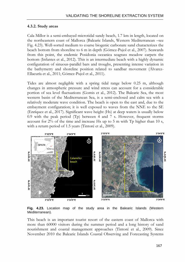
VALIDATING THE SHORELINE EXTRACTION SYSTEM
167
4.3.2. Study areas
Cala Millor is a semi-embayed microtidal sandy beach, 1.7 km in length, located on the northeastern coast of Mallorca (Balearic Islands, Western Mediterranean –see Fig. 4.23). Well-sorted medium to coarse biogenic carbonate sand characterizes the beach bottom from shoreline to 6 m in depth (Gómez-Pujol et al., 2007). Seawards from this point, the endemic Posidonia oceanica seagrass meadow carpets the bottom (Infantes et al., 2012). This is an intermediate beach with a highly dynamic configuration of sinuous-parallel bars and troughs, presenting intense variation in the bathymetry and shoreline position related to sandbar movement (Álvarez-Ellacuría et al., 2011; Gómez-Pujol et al., 2011).
Tides are almost negligible with a spring tidal range below 0.25 m, although changes in atmospheric pressure and wind stress can account for a considerable portion of sea level fluctuations (Gomis et al., 2012). The Balearic Sea, the most western basin of the Mediterranean Sea, is a semi-enclosed and calm sea with a relatively moderate wave condition. The beach is open to the east and, due to the embayment configuration; it is well exposed to waves from the NNE to the SE (Enríquez et al., 2017). Significant wave height (Hs) at deep waters is usually below 0.9 with the peak period (Tp) between 4 and 7 s. However, frequent storms account for 2% of the time and increase Hs up to 5 m with Tp higher than 10 s, with a return period of 1.5 years (Tintoré et al., 2009).
Fig. 4.23. Location map of the study area in the Balearic Islands (Western Mediterranean).
This beach is an important tourist resort of the eastern coast of Mallorca with more than 60000 visitors during the summer period and a long history of sand nourishment and coastal management approaches (Tintoré et al., 2009). Since November 2010 the Balearic Islands Coastal Observing and Forecasting Systems
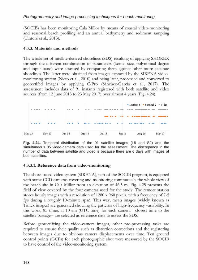
Photogrammetry and image processing techniques for beach monitoring
168
(SOCIB) has been monitoring Cala Millor by means of coastal video-monitoring and seasonal beach profiling and an annual bathymetry and sediment sampling (Tintoré et al., 2013). 4.3.3. Materials and methods
The whole set of satellite-derived shorelines (SDS) resulting of applying SHOREX through the different combination of parameters (kernel size, polynomial degree and input band) were assessed by comparing them against other more accurate shorelines. The latter were obtained from images captured by the SIRENA video-monitoring system (Nieto et al., 2010) and being later, processed and converted to georectifed images by applying C-Pro (Sánchez-García et al., 2017). The assessment includes data of 91 instants registered with both satellite and video sources (from 12 June 2013 to 23 May 2017) over almost 4 years (Fig. 4.24).
Fig. 4.24. Temporal distribution of the 91 satellite images (L8 and S2) and the
simultaneous 85 video-camera data used for the assessment. The discrepancy in the number of data between satellite and video is because there are 6 days with images of both satellites. 4.3.3.1. Reference data from video-monitoring
The shore-based video system (SIRENA), part of the SOCIB program, is equipped with some CCD cameras covering and monitoring continuously the whole view of the beach site in Cala Millor from an elevation of 46.5 m. Fig. 4.25 presents the field of view covered by the four cameras used for the study. The remote station stores hourly images with a resolution of 1280 x 960 pixels, with a frequency of 7-5 fps during a roughly 10-minute span. This way, mean images (widely known as Timex images) are generated showing the patterns of high-frequency variability. In this work, 85 timex at 10 am (UTC time) for each camera −closest time to the satellite passage− are selected as reference data to assess the SDS.
Before georectifying the video-camera images, other pre-processing tasks are required to ensure their quality such as distortion corrections and the registering between images due to obvious camera displacements over time. Ten ground control points (GCPs) for each photographic shot were measured by the SOCIB to have control of the video-monitoring system.
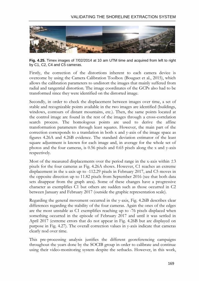
VALIDATING THE SHORELINE EXTRACTION SYSTEM
169
Fig. 4.25. Timex images of 7/02/2014 at 10 am UTM time and acquired from left to right
by C1, C2, C4 and C5 cameras.
Firstly, the correction of the distortions inherent to each camera device is overcome by using the Camera Calibration Toolbox (Bouguet et al., 2015), which allows the calibration parameters to undistort the images that mainly suffered from radial and tangential distortion. The image coordinates of the GCPs also had to be transformed since they were identified on the distorted image.
Secondly, in order to check the displacement between images over time, a set of stable and recognizable points available in the two images are identified (buildings, windows, contours of distant mountains, etc.). Then, the same points located at the control image are found in the rest of the images through a cross-correlation search process. The homologous points are used to derive the affine transformation parameters through least squares. However, the main part of the correction corresponds to a translation in both x and y-axis of the image space as figures 4.26A and 4.26B evidence. The standard deviation estimator of the least square adjustment is known for each image and, in average for the whole set of photos and the four cameras, is 0.56 pixels and 0.65 pixels along the x and y-axis respectively.
Most of the measured displacements over the period range in the x-axis within ±3 pixels for the four cameras as Fig. 4.26A shows. However, C1 reaches an extreme displacement in the x-axis up to -112.29 pixels in February 2017, and C5 moves in the opposite direction up to 11.82 pixels from September 2016 (see that both data sets disappear from the graph area). Some of these changes have a progressive character as exemplifies C1 but others are sudden such as those occurred in C2 between January and February 2017 (outside the graphic representation scale).
Regarding the general movement occurred in the y-axis, Fig. 4.26B describes clear differences regarding the stability of the four cameras. Again the ones of the edges are the most unstable as C1 exemplifies reaching up to -76 pixels displaced when something occurred in the episode of February 2017 and until it was settled in April 2017 (extreme errors that do not appear in Fig. 4.26B but are displayed on purpose in Fig. 4.27). The overall correction values in y-axis indicate that cameras clearly nod over time.
This pre-processing analysis justifies the different georeferencing campaigns throughout the years done by the SOCIB group in order to calibrate and continue using their video-monitoring system despite the setbacks. However, in this work,
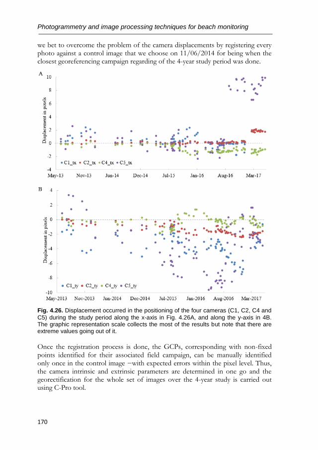
Photogrammetry and image processing techniques for beach monitoring
170
we bet to overcome the problem of the camera displacements by registering every photo against a control image that we choose on 11/06/2014 for being when the closest georeferencing campaign regarding of the 4-year study period was done.
Fig. 4.26. Displacement occurred in the positioning of the four cameras (C1, C2, C4 and
C5) during the study period along the x-axis in Fig. 4.26A, and along the y-axis in 4B. The graphic representation scale collects the most of the results but note that there are extreme values going out of it.
Once the registration process is done, the GCPs, corresponding with non-fixed points identified for their associated field campaign, can be manually identified only once in the control image −with expected errors within the pixel level. Thus, the camera intrinsic and extrinsic parameters are determined in one go and the georectification for the whole set of images over the 4-year study is carried out using C-Pro tool.
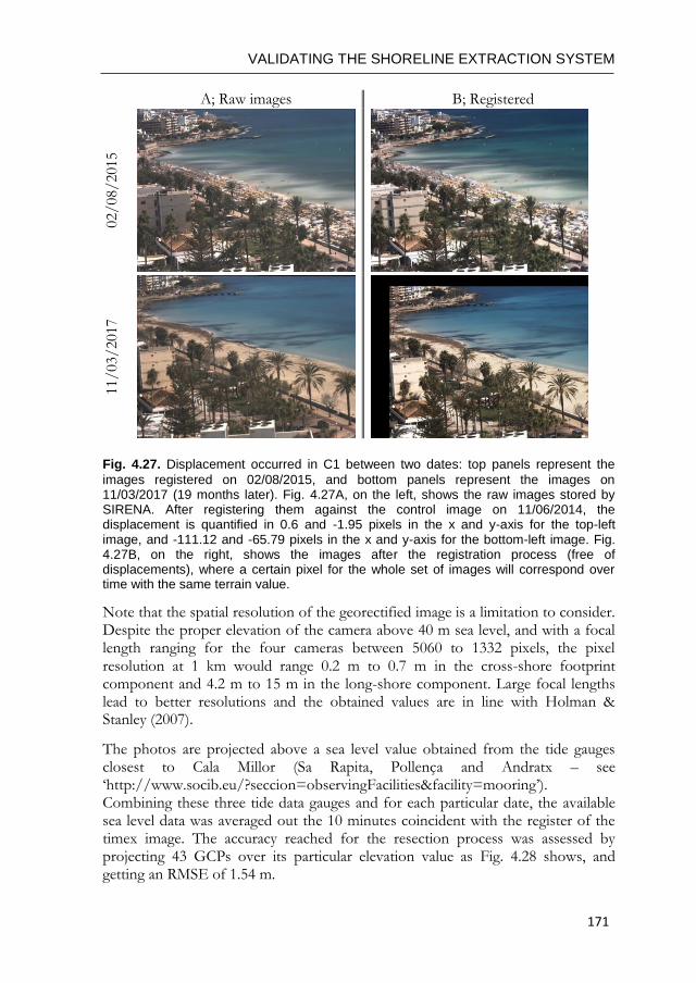
VALIDATING THE SHORELINE EXTRACTION SYSTEM
171
A; Raw images B; Registered 02/
08/
2015
11/03/2017
Fig. 4.27. Displacement occurred in C1 between two dates: top panels represent the
images registered on 02/08/2015, and bottom panels represent the images on 11/03/2017 (19 months later). Fig. 4.27A, on the left, shows the raw images stored by SIRENA. After registering them against the control image on 11/06/2014, the displacement is quantified in 0.6 and -1.95 pixels in the x and y-axis for the top-left image, and -111.12 and -65.79 pixels in the x and y-axis for the bottom-left image. Fig. 4.27B, on the right, shows the images after the registration process (free of displacements), where a certain pixel for the whole set of images will correspond over time with the same terrain value.
Note that the spatial resolution of the georectified image is a limitation to consider. Despite the proper elevation of the camera above 40 m sea level, and with a focal length ranging for the four cameras between 5060 to 1332 pixels, the pixel resolution at 1 km would range 0.2 m to 0.7 m in the cross-shore footprint component and 4.2 m to 15 m in the long-shore component. Large focal lengths lead to better resolutions and the obtained values are in line with Holman & Stanley (2007).
The photos are projected above a sea level value obtained from the tide gauges closest to Cala Millor (Sa Rapita, Pollença and Andratx – see ‘http://www.socib.eu/?seccion=observingFacilities&facility=mooring’). Combining these three tide data gauges and for each particular date, the available sea level data was averaged out the 10 minutes coincident with the register of the timex image. The accuracy reached for the resection process was assessed by projecting 43 GCPs over its particular elevation value as Fig. 4.28 shows, and getting an RMSE of 1.54 m.
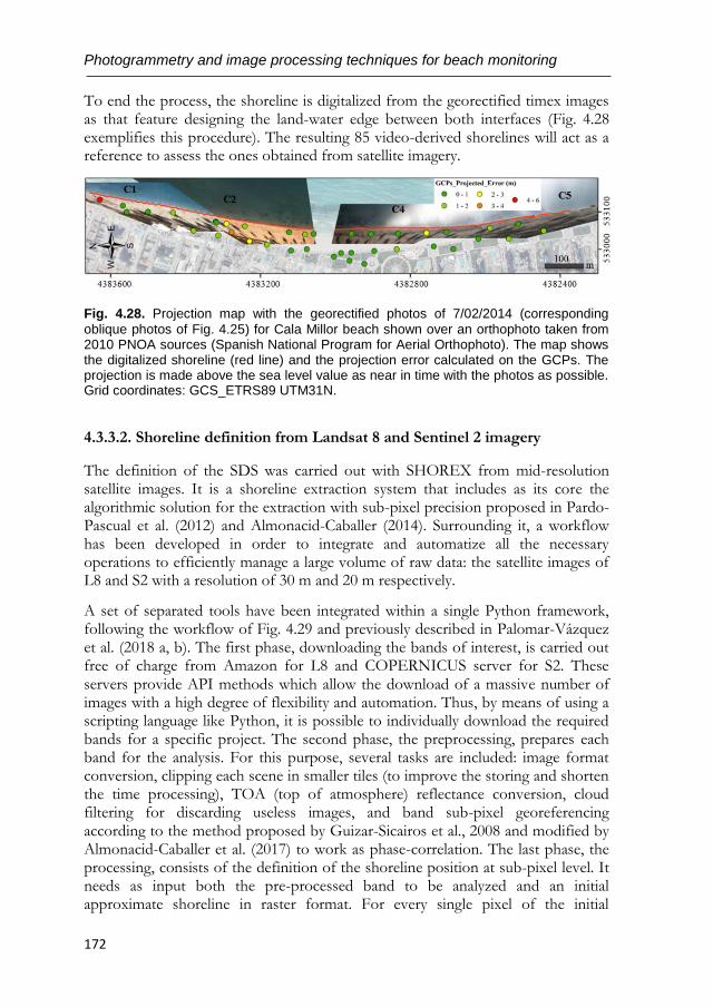
Photogrammetry and image processing techniques for beach monitoring
172
To end the process, the shoreline is digitalized from the georectified timex images as that feature designing the land-water edge between both interfaces (Fig. 4.28 exemplifies this procedure). The resulting 85 video-derived shorelines will act as a reference to assess the ones obtained from satellite imagery.
Fig. 4.28. Projection map with the georectified photos of 7/02/2014 (corresponding
oblique photos of Fig. 4.25) for Cala Millor beach shown over an orthophoto taken from 2010 PNOA sources (Spanish National Program for Aerial Orthophoto). The map shows the digitalized shoreline (red line) and the projection error calculated on the GCPs. The projection is made above the sea level value as near in time with the photos as possible. Grid coordinates: GCS_ETRS89 UTM31N.
4.3.3.2. Shoreline definition from Landsat 8 and Sentinel 2 imagery
The definition of the SDS was carried out with SHOREX from mid-resolution satellite images. It is a shoreline extraction system that includes as its core the algorithmic solution for the extraction with sub-pixel precision proposed in Pardo-Pascual et al. (2012) and Almonacid-Caballer (2014). Surrounding it, a workflow has been developed in order to integrate and automatize all the necessary operations to efficiently manage a large volume of raw data: the satellite images of L8 and S2 with a resolution of 30 m and 20 m respectively.
A set of separated tools have been integrated within a single Python framework, following the workflow of Fig. 4.29 and previously described in Palomar-Vázquez et al. (2018 a, b). The first phase, downloading the bands of interest, is carried out free of charge from Amazon for L8 and COPERNICUS server for S2. These servers provide API methods which allow the download of a massive number of images with a high degree of flexibility and automation. Thus, by means of using a scripting language like Python, it is possible to individually download the required bands for a specific project. The second phase, the preprocessing, prepares each band for the analysis. For this purpose, several tasks are included: image format conversion, clipping each scene in smaller tiles (to improve the storing and shorten the time processing), TOA (top of atmosphere) reflectance conversion, cloud filtering for discarding useless images, and band sub-pixel georeferencing according to the method proposed by Guizar-Sicairos et al., 2008 and modified by Almonacid-Caballer et al. (2017) to work as phase-correlation. The last phase, the processing, consists of the definition of the shoreline position at sub-pixel level. It needs as input both the pre-processed band to be analyzed and an initial approximate shoreline in raster format. For every single pixel of the initial
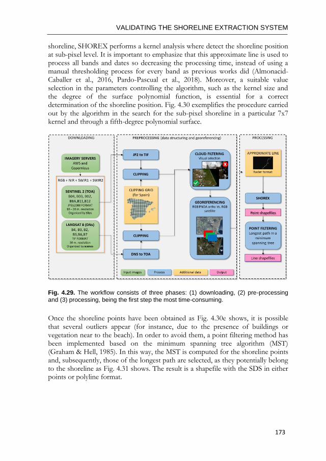
VALIDATING THE SHORELINE EXTRACTION SYSTEM
173
shoreline, SHOREX performs a kernel analysis where detect the shoreline position at sub-pixel level. It is important to emphasize that this approximate line is used to process all bands and dates so decreasing the processing time, instead of using a manual thresholding process for every band as previous works did (Almonacid-Caballer et al., 2016, Pardo-Pascual et al., 2018). Moreover, a suitable value selection in the parameters controlling the algorithm, such as the kernel size and the degree of the surface polynomial function, is essential for a correct determination of the shoreline position. Fig. 4.30 exemplifies the procedure carried out by the algorithm in the search for the sub-pixel shoreline in a particular 7x7 kernel and through a fifth-degree polynomial surface.
Fig. 4.29. The workflow consists of three phases: (1) downloading, (2) pre-processing
and (3) processing, being the first step the most time-consuming.
Once the shoreline points have been obtained as Fig. 4.30e shows, it is possible that several outliers appear (for instance, due to the presence of buildings or vegetation near to the beach). In order to avoid them, a point filtering method has been implemented based on the minimum spanning tree algorithm (MST) (Graham & Hell, 1985). In this way, the MST is computed for the shoreline points and, subsequently, those of the longest path are selected, as they potentially belong to the shoreline as Fig. 4.31 shows. The result is a shapefile with the SDS in either points or polyline format.
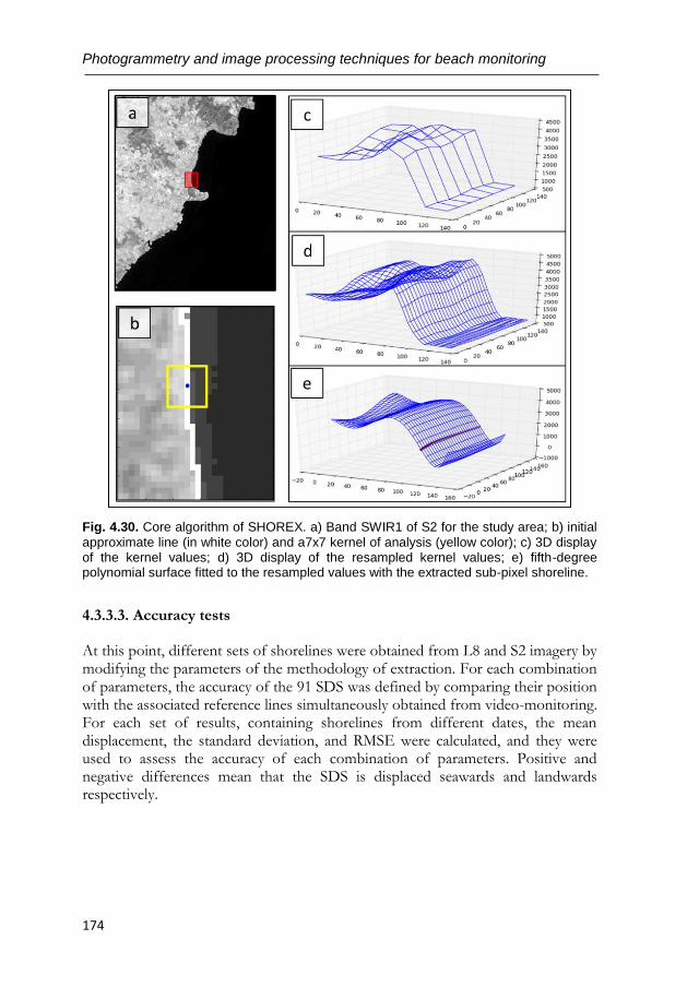
Photogrammetry and image processing techniques for beach monitoring
174
Fig. 4.30. Core algorithm of SHOREX. a) Band SWIR1 of S2 for the study area; b) initial
approximate line (in white color) and a7x7 kernel of analysis (yellow color); c) 3D display of the kernel values; d) 3D display of the resampled kernel values; e) fifth-degree polynomial surface fitted to the resampled values with the extracted sub-pixel shoreline.
4.3.3.3. Accuracy tests
At this point, different sets of shorelines were obtained from L8 and S2 imagery by modifying the parameters of the methodology of extraction. For each combination of parameters, the accuracy of the 91 SDS was defined by comparing their position with the associated reference lines simultaneously obtained from video-monitoring. For each set of results, containing shorelines from different dates, the mean displacement, the standard deviation, and RMSE were calculated, and they were used to assess the accuracy of each combination of parameters. Positive and negative differences mean that the SDS is displaced seawards and landwards respectively.
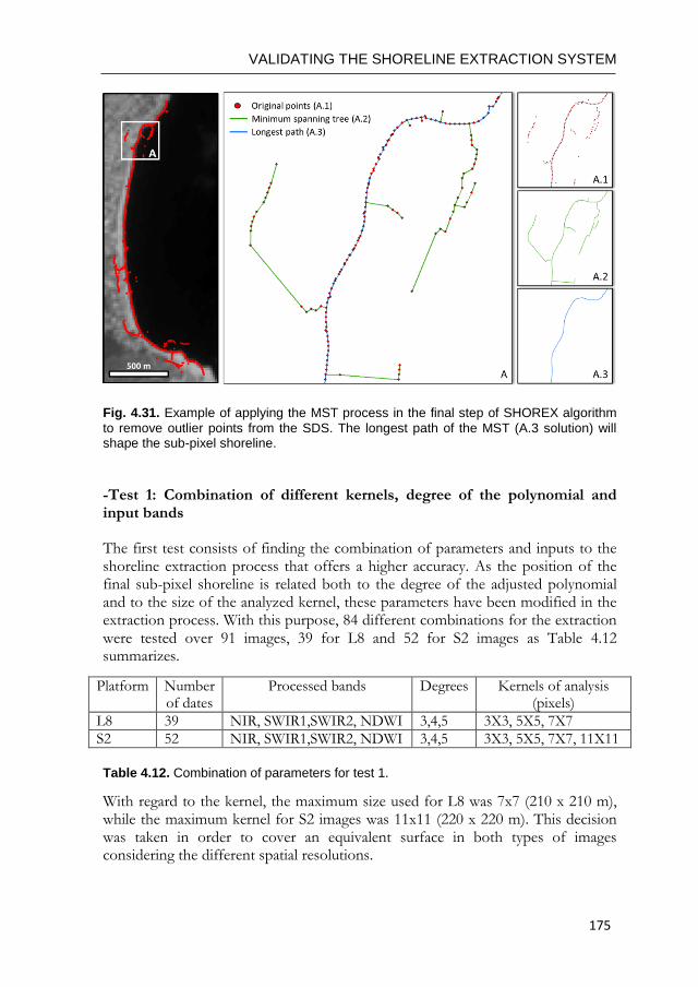
VALIDATING THE SHORELINE EXTRACTION SYSTEM
175
Fig. 4.31. Example of applying the MST process in the final step of SHOREX algorithm
to remove outlier points from the SDS. The longest path of the MST (A.3 solution) will shape the sub-pixel shoreline.
-Test 1: Combination of different kernels, degree of the polynomial and input bands
The first test consists of finding the combination of parameters and inputs to the shoreline extraction process that offers a higher accuracy. As the position of the final sub-pixel shoreline is related both to the degree of the adjusted polynomial and to the size of the analyzed kernel, these parameters have been modified in the extraction process. With this purpose, 84 different combinations for the extraction were tested over 91 images, 39 for L8 and 52 for S2 images as Table 4.12 summarizes.
Platform Number of dates
Processed bands Degrees Kernels of analysis (pixels)
L8 39 NIR, SWIR1,SWIR2, NDWI 3,4,5 3X3, 5X5, 7X7
S2 52 NIR, SWIR1,SWIR2, NDWI 3,4,5 3X3, 5X5, 7X7, 11X11
Table 4.12. Combination of parameters for test 1.
With regard to the kernel, the maximum size used for L8 was 7x7 (210 x 210 m), while the maximum kernel for S2 images was 11x11 (220 x 220 m). This decision was taken in order to cover an equivalent surface in both types of images considering the different spatial resolutions.
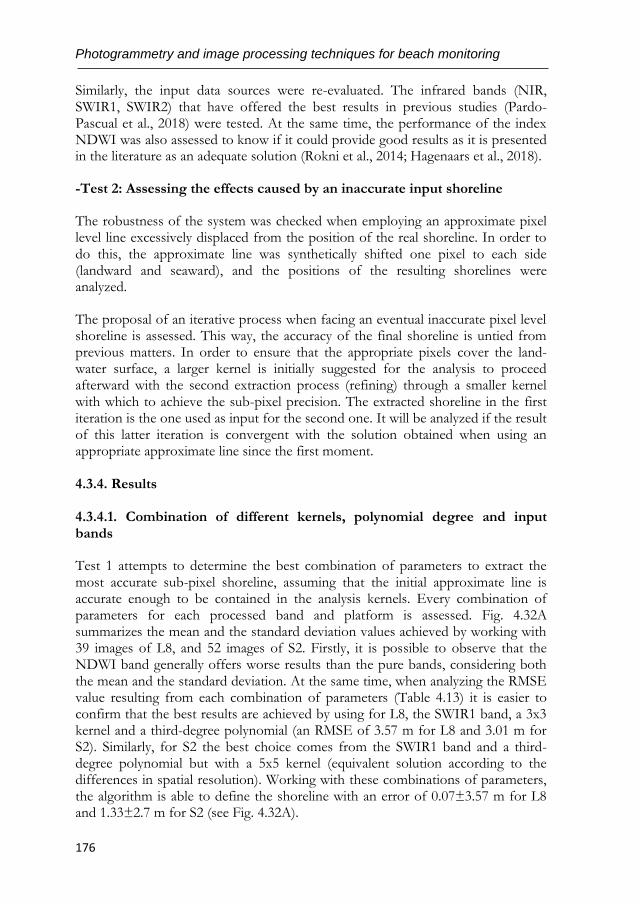
Photogrammetry and image processing techniques for beach monitoring
176
Similarly, the input data sources were re-evaluated. The infrared bands (NIR, SWIR1, SWIR2) that have offered the best results in previous studies (Pardo-Pascual et al., 2018) were tested. At the same time, the performance of the index NDWI was also assessed to know if it could provide good results as it is presented in the literature as an adequate solution (Rokni et al., 2014; Hagenaars et al., 2018).
-Test 2: Assessing the effects caused by an inaccurate input shoreline
The robustness of the system was checked when employing an approximate pixel level line excessively displaced from the position of the real shoreline. In order to do this, the approximate line was synthetically shifted one pixel to each side (landward and seaward), and the positions of the resulting shorelines were analyzed.
The proposal of an iterative process when facing an eventual inaccurate pixel level shoreline is assessed. This way, the accuracy of the final shoreline is untied from previous matters. In order to ensure that the appropriate pixels cover the land-water surface, a larger kernel is initially suggested for the analysis to proceed afterward with the second extraction process (refining) through a smaller kernel with which to achieve the sub-pixel precision. The extracted shoreline in the first iteration is the one used as input for the second one. It will be analyzed if the result of this latter iteration is convergent with the solution obtained when using an appropriate approximate line since the first moment. 4.3.4. Results 4.3.4.1. Combination of different kernels, polynomial degree and input bands
Test 1 attempts to determine the best combination of parameters to extract the most accurate sub-pixel shoreline, assuming that the initial approximate line is accurate enough to be contained in the analysis kernels. Every combination of parameters for each processed band and platform is assessed. Fig. 4.32A summarizes the mean and the standard deviation values achieved by working with 39 images of L8, and 52 images of S2. Firstly, it is possible to observe that the NDWI band generally offers worse results than the pure bands, considering both the mean and the standard deviation. At the same time, when analyzing the RMSE value resulting from each combination of parameters (Table 4.13) it is easier to confirm that the best results are achieved by using for L8, the SWIR1 band, a 3x3 kernel and a third-degree polynomial (an RMSE of 3.57 m for L8 and 3.01 m for S2). Similarly, for S2 the best choice comes from the SWIR1 band and a third-degree polynomial but with a 5x5 kernel (equivalent solution according to the differences in spatial resolution). Working with these combinations of parameters, the algorithm is able to define the shoreline with an error of 0.07±3.57 m for L8 and 1.33±2.7 m for S2 (see Fig. 4.32A).
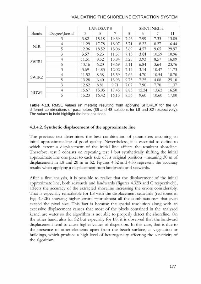
VALIDATING THE SHORELINE EXTRACTION SYSTEM
177
LANDSAT 8 SENTINEL 2
Bands Degree\kernel 3 5 7 3 5 7 11
NIR
3 3.82 15.18 19.39 7.26 7.99 7.33 13.05
4 11.29 17.78 18.07 3.71 8.22 8.27 16.44
5 12.96 18.52 18.06 3.69 4.57 9.65 29.97
SWIR1
3 3.57 6.23 11.57 7.13 3.01 10.59 10.96
4 11.51 8.52 15.84 3.25 3.93 8.57 16.09
5 13.16 6.20 18.69 3.11 6.84 3.64 23.76
SWIR2
3 3.69 14.83 12.02 7.14 3.14 10.47 11.73
4 11.52 8.38 15.59 7.66 4.70 10.54 18.70
5 13.28 6.40 13.93 9.75 7.25 4.08 25.10
NDWI
3 12.62 8.81 9.71 7.07 7.90 7.70 11.37
4 15.67 15.05 17.45 8.83 12.24 13.62 16.50
5 15.23 16.42 16.15 8.36 9.60 10.60 17.00
Table 4.13. RMSE values (in meters) resulting from applying SHOREX for the 84
different combinations of parameters (36 and 48 solutions for L8 and S2 respectively). The values in bold highlight the best solutions.
4.3.4.2. Synthetic displacement of the approximate line
The previous test determines the best combination of parameters assuming an initial approximate line of good quality. Nevertheless, it is essential to define to which extent a displacement of the initial line affects the resultant shoreline. Therefore, test 2 consists on repeating test 1 but synthetically shifting the initial approximate line one pixel to each side of its original position −meaning 30 m of displacement in L8 and 20 m in S2. Figures 4.32 and 4.33 represent the accuracy results when applying a displacement both landwards and seawards. After a first analysis, it is possible to realize that the displacement of the initial approximate line, both seawards and landwards (figures 4.32B and C respectively), affects the accuracy of the extracted shoreline increasing the errors considerably. That is especially remarkable for L8 with the displacement seawards (red tones in Fig. 4.32B) showing higher errors −for almost all the combinations− that even exceed the pixel size. This fact is because the spatial resolution along with an excessive displacement causes that most of the pixels contained in the analyzed kernel are water so the algorithm is not able to properly detect the shoreline. On the other hand, also for S2 but especially for L8, it is observed that the landward displacement tend to cause higher values of dispersion. In this case, that is due to the presence of other elements apart from the beach surface, as vegetation or buildings, which produce a high level of heterogeneity affecting the sensitivity of the algorithm.
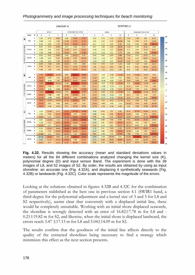
Photogrammetry and image processing techniques for beach monitoring
178
Fig. 4.32. Results showing the accuracy (mean and standard deviations values in
meters) for all the 84 different combinations analyzed changing the kernel size (K), polynomial degree (D) and input sensor Band. The experiment is done with the 39 images of L8, and 52 images of S2. By order, the results are obtained by using as input shoreline: an accurate one (Fig. 4.32A), and displacing it synthetically seawards (Fig. 4.32B) or landwards (Fig. 4.32C). Color scale represents the magnitude of the errors.
Looking at the solutions obtained in figures 4.32B and 4.32C for the combination of parameters stablished as the best one in previous section 4.1 (SWIR1 band, a third-degree for the polynomial adjustment and a kernel size of 3 and 5 for L8 and S2 respectively), seems clear that conversely with a displaced initial line, these would be completely unsuitable. Working with an initial shore displaced seawards, the shoreline is wrongly detected with an error of 16.82±7.78 m for L8 and -0.21±19.82 m for S2, and likewise, when the initial shore is displaced landward, the errors reach 3.47 ±17.13 m for L8 and 5.04±14.09 m for S2.
The results confirm that the goodness of the initial line affects directly to the quality of the extracted shorelines being necessary to find a strategy which minimizes this effect as the next section presents.
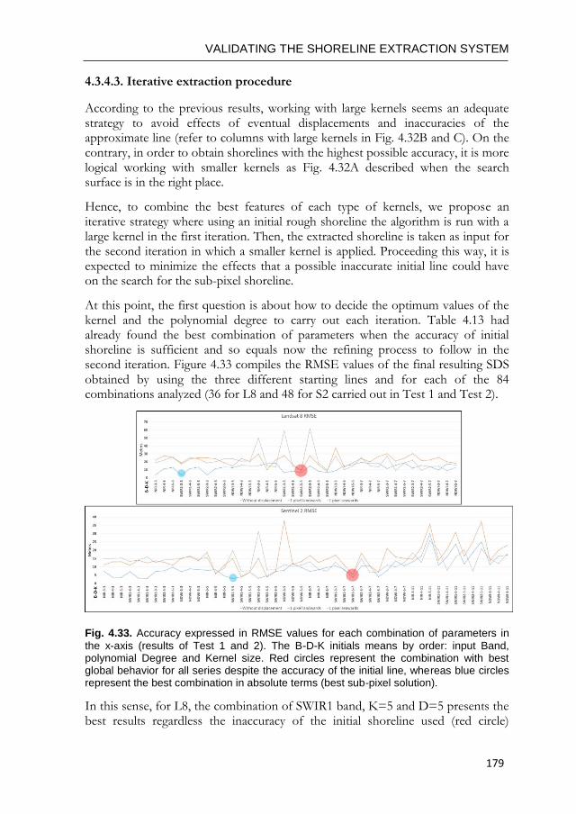
VALIDATING THE SHORELINE EXTRACTION SYSTEM
179
4.3.4.3. Iterative extraction procedure
According to the previous results, working with large kernels seems an adequate strategy to avoid effects of eventual displacements and inaccuracies of the approximate line (refer to columns with large kernels in Fig. 4.32B and C). On the contrary, in order to obtain shorelines with the highest possible accuracy, it is more logical working with smaller kernels as Fig. 4.32A described when the search surface is in the right place.
Hence, to combine the best features of each type of kernels, we propose an iterative strategy where using an initial rough shoreline the algorithm is run with a large kernel in the first iteration. Then, the extracted shoreline is taken as input for the second iteration in which a smaller kernel is applied. Proceeding this way, it is expected to minimize the effects that a possible inaccurate initial line could have on the search for the sub-pixel shoreline.
At this point, the first question is about how to decide the optimum values of the kernel and the polynomial degree to carry out each iteration. Table 4.13 had already found the best combination of parameters when the accuracy of initial shoreline is sufficient and so equals now the refining process to follow in the second iteration. Figure 4.33 compiles the RMSE values of the final resulting SDS obtained by using the three different starting lines and for each of the 84 combinations analyzed (36 for L8 and 48 for S2 carried out in Test 1 and Test 2).
Fig. 4.33. Accuracy expressed in RMSE values for each combination of parameters in
the x-axis (results of Test 1 and 2). The B-D-K initials means by order: input Band, polynomial Degree and Kernel size. Red circles represent the combination with best global behavior for all series despite the accuracy of the initial line, whereas blue circles represent the best combination in absolute terms (best sub-pixel solution).
In this sense, for L8, the combination of SWIR1 band, K=5 and D=5 presents the best results regardless the inaccuracy of the initial shoreline used (red circle)
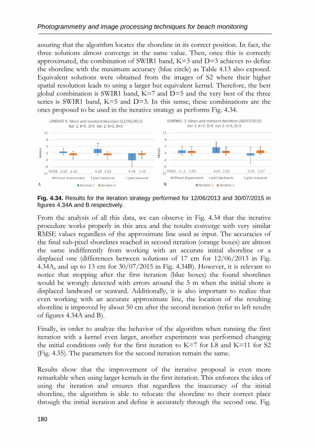
Photogrammetry and image processing techniques for beach monitoring
180
assuring that the algorithm locates the shoreline in its correct position. In fact, the three solutions almost converge in the same value. Then, once this is correctly approximated, the combination of SWIR1 band, K=3 and D=3 achieves to define the shoreline with the maximum accuracy (blue circle) as Table 4.13 also exposed. Equivalent solutions were obtained from the images of S2 where their higher spatial resolution leads to using a larger but equivalent kernel. Therefore, the best global combination is SWIR1 band, K=7 and D=5 and the very best of the three series is SWIR1 band, K=5 and D=3. In this sense, these combinations are the ones proposed to be used in the iterative strategy as performs Fig. 4.34.
Fig. 4.34. Results for the iteration strategy performed for 12/06/2013 and 30/07/2015 in figures 4.34A and B respectively.
From the analysis of all this data, we can observe in Fig. 4.34 that the iterative procedure works properly in this area and the results converge with very similar RMSE values regardless of the approximate line used as input. The accuracies of the final sub-pixel shorelines reached in second iteration (orange boxes) are almost the same indifferently from working with an accurate initial shoreline or a displaced one (differences between solutions of 17 cm for 12/06/2013 in Fig. 4.34A, and up to 13 cm for 30/07/2015 in Fig. 4.34B). However, it is relevant to notice that stopping after the first iteration (blue boxes) the found shorelines would be wrongly detected with errors around the 5 m when the initial shore is displaced landward or seaward. Additionally, it is also important to realize that even working with an accurate approximate line, the location of the resulting shoreline is improved by about 50 cm after the second iteration (refer to left results of figures 4.34A and B).
Finally, in order to analyze the behavior of the algorithm when running the first iteration with a kernel even larger, another experiment was performed changing the initial conditions only for the first iteration to K=7 for L8 and K=11 for S2 (Fig. 4.35). The parameters for the second iteration remain the same. Results show that the improvement of the iterative proposal is even more remarkable when using larger kernels in the first iteration. This enforces the idea of using the iteration and ensures that regardless the inaccuracy of the initial shoreline, the algorithm is able to relocate the shoreline to their correct place through the initial iteration and define it accurately through the second one. Fig.
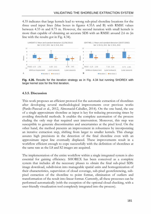
VALIDATING THE SHORELINE EXTRACTION SYSTEM
181
4.35 indicates that large kernels lead to wrong sub-pixel shoreline locations for the three used input lines (blue boxes in figures 4.35A and B) with RMSE values between 4.33 m and 8.75 m. However, the second iteration with small kernels is more than capable of obtaining an accurate SDS with an RMSE around 2.6 m (in line with the results got in Fig. 4.34).
Fig. 4.35. Results for the iteration strategy as in Fig. 4.34 but running SHOREX with larger kernel size for the first iteration.
4.3.5. Discussion
This work proposes an efficient protocol for the automatic extraction of shorelines after developing several methodological improvements over previous works (Pardo-Pascual et al., 2012, Almonacid-Caballer, 2014). On the one hand, the use of a single approximate shoreline as input is key for reducing processing times by avoiding threshold methods. It enables the complete automation of the process eluding the only step that required user intervention. Moreover, this step was susceptible to generate discontinuities and uncertainties at the pixel level. On the other hand, the method presents an improvement in robustness by incorporating an iterative extraction step, shifting from larger to smaller kernels. This change assures high precisions in the detection of the final shoreline even with an approximate input line eventually displaced. These improvements result in a workflow efficient enough to cope successfully with the definition of shorelines at the same rate as the L8 and S2 images are acquired.
The implementation of the entire workflow within a single integrated system is also essential for gaining efficiency. SHOREX has been conceived as a complete system that includes all the necessary phases to obtain the final sub-pixel SDS: image download, subdivision into manageable spatial units and homogenization of their characteristics, supervision of cloud coverage, sub-pixel georeferencing, sub-pixel extraction of the shoreline to point format, elimination of outliers and transformation of the result into linear format. Currently, all these processes can be performed automatically (with the exception of the optional cloud checking, with a user-friendly visualization tool completely integrated into the process).
Photogrammetry and image processing techniques for beach monitoring
182
The efficiency of the extraction protocol and its limiting factors had been previously analyzed. Palomar-Vázquez et al. (2018a) evaluated the time consumption of the workflow by performing a single extraction (without additional iterations, accepting the accuracy of the approximate line). The time invested in extracting all the shorelines along one year in a 22.7 km segment of the Mediterranean coast was calculated. For this purpose, 81 images of satellite S2 and 23 of L8 were initially downloaded but only 28 images of S2 and 14 of L8 were finally used (as they were free of clouds) leading to the definition of 42 shorelines. The process required 4h 34 minutes, of which 83% was used to download and homogenize the images (assign TIFF format and TOA values) and 17% for processing. This showed, in line with works in other coastal sectors (Palomar-Vázquez et al., 2018b), that downloading is the most time-consuming phase, without constituting a limiting element for defining the shorelines that can potentially be obtained from the L8 and S2 imagery.
The accuracy and precision of the obtained shorelines is a second key aspect in order to determine their usefulness in coastal change studies. However, to carry out a thorough assessment is not simple and relatively few studies have made a metric evaluation of the errors. This is largely due to the difficulty of recording the shoreline position with sufficient precision at the same time the image is captured by satellite, as the shore varies continuously due to waves, water level and alterations in the beach profile.
In the present work, the availability of continuous records of images of specific beach segments taken by a video-monitoring system made it possible to employ these data as reference values of the real position of the shoreline. The monitoring system managed by SOCIB, together with the versatile photogrammetric tool C-Pro (Sánchez-García et al., 2017) have allowed the obtaining of georectified images of the coastal area at the same instants when the S2 and L8 images were acquired. The geometric accuracy of these georectified images has been estimated using the ground coordinates of 43 GCPs with a 1.54 m RMSE. However, the precision of the digitalized shoreline on these images was also conditioned to the criterion and audacity of the interpreter himself, as well as the indeterminacy of the spatial resolution of the georectified image. At a distance of 650 m and for the worst cases, working with a focal of 1332 pixels, the cross and long size of the pixel footprint have been 0.45 m and 6.36 m respectively. Despite these errors, the video-derived shorelines are amply valid to use as reference data. Pardo-Pascual, et al., 2018 already proved the quality of these video-derived shorelines obtained with C-Pro in a sector of the Valencian coast. Comparing these against other high accurate shorelines measured by GPS −at the same instant as the photos were taken−, the trivial and encouraging mean error reached was 0.15 ±1.05 m.
In the present work, the large number of evaluations carried out (91) ensures that the images have been recorded with very diverse sea states, giving a high
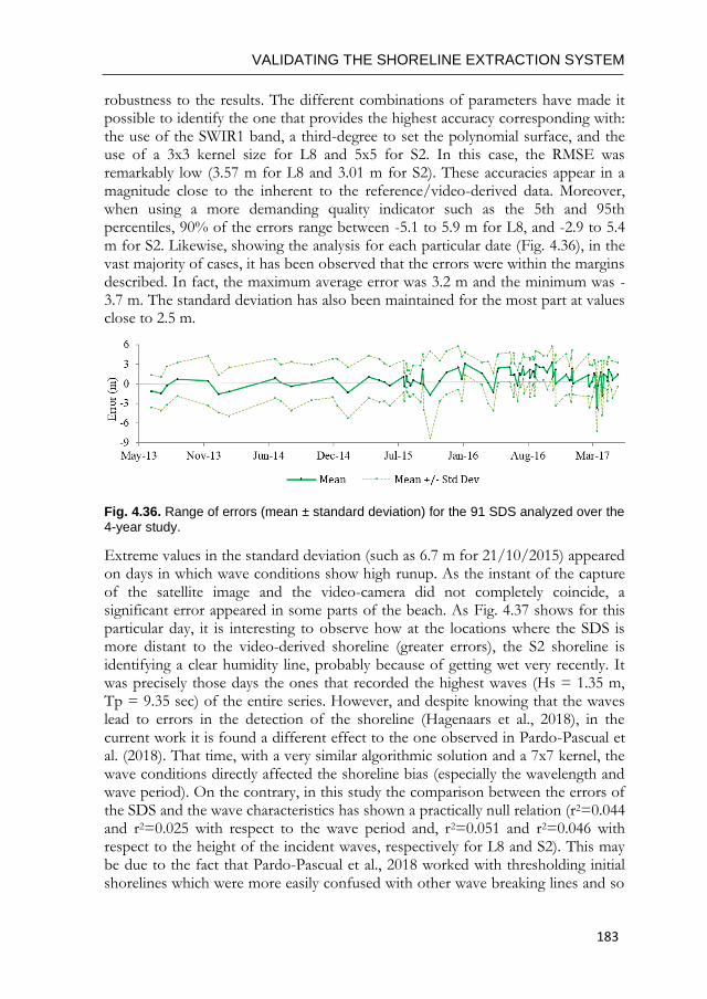
VALIDATING THE SHORELINE EXTRACTION SYSTEM
183
robustness to the results. The different combinations of parameters have made it possible to identify the one that provides the highest accuracy corresponding with: the use of the SWIR1 band, a third-degree to set the polynomial surface, and the use of a 3x3 kernel size for L8 and 5x5 for S2. In this case, the RMSE was remarkably low (3.57 m for L8 and 3.01 m for S2). These accuracies appear in a magnitude close to the inherent to the reference/video-derived data. Moreover, when using a more demanding quality indicator such as the 5th and 95th percentiles, 90% of the errors range between -5.1 to 5.9 m for L8, and -2.9 to 5.4 m for S2. Likewise, showing the analysis for each particular date (Fig. 4.36), in the vast majority of cases, it has been observed that the errors were within the margins described. In fact, the maximum average error was 3.2 m and the minimum was -3.7 m. The standard deviation has also been maintained for the most part at values close to 2.5 m.
Fig. 4.36. Range of errors (mean ± standard deviation) for the 91 SDS analyzed over the 4-year study.
Extreme values in the standard deviation (such as 6.7 m for 21/10/2015) appeared on days in which wave conditions show high runup. As the instant of the capture of the satellite image and the video-camera did not completely coincide, a significant error appeared in some parts of the beach. As Fig. 4.37 shows for this particular day, it is interesting to observe how at the locations where the SDS is more distant to the video-derived shoreline (greater errors), the S2 shoreline is identifying a clear humidity line, probably because of getting wet very recently. It was precisely those days the ones that recorded the highest waves (Hs = 1.35 m, Tp = 9.35 sec) of the entire series. However, and despite knowing that the waves lead to errors in the detection of the shoreline (Hagenaars et al., 2018), in the current work it is found a different effect to the one observed in Pardo-Pascual et al. (2018). That time, with a very similar algorithmic solution and a 7x7 kernel, the wave conditions directly affected the shoreline bias (especially the wavelength and wave period). On the contrary, in this study the comparison between the errors of the SDS and the wave characteristics has shown a practically null relation (r2=0.044 and r2=0.025 with respect to the wave period and, r2=0.051 and r2=0.046 with respect to the height of the incident waves, respectively for L8 and S2). This may be due to the fact that Pardo-Pascual et al., 2018 worked with thresholding initial shorelines which were more easily confused with other wave breaking lines and so
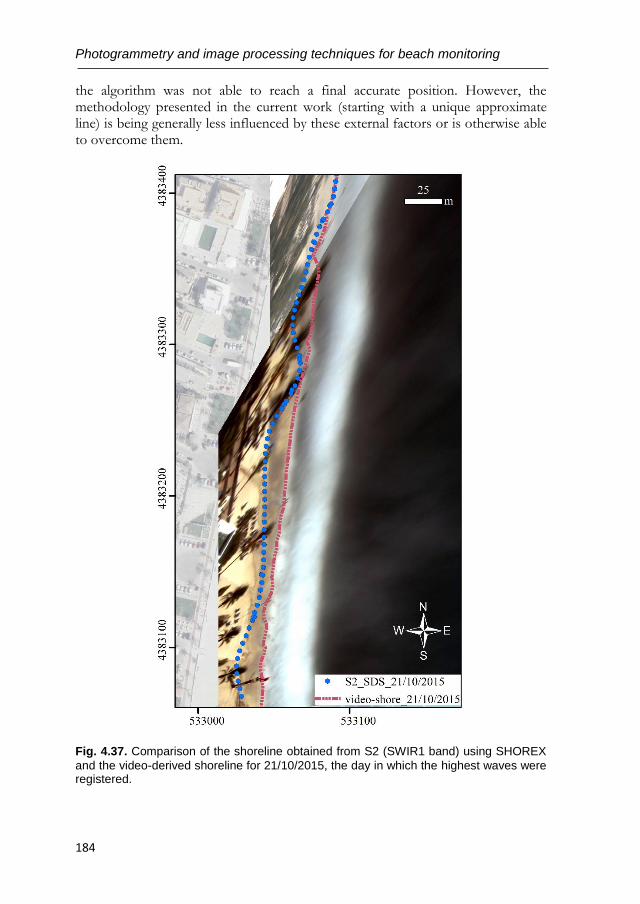
Photogrammetry and image processing techniques for beach monitoring
184
the algorithm was not able to reach a final accurate position. However, the methodology presented in the current work (starting with a unique approximate line) is being generally less influenced by these external factors or is otherwise able to overcome them.
Fig. 4.37. Comparison of the shoreline obtained from S2 (SWIR1 band) using SHOREX
and the video-derived shoreline for 21/10/2015, the day in which the highest waves were registered.
VALIDATING THE SHORELINE EXTRACTION SYSTEM
185
The results evidence a substantial improvement in the level of accuracy with respect to previous solutions described in the bibliography in which SDS could be compared with field measurements (García-Rubio et al., 2015; Liu et al., 2017b; Pardo-Pascual et al., 2018, Hagenaars et al., 2018; Splinter et al., 2018, Do et al., 2019). In agreement with Almonacid-Caballer et al. (2016), Liu et al. (2017b) remarked that the shorelines obtained from Landsat images (using an algorithmic solution different from the one exposed in this work) were adequate to monitor the average annual behavior of the beaches, but they could be subjected to excessively large errors (tens of meters). Hagenaars et al. (2018) have recently suggested applying image composite processing −following Donchyts et al., 2016 technique− to a sequence of images in order to obtain a single image that minimizes the effect of bias factors. Thus, it could be accepted that with relatively high errors (RMSE between 6 and 15 m, depending on the method) it is possible to study evolutionary trends over large coastal segments (Sánchez-García et al., 2015a; Almonacid-Caballer et al., 2016; Do et al., 2019) or even on a global scale as proposed Luijendijk et al., (2018).
SHOREX system, with the methodology and accuracy here shown, resolves this limitation and opens up the possibility of using the SDS in analytical processes that require greater precision. The methodology makes it possible to offer continuous data throughout the year, with a high revisited frequency, of wide coastal segments, making it possible to derive useful indicators for coastal management as the beach width, as well as monitoring the beach response to nourishment projects and coastal storms. At the same time, the availability of accurate shoreline data could help to estimate volumetric changes based on certain beach profiles (Do et al., 2019).
This application is immediate on microtidal beaches as the wet zone is rarely very wide. However, in beaches with completely different tidal and wave conditions this solution would need to be re-evaluated. In meso or macrotidal coasts, the shoreline definition can be compromised in areas with very low slopes and high tidal range, where the intertidal space can be extended to hundreds of meters. Following the iterative procedure here described, the use of an approximate line makes it possible that the kernel of 7 x 7 pixels for the first iteration did not include the position of the real shoreline, making insufficient the proposed protocol with one iteration. The solution could come from the definition of different approximate lines associated with different sea levels or the performance of consecutive iterations starting from larger kernels of analysis. Anyways, future research is required to continue testing SHOREX on a wide miscellany of coastal environments and achieve its full automation on a large spatial scale.
Photogrammetry and image processing techniques for beach monitoring
186
4.3.6. Conclusions
The present work proposes an efficient protocol for shoreline extraction from mid-resolution satellite images using the SHOREX system. A workflow that integrates all the necessary steps for an automatic definition of satellite-derived shorelines (SDS) at sub-pixel level has been described, increasing the efficiency of the extraction process as well as the accuracy. The protocol constitutes a way for the massive definition of shorelines at the same rate as the acquisition of satellite images. This is of great value for the continuous monitoring of beaches and the decision-making of coastal managers.
A complete assessment with 91 different SDS over almost 4 years of study has been carried out in Cala Millor, a Mediterranean sandy beach. This was possible thanks to the availability of highly accurate shorelines from a video-monitoring system in the same instant the satellite images were recorded. The evaluation has allowed analyzing 84 different combinations of parameters for working with SHOREX by merging the type of input band, the kernel of analysis and adjustment degree. Accordingly, it was possible to establish that the combination leading to the best solution (an RMSE of 3.57 m for L8 and 3.01 m for S2) was using the SWIR1 band, a third-degree polynomial, and a 3x3 kernel size for L8 and 5x5 for S2 (equivalent kernel according to the different spatial resolution). Moreover, the results showed that the accuracy of the input line strongly affects the final sub-pixel shoreline definition. Therefore, an iterative strategy using SHOREX was proposed to minimize this effect and ensuring a robust method for shoreline detection regardless of the reliability of the input line and external factors.
The huge availability of satellite-image data worldwide together with the efficiency and accuracy of SHOREX creates a new scenario and an opportunity to understand the morphodynamics at coastal zones on different spatio-temporal scales.

VALIDATING THE SHORELINE EXTRACTION SYSTEM
187

Photogrammetry and image processing techniques for beach monitoring
188
VALIDATING THE SHORELINE EXTRACTION SYSTEM
189
4.4. OVERALL CHAPTER DISCUSSIONS AND CONCLUSIONS
The main purpose of the numerous studies carried out around the evolution of coastal areas is to obtain an overview for subsequent prediction and identification of future actions in the context of coastal planning. In this regard, the shoreline extraction methodology tested in this chapter using mid-resolution images − Landsat (5, 7, 8) and Sentinel 2 − plays a decisive role in the accurate and effective detection and analysis of the magnitude of beach changes (as started Sánchez-García et al., 2015a). Different evaluations of quality and soundness have been presented through different stages and during the three previous works (each discussed in the corresponding section of Chapter 4).
The followed methodology comes from the solution proposed in Pardo-Pascual et al. (2012) and Almonacid-Caballer (2014). This has been applied in different ways and with a clear and progressive improvement in the procedures, achieving the greatest precision and robustness in the final work of Section 4.3. However, various key conclusions are presented regarding with the best way to extract the shorelines and the type of application derived.
Firstly, in Section 4.1, the value of the annual average SDS for evolutionary studies has been demonstrated on dynamic beaches against other results (between the years 2005 and 2010) obtained, prior to the PhD, from accurate sources but not coincident in time. Minimizing the intra-annual oscillations in a year and working with annual average SDS from Landsat (5, 7 & 8) was instrumental for assessing mid-term changes on long beach segments. Using annual SDS, the change rates obtained were almost the same (r2>0.98) than when all the set of single SDS were used but management and geomorphological analysis were easier, especially when working over large areas, and data may be analyzed by cartographic comparison. Another issue overcome in this work was establishing the accuracy of SDS on sedimentary beaches. As accurate records (HPS) taken at the same time as each Landsat image were unavailable, comparison between both sources of data was made using annual mean shorelines and analyzing those instantaneous SDS and HPS closest in time (a few days before or later). Results indicated that SDS defined the shorelines with a seaward bias of 4.7 m for instantaneous shorelines and 4.9 m for mean annual shorelines. These magnitudes were in line with the error found by García-Rubio et al. (2015) at Yucatan beaches relative to a GNSS shoreline registered on the same day (with a 5-hour delay) as the Spot image from which the shoreline was extracted. On the work in Section 4.1, an estimation of the shoreline partially corrected by sea level variations was proposed. This was simply an approximation because the beach slope was estimated as an average of surveys measured at times that differed from those corresponding to each shoreline. Moreover, the sea level value was set with the tide gauge register without considering the runup associated with the incident waves.
Photogrammetry and image processing techniques for beach monitoring
190
However, results proved that this partial correction using “datum-based” shorelines enabled an accurate measurement of changes.
Secondly, in Section 4.2 the accuracy of instantaneous shorelines was assessed on natural sandy beaches from satellite images produced by Landsat (7, 8) and Sentinel-2. The evaluation against GNSS and photo-derived shorelines enabled the analysis of the various instantaneous factors that may affect shoreline accuracy. The first issue addressed was to establish if the polynomial radiometric correction (PRC) fitted to seawall areas in former works (Pardo-Pascual et al., 2012) could be extrapolated to beaches. The original workflow was then slightly modified by bypassing this last step in the shoreline extraction process. The assessment carried out for 21 days confirmed that mean seaward bias was greater at the beach than at the port, and bright zones in the terrestrial area influenced shoreline detection and moved it landwards. The availability of coincident photo data to use as a reference proved that NIR bands were more easily confused with whitewater than SWIR bands, and this offered the most accurate and robust sub-pixel shorelines. However, these last SDS were also affected by the state of the sea – with a slight relation between shoreline bias and sea swell, and especially with wave length. The comparison in a particular day with shorelines from bands 11 and 12 of S2 and bands 6 and 7 of L8 verified their similar radiometric response with a shoreline difference of -0.75 ± 2.5 m. In short, it was concluded that sub-pixel SDS were a clearly valid source of data for detecting and quantifying beach changes – as other works had also shown (Liu et al., 2016). The whole set of L7 shorelines located the shoreline with a mean error of 4.63 m (±6.55 m) and 5.5 m (±4.86 m), for high and low gain images; and the L8 and S2 shorelines with an error of 3.06 m (±5.79 m).
In Section 4.3 it is shown how the SHOREX system mostly solved the problem of mid-resolution satellite images and opens the possibility of using these SDS in analytical processes that require greater accuracy. A wide evaluation with 91 SDS (from L8 and S2 images) over almost four years of study, and coincident with video data registers, determined the best procedure to follow for detecting the shoreline within an RMSE of 3.5 m. This was achieved by proceeding with the SWIR1 band, a third-degree polynomial, and a 3x3 kernel size for L8 and 5x5 for S2 (equivalent kernel according to the different spatial resolution). Note that the image had previously been upsampled using a cubic convolution interpolation. Moreover, a unique initial line for the whole set of images was used (it did not come from thresholding techniques as prior works), and so the results seemed to be less influenced by external factors such as those derived from wave characteristics. However, an iterative strategy was proposed to avoid difficulties when faced by possible inaccuracies of the input line. The application was immediate on microtidal beaches where the wet zone was rarely very wide. However, in meso or macrotidal coasts, the shoreline definition could be compromised in areas with very low slopes and high tidal ranges, where the
VALIDATING THE SHORELINE EXTRACTION SYSTEM
191
intertidal space may be hundreds of meters wide. Even so, the described protocol for shoreline extraction constituted a robust approach for the massive definition of shorelines at the same rate as the acquisition of satellite images. An estimation of the tool efficiency was presented in Palomar-Vázquez et al., 2018a, where the time invested in extracting 104 shorelines for one year for a 22.7 km segment was 4h 34 minutes (83% of time for downloading and homogenizing the images, and 17% for processing).
Further research should continue combining the two proposed solutions in Chapter 3 and in Section 4.3, to continue providing methodological robustness regardless of beach typology and tidal conditions.
The applicability of the SDS has already been tested using long shoreline datasets for the calibration and validation of equilibrium shoreline evolution models (Yates et al., 2009 and Jara et al., 2015; YA09 and JA15 respectively) in the context of cross-shore motion. This work (Jaramillo et al., under review) has been directly derived from the current doctoral thesis and the PhD stay made at IH Cantabria. Despite the importance of this work in the overall research (as it reinforces the quality of the techniques studied in the present doctoral thesis), this work does not form a part of it since it will be in another dissertation.
Conceptually, the evolution models are based on the balance between destructive and constructive forces that act upon a beach. The former “YA09” is probably the most widely used model of this type in recent years, and the second “JA15” is a novel model that requires the lowest number of calibration parameters of all the models of the same type. The empirical nature of these requires high-quality observational datasets to calibrate model parameters. Until now, shoreline positions from satellite images had been neglected because resolution was too coarse (10-30 m or more) and this prevented the identification of small-scale movements along coastlines. Thus, all the cross-shore evolution model applications in the literature correspond to target study sites where high-resolution data was available (video-camera systems or topo-bathymetric surveys). However, no studies have applied shoreline-position datasets from satellite imagery. SHOREX opens a new and promising scenario that is explored in Jaramillo et al. (under review) to apply these SDS as input data for shoreline evolution models. A comparative analysis on model calibration and validation that uses shoreline datasets from a video-camera system and satellite imagery was conducted. An initial analysis of the shoreline evolution is shown from January 2005 to March 2007, in which video-camera and satellite data was collected to select a representative study period for the calibration of the equilibrium models (Fig. 4.38). Thirteen sub-pixel shorelines were then used to evaluate Nova Icaria Beach (Barcelona, Spain) over a four-month period.
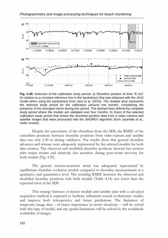
Photogrammetry and image processing techniques for beach monitoring
192
Fig. 4.38. Selection of the calibration study period. a) Shoreline position at time “S (m)”
(in relation to a constant reference line in the backshore) that was obtained with the JA15 model when using the parameters from Jara et al. (2015). The shaded area represents the selected study period for the calibration (around one month), considering the presence of the strongest storm during this period. The dashed lines delimit the complete study period where the models are validated over four months. b) Zoom of the selected calibration study period that shows the shoreline-position data from a video camera and satellite images that were processed with the SHOREX algorithm (from Jaramillo et al., under review).
Despite the uncertainty of the shorelines from the SDS, the RMSE of the coincident positions between shoreline positions from video-camera and satellite data was only 2.49 m during validation. The results show that general shoreline advances and retreats were adequately represented by the selected models for both data sources. The observed and modelled shoreline positions showed fast erosion after major storms and relatively fast accretion during post-storm recovery for both models (Fig. 4.39).
The general erosion-accretion trend was adequately represented by equilibrium shoreline evolution models compared to shoreline measurements at a qualitative and quantitative level. The resulting RMSE between the observed and modelled shoreline positions with both models (Table 4.14) was lower than the expected error of the SDS.
This synergy between evolution models and satellite data with a sub-pixel acquisition method is expected to facilitate influential coastal evolutionary studies and improve both retrospective and future predictions. The limitation of temporary image data – of major importance in storm situations − will be solved with this type of model, and any spatial limitations will be solved by the worldwide availability of images.
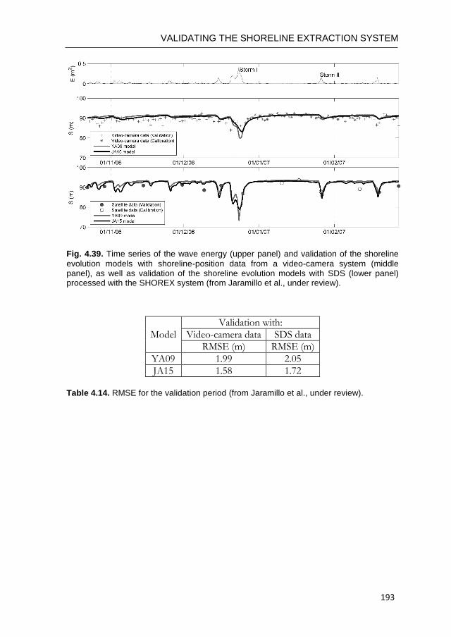
VALIDATING THE SHORELINE EXTRACTION SYSTEM
193
Fig. 4.39. Time series of the wave energy (upper panel) and validation of the shoreline
evolution models with shoreline-position data from a video-camera system (middle panel), as well as validation of the shoreline evolution models with SDS (lower panel) processed with the SHOREX system (from Jaramillo et al., under review).
Model
Validation with:
Video-camera data SDS data
RMSE (m) RMSE (m)
YA09 1.99 2.05
JA15 1.58 1.72
Table 4.14. RMSE for the validation period (from Jaramillo et al., under review).

Cover photo of Chapter 5: Palm Beach, Sydney, Australia (taken Sept 2017)

OTHER PHOTOGRAMMETRIC APPLICATIONS & TECHNIQUES
197
This chapter delves into the photogrammetric aspect of the present thesis through the analysis and development of diverse methods and new techniques for beach monitoring.
Regularly measuring changes in beach width and shoreline position is essential for understanding how environmental drivers control beach behaviour, and why some beaches are more resilient than others. Among remote sensing techniques, coastal imaging has been widely proven as a useful tool by providing high-resolution space and time data for the last 20 years. However, specific video monitoring system implementation continues being expensive in terms of installation and maintenance (and they are costly to upscale), so other lines must be investigated.
Many beach webcams are working worldwide providing visual information of beach and wave conditions to beachgoers and surfers, and these would be useful for monitoring shoreline and intertidal beaches, incident wave characteristics, and even nearshore bathymetry. The first study in Section 5.1 (published in Remote Sensing, 2019) describes various modus operandis with the C-Pro tool (previously presented in Chapter 2) to convert Surfcam images into quality quantitative coastal data. Some practical methodological approaches to exploit these online-streamed images are assessed (one of the major challenges being related to the lack of knowledge of both camera position and optical parameters). Moreover, a further complication is encountered when there is no possibility of measuring the minimum required in situ ground control points to carry out the georectification. Acquisition through freely available web tools (such as Google Earth) is evaluated and presented as a feasible procedure to generate accurate georectified planar images with a sufficient horizontal accuracy compatible with that required for a quantitative analysis of coastal processes. Lastly, its usefulness as a fully remote shore-based observational system is shown by using these georectified images (snaps, timex, variance or timestack images) as accurate data to extract coastal indicators – and so support the characterization of several nearshore features and identify of shoal, surf, and swash zones. An application of C-Pro and online streaming surfcam data for measuring wave runup and intertidal beach topography is shown. Spectral analysis of images across the nearshore zone also produce useful insights on incident wave characteristics such as wave celerity and breaking height (Andriolo, 2018).
Citizen science projects are a very inexpensive method of photographic monitoring through community-derived data. The growth of smartphone technology means that mobile camera lenses are now of sufficient resolution and quality for coastal imaging applications. Community beach monitoring programs based entirely on smartphone images contributed by citizens such as the CoastSnap initiative (started in May 2017) are also making their way into the field of beach monitoring. This project harnesses the wide availability of smartphones, with the duel aim of significantly expanding the spatial coverage of current
Photogrammetry and image processing techniques for beach monitoring
198
network of coastal monitoring and encouraging community participation in the data collection process. Surveyed information within the beach image − submitted by sharing on popular social media platforms – is subsequently used to obtain quantitative measurements of beach change from the community-sourced photo database. This information includes shoreline position, rip-channels, sandbar locations and subtidal bathymetry – information that is eventually returned to the public domain. The starting procedures and methods used in the CoastSnap project are presented in Section 5.2 (work published in Coastal Engineering, 2019). Image processing algorithms subsequently convert the community-sourced images to world coordinates and edge detection techniques are applied to detect and map the shoreline position. Successful trials of this system at two sites in southeastern Australia (Manly and North Narrabeen) have demonstrated strong community participation (1-2 images/site/day on average), as well as an ability to obtain shoreline information of reasonable accuracy (approx. 2-3 m cross-shore). This is despite the processing challenges related to these types of images, which include multiple camera lenses, no image calibration, relatively poor image stability, and low resolution. These encouraging results both in terms of quantitative shoreline data and community engagement has seen this network rapidly expand to multiple sites both inside and outside Australia (Portugal, Spain, Brazil and the UK).
Towards the end of the chapter, Section 5.3 through the work published in the ISPRS Archives (2016) analyzes the potential that terrestrial photogrammetry has to estimate beach profiles using, in this case, the commercial Agisoft PhotoScan software to achieve a 3D point cloud. It is very important for environmental management to have tools that enable low cost modeling in a simple and competent way – and using terrestrial cameras instead the tedious and expensive fieldwork that has been carried out until now. For this work, photos were taken by simple and non-metric cameras, and the photograph capture procedure was refined depending on the studied beach morphology (two different coastal areas were modeled). A minimum of three GCPs was compulsory for georeferencing the models. However, more control points were sometimes required to achieve correlation in those cases limited by insufficient heterogeneity of colors, textures, and forms found in some natural spaces. The calibration of the models was made by comparison of the differences in the elevation among the photogrammetric point cloud and the GPS data in different beach profiles acquired on the same day as the photos. Furthermore, some modeling assays were also performed in a hydraulic pilot channel. Results denoted the potential offered by photogrammetry 3D modelling for monitoring sedimentary changes and natural events.

OTHER PHOTOGRAMMETRIC APPLICATIONS & TECHNIQUES
199

Photogrammetry and image processing techniques for beach monitoring
200
OTHER PHOTOGRAMMETRIC APPLICATIONS & TECHNIQUES
201
5.1. OPERATIONAL USE OF SURFCAM ONLINE STREAMING IMAGES FOR COASTAL MORPHODYNAMIC STUDIES
Coastal video monitoring has been proven to be a valuable shore-based remote sensing technique to study coastal processes, as it offers the possibility of high frequency, continuous and autonomous observations of the coastal area. However, the installation of a video systems infrastructure requires economical and technical efforts, along with being often limited by logistical constraints. This study presents methodological approaches to exploit “surfcam” internet streamed images for quantitative scientific studies. Two different methodologies to collect the required Ground Control Points (GCPs), both during fieldwork and using web tool freely available are presented, in order to establish a rigorous geometric connection between terrestrial and image spaces. The application of an image projector tool allowed the estimation of the unknown camera parameters necessary to georectify the online streamed images. Three photogrammetric procedures are shown, distinct both in the design of the computational steps and in number of GCPs available to solve the spatial resection system. Results showed the feasibility of the methodologies to generate accurate rectified planar images, with the best horizontal projection accuracy of 1.3 m compatible with the one required for a quantitative analysis of coastal processes. The presented methodologies can turn “surfcam” infrastructures and any online streaming beach cam into a fully remote shore-based observational system, fostering the use of these freely available images for the study of nearshore morphodynamics.
5.1.1. Introduction
The coastal zone is an extremely dynamic environment where the complex interaction between wave action and coastal morphological processes often endanger human occupation and the use of the littoral. Therefore, coastal studies should be as comprehensive as possible, to allow the simultaneous description of both hydrodynamic processes and morphological features, with adequate coverage in spatial and temporal scales. On-ground measurements of nearshore morphology such as bathymetry and beach topography are usually performed by vessel-based or RTK-GPS instrumentations (Short and Trembanis, 2004), respectively. Although these conventional practices provide high spatial resolution measures, their repeatability and thus temporal coverage are limited by their technical, logistical and economical demands (Mason et al., 2000). Besides, direct measurements of wave properties (e.g., wave height and wave period) are traditionally obtained by oceanographic devices (e.g., wave gauges, pressure transducers, Acoustic Doppler Current Profiler etc.), whose deployment is operationally demanding and difficult, especially at high energy environments with mobile sandy bottoms.
Photogrammetry and image processing techniques for beach monitoring
202
As many nearshore processes have a visible signature on the sea surface, remote sensing has emerged in this context as a valid alternative to provide nearshore measurements. Among numerous remote sensing methodologies and approaches (e.g., aerial photography, satellite imagery, wave radar, Light Detection And Ranging - LiDAR), shore-based coastal video monitoring has been proved as a cost-efficient and high-quality data collection tool to support coastal scientists and engineers over the last three decades (Holman and Stanley, 2007).
A video-monitoring station is usually composed by one (or more) video-cameras connected to a personal computer, which has the functions of controlling the optical device and storing the video acquisitions. The optical device is usually installed stable at an elevated position looking at the beach and the nearshore. The pioneer Argus monitoring program (Holman and Stanley, 2007) was the first scientific program to install a shore-based video monitoring system with the aim of supporting coastal studies through video-derived observations. The Argus system was developed by the Coastal Imaging Lab at the Oregon State University in the early 90’s, and several Argus-based video monitoring stations has been providing coastal image data worldwide (Holman and Stanley, 2007 and references therein). To 2003, approximately 30 Argus video-monitoring stations and 120 cameras were operating daily in 8 countries (Aarnikhoff et al., 2003). To date, around 40 Argus stations are still operative on the coasts of three continents.
In the 2000’s, the expansion of commercial video systems (e.g., CoastalComs, www.coastalcoms.com, Erdman www.video-monitoring.com) and the development of dedicated image processing tools (e.g., SIRENA - Nieto et al., 2010; COSMOS - Taborda & Silva, 2012, http://cosmos.fc.ul.pt; Beachkeeper plus - Brignone et al., 2012; ULISES - Simarro et al., 2017) promoted the installation of video monitoring stations for scientific purpose with the use of relatively cheap Internet Protocol (IP) video cameras to overcome the expensive installation and purchase of Argus system (e.g., Vousdouskas et al., 2011). Although the lower spatial coverage in comparison with other remote sensing technologies (e.g., satellite imagery, wave radar, LiDAR), shore-based video monitoring technique gives an excellent compromise between spatial and temporal resolutions, beneficial to support both short- and long-term synoptic analysis of the hydro- and morphodynamic processes occurring in the nearshore.
Despite the large exploitation of coastal video stations over last decades, the use of online streaming web-cam for quantitative scientific studies has been weakly investigated. For example, coastal “surfcams” are video cameras installed at the coast with the main aim of remotely providing visual information of beach and sea state to beachgoers and surf users, streaming near-continuous video over the internet. The main objective of this work is to provide operational procedures for a research-oriented use of surfcam images.
OTHER PHOTOGRAMMETRIC APPLICATIONS & TECHNIQUES
203
The following Section 5.1.1.1 and Section 5.1.1.2 present a comprehensive overview of standard video image pre-processing and scientific applications of coastal video monitoring, in order to give a perception of the importance that such technique has gained in coastal studies over the last decades. Section 5.1.1.3 describes the main issues related to the use of surfcams and underlines the specific objectives of this work, outlining the main methodological steps that are presented.
5.1.1.1. Standard image rectification procedure
In order to exploit the images acquired by a coastal video system, an accurate procedure must be applied to raw imagery data to obtain referenced planar images (Hartley and Zisserman, 2004). The camera calibration process is the procedure that estimates the intrinsic parameters of camera lens and sensor. The intrinsic camera parameters, also called Internal Orientation Parameters (IOPs), are namely the focal length f, the position of the principal point (uc , vc), and the distortion coefficients of the camera lens kj. Determination of IOPs is necessary to correct the image distortion inducted by the lens curvature. Conventional camera calibration procedure is performed using several screenshots of checkerboard patterns panel taken by the camera with different poses. Freely available toolboxes such as Camera Calibration Toolbox for Matlab (Bouget, 2007) can be extensively used to execute this required process and apply the correction to the images (Vousdoukas et al., 2011; Andriolo et al., 2018).
The image rectification procedure transforms an undistorted oblique image into a plan view equivalent image, known as rectified image (Taborda & Silva, 2012). Given the IOPs computed by the preliminary camera calibration, standard photogrammetric procedures such as the collinearity or the Direct Linear Transformation (DLT) methods (Holland et al., 1997; Hartley and Zisserman, 2004), establish the relation between terrain (X,Y,Z) and image (u,v) spaces by determining the External camera Orientation Parameters (EOPs), namely the camera position XC, YC, ZC, and orientation (azimuth α; tilt τ, and roll θ). The basis of the spatial resection process follow the classical physical pinhole camera model (Fig. 5.1), which describes the mathematical relationship between the coordinates of a point in the 3D space (Xo, Yo, Zo) and its projection onto the image plane (uo, vo).
In order to solve the collinearity equation or the DLT equation systems for the spatial resection geometry, it is necessary to identify on the oblique undistorted image a minimum of GCPs whose real-world coordinates are known. In general, a minimum amount of six GCPs is required. GCPs can be selected on fixed structure on the coast (such as breakwaters, houses, paths), can be installed in form of panels visible on the image (Harley et al., 2013), or can be collected by RTK-GPS survey and later identified on the acquired image sequence. The solution of the equations system allows the transformation of the undistorted image into a planar image map, whose pixels have real-world coordinates.
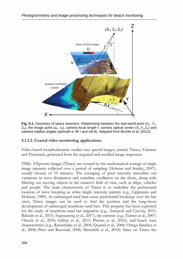
Photogrammetry and image processing techniques for beach monitoring
204
Fig. 5.1. Geometry of space resection. Relationship between the real-world point (Xo, Yo,
Zo), the image point (uo, vo), camera focal length f, camera optical center (Xc,Yc,Zc) and camera rotation angles (azimuth α; tilt τ and roll θ). Adapted from Bechle et al. (2012).
5.1.1.2. Coastal video monitoring applications
Video-based morphodynamic studies uses special images, namely Timex, Variance and Timestack, generated from the acquired and rectified image sequences.
TIMe- EXposure images (Timex) are created by the mathematical average of single image intensity collected over a period of sampling (Holman and Stanley, 2007), usually chosen of 10 minutes. The averaging of pixel intensity smoothes out variations in wave dissipation and waterline oscillation on the shore, along with filtering out moving objects in the camera's field of view, such as ships, vehicles and people. The main characteristic of Timex is to underline the preferential location of wave breaking as white bright intensity pattern (e.g., Lippmann and Holman, 1989). As submerged sand bars cause preferential breakings over the bar crest, Timex images can be used to find the position and the long-shore development of submerged nearshore sand bars. This property has been exploited for the study of nearshore sand bar migration (e.g., Armaroli and Ciavola, 2011; Balouin et al., 2013; Angnuureng et al., 2017), rip currents (e.g., Turner at al., 2007; Orzech et al., 2010; Gallop et al., 2011; Pitman et al., 2016), and beach state characteristics (e.g., Ranashinke et al., 2004, Quartel et al., 2006; Ortega-Sánchez et al., 2008; Price and Ruessink, 2008; Masselink et al., 2014). Since on Timex the
OTHER PHOTOGRAMMETRIC APPLICATIONS & TECHNIQUES
205
swash movements on the foreshore slope are smoothed out, several algorithms have been proposed for shoreline detection on Timex images (e.g., Aarninkhof et al., 2003; Alvarez-Ellacuria et al., 2011; Osorio et al., 2012; Valentini et al., 2017b) and have been widely used for a long-term monitoring of shoreline change (e.g., Fairley et al., 2009; Ruiz de Alegria-Arzaburu and Masselink, 2010; Blossier et al., 2017).
Variance images are created by computing the standard deviation (and despite the name, not the variance) of the individual images which are collected over a period of sampling, as for Timex (Holman and Stanley, 2007). Variance images are bright on the areas with large temporal variability, while unchanged areas appear dark. Thus, a sandy beach is shown as dark in a Variance, while the surf zone appears very bright, due to the pixel intensity variation in relation to breaking waves. Although Argus stations and other video systems have been producing Variance for long time, this kind of images has been seldom used. Few examples of the use of Variance can be seen in Vousdoukas et al. (2011), in Simarro et al. (2015) and in Rigos et al. (2016), mainly regarding shoreline contour detection.
A third kind of special image, Timestack image, is generated by sampling a single line of pixels from each image over the period of acquisition and concatenating such array of pixel according to the frame acquisition frequency. Timestack is therefore composed by pixel intensity time series over a given image sequence. In general, a video data sampling period of 10 minutes is considered, however the chosen time interval can vary depending on the system set up and/or on the main purposes of the study (e.g., from 7 mins to 34 mins in Stockdon et al., 2006; 20 mins in Almar et al., 2011). Timestacks were originally produced with the main purpose of studying wave runup process on the foreshore (Aagaard and Holm, 1989; Holland and Holman, 1993; Birkemeier et al., 1997), as the camera acquisitions allowed the monitoring of the high-frequency waterline oscillation on the beach slope. Over the last decades, Timestack images have been extensively applied to advance in foreshore runup knowledge (Bailey and Shand, 1994; Holland et al., 1995; Ruggiero et al., 2004; Vousdoukas et al., 2009; Guedes et al, 2011a; Power et al., 2011; Senechal et al., 2011; Brinkkemper et al, 2014; Stockdon et al, 2014; Vousdoukas et al., 2014), to improve runup measurements (Simarro et al., 2015; Blenkinsopp et al., 2016; Almar et al., 2017a) and to propose new wave runup parameterization (Stockdon et al., 2006; Vousdoukas et al., 2012; Poate et al., 2016; Atkinson et al., 2017). Besides the possibility of measuring wave runup, Lippmann and Holman (1990) related Timestack pixel intensity to temporal series of water surface elevation. Exploiting such property, authors measured the wave period applying frequency domain analysis (Lippman and Holman, 1989; Almar, 2009) or computing wave spectrum (Zikra et al., 2012). Another Timestack application resides on the measurement of wave celerity (Almar et al, 2008; Tissier et al., 2011; Almar et al., 2014; Postacchini and Brocchini, 2014), which allowed to retrieve the nearshore subtidal bathymetry through depth inversion technique
Photogrammetry and image processing techniques for beach monitoring
206
(Stockdon and Holman, 2000; Yoo, 2007; Almar et al., 2011; Holman et al., 2013). Finally, Timestack images were used to estimate wave breaking height (Gal et al., 2011; Almar et al., 2012a; Gal et al., 2014; Robertson et al., 2015), to measure overwash velocity (Matias et al., 2017), and along-shore Timestacks were adopted to estimate longshore currents (Chickadel, 2007).
5.1.1.3. Surfcam images
The state of art presented in Section 5.1.1.2 emphasizes the capability of standard coastal video monitoring technique in quantifying a diverse range of important coastal processes. Therefore, it is of interest to explore the opportunities of potentially increasing the coastal imaging acquisition. For instance, two previous studies were conducted to investigate the possibility of using surfcam network for coastal monitoring (Mole et al., 2013; Bracs et al., 2016), however these works were limited to the use of a commercial software for shoreline monitoring and inshore wave measurements (e.g. Shand et al., 2012).
The main purpose of this study is to present practical methodological approaches to accurately rectify surfcam images, in order to exploit online-streamed images for scientific studies. The video acquired by a surfcam at the Riberia d’Ilhas beach on Portuguese coast are used as case study.
The quantitative use of surfcam recreational cameras is mostly limited by their logistic. Most of the installation sites of these devices are not directly accessible, as they are located for instance on rooftop buildings, private houses or streetlights posts. As a consequence, it is often not possible to perform the conventional camera calibration procedure described in Section 5.1.1.1, and neither to survey the camera position coordinates. In the context in which standard rectification process cannot be performed, the Coastal Projector monitoring system “C-Pro” (Sánchez-García et al., 2017) offers a valuable computational solution to provide the missing photogrammetric requirements, thus to solve the spatial resection systems for getting precise rectified planar images.
C-Pro adopts the terrestrial horizon visible on image as a photogrammetric constraint, to incorporate the two equations that describe the horizon inclination in the collinearity system. As working with surfcam images generally implies the lack of knowledge of the IOPs and EOPs, the horizon constraint reduces the number of unknowns in the equations system. In order to achieve an accurate determination of all photogrammetric parameters, C-Pro solves the linearized equations system with the weighted least square method, whose finest solution gives the IOPs and EOPs corrections after an iterative optimization. The minimum amount of required GCPs changes depending on the number of unknowns to be solved by the equations system, given that the incorporation of the horizon equations can also reduce the required number of GCPs.
OTHER PHOTOGRAMMETRIC APPLICATIONS & TECHNIQUES
207
This work addresses firstly the GCPs sampling problem. Besides the conventional in situ collection of GCPs (Section 5.1.3.3), we propose a novel method to remotely acquire Ground Control Points (GCPs) coordinates and elevation. The synoptic combination of freely-available-online tool and video technique supplies the required points to transform image information into real-world coordinates (Section 5.1.3.4). Successively, we tested C-Pro operational capability in retrieving the set of parameters required to perform the image rectification process. Since C-Pro adapts its methodology in accordance with the available input dataset, three analytical procedures are shown (Section 5.1.3.6), distinct both in the design of the computational steps and in number of GCPs available to solve the spatial resection system. The analysis of the results focus on the accuracy achieved by the remote method for GCPs collection (Section 5.1.4.1) and compares the positional accuracy of rectified planar images generated by C-Pro through the different procedures (Section 5.1.4.2 and Section 5.1.4.3). A discussion of the advantages and backwards of the proposed solutions associated with surfcam images use and rectification is then presented.
5.1.2. Study site
The present work is supported on images acquired at the case study of Ribeira d’Ilhas (38°59'17.0"N, 9°25'10.4"W), a beach that develops over a rocky-shore platform located on the Portuguese western coast, facing North Atlantic Ocean (Fig. 5.2). The beach extends for about 300 m along-shore, with a NW-SE orientation, and it is limited southwards by a 55 m high cliff and northwards by a small headland. The intertidal shore platform presents a low gradient slope (tanβ = 0.01). This site is a famous stage for many national and international surfing events. The collaboration with the company Surftotal (https://www.surftotal.com/) allowed the use of the images (Fig. 5.2c) acquired by a surfcam installed at the study site.
The video station consisted in a video camera mounted on a house roof at an elevation of about 80 m (MSL) and about 400 m from the shoreline. The camera was installed in a private property which was not accessible. The camera view was set steady looking at the Riberia d’Ilhas shore and nearshore during two days (28 and 29 of March 2017).
5.1.3. Methods
This section describes methodological steps to obtain rectified images from raw surfcam video acquisition. The methods differ in the sources used to retrieve the GCP locations, conditioning theirs reliability and number, and in the C-Pro methodological procedures to compute the resection parameters and generate the image planar map.
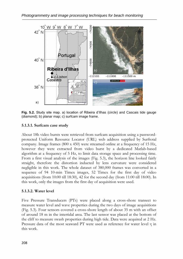
Photogrammetry and image processing techniques for beach monitoring
208
Fig. 5.2. Study site map. a) location of Ribeira d’Ilhas (circle) and Cascais tide gauge
(diamond); b) planar map; c) surfcam image frame.
5.1.3.1. Surfcam case study
About 18h video bursts were retrieved from surfcam acquisition using a password-protected Uniform Resource Locator (URL) web address supplied by Surftotal company. Image frames (800 x 450) were streamed online at a frequency of 15 Hz, however they were extracted from video burst by a dedicated Matlab-based algorithm at a frequency of 5 Hz, to limit data storage space and processing time. From a first visual analysis of the images (Fig. 5.3), the horizon line looked fairly straight, therefore the distortion inducted by lens curvature were considered negligible in this work. The whole dataset of 380,000 frames was converted in a sequence of 94 10-min Timex images, 52 Timex for the first day of video acquisitions (from 10:00 till 18:30), 42 for the second day (from 11:00 till 18:00). In this work, only the images from the first day of acquisition were used.
5.1.3.2. Water level
Five Pressure Transducers (PTs) were placed along a cross-shore transect to measure water level and wave properties during the two days of image acquisitions (Fig. 5.3). Four sensors covered a cross-shore length of about 35 m with an offset of around 18 m in the intertidal area. The last sensor was placed at the bottom of the cliff to measure swash properties during high tide. Data were acquired at 2 Hz. Pressure data of the most seaward PT were used as reference for water level η in this work.
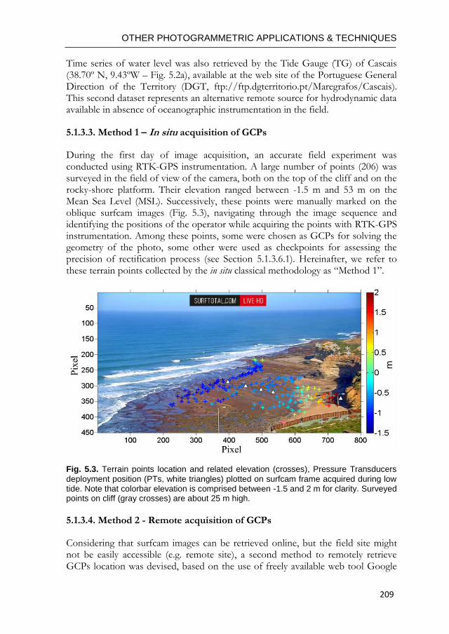
OTHER PHOTOGRAMMETRIC APPLICATIONS & TECHNIQUES
209
Time series of water level was also retrieved by the Tide Gauge (TG) of Cascais (38.70º N, 9.43ºW – Fig. 5.2a), available at the web site of the Portuguese General Direction of the Territory (DGT, ftp://ftp.dgterritorio.pt/Maregrafos/Cascais). This second dataset represents an alternative remote source for hydrodynamic data available in absence of oceanographic instrumentation in the field.
5.1.3.3. Method 1 – In situ acquisition of GCPs
During the first day of image acquisition, an accurate field experiment was conducted using RTK-GPS instrumentation. A large number of points (206) was surveyed in the field of view of the camera, both on the top of the cliff and on the rocky-shore platform. Their elevation ranged between -1.5 m and 53 m on the Mean Sea Level (MSL). Successively, these points were manually marked on the oblique surfcam images (Fig. 5.3), navigating through the image sequence and identifying the positions of the operator while acquiring the points with RTK-GPS instrumentation. Among these points, some were chosen as GCPs for solving the geometry of the photo, some other were used as checkpoints for assessing the precision of rectification process (see Section 5.1.3.6.1). Hereinafter, we refer to these terrain points collected by the in situ classical methodology as “Method 1”.
Fig. 5.3. Terrain points location and related elevation (crosses), Pressure Transducers
deployment position (PTs, white triangles) plotted on surfcam frame acquired during low tide. Note that colorbar elevation is comprised between -1.5 and 2 m for clarity. Surveyed points on cliff (gray crosses) are about 25 m high.
5.1.3.4. Method 2 - Remote acquisition of GCPs
Considering that surfcam images can be retrieved online, but the field site might not be easily accessible (e.g. remote site), a second method to remotely retrieve GCPs location was devised, based on the use of freely available web tool Google
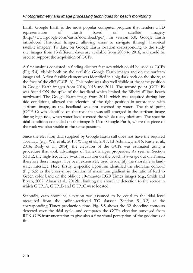
Photogrammetry and image processing techniques for beach monitoring
210
Earth. Google Earth is the most popular computer program that renders a 3D representation of Earth based on satellite imagery (http://www.google.com/earth/download/ge/). In version 5.0, Google Earth introduced Historical Imagery, allowing users to navigate through historical satellite imagery. To date, on Google Earth location corresponding to the study site, images from 13 different dates are available from 2006 to 2016, and could be used to support the acquisition of GCPs.
A first analysis consisted in finding distinct features which could be used as GCPs (Fig. 5.4), visible both on the available Google Earth images and on the surfcam image and. A first feasible element was identified in a big dark rock on the shore, at the foot of the cliff (GCP_A). This point was also well visible at the same position in Google Earth images from 2016, 2015 and 2014. The second point (GCP_B) was found ON the spike of the headland which limited the Ribeira d’Ilhas beach northward. The Google Earth image from 2014, which was acquired during low tide conditions, allowed the selection of the right position in accordance with surfcam image, as the headland was not covered by water. The third point (GCP_C) was identified on the rock that was still emerged in the surfcam image during high tide, when water level covered the whole rocky platform. The specific tidal condition coincided on the image 2015 of Google Earth, where the piece of the rock was also visible in the same position.
Since the elevation data supplied by Google Earth still does not have the required accuracy. (e.g., Wei et al., 2018; Wang et al., 2017; El-Ashmawy, 2016; Rusly et al., 2016; Rusly et al., 2014), the elevation of the GCPs was estimated using a procedure that took advantages of Timex images properties. As seen in Section 5.1.1.2, the high-frequency swash oscillation on the beach is average out on Timex, therefore these images have been extensively used to identify the shoreline as land-water interface. Here, firstly, a specific algorithm identified the shoreline contour (Fig. 5.5) as the cross-shore location of maximum gradient in the ratio of Red to Green color band on the oblique 10-minutes RGB Timex images (e.g., Smith and Bryan, 2007; Almar et al., 2012b), limiting the shoreline detection to the sector in which GCP_A, GCP_B and GCP_C were located.
Secondly, each shoreline elevation was assumed to be equal to the tidal level measured from the online-retrieved TG dataset (Section 5.1.3.2) at the corresponding Timex production time. Fig. 5.5 shows the 32 shoreline contours detected over the tidal cycle, and compares the GCPs elevation surveyed from RTK-GPS instrumentation to give also a first visual perception of the goodness of fit.
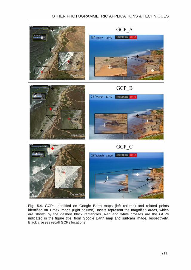
OTHER PHOTOGRAMMETRIC APPLICATIONS & TECHNIQUES
211
Fig. 5.4. GCPs identified on Google Earth maps (left column) and related points
identified on Timex image (right column). Insets represent the magnified areas, which are shown by the dashed black rectangles. Red and white crosses are the GCPs indicated in the figure title, from Google Earth map and surfcam image, respectively. Black crosses recall GCPs locations.
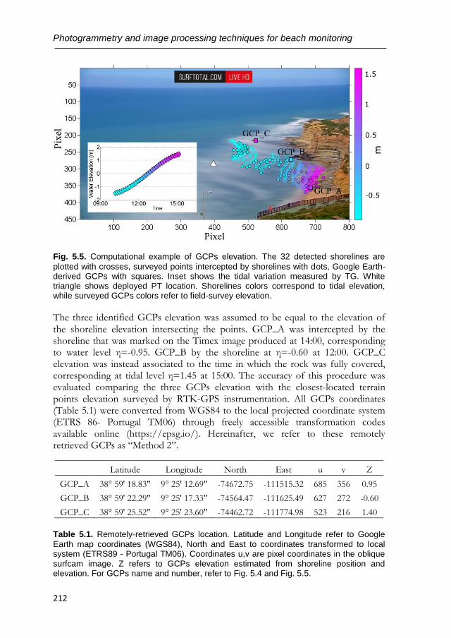
Photogrammetry and image processing techniques for beach monitoring
212
Fig. 5.5. Computational example of GCPs elevation. The 32 detected shorelines are
plotted with crosses, surveyed points intercepted by shorelines with dots, Google Earth-derived GCPs with squares. Inset shows the tidal variation measured by TG. White triangle shows deployed PT location. Shorelines colors correspond to tidal elevation, while surveyed GCPs colors refer to field-survey elevation.
The three identified GCPs elevation was assumed to be equal to the elevation of the shoreline elevation intersecting the points. GCP_A was intercepted by the shoreline that was marked on the Timex image produced at 14:00, corresponding to water level η=-0.95. GCP_B by the shoreline at η=-0.60 at 12:00. GCP_C elevation was instead associated to the time in which the rock was fully covered, corresponding at tidal level η=1.45 at 15:00. The accuracy of this procedure was evaluated comparing the three GCPs elevation with the closest-located terrain points elevation surveyed by RTK-GPS instrumentation. All GCPs coordinates (Table 5.1) were converted from WGS84 to the local projected coordinate system (ETRS 86- Portugal TM06) through freely accessible transformation codes available online (https://epsg.io/). Hereinafter, we refer to these remotely retrieved GCPs as “Method 2”.
Latitude Longitude North East u v Z
GCP_A 38° 59' 18.83" 9° 25' 12.69" -74672.75 -111515.32 685 356 0.95
GCP_B 38° 59' 22.29" 9° 25' 17.33" -74564.47 -111625.49 627 272 -0.60
GCP_C 38° 59' 25.52" 9° 25' 23.60" -74462.72 -111774.98 523 216 1.40
Table 5.1. Remotely-retrieved GCPs location. Latitude and Longitude refer to Google
Earth map coordinates (WGS84), North and East to coordinates transformed to local system (ETRS89 - Portugal TM06). Coordinates u,v are pixel coordinates in the oblique surfcam image. Z refers to GCPs elevation estimated from shoreline position and elevation. For GCPs name and number, refer to Fig. 5.4 and Fig. 5.5.
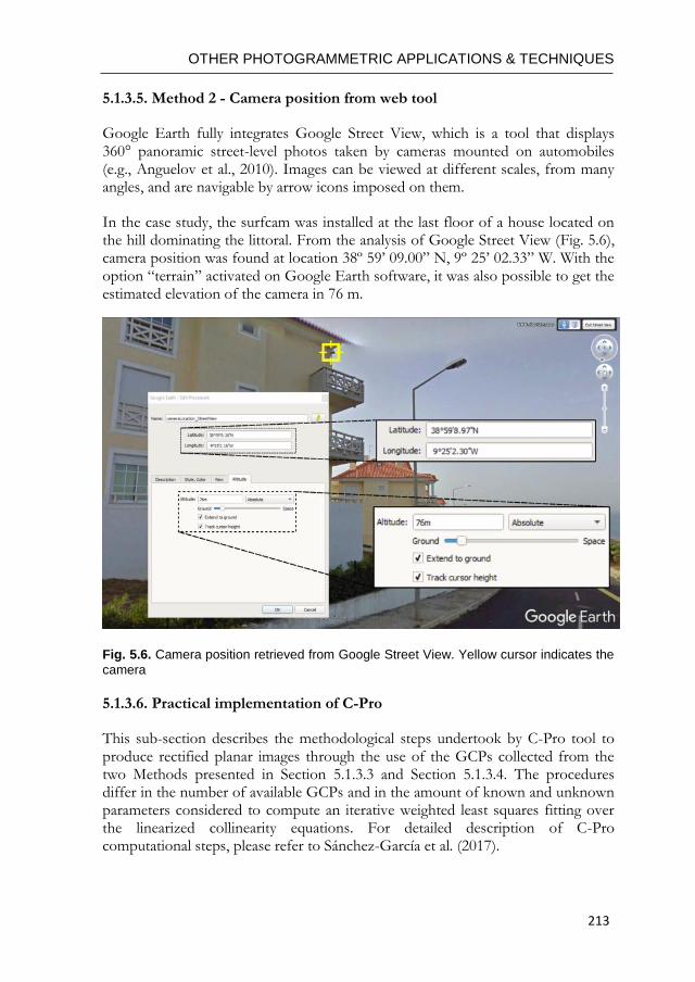
OTHER PHOTOGRAMMETRIC APPLICATIONS & TECHNIQUES
213
5.1.3.5. Method 2 - Camera position from web tool
Google Earth fully integrates Google Street View, which is a tool that displays 360° panoramic street-level photos taken by cameras mounted on automobiles (e.g., Anguelov et al., 2010). Images can be viewed at different scales, from many angles, and are navigable by arrow icons imposed on them.
In the case study, the surfcam was installed at the last floor of a house located on the hill dominating the littoral. From the analysis of Google Street View (Fig. 5.6), camera position was found at location 38º 59’ 09.00” N, 9º 25’ 02.33” W. With the option “terrain” activated on Google Earth software, it was also possible to get the estimated elevation of the camera in 76 m.
Fig. 5.6. Camera position retrieved from Google Street View. Yellow cursor indicates the
camera
5.1.3.6. Practical implementation of C-Pro
This sub-section describes the methodological steps undertook by C-Pro tool to produce rectified planar images through the use of the GCPs collected from the two Methods presented in Section 5.1.3.3 and Section 5.1.3.4. The procedures differ in the number of available GCPs and in the amount of known and unknown parameters considered to compute an iterative weighted least squares fitting over the linearized collinearity equations. For detailed description of C-Pro computational steps, please refer to Sánchez-García et al. (2017).
Photogrammetry and image processing techniques for beach monitoring
214
The procedures are numbered following the considered GCPs for the computation, namely Procedure 1 and Procedure 2, recalling the methods that were used to retrieve the points (Section 5.1.3.3 and Section 5.1.3.4).
Procedure 1
Among the 206 points collected in the field by the conventional RTK-GPS survey (Method 1), 72 were chosen as GCPs, heterogeneously distributed on the rocky platform (Fig. 5.7). As the number of available GCPs was more than six, C-Pro tool computed firstly the eleven DLT coefficients that express the relationships between terrain coordinates and image space. This initial step led to first approximated values of focal length f and camera location (XC, YC, ZC,). The first estimation of the three-angle describing camera orientation (α, τ, θ) came instead from the horizon constraint detected on surfcam image. In the second computational step, the approximated values of f and EOPs were used as input data to complete the collinearity least squares fitting, whose iterative process finished when each of the correction values for the seven parameters became negligible. Although the high number of GCPs promoted an over-determined system to solve the geometry, the two extra horizon equations were included in the iterative process to improve the camera repositioning result. The final step consisted in using the optimized IOPs and EOPs to generate a geo-rectified planar Timex image. The image was projected on a specific plane through inverse mapping technique and applying the nearest neighbor interpolation method. The Z elevation value for the projected plane was taken equal to the tidal level at the correspondent image time.
Among the 206 terrain points, the remaining 134 terrain points −not chosen as GCPs− were used as checkpoints (Fig. 5.7) to assess the goodness of the photogrammetric solution and the positional accuracy of the rectified image generated by C-Pro. The horizontal projection error for the 134 checkpoints was found firstly projecting each point on its associated altimetric Z coordinate (measured by RTK-GPS), finally computing the Euclidean distance between its projected coordinates (X,Y) and its real-world coordinates measured in the field. The camera location computed by C-Pro was compared to the one retrieved from Google Street View (Section 5.1.3.5).
Procedure 2
A second example of C-Pro application (Procedure 2) considered the three GCPs remotely-retrieved in Method 2. Here, two sub-examples of C-Pro computations were made.
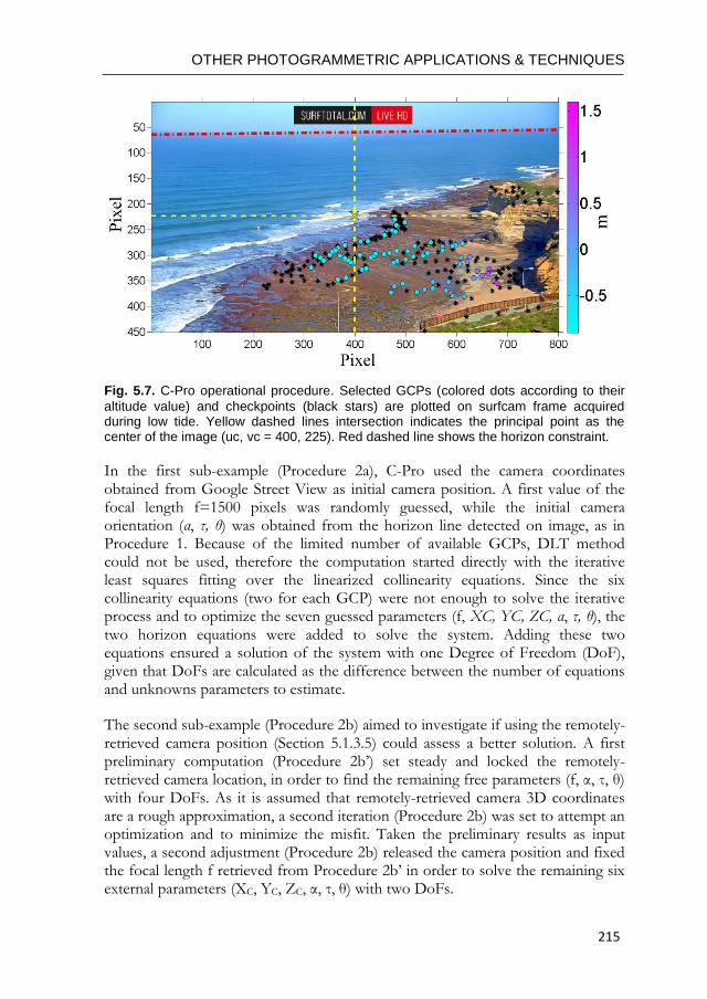
OTHER PHOTOGRAMMETRIC APPLICATIONS & TECHNIQUES
215
Fig. 5.7. C-Pro operational procedure. Selected GCPs (colored dots according to their
altitude value) and checkpoints (black stars) are plotted on surfcam frame acquired during low tide. Yellow dashed lines intersection indicates the principal point as the center of the image (uc, vc = 400, 225). Red dashed line shows the horizon constraint.
In the first sub-example (Procedure 2a), C-Pro used the camera coordinates obtained from Google Street View as initial camera position. A first value of the focal length f=1500 pixels was randomly guessed, while the initial camera orientation (α, τ, θ) was obtained from the horizon line detected on image, as in Procedure 1. Because of the limited number of available GCPs, DLT method could not be used, therefore the computation started directly with the iterative least squares fitting over the linearized collinearity equations. Since the six collinearity equations (two for each GCP) were not enough to solve the iterative process and to optimize the seven guessed parameters (f, XC, YC, ZC, α, τ, θ), the two horizon equations were added to solve the system. Adding these two equations ensured a solution of the system with one Degree of Freedom (DoF), given that DoFs are calculated as the difference between the number of equations and unknowns parameters to estimate.
The second sub-example (Procedure 2b) aimed to investigate if using the remotely-retrieved camera position (Section 5.1.3.5) could assess a better solution. A first preliminary computation (Procedure 2b’) set steady and locked the remotely- retrieved camera location, in order to find the remaining free parameters (f, α, τ, θ) with four DoFs. As it is assumed that remotely-retrieved camera 3D coordinates are a rough approximation, a second iteration (Procedure 2b) was set to attempt an optimization and to minimize the misfit. Taken the preliminary results as input values, a second adjustment (Procedure 2b) released the camera position and fixed the focal length f retrieved from Procedure 2b’ in order to solve the remaining six external parameters (XC, YC, ZC, α, τ, θ) with two DoFs.
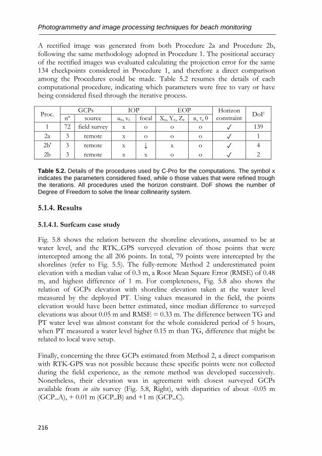
Photogrammetry and image processing techniques for beach monitoring
216
A rectified image was generated from both Procedure 2a and Procedure 2b, following the same methodology adopted in Procedure 1. The positional accuracy of the rectified images was evaluated calculating the projection error for the same 134 checkpoints considered in Procedure 1, and therefore a direct comparison among the Procedures could be made. Table 5.2 resumes the details of each computational procedure, indicating which parameters were free to vary or have being considered fixed through the iterative process.
Proc. GCPs IOP EOP Horizon
constraint DoF
nº source uc, vc focal Xc, Yc, Zc α, τ, θ
1 72 field survey x o o o ✓ 139
2a 3 remote x o o o ✓ 1
2b' 3 remote x ↓ x o ✓ 4
2b 3 remote x x o o ✓ 2
Table 5.2. Details of the procedures used by C-Pro for the computations. The symbol x
indicates the parameters considered fixed, while o those values that were refined trough the iterations. All procedures used the horizon constraint. DoF shows the number of Degree of Freedom to solve the linear collinearity system.
5.1.4. Results
5.1.4.1. Surfcam case study
Fig. 5.8 shows the relation between the shoreline elevations, assumed to be at water level, and the RTK_GPS surveyed elevation of those points that were intercepted among the all 206 points. In total, 79 points were intercepted by the shorelines (refer to Fig. 5.5). The fully-remote Method 2 underestimated point elevation with a median value of 0.3 m, a Root Mean Square Error (RMSE) of 0.48 m, and highest difference of 1 m. For completeness, Fig. 5.8 also shows the relation of GCPs elevation with shoreline elevation taken at the water level measured by the deployed PT. Using values measured in the field, the points elevation would have been better estimated, since median difference to surveyed elevations was about 0.05 m and RMSE = 0.33 m. The difference between TG and PT water level was almost constant for the whole considered period of 5 hours, when PT measured a water level higher 0.15 m than TG, difference that might be related to local wave setup.
Finally, concerning the three GCPs estimated from Method 2, a direct comparison with RTK-GPS was not possible because these specific points were not collected during the field experience, as the remote method was developed successively. Nonetheless, their elevation was in agreement with closest surveyed GCPs available from in situ survey (Fig. 5.8, Right), with disparities of about -0.05 m (GCP_A), + 0.01 m (GCP_B) and +1 m (GCP_C).
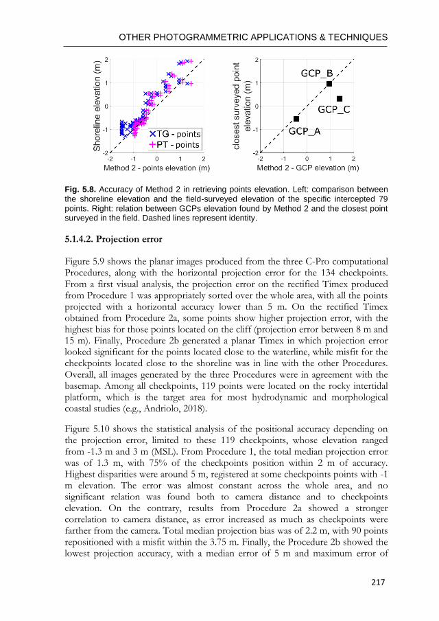
OTHER PHOTOGRAMMETRIC APPLICATIONS & TECHNIQUES
217
Fig. 5.8. Accuracy of Method 2 in retrieving points elevation. Left: comparison between
the shoreline elevation and the field-surveyed elevation of the specific intercepted 79 points. Right: relation between GCPs elevation found by Method 2 and the closest point surveyed in the field. Dashed lines represent identity.
5.1.4.2. Projection error
Figure 5.9 shows the planar images produced from the three C-Pro computational Procedures, along with the horizontal projection error for the 134 checkpoints. From a first visual analysis, the projection error on the rectified Timex produced from Procedure 1 was appropriately sorted over the whole area, with all the points projected with a horizontal accuracy lower than 5 m. On the rectified Timex obtained from Procedure 2a, some points show higher projection error, with the highest bias for those points located on the cliff (projection error between 8 m and 15 m). Finally, Procedure 2b generated a planar Timex in which projection error looked significant for the points located close to the waterline, while misfit for the checkpoints located close to the shoreline was in line with the other Procedures. Overall, all images generated by the three Procedures were in agreement with the basemap. Among all checkpoints, 119 points were located on the rocky intertidal platform, which is the target area for most hydrodynamic and morphological coastal studies (e.g., Andriolo, 2018).
Figure 5.10 shows the statistical analysis of the positional accuracy depending on the projection error, limited to these 119 checkpoints, whose elevation ranged from -1.3 m and 3 m (MSL). From Procedure 1, the total median projection error was of 1.3 m, with 75% of the checkpoints position within 2 m of accuracy. Highest disparities were around 5 m, registered at some checkpoints points with -1 m elevation. The error was almost constant across the whole area, and no significant relation was found both to camera distance and to checkpoints elevation. On the contrary, results from Procedure 2a showed a stronger correlation to camera distance, as error increased as much as checkpoints were farther from the camera. Total median projection bias was of 2.2 m, with 90 points repositioned with a misfit within the 3.75 m. Finally, the Procedure 2b showed the lowest projection accuracy, with a median error of 5 m and maximum error of
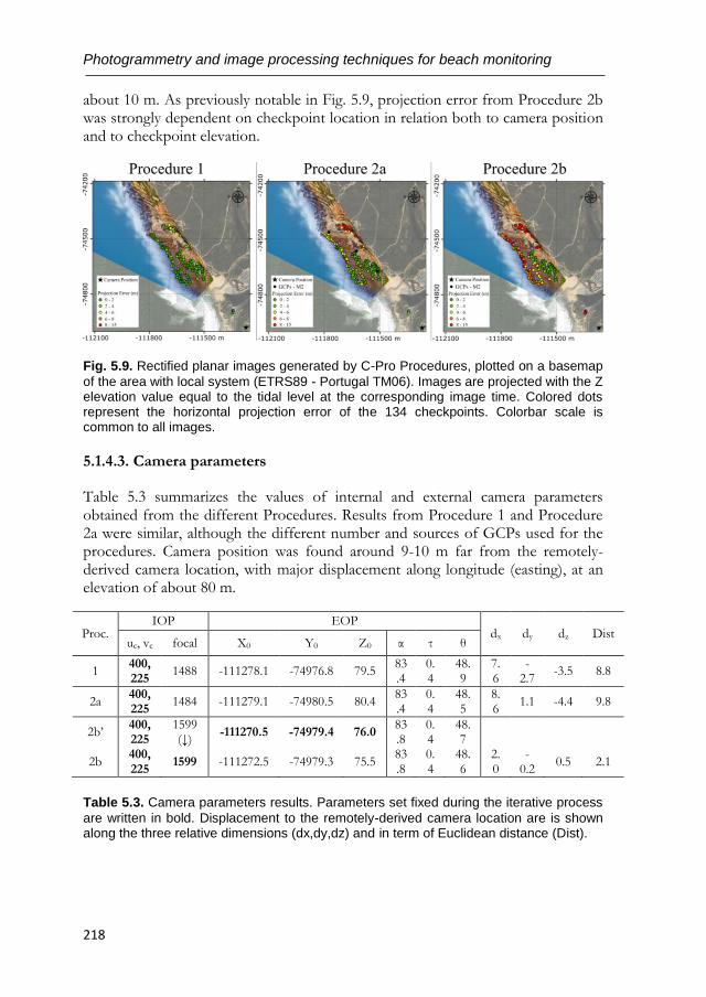
Photogrammetry and image processing techniques for beach monitoring
218
about 10 m. As previously notable in Fig. 5.9, projection error from Procedure 2b was strongly dependent on checkpoint location in relation both to camera position and to checkpoint elevation.
Fig. 5.9. Rectified planar images generated by C-Pro Procedures, plotted on a basemap
of the area with local system (ETRS89 - Portugal TM06). Images are projected with the Z elevation value equal to the tidal level at the corresponding image time. Colored dots represent the horizontal projection error of the 134 checkpoints. Colorbar scale is common to all images.
5.1.4.3. Camera parameters
Table 5.3 summarizes the values of internal and external camera parameters obtained from the different Procedures. Results from Procedure 1 and Procedure 2a were similar, although the different number and sources of GCPs used for the procedures. Camera position was found around 9-10 m far from the remotely-derived camera location, with major displacement along longitude (easting), at an elevation of about 80 m.
Proc. IOP EOP
dx dy dz Dist uc, vc focal X0 Y0 Z0 α τ θ
1 400,225
1488 -111278.1 -74976.8 79.5 83.4
0.4
48.9
7.6
-2.7
-3.5 8.8
2a 400,225
1484 -111279.1 -74980.5 80.4 83.4
0.4
48.5
8.6
1.1 -4.4 9.8
2b’ 400,225
1599 (↓)
-111270.5 -74979.4 76.0 83.8
0.4
48.7
2b 400,225
1599 -111272.5 -74979.3 75.5 83.8
0.4
48.6
2.0
-0.2
0.5 2.1
Table 5.3. Camera parameters results. Parameters set fixed during the iterative process
are written in bold. Displacement to the remotely-derived camera location are is shown along the three relative dimensions (dx,dy,dz) and in term of Euclidean distance (Dist).
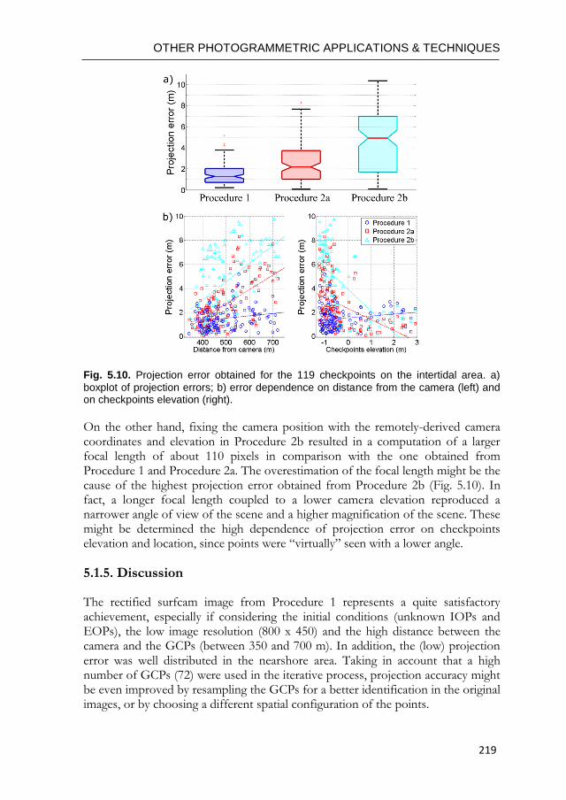
OTHER PHOTOGRAMMETRIC APPLICATIONS & TECHNIQUES
219
Fig. 5.10. Projection error obtained for the 119 checkpoints on the intertidal area. a)
boxplot of projection errors; b) error dependence on distance from the camera (left) and on checkpoints elevation (right).
On the other hand, fixing the camera position with the remotely-derived camera coordinates and elevation in Procedure 2b resulted in a computation of a larger focal length of about 110 pixels in comparison with the one obtained from Procedure 1 and Procedure 2a. The overestimation of the focal length might be the cause of the highest projection error obtained from Procedure 2b (Fig. 5.10). In fact, a longer focal length coupled to a lower camera elevation reproduced a narrower angle of view of the scene and a higher magnification of the scene. These might be determined the high dependence of projection error on checkpoints elevation and location, since points were “virtually” seen with a lower angle.
5.1.5. Discussion
The rectified surfcam image from Procedure 1 represents a quite satisfactory achievement, especially if considering the initial conditions (unknown IOPs and EOPs), the low image resolution (800 x 450) and the high distance between the camera and the GCPs (between 350 and 700 m). In addition, the (low) projection error was well distributed in the nearshore area. Taking in account that a high number of GCPs (72) were used in the iterative process, projection accuracy might be even improved by resampling the GCPs for a better identification in the original images, or by choosing a different spatial configuration of the points.
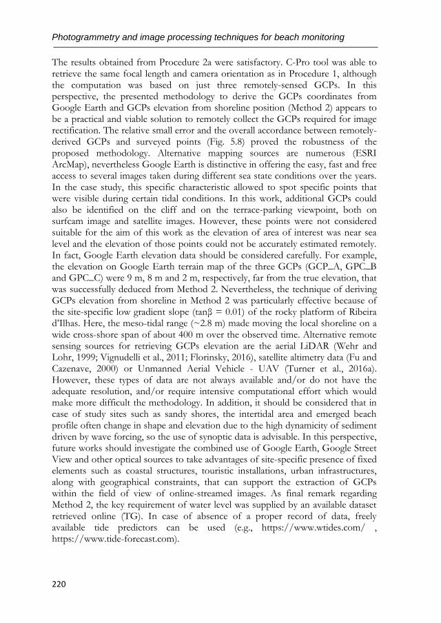
Photogrammetry and image processing techniques for beach monitoring
220
The results obtained from Procedure 2a were satisfactory. C-Pro tool was able to retrieve the same focal length and camera orientation as in Procedure 1, although the computation was based on just three remotely-sensed GCPs. In this perspective, the presented methodology to derive the GCPs coordinates from Google Earth and GCPs elevation from shoreline position (Method 2) appears to be a practical and viable solution to remotely collect the GCPs required for image rectification. The relative small error and the overall accordance between remotely-derived GCPs and surveyed points (Fig. 5.8) proved the robustness of the proposed methodology. Alternative mapping sources are numerous (ESRI ArcMap), nevertheless Google Earth is distinctive in offering the easy, fast and free access to several images taken during different sea state conditions over the years. In the case study, this specific characteristic allowed to spot specific points that were visible during certain tidal conditions. In this work, additional GCPs could also be identified on the cliff and on the terrace-parking viewpoint, both on surfcam image and satellite images. However, these points were not considered suitable for the aim of this work as the elevation of area of interest was near sea level and the elevation of those points could not be accurately estimated remotely. In fact, Google Earth elevation data should be considered carefully. For example, the elevation on Google Earth terrain map of the three GCPs (GCP_A, GPC_B and GPC_C) were 9 m, 8 m and 2 m, respectively, far from the true elevation, that was successfully deduced from Method 2. Nevertheless, the technique of deriving GCPs elevation from shoreline in Method 2 was particularly effective because of the site-specific low gradient slope (tanβ = 0.01) of the rocky platform of Ribeira d’Ilhas. Here, the meso-tidal range (~2.8 m) made moving the local shoreline on a wide cross-shore span of about 400 m over the observed time. Alternative remote sensing sources for retrieving GCPs elevation are the aerial LiDAR (Wehr and Lohr, 1999; Vignudelli et al., 2011; Florinsky, 2016), satellite altimetry data (Fu and Cazenave, 2000) or Unmanned Aerial Vehicle - UAV (Turner et al., 2016a). However, these types of data are not always available and/or do not have the adequate resolution, and/or require intensive computational effort which would make more difficult the methodology. In addition, it should be considered that in case of study sites such as sandy shores, the intertidal area and emerged beach profile often change in shape and elevation due to the high dynamicity of sediment driven by wave forcing, so the use of synoptic data is advisable. In this perspective, future works should investigate the combined use of Google Earth, Google Street View and other optical sources to take advantages of site-specific presence of fixed elements such as coastal structures, touristic installations, urban infrastructures, along with geographical constraints, that can support the extraction of GCPs within the field of view of online-streamed images. As final remark regarding Method 2, the key requirement of water level was supplied by an available dataset retrieved online (TG). In case of absence of a proper record of data, freely available tide predictors can be used (e.g., https://www.wtides.com/ , https://www.tide-forecast.com).
OTHER PHOTOGRAMMETRIC APPLICATIONS & TECHNIQUES
221
The lower accuracy achieved from Procedure 2a in respect to Procedure 1 may be due several uncertainties added during the process. A first reason might be related to the small number of GCPs used for resection, as the image area was not well covered by the points. Secondly, the procedure of marking the GCPs, both on satellite image and on surfcam frame, is subjective and prune to error. Thirdly, shoreline elevation to estimate GCPs height was simply considered equal to tidal level, although previous works proved that swash excursion and wave set up contributions should be taken in account for assessing shoreline elevation (e.g., Aarnikhoff et al., 2003; Andriolo et al., 2018). This explains the closer relation found between GCPs elevation and water level measured by the PT in the nearshore (Fig. 5.8). Finally, Google Earth image horizontal resolution also has impact on the final result, as it can change in space and time (Potere, 2008; Yu and Gong, 2011).
Computed camera positional error in relation to the remotely-derived surfcam location looked to be not significant in the rectification process, as C-Pro can compensate such error with a different estimation of the three angles (α, τ, θ) which describe the camera orientation. On the contrary, C-Pro results were considerably sensitive to camera elevation, since fixing camera elevation found from Google Street View in Procedure 2b led to an overestimation of the focal length and determined larger projection errors. The Procedure 2b test finally suggests that future works should not consider fix the remotely-retrieved camera position through the iterative process, since C-Pro performs better when all parameters are set free to be adjusted.
Common to all C-Pro procedures was the fact that lens-inducted distortions have being considered negligible. Future works should carefully analyze image properties and in case taking in account the image curvature, as one preliminary C-Pro computational step can be added to compute the distortion coefficients and correct the skewness of the image. In general, it should be stressed out that most video monitoring applications in coastal studies do not rely on absolute location but, instead, on relative positioning. For instance, morphological analysis (see Section 5.1.1.2 for a detailed video monitoring applications description) of the shoreline change, offshore bar migration, along with the estimation of hydrodynamics such as wave height, need a planar image to simply associate pixel features to geometry measurements, therefore the images should be appropriately corrected from perspective distortions and accurately rectified, but do not require a precise absolute positioning. For instance, Fig. 5.11 shows the comparison among the water breaklines detected on the planar images generated from each Procedure, during low tide and high tide. Breaklines were found sampling a series of cross-shore pixel transects, and identified at the pixel with highest intensity (Armaroli and Ciavola, 2011; Balouin et al., 2013). Comparing the position among breaklines found on Timex rectified by Procedure 1 and the other two examples (Procedure 2a and Procedure 2b), median differences were in the range of 1-2 m for both low
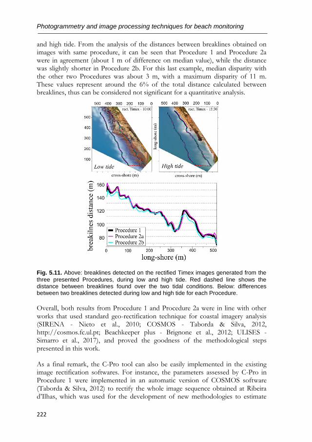
Photogrammetry and image processing techniques for beach monitoring
222
and high tide. From the analysis of the distances between breaklines obtained on images with same procedure, it can be seen that Procedure 1 and Procedure 2a were in agreement (about 1 m of difference on median value), while the distance was slightly shorter in Procedure 2b. For this last example, median disparity with the other two Procedures was about 3 m, with a maximum disparity of 11 m. These values represent around the 6% of the total distance calculated between breaklines, thus can be considered not significant for a quantitative analysis.
Fig. 5.11. Above: breaklines detected on the rectified Timex images generated from the
three presented Procedures, during low and high tide. Red dashed line shows the distance between breaklines found over the two tidal conditions. Below: differences between two breaklines detected during low and high tide for each Procedure.
Overall, both results from Procedure 1 and Procedure 2a were in line with other works that used standard geo-rectification technique for coastal imagery analysis (SIRENA - Nieto et al., 2010; COSMOS - Taborda & Silva, 2012, http://cosmos.fc.ul.pt; Beachkeeper plus - Brignone et al., 2012; ULISES - Simarro et al., 2017), and proved the goodness of the methodological steps presented in this work.
As a final remark, the C-Pro tool can also be easily implemented in the existing image rectification softwares. For instance, the parameters assessed by C-Pro in Procedure 1 were implemented in an automatic version of COSMOS software (Taborda & Silva, 2012) to rectify the whole image sequence obtained at Ribeira d’Ilhas, which was used for the development of new methodologies to estimate
OTHER PHOTOGRAMMETRIC APPLICATIONS & TECHNIQUES
223
nearshore hydrodynamic and morphology (Andriolo, 2018). Nonetheless, C-Pro is an independent coastal projector monitoring system that is freely available upon request to the authors.
5.1.6. Conclusions
This communication presented operational applications of C-Pro projection tool to obtain rectified planar images from an online streaming camera. Two examples to retrieve GCPs were presented. A first method used the in situ standard RTK-GPS instrumentation for the collection of points, while a second novel methodology derived GCPs location and elevation coupling Google Earth historical images to shoreline detection on video imagery. C-Pro has been shown to work efficiently with both in situ and remotely-derived GCPs, estimating the seven unknown parameters of the camera to generate accurate georectified images. The median horizontal projection errors obtained by Procedure 1 and Procedure 2a were acceptable, being of 1.3 m and 2.2 m, respectively, whereas Procedure 2b was less accurate with 5 m of median positional misfit. The presented procedures promote the use of online streaming images for the application of a coastal video monitoring technique, avoiding the installation of new monitoring systems. The methodologies give the opportunity to turn surfcam infrastructure into a fully remote shore-based observational system, in order to apply the video-based scientific techniques for improving knowledge of coastal processes.
5.1.7. Annexed work: an application of C-Pro and online streaming surfcam data for measuring wave runup and intertidal beach topography (presented in X Jornadas do Mar, 2016).
The variation of beach profile is fundamental to understand shore morphodynamics, while wave runup is a key parameter to evaluate coastal vulnerability to extreme events. In such context, this work aimed to develop and validate two complementary methods to video-derive wave runup measurements and intertidal beach topography.
Wave runup is defined as the upper limit of wave on the beach face, and the leading edge of the swash is visible as wet–dry boundary on Timestacks (Vousdoukas et al., 2012). Coversely, shoreline position is defined by the boundary between water and dry sand (Boak and Turner, 2005), and its elevation on beach slope is considered as the sum of tidal level, wave-induced setup and swash induced height (Vousdoukas et al., 2011).
Video data were obtained from a freely-available online streaming (25 frames per seconds) surfcam installed at Costa da Caparica using a Matlab-based algorithm specifically developed for the aim. The access to the installation site and the
Photogrammetry and image processing techniques for beach monitoring
224
technical properties of the camera were denied by the company (http://www.surfline.com). Thus, camera position in real-world coordinates, camera internal and external parameters were unknown. Usually, the camera is set up for mechanically rotating and zooming to show different areas of the coast at the 8th floor of a hotel (around 40 m over MSL). For this experimental work, it was considered the data acquired by the video camera between 08:30 and 14:30 on 11/11/2015 (increasing tide), when the camera was set steady looking at the south part of Praia do Paraíso beach.
RTK-GPS survey was performed to characterize the study area and to validate video-derived results on 12/11/2015. Four cross-shore transects were surveyed during low tide in order to describe the beach slope from about -1 m to about 3.5 m, relatively to the MSL (refer to Fig. 5.16a). 39 GCPs were also collected both on the dry beach and on structures to cover the image. Wave data were retrieved from a wave model developed by the Portuguese Laboratory of Civil Engineering (wave height Hs was about 1.25 m), and tidal data were obtained by the Cascais tide gauge (-0.9 m to 1.43 m of tidal range).
This section reports the proposed methods to: compute precise repositioning of the camera, and surfcam images rectification; detect wave swash and measure wave runup from Timestacks; and derive beach intertidal topography through Timestacks and Variance images.
The outcomes provide new methods for swash zone hydro- and morphodynamic characterization and for studying the dynamics induced by climate changes or the impact of extreme events on coastal areas.
5.1.7.1. Surfcam images rectification
The surfcam retrieved dataset consisted in 36 10-minutes videos, successively converted in a sequence of 21600 images (800 x 450 pixels resolution). Timex and Variance images were produced over 10 minutes image sequence for the 6 monitored hours, and using C-Pro could be rectified within an estimated projection error of 1.5 m. The camera repositioning error was estimated around 0.9 m by comparing against the camera location on an orthophoto. The images were projected on the referenced plane identified by the 10-minutes-averaged sea level over the actual image sequence. Timestacks were composed by the time series of pixel intensity sampled along four cross-shore transects, corresponding to the four cross-shore profiles surveyed in the field.
5.1.7.2. Wave runup measurements
Swash zone can be identified on Timestack between highest brightness (breaking waves) and lowest value (dry beach), through computing standard deviation along time-axis (Simarro et al., 2015). We refer to “wave swash” for the cross-shore
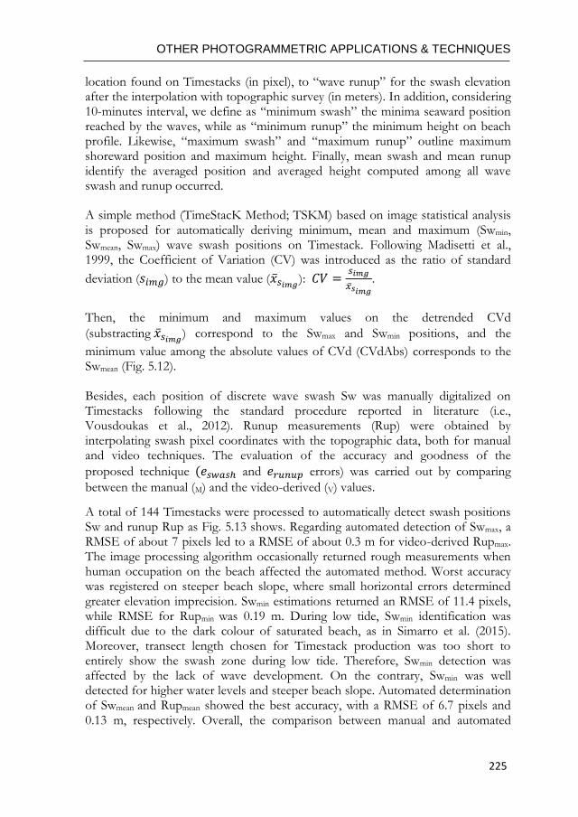
OTHER PHOTOGRAMMETRIC APPLICATIONS & TECHNIQUES
225
location found on Timestacks (in pixel), to “wave runup” for the swash elevation after the interpolation with topographic survey (in meters). In addition, considering 10-minutes interval, we define as “minimum swash” the minima seaward position reached by the waves, while as “minimum runup” the minimum height on beach profile. Likewise, “maximum swash” and “maximum runup” outline maximum shoreward position and maximum height. Finally, mean swash and mean runup identify the averaged position and averaged height computed among all wave swash and runup occurred.
A simple method (TimeStacK Method; TSKM) based on image statistical analysis is proposed for automatically deriving minimum, mean and maximum (Swmin, Swmean, Swmax) wave swash positions on Timestack. Following Madisetti et al., 1999, the Coefficient of Variation (CV) was introduced as the ratio of standard
deviation (𝑠𝑖𝑚𝑔) to the mean value (�̅�𝑠𝑖𝑚𝑔): 𝐶𝑉 =𝑠𝑖𝑚𝑔
�̅�𝑠𝑖𝑚𝑔.
Then, the minimum and maximum values on the detrended CVd
(substracting �̅�𝑠𝑖𝑚𝑔) correspond to the Swmax and Swmin positions, and the
minimum value among the absolute values of CVd (CVdAbs) corresponds to the Swmean (Fig. 5.12). Besides, each position of discrete wave swash Sw was manually digitalized on Timestacks following the standard procedure reported in literature (i.e., Vousdoukas et al., 2012). Runup measurements (Rup) were obtained by interpolating swash pixel coordinates with the topographic data, both for manual and video techniques. The evaluation of the accuracy and goodness of the
proposed technique (𝑒𝑠𝑤𝑎𝑠ℎ and 𝑒𝑟𝑢𝑛𝑢𝑝 errors) was carried out by comparing
between the manual (M) and the video-derived (V) values.
A total of 144 Timestacks were processed to automatically detect swash positions Sw and runup Rup as Fig. 5.13 shows. Regarding automated detection of Swmax, a RMSE of about 7 pixels led to a RMSE of about 0.3 m for video-derived Rupmax. The image processing algorithm occasionally returned rough measurements when human occupation on the beach affected the automated method. Worst accuracy was registered on steeper beach slope, where small horizontal errors determined greater elevation imprecision. Swmin estimations returned an RMSE of 11.4 pixels, while RMSE for Rupmin was 0.19 m. During low tide, Swmin identification was difficult due to the dark colour of saturated beach, as in Simarro et al. (2015). Moreover, transect length chosen for Timestack production was too short to entirely show the swash zone during low tide. Therefore, Swmin detection was affected by the lack of wave development. On the contrary, Swmin was well detected for higher water levels and steeper beach slope. Automated determination of Swmean and Rupmean showed the best accuracy, with a RMSE of 6.7 pixels and 0.13 m, respectively. Overall, the comparison between manual and automated
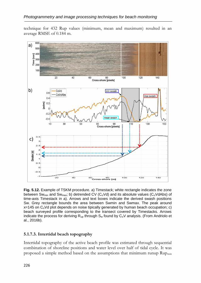
Photogrammetry and image processing techniques for beach monitoring
226
technique for 432 Rup values (minimum, mean and maximum) resulted in an average RMSE of 0.184 m.
Fig. 5.12. Example of TSKM procedure. a) Timestack; white rectangle indicates the zone
between Swmin and Swmax; b) detrended CV (CoVd) and its absolute values (CoVdAbs) of time-axis Timestack in a). Arrows and text boxes indicate the derived swash positions Sw. Grey rectangle bounds the area between Swmin and Swmax. The peak around x=145 on CoVd plot depends on noise tipically generated by human beach occupation; c) beach surveyed profile corresponding to the transect covered by Timestacks. Arrows indicate the process for deriving Rup through Sw found by CoV analysis. (From Andriolo et al., 2016b).
5.1.7.3. Intertidal beach topography
Intertidal topography of the active beach profile was estimated through sequential combination of shoreline positions and water level over half of tidal cycle. It was proposed a simple method based on the assumptions that minimum runup Rupmin
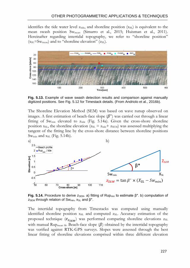
OTHER PHOTOGRAMMETRIC APPLICATIONS & TECHNIQUES
227
identifies the tide water level ztide, and shoreline position (xSL) is equivalent to the mean swash position Swmean (Simarro et al., 2015; Huisman et al., 2011). Hereinafter regarding intertidal topography, we refer to “shoreline position” (xSL=Swmean) and to “shoreline elevation” (zSL).
Fig. 5.13. Example of wave swash detection results and comparison against manually digitized positions. See Fig. 5.12 for Timestack details. (From Andriolo et al., 2016b).
The Shoreline Elevation Method (SEM) was based on wave runup observed on
images. A first estimation of beach-face slope (𝛽∗) was carried out through a linear fitting of Swmin elevated to ztide (Fig. 5.14a). Given the cross-shore shoreline position xSL, the shoreline elevation (zSL = ztide+ zSEM) was assessed multiplying the tangent of the fitting line by the cross-shore distance between shoreline positions Swmin and xSL (Fig. 5.14b).
a) b)
Fig. 5.14. Procedure to derive zSEM. a) fitting of Rupmin to estimate β*. b) computation of
zSEM through relation of Swmin, xSL and β*.
The intertidal topography from Timestacks was computed using manually identified shoreline position xSL and computed zSL. Accuracy estimation of the
proposed technique (𝑒𝑧𝑆𝐸𝑀) was performed comparing shoreline elevations zSL
with manual Rupmean M. Beach-face slope (𝛽) obtained by the intertidal topography was verified against RTK-GPS surveys. Slopes were assessed through the best linear fitting of shoreline elevations comprised within three different elevation
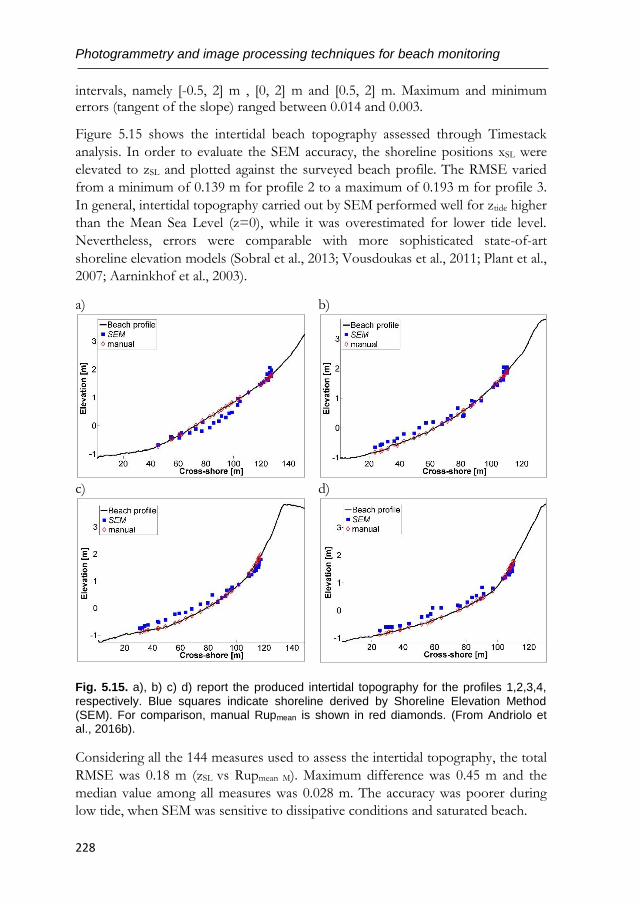
Photogrammetry and image processing techniques for beach monitoring
228
intervals, namely [-0.5, 2] m , [0, 2] m and [0.5, 2] m. Maximum and minimum errors (tangent of the slope) ranged between 0.014 and 0.003.
Figure 5.15 shows the intertidal beach topography assessed through Timestack
analysis. In order to evaluate the SEM accuracy, the shoreline positions xSL were
elevated to zSL and plotted against the surveyed beach profile. The RMSE varied
from a minimum of 0.139 m for profile 2 to a maximum of 0.193 m for profile 3.
In general, intertidal topography carried out by SEM performed well for ztide higher
than the Mean Sea Level (z=0), while it was overestimated for lower tide level.
Nevertheless, errors were comparable with more sophisticated state-of-art
shoreline elevation models (Sobral et al., 2013; Vousdoukas et al., 2011; Plant et al.,
2007; Aarninkhof et al., 2003).
a)
b)
c)
d)
Fig. 5.15. a), b) c) d) report the produced intertidal topography for the profiles 1,2,3,4,
respectively. Blue squares indicate shoreline derived by Shoreline Elevation Method (SEM). For comparison, manual Rupmean is shown in red diamonds. (From Andriolo et al., 2016b).
Considering all the 144 measures used to assess the intertidal topography, the total
RMSE was 0.18 m (zSL vs Rupmean M). Maximum difference was 0.45 m and the
median value among all measures was 0.028 m. The accuracy was poorer during
low tide, when SEM was sensitive to dissipative conditions and saturated beach.
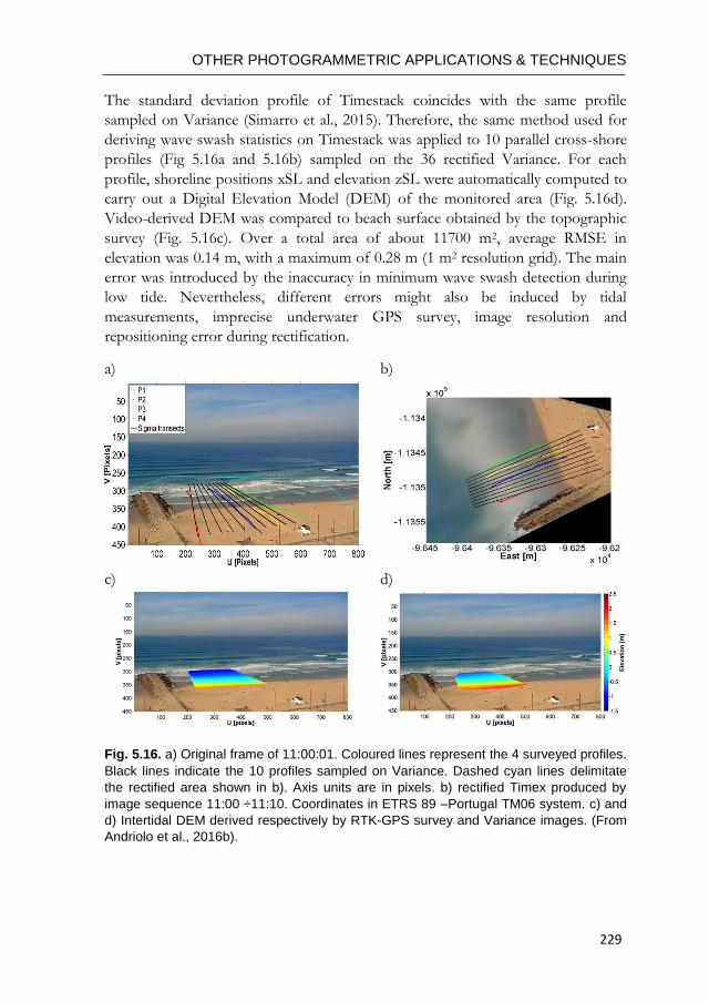
OTHER PHOTOGRAMMETRIC APPLICATIONS & TECHNIQUES
229
The standard deviation profile of Timestack coincides with the same profile
sampled on Variance (Simarro et al., 2015). Therefore, the same method used for
deriving wave swash statistics on Timestack was applied to 10 parallel cross-shore
profiles (Fig 5.16a and 5.16b) sampled on the 36 rectified Variance. For each
profile, shoreline positions xSL and elevation zSL were automatically computed to
carry out a Digital Elevation Model (DEM) of the monitored area (Fig. 5.16d).
Video-derived DEM was compared to beach surface obtained by the topographic
survey (Fig. 5.16c). Over a total area of about 11700 m2, average RMSE in
elevation was 0.14 m, with a maximum of 0.28 m (1 m2 resolution grid). The main
error was introduced by the inaccuracy in minimum wave swash detection during
low tide. Nevertheless, different errors might also be induced by tidal
measurements, imprecise underwater GPS survey, image resolution and
repositioning error during rectification.
a) b)
c) d)
Fig. 5.16. a) Original frame of 11:00:01. Coloured lines represent the 4 surveyed profiles.
Black lines indicate the 10 profiles sampled on Variance. Dashed cyan lines delimitate
the rectified area shown in b). Axis units are in pixels. b) rectified Timex produced by
image sequence 11:00 ÷11:10. Coordinates in ETRS 89 –Portugal TM06 system. c) and
d) Intertidal DEM derived respectively by RTK-GPS survey and Variance images. (From
Andriolo et al., 2016b).

Photogrammetry and image processing techniques for beach monitoring
230
OTHER PHOTOGRAMMETRIC APPLICATIONS & TECHNIQUES
231
5.2. SHORELINE CHANGE MAPPING USING CROWD-SOURCED SMARTPHONE IMAGES
Shoreline change information is critical for effective management of the coastal zone. This study presents a low-cost method for mapping shoreline change that harnesses smartphone images collected by the community and uploaded to social media platforms. A smartphone camera cradle installed overlooking a coastal region is used to constrain the crowd-sourced camera extrinsic parameters and accompanying signage instructs participants on how to share their image to social media using a site-specific hashtag identifier. Surveyed ground control points solve for the focal length of the smartphone lens and more-accurately resolve the camera extrinsic parameters. Shoreline position is subsequently mapped on georectified images using an edge detection technique based on the red and blue colour channels. A validation of the method was conducted at two sandy beaches in SE Australia and resulted in strong community participation (400 images submitted over 7 months by 198 individual contributors). Concurrent shoreline surveys using RTK-GNSS indicated that shoreline accuracy using this crowd-sourced approach is comparable to that of established coastal imaging systems, with cross-shore shoreline accuracy best for these two elevated validation sites (camera elevation = 17.3 m – 27.1 m above MSL) in the camera nearfield (RMSD ≈ 1.4 m) and RMSD ranging between 2.6-3.9 m over coastal stretches spanning up to 1 km. Minimal differences in shoreline accuracy were observed between low resolution images characteristic of those uploaded to social media and higher resolution images sourced from the smartphone. The successful application of this low-cost approach, combined with the proliferation of smartphones and social media usage, open up new possibilities for crowd-sourced shoreline change mapping at suitable coastal locations worldwide.
5.2.1. Introduction
The shoreline and its surrounds is a focal point of human occupation, environmental biodiversity, economic activity and recreational amenity. It plays a vital role as a buffer separating energetic waves and elevated water levels from vulnerable coastal settlements. During extreme storm conditions, the shoreline can retreat landwards by more than 50 metres as sediment is removed from the upper beach and deposited offshore (e.g. Harley et al., 2017; List et al., 2006; Masselink et al., 2016; Sopkin et al., 2014; Thom and Hall, 1991). Over the longer-term, factors such as relative sea-level rise, changing wave climates and human interventions can result in shoreline fluctuations in the order of 100 metres (e.g. Hansen and Barnard, 2010; Harley et al., 2011a) and accretion or erosion trends at rates in excess of 10 metres/year (e.g. Luijendijk et al., 2018; Mentaschi et al., 2018). Continued pressure to develop in these dynamic coastal zones means that effective coastal management and planning is crucial, so that present and future exposure to coastal change is minimised (Kinsela et al., 2017; Nicholls, 2004; Wainwright et al.,
Photogrammetry and image processing techniques for beach monitoring
232
2015). This is particularly important in light of present and projected changes in both extreme waves (Castelle et al., 2018; Hemer et al., 2016; Mentaschi et al., 2017) and rising sea-levels (Church et al., 2013), which combined place great uncertainty in future shoreline behaviour.
For most coastlines, limited observation data exists to provide an understanding of the rates and magnitudes of shoreline response due to extreme storms and longer-term coastal processes (Barnard et al., 2015; Turner et al., 2016b). In southeastern Australia, for example, observation records for most beaches are limited to photogrammetry analyses of historical aerial photographs, which have been typically captured only once every several to ten years (Hanslow et al., 1997; Harrison et al., 2017). The sparse observation record introduces uncertainty into coastal management and planning strategies, because the potential influences of storms and subtle gradients in the coastal sediment balance on beach resilience remain poorly known. Frequent and long-term beach monitoring records are therefore needed to quantify and differentiate between seasonal to inter-decadal shoreline variability, and mean-trend change, at individual beaches and along regional coastlines (Barnard et al., 2015; Kuriyama et al., 2012; Splinter et al., 2013). However, the costs and logistics of regular and long-term monitoring using conventional survey techniques remain a prohibitive factor.
Technological advances in survey instruments and analysis methods have led to an ongoing shift in shoreline monitoring from in situ measurements to remote sensing (Splinter et al., 2018). At the forefront of this change has been the development since the 1980s in optical coastal imaging techniques such as Argus (Holman and Stanley, 2007) and related systems (Nieto et al., 2010; Smith and Bryan, 2007; Taborda & Silva, 2012; Vousdoukas et al., 2012). Coastal imaging combines fixed video cameras and image processing methods to measure a range of nearshore processes, with shoreline position being a core data product because of its relevance as a proxy for many beach attributes (Aarninkhof et al., 2003; Harley et al., 2014, 2011b; Pianca et al., 2015; Plant et al., 2007; Smith and Bryan, 2007; Turner et al., 2004). Addressing several of the logistical demands of regular shoreline monitoring using conventional techniques, coastal imaging has led to the establishment of permanent observation stations collecting shoreline data at sampling frequencies that would be impractical to obtain otherwise (i.e., every daylight hour). Coastal imaging stations nonetheless require access to electricity and communications, protection from the elements and vandals, and come with appreciable set-up and maintenance costs. These factors have played a large part in limiting the comprehensive roll-out of coastal imaging networks globally, particularly in countries with limited resources.
More recent advances in camera lens technology and the proliferation of consumer smartphones worldwide (Poushter, 2016) suggest there might be untapped opportunities for shoreline monitoring using crowd-sourced images. The general
OTHER PHOTOGRAMMETRIC APPLICATIONS & TECHNIQUES
233
public routinely visit beaches, carrying with them camera devices that are more powerful than the technology that has been successfully applied in coastal imaging for decades. Coupled with that, social media provides established and widely-used platforms (e.g. Facebook, Instagram and Twitter) for sharing and managing images amongst local communities or global audiences. Recognising the potential of smartphone images and social media, several photo-point citizen science initiatives have been developed that make use of crowd-sourced images taken over time at the same location, for monitoring various forms of environmental change (Augar and Fluker, 2014; Bayas et al., 2016; Droege, 2013). These photo point initiatives typically comprise a rudimentary camera cradle that helps control the viewpoint of the smartphone camera and are accompanied by instructions detailing ways to share the image to a centralised database. To date however, these programs have been limited to compiling qualitative environmental change information and do not make use of photogrammetry techniques for quantitative data collection.
Compared with established coastal imaging systems, crowd-sourced shoreline change mapping presents a number of challenges that must be overcome in order to generate shoreline datasets of sufficient accuracy for coastal research and management applications. Established coastal imaging systems use a fixed camera of suitable specifications that is mounted on a stable platform of known coordinates. Camera intrinsic parameters (i.e., focal length, image centre and lens distortion properties) are carefully determined prior to camera installation using standard lens calibration techniques. The video camera is also usually configured to capture time-averaged (“timex”) images over several minutes, so the oscillatory influence of swash processes on the shoreline position can be accounted for, to identify the mean shoreline position at regular intervals over time. Because the camera lens and image properties are constant through time, image analysis techniques to detect and map beach features can be readily automated (e.g. Uunk et al., 2010).
The crowd-sourced approach on the other hand comprises images collected by non-professionals using a broad range of smartphone camera devices. The platform itself may not necessarily be stable as it involves people manually positioning the camera in a suitable camera cradle installed at the site. To encourage participation, it may also be unreasonable to request participants spend several minutes at the site in order to derive time-averaged images, so shorelines may be mapped using instantaneous “snapshot” images instead. A further challenge is related to image resolution and image metadata (e.g. image capture time, camera lens model), particularly if social media platforms are used for image submission. This is because considerable image compression is applied by social media platforms prior to image upload, and standard Exif image metadata is removed by the platform for privacy concerns. Overcoming these challenges with suitable methods for managing the potential volume and diversity of crowd-
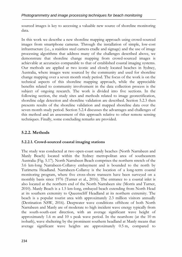
Photogrammetry and image processing techniques for beach monitoring
234
sourced images is key to accessing a valuable new source of shoreline monitoring data.
In this work we describe a new shoreline mapping approach using crowd-sourced images from smartphone cameras. Through the installation of simple, low-cost infrastructure (i.e., a stainless steel camera cradle and signage) and the use of image processing algorithms that address many of the challenges described above, we demonstrate that shoreline change mapping from crowd-sourced images is achievable at accuracies comparable to that of established coastal imaging systems. Our methods are applied at two iconic and closely located beaches in Sydney, Australia, where images were sourced by the community and used for shoreline change mapping over a seven month study period. The focus of the work is on the technical aspects of this shoreline mapping approach, while the appreciable benefits related to community involvement in the data collection process is the subject of ongoing research. The work is divided into five sections. In the following section, the study sites and methods related to image georectification, shoreline edge detection and shoreline validation are described. Section 5.2.3 then presents results of the shoreline validation and mapped shoreline data over the seven month study period. Section 5.2.4 discusses the advantages and challenges of this method and an assessment of this approach relative to other remote sensing techniques. Finally, some concluding remarks are provided.
5.2.2. Methods
5.2.2.1. Crowd-sourced coastal imaging stations
The study was conducted at two open-coast sandy beaches (North Narrabeen and Manly Beach) located within the Sydney metropolitan area of southeastern Australia (Fig. 5.17). North Narrabeen Beach comprises the northern stretch of the 3.6 km-long Narrabeen-Collaroy embayment and is bounded to the north by Turimetta Headland. Narrabeen-Collaroy is the location of a long-term coastal monitoring program, where five cross-shore transects have been surveyed on a monthly basis since 1976 (Turner et al., 2016). The entrance to a coastal inlet is also located at the northern end of the North Narrabeen site (Morris and Turner, 2010). Manly Beach is a 1.5 km-long, embayed beach extending from North Head at its southern extremity to Queenscliff Headland at its northern extremity. The beach is a popular tourist area with approximately 2.3 million visitors annually (Destination NSW, 2016). Deepwater wave conditions offshore of both North Narrabeen and Manly are of moderate to high incident wave energy typically from the south-south-east direction, with an average significant wave height of approximately 1.6 m and 10 s peak wave period. In the nearshore (at the 10 m isobath), wave sheltering by the prominent southern headland at Manly means that average significant wave heights are approximately 0.5 m, compared to
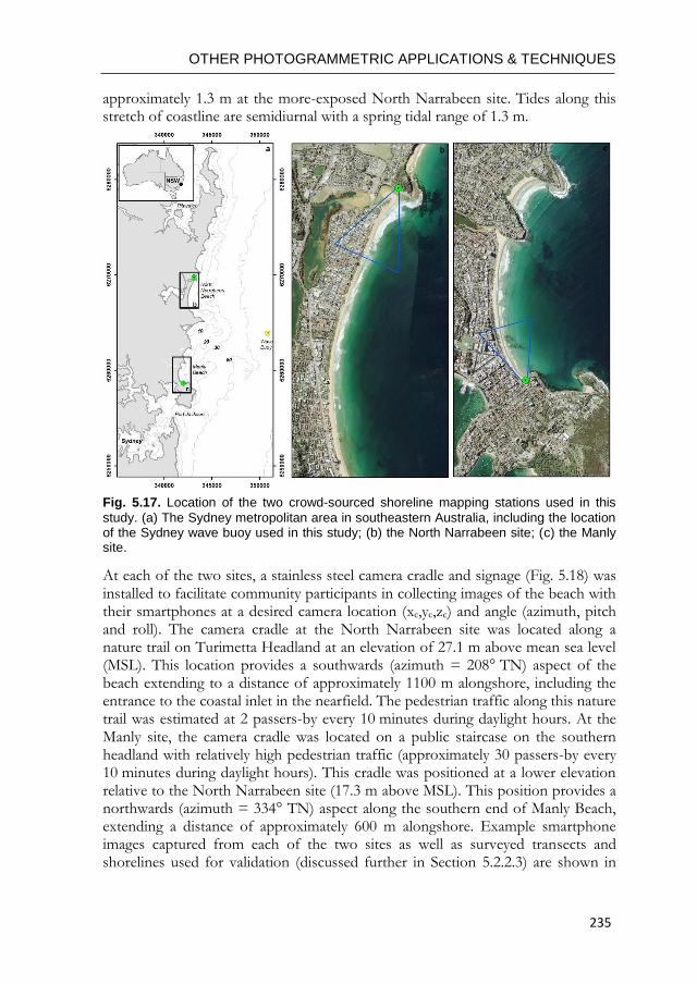
OTHER PHOTOGRAMMETRIC APPLICATIONS & TECHNIQUES
235
approximately 1.3 m at the more-exposed North Narrabeen site. Tides along this stretch of coastline are semidiurnal with a spring tidal range of 1.3 m.
Fig. 5.17. Location of the two crowd-sourced shoreline mapping stations used in this
study. (a) The Sydney metropolitan area in southeastern Australia, including the location of the Sydney wave buoy used in this study; (b) the North Narrabeen site; (c) the Manly site.
At each of the two sites, a stainless steel camera cradle and signage (Fig. 5.18) was installed to facilitate community participants in collecting images of the beach with their smartphones at a desired camera location (xc,yc,zc) and angle (azimuth, pitch and roll). The camera cradle at the North Narrabeen site was located along a nature trail on Turimetta Headland at an elevation of 27.1 m above mean sea level (MSL). This location provides a southwards (azimuth = 208° TN) aspect of the beach extending to a distance of approximately 1100 m alongshore, including the entrance to the coastal inlet in the nearfield. The pedestrian traffic along this nature trail was estimated at 2 passers-by every 10 minutes during daylight hours. At the Manly site, the camera cradle was located on a public staircase on the southern headland with relatively high pedestrian traffic (approximately 30 passers-by every 10 minutes during daylight hours). This cradle was positioned at a lower elevation relative to the North Narrabeen site (17.3 m above MSL). This position provides a northwards (azimuth = 334° TN) aspect along the southern end of Manly Beach, extending a distance of approximately 600 m alongshore. Example smartphone images captured from each of the two sites as well as surveyed transects and shorelines used for validation (discussed further in Section 5.2.2.3) are shown in
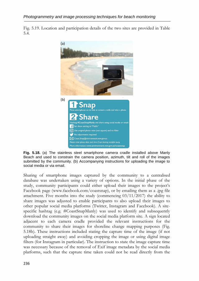
Photogrammetry and image processing techniques for beach monitoring
236
Fig. 5.19. Location and participation details of the two sites are provided in Table 5.4.
Fig. 5.18. (a) The stainless steel smartphone camera cradle installed above Manly
Beach and used to constrain the camera position, azimuth, tilt and roll of the images submitted by the community. (b) Accompanying instructions for uploading the image to social media or via email.
Sharing of smartphone images captured by the community to a centralised database was undertaken using a variety of options. In the initial phase of the study, community participants could either upload their images to the project’s Facebook page (www.facebook.com/coastsnap), or by emailing them as a .jpg file attachment. Five months into the study (commencing 03/11/2017) the ability to share images was adjusted to enable participants to also upload their images to other popular social media platforms (Twitter, Instagram and Facebook). A site-specific hashtag (e.g. #CoastSnapManly) was used to identify and subsequently download the community images on the social media platform site. A sign located adjacent to each camera cradle provided the relevant instructions for the community to share their images for shoreline change mapping purposes (Fig. 5.18b). These instructions included stating the capture time of the image (if not uploading straight away) and avoiding cropping the image or using digital image filters (for Instagram in particular). The instruction to state the image capture time was necessary because of the removal of Exif image metadata by the social media platforms, such that the capture time taken could not be read directly from the
OTHER PHOTOGRAMMETRIC APPLICATIONS & TECHNIQUES
237
image file itself. In these cases, the image capture time was recorded as that stated by the participant. If no capture time was stated then the upload time was used and possible erroneous times flagged accordingly.
Site North Narrabeen Manly
Coordinates (151º18’29.28’’ E, 33º 42’
8.6’’ S) (151º17’26.44’’ E,
33º47’59’’ S)
Camera cradle elevation above MSL 27.1 m 17.3 m
Installation date 24/05/2017 17/05/2017
Total no. of community photos (until 31/12/2017)
272 128
Total no. of contributors (until 31/12/2017)
124 74
Images per day (average) 1.23 0.56
Images per contributor (average) 2.19 1.73
Table 5.4. General location and participation details of the two site locations for
community-sourced shoreline change mapping.
Over the entire seven month study period (17/05/2017 – 31/12/2017) a total of 400 crowd-sourced images were obtained from the two sites from 198 individuals (Fig. 5.20). This is equivalent to an average contribution rate of 0.89 images/site/day and 2.02 images/individual. The majority of images (57%) were shared via the project’s Facebook page, with email submissions providing the second most common type of sharing method (40%). Instagram and Twitter contributions amounted only to 3% of all images, although this in part reflected that these sharing options were only available in the latter stage of the study, as well as the fact that Facebook was used as the primary mode for dissemination of results. Comparing the relative contributions from each of the two sites, the less-frequented North Narrabeen site surprisingly received the majority of images (68%). We attribute this to the different motivations and social characteristics of the people frequenting each site and participating in the program, although these aspects are beyond the scope of this study.
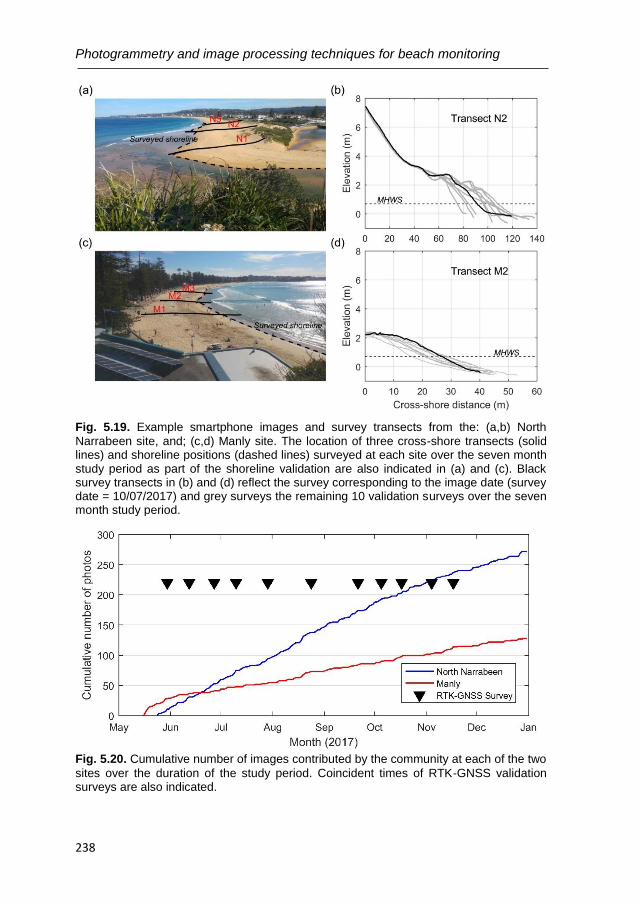
Photogrammetry and image processing techniques for beach monitoring
238
Fig. 5.19. Example smartphone images and survey transects from the: (a,b) North
Narrabeen site, and; (c,d) Manly site. The location of three cross-shore transects (solid lines) and shoreline positions (dashed lines) surveyed at each site over the seven month study period as part of the shoreline validation are also indicated in (a) and (c). Black survey transects in (b) and (d) reflect the survey corresponding to the image date (survey date = 10/07/2017) and grey surveys the remaining 10 validation surveys over the seven month study period.
Fig. 5.20. Cumulative number of images contributed by the community at each of the two
sites over the duration of the study period. Coincident times of RTK-GNSS validation surveys are also indicated.
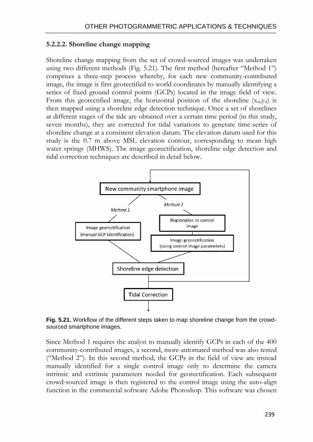
OTHER PHOTOGRAMMETRIC APPLICATIONS & TECHNIQUES
239
5.2.2.2. Shoreline change mapping
Shoreline change mapping from the set of crowd-sourced images was undertaken using two different methods (Fig. 5.21). The first method (hereafter “Method 1”) comprises a three-step process whereby, for each new community-contributed image, the image is first georectified to world coordinates by manually identifying a series of fixed ground control points (GCPs) located in the image field of view. From this georectified image, the horizontal position of the shoreline (xsl,ysl) is then mapped using a shoreline edge detection technique. Once a set of shorelines at different stages of the tide are obtained over a certain time period (in this study, seven months), they are corrected for tidal variations to generate time-series of shoreline change at a consistent elevation datum. The elevation datum used for this study is the 0.7 m above MSL elevation contour, corresponding to mean high water springs (MHWS). The image georectification, shoreline edge detection and tidal correction techniques are described in detail below.
Fig. 5.21. Workflow of the different steps taken to map shoreline change from the crowd-
sourced smartphone images.
Since Method 1 requires the analyst to manually identify GCPs in each of the 400 community-contributed images, a second, more-automated method was also tested (“Method 2”). In this second method, the GCPs in the field of view are instead manually identified for a single control image only to determine the camera intrinsic and extrinsic parameters needed for georectification. Each subsequent crowd-sourced image is then registered to the control image using the auto-align function in the commercial software Adobe Photoshop. This software was chosen
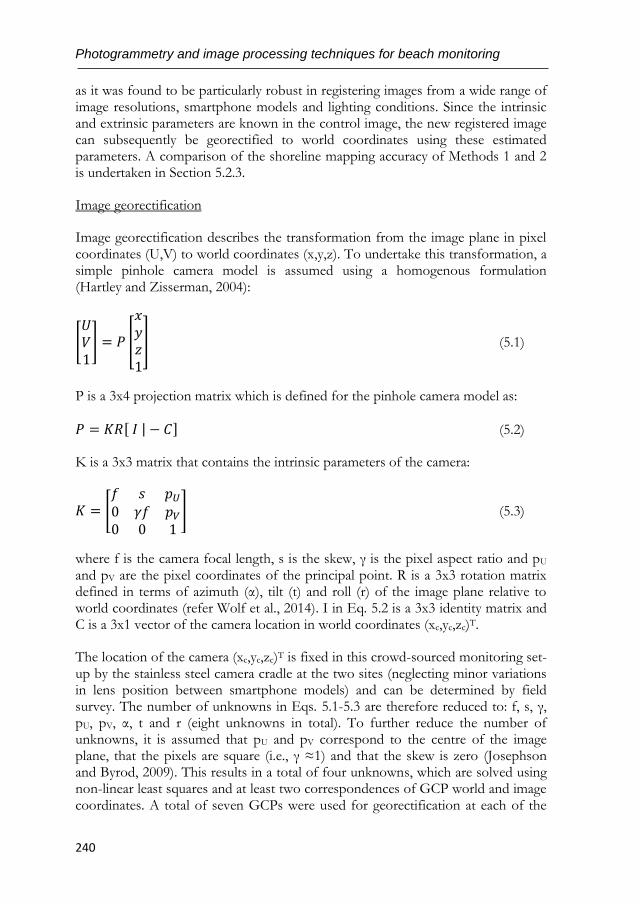
Photogrammetry and image processing techniques for beach monitoring
240
as it was found to be particularly robust in registering images from a wide range of image resolutions, smartphone models and lighting conditions. Since the intrinsic and extrinsic parameters are known in the control image, the new registered image can subsequently be georectified to world coordinates using these estimated parameters. A comparison of the shoreline mapping accuracy of Methods 1 and 2 is undertaken in Section 5.2.3.
Image georectification
Image georectification describes the transformation from the image plane in pixel coordinates (U,V) to world coordinates (x,y,z). To undertake this transformation, a simple pinhole camera model is assumed using a homogenous formulation (Hartley and Zisserman, 2004):
[𝑈𝑉1] = 𝑃 [
𝑥𝑦𝑧1
] (5.1)
P is a 3x4 projection matrix which is defined for the pinhole camera model as:
𝑃 = 𝐾𝑅[ 𝐼 | − 𝐶] (5.2)
K is a 3x3 matrix that contains the intrinsic parameters of the camera:
𝐾 = [𝑓 𝑠 𝑝𝑈0 𝛾𝑓 𝑝𝑉0 0 1
] (5.3)
where f is the camera focal length, s is the skew, γ is the pixel aspect ratio and pU and pV are the pixel coordinates of the principal point. R is a 3x3 rotation matrix defined in terms of azimuth (α), tilt (t) and roll (r) of the image plane relative to world coordinates (refer Wolf et al., 2014). I in Eq. 5.2 is a 3x3 identity matrix and C is a 3x1 vector of the camera location in world coordinates (xc,yc,zc)T.
The location of the camera (xc,yc,zc)T is fixed in this crowd-sourced monitoring set-up by the stainless steel camera cradle at the two sites (neglecting minor variations in lens position between smartphone models) and can be determined by field survey. The number of unknowns in Eqs. 5.1-5.3 are therefore reduced to: f, s, γ, pU, pV, α, t and r (eight unknowns in total). To further reduce the number of unknowns, it is assumed that pU and pV correspond to the centre of the image plane, that the pixels are square (i.e., γ ≈1) and that the skew is zero (Josephson and Byrod, 2009). This results in a total of four unknowns, which are solved using non-linear least squares and at least two correspondences of GCP world and image coordinates. A total of seven GCPs were used for georectification at each of the
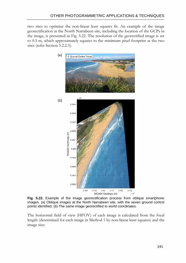
OTHER PHOTOGRAMMETRIC APPLICATIONS & TECHNIQUES
241
two sites to optimise the non-linear least squares fit. An example of the image georectification at the North Narrabeen site, including the location of the GCPs in the image, is presented in Fig. 5.22. The resolution of the georectified image is set to 0.5 m, which approximately equates to the minimum pixel footprint at the two sites (refer Section 5.2.2.3).
Fig. 5.22. Example of the image georectification process from oblique smartphone
images. (a) Oblique images at the North Narrabeen site, with the seven ground control points identified. (b) The same image georectified to world coordinates.
The horizontal field of view (HFOV) of each image is calculated from the focal length (determined for each image in Method 1 by non-linear least squares) and the image size:
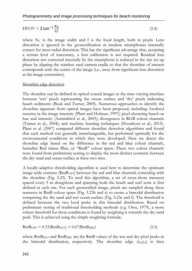
Photogrammetry and image processing techniques for beach monitoring
242
HFOV = 2 tan−1𝑁𝑈
2𝑓 (5.4)
where NU is the image width and f is the focal length, both in pixels. Lens distortion is ignored in the georectification as modern smartphones internally correct for most radial distortion. This has the significant advantage that, accepting a certain level of inaccuracy, a lens calibration is not required. Residual lens distortion not corrected internally by the smartphone is reduced in the site set-up phase by aligning the stainless steel camera cradle so that the shoreline of interest corresponds with the centre of the image (i.e., away from significant lens distortion at the image extremities).
Shoreline edge detection
The shoreline can be defined in optical coastal images as the time-varying interface between ‘wet’ pixels representing the ocean surface and ‘dry’ pixels indicating beach sediments (Boak and Turner, 2005). Numerous approaches to identify the shoreline signature from optical images have been proposed, including: localised maxima in the image intensity (Plant and Holman, 1997); pixel clustering based on hue and intensity (Aarninkhof et al., 2003); divergences in RGB colour channels (Turner et al., 2004); and machine learning techniques (Hoonhout et al., 2015). Plant et al. (2007) compared different shoreline detection algorithms and found that each method was generally interchangeable, but performed optimally for the environmental conditions in which they were developed. Here we detect the shoreline edge based on the difference in the red and blue colour channels, hereafter Red minus Blue, or “RmB” colour space. These two colour channels were found from preliminary testing to display the most distinct contrasts between the dry sand and ocean surface at these two sites.
A locally-adaptive thresholding algorithm is used here to determine the optimum image-wide contrast (RmBOPT) between the red and blue channels coinciding with the shoreline (Fig. 5.23). To seed this algorithm, a set of cross-shore transects spaced every 5 m alongshore and spanning both the beach and surf zone is first defined at each site. For each georectified image, pixels are sampled along these transects in RmB colour space (Fig. 5.23b and e) to create a bimodal distribution comprising the dry sand and wet ocean surface (Fig. 5.23c and f). The threshold is defined between the two local peaks in this bimodal distribution. Based on preliminary testing of traditional thresholding methods (e.g. Otsu, 1979), a more robust threshold for these conditions is found by weighting it towards the dry sand peak. This is achieved using the simple weighting formula:
RmBOPT = 0.33(RmBWET) + 0.67(RmBDRY) (5.5)
where RmBWET and RmBDRY are the RmB values of the wet and dry pixel peaks in the bimodal distribution, respectively. The shoreline edge (xsl,ysl) is then
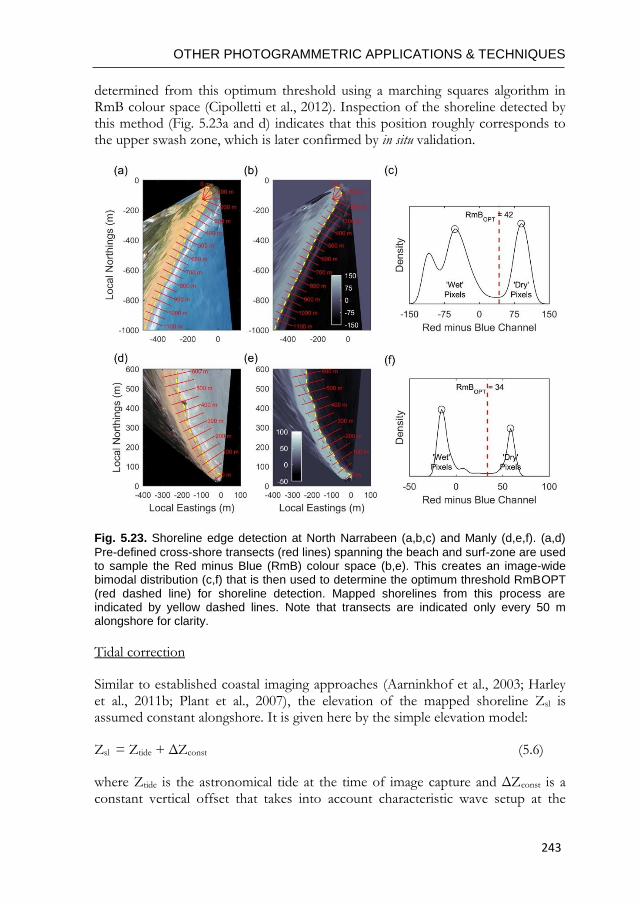
OTHER PHOTOGRAMMETRIC APPLICATIONS & TECHNIQUES
243
determined from this optimum threshold using a marching squares algorithm in RmB colour space (Cipolletti et al., 2012). Inspection of the shoreline detected by this method (Fig. 5.23a and d) indicates that this position roughly corresponds to the upper swash zone, which is later confirmed by in situ validation.
Fig. 5.23. Shoreline edge detection at North Narrabeen (a,b,c) and Manly (d,e,f). (a,d)
Pre-defined cross-shore transects (red lines) spanning the beach and surf-zone are used to sample the Red minus Blue (RmB) colour space (b,e). This creates an image-wide bimodal distribution (c,f) that is then used to determine the optimum threshold RmBOPT (red dashed line) for shoreline detection. Mapped shorelines from this process are indicated by yellow dashed lines. Note that transects are indicated only every 50 m alongshore for clarity.
Tidal correction
Similar to established coastal imaging approaches (Aarninkhof et al., 2003; Harley et al., 2011b; Plant et al., 2007), the elevation of the mapped shoreline Zsl is assumed constant alongshore. It is given here by the simple elevation model:
Zsl = Ztide + ΔZconst (5.6)
where Ztide is the astronomical tide at the time of image capture and ΔZconst is a constant vertical offset that takes into account characteristic wave setup at the
Photogrammetry and image processing techniques for beach monitoring
244
shoreline and differences between the actual and detected shoreline. Tidal anomalies are ignored in this elevation model as these are typically small (+/- 0.09 m for one standard deviation) for this coastline (Turner et al., 2016b). Shoreline elevation changes due to varying offshore wave conditions are also ignored as, due to saturation of the incident swash band, these influences have been found to be relatively small under most conditions on this coastline (Harley et al., 2011b). These two assumptions have the significant advantage of removing the need for measured tide and wave data, which is often sparse or difficult to obtain. The potential for large errors resulting from these assumptions (e.g. during storm conditions when significant tidal anomalies and/or offshore waves may occur) are reduced by community images rarely being collected during extreme conditions. ΔZconst is determined from field survey measurements as described in Section 5.2.2.3.
Beach Width (BW) is defined at each cross-shore transect (refer Fig. 5.23) as the distance from a fixed landward benchmark in the backshore to the shoreline edge (xsl,ysl). Since crowd-sourced images are by their nature collected at random stages of the tidal cycle, a tidal correction is needed for direct comparison of BW collected at different tide levels. Assuming a stationary and planar beachface slope, this BW correction is undertaken using the equation:
∆BW𝑡𝑖𝑑𝑒 = 𝑍𝑠𝑙−𝑍𝑑𝑎𝑡𝑢𝑚
(𝛽𝑏𝑓) (5.7)
where Zsl is the elevation of the shoreline calculated in Eq. 5.6, Zdatum is the shoreline elevation datum (i.e., 0.7 m above MSL) and <ßbf> is the stationary and planar beachface slope for the transect of interest. The tidally-corrected beach
width (BW𝑐𝑜𝑟𝑟) at each transect is subsequently calculated by:
BW𝑐𝑜𝑟𝑟 = BW - ∆BW𝑡𝑖𝑑𝑒 (5.8)
Equation 5.7 requires knowledge of the beachface slope, which is usually determined from in situ measurements. To avoid a reliance on in situ data, a simple method to estimate <ßbf> directly from the set of crowd-sourced shorelines is applied. This method assumes that the optimum beachface slope is that which minimises the variance of the tidally-corrected beach width time-series. An iterative procedure using Eqs. 5.7 and 5.8 thereby calculates the standard deviation of
BW𝑐𝑜𝑟𝑟 for a range of <ßbf> (between 0.01 and 0.3, typical of a sandy beach). The
optimum slope is then determined as that where the standard deviation of BW𝑐𝑜𝑟𝑟 is a minimum.
5.2.2.3. Validation of smartphone-derived shoreline measurements
OTHER PHOTOGRAMMETRIC APPLICATIONS & TECHNIQUES
245
Validation of the smartphone-derived shoreline measurements was undertaken by a series of approximately bi-weekly field surveys performed over the seven month study period (11 surveys in total, Fig. 5.20). The field surveys were designed to quantify a number of aspects related to accuracy of the smartphone-derived shorelines, specifically: 1) the overall shoreline accuracy and its variability alongshore; 2) the influence of image resolution; 3) the influence of instantaneous snapshot versus timex images, and; 4) the effect of the image registration algorithm.
During each survey, the shoreline was measured directly by a field operator at both sites using RTK-GNSS (horizontal accuracy ~ 0.05 m). Shoreline measurements were undertaken by following the upper part of the swash zone along the beach within the field of view of each station (refer Fig. 5.19a and c). Simultaneously to these in situ shoreline measurements, a second field operator positioned at the camera cradle collected smartphone data (using an LG G5 model smartphone) in order to obtain smartphone-derived shorelines for direct comparison. These data consisted of 10-minute videos which were post-processed to create a set of snapshots sampled at different instances of swash excursions on the beach face (10 snapshots in total for each site and field survey). Timex images were also calculated by averaging all video frames over the 10-minute time period. The resolution of these snapshot and timex images were 1920x1080 pixels (i.e., 2 MP) and are hereafter referred to as “HighRes” images. In order to test the effect of image resolution on the shoreline accuracy, these same images were down-sampled to lower resolution (“LowRes”) images, equivalent to the resolution (720x405 pixels, or 0.3 MP) of images uploaded to Facebook, Twitter or Instagram.
In addition to shoreline measurements, three cross-shore transects spanning the near and farfields of each site were surveyed (North Narrabeen: transects N1, N2 and N3, Manly: transects M1, M2 and M3). RTK-GNSS surveys along these transects were measured from the backshore to approximately MSL and were used for two validation purposes: 1) to accurately identify the cross-shore position of the 0.7 m elevation contour at three locations for direct comparison with corrected beach width time-series (Eqs. 5.7 and 5.8), and; 2) to validate beachface slope estimates. The location of these transects correspond to alongshore distances of 135 m, 345 m and 530 m for N1, N2 and N3, respectively, and 40 m, 95 m and 200 m for M1, M2 and M3, respectively (refer Fig. 5.23). These transect locations as well as example shoreline measurements for a survey performed on 10/7/2017 are presented in Fig. 5.19a and c.
Table 5.5 summarises the environmental conditions (offshore waves and astronomical tides) during each of the 11 field surveys. Surveys were undertaken at different stages of the tide and during deepwater wave conditions ranging from H0 = 0.85 to 1.82 m. To determine the constant ΔZconst in the shoreline elevation model (Eq. 5.6), Fig. 5.24 indicates the alongshore-averaged shoreline elevation from RTK-GNSS (Zgnss) plotted against the astronomical tide (Ztide). The results
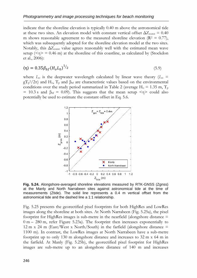
Photogrammetry and image processing techniques for beach monitoring
246
indicate that the shoreline elevation is typically 0.40 m above the astronomical tide at these two sites. An elevation model with constant vertical offset ΔZconst = 0.40 m shows reasonable agreement to the measured shoreline elevation (R2 = 0.77), which was subsequently adopted for the shoreline elevation model at the two sites. Notably, this ΔZconst value agrees reasonably well with the estimated mean wave setup (<η> = 0.46 m) at the shoreline of this coastline, as calculated by (Stockdon et al., 2006):
⟨η⟩ = 0.35𝛽𝑏𝑓(𝐻𝑜𝐿0)12⁄ (5.9)
where Lo is the deepwater wavelength calculated by linear wave theory (Lo = gTp
2/2π) and Ho, Tp and βbf are characteristic values based on the environmental conditions over the study period summarized in Table 2 (average Ho = 1.35 m, Tp = 10.3 s and βbf = 0.09). This suggests that the mean setup <η> could also potentially be used to estimate the constant offset in Eq. 5.6.
Fig. 5.24. Alongshore-averaged shoreline elevations measured by RTK-GNSS (Zgnss)
at the Manly and North Narrabeen sites against astronomical tide at the time of measurements (Ztide). The solid line represents a 0.4 m vertical offset from the astronomical tide and the dashed line a 1:1 relationship.
Fig. 5.25 presents the georectified pixel footprints for both HighRes and LowRes images along the shoreline at both sites. At North Narrabeen (Fig. 5.25a), the pixel footprint for HighRes images is sub-metre in the nearfield (alongshore distance = 0 m – 280 m, refer Figure 5.23a). The footprint then increases exponentially to 12 m x 24 m (East/West x North/South) in the farfield (alongshore distance = 1100 m). In contrast, the LowRes images at North Narrabeen have a sub-metre footprint up to only 130 m alongshore distance and increases to 32 m x 64 m in the farfield. At Manly (Fig. 5.25b), the georectified pixel footprint for HighRes images are sub-metre up to an alongshore distance of 140 m and increases
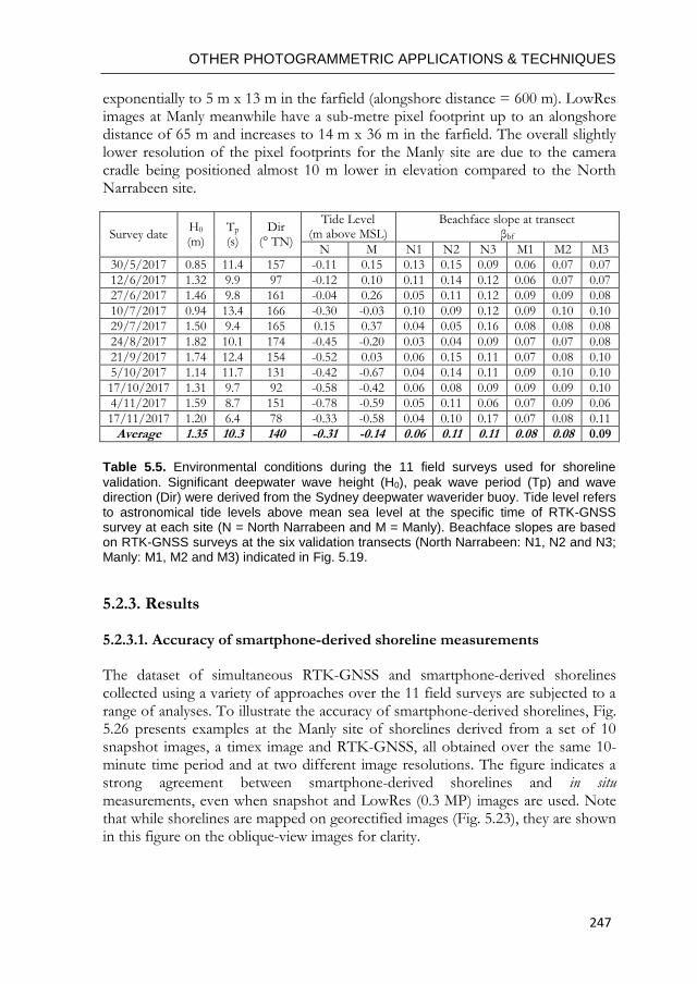
OTHER PHOTOGRAMMETRIC APPLICATIONS & TECHNIQUES
247
exponentially to 5 m x 13 m in the farfield (alongshore distance = 600 m). LowRes images at Manly meanwhile have a sub-metre pixel footprint up to an alongshore distance of 65 m and increases to 14 m x 36 m in the farfield. The overall slightly lower resolution of the pixel footprints for the Manly site are due to the camera cradle being positioned almost 10 m lower in elevation compared to the North Narrabeen site.
Survey date H0
(m) Tp
(s) Dir
(° TN)
Tide Level (m above MSL)
Beachface slope at transect βbf
N M N1 N2 N3 M1 M2 M3
30/5/2017 0.85 11.4 157 -0.11 0.15 0.13 0.15 0.09 0.06 0.07 0.07
12/6/2017 1.32 9.9 97 -0.12 0.10 0.11 0.14 0.12 0.06 0.07 0.07
27/6/2017 1.46 9.8 161 -0.04 0.26 0.05 0.11 0.12 0.09 0.09 0.08
10/7/2017 0.94 13.4 166 -0.30 -0.03 0.10 0.09 0.12 0.09 0.10 0.10
29/7/2017 1.50 9.4 165 0.15 0.37 0.04 0.05 0.16 0.08 0.08 0.08
24/8/2017 1.82 10.1 174 -0.45 -0.20 0.03 0.04 0.09 0.07 0.07 0.08
21/9/2017 1.74 12.4 154 -0.52 0.03 0.06 0.15 0.11 0.07 0.08 0.10
5/10/2017 1.14 11.7 131 -0.42 -0.67 0.04 0.14 0.11 0.09 0.10 0.10
17/10/2017 1.31 9.7 92 -0.58 -0.42 0.06 0.08 0.09 0.09 0.09 0.10
4/11/2017 1.59 8.7 151 -0.78 -0.59 0.05 0.11 0.06 0.07 0.09 0.06
17/11/2017 1.20 6.4 78 -0.33 -0.58 0.04 0.10 0.17 0.07 0.08 0.11
Average 1.35 10.3 140 -0.31 -0.14 0.06 0.11 0.11 0.08 0.08 0.09
Table 5.5. Environmental conditions during the 11 field surveys used for shoreline
validation. Significant deepwater wave height (H0), peak wave period (Tp) and wave direction (Dir) were derived from the Sydney deepwater waverider buoy. Tide level refers to astronomical tide levels above mean sea level at the specific time of RTK-GNSS survey at each site (N = North Narrabeen and M = Manly). Beachface slopes are based on RTK-GNSS surveys at the six validation transects (North Narrabeen: N1, N2 and N3; Manly: M1, M2 and M3) indicated in Fig. 5.19.
5.2.3. Results
5.2.3.1. Accuracy of smartphone-derived shoreline measurements
The dataset of simultaneous RTK-GNSS and smartphone-derived shorelines collected using a variety of approaches over the 11 field surveys are subjected to a range of analyses. To illustrate the accuracy of smartphone-derived shorelines, Fig. 5.26 presents examples at the Manly site of shorelines derived from a set of 10 snapshot images, a timex image and RTK-GNSS, all obtained over the same 10-minute time period and at two different image resolutions. The figure indicates a strong agreement between smartphone-derived shorelines and in situ measurements, even when snapshot and LowRes (0.3 MP) images are used. Note that while shorelines are mapped on georectified images (Fig. 5.23), they are shown in this figure on the oblique-view images for clarity.
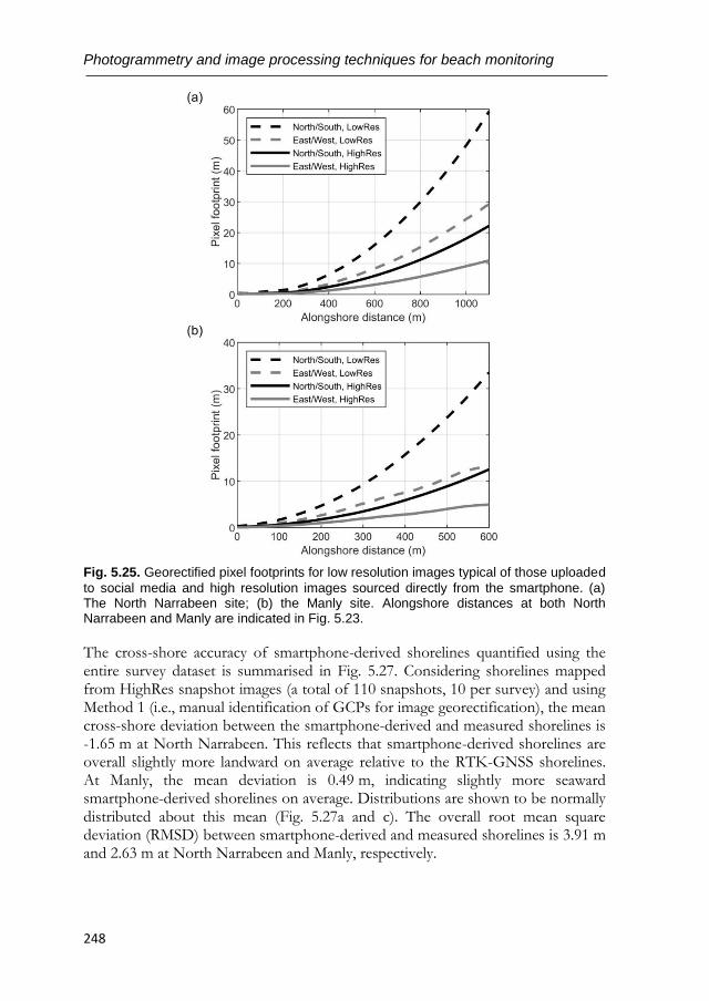
Photogrammetry and image processing techniques for beach monitoring
248
Fig. 5.25. Georectified pixel footprints for low resolution images typical of those uploaded
to social media and high resolution images sourced directly from the smartphone. (a) The North Narrabeen site; (b) the Manly site. Alongshore distances at both North Narrabeen and Manly are indicated in Fig. 5.23.
The cross-shore accuracy of smartphone-derived shorelines quantified using the entire survey dataset is summarised in Fig. 5.27. Considering shorelines mapped from HighRes snapshot images (a total of 110 snapshots, 10 per survey) and using Method 1 (i.e., manual identification of GCPs for image georectification), the mean cross-shore deviation between the smartphone-derived and measured shorelines is -1.65 m at North Narrabeen. This reflects that smartphone-derived shorelines are overall slightly more landward on average relative to the RTK-GNSS shorelines. At Manly, the mean deviation is 0.49 m, indicating slightly more seaward smartphone-derived shorelines on average. Distributions are shown to be normally distributed about this mean (Fig. 5.27a and c). The overall root mean square deviation (RMSD) between smartphone-derived and measured shorelines is 3.91 m and 2.63 m at North Narrabeen and Manly, respectively.
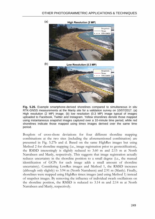
OTHER PHOTOGRAMMETRIC APPLICATIONS & TECHNIQUES
249
Fig. 5.26. Example smartphone-derived shorelines compared to simultaneous in situ
RTK-GNSS measurements at the Manly site for a validation survey on 10/07/2017. (a) High resolution (2 MP) image; (b) low resolution (0.3 MP) image typical of images uploaded to Facebook, Twitter and Instagram. Yellow shorelines denote those mapped using instantaneous snapshot images captured over a 10-minute time period, while red shorelines indicate those mapped using timex images derived over the same time period.
Boxplots of cross-shore deviations for four different shoreline mapping combinations at the two sites (including the aforementioned combination) are presented in Fig. 5.27b and d. Based on the same HighRes images but using Method 2 for shoreline mapping (i.e., image registration prior to georectification), the RMSD interestingly is slightly reduced to 3.60 m and 2.15 m at North Narrabeen and Manly, respectively. This suggests that image registration actually reduces uncertainty in the shoreline position to a small degree (i.e., the manual identification of GCPs for each image adds a small amount of shoreline uncertainty). Considering LowRes images and Method 1, the RMSD increases (although only slightly) to 3.94 m (North Narrabeen) and 2.91 m (Manly). Finally, shorelines were mapped using HighRes timex images (and using Method 1) instead of snapshot images. By removing the influence of individual swash oscillations on the shoreline position, the RMSD is reduced to 3.14 m and 2.14 m at North Narrabeen and Manly, respectively.
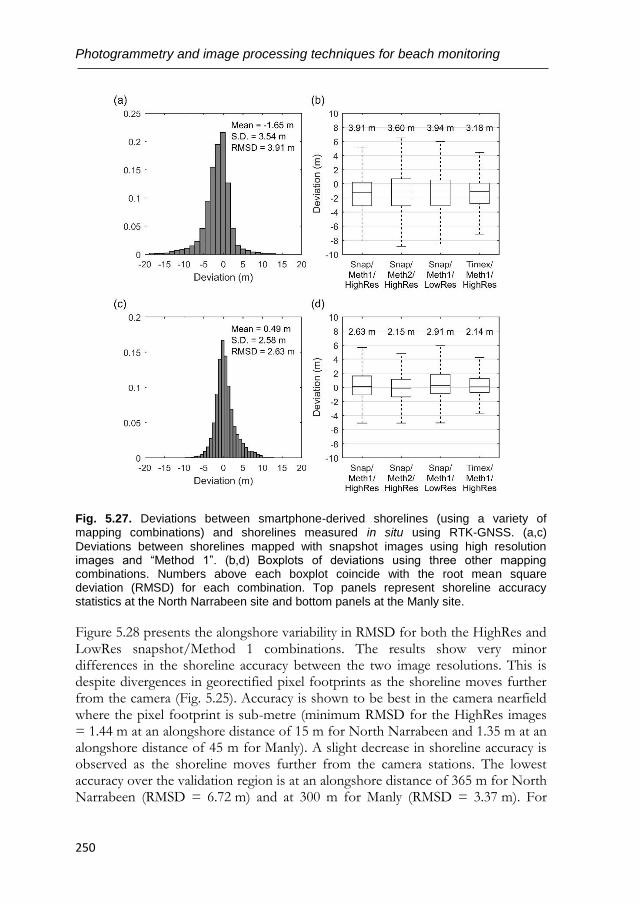
Photogrammetry and image processing techniques for beach monitoring
250
Fig. 5.27. Deviations between smartphone-derived shorelines (using a variety of mapping combinations) and shorelines measured in situ using RTK-GNSS. (a,c)
Deviations between shorelines mapped with snapshot images using high resolution images and “Method 1”. (b,d) Boxplots of deviations using three other mapping combinations. Numbers above each boxplot coincide with the root mean square deviation (RMSD) for each combination. Top panels represent shoreline accuracy statistics at the North Narrabeen site and bottom panels at the Manly site.
Figure 5.28 presents the alongshore variability in RMSD for both the HighRes and LowRes snapshot/Method 1 combinations. The results show very minor differences in the shoreline accuracy between the two image resolutions. This is despite divergences in georectified pixel footprints as the shoreline moves further from the camera (Fig. 5.25). Accuracy is shown to be best in the camera nearfield where the pixel footprint is sub-metre (minimum RMSD for the HighRes images = 1.44 m at an alongshore distance of 15 m for North Narrabeen and 1.35 m at an alongshore distance of 45 m for Manly). A slight decrease in shoreline accuracy is observed as the shoreline moves further from the camera stations. The lowest accuracy over the validation region is at an alongshore distance of 365 m for North Narrabeen (RMSD = 6.72 m) and at 300 m for Manly (RMSD = 3.37 m). For
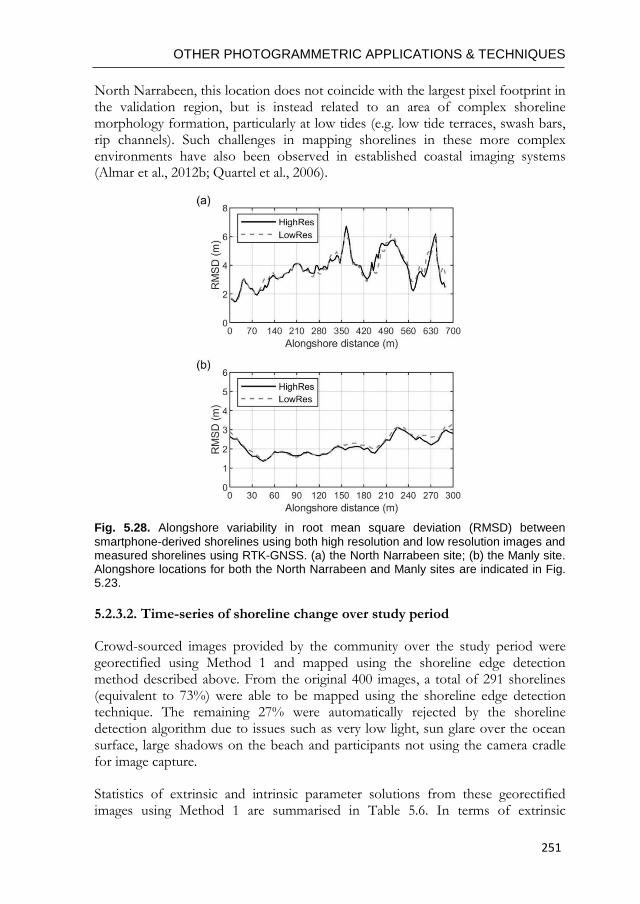
OTHER PHOTOGRAMMETRIC APPLICATIONS & TECHNIQUES
251
North Narrabeen, this location does not coincide with the largest pixel footprint in the validation region, but is instead related to an area of complex shoreline morphology formation, particularly at low tides (e.g. low tide terraces, swash bars, rip channels). Such challenges in mapping shorelines in these more complex environments have also been observed in established coastal imaging systems (Almar et al., 2012b; Quartel et al., 2006).
Fig. 5.28. Alongshore variability in root mean square deviation (RMSD) between
smartphone-derived shorelines using both high resolution and low resolution images and measured shorelines using RTK-GNSS. (a) the North Narrabeen site; (b) the Manly site. Alongshore locations for both the North Narrabeen and Manly sites are indicated in Fig. 5.23.
5.2.3.2. Time-series of shoreline change over study period
Crowd-sourced images provided by the community over the study period were georectified using Method 1 and mapped using the shoreline edge detection method described above. From the original 400 images, a total of 291 shorelines (equivalent to 73%) were able to be mapped using the shoreline edge detection technique. The remaining 27% were automatically rejected by the shoreline detection algorithm due to issues such as very low light, sun glare over the ocean surface, large shadows on the beach and participants not using the camera cradle for image capture.
Statistics of extrinsic and intrinsic parameter solutions from these georectified images using Method 1 are summarised in Table 5.6. In terms of extrinsic
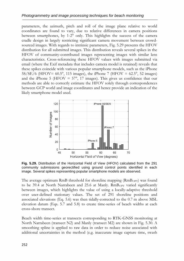
Photogrammetry and image processing techniques for beach monitoring
252
parameters, the azimuth, pitch and roll of the image plane relative to world coordinates are found to vary, due to relative differences in camera positions between smartphones, by 1-2° only. This highlights the success of the camera cradle design in largely restricting significant camera movement between crowd-sourced images. With regards to intrinsic parameters, Fig. 5.29 presents the HFOV distribution for all submitted images. This distribution reveals several spikes in the HFOV of community-contributed images representing images with similar lens characteristics. Cross-referencing these HFOV values with images submitted via email (where the Exif metadata that includes camera model is retained) reveals that these spikes coincide with various popular smartphone models, such as the iPhone 5S/SE/6 (HFOV= 60.5°, 115 images), the iPhone 7 (HFOV = 62.5°, 52 images) and the iPhone 5 (HFOV = 57°, 17 images). This gives us confidence that our methods are able to correctly estimate the HFOV solely through correspondences between GCP world and image coordinates and hence provide an indication of the likely smartphone model used.
Fig. 5.29. Distribution of the Horizontal Field of View (HFOV) calculated from the 291
community submissions georectified using ground control points identified in each image. Several spikes representing popular smartphone models are observed.
The average optimum RmB threshold for shoreline mapping (RmBOPT) was found to be 39.4 at North Narrabeen and 25.6 at Manly. RmBOPT varied significantly between images, which highlights the value of using a locally-adaptive threshold over user-defined stationary values. The set of 291 shoreline positions and associated elevations (Eq. 5.6) was then tidally-corrected to the 0.7 m above MSL elevation datum (Eqs. 5.7 and 5.8) to create time-series of beach widths at each cross-shore transect.
Beach width time-series at transects corresponding to RTK-GNSS monitoring at North Narrabeen (transect N2) and Manly (transect M2) are shown in Fig. 5.30. A smoothing spline is applied to raw data in order to reduce noise associated with additional uncertainties in the method (e.g. inaccurate image capture time, swash
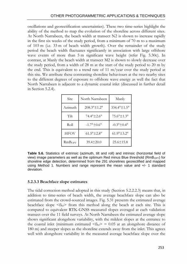
OTHER PHOTOGRAMMETRIC APPLICATIONS & TECHNIQUES
253
oscillations and georectification uncertainties). These two time-series highlight the ability of the method to map the evolution of the shoreline across different sites. At North Narrabeen, the beach width at transect N2 is shown to increase rapidly in the first six weeks of the study period, from a minimum of 70 m to a maximum of 103 m (i.e. 33 m of beach width growth). Over the remainder of the study period the beach width fluctuates significantly in association with large offshore wave events of more than 5 m significant wave height (refer Fig. 5.30c). In contrast, at Manly the beach width at transect M2 is shown to slowly decrease over the study period, from a width of 28 m at the start of the study period to 20 m by the end. This is equivalent to a trend rate of 11 m/year over the study period at this site. We attribute these contrasting shoreline behaviours at the two nearby sites to the different degrees of exposure to offshore wave energy as well the fact that North Narrabeen is adjacent to a dynamic coastal inlet (discussed in further detail in Section 5.2.4).
Site North Narrabeen Manly
Azimuth 208.3°±1.2° 334.4°±1.5°
Tilt 74.4°±2.6° 75.6°±1.3°
Roll -1.7°±0.6° -0.3°±0.4°
HFOV 61.5°±2.8° 61.9°±3.2°
RmBOPT 39.4±20.0 25.6±15.8
Table 5.6. Statistics of extrinsic (azimuth, tilt and roll) and intrinsic (horizontal field of
view) image parameters as well as the optimum Red minus Blue threshold (RmBOPT) for shoreline edge detection, determined from the 291 shorelines georectified and mapped using Method 1. Numbers and range represent the mean value and +/- 1 standard deviation.
5.2.3.3 Beachface slope estimates
The tidal correction method adopted in this study (Section 5.2.2.2.3) means that, in addition to time-series of beach width, the average beachface slope can also be estimated from the crowd-sourced images. Fig. 5.31 presents the estimated average beachface slope <ßbf> from this method along the beach at each site. This is compared to equivalent RTK-GNSS measured slopes averaged at each validation transect over the 11 field surveys. At North Narrabeen the estimated average slope shows significant alongshore variability, with the mildest slopes at the entrance to the coastal inlet (minimum estimated <ßbf> = 0.05 at an alongshore distance of 180 m) and steeper slopes as the shoreline extends away from the inlet. This agrees well with alongshore variability in the measured average beachface slope over the
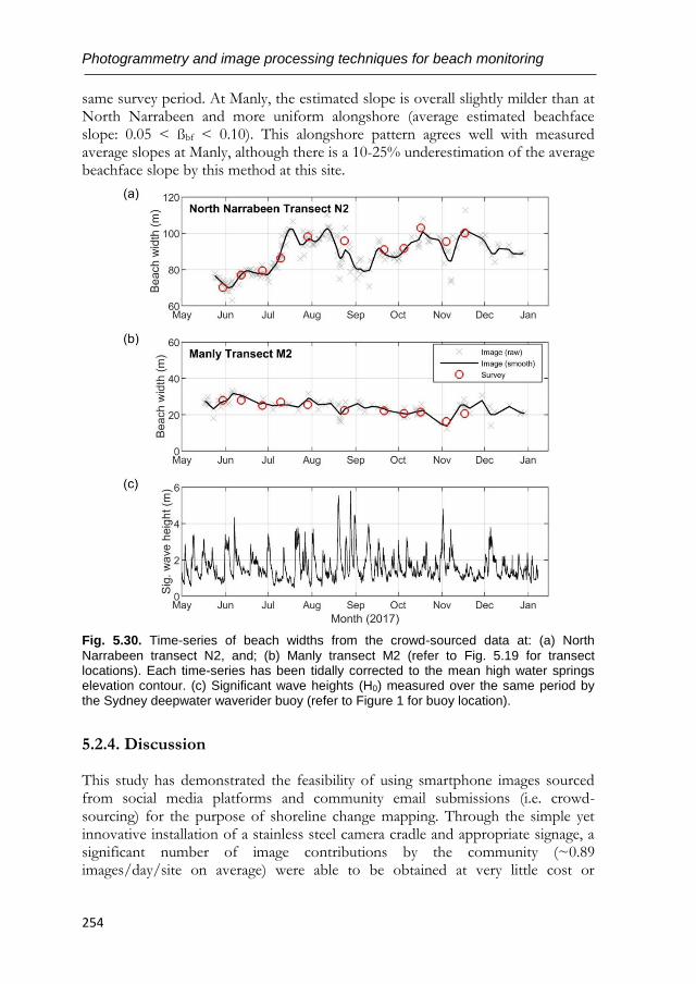
Photogrammetry and image processing techniques for beach monitoring
254
same survey period. At Manly, the estimated slope is overall slightly milder than at North Narrabeen and more uniform alongshore (average estimated beachface slope: 0.05 < ßbf < 0.10). This alongshore pattern agrees well with measured average slopes at Manly, although there is a 10-25% underestimation of the average beachface slope by this method at this site.
Fig. 5.30. Time-series of beach widths from the crowd-sourced data at: (a) North
Narrabeen transect N2, and; (b) Manly transect M2 (refer to Fig. 5.19 for transect locations). Each time-series has been tidally corrected to the mean high water springs elevation contour. (c) Significant wave heights (H0) measured over the same period by the Sydney deepwater waverider buoy (refer to Figure 1 for buoy location).
5.2.4. Discussion
This study has demonstrated the feasibility of using smartphone images sourced from social media platforms and community email submissions (i.e. crowd-sourcing) for the purpose of shoreline change mapping. Through the simple yet innovative installation of a stainless steel camera cradle and appropriate signage, a significant number of image contributions by the community (~0.89 images/day/site on average) were able to be obtained at very little cost or
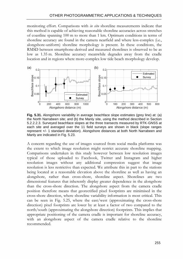
OTHER PHOTOGRAMMETRIC APPLICATIONS & TECHNIQUES
255
monitoring effort. Comparisons with in situ shoreline measurements indicate that this method is capable of achieving reasonable shoreline accuracies across stretches of coastline spanning 100 m to more than 1 km. Optimum conditions in terms of shoreline accuracy are found in the camera nearfield and where less-complex (i.e., alongshore-uniform) shoreline morphology is present. In these conditions, the RMSD between smartphone-derived and measured shorelines is observed to be as low as 1.35 m. Shoreline accuracy meanwhile degrades away from the cradle location and in regions where more-complex low tide beach morphology develop.
Fig. 5.31. Alongshore variability in average beachface slope estimates (grey line) at: (a)
the North Narrabeen site; and (b) the Manly site, using the method described in Section 5.2.2.2.3. Surveyed beachface slopes at the three transects measured by RTK-GNSS at each site and averaged over the 11 field surveys are shown in black (slope ranges represent +/- 1 standard deviation). Alongshore distances at both North Narrabeen and Manly are indicated in Fig. 5.23.
A concern regarding the use of images sourced from social media platforms was the extent to which image resolution might restrict accurate shoreline mapping. Comparisons undertaken in this study however between low resolution images typical of those uploaded to Facebook, Twitter and Instagram and higher resolution images without any additional compression suggest that image resolution is less restrictive than expected. We attribute this in part to the stations being located at a reasonable elevation above the shoreline as well as having an alongshore, rather than cross-shore, shoreline aspect. Shorelines are two dimensional features that inherently display greater dependence in the alongshore than the cross-shore direction. The alongshore aspect from the camera cradle position therefore means that georectified pixel footprints are minimised in the cross-shore direction, where shoreline variability information is most critical. This can be seen in Fig. 5.25, where the east/west (approximating the cross-shore direction) pixel footprints are lower by at least a factor of two compared to the north/south (approximating the alongshore direction) footprints. This implies that appropriate positioning of the camera cradle is important for shoreline accuracy, with an alongshore aspect of the camera cradle relative to the shoreline recommended.
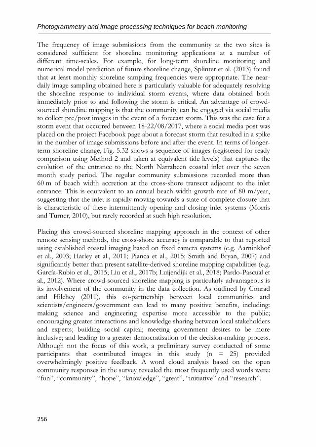
Photogrammetry and image processing techniques for beach monitoring
256
The frequency of image submissions from the community at the two sites is considered sufficient for shoreline monitoring applications at a number of different time-scales. For example, for long-term shoreline monitoring and numerical model prediction of future shoreline change, Splinter et al. (2013) found that at least monthly shoreline sampling frequencies were appropriate. The near-daily image sampling obtained here is particularly valuable for adequately resolving the shoreline response to individual storm events, where data obtained both immediately prior to and following the storm is critical. An advantage of crowd-sourced shoreline mapping is that the community can be engaged via social media to collect pre/post images in the event of a forecast storm. This was the case for a storm event that occurred between 18-22/08/2017, where a social media post was placed on the project Facebook page about a forecast storm that resulted in a spike in the number of image submissions before and after the event. In terms of longer-term shoreline change, Fig. 5.32 shows a sequence of images (registered for ready comparison using Method 2 and taken at equivalent tide levels) that captures the evolution of the entrance to the North Narrabeen coastal inlet over the seven month study period. The regular community submissions recorded more than 60 m of beach width accretion at the cross-shore transect adjacent to the inlet entrance. This is equivalent to an annual beach width growth rate of 80 m/year, suggesting that the inlet is rapidly moving towards a state of complete closure that is characteristic of these intermittently opening and closing inlet systems (Morris and Turner, 2010), but rarely recorded at such high resolution.
Placing this crowd-sourced shoreline mapping approach in the context of other remote sensing methods, the cross-shore accuracy is comparable to that reported using established coastal imaging based on fixed camera systems (e.g. Aarninkhof et al., 2003; Harley et al., 2011; Pianca et al., 2015; Smith and Bryan, 2007) and significantly better than present satellite-derived shoreline mapping capabilities (e.g. García-Rubio et al., 2015; Liu et al., 2017b; Luijendijk et al., 2018; Pardo-Pascual et al., 2012). Where crowd-sourced shoreline mapping is particularly advantageous is its involvement of the community in the data collection. As outlined by Conrad and Hilchey (2011), this co-partnership between local communities and scientists/engineers/government can lead to many positive benefits, including: making science and engineering expertise more accessible to the public; encouraging greater interactions and knowledge sharing between local stakeholders and experts; building social capital; meeting government desires to be more inclusive; and leading to a greater democratisation of the decision-making process. Although not the focus of this work, a preliminary survey conducted of some participants that contributed images in this study (n = 25) provided overwhelmingly positive feedback. A word cloud analysis based on the open community responses in the survey revealed the most frequently used words were: “fun”, “community”, “hope”, “knowledge”, “great”, “initiative” and “research”.
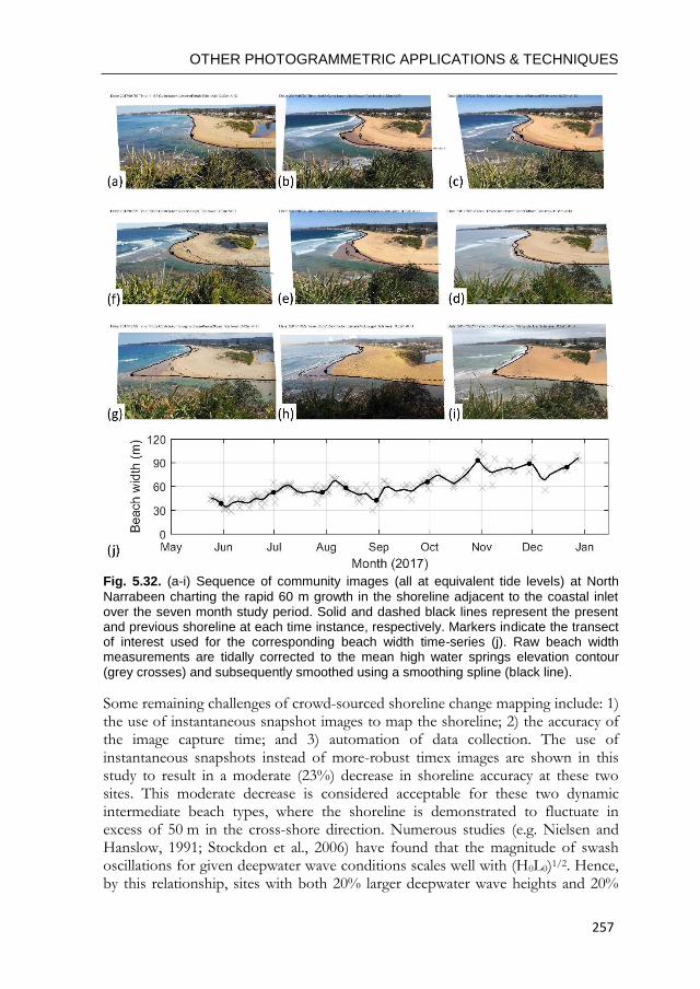
OTHER PHOTOGRAMMETRIC APPLICATIONS & TECHNIQUES
257
Fig. 5.32. (a-i) Sequence of community images (all at equivalent tide levels) at North
Narrabeen charting the rapid 60 m growth in the shoreline adjacent to the coastal inlet over the seven month study period. Solid and dashed black lines represent the present and previous shoreline at each time instance, respectively. Markers indicate the transect of interest used for the corresponding beach width time-series (j). Raw beach width measurements are tidally corrected to the mean high water springs elevation contour (grey crosses) and subsequently smoothed using a smoothing spline (black line).
Some remaining challenges of crowd-sourced shoreline change mapping include: 1) the use of instantaneous snapshot images to map the shoreline; 2) the accuracy of the image capture time; and 3) automation of data collection. The use of instantaneous snapshots instead of more-robust timex images are shown in this study to result in a moderate (23%) decrease in shoreline accuracy at these two sites. This moderate decrease is considered acceptable for these two dynamic intermediate beach types, where the shoreline is demonstrated to fluctuate in excess of 50 m in the cross-shore direction. Numerous studies (e.g. Nielsen and Hanslow, 1991; Stockdon et al., 2006) have found that the magnitude of swash oscillations for given deepwater wave conditions scales well with (H0L0)1/2. Hence, by this relationship, sites with both 20% larger deepwater wave heights and 20%
Photogrammetry and image processing techniques for beach monitoring
258
longer wave periods can expect a further ~30% reduction in shoreline accuracy. Such a reduction might reduce the capacity of the method to detect actual shoreline signals against considerable measurement noise, particularly for less-dynamic shorelines such as reflective or dissipative beach types (Wright and Short, 1984). In these instances, we suggest the following possible adaptations to our approach to further reduce shoreline uncertainty:
1) restricting shoreline mapping from the community images to wave conditions below a certain threshold; 2) incorporating the use of a smartphone app capable of calculating timex images on-the-fly over several minutes (e.g. “Average Camera Pro” for the iPhone); and/or 3) using a more complex shoreline elevation model that accounts for time-varying wave setup and swash oscillations (e.g. Aarninkhof et al., 2003; Harley et al., 2011b; Plant et al., 2007).
The trade-offs of these adaptations however are a reduction in available shoreline data, a greater reliance on field measurements and increased effort by the community in capturing image data.
With regards to challenges associated with image capture time, the method is presently reliant on the upload time to social media unless otherwise stated by the participant. While only two of the 400 images in this study were manually flagged with very suspicious capture times (meaning that the image times appeared to be several hours different to when it was uploaded or stated), this issue becomes increasingly critical on coastlines with larger tidal ranges, where even small errors in image capture time can lead to poor estimates of the shoreline elevation. Finally, the diversity of images collected (i.e., high and low resolution images and different smartphone camera models) and various modes of image submission (i.e., Facebook, Instagram, Twitter and email) make automation of data collection a challenge. The successful application in this study of image registration is shown to remove the need for manual identification of GCPs in every single image and thereby improve automation. Further automation could also include: the use of machine learning algorithms (e.g. Lecun et al., 2015) to automatically detect false images; the use of the horizon edge for georectification (e.g. Sánchez-García et al., 2017); and a customised smartphone app or web application for greater control of image submissions and metadata.
5.2.5. Conclusions
Oblique images of the coastline using fixed video systems have been used by coastal practitioners for decades as a means of obtaining critical information about dynamic shoreline processes over a range of time-scales. The proliferation in smartphone ownership worldwide and the corresponding abundance of images uploaded to social media platforms like Facebook, Twitter and Instagram suggests
OTHER PHOTOGRAMMETRIC APPLICATIONS & TECHNIQUES
259
that, with the aid of simple infrastructure installed at an appropriate location, these images could also be harnessed as an alternative low-cost means of obtaining shoreline change information. This new crowd-sourced shoreline change mapping approach however entails several challenges and trade-offs with respect to established and highly-controlled coastal imaging techniques. These challenges include: the use of low resolution images; images sourced from a wide range of different smartphone lenses of unknown intrinsic camera properties; less-stable repeat images; restricted abilities for time-averaging of swash oscillations on the shoreline; and uncertainty in image capture times.
Our results show that, despite these various challenges, it is possible to obtain shoreline positions of comparable accuracy to that of established coastal imaging systems. This is achieved through the use of surveyed ground control points in the image to numerically solve for the most relevant intrinsic and extrinsic camera information (i.e., focal length, azimuth pitch and roll) and assisted by the internal correction of most radial image distortion in modern smartphone images. Image resolution and the use of instantaneous snapshot images for shoreline mapping are meanwhile shown in this study at two nearby sites in southeastern Australia (North Narrabeen and Manly Beach) to cause only moderate decreases in shoreline accuracy. Such decreases are deemed an acceptable trade-off when considering both the benefits of crowd-sourced data in terms of costs, logistics and community participation, as well as the large degree of shoreline variability typically observed on dynamic coastlines. This is particularly exemplified in this study at the North Narrabeen site, where the crowd-sourced shoreline mapping was able to capture an impressive 60 m growth of the shoreline in just seven months and gain rare, high-resolution, insights into the morphodynamics of shorelines adjacent to unstable coastal inlets.
The successful application of this crowd-sourced method at these two Australian sites opens up new possibilities for shoreline change mapping at suitable locations worldwide. This is especially the case for emerging and developing countries, where uptake of established coastal imaging systems – and methods to monitor the shoreline more generally – has previously been restrictive, but smartphone and social media usage is high (Poushter, 2016). Through a network of similar stations it might be possible to not only map shoreline evolution at nearby coastal locations (as in this study), but detect patterns in shoreline behaviour across regional coastlines and ocean basins. Such data could significantly expand our present capabilities in tracking and understanding shoreline variability and trends at a wide variety of spatial and temporal scales.

Photogrammetry and image processing techniques for beach monitoring
260
OTHER PHOTOGRAMMETRIC APPLICATIONS & TECHNIQUES
261
5.3. MODELLING LANDSCAPE MORPHODYNAMICS BY TERRESTRIAL PHOTOGRAMMETRY: AN APPLICATION TO BEACH AND FLUVIAL SYSTEMS
Beach and fluvial systems are highly dynamic environments, being constantly modified by the action of different natural and anthropic phenomena. To understand their behaviour and to support a sustainable management of these fragile environments, it is very important to have access to cost-effective tools. These methods should be supported on cutting-edge technologies that allow monitoring the dynamics of the natural systems with high periodicity and repeatability at different temporal and spatial scales instead the tedious and expensive fieldwork that has been carried out up to date. The work herein presented analyzes the potential of terrestrial photogrammetry to describe beach morphology. Data processing and generation of high resolution 3D point clouds and derived DEMs is supported by the commercial Agisoft PhotoScan. Model validation is done by comparison of the differences in the elevation among the photogrammetric point cloud and the GPS data along different beach profiles. Results obtained denote the potential that the photogrammetry 3D modelling has to monitor morphological changes and natural events getting differences between 6 and 25 cm. Furthermore, the usefulness of these techniques to control the layout of a fluvial system is tested by the performance of some modeling essays in a hydraulic pilot channel.
5.3.1. Introduction
The understanding of the unceasing dynamics in natural systems and the knowledge of its morphological response at different spatial and temporal scales might be the key for a sustainable management of the natural resources. Beaches and rivers are continuously suffering the impact of numberless factors that modify the (eco)system dynamics. Therefore, the possibility of monitoring these spaces will be helpful in a decision-making process which concerns not only environmental values but also socioeconomic interests.
In that context, some institutions have realised the need of monitoring their resources, and they are carrying out more initiatives and studies to achieve it at low spatial and temporal scale. However, up to date, known techniques that allow a high accuracy monitoring are expensive and require tedious field campaigns as well as specialized software (James et al., 2013). Thus, despite their high accuracy, these techniques cannot be understood as efficient tools to monitor dynamics with the frequency required by natural spaces. Some examples are: the Airborne Light Detection and Ranging (LiDAR) and the Terrestrial Laser Scanner (TLS) that allow to obtain high accuracy dense point clouds; the geodetics GPS capable of defining a light DEM; the video imaging systems that enable to recreate the intertidal beach
Photogrammetry and image processing techniques for beach monitoring
262
bathymetry (Uunk et al., 2010); and the remote sensing techniques that allow an accurate shoreline detection (Almonacid-Caballer et al., 2016).
Nevertheless, a relatively novel technique (Westoby et al., 2012) has overcome the listed inconveniences and is positioned as a pioneer in the field of monitoring. The terrestrial photogrammetry will be successful for small areas and high frequency. The method is based on Structure-from-Motion (SfM) photogrammetry coupled with Multi-View Stereo (MVS). Using Agisoft PhotoScan Pro and, in contrast to conventional photogrammetry requirements, its inner algorithms achieve an initial model reconstruction without need any additional camera, nor field information and operator intervention (Agisoft, 2014). The generated 3D point cloud is located in an arbitrary coordinate system that can be changed through the definition of GCPs whose accuracy will condition the final model errors. Moreover, it is possible to obtain a high resolution SfM-DEM from the 3D point cloud.
The Agisoft PhotoScan software uses overlapped photos taken from different angles. However, the way in which these images are acquired can vary and be equally suitable to create the models. For example, Hugenholtz et al. (2013) uses a small unmanned aircraft system (sUAS) for geomorphological mapping, and Gonçalves and Henriques (2015) recreate and monitor both sand dunes and the beach area with an unmanned aerial vehicle (UAV). Moreover, other studies check that the SfM also works with aerial photos captured up to 800 m above the ground level (Javernick et al., 2014). Finally, some analyses using ground based photogrammetry have already modelled coastal environments and measured successfully morphological changes by SfM (Pikelj et al., 2015; Ružić, et al., 2014).
Herein, we use terrestrial photogrammetry for monitoring morphological changes in beaches and fluvial systems. The main goal is to prove its potential in other places and scenarios (cameras at different heights, with different orientations and even for different camera models) and to test its quality against high accuracy GPS techniques. To achieve it, we study three different areas following specific methodologies.
SfM photogrammetric technique is becoming also useful for accurate numerical-experimental modelling that act as reality simulators. Thus, in the field of hydraulic engineering, the knowledge of sedimentary changes in narrow channels may be done by measurements along simple profiles (Nácher-Rodríguez et al., 2015). However, in complex and realistic wider pilot channels (see below) the availability of a 3D model will be of great importance to compute the changes and to make easier the analysis of the studied phenomenon.
5.3.2. Data and study area
Two very different coastal areas are modelled in this work. The first one (see Fig. 5.33B) is El Saler (Valencia, Mediterranean coast, Spain), a long micro-tidal beach
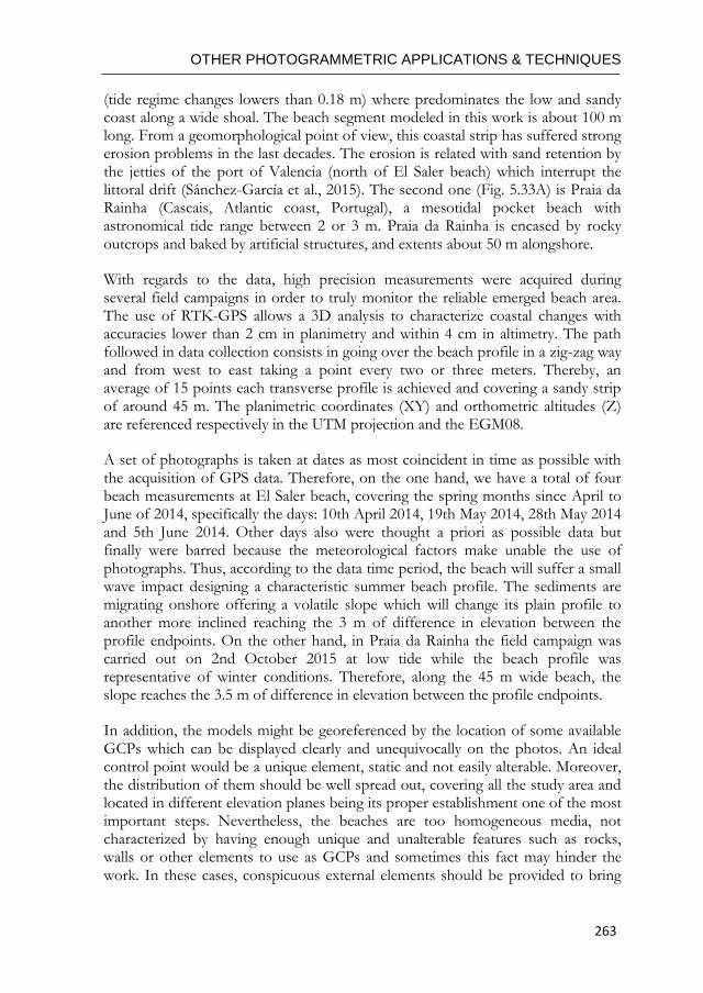
OTHER PHOTOGRAMMETRIC APPLICATIONS & TECHNIQUES
263
(tide regime changes lowers than 0.18 m) where predominates the low and sandy coast along a wide shoal. The beach segment modeled in this work is about 100 m long. From a geomorphological point of view, this coastal strip has suffered strong erosion problems in the last decades. The erosion is related with sand retention by the jetties of the port of Valencia (north of El Saler beach) which interrupt the littoral drift (Sánchez-García et al., 2015). The second one (Fig. 5.33A) is Praia da Rainha (Cascais, Atlantic coast, Portugal), a mesotidal pocket beach with astronomical tide range between 2 or 3 m. Praia da Rainha is encased by rocky outcrops and baked by artificial structures, and extents about 50 m alongshore.
With regards to the data, high precision measurements were acquired during several field campaigns in order to truly monitor the reliable emerged beach area. The use of RTK-GPS allows a 3D analysis to characterize coastal changes with accuracies lower than 2 cm in planimetry and within 4 cm in altimetry. The path followed in data collection consists in going over the beach profile in a zig-zag way and from west to east taking a point every two or three meters. Thereby, an average of 15 points each transverse profile is achieved and covering a sandy strip of around 45 m. The planimetric coordinates (XY) and orthometric altitudes (Z) are referenced respectively in the UTM projection and the EGM08.
A set of photographs is taken at dates as most coincident in time as possible with the acquisition of GPS data. Therefore, on the one hand, we have a total of four beach measurements at El Saler beach, covering the spring months since April to June of 2014, specifically the days: 10th April 2014, 19th May 2014, 28th May 2014 and 5th June 2014. Other days also were thought a priori as possible data but finally were barred because the meteorological factors make unable the use of photographs. Thus, according to the data time period, the beach will suffer a small wave impact designing a characteristic summer beach profile. The sediments are migrating onshore offering a volatile slope which will change its plain profile to another more inclined reaching the 3 m of difference in elevation between the profile endpoints. On the other hand, in Praia da Rainha the field campaign was carried out on 2nd October 2015 at low tide while the beach profile was representative of winter conditions. Therefore, along the 45 m wide beach, the slope reaches the 3.5 m of difference in elevation between the profile endpoints.
In addition, the models might be georeferenced by the location of some available GCPs which can be displayed clearly and unequivocally on the photos. An ideal control point would be a unique element, static and not easily alterable. Moreover, the distribution of them should be well spread out, covering all the study area and located in different elevation planes being its proper establishment one of the most important steps. Nevertheless, the beaches are too homogeneous media, not characterized by having enough unique and unalterable features such as rocks, walls or other elements to use as GCPs and sometimes this fact may hinder the work. In these cases, conspicuous external elements should be provided to bring
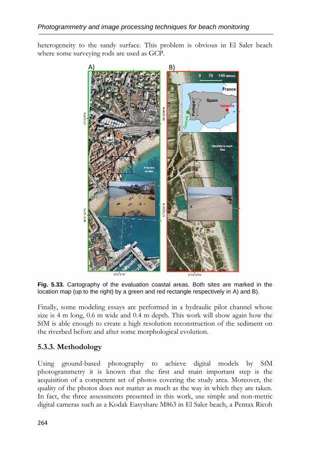
Photogrammetry and image processing techniques for beach monitoring
264
heterogeneity to the sandy surface. This problem is obvious in El Saler beach where some surveying rods are used as GCP.
Fig. 5.33. Cartography of the evaluation coastal areas. Both sites are marked in the
location map (up to the right) by a green and red rectangle respectively in A) and B).
Finally, some modeling essays are performed in a hydraulic pilot channel whose size is 4 m long, 0.6 m wide and 0.4 m depth. This work will show again how the SfM is able enough to create a high resolution reconstruction of the sediment on the riverbed before and after some morphological evolution.
5.3.3. Methodology
Using ground-based photography to achieve digital models by SfM photogrammetry it is known that the first and main important step is the acquisition of a competent set of photos covering the study area. Moreover, the quality of the photos does not matter as much as the way in which they are taken. In fact, the three assessments presented in this work, use simple and non-metric digital cameras such as a Kodak Easyshare M863 in El Saler beach, a Pentax Ricoh
A) B)
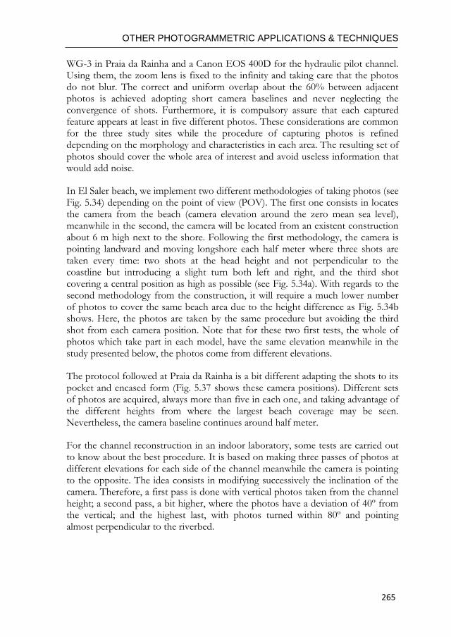
OTHER PHOTOGRAMMETRIC APPLICATIONS & TECHNIQUES
265
WG-3 in Praia da Rainha and a Canon EOS 400D for the hydraulic pilot channel. Using them, the zoom lens is fixed to the infinity and taking care that the photos do not blur. The correct and uniform overlap about the 60% between adjacent photos is achieved adopting short camera baselines and never neglecting the convergence of shots. Furthermore, it is compulsory assure that each captured feature appears at least in five different photos. These considerations are common for the three study sites while the procedure of capturing photos is refined depending on the morphology and characteristics in each area. The resulting set of photos should cover the whole area of interest and avoid useless information that would add noise.
In El Saler beach, we implement two different methodologies of taking photos (see Fig. 5.34) depending on the point of view (POV). The first one consists in locates the camera from the beach (camera elevation around the zero mean sea level), meanwhile in the second, the camera will be located from an existent construction about 6 m high next to the shore. Following the first methodology, the camera is pointing landward and moving longshore each half meter where three shots are taken every time: two shots at the head height and not perpendicular to the coastline but introducing a slight turn both left and right, and the third shot covering a central position as high as possible (see Fig. 5.34a). With regards to the second methodology from the construction, it will require a much lower number of photos to cover the same beach area due to the height difference as Fig. 5.34b shows. Here, the photos are taken by the same procedure but avoiding the third shot from each camera position. Note that for these two first tests, the whole of photos which take part in each model, have the same elevation meanwhile in the study presented below, the photos come from different elevations.
The protocol followed at Praia da Rainha is a bit different adapting the shots to its pocket and encased form (Fig. 5.37 shows these camera positions). Different sets of photos are acquired, always more than five in each one, and taking advantage of the different heights from where the largest beach coverage may be seen. Nevertheless, the camera baseline continues around half meter.
For the channel reconstruction in an indoor laboratory, some tests are carried out to know about the best procedure. It is based on making three passes of photos at different elevations for each side of the channel meanwhile the camera is pointing to the opposite. The idea consists in modifying successively the inclination of the camera. Therefore, a first pass is done with vertical photos taken from the channel height; a second pass, a bit higher, where the photos have a deviation of 40º from the vertical; and the highest last, with photos turned within 80º and pointing almost perpendicular to the riverbed.
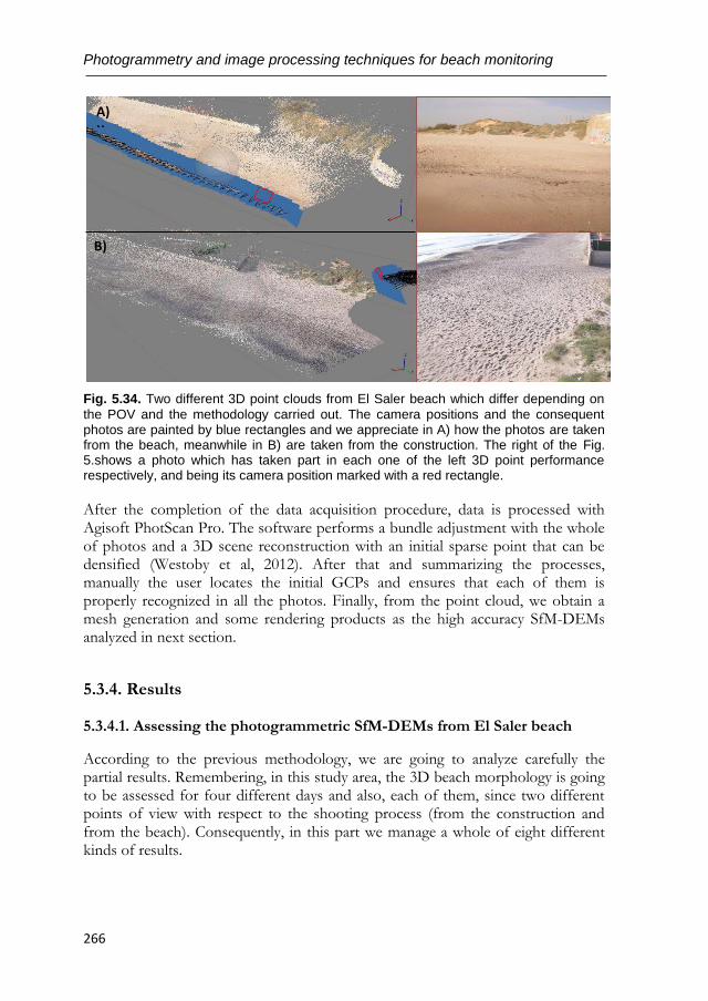
Photogrammetry and image processing techniques for beach monitoring
266
Fig. 5.34. Two different 3D point clouds from El Saler beach which differ depending on
the POV and the methodology carried out. The camera positions and the consequent photos are painted by blue rectangles and we appreciate in A) how the photos are taken from the beach, meanwhile in B) are taken from the construction. The right of the Fig. 5.shows a photo which has taken part in each one of the left 3D point performance respectively, and being its camera position marked with a red rectangle.
After the completion of the data acquisition procedure, data is processed with Agisoft PhotScan Pro. The software performs a bundle adjustment with the whole of photos and a 3D scene reconstruction with an initial sparse point that can be densified (Westoby et al, 2012). After that and summarizing the processes, manually the user locates the initial GCPs and ensures that each of them is properly recognized in all the photos. Finally, from the point cloud, we obtain a mesh generation and some rendering products as the high accuracy SfM-DEMs analyzed in next section.
5.3.4. Results
5.3.4.1. Assessing the photogrammetric SfM-DEMs from El Saler beach
According to the previous methodology, we are going to analyze carefully the partial results. Remembering, in this study area, the 3D beach morphology is going to be assessed for four different days and also, each of them, since two different points of view with respect to the shooting process (from the construction and from the beach). Consequently, in this part we manage a whole of eight different kinds of results.
A)
))
B)
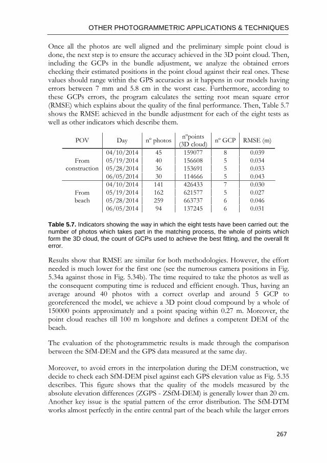
OTHER PHOTOGRAMMETRIC APPLICATIONS & TECHNIQUES
267
Once all the photos are well aligned and the preliminary simple point cloud is done, the next step is to ensure the accuracy achieved in the 3D point cloud. Then, including the GCPs in the bundle adjustment, we analyze the obtained errors checking their estimated positions in the point cloud against their real ones. These values should range within the GPS accuracies as it happens in our models having errors between 7 mm and 5.8 cm in the worst case. Furthermore, according to these GCPs errors, the program calculates the setting root mean square error (RMSE) which explains about the quality of the final performance. Then, Table 5.7 shows the RMSE achieved in the bundle adjustment for each of the eight tests as well as other indicators which describe them.
Table 5.7. Indicators showing the way in which the eight tests have been carried out: the
number of photos which takes part in the matching process, the whole of points which form the 3D cloud, the count of GCPs used to achieve the best fitting, and the overall fit error.
Results show that RMSE are similar for both methodologies. However, the effort needed is much lower for the first one (see the numerous camera positions in Fig. 5.34a against those in Fig. 5.34b). The time required to take the photos as well as the consequent computing time is reduced and efficient enough. Thus, having an average around 40 photos with a correct overlap and around 5 GCP to georeferenced the model, we achieve a 3D point cloud compound by a whole of 150000 points approximately and a point spacing within 0.27 m. Moreover, the point cloud reaches till 100 m longshore and defines a competent DEM of the beach.
The evaluation of the photogrammetric results is made through the comparison between the SfM-DEM and the GPS data measured at the same day.
Moreover, to avoid errors in the interpolation during the DEM construction, we decide to check each SfM-DEM pixel against each GPS elevation value as Fig. 5.35 describes. This figure shows that the quality of the models measured by the absolute elevation differences (ZGPS - ZSfM-DEM) is generally lower than 20 cm. Another key issue is the spatial pattern of the error distribution. The SfM-DTM works almost perfectly in the entire central part of the beach while the larger errors
POV Day nº photos nºpoints
(3D cloud) nº GCP RMSE (m)
From construction
04/10/2014 45 159077 8 0.039
05/19/2014 40 156608 5 0.034
05/28/2014 36 153691 5 0.033
06/05/2014 30 114666 5 0.043
From beach
04/10/2014 141 426433 7 0.030
05/19/2014 162 621577 5 0.027
05/28/2014 259 663737 6 0.046
06/05/2014 94 137245 6 0.031
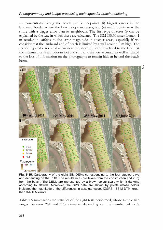
Photogrammetry and image processing techniques for beach monitoring
268
are concentrated along the beach profile endpoints: (i) biggest errors in the landward border where the beach slope increases, and (ii) many points near the shore with a bigger error than its neighbours. The first type of error (i) can be explained by the way in which these are calculated. The SfM-DEM raster format -1 m resolution- affects to the error magnitude in steeper areas, especially if we consider that the landward end of beach is limited by a wall around 2 m high. The second type of error, that occur near the shore (ii), can be related to the fact that the measured GPS altitudes in wet and soft sand are less accurate, as well as related to the loss of information on the photographs to remain hidden behind the beach berm.
Fig. 5.35. Cartography of the eight SfM-DEMs corresponding to the four studied days
and depending on the POV. The results in a) are taken from the construction and in b) from the beach. The DEMs are represented by a brown colour scale which it darkens according to altitude. Moreover, the GPS data are shown by points whose colour indicates the magnitude of the differences in absolute values |ZGPS - ZSfM-DTM| ergo, the SfM-DEM errors.
Table 5.8 summarizes the statistics of the eight tests performed; whose sample size ranges between 254 and 773 elements depending on the number of GPS
±A)
B)
19th May 2014 10th April 2014 28th May 2014 5th June 2014
SfM-DEM
error (m)
ZSfM-DEM (m)
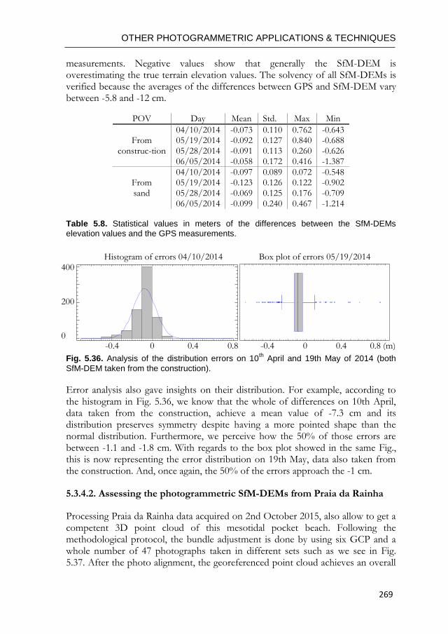
OTHER PHOTOGRAMMETRIC APPLICATIONS & TECHNIQUES
269
Errors
Box plot of errors on may 19, 2014
-0,7 -0,6 -0,5 -0,4 -0,3 -0,2 -0,1 0 0,1 0,2 0,3 0,4 0,5 0,6 0,7 0,8 0,9
Histogram of errors on April 10, 2014
Fre
qu
en
cy
Errors
DistributionNormal
-0,7 -0,6 -0,5 -0,4 -0,3 -0,2 -0,1 0 0,1 0,2 0,3 0,4 0,5 0,6 0,7 0,8
0
100
200
300
400400
200
0
Histogram of errors 04/10/2014 Box plot of errors 05/19/2014
-0.4 0 0.4 0.8 -0.4 0 0.4 0.8 (m)
measurements. Negative values show that generally the SfM-DEM is overestimating the true terrain elevation values. The solvency of all SfM-DEMs is verified because the averages of the differences between GPS and SfM-DEM vary between -5.8 and -12 cm.
POV Day Mean Std. Max Min
From construc-tion
04/10/2014 -0.073 0.110 0.762 -0.643 05/19/2014 -0.092 0.127 0.840 -0.688 05/28/2014 -0.091 0.113 0.260 -0.626 06/05/2014 -0.058 0.172 0.416 -1.387
From sand
04/10/2014 -0.097 0.089 0.072 -0.548 05/19/2014 -0.123 0.126 0.122 -0.902 05/28/2014 -0.069 0.125 0.176 -0.709 06/05/2014 -0.099 0.240 0.467 -1.214
Table 5.8. Statistical values in meters of the differences between the SfM-DEMs
elevation values and the GPS measurements.
Fig. 5.36. Analysis of the distribution errors on 10th April and 19th May of 2014 (both
SfM-DEM taken from the construction).
Error analysis also gave insights on their distribution. For example, according to the histogram in Fig. 5.36, we know that the whole of differences on 10th April, data taken from the construction, achieve a mean value of -7.3 cm and its distribution preserves symmetry despite having a more pointed shape than the normal distribution. Furthermore, we perceive how the 50% of those errors are between -1.1 and -1.8 cm. With regards to the box plot showed in the same Fig., this is now representing the error distribution on 19th May, data also taken from the construction. And, once again, the 50% of the errors approach the -1 cm.
5.3.4.2. Assessing the photogrammetric SfM-DEMs from Praia da Rainha
Processing Praia da Rainha data acquired on 2nd October 2015, also allow to get a competent 3D point cloud of this mesotidal pocket beach. Following the methodological protocol, the bundle adjustment is done by using six GCP and a whole number of 47 photographs taken in different sets such as we see in Fig. 5.37. After the photo alignment, the georeferenced point cloud achieves an overall
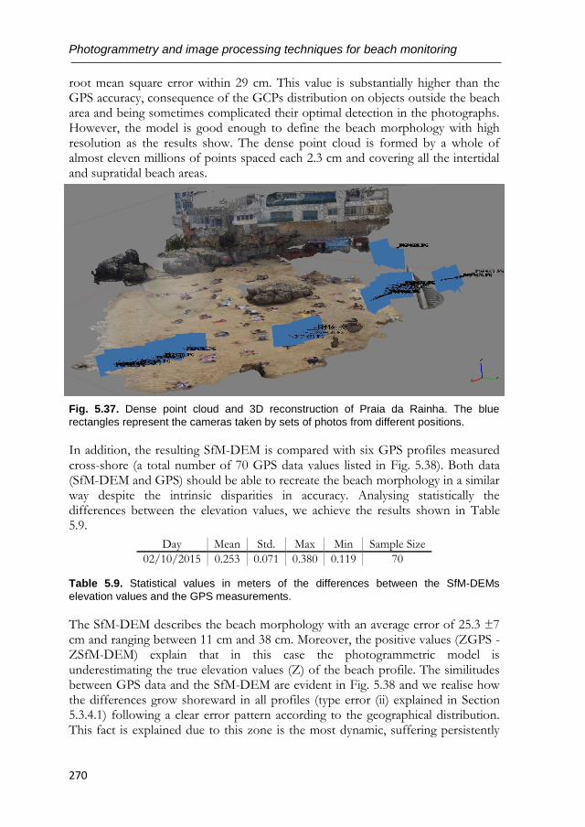
Photogrammetry and image processing techniques for beach monitoring
270
root mean square error within 29 cm. This value is substantially higher than the GPS accuracy, consequence of the GCPs distribution on objects outside the beach area and being sometimes complicated their optimal detection in the photographs. However, the model is good enough to define the beach morphology with high resolution as the results show. The dense point cloud is formed by a whole of almost eleven millions of points spaced each 2.3 cm and covering all the intertidal and supratidal beach areas.
Fig. 5.37. Dense point cloud and 3D reconstruction of Praia da Rainha. The blue
rectangles represent the cameras taken by sets of photos from different positions.
In addition, the resulting SfM-DEM is compared with six GPS profiles measured cross-shore (a total number of 70 GPS data values listed in Fig. 5.38). Both data (SfM-DEM and GPS) should be able to recreate the beach morphology in a similar way despite the intrinsic disparities in accuracy. Analysing statistically the differences between the elevation values, we achieve the results shown in Table 5.9.
Table 5.9. Statistical values in meters of the differences between the SfM-DEMs
elevation values and the GPS measurements.
The SfM-DEM describes the beach morphology with an average error of 25.3 ±7 cm and ranging between 11 cm and 38 cm. Moreover, the positive values (ZGPS - ZSfM-DEM) explain that in this case the photogrammetric model is underestimating the true elevation values (Z) of the beach profile. The similitudes between GPS data and the SfM-DEM are evident in Fig. 5.38 and we realise how the differences grow shoreward in all profiles (type error (ii) explained in Section 5.3.4.1) following a clear error pattern according to the geographical distribution. This fact is explained due to this zone is the most dynamic, suffering persistently
Day Mean Std. Max Min Sample Size
02/10/2015 0.253 0.071 0.380 0.119 70
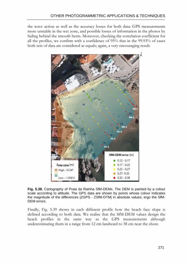
OTHER PHOTOGRAMMETRIC APPLICATIONS & TECHNIQUES
271
the wave action as well as the accuracy losses for both data: GPS measurements more unstable in the wet zone, and possible losses of information in the photos by hiding behind the smooth berm. Moreover, checking the correlation coefficient for all the profiles, we confirm with a confidence of 95% that in the 99.93% of cases both sets of data are considered as equals; again, a very encouraging result.
Fig. 5.38. Cartography of Praia da Rainha SfM-DEMs. The DEM is painted by a colour
scale according to altitude. The GPS data are shown by points whose colour indicates the magnitude of the differences |ZGPS - ZSfM-DTM| in absolute values; ergo the SfM-DEM errors.
Finally, Fig. 5.39 shows in each different profile how the beach face slope is defined according to both data. We realise that the SfM-DEM values design the beach profiles in the same way as the GPS measurements although underestimating them in a range from 12 cm landward to 38 cm near the shore.
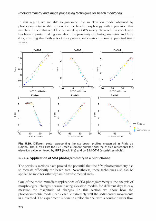
Photogrammetry and image processing techniques for beach monitoring
272
In this regard, we are able to guarantee that an elevation model obtained by photogrammetry is able to describe the beach morphology with a precision that matches the one that would be obtained by a GPS survey. To reach this conclusion has been important taking care about the proximity of photogrammetric and GPS data, ensuring that both sets of data provide information of similar punctual time values.
Fig. 5.39. Different plots representing the six beach profiles measured in Praia da
Rainha. The X axis lists the GPS measurement number and the Y axis represents the elevation value achieved by GPS (black line) and by SfM-DTM (asterisk symbols).
5.3.4.3. Application of SfM photogrammetry in a pilot channel
The previous sections have proved the potential that the SfM photogrammetry has to recreate efficiently the beach area. Nevertheless, these techniques also can be applied to monitor other dynamic environmental areas.
One of the most immediate applications of SfM photogrammetry is the analysis of morphological changes because having elevation models for different days is easy measure the magnitude of changes. In this section we show how the photogrammetric models can describe extremely well the sedimentary movements in a riverbed. The experiment is done in a pilot channel with a constant water flow
ZGPS (m)
ZSfM-DEM (m)
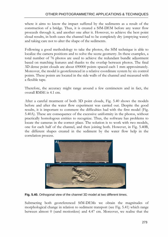
OTHER PHOTOGRAMMETRIC APPLICATIONS & TECHNIQUES
273
A)
B)
where it aims to know the impact suffered by the sediments as a result of the construction of a bridge. Thus, it is created a SfM-DEM before any water flow proceeds through it, and another one after it. However, to achieve the best point cloud results, in both cases the channel had to be completely dry (emptying water) and taking care not to alter the shape of the sediments.
Following a good methodology to take the photos, the SfM technique is able to localize the camera positions and to solve the scene geometry. In these examples, a total number of 76 photos are used to achieve the redundant bundle adjustment based on matching features and thanks to the overlap between photos. The final 3D dense point clouds are about 690000 points spaced each 1 mm approximately. Moreover, the model is georeferenced in a relative coordinate system by six control points. These points are located in the side walls of the channel and measured with a flexible tape.
Therefore, the accuracy might range around a few centimeters and in fact, the overall RMSE is 4.1 cm.
After a careful treatment of both 3D point clouds, Fig. 5.40 shows the models before and after the water flow experiment was carried out. Despite the good results, it is important to comment the difficulties had with the first model (Fig. 5.40A). These are consequence of the excessive uniformity in the photos, without practically homologous entities to recognize. Thus, the software has problems to locate the cameras in the correct place. The solution is to work with two models, one for each half of the channel, and then joining both. However, in Fig. 5.40B, the different shapes created in the sediment by the water flow help in the correlation process.
Fig. 5.40. Orthogonal view of the channel 3D model at two different times.
Subtracting both georeferenced SfM-DEMs we obtain the magnitudes of morphological change in relation to sediment transport (see Fig. 5.41) which range between almost 0 (sand motionless) and 4.47 cm. Moreover, we realise that the
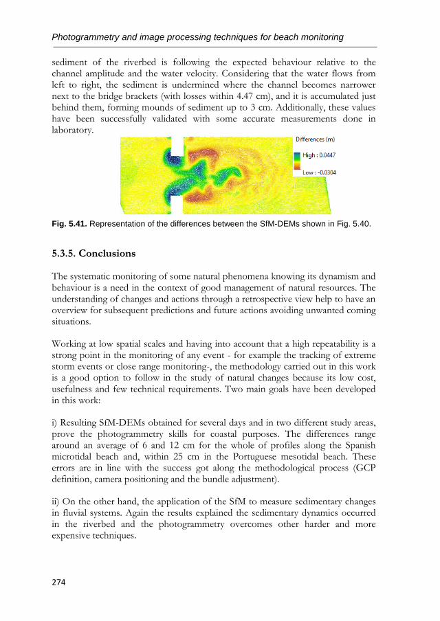
Photogrammetry and image processing techniques for beach monitoring
274
sediment of the riverbed is following the expected behaviour relative to the channel amplitude and the water velocity. Considering that the water flows from left to right, the sediment is undermined where the channel becomes narrower next to the bridge brackets (with losses within 4.47 cm), and it is accumulated just behind them, forming mounds of sediment up to 3 cm. Additionally, these values have been successfully validated with some accurate measurements done in laboratory.
Fig. 5.41. Representation of the differences between the SfM-DEMs shown in Fig. 5.40.
5.3.5. Conclusions
The systematic monitoring of some natural phenomena knowing its dynamism and behaviour is a need in the context of good management of natural resources. The understanding of changes and actions through a retrospective view help to have an overview for subsequent predictions and future actions avoiding unwanted coming situations.
Working at low spatial scales and having into account that a high repeatability is a strong point in the monitoring of any event - for example the tracking of extreme storm events or close range monitoring-, the methodology carried out in this work is a good option to follow in the study of natural changes because its low cost, usefulness and few technical requirements. Two main goals have been developed in this work:
i) Resulting SfM-DEMs obtained for several days and in two different study areas, prove the photogrammetry skills for coastal purposes. The differences range around an average of 6 and 12 cm for the whole of profiles along the Spanish microtidal beach and, within 25 cm in the Portuguese mesotidal beach. These errors are in line with the success got along the methodological process (GCP definition, camera positioning and the bundle adjustment).
ii) On the other hand, the application of the SfM to measure sedimentary changes in fluvial systems. Again the results explained the sedimentary dynamics occurred in the riverbed and the photogrammetry overcomes other harder and more expensive techniques.

OTHER PHOTOGRAMMETRIC APPLICATIONS & TECHNIQUES
275
However, and despite the large benefits of the SfM photogrammetry, we want to remark the importance of conducting a careful methodological protocol especially in the process of taking photographs to achieve a good 3D model. The excessive uniformity found in environments such as beaches or riverbeds requires a systematic overlapping between photos and a brainy procedure in the positioning and orientation of the cameras.
The culmination of a study as here presented, contains its full potential and practical use in the monitoring of confined spaces that allow the subsequent prediction of future situations. Reach something as tangible as the mapping of a coming situation, will help in the sustainable planning of the natural resources. New prospects and applicability must be investigated.

Photogrammetry and image processing techniques for beach monitoring
276
OTHER PHOTOGRAMMETRIC APPLICATIONS & TECHNIQUES
277
5.4. OVERALL CHAPTER CONCLUSIONS
Beaches are dynamic spaces and their shapes and arrangements are constantly being modified by various natural and anthropic phenomena. For a morphological study it is necessary to distinguish between the changes related to weather conditions − with seasonal and oscillating behavioural rhythms throughout the year − than those showing a trend of progressive change. Photogrammetric techniques are a key tool for the monitoring of these natural systems with high periodicity and repeatability, and facilitate studies of sedimentary changes in various time scales.
Highlighting the contributions in this chapter it has been proven that using an adequate working methodology, there are various low-cost tools that offer much useful information about our coasts (leaving aside the costly coastal camera systems established until now for this purposes).
Firstly, Section 5.1 has reported various efforts to take advantage of online video streaming surfcams for supporting coastal change monitoring and coastal management. The adoption of the existing worldwide surfcam network infrastructure has been shown as an attractive solution for assessing wave runup measurements and intertidal beach topography, as well as other coastal information (Andriolo, 2018). The application of C-Pro tool − presented in Chapter 2 − has lead to rectified surfcam images being retrieved online with accuracies within 2.5 m and comparable to classic phogrammetric techniques. These images enable quantitative hydro- and mophodynamic analysis of the monitored area. The major achievement has been the possibility of using these remote video systems when the photogrammetric conditions are null (non-availability of accurate control points, nor knowledge of camera parameters). These advanced geo-referencing techniques have facilitated the use of existing low-elevation surfcam (or other recreational cameras such as those presented in Section 5.2) with unknown image calibration to provide quality quantitative data. With networks of recreational cameras continuing to grow rapidly, such tools will very likely play an increasing role in expanding world-wide coastal monitoring, especially along more developed regions of the coastline (Splinter et al., 2018). Beyond testing the capability of the proposed methodology in Section 5.1 (Andriolo et al., 2019) using remotely-derived GCPs and the horizon constraint, different soft-computing algorithms based on the statistical properties of Timestack and Variance images have also been derived and implemented to automate runup measurements and represent beach slope and intertidal beach topography. It is worth emphasizing the importance of these developed procedures and techniques inasmuch as dozens of coastal video systems worldwide have been storing these images for the last two decades.
Photogrammetry and image processing techniques for beach monitoring
278
Far from the logistical issues of securely housing camera and computer
equipment related with professional imaging technology, Section 5.2 has focused
on presenting the CoastSnap iniciative by applying the image capture and
processing principles of established coastal camera systems to ubiquitous
community smartphone technology. Rigid photo-point phone cradles ensured that
every image was captured from the same position and angle, while advanced image
processing techniques accounted for the varying lens properties of different
smartphones and for those challenges related with sharing data on social media
platforms. Firstly, the diversity of images collected (different resolutions and
smartphone camera models) and various modes of image submission (Facebook,
Instagram, Twitter and email) made automation of data collection a risky. The
successful application in the study of image registration removed the need for
manual identification of GCPs in every image and thereby improved automation.
Secondly, the lack of knowledge of the camera orientation parameters (focal and
camera rotation angles) was overcome with surveyed GCPs and assisted by the
internal correction of most radial image distortion in modern smartphone images.
Concerning image capture time, the method is currently reliant on the upload time
to social media. However, this issue will become increasingly critical on coastlines
with larger tidal ranges, where even small errors in image capture time would lead
to poor estimates of the shoreline elevation.
Results showed that the presented new crowd-sourced shoreline change
mapping approach is an excellent way to map beach features and shoreline change.
Compared with in situ shoreline measurements it was evidenced that the method is
capable of achieving reasonable shoreline accuracies across stretches of coastline
spanning 100 m to more than 1 km. Optimum conditions in terms of shoreline
accuracy were found in the camera nearfield and where less-complex (i.e.,
alongshore-uniform) shoreline morphology was within an RMSD of 1.35 m.
Moreover, the study proved that poor image resolution resulting from crowd-
sourced data is less restrictive than expected and that the use of instantaneous
snapshot images for shoreline mapping entailed only moderate decreases in
shoreline accuracy (about 23%). The frequency of image submissions from the
community was considered sufficient for shoreline monitoring applications at a
number of different time-scales – one data per month being stipulated as sufficient
for long-term studies (Splinter et al., 2013). In the work on Section 5.2, near-daily
image sampling was considered as particularly valuable for adequately resolving the
shoreline response to individual storm events. Regular community submissions
were able to record a coastal inlet at the study area with a beach width expansion
of 60 m over the seven months of study – a phenomenon known but never
monitored at such high resolution. Lastly, the tidal correction method adopted in
the study enabled an accurate estimation of the average beachface slope from the
crowd-sourced images.
OTHER PHOTOGRAMMETRIC APPLICATIONS & TECHNIQUES
279
Continuing with the evaluation of image processing techniques to obtain
affordable beach information, the work in Section 5.3 applied different techniques
to generate 3D models of the intertidal beach zone – this time using a set of
photographs with different points of view. By using ground-based photography to
achieve digital models with SfM photogrammetry, it was found that the most
important element was the acquisition of a competent set of photos covering the
study area (more important than the quality of the photos). The experiments in this
work were carried out using the Agisoft PhotoScan software with 60% overlapped
photos taken from different angles. However, the images were captured in a
manner adapted to the morphology and characteristics of each area. The excessive
uniformity found in environments such as beaches required a systematic
overlapping between photos and an intelligent methodological procedure in the
positioning and orientation of the cameras. Therefore, the main goal is to assess
the potential in three different scenarios and conduct different methodological
protocols – cameras at different heights, with different orientations, and even
different camera models − against high accuracy GPS data. Resulting SfM-DEMs
proved the photogrammetry abilities for coastal purposes with accuracies ranging
between 6 and 25 cm – errors that may be derived from the GCP definition,
camera positioning, and bundle adjustment.
Working at low spatial scales and considering that a high repeatability is a
strong point when monitoring any event, the new methodologies developed
throughout this chapter are validated as a good option for the study of natural
changes – because of their low cost, usefulness, and few technical requirements.

Cover photo of Chapter 6: Tallow Beach, Byron Bay, Australia (taken Oct. 2017)

CONCLUSIONS
283
6.1. ANSWERS TO THE ORIGINAL RESEARCH QUESTIONS
The main purpose for which many of the evolutionary studies of coastal zones are
carried out is to obtain an overview of their state in order to subsequently predict
and determine future actions for good coastal planning. The study of coastal
changes is unavoidable when it involves a set of negative implications on the
resources and uses of the coastal space itself, affecting natural values and socio-
economic interests. The methodological procedures used play a decisive role in the
detection and analysis of the magnitude of the changes with precision and
effectiveness.
The whole of this doctoral thesis has shown the capacity of
photogrammetric and image processing techniques for coastal monitoring at
different time and spatial scales.
The literature review shows the potential of well-known fixed coastal
video monitoring systems (Argus, Sirena, Cosmos, Horus) intended for site
specific evolutionary studies. However, these systems are expensive and complex
to maintain and present certain requirements that limit and make them difficult to
extend to other places. Their associated software requires understanding the
characteristics and parameters of particular cameras, as well as accurate and
adequate terrain control points to georeference the photos. A versatile tool such as
C-Pro (presented in Chapter 2) enables automatic georectification of any beach
terrestrial photograph regardless of the conditions. The tool adapts its
methodology according to the available information to achieve the best possible
spatial resection adjustment and thus offer a suitable result − even when
photogrammetric conditions are very poor. In addition, its robustness is largely
due to the inclusion of two extra equations corresponding to the horizon line that
depend on the external and internal camera orientation parameters and reduce the
number of terrain points needed.
The C-Pro tool is shown to be very effective for analysis and coastal
management because of its easy acquisition, speed, low cost, and volume of data,
and because any person with a conventional camera can take a photograph. This
fact has been reflected throughout the thesis (especially in Chapter 4) where its
application has enabled registering the state of the coast at a specific time and
validating instantaneous satellite-derived shorelines (SDS) on different beaches.
Moreover, it has been used to georeference images from recreational video
cameras “surfcams” and so facilitate their use for scientific purposes. Its
implementation in other novel citizen monitoring projects will also be very useful
Photogrammetry and image processing techniques for beach monitoring
284
since these are spreading to numerous sites and where the necessary requirements
for traditional methods are probably unavailable (see Chapter 5). However,
surfcams are expected to offer the worst conditions because their placement was
planned simply to provide visual information of the beach and wave conditions for
surfers. Therefore, even the use of remote control points obtained from Google
Earth has been explored.
Secondly, and encompassing larger spatial scales, it is well known that
satellite imagery plays a decisive role. Since the USGS in 2008 and ESA in 2015
made their database freely available, Landsat and Sentinel satellite images constitute
the main territorial database worldwide. Bearing this in mind, the current doctoral
thesis extensively worked on the evaluation and improvement of the Almonacid-
Caballer, 2014 algorithm. The goal was to obtain from these mid-resolution images
multiple accurate shoreline data for trend and coastal evolution analysis.
Throughout the thesis, the obtained results have been conditioning the
development of the methodology, varying and adjusting to the needs of processing
and evaluating data. Dealing with a large volume of information forced the
development of automated modules − developed by the CGAT group − to
minimize analysis time and facilitate its use.
According to the tests carried out so far, a good location of the input
shoreline at pixel level was essential for the algorithm's search window to be made
in the right place – former thresholding techniques used to define this initial line
were not always successful. Therefore, Chapter 3 dealt with this problem by means
of working with a neighborhood able to adapt itself according to the image
radiometry and improve the final sub-pixel accuracy. The transition between land
and water was found where the maximum radiometric variation in terms of divided
differences ocurred. The accuracy of the final sub-pixel shoreline is not
conditioned by the precision of the input line.
Working in parallel after the completion of the works in Sections 4.1 and
4.2, Section 4.3 completed the evaluation by demonstrating with which parameters
and bands or indexes of the satellite images, the algorithm (presented as
SHOREX) achieved greatest accuracy. It was seen that the algorithm seemed more
accurate in the final shoreline detection when working with small neighborhoods.
However, this fact required ensuring the quality of the input line around which to
perform the sub-pixel search. Accordingly, the use of a threshold input line per
image was changed – this step also slowed down the process – and a unique
digitalized or available shoreline for the whole set of images was used. While the
reliability of the line was still uncertain, the protocol (presented in Section 4.3)
consists of working first with large neighborhoods and ensuring that the real
shoreline was contained, and then continuing with a second iteration where smaller
CONCLUSIONS
285
neighborhoods would define accurately the sub-pixel shoreline. In this case, and
unlike Chapter 3, a centered interpolation is first used and then the least squares
method is used to define the land-water surface over an upsampled satellite image.
At this point, where the accuracies reached are at the level of other
systems such as video monitoring, the SHOREX methodology is presented as very
effective for coastal monitoring. Despite the advantages of having such a
magnitude of data, a correct management is necessary. Hence, the idea of
obtaining annual average lines to work in coastal evolution analysis (seen in Section
4.1). With this, changes due to factors related to meteorological processes − with
seasonal or oscillating rhythms throughout the year − were avoided and separated
from those useful for long-term studies with progressive changes over time.
Focusing on a shorter time scale, this same idea could resemble the work with
timex images in photogrammetry whose aim was to obviate the random and
oscillating behavior of the waves and make shoreline definition easier.
This dissertation contains all its potential and practical utility in the
monitoring of coastal segments to enable predictions. High-resolution coastal
evolution models play an important role but require multiple shorelines for their
calibration and evaluation (refer to Section 4.4). Therefore, this synergy gives rise
to powerful coastal evolutionary studies resolving the temporal limitation of the
images with the model, and the spatial limitation of the model with the images.
Valuable coastal hazard maps and warning systems that are able to highlight critical
situations may be derived.
This research work seeks to bring the photogrammetry and remote
sensing worlds closer to regional scientists, engineers, government and coastal
managers by providing new evidence about the usefulness of low-cost and feasible
techniques. These can turn existing and freely available information (satellite
imagery, crowd-sourced data, or internet-streamed beach images) into high-quality
data for the continuous monitoring of beaches and a consequent sustainable
decision-making for coastal resources. In addition, using mundane information and
involving the local community generates many benefits by making science and
engineering expertise more accessible to the public, encouraging greater
interactions, and knowledge sharing between local stakeholders and experts, and
leading to a greater democratisation of decision-planning on coastal management.
6.2. FURTHER RESEARCH
This thesis has provided insight into the development and application of new
photogrammetry and image processing techniques that take advantage of various
Photogrammetry and image processing techniques for beach monitoring
286
data for beach monitoring. However, as the assessments have been site specific,
other obervations in diverse coastal systems are necessary in order to establish the
weaknesses and thoroughly improve and expand the methods for any type of
beach.
As is well known, the relative tidal range reflects the relative importance of
swash, surf zone, and shoaling wave processes (Masselink and Short, 1993).
Therefore, before attempting to gain an understanding of beach processes, it is
necessary to understand the factors acting in each study site. In this thesis, most of
the beaches analyzed with photos have a microtidal regime (<2 m) that, in
principle, simplifies the shoreline detection and evaluation of the changes – expect
for the works on the Portuguese coast with a mesotidal regime (2-4 m). However,
the interaction with other factors − such as the wave forcing − makes the
definition of the land-water border and the association with its appropriate
elevation value more difficult. The works carried out throughout the thesis have
been adapted to each site. While for those Mediterranean beaches with a generally
weak energetic swell (Valencian and Balearic coasts) shoreline detection was
directly related with the sea level value, in beaches with stronger oceanic waves,
such as in eastern Australia or the Portuguese beaches, it was necessary to add an
estimated offset value because of the runup.
The main weakness of satellite imagery is related to the physical shoreline
that the SHOREX algorithm is detecting. Theoretically, the land-water border is
the feature that we expect to be detected because this is the aim of the algorithm.
However, the contact limit between emerged and oceanic surface is conditioned by
multiple factors that affect the algorithm: such as the beach slope; extent of the
intertidal zone; rising or ebbing tide; wave energy; maximum swash; beach width;
as well as the beach characteristics in the dry zone. The synergy of the
improvements developed in this doctoral thesis in the intrinsic of SHOREX
algorithm (Chapter 3) and its usage protocol (Section 4.3) is expected to provide
the methodological robustness needed regardless of the diverse acting factors. The
workflow would then consist in an iterative process that firstly works with a pixel
neighborhood that is sufficiently large but adaptable to the raw image radiometry
in order to ensure that the searched shoreline is contained and, so that in a second
iteration it can be precisely detected at sub-pixel level.
Nonetheless, more evaluation analysis must be carried out by comparing
with reference photogrammetry data obtained using C-Pro. Since February 2018,
an assessment is underway in the microtidal coast of central Chile, specifically at
Reñaca beach, where photographs are being systematically taken when the satellite
image is captured (see Fig. 6.1). This work will lead SHOREX to handle strong
swells – generated by prevailing SSW winds – that constitute a permanent source
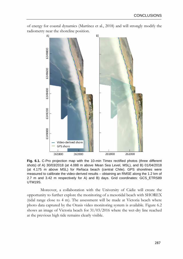
CONCLUSIONS
287
of energy for coastal dynamics (Martínez et al., 2018) and will strongly modify the
radiometry near the shoreline position.
Fig. 6.1. C-Pro projection map with the 10-min Timex rectified photos (three different
shots) of A) 30/03/2018 (at 4.088 m above Mean Sea Level, MSL), and B) 01/04/2018
(at 4.175 m above MSL) for Reñaca beach (central Chile). GPS shorelines were
measured to calibrate the video-derived results – obtaining an RMSE along the 1.2 km of
2.7 m and 3.42 m respectively for A) and B) days. Grid coordinates: GCS_ETRS89
UTM19S.
Moreover, a collaboration with the University of Cádiz will create the
opportunity to further explore the monitoring of a mesotidal beach with SHOREX
(tidal range close to 4 m). The assessment will be made at Victoria beach where
photo data captured by the Orasis video monitoring system is available. Figure 6.2
shows an image of Victoria beach for 31/03/2016 where the wet-dry line reached
at the previous high tide remains clearly visible.
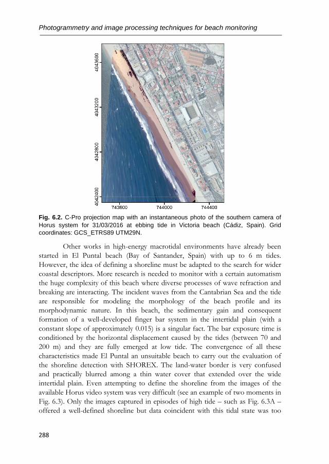
Photogrammetry and image processing techniques for beach monitoring
288
Fig. 6.2. C-Pro projection map with an instantaneous photo of the southern camera of
Horus system for 31/03/2016 at ebbing tide in Victoria beach (Cádiz, Spain). Grid
coordinates: GCS_ETRS89 UTM29N.
Other works in high-energy macrotidal environments have already been
started in El Puntal beach (Bay of Santander, Spain) with up to 6 m tides.
However, the idea of defining a shoreline must be adapted to the search for wider
coastal descriptors. More research is needed to monitor with a certain automatism
the huge complexity of this beach where diverse processes of wave refraction and
breaking are interacting. The incident waves from the Cantabrian Sea and the tide
are responsible for modeling the morphology of the beach profile and its
morphodynamic nature. In this beach, the sedimentary gain and consequent
formation of a well-developed finger bar system in the intertidal plain (with a
constant slope of approximately 0.015) is a singular fact. The bar exposure time is
conditioned by the horizontal displacement caused by the tides (between 70 and
200 m) and they are fully emerged at low tide. The convergence of all these
characteristics made El Puntal an unsuitable beach to carry out the evaluation of
the shoreline detection with SHOREX. The land-water border is very confused
and practically blurred among a thin water cover that extended over the wide
intertidal plain. Even attempting to define the shoreline from the images of the
available Horus video system was very difficult (see an example of two moments in
Fig. 6.3). Only the images captured in episodes of high tide – such as Fig. 6.3A –
offered a well-defined shoreline but data coincident with this tidal state was too
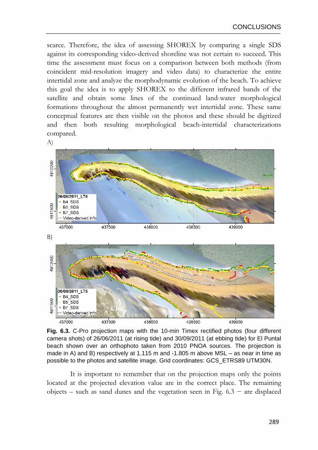
CONCLUSIONS
289
scarce. Therefore, the idea of assessing SHOREX by comparing a single SDS
against its corresponding video-derived shoreline was not certain to succeed. This
time the assessment must focus on a comparison between both methods (from
coincident mid-resolution imagery and video data) to characterize the entire
intertidal zone and analyze the morphodynamic evolution of the beach. To achieve
this goal the idea is to apply SHOREX to the different infrared bands of the
satellite and obtain some lines of the continued land-water morphological
formations throughout the almost permanently wet intertidal zone. These same
conceptual features are then visible on the photos and these should be digitized
and then both resulting morphological beach-intertidal characterizations
compared.
A)
B)
Fig. 6.3. C-Pro projection maps with the 10-min Timex rectified photos (four different
camera shots) of 26/06/2011 (at rising tide) and 30/09/2011 (at ebbing tide) for El Puntal
beach shown over an orthophoto taken from 2010 PNOA sources. The projection is
made in A) and B) respectively at 1.115 m and -1.805 m above MSL – as near in time as
possible to the photos and satellite image. Grid coordinates: GCS_ETRS89 UTM30N.
It is important to remember that on the projection maps only the points
located at the projected elevation value are in the correct place. The remaining
objects – such as sand dunes and the vegetation seen in Fig. 6.3 − are displaced
Photogrammetry and image processing techniques for beach monitoring
290
unless we project the photo over a digital terrain model supporting each pixel of
the image with its associate altitudinal value.
For collaboration with the IH Cantabria, calibrations of the evolutionary
models are exploring other coastal areas. A similar work to that mentioned in
Section 4.4 (Jaramillo et al., under review) is being carried out in Cala Millor beach
(Mallorca, Spain). The satellite-derived shorelines obtained with SHOREX along
with others derived from video data (acquired by SIRENA and processed with C-
Pro) are being used to calibrate the Jara et al., 2015 evolutionary model between
2013 and 2017.
The practical utility of using C-Pro for mapping the inland wave
penetration range during a storm, or any coastal event, is being manifested through
collaboration with the Valencian Coastal Demarcation unit (see photos of the
devastating storm of January 2017 in Fig. 6.4). Mapping the instantaneous
shoreline was of singular interest to coastal managers – especially after the
publication of the Royal Decree 876/2014 of 10 October, which stated that the
delimitation of the maritime-terrestrial domain had to be supported by the real
position reached during storms. Before starting the collaboration, the basic
cameras with which the employees regularly took coastal photos were calibrated
and several field campaigns were made to measure fixed ground control points in
the chosen areas. Over time and as the photos are being taken and processed, the
resulting product is being returned to the coastal managers by mapping the
shoreline position for every moment and photographed location. In this way,
valuable quantitative information is being added to the qualitative visual value of
the photo itself. During a storm, the use of terrestrial photos is crucial because it is
unlikely that satellite images coincide with the moment of the storm – and even if
they did then the presence of clouds would make it useless.
As a last point, it is important to mention the future coastal monitoring
studies that the CoastSnap network is expecting to generate worldwide. This beach
monitoring program is rapidly expanding to multiple sites within Australia where
three sites are in full operation (Manly, North Narrabeen, Byron Bay) and
internationally. Cascais (Portugal), Galicia (Spain), Bournemouth (UK),
Florianópolis (Brasil) and Fiji Island have already realized the benefits of this
shoreline variability tracking data and are supporting the initiative. With a large
network of CoastSnap stations, it may be possible to map shoreline evolution at
nearby coastal locations, and detect patterns in shoreline behaviour across regional
coastlines.
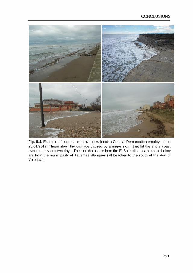
CONCLUSIONS
291
Fig. 6.4. Example of photos taken by the Valencian Coastal Demarcation employees on
23/01/2017. These show the damage caused by a major storm that hit the entire coast
over the previous two days. The top photos are from the El Saler district and those below
are from the municipality of Tavernes Blanques (all beaches to the south of the Port of
Valencia).

Photogrammetry and image processing techniques for beach monitoring
292
Bibliography
293
Bibliography
A
Aagaard, T., Holm, D., 1989. Digitization of wave runup using video records. Journal of Coastal Research, 5: 547-551.
Aarninkhof, S.G., Turner, I.L., Dronkers, T.D.T., Caljouw, M., Nipius, L., 2003. A video-based technique for mapping intertidal beach bathymetry. Coastal Engineering, 49: 275-289.
Abdel-Aziz, Y.I., Karara, H.M., 1971. Direct linear transformation from comparator coordinates into object space coordinates in close-range photogrammetry. ASP Symposium on Close-range Photogrammetry, Falls Church, Virginia, pp. 1-18.
Addo, K.A., Jayson-Quashigah, P.N., Kufogbe, K.S., 2011. Quantitative analysis of shoreline change using medium resolution satellite imagery in Keta, Ghana. Marine Science, 1 (1): 1-9.
Aedla, R., Dwarakish, G.S., Venkat R.D., 2015. Automatic shoreline detection and change detection analysis of Netravati-GurpurRivermouth using histogram equalization and adaptive thresholding techniques. Aquatic Procedia, 4: 563-570.
Alharbi, O.A., Phillips, M.R., Williams, A.T., Thomas, T., Hakami, M., Kerbe, J., Al-Ghamdi, K., 2017. Temporal shoreline change and infrastructure influences along the southern Red Sea coast of Saudi Arabia. Arabian Journal of Geosciences, 10 (16): 360.
AgiSoft, 2014. AgiSoft PhotoScan professional edition. http://www.agisoft.ru/products/photoscan/.
Almar, R., Bonneton, P., Senechal, N., Roelvink, D., 2008. Wave celerity from video imaging: A new method. Proceedings of 31st Conference on Coastal Engineering, Hamburg, Germany, pp. 1-14.
Almar, R., 2009. Morphodynamique littorale haute fréquence par imagerie vidéo. PhD dissertation, University of Bordeaux, pp. 228.
Almar, R., Cienfuegos, R., Catalán, P.A., Birrien, F., Castelle, B., Michallet, H., 2011. Nearshore bathymetric inversion from video using a fully non-linear Boussinesq wave model. Journal of Coastal Research, SI 64: 20-24.
Almar, R., Cienfuegos, R., Catalán, P.A., Michallet, H., Castelle, B., Bonneton, P., Marieu, V., 2012a. A new breaking wave height direct estimator from video imagery. Coastal Engineering, 61: 42-48.
Photogrammetry and image processing techniques for beach monitoring
294
Almar, R., Ranasinghe, R., Sénéchal, N., Bonneton, P., Roelvink, D., Bryan, K.R., Parisot, J., 2012b. Video-Based Detection of Shorelines at Complex Meso–Macro Tidal Beaches. Journal of Coastal Research, 284: 1040-1048.
Almar, R., Michallet, H., Cienfuegos, R., Bonneton, P., Tissier, M., Ruessink, G., 2014. On the use of the Radon Transform in studying nearshore wave dynamics. Coastal Engineering, 92: 24-30.
Almar, R., Blenkinsopp, C., Almeida, L.P., Cienfuegos, R., Catalán, P.A., 2017a. Wave runup video motion detection using the Radon Transform. Coastal Engineering, 130: 46-51.
Almonacid-Caballer, J., Pardo-Pascual, J.E., Ruiz, L.A., 2013. Detección automática de la línea de costa con precisión subpíxel en imágenes Landsat 7 con error de bandeado. XV Congreso de la Asociación Española de Teledetección INTA, Torrejón de Ardoz, Madrid, pp. 270-273.
Almonacid-Caballer, J., 2014. Extraction of shorelines with sub-pixel precision from Landsat images (TM, ETM+, OLI) [Obtención de líneas de costa con precisión sub-píxel a partir de imágenes Landsat (TM, ETM+ y OLI)]. PhD dissertation, Universitat Politècnica de València, Valencia, Spain, pp. 365.
Almonacid-Caballer, J., Sánchez-García, E., Pardo-Pascual, J.E., Balaguer-Beser, A.A., Palomar-Vázquez, J., 2016. Evaluation of annual mean shoreline position deduced from Landsat imagery as a mid-term coastal evolution indicator. Marine Geology, 372: 79-88.
Almonacid-Caballer, J., Pardo-Pascual, J.E., Ruiz, L.A., 2017. Evaluating fourier cross-correlation sub-pixel registration in Landsat images. Remote Sensing, 9 (10): 1051.
Alvarez-Ellacuria, A., Orfila, A., Gómez-Pujol, L., Simarro, G., Obregon, N., 2011. Decoupling spatial and temporal patterns in short-term beach shoreline response to wave climate. Geomorphology, 128 (3-4): 199-208.
Andriolo, U., Sánchez-García, E., Taborda, R., 2016a. Using surfcam online streaming images for nearshore hydrodynamics characterization. 4as Jornadas de Engenharia Hidrográfica, Lisbon, Portugal, pp. 377-380.
Andriolo, U., Taborda, R., Sánchez-García, E., 2016b. Measuring wave runup and intertidal beach topography from online streaming surfcam. X Jornadas do Mar, Naval School of Lisbon, pp. 112-121.
Andriolo, U., Almeida, L.P., Almar, R., 2018. Coupling terrestrial LiDAR and video imagery to perform 3D intertidal beach topography. Coastal Engineering, 140: 232-239.
Andriolo, U., 2018. Nearshore hydrodynamics and morphology derived from video imagery. PhD dissertation, University of Lisbon, pp. 197.
Andriolo, U., Sánchez-García, E., Taborda, R., 2019. Operational use of surfcam online streaming images for coastal morphodynamic studies. Remote Sensing, 11 (1): 78.
Bibliography
295
Angnuureng, D.B., Almar, R., Senechal, N., Castelle, B., Addo, K.A., Marieu, V., Ranasinghe, R., 2017. Shoreline resilience to individual storms and storm clusters on a meso-macrotidal barred beach. Geomorphology, 290: 265-276.
Anguelov, D., Dulong, C., Filip, D., Frueh, C., Lafon, S., Lyon, R., et al., 2010. Google street view: Capturing the world at street level. Computer, 43 (6): 32-38.
Archetti, R., Schiaffi, C.F., Ferrari, M., Brignone, M., Rihouey, D., 2008. Video systems for coastal monitoring. Pranzini, E., Wetzel, L. (eds.). Beach Eros. Monit. Beachmed-e/OpTIMAL Proj. pp. 101-109.
Armaroli, C., Ciavola, P., 2011. Dynamics of a nearshore bar system in the northern Adriatic: a video-based morphological classification. Geomorphology, 126: 201-216.
Augar, N., Fluker, M., 2014. Developing social media for community based environmental monitoring. Proceedings of the 25th Australasian Conference on Information Systems, pp. 1-10.
Atkinson, A.L., Power, H.E., Moura, T., Hammond, T., Callaghan, D.P., Baldock, T.E., 2017. Assessment of runup predictions by empirical models on non-truncated beaches on the south-east Australian coast. Coastal Engineering, 119: 15-31.
B
Balaguer, A., Conde, C., López, J.A., Martínez, V., 2001. A finite volume method with a modified ENO scheme using a Hermite interpolation to solve advection diffusion equations. International Journal for Numerical Methods in Engineering, 50 (10): 2339-2371.
Balaguer, A., Conde, C., 2005. Fourth-order non-oscillatory upwind and central schemes for hyperbolic conservation laws. SIAM Journal on Numerical Analysis, 43 (2): 455-473.
Bacakoglu, H., Kamel, M.S., 1997. A three-step camera calibration method. IEEE transactions on instrumentation and measurement, 46 (5): 1165-1172.
Bailey, D.G., Shand, R.D., 1994. Determining wave run-up using automated video analysis. Proceedings of the 2nd New Zealand Conference on Image and Vision Computing: 2.11.1-2.11.10.
Balouin, Y., Tesson, J., Gervais, M., 2013. Cuspate shoreline relationship with nearshore bar dynamics during storm events – field observations at Sete beach, France. Journal of Coastal Research, 65: 440-445.
Barnard, P.L., Short, A.D., Harley, M.D., Splinter, K.D., Vitousek, S., Turner, I.L., Allan, J., Banno, M., Bryan, K.R., Doria, A., Hansen, J.E., Kato, S., Kuriyama, Y., Randall-Goodwin, E., Ruggiero, P., Walker, I.J., Heathfield, D.K., 2015. Coastal vulnerability across the Pacific dominated by El Niño/Southern Oscillation. Nature Geoscience, 8: 801-807.
Baztan J., Chouinard O., Jorgensen B., Tett P., Vanderlinden J-P., Vasseur L.,
Photogrammetry and image processing techniques for beach monitoring
296
2015. Coastal Zones. Solutions for the 21st Century, pp. 376. Bayas, J.C.L., See, L., Fritz, S., Sturn, T., Perger, C., Dürauer, M., Karner, M.,
Moorthy, I., Schepaschenko, D., Domian, D., McCallum, I., 2016. Crowdsourcing in-situ data on land cover and land use using gamification and mobile technology. Remote Sensing, 8: 1-18.
Bechle, A.J., Wu, C. H., Liu, W., Kimura, N., 2012. Development and Application of an Automated River-Estuary Discharge Imaging System. Journal of Hydraulic Engineering, 138 (4): 327-339.
Birkemeier, W.A., Donohue, C., Long, C.E., Hathaway, K.K., Baron, C.F., 1997. The 1990 DELILAH nearshore experiment: Summary report, Technical Report CHL-97-24, U.S. Army Corps of Engineers, Waterways Experiment Station, Vicksburg, Ms.
Blenkinsopp, C.E., Matias, A., Howe, D., Castelle, B., Marieu, V., Turner, I.L., 2016. Wave runup and overwash on a prototype-scale sand barrier. Coastal Engineering, 113: 88-103.
Blossier, B., Bryan, K.R., Daly, C.J., Winter, C., 2017. Spatial and temporal scales of shoreline morphodynamics derived from video camera observations for the island of Sylt, German Wadden Sea. Geo-Marine Letters, 37 (2): 111-123.
Boak, E.H., Turner, I.L., 2005. Shoreline definition and detection: A review. Journal of Coastal Research, 214: 688-703.
Bouguet, J.Y., 2015. Camera calibration toolbox for Matlab. Available at: http:// www.vision.caltech.edu/bouguetj/calib_doc/. (accessed November 2018).
Bracs, M.A., Turner, I.L., Splinter, K.D., Short, A.D., Lane, C., Davidson, M.A., Goodwin, I.D., Pritchard, T., Cameron, D., 2016. Evaluation of opportunistic shoreline monitoring capability utilizing existing “Surfcam” infrastructure. Journal of Coastal Research, 32 (3): 542-555.
Bradley, J.V., 1968. Distribution-free statistical tests. Prentice-Hall, Englewood Cliffs, New Jersey, pp. 388.
Brignone, M., Schiaffino, C.F., Isla, F.I., Ferrari, M., 2012. A system for beach video-monitoring: Beachkeeper plus. Computers & Geosciences, 49: 53-61.
Brinkkemper, J.A., Lanckriet, T., Grasso, F., Puleo, J.A., Ruessink, B.G., 2014. Observations of turbulence within the surf and swash zone of a field-scale sandy laboratory beach. Coastal Engineering, 113: 62-72.
C
Cabezas-Rabadán, C., Pardo-Pascual, J.E., Palomar-Vázquez, J., Almonacid-Caballer, J., Fernández-Sarría, A., 2018. La posición de la línea de costa extraída de imágenes satelitales como herramienta de seguimiento y análisis de cambios en playas mediterráneas. XVIII Congreso Nacional de Tecnologías de La Información Geográfica (TIG). Dept. Geografia. Universitat de València, València, pp. 36-46.
Canalejo, P., Peña, C. 1995. Regeneración de la playa de Pinedo (Valencia). Ingeniería del Agua, 2: 209-222.
Bibliography
297
Capilla, M.T., Balaguer, A., 2013. A new well-balanced non-oscillatory central scheme for the shallow water equations on rectangular meshes. Journal of Computational and Applied Mathematics, 252: 62-74.
Castelle, B., Dodet, G., Masselink, G., Scott, T., 2018. Increased winter-mean wave height, variability, and periodicity in the Northeast Atlantic over 1949-2017. Geophysical Research Letters, 45: 3586-3596.
Carter, R.W.G., 1988. Coastal environments. An introduction to physical, ecological and cultural systems of coastlines. Academic Press, pp. 617.
Cipolletti, M.P., Delrieux, C.A., Perillo, G.M.E., Cintia Piccolo, M., 2012. Superresolution border segmentation and measurement in remote sensing images. Computers & Geosciences, 40: 87-96.
Chandler, J., Fryer, J., Jack, A., 2005. Metric capabilities of low cost digital cameras for close range surface measurement. The Photogrammetric Record, 20 (109): 12-27.
Chickadel, C.C., 2007. Remote measurements of waves and currents over complex bathymetry. College of oceanic and atmospheric sciences. PhD dissertation, Oregon State University.
Choung, Y.J., Jo, M.H., 2015. Shoreline change assessment for various types of coasts using multi-temporal Landsat imagery of the east coast of South Korea. Remote Sensing Letters, 7 (1): 91-100.
Church, J.A., Clark, P.U., Gregory, J.M., Jevrejeva, S., Levermann, A., Merrifield, M.A., Milne, G.A., Nerem, R.S., Nunn, P.D., Payne, A.J., Pfeffer, W.T., Stammer, D., Unnikrishnan, A.S., 2013. Sea level change. In Stocker, T.F., Qin, D., Plattner, G.-K., Tignor, M., Allen, S.K., Boschung, J., Nauels, A., Xia, Y., Bex, V., Midgley, P.M. (eds.). Climate change 2013: The physical science basis. Contribution of working group I to the fifth assessment report of the intergovernmental panel on climate change. Cambridge University Press, Cambridge, United Kingdom, pp. 1137-1216.
Clerc, S. M.P.C. Team. S2 M.P.C. Data quality report, 2017, reference S2-PDGS-MPC-DQR, issue 20, Available in https://sentinels.copernicus.eu/documents/247904/685211/Sentinel-2-Data-Quality-Report.
Conrad, C.C., Hilchey, K.G., 2011. A review of citizen science and community-based environmental monitoring: Issues and opportunities. Environmental Monitoring and Assessment, 176 (1-4): 273-291.
Cornall, T.D., Egan, G.K., 2004. Measuring horizon angle from video on a small unmanned air vehicle. In 2nd International Conference on Autonomous Robots and Agents.
Cowell, P.J., Thom, B.G., 1994. Morphodynamics of coastal evolution. In Carter, R.W.G., Woodroffe, C.D (eds.). Coastal evolution: an introduction.
Photogrammetry and image processing techniques for beach monitoring
298
Cambridge University Press, Cambridge, pp. 33-86.
Crossland, C.J., Kremer, H.H., Lindeboom, H.J., Marshall Crossland, J.I., Le Tissier, M.D.A., 2005. Coastal fluxes in the antropocene: The land-ocean interactions in the coastal zone project of the international geosphere-biosphere programme. Global Change - The IGBP Series. Springer-Verlag, Berlin, pp. 232.
D
Dai, F., Lu, M., Kamat, V.R., 2011. Analytical Approach to Augmenting Site Photos with 3D Graphics of Underground Infrastructure in Construction Engineering Applications. Journal of Computing in Civil Engineering, 25 (1): 66-74.
Davidson-Arnott, R., 2010. Introduction to coastal processes and geomorphology. Cambridge University Press.
Davidson, M., Van Koningsveld, M., de Kruif, A., Rawson, J., Holman, R., Lamberti, A., Medina, R., Kroon, A., Aarninkhof, S., 2007. The CoastView project: Developing video-derived Coastal State Indicators in support of coastal zone management. Coastal Engineering, 54: 463-475.
Del Rio L, Gracia J., 2013. Error determination in the photogrammetric assessment of shoreline changes. Natural Hazards, 65: 2385-2397.
Destination NSW, 2016. Manly Visitor Profile: Year Ended December 2016. URL http://www.destinationnsw.com.au/wp-content/uploads/2013/01/Manly-Visitor-Profile-YE-Dec-2016.pdf?x15361 (accessed 4.12.18).
Do, T.K.A., de Vries S., Stive, M.J.F., 2019. The estimation and evaluation of shoreline locations, shoreline-change rates, and coastal volume changes derived from Landsat images. Journal of Coastal Research, 35 (1): 56-71.
Donchyts, G., Baart, F., Winsemius, H., Gorelick, N., Kwadijk, J., Van de Giesen, N., 2016. Earth's surface water change over the past 30 years. Nature Climate Change, 6: 810-813.
Droege, S., 2013. Monitorchange.org [WWW Document]. Monit. Environ. Soc. Chang. using iPhones, photo-stitching, time lapse | Monit. Chang. URL http://monitorchange.org/ (accessed 9.15.18).
E
Ekercin, S., 2007. Coastline change assessment at the Aegean Sea Coasts in Turkey using multitemporal Landsat imagery. Journal of Coastal Research, 233: 691-699.
El-Ashmawy, K.L., 2016. Investigation of the accuracy of Google Earth elevation
Bibliography
299
data. Artificial Satellites, 51 (3): 89-97.
Enríquez, A.R., Marcos, M., Álvarez-Ellacuría, A., Orfila, A., Gomis, D. 2017. Changes in beach shoreline due to sea level rise and waves under climate change scenarios: application to the Balearic Islands (western Mediterranean). Natural Hazards and Earth System Sciences, 17 (7): 1075-1089.
Esteves, L.S., Williams, J.J., Nock, A., Lymbery, G., 2009. Quantifying shoreline changes along the Sefton coast (UK) and the implications for research-informed coastal management. Journal of Coastal Research, SI 56 (Proceedings of the 10th Int. Coastal Symposium), 602-606. Lisbon, Portugal.
Erdman, 1998. Erdman Video System, http://video-monitoring.com. (Accessed 2 March, 2016).
F
Fairley, I., Davidson, M., Kingston, K., Dolphin, T., Phillips, R., 2009. Empirical orthogonal function analysis of shoreline changes behind two different designs of detached breakwaters. Coastal Engineering, 56 (11-12): 1097-1108.
Farris, A.S., List, J.L., 2007. Shoreline change as a proxy for subaerial beach volume change. Journal of Coastal Research, 23 (3): 740-748.
Fay, M.P., Proschan, M.A., 2010. Wilcoxon-Mann-Whitney or t-test? On assumptions for hypothesis tests and multiple interpretations of decision rules. Statistics Surveys, 4: 1-39.
Feyisa, G.L., Meilby, H., Fensholt, R., Proud, S.R., 2014. Automated Water Extraction Index: A new technique for surface water mapping using Landsat imagery. Remote Sensing of Environment, 140: 23-35.
Florinsky, I.V., 2016. Digital terrain analysis in soil science and geology. Elsevier, London, UK, pp. 506.
Foody, G.M., Muslim, A.M., Atkinson, P.M., 2005. Super-resolution mapping of the waterline from remotely sensed data. International Journal of Remote Sensing, 26 (24): 5381-5392.
Ford, M., 2013. Shoreline changes interpreted from multi-temporal aerial photographs and high resolution satellite images: Wotje Atoll, Marshall Islands. Remote Sensing of Environment, 135: 130-140.
Frazier, P.S., Page, K.J., 2000. Water body detection and delineation with Landsat TM data. Photogrammetric Engineering & Remote Sensing, 66 (12): 1461-1467.
Frouin, R.M., Schwindling, M., Deschamps, P.Y., 1996. Spectral reflectance of sea foam in the visible and near infrared: In situ measurements and remote sensing implications. Journal of Geophysical Research: Oceans, 101 (C6):
Photogrammetry and image processing techniques for beach monitoring
300
14361-14371. Fu, L., Cazenave, A., 2000. Satellite altimetry and earth sciences: A handbook of
techniques and applications. Academic Press, pp. 463.
G
Gal, Y., Browne, M., Lane, C., 2011. Automatic estimation of nearshore wave height from video timestacks. In Proceedings - 2011 International Conference on Digital Image Computing: Techniques and Applications, DICTA 2011.
Gal, Y., Browne, M., Lane, C., 2014. Long-term automated monitoring of nearshore wave height from digital video. IEEE Transactions on Geoscience and Remote Sensing, 52 (6): 3412-3420.
Gallop, S., Bryan, K., Coco, G., Stephens, S., 2011. Storm-driven changes in rip channel patterns on an embayed beach. Geomorphology, 127 (3-4): 179-188.
García-Rubio, G., Huntley, D., Russell, P., 2015. Evaluating shoreline identification using optical satellite images, Marine Geology, 359: 96-105.
Gares, P., Wang, Y., White, S.A., 2006. Using LIDAR to monitor a beach nourishment project at Wrightsville Beach, North Carolina, USA. Journal of Coastal Research, 22 (5): 1206-1219.
Gens, R., 2010. Remote sensing of coastlines: Detection, extraction and monitoring. International Journal of Remote Sensing, 31 (7): 1819-1836.
Gómez-Pujol, L., Orfila, A., Álvarez-Ellacuría, A., Tintoré, J., 2011. Controls on sediment dynamics and medium-term morphological change in a barred microtidal beach (Cala Millor, Mallorca, Western Mediterranean). Geomorphology, 132: 87-98.
Gómez-Pujol, L., Orfila, A., Cañellas, B., Álvarez-Ellacuría, A., Méndez, F.J., Medina, R., Tintoré, J., 2007. Morphodynamic classification of sandy beaches in low energetic marine environment. Marine Geology, 242: 235-246.
Gomis, D., Tsimplis, M., Marcos, M., Fenoglio-Marc, L., Pérez, B., Raicich, F., Vilibic, I., Wöppelmann, G., Montserrat, S., 2012. Mediterranean sea-level variability and trends. In: Lionello, P. (ed.) The climate of Mediterranean region: from the past to the future, 257-299.
Gonçalves, J.A., Henriques, R., 2015. UAV photogrammetry for topographic monitoring of coastal areas. ISPRS Journal of Photogrammetry and Remote Sensing, 104: 101-111.
Graham, R.L., Hell, P., 1985. On the history of the minimum spanning three problem. IEEE Annals of the History of Computing, 7: 43-57.
Graham, D., Sault, M., Bailey, J., 2003. National Ocean Service Shoreline -Past, Present, and Future. Journal of Coastal Research, 38: 14-32.
Bibliography
301
Guedes, R. M. C., Bryan, K. R., Coco, G., Holman, R. A., 2011a. The effects of tides on swash statistics on an intermediate beach. Journal of Geophysical Research: Oceans, 116 (C4): 1-13.
Guizar-Sicairos, M., Thurman, S.T., Fienup, J.R., 2008. Efficient sub-pixel image registration algorithms. Optics Letters, 32 (2): 156-158.
H
Hagennars G., de Vries S., Luijendijk A.P., de Boer W.P., 2018. On the accuracy of automated shoreline detection derived from satellite imagery: A case study of the sand motor mega-scale nourishment. Coastal Engineering, 133: 113-125.
Hansen, J.E., Barnard, P.L., 2010. Sub-weekly to interannual variability of a high-energy shoreline. Coastal Engineering, 57: 959-972.
Hanslow, D.J., Clout, B., Evans, P., Coates, B., 1997. Monitoring coastal change using photogrammetry. Proceedings of the Institute of Australian Geographers and New Zealand Geographical Society Second Joint Conference, pp. 1-10.
Harley, M.D., Turner, I.L., Short, A.D., Ranasinghe, R., 2011a. A reevaluation of coastal embayment rotation: The dominance of cross-shore versus alongshore sediment transport processes, Collaroy-Narrabeen Beach, southeast Australia. Journal of Geophysical Research: Earth Surface, 116 (F4).
Harley, M.D., Turner, I.L., Short, A.D., Ranasinghe, R., 2011b. Assessment and integration of conventional, RTK-GPS and image-derived beach survey methods for daily to decadal coastal monitoring. Coastal Engineering, 58: 194-205.
Harley, M.D., Andriolo, U., Armaroli, C., Ciavola, P., 2014. Shoreline rotation and response to nourishment of a gravel embayed beach using a low-cost video monitoring technique: San Michele-Sassi Neri, Central Italy. Journal of Coastal Conservation, 18 (5): 551-565.
Harley, M.D., Turner, I.L., Kinsela, M.A., Middleton, J.H., Mumford, P.J., Splinter, K.D., Phillips, M.S., Simmons, J.A., Hanslow, D.J., Short, A.D., 2017. Extreme coastal erosion enhanced by anomalous extratropical storm wave direction. Scientific Reports, 7: 6033.
Harrison, A.J., Miller, B.M., Carley, J.T., Clout, R., Coates, B., 2017. NSW beach photogrammetry: A new online database and toolbox. The Australasian Coasts & Ports 2017 Conference, pp. 1-7.
Harten, A., Engquist, B., Osher, S., Chakravarthy, S.R., 1987. Uniformly high order accurate essentially non-oscillatory schemes, III. Journal of Computational
Photogrammetry and image processing techniques for beach monitoring
302
Physics, 71 (2): 231-303.
Hartley, R., Zisserman, A., 2004. Chapter 6: Camera Models, in: Multiple View Geometry in Computer Vision. Cambridge University Press, 153-236.
Heikkila, J., Silvén, O., 1997. A four-step camera calibration procedure with implicit image correction. Proceedings of IEEE Computer Society Conference on Computer Vision and Pattern Recognition, 1106-1112.
Helsel, D.R., Hirsch, R.M., 2002. Statistical Methods in Water Resources. U.S. Geological Survey Techniques of Water Resources Investigations. Book 4, Chapter A3. Publication available at: http://water.usgs.gov/pubs/twri/twri4a3/.
Hemer, M.A., Zieger, S., Durrant, T., O’Grady, J., Hoeke, R.K., McInnes, K.L., Rosebrock, U., 2016. A revised assessment of Australia’s national wave energy resource. Renewable Energy, 114A: 85-107.
Hermosilla, T., Wulder, M.A., White, J.C., Coops, N.C., Pickell, P.D., Bolton, D.K., 2019. Impact of time on interpretations of forest fragmentation: Three-decades of fragmentation dynamics over Canada. Remote Sensing of Environment, 222: 65-77.
Hermosilla, T., Bermejo, E., Balaguer, A., Ruiz, L.A., 2008. Non-linear fourth-order image interpolation for subpixel edge detection and localization. Image and Vision Computing, 26 (9): 1240-1248.
Hobbs, P., Gibson, A., Jones, L., Poulton, C., Jenkins, G., Pearson, S., Freeborough, K., 2010. Monitoring coastal change using terrestrial LiDAR. In: Elevation models for geoscience, Fleming, C., Marsh, S., Giles, J.M., (eds.): Geological Society of London, 345, 117-127.
Holland, K.T., Holman, R.A, Lippmann, T.C., Stanley, J., Plant, N., 1997. Practical use of video imagery in nearshore oceanographic field studies. IEEE Journal of Oceanic Engineering, 22 (1): 81-92.
Holland, K.T., Raubenheimer, B., Guza, R.T., Holman, R.A., 1995. Runup kinematics on a natural beach. Journal of Geophysical Research, 100 (C3): 4985.
Holland, K.T., Holman, R.A., 1993. The statistical distribution of swash maxima on natural beaches. Journal of Geophysical Research, 98: 10271-10278.
Holman, R., Plant, N., Holland, T., 2013. CBathy: A robust algorithm for estimating nearshore bathymetry. Journal of Geophysical Research: Oceans, 118 (5): 2595-2609.
Holman, R., Stanley, J., 2007. The history and technical capabilities of Argus. Coastal Engineering, 54 (6): 477-491.
Holman, R., Sallenger, A., Lippmann, T., Haines, J., 1993. The Application of Video Image Processing to the Study of Nearshore Processes.
Bibliography
303
Oceanography, 6: 78-85.
Hoonhout, B.M., Radermacher, M., Baart, F., Maaten, L.J.P. Van Der, 2015. An automated method for semantic classification of regions in coastal images. Coastal Engineering, 105: 1-12.
Horus, 2007. Horus System, http://www.horusvideo.com/. (Accessed 5 October, 2016).
Hugenholtz, C.H., Whitehead, K., Brown, O.W., Barchyn, T.E., Moorman, B.J., LeClair, A., Riddell, K., Hamilton, T., 2013. Geomorphological mapping with a small unmanned aircraft system (sUAS): Feature detection and accuracy assessment of a photogrammetrically-derived digital terrain model. Geomorphology, 194: 16-24.
Hui, F., Xu, B., Huang, H., Yu, Q., Gong, P., 2008. Modelling spatial–temporal change of Poyang Lake using multitemporal Landsat imagery. International Journal of Remote Sensing, 29 (20): 5767-5784.
Huisman, C. E., Bryan, K. R., Coco, G., Ruessink, B., 2011. The use of video imagery to analyse groundwater and shoreline dynamics on a dissipative beach. Continental Shelf Research, 31 (16): 1728-1738.
I
Infantes, E., Orfila, A., Terrados, J., Luhar, M., Nepf, H., 2012. Effect of a seagrass (Posidonia oceanica) meadow on wave propagation. Marine Ecology Progress Series, 456: 63-72.
IPCC, 2018: Summary for Policymakers. In: Global warming of 1.5°C. An IPCC Special Report on the impacts of global warming of 1.5°C above pre-industrial levels and related global greenhouse gas emission pathways, in the context of strengthening the global response to the threat of climate change, sustainable development, and efforts to eradicate poverty [V. Masson-Delmotte, P. Zhai, H. O. Pörtner, D. Roberts, J. Skea, P. R. Shukla, A. Pirani, W. Moufouma-Okia, C. Péan, R. Pidcock, S. Connors, J. B. R. Matthews, Y. Chen, X. Zhou, M. I. Gomis, E. Lonnoy, T. Maycock, M. Tignor, T. Waterfield (eds.)]. World Meteorological Organization, Geneva, Switzerland, 32.
Iron, J.R., Dwyer, J.L., Barsi, J.A., 2012. The next Landsat satellite: The Landsat Data Continuity Mission. Remote Sensing of Environment, 122: 11-21.
J
James, M.R., Ilic, S., Ruzic, I., 2013. Measuring 3D coastal change with a digital camera. Coastal Dynamics, 893-904.
Jara, M.S., González, M., Medina, R., 2015. Shoreline evolution model from a
Photogrammetry and image processing techniques for beach monitoring
304
dynamic equilibrium beach profile. Coastal Engineering, 99: 1-14.
Jaramillo, C., Sánchez-García, E., Martínez-Sánchez, J., González, M., Medina, R., Palomar-Vázquez, J., under review in Earth Surface Processes & Landforms. Calibration and validation of shoreline high-resolution evolution models using remote-sensing techniques.
Javernick, L., Brasington, J., Caruso, B., 2014. Modeling the topography of shallow braided rivers using Structure-from-Motion photogrammetry. Geomorphology, 213: 166-182.
Ji, L., Zhang, L., Wylie, B., 2009. Analysis of dynamic thresholds for the normalized difference water index. Photogrammetric Engineering and Remote Sensing, 75: 1307-1317.
Jiménez, J. A., Osorio, A., Marino-Tapia, I., Davidson, M., Medina, R., Kroon, A., Archetti, R., Ciavola, P., Aarnikhof, S.G.J., 2007. Beach recreation planning using video-derived coastal state indicators. Coastal Engineering, 54: 507-521.
Jiménez, J.A., Sánchez-Arcilla, A., Bou, J., Ortiz, M.A., 1997. Analysing short-term shoreline changes along the Ebro Delta (Spain) using aerial photographs. Journal of Coastal Research, 13 (4): 1256-1266.
Jones, B.M., Arp, C.D., Jorgenson, M.T., Hinkel, K.M., Schmutz, J.A., Flint, P.L., 2009. Increase in the rate and uniformity of shoreline erosion in Arctic Alaska. Geophysical Research Letters, 36: 1-5.
Josephson, K., Byrod, M., 2009. Pose estimation with radial distortion and unknown focal length. IEEE Conference on Computer Vision and Pattern Recognition, 2419-2426.
K
Kelly, J.T., Gontz, A.M., 2018. Using GPS-surveyed intertidal zones to determine the validity of shorelines automatically mapped by Landsat water indices. International Journal of Applied Earth Observation and Geoinformation, 65: 92-104.
Kim, J., Lee, S., Ahn, H., Seo, D., Seo, D., Lee, J., Choi, C., 2013. Accuracy evaluation of a smartphone-based technology for coastal monitoring. Measurement, 46 (1): 233-248.
Kinsela, M.A., Morris, B.D., Linklater, M., Hanslow, D.J., 2017. Second-pass assessment of potential exposure to shoreline change in New South Wales, Australia, using a sediment compartments framework. Journal of Marine Science and Engineering, 5: 61.
Koepke, P., 1984. Effective reflectance of oceanic whitecaps. Applied Optics, 23 (11): 1816-1824.
Kosta, 2006. KOSTASystem by AZTI, http://www.kostasystem.com/. (Accessed
Bibliography
305
9 June, 2016).
Kraus, N.C., Larson, M., Kriebel, D.L., 1991. Evaluation of beach erosion and accretion predictors. Coastal Sediments '91, American Society of Civil Engineers, Seattle, pp. 527-587.
Kuriyama, Y., Banno, M., Suzuki, T., 2012. Linkages among interannual variations of shoreline, wave and climate at Hasaki, Japan. Geophysical Research Letters, 39: 1-4.
L
Lafon V, Froidefond J, Lahet F, Castaing P. 2002. SPOT shallow water bathymetry of a moderately turbid tidal inlet based on field measurements. Remote Sensing of Environment, 81: 136-148.
Lecun, Y., Bengio, Y., Hinton, G., 2015. Deep learning. Nature, 521: 436-444.
Li, L., Chen, Y., Xu, T., Liu, R., Shi, K., Huang, C., 2015. Super-resolution mapping of wetland inundation from remote sensing imagery based on integration of back-propagation neural network and genetic algorithm. Remote Sensing of Environment, 164: 142-154.
Li, J., Roy, D.P., 2017. A global analysis of Sentinel-2A, Sentinel-2B and Landsat-8 data revisit intervals and implications for terrestrial monitoring. Remote Sensing, 9 (9): 902.
Li, X., Ling, F., Foody, G.M., Du, Y., 2016. Improving super-resolution mapping through combining multiple super-resolution land-cover maps. International Journal of Remote Sensing, 37 (10): 2415-2432.
Li, X., Damen, M.C.J., 2010. Coastline change detection with satellite remote sensing for environmental management of the Pearl River Estuary, China, Journal of Marine Systems, 82: 554-561.
Li, W., Gong, P., 2016. Continuous monitoring of coastline dynamics in western Florida with a 30-year time series of Landsat imagery. Remote Sensing of Environment, 179: 196-209.
Lippmann, T.C., Holman, R.A., 1989. Quantification of sand bar morphology: A video technique based on wave dissipation. Journal of Geophysical Research, 94 (C1): 995-1011.
Lippmann, T.C. and Holman, R.A., 1990. The spatial and temporal variability of sand bar morphology. Journal of Geophysical Research, 95: 11575-11590.
List, J.H., Farris, A.S., Sullivan, C., 2006. Reversing storm hotspots on sandy beaches: Spatial and temporal characteristics. Marine Geology, 226: 261-279.
Liu, H., Jezek, K.C., 2004. Automated extraction of coastline from satellite imagery by integrating Canny edge detection and locally adaptive thresholding
Photogrammetry and image processing techniques for beach monitoring
306
methods. International Journal of Remote Sensing, 25: 937-958.
Liu, H., Wang, L., Sherman, D.J., Wu, Q., Su, H., 2011. Algorithmic foundation and software tools for extracting shoreline features from remote sensing imagery and LiDAR data. Journal of Geographic Information System, 3: 99-119.
Liu, Q., Trinder, J., Turner, I.L., 2017b. Automatic super-resolution shoreline change monitoring using Landsat archival data: a case study at Narrabeen-Collaroy Beach, Australia. Journal of Applied Remote Sensing, 11: 016036.
Liu, Q., Trinder, J., Turner, I.L., 2016. A comparison of sub-pixel mapping methods for coastal areas, ISPRS Annals of the Photogrammetry, Remote Sensing and Spatial Information Sciences, Volume III-7, 2016 XXIII ISPRS Congress, Prague, pp. 67-74.
Liu, Y., Wang, X., Ling, F., Xu, S., Wang, C., 2017a. Analysis of coastline extraction from Landsat-8 OLI imagery. Water, 9 (11): 816.
Luijendijk, A., Hagenaars, G., Ranasinghe, R., Baart, F., Donchyts, G., Aarninkhof, S., 2018. The state of the world’s beaches. Scientific Reports, 8: 6641.
M
Maiti, S., Bhattacharya, A.K., 2009. Shoreline change analysis and its application to prediction: A remote sensing and statistics based approach. Marine Geology, 257: 11-23.
Madisetti, V., Williams, D.B., 1999. Digital signal processing handbook: CRC Press, Boca Raton, Chapman & Hall/CRCnetBase.
Mandanici, E., Bitelli, G., 2016. Preliminary comparison of Sentinel-2 and Landsat 8 imagery for a combined use. Remote Sensing, 8: 1014.
Mann, T., Westphal, H., 2014. Assessing long-term changes in the beach width of reef islands based on temporally fragmented remote sensing data. Remote Sensing, 6: 6961-6987.
Martínez, C., Contreras-López, M., Winckler, P., Hidalgo, H., Godoy, E., Agredano, R., 2018. Coastal erosion in central Chile: A new hazard?. Ocean & coastal management, 156: 141-155.
Mason, D. C., Gurney, C., Kennett, M., 2000. Beach topography mapping: a comparison of techniques. Journal of Coastal Conservation, 6(1): 113-124.
Masselink, G., Short, A., 1993. The effect of tide range on beach morphodynamics and morphology: a conceptual beach model. Journal of Coastal Research, 9: 785-800.
Masselink, G., Austin, M., Scott, T., Poate, T., Russell, P., 2014. Role of wave forcing, storms and NAO in outer bar dynamics on a high-energy, macro-
Bibliography
307
tidal beach. Geomorphology, 226: 76-93.
Masselink, G., Castelle, B., Scott, T., Dodet, G., Suanez, S., Jackson, D., Floc’h, F., 2016. Extreme wave activity during 2013/2014 winter and morphological impacts along the Atlantic coast of Europe. Geophysical Research Letters, 43: 2135-2143.
Matias, A., Carrasco, A.R., Loureiro, C., Andriolo, U., Masselink, G., Guerreiro, M., Pacheco, A., McCall, R., Ferreira, O., Plomaritis, T.A., 2017. Measuring and modelling overwash hydrodynamics on a barrier island. Proceedings Coastal Dynamics, ASCE, Helsingor, Denmark, 1616-1627.
McFeeters, S. K., 1996. The use of the Normalized Difference Water Index (NDWI) in the delineation of open water features, International Journal of Remote Sensing, 17 (7): 1425-1432.
Mentaschi, L., Vousdoukas, M.I., Pekel, J.-F., Voukouvalas, E., Feyen, L., 2018. Global long-term observations of coastal erosion and accretion. Scientific Reports, 8: 12876.
Mentaschi, L., Vousdoukas, M.I., Voukouvalas, E., Dosio, A., Feyen, L., 2017. Global changes of extreme coastal wave energy fluxes triggered by intensified teleconnection patterns. Geophysical Research Letters, 44: 2416-2426.
Milliken, G.A., Johnson, D.E., 1992. Analysis of messy data, Vol. 1. Chapman & Hall/CRC. ISBN 10: 0412990814.
Mills, J.P., Buckley, S.J., Mitchell, H.L., Clarke, P.J., Edwards, S.J., 2005. A geomatics data integration technique for coastal change monitoring. Earth Surface Processes and Landforms: The Journal of the British Geomorphological Research Group, 30 (6): 651-664.
Mole, M. A., Mortlock, T. R. C., Turner, I. L., Goodwin, I. D., Splinter, K. D., Short, A. D., 2013. Capitalizing on the surfcam phenomenon: a pilot study in regional- scale shoreline and inshore wave monitoring utilizing existing camera infrastructure. Journal of Coastal Research, 65 (sp2): 1433-1439.
Morton, R. A., Miller, T. L., Moore, L. J., 2004, National assessment of shoreline change: Part 1, Historical shoreline changes and associated coastal land loss along the U.S. Gulf of Mexico. USGS Open File Report 2004-1043, pp. 45.
Moore, L.J., Ruggiero, P., List, J.H., 2006. Comparing mean high water and high water line shorelines: Should proxy-datum offsets be incorporated into shoreline change analysis? Journal of Coastal Research, 22 (4): 894-905.
Moore L.J., 2000. Shoreline mapping techniques. Journal of Coastal Research, 16 (1): 111-124.
Morris, B.D., Turner, I.L., 2010. Morphodynamics of intermittently open-closed coastal lagoon entrances: New insights and a conceptual model. Marine Geology, 271 (1-2): 55-66.
Photogrammetry and image processing techniques for beach monitoring
308
Muslim, A.M., Foody, G.M., Atkinson, P.M., 2006. Localized soft classification for super resolution mapping of the shoreline. International Journal of Remote Sensing, 27 (11): 2271-2285.
N
Nácher-Rodríguez, B., Vallés-Morán, F.J., Balaguer-Beser, A., Capilla, M.T., 2015. Numerical-experimental modelling of local scouring downstream of protected bridges in alluvial river beds. E-proceedings 36th IAHR World Congr., pp. 1-12.
NASA, 2009. Landsat 7 science data users handbook. National Aeronautics and Space Administration.
Nicholls, R.J., Wong, P.P., Burkett, V., Codignotto, J., Hay, J., McLean, R., Saito, Y., 2007. Coastal systems and low-lying areas. In Parry, M.L., Canziani, O.F., Palutikof, J.P., van der Linden, J.P., Hanson, C.E. (eds.), Climate Change 2007: Impacts, Adaptation and Vulnerability: Contribution of Working Group II to the Fourth Assessment Report of the Intergovernmental Panel on Climate Change. Cambridge University Press, Cambridge, UK, pp. 315-356.
Nicholls, R.J., 2004. Coastal flooding and wetland loss in the 21st century : changes under the SRES climate and socio-economic scenarios, 14: 69-86.
Nieto, M.A., Garau, B., Balle, S., Simarro, G., Zarruk, G.A., Ortiz, A., Tintoré, J., Álvarez-Ellacuría, Gómez-Pujol, L., Orfila, A., 2010. An open source, low cost video-based coastal monitoring system. Earth Surface Processes and Landforms, 35: 1712-1719.
O
Ooi, T.L., Wu, B., He, Z.J., 2001. Distance determined by the angular declination below the horizon. Nature, 414: 197-200.
Oreifej, O., Lobo, N., Shah, M., 2011. Horizon constraint for unambiguous UAV navigation in planar scenes. IEEE International Conference on Robotics and Automation, 1159-1165.
Ortega-Sánchez, M., Fachin, S., Sancho, F., Losada, M. A., 2008. Relation between beachface morphology and wave climate at Trafalgar beach (Cádiz, Spain). Geomorphology, 99 (1-4): 171-185.
Orzech, M.D., Thornton, E.B., MacMahan, J.H., O'Reilly, W.C., Stanton, T.P., 2010. Alongshore rip channel migration and sediment transport. Marine Geology, 271 (3-4): 278-291.
Osorio, A., Medina, R., Gonzalez, M., 2012. An algorithm for the measurement of
Bibliography
309
shoreline and intertidal beach profiles using video imagery: PSDM. Computers & Geosciences, 46: 196-207.
Otsu, N., 1979. A threshold selection method from gray-level histograms. IEEE Transactions on Systems, Man, and Cybernetics, 9 (1): 62-66.
Ouma, Y.O., Tateishi, R., 2006. A water index for rapid mapping of shoreline changes of five East African Rift Valley lakes: An empirical analysis using Landsat TM and ETM+ data. International Journal of Remote Sensing, 27 (15): 3153-3181.
P
Pajak, M.J., Leatherman, S., 2002. The high water line as shoreline indicator. Journal of Coastal Research, 18 (2): 329-337.
Palomar-Vázquez, J.M., Almonacid-Caballer, J., Pardo-Pascual, J.E., Sánchez-García, E., 2018a. SHOREX: a new tool for automatic and massive extraction of shorelines from Landsat and Sentinel 2 imagery. Proceedings of the 7th International Conference on the Application of Physical Modelling in Coastal and Port Engineering and Science (Coastlab18), Santander.
Palomar-Vázquez, J.M., Almonacid-Caballer, J., Pardo-Pascual, J.E., Cabezas-Rabadán, C., Fernández-Sarría, A., 2018b. Sistema para la extracción masiva de líneas de costa a partir de imágenes satélite de resolución media para la monitorización costera: SHOREX. Perspectivas multidisciplinares en la sociedad del conocimiento. XVIII Congreso de Tecnologías de la Información Geográfica, pp. 25-35, València.
Pardo-Pascual, JE, García-Asenjo, L., Palomar-Vázquez, J., Garrigues-Talens, P., 2005. New methods and tolos to analyze beach-dune system evolution using a Real-Time Kinematic Global Positioning System and Geographic Information Systems. Journal of Coastal Research, 49: 34-39.
Pardo-Pascual, JE, Ruiz, L.A., Palomar-Vázquez, J., Calaf, X., Colmenárez, G.R., Almonacid-Caballer, J., Gracia, G., 2008. Teledetección, GPS y LIDAR: nuevas técnicas de análisis y evolución de la línea de costa y de los espacios playa-duna, in Pardo-Pascual, JE and Ruiz, LA (eds.): Actas de las Jornadas Técnicas Las nuevas técnicas de información geográfica al servicio de la gestión de zonas costeras. Análisis de la evolución de playas y dunas. Universitat Politècnica de València, 62-68.
Pardo-Pascual J.E., Palomar-Vázquez J.M., García-Asenjo Villamayor L., Garrigues P., 2011. Determinación de la tendencia evolutiva en un segmento de playa basándose en múltiples levantamientos tridimensionales. Avances en Geomorfología Litoral, VI Jornadas de Geomorfología Litoral, Tarragona, pp. 493-496.
Pardo-Pascual, J.E., Almonacid-Caballer, J., Ruiz, L.A., Palomar-Vázquez, J., 2012.
Photogrammetry and image processing techniques for beach monitoring
310
Automatic extraction of shorelines from Landsat TM and ETM+ multi-temporal images with subpixel precision. Remote Sensing of Environment, 123: 1-11.
Pardo-Pascual, J.E., Almonacid-Caballer, J., Ruiz, L.A., Palomar-Vázquez, J., Rodrigo-Alemany, R., 2014. Evaluation of storm impact on sandy beaches of the Gulf of Valencia using Landsat imagery series. Geomorphology, 214: 388-401.
Pardo-Pascual, J.E., Sánchez-García, E., Almonacid-Caballer, J., Palomar-Vázquez, J.M., de los Santos, E.P., Fernández-Sarría, A., Balaguer-Beser, A., 2018. Assessing the accuracy of automatically extracted shorelines on microtidal beaches from Landsat 7, Landsat 8 and Sentinel-2 imagery. Remote Sensing, 10 (2): 326.
Pardo-Pascual J.E., Sanjaume E., 2019. Beaches in Valencian Coast. In: Morales J. (eds.) The Spanish Coastal Systems. Springer, Cham: 209-236.
Paziewski, J., Wielgosz, P., 2017. Investigation of some selected strategies for multi-GNSS instantaneous RTK positioning. Advances in Space Research, 59(1): 12-23.
Pekel, J.F., Cottam, A., Gorelick, N., Belward, A.S., 2016. High-resolution mapping of global surface water and its long-term changes. Nature, 540: 418-422.
Pianca, C., Holman, R.A., Siegle, E., 2015. Shoreline variability from days to decades: Results of long-term video imaging. Journal of Geophysical Research: Oceans, 120: 2159-2178.
Pikelj, K., Ilić, S., James, M.R., Kordić, B., 2015. Application of SfM photogrammetry for morphological changes on gravel beaches: Dugi Rat case study (Croatia). Conférence Méditerranéenne Côtière Marit. Ed. 3, Ferrara, Ital., pp. 67-72.
Pitman, S., Gallop, S.L., Haigh, I.D., Masselink, G., Ranasinghe, R., 2016. Wave breaking patterns control rip current flow regimes and surfzone retention. Marine Geology, 382: 176-190.
Plant, N.G., Aarninkhof, S.G.J., Turner, I.L., Kingston, K.S., 2007. The performance of shoreline detection models applied to video imagery. Journal of Coastal Research, 23 (3): 658-670.
Plant, N.G., Holman, R.A., 1997. Intertidal beach profile estimation using video images. Marine Geology, 140 (1-2): 1-24.
Poate, T.G., McCall, R.T., Masselink, G., 2016. A new parameterisation for runup on gravel beaches. Coastal Engineering, 117: 176-190.
Postacchini, M., Brocchini, M., 2014. A wave-by-wave analysis for the evaluation of the breaking-wave celerity. Applied Ocean Research, 46: 15-27.
Bibliography
311
Potere, D., 2008. Horizontal positional accuracy of Google Earth’s high-resolution imagery archive. Sensors, 8 (12), 7973-7981.
Poushter, J., 2016. Smartphone ownership and internet usage continues to climb in emerging economies. Pew Research Center: 1-45.
Power, H.E., Holman, R.A., Baldock, T.E., 2011. Swash zone boundary conditions derived from optical remote sensing of swash zone flow patterns. Journal of Geophysical Research: Oceans, 116: C06007.
Price, T., Ruessink, B., 2008. Morphodynamic zone variability on a microtidal barred beach. Marine Geology, 251(1-2): 98-109.
Prochniewicz, D., Szpunar, R., Walo, J., 2016. A new study of describing the reliability of GNSS Network RTK positioning with the use of quality indicators. Measurement Science and Technology, 28: 015012.
Press, W.H., Teukolsky, S.A., 1990. Savitzky-Golay smoothing filters. Computers in Physics, 4: 669.
Psuty N.P., Silvera T.M., 2011. Tracking coastal geomorphological change: an application of protocols to collect geotemporal data sets at the national level in the US. Journal of Coastal Research, 64: 1253-1257.
Pye, K., Blott, S.J., 2008. Decadal-scale variation in dune erosion and accretion rates: an investigation of the significance of changing storm tide frequency and magnitude on the Sefton coast, UK. Geomorphology, 102: 652-666.
Q
Quang Tuan, N., Cong Tin, H., Quang Doc, L., Anh Tuan, T., 2017. Historical monitoring of shoreline changes in the Cua Dai Estuary, Central Vietnam using multi-temporal remote sensing data, Geosciences, 7 (3): 72.
Quartel, S., Addink, E.A., Ruessink, B.G., 2006. Object-oriented extraction of beach morphology from video images. International Journal of Applied Earth Observation and Geoinformation, 8 (4): 256-269.
R
Ranasinghe, R., Symonds, G., Black, K., Holman, R., 2004. Morphodynamics of intermediate beaches: a video imaging and numerical modelling study. Coastal Engineering, 51(7): 629-655.
REDMAR (Red de Mareógrafos de Puertos del Estado), 2014. Resumen de los parámetros relacionados con el nivel del mar y la marea que afectan a las condiciones de diseño y explotación portuaria. Puerto de Valencia¸ Dirección Técnica Puertos del Estado. Available in
Photogrammetry and image processing techniques for beach monitoring
312
http://calipso.puertos.es/BD/informes/globales/GLOB_2_3_3651.pdf.
Rigos, A., Tsekouras, G.E., Vousdoukas, M.I., Chatzipavlis, A., Velegrakis, A.F., 2016. A Chebyshev polynomial radial basis function neural network for automated shoreline extraction from coastal imagery. Integrated Computer-Aided Engineering, 23(2): 141-160.
Robertson, B., Gharabaghi, B., Hall, K., 2015. Prediction of incipient breaking wave-heights using artificial neural networks and empirical relationships. Coastal Engineering Journal, 57 (4): 1550018-1-1550018-27.
Robertson, W.G., Zhang, K., Whitman, D., 2007. Hurricane-induced beach change derived from airborne laser measurements near Panama City, Florida. Marine Geology, 237: 191-205.
Rodríguez, I., Sánchez, M.J., Montoya, I., 2009. Estudios de erosión con satélite en costas sedimentarias micromareales. En Métodos en Teledetección Aplicada a la Prevención de Riesgos Naturales en el Litoral. Alcántara, J., Correa, I., Isla, F., Alvarado, M. Editores. Manuales CYTED, pp. 297.
Rodríguez, J., Martín, M.T., Herráez, J., Arias, P., 2008. Three-dimensional image orientation through only one rotation applied to image processing in engineering. Applied Optics, 47 (35): 6631-6637.
Rokni, K., Ahmar, A., Selemat, A., Sharifeh, H., 2014. Water feature extraction and change detection using multitemporal Landsat imagery, Remote Sensing, 6 (5): 4173-4189.
Roy, D.P., Wulder, M.A., Loveland, T.R., Woodcock, C.E., Allen, R.G., Anderson, M.C., Helder, D., Irons, J.R., Johnson, D.M., Kennedy, R., Scambos, T.A., Schaaf, C.B., Schott, J.R., Sheng, Y., Vermote, E.F., Belward, A.S., Bindschadler, R., Cohen, W.B., Gao, F., Hipple, J.D., Hostert, P., Huntington, J., Justice, C.O., Kilic, A., Kovalskyy, V., Lee, Z.P., Lymburner, L., Masek, J.G., McCorkel, J., Shuai, Y., Trezza, R., Vogelmann, J., Wynne, R.H., Zhu, Z., 2014. Landsat-8: Science and product vision for terrestrial global change research. Remote Sensing of Environment, 145: 154-172.
Ruggiero P., Holman R.A., Beach R.A., 2004. Wave run-up on a high-energy dissipative beach. Journal of Geophysical Research 109: C06025.
Ruggiero, P., Kaminsky, G.M., Gelfenbaum, G., Voigt, B., 2005. Seasonal and interannual morphodynamics along a high-energy dissipative littoral cell, Journal of Coastal Research, 21 (3): 553-578.
Ruiz, L.A., Pardo, J.E., Almonacid-Caballer, J., Rodríguez, B., 2007. Coastline automated detection and multi-resolution evaluation using satellite images. In Proceedings of the Coastal Zone 7, Portland, OR, USA, 22-26.
Ruiz de Alegria-Arzaburu, A., Masselink, G., 2010. Storm response and beach rotation on a gravel beach, Slapton Sands, U.K. Marine Geology, 278 (1-4): 77-99.
Bibliography
313
Rusli, N., Majid, M.R., Din, A.H., 2014. Google Earth's derived digital elevation model: A comparative assessment with Aster and SRTM data. IOP Conference Series: Earth and Environmental Science, 18: 012065.
Rusli, N., Pa'suya, M. F., Talib, N., 2016. A comparative accuracy of Google Earth height with MyGeoid, EGM96 and MSL. IOP Conference Series: Earth and Environmental Science, 37: 012003.
Ružić, I., Marović, I., Benac, Č., Ilić, S., 2014. Coastal cliff geometry derived from structure-from-motion photogrammetry at Stara Baška, Krk Island, Croatia. Geo-Marine Letters, 34 (6): 555-565.
Ryu, J.H., Won, J.S., Min, K.D., 2002. Waterline extraction from Landsat TM data in a tidal flat: A case study in Gomso Bay, Korea. Remote Sensing of Environment, 83: 442-456.
S
Sagar, S., Roberts, D., Bala, B., Lymburner, L., 2017. Extracting the intertidal extent and topography of the Australian coastline from a 28 year time series of Landsat observations. Remote Sensensing of Environment, 195: 153-169.
Sánchez-García, E., Pardo-Pascual, J.E., Balaguer-Beser, A., Almonacid-Caballer, J., 2015a. Analysis of the shoreline position extracted from Landsat TM and ETM+ imagery. The International Archives of Photogrammetry, Remote Sensing and Spatial Information Sciences, XL-7/W3: 991-998.
Sánchez-García, E., Pardo-Pascual, J.E., Balaguer-Beser, A., Almonacid-Caballer, J., 2015b. Monitorización de espacios costeros mediante un sistema fotogramétrico: C-Pro. XVI Congreso de la Asociación Española de Teledetección “Teledetección Humedales y Espacios protegidos” 281-284.
Sánchez-García, E., Balaguer-Beser, A., Taborda, R., Pardo-Pascual, J.E., 2016. Modelling landscape morphodynamics by terrestrial photogrammetry: An application to beach and fluvial systems. The International Archives of Photogrammetry, Remote Sensing and Spatial Information Sciences, XLI-B8: 1175-1182.
Sánchez-García, E., Balaguer-Beser, A., Pardo-Pascual, J.E., 2017. C-Pro: A coastal projector monitoring system using terrestrial photogrammetry with a geometric horizon constraint. ISPRS Journal of Photogrammetry and Remote Sensing, 128: 255-273.
Sanjaume, E., Rosselló, V.M., Pardo-Pascual, J.E., Carmona, P., Segura, F., López-García, M.J., 1996. Recent coastal changes in the Gulf of Valencia (Spain). Zeitschrift fur Geomorphologie, 102: 95-118.
Sanjaume E., Pardo-Pascual, J.E., 2005. Erosion by human impact on the Valencian coastline. Journal of Coastal Research, 49: 76-82.
Photogrammetry and image processing techniques for beach monitoring
314
Sawilowsky, S.S., 2002. Fermat, Schubert, Einstein, and Behrens–Fisher: The probable difference between two means when σ1 ≠ σ2. Journal of Modern Applied Statistical Methods, 1 (2): 461-472.
Schwendeman, M., Thomson, J., 2015. A horizon-tracking method for shipboard video stabilization and rectification. Journal of Atmospheric and Oceanic Technology, 32: 164-176.
Seedahmed, G.H., Habib, A.F., 2002. Linear recovery of the exterior orientation parameters in a planar object space. The International Archives of the Photogrammetry, Remote Sensing and Spatial Information Sciences, XXX: 245-248.
Senechal, N., Coco, G., Bryan, K.R., Holman, R.A., 2011. Wave runup during extreme storm conditions. Journal of Geophysical Research, 116: C07032.
Shand, T.D., Bailey, D.G., Shand, R.D., 2012. Automated detection of breaking wave height using an optical technique. Journal of Coastal Research, 282: 671-682.
Shi Z., Li, P., Jin, H., Tian, Y., Chen, Y., Zhang, X., 2017. Improving super-resolution mapping by combining multiple realizations obtained using the indicator-geostatistics based method. Remote Sensing, 9(8): 773.
Short, A.D., Trembanis, A.C., 2004. Decadal scale patterns in beach oscillation and rotation Narrabeen Beach, Australia—Time Series, PCA and Wavelet analysis. Journal of Coastal Research, 202: 523-532.
Shrestha, R.L., Carter, W.E., Sartori, M., Luzum, B.J., Slatton, K.C., 2005. Airborne laser swath mapping: Quantifying changes in sandy beaches over time scales of weeks to years. ISPRS Journal of Photogrammetry and Remote Sensing, 59: 222-232.
Shrivakshan, G.T., Chandrasekar, D., 2012. A comparison of various edge detection techniques used in image processing. IJCSI International Journal of Computer Science Issues, 9: 269-276.
Shu, C.W., Osher, S., 1988. Efficient implementation of essentially non-oscillatory shock-capturing schemes. Journal of Computational Physics, 77: 439-471.
Simarro, G., Ribas, F., Álvarez, A., Guillén, J., Chic, Ò., Orfila, A., 2017. ULISES: an open source code for extrinsic calibrations and planview generations in coastal video monitoring systems. Journal of Coastal Research, 335: 1217-1227.
Simarro, G., Bryan, K. R., Guedes, R. M., Sancho, A., Guillen, J., Coco, G., 2015. On the use of variance images for runup and shoreline detection. Coastal Engineering, 99: 136-147.
Smeeckaert, J., Mallet, C., David, N., Chehata, N., Ferraz, A., 2013. Large-scale classification of water areas using airborne topographic lidar data. Remote Sensing of Environment, 138: 134-148.
Bibliography
315
Smith, R.K., Bryan, K.R., 2007. Monitoring beach face volume with a combination of intermittent profiling and video imagery. Journal of Coastal Research, 23 (4): 892-898.
Sobral, F., Pereira, P., Cavalcanti, P., Guedes, R., Calliari, L., 2013. Intertidal Bathymetry Estimation Using Video Images on a Dissipative Beach. Journal of Coastal Research, 165: 1439-1444.
Sopkin, K.L., Stockdon, H.F., Doran, B.K.S., Plant, N.G., Morgan, K.L.M., Guy, K.K., Smith, K.E.L., 2014. Hurricane Sandy: observations and analysis of coastal change. U.S. Geological Survey Open-File Report, 2014-1088.
Splinter, K.D., Turner, I.L., Davidson, M.A., 2013. How much data is enough? The importance of morphological sampling interval and duration for calibration of empirical shoreline models. Coastal Engineering, 77: 14-27.
Splinter, K.D., Harley, M.D., Turner, I.L., 2018. Remote sensing is changing our view of the coast: Insights from 40 years of monitoring at Narrabeen-Collaroy, Australia. Remote Sensing, 10 (11): 1744.
Stockdon, H.F., Sallenger, A.H., List, J.H., Holman, R.A., 2002. Estimation of the shoreline position and change using airborne topographic lidar data. Journal of Coastal Research, 18 (3): 502-513.
Stockdon, H.F., Holman, R.A., Howd, P.A., Sallenger, A.H., 2006. Empirical parameterization of setup, swash, and runup. Coastal Engineering, 53: 573-588.
Stockdon, H.F., Thompson, D.M., Plant, N.G., Long, J.W., 2014. Evaluation of wave runup predictions from numerical and parametric models. Coastal Engineering, 92: 1-11.
Szmytkiewicz, M., Biegowski, J., Kaczmarek, L.M., Okrój, T., Ostrowski, R., Pruszak, Z., Rózynsky, G., Skaja, M., 2000. Coastline changes nearby harbour structures: comparative analysis of one-line models versus field data. Coastal Engineering, 40: 119-139.
T
Taborda, R., Silva, A., 2012. COSMOS: A lightweight coastal video monitoring system. Computers & Geosciences, 49: 248-255.
Thieler, E.R., Himmelstoss, E.A., Zichichi, J.L., Ayhan, E., 2009. Digital Shoreline Analysis System (DSAS) version 4.0 An ArcGIS extension for calculating shoreline changes. U.S. Geological Survey Open-File Report 2008-1278.
Thom, B.G., Hall, W., 1991. Behaviour of beach profiles during accretion and erosion dominated periods. Earth Surface Processes and Landforms, 16: 113-127.
Tintoré, J., Medina, R., Gómez-Pujol, L., Orfila, A., Vizoso, G., 2009. Integrated
Photogrammetry and image processing techniques for beach monitoring
316
and interdisciplinary approach to coastal management. Ocean Coastal Management, 52: 493-505.
Tintoré, J. et al. 2013. SOCIB: The Balearic Islands Coastal Ocean Observing and Forecasting System Responding to Sciene, Technology and Society Needs. Marine Technology Society Journal, 47 (1): 101-117.
Tissier, M., Bonneton, P., Almar, R., Castelle, B., Bonneton, N., Nahon, A., 2011. Field measurements and non-linear prediction of wave celerity in the surf zone. European Journal of Mechanics - B/Fluids, 30 (6): 635-641.
Turner, I.L., Aarninkhof, S.G.J., Dronkers, T.D.T., Mcgrath, J., Turnert, I.L., Aarninkhoft, S.G.J., Dronkerst, T.D.T., Mcgrath, J., Street, K., Vale, M., 2004. CZM applications of Argus coastal imaging at the Gold Coast, Australia. Journal of Coastal Research, 20: 739-752.
Turner, I. L., Whyte, D., Ruessink, B., Ranasinghe, R., 2007. Observations of rip spacing, persistence and mobility at a long, straight coastline. Marine Geology, 236 (3-4): 209-221.
Turner, I. L., Harley, M.D., Drummond, C.D., 2016a. UAVs for coastal surveying. Coastal Engineering, 114: 19-24.
Turner, I.L., Harley, M.D., Short, A.D., Simmons, J.A., Bracs, M.A., Phillips, M.S., Splinter, K.D., 2016b. A multi-decade dataset of monthly beach profile surveys and inshore wave forcing at Narrabeen, Australia. Scientific Data, 3: 160024.
U
USGS, 2008. Technical announcement: Imagery for Everyone <https://landsat.usgs.gov/sites/default/files/1f031_7f618-pdf-usgs-landsat-imagery-release.pdf> (accessed 8 May, 2018).
Uunk, L., Wijnberg, K.M., Morelissen, R., 2010. Automated mapping of the intertidal beach bathymetry from video images. Coastal Engineering, 57: 461-469.
V
Valentini, N., Saponieri, A., Damiani, L., 2017a. A new video monitoring system in support of Coastal Zone Management at Apulia Region, Italy. Ocean and Coastal Management, 142: 122-135.
Valentini, N., Saponieri, A., Molfetta, M.G., Damiani, L., 2017b. New algorithms for shoreline monitoring from coastal video systems. Earth Science Informatics, 10 (4): 495-506.
Van Den Heuvel, F.A., 1998. 3D reconstruction from a single image using
Bibliography
317
geometric constraints. ISPRS Journal of Photogrammetry and Remote Sensing, 53: 354-368.
Vandebroek, E., Lindenbergh, R., van Leijen, F., de Schipper, M., de Vries, S., Hanssen, R., 2017. Semi-automated monitoring of a mega-scale beach nourishment using high-resolution TerraSAR-X satellite data. Remote Sensing, 9: 653.
Vignudelli, S., Kostianoy, A., Cipollini, P., Benveniste, J., 2011. Coastal Altimetry, Springer.
Vousdoukas, M.I., Velegrakis, A.F., Dimou, K., Zervakis, V., Conley, D.C., 2009. Wave run-up observations in microtidal, sediment-starved pocket beaches of the Eastern Mediterranean. Journal of Marine Systems, 78(SUPPL. 1): S37-S47.
Vousdoukas, M.I., Ferreira, P.M., Almeida, L.P., Dodet, G., Psaros, F., Andriolo, U., Ferreira, Ó.M., 2011. Performance of intertidal topography video monitoring of a meso-tidal reflective beach in South Portugal. Ocean Dynamics, 61 (10): 1521-1540.
Vousdoukas, M.I., Wziatek, D., Almeida, L.P., 2012. Coastal vulnerability assessment based on video wave run-up observations at a mesotidal, steep-sloped beach. Ocean Dynamics, 62 (1): 123-137.
Vousdoukas, M., Kirupakaramoorthy, T., Oumeraci, H., De la Torre, M., Wübbold, F., Wagner, B., Schimmels, S., 2014. The role of combined laser scanning and video techniques in monitoring wave-by-wave swash zone processes. Coastal Engineering, 83: 150-165.
W
Wainwright, D.J., Ranasinghe, R., Callaghan, D.P., Woodroffe, C.D., Jongejan, R., Dougherty, A.J., Rogers, K., Cowell, P.J., 2015. Moving from deterministic towards probabilistic coastal hazard and risk assessment: Development of a modelling framework and application to Narrabeen Beach, New South Wales, Australia. Coastal Engineering, 96: 92-99.
Wang, C. L., Zhao, C.X., Yang, J.Y., 2011. Local Upsampling Fourier Transform for high accuracy image rotation estimation. Advanced Materials Research, (268-270): 1488-1493.
Wang, Y., Zou, Y., Henrickson, K., Wang, Y., Tang, J., Park, B., 2017. Google Earth elevation data extraction and accuracy assessment for transportation applications. PLoS ONE, 12(4): e0175756.
Wei, H., Luan, X., Li, H., Jia, J., Chen, Z., Han, L., 2018. Elevation data fitting and precision analysis of Google Earth in road survey. AIP Conference Proceedings 1967, 020031.
Photogrammetry and image processing techniques for beach monitoring
318
Wehr, A., Lohr, U., 1999. Airborne laser scanning — an introduction and overview ISPRS Journal of Photogrammetry and Remote Sensing, 54 (2-3): 68-82.
Westoby, M.J., Brasington, J., Glasser, N.F., Hambrey, M.J., Reynolds, J.M., 2012. “Structure-from-Motion” photogrammetry: A low-cost, effective tool for geoscience applications. Geomorphology, 179: 300-314.
White, K., El-Asmar, H.M., 1999. Monitoring changing position of coastlines using Thematic Mapper imagery, an example from the Nile Delta. Geomorphology 29: 93-105.
White, S.A., Wang, Y., 2003. Utilizing DEMs derived from LIDAR data to analyze morphologic change in the North Carolina shoreline. Remote Sensing of Environment, 85: 39-47.
Whitlock, C.H., Barlett, D.S., Gurganus, E.A., 1982. Sea foam reflectance and optimum wavelength for remote sensing of ocean aerosols, Geophysical Reseach Letters, 9: 719-722.
Wolf, P.R., Dewitt, B.A., Wilkinson, B.E., 2014. Development of Collinearity Condition Equations. Elements of Photogrammetry with Applications in GIS, Fourth Edition.
X
Xu, N., 2018. Detecting coastline change with all available Landsat data over 1986-
2015 : A case study for the state of Texas, USA. Atmosphere, 9 (3): 107.
Y
Yamano, H., Shimazaki, H., Matsunaga, T., Ishoda, A., McClennen, C., Yokoki, H., Fujita, K., Osawa, Y., Kayanne, H., 2006. Evaluation of various satellite sensors for waterline extraction in a coral reef environment: Majuro Atoll, Marshall Islands. Geomorphology, 82: 398-411.
Yates, M.L., Guza, R.T., O’Reilly, W.C., 2009. Equilibrium shoreline response: Observations and modeling. Journal of Geophysical Research: Oceans, 114 (C09014): 1-16.
Yazici, B., Yolacan, S., 2007. A comparison of various tests of normality. Journal of Statistical Computation and Simulation, 77 (2): 175-183.
Yoo, J., 2007. Nonlinear Bathymetry Inversion Based on Wave Property Estimation from Nearshore Video Imagery. PhD dissertation, Georgia Institute of Technology.
Yu, L., Gong, P., 2011. Google Earth as a virtual globe tool for Earth science applications at the global scale: progress and perspectives. International Journal of Remote Sensing, 33 (12): 3966-3986.
Bibliography
319
Yu, K., Hu, C., Muller-Karger, F., Lu, D., Soto, I., 2011. Shoreline changes in west-central Florida between 1987 and 2008 from Landsat observations. International Journal of Remote Sensing, 32: 8299-8313.
Z
Zhang, Y., Chen, S.L., 2010. Super-resolution mapping of coastline with remotely sensed data and geostatistics. Journal of Remote Sensing, 14 (3): 148-164.
Zikra, M., Hashimoto, N., Yamashiro, M., Yokota, M., Suzuki, K., 2012. Analysis of directional wave spectra in shallow water areas using video image data. Coastal Engineering Journal, 54 (3): 1250020.

Photogrammetry and image processing techniques for beach monitoring
320
Research activity
321
Research activity
The following references have been produced during the present investigation:
INTERNATIONAL PAPERS (8)
1. ANDRIOLO, U., SÁNCHEZ-GARCÍA, E., TABORDA, R. (2019). Operational use of
surfcam online streaming images for coastal morphodynamic studies. Remote Sensing, 11 (1): 78, https://doi.org/10.3390/rs11010078 (Impact factor 2017: 3.406).
2. HARLEY, M., KINSELA M., SÁNCHEZ-GARCÍA, E., VOS., K. (2019). Shoreline change mapping using crowd-sourced smartphone images. Coastal Engineering.
3. SÁNCHEZ-GARCÍA, E., PALOMAR-VÁZQUEZ, J., PARDO-PASCUAL, J.E., ALMONACID-CABALLER, J., CABEZAS-RABADÁN, C., GÓMEZ-PUJOL, L. (under review in Coastal Engineering). An efficient protocol for accurate and massive shoreline definition from mid-resolution satellite imagery.
4. SÁNCHEZ-GARCÍA, E., BALAGUER-BESER, A., ALMONACID-CABALLER, J., PARDO-
PASCUAL, J.E. (under review in ISPRS Journal of Photogrammetry & Remote Sensing). A new adaptive image interpolation method to define the shoreline at sub-pixel level.
5. JARAMILLO, C., SÁNCHEZ-GARCÍA, E., MARTÍNEZ-SÁNCHEZ, J., GONZÁLEZ, M.,
MEDINA, R., PALOMAR-VÁZQUEZ, J. (under review in Earth Surface Processes & Landforms). Calibration and validation of shoreline high-resolution evolution models using remote-sensing techniques.
6. PARDO-PASCUAL, J.E., SÁNCHEZ-GARCÍA, E., ALMONACID-CABALLER, J., PALOMAR-
VÁZQUEZ, J., PRIEGO DE LOS SANTOS, E., FERNÁNDEZ-SARRÍA, A., BALAGUER-BESER, A. (2018). Assessing the accuracy of automatically extracted shorelines on microtidal beaches from Landsat 7, Landsat 8 and Sentinel-2 imagery. Remote Sensing, 10 (2): 326, https://doi.org/10.3390/rs10020326, (Impact factor 2017: 3.406).
7. SÁNCHEZ-GARCÍA, E., BALAGUER-BESER, A., PARDO-PASCUAL, J.E. (2017). C-Pro: A
coastal projector monitoring system using terrestrial photogrammetry with a geometric horizon constraint. ISPRS Journal of Photogrammetry & Remote Sensing, 128: 255-273, https://doi.org/10.1016/j.isprsjprs.2017.03.023, (Impact factor 2017: 5.994).
8. ALMONACID-CABALLER, J., SÁNCHEZ-GARCÍA, E., PARDO-PASCUAL, J.E, BALAGUER-
BESER, A., PALOMAR-VÁZQUEZ, J. (2016). Evaluation of annual mean shoreline position deduced from Landsat imagery as a mid-term coastal evolution indicator.
Photogrammetry and image processing techniques for beach monitoring
322
Marine Geology, 372: 79-88, https://doi.org/10.1016/j.margeo.2015.12.015 (Impact factor 2016: 3.572).
INTERNATIONAL CONFERENCE PAPERS (2)
1 SÁNCHEZ-GARCÍA, E., BALAGUER-BESER, A., TABORDA, R., PARDO-PASCUAL, J.E, (2016). Modelling landscape morphodynamics by terrestrial photogrammetry: an application to beach and fluvial systems. The International Archives of Photogrammetry, Remote Sensing and Spatial Information Sciences, XLI-B8: 1175-1182, https://doi.org/10.5194/isprs-archives-XLI-B8-1175-2016. XXIII ISPRS Congress, Prague, Czech Republic. July 12-19, 2016 (Oral).
2 SÁNCHEZ-GARCÍA, E., PARDO-PASCUAL, J.E., BALAGUER-BESER, A., ALMONACID-CABALLER, J. (2015a). Analysis of the shoreline position extracted from Landsat TM and ETM+ imagery. The International Archives of Photogrammetry, Remote Sensing and Spatial Information Sciences, XL-7/W3, 991-998, https://doi.org/10.5194/isprsarchives-XL-7-W3-991-2015. 36th International Symposium on Remote Sensing of Environment (ISRSE), Berlin, Germany. May 11-15, 2015 (Oral).
NATIONAL CONFERENCE PAPERS (7)
1. PALOMAR-VÁZQUEZ, J., ALMONACID-CABALLER, J., PARDO-PASCUAL, J.E., SÁNCHEZ-GARCÍA, E. (2018). SHOREX: a new tool for automatic and massive extraction of shorelines from Landsat and Sentinel 2 imagery. Proceedings of the 7th International Conference on the Application of Physical Modelling in Coastal and Port Engineering and Science (Coastlab18); Santander, Spain. May 22-26, 2018 (Oral).
2. ANDRIOLO, U., AZEVEDO, A., TABORDA, R., MENDES, D., SÁNCHEZ-GARCÍA, E. (2018). Nearshore hydro-morphological assessment from video monitoring technique: application on high-energy environment. IX Symposium on the Iberian Atlantic Margin (MIA2018), Coimbra, Portugal. September 4-7, 2018 (Oral). ISBN: 978-989-98914-2-5; pp. 143-144.
3. ANDRIOLO, U., AZEVEDO, A., TABORDA, R., MENDES, D., SÁNCHEZ-GARCÍA, E. (2018). Nearshore bathymetry from surfcam images: a new depth inversion technique. 5as Jornadas de Engenharia Hidrográfica (5JEH), Lisbon, Portugal. June 19-21, 2018 (Oral). ISBN. 978-989-705-128-9; pp. 65-68.
4. ANDRIOLO, U., TABORDA, R., MENDES, D., SÁNCHEZ-GARCÍA, E. (2018). Measuring wave breaking height from video: a novel methodology applied to surfcam images. 5as Jornadas de Engenharia Hidrográfica (5JEH), Lisbon, Portugal. June 19-21, 2018 (Oral). ISBN. 978-989-705-128-9; pp. 214-217.
5. ANDRIOLO, U., TABORDA, R., SÁNCHEZ-GARCÍA, E. (2016b). Measuring wave runup and intertidal beach topography from online streaming surfcam. X Jornadas do Mar, Naval School of Lisbon. Frist Prize for the best communication in the area of Geography, Oceanography, Environment and Natural Science; Lisbon, Portugal. November 8-11, 2016 (Oral). ISBN 978-972-98098-8-0; pp. 112-121.
6. ANDRIOLO, U., SÁNCHEZ-GARCÍA, E., TABORDA, R. (2016a). Using surfcam online streaming images for nearshore hydrodynamics characterization. 4as Jornadas de
Research activity
323
Engenharia Hidrográfica (4JEH); Lisbon, Portugal. June 21-23, 2016 (Oral). ISBN. 978-989-705-097-8; pp. 377-380
7. SÁNCHEZ-GARCÍA, E., PARDO-PASCUAL, J.E., BALAGUER-BESER, A., ALMONACID-CABALLER, J. (2015b). Monitorización de espacios costeros mediante un sistema fotogramétrico: C-Pro. XVI Congreso de la Asociación Española de Teledetección “Teledetección: Humedales y Espacios protegidos”; Sevilla, Spain. ISBN: 978-84-608-1726-0; pp. 281-284 (Oral).
CONFERENCE REPORTS (5) 1. HARLEY, M., KINSELA, M., SÁNCHEZ-GARCÍA, E., VOS, K. (2018). CoastSnap: crowd-
sourced shoreline change mapping using smartphones. American Geophysical Union (AGU) 2018 Fall Meeting; Advancing Earth and Space Science. Washington, D.C.; 10-14 Dec, 2018 (Oral).
2. SÁNCHEZ-GARCÍA, E., BALAGUER-BESER, A., PARDO-PASCUAL, J.E. (2018). Un método de interpolación sub-píxel para la detección de la línea de costa a partir de imágenes de satélite. VI Jornadas de Modelización 2018. UPV, Valencia, Spain. May 24-26, 2018 (Poster).
3. KINSELA, M., HARLEY, M., SÁNCHEZ-GARCÍA, E., VOS, K., TAYLOR, K. (2018). CoastSnap: Community Beach Monitoring in Your Pocket. Australian Citizen Science Conference 2018. Adelaide (Australia), February 7-9, 2018 (Oral).
4. HARLEY, M., KINSELA, M., VOS, K., SÁNCHEZ-GARCÍA, E., TAYLOR, K. (2017). CoastSnap: a novel community beach monitoring program using smartphones and coastal imaging technology. 26th Annual NSW Coastal Conference; The Next Wave. Conference proceedings from http://nla.gov.au/nla.obj-489814475. Port Stephens, NSW (Australia). November 8-10, 2017 (Oral).
5. SÁNCHEZ-GARCÍA, E., PARDO-PASCUAL, J.E., BALAGUER-BESER, A., ALMONACID-CABALLER, J. (2015). Development of a low cost photogrammetric tool for coastal monitoring and assessing the accuracy of shorelines obtained from Landsat imagery. 36th International Symposium on Remote Sensing of Environment (ISRSE), Berlin, Germany. May 11-15, 2015 (Poster).
SHORT STAYS IN SPAIN & FOREIGN INSTITUTIONS (5)
2018 Hémera, Centro de observación de la tierra, Universidad Mayor; (Santiago de Chile)
Invited as a PhD researcher to train and collaborate with the Hemera research group in order to develop a pilot project in which both universities Politècnica de València (UPV) and Universidad Mayor are working “Historic evolution of the Chilean coast in the V Region of Valparaiso”. Duration: Two weeks (3 Feb-18 Feb) Advisor: Waldo Pérez Martínez Financing: Start-Up Universidad Mayor, Código I-20018003 “Espacios Litorales”.
2017 The Water Research Laboratory, UNSW; School of Civil and Environmental Engineering (Sydney, Australia)
Photogrammetry and image processing techniques for beach monitoring
324
Developing and testing new coastal monitoring techniques. Working on an innovative citizen science program for community beach monitoring using smartphone technology, CoastSnap: development of new algorithms for coastal monitoring. Duration: Three months (15 Sept-14 Dec) Advisor: Dr. Mitchell Harley Financing: “Ayudas FPU de movilidad predoctoral para la realización de estancias breves en centros de I+D españoles y extranjeros 2016”; Spanish Ministry of Education, Culture and Sport (MECD) Grant #: EST16/00907
2016 Universidad de Cantabria, Instituto de Hidráulica Ambiental de Cantabria (Santander, Spain) Assessment of the shoreline position extracted from Landsat imagery using a video-monitoring system in macro and microtidal beaches. Application to calibrate a shoreline evolution model. Duration: Three months (1 Sept-30 Nov) Advisor: Dr. Ernesto Mauricio González Rodríguez Financing: “Ayudas FPU de movilidad predoctoral para la realización de estancias breves en centros de I+D españoles y extranjeros 2015”; Spanish Ministry of Education, Culture and Sport (MECD) Grant #: EST15/00313
2015 Faculdade de Ciências da Universidade de Lisboa (Lisboa, Portugal) Use of remote sensing and photogrammetric techniques applied to the study of beach morphodynamics. Duration: Three months (1 Oct-31 Dec) Advisor: Dr. Rui Pires de Matos Taborda Financing: “Becas erasmus prácticas 2015- E+”; programa SMT 15-16”; Polytechnic University of Valencia (UPV) Grant #: Exp.93286
2015 Universidad de Cantabria, Instituto de Hidráulica Ambiental de Cantabria (Santander, Spain) Consulting data and learning of applied coastal techniques. Duration: 11 days (4 Sept-14 Sept) Advisor: Dr. Raúl Medina Santamaría Financing: AICO/2015/098, Valencian government (GVA).