Retrospective Theses and Dissertations Iowa State University Capstones, Theses andDissertations

1997

Autocorrelation techniques for softphotogrammetryWu YaoIowa State University

Follow this and additional works at: https://lib.dr.iastate.edu/rtd

Part of the Applied Mathematics Commons, Civil Engineering Commons, Electrical andComputer Engineering Commons, Environmental Monitoring Commons, Geophysics andSeismology Commons, and the Remote Sensing Commons

This Dissertation is brought to you for free and open access by the Iowa State University Capstones, Theses and Dissertations at Iowa State UniversityDigital Repository. It has been accepted for inclusion in Retrospective Theses and Dissertations by an authorized administrator of Iowa State UniversityDigital Repository. For more information, please contact digirep@iastate.edu.

Recommended CitationYao, Wu, "Autocorrelation techniques for soft photogrammetry " (1997). Retrospective Theses and Dissertations. 11575.https://lib.dr.iastate.edu/rtd/11575

INFORMATION TO USERS

This manuscript has been reproduced from the microfilm master. UME

fihns the text directty fiom the origmal or copy submitted. Thus, some

thesis and dissertation coines are in typewriter fice; whfle others may be

fixnn any type of computer printer.

The quality of this reprodnctioii is dependent upon the quality of the

copy submitted. Broken or indistinct print, colored or poor quality

illustrations and photographs, prim bleedthrough, substandard margins,

and improper alignment can adversely affect reproduction.

In the unlikdy event that the author did not send UNO a complete

manuscript and there are missing pages, these will be noted. Also, if

unauthorized copyright material had to be removed, a note wiU mdicate

the ddetion.

Oversize materials (e.g., maps, drawmgs, charts) are reproduced by

sectioning the original, b^inning at the upper left-hand comer and

continuing from left to right in equal sections with small overl^s. Eadi

original is also photographed in one exposure and is inchided in reduced

form at the back of the book.

Photographs included in the original manuscript have been reproduced

xerographically in this copy. Higher quality 6" x 9" black and white

photographic prints are avaflable for any photographs or illustrations

appearing in this copy for an additional charge. Contact UMI directly to

order.

UMI A Bell ft Howell Infi)iiiiation ConqniQr

300 North TxA Road, Ann Aibor MI 48106-1346 USA 313/761-4700 800/521-0600

\

I

il

Aotocorrelatioii techmqaes for soft photogrammetry

by

Wu Yao

A dissertation submitted to the graduate faculty

in partial fiilfillment of the requirements for the degree of

DCXTOR OF PHILOSOPHY

Major Civil Engineering (Geometronics)

Major Professor K. Jeyapalan

Iowa State University

Ames, Iowa

1997

Copyright © Wu Yao, 1997. All rights reserved

i

UMI Number: 9814712

UMI Microform 9814712 Copsrright 1998, by UMI Company. All rigiits reserved.

This microform edition is protected against unauthorized copjring under Title 17, United States Code.

UMI 300 North Zeeb Road Ann Arbor, MI 48103

II

Graduate College Iowa State University

This is to certify that the doctoral dissertation of

WuYao

has met the dissertation requirements of Iowa State University

!omm ^ember

Comi Member

Committee Member

Major Professor

For thfe Major Program

For the Graduate College

Signature was redacted for privacy.

Signature was redacted for privacy.

Signature was redacted for privacy.

Signature was redacted for privacy.

Signature was redacted for privacy.

Signature was redacted for privacy.

Signature was redacted for privacy.

Ill

TABLE OF CONTENTS

UST OF FIGURES xii

LIST OF TABLES xvi

UST OF SYMBOLS xvii

ABSTRACT xx

CHAPTER I INTRODUCTION I

1.1 Development of Photogranunetiy 1

1.1.1 General Procedures in Photogrammetry I

1.12 Analogue and Analytical Photogrammetry 2

1.1.2.1 Analogue Photogrammetry 2

1.1.2.2 Analytical Photogrammetry 2

1.1.3 Soft Photogrammetry 3

1.1.3.1 Development of Soft Photogrammetry 3

1.1.3.2 General Procedures of Data Processing in Soft Photogrammetry 5

1.1.3.3 Advantages of Soft Photogrammetry 6

1.1.3.4 Disadvantages of Soft Photogranunetry 7

1.2 Image Matching and Related Image Processing Algorithms Used in Soft Photogrammetry 8

1.2.1 Area-based Image Matching (AIM) 8

1.2.1.1 Cross Correlation Image Matching (CCIM) 9

1.2.1.2 Least Square Sum Image Matching (LSSIM) 10

1.2.1.3 Least Difference Image Matching (LDIM) 10

1.2.2 Least Square Image Matching (LSIM) 10

1.2.3 Feature-based Image Matching (FIM) 12

1.2.4 Hybrid Image Matching (HIM): Combination of Area-based and Feature-based Image Matching 13

1.2.5 Object Space Image Matching 13

1.2.6 Spatial and Spectral Image Matching 14

iv

12.7 Optimal Window Size in Area-based Image Matching 14

12.8 Image Pre-processing in Image Matching 15

12.9 Multi-Image Matching 15

12.10 Factors That Affect boage Matching 15

12.11 Image Pyramid in bnage Matching 15

1.2.12 Automatic Relative Orientation 16

12.13 Close-range Applications 16

12.14 Different Scale Image Matching 16

12.15 Other Image Matching Methods Used in Soft Photogrammetry 16

1.3 Software in Soft Photogrammetry 16

1.3.1 Appearance and User Interface 17

1.3.2 Creation of New Project 18

1.3.3 Project Information Management 19

1.3.4 Image Importing 19

1.3.5 Camera Calibration Data 20

1.3.6 Interior Orientation 21

1.3.7 Ground Point Measurement 21

1.3.8 Triangulation 22

1.3.9 Other Functions 23

1.3.10 Summary 23

1.4 Objective of This Research 23

CHAPTER 2 INTERIOR ORIENTATION 26

2.1 Definition of Coordinate System in Interior Orientation 26

2.1.1 Pixel Coordinate System 26

2.1.2 Photo Coordinate System 27

2.1.3 Camera Coordinate System 28

2.2 Acquisition of Digital Image Data 29

2.2.1 Digitizing Aerial Photographs 29

V

22 J. Relationship between Pixel Size and Root Mean Square (RMS) of Interior Orientation 32

2.2.3 Content of the Header of the Modified LAN Image 34

2.2.4 Initialization of the Header of the LAN Images 36

2.3 Interior Orientation of the Digital Aerial Photogr^hs 37

2.3.1 Detennination of Transformation Parameters in the Interior Orientation 37

2.3.2 Transformation Equation for the Interior Orientation 38

2.3.3 Determination of Pixel Sizes 38

2.3.4 Determination of Initial Position in Photo Coordinate 39

2.3.5 Determination of Photograph Size after Interior Orientation 39

2.3.6 Resampling Equation in the Interior Orientation 40

2.4 Resampling in Digital Image Transformation 40

2.4.1 Nearest Neighbor Interpolation 41

2.4.2 Bilinear bterpolation 41

2.4.3 Distance Weighted Interpolation 42

2.4.3.1 Bilinear Interpolation 42

2.4.3.2 Cubic Convolution Interpolation 43

2.5 Results of the Interior Orientation 43

2.5.1 The Six Transformation Parameters 43

2.5.2 Interior Orientation Results 44

2.5.3 Subsets of the Interiorly Oriented Photographs 45

2.6 Conclusions 50

CHAPTER 3 SINGLE PHOTOGRAPH RECTIFICATION 51

3.1 Definition of Coordinate System and Angles 51

3.1.1 Camera Coordinate System 51

3.1.2 Ground Coordinate System 52

3.1.3 Rectified Coordinate System 52

J

vi

3.1.4 Definition of the Angles of O)^ <|) and ic S3

3.2 Aerotriangulation 55

32.1 Detennination of the Exterior Orientation Parameters 55

3.2.2 Results of Aerotriangulation 56

3.2.3 Relative Orientation 57

3.2.4 Aerial Intersection for Locating Unknown Ground Points 57

3.3 Single Photograph Rectification of Aerial Photograph 58

3.3.1 Process of Digital Rectification 58

3.32 Single Rectification Equation 59

3.3.3 Detennination of Initial Points, Pixel Size and Image Size of the Rectified Photographs 59

3.3.3.1 Pixel Size 59

3.3.32 Determination of Initial Points and Image Size 60

3.3.4 Resampling Equation in Rectification of Photographs 61

3.4 Results of the Rectification of Aerial Photographs 62

3.4.1 LAN Headers of the Rectified Photographs 62

3.4.2 Images of the Rectified Photographs 63

3.5 Conclusions 63

CHAPTER 4 STEREO RECTIFICATION 66

4.1 Definition of Coordinate System 66

4.2 Equalizing Pixel Size in A Stereo Pair 67

4.2.1 Image Resizing 67

4.2.2 Size of the Resized Photographs 68

4.2.3 Resampling in Photograph Resizing 68

4.2.4 Image Resizing in A Stereo Pair 68

4.3 Determination of the Scale of the Stereo Pair 69

4.3.1 Scale of A Photograph 69

4.3.2 Detennination of the New Flight Height 70

I

vii

4.3.3 Transformation between the Old and New Coordinates 70

4.3.4 Determination of New Initial Position and Image Size 71

4.3.5 Transformation Equation 71

4.3.6 Resampling Formula 71

4.3.7 Results of Equalizing Scale 72

4.3.8 Error in the Equalizing Scale Process and the Correction 74

4.4 Epipolar Rectification 75

4.4.1 Determination of the Rotation Angle for Epipolar Rectification 75

4.4.2 Transformation Formula 76

4.4.3 Determination of the New Image Size, Initial Location and the Pixel Sizes 76

4.4.4 Resampling Formula 77

4.4.5 Results of Epipolar Rectification 77

4.5 Comparison of Rectification with SoftPlotter 78

4.5.1 Comparison of the Rectification of Single Photograph Using SoftPlotter 83

4.5.2 Comparison of the Rectification of Single Photograph with the Original Model 84

4.5.3 Check o f y Parallax for Some Selected Points 85

4.6 Direct Transformation firom Interior Orientation to Stereo Rectification 87

4.6.1 Direct Transformation Formula 87

4.6.2 Determination of the Pixel Size 88

4.6.3 Determination of the Initial Location and the New Image Size 89

4.6.4 Resampling Equation for the Direct Transformation 90

4.7 Conclusions 91

CHAPTER 5 INmALEATION OF IMAGE MATCHING 93

5.1 Determination of the Ground Coordinates 93

5.1.1 Ground Height from thex Parallax 93

5.1.2 Calculation of the Ground X and Y Coordinates from Matched Ground Height 94

5.2 Initialization of Image Matching 95

VIU

5.2.1 Average Ground Height and the Ground Variance 95

5.2.2 Estimation of the Initial Matching Positions 96

5.2.3 Estimation of the Searching Range 96

5.2.4 Ground Spacing 97

5.2 J Maximum of the Ground Slope 97

5.2.6 Window Size 98

5.2.7 Number of Bits Per Pixel in Output DEM 98

5.2.8 Checking on the Overlapping Area of Photographs in A Stereo Pair 99

5.2.9 Selection of Mtial Points 99

5.2.10 Using the Initial Points to Determine Some Threshold Values 101

5.2.11 The Check Points Used in the Study 102

5.2.12 The Common Area to Be Used to Create DEM 103

5.3 Conclusions 103

CHAPTER 6 BASIC IMAGE MATCHING ALGORITHMS AND SEARCHING STRATEGIES USED 105

6.1 Cross Correlation Image Matching (CCIM) 105

6.1.1 Normalized CCIM Equation 105

6.1.2 Determination of Location immx for the Maximum CoefBcient 106

6.1.3 E)etermination of Ground Height from i,j 106

6.2 Least Difference (or Distance) Image Matching (LDIM) 106

6.3 Least Square Image Matching (LSIM) 107

6.3.1 LSIM Equation Used 108

6.3.2 Determination of the Initial Transformation Parameters in LSEM 110

6.3.3 Pixel Interpolating and Resampling 111

6.3.4 Determination of the Derivatives in Jt and jr Directions 112

6.4 Searching Strategies; Whole Range and Best-track 113

6.4.1 Whole Range Searching 113

6.4.2 Best-track Searching 114

ix

6.4.3 Comparison between These Two Types of Searching Strategies 115

6.4.4 Comparison between x and j First Best-track Searching 115

6.5 Comparison between CCIM and LDIM 116

6.5.1 Correlation CoefiBcient Surface from COM 117

6.5.2 Difference Surface from LDIM 125

6.5.3 Comparison between CCIM and LDIM in Terms of Speed 131

6.5.4 Comparison between CCIM and LDIM in Terms of Accuracy 131

6.5.5 Comparison between CCIM and LDIM in Terms of Accuracy for Different Types of Ground Features 132

6.6 Image Matching Results from LSIM 133

6.6.1 LSIM with Initial Position from the Average Height 134

6.6.2 LSIM with Initial Position from CCIM 136

6.6.3 LSIM with Initial Position from LDIM 136

6.6.4 Comparison between the Results in 6.6.1,6.6.2 and 6.6.3 137

6.7 Conclusions 139

CHAPTER 7 MULTI-METHOD IMAGE MATCHING 140

7.1 Multi-method Image Matching(MMIM) with Whole Range Searching 140

7.1.1 Determination of the Threshold Value fro the Difference 140

7.1.2 Matching Differences and the Window Size 142

7.1.3 Improvement of Accuracy by the Multi-method 143

7.2 Multi-method Image Matching with Best-track Searching 145

7.2.1 Matching Differences Vs. Window Size with Best-track Searching 146

7.3 Determination of Optimal Matching Window Size 148

7.3.1 Window Size and the Signal to Noise Ratio (SNR) 148

7.3.2 Use MMIM to Determine the Optimal Matching Window Size 151

7.3.3 Use Number of Points Agreed in MMIM to Determine the Optimal Window Size 152

7.4 Test on Random Selected Points 155

7.4.1 Difference Curves for Different Number of Initial Points 156

7.4.2 Number of Agreed Points for Different Number of Initial Points 157

7.5 Conclusions 158

CHAPTERS UNSQUARE WINDOW IMAGE MATCHING 159

8.1 Unsquare Window Image Matching 159

8.2 Comparison between Different Types of Unsquare Windows 160

8.2.1 Comparison between the Mean Values with Fixed Number of Rows and Columns 160

8.2.2 Comparison between the Check Points with Certain Shape of Window 165

8.2.3 Comparison between Different Shape of y Windows 168

8.3 Conclusions 170

CHAPTER 9 CONCLUSIONS 171

9.1 Image Pre-processing 171

9.1.1 Modified LAN Image Format 171

9.1.2 Interior Orientation and Rectification of Photographs 171

9.1.3 Direct Transformation 172

9.1.4 Equations and Their Programming Implementation 172

9.2 Image Matching Searching Strategy 173

9.2.1 Comparison between Best-track and Whole Range Image Searching Strategies 173

9.3 Study on Feature Type and Image Matching 173

9.4 Study on Determination of Optimal Window Size 174

9.4.1 Single MMIM in Determination of the Optimal Window Size 174

9.4.2 Double MMIM in Determination of the Optimal Window Size 174

9.5 Comparison between CCIM, LDIM and LSIM 175

9.6 Study on Image Matching Algorithms 175

9.6.1 Multi-method Image Matching (MMIM) 175

9.6.2 Unsquare Window Image Matching 175

9.7 Recommendations 176

REFERENCES

ACKNOWLEDGMENTS

xii

LIST OF FIGURES

Figure 1.1 Digital Representative of Image 9

Figure 2.1 Pixel Coordinate System 27

Figure 2.2 Photo Coordinate System 28

Figure 2.3 Photo No. 1 of the Campus High Flight 94 30

Figure 2.4 Photo No. 2 of the Campus High Flight 94 31

Figure 2.5 RMS vs. Pixel Size for HP ScanJet 3C 33

Figure 2.6 RMS vs. Pixel Size for HP ScanJet 4C 33

Figure 2.7 HP ScanJet 4C vs. HP ScanJet 3C 33

Figure 2.8 Interpolation in Resampling 42

Figure 2.9 Photo No. 1 after Interior Orientation 46

Figure 2.10 Photo No. 2 after Interior Orientation 47

Figure 2.11 Overlapping Area from Photo No. 1 48

Figure 2.12 Overlapping Area from Photo No. 2 49

Figure 3.1 Camera Coordinate System 52

Figure 3.2 Ground Coordinate System 53

Figure 3.3 Definition and Order of ax 0 and k 54

Figure 3.4 Rectification of Photographs 58

Figure 3.5 Rectified Photograph from Photograph No. 1 64

Figure 3.6 Rectified Photograph from Photograph No. 2 65

Figure 4.1 Epipolar Coordinate System 66

Figure 4.2 Photograph NO. 2 after Equalizing Scale 73

Figure 4.3 Error Appears in Equalizing Scale Process 74

Figure 4.4 Determination of Rotation Angle 9 75

Figwe 4.5 Photograph No. 1 after Epipolar Rectification 79

Figure 4.6 Photograph No. 2 after Epipolar Rectification 80

Figure 4.7 New Common Area on Photograph No. 1 81

Figure 4.8 New Common Area on Photograph No. 2 82

xiii

Figure S. 1 Average Ground Height and Its Variance 94

Figure 5.2 Flowchart for Checking on Two Photographs in the Stereo Pair 100

Figure 5.3 Selected Area from Photograph No. 1 104

Figure 5.4 Selected Area from Photograph No. 2 104

Figure 6.1 Determination of Tangent at Point 1 112

Figure 6.2 Flowchart of the Whole Range Searching Algorithm 113

Figure 6.3 Flowchart of Best-track Searching Algorithm 114

Figure 6.4 Precision and Speed Comparison between Best-track and Whole Range 116

Figure 6.5 Comparison between x and y Hrst in Best-track 117

Figure 6.6 Correlation Coefficient Surface from CCIM 120

Figure 6.7 Correlation Surface for Control Point No. 1720 at Different Window Size 121

Figure 6.8 Correlation Coefficient Surface at Different Window Size for Ground Point No. tl5 122

Figure 6.9 Correlation Coefficient Surface at Different Window Size for Building Roof Point No. t33 123

Figure 6.10 Correlation Coefficient Surface at Different Window Size for Tree and Grass Point No. t24 124

Figure 6.11 Difference Surface from LDIM 126

Figure 6.12 Difference Surface at Different Window Size for Control Point No. 1720 127

Figure 6.13 Difference Surface at Different Window Size for Ground Point NO. tl5 128

Figure 6.14 Difference Surface at Different Window Size for Building Roof Point No. t33 129

Figure 6.15 Difference Surface at Different Window Size for Tree and Grass Point No. t24 130

Figure 6.16 Time Vs Window Size for Cross Correlation and Least Difference 132

Figure 6.17 Accuracy Vs Window Size between CCIM and LDIM 132

Figure 6,18 Accuracy Vs Window Size for Different Types of Ground Features with CCIM 133

Figure 6.19 Accuracy Vs Window Size for Different Ground Features with LDIM 133

Figure 6.20 Comparison of Speed among 8 and 5 Parameters and 3 and 5 Iterations 134

xiv

Figure 6.21 Comparison of Accuracy among 8 and S Parameters and 3 and S Iterations 134

Figure 6.22 Comparison among Different Types of Ground Features (8 Para, and 3 Iter.) 135

Figure 6.23 Accuracy of LSIM (8 Para, and 3 Iter.) with Initial Position from CCIM 136

Figure 6.24 Accuracy of LSIM (8 Para, and 3 Iter.) with Initial Position from LDIM 136

Figure 6.25 Speed Comparison among LSIM (8 Para, and 3 Iter.), CCIM and LDIM 137

Figure 6.26 Accuracy Comparison among LSIM (8 Para, and 3 Iter.), COM and LDIM 137

Figure 6.27 Comparison between LSIM (8 Para, and 3 Iter.) with CCIM and CCIM 138

Figure 6.28 Comparison between LSIM (8 Para, and 3 Iter.) with LDIM and LDIM 138

Figure 7.1 Histogram of Difference between LDIM and CCIM 141

Figure 12 Matching Difference between LDIM and CCIM Vs Window Size 142

Figure 7.3 Matching Differences between LDIM and CCIM Vs Window Size for the Four Types of Ground Features 143

Figure 7.4 Comparison of Accuracy between Different Threshold Values 144

Figure 7.5 Number of Points Removed for Different Threshold Values 144

Figure 7.6 Accuracy Comparison between CCIM and MMIM with A h = 0.5 M 145

Figure 7.7 Comparison between Whole Range and Best-track Searching for MMIM 146

Figure 7.8 Accuracy Comparison between Whole Range and Best-track with MMIM forAh = 0.5 M 147

Figure 7.9 Speed Comparison between Whole Range and Best-track Searching 147

Figure 7.10 Correlation CoefGcient Vs Window Size 149

Figure 7.11 Mean of Height Differences Vs Window Size 150

Figure 7.12 Comparison between Difference from MMIM and Accuracy fix)m CCIM 151

Figure 7.13 Flowchart of Using MMIM to Determine Optimal Window Size 152

Figure 7.14 Flowchart for Determining the Optimal Window Size Using Double MMIM 154

Figure 7.15 Number of Point Agreed in Double MMIM with Whole Range Searching 155

Figure 7.16 Number of Agreed Points in Double MMIM with Best-track Searching 155

Figure 7.17 Comparison between Single and Double MMIM 156

XV

Figure 7.18 Difference Curve for Different Number of biitial Points IS6

Figure 7.19 Number of Agreed Points Vs Window Size for Different Number of biitial Points 157

Figure 8.1 Results for Given m 160

Figure S2 Results for Building Roof Points for Different Values of m 161

Figure 8.3 Results with n Hxed 162

Figure 8.4 Comparison between the Four Types of Ground Points for Number of Rows ns 51 163

Figure 8.5 Comparison between the Four Types of Ground Points for Number of Rows ft = 11 164

Figure 8.6 Results for Building Roof Points for Different Values of n 164

Figure 8.7 Precision Comparison between Window Shape 2*m = n and m = 2*n 166

Figure 8.8 Comparison between Results for Different Types of Points 167

Figure 8.9 Comparison between Different Windows 168

Figure 8.10 Comparison between Results fix)m Different y Windows for Building Roof Points 169

xvi

LIST OF TABLES

Table 1.1 Main Menu Comparison 18

Table 1.2 Creating New Project 19

Table 13 Comparison on Image Importing 20

Table 1.4 Comparison of Ground Point Measurement 22

Table 2.1 Content of the Modified LAN Header 34

Table 2.2 Initialization of the Modified LAN Header 36

Table 2.3 Measurements of the Fiducial Marks and the Calibration Data 44

Table 2.4 Values of the 6 Parameters for Both Photographs 44

Table 2.5 Header Information about the Subset Photographs 45

Table 3.1 Comparison of Triangulation Results Using the Three Different Softwares 56

Table 3.2 Content of Some Items of the LAN Header of the Rectified Photographs 62

Table 4.1 Some Information in the Header after Resizing 68

Table 4.2 Some Information about the Header of Photograph No. 2 72

Table 4.3 Part of the Header Information after Epipolar Rectification 78

Table 4.4 Some of the Header Information about the New Common Area 78

Table 4.5 Comparison between Expected Values and SoftPlotter Results 83

Table 4.6 Comparison for the Difference in Control Points 85

Table 4.7 Comparison with the Original Model 85

Table 4.8 Check of the Result of Epipolar Rectification 86

Table 4.9 Comparison between Direct Transformation and the Multi-procedures 91

Table 4.10 Comparison between the Radiometric Transformations 91

Table 5.1 Pixel and Ground Coordinates of Check Points 102

i

xvu

LIST OF SYMBOLS

/, /: Pixel coordinate system for the photographs before interior orientation

size J, size J'. Photo size of the photograph before interior orientation

g(J, J): Gray value of pixel (/, J) on the photograph before interior orientation

Ip, Jp' Pixel coordinate system for the photographs after interior orientation

Xp, yp'. Photo coordinate system

Xftp, yop-. Initial photo coordinates of a photograph

Czp, Cypi Pixel sizes of photograph after interior orientation in x and y directions

sizejCp, size_yp: Photo size of the photograph in photo coordinate system

gp(Ip, Jp)' Gray value of pixel (Jp, Jp) on the photograph after interior orientation

le, Je' Pixel coordinate system related to the camera coordinate

Xc, ye'' Camera coordinate system

xoc, yoc- Initial camera coordinates of a photograph

Cic, Cyc. Pixel sizes of photograph in x and j directions in camera coordinate

size_Xc, sizejfe'. Photo size of the photograph in camera coordinate system

geiJc, Je)'- Gray value of pixel (/«, Je) on the photograph in the camera coordinate system

/r, Jr. Pixel coordinate system related to rectified coordinate

Xr, yr, Zr ^ Rectified coordinate system

xor> yor'- Initial rectified coordinates of a photograph

Cxr, Cyr'. Pixel sizes of photograph after rectification inx and^ directions

size_Xr, sizej^,: Photo size of the photograph after rectification

gr(Iry Jr)' Gray value of pixel (/r, Jr) on the photograph after rectification

/i, Jsi Pixel coordinate system related to the equal scale coordinate

XVIU

x„ Zt'- Equal scale coordinate system

xot, yg,: Initial equal scale coordinates of a pbotogr^b

Cxs, Cys- Pixel sizes of photograph after in x and y directions in equal scale coordinate

sizejCt, size^t- Photo size of the photograph m the coordinate after equal scale

transformation

gsih, Jt)'- Gray value of pixel {It, /,) on the photograph after equalizing the scale in a stereo

pair

/e, Jt. Pixel coordinate system related to epipolar coordinate

Xe, yt, Ze'- Epipolar coordinate system

xot, yoe- Initial epipolar coordinates of a photograph

Cxe, Cyei Pixel sizes of photograph after epipolar rectification in x and y directions

size_Xe, 5ize_y,: Photo size of the photograph in epipolar coordinate system

geilt, Jt)' Gray value of pixel (J,, Jf) on the photogr^h after epipolar rectification

Xmin. Xmn, jTmin. Jmax: Limits of in X and y axes of a digital image

^0, Fo, Zo: Location of camera in ground coordinate system

X, Y, Z: Ground coordinate system

a, c, b, d, xo, yQ. 6 parameters for the interior orientation transformation

/: Focal length of camera or principal distance

GO, <|), ic Three independent angles used to determine the relationship between ground and

camera coordinate

9; Angle rotated around Zt axis to transform firom equal scale coordinate to epipolar

coordinate

HI rn ^3 R = 'ai

1

: Rotation matrix defines the direction relationship between ground

coordinate system and the camera coordinate system

M: Matrix used in the computation of rectification of single photograph

xix

S: Matrix used in the epipolar cectification

g(/, J): pixel value on pixel (/. J)

go(/. J): pixel value on pixel (/, J) after interior orientation

Cx, Cyi pixel sizes inx andjr directions respectively

Xq , >0 • Photo coordinates of the upper-left comer pixel on a digital photograph

Xo, >0 : Camera coordinates of the upper-left comer pixel on a digital photograph

XX

ABSTRACT

In this thesis research is carried out on image processing, image matching searching

strategies, feature type and image marching, and optimal window size in image matching. To

make comparisons, the soft photogrammetry package SoftPlotter is used. Two aerial

photographs from the Iowa State University campus high flight 94 are scanned into digital

format. In order to create a stereo model from them, interior orientation, single photograph

rectification and stereo rectification are done.

Two new image matching methods, multi-method image matching (MMIM) and unsquare

window image matching are developed and compared. MMIM is used to determine the

optimal window size in image matching. Twenty four check points from four different types of

ground features are used for checking the results from image matching. Comparison between

these four types of ground feature shows that the methods developed here improve the speed

and the precision of image matching.

A process called direct transformation is described and compared with the multiple steps

in image processing The results from image processing are consistent with those from

SoftPlotter. A noodified LAN image header is developed and used to store the information

about the stereo model and image matching. A comparison is also made between cross

correlation image matching (CCIM), least difference image matching (LDIM) and least square

image matching (LSIM). The quality of image matching in relation to ground features are

compared using two methods developed in this study, the coefBcient surface for CCIM and

xxi

the difference surface for LDIM. To reduce the amount of computation in image matching,

the best-track searching algorithm, developed in this research, is used instead of the whole

range searching algorithm.

I

CHAPTER 1 INTRODUCTION

Photogranmietiy is the science of obtaining the location, shape and size of objects by

measuring them using aenal photographs. It has many ^)plications in areas such as civil

engineering, mapping and medicine. Photogrammetry is described under different headings

such as topographic photogrammetry and non-topographic photogrammetry, and close-range

photogrammetry. When the photogrammetric work is done by optical and mechanical

instruments, it is known as analogue photognumnetry, and when combined with digital

computers, as analytical photognumnetry. The latest development m photogranunetry, which

is called soft photogrammetry, is mainly based on the computer and related digital techniques.

The main differences between the conventional photogrammetry and the soft photogrammetry

are that in the latter, computers do most of the work, such as rectifying the aerial

photographs, the interior and exterior orientation, creating maps etc. automatically or

interactively using only digital data processing techniques, without any other optical or

mechanical parts. In addition to the human operator only digital data and digital processing

devices like computers are involved in soft photogrammetry. With the computer, operators

can do the photogranometric work much faster and perhaps even better than with the

conventional analogue or analytical photogrammetric instruments.

1.1 Development of Photogrammetry

As in the development of other computer-based technologies, the field of

photogranunetry underwent three stages of development, from analogue to analytical and then

to digital viz., soft photogrammetry.

1.1.1 General Procedures in Photogrammetry

Although so many different types of photogrammetric instruments have been or are being

used, the data processing procedures involved are similar. A particular photogrammetric

instrument is used in each step of the procedures. These procedures can be applied no matter

what kind of imagery is used. The procedures are:

1. Interior orientation

I

2

2. Exterior orientation or triangulation

3. Rectification

4. Compilation of different types of maps

The first three procedures involve the pre-processing of the aenal photographs. Interior

orientation registers the photographs into the instrumental coordinates like photo coordinate

and removes the image deformation caused by the camera imaging system by using the camera

calibration data. The exterior orientation or triangulation is used to determine the orientation

of the photographs. Rectification is used to remove the errors brought by the tilt of the camera

when the photograph was taken.

The fourth procedure is for the purpose of making maps. Different types of maps, such as

topographic maps or contour maps can be made.

Three types of photogrammetry will be discussed in the following sections: analogue,

analytical and digital photogrammetry.

1.1.2 Analogue and Analytical Photogrammetry

1.1.2.1 Analogue Photogrammetry

Many of the analogue photogrammetric instruments such as analogue stereo plotters were

designed before 1950 [Blachut and Burkhardt, 1989]. At that time, only optical and

mechanical devices were used in photogrammetric data processing. After the invention of

analogue and digital computers, computer techniques were also used in sampling and

processing the data on the analogue photogrammetric instruments. All of the modem analogue

stereo plotters use computers for data digitizing and processing.

1.1.2.2 Analytical Photogrammetry

Since the 19S0s analytical photogrammetry has had more wide applications [D. Frederick,

1964; Ghosh, 1979 , 1988; Church]. In analytical photogrammetry, the solution of problems

are by mathematical computations. The basic theory of analytical photogrammetry had already

been developed long before the design of the analytical photogrammetric instruments- In

analjrtical photogrammetry, the solution of problems are by mathematical computadon, so it

was only after the development of computer technology that analytical photogrammetry came

into wide use.

J

3

The first analytical stereo plotter was introduced by Dr. U. V. Helava in 1957 (Lanckton,

1969; Helava, 1958, 1960; Hohnson, 1961]. In analytical photogrammetry, computer

techniques are used in interior orientation, triangulation, and to manage the data in

compilation. Spatial analysis techniques are a{^lied to analytical photogrammetry so the

operator can pick up the ground features like break lines which can be stored and processed

easily by the computers. Compared to analogue photogrammetiy, analytical photogranunetry

techniques are more efficient and accurate. But they also need operators for map compilation.

In analogue, as well as in analytical photogrammetiy, optical and mechanical systems are

still used to display and measure images. The photographs are in analogue form in both types

of photogrammetry.

l.U Soft Photogrammetry

Soft photogrammetry is also called Digital Photogrammetry or Softcopy Photogrammetry.

Soft photogrammetry is totally different fijom the analogue and analytical photogrammetry

in the method of image displaying and processing. Only digital image data are used and

processed in soft photogrammetry. In soft photogrammetry the triangulation, rectification and

compilation of maps mentioned before can be automatically performed.

1.13.1 Development of Soft Photograminetry

The main goals of soft photogrammetiy are (1) the automation of map creation from

imageries and (2) the digitalized system. The capacity of computers and digital electronic

devices for image and data storing and processing provide a veiy powerful tool for

photogrammetiy. In the beginning, analogue computeis combined with optical instruments

were used in soft photogrammetry. In this early soft photogrammetry system, electronic

correlator and microdensitometer were used to Higitiye and match the images in a stereo pair

[Hobrough, 1959; Bertram, 1963; Helava, 1966]. But soon different types of computerized

photogrammetric systems and mathematical algorithms with analytical plotters were used to

achieve a high level of automation in photogrammetric data processing [Scarano, 1976;

Helava, 1978; P. Alfted, 1984; Masry, 1974]. In these systems, additional electronic systems,

such as a microdensitometer, are added to the analytical plotter to convert the image to digital

signals for one small area at a time, and an analogue or digital computer is used to do the

4

image cotrelauon. Many of these old systems were on-line systems. Now all im^ety data are

stored, nuinipulated and displayed by computers. Therefore, the performance m soft

photogrammetry largely depends on the following factors:

For the hardware:

• the storage size of the computer disks

• the speed of the CPU and data accessing to the storage disks

• the capacity of the computer memory

• the quality of the computer monitor for displaying images

• the precision of the digitizing or scanning device

For the software:

• the quality of the triangulation software

• the quality of the matching algorithms

• the speed of the matching algorithms

• the speed and quali^ of image compression/decompression

• Scale of the imageries

• Ground variance of the area of interest

• Characteristics of ground features

Since digital files can be very large(> 100 MB) in high precision images, and the data

processing takes time, CPU speed in data processing is a very important factor. Therefore,

soft photogrammetry systems are mainly based on workstations or a main frame computer

system. With the parallel computation technique, a PC computer system with more than one

CPU can work as fast as workstations. For some low resolution work a high speed PC may be

sufficient. Since Windows NT operating systems can works on different types of CPU or

processors, more and more soft photogranunetric system are based on Windows NT operating

systems.

An image matching algorithm is the most important consideration in the software. It

determines the precision and speed of map compilation. Since the software used to process

the imageries in soft photogrammetry is the only interface that the operators can use to

5

control the procedure of processing, user friendliness, efficiency and flexibili^ of the software

are also very in^rtant considerations.

An image compression/decompression technique is needed because of the quanti^ of data.

An image compression technique can save a lot of disk storage space. Since image

compression/decompression will take time, its speed is important to the data processing.

Hardware can be used to speed up the image compression/decompression process.

Scale of the imageries, ground variance, and characteristics of the ground features also

affect the precision of the soft photogrammetric process. The larger the scale and ground

variance, the less similar the images in a stereo pair because of more obstructions from the

height variance.

There are many factors in soft photogrammetry that will affect the outpuL

With about 30 years of development in soft photogrammetry, it is already better than

analytical photogrammetry.

1.13J2 General Procedures of Data Processing in Soft Photogranunetry

A soft photogrammetry system consisting of only a computer system, a digitizing device

(Scanners) and software, is totally different from the conventional photogrammetry system.

Since all the data are in digital format, the data processing is also different from that in

conventional photogrammetry. There are also different imagery sources such as aerial

photographs, satellite imageries and video imageries. The general steps to process imageries

are:

1. Digitize them by scanning if they are not in digital fomiat

2. Perform interior orientation

3. Perform triangulation and relative orientation

4. Rectify the digital imageries

5. Perform epipolar or stereo rectification

6. Pre-process the image data

7. Perform image matching

8. Post-process the image matching output

9. Create DEMs, orthophotos and/or maps like contour maps

6

Image resampling needs to be applied m the above procedures before the image matching.

Since image resampling will change the values of the pixels in an image and will affect the

image matching, it would be better to have few image resamplings. Steps 2, 3, 4, 5 can be

performed together thereby reducing image resampling to only once.

Different image processing techniques can be used in the image pre-processing to improve

them before image matching.

Post-processing gives the operator a chance to interactively edit the image matching

results.

Advantages of Soft Photogrammetry

Automation of the photogrammetric process is the biggest advantage of soft

photogrammetry. It can produce maps without or with only little interaction with operators.

Once all the parameters are set, the operator can just leave the computer program running and

attend to other work. Since all image data are in digital format and stored on small disks, and

the only instrument needed is the computer, the soft photogrammetry system unlike the

conventional photogrammetry is sinq)le and easy to manipulate. Once the image data and

output maps in soft photogrammetry are created and stored in computers, they can be

retrieved quickly and easily any time they are needed. Since all the imageries are displayed on

a computer screen, they are more comfortably viewed than in conventional photogrammetric

instruments.

There is flexibili^ in manipulating the display system in soft photogrammetry which is

probably another of its advantages. A digital image processing technique provides a powerful

tool for enhancing the displaying images for the operators. Theoretically, the brightness and

contrast of the images displayed on screen can be used to show better the details of both

bright and dark areas of the imagery. This is done by using image processing techniques such

as changing the histograms. Image filtering and restoration can also be used to preprocess the

imageries for better image matching results [M. Ehlers, 1982; Dowman, 1984; J. O. Fallvik,

1986]. This facility for image filtering and restoration makes soft photogrammetry a more

flexible and powerful system unlike conventional photogrammetiy where only changes in

brightness of the images can be done to obtain better matching results. Unlike the limited

7

number of choices of magnifications in the optical systems used in conventional

photogrammetry, image processing techniques in soft photogrammetiy can also supply more

magnifications for better measurement or viewing.

Sometimes it is difBcult for operators to identify or measure points in an obstructed area

on the two photographs in a stereo model, bi soft photogranometry more than two images can

be used in a stereo model. So the obstructed areas can be seen on the third or forth image, and

the reconstruction of all faces of an object is possible [A. Gruen, 1987; T. Schenk, 1992].

Scale is not a problem when the imageries in the stereo model have approximately the

same scales. But, if in the application of close-range photogrammetry, the scales of the

imageries in the stereo model are much different from each other, soft photograrmnetry can

make the imageries in the same stereo model have the same scale by image resampling during

image processing [F. Schneider, 1992]. Different types of image matching algorithms can be

applied for different types of images to improve the image matching precision.

In soft photogrammetry, the aerial photographs are first converted to digital forms

scanning or digitizing. Then computers are used to display and process the digitized

photographs. Once the necessary parameters or measurements are set or done, computers are

used to rectify, mosaic and subdivide the digital aerial photographs without operator

interruption; and computer techniques are s^plied to do the relative and absolute orientation

of the stereo pair and aerotriangulation, and to produce digital three dimensional model and

orthophotographs autotnatically. The output of soft photogrammetry can be Digital Elevation

Models (DEMs), which represent the ground surface in digital format, and digital

orthophotographs. These digital format outputs can be delivered easily by different types of

disks or tapes, and retrieved, displayed and printed out as hard copy at any time

Photogrammetry produces a hard copy which is the conventional map while soft

photogrammetry produces digital computer files known as the soft copy.

1.13.4 Disadvantages of Soft Photogrammetiy

Some of the obvious disadvantages of soft photogrammetry are; high performance

requirement for the computer; large storage space required for huge digital imagery files and

output digital maps; high resolution screen and printing devices for better looking output

8

maps; expensive hardware and software; high expense needed for software maintenance; and

expensive scanning devices. The retiabili^ of the storage is also a big problem. In order to

avoid losing data, all the digital data must be backed up which will take even more storage

space.

In the orientation of a stereo pair, creation of DEMs and digital orthophotographs

automatically, image matching or image registration is the key technique. There are various

types of mathematical algorithms used in the image matching each with its unique set of

advantages and disadvantages.

1.2 Image Matching and Related bnage Processing Algorithms Used in Soft

niotogrammetry

Image matching can be performed in many different ways. These image matching methods

can be grouped into three types [Ghaffary, 1985]: area-based image matching; feature-based

image matching; or hybrid-based image matching which is a combination of these two

methods. As shown in Figure l.I, the digital image is made up of thousands of pixels arranged

in a certain format such as the grid points in Figure 1.1. The center of each pixel is used to

represent the location of that pixel. Let gy (x, y), gzix+i,y + j) represent the gray level of the

pixels located on (x, >) on the left image and (x+i, y+j) on the right image in a stereo pair. The

purpose of image matching is to find out the values of i, j so that the pixels

8iix,y),g2(x-i'i,y-i-f) are the images of one identical ground point on the digital

photographs.

Thus image matching can be done with area-based or feature-based image marching

algorithms, it can be done in spatial or spectral space, and it can be done in the image or

object space. In order to obtain a better image contrast or higher signal-to-noise ratio (SNR),

some types of image processing algorithms can be used as pre-processing for image matching

1.2.1 Area-based Image Matching (AIM)

In AIM, the gray level similarity of the pixels in a certain area on the photograph, called

the mask or window, provides the information for image matching. The size of the window

determines the number of pixels involved in the matching, and the location of the window

J

9

detennines which pixels will be used m the matching. Since all the pixels within the search

limits will be used in the comparison, this method can have high matching precision. The

disadvantage of the AIM is that it may be time consuming because of the large amount of

computation within the large search limits. Some different algorithms are used in the AIM.

g'(x,y) fi2(x+i.v i)

a. Left Image b. Right Image

Figure 1.1 Digital Representative of Image

1.2.1.1 Cross Correlatioii Image Matching (CCSM)

Since each pixel in the window can be considered as one element in a two-dimensional

matrix, the similarity between the pixels in the two windows can be computed by the two-

dimensional correlation method that has been developed in statistics. The normalized cross

correlation equation is [Quam and Hannah, 1974] ^^1 y=>i

g 2 i x + i , y + j ) *='or=yo

.*=>1 1/2

X X 8 1 y ) • 2 X S i i x + i , y + j ) _x=xj,T=yo ^•«b.f=yo

1.1

Where the values of define the size of the window used in the image

matching. C(i,y) is the correlation coefBcient The matched position determine-^ the largest

correlation coefBcient C(i,y)-

10

1.2.1 ̂Least Square Sum Image Matching (LSSIM)

The similari^ of the windows in the stereo pair can also be determined by the Euclidean

distance between the pixels in the windows on the two images as

d(.i , j) = X X bi y) - ̂2 y+y)] x=Joy=)o

1/2

1.2

The position with the minimum value of d(<, f) gives the matched position. Radiometric

correction can be added to the above equation for better results.

1 .̂13 Least Difference Image Matching (LDIM)

Sum of the absolute values of the difference between the corresponding pixels in the two

windows can also be used to perform the image matching. The equation for LDIM is:

x=»o.i^yo

The matched location is that with the least value of </(i, j). Again the radiometric

correction should be added to the above equation.

Among the above AIM methods, cross correlation has the highest matching precision.

Least Square Image Matching (LSIM)

Basically, LSIM is area-based image matching since it transfers the geometric and

radiometric information about the pixels in the window from one image to the other in the

stereo model. Geometric and radiometric transformation are both considered in the LSIM.

Wrobel [1991] has a complete summary on the development of the LSIM. In early 1980s, the

LSIM was applied by Ackerman and his team in Stuttgart [Ackerman, 1983a, 1984]. The

basic principle of this method can be explained in the one dimensional case. Let the gray level

matrices for the left and right photographs be g, and and assume they are superimposed

on the same pixel coordinate. Then, we have

— 1.4 = (x,) +^2(or,.) = /i, Xg,(aXx, +^>)+^ + /ijCx;)

Where a,b are the geometric transformation parameters; are the radiometric

transformation parameters; /i,(X;),/i2(jc,) are the noise signals. The purpose of the LSIM is to

11

estimate the unknown parameters a,byh^,l\ by the least square method which minimizes the

difference between these two images at the matched points within the window. The difference

is

=/i, X (a X X,+6)- g, (jTf) - v(Xf)

For the initial ^>proximation of ^ = 0,a = 1, A, = i,A;, = 0, we have

g2(jr,) = giix.,) + gyix.,)db-^- x.g^{Xi)da-i'dh^-\- gy{Xf)dh^ 1.6

Substimting equation 1.6 in equation 1.5, we have

Ag(x,.) + v(x,.) =s g, +</^ + gtiXi)dh^ 1.7

In the equation 1.7, the four unknown parameters are db^da,dh^,dhy. For each pixel in the

interested area or window, we can construct one equation for the four unknown parameters.

To solve these equations we can find the least square estimates of the four unknown

parameters.

Because of the existence of the geometric and radiometric transformation, there is a

resampling problem in the LSIM. From equation 1.7 we know, for a pixel position x,., the

value of ax. +b may not be an integer. The bilinear interpolation method is used and the

value of iiiXf) in the equation 1.7 determined by the surrounding pixels. For the two

dimensional case, by the same principle, we have the equations as;

h (x, . yy) = (Xi , yj ) +/I, (x„ y,)

Sz (-«/. >/) = gz(Xi, yj)+«2 (Xf, y,.) 1.8

= ̂ )5IK + v. +^23'/)+^ +fh(.x.,yj)

The geometric transformations used in the equation 1.8 are AfGne transformations. The

radiometric transformations used are the same parameters as those used for the one-

dimensional case. Then the total number of unknown parameters used in equation 1.8 are

eight. Thus, we can write the least square equation for the first iteration as:

^(Xi,yj) + vixi,yj) = gAXi,yJ)dao•^x,g^iXl,yJ)da^ -^yjgS^i^yj)^! ^ ̂

+ gy , yj )dbo + Xfgy (x., yj )db^ + y^g^ (x,., y^ )db^ + rfAp + g, (x,. ,y )dh^

12

As in the one dimensinnal case, resampling is also needed in the two dimensional case. By

the iterative method, the solution of the least square equation 1.9 can be found.

The advantage of the LSIM is the high precision you can obtain from 1/180 to 1/10 pixel,

according to the quality of the aerial photographs. But from the equations 1.6 and 1.9, the

convergence of the least square equation strongly depends on the initial approximation and the

feature of the images in the stereo pair. The more iteration means that more time will be spent

in the computation. Therefore it may be time consuming for matching a whole stereo pair.

See [Helava, 1987; D. Rosenholm, 1987a, 1987b and 1987c] for more about LSIM.

1.23 Feature-based Image Matching (FIM)

In FIM the feature similarities between the images in the stereo pair are used in the image

matching. There is no matching window used in the FIM. Some of the ground features used in

the FIM are:

• Location of the edges, boundaries, points, center of mass, etc.

• Orientation of the edges and boundaries

• Comers and Intersections

• Shape similarities of the edges and boundaries

• Colors similarities in the color photographs

• Changes of gray level around the features

Since only these features are extracted and compared, this method will take less

processing time. But the disadvantage of this method is that the matching precision is not as

high as in area-based im^e matching. It can be used in image pre-matching and some process

like automatic relative orientation.

The first step in the FIM is to extract the useful image feature. According to Ghaffary

[1985], the FIM algorithms can be divided into three groups: Edge-following approach;

Feature clustering approach; Symbolic matching.

Edge-following approach is the method often used. In this method, the edges are detected.

The purpose of the edge detection is to extract the edges from the images. There are various

edge detectors used to detect the local edges and boundaries by using the zero-crossing, and

image enhancing methods [ References 30 - 34 in Ghaffary, 1985; Reference 7 in Gieenfeld;

Forstner, 1987 and 1986; J. Gteenfeld, 1989; A. Huertas, 1986; D. Li, 1994; T. Luhman,

1986; J. Piechel, 1986; Z. C. Qiu, 1992; J. Zong, 1992]. The detected edges are then used to

form line segments. These line segments axe of simple form such as polygon vertices of edge

pixels [ References 37 - 51 in B. K. Ghaffary, 1985. Greenfeld, 1988 ].

1.2.4 Hybrid Image Matching (HIM): Combination of Area-iiased and Feature>based

Image Matciiing

Combination of area-based and feature-based image matching can take advantage of both

area-based image matching and feature-based image matching. The AIM has a high matching

accuracy. In case of LSIM the matching results highly depend on the quality of the initial

points. On the other hand, FIM has lower matching accuracy but high matching speed. So the

FIM can be used to provide the good initial positions for AIM.

Some examples of the HIM are given by Helava [1987], M. Li [1990]. The feature

information is extracted and checked by some algorithms. The results are then used as the

initial approximation of the LSIM. A four parameters transformation is used. Two of the

parameters are for the geometric shift, and the other two are for the radiometric

transformation. The estimated precision for the text photographs for stereo parallax

measurement is 0.06 pixels.

1.2.5 Object Space Image Matching

Image matching can be performed in image or object space. When matching in object

space, the location in the real world coordinate system is considered and converted back to

the image space. The advantage of the object space image matching is that the images in the

stereo pair do not have to be rectified into an epipolar coordinate system and single

photograph rectification is not needed. Only the triangulation results of the photographs are

used in the image matching [M. Benard, 1986]. The image matching algorithms which can be

used in image space matching can also be used in the object space matching.

Object space image least square methods are also being developed [Helava, 1988; Wrobel,

1987; Lo, 1992]. These methods consider the groimd surface consisting of small elements or

facets and do the matching directly in the object space. In the object space image least square

14

methods, the elevations of the ground elements at the gray level on the photographs are

considered and the least square equations are formed.

Vertical Line Locus [M. Benard, 1986] uses the image pixels fix)m location in the object

space to do the image matching. Only the elevation of the location in the object space is

changed during the image matching. For each location in object space, the height of that

location is changed until the required image matching is reached. Dual space image matching

is also being researched [Y. N. Zhang, 1992].

1 .̂6 Spatial and Spectral bnage Matching

Image matching can be performed in spectral space. Fourier transformation is used to

transform the image from spatial space to spectral space [R. A. Schowengerdt, 1983; Anuta,

1970]. Assume the correlation between fimctions gi(x,y) and g2(x,y) is expressed as;

y) = gi (x, y)* (x, y) 1.10

then the Fourier transformation of the above equation is;

C(v, ,Vj) = G, (v^, Vj. )G,* (v_,, V J 1.11

Where C, Gu Gz are the Fourier Transformation of c,g,,g2 respectively; Ci is the

complex conjugate of G2; v,, Vj; are the variables in the spectral space.

Fourier transformation converts the correlation computation in the spatial space to

product in the spectral space. Fast Fourier Transformation (FFT) are used to facilitate the

process. FFT is generally used for images less than S12 by 512 pixels. For more information

see the references space [R. A. Schowengerdt, 1983; Anuta, 1970].

1,2.7 Optimal Window Size in Area-based Image Matciiing

Window size is an important factor affecting the speed and precision of image matching.

Dan Rosenholm [1987a] using LSIM and square window size 12x12, 16x16, 20x20, 30x30,

40x40 and 50x50 with AfBne and without Affine transformation to check the precision,

concluded the optimal window size to be between 20x20 and 30x30 pixels. M. Li [1990]

obtained almost the same precision curve, but the optimal window sizes range is a little larger.

15

Image Pre-processing in Image Matching

Different types of image processing, such as filtering [Dowman, 1984; M. Ehlers, 1982; S.

B. Abramson, 1993; Adamos, 1992; Z. X. Zhang, 1992], and image restoration [J. O. Fallvik,

1986] can be applied before or during performing image matching. These image processing

methods can improve the quali^ of the imagery for better image matching results in AIM, or

obtain information fix>m the images for the image matching in FIM.

1 .̂9 Multi-Image Matciiing

More than two images can be used in image matching [Rosenholm , 1987c; A. W. Gruen,

1987; T. Schenk, 1992]. The advantage of multi-image matching is that more than one stereo

pair over the same area can be used in the matching. Therefore the obstructed area on one

stereo pair might be seen on other pairs. It is also helpful to use multi-images in generating

orthophotos.

U.10 Factors That Affect Image Matching

Some of the factors that may affect the precision of image matching are:

• image texture ( gradients of gray-value functions)

• pixel size

• geometric precision of the pixels

• window size

• window shape

• image preprocessing

• signal to noise ratio (SNR)

1.2.11 Image Pyramid in Image Matching

Image pyramid or tiling technique is used in image matching [El-Hakim, 1989; Kaiser,

1992; S. Hattori, 1986]. In the image pyramid the images in the stereo pair are resampled into

different lower resolutions of power of 2 such as 2, 4, 8, 16. The image on the top of the

pyramid has the lowest resolution or the largest pixel size. Image matching starts at the top

tile of the image pyramid, then goes to the next one on the pyramid and the matching results

from the previous one will be improved. This important technique used in image matching. It

16

can save a lot of processing time and improve the matching results. The disadvantage of this

method is that it will use more storage space for the extra images.

1^12 Automatic Relative Orientation

Since automatic image matching can be used to transfer the points from one image to

another in the stereo pairs, automatic relative orientation is also available [J. S. Gieenfeld,

1990; Li M., 1990; J. Q. Zhang, 1992]. FIM is better for the automatic relative orientation

since the geometric constraints for the stereo pair are not established before relative

orientation.

1 .̂13 Close-range Applications

Close-range application is different fix)m the aerial photograph ^plication in

photogrammetry. Large scale and angles may be involved in the close-range application, soft

photogrammetry can be used in the close-range applications [G. P. He, 1992].

1.2.14 Different Scale Image Matching

Soft photogrammetry can used to match images with different geometric scales

automatically [F. Schneider, 1992]. Image processing techniques make it easy to change the

images with different scale into the same scale, either in image rectification or matching.

1.2.15 Other Image Matching Methods Used in Soft Photogrammetry

There are some other methods used in image matching, such as multi-criterion matching

[Z. J. Lin, 1986], multi-template matching [K5lbl, 1987], phase shift matching [J. Stokes,

1986]. Other new technologies such as artificial neural networks [L. Gong, 1992] are also

being used in soft photogranunetry.

1.3 Software in Soft Photogrammetry

Since computer software in soft photogrammetry is used to implement all the image

matching algorithms discussed above, the software packages are the most important part in

soft photogrammetry. Therefore the quality of the software in soft photogrammetry

represents the level of soft photogrammetry.

17

Two soft photogrammetiy software packages, SoftPlotter [Vision International] and

Socet Set [HELAVA Associates Die.], will be conq)ared m this section. The current

development of software in soft pbotogrammetry is presented through this comparison.

SoftPlotter is a soft photogrammetry software package from Vision International, and

Socet Set is a soft photogrammetry software package from Heleva Inc.. Both software

packages can be used to perform what can be done by conventional photogrammetry to the

digital images, and they have versions based on different types of workstations. The ones used

in this research are based on a UNIX operating system on SGI workstation. SGI workstations

have strong image processing abili^ and high qualiQr image display which are suitable for soft

photogrammetry applications.

The general advantage of SoftPlotter is its simple and friendly user interface. Everything in

it is grouped into modules with certain fiuctionali^, so that the user knows how to process

the images according to the information from each module. This is different from Socet SeL

In Socet Set all the functions are grouped by different levels of menus in terms of the

similariQr of processing procedures, which makes it not very user friendly. In terms of

functionality, Socet Set has more complicated and complete fimctions that can be used to deal

with more different situations, although the SoftPlotter has sufBcient accuracy for all

applications.

U.l Appearance and User Interface

SoftPlotter has a module menu called tool bar that shows all the available function

modules on it. All the modules are arranged in the proper order of processing. Therefore, it is

possible for the users to use the SoftPlotter for basic operations without or with little help

from the manual.

In Socet Set, there is no such module menu. Basically it consists of three separate

windows vertically arranged on the screen. The upper one has all the fimctions in the menu,

the middle one is for displaying images, the lower one controls the image display in the middle

window. For dual-head displaying, there is another window on the secondary monitor. Since

all the fimctions in the upper window are not grouped into fimction modules as in the

SoftPlotter. it is not as user-friendly.

18

The general impression is that in relation to the functions or operations the Socet Set is

more complicated than SoftPlotter. Since SoftPlotter has all its functions in modules and

arrange them on the tool bar m the order of processing, it is more efiBcient than the Socet Set.

It is not difBcult to add more complicated fiinctions, if needed, to SoftPlotter to improve its

processing precision or functitmali^ for each module. Table LI presents the main menu

comparison between the SoftPlotter and Socet Set

Table 1.1 Main Menu Comparison

SoftPlotter Socet Set Functions in modules? Yes No

User friendly? Yes Not much Image window always

available? No, different graphic window

for different function Yes, always the same

graphic window Saving current status

when exiting? No, it uses default project Yes, it will come back to

the same status next time Is the main menu

complicated? No, there is only one tool bar Yes, there are three

separate windows

13,2 Creation of New Project

In both software packages, the first step in data processing is to create a new project. In

the SoftPlotter. information like project name, projection or datum type, average height,

output image format and ground spacing of the output DEM are needed. Once a new project

is created, then a subdirectory under the project name is created and a certain number of

subdirectories under that project subdirectory are created for storing the input and output for

corresponding modules. Unlike SoftPlotter. in Socet Set the paths of images and project files

are needed for the new project, biput and output information will be put in these two

subdirectories. If the default path is not used, the subdirectory for the new project needs to be

created before setting the path to define the new project. The coordinate system and estimate

of the minimum and maximum ground elevations are needed for the definition of the new

project. Table 1.2 shows a comparative account between the SoftPlotter and Socet Set when

creating a new project

19

Table 12 Creating New Project

SoftPlotter Socet Set Subdirectory for each module? Yes. This makes it easy

to access the results No, only two subdirectories

for images and project Easy to create new project? Yes

Need ground height estimate? Yes Yes Need ground spacing for DEM Yes No

U J Project Information Management

In SoftPlotter all the information is kept in the corresponding subdirectory for the module.

For example, the information about the photographs and ground points in the current project

are kept in the files m the subdirectory called the block. In this way it is easy to have the

information you need, and monitor its stams. In Socet Set, the information are kept in the files

in the same subdirectory. So it is not easy to find the information if you are not familiar with

the project stracture of the software. On the other hand, since the SoftPlotter has different

modules, and the status information are displayed when any of the modules is opened, it is

easy for users to get the inforaoation they need about the current status of the module or the

project.

13.4 Image Importing

Both software packages can use different types of digital imagery formats. Since different

types of imagery format can be converted to each other, it is not a problem for them to use

different formats. But the way that they import imageries is slightly different. It is interesting

that Socet Set can not read TIFF images correctly with more than one strip.

In SoftPlotter the images are imported after selection of the camera. There is a camera

database which must contain at least one camera before the image frames can be read. The

exterior orientation parameters or the aerotriangulations can be imported from some other

results like Albany. In the importing process, all the information on the imported frames are

displayed in the information table.

In Socet SeL the camera calibration data are stored in different camera data files. Before

the image is imported, the camera data file has to been chosen. The exterior orientation can be

imported as one of the options. The imported images are arranged as separate files. It is not

20

easy to get the mfonnation on the imported images. There is a function that can be used to

group stereo models from the imported images. Table 1.3 summarizes this comparison.

Camera Calibration Data

In SoftPlotter all the camera calibration data are stored in a central camera database that

can be used by any project. In the Block tool of each project, there is another local camera

database which is only valid for the current project. The calibration data in the database can be

modified at any time.

Table 1.3 Comparison on Image Importing

SoftPlotter Socet Set Can it import triangulation? Yes, at any time during

processing Yes

Can it use multiple cameras? Yes, any camera in the database

Yes

Can it modify camera data? Yes, at any time during processing

Yes

Can it display information for ail the frames?

Yes, displayed in a table No

Easy to import? Yes Hne, little problem with importing rihi* unages

In Socet Set the calibration data for one camera are stored in a file. There is a function

that can be used to modify the camera calibration data in the camera calibration data file.

Since the camera calibration data for each camera are stored in separate files, it is not easy to

know the number of cameras and the types of cameras used in a project. But it is not difficult

to modify the content of the camera calibration data using the function in Socet Set. It has a

veiy good graphic interface for users to locate the fiducial point and input the photo

coordinates.

Since SoftPlotter uses database to handle the camera calibration data, it is easy for its

users to manage the camera data.

21

13.6 Interior Orientation

Both software packages have good gr^hic user interfaces to do the interior orientation.

In SoftPlotter. the basic image processing tools like magnification are in the same window

as other information. But in Socet Set, there is a separate tool window for these basic ims^e

processing. The latter is better but more complicated.

In Socet Set, the fiducial points can be enabled or disabled checking on option yes or

no. In SoftPlotter. for those unused fiducials, the users do not measure them.

Both software packages provide the correction for radial distortion of the camera.

13.7 Ground Point Measurement

The process used in Socet Set for measuring ground points is complex for a beginner.

There is a function that can be used to input all the ground points as control, tie, and check

points. The points can also be added or deleted in the measurement window. Since only two

images can be displayed at a time, in order to measure the points on more than two images, a

new image has to be loaded after measurement is done with measuring. It has one cursor for

each image. One cursor has to be locked before the measurement on the other image can be

made. Although only two images can be displayed at a time, any number of images can be

loaded if the points to be measured appear on them. Automatic point measurement can also be

done.

It is easier to measure the points in SoftPlotter than in Socet Set Since the ground point

information is stored in a table which can be accessed from almost any where in the Block

tool, its content can be modified very easily. The ground point information can also be

imported from a text file. When measuring the ground points, up to 6 images can be displayed

on the graphic window at the same time. Automatic measurement is also available for both

pug and control points. Once the point is measured, the point number is marked on the

displayed photograph. Another big advantage for SoftPlotter is that the firame information can

be accessed from the ground point measurement window and the triangulation can be

performed immediately after the ground point measurement is done. It takes little time to do

tri angulation and see the triangulation results after finishing the ground point measurement.

The triangulation results from each iteration are displayed for checking. Table 1.4 presents

22

some comparisons. Since all the infonnation about the ground points ate tabulated, it is easy

to check and modify the values for each point. Since up to 6 images can be displayed at the

same time in SoftPlotter. sometimes this can cause memory problems such as memory

overflow or segment violation. One of the reasons for this may be that some previously

claimed memories are not released when they have been used. It also has some problems with

color images. It is slow in loading a certain type of color images even when the images are not

that big.

Table 1.4 Comparison of Ground Point Measurement

SoftPlotter Socet Set User friendly? Yes OK

Efficient? Yes No Measured points marked? Yes No Automatic measurement

available? Yes, for both pug and control

points Yes

Can it import ground points? Yes No Can it display more than two

images? Yes No

Any memory managing problem?

Yes, memory error for big image(i.e. 160MB)

Not test

Easy to activate or deactivate points?

Yes OK

Complicated? No Yes

13.8 Triangulation

There is no problem in performing triangulation in SoftPlotter. The triangulation can be

performed either in ground point measurement or from the menu in Block tool. The results of

triangulation can be viewed immediately after the triangulation is done, whether the results are

good or not. All the information about the triangulation are stored in a text file which can be

easily accessed. Also, the triangulation results can be dumped into a text file or sent to the

printer.

The same control and point measurements used in SoftPlotter were carried out in Socet

Set. The triangulation program of the Socet Set was unavailable for this research.

23

13.9 Other Functions

The results of other functions like automatic creation of stereo pair, DEM, triangulated

irregular network (TIN) and orthophotos, three-dimensional digitizing are avaflable only from

SoftPlotter. All the nomial photogrammetric operations can be performed automatically or

manually in SoftPlotter. such as the creation of contour and planimetric maps.

13.10 Summary

All the operations in SoftPlotter are easy to perfomi. It is user-firiendly, whereas the same

operation in Socet Set can be complicated. There is no doubt that Socet Set is a good

softcopy photogrammetry software. It has more functions than SoftPlotter and probably

produces better results in some cases. From the user's point of view, however, SoftPlotter is

much more user-friendly, and it can also produce high quali^ output maps.

From the above comparison of the two soft photogrammetry software packages, it can be

established that the current soft photogrammetry software packages have the following

characteristics;

• Complete functions for all the operations in photogrammetry.

• Automatic creation of DEM, TIN and orthophotos.

• Manual processing is available which is the same as the operations in conventional

photogrammetry. In manual procedure the only difference from conventional

photogrammetry is that digital images are used.

• User-friendly interface for easy learning and using.

• High precision image matching.

1.4 Objective of This Research

Soft photogrammetry has developed to a high level of efficiency, but improvements can be

made. This research attempts to find a way to improve the image matphing accuracy by using

different searching strategies, image matching algorithms, and matching windows. Also,

computer programs are developed for processing the images.

The aerial photographs used in this research are the high flight aerial photographs No. 1

and 2 in the Iowa State University campus project of 1994.

t 1

24

In order to evaluate the results, a project with the same control and ground point

measurements is created in SoftPlotter and 24 points with known heights are used. These 24

check points are of four different ^pes;

• 6 control points

• 6 points located on the ground with sharp contrast

• 6 points located in grass or tree areas

• 6 points located at comers of building roofs or top of the water tower

The heights of points other than control points are manually determined in SoftPlotter. All

the matching results are evaluated by using these 24 check points.

The main purpose of this research is to complete a procedure for matching digital images

from aerial photographs and to study the image matehing algorithms by soft photogrammetric

methods. Specifically, its objectives are:

• to obtain the pre-processing of the stereo pair. This pre-processing includes interior

orientation, and single and stereo rectification. All the formulae suitable for programming

are derived. A modified LAN image format suitable for storing the digital images in soft

photogrammetry is used, and all the information about the stereo model are stored in the

modified LAN header. This is discussed in Chapters 2,3,4 and 5.

• to study a new searching strategy and characteristics of CCIM and LDIM. The surfaces of

the coefficient of CCIM or the difference in LDIM are displayed and used to do the

analysis. This is discussed in Chapter 6.

• to study multi-method image matching and its ^jplication in determining optimal window

size for different stereo pairs. Results of the 24 check points with different types of ground

features are compared. This is discussed in Chapter 7.

• to study unsquare window image matching. The results of the 24 check points are

obtained and compared in Chapter 8.

Through this research, a stereo pair of digital images in modified LAN format is created

from the raw aerial photographs. The results for the four different types of ground points used

to evaluate the methods are consistent with the results from ISoftPlotter. A new searching

strategy, best-track searching, is compared with whole range searching using CCIM and

25

LDIM. The results show that the best-track searching strategy can give the same precision as

the whole range searching when the window size is large enough. Also, the surfaces of

correlation coefBcients from CCIM and their absolute differences give the relationship

between the image matching for different types of ground features. The multi-method image

mattrhing uses more than one image matching algorithm to check the correctness of image

matching. Its use in determining optimal window size for image marching is shown. An

unsquare window is used and compared with the square window. The results show that a

window which has more columns than rows may improve the image matching accuracy and its

speed. The conclusions are given in Chapter 9.

26

CHAPTER 2 INTERIOR ORIENTATION

Interior orientation is the process of registering the digital photographs into a certain pre­

defined coordinate system so they can be further processed. Some of the geometric distortion

on the photographs can also be removed during this process.

2.1 Definition of Coordinate Systems in Interior Orientation

There are two coordinate systems used in the interior orientation of the digital

photographs. One is the pixel coordinate system which is formed by the rows and columns of

the image raster matrix; and the other is the photo coordinate system which determines the

real location of each pixel on the photograph. Notice that every digital photograph has its

pixel coordinate defined by rows and columns if all the pixels have the same size, but only the

digital photographs after interior orientation or similar process will have the photo coordinate

system.

2.1.1 Pixel Coordinate System

As shown in Figure 2.1, the digital photographs are always stored in the format of a pixel

matrix which is sized by its number of rows and columns. Each pixel represents a certain area.

The shape of each pixel could be regular like a square or a rectangular, or irregular. Only

square or rectangular pixels are used in this research. Each grid intersection point in Hgure

2.1 represents the location of the center of one pixel area. The rows and coluimis of the pixel

matrix are used to define the pixel coordinate system. According to convention, / is used to

denote the X or horizontal axis from the left-hand side to the right-hand side of the image

pixel matrix; J is used to denote the Y or vertical axis from top to bottom of the image pixel

matrix. The directions of /, / are shown in the Figure 2.1. According to this definition shown

in Figure 2.1, the pixel coordinate system is a left-hand coordinate system.

Notice that /, 7 are integers beginning from 0, 0 to sizeJ-Y, and «re_J-\ respectively.

Here size_I, size_J are the number of columns and rows for the directions of I and J ,

respectively.

27

(0.0)

1 ! 1 i • /J 1

1

1 !

Hgure 2.1 Pixel Coordinate System

The origin of the pixel coordinate system is the center of the pixel on the upper-left comer

of the digital image; and that pixel is called the initial pixel.

2.1 ̂Photo Coordinate System

The photo coordinate system is used to determine the location of each pixel on the digital

photograph after the interior orientation. In fact the photo coordinate system is defined by the

calibration data of the camera. The main objective of the interior orientation process is to

register the digital photograph into the photo coordinate system. As shown in Figure 2.2, for

an interiorly oriented digital photogn^hs on the screen, axis is always defined horizontally

on the image from left-hand to right-hand; axis is always defined vertically from bottom to

top or the opposite. The definition of the photo coordinate indicates that the x, is always

displayed on the screen from the left-hand to the right-hand. The location of the origin of the

photo coordinate on a photograph is determined by some pre-calibrated control points such as

fiducial points in camera calibration. Assume the pixel sizes Cip, Cyp for axes Xp and

respectively are of the correct sign and the photo coordinates of center of the upper-left

comer pixel is Xop, yep, then the relationship between pixel coordinates defined in Figure 2.1

and photo coordinates defined in Figure 2.2 on a photograph after interior orientation is;

28

Vp ^jp'^p "^yop

After the interior orientation has been done, each pixel on a digital photograph has both

pixel and photo coordinates which are related by equation 2.1. The sign of Cyp is determined

by the type of the photo coordinate system. the photo coordinate system is a right-hand

system as shown in Hgure 2.2, since the Y axes in these two coordinates are in opposite

directions, then Cyp is a negative number in equation 2.1. Generally, when the photo

coordinate system is a right-hand, the sign of Cyp is negative; when the photo coordinate

system is left-hand, it is a positive number.

yp

U,U) Xp

Figure 2.2 Photo Coordinate System

2.U Camera Coordinate System

The camera coordinate system defines the rotation relationship between the camera and

the ground coordinate system. The relationship between the camera and the photograph is

fixed. If the ground control points are used in the aerial triangulation, the relationship between

the photo coordinate and the ground coordinates can be directly calculated provided the photo

coordinate is a right-hand system. In some situations described below, the camera coordinate

system is needed;

29

• When it is necessary to keep the photo coordinate in the left-hand coordinate system so

that it has the same orientation as the pixel coordinate of the photograph.

• When airborne GPS is used to determine the exterior orientation of the photographs,

one pair of intermediate coordinates, like camera coordinates, may be needed.

The relationship between the photo coordinates and the camera coordinates can be

determined by rotation and translation. In this study case the relationship between them is as

simple as;

=x„ ' " 2.2

=-yp

More discussion about the camera coordinate system will be presented in the next chapter.

2.2 Acquisition of Digital Image Data

Digital images are available from many different sources. Some of the examples are

satellite imagery, video imagery, scaimed imagery, and so on. If the images to be processed

are aerial photographs, they have to be converted to digital images first. This process is called

digitization.

2J1.\ Digitizing Aerial Photographs

Digitizing aerial photographs involves sampling the photographs into pixels so that the

pixel gray value of a certain area can represent the relative brightness of this area on the

photograph. There are different types of scaimers used in photogrammetry. Since precision is

an important requirement in photogrammetry, the scaimers should be able to digitize the

photographs into digital images with very small pixel and very litde geometric distortion.

Some manufactures of the scaimers used in digitizing aerial photographs are VEXCEL and

WehrlL

The scanner used in this study is an ordinaiy image scanner, HP ScanJet 3C, with a

standard 75 dpi which may be not very good for image processing in soft photogrammetry.

The scaimed photographs are photos No. 1 and No. 2 of the campus high flight 94, as shovm

in Figure 2.3 and Figure 2.4. Due to the size limitation of the scarmer, only five out of the

eight fiducial marks are included in the scanned photographs.

30

Figure 2.3 Photo No. 1 of the Campus High Flight 94

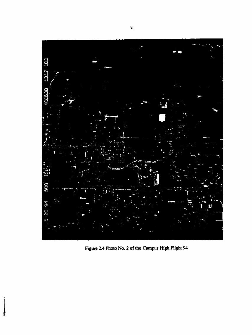
Figure 2.4 Photo No. 2 of the Campus High Flight 94

32

The TIFF image format is used to store the scamied images. Since the LAN fonnat is used

as the processing format, a program was written to convert all the scanned images to LAN

format. The size of these two scanned images were:

For No. 1: 4361 columns by 5040 rows

For No. 2: 4380 columns by 5026 rows

2.2 ̂ Relationship between Pixel Size and Root Mean Square (RMS) of Interior

Orientation

Because of the small pixel size, the size of output image file of the digital image is very

large. If the standard size of a aerial photograph is 23 cm by 23 cm, and the pixel size is 25

pjn by 25 ^m, for example, the number of pixels on the scanned digital photograph would be

about 84 Mb. Since the scanner HP ScanJet 3C is used to scan the aerial photographs used m

this research, it is used to test the relationship between pixel size and the RMS in the interior

orientation. The results of five different pixel sizes are shown in Figure 2.5. The RMS is from

five fiducial marks on each scanned photograph.

The results shown in Figure 2.5 indicate that even when the pixel size is about 25 ^m, the

RMS for these five fiducial marks is around 30 nm, which means that a geometric precision

less than 30 ^m is not available from the photographs scanned with the HP ScanJet 3C

scanner. But the RMS is much smaller than the nominal 75 dpi or 0.37 nun precision.

Another scaimer HP ScanJet 4C with 600 dpi resolution was also compared. The results

from the HP ScanJet 4C are shown in Figure 2.6. The RMS shown in Figure 2.6 is much less

than that in Hgure 2.5 since the higher precision scanner HP ScanJet 4C was used. The lowest

RMS here is about 10 pjn at the pixel size of about 40 ^m. An image with the pixel size of

about 28 nm was tried but failed because of the software SoftPlotter may not be able to

handle some a big file in the interior process. But according to the trend in Figure 2.6, a lower

RMS than 10 ^im is available by using the HP ScanJet 4C scanner. The conclusion here is that

the higher resolution or smaller pixel size than the nominal value can be obtained from a low

precision scanner, but the geometric accuracy still remains low, which means the distortion of

the scanned image is determined by the geometric precision of the scanner.

I A

33

50 50

^ 40 e 1 30 — £ M 20 -Z ae.

10

A 1 1 1 1 1 U 102.8 74.4 49.4 32.9 24.68

Pixel Size (microns)

Figure 2,5 RMS vs. Pixel Size for HP ScanJet 3C

30

20

10

95.12 72.82 49.06 32.74 24.52 Pixel Size (microns)

Figure 2.6 RMS vs. Pixel Size for HP ScanJet 4C

HO

(A c 60 o w u

S 40 — —4C

V9 ~3C 5 o

CM

1)1

A 1 1 • 1 1

95.12 72.82 49.06 32.74 24.52 Pixel Size (microns)

Figure 2.7 HP ScanJet 4C vs. HP ScanJet 3C

i

34

Hguie 2.7 shows the relationship between the RMS and the different pixel sizes for both

3Cand4C.

2.23 Content of the Header of the Modified LAN Images

The LAN image format is used in this research to store the images involved and all the

information about the images and the stereo model (if it exists). All the information about the

LAN images are stored in the header which is the first 128 bits in the image data. In addition

to the normal LAN header, some new items are added to the header to provide more

information about the images. Table 2.1 shows the content of the modified LAN header.

Table 2.1 Content of the Modified LAN Header

NAME WIDTH

fBYTES)

TYPE REMARKS

HDWORD 6 CHAR Head word, always "HEAD74" UNUSEDl 6 CHAR Unused bytes

IPACK 2 SHORT INT Number of bits per sample NBANDS 2 SHORT INT Number of bands

ICOLS 4 LONG Number of columns IROWS 4 LONG Number of rows

XSTART 4 LONG X stait position of this image in the map database YSTART 4 LONG Y start posidon of this image in the map database

UNUSED2 15 CHAR Unused bytes COMPRESSION I CHAR Compression type

DIR 2 CHAR Flight and reference directions SCALE 2 SHORT INT Ratio between pixel gray value and real height on DEM

MAXIMUM 4 LONG Maximum height on DEM * SCALE RATIO 8 DOUBLE Ratio used in the scale equalizing

XL 8 DOUBLE X ground coordinate of the camera YL 8 DOUBLE Y ground coordinate of the camera ZL 4 FLOAT Z ground coordinate of the camera

FOCAL 4 FLOAT PriiKipal Distance MAPTYPE 2 SHORT INT Type of map unit NCLASS 2 SHORT INT Number of class

MINIMUM 4 LONG Minimum height on DEM * SCALE ANGLE 8 DOUBLE Angle rotated in epipolar rectification MARK 2 SHORT INT Type of photograph in the image matching

lAUTYP 2 SHORT INT Unit of area ACRE 4 FLOAT Area of this image XMAP 4 FLOAT X initial location of this image YMAP 4 FLOAT Y inidal location of this image XCELL 4 FLOAT Pixel size in X direction YCELL 4 FLOAT Pixel size in Y direction

I

35

The standard LAN image format is used for Landsat images. In the process of soft

photogrammetry, large quantities of information about the status of the process and many

parameters, such as the exterior orientation parameters and focal length of the camera, are

needed. In SoftPlotter and Socet Set, the types of information are kept in separate project

files. In this research, all the information needed is kept in the modified LAN header. There

are some bits in the header that are not used. The unused space in the LAN header can be

used to store the information for the soft photogrammetric process. More bits can be added to

the end of the image data if the unused space in the header is not enough, just like the TIFF

image format. The advantage of this is that image files have almost all of the information

about the processing. Also, the images with the modified LAN header can still be recognized

by software packages like IMAGINE, they can work just like the standard LAN format

images.

Values of some of the items in Table 2.1 are:

IPACK;

• 0 for 8 bits per sample

• 2 for 16 bits per sample

• 4 for 32 bits per sample

MARK:

• 0 for the raw photographs

• 1 for the photographs after interior orientation

• 2 for rectified photographs

• 3 for photographs in a stereo pair with the same scale

• 4 for DEM before post-processing

• S for DEM represented by the minimum and the difference between the

minimum and the maximum of the pixels in the image space

• 6 for DEM in the ground space

• 7 for orthophotographs in the ground coordinate system

• 8 for relatively oriented photographs in a stereo pair

36

• 9 for a pair of photographs in epipolar coordinates system

2^4 Initialization of the Header the LAN Images

Before doing the interior orientation, the header of the LAN images needs to be initialized

for the items that are not determined by the images. Table 2.2 shows the initialization values.

The iinir of the coordinates in the image space is millimeters. For location of the

photograph in the ground coordinate system, the unit is meters.

Table 2.2 Initialization of the Modified LAN Header

NAME REMARKS HDWORD Head word, always •'HEAD74" UNUSED I Unused bytes

IPACK Determined by image NBANDS Determined by image

ICOLS Determined by image IROWS Determined by image

XSTART Set to 0 YSTART Set to 0

UNUSED2 Unused bytes COMPRESSION Set to 0

DIR Set to 'EE' SCALE Set to I

MAXIMUM Set to I RATIO Set to 1

XL No iniu'aiization YL No initialization ZL No initialization

FOCAL No initialization MAPTYPE Set to 0 NCLASS No initialization

MINIMUM Set to 1 ANGLE Set to 0 MARK Set to 0

lAUTYP No initialization ACRE No initialization XMAP No initialization YMAP No initialization XCELL No initialization YCELL No initialization

i

37

23 Interior Orientation of the Digital Aerial Photographs

The location of a point on the digital photogr^h depends on how the scanning is done,

but its photo coordinate is independent of the scanning process. The goal of interior

orientation of the digital photogr^hs is to (1) get the photo coordinates of all the pixels on

the digital photograph (2) remove some of the distortion caused by scanning and the camera

imaging system.

13,1 Detenniiiation of Transformation Parameters in the Interior Orientation

The transformation between the digital photographs before and after the interior

orientation can be linear or non-linear according to the number of control points and the

precision requirement throughout the photograph. In this research 6 parameter Affine

transformation shown in equation 2.3 is used, which is sufBcient for many applications. The

Affine transformation equation is:

2.3

Here a, b, c, d, Xo, >o are 6 transformation parameters; /, / are the pixel coordinates

before the interior orientation. Each fiducial point or known control point can give two

equations, so at least 3 known points are needed to find the 6 parameters. More than three

points are recommended so that the least square method can be used to solve the equation and

check to ensure that the measurements are correct.

To get these 6 unknown parameters from m known control points, the following equations

are established:

'a

b '•t," 1 0 0 0]

0 0 0 /, 1

K J. 1 0 0 0 0 0 0 L K 1J

c

d

L^oJ

2.4

38

Solve the equation 2.4 for these 6 unknown parameters. The standard errors can be used

to check the quality of the measurements. La this process, some of the geometric distortion

caused by scanning and the camera imaging system can be removed.

The camera radial distortion should also be removed when observing the control and tie

points. All the observations should be corrected before implied.

232 Transformatioii Equation for the Interior Orientation

To perform the interior orientation, the pixel coordinate system must be used. The pixel

coordinates on the photograph after interior orientation are given by equation 2.3 and the

equation below

Where Cip, Cyp are the pixel sizes in x, and directions respectively; Ip, Jp are the pixel

coordinates on the interiorly oriented photographs; and yop, are the initial photo

coordinates of the interiorly oriented photographs in the photo coordinate. The equation 2.3

can be written in terms of pixel coordinates as:

/ = Q,-'-,size_I — l;J ==0,'",size_J — I

Then the location (/, J) of each pixel on the raw photo can be transformed to the photo

coordinate (/^, Jp). Before performing the interior orientation, some parameters in equation

2.5 need to be determined.

233 Determination of Pixel Sizes

From these 6 parameters the pixel size on the digital images after interior orientation are

calculated as;

yp=^yp^p-*-yop

2.5

2.6

39

The sign of Cjp is determined by the product of parameters a and d minus the product of b

and c. If the result is positive, the photo coordinate is of the same coordinate orientation as

the pixel coordinate, that is the left-hand coordinate system, then Of is a positive number.

Otherwise the photo coordinate system is a right-hand coordinate system like the one shown

in Figure 2.2, and Of is negative.

23.4 Detennination of Initial Position in Piioto Coordinate

The initial photo coordinates in equation 2.5 need to be determined before the

interior orientation can be performed. Since x«^, are the photo coordinates of the center of

the upper-left comer pixel on the photograph after interior orientation and the Xf is defined as

shown in Figure 2.2, only the minimum of Xp and minimum or maximum of on the interiorly

oriented photograph can be taken as the values of xc^, y^f. Therefore, from equation 2.5, the

limits of the interiorly oriented photograph are;

= min(a/ +bJ+Xo) =mmicI+dJ + yo) = maxial + ) 2.7

y^^ = max(^cI+dJ + >„) I = 0,size_I— I; J = 0,size_J — l

Where size J, size J are the number of columns and rows on the raw photograph,

corresponding to the size of the photograph before ±e interior orientation; Xnun, y,^, y^

are the limits of the photograph after interior orientation. Then the initial photo coordinates of

the interiorly oriented photograph is given by;

^Op >'op=ym„ if Cvp<0 2.8

> 0

23£ Detennination of Photograpli Size after Interior Orientation

From equation 2.7 the pixel size of the interiorly oriented photograph is given as;

40

Where sizfjc,, sizejff are the number of columns and rows on the interiorly oriented

photographs. Therefore by using equation 2.5 through 2.9 for each pixel on the raw digital

photograph, the corresponding interiorly oriented pixel and photo coordinates can be

calculated. Since the interiorly oriented photographs are also in the pixel coordinate, and the

pixel coordinates from the equation 2.5 may not be integers, resampling processing is needed

in the interior orientadon.

23.6 Resampling Equation in the Interior Orientation

Resampling is a interpolation process used to find the pixel gray values other than the

center of the pixel on the digital images. Different resampling methods will be introduced in

the next section. In this secuon only the resampling equation is given. Resampling equation is

the reverse equation of the interior orientadon transformation equation shown in equation 2.5.

For a given pixel on the interiorly oriented photograph, the corresponding pixel location on

the raw photograph can be found. If that pixel locadon is not an integer, then the pixel gray

value on that location needs to be interpolated from the surrounding pixels. The resampling

equadon for interior orientation is

7" a b -1 f 1

-Xo \

J c d < yop y

/p =0,--,JKe_Xp -l;7p -I

For each pixel (Ip, Jp) on the photograph after interior orientation, its corresponding pixel

location (/, /) on the raw photograph can be computed with equation 2.10; and the pixel gray

value is available by means of interpolation.

2.4 Resampling in Digital Image Transformation

Resampling is the process used to obtain the pixel gray value on the inu^ery after

transformation from the original imagery by means of interpolation. Resampling is needed in

almost all the digital image transformation. The resampling in the interior orientation process

is one of the examples. Assume the pixel gray value for the raw photograph is ;(/, J) for the

pixel on (/, J); and the pixel gray value for the photograph after interior orientation is

41

Jp) . The resampling equation is the same as the equation 2.10. Since the pixel position on the

raw photograph from equation 2.10 may not be integers, equation 2.10 is rewritten as:

'r' a b -1 1 1

•+-

1 1

r c d < pyp'^ p. yop-yo.

/

/p =Q,—,size_Xp-V,Jp -0,—,size_y 1,-1

Where /', J* are not integers. Once I*, J* are calculated, gfil,, Jf) can be determined

interpolation of the neighbor pixels around location {T, T) on the raw photograph. There ate

many different interpolation methods used in the resampling process. In this smdy, only

nearest neighbor, bilinear interpolation, and distance weighted interpolation methods are used.

2.4.1 Nearest Neighbor Interpoiation

Nearest neighbor is the simplest and fastest resampling method to get the pixel gray

value on the photograph after the transformation. Its idea is to take the value of the nearest

pixel as the interpolated value. So actually there is no interpolation in the nearest neighbor

resampling. As shown in Figure 2.8 the distances between (T, f) of location A and the other

four surrounding pixels are calculated and compared. The pixel gray value with the shortest

distance is taken as the value of pixel {F, T). According to equations 2.5, 2.11, assume the

shonest distance is between the points A and F shown in Figure 2.8, then the pixel gray value

on the interiorly oriented photograph is given by

Jp) J ' ) = g(/. /+1) 2.12

So the pixel gray value of the nearest pixel F is taken as the pixel gray value on the

transformed photograph. This algorithm has the least computation, so it is the fastest one. It

can give satisfactory results form some applications, especially for those which need to keep

the pixel gray values.

2.4.2 Bilinear Interpolation

In the bilinear interpolation the four surrounding pixels are involved. As shown in Figure

2.8, the pixel gray value on location (/', /') on the raw image can be determined by the

following bilinear interpolation equation:

g U ' j ' ) = J ) a +1 - /')+g(/+1. /)(/'- /))(/+1 - y 0+ {g{I +1, y +!)( / ' - / ) + g( / , y +1)( / + ! - / ' ) ) ( / '_ / )

42

and the pixel gray value for the point {I,, J,) on the transformed photograph is:

since they are the same point on the two photographs before and after transformation.

2.43 Distance Weighted Interpolation

The inverses of the distances between the location to be interpolated and the surrounding

pixels are used as weights in the distance weighted interpolation. Two types of interpolation

are used in the distance weighted interpolation. They are bilinear and cubic convolution. The

weight used in bilinear and cubic convolution interpolation for each pixel involved is inversely

proportional to the distance between the location to be interpolated and the surrounding

pixels.

Bf(/^ CgiM^

Fgilrf-*-!) Dg(f+lJ+l)

Figure 2.8 Inpterpolation in Resampling

As shown in Figure 2.8, assume for given pixel {Ip, Jp) on the transformed image, (/*, J ' )

are the pixel coordinates calculated fix>m equation 2.11. If the location of (!', J') is similar to

that shown in Figure 2.8, the algorithms used in the two types of interpolation are bilinear and

cubic convolution interpolation.

2.43.1 Bilinear Interpolation

In this case the four surrounding pixels are used in the interpolation, just like that one

discussed above. The inverse distances are used as the weights in the interpolation. According

to Figure 2.8, numbering the distances between the point A and others as Du i = 1,2,3,4, then

the pixel gray value of the point A is determined by

43

guj) . g(/-n,y) g(/+u/-n) g(/,y-n) O' p; Df

2.14 4

Where the is a constant and normally its value is larger than 2. 2 is used her for the k.

According to the equation 2.14 it is known that the shorter ±e distance, the larger the weight

of that pixel has in the interpolation. The weight will be infinite for one pixel if the distance to

that pixel is 0. In the case of zero distance, the gray value of that pixel should be used, similar

to the nearest neighbor interpolation.

2.4.3 ̂Cubic Convolution Interpolation

The only difference between the bilinear and the cubic convolution is that more pixels are

used in the cubic convolution interpolation. In this case, there are 16 surrounding pixels

involved in the interpolation. Number all the pixels and their distances between the point m

the Figure 2.8 as g.-. A; i = 1,2 16. Then the pixel gray value of the point A is calculated

The interiorly oriented images of Figure 2.3 and Figure 2.4 are given in this section. The

results include the six transformation parameters, the two interiorly oriented photographs, and

the subset photographs from the interiorly oriented photographs in the overlapping area.

2 .̂1 The Six Transformation Parameters

Before determining the 6 unknown transformation parameters, the location of the five

fiducial marks on the scanned photographs must be measured. Table 2.3 shows the calibration

data and the measurements of the fiducial points.

by

2.15

Where k is the same constant as that in the bilinear interpolation.

2S Results of the Interior Orientation

44

Substituting the values from Table 2.3 in equation 2.4 and solving the equation to get the

six Affine transforaiation parameters as shown in Table 2.4.

The pixel sizes in Xf and » direction after interior orientation can calculated from the

Table 2.4 with the parameters a, b and c, d. The pixel size will be shown in the section 2.5.3.

Table 2.3 Measurements of the Hducial Marks and the Calibration Data

Mark No. Calibration Data (mm) Measurements for Photo

No. I

Measurements for Photo

No. 2

X Y Pixel X Pixel Y Pixel X Pixel Y

I 109.989 109.994 4185.06 203.56 0 110.001 -109.999 4194.94 4646.44 3 111.995 -0.001 4230.56 2424.06 4 -0.008 111.998 1966.06 166.06 2291.81 175.06 5 0.004 -112.003 1976.94 4688.94 2291.81 4724.06 6 -109.994 -109.999 62.69 4681.19 7 -110.007 109.996 63.69 212.94 § -112,092 0.002 24,? 1 2447.19

Table 2.4 Values of the 6 Parameters for both Photographs

Name of the Parameter Parameters for No. I Parameters for No. 2 a 0.04 957986 0.04936983 b -0.00011216 0.00000820 Xo -97.47634405 -113-16788498 c -0.00006239 0.00005287 d -0.04952097 -0.04923854 >0 I20J3290581 120.48901416

23 ̂Interior Orientation Results

The photographs after interior orientation are shown in Figures 2.9 and 2.10. It does not

seem to be much difference between the raw photographs shown in Figures 2.3 and 2.4 and

the photographs after interior orientation shown in Figures 2.9 and 2.10. But they are in

totally different systems. In the interiorly oriented photographs, the photo coordinates of any

pixel are available from its pixel coordinates; and the pixel sizes in x and y directions are also

available. The initialization of the LAN header of each photograph is also done after the

a!

45

interior orientation. So the photogrsq)hs after interior orientation are in the coordinate system

that is connected to the camera.

2^3 Subsets of the Interioriy Oriented Photographs

Since only the overtyping area can be used in the stereo model, the selected subsets in the

common area for both photographs are used.

In the process of getting the subset of a photograph, the photo coordinates of one pixel

on the subset photographs should remain the same coordinates as they are on the original

photograph. The formula used to obtain subset from a given photograph is:

2 15 y^p ~ Vop "^^yp-^Ol s i ze ^ X p =Ia2~Ioi

size^y'p =/o2-^i

Where I'p, J'p are the pixel coordinates on the subset image; ip, Jp are the pixel

coordinates on the original image; Ioi,Joi and /02, Joz are the coordinates of the upper-left and

lower-right pixels of the subset images on the original image respectively; Xop, yop are the

initial position of the subset image; sizejc'p, 5ize_y'p are the new size. Since all the pixel

coordinates in equation 2.16 are integers, there is no need for resampling.

The subset photographs are shown in Figures 2.11 and 2.12.

The information about the header of these two subset photographs are shown in Table 2.5.

Table 2.5 Header Information about the Subset Photographs

Name of the Parameter Parameters for No. 1 Parameters for No. 2 Xo. -13.755544 -106.453590 Vn. 105.476608 105.948967

sizex. 2600 2715 size V- 3700 3700

Pixel size in x 0.049580 0.049370 Pixel Size in v -0.049521 -0.049239

46

Figure 2.9 Photo No. 1 after Interior Orientation

Rgure 2.10 Photo No. 2 after Interior Orientation

48

Rgure 2.11 Overlapping Area from Photo No. 1

Rgure 2.12 Overlapping Area from Photo No. 2

50

2.6 Conclusions

The details of the process of interior orientation and some related topics have been

discussed above. They include the modified LAN image format, scanning process, resampling

process in soft photogrammetry, and interior orientation.

The modified LAN image format was presented and will be used in this research for

storing the information about all the kinds of images, such as raw, rectified, DEM and

orthophotos. All the information about the digital image will be kept in the modified header of

the LAN file, which makes the management of the digital images easy.

As shown in Figure 2.7, the more accurate the scarmer, the less the RMS for the digital

images scanned at the same file size. Due to the limitation of pixel size, to a certain extent

more accurate scarmer will not produce higher geometrically accurate digital image for a

certain pixel size. The other limitation for the ordinary scarmer is that the size of the scarmer

may not be large enough to accommodate the entire aerial photograph.

The complete interior orientation process was presented by using the example of two

scanned aerial photographs, and two subsets of the interiorly oriented photographs are

obtained for the same overlapping area.

The programs written can be £^plied to accomplish each step in the interior orientation

discussed in this chapter.

i

51

CHAPTERS SINGLE PHOTOGRAPH RECTIFICATION

Single photograph rectification is the process used to correct errors on each aerial

photograph caused by the tilt of the camera when they were taken, and brings the photo

coordinate system parallel to the ground coordinate system. Since the aerial photographs may

act be taken exactly vertically, the rectification process is necessary before image matching. In

rectifying the aerial photographs, it is brought back to vertical position and the distortion

caused by the tilt of the camera is removed. For each aerial photograph, there are six

parameters used to determine the exterior orientation of the photograph. They are three angles

Qi, K and ground coordinates X, Y, Z of the camera nodal point which will be discussed in

the next section. The single photograph rectification process is also called exterior orientation.

Similar to the interior orientation, the exterior orientation process connect the aerial

photographs to the ground coordinate system.

Unlike the stereo rectification discussed in the next chapter, the single photograph

rectification for each photograph is separately performed, or it is only applied to single

photograph.

In order to perform the single photograph rectification, some triangulation results fiom

different software packages are used and compared.

3.1 Definition of Coordinate Systems and Angles

There are two coordinate systems involved in the process of rectification, they are camera

coordinate system and ground coordinate system. The relationship between the directions of

these two coordinate systems is defined by three independent angles.

3.1.1 Camera Coordinate System

Camera coordinate system has the same origin as the photo coordinate system. As shown

in Figure 3.1, it is a right-hand coordinate. Unlike the photo coordinate system, the camera

coordinate system is a three dimensional coordinate system, which is connected to the

orientation of the camera in or attached to the airplane. Assuming that the x axis of the

camera coordinate system has the same direction as the photo coordinate system. Since the

52

camera coordinate system is a three dimensional coordinate system, the z coordinate of the

origin is -/. Where/is the principal distance of the camera.

In the sinq)Iest case, the photo coordinates can be converted to camera coordinates with

the following equation:

y^=ypWhen C, <0 or

yc=-ypW/icn C y > 0

2c =-/

Where Xp, y, are photo coordinates and Xg, Ze are camera coordinates.

2c

k

(0. 0. -f)

Hgure 3.1 Camera Coordinate System

3.1.2 Ground Coordinate System

The ground coordinate system used in map making can be in either UTM, SPC or any

local system. Generally speaking, the ground coordinate system is a right-hand coordinate

system and defined in Figure 3.2.

Conventionally, the X axis is in the direction of east and the Y axis in the direction of

north; the Z axis is in vertical direction.

3.U Rectified Coordinate System

The rectified coordinate system (Xr, yt, Zt) has the same orientation as the ground

coordinate system, the only difference is that the origin of rectified coordinate system is the

53

same as that of the camera coordinate system. Unlike the ground coordinate system, the

rectified coordinate system is more related to the image space of the camera.

The value of zjf defines the ratio of the scale of the rectified photograph to the scale of

the photograph before rectification.

(0,0)

Figure 3.2 Ground Coordinate System

Usually, Zr = -/ in the rectification for same scale rectification. Therefore, the relation

between rectified and ground coordinate systems is

x ^ = X - X ^

yr^Y-Y, 3.2 Zr=Z--Z,

Where XO, Yq, Zo are the ground coordinates of the camera nodal point.

3.1.4 Definition of tiie Angles of (|> and ic

The three angles are defined as the (a), (b) and (c) in Figure 3.3. The first rotation is the

angle od around the X axis of the ground coordinate to obtain the new coordinate XY*Z'; then

the new coordinate rotated around axis Y' by the angle ^ becomes the next coordinate X'T'z',

the last rotation is around z by the angle of k; then the coordinate is turned into camera

coordinates from the ground coordinates. Notice that these angles are right-hand rotation

angles and the rotation order can not be changed.

54

Z(Z")

(a) Rotation (b) Rotation (c) Rotation around X axis around Y' axis around z (Z")

axis

Figure 3.3 Definition and order of (o, 0 and k

Assuming Ro>, R«, R^ are the transformation matrices for the above rotation. In terms of ax

<t>, K, these matrices are determined by equation 3.3. Then the rotation matrix from the ground

coordinates to the camera coordinates is computed by equation 3.4.

The directional relationship between camera coordinates (Xc, yc, Zc) and the ground

coordinates (X, Y, Z) is determined by equation 3.5 for all the pixels on the photograph.

Where is a unit orthogonal matrix from equation 3.4; (Xq, Yq, Zo) are the coordinates of the

camera nodal point; s is the scale factor. The value of s is different from pixel to pixel on the

photograph, which is the function of ground height.

Notice that the order of these three rotation can not be changed, especially in the case of

large rotation angles; otherwise the value of the matrix R could be much different. In the case

of small angles less than 3°, there might not be much difference. The order of the rotation in

this research is defined by Figure 3.3. In fact, what is really needed here is the transformation

matrix i{. If the in equation 3.5 can be found, then the relationship between the image and

the ground coordinate is available, and it is sufficient to do the single photograph rectification.

55

" 1 0 0 0 cos(D sino)

0 -sino) coscD

COS0 0 -siA<|>

0 1 0

sin<ti 0 cos<|>

COSK sinK o"

-sinic COSK 0

0 0 1

I'll ^13' fzi >22 ^23

/31 ''33.

= R X - X , y-Yo

Z-Z„

3.3

3.4

3.5

3 ̂Aerotriangulatioii

Aerotriangulation is the process used to detennine the six exterior parameters for each

aerial photograph in strip or block of photographs and the position of the pass points or other

unknown points on the photographs.

3.2.1 Determination of the Exterior Orientation Parameters

The exterior orientation parameters of each photograph are ATo, Y q, Zo, (O, K which can

be determined by using ground control points with the co-lineaiity condition. The coplanerity

condition can be used as constraints for checking the relative orientation at the same time. For

given ground control points ATj, Yu Zi and its image point on photo xu yi, I ~ 1 n the

following co-linearity equation is used.

In equation 3.6,/is the principal distance; rn are the elements from the rotation

matrix R in equation 3.4 which is the fimction of ai, ^ and K. Since each control point can give

two equations, at least three control points are needed to solve the six unknown parameters.

56

X. = rn(X

Vi = r^^(X

-A'o)-»T,3(i:-ro)-Kr,3(Z,-Zo) i - f ) --Sro)+r3,(i:-r„) + r33(Z,-Zo)

--X'o) + '-32(J:-I'o) + ''33(^f-2o)

Notice that in equation Zi~- f is used for the camera coordinates in the above equation.

The equations 3.6 are nonlinear equations, so the linearization is needed for solving them.

If the number of control points are mote than three, the least square method is needed. Refer

to Ghost [1988] for the expression of R and details on solving the equation 3.6.

Aerotriangulation is also available by software packages like Albany [ERIO Technologies].

With the development of the Global Positioning System (GPS), the exterior parameters of

the camera can be precisely determined by the airborne differential GPS techniques or the

combination of GPS and photogrammetry techniques.

3^ Results of Aerotriangulation

Three different types of aerotriangulation methods are used here. They are: Albany from

ERIO, Calib from Dr. Jeyapalan, my major professor, Softplotter from Vision International.

The results from these three different software packages are available for the aerial

photographs discussed in the chapter 2; and the results are shown in Table 3.1.

Table 3.1 Comparison of Triangulation Results Using the Three Different Software Packages

Parameter Photograph No. 1 Photograph No. 2 Softplotter Albanv Calib Softolotter Albany Calib

^0 (meters) 1487238J63 1487238.563 1487239.2576 1487792.068 1487791.822 1487791.865

Ko (meters) 10S838S.185 1058385.689 1058386.2669 1058411.816 1058411.773 1058412.343

Zo (meters) 1229.815 1230.691 1203.4923* 1230.331 1230.980 1203.7212*

(D (decrees) 2.4992711 2.7455 2.1695047 2.4138072 2.6714 2.41656409

* (degrees) -2.6663S14 -2.9648 -2.6786350 -2.7655344 -3.0804 -3.49479308

K (degrees) 4.5477386 5.0931 4.2312360 2.7041475 7.1378 2.55292799

The heights with are ellipsoid heights. The geoid undulation in Ames, state of Iowa

area is about -29 meters, therefore the heights above mean sea level for those two exposure

stations are close to 1230 meters. From the above table we see that the results are close,

especially these results from Softplotter and Calib programs. Since Softplotter is used as a

57

comparison software in this research, the triangulation from Softplotter is used in the

rectification of these two photographs.

3^3 Relative Orientatioii

The coplanerity condition must be met in a stereo pair. So the coplanerity condition can be

used to check the stereo pair or to do the relative orientation as constraint. The relative

orientation can also be used to extend the ground control for those photographs which do not

have ground controls in the same strip by means of pass points. There are seven parameters

involved in the relative orientation.

If the aerotriangulation is done with the ground control points and the pass points, the

coplanerity condition is generally satisfied. The pass points are needed for checking the

relative orientation if the exterior orientation parameters are imported &om the results of

other software packages like Albany.

3,2.4 Aerial Intersection for Locating Unknown Ground Points

After the exterior orientation is completed and the relative orientation is checked, equation

3.6 can be used to calculate the ground positions of any unknown points on the photographs

in a stereo pair. Equation 3.6 is rewritten in the following format;

X = J''/' TijX,+r23y, Tjj/,

y _ zi)+>; r i jXi+r^y , Tjj/,

X = +x; ''is^r'^'zsyr '33 fr

"'"'byr '33/r

Where xi, jru Xr, yr are the camera coordinates for the same point on the left-hand and

right-hand photographs in the stereo pair; (Xo,I '̂,Zo) are the ground coordinates of the left-

hand photograph; (X^,YQJZQ) are the ground coordinates of the right-hand photograph;

^ the elcmcnts from the rotation matrix R for the left-hand

photograph; '•n''i2''i3'*"''3i''32''33 ^^e the elements from the rotation matrixfor the right-

58

hand photograph; and are the principal distances for the two photographs, respectively.

The ground coordinates X, K, Z of the unknown point are the three unknowns in equation 3.7.

Since for each point on the ground there are four equations can be established, the ground

position of each unknown point can be solved.

33 Sin^e Photograph Rectification of Aerial Photografrtis

There are many ways to rectify the aerial photographs in photogrammetry. To do so in

soft photogrammetry, digital single photograph rectification is used.

3 J.l Process of Digital Rectiflcatioii

Figure 3.4 shows the process of rectification. X, Y, Z andx, y, z are the ground coordinate

and camera coordinate respectively;/is the focal length; XQ, Kq, Zo are the ground coordinates

of the camera nodal point O; the plane a'̂ ' is the photograph plane before rectification; the

plane ab is the photograph plane after rectification; points A and B are two points on the

ground and a, a\ b, b' are their image points on the photographs before and after

rectification, respectively; p' and p are the principal points on the photographs before and

after rectification, respectively. In Hgure 3.4 all the symbols with prime are related to the

photograph before rectification.

O (Xb,yb,Zb)

Photo af rectificai

Photo b rectifies

Figure 3.4 Rectification of Photographs

59

From the definition of angles and the order of the rotation from the ground coordinate

system to the camera coordinate system, the aerial photographs can be brought back into the

ground coordinate system by transforming the coordinate of each image pixel from the camera

coordinate to the ground coordinate or the rectified camera coordinate. So the points a\ f

will be transformed to points a, b, respectively on the photograph after the single rectification.

3 J.2 Single Rectification Equation

Combine equations 3.2 and 3.6 to obtain the rectification equation as:

'i3^c 'hyc '33/ 2 g

Where Zr is replaced by •/ for the same scale rectification. The pixel gray values must be

used when displaying the digital photograph, the relation between the pixel and camera,

rectified coordinates is determined by the position of the initial point and the pixel size

using the following equation:

yc = yoc+c^cJc

X ^ = X Q R +C„I,

yr=yOr-*-C„Jr

Where h, Je, It, Ji are the pixel coordinates for the camera and rectified coordinates

respectively; Ck, Cyc, C„, Cr are the pixel sizes for the camera and rectified coordinates,

respectively; Xe, ye, Xr, yr are the coordinates of the initial points of the camera and rectified

coordinates respectively; and (jcoe, >qc); yor) are the inidal positions for the camera and

rectified coordinate systems, respectively.

3^3 Determination of Initial Point, Pixel Size and Image Size of the Rectified

Photographs

33J.1 Pixel Size

The same pixel size as the photographs before rectification will be used for the

photographs after rectification. Since the shape of the pixels is not square, the direction

relationship between the pixel before and after rectification should be considered. The pixel

60

size in x and> directions should be switched if the coordinate system is rotated more than 45°.

In equation assume the coordinates of a point m the camera coordinate system is (1, 0, -/),

then the rectified coordinates of the point are;

'*13-'33/

The values of Xr and^r can be used to determine if the switch is needed as in equation 3.10

if kr|<k| C =C ^Jtr ^xc c =c yr yc

else 3.10

C =|c jt 1* ̂vc c c c = •

The absolute symbol used in the above equation ensures that the signs of the values are

correct if the switch is performed.

333 ̂Determination of Initial Points and Image Size

From equation 3.8 the rectified coordinates of the four comers on the rectified photo can

be determined by substituting the camera coordinates of the four comers of the photograph

before rectification. Assume the four comers of the rectified photograph have the maximum

and minimum values of Xmin. Xnax^ and^max from equation 3.8, then the initial point location

and the image size are given by equation 3.11.

In equation 3.11 sizej,, sw_Jr are the pixel size of the rectified image. Other symbols are

the same as in the previous section.

61

>'or=y«m'/

yor = y^if c^<o

size_I, = c„ XT

3.11

33.4 Resampling Equation in Rectification of Photograpiis

Same as the transfonnation in the interior process, digital resampling is necessary in the

process of rectification. The actual formula used in rectification is the resampling formula. The

single rectification resampling fonnula needed is the reverse form of equation 3.8, which is

similar to equation 3.6. Combine equations 3.6 and 3.9 to obtain the resampling equation as

=r>lXor-^nnyOr-''23f

~ ^iZyOr 3.12

J , _ (Zr^l J^0c^32)<^yr-^r +(ZrA -^00^ )

r _ (5^2I+>V3I)£^+ (Zr'K>>V'32 X^vr )

Where Ai, Bi, C\ are three intermediate symbols; V, J* are the camera coordinates

calculated from the given rectified coordinates /„ Jt which range from 0, 0 to 5K«_/r-l,

size_J,-l (see equation 3.11) respectively; Zr is the z coordinate in the rectified coordinate

system and here is set to -/. Since /*, J' may not be integers, the interpolation methods

discussed in Chapter 2 are applied. To simplify the computation in the rectification, rewrite

the equation 3.12 as equation 3.13.

Where k is a. constant; M is called rectification matrix; A|, Bi are the same constants as

that in equation 3.12. So the rectification can be done at any scale.

62

' r' ' / /

r = Af Jr

rf. rf.

M =

+xo,r3,)C^ a,r^,-hxo,r3^)C, -C^ -C^

Ur^l-<-yOc'3l)C„ (^^^a•^yOc^3l)^x -c„ -c^

^r-^l "^-^Oc^l

^^ ypcQ

-Cv, 'si-^Or "'"'nyor ""yi f

3.13

3.4 Results of the Rectificatioii of Aerial Photographs

The rectification results of these two aerial photographs are represented in this section.

3.4.1 LAN Headers of the Rectified Photographs

Table 3.2 shows some of contents of the headers of these two rectified photographs.

Notice that different item may have different type of unit

Table 3.2 Content of Some Items of the LAN Header of the Rectified Photographs

Name Photograph No. 1 Photograph No. 2

Xo (meters) 1487238.563 1487792.068 Yo (meters) 1058385.185 1058411.816

Zo (meters) 1229.815 1230.331

xoc(mm) -15.343071 -103.299477

>oc(mm) 129.266998 117.976028 /(mm) 152.473 152.473

size_Xe 2940 2865

sizejfe 4029 3833 Cc(mm) 0.049580 0.049370

Cvc(nrai) -0.049521 -0.049239

63

Comparing this table with Table 2.5 it is known that the pixel sizes remain the same, but

the initial positions are different The image sizes are also changed because the rotation in the

rectification process. The other differences are that the location for each photographs in the

ground coordinate system and the focal length are added to the header.

3.4 ̂Images of the Rectified Photographs

These two rectified aerial photographs are shown in Figures 3.5 and 3.6. Comparing them

with the two photographs before rectification shown in Figures 2.9 and 2.10, the differences

between them are obvious. Since the roads are in due east and north directions, the rectified

images look more correct.

3 ̂Conclusfons

Single photograph rectification, triangulation, and resampling are discussed in this chapter.

Different types of interpolation methods are used. The transformation and resampling

equations for the single photograph rectification are derived, the parameters in the

transformation are also determined. All these equations and determination of parameters are

implemented in computer programs. Two photographs and some information in their header

after the single photograph rectification are shown and examined.

64

Figure 3.5 Rectined Photograph from Photograph No. 1

Figure 3.6 Rectified Photograph from Photograph No. 2

66

CHAPTER 4 STEREO RECTIFICATION

In Chapter 3 the rectification of single photograph is described. In a stereo pair two or

more photographs that are corrected. Before the image matching can be performed, all the

photographs in the same stereo pair must have the same pixel size, scale and be in the same

coordinate system - the epipolar coordinate system. This processing is called stereo

rectification.

4.1 Epipolar Coordinate System

As shown in Figure 4.1, the direction of Xe axis of the epipolar coordinate system is

defined by the line O'O" between the nodal points of the adjacent cameras of the photographs

in the stereo pair. In Figure 4.1, x'y'z',x"y"z" are the rectified coordinates; x'^y'eZt,x"y"z"

are the epipolar coordinates. Each photograph has its own epipolar coordinate system in the

stereo pair. The only difference between the epipolar coordinate systems is the different

origins.

z" (Z"c)

O'

Figure 4.1 Epipcpiar Coordinate System

67

To transform from rectified coordinates to epipolar coordinates, only rotation around the z

axis is involved. So the origin and z axis of the rectified coordinate are not changed in this

transformation provided the scales are the same.

42 Equaliring Pixel Size in A Stereo Pair

The pixel sizes of the photographs in the same stereo pair are assumed to be the same in

the directions of both rows and columns to make the image matching simple. Thus the number

of the pixels can be used as the unit of distance on each photograph in the stereo pair without

concern for real distance provided the scales of the photographs are the same.

4.2.1 Image Resizing

Pixel size is changed in the process of image resizing. Although the pixel coordinates of

any location on the photograph could be different, the rectified coordinates of any location on

the photograph will remains the same in this process. Assume the values of pixel size in

columns and rows are Cc, Cy and C\, C\ before and after resizing, respectively and /, / and

/', J' are the number of columns and rows of the photograph before and after resizing,

respectively. Since the distance remains the same in the resizing and thus the coordinates of

the initial pixel are the same for both photographs, the transformation equation is:

The resized photograph has more colurmis and rows if its pixel size is smaller than that of

the photograph before resizing. Since the coordinates of the initial pixel in the upper-left

comer are not changed, the coordinates of the initial position are not needed in equation 4.1.

The values of C, / and / C' here are the scale factors. If the scale factor for a direction

is larger than 1, then the image after resizing will look larger with smaller pixel size in this

direction.

i

a.̂

68

4 .̂2 Size of the Resized Photograph

The size of the resized photograph can be determined by equation 4.1 as:

, size_xC^ size_x = —

, size_yC, size_y =—

Where sizejc, size_y and size_x', size^' are the size of the photograph in number of

columns and rows before and after resizing, respectively.

4.23 Resampling in Pimtograph Resizing

The resampling formula is:

C C.

C J = 4.3

y

I' = 0,-",size_x' — I

J' = Q,'-',size_y'

Since /, J could be floating numbers, the interpolation mentioned before can be used to

determine the pixel gray value on the resized photograph for all the pixels on that photograph.

4.2.4 Image Resizing in A Stereo Pair

One photograph in the stereo pair is used as the reference photograph in this process. Its

pixel size is used for both photographs in this stereo pair. After resizing, all the photographs in

this stereo pair should have the same pixel size in bothx and^ directions.

Table 4.1 Some Information in the Header after Resizing

Name Photograph No. 2 Before Resizing After Resizing

Xik-(mm) -103.299477 -103.299477 jTorCmm) 117.976028 117.976028

Cjcr(mm) 0.049370 0.049580 Cvr(mm) -0.049239 -0.049521 size_Xr 2865 2853 size_yr 3833 3811

69

Here, photograph No. I is considered as the reference photograph in the stereo pair. After

resizing this stereo pair, some of the information in the header of photograph No. 2 are shown

in Table 4.1. In order to make the comparison between the photographs before and after

resizing, the header information of both photographs are shown in Table 4.1. According to the

listed information, the differences between them are the image size and the pixel size. The

image after resizing looks the same as the image before resizing since there is no change in the

rectified coordinates of points on the image. The information about the photograph No. 1 is

not shown in Table 4.1 since it is the reference image. Comparing Table 4.1 with Table 3.3 it

can be seen that the two photographs have the same pixel size in both x and directions.

4 J Determination of the Scale of tiie Stereo Pair

The photographs in the same stereo pair must have the same scale before image matching.

By equalizing the scale in both photographs the pixels would have the same ground size at the

average ground height of the stereo model.

4,3.1 Scale of A Photograph

The scale of each photograph is the function of the flight height, principal distance, and

the ground height expressed as:

for the vertical or rectified photograph. Where Zo is the flight height above mean sea level

(MSL); ha is the average height of the ground above MSL;/is the principal distance or the Zr

distance after the single photograph rectification. Since the ground height is different firom

point to point on the photograph and not available at this time, the average ground height is

used in equation 4.4. Because there is only one common area involved in one stereo pair, the

average height is the same for all the photographs in the stereo pair.

In equation 4.4, the principal distance for the photographs taken by the same camera is the

same. If a photograph in the stereo pair was taken by a different camera at different object

distance, its principal distance may be different from the other.

70

To change the scale of a photograph in the stereo pair, one can change the flight height or

the principal distance. Since different flight height is the most likely reason to cause the

different scales in the stereo pair, changing flight height method is used. In this a way, the

principal distance can remain the same.

432 Determimitioii of the New Flight Height

To get an equal scale in the stereo pair, changing flight height is used to change the

photograph scale. One photograph in the stereo pair is used as the reference photograph.

Assume its flight height and principal distance are Hr and /• respectively, the changed

photographs have Ho, Ho as old and new flight heights, respectively; and / as the principal

distance. To have equal scale.

If the photograph has the same principal distance as the reference photograph, equation

4.5 becomes

Since the photographs in the stereo pair are after single photograph rectification, the/here

refers to the principal distance which is the same as the Zr in equation 3.2. The principal

distance in the photographs after single photograph rectification could be different from the

camera focal length, it depends on the single photograph rectification scale of the each

photograph.

4 Transformation between the Old and New Coordinates

Assume the 5 is the ratio of the new scale Sa and the old scale So, called scale unification

factor, the relation between them is:

f - fr

is needed. Therefore,

a 4.5

J - / i j _ _ x „ _ y „ S . nHr-h„) (Hn-K) y .

4.6

71

When fr -/• Where and Xg, are the rectified coordinates for each pixel on the

photographs before and after the transformation, respectively, f is the magnification factor for

the photographs to be changed, and equation 4.6 is the transformation equation for the

equalizing scale process.

4 J.4 Determiiiatioii of New Initial Position and Image Size

From equation 4.6 the relation between the old and new initial position is

^Or ~ ̂ Or . _ 4.7 yor = •^Or

and the new photograph size is

size_x„^=size,x„,s

size_y^ = size_y„s

Where x\, y'or, size_x„, size_ymr are for the new photograph after this process; sizejc^,

size_y„r are for the old photograph. Unlike in section 4.2, here the coordinates of the initial

position do not remain the same after the transformation.

43S Transformation Equation

Since the equalizing scale process is after the image resizing discussed in the previous

section, the photographs in the stereo pair should have the same pixel size, and consider

equation 4.6, then transformation equation in pixel coordinate is

^'•r=^Lr 4.9 J =sJ nr ̂or

Where /«r, /«r and J„ are the pixel coordinates before and after transformation,

respectively. Notice that the pixel size remain the same after transformation.

43.6 Resampling Formula

The resampling formula is the reverse process of equation 4.9. It is given by

C = — /„r = 0'• * •.-1

J 4.10 ~ y,, = 0, • • •, Size_ -1 s

One of these interpolation methods can be applied to complete the transformation.

72

43.7 Results of Equalizing Scale

As before, photograph No. 1 is considered as the reference photograph. Table 4.2 shows

some new infonnation about the LAN header of photograph No. 2 after the transformation.

Since the scale difference between these two photographs is small, the change of image size

for the photograph No. 2 is small. In Table 4.2 the ground height is assumed as 0. The new

photograph scale is larger then the old one because s is larger than I. So the initial pixel is

farther to the coordinate origin than it was before. Notice that the flight height in the header

remains the same as before, s can give the new height by using equation 4.6. The pixel size

remains the same so it is not shown in Table 4.2. The information of photograph No. 1 is not

shown in Table 4.2 since it is unchanged.

Table 4.2 Some Information about the Header of Photograph No. 2

Name Photograph No. 2 Before Scaling After Scaling

s 1 1.000420 xoritam) -103.299477 -103.342827 y Or (ram) 117.976028 117.025536

Zo (meters) 1230.331 1230.331 size_Xr 2853 2854 size_yr 3811 3812

The s in Table 4.2 is defined in equation 4.6. Comparing Table 4.3 with Table 3.3 it can be

seen that the flight height remains the same. According to equation 4.6 the flight height after

equalizing the scale is

therefore the value of H from the above equation and the Zc from Table 4.2 is about 1229.815

Meters which is equal to the flight height of the photograph No. 1 in Table 3.3.

Figure 4.2 shows the photograph No. 2 in the stereo pair after equalizing the scale.

Figure 4.2 Photograph No. 2 after Equalizing Scale

74

4 .̂8 Error in the Equaliring Scale Process and the Correction

In the equalizing scale process, the average ground height is used to determine the scale of

each photograph. But the actual scale on the photograph varies fiom point to point

Therefore, position error will occur on the photograph for those pixels whose ground heights

are not equal to the average ground height after processing.

As shown in Figure 4.3, O2, ON are the locations for the right-handed photograph before

and after the processing, respectively; point A is the point on the ground; point a is the image

of the point A on the right-handed photograph before the processing. Point B in the

intersection of line AO2 and the average ground height ha. Since the scaling is performed

according to the average ground height ha, the image point of the point A on the processed

photograph is located on point a', but its correct position should be located on point a",

according to the geometric relationship shown in Figure 4.3. Therefore the error of distance

a'a" is introduced after the processing. If the position a' is used to compute the height of the

point A after image matching, if will give the wrong height information. So correction is

needed when computing the ground height

In Figure 4.3 the relationship between point a and a' is determined by the scaling factor s

as d{i' * sdj|.

O2

1

Figure 4.3 Error Appears in Equalizing Scale Process

75

Where d„ d,* are the radial distances of the image point of the ground point A in the

rectified coordinates before and after equalizing the stereo pair scale.

If the matched point a' is converted back to the original photograph with the (xiginal

height, according to the geometry shown in Figure 4.3, the correct height of the point A is

available. Therefore, before calculating the location for each pixel after image matching, the

pixel position should be corrected by dividing the scaling factor s. In this way the error

brought by the scale equalizing process can be removed when computing the ground height.

4.4 Epipolar Rectification

After all the previous processing are done, all the photographs in the stereo pair should

have same photo scale and flight height, then the epipolar rectification can be performed. In

the process of transforming to the epipolar coordinate system, only one rotation around z axis

of the rectified coordinate needs to be done.

4.4.1 Detemunation of the Rotation Angle for Epipolar Rectification

The location of each camera is known after the photograph has been rectified. Assmne the

locations of the photographs are (Xi, Ki), (Xr, Kr) in the ground coordinate system for the left

and right photographs shown in Figure 4.5 (Z axes are not shown).

Xr

Figure 4.4 Determination of Rotation Angle 9

76

The rotation angle is given by;

^ K-r , x , -x .

0 = tan"' 4.11

The rectified coordinate is transformed to epipolar coordinate system by rotating angle 6

around Zc axis. The Z axes are not shown in Hgure 4.4. The sign of the angle 6 is positive

when the rotation is counter-clockwise.

4.4 ̂Transformation Formula

The transformation equation is given by equation 4.12. Where Xe, and Xr, yr are the

epipolar and rectified coordinates, respectively; 5 is the epipolar transformation matrix.

' cos6 sinO 0 "r —sin0 COS0 ofyr —S y. 4.12

0 0 I

yr

Zr.

•fr

Vr Zr,

Using the pixel coordinates to represent the equation 4.12 as;

' cosO sin0 1/

y,. -sin0 COS0 Kl Xo^cos0-Kyo^sin0-Xo,

-Xo,sin0-4-yo,cos0-yo, 4.13

Where I^, Je and A, Jr are the pixel coordinates for the epipolar and rectified coordinates,

respectively; xoe, j'oe and xot, yor are the initial locations for epipolar and rectified coordinates,

respectively; CM, Cye and C„, Cyr are the pixel sizes for epipolar and rectified coordinates,

respectively.

4.43 Determination of the New Image Size, Initial Location and the Pixel Sizes

The equation 4.12 can be used to determine the initial location of the new photograph.

Assume the image sizes for both photographs are «ze_Xe, sizejfe and SK«_Xr, sizejfr, the new

image limit can be determined by using equation 4.12, say x^, ymin, ymw, then image

constants for the new image size are given by equation 4.14.

After the epipolar transformation, the stereo pair is in the epipolar coordinate system. If

the stereo rectification is perfect, there will be no parallax in the stereo model. A good

relative orientation may help to reduce thejr parallax in the stereo model significantly.

77

if |0| < 45° then

C„=C„

~ ̂ yr

else

C„ =|C„

c =c.

size_x^

size_y^

X — J t . '̂ tfox •^min

^xe

yuan ~yn

^Qe "^min

yor = ymin'f c„>o

yo. = y^if Cvr<o 4.14

4.4.4 Resampling Formula

Like the processes mentioned before, resampling is needed for performing the digital

image transformation. Reversing the equation 4.13 to get the resampling formula as:

Ir J.

COS0 — sinG

sin6 cos6 CJ. CJ.

-co^cose -yo,sin0-x, Or

Xo, sine + cos0 -

4.15

C C ^yr ^yr / , =0," ,s ize_f / ,

J . =0," ,s ize_J/ ,

Interpolation will be applied.

4.4.5 Results of Epipolar Rectification

Table 4.3 shows part of the LAN header of the photographs after epipolar rectification.

The 0 in Table 4.3 is the angle rotated in the process of epipolar rectification. The

photographs after epipolar rectification are shown in Figures 4.5 and 4.6.

78

Table 4.3 Pait of the Header Information after Epipolar Rectification

Name Photoeraph No. 1 Photograph No. 2 XgrCmm) -18.699175 -106.621063

129.854996 122.855591 Zo (meters) 1229.815 1230J31

s 1 1.000420 9 (degrees) 2.754570 2.754570 C„.(mm) 0.049580 0.049580 C,r(mm) -0.049521 -0.049521 size_Xr 3130 3034 5Kje_yr 4166 3945

Since some areas on the photographs after transformation show no features because of the

rotations, it is better to redefine the common area to be used in image matching. The new

common area is shown in Figures 4.7 and 4.8 for both images; and Table 4.4 shows the new

LAN header information for the new common area on each photograph.

Table 4.4 Some of the Header Information about the New Conmion Area

Name Photograph No. I Photograph No. 2 Xor (mm) -9.576458 -97.894989 yor(mm) 123.516304 116.714989

Zo (meters) 1229.815 1230.331 s 1 1.000420

6 (degrees) 2.754570 2.754570 C„^(mm) 0.049580 0.049580 Cvr(mm) -0.049521 -0.049521 size_Xr 2153 2689 sizejfr 3933 3772

4 ̂Comparison of Rectification witii SoftPlotter

The results from rectification of a single photograph and stereo rectification are compared

with that firom the SoftPlotter. For the comparison in the rest of the smdy, 24 points are

selected and their locations are manually determined. The heights determined are also

calculated and compared in this section.

79

Figure 4.5 Photograph No. I after Epipolar Rectiflcation

80

Figure 4.6 Photograph No. 2 after Epipolar Rectification

Figure 4.7 New Common Area on Photograph No. 1

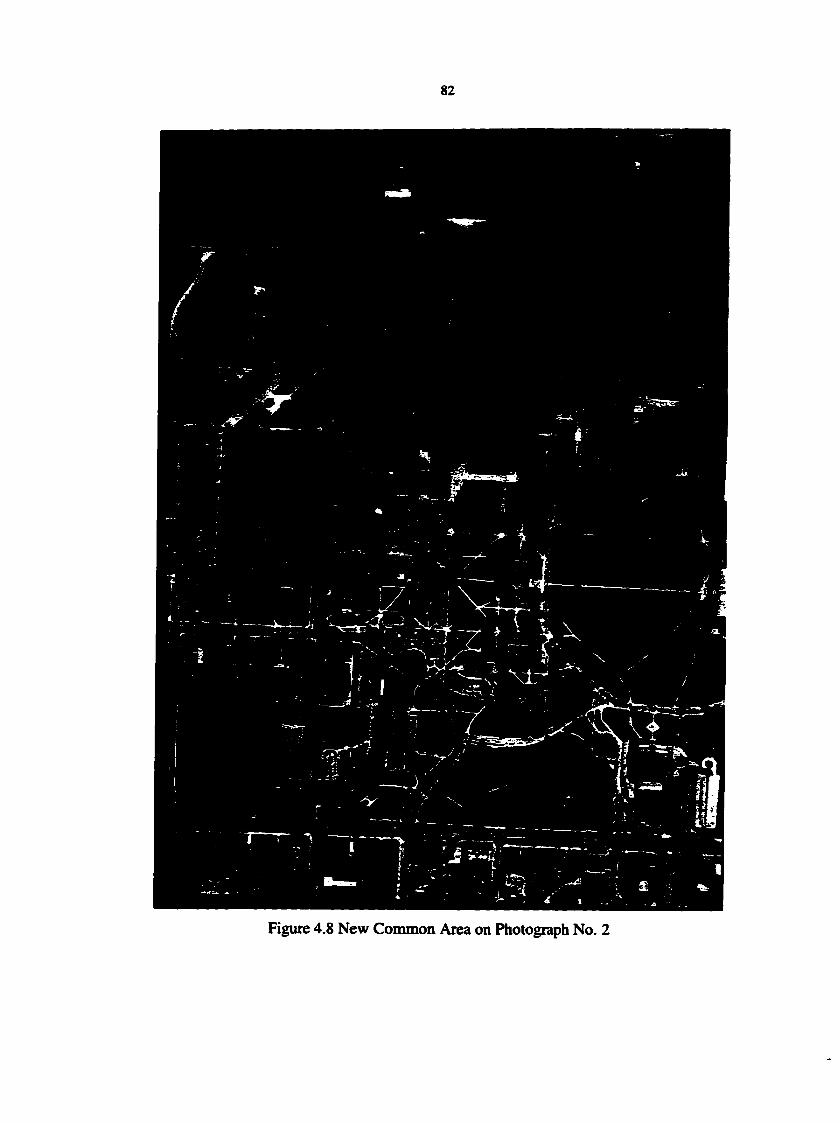
Figure 4.8 New Common Area on Photograph No. 2

83

45.1 CiMnparison of the Rectification of Single Photograph Using SoftPlotter

In order to check the rectification of each single photograph, the photographs in Figures

4.7 and 4.8 are imported to the SoftPlotter and were rectified again by means of ground

control points.

Since the exterior parameters of each photograph used in the above processing were from

the SoftPlotter. the rectification in the SoftPlotter for the photographs in Hgures 4.7 and 4.8

should give the results shown in the expected column in Table 4.5 if the same ground control

points are used again and the rectification discussed in Chapters 3 and 4 are correct. 2.7S4S70

degrees in the table is the angle from the epipolar transformation. The results from SoftPlotter

are also listed in Table 4.5

Table 4.5 Comparison between Expected Values and SoftPlotter Results

Name Photo graph No. 1 Photograph No. 2 Expected SoftPlotter Results Expected SoftPlotter Results

ATo (meters) 1487238.563 1487236.119 1487792.068 1487791.914 Yo (meters) 1058385.185 1058386.057 1058411.816 1058412.801 Zo (meters) 1229.815 1228.750 1229.815 1229.692 Q) (degrees) 0 -0.052169 0 -0.084324

(degrees) 0 -0.161815 0 -0.028110 K(degrees) 2.754570 2.746991 2.754570 2.735340

The standard error for the locations of both photographs is about 1.283 meters; the

standard error for the angles is about 0.057351 degree or 0°03'26.47". The differences

probably are caused by the following reasons:

• In the SoftPlotter. the control points for both models are not exactly the same since one

vertical control point on the original model does not appear on the compared photographs.

The difference in the control point is shown in Table 4.6. The difference could be the main

reason. In Table 4.6 the blank cell means that these values are not used as control value. The

only difference is that point 163 is used as horizontal control in the original model, but in the

check model the point 161 is used as horizontal control instead of the point 163. This

difference in control results in the differences of the aerial triangulation for these two cases. If

84

the flight height above ground is about 7S0 meters; the angle differences of both (D and ^ are

about 0.057351 degrees, then the estimated distance on the ground is about 1.06 meters.

• All the points on the photographs to be checked are remeasured. These new

measurements can be slightly different from those on the original photographs. The

approximate formula for calculating the height difference caused by the factor is

*X

Where is the difference in measurement; airbase B is the distance between these two

exposure stations, which is about 554 meters; is the x parallax; and / is the focal length

equal to 152 mm. If the r parallax for the flight height 750 meters above average ground

height is used, which is about 111.4667 mm, and the pixel measurement difference is about

0.05 mm, the difference in height is about 0.336 meters. The difference in XY plane is

approximately equal to

c^H-K) ̂

which is about 0.349 meters. Where H-ha is the flight height above the average ground height,

which is about 750 meters.

From the above discussion it is seen that these two reasons can account for about

Vl.06'+0J39- =L113 meters, which is close to 1.283 meters found as the standard error.

So we may conclude that the rectification of single photograph in Chapter 3 was correct.

Since the method used for calculating the precision is an approximation, another check is

presented in the next section.

4^ ̂Comparison of the Rectification of A Single Photograph witii the Original Model

Another way to check the correctness of the rectification of a single photograph is to

compare the ground coordinates from the stereo pair in Figures 4.7 and 4.8 with these of

original model in the SoftPlotter. The check performed in the previous section is on the

location and orientation of the photographs, or the exterior orientation parameters. In this

section, the check is on the location of the control points in the groimd coordinate system.

Since the same exterior orientation parameters are used in both models, the ground

jl

85

coordinates of the same point should be the same for both models if the rectification is correct

and the mgaqirgnients of these groimd points are same on both models. The comparison for

those control point locations computed after rectification is shown in Table 4.7. From Table

4.7 the standard errors of the differences of the listed control points for X, Y and Z are 0.159

meters, 0.225 meters and 0.209 meters, respectively. From the discussion in the previous

section it is known that one pixel measurement difference can bring about 0.34 meters

difference in each direction for a point, which is larger than the difference from Table 4.7. So

it is reasonable to conclude that the one of the reasons for the difference in the comparison is

the measurement difference between these two models. Therefore the rectification of single

photograph presented in Chapter 3 agrees with the rectification done by the SoftPlotter.

433 Check of j Parallax for Some Selected Points

The jr parallax is the difference o f y coordinates for the same point on each photograph in

the s t e r e o p a i r i n e p i p o l a r c o o r d i n a t e s y s t e m I f t h e e p i p o l a r r e c t i f i c a t i o n i s s u c c e s s f u l , t h e y

Table 4.6 Comparison for the Difference in Control Points

Point No. Original Model In SoftPk )tter Comparec Model in SoftPlotter X Y Z X Y Z

161 1487238.331 1058922.364 162 1487217.821 1058522.4^7 291.047 1487217.821 1058522.447 291.047 163 1487223.801 1058124.074 172 1487494.664 1058486.702 290.610 1487494.664 1058486.702 290.610 173 1487748.207 1058082.750 284.719 1487748.207 1058082.750 284.719

Table 4.7 Comparison with the Original Model

Point No. From Orieinal Model in SoftPlotter Computed from the Stereo Pair in Figures 5.7,5.8

X Y Z X Y Z 161 1487237.923 1058922.102 292.434 148237.63 1058922.25 292.336 162 1487217.875 1058522.182 291.021 148721738 1058522.38 290.903 172 1487494.556 1058486.756 290.659 1487494.25 1058487.00 290.216 1710 1487640.188 1058930.648 288.443 1487640.00 1058931.00 287.972 173 1487748.160 1058082.621 283328 1487748.13 1058082.75 283311 1720 1487643.620 1058493.276 290.455 148764325 105849330 290.442

86

parallax should be zero for all points. To check this, some points are randomly selected and

theiry coordinates are shown in Table 4.8.

In Table 4.8 the points beginning with letter "t" are the tie points and the others are

control points. The tie points beginning with "tl" are the ground points which can be easily

identified, such as the comer of lawns, intersections. The tie points beginning with "t2" are the

points on lawns, trees. The tie points beginning with "t3" are the points on the roof of

b u i l d i n g s . T h e y c o o r d i n a t e o f e a c h p o i n t i s n o t s h o w n i n T a b l e 4 . 8 . T o o b t a i n t h e y

c o o r d i n a t e s o f t h e s e p o i n t s , e q u a t i o n y , = y o , + i s u s e d . T h e d i f f e r e n c e b e t w e e n t h e y

coordinates of each pixel on all the photographs in the stereo pair is they parallax.

Table 4.8 Check of the Result of Epipolar Rectification

Point No. Photograph No. 1 Photogra !)hNo.2 y Parallax (pixels) Pixel X Pixel y Pixel X Pixel y

161 274.87 732.37 238.62 594.37 0.66 162 145.62 2041.62 112.16 1903.26 1.02 172 1045.12 2201J7 1012.87 2064.12 -0.09

1710 1588.12 775.12 1560.12 636.87 0-91 173 1799.87 3556.62 1780J7 3418.62 0.66

1720 1533.62 2203.37 1500.87 2065.87 0.16 til 836.25 698.25 800.67 560.41 OJO tl2 114.75 2034.75 81.25 1896.75 0.66 tl3 362.75 3538.75 336.93 3400.67 0.74 tl4 1174.75 3480.25 1157.44 3342-74 0.17 tl5 1267.75 2021.25 1234.83 1882.79 1.12 tl6 2412.25 1044.25 2391.02 905.04 1.87 tI7 2479.75 2969.75 2458.90 2831.48 0.93 t31 682.25 1066.75 605.75 927.75 1-66 t21 137.00 1094.00 97.92 954.54 2-12 132 362.00 2247.00 300.00 2110.00 -0-34 122 482.75 2180.25 446.60 2042.01 0-90 t23 413.00 2805.00 377.50 2665.19 2.47 t33 1168.00 1979.00 1033.00 1843.00 -1.34 t34 1719.00 2623.00 1648.49 2486.05 -0-39 t36 2042.00 1150.00 1991.00 1012.00 0-66 124 2239.00 1853.00 2207.58 1713.81 1.85 t25 2371.00 2299.00 2349.25 2155.10 6.56 t26 2318.25 2859.75 2295.74 2720.31 2.10

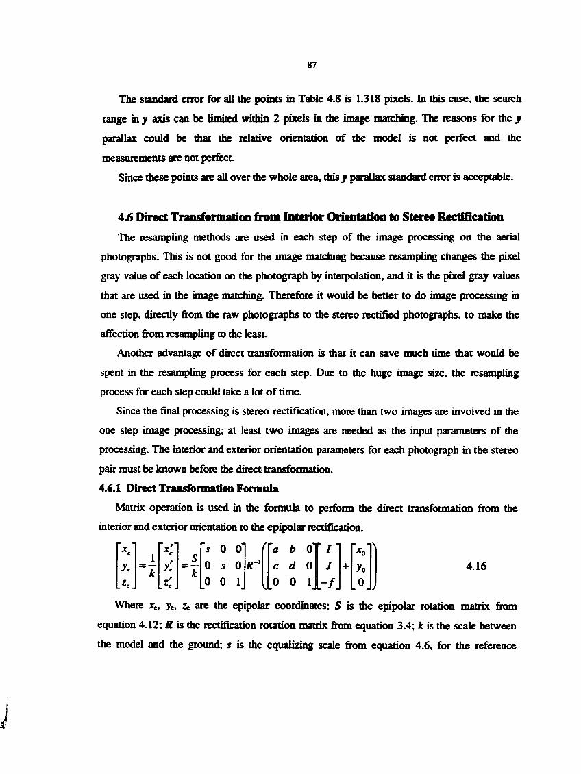
87

The standard error for all the points in Table 4.8 is 1.318 pixels. In this case, the search

range in y axis can be limited within 2 pixels in the image matching. The reasons for the y

parallax could be that the relative orientation of the model is not perfect and the

measurements are not perfect.

Since these points are all over the whole area, this y parallax standard error is acceptable.

4.6 Direct Transfonnatioii from Interior Orientation to Stereo Rectification

The resampling methods are used in each step of the image processing on the aerial

photographs. This is not good for the image matching because resampling changes the pixel

gray value of each location on the photograph by interpolation, and it is the pixel gray values

that are used in the image matching. Therefore it would be better to do image processing m

one step, directly from the raw photographs to the stereo rectified photographs, to make the

affection from resampling to the least.

Another advantage of direct transformation is that it can save much time that would be

spent in the resampling process for each step. Due to the huge image size, the resampling

process for each step could take a lot of time.

Since the final processing is stereo rectification, more than two images are involved in the

one step image processing; at least two images are needed as the input parameters of the

processing. The interior and exterior orientation parameters for each photograph in the stereo

pair must be known before the direct transformation.

4.6.1 Direct Transfomiation Formula

Matrix operation is used in the formula to perform the direct transformation from the

interior and exterior orientation to the epipolar rectification.

_ 1 _s s 0 0"

R-^

r a b 0' • / • *^o" \

y'e ~T 0 s 0 R-^ c d 0 / + yo

.Zr . X. 0 0 1 < 0 0 1 0 >

Where x^, Ze are the epipolar coordinates; S is the epipolar rotation matrix from

equation 4.12; H is the rectification rotation matrix from equation 3.4; A; is the scale between

the model and the ground; ^ is the equalizing scale from equation 4.6, for the reference

88

photograph it equals 1; a, b, e, <f, Xo, yo are the traiisfonnation parameters finm the control

points for the interior orientation; /, / ate the pixel coordinates before the interior orientation.

Then the values ofx«,>e are:

Notice that the Zc is the value for z coordinates of all image pixels on the photograph in the

epipolar coordinate system. Normally it is equal to -/ for the same scale transformation. The

equations 4.16 and 4.17 can be applied to each photograph in the stereo pair with different

transformation parameters.

4.6 ̂ Deteniiuiation of the Pixel Size

Equations 4.16 and 4.17 only gives the coordinate relationship between the raw pixel

coordinates and the epipolar coordinates. In order to represent the digital photograph, the

constants of the pixel coordinates associated with the epipolar coordinates have to be

available, which means the pixel size, location of the initial pixel in the epipolar coordinate

system and the size of the photograph in the epipolar coordinate system have to be known

before the direct transformation.

Equation 2.6 determines the pixel size after interior orientation. Since there are more than

one photograph are used in the direct transformation process, asstmiing Cxn Cyr are the pixel

size of the reference photograph and Cx, Cy are the pixel size to be changed. After the

correction of the pixel size, all the photographs should have the same pixel sizes of Cyr.

If the absolute rotation angle around z axis in the direct transformation is less than 45° or

larger than 135° and less then 180°, the pixel size of the epipolar images will remain the same.

To determine this, assimiing / = l,/ = 0, Xo-yo-O, equation 4.16 becomes

Vc _5

h.

's 0 0" 0 5 0

a c 4.18

A. K

0 0 I rf.

89

Once the values of and are available, the pixel sizes in the epipolar coordinate system

are:

' / k l>W

c =c else 4.19

c =C jS:-" 'K

Therefore the final pixel size can be determined. Notice that the Cv, Cyr are the pixel size

of the reference image in the stereo pair which needs to be determined before the direct

transformation.

4.63 Determination of the Initial Location and the New Image Size

To determine the coordinates of the initial locations of the photograph in the stereo pair in

the epipolar coordinate system, one needs to determine the limits of each photograph in the

epipolar coordinate system. Assume the sizes of one photograph in the stereo pair before the

direct transformation are size_x, size_y, then the limits of Xmn, x^mx, ymm, y-" in the epipolar

coordinates are available by substituting 0, size_x - 1 and 0, sizje_y - 1 in equation 4.16, then

the initial location xoc, yoe for this photograph are:

yoc^y^m^f c„>o 4.20

yoc = yn^if c«<o

and the new photograph size are:

size X, = ~ C

size V = -^^5 Ic.

Although the pixel size for all the photographs in the stereo pair must be the same, the

initial location and the image size of them are different.

90

4.6.4 Resampling Equation for the Direct Transfonnation

Assume

'd. MI

'21

•31

^,2 d,; s 0 0"

dn d^ = s 0 s 0

dn 1 0 0 I R-' A22

for the process of single photograph rectification, equalizing scale and epipolar rectification,

then equation 4.16 becomes

ye

If

D it

\L

a b 0" * / • "•̂ 0 c d 0 J + yo 0 0 1 rf 0

4.23

x'" y' Voc ^yc-^e for r'

/, = 0,"-,size_x^ J, =0,"-,size_y^

where Ze normally equals -f. Then equation 4.23 becomes:

4.24

x'' a b

z' - f - f 7" -/ y' c d / yo

Lz'J 1 V L-/J

It can be proved that f - -/from equations 4.23 and 4.24, therefore the final equation for

the resampling is:

H-t Jp;;: 4.25

The resampling formula for the direct transformation consists of two equations, equations

4.24 and 4.25. Equation 4.24 gives the values of x' ,y' for the equation 4.25. The comparison

between the direct transfonnation and the results from the multi-procedures discussed in

Chapters 2 and 3 are shown in Table 4.9.

91

Table 4.9 Comparison between Direct Transfonnation and the Multi-Pioceduies

PtNo. Direct Transformation Multi-Procedures Phocogra PhNo. 1 Photogra ph No. 2 Photogra ph No. 1 Photograi phNo. 2 jr(mm) y (mm) x(mm) y (mm) r (mm) jr(mm) x(mm) y (mm)

161 4.077 fn25^ -86.034 87.232 4.052 87.248 -86.064 87.281 162 -2304 22J90 -92.278 22J92 -2356 22.413 -92334 22.463 172 42.292 14J05 -47.654 14.465 42.241 14502 -47.677 14.497

1710 69.215 85.155 -20330 85.109 69.163 85-131 -20.544 85.176 173 79.665 -52.616 -9.610 -52.632 79.661 -52.611 -9.624 -52J79

1720 66.505 14J94 -23.428 14363 66.461 14.403 -23.482 14.411

The standard error of the difference between these two sets of results is about 0.041 mm

or 0.83 pixel. Again there is a re-measurement problem here which could cause error around

one pixel or less. So the comparison shown in Table 4.9 the agreement on geometric

transformation between these two methods. Table 4.10 shows the radiometric comparison

between these two methods.

Table 4.10 Comparison between the Radiometric Transformations

Point No. On finals Direct Transfonnation Multi-Procedures Photo 1 Photo 2 Photo 1 Photo 2 Photo 1 Photo 2

Pixel Radiometric Value 161 110 88 110 82 146 172 162 171 157 169 155 86 102 172 159 131 149 132 106 127 1710 163 157 151 148 104 106 173 131 123 133 122 123 132 1720 123 83 119 82 132 173

Although the photographs after the multi-procedure processing virtually are the same as

the originals on the contrast for the above points, their pixel gray values have been changed

much more than the change resulted from the direct transformation. So the direct

transfonnation preserves the image better for image matching.

4.7 Condusioiis

Stereo rectification and direct transformation are discussed and applied in this chapter.

Equalizing pixel size and photograph scale in the stereo rectification makes pixels the distance

92

units that can be used in the image matching. An error from the stereo rectification is

discussed and its correction is also given.

In the direct transformation, one resampling brings the digital photograph from the raw

image to the image after stereo rectification which is ready for image matching. This method

decreases resampling to one time, therefore it has the least effect on the radiometric

characteristics, which is good for image matching; and it also need much less resampling so

that much time can be saved.

The results shown above indicate that the direct transformation is consistent with the

multi-procedures on the geometric transformation, but the radiometric transformation is

different between them. The direct transformation shows much better results on preserving the

original image information.

The direct transformation formulas are not simply the combination of all the formulas m

the mutli-procedure since more than one photographs are involved in the stereo rectification.

It has big advantage over the multi-procedure methods.

93

CHAPTERS INITIALIZATION OF IMAGE MATCHING

Before performing image matching, certain information about the stereo pair should be

given. Some of the information include the ground height variance, the average ground height,

the ground spacing of the output DEMs, matching window size.

5.1 Determinatioii of the Ground Coordinates

After image matching, the ground height for each pixel on the reference photograph can

be obtained. But the x and y coordinates are still in the image coordinate system, such as

epipolar coordinate system. We need to compute the X and Y coordinates of these pixels and

convert them to the ground coordinate system.

5.1.1 Ground Height from the x Parallax

Figure 5.1 shows the geometry in a stereo pair of photographs. Where/*, f are the

principal distances for these two exposures; H\ i7 are the flight heights above Mean Sea

Level (MSL); is the airbase or the distance between these two exposure stations; A is a

ground point; a', a are its image points on the left-hand and right-hand photographs,

respectively; x', x are the x coordinates in the epipolar coordinate systems on the left-hand

and right-hand photographs, respectively. Assuming the ground locations of the left-hand and

the right-hand photographs are {X*, Y\ Z') and (X, Y, Z), respectively, according to Hgure

S. 1 the X parallax of the point A is determined as (x' - x) if they have the same flight height

and principal distance. Since after epipolar rectification the scale of all the photographs except

the reference photograph in the stereo pair may be changed by the scale equalizing factor s,

the X parallax may be slightly different Using the left photogr^h as the reference photograph,

the ground height of the point A is given by:

5.1

s

94

for the case shown in Figure S.l. Where f is the scale equalizing factor discussed in the

Chapter 4. Notice that it is impottant to include the f in calculating the heights for the correct

ground height. In the equation S.l, r divided by s is the correction applied to remove the error

introduced in the scale equalizing process. Z in the above equation is the real flight height

above MSL for the right-hand camera, not the height after equalizing scale process.

4 y

^1 / i f / i

\0' O" J

\a' J \ ̂ *

\ »

FT

Ground surface /

/ 1

^ \

\ ^ /

H FT

Ground surface /

/ 1

H

/ k y i hi

T

' 4 Hz

!_

Figure 5.1 Average Ground Height and Its Variance

5.1.2 Calculation of the Ground X and Y Coordinates from Matched Ground Height

The height of a point in the stereo pair can be determined with equation 5.1 or equation

5.2 once the image matching is done and the x parallax is available. But this does not change

the X, y location of the pixels on the reference image. In order to get the ground coordinates

of each pixel in the stereo pair, the rectified coordinates must be restored from the epipolar

coordinate system. Assuming that the left photograph in Figure 5.1 is the reference

photograph in the stereo pair, and the pixel coordinates of the point a' is T, J'-, the initial

location of the left photograph is x'o, y*o', the pixel sizes are Ct-, CV-; the angle rotation in the

epipolar rectification process is 6; and the ground coordinates of the point A is Y\, the

ground XK and Fa can be expressed as:

cos6 -sin0 rc^^x'^ x,' +

sin6 cos6 K.

95

Where Xr, Yr, Zr are the ground location of the reference photograph. Then all the ground

coordinates of each matched pixel on the reference image are available.

5.2 Diitialization of Image Matching

Before the image matching can get started, some parameters of the stereo model and the

image searching must be determined. Those parameters include the average ground height, the

maximum variance of the ground around the average ground height, the x parallax on that

average ground height, the searching range or pull-in distance for given maximum variance of

the ground surface, the ground spacing of the output DEM, the maximum slope expected in

the output DEM, searching window sizes in terms of number of row and column, initializadon

of the LAN header of each image file, number of bits per pixel of output DEM and so on.

5 .̂1 Average Ground Height and the Ground Variance

The average ground height above the MSL determines the average scale of each

photograph in the stereo pair; and the maximum ground variance determines the largest scale

variance of the photograph. As shown in Figure S.l, ITa is the average ground height; hv is the

maximum deviation of the ground surface from the average ground height; is the flying

height above the average height.

If the flight height above MSL is Zo, then

and

is defined as the variance of the model. In this research the flight height above the MSL is

about 1230 meters, the average ground height above the MSL is about 290 meters; if V= 0.1,

then the maximum ground variance from the average ground height is about 94 meters; and

the total variance for the ground is 188 meters. The value of V is directly related to the

searching range in the image matching. The larger the V, the larger the searching range. The

value of V depends on the type of ground features. For flat area, a small V may be good

96

enough since the height of the ground surface is closely around the average height For a hOly

areas or large scale areas like cities, V needs to be larger.

5.2 ̂Estimation of the Initial Matciiing Positions

For the given pixel position F on the reference photograph and the flight height above the

average ground (Z' - h,), the initial matching pixel position I on the photograph to be matched

can be calculated as:

^0-^0-777^ / = /'+ 1—5.4

c.

Where x'o, Xo are the initial x coordinates of reference and matched photographs,

respectively; Cx is the pixel size in x direction; t here is used as a constant for shifting the

position on the reference photograph to obtain the initial estimated position on the matched

photograph.

5.2«3 Estimate of the Searching Range

If the value of V and the flight height above the average ground height is given, from

equation 5.4 the searching range on the photographs to be matched can be determined by

V 5.5 C A Z ' - K )

in number of pixels. For this case, B = 554 meters,/* = 152.473 mm; (Z' - ha) = 940 meters;

Cx = 0.04958 mm; if V = 0.05, then the value of M ~ 90.6 pixels on the row, which means

that the matching position is supposed be within 90.6 pixels from the initial estimated position.

It is not always necessary to search such a large range. For a matched pixel, the next matching

pixel should be very close since the surface of the ground is continuous, except for the walk

of buildings.

The searching range in the jr or the columns depends on the accuracy of the relative

orientation of the model, the less the y parallax is, the smaller the y search range is needed. It

should be less than 5 pixels in a normal situation.

97

5 .̂4 Groand Spacing

The ground spacing detennines the spacing of the output DEM raster. Assume the ground

spacing in X and Y is Cx, Cy, the numbers of pixels within one ground spacing are:

f t Y ^ '' ' * C,H

5-6 n -£lL

C,H

Where ^ is the flight height above the average ground height; Cx, Cy are the pixel sizes. If

itx, nrare larger than 1, only every itx, itv pixels needs to be matched. Otherwise all the pixels

must be matched.

5^ ̂Maximiim of the Ground Slope

For some types of features like buildings, the slope angle for the walls is almost 90°. The

large slope on the ground can cause the discontinuity or dissimilarities on the photographs in

the stereo pair. On the other hand, the larger the slope angle is, the larger the searching range

is needed to match the neighbor pixels. So it is reasonable to set the fnaximiim slope in the

image niatching process. From equation S.5, if the maximum ground slope is oc, for the given

ground spacing Cx, the ground height difference is tan(a)Cx. So the number of pixels caused

by this height difference is:

A/ = BfC^ tan(a)

CAr-KV

Substituting equation 5.6 into the above equation:

_ Brij^ tan(a) A / = — i ^ 5 . 7 (Z'-hJ

If the number of pixels for a given ground spacing nx = 2, slope angle a = 85° and

tan(85°) = 11.43, the searching range is about 13.47 pixels that is much less than the searching

range shown in section 5.2.3.

The maximum slope can be defined according to the type of ground features and any other

particular requirement.

98

5.2.6 Window Size

A window is defined before the image matching process as a mask. All the pixels in the

window are used in the process of matching. Generally speaking, the larger the window, the

more time is consumed in the process and the better is the matching. Therefore, from the point

of view of processing speed, the smaller the window, the better; but for matching precision,

the larger window, the better matching results. Normally, the larger the window is, the more

the similarity and dissimilari^ will be from the ground features. the increase of dissimilari^

is more than the increase of similarity then increasing the window size, the matching precision

will decrease for larger window. The information in the window may be not enough for a

good matching if the window is too small; the window size should be big enough to have

enough information in the window so that the image matching can be successfully done. Since

ail the pixels except the matched pixel are geometrically distorted because of the ground relief,

and some other noises that might appear in the window, smaller window are better. So it is

necessary to balance between the above factors and determine the optimal window size

according to the situation.

Although the number of rows and columns of a window can be an even number, the odd

number is preferred for simplification. This means only odd number like 3, 5 should be used as

the size of a window. The only difference between these two types of window is the

calculation of the matched position. The shape of a window can be square or non-square.

Both square and non-square windows will be discussed in Chapter 8.

5.2.7 Number of Bits Per Pixel in Output DEM

The number of bits per pixel in the output DEM determines the mayinwim height variance

and precision of the output DEM. For example, a 8 bits number per pixel can represent a

maximum number of 255 which can represent a maximum variance of 256 meters if precision

of the ground is 1 meter. In order to reduce the storage space for the output DEM, integers

are used. In practice, a precision less than 1 meter may be needed. To solve this problem,

assume there is a scale factor Scale between the real ground height and the pixel gray value in

DEM as

99

5.8 Scale

Where Z is the real ground height; gil, 7) is the pixel gray value. Therefore the integer

values of pixels can be used to represent floating numbers that have precision of less than 1

meter. For example, the real height is 300.03 M if the pixel gray value is 30003 and the Scale

is 100. Therefore the precision acmally is the inverse of the value of the Scale, in this example

0.0 IM. In order to have sufficient bits to accommodate the largest possible height variance on

the ground, 16 bits or 24 bits per pixel can be used to represent maximum of 6SS3S or

16777215 depending on the height variance and the required precision. To extend the

expressing range of a 16 bits number, equation 5.9 is used. In equation 5.9 the difference

between the original height value and the minimum height in the stereo pair, Mn, is used to

replace the original height value. Since g'(f, J) <= g(J, J) is always correct, the range of height

is larger than it was.

^ g'(/,y)-h Afi/i Scale 5.9

g\l, J) = gU, J) - Min

5.2.8 Checking on the Overlapping Area of Piiotographs in A Stereo Pair

The image matching can be done successfully only if ail the photographs in a stereo pair

have the same overlapping area. Otherwise the image matching will definitely fail or give the

wrong results. In order to check this, the flowchart shown in Figure 5.2 is used to check if

two photographs in a stereo pair have common overlapping area on the average ground height

ha. The basic idea here in Figure 5.2 is to check to see if the extreme area on one photograph

can be transferred to another.

5.2.9 Selection of Initial Points

In order to obtain some information about the stereo model to be matched, a certain

number of initial points can be used. To select the initial points, evenly distributed points on

the stereo pair are used. The simplest way to locate these initial points is to put these points

on the pixels. Assuming the number of initial points is m; image size is size_x, size^, let the

m initial points be arranged as niz by my matrix on the reference image in the stereo pair, the

values of nix and my are determined by:

ji!

100

Start

Yes

No

Yes-

Yas-Yes

No

-No-

Yas

Yes

No

Yes No

No >^:M^A)<yo2+c^seej^2-yo,v^

X,-A^+{Z-/),KJ^i+C,,SBe_x,-;^2yf < 0

Not in the same stereo pair

In the same stereo pair

Hgure 5.2 Flowchart for Checking on Two Photographs in the Stereo Pair

J.

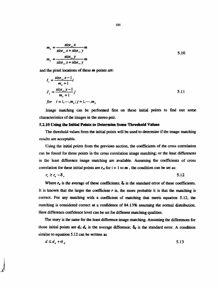
101

stze_x m m

size_x+size_y 5.10

m 'v s t z e y

m size^x+size_y

and the pixel locations of these m points are:

sire X — i

5.11 wiy +1

for i = =

Image matching can be performed first on these initial points to find out some

characteristics of the images in the stereo pair.

5.2.10 Using the Initial Points to Determine Some Thresiiold Values

The threshold values from the initial points will be used to determine if the image matching

results are acceptable.

Using the initial points firom the previous section, the coefficients of the cross correlation

can be found for those points in the cross correlation image matching; or the least differences

in the least difference image matching are available. Assuming the coefficients of cross

correlation for these initial points are ra- for i s 1 to m , the condition can be set as:

Where r, is the average of these coefficients; is the standard error of these coefficients.

It is known that the larger the coefficient r is, the more probable it is that the matching is

correct. For any matching with a coefficient of matching that meets equation 5.12, the

matching is considered correct at a confidence of 84.13% assuming the normal distribution.

Here difference confidence level can be set for different matching qualities.

The story is the same for the least difference image matching. Assuming the differences for

those initial points are d, is the average difference; 5^ is the standard error. A condition

similar to equation 5.12 can be written as

r > r - S ' c " 'a ̂r 5.12

d < d ^ + G j 5.13

102

Differing from equation 5.12, the smaller the difference is, the higher probability the

matching is conecL

After the results from the equation S.12 or 5.13 for the initial points are available, it can

also be used to check the points so that those initial points that do not meet the condition can

be removed. Sometimes, the matching could be wrong even when the matching shows very

good results with very large coefficients or small differences. To detect this, multi-method is

used which will be discussed in Chapter 7.

5.2.11 The Check Points Used in the Study

The check points are those listed in Table 4.8. Here the photo pixel coordinates and the

ground coordinates of these points on photographs in Figures 4.7 and 4.8 are listed in Table

5.1.

Table 5.1 Pixel and Ground Coordinates of Check Points

Point No. Photograph No. 1 Photograph No. 2 Ground Coordinates Pixel X Pixel V Pixel X Pixel V Xfmeters) Kfmeters) Zfineters)

161 274.87 732.37 238.62 594J7 1487237.63 1058922.25 292J36 162 145.62 2041.62 112.16 1903.26 I487217J8 1058522.38 290.903 172 1045.12 2201.37 1012.87 2064.12 148749425 1058487.00 290.216

1710 1588.12 775.12 1560.12 636.87 1487640.00 1058931.00 287.972 173 1799.87 3556.62 1780.37 3418.62 1487748.13 1058082.75 293311 1720 1533.62 2203.37 1500.87 2065.87 1487643.25 1058493J0 290.442 tll 836.25 698.25 800.67 560.41 1487408.13 1058941.00 291.952 tl2 114.75 2034.75 81.25 1896.75 1487207.88 1058524.00 290.925 tl3 362.75 3538.75 336.93 3400.67 1487305.88 1058068.13 286.917 tl4 1174.75 3480.25 1157.44 3342.74 1487555.25 1058096.63 282.400 tl5 1267.75 2021.25 1234.83 1882.79 148755930 1058545.13 290348 tl6 2412.25 1044.25 2391.02 905.04 1487898.63 1058862.75 284J79 tl7 2479.75 2969.75 2458.90 2831.48 1487947.88 1058273.13 284.149 131 682.25 1066.75 605.75 927.75 1487363.88 1058816.13 312.629 i21 137.00 1094.00 97.92 954.54 1487201.00 1058809.50 293.803 132 362.00 2247.00 300.00 2110.00 1487285.75 1058461.75 305.433 t22 482.75 2180.25 446.60 2042.01 1487322.13 1058484.88 292.270 t23 413.00 2805.00 377.50 2665.19 1487310.13 1058293.88 291.940 t33 1168.00 1979.00 1033.00 1843.00 1487513.00 1058547 J8 340.604 t34 1719.00 2623.00 1648.49 2486.05 14876%30 1058368.63 309388 G6 2042.00 1150.00 1991.00 1012.00 148777750 1058817.63 299.766 t24 2239.00 1853.00 2207.58 1713.81 1487853.88 1058610.75 289.705 t25 2371.00 2299.00 2349.25 2155.10 1487904.25 1058477.25 284.654 t26 2318.25 2859.75 2295.74 2720.31 1487896.00 1058304.50 285.056

103

From the previous chapters it is ioiow that the coordinates of these check points can be

considered correct. So they will be used in this study as the check for the image matching

results. As mentioned before, all the points beginning with "tl" are the highly contrasted

ground points; all the points beginning with "t2" are the ground points in the area of grass and

trees; and all the points beginning with "t3" are the points on the top of buildings. The highest

and lowest points in the above table arc 't33' and 'tl4* with the heights of 340.604 meters and

282.400 meters, respectively. Therefore the height variance of the area of interest is about 58

meters.

5.2.12 The Coniinon Area to Be Used to Create DEM

A smaller test area is selected from the rectified stereo pair to create the DEM. The

selected area is shown in Hgures 5.3 and 5.4. In this area almost all the types of ground

features in the flight project, such as buildings, roads, grass and trees, are available. So the

image matching on the selected area should be typical for the whole model area.

53 Condusioiis

Image matching is a process to find the best-matched point on the photograph to be

matched pixel by pixel in the searching range. Some initial parameters, such as the average

ground height, the ground variance, are set in this chapter so that the image matching can be

performed. A number of pixel points are used to determine the characteristics of the images in

the stereo pair. The threshold values used to check the matching results can be found from

these initial points. For this research, only 24 given points are used as the initial points. Both

the pixel and photo coordinates of the 24 check points are given. Two images in a common

area that can be used to create DEM are generated.

104

Figure 5.3 Selected Area firom Photograph No. 1

Figure 5.4 Selected Area from Photograph No. 2

105

CHAPTER6 BASIC BfAGE MATCHING ALGORITHMS

AND SEARCHING STRATEGIES USED

Only three types of area based image matching methods, cross correlation, least difference

and least square image matching, are used in this study. The methods to be discussed in the

following chapters can be ^>plied to any other area based image matching algorithms. Two

types of searching strategies, whole range and best-track, are discussed. The differences

between these image matching algorithms and searching strategies will be shown in the

matching results. The 24 check points given in the previous chapter are used as the matching

control points for checking the matching results. The height of each point after matching will

be compared to the correct height shown in Table S.l.

6.1 Cross Correlation Image Matching (CCIM)

6.1.1 Normalized CCIM Equation

The equation of cross correlation used here is the normalized cross equation shown in

Chapter I. The only difference is that the square of the coefBcient is used in order to reduce

the amount of computation, as shown in equation 6.1. ^^1 y=>i

r=*or=yo Jt=x, jr=y, isx, y=y,

6.1

x=Xoy=yo •«=^*=jro

Where gi(x, y), gzix-i, y-J) are the pixel gray values on the stereo pain i, j are the shift of

rows and columns on the image to be matched; (yi-yo+1) and (xi-JCb+l) define the window

size. The limits of i, j on the matched image is defined by the search range. The coefficient can

not be larger than 1. In order to find out the position i, j with the maximum coefficient value

within the searching range, all the calculated coefficients are compared. More information on

CCIM is given in Chapter 1.

106

6.1.2 Determimition of Locatkm for the Maximum Coefficient

The /, j from equation 6.1 must be integers if no interpolation is applied. Therefore the

precision of heights from the integer matching results are confined by at least one pixel. In

order to improve the precision of the heights, interpolation is used. Assuming the correlation

coefficients of the pixel position with the maximum coefBcient and these of two surrounding

pixels on the same row are found. The matched location should be within this range of three

pixels. In order to find the matched position, parabolic curve is used to do interpolation from

these three pixels. The formula for the i„ux is given by:

. ^ 3rO-l)-4r(i)-Hr(y-H) ^2 2(r(/-I)-2r(0 + r(i + l))

Where i-l, /, i+l and K'-l). KO, K'+l) are the pixel locations and the correlation

coefficients of the position with maximiim coeCBcient and the two surrounding pixels from

equation 6.1; /'max is the interpolated location.

6.U Determinatioii of Ground Height from i,j

Once the i, j have be determined, the height of a matched pixel can be calculated

by using equation 5.1. The epipolar photo coordinates for the pixels on the reference

image and on the matched image are given by;

~ •*" l ^ -^ A' -

Where Xio> X20 are the initial x coordinates of the photographs; Cxis the pixel size

in X direction; // is the x location of the pixel on the reference image.

Other information such as focal lengths, the airbase, flight, and the epipolar

rectification scale of each photograph are available fi'om the information about the

stereo pair.

6 ̂Least Difference (or Distance) Image Matching (LDO ̂

As discussed in Chapter 1, two types of algorithms can be used in LDIM. The normalized

equations used in the computer programs are shown in equations 6.4 and 6.5 as:

107

'̂1 y=yi Differenced, j) = X S

'̂0 ̂ >0

*='1 v=yi A = X

*='0 y^yo

gi(.x,y) g 2 ( x - i , y - j ' ) A ^

X=X, v= iy=yi 2 ̂ 8 2 ( ^ x - i , y - f ) '='ojr=yo

6.4

and

y=yi Difference(i,j) = X X

*=yo

n2

gi (x ,y ) X=X,v=y,

X ^ 8 z i x - i , y - j ) ^^y=yQ

6.5

All the symbols are the same as those used in equation 6.1 except At which is the sum of

JC ^ X V ^ V the pixel gray values for the pixels within the window around the pixel ( ° ~—!-) on

the reference image, is used to normalize the equations. The average pixel gray value on each

window is supposed to be used in the normalized equations to calculate the difference or

distance. Since the value of Ai is a constant for each particular pixel on the reference image, it

will be easier and faster to use the above format in the computation and will keep the same

scale in the comparison between values from different windows in the matching process. Also

the square of the distance in the equation is used for less computation time.

Similar to the process in section 6.1, in order to determine the ground height of each

matched point, equations 6.2 and 6.3 are used to interpolate the better matching position and

determine the parameters needed by equation 5.1 to calculate the ground height of the

matched point.

63 Least Square Image Matching (LSIM)

The LSIM has been discussed in Chapter 1. The equations used in the computer programs

and the problem solving procedures used are explained in this section.

108

6 J.l LSIM Equations Used

Assuming pixel location of xu yi on the reference image is conjugated with a location of

X2, yz on the image to be matched and the transformation relationship between them is:

X2=ao+fl,*i+a2yi y, =^0+^1-^1+^2^1

and the pixel gray values between them should have the relationship;

gi(Xi,yi)=^hog2iao +a,x, +a,y,,fco +^,y,)+/i, +n, -n, 6.7

Where gu gz are the pixel gray values on the reference and matched images, respectively;

oq, au 02, bo, bi, bz, ho, hi are the geometric and radiometric transformation parameters

between these two images; rit, no are the noise portions of the pixel gray values on these two

images. Using Taylor's series, for the estimated inidal position on the matched

image, the equation 6.7 can be written as:

(-fI. (^2 ' >2 ) + 'h ) + ^2 (^2 ' y" (-^2 • yl ^2r (-^2 . >2 )^X

+Ky\S2s^A^yl'^'i'^z +^)^2,•(^^3'2) '̂̂ o -^KxigzyXA^yl^^b,

+^0>1^2>(-*^2.y2)<'̂ 2

if all the small items, including n2-/ti, are neglected. So basically the least square equation

for a pixel on the reference image in a given window can be expressed as equation 8. Where

hl,h^ ,al,a^,al,bQ,b°,bl and Ao,A,,aQ,a,,a2,Z>o,fc,,fc, are the eight transformauon

parameters before and after each iteration respectively; dhQ,dh^,daQ,da^,da^,dbf^,db^,db^ are

the unknowns in the least square equations or the corrections for each transformauon

parameter, x,,y,is the location of the pixel on the reference image; x'.y" is the location

which is determined by the geometric transformation parameters on the matched image;

i2x(^2^y2)^i2r(-^2^yD derivatives along x andy directions at location on

the matched image, respectively. Once the initial location on the matched image or the initial

transformation parameters are determined, equation 6.8 can be used for all the pixels in the

window to solve for the unknowns iteratively. Since there are eight unknowns in equation 6.7,

at least 8 equations are needed. So the window size should be larger than 3 by 3.

109

-^Kyigix^Ayz'i^z

+Ksiyixl,yl)db^ •^t^x^g^^{j^y^)db^ •^hl^y^giy{J^,yl)db^ +dh^

= g i (-"^1. y I) - ( f ^ S i (j^. y")+^°)

HQ =^h^+dh^

h, =h°+dh,

flo =«o +^«o a, =a,°+<fo, 6.8

a, ~d\-¥- da^

b,=bl^db,

b, =b°+db^

b. =b^_+db,

x° =00 +fl,\ +a°y,

y°_=b°+b°x,i-b.y,

If the relative orientation of the stereo pair is good enough, and the stereo pair is in the

epipolar coordinate system, the transformation parameters az, bi in equation 6.6 can be

considered very small values and are ignored. Then the equation 6.8 becomes:

+Kxigz^{xl,yl)da^ •*-h^8zyix°,y°)dbo

ViSly.V z ) d b z + A = ̂ 1 ( ^ i . 3 ^ 1 ) - ( . K 8 z ( - ^ 2 ' y l ) + h ° )

h,=h^+dh,

h, =h^+dh^

^0 ~ ®0 •*" ^0 g g a, =0,° +<ia,

K-^K-^db, b. =b°+db.

x" =ao

yl=b',^bly,

There are only six unknowns in the above equation. Therefore the time spent in computing

will be less than time in computing the eight parameters equation 6.8.

110

63 J1 Determimition of the Initial Transformatioii Parameters in LSIM

Before the iterative process in solving equations 6.8 and 6.9, the mitial values of these

unknown transformation parameters must be estimated. These initial values can be determined

by other image matrhing algorithms like cross correlation or least difference, or they can be

obtained from the average ground height, and some assumption about the radiometric

parameters can be made. Hrst of all, before the first iteration, all the photographs in the stereo

pair can be considered at the same radiometric scale and no radiometric shift among them, so

the initial value of Aq, hi are;

= ' 6.10 h° =0

For the initial parameters from the average ground height, assume the rectification of these

photographs are nearly perfect, all the photographs have the same scale and not much y

parallax left, then the initial values of ai, uz, bu bz are:

a ° = 0 - 6.11

b° =0

b ^ = l

a, b arc actually the shift firom the location on the reference image to the estimated

location on the image to be matched. Equation 6.12 gives their initial values as:

lo _ ^01 ~ Vol 6.12 c—

Where t is determined by equation 5.4; yoi, yo2 are the initial epipolar ^ photo coordinates

for the reference and matched images, respectively; Cy is the > pixel size. Therefore, all the

unknown parameters can be initialized by using equations 6.10,6.11,6.12.

If the initial matching position for LSIM is given by other image matching algorithms, then

the initial pixel location and radiometric relationships are known. For example, assuming the

initial pixel locations on the reference and matched images are Xi, X2, yi, the equation 6.11

is still valid and hi is 0, then

A

I l l

«o

A.°=# gx

can be used to compute the initial values for oo, hi. Where g^ ,g2 are the mean pixel gray

values in the window for both images.

633 Pixel Interpolating and Resampling

Since the pixel location xz, yt calculated with equation 6.6 are no longer integers in the

iterative process, the pixel gray values on these non-integer locations in the window have to

be derived from the surrounding pixels by resampling and interpolation. If the interpolated

pixels are put in a matrix called win{1,7) for / = 0 to /n+l(number of columns^; / = 0 to n+l

(number of rows) as the size of the window, where m, n are the number of columns and rows

of the window used in the image matching, and bilinear interpolation which has been explained

in equation 2.13 is used, then from interpolation each pixel in the matrix winil, J) will have

pixel gray value as:

i = int(x, — OS) j = 'mt{y^ -0^

2

winU, /) = (1 - y, + j)({X - X, +0^,(/ + /'./ + /')+ (^2-i)gz (/ + /' + !,/ + J'i)

+(>2 - j) ((^^2 - + /' +1,/ + /' +1)+ (1 - X, + Og, (/ + /',/ + /' + D)

Here ij are the largest integers which are less thanx2,y2, respectively. After interpolating

with equation 6.14, all the pixels in the matrix win(J, J) can be used to generate the least

square equations for the next iteration, therefore in the following discussion, the matrix win(l,

J) is used instead of gz. Notice that the matching window is two pixels less than the size of

winil, J), which ranges from / s 1 to m on column and 7 = 1 to #i on row. Why the

interpolated window is two pixels larger than the image matching window will be explained in

the next section.

i A

112

6 J.4 Determimition of the Derivatives in x and y Directions

In equations 6.8 and 6.9, the derivatives in x and y of pixel location {Xt, yz) on the

matched image g2x( '̂y2)'̂ 2.r(^»3'2)2rc needed in order to solve the least square

equations. As shown in Figure 6.1, point 0,1,2 are three adjacent pixels with the values of >i,

yz, >3. If a parabolic line y = ax' -t-bx-hc is used to connect the three pixels, the constants a,

c in the equation are:

0 1 2

Figure 6.1 Determinatitm of Tangent at Point 1

c = y ,

2 ^ = >2 ->1

Then the slope at the point 1 is:

y, = 2ax-t-b = 2a-hb

Substimting a, b with yi, yz, >3 the above equation becomes:

So the slope at a pixel in a given direction is the half difference of pixel gray values of the

two pixels surrounding it in that direction. For those pixels on the edge of the matrhing

window, one more pixel outside the matching window boundary is needed to compute the

i

113

slopes of the edge pLxels. This is why the interpolated window is two pixels larger than the

matching window.

6.4 Searching Strategies: Whole Range and Best-track

Two types of searching strategies, whole range and best-track, are used in this study.

6.4.1 Whole Range Searching

In whole range searching, all the pixels in the searching range in both rows and columns

are used in the matching. As shown in Figure 6.2, once the initialization is done as described

Start

initialize the stereo model to get search limits of x, y; tranformation constant for estimating position on the photo to be matched

* row post'on = 0; column postion = 0 on the reference

photo

Estimate the initial matching position (x, y) on the photo to be matched

Using the initial position as center to search ail the pixels within the limit of x-x_range, x+x_range and y-y_range, y+y_range to find the pixel

with maximum coefficient

Figure 6.2 Flowchart of Whole Range Searching Algorithm

114

in Chapter 5, for each pixel on the reference photograph, all the pixels on the photo to be

matched within the defined search area will be used in the cross correlation process to obtain

the location with the maximum cross correlation coefficienL

In Hgure 6.2, x_range, y_range are used to define the searching range on each row and

column. The initialization process was described in detail in Chapter 5. As mentioned before,

the basic idea for the whole range searching is that all the pixels within the defined range will

be used in the matching process.

6.4,2 Best-track Searching

In the best-track searching, only the pixels on certain rows and columns are used in the

matching, as shown in Figure 6.3.

Start searching

Yes

find the maximum on row X as position (x, y')

find the maximum position at column y* as (x', y')

Rnd the maximum position on a initial row as (x. y)

Yes

r(x. y-) > r(x, y) ? r(x', y') > r(x, y') ?

No

i Stop No-

Figure 6.3 Flowchart of Best-track Searching Algorithm

115

The idea of the best-track searching is to follow the positions with maximum coefBcient

on the rows and columns until the largest is found. So the basic steps in the searching is to

find the position on a row or column with the largest coefBcient, then continue to search the

column or row from that position, and repeat the same process within the search limit until the

largest is located.

It is obvious that this searching algorithm wHi be faster than the whole range searching

algorithm. They will be compared in the next section.

6.4 J Comparison between These Two Types of Searching Strategies

The comparison is done in terms of speed and accuracy. As shown in Figure 6.4 a, it can

be seen that the best-track searching algorithm is much faster, on the average the best-track is

almost three times as fast as the whole range searching.

Figure 6.4 b shows the precision comparison of these two methods. When the window

size is less than 35 by 35, the whole range searching is obviously better than the best-track

searching, but there is almost no difference in the precision when the window size is larger

than 35 by 35.

Therefore, the conclusion here is the best-track searching algorithm is better than the

whole range if the matching window size is big enough. In this research case, the mininnnin

window size is about 35 by 35.

6.4.4 Comparison between x andy First Best-track Searching

The best-track searching algorithm shown in Figure 6.3 starts with x axis or rows, which

is called jc first best-track searching, bi the best-track image matching algorithm, either x ory

first searching can be used.

The comparisons between them on matching speed and precision are shown in Figure 6.5

a, b. These two figures show that they have no much difference on the time consumed, but the

precision difference between them is significant when window size is less than about 47 by 47,

the X first best-track searching has the better matching precision. So all the best-track

searching used in rest of the study refers to the x first best-track searching.

116

200 -p

180 -

160 -

140 --

•8 120 --

1 100 --

80 -

60

40 - •

20 -

0 -I"

-Best-oack •Whole Range

WimhnrSize

a. Time Consumed vs Window Size

25

-Best-track -Whole Range

WndowSiR " b. Precision vs Window Size

Figiire 6.4 Precision and Speed Comparison between Best-track and Whole Range

6 ̂Comparison between CCIM and LDIM

Generally speaking the CCIM has higher precision than LDIM but it is slower. In this

section the empirical matching characteristics of these two image matching methods are

discussed and compared using the search algorithms.

jL

117

6 .̂1 Correlation Coefficient Surface from CCBVl

Figure 6.6 shows the conelation coefficient surface from CCIM. The vertical axis in the

Figure is the coefBcient values; the x axis is the number of columns from the initially estimated

position on the image to be matched; the y axis is the number of rows from the initially

estimated position on the image to be matched. The width in the y direction is given by the

search range in y direction. The window size used here is 37 by 37 which gives the good

matching results in Hgiire 6.5 and in others shown later in this chapter.

H f n n t m n i I n n 1111 n i [ Mi Ml m f

B • - C M n ^ i o i o c o t ^ a S t t Window Sizr

—Besmack* — Best-ttacky

a. Precision vs Window Size

60

-Best-traclcx

Best-track y

Window Size

b. Time Consumed vs Window Size

Figure 6.5 Comparison between x and First in Best-track

118

From Hguie 6.6 it is obvious that the control points and the ground points have the best

correlation surface shape whose mountain peak gives a good location of the maximum and the

coefficient surface is more smooth. There is no big slope change in the correlation coefiBcient

surface from the control points and the ground points. The surface shape from tree and grass

points and the roof points of building are not so good because the correlation coefficients

change a lot in some areas, especially for the roof points. The grass and tree points are better

than the roof points since its peak location is more obvious and their surface is better than the

roof points; they also have more discontinuous surrounding features even though they may

have better contrasL Therefore the points with distinct and continuous surrounding features

will have the best matching results from CCIM.

Since there are four different types of ground features, for a point from a certain type of

ground feature, the correlation coefficient surface from CCIM at different window size are

shown in Figures 6.7,6.8,6.9 and 6.10.

The first point is the control point No. 1720. This is a control point in a center of a

sidewalk surrounded by grass. It is a point with good surrounding contrast and continuiQr. As

shown in Figure 6.7, the first matching window size is 3 by 3. The interesting thing is that the

correlation coefficient surface for the window of 3 by 3 looks just like the intersection on the

photographs. This also means the information available in the image matching is not sufficient.

The area outside the edge of the sidewalk has smaller correlation coefficients which makes the

sidewalks appear on the coefficient surface. The sidewalk appears on the coefficient surface

until the window size is about 27 by 27. On the other hand, the maximum of the coefficient

surface rises and becomes obvious with respect to the surroundings as the window size

increases. Therefore, for a point with good contrast and continuiQr to its surrounding, the

CCIM can give good matching results when the matching window size is larger than a certain

number, such as 11 by 11, in this smdy case.

The second point is also a point on the ground, point No. tlS. It is a comer of sidewalk

with tress and buildings nearby. In a small area it has good contrast, but the trees and

buildings bring a lot of surrounding discontinuity.

119

T -ilcp- the first point, the coe£5cient surface fixwn the 3 by 3 window size also shows the

shape of the ground feature. It is hard to tell where the peak is even at a window size of 11 by

11. The location of the peak appears clearly in the window size of 19 by 19. The second point

has the best coefficient surface shape when the window size is between 27 by 27 and 51 by

51.

After the window size increases beyond 75 by 75, the coefficient surface worsens losing

the peak because the discontinuous surroundings begin to be involved and this affects the

matching results. When the window size is between 19 by 19 and 51 by 51, the matching is

good because of the good contrast in the small area, but the matching worsens when the

window size is larger than 51 by 51 because mote and more discontinuity surrounding is

involved. From the above discussion the conclusion is that for points with some good contrast

and some discontinuity surroundings, the better the good contrast portion is in the searching

window, the better the matching result.

Figure 6.9 shows the correlation coefficient surface of the roof point No. t33 at different

window size. Actually this point is the top of the water tower. It is the highest point in the

ISU central campus area. So it has the most discontinuity surrounding, and it should have the

worst matching result. According to its height, the matching location should be located on the

left-hand side. Windows of 3 by 3 and 11 by 11 do not give the right matching results. They

give the right location of the maximum when the window size is between 35 by 35 and 75 by

75, even though the surface sh^ around the maximum is not good. It seems that the

discontinuity here causes too many variations.

Figure 6.10 shows the correlation coefficient surface for the point No. t24 which is a tree

and grass point. This point is on top of a small bush within a lawn, with tree and grass and a

little low contrast. From Figure 6.10 we see that it does not have a good correlation

coefficient surface until the window size is 19 by 19. Since there is not much discontinuity in

this area, the larger the window size, the better the matching.

From the above discussions on these correlation coefficient surface we see that the trees

and grass have low contrast and the buildings bring discontinuity to the matching

i

120

b- Control Point No. 1720 a. Control Point No. 162

c. Ground Point No. tl3 d. Ground Point No. tl5

e. Tree and Grass Point No. t23 f. Grass and Tree Point No. t24

g. Building Roof Point No. t33 h. Building Roof Point No. t34

Figure 6.6 Correlation Coefficient Surface from CCIM Window Size: 27 by 27

121

a. 3 by 3 b. 11 by 11

c. 19 by 19 d 27 by 27

e. 35 by 35 f. 51 by 51

g. 75 by 75 h. 83 by 83

Figure 6.7 Correlation Surface for Control Point No. 1720 at Different Window Size

122

a. 3 by 3 b. 11 by 11

c. 19 by 19 d- 27 by 27

e. 35 by 35 f. 51 by 51

g. 75 by 75 h. 83 by 83

Figure 6.8 Correlation Coefficient Surface at Different Window Size for Ground Point No. tl 5

123

a. 3 by 3 b. 11 by 11

c. 19 by 19

e. 35 by 35

d. 27 by 27

f.51 by 51

g. 75 by 75 h 33 33

Figure 6.9 Correlation Coefficient Surface at Different Window Size for Building Roof Point No. t33

124

a. 3 by 3 b. II by 11

c. 19 by 19 d. 27 by 27

mm

e. 35 by 35 f. 51 by 51

g. 75 by 75 h. 83 by 83

Figure 6.10 Correlation Coefficient Surface at Different Window Size for Tree and Grass Point No. t24

125

The larger window size is good for low contrast area, but it is bad for discontinuous

ground features.

6^ ̂Difference Surface from LDIM

Figure 6.11 shows the difference surface from LDIM. As in CCIM, the window size used

in the following figures is also 37 by 37. This is good for the comparison.

The difference surface from eight points of four different types of ground features are

shown in the Figure 6.11. Note that unlike in CCIM, the minimum value on the surface is used

in LDIM to locate the matching position.

For a given point, different window sizes give various difference surface, and the results

are compared. Figures 6.12, 6.13, 6.14, 6.15 give the difference surface from LDIM vs.

window size for each type of ground feature. The same points are used here as those in the

previous section for comparison.

Figure 6.12 shows the difference surface from control point No. 1720. The difference

surface gives good results at the window size of 3 by 3 even though the surface is rough. It is

obvious that the larger the window size, the better the matching because the surface gives

better location of the minimum as the window size increases. This is because the point is on an

open area with good contrast and low discontinuity. The LDIM gives the same matching

results as the CCIM does for this point.

Figure 6.13 gives the difference surface for the point No. tl5. Obviously the window of

size 3 by 3 does not give good matching result. Although window of 11 by 11 has a much

better result than window of 3 by 3, it is still not good enough. The matching gives good

result when window size is larger than 19 by 19. The best results are when the window size is

between 35 by 35 and 51 by 51, beyond that, the difference surface begins to worsen, and

finally at window of 83 by 83 some portion is eliminated because of the bad results from

LDIM. The conclusion is similar to that from CCIM.

Figure 6.14 gives the difference surface form the point No. t33. Since this point is the

highest point in this area, has large height difference, and is also surrounded by a lot of trees

and buildings, so it should have the largest discontinuity. This can be seen on the difference

surface at the window sizes of 3 by 3 and 11 by 11. The matching position should be on the

126

b. Control Point No. 1720 a. Control Point No. 162

d. Ground Point No. tl6 c. Ground Point No. tl3

f. Tree and Grass Point No. t24 e. Tree and Grass Point No. t23

g. Building Roof Point No. t33 h. Building Roof Point No. t34

Figure 6.11 Difference Surface from LDIM Window Size: 27 by 27

127

c. 19 by 19 d. 27 by 27

Figure 6.12 Difference Surface at Different Window Size for Control Point No. 1720

128

c. 19 by 19 d. 27 by 27

e. 35 by 35 f. 51 by 51

g. 75 by 75 h. 83 by 83

Figure 6.13 Difference Surface at Different Window Size for Ground Point No. tl5

129

a. 3 by 3 b. 11 by 11

c. 19 by 19 d. 27 by 27

e. 35 by 35 f. 51 by 51

g. 75 by 75 h. 83 by 83

Figure 6.14 Difference Surface at Different \^dow Size for Building Roof Point No. t33

130

c. 19 by 19 d. 27 by 27

e. 35 by 35 f. 51 by 51

g. 75 by 75 h. 83 by 83

Figure 6.15 Difference Surface at Different \^dow Size for Tree and Grass Point No. t24

131

left-hand side. The diCfeience surface is too rough to indicate where the minimum value is. It

is interesting that the window of 19 by 19 gives the right matching location which is located

on the left-hand side, but the windows of 27 by 27 and 35 by 35 do not give the right

matching locations. However when the window size is larger than 51 by 51 we again get good

results. This is because the discontinuity causes inconsistent results. Therefore LDIM is less

sensitive to the discontinuity than the CCIM.

The difference surface for point No. t24 is shown in Figure 6.15. The matching result is

not good until the window size is larger than 35 by 35. The matching result is better when

window size is between 51 by 51 and 75 by 75. However, when window size is larger than 75

by 75, even though the matching result is good, the difference surface shape begins to worsen

with the increase of the window size. It seems that the LDIM is more sensitive to the low

contrast than the CCIM.

The conclusions from the above discussion are:

• Good contrast is needed for a good matching

• CCIM is more sensitive to discontinuity

• LDIM is more sensitive to low contrast

Comparison between CCIM and LDIM in Terms of Speed

Figure 6.16 shows the comparison between CCIM and LDIM in terms of speed for all 24

check points.

The difference between them is not much. Since much time is consumed in normalizing the

results in LDIM, it seems that the LDIM is slower than CCIM.

6,5.4 Comparison between CCIM and LDIM in Terms of Accuracy

Figure 6.17 shows the accuracy difference between LDIM and CCIM for all 24 check

points. There is much difference when the window size is less than 31 by 31, or between 71 by

71 and 81 by 81, and these two methods match well when the window size is between 31 by

31 and 71 by 71.

132

Window SUe

Figure 6.16 Time vs. Window Size for Cross Coiielation and Least Difference

25

20

15-1

a> to CO o> m CM CM CO CO ^ ^ n o lo to to (O to QD Window Size

OQM

UM

Figure 6.17 Accuracy vs. Window Size between CCIM and LDIM

6.5J Comparison between CCIM and LDIM in terms of Accuracy for Different Types

of Ground Features

The comparison of accuracy for the four different ^pes of points with CCIM is shown in

Figure 6.18. According to the Figure 6.18 the roof points of buildings have the worst

matching accuracy, and the ground points have the best results because they are the comers or

intersections which can be correlated with no difficulty.

The comparison of different ground features with LDIM is shown in Figure 6.19. It has

similar results as CCIM except that ground points from LDIM are better.

J

133

6.6 image Matching Results from LSIM

The LSIM results mainly depend on the initial matching position. Here CdM, LDIM and

the estimate position from the average ground height are used as the initial matching position.

As mentioned before, 8 or 6 parameters can be used in LSIM, and different number of

iterations can be applied according to the real situation.

45 40 35

I 30 i 25

10

0 - WJv e I

Window Size

Control Mnts

Ground Raints

— — Tree & Grass

BuHingRoof

Figure 6.18 Accuracy vs. Window Size for Different Types of Ground Features with CCIM

ControtR.

Ground Pt

Tree & Grass

Buldng Roof

Windttw Size

Figure 6.19 Accuracy vs. Window Size for Different Types of Ground Features with LDIM

134

6.6.1 LSIM with Initial Position from tlie Average Heigiit

Figures 6.20 and 6.21 shows the comparison between 8 parameters and 6 parameters and

3 and 5 iterations. From Bgure 6.20 it is obvious that the combination of 6 parameters and 3

iterations is the fastest, and the one with 8 parameters and 5 iterations is the slowest. From

Figure 6.21 it is known that there is not much difference between 6 or 8 parameters and 3 or 5

iterations except that the 6 parameters have very a height difference around the window size

of 71 by 71.

120

100 •• /

I 80 -

« 60--

8 Parx & 3 tier. 8 Pafx & S Iter. '6 Para. Sc. 3 Iter. 6 Para. & 5 Iier.

^ C M A ^ I O ( O N . O O S O ^ Window Size

Figure 6.20 Comparison of Speed among 8 and 5 Parameters and 3 and S Iterations

30

0> ^ CO ® CM n to CO OD 9>

6 Para. & 3 Iter.

6 Para. & S Iter.

8 Para. & 3 Iter.

8 Para. & S Iter.

Window Size

Figure 6.21 Comparison of Accuracy among 8 and 5 Parameters and 3 and 5 Iterations

135

So 8 parameter method is better than the 6, and 3 iteration is enough if the solution is

convergent. The average accuracy here is about 6 meters which is worse than LDIM and

CCIM. From the above results we see that the combination of 6 parameters and 3 iteration is

good in most cases.

Since Hgures 6.20 and 6.21 only give the mean results of the different ground features, in

order to know more about each ^pe of ground feature, we show the comparison between

them in Figure 6.22. It is known that the roof points have the worst matching accuracy

probably caused by the discontinuity of the surrounding. The height differences are big for the

grass and tree points when the window size is less than 7 by 7. After the window size is larger

than about 39 by 39, the matching results stabilize around 2 meters except for the roof points.

Therefore the LSIM is not good for the image matching when there is a great deal of feature

dissimilarities around the points on the photographs in the stereo pair.

60

50 -e

Control Points Ground Points

•""••""Grass & Tree - - - BuidHgRoof

CO in Q ^ o 9 a> S o ^

Figure 6.22 Comparison among Different Types of Ground Features (8 Para, and 3 Iter.)

136

6.6 ̂LSIM with Initial Position from COM

Hgure 6.23 shows the LSIM of 8 parameters and 3 iterations using the initial position

from CCIM. It looks more like the results from COM.

6.63 LSIM with Initial Position firom Average Ground Height

Figure 6.24 shows the LSIM results of 8 parameters and 3 iterations using the initial

position from LDIM. Again it looks mote like the results directly from LDIM.

20

18

O) hw in CM w

a> rs. lo CO eo •• 00 a> a» a> Window Sise

Figure 6.23 Accuracy of LSIM (8 Para, and 3 Iter.) with Initial Positions from CCIM

18

16

14

12

10

8

6

4

2

0 CO to o CM ^ h*- lO n CO rv 00 O) a>

Window Siie

Figure 6J24 Accuracy of LSIM (8 Para, and 3 Iter.) with Initial Positions from LDIM

137

6.6.4 Comparison between the Results in Sections 6.6.1,6.6.2 and 6.63

As shown in Figure 6.2S, LSIM method with 8 parameters and 3 iterations has the fastest

matching speed among these three image matching methods. LSIM is time consuming if the

solution is not convergent or stable.

As shown in Hgure 6.26, LSIM with the estimate from the average height is not as good

as the CCIM and LDIM.

400

350

300 m e 250

I 200 150 «> g 100

50

Window Site

LSM OCM LOM

Figure 6.25 Speed Comparison among LSIM (8 Para, and 3 Iter.), CCIM and LDIM

25 •

e i*

s •»

s & s

WindoirSIze

LSM CCM LOM

Figure 6.26 Accuracy Comparison among LSIM (8 Para, and 3 Iter.), CCIM and LDIM

i

138

Hgure 6.27 shows the comparison between the CCIM and the LSIM using the initial

position from CCIM. From this figure it is seen that there is not much change after applying

LSIM to CCIM. The comparison between the LDIM and the LSIM using the initial position

from LDIM shown in Figure 6.28, does not show much improvement after applying the LSIM

to the LDIM. Compared to the LSIM results with the initial position from the average height,

different initial positions let LSIM give out different results. Therefore LSIM is very sensitive

to the initial location, and if the initial position is good, there is not much improvement from

LSIM.

30

25 -

20 LSIM with CaM

COM

10 •

n n o CO ^ lo (o CO W w OO 0) o

CO W W CO CM CO

Window SUe

Figure 6.27 Comparison between LSIM (8 Para, and 3 Iter.) with CCIM and CCIM

LSIM witli COM

COM

Window SIxe

Figure 6.28 Comparison between LSIM (8 Para, and 3 Iter.) with LDIM and LDIM

139

6.7 Conclosioiis

From the above discussion on the three ^pes of image matching algorithms, we can

conclude:

• LSIM is the fastest of the three methods tested

• LSIM is sensitive to the initial position

• The results from CCIM or LDIM can be used as the initial position of LSIM, but there is

not much difference from LSIM

• From the results shown in Figure 6.22, the building roof points have the lowest accuracy.

Therefore LSIM is sensitive to the discontinuity of the feature on the photograph

• The roof points have the lowest accuracy in LDIM and CCIM, So discontinuiQr on the

photographs can cause errors in the image matching.

• There is a range of window size which has the best matching results. In this case, the

range of window size is from approximately 31 by 31 to 71 by 71.

• Good image matching needs (a), sufficient information for the matching (b). good

contrast, (c). and little discontinuity

140

CHAPTER 7 MULTI-METHOD IMAGE MATCHING

The conclusion of the previous chapter is that different image matching algorithms differ

in sensitivity to the same types of error on the photographs. Since the errors in different types

of image matching methods even when they are from the same data source can differ, the

comparison between them could show some of the errors. Therefore this method can be used

to eliminate some bad matching results.

There are several ways of getting the difference from image matching techniques. As

mentioned before, different image matching algorithms can be used in the comparison.

Different window sizes in the same image matching algorithm can also used in the comparison

to remove bad matching results; or different searching algorithms can be used in the same

window size and the image matching algorithm. Different combinations of these can be used

for the largest difference between the matching results to get the best matching. In this

research only the different image matching algorithms with the same window size and

searching algorithm are described.

The combination methods are slower than the single methods, so they suitable for some

kinds of work such as automatic relative orientation, determination of the optimal image

matching window size for the current stereo pair and for matching some initial points as the

Hrst part of the image matching process, and so on.

7.1 Multi-method Image Matching (MMIM) with Whole Range Searching

Methods such as the signal to noise ratio are used to evaluate the matching results. In this

section multi-method image matching is described. The so-called multi-method image

matching employs more than one image matching algorithm to do the image mafching and the

matching results are compared, so that the evaluation of the matching results can be done.

7.1.1 Determination of the Threshold Value for the Difference

Assume the CCIM and LDIM and the whole range searching algorithm are used in the

multi-method image matching (MMIM). In order to perform MMIM, the threshold for the

difference between the matching results from these two matching methods needs to be

141

defined. There are two ways to do so, one is to define the ground difference, the other is to

determine it by statistical analysis.

In the first, assume the difference on the ground is the heights from CCIM and LDIM

for the processed points are he, hi, respectively, then if

\h^-h,\>&h 7.1

for one point, then the matching result for the point is not good. The mean of these two

marching results is taken as the final matching result. Hgure 7.1 shows the histogram of the

difference between LDIM and CCIM for all the 24 check point in the range of window size

fi-om 3 by 3 to 95 by 95. Since in Rgure 7.1 the differences for most data are 0, only a few

matching results have large differences between LDIM and CCIM. So the threshold can be

used to remove the matching results with such differences.

L Bg 163 344 agS 406 487 588 649 730 ai1 aflg 973 1QS1113S

Figure 7.1 Histogram of Difference between LDIM and CCIM

To determine the value of the bh, the expected height accuracy is considered. For

example, if a height accuracy of 0.5 meter is expected, then the value of tsh should be less

than 0.5 meter. Since most of the differences are 0, the values of AA will not gready affect the

multi-method matching results, which means that the value of threshold can be in a relative

large range and a few points eliminated.

4 a.

142

Using statistical techniques to detennine the value of Ah, we assume there are n initial

points used and their differences are A/i, for t = 1 to 20. The standard deviation 5 and mean m

for the results of these twenty points can be calculated, then define the as

7.2

Doing so we can define the matching result in more than two categories such as good, fair

and poor. Since the Ah and the matching accuracy are not directly related, the second method

may not be accurate.

7.1,2 Matching Differences and the Window Size

Figure 7.2 shows the mean of differences between LDIM and CCIM Vs. the window size

for the 24 check points.

4 ••

zs V w s e & a

2 -

f

m

Figure 7.2 Matching Difference between LDIM and CCIM vs. Window Size

In Figure 7.3 the differences are displayed in four categories according to the type of

ground feature. All the results shown in the Figures 7.1, 7.2 and 7.3 are the differences

between LDIM and CCIM without modification. From Figures 7.2 and 7.3 it is knoMm that

the matching differences are large except in the window size of around 37 by 37 and 71 by 71.

The matching difference for the ground points is less than that for others. Comparing Hgures

7.2, 7.3 and 6.17, matching is good in the similar window size range. The similarity between

them shows that the best window size range can also be obtained by analyzing the difference

143

between the matching results of LDIM and CCIM for some initial points, although the correct

heights of these initial points are not known. This conclusion gives one possible method to

determine the optimal window size for the image matching.

Figures 7.2 and 7.3 only show the relationship between the matching differences and the

window size. They can not tell how much the multi-method improves matching accuracy. This

will be discussed in the following sections.

16 -

E 12 Grouiid Poims Building Roo6

e 10 -

4-

m lO a> CM lO CM to

Window Sice

Hgure 7.3 Matching Difference between LDIM and CCIM vs. Window Size for the Four

Types of Ground Features

7.13 Improvement of Accuracy by the Multi-method

The accuracy comparison for A/i s 0.5, 1 and 2 meters is shown in Figure 7.4. From

Figure 7.4 it is seen that although the threshold values are different, the accuracy difference

between them are small almost throughout the whole range. Figure 7.5 shows that the number

of points removed because they exceed the threshold value is the same for these threshold

values. Beyond window size 41 by 41, no points exceed the threshold value.

144

30

25

20 •OJM

-1.0M

2.0M

a> r - i o m ^ o r ^ - i o m ^ • - c a m i - i n i o c o r - t D O ) Window Size

Figure 7.4 Comparison of Accuracy between Different Threshold Values

18

16

14 14

g 12 i

12 w a: 10

£

£ e 3 z

Window Size

Figure 7.5 Number of Points Removed for Different Threshold Values

Figure 7.6 shows the accuracy comparison between CCIM and MMIM for A/z = 0.5M.

When the window size is less than 27 by 27, the MMIM is better than CCIM even by a few

meters at some window sizes. The difference after the window size of 75 by 75 is about a few

meters. When the window size is between 31 by 31 and 73 by 73, the difference is at a

minimum of about half a meter. According to Hgure 7.5, the number of points removed

diminishes with increase of the window size, and the accuracy of MMIM increases slowly.

145

The reason for the lower accuracy of CCIM is that a few points have large differences

between the matched locations and the actual ones. Therefore MMIM can help to remove

some of the points with bad matching results.

In Rgure 7.6 the CCIM has higher accuracy than MMIM for some window sizes. This is

the MMIM take the mean of LDIM and CCIM as the final matched location. If the

LDIM results are worse than the CCIM, this will happen.

30

25

t 20

S

< 5 -

A S •- a> lO Id (D CM

n

Window Size

Figure 7.6 Accuracy Comparison between CCIM and MMIM with Ah = 0.5M

From^ the above discussion we see that the MMIM can improve the matching by increasing

the matching accuracy when the window size is large, and the difference curve is similar to the

accuracy curve described in chapter 6 so that it can be used to determine the optimal

searching window size. The obvious disadvantage of MMIM is that it is slower than the single

method image matching because it employs more than one image matching method.

7JS Multi-method Image Matching with Best-track Searching

The idea in the multi-method image matching is to make use of the differences from the

image matching algorithms so that the errors in the matching can identiiy the matched position

from different matching algorithms. In this way the incorrect points can be detected. The

previous chapter shows that the best-track searching algorithms have less constraint since only

146

the pixels on some rows and columns are used in the matching. So perhaps best-track method

can reveal mote differences between COM and LDIM.

7 .̂1 Matching Difference Vs Window Siie witii Best-tracic Searciiing

The comparison between the whole range and best-track searching algorithms is shown in

Figure 1.1. According to Figure 7.7, the height difference from the best-track is much larger

than from whole range searching, though from their trend that they have the same pattern can

be seen. The best-track can have a large difference between the two matching methods m

MMIM. It will give better results if these differences reflect the impact from the errors on the

image matching algorithms and not from the mismatching.

Figure 7.8 shows the comparison between whole range and best-track using MMIM for

Ah=0.5 M. It is obvious that the best-track has a more unstable accuracy when the window

size is less than 35 by 35. But the difference between these two methods is very small when

the window size is larger than 35 by 35. The matching results from best-track is better than

the results from whole range searching when the window size is large. So the unstable

matching results from the small window size is because of the mismatching. When the window

size is big enough, the mismatching is less, and the large difference from the best-track gives

better matching results than whole range.

20 J 18

_ 16 e ....

—Whole Range

Best-track

Window Site

Figure 7.7 Comparison between Whole Range and Best-track Searching for MMIM

147

e ——Whole Ftange

Best-vack >k W e 9 10 -w V < S '

in « CM CO ̂

Figure 7.8 Accuracy Comparison between Whole Range and Best-track with MMIM for Ah s

0.5M

As shown in Figure 7.9, the best-track has a almost linear relationship between time

consumed and the window size. The relationship between speed and window size for whole

range is that the square of the time consumed is proportional to window size. So the larger the

window size, the slower the whole range searching. Since the best-track searching is much

faster than the whole range searching, especially for large window size, it could be used in the

matching of the initial points, and for the whole stereo pair.

700

600

Best-track

Whole Range 400

200

100-

n n n CT cvi n

W W W CO ̂ to

Window Size

Figure 7.9 Speed Comparison between Whole Range and Best-track Searching

148

13 Determinatioii of Optimal Matching Window Size

Since area-based Image marrhing js peifonned on a number of pixels in the certain area

defined by the searching window, the matching process is affected by the qualiQr of the

photographs used in the matching, types of the ground features, scale of the photograph,

marching algorithms, searching strategies such as the searching range in both directions, and

the window size. Apparently, the window size determines the information which can be used

in the matching. For a certain area of a photograph, there should be an optimal window size

for the best matching results, for a stereo pair, there should be a window size for the best

matching in terms of statistics. Multiple window sizes for a stereo pair can be considered if the

selected area contains different ^pes of ground features with different characteristics. In this

case, the division of the area is the first step that should be done. Only one optimal window

size is described here.

7,3.1 Window Size and the Signal to Noise Ratio (SNR)

Since window size actually contains the information used to do the image matching, the

Signal to Noise Ratio (SNR) determines the amoimt of correct information in the matching.

The inforaiation in a window consists of (1) background noise; (2) correlated information; and

(3) uncorrelated information. A good matching requires (a) enough correlated information and

(b) enough SNR. The first means that the correlated information in the window on each

photograph in the stereo pair needs to be large enough for the matching; the second means

that the ratio of correlated information to the uncorrelated information and the background

noise also needs to be sufficiently large. The background noise is firom any noise that could

appear in the data processing such as in film exposing and developing, imagery scanning and

so on. The correlated information is given by the similarity of the pixels in the windows during

matching. The uncorrelated information could come from different sources such as ground

relief and wrong window position. The coefficient can not be one even for both windows on

the same spot on each photograph in the stereo pair because of the change of brighmess

between the exposures, and the geometric and obstruction changes caused by the different

exposure positions. So the uncorrelated information and the background noise can be

considered together as matching noise. The SNR is the ratio of correlated information to the

149

matching noise. So the optimal window is the combination of larger SNR and proper

processing speed.

In terms of correlation coefficient the SNR can be written as:

2 SNR- =-^

for the cross correlation image matching. Therefore the larger the re, the larger the SNR.

Normally smaller window can have higher because of less matching noise and more

similarity as there are fewer elements in a smaller window. Figure 7.10 shows the relationship

between the window size and the value of tc. The coefBcient tc drops from almost 1 to 0.97

when the window size is about 113 by 113.

So the larger the window size, the smaUer the SNR. But SNR only gives the evaluation on

the fitness of the correlation between the two windows at a certain window size, which does

not necessarily mean that the larger window will give the worse matching results. Only the

SNRs of similar window sizes can be compared.

0.995

S 0.99

J 0.985

s 0.975

i 0.97

I 0.965 W 0.96

0.955

CM CO CD

CO CO CO

CO 01 CO 00 CO o CO

Window Size

Figure 7.10 Correlation Coefficient vs. Window Size

In order to get the best matching result, the largest ratio between correlated and

uncorrelated information is needed. The assumption here is that, at first, the correlated

information increases faster than the uncorrelated information as the window size increases

when the window size is small, the ratio increases until to its maximinn with the best matching

150

results. After the window size with the maicimum ratio, the uncorrelated information increased

faster than the correlated information and the matching worsens. The relationship between the

window size and the mean of the height differences between the matching results and the

correct heights for these check points is shown in Figure 7.11 using the cross correlate image

mafrhing method. In this stereo model, the mean of the height difference for the smallest

window of 3 by 3 is about 18 meters, then it drops to about 4 meters at the window between

7 by 7 and 9 by 9. It has the smallest height differences at the window sizes between 31 by 31

and 77 by 77, thereafter the difference increases to about 4 meters.

From the previous discussion it can be concluded that fix)m window 3 by 3 to 7 by 7, the

correlation increases; from window 7 by 7 to 17 by 17, the uncorrelated information and noise

increase faster than the correlated information; from window size of 13 by 13 to 31 by 31, the

correlated information increases faster than the uncorrelated information, so the height

difference is decreasing; the increase of all the information remains balanced from window 31

by 31 to 77 by 77, then uncorrelated information is increasing faster than the correlated

information and the accuracy is decreasing. From the Figure 7.11 it can be concluded that

after a certain window size, the image matching gets stabilized. This conclusion is based on all

the 24 check points.

e 1 2 -

6 --JS A -

Window Size

Figure 7.11 Mean of Height Differences vs. Window Size

151

At each point, the balance between these types of information will be different depending

on the type of the ground feature.

7 Use MMIM to Determine the Optiiiial Matching Window Size

The curve shown in Figure 7.11 is not known in real cases. Therefore it is not possible to

use it to determine the optimal window size. From the above analysis we know that the

difference between LDIM and CCIM is at a minimum when the window is the optimal size.

Therefore the difference between LDIM and CCIM can be used to detect the optimal window

size. The similarity between the height difference curve from MMIM and the accuracy curve

in Chapter 6 has been mentioned.

30

25

lo r» »- CM CM S® US ̂<o eo OD

-5

-CCIM

Window Size

Figure 7.12 Comparison between Difference from MMIM and Accuracy from CCIM

As shown in Hgure 7.9, both curves have the stable low values in the same area. In other

words, they have the same pattern. It seems that the low area of MMIM curve is covered by

the low area of CCIM curve. This finding can be used to determine optimal window size for

image matching. Note that in Figure 7.12 the curve of CCIM is accuracy vs. window size, the

curve of MMIM is the difference between CCIM and LDIM vs. window size.

i

152

The procedure used to determine the optimal window size is described by the flowchart in

Figure 7.13. Basically, it looks for the smallest matching window size with a low and stable

difference between CCIM and LDIM in MMIM. Since the difference shown in Hgure 7.12 for

MMIM could be small before reaching the range of optimal window size, we must ensure that

the low difference is stable. Before determining the optimal matching window size, a certain

number of initial points should be selected on the stereo pair to be matched.

( san )

low & Stable? No-» No

Yes

No

Stop

/^larger than\ maximum window

size?

Failed

Window size increases by two

Use the last window size as the optimal window size

Given window size range and do the loop

Select certain number of initial points on the reference photograph

Ftfid the difference using MMIM and compare with the previous difference

Figure 7.13 Flowchart of Using MMIM to Determine Optimal Window Size

7.33 Use Number of Points Agreed in MMIM to Determine the Optimal Window Size

Assume that the matching has the most correct position when the SNR is the largest. So

there are the most agreed positions when SNR reaches the maximimi because of the

uniqueness of correct positions. Therefore, the window size of maximum SNR can be

determined by comparing the matching result between consecutive window sizes. As the

£

153

window size increases, the SNR may be decreasing because of more similarity than the

dissimilarity; therefore the number of agreed points may be increasing. The optimal window

size is detected if the matching from two consecutive windows agree the mosL It is possible

that there are many optimal window size at which the matching is good, and only the smallest

is used. Therefore, to search for smallest optimal window size is to search for the first

maximum number of agreed points. The flow chart of this process is shown in Figure 7.14.

Any area-based image matching algorithms can be used in this process.

Since the ratio of similariQr to dissimilaii^ varies when the window size changes from

small to large, a false maximum could appear, as shown in Figure 7.16. To remove the error

of the false maximum, a number of window sizes will be checked after the first maximum is

reached. If the previous maximum is exceeded at a larger window, then this number is taken

as the new maximum and the same procedure is repeated until no new mayimum is found. The

number of window that needs to be checked depends on the number of initial points and the

images. For the case shown in Figure 7.16 eight more windows are sufficient Therefore, we

used 10.

To distinguish the MMIM for consecutive windows from the MMIM discussed before, we

call the former double MMIM, and the earlier single MMIM. Double MMIM means there are

two threshold values used in the process of matching, one to check the matching difference at

the same window size when doing MMIM, another one to check the matching difference

between the consecutive window sizes.

Figure 7.15 shows the relationship between the window size and the number of positions

matched using double MMIM and the whole range searching algorithms. Figure 7.16 shows

the results from best-track. Although they do not have a similar curve pattern, their first

maximum occurs at almost the same window size. So the best-track searching can be used

instead of the whole range searching because of its faster speed. Since the best-track searching

has a large difference between the two image matching algorithms in MMIM than that with

whole range searching method, the number of agreed points in Figure 7.15 is more than in

Figure 7.16.

154

If the process shown in Figure 7.14 is used to search the optimal window size then, from

Figures 7.1S and 7.16, the optimal window size will be about 33 by 33 which matches the

optimal window size obtained in the previous discussion.

As shown in Hgure 7.17, double MMIM can improve the matching accuracy when the

window size is small, in this case, less than window size of 29 by 29. When the window size is

larger, the difference between them is not significant although the result from MMIM is still

less than that from CCIM.

START

n = 3

n = n+ 1

No n = n + 1

Yes No

tw maximum > m

Yes Yes

No

new m < old m ?

Use n - 1 as the optimal window size

keep new maximum as new m and new window size n

Keep m as the maximum, searaching 10 more window size, look for new maximum

Do Image nutching with CCIM & LDIM for window size n

Do Image matching with CCIM &. LDIM for window size n

Compare the results from the above previous matching, keep the number m of points matched within a certain distance

Figure 7.14 Flow Chart for Determing the optimal Window size Using Double MMIM

155

16

£ 1 2 -

1 10 i

N" n O) CM

«n « lO to o o> <o o Window Sise

Figiue 7.15 Number of Point Agreed in Double MMIM with Whole Range Searching

a 10 -•

8 -

N. ^ 65 S S Window Size

at

Figure 7.16 Number of Agreed Points in Double MMIM with Best-track Searching

7.4 Test on Random Selected Points

The above conclusions are the matching results fix)m the 24 check points. In this section a

number of randomly selected points are used to test these conclusions.

Since the 24 selected check points have relatively good location or contrast which the

randomly selected initial points of the real situation may not have, it is necessary to test them

on the randomly selected initial points. These initial points are evenly distributed over the

whole reference image.

156

—Single MMIM

DonUeMMIM

Window Size

Figure 7.17 Comparison between Single and Double MMIM

18

16 -

^ u - .

4 •• 2

« CO CO « ^ lo (O Window Size

« CM

CO CO

«

Figure 7.18 Difference Curve for Different Number of Initial Points

7.4.1 Difference Curve for Different Number of Initial Points

Figure 7.18 shows the curves for differences Vs. window size for 25, 36 and 49 initial

points. Since the best-track searching is used these curves are not very stable, but they all have

the same pattern. The optimal window size using varying initial points is different, but they are

all in the range of good matching results. According to Figure 7.7, the matching difference

from the best-track searching is not as stable as that from the whole range searching, so it may

be better if the whole range searching is used.

25

20

IS

5

0 C » lO e I to CM

157

Another problem here is how to determine the optimal window size using the curves in

Figure 7.18. Unlike the curves in Figure 7.7 in which the optimal window size is easy to

select. Some statistical method may be needed to determine the optimal window size.

7.4 ̂Number of Agreed Points for Different Numiier of Initial Points

Figure 7.19 shows the number of agreed points Vs window size for different number of

initial points for different threshold values.

The first two lines in Hgure 7,19 shows the comparison between AsO.SM and A-l.OM for

25 initial points. It is understandable that the curve from A=1.0M is above that from A=0.5M

because the threshold value for the latter is larger. But the optimal window sizes from both

are almost the same, which is around 41 by 41. 16 initial points are also tried but no result is

available. From a statistical point of view, the similar results can be obtained if the number of

initial points is sufGcient.

. Window Siie

-25Pt,0.5M

-2SR.,1.0M

36R..0.5M

'49Pt.0.5M

Figure 7.19 Number of Agreed Points vs. Window Size for Different Number of Initial Points

According to Figure 7.19, the optimal window size obtained from different initial points

vary but are very close, in the range 41 by 41 to 47 by 47.

According to the above results, the optimal window sizes from those randomly selected

initial points are larger than those from the 24 check point. Statistically the number of agreed

Jit

158

point decreases after a certain window size since the noise or dissimilarities will be more than

the similarities after that window size. Unlike the 24 check points, some of the randomly

selected initial points may have low contrasts, so a larger window might be needed to get the

optimal matching results. The optimal window size is larger for the randomly selected initial

point, which is closer to the real situation.

73 Conclusioiis

From above discussions it is known that the MMIM can be used to determine the optimal

window size according to the difference between the image matching algorithms in the

MMIM. A different number of initial points can be used in the MMIM process. This is an

automatic process which does not receive a priori knowledge of the height control points.

159

CHAPTERS UNSQUARE WINDOW IMAGE MATCHING

The windows used in the previous ch^ters were squares with equal number of rows and

colunms. As mentioned in Chapter 5, the window with more rows than columns should be

better than the square window, bi this chapter the comparison between them will be

presented.

8.1 Unsquare Window Image Matching

Assume the pixel is a square, then in an unsquare window the number of rows is not equal

to the number of colunms. After epipolar rectification, the x axis is along the flight direction.

As discussed before, for the photographs in the same stereo pair the x parallax is much larger

than the jr parallax because of the larger difference in distance in the flight direction. So unlike

in the case of x direction, the viewing angle in direction is almost the same for every point,

and the obstruction for its image on the photographs in the stereo pair should be almost the

same. The conclusion here is that there are more similarities in the > direction than in the x

direction. The window should extend more in the direction of y axis, and the window with

more rows will give more useful signals than the square window does when the number of

pixels are the same.

In the following discussion, m will be standing for the number of columns of the window,

n will be the number of rows of the window. It is a square window if m - n.

When m > n we shall refer to it as x window. When m < n it is called > window. For the

same 24 check points the image matching results will be compared.

Unlike in square window, the number of pixels and not the window size is used here as the

X axis of the figures in the comparison.

160

&2 Comparison between Different Types of Unsquare Windows

8J2.1 Comparison iietween tiie Mean Values witli Fixed Number of Rows and Columns

One way to analyze the unsquare window is to get matching result by keeping one

dimension and increasing the other. The matching results with fixed number of rows and fixed

number of colunms are compared.

Figure 8.1 shows the comparison between the results when the number of columns is

fixed.

20

18

16

e

i s

"•null • - 'ins21 —111=31

- 111=51

0 liiiiiiiiiiiwiiiiiiiiiiiiiiiiiiiiiiiiiiiiiiiiiiiiiiiiiiiiiiiiiiiiiiiiiiiiiiiiiiiiiiiiiiiiiiiiiiiiiiiiiiiiiiiiiiiiiiniiiiiiiniiiiiiiiiiiiiiiiiiiiiiiiiiiiiiiiiiiiiiiiiiiiiiiiiiiiiiiiiiiiiiiiiiiiiiiiiiiiiiiiiiiiiNiiiiiiiiii

Ninaberaf Pfttb

Figure 8.1 Results for Given m

The window with m s 51 has the best precision of about 6 meters when the number of

pixel is less than about 200. After 200, with m = 11 precision increases rapidly to about 2.5

meters. All the curves have almost the same precision when the number of pixel in the window

is large. It is obvious that the curve with m s 51 is the most stable, although it has the lowest

precision when the pixel number is larger than about 2300. The above figure shows that as the

I

»

•I

161

number of rows or n increases and the number of columns or m remains constant, the

matching precision improves.

Since the roof points have the most height variance in the matching window, the results

for the building roof points for different m values are shown m Figures 8.2 a, b, c and d. The

curves for m = 11 and 21 decreases when the window size in the direction is about 15

pixels. For m ^ 31, the curve decreases when the window size in y direction is about 26

pixels. For m =: 51 the window size in> direction is about 12 pixels when the curve begins to

decrease. The curve form — 51 looks more stable than others, but it has a little larger errors

than the others.

Number of PiMIs

a. Results for Building Points for m = 11

n lo ^ 9 CO ^ (p ^ CO SS CO ^ « lO r^ ^ ^ C5 & ^ lO CD o n ̂ ̂ ̂ cQ CM

Nunbcr or Pixels

b. Results for BuUii^ Points for m = 21

35 ^30 S 25 I S 20 \

ic . A IS 10 5 0 l i i imii

O W ^ W s « « $ s s s $

lO t ® •• M oi e ^ N S n S

Number of Pixels

c. Results for Building Po^ for m = 31

rt CO w CO CO CO w w SK 9 O) O ̂ CM 9$ 3) rr ^ ̂ ̂ CM CM CO « V

Nomiier of Pixels

d. Results for Building Points for m = 51

Figure 8.2 Results for Building Roof Points for Different Values of m

i

162

Figure 83 shows the comparison between the results when the number of rows is fixed.

Compared to the results shown in Figure 8.1 it has much lower matching precisira. In the

beginning all the curves except n s 11 drop fast This is because that the number of rows for n

= 11 is too small, the information for matching from the jr direction is not sufBcient. the curve

forn - 11 starts to drop at the pixel number of about SOO, Since the number of rows is fixed,

and does not increase with the window and the number of columns, the information ratio

between x and y will decrease as the number of pixels increase. Because of this, the best

precision for n = 31 and 51 is about 2 meters; and for n s 21 and 11 is about 4 meters.

u-ll 11=21

- - n=3I n=SI

0 liiiiiiiiiiniiiimiiiiiiniiiiiiNiiiiiiiiiiiiiiniiiiiiiiiiiiiiiiiiiiiiniiiiiiiiiiiiiiniiiiiiniiiiiiiiMiiiifliiiiiiiiiiiiiiiiiiiiiniiiiiiiiiNiiiiiiiiiiniiiiiiiiiiiiiiniiiiiiiiiiiiiiiiiiiiiiniHiiiiiiiiiiiniiiiiiiiii lO A a» M n in CM O 11) Q) n ^ to

Number of Pisds

Figure 8.3 Results with n Fixed

Figure 8.3 shows worse results than that shown in Figure 8.1. In Figure 8.3, all curves

rise sharply when the number of colunms is about 80. The main reason for this is the sharply

elevated roof points, they have the worst results through the whole range of pixels. The

ground control points do not have good matching results until there are about 1400 pixels in

the window. This is because the roof points have the most ground height change and so they

have the most dissimilarities in the x direction. When the window size in Jt direction is larger

163

than a certain number, the matching precision will drop due to the sharply increasing

diigsiinilarities. Since these ground points are selected as comer points or intersection with

good contrast, they have good matching results. The control points are targeted points on the

ground which do not necessarily have good contrast.

Hgure 8.4 shows the precision between the four different types of ground features for n =

51.

~ ~ " Conlrol Points Ground Potnts

"Grass iTree Buflding Poims

S^ a > r > . i n n < - o r ^ i o « > - o ) r > . « m K < o a > o S ^ M m « v i n Number orPfnls

Figure 8.4 Comparison between the Four Types of Ground Points for Number of Row n = 51

Figure 8.5 shows the results for the four types of groiud points for n = 11. Compared to

Figure 8.4, only the ground points still have good matching results. In fact, the ground points

have better matching results in Figure 8.5 than it is in Figure 8.4. Because in the feature the

ground points have good contrast in a small area. As the matching window increases, the

contrast could decrease. The curve for roof points also rises sharply when the number of

columns of the matching window is about 80 pixels. Even considering the different scales of

the X axis, the ground points have the best results shown in Figure 8.5.

25 '•

e s e e 3

I 10 -

164

* * Coamt Points CiDund Mots

• • - - -Gfass&Ttee •""Buifcliiig Poiws

n « - s ^ i a n ^ d > N . u ) n f a i K - ! S ^ s i i s s i ^ s s s s i s s s B s

Nmniicramwb

Figure 8.5 Comparison between the Four Types of Ground Points for Number of Row n =

M ( M ! I M M H-+- t ( { I i M < I i f H '

2A i A ^ ^ m a i o ^ K > c o ® 5 5 8 a T : a ^ t r ® -NamberorPixcb

a. Results for Building Points for n =21

SO) m ^ rx- m CM ̂ (O

n A M ^ s s i i s

a II) ^ K-n M ^ o> ^ H m (o CM CM CM M

wj § i

Number of Pisds

b. Results for Building Points forn s 31

Figure 8.6 Results for Building Roof Points for Different Values of #i

165

Figuies 8.6 a and b show the results for roof points forn s 21 and n s 31. Comparing the

curves for building roof points in Hgures 8.4, 8.5, 8.6 it can be seen that the best results are

when n is the largest number, 51; and the worst results are when n is the smallest number, 11.

Also comparing these with the results shown in Figures 8.2a to 8.2d, these results have much

worse mabrhing precision. Therefore the larger window size in y direction can to a certain

extent that is when the number of columns are below a certain number improve matching of

roof points.

The above comparison can be done for other types of points.

From the above discussions and figures the conclusion is that the larger number of n can

give a better matching results for an area with large height change.

8.2 JL Comparison between the Check Points with Certain Shape of Window

The above section discusses the results from windows with fixed m or n. In this section

the results from the window size of a certain ratio between the two dimensions of the window

are discussed.

Figure 8.7 shows the comparison for two windows with m = 2*n and 2*m = n.

The curves in Figure 8.7 can explain some of the differences between x and y windows.

When the number of pixels involved in the matching is less than 1000, the matching with the y

window has much better results than that with the x window, though the difference decreases.

Therefore the pixels along y axis are more informative than pixels along x axis, the same

conclusion from the previous section. This is more obvious when the ground height changes

dramatically in the searching area due to the presence of buildings which will be shown later.

Since different Q^s of ground points are used in the 24 check points, the curves in Figure 8.7

are only the mean values of them. On the other hand, for x windows, since the number of

rows increases as the number of columns increases, the information from pixel along y axis

also increases. Therefore, the difference between x and y windows could decrease and be

close together a certain level. In Figure 8.7 this happens when number of pixels ranges

between 1400 and 3000. After that, the difference between these two curves increases again

with the increasing window size. This means that the increases in x direction bring more noise

than useful signals making the matching precision to drop for the x windows.

166

Both sides of the window are increasing simultaneously according to the given ratio;

therefore, regardless of what this ratio is, the window in y direction will increase with the

increasing number of pixels. The results will be different from those shown in the previous

section. Even the size of the window is larger in x direction than in jr direction.

I • A.

1? m ^ O CO lO

^ « lo CO CO lo to jr « h"- lo m ^ pw ̂ K. 115

Pixd Numbers

2*m=n

ss 2*11

Figure 8.7 Precision Comparison between Window Shape l*m - n and m sr 2*n

Figures 8.8 a, b, c, d show the comparison between the different types of points.

The thiimer line in each figure represents the y window with the larger number of rows. It

can be seen that, in general, the y window has better results than the x window for all four

tj^s of ground points. The differences for grass and tree points and roof points are larger

than that for control points and ground points because of the height variance in the matching

window for roof and the tree points. For the control points, the y window is better than the x

window when the number of pixels is less than about 1000, after where they have close

results.

167

14 .

3 10

e 7 S S ^ S » I " e 5 s; 5i e ! MMHbaramM

b. Results for Ground Points X Results for Control Points

4 0 . .

10 . 10 .

¥>

NMik(r«rni»l*

d. Results for Building Roof Points MimkaramMls

c. Results for Grass & Tree Points

Figure 8.8 Comparison between Results for Different Types of Points

For the ground points, the y window is slightly better than x window when the number of

pixels involved is less than about 150. The results are close when the number of pixels is

between 150 and 1270. The x window has even better results when the number of pixels is

between 1270 and 3700, after which the curve firomx window rises sharply. Since the ground

points have good contrast and location, the shape of the window does not really matter. If

there are obstructions in the direction, the results from y window will be worse than that

from the * window.

For the grass and tree points, the y window has better results when the number of pixels is

less than 1000, after which the results are close.

For the roof points the jr window has better results when the number of pixels is between

120 and 740 or larger than 2800. They has close results when the number of pixels is between

740 and 2800.

168

8.2 J Comparison between Different Siiape of y Windows

The companson in this section is about the y windows with a different ratio between the

number of rows and the number of columns. Figures 8.9 a, b, c, d, e and f show the

comparisons. Notice the different scale in these figures.

30

25 .

z 20

15.

1 10 . .

5. .

0 01

-T-IHMItmill l i t l imimililMIMHIMIIMMlU

' l i i i i i i i i i l Nam bcrof Pixels

a. Results from Window with m = n

NuikcrarnxtU

b. Results from y Window with I.5*m = n

X Z

Number af Plxcli

c. Results from y Window with 2*m = n

NwnbcrofPUcit

d. Results from y Window with 3*m = n

•E 25. a 20. s 15.

1 10 . •i 5. . a. 0.4

01

Nwnbcr af PUcIt

e. Results from y Window with 4*m = n

NWnker of Pixels

f. Results from y Window with 5*m = n

Figure 8.9 Comparison between Different j? Windows

169

Assume k*m = ii for k ^ 1. The number of pixels at which the curve yields good results

increases with the increasing value of k from 1200 for k - 1.5 to about 2160 for k - 5. But

the larger the k, the better the best results for a certain range of k values. Accordint to Hguie

8.10, a k s 3 is the best.

«» X g

40 ..

20 .

10 .. 10. .

Ai •m o> A 9 01 h. Ill Id

CM

NiunkcrarFlxcli NiiMkcr«rnxcU b. Results fnmi y Window with 1.5*ni = n a. Results from Window with m = n

40

XJ 30 .

20 .. 2 0 . .

10. .

® 2 & fe " " 5 8 8 R s R P> 0 ip at at p m m ?AimbcrarrUcli

d. Results from y Window with 3*m = n c. Results from y Window with 2*m = n

40. .

20 ..V 10.

0 . HfW at u)

20.. '

10 ..

at at at

Nimhcrcf PIxtis rtembtrafPUcU

e. Results from y Window with 4*m = n f. Results fhrn y Window with 5*m = n

Figure 8.10 Comparison between Results ftom Different^ Windows for Building Roof Points

170

The comparison between y window and the square window is also shown in Figure 8.9 a.

Although the curve from square window drops earlier than the y window, it increases again

when number of pixels is about 5S00, while the curves from jr window do not increase; and it

has worse matching results than that from the y windows even in the good matching area.

Therefore, the y window has better matching results.

The results for the roof points are used here as example for the different types of ground

points since they have the largest ground height change.

Figures 8.10 a, b, c, d, e and f show the results for roof points for different shapes of

windows. From these figures it can be seen that the larger the k, the better the results. So a

larger k or getting more information from the y direction can improve the matching results for

the roof points.

Since the square windows are also included in the above figures, the comparison between

the square and unsquare windows can also be seen.

S3 Conclusioiis

The above results from the comparison between unsquare window and square window

indicates that the unsquare window can give better matching results, especially when the y

window. The conclusions are:

• A larger window in the direction can have better matching results than the larger square

and X window, especially for the area with extreme height changes.

• More information from the y direction is helpfiil improving the image matching.

• Fewer pixels may be needed in getting the best matching results.

• The image size will limit the size of the unsquare window.

171

CHAPTER 9 CONCLUSIONS

In this thesis, research was carried out on image processing, image matching searching

strategies, feature type and image matching, and optimal window size. A comparison was also

made between CCIM, LDIM and LSIM. Two new image matching methods, multi-method

image matching and unsquare window image matching were also developed. In the process of

doing so, several issues in soft photograimnetty were discussed. The conclusions and

recommendation are presented in this chapter.

9.1 Image Pre-processing

Image pre-processing processes the raw images so that they are in stereo pairs and can be

used in image matching. The steps involved in the pre-processing are image orientation and

rectification. The format used to store the processed images and output DEMs need to be

considered. In this research, a modified LAN image format has been developed to store all the

information necessary in image matching.

9.1.1 Modified LAN Image Format

The standard LAN image format is for Landsat imagery. A modified LAN format is used

in this research to store the information on image matching. Chapter 2 presented the modified

LAN image format. The advantage of the modified LAN image format is that fewer files are

needed in a project. The images in the OKxiified LAN format can still be used by software like

IMAGINE which recognizes the standard LAN format.

The size of the normal LAN header is 128 bits. Some of which are not used. For now the

unused bits are enough for the purpose of this research. If the information needed is more than

the unused space, more bits can be used.

9.1.2 Interior Orientation and Rectification of Piiotograpiis

Interior orientation and rectification make the photographs ready for image matching

Image matching will be better if the photographs in the same stereo pair have the same scale

and pixel size, and are in epipolar coordinates.

172

In order to obtain the same pixel size, a resampling process that makes all the photographs

the same pixel size is used in the stereo rectification. Also, a process that makes the

photogr^hs in the stereo pair the same scale is applied m the stereo rectification. Therefore,

the stereo rectification not only transforms the photographs into an epipolar coordinate

system, it also makes them the same scale and pixel size.

As discussed in section 4.3.8, an error will be introduced in the equalizing scale process.

This error can be removed by finding the correct position after image matching. Therefore, the

above resampling process will not introduce any additional principal errors.

For better resampling results, different types of interpolation methods are applied in the

process of orientation and rectification.

All the results from rectification were checked with SoftPlotter and the comparisons are

good.

9.13 Direct Transfonnatioii

By using direct transformation, all the steps discussed in the previous sections are done in

one step. Before the direct transformation can be done, the information about the interior and

rectification should be known. Thus, the direct transformation is a combination of the

equations used in orientation and rectification. The difference between this two types of

processing is that at least two photographs need to be used in the direct transformation

because of the stereo rectification. In the previous processing, only one photograph is needed

until the stereo rectification is done.

The advantage of direct transformation is that only one resampling is implied in the whole

process. Therefore, the impact on the images from resampling is kept at a minimnm-

9.1.4 Equatkms and Their Programming Implementation

The equations suitable for programming implementation are derived and shown in

ch£^ters 7, 8. The results obtained using these equations compare with those obtained by

SoftPlotter confirming the correctness of these equations. These include the determination of

the parameters used in the equations and for the images. The comparison with SoftPlotter

shows their correctness.

173

The programs used in the process are for measuring fiducial points, interior orientation,

single photograph rectification, stereo rectification, equalizing pixel size and photograph scale.

9 ̂Image Matching Searching Strategy

Two types of searching strategies in image matching are discussed in the same searching

range. One is called whole range searching in which all the pixels within the searching range

will be used in image matching. Its description and discussion are presented in the section

6.4.1. The other is called best-track searching in which only the pixels in the searching path

are involved in image matching. It is described and discussed in the section 6.4.2. The

comparison between these two types of searching strategies is also presented.

9 .̂1 Comparison between Best-trade and Whole Range Image Searching Strategies

The comparison between them are performed in terms of speed and matching precision.

The best-track searching is much faster than the whole range searching since fewer pixels are

involved in image matching. For matching precision, there is almost no difference between

them when the window is big enough. The conclusion is that the best-track searching is better

than the whole range searching. Therefore, application of the best-track searching can save

time in tm^e matching.

Since four different types of ground points in four different types of ground features are

used in this process, the conclusion should be good for most of the cases.

93 Study on Feature Type and Image Matching

The correlation coefficient surface fitom CCIM and the absolute difference surface firom

LDIM for the 24 check points are presented in chapter 6. According to the figures showing

the surfaces, it can be concluded whether the matching results are good. This is the graphical

way to analyze the relationship between the type of ground feature and the quality of image

matching algorithm. The conclusions are:

1. Points with good contrast and surrounding continuity will give good peaks on the surface

graphs and good matching results.

2. CCIM is more sensitive to surrounding discontinuity

174

3. LDEM is more sensitive to low contrast

9.4 Study on Determinatioii of Optimal Window Size

The optimal window size for different stereo pairs and different ^pes of imageries could

be different It is related to a number of factors such as the type of imagery and digitizing

device (scanner), the brighmess and contrast used in scanning, the pixel size and geometric

precision of the digital imageries, and the characteristics of ground features in the image

matching. Therefore, the determination of the optimal window size for a stereo pair is a

dynamic process. The optimal window size could be different in different parts of the stereo

pair. The multi-method image matching is used to determine the optimal window size.

9.4.1 Single MMIM in Determination of the Optimal Window Size

Single MMIM method uses the similarity between the difference curve of MMIM and the

precision curve of CCIM shown in Figure 7.12. Both curves have similar low value ranges.

The low value range from CCIM corresponds to the range of the good image matching. So

the low range of the difference from MMIM is used to determine the optimal window size.

The stability of the low difference from MMIM is needed to obtain the correct optimal

window size.

9.4.2 Double MMIM in Determination of the Optimal Window Size

In double MMIM the window size increases when image matching for the check points

are performed. The number of points within the height difference from the image matching

algorithms is compared with the number of good points from the previous window size and

the maximum number is recorded. The window size with the maximum number of good

matching is considered as the optimal window size. The results on the 24 check points show

that this method gives the optimal window size which is consistent with the previous results

on the relationship between the precision and the window size.

I I i }

i

175

9 ̂Comparison between CCIM, LDIM and LSIM

The LSIM is the fastest in all three methods when 4 iterations are done. Since LSIM is

sensitive to the initial position, and it needs to use CCIM or LDIM to get the initial position, it

may not be the fastest method.

The results show that LSIM combined with CCIM has higher precision than CCIM alone.

The results from the roof points also show that LSIM is sensitive to surrounding discontinuity.

9.6 Study on Image Matching Algorithms

Two new image matching methods, multi-method image matching and unsquare window

image matching are discussed. They are described in chapters 7 and 8.

9.6.1 Multi-method Image Matching (MMIM)

Any image matching algorithm should give the perfect results when the images in the

matching are identical. The dissimilarities around the image pixels of the same ground points

make the results from the matching algorithms to shift sway from their correct matching

positions. Generally, the more the dissimilariQr that exists, the more the shift If the same

dissimilarity affects different image matching algorithms differently, the shifts will occur in

different directions. Therefore, more than one image matching algorithm can be used and their

matching results are compared. The matching results can be considered correct if the height

difference between the matching results are less than a certain value.

The results in chapter 7 shows that the MMIM can improve the matching results,

especially for some window size ranges. The test results also indicates that the MMIM with

the best-track searching method is much faster than the MMIM with the whole range

searching method.

9.6.2 Unsquare Wmdow Image Matchuig

Different shapes of windows are checked and compared in the chapter 8. The assumption

is that, in image matching, the pixels in the j direction give more useful information than the

pixels in the X direction. Here y refers to the columns, and x refers to the rows of the image.

The test results support this assumption. The conclusions are:

176

1. Windows longer in the > direction have better matching results than windows longer in x

direction or square windows.

2. More infomiation in the direction is helpfiil for improving the image matching.

3. The ratio between the y and x directions of the unsquaie window should be about 2 to 3

for the better matching results.

4. Fewer pixels than in the square window may be necessaiy to get good matching results.

9.7 Recommendatioiis

The more complicated the algorithm used in image matching, the more time it takes. For a

fixed image matching algorithm, a digital hardware correlator can provide a way to solve the

conflict between the complexiQr of algorithm and the speed.

Optical information processing and the combination of optical and electronic system may

be one of the ways to obtain high speed image matching. The optical correlator has been used

in the automatic target seeking system.

In addition to rectangular window, irregular-shape window can also be used in image

matching. The difference between the image areas around the same spot on photographs in a

stereo pair could be caused by the moving objects in the area, or some other reasons. Irregular

window could be a way to remove this difference. Research can be carried out on how to

determine the shape of irregular window in image matching for each point matched.

More study can be done on the determination of optimal window size using double

MMIM described in Chapter 7. A more effective and accurate method should be used to

determine the threshold value which can be used to determine the optimal window size.

Combinations of rectangular, irregular windows and MMIM can be tested to find a more

accurate and faster method which can be used in relative orientation, and determination of

optimal window size.

The purpose of image matching is to create DEM from aerial photographs by a certain

ground spacing distance. The image algorithms described in Chapters 7 and 8, and

recommended in this chapter can be used to create a DEM from the stereo pair used in this

study by a certain ground spacing distance.

177

REFERENCES

Abramson B. S., 1993, "Evaluatioa of Edge-pteseiving Smoothing Enters for Digital Image Mapping' ISPRS, Vol. 48, No. 2, pp. 2 - 17.

Ackermann F., 1984, "Digital Image Correlation: Performance and Potential Application in Photogrammety", Photogrammetric Record, 11 (64), pp. 429 - 439.

Ackermann F., 1983, "High Precision Digital Image Correlation", Proceeding 39th Photogrammetric Week, pp. 231 - 243.

Ackemiann F., Schneider W., 1986, "High Precision Aerial Triangulation with Point Transfer by Digital Image Correlation", ISPRS International Archives of Photogranmietry and Remote Sensing, Vol. 26, Commission m, pp. 18 - 27.

Ackermann F., Schneider W., 1986, "Empirical Investigation into the Precision of Digital Image Correlation", ISPRS International Archives of Photogranmietry and Remote Sensing, Vol. 26, Commission HI, pp. 115 - 130.

Adamos C., Faig W., 1992, "Hough Transform in Digital Photogrammetry", ISPRS International Archives of Photogrammetry and Remote Sensing, Vol. 28, Commission m, pp. 250 - 254.

Al-Tahir R., Schenk T., 1992, "On the Interpolation Problem of Automated Surface Reconstruction", ISPRS International Archives of Photogrammetry and Remote Sensing, Vol. 28, Commission HI, pp. 227 - 232.

Atkinson K. B., 1980, "Developments in Close Range Photogranmietry - 1", Applied Science Publishers Ltd., London.

Armstrong M. P., Marciano R., 1994, "Inverse-Distance-Weighted Spatial Interpolation Using Parallel Supercomputers", Photogrammetric Engineering and Remote Sensing, Vol. 60, No. 9, Sept. 1994, pp. 1097 - 1103.

Balce A. E., 1986, "Determination of Optimum Sampling Interval in Grid Sampling of Digital Elevation Models for Large-Scde Application", ISPRS Interaationzd Archives of Photogrammetry and Remote Sensing, Vol. 26, Commission HI, pp. 40 - 54.

Barbalata I. C., 1992, "Digital Analysis of Error Ellipsoids in Analytical Photogrammetric Stereotiiangulation", ISPRS International Archives of Photogrammetry and Remote Sensing, Vol. 28, Commission HI, pp. 639 - 726.

178

Barnard S. T., Thompson W. B., 1980, **Dispari^ Analysis of Images", IEEE Transaction on Pattern Analysis and Machine Intelligence, Vol. PAMI-2, No. 4, pp. 333 - 340.

Benard M., Boutaleb A. K., Kdlbl O., Pbnis C., 1986, "Automatic Steteophotogrammetry: Implementation and Comparison of Qassical Correlation Methods and Dynamic Programming Based Tech^ques", ISPRS International Archives of Photogrammetry and Remote Sensing, Vol. 26, Commission HI, pp. 131 - 140.

Benard M., 1984, '̂ Automatic Stereophotogrammetry: A Method Based on Feature Detection and Dynamic Prognunming", Photogrammetria, Vol. 39, pp. 169 - 181.

Bertram S., 1963, "The Automatic Map Compilation System", Photogranmietric Engineering, Vol. 29, No. 4, pp. 675 - 679.

Bethel J. S., Mikhail E. M., 1984, 'Terrain Surface Approximation and On-line QualiQr Assessment", ISPRS International Archives of Photogrammetry and Remote Sensing, Vol. 25, Part A 3a, Commission III, pp. 23 - 32.

Biachut T. J., Burkhardt R., 1989, "Historical Development of Photogrammetric Methods and Instruments", American Society for Photogrammetry and Remote Sensing, 1989

Boochs P., 1992, "Object Space Based Correlation with Additional Information", ISPRS International Archives of Photogrammetry and Remote Sensing, Vol. 28, Commission in, pp. 127 - 132.

Boochs P., 1987, "Off-Line Compilation of Photogrammetric Stereo Models Using Digital Image Correlation", Photogrammetria,41 (1987), pp. 183 - 199

Boochs F., 1986, "Determination of A Digital Terrain Model from Space Metric Camera Pictures by Means of Digital Image Correlation", ISPRS International Archives of Photogrammetry and Remote Sensing, Vol. 26, Commission m, pp. 79 - 92.

Castleman K., 1979, "Digital Image Processing", Prentice Hall, Englewood Cliffs, NJ.

Cho W. S., Schenk T., 1992, "Resampling Digital Imagery to Epipolar Geometry", ISPRS International Archives of Photogrammetry and Remote Sensing, Vol. 28, Commission in, pp. 404 - 408.

Claus M., 1984, *T)igital Terrain Models through Digital Stereo Correlation", Photogrammetria, 39 (1984), pp. 183 - 192.

Church E., 1942 - 1948, "A Series of Bulletins on Aerial Photogrammetry", No. 13 - No. 19, Syracuse University.

179

Day T., 1989, "DEM Production by Stereo-matching SPOT Image-pairs: A Comparison of Algorithms", bnage and Vision Computing, 7 (2), pp. 95 - 101.

Diehl H., Heipke C., 1992, "Surface Reconstruction from Data of Digital Line Cameras fay Means of Object Based Matching", ISPRS International Archives of Photogranmietry and Remote Sensing, Vol. 28, Commission HI, pp. 287 - 294.

Ding M. Y., 1992, "The Evaluation of Acquisition Probability in Image Matching", ISPRS International Archives of Photogrammetry and Remote Sensing, Vol. 28, Commission in, pp. 375 - 378.

Dowman L. J., 1984, "Problems and Some Solutions in Digital Correlation for Photogrammetric Profiling", Photogrammetria, 39 (1984), pp. 155 - 167.

Doyle F. J., 1964, "The historical Development of Analytical Photogrammetry", Photogrammetric Engineering, Vol. 30, pp. 259 - 265

Ebner H., Fritsch D., 1986, "The Multigrid Method and Its Application in Photogrammetry", ISPRS International Archives of Photogrammetry and Remote Sensing, Vol. 26, Commission IE, pp. 141 - 149.

Ehlers M., 1984, On the Probability of Genealized Correlation Functions", ISPRS International Archives of Photogrammetry and Remote Sensing, Vol. 25, Part A 3a, Commission HI, pp. 139 - 150.

Ehlers M., Welch R., 1987, "Stereo Correlation of Landsat TM Image", Photogrammetric Engineering and Remote Sensing, Vol. 53, No. 9, pp. 1231 - 1237.

Ehlers M.., 1985, "The Effects of Image Noise on Digital Correlation Probability", Photogranunetric Engineering and Remote Sensing, Vol. 51, No. 3, pp. 357 - 365.

Ehlers M., 1982, "Increase in Correlation Accuracy of Remote Sensing Imagery by Digital Filtering", Photogrammetic Engineering and Remote Sensing, Vol. 48, No. 3, pp. 415 -420.

El-Hakim S. F., 1989, "A Hierarchical Approach to Stereo Vision", Photogrammetric Engineering and Remote Sensing, Vol. 55, No. 4, pp. 443 - 448.

ERIO Technologies, 1991, "MAPP/PAiyALBANY User's Manual". 800 Sunrise Avenue, Suite C, Roseville, CA 95661, Telephone: 9160782-6671.

Faintich M. B., 1984, "State-of-the-art and Future Needs for Development of Digital Terrain Models", ISPRS International Archives of Photogrammetry and Remote Sensing, Vol. 25, Part A 3a, Conmiission HI, pp. 180 - 196.

180

Fallvik J. O., 1986, " Image Restoration Methods as Preprocessing Tools in Digital Stereo Matching", ISPRS International Archives of Photogrammetry and Remote Sensing, Vol. 26, Conunission m, pp. 223 - 235.

Forstner W., GUlch E., 1987, "A Fast Operator for Detection and Precise Location of Distinct Points, Comers and Centres of Circular Features", ISPRS hiterconunission Conference on Fast Processing of Photogrammetric Data, Interlaken, Switzerland, June, 1987, pp. 281 - 305.

Forstner W., 1986, "A Feature Based Correspondence Algorithm for hnage Matching", ISPRS International Archives of Photogranunetry and Remote Sensing, Vol. 26, Commission m, pp. 150 - 163.

Forsmer W., 1984, "Quali^ Assessment of Object Location and Point Transfer Using Digital Image Correlation Techniques", ISPRS bitemational Archives of Photogrammetry and Remote Sensing, Vol. 25, Part A 3a, Commission m, pp. 197 - 219.

Forsmer W., 1982, "On the Geometric Precision of Digital Correlation", International Archives of Photogranmietry and Remote Sensing, Symposium Helsinki, Commission in„ Vol. 24, Part 3, pp. 176 - 189.

Frederiksen P., Jacobi O., 1986, "Optimal Sample Spacing in Digital Elevation Models", ISPRS International Archives of Photogrammetry and Remote Sensing, Vol. 26, Commission in, pp. 252 - 259.

Frederiksen P., Jacovi O., Kubik K-, 1985, "A Review of Current Trade in Terrain Modeling", rrC Journal, 1985-2, pp. 101 - 106.

Fukushima Y., 1988, "Generation of DTM using SPOT Image Near Mt. Fuji by Digital Image Correlation", International Archives of Photogrammetry and Remote Sensing, Vol. 27, Part B3, Commission m, pp. 225 - 234.

Ghaffary B. K., 1985, "A Review of Image Techniques", SPIE 596, Cannes, pp. 164 - 172.

Ghosh K. Sanjib, 1988, "Analytical Photogrammetry", Second Edition, Pergamon Press, 1988.

Gremain F., Skordas T., 1992, "A Computer Vision Method for Motion Detection Using Cooperative Kalman Filters", ISPRS International Archives of Photogrammetry and Remote Sensing, Vol. 28, Commission IQ, pp. 303 - 306.

Goung L., Zheng T., 1992, "Stereo Matching Using Artificial Neural Networks", ISPRS International Archives of Photogrammetry and Remote Sensing, Vol. 28, Conunission in, pp. 417 -421.

181

Greenfeld J. S., 1990, "An Automatic Relative Orientation Based on Computer Vision Principles", Proceedings of 1990 ACSM-ASPRS Annual Convention, Vol. 5, pp. 34 -43.

Greenfeld J. S., 1988, "Stereo Matching without An Operator's Intervention", Proceedings of 1988 ACSM-ASPRS Annual Convention, Vol. 3, pp. 56 - 65.

Greenfeld J. S., Schenk A. F., 1989, "Experiments vdth Edge-Based Stereo Matching", Photogrammetric Engineering and Remote Sensing, Vol. 55, No. 12, pp. 1771 - 1777.

Gruen A. W., Baltsavias E. P., 1987, "Geometrical Constrained Mutliphoto matching", ISPRS Intercommission Conference on Fast Processing of Photogrammetric Data, Interlaken, Switzerland, June, 1987, pp. 204 - 231.

Gruen A. W., Baltsavias E. P., 1986, "High Precision Image Matching for Digital Terrain Model Generation", ISPRS, Vol. 26, Commission OX, pp. 284 - 296.

GOlch E., 1991, "Results of Test on Image Matching of ISPRS WG III/4", ISPRS, Vol. 46, pp. 1 - 18.

Hahn M., 1992, 'Towards Automatic DTM Verification Exploiting Stereo Orthphotos", ISPRS International Archives of Photogrammetiy and Remote Sensing, Vol. 28, Commission m, 233 - 240.

Hannah M. J., 1989, "A System for Digital Stereo Image Matching", Photogrammetric Engineering and Remote Sensing, Vol. 55, No. 12, pp. 1765 - 1770.

Hassan M. M., 1986, "A Special Analysis Method for Estimating the Sampling Density of Digital Elevation Models", ISPRS International Archives of Photogrammetry and Remote Sensing, Vol. 26, Conunission m, pp. 306 - 316.

Hattori S., Mori C., Uchida O., 1986, "A Coarse-to-Fine Correlation Algorithm Considering Occlusions", ISPRS International Archives of Photogrammetry and Remote Sensing, Vol. 26, Commission OX, pp. 317 -328.

He G. P., Novak K., 1992, "Automatic Analysis of Highway Features from Digital Stereo Images", International Society of Photogrammetry and Remote Sensing, Vol. 28, Commission m, pp. 119 - 124.

Heipke C., 1992, "A Global Approach for Least-Squares Image Matching and Surface Reconstruction in Object Space", Photogrammetric Engineering and Remote Sensing, Vol. 58, No. 3, pp. 317 - 323.

182

HELAVA Associates Inc., 1996, "Socet Set System Administrators Manual", GDE Systems Inc. Telephone: 800-227-3104.

Helava U. V., 1992a, "State of the Art in Digital Photogrammetric Workstations", ASPRS/ACSM/RT 92 Technical Papers, Washington D. C., Vol. 2, pp. 10 - 18.

Helava U. V., 1992b, "Prospects in Digital Photogrammetry", ASPRS/ACSM/RT 92 Technical Papers, Washington D. C., Vol- 2, pp. 19 - 24.

Helava U. V., 1988, "Object Space Least Squares Correlation", Proceedings of 1988 ACSM-ASPRS Annual Convention, Vol. 3, pp. 46 - 55.

Helava U. V., 1987, "Digital Comparator Correlation System", ISPRS Intercommission Conference on Fast Processing of Photogranmietric Data, Interlaken, Switzerland, June, 1987, pp. 404 - 417.

Helava U. V., 1978, 'T>igital Correlation in Photogrammetric Instruments", Photogrammetria, Vol. 34, pp. 19-41.

Helava U. V., 1976, "Digital Correlation in Photogrammetric Instruments" International Archives of Photogrammetry and Remote Sensing, Congress Helsinki, Commission n, Vol.21.

Helava U. V., 1966, "A Fast Automatic Plotter", Photogrammetric Engineering, Vol. 32, No. 1, pp. 58-66.

Helava U. V., 1960, "Analytical Plotter Using Incremental Computer", Photogrammetric Engineering, Vol. 26, No. 3, pp. 428 - 435.

Helava U. V., 1958, "Analytical Plotter in Photogrammetric Production Line", Photogrammetric Engineering, Vol. 24, No. 5, pp. 794 - 797.

Hellwich O., Faig W., 1992, "Graph-based Matching of Stereo Image Features", ISPRS International Archives of Photogrammetry and Remote Sensing, Vol. 28, Commission in, pp. 307-317.

Hobrough G. L., 1959, "Automatic Stereo Plotting", Photogrammetric Engineering, Vol. 25, No. 5, pp. 763 - 769.

Hoff W., 1989, "Surface from Stereo: Integrating Feature Matching, Disparity, Estimation and Contour Detection", lEEE-PAMI Vol. 11, No. 2, pp. 121 -136.

Huertas A., Medioni G., 1986, "Detection of Intensity Changes with Subpixel Accuracy Using Lapacian-Guassian Masks", IEEE Transactions on Pattern Analysis and Machine Intelligence, Vol. PAMI-8, No. 5, pp. 651 -664.

183

Johnson E. C., 1961, "System Design of a Digital Control Computer for an Analytical Stereoplotter", Photogrammetric Engineering, Vol. 27. pp. 583 - S89.

Kaiser B., S. M., Wrobel B. P., 1992, "Application of Image Pyramid for Surface Reconstruction with FAST Vision (=Facets Stereo Vision)", ISPRS Ihtemational Archives of Photogrammetry and Remote Sensing, Vol. 28, Commission m, pp. 341 -374.

Koibl O., Bach U., Gasior D., de laporte K., 1992, "Multi-Templet-Matching for the Automation of Photogranunetric Measurements", ISPRS International Archives of Photogrammetry and Remote Sensing, Vol. 28, Commission m, pp. 540 - 548.

Koibl O., 1991, "The DSR 15T - A System for Automatic Image Correlation", 1991 ACSM-ISPRS Annual Convention, Vol. 15, pp. 218 - 227.

Koibl O., 1990, "Automatic Derivation of A DTM", ASPRS-ACSM Annual Convention, Vol. 5, pp. 54 - 66.

Koibl O., 1989, "Replacement of the Human Operator by Image Processing Shown on the Example of the Elatwration of A DTM", 1989 ASPRS-ACSM Annual Convention, Vol. 2, pp. 126-141.

Koibl O., Boutaleb A. K., Penis C., 1987, "A Concept for Automatic Derivation of A Digital Terrain Model with the KERN DSR 11", ISPRS Intercommission Conference on Fast Processing of Photogrammetric Data, Interlaken, Switzerland, June, 1987, pp. 306 -317.

Kropatsch W. G., 1985, "A Pyramid That Grows by Powers of Two", Pattern Recognition Letters, Vol. 3, pp. 315 - 322.

Krupnik A., Schenk T., 1992, "Segmentation of Edges in 3-D Object Space", ISPRS International Archives of Photogrammetry and Remote Sensing, Vol. 28, Commission m, pp. 522 - 527.

Krzystek P., Ackermann F., 1995, "New Investigation into the Practical Performance of Automatic DEM Generation", ACSM/ASPRS Annual Convention & Exposition Technical Papers, Vol. 2, pp. 488 - 500.

Lanckton A. H., 1969, "Analytical Stereoplotter Development", Photognumnetric Engineering, Vol. 35, No. 11, pp. 1160 - 1168.

Lawrence C. H., 1967, "Stereomat IV, Automatic Plotter", Photogrammetric Engineering, Voi. 33, No. 4, pp. 394 - 406.

184

Lee D, C., Scbenlc T., 1992, "Image Segmentatioii from Texture Measurement", ISPRS International Archives of Photogrammetry and Remote Sensing, Vol. 28, Commission in, pp. 195 - 199.

Li D. R., Sbao J. L., 1994, "The Wavelet and Its Application in Image Edge Detection", ISPRS Journal of Photogrammetry and Remote Sensing, Vol. 49, No. 3, pp. 4 - 11.

Li M. X., 1990, "High-precision Relative Orientation Using Feature-based Matching Techniques", ISPRS Journal of Photogrammetry and Remote Sensing, Vol. 44, pp. 311 -324.

Light D. L., 1966, "The Orientation Matrix", Photogrammetric Engineering, Vol. 32, pp. 434 -438.

Lin Z. J., 1986, "Multi-Criterions for Similarity Assessment in Photogrammetric Image Correlation", ISPRS International Archives of Photogrammetry and Remote Sensing, Vol. 26, Commission HI, pp. 415 - 426.

Lo K. C., Mulder N. J., 1992, "High Precision DEM Generation firom SPOT Stereo Imagery by Object Space Least Square Matching", ISPRS International Archives of Photogrammetry and Remote Sensing, Vol. 28, Commission HI, pp. 133 - 137.

Luhman T., Altrogge G., 1986, "Inerest-Operator for Image Matching", ISPRS International Archives of Photogrammetry and Remote Sensing, Vol. 26, Commission m, pp. 459 -474.

Makarovic B., 1992, "Consideration on Image Matching - An Engineering Perspective", ISPRS, Vol. 29, Part 2, pp. 613 - 622.

Masry S. E., 1974, "Digital Correlation Principles", Photogrammetric Engineering, Vol. 40, No. 3, pp. 303 - 308.

Medioni G., Nevatia R., 1984, "Matching Images Using Linear Features", IEEE Transactions on Pattern Analysis and Machine Intelligence, Vol. PAMI-6, No. 6, pp. 675 - 685.

Miller S. B., 1992a, "Automatic Elevation Extraction and the Digital Photogrammetric Workstation", ASPRS-ACSM Armual Convention, pp. 572 - 580.

Miller S. B., 1992b, "Softcopy Photogrammetric Workstations", Photogrammetric Engineering and Remote Sensing, Vol. 58, No. 1, pp. 77 - 83.

Pertl A., 1985, "Digital Image Correlation with An Analytical Plotter", Photogrammetria, 40(1985), pp. 9 -19.

185

Piechel J., 1986, "Investigations of Different Interest Operators for DTM-Generation by Epipolar Line Correlation", ISPRS bitetnational Archives of Photogrammetry and Remote Sensing, Vol. 26, Commission IH, pp. 564 > S72.

Pratt W., 1978, "Digital Image Processing", John Wiley and Sons, New York, N.Y.

Qiu Z. C., Liu Y. T., 1992, "A Research of Boundary Extraction Based on Zero Crossing of Second Directional Derivatives", ISPRS Interaational Archives of Photogranmietry and Remote Sensing, Vol. 28, Commission IQ, pp. 43 - 46.

Rauhala U. A., 1992, "Automation of Global Digital Image Mapping by Array Algebra", ASPRS/ACSM/RT Technical Papers, Washington, D. C., Vol. 2, pp. 65 - 75.

Rauhala U. A., 1987, "Fast Compiler Positioning Algorithms and Techniques of Array Algebra in Analytical and Digital Photogrammetry", ISPRS Intercommission Conference on Fast Processing of Photogrammetric Data, Interlaken, Switzerland, June, 1987, pp. 156 - 178.

Reis M. L., 1992, "Optimized Algorithm for Three Dimensional Object Reconstruction", ISPRS International Archives of Photogrammetry and Remote Sensing, Vol. 28, Commission HI, pp. 335 - 340.

Rosenholm D., 1987, "Least Squares Matching Method: Some Experimental Results", Photogrammetric Records, 12 (70), pp. 493 - 512.

Rosenholm D., 1987, "Empirical Investigation of Optimal Window Size Using the Least Squares Image Matching Method", Photogranunetria (PRS), Vol. 42, pp. 113 - 125.

Rosenholm D., 1987, "Multi-point Matching Using the Least Squares Technique for Evaluation of Thiee-Dimensional Model", Photogrammetric Engineering and Remote Sensing, Vol. 27, pp. 621 - 626.

Rosenholm D., 1986, "Accuracy Improvement of Digital Matching for Evaluation of Digital Terrain Models", ISPRS International Archives of Photogrammetry and Remote Sensing, Vol. 26, Commission HI, pp. 573 - 587.

Russell R. L., McClain R. A., Landell B. P., 1992," A 3-D Model Extraction System", ISPRS International Archives of Photogrammetry and Remote Sensing, Vol. 28, Commission in, pp. 446 - 451.

Saleh R. A., Scarpace F. L., 1992, "Multispectral Matching techniques for DTM Generation", ASPRS/ACSM/RT Technical Papers, Washington D. C., Vol. 2, pp. 36 - 46.

186

Scarano F. A., 1976, "A Digital Elevation Data Collection Systein'\ Photogrammetric Engineering and Remote Sensing*', Vol. 42, No. 4, pp. 489 - 496.

Schenk A., 1986, ''Stereo Matching Using Line Segments of Zero Crossings", ISPRS International Archives of Photogrammetry and Remote Sensing, Vol. 26, Commission in, pp. 602 - 607.

Schenk T., Toth C. K., 1992, "Reconstructing Small Surface from Multiple Images", ISPRS International Archives of Photogrammetry and Remote Sensing, Vol. 28, Commission in, pp. 255 - 258.

Schewe H., Forstner, 1986, "The Program PALM for Automatic Line and Surface Measurement Using Image Matching Techniques", ISPRS International Archives of Photogrammetry and Remote Sensing, Vol. 26, Commission m, pp. 608 - 622.

Schewe H., Forstner W., 1986, "A Feature Based Correspondence Algorithm for Image Matching", ISPRS International Archives of Photogranmietry and Remote Sensing, Vol. 26, Conunission HI, pp. 150 - 163.

Schneider F., Hahan M., 1992, "Matching Images of Different Geometric Scale", ISPRS International Archives of Photogranunetty and Remote Sensing, Vol. 28, Commission m, pp. 295 -302.

Smith J. A., Lin T. L., Ranson K. J., 1980, "The Lambertian Assumption and Landsat Data", Photogrammetric Engineering and Remote Sensing, Vol. 46, No. 9, pp. 1183 - 1189.

Stefanidis A., Schenk T., 1992, "On the Application of Scale Space Techniques in Digital Photogrammetry", ISPRS International Archives of Photogrammetry and Remote Sensing, Vol. 28, Commission m, pp. 586 - 590.

Stokes John, 1986, "Image Matching with Phase Shift Methods", ISPRS International Archives of Photogrammetry and Remote Sensing, Vol. 26, Conmiission m, pp. 638 -652.

Toth Charles K., Schenk T., 1992, "On Matching Image Patches under Various Geometrical Constraints", ISPRS International Archives of Photogrammetry and Remote Sensing, Vol. 28, Commission HI, pp. 400 - 403.

Trinder J. C., 1975, "Autocorrelation Function in Stereoscopy", Photogrammetric Engineering and Remote Sensing, Vol. 41, No. 3, pp. 325 - 330.

Vision International, a division of Autometric Inc., 1996, "SoftPiotter Product Functional Inscription, Version 1.6", 502 Earth City Expressway, Suite 203, Earth City, MO 63045. Telephone: 314-770-2015.

I I

187

Wang S., Haralick R. M., Canqibell J., 1984, '̂ Relative Elevation Detennination firom

LANDSAT Imagery", Photogrammetria, 39(1984), pp. 193 - 215.

Wang Z. Z., 1984, "Principles of Photogrammetry", Surveying Press, People's Republic of China, 1984.

Wrobel B. P., 1991, "Least-square methods for surface reconstruction firom images", ISPRS Journal of Photogrammetry and Remote Sensing, Vol. 46(1991), pp. 67 - 84.

Wrobel B. P., 1987, "Facet Stereo vision(FAST Vision) - A New Approach to Computer Stereo Vision and to Digital Photogrammetry", Proceedings of hiterconmiission Conference on Fast Processing of Photogrammetric Data, Interlaken, pp. 231 - 258.

Zhang J. Q., Zhang Z. X., Wang Z. H., 1992," High Accurate Location on Digital Image and Application in Automatic Relative Orientation", ISPRS Litemation^ Archives of Photogranmietry and Remote Sensing, Vol. 28, Commission m, pp. 78 - 82.

Zhang J. Q., Fan Q. S., 1992, "Image Analysis Based on Mathematical Morphology", ISPRS International Archives of Photogrammetry and Remote Sensing, Vol. 28, pp. 72 - 77.

Zhang Y. N., 1992, "A New Stereo Matching Approach in Image/Object Dual Space", ISPRS International Archives of Photogrammetry and Remote Sensing, Vol. 28, Commission in, pp. 534 - 539.

Zhang Z. X., Min Y. R., 23iang J. Q., 1992, "Image Segmentation Based on Hough Transformation", ISPRS International Archives of Photogrammetry and Remote Sensing, Vol. 28, Commission HI, pp. 633 - 638.

Zong J., Li J. C., Schenk T., 1992, "Aerial Image Matching Based on Zero-Crossings", ISPRS International Archives of Photogrammetry and Remote Sensing, Vol. 28, Commission DI, pp. 144 - 150.

188

ACKNOWLEDGMENTS

I would like to thank Dr. Kandiab Jey^Kilan, my major professor, for his guidance,

assistance and supervision throughout my research project I could not have finished this

research without his help. I also wish to thanks Dr. U. Sunday Tim, Dr. Mushtaq-ur Rahman,

Dr. Dah-Yinn Lee, Dr. Thomas Colvin, and Dr. John M. Pitt for their input and for serving on

the program of study committee.

I also would like to thank Civil and Construction Engineering Department for the teaching

assistant (TA) position, and College of Engineering and Iowa State Universi^ for the research

assistant (RA) position which supported this study during the four years it took to complete.

I also wish to thank Mrs. Alice Welch from Iowa Department of Transportation for her

support and help.

Software packages from Vision International, HELAVA Inc. and ERIO were used in this

research. I want to express my appreciation to them. I am also indebted Dr. Jeyapalan for his

software which was used in this research.

A special thanks to my fellow graduate students, Mr. Sarath, Mr. Ruifeng, Mr. Rocky, and

Mr. Kang, who assisted my in various aspects of this research.

Finally, I wish to express my gratitude to my wife, Jing Zhang, for her support and

encouragement when I needed it.