exploratory fmri analysis by autocorrelation maximization

NeuroImage 16, 454–464 (2002)doi:10.1006/nimg.2002.1067, available online at http://www.idealibrary.com on

Exploratory fMRI Analysis by Autocorrelation MaximizationOla Friman, Magnus Borga, Peter Lundberg,* and Hans Knutsson

Department of Biomedical Engineering and *Departments of Radiation Physics and Diagnostic Radiology, Linkoping University,University Hospital, 581 85 Linkoping, Sweden

Received June 6, 2001

A novel and computationally efficient method forexploratory analysis of functional MRI data is pre-sented. The basic idea is to reveal underlying compo-nents in the fMRI data that have maximum autocorre-lation. The tool for accomplishing this task isCanonical Correlation Analysis. The relation to Prin-cipal Component Analysis and Independent Compo-nent Analysis is discussed and the performance of themethods is compared using both simulated and realdata. © 2002 Elsevier Science (USA)

INTRODUCTION

Techniques for analyzing fMRI data can coarsely bedivided into hypothesis-driven and data-driven meth-ods. Hypothesis-driven methods require prior knowl-edge of event timing from which an anticipated hemo-dynamic response can be modeled. In a vast majority offMRI experiments, the event timing is predefined andthe acquired fMRI data can be subjected to hypothesis-driven analysis such as t tests or cross-correlationanalysis. Data-driven methods employ a different ap-proach by exploring the fMRI data for, in some sense,interesting components. These components may dis-play structures or patterns, which are difficult to spec-ify a priori, such as unexpected activations, drifts andmotion related artifacts.

Data-driven methods can explore fMRI data in dif-ferent ways. The viewpoint taken here is that fMRIdata consist of linear mixtures of underlying indepen-dent components. The general problem of unmixingand recovering the underlying components is referredto as the Blind Source Separation problem. A popularmethod for solving this problem is Independent Com-ponent Analysis (Bell and Sejnowski, 1995; Hyvarinenand Oja, 2000), which also has been successfully ap-plied on fMRI data (McKeown et al., 1998).

We introduce a new method for data-driven explora-tion of fMRI data. It relies on the fact that all interest-ing real signals are autocorrelated, as opposed to whitenoise which in general is not particularly interesting.When independent autocorrelated signals are linearly

4541053-8119/02 $35.00© 2002 Elsevier Science (USA)All rights reserved.

mixed the resulting signal generally becomes less au-tocorrelated than the original signals. Assuming thatthe observed fMRI data consist of such mixtures ofunderlying sources, it is potentially possible to recoverthese underlying sources by finding a new set of signalswhich are maximally autocorrelated. The linear trans-formation achieving this can be obtained by CanonicalCorrelation Analysis (CCA). In the following sectionswe will describe the novel CCA method and its relationto Principal Component Analysis (PCA) and Indepen-dent Component Analysis (ICA).

THEORY

Canonical correlation analysis is a multivariate gen-eralization of the ordinary Pearson correlation (Hotell-ing, 1936; Anderson, 1984). Consider two zero meanrandom vectors x � [x1, x2, . . . , xp]

T and y � [y1,y2, . . . , yq]

T of dimensions p and q. Construct two newscalar random variables x and y as linear combinationsof the components in x and y;

x � wx1x1 � . . . � wxp

xp � w xTx, (1)

y � wy1y1 � . . . � wy q

yq � w yTy. (2)

The problem is to find the vectors wx � [wx1, . . . , wxp]T

and wy � [wy1, . . . , wyq]T that maximize the correlation

� between x and y. Such vectors are found by solvingthe following maximization problem;

maxwx,wy

� (wx, wy) �w x

TCxywy

�(w xTCxxwx) (w y

TCyywy), (3)

where Cxx and Cyy are the within-set covariance ma-trices of x and y, respectively, and Cxy is the between-sets covariance matrix. In practice, estimated covari-ance matrices are used. Once an optimal pair of vectorswx1 and wy1 has been found, which maximize the cor-relation between the so-called canonical variates wx1

T xand wT y, it is possible to go on to find a second pair w
y1 x2

and wy2 that maximize Eq. (3) with the constraint thatthe produced variates wx2

T x and wy2T y are uncorrelated

with the first pair of variates. Proceeding in this man-ner, it is possible to find several pairs of vectors thatmaximize Eq. (3) with the constraint that the corre-sponding variates are mutually uncorrelated with allthe preceedingly found variates. All in all min(p, q)such pairs of vectors wxi and wyi i � 1 . . . min(p, q)exist along with the corresponding correlation coeffi-cients. We find the wxi vectors by solving the eigen-value problem;

C xx�1 Cxy C yy

�1 Cyx wxi� � i

2 wxi. (4)

Thus we find the squared correlations �i2 and the vec-

tors wxi as the eigenvalues and eigenvectors to thesquare matrix Cxx

�1CxyCyy�1Cyx. The wyi vectors are found

by exchanging the x and y subscripts in Eq. (4) andsolving the corresponding eigenvalue problem.

METHODS

FMRI data can be explored from both a temporal anda spatial point of view. Computationally the basic dif-ference is the organization of the data matrix. The twocases are illustrated in Fig. 1.

Temporal Analysis

In temporal analysis we are searching for interestingtimecourses in the fMRI data. Examples are stimulusinduced timecourses or timecourses containing pro-nounced drift or motion artifacts. We assume that theobserved voxel timecourses x(t) � [x1(t), x2(t), . . . ,xn(t)]

T, t � 1 . . . N, consist of different mixtures of anequal number of underlying independently generatedsource signals, s(t) � [s1(t), s2(t), . . . , sn(t)]

T, t �1 . . . N,

�x1�t� � a11s1�t� � . . . � a1nsn�t� � a 1

Ts�t�

x2�t� � a21s1�t� � . . . � a2nsn�t� � a 2Ts�t�

···xn�t� � an1s1�t� � . . . � annsn�t� � a n

Ts�t�,

which conveniently can be written in matrix form

x�t� � As(t). (5)

Both the mixing matrix A and the underlying sourcess(t) are unknown. The aim is to recover the underlyings(t) signals by linearly unmixing the observed fMRItimecourses x(t),

�s1�t� � w11x1�t� � . . . � w1nxn�t� � w 1

Tx�t�

s2�t� � w21x1�t� � . . . � w2nxn�t� � w 2Tx�t�

···sn�t� � wn1x1�t� � . . . � wnnxn�t� � w n

Tx�t�,

or in matrix form

s�t� � Wx�t�. (6)

Ideally, W is the inverse (up to a scaling and permu-tation) of the unknown mixing matrix A. The commonsituation in temporal data-driven fMRI analysis is thatthere are more voxels than timepoints. Often allwithin-brain voxels are used so that n can be severalthousands while the number of acquired timepoints Nusually is in the range of 100–200. Hence, there areconsiderably more mixtures than there are samples ofeach mixture, making the problem of recovering theunderlying sources ill-posed. Therefore, preprocessingand relevant dimensionality reduction are required inorder to reduce the number of mixtures.

FIG. 1. The organization of the data matrix for (a) temporal and(b) spatial analysis. Each row is considered to be an observed linearmixture of a set of underlying components.

455EXPLORATORY FMRI ANALYSIS BY AUTOCORRELATION MAXIMIZATION

Spatial Analysis

In spatial analysis we transpose the data matrix, asillustrated in Fig. 1b, and assume that each acquiredfMRI image xi(k), i � 1 . . . N, where k is a voxel index,is a mixture of a set of underlying basis images or‘spatial modes’ si(k), i � 1 . . . N,

x�k� � As�k�. (7)

Note that xi(k) and si(k) now denote images. The basisimages si(k) are assumed to reflect locations of inde-pendently occurring processes. In the same manner asin the temporal analysis we try to recover the under-lying basis images by linearly unmixing the acquiredfMRI images,

si�k� � w iTx�k�, i � 1 . . . N. (8)

By transposing the data matrix we obtain significantlymore samples of each mixture and therefore dimensionreduction may not be necessary.

Overview of Methods

The three data-driven analysis methods (PCA, ICA,and CCA) considered here have a common principle;they are constrained to find linear transformations wi

of the original fMRI data that produce mutually uncor-related components si, where si represents an underly-ing timecourse in the temporal case and a basis imagein the spatial case. Uncorrelatedness is a reasonableconstraint since the original sources are assumed to beindependent. However, there are an infinite number oflinear transformations producing uncorrelated compo-nents and therefore an additional objective must beused. PCA, ICA, and the novel CCA method employdifferent additional objectives. Subject to the con-straint of uncorrelated components, PCA maximizesvariance or signal energy, ICA minimizes Gaussianityor some related measure and the CCA method maxi-mizes autocorrelation of the resulting components.PCA and ICA are extensively described in the litera-ture (Hyvarinen and Oja, 2000; Bell and Sejnowski,1995; McKeown et al., 1998; Andersen et al., 1999) andare therefore only briefly reviewed here. The CCAmethod is described in more detail.

Principal Component Analysis

The tacit assumption made when applying PCAis that the underlying sources si have high energyor variability. In practice, the unmixing vectors wi

are found as the eigenvectors of the estimated covari-ance matrix C of the data. In the temporal case C �1/N�x(t)x(t)T and in the spatial case C � 1/n�x(k)x(k)T,where the mean is assumed removed from each row of

the data matrices. Thus wi is found by solving theeigenvalue problem

Cwi � �iwi. (9)

Transforming the original fMRI data with these vec-tors as rows in a transformation matrix W, according toEq. (6), yields a new set of “eigen-timecourses” or “ei-gen-images” si, which are uncorrelated and sorted byincreasing variance.

Independent Component Analysis

The aim of ICA is, as the name implies, to findmutually statistically independent components si. Thisgoal can, however, not be achieved in practice, a fun-damental problem being the lack of general measuresof statistical independence. Instead, most ICA methodsfind transformations that minimize some measure ofGaussianity of the resulting components si, which canbe interpreted as producing as independent compo-nents as possible. Examples of Gaussianity measuresor related measures are kurtosis, negentropy and mu-tual information. Even though ICA in general does notreach its goal, it is still a useful method that has provento perform well in many applications, fMRI included.

A commonly applied preprocessing step is to pre-white the data, which essentially implies performing aPCA. Most often the dimensionality of the data is alsoreduced by discarding the principal components withlowest variance, i.e., the number of mixtures is re-duced. An unmixing matrix W is subsequently foundby iteration from a random starting point. Tradition-ally the components found by ICA are presented inrandom order. However, a natural order is induced bythe measure of Gaussianity used for finding the com-ponents.

The Canonical Correlation Analysis Method

As mentioned in the introduction, all interesting realsignals are autocorrelated. When such signals aremixed the autocorrelation of the resulting mixtureswill in general be lower compared to the original sourcesignals. The exploratory method introduced here usesCCA in a special fashion to find unmixing vectors thatproduce components si with maximum autocorrelation(Borga and Knutsson, 2001).

We begin by describing the temporal analysis ver-sion of the CCA method and thus assume that theoriginal data matrix is organized as in Fig. 1a. CCArequires two sets of data, here denoted by x(t) and y(t).Let x(t) be the original data matrix, or a dimensionalityreduced data matrix obtained by for example PCA,with n mixtures and t � 1 . . . N samples of each mix-ture. Construct y(t) as a temporally delayed version ofx(t),

456 FRIMAN ET AL.

y�t� � x�t � 1�. (10)

Subtract the mean of each row from the data matricesx(t) and y(t) and estimate the within- and between-setcovariance matrices by

Cxx �1

N�x�t�x�t�T (11)

Cyy �1

N�y�t�y�t�T (12)

Cxy � CyxT �

1

N�x�t�y�t�T. (13)

Insert the estimated covariance matrices into Eq. (4)and solve the eigenvalue problem to find a set of eig-envectors wxi. As pointed out in the Theory section wemust solve a similar eigenvalue problem to find the wyi

vectors, but since the datasets x(t) and y(t) essentiallycontain the same data if border effects are neglected,wxi and wyi will essentially also contain the same com-ponents. Hence it suffices to calculate wxi. Thereforethe set-index is dropped and we denote the eigenvec-tors just by wi, i � 1 . . . n. By construction, the eigen-vector w1 belonging to the largest eigenvalue trans-forms the original data so that s1(t) � w1

Tx(t) andw1

Ty(t) are maximally correlated. But y(t) is just x(t)shifted one step so that

w 1Ty�t� � w1

Tx�t � 1� � s1�t � 1�. (14)

Hence, of all linear transformations of the originaltimecourses in x(t), the transform given by w1 yieldsthe timecourse s1(t) that has maximal temporal auto-correlation (at lag one). The autocorrelation is given asthe square root of the corresponding eigenvalue, cf. theTheory section. Proceeding, s2(t) � w2

Tx(t) has maxi-mum autocorrelation of all possible timecourses thatcan be obtained by a linear transformation and that isuncorrelated with s1(t). In this manner we find n mu-tually uncorrelated timecourses si(t) � wi

Tx(t), i �1 . . . n, which are maximally autocorrelated. Since theunderlying source timecourses were assumed to be in-dependent and to have larger autocorrelation than theoriginal fMRI data in x(t), it is likely that the CCAmethod reveals those signals. As in PCA and ICA, theunderlying source signals can however only be foundup to a multiplicative factor.

The spatial version of the CCA method differs only inthe manner in which the y(k) data are constructed. Inimages, the autocorrelation function is two-dimen-sional and there is no unique neighbor that can be usedfor constructing y(k). Instead, consider a voxel x(i, j) inan fMRI image, where i and j denote image coordi-

nates. y(i, j) is constructed as the sum of the neighborsto x(i, j),

y�i, j� � x�i � 1, j� � x�i � 1, j�

� x�i, j � 1� � x�i, j � 1�,(15)

which is illustrated in Fig. 2. x(i, j) and y(i, j) are thenreorganized as in Fig. 1b for spatial analysis and usedas input to the CCA. By the same reasoning as in thetemporal analysis case, the CCA method finds mutu-ally orthogonal basis images with maximal spatial au-tocorrelation. Hence, the spatial CCA method favorscomponents with spatially connected regions. The gen-eralization to 3-D volumes is straightforward by con-structing y(k) as the sum of all neighbors in the 3-di-mensional space.

Note that while both PCA and ICA are concernedwith the shapes of the distributions of the samples(variance and non-Gaussianity), the CCA method fo-cuses on the temporal or spatial characteristic of thesignals in terms of autocorrelation. The usefulness ofthis approach is shown in the next section. Anotherpoint that should be stressed is that PCA and CCAalways give the same output when applied on the sameinput data, while standard implementations of ICAgenerally give different results when repeatedly ap-plied on the same data.

RESULTS

We use both simulated and experimental fMRI datato demonstrate and compare the PCA, ICA, and CCAmethods. The PCA and CCA methods were imple-mented in MATLAB (The MathWorks, Inc.). For theICA analysis the FastICA package1 was used (Hyvari-nen, 1999; Hyvarinen and Oja, 2000). FastICA waschosen because it is computationally orders of magni-

1 Available at http://www.cis.hut.fi/projects/ica/fastica/.

FIG. 2. In temporal CCA analysis, y(t) is just x(t) shifted onestep. In spatial CCA analysis, y(k) is constructed as the sum of thevoxels surrounding voxel k.


tude faster than for example the algorithm by Bell andSejnowski (1995) and with roughly the same perfor-mance (Hyvarinen et al., 2001). Still we emphasize thatreported ICA results are obtained using FastICA andmay not extrapolate to all ICA methods. The bestperformance with FastICA was obtained using a ’tanh’-nonlinearity and symmetric computation of the inde-pendent components (not shown), and this configura-tion was used in the experiments below.

Simulated Data

The three methods were first applied on simulateddata. Regions with boxcar-“activity” were generatedand embedded in Gaussian white noise. The signal tonoise ratio, defined as the ratio between boxcar andnoise standard deviations, was 0.3 (Fig. 3b). Addition-ally, a patch containing a strong quadratic trend (sig-nal to noise ratio 0.6, Fig. 3c) was superimposed creat-ing different overlaps between the two regions, Fig. 3ashows three representative simulated shapes. Thelength of each timecourse was 200 timepoints, the sizeof the boxcar regions was 30 voxels and the size of thequadratic trend patch was 8 voxels. It should bestressed that the simulated data only was used forevaluating the general source separation capabilitiesof the methods, the intention was not to imitate anactual fMRI situation. Five thousand randomly shapedregions were simulated and both the temporal andspatial versions of the PCA, ICA, and CCA methodswere applied on each of the simulated data sets. As thenumber of voxels in this case was approximately equalto the number of timepoints in each timecourse, dimen-sion reduction was necessary in both the temporal andspatial analysis for ICA and CCA. Dimension reduction

was implemented using PCA, i.e., the principal compo-nents with highest variance were used as input to theICA and CCA methods. The number of mixtures wasreduced so that there were 20 times more samples ofeach mixture than the total number of mixtures. Asthere were 200 samples in each simulated timecourse,the 10 first principal components were used as input tothe ICA and CCA methods in the temporal analysisand roughly the same number in the spatial analysis(slightly varying with the spatial size of the simulateddataset). For each simulated case the components foreach method that correlated the most with the knowntemporal or spatial patterns, of which examples areshown in Fig. 3a, were picked out. In Fig. 4, the per-formance of the temporal analysis over the 5000 sim-ulations are shown as histograms of how well the ex-tracted components correlated with the known idealtimecourses. PCA finds the boxcar and quadratic sig-nals but it mixes them up, which can be seen in theexample to the right in Fig. 4. Moderate correlationlevels are therefore obtained as the histograms indi-cate. ICA easily finds the boxcar due to its non-Gaus-sian nature, but the difficulties ICA has in capturingthe quadratic component is apparent. In contrast, theCCA method reliably finds the highly autocorrelatedboxcar and quadratic signal in its first and secondcomponents, see Fig. 4.

The result from the spatial analysis is shown in Fig.5. The patch containing the quadratic signal is foundmost accurately, ICA being the most accurate methodas is seen from the histograms. The following compo-nents are constrained to be uncorrelated with thepatch containing the quadratic timecourse, and thepattern containing the boxcar can therefore not bereliably found where the two regions overlap.

Note that in the examples to the right in Fig. 5, PCAhas difficulties separating the two regions just as in thetemporal analysis. Moreover, ICA occasionally failscompletely in finding the boxcar pattern which is seenin the histogram for the boxcar pattern.

To summarize, PCA performs moderately in bothtemporal and spatial analysis. ICA can find the under-lying components very well but there is also a signifi-cant risk of failure. If also taking into account thatdifferent results are produced each time ICA is appliedon identical data, the performance of ICA is in this casenot very satisfying. In contrast, the CCA method findsthe underlying components reliably, especially in thetemporal analysis.

Experimental Data

The PCA, ICA, and CCA methods were also appliedon experimental fMRI data. The experiment was a 180timepoints long mental calculation task where a vol-unteer added two and three digit numbers which wereprojected onto a screen. The paradigm was of a blocked

FIG. 3. (a) Three examples of generated regions where the box-car and quadratic signals were embedded in the noise. The blackareas indicate overlaps between the two regions. Examples of boxcarand quadratic timecourses embedded in noise is shown in (b) and (c),respectively.

458 FRIMAN ET AL.

design with alternating 30-s periods of rest and mentalcalculation. The image size was 128 � 128 voxels, TR2 s, TE 60 ms, and slice thickness 6 mm. The imageswere motion corrected prior to the analysis. A single

slice was subjected to both temporal and spatial anal-ysis.

In the temporal analysis all within-brain voxel time-courses were used as input to PCA. The nine first

FIG. 4. The histograms show how well the timecourses extracted by the temporal PCA, ICA, and CCA methods correlated with the knowntemporal boxcar and quadratic signals over the 5000 simulated examples. To the right typical examples of the extracted timecourses for eachmethod are shown.

FIG. 5. Histograms of how well the spatial components extracted by the spatial PCA, ICA, and CCA methods correlated with the knownshapes containing the boxcar and quadratic timecourses. To the right typical examples of the extracted patterns for each method are shown.The correct spatial pattern is pattern (i) in Fig. 3a.


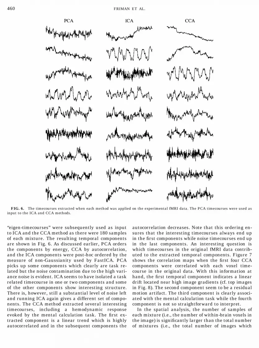
“eigen-timecourses” were subsequently used as inputto ICA and the CCA method as there were 180 samplesof each mixture. The resulting temporal componentsare shown in Fig. 6. As discussed earlier, PCA ordersthe components by energy, CCA by autocorrelation,and the ICA components were post-hoc ordered by themeasure of non-Gaussianity used by FastICA. PCApicks up some components which clearly are task re-lated but the noise contamination due to the high vari-ance noise is evident. ICA seems to have isolated a taskrelated timecourse in one or two components and someof the other components show interesting structure.There is, however, still a substantial level of noise leftand running ICA again gives a different set of compo-nents. The CCA method extracted several interestingtimecourses, including a hemodynamic responseevoked by the mental calculation task. The first ex-tracted component is a linear trend which is highlyautocorrelated and in the subsequent components the

autocorrelation decreases. Note that this ordering en-sures that the interesting timecourses always end upin the first components while noise timecourses end upin the last components. An interesting question iswhich timecourses in the original fMRI data contrib-uted to the extracted temporal components. Figure 7shows the correlation maps when the first four CCAcomponents were correlated with each voxel time-course in the original data. With this information athand, the first temporal component indicates a lineardrift located near high image gradients (cf. top imagesin Fig. 8). The second component seem to be a residualmotion artifact. The third component is clearly associ-ated with the mental calculation task while the fourthcomponent is not so straightforward to interpret.

In the spatial analysis, the number of samples ofeach mixture (i.e., the number of within-brain voxels inthe image) is significantly larger than the total numberof mixtures (i.e., the total number of images which

FIG. 6. The timecourses extracted when each method was applied on the experimental fMRI data. The PCA timecourses were used asinput to the ICA and CCA methods.

460 FRIMAN ET AL.

were 180 in this case) but we still reduce the dimen-sionality by keeping the first 30 “eigen-images” ob-tained by the spatial PCA analysis. The reason for

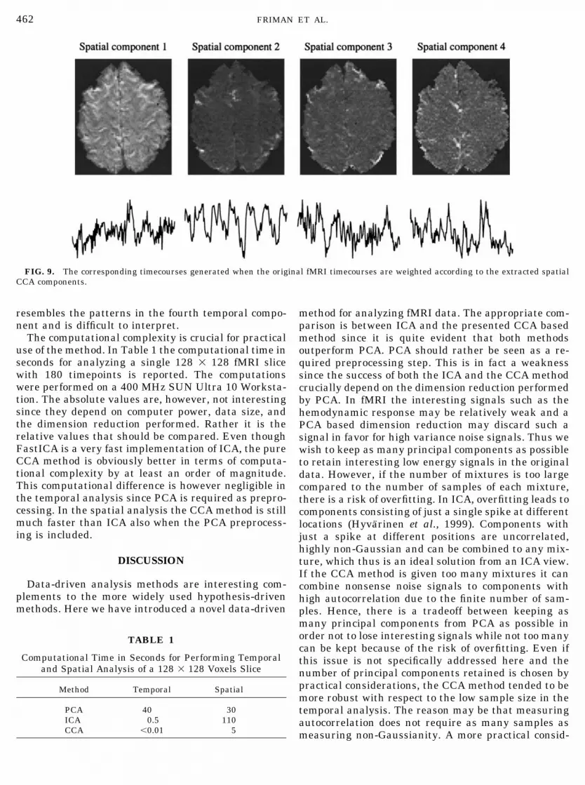
reducing the dimensionality is partly justified by reli-ability considerations discussed later. Another reasonwas that the proposed ordering of the ICA components(by non-Gaussianity) did not produce a satisfactoryresult and there was a need to screen the output fromICA and PCA manually. An ordering of the componentsis more important in the spatial case than in the tem-poral case since in general more components are gen-erated. In Fig. 8, 4 of the 30 spatial components pro-duced by each method are shown. In the CCA case thefirst four components are shown. The order provided byPCA and ICA did as mentioned not coincide with whatvisually appeared interesting. Therefore PCA compo-nents 1, 4, 9, and 7, and ICA components 5, 1, 2, and 8,were manually selected by a visual interestingnesscriterion and aligned with the closest CCA compo-nents. All three methods give the average image as acomponent, in the PCA and CCA cases as the firstcomponent. In the PCA case this is explained by thelarge spread of intensity values in the image. The CCAmethod extracts the average image since, as all imagesof natural objects, it has a large autocorrelation. Theremaining components most likely indicate areas inthe brain involved in the mental calculation task orperhaps draining veins. Despite different ordering,there are no dramatic differences between the compo-nents. As in the temporal case it is interesting to moveover to the dual space, i.e., examining what the time-courses look like if the original fMRI timecourses areweighted according to the voxel values in the spatialcomponents. Figure 9 shows the dual timecourses cor-responding to the first four spatial CCA components.Since the first spatial component is the mean image thedual timecourse should be some global signal. The sec-ond and third components are probably task-related.The patterns in the fourth spatial component closely

FIG. 7. Correlation maps obtained when the four first temporal CCA components were correlated with the original voxel timecourses. Themaps indicate where in the analyzed fMRI slice the extracted CCA timecourses can be found (air voxels were excluded from analysis).

FIG. 8. Spatial components extracted by each method. The num-bers indicate the original order. The displayed PCA and ICA compo-nents were selected manually.


resembles the patterns in the fourth temporal compo-nent and is difficult to interpret.

The computational complexity is crucial for practicaluse of the method. In Table 1 the computational time inseconds for analyzing a single 128 � 128 fMRI slicewith 180 timepoints is reported. The computationswere performed on a 400 MHz SUN Ultra 10 Worksta-tion. The absolute values are, however, not interestingsince they depend on computer power, data size, andthe dimension reduction performed. Rather it is therelative values that should be compared. Even thoughFastICA is a very fast implementation of ICA, the pureCCA method is obviously better in terms of computa-tional complexity by at least an order of magnitude.This computational difference is however negligible inthe temporal analysis since PCA is required as prepro-cessing. In the spatial analysis the CCA method is stillmuch faster than ICA also when the PCA preprocess-ing is included.

DISCUSSION

Data-driven analysis methods are interesting com-plements to the more widely used hypothesis-drivenmethods. Here we have introduced a novel data-driven

method for analyzing fMRI data. The appropriate com-parison is between ICA and the presented CCA basedmethod since it is quite evident that both methodsoutperform PCA. PCA should rather be seen as a re-quired preprocessing step. This is in fact a weaknesssince the success of both the ICA and the CCA methodcrucially depend on the dimension reduction performedby PCA. In fMRI the interesting signals such as thehemodynamic response may be relatively weak and aPCA based dimension reduction may discard such asignal in favor for high variance noise signals. Thus wewish to keep as many principal components as possibleto retain interesting low energy signals in the originaldata. However, if the number of mixtures is too largecompared to the number of samples of each mixture,there is a risk of overfitting. In ICA, overfitting leads tocomponents consisting of just a single spike at differentlocations (Hyvarinen et al., 1999). Components withjust a spike at different positions are uncorrelated,highly non-Gaussian and can be combined to any mix-ture, which thus is an ideal solution from an ICA view.If the CCA method is given too many mixtures it cancombine nonsense noise signals to components withhigh autocorrelation due to the finite number of sam-ples. Hence, there is a tradeoff between keeping asmany principal components from PCA as possible inorder not to lose interesting signals while not too manycan be kept because of the risk of overfitting. Even ifthis issue is not specifically addressed here and thenumber of principal components retained is chosen bypractical considerations, the CCA method tended to bemore robust with respect to the low sample size in thetemporal analysis. The reason may be that measuringautocorrelation does not require as many samples asmeasuring non-Gaussianity. A more practical consid-

FIG. 9. The corresponding timecourses generated when the original fMRI timecourses are weighted according to the extracted spatialCCA components.

TABLE 1

Computational Time in Seconds for Performing Temporaland Spatial Analysis of a 128 � 128 Voxels Slice

Method Temporal Spatial

PCA 40 30ICA 0.5 110CCA �0.01 5

462 FRIMAN ET AL.

eration related to dimensionality reduction and thenumber of underlying components revealed is the or-dering of the components. Since most ICA methods donot provide an ordering of the components they mustbe inspected manually. The CCA method orders thecomponents by autocorrelation which is a natural mea-sure of “interestingness” and thus only the first com-ponents need to be inspected. It should be noted thatthere are other similar methods that use temporal orspatial structure to decompose multidimensional data(Switzer and Green, 1984; Molgedey and Schuster,1994; Ziehe and Muller, 1998; Stone, 2001) and thatthe CCA method is not novel in that sense. The CCAapproach has however not been reported earlier and webelieve it is well suited for exploratory analysis of fMRIdata where temporal and spatial patterns are impor-tant features. Such patterns are ignored by PCA andICA, which for example produce the same unmixingvectors after a random permutation of the samples inthe mixtures.

An important issue that has to be considered beforedrawing any conclusions about the observed patternsin the obtained components is how well the mixtureassumption apply. In the temporal case, the assump-tion that the observed voxel timeseries are combina-tions of different independent basis timeseries (hemo-dynamic response, low frequency drifts, etc.) isgenerally made and accepted in fMRI data analysis.However, in temporal exploratory analysis we areforced to perform heavy dimension reduction whichmay discard interesting information. In addition, theconstraint to find uncorrelated component time-courses may introduce problems due to the finite num-ber of samples in each timecourse. Even though theunderlying components are assumed independent, thesample correlation between two finite length observa-tions of the sources need not be zero. This is the case inthe simulated experiment where the sample correla-tion between the boxcar and the quadratic signals isnot zero, implying that it is impossible to perfectlyseparate them when there is a constraint to produce anuncorrelated result. The consequence may be an un-satisfactory separation with underlying signals frac-tionated into several components. In the spatial anal-ysis the sample size is significantly larger. Hence thereis a smaller probability that the sample correlationbetween two observations of hypothized independentbasis images differ significantly from zero. Also, theremay not be a need for reducing the dimensionality ofthe problem. The critical question is instead whetherfMRI data can be assumed to consist of a linear mix-ture of underlying independent basis images, which isnot an obvious assumption (McKeown and Sejnowski,1998; Friston, 1998). The implication from the abovediscussion is that caution should be taken when inter-preting and drawing inferences from the patterns seenin the components. Reported observations such as un-

expected activations, transient task-related activa-tions and infered spatial connectivity between differ-ent areas in the brain may very well be results of aviolation of the mixture assumption, limited samplesizes or other artifacts such as patient motion.

The above issues do, however, by no means implythat exploratory analysis are not useful. The resultmay for example be used to build more accurate modelsof the drifts in the fMRI data set at hand, to detectresidual motion artifacts or other unexpected compo-nents which for example can be included as additionalregressors in a hypothesis-driven method (McKeown,2000).

As a final point, the noise in fMRI data has repeat-edly been shown to be temporally autocorrelated (Fris-ton et al., 2000; Zarahn et al., 1997). Since the CCAmethod explore fMRI data for autocorrelated compo-nents the noise characteristics may have implicationsregarding the performance. The main effect of corre-lated noise is a reduced robustness against low samplesizes as it becomes easier to combine noise timecoursesto something that can appear interesting. However,this is a general issue also hampering for example ICA(Hyvarinen et al., 1999).

CONCLUSIONS

A method for data-driven analysis of fMRI data hasbeen presented and compared primarily with Indepen-dent Component Analysis. The novel CCA method hasseveral advantages over ICA. It is computationally ef-ficient, the components are ordered by a natural mea-sure of relevance so that not all components need to beinspected manually, and the same components are al-ways obtained when the method is applied on the samedata. Additionally, the CCA method performed ro-bustly in the simulated study and appeared less sen-sitive to the high noise level when applied on the ex-perimental fMRI data. It is therefore an interestingalternative to ICA as a tool for routinely screening thefMRI data prior to analyzing the data using a hypoth-esis-driven method.

REFERENCES

Andersen, A., Gash, D., and Avison, M. 1999. Principal componentanalysis of the dynamic response measured by fMRI: A generalizedlinear systems framework. Magn. Reson. Imag. 17(6): 795–815.

Anderson, T. W. 1984. An Introduction to Multivariate StatisticalAnalysis, 2nd ed. Wiley.

Bell, A. J., and Sejnowski, T. J. 1995. An information-maximizationapproach to blind separation and blind deconvolution. NeuralComputat. 7: 1129–1159.

Borga, M., and Knutsson, H. 2001. A canonical correlation approachto blind source separation. Technical Report LiU-IMT-EX-0062,Department of Biomedical Engineering, Linkoping University.


Friston, K. 1998. Modes or models: A critique on independent com-ponent analysis for fMRI. Trends Cogn. Sci. 2(10): 373–375.

Friston, K., Josephs, O., Zarahn, E., Holmes, A., Rouquette, S., andPoline, J. 2000. To smooth or not to smooth? Bias and efficiency infMRI time-series analysis. NeuroImage 12(2): 196–208.

Hotelling, H. 1936. Relations between two sets of variates. Bi-ometrika 28: 321–377.

Hyvarinen, A. 1999. Fast and robust fixed-point algorithms for in-dependent component analysis. IEEE Trans. Neural Networks10(3): 626–634.

Hyvarinen, A., Karhunen, J., and Oja, E. 2001. Independent Compo-nent Analysis. Wiley.

Hyvarinen, A., and Oja, E. 2000. Independent component analysis:Algorithms and applications. Neural Networks 13: 411–430.

Hyvarinen, A., Sarela, J., and Vigaro, R. 1999. Spikes and bumps:Artefacts generated by independent component analysis with in-sufficient sample size. In Proc. Int. Workshop on IndependentComponent Analysis and Signal Separation (ICA ’99)

McKeown, M. 2000. Detection of consistently task-related activa-tions in fMRI data with hybrid independent component analysis.NeuroImage 11(1): 24–35.

McKeown, M., Makeig, S., Brown, G., Jung, T., Kindermann, S., Bell,A., and Sejnowski, T. 1998. Analysis of fMRI data by blind sepa-ration into independent spatial components. Hum. Brain Mapp.6(3): 160–188.

McKeown, M., and Sejnowski, T. 1998. Independent component anal-ysis of fMRI data: Examining the assumptions. Hum. Brain Mapp.6(5–6): 368–372.

Molgedey, L., and Schuster, H. 1994. Separation of a mixture ofindependent signals using time delayed correlations. Phys. Rev.Lett. 72(23): 3634–3636.

Stone, J. 2001. Blind source separation using temporal predictabil-ity. Neural Computat. 13(7):1559–1574.

Switzer, P., and Green, A. A. 1984. Min/max autocorrelation factorsfor multivariate spatial imagery. Technical Report 6, Departmentof Statistics, Stanford University.

Zarahn, E., Aguirre, G., and D’Esposito, M. 1997. Empirical anal-yses of BOLD fMRI statistics, spatially unsmoothed datacollected under null-hypothesis conditions. NeuroImage 5(3):179 –197.

Ziehe, A., and Muller, K.-R. 1998. TDSEP—An efficient algorithm forblind separation using time structure. In Proc. Int. Conf. on Arti-ficial Neural Networks (ICANN ’98), pp. 675–680.

464 FRIMAN ET AL.

exploratory fmri analysis by autocorrelation maximization

Documents