shrinkage factor autocorrelation - north dakota state university
TRANSCRIPT
SPATIAL STATISTICAL AND MULTIVARIATE REGRESSION APPROACH TO
EARTHWORK SHRINKAGE-FACTOR CALCULATION
A Thesis
Submitted to the Graduate Faculty
of the
North Dakota State University
of Agriculture and Applied Science
By
Benedict Tetteh Shamo
In Partial Fulfillment of the Requirements
for the Degree of
MASTER OF SCIENCE
Major Department:
Construction Management and Engineering
May 2013
Fargo, North Dakota

North Dakota State University
Graduate School
Title
Spatial Statistical and Multivariate approach to earthwork shrinkage factor
calculation
By
Benedict Tetteh Shamo
The Supervisory Committee certifies that this disquisition complies with North Dakota State
University’s regulations and meets the accepted standards for the degree of
MASTER OF SCIENCE
SUPERVISORY COMMITTEE:
Eric Asa
Chair
Darshi De Saram
Majura Selekwa
Approved:
08/12/2013 Yong Bai
Date Department Chair

iii
ABSTRACT
In this research, a linear shrinkage factor model, which is the result of spatial and statistical
modeling, was developed for the state of North Dakota. The input variables for the developed shrinkage
factor models were derived from spatially modeled soil data which makes the function responsive to soil
variability across the state. The current approach for selecting the shrinkage correction factor in earthwork
contracts across the state of North Dakota is through a trial-and-error system. This deterministic system
employs the judgment of experienced engineers in selecting a shrinkage factor value for earthwork
contracts. The current approach assumes shrinkage factor uniformity and does not provide a measure of
the estimate’s reliability. Due to the heterogeneous nature of soil properties across the state, the trial-and-
error approach for selecting the shrinkage factor greatly impacts earthwork volumes, which could lead to
contract variations and increase the cost of contract administration.

iv
ACKNOWLEDGEMENTS
My sincere gratitude goes to Dr. Eric Asa and my committee members, Dr. Selekwa and Dr.
Darshi, for their time and efforts in shaping my thought process. I am grateful to the North Dakota
Department of Transportation for its sponsorship of this research. My thanks go to Greg Thompson of
Terracon Consulting Engineers and Scientists for his support in the field and laboratory testing. My
thanks also go to the contractors and their representatives on the various projects for accommodating the
research team to use the right of way for research activities. It is in high honor that I hold Ingrid, Ann, and
all the faculty of the construction management department. I am grateful for the opportunity.
v
TABLE OF CONTENTS
ABSTRACT ................................................................................................................................................. iii
ACKNOWLEDGEMENTS ......................................................................................................................... iv
LIST OF TABLES ....................................................................................................................................... xi
LIST OF FIGURES .................................................................................................................................... xv
CHAPTER 1. INTRODUCTION ................................................................................................................. 1
1.1. Background ........................................................................................................................................ 1
1.2. Problem statement .............................................................................................................................. 2
1.3. Aims and objectives ........................................................................................................................... 2
1.4. Research contribution ........................................................................................................................ 3
1.5. Research methodology ....................................................................................................................... 4
CHAPTER 2. LITERATURE REVIEW ...................................................................................................... 5
2.1. Shrinkage factor and geostatistics ...................................................................................................... 5
2.1.1. Modeling soil properties ............................................................................................................. 9
2.1.2. Geostatistics .............................................................................................................................. 10
2.2. Statistical concepts ........................................................................................................................... 13
2.2.1. Multivariate regression analysis ................................................................................................ 13
2.2.2. Linearity .................................................................................................................................... 13
2.2.3. Normality .................................................................................................................................. 14
2.2.4. Residuals ................................................................................................................................... 14
2.2.5. Homoscedasticity ...................................................................................................................... 14
vi
2.2.6. Random variable ....................................................................................................................... 14
2.2.7. Covariance ................................................................................................................................ 15
2.2.8. Spatial autocorrelation .............................................................................................................. 15
2.2.9. Hypothesis testing ..................................................................................................................... 15
2.2.10. Exploratory spatial data analysis ............................................................................................. 16
2.2.11. Principal component and factor analysis................................................................................. 16
2.3. Earthwork calculation methods ........................................................................................................ 16
2.3.1. Average end area method .......................................................................................................... 17
2.3.2. Grid method .............................................................................................................................. 18
2.3.3. Electronic methods .................................................................................................................... 18
2.4. Standard soil testing methods used in research ................................................................................ 19
2.4.1. Standard proctor test ................................................................................................................. 19
2.4.1.1. Test procedure ...................................................................................................... 20
2.4.1.2. One-point and multi-point moisture- density relationship: mechanical and
manual test procedure ........................................................................................ 21
2.4.2. Oven dry moisture test .............................................................................................................. 26
2.4.2.1. Test procedure ...................................................................................................... 26
2.4.3. Nuclear density test ................................................................................................................... 27
2.4.3.1. Test procedure ...................................................................................................... 27
2.4.3.2. Steps ..................................................................................................................... 28
2.4.4. Atterberg limit test .................................................................................................................... 31
2.4.4.1. Procedure for liquid limit test .............................................................................. 31
vii
2.4.4.2. Steps ..................................................................................................................... 31
2.4.4.3. Procedure for plastic limit test ............................................................................. 33
2.4.4.4. Steps ..................................................................................................................... 33
2.4.4.5. Plasticity index ..................................................................................................... 34
2.4.5. Grain size distribution test ........................................................................................................ 34
2.4.5.1. Steps ..................................................................................................................... 35
2.4.5.2. Calculation ........................................................................................................... 36
2.5. Summary .......................................................................................................................................... 37
CHAPTER 3. RESEARCH METHODOLOGY ........................................................................................ 38
3.1. Introduction ...................................................................................................................................... 38
3.2. Step 1: Initial shrinkage factor model postulation ........................................................................... 40
3.3. Step 2: NRCS soil data set, kriging, and ranking of cross-validated results .................................... 45
3.4. Step 3: Field study on shrinkage-factor related variables ................................................................ 57
3.5. Step 4: Multivariate linear-regression modeling .............................................................................. 58
3.5.1. Assumptions .............................................................................................................................. 59
3.5.2. Hypothesis testing and model validation .................................................................................. 60
3.6. Summary .......................................................................................................................................... 63
CHAPTER 4. RESULTS AND DISCUSSIONS ........................................................................................ 64
4.1. Discussion of Minot results.............................................................................................................. 64
4.1.1. Step 2 ........................................................................................................................................ 65
4.1.1.1. Preliminary data set analysis ................................................................................ 65
viii
4.1.2. Step 3 ........................................................................................................................................ 68
4.1.2.1. Construction process and test result ..................................................................... 68
4.1.3. Step 4 ........................................................................................................................................ 70
4.2. Analysis of results ............................................................................................................................ 78
4.3. Discussion of Valley City results ..................................................................................................... 82
4.3.1. Step 2 ........................................................................................................................................ 83
4.3.1.1. Preliminary data set analysis ................................................................................ 83
4.3.2. Step 3 ........................................................................................................................................ 86
4.3.2.1. Construction process and test result ..................................................................... 86
4.3.3. Step 4 ........................................................................................................................................ 88
4.4. Analysis of results ............................................................................................................................ 89
4.5. Discussion of Dickinson results ....................................................................................................... 93
4.5.1. Step 2 ........................................................................................................................................ 94
4.5.1.1. Preliminary data set analysis ................................................................................ 94
4.5.2. Step 3 ........................................................................................................................................ 97
4.5.2.1. Construction process and test result ..................................................................... 97
4.5.3. Step 4 ........................................................................................................................................ 99
4.6. Devils Lake results and modeling .................................................................................................. 103
4.6.1. Step 2 ...................................................................................................................................... 104
4.6.1.1. Preliminary data set analysis .............................................................................. 104
4.7. Discussion of Fargo results ............................................................................................................ 107
ix
4.7.1. Step 2 ...................................................................................................................................... 107
4.7.1.1. Preliminary data set analysis .............................................................................. 108
4.8. Discussion of Bismarck results ...................................................................................................... 112
4.8.1. Step 2 ...................................................................................................................................... 112
4.8.1.1. Preliminary data set analysis .............................................................................. 112
4.9. Discussion of Williston results ...................................................................................................... 115
4.9.1. Step 2 ...................................................................................................................................... 115
4.9.1.1. Preliminary data set analysis .............................................................................. 115
4.10. Discussion of Grand Forks results ............................................................................................... 119
4.10.1. Step 2 .................................................................................................................................... 119
4.10.1.1. Preliminary data set analysis ............................................................................ 119
4.11. General shrinkage factor model ................................................................................................... 123
4.12. Comparison of all models ............................................................................................................ 127
4.13. Results comparison ...................................................................................................................... 127
CHAPTER 5. CONCLUSION AND FURTHER RESEARCH ............................................................... 134
5.1. Conclusion ..................................................................................................................................... 134
5.2. Future research recommendation ................................................................................................... 136
REFERENCES ......................................................................................................................................... 138
APPENDIX A. FIELD DENSITY REPORT FOR DEVILS LAKE ........................................................ 144
APPENDIX B. OPTIMUM MOISTURE CONTENT REPORT FOR DEVILS LAKE.......................... 145
APPENDIX C. FIELD DENSITY REPORT FOR DICKINSON ............................................................ 146

x
APPENDIX D. OPTIMUM MOISTURE CONTENT REPORT FOR DICKINSON ............................. 147
APPENDIX E. FIELD DENSITY REPORT FOR MINOT ..................................................................... 148
APPENDIX F. OPTIMUM MOISTURE CONTENT REPORT FOR MINOT ....................................... 149
APPENDIX G. FIELD DENSITY REPORT FOR GACKLE ................................................................. 150
APPENDIX H. OPTIMUM MOISTURE CONTENT REPORT FOR GACKLE ................................... 151
xi
LIST OF TABLES
Table Page
2.1. Typical soil weight and volume change characteristics (Source, Nunnally, 2011)………….......……7
2.2. Material volume conversion factors (United States Army Engineer School [USAES], 2000)….……7
2.3. Sample end area method calculation sheet……..……………...……………………….....................17
2.4. NDDOT modified AASHTO T99 and T180, method A (NDDOT, 2011)…………….………...…..20
2.5. NDDOT modified AASHTO T99 and T180, method D (NDDOT, 2011)…..………………..……..20
2.6. Sample aggregate calculation sheet………….…...….………………………………………………26
2.7. Sample compaction correction factors……………………………. …………………....…….……..33
2.8. Maximum amount of material retained on a sieve for overload condition….………….……………35
3.1. Independent and dependent variables used in the multivariate analysis…………..……………...….39
3.2. Bulkage factors used by DOT districts…...………………...……….………………….……………43
3.3. Sample distance matrix……......…………………………………………….……………………….52
3.4. g vector for unsampled locations…...………………….……………...……………………………..53
3.5. Inverse of distance matrix……………….…………………………………………………………...54
3.6. Summary parameters..…..…………………………….……………….……………………………..55
3.7. Decision table for independent variable rejection or acceptance……………...……………………..62
4.1. Statistical results of Minot soil data set analysis……………..…………………….………………..65
4.2. Crossvalidated kriging results for Minot………………….………………..……………………..…67
xii
4.3. Minot soil properties………………………………………………………………………………....69
4.4. Observed field and laboratory results for Minot project…………...………………….……………..70
4.5. Correlation matrix of Minot variables………...……………………………………….…………….72
4.6. Coefficients and their test values..……………………..……………………………….……………78
4.7. Analysis of Variance for initial shrinkage factor function for Minot……………………..…..……..79
4.8. Independent variables and known sum of squares error associated with each……………...…...…..79
4.9. Coefficients and their test values……..……………...….………………….………………………..80
4.10. Breakdown of sum of squares error…………...……….…………………………………………...80
4.11. Variance analysis of initial shrinkage factor function for Minot………………..…………..……...80
4.12. Coefficients and their test values …………………………………………………………………..81
4.13. Variance analysis of initial shrinkage factor function for Minot…………...……………...……….81
4.14. Statistical results of Valley City soil data set analysis………………...………...………………….84
4.15. Crossvalidated kriging results for Valley City……………………………………………………...85
4.16. Observed results for Valley City project………………………..……………...…………………..87
4.17. Classification of Valley City soil…………………….…………………………………………….87
4.18. Correlation matrix Valley City variables……………….…..………….………………….……….89
4.19. Coefficients and their test values……………………….……………….…………………………90
4.20. Variance analysis of initial shrinkage factor function for Valley City………….…………………91
xiii
4.21. Independent variables and known sum of squares error associated with each predictor…………...91
4.22. Coefficient analysis of refined shrinkage factor function for Valley City……………..…….……..91
4.23. Variance analysis for refined function for Valley City………….……….…………………….…..91
4.24. Observed results for Dickinson project………………….…………..……………………………..96
4.25. Observed results for Dickinson project……….……………………..……………………………..98
4.26. Classification of Dickinson soil…………………..……………………….……………………….98
4.27. Correlation matrix of Dickinson variables…………………………………...………….………...100
4.28. Coefficients and their test values……………...………………………...………………………...100
4.29. Analysis of variance table for Equation 4.6………………..…………………….……….……….101
4.30. Coefficients and their test values…………………………..…………...…………………..……..102
4.31. Variance analysis for refined Dickinson model……………………..…………...….…………….102
4.32. Ranked crossvalidated kriging result for Devils Lake…………..………………..……………….106
4.33. Ranked kriging results for Fargo District………..………………..……………………………....110
4.34. Ranked crossvalidated modeling results……………………..……………………………………114
4.35. Ranked crossvalidated results of linear kriging………………………..……………………….…117
4.36. Ranked crossvalidated kriging result…………..……………….…………...…………………….121
4.37. Correlation matrix for combined data set……………..…………………………………………..124
4.38. Predictors with the p-values for combined model……………………..………………...…….….125
xiv
4.39. Variance analysis of initial shrinkage factor function for combined data set…………...…..…….125
4.40. Predictors with the p-value………..………………………..……………………………………..126
4.41. Minot shrinkage factor comparison…………………..………………………………….………..127
4.42. Normalized objective function and modeling efficiency for linear models……………..…..…....129
4.43. Dickinson shrinkage factor comparison…………………...…………..……………………..……129
4.44. Valley City shrinkage factor comparison…...……………………………….…………………….131
4.45. Shrinkage factor comparison……………...………..……………………………………………..132
xv
LIST OF FIGURES
Figure Page
1.1. Research flowchart ……………………......…………………..………………………………………4
2.1. Typical soil volume change during earthmoving (Nunnally, 2011)……….…………...………..……6
2.2. Graphical representation of semivariogram (Goovaerts, 1979)…………………..……...….……….12
2.3. Sample 5’x5’ gridded site…………………..………………………………………………………..18
2.4. GEOPAK software (http://www.ncdot.gov accessed 05/17/2012)………………………..…………19
2.5. T-99 Density curves (NDDOT, 2011)………...…………..…..……………………………………..24
2.6. T-180 Density curves (NDDOT, 2011)…………….…………….……….…………………………25
3.1. Shrinkage-factor function development process…………………….....…………………………….38
3.2. Response to shrinkage factor question…………………………..………………….………………..41
3.3. Response to methods of testing……………………………………….……….……………………..41
3.4. Response to shrinkage factor variability………………………………….………………………….42
3.5. Response to causes of deviation in shrinkage factor……………………………………………....…44
3.6. Sample NRCS (USDA) soil data set showing clay, silt and sand at varying depths……………..….47
3.7. Geostatistical research approach (Asa et al.,2011)……………………………………..……………47
3.8. Histogram plot for % clay in soils from Bismarck transportation district……………...……………48
3.9. Normal Q-Q plot of % clay in soils from Bismarck transportation district……………………...…..49
3.10. Graphical representation of semivariogram (Source; Goovaerts, 1979)……………………..……..50
xvi
3.11. Fitted spherical variogram for Bismarck soil data set……………………….…...……..…………..51
3.12. Study sites in North Dakota…………...……………………………………………………………57
4.1. Minot research site with borrow pits………………………………...……………………………….64
4.2. Histogram of Minot data points…………………………...…………………………………………66
4.3. Kriged average clay content of soils in Minot transportation district.…………..……..………...….68
4.4. Multivariate regression in Minitab 15…………………………………………..……………………71
4.5. A plot of the residuals for the independent and dependent variable for Minot……………...….…...72
4.6. Correlation plot between shrinkage factor and clay content of borrow material……………………74
4.7. Correlation plot between shrinkage factor and bulk density of borrow material…………………….75
4.8. Correlation plot between shrinkage factor and bulk density of embankment material.…...................76
4.9. Correlation plot between shrinkage factor and density of borrow material……….……....................76
4.10. Correlation plot between shrinkage factor and dry of density of embankment material...................77
4.11. Valley City research site with borrow pits…………..…………………………………….……….82
4.12. Histogram of Valley City data points…………………...…....……………………….……………83
4.13. Kriged average clay content of soils in Valley City transportation district…….……………..…....86
4.14. Residual plot of fitted values in Valley City…...……………………………….………….……….88
4.15. Residual plots for Valley City refined model..……….……….……………………………………92
4.16. Dickinson research site with borrow pits..…………………….……………………………………93
xvii
4.17. Histogram of Dickinson data points……………………………………..……...…………….……94
4.18. Ordinary kriging of clay for Dickinson transportation district……….….……….……..………….97
4.19. A residual plot for Dickinson data set……………………………………………………..………..99
4.20. Residual plots for Dickinson refined model…...…………...………………………...…….……..102
4.21. Devils Lake project SNH-SER-3-057 (047) 006 profile……...……….……………………….…104
4.22. Histogram of Devils Lake data points…………….….………………………………….…….….105
4.23. Map of clay distribution in Devils Lake district………………………………..…………………107
4.24. Histogram of Fargo data points…..…………….………………………………………………….108
4.25. Q-Q plot for Fargo clay data set………………..………….……………...………………….……109
4.26. Map of clay distribution in Fargo district……...……………….…...……………...……………..111
4.27. Histogram of Bismarck data points……….…………..………...………..…………………….….112
4.28. Clay distribution in Bismarck district modeled with ordinary kriging………..…………….….…115
4.29. Histogram of Williston data points……….……………..……………………………………..….116
4.30. Clay distribution in Williston modeled with simple kriging……………………….…………..….118
4.31. Histogram of Grand Forks data points………….……….……..…………………....…….………119
4.32. Clay distribution in Grand Forks modeled with universal kriging………………………………..122
4.33. Residual plot for combined data set……………………………………………………….………123
4.34. Residual plot for modified combined data set……………………………...…………..…………126
4.35. Three districts with their shrinkage values…………………………………….………………….133
1
CHAPTER 1. INTRODUCTION
1.1. Background
Earthwork construction is the excavation, hauling, placing, and compaction of soil, gravel, or
other material found on the Earth’s surface. The definition also includes the measurement of such material
in the field, the computation in the office of the volume of such material, and the determination of the
most economical method of performing such work (Cole and Harbin, 2006).Earthwork construction
usually involves the excavation and piling of earth in connection with an engineering operation.
Determining the volume of material involved in an earthwork project is performed both electronically and
manually. Manual determination of earthwork quantities is done through the use of mass diagrams and
grids, and the electronic approach is through the use of software packages such as GEOPAK and
AutoCAD civil3D. With both approaches, the final volumes generated are adjusted for changes in volume
during excavation, transportation, and placement by applying shrinkage- and load-correction factors. The
current and general approach is to use an arbitrary value of 25-30% for the shrinkage-correction factor.
For instance, the North Dakota Department of Transportation (NDDOT) plan sets accompanying every
project in the state specify a percentage of additional volume in section 210 that is used to account for
earthwork shrinkage on the project (NDDOT,2008).This approach is deterministic and invariably
undermines the shrinkage variability of soil at different locations across the state. The engineering
properties of soil, such as density, particle size, and structure, vary from place to place. There are inherent
variations in individual soil constituents; for instance, soil density could change from place to place. The
behavior of soil, therefore, depends not only on its properties, but also on its location. Vibration, for
example, could be used to change loose soil into dense soil by altering the arrangement of soil particles.
The deterministic and trial-and-error approaches for gauging shrinkage factors do not, therefore, account
for the variability caused by construction process, location, and environmental factors such as moisture.
Failure to account for these variables could result in volume loss or gains in contract quantities, which
2
affects all parties for the earthwork contract. For example, the resultant change in earthwork volume
during construction leads to contract variations during project execution. This variation implies an
increase in change orders, extra work for contract administration, budget overruns, disputes between
contractors and project owners, and schedule delays.
1.2. Problem statement
All Department of Transportation (DOT) earthwork contracts have a soil shrinkage factor value
written in them as means of capturing soil shrinkage during construction. Contractors are therefore paid
for increased soil volume on the basis of this predetermined shrinkage factor value. The challenge is that,
this soil shrinkage factor has to be captured in the contract document prior to construction. Evidence
shows that, this shrinkage factor value is selected on the basis of the judgment of an experience engineer
combined with few random pre-construction soil tests. This approach to determining soil shrinkage factor
fails to account for variability in the composition of different soil types and the uncertainty associated
with different soil types that exist across the state. This approach also fails to capture error associated with
the prediction and leaves the contract open to challenge through change orders. The spatial statistic,
however, offers the prospect of overcoming this shortfall. The purpose of this research is therefore to
develop a model that predicts soil shrinkage factor with an expected degree of reliability by correlating
the weights of different parameters that affect the shrinkage factor and accounts for spatial variability.
1.3. Aims and objectives
The objectives of this study are as follows:
1. A review of the current approaches to determine earthwork quantities and how the shrinkage
factor is used in DOT districts.
2. Identify typical shrinkage-factor values for different soil types.
3. Identify the factors that influence the shrinkage factor.

3
4. Identify the cause for variations of the shrinkage factor from one transportation district to another
in North Dakota.
5. Develop a model that helps show the relationship between the shrinkage factor and these
variables. Use the model to predict shrinkage-factor values.
6. Investigate how the uncertainty associated with predicting the shrinkage factor could be reduced.
7. Develop a spatial map showing variations in the different factors across North Dakota.
1.4. Research contribution
This thesis is part of NDDOT-sponsored research that is looking at the various factors that must
be considered in determining the shrinkage factor for earthwork projects in North Dakota. In the first
phase of the research, the hypothesis postulated was that the soil shrinkage factor is a multivariate of the
soil’s clay content, the soil’s moisture content, soil type, construction losses, the density of the soil, and a
random error. The clay content hypothesis was tested and validated. The second phase dealt with the
density and moisture content functions. This thesis, therefore, employed multivariate statistics and spatial
statistics to explore this concept. Due to the variability of soil from place to place, this thesis also used a
Geographic information system to explore and enhance the understanding about the relationships between
these factors by examining spatial autocorrelation and spatial heterogeneity through the process of
exploratory spatial data analysis. The results of this thesis will form the basis of a guideline to be
developed by the North Dakota Department of Transportation (NDDOT) for contract administration in
the area of selecting shrinkage factors for its earthwork projects in order to ensure fairness and
consistency and to reduce variations with field conditions when using shrinkage factors. The results of
this research will help improve shrinkage-factor calculation and use for earthwork contracts. The results
will also help close the current knowledge gap about shrinkage-factor uncertainty.
4
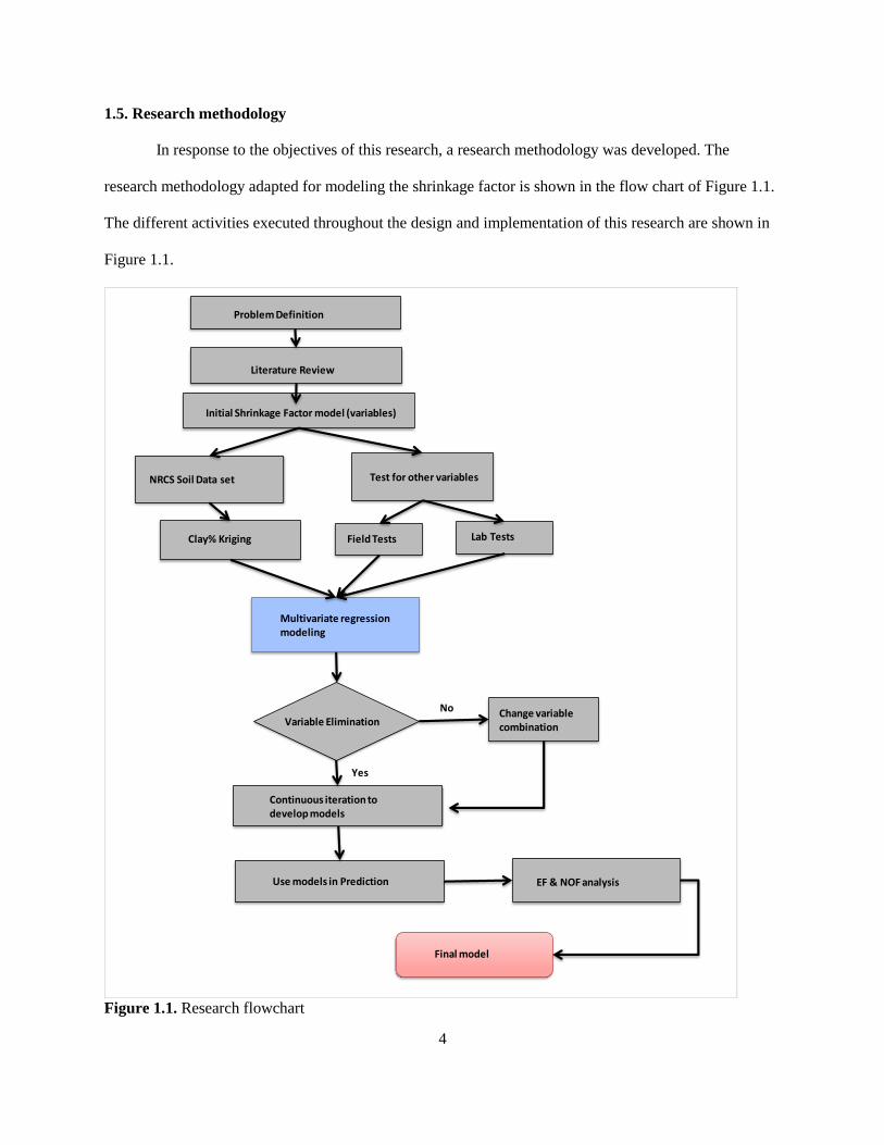
1.5. Research methodology
In response to the objectives of this research, a research methodology was developed. The
research methodology adapted for modeling the shrinkage factor is shown in the flow chart of Figure 1.1.
The different activities executed throughout the design and implementation of this research are shown in
Figure 1.1.
Figure 1.1. Research flowchart
Initial Shrinkage Factor model (variables)
NRCS Soil Data set Test for other variables
Clay% Kriging Field Tests
Multivariate regression modeling
Variable EliminationChange variable combination
Lab Tests
No
Continuous iteration to develop models
EF & NOF analysisUse models in Prediction
Yes
Final model
Problem Definition
Literature Review
5
CHAPTER 2. LITERATURE REVIEW
In this chapter, the shrinkage factor and existing shrinkage-factor calculation methods are
reviewed. The modeling concepts that were used for shrinkage-factor calculation are discussed. The test
procedures used for measuring the soil properties relevant to the study are also reviewed. Another purpose
of this chapter is to discuss the statistical concepts relevant to the modeling used and to review
geostatistics.
2.1. Shrinkage factor and geostatistics
The shrinkage factor is one of many factors used to convert earthmoving materials between one
of the three major states (bank, loose, or compacted) in which it may exist (Nunnally, 2011). The bank
state represents the natural state of the material before any disturbance, and it is often referred to as “in
place” or “in-situ.” A unit volume is identified as bank cubic yard (BCY) or bank cubic meter (BCM). A
loose condition is the state of the material when it has been excavated or loaded. Unit volume is identified
as loose cubic yard (LCY) or loose cubic meter (LCM). A compacted condition represents the state of the
material after compaction. Unit volume is identified as compacted cubic yard (CCY) or compacted cubic
meter (CCM) (Nunnally, 2011).
Conversion between different soil states is required to ensure consistency with the unit of volume
specified as the basis for payment in an earthmoving contract. A pay yard (or meter) is the volume unit
specified as the basis for payment in an earthmoving contract (Nunnally, 2011).
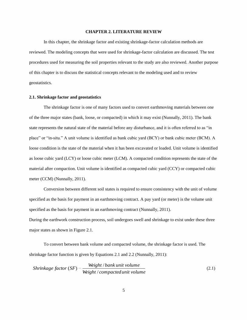
During the earthwork construction process, soil undergoes swell and shrinkage to exist under these three
major states as shown in Figure 2.1.
To convert between bank volume and compacted volume, the shrinkage factor is used. The
shrinkage factor function is given by Equations 2.1 and 2.2 (Nunnally, 2011):
volumeunitcompactedWeight
volumeunitbankWeightSFfactorShrinkage
/
/)( (2.1)
6
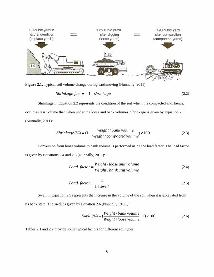
Figure 2.1. Typical soil volume change during earthmoving (Nunnally, 2011)
shrinkagefactorShrinkage 1 (2.2)
Shrinkage in Equation 2.2 represents the condition of the soil when it is compacted and, hence,
occupies less volume than when under the loose and bank volumes. Shrinkage is given by Equation 2.3
(Nunnally, 2011):
100)/
/1((%)
volumecompactedWeight
volumebankWeightShrinkage (2.3)
Conversion from loose volume to bank volume is performed using the load factor. The load factor
is given by Equations 2.4 and 2.5 (Nunnally, 2011):
volumeunitbankWeight
volumeunitlooseWeightfactorLoad
/
/ (2.4)
swellfactorLoad
1
1 (2.5)
Swell in Equation 2.5 represents the increase in the volume of the soil when it is excavated from
its bank state. The swell is given by Equation 2.6 (Nunnally, 2011):
100)1/
/((%)
volumelooseWeight
volumebankWeightSwell (2.6)
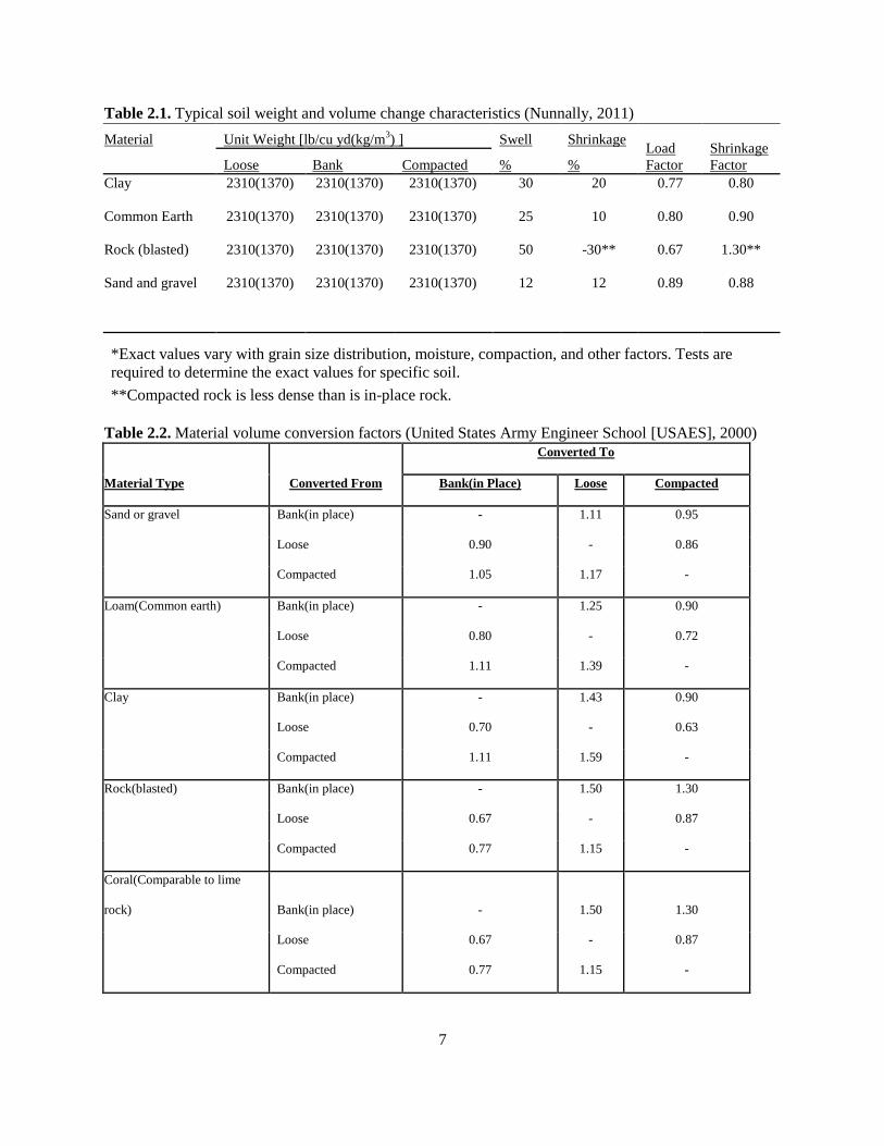
Tables 2.1 and 2.2 provide some typical factors for different soil types.
7
Table 2.1. Typical soil weight and volume change characteristics (Nunnally, 2011)
Material Unit Weight [lb/cu yd(kg/m3) ] Swell Shrinkage
Load
Factor
Shrinkage
Factor Loose Bank Compacted % %
Clay 2310(1370) 2310(1370) 2310(1370) 30 20 0.77 0.80
Common Earth 2310(1370) 2310(1370) 2310(1370) 25 10 0.80 0.90
Rock (blasted) 2310(1370) 2310(1370) 2310(1370) 50 -30** 0.67 1.30**
Sand and gravel 2310(1370) 2310(1370) 2310(1370) 12 12 0.89 0.88
*Exact values vary with grain size distribution, moisture, compaction, and other factors. Tests are
required to determine the exact values for specific soil.
**Compacted rock is less dense than is in-place rock.
Table 2.2. Material volume conversion factors (United States Army Engineer School [USAES], 2000)
Material Type Converted From
Converted To
Bank(in Place) Loose Compacted
Sand or gravel Bank(in place) - 1.11 0.95
Loose 0.90 - 0.86
Compacted 1.05 1.17 -
Loam(Common earth) Bank(in place) - 1.25 0.90
Loose 0.80 - 0.72
Compacted 1.11 1.39 -
Clay Bank(in place) - 1.43 0.90
Loose 0.70 - 0.63
Compacted 1.11 1.59 -
Rock(blasted) Bank(in place) - 1.50 1.30
Loose 0.67 - 0.87
Compacted 0.77 1.15 -
Coral(Comparable to lime
rock) Bank(in place) - 1.50 1.30
Loose 0.67 - 0.87
Compacted 0.77 1.15 -
8
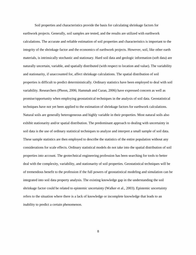
Soil properties and characteristics provide the basis for calculating shrinkage factors for
earthwork projects. Generally, soil samples are tested, and the results are utilized with earthwork
calculations. The accurate and reliable estimation of soil properties and characteristics is important to the
integrity of the shrinkage factor and the economics of earthwork projects. However, soil, like other earth
materials, is intrinsically stochastic and stationary. Hard soil data and geologic information (soft data) are
naturally uncertain, variable, and spatially distributed (with respect to location and value). The variability
and stationarity, if unaccounted for, affect shrinkage calculations. The spatial distribution of soil
properties is difficult to predict deterministically. Ordinary statistics have been employed to deal with soil
variability. Researchers (Phoon, 2006; Hammah and Curan, 2006) have expressed concern as well as
promise/opportunity when employing geostatistical techniques in the analysis of soil data. Geostatistical
techniques have not yet been applied to the estimation of shrinkage factors for earthwork calculations.
Natural soils are generally heterogeneous and highly variable in their properties. Most natural soils also
exhibit stationarity and/or spatial distribution. The predominant approach to dealing with uncertainty in
soil data is the use of ordinary statistical techniques to analyze and interpret a small sample of soil data.
These sample statistics are then employed to describe the statistics of the entire population without any
considerations for scale effects. Ordinary statistical models do not take into the spatial distribution of soil
properties into account. The geotechnical engineering profession has been searching for tools to better
deal with the complexity, variability, and stationarity of soil properties. Geostatistical techniques will be
of tremendous benefit to the profession if the full powers of geostatistical modeling and simulation can be
integrated into soil data property analysis. The existing knowledge gap in the understanding the soil
shrinkage factor could be related to epistemic uncertainty (Walker et al., 2003). Epistemic uncertainty
refers to the situation where there is a lack of knowledge or incomplete knowledge that leads to an
inability to predict a certain phenomenon.
9
2.1.1. Modeling soil properties
Modeling soil properties requires tools which can deal with large uncertainties, variations,
multiple data points, correlated collocated data, soft data, etc. One of the tools that is gaining acceptance
is stochastic modeling via geostatistical algorithms. However, geostatistical algorithms have not been
applied to shrinkage-factor and earthwork calculations. The lack of documented methodologies is one of
the biggest obstacles. Uncertainty and stationarity are intrinsic to soils and other earth-science data. The
inability to effectively deal with these characteristics can gravely affect the reliability of shrinkage-factor
estimates. The impact of uncertainty and stationarity has long been recognized by the pioneers of the
geotechnical profession (Casagrande, 1965). However, the industry always lacked the practical tools to
quantify and account for uncertainty. Nearly two decades ago, Einstein and Baecher (1982) wrote, "The
question is not whether to deal with uncertainty, but how?"
Spatial variability of soil properties from one point to another is attributed to factors such as
variations in mineralogical composition, conditions during deposition, stress history, and physical and
mechanical decomposition processes. The spatial variability of soil is controlled by some form of
correlation relating the soil property to a location in space. In statistical terms, this phenomenon is known
as spatial structure. That correlation is expected to diminish as the distance between data points increases.
Even though soil properties are multivariate, data analysis is univariate. The predominant
approach to dealing with uncertainty in soil data is the use of ordinary, linear statistical-modeling
techniques. In ordinary linear statistics, the mean is used to represent the data, even though it is not the
best linear unbiased estimator (BLUE). The stationarity problem is not addressed with the linear statistical
approach. This work is, therefore, aimed at employing stochastic modeling, simulation, and optimization
techniques in the form of geostatistics and decision sciences to effectively characterize and analyze soil
data and information in earthwork shrinkage-ratio calculations.
Based on existing literature, this research was classified under epistemic uncertainty and aleatory
uncertainty (Helton et al., 2004). The epistemic uncertainty concept allowed for the use of learning from
10
research to reduce the existing knowledge gap. The aleatory uncertainty concept allowed for modeling the
shrinkage factor as a probability-distribution function. The geostatistical tools of kriging and multivariate
regression were explored as a means of analyzing shrinkage-factor distribution in this research.
2.1.2. Geostatistics
Geostatistics was invented by D. G.Krige and H. S.Sichel and formalized (theorized) by Georges
Matheron in his theory of regionalized variables (Krige, 1951; Matheron, 1955). Geostatistics is a
collection of mathematical techniques and algorithms employed to characterize and analyze the behavior
of spatially correlated data. It is based on the theory of regionalized variables (Journel and Huijbregts,
1978; Goovaerts, 1997). This property allows one to capitalize on the spatial correlation between
neighboring observations to predict attribute values at unsampled locations.
Geostatistics is a branch of applied statistics which is focused on the spatial relationships among
geological/earth-science data, the geological processes underlying earth-science data, and the support
effects and the precision of data. Several authors (Tabios and Salas, 1985; Phillips et al., 1992) have
shown that geostatistical prediction techniques (kriging) provide better estimates of earth-science data
than conventional methods. The difference between kriging and other linear estimation methods is that it
is aimed at minimizing the error variance. Laslett et al. (1987) compared kriging with other techniques of
interpolation and showed that kriging was the only methodology that performed reliably in all
circumstances. Kriging has been successfully used for the spatial prediction of soil properties (Burgess
and Webster, 1980), mineral resources, petroleum property evaluation, aquifer interpolation (Doctor,
1979), soil salinity through interpolation of electrical conductivity measurements (Oliver and Webster,
1990), meteorology, and forestry.
The fundamental elements of the modeling process are:
1. calculating an experimental semivariogram/variogram;
11
2. considering geological information and knowledge of the area (if available) to
supplement calculated points;
3. fitting a licit positive definite model to data.
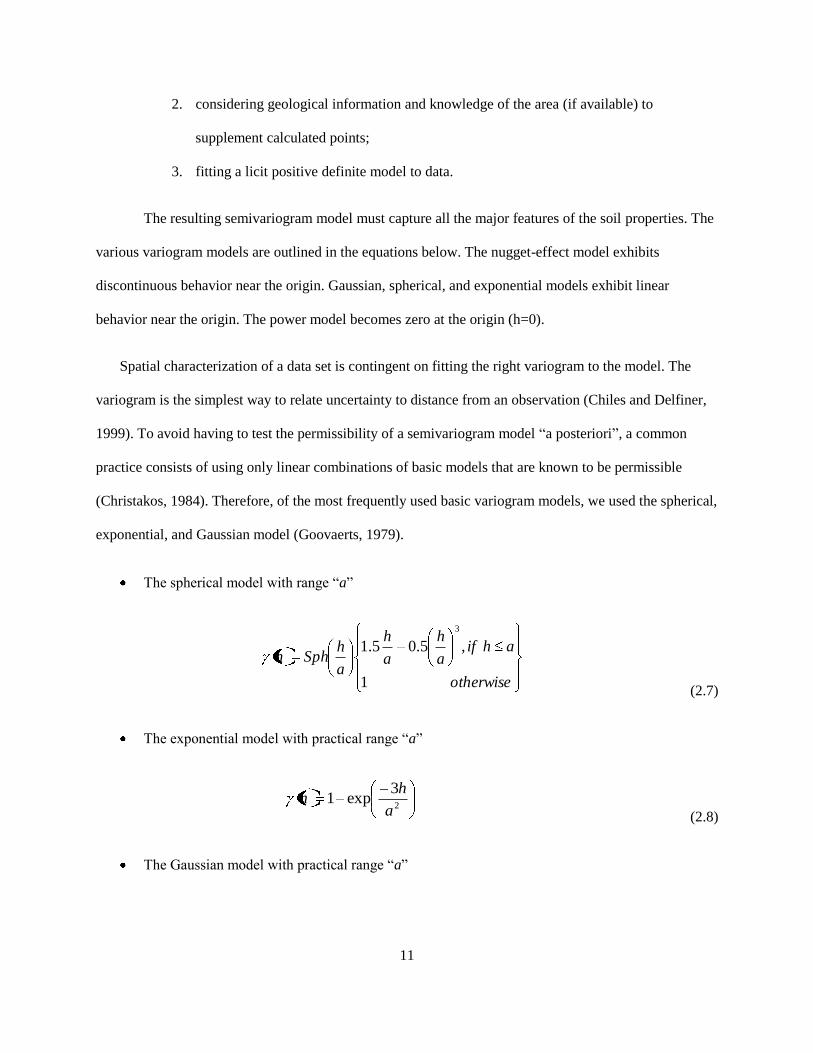
The resulting semivariogram model must capture all the major features of the soil properties. The
various variogram models are outlined in the equations below. The nugget-effect model exhibits
discontinuous behavior near the origin. Gaussian, spherical, and exponential models exhibit linear
behavior near the origin. The power model becomes zero at the origin (h=0).
Spatial characterization of a data set is contingent on fitting the right variogram to the model. The
variogram is the simplest way to relate uncertainty to distance from an observation (Chiles and Delfiner,
1999). To avoid having to test the permissibility of a semivariogram model “a posteriori”, a common
practice consists of using only linear combinations of basic models that are known to be permissible
(Christakos, 1984). Therefore, of the most frequently used basic variogram models, we used the spherical,
exponential, and Gaussian model (Goovaerts, 1979).
The spherical model with range “a”
otherwise
ahifa
h
a
h
a
hSphh
1
,5.05.1
3
(2.7)
The exponential model with practical range “a”
2
3exp1
a
hh
(2.8)
The Gaussian model with practical range “a”
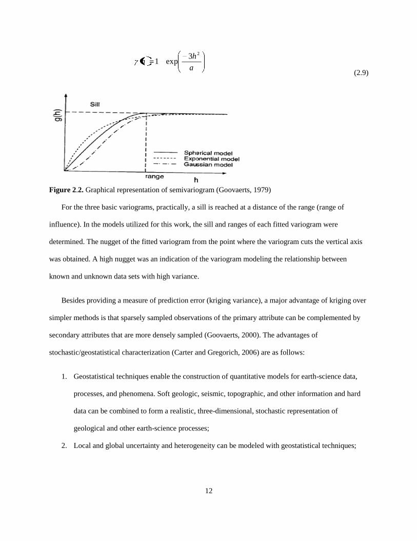
12
a
hh
23exp1
(2.9)
Figure 2.2. Graphical representation of semivariogram (Goovaerts, 1979)
For the three basic variograms, practically, a sill is reached at a distance of the range (range of
influence). In the models utilized for this work, the sill and ranges of each fitted variogram were
determined. The nugget of the fitted variogram from the point where the variogram cuts the vertical axis
was obtained. A high nugget was an indication of the variogram modeling the relationship between
known and unknown data sets with high variance.
Besides providing a measure of prediction error (kriging variance), a major advantage of kriging over
simpler methods is that sparsely sampled observations of the primary attribute can be complemented by
secondary attributes that are more densely sampled (Goovaerts, 2000). The advantages of
stochastic/geostatistical characterization (Carter and Gregorich, 2006) are as follows:
1. Geostatistical techniques enable the construction of quantitative models for earth-science data,
processes, and phenomena. Soft geologic, seismic, topographic, and other information and hard
data can be combined to form a realistic, three-dimensional, stochastic representation of
geological and other earth-science processes;
2. Local and global uncertainty and heterogeneity can be modeled with geostatistical techniques;
13
3. Geostatistical techniques can be employed to optimize the design of sampling/survey programs
used to collect earth-science information and data. The techniques could be used to minimize the
risk associated with the characterization process;
4. Geostatistics could be used to simulate the geological processes and phenomena underlying the
quantitative geological models;
5. Geostatistical models enable the characterization, estimation, and inference of geological
processes based on limited conditioning data coupled with a measure of the spatial structure and
heterogeneity; and finally, uncertainty analysis, sensitivity analysis, and decision techniques
could be combined in geostatistical modeling to improve decision making.
2.2. Statistical concepts
Spatial statistics offer tools for analyzing the spatial distribution of data sets, trends, and
processes as well as the relationship among them. This section is a general review of the statistical
concepts associated with multivariate analysis and spatial data modeling which were used to develop the
shrinkage-factor function that is consistent with spatial variation.
2.2.1. Multivariate regression analysis
Multivariate regression is a technique that estimates a single regression model with more than one
outcome variable. Regression analyses are, therefore, a set of statistical techniques which allow us to
assess the relationship between one dependent variable and several independent variables (Rencher,
2002). Regression analyses only reveal relationships between variables; this does not imply that the
relationships are causal.
2.2.2. Linearity
Linearity is the assumption that there is a linear model that can be well fitted between the
dependent and independent variables (Decision 411, 2012).Linearity is essential for the calculation of
multivariate statistics due to the basis upon the general linear model and the assumption of multivariate
14
normality which implies that there is linearity between all pairs of variables, with significance tests based
upon that assumption. Linearity between two variables may be assessed through the observation of
bivariate scatter plots. When both variables are normally distributed and linearly related, the scatter plot is
oval shaped; if one of the variables is non-normal, then the scatter plot is not oval.
2.2.3. Normality
The underlying assumption of most multivariate analysis and statistical tests is multivariate
normality, the assumption that all variables and all combinations of the variables are normally distributed.
When the assumption is met, the residuals are normally distributed and independent; the differences
between the predicted and obtained scores (the errors) are symmetrically distributed around a mean of
zero; and there is no pattern to the errors. Screening for normality may be done in either the statistical or
graphical method (Rencher, 2002).
2.2.4. Residuals
Residuals are the difference between an observed value of the response variable and the value
predicted by the model (Moore and McCabe, 1993).
2.2.5. Homoscedasticity
This is one of the assumptions with multivariate regression analysis. Homoscedasticity is the
assumption that the response variables have the same variance. Therefore, when the residuals of an
analysis seem to increase or decrease in average magnitude with the fitted values, it is an indication that
the variance of the residuals is not constant (Decision 411, 2012).
2.2.6. Random variable
A random variable is a variable where the possible values are numerical outcomes of a random
phenomenon (Easton and McColl, 1997). Random variables are used to represent stochastic phenomenon
mathematically. Random variables could be discrete, in which case they take the value of finite values, or
could be continuous, in which case they take the value of an infinite number or values within a range. The
15
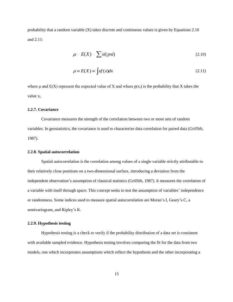
probability that a random variable (X) takes discrete and continuous values is given by Equations 2.10
and 2.11:
)()( pxixiXE (2.10)
dxxxfXE )()( (2.11)
where μ and E(X) represent the expected value of X and where p(xi) is the probability that X takes the
value xi.
2.2.7. Covariance
Covariance measures the strength of the correlation between two or more sets of random
variables. In geostatistics, the covariance is used to characterize data correlation for paired data (Griffith,
1987).
2.2.8. Spatial autocorrelation
Spatial autocorrelation is the correlation among values of a single variable strictly attributable to
their relatively close positions on a two-dimensional surface, introducing a deviation from the
independent observation’s assumption of classical statistics (Griffith, 1987). It measures the correlation of
a variable with itself through space. This concept seeks to test the assumption of variables’ independence
or randomness. Some indices used to measure spatial autocorrelation are Moran’s I, Geary’s C, a
semivariogram, and Ripley’s K.
2.2.9. Hypothesis testing
Hypothesis testing is a check to verify if the probability distribution of a data set is consistent
with available sampled evidence. Hypothesis testing involves comparing the fit for the data from two
models, one which incorporates assumptions which reflect the hypothesis and the other incorporating a
16
less-specific set of assumptions. Some hypothesis-testing tools include the Z-Test, T-Test, and Chi-square
Test (Rencher, 2002).
2.2.10. Exploratory spatial data analysis
Exploratory spatial data analysis is an extension of exploratory data analysis (EDA) to detect
spatial properties for any given data. It focuses on the distinguishing characteristics of geographic data,
specifically on spatial autocorrelation and spatial heterogeneity (Haining ,1990;Cressie, 1993). EDA is
done through the use of techniques such as trend identification and smoothening through the use spatial
averaging.
2.2.11. Principal component and factor analysis
Principal component analysis (PCA) and factor analysis (FA) are statistical techniques applied to
a single set of variables to discover which variables in the set form coherent subsets that are relatively
independent of one another. Variables that are correlated with one another which are also largely
independent of other variable subsets are combined into factors. The generated factors are thought to be
representative of the underlying processes that have created the correlations among variables (Rencher,
2002).
2.3. Earthwork calculation methods
There are different methods of determining the quantity of earthwork material for a project. The
most commonly used method is the end-area method. The other methods are the contour line/grid method
and electronic means. Examples of the electronic means include GEOPAK, AutoCAD 3D,IGrid, and
Tally Systems Earthwork. The information technology industry has transformed the ways in which
earthwork information and data are obtained and processed (Leick, 2004). Irrespective of the earthwork-
quantity calculation method, the input data are obtained either through manual surveying or through the
use of sophisticated GPS-based instruments. Manual surveys use levels, theodolite, and total stations to
obtain elevations and angle data. GPS-based instruments utilize signals to obtain elevation data. The data
17
sets obtained from these data-collection methods form the building blocks of the different methods for
calculating earthwork quantities.
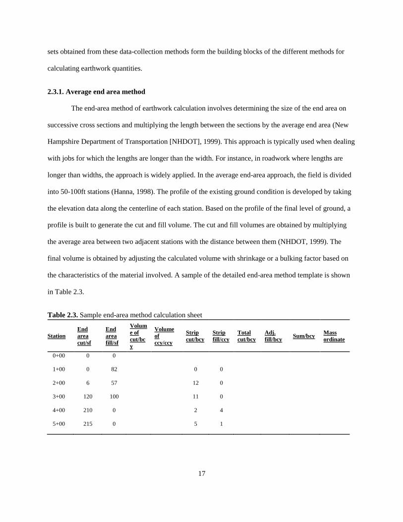
2.3.1. Average end area method
The end-area method of earthwork calculation involves determining the size of the end area on
successive cross sections and multiplying the length between the sections by the average end area (New
Hampshire Department of Transportation [NHDOT], 1999). This approach is typically used when dealing
with jobs for which the lengths are longer than the width. For instance, in roadwork where lengths are
longer than widths, the approach is widely applied. In the average end-area approach, the field is divided
into 50-100ft stations (Hanna, 1998). The profile of the existing ground condition is developed by taking
the elevation data along the centerline of each station. Based on the profile of the final level of ground, a
profile is built to generate the cut and fill volume. The cut and fill volumes are obtained by multiplying
the average area between two adjacent stations with the distance between them (NHDOT, 1999). The
final volume is obtained by adjusting the calculated volume with shrinkage or a bulking factor based on
the characteristics of the material involved. A sample of the detailed end-area method template is shown
in Table 2.3.
Table 2.3. Sample end-area method calculation sheet
Station
End
area
cut/sf
End
area
fill/sf
Volum
e of
cut/bc
y
Volume
of
ccy/ccy
Strip
cut/bcy
Strip
fill/ccy
Total
cut/bcy
Adj.
fill/bcy Sum/bcy
Mass
ordinate
0+00 0 0
1+00 0 82
0 0
2+00 6 57
12 0
3+00 120 100
11 0
4+00 210 0
2 4
5+00 215 0 5 1
18
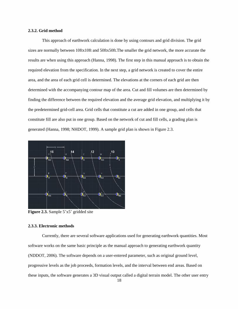
2.3.2. Grid method
This approach of earthwork calculation is done by using contours and grid division. The grid
sizes are normally between 10ftx10ft and 50ftx50ft.The smaller the grid network, the more accurate the
results are when using this approach (Hanna, 1998). The first step in this manual approach is to obtain the
required elevation from the specification. In the next step, a grid network is created to cover the entire
area, and the area of each grid cell is determined. The elevations at the corners of each grid are then
determined with the accompanying contour map of the area. Cut and fill volumes are then determined by
finding the difference between the required elevation and the average grid elevation, and multiplying it by
the predetermined grid-cell area. Grid cells that constitute a cut are added in one group, and cells that
constitute fill are also put in one group. Based on the network of cut and fill cells, a grading plan is
generated (Hanna, 1998; NHDOT, 1999). A sample grid plan is shown in Figure 2.3.
Figure 2.3. Sample 5’x5’ gridded site
2.3.3. Electronic methods
Currently, there are several software applications used for generating earthwork quantities. Most
software works on the same basic principle as the manual approach to generating earthwork quantity
(NDDOT, 2006). The software depends on a user-entered parameter, such as original ground level,
progressive levels as the job proceeds, formation levels, and the interval between end areas. Based on
these inputs, the software generates a 3D visual output called a digital terrain model. The other user entry
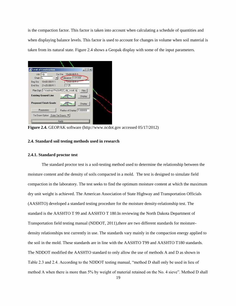
19
is the compaction factor. This factor is taken into account when calculating a schedule of quantities and
when displaying balance levels. This factor is used to account for changes in volume when soil material is
taken from its natural state. Figure 2.4 shows a Geopak display with some of the input parameters.
Figure 2.4. GEOPAK software (http://www.ncdot.gov accessed 05/17/2012)
2.4. Standard soil testing methods used in research
2.4.1. Standard proctor test
The standard proctor test is a soil-testing method used to determine the relationship between the
moisture content and the density of soils compacted in a mold. The test is designed to simulate field
compaction in the laboratory. The test seeks to find the optimum moisture content at which the maximum
dry unit weight is achieved. The American Association of State Highway and Transportation Officials
(AASHTO) developed a standard testing procedure for the moisture density-relationship test. The
standard is the AASHTO T 99 and AASHTO T 180.In reviewing the North Dakota Department of
Transportation field testing manual (NDDOT, 2011),there are two different standards for moisture-
density relationships test currently in use. The standards vary mainly in the compaction energy applied to
the soil in the mold. These standards are in line with the AASHTO T99 and AASHTO T180 standards.
The NDDOT modified the AASHTO standard to only allow the use of methods A and D as shown in
Table 2.3 and 2.4. According to the NDDOT testing manual, “method D shall only be used in lieu of
method A when there is more than 5% by weight of material retained on the No. 4 sieve”. Method D shall
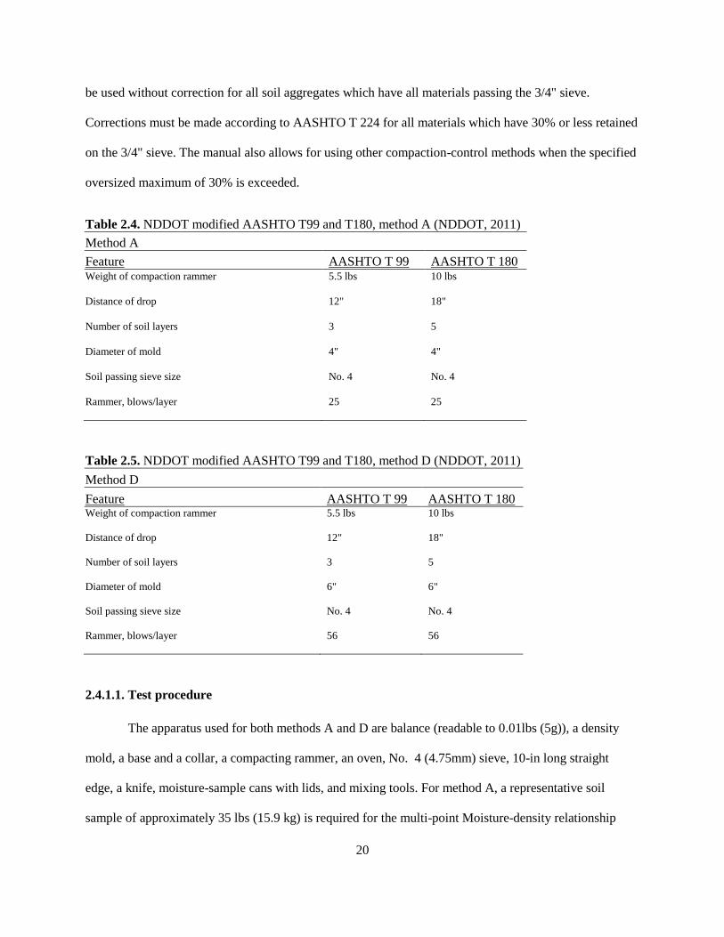
20
be used without correction for all soil aggregates which have all materials passing the 3/4" sieve.
Corrections must be made according to AASHTO T 224 for all materials which have 30% or less retained
on the 3/4" sieve. The manual also allows for using other compaction-control methods when the specified
oversized maximum of 30% is exceeded.
Table 2.4. NDDOT modified AASHTO T99 and T180, method A (NDDOT, 2011)
Method A
Feature AASHTO T 99 AASHTO T 180 Weight of compaction rammer 5.5 lbs 10 lbs
Distance of drop 12" 18"
Number of soil layers 3 5
Diameter of mold 4" 4"
Soil passing sieve size No. 4 No. 4
Rammer, blows/layer 25 25
Table 2.5. NDDOT modified AASHTO T99 and T180, method D (NDDOT, 2011)
Method D
Feature AASHTO T 99 AASHTO T 180 Weight of compaction rammer 5.5 lbs 10 lbs
Distance of drop 12" 18"
Number of soil layers 3 5
Diameter of mold 6" 6"
Soil passing sieve size No. 4 No. 4
Rammer, blows/layer 56 56
2.4.1.1. Test procedure
The apparatus used for both methods A and D are balance (readable to 0.01lbs (5g)), a density
mold, a base and a collar, a compacting rammer, an oven, No. 4 (4.75mm) sieve, 10-in long straight
edge, a knife, moisture-sample cans with lids, and mixing tools. For method A, a representative soil
sample of approximately 35 lbs (15.9 kg) is required for the multi-point Moisture-density relationship

21
Test, and approximately 7 lbs (3.2 kg) are required for the One-Point Moisture-Density Relationship Test.
For method D, a representative soil sample of approximately 125 lbs (55 kg) is required for the Multi-
Point Moisture-Density Relationship Test, and approximately 25 lbs (11 kg) are required for the One-
Point Moisture-Density Relationship Test.
2.4.1.2. One-point and multi-point moisture- density relationship: mechanical and manual test
procedure
1. Weigh empty mold without base plate and collar to the nearest 0.01lb (5g).
2. Thoroughly mix the first test sample with water to dampen it approximately four percentage
points below the optimum moisture content (soil barely forms a “cast” when squeezed together).
Avoid moisture loss by placing the specimen in a moisture-proof container. Mix remaining
specimens in the same manner as test sample one, increasing water content by approximately one
or two percentage points (not exceeding 2.5%). This water content increase can be done by
adding approximately 60 ml of water to the sample for method A and 250ml for method D.
3. Attach the collar to the mold, and form test samples by adding sufficient material to the mold to
produce a compacted layer of approximately 13/4" for AASHTO T 99 or 1" for AASHTO T 180.
4. Using a manual compaction rammer or a similar device with a 2" face (50 mm), lightly tamp the
soil until it is no longer loose or fluffy.
5. Compact the soil with 25 evenly distributed blows (method A) or 56 blows (method D) of the
compaction rammer. After each layer, trim any soil along the mold walls that has not been
compacted with a knife and distribute on top of the layer.
6. Repeat this procedure by adding more soil from the same sample each time so that, at the end of
the last cycle, the top surface of the compacted soil is above the top rim of the mold when the
collar is removed.
7. Remove the collar, and trim the extruding soil level with the top of the mold. In removing the
collar, rotate it to break the bond between it and the soil before lifting it off the mold.
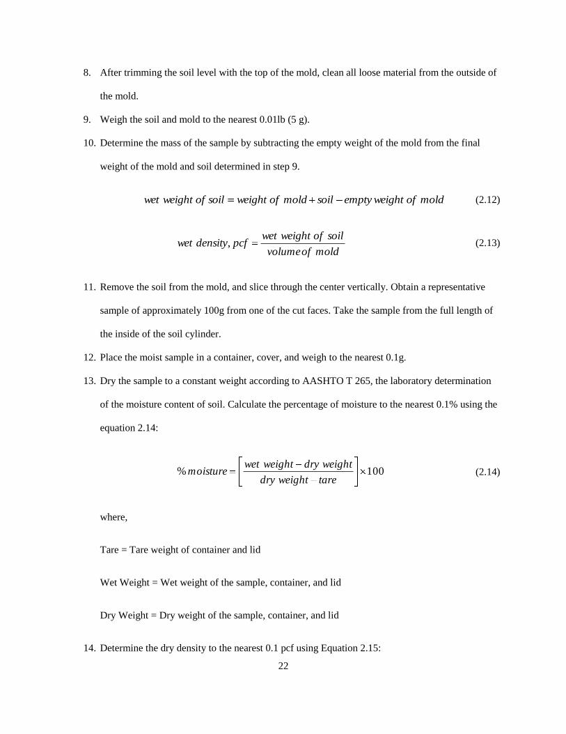
22
8. After trimming the soil level with the top of the mold, clean all loose material from the outside of
the mold.
9. Weigh the soil and mold to the nearest 0.01lb (5 g).
10. Determine the mass of the sample by subtracting the empty weight of the mold from the final
weight of the mold and soil determined in step 9.
moldofweightemptysoilmoldofweightsoilofweightwet (2.12)
moldofvolume
soilofweightwetpcfdensitywet , (2.13)
11. Remove the soil from the mold, and slice through the center vertically. Obtain a representative
sample of approximately 100g from one of the cut faces. Take the sample from the full length of
the inside of the soil cylinder.
12. Place the moist sample in a container, cover, and weigh to the nearest 0.1g.
13. Dry the sample to a constant weight according to AASHTO T 265, the laboratory determination
of the moisture content of soil. Calculate the percentage of moisture to the nearest 0.1% using the
equation 2.14:
100%tareweightdry
weightdryweightwetmoisture (2.14)
where,
Tare = Tare weight of container and lid
Wet Weight = Wet weight of the sample, container, and lid
Dry Weight = Dry weight of the sample, container, and lid
14. Determine the dry density to the nearest 0.1 pcf using Equation 2.15:

23
moisture
densitywetpcfdensityDry
%100
100, (2.15)
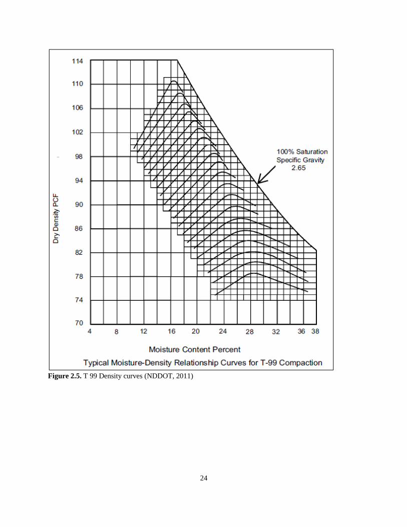
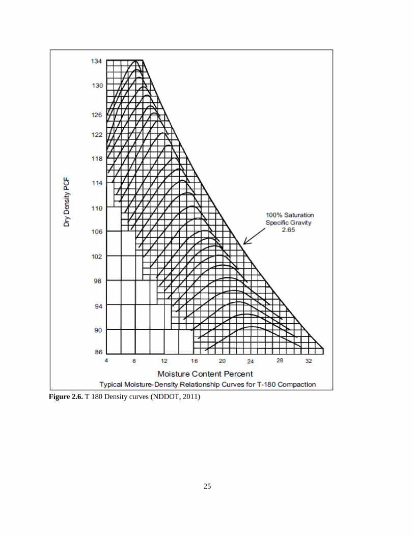
After analyzing a large number of both T 99 and T 180 moisture-density curves that generally
represent statewide soil types, it was found that the curves follow the trends shown on the graphs of
Figures 2.5 and 2.6. The graphs with the T 99 and T 180 procedure may be used in place of performing
the entire moisture-density relationship test. It is recommended that the multi-point moisture-density
relationship test be used whenever possible.
24
Figure 2.5. T 99 Density curves (NDDOT, 2011)
25
Figure 2.6. T 180 Density curves (NDDOT, 2011)
26
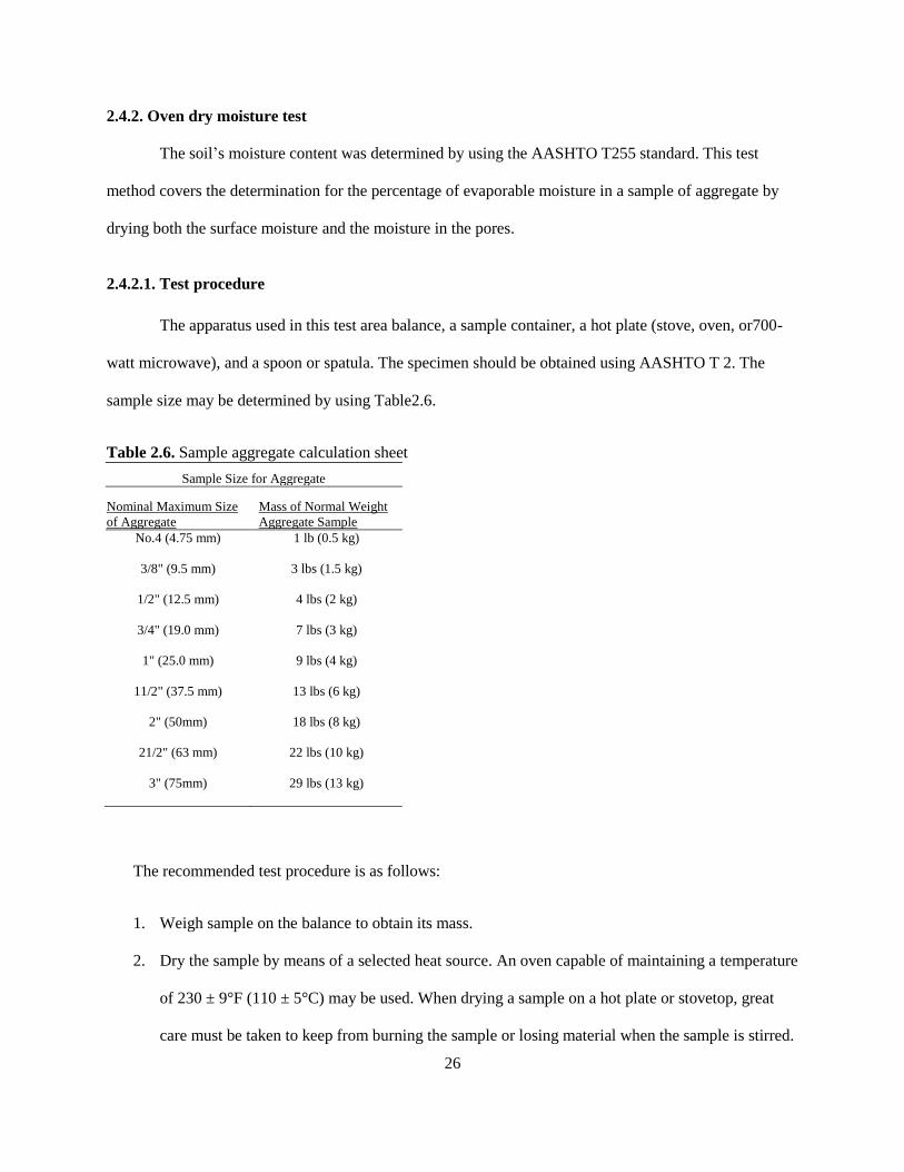
2.4.2. Oven dry moisture test
The soil’s moisture content was determined by using the AASHTO T255 standard. This test
method covers the determination for the percentage of evaporable moisture in a sample of aggregate by
drying both the surface moisture and the moisture in the pores.
2.4.2.1. Test procedure
The apparatus used in this test area balance, a sample container, a hot plate (stove, oven, or700-
watt microwave), and a spoon or spatula. The specimen should be obtained using AASHTO T 2. The
sample size may be determined by using Table2.6.
Table 2.6. Sample aggregate calculation sheet
Sample Size for Aggregate
Nominal Maximum Size
of Aggregate
Mass of Normal Weight
Aggregate Sample
No.4 (4.75 mm) 1 lb (0.5 kg)
3/8" (9.5 mm) 3 lbs (1.5 kg)
1/2" (12.5 mm) 4 lbs (2 kg)
3/4" (19.0 mm) 7 lbs (3 kg)
1" (25.0 mm) 9 lbs (4 kg)
11/2" (37.5 mm) 13 lbs (6 kg)
2" (50mm) 18 lbs (8 kg)
21/2" (63 mm) 22 lbs (10 kg)
3" (75mm) 29 lbs (13 kg)
The recommended test procedure is as follows:
1. Weigh sample on the balance to obtain its mass.
2. Dry the sample by means of a selected heat source. An oven capable of maintaining a temperature
of 230 ± 9°F (110 ± 5°C) may be used. When drying a sample on a hot plate or stovetop, great
care must be taken to keep from burning the sample or losing material when the sample is stirred.
27
3. Dry the sample until a constant weight is achieved (when further drying will cause less than 0.1%
additional loss in mass.).
4. Calculate the moisture-content percentage to the nearest 0.1% by using equation 2.16:
100%sampledryofmass
sampledryofmasssampleoriginalofmassmoisture (2.16)
2.4.3. Nuclear density test
The nuclear density test is conducted to determine the in-place density of soil, moisture content,
and aggregates. In the state of North Dakota, the procedure is performed in line with AASHTO T 310.
The procedure covers the determination of density; moisture content; and the relative compaction of soil,
aggregate, and soil-aggregate mixes in accordance with AASHTO T 310. There are two methods for
determining the in-place density of soil or soil-aggregate mixtures. They are single-direction method A
and two-direction method B (NDDOT, 2011).
2.4.3.1. Test procedure
The apparatus for this test are a nuclear density gauge with the factory-matched standard
reference block, drive pin, guide/scraper plate, and a hammer for testing in direct transmission mode;
transport case for properly shipping and housing the gauge and tools; an instruction manual for the
specific gauge’s make and model; sealable containers and utensils for moisture-content determinations;
radioactive-material information; and a calibration packet containing the daily standard count log, factory
and laboratory calibration data sheets, the leak test certificate, the shippers’ declaration for dangerous
goods, the procedure memo for storing, transporting, and handling nuclear testing equipment, and other
radioactive material documentation as needed by local regulatory requirements (NDDOT, 2011).

28
2.4.3.2. Steps
1. Select (a) test location(s) randomly and in accordance with agency requirements. Test sites should
be relatively smooth and flat, meeting the following conditions:
a) At least 10 m (30 ft) away from other sources of radioactivity
b) At least 3 m (10 ft) away from large objects
c) The test site should be at least 150 mm (6 in.) away from any vertical projection, unless the
gauge is corrected for the trench wall effect
2. Remove all loose and disturbed material, and remove additional material as necessary to expose
the top of the material to be tested.
3. Prepare a flat area sufficient in size to accommodate the gauge. Plane the area to a smooth
condition to obtain the maximum contact between the gauge and the material being tested. For
Method B, the flat area must be sufficient to permit rotating the gauge 90 or 180 degrees about
the source rod.
4. Fill in surface voids beneath the gauge with native fines passing the 4.75-mm (No. 4) sieve or
finer. Smooth the surface with the guide plate or other suitable tool. The depth of the native-fine
filler should not exceed approximately 3 mm (1/8 in.).
5. Make a hole perpendicular to the prepared surface using the guide plate and drive pin. The hole
shall be at least 50 mm (2 in.) deeper than the desired probe depth and shall be aligned such that
insertion of the probe will not cause the gauge to tilt from the plane of the prepared area. Remove
the drive pin by pulling straight up and twisting the extraction tool.
6. Place the gauge on the prepared surface so that the source rod can enter the hole without
disturbing loose material.
7. Insert the probe into the hole, and lower the source rod to the desired test depth using the handle
and trigger mechanism.
29
8. Seat the gauge firmly by partially rotating it back and forth about the source rod. Ensure that the
gauge is seated flush against the surface by pressing down on the gauge corners and making sure
that the gauge does not rock.
9. Pull gently on the gauge to bring the side of the source rod nearest to the scaler/detector firmly
against the side of the hole.
10. Perform one of the following methods, per agency requirements:
a) Method A, single direction: Take a test consisting of the average of two1-minute readings,
and record both density and moisture data. The two wet-density readings should be
within32kg/m3(2.0lb/ft
3) of each other. The average of the two wet densities and moisture
contents is used to compute dry density.
b) Method B, two direction: Take a one-minute reading, and record both density and moisture
data. Rotate the gauge 90 or 180 degrees, pivoting it around the source rod. Reseat the
gauge by pulling gently on it to bring the side of the source rod nearest to the scaler or
detector firmly against the side of the hole, and take a one-minute reading. (In trench
locations, rotate the gauge 180 degrees for the second test.) Some agencies require multiple
one-minute readings in both directions. Analyze the density and moisture data. A valid test
consists of wet-density readings in both gauge positions that are within 50kg/m3 (3.0lb/ft
3).
If the tests do not agree within this limit, move to a new location. The average of the wet-
density and moisture contents is used to compute dry density.
11. If required by the agency, obtain a representative sample of the material, 4kg (9lb) minimum,
from directly beneath the gauge’s full depth for the material tested. This sample is used to verify
moisture content and or to identify the correct density standard. Immediately seal the material to
prevent a moisture loss. The material tested by direct transmission can be approximated by a
cylinder of soil, approximately 300 mm (12 in.) in diameter, directly beneath the centerline of the
radioactive source and detector. The height of the cylinder is approximately the measurement
30
depth. When organic material or large aggregate is removed during this operation, disregard the
test information, and move to a new test site.
12. To verify the moisture content from the nuclear gauge, determine the moisture content with a
representative portion of the material using the FOP for AASHTO T 255 and T 265, or other
agency-approved methods. If the moisture content from the nuclear gauge is within ±1%, the
nuclear gauge readings can be accepted. Retain the remainder of the sample at its original
moisture content for a one-point compaction test under the FOP for AASHTO T 272, or for
gradation, if required.
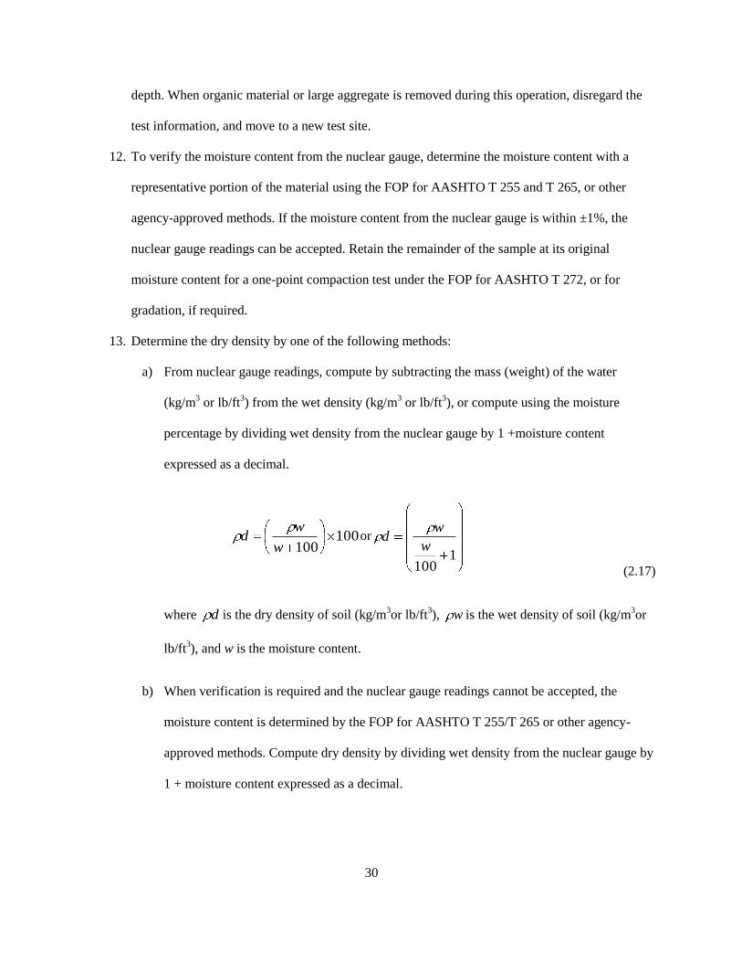
13. Determine the dry density by one of the following methods:
a) From nuclear gauge readings, compute by subtracting the mass (weight) of the water
(kg/m3 or lb/ft
3) from the wet density (kg/m
3 or lb/ft
3), or compute using the moisture
percentage by dividing wet density from the nuclear gauge by 1 +moisture content
expressed as a decimal.
100100w
wd or
1100
w
wd
(2.17)
where d is the dry density of soil (kg/m3or lb/ft
3), w is the wet density of soil (kg/m
3or
lb/ft3), and w is the moisture content.
b) When verification is required and the nuclear gauge readings cannot be accepted, the
moisture content is determined by the FOP for AASHTO T 255/T 265 or other agency-
approved methods. Compute dry density by dividing wet density from the nuclear gauge by
1 + moisture content expressed as a decimal.
31
2.4.4. Atterberg limit test
The objective of the Atterberg limit test is to obtain soil indices such as plastic limit, liquid limit,
and plasticity index. Atterberg limits are the limits of water content used to define soil behavior. The soil
properties that are determined by using the Atterbergs limit test are the plastic limit, liquid limit, and the
plasticity index. The liquid limit of a soil is the moisture content at which the soil passes from a plastic
state to a liquid state. The plastic limit of a soil is the lowest water content at which the soil remains
plastic. The plasticity index of a soil is the numerical difference between the liquid limit and the plastic
limit. It is the moisture content at which the soil is in a plastic state.
2.4.4.1. Procedure for liquid limit test
NDDOT conducts the plastic limit test in accordance with AASHTO T89. The liquid limit is the
water content at which it will takes 25 blows to close the groove over a distance of 13 mm. The apparatus
used in this test are a mixing dish, spatula, manual or mechanical liquid limit device, a gauge for the
liquid limit device, a flat or curved grooving device, moisture-proof containers with covers, balance,
oven, and distilled water.
2.4.4.2. Steps
1. Take a sample of approximately 50 g from the thoroughly mixed portion of the 100g obtained in
accordance with T 87. The portion of the material used passes the No. 40 (0.425mm) sieve.
2. Place the sample in the mixing dish, and thoroughly mix with 8 -10mlof distilled water by
alternately and repeatedly stirring, kneading, and chopping with a spatula.
3. Add additional water in increments of 1-3 ml, and thoroughly mix until a stiff uniform mass of
soil and water is achieved.
4. Place a sufficient quantity of the mixture in the cup above the spot where the cup rests on the
base.
32
5. Squeeze and spread the mixture level with the spatula, and at the same time, trim the material to a
depth of 10 mm at the point of maximum thickness.
6. Divide the soil with a firm stroke of the grooving tool (maximum of six strokes from back to
front) along the diameter through the centerline of the cam follower so that a clean, sharp groove
is formed. Increase the depth of the groove with each stroke, and only scrape the bottom of the
cup with the last stroke.
7. Lift and drop the cup containing the prepared sample by turning the crank at a rate of
approximately 2 revolutions per second for 22-28 blows. Continue cranking until the two halves
of the soil specimen meet each other at the bottom of the groove. The two halves must meet along
a distance of 13mm (1/2 in.).
8. If the two sides fail to come into contact at approximately 1/2" (13 mm) by 28 blows, return the
soil to the mixing dish, and add additional water in increments of 1-3ml. If the sides come
together at approximately 1/2" (13 mm) in less than 22 blows, the soil is too wet. Discard and
start over with a new 50-g sample using less water, or knead the sample until natural evaporation
lowers the moisture content to an acceptable range.
9. When two groove closures have been achieved within the test requirements, obtain a moisture
content sample by removing a slice of soil approximately as wide as the spatula extending from
edge to edge at right angles to the groove. Include that portion of the groove where the material
flowed together.
10. Place in a suitable tared container and cover. Weigh and record to the nearest 0.01 g.
11. Determine the moisture content of the sample according to T 265.
12. Upon completion of the moisture-content calculation, apply the correction factors in Table 2.7 to
the liquid limit at 25 blows.
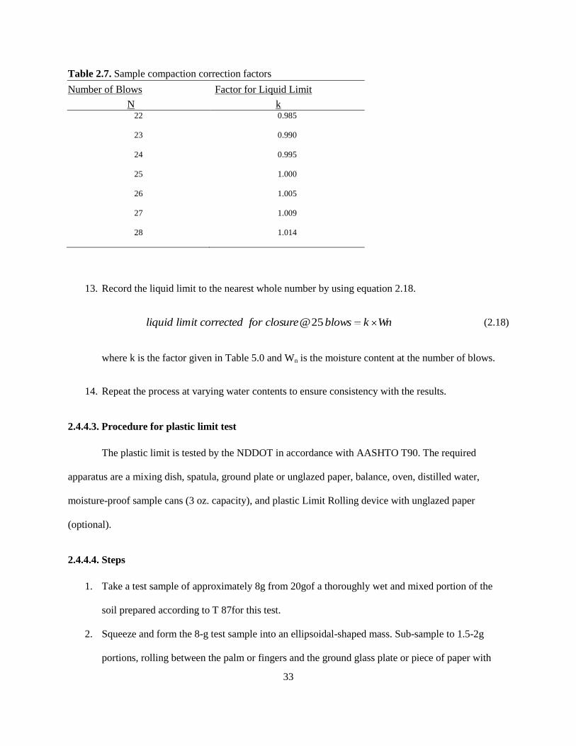
33
Table 2.7. Sample compaction correction factors
Number of Blows Factor for Liquid Limit
N k 22 0.985
23 0.990
24 0.995
25 1.000
26 1.005
27 1.009
28 1.014
13. Record the liquid limit to the nearest whole number by using equation 2.18.
Wnkblowsclosureforcorrectedlimitliquid 25@ (2.18)
where k is the factor given in Table 5.0 and Wn is the moisture content at the number of blows.
14. Repeat the process at varying water contents to ensure consistency with the results.
2.4.4.3. Procedure for plastic limit test
The plastic limit is tested by the NDDOT in accordance with AASHTO T90. The required
apparatus are a mixing dish, spatula, ground plate or unglazed paper, balance, oven, distilled water,
moisture-proof sample cans (3 oz. capacity), and plastic Limit Rolling device with unglazed paper
(optional).
2.4.4.4. Steps
1. Take a test sample of approximately 8g from 20gof a thoroughly wet and mixed portion of the
soil prepared according to T 87for this test.
2. Squeeze and form the 8-g test sample into an ellipsoidal-shaped mass. Sub-sample to 1.5-2g
portions, rolling between the palm or fingers and the ground glass plate or piece of paper with
34
sufficient pressure to roll the sample into a uniform thread about 1/8" in. diameter throughout its
length.
3. Roll the sample at a rate of 80-90 strokes (A stroke is a complete forward and back motion,
returning to the starting place.) per minute. A plastic limit rolling device may also be used for this
stage.
4. When the diameter of the thread reaches 1/8", break the thread into six or eight pieces, and
squeeze the pieces together between the thumbs and fingers of both hands, making a roughly
uniform, ellipsoidal shape and re-roll. Continue this procedure until the thread crumbles under the
pressure required for rolling and the soil can no longer be rolled into a thread.
5. Weigh to the nearest 0.01 g and record. Determine the moisture content according to T 265.
6. Repeat this procedure until the entire 8g specimen is completely tested.
7. The moisture percentage is the plastic limit.
2.4.4.5. Plasticity index
Obtain the plasticity index of the soil sample after the plastic limit and the liquid limit have been
computed. Equation 2.19 is used to compute the plasticity index:
limitliquidlimitplasticindexPlasticity (2.19)
2.4.5. Grain size distribution test
The distribution of different grain sizes of the soil affects the soil’s engineering properties. Grain-
size analysis provides a means of obtaining the grain-size distribution of a particular soil, and the
distribution helps in classifying the soil. For the NDDOT, the procedure is conducted in accordance with
AASHTO T27. AASHTO T27 is used in conjunction with AASHTO T11 if the sample has material
smaller than 75μm (No. 200). This standard test procedure reports the percentage of material finer than
the No. 200 sieve to the nearest 0.1%, except if the result is 10% or more which is then reported to the
nearest whole number.
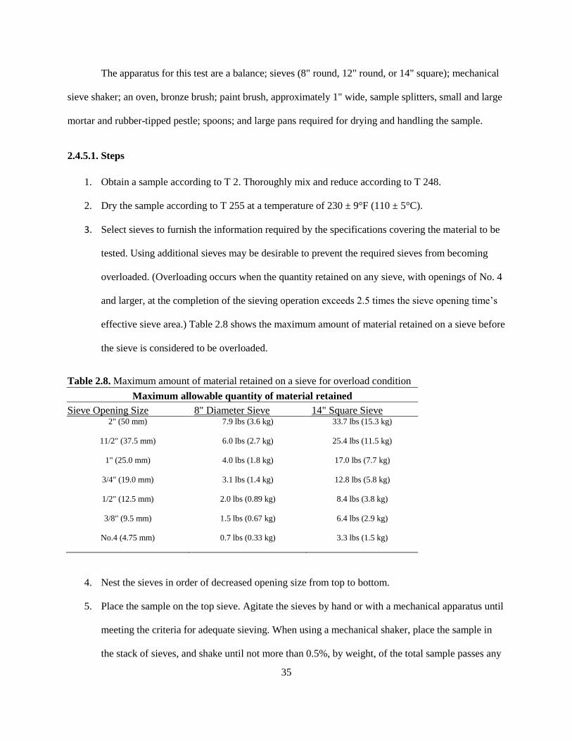
35
The apparatus for this test are a balance; sieves (8" round, 12" round, or 14" square); mechanical
sieve shaker; an oven, bronze brush; paint brush, approximately 1" wide, sample splitters, small and large
mortar and rubber-tipped pestle; spoons; and large pans required for drying and handling the sample.
2.4.5.1. Steps
1. Obtain a sample according to T 2. Thoroughly mix and reduce according to T 248.
2. Dry the sample according to T 255 at a temperature of 230 ± 9°F (110 ± 5°C).
3. Select sieves to furnish the information required by the specifications covering the material to be
tested. Using additional sieves may be desirable to prevent the required sieves from becoming
overloaded. (Overloading occurs when the quantity retained on any sieve, with openings of No. 4
and larger, at the completion of the sieving operation exceeds 2.5 times the sieve opening time’s
effective sieve area.) Table 2.8 shows the maximum amount of material retained on a sieve before
the sieve is considered to be overloaded.
Table 2.8. Maximum amount of material retained on a sieve for overload condition
Maximum allowable quantity of material retained
Sieve Opening Size 8" Diameter Sieve 14" Square Sieve 2" (50 mm) 7.9 lbs (3.6 kg) 33.7 lbs (15.3 kg)
11/2" (37.5 mm) 6.0 lbs (2.7 kg) 25.4 lbs (11.5 kg)
1" (25.0 mm) 4.0 lbs (1.8 kg) 17.0 lbs (7.7 kg)
3/4" (19.0 mm) 3.1 lbs (1.4 kg) 12.8 lbs (5.8 kg)
1/2" (12.5 mm) 2.0 lbs (0.89 kg) 8.4 lbs (3.8 kg)
3/8" (9.5 mm) 1.5 lbs (0.67 kg) 6.4 lbs (2.9 kg)
No.4 (4.75 mm) 0.7 lbs (0.33 kg) 3.3 lbs (1.5 kg)
4. Nest the sieves in order of decreased opening size from top to bottom.
5. Place the sample on the top sieve. Agitate the sieves by hand or with a mechanical apparatus until
meeting the criteria for adequate sieving. When using a mechanical shaker, place the sample in
the stack of sieves, and shake until not more than 0.5%, by weight, of the total sample passes any
36
sieve during 1 minute. Approximately 10 minutes will be sufficient for most materials. Use
manual shaking for the material on any one sieve to check on the thoroughness of sieving by any
mechanical shaker.
6. Remove the top sieve; brush the retained material thoroughly into a pan, weigh, and record.
Repeat this process with each succeeding sieve, brushing the material into individual pans, and
record the non-cumulative weights.
2.4.5.2. Calculation
7. Add the non-cumulative weight retained on the largest sieve to the weight retained on the next
smallest sieve to obtain the cumulative weight.
8. Calculate the percentage retained on each sieve with Equation 2.20:
100weightTotal
weightcumulativesieveonretainedpercentage (2.20)
retainedpercentagegsinpas 100% (2.21)
9. Use Equation 2.21 to obtain the percentage passing each sieve.
10. If an accurate determination of the amount of material passing the No. 200 was accomplished by
performing T 11, subtract the weight after wash from the original weight and record as wash loss.
11. Sum the cumulative weight retained on the No. 200, the weight of the Minus No. 200 material,
and the wash loss; record that number as the weight check.
12. Calculate the percentage of the total sample passing for the fine portion of the aggregate using
Equation 2.22:
100
4. sievesmallerpassingpercentNopassingpercentsampleTotalPercent (2.22)
37
2.5. Summary
In this chapter, the concept behind using the shrinkage factor has been explored with the current
shrinkage-factor equations used in the literature. The literature used as sources of shrinkage-factor values
is clear in stating that the values are not generic and that there was a need to run field tests on samples to
corroborate their shrinkage-factor values. A review of the NDDOT-recommended soil-testing procedures
was also discussed. These procedures were used in the field and laboratory during the research for
sampling, identifying, and characterizing the collected samples. The existing methods of soil-volume
determination were also discussed in this chapter. The soil-sampling method applied in this research was
random. This approach of selecting sample points based on probability allowed for the measured soil
parameters to be calculated based on the chances of occurrence at the location. This method also allowed
for a range of statistical analyses based on the estimates of variability about the mean used. The
geostatistical concept of kriging used to model the spatial patterns for soil properties was discussed.
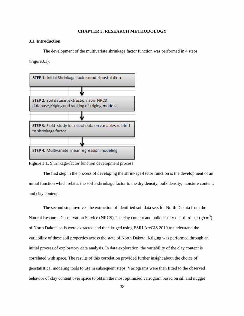
38
CHAPTER 3. RESEARCH METHODOLOGY
3.1. Introduction
The development of the multivariate shrinkage factor function was performed in 4 steps
(Figure3.1).
Figure 3.1. Shrinkage-factor function development process
The first step in the process of developing the shrinkage-factor function is the development of an
initial function which relates the soil’s shrinkage factor to the dry density, bulk density, moisture content,
and clay content.
The second step involves the extraction of identified soil data sets for North Dakota from the
Natural Resource Conservation Service (NRCS).The clay content and bulk density one-third bar (g/cm3)
of North Dakota soils were extracted and then kriged using ESRI ArcGIS 2010 to understand the
variability of these soil properties across the state of North Dakota. Kriging was performed through an
initial process of exploratory data analysis. In data exploration, the variability of the clay content is
correlated with space. The results of this correlation provided further insight about the choice of
geostatistical modeling tools to use in subsequent steps. Variograms were then fitted to the observed
behavior of clay content over space to obtain the most optimized variogram based on sill and nugget
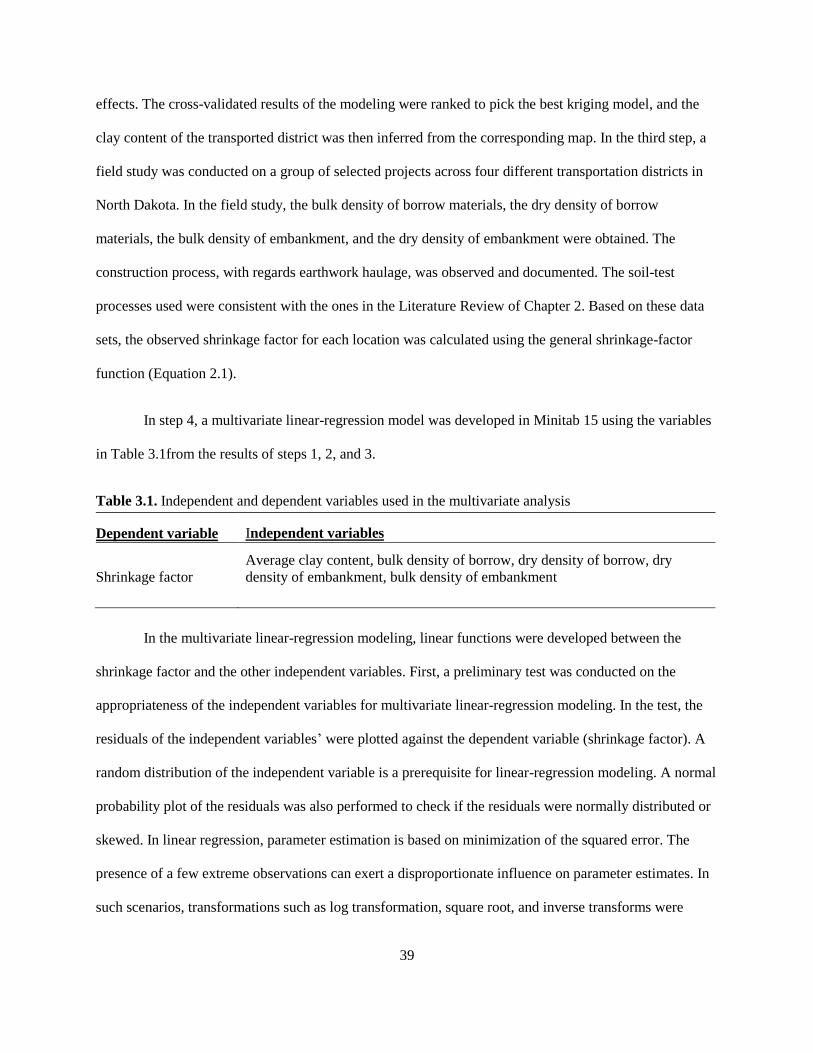
39
effects. The cross-validated results of the modeling were ranked to pick the best kriging model, and the
clay content of the transported district was then inferred from the corresponding map. In the third step, a
field study was conducted on a group of selected projects across four different transportation districts in
North Dakota. In the field study, the bulk density of borrow materials, the dry density of borrow
materials, the bulk density of embankment, and the dry density of embankment were obtained. The
construction process, with regards earthwork haulage, was observed and documented. The soil-test
processes used were consistent with the ones in the Literature Review of Chapter 2. Based on these data
sets, the observed shrinkage factor for each location was calculated using the general shrinkage-factor
function (Equation 2.1).
In step 4, a multivariate linear-regression model was developed in Minitab 15 using the variables
in Table 3.1from the results of steps 1, 2, and 3.
Table 3.1. Independent and dependent variables used in the multivariate analysis
Dependent variable Independent variables
Shrinkage factor
Average clay content, bulk density of borrow, dry density of borrow, dry
density of embankment, bulk density of embankment
In the multivariate linear-regression modeling, linear functions were developed between the
shrinkage factor and the other independent variables. First, a preliminary test was conducted on the
appropriateness of the independent variables for multivariate linear-regression modeling. In the test, the
residuals of the independent variables’ were plotted against the dependent variable (shrinkage factor). A
random distribution of the independent variable is a prerequisite for linear-regression modeling. A normal
probability plot of the residuals was also performed to check if the residuals were normally distributed or
skewed. In linear regression, parameter estimation is based on minimization of the squared error. The
presence of a few extreme observations can exert a disproportionate influence on parameter estimates. In
such scenarios, transformations such as log transformation, square root, and inverse transforms were
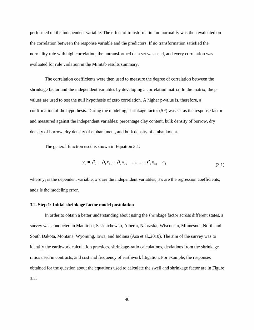
40
performed on the independent variable. The effect of transformation on normality was then evaluated on
the correlation between the response variable and the predictors. If no transformation satisfied the
normality rule with high correlation, the untransformed data set was used, and every correlation was
evaluated for rule violation in the Minitab results summary.
The correlation coefficients were then used to measure the degree of correlation between the
shrinkage factor and the independent variables by developing a correlation matrix. In the matrix, the p-
values are used to test the null hypothesis of zero correlation. A higher p-value is, therefore, a
confirmation of the hypothesis. During the modeling, shrinkage factor (SF) was set as the response factor
and measured against the independent variables: percentage clay content, bulk density of borrow, dry
density of borrow, dry density of embankment, and bulk density of embankment.
The general function used is shown in Equation 3.1:
1112211101 ........ qq xxxy (3.1)
where y1 is the dependent variable, x’s are the independent variables, β’s are the regression coefficients,
andε is the modeling error.
3.2. Step 1: Initial shrinkage factor model postulation
In order to obtain a better understanding about using the shrinkage factor across different states, a
survey was conducted in Manitoba, Saskatchewan, Alberta, Nebraska, Wisconsin, Minnesota, North and
South Dakota, Montana, Wyoming, Iowa, and Indiana (Asa et al.,2010). The aim of the survey was to
identify the earthwork calculation practices, shrinkage-ratio calculations, deviations from the shrinkage
ratios used in contracts, and cost and frequency of earthwork litigation. For example, the responses
obtained for the question about the equations used to calculate the swell and shrinkage factor are in Figure
3.2.
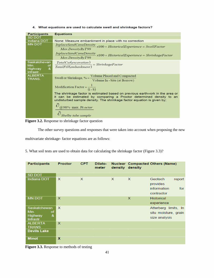
41
Figure 3.2. Response to shrinkage factor question
The other survey questions and responses that were taken into account when proposing the new
multivariate shrinkage- factor equations are as follows:
5. What soil tests are used to obtain data for calculating the shrinkage factor (Figure 3.3)?
Figure 3.3. Response to methods of testing
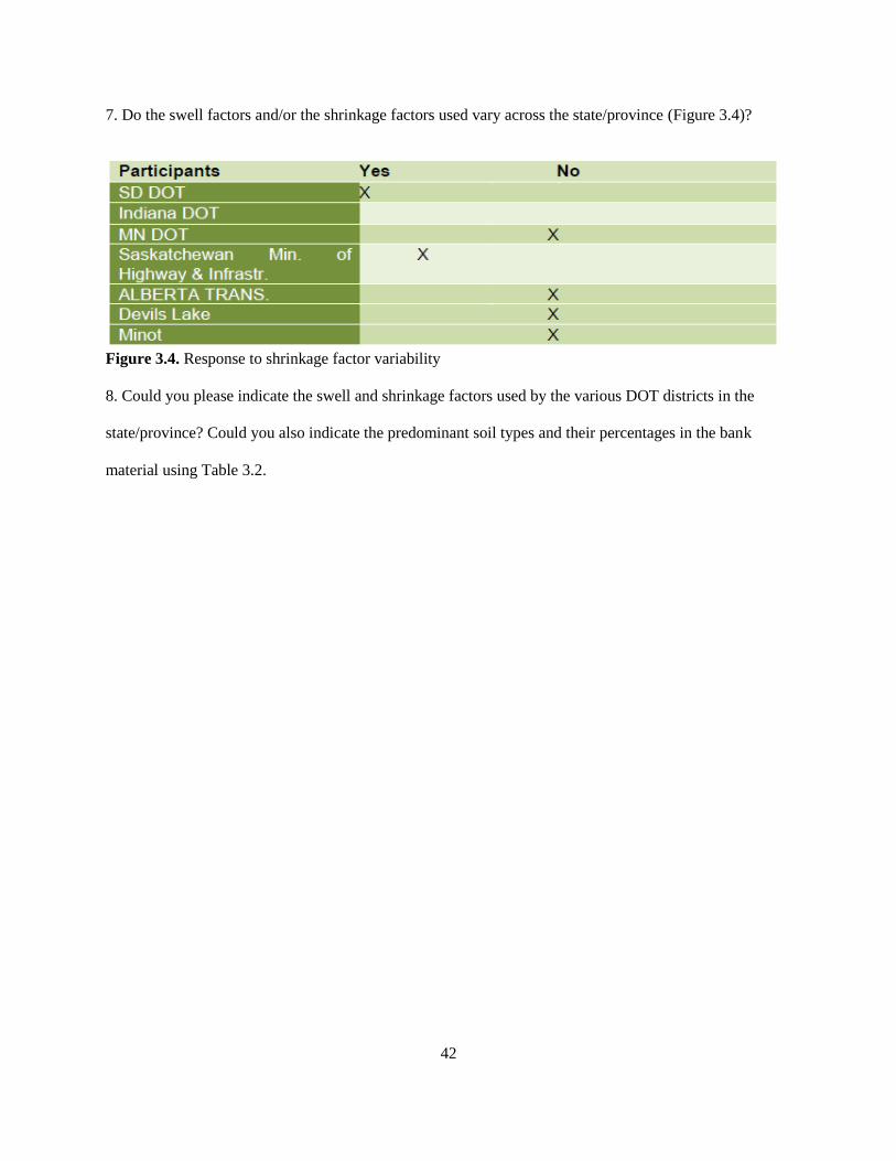
42
7. Do the swell factors and/or the shrinkage factors used vary across the state/province (Figure 3.4)?
Figure 3.4. Response to shrinkage factor variability
8. Could you please indicate the swell and shrinkage factors used by the various DOT districts in the
state/province? Could you also indicate the predominant soil types and their percentages in the bank
material using Table 3.2.
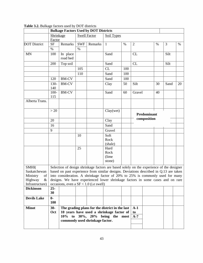
43
Table 3.2. Bulkage factors used by DOT districts
Bulkage Factors Used by DOT Districts
Shrinkage
Factor
Swell Factor Soil Types
DOT District SF Remarks SWF Remarks 1 % 2 % 3 %
% %
MN 100 In place
road bed
Sand CL Silt
200 Top soil Sand CL Silt
105 CL 100
110 Sand 100
120 BM-CV Sand 100
130-
140
BM-CV Clay 50 Silt 30 Sand 20
100-
115
BM-CV Sand 60 Gravel 40
Alberta Trans.
> 20 Clay(wet)
20 Clay
16 Sand
9 Gravel
10 Soft
Rock
(shale)
25 Hard
Rock
(lime
stone)
SMHI(
Saskatchewan
Ministry of
Highway &
Infrastructure)
Selection of design shrinkage factors are based solely on the experience of the designer
based on past experience from similar designs. Deviations described in Q.13 are taken
into consideration. A shrinkage factor of 20% to 25% is commonly used for many
designs. We have experienced lower shrinkage factors in some cases and on rare
occasions, even a SF < 1.0 (i.e swell)
Dickinson 25-
30
Devils Lake 0-
100
Minot 30-
Oct
The grading plans for the district in the last
10 years have used a shrinkage factor of
10% to 30%, 20% being the most
commonly used shrinkage factor.
A-1
to
A-7
Predominant
composition
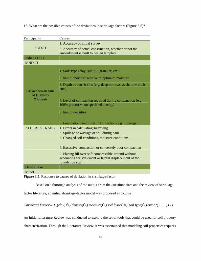
44
13. What are the possible causes of the deviations in shrinkage factors (Figure 3.5)?
Participants Causes
SDDOT
1. Accuracy of initial survey
2. Accuracy of actual construction, whether or not the
embankment is built to design template
Indiana DOT
MNDOT
Saskatchewan Min.
of Highway
&Infrastr
1. Soils type (clay, silt, till, granular, etc.)
2. In-situ moisture relative to optimum moisture
3. Depth of cuts & fills (e.g. deep borrows vs shallow ditch
cuts)
4. Level of compaction required during construction (e.g.
100% proctor vs no specified density).
5. In-situ densities
6. Foundation conditions in fill section (e.g. muskegs)
ALBERTA TRANS. 1. Errors in calculating/surveying
2. Spillage or wastage of soil during haul
3. Changed soil conditions, moisture conditions
4. Excessive compaction or conversely poor compaction
5. Placing fill over soft compressible ground without
accounting for settlement or lateral displacement of the
foundation soil
Devils Lake
Minot
Figure 3.5. Response to causes of deviation in shrinkage-factor
Based on a thorough analysis of the output from the questionnaires and the review of shrinkage-
factor literature, an initial shrinkage-factor model was proposed as follows:
))2(,)(,)(,)(,)(,)(( errortypesoillossessoilmoisturedensityclayfFactorShrinkage (3.2)
An initial Literature Review was conducted to explore the set of tools that could be used for soil property
characterization. Through the Literature Review, it was ascertained that modeling soil properties requires
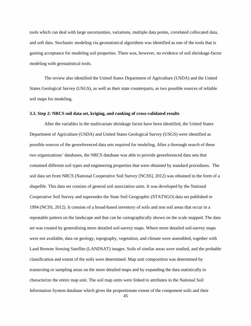
45
tools which can deal with large uncertainties, variations, multiple data points, correlated collocated data,
and soft data. Stochastic modeling via geostatistical algorithms was identified as one of the tools that is
gaining acceptance for modeling soil properties. There was, however, no evidence of soil shrinkage-factor
modeling with geostatistical tools.
The review also identified the United States Department of Agriculture (USDA) and the United
States Geological Survey (USGS), as well as their state counterparts, as two possible sources of reliable
soil maps for modeling.
3.3. Step 2: NRCS soil data set, kriging, and ranking of cross-validated results
After the variables in the multivariate shrinkage factor have been identified, the United States
Department of Agriculture (USDA) and United States Geological Survey (USGS) were identified as
possible sources of the georeferenced data sets required for modeling. After a thorough search of these
two organizations’ databases, the NRCS database was able to provide georeferenced data sets that
contained different soil types and engineering properties that were obtained by standard procedures. The
soil data set from NRCS (National Cooperative Soil Survey [NCSS], 2012) was obtained in the form of a
shapefile. This data set consists of general soil association units. It was developed by the National
Cooperative Soil Survey and supersedes the State Soil Geographic (STATSGO) data set published in
1994 (NCSS, 2012). It consists of a broad-based inventory of soils and non soil areas that occur in a
repeatable pattern on the landscape and that can be cartographically shown on the scale mapped. The data
set was created by generalizing more detailed soil-survey maps. Where more detailed soil-survey maps
were not available, data on geology, topography, vegetation, and climate were assembled, together with
Land Remote Sensing Satellite (LANDSAT) images. Soils of similar areas were studied, and the probable
classification and extent of the soils were determined. Map unit composition was determined by
transecting or sampling areas on the more detailed maps and by expanding the data statistically to
characterize the entire map unit. The soil map units were linked to attributes in the National Soil
Information System database which gives the proportionate extent of the component soils and their
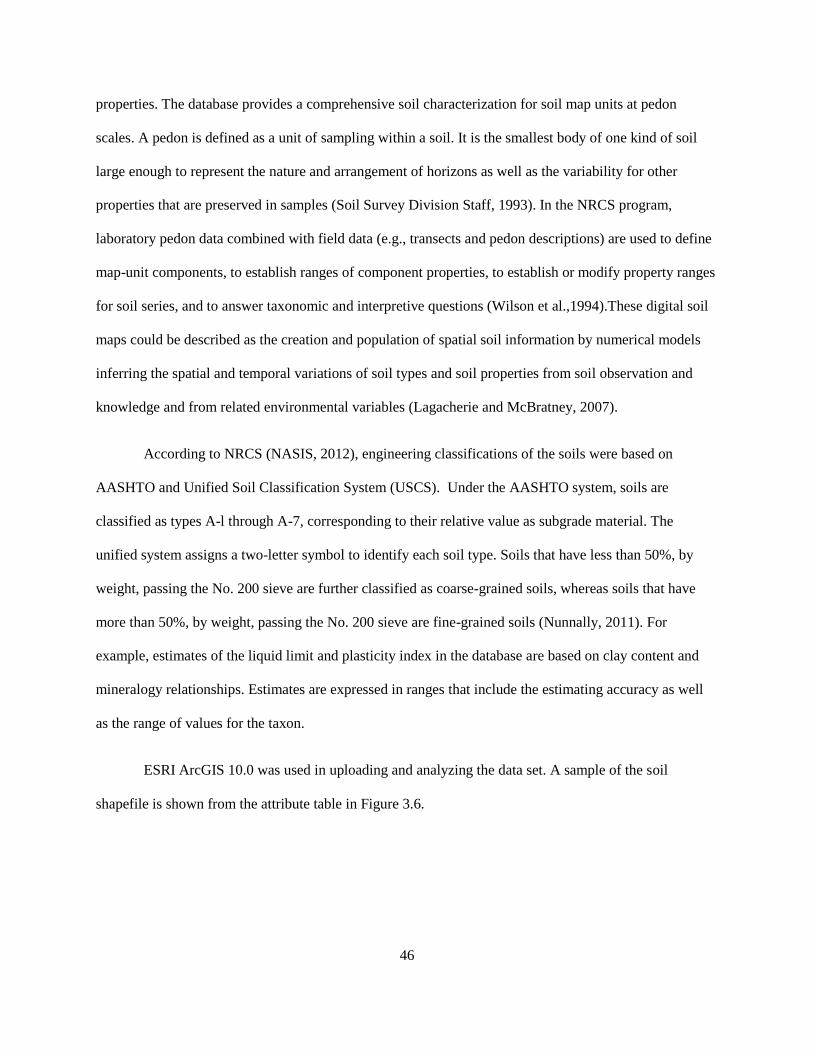
46
properties. The database provides a comprehensive soil characterization for soil map units at pedon
scales. A pedon is defined as a unit of sampling within a soil. It is the smallest body of one kind of soil
large enough to represent the nature and arrangement of horizons as well as the variability for other
properties that are preserved in samples (Soil Survey Division Staff, 1993). In the NRCS program,
laboratory pedon data combined with field data (e.g., transects and pedon descriptions) are used to define
map-unit components, to establish ranges of component properties, to establish or modify property ranges
for soil series, and to answer taxonomic and interpretive questions (Wilson et al.,1994).These digital soil
maps could be described as the creation and population of spatial soil information by numerical models
inferring the spatial and temporal variations of soil types and soil properties from soil observation and
knowledge and from related environmental variables (Lagacherie and McBratney, 2007).
According to NRCS (NASIS, 2012), engineering classifications of the soils were based on
AASHTO and Unified Soil Classification System (USCS). Under the AASHTO system, soils are
classified as types A-l through A-7, corresponding to their relative value as subgrade material. The
unified system assigns a two-letter symbol to identify each soil type. Soils that have less than 50%, by
weight, passing the No. 200 sieve are further classified as coarse-grained soils, whereas soils that have
more than 50%, by weight, passing the No. 200 sieve are fine-grained soils (Nunnally, 2011). For
example, estimates of the liquid limit and plasticity index in the database are based on clay content and
mineralogy relationships. Estimates are expressed in ranges that include the estimating accuracy as well
as the range of values for the taxon.
ESRI ArcGIS 10.0 was used in uploading and analyzing the data set. A sample of the soil
shapefile is shown from the attribute table in Figure 3.6.
47
Figure 3.6. Sample NRCS (USDA) soil data set showing clay, silt, and sand at varying depths
Analysis and kriging of the extracted data set were performed in line with the geostatistical
process depicted in Figure 3.7.
Figure 3.7. Geostatistical research approach (Asa et al., 2011)
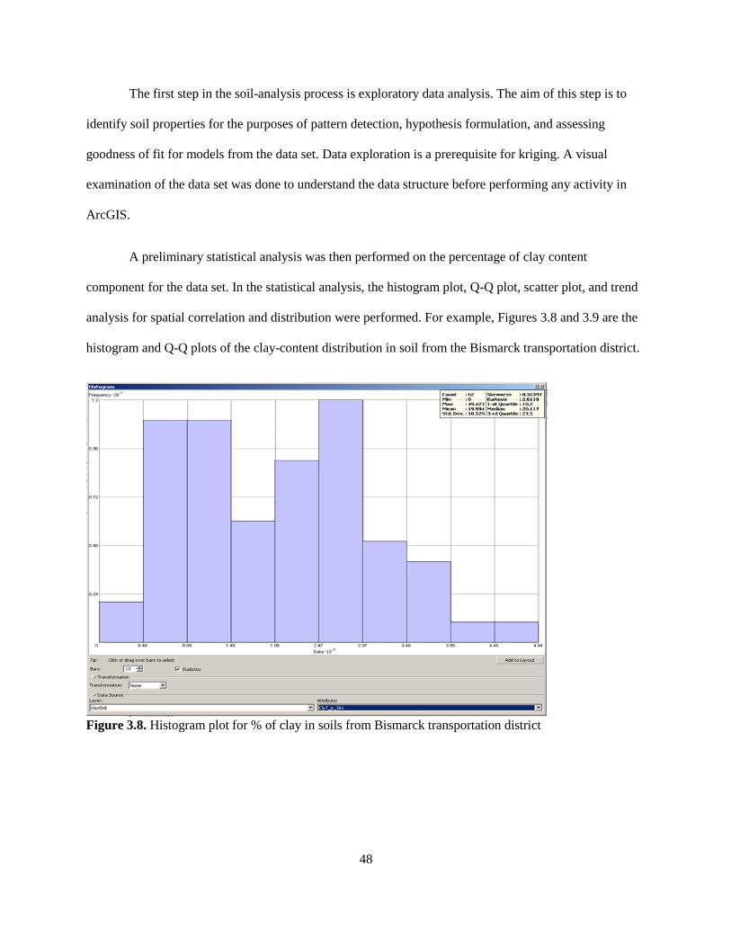
48
The first step in the soil-analysis process is exploratory data analysis. The aim of this step is to
identify soil properties for the purposes of pattern detection, hypothesis formulation, and assessing
goodness of fit for models from the data set. Data exploration is a prerequisite for kriging. A visual
examination of the data set was done to understand the data structure before performing any activity in
ArcGIS.
A preliminary statistical analysis was then performed on the percentage of clay content
component for the data set. In the statistical analysis, the histogram plot, Q-Q plot, scatter plot, and trend
analysis for spatial correlation and distribution were performed. For example, Figures 3.8 and 3.9 are the
histogram and Q-Q plots of the clay-content distribution in soil from the Bismarck transportation district.
Figure 3.8. Histogram plot for % of clay in soils from Bismarck transportation district
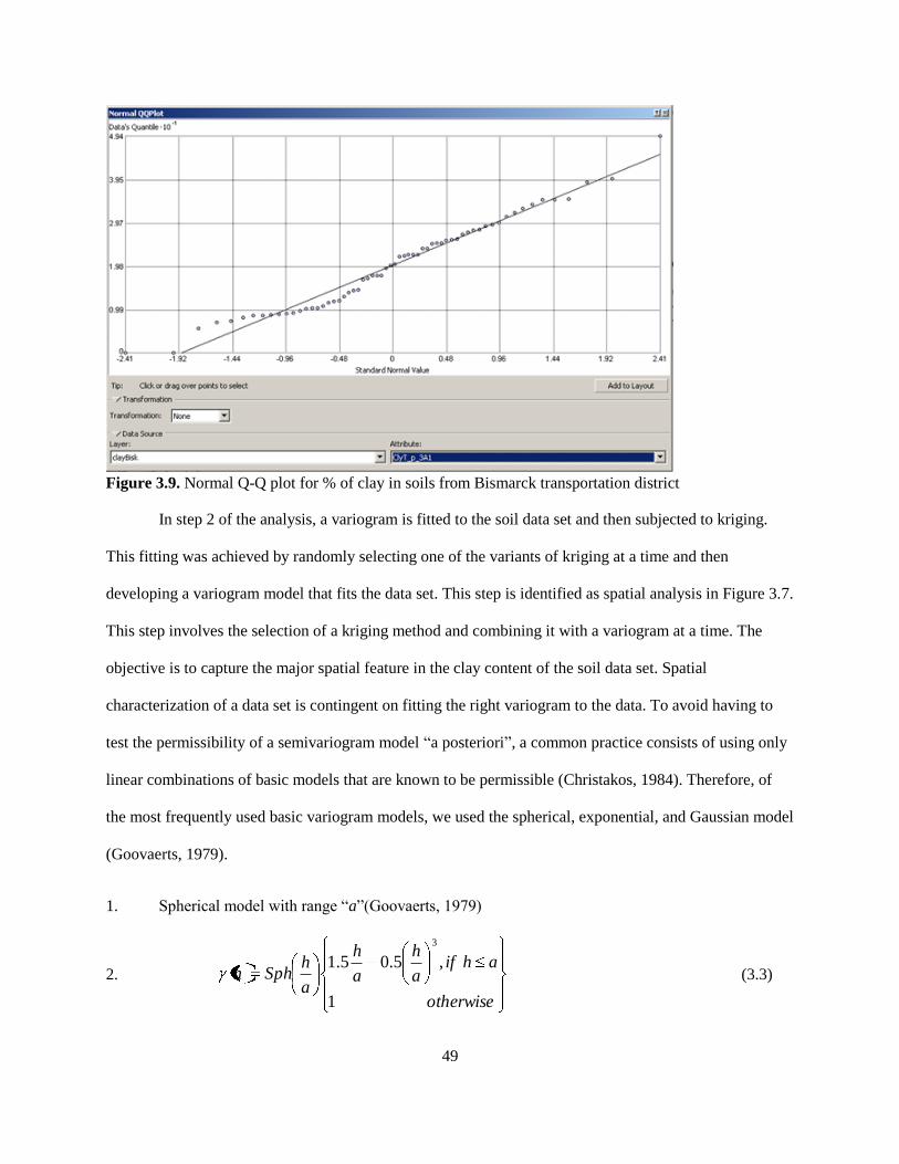
49
Figure 3.9. Normal Q-Q plot for % of clay in soils from Bismarck transportation district
In step 2 of the analysis, a variogram is fitted to the soil data set and then subjected to kriging.
This fitting was achieved by randomly selecting one of the variants of kriging at a time and then
developing a variogram model that fits the data set. This step is identified as spatial analysis in Figure 3.7.
This step involves the selection of a kriging method and combining it with a variogram at a time. The
objective is to capture the major spatial feature in the clay content of the soil data set. Spatial
characterization of a data set is contingent on fitting the right variogram to the data. To avoid having to
test the permissibility of a semivariogram model “a posteriori”, a common practice consists of using only
linear combinations of basic models that are known to be permissible (Christakos, 1984). Therefore, of
the most frequently used basic variogram models, we used the spherical, exponential, and Gaussian model
(Goovaerts, 1979).
1. Spherical model with range “a”(Goovaerts, 1979)
2.
otherwise
ahifa
h
a
h
a
hSphh
1
,5.05.1
3
(3.3)
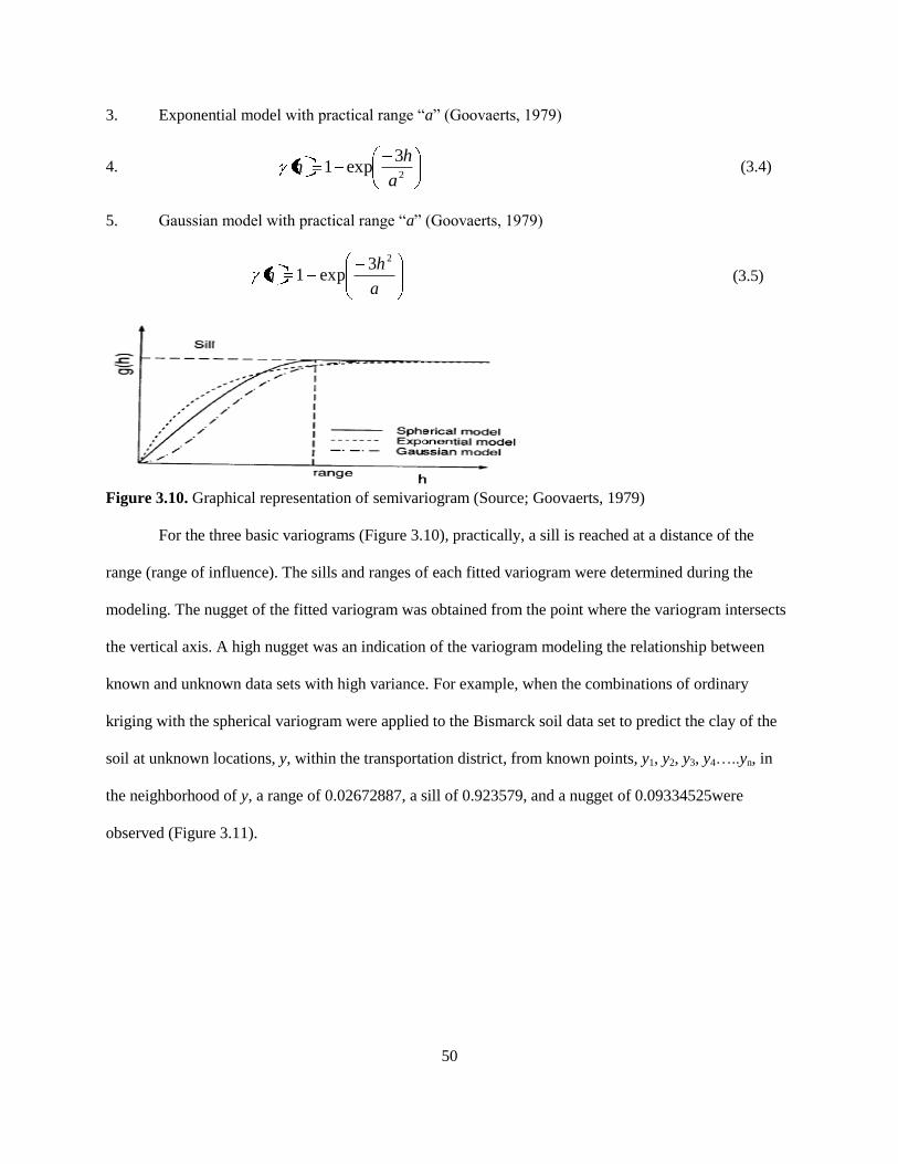
50
3. Exponential model with practical range “a” (Goovaerts, 1979)
4. 2
3exp1
a
hh (3.4)
5. Gaussian model with practical range “a” (Goovaerts, 1979)
a
hh
23exp1 (3.5)
Figure 3.10. Graphical representation of semivariogram (Source; Goovaerts, 1979)
For the three basic variograms (Figure 3.10), practically, a sill is reached at a distance of the
range (range of influence). The sills and ranges of each fitted variogram were determined during the
modeling. The nugget of the fitted variogram was obtained from the point where the variogram intersects
the vertical axis. A high nugget was an indication of the variogram modeling the relationship between
known and unknown data sets with high variance. For example, when the combinations of ordinary
kriging with the spherical variogram were applied to the Bismarck soil data set to predict the clay of the
soil at unknown locations, y, within the transportation district, from known points, y1, y2, y3, y4…..yn, in
the neighborhood of y, a range of 0.02672887, a sill of 0.923579, and a nugget of 0.09334525were
observed (Figure 3.11).
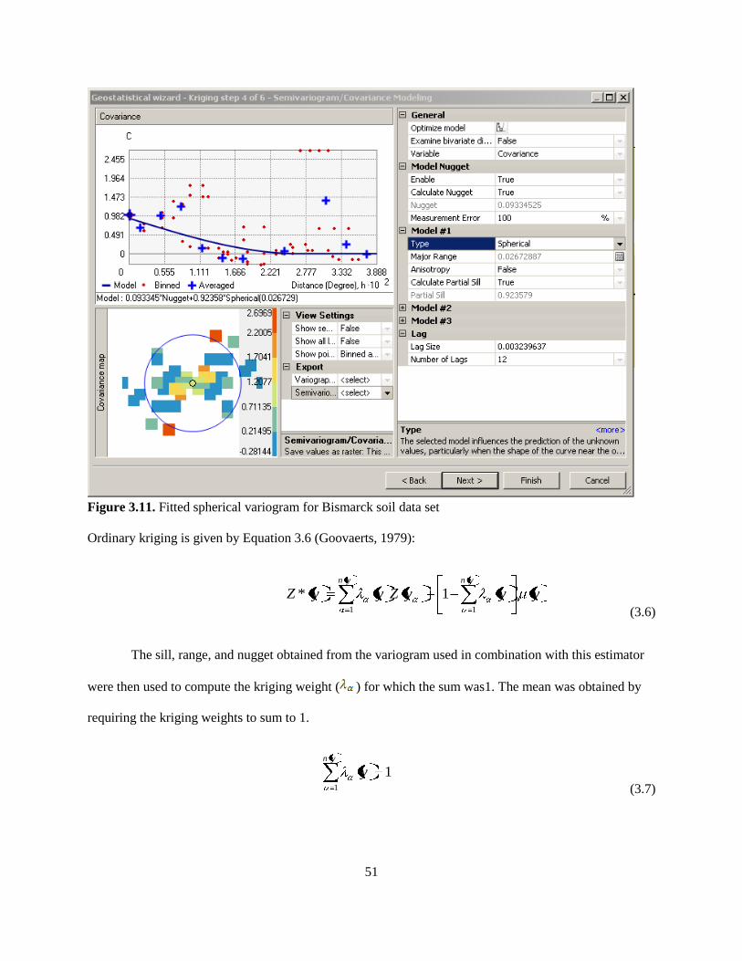
51
Figure 3.11. Fitted spherical variogram for Bismarck soil data set
Ordinary kriging is given by Equation 3.6 (Goovaerts, 1979):
yyyZyyZynyn
11
1*
(3.6)
The sill, range, and nugget obtained from the variogram used in combination with this estimator
were then used to compute the kriging weight ( ) for which the sum was1. The mean was obtained by
requiring the kriging weights to sum to 1.
11
yn
y
(3.7)
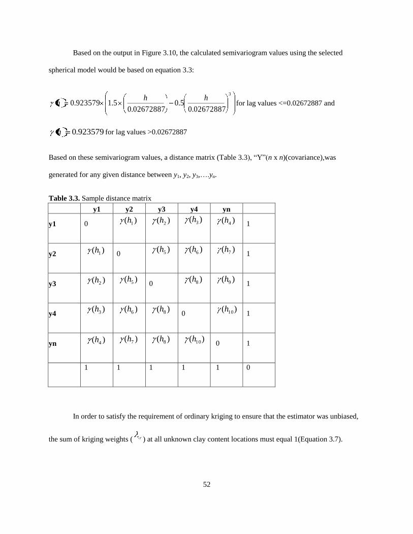
52
Based on the output in Figure 3.10, the calculated semivariogram values using the selected
spherical model would be based on equation 3.3:
3
02672887.05.0
02672887.05.1923579.0
hhh for lag values <=0.02672887 and
923579.0h for lag values >0.02672887
Based on these semivariogram values, a distance matrix (Table 3.3), “Y”(n x n)(covariance),was
generated for any given distance between y1, y2, y3,….yn.
Table 3.3. Sample distance matrix
y1 y2 y3 y4 yn
y1 0 )( 1h )( 2h )( 3h
)( 4h 1
y2 )( 1h 0 )( 5h
)( 6h
)( 7h
1
y3 )( 2h )( 5h
0 )( 8h
)( 9h
1
y4 )( 3h
)( 6h
)( 8h
0 )( 10h
1
yn )( 4h )( 7h
)( 8h
)( 10h
0 1
1 1 1 1 1 0
In order to satisfy the requirement of ordinary kriging to ensure that the estimator was unbiased,
the sum of kriging weights ( ) at all unknown clay content locations must equal 1(Equation 3.7).
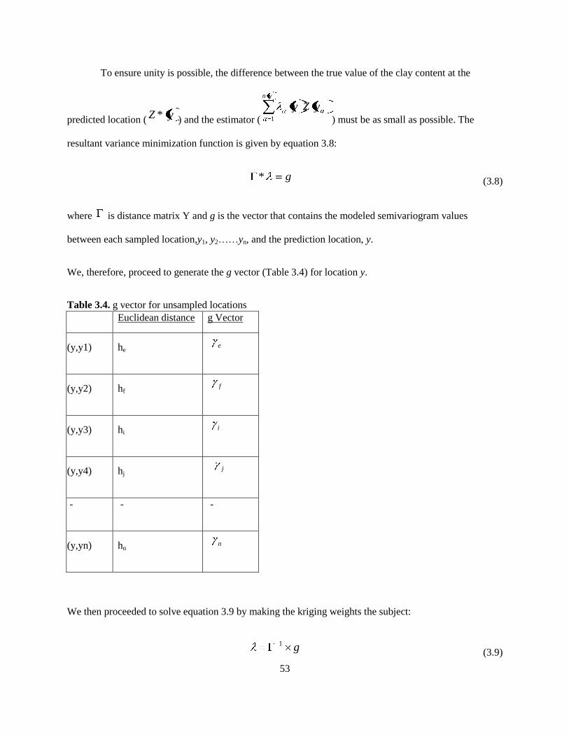
53
To ensure unity is possible, the difference between the true value of the clay content at the
predicted location ( yZ * ) and the estimator (
yZyyn
1 ) must be as small as possible. The
resultant variance minimization function is given by equation 3.8:
g* (3.8)
where is distance matrix Y and g is the vector that contains the modeled semivariogram values
between each sampled location,y1, y2……yn, and the prediction location, y.
We, therefore, proceed to generate the g vector (Table 3.4) for location y.
Table 3.4. g vector for unsampled locations
Euclidean distance g Vector
(y,y1) he e
(y,y2) hf f
(y,y3) hi i
(y,y4) hj j
- - -
(y,yn) hn n
We then proceeded to solve equation 3.9 by making the kriging weights the subject:
g1
(3.9)
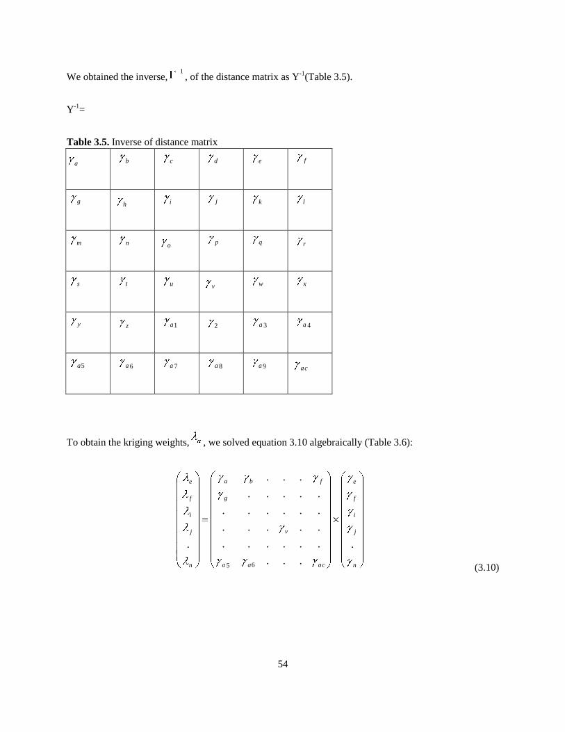
54
We obtained the inverse,1, of the distance matrix as Y
-1(Table 3.5).
Y-1
=
Table 3.5. Inverse of distance matrix
a b c d e f
g h i j k l
m n o p q r
s t u v w x
y z 1a 2 3a 4a
5a 6a 7a 8a 9a ac
To obtain the kriging weights, , we solved equation 3.10 algebraically (Table 3.6):
n
j
i
f
e
acaa
v
g
fba
n
j
i
f
e
.
...
......
.....
......
.....
...
.
65 (3.10)
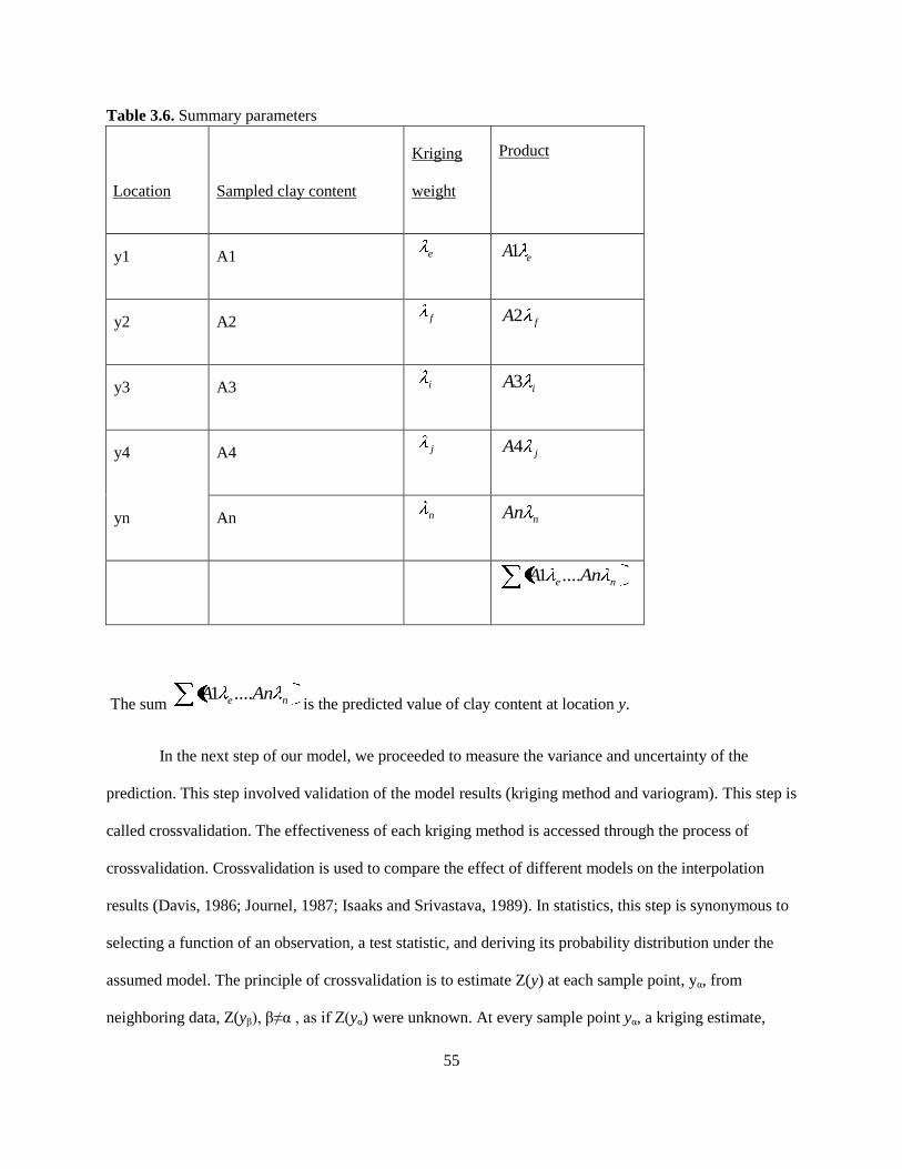
55
Table 3.6. Summary parameters
Location Sampled clay content
Kriging
weight
Product
y1 A1 e eA1
y2 A2 f fA2
y3 A3 i iA3
y4 A4 j jA4
yn An n nAn
ne AnA ....1
The sum ne AnA ....1 is the predicted value of clay content at location y.
In the next step of our model, we proceeded to measure the variance and uncertainty of the
prediction. This step involved validation of the model results (kriging method and variogram). This step is
called crossvalidation. The effectiveness of each kriging method is accessed through the process of
crossvalidation. Crossvalidation is used to compare the effect of different models on the interpolation
results (Davis, 1986; Journel, 1987; Isaaks and Srivastava, 1989). In statistics, this step is synonymous to
selecting a function of an observation, a test statistic, and deriving its probability distribution under the
assumed model. The principle of crossvalidation is to estimate Z(y) at each sample point, yα, from
neighboring data, Z(yβ), β≠α , as if Z(yα) were unknown. At every sample point yα, a kriging estimate,
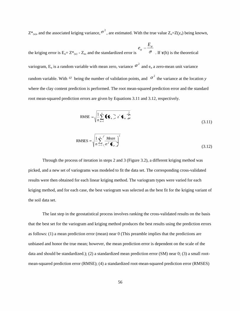
56
Z*(α), and the associated kriging variance,2
, are estimated. With the true value Zα=Z(yα) being known,
the kriging error is Eα= Z*(α) - Zα, and the standardized error is
Ee
. If ɤ(h) is the theoretical
variogram, Eα is a random variable with mean zero, variance 2
and eα a zero-mean unit variance
random variable. With being the number of validation points, and 2
the variance at the location y
where the clay content prediction is performed. The root mean-squared prediction error and the standard
root mean-squared prediction errors are given by Equations 3.11 and 3.12, respectively.
1
RMSE
2
1
*n
yzyzn
(3.11)
1
RMSES
2
12
n
i y
Mean
n (3.12)
Through the process of iteration in steps 2 and 3 (Figure 3.2), a different kriging method was
picked, and a new set of variograms was modeled to fit the data set. The corresponding cross-validated
results were then obtained for each linear kriging method. The variogram types were varied for each
kriging method, and for each case, the best variogram was selected as the best fit for the kriging variant of
the soil data set.
The last step in the geostatistical process involves ranking the cross-validated results on the basis
that the best set for the variogram and kriging method produces the best results using the prediction errors
as follows: (1) a mean prediction error (mean) near 0 (This preamble implies that the predictions are
unbiased and honor the true mean; however, the mean prediction error is dependent on the scale of the
data and should be standardized.); (2) a standardized mean prediction error (SM) near 0; (3) a small root-
mean-squared prediction error (RMSE); (4) a standardized root-mean-squared prediction error (RMSES)

57
near 1; and (5) a small average standard error (ASE);(Pardo-Igusquiza, 1998; Robinson and Metternicht,
2006; Asa et al., 2012).
Ranking the performance of each model with regards to the closeness of its prediction errors to
the expected values is then performed. A rank of 1 to 3, with 1 being the best and 3 being the worst in
comparison with the other variants, was assigned to each outcome.
3.4. Step 3: Field study on shrinkage-factor related variables
A field study was conducted in four transportation districts of North Dakota. Figure 3.12 shows
the Minot, Devils Lake, Dickinson, and Valley City transportation districts with the project locations.
Figure 3.12. Study sites in North Dakota
58
For each project site, the earthwork component associated with the construction process was
observed and documented. The equipment associated with the earthwork process was also documented. A
series of in-field density tests were conducted on both borrow and road embankments. In the borrow pit,
where the haul material was excavated, the location was georeferenced using the global navigation
satellite system survey instrument. The in-place density of the soil was then measured at the location
using a nuclear gage. Samples were also collected for laboratory tests. In the laboratory, the maximum
dry density, the particle-size distribution, the plastic limit, and the liquid limit were measured for the
georeferenced soil. The standard and modified proctor tests (T 99 and T180) were conducted to obtain the
densities and optimum moisture content of the soil samples. Sieve analysis was performed on the samples
to aid in AASHTO classification. In the laboratory, the Atterberg limit test was conducted on the samples
to determine the plastic limit, liquid limit, and plasticity index. Results from the series of tests were used
to classify the samples. After the soil was excavated, the location where the excavated soil was dumped
was also georeferenced. The compacted density of the placed soil was measured using the nuclear gage.
The shrinkage factor was then calculated by using the georeferenced densities of the borrow soil
and compacted soil. The shrinkage factor was calculated using Equation 2.1 by relating the in-place
density of borrow soil to the compacted density of the same soil in the embankment.
3.5. Step 4: Multivariate linear-regression modeling
In step 4 of the research methodology, Minitab 15 was used to perform multivariate linear-
regression modeling. The linear-regression modeling was performed to relate other soil properties
measured in addition to the density during the georeferenced borrow and embankment testing. Regression
modeling was also used to relate the clay content of soils in the study area which was obtained from the
NRCS database to the measured shrinkage factor.
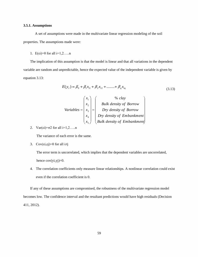
59
3.5.1. Assumptions
A set of assumptions were made in the multivariate linear regression modeling of the soil
properties. The assumptions made were:
1. E(εi)=0 for all i=1,2…..n
The implication of this assumption is that the model is linear and that all variations in the dependent
variable are random and unpredictable, hence the expected value of the independent variable is given by
equation 3.13:
iqqiiI xxxyE ........)( 22110 (3.13)
EmbankmentofdensityBulk
EmbankmentofdensityDry
BorrowofdensityDry
BorrowofdensityBulk
clay
x
x
x
x
x
Variables
%
5
4
3
2
1
2. Var(εi)=σ2 for all i=1,2…..n
The variance of each error is the same.
3. Cov(εi,εj)=0 for all i≠j
The error term is uncorrelated, which implies that the dependent variables are uncorrelated,
hence cov(yi,yj)=0.
4. The correlation coefficients only measure linear relationships. A nonlinear correlation could exist
even if the correlation coefficient is 0.
If any of these assumptions are compromised, the robustness of the multivariate regression model
becomes low. The confidence interval and the resultant predictions would have high residuals (Decision
411, 2012).
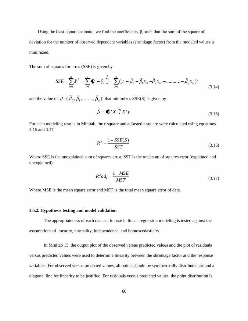
60
Using the least-square estimate, we find the coefficients, β, such that the sum of the square of
deviation for the number of observed dependent variables (shrinkage factor) from the modeled values is
minimized.
The sum of squares for error (SSE) is given by
2
22
1
110
2
1 1
2)ˆ............ˆˆˆ(ˆˆ
iqqi
n
i
ii
n
i
n
i
iii xxxyyySSE (3.14)
and the value of ˆ =(0
ˆ ,1
ˆ ,……..,q
ˆ )’ that minimizes SSE(S) is given by
yXXX ''ˆ 1
(3.15)
For each modeling results in Minitab, the r-square and adjusted r-square were calculated using equations
3.16 and 3.17
SST
SSSER
)(12
(3.16)
Where SSE is the unexplained sum of squares error, SST is the total sum of squares error (explained and
unexplained)
MST
MSEadjR
12
(3.17)
Where MSE is the mean square error and MST is the total mean square error of data.
3.5.2. Hypothesis testing and model validation
The appropriateness of each data set for use in linear-regression modeling is tested against the
assumptions of linearity, normality, independence, and homoscedasticity.
In Minitab 15, the output plot of the observed versus predicted values and the plot of residuals
versus predicted values were used to determine linearity between the shrinkage factor and the response
variables. For observed versus predicted values, all points should be symmetrically distributed around a
diagonal line for linearity to be justified. For residuals versus predicted values, the point distribution is
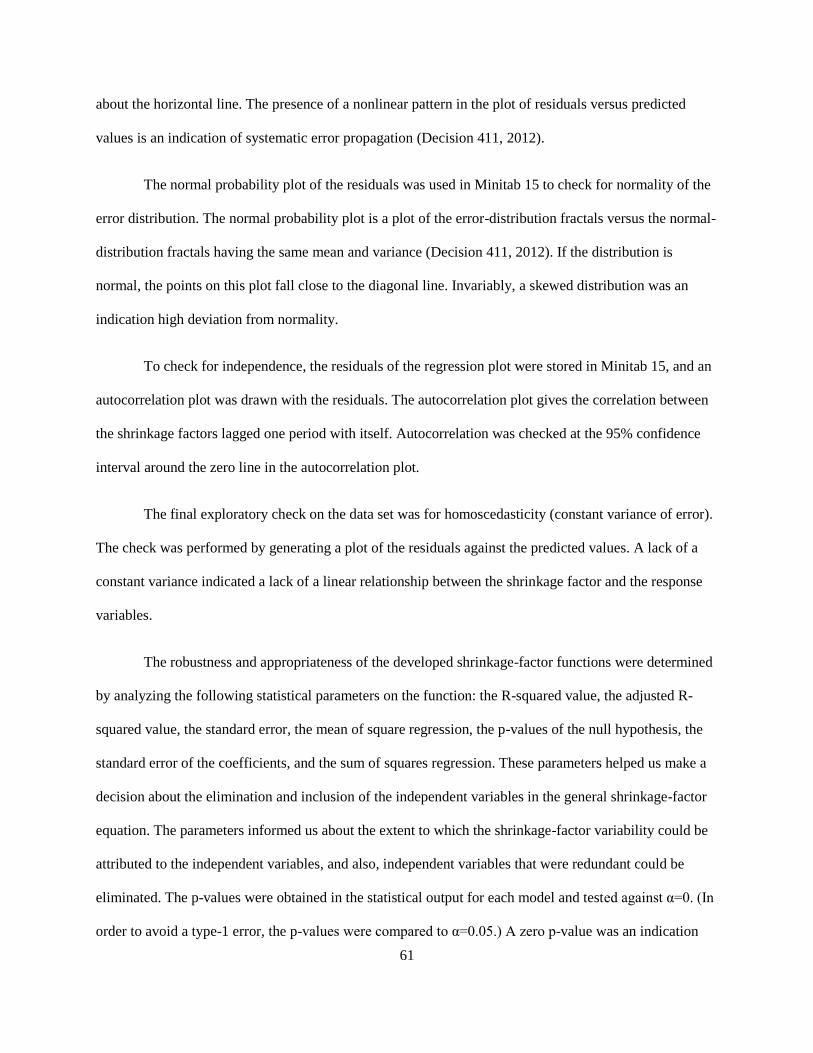
61
about the horizontal line. The presence of a nonlinear pattern in the plot of residuals versus predicted
values is an indication of systematic error propagation (Decision 411, 2012).
The normal probability plot of the residuals was used in Minitab 15 to check for normality of the
error distribution. The normal probability plot is a plot of the error-distribution fractals versus the normal-
distribution fractals having the same mean and variance (Decision 411, 2012). If the distribution is
normal, the points on this plot fall close to the diagonal line. Invariably, a skewed distribution was an
indication high deviation from normality.
To check for independence, the residuals of the regression plot were stored in Minitab 15, and an
autocorrelation plot was drawn with the residuals. The autocorrelation plot gives the correlation between
the shrinkage factors lagged one period with itself. Autocorrelation was checked at the 95% confidence
interval around the zero line in the autocorrelation plot.
The final exploratory check on the data set was for homoscedasticity (constant variance of error).
The check was performed by generating a plot of the residuals against the predicted values. A lack of a
constant variance indicated a lack of a linear relationship between the shrinkage factor and the response
variables.
The robustness and appropriateness of the developed shrinkage-factor functions were determined
by analyzing the following statistical parameters on the function: the R-squared value, the adjusted R-
squared value, the standard error, the mean of square regression, the p-values of the null hypothesis, the
standard error of the coefficients, and the sum of squares regression. These parameters helped us make a
decision about the elimination and inclusion of the independent variables in the general shrinkage-factor
equation. The parameters informed us about the extent to which the shrinkage-factor variability could be
attributed to the independent variables, and also, independent variables that were redundant could be
eliminated. The p-values were obtained in the statistical output for each model and tested against α=0. (In
order to avoid a type-1 error, the p-values were compared to α=0.05.) A zero p-value was an indication
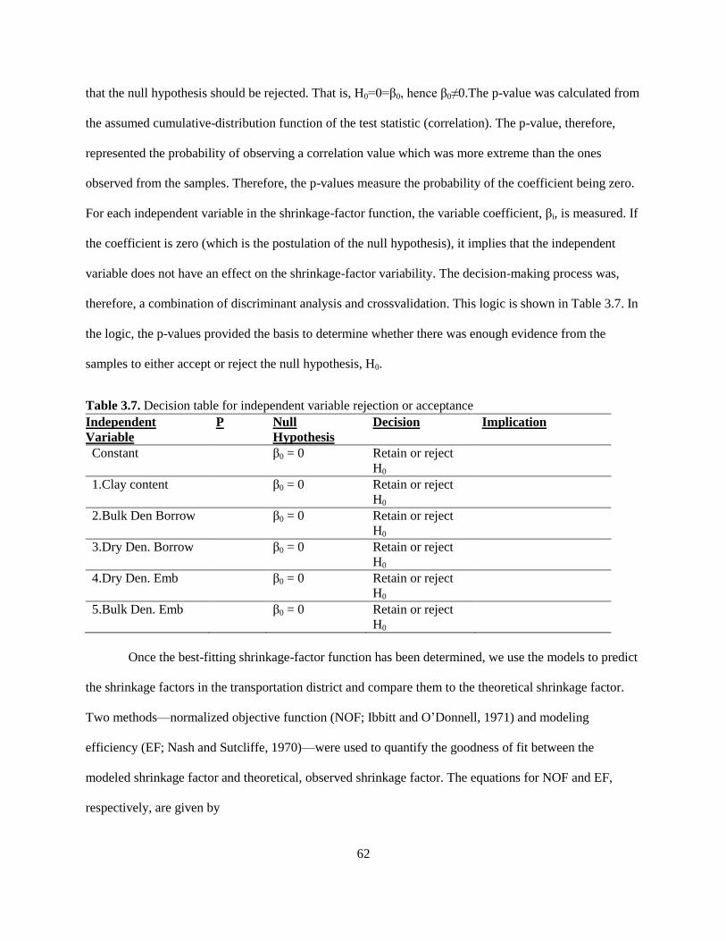
62
that the null hypothesis should be rejected. That is, H0=0=β0, hence β0≠0.The p-value was calculated from
the assumed cumulative-distribution function of the test statistic (correlation). The p-value, therefore,
represented the probability of observing a correlation value which was more extreme than the ones
observed from the samples. Therefore, the p-values measure the probability of the coefficient being zero.
For each independent variable in the shrinkage-factor function, the variable coefficient, βi, is measured. If
the coefficient is zero (which is the postulation of the null hypothesis), it implies that the independent
variable does not have an effect on the shrinkage-factor variability. The decision-making process was,
therefore, a combination of discriminant analysis and crossvalidation. This logic is shown in Table 3.7. In
the logic, the p-values provided the basis to determine whether there was enough evidence from the
samples to either accept or reject the null hypothesis, H0.
Table 3.7. Decision table for independent variable rejection or acceptance
Independent
Variable
P Null
Hypothesis
Decision Implication
Constant β0 = 0 Retain or reject
H0
1.Clay content β0 = 0 Retain or reject
H0
2.Bulk Den Borrow β0 = 0 Retain or reject
H0
3.Dry Den. Borrow β0 = 0 Retain or reject
H0
4.Dry Den. Emb β0 = 0 Retain or reject
H0
5.Bulk Den. Emb β0 = 0 Retain or reject
H0
Once the best-fitting shrinkage-factor function has been determined, we use the models to predict
the shrinkage factors in the transportation district and compare them to the theoretical shrinkage factor.
Two methods—normalized objective function (NOF; Ibbitt and O’Donnell, 1971) and modeling
efficiency (EF; Nash and Sutcliffe, 1970)—were used to quantify the goodness of fit between the
modeled shrinkage factor and theoretical, observed shrinkage factor. The equations for NOF and EF,
respectively, are given by
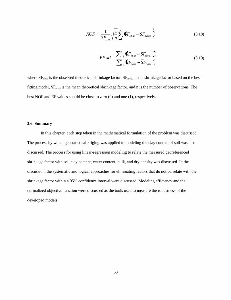
63
2
1
mod,,
11 n
i
iiobs
obs
SFSFnSF
NOF (3.18)
n
i iobsiobs
n
i iiobs
FSSF
SFSFEF
1
2
,,
1
2
mod,,1 (3.19)
where SFobs,i is the observed theoretical shrinkage factor, SFmod,i is the shrinkage factor based on the best
fitting model, ŚFobs,i is the mean theoretical shrinkage factor, and n is the number of observations. The
best NOF and EF values should be close to zero (0) and one (1), respectively.
3.6. Summary
In this chapter, each step taken in the mathematical formulation of the problem was discussed.
The process by which geostatistical kriging was applied to modeling the clay content of soil was also
discussed. The process for using linear-regression modeling to relate the measured georeferenced
shrinkage factor with soil clay content, water content, bulk, and dry density was discussed. In the
discussion, the systematic and logical approaches for eliminating factors that do not correlate with the
shrinkage factor within a 95% confidence interval were discussed. Modeling efficiency and the
normalized objective function were discussed as the tools used to measure the robustness of the
developed models.
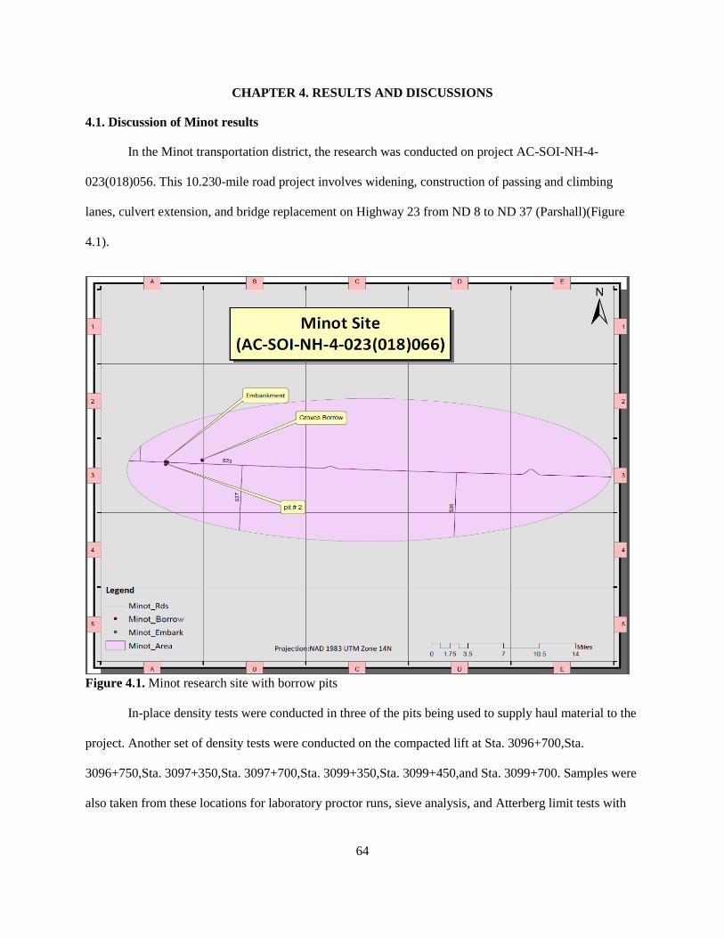
64
CHAPTER 4. RESULTS AND DISCUSSIONS
4.1. Discussion of Minot results
In the Minot transportation district, the research was conducted on project AC-SOI-NH-4-
023(018)056. This 10.230-mile road project involves widening, construction of passing and climbing
lanes, culvert extension, and bridge replacement on Highway 23 from ND 8 to ND 37 (Parshall)(Figure
4.1).
Figure 4.1. Minot research site with borrow pits
In-place density tests were conducted in three of the pits being used to supply haul material to the
project. Another set of density tests were conducted on the compacted lift at Sta. 3096+700,Sta.
3096+750,Sta. 3097+350,Sta. 3097+700,Sta. 3099+350,Sta. 3099+450,and Sta. 3099+700. Samples were
also taken from these locations for laboratory proctor runs, sieve analysis, and Atterberg limit tests with
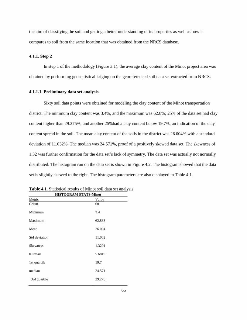
65
the aim of classifying the soil and getting a better understanding of its properties as well as how it
compares to soil from the same location that was obtained from the NRCS database.
4.1.1. Step 2
In step 1 of the methodology (Figure 3.1), the average clay content of the Minot project area was
obtained by performing geostatistical kriging on the georeferenced soil data set extracted from NRCS.
4.1.1.1. Preliminary data set analysis
Sixty soil data points were obtained for modeling the clay content of the Minot transportation
district. The minimum clay content was 3.4%, and the maximum was 62.8%; 25% of the data set had clay
content higher than 29.275%, and another 25%had a clay content below 19.7%, an indication of the clay-
content spread in the soil. The mean clay content of the soils in the district was 26.004% with a standard
deviation of 11.032%. The median was 24.571%, proof of a positively skewed data set. The skewness of
1.32 was further confirmation for the data set’s lack of symmetry. The data set was actually not normally
distributed. The histogram run on the data set is shown in Figure 4.2. The histogram showed that the data
set is slightly skewed to the right. The histogram parameters are also displayed in Table 4.1.
Table 4.1. Statistical results of Minot soil data set analysis
HISTOGRAM STATS-Minot
Metric Value
Count 60
Minimum 3.4
Maximum 62.833
Mean 26.004
Std deviation 11.032
Skewness 1.3201
Kurtosis 5.6819
1st quartile 19.7
median 24.571
3rd quartile 29.275
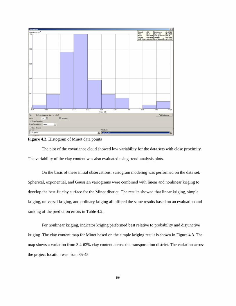
66
Figure 4.2. Histogram of Minot data points
The plot of the covariance cloud showed low variability for the data sets with close proximity.
The variability of the clay content was also evaluated using trend-analysis plots.
On the basis of these initial observations, variogram modeling was performed on the data set.
Spherical, exponential, and Gaussian variograms were combined with linear and nonlinear kriging to
develop the best-fit clay surface for the Minot district. The results showed that linear kriging, simple
kriging, universal kriging, and ordinary kriging all offered the same results based on an evaluation and
ranking of the prediction errors in Table 4.2.
For nonlinear kriging, indicator kriging performed best relative to probability and disjunctive
kriging. The clay content map for Minot based on the simple kriging result is shown in Figure 4.3. The
map shows a variation from 3.4-62% clay content across the transportation district. The variation across
the project location was from 35-45
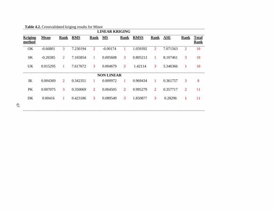
67
Table 4.2. Crossvalidated kriging results for Minot
LINEAR KRIGING
Kriging
method
Mean Rank RMS Rank MS Rank RMSS Rank ASE Rank Total
Rank
OK -0.66801 3 7.230194 2 -0.00174 1 1.059392 2 7.071563 2 10
SK -0.26585 2 7.165854 1 0.005608 3 0.805213 1 8.107461 3 10
UK 0.015295 1 7.617672 3 0.004679 2 1.42114 3 5.346366 1 10
NON LINEAR
IK 0.004369 2 0.342351 1 0.000972 1 0.969434 1 0.361757 3 8
PK 0.007075 3 0.350069 2 0.004505 2 0.995279 2 0.357717 2 11
DK 0.00416 1 0.423186 3 0.089549 3 1.850877 3 0.28296 1 11
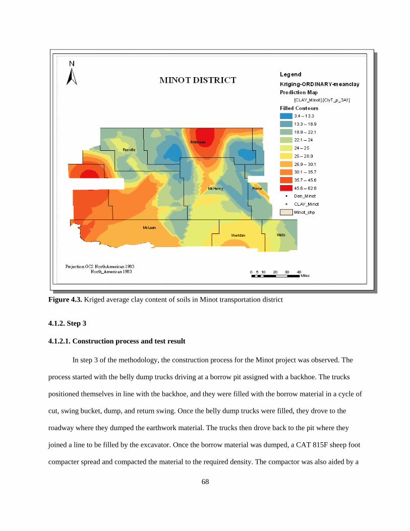
68
Figure 4.3. Kriged average clay content of soils in Minot transportation district
4.1.2. Step 3
4.1.2.1. Construction process and test result
In step 3 of the methodology, the construction process for the Minot project was observed. The
process started with the belly dump trucks driving at a borrow pit assigned with a backhoe. The trucks
positioned themselves in line with the backhoe, and they were filled with the borrow material in a cycle of
cut, swing bucket, dump, and return swing. Once the belly dump trucks were filled, they drove to the
roadway where they dumped the earthwork material. The trucks then drove back to the pit where they
joined a line to be filled by the excavator. Once the borrow material was dumped, a CAT 815F sheep foot
compacter spread and compacted the material to the required density. The compactor was also aided by a
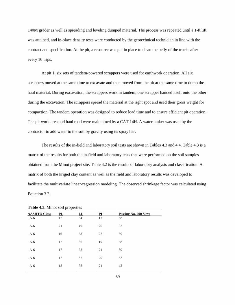
69
140M grader as well as spreading and leveling dumped material. The process was repeated until a 1-ft lift
was attained, and in-place density tests were conducted by the geotechnical technician in line with the
contract and specification. At the pit, a resource was put in place to clean the belly of the trucks after
every 10 trips.
At pit 1, six sets of tandem-powered scrappers were used for earthwork operation. All six
scrappers moved at the same time to excavate and then moved from the pit at the same time to dump the
haul material. During excavation, the scrappers work in tandem; one scrapper handed itself onto the other
during the excavation. The scrappers spread the material at the right spot and used their gross weight for
compaction. The tandem operation was designed to reduce load time and to ensure efficient pit operation.
The pit work area and haul road were maintained by a CAT 14H. A water tanker was used by the
contractor to add water to the soil by gravity using its spray bar.
The results of the in-field and laboratory soil tests are shown in Tables 4.3 and 4.4. Table 4.3 is a
matrix of the results for both the in-field and laboratory tests that were performed on the soil samples
obtained from the Minot project site. Table 4.2 is the results of laboratory analysis and classification. A
matrix of both the kriged clay content as well as the field and laboratory results was developed to
facilitate the multivariate linear-regression modeling. The observed shrinkage factor was calculated using
Equation 3.2.
Table 4.3. Minot soil properties
AASHTO Class PL LL PI Passing No. 200 Sieve
A-6 17 34 17 58
A-6 21 40 20 53
A-6 16 38 22 59
A-6 17 36 19 58
A-6 17 38 21 59
A-6 17 37 20 52
A-6 18 38 21 42
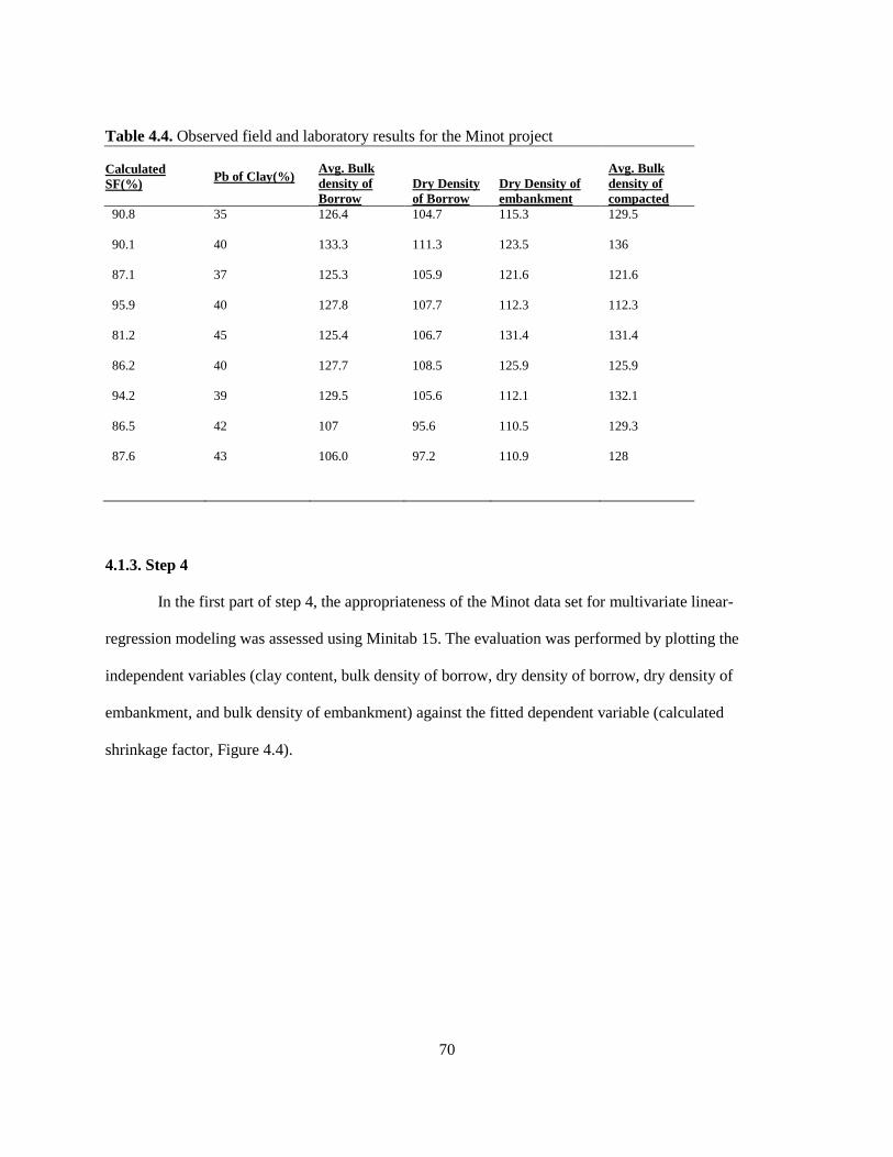
70
Table 4.4. Observed field and laboratory results for the Minot project
Calculated
SF(%) Pb of Clay(%)
Avg. Bulk
density of
Borrow
Dry Density
of Borrow
Dry Density of
embankment
Avg. Bulk
density of
compacted
90.8 35 126.4 104.7 115.3 129.5
90.1 40 133.3 111.3 123.5 136
87.1 37 125.3 105.9 121.6 121.6
95.9 40 127.8 107.7 112.3 112.3
81.2 45 125.4 106.7 131.4 131.4
86.2 40 127.7 108.5 125.9 125.9
94.2 39 129.5 105.6 112.1 132.1
86.5 42 107 95.6 110.5 129.3
87.6 43 106.0 97.2 110.9 128
4.1.3. Step 4
In the first part of step 4, the appropriateness of the Minot data set for multivariate linear-
regression modeling was assessed using Minitab 15. The evaluation was performed by plotting the
independent variables (clay content, bulk density of borrow, dry density of borrow, dry density of
embankment, and bulk density of embankment) against the fitted dependent variable (calculated
shrinkage factor, Figure 4.4).
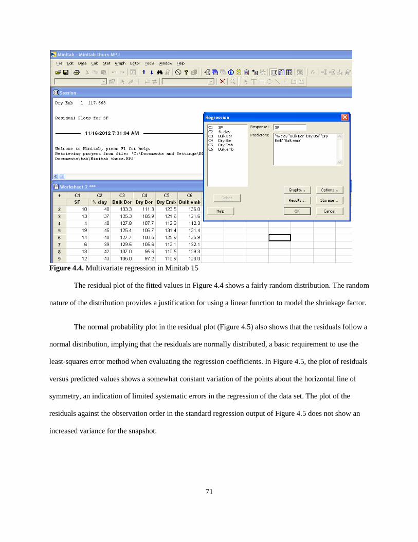
71
Figure 4.4. Multivariate regression in Minitab 15
The residual plot of the fitted values in Figure 4.4 shows a fairly random distribution. The random
nature of the distribution provides a justification for using a linear function to model the shrinkage factor.
The normal probability plot in the residual plot (Figure 4.5) also shows that the residuals follow a
normal distribution, implying that the residuals are normally distributed, a basic requirement to use the
least-squares error method when evaluating the regression coefficients. In Figure 4.5, the plot of residuals
versus predicted values shows a somewhat constant variation of the points about the horizontal line of
symmetry, an indication of limited systematic errors in the regression of the data set. The plot of the
residuals against the observation order in the standard regression output of Figure 4.5 does not show an
increased variance for the snapshot.
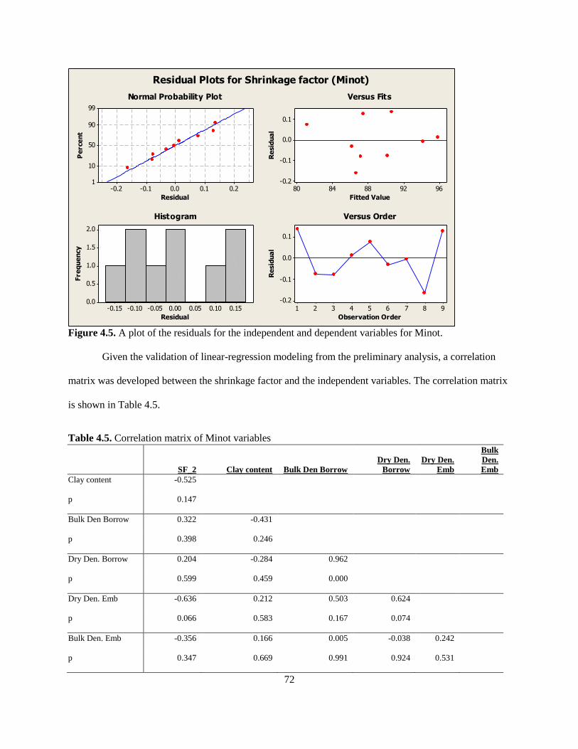
72
0.20.10.0-0.1-0.2
99
90
50
10
1
Residual
Pe
rce
nt
9692888480
0.1
0.0
-0.1
-0.2
Fitted Value
Re
sid
ua
l
0.150.100.050.00-0.05-0.10-0.15
2.0
1.5
1.0
0.5
0.0
Residual
Fre
qu
en
cy
987654321
0.1
0.0
-0.1
-0.2
Observation Order
Re
sid
ua
l
Normal Probability Plot Versus Fits
Histogram Versus Order
Residual Plots for Shrinkage factor (Minot)
Figure 4.5. A plot of the residuals for the independent and dependent variables for Minot.
Given the validation of linear-regression modeling from the preliminary analysis, a correlation
matrix was developed between the shrinkage factor and the independent variables. The correlation matrix
is shown in Table 4.5.
Table 4.5. Correlation matrix of Minot variables
SF_2 Clay content Bulk Den Borrow
Dry Den.
Borrow
Dry Den.
Emb
Bulk
Den.
Emb
Clay content -0.525
p 0.147
Bulk Den Borrow 0.322 -0.431
p 0.398 0.246
Dry Den. Borrow 0.204 -0.284 0.962
p 0.599 0.459 0.000
Dry Den. Emb -0.636 0.212 0.503 0.624
p 0.066 0.583 0.167 0.074
Bulk Den. Emb -0.356 0.166 0.005 -0.038 0.242
p 0.347 0.669 0.991 0.924 0.531
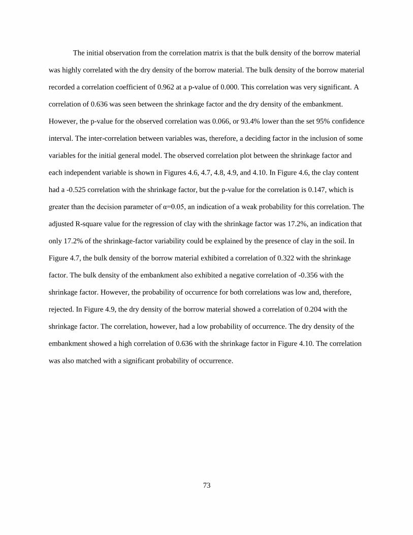
73
The initial observation from the correlation matrix is that the bulk density of the borrow material
was highly correlated with the dry density of the borrow material. The bulk density of the borrow material
recorded a correlation coefficient of 0.962 at a p-value of 0.000. This correlation was very significant. A
correlation of 0.636 was seen between the shrinkage factor and the dry density of the embankment.
However, the p-value for the observed correlation was 0.066, or 93.4% lower than the set 95% confidence
interval. The inter-correlation between variables was, therefore, a deciding factor in the inclusion of some
variables for the initial general model. The observed correlation plot between the shrinkage factor and
each independent variable is shown in Figures 4.6, 4.7, 4.8, 4.9, and 4.10. In Figure 4.6, the clay content
had a -0.525 correlation with the shrinkage factor, but the p-value for the correlation is 0.147, which is
greater than the decision parameter of α=0.05, an indication of a weak probability for this correlation. The
adjusted R-square value for the regression of clay with the shrinkage factor was 17.2%, an indication that
only 17.2% of the shrinkage-factor variability could be explained by the presence of clay in the soil. In
Figure 4.7, the bulk density of the borrow material exhibited a correlation of 0.322 with the shrinkage
factor. The bulk density of the embankment also exhibited a negative correlation of -0.356 with the
shrinkage factor. However, the probability of occurrence for both correlations was low and, therefore,
rejected. In Figure 4.9, the dry density of the borrow material showed a correlation of 0.204 with the
shrinkage factor. The correlation, however, had a low probability of occurrence. The dry density of the
embankment showed a high correlation of 0.636 with the shrinkage factor in Figure 4.10. The correlation
was also matched with a significant probability of occurrence.
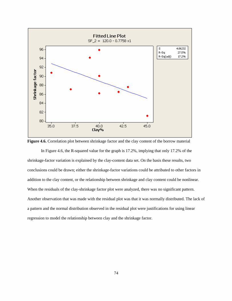
74
Figure 4.6. Correlation plot between shrinkage factor and the clay content of the borrow material
In Figure 4.6, the R-squared value for the graph is 17.2%, implying that only 17.2% of the
shrinkage-factor variation is explained by the clay-content data set. On the basis these results, two
conclusions could be drawn; either the shrinkage-factor variations could be attributed to other factors in
addition to the clay content, or the relationship between shrinkage and clay content could be nonlinear.
When the residuals of the clay-shrinkage factor plot were analyzed, there was no significant pattern.
Another observation that was made with the residual plot was that it was normally distributed. The lack of
a pattern and the normal distribution observed in the residual plot were justifications for using linear
regression to model the relationship between clay and the shrinkage factor.
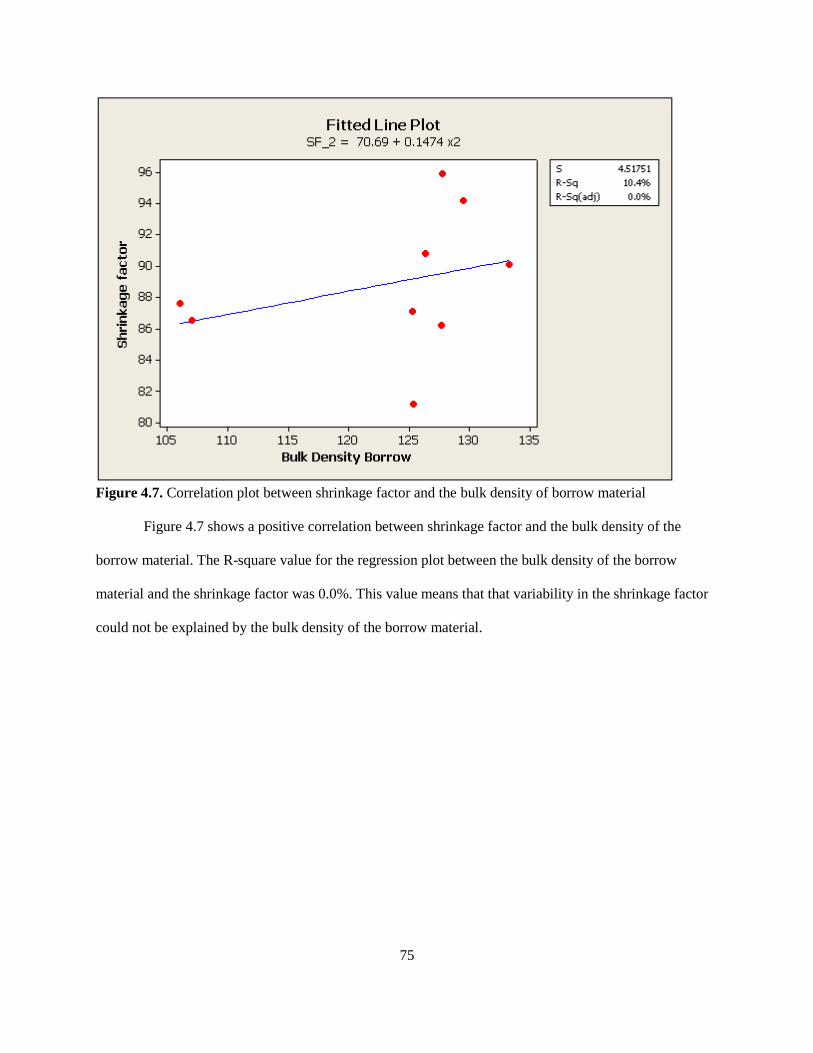
75
Figure 4.7. Correlation plot between shrinkage factor and the bulk density of borrow material
Figure 4.7 shows a positive correlation between shrinkage factor and the bulk density of the
borrow material. The R-square value for the regression plot between the bulk density of the borrow
material and the shrinkage factor was 0.0%. This value means that that variability in the shrinkage factor
could not be explained by the bulk density of the borrow material.
76
135130125120115110
96
94
92
90
88
86
84
82
80
Bulk density of embankment
Sh
rin
ka
ge
fa
cto
r
S 4.45868
R-Sq 12.7%
R-Sq(adj) 0.2%
Fitted Line PlotSF_2 = 118.1 - 0.2294 x5
Figure 4.8. Correlation plot between shrinkage factor and bulk density of the embankment material
Figure 4.9. Correlation plot between the shrinkage factor and the density of borrow material
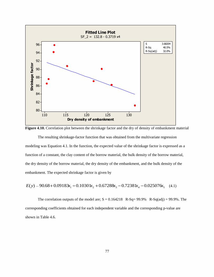
77
Figure 4.10. Correlation plot between the shrinkage factor and the dry of density of embankment material
The resulting shrinkage-factor function that was obtained from the multivariate regression
modeling was Equation 4.1. In the function, the expected value of the shrinkage factor is expressed as a
function of a constant, the clay content of the borrow material, the bulk density of the borrow material,
the dry density of the borrow material, the dry density of the embankment, and the bulk density of the
embankment. The expected shrinkage factor is given by
54321 025076.072381.067288.010301.009183.068.90)( xxxxxyE (4.1)
The correlation outputs of the model are; S = 0.164218 R-Sq= 99.9% R-Sq(adj) = 99.9%. The
corresponding coefficients obtained for each independent variable and the corresponding p-value are
shown in Table 4.6.
130125120115110
96
94
92
90
88
86
84
82
80
Dry density of embankment
Sh
rin
ka
ge
fa
cto
r
S 3.68204
R-Sq 40.5%
R-Sq(adj) 32.0%
Fitted Line PlotSF_2 = 132.8 - 0.3719 x4
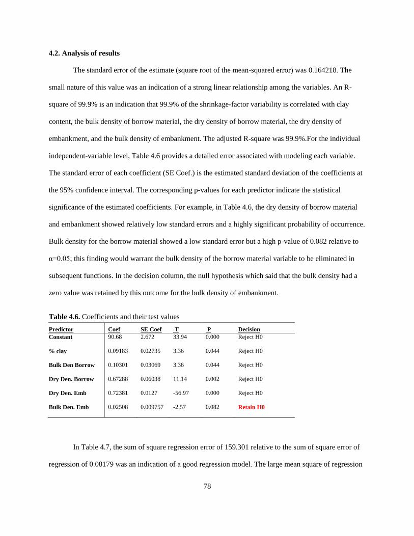
78
4.2. Analysis of results
The standard error of the estimate (square root of the mean-squared error) was 0.164218. The
small nature of this value was an indication of a strong linear relationship among the variables. An R-
square of 99.9% is an indication that 99.9% of the shrinkage-factor variability is correlated with clay
content, the bulk density of borrow material, the dry density of borrow material, the dry density of
embankment, and the bulk density of embankment. The adjusted R-square was 99.9%.For the individual
independent-variable level, Table 4.6 provides a detailed error associated with modeling each variable.
The standard error of each coefficient (SE Coef.) is the estimated standard deviation of the coefficients at
the 95% confidence interval. The corresponding p-values for each predictor indicate the statistical
significance of the estimated coefficients. For example, in Table 4.6, the dry density of borrow material
and embankment showed relatively low standard errors and a highly significant probability of occurrence.
Bulk density for the borrow material showed a low standard error but a high p-value of 0.082 relative to
α=0.05; this finding would warrant the bulk density of the borrow material variable to be eliminated in
subsequent functions. In the decision column, the null hypothesis which said that the bulk density had a
zero value was retained by this outcome for the bulk density of embankment.
Table 4.6. Coefficients and their test values
Predictor Coef SE Coef T P Decision
Constant 90.68 2.672 33.94 0.000 Reject H0
% clay 0.09183 0.02735 3.36 0.044 Reject H0
Bulk Den Borrow 0.10301 0.03069 3.36 0.044 Reject H0
Dry Den. Borrow 0.67288 0.06038 11.14 0.002 Reject H0
Dry Den. Emb 0.72381 0.0127 -56.97 0.000 Reject H0
Bulk Den. Emb 0.02508 0.009757 -2.57 0.082 Retain H0
In Table 4.7, the sum of square regression error of 159.301 relative to the sum of square error of
regression of 0.08179 was an indication of a good regression model. The large mean square of regression
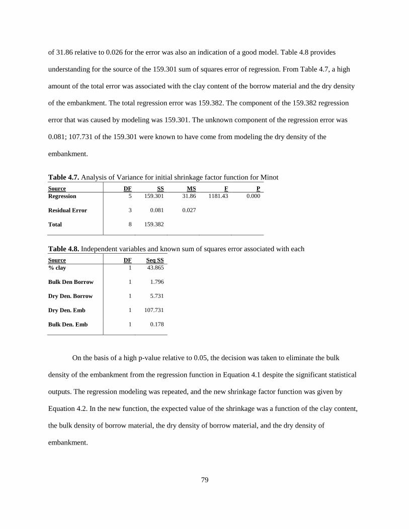
79
of 31.86 relative to 0.026 for the error was also an indication of a good model. Table 4.8 provides
understanding for the source of the 159.301 sum of squares error of regression. From Table 4.7, a high
amount of the total error was associated with the clay content of the borrow material and the dry density
of the embankment. The total regression error was 159.382. The component of the 159.382 regression
error that was caused by modeling was 159.301. The unknown component of the regression error was
0.081; 107.731 of the 159.301 were known to have come from modeling the dry density of the
embankment.
Table 4.7. Analysis of Variance for initial shrinkage factor function for Minot
Source DF SS MS F P
Regression 5 159.301 31.86 1181.43 0.000
Residual Error 3 0.081 0.027
Total 8 159.382
Table 4.8. Independent variables and known sum of squares error associated with each
Source DF Seq SS
% clay 1 43.865
Bulk Den Borrow 1 1.796
Dry Den. Borrow 1 5.731
Dry Den. Emb 1 107.731
Bulk Den. Emb 1 0.178
On the basis of a high p-value relative to 0.05, the decision was taken to eliminate the bulk
density of the embankment from the regression function in Equation 4.1 despite the significant statistical
outputs. The regression modeling was repeated, and the new shrinkage factor function was given by
Equation 4.2. In the new function, the expected value of the shrinkage was a function of the clay content,
the bulk density of borrow material, the dry density of borrow material, and the dry density of
embankment.
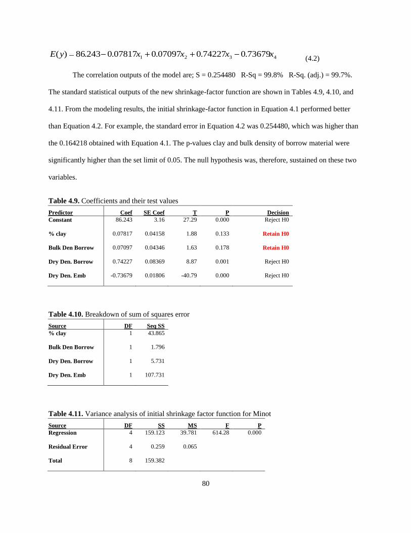
80
4321 73679.074227.007097.007817.0243.86)( xxxxyE (4.2)
The correlation outputs of the model are; S = 0.254480 R-Sq = 99.8% R-Sq. (adj.) = 99.7%.
The standard statistical outputs of the new shrinkage-factor function are shown in Tables 4.9, 4.10, and
4.11. From the modeling results, the initial shrinkage-factor function in Equation 4.1 performed better
than Equation 4.2. For example, the standard error in Equation 4.2 was 0.254480, which was higher than
the 0.164218 obtained with Equation 4.1. The p-values clay and bulk density of borrow material were
significantly higher than the set limit of 0.05. The null hypothesis was, therefore, sustained on these two
variables.
Table 4.9. Coefficients and their test values
Predictor Coef SE Coef T P Decision
Constant 86.243 3.16 27.29 0.000 Reject H0
% clay 0.07817 0.04158 1.88 0.133 Retain H0
Bulk Den Borrow 0.07097 0.04346 1.63 0.178 Retain H0
Dry Den. Borrow 0.74227 0.08369 8.87 0.001 Reject H0
Dry Den. Emb -0.73679 0.01806 -40.79 0.000 Reject H0
Table 4.10. Breakdown of sum of squares error
Source DF Seq SS
% clay 1 43.865
Bulk Den Borrow 1 1.796
Dry Den. Borrow 1 5.731
Dry Den. Emb 1 107.731
Table 4.11. Variance analysis of initial shrinkage factor function for Minot
Source DF SS MS F P
Regression 4 159.123 39.781 614.28 0.000
Residual Error 4 0.259 0.065
Total 8 159.382
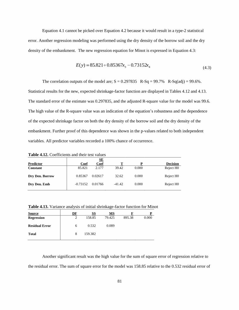
81
Equation 4.1 cannot be picked over Equation 4.2 because it would result in a type-2 statistical
error. Another regression modeling was performed using the dry density of the borrow soil and the dry
density of the embankment. The new regression equation for Minot is expressed in Equation 4.3:
43 73152.085367.0821.85)( xxyE (4.3)
The correlation outputs of the model are; S = 0.297835 R-Sq = 99.7% R-Sq(adj) = 99.6%.
Statistical results for the new, expected shrinkage-factor function are displayed in Tables 4.12 and 4.13.
The standard error of the estimate was 0.297835, and the adjusted R-square value for the model was 99.6.
The high value of the R-square value was an indication of the equation’s robustness and the dependence
of the expected shrinkage factor on both the dry density of the borrow soil and the dry density of the
embankment. Further proof of this dependence was shown in the p-values related to both independent
variables. All predictor variables recorded a 100% chance of occurrence.
Table 4.12. Coefficients and their test values
Predictor Coef
SE
Coef T P Decision
Constant 85.821 2.177 39.42 0.000 Reject H0
Dry Den. Borrow 0.85367 0.02617 32.62 0.000 Reject H0
Dry Den. Emb -0.73152 0.01766 -41.42 0.000 Reject H0
Table 4.13. Variance analysis of initial shrinkage-factor function for Minot
Source DF SS MS F P
Regression 2 158.85 79.425 895.38 0.000
Residual Error 6 0.532 0.089
Total 8 159.382
Another significant result was the high value for the sum of square error of regression relative to
the residual error. The sum of square error for the model was 158.85 relative to the 0.532 residual error of
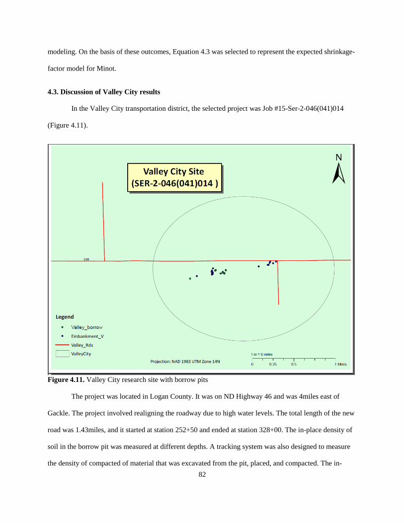
82
modeling. On the basis of these outcomes, Equation 4.3 was selected to represent the expected shrinkage-
factor model for Minot.
4.3. Discussion of Valley City results
In the Valley City transportation district, the selected project was Job #15-Ser-2-046(041)014
(Figure 4.11).
Figure 4.11. Valley City research site with borrow pits
The project was located in Logan County. It was on ND Highway 46 and was 4miles east of
Gackle. The project involved realigning the roadway due to high water levels. The total length of the new
road was 1.43miles, and it started at station 252+50 and ended at station 328+00. The in-place density of
soil in the borrow pit was measured at different depths. A tracking system was also designed to measure
the density of compacted of material that was excavated from the pit, placed, and compacted. The in-
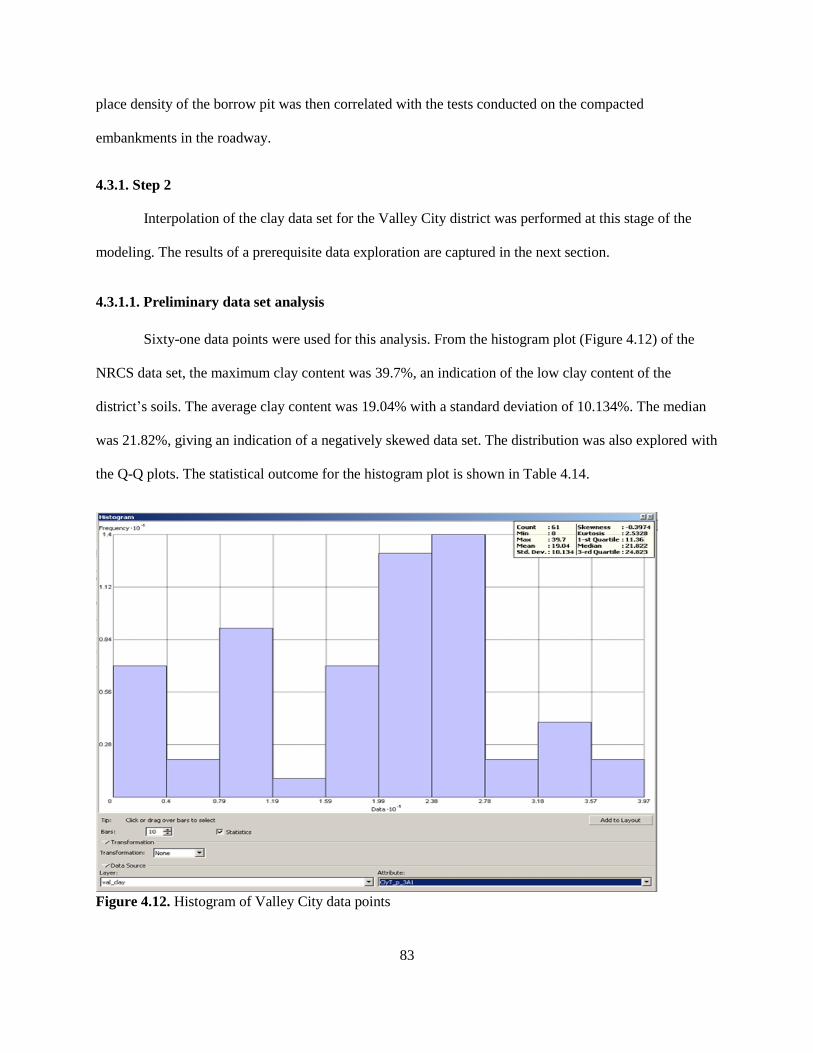
83
place density of the borrow pit was then correlated with the tests conducted on the compacted
embankments in the roadway.
4.3.1. Step 2
Interpolation of the clay data set for the Valley City district was performed at this stage of the
modeling. The results of a prerequisite data exploration are captured in the next section.
4.3.1.1. Preliminary data set analysis
Sixty-one data points were used for this analysis. From the histogram plot (Figure 4.12) of the
NRCS data set, the maximum clay content was 39.7%, an indication of the low clay content of the
district’s soils. The average clay content was 19.04% with a standard deviation of 10.134%. The median
was 21.82%, giving an indication of a negatively skewed data set. The distribution was also explored with
the Q-Q plots. The statistical outcome for the histogram plot is shown in Table 4.14.
Figure 4.12. Histogram of Valley City data points
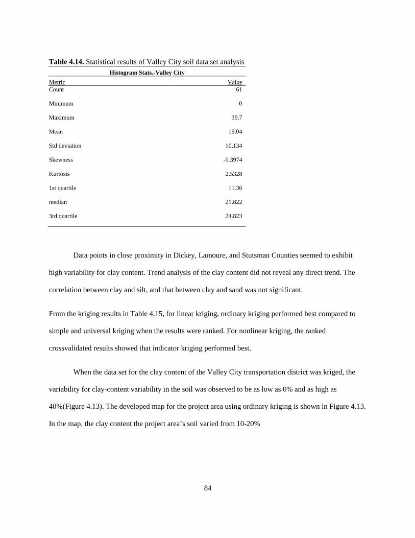
84
Table 4.14. Statistical results of Valley City soil data set analysis
Histogram Stats.-Valley City
Metric Value
Count 61
Minimum 0
Maximum 39.7
Mean 19.04
Std deviation 10.134
Skewness -0.3974
Kurtosis 2.5328
1st quartile 11.36
median 21.822
3rd quartile 24.823
Data points in close proximity in Dickey, Lamoure, and Stutsman Counties seemed to exhibit
high variability for clay content. Trend analysis of the clay content did not reveal any direct trend. The
correlation between clay and silt, and that between clay and sand was not significant.
From the kriging results in Table 4.15, for linear kriging, ordinary kriging performed best compared to
simple and universal kriging when the results were ranked. For nonlinear kriging, the ranked
crossvalidated results showed that indicator kriging performed best.
When the data set for the clay content of the Valley City transportation district was kriged, the
variability for clay-content variability in the soil was observed to be as low as 0% and as high as
40%(Figure 4.13). The developed map for the project area using ordinary kriging is shown in Figure 4.13.
In the map, the clay content the project area’s soil varied from 10-20%
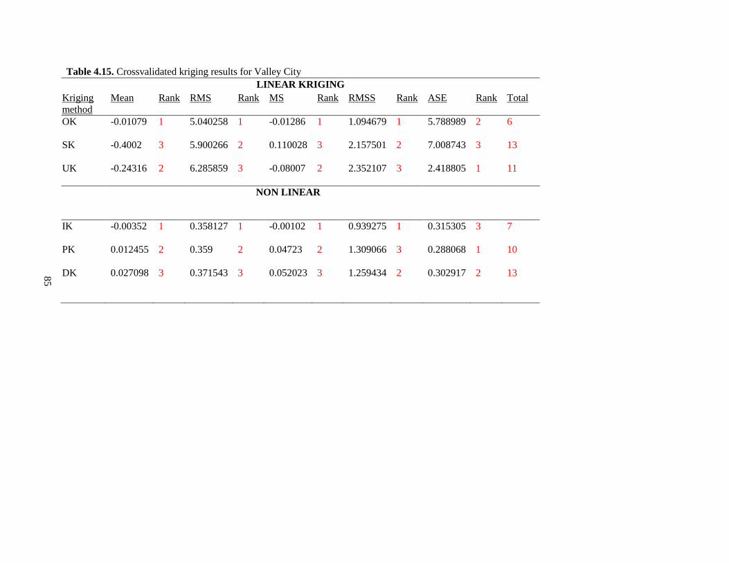
85
Table 4.15. Crossvalidated kriging results for Valley City
LINEAR KRIGING
Kriging
method
Mean Rank RMS Rank MS Rank RMSS Rank ASE Rank Total
OK -0.01079 1 5.040258 1 -0.01286 1 1.094679 1 5.788989 2 6
SK -0.4002 3 5.900266 2 0.110028 3 2.157501 2 7.008743 3 13
UK -0.24316 2 6.285859 3 -0.08007 2 2.352107 3 2.418805 1 11
NON LINEAR
IK -0.00352 1 0.358127 1 -0.00102 1 0.939275 1 0.315305 3 7
PK 0.012455 2 0.359 2 0.04723 2 1.309066 3 0.288068 1 10
DK 0.027098 3 0.371543 3 0.052023 3 1.259434 2 0.302917 2 13
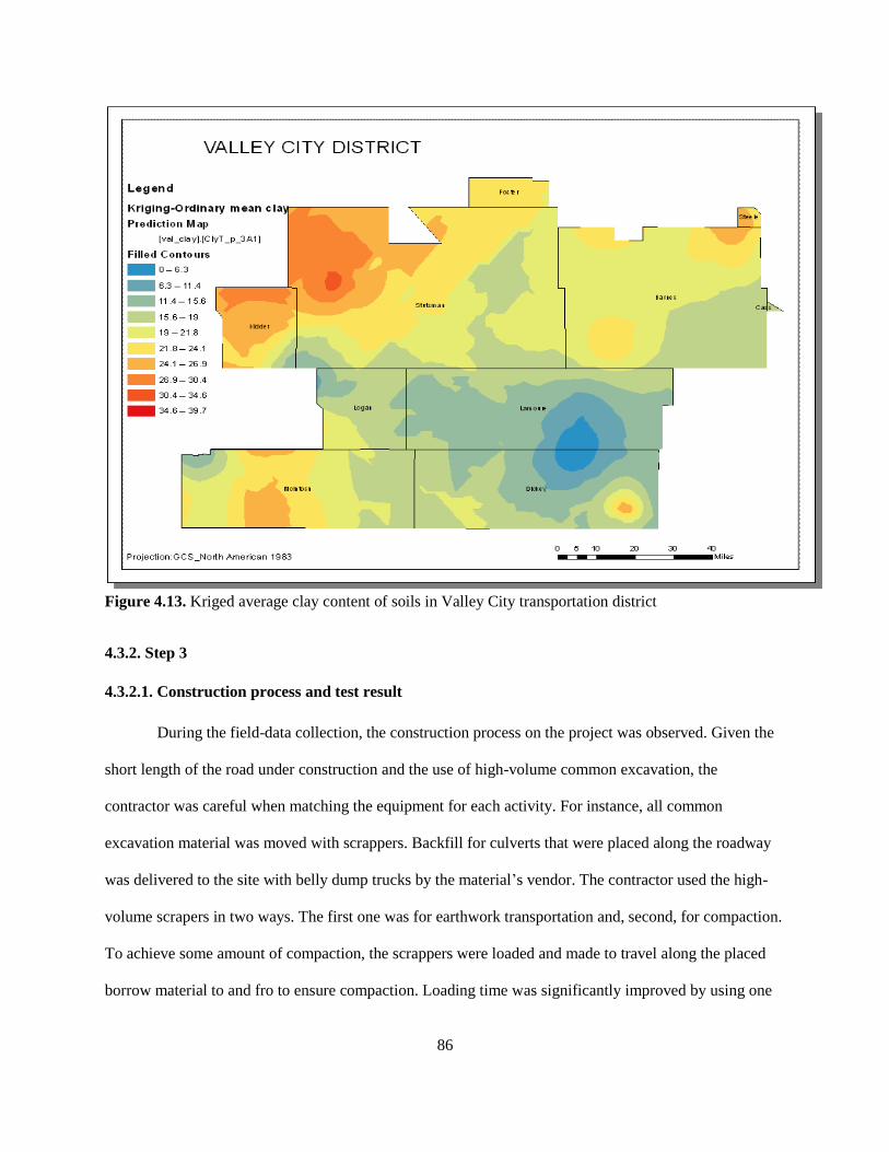
86
Figure 4.13. Kriged average clay content of soils in Valley City transportation district
4.3.2. Step 3
4.3.2.1. Construction process and test result
During the field-data collection, the construction process on the project was observed. Given the
short length of the road under construction and the use of high-volume common excavation, the
contractor was careful when matching the equipment for each activity. For instance, all common
excavation material was moved with scrappers. Backfill for culverts that were placed along the roadway
was delivered to the site with belly dump trucks by the material’s vendor. The contractor used the high-
volume scrapers in two ways. The first one was for earthwork transportation and, second, for compaction.
To achieve some amount of compaction, the scrappers were loaded and made to travel along the placed
borrow material to and fro to ensure compaction. Loading time was significantly improved by using one
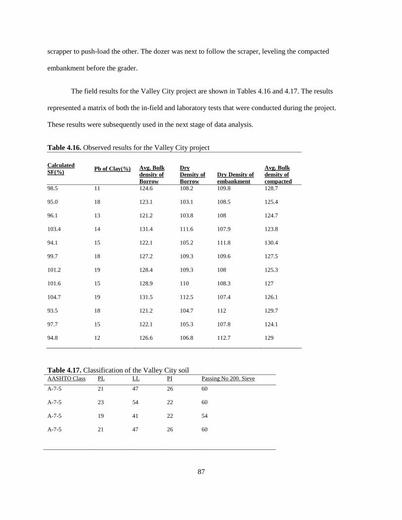
87
scrapper to push-load the other. The dozer was next to follow the scraper, leveling the compacted
embankment before the grader.
The field results for the Valley City project are shown in Tables 4.16 and 4.17. The results
represented a matrix of both the in-field and laboratory tests that were conducted during the project.
These results were subsequently used in the next stage of data analysis.
Table 4.16. Observed results for the Valley City project
Calculated
SF(%) Pb of Clay(%) Avg. Bulk
density of
Borrow
Dry
Density of
Borrow
Dry Density of
embankment
Avg. Bulk
density of
compacted
98.5 11 124.6 108.2 109.8 128.7
95.0 18 123.1 103.1 108.5 125.4
96.1 13 121.2 103.8 108 124.7
103.4 14 131.4 111.6 107.9 123.8
94.1 15 122.1 105.2 111.8 130.4
99.7 18 127.2 109.3 109.6 127.5
101.2 19 128.4 109.3 108 125.3
101.6 15 128.9 110 108.3 127
104.7 19 131.5 112.5 107.4 126.1
93.5 18 121.2 104.7 112 129.7
97.7 15 122.1 105.3 107.8 124.1
94.8 12 126.6 106.8 112.7 129
Table 4.17. Classification of the Valley City soil AASHTO Class PL LL PI Passing No 200. Sieve
A-7-5 21 47 26 60
A-7-5 23 54 22 60
A-7-5 19 41 22 54
A-7-5 21 47 26 60
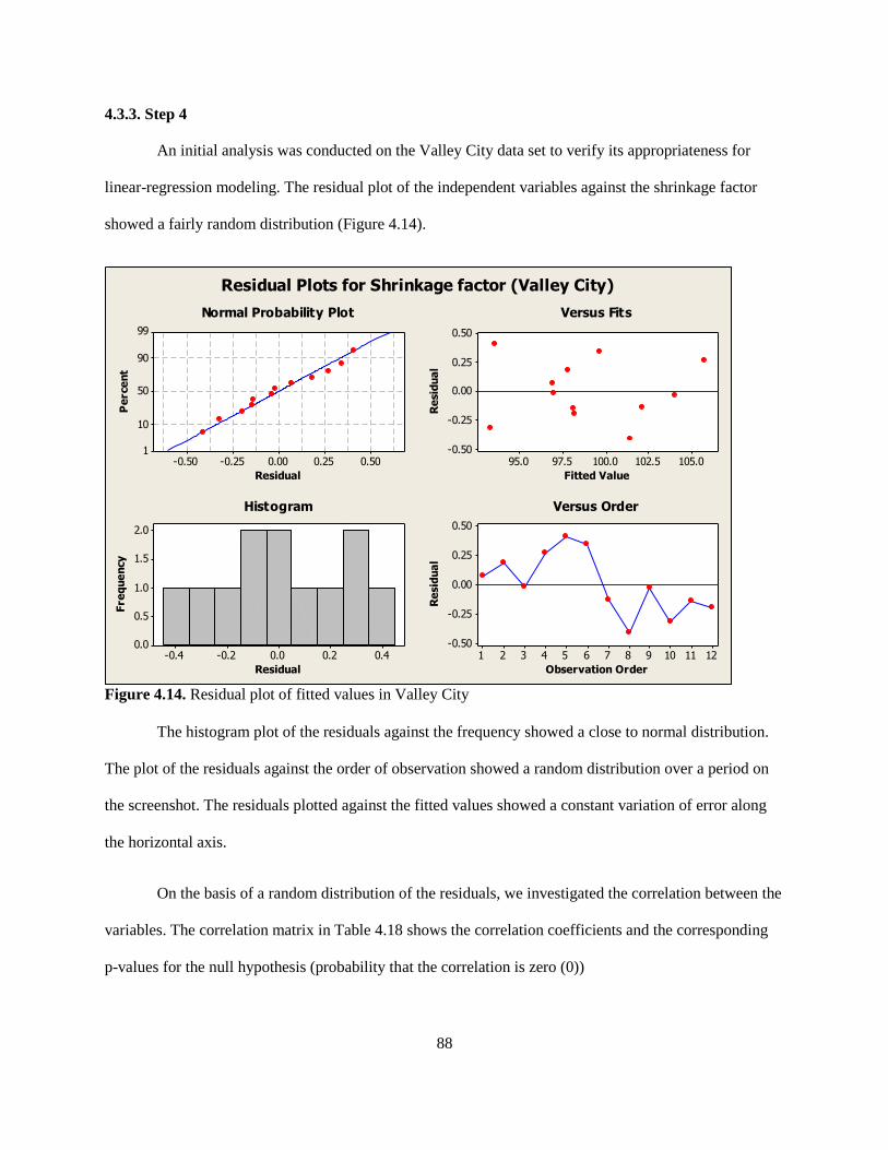
88
4.3.3. Step 4
An initial analysis was conducted on the Valley City data set to verify its appropriateness for
linear-regression modeling. The residual plot of the independent variables against the shrinkage factor
showed a fairly random distribution (Figure 4.14).
0.500.250.00-0.25-0.50
99
90
50
10
1
Residual
Pe
rce
nt
105.0102.5100.097.595.0
0.50
0.25
0.00
-0.25
-0.50
Fitted Value
Re
sid
ua
l
0.40.20.0-0.2-0.4
2.0
1.5
1.0
0.5
0.0
Residual
Fre
qu
en
cy
121110987654321
0.50
0.25
0.00
-0.25
-0.50
Observation Order
Re
sid
ua
l
Normal Probability Plot Versus Fits
Histogram Versus Order
Residual Plots for Shrinkage factor (Valley City)
Figure 4.14. Residual plot of fitted values in Valley City
The histogram plot of the residuals against the frequency showed a close to normal distribution.
The plot of the residuals against the order of observation showed a random distribution over a period on
the screenshot. The residuals plotted against the fitted values showed a constant variation of error along
the horizontal axis.
On the basis of a random distribution of the residuals, we investigated the correlation between the
variables. The correlation matrix in Table 4.18 shows the correlation coefficients and the corresponding
p-values for the null hypothesis (probability that the correlation is zero (0))
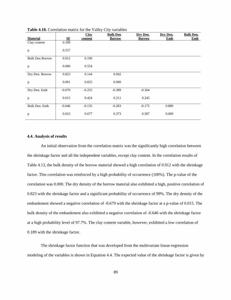
89
Table 4.18. Correlation matrix for the Valley City variables
Material SF
Clay
content
Bulk Den
Borrow
Dry Den.
Borrow
Dry Den.
Emb
Bulk Den.
Emb
Clay content 0.189
p 0.557
Bulk Den Borrow 0.912 0.190
p 0.000 0.554
Dry Den. Borrow 0.823 0.144 0.942
p 0.001 0.655 0.000
Dry Den. Emb -0.679 -0.255 -0.389 -0.364
p 0.015 0.424 0.211 0.245
Bulk Den. Emb -0.646 -0.135 -0.283 -0.175 0.880
p 0.023 0.677 0.373 0.587 0.000
4.4. Analysis of results
An initial observation from the correlation matrix was the significantly high correlation between
the shrinkage factor and all the independent variables, except clay content. In the correlation results of
Table 4.13, the bulk density of the borrow material showed a high correlation of 0.912 with the shrinkage
factor. This correlation was reinforced by a high probability of occurrence (100%). The p-value of the
correlation was 0.000. The dry density of the borrow material also exhibited a high, positive correlation of
0.823 with the shrinkage factor and a significant probability of occurrence of 99%. The dry density of the
embankment showed a negative correlation of -0.679 with the shrinkage factor at a p-value of 0.015. The
bulk density of the embankment also exhibited a negative correlation of -0.646 with the shrinkage factor
at a high probability level of 97.7%. The clay content variable, however, exhibited a low correlation of
0.189 with the shrinkage factor.
The shrinkage factor function that was developed from the multivariate linear-regression
modeling of the variables is shown in Equation 4.4. The expected value of the shrinkage factor is given by
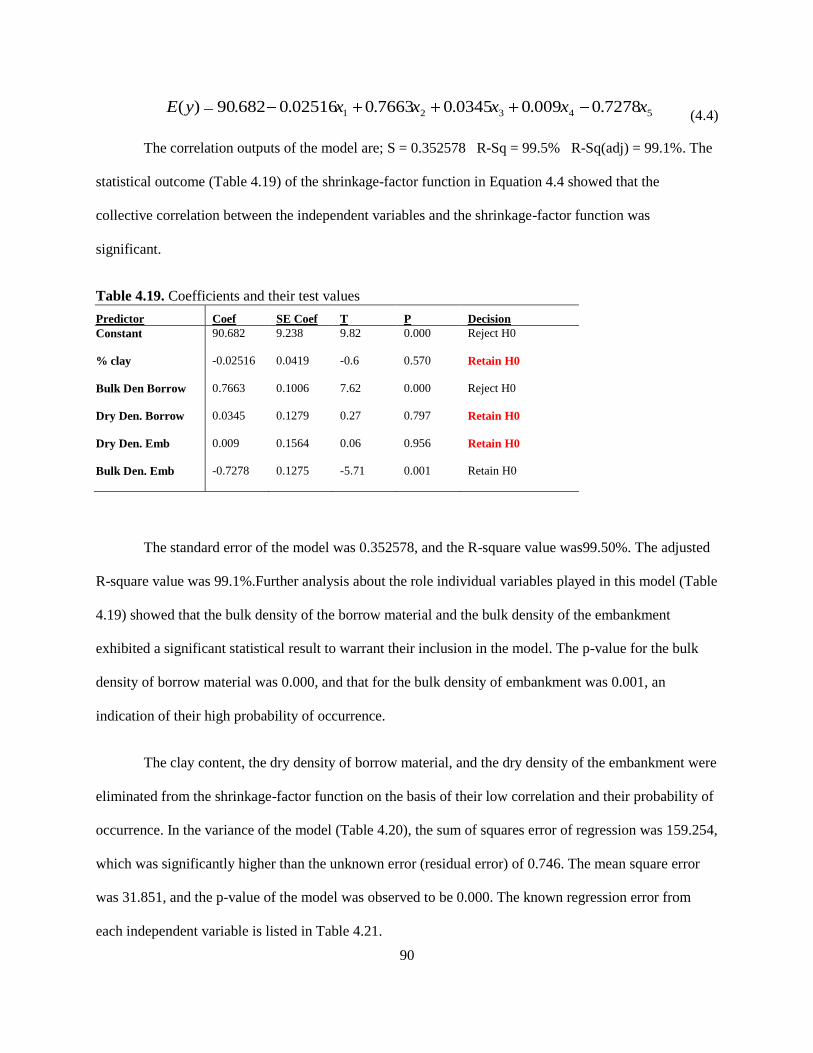
90
54321 7278.0009.00345.07663.002516.0682.90)( xxxxxyE (4.4)
The correlation outputs of the model are; S = 0.352578 R-Sq = 99.5% R-Sq(adj) = 99.1%. The
statistical outcome (Table 4.19) of the shrinkage-factor function in Equation 4.4 showed that the
collective correlation between the independent variables and the shrinkage-factor function was
significant.
Table 4.19. Coefficients and their test values
Predictor Coef SE Coef T P Decision
Constant 90.682 9.238 9.82 0.000 Reject H0
% clay -0.02516 0.0419 -0.6 0.570 Retain H0
Bulk Den Borrow 0.7663 0.1006 7.62 0.000 Reject H0
Dry Den. Borrow 0.0345 0.1279 0.27 0.797 Retain H0
Dry Den. Emb 0.009 0.1564 0.06 0.956 Retain H0
Bulk Den. Emb -0.7278 0.1275 -5.71 0.001 Retain H0
The standard error of the model was 0.352578, and the R-square value was99.50%. The adjusted
R-square value was 99.1%.Further analysis about the role individual variables played in this model (Table
4.19) showed that the bulk density of the borrow material and the bulk density of the embankment
exhibited a significant statistical result to warrant their inclusion in the model. The p-value for the bulk
density of borrow material was 0.000, and that for the bulk density of embankment was 0.001, an
indication of their high probability of occurrence.
The clay content, the dry density of borrow material, and the dry density of the embankment were
eliminated from the shrinkage-factor function on the basis of their low correlation and their probability of
occurrence. In the variance of the model (Table 4.20), the sum of squares error of regression was 159.254,
which was significantly higher than the unknown error (residual error) of 0.746. The mean square error
was 31.851, and the p-value of the model was observed to be 0.000. The known regression error from
each independent variable is listed in Table 4.21.
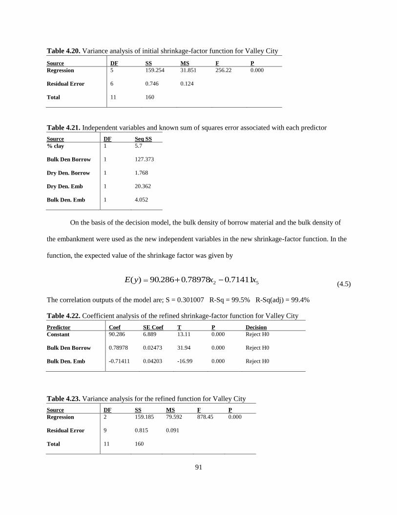
91
Table 4.20. Variance analysis of initial shrinkage-factor function for Valley City
Source DF SS MS F P
Regression 5 159.254 31.851 256.22 0.000
Residual Error 6 0.746 0.124
Total 11 160
Table 4.21. Independent variables and known sum of squares error associated with each predictor
Source DF Seq SS
% clay 1 5.7
Bulk Den Borrow 1 127.373
Dry Den. Borrow 1 1.768
Dry Den. Emb 1 20.362
Bulk Den. Emb 1 4.052
On the basis of the decision model, the bulk density of borrow material and the bulk density of
the embankment were used as the new independent variables in the new shrinkage-factor function. In the
function, the expected value of the shrinkage factor was given by
52 71411.078978.0286.90)( xxyE (4.5)
The correlation outputs of the model are; S = 0.301007 R-Sq = 99.5% R-Sq(adj) = 99.4%
Table 4.22. Coefficient analysis of the refined shrinkage-factor function for Valley City
Predictor Coef SE Coef T P Decision
Constant 90.286 6.889 13.11 0.000 Reject H0
Bulk Den Borrow 0.78978 0.02473 31.94 0.000 Reject H0
Bulk Den. Emb -0.71411 0.04203 -16.99 0.000 Reject H0
Table 4.23. Variance analysis for the refined function for Valley City
Source DF SS MS F P
Regression 2 159.185 79.592 878.45 0.000
Residual Error 9 0.815 0.091
Total 11 160
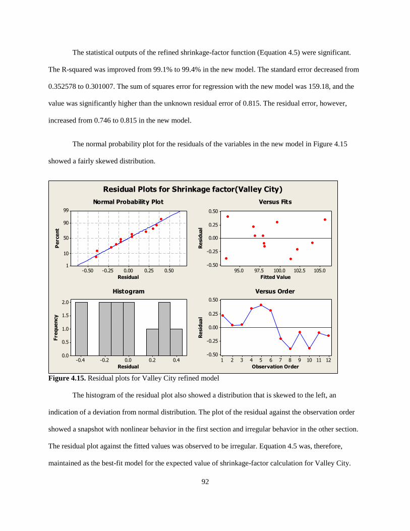
92
The statistical outputs of the refined shrinkage-factor function (Equation 4.5) were significant.
The R-squared was improved from 99.1% to 99.4% in the new model. The standard error decreased from
0.352578 to 0.301007. The sum of squares error for regression with the new model was 159.18, and the
value was significantly higher than the unknown residual error of 0.815. The residual error, however,
increased from 0.746 to 0.815 in the new model.
The normal probability plot for the residuals of the variables in the new model in Figure 4.15
showed a fairly skewed distribution.
0.500.250.00-0.25-0.50
99
90
50
10
1
Residual
Pe
rce
nt
105.0102.5100.097.595.0
0.50
0.25
0.00
-0.25
-0.50
Fitted Value
Re
sid
ua
l
0.40.20.0-0.2-0.4
2.0
1.5
1.0
0.5
0.0
Residual
Fre
qu
en
cy
121110987654321
0.50
0.25
0.00
-0.25
-0.50
Observation Order
Re
sid
ua
lNormal Probability Plot Versus Fits
Histogram Versus Order
Residual Plots for Shrinkage factor(Valley City)
Figure 4.15. Residual plots for Valley City refined model
The histogram of the residual plot also showed a distribution that is skewed to the left, an
indication of a deviation from normal distribution. The plot of the residual against the observation order
showed a snapshot with nonlinear behavior in the first section and irregular behavior in the other section.
The residual plot against the fitted values was observed to be irregular. Equation 4.5 was, therefore,
maintained as the best-fit model for the expected value of shrinkage-factor calculation for Valley City.
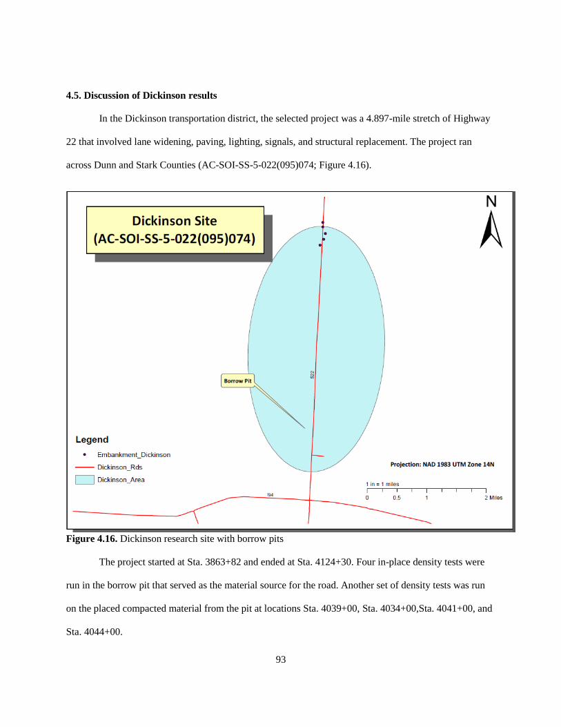
93
4.5. Discussion of Dickinson results
In the Dickinson transportation district, the selected project was a 4.897-mile stretch of Highway
22 that involved lane widening, paving, lighting, signals, and structural replacement. The project ran
across Dunn and Stark Counties (AC-SOI-SS-5-022(095)074; Figure 4.16).
Figure 4.16. Dickinson research site with borrow pits
The project started at Sta. 3863+82 and ended at Sta. 4124+30. Four in-place density tests were
run in the borrow pit that served as the material source for the road. Another set of density tests was run
on the placed compacted material from the pit at locations Sta. 4039+00, Sta. 4034+00,Sta. 4041+00, and
Sta. 4044+00.
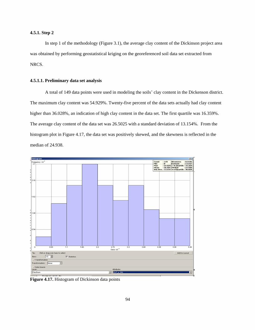
94
4.5.1. Step 2
In step 1 of the methodology (Figure 3.1), the average clay content of the Dickinson project area
was obtained by performing geostatistical kriging on the georeferenced soil data set extracted from
NRCS.
4.5.1.1. Preliminary data set analysis
A total of 149 data points were used in modeling the soils’ clay content in the Dickenson district.
The maximum clay content was 54.929%. Twenty-five percent of the data sets actually had clay content
higher than 36.028%, an indication of high clay content in the data set. The first quartile was 16.359%.
The average clay content of the data set was 26.5025 with a standard deviation of 13.154%. From the
histogram plot in Figure 4.17, the data set was positively skewed, and the skewness is reflected in the
median of 24.938.
Figure 4.17. Histogram of Dickinson data points
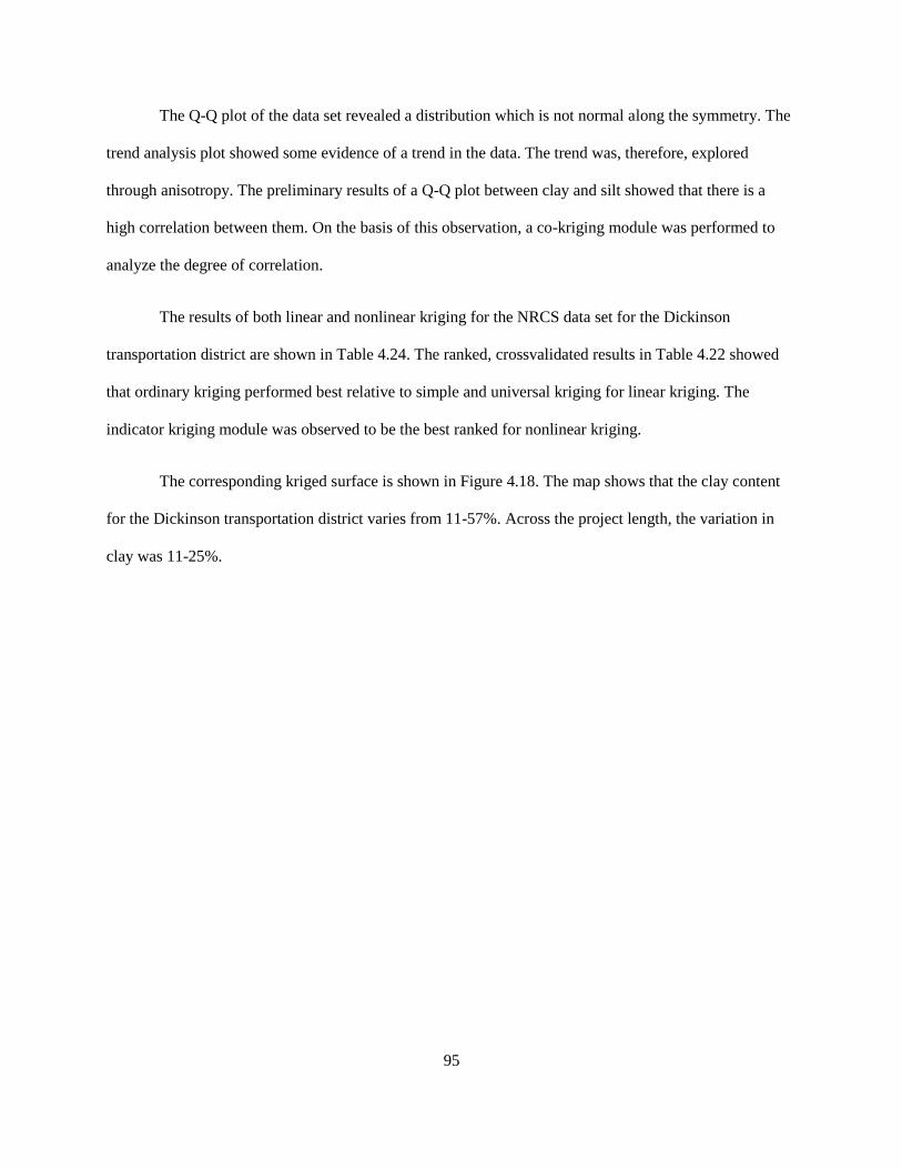
95
The Q-Q plot of the data set revealed a distribution which is not normal along the symmetry. The
trend analysis plot showed some evidence of a trend in the data. The trend was, therefore, explored
through anisotropy. The preliminary results of a Q-Q plot between clay and silt showed that there is a
high correlation between them. On the basis of this observation, a co-kriging module was performed to
analyze the degree of correlation.
The results of both linear and nonlinear kriging for the NRCS data set for the Dickinson
transportation district are shown in Table 4.24. The ranked, crossvalidated results in Table 4.22 showed
that ordinary kriging performed best relative to simple and universal kriging for linear kriging. The
indicator kriging module was observed to be the best ranked for nonlinear kriging.
The corresponding kriged surface is shown in Figure 4.18. The map shows that the clay content
for the Dickinson transportation district varies from 11-57%. Across the project length, the variation in
clay was 11-25%.
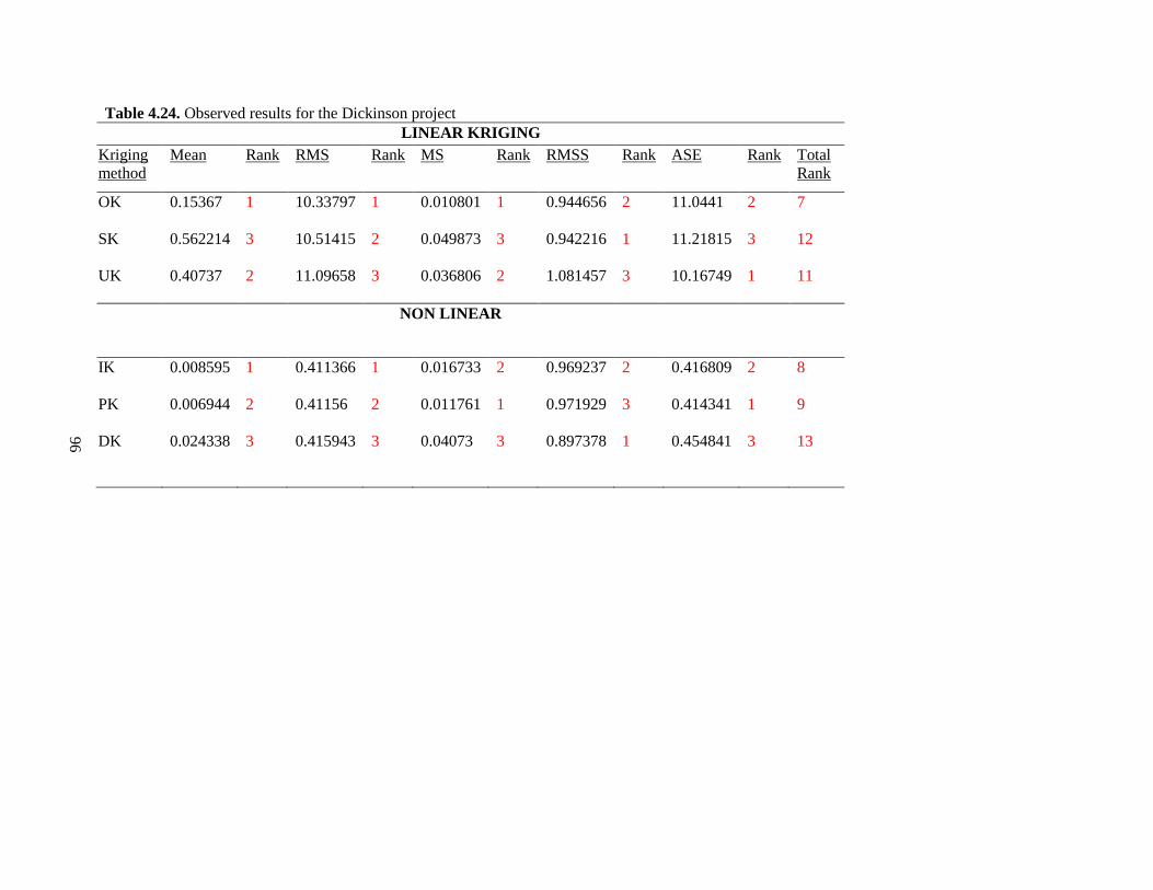
96
Table 4.24. Observed results for the Dickinson project
LINEAR KRIGING
Kriging
method
Mean Rank RMS Rank MS Rank RMSS Rank ASE Rank Total
Rank
OK 0.15367 1 10.33797 1 0.010801 1 0.944656 2 11.0441 2 7
SK 0.562214 3 10.51415 2 0.049873 3 0.942216 1 11.21815 3 12
UK 0.40737 2 11.09658 3 0.036806 2 1.081457 3 10.16749 1 11
NON LINEAR
IK 0.008595 1 0.411366 1 0.016733 2 0.969237 2 0.416809 2 8
PK 0.006944 2 0.41156 2 0.011761 1 0.971929 3 0.414341 1 9
DK 0.024338 3 0.415943 3 0.04073 3 0.897378 1 0.454841 3 13
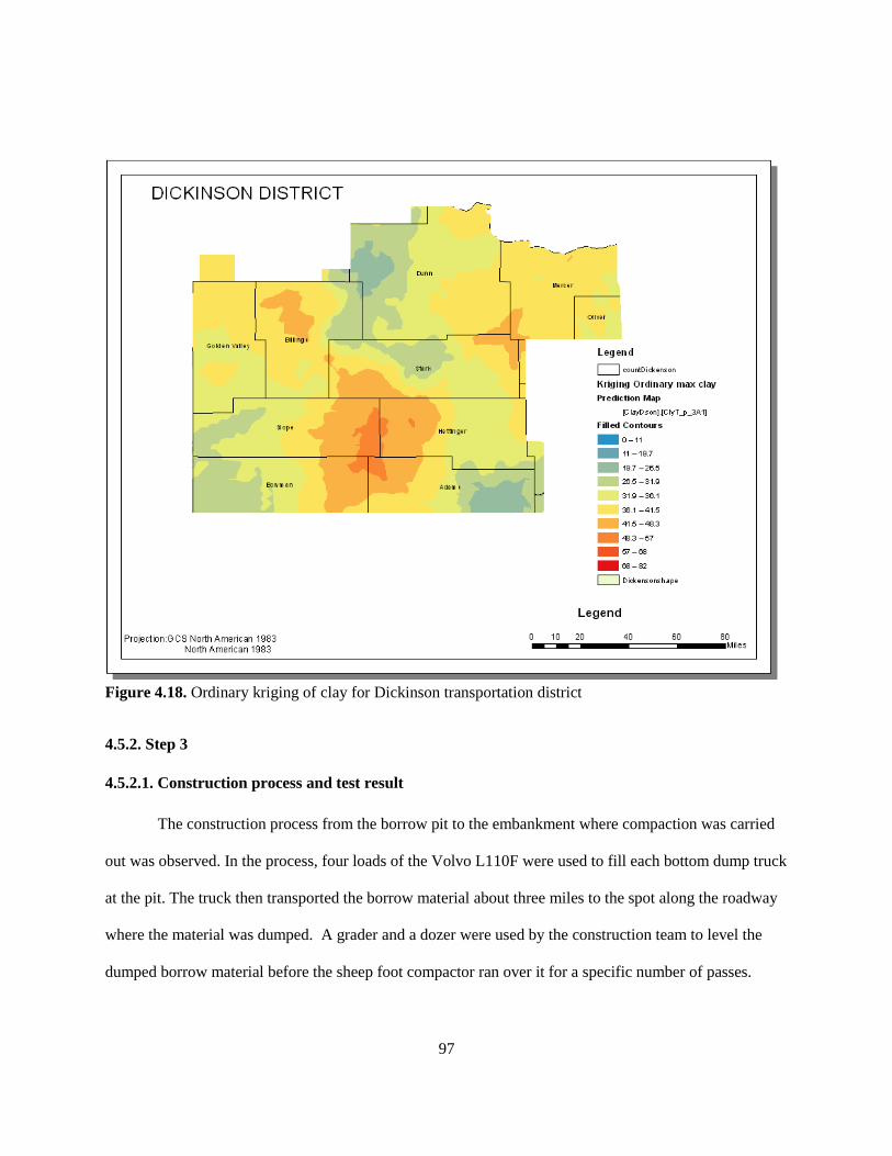
97
Figure 4.18. Ordinary kriging of clay for Dickinson transportation district
4.5.2. Step 3
4.5.2.1. Construction process and test result
The construction process from the borrow pit to the embankment where compaction was carried
out was observed. In the process, four loads of the Volvo L110F were used to fill each bottom dump truck
at the pit. The truck then transported the borrow material about three miles to the spot along the roadway
where the material was dumped. A grader and a dozer were used by the construction team to level the
dumped borrow material before the sheep foot compactor ran over it for a specific number of passes.
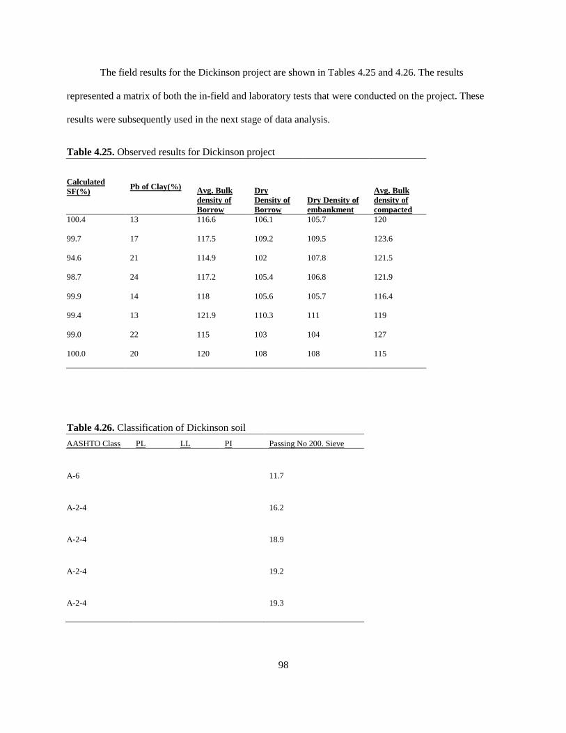
98
The field results for the Dickinson project are shown in Tables 4.25 and 4.26. The results
represented a matrix of both the in-field and laboratory tests that were conducted on the project. These
results were subsequently used in the next stage of data analysis.
Table 4.25. Observed results for Dickinson project
Calculated
SF(%) Pb of Clay(%)
Avg. Bulk
density of
Borrow
Dry
Density of
Borrow
Dry Density of
embankment
Avg. Bulk
density of
compacted
100.4 13 116.6 106.1 105.7 120
99.7 17 117.5 109.2 109.5 123.6
94.6 21 114.9 102 107.8 121.5
98.7 24 117.2 105.4 106.8 121.9
99.9 14 118 105.6 105.7 116.4
99.4 13 121.9 110.3 111 119
99.0 22 115 103 104 127
100.0 20 120 108 108 115
Table 4.26. Classification of Dickinson soil
AASHTO Class PL LL PI Passing No 200. Sieve
A-6 11.7
A-2-4 16.2
A-2-4 18.9
A-2-4 19.2
A-2-4 19.3
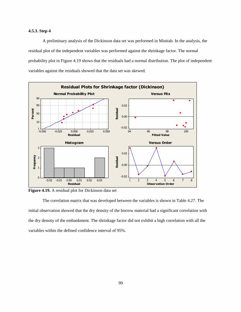
99
4.5.3. Step 4
A preliminary analysis of the Dickinson data set was performed in Minitab. In the analysis, the
residual plot of the independent variables was performed against the shrinkage factor. The normal
probability plot in Figure 4.19 shows that the residuals had a normal distribution. The plot of independent
variables against the residuals showed that the data set was skewed.
0.0500.0250.000-0.025-0.050
99
90
50
10
1
Residual
Pe
rce
nt
100989694
0.02
0.00
-0.02
Fitted Value
Re
sid
ua
l
0.030.020.010.00-0.01-0.02
3
2
1
0
Residual
Fre
qu
en
cy
87654321
0.02
0.00
-0.02
Observation Order
Re
sid
ua
l
Normal Probability Plot Versus Fits
Histogram Versus Order
Residual Plots for Shrinkage factor (Dickinson)
Figure 4.19. A residual plot for Dickinson data set
The correlation matrix that was developed between the variables is shown in Table 4.27. The
initial observation showed that the dry density of the borrow material had a significant correlation with
the dry density of the embankment. The shrinkage factor did not exhibit a high correlation with all the
variables within the defined confidence interval of 95%.
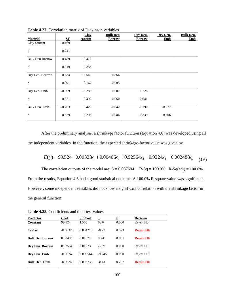
100
Table 4.27. Correlation matrix of Dickinson variables
Material SF
Clay
content
Bulk Den
Borrow
Dry Den.
Borrow
Dry Den.
Emb
Bulk Den.
Emb
Clay content -0.469
p 0.241
Bulk Den Borrow 0.489 -0.472
p 0.219 0.238
Dry Den. Borrow 0.634 -0.540 0.866
p 0.091 0.167 0.005
Dry Den. Emb -0.069 -0.286 0.687 0.728
p 0.871 0.492 0.060 0.041
Bulk Den. Emb -0.263 0.423 -0.642 -0.390 -0.277
p 0.529 0.296 0.086 0.339 0.506
After the preliminary analysis, a shrinkage factor function (Equation 4.6) was developed using all
the independent variables. In the function, the expected shrinkage-factor value was given by
54321 002488.09224.092564.000406.000323.0524.99)( xxxxxyE (4.6)
The correlation outputs of the model are; S = 0.0376841 R-Sq = 100.0% R-Sq(adj) = 100.0%.
From the results, Equation 4.6 had a good statistical outcome. A 100.0% R-square value was significant.
However, some independent variables did not show a significant correlation with the shrinkage factor in
the general function.
Table 4.28. Coefficients and their test values
Predictor Coef SE Coef T P Decision
Constant 99.524 1.565 63.6 0.000 Reject H0
% clay -0.00323 0.004213 -0.77 0.523 Retain H0
Bulk Den Borrow 0.00406 0.01671 0.24 0.831 Retain H0
Dry Den. Borrow 0.92564 0.01273 72.71 0.000 Reject H0
Dry Den. Emb -0.9224 0.009564 -96.45 0.000 Reject H0
Bulk Den. Emb -0.00249 0.005738 -0.43 0.707 Retain H0
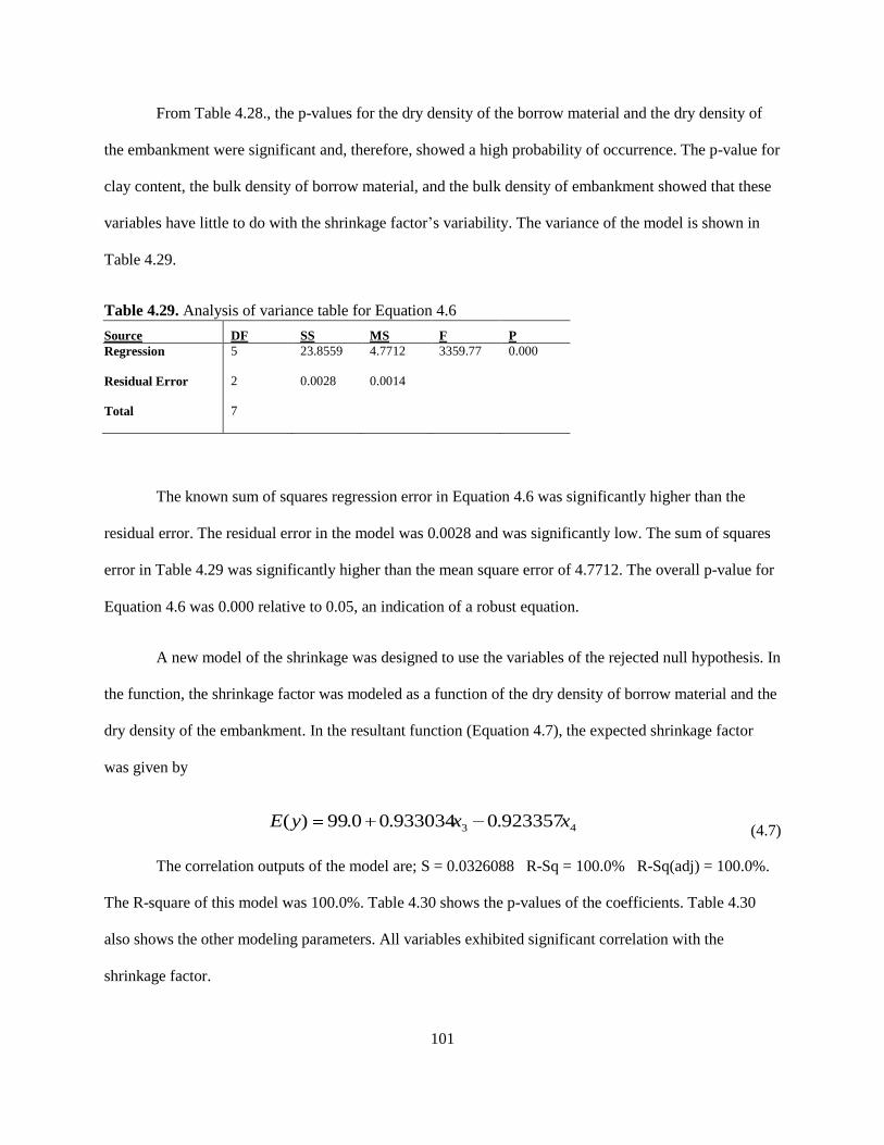
101
From Table 4.28., the p-values for the dry density of the borrow material and the dry density of
the embankment were significant and, therefore, showed a high probability of occurrence. The p-value for
clay content, the bulk density of borrow material, and the bulk density of embankment showed that these
variables have little to do with the shrinkage factor’s variability. The variance of the model is shown in
Table 4.29.
Table 4.29. Analysis of variance table for Equation 4.6
Source DF SS MS F P
Regression 5 23.8559 4.7712 3359.77 0.000
Residual Error 2 0.0028 0.0014
Total 7
The known sum of squares regression error in Equation 4.6 was significantly higher than the
residual error. The residual error in the model was 0.0028 and was significantly low. The sum of squares
error in Table 4.29 was significantly higher than the mean square error of 4.7712. The overall p-value for
Equation 4.6 was 0.000 relative to 0.05, an indication of a robust equation.
A new model of the shrinkage was designed to use the variables of the rejected null hypothesis. In
the function, the shrinkage factor was modeled as a function of the dry density of borrow material and the
dry density of the embankment. In the resultant function (Equation 4.7), the expected shrinkage factor
was given by
43 923357.0933034.00.99)( xxyE (4.7)
The correlation outputs of the model are; S = 0.0326088 R-Sq = 100.0% R-Sq(adj) = 100.0%.
The R-square of this model was 100.0%. Table 4.30 shows the p-values of the coefficients. Table 4.30
also shows the other modeling parameters. All variables exhibited significant correlation with the
shrinkage factor.
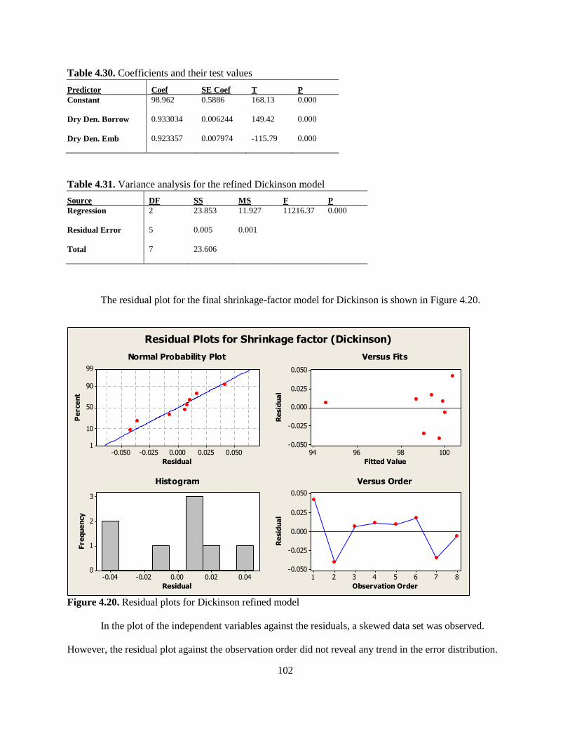
102
Table 4.30. Coefficients and their test values
Predictor Coef SE Coef T P
Constant 98.962 0.5886 168.13 0.000
Dry Den. Borrow 0.933034 0.006244 149.42 0.000
Dry Den. Emb 0.923357 0.007974 -115.79 0.000
Table 4.31. Variance analysis for the refined Dickinson model
Source DF SS MS F P
Regression 2 23.853 11.927 11216.37 0.000
Residual Error 5 0.005 0.001
Total 7 23.606
The residual plot for the final shrinkage-factor model for Dickinson is shown in Figure 4.20.
0.0500.0250.000-0.025-0.050
99
90
50
10
1
Residual
Pe
rce
nt
100989694
0.050
0.025
0.000
-0.025
-0.050
Fitted Value
Re
sid
ua
l
0.040.020.00-0.02-0.04
3
2
1
0
Residual
Fre
qu
en
cy
87654321
0.050
0.025
0.000
-0.025
-0.050
Observation Order
Re
sid
ua
l
Normal Probability Plot Versus Fits
Histogram Versus Order
Residual Plots for Shrinkage factor (Dickinson)
Figure 4.20. Residual plots for Dickinson refined model
In the plot of the independent variables against the residuals, a skewed data set was observed.
However, the residual plot against the observation order did not reveal any trend in the error distribution.
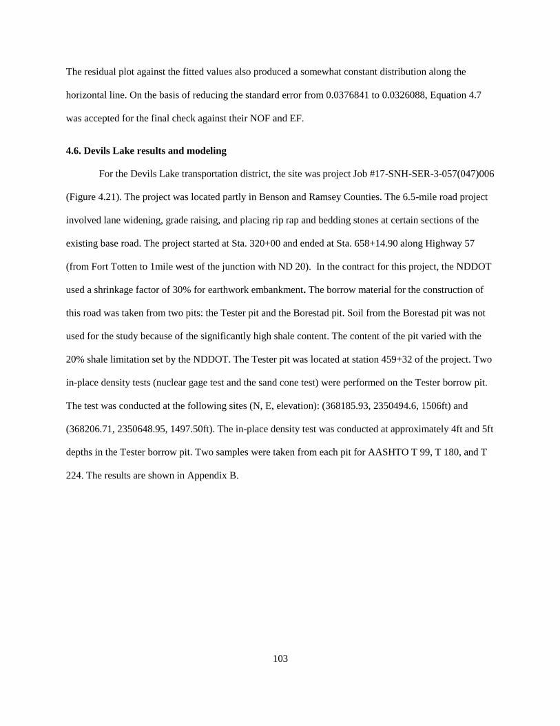
103
The residual plot against the fitted values also produced a somewhat constant distribution along the
horizontal line. On the basis of reducing the standard error from 0.0376841 to 0.0326088, Equation 4.7
was accepted for the final check against their NOF and EF.
4.6. Devils Lake results and modeling
For the Devils Lake transportation district, the site was project Job #17-SNH-SER-3-057(047)006
(Figure 4.21). The project was located partly in Benson and Ramsey Counties. The 6.5-mile road project
involved lane widening, grade raising, and placing rip rap and bedding stones at certain sections of the
existing base road. The project started at Sta. 320+00 and ended at Sta. 658+14.90 along Highway 57
(from Fort Totten to 1mile west of the junction with ND 20). In the contract for this project, the NDDOT
used a shrinkage factor of 30% for earthwork embankment. The borrow material for the construction of
this road was taken from two pits: the Tester pit and the Borestad pit. Soil from the Borestad pit was not
used for the study because of the significantly high shale content. The content of the pit varied with the
20% shale limitation set by the NDDOT. The Tester pit was located at station 459+32 of the project. Two
in-place density tests (nuclear gage test and the sand cone test) were performed on the Tester borrow pit.
The test was conducted at the following sites (N, E, elevation): (368185.93, 2350494.6, 1506ft) and
(368206.71, 2350648.95, 1497.50ft). The in-place density test was conducted at approximately 4ft and 5ft
depths in the Tester borrow pit. Two samples were taken from each pit for AASHTO T 99, T 180, and T
224. The results are shown in Appendix B.
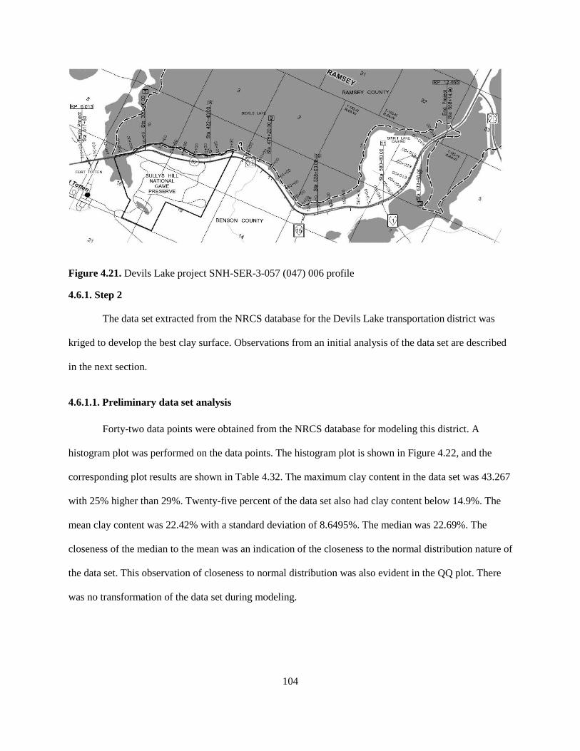
104
Figure 4.21. Devils Lake project SNH-SER-3-057 (047) 006 profile
4.6.1. Step 2
The data set extracted from the NRCS database for the Devils Lake transportation district was
kriged to develop the best clay surface. Observations from an initial analysis of the data set are described
in the next section.
4.6.1.1. Preliminary data set analysis
Forty-two data points were obtained from the NRCS database for modeling this district. A
histogram plot was performed on the data points. The histogram plot is shown in Figure 4.22, and the
corresponding plot results are shown in Table 4.32. The maximum clay content in the data set was 43.267
with 25% higher than 29%. Twenty-five percent of the data set also had clay content below 14.9%. The
mean clay content was 22.42% with a standard deviation of 8.6495%. The median was 22.69%. The
closeness of the median to the mean was an indication of the closeness to the normal distribution nature of
the data set. This observation of closeness to normal distribution was also evident in the QQ plot. There
was no transformation of the data set during modeling.
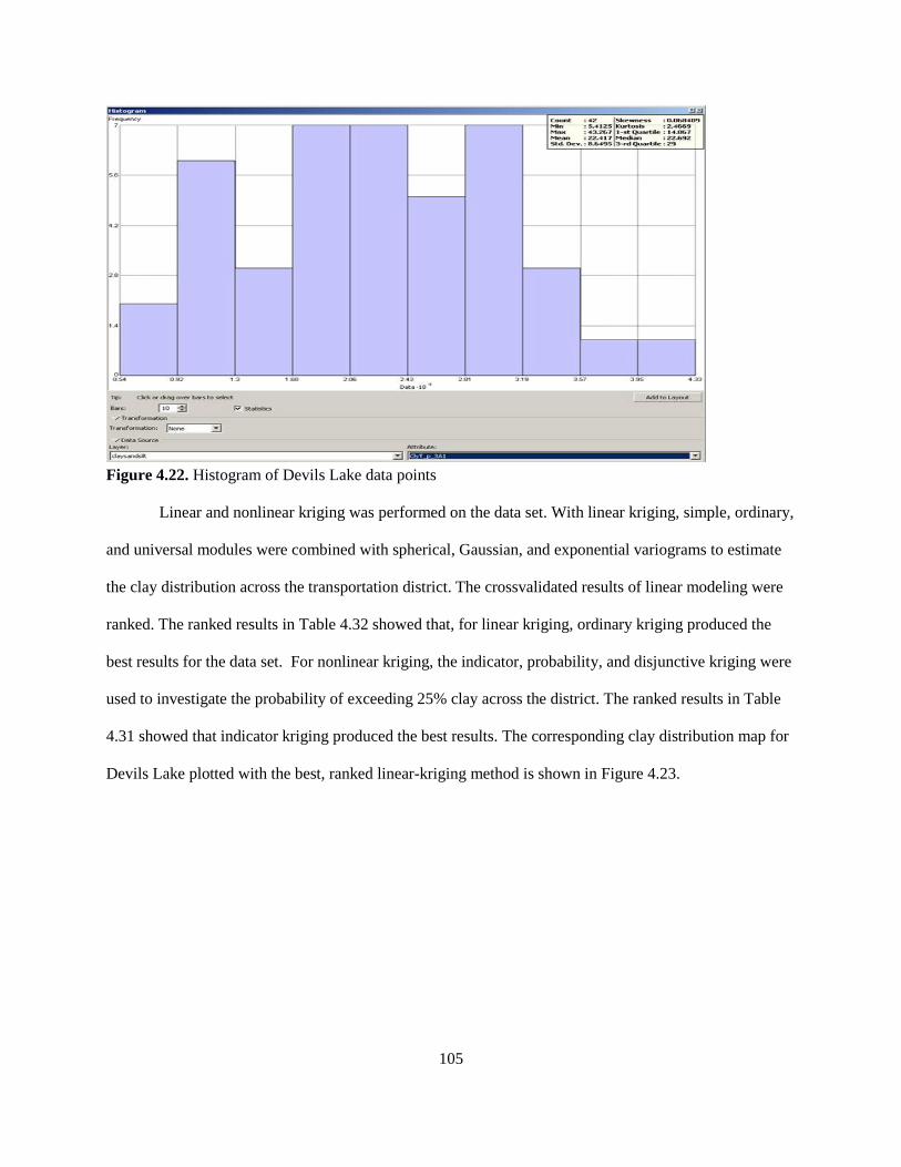
105
Figure 4.22. Histogram of Devils Lake data points
Linear and nonlinear kriging was performed on the data set. With linear kriging, simple, ordinary,
and universal modules were combined with spherical, Gaussian, and exponential variograms to estimate
the clay distribution across the transportation district. The crossvalidated results of linear modeling were
ranked. The ranked results in Table 4.32 showed that, for linear kriging, ordinary kriging produced the
best results for the data set. For nonlinear kriging, the indicator, probability, and disjunctive kriging were
used to investigate the probability of exceeding 25% clay across the district. The ranked results in Table
4.31 showed that indicator kriging produced the best results. The corresponding clay distribution map for
Devils Lake plotted with the best, ranked linear-kriging method is shown in Figure 4.23.
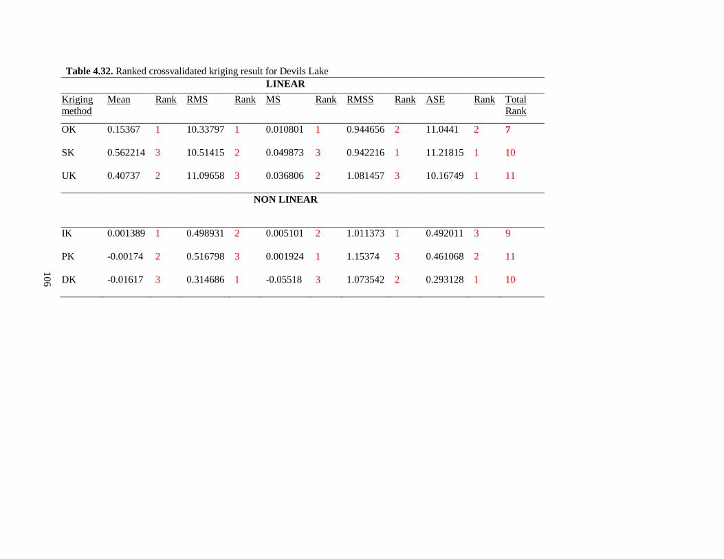
106
Table 4.32. Ranked crossvalidated kriging result for Devils Lake
LINEAR
Kriging
method
Mean Rank RMS Rank MS Rank RMSS Rank ASE Rank Total
Rank
OK 0.15367 1 10.33797 1 0.010801 1 0.944656 2 11.0441 2 7
SK 0.562214 3 10.51415 2 0.049873 3 0.942216 1 11.21815 1 10
UK 0.40737 2 11.09658 3 0.036806 2 1.081457 3 10.16749 1 11
NON LINEAR
IK 0.001389 1 0.498931 2 0.005101 2 1.011373 1 0.492011 3 9
PK -0.00174 2 0.516798 3 0.001924 1 1.15374 3 0.461068 2 11
DK -0.01617 3 0.314686 1 -0.05518 3 1.073542 2 0.293128 1 10
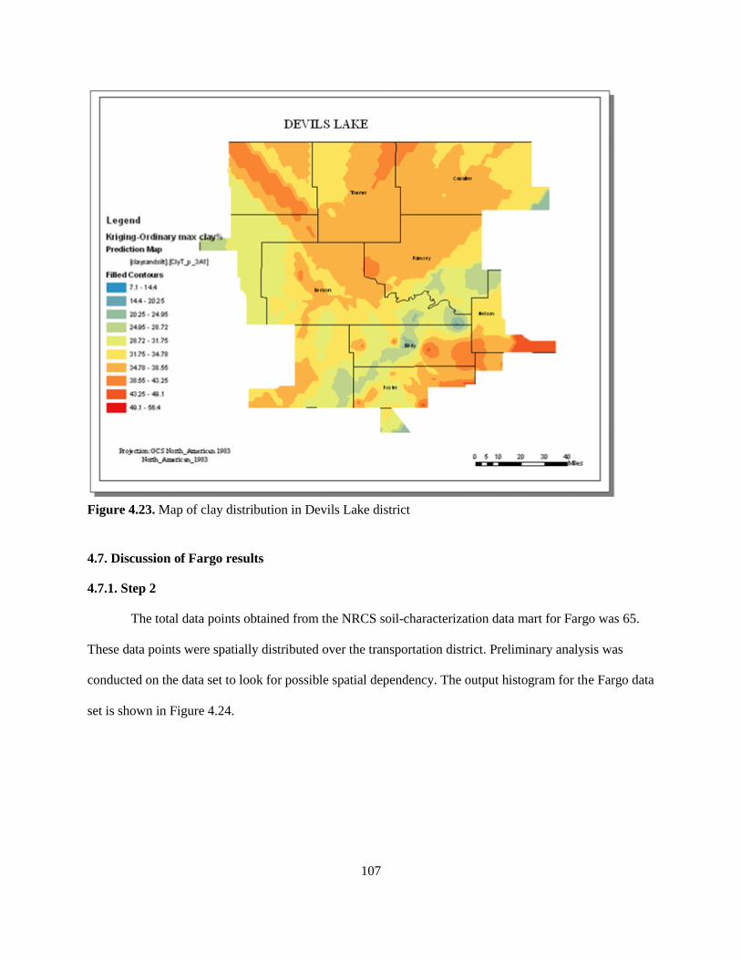
107
Figure 4.23. Map of clay distribution in Devils Lake district
4.7. Discussion of Fargo results
4.7.1. Step 2
The total data points obtained from the NRCS soil-characterization data mart for Fargo was 65.
These data points were spatially distributed over the transportation district. Preliminary analysis was
conducted on the data set to look for possible spatial dependency. The output histogram for the Fargo data
set is shown in Figure 4.24.
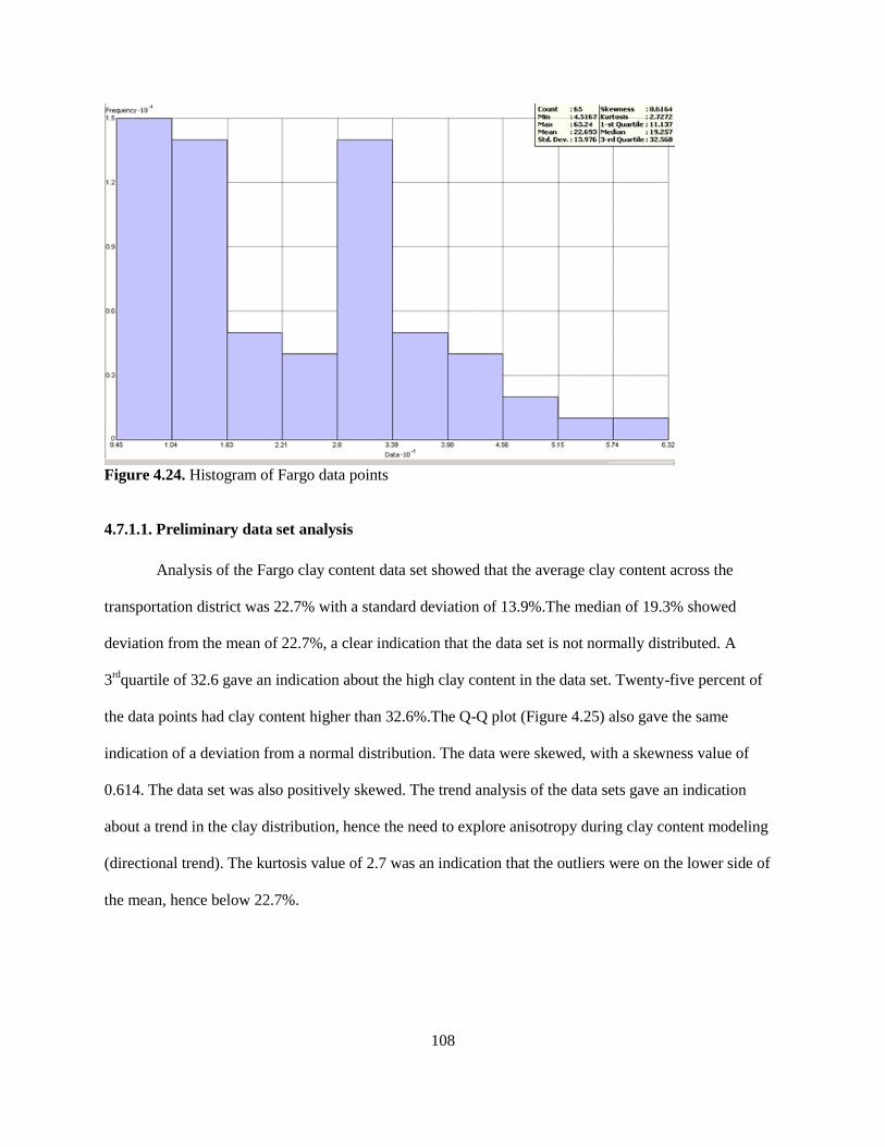
108
Figure 4.24. Histogram of Fargo data points
4.7.1.1. Preliminary data set analysis
Analysis of the Fargo clay content data set showed that the average clay content across the
transportation district was 22.7% with a standard deviation of 13.9%.The median of 19.3% showed
deviation from the mean of 22.7%, a clear indication that the data set is not normally distributed. A
3rd
quartile of 32.6 gave an indication about the high clay content in the data set. Twenty-five percent of
the data points had clay content higher than 32.6%.The Q-Q plot (Figure 4.25) also gave the same
indication of a deviation from a normal distribution. The data were skewed, with a skewness value of
0.614. The data set was also positively skewed. The trend analysis of the data sets gave an indication
about a trend in the clay distribution, hence the need to explore anisotropy during clay content modeling
(directional trend). The kurtosis value of 2.7 was an indication that the outliers were on the lower side of
the mean, hence below 22.7%.
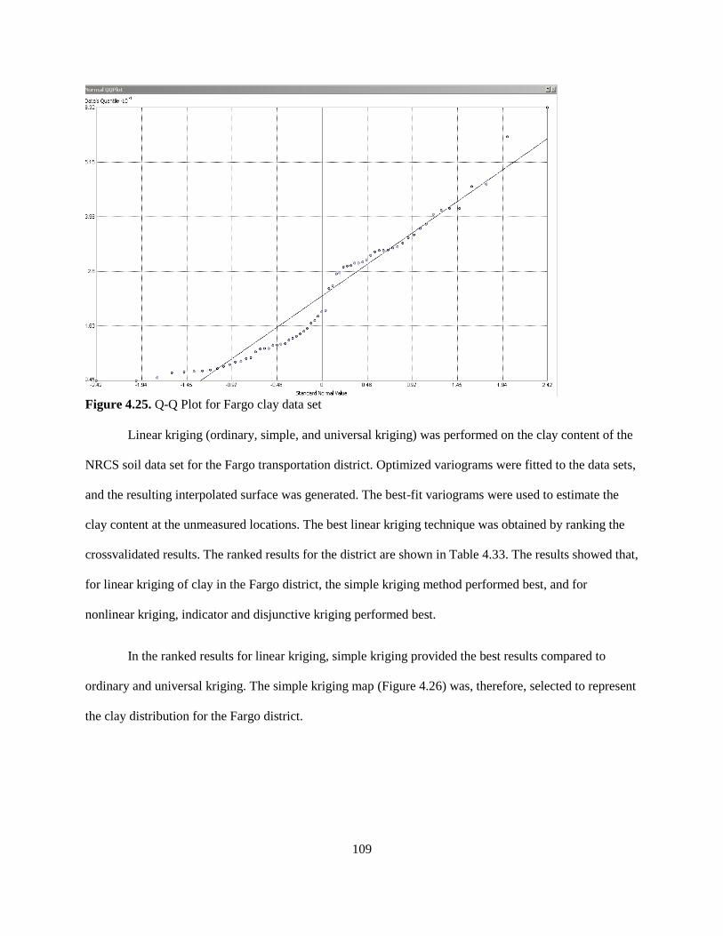
109
Figure 4.25. Q-Q Plot for Fargo clay data set
Linear kriging (ordinary, simple, and universal kriging) was performed on the clay content of the
NRCS soil data set for the Fargo transportation district. Optimized variograms were fitted to the data sets,
and the resulting interpolated surface was generated. The best-fit variograms were used to estimate the
clay content at the unmeasured locations. The best linear kriging technique was obtained by ranking the
crossvalidated results. The ranked results for the district are shown in Table 4.33. The results showed that,
for linear kriging of clay in the Fargo district, the simple kriging method performed best, and for
nonlinear kriging, indicator and disjunctive kriging performed best.
In the ranked results for linear kriging, simple kriging provided the best results compared to
ordinary and universal kriging. The simple kriging map (Figure 4.26) was, therefore, selected to represent
the clay distribution for the Fargo district.
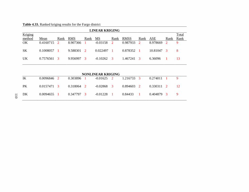
110
Table 4.33. Ranked kriging results for the Fargo district
LINEAR KRIGING
Kriging
method Mean Rank RMS Rank MS Rank RMSS Rank ASE Rank
Total
Rank
OK 0.4160715 2 8.907366 1 -0.03158 2 0.987933 2 8.978669 2 9
SK 0.1008057 1 9.588301 2 0.022497 1 0.878352 1 10.81047 3 8
UK 0.7576561 3 9.956997 3 -0.10262 3 1.467241 3 6.36096 1 13
NONLINEAR KRIGING
IK 0.0096846 2 0.303896 1 -0.01625 2 1.216733 3 0.274011 1 9
PK 0.0157471 3 0.318064 2 -0.02868 3 0.894603 2 0.330311 2 12
DK 0.0094655 1 0.347797 3 -0.01228 1 0.84433 1 0.404879 3 9
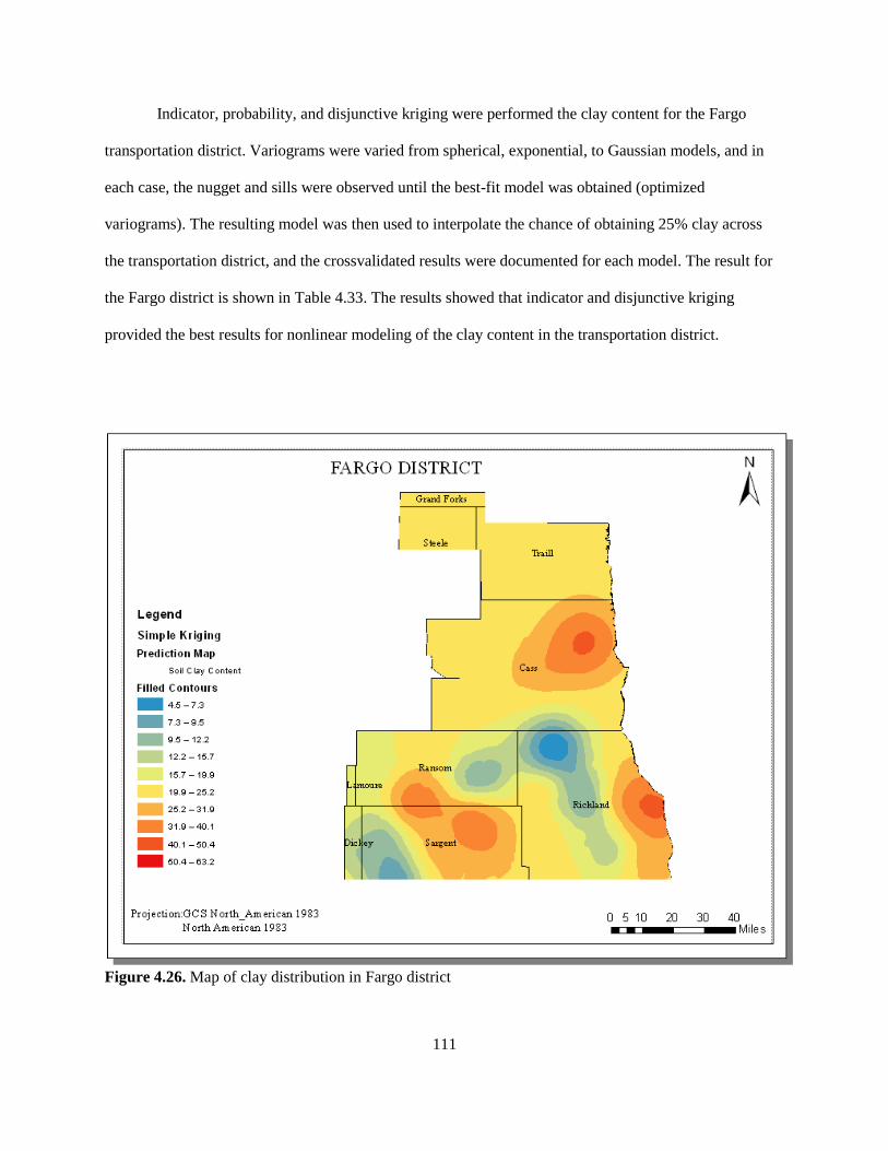
111
Indicator, probability, and disjunctive kriging were performed the clay content for the Fargo
transportation district. Variograms were varied from spherical, exponential, to Gaussian models, and in
each case, the nugget and sills were observed until the best-fit model was obtained (optimized
variograms). The resulting model was then used to interpolate the chance of obtaining 25% clay across
the transportation district, and the crossvalidated results were documented for each model. The result for
the Fargo district is shown in Table 4.33. The results showed that indicator and disjunctive kriging
provided the best results for nonlinear modeling of the clay content in the transportation district.
Figure 4.26. Map of clay distribution in Fargo district
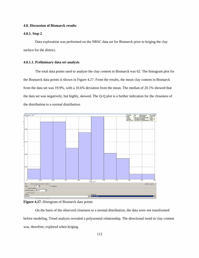
112
4.8. Discussion of Bismarck results
4.8.1. Step 2
Data exploration was performed on the NRSC data set for Bismarck prior to kriging the clay
surface for the district.
4.8.1.1. Preliminary data set analysis
The total data points used to analyze the clay content in Bismarck was 62. The histogram plot for
the Bismarck data points is shown in Figure 4.27. From the results, the mean clay content in Bismarck
from the data set was 19.9%, with a 10.6% deviation from the mean. The median of 20.1% showed that
the data set was negatively, but highly, skewed. The Q-Q plot is a further indication for the closeness of
the distribution to a normal distribution.
Figure 4.27. Histogram of Bismarck data points
On the basis of the observed closeness to a normal distribution, the data were not transformed
before modeling. Trend analysis revealed a polynomial relationship. The directional trend in clay content
was, therefore, explored when kriging.
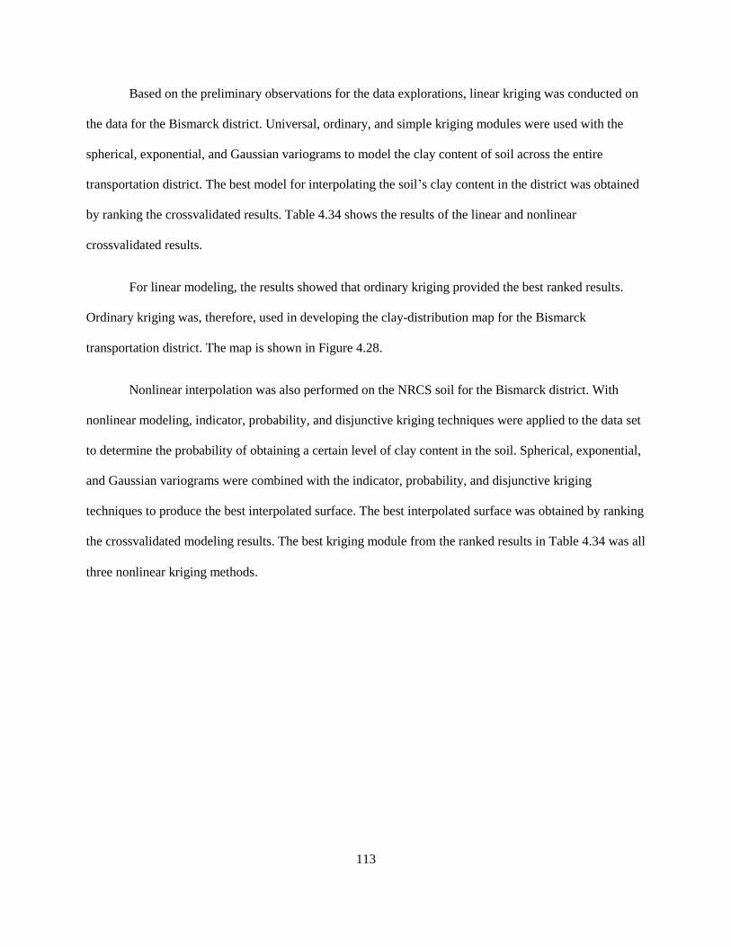
113
Based on the preliminary observations for the data explorations, linear kriging was conducted on
the data for the Bismarck district. Universal, ordinary, and simple kriging modules were used with the
spherical, exponential, and Gaussian variograms to model the clay content of soil across the entire
transportation district. The best model for interpolating the soil’s clay content in the district was obtained
by ranking the crossvalidated results. Table 4.34 shows the results of the linear and nonlinear
crossvalidated results.
For linear modeling, the results showed that ordinary kriging provided the best ranked results.
Ordinary kriging was, therefore, used in developing the clay-distribution map for the Bismarck
transportation district. The map is shown in Figure 4.28.
Nonlinear interpolation was also performed on the NRCS soil for the Bismarck district. With
nonlinear modeling, indicator, probability, and disjunctive kriging techniques were applied to the data set
to determine the probability of obtaining a certain level of clay content in the soil. Spherical, exponential,
and Gaussian variograms were combined with the indicator, probability, and disjunctive kriging
techniques to produce the best interpolated surface. The best interpolated surface was obtained by ranking
the crossvalidated modeling results. The best kriging module from the ranked results in Table 4.34 was all
three nonlinear kriging methods.
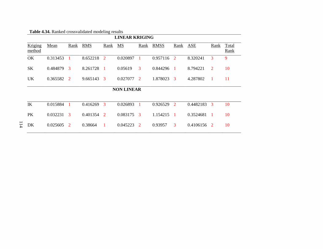
114
Table 4.34. Ranked crossvalidated modeling results
LINEAR KRIGING
Kriging
method
Mean Rank RMS Rank MS Rank RMSS Rank ASE Rank Total
Rank
OK 0.313453 1 8.652218 2 0.020897 1 0.957116 2 8.320241 3 9
SK 0.484879 3 8.261728 1 0.05619 3 0.844296 1 8.794221 2 10
UK 0.365582 2 9.665143 3 0.027077 2 1.878023 3 4.287802 1 11
NON LINEAR
IK 0.015884 1 0.416269 3 0.026893 1 0.926529 2 0.4482183 3 10
PK 0.032231 3 0.401354 2 0.083175 3 1.154215 1 0.3524681 1 10
DK 0.025605 2 0.38664 1 0.045223 2 0.93957 3 0.4106156 2 10
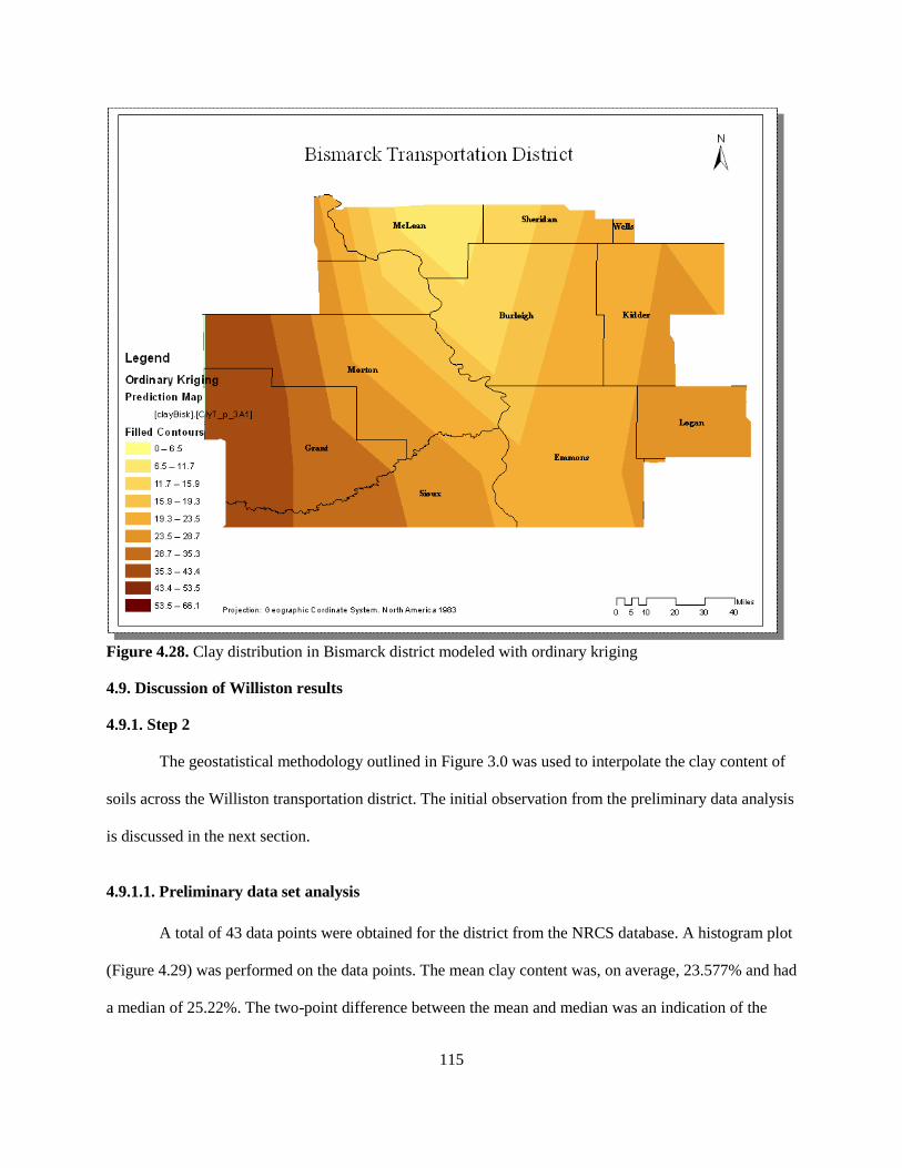
115
Figure 4.28. Clay distribution in Bismarck district modeled with ordinary kriging
4.9. Discussion of Williston results
4.9.1. Step 2
The geostatistical methodology outlined in Figure 3.0 was used to interpolate the clay content of
soils across the Williston transportation district. The initial observation from the preliminary data analysis
is discussed in the next section.
4.9.1.1. Preliminary data set analysis
A total of 43 data points were obtained for the district from the NRCS database. A histogram plot
(Figure 4.29) was performed on the data points. The mean clay content was, on average, 23.577% and had
a median of 25.22%. The two-point difference between the mean and median was an indication of the
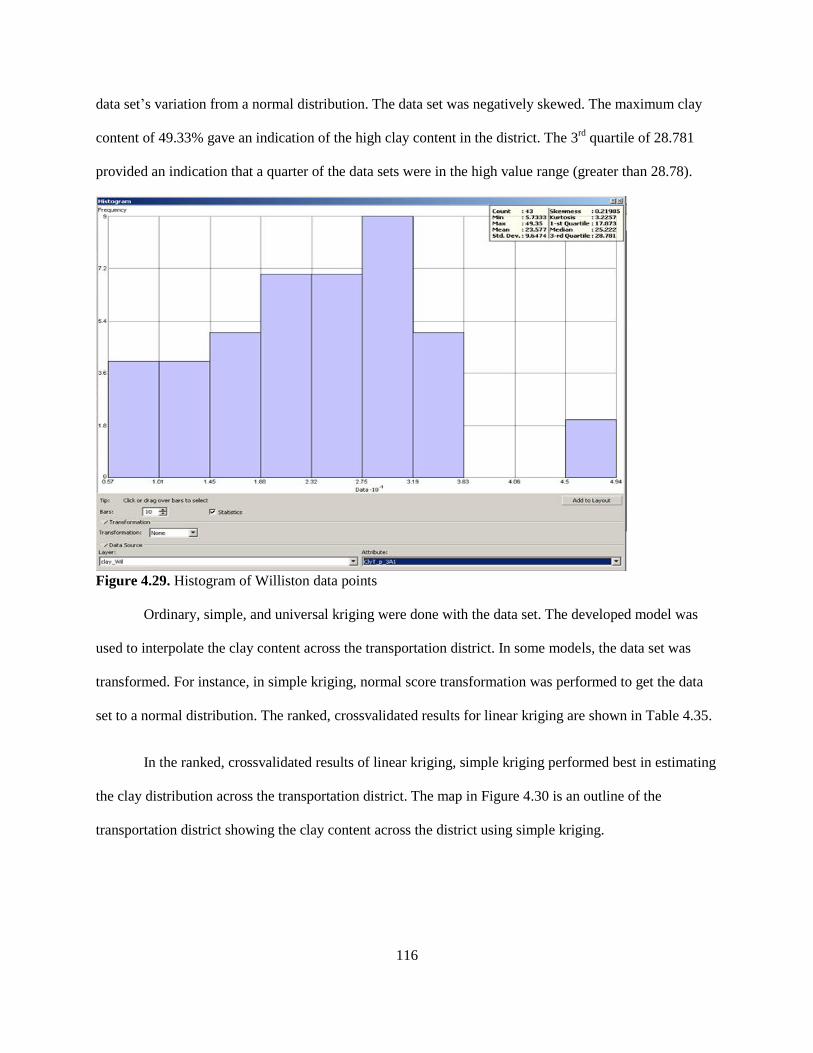
116
data set’s variation from a normal distribution. The data set was negatively skewed. The maximum clay
content of 49.33% gave an indication of the high clay content in the district. The 3rd
quartile of 28.781
provided an indication that a quarter of the data sets were in the high value range (greater than 28.78).
Figure 4.29. Histogram of Williston data points
Ordinary, simple, and universal kriging were done with the data set. The developed model was
used to interpolate the clay content across the transportation district. In some models, the data set was
transformed. For instance, in simple kriging, normal score transformation was performed to get the data
set to a normal distribution. The ranked, crossvalidated results for linear kriging are shown in Table 4.35.
In the ranked, crossvalidated results of linear kriging, simple kriging performed best in estimating
the clay distribution across the transportation district. The map in Figure 4.30 is an outline of the
transportation district showing the clay content across the district using simple kriging.
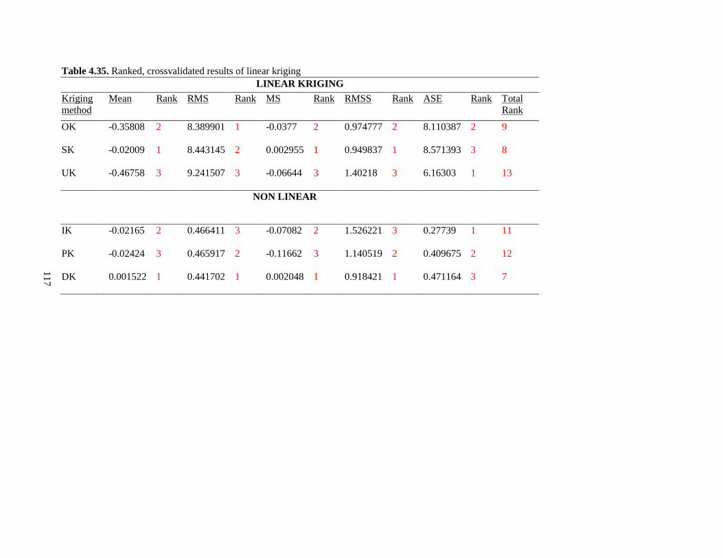
117
Table 4.35. Ranked, crossvalidated results of linear kriging
LINEAR KRIGING
Kriging
method
Mean Rank RMS Rank MS Rank RMSS Rank ASE Rank Total
Rank
OK -0.35808 2 8.389901 1 -0.0377 2 0.974777 2 8.110387 2 9
SK -0.02009 1 8.443145 2 0.002955 1 0.949837 1 8.571393 3 8
UK -0.46758 3 9.241507 3 -0.06644 3 1.40218 3 6.16303 1 13
NON LINEAR
IK -0.02165 2 0.466411 3 -0.07082 2 1.526221 3 0.27739 1 11
PK -0.02424 3 0.465917 2 -0.11662 3 1.140519 2 0.409675 2 12
DK 0.001522 1 0.441702 1 0.002048 1 0.918421 1 0.471164 3 7
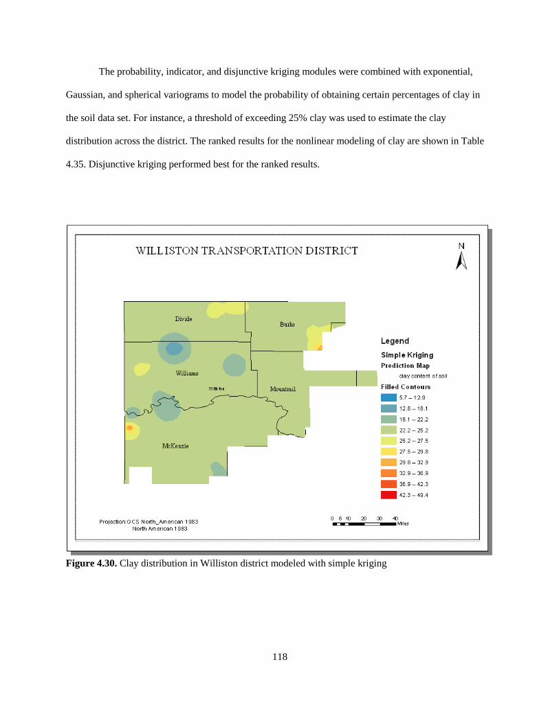
118
The probability, indicator, and disjunctive kriging modules were combined with exponential,
Gaussian, and spherical variograms to model the probability of obtaining certain percentages of clay in
the soil data set. For instance, a threshold of exceeding 25% clay was used to estimate the clay
distribution across the district. The ranked results for the nonlinear modeling of clay are shown in Table
4.35. Disjunctive kriging performed best for the ranked results.
Figure 4.30. Clay distribution in Williston district modeled with simple kriging
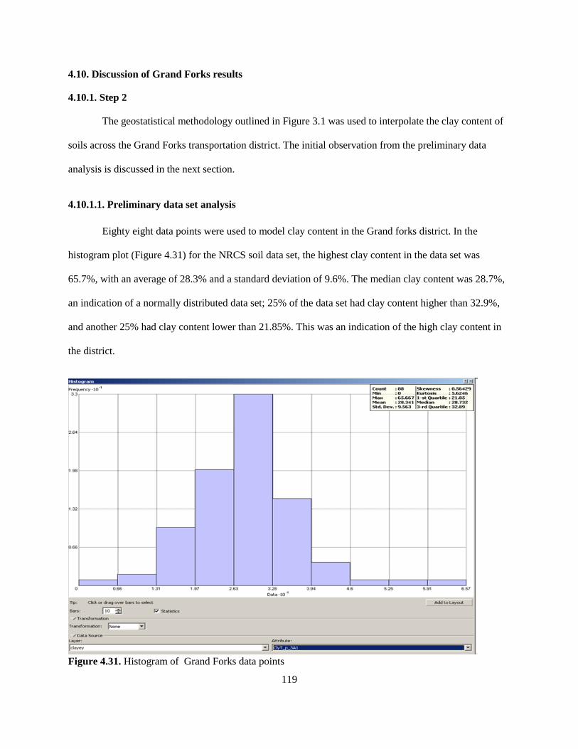
119
4.10. Discussion of Grand Forks results
4.10.1. Step 2
The geostatistical methodology outlined in Figure 3.1 was used to interpolate the clay content of
soils across the Grand Forks transportation district. The initial observation from the preliminary data
analysis is discussed in the next section.
4.10.1.1. Preliminary data set analysis
Eighty eight data points were used to model clay content in the Grand forks district. In the
histogram plot (Figure 4.31) for the NRCS soil data set, the highest clay content in the data set was
65.7%, with an average of 28.3% and a standard deviation of 9.6%. The median clay content was 28.7%,
an indication of a normally distributed data set; 25% of the data set had clay content higher than 32.9%,
and another 25% had clay content lower than 21.85%. This was an indication of the high clay content in
the district.
Figure 4.31. Histogram of Grand Forks data points
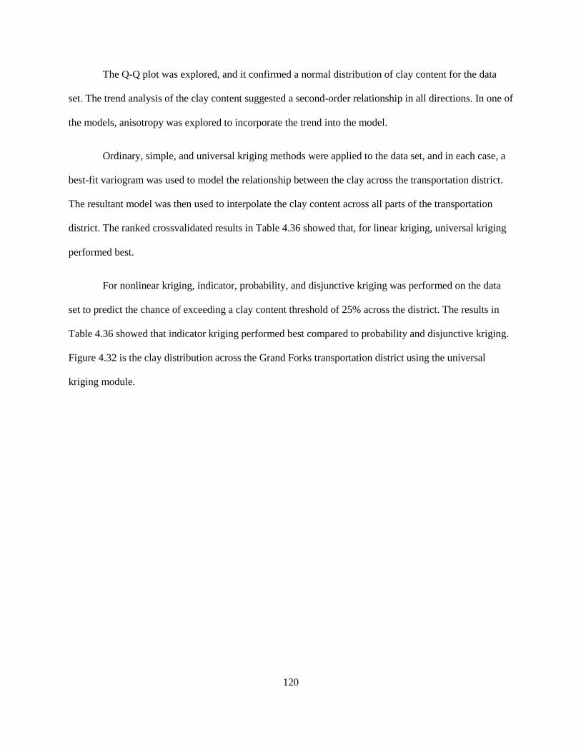
120
The Q-Q plot was explored, and it confirmed a normal distribution of clay content for the data
set. The trend analysis of the clay content suggested a second-order relationship in all directions. In one of
the models, anisotropy was explored to incorporate the trend into the model.
Ordinary, simple, and universal kriging methods were applied to the data set, and in each case, a
best-fit variogram was used to model the relationship between the clay across the transportation district.
The resultant model was then used to interpolate the clay content across all parts of the transportation
district. The ranked crossvalidated results in Table 4.36 showed that, for linear kriging, universal kriging
performed best.
For nonlinear kriging, indicator, probability, and disjunctive kriging was performed on the data
set to predict the chance of exceeding a clay content threshold of 25% across the district. The results in
Table 4.36 showed that indicator kriging performed best compared to probability and disjunctive kriging.
Figure 4.32 is the clay distribution across the Grand Forks transportation district using the universal
kriging module.
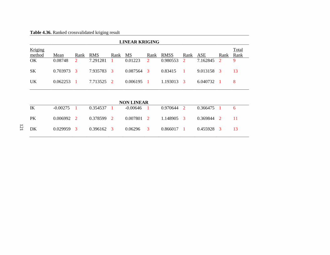
121
Table 4.36. Ranked crossvalidated kriging result
LINEAR KRIGING
Kriging
method Mean Rank RMS Rank MS Rank RMSS Rank ASE Rank
Total
Rank
OK 0.08748 2 7.291281 1 0.01223 2 0.980553 2 7.162845 2 9
SK 0.703973 3 7.935783 3 0.087564 3 0.83415 1 9.013158 3 13
UK 0.062253 1 7.713525 2 0.006195 1 1.193013 3 6.040732 1 8
NON LINEAR
IK -0.00275 1 0.354537 1 -0.00646 1 0.970644 2 0.366475 1 6
PK 0.006992 2 0.378599 2 0.007801 2 1.148905 3 0.369844 2 11
DK 0.029959 3 0.396162 3 0.06296 3 0.866017 1 0.455928 3 13
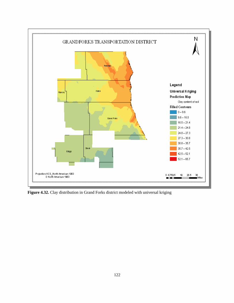
122
Figure 4.32. Clay distribution in Grand Forks district modeled with universal kriging
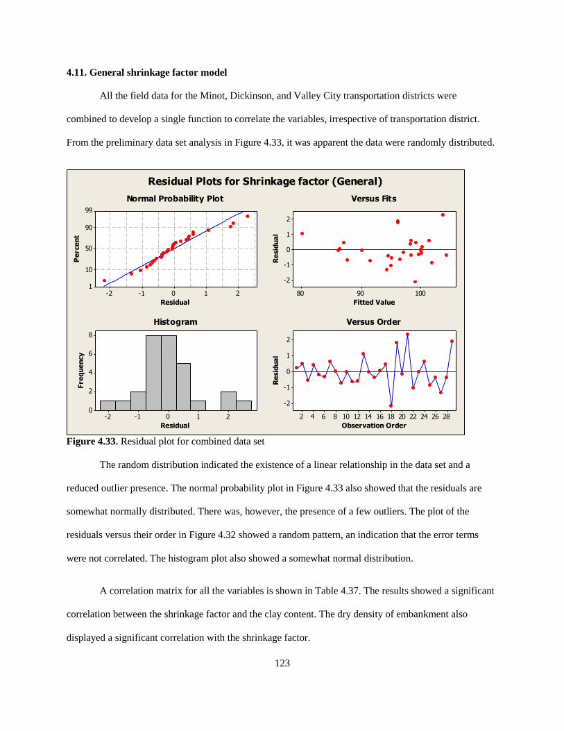
123
4.11. General shrinkage factor model
All the field data for the Minot, Dickinson, and Valley City transportation districts were
combined to develop a single function to correlate the variables, irrespective of transportation district.
From the preliminary data set analysis in Figure 4.33, it was apparent the data were randomly distributed.
210-1-2
99
90
50
10
1
Residual
Pe
rce
nt
1009080
2
1
0
-1
-2
Fitted Value
Re
sid
ua
l
210-1-2
8
6
4
2
0
Residual
Fre
qu
en
cy
282624222018161412108642
2
1
0
-1
-2
Observation Order
Re
sid
ua
l
Normal Probability Plot Versus Fits
Histogram Versus Order
Residual Plots for Shrinkage factor (General)
Figure 4.33. Residual plot for combined data set
The random distribution indicated the existence of a linear relationship in the data set and a
reduced outlier presence. The normal probability plot in Figure 4.33 also showed that the residuals are
somewhat normally distributed. There was, however, the presence of a few outliers. The plot of the
residuals versus their order in Figure 4.32 showed a random pattern, an indication that the error terms
were not correlated. The histogram plot also showed a somewhat normal distribution.
A correlation matrix for all the variables is shown in Table 4.37. The results showed a significant
correlation between the shrinkage factor and the clay content. The dry density of embankment also
displayed a significant correlation with the shrinkage factor.
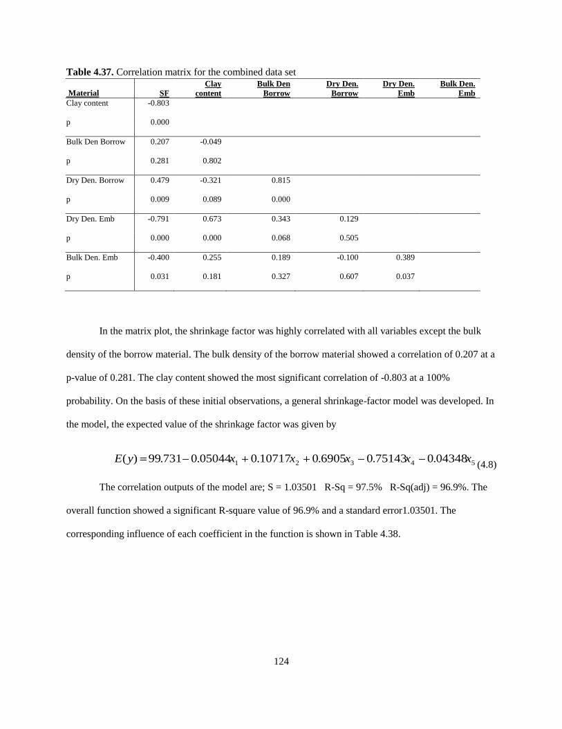
124
Table 4.37. Correlation matrix for the combined data set
Material SF
Clay
content
Bulk Den
Borrow
Dry Den.
Borrow
Dry Den.
Emb
Bulk Den.
Emb
Clay content -0.803
p 0.000
Bulk Den Borrow 0.207 -0.049
p 0.281 0.802
Dry Den. Borrow 0.479 -0.321 0.815
p 0.009 0.089 0.000
Dry Den. Emb -0.791 0.673 0.343 0.129
p 0.000 0.000 0.068 0.505
Bulk Den. Emb -0.400 0.255 0.189 -0.100 0.389
p 0.031 0.181 0.327 0.607 0.037
In the matrix plot, the shrinkage factor was highly correlated with all variables except the bulk
density of the borrow material. The bulk density of the borrow material showed a correlation of 0.207 at a
p-value of 0.281. The clay content showed the most significant correlation of -0.803 at a 100%
probability. On the basis of these initial observations, a general shrinkage-factor model was developed. In
the model, the expected value of the shrinkage factor was given by
54321 04348.075143.06905.010717.005044.0731.99)( xxxxxyE(4.8)
The correlation outputs of the model are; S = 1.03501 R-Sq = 97.5% R-Sq(adj) = 96.9%. The
overall function showed a significant R-square value of 96.9% and a standard error1.03501. The
corresponding influence of each coefficient in the function is shown in Table 4.38.
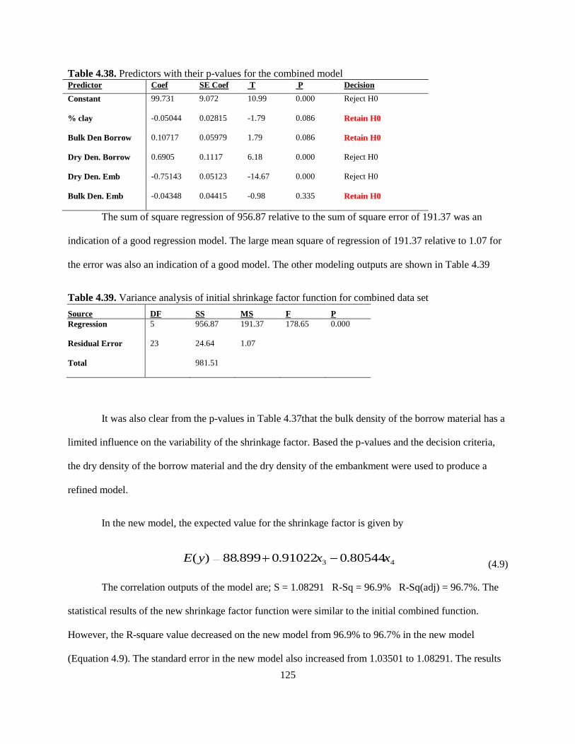
125
Table 4.38. Predictors with their p-values for the combined model Predictor Coef SE Coef T P Decision
Constant 99.731 9.072 10.99 0.000 Reject H0
% clay -0.05044 0.02815 -1.79 0.086 Retain H0
Bulk Den Borrow 0.10717 0.05979 1.79 0.086 Retain H0
Dry Den. Borrow 0.6905 0.1117 6.18 0.000 Reject H0
Dry Den. Emb -0.75143 0.05123 -14.67 0.000 Reject H0
Bulk Den. Emb -0.04348 0.04415 -0.98 0.335 Retain H0
The sum of square regression of 956.87 relative to the sum of square error of 191.37 was an
indication of a good regression model. The large mean square of regression of 191.37 relative to 1.07 for
the error was also an indication of a good model. The other modeling outputs are shown in Table 4.39
Table 4.39. Variance analysis of initial shrinkage factor function for combined data set
Source DF SS MS F P
Regression 5 956.87 191.37 178.65 0.000
Residual Error 23 24.64 1.07
Total 981.51
It was also clear from the p-values in Table 4.37that the bulk density of the borrow material has a
limited influence on the variability of the shrinkage factor. Based the p-values and the decision criteria,
the dry density of the borrow material and the dry density of the embankment were used to produce a
refined model.
In the new model, the expected value for the shrinkage factor is given by
43 80544.091022.0899.88)( xxyE (4.9)
The correlation outputs of the model are; S = 1.08291 R-Sq = 96.9% R-Sq(adj) = 96.7%. The
statistical results of the new shrinkage factor function were similar to the initial combined function.
However, the R-square value decreased on the new model from 96.9% to 96.7% in the new model
(Equation 4.9). The standard error in the new model also increased from 1.03501 to 1.08291. The results
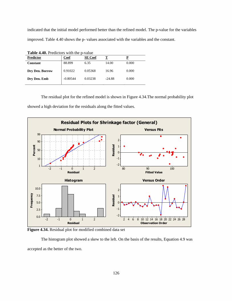
126
indicated that the initial model performed better than the refined model. The p-value for the variables
improved. Table 4.40 shows the p- values associated with the variables and the constant.
Table 4.40. Predictors with the p-value Predictor Coef SE Coef T P
Constant 88.899 6.35 14.00 0.000
Dry Den. Borrow 0.91022 0.05368 16.96 0.000
Dry Den. Emb -0.80544 0.03238 -24.88 0.000
The residual plot for the refined model is shown in Figure 4.34.The normal probability plot
showed a high deviation for the residuals along the fitted values.
210-1-2
99
90
50
10
1
Residual
Pe
rce
nt
1009080
2
1
0
-1
-2
Fitted Value
Re
sid
ua
l
210-1-2
10.0
7.5
5.0
2.5
0.0
Residual
Fre
qu
en
cy
282624222018161412108642
2
1
0
-1
-2
Observation Order
Re
sid
ua
l
Normal Probability Plot Versus Fits
Histogram Versus Order
Residual Plots for Shrinkage factor (General)
Figure 4.34. Residual plot for modified combined data set
The histogram plot showed a skew to the left. On the basis of the results, Equation 4.9 was
accepted as the better of the two.
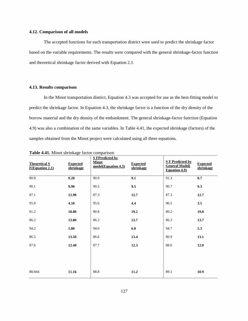
127
4.12. Comparison of all models
The accepted functions for each transportation district were used to predict the shrinkage factor
based on the variable requirements. The results were compared with the general shrinkage-factor function
and theoretical shrinkage factor derived with Equation 2.1.
4.13. Results comparison
In the Minot transportation district, Equation 4.3 was accepted for use as the best-fitting model to
predict the shrinkage factor. In Equation 4.3, the shrinkage factor is a function of the dry density of the
borrow material and the dry density of the embankment. The general shrinkage-factor function (Equation
4.9) was also a combination of the same variables. In Table 4.41, the expected shrinkage (factors) of the
samples obtained from the Minot project were calculated using all three equations.
Table 4.41. Minot shrinkage factor comparison
Theoretical S
F(Equation 2.1)
Expected
shrinkage
S FPredicted by
Minot
model(Equation 4.3) Expected
shrinkage
S F Predicted by
General Model(
Equation 4.9)
Expected
shrinkage
90.8 9.20 90.9 9.1 91.3 8.7
90.1 9.90 90.5 9.5 90.7 9.3
87.1 12.90 87.3 12.7 87.3 12.7
95.9 4.10 95.6 4.4 96.5 3.5
81.2 18.80 80.8 19.2 80.2 19.8
86.2 13.80 86.3 13.7 86.3 13.7
94.2 5.80 94.0 6.0 94.7 5.3
86.5 13.50 86.6 13.4 86.9 13.1
87.6 12.40 87.7 12.3 88.0 12.0
88.844 11.16 88.8 11.2 89.1 10.9
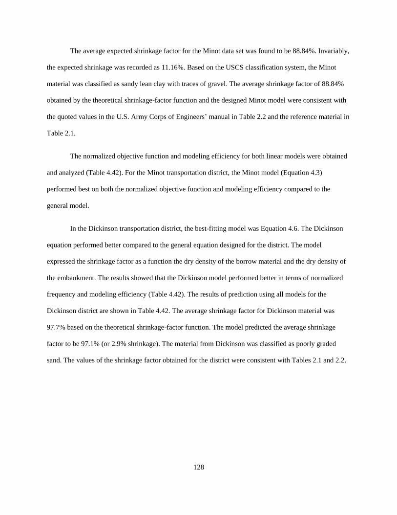
128
The average expected shrinkage factor for the Minot data set was found to be 88.84%. Invariably,
the expected shrinkage was recorded as 11.16%. Based on the USCS classification system, the Minot
material was classified as sandy lean clay with traces of gravel. The average shrinkage factor of 88.84%
obtained by the theoretical shrinkage-factor function and the designed Minot model were consistent with
the quoted values in the U.S. Army Corps of Engineers’ manual in Table 2.2 and the reference material in
Table 2.1.
The normalized objective function and modeling efficiency for both linear models were obtained
and analyzed (Table 4.42). For the Minot transportation district, the Minot model (Equation 4.3)
performed best on both the normalized objective function and modeling efficiency compared to the
general model.
In the Dickinson transportation district, the best-fitting model was Equation 4.6. The Dickinson
equation performed better compared to the general equation designed for the district. The model
expressed the shrinkage factor as a function the dry density of the borrow material and the dry density of
the embankment. The results showed that the Dickinson model performed better in terms of normalized
frequency and modeling efficiency (Table 4.42). The results of prediction using all models for the
Dickinson district are shown in Table 4.42. The average shrinkage factor for Dickinson material was
97.7% based on the theoretical shrinkage-factor function. The model predicted the average shrinkage
factor to be 97.1% (or 2.9% shrinkage). The material from Dickinson was classified as poorly graded
sand. The values of the shrinkage factor obtained for the district were consistent with Tables 2.1 and 2.2.
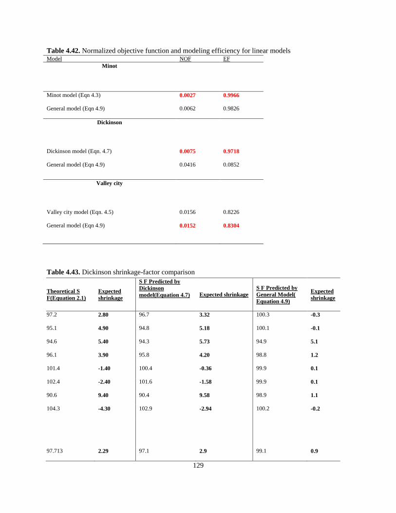
129
Table 4.42. Normalized objective function and modeling efficiency for linear models Model NOF EF
Minot
Minot model (Eqn 4.3) 0.0027 0.9966
General model (Eqn 4.9) 0.0062 0.9826
Dickinson
Dickinson model (Eqn. 4.7) 0.0075 0.9718
General model (Eqn 4.9) 0.0416 0.0852
Valley city
Valley city model (Eqn. 4.5) 0.0156 0.8226
General model (Eqn 4.9) 0.0152 0.8304
Table 4.43. Dickinson shrinkage-factor comparison
Theoretical S
F(Equation 2.1)
Expected
shrinkage
S F Predicted by
Dickinson
model(Equation 4.7) Expected shrinkage
S F Predicted by
General Model(
Equation 4.9)
Expected
shrinkage
97.2 2.80 96.7 3.32 100.3 -0.3
95.1 4.90 94.8 5.18 100.1 -0.1
94.6 5.40 94.3 5.73 94.9 5.1
96.1 3.90 95.8 4.20 98.8 1.2
101.4 -1.40 100.4 -0.36 99.9 0.1
102.4 -2.40 101.6 -1.58 99.9 0.1
90.6 9.40 90.4 9.58 98.9 1.1
104.3 -4.30 102.9 -2.94 100.2 -0.2
97.713 2.29 97.1 2.9 99.1 0.9
130
In the Valley City transportation district, the best-fitting model was observed to be Equation 4.4.
The model expressed the expected shrinkage factor as a function of the bulk density of the borrow
material and the dry density of the embankment. The model was applied when calculating the shrinkage
factor for samples collected in the field and compared with the results of the theoretical shrinkage factor
(Table 4.44). The material from Valley City was classified as clayey soil based on the USCS
classification. The average shrinkage factor was obtained to be 99.0% for the material. This shrinkage
factor was higher than the quoted value of 90% in Tables 2.1 and 2.2.
The normalized objective function and modeling efficiency of the Valley City model was
obtained and compared with the general shrinkage-factor model. The results (Table 4.42) showed that the
general model performed better in terms of the normalized objective frequency and modeling efficiency
compared to the Valley City model.
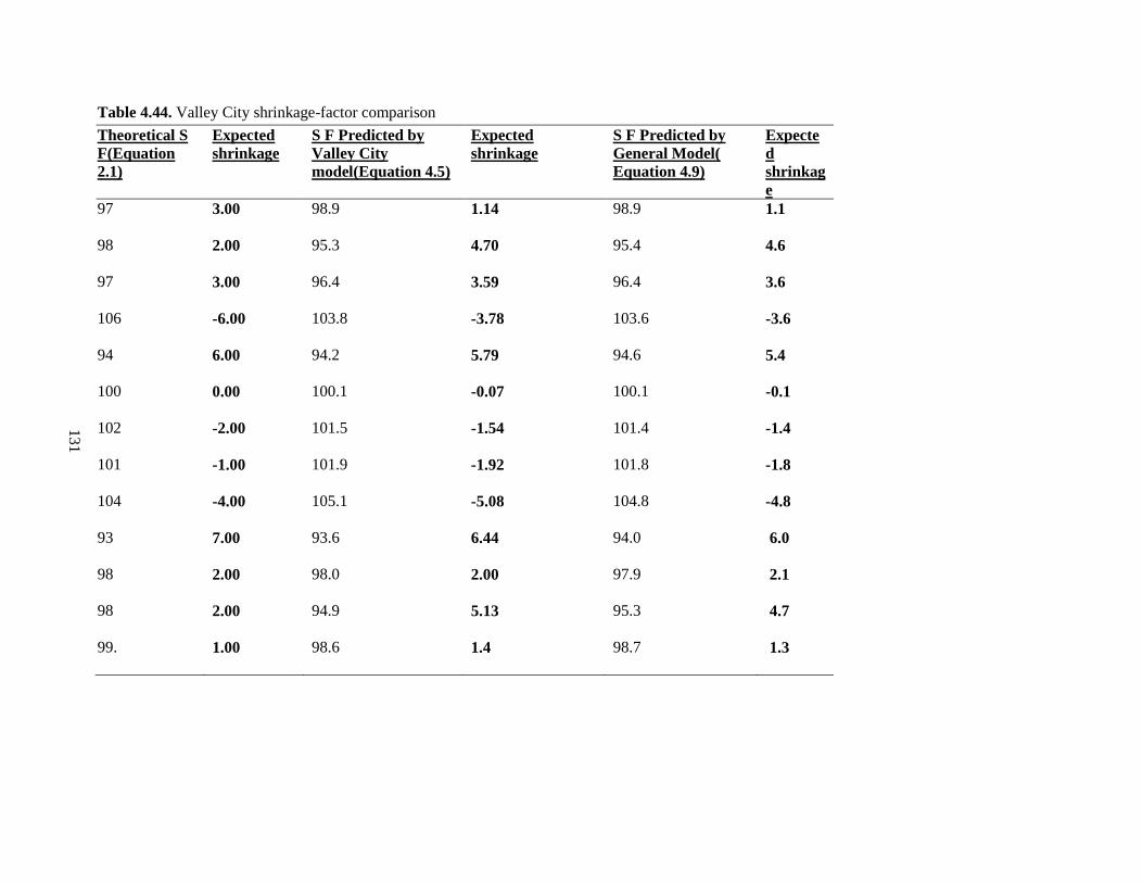
131
Table 4.44. Valley City shrinkage-factor comparison
Theoretical S
F(Equation
2.1)
Expected
shrinkage
S F Predicted by
Valley City
model(Equation 4.5)
Expected
shrinkage
S F Predicted by
General Model(
Equation 4.9)
Expecte
d
shrinkag
e
97 3.00 98.9 1.14 98.9 1.1
98 2.00 95.3 4.70 95.4 4.6
97 3.00 96.4 3.59 96.4 3.6
106 -6.00 103.8 -3.78 103.6 -3.6
94 6.00 94.2 5.79 94.6 5.4
100 0.00 100.1 -0.07 100.1 -0.1
102 -2.00 101.5 -1.54 101.4 -1.4
101 -1.00 101.9 -1.92 101.8 -1.8
104 -4.00 105.1 -5.08 104.8 -4.8
93 7.00 93.6 6.44 94.0 6.0
98 2.00 98.0 2.00 97.9 2.1
98 2.00 94.9 5.13 95.3 4.7
99. 1.00 98.6 1.4 98.7 1.3

132
From the results, all the best-fitting models for each district (Equations 4.3, 4.5, 4.7, and 4.9)
were found to be functions of the bulk density of the borrow material, the dry density of the borrow
material, the bulk density of the embankment, and the dry density of the embankment. All these models
performed significantly better than the other models without the same combination of independent
variables.
The average shrinkage factor obtained for each project was compared to the quoted shrinkage
factor for each project’s contract in Table 4.45. The comparison showed a significant difference among
the shrinkage factor quoted by the NDDOT contract documents, the theoretical shrinkage factor, and the
modeled shrinkage factor. The theoretical shrinkage factor and the modeled shrinkage factor were highly
correlated from the results in Table 4.45 and Figure 4.35.
Table 4.45. Shrinkage factor comparison
Project Transportation
District
Shrinkage
factor on
Contract
Avg.
Theoretical
Shrinkage
factor
Avg. Modeled
shrinkage
factor
Shrinkage factor
quoted for such soils
AC-SOI-NH-4-
023(018)066 Minot - 88.84%(11.16) 88.84%(11.2) 80%-95%
AC-SOI-SS-5-
022(095)074 Dickinson 70% 97.71%(2.29) 97.10%(2.9) 90%-95%
SER-2-046(041)014 Valley City - 99.00%(1.0) 98.7%(1.3) 80%-90%
SNH-SER-3-
057(047)006 Devils Lake 70% - - -

133
. Figure 4.35. Three districts with their shrinkage values
134
CHAPTER 5. CONCLUSION AND FURTHER RESEARCH
5.1. Conclusion
In this research a systematic process was used to model a location dependent predictive model for
soil shrinkage factor. The model predicts shrinkage factors at locations within the state of North Dakota
by correlating soil bulk and dry densities and clay content of soil.
These shrinkage factor parameters are linked to soil structure and the amount of compactive effort
that could be applied to it. The proposed model derives its inputs from georeferenced soil database for
modeling shrinkage factor variability. In this research, of the five proposed shrinkage factor drivers (clay
content, bulk density of borrow, dry density of borrow, bulk density of embankment and dry density of
embankment), only the clay content of soil was obtained from a georeferenced database. The other soil
parameters were obtained in the field and laboratory from randomly sample soil in four transportation
districts in North Dakota. ArcGIS was used to quantitatively express the variability in soil shrinkage
factor from one transportation district to the other through a map. ArcGIS was also used to predict the
probability of occurrence of shrinkage factor values by modeling the errors associated with the occurrence
of shrinkage factor parameters across the different locations.
The shrinkage factor model developed in two of three transportation districts expressed the
expected shrinkage factor at any location as a function of the dry density of the borrow material and the
dry density of the embankment. These outcomes are consistent with the general shrinkage-factor function
in the literature.
The initial models developed for all districts expressed high levels of correlation between the
expected shrinkage factor and the clay content, moisture content, and bulk density, with very high
standard error and R-square values. The probability for the occurrence of such a multivariate combination
was below the set 95% confidence interval. The elimination of clay content, for instance, by the high p-
135
value, resulted in the loss of correlation between the moisture content and bulk densities in the
multivariable functions. The results showed that there is a correlation between the expected shrinkage
factor and the clay content, moisture content, and bulk density. However, the degree to which this
correlation influenced the variability of the shrinkage factor was limited based on the results of the data
collected.
For various transportation districts, different kriging variants were ranked best for modeling the
clay-content variability. The ranked kriging results showed that not one particular kriging method could
be used in modeling the soil property’s variability. The lack of a constant kriging module could be
explained by the fact that the variograms used for modeling soil property did not exhibit a fixed response
to autocorrelation. The variogram responses were determined by the intrinsic nature and behavior of the
samples. For instance, directional variation in the soil property changed the nature of autocorrelation and
the variograms used to model the autocorrelation.
From the results, the average expected shrinkage factor in the Minot, Dickinson, and Valley City
transportation districts was88.8% (11.2%, 97.7% (2.3%), and 98% (2%) respectively (Table 4.43). The
relatively conservative expected shrinkage-factor values for Dickinson and Valley City could be
explained by the relatively high densities of the borrow materials in these areas. This observation could be
predicted by using the density distribution kriging map and incorporated into the process of setting
shrinkage factors for projects in that area.
The deterministic shrinkage factor suggested for use in the contracts of these projects was 70%
(30% shrinkage). The DOT-suggested shrinkage factor was found to be significantly higher than the
expected shrinkage factor for the field results and the U.S. Army Corps of Engineers’ recommended
values (Table 2.2).This variability could be explained by the density changes for the same soil types
across the transportation district. The use of geostatistical kriging for modeling soil density would help in
capturing s variability.
136
From the results of this research, it can be concluded that geostatistics can be used to model
shrinkage-factor variables that are responsive to variation in space. A combination of spatial modeling
and the linear equation developed could be used to predict the value of the shrinkage factor in earthwork
projects. This approach ensures the use of a more reliable shrinkage factor because it provides a measure
of the statistical estimate for the accuracy of the values. The robustness of the shrinkage factor developed
from this approach could be assessed based on the statistical measurements associated with modeling the
variable maps.
To practically carry out this model, a georeferenced database of field densities for soil across the
state would have to be collected and kriged. These densities would then be linked with the densities of
embankments developed during construction. Shrinkage factor maps would then be developed from them
using the density maps.
5.2. Future research recommendation
The development of a linearly correlated shrinkage factor function does not preclude the
existence of a nonlinear function. In fact, in the analysis of the residuals for some models, the observation
was made that some residuals for the models that performed badly were not randomly distributed but,
rather, exhibited a nonlinear distribution. It is, therefore, important to conduct a nonlinear modeling of the
shrinkage factor with the same independent variables. There is also the need to conduct the same studies
across the other transportation districts in order to increase the spread and to make the general function
representative of conditions across the state.
The current historical data provided by the DOT for use in this project do not allow the
development of shrinkage-factor maps. An effort would have to be made by the DOT to collect

137
georeferenced soil density and embankment densities during construction in order to build a database that
could be used to develop a progressively robust model.
I also recommend the study and development of a function that models time based variability in
shrinkage factor of soils in the various transportation districts of North Dakota. This recommendation is
driven by the knowledge that weathering is a time based soil forming activity.
138
REFERENCES
Asa Eric, Mohamed Saafi, Joseph Membah and Arun Billa (2012). Comparison of linear and nonlinear
kriging methods for characterization and interpolation of soil data. Journal of Computing in Civil
Engineering, Vol. 26, pp. x-y.
Asa Eric, Jongchul Song, and Zhili Gao (2010). Earthwork shrinkage calculation. A research report for
the North Dakota Department of Transportation.
Bailey Trevor and Gatrell Anthony (1995). Interactive spatial data analysis. John Wiley and Sons, New
York.
Burgess, T. M. and Webster, R. (1980).'Optimal interpolation and isarithmic mapping of soil properties.
The semi-variogram and punctual kriging', 1. Soil Sci. 31: 315-31
Burrough, P.A. (1993). Soil variability: A late 20th century view. Soil and Fertilizers,56.5: 529-562.
Carter M. R. and GregorichE.G. (2006). Soil sampling and methods of analysis. Taylor and Francis
Group, Florida.
Casagrande A, 1965.”Role of calculated risk in earthwork and foundation engineering. Proc Asce Vol. 91,
No SM4,pp, 1-40.
Chen, D., W. Brutsaert. (1995). Diagnostics of land surface spatial variability and water vapor flux.J.
Geophys. Res.,101,7251-7268.
Chiles J. and Delfiner P (1999). Geostatistics: Modeling Spatial Uncertainty. Wiley, New York.
Christakos G.(1984). On the problem of permissible covariance and the variogram models. Water
resource research, 20(2), 251-265.
139
Civil Engineering Road Design and Transportation Infrastructure Design Software.http://www.ncdot.gov
(accessed 05/17/2012).
Cliff A.D. and Ord J.K. (1975). The choice of a test for spatial autocorrelation. In J. C. Davies and M. J.
McCullagh (eds) Display and Analysis of Spatial Data, John Wiley and Sons, London, 54-77.
Cole George M. and Harbin, Andrew L. (2006). Surveyor reference manual. Professional publications,
Inc., Belmont, CA.
Cressie, N. A. C., 1993. Statistics for Spatial Data. John Wiley and Sons, Inc. New Jersey.
Congalton Russell(1991). A review of assessing the accuracy of classifications of remotely sensed data.
Remote Sensing of Environment, Vol. 37, pp. 35-46.
Davis J.C. (1986). Statistics and Data Analysis in Geology. John Wiley & Sons, New York.
Decision 411. (2012). Testing the assumptions of linear regression.
http://people.duke.edu/~rnau/411home.htm (accessed 12/01/2012)
Doctor, P.G. (1979).An Evaluation of Kriging Techniques for High Level. Radioactive Waste Repository
Site Characterization. Pacific Northwest Lab, Richland, Washington 99352.
Easton Vallerie and McColl John (1997). Statistical Education Through Problem Solving (STEPS)
Statistics Glossary volume 1.1.
Einstein, H.H. & Baecher, G.B. 1982. Probabilistic and statistical methods in engineering geology. Rock
Mechanics, Supplement. 12: 47–61.
Field manual on earthmoving operations (2000). United States Army Engineer School.
140
Goodman Richard E (1989) Introduction to Rock Mechanics (Second Edition). John Wiley and Sons,
New York.
Goovaerts P. (1997). Geostatistics for Natural Resources Evaluation. Oxford University Press, New York.
Goovaerts P. (2000).Geostatistical approaches for incorporating elevation into the spatial interpolation of
rainfall. Journal of Hydrology, 228,113-129.
Gordon, S. and Gordon, F. (2004). Deriving the regression equations without calculus. Mathematics and
Computer Education, 38(1):64-68.
Griffith, D. (1987). Spatial Autocorrelation: A Primer. Association of American Geographers Resource
Publication, Washington, DC.
Hanna Awad S. (1998). Earthwork estimating. College of Engineering, University of Wisconsin-
Madison. Homepages.cae.wisc.edu/~cee492/note/L11_EstEarthWk9811.ppt(accessed 05/12/2012).
Haining, R. (1990) Spatial Data Analysis in Social and Environmental Sciences. Cambridge University
Press: New York, NY.
Haining R. F. (1994). Designing spatial data analysis modules for Geographical Information Systems. In
Fortheringham S., Rogerson P (eds) Spatial analysis and GIS. London,Taylor & Francis: 45–63.
Hammah, R. and Curran, J. (2006) Geostatistics in Geotechnical Engineering: Fad or Empowering?.
GeoCongress 2006: pp. 1-5.
Helton, J.C., Johnson, J.D., and OberkampfW.L. (2004). An exploration of alternative approaches to the
representation of uncertainty in model predictions.Reliability Engineering and System Safety.Vol. 85,
pp. 39-71.
141
Ibbitt, R. P., and O’Donnell, T. (1971). “Fitting methods for conceptual catchment models.”J. Hydr. Div.,
97_9_, 1331-1342.
Isaaks E. H. and Srivastava R. M. (1989). Applied Geostatistics. Oxford University Press,New York.
Jabro, J.D., (1992). Estimation of saturated hydraulic conductivity of soils from particle 926 size
distribution and bulk density data. Transactions of ASAE, 35 (2), 557-560.
Journel A.G. and Huijbregts, C.J. (1981).Mining Geostatistics. Academic Press. Salt Lake city.
Journel A.G. (1987). Geostatistics for the environmental sciences, department of applied earth sciences,
Stanford University. 135p.
Krige, D.G. (1951). “A statistical approach to some basic mine evaluation problems on the
Witswatersrand 1”. Chem. Metall. and Mining Soc. of 5.Afr. 52: 119-39.
Lagacherie P. and McBratney A.B., Chapter 1. Spatial Soil Information Systems and Spatial Soil
Inference Systems: Perspectives for Digital Soil Mapping. In: Digital Soil Mapping, An Introductory
Perspective, Developments in Soil Science (Lagacherie, P., McBratney, A.B., and Voltz, M., Editors),
2007.
Laslett, G. M., McBratney, A. B., Pahl, P. J. and Hutchinson, M. F. (1987). “Comparison of several
spatial prediction methods for soil PH”, 1. Soil Sci. 38:325-41.
Leick A.(2004).GPS Satellite Surveying(3rd Edition). Wiley, New York.
Matheron, G.(1955). Applications des methods statistiques a l’evaluation des gisements. Annales des
Mines, No. 12, 50-75.
Moore D. and G. McCabe (1993).Introduction to the Practice of Statistics.W.H. Freeman and Company,
New York.
142
Nash, J. E., and Sutcliffe, J. V. (1970). “River flow forecasting throughconceptual models. Part I—A
discussion of principles.” Journal of Hydrology, 10_3_, 282-290.
New Hampshire Department of Transportation.(1999). Highway design manual.
North Dakota Department of Transportation (2006). Guide for calculating earthwork quantities using
GEOPAK.
North Dakota Department of Transportation (2008).Standard Specifications for Road and Bridge
Construction.
North Dakota Department of Transportation field sampling and testing manual (2011).
National Cooperative Soil Characterization Database Available online at
http://ncsslabdatamart.sc.egov.usda.gov(accessed 5/31/2012).
National Cooperative Soil Survey.(2012). http://soils.usda.gov/partnerships/ncss/map.html (accessed
12/03/2012).
National Soil Information System (2012).
http://www.soils.usda.gov/technical/nasis/documents/metadata/index.html.(accessed 12/03/2012).
Nunnally S. W. (2011). Construction Methods and Management (Eighth Edition). Prentice-Hall,Inc. New
Jersey.
Oliver, M.A. and Webster R. (1990). Kriging: a method of interpolation for geographical information
systems, International journal of geographical information systems, 4,313-32.
Pardo-Igu´zquiza, E. (1998). “Comparison of geostatistical methods for estimating the areal average
climatological rainfall mean using information of precipitation and topography”. Int. J. Climatol., 18,
1031–1047.
143
Phillips, D.L., J. Dolph and D. Marks, 1992. A comparison of geostatistical procedures for spatial
analysis of precipitation in mountainous terrain. Agric. For. Meteorol., 58: 119-141.
Phoon, K. K. (2006). Modeling and simulation of stochastic data, In the proceedings of Geocongress
2006: Geotechnical engineering in the information technology age. Cd rom.
Rencher A. C (2002). Methods of Multivariate Analysis(Second Edition).John Wiley and Sons, New
York.
Robinson T.P.& G. Metternicht. (2006). Testing the performance of spatial interpolation techniques for
mapping soil properties. Computers and Electronics in Agriculture 50:97–108.
Soil Survey Division Staff. (1993). Soil survey manual. USDA Handb. 18. U.S. Government Printing
Office, Washington, DC.
Walker, W. E., Harremoës P., Rotmans J., Van der SluijsJ. P., Van Asselt M. B. A., Janssen P., and
Krayer von Krauss M. P. (2003). Defining uncertainty. A conceptual basis for uncertainty
management in model based decision support. Integrated Assessment,4(1):5-17.
Wetherill G. (1986).Regression Analysis with Applications. Chapman and Hall, New York.
Wilson M.A., S.P. Anderson, K.D. Arroues, S.B. Southard, R.L. D’Agostino, and S.L. Baird. (November
15, 1994). No. 6 Publication of Laboratory Data in Soil Surveys. National Soil Survey Center Soil
Technical Note Handbook 430-VI Amendment 5.
Wilson, W., Geiger, L., Madden, S., Mecklin, C. J., and Dong, A. (2004). Multiple linear regression using
a graphing calculator. Journal of Chemical Education, 81(6):903-907.
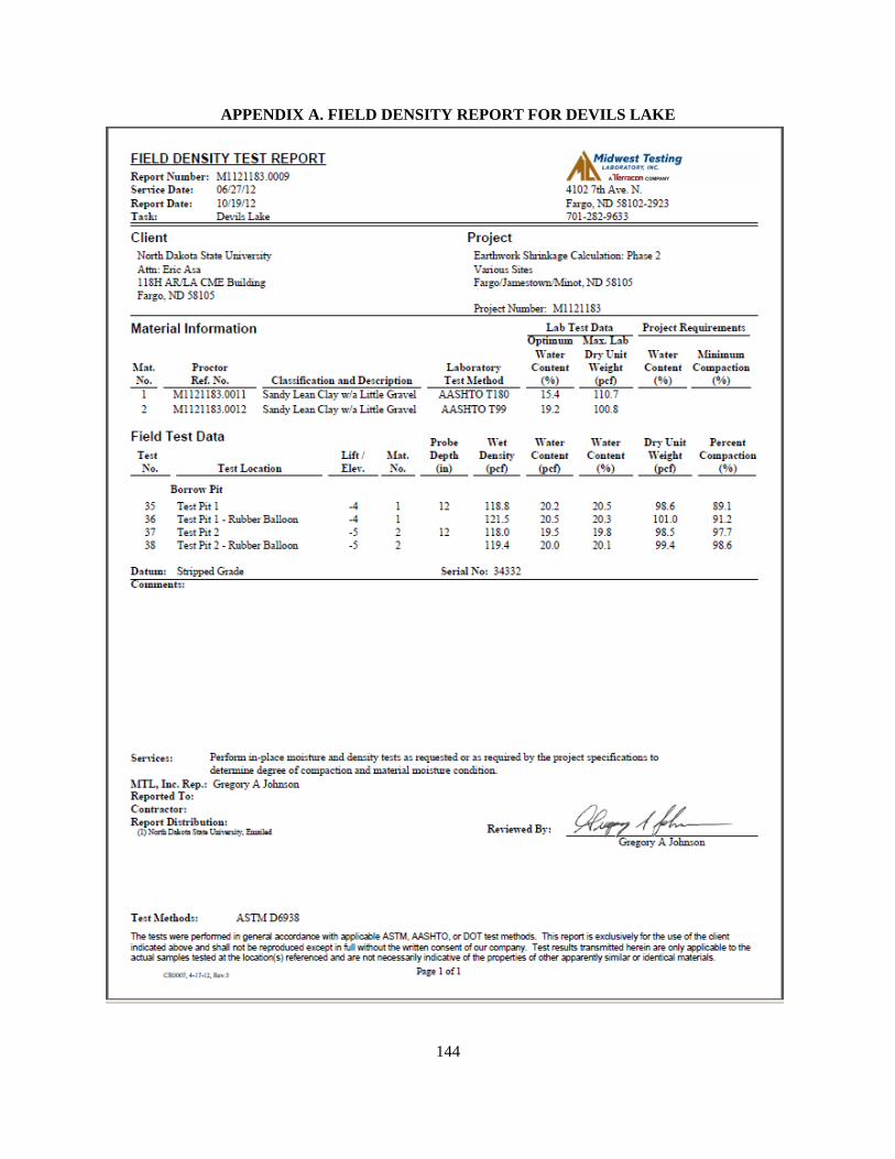
144
APPENDIX A. FIELD DENSITY REPORT FOR DEVILS LAKE
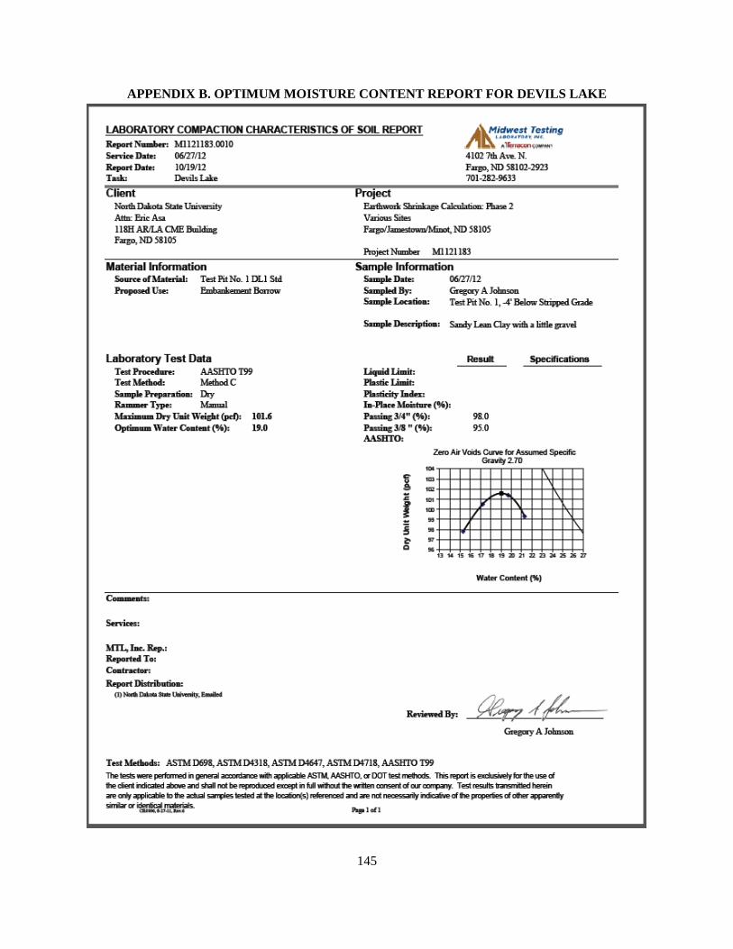
145
APPENDIX B. OPTIMUM MOISTURE CONTENT REPORT FOR DEVILS LAKE
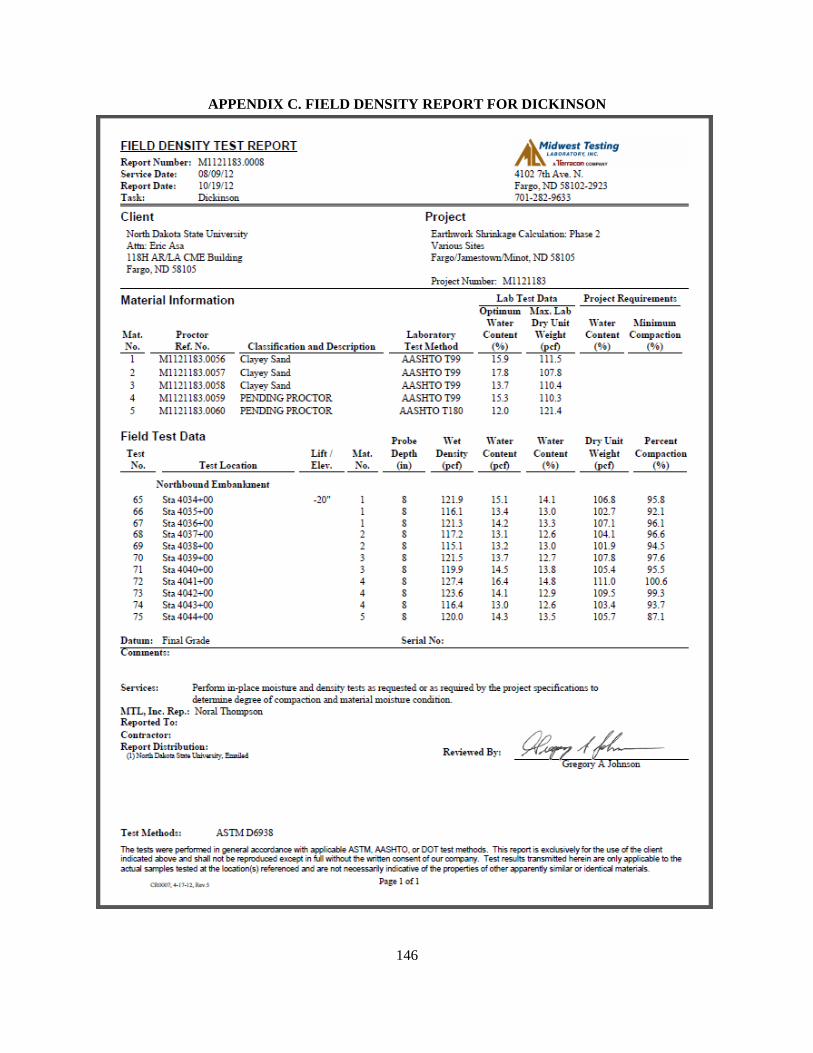
146
APPENDIX C. FIELD DENSITY REPORT FOR DICKINSON
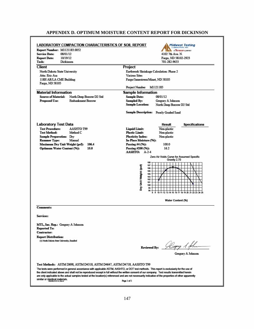
147
APPENDIX D. OPTIMUM MOISTURE CONTENT REPORT FOR DICKINSON
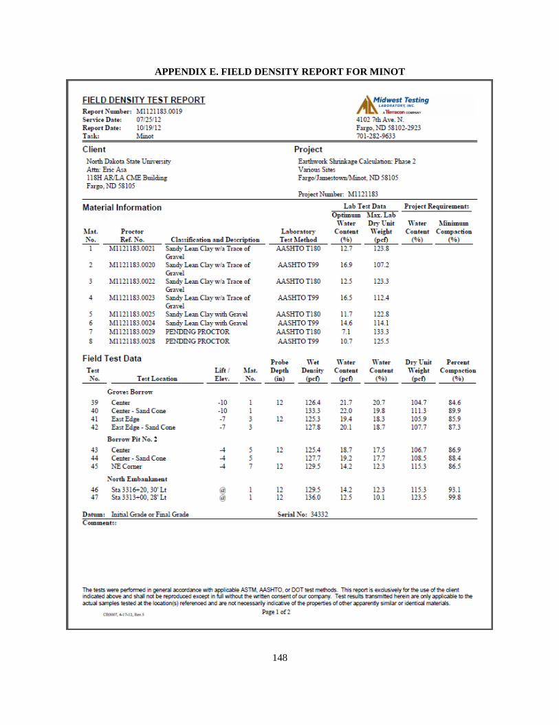
148
APPENDIX E. FIELD DENSITY REPORT FOR MINOT
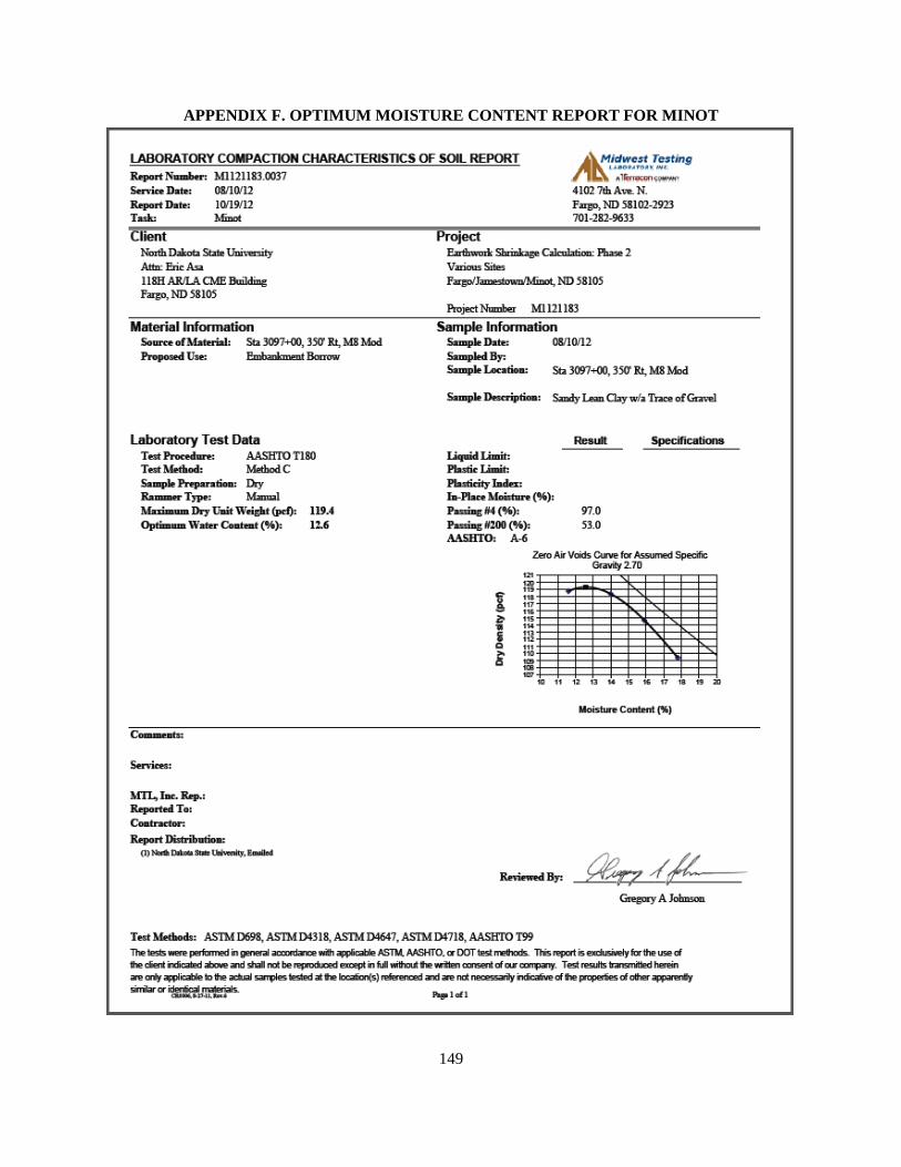
149
APPENDIX F. OPTIMUM MOISTURE CONTENT REPORT FOR MINOT
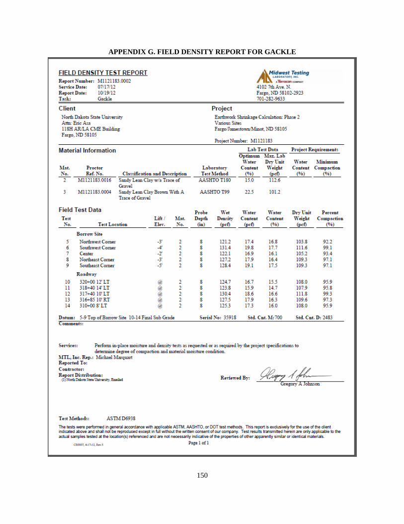
150
APPENDIX G. FIELD DENSITY REPORT FOR GACKLE
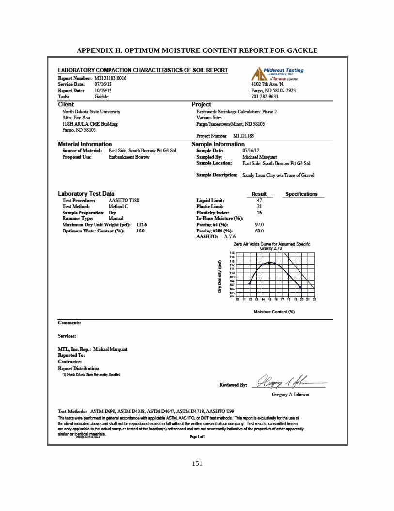
151
APPENDIX H. OPTIMUM MOISTURE CONTENT REPORT FOR GACKLE