effective geographic sample size in the presence of spatial autocorrelation

Effective Geographic Sample Size in the Presence ofSpatial Autocorrelation

Daniel A. Griffith

Ashbel Smith Professor, School of Social Sciences, University of Texas at Dallas

As spatial autocorrelation latent in georeferenced data increases, the amount of duplicate information containedin these data also increases. This property suggests the research question asking what the number of independentobservations, say n�, is that is equivalent to the sample size, n, of a data set. This is the notion of effective samplesize. Intuitively speaking, when zero spatial autocorrelation prevails, n� ¼ n; when perfect positive spatial au-tocorrelation prevails in a univariate regional mean problem, n� ¼ 1. Equations are presented for estimatingn� based on the sampling distribution of a sample mean or sample correlation coefficient with the goal of ob-taining some predetermined level of precision, using the following spatial statistical model specifications: (1)simultaneous autoregressive, (2) geostatistical semivariogram, and (3) spatial filter. These equations are eval-uated with simulation experiments and are illustrated with selected empirical examples found in the literature.Key Words: geographic sample, geostatistics, redundant information, spatial autocorrelation, spatial autoregression.

Sampling for data-gathering purposes must addressquestions asking how and what to sample (Levyand Lemeshow 1991), and it is the foundation of

much empirical social science research, whether quan-titative or qualitative methodologies are employed. Onedistinction between these two methodological ap-proaches is that quantitative research frequently requiresrelatively large sample sizes to collect somewhat super-ficial, albeit important, attribute information that isgeneralizable to a population, while qualitative researchoften is restricted to relatively small sample sizes in orderto collect large quantities of in-depth, detailed infor-mation from subjects or case studies. Quantitativeanalysis generalization is achieved through a soundrandom-sampling design (i.e., how to sample); qualita-tive analysis generalization, if desired, may be achievedthrough such techniques as triangulation. Considerableeffort has been devoted to geographic sampling designsfor quantitative investigations (e.g., Stehman andOverton 1996)—translating the what into where tosample—designs that exploit random sampling error.Impacts of spatial autocorrelation in this context arepartially understood and are the topic of this article. Oneof an array of purposive sampling strategies (i.e., how tosample) can be employed in qualitative research (seeMarshall and Rossman 1999, 78). The goal often isrepresentativeness and adherence to selected theoreticalconsiderations, as well as convenience. Impacts of spatialautocorrelation in this latter context are almost com-pletely unknown, although a spatial researcher shouldrealize that it still will come into play. For example, asnowball sampling strategy will be impacted by spatial

autocorrelation if subjects are from nearby locations andby social network autocorrelation because of the way thesample is generated. And an extreme-cases strategycould be impacted by the existence of geographicallynonrandom ‘‘hot spots’’ or ‘‘cold spots,’’ which arise be-cause of spatial autocorrelation. Findings reported in thisarticle for quantitative methodologies offer at least somespeculative insights into qualitative sample sizes, too.

Important Sample Properties

Sample size determination, often in terms of statisticalpower calculations, frequently is a valuable step inplanning a sample-based, quantitative study. Most in-troductory statistics textbooks discuss hypothesis testingin the context of appropriate sample size determination,with or without statistical power specification. Thepopularity and cumbersomeness of these calculationshave resulted in web-based interactive calculators toexecute the necessary computations for researchers (e.g.,http://calculators.stat.ucla.edu/powercalc/). For the caseof independent observations, Flores, Martınez, and Fe-rrer (2003) furnish some insights into sample-size de-termination for arithmetic means of georeferenced data,but for systematic sampling designs rather than thetessellated random sampling design promoted in thisarticle. As this literature illustrates, calculating an ap-propriate sample size unavoidably involves mathematicalnotation, which accordingly appears in the ensuingdiscussion.

Annals of the Association of American Geographers, 95(4), 2005, pp. 740–760 r 2005 by Association of American GeographersInitial submission, April 2004; revised submission, December 2004; final acceptance, February 2005

Published by Blackwell Publishing, 350 Main Street, Malden, MA 02148, and 9600 Garsington Road, Oxford OX4 2DQ, U.K.

Statistical power (Tietjen 1986, 38) is the probabili-ty—frequently denoted by 1� b, where b is the proba-bility of failing to reject the null hypothesis when thealternative hypothesis is true (i.e., a Type II error)—thata test will reject a false null hypothesis (i.e., the com-plement of a Type II error). The higher the power, thegreater the chance of obtaining a statistically significantresult when a null hypothesis is false. The power of allstatistical tests is dependent on the following designparameters: significance level selected for a statisticaltest; sample size; the tolerable magnitude of differencebetween a sample statistic and its corresponding popu-lation parameter; and natural variability for the phe-nomenon under study.

Spatial autocorrelation, which may arise from com-mon variables associated with locations or from directinteraction between locations (see Griffith 1992), hasan impact on significance levels, detectable differencesin attribute measures for a population, and measures ofattribute variability (see, e.g., Arbia, Griffith, and Ha-ining 1998, 1999). These impacts motivated Clifford,Richardson, and Hemon (1989) to apply the phrase‘‘effective degrees of freedom’’1—the equivalent numberof degrees of freedom for spatially unautocorrelated (i.e.,independent) observations, exploiting redundant orduplicated information contained in georeferenced datadue to the relative locations of observations (i.e., spatialautocorrelation)—to analyses in which these spatialautocorrelation effects are adjusted for in the case ofcorrelation coefficients. The duplicate information inquestion may arise from geographic trends induced bycommon variables or from information sharing resultingfrom spatial interaction (e.g., geographic diffusion). Thisarticle highlights the nearly equivalent notion of effec-tive sample size2: the number of independent observa-tions, say n�, that is equivalent to a spatiallyautocorrelated data set’s sample size, n. Intuitivelyspeaking, when zero spatial autocorrelation prevails anda regional mean is being estimated, n� ¼ n; when perfectpositive spatial autocorrelation prevails, n� ¼ 1. Theimportance of correcting n to n�may be illustrated byanalysis of remotely sensed data for the High Peak dis-trict of England, for which n 5 900 pixels containingmarkedly high positive spatial autocorrelation is equiv-alent to n� � 5 independent pixels (see the ensuingdiscussion for details). As an aside, Getis and Ord (2000)furnish a similar type of analysis for the multiple testingof local indices of spatial autocorrelation, which them-selves are highly spatially autocorrelated by construction.

Of note is that establishing effective sample size una-voidably requires mathematical derivations; basic onesare outlined in the body of this article in order to establish

the soundness of results. The validity of reported findingsis further bolstered with simulation experiment results.

Important Considerations When Designing aSampling Network

Random sampling in a geographic landscape requiresconsiderations much like those used when designinga conventional stratified random sample. Geographicrepresentativeness needs to be cast in terms of spatialcoverage rather than in terms of, say, stratification toachieve good socioeconomic/demographic coverage.Designing a geographic sampling network also needs toprotect against sample locations being correlated withthe geographic distribution to be studied; this specificconcern is why purely systematic sampling often is notused. Geographic sampling networks enable regionalmeans to be estimated, either for predefined sets of ag-gregate areal units (choropleth maps) or as interpola-tions of continuous surfaces (contour maps). Geographicsampling networks, designed for efficient estimation ofparameters describing the geographic distribution of in-terest, need to guard against grossly inefficient spatialprediction (Martin 2001; Muller 2001; Diggle andLophaven 2004) and vice versa. This trade-off results ina compromise between a systematic sample, comprisingregularly spaced sampling locations in order to achievegood geographic coverage and hence good interpolationaccuracy, and irregularly spaced sampling locations inorder to achieve better estimation of parameters for thegeographic distribution of interest.

A sampling network can be devised in various waysto satisfy the condition of containing both regularlyand irregularly spaced sampling locations. One way is toposition n/2 of the locations systematically (e.g., on aregular square tessellation) and the remaining n/2 loca-tions in a random fashion (i.e., randomly select east–west and, independently, north–south coordinates). Thisis the type of design associated with the GEOEAS dataexample (Englund and Sparks 1991; see http://www.webs1.uidaho.edu/geoe428/data_files.htm). A sec-ond method proposed by Diggle and Lophaven (2004)involves positioning some sampling locations on a reg-ular square tessellation grid and the remaining locationson more finely spaced regular square tessellation gridswithin a randomly selected subset of cells demarcatingthe coarser grid—the lattice plus in-fill design. Diggleand Lophaven also propose a third design, which theyprefer, that involves positioning some sampling locationson a regular square tessellation grid, with the remaininglocations being randomly selected from constant radiuscircular buffer zones circumscribing a random subset of

Effective Geographic Sample Size in the Presence of Spatial Autocorrelation 741

the systematically positioned locations—the lattice plusclose pairs design. Unfortunately, the software currentlyavailable to support their designs ‘‘would encounter se-rious difficulties . . . with numbers of locations largerthan a few hundred’’ (Diggle and Lophaven 2004, 8). Yeta fourth design is the one employed for this article,which is based on hexagonal-tessellation, stratified,random sampling (Stehman and Overton 1996). Aregular hexagonal tessellation containing n cells is su-perimposed on a region—the systematic component.Then a single location is randomly selected from withineach hexagon—the random component. This designshares many similarities with the lattice plus close pairsdesign. Of note is that these network layout issues arecentral to debates about geostatistical sampling designs.Cressie (1991, §5.6) furnishes a useful overview of nu-merous spatial sampling designs.

Mixing regularly and irregularly spaced sampling lo-cations highlights another important feature of spatialanalysis, namely designed-based and model-based infer-ence. The preceding sampling designs support design-based inference, which assumes that a given location hasa unique fixed but unknown value for the geographicdistribution of interest. The reference sampling distri-bution is constructed, conceptually, by repeatedly sam-pling from a geographic landscape and using the samedesign and calculating parameter estimates with eachsample. Initially, spatial scientists believed that thisstrategy could not be legitimately used when data con-tain non-zero spatial autocorrelation (Brus and deGruijter 1993). An alternative strategy is to let the valuefor some geographic distribution at a given location vary.In other words, the joint distribution of data valuesforming a map is one of an infinite number of possiblerealizations of some stochastic process; the total set ofpossible maps is called a superpopulation. Hence, the es-sential tool for describing a map is a model, resulting inthis inferential basis being labeled model-based. A severeshortcoming of this latter approach is the difficulty inknowing whether or not model assumptions are valid,necessitating diagnostic analyses. But it furnishes anindispensable analytical tool for understanding nonran-domly sampled data such as remotely sensed data andfor enabling spatial autocorrelation to be accounted forwhen devising a sampling design: the model-informed,design-based perspective outlined in this article.

A Conceptual Framework: The Effective Size of aGeographic Sample

A basis for establishing effective sample size for nor-mally distributed georeferenced data is presented in

terms of the sampling distribution of a single samplemean; extensions exploiting multiple sample means orthe sample correlation coefficient are presented in Ap-pendices A, B, and C. This approach, for which the as-sumption of a bell-shaped curve is critical, is directlyanalogous to that reported for time series (e.g., see the RDocumentation) and is indirectly analogous to what isreported for survey weights with superpopulation models(Pottchoff, Woodbury, and Manton 1992), whereby ap-plying weights to sample results alters the value of n.

Measuring natural variability for some georeferencedphenomenon results in an inflated variance estimatewhen spatial autocorrelation is overlooked (see Haining2003, §8.1). Suppose the n� n matrix V contains thecovariation structure among n georeferenced observa-tions (more precisely, matrix s2V� 1 is the covariancematrix), such that Y ¼ mþ e ¼ mþV�1=2e�, where Ydenotes an n� 1 vector of georeferenced attribute val-ues, m denotes the population mean of variable Y, 1denotes an n� 1 vector of ones, and e and e�, respec-tively, denote n � 1 vectors of spatially autocorrelatedand unautocorrelated errors. Suppose e� is independentand identically distributed Nð0; s2

e�Þ, where N denotesthe normal distribution, and s2

e� denotes the populationvariance for variate e�. If V 5 I, the n � n identity ma-trix, then the n observations are uncorrelated. Usingmatrix notation, the population variance estimate basedupon a sample, and ignoring spatial autocorrelation, isgiven by

Eðs2YÞ ¼ E½ðY� m1ÞTðY� m1Þ=n�TRðV�1Þ

ns2

e� ; ð1AÞ

where s2Y denotes the estimate of sY

2 , the variance ofattribute variable Y, E denotes the calculus of expecta-tions operator, and T and TR respectively denote thematrix transpose and trace operators. The quantityTRðV�1Þ=n is a variance inflation factor (VIF), similar tothe VIF generated by multicollinearity in conventionalmultiple linear regression analysis; it expresses the degreeto which collinearity among georeferenced observationsdegrades the precision of Y relative to similarly dispersedspatially uncorrelated values. Popular versions of ma-trix V include, for spatial autoregressive parameter rand binary geographic weights matrix C: (I� rC) forthe conditional autoregressive (CAR) model; and,[(I� rW)T(I� rW)] for the autoregressive response(AR) and simultaneous autoregressive (SAR) models,where matrix W is the row-standardized version of ma-trix C.3 Cliff and Ord (1981, Ch. 7), Anselin (1988),Griffith (1988), Haining (1990), and Cressie (1991, Ch.1), among others, furnish additional details about thesemodels.

Griffith742

Again using matrix notation, the variance of thesample mean of variable Y, �y, ignoring spatial autocor-relation, is given by

Eðs2yÞ ¼ s2

e�1TV�11=n2: ð1BÞ

Rearranging the terms on the right-hand side of thisequation and making the necessary algebraic manipula-tions yields

Eðs2yÞ ¼

TRðV�1Þn s2

e�

TRðV�1Þ1TV�11

n: ð1CÞ

The denominator on the right-hand side of this equationfurnishes the formula for effective sample size, namely,

n� ¼ TRðV�1Þ1TV�11

n: ð2Þ

If the n observations are independent, and hence V 5 I,then n� ¼ n, and the VIF becomes TRðV�1Þ

n ¼ 1. If perfectpositive spatial autocorrelation prevails, then, concep-tually, V� 1 5 k11T, with k! 1 as positive spatial au-tocorrelation increases, and n� ¼ 1.

In addition to the mathematical statistical theory deri-vation of Equation (2), its validity can be assessed throughsimulation experimentation. A simple exploratory experi-ment (100 replications) was conducted for selected casesin which variable Y was distributed N(0, 1), spatial auto-correlation was embedded with an SAR model, and n, thelevel of positive spatial autocorrelation r, and geographicconnectivity were varied. Figure 1A portrays a scatterplotof the simulated standard error versus a standard errorcomputed with the VIF and Equation (2). The goodness-of-fit of the regression line appearing in this graph high-lights the soundness of Equation (2), with a noticeabledeviation being attributable only to simulation variability.

Mean-Based Results for a SpatialAutoregression Model Specification: TheSAR Model

Findings based on a SAR model are illuminating herebecause a SAR model can be rewritten as a CAR model(see Cliff and Ord 1981), whereas semivariogram modelscan be directly related to it (see Griffith and Layne 1997).

The Case of a Single Geographic Mean

Griffith (2003) reports findings for Equation (2) and itsextension to expression (A1) in Appendix A, includingthe following conjecture, which is a slight improvementon the result reported by Griffith and Zhang (1999):

If georeferenced attribute variable Y is normally dis-tributed, or approximately so, and r is the spatial auto-correlation parameter estimate for a SAR modelspecification, then the effective sample size is given by

n� � n

� 1� 1

1� e�1:92369

n� 1

nð1� e�2:12373rþ0:20024

ffiffirpÞ

� �:

ð3ÞOf note, again, is that the normality assumption is criticalhere. In addition to a nonlinear regression analysis ofempirical cases used to calibrate Equation (3), its validity

Figure 1. (A): a scatterplot of the simulated standard error (100replications) versus a standard error computed with the varianceinflation factor (VIF) and Equation (2), denoted by solid circles( � ); the superimposed solid straight gray line denotes predictedvalues produced by the estimated regression equation. (B): a scat-terplot of n� computed with Equation (2) versus n� computed withapproximation Equation (3), denoted by asterisks (*), and withCressie’s (1991, 15) equation, denoted by open circles (o); thesuperimposed solid straight gray line denotes predicted valuesproduced by the estimated regression equation based upon Equa-tion (3) results, and the broken straight gray line denotes predictedvalues produced by the estimated regression equation based uponCressie’s equation’s results.


can be assessed through simulation experimentation. Theexperiment used to validate Equation (2) also was usedto validate Equation (3). Figure 1B portrays a scatterplotof n� computed with Equation (2) versus n� computedwith Equation (3). The goodness-of-fit of the regressionline appearing in this graph highlights the soundness ofEquation (3). Of note is that altering the geographicconnectivity definition results in slight but perceptiblevariation about values calculated with Equation (3).

Cressie (1991, 15) reports a comparable effectivesample size formula, which also was used to predict n� forthe simulation experiment (see Figure 1A). Equation (3)outperforms Cressie’s equation, yielding a mean squarederror (MSE) of 55 that is substantially less than the MSEof 334 for his equation.

The Case of Two Geographic Means

Following the same logic that establishes Equation (2),Griffith also reports, for the bivariate weighted meancase (see additional details in Appendix A) specified interms of a SAR model, the conventional variance termin expression (A1), namely

w2s2X þ ð1� wÞ2s2

Y þ 2wð1� wÞrXYsXsY

n; ð4AÞ

where sX2 and sY

2 respectively denote the variance ofvariables X and Y, rXY denotes the correlation betweenattribute variables X and Y, w (0 � w � 1) is the weightapplied to the mean of variable X, and the term2w(1�w)rXYsXsY adjusts for the presence of redun-dant attribute information in a bivariate georeferenceddataset. This expression is multiplied by the VIF ap-pearing in expression (A1), namely,

w2s2XTRf½ðI� rXWÞTðI� rXWÞ��1gþ ð1� wÞ2s2

YTRf½ðI� rYWÞTðI� rYWÞ��1g=n;

ð4BÞwhere rX and rY, respectively, are the spatial autocor-relation parameter estimates for variables X and Y. Theresulting product then is divided by the term denotingsampling variability of means in the presence of non-zerospatial autocorrelation, also appearing in expression(A1), namely,

w2s2X1T½ðI� rXWÞTðI� rXWÞ��11

þð1�wÞ2s2Y1T½ðI� rYWÞTðI� rYWÞ��11

þ2wð1�wÞrXYsXsY1T½ðI� rXWÞTðI� rYWÞ��11=n2:

ð4CÞ

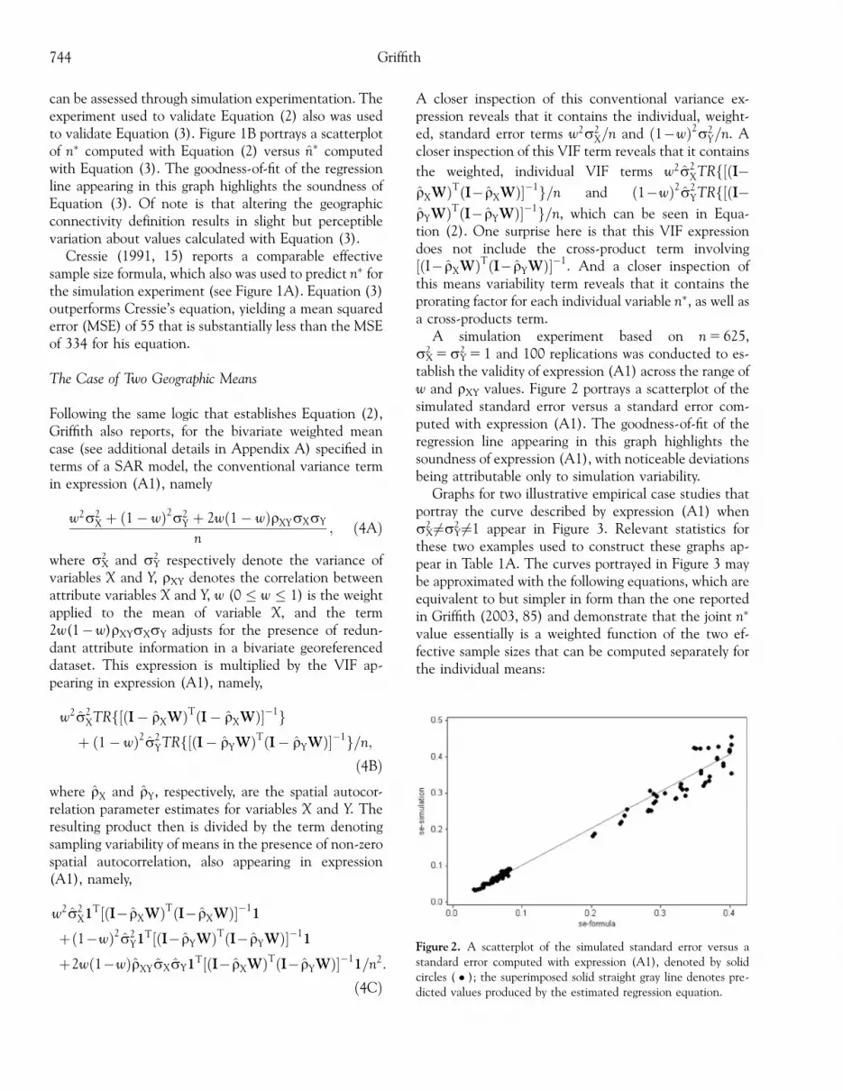
Figure 2. A scatterplot of the simulated standard error versus astandard error computed with expression (A1), denoted by solidcircles ( � ); the superimposed solid straight gray line denotes pre-dicted values produced by the estimated regression equation.

A closer inspection of this conventional variance ex-pression reveals that it contains the individual, weight-ed, standard error terms w2s2

X=n and ð1�wÞ2s2Y=n. A

closer inspection of this VIF term reveals that it contains

the weighted, individual VIF terms w2s2XTRf½ðI�

rXWÞTðI� rXWÞ��1g=n and ð1�wÞ2s2YTRf½ðI�

rYWÞTðI� rYWÞ��1g=n, which can be seen in Equa-tion (2). One surprise here is that this VIF expressiondoes not include the cross-product term involving½ðI� rXWÞTðI� rYWÞ��1. And a closer inspection ofthis means variability term reveals that it contains theprorating factor for each individual variable n�, as well asa cross-products term.

A simulation experiment based on n 5 625,sX

2 5sY2 5 1 and 100 replications was conducted to es-

tablish the validity of expression (A1) across the range ofw and rXY values. Figure 2 portrays a scatterplot of thesimulated standard error versus a standard error com-puted with expression (A1). The goodness-of-fit of theregression line appearing in this graph highlights thesoundness of expression (A1), with noticeable deviationsbeing attributable only to simulation variability.

Graphs for two illustrative empirical case studies thatportray the curve described by expression (A1) whensX

2 6¼sY2 6¼1 appear in Figure 3. Relevant statistics for

these two examples used to construct these graphs ap-pear in Table 1A. The curves portrayed in Figure 3 maybe approximated with the following equations, which areequivalent to but simpler in form than the one reportedin Griffith (2003, 85) and demonstrate that the joint n�

value essentially is a weighted function of the two ef-fective sample sizes that can be computed separately forthe individual means:

Griffith744

Puerto Rico

n� ¼ n��ew1:5899

w1:5899 þ ð1� wÞ1:5968þ n�se

� ð1� wÞ1:5968

w1:5899 þ ð1� wÞ1:5968; pseudo-R2

¼ 0:9998; ð5AÞ

and

Murray

n� ¼ n�As

w2:0171

w2:0171 þ ð1� wÞ1:3475þ n�Pb

� ð1� wÞ1:3475

w2:0171 þ ð1� wÞ1:3475; pseudo-R2

¼ 0:9994; ð5BÞ

where pseudo-R2 is the squared multiple correlationcoefficient (R2) between n� and n�. Because of the roleplayed by variance terms, which are specific to cases,only the general form of the equation can be establishedat this time. This empirical analysis further corroboratesthe validity of expression (A1).

As an aside, the extension of this two-means to amultiple-means result is summarized in Appendix B.

The Case of a Pearson Product-Moment CorrelationCoefficient

Spatial scientists are often interested in measuringrelationships between, rather than means of, geograph-ically distributed variables. Details for computing effec-tive sample size in this context, again assuming normallydistributed variables, appear in Appendix C. The fol-lowing approximate relationship holds between the in-dividual mean-based univariate effective sample sizesand their corresponding bivariate correlation-based ef-fective sample size:

n �XY�1þn�1

n

� n�Xþn�Y2þ

ffiffiffi2pðrXþrYÞ1:16ð1�r2

XYÞ0:04

ffiffiffiffiffiffiffiffiffiffin�Xn�Y

p� �:

ð6ÞThis approximation results in: n�XY¼n when spatial au-tocorrelation is absent; n�XY asymptotically converging on2 from below when rX 5 rY � 1 and rXY 5 1; and, n �XY

asymptotically converging on roughly 5 whenrX 5 rY � 1 and rXY 5 0, highlighting that it is an

Figure 3. Plots of the bivariate curve for the illustrative examples;the approximation curve is denoted by the dotted line (. . .), and thescatterplot of the exact n� values is denoted by solid circles ( � ).(A): the Puerto Rico digital elevation model (Dem). (B): theMurray Smelter site.

Table 1A. Selected descriptive statistics for the Puerto Rico digital elevation model (DEM) and Murray smelter site soilcontaminants

Landscape Variable Standard deviation r Bivariate correlation n�

Puerto Rico (n 5 73) DEM mean elevation (�e) 0.80270 0.83139 0.68102 6.24DEM elevation standard deviation (se) 3.54528 0.67638 12.69

Murray smelter site (n 5 253) Arsenic (As) 3.46316 0.53180 0.74775 68.24Lead (Pb) 7.69417 0.49363 76.95

NOTE: Griffith (2003) provides descriptions of these two datasets. The Murray, Utah, landscape is a superfund site. DEM denotes digital elevation model.


approximation; theoretically, desired values here are 1and 2. Results for five Thiessen polygon-based empiricalexamples appear in Table 1B; these results demonstratethat Equation (6) furnishes a good approximation forEquation (C1).

These findings highlight the implication that impactsof spatial autocorrelation can be mitigated to some ex-tent by incorporating redundant georeferenced attributeinformation into an analysis, a natural form of whicharises in space-time data series. Lahiri (1996, 2003)notes that this is one way of regaining estimator con-sistency when employing infill asymptotics (i.e., thesample size increases by keeping the study area sizeconstant and increasing the sampling intensity).

Mean-Based Results for SelectedGeostatistical/Semivariogram ModelSpecifications

Geostatistical models involve defining matrix V� 1

rather than matrix V. The scalar form of expression (2)for semivariogram models is given by

n� ¼ nðC0 þ C1Þ

nðC0 þ C1Þ � C1

Pni¼1

Pnj¼1j6¼i

fðdij; rÞn

¼ n

n� C1

ðC0þC1ÞPni¼1

Pnj¼1j6¼i

fðdij; rÞn; ð7Þ

where f(dij, r) denotes a particular semivariogram modelwith range parameter r, nugget C0, and slope C1, with dij

denoting distance separating locations i and j. The sill ina semivariogram model ‘‘represents a value that thesemivariogram tends to when distance gets very large,’’and hence at such extremely large distances equals thevariance of the variable under study (K. Johnson et al.2001, 283), C01C1. If no spatial autocorrelation ispresent, then the right-hand term in the denominator ofEquation (7) equals (n� 1), and n� ¼ n; as spatial au-tocorrelation increases, the denominator increases [itsright-hand term goes to nðC0 þ C1Þ=C0 þ nC1, sincef(dij, r " )! 1], resulting in n� decreasing from n to1 when C0 5 0. The following are three model-specif-ic special instances of Equation (7), when C0 is ze-ro, where the approximation formula is given by1þ ðn� 1=ð1þ b r

dmaxÞcÞ, in which dmax denotes the

maximum interpoint distance, which is the counterpartto Equation (3) for semivariogram models:

sphericaln

n� 32

1r

Pn

i¼1

Pn

j¼1j6¼1

dij

n þ 12

1r3

Pn

i¼1

Pn

j¼1

d3ij

n

� 1þ n� 1

1þ 251:5132ð rdmaxÞ1:9324

; dij � r; ð8AÞ

exponentialn

1þPni¼1

Pnj¼1j6¼i

e�dij=r

,n

� 1þ n� 1

ð1þ 51:4879Þ rdmaxÞ1:7576

; and ð8BÞ

K-Besseln

1þPni¼1

Pnj¼1j6¼i

dij

r K1dij

r

� �,n

� 1þ n� 1

ð1þ 69:6698 rdmaxÞ1:8601

; ð8CÞ

where K1 is a modified Bessel function of the first orderand second kind and the respective relative error sums ofsquares (RESSs) for the approximations are 5.4 � 10� 7,8.9� 10� 6, and 7.5� 10� 7. The spherical modelfinding helps highlight why average nearest-neighbordistance could serve as an informative index aboutspatial autocorrelation here. For the spherical model,if n 5 1 then n� ¼ 1

1�0 ¼ 1. If n 5 2, n� ¼ 2=2�ð1r 3

2 d12 � 12

1r3 d3

12Þ. As d12! 0, n� ! 1; in the limit,when an observation is replicated, only a single obser-vation effectively exists. As d12! r, n� ! 2; in the limit,when two observations are far enough apart, they con-tain no duplicated information. For the exponentialmodel, again, if n 5 1 then n� ¼ 1

1�0 ¼ 1. If n 5 2,n� ¼ 2=ð1þ e�d12=rÞ. As d12! 0, n*! 1; as d12! 1,n*! 2. For the K-Bessel function model, once more,if n 5 1 then n� ¼ 1

1�0 ¼ 1. If n 5 2, n� ¼ 2=ð1þd12

r K1d12

r

� �Þ. As d12! 0, n� ! 1; as d12! 1, n� ! 2—

these particular limits can be confirmed with Maple orMathematica. Graphs of these three functions—basedon nonlinear regression generalizations of a simulationexperiment using 250 randomly selected points from aunit square geographic region and with 500 replica-tions—appear in Figure 4. These graphs suggest that therange parameter of a semivariogram model behavessimilar to r for an autoregressive model; the (practi-cal) range increases as the degree of spatial autocorre-lation increases. These graphs also suggest that spatial

Griffith746

autocorrelation increases as a model description goesfrom the spherical specification, to the exponentialspecification, to the K-Bessel function specification. Thisimplication is consistent with Griffith and Csillag’s(1993) and Griffith and Layne’s (1997, 1999) findingsthat conceptually and numerically link the exponentialand CAR models and the K-Bessel function and SAR

models. This correspondence is closest for georeferenceddata distributed across a regular square tessellation (e.g.,remotely sensed data). Whereas autoregressive modelsare specified in terms of an inverse covariance matrix,semivariogram models are specified in terms of the as-sociated covariance matrix itself. Therefore, Equation(2), expression (A1), and Equation (C3) also can beemployed with semivariogram modeling results.

The Case of Negative Spatial Autocorrelation

A large majority of georeferenced data display mod-erate positive spatial autocorrelation. One exception isremotely sensed data, which tend to display very strongpositive spatial autocorrelation. Negative spatial auto-correlation is not encountered in practice nearly as oftenas is positive spatial autocorrelation. Rare examples of itare furnished by Anselin (1988), and by Griffith, Wong,and Whitfield (2003). Richardson (1990) notes thatwhen negative spatial autocorrelation is present, n�> n,which at first glance seems counterintuitive. But negativespatial autocorrelation is nothing more than an antitheticvariate (see Hall 1989) in spatial guise, which allowsmore to be gleaned from less, rather than less from morewhen spatial autocorrelation is positive. This type of re-sult can be obtained with Equation (2) by letting theautoregressive parameter be negative (i.e., ro0). Forexample, for the Murray site, n� nearly reaches 1,200when r � � 0.9. The wave-hole specification is the mostpopular semivariogram model for describing negativespatial autocorrelation (other possibilities include thecubic model). But for it, as the range increases, n� de-creases from n to 1. This fundamental difference betweenthese two classes of models is attributable to factors otherthan continuity (e.g., autoregressive models depend upona rigid neighborhood structure for discretized dataaggregations that is defined a priori, whereas geostatisti-cal models tend to over-smooth when spatial intensitiesare scattered in small clusters) and matrix inversion im-pacts (e.g., edge effects due to the shape and size of botha region and the areal units into which it is partitioned).The wave-hole semivariogram model actually behavesmore like the AR(2) time series model

Yt ¼ mþ j1Yt�1 þ j2Yt�2 þ et;

for which j140 and j2o0 (e.g., j1 5 0.66 andj2 5� 0.22). As such, positive spatial autocorrelationstill exists locally at relatively short distances. This fea-ture is necessarily so because in a continuous situation,changing nearby distances by a small amount cannot beaccompanied by continual dissimilarity.

Figure 4. Effective sample size (n�) for selected semivariogrammodels across their respective range parameters based upon simu-lation experiments (250 replications); solid circles ( � ) denotesimulation results, and dots (. . .) denote generalized function re-sults. (A): spherical semivariogram. (B): exponential semivario-gram. (C): Bessel function semivariogram.


A Remotely Sensed Image Example

Bailey and Gatrell (1995, 254) analyze LANDSAT 5‘‘Thematic Mapper’’ (TM) sensor data from a 1-km2,30� 30 pixels (n 5 900) portion of the High Peak Districtin England. This image includes a mix of land uses, from areservoir located in the southwest part, through mixeddeciduous and coniferous woodland inhabiting the south-central area, to rough grazing and moorland covering thenorthern part of this region. In other words, these data arevery heterogeneous. The illustration discussed here is interms of the ratio of spectral Band #4 (B4) to spectralBand #3 (B3), bands that, respectively, represent the near-infrared and red wavelengths of the electromagneticspectrum. The geographic visualization of this ratio pro-vides a good picture of spatial variation in biomass, withhealthy green vegetation reflecting strongly in B4, whichmeasures the vigor of vegetation, whereas its energy ab-sorption is strongly sensed in B3, which aids in the iden-tification of plant species.

The following heterogeneous Box-Cox power trans-formation was applied to the biomass index to betterstabilize the variance across the High Peak geographiclandscape, better aligning the transformed index with anormal distribution:

LNB4 þ 29

B3 þ 17þ

rankB4=B3

nþ 1

� 0:44

1�rankB4=B3

nþ 1

� �0:18" #

;

ð9Þ

where LN denotes the natural logarithm. Spatial SARmodel estimation results for these transformed data in-

clude: r ¼ 0:98834 and n� ¼ 5:12. In other words,on average, the 900 spatially autocorrelated pixelsforming the High Peak image attain approximately thesame level of statistical precision as only five independ-ent pixels.

Eleven semivariogram models were fitted to theseHigh Peak data. In all but one case (cubic), the C0 in-tercept parameter (i.e., nugget effect) estimate was veryclose to zero, and thus, for simplicity, C0 was set to zero.Estimation and (practical) range results appear in Table2. Most of the semivariogram models furnish a very gooddescription of spatial autocorrelation latent in thesedata. Most RESSs are roughly 2–3 percent. Semivario-gram plots (Figure 5) also reveal that the model pre-dictions closely track the data; the two poorestdescriptions are provided by the cubic model, whichtends to yield values that are too high for short distances,and the Gaussian model, which tends to yield values thatare too low for short distances.

Effective sample sizes here range from 6.75 to 17.42.Although these values are of the same order of magni-tude as the one produced with the SAR model, theytend to be noticeably higher. Furthermore, the K-Besselfunction, which is the theoretical semivariogram modelcompanion for the SAR model, does not produce theclosest of the set of n� values to 5.12. Of note is thatthe SAR value is consistent with what would be ob-tained with a time series for which r ¼ 0:98834:

n� ¼ 900ð1� 0:98834Þ=ð1þ 0:98834Þ ¼ 5:28:

And it is consistent with the value of 5.83 ren-dered by Cressie’s (1991, 15) formulae, for which this

Figure 5. Semivariogram plots and predictedvalues for eleven geostatistical models de-scribing spatial dependency latent in the HighPeak biomass index.

Griffith748

preceding time series result is the asymptotic limit interms of n.

Interestingly, the negative relationship between the(practical) range and n� can be detected from thesemodeling results (see Figure 6). In other words, as aspatial dependency field increases in size, more infor-mation becomes redundant, and effective sample sizedecreases.

The Murray Smelter Site Revisited

To illustrate results obtainable using irregular spacedpoint data and semivariogram depictions of spatial auto-correlation, the Murray smelter site data were analyzedin detail. SAR model descriptions of arsenic (As) andlead (Pb) are reported in Table 1B. As previously seenwith the High Peak data, these SAR-based, effectivesample size values differ from the range of similar semi-variogram model results reported in Table 3, althoughthey all are of the same order of magnitude. Here thevalues are lower than their autoregressive counterparts,with the SAR-based values of 77.0 falling above the in-

terval (56.3, 74.5) and 68.2 falling above the interval(46.0, 67.6).

Infill Sampling and a Single Mean: The Murray SmelterSite Example

Semivariogram models, because of their continuousnature, are especially useful for assessing the situation ofinfill sampling (i.e., the size of a region is held constantwhile sampling increasingly is more intensive). In otherwords, for a given region, as sampling becomes increas-ingly more intense, what happens to n�? In this context,n� should become a function of the average first nearest-neighbor distance, say �dNN1, between sample locations.As distance between nearby locations decreases, theoverall amount of redundant information in a samplecontaining spatial autocorrelation will tend to increase.

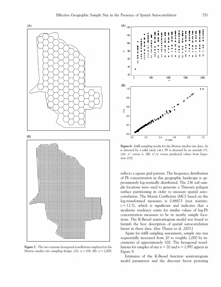
A second exploratory simulation experiment was con-ducted with the Murray smelter site data, which is basedupon hexagonal-tessellation stratified random sampling(Stehman and Overton 1996). Sample size wassequentially increased from roughly 100 to roughly 2,000by increments of approximately 100. The design for thistype of sampling is outlined in Appendix D. The hexag-onal tessellations for samples of size n 5 104 and n 5 2,008appear in Figure 7. Because these sampling schemes arebeing used for illustrative purposes, the noncovered sec-tions of the landscape are ignored; in reality, these parts ofthe landscape would be covered with partial hexagons thatthen could be grouped into a set of artificial piecemealhexagons whose individual areas would equal that of eachcomplete hexagon for sampling purposes.

Relationships between n� and n, by semivariogrammodel specification (see Table 3) for As and Pb sepa-rately, are portrayed in Figure 8A. These graphs suggestasymptotic diminishing returns for n� in each case.Meanwhile, as n increases, the average first nearest-neighbor distance, �dNN1, for a regular hexagonal tessel-lation will tend to decrease; this value, which can be

Table 1B. Selected descriptive statistics for five particular geographic landscape examples

Geographic landscape variables rX rY rXY n n�X n�Y n�XY n�XY

Puerto Rico DEM Elevation mean & variance 0.8314 0.6764 0.6810 73 6.24 12.69 30.97 29.12Kansas oil wells Thickness & % shale 0.3743 0.1093 � 0.5463 124 52.95 98.97 119.38 117.25Texas pH & Se 0.1398 0.3605 � 0.0031 127 95.03 56.82 120.57 120.59Texas u & SO4 0.3452 0.6834 � 0.2521 127 59.07 20.93 90.12 91.23Texas Mo & B 0.3218 0.3022 � 0.4942 127 62.59 65.66 113.98 114.26Texas V & As 0.3881 0.6878 0.7122 127 52.92 20.56 84.55 85.65Texas Bu & SO4 0.4530 0.6834 � 0.7686 127 44.44 20.93 77.31 80.52Murray site As & Pb 0.5318 0.4936 0.7478 253 68.24 76.95 179.08 175.41Minnesota forest stand basal area & suitability index 0.3648 0.3569 0.4200 513 219.49 224.27 436.52 437.48

Figure 6. Model estimated (practical) range versus effective samplesize (n�) for 11 geostatistical models, the High Peak biomass index.


standardized by the observed maximum interpoint dis-tance, yielding

�dNN1

dmax, will be a function of the regular

hexagonal tessellation centroids.Infill sampling results are for a fixed range parameter,

r, and may be expressed as the following function of�dNN1

dmax

and of the product n�dNN1

dmax, which is equivalent to the sum

of the individual point nearest-neighbor distances di-vided by the maximum interpoint distance:

n�infilljr ¼n

1þ be�0:13867c�3:46687d

� ð1þ be�c�dNN1=dmax�d�ndNN1=dmaxÞ;4ð10Þ

which equals n, as it should, when the uniform spacing ofall neighboring points is at a distance exceeding the(practical) range. The quantity 1

1þbe�0:13867c�3:46687d is theinfill asymptotic effective sample size discount factor bywhich n needs to be multiplied to calculate n�. Estimatesof b, c, d, and the discount factor for the Murray dataappear in Table 4. A scatterplot for the observed andpredicted values associated with Equation (10) appearsin Figure 8B, corroborating the high pseudo-R2 values

reported in Table 4 that imply a close correspondencebetween Equation (10) and the infill sampling results.

Whereas Equation (7) describes how n� changes asspatial autocorrelation in an attribute variable changes,Equation (10) describes particular model instances ofhow n� changes as spatial autocorrelation in a samplechanges, while the spatial autocorrelation of the attributevariable remains constant. Of note is that the practicalrange of As for the Gaussian semivariogram model is lessthan �dNN1 for that case, resulting in n� ¼ n for both theunivariate and bivariate cases, as it should be.

Infill Sampling and a Single Mean: A SkeetshootingSuperfund Site Example

A third exploratory simulation experiment was con-ducted with data collected for a skeetshooting superfundsite. For evaluation purposes, 236 surface soil sampleswere collected in the superfund site. A generalization ofthe geographic distribution of these measures reveals asingle spot within the site that was intensively sampled.The sampling network used throughout most of the site

Table 3. Selected semivariogram modeling results for soil samples from the Murray smelter site using a maximum standardizeddistance of 0.20; the maximum standardized distance is 1.05010

Model

Arsenic (As) Lead (Pb)

C0

C0þC1

C1

C0þC1Range/practical range 100 � RESS n�X

C0

C0þC1

C1

C0þC1Range/practical range 100 � RESS n�Y

Spherical 0.13235 0.86765 0.08139 44.9 73.5 0.09189 0.90811 0.08511 33.4 67.0Exponential 0.03661 0.96339 0.09179 43.4 64.6 0.02487 0.97513 0.10630 31.0 52.0Stable 0.00222 0.99778 0.10922 43.2 56.3 0.00000 1.00000 0.12260 30.9 46.0Penta-spherical 0.11345 0.88655 0.09566 44.9 73.4 0.08819 0.91181 0.10371 33.2 64.4Rational quadratic 0.07561 0.92439 0.10600 44.3 59.6 0.07642 0.92358 0.12476 31.7 47.2Bessel function 0.09468 0.90532 0.08021 44.4 70.2 0.08561 0.91439 0.09130 32.0 58.2Gaussian 0.21566 0.78434 0.06706 47.2 74.5 0.18588 0.81412 0.07175 35.0 66.1Circular 0.16236 0.83764 0.07522 45.1 71.9 0.10731 0.89269 0.07607 33.6 67.6

Table 2. Selected semivariogram modeling results for the High Peak remotely sensed image biomass index

Model C1 r 100 � RESS (practical) range n�

Spherical 0.0858 0.3527 2.7 0.3527 15.55Exponential 0.1066 0.2133 2.3 0.6399 6.75Stable 0.0986 0.1857 2.2 0.4956 9.15Penta-spherical 0.0868 0.4298 2.4 0.4298 14.86Rational quadratic 0.0962 0.1301 4.1 0.5671 9.03Bessel 0.0923 0.1001 2.8 0.4004 11.95Gaussian 0.0837 0.1505 8.8 0.2607 17.42Cubic 0.0538 0.5002 45.8 0.5002 unacceptable fitCircular 0.0852 0.3107 3.5 0.3107 15.89Cauchy 0.4772 0.0431 2.5 essentially no practical range NAPower 0.1605 0.5837 4.5 no range NA

C1 denotes the variance estimate (i.e., C0 5 0); r denotes the range parameter. Practical ranges are calculated following Griffith and Layne (1999, 468).

Griffith750

reflects a square grid pattern. The frequency distributionof Pb concentration in this geographic landscape is ap-proximately log-normally distributed. The 236 soil sam-ple locations were used to generate a Thiessen polygonsurface partitioning in order to measure spatial auto-correlation. The Moran Coefficient (MC) based on thelog-transformed measures is 0.48873 (test statistic:z 5 12.7), which is significant and indicates that amoderate tendency exists for similar values of log-Pbconcentration measures to be in nearby sample loca-tions. The K-Bessel semivariogram model was found tofurnish the best description of spatial autocorrelationlatent in these data. (See Thayer et al. 2003.)

Again for infill sampling assessment, sample size wassequentially increased from 20 to roughly 2,000 by in-crements of approximately 100. The hexagonal tessel-lations for samples of size n 5 20 and n 5 1,997 appear inFigure 9.

Estimates of the K-Bessel function semivariogrammodel parameters and the discount factor prorating

Figure 7. The two extreme hexagonal tessellations employed in theMurray smelter site sampling design. (A): n 5 104. (B): n 5 2,008.

Figure 8. Infill sampling results for the Murray smelter site data. Asis denoted by a solid circle ( � ). Pb is denoted by an asterisk (*).(A): n� versus n. (B): n�=n versus predicted values from Equa-tion (10).


coefficients for the skeetshoot data appear in Table 5.Spatial autocorrelation latent in these Pb data is muchstronger than that latent in the Murray site data (seeTable 4), a feature reflected in the smaller discountfactor. Furthermore, the goodness-of-fit for the discountfactor Equation (10) implies just as close a tracking ofthe data as is found for the Murray site.

Results for a Spatial Filter ModelSpecification

Spatial filtering techniques (Getis 1990, 1995; Griffith2000, 2003; Borcard and Legendre 2002; Getis andGriffith 2002) allow spatial analysts to employ traditionalregression techniques while insuring that regression re-siduals behave according to the traditional model as-sumption of no spatial autocorrelation in these residuals.One spatial filtering method exploits an eigenfunctiondecomposition associated with the MC. A spatial filter isconstructed from the eigenfunctions of a modified geo-graphic weights matrix that depicts the configuration ofareal units in the MC and is used to capture the co-variation among attribute values of one or more geo-referenced random variables. The simplest version ofthis weights matrix is denoted by the binary 0-1 matrixC. Spatial filtering uses such geographic configurationinformation to partition georeferenced data into a syn-thetic spatial variate containing the spatial autocorrela-tion and a synthetic aspatial attribute that is free ofspatial autocorrelation.

The preceding spatial autoregressive and geostatisti-cal models are nonlinear in form; a spatial filter model islinear in form. In addition, the eigenvectors used toconstruct the aforementioned spatial filter come fromthe following modified version of matrix C found in thenumerator of a MC:

ðI� 11T=nÞCðI� 11T=nÞ;where (I� 11T/n) is the projection matrix commonlyfound in conventional multivariate and regressionanalysis that centers the n� 1 vector of attribute values.The eigenvectors of this modified form of matrix C areboth orthogonal and uncorrelated. Consequently, thesampling variability of the mean of some attribute vari-able Y is given by the standard result, s2

Y=n. But when

Table 4. Coefficient estimates for Equation (10), and the resulting spatial autocorrelation discount factor, by semivariogrammodel specification, for the Murray smelter site

Model

Arsenic (As) Lead (Pb)

b c d discount factor b c d discount factor

Spherical 68.908 6.233 0.223 0.06942 67.902 5.004 0.223 0.06010Exponential 40.567 � 0.799 0.163 0.03742 40.722 � 1.941 0.194 0.03549Stable 39.583 � 1.467 0.190 0.03830 32.623 � 6.090 0.161 0.02251Penta-spherical 59.645 4.916 0.207 0.06355 56.928 3.030 0.207 0.05195Rational quadratic 43.906 0.010 0.191 0.04242 38.716 � 4.464 0.169 0.02442Bessel function 46.542 1.440 0.171 0.04536 44.739 � 0.593 0.180 0.03696Gaussian 120.588 10.568 0.268 0.08332 66.168 4.581 0.218 0.05733Circular 81.921 7.365 0.243 0.07296 87.816 7.172 0.250 0.06822Pseudo-R2 0.9969 0.9980

Figure 9. Two extreme hexagonal tessellations employed in theskeetshooting superfund site sampling design. (A): n 5 101. (B):n 5 1,997.

Griffith752

spatial autocorrelation is overlooked, then s2Y is inflated,

as has been shown for autoregressive and geostatisticalmodel specifications. This VIF is given by the standardregression result of 1

ð1�R2Þ , where R is the multiple cor-relation coefficient for attribute variable Y regressedon H eigenvectors contained in a spatial filter, yielding

s2y ¼

s2e�

ð1�R2Þn. In other words, the effective sample size forthis linear model is given by

n� ¼ ð1� R2Þn; ð11Þwhich produces a linear plot for n�versus R2. Of noteis that the degrees of freedom adjustment, n–H–1, oc-curs in the numerator of s2

e� only in the common caseof the regression parameters being unknown, highlight-ing that n� is not truly a function of this adjustment.If zero spatial autocorrelation is contained in variableY, then R 5 0, and n� ¼ n; as R! 1, n� goes to one, with

an upper limit of R ¼ffiffiffiffiffiffin�1

n

q; only n� 1 eigenvectors are

available for constructing a spatial filter, since one ei-genvector is proportional to vector 1, which is the vectorfor the linear regression intercept term.

Spatial filter-based values of n� are reported in Table 6.Comparing the n� values for As and Pb in Tables 1 and 6indicates that spatial filtering produces a more modestadjustment when converting sample size to effectivesample size in the presence of non-zero spatial autocor-relation. Results tend to be very similar when either an R2

maximization or a residual MC minimization criterion isused. In cases where the residual spatial autocorrelationfails to become trivial (e.g., High Peak biomass andPuerto Rico mean elevation, in Table 6), the thresholdvalue of MC could be reduced, prominent negativespatial autocorrelation eigenvectors could become can-didates, the stepwise regression inclusion probabilitycould be altered, and/or geographic contiguity could beredefined (e.g., a ‘‘queen’s’’ connection criterion couldbe substituted for a ‘‘rook’s’’ connection criterion). Ofnote is that the average univariate semivariogram valuesare closer to those values reported in Table 1A.

Implications: Model-InformedGeographic Sampling

Results reviewed and new findings reported in thisarticle are of great importance to geographers interestedin collecting data and provide necessary input for model-informed geographic sampling designs. During the plan-ning stage of a study, a quantitative spatial researcher maynaively compute the following when deciding on a samplesize for a given power in order to estimate the regionalmean, m, of attribute variable Y (Ott 1988, 147):

n ¼ s2Y

ðz1�a=2 þ z1�bÞ2

D2;

Table 5. Coefficient estimates for Equation (10), and the resulting spatial autocorrelation discount factor, by semivariogrammodel specification for lead (Pb), for the skeetshooting superfund site

model

Semivariogram coefficients Infill sampling prorating coefficients

C0 C1 Practical range b c d discount factor

Bessel function 0w 1.0706 0.1916 131.122 � 0.101 0.375 0.02686Goodness-of-fit 100 � RESS 5 17.5 Pseudo-R2 5 0.9989wThe estimated value of C0 is 0.1284, which was not significantly different from 0. For simplicity, then, C0 was set to 0.

Table 6. Selected spatial filter (a5 0.10 for inclusion) features used to compute n� for three particular geographiclandscape examples

Geographic landscape variable

Eigenvector(MC40.25)

selection criterion K R2 Residual zMC Spatial filter MC n n�

Puerto Rico DEM mean elevation Max R2 11 0.7487 2.7356 0.6155 73 18.34Min MC 15 0.7849 2.2617 0.6753 73 15.70

DEM elevation standard deviation Max R2 9 0.5876 0.7685 0.6316 73 30.11Min MC 12 0.6230 0.4924 0.6856 73 27.52

Murray smelter site arsenic (As) Max R2 19 0.4520 � 0.5589 0.7601 253 138.64Min MC 19 0.4317 0.0001 0.8306 253 143.78

lead (Pb) Max R2 13 0.3684 � 0.1687 0.7331 253 159.79Min MC 15 0.3642 0.0021 0.7989 253 160.86

High Peak biomass Max R2 191 0.9698 8.4710 0.8882 900 27.18Min MC 214 0.9717 8.0830 0.9062 900 25.47


where z1�a/2 represents the Type I error (i.e., rejectingthe null hypothesis when it is true) probability for a two-tailed test, z1�b represents the Type II error probability,and D5 |m� mo|, with m and mo, respectively, denotingthe null and the alternate hypothesis means. The value ofn rendered by this computation seeks to allow a prede-termined, desired level of statistical precision to be ob-tained for an analysis.

All three of the preceding n� results are helpful withincreasing domain sampling (i.e., the size of a geographicregion is expanded in order to increase the number of arealunits). Accordingly, from Equations (3), (7) and (11),

spatial autoregression

n ¼s2

e�ðz1�a=2þz1�bÞ2

D2 � 1�e�2:12373rþ0:20024ffiffirp

1�e�1:92349

1� 1�e�2:12373rþ0:20024ffiffirp

1�e�1:92349

;ð12AÞ

geostatistics n ¼ 1þ ðC0 þ C1Þðz1�a=2 þ z1�bÞ2

D2� 1

" #

� 1þ br

dmax

� c;

ð12BÞand

spatial filtering n ¼s2

e�ðz1�a=2þz1�bÞ2

D2

1� R2: ð12CÞ

For the High Peak biomass example data, s2Y ¼ 0:267012,

from the SAR model analysis s2e� ¼ 0:074242, from

the K-Bessel function semivariogram model analysiss2

e� ¼ 0:092342, and from the spatial filtering analysis

s2e� ¼ 0:024322. If the mean of the normally distributed

transformed biomass index is hypothesized to be 2, themaximum discrepancy to be detected is 0.1 (D), a two-tailed hypothesis test with a 5 percent level of significanceis to be employed (i.e., z1� a/2 5 1.95996), and statisticalpower is set to 0.9 (i.e., z1� b5 1.28115), then rather thann 5 75 (i.e., approximately a 9� 9 image) when spatialautocorrelation is overlooked, the SAR model resultssuggest that n 5 1,236, the K-Bessel semivariogram modelresults suggest that n 5 2,382, and the spatial filter modelresults suggest that n 5 963. In other words, ratherthan the 30� 30 pixels image being more than ade-quate in size, it needs to be expanded to at least a 35� 35image for a SAR analysis, a 49� 49 image for a geosta-tistical analysis, and a 31� 31 image for a spatial filteranalysis.

If a spatial researcher wants to estimate an attributemean for a particular geographic region, with a specificdegree of precision (i.e., a specific confidence interval),then power becomes irrelevant (Ott 1988, 131) and infill

sampling becomes relevant. Consider a current projectwhose goal is to determine soil Pb pollution across theCity of Syracuse (also see Griffith 2002). Then, based ona pilot study involving 167 sample points (see Figure10A), transformed attribute values LN(Pb13), a K-Be-ssel semivariogram model whose practical range is0.09392, in standardized distance units, and an equationof the form given by Equation (10),

n ¼ðC0 þ C1Þðz1�a=2Þ2

D2

� ½1þ 47:9041e�ð0:0958Þð�7:4247Þ�70ð0:0958Þð0:1317Þ�;ð13Þ

which contains the following substitutions [see Equa-tion (10)]: nr 5 70 [the value of n at (effective) range r

Figure 10. (A): soil sample locations, denoted by crosses (x), andone of the hexagonal tessellations together with its centroids, de-noted by solid circles ( � ), for the Syracuse, NY, study. (B): scat-terplots of relative n� versus n/nmax, denoted by solid circles ( � ),and relative standardized nearest neighbor distance versus n/nmax,denoted by solid squares (& ), for the Syracuse, NY, study.

Griffith754

for which spatial autocorrelation is negligible],�dNN1

dmax¼ 0:0958, b 5 47.9041, c 5� 7.4247, and d 5

0.1317 (see Figure 10). As was done for the Murray data,estimates of coefficients b, c, and d were obtained here byestimating n� for increasingly denser hexagonal tessel-lations. Because power is not of interest here, z1�b

disappears from the formula. Because spatial autocorre-lation increases with increasing infill sampling, andbecause diminishing returns for obtaining new, nonre-dundant information are encountered as n increases,with the limiting case (n goes to1) approaching no newinformation with each additional sample selection, moreand more samples have to be taken in order to acquireless and less new information. A reasonable value of Dfor the Syracuse study would be 0.25, indicating a con-fidence interval of m � 0.25. For a5 0.05 and K-Bessel function semivariogram coefficient estimates ofC1 5 0.98432 and C0 5 0, Equation (13) indicates thatachieving this level of precision would require a samplesize of 2,501. Given that the mean of the pilot studysample is roughly 4.5, this level of precision would allowa researcher to estimate the log-population mean towithin roughly � 6% of its actual value. Of note is thatthe RESS for the semivariogram model is 0.416, and thedescription of the experiment furnishing Equation (10)coefficient estimates is accompanied by a pseudo-R2 ofapproximately 0.996.

Therefore, findings reported in this article furnish amethodology and formulae that enable the computationof appropriate sample sizes for quantitative studies whennon-zero spatial autocorrelation is present in georefer-enced data. The first step (Step #1) of this methodologyinvolves a pilot study to obtain initial estimates of spatialautocorrelation and variable variance. If a researcherchooses to obtain a variance estimate from the literature,then assuming moderate positive spatial autocorrelationfor most variables and extremely strong positive spatialautocorrelation for remotely sensed images would bereasonable, too. The second step (Step #2) involvesselection of a spatial model specification to be used insubsequent data analyses. Although this model-informedsampling design approach is somewhat sensitive to theway in which spatial autocorrelation is modeled, all threealternative model specifications indicate that geographicstudies require substantially larger sample sizes than aresuggested by conventional statistical theory. This partic-ular result is relevant to qualitative sampling, too. Thethird step (Step #3) is to compute n, superimpose thecorresponding hexagonal tessellation over the study area,and then randomly select a single point from within eachhexagon. This is the sample to be drawn. A useful post-data-collection diagnostic exercise would be to compare

parameter estimates based on the sample data with thoseused to formulate the sampling design. Of note is that theprincipal contribution of this article is the developmentof Equations (12A)-(12C) for calculating n.

Future research needs to address extensions of find-ings reported here to other than means of normallydistributed georeferenced variables. The previously list-ed UCLA web page furnishes calculators for means ofPoisson (which would require the Winsorized auto-Poisson model) and exponential variables, and correla-tion coefficients (which are touched upon in this article).Meanwhile, the Web page http://www.stat.uiowa.edu/%7Erlenth/Power/index.html furnishes Russ Lenth’scalculators for proportions (which would require theautobinomial model), and analysis of variance (multiplemeans, which are touched upon in this article; also seeCliff and Ord 1975; Griffith 1978). Future research alsoneeds to outline impacts of spatial autocorrelation ex-plicitly for purposeful samples used in qualitative studies.

Acknowledgements

This material is based on work supported by theNational Science Foundation under Grant #BCS-0400559. Execution of computational and GIS work byMatthew Vincent and Marco Millones is gratefully ac-knowledged. This research was completed while theauthor was in the Department of Geography and Re-gional Studies, University of Miami.

Appendix A

The Case of a Weighted Average of Two CorrelatedSample Means

Sometimes a spatial scientist may be simultaneouslyinterested in two variables. One consequence of ex-tending Equation (2) results to the joint treatment of thepair of means, �x and �y, for two attribute variables, X andY, is the presence of two sources of redundant informa-tion: correlation between the two attribute variables andspatial autocorrelation within each attribute variable.Dutilleul (1993) updates the Clifford, Richardson, andHemon (1989) discussion about how spatial autocorre-lation impacts upon the correlation coefficient. Ex-tending his discussion reveals that covariation also has aVIF similar to that appearing in Equation (2), with thisfactor being compensated for by the individual variableVIFs when a correlation coefficient is computed; that is,a correlation coefficient must be contained in the inter-val [�1, 1], regardless of the nature and degree ofspatial autocorrelation present. Constructing a weighted


average of X and Y, say [wX1(1�w)Y] for 0 � w � 1,results in the sampling distribution variance of interest

being for w�xþ ð1� wÞ�y. If variables X and Y are inde-pendent, then this standard error reduces to the theo-retical result of a weighted sum of the variables’ twovariances.

In this bivariate means case, effective sample sizebecomes a weighted average of the individual variables’effective sample sizes that is adjusted for the attributecorrelation between X and Y. The general expression forn� becomes

where VX and VY respectively are the n� n inversecovariance structure matrices containing the spatialautocorrelation among n observations for attributevariables X and Y. If VX 5 VY 5 I, then this expres-sion reduces to n. If w 5 0, w 5 1, or VX 5 VY, thenthis expression reduces to the right-hand side of Equa-tion (2). In other words, the bivariate means effec-tive sample size is a weighted average of the individualunivariate effective sample sizes (i.e., it must be con-tained in the interval defined by them). And as VX

and VY approach the case of perfect positive spatialautocorrelation for both attribute variables, n� ap-proaches one. The weighting of the two limiting effec-tive sample sizes is determined by both the relativevariances of X and Y and the weights used in con-structing a linear combination of X and Y and is im-pacted little by the attribute correlation, rXY, computedfor variables X and Y.

Appendix B

The Case of a Linear Combination of P42Correlated Sample Means

Generalizing Equation (2) and expression (A1) to amultivariate situation involving P variable means, whichis particularly relevant to the use of principal compo-

nents or factor scores (see R. Johnson and Wichern2002, for a discussion of large sample inference), yields

where denotes Kronecker product, Ad is a P � P di-agonal matrix containing the linear combination coeffi-cient aP in diagonal cell P, Fd is a P � P diagonalmatrix containing standard deviation sP in diagonal cellP, Vd is an nP� nP block-diagonal matrix containingn� n inverse covariance structure matrix VP

� 1 in diag-onal block P, < is a P � P attribute correlation matrix,and I is an n� n identity matrix. If Vd 5 I, then ex-pression (B1) reduces to n. As all of the VP matrices

approach the case of perfect positive spatial autocorre-lation, n� approaches one. If all but one of the weightsare zero, then expression (B1) reduces to the right-handside of Equation (2). The numerical value produced byexpression (B1) is contained in the interval defined bythe extremes for the P individual results obtained withEquation (2).

Consider the 2-means case (see Appendix A). Then

AdFd ¼w 00 1� w

� sX 00 sY

�

¼ wsX 00 ð1� wÞsY

�

AdFd<FdAd

wsX 0

0 ð1� wÞsY

!1 rXY

rXY 1

!

�wsX 0

0 ð1� wÞsY

!

¼w2s2

X wð1� wÞsXsXrXY

wð1� wÞsXsYrXY ð1� wÞ2s2Y

0@

1A


Y þ 2wð1� wÞrXYsXsY


Y

w2s2XTRðV�1

X Þ þ ð1� wÞ2s2YTRðV�1

Y Þh i

w2s2X1TV�1

X 1þ ð1� wÞ2s2Y1TV�1

Y 1þ 2wð1� wÞrXYsXsY1TðVTXÞ�1=2V

�1=2X 1

n;

1TAdFd<FdAd1

TRðAdFd<FdAdÞTR ðAdFd IÞV1=2

d

� �Tð< IÞ ðAdFd IÞV1=2

d

� ��

1T ðAdFd IÞV1=2d

� �T

ð< IÞ ðAdFd IÞV1=2d

� �1

n; ðB1Þ

(A1)

Griffith756

1TAdFd<FdAd1 ¼ w2s2X þ ð1� wÞ2s2

Y

þ 2wð1� wÞrXYsXsY

TRðAdFd<FdAdÞ ¼ w2s2X þ ð1� wÞ2s2

Y

ðAdFd IÞV1=2d

� �T

¼wsX 0

0 ð1� wÞsY

� I

� �

�ðV�1=2

X ÞT 0

0 ðV�1=2Y ÞT

!

¼wsXI 0

0 ð1� wÞsYI

�

�ðV�1=2

X ÞT 0

0 ðV�1=2Y ÞT

!

¼wsXðV�1=2

X ÞT 0

0 ð1� wÞsYðV�1=2X ÞT

!

< I ¼ 1 rXY

rXY 1

� I ¼ I rXYI

rXYI I

�

1T ðAdFd IÞV1=2d

� �T

< Ið Þ ðAdFd IÞV1=2d

� �1

¼ w2s2X1TV�1

X 1þ ð1� wÞ2s2Y1TV�1

Y 1

þ 2wð1� wÞrXYsXsY1TðVTXÞ�1=2V

�1=2X 1

TR ðAdFd IÞV1=2d

� �T


� ��

¼ w2s2XTRðV�1

X Þ þ ð1� wÞ2s2YTRðV�1

Y ÞTherefore, expression (B1) reduces to expression (A1)when only two means are being considered.

Appendix C

An Illustration of Other Possible Extensions: TheCase of Bivariate Attribute Correlation Coupled withPositive Spatial Autocorrelation

Clifford, Richardson, and Hemon (1989) and Ri-chardson (1990) use semivariogram modeling to link the

correlation coefficient, r, to its correct sampling distri-bution for georeferenced data (also see Haining 2003,§8.2). They develop the notion of effective degrees offreedom. Based on the standard result of sr ¼ 1ffiffiffiffiffiffi

n�1p , the

standard error of the correlation coefficient r, under thenull hypothesis of rXY 5 0, the number of observations,n, may be prorated to n� using the formula

n� ¼ 1þ s�2r ðC1Þ

where sr2 denotes the variance of the sampling distri-

bution of the correlation coefficient r. Equation (C1)indicates that low sampling variability is associated withlarger values of n and sizeable sampling variability isassociated with smaller values of n. Consider two varia-bles containing maximal positive spatial autocorrelation,which manifests itself approximately as a linear datagradient across a geographic landscape. This situationrelates to three qualitatively different values of rXY,namely, rXY � 1 (both gradients align), rXY � � 1 (thegradients are in exactly opposite directions), and twocases of rXY � 0 (the gradients are orthogonal in two

different ways). Hence, positive spatial autocorrelationincreases sr , resulting in n� decreasing. Meanwhile, ifzero spatial autocorrelation is present, then n� ¼ n; ifperfect positive spatial autocorrelation is present, thenn� approaches one. Dutilleul (1993) rewrites Equation(C1) using matrix notation and incorporates impacts ofestimating means and variances for a correlation coeffi-cient, an adjustment that is set aside here for simplicity(these types of adjustments also are outlined by Griffithand Zhang 1999). These results are for the case of in-dependent attribute variables (i.e., rXY 5 0).

The new development presented here departs fromthis earlier work in order to incorporate the entire rangeof correlation values by beginning with the followingstandard error of a correlation coefficient:

sr ¼1� r2

XYffiffiffiffiffiffiffiffiffiffiffin� 1p : ðC2Þ

Following the developments for sample means and for runder the null hypothesis of rXY 5 0, the logic for

ðAdFd IÞV1=2d

� �T


� �¼

wsXðV�1=2X ÞT 0

0 ð1� wÞsYðV�1=2Y ÞT

!

�I rXYI

rXYI I

� wsXðV�1=2

X Þ 0

0 ð1� wÞsYðV�1=2Y Þ

!

¼w2s2

XV�1X wð1� wÞsXsYrXYðV

�1=2X ÞTðV�1=2

Y Þwð1� wÞsXsYrXYðV

�1=2X ÞTðV�1=2

Y Þ ð1� wÞ2s2YðV

�1=2Y Þ

!


deriving Equation (2) suggests

s2r �

1� r2XY

n� 1n

TRðV�1X V�1

Y Þ � TR½ðV�1XYÞ

2�r2XY

TRðV�1X ÞTRðV�1

Y Þ�


Y Þð1þ 16:40=nÞTRðV�1

X ÞTRðV�1Y Þ þ 16:40TR½ðV�1

XYÞ2�

" #0:47ð1�r2XYÞþ8=½nð1þrXþrYÞ6=n�

;

where VX� 1 and VY

� 1, respectively, are the n� n spatialautocorrelation covariance structure matrices for attributevariables X and Y. This equation was established with asimulation experiment conducted using regular squaretessellations forming rectangular regions ranging in sizefrom 3� 3 to 40� 40, combinations of SAR autocorre-lation parameter values, rX and rY, in the set {0.00, 0.25,0.50, 0.75, 0.99}, rXY values in the set {0.0, 0.2, 0.4, 0.6,0.8, 0.999}, and 10,000 replications. Pseudo-R2 values forthe three special theoretical cases that can be checked areas follows: 0.9984 for rX 5rY 5 0 (and, as a check, 0.9957for the analytical results); 0.9874 for rXY 5 0; and, 0.9814for rX 5rY � 1. The overall pseudo-R2 value is 0.9954,with the performance of this equation improving asymp-totically. In addition, it has been validated using the ir-regular Thiessen polygon surface partitonings for the 127Texas groundwater sample locations and the 124 Kansasoil well locations, the 73 municipios of Puerto Rico, and the513 Minnesota forest stands reported by Griffith andLayne (1999). These four irregular surface partitioningdata sets were supplemented with the Murray smelterThiessen polygons data. The pseudo-R2 for results ob-tained by reexecuting the simulation experiment using thegeographic configuration matrices for these five empiricalgeographic landscapes and the coefficients obtained withthe preceding simulation experiment is 0.9995.

Therefore, following the same logic used to establishEquation (2), as well as employing the common statisticalpractice of using r to estimate its own standard deviation,

n�XY�1þð1� r2XYÞ

n�1

n


Y Þr2XY

TRðV�1X V�1

Y Þ�TR½ðV�1XYÞ

2�

� TRðV�1X ÞTRðV�1

Y Þþ16:40TR½ðV�1XYÞ

2�TRðV�1

X ÞTRðV�1Y Þð1þ16:40=nÞ

" #0:47ð1�r2XYÞþ8=½nð1þrXþrYÞ6=n�

:

ðC3ÞIf the n observations contain zero spatial autocorrela-tion, then VX

�1 5 VY�1 5 I and Equation (C3) becomes

11(n�1) 5 n; if the n observations contain perfect pos-itive spatial autocorrelation, then, conceptually,VX�1 5 VY

�1 5 11T and hence Equation (C3) asymptoti-cally converges on 2 for rXY 5 1—calculation of a cor-relation coefficient requires at least 2 observations—andequals roughly 5 for rXY 5 0. This latter result coupled

with the aforementioned pseudo-R2 values suggests theneed for further refinement of Equations (C2) and (C3).If rXY 5 0, Equation (C3) differs from the one report-ed by Clifford, Richardson, and Hemon (1989) andby Dutilleul (1993), by the multiplicative factor

n�1n


Y Þþ16:40TR½ðV�1XYÞ

2�TRðV�1

X ÞTRðV�1Y Þð1þ16:40=nÞ

h i0:47þ8=½nð1þrXþrYÞ6=n�.

This adjustment factor may relate to the use of samplestatistics, rather than population parameter values, incalculations, a modification Dutilleul introduces.

Equation (C3) links to the spatial autoregressivemodel specifications through the inverse covariancematrix, rather than the covariance matrix itself (see, e.g.,Haining 1991). Because it is specified in terms of SARspatial autocorrelation parameters, it will need to have asemivariogram counterpart formulated, which presuma-bly needs to be specified in terms of the range parameter.

Appendix D

The Hexagonal Tessellation Stratified SamplingDesign

Because a regular hexagonal tessellation is employed,the radius, rh, of a desired hexagon can be approximated

by calculating the quantityffiffiffiffiffiffiffiffiffiffiffiffiffiffi

23ffiffi3p area

n

q, where ‘‘area’’ de-

notes the area of the landscape to be sampled. The valueproduced by this computation actually is an upper limit forthe desired radius. Next, starting with an arbitrary (0, 0)point positioned outside of the study landscape, a grid ofhexagon centroid coordinates can be generated with the

formula (3urh,ffiffiffi3p

vrh/2), u 5 0, 1, . . . umax, and v 5 0, 1,. . ., vmax, where the rectangular grid defined by (umax, vmax)extends beyond the study landscape in all directions. Next,the hexagons can be generated with a standard Thiessenpolygon program. Both of these last two steps have beenimplemented in ArcView 3.3 with Avenue scripts.

Sample locations (u, v) within a hexagon can begenerated by drawing pairs of independent samples fromthe uniform distribution U(0, 1); the coordinate pair isbeing drawn from a unit square, and its joint probabilitydistribution will be a Poisson. First, the v-coordinate isselected; then, the u-coordinate is selected such thatu � v

2. Because the partial hexagon eliminates one-quarter of the unit square, roughly 25 percent of theselected values of u will be rejected. Next, a randomselection is made from the set of integers {1, 2, 3, 4}. Ifthe integer 1 is selected, then the coordinate pair (u, v) isretained. If 2 is selected, then the coordinate pairbecomes (� u, v), a reflection of the originally selected

Griffith758

(u, v) coordinate along the vertical axis. If 3 is selected,then the coordinate pair becomes (� u, � v), a reflectionof the originally selected (u, v) coordinate across the ori-gin. And if 4 is selected, then the coordinate pair becomes(u, � v), a reflection of the originally selected (u, v) co-ordinate along the horizontal axis. A simulation experi-ment, involving 10,000 replications and executed usingthis sampling design, produced Figure D-1A.

For a single sample of size n, n sample coordinate pairs(u, v) are drawn according to the preceding protocol.Each coordinate value has to be rescaled by the radius ofthe hexagon, rh, contained in the tessellation. Then, inturn, one of the sample coordinate pairs is added to eachhexagon centroid. The resulting sample furnishes goodgeographic coverage and allows all points in a landscapethat are covered by the hexagonal tessellation to haveequal probability of selection. One sample of this type isportrayed in Figure D-1B.

Notes

1. The notion of effective degrees of freedom dates to Sat-terthwaite (1946), whose adjustment for the two-sampledifference of means test when population variances are un-equal, for example, is popularized in many introductory sta-tistics books.

2. This concept also appears in the time series literature (e.g.,see Dawdy and Matalas 1964). Additional insight may befound in papers by Box (1954a, b).

3. Frequently, C is an n � n binary matrix whose entries arecij 5 1 if areal units i and j are neighbors, and cij 5 0 otherwise.

4. The estimation equation is

n�infilljr=n ¼ 1

1þ be�0:13867c�3:46687dð1þ be�c�dNN1=dmax�d�dNN1=dmaxÞ

References

Anselin, L. 1988. Spatial econometrics: Methods and models. Do-rdrecht, the Netherlands: Martinus Nijhoff.

Arbia, G., D. Griffith, and R. Haining. 1998. Error propagationmodelling in raster GIS: Overlay operations. InternationalJournal of Geographical Information Systems 12:145–67.

FFF. 1999. Error propagation modelling in raster GIS: Ad-dition and ratioing operations. Cartography & GeographicInformation Systems 26:297–315.

Bailey, T., and A. Gatrell. 1995. Interactive spatial data analysis.London: Longman.

Borcard, D., and P. Legendre. 2002. All-scale spatial analysis ofecological data by means of principal coordinates of neigh-bour matrices. Ecological Modelling 153:51–68.

Box, G. 1954a. Some theorems on quadratic forms applied inthe study of analysis of variance problems. I. Effect of in-equality of variance in the one-way classification. Annals ofMathematical Statistics 25:290–302.

FFF. 1954b. Some theorems on quadratic forms applied inthe study of analysis of variance problems. II. Effects of in-equality of variance and of correlation between errors in the

Figure D-1. Example hexagonal tessellation random samplingoutcomes. (A): 10,000 selections from the unit square that havebeen converted to the base sampling hexagon. (B): a single tes-sellation stratified random sample, denoted by crosses (x), drawn forthe case of n 5 104 hexagons, whose centroids are denoted by solidcircles ( � ), covering the Murray smelter site.


two-way classification. Annals of Mathematical Statistics25:484–98.

Brus, D., and J. de Gruijter. 1993. Design-based versus model-based estimates of spatial means: Theory and application inenvironmental science. Environmetrics 4:123–52.

Cliff, A., and J. Ord. 1975. The comparison of means whensamples consist of spatially autocorrelated observations.Environment and Planning A 7:725–34.

FFF. 1981. Spatial processes. London: Pion.Clifford, P., S. Richardson, and D. Hemon. 1989. Assessing the

significance of the correlation between two spatial process-es. Biometrics 45:123–34.

Cressie, N. 1991. Statistics for spatial data. New York: Wiley.Dawdy, D., and N. Matalas. 1964. Statistical and probability

analysis of hydrologic data, Part III: Analysis of variance,covariance and time series. In Handbook of hydrology, Acompendium of water-resources technology, ed. V. Chow, 8.68–8.90. New York: McGraw-Hill.

Diggle, P., and S. Lophaven. 2004. Bayesian geostatistical design,Working Paper #42. Baltimore: Department of Biostatistics,Johns Hopkins University.

Dutilleul, P. 1993. Modifying the t test for assessing the corre-lation between two spatial processes. Biometrics 49:305–14.

Englund, E., and A. Sparks. 1991. Geostatistical EnvironmentalAssessment Software: User’s Guide. Las Vegas, NV: Environ-mental Monitoring Systems Laboratory, U.S. EPA.

Flores, L., L. Martınez, and C. Ferrer. 2003. Systematic sample de-sign for estimation of spatial means. Environmetrics 14:45–61.

Getis, A. 1990. Screening for spatial dependence in regressionanalysis. Papers of the Regional Science Association 69:69–81.

FFF. 1995. Spatial filtering in a regression framework: ex-periments on regional inequality, government expenditures,and urban crime. In New directions in spatial econometrics,ed. L. Anselin and R. Florax, 172–88. Berlin: Springer.

Getis, A., and D. Griffith. 2002. Comparative spatial filtering inregression analysis. Geographical Analysis 34:130–40.

Getis, A., and J. Ord. 2000. Seemingly independent tests: Address-ing the problem of multiple simultaneous and dependent tests.Paper presented at the 39th Annual Meeting of the WesternRegional Science Association, Kauai, HI, 28 February.

Griffith, D. 1978. A spatially adjusted ANOVA model. Geo-graphical Analysis 10:296–301.

FFF. 1988. Advanced spatial statistics. Dordrecht, the Neth-erlands: Martinus Nijhoff.

FFF. 1992. What is spatial autocorrelation? Reflections onthe past 25 years of spatial statistics. l’Espace Geographique21:265–80.

FFF. 2000. A linear regression solution to the spatial autocor-relation problem. Journal of Geographical Systems 2:141–56.

FFF. 2002. The geographic distribution of soil-lead concen-tration: Description and concerns. URISA Journal 14:5–15.

FFF. 2003. Spatial autocorrelation and spatial filtering: Gainingunderstanding through theory and scientific visualization. Ber-lin: Springer-Verlag.

Griffith, D., and F. Csillag. 1993. Exploring relationships be-tween semi-variogram and spatial autoregressive models.Papers in Regional Science 72:283–96.

Griffith, D., and L. Layne. 1997. Uncovering relationships betweengeo-statistical and spatial autoregressive models. In the 1996

Proceedings of the Section on Statistics and the Environment, 91–96. Washington, DC: American Statistical Association.

FFF. 1999. A casebook for spatial statistical data analysis: Acompilation of analyses of different thematic datasets. NewYork: Oxford University Press.

Griffith, D., D. Wong, and T. T. Whitfield. 2003. Exploring re-lationships between the global and regional measures of spa-tial autocorrelation. Journal of Regional Science 43:683–710.

Griffith, D., and Z. Zhang. 1999. Computational simplificationsneeded for efficient implementation of spatial statisticaltechniques in a GIS. Journal of Geographic Information Sci-ence 5:97–105.

Haining, R. 1990. Spatial data analysis in the social and environmen-tal sciences. Cambridge, U.K.: Cambridge University Press.

FFF. 1991. Bivariate correlation and spatial data. Geograph-ical Analysis 23:210–27.

FFF. 2003. Spatial data analysis: Theory and practice. Cam-bridge, U.K.: Cambridge University Press.

Hall, P. 1989. Antithetic resampling for the bootstrap. Biome-trika 76:713–24.

Johnson, K., J. ver Hoef, K. Krivoruchko, and N. Lucas. 2001.Using ArcGIS Geostatistical Analyst. Redlands, CA: ESRI.

Johnson, R., and D. Wichern. 2002. Applied multivariate statis-tical analysis, 5th ed. Upper Saddle River, NJ: Prentice Hall.

Lahiri, S. 1996. On inconsistency of estimators under infillasymptotics for spatial data. Sankhya, Series A 58:403–17.

FFF. 2003. Central Limit Theorems for weighted sums un-der some stochastic and fixed spatial sampling designs.Sankhya, Series A 65:356–88.

Levy, P., and S. Lemeshow. 1991. Sampling of populations: Meth-ods and applications. New York: Wiley.

Marshall, C., and G. Rossman. 1999. Designing qualitative re-search, 3rd ed. Thousand Oaks, CA: Sage.

Martin, R. 2001. Comparing and contrasting some environmentaland experimental design problems. Environmetrics 12:303–17.

Muller, W. 2001. Collecting spatial data. Heidelberg: Springer-Verlag.

Ott, L. 1988. An introduction to statistical methods and data anal-ysis, 3rd ed. Boston: Duxbury Press.

Pottchoff, R., M. Woodbury, and K. Manton. 1992. ‘‘Equivalentsample size’’ and ‘‘equivalent degrees of freedom’’ refinementsfor inference using survey weights under superpopulation mod-els. Journal of the American Statistical Association 87:383–96.

R Documentation. http://www.maths.lth.se/help/R/.R/library/coda/html/effectiveSize.html (last accessed 10 October 2003).

Richardson, S. 1990. Some remarks on the testing of associationbetween spatial processes. In Spatial statistics: Past, present,and future, ed. D. Griffith, 277–309. Ann Arbor, MI: Insti-tute of Mathematical Geography.

Satterthwaite, F. 1946. An approximate distribution of estimatesof variance components. Biometric Bulletin 2:110–14.

Stehman, S., and W. Overton. 1996. Spatial sampling. In Prac-tical handbook of spatial statistics, ed. S. Arlinghaus, 31–63.Boca Raton, FL: CRC Press.

Thayer, W., D. Griffith, P. Goodrum, G. Diamond, and J. Has-sett. 2003. Application of geostatistics to risk assessment.Risk Analysis: An International Journal 23:945–60.

Tietjen, G. 1986. A topical dictionary of statistics. New York:Chapman and Hall.

Correspondence: School of Social Sciences, University of Texas at Dallas, P.O. Box 830688, GR31, Richardson, TX 75083-0688, e-mail:[email protected].

Griffith760

effective geographic sample size in the presence of spatial autocorrelation

Documents