patterns of herbivory and decomposition in

Ecological Monographs, 74(2), 2004, pp. 237-259© 2004 by tbe Ecological Society of America

PATTERNS OF HERBIVORY AND DECOMPOSITION IN AQUATICAND TERRESTRIAL ECOSYSTEMS

JUST CEBRIAN1,2,3 AND JULIEN LARTIGUE1,2

IDauphin Island Sea Lab, 101 Bienville Boulevard, Dauphin Island, Alabama 36528 USA2Department of Marine Sciences, University of South Alabama, Mobile, Alabama 36688 USA

Abstract. Describing the relative magnitude and controls of herbivory and decomposition is important in understanding the trophic transference, recycling, and storage of carbonand nutrients in diverse ecosystems. We examine the variability in herbivory and decomposition between and within a wide range of aquatic and terrestrial ecosystems. We alsoanalyze how that variability is associated with differences in net primary production andproducer nutritional quality. Net primary production and producer nutritional quality areuncorrelated between the two types of system or within either type. Producer nutritionalquality is correlated to the percentage of primary production consumed by herbivores orpercentage of detrital production decomposed annually, regardless of whether the comparison is made between the two types of systems or within either type of system. Thus,producer nutritional quality stands out as a consistent indicator of the importance of consumers as top-down controls of producer biomass and detritus accumulation and nutrientrecycling. However, absolute consumption by herbivores and absolute decomposition (bothin g C·rn-2·ye l) are often associated with absolute primary production and independent ofproducer nutritional quality, because the variability in net primary production across systemslargely exceeds that in the percentage consumed or decomposed. Thus, primary productionoften stands out as an indicator of the absolute flux of producer carbon transferred toconsumers and of the potential levels of secondary production maintained in the system.These patterns contribute to our understanding of the variability and control of herbivoryand decomposition, and implications on carbon and nutrient cycling, in aquatic and terrestrial ecosystems, Furthermore, in view of their robustness, they may offer a templatefor global change models seeking to predict anthropogenic effects on carbon and nutrientfluxes.

Key words: decomposition; detritus; herbivory; net primary production; producer nutrient con~centration.

INTRODUCTION

Transfer of fixed carbon to herbivores and decomposers/detritivores are major pathways of material flowin both aquatic and terrestrial ecosystems. The absoluteand proportional size of these transfers has consequences for carbon storage, nutrient recycling, and consumer populations. When regarded as an absolute flux,herbivory reflects the levels of herbivore biomass andproduction maintained in the ecosystem. Herbivoreproduction is a fraction of the amount of producer biomass ingested and the proportion is less variable thanabsolute consumption among diverse ecosystems(Krebs 1994, Begon et a1. 1996). Consequently, systems supporting higher consumption tend to supportlarger herbivore standing stocks and production (McNaughton et a1. 1989, Cyr and Pace 1993).

Considering herbivory as the percentage of primaryproduction removed has consequences for the role ofherbivores in carbon and nutrient storage (as plant biomass) and recycling in the ecosystem. When herbivores

Manuscript received 27 January 2003; revised 5 August 2003;accepted 22 August 2003. Corresponding Editor: S. Findlay.

3 E-mail: [email protected]

remove a large percentage of primary production, theyleave only a small percentage of carbon and nutrientsfixed by producers available for accumulation as producer biomass, and thus have the potential to act assignificant controls of carbon and nutrient storage byproducers (top-down regulation; Carpenter et a1. 1985,McNaughton 1985, Cehrian and Duarte 1994, Paine2002). Similarly, consumer-driven recycling also increases with the percentage of primary production consumed (Sterner et a1. 1997, Sterner and Elser 2002). Itis important to notice that absolute consumption andpercentage of primary production consumed are notnecessarily related: absolute consumption can be relatively high but only represent a small percentage ofprimary production in communities with high levels ofprimary production (Cebrian and Duarte 1994, Cebrian1999). In such cases, herbivores usually exert little control on elemental cycling or storage as plant biomass.

The percentage of primary production consumed byherbivores tends to be higher in aquatic than in terrestrial systems (Whittaker 1970, Petrusewicz and Grodzinski 1975, Cyr and Pace 1993, Cebrian and Duarte1994, Griffin et al. 1998), but this percentage may behighly variable within either type of system (see re-

237

238 JUST CEBRIAN AND JULIEN LARTIGUE Ecological MonographsVol. 74, No.2

views by Cebrian et a1. 1998 and Cebrian 1999). Several reports have suggested that the variability in thepercentage of primary production consumed by herbivores found among diverse systems is associated withdifferences in the internal nutrient concentrations ofthe dominant producers (Sterner et aL 1997, Cebrianet a1. 1998, Griffin et a1. 1998, Cebrian 1999). Theunderlying rationale is that herbivore metabolism andgrowth are often limited by the nutrient concentrationsof their plant diets (Mattson 1980, Sterner and Hessen1994, Elser et a1. 1996, Hartley and Jones 1997). Onthese grounds, producers with a higher nutritional quality would promote herbivore metabolism and growth(Sterner et a1. 1998, Elser et a1. 2000b, Stelzer andLamberti 2002, Urabe et a1. 2002) and thereby supporthigher consumption rates and have a larger percentageof production removed by herbivores. The associationbetween producer nutritional quality and herbivoregrowth seems to apply to both aquatic and terrestrialsystems (Elser et a1. 2000a, Sterner and Elser 2002)but the role of producer nutrient concentrations as acontrol of the variability in the percentage of primaryproduction consumed needs further examination. Otherfactors, such as herbivore size (Crawley 1983), ectothermy vs. endothermy (Began et a1. 1996), behavior(Portig et al. 1994), and predation intensity (Heck andValentine 1995), may be of greater importance andoverride the expected effects of producer nutritionalquality.

A number of reports have shown that aquatic systems, along with larger percentages of primary production removed by herbivores, also tend to supporthigher levels of absolute consumption than do terrestrial systems (Cyr and Pace 1993, Cebrian and Duarte1994, Cebrian 1999). Absolute consumption, however,may vary over several orders of magnitude within either type of system. Within aquatic and terrestrial systems, the variability in absolute consumption is associated with the variability in primary production, withmore productive systems supporting higher levels ofconsumption (McNaughton et a1. 1989, eyr and Pace1993, Cebrian 1999). However, whetherlargerabsoluteconsumption is also associated with higher producernutritional quality within aquatic and terrestrial systems is still unclear. Existing comparisons suggest thatassociation should not exist because primary production and producer nutritional quality seem unrelatedwithin either type of system (Cebrian et a1. 1998, Griffin et a1. 1998, Cebrian 1999).

As for herbivory, decomposition may also be viewedas an absolute flux or as the proportion of detrital production decomposed per unit time. When viewed as anabsolute flux, decomposition corresponds to theamount of detritus consumed by microbial decomposers and detritivorous organisms. This process leads tothe gradual breaking of particulate and dissolved detritus into simpler constituents and eventually, to nutrient mineralization (Tenore et a1. 1982, Mann 1988,

Schlesinger 1997, Cebrian 1999). Because the efficiency of microbial and detritivore production (ratio ofproductivity to carbon ingestion) does not seem to varyamong diverse ecosystems as much as absolute decomposition (Begon et a1. 1996), higher values of absolutedecomposition should lead to larger standing stocksand production of microbial decomposers, invertebrateand vertebrate detritivores, and microbial predators(Bird and Kalff 1984, Sanders et al. 1992, Zak et al.1994). On the other hand, the proportion of detritalproduction decomposed per unit time reflects how fastcarbon and nutrients flow through the detrital pool (Enriquez et a1. 1993, Schlesinger 1997, Sterner et al.1997). Ecosystems where the proportion of detrital production decomposed per unit time is high also tend tostore smaller detrital carbon pools in spite of largedifferences in detrital production (Cebrian and Duarte1995, Cebrian 1999). Higher values of absolute decomposition are not necessarily associated with higherproportions of detrital production decomposed per unittime. For instance, some ecosystems have a high proportion of detrital production decomposed per unittime, but low absolute decomposition because they produce little detritus (oligotrophic planktonic systems;Welschmeyer and Lorenzen 1985, Legendre and Rassoulzadegan 1995). Other ecosystems (e.g., borealshrublands and forests) have a small proportion of detrital production decomposed per unit time, yet highlevels of absolute decomposition and production of decomposers and detritivores because detrital productionis high (Harris et a1. 1975, Zak et a1. 1994).

The proportion of detrital production decomposedper unit time is generally higher in aquatic than interrestrial systems (Enriquez et al. 1993, Cebrian andDuarte 1995, Schlesinger 1997, Cebrian et al. 1998),although that proportion is highly variable within eithertype of system. This variability has been attributed tothe concentration of nutrients in the detritus, with systems composed of detritus with a higher nutrient content having higher proportions decomposed (Melillo etal. 1982, Enriquez et a1. 1993, Schlesinger 1997). Oneof the reasons for this association seems to be that thegrowth and metabolism of microbial decomposers anddetritivorous organisms, similarly to herbivores, is often limited by the nutrient concentrations in their detrital diets (Goldman et al. 1987, Vadstein and Olsen1989, Elser et a1. 1996, 2000b). On that basis, decomposers and detritivores in systems composed of detrituswith higher nutrient concentrations would have highermetabolical and growth rates and, as a consequence,consume a larger proportion of detrital production perunit time. However, whether greater levels of absolutedecomposition are also associated with detritus of higher nutritional quality remains to be determined. Pastreports suggest that the variability in absolute decomposition within aquatic and terrestrial systems shouldinstead be associated with variation in detrital production because the magnitude of detrital production varies

May 2004 HERBIVORY AND DECOMPOSITION IN ECOSYSTEMS 239

to a larger extent than does the proportion decomposed(Cebrian 1999, 2002).

In this paper, we use published values to first seekfor patterns of variability in herbivory and decomposition between and within aquatic and terrestrial ecosystems, and then determine whether that variability isassociated with net primary (or detrital) productionand/or producer (or detritus) nutritional quality. Specifically we examine whether (1) the magnitude of primary production is independent of producer nutritionalquality; (2) herbivory and decomposition, when expressed as a percentage of primary or detrital production, increase with higher producer or detritus nutritional quality; (3) herbivory and decomposition, whenexpressed as absolute fluxes, increase with higher primary or detrital production and are independent of producer or detritus nutritional quality. We end by discussing how our results contribute to a better understanding of the extent, controls, and effects of herbivory and decomposition in aquatic and terrestrialecosystems.

METHODS

Variables compiled: definition and derivationof indirect estimates

We compiled an extensive data set with values ofnet primary production, nitrogen and phosphorus concentrations in producer biomass and detritus, herbivory, detrital production, decomposition rates (proportion of detritus decomposed per unit time), and absolutedecomposition in a wide range of aquatic and terrestrialecosystems. Reports were considered only if they metthree criteria. First, they corresponded to natural conditions (i.e., not deliberately impacted by human activities). Second, they represented the community studied (i.e., included the most abundant species of producers and consumers). Finally, they spanned at leastone year or the growing season for annual producers.See the Supplement for the data set and references.

In total, we gathered >350 reports with data for>800 systems. When collecting the reports, we madean effort to search a wide range of scientific journalsand other sources of information (e.g., "gray literature" and web pages). Such a procedure and extensivecollection should warrant that each community type isrepresented in accordance with its availability in theliterature. Indeed, the number of entries obtained percommunity type ranged from < 10 for little studiedcommunities such as freshwater benthic microalgalbeds to > 100 for much more studied communities suchas marine phytoplankton, seagrass meadows, and temperate and tropical forests and shrublands (see data setfor the exact representation by each community type).A close look at the patterns presented here also revealsthat, even for those patterns based on the fewest observations (e.g., Figs. 8 and 10), the number of community types contained is in accordance with their rel-

ative occurrence in the data set. Aquatic ecosystemsincluded communities of marine pelagic or coastal phytoplankton, freshwater phytoplankton, marine andfreshwater benthic microalgae, marine macroalgae,submerged freshwater macrophytes, and seagrasses.Terrestrial ecosystems included communities of freshwater and marine marshes (i.e., emergent macrophytes), mangals (i.e., mangroves), temperate and tropical shrubs and trees, temperate and tropical grasses,and tundra shrubs and grasses.

Net primary production (in g C·m-Z·ye l ) corresponds to the excess of carbon assimilated through photosynthesis that is not respired by the producer, In communities dominated by microalgae, net primary production was usually measured with methods based onthe 14C technique. Alternatively, it was calculated frommeasurements of community metabolism as the difference between gross community production and producer respiration, both in g oxygen'm-Z'ye l , and subsequently transformed to carbon units using conversionfactors provided by the authors or elsewhere (Qasimand Bhattathiri 1971, Strickland and Parsons 1972). Ina few reports of benthic microalgae, net primary production was derived as biomass accrual after correctingfor losses due to herbivory and dislodgment due towater scouring. If gross primary production was directly provided, but not producer respiration, we estimated producer respiration from the mean values(± I SE) of the percentage of gross primary productionrespired by phytoplankton (35.4 ± 2.3%) and benthicmicroalgae (26.4 ± 2.9%) compiled by Duarte and Cebrian (1996) and calculated net primary production asthe difference between gross primary production andour estimate of producer respiration. This was done for~40% of the values compiled for both phytoplanktonicand benthic microalgal communities.

Net primary production in macroalgal and seagrasscommunities was measured with 14C techniques or metabolism measurements as explained in the previousparagraph for mitroalgae, using the punching method(for kelp species or broad-leaved seagrass species; Zieman and Wetzel 1980), or as biomass accrual after correcting for losses due to herbivory and dislodgment bywater scouring. Net primary production in communitiesof freshwater macrophytes was most often measuredusing the latter approach. In terrestrial systems, netprimary production was frequently measured as biomass accrual after correcting for losses due to herbivory and senescence, or else as the product of meanannual biomass and mass-specific growth rate (g C produced·g C biomass-eye I ) derived in the absence ofherbivory and senescence losses. For a number of communities of macroalgae and seagrasses, only values ofgross primary production, but not net primary production, were provided. Most of those macroalgal communities were composed of coral reef algae. In thosecases, we estimated primary production following thesame procedure explained in the previous paragraph


for phytoplanktonic and benthic microalgal communities (mean percentage gross primary production(±1 SE) respired by macroalgae, 14.1 ± 3.4%; and byseagrasses, 57.1 ± 5.7%; Duarte and Cebrian 1996).These indirect estimates represented ~25% and 50%of all the values of net primary production compiledfor macroalgae and seagrasses. Finally, for a few« 10%) communities of aquatic macrophytes (macroalgae, seagrass or freshwater macrophytes) and terrestrial communities where only producer biomass wasprovided. we estimated net primary production as theproduct of mean biomass and the mean mass-specificgrowth rate for that kind of producer as reported byCebrian (1999).

We also compiled values of nitrogen and phosphorusconcentrations in producer biomass and detritus (percentage of dry mass). Values were weighted for thedominant producers in the system and, if based on onespecies, they were only accepted if that species wasdominant in the system considered. Most values(>90%) were directly provided in the reports or obtained from other reports of the same system. Otherwise, we compiled them from other systems that weredominated by the same type of producer or, alternatively, they corresponded to type-specific mean valuesprovided by Dnarte (1992), Enriqnez et a1. (1993), andCebrian (1999). Because the variability in nitrogen andphosphorus concentrations among producer typeslargely exceeds that within types (Duarte 1992, Enriquez et a1. 1993, Cebrian 1999), the error introducedby using those mean values is small. Values reportedas atomic ratios of carbon to nutrients were convertedto a percent dry mass basis using the producer carbonconcentration (percent dry mass), which was providedin the report or obtained from the literature (Gasol eta1. 1997, Wiebe 1988, Elser et aI. 2000a). Carbon concentrations vary little within a given producer type(Dnarte 1992, Elser et a1. 1996, Elser et a1. 2000a) and,hence, the error committed when using producer-specific mean values obtained from the literature is alsounimportant for the patterns presented here.

Depending on the measurement technique used, herbivory (in g C·m-2·yc l ) corresponded to the amountof producer biomass ingested by herbivores or to thetotal amount removed (i.e., also including discardedbiomass). Very few reports quantified the two fractionsand, thus, we did not make any attempt to do so in ourdata set. Usually, much of the producer biomass removed by herbivores is subsequently ingested, although in some systems the amount of discarded biomass may be sizeable ("wasteful herbivory"; Ziemanet a1. 1979, Thayer et a1. 1984), Nevertheless, the variability introduced by comparing total removal withingestion is small in comparison with the several ordersof magnitude encompassed by all of the herbivory values compared here. Most of the herbivory values compiled (>95%) corresponded to quantitative estimatesdirectly provided in the reports or in other reports of

the same system. The rest of values corresponded toqualitative approximations given by the authors. Wethen assumed that low herbivory corresponded to 10%of the net primary production in the system, moderateto 25%, intermediate to 50%, and high to 75%, Becausethis was done for a small percentage of the total numberof herbivory values compiled, and because all the values compared here range over five orders of magnitude,the error introduced by these qualitative estimatesshould bear no noticeable consequences on the resultant patterns.

For phytoplanktonic communities, herbivory wasmost often estimated following methods based on gutevacuation rates, if the main herbivores were macrozooplankton (Kiorbe and Tiselius 1987), or based onthe dilution technique if the main grazers were ciliatesand flagellates (Landry and Hassett 1982, Dolan et a1.2000). For communities of benthic microalgae, fieldexclosures/enclosures were frequently used for estimating herbivory by macrograzers (e.g., snails, crabs;Worm et a1. 2000, Hillebrand and Kahlert 2001) and,for herbivory by meiofauna, measurements of individual-based consumption rates were done in the laboratory and subsequently extrapolated to the field usingnatural grazer densities (Admiraal et a1. 1983). Modelsof grazer metabolism (Ziemann et a1. 1993) were usedto derive herbivory for a few communities of phytoplankton and benthic microalgae. For communities ofaquatic macrophytes (macroalgae, seagrasses, andfreshwater macrophytes), field exclosures/enc1osureswere most often used (Valentine and Heck 1991, Hecket a1. 2000). Alternatively, herbivory was derived asthe product of herbivore densities in the field and individual-based consumption rates measured in the labor in the field (Jacobs et aI. 1981). Tn a few reports,herbivory was derived from models of herbivore metabolism (Nienhuis and Groenendijk 1986). In addition,the number and size of bite marks imprinted on leaveswas used as a means to estimate herbivory in a numberof seagrass communities (Greenway 1976, Cebrian eta1. 1996). Field exclosures/enc1osures, combining fieldherbivore densities and individual consumption rates(measured in the field or in the laboratory), and modelsof herbivore metabolism were also the techniques mostoften used to derive herbivory in terrestrial communities.

Detrital production (in g C·m-2·yc l) corresponds tothe amount of net primary production that is not consumed by herbivores and enters the detrital compartment after senescence, We derived 50% of detrital production values for aquatic communities, and 40% forterrestrial communities, as the difference between netprimary production and herbivory over the study period(;:=: 1 yr). This approach assumes steady state of producer biomass (i.e., no significant net change) over thestudy period, which was apparent in most of the reportsconsidered.


Most authors estimated decomposition rate (proportion of detrital mass decomposed per day, in d- 1) byfitting the following single exponential equation to thepattern of detritus decay observed in experimental incubations:

where D is absolute decomposition, DM is the in situdetrital mass, k is the decomposition rate (proportionof detrital mass decomposed per day) derived using Eq.1, and t is duration of the study period. Other reportsderived absolute decomposition from the rate of oxygen consumption in detritus incubations in the lab orin the field (i.e., respiration by Dec + Det), which wassubsequently converted to carbon units. In some reportsfor oceanic phytoplankton, absolute decomposition wasestimated as the decay in the mass of particulate detritus with increasing water-column depth (Muller andSuess 1979, Suess 1980).

where k is the decomposition rate (proportion of detritus decomposed per day), DMt is the detrital massremaining in the experimental incubation at time t,DMto is the initial detrital mass, and (t - to) is theincubation time. In most cases, other models of detritusdecay (linear and double-exponential equations;O'Connell 1987, Romero et a1. 1992) did not yield abetter adjustment. Alternatively, some authors estimated decomposition rate as the ratio of detrital production to standing detrital mass, since the latter variable remained unchanged over the duration of thestudy (Le., the degradable detrital pool remained insteady state; Olson 1963, Schlesinger 1997). We alsoused this latter approach in a number of aquatic (10%of all the decomposition rates compiled) and terrestrial(50% of all the rates compiled) systems where the poolof degradable detritus was seemingly in steady state.

Absolute decomposition (in g C·m-Z·yc l ) corresponds to the amount of detritus consumed by microbial decomposers (e.g., bacteria, fungi; "Dec") andinvertebrate and vertebrate detritivores ("Del"). Invertebrate detritivores range from detritivorous micro-,macro-, and gelatinous zooplankton in pelagic systems,to micro- « 100 !-Lm), meio- (100-500 !-Lm), and macrofauna (>500 p.m) in benthic and terrestrial systems.Bacteria and fungi metabolize detritus, and invertebrateand vertebrate detritivores usually feed on detritus andattached bacteria and fungi. During decomposition, dissolved and particulate detritus are broken down intosimpler constituents and, eventually, into remineralizednutrients (Begon et a1. 1996, Schlesinger 1997, Findlayet a1. 2002). Direct values of absolute decompositionin pelagic and benthic microalgal communities wererare (-15%). When directly provided, they were mostly estimated using the equation

(3)D ~ (DP - E) X (I - e-")

where DP and E are the cumulative detrital productionand detritus exported from the community over thestudy duration (g C·m-z·[study period]-'), k is the de-

When not directly provided in the reports, w.e estimated absolute decomposition in communities of pelagic and benthic microalgae from measurements ofcommunity respiration (Re ) obtained with in situ incubations in dark containers. Re corresponds to Rp +RDcc + Det + Rg (Valiela 1995), where Rp, RDcc + Oct' andRg are the respiration by producers, (Dec + Det), andby the grazers enclosed in the incubation container (flagellates and ciliates in pelagic communities and microand meiofauna in benthic communities). RDec + Det canbe interpreted as a proxy for absolute decomposition(Valiela 1995, Begon et a1. 1996) and, thns, we estimated absolute decomposition as Rc - Rp - Rg• Whenreports did not provide direct estimates of Rp, we estimated it from community-specific mean values of thepercentage of gross primary production respired by theproducers as described in the third paragraph of thissubsection. Few reports provided direct estimates ofRg• As a reSUlt, we used the conversion factor that, onaverage, Rg corresponds to 50% (±30%) of the respiration by the entire grazer community (Duarte and Cebrian 1996). A few reports provided values of totalgrazer respiration. For reports with measurements oftotal herbivory, but not total grazer respiration, we estimated total grazer respiration by applying models ofgrazer metabolism (i.e., the ratio of respiration to ingestion; Valiela 1995, Begon et a1. 1996) to the herbivory measurements. Otherwise, and most often, wefirst estimated total herbivory by multiplying net primary production and the community-specific mean percentage of production consumed by herbivores reportedby Cebrian et a1. (1998) and Cebrian (1999), and tbenestimated total grazer respiration by applying the models of grazer metabolism to the total herbivory estimates. Finally, the absolute decomposition of sedimenting phytoplankton detritus beyond the mixing layer was assumed to be 17% of the net primary production of the phytoplanktonic community (Martin et a1.1987) and that value was added to the estimates ofabsolute decomposition obtained from measurementsof community respiration. Values were transformed tocarbon units using conversion factors provided by theauthors or elsewhere (Qasim and Bhattathiri 1971,Strickland and Parsons 1972).

When absolute decomposition was directly reportedfor communities of aquatic macrophytes and terrestrialcommunities, it was most often estimated using Eq. 2,or alternatively, from models of community metabolism (Odnm 1971, Woodwell et a1. 1979). Direct valnes,however, were not common (~35% of all values compiled for those communities). When not directly reported, we estimated absolute decomposition (D) fromthe equation

(2)

(I)


composition rate (proportion of detrital production decomposed per day), and t is the duration of the study(in days), which is at least one year. This approach isvalid in communities with a steady p'ool of degradabledetritus, which was seemingly the case in most of thesystems examined, and where all detrital production isexported, decomposed in situ, or incorporated into thepool of refractory detritus. If DP was not given directlyby the authors, we then estimated it as the differencebetween net primary production and herbivory. In-25% of these cases, we also estimated herbivory asthe product of net primary production and the community-specific mean _percentage of net primary production consumed by herbivores reported by Cebrianet a1. (1998) and Cebrian (1999). Very few reports provided direct measurements of E. As a result, we mostlyestimated it as the product of net primary productionand published community-specific mean values of thepercentage of primary production that is exported fromthe community (Cebrian 1999, Cebrian 2002). For-25% of the absolute decomposition values estimatedwith Eq. 3, we used community-specific mean valuesof k provided by Enriquez et a1. (1993).

Finally, we estimated -75% of the absolute decomposition values compiled for both macroalgal and seagrass communities from measurements of communityrespiration following a similar procedure as describedin this subsection for communities of phytoplanktonand benthic rnicroalgae. In this case, though, and sincemost grazers are excluded from the incubation chambers, we estimated decomposition as Rc - Rp, whereRc is community respiration and Rp is the respirationby the macroalgal or seagrass producers. Most of themacroalgal communities where this approach was usedwere dominated by coral reef algae. If R p was not directly provided in the report, we calculated it from themean percentage of gross primary production respiredby the producer type, as described earlier in this subsection (Duarte and Cebrian 1996).

Our indirect estimates of absolute decomposition forcommunities of pelagic and benthic microalgae arebased on measurements of respiration by Dec + Det,and, thus, they should be indicative of the extent ofdetritus consumption by these organisms. This is alsothe case for a fraction of the direct values gathered forcommunities of pelagic and benthic microalgae (seeearlier in this subsection). The rest of direct values forthose communities, except when absolute decomposition was measured from the decay in the mass of sedimenting particulate detritus with increasing water-column depth, were obtained following the mass decayrate of algal detritus enclosed in experimental containers. Since the only possible reason for detritus loss inthose containers is consumption by Dec + Det, thosemeasurements are also indicative of the extent of detritus consumption by these organisms. On the contrary, many direct values and indirect estimates of absolute decomposition for communities of aquatic mac-

rophytes and terrestrial communities rely on measuringthe mass loss of detritus enclosed in litter bags. Besidesconsumption by Dec + Det, that loss also includes theflushing of fragmented detrital particles and dissolveddetritus out of the bags (Harrison 1989, Romero et a1.1992). Nevertheless, since a substantial fraction of thefragmented and dissolved detritus flushed out of experimental litter bags is metabolized by Dec + Detwithin the same year as the detritus is produced (Mateoand Romero 1996, 1997), the error introduced whencomparing values based on Dec + Det metabolism withvalues based on detritus loss in litter bags should besmall in relation to the four orders of magnitude covered by all the absolute decomposition values compiledin the data set.

Statistical methods

Due to the markedly non-normal nature of the variables examined, we used the nonparametric MannWhitney statistic to test for differences between aquaticand terrestrial systems. Nonparametric tests are moreconservative than parametric approaches but, in viewof the large sample size of all our comparisons, ourstatistical power is high (Zar 1998). Associations between variables were examined with techniques ofModel I least-square linear regression and data werelog-transformed to comply with the assumptions of thistechnique. Both the dependent and independent variables used in our regression analyses are subject tomeasurement error, but two reasons allow for the legitimate use of Model I regression here. First, ModelI regression yields acceptable results when the measurement error committed with the dependent variablelargely exceeds that committed with the independentvariable (Sakal and Rohlf 1995, Zar 1998). This is thecase here since, as it can be easily inferred from thedetailed description of methods provided in the Meth~

ods: Variables compiled; definition and derivation ofindirect estimates, the techniques used to measure ourindependent variables (i.e., producer and detritus nutrient concentrations and net primary production) normally bear much less measurement error and are basedon fewer assumptions than the techniques used to measure our dependent variables. Second, our intention isto examine the strength of associations between variables (i.e, predictive aspect of regression analyses), andnot functional differences (i.e., comparison of slopesand intercepts) among regression equations. In suchcases, Model I regression yields robust results (Sokaland Roblf 1995).

Effects of within-study variabilityon the results obtained

Attempts to draw conclusions from the comparisonof published values in different studies should considerthe within-study variability of the data compiled. Failure to do so may involve serious problems for the conclusions achieved, such as low statistical power (i.e.,

May 2004 HERBNORY AND DECOMPOSITION IN ECOSYSTEMS 243

of action for examining th.e validity of regression models based-.- on unweighted data (Gurevitch and Hedges1999), and it assesses the probability the pattern resultsfrom random processes. We ran 30 random adjustmentsfor each of the two regressions, and in all cases wefound our observed pattern much more significant(much higher F ratio) than any of the random adjustments.

The third argument refers to our nonsignificant regressions (Ro: regression slope = 0, P > 0.05; Table1). This may seem a serious limitation since it is wellknown that failure to weight individual observationsin meta-analyses may result in drastically reduced statistical power and, thus, a much greater chance to accept a false null hypothesis (Hedges and Olkin 1985,Gurevitch and Hedges 1999). To shed some light onthe importance of this caveat, we q,lculated the powerof our nonsignificant regressions as 1 - f)(1), wheref)(1) is the one-tailed probability of the normal deviate(Cohen 1977):

where z and z" are the values of the Fisher z transformation for the sample and critical values of the correlation coefficient (i.e., the correlation coefficient between the two variables compared is the square root ofthe coefficient of determination of the regression equation), and n is the number of observations in the regression model. In view of their large number of observations (see Table 1), most of our nonsignificantregressions have low f)(l) and, thUS, high power (l ~(1) > 0.75). Weighting the observations by dividingby the inverse of their within-study variance wouldcertainly increase the power of our analysis, but thepower of the unweighted regressions is generally sohigh that their validity does not seem compromised.

Finally, there is a fourth argument that our conclusions should be robust in spite of our ignorance ofwithin-study variability. Working on a logarithmicscale and covering several orders of magnitude, ourconclusions are mostly based on comparing the coefficient of determination of the regressions fitted (i.e.,strength of the associations) and not as much on comparing their significance values (F ratio of the regression). From the arguments elaborated in the previoustwo paragraphs, it seems that weighting the observations compiled here might, at the most, render somebarely significant regressions (0.01 < P < 0.05) nonsignificant (P > 0.05) and/or some nonsignificant regressions (P > 0.05) based on relatively few data significant (P < 0.05). However, the coefficients of determination for those corrected regression equationswould continue to be low and, therefore, the conclusions of the paper would remain unchanged.

Effects of the calculation error involved with ourindirect estimates on the results obtained

In the Methods: Variables compiled: definition andderivation of indirect estimates, we have explained how

high possibility of accepting a false null hypothesis)and considerable uncertainty around the significancelevel of the test applied (i.e., a. value). Meta-analysiscomprises a series of statistical techniques that allowfor the inclusion of within-study variability in comparisons among studies by weighting each study contribution by the inverse of its sampling variance (Hedges and -Olkin 1985, Gurevitch and Hedges 1999, Rosenberg et al. 1999). These techniques provide adequate tools to derive robust conclusions on diverseecological issues when comparing studies with different samples sizes and reliability (Downing et al. 1999,Osenberg et al. 1999). Unfortunately, the use of metaanalysis techniques requires knowledge of within-studyvariability (i.e., sample size or variance in each study),which, due to poor reporting on data acquisition andcharacteristics in the studies compared, is often notpossible (Gurevitch and Hedges 1999, 2001). Only asmall percentage of the many studies examined hereprovide variance estimates for the values compiled.Therefore, our results inevitably rest on an unweighted(i.e., not corrected for within-study variability) comparison of the values compiled. We provide a series ofarguments as to why this limitation should not significantly affect our conclusions.

First, our analysis corresponds to a community-levelcomparison, which implies that the values compiledintegrate the main producers and consumers in the community thus averaging much of the within-study spatialvariability. Most of the values compiled also integrateseveral observations spanning at least one year, or thegrowing season for highly seasonal systems, whichshould also substantially reduce the within-stUdy temporal variability in the variables compiled. Therefore,these two characteristics of the data set should reducethe possible impact of neglecting within-study variability on the patterns reported.

The second argument emerges from examining oursignificant regression equations (Ho: regression slope= 0, P < 0.05; Table 1). In this case, one is concernedabout how neglecting Within-study variability may affect the significance level (a.) of the test and, thus, thepossibility of rejecting a true null hypothesis (Hedgesand Olkin 1985, Gurevitch and Hedges 1999). To examine how neglecting within-study variability couldaffect the less significant regressions (0.05 > P >0.000001), we ran a randomization test on two of theregression equations: the percentage of production consumed by herbivores vs. producer nitrogen concentration in terrestrial systems (P = 0.000002) and absoluteherbivory vs. producer phosphorus concentration inaquatic systems (P = 0.01, see Table 1). The test consisted of randomly generating new pairs of independentand dependent values without repetition, calculatingthe significance (F ratio) of the regression model fittedto each random generation, and contrasting the distribution of random significance levels with the significance of the pattern observed. This is one of the paths

2"" ~ (z - zJ (n - 3F' (4)


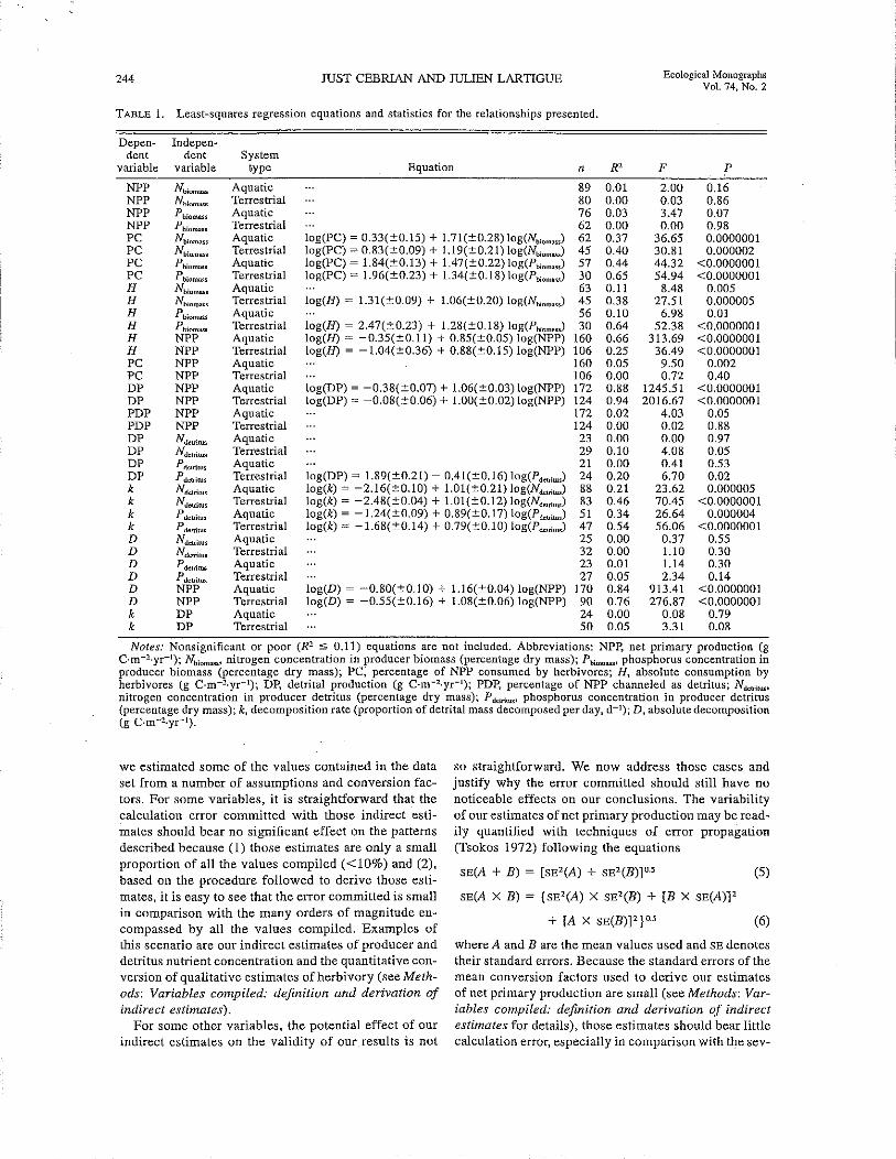
TABLE 1. Least-squares regression equations and statistics for the relationships presented.

Depen- Indepen~

dent dent Systemvariable variable type Equation n R' F P

NPP Nbiom;J>;s Aquatic 89 0.01 2.00 0.16NPP NbiomlJJ;s Terrestrial 80 0.00 0.03 0.86NPP Pbiomos, Aquatic 76 0.03 3.47 0.07NPP Phiomas. Terrestrial 62 0.00 0.00 0.98PC Nbioma.. Aquatic log(PC) ~ 0.33(±0.15) + 1.71(±0.28) log(N"om..) 62 0.37 36.65 0.0000001PC Nbiom"", Terrestrial log(PC) ~ 0.83(±0.09) + 1.19(±0.21) log(N"om.,) 45 0.40 30.81 0.000002PC Pbiomu" Aquatic log(PC) ~ 1.84(±0.13) + 1.47(±0.22) log(P"om.,,) 57 0.44 44.32 <0.0000001PC Pbiomo," Terrestrial log(PC) ~ 1.96(±0.23) + 1.34(±0.18) log(P';om..,) 30 0.65 54.94 <0.0000001H Nbiom""s Aquatic 63 0.11 8.48 0.005H Nbioma>;s Terrestrial log(R) ~ 1.31(±0.09) + 1.06(±0.20) log(N';om.,) 45 0.38 27.51 0.000005H Pbiom".. Aquatic 56 0.10 6.98 0.01H Pbiom.., Terrestrial log(R) ~ 2.47(±0.23) + 1.28(±0.18) log(P';om.J 30 0.64 52.38 <0.0000001H NPP Aquatic log(R) ~ -0.35(±0.ll) + 0.85(±0.05) log(NPP) 160 0.66 313.69 <0.0000001H NPP Terrestrial log(R) ~ -1.04(±0.36) + 0.88(±0.15) log(NPP) 106 0.25 36.49 <0.0000001PC NPP Aquatic 160 0.05 9.50 0.002PC NPP Terrestrial 106 0.00 0.72 0.40DP NPP Aquatic log(DP) ~ -0.38(±0.07) + 1.06(±0.03) log(NPP) 172 0.88 1245.51 <0.0000001DP NPP Terrestrial log(DP) ~ -0.08(±0.06) + 1.00(±0.02) log(NPP) 124 0.94 2016.67 <0.0000001PDP NPP Aquatic 172 0.02 4.03 0.05PDP NPP Terrestrial 124 0.00 0.02 0.88DP NdelriNs Aquatic 23 0.00 0.00 0.97DP Ndotrirus Terrestrial 29 0.10 4.08 0.05DP Pdeuiws Aquatic 21 0.00 0.41 0.53DP Pdelrirus Terrestrial log(DP) ~ 1.89(±0.21) - 0.41(±0.16) log(P,,,",.) 24 0.20 6.70 0.02k Ndelriru, Aquatic log(k) ~ -2.16(±0.1O) + 1.01(±0.21) log(N",,;,.) 88 0.21 23.62 0.000005k N delriru• Terrestrial log(k) ~ -2.48(±0.04) + 1.01(±0.12) log(N,,";,",) 83 0.46 70.45 <0.0000001k Pdelrltus Aquatic log(k) ~ -1.24(±0.09) + 0.89(±0.17) log(P',m,",) 51 0.34 26.64 0.000004k P deuil.... Terrestrial log(k) '" -1.68(±0.14) + 0.79(±0.10) log(P',m",) 47 0.54 56.06 <0.0000001D N dclrilU• Aquatic 25 0.00 0.37 0.55D Nl.kuiru. Terrestrial 32 0.00 1.10 0.30D Pdelriru. Aquatic 23 0.01 1.14 0.30D Pdelrirus Terrestrial 27 0.05 2.34 0.14D NPP Aquatic log(D) ~ -0.80(±0.10) + 1.16(±0.04) log(NPP) 170 0.84 913.41 <0.0000001D NPP Terrestrial log (D) ~ -0.55(±0.16) + 1.08(±0.06) log(NPP) 90 0.76 276.87 <0.0000001k DP Aquatic 24 0.00 0.08 0.79k DP Terrestrial 50 0.05 3.31 0.08

Notes: Nonsignificant or poor (R2 ::S 0.11) equations are not included. Abbreviations: NPP, net primary production (gC·m-2.yr- I); Nbiomos.' nitrogen concentration in producer biomass (percentage dry mass); Pbiomass' phosphorus concentration inproducer biomass (percentage dry mass); PC, percentage of NPP consumed by herbivores; H, absolute consumption byherbivores (g C·m-2.yr-1); DP, detrital production (g C·m-2.yr-1); PDP, percentage of NPP channeled as detritus; NdeuilUf,'

nitrogen concentration in producer detritus (percentage dry mass); Pdelrilus, phosphorus concentration in producer detritus(percentage dry mass); k, decomposition rate (proportion of detrital mass decomposed per day, d- 1); D, absolute decomposition(g C·m-2.yr-1).

so straightforward. We now address those cases andjustify why the error committed should still have nonoticeable effects on our conclusions. The variabilityof our estimates of net primary production may be readily quantified with techniques of error propagation(Tsokos 1972) following the equations

where A and B are the mean values used and SE denotestheir standard errors. Because the standard errors of themean conversion factors used to derive our estimatesof net primary production are small (see Methods: Variables compiled: definition and derivation of indirectestimates for details), those estimates should bear littlecalculation error, especially in comparison with t1}e sev-

we estimated some of the values contained in the dataset from a number of assumptions and conversion factors. For some variables, it is straightforward that thecalculation error committed with those indirect estimates should bear no significant effect on the patternsdescribed because (1) those estimates are only a smallproportion of all the values compiled «10%) and (2),based on the procedure followed to derive those estimates, it is easy to see that the error committed is smallin comparison with the many orders of magnitude encompassed by all the values compiled. Examples ofthis scenario are our indirect estimates of producer anddetritus nutrient concentration and the quantitative conversion of qualitative estimates of herbivory (see Methods: Variables compiled: definition and derivation ofindirect estimates).

For some other variables, the potential effect of ourindirect estimates on the validity of our,results is not

SE(A + B) ~ [sE'(A) + sE'(B)]O.5

sE(A X B) '" {sE'(A) X sE'(B) + [B X sE(A)]'

+ [A X sE(B)]' JO.5

(5)

(6)

May 2004 HERBNORY AND DECOMPOSmON IN ECOSYSTEMS 245

eral orders of magnitude enco:mpassed by all the production values gathered. In addition, most productionvalues compiled were dIrectly provided by the authors(~80% of all values compiled), and, thus, the errorcommitted with our indirect estimates of primary production should overall bear little effect on the resultsobtained.

Tn some other cases, however, it is more difficult toset limits to the calculation error committed in derivingthe indirect estimates. Detrital production is one example, as the uncertainty of our calculation error willgreatly depend on the validity of the assumption thatproducer biomass remains in steady state over the studyduration. As that assumption seemed to hold in mostcases, the error committed with our indirect estimatesof detrital production should also be inconsequentialfor the many orders of magnitude covered by all thevalues compiled and, thus, for the results obtained. Tofurther support this expectation, we· compared, foraquatic and terrestrial ecosystems separately, the regression equation fitted between values of detrital production directly provided by the authors and net primary production to the equation fitted between our detrital production estimates and net primary production.The four regression equations were highly significant(P < 0.00001 and R2 :2': 0.85 for all regressions) and,for both ecosystem types, the slope and intercept of theregression fitted with direct values of detrital production did not differ from the slope and intercept of theregression fitted with our estimates (slope, t test, P >0.05; intercept, ANCOVA, P > 0.05).

OUf absolute decomposition estimates are anotherexample where the calculation error committed is difficult to ascertain because the standard errors of someof the mean conversion factors used (see Methods: Variables compiled: definition and derivation of indirectestimates) are not known with rigor. It seems that theuncertainty of our absolute decomposition estimatesmay be substantial because they are based on a relatively high number of conversion factors and the standard errors of some of those conversion factors seemhigh. For instance, the assumption that the absolutedecomposition of sedimenting phytoplankton is 17%of the net primary production in the community is arough oversimplification since that percentage can varytremendously among different oceanic areas (Mullerand Suess 1979, Suess 1980). In addition, our indirectestimates account for most (>75%) of the absolute decomposition values contained in the data set.

We ran two sensitivity analyses to investigate howthe calculation error committed with our many estimates of absolute decomposition affected the strongassociations found between absolute decompositionand net primary production in aquatic and terrestrialsystems (Table 1, see also Fig. IIA). Our rationale isthat if the error committed with our absolute decomposition estimates is important, it should then affectsignificantly those associations. To run the sensitivity

analyses, we first estimated, using Eqs. 5 and 6 andsome first-order approximations, that the maximum calculation error of our indirect estimates of absolute decomposition (i.e., the standard error of the estimate)oscillated around ±50% of the estimate, but was frequently less. For the first analysis, we assigned to eachof the initial absolute decomposition values an errorterm randomly distributed between - 50% and +50%of the value, and recalculated each initial value as

new value = initial value

+ [initial value X (error assigned/lOG)]

(7)

Following this procedure, we generated five new seriesof absolute decomposition values for both aquatic andterrestrial systems. Then, for aquatic and terrestrial systems separately, we regressed each of those absolutedecomposition series against the initial values of primary production and compared each of those new regressions with the initial regressions (see Table 1). Thenew regressions were also highly significant (P <0.00001 and R2 ;;:;: 0.70 for all ten regressions) and withsimilar slopes and intercepts to the initial regressions(all t tests and ANCOVA, P > 0.05).

In the second analysis, we examined the effects under the assumption that the calculation error is not randomly distributed among the absolute decompositionvalues but associated with the magnitude of the value.Namely, we assumed that the calculation error changedmonotonically (either positively or negatively, see nextparagraph) for observations progressively farther fromthe median using the equation

calculation error

= 50%(number of values between median and

given value

-;- total number of values between median

and minimum or maximum value) (8)

Using Eq. 7, we then generated, separately for aquaticand terrestrial systems, a first series of new absolutedecomposition values by subtracting the absolute calculation error (i.e., value X [error derived using Eq.8]/100) from the values above the median and addingthe absolute error to the values below the median. This"worst case" biasing acts to rotate the regressionclockwise towards a zero slope. We also calculated asecond series by adding the absolute error to the valuesabove the median and subtracting it from the valuesbelow the median. This biasing represents another"worst-case" scenario that rotates the regression slopecounterclockwise towards infinity. We regressed thenew absolute decomposition values against the initialvalues of primary production. The four new equations(I.e.• clockwise and counterclockwise rotations for bothaquatic and terrestrial systems) were highly significant


(P < 0.00001 and R2 ~ 0.74 for all four regressions),·which further supports the robustness of the initial associations observed between absolute decompositionand primary production. If the calculation error committed with our absolute decomposition estimates doesnot seem to impact the strong associations betweenabsolute decomposition and net primary production, itshould not impact either the strong independence between absolute decomposition and detritus nutrientconcentrations that our results reveal (Table 1, see alsoFig. 10). In all, these analyses support that the errorcommitted with our indirect estimates of absolute decomposition does not affect the conclusions obtained.

Effects of comparing different producercompartments on the results obtained

Most direct values and indirect estimates compiledfor communities of aquatic rooted macrophytes andterrestrial communities refer only to the abovegroundcompartment (see Appendix). A few others also includethe belowground compartment, while the rest only referred to the leaf compartment. It seems that the variability introduced by comparing different producercompartments is small in relation to the wide rangeencompassed in our data set (DeAngelis et a1. 1981)and, thus, that variability should bear little effect onthe patterns presented here. To examine this expectation, we analyzed how comparing different producercompartments affected two of the associations foundin this paper, i.e., the association between absolute herbivory and net primary production and the associationbetween absolute decomposition and net primary production (see Results). Namely, we fitted one regressionequation between absolute herbivory and net primaryproduction to the entries for aquatic· rooted macrophytes and terrestrial producers that included both thebelow- and· aboveground compartments and a secondregression equation to the rest of entries for aquaticrooted macrophytes and terrestrial producers. We thencompared the slopes (t test, Ho: equality of slopes) andintercepts (ANCOVA, flo: equality of intercepts) of thetwo regression equations. We did the same thing forthe regression between absolute decomposition and netprimary production.

For the association between absolute herbivory andnet primary production, we found a similar slope (ttest, P > 0.05) but a different intercept (ANCOVA, P< 0.05) between the two sets of data. Differences inintercept for the association between absolute herbivory and net primary production are expected since generally herbivores consume only aboveground organsand, hence, a given level of absolute herbivory shouldcorrespond to a larger level of primary production ifboth the below- and aboveground compartments areincluded. However, ANCOVA also revealed that thevariability in absolute herbivory explained by the producer compartments included is minute (eight timeslower) in comparison with the variability explained by

primary production, which implies that comparing different producer compartments has little effect on theassociation between absolute herbivory and primaryproduction. For the association between absolute decomposition and net primary production, we found nodifferences in slope and intercept (P > 0.05 for bothtests). In all, this analysis supports that, in view of widerange covered by the values compiled here, the inclusion of different producer compartments in our analysisis of little importance, if any, for the patterns found.

RESULTS

Net primary production ranged over five orders ofmagnitude within aquatic ecosystems and over threeorders of magnitude within terrestrial ecosystems (Fig.lA). Overall, however, net primary production did notdiffer greatly between aquatic and terrestrial ecosystems, with only a marginal tendency for the formerecosystems to show higher values (Mann-Whitney, P= 0.03). Nitrogen and phosphorus concentrations varied greatly within aquatic and terrestrial producers(Figs. IB and lC), with aquatic producers tending tohave higher concentrations (Mann-Whitney, P < 0.01for both nutrients). The percentage of net primary production consumed by herbivores was also highly variable, ranging from <1 % to 100% within aquatic systems and from <0.1 % to 75% within terrestrial systems. Overall, however, aquatic systems tended to havehigher percentages consumed (Fig. ID; Mann-Whitney, P < 0.01). A similar result was found with absolute consumption, which also varied greatly withineither type of ecosystem but tended to be greater inaquatic ecosystems (Fig IE; Mann~Whitney,P < 0.01).

Net primary production was independent of producernutrient concentration in aquatic and terrestrial ecosystems (Fig. 2, Table 1). Indeed, for a given concentration, net primary production could vary over twoorders of magnitude within aquatic systems and overone order of magnitude within terrestrial systems. Thepercentage of net primary production consumed by herbivores was positively associated with producer nutrient concentration within aquatic and terrestrial ecosystems (Fig. 3, Table 1). Yet for a given nutrient concentration, the percentage consumed varied considerably. Accordingly, the strength of the association wasgenerally moderate, as indicated by the coefficient ofdetermination for the regression equations (0.37 .s R2.; 0.65; Table I).

Within terrestrial ecosystems, increasing absoluteconsumption was also associated with higher producernutrient concentrations with varying degrees ofstrength (0.38 .s R2 ::; 0.64), but, in contrast, absoluteconsumption and producer nutrient concentration werevery poorly related within aquatic ecosystems (0.11 ~

R2; Fig. 4, Table 1). Instead, absolute consumption wasstrongly associated with net primary production withinaqnatic ecosystems (R' ~ 0.66; Fig. SA, Table I). Within these ecosystems, the percentage of net primary pro-

May 2004 HERBIVORY AND DECOMPOSmON IN ECOSYSTEMS 247

ISOA 30 B

100

50

20

10

0.01 I 100 10000Net primary production (g C'm-2 'yr-')

0 2 4 6 8 10Nitrogen concentration

(% dry mass)

D

50

30

10

0 20 40 60 80 100Primary production consumed (%)

1.50.3 0.6 0.9 1.2Phosphorus concentration

(% dry mass)

o

C50

10

30

E

30

10

0.01 1 100 10000Absolute consumption (g C'm-2'yr-')

FIG. 1. Histograms comparing aquatic (open bars with solid outlines) and terrestrial (gray bars with dashed outlines)ecosystems: (A) net primary production, (B) producer nitrogen concentration, (C) producer phosphorus concentration, (D)percentage of primary production consumed by herbivores, and (E) absolute consumption by herbivores. Note the logarithmicscales for the horizontal axis in panels (A) and (E).

duction consumed by herbivores only varies about oneorder of magnitude throughout most of the productionrange (0.1-100 g C m-2 ye l), and it varies a little morethan two orders of magnitude for production valueswhich ranged between 100 and 3000 g C'm-2'yc l (Fig.5B). Absolute consumption corresponds to the productof net primary production and the percentage consumedand hence, in view of the interaction between production and percentage consumed, the variability 'in absolute consumption within aquatic systems' remains

closely associated with that in production. In view ofthe independence between net primary production andproducer nutrient concentration (Fig. 2), it is also clearwhy absolute consumption and producer nutrient concentration are very poorly associated within aquaticsystems (Fig. 4).

Conversely, the association between absolute consumption and net primary production within terrestrialecosystems was weak (R' ~ 0.25; Fig. SA, Table I).Again, the reason lies in t,he interaction between net

248 JUST CEBRIAN AND mLIEN LARTIGUE Ecological MonographsVoL 74, No.2

\ L-~~""-~~~~~~.L...~""",-~~uL-~.....J.~~""

0.01 0.1 10 0.001 0.01 0.1 \0

\00

A B

I"' · l'i :.. ~~•••

1 t :t~ a 0

" '" 0 '110 1-. cP• • 0 .... • l' '!3

(. 0 0 •• t::. 0

• ; -';·S #: .,•• ..- ott• • 0

0 '" 0

<X> <l WJ

o <l 0

Producer nitrogen concentration(% dry mass)

Producer phosphorus concentration(% dry mass)

FIG. 2. The relationship between net primary production and producer nutrient concentration in aquatic (open symbols)and terrestrial (closed symbols) ecosystems: (A) net primary production VS. producer nitrogen concentration and (B) netprimary production VB. producer phosphorus concentration. Open symbols denote the following aquatic communities: communities of freshwater phytoplankton (open circles), communities of marine phytoplankton (open squares), freshwater benthicmicroalgal beds (open left-pointing triangles), marine benthic microalgal beds (open right-pointing triangles), marine macroalgal beds (open diamonds), meadows of freshwater submerged macrophytes (open down-pointing triangles), and seagrassmeadows (open triangles). Solid symbols denote the following terrestrial communities: communities of tundra shrubs andgrasses (solid down~pointing triangles), freshwater and marine marshes, i.e., emergent macrophytes (solid diamonds), temperate and tropical shrublands and forests (solid circles), temperate and tropical grasslands (solid squares), and mangroves(solid triangles).

primary production and the percentage consumed within terrestrial ecosystems. The percentage consumedvaries by three orders of magnitude throughout the entire range of terrestrial production values, which onlyencompasses about two orders of magnitude (Fig. 5B).Hence, within terrestrial ecosystems the variability inabsolute consumption is poorly related to that in primary production, but better related to the percentage

consumed and, as a consequence, to producer nutrientconcentration (Fig. 4).

The percentage of net primary production channeledas detritus varied from -0% to 100% within aquaticecosystems, and from ~25% to 100% within terrestrialecosystems (Fig. 6A). The percentage was >50% inmost aquatic and terrestrial systems, demonstrating thegeneral predominance of the detrital pathway. Overall,

100 ,"A B

"0v§ 10~ •0 •0u

§ ••._~ •ge- I •"08 • '" • '"p.

~ 0.1 •8 • •'C

P.

10 0.01 0.1 1 10


0.01 L.._~~.....L~~~~.L-~~~...L __~~L-~__~ .....J

0.01 0.1


FIG. 3. The relationship between percentage of primary production consumed by herbivores and producer nutrient con~

centration in aquatic and terrestrial ecosystems: (A) percentage consumed vs. producer nitrogen concentration and (B)percentage consumed vs. producer phosphorus concentration. Dashed (aquatic ecosystems) and continuous (terrestrial ecosystems) lines depict the regression equations (see Table 1). ~ymbols are as in Fig. 2.

May 2004 HERBIVORY AND DECOMPOSmON IN ECOSYSTEMS 249

10 0.01 0.1 1 10


.~ ~B 07>

... & D<oo atDD

°D 00 D 0

.~'V D 'V

D

• I>• •~D 1>& ... 6>0[> D

• D~ ... • if' DI>

~~6 0°iJ,liiM[', D

I I 6 ",66<]

• .,.'" ~<]• .... " "0 <] •• 6 • 6••• 0 • [',0

0 0

0.1 '---~~~.J-~~~...L~~~w..L~~~~_~~~~~~~..J

0.01 0.1


A

10

100

FIG. 4. The relationship between absolute consumption by herbivores and producer nutrient concentration in aquatic andterrestrial ecosystems: (A) absolute consumption vs. producer nitrogen concentration and (B) absolute consumption vs.producer phosphorus concentration. Continuous lines depict the regression equations for terrestrial ecosystems (see Table 1).Symbols are as in Fig. 2.

however, terrestrial ecosystems tended to channel ahigher percentage of production as detritus (MannWhitney; P < 0.01), as expected from the lower percentage of production lost to herbivores (Fig. ID). Detrital production varied widely within aquatic systems,and to a lesser extent within terrestrial systems, and italso tended to be larger in terrestrial systems (Fig. 6B;Mann-Whitney, P < 0.01). Aquatic detritus had highernitrogen and phosphorus concentrations than did terrestrial detritus (Figs. 6C and 6D; Mann-Whitney, P <0.01 for both nutrients), although nutrient concentrations could vary substantially within either type of detritus. A similar result was found with decompositionrates (proportion of detrital mass decomposed per day),with substantial variability within either type of system

but higher values overall for aquatic systems (Fig. 6E;Mann-Whitney, P < 0.01). Absolute decompositionalso varied widely within either type of system but didnot differ significantly between the two types of system(Fig. 6F; Mann-Whitney, P = 0.20).

Larger detrital production was strongly associatedwith higher net primary production within either typeof system. Changes in primary production accountedfor 88% of the variability in detrital production withinaquatic systems, and for 94% within terrestrial systems(Fig. 7A, Table 1). The strong association between detrital production and primary production results fromthe fact that, in general, most primary production entersthe detrital compartment in both types of systems (Fig6A). Indeed, the percentage of primary production

10000 100~

~ ~'- A e B;., 0 07~ ."

~

6 § 10

100~

~ c0 •c <.>

oIf'""0 c.~

0 .., ..~..'f]~ .g~ .., ..c aa <] -<.> ,!"

0. •~ ~

0.1

.3 V ; E.., •

0,

~ " .., ~.D /0-< 0.01 0.01

0.01 100 10000 0.01 100 10000

Net primary production (g C'm-2'yr-l) Net primary production (g C'm-2'yr-l

)

FIG. 5. (A) The relationship between absolute consumption and net primary production in aquatic and terrestrial ecosystems. (B) The relationship between the percentage of primary production consumed by herbivores and net primaryproduction in aquatic and terrestrial ecosystems. Dashed (aquatic ecosystems) and continuous (terrestrial ecosystems) linesdepict the regression equations (see Table 1). Symbols are as in Fig. 2.

250 JUST CEBRlAN AND JULIEN LARTIGUE Ecological MonographsVol. 74, No.2

70 A 50 B

50

30

10

30

10

o 20 40 60 80 100Detrital production (% primary production)

0.01 1 100 10000Detrital production (g C'm-2 'yr-')

40.r---------------,

21.61.20.80.4o

D

10

20

40,--------------,

30

108642o

C

20

10

30

Nitrogen concentration(% dry mass)

Phosphorus concentration(% dry mass)

E F

50

30

10

0.00001 0.0001 0.001 0.01 0.1

50

30

10

1 10 100 1000 10000

Proportion of detrital mass decomposed (d- l ) Absolute decomposition (g C'm-2 'yr- I)

FIG. 6. Histograms comparing aquatic (open bars with solid outlines) and terrestrial (gray bars with dashed outlines)ecosystems: (A) percentage of net primary production channeled as detritus, (B) absolute detrital production, (C) detritusnitrogen concentration, (D) detritus phosphorus concentration, (E) proportion of detrital mass decomposed per day, and (F)absolute decomposition. Note the logarithmic scales for the horizontal axes in panels (B), (E), and (F).

channeled as detritus varies little in comparison withthe extent of variability in primary production bothwithin aquatic and within terrestrial systems (Fig. 7B).In contrast, detrital production is independent of, oronly weakly (0 ~ R2 ~ 0.20) related to, detritus nutrientconcentration (Fig. 8, Table 1).

Aquatic and terrestrial detritus with higher nutrientconcentrations tended to have a larger proportion of itsmass decomposed per day (Fig. 9, Table 1). This proportion, however, varied substantially for any givennutrient concentration and the tendency varied fromweak (proportion decomposed vs. nitrogen concentra-

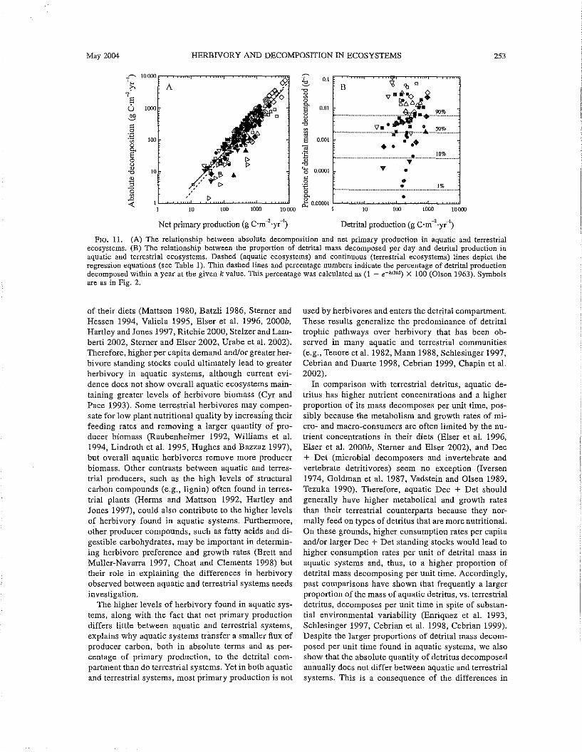
tion in aquatic systems, R2 = 0.21) to moderate (proportion decomposed vs. phosphorus concentration interrestrial systems, R2 = 0.54). In contrast, absolutedecomposition was totally unrelated to detritus nutrientconcentration within either type of system (Fig. 10,Table 1), but instead strongly (0.76 " R2 " 0.84) associated with net primary production (Fig. IIA, Table1). The reason for the strong dependence of absolutedecomposition on primary production lies in the factthat the percentage of detrital production that is decomposed within a year varies little in relation to theextent of variability in annual detrital production both


10000

o

o

100

o

0.1 L..~"--..~wL~-,-~ .....~.....c............J

0.0110000100

0.01 L.._.......~~~"""-~~~_~ .........

0.01

Net primary production (g C'm-2'yr-1)

FIG. 7. (A) The relationship between detrital production and net primary production in aquatic and terrestrial ecosystems.(B) The relationship between the percentage of primary production channeled as detritus and net primary production inaquatic and terrestrial ecosystems. Dashed" (aquatic ecosystems) and continuous (terrestrial ecosystems) lines depict theregression equations (see Table 1). Symbols are as in Fig. 2.

within aquatic and terrestrial ecosystems (Fig. llB).Hence, within either type of ecosystem the variabilityin absolute decomposition remains closely associatedwith that in detrital production and, in turn, with thatin primary production. The independence between detrital production and detritus nutrient concentration(Fig. 8) further explains why absolute decompositionand detritus nutrient concentration are also independent(Fig. 10).

DISCUSSION

Overall differences between aquaticand terrestrial ecosystems

Our results present an integrated view of how muchaquatic and terrestrial ecosystems differ in net primary

production, nutritional quality of producer biomass anddetritus, consumption by herbivores, in absolute decomposition, and in the proportion of detritus decomposed per unit time. Overall, net primary productiondiffers little between aquatic and terrestrial systems,but the former systems support much greater losses toherbivores, both as an absolute carbon flux and as apercentage of primary production. Greater absolutefluxes of producer carbon transferred to herbivores inaquatic systems suggest that these systems supporthigher levels of herbivore production than do terrestrialsystems because production efficiency (ratio of herbivore growth to producer carbon ingested) does notseem to vary significantly between the two types ofsystem (Schroeder 1981, Elser et a!. 2000a). Past re-

~ A B,~,.,

6~I'~ ... <> • 0 • <+

1 .Jto ~6 6

U • oS ~<>6 0

~ ~ \ • &06 "0 0~ 60 100

o ""~ o ,,1!10..,0 • • ".g • ...8 " "p.

~"Q

Detritus phosphorus concentration(% dry mass)

0.1

Detritus nitrogen concentration(% dry mass)

10 0.01 0.1 10

FIG. 8. The relationship between detrital production and detritus nutrient concentration in aquatic and terrestrial ecosys~

terns: (A) detrital production ys. detritus nitrogen concentration and (B) detrital production VS. detritus phosphorus concentration. Symbols are as in Fig. 2.

JUST CEBRIAN AND JULIEN LARTIGUE

....................•....•................................................__....

•

Ecological MonographsVol. 74, No.2

B \] \Jq~':Ii'O<>~"... .

~ ".'&i'..1••••••••..•••••••••••••••••••.•••••~!•••••••••••••••.•••.•..•••__ ••...•

/ ~.. 9.

..................•..../ "" "' .. ~

.+ ..'+•

•

A

........~.?'!? ..............•..............

0.01

0.001

252

~

~""~aS'ag""g]~

""""'a~

"Bag.~

P-<

Detritus nitrogen concentration(% dry mass)

Detritus phosphorus concentration(% dry mass)

FIG. 9. The relationship between the proportion of detrital mass decomposed per day and detritus nutrient concentrationin aquatic and terrestrial ecosystems: (A) proportion of detrital mass decompo.sed (d- I ) vs. detritus nitrogen concentrationand (B) proportion of detrital mass decomposed (d- I ) vs. detritus phosphorus concentration. Dashed (aquatic ecosystems)and continuous (terrestrial ecosystems) lines depict the regression equations (see Table 1). Thin dashed lines and percentagenumbers indicate the percentage of detrital production decomposed within a year at the given k value. This percentage wascalculated as (1 - e-kx365) X 100 (Olson 1963). Symbols are as in Fig. 2.

ports also suggest that aquatic systems should havehigher levels of herbivore production than terrestrialsystems (Cyr and Pace 1993), but empirical demonstration of this hypothesis is lacking. On the other hand,higher percentages of primary production removed byherbivores in aquatic systems suggest that herbivoresplaya greater role in carbon and nutrient recycling andaccumulation of producer biomass in aquatic systemsthan they do in terrestrial systems. Indeed, most reportsof top-down control of producer biomass refer to aquatic systems (Valiela 1995, Valentine and Heck 1999,Paine 2002), although herbivores may also occasion-

ally regulate plant biomass in terrestrial ecosystems(McNaughton 1985, McNaughton and Georgiadis1986). There is also abundant evidence that herbivoresmay be important agents of nutrient recycling in aquaticsystems (Zieman et a1. 1984, Urabe et a1. 1995, Elseret al. 2001, Sterner and Elser 2002), whereas such evidence is scant for terrestrial systems (Day and Detling1990, McNaughton et a1. 1997).

Aquatic producers tend to have much higher nutrientconcentrations than do terrestrial producers and manyreports have shown that the growth rates of aquatic andterrestrial herbivores are limited by the nutrient content

10000

~ A B,~

?'\' + ~O +g o <>0 .. "ft:,"

• (:,• :; .+ ~<> " 0-:'9 • •" • • ..~~ .~.a ~ ~D" • ""l.\,,~

0

:-8 100,

" ;r",

~ • V'va • • " ""'" "g •au • " ."~

"" + +~ "a

~ 1

0.01 0.1 10 0.01 0.1 10

Detritus nitrogen concentration Detritus phosphorus concentration(% dry mass) (% dry mass)

Fro. 10. The relationship between absolute decomposition and detritus nutrient concentration in aquatic and terrestrialecosystems: (A) absolute decomposition vs. detritus nitrogen concentration and (B) absolute decomposition vs. detritusphosphorus concentration, Symbols are as in Fig. 2.


•

••• 1%

0.1 "--'-~~~~"""~~~~~'"lB Ilq,o

'i7. ~·O ~

~"''''tI.............................~.p .•...?~~ .

'\7. •• 50%......................f" .+ • ••+

.........................".•..........~.~~ .T

Detrital production (g C'm-2'yr-l)

O.oI

0.001

~~d 0.0001

.~og.P: 0.00001 IL~=~I':cO-~~I"OO:-~~looo'::-~~I...JOOoo

10000

~A~

~0

10000-E0u~~

:l100 E

FIG. 11. (A) The relationship between absolute decomposition and net primary production in aquatic and terrestrialecosystems. (B) The relationship between the proportion of detrital mass decomposed per day and detrital production inaquatic and terrestrial ecosystems. Dashed (aquatic ecosystems) and continuous (terrestrial ecosystems) lines depict theregression equations (see Table 1). Thin dashed lines and percentage numbers indicate the percentage of detrital productiondecomposed within a year at the given k value. This percentage was calculated as (1 - e-k.r365) X 100 (Olson 1963). Symbolsare as in Fig. 2.

of their diets (Mattson 1980, Batzli 1986, Sterner andHessen 1994, Valiela 1995, Elser et a1. 1996, 2000b,Hartley and Jones 1997, Ritchie 2000, Stelzer and Lamberti 2002, Sterner and Elser 2002, Urabe et a1. 2002).Therefore, higher per capita demand and/or greater herbivore standing stocks could ultimately lead to greaterherbivory in aquatic systems, although current evidence does not show overall aquatic ecosystems maintaining greater levels of herbivore biomass (Cyr andPace 1993). Some terrestrial herbivores may compensate for low plant nutritional quality by increasfng theirfeeding rates and removing a larger quantity of producer biomass (Raubenheimer 1992, Williams et al.1994, Lindroth et a1. 1995, Hughes and Bazzaz 1997),but overall aquatic herbivores remove more producerbiomass. Other contrasts between aquatic and terrestrial producers, such as the high levels of structuralcarbon compounds (e.g., lignin) often found in terrestrial plants (Herms and Mattson 1992, Hartley andJones 1997), could also contribute to the higher levelsof herbivory found in aquatic systems. Furthermore,other producer compounds, such as fatty acids and digestible carbohydrates, may be important in determining herbivore preference and growth rates (Brett andMuller-Navarra 1997, Choat and Clements 1998) buttheir role in explaining the differences in herbivoryobserved between aquatic and terrestrial systems needsinvestigation.

The higher levels of herbivory found in aquatic systems, along with the fact that net primary productiondiffers little between aquatic and terrestrial systems,explains why aquatic systems transfer a smaller flux ofproducer carbon, both in absolute terms and as percentage of primary production, to the detrital compartment than do terrestrial systems. Yet in both aquaticand terrestrial systems, most primary production is not

used by herbivores and enters the detrital compartment.These results generalize the predominance of detritaltrophic pathways over herbivory that has been observed in many aquatic and terrestrial communities(e.g., Tenore et a1. 1982, Mann 1988, Schlesinger 1997,Cebrian and Duarte 1998, Cebrian 1999, Chapin et al.2002).

In comparison with terrestrial detritus, aquatic detritus has higher nutrient concentrations and a higherproportion of its mass decomposes per unit time, possibly because the metabolism and growth rates of micro- and macro-consumers are often limited by the nutrient concentrations in their diets (Elser et a1. 1996,Elser et al. 2000b, Sterner and Elser 2002), and Dec+ Det (microbial decomposers and invertebrate andvertebrate detritivores) seem no exception (Iversen1974, Goldman et a1. 1987, Vadstein and Olsen 1989,Tezuka 1990). Therefore, aquatic Dec + Det shouldgenerally have higher metabolical and growth ratesthan their terrestrial counterparts because they normally feed on types of detritus that are more nutritional.On these grounds, higher consumption rates per capitaand/or larger Dec + Det standing stocks would lead tohigher consumption rates per unit of detrital mass inaquatic systems and, thus, to a higher proportion ofdetrital mass decomposing per unit time. Accordingly,past comparisons have shown that frequently a largerproportion of the mass of aquatic detritus, vs. terrestrialdetritus, decomposes per unit time in spite of substantial environmental variability (Enriquez et al. 1993,Schlesinger 1997, Cebrian et a1. 1998, Cebrian 1999).Despite the larger proportions of detrital mass decomposed per unit time found in aquatic systems, we alsoshow that the absolute quantity of detritus decomposedannually does not differ between aquatic and terrestrialsystems. This is a consequence of the differences in

254 JUST CEBRIAN AND JULIEN LARTIGUE Ecological MonographsVoL 74, No.2

detrital production and proportion decomposed annually between the two types of system; aquatic systemsproduce less detritus, but a higher percentage of thedetritus decomposes annually, and conversely for terrestrial systems.

A higher proportion of detrital mass decomposingper unit time in aquatic systems implies faster rates ofnutrient recycling through the detrital compartment.Accordingly, turnover rates of nutrients through thedetrital pool tend to be faster in aquatic (Legendre andRassoulzadegan 1995, Urabe et al. 1995, Valiela 1995,Elser and Urabe 1999) than in terrestrial systems (Melillo et al. 1982, Van Cleve et al. 1983, Taylor et al.1989, Chapin et al. 2002). Moreover,a higher proportion of detrital mass decomposed per unit time in aquatic systems, along with lower levels of detrital production, imply that those systems accumulate smaller poolsof detrital carbon on a per m2 basis, which is in accordance with past comparisons of detrital storage between terrestrial and aquatic communities (Cebrian andDuarte 1995, Cebrian et a1. 1998, Cebrian 1999). Inspite of these differences, our analysis shows that theabsolute flux of producer carbon transferred annuallyto Dec + Det does not vary between aquatic and terrestrial systems. Hence, because the efficiency of Dec+ Det production (ratio of Dec + Det growth to carboningested) does not differ between aquatic and terrestrialsystems (Begon et a1. 1996), overall the two systemsshould support similar levels of Dec + Det production.

Patterns within aquatic and terrestrial ecosystems

So far we have discussed the extent and some consequences of the differences in herbivory and decomposition between aquatic and terrestrial ecosystems. Wenow discuss the patterns within each type of ecosystem.Our results first identify a general independence between primary production and producer nutrient concentrations. Increased nutrient availability often leadsto increased nutrient concentrations in producer biomass and higher levels of primary production in manyaquatic and terrestrial systems (LaPointe and Clark1992, Valie1a 1995, Hauxwel1 et a1. 1998, Ritchie 2000,Reich et a1. 2001), but here we show that in generalproducer nutrient concentrations are unrelated to primary production within either type of system. We thinkthis independence stems from the fact that environmental constraints can generate large variability in netprimary production at any given level of producer nutrient concentration. Indeed, many reports have shownthat systems composed of producers with similar nutrient concentrations may reach different levels of primary production depending on the extent of environmental stress they endure (e.g., growth limitation bylight and temperature, and in terrestrial systems, bywater availability, Valiela 1995, Schlesinger 1997,Alongi 1998, Chapin et a1. 2002; exposure to waveaction in marine systems, Gerard and Mann 1979,Mann 2000).

Aquatic and terrestrial ecosystems composed of producers that have higher nutrient concentrations tend tohave a larger percentage of production removed byherbivores. The tendencies range from moderate tostrong, with coefficients of determination varying between 37% and 65%, but they are still relevant considering the diversity of herbivore populations (invertebrate vs. vertebrate), metabolical patterns (ectothermy vs. endothermy), behavior (migratory vs. resident),and feeding specificity (specialized vs. generalists) encompassed by the data set. Hence, producer nutrientconcentration stands out as a significant correlate ofthe percentage of primary production consumed by herbivores within both aquatic and terrestrial systems.Based on substantial evidence that the growth rates ofaquatic and terrestrial herbivores are often limited bythe nutrient content of their diets (Mattson 1980, Batzli1986, Sterner and Hessen 1994, Valiela 1995, Elser etal. 1996, 2000b, Hartley and Jones 1997, Ritcbie 2000,Stelzer and Lamberti 2002, Sterner and Elser 2002,Urabe et a1. 2002), faster consumption rates per capitaandlor larger herbivore standing stocks could be responsible for the larger percentage of primary production consumed in high nutrient-content aquatic and terrestrial systems. The patterns presented imply that herbivores, by removing a greater percentage of primaryproduction, should playa greater role as controls ofproducer biomass accumulation and carbon and nutrient recycling in systems composed of producers withhigher nutrient concentrations, regardless of whetherwe compare aquatic or terrestrial systems. This is inaccordance with numerous experimental observationsin the two types of system (e.g., Cebrian and Duarte1994, McNaugbton et a1. 1997, Sterner et al. 1997,Cebrian 1999, Sterner and Elser 2002).

In contrast to the positive association between thepercentage of primary production consumed by herbivores and producer nutrient concentration, absoluteconsumption by herbivores is only poorly associatedwith producer nutrient concentration. within aquaticsystems but strongly associated with the absolute magnitude of primary production. The reason for these patterns lies in the interaction between the variability inprimary production and that in the percentage consumed within aquatic systems. Aquatic systems composed of producers with higher nutrient concentrationslose a higher percentage to herbivores, but that percentage varies little in relation to the differences inprimary production. Hence, absolute consumption,which corresponds to the product of primary production and percentage consumed, remains closely associated with primary production and only poorly relatedto the percentage consumed and producer nutritionalquality. In other words, aquatic systems that are moreproductive, and not those composed of producers thatare more nutritional, transfer more producer carbon toherbivores. In turn, because the efficiency of herbivoreproduction does not seem to vary consistently across


systems (Schroeder 1981, Elser et a1. 2000a), theyshould also support higher levels of herbivore production.

Within terrestrial systems, however, absolute consumption is only weakly associated with primary production, but the associations with producer nutrientconcentration vary from moderate to strong. Again, thereason resides in the interaction between the variabilityin primary production and that in the percentage consumed within these systems; primary production variesto a lesser extent than does the percentage consumedwithin terrestrial systems and, as a consequence, absolute consumption remains more closely associatedwith the percentage consumed and producer nutrientconcentration than with primary production. Withinterrestrial systems, producer nutritional quality, besidesbeing indicative of the role of herbivores as controlsof producer biomass accumulation and carbon and nutrient recycling, is also an indicator of the absolutemagnitude of producer carbon transferred to herbivoresand potential levels of herbivore production in the system.

Detrital production is unrelated, or only weakly related, to detritus nutrient concentration within bothaquatic and terrestrial systems. Hence, within eithertype of system the quantity of detritus produced annually is generally independent of its nutritional quality. This result is mostly a consequence of the independence between net primary production and producernutrient concentration. Detrital production is stronglyassociated with primary production in aquatic and terrestrial systems because most primary production enters the detrital compartment in each type of system.Furthermore, the changes in nutrient concentration thatoccur with producer senescence are small in comparison with the wide range encompassed by all the concentration values compiled (Vitousek 1982, Thayer etaL 1984, Sterner and Elser 2002). Hence, the fact thatnet primary production and producer nutrient concentration are independent within either type of systemimplies that detrital production and detritus nutrientconcentration are also unrelated or, at the most, onlyweakly related.

Our results generalize many past observations thataquatic and terrestrial detritus with higher nutrient concentrations has a larger proportion of its mass decomposed per unit time; Melillo et al. 1982, Harrison 1989,Enriquez et al. 1993, ScWesinger 1997). That proportion, however, may vary widely for any given nutrientconcentration in aquatic or terrestrial detritus. In fact,the associations between a larger proportion of detritalmass decomposed per unit time and higher nutrientconcentrations in the detritus vary from weak to moderate. Still, these associations are relevant in view ofthe many contrasting environmental effects on decomposition encompassed by the data set, such as temperature (Edwards 1975, Van Cleve et a1. 1981), soil orsediment redox conditions (Post et aL 1982), and, in

terrestrial systems, moisture (Wildung et aL 1977, Santos et al. 1984). As we did for the comparison betweenaquatic and terrestrial ecosystems, we suggest that, inview of the evidence that Dec + Det growth rates areoften limited by the nutrient concentrations in theirdetrital diets (Iversen 1974, Goldman et a1. 1987, Vadstein and Olsen 1989, Tezuka 1990, Elser et a1. 1996,Sterner and Elser 2002), higher consumption rates percapita and/or large Dec + Det standing stocks couldbe responsible for the higher proportion of detrital massdecomposed per unit time observed in systems withmore nutritional detritus.

The association shown here between a higher proportion of detrital mass decomposed per unit time andmore nutritional detritus for aquatic and terrestrial systems bears two important corollaries. First, aquatic andterrestrial systems composed of detritus with highernutrient concentrations should exhibit faster recyclingand turnover rates of nutrients through the detrital compartment. This hypothesis is in accordance with pastobservations of detrital turnover and recycling rates insystems composed of detritus with contrasting nutrientconcentrations (Valiela et aL 1984, Elser and Urabe1999, Reich et aL 2001). Second, there may be a tendency for aquatic and terrestrial systems composed ofdetritus with higher nutrient concentrations to accumulate smaller detrital pools. It has been shown thatlarger proportions of detrital mass decomposed per unittime result in smaller detrital pools when aquatic andterrestrial systems are compared (Cebrian and Duarte1995, Cebrian et al. 1998), but it remains to be seenwhether this association also holds within each type ofsystem.

Conversely, absolute decomposition is independentof detritus nutritional quality, but is instead stronglyassociated with detrital production and primary production, within both aquatic and terrestrial systems.The reason for these patterns lies in the interactionbetween the variability in annual detrital productionand in the percentage decomposed annually within either type of system. The percentage of detrital production decomposed annually varies little relative tothe variability in annual detrital production within either type of system. As a consequence, absolute decomposition, which corresponds to the product of detrital production and percentage decomposed, remainsclosely associated with detrital and primary production,but unrelated to the percentage decomposed and detritus nutritional quality, within either type of system.Thus, aquatic and terrestrial systems that are more productive, and not those having detritus with higher nutrient concentrations, transfer more carbon to Dec +Det. Furthermore, because the efficiency of Dec + Detproduction varies relatively little across systems (Began et al. 1996), aquatic and terrestrial systems withhigher primary production should also support higherlevels of Dec + Det production.


CONCLUSIONS

The results presented identify producer nutritionalquality and net primary production as two independentcorrelates of the variability in herbivory and decomposition between and within aquatic and terrestrial ecosystems. Producer nutrient concentration stands out asa positive correlate of the percentage of primary production consumed by herbivores and the percentage ofdetrital production decomposed annually regardless ofwhether the comparison is made between the two ecosystem types or within either type. Thus, producer nutritional quality appears to be a consistent indicator ofthe extent of top-down control of the accumulation ofproducer biomass and detritus and nutrient recyclingin ecosystems. However, absolute consumption by herbivores and absolute decomposition are often associated with absolute primary. production, and independent of producer nutrient concentration, because thevariability in net primary production largely exceedsthat in the percentage consumed or decomposed acrossthe range of ecosystems compared. Hence, primaryproduction is often an indicator of the absolute flux ofproducer carbon transferred to consumers and, thus, ofthe potential levels of secondary production maintainedin the ecosystem.

Aside from these important implications, the empirical relationships presented here also point to a seriesof regulatory mechanisms of herbivory and decomposition in ecosystems. For instance, because thegrowth rates of herbivores and D~c + Det are oftenlimited by the nutrient concentrations of their diets, itis possible that larger herbivore and Dec + Det standing stocks and/or higher consumption rates per capitaare at the base of the consistent associations observedbetween higher producer nutrient concentrations andlarger percentages of primary production consumed byherbivores and decomposed. Demonstrating this hypothesis with ecosystem-level experimental manipulations would certainly improve our understanding ofcarbon and nutrient cycling in ecosystems. Finally, because the patterns presented here are robust (e.g., basedon large data sets), they can also be of use for globalchange models seeking to predict how anthropogenicimpacts on primary production and producer nutrientconcentration may alter carbon and nutrient cycling andconsumer populations.

ACKNOWLEDGMENTS

We thank Melissa Kincke for assistance with setting up theelectronic data set and Connie Mallon for assistance with theliterature compilation. Comments by two anonymous refereesand Cliff Dahm for the initial submission, and by two otherreferees and Stuart Findlay for the second submission, greatlyimproved the final version. Special thanks to Stuart Findlayfor his editorial help with the final version. We dedicate thispaper to little Sergi and his mom Marian for all their patienceand support during the composition of this paper. This is DISLcontribution #327.

LITERATURE CITED

Admiraal, W., L. A. Bouwman, L. Hoekstra, and K. Romeyn.1983. Qualitative and quantitative interactions between microphytobenthos and herbivorous meiofauna on a brackishintertidal mudflat. Internationale Revue der gesamten Hydrobiologie 68:175-191.

Alongi, D. M. 1998. Coastal ecosystems processes. CRePress, New York, New York, USA.

Batzli, G. O. 1986. Nutritional ecology of the California vole:effects of food quality on reproduction. Ecology 67:406412.

Began, M., J. L. Harper, and C. R. Townsend. 1996. Ecology:individuals, populations and communities. Second edition.Blackwell Science, Oxford, UK.

Bird, D. E, and J. Kalff. 1984. Empirical relationships between bacterial abundance and chlorophyll concentrationsin fresh and marine waters. Canadian Journal of Fisheriesand Aquatic Sciences 41:1015-1023.

Brett, M. T., and D. C. Muller-Navarra. 1997. The role ofhighly unsaturated fatty acids in aquatic foodweb processes. Freshwater Biology 38:483-499.

Carpenter, S. R., J. E Kitchell, and J. R. Hodgson. 1985.Cascading trophic interactions and lake productivity.BioScience 35:634-639.

Cebrian, 1. 1999. Patterns in the fate of production in plantcommunities. American Naturalist 154:449-468.

Cebrian, J. 2002. Variability and control of carbon consumption, export and accumulation in marine communities.Limnology and Oceanography 47:11-22.

Cebrian, J., and C. M. Duarte. 1994. The dependence ofherbivory on growth rate in natural plant communities.Functional Ecology 8:518-525.

Cebrian, 1., and C. M. Duarte. 1995. Plant growth dependenceof detrital carbon storage in ecosytems. Science 268:16061608.

Cebrian, J., and C. M. Duarte. 1998. Patterns in leaf herbivory on seagrasses. Aquatic Botany 60:67-82.

Cebrian, J., C. M. Duarte, N. MarM., S. Enriquez, M. Gallegos, and B. Olesen. 1996. Herbivory on Posidonia oceanica (L.) Delile: magnitude and variability in the SpanishMediterranean. Marine Ecology Progress Series 130:147155.

Cebrian, J., M. Williams, J. McClelland, and 1. Valiela. 1998.The dependence of heterotrophic consumption and C ac~

cumulation on autotrophic nutrient content in ecosystems.Ecology Letters 1:165-170.

Chapin, F. S., III, P. A. Matson, and H. A. Mooney. 2002.Principles of terrestrial ecosystem ecology. Springer-Verlag, New York, New York, USA.

Choat, J. R., and K. D. Clements. 1998. Vertebrate herbivoresin marine and terrestrial environments: a nutritional ecology perspective. Annual Review of Ecology and Systematics 29:375-403.

Cohen, J. 1977. Statistical power analysis for the behavioralsciences. Academic Press, New York, New York, USA.

Crawley, M. J. 1983. Herbivory: the dynamics of animalplant interactions. Blackwell Scientific, Los Angeles, California, USA.

Cyr, H., and M. L. Pace. 1993. Magnitude and patterns ofherbivory in aquatic and terrestrial ecosystems. Nature 361:148-150.

Day, T. A., and J. K. Detling. 1990. Grassland patch dynamicsand herbivory grazing preference following urine deposition. Ecology 71:180-188.

DeAngelis. D. L., R. H. Gardner, and H. H. Shugart. 1981.Productivity of forest ecosystems studied during the IBP:the woodlands data set. Pages 567-672 in D. E. Reichle,editor. Dynamic properties of forest ecosystems. Cambridge University Press, New York, New York, USA.


Dolan, J. R., C. L. Gallegos, and A. Moigis. 2000. Dilutioneffects on microzooplankton in dilution grazing experiments. Marine Ecology Progress Series 200:127-139.

Downing, J. A., C. W. Osenberg, and O. Sarnelle. 1999.Meta-analyses of marine nutrient-enrichment experiments:variation in the magnitude of nutrient limitation. Ecology80:1157-1167.

Duarte, C. M. 1992. Nutrient concentration of aquatic plants:patterns across species. Limnology and Oceanography 37:882-889.

Duarte, C. M., and J. Cebrian. 1996. The fate of marineautotrophic production. Limnology and Oceanography 41:1759-1766.

Edwards, N. T. 1975. Effects of temperature and moisture oncarbon dioxide evolution in a mixed deciduous forest floor.Soil Science Society of America Proceedings 39:361-365.

Elser, J. J., D. R. Dobberfuhl, N. A. MacKay, andJ. H. Schampel. 1996. Organism size, life history, and N:P stoichiometry. BioScience 46:674-684.

Elser, J. 1., W. F. Fagan, R. F. Denno, D. R. Dobberfuhl, A.Folarin, A. Huberty, S. Interlandi, S. K. Kilham, E.McCauley, K. L. Schulz, E. H. Siemann, and R. W. Sterner.2000a. Nutritional constraints in terrestrial and freshwaterfood webs. Nature 408:578-580.

Elser, J. J., K. Hayakawa, and J. Urabe. 2001. Nutrient limitation reduces food quality for zooplankton: Daphnia response to seston phosphorus enrichment. Ecology 82:898903.

Elser, J. J., R. W. Sterner, E. Gorokhova, W. F Fagan, T. A.Markow, J. B. Cotner, J. F. Harrison, S. H. Hobbie, G. M.Odell, and L. 1. Weider. 2000b. Biological stoichiometryfrom genes to ecosystems. Ecology Letters 3:540-550.

Elser, J. J., and J. Urabe. 1999. The stoichiometry of consumer-driven nutrient recycling: theory, observations andconsequences. Ecology 80:735-751.

Enriquez, S., C. M. Duarte, and K. Sand-Jensen. 1993. Patterns in decomposition rates among photosynthetic organisms: the importance of detritus C:N:P content. Oecologia94:457-471.

Findlay, S., J. Tank, S. Dye, H. M. Valett, P. J. Mulholland,W. H. McDowell, S. L. Johnson, S. K. Hamilton, J. Edmonds, W. K. Dodds, and W. Bowden. 2002. A crosssystem comparison of bacterial and fungal biomass in detritus pools of headwater streams. Microbial Ecology 43:55-66.

Gasol, J. M., P. A. del Giorgio, and C. M. Dnarte. 1997.Biomass distribution in marine planktonic communities.Limnology and Oceanography 42:1353-1363.

Gerard, V. A., and K. H. Mann. 1979. Growth and productionof Laminaria longicruris (Phaeophyta) populations exposed to different intensities of water movement. Journalof Phycology 15:33-41.

Goldman, J. C., D. A. Caron, and M. R. Dennett. 1987. Regulation of gross growth efficiency and ammonium regeneration in bacteria by substrate C:N ratio. Limnology andOceanography 32:1239-1252.

Greenway, M. 1976. The grazing of Thalassia testudinum inKingston Harbour, Jamaica. Aquatic Botany 2:117-126.

Griffin, M. P. A., M. L. Cole, K. D. Kroeger, and J. Cebrian.1998. Dependence of herbivory on autotrophic content andnet primary production across ecosystems. Biological Bulletin 195:233-234.

Gurevitch, J., and L. V. Hedges. 1999. Statistical issues inecological meta-analyses. Ecology 80:] ]42-] 149.

Gurevitch, J., and L. V. Hedges. 2001. Meta-analysis: combining the results of independent experiments. Pages 347370 in S. M. Scheiner and J. Gurevitch, editors. Designand analysis of ecological experiments. Second edition.Oxford University Press, Oxford, UK.

Harris, W. E, P. SoIlins, N. T. Edwards, B. E. Dinger, and H.H. Shugart. 1975. Analysis of carbon flow and productivityin a temperate deciduous forest ecosystem. Pages 116-122in D. Reichle, J. Franklin, and D. Goodall, editors. Productivity of the world systems. Symposium. National Academy of Sciences, Washington, D.C., USA.

Harrison, P. G. 1989. Detrital processing in seagrass systems:a review of factors affecting decay rates, remineralizationand detritivory. Aquatic Botany 23:263-288.

Hartley, S. E., and C. G. Jones. 1997. Plant chemistry andherbivory, or why the world is green. Pages 284-324 inM. J. Crawley, editor. Plant ecology. Blackwell Science,Oxford, UK.

Hauxwell, J., J. McClelland, P. J. Behr, and 1. Valiela. 1998.Relative importance of grazing and nutrient controls ofmacroalgal biomass in three temperate shallow estuaries.Estuaries 21:347-360.

Heck, K. L., J. R. Pennock, J. F. Valentine, L. D. Coen, andS. A. Sklenar. 2000. Effects of nutrient enrichment andsmall predator density on seagrass ecosystems: an experimental assessment. Limnology and Oceanography 45:1041-1057.

Heck, K. L., and J. F. Valentine. 1995. Sea urchin herbivory:evidence for long-lasting effects in subtropical seagrassmeadows. Journal of Experimental Marine Biology andEcology 189:205-217.

Hedges, L. v., and 1. Olkin. 1985. Statistical methods formeta-analysis. Academic Press, New York, New York,USA.

Herms, D. A., and W. J. Mattson. 1992. The dilemma ofplants-to grow or defend? Quarterly Review of Biology67:283-335.

Hillebrand, H., and M. Kahlert. 200t. Effect of grazing andnutrient supply on periphyton biomass and nutrient stoichiometry in habitats of different productivity. Limnologyand Oceanography 46:1881-1898.

Hughes, L., and F. A. Bazzaz. 1997. Effect of elevated CO2

on interactions between the western flower thrips, FrankIiniella occidentalis (Thysanoptera: Thripidae) and thecommon milkweed, Asclepias syriaca. Oecologia 109:286290.

Iversen, T. M. 1974. Ingestion and growth in Sericostomapersonatum (Trichoptera) in relation to nitrogen content ofingested leaves. Oikos 25:278-282.

Jacobs, R., C. den Hartog, C. Braster, and F. Carriere. 1981.Grazing of the seagrass Zostera noltii by birds at Terschelling (Dutch Wadden Sea). Aquatic Botany 10:241259.

Kiorbe, T., and P. T. Tiselius. 1987. Gut clearance and pigment destruction in a herbivorous copepod, Acartia tonsa,and the determination of in situ grazing rates. Journal ofPlankton Research 9:525-534.

Krebs, C. J. 1994. Ecology. Fourth edition. Harper Collins,New York, New York, USA.

Landry, M. R., and R. P. Hassett. 1982. Estimating the grazing impact of marine microzooplankton. Marine Biology67:283-288.

Lapointe, B. E., and M. W. Clark. 1992. Nutrient inputs fromthe watershed and coastal eutrophication in the FloridaKeys. Estuaries 15:465-476.

Legendre, L., and F. Rassoulzadegan. 1995. Plankton andnutrient dynamics in marine waters. Ophelia 41:153-170.

Lindroth, R. L., G. E. Arteel, and K. K. Kinney. 1995. Re~

sponses of three saturniid species to paper birch grownunder enriched CO2 atmospheres. Functional Ecology 9:306-31l.

Mann, K. H. 1988. Production and use of detritus in variousfreshwater, estuarine and coastal marine ecosystems. Limnology and Oceanography 33:910-931.

258 JUST CEBRIAN AND JULIEN LARTIGIIE Ecological MonographsVol. 74, No.2

Mann, K. H. 2000. Ecology of coastal waters with implications for management. Blackwell Science, Malden, Massachusetts, USA.

Martin, J. H., G. A. Knauer. D. M. Karl, and W. W. Broenkow.1987. VERTEX: carbon cycling in the northeast Pacific.Deep-Sea Research 34:267-285.

Mateo, M. A., and 1. Romero. 1996. Evaluating seagrass leaflitter decomposition: an. experimental comparison betweenlitter-bag and oxygen-uptake methods. Journal of Experimental Marine Biology and Ecology 202:97-106.

Mateo, M. A., and J. Romero. 1997. Detritus dynamics inthe seagrass Posidonia oceanica: elements for an ecosystemcarbon and nutrient budget. Marine Ecology Progress Series 151:43-53.

Mattson, W. J. 1980. Herbivory in relation to plant nitrogencontent. Annual Review of Ecology and Systematics 11:119-16l.

McNaughton, S. J. 1985. Ecology of a grazing ecosystem:the SerengetL Ecological Monographs 55:259-294.

McNaughton, S. J., F. F. Banyikwa, and M. M. McNaughton.1997. Promotion of the cycling of diet-enhancing nutrientsby African grazers. Science 278:1798-1800.

McNaughton, S. J., and N. J. Georgiadis. 1986. Ecology ofAfrican grazing and browsing mammals. Annual Reviewof Ecology and Systematics 17:39-65.

McNaughton, S. J., M. Oesterheld, D. A. Frank, and K. J.Williams. 1989. Ecosystem-level patterns of primary productivity and herbivory in terrestrial habitats. Nature 341:142-144.

Melillo, 1. M., J. D. Aber, and J. M. Muratore. 1982. Nitrogenand lignin control of hardwood leaf litter decompositiondynamics. Ecology 63:621-626.

Muller, P. J., and E. Suess. 1979. Productivity, sedimentationrate, and sedimentary organic matter in the oceans. L Organic carbon preservation. Deep-Sea Research 26A: 13471362.

Nienhuis, P., andA. Groenendijk. 1986. Consumption of eelgrass (Zostera marina) by birds and invertebrates: an annual budget. Marine Ecology Progress Series 29:29-35.

O'Connell, A. M. 1987. Litter dynamics in Karri (Eucalyptusdiversicolor) forest of South-Western Australia. Journal ofEcology 75:781-796.

Odum, E. P. 1971. Fundamentals of ecology. Third edition.Saunders, Philadelphia, Pennsylvania, USA.

Olson, J. S. 1963. Energy storage and the balance of producers and decomposers in ecological systems. Ecology 44:322-33l.

Osenberg, C. W., O. Samelle, S. D. Cooper, and R. D. Holt.1999. Resolving ecological questions through meta-analysis: goals, metrics, and models. Ecology 80: 11 05-1117.

Paine, R. T. 2002. Trophic control of production in a rockyintertidal community. Science 296:736-739.

Petrusewicz, K., and W. Grodzinski. 1975. The role of herbivore consumers in various ecosystems. Pages 64-70 inD. W. Reichle, J. F. Franklin, and D. W. Goodall, editors.Productivity of world ecosystems. National Academy ofSciences, Washington, D.C., USA.

Portig, A. A., R. G. Mathers, W. 1. Montgomery, and R. N.Govier. 1994. The distribution and utilisation of Zosteraspecies in Strangford Lough, Northern Ireland. AquaticBotany 47:317-328.

Post, W. M., W. R. Emanuel, P. J. Zinke, and A. G. Stangenberger. 1982. Soil carbon pools and world life zones. Naw

ture 298:156-159.Qasim, S., and P. Bhattathiri. 1971. Primary production of a

seagrass bed on Kavarotti Atoll (Laccavides). Hydrobiologia 38:29-38.

Raubenheimer, D. 1992. Tannic acid, protein, and digestiblecarbohydrate: dietary imbalance and nutritional compensation in locusts. Ecology 73:1012-1027.

Reich, P., D. A. Petersen, K. Wrage, and D. Wedin. 2001.Fire and vegetation effects on productivity and nitrogencycling across a forest-grassland continuum. Ecology 82:1703-1719.

Ritchie, M. E. 2000. Nitrogen limitation and trophic vs. abiotic influences on insect herbivores in a temperate grassland. Ecology 81:1601-1612.

Romero, J., G. Pergent, C. Pergent-Martini, M. A. Mateo,and C. Regnier. 1992. The detritic compartment in a Posidonia oceanica meadow: litter features, decompositionrates and mineral stocks. Marine Ecology 13:69-83.

Rosenberg, M. S., D. C. Adams, and J. Gurevitch. 1999.MetaWin 2.0. Statistical software for conducting metaanalyses: fixed effects models, mixed effect models andresampling tests. Sinauer Associates, Sunderland, Massachusetts, USA.

Sanders, R. W., D. A. Caron, and U. G. Berninger. 1992.Relationships between bacteria and heterotrophic nanoplankton in marine and freshwaters: an inter-ecosystemcomparison. Marine Ecology Progress Series 86:1-14.

Santos, P. F., N. Z. Elkins, Y. Steinberger, and W. G. Whitford.1984. A comparison of surface and buried Larrea tridentata leaf litter decomposition in North American hot deserts. Ecology 65:278-284.

Schlesinger, W. H. 1997. Biogeochemistry: an analysis ofglobal change. Academic Press, San Diego, California,USA.

Schroeder, L. A. 1981. Consumer growth efficiencies: theirlimits and relationships to ecological energetics. Journal ofTheoretical Biology 93:805-828.

Sokal, R R., and F. J. Rohlf. 1995. Biometry. Third edition.W. H. Freeman and Company, New York, New York, USA.

Stelzer, R. S., and G. A. Lamberti. 2002. Ecological stoichiometry in running waters: periphyton chemical composition and snail growth. Ecology 83:1039-1051.

Sterner, R. W., J. Clasen, W. Lampert, and T. Weisse. 1998.Carbon:phosphoms stoichiometry and food chain production. Ecology Letters 1:146-150.

Sterner, R. W., and J. J. Elser. 2002. Ecological stoichiometry: the biology of elements from molecules to the biosphere. Princeton University Press, Princeton, New Jersey,USA.

Sterner, R. W., 1. J. Elser, E. 1. Fee, S. J. Guildford, and T.H. Chrzanowski. 1997. The lightnutrient ration in lakes:the balance of energy and materials affects ecosystem structure and process. American Naturalist 150:663-684.

Sterner, R. W., and D. O. Hessen. 1994. Algal nutrient limitation and the nutrition of aquatic herbivores. Annual Review of Ecology and Systematics 25:1-29.

Strickland, J. D. H., and T. R Parsons. 1972. A practicalhandbook of seawater analysis. Bulletin 167. Second edition. Fisheries Research Board of Canada, Ottawa, Ontario,Canada.

Suess, E. 1980. Particulate organic carbon flux in the oceanssurface productivity and oxygen utilization. Nature 288:260-263.

Taylor, B. R., D. Parkinson, and W. F. J. Parsons. 1989. Nitrogen and lignin content as predictors of litter decay rates:a microcosm test. Ecology 70:97-104.

Tenore, K. R, L. Cammen, S. E. G. Findlay, and N. Phillips.1982. Perspectives of research on detritus: do factors controlling the availability of detritus to macroconsumers depend on its source? Journal of Marine Research 40:473490.

Tezuka, Y. 1990. Bacterial regeneration of ammonium andphosphate as· affected by the carbon:nitrogen:phosphorusratio of organic substrates. Microbial Ecology 19:228-238.

Thayer, G. W., K. A. Bjorndal, J. Ogden, S. Williams, and J.Zieman. 1984. Role of larger herbivores in seagrass communities. Estuaries 7:351-376.


Tsokos, C. P. 1972. Probability distributions: an introductionto probability theory with applications. Duxbury Press,Belmont, California, USA.

Urabe, 1., M. Kyle, W, Makino, T. Yoshida, T. Andersen, andJ. J. Elser. 2002. Reduced light increases herb~vore prowduction due to stoichiometric effects of light: nutrient balance. Ecology 83:619-627.

Urabe, J., M. Nakanishi, and K. Kawabata. 1995. Contribution of metazooan plankton to the cycling of nitrogenand phosphorus in Lake Biwa. Limnology and Oceanography 40:232-241.

Vadstein, 0., and Y. Olsen. 1989. Chemical composition andphosphate uptake kinetics of limnetic bacterial communities cultures in chemostats under phosphorus limitation.Limnology and Oceanography 34:939-946.

Valentine, J. E, and K. L. Heck. 1991. The role of sea urchingrazing in regulating subtropical seagrass meadows: evidence from field manipulations in the northern Gulf ofMexico. Journal of Experimental Marine Biology and Ecology154:215-230.

Valentine, J. E, and K. L. Heck. 1999. Seagrass herbivory:evidence for the continued grazing of marine grasses. Marine Ecological Progress Series 176:291-302.

Valiela, I. 1995. Marine ecological processes. Second edition.Springer-Verlag, New York, New York, USA.

Valie1a, 1., J. Wilson, R. Buchsbaum, C. Rietsma, D. Bryant,K. Foreman, and J. Teal. 1984. Importance of chemicalcomposition of salt marsh litter on decay rates and feedingby detritivores. Bulletin of Marine Science 35:261-269.

Van Cleve, K., R. Barney, and R. Schlentner. 1981. Evidenceof temperature control of production and nutrient cyclingin two interior Alaska black spruce ecosystems. CanadianJournal of Forest Research 11:258-273.

Van Cleve, K., L. Oliver, R. Schlentner, L. A. Viereck, andC. T. Dyrness. 1983. Productivity and nutrient cycling intaiga forests ecosystems. Canadian Journal of Forest Re·search 13:747-766.

Vitousek, P. M. 1982. Nutrient cycling and nutrient use efficiency. American Naturalist 119:553-572.

Welschmeyer, N. A., and C. J. Lorenzen. 1985. Chlorophyllbudgets: zooplankton grazing and phytoplankton growth ina temperate fjord and the Central Pacific Gyres. Limnologyand Oceanography 30:1-21.

Whittaker, R. H. 1970. Communities and ecosystems. Secondedition. Macmillan, New York, New York, USA.

Wiebe, P. H. 1988. Functional regression equations for zooplankton displacement volume, wet weight, dry weight, andcarbon: a correction. Fisheries Bulletin 86:833-835.

Wildung, R. E., T. R. Garland, and R. L. Buschbom. 1977.The interdependent effects of soil temperature and watercontent on soil respiration rate and plant root decomposition in arid grassland soils. Soil Biology and Biochemistry7:373-378.

Williams, R. S., D. E. Lincoln, and R. B. Thomas. 1994.Loblolly pine grown under elevated CO2 affects early instarpine sawfly performance. Oecologia 98:64-71.

Woodwell, G. M., R. A. Houghton, C. A. S. Hall, D. E.Whitney, R. A Moll, and D. W. Juers. 1979. The FlaxPond ecosystem study: the annual metabolism and nutrientbudgets of a salt marsh. Pages 491-511 in R. L. Jefferiesand A. J. Davy, editors. Ecological processes in coastalenvironments. Blackwell Scientific, Oxford, UK.

Worm, B., H. K. Lotze, and U. Sommer. 2000. Coastal foodweb structure, carbon storage and nitrogen retention regulated by consumer pressure and nutrient loading. Limnology and Oceanography 45:339-349.

Zak, D. R., D. Tilman, R. P. Parmenter, C. W. Rice, R M.Fisher, J. Vose, D. Milchunas, and C. W. Martin. 1994.Plant production -and soil microorganisms in late-successional ecosystems: a continental study. Ecology 75:23332347.

Zar, 1. H. 1998. Biostatistical analyses. Fourth edition. Prentice Hall, Englewood Cliffs, New Jersey, USA.

Zieman, J. C., R. L. Iverson, and J. C. Ogden. 1984. Herbivory effects on Thalassia testudinum leaf growth andnitrogen cOntent. Marine Ecology Progress Series 15:151]58.

Zieman, J. C., G. W. Thayer, M. B. Robblee, and R. T. Zieman.1979. Production and export of seagrasses from a tropicalbay. Pages 21-34 in R. J. Livingston, editor. Ecologicalprocesses in coastal and marine systems. Plenum Press,New York, New York, USA.

Zieman, J. C., and R. G. Wetzel. 1980. Productivity in seagrasses: methods and rates. Pages 87-116 in R. C. Phillips,and C. P. McRoy, editors. Handbook of seagrass biology:an ecosystem perspective. Garland STPM Press, New York,New York, USA.

Ziemann, D. A, P. K. Bienfag, K. W. Fulton-Bennett, W.Kottenmeier, and L. D. Conquest. 1993. Carbon budget forthe spring bloom in Auke Bay, Alaska. Marine Biology115:509-521.

SUPPLEMENT

The data set and list of references are available in ESA's Electronic Data Archive: Ecological Archives M074-004-Sl.

patterns of herbivory and decomposition in

Documents