Struct Multidisc Optim 22, 208–218 Springer-Verlag 2001

Pareto analysis in multiobjective optimization usingthe collinearity theorem and scaling method

E.M. Kasprzak and K.E. Lewis

Abstract This paper presents a method to predict therelative objective weighting scheme necessary to causearbitrary members of a Pareto solution set to become op-timal. First, a polynomial description of the Pareto setis constructed utilizing simulation and high performancecomputing. Then, using geometric relationships betweenthe member of the Pareto set in question, the locationof the utopia point and the polynomial coefficients, theweighting of the performance metrics which causes a par-ticular member of the Pareto set to become optimal isdetermined. The use of this technique, termed the scal-ing method, is examined via using a sample problem fromthe field of vehicle dynamics optimization. The scalingmethod is based on the collinearity theorem which is alsopresented in the paper.

Key words multiobjective optimization, Pareto set,objective weighting

1Introduction

It is widely recognized that design is a series of compro-mises. Compromises are made using tradeoffs betweenperformance, cost, risk, and quality attributes. In a mul-tiattribute design problem there are typically an infinitenumber of “optimal” solutions, based on the preferencesand risk assessments of the designer(s). The final designwill be a result of numerous tradeoffs, many times ad-hoc,each aimed at making a compromise decision betweenconflicting attributes. Viewing design formally as a col-lection of compromise decisions, however, is only a very

July 25, 2000

E.M. Kasprzak1 and K.E. Lewis2

1Milliken Research Associates, Inc., 245 Brompton Road,Williamsville, NY 14221-5942, USAe-mail: kasprzak@mail.localnet.com2Department of Mechanical and Aerospace Engineering, Uni-versity at Buffalo, 1010 Furnas Hall, Buffalo, NY 14260, USAe-mail: kelewis@eng.buffalo.edu

recent evolution. Indeed, interest in decision theory canbe traced back to the 1950’s (e.g. Luce and Raiffa 1957),but the application of decision theory to multidisciplinarydesign is relatively recent and reviewed by Lewis andMistree (1998).

In decision theory, and more specifically in decision-based design, there are two primary steps: generate theoption space, and select the best option (Hazelrigg 1996).The option space is the accumulation of all potentialdesign solutions. Choosing from among this space iscertainly not trivial but rather a function of tradeoffsand compromises. In this work, we are concerned withboth of these steps. The decision making environmentfor this work is multiattribute design problems wherethere is more than one attribute under question. Also, weare dealing with mathematical representations of designproblems and therefore are working with multiobjec-tive optimization problems. This does not exclude theresults of this paper from nonmathematical representa-tions, such as look-up tables or logical rule-based models,but we focus on mathematical models specifically. We in-tend on providing decision support for determining theoptimal solution, given a set of operating conditions,assumptions, risk profiles, and preferences. We do not in-tend to construct risk profiles or model preferences, butsimply acknowledge that they must play a role in thiskind of decision making problem.

In multiobjective optimization problems, there aretwo primary approaches to finding the preferred, if notoptimal, design. The first involves determining the rela-tive importance of the attributes and aggregating theattributes into some kind of overall objective. Then, solv-ing the optimization problem presumably would generatethe optimal solution for a given set of attribute impor-tances. The second approach involves populating a num-ber of optimal solutions along the Pareto frontier andthen selecting one based on the values of the attributes fora given solution. In both cases, there are complications.First, coming up with exact relative attribute weights isa daunting task with complicated ramifications (Messac2000). Only in the rarest of circumstances can this ap-proach be taken and relied upon. Second, while selectingfrom a set of Pareto solutions may seem straightforwardonce a set of preferences are established, it may result

209

in a nonoptimal design for certain design operating con-ditions. It is difficult to relate the choice of Pareto so-lution to any kind of optimal criteria. In this work, wedevelop a technique that can provide decision supportfor both of the approaches to multiobjective optimizationproblems. In the next section, we provide the necessarybackground on Pareto sets for the development of thetechnique.

2Pareto set background

Since multiobjective optimization problems are in ques-tion, we make use of the concept of Pareto sets, an effi-cient frontier of solutions in the performance space. Therecontinue to be two primary challenges in Pareto sets: pop-ulating the Pareto set or finding Pareto solutions, andselecting from among the Pareto solutions. These chal-lenges parallel the challenges of decision-based design.They are analogous to determining potential solutionsand selecting from among the solutions. In Pareto analy-sis, there are added restrictions on the criteria for decid-ing upon a solution’s inclusion in the set. A design vectorx∗ is a Pareto optimum if and only if, there is no otherfeasible vector x such that

fi(x) ≤ fi(x∗) , j = 1, . . . ,m

and

fi(x) < fi(x∗) for at least one i , 1≤ i≤m. (1)

We address both of these challenges in this work, al-though most of the paper is focused on the second chal-lenge. In the next sections, we address both challengesand the current research in each area.

2.1Population of the Pareto set

The notion of an efficient frontier of solutions is notnew (e.g. Luce and Raiffa 1957), but methods of gen-erating Pareto sets continue to be a topic of research.The weighted sum method of generating Pareto sets wasshown to work well with convex problems decades agoby Geoffrion (1968), and while it is still a very popularmethod its deficiencies have been noted. Messac (2000)has effectively illustrated the problems associated withchoosing weights for an aggregate objective function andhas derived conditions that predict which Pareto solu-tions can be found using weights (Messac et al. 2000).Dennis and Das (1997) notes that, even with convex prob-lems, taking an even spread of weights will not resultin an even spread of points in the Pareto set, makingsome sections of the Pareto set difficult to populate. Koski(1985) emphasizes the weighted sum method’s inade-quacies when dealing with nonconvex problems. Athan

and Papalabmros (1996) also looked at using nonlinearweights to better capture the non-convex Pareto set.

An alternative to these methods, compromise pro-gramming, was developed in the 1970’s and it, too, isa subject of continuing research. This approach has theadvantage of being able to generate many points on theefficient frontier. It works from a stationary utopia pointand, through variation of a vector of weights, intersectspoints in the Pareto set. Chen et al. (1999) used thismethod in an approach to robust design with reason-able success, although implementation of compromiseprogramming is notably more difficult than the weightedsum method. Tappeta and Renaud (1999) used compro-mise programming to find an initial Pareto solution, andthen constructed local approximations to the Pareto sur-face and iteratively presented the decision maker witha set of solution options to choose from.

Yoo and Hajela (1999) effectively use an immune-based genetic algorithm (GA) to generate the Pareto-Edgeworth solutions in one run of the GA. Narayananand Azarm (1999) improve multiobjective GA’s using fil-tering, mating restrictions, and the idea of objective con-straints in order to detect Pareto solutions in the noncon-vex region of the Pareto set.

This work will use yet another method to determinethe Pareto set: a grid search of the design space. Effi-cient points from the grid search are fit by a polynomialto approximate the Pareto set, resulting in several advan-tages over other methods. This is pursued in Sect. 3. Oncethe Pareto set has been generated, the next challenge ischoosing the best solution from among the set. This is thesubject of the next section.

2.2Selection from among the Pareto solutions

Just as several methods exist to determine what solu-tions compose the Pareto set of efficient solutions, thereare several techniques to determine which member of thePareto set is the optimal solution. Similar to decision-based design, the simplest method is to choose a so-lution based on the values of the objectives and howwell they match the preferred values. This method isused by Nelson et al. (1999) when manipulating multi-ple Pareto solution sets in product platform design. Das(1999) introduces the concept of “order of efficiency” asan attempt to create a meta-metric, stronger than thePareto conditions, in order to rank order Pareto solu-tions. Hazelrigg (1996) argues that the selection froma set of solutions should be guided by a “meta-objective”of maximizing profit. Designer preferences can be ac-commodated by using utility theory to establish a rank-ordering of solutions based on uncertain and changingindividual and group preferences (Callaghan and Lewis2000). Horn et al. (1994) use multi-attribute utility an-alysis to select the preferred solution from the Pareto setof solutions. Eschenauer et al. (1990) describes the most

210

widely used method: Lp norms. This technique minimizesthe distance from the Pareto set to an ideal solution (i.e.utopia point) to find the optimal solution according to thefollowing formula:

minimize

[m∑i=1

(fi(x)−f∗i )p

]1/p. (2)

Typical applications of the Lp norm are the L1, L2 andL∞ norms (where p = 1, 2 and ∞, respectively). A finesummary of solution techniques is provided by Palli et al.(1998) should the reader desire a more in-depth explo-ration of the subject.

In this work, we utilize the L2 norm (p = 2) to de-rive a technique for finding the optimal attribute weightsnecessary to make any member of the Pareto set opti-mal. In other words, we determine what design conditionsare required to make a certain Pareto solution the pre-ferred solution. In Sect. 3, we present a new theorem, thecollinearity theorem, in a general sense and then applyit in a new method called the scaling method in Sect. 4.We then illustrate the use of these techniques in a vehicledynamics design example. First, however, it is instructiveto step back and examine the performance space in moredetail. This is done in the next section.

2.3A conceptual look at the performance space and axisscaling

Pareto set analysis typically takes place in the perform-ance space. This is the space created by considering thedesign objectives as coordinate axes. On these axes theperformance of each possible design is plotted, one pointper design. Each possible design has associated with ita specific performance or outcome for each objective. Ingeneral, the plot of possible outcomes appears as a regionin the performance space, as depicted in a general two ob-jective problem in Fig. 1.

Figure 1 notes that the intention is to minimize bothobjectives. The individual optimum for each objective isalso noted in Fig. 1. These correspond to the best pos-sible performance for each given objective. Unfortunately,two distinct points appear, one for each objective. Sinceboth objectives cannot be simultaneously optimized, anyattempt to choose a single design to perform well acrossboth objectives will necessarily be a compromise design.Being optimal for one objective implies being suboptimalfor the other.

Figure 2 shows how a certain distance measure, the L2norm, determines the optimal compromise design. First,the range of possible designs is narrowed significantlythrough the concept of a Pareto set, a subset of the setof possible outcomes shown in Fig 1. The Pareto set hasthe property that, for any point in the Pareto set, theredoes not exist another point in the set of possible out-comes with a better performance on both objective axes

Fig. 1 A generic performance space

simultaneously. As such, the Pareto set is sometimes re-ferred to as the “efficient frontier” of the performancespace. Whatever compromise design is chosen, it mustbe a member of the Pareto set, and the remainder ofpossible outcomes can be ignored. They represent designpoints that give suboptimal performance on both axessimultaneously.

Fig. 2 Optimal compromise solution using the L2 norm

The concept of utopia point is important when usingdistance functions, such as the L2 norm. It is the theoret-ical best performance point that can be achieved. Whilemore than one method for locating the utopia point exists(e.g. Miettinen 1999), this discussion presents the defin-ition which agrees with the vehicle dynamics problemspresented later. In this case, the utopia point is taken toreside at the origin of the coordinate system. While wepresent the results of the example using this utopia pointlocation, the derivation in Sect. 4 is general. The develop-ments can be used with other utopia point definitions.

Now, according to the L2 norm method (Eschenaueret al. 1990), the optimal compromise design is the mem-ber of the Pareto set which lies geometrically closest tothe utopia point, calculated in terms of vector distance inthe performance space. Figure 2 locates the optimal point

211

using the L2 norm method. A vector is drawn from theutopia point to the optimal point on the Pareto set. Toemphasize that this is, indeed, the closest point, a circlecentered at the utopia point with the radius of the vectoris included. Since no other points on the Pareto set appearwithin this circle the point shown must be the closest tothe utopia point.

This sample problem is investigated with an arbitrarybaseline weighting of the performance objectives. That is,a certain relative importance (ratio of objective weights)is assumed to produce Figs. 1 and 2. At this point theprecise ratio used is not important. What is important,however, is how Fig. 2 changes if the relative importanceof the weights changes. Suppose the scenario in Figs. 1and 2 is generated by considering the two objectives tohave equal importance. If the importance placed on ob-jective I doubles (such that objective I is twice as import-ant as objective II) a different compromise design may bethe optimal solution.

Figure 3 shows how this change in relative importanceof the objectives is handled. Compared with Fig. 2, theobjective I axis in Fig. 3 is stretched to twice its originallength, reflecting the doubling of the importance on thataxis. This reshapes or “rescales” the set of possible out-comes and the Pareto set. As a result, the member of thePareto set which is closest to the utopia point is differ-ent than that in Fig. 2. A new optimal compromise designis located using the L2 norm in Fig. 3 for the case whenobjective I is twice as important as objective II.

Fig. 3 Rescaled performance space doubling the importanceof objective I

It is important to note that the design points compos-ing the Pareto Set are no different in Fig. 3 than they werewith the baseline weighting of the objectives. By defin-ition Pareto set points are independent of the relativeimportance of the design objectives. The only differenceis the way these points are plotted in the performancespace. In Sect. 4 this geometric interpretation of objectiveweighting is applied in the scaling method.

Through the use of a generic example, a conceptualsummary of performance space analysis has been pre-

sented. In the next section the collinearity theorem isintroduced and a proof is given.

3Mathematical basis: the collinearity theorem

When analysing problems involving compromise deci-sions, the construction of a Pareto set is useful in identi-fying all possible “good” solutions from the set of possibledesigns. Each member of the Pareto set is potentiallythe optimal solution to the problem at hand, dependingon the relative weights of the objectives. Deciding whichPareto set member is optimal requires these weights to beknown so that existing methods, such as the Lp-norm andutopia point concept, can be applied, thereby determin-ing the optimal solution. Definitions of these decision the-ory terms and techniques are summarized by Palli et al.(1998), many of which follow from the early game the-ory and compromise decision work described by Luce andRaiffa (1957).

A substantial number of analysis techniques exist, asreflected by Chen et al. (1999). Every technique study-ing compromise decisions which strives to identify anoptimum point is constrained by a given set of perform-ancemetrics. That is, had the relative objective weightingbeen different, the point chosen from the Pareto set asoptimal would likely also have been different. While thedesigns composing the Pareto set are, by definition, inde-pendent of any specific objective weighting, the optimalPareto set solution is necessarily a function of the particu-lar objective weighting under discussion.

This section states and proves a new theorem termedthe collinearity theorem. It has been developed as an ex-tension of the L2 norm in the performance space. TheL2 norm locates the best point in a Pareto set as theone which lies geometrically closest to the utopia point.This is visualized as a circle, centered at the utopia point,which determines the optimum point as the first designpoint encountered as the radius of the circle is increased.Instead, the collinearity theorem relates the best pointin a Pareto set to the utopia point in terms of anothergeometric construct, the shape of the Pareto set itself.It is the inclusion of information regarding the shape ofthe Pareto set which gives the collinearity theorem itsvalue. While the L2 norm and collinearity theorem are inagreement in that they always determine the same Paretopoint to be the optimal solution, the collinearity theoremlends itself more readily to expansion and generalization.Indeed, the collinearity theorem is the underlying mathe-matical premise for the scaling method, developed later inthis paper in Sect. 5.

3.1Development of the collinearity theorem

For the time being assume that the Pareto set is describedby a line � in the performance space whose equation or

212

mathematical representation is known. A technique fordetermining this representation of the Pareto set is givenin Sect. 3.2. With this information the collinearity theo-rem can be defined as follows.

The collinearity theorem. An internal point B in a Paretoset � is an optimal point if and only if the utopia point,point B and the instantaneous centre of curvature ofthe Pareto set � at point B are collinear, provided theinstantaneous centre of curvature of the Pareto set atpoint B does not lie between point B and the utopiapoint.Exception. If the Pareto set does not have a continu-ous slope at B or if B is an endpoint (i.e. “noninternal”point) of the Pareto set then this condition need notbe met for point B to be optimal.

As an aid to the proof to this theorem, consider Fig. 4where

� is a curve representing a Pareto set,A is the utopia point,B is the point on � closest to the utopia point,C is the instantaneous centre of curvature of � at B, andT is the tangent to � at B.

Fig. 4 Geometry associated with the collinearity theorem

A proof of the collinearity theorem is now presented.Three points are said to be collinear if they are points onthe same line, according to elementary geometry. Addi-tionally, a line drawn between any two points on a line willhave the same slope as the original line. If A, B and C inFig. 4 are collinear then line segment AB and line segmentBC must have the same slope as line segment AC. By ver-ifying this is the case the collinearity of A, B and C can beproven.Proof. Because C is the instantaneous centre of curva-

ture of � at point B the line segment BC is, by definition,perpendicular to the tangent of � at B. The tangent to � atpoint B is denoted T in Fig. 4.

By the definition of optimal point using the L2 norm,point B is known to be the closest member of � to theutopia point, A. Thus, a circle drawn about A with radiusAB will touch line � only at point B. Since the circle andthe line at point B have continuous slopes the circle cen-tered at A must be tangent to � at B. The tangent to � atB is T . A circle’s radius is always perpendicular to a tan-gent on the circumference, so line segment AB must beperpendicular to T .

Both AB and BC are perpendicular to T and there-fore parallel to each other. Parallel line segments, bydefinition, have the same slope. Since point B is com-mon to both line segments we know that A, B and Cmust be members of the same line. This completes theproof of the collinearity theorem for internal Pareto setpoints.

At points where the slope of the Pareto set is dis-continuous or where the optimal point is a Pareto setendpoint the collinearity theorem does not need to besatisfied for optimality to exist, thus the reference to “in-ternal points” of the Pareto set. Noninternal points canbe corners, jumps or endpoints of the Pareto set. Thesepoints do not have a continuous derivative. As such, thesepoints do not have an instantaneous centre of curvatureand cannot satisfy the collinearity theorem for optimal-ity. Noninternal points are typically few and can easilybe checked individually. Through the use of the scalingmethod they can often be readily examined without addi-tional analysis.

This proof has assumed that the objectives are beingminimized. This is not a requirement, but presented forillustrative purposes.

3.2Polynomial description of the Pareto set

The approach of the collinearity theorem is based uponknowledge of the shape of the Pareto set. It is the localcurvature of the Pareto set which determines what rela-tive objective weighting will cause a local Pareto set mem-ber to become optimal.

Section 2.1 presented various different techniques topopulate the Pareto set. Our approach centres on a gridsearch of the design space followed by a polynomialfit in the performance space. First, a discretization ofthe design space is conducted. Each combination of de-sign variables is evaluated to determine the correspond-ing performance with respect to the design objectives.The results are then plotted in the performance spaceand, in a manner similar to that shown in Fig. 2, thepoints which satisfy the criteria for the Pareto set areidentified.

Despite the fact that most of the design points cho-sen will not be members of the efficient frontier there aredistinct advantages to the grid search approach. Perhapskey among these are the fact that the entire Pareto Set,both convex and nonconvex regions, is guaranteed to be

213

located given a fine enough discretization of the designspace. This overcomes a principal shortcoming of any ofthe techniques of Sect. 2.1. Furthermore, advanced gridsearch techniques may be employed to enhance the effi-ciency of the search, although this has not been addressedby the authors.

With a representative number of Pareto set points de-termined by the grid search, the process of polynomial fit-ting can begin. In a two-objective problem, one objectiveis represented as a function of the other and a polynomialfit applied in the performance space. Since a polynomialhas two fewer inflection points than the order of the poly-nomial, the use of a high order is important to captureboth the convex and nonconvex regions in the approxima-tion. The result is a simple, continuous description of thePareto set.

The fitting of a polynomial allows information aboutthe shape of the Pareto set to be easily accessed as re-quired by the collinearity theorem. While it has not beenpursued, a series of splines, done properly, would alsosatisfactorily represent the Pareto set for use with thecollinearity theorem. Also, when dealing with three ormore objectives the Pareto set is no longer a line butrather a hyperplane. In such problems a response surfacewould be fit to the Pareto set. This, too, is the subject offuture research.

4Application of the collinearity theorem:the scaling method

Now that the collinearity theorem is stated and proven,it is developed into a method to predict the scaling of theobjective weights needed to cause a member of the Paretoset to become the optimal solution. This new procedure,termed the scaling method, has been developed to realizethe information the collinearity theorem makes available.The goal is to predict the relative objective weighting re-quired to cause any member of the Pareto set to becomethe optimal solution on the basis of the information con-tained in the shape of the Pareto set.

Figure 5 presents the performance space for a generalcompromise decision problem. The point (f∗1 , f

∗2 ) is the

optimal solution for a baseline weighting of the objectiveson the abscissa and ordinate. This baseline weighting ofobjectives f1 and f2 is arbitrary, although for simplicity itis convenient to weight the objectives equally. Other im-portant points on this figure are the utopia point, denoted(f1u, f2u), the instantaneous centre of curvature at theoptimal point, denoted (f∗1c, f

∗2c), and a nonoptimal point

on the Pareto set, (f1, f2).Stretching or “rescaling” the f1-axis by an appropri-

ate amount k will, in general terms, cause Fig. 5 to looklike Fig. 6. The point (f1, f2) is now (kf1, f2). Becauseof the value of k selected, the formerly suboptimal point(f1, f2) is now the optimal point (kf1, f2). The previouslyoptimal point is now suboptimal.

Fig. 5 Relating the collinearity theorem to Pareto set termi-nology

Fig. 6 Rescaled abscissa by an amount k

The collinearity theorem allows the appropriate valueof k to be determined. Three points, the utopia point, thepoint we wish to make optimal (f1, f2) and the centre ofcurvature of the Pareto set at (f1, f2) from Fig. 5, must becollinear for optimality to occur. Equating slopes betweenthe first pair of points and the second pair of points (referto Fig. 6) and considering objective f2 to be a function ofobjective f1, gives the relationship

f2−f2vkf1−kf1u

=−1

f ′2. (3)

See the Appendix for a detailed explanation of how rela-tionships change when the abscissa is rescaled. Solving fork, the only unknown, gives

k =−(f2−f2v)f ′2f1−f1u

. (4)

Through the use of (4) the change in relative objectiveweights, k, needed to change a suboptimal member ofthe Pareto set (f1, f2) into the optimal point can be de-termined. Implementation of (4) to predict under whatpreferences a member of the efficient frontier becomes theoptimal solution is termed the scaling method. It is an

214

extension of the collinearity theorem and it predicts thechange in relative weighting of the objectives, k, from thebaseline condition as a function of

1. the original (unscaled) location of the point of intereston the Pareto Set (f1, f2);

2. the original slope, f ′2, of the Pareto set at the point ofinterest (f1, f2); and

3. the original location of the utopia point (f1u, f2u).

This approach is illustrated in the vehicle design prob-lem that follows.

5Case study: vehicle dynamics design

Whether it is NASCAR, CART, Formula One, or evenlocal racetracks, the difference between winning a raceand not winning comes down to the ability of a driverto get the most out of his or her racecar. While havinga talented driver is always desirable, even the most tal-ented driver can do nothing more than realize the fullpotential of the vehicle. The core vehicle design, how itis “set-up” and the “tuning” done by a race team areaimed at an optimal compromise that allows the driver torepeatedly turn fast lap times at a particular racetrack.Any advantage gained though vehicle design and tuning,however small, increases the vehicle’s potential and, witha talented driver, will translate into an increase in on-track performance. Vehicle simulations are now used notonly prior to and during a race weekend to guide tun-ing of the race car, but also in the design phase whereparameters which are not adjustable must be set andoptimized.

The scope of vehicle simulation continues to grow. Ad-vances in the memory and speed of computers have ledto the use of increasingly complex vehicle models withan ever expanding scope. The modelling of performancearound a single corner has developed into full lap analy-sis. Even further, it is now possible to analyse all thetracks on the season schedule when designing a new carand attempt to optimize core design parameters, thosewhich are not easily changed once the car is built, be-fore the car even exists. An example of one such vari-able is the longitudinal (fore/aft) centre of gravity loca-tion. The range of possible adjustment on this variablethroughout a season is very small. It must be optimizedin the design stage before the car is constructed. Furtherimportance is placed on the use of vehicle simulationsas racing sanctioning bodies impose tighter restrictionson the amount of on-track testing teams are allowed todo.

Vehicle design is considered an excellent example ofa multidisciplinary design optimization problem. Thereare vehicle dynamicists, aerodynamicists, tyre designers,engine builders, shock absorber specialists, mechanics,a driver, all of whom have different outlooks and con-

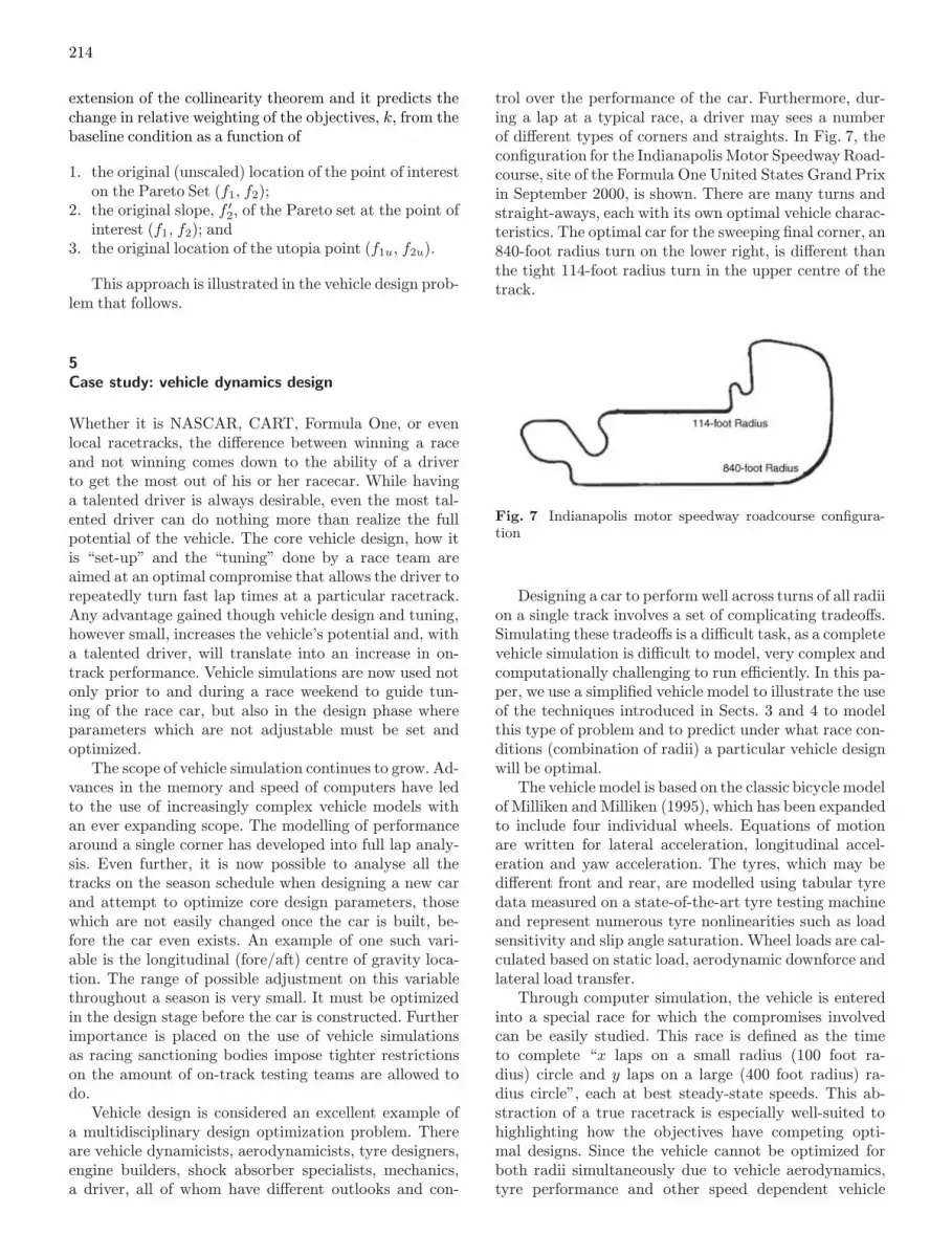
trol over the performance of the car. Furthermore, dur-ing a lap at a typical race, a driver may sees a numberof different types of corners and straights. In Fig. 7, theconfiguration for the Indianapolis Motor Speedway Road-course, site of the Formula One United States Grand Prixin September 2000, is shown. There are many turns andstraight-aways, each with its own optimal vehicle charac-teristics. The optimal car for the sweeping final corner, an840-foot radius turn on the lower right, is different thanthe tight 114-foot radius turn in the upper centre of thetrack.

Fig. 7 Indianapolis motor speedway roadcourse configura-tion

Designing a car to performwell across turns of all radiion a single track involves a set of complicating tradeoffs.Simulating these tradeoffs is a difficult task, as a completevehicle simulation is difficult to model, very complex andcomputationally challenging to run efficiently. In this pa-per, we use a simplified vehicle model to illustrate the useof the techniques introduced in Sects. 3 and 4 to modelthis type of problem and to predict under what race con-ditions (combination of radii) a particular vehicle designwill be optimal.

The vehicle model is based on the classic bicycle modelof Milliken andMilliken (1995), which has been expandedto include four individual wheels. Equations of motionare written for lateral acceleration, longitudinal accel-eration and yaw acceleration. The tyres, which may bedifferent front and rear, are modelled using tabular tyredata measured on a state-of-the-art tyre testing machineand represent numerous tyre nonlinearities such as loadsensitivity and slip angle saturation. Wheel loads are cal-culated based on static load, aerodynamic downforce andlateral load transfer.

Through computer simulation, the vehicle is enteredinto a special race for which the compromises involvedcan be easily studied. This race is defined as the timeto complete “x laps on a small radius (100 foot ra-dius) circle and y laps on a large (400 foot radius) ra-dius circle”, each at best steady-state speeds. This ab-straction of a true racetrack is especially well-suited tohighlighting how the objectives have competing opti-mal designs. Since the vehicle cannot be optimized forboth radii simultaneously due to vehicle aerodynamics,tyre performance and other speed dependent vehicle

215

behaviours, a compromise design is needed. This com-promise design is one which allows the vehicle to per-form optimally for the race, not just an individual circle.The ratio of x to y, denoted k can be viewed as theweighting of two design objectives, the elapsed timeson each individual radius. The shortest time to com-plete the total distance around both radii will win therace.

For this study, the vehicle has two design variables.These variables, roll stiffness distribution (K’) and weightdistribution (a’), are two of the three “magic numbers”Wright (1998) identifies as being fundamental to racecar design and performance. They are used by the vehi-cle designer and vehicle dynamicist to “tune” the car’shandling in an attempt to optimize performance. The an-alysis begins with a grid search of the design space fromwhich the performance space is plotted and the Pareto setidentified. The design space has been discretized into 546(a’,K’) pairs. Each design pair results in a certain level ofperformance on each of the two radii. Figure 8 plots theperformance space for the vehicle for a baseline race de-fined as one lap on each radius (k = 1). This gives eachradius equal importance. Thus, the axes are the time re-quired to complete one lap on each of the 100’ radius and400’ radius circles.

From Fig. 8 the optimum lap times for each radius areeasily located. For the 100’ radius the leftmost point onthis figure gives the optimum where the vehicle can do nobetter than approximately an 8.88 second lap. Likewise,for the 400’ radius the bottommost point in the plot givesthe optimum. This point indicates approximately a 9.1second lap as the best possible. These two points are con-sistent with the detailed vehicle simulations of Kasprzak(1998). The two optima do not occur at the same pointso the race definition, combining laps on each radius, willneed a compromise solution to arrive at the optimal de-sign and performance.

Fig. 8 Grid search results in the performance space

Figure 9 shows the grid search points which are mem-bers of the Pareto set along with the results of fittinga seventh-order polynomial via least-squares criteria.The polynomial gives a representative description of thePareto set throughout the range of the Pareto set, exceptat the far right end where the fit acquires a positive slope.As a result, analysis of this Pareto set for cases where the400’ radius design dominates the compromise design canbe expected to produce slightly inaccurate results. Whilethe use of an eighth order fit resolves this inaccuracy, theseventh-order fit is presented here to highlight potentialerrors caused by a fit which does not fully represent thePareto set.

Fig. 9 The Pareto set with seventh-order polynomial

Figure 10 presents the outcome of applying the scalingmethod (4) to the seventh-order fit Pareto set. This figureassociates the optimal race definition k with the vehicleperformance on the 100 foot radius. Note that since theorigin (0,0) is being used as the utopia point, (4) reducesto a simple form. Since Fig. 9 shows a one-to-one corres-pondence of performance on the 100 foot radius to thaton the 400 foot radius, Fig. 10 also specifies the optimal400 foot radius performance for any race definition k. Fur-thermore, since each point on the Pareto set is the resultof a unique combination of design variables, a relationshipbetween race definition and vehicle design is also acquiredfor the entire range of k values.

Consider the case of a race definition k = 15. That is,the race will contain 15 laps on the 100 foot radius andone lap on the 400 foot radius, each at best steady-stateperformance. Figure 10 predicts an optimal performanceon the 100 foot radius circle of 8.894 seconds per lap, or133.4117 seconds total time on the 100 foot radius. If theabscissa of Fig. 9 is rescaled by an amount equal to k (15)then Fig. 11 is generated. It shows the shape of the Paretoset in terms of the elapsed time on each radius for ank = 15 race. A circle drawn about the utopia point (0,0),

216

Fig. 10 Corresponding optimal scaling predicted by (4)

representative of the L2 norm technique for locating anoptimum point, identifies 113.4117 seconds as the opti-mum performance on the 100 foot radius, identical to thatpredicted by the scaling method. The L2 norm and thescaling method each predict the same optimal perform-ance, as desired.

Fig. 11 Verification of theoretical optimal scaling whenk = 15

Close examination of Fig. 10 reveals a region wherethe scaling k is associated with more than one perform-ance criteria on the 100 foot radius. One such value isk = 8.4. For this race definition three optimal 100 footradius performance points are predicted: 8.9198, 8.9114and 8.9031 seconds per lap on the 100 foot radius. Theseare denoted by the dashed lines in Fig. 12. Rescalingthe original Fig. 9 by k (8.4) produces Fig. 12. In thisfigure the circle about the utopia point touches onlytwo of the three points. The middle point is not an

optimum point. For the central, nonoptimal point, thecentre of curvature of the Pareto set lies between thePareto set and the utopia point. This point does not sat-isfy the collinearity theorem and is therefore not a can-didate to be an optimal point, even though (4) pro-duces this point as a solution. Thus, the scaling methodand the collinearity theorem are best used in tandemto arrive at optimal solutions in the Pareto set. Calcu-lation of the centre of curvature in addition to the useof (4) gives a more complete picture of the Pareto set’sbehaviour.

Fig. 12 Theoretical optimal scaling when k = 8.4

The other two points identified in this k = 8.4 exampleare indeed optimal design points and produce identicalrace times to one another. The left most optimum resultsin a race time of (8.4 × 8.9031) + 9.1688 = 83.9545 sec-onds while the right most optimum gives (8.4 × 8.9198)+ 9.0282 = 83.9545 seconds. These are identical, optimalrace times. In contrast, the centre point gives a race timeof (8.4 × 8.9114) + 9.2459 = 84.102 seconds, nearly 0.15seconds slower than the other two design points. As pre-dicted by the collinearity theorem, because the centre ofcurvature of the Pareto set is between the utopia pointand the Pareto set, this point is not optimal.

These two race definitions serve to show the valid-ity and usefulness of the scaling method and collinearitytheorem. A more detailed discussion of this example isprovided by Kasprzak et al. (1999). Additional commentsabout these techniques are provided in the next section.

6Comments on the scaling method

When using the scaling method, arriving at a polynomialwhich describes the Pareto set accurately is critical. Useof a high-order polynomial is desirable so that boththe concave and convex regions of the Pareto set can

217

be represented. A polynomial curve has two less inflec-tion points than the order of the polynomial and thesepolynomial inflection points may not all fall within therange of the Pareto set. It is very important that thepolynomial chosen meets the criteria used to specify thePareto set. As noted earlier, the seventh-order fit pre-sented violates a Pareto set criterion by reversing thesign of its slope near the right end of the fit. This re-sults in negative scaling values being predicted for thisregion, seen at the right end of the trace in Fig. 10.These negative values have no physical meaning and leadto solution inaccuracies. The use of an eighth-order fitwith this example, while not presented here, with thisexample provides a better representation of the Paretoset.

The polynomial fit can only be as good as the datato which it is applied. A sufficiently fine grid search ofthe design space is required to populate the Pareto set.While this method has the distinct advantage of find-ing the entire Pareto set, both concave and convex re-gions, the search increment may be very small and re-quire a large number of points to be calculated. Sincemost points calculated will not be Pareto set points thismethod may, at first glance, be deemed inefficient. Still,the grid search technique is guaranteed to find the en-tire Pareto set, given a fine enough discretization. Thisalone is a key point. The combination of a grid search andpolynomial to describe the Pareto set has the ability toprovide an accurate, smooth and continuous descriptionof the whole Pareto set, regardless of the existence of bothconvex and nonconvex regions.

The collinearity theorem and scaling method exploitthe use of this grid search and polynomial description ofthe Pareto set. These techniques pull a vast amount ofinformation out of the polynomial fit. The optimal ob-jective performances can be calculated for any and allratios of objective weights with ease via (4). To be ofreal use to the designer, relating these performance re-sults to their corresponding design variables is desirable.While these results appear in the performance space, an-other method has been developed, termed the contourmethod, which relates these results to the design space.This method, presented by Kasprzak and Lewis (2000),further enhances the utility of the scaling method andcollinearity theorem.

7Conclusions

Starting with a grid search of the design space, thePareto set is populated and then approximated usinga least-squares fit polynomial. This Pareto set is basedon a baseline goal definition with equally weighted ob-jectives, referred to as k = 1. The collinearity theoremstates that any internal member of the Pareto set is op-timal only if the utopia point, the point of interest inthe Pareto set and the instantaneous centre of curvature

of the Pareto set at the point of interest are collinear.From this the scaling method is derived, which allowsthe relative objective weighting to be predicted for anypoint on the Pareto set, based on the polynomial fit.Alternatively, the optimal performance for all ratios ofobjective weights can be readily determined. Thus, froma grid search of the design space the shape of the en-tire Pareto set can be determined, as well as the entiremapping of the optimum Pareto set solution to the rela-tive objective weighting. This provides a vast amount ofinformation and practical insight to the problem underconsideration. Verification of this method against re-sults obtained using an L2 norm shows the new methodsproduce results complementary to the established tech-nique. While the method presented here addresses onlytwo-objective compromise decision making, the meritsof extending the collinearity theorem and the scalingmethod to multiple dimensions are clear. Describing thePareto set as a hyperplane in n-dimensions and apply-ing the collinearity theorem in n-dimensional space ap-pear to be possible. While the concepts involved remainunchanged, the mathematical expression of these ideasin n-dimensions will be more complicated than in twodimensions.

Acknowledgements The authors would like to thank Milliken

Research Associates, Inc. for their support of this research.

The authors would also like to thank the National Science

Foundation, Grant DMI-9875706, for their support.

References

Athan, T.W.; Papalambros, P.Y. 1996: A note on weightedcriteria methods for compromise solutions in multi-objectiveoptimization. Eng. Opt. 27, 155–176

Callaghan, A.; Lewis, K. 2000: A 2-phase aspiration-level andutility theory approach to large scale design. 2000 ASMEDesign Engineering Technical Conf., DETC2000/DTM-14569

Chen, W.; Wiecek, M.M.; Zhang, J. 1999: Quality util-ity: a compromise programming approach to robust design.ASME J. Mech. Des. 121, 179–187

Das, I. 1999: A preference ordering among various Pareto op-timal alternatives. Struct. Optim. 18, 30–35

Dennis, J.E.; Das, I. 1997: A closer look at drawbacks of min-imizing weighted sums of objective for Pareto set generationin multicriteria optimization problems. Struct. Optim. 14,63–64

Eschenauer, H.; Koski, J.; Osyczka, A.E. 1990: Multicriteriadesign optimization: procedures and applications. Berlin, Hei-delberg, New York: Springer

Geoffrion, A.M. 1968: Proper efficiency and the theory of vec-tor maximization. J. Math. Analysis Appl. 22, 618–630

Hazelrigg, G. 1996: Systems engineering: an approach toinformation-based design. Upper Saddle River, NJ: Prentice-Hall

218

Horn, J.; Nafpliotis, N.; Goldberg, D.E. 1994: A niched Paretogenetic algorithm for multiobjective optimization. Proc. 1stIEEE Conf. on Evolutionary Computation, IEEE WorldCongr. of Computational Intelligence (held in Piscataway,NJ), Vol. 1, pp. 82–87

Kasprzak, E.M. 1998: Multivariate optimization and gametheory applications in vehicle dynamics simulations. M.S.Thesis, Department of Mechanical and Aerospace Engineer-ing, University at Buffalo, NY

Kasprzak, E.M.; Lewis, K.E. 2000: An approach to facilitatedecision tradeoffs in Pareto solution sets. J. Eng. Value CostAnalysis 3, 173–187

Kasprzak, E.M.; Lewis, K.E.; Milliken, D.L. 1999: Steady-state vehicle optimization using Pareto-minimum analysis.SAE Trans., J. Passenger Cars 107, 2624–2631

Koski, J. 1985: Defectiveness of weighting method in multicri-terion optimization of structures. Comm. Appl. Numer. Meth.1, 333–337

Lewis, K.; Mistree, F. 1998: The other side of multidisci-plinary design optimization: accommodating a multiobjec-tive, uncertain and non-deterministic world. Eng. Opt. 31,161–189

Luce, R.D.; Raiffa, H. 1957: Games and decisions. New York:John Wiley

Messac, A. 2000: From the dubious construction of objectivefunctions to the application of physical programming. AIAAJ. 38, 155–163

Messac, A.; Sundararaj, J.G.; Tappeta, R.V.; Renaud, J.E.2000: The ability of ojective functions to generate non-convexPareto frontiers. AIAA J. 38, 1084–1091

Table 1 Effects of abscissa scaling on Pareto set attributes

Before rescaling After rescaling by k

suboptimal point of interest on Pareto set (x1, y1) (kx1, y1)instantaneous slope of Pareto m1 m1/kset at point of interestequation of line tangent to Pareto y1 =m1x1+ b y1 =

m1k (kx1)+ b1

set at point of interest y1 =m1x1+ b1slope of line normal to Pareto −1/m1 −1/m1set at point of interest

Miettinen, K.M. 1999: Nonlinear multiobjective optimization.Boston: Kluwer

Milliken, W.F.; Milliken, D.L. 1995: Race car vehicle dynam-ics. Warrendale, PA: SAE Int. No R-146

Narayanan, S.; Azarm, S. 1999: On improving multiobjectivegenetic algorithms for design optimization. Struct. Optim. 18,146–155

Nelson, S.; Parkinson, M.; Papalambros, P. 1999: Multicri-teria optimization in product platform design. Proc. ASMEDesign Engineering Technical Conf. (held in Las Vegas),DETC99/DAC-8676

Palli, N.; McCluskey, P.; Azarm, S.; Sundararajan, R. 1998:An interactive multistage ε-inequality constraint method formultiple objectives decision making. ASME J. Mech. Des.120, 678–686

Tappeta, R.; Renaud, J. 1999: Interactive multiobjective op-timization design strategy for decision based design. Proc.ASME Design Engineering Technical Conf. (held in LasVegas, NV), DETC99/DAC-8581

Wright, P. 1998: What is McLaren’s secret? Racecar Eng. 8,6–7

Yoo, J.; Hajela, P. 1999: Immune network simulations in mul-ticriterion design. Struct. Optim. 1, 85–94

Appendix

Table 1 supports the development in Sect. 4. It shows howvarious Pareto Set parameters change with rescaling ofthe abscissa in the performance space by an amount k.