week 11: collinearity
TRANSCRIPT

Week 11: Collinearity
Marcelo Coca Perraillon
University of ColoradoAnschutz Medical Campus
Health Services Research Methods IHSMP 7607
2019
These slides are part of a forthcoming book to be published by CambridgeUniversity Press. For more information, go to perraillon.com/PLH. c©Thismaterial is copyrighted. Please see the entire copyright notice on the book’swebsite.
Updated notes are here: https://clas.ucdenver.edu/marcelo-perraillon/
teaching/health-services-research-methods-i-hsmp-76071
Outline
Regression and “holding other factors” constant
Perfect collinearity
Highly correlated predictors
More complicated forms
Variance inflation factor
Solutions
2
Collinearity
We have seen that interpreting multiple linear models involves theidea of “holding other factors constant” or “once we have taken theother factors into account”
In the model wagei = β0 + β1agei + β2educi + ui where ui ∼ N(0, σ2)
We interpret β1 as the effect on average wage for an additional yearof age, holding education constant
We know that with observational data holding other factorsconstant is not literal (recall the Ted Mosby, architect, theory ofstatistics)
If we don’t have experimental data, holding factors constant isfiguratively, not literally
3
Collinearity
Regardless of the data generating process, we can always interpret theregression in this way (either literally or figuratively)
But what if holding the other variable constant doesn’t make senseeven figuratively?
For example, if we have a sample of young people, an extra year ofage also implies another year of education (assuming that they all goto school)
In this simple scenario we can’t really hold education constant whenanalyzing a change in the value of age – or the “effect” of age
Let’s call this the Ted Mosby modeling failure
4
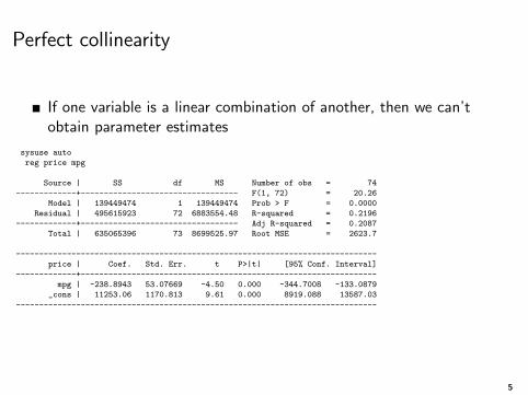
Perfect collinearity
If one variable is a linear combination of another, then we can’tobtain parameter estimates
sysuse auto
reg price mpg
Source | SS df MS Number of obs = 74
-------------+---------------------------------- F(1, 72) = 20.26
Model | 139449474 1 139449474 Prob > F = 0.0000
Residual | 495615923 72 6883554.48 R-squared = 0.2196
-------------+---------------------------------- Adj R-squared = 0.2087
Total | 635065396 73 8699525.97 Root MSE = 2623.7
------------------------------------------------------------------------------
price | Coef. Std. Err. t P>|t| [95% Conf. Interval]
-------------+----------------------------------------------------------------
mpg | -238.8943 53.07669 -4.50 0.000 -344.7008 -133.0879
_cons | 11253.06 1170.813 9.61 0.000 8919.088 13587.03
------------------------------------------------------------------------------
5
Perfect collinearity
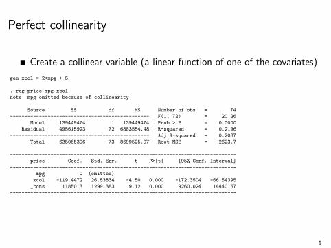
Create a collinear variable (a linear function of one of the covariates)
gen xcol = 2*mpg + 5
. reg price mpg xcol
note: mpg omitted because of collinearity
Source | SS df MS Number of obs = 74
-------------+---------------------------------- F(1, 72) = 20.26
Model | 139449474 1 139449474 Prob > F = 0.0000
Residual | 495615923 72 6883554.48 R-squared = 0.2196
-------------+---------------------------------- Adj R-squared = 0.2087
Total | 635065396 73 8699525.97 Root MSE = 2623.7
------------------------------------------------------------------------------
price | Coef. Std. Err. t P>|t| [95% Conf. Interval]
-------------+----------------------------------------------------------------
mpg | 0 (omitted)
xcol | -119.4472 26.53834 -4.50 0.000 -172.3504 -66.54395
_cons | 11850.3 1299.383 9.12 0.000 9260.024 14440.57
------------------------------------------------------------------------------
6
Perfect collinearity
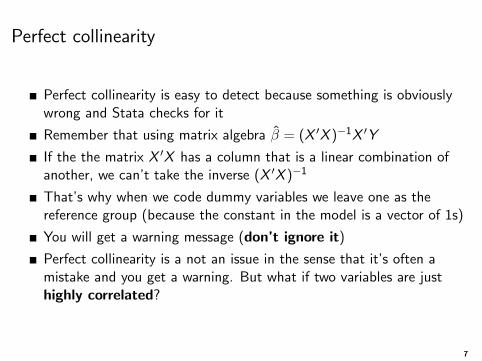
Perfect collinearity is easy to detect because something is obviouslywrong and Stata checks for it
Remember that using matrix algebra β = (X ′X )−1X ′Y
If the the matrix X ′X has a column that is a linear combination ofanother, we can’t take the inverse (X ′X )−1
That’s why when we code dummy variables we leave one as thereference group (because the constant in the model is a vector of 1s)
You will get a warning message (don’t ignore it)
Perfect collinearity is a not an issue in the sense that it’s often amistake and you get a warning. But what if two variables are justhighly correlated?
7
Collinearity
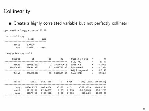
Create a highly correlated variable but not perfectly collinear
gen xcol1 = 2*mpg + rnormal(0,5)
corr xcol1 mpg
| xcol1 mpg
-------------+------------------
xcol1 | 1.0000
mpg | 0.9482 1.0000
. reg price mpg xcol1
Source | SS df MS Number of obs = 74
-------------+---------------------------------- F(2, 71) = 10.99
Model | 150153413 2 75076706.3 Prob > F = 0.0001
Residual | 484911983 71 6829746.25 R-squared = 0.2364
-------------+---------------------------------- Adj R-squared = 0.2149
Total | 635065396 73 8699525.97 Root MSE = 2613.4
------------------------------------------------------------------------------
price | Coef. Std. Err. t P>|t| [95% Conf. Interval]
-------------+----------------------------------------------------------------
mpg | -436.4372 166.4158 -2.62 0.011 -768.2609 -104.6136
xcol1 | 91.07191 72.74697 1.25 0.215 -53.98143 236.1253
_cons | 11576.59 1194.518 9.69 0.000 9194.79 13958.39
------------------------------------------------------------------------------
8
Collinearity
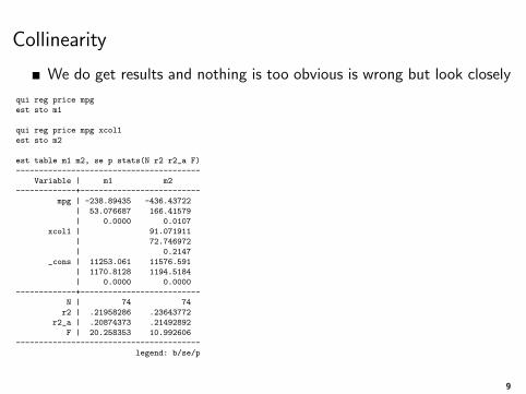
We do get results and nothing is too obvious is wrong but look closely
qui reg price mpg
est sto m1
qui reg price mpg xcol1
est sto m2
est table m1 m2, se p stats(N r2 r2_a F)
----------------------------------------
Variable | m1 m2
-------------+--------------------------
mpg | -238.89435 -436.43722
| 53.076687 166.41579
| 0.0000 0.0107
xcol1 | 91.071911
| 72.746972
| 0.2147
_cons | 11253.061 11576.591
| 1170.8128 1194.5184
| 0.0000 0.0000
-------------+--------------------------
N | 74 74
r2 | .21958286 .23643772
r2_a | .20874373 .21492892
F | 20.258353 10.992606
----------------------------------------
legend: b/se/p
9
Collinearity
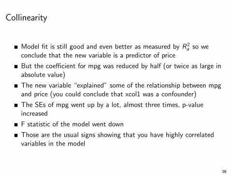
Model fit is still good and even better as measured by R2a so we
conclude that the new variable is a predictor of price
But the coefficient for mpg was reduced by half (or twice as large inabsolute value)
The new variable “explained” some of the relationship between mpgand price (you could conclude that xcol1 was a confounder)
The SEs of mpg went up by a lot, almost three times, p-valueincreased
F statistic of the model went down
Those are the usual signs showing that you have highly correlatedvariables in the model
10
Another example
The example above is typical of collinearity
Collinearity makes estimation “unstable” in the sense that theinclusion of one variable changes SEs and parameter estimates
Perhaps the best way to think about collinearity is that one variablecould be used as a proxy of the other because they measure similarfactors affecting an outcome
Sometimes, though, is more complicated and not so clear andcollinearity could be more complex to detect (more on this soon)
11
Another example
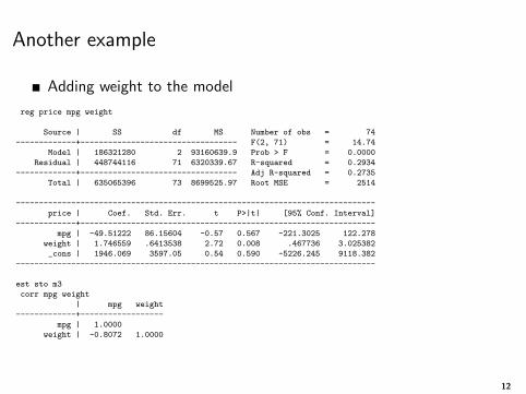
Adding weight to the model
reg price mpg weight
Source | SS df MS Number of obs = 74
-------------+---------------------------------- F(2, 71) = 14.74
Model | 186321280 2 93160639.9 Prob > F = 0.0000
Residual | 448744116 71 6320339.67 R-squared = 0.2934
-------------+---------------------------------- Adj R-squared = 0.2735
Total | 635065396 73 8699525.97 Root MSE = 2514
------------------------------------------------------------------------------
price | Coef. Std. Err. t P>|t| [95% Conf. Interval]
-------------+----------------------------------------------------------------
mpg | -49.51222 86.15604 -0.57 0.567 -221.3025 122.278
weight | 1.746559 .6413538 2.72 0.008 .467736 3.025382
_cons | 1946.069 3597.05 0.54 0.590 -5226.245 9118.382
------------------------------------------------------------------------------
est sto m3
corr mpg weight
| mpg weight
-------------+------------------
mpg | 1.0000
weight | -0.8072 1.0000
12
Effect on inference
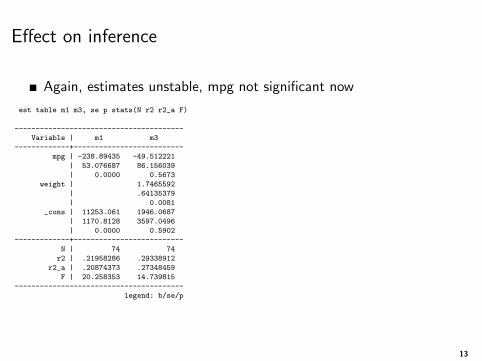
Again, estimates unstable, mpg not significant now
est table m1 m3, se p stats(N r2 r2_a F)
----------------------------------------
Variable | m1 m3
-------------+--------------------------
mpg | -238.89435 -49.512221
| 53.076687 86.156039
| 0.0000 0.5673
weight | 1.7465592
| .64135379
| 0.0081
_cons | 11253.061 1946.0687
| 1170.8128 3597.0496
| 0.0000 0.5902
-------------+--------------------------
N | 74 74
r2 | .21958286 .29338912
r2_a | .20874373 .27348459
F | 20.258353 14.739815
----------------------------------------
legend: b/se/p
13
Proxy, confounder?
Is mpg and weight measuring the same concept? Is one a proxy forthe other? Clearly not
In some cases, it’s easy to conceptually settle on one variable over theother because their correlation is due to both measuring the sameconcept
For example, think of two tests that measure “intelligence”
But the auto example is more complicated. It’s not that cars withbetter mpg are less expensive, it’s that we are bunching togetherdifferent types of cars and markets
Trucks are heavier and more expensive and have less mpg; otherfactors being constant, better mileage implies higher prices
Regardless of the interpretation, adding highly correlated variables is aproblem for both, inference and interpretation
14
Signs of collinearity
Typical signs of collinearity:
1) Large changes in estimated parameters when a variable is added ordeleted
2) Large changes when some data points are added or deleted
3) Signs of coefficients do not agree with expectations (subjectknowledge)
4) Coefficients of variables that are expected to be important havelarge SEs (low t-values, large p-values)
If two variables highly correlated measure the same concept, thendrop one. If not, we need subject knowledge to understand what isdriving the results and what can be done about it
We might need better data, more data, or other covariates in ourmodel
15
Some solutions
If two highly-correlated variables measure the same concept, thendrop one
If not, we need subject knowledge to understand what is driving theresults and what can be done about it
Which variable is conceptually more important? Do we want to showthe relationship between price and mpg? Or the effect of weight onprice?
We might need better data, more data, or other covariates in ourmodel
Note something though: this is a CONCEPTUAL PROBLEM, nota stats problem. We will see ways to detect it but the solution isconceptual, based on subject knowledge
16
Detecting the problem early
In a exploratory analysis, you should have noticed that somepredictors are highly correlated
Collinearity also highlights the importance of carefully exploring therelationship of interest, for example, price and mpg before addingother variables in the model
When you add one variable at a time, you can see the impact on SEsand parameter estimates. Always, always, use est sto and est tableto build models
If you follow this procedure, you will find the variable(s) that arehighly collinear early
We always need subject knowledge to understand the reasons for highcorrelation
17
Digression: prediction
Remember what I say all the time: every time you hear rule ofthumbs or things you should do or not should do in statistics,remember the context
We are discussing collinearity in the context of models that we areestimating because we care about inference (hypothesis testing,description, causality)
But what if we only care about prediction? Not uncommon to usevariables that are correlated. Not uncommon to use variables thatmeasure similar concepts. We don’t care about Ted Mosby here
But it’s still a problem of interpretation. For example, some machinelearning algorithms (say, Lasso) drop some variables and keep others.But you can’t conclude that the variables dropped were not“important” because some of them could be correlated with variableskept in the model. Next time you run the model the variable variabledropped could be kept
18
Another example
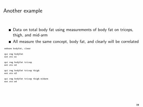
Data on total body fat using measurements of body fat on triceps,thigh, and mid-arm
All measure the same concept, body fat, and clearly will be correlated
webuse bodyfat, clear
qui reg bodyfat
est sto m1
qui reg bodyfat tricep
est sto m2
qui reg bodyfat tricep thigh
est sto m3
qui reg bodyfat tricep thigh midarm
est sto m4
19
Another example
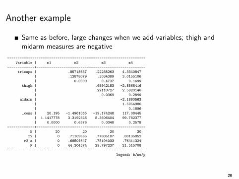
Same as before, large changes when we add variables; thigh andmidarm measures are negative
------------------------------------------------------------------
Variable | m1 m2 m3 m4
-------------+----------------------------------------------------
triceps | .85718657 .22235263 4.3340847
| .12878079 .3034389 3.0155106
| 0.0000 0.4737 0.1699
thigh | .65942183 -2.8568416
| .29118727 2.5820146
| 0.0369 0.2849
midarm | -2.1860563
| 1.5954986
| 0.1896
_cons | 20.195 -1.4961065 -19.174248 117.08445
| 1.1417778 3.3192346 8.3606404 99.782377
| 0.0000 0.6576 0.0348 0.2578
-------------+----------------------------------------------------
N | 20 20 20 20
r2 | 0 .71109665 .77805187 .80135852
r2_a | 0 .69504647 .75194033 .76411324
F | 0 44.304574 29.797237 21.515708
------------------------------------------------------------------
legend: b/se/p
20
Another example
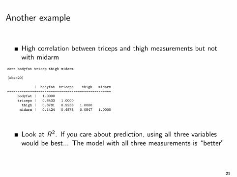
High correlation between triceps and thigh measurements but notwith midarm
corr bodyfat tricep thigh midarm
(obs=20)
| bodyfat triceps thigh midarm
-------------+------------------------------------
bodyfat | 1.0000
triceps | 0.8433 1.0000
thigh | 0.8781 0.9238 1.0000
midarm | 0.1424 0.4578 0.0847 1.0000
Look at R2. If you care about prediction, using all three variableswould be best... The model with all three measurements is “better”
21
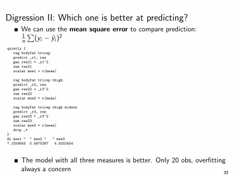
Digression II: Which one is better at predicting?We can use the mean square error to compare prediction:1n
∑(yi − yi )
2
quietly {
reg bodyfat tricep
predict _r1, res
gen res21 = _r1^2
sum res21
scalar mse1 = r(mean)
reg bodyfat tricep thigh
predict _r2, res
gen res22 = _r2^2
sum res22
scalar mse2 = r(mean)
reg bodyfat tricep thigh midarm
predict _r3, res
gen res23 = _r3^2
sum res23
scalar mse3 = r(mean)
drop _*
}
di mse1 " " mse2 " " mse3
7.1559845 5.4975387 4.9202454
The model with all three measures is better. Only 20 obs, overfittingalways a concern
22
More complicated forms
It’s possible that collinearity will take more complicated forms , notjust two predictors being highly correlated
It could be that two variables combined are highly related to a thirdvariable. This is harder to detect and understand
One way to diagnose collinearity is to investigate how eachexplanatory variable in a model is related to all other explanatoryvariables in the model
One metric: variance inflation factor or VIF
23
Variance inflation factor
The variance inflation factor for variable Xj is defined as
VIFj = 11−R2 for j = 1, ..., p
The R2 in VIF is the R2 obtained from regressing Xj against allother explanatory variables (p − 1). (We leave the outcomevariable out)
If R2 is low, VIF will be close to 1. If R2 is high, VIF will be high
Note the logic. If you run the model, say,X1 = γ0 + γ1X2 + · · · + γ5X5 and it has a high R2, that means thatthe variables X2 to X5 are strong predictors of X1
A rule of thumb is that a VIF > 10 provides evidence of collinearity.That implies that R2 ≥ 0.9
In HSR and social sciences a VIF above 3 could be problematic or atleast you should check covariates since it implies an R2 around 0.66
24
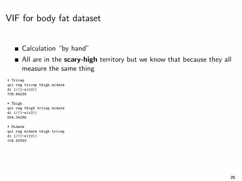
VIF for body fat dataset
Calculation “by hand”
All are in the scary-high territory but we know that because they allmeasure the same thing
* Tricep
qui reg tricep thigh midarm
di 1/(1-e(r2))
708.84239
* Thigh
qui reg thigh tricep midarm
di 1/(1-e(r2))
564.34296
* Midarm
qui reg midarm thigh tricep
di 1/(1-e(r2))
104.60593
25
VIF for body fat dataset
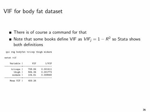
There is of course a command for that
Note that some books define VIF as VIFj = 1 − R2 so Stata showsboth definitions
qui reg bodyfat tricep thigh midarm
estat vif
Variable | VIF 1/VIF
-------------+----------------------
triceps | 708.84 0.001411
thigh | 564.34 0.001772
midarm | 104.61 0.009560
-------------+----------------------
Mean VIF | 459.26
26
Back to the auto dataset and caution
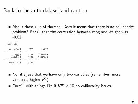
About those rule of thumbs. Does it mean that there is no collinearityproblem? Recall that the correlation between mpg and weight was-0.81
estat vif
Variable | VIF 1/VIF
-------------+----------------------
mpg | 2.87 0.348469
weight | 2.87 0.348469
-------------+----------------------
Mean VIF | 2.87
No, it’s just that we have only two variables (remember, morevariables, higher R2)
Careful with things like if VIF < 10 no collinearity issues...
27
Other solutions
The body fat example illustrates another possible solution
Rather than choosing one and dropping the rest, why not createcombination of all of them, which could be a stronger predictor ofbody fat?
For example, take the average of the three measurements as acovariate
Or the average of two, since thigh and tricep seem more related tobodyfat
28

Boby fat again
* Rowmean uses more information since it calculates the mean of the non-missing variables
egen avgmes = rowmean(tricep thigh midarm)
egen avgmes1 = rowmean(thigh tricep)
reg bodyfat tricep
est sto m1
reg bodyfat thigh
est sto m2
reg bodyfat midarm
est sto m3
reg bodyfat avgmes
est sto m4
reg bodyfat avgmes1
est sto m5
est table m1 m2 m3 m4 m5, se p stats(N r2 r2_a F)
29
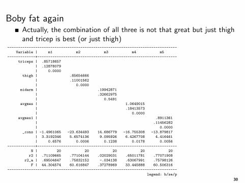
Boby fat againActually, the combination of all three is not that great but just thighand tricep is best (or just thigh)
-------------------------------------------------------------------------------
Variable | m1 m2 m3 m4 m5
-------------+-----------------------------------------------------------------
triceps | .85718657
| .12878079
| 0.0000
thigh | .85654666
| .11001562
| 0.0000
midarm | .19942871
| .32662975
| 0.5491
avgmes | 1.0649015
| .18413573
| 0.0000
avgmes1 | .8911361
| .11456282
| 0.0000
_cons | -1.4961065 -23.634493 14.686779 -16.755308 -13.879817
| 3.3192346 5.6574136 9.095926 6.4267708 4.416461
| 0.6576 0.0006 0.1238 0.0178 0.0056
-------------+-----------------------------------------------------------------
N | 20 20 20 20 20
r2 | .71109665 .77104144 .02029031 .65011781 .77071908
r2_a | .69504647 .75832152 -.034138 .63067991 .75798126
F | 44.304574 60.616847 .37278969 33.445888 60.506316
-------------------------------------------------------------------------------
legend: b/se/p
30
Factor analysis
Factor analysis is a data reduction technique
It creates a smaller set of uncorrelated variables
Results in an index or a combination, much like the average of themeasures but with different weights
Two types: exploratory (no pre-defined idea of structure) andconfirmatory (you have an idea and the analysis confirms)
Note that factor analysis does not take into account the outcome;it just combines explanatory variables
It’s used a lot in surveys. Popular in psychology
31
Summary
Always check for multicollinearity and think whether you are includinghighly correlated variables in your models
A problem regardless of the model (linear, logit, Poisson, etc)
Nothing substitutes subject knowledge to understand what drivesmulticollinearity
In easy cases, a matter of dropping one variable that is measuring thesame concept as another one
Gray area: do you care if two variables that you just want tocontrol for are highly correlated? Maybe not
32