package 'psych' - citeseerx
TRANSCRIPT

Package ‘psych’September 22, 2010
Version 1.0-92
Date 2010-09-31
Title Procedures for Psychological, Psychometric, and Personality Research
Author William Revelle <[email protected]>
Maintainer William Revelle <[email protected]>
Description A number of routines for personality, psychometrics and experimental psychology.Functions are primarily for scale construction using factor analysis, cluster analysis andreliability analysis, although others provide basic descriptive statistics. Functions for simulatingparticular item and test structures are included. Several functions serve as a useful front end forstructural equation modeling. Graphical displays of path diagrams, factor analysis and structuralequation models are created using basic graphics. Some of the functions are written to support abook on psychometrics as well as publications in personality research. For more information, seethe personality-project.org/r webpage.
License GPL (>= 2)
Suggests polycor, GPArotation, sem, MASS,graph,Rgraphviz,mvtnorm, Rcsdp
URL http://personality-project.org/r,http://personality-project.org/r/psych.manual.pdf
Repository CRAN
Date/Publication 2010-09-22 19:37:15
R topics documented:00.psych . . . . . . . . . . . . . . . . . . . . . . . . . . . . . . . . . . . . . . . . . . . 4affect . . . . . . . . . . . . . . . . . . . . . . . . . . . . . . . . . . . . . . . . . . . . 13alpha . . . . . . . . . . . . . . . . . . . . . . . . . . . . . . . . . . . . . . . . . . . . . 14bfi . . . . . . . . . . . . . . . . . . . . . . . . . . . . . . . . . . . . . . . . . . . . . . 17bifactor . . . . . . . . . . . . . . . . . . . . . . . . . . . . . . . . . . . . . . . . . . . 19block.random . . . . . . . . . . . . . . . . . . . . . . . . . . . . . . . . . . . . . . . . 21blot . . . . . . . . . . . . . . . . . . . . . . . . . . . . . . . . . . . . . . . . . . . . . 22
1
2 R topics documented:
bock . . . . . . . . . . . . . . . . . . . . . . . . . . . . . . . . . . . . . . . . . . . . . 23burt . . . . . . . . . . . . . . . . . . . . . . . . . . . . . . . . . . . . . . . . . . . . . 24circ.tests . . . . . . . . . . . . . . . . . . . . . . . . . . . . . . . . . . . . . . . . . . . 25cities . . . . . . . . . . . . . . . . . . . . . . . . . . . . . . . . . . . . . . . . . . . . . 27cluster.cor . . . . . . . . . . . . . . . . . . . . . . . . . . . . . . . . . . . . . . . . . . 29cluster.fit . . . . . . . . . . . . . . . . . . . . . . . . . . . . . . . . . . . . . . . . . . . 31cluster.loadings . . . . . . . . . . . . . . . . . . . . . . . . . . . . . . . . . . . . . . . 32cluster.plot . . . . . . . . . . . . . . . . . . . . . . . . . . . . . . . . . . . . . . . . . . 34cluster2keys . . . . . . . . . . . . . . . . . . . . . . . . . . . . . . . . . . . . . . . . . 35cohen.kappa . . . . . . . . . . . . . . . . . . . . . . . . . . . . . . . . . . . . . . . . . 36comorbidity . . . . . . . . . . . . . . . . . . . . . . . . . . . . . . . . . . . . . . . . . 39cor.plot . . . . . . . . . . . . . . . . . . . . . . . . . . . . . . . . . . . . . . . . . . . 40corr.test . . . . . . . . . . . . . . . . . . . . . . . . . . . . . . . . . . . . . . . . . . . 42correct.cor . . . . . . . . . . . . . . . . . . . . . . . . . . . . . . . . . . . . . . . . . . 43cortest.bartlett . . . . . . . . . . . . . . . . . . . . . . . . . . . . . . . . . . . . . . . . 44cortest.mat . . . . . . . . . . . . . . . . . . . . . . . . . . . . . . . . . . . . . . . . . . 45cosinor . . . . . . . . . . . . . . . . . . . . . . . . . . . . . . . . . . . . . . . . . . . . 47count.pairwise . . . . . . . . . . . . . . . . . . . . . . . . . . . . . . . . . . . . . . . . 49cta . . . . . . . . . . . . . . . . . . . . . . . . . . . . . . . . . . . . . . . . . . . . . . 50cubits . . . . . . . . . . . . . . . . . . . . . . . . . . . . . . . . . . . . . . . . . . . . 51describe . . . . . . . . . . . . . . . . . . . . . . . . . . . . . . . . . . . . . . . . . . . 52describe.by . . . . . . . . . . . . . . . . . . . . . . . . . . . . . . . . . . . . . . . . . 54diagram . . . . . . . . . . . . . . . . . . . . . . . . . . . . . . . . . . . . . . . . . . . 56draw.tetra . . . . . . . . . . . . . . . . . . . . . . . . . . . . . . . . . . . . . . . . . . 58eigen.loadings . . . . . . . . . . . . . . . . . . . . . . . . . . . . . . . . . . . . . . . . 59ellipses . . . . . . . . . . . . . . . . . . . . . . . . . . . . . . . . . . . . . . . . . . . 60epi.bfi . . . . . . . . . . . . . . . . . . . . . . . . . . . . . . . . . . . . . . . . . . . . 61error.bars . . . . . . . . . . . . . . . . . . . . . . . . . . . . . . . . . . . . . . . . . . 63error.bars.by . . . . . . . . . . . . . . . . . . . . . . . . . . . . . . . . . . . . . . . . . 65error.crosses . . . . . . . . . . . . . . . . . . . . . . . . . . . . . . . . . . . . . . . . . 66fa . . . . . . . . . . . . . . . . . . . . . . . . . . . . . . . . . . . . . . . . . . . . . . 68fa.diagram . . . . . . . . . . . . . . . . . . . . . . . . . . . . . . . . . . . . . . . . . . 73fa.parallel . . . . . . . . . . . . . . . . . . . . . . . . . . . . . . . . . . . . . . . . . . 75fa.sort . . . . . . . . . . . . . . . . . . . . . . . . . . . . . . . . . . . . . . . . . . . . 78factor.congruence . . . . . . . . . . . . . . . . . . . . . . . . . . . . . . . . . . . . . . 79factor.fit . . . . . . . . . . . . . . . . . . . . . . . . . . . . . . . . . . . . . . . . . . . 80factor.model . . . . . . . . . . . . . . . . . . . . . . . . . . . . . . . . . . . . . . . . . 81factor.residuals . . . . . . . . . . . . . . . . . . . . . . . . . . . . . . . . . . . . . . . 82factor.rotate . . . . . . . . . . . . . . . . . . . . . . . . . . . . . . . . . . . . . . . . . 83factor.stats . . . . . . . . . . . . . . . . . . . . . . . . . . . . . . . . . . . . . . . . . . 85factor2cluster . . . . . . . . . . . . . . . . . . . . . . . . . . . . . . . . . . . . . . . . 87fisherz . . . . . . . . . . . . . . . . . . . . . . . . . . . . . . . . . . . . . . . . . . . . 89galton . . . . . . . . . . . . . . . . . . . . . . . . . . . . . . . . . . . . . . . . . . . . 90geometric.mean . . . . . . . . . . . . . . . . . . . . . . . . . . . . . . . . . . . . . . . 91glb.algebraic . . . . . . . . . . . . . . . . . . . . . . . . . . . . . . . . . . . . . . . . . 92guttman . . . . . . . . . . . . . . . . . . . . . . . . . . . . . . . . . . . . . . . . . . . 94Harman . . . . . . . . . . . . . . . . . . . . . . . . . . . . . . . . . . . . . . . . . . . 98harmonic.mean . . . . . . . . . . . . . . . . . . . . . . . . . . . . . . . . . . . . . . . 100

R topics documented: 3
headtail . . . . . . . . . . . . . . . . . . . . . . . . . . . . . . . . . . . . . . . . . . . 101heights . . . . . . . . . . . . . . . . . . . . . . . . . . . . . . . . . . . . . . . . . . . . 101ICC . . . . . . . . . . . . . . . . . . . . . . . . . . . . . . . . . . . . . . . . . . . . . 102iclust . . . . . . . . . . . . . . . . . . . . . . . . . . . . . . . . . . . . . . . . . . . . . 104ICLUST.cluster . . . . . . . . . . . . . . . . . . . . . . . . . . . . . . . . . . . . . . . 109iclust.diagram . . . . . . . . . . . . . . . . . . . . . . . . . . . . . . . . . . . . . . . . 110ICLUST.graph . . . . . . . . . . . . . . . . . . . . . . . . . . . . . . . . . . . . . . . 111ICLUST.rgraph . . . . . . . . . . . . . . . . . . . . . . . . . . . . . . . . . . . . . . . 115ICLUST.sort . . . . . . . . . . . . . . . . . . . . . . . . . . . . . . . . . . . . . . . . . 117income . . . . . . . . . . . . . . . . . . . . . . . . . . . . . . . . . . . . . . . . . . . . 118interp.median . . . . . . . . . . . . . . . . . . . . . . . . . . . . . . . . . . . . . . . . 119iqitems . . . . . . . . . . . . . . . . . . . . . . . . . . . . . . . . . . . . . . . . . . . . 121irt.1p . . . . . . . . . . . . . . . . . . . . . . . . . . . . . . . . . . . . . . . . . . . . . 122irt.fa . . . . . . . . . . . . . . . . . . . . . . . . . . . . . . . . . . . . . . . . . . . . . 123irt.item.diff.rasch . . . . . . . . . . . . . . . . . . . . . . . . . . . . . . . . . . . . . . 125logistic . . . . . . . . . . . . . . . . . . . . . . . . . . . . . . . . . . . . . . . . . . . . 126make.keys . . . . . . . . . . . . . . . . . . . . . . . . . . . . . . . . . . . . . . . . . . 128mat.regress . . . . . . . . . . . . . . . . . . . . . . . . . . . . . . . . . . . . . . . . . 129mat.sort . . . . . . . . . . . . . . . . . . . . . . . . . . . . . . . . . . . . . . . . . . . 130matrix.addition . . . . . . . . . . . . . . . . . . . . . . . . . . . . . . . . . . . . . . . 131msq . . . . . . . . . . . . . . . . . . . . . . . . . . . . . . . . . . . . . . . . . . . . . 132multi.hist . . . . . . . . . . . . . . . . . . . . . . . . . . . . . . . . . . . . . . . . . . 136neo . . . . . . . . . . . . . . . . . . . . . . . . . . . . . . . . . . . . . . . . . . . . . . 137omega . . . . . . . . . . . . . . . . . . . . . . . . . . . . . . . . . . . . . . . . . . . . 139omega.graph . . . . . . . . . . . . . . . . . . . . . . . . . . . . . . . . . . . . . . . . . 145p.rep . . . . . . . . . . . . . . . . . . . . . . . . . . . . . . . . . . . . . . . . . . . . . 147paired.r . . . . . . . . . . . . . . . . . . . . . . . . . . . . . . . . . . . . . . . . . . . 149pairs.panels . . . . . . . . . . . . . . . . . . . . . . . . . . . . . . . . . . . . . . . . . 150partial.r . . . . . . . . . . . . . . . . . . . . . . . . . . . . . . . . . . . . . . . . . . . 152peas . . . . . . . . . . . . . . . . . . . . . . . . . . . . . . . . . . . . . . . . . . . . . 153phi . . . . . . . . . . . . . . . . . . . . . . . . . . . . . . . . . . . . . . . . . . . . . . 154phi.demo . . . . . . . . . . . . . . . . . . . . . . . . . . . . . . . . . . . . . . . . . . 155phi2poly . . . . . . . . . . . . . . . . . . . . . . . . . . . . . . . . . . . . . . . . . . . 156plot.psych . . . . . . . . . . . . . . . . . . . . . . . . . . . . . . . . . . . . . . . . . . 157polar . . . . . . . . . . . . . . . . . . . . . . . . . . . . . . . . . . . . . . . . . . . . . 159polychor.matrix . . . . . . . . . . . . . . . . . . . . . . . . . . . . . . . . . . . . . . . 160principal . . . . . . . . . . . . . . . . . . . . . . . . . . . . . . . . . . . . . . . . . . . 161print.psych . . . . . . . . . . . . . . . . . . . . . . . . . . . . . . . . . . . . . . . . . 164Promax . . . . . . . . . . . . . . . . . . . . . . . . . . . . . . . . . . . . . . . . . . . 166r.test . . . . . . . . . . . . . . . . . . . . . . . . . . . . . . . . . . . . . . . . . . . . . 167read.clipboard . . . . . . . . . . . . . . . . . . . . . . . . . . . . . . . . . . . . . . . . 169rescale . . . . . . . . . . . . . . . . . . . . . . . . . . . . . . . . . . . . . . . . . . . . 170reverse.code . . . . . . . . . . . . . . . . . . . . . . . . . . . . . . . . . . . . . . . . . 171sat.act . . . . . . . . . . . . . . . . . . . . . . . . . . . . . . . . . . . . . . . . . . . . 172scaling.fits . . . . . . . . . . . . . . . . . . . . . . . . . . . . . . . . . . . . . . . . . . 173Schmid . . . . . . . . . . . . . . . . . . . . . . . . . . . . . . . . . . . . . . . . . . . 174schmid . . . . . . . . . . . . . . . . . . . . . . . . . . . . . . . . . . . . . . . . . . . . 175score.alpha . . . . . . . . . . . . . . . . . . . . . . . . . . . . . . . . . . . . . . . . . 177
4 00.psych
score.items . . . . . . . . . . . . . . . . . . . . . . . . . . . . . . . . . . . . . . . . . 179score.multiple.choice . . . . . . . . . . . . . . . . . . . . . . . . . . . . . . . . . . . . 182scrub . . . . . . . . . . . . . . . . . . . . . . . . . . . . . . . . . . . . . . . . . . . . . 184SD . . . . . . . . . . . . . . . . . . . . . . . . . . . . . . . . . . . . . . . . . . . . . . 185sim . . . . . . . . . . . . . . . . . . . . . . . . . . . . . . . . . . . . . . . . . . . . . . 186sim.anova . . . . . . . . . . . . . . . . . . . . . . . . . . . . . . . . . . . . . . . . . . 190sim.congeneric . . . . . . . . . . . . . . . . . . . . . . . . . . . . . . . . . . . . . . . 192sim.hierarchical . . . . . . . . . . . . . . . . . . . . . . . . . . . . . . . . . . . . . . . 193sim.item . . . . . . . . . . . . . . . . . . . . . . . . . . . . . . . . . . . . . . . . . . . 195sim.structure . . . . . . . . . . . . . . . . . . . . . . . . . . . . . . . . . . . . . . . . . 197sim.VSS . . . . . . . . . . . . . . . . . . . . . . . . . . . . . . . . . . . . . . . . . . . 198simulation.circ . . . . . . . . . . . . . . . . . . . . . . . . . . . . . . . . . . . . . . . 199skew . . . . . . . . . . . . . . . . . . . . . . . . . . . . . . . . . . . . . . . . . . . . . 201smc . . . . . . . . . . . . . . . . . . . . . . . . . . . . . . . . . . . . . . . . . . . . . 202structure.diagram . . . . . . . . . . . . . . . . . . . . . . . . . . . . . . . . . . . . . . 203structure.list . . . . . . . . . . . . . . . . . . . . . . . . . . . . . . . . . . . . . . . . . 206super.matrix . . . . . . . . . . . . . . . . . . . . . . . . . . . . . . . . . . . . . . . . . 207table2matrix . . . . . . . . . . . . . . . . . . . . . . . . . . . . . . . . . . . . . . . . . 208test.psych . . . . . . . . . . . . . . . . . . . . . . . . . . . . . . . . . . . . . . . . . . 209tetrachoric . . . . . . . . . . . . . . . . . . . . . . . . . . . . . . . . . . . . . . . . . . 210thurstone . . . . . . . . . . . . . . . . . . . . . . . . . . . . . . . . . . . . . . . . . . 213tr . . . . . . . . . . . . . . . . . . . . . . . . . . . . . . . . . . . . . . . . . . . . . . . 215Tucker . . . . . . . . . . . . . . . . . . . . . . . . . . . . . . . . . . . . . . . . . . . . 216vegetables . . . . . . . . . . . . . . . . . . . . . . . . . . . . . . . . . . . . . . . . . . 217VSS . . . . . . . . . . . . . . . . . . . . . . . . . . . . . . . . . . . . . . . . . . . . . 218VSS.parallel . . . . . . . . . . . . . . . . . . . . . . . . . . . . . . . . . . . . . . . . . 221VSS.plot . . . . . . . . . . . . . . . . . . . . . . . . . . . . . . . . . . . . . . . . . . . 222VSS.scree . . . . . . . . . . . . . . . . . . . . . . . . . . . . . . . . . . . . . . . . . . 223winsor . . . . . . . . . . . . . . . . . . . . . . . . . . . . . . . . . . . . . . . . . . . . 224Yule . . . . . . . . . . . . . . . . . . . . . . . . . . . . . . . . . . . . . . . . . . . . . 225
Index 228
00.psych A package for personality, psychometric, and psychological research
Description
Overview of the psych package.
The psych package has been developed at Northwestern University to include functions most use-ful for personality and psychological research. Some of the functions (e.g., read.clipboard,describe, pairs.panels, error.bars ) are useful for basic data entry and descriptiveanalyses. Use help(package="psych") for a list of all functions.
00.psych 5
Psychometric applications include routines (fa for principal axes (factor.pa), minimum resid-ual (minres: factor.minres), and weighted least squares (link{factor.wls} factor anal-ysis as well as functions to do Schmid Leiman transformations (schmid) to transform a hier-archical factor structure into a bifactor solution. Factor or components transformations to a tar-get matrix include the standard Promax transformation (Promax), a transformation to a clus-ter target, or to any simple target matrix (target.rot) as well as the ability to call many ofthe GPArotation functions. Functions for determining the number of factors in a data matrix in-clude Very Simple Structure (VSS) and Minimum Average Partial correlation (MAP). An alter-native approach to factor analysis is Item Cluster Analysis (ICLUST). Reliability coefficients al-pha (score.items, score.multiple.choice), beta (ICLUST) and McDonald’s omega(omega and omega.graph) as well as Guttman’s six estimates of internal consistency reliability(guttman) and the six measures of Intraclass correlation coefficients (ICC) discussed by Shroutand Fleiss are also available.
The score.items, and score.multiple.choice functions may be used to form single ormultiple scales from sets of dichotomous, multilevel, or multiple choice items by specifying scoringkeys.
Additional functions make for more convenient descriptions of item characteristics. Functionsunder development include 1 and 2 parameter Item Response measures. The tetrachoric,polychoric and irt.fa functions are used to find 2 parameter descriptions of item function-ing.
A number of procedures have been developed as part of the Synthetic Aperture Personality Assess-ment (SAPA) project. These routines facilitate forming and analyzing composite scales equivalentto using the raw data but doing so by adding within and between cluster/scale item correlations.These functions include extracting clusters from factor loading matrices (factor2cluster),synthetically forming clusters from correlation matrices (cluster.cor), and finding multiple((mat.regress) and partial ((partial.r) correlations from correlation matrices.
Functions to generate simulated data with particular structures include sim.circ (for circumplexstructures), sim.item (for general structures) and sim.congeneric (for a specific demonstra-tion of congeneric measurement). The functions sim.congeneric and sim.hierarchicalcan be used to create data sets with particular structural properties. A more general form for all ofthese is sim.structural for generating general structural models. These are discussed in moredetail in the vignette (psych_for_sem).
Functions to apply various standard statistical tests include p.rep and its variants for testing theprobability of replication, r.con for the confidence intervals of a correlation, and r.test to testsingle, paired, or sets of correlations.
In order to study diurnal or circadian variations in mood, it is helpful to use circular statistics. Func-tions to find the circular mean (circadian.mean), circular (phasic) correlations (circadian.cor)and the correlation between linear variables and circular variables (circadian.linear.cor)supplement a function to find the best fitting phase angle (cosinor) for measures taken with afixed period (e.g., 24 hours).
The most recent development version of the package is always available for download as a sourcefile from the repository at http://personality-project.org/r/src/contrib/.
Details
Two vignettes (overview.pdf) and psych_for_sem.pdf) are useful introductions to the package. Theymay be found as vignettes in R or may be downloaded from http://personality-project.

6 00.psych
org/r/book/overview.pdf and http://personality-project.org/r/book/psych_for_sem.pdf.
The psych package was originally a combination of multiple source files maintained at the http://personality-project.org/r repository: “useful.r", VSS.r., ICLUST.r, omega.r, etc.“useful.r"is a set of routines for easy data entry (read.clipboard), simple descriptive statistics (describe),and splom plots combined with correlations (pairs.panels, adapted from the help files ofpairs). It is now a single package.
The VSS routines allow for testing the number of factors (VSS), showing plots (VSS.plot) ofgoodness of fit, and basic routines for estimating the number of factors/components to extract byusing the MAP’s procedure, the examining the scree plot (VSS.scree) or comparing with the screeof an equivalent matrix of random numbers (VSS.parallel).
In addition, there are routines for hierarchical factor analysis using Schmid Leiman tranformations(omega, omega.graph) as well as Item Cluster analysis (ICLUST, ICLUST.graph).
The more important functions in the package are for the analysis of multivariate data, with anemphasis upon those functions useful in scale construction of item composites.
When given a set of items from a personality inventory, one goal is to combine these into higherlevel item composites. This leads to several questions:
1) What are the basic properties of the data? describe reports basic summary statistics (mean,sd, median, mad, range, minimum, maximum, skew, kurtosis, standard error) for vectors, columnsof matrices, or data.frames. describe.by provides descriptive statistics, organized by one ormore grouping variables. pairs.panels shows scatter plot matrices (SPLOMs) as well as his-tograms and the Pearson correlation for scales or items. error.bars will plot variable meanswith associated confidence intervals. error.bars will plot confidence intervals for both the xand y coordinates. corr.test will find the significance values for a matrix of correlations.
2) What is the most appropriate number of item composites to form? After finding either standardPearson correlations, or finding tetrachoric or polychoric correlations using a wrapper (poly.mat)for John Fox’s hetcor function, the dimensionality of the correlation matrix may be examined. Thenumber of factors/components problem is a standard question of factor analysis, cluster analysis,or principal components analysis. Unfortunately, there is no agreed upon answer. The Very SimpleStructure (VSS) set of procedures has been proposed as on answer to the question of the optimalnumber of factors. Other procedures (VSS.scree, VSS.parallel, fa.parallel, and MAP)also address this question.
3) What are the best composites to form? Although this may be answered using principal com-ponents (principal), principal axis (factor.pa) or minimum residual (factor.minres)factor analysis (all part of the fa function) and to show the results graphically (fa.graph), itis sometimes more useful to address this question using cluster analytic techniques. (Some wouldargue that better yet is to use maximum likelihood factor analysis using factanal from the statspackage.) Previous versions of ICLUST (e.g., Revelle, 1979) have been shown to be particularlysuccessful at forming maximally consistent and independent item composites. Graphical outputfrom ICLUST.graph uses the Graphviz dot language and allows one to write files suitable forGraphviz. If Rgraphviz is available, these graphs can be done in R.
Graphical organizations of cluster and factor analysis output can be done using cluster.plotwhich plots items by cluster/factor loadings and assigns items to that dimension with the highestloading.
4) How well does a particular item composite reflect a single construct? This is a question of relia-bility and general factor saturation. Multiple solutions for this problem result in (Cronbach’s) alpha

00.psych 7
(alpha, score.items), (Revelle’s) Beta (ICLUST), and (McDonald’s) omega (both omegahierarchical and omega total). Additional reliability estimates may be found in the guttman func-tion.
This can also be examined for a single dimension by applying irt.fa Item Response Theorytechniques using factor analysis of the tetrachoric or polychoric correlation matrices andconverting the results into the standard two parameter parameterization of item difficulty and itemdiscrimination. Information functions for the items suggest where they are most effective.
5) For some applications, data matrices are synthetically combined from sampling different itemsfor different people. So called Synthetic Aperture Personality Assessement (SAPA) techniques al-low the formation of large correlation or covariance matrices even though no one person has takenall of the items. To analyze such data sets, it is easy to form item composites based upon thecovariance matrix of the items, rather than original data set. These matrices may then be ana-lyzed using a number of functions (e.g., cluster.cor, factor.pa, ICLUST, principal,mat.regress, and factor2cluster.
6) More typically, one has a raw data set to analyze. alpha will report several reliablity estimatesas well as item-whole correlations for items forming a single scale, score.items will score datasets on multiple scales, reporting the scale scores, item-scale and scale-scale correlations, as wellas coefficient alpha, alpha-1 and G6+. Using a ‘keys’ matrix (created by make.keys or by hand),scales can have overlapping or independent items. score.multiple.choice scores multiplechoice items or converts multiple choice items to dichtomous (0/1) format for other functions.
An additional set of functions generate simulated data to meet certain structural properties. sim.anovaproduces data simulating a 3 way analysis of variance (ANOVA) or linear model with or with outrepeated measures. sim.item creates simple structure data, sim.circ will produce circumplexstructured data, sim.dichot produces circumplex or simple structured data for dichotomousitems. These item structures are useful for understanding the effects of skew, differential item en-dorsement on factor and cluster analytic soutions. sim.structural will produce correlationmatrices and data matrices to match general structural models. (See the vignette).
When examining personality items, some people like to discuss them as representing items in atwo dimensional space with a circumplex structure. Tests of circumplex fit circ.tests havebeen developed. When representing items in a circumplex, it is convenient to view them in polarcoordinates.
Additional functions for testing the difference between two independent or dependent correlationr.test, to find the phi or Yule coefficients from a two by table, or to find the confidence intervalof a correlation coefficient.
Ten data sets are included: bfi represents 25 personality items thought to represent five factorsof personality, iqitems has 14 multiple choice iq items. sat.act has data on self reportedtest scores by age and gender. galton Galton’s data set of the heights of parents and theirchildren. peas recreates the original Galton data set of the genetics of sweet peas. heights andcubits provide even more Galton data, vegetables provides the Guilford preference matrix ofvegetables. cities provides airline miles between 11 US cities (demo data for multidimensionalscaling).
Package: psychType: PackageVersion: 1.0-92Date: 2010-09-31License: GPL version 2 or newer
8 00.psych
Index:
psych A package for personality, psychometric, and psychological research.
Useful data entry and descriptive statistics
read.clipboard shortcut for reading from the clipboardread.clipboard.csv shortcut for reading comma delimited files from clipboardread.clipboard.lower shortcut for reading lower triangular matrices from the clipboardread.clipboard.upper shortcut for reading upper triangular matrices from the clipboarddescribe Basic descriptive statistics useful for psychometricsdescribe.by Find summary statistics by groupsheadtail combines the head and tail functions for showing data setspairs.panels SPLOM and correlations for a data matrixcorr.test Correlations, sample sizes, and p values for a data matrixcor.plot graphically show the size of correlations in a correlation matrixmulti.hist Histograms and densities of multiple variables arranged in matrix formskew Calculate skew for a vector, each column of a matrix, or data.framekurtosi Calculate kurtosis for a vector, each column of a matrix or dataframegeometric.mean Find the geometric mean of a vector or columns of a data.frameharmonic.mean Find the harmonic mean of a vector or columns of a data.frameerror.bars Plot means and error barserror.bars.by Plot means and error bars for separate groupserror.crosses Two way error barsinterp.median Find the interpolated median, quartiles, or general quantiles.rescale Rescale data to specified mean and standard deviationtable2df Convert a two dimensional table of counts to a matrix or data frame
Data reduction through cluster and factor analysis
fa Combined function for principal axis, minimum residual, weighted least squares, and maximum likelihood factor analysisfactor.pa Do a principal Axis factor analysis (deprecated)factor.minres Do a minimum residual factor analysis (deprecated)factor.wls Do a weighted least squares factor analysis (deprecated)fa.graph Show the results of a factor analysis or principal components analysis graphicallyfa.diagram Show the results of a factor analysis without using Rgraphvizfa.sort Sort a factor or principal components outputprincipal Do an eigen value decomposition to find the principal components of a matrixfa.parallel Scree test and Parallel analysisfactor.scores Estimate factor scores given a data matrix and factor loadingsguttman 8 different measures of reliability (6 from Guttman (1945)irt.fa Apply factor analysis to dichotomous items to get IRT parametersiclust Apply the ICLUST algorithmICLUST.graph Graph the output from ICLUST using the dot language

00.psych 9
ICLUST.rgraph Graph the output from ICLUST using rgraphvizpolychoric Find the polychoric correlations for items and find item thresholds (uses J. Fox’s polycor)poly.mat Find the polychoric correlations for items (uses J. Fox’s hetcor)omega Calculate the omega estimate of factor saturation (requires the GPArotation package)omega.graph Draw a hierarchical or Schmid Leiman orthogonalized solution (uses Rgraphviz)schmid Apply the Schmid Leiman transformation to a correlation matrixscore.items Combine items into multiple scales and find alphascore.multiple.choice Combine items into multiple scales and find alpha and basic scale statisticssmc Find the Squared Multiple Correlation (used for initial communality estimates)tetrachoric Find tetrachoric correlations and item thresholdspolyserial Find polyserial and biserial correlations for item validity studiesVSS Apply the Very Simple Structure criterion to determine the appropriate number of factors.VSS.parallel Do a parallel analysis to determine the number of factors for a random matrixVSS.plot Plot VSS outputVSS.scree Show the scree plot of the factor/principal componentsMAP Apply the Velicer Minimum Absolute Partial criterion for number of factors
Functions for reliability analysis (some are listed above as well).
alpha Find coefficient alpha and Guttman Lambda 6 for a scale (see also score.items)guttman 8 different measures of reliability (6 from Guttman (1945)omega Calculate the omega estimates of reliability (requires the GPArotation package)ICC Intraclass correlation coefficientsscore.items Combine items into multiple scales and find alphaglb.algebraic The greates lower bound found by an algebraic solution (requires Rcsdp). Written by Andreas Moeltner
Procedures particularly useful for Synthetic Aperture Personality Assessment
alpha Find coefficient alpha and Guttman Lambda 6 for a scale (see also score.items)make.keys Create the keys file for score.items or cluster.corcorrect.cor Correct a correlation matrix for unreliabilitycount.pairwise Count the number of complete cases when doing pair wise correlationscluster.cor find correlations of composite variables from larger matrixcluster.loadings find correlations of items with composite variables from a larger matrixeigen.loadings Find the loadings when doing an eigen value decompositionfa Do a minimal residual or principal axis factor analysis and estimate factor scoresfactor.pa Do a Principal Axis factor analysis and estimate factor scoresfactor2cluster extract cluster definitions from factor loadingsfactor.congruence Factor congruence coefficientfactor.fit How well does a factor model fit a correlation matrixfactor.model Reproduce a correlation matrix based upon the factor modelfactor.residuals Fit = data - modelfactor.rotate “hand rotate" factorsguttman 8 different measures of reliabilitymat.regress standardized multiple regression from raw or correlation matrix input
10 00.psych
polyserial polyserial and biserial correlations with massive missing data
Functions for generating simulated data sets
sim The basic simulation functionssim.anova Generate 3 independent variables and 1 or more dependent variables for demonstrating ANOVA and lm designssim.circ Generate a two dimensional circumplex item structuresim.item Generate a two dimensional simple structrue with particular item characteristicssim.congeneric Generate a one factor congeneric reliability structuresim.minor Simulate nfact major and nvar/2 minor factorssim.structural Generate a multifactorial structural modelsim.irt Generate data for a 1, 2, 3 or 4 parameter logistic modelsim.VSS Generate simulated data for the factor modelphi.demo Create artificial data matrices for teaching purposessim.hierarchical Generate simulated correlation matrices with hierarchical or any structure
Graphical functions (require Rgraphviz) – deprecated
structure.graph Draw a sem or regression graphfa.graph Draw the factor structure from a factor or principal components analysisomega.graph Draw the factor structure from an omega analysis (either with or without the Schmid Leiman transformation)ICLUST.graph Draw the tree diagram from ICLUST
Graphical functions that do not require Rgraphviz
diagram A general set of diagram functions.structure.diagram Draw a sem or regression graphfa.diagram Draw the factor structure from a factor or principal components analysisomega.diagram Draw the factor structure from an omega analysis (either with or without the Schmid Leiman transformation)ICLUST.diagram Draw the tree diagram from ICLUSTplot.psych A call to plot various types of output (e.g. from irt.fa, fa, omega, iclust
Circular statistics (for circadian data analysis)
circadian.cor Find the correlation with e.g., mood and time of daycircadian.linear.cor Correlate a circular value with a linear valuecircadian.mean Find the circular mean of each column of a a data setcosinor Find the best fitting phase angle for a circular data set
00.psych 11
Miscellaneous functions
comorbidity Convert base rate and comorbity to phi, Yule and tetrachoricfisherz Apply the Fisher r to z transformfisherz2r Apply the Fisher z to r transformICC Intraclass correlation coefficientscortest.mat Test for equality of two matrices (see also cortest.normal, cortest.jennrich )cortest.bartlett Test whether a matrix is an identity matrixpaired.r Test for the difference of two paired or two independent correlationsr.con Confidence intervals for correlation coefficientsr.test Test of significance of r, differences between rs.p.rep The probability of replication given a p, r, t, or Fphi Find the phi coefficient of correlation from a 2 x 2 tablephi.demo Demonstrate the problem of phi coefficients with varying cut pointsphi2poly Given a phi coefficient, what is the polychoric correlationphi2poly.matrix Given a phi coefficient, what is the polychoric correlation (works on matrices)polar Convert 2 dimensional factor loadings to polar coordinates.poly.mat Use John Fox’s hetcor to create a matrix of correlations from a data.frame or matrix of integer valuespolychor.matrix Use John Fox’s polycor to create a matrix of polychoric correlations from a matrix of Yule correlationsscaling.fits Compares alternative scaling solutions and gives goodness of fitsscrub Basic data cleaningtetrachor Finds tetrachoric correlationsthurstone Thurstone Case V scalingtr Find the trace of a square matrixwkappa weighted and unweighted versions of Cohen’s kappaYule Find the Yule Q coefficient of correlationYule.inv What is the two by two table that produces a Yule Q with set marginals?Yule2phi What is the phi coefficient corresponding to a Yule Q with set marginals?Yule2phi.matrix Convert a matrix of Yule coefficients to a matrix of phi coefficients.Yule2phi.matrix Convert a matrix of Yule coefficients to a matrix of polychoric coefficients.
Functions that are under development and not recommended for casual use
irt.item.diff.rasch IRT estimate of item difficulty with assumption that theta = 0irt.person.rasch Item Response Theory estimates of theta (ability) using a Rasch like model
Data sets included in the psych package
bfi represents 25 personality items thought to represent five factors of personalitybifactor 8 different data sets with a bifactor structurecities The airline distances between 11 cities (used to demonstrate MDS)
12 00.psych
epi.bfi 13 personality scalesiqitems 14 multiple choice iq itemsmsq 75 mood itemssat.act Self reported ACT and SAT Verbal and Quantitative scores by age and genderTucker Correlation matrix from Tuckergalton Galton’s data set of the heights of parents and their childrenheights Galton’s data set of the relationship between height and forearm (cubit) lengthcubits Galton’s data table of height and forearm lengthpeas Galton‘s data set of the diameters of 700 parent and offspring sweet peasvegetables Guilford‘s preference matrix of vegetables (used for thurstone)
A debugging function that may also be used as a demonstration of psych.
test.psych Run a test of the major functions on 5 different data sets. Primarily for development purposes. Although the output can be used as a demo of the various functions.
Note
Development versions (source code) of this package are maintained at the repository http://personality-project.org/r along with further documentation. Specify that you are down-loading a source package.Some functions require other packages. Specifically, omega and schmid require the GPArota-tion package, and poly.mat, phi2poly and polychor.matrix requires John Fox’s polychor package.ICLUST.rgraph and fa.graph require Rgraphviz but have alternatives using the diagram functions.i.e.:
function requiresomega GPArotationschmid GPArotationpoly.mat polychorphi2poly polychorpolychor.matrix polychorICLUST.rgraph Rgraphvizfa.graph Rgraphvizstructure.graph Rgraphvizglb.algebraic Rcsdp
Author(s)
William RevelleDepartment of PsychologyNorthwestern UniversityEvanston, Illinioishttp://personality-project.org/revelle.html
Maintainer: William Revelle <[email protected]>

affect 13
References
A general guide to personality theory and research may be found at the personality-project http://personality-project.org. See also the short guide to R at http://personality-project.org/r. In addition, see
Revelle, W. (in preparation) An Introduction to Psychometric Theory with applications in R. Springer.at http://personality-project.org/r/book/
Examples
#See the separate man pagestest.psych()
affect Two data sets of affect and arousal scores as a function of personalityand movie conditions
Description
A recurring question in the study of affect is the proper dimensionality and the relationship tovarious personality dimensions. Here are two data sets taken from studies of mood and arousalusing movies to induce affective states.
Usage
data(affect)
Details
These are data from two studies conducted in the Personality, Motivation and Cognition Laboratoryat Northwestern University. Both studies used a similar methodology:
Collection of pretest data using 5 scales from the Eysenck Personality Inventory and items takenfrom the Motivational State Questionnaire. In addition, state and trait anxiety measures were given.In the “maps" study, the Beck Depression Inventory was given also.
Then subjects were randomly assigned to one of four movie conditions: Frontline. A documentaryabout the liberation of the Bergen-Belsen concentration camp. Halloween. A horror film. 3: Na-tional Geographic, a nature film about the Serengeti plain. 4: Parenthood. A comedy. Each filmclip was shown for 9 minutes. Following this the MSQ was given again.
Data from the MSQ was scored for Energetic and Tense Arousal (EA and TA) as well as Positiveand Negative Affect (PA and NA).
Study flat had 170 participants, study maps had 160.
These studies are described in more detail in various publications from the PMC lab. In particular,Revelle and Anderson, 1997 and Rafaeli and Revelle (2006).
Source
Data collecte at the Personality, Motivation, and Cognition Laboratory, Northwestern University.
14 alpha
References
William Revelle and Kristen Joan Anderson (1997) Personality, motivation and cognitive perfor-mance: Final report to the Army Research Institute on contract MDA 903-93-K-0008
Rafaeli, Eshkol and Revelle, William (2006), A premature consensus: Are happiness and sadnesstruly opposite affects? Motivation and Emotion, 30, 1, 1-12.
Examples
data(affect)describe(flat)pairs.panels(flat[15:18],bg=c("red","black","white","blue")[maps$Film],pch=21,main="Affect varies by movies (study 'flat')")describe(maps)pairs.panels(maps[14:17],bg=c("red","black","white","blue")[maps$Film],pch=21,main="Affect varies by movies (study 'maps')")
alpha Find two estimates of reliability: Cronbach’s alpha and Guttman’sLambda 6.
Description
Internal consistency measures of reliability range from ωh to α to ωt. This function reports twoestimates: Cronbach’s coefficient α and Guttman’s λ6. Also reported are item - whole correlations,α if an item is omitted, and item means and standard deviations.
Usage
alpha(x, keys=NULL,cumulative=FALSE, title=NULL, na.rm = TRUE)
Arguments
x A data.frame or matrix of data, or a covariance or correlation matrix
keys If some items are to be reversed keyed, then the direction of all items must bespecified in a keys vector
title Any text string to identify this run
cumulative should means reflect the sum of items or the mean of the items. The defaultvalue is means.
na.rm The default is to remove missing values and find pairwise correlations
Details
Alpha is one of several estimates of the internal consistency reliability of a test.
Surprisingly, 105 years after Spearman (1904) introduced the concept of reliability to psychologists,there are still multiple approaches for measuring it. Although very popular, Cronbach’s α (1951)underestimates the reliability of a test and over estimates the first factor saturation.

alpha 15
α (Cronbach, 1951) is the same as Guttman’s λ3 (Guttman, 1945) and may be found by
λ3 =n
n− 1
(1− tr(~V )x
Vx
)=
n
n− 1Vx − tr(~Vx)
Vx= α
Perhaps because it is so easy to calculate and is available in most commercial programs, alpha iswithout doubt the most frequently reported measure of internal consistency reliability. Alpha is themean of all possible spit half reliabilities (corrected for test length). For a unifactorial test, it is areasonable estimate of the first factor saturation, although if the test has any microstructure (i.e., if itis “lumpy") coefficients β (Revelle, 1979; see ICLUST) and ωh (see omega) are more appropriateestimates of the general factor saturation. ωt (see omega) is a better estimate of the reliability ofthe total test.
Guttman’s Lambda 6 (G6) considers the amount of variance in each item that can be accounted forthe linear regression of all of the other items (the squared multiple correlation or smc), or moreprecisely, the variance of the errors, e2
j , and is
λ6 = 1−∑e2j
Vx= 1−
∑(1− r2
smc)Vx
.
The squared multiple correlation is a lower bound for the item communality and as the number ofitems increases, becomes a better estimate.
G6 is also sensitive to lumpyness in the test and should not be taken as a measure of unifactorialstructure. For lumpy tests, it will be greater than alpha. For tests with equal item loadings, alpha >G6, but if the loadings are unequal or if there is a general factor, G6 > alpha.
Alpha and G6 are both positive functions of the number of items in a test as well as the averageintercorrelation of the items in the test. When calculated from the item variances and total testvariance, as is done here, raw alpha is sensitive to differences in the item variances. Standardizedalpha is based upon the correlations rather than the covariances.
More complete reliability analyses of a single scale can be done using the omega function whichfinds ωh and ωt based upon a hierarchical factor analysis.
Alternative functions score.items and cluster.cor will also score multiple scales and re-port more useful statistics. “Standardized" alpha is calculated from the inter-item correlations andwill differ from raw alpha.
Three alternative item-whole correlations are reported, two are conventional, one unique. r is thecorrelation of the item with the entire scale, not correcting for item overlap. r.drop is the correlationof the item with the scale composed of the remaining items. Although both of these are conventionalstatistics, they have the disadvantage that a) item overlap inflates the first and b) the scale is differentfor each item when an item is dropped. Thus, the third alternative, r.cor, corrects for the item overlapby subtracting the item variance but then replaces this with the best estimate of common variance,the smc.
Value
total a list containing
raw_alpha alpha based upon the covariances
std.alpha The standarized alpha based upon the correlations

16 alpha
G6(smc) Guttman’s Lambda 6 reliability
average_r The average interitem correlation
mean For data matrices, the mean of the scale formed by summing the items
sd For data matrices, the standard deviation of the total score
alpha.drop A data frame with all of the above for the case of each item being removed oneby one.
item.stats A data frame including
r The correlation of each item with the total score (not corrected for item overlap)
r.cor Item whole correlation corrected for item overlap and scale reliability
r.drop Item whole correlation for this item against the scale without this item
mean for data matrices, the mean of each item
sd For data matrices, the standard deviation of each itemresponse.freq
For data matrices, the frequency of each item response (if less than 20)
Author(s)
William Revelle
References
Cronbach, L.J. (1951) Coefficient alpha and the internal strucuture of tests. Psychometrika, 16,297-334.
Guttman, L. (1945). A basis for analyzing test-retest reliability. Psychometrika, 10 (4), 255-282.
Revelle, W. Hierarchical Cluster Analysis and the Internal Structure of Tests. Multivariate Behav-ioral Research, 1979, 14, 57-74.
Revelle, W. and Zinbarg, R. E. (2009) Coefficients alpha, beta, omega and the glb: comments onSijtsma. Psychometrika, 2009.
See Also
omega, ICLUST, guttman, score.items, cluster.cor
Examples
r4 <- sim.congeneric()alpha(r4)r9 <- sim.hierarchical()alpha(r9)#an example of two independent factors that produce reasonable alphas#this is a case where alpha is a poor indicator of unidimensionalitytwo.f <- sim.item(8)alpha(two.f,keys=c(rep(1,4),rep(-1,4)))#an example with discrete item responses -- show the frequenciesitems <- sim.congeneric(N=500,short=FALSE,low=-2,high=2,categorical=TRUE) #500 responses to 4 discrete itemsa4 <- alpha(items$observed) #item response analysis of congeneric measures

bfi 17
a4#summary just gives Alphasummary(a4)
bfi 25 Personality items representing 5 factors
Description
25 personality self report items taken from the International Personality Item Pool (ipip.ori.org)were included as part of the Synthetic Aperture Personality Assessment (SAPA) web based per-sonality assessment project. The data from 2800 subjects are included here as a demonstrationset for scale construction, factor analysis, and Item Response Theory analysis. Three additionaldemographic variables (sex, education, and age) are also included.
Usage
data(bfi)
Format
A data frame with 2800 observations on the following 28 variables. (The q numbers are the SAPAitem numbers).
A1 Am indifferent to the feelings of others. (q_146)
A2 Inquire about others’ well-being. (q_1162)
A3 Know how to comfort others. (q_1206)
A4 Love children. (q_1364)
A5 Make people feel at ease. (q_1419)
C1 Am exacting in my work. (q_124)
C2 Continue until everything is perfect. (q_530)
C3 Do things according to a plan. (q_619)
C4 Do things in a half-way manner. (q_626)
C5 Waste my time. (q_1949)
E1 Don’t talk a lot. (q_712)
E2 Find it difficult to approach others. (q_901)
E3 Know how to captivate people. (q_1205)
E4 Make friends easily. (q_1410)
E5 Take charge. (q_1768)
N1 Get angry easily. (q_952)
N2 Get irritated easily. (q_974)
N3 Have frequent mood swings. (q_1099
18 bfi
N4 Often feel blue. (q_1479)
N5 Panic easily. (q_1505)
O1 Am full of ideas. (q_128)
O2 Avoid difficult reading material.(q_316)
O3 Carry the conversation to a higher level. (q_492)
O4 Spend time reflecting on things. (q_1738)
O5 Will not probe deeply into a subject. (q_1964)
gender Males = 1, Females =2
education 1 = HS, 2 = finished HS, 3 = some college, 4 = college graduate 5 = graduate degree
age age in years
Details
The first 25 items are organized by five putative factors: Agreeableness, Conscientiousness, Ex-traversion, Neuroticism, and Opennness. The scoring key is created using make.keys, the scoresare found using score.items.
These five factors are a useful example of using irt.fa to do Item Response Theory based latentfactor analysis of the polychoric correlation matrix. The endorsement plots for each item, aswell as the item information functions reveal that the items differ in their quality.
Source
The items are from the ipip (Goldberg, 1999). The data are from the SAPA project (Revelle, Wiltand Rosenthal, 2010) , collected Spring, 2010.
References
Goldberg, L.R. (1999) A broad-bandwidth, public domain, personality inventory measuring thelower-level facets of several five-factor models. In Mervielde, I. and Deary, I. and De Fruyt, F. andOstendorf, F. (eds) Personality psychology in Europe. 7. Tilburg University Press. Tilburg, TheNetherlands.
Revelle, W., Wilt, J., and Rosenthal, A. (2010) Personality and Cognition: The Personality-CognitionLink. In Gruszka, A. and Matthews, G. and Szymura, B. (Eds.) Handbook of Individual Differencesin Cognition: Attention, Memory and Executive Control, Springer.
Examples
data(bfi)describe(bfi)keys.list <- list(Agree=c(-1,2:5),Conscientious=c(6:8,-9,-10),Extraversion=c(-11,-12,13:15),Neuroticism=c(16:20),Openness = c(21,-22,23,24,-25))keys <- make.keys(28,keys.list,item.labels=colnames(bfi))score.items(keys,bfi)scores <- score.items(keys[1:27,],bfi[1:27]) #don't score agescores

bifactor 19
bifactor Seven data sets showing a bifactor solution.
Description
Holzinger-Swineford (1937) introduced the bifactor model of a general factor and uncorrelatedgroup factors. The Holzinger data sets are original 14 * 14 matrix from their paper as well as a 9*9 matrix used as an example by Joreskog. The Thurstone correlation matrix is a 9 * 9 matrix ofcorrelations of ability items. The Reise data set is 16 * 16 correlation matrix of mental health items.The Bechtholdt data sets are both 17 x 17 correlation matrices of ability tests.
Usage
data(bifactor)
Details
Holzinger and Swineford (1937) introduced the bifactor model (one general factor and several groupfactors) for mental abilities. This is a nice demonstration data set of a hierarchical factor structurethat can be analyzed using the omega function or using sem. The bifactor model is typically usedin measures of cognitive ability.
The 14 variables are ordered to reflect 3 spatial tests, 3 mental speed tests, 4 motor speed tests, and4 verbal tests. The sample size is 355.
Another data set from Holzinger (Holzinger.9) represents 9 cognitive abilities (Holzinger, 1939)and is used as an example by Karl Joreskog (2003) for factor analysis by the MINRES algorithmand also appears in the LISREL manual as example NPV.KM.
Another classic data set is the 9 variable Thurstone problem which is discussed in detail by R.P. McDonald (1985, 1999) and and is used as example in the sem package as well as in the PROCCALIS manual for SAS. These nine tests were grouped by Thurstone and Thurstone, 1941 (based onother data) into three factors: Verbal Comprehension, Word Fluency, and Reasoning. The originaldata came from Thurstone and Thurstone (1941) but were reanalyzed by Bechthold (1961) whobroke the data set into two. McDonald, in turn, selected these nine variables from the larger set of17 found in Bechtoldt.2. The sample size is 213.
Another set of 9 cognitive variables attributed to Thurstone (1933) is the data set of 4,175 studentsreported by Professor Brigham of Princeton to the College Entrance Examination Board. This setdoes not show a clear bifactor solution but is included as a demonstration of the differences betweena maximimum likelihood factor analysis solution versus a principal axis factor solution.
More recent applications of the bifactor model are to the measurement of psychological status. TheReise data set is a correlation matrix based upon >35,000 observations to the Consumer Assess-ment of Health Care Provideers and Systems survey instrument. Reise, Morizot, and Hays (2007)describe a bifactor solution based upon 1,000 cases.
The five factors from Reise et al. reflect Getting care quickly (1-3), Doctor communicates well (4-7), Courteous and helpful staff (8,9), Getting needed care (10-13), and Health plan customer service(14-16).

20 bifactor
The two Bechtoldt data sets are two samples from Thurstone and Thurstone (1941). They include 17variables, 9 of which were used by McDonald to form the Thurstone data set. The sample sizes are212 and 213 respectively. The six proposed factors reflect memory, verbal, words, space, numberand reasoning with three markers for all expect the rote memory factor. 9 variables from this setappear in the Thurstone data set.
Two more data sets with similar structures are found in the Harman data set.
• Bechtoldt.1: 17 x 17 correlation matrix of ability tests, N = 212.
• Bechtoldt.2: 17 x 17 correlation matrix of ability tests, N = 213.
• Holzinger: 14 x 14 correlation matrix of ability tests, N = 355
• Holzinger.9: 9 x 9 correlation matrix of ability tests, N = 145
• Reise: 16 x 16 correlation matrix of health satisfaction items. N = 35,000
• Thurstone: 9 x 9 correlation matrix of ability tests, N = 213
• Thurstone.33: Another 9 x 9 correlation matrix of ability items, N=4175
Source
Holzinger: Holzinger and Swineford (1937)Reise: Steve Reise (personal communication)sem help page (for Thurstone)
References
Bechtoldt, Harold, (1961). An empirical study of the factor analysis stability hypothesis. Psy-chometrika, 26, 405-432.
Holzinger, Karl and Swineford, Frances (1937) The Bi-factor method. Psychometrika, 2, 41-54
Holzinger, K., & Swineford, F. (1939). A study in factor analysis: The stability of a bifactorsolution. Supplementary Educational Monograph, no. 48. Chicago: University of Chicago Press.
McDonald, Roderick P. (1999) Test theory: A unified treatment. L. Erlbaum Associates. Mahwah,N.J.
Reise, Steven and Morizot, Julien and Hays, Ron (2007) The role of the bifactor model in resolvingdimensionality issues in health outcomes measures. Quality of Life Research. 16, 19-31.
Thurstone, Louis Leon (1933) The theory of multiple factors. Edwards Brothers, Inc. Ann Arbor
Thurstone, Louis Leon and Thurstone, Thelma (Gwinn). (1941) Factorial studies of intelligence.The University of Chicago Press. Chicago, Il.
Examples
data(bifactor)if(!require(GPArotation)) {message("I am sorry, to run omega requires GPArotation") } else {holz <- omega(Holzinger,4, title = "14 ability tests from Holzinger-Swineford")bf <- omega(Reise,5,title="16 health items from Reise")omega(Reise,5,labels=colnames(Reise),title="16 health items from Reise")thur.bf <- omega(Thurstone,title="9 variables from Thurstone")}

block.random 21
block.random Create a block randomized structure for n independent variables
Description
Random assignment of n subjects with an equal number in all of N conditions may done by blockrandomization, where the block size is the number of experimental conditions. The number ofIndependent Variables and the number of levels in each IV are specified as input. The output is athe block randomized design.
Usage
block.random(n, ncond = NULL)
Arguments
n The number of subjects to randomize. Must be a multiple of the number ofexperimental conditions
ncond The number of conditions for each IV. Defaults to 2 levels for one IV. If morethan one IV, specify as a vector. If names are provided, they are used, otherwisethe IVs are labeled as IV1 ... IVn
Value
blocks A matrix of subject numbers, block number, and randomized levels for each IV
Note
Prepared for a course on Research Methods in Psychology http://personality-project.org/revelle/syllabi/205/205.syllabus.html
Author(s)
William Revelle
Examples
br <- block.random(n=24,c(2,3))pairs.panels(br)br <- block.random(96,c(time=4,drug=3,sex=2))pairs.panels(br)

22 blot
blot Bond’s Logical Operations Test – BLOT
Description
35 items for 150 subjects from Bond’s Logical Operations Test. A good example of Item ResponseTheory analysis using the Rasch model. One parameter (Rasch) analysis and two parameter IRTanalyses produce somewhat different results.
Usage
data(blot)
Format
A data frame with 150 observations on 35 variables. The BLOT was developed as a paper andpencil test for children to measure Logical Thinking as discussed by Piaget and Inhelder.
Details
Bond and Fox apply Rasch modeling to a variety of data sets. This one, Bond’s Logical OperationsTest, is used as an example of Rasch modeling for dichotomous items. In their text (p 56), Bond andFox report the results using WINSTEPS. Those results are consistent (up to a scaling parameter)with those found by the rasch function in the ltm package. The WINSTEPS seem to producedifficulty estimates with a mean item difficulty of 0, whereas rasch from ltm has a mean difficultyof -1.52. In addition, rasch seems to reverse the signs of the difficulty estimates when reporting thecoefficients and is effectively reporting "easiness".
However, when using a two parameter model, one of the items (V12) behaves very differently.
This data set is useful when comparing 1PL, 2PL and 2PN IRT models.
Source
The data are taken (with kind permission from Trevor Bond) from the webpage http://homes.jcu.edu.au/~edtgb/book/data/Bond87.txt and read using read.fwf.
References
T.G. Bond. BLOT:Bond’s Logical Operations Test. Townsville, Australia: James Cook Univer-sity. (Original work published 1976), 1995.
T. Bond and C. Fox. (2007) Applying the Rasch model: Fundamental measurement in the humansciences. Lawrence Erlbaum, Mahwah, NJ, US, 2 edition.
See Also
See also the irt.fa and associated plot functions.

bock 23
Examples
data(blot)#not run#library(ltm)#bblot.rasch <- rasch(blot, constraint = cbind(ncol(blot) + 1, 1)) #a 1PL model#blot.2pl <- ltm(blot~z1) #a 2PL model#do the same thing with functions in psych#blot.fa <- irt.fa(blot) # a 2PN model#plot(blot.fa)
bock Bock and Liberman (1970) data set of 1000 observations of the LSAT
Description
An example data set used by McDonald (1999) as well as other discussions of Item ResponseTheory makes use of a data table on 10 items (two sets of 5) from the Law School Admissions Test(LSAT). Included in this data set is the original table as well as the reponses for 1000 subjects onthe first set (Figure Classification) and second set (Debate).
Usage
data(bock)
Format
A data frame with 32 observations on the following 8 variables.
index 32 response patterns
Q1 Responses to item 1
Q2 Responses to item 2
Q3 Responses to item 3
Q4 Responses to item 4
Q5 Responses to item 5
Ob6 count of observations for the section 6 test
Ob7 count of observations for the section 7 test
Two other data sets are derived from the bock dataset. These are converted using the table2dffunction.
lsat6 reponses to 5 items for 1000 subjects on section 6
lsat7 reponses to 5 items for 1000 subjects on section 7
24 burt
Details
The lsat6 data set is analyzed in the ltm package as well as by McDonald (1999). lsat7 is another1000 subjects on part 7 of the LSAT. Both sets are described by Bock and Lieberman (1970). Bothsets are useful examples of testing out IRT procedures and showing the use of tetrachoriccorrelations and item factor analysis using the irt.fa function.
Source
R. Darrell Bock and M. Lieberman (1970). Fitting a response model for dichotomously scoreditems. Psychometrika, 35(2):179-197.
References
R.P. McDonald. Test theory: A unified treatment. L. Erlbaum Associates, Mahwah, N.J., 1999.
Examples
data(bock)responses <- table2df(bock.table[,2:6],count=bock.table[,7],labs= paste("lsat6.",1:5,sep=""))describe(responses)## maybe str(bock.table) ; plot(bock.table) ...
burt 11 emotional variables from Burt (1915)
Description
Cyril Burt reported an early factor analysis with a circumplex structure of 11 emotional variables in1915. 8 of these were subsequently used by Harman in his text on factor analysis. Unfortunately, itseems as if Burt made a mistake for the matrix is not positive definite. With one change from .87 to.81 the matrix is positive definite.
Usage
data(burt)
Format
A correlation matrix based upon 172 "normal school age children aged 9-12".
Sociality Sociality
Sorrow Sorrow
Tenderness Tenderness
Joy Joy
Wonder Wonder
Elation Elation
circ.tests 25
Disgust Disgust
Anger Anger
Sex Sex
Fear Fear
Subjection Subjection
Details
The Burt data set is interesting for several reasons. It seems to be an early example of the orga-nizaton of emotions into an affective circumplex, a subset of it has been used for factor analysisexamples (see Harman.Burt, and it is an example of how typos affect data. The original datamatrix has one negative eigenvalue. With the replacement of the correlation between Sorrow andTenderness from .87 to .81, the matrix is positive definite.
Source
(retrieved from the web at http://www.biodiversitylibrary.org/item/95822#790) Following a sugges-tion by Jan DeLeeuw.
References
Burt, C.General and Specific Factors underlying the Primary Emotions. Reports of the British As-sociation for the Advancement of Science, 85th meeting, held in Manchester, September 7-11, 1915.London, John Murray, 1916, p. 694-696 (retrieved from the web at http://www.biodiversitylibrary.org/item/95822#790)
See Also
Harman.Burt in the Harman dataset.
Examples
data(burt)eigen(burt)$values #one is negative!burt.new <- burtburt.new[2,3] <- burt.new[3,2] <- .80eigen(burt.new)$values #all are positive
circ.tests Apply four tests of circumplex versus simple structure
Description
Rotations of factor analysis and principal components analysis solutions typically try to representcorrelation matrices as simple structured. An alternative structure, appealing to some, is a cir-cumplex structure where the variables are uniformly spaced on the perimeter of a circle in a twodimensional space. Generating these data is straightforward, and is useful for exploring alternativesolutions to affect and personality structure.

26 circ.tests
Usage
circ.tests(loads, loading = TRUE, sorting = TRUE)
Arguments
loads A matrix of loadings loads here
loading Are these loadings or a correlation matrix loading
sorting Should the variables be sorted sorting
Details
“A common model for representing psychological data is simple structure (Thurstone, 1947). Ac-cording to one common interpretation, data are simple structured when items or scales have non-zero factor loadings on one and only one factor (Revelle & Rocklin, 1979). Despite the common-place application of simple structure, some psychological models are defined by a lack of simplestructure. Circumplexes (Guttman, 1954) are one kind of model in which simple structure is lack-ing.
“A number of elementary requirements can be teased out of the idea of circumplex structure. First,circumplex structure implies minimally that variables are interrelated; random noise does not acircumplex make. Second, circumplex structure implies that the domain in question is optimallyrepresented by two and only two dimensions. Third, circumplex structure implies that variables donot group or clump along the two axes, as in simple structure, but rather that there are always inter-stitial variables between any orthogonal pair of axes (Saucier, 1992). In the ideal case, this qualitywill be reflected in equal spacing of variables along the circumference of the circle (Gurtman, 1994;Wiggins, Steiger, & Gaelick, 1981). Fourth, circumplex structure implies that variables have a con-stant radius from the center of the circle, which implies that all variables have equal communality onthe two circumplex dimensions (Fisher, 1997; Gurtman, 1994). Fifth, circumplex structure impliesthat all rotations are equally good representations of the domain (Conte & Plutchik, 1981; Larsen& Diener, 1992). (Acton and Revelle, 2004)
Acton and Revelle reviewed the effectiveness of 10 tests of circumplex structure and found thatfour did a particularly good job of discriminating circumplex structure from simple structure, orcircumplexes from ellipsoidal structures. Unfortunately, their work was done in Pascal and is noteasily available. Here we release R code to do the four most useful tests:
1 The Gap test of equal spacing
2 Fisher’s test of equality of axes
3 A test of indifference to Rotation
4 A test of equal Variance of squared factor loadings across arbitrary rotations.
To interpret the values of these various tests, it is useful to compare the particular solution to simu-lated solutions representing pure cases of circumplex and simple structure. See the example outputfrom circ.simulation and compare these plots with the results of the circ.test.
Value
A list of four items is returned. These are the gap, fisher, rotation and variance test results.
gaps gap.test
cities 27
fisher fisher.test
RT rotation.test
VT variance.test
Note
Of the 10 criterion discussed in Acton and Revelle (2004), these tests operationalize the four mostuseful.
Author(s)
William Revelle
References
Acton, G. S. and Revelle, W. (2004) Evaluation of Ten Psychometric Criteria for Circumplex Struc-ture. Methods of Psychological Research Online, Vol. 9, No. 1 http://personality-project.org/revelle/publications/acton.revelle.mpr110_10.pdf
See Also
circ.simulation, sim.circ
Examples
circ.data <- circ.sim(24,500)circ.fa <- factor.pa(circ.data,2)#plot(circ.fa$loadings)ct <- circ.tests(circ.fa)#compare with non-circumplex datasimp.data <- item.sim(24,500)simp.fa <- factor.pa(simp.data,2)#plot(simp.fa$loadings)st <- circ.tests(simp.fa)print(rbind(ct,st),digits=2)
cities Distances between 11 US cities
Description
Airline distances between 11 US cities may be used as an example for multidimensional scaling orcluster analysis.
Usage
data(cities)

28 cities
Format
A data frame with 11 observations on the following 11 variables.
ATL Atlana, Georgia
BOS Boston, Massachusetts
ORD Chicago, Illinois
DCA Washington, District of Columbia
DEN Denver, Colorado
LAX Los Angeles, California
MIA Miami, Florida
JFK New York, New York
SEA Seattle, Washington
SFO San Francisco, California
MSY New Orleans, Lousianna
Details
An 11 x11 matrix of distances between major US airports. This is a useful demonstration of multipledimensional scaling.
city.location is a dataframe of longitude and latitude for those cities.
Note that the 2 dimensional MDS solution does not perfectly capture the data from these city dis-tances. Boston, New York and Washington, D.C. are located slightly too far west, and Seattle andLA are slightly too far south.
Source
http://www.timeanddate.com/worldclock/distance.html
Examples
data(cities)city.location[,1] <- -city.location[,1]if(require(maps)) {map("usa")title("MultiDimensional Scaling of US cities")points(city.location)} else {plot(city.location, xlab="Dimension 1", ylab="Dimension 2",main ="multidimensional scaling of US cities")}city.loc <- cmdscale(cities, k=2) #ask for a 2 dimensional solution round(city.loc,0)city.loc <- -city.loccity.loc <- rescale(city.loc,mean(city.location),sd(city.location))points(city.loc,type="n")text(city.loc,labels=names(cities))
cluster.cor 29
cluster.cor Find correlations of composite variables from a larger matrix
Description
Given a n x c cluster definition matrix of -1s, 0s, and 1s (the keys) , and a n x n correlation matrix,find the correlations of the composite clusters. The keys matrix can be entered by hand, copied fromthe clipboard (read.clipboard), or taken as output from the factor2cluster function.Similar functionality to score.items which also gives item by cluster correlations.
Usage
cluster.cor(keys, r.mat, correct = TRUE,digits=2,SMC=TRUE)
Arguments
keys A matrix of cluster keys
r.mat A correlation matrix
correct TRUE shows both raw and corrected for attenuation correlations
digits round off answer to digits
SMC Should squared multiple correlations be used as communality estimates for thecorrelation matrix?
Details
This is one of the functions used in the SAPA procedures to form synthetic correlation matrices.Given any correlation matrix of items, it is easy to find the correlation matrix of scales made upof those items. This can also be done from the original data matrix or from the correlation matrixusing score.items which is probably preferred.
A typical use in the SAPA project is to form item composites by clustering or factoring (seefactor.pa, ICLUST, principal), extract the clusters from these results (factor2cluster),and then form the composite correlation matrix using cluster.cor. The variables in this reducedmatrix may then be used in multiple correlatin procedures using mat.regress.
The original correlation is pre and post multiplied by the (transpose) of the keys matrix.
If some correlations are missing from the original matrix this will lead to missing values (NA) forscale intercorrelations based upon those lower level correlations.
Because the alpha estimate of reliability is based upon the correlations of the items rather thanupon the covariances, this estimate of alpha is sometimes called “standardized alpha". If the rawitems are available, it is useful to compare standardized alpha with the raw alpha found usingscore.items. They will differ substantially only if the items differ a great deal in their vari-ances.

30 cluster.cor
Value
cor the (raw) correlation matrix of the clusters
sd standard deviation of the cluster scores
corrected raw correlations below the diagonal, alphas on diagonal, disattenuated abovediagonal
alpha The (standardized) alpha reliability of each scale.
G6 Guttman’s Lambda 6 reliability estimate is based upon the smcs for each itemin a scale. G6 uses the smc based upon the entire item domain.
av.r The average inter item correlation within a scale
size How many items are in each cluster?
Note
See SAPA Revelle, W., Wilt, J., and Rosenthal, A. (2010) Personality and Cognition: The Personality-Cognition Link. In Gruszka, A. and Matthews, G. and Szymura, B. (Eds.) Handbook of IndividualDifferences in Cognition: Attention, Memory and Executive Control, Springer.
Author(s)
Maintainer: William Revelle <[email protected]>
See Also
factor2cluster, mat.regress, alpha.scale, score.items
Examples
## Not run:data(attitude)keys <- matrix(c(1,1,1,0,0,0,0,
0,0,0,1,1,1,1),ncol=2)colnames(keys) <- c("first","second")r.mat <- cor(attitude)cluster.cor(keys,r.mat)
## End(Not run)#$cor# first second#first 1.0 0.6#second 0.6 1.0##$sd# first second# 2.57 3.01##$corrected# first second#first 0.82 0.77#second 0.60 0.74

cluster.fit 31
##$size# first second# 3 4
cluster.fit cluster Fit: fit of the cluster model to a correlation matrix
Description
How well does the cluster model found by ICLUST fit the original correlation matrix? A similaralgorithm factor.fit is found in VSS. This function is internal to ICLUST but has more generaluse as well.
In general, the cluster model is a Very Simple Structure model of complexity one. That is, everyitem is assumed to represent only one factor/cluster. Cluster fit is an analysis of how well this modelreproduces a correlation matrix. Two measures of fit are given: cluster fit and factor fit. Cluster fitassumes that variables that define different clusters are orthogonal. Factor fit takes the loadingsgenerated by a cluster model, finds the cluster loadings on all clusters, and measures the degree offit of this somewhat more complicated model. Because the cluster loadings are similar to, but notidentical to factor loadings, the factor fits found here and by factor.fit will be similar.
Usage
cluster.fit(original, load, clusters, diagonal = FALSE)
Arguments
original The original correlation matrix being fitload Cluster loadings – that is, the correlation of individual items with the clusters,
corrected for item overlapclusters The cluster structurediagonal Should we fit the diagonal as well?
Details
The cluster model is similar to the factor model: R is fitted by C’C. Where C <- Cluster definitionmatrix x the loading matrix. How well does this model approximate the original correlation matrixand how does this compare to a factor model?
The fit statistic is a comparison of the original (squared) correlations to the residual correlations.Fit = 1 - r*2/r2 where r* is the residual correlation of data - model and model = C’C.
Value
clusterfit The cluster model is a reduced form of the factor loading matrix. That is, it isthe product of the elements of the cluster matrix * the loading matrix.
factorfit How well does the complete loading matrix reproduce the correlation matrix?
32 cluster.loadings
Author(s)
Maintainer: William Revelle <[email protected]>
References
http://personality-project.org/r/r.ICLUST.html
See Also
VSS, ICLUST, factor2cluster, cluster.cor, factor.fit
Examples
r.mat<- Harman74.cor$coviq.clus <- ICLUST(r.mat,nclusters =2)fit <- cluster.fit(r.mat,iq.clus$loadings,iq.clus$clusters)fit
cluster.loadings Find item by cluster correlations, corrected for overlap and reliability
Description
Given a n x n correlation matrix and a n x c matrix of -1,0,1 cluster weights for those n items on cclusters, find the correlation of each item with each cluster. If the item is part of the cluster, correctfor item overlap. Part of the ICLUST set of functions, but useful for many item analysis problems.
Usage
cluster.loadings(keys, r.mat, correct = TRUE,SMC=TRUE)
Arguments
keys Cluster keys: a matrix of -1,0,1 cluster weights
r.mat A correlation matrix
correct Correct for reliability
SMC Use the squared multiple correlation as a communality estimate, otherwise usethe greatest correlation for each variable
cluster.loadings 33
Details
Given a set of items to be scored as (perhaps overlapping) clusters and the intercorrelation matrixof the items, find the clusters and then the correlations of each item with each cluster. Correct foritem overlap by replacing the item variance with its average within cluster inter-item correlation.
Although part of ICLUST, this may be used in any SAPA application where we are interested initem- whole correlations of items and composite scales.
These loadings are particularly interpretable when sorted by absolute magnitude for each cluster(see ICLUST.sort).
Value
loadings A matrix of item-cluster correlations (loadings)
cor Correlation matrix of the clusters
corrected Correlation matrix of the clusters, raw correlations below the diagonal, alpha ondiagonal, corrected for reliability above the diagonal
sd Cluster standard deviations
alpha alpha reliabilities of the clusters
G6 G6* Modified estimated of Guttman Lambda 6
count Number of items in the cluster
Note
Although part of ICLUST, this may be used in any SAPA application where we are interested initem- whole correlations of items and composite scales.
Author(s)
Maintainer: William Revelle <[email protected]>
References
ICLUST: http://personality-project.org/r/r.iclust.html
See Also
ICLUST, factor2cluster, cluster.cor
Examples
r.mat<- Harman74.cor$covclusters <- matrix(c(1,1,1,rep(0,24),1,1,1,1,rep(0,17)),ncol=2)cluster.loadings(clusters,r.mat)
34 cluster.plot
cluster.plot Plot factor/cluster loadings and assign items to clusters by their high-est loading.
Description
Cluster analysis and factor analysis are procedures for grouping items in terms of a smaller numberof (latent) factors or (observed) clusters. Graphical presentations of clusters typically show treestructures, although they can be represented in terms of item by cluster correlations.
Cluster.plot plots items by their cluster loadings (taken, e.g., from ICLUST) or factor loadings(taken, eg., from factor.pa). Cluster membership may be assigned apriori or may be determinedin terms of the highest (absolute) cluster loading for each item.
If the input is an object of class "kmeans", then the cluster centers are plotted.
Usage
cluster.plot(ic.results, cluster = NULL, cut = 0, labels=NULL,title = "Cluster plot",...)factor.plot(ic.results, cluster = NULL, cut = 0, labels=NULL,title,...)
Arguments
ic.results A factor analysis or cluster analysis output including the loadings, or a matrixof item by cluster correlations. Or the output from a kmeans cluster analysis.
cluster A vector of cluster membership
cut Assign items to clusters if the absolute loadings are > cut
labels If row.names exist they will be added to the plot, or, if they don’t, labels canbe specified. If labels =NULL, and there are no row names, then variables arelabeled by row number.)
title Any title
... Further options to plot
Details
Results of either a factor analysis or cluster analysis are plotted. Each item is assigned to its highestloading factor, and then identified by variable name as well as cluster (by color).
Both of these functions may be called directly or by calling the generic plot function. (see example).
Value
Graphical output is presented.

cluster2keys 35
Author(s)
William Revelle
See Also
ICLUST, ICLUST.graph, fa.graph, plot.psych
Examples
circ.data <- circ.sim(24,500)circ.fa <- fa(circ.data,2)plot(circ.fa,cut=.5)
cluster2keys Convert a cluster vector (from e.g., kmeans) to a keys matrix suitablefor scoring item clusters.
Description
The output of the kmeans clustering function produces a vector of cluster membership. The score.itemsand cluster.cor functions require a matrix of keys. cluster2keys does this.
May also be used to take the output of an ICLUST analysis and find a keys matrix. (By doing a callto the factor2cluster function.
Usage
cluster2keys(c)
Arguments
c A vector of cluster assignments or an object of class “kmeans" that contains avector of clusters.
Details
Note that because kmeans will not reverse score items, the clusters defined by kmeans will notnecessarily match those of ICLUST with the same number of clusters extracted.
Value
keys A matrix of keys suitable for score.items or cluster.cor
Author(s)
William Revelle
36 cohen.kappa
See Also
cluster.cor,score.items, factor2cluster, make.keys
Examples
test.data <- Harman74.cor$covkc <- kmeans(test.data,4)keys <- cluster2keys(kc)keys #these match those found by ICLUSTcluster.cor(keys,test.data)
cohen.kappa Find Cohen’s kappa and weighted kappa coefficients for correlationof two raters
Description
Cohen’s kappa (Cohen, 1960) and weighted kappa (Cohen, 1968) may be used to find the agreementof two raters when using nominal scores.
weighted.kappa is (probability of observed matches - probability of expected matches)/(1 - prob-ability of expected matches). Kappa just considers the matches on the main diagonal. Weightedkappa considers off diagonal elements as well.
Usage
cohen.kappa(x, w=NULL,n.obs=NULL,alpha=.05)wkappa(x, w = NULL) #deprectated
Arguments
x Either a two by n data with categorical values from 1 to p or a p x p table. If adata array, a table will be found.
w A p x p matrix of weights. If not specified, they are set to be 0 (on the diagonal)and (distance from diagonal) off the diagonal)^2.
n.obs Number of observations (if input is a square matrix.
alpha Probability level for confidence intervals
Details
When cateogorical judgments are made with two cateories, a measure of relationship is the phicoefficient. However, some categorical judgments are made using more than two outcomes. Forexample, two diagnosticians might be asked to categorize patients three ways (e.g., Personalitydisorder, Neurosis, Psychosis) or to categorize the stages of a disease. Just as base rates affectobserved cell frequencies in a two by two table, they need to be considered in the n-way table(Cohen, 1960).

cohen.kappa 37
Kappa considers the matches on the main diagonal. A penalty function (weight) may be applied tothe off diagonal matches. If the weights increase by the square of the distance from the diagonal,weighted kappa is similar to an Intra Class Correlation (ICC).
Derivations of weighted kappa are sometimes expressed in terms of similarities, and sometimes interms of dissimilarities. In the latter case, the weights on the diagonal are 1 and the weights off thediagonal are less than one. In this, if the weights are 1 - squared distance from the diagonal / k, thenthe result is similar to the ICC (for any positive k).
cohen.kappa may use either similarity weighting (diagonal = 0) or dissimilarity weighting (diagonal= 1) in order to match various published examples.
The input may be a two column data.frame or matrix with columns representing the two judges androws the subjects being rated. Alternatively, the input may be a square n x n matrix of counts orproportion of matches. If proportions are used, it is necessary to specify the number of observations(n.obs) in order to correctly find the confidence intervals.
The confidence intervals are based upon the variance estimates discussed by Fleiss, Cohen, andEveritt who corrected the formulae of Cohen (1968) and Blashfield.
Value
kappa Unweighted kappaweighted.kappa
The default weights are quadratric.
var.kappa Variance of kappa
var.weighted Variance of weighted kappa
n.obs number of observations
weight The weights used in the estimation of weighted kappa
confid The alpha/2 confidence intervals for unweighted and weighted kappa
plevel The alpha level used in determining the confidence limits
Note
As is true of many R functions, there are alternatives in other packages. The Kappa function inthe vcd package estimates unweighted and weighted kappa and reports the variance of the estimate.The input is a square matrix. The ckappa and wkappa functions in the psy package take raw datamatrices.
To avoid confusion with Kappa (from vcd) or the kappa function from base, the function was orig-inally named wkappa. With additional features modified from psy::ckappa to allow input with adifferent number of categories, the function has been renamed cohen.kappa.
Unfortunately, to make it more confusing, the weights described by Cohen are a function of thereciprocals of those discucssed by Fleiss and Cohen. The cohen.kappa function uses the appropriateformula for Cohen or Fleiss-Cohen weights.
Author(s)
William Revelle

38 cohen.kappa
References
Banerjee, M., Capozzoli, M., McSweeney, L and Sinha, D. (1999) Beyond Kappa: A review ofinterrater agreement measures The Canadian Journal of Statistics / La Revue Canadienne de Statis-tique, 27, 3-23
Cohen, J. (1960). A coefficient of agreement for nominal scales. Educational and PsychologicalMeasurement, 20 37-46
Cohen, J. (1968). Weighted kappa: Nominal scale agreement provision for scaled disagreement orpartial credit. Psychological Bulletin, 70, 213-220.
Fleiss, J. L., Cohen, J. and Everitt, B.S. (1969) Large sample standard errors of kappa and weightedkappa. Psychological Bulletin, 72, 332-327.
Zwick, R. (1988) Another look at interrater agreement. Psychological Bulletin, 103, 374 - 378.
Examples
cohen <- matrix(c(0.44, 0.07, 0.09,0.05, 0.20, 0.05,0.01, 0.03, 0.06),ncol=3,byrow=TRUE)
#cohen.weights weight differencescohen.weights <- matrix(c(0,1,3,1,0,6,3,6,0),ncol=3)
cohen.kappa(cohen,cohen.weights,n.obs=200)#cohen reports .492 and .348
#another set of weights#what if the weights are non-symmetricwc <- matrix(c(0,1,4,1,0,6,2,2,0),ncol=3,byrow=TRUE)cohen.kappa(cohen,wc)#Cohen reports kw = .353
cohen.kappa(cohen,n.obs=200) #this uses the squared weights
fleiss.cohen <- 1 - cohen.weights/9cohen.kappa(cohen,fleiss.cohen,n.obs=200)
#however, Fleiss, Cohen and Everitt weight similaritiesfleiss <- matrix(c(106, 10,4,22,28, 10,2, 12, 6),ncol=3,byrow=TRUE)
comorbidity 39
#Fleiss weights the similaritiesweights <- matrix(c(1.0000, 0.0000, 0.4444,0.0000, 1.0000, 0.6666,0.4444, 0.6666, 1.0000),ncol=3)
cohen.kappa(fleiss,weights,n.obs=200)
#data may be a 2 column matrix#compare weighted and unweighted#also look at the ICC for this data set.twins <- matrix(c(
1, 2,2, 3,3, 4,5, 6,6, 7), ncol=2,byrow=TRUE)
cohen.kappa(twins)
#data may be explicitly categoricalx <- c("red","yellow","blue","red")y <- c("red", "blue", "blue" ,"red")xy.df <- data.frame(x,y)ck <- cohen.kappa(xy.df)ckck$agree
#finally, input can be a data.frame of ratings from more than two ratersratings <- matrix(rep(1:5,4),ncol=4)ratings[1,2] <- ratings[2,3] <- ratings[3,4] <- NAratings[2,1] <- ratings[3,2] <- ratings[4,3] <- 1cohen.kappa(ratings)
comorbidity Convert base rates of two diagnoses and their comorbidity into phi,Yule, and tetrachorics
Description
In medicine and clinical psychology, diagnoses tend to be categorical (someone is depressed or not,someone has an anxiety disorder or not). Cooccurrence of both of these symptoms is called comor-bidity. Diagnostic categories vary in their degree of comorbidity with other diagnostic categories.From the point of view of correlation, comorbidity is just a name applied to one cell in a four foldtable. It is thus possible to analyze comorbidity rates by considering the probability of the separatediagnoses and the probability of the joint diagnosis. This gives the two by two table needed for aphi, Yule, or tetrachoric correlation.
Usage
comorbidity(d1, d2, com, labels = NULL)

40 cor.plot
Arguments
d1 Proportion of diagnostic category 1
d2 Proportion of diganostic category 2
com Proportion of comorbidity (diagnostic category 1 and 2)
labels Names of categories 1 and 2
Value
twobytwo The two by two table implied by the input
phi Phi coefficient of the two by two table
Yule Yule coefficient of the two by two table
tetra Tetrachoric coefficient of the two by two table
Note
Requires the polycor package
Author(s)
William Revelle
See Also
phi, Yule
Examples
if(require(polycor)) {comorbidity(.2,.15,.1,c("Anxiety","Depression")) }
cor.plot Create an image plot for a correlation or factor matrix
Description
Correlation matrices may be shown graphically by using the image function to emphasize structure.This is a particularly useful tool for showing the structure of small correlation matrices with a clearstructure. Meant for the pedagogical value of the graphic for teaching or discussing factor analysisand other multivariate techniques.
Usage
cor.plot(r,colors=FALSE, n=10,main=NULL,zlim=c(0,1),show.legend=TRUE,labels=NULL,...)

cor.plot 41
Arguments
r A correlation matrix or the output of factor.pa, factor.minres or omega.
colors Defaults to FALSE (grey), but colors=TRUE will use topo.colors
n The number of levels of shading to use. Defaults to 10
main A title. Defaults to “correlation plot"
zlim The range of values to color – defaults to 0 to 1
show.legend A legend (key) to the colors is shown on the right hand side
labels if NULL, use column and row names, otherwise use labels
... Other parameters for axis (e.g., cex.axis to change the font size)
Details
When teaching about factor analysis or cluster analysis, it is useful to graphically display the struc-ture of correlation matrices. This is a simple graphical display using the image function.
The difference of mat.plot with a regular image plot is that the primary diagonal goes from the topleft to the lower right.
The zlim parameter defaults to 0 to 1. This means that negative correlations are treated as zero.This is advantageous when showing general factor structures, because it makes the 0 white.
The default shows a legend for the color coding on the right hand side of the figure.
Inspired, in part, by a paper by S. Dray (2008) on the number of components problem.
Author(s)
William Revelle
References
Dray, Stephane (2008) On the number of principal components: A test of dimensionality based onmeasurements of similarity between matrices. Computational Statistics \& Data Analysis. 52, 4,2228-2237.
See Also
fa, mat.sort
Examples
data(bifactor)cor.plot(Thurstone,TRUE, main="9 cognitive variables from Thurstone")cor.plot(mat.sort(Thurstone),TRUE, main="9 cognitive variables from Thurstone (sorted by factor loading) ")simp <- sim.circ(24)cor.plot(cor(simp),colors=TRUE,zlim=c(-1,1),main="24 variables in a circumplex")

42 corr.test
corr.test Find the correlations, sample sizes, and probability values betweenelements of a matrix or data.frame.
Description
Although the cor function finds the correlations for a matrix, it does not report probability values.corr.test uses cor to find the correlations for either complete or pairwise data and reports the samplesizes and probability values as well.
Usage
corr.test(x, y = NULL, use = "pairwise",method="pearson")
Arguments
x A matrix or dataframey A second matrix or dataframe with the same number of rows as xuse use="pairwise" is the default value and will do pairwise deletion of cases. use="complete"
will select just complete cases.method method="pearson" is the default value. The alternatives to be passed to cor are
"spearman" and "kendall"
Details
corr.test uses the cor function to find the correlations, and then applies a t-test to the individualcorrelations using the formula
t =r ∗√
(n− 2)√(1− r2)
Value
r The matrix of correlationsn Number of cases per correlationt value of t-test for each correlationp two tailed probability of t for each correlation
See Also
cor.test for tests of a single correlation, Hmisc::rcorr for an equivalant function, r.test totest the difference between correlations, and cortest.mat to test for equality of two correlationmatrices.
Examples
data(sat.act)corr.test(sat.act)
correct.cor 43
correct.cor Find dis-attenuated correlations given correlations and reliabilities
Description
Given a raw correlation matrix and a vector of reliabilities, report the disattenuated correlationsabove the diagonal.
Usage
correct.cor(x, y)
Arguments
x A raw correlation matrix
y Vector of reliabilities
Details
Disattenuated correlations may be thought of as correlations between the latent variables measuredby a set of observed variables. That is, what would the correlation be between two (unreliable)variables be if both variables were measured perfectly reliably.
This function is mainly used if importing correlations and reliabilities from somewhere else. If theraw data are available, use score.items, or cluster.loadings or cluster.cor.
Examples of the output of this function are seen in cluster.loadings and cluster.cor
Value
Raw correlations below the diagonal, reliabilities on the diagonal, disattenuated above the diagonal.
Author(s)
Maintainer: William Revelle <[email protected]>
References
http://personality-project.org/revelle/syllabi/405.syllabus.html
See Also
cluster.loadings and cluster.cor

44 cortest.bartlett
Examples
# attitude from the datasets package#example 1 is a rather clunky way of doing things
a1 <- attitude[,c(1:3)]a2 <- attitude[,c(4:7)]x1 <- rowSums(a1) #find the sum of the first 3 attitudesx2 <- rowSums(a2) #find the sum of the last 4 attitudesalpha1 <- alpha(a1)alpha2 <- alpha(a2)x <- matrix(c(x1,x2),ncol=2)x.cor <- cor(x)alpha <- c(alpha1$total$raw_alpha,alpha2$total$raw_alpha)round(correct.cor(x.cor,alpha),2)##much better - although uses standardized alphaclusters <- matrix(c(rep(1,3),rep(0,7),rep(1,4)),ncol=2)cluster.loadings(clusters,cor(attitude))# orclusters <- matrix(c(rep(1,3),rep(0,7),rep(1,4)),ncol=2)cluster.cor(clusters,cor(attitude))##bestscores <- score.items(matrix(c(rep(1,3),rep(0,7),rep(1,4)),ncol=2),attitude)scores$corrected
cortest.bartlett Bartlett’s test that a correlation matrix is an identity matrix
Description
Bartlett (1951) proposed that -ln(det(R)*(N-1 - (2p+5)/6) was distributed as chi square if R were anidentity matrix. A useful test that residuals correlations are all zero.
Usage
cortest.bartlett(R, n = NULL)
Arguments
R A correlation matrix. (If R is not square, correlations are found and a warningis issued.
n Sample size (if not specified, 100 is assumed.
Details
More useful for pedagogical purposes than actual applications. The Bartlett test is asymptoticallychi square distributed.
cortest.mat 45
Value
chisq Assymptotically chisquare
p.value Of chi square
df The degrees of freedom
Author(s)
William Revelle
References
Bartlett, M. S., (1951), The Effect of Standardization on a chi square Approximation in FactorAnalysis, Biometrika, 38, 337-344.
See Also
cortest.mat, cortest.normal, cortest.jennrich
Examples
set.seed(42)x <- matrix(rnorm(1000),ncol=10)r <- cor(x)cortest.bartlett(r) #random data don't differ from an identity matrixdata(bfi)cortest.bartlett(bfi) #not an identity matrix
cortest.mat Chi square tests of whether a single matrix is an identity matrix, or apair of matrices are equal.
Description
Steiger (1980) pointed out that the sum of the squared elements of a correlation matrix, or the Fisherz score equivalents, is distributed as chi square under the null hypothesis that the values are zero(i.e., elements of the identity matrix). This is particularly useful for examining whether correlationsin a single matrix differ from zero or for comparing two matrices. Jennrich (1970) also examinedtests of differences between matrices.
Usage
cortest.normal(R1, R2 = NULL, n1 = NULL, n2 = NULL, fisher = TRUE)cortest(R1,R2=NULL,n1=NULL,n2 = NULL, fisher = TRUE) #same as cortest.normalcortest.mat(R1,R2=NULL,n1=NULL,n2 = NULL)cortest.jennrich(R1,R2,n1=NULL, n2=NULL)

46 cortest.mat
Arguments
R1 A correlation matrix. (If R1 is not rectangular, the correlations are found).
R2 A correlation matrix. If R2 is not rectangular, the correlations are found. If R2is NULL, then the test is just whether R1 is an identity matrix.
n1 Sample size of R1
n2 Sample size of R2
fisher Fisher z transform the correlations?
Details
There are several ways to test if a matrix is the identity matrix. The most well known is the chisquare test of Bartlett (1951) and Box (1949). A very straightforward test, discussed by Steiger(1980) is to find the sum of the squared correlations or the sum of the squared Fisher transformedcorrelations. Under the null hypothesis that all the correlations are equal, this sum is distributed aschi square.
Yet another test, is the Jennrich(1970) test of the equality of two matrices.
Value
chi2 The chi square statistic
df Degrees of freedom for the Chi Square
prob The probability of observing the Chi Square under the null hypothesis.
Note
Both the cortest.jennrich and cortest.normal are probably overly stringent. The ChiSquare valuesfor pairs of random samples from the same population are larger than would be expected. This is agood test for rejecting the null of no differences.
Author(s)
William Revelle
References
Steiger, James H. (1980) Testing pattern hypotheses on correlation matrices: alternative statisticsand some empirical results. Multivariate Behavioral Research, 15, 335-352.
See Also
cortest.bartlett

cosinor 47
Examples
x <- matrix(rnorm(1000),ncol=10)y <- matrix(rnorm(500),ncol=10)cortest.normal(x) #just test if this matrix is an identitycortest.normal(x,y) #do these two matrices differ?cortest.mat(x)cortest.mat(x,y) #twice the degrees of freedom as the Jennrichcortest.jennrich(x,y) #
cosinor Functions for analysis of circadian or diurnal data
Description
Circadian data are periodic with a phase of 24 hours. These functions find the best fitting phaseangle (cosinor), the circular mean, circular correlation with circadian data, and the linear by circularcorrelation
Usage
cosinor(angle,x=NULL,code=NULL,period=24,plot=FALSE,opti=FALSE)circadian.mean(angle, hours=TRUE)circadian.cor(angle, hours=TRUE)circadian.linear.cor(angle,x,hours=TRUE)
Arguments
angle A data frame or matrix of observed values with the time of day as the first value(unless specified in code) angle can be specified either as hours or as radians)
code A subject identification variable
period Although time of day is assumed to have a 24 hour rhythm, other rhythms maybe fit.
plot if TRUE, then plot the first variable (angle)
opti opti=TRUE: iterative optimization (slow) or opti=FALSE: linear fitting (fast)
hours If TRUE, measures are in 24 hours to the day, otherwise, radians
x A set of external variables to correlate with the phase angles
Details
When data represent angles (such as the hours of peak alertness or peak tension during the day), weneed to apply circular statistics rather than the more normal linear statistics (see Jammalamadaka(2006) for a very clear set of examples of circular statistics). The generalization of the mean tocircular data is to convert each angle into a vector, average the x and y coordinates, and convert theresult back to an angle. The generalization of Pearson correlation to circular statistics is straightforward and is implemented in cor.circular in the circular package and in circadian.cor here.

48 cosinor
Just as the Pearson r is a ratio of covariance to the square root of the product of two variances,so is the circular correlation. The circular covariance of two circular vectors is defined as theaverage product of the sines of the deviations from the circular mean. The variance is thus theaverage squared sine of the angular deviations from the circular mean. Circular statistics are usedfor data that vary over a period (e.g., one day) or over directions (e.g., wind direction or bird flight).Jammalamadaka and Lund (2006) give a very good example of the use of circular statistics incalculating wind speed and direction.
The code from CircStats and circular was adapted to allow for analysis of data from various studiesof mood over the day.
The cosinor function will either iteratively fit cosines of the angle to the observed data (opti=TRUE)or use the circular by linear regression to estimate the best fitting phase angle. If cos.t <- cos(time)and sin.t = sin(time) (expressed in hours), then beta.c and beta.s may be found by regression andthe phase is sign(beta.c) ∗ acos(beta.c/
√(beta.c2 + beta.s2)) ∗ 12/pi
Simulations (see examples) suggest that with incomplete times, perhaps the optimization procedureyields slightly better fits with the correct phase than does the linear model, but the differences arevery small. In the presence of noisey data, these advantages seem to reverse. The recommendationthus seems to be to use the linear model approach (the default).
Value
phase The phase angle that best fits the data
fit Value of the correlation of the fit
mean.angle A vector of mean angles
R A matrix of circular correlations or linear by circular correlations
Author(s)
William Revelle
References
See circular statistics Jammalamadaka, Sreenivasa and Lund, Ulric (2006),The effect of wind di-rection on ozone levels: a case study, Environmental and Ecological Statistics, 13, 287-298.
See Also
See the circular and CircStats packages.
Examples
time <- seq(1:24)pure <- matrix(time,24,18)pure <- cos((pure + col(pure))*pi/12)matplot(pure,type="l",main="Pure circadian arousal rhythms",xlab="time of day",ylab="Arousal")p <- cosinor(time,pure)#set.seed(42)noisy <- pure + rnorm(24*18)n <- cosinor(time,noisy)

count.pairwise 49
#small.pure <- pure[c(6:18),]small.pure <- pure[c(8,11,14,17,20,23),]#small.noisy <- noisy[c(6:18),]small.noisy <- noisy[c(8,11,14,17,20,23),]matplot(small.noisy,type="l",main="Noisy circadian arousal rhythms",xlab="time of day",ylab="Arousal")#sp <- cosinor(time[c(6:18)],small.pure) #linear fitsp <- cosinor(time[c(8,11,14,17,20,23)],small.pure)spo <- cosinor(time[c(8,11,14,17,20,23)],small.pure,opti=TRUE) #iterative fitsn <- cosinor(time[c(8,11,14,17,20,23)],small.noisy) #linearsno <- cosinor(time[c(8,11,14,17,20,23)],small.noisy,opti=TRUE) #iterativesum.df <- data.frame(pure=p,noisy = n, small=sp,small.noise = sn, small.opt=spo,small.noise.opt=sno)round(sum.df,2)round(circadian.cor(sum.df[,c(1,3,5,7,9,11)]),2) #compare alternativesround(cor(sum.df[,c(2,4,6,8,10,12)]),2)
count.pairwise Count number of pairwise cases for a data set with missing (NA) data.
Description
When doing cor(x, use= "pairwise"), it is nice to know the number of cases for each pairwisecorrelation. This is particularly useful when doing SAPA type analyses.
Usage
count.pairwise(x, y = NULL)
Arguments
x An input matrix, typically a data matrix ready to be correlated.
y An optional second input matrix
Value
result = matrix of counts of pairwise observations
Author(s)
Maintainer: William Revelle <[email protected]>
Examples
## Not run:x <- matrix(rnorm(1000),ncol=6)y <- matrix(rnorm(500),ncol=3)x[x < 0] <- NAy[y> 1] <- NA
count.pairwise(x)

50 cta
count.pairwise(y)count.pairwise(x,y)
## End(Not run)
cta Simulate the C(ues) T(endency) A(ction) model of motivation
Description
Dynamic motivational models such as the Dynamics of Action (Atkinson and Birch, 1970, Revelle,1986) may be reparameterized as a simple pair of differential (matrix) equations (Revelle, 1986,2008). This function simulates the dynamic aspects of the CTA.
Usage
cta(n = 3, t = 5000, cues = NULL, act = NULL, inhibit = NULL, consume = NULL, ten = NULL, type = "both", fast = 2, compare = FALSE)
Arguments
n number of actions to simuatet length of time to simulatecues a vector of cue strengthsact matrix of associations between cues and action tendenciesinhibit inhibition matrixconsume Consummation matrixten Initial values of action tendenciestype show actions, tendencies, both, or state diagramsfast display every fast time (skipscompare Compare?
Details
A very thorough discussion of the CTA model is available from Revelle (2008).
Value
graphical output
cues echo back the cue inputinhibition echo back the inhibitory matrixtime time spent in each activityfrequency Frequency of each activityten final tension valuesact final action values

cubits 51
Author(s)
William Revelle
References
Atkinson, John W. and Birch, David (1970) The dynamics of action. John Wiley, New York, N.Y.
Revelle, William (1986) Motivation and efficiency of cognitive performance in Brown, Donald R.and Veroff, Joe (ed). Frontiers of Motivational Psychology: Essays in honor of J. W. Atkinson.Springer.
Revelle, W. (2008) Cues, Tendencies and Actions. The Dynamics of Action revisted. http://personality-project.org/revelle/publications/cta.pdf
Examples
#not run#cta() #default values, running over time#cta(type="state") #default values, in a state space of tendency 1 versus tendency 2
cubits Galton’s example of the relationship between height and ’cubit’ orforearm length
Description
Francis Galton introduced the ’co-relation’ in 1888 with a paper discussing how to measure therelationship between two variables. His primary example was the relationship between height andforearm length. The data table (cubits) is taken from Galton (1888). Unfortunately, there seem tobe some errors in the original data table in that the marginal totals do not match the table.
The data frame, heights, is converted from this table.
Usage
data(cubits)
Format
A data frame with 9 observations on the following 8 variables.
16.5 Cubit length of lowest category
16.75 a numeric vector
17.25 a numeric vector
17.75 a numeric vector
18.25 a numeric vector
18.75 a numeric vector
19.25 a numeric vector
19.75 a numeric vector

52 describe
Details
Sir Francis Galton (1888) published the first demonstration of the correlation coefficient. The re-gression (or reversion to mediocrity) of the height to the length of the left forearm (a cubit) wasfound to .8. There seem to be some errors in the table as published in that the row sums do notagree with the actual row sums. These data are used to create a matrix using table2matrix fordemonstrations of analysis and displays of the data.
Source
Galton (1888)
References
Galton, Francis (1888) Co-relations and their measurement. Proceedings of the Royal Society.London Series,45,135-145,
See Also
table2matrix, table2df, ellipses, heights, peas,galton
Examples
data(cubits)cubitsheights <- table2df(cubits,labs = c("height","cubit"))ellipses(heights,n=1,main="Galton's co-relation data set")ellipses(jitter(heights$cubit,3),jitter(heights$height,3),pch=".",main="Galton's co-relation data set") #add in some noise to see the points
describe Basic descriptive statistics useful for psychometrics
Description
There are many summary statistics available in R; this function provides the ones most useful forscale construction and item analysis in classic psychometrics. Range is most useful for the first passin a data set, to check for coding errors.
Usage
describe(x, na.rm = TRUE, interp=FALSE,skew = TRUE, ranges = TRUE,trim=.1)

describe 53
Arguments
x A data frame or matrix
na.rm The default is to delete missing data. na.rm=FALSE will delete the case.
interp Should the median be standard or interpolated
skew Should the skew and kurtosis be calculated?
ranges Should the range be calculated?
trim trim=.1 – trim means by dropping the top and bottom trim fraction
Details
In basic data analysis it is vital to get basic descriptive statistics. Procedures such as summaryand hmisc::describe do so. The describe function in the psych package is meant to produce themost frequently requested stats in psychometric and psychology studies, and to produce them inan easy to read data.frame. The results from describe can be used in graphics functions (e.g.,error.crosses).
The range statistics (min, max, range) are most useful for data checking to detect coding errors, andshould be found in early analyses of the data.
Although describe will work on data frames as well as matrices, it is important to realize that fordata frames, descriptive statistics will be reported only for those variables where this makes sense(i.e., not for alphanumeric data). Variables that are categorical or logical are converted to numericand then described. These variables are marked with an * in the row name.
In a typical study, one might read the data in from the clipboard (read.clipboard), show thesplom plot of the correlations (pairs.panels), and then describe the data.
na.rm=FALSE is equivalent to describe(na.omit(x))
Value
A data.frame of the relevant statistics:item nameitem numbernumber of valid casesmeanstandard deviationtrimmed mean (with trim defaulting to .1)median (standard or interpolatedmad: median absolute deviation (from the median)minimummaximumskewkurtosisstandard error
54 describe.by
Note
Describe uses either the mean or colMeans functions depending upon whether the data are a data.frameor a matrix. The mean function supplies means for the columns of a data.frame, but the overallmean for a matrix. Mean will throw a warning for non-numeric data, but colMeans stops withnon-numeric data. Thus, the describe function uses either mean (for data frames) or colMeans (formatrices). This is true for skew and kurtosi as well.
Author(s)
http://personality-project.org/revelle.html
Maintainer: William Revelle <[email protected]>
See Also
describe.by, skew, kurtosi interp.median, pairs.panels, read.clipboard,error.crosses
Examples
data(sat.act)describe(sat.act)
describe(sat.act,skew=FALSE)
describe.by Basic summary statistics by group
Description
Report basic summary statistics by a grouping variable. Useful if the grouping variable is someexperimental variable and data are to be aggregated for plotting. Partly a wrapper for by anddescribe
Usage
describe.by(x, group,mat=FALSE,...)

describe.by 55
Arguments
x a data.frame or matrix
group a grouping variable or a list of grouping variables
mat provide a matrix output rather than a list
... parameters to be passed to describe
Details
To get descriptive statistics for several different grouping variables, make sure that group is a list. Inthe case of matrix output with multiple grouping variables, the grouping variable values are addedto the output.
Value
A data.frame of the relevant statistics broken down by group:item nameitem numbernumber of valid casesmeanstandard deviationmedianmad: median absolute deviation (from the median)minimummaximumskewstandard error
Author(s)
William Revelle
See Also
describe
Examples
data(sat.act)describe.by(sat.act,sat.act$gender) #just one grouping variable#describe.by(sat.act,list(sat.act$gender,sat.act$education)) #two grouping variablesdes.mat <- describe.by(sat.act$age,sat.act$education,mat=TRUE) #matrix (data.frame) outputdes.mat <- describe.by(sat.act$age,list(sat.act$education,sat.act$gender),mat=TRUE) #matrix output

56 diagram
diagram Helper functions for drawing path model diagrams
Description
Path models are used to describe structural equation models or cluster analytic output. These func-tions provide the primitives for drawing path models. Used as a substitute for some of the function-ality of Rgraphviz.
Usage
diagram()dia.rect(x, y = NULL, labels = NULL, cex = 1, xlim = c(0, 1), ylim = c(0, 1), ...)dia.ellipse(x, y = NULL, labels = NULL, cex=1,e.size=.05, xlim=c(0,1), ylim=c(0,1), ...)dia.triangle(x, y = NULL, labels =NULL, cex = 1, xlim=c(0,1),ylim=c(0,1),...)
dia.ellipse1(x,y,e.size=.05,xlim=c(0,1),ylim=c(0,1),...)dia.shape(x, y = NULL, labels = NULL, cex = 1, e.size=.05, xlim=c(0,1), ylim=c(0,1), shape=1, ...)dia.arrow(from,to,labels=NULL,scale=1,cex=1,...)dia.curve(from,to,labels=NULL,scale=1,...)dia.curved.arrow(from,to,labels=NULL,scale=1,...)dia.self(location,labels=NULL,scale=.8,side=2,...)
Arguments
x x coordinate of a rectangle or ellipse
y y coordinate of a rectangle or ellipse
e.size The size of the ellipse (scaled by the number of variables
labels Text to insert in rectangle, ellipse, or arrow
cex adjust the text size
scale modifies size of rectangle and ellipse as well as the curvature of curves. (Forcurvature, positive numbers are concave down and to the left
from arrows and curves go from
to arrows and curves go to
location where is the rectangle?
shape Which shape to draw
xlim default ranges
ylim default ranges
side Which side of boxes should errors appear
... Most graphic parameters may be passed here
diagram 57
Details
These functions are the graphic primitives used by fa.diagram, structure.diagram, omega.diagram,and ICLUST.diagram.
They create rectangles, ellipses or triangles surrounding text, connect them to straight or curvedarrows, and can draw an arrow from and to the same rectangle.
Each shape (ellipse, rectangle or triangle) has a left, right, top and bottom and center coordinate thatmay be used to connect the arrows.
Curves are double-headed arrows.
These functions were developed to get around the infelicities associated with trying to installRgraphviz and graphviz.
Better documentation will be added as these functions get improved. Currently the functions arejust a work around for Rgraphviz.
Value
Graphic output
Author(s)
William Revelle
See Also
The diagram functions that use the dia functions: fa.diagram, structure.diagram, omega.diagram,and ICLUST.diagram.
Examples
#first, show the primitivesxlim=c(-2,10)ylim=c(0,10)plot(NA,xlim=xlim,ylim=ylim,main="Demonstration of diagram functions",axes=FALSE,xlab="",ylab="")ul <- dia.rect(1,9,labels="upper left",xlim=xlim,ylim=ylim)ml <- dia.rect(1,6,"middle left",xlim=xlim,ylim=ylim)ll <- dia.rect(1,3,labels="lower left",xlim=xlim,ylim=ylim)bl <- dia.rect(1,1,"bottom left",xlim=xlim,ylim=ylim)lr <- dia.ellipse(7,3,"lower right",xlim=xlim,ylim=ylim,e.size=.07)ur <- dia.ellipse(7,9,"upper right",xlim=xlim,ylim=ylim,e.size=.07)mr <- dia.ellipse(7,6,"middle right",xlim=xlim,ylim=ylim,e.size=.07)lm <- dia.triangle(4,1,"Lower Middle",xlim=xlim,ylim=ylim)br <- dia.rect(9,1,"bottom right",xlim=xlim,ylim=ylim)dia.curve(from=ul$left,to=bl$left,"double headed",scale=-1)
dia.arrow(from=lr,to=ul,labels="right to left")dia.arrow(from=ul,to=ur,labels="left to right")dia.curved.arrow(from=lr,to=ll,labels ="right to left")dia.curved.arrow(to=ur,from=ul,labels ="left to right")dia.curve(ll$top,ul$bottom,"right") #for rectangles, specify where to point

58 draw.tetra
dia.curve(ll$top,ul$bottom,"left",scale=-1) #for rectangles, specify where to pointdia.curve(mr,ur,"up") #but for ellipses, you may just point to it.dia.curve(mr,lr,"down")dia.curve(mr,ur,"up")dia.curved.arrow(mr,ur,"up") #but for ellipses, you may just point to it.dia.curved.arrow(mr,lr,"down") #but for ellipses, you may just point to it.
dia.curved.arrow(ur$right,mr$right,"3")dia.curve(ml,mr,"across")dia.curve(ur,lr,"top down")dia.curved.arrow(br$top,lr$bottom,"up")dia.curved.arrow(bl,br,"left to right")dia.curved.arrow(br,bl,"right to left",scale=-1)dia.arrow(bl,ll$bottom)dia.curved.arrow(ml,ll$right)dia.curved.arrow(mr,lr$top)
#now, put them together in a factor analysis diagramv9 <- sim.hierarchical()f3 <- fa(v9,3,rotate="cluster")fa.diagram(f3,error=TRUE,side=3)
draw.tetra Draw a correlation ellipse and two normal curves to demonstratetetrachoric correlation
Description
A graphic of a correlation ellipse divided into 4 regions based upon x and y cutpoints on two normaldistributions. This is also an example of using the layout function.
Usage
draw.tetra(r, t1, t2,shade=TRUE)
Arguments
r the underlying Pearson correlation defines the shape of the ellipse
t1 X is cut at tau
t2 Y is cut at Tau
shade shade the diagram (default is TRUE)
Details
A graphic demonstration of the tetrachoric correlation. Used for teaching purposes. Thedefault values are for a correlation of .5 with cuts at 1 and 1. Any other values are possible. Thecode is also a demonstration of how to use the layout function for complex graphics using basegraphics.
eigen.loadings 59
Author(s)
William Revelle
See Also
tetrachoric, irt.fa
Examples
draw.tetra(.5,1,1)draw.tetra(.8,2,1)
eigen.loadings Convert eigen vectors and eigen values to the more normal (for psy-chologists) component loadings
Description
The default procedures for principal component returns values not immediately equivalent to theloadings from a factor analysis. eigen.loadings translates them into the more typical metric of eigenvectors multiplied by the squareroot of the eigenvalues. This lets us find pseudo factor loadings ifwe have used princomp or eigen.If we use principal to do our principal components analysis, then we do not need this routine.
Usage
eigen.loadings(x)
Arguments
x the output from eigen or a list of class princomp derived from princomp
Value
A matrix of Principal Component loadings more typical for what is expected in psychometrics. Thatis, they are scaled by the square root of the eigenvalues.
Note
Useful for SAPA analyses
Author(s)
< [email protected] >http://personality-project.org/revelle.html

60 ellipses
Examples
x <- eigen(Harman74.cor$cov)x$vectors[1:8,1:4] #as they appear from eigeny <- princomp(covmat=Harman74.cor$cov)y$loadings[1:8,1:4] #as they appear from princompeigen.loadings(x)[1:8,1:4] # rescaled by the eigen values
ellipses Plot data and 1 and 2 sigma correlation ellipses
Description
For teaching correlation, it is useful to draw ellipses around the mean to reflect the correlation. Thisvariation of the ellipse function from John Fox’s car package does so. Input may be either twovectors or a matrix or data.frame. In the latter cases, if the number of variables >2, then the ellipsesare done in the pairs.panels function. Ellipses may be added to existing plots. The minkowskifunction is included as a generalized ellipse.
Usage
ellipses(x, y = NULL, add = FALSE, smooth=TRUE, lm=FALSE,data=TRUE, n = 2,span=2/3, iter=3, col = "red", xlab =NULL,ylab= NULL, ...)minkowski(r=2,add=FALSE,main=NULL,xl=1,yl=1)
Arguments
x a vector,matrix, or data.frame
y Optional second vector
add Should a new plot be created, or should it be added to?
smooth smooth = TRUE -> draw a loess fit
lm lm=TRUE -> draw the linear fit
data data=TRUE implies draw the data points
n Should 1 or 2 ellipses be drawn
span averaging window parameter for the lowess fit
iter iteration parameter for lowess
col color of ellipses (default is red
xlab label for the x axis
ylab label for the y axis
... Other parameters for plotting
r r=1 draws a city block, r=2 is a Euclidean circle, r > 2 tends towards a square
main title to use when drawing Minkowski circles
xl stretch the x axis
yl stretch the y axis
epi.bfi 61
Details
Ellipse dimensions are calculated from the correlation between the x and y variables and are scaledas sqrt(1+r) and sqrt(1-r).
Value
A single plot (for 2 vectors or data frames with fewer than 3 variables. Otherwise a call is made topairs.panels.
Note
Adapted from John Fox’s ellipse and data.ellipse functions.
Author(s)
William Revelle
References
Galton, Francis (1888), Co-relations and their measurement. Proceedings of the Royal Society.London Series, 45, 135-145.
See Also
pairs.panels
Examples
data(galton)ellipses(galton,lm=TRUE)ellipses(galton$parent,galton$child,xlab="Mid Parent Height",ylab="Child Height") #input are two vectorsdata(sat.act)ellipses(sat.act) #shows the pairs.panels ellipsesminkowski(2,main="Minkowski circles")minkowski(1,TRUE)minkowski(4,TRUE)
epi.bfi 13 personality scales from the Eysenck Personality Inventory and Big5 inventory
Description
A small data set of 5 scales from the Eysenck Personality Inventory, 5 from a Big 5 inventory,a Beck Depression Inventory, and State and Trait Anxiety measures. Used for demonstrations ofcorrelations, regressions, graphic displays.
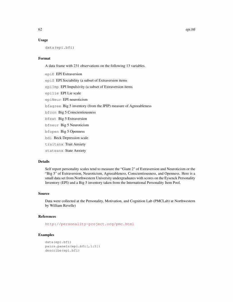
62 epi.bfi
Usage
data(epi.bfi)
Format
A data frame with 231 observations on the following 13 variables.
epiE EPI Extraversion
epiS EPI Sociability (a subset of Extraversion items
epiImp EPI Impulsivity (a subset of Extraversion items
epilie EPI Lie scale
epiNeur EPI neuroticism
bfagree Big 5 inventory (from the IPIP) measure of Agreeableness
bfcon Big 5 Conscientiousness
bfext Big 5 Extraversion
bfneur Big 5 Neuroticism
bfopen Big 5 Openness
bdi Beck Depression scale
traitanx Trait Anxiety
stateanx State Anxiety
Details
Self report personality scales tend to measure the “Giant 2" of Extraversion and Neuroticism or the“Big 5" of Extraversion, Neuroticism, Agreeableness, Conscientiousness, and Openness. Here is asmall data set from Northwestern University undergraduates with scores on the Eysenck PersonalityInventory (EPI) and a Big 5 inventory taken from the International Personality Item Pool.
Source
Data were collected at the Personality, Motivation, and Cognition Lab (PMCLab) at Northwesternby William Revelle)
References
http://personality-project.org/pmc.html
Examples
data(epi.bfi)pairs.panels(epi.bfi[,1:5])describe(epi.bfi)

error.bars 63
error.bars Plot means and confidence intervals
Description
One of the many functions in R to plot means and confidence intervals. Can be done using barplotsif desired. Can also be combined with such functions as boxplot to summarize distributions. Meansand standard errors are calculated from the raw data using describe. Alternatively, plots ofmeans +/- one standard deviation may be drawn.
Usage
error.bars(x,stats=NULL, ylab = "Dependent Variable",xlab="Independent Variable", main=NULL, ylim = NULL, alpha=.05,sd=FALSE, labels = NULL, pos = NULL, arrow.len = 0.05,arrow.col="black", add = FALSE,bars=FALSE,within=FALSE, ...)
Arguments
x A data frame or matrix of raw data
stats Alternatively, a data.frame of descriptive stats from (e.g., describe)
ylab y label
xlab x label
main title for figure
ylim if specified, the limits for the plot, otherwise based upon the data
alpha alpha level of confidence interval – defaults to 95% confidence interval
sd if TRUE, draw one standard deviation instead of standard errors at the alphalevel
labels X axis label
pos where to place text: below, left, above, right
arrow.len How long should the top of the error bars be?
arrow.col What color should the error bars be?
add add=FALSE, new plot, add=TRUE, just points and error bars
bars bars=TRUE will draw a bar graph if you really want to do that
within should the error variance of a variable be corrected by 1-SMC?
... other parameters to pass to the plot function, e.g., typ="b" to draw lines, lty="dashed"to draw dashed lines
Details
Drawing the mean +/- a confidence interval is a frequently used function when reporting experi-mental results. By default, the confidence interval is 1.96 standard errors.
If within=TRUE, the error bars are corrected for the correlation with the other variables by reducingthe variance by a factor of (1-smc). This allows for comparisons between variables.

64 error.bars
The error bars are normally calculated from the data using the describe function. If, alternatively,a matrix of statistics is provided with column headings of values, means, and se, then those valueswill be used for the plot (using the stats option).
If sd is TRUE, then the error bars will represent one standard deviation from the mean rather thanbe a function of alpha and the standard errors.
Value
Graphic output showing the means + x
These confidence regions are based upon normal theory and do not take into account any skew inthe variables. More accurate confidence intervals could be found by resampling.
Author(s)
William Revelle
See Also
error.crosses for two way error bars, error.bars.by for error bars for different groups
In addition, as pointed out by Jim Lemon on the R-help news group, error bars or confidenceintervals may be drawn using
function packagebar.err (agricolae)plotCI (gplots)xYplot (Hmisc)dispersion (plotrix)plotCI (plotrix)
For advice why not to draw bar graphs with error bars, see http://biostat.mc.vanderbilt.edu/wiki/Main/DynamitePlots
Examples
x <- replicate(20,rnorm(50))boxplot(x,notch=TRUE,main="Notched boxplot with error bars")error.bars(x,add=TRUE)abline(h=0)
error.bars(attitude,alpha=.5,main="50 percent confidence limits") #another exampleerror.bars(attitude,bar=TRUE) #show the use of bar graphs
#combine with a strip chart and boxplotstripchart(attitude,vertical=TRUE,method="jitter",jitter=.1,pch=19,main="Stripchart with 95 percent confidence limits")boxplot(attitude,add=TRUE)error.bars(attitude,add=TRUE,arrow.len=.2)

error.bars.by 65
#use statistics from somewhere elsemy.stats <- data.frame(values=c(1,4,8),means=c(10,12,18),se=c(2,3,5))error.bars(stats=my.stats,type="b",main="data with confidence intervals")
#use describe and then plot the resultsds <- describe(attitude)error.bars(stats=ds)
error.bars.by Plot means and confidence intervals for multiple groups
Description
One of the many functions in R to plot means and confidence intervals. Meant mainly for demon-stration purposes for showing the probabilty of replication from multiple samples. Can also becombined with such functions as boxplot to summarize distributions. Means and standard errors foreach group are calculated using describe.by.
Usage
error.bars.by(x,group,by.var=FALSE,x.cat=TRUE,ylab =NULL,xlab=NULL,main=NULL,ylim= NULL, alpha=.05,sd=FALSE, labels=NULL,pos=NULL,arrow.len=.05,add=FALSE,bars=FALSE,within=FALSE,colors=c("black","blue","red"),lty=NULL,...)
Arguments
x A data frame or matrixgroup A grouping variableby.var A different line for each group (default) or each variablex.cat Is the grouping variable categorical (TRUE) or continuous (FALSEylab y labelxlab x labelmain title for figureylim if specified, the limits for the plot, otherwise based upon the dataalpha alpha level of confidence interval. Default is 1- alpha =95% confidence intervalsd sd=TRUE will plot Standard Deviations instead of standard errorslabels X axis labelpos where to place text: below, left, above, rightarrow.len How long should the top of the error bars be?add add=FALSE, new plot, add=TRUE, just points and error barsbars Draw a barplot with error bars rather than a simple plot of the meanswithin Should the s.e. be corrected by the correlation with the other variables?colors groups will be plotted in different colors (mod n.groups)lty line type may be specified in the case of not plotting by variables... other parameters to pass to the plot function, e.g., typ="b" to draw lines, lty="dashed"
to draw dashed lines

66 error.crosses
Details
Drawing the mean +/- a confidence interval is a frequently used function when reporting experi-mental results. By default, the confidence interval is 1.96 standard errors.
This function was originally just a wrapper for error.bars but has been written to allow groupsto be organized either as the x axis or as separate lines.
If desired, a barplot with error bars can be shown. Many find this type of plot to be uninformative(e.g., http://biostat.mc.vanderbilt.edu/DynamitePlots )
Value
Graphic output showing the means + x% confidence intervals for each group. For ci=1.96, andnormal data, this will be the 95% confidence region. For ci=1, the 68% confidence region.
These confidence regions are based upon normal theory and do not take into account any skew inthe variables. More accurate confidence intervals could be found by resampling.
See Also
See Also as error.crosses, error.bars
Examples
data(sat.act)error.bars.by(sat.act[1:4],sat.act$gender)error.bars.by(sat.act[5:6],sat.act$gender,bars=TRUE,labels=c("male","female"),main="SAT V and SAT Q by gender") #draw a barplot
error.bars.by(sat.act[5:6],sat.act$education,bars=TRUE,xlab="Education",main="95 percent confidence limits of Sat V and Sat Q")
error.bars.by(sat.act[5:6],sat.act$education,TRUE, xlab="Education") #plot SAT V and SAT Q by education
error.crosses Plot x and y error bars
Description
Given two vectors of data, plot the means and show standard errors in both X and Y directions.
Usage
error.crosses(x,y,labels=NULL,main=NULL,xlim=NULL,ylim= NULL,xlab=NULL,ylab=NULL,pos=NULL,offset=1,arrow.len=.2,alpha=.05,sd=FALSE,...)
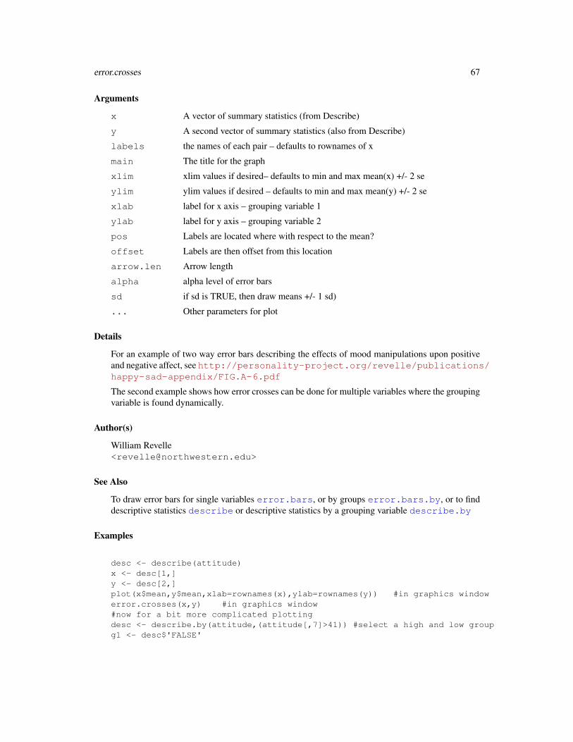
error.crosses 67
Arguments
x A vector of summary statistics (from Describe)
y A second vector of summary statistics (also from Describe)
labels the names of each pair – defaults to rownames of x
main The title for the graph
xlim xlim values if desired– defaults to min and max mean(x) +/- 2 se
ylim ylim values if desired – defaults to min and max mean(y) +/- 2 se
xlab label for x axis – grouping variable 1
ylab label for y axis – grouping variable 2
pos Labels are located where with respect to the mean?
offset Labels are then offset from this location
arrow.len Arrow length
alpha alpha level of error bars
sd if sd is TRUE, then draw means +/- 1 sd)
... Other parameters for plot
Details
For an example of two way error bars describing the effects of mood manipulations upon positiveand negative affect, see http://personality-project.org/revelle/publications/happy-sad-appendix/FIG.A-6.pdf
The second example shows how error crosses can be done for multiple variables where the groupingvariable is found dynamically.
Author(s)
William Revelle<[email protected]>
See Also
To draw error bars for single variables error.bars, or by groups error.bars.by, or to finddescriptive statistics describe or descriptive statistics by a grouping variable describe.by
Examples
desc <- describe(attitude)x <- desc[1,]y <- desc[2,]plot(x$mean,y$mean,xlab=rownames(x),ylab=rownames(y)) #in graphics windowerror.crosses(x,y) #in graphics window#now for a bit more complicated plottingdesc <- describe.by(attitude,(attitude[,7]>41)) #select a high and low groupg1 <- desc$'FALSE'

68 fa
g2 <- desc$'TRUE'plot(g1$mean,g2$mean,xlab = "Low Advance",ylab="High Advance",xlim=c(30,80),ylim=c(50,80))error.crosses(g1,g2,labels=rownames(g1),pos=rep(1,7))title("Attitudes grouped by high and low scores on Advance")
fa MinRes (minimum residual) Factor analysis as well as Factor Analysisby Principal Axis, Weighted Least Squares or Maximum Likelihood
Description
Among the many ways to do latent variable factor analysis, one of the better is to use Ordinary LeastSquares to find the minimum residual (minres) solution. This produces solutions very similar tomaximum likelihood even for badly behaved matrices. A variation on minres is to do weighted leastsquares. Perhaps the most conventional technique is principal axes. An eigen value decompositionof a correlation matrix is done and then the communalities for each variable are estimated by the firstn factors. These communalities are entered onto the diagonal and the procedure is repeated untilthe sum(diag(r)) does not vary. Yet another estimate procedure is maximum likelihood. For wellbehaved matrices, maximum likelihood factor analysis (either in the fa or in the factanal fuction) isprobably preferred.
Usage
fa(r,nfactors=1,n.obs = NA, rotate="oblimin", scores=FALSE, residuals=FALSE, SMC=TRUE, covar=FALSE,missing=FALSE,impute="median",min.err = 0.001, max.iter = 50,symmetric=TRUE,warnings=TRUE,fm="minres",alpha=.1, ...)
factor.pa(r, nfactors=1, residuals = FALSE, rotate = "varimax",n.obs = NA,scores = FALSE,SMC=TRUE, missing=FALSE,impute="median",min.err = 0.001, digits = 2, max.iter = 50,symmetric=TRUE,warnings=TRUE,fm="pa")
factor.minres(r, nfactors=1, residuals = FALSE, rotate = "varimax",n.obs = NA,scores = FALSE,SMC=TRUE, missing=FALSE,impute="median",min.err = 0.001, digits = 2, max.iter = 50,symmetric=TRUE,warnings=TRUE,fm="minres")
factor.wls(r,nfactors=1,residuals=FALSE,rotate="varimax",n.obs = NA,scores=FALSE,SMC=TRUE,missing=FALSE,impute="median", min.err = .001,digits=2,max.iter=50,symmetric=TRUE,warnings=TRUE,fm="wls")
Arguments
r A correlation matrix or a raw data matrix. If raw data, the correlation matrixwill be found using pairwise deletion.
nfactors Number of factors to extract, default is 1
n.obs Number of observations used to find the correlation matrix if using a correlationmatrix. Used for finding the goodness of fit statistics.
rotate "none", "varimax", "quartimax", "bentlerT", and "geominT" are orthogonal ro-tations. "promax", "oblimin", "simplimax", "bentlerQ, and "geominQ" or "clus-ter" are possible rotations or transformations of the solution. The default is todo a oblimin transformation, although prior versions defaulted to varimax.

fa 69
residuals Should the residual matrix be shown
scores If TRUE, estimate factor scores
SMC Use squared multiple correlations (SMC=TRUE) or use 1 as initial communalityestimate. Try using 1 if imaginary eigen values are reported.
covar if covar is TRUE, factor the covariance matrix, otherwise factor the correlationmatrix
missing if scores are TRUE, and missing=TRUE, then impute missing values using eitherthe median or the mean
impute "median" or "mean" values are used to replace missing values
min.err Iterate until the change in communalities is less than min.err
digits How many digits of output should be returned– deprecated – now specified inthe print function
max.iter Maximum number of iterations for convergence
symmetric symmetric=TRUE forces symmetry by just looking at the lower off diagonalvalues
warnings warnings=TRUE => warn if number of factors is too many
fm factoring method fm="minres" will do a minimum residual (OLS), fm="wls"will do a weighted least squares (WLS) solution, fm="gls" does a generalizedweighted least squares (GLS), fm="pa" will do the principal factor solution,fm="ml" will do a maximum likelihood factor analysis
alpha alpha level for the confidence intervals for RMSEA
... additional parameters, specifically, keys may be passed if using the target rota-tion, or delta if using geominQ, or whether to normalize if using Varimax
Details
Factor analysis is an attempt to approximate a correlation or covariance matrix with one of lesserrank. The basic model is that nRn ≈n FkkF ′n + U2 where k is much less than n. There are manyways to do factor analysis, and maximum likelihood procedures are probably the most preferred (seefactanal ). The existence of uniquenesses is what distinguishes factor analysis from principalcomponents analysis (e.g., principal). If variables are thought to represent a “true" or latent partthen factor analysis provides an estimate of the correlations with the latent factor(s) representing thedata. If variables are thought to be measured without error, then principal components provides themost parsimonious description of the data.
The fa function will do factor analyses using one of four different algorithms: minimum residual(minres), principal axes, weighted least squares, or maximum likelihood.
Principal axes factor analysis has a long history in exploratory analysis and is a straightforwardprocedure. Successive eigen value decompositions are done on a correlation matrix with the diag-onal replaced with diag (FF’) until sum(diag(FF’)) does not change (very much). The current limitof max.iter =50 seems to work for most problems, but the Holzinger-Harmon 24 variable problemneeds about 203 iterations to converge for a 5 factor solution.
Principal axes may be used in cases when maximum likelihood solutions fail to converge.
A problem in factor analysis is to find the best estimate of the original communalities. Using theSquared Multiple Correlation (SMC) for each variable will underestimate the communalities, using
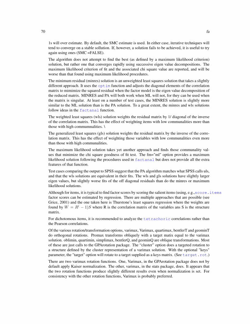
70 fa
1s will over estimate. By default, the SMC estimate is used. In either case, iterative techniques willtend to converge on a stable sollution. If, however, a solution fails to be achieved, it is useful to tryagain using ones (SMC =FALSE).
The algorithm does not attempt to find the best (as defined by a maximum likelihood criterion)solution, but rather one that converges rapidly using successive eigen value decompositions. Themaximum likelihood criterion of fit and the associated chi square value are reported, and will beworse than that found using maximum likelihood procedures.
The minimum residual (minres) solution is an unweighted least squares solution that takes a slightlydifferent approach. It uses the optim function and adjusts the diagonal elements of the correlationmatrix to mimimize the squared residual when the factor model is the eigen value decomposition ofthe reduced matrix. MINRES and PA will both work when ML will not, for they can be used whenthe matrix is singular. At least on a number of test cases, the MINRES solution is slightly moresimilar to the ML solution than is the PA solution. To a great extent, the minres and wls solutionsfollow ideas in the factanal function.
The weighted least squares (wls) solution weights the residual matrix by 1/ diagonal of the inverseof the correlation matrix. This has the effect of weighting items with low communalities more thanthose with high commumnalities. \
The generalized least squares (gls) solution weights the residual matrix by the inverse of the corre-lation matrix. This has the effect of weighting those variables with low communalities even morethan those with high communalities.
The maximum likelihood solution takes yet another approach and finds those communality val-ues that minimize the chi square goodness of fit test. The fm="ml" option provides a maximumlikelihood solution following the procedures used in factanal but does not provide all the extrafeatures of that function.
Test cases comparing the output to SPSS suggest that the PA algorithm matches what SPSS calls uls,and that the wls solutions are equivalent in their fits. The wls and gls solutions have slightly largereigen values, but slightly worse fits of the off diagonal residuals than do the minres or maximumlikelihood solutions.
Although for items, it is typical to find factor scores by scoring the salient items (using, e.g.,score.itemsfactor scores can be estimated by regression. There are multiple approaches that are possible (seeGrice, 2001) and the one taken here is Thurstone’s least squares regression where the weights arefound by W = R( − 1)S where R is the correlation matrix of the variables ans S is the structurematrix.
For dichotomous items, it is recommended to analyze the tetrachoric correlations rather thanthe Pearson correlations.
Of the various rotation/transformation options, varimax, Varimax, quartimax, bentlerT and geominTdo orthogonal rotations. Promax transforms obliquely with a target matix equal to the varimaxsolution. oblimin, quartimin, simplimax, bentlerQ, and geominQ are oblique transformations. Mostof these are just calls to the GPArotation package. The “cluster” option does a targeted rotation toa structure defined by the cluster representation of a varimax solution. With the optional "keys"parameter, the "target" option will rotate to a target supplied as a keys matrix. (See target.rot.)
There are two varimax rotation functions. One, Varimax, in the GPArotation package does not bydefault apply Kaiser normalization. The other, varimax, in the stats package, does. It appears thatthe two rotation functions produce slightly different results even when normalization is set. Forconsistency with the other rotation functions, Varimax is probably preferred.

fa 71
Value
values Eigen values of the common factor solution
e.values Eigen values of the original matrix
communality Communality estimates for each item. These are merely the sum of squaredfactor loadings for that item.
rotation which rotation was requested?
n.obs number of observations specified or found
loadings An item by factor loading matrix of class “loadings" Suitable for use in otherprograms (e.g., GPA rotation or factor2cluster. To show these by sorted order,use print.psych with sort=TRUE
fit How well does the factor model reproduce the correlation matrix. This is justΣr2ij−Σr∗2ij
Σr2ij
(See VSS, ICLUST, and principal for this fit statistic.
fit.off how well are the off diagonal elements reproduced?
dof Degrees of Freedom for this model. This is the number of observed correlationsminus the number of independent parameters. Let n=Number of items, nf =number of factors thendof = n ∗ (n− 1)/2− n ∗ nf + nf ∗ (nf − 1)/2
objective value of the function that is minimized by maximum likelihood procedures. Thisis reported for comparison purposes and as a way to estimate chi square good-ness of fit. The objective function isf = log(trace((FF ′ + U2)−1R)− log(|(FF ′ + U2)−1R|)− n.items.
STATISTIC If the number of observations is specified or found, this is a chi square basedupon the objective function, f. Using the formula from factanal(which seemsto be Bartlett’s test) :χ2 = (n.obs− 1− (2 ∗ p+ 5)/6− (2 ∗ factors)/3)) ∗ f
PVAL If n.obs > 0, then what is the probability of observing a chisquare this large orlarger?
Phi If oblique rotations (using oblimin from the GPArotation package or promax)are requested, what is the interfactor correlation.
communality.iterationsThe history of the communality estimates (For principal axis only.) Probablyonly useful for teaching what happens in the process of iterative fitting.
residual If residuals are requested, this is the matrix of residual correlations after thefactor model is applied.
rms This is the sum of the squared (off diagonal residuals) divided by the degreesof freedom. Comparable to an RMSEA which, because it is based upon χ2,requires the number of observations to be specified. The rms is an empiricalvalue while the RMSEA is based upon normal theory and the non-central χ2
distribution.
TLI The Tucker Lewis Index of factoring reliability which is also known as the non-normed fit index.
BIC Based upon χ2

72 fa
R2 The multiple R square between the factors and factor score estimates, if theywere to be found. (From Grice, 2001). Derived from R2 is is the minimumcorrelation between any two factor estimates = 2R2-1.
r.scores The correlations of the factor score estimates, if they were to be found.
weights The beta weights to find the factor score estimates
valid The validity coffiecient of course coded (unit weighted) factor score estimates(From Grice, 2001)
score.cor The correlation matrix of course coded (unit weighted) factor score estimates, ifthey were to be found, based upon the loadings matrix rather than the weightsmatrix.
Note
Thanks to Erich Studerus for some very helpful suggestions about various rotation and factor scor-ing algorithms, and to Gumundur Arnkelsson for suggestions about factor scores for singular ma-trices.
Author(s)
William Revelle
References
Gorsuch, Richard, (1983) Factor Analysis. Lawrence Erlebaum Associates.
Grice, James W. (2001), Computing and evaluating factor scores. Psychological Methods, 6, 430-450
Harman, Harry and Jones, Wayne (1966) Factor analysis by minimizing residuals (minres), Psy-chometrika, 31, 3, 351-368.
Revelle, William. (in prep) An introduction to psychometric theory with applications in R. Springer.Working draft available at http://personality-project.org/r/book/
See Also
principal, VSS, ICLUST
Examples
#using the Harman 24 mental tests, compare a principal factor with a principal components solutionpc <- principal(Harman74.cor$cov,4,rotate="varimax")pa <- fa(Harman74.cor$cov,4,fm="pa" ,rotate="varimax") #principal axisuls <- fa(Harman74.cor$cov,4,rotate="varimax") #unweighted least squares is minreswls <- fa(Harman74.cor$cov,4,fm="wls") #weighted least squares
#to show the loadings sorted by absolute valueprint(uls,sort=TRUE)
#then compare with a maximum likelihood solution using factanalmle <- factanal(covmat=Harman74.cor$cov,factors=4)

fa.diagram 73
factor.congruence(list(mle,pa,pc,uls,wls))#note that the order of factors and the sign of some of factors differ
#finally, compare the unrotated factor, ml, uls, and wls solutionswls <- factor.wls(Harman74.cor$cov,4,rotate="none")pa <- factor.pa(Harman74.cor$cov,4,rotate="none")mle <- factanal(factors=4,covmat=Harman74.cor$cov,rotation="none")uls <- factor.minres(Harman74.cor$cov,4,rotate="none")
factor.congruence(list(mle,pa,uls,wls))#note that the order of factors and the sign of some of factors differ
#an example of where the ML and PA and MR models differ is found in Thurstone.33.#compare the first two factors with the 3 factor solutiondata(bifactor)Thurstone.33 <- as.matrix(Thurstone.33)mle2 <- factanal(covmat=Thurstone.33,factors=2,rotation="none")mle3 <- factanal(covmat=Thurstone.33,factors=3 ,rotation="none")pa2 <- factor.pa(Thurstone.33,2,rotate="none")pa3 <- factor.pa(Thurstone.33,3,rotate="none")mr2 <- fa(Thurstone.33,2,rotate="none")mr3 <- fa(Thurstone.33,3,rotate="none")factor.congruence(list(mle2,mle3,pa2,pa3,mr2,mr3))
fa.diagram Graph factor loading matrices
Description
Factor analysis or principal components analysis results are typically interpreted in terms of themajor loadings on each factor. These structures may be represented as a table of loadings or graph-ically, where all loadings with an absolute value > some cut point are represented as an edge (path).
Usage
fa.diagram(fa.results,Phi=NULL,sort=TRUE,labels=NULL,cut=.3,simple=TRUE,errors=FALSE,digits=1,e.size=.05,rsize=.15,side=2,main="Factor Analysis",cex=NULL, ...)
fa.graph(fa.results,out.file=NULL,labels=NULL,cut=.3,simple=TRUE,size=c(8,6), node.font=c("Helvetica", 14),edge.font=c("Helvetica", 10), rank.direction=c("RL","TB","LR","BT"), digits=1,main="Factor Analysis",graphviz=TRUE, ...)
Arguments
fa.results The output of factor analysis, principal components analysis, or ICLUST analy-sis. May also be a factor loading matrix from anywhere.

74 fa.diagram
Phi Normally not specified (it is is found in the FA, pc, or ICLUST, solution), thismay be given if the input is a loadings matrix.
out.file If it exists, a dot representation of the graph will be stored here (fa.graph)
labels Variable labels
cut Loadings with abs(loading) > cut will be shown
simple Only the biggest loading per item is shown
size graph size
sort sort the factor loadings before showing the diagram
errors include error estimates (as arrows)
e.size size of ellipses
rsize size of rectangles
side on which side should error arrows go?
cex modify font size
node.font what font should be used for nodes in fa.graph
edge.font what font should be used for edges in fa.graphrank.direction
parameter passed to Rgraphviz– which way to draw the graph
digits Number of digits to show as an edgelable
main Graphic title
graphviz Should we try to use Rgraphviz for output?
... other parameters
Details
Path diagram representations have become standard in confirmatory factor analysis, but are notyet common in exploratory factor analysis. Representing factor structures graphically helps somepeople understand the structure.
fa.diagram does not use Rgraphviz and is the preferred function.
In fa.graph, although a nice graph is drawn for the orthogonal factor case, the oblique factor drawingis acceptable, but is better if cleaned up outside of R or done using fa.diagram.
The normal input is taken from the output of either fa or ICLUST. It is also possible to just givea factor loading matrix as input. In this case, supplying a Phi matrix of factor correlations is alsopossible.
To specify the model for a structural equation confirmatory analysis of the results, use structure.diagraminstead.
Value
fa.diagram: A path diagram is drawn without using Rgraphviz. This is probably the more usefulfunction.
fa.graph: A graph is drawn using rgraphviz. If an output file is specified, the graph instructions arealso saved in the dot language.
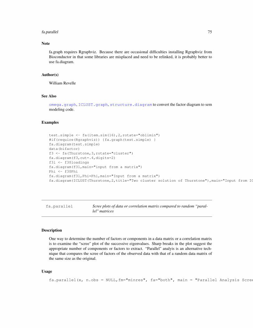
fa.parallel 75
Note
fa.graph requires Rgraphviz. Because there are occasional difficulties installing Rgraphviz fromBioconductor in that some libraries are misplaced and need to be relinked, it is probably better touse fa.diagram.
Author(s)
William Revelle
See Also
omega.graph, ICLUST.graph, structure.diagram to convert the factor diagram to semmodeling code.
Examples
test.simple <- fa(item.sim(16),2,rotate="oblimin")#if(require(Rgraphviz)) {fa.graph(test.simple) }fa.diagram(test.simple)data(bifactor)f3 <- fa(Thurstone,3,rotate="cluster")fa.diagram(f3,cut=.4,digits=2)f3l <- f3$loadingsfa.diagram(f3l,main="input from a matrix")Phi <- f3$Phifa.diagram(f3l,Phi=Phi,main="Input from a matrix")fa.diagram(ICLUST(Thurstone,2,title="Two cluster solution of Thurstone"),main="Input from ICLUST")
fa.parallel Scree plots of data or correlation matrix compared to random “paral-lel" matrices
Description
One way to determine the number of factors or components in a data matrix or a correlation matrixis to examine the “scree" plot of the successive eigenvalues. Sharp breaks in the plot suggest theappropriate number of components or factors to extract. “Parallel" analyis is an alternative tech-nique that compares the scree of factors of the observed data with that of a random data matrix ofthe same size as the original.
Usage
fa.parallel(x, n.obs = NULL,fm="minres", fa="both", main = "Parallel Analysis Scree Plots",ntrials=20,error.bars=FALSE,smc=FALSE,ylabel=NULL,show.legend=TRUE)

76 fa.parallel
Arguments
x A data.frame or data matrix of scores. If the matrix is square, it is assumed tobe a correlation matrix. Otherwise, correlations (with pairwise deletion) will befound
n.obs n.obs=0 implies a data matrix/data.frame. Otherwise, how many cases wereused to find the correlations.
fm What factor method to use. (minres, ml, uls, wls, gls, pa) See fa for details.fa show the eigen values for a principal components (fa="pc") or a principal axis
factor analysis (fa="fa") or both principal components and principal factors (fa="both")main a title for the analysisntrials Number of simulated analyses to performerror.bars Should error.bars be plotted (default = FALSE)smc smc=TRUE finds eigen values after estimating communalities by using SMCs.
smc = FALSE finds eigen values after estimating communalities with the firstfactor.
ylabel Label for the y axis – defaults to “eigen values of factors and components", canbe made empty to show many graphs
show.legend the default is to have a legend. For multiple panel graphs, it is better to not showthe legend
Details
Cattell’s “scree" test is one of most simple tests for the number of factors problem. Horn’s (1965)“parallel" analysis is an equally compelling procedure. Other procedures for determining the mostoptimal number of factors include finding the Very Simple Structure (VSS) criterion (VSS) andVelicer’s MAP procedure (included in VSS). fa.parallel plots the eigen values for a principal compo-nents and the factor solution (minres by default) and does the same for random matrices of the samesize as the original data matrix. For raw data, the random matrices are 1) a matrix of univariatenormal data and 2) random samples (randomized across rows) of the original data.
The means of (ntrials) random solutions are shown. Error bars are usually very small and aresuppressed by default but can be shown if requested.
Alternative ways to estimate the number of factors problem are discussed in the Very Simple Struc-ture (Revelle and Rocklin, 1979) documentation (VSS) and include Wayne Velicer’s MAP algorithm(Veicer, 1976).
Parallel analysis for factors is actually harder than it seems, for the question is what are the appro-priate communalities to use. If communalities are estimated by the Squared Multiple Correlation(SMC) smc, then the eigen values of the original data will reflect major as well as minor factors(see sim.minor to simulate such data). Random data will not, of course, have any structure andthus the number of factors will tend to be biased upwards by the presence of the minor factors.
By default, fa.parallel estimates the communalities based upon a one factor minres solution. Al-though this will underestimate the communalities, it does seem to lead to better solutions on simu-lated or real (e.g., the bfi or Harman74) data sets.
For comparability with other algorithms (e.g, the paran function in the paran package), settingsmc=TRUE will use smcs as estimates of communalities. This will tend towards identifying morefactors than the default option.

fa.parallel 77
Value
A plot of the eigen values for the original data, ntrials of resampling of the original data, and of aequivalent size matrix of random normal deviates. If the data are a correlation matrix, specify thenumber of observations.
Also returned (invisibly) are:
fa.values The eigen values of the factor model for the real data.
fa.sim The descriptive statistics of the simulated factor models.
pc.values The eigen values of a principal components of the real data.
pc.sim The descriptive statistics of the simulated principal components analysis.
nfact Number of factors with eigen values > eigen values of random data
ncomp Number of components with eigen values > eigen values of random data
Printing the results will show the eigen values of the original data that are greater than simulatedvalues.
Author(s)
William Revelle
References
Floyd, Frank J. and Widaman, Keith. F (1995) Factor analysis in the development and refinementof clinical assessment instruments. Psychological Assessment, 7(3):286-299, 1995.
Horn, John (1965) A rationale and test for the number of factors in factor analysis. Psychometrika,30, 179-185.
Humphreys, Lloyd G. and Montanelli, Richard G. (1975), An investigation of the parallel analysiscriterion for determining the number of common factors. Multivariate Behavioral Research, 10,193-205.
Revelle, William and Rocklin, Tom (1979) Very simple structure - alternative procedure for estimat-ing the optimal number of interpretable factors. Multivariate Behavioral Research, 14(4):403-414.
Velicer, Wayne. (1976) Determining the number of components from the matrix of partial correla-tions. Psychometrika, 41(3):321-327, 1976.
See Also
fa, VSS, VSS.plot, VSS.parallel, sim.minor
Examples
test.data <- Harman74.cor$covfa.parallel(test.data,n.obs=145)set.seed(123)minor <- sim.minor(24,4,400) #4 large and 12 minor factorsfa.parallel(minor$observed) #shows 4 factors -- compare withfa.parallel(minor$observed,smc=TRUE) #which shows 8 factors
78 fa.sort
fa.sort Sort factor analysis or principal components analysis loadings
Description
Although the print.psych function will sort factor analysis loadings, sometimes it is useful to do thisoutside of the print function. fa.sort takes the output from the fa or principal functions and sorts theloadings for each factor. Items are located in terms of their greatest loading.
Usage
fa.sort(fa.results)
Arguments
fa.results The output from a factor analysis or principal components analysis using fa orprincipal.
Details
The fa.results$loadings are replaced with sorted loadings.
Value
A sorted factor analysis, principal components analysis, or omega loadings matrix.
These sorted values are used internally by the various diagram functions.
Author(s)
William Revelle
See Also
See Also as fa,print.psych, fa.diagram,
Examples
test.simple <- fa(item.sim(16),2,rotate="oblimin")fa.sort(test.simple)
factor.congruence 79
factor.congruence Coefficient of factor congruence
Description
Given two sets of factor loadings, report their degree of congruence (vector cosine).
Usage
factor.congruence(x, y=NULL,digits=2)
Arguments
x A matrix of factor loadings or a list of matrices of factor loadings
y A second matrix of factor loadings (if x is a list, then y may be empty)
digits Round off to digits
Details
Find the coefficient of factor congruence between two sets of factor loadings.
Factor congruences are the cosines of pairs of vectors defined by the loadings matrix and based atthe origin. Thus, for loadings that differ only by a scaler (e.g. the size of the eigen value), the factorcongruences will be 1.
It is an interesting exercise to compare factor congruences with the correlations of factor loadings.Factor congruences are based upon the raw cross products, while correlations are based upon cen-tered cross products. That is, correlations of factor loadings are cosines of the vectors based at themean loading for each factor.
Input may either be matrices or factor analysis or principal components analyis output (which in-cludes a loadings object), or a mixture of the two.
To compare more than two solutions, x may be a list of matrices, all of which will be compared.
Value
A matrix of factor congruences.
Author(s)
<[email protected]>http://personality-project.org/revelle.html
References
Gorsuch, Richard, (1983) Factor Analysis. Lawrence Erlebaum Associates.Revelle, W. (In preparation) An Introduction to Psychometric Theory with applications in R (http://personality-project.org/r/book/)
80 factor.fit
See Also
principal, factor.pa
Examples
#fa <- factanal(x,4,covmat=Harman74.cor$cov)#pc <- principal(Harman74.cor$cov,4)#pa <- factor.pa(Harman74.cov$cor,4)#factor.congruence(fa,pc)## Factor1 Factor2 Factor3 Factor4#PC1 1.00 0.60 0.45 0.55#PC2 0.44 0.49 1.00 0.56#PC3 0.54 0.99 0.44 0.55#PC4 0.47 0.52 0.48 0.99
# pa <- factor.pa(Harman74.cor$cov,4)# factor.congruence(fa,pa)# PA1 PA3 PA2 PA4#Factor1 1.00 0.61 0.46 0.55#Factor2 0.61 1.00 0.50 0.60#Factor3 0.46 0.50 1.00 0.57#Factor4 0.56 0.62 0.58 1.00
#compare with#round(cor(fa$loading,pc$loading),2)
factor.fit How well does the factor model fit a correlation matrix. Part of theVSS package
Description
The basic factor or principal components model is that a correlation or covariance matrix may bereproduced by the product of a factor loading matrix times its transpose: F’F or P’P. One simpleindex of fit is the 1 - sum squared residuals/sum squared original correlations. This fit index is usedby VSS, ICLUST, etc.
Usage
factor.fit(r, f)
Arguments
r a correlation matrix
f A factor matrix of loadings.

factor.model 81
Details
There are probably as many fit indices as there are psychometricians. This fit is a plausible estimateof the amount of reduction in a correlation matrix given a factor model. Note that it is sensitive tothe size of the original correlations. That is, if the residuals are small but the original correlationsare small, that is a bad fit.
Value
fit
Author(s)
William Revelle
See Also
VSS, ICLUST
Examples
## Not run:#compare the fit of 4 to 3 factors for the Harman 24 variablesfa4 <- factanal(x,4,covmat=Harman74.cor$cov)round(factor.fit(Harman74.cor$cov,fa4$loading),2)#[1] 0.9fa3 <- factanal(x,3,covmat=Harman74.cor$cov)round(factor.fit(Harman74.cor$cov,fa3$loading),2)#[1] 0.88
## End(Not run)
factor.model Find R = F F’ + U2 is the basic factor model
Description
The basic factor or principal components model is that a correlation or covariance matrix may bereproduced by the product of a factor loading matrix times its transpose. Find this reproducedmatrix. Used by factor.fit, VSS, ICLUST, etc.
Usage
factor.model(f,Phi=NULL,U2=TRUE)

82 factor.residuals
Arguments
f A matrix of loadings.
Phi A matrix of factor correlations
U2 Should the diagonal be model by ff’ (U2 = TRUE) or replaced with 1’s (U2 =FALSE)
Value
A correlation or covariance matrix.
Author(s)
<[email protected] >http://personality-project.org/revelle.html
References
Gorsuch, Richard, (1983) Factor Analysis. Lawrence Erlebaum Associates.Revelle, W. In preparation) An Introduction to Psychometric Theory with applications in R (http://personality-project.org/r/book/)
See Also
ICLUST.graph,ICLUST.cluster, cluster.fit , VSS, omega
Examples
f2 <- matrix(c(.9,.8,.7,rep(0,6),.6,.7,.8),ncol=2)mod <- factor.model(f2)round(mod,2)
factor.residuals R* = R- F F’
Description
The basic factor or principal components model is that a correlation or covariance matrix may bereproduced by the product of a factor loading matrix times its transpose. Find the residuals of theoriginal minus the reproduced matrix. Used by factor.fit, VSS, ICLUST, etc.
Usage
factor.residuals(r, f)
factor.rotate 83
Arguments
r A correlation matrix
f A factor model matrix or a list of class loadings
Details
The basic factor equation is nRn ≈n FkkF ′n + U2. Residuals are just R* = R - F’F. The residualsshould be (but in practice probably rarely are) examined to understand the adequacy of the factoranalysis. When doing Factor analysis or Principal Components analysis, one usually continues toextract factors/components until the residuals do not differ from those expected from a randommatrix.
Value
rstar is the residual correlation matrix.
Author(s)
Maintainer: William Revelle <[email protected]>
See Also
factor.pa, principal, VSS, ICLUST
Examples
fa2 <- factor.pa(Harman74.cor$cov,2,rotate=TRUE)fa2resid <- factor.residuals(Harman74.cor$cov,fa2)fa2resid[1:4,1:4] #residuals with two factors extractedfa4 <- factor.pa(Harman74.cor$cov,4,rotate=TRUE)fa4resid <- factor.residuals(Harman74.cor$cov,fa4)fa4resid[1:4,1:4] #residuals with 4 factors extracted
factor.rotate “Hand" rotate a factor loading matrix
Description
Given a factor or components matrix, it is sometimes useful to do arbitrary rotations of particularpairs of variables. This supplements the much more powerful rotation package GPArotation and ismeant for specific requirements to do unusual rotations.
Usage
factor.rotate(f, angle, col1=1, col2=2,plot=FALSE,...)

84 factor.rotate
Arguments
f original loading matrix or a data frame (can be output from a factor analysisfunction
angle angle (in degrees!) to rotate
col1 column in factor matrix defining the first variable
col2 column in factor matrix defining the second variable
plot plot the original (unrotated) and rotated factors
... parameters to pass to factor.plot
Details
Partly meant as a demonstration of how rotation works, factor.rotate is useful for those cases thatrequire specific rotations that are not available in more advanced packages such as GPArotation. Ifthe plot option is set to TRUE, then the original axes are shown as dashed lines.
The rotation is in degrees counter clockwise.
Value
the resulting rotated matrix of loadings.
Note
For a complete rotation package, see GPArotation
Author(s)
Maintainer: William Revelle <[email protected] >
References
http://personality-project.org/r/book
Examples
#using the Harman 24 mental tests, rotate the 2nd and 3rd factors 45 degreesf4<- fa(Harman74.cor$cov,4,rotate="TRUE")f4r45 <- factor.rotate(f4,45,2,3)f4r90 <- factor.rotate(f4r45,45,2,3)print(factor.congruence(f4,f4r45),digits=3) #poor congruence with originalprint(factor.congruence(f4,f4r90),digits=3) #factor 2 and 3 have been exchanged and 3 flipped
#a graphic exampledata(Harman23.cor)f2 <- fa(Harman23.cor$cov,2,rotate="none")op <- par(mfrow=c(1,2))cluster.plot(f2,xlim=c(-1,1),ylim=c(-1,1),title="Unrotated ")f2r <- factor.rotate(f2,-33,plot=TRUE,xlim=c(-1,1),ylim=c(-1,1),title="rotated -33 degrees")

factor.stats 85
op <- par(mfrow=c(1,1))
factor.stats Find various goodness of fit statistics for factor analysis and principalcomponents
Description
Chi square and other goodness of fit statistics are found based upon the fit of a factor or componentsmodel to a correlation matrix. Although these statistics are normally associated with a maximumlikelihood solution, they can be found for minimal residual (OLS), principal axis, or principal com-ponent solutions as well. Primarily called from within these functions, factor.stats can be used byitself. Measures of factorial adequacy and validity follow the paper by Grice, 2001.
Usage
factor.stats(r, f, phi=NULL, n.obs = NA,alpha=.1)factor.scores(x,f)
Arguments
r A correlation matrix or a data frame of raw data
x A data frame or matrix of raw data
f A factor analysis loadings matrix or the output from a factor or principal com-ponents analysis
phi A factor intercorrelation matrix if the factor solution was oblique
n.obs The number of observations for the correlation matrix. If not specified, and acorrelation matrix is used, chi square will not be reported. Not needed if theinput is a data matrix.
alpha alpha level of confidence intervals for RMSEA
Details
Combines the goodness of fit tests used in factor.pa, factor.minres, and principal into one function.If the matrix is singular, will smooth the correlation matrix before finding the fit functions. Nowwill find the RMSEA (root mean square error of approximation) and the alpha confidence intervalssimilar to a SEM function. Also reports the root mean square residual.
Value
fit How well does the factor model reproduce the correlation matrix. (See VSS,ICLUST, and principal for this fit statistic.
fit.off how well are the off diagonal elements reproduced?

86 factor.stats
dof Degrees of Freedom for this model. This is the number of observed correlationsminus the number of independent parameters. Let n=Number of items, nf =number of factors thendof = n ∗ (n− 1)/2− n ∗ nf + nf ∗ (nf − 1)/2
objective value of the function that is minimized by maximum likelihood procedures. Thisis reported for comparison purposes and as a way to estimate chi square good-ness of fit. The objective function isf = log(trace((FF ′ + U2)−1R)− log(|(FF ′ + U2)−1R|)− n.items.
STATISTIC If the number of observations is specified or found, this is a chi square basedupon the objective function, f. Using the formula from factanal(which seemsto be Bartlett’s test) :χ2 = (n.obs− 1− (2 ∗ p+ 5)/6− (2 ∗ factors)/3)) ∗ f
PVAL If n.obs > 0, then what is the probability of observing a chisquare this large orlarger?
Phi If oblique rotations (using oblimin from the GPArotation package or promax)are requested, what is the interfactor correlation.
R2 The multiple R square between the factors and factor score estimates, if theywere to be found. (From Grice, 2001)
r.scores The correlations of the factor score estimates, if they were to be found.
weights The beta weights to find the factor score estimates
valid The validity coffiecient of course coded (unit weighted) factor score estimates(From Grice, 2001)
score.cor The correlation matrix of course coded (unit weighted) factor score estimates, ifthey were to be found, based upon the loadings matrix.
RMSEA The Root Mean Square Error of Approximation and the alpha confidence inter-vals. Based upon the chi square non-centrality parameter.
rms The empirically found square root of the squared residuals. This does not requiresample size to be specified nor does it make assumptions about normality.
crms While the rms uses the number of correlations to find the average, the crms usesthe number of degrees of freedom. Thus, there is a subtle penalty for having toocomplex a model.
Author(s)
William Revelle
References
Grice, James W.,2001, Computing and evaluating factor scores, Psychological Methods, 6,4, 430-450.
See Also
factor.pa for principal axis factor analysis, factor.minres for minimum residual factoranalysis, and principal for principal components.
factor2cluster 87
Examples
v9 <- sim.hierarchical()f3 <- factor.minres(v9,3)factor.stats(v9,f3,n.obs=500)f3o <- factor.pa(v9,3,rotate="Promax")factor.stats(v9,f3o,n.obs=500)
factor2cluster Extract cluster definitions from factor loadings
Description
Given a factor or principal components loading matrix, assign each item to a cluster correspondingto the largest (signed) factor loading for that item. Essentially, this is a Very Simple Structureapproach to cluster definition that corresponds to what most people actually do: highlight the largestloading for each item and ignore the rest.
Usage
factor2cluster(loads, cut = 0)
Arguments
loads either a matrix of loadings, or the result of a factor analysis/principal compo-nents analyis with a loading component
cut Extract items with absolute loadings > cut
Details
A factor/principal components analysis loading matrix is converted to a cluster (-1,0,1) definitionmatrix where each item is assigned to one and only one cluster. This is a fast way to extractitems that will be unit weighted to form cluster composites. Use this function in combination withcluster.cor to find the corrleations of these composite scores.
A typical use in the SAPA project is to form item composites by clustering or factoring (seeICLUST, principal), extract the clusters from these results (factor2cluster), and thenform the composite correlation matrix using cluster.cor. The variables in this reduced matrixmay then be used in multiple R procedures using mat.regress.
The input may be a matrix of item loadings, or the output from a factor analysis which includes aloadings matrix.
Value
a matrix of -1,0,1 cluster definitions for each item.
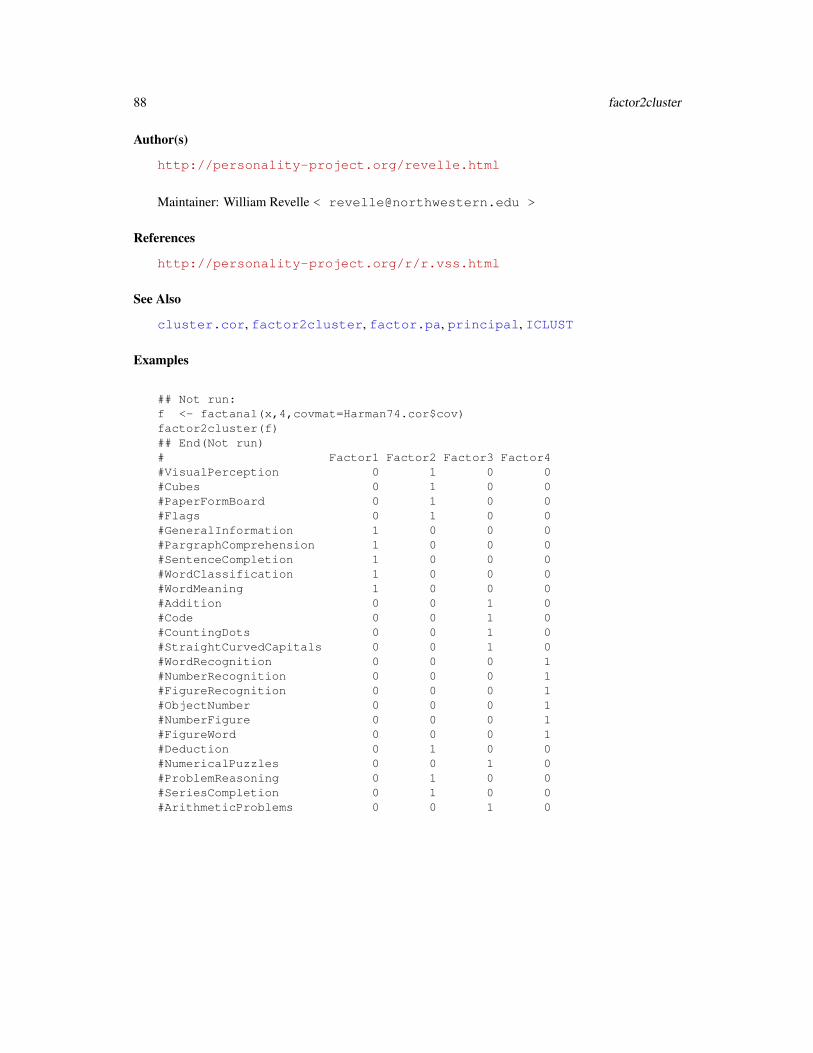
88 factor2cluster
Author(s)
http://personality-project.org/revelle.html
Maintainer: William Revelle < [email protected] >
References
http://personality-project.org/r/r.vss.html
See Also
cluster.cor, factor2cluster, factor.pa, principal, ICLUST
Examples
## Not run:f <- factanal(x,4,covmat=Harman74.cor$cov)factor2cluster(f)## End(Not run)# Factor1 Factor2 Factor3 Factor4#VisualPerception 0 1 0 0#Cubes 0 1 0 0#PaperFormBoard 0 1 0 0#Flags 0 1 0 0#GeneralInformation 1 0 0 0#PargraphComprehension 1 0 0 0#SentenceCompletion 1 0 0 0#WordClassification 1 0 0 0#WordMeaning 1 0 0 0#Addition 0 0 1 0#Code 0 0 1 0#CountingDots 0 0 1 0#StraightCurvedCapitals 0 0 1 0#WordRecognition 0 0 0 1#NumberRecognition 0 0 0 1#FigureRecognition 0 0 0 1#ObjectNumber 0 0 0 1#NumberFigure 0 0 0 1#FigureWord 0 0 0 1#Deduction 0 1 0 0#NumericalPuzzles 0 0 1 0#ProblemReasoning 0 1 0 0#SeriesCompletion 0 1 0 0#ArithmeticProblems 0 0 1 0

fisherz 89
fisherz Fisher r to z and z to r and confidence intervals
Description
convert a correlation to a z score or z to r using the Fisher transformation or find the confidenceintervals for a specified correlation
Usage
fisherz(rho)fisherz2r(z)r.con(rho,n,p=.95,twotailed=TRUE)r2t(rho,n)
Arguments
rho a Pearson r
z A Fisher z
n Sample size for confidence intervals
p Confidence interval
twotailed Treat p as twotailed p
Value
z value corresponding to r (fisherz) \ r corresponding to z (fisherz2r) \ lower and upper p confidenceintervals (r.con) \ t with n-2 df (r2t)
Author(s)
Maintainer: William Revelle <[email protected] >
Examples
cors <- seq(-.9,.9,.1)zs <- fisherz(cors)rs <- fisherz2r(zs)round(zs,2)n <- 30r <- seq(0,.9,.1)rc <- matrix(r.con(r,n),ncol=2)
t <- r*sqrt(n-2)/sqrt(1-r^2)p <- (1-pt(t,n-2))/2r.rc <- r.rc <- data.frame(r=r,z=fisherz(r),lower=rc[,1],upper=rc[,2],t=t,p=p)round(r.rc,2)

90 galton
galton Galton’s Mid parent child height data
Description
Two of the earliest examples of the correlation coefficient were Francis Galton’s data sets on therelationship between mid parent and child height and the similarity of parent generation peas withchild peas. This is the data set for the Galton height.
Usage
data(galton)
Format
A data frame with 928 observations on the following 2 variables.
parent Mid Parent heights (in inches)
child Child Height
Details
Female heights were adjusted by 1.08 to compensate for sex differences. (This was done in theoriginal data set)
Source
This is just the galton data set from UsingR, slightly rearranged.
References
Stigler, S. M. (1999). Statistics on the Table: The History of Statistical Concepts and Methods.Harvard University Press. Galton, F. (1869). Hereditary Genius: An Inquiry into its Laws and Con-sequences. London: Macmillan.
Wachsmuth, A.W., Wilkinson L., Dallal G.E. (2003). Galton’s bend: A previously undiscoverednonlinearity in Galton’s family stature regression data. The American Statistician, 57, 190-1922.
See Also
The other Galton data sets: heights, peas,cubits
Examples
data(galton)describe(galton)pairs.panels(galton,main="Galton's Parent child heights") #show the scatter plot and the lowess fitpairs.panels(galton,lm=TRUE,main="Galton's Parent child heights") #but this makes the regression lines look the samepairs.panels(galton,lm=TRUE,xlim=c(62,74),ylim=c(62,74),main="Galton's Parent child heights") #better is to scale them
geometric.mean 91
geometric.mean Find the geometric mean of a vector or columns of a data.frame.
Description
The geometric mean is the nth root of n products or e to the mean log of x. Useful for describingnon-normal, i.e., geometric distributions.
Usage
geometric.mean(x,na.rm=TRUE)
Arguments
x a vector or data.framena.rm remove NA values before processing
Details
Useful for teaching how to write functions, also useful for showing the different ways of estimatingcentral tendency.
Value
geometric mean(s) of x or x.df.
Note
Not particularly useful if there are elements that are <= 0.
Author(s)
William Revelle
See Also
harmonic.mean, mean
Examples
x <- seq(1,5)x2 <- x^2x2[2] <- NAX <- data.frame(x,x2)geometric.mean(x)geometric.mean(x2)geometric.mean(X)geometric.mean(X,na.rm=FALSE)

92 glb.algebraic
glb.algebraic Find the greatest lower bound to reliability.
Description
The greatest lower bound solves the “educational testing problem". That is, what is the reliabilityof a test? (See guttman for a discussion of the problem). Although there are many estimates of atest reliability (Guttman, 1945) most underestimate the true reliability of a test.
For a given covariance matrix of items, C, the function finds the greatest lower bound to reliabilityof the total score using the csdp function from the Rcsdp package.
Usage
glb.algebraic(Cov, LoBounds = NULL, UpBounds = NULL)
Arguments
Cov A p * p covariance matrix. Positive definiteness is not checked.
LoBounds A vector l = (l1, . . . , lp) of length p with lower bounds to the diagonal elementsxi. The default l=(0, . . . , 0) does not imply any constraint, because positivesemidefiniteness of the matrix C̃ +Diag(x) implies 0 ≤ xi
UpBounds A vector u =(u1, . . . , up) of length p with upper bounds to the diagonalelements xi. The default is u = v.
Details
If C is a p * p-covariance matrix, v = diag(C) its diagonal (i. e. the vector of variances vi = cii),C̃ = C −Diag(v) is the covariance matrix with 0s substituted in the diagonal and x = the vectorx1, . . . , xn the educational testing problem is (see e. g., Al-Homidan 2008)
p∑i=1
xi → min
s.t.C̃ +Diag(x) ≥ 0
(i.e. positive semidefinite) and xi ≤ vi, i = 1, . . . , p. This is the same as minimizing the trace ofthe symmetric matrix
C̃ + diag(x) =
x1 c12 . . . c1pc12 x2 . . . c2p...
.... . .
...c1p c2p . . . xp
s. t. C̃ +Diag(x) is positive semidefinite and xi ≤ vi.

glb.algebraic 93
The greatest lower bound to reliability is∑ij c̄ij +
∑i xi∑
ij cij
Additionally, function glb.algebraic allows the user to change the upper bounds xi ≤ vi to xi ≤ uiand add lower bounds li ≤ xi.The greatest lower bound to reliability is applicable for tests with non-homogeneous items. It givesa sharp lower bound to the reliability of the total test score.
Caution: Though glb.algebraic gives exact lower bounds for exact covariance matrices, the esti-mates from empirical matrices may be strongly biased upwards for small and medium sample sizes.
glb.algebraic is wrapper for a call to function csdp of package Rcsdp (see its documentation).
If Cov is the covariance matrix of subtests/items with known lower bounds, rel, to their reliabilities(e. g. Cronbachs α), LoBounds can be used to improve the lower bound to reliability by settingLoBounds <- rel*diag(Cov).
Changing UpBounds can be used to relax constraints xi ≤ vi or to fix xi-values by setting LoBounds[i]< -z; UpBounds[i] <- z.
Value
glb The algebraic greatest lower bound
solution The vector x of the solution of the semidefinite program. These are the elementson the diagonal of C.
status Status of the solution. See documentation of csdp in package Rcsdp. If status is2 or greater or equal than 4, no glb and solution is returned. If status is not 0, awarning message is generated.
Call The calling string
Author(s)
Andreas MoltnerCenter of Excellence for Assessment in Medicine/Baden-WurttembergUniversity of Heidelberg
William RevelleDepartment of PsychologyNorthwestern University Evanston, Illinioishttp://personality-project.org/revelle.html
References
Al-Homidan S (2008). Semidefinite programming for the educational testing problem. CentralEuropean Journal of Operations Research, 16:239-249.
Bentler PM (1972) A lower-bound method for the dimension-free measurement of internal consis-tency. Soc Sci Res 1:343-357.

94 guttman
Fletcher R (1981) A nonlinear programming problem in statistics (educational testing). SIAM J SciStat Comput 2:257-267.
Shapiro A, ten Berge JMF (2000). The asymptotic bias of minimum trace factor analysis, withapplications to the greatest lower bound to reliability. Psychometrika, 65:413-425.
ten Berge, Socan G (2004). The greatest bound to reliability of a test and the hypothesis of unidi-mensionality. Psychometrika, 69:613-625.
See Also
For an alternative estimate of the greatest lower bound, see glb.fa. For multiple estimates ofreliablity, see guttman
Examples
Cv<-matrix(c(215, 64, 33, 22,64, 97, 57, 25,33, 57,103, 36,22, 25, 36, 77),ncol=4)
Cv # covariance matrix of a test with 4 subtestsCr<-cov2cor(Cv) # Correlation matrix of testsif(require(Rcsdp)) {glb.algebraic(Cv)} # glb of total scoreif(require(Rcsdp)) {glb.algebraic(Cr) } # glb of sum of standardized scores
w<-c(1,2,2,1) # glb of weighted total score# glb.algebraic(diag(w) %*% Cv %*% diag(w))alphas <- c(0.8,0,0,0) # Internal consistency of first test is knownif(require(Rcsdp)) {glb.algebraic(Cv,LoBounds=alphas*diag(Cv))}
# Fix all diagonal elements to 1 but the first:if(require(Rcsdp)) {lb<-glb.algebraic(Cr,LoBounds=c(0,1,1,1),UpBounds=c(1,1,1,1))lb$solution[1] # should be the same as the squared mult. corr.smc(Cr)[1]
} else {print ('I am sorry, you need to have the package Rcsdp installed to use glb.algebraic') }
guttman Alternative estimates of test reliabiity
Description
Eight alternative estimates of test reliability include the six discussed by Guttman (1945), fourdiscussed by ten Berge and Zergers (1978) (µ0 . . . µ3) as well as β (the worst split half, Revelle,1979), the glb (greatest lowest bound) discussed by Bentler and Woodward (1980), and ωh and ωt(McDonald, 1999; Zinbarg et al., 2005).

guttman 95
Usage
guttman(r,key=NULL)tenberge(r)glb(r,key=NULL)glb.fa(r,key=NULL)
Arguments
r A correlation matrix or raw data matrix.
key a vector of -1, 0, 1 to select or reverse items
Details
Surprisingly, 105 years after Spearman (1904) introduced the concept of reliability to psychologists,there are still multiple approaches for measuring it. Although very popular, Cronbach’s α (1951)underestimates the reliability of a test and over estimates the first factor saturation. The guttmanfunction includes the six estimates discussed by Guttman (1945), four of ten Berge and Zergers(1978), as well as Revelle’s β (1979) using ICLUST. The companion function, omega calculatesomega hierarchical (ωh) and omega total (ωt).
Guttman’s first estimate λ1 assumes that all the variance of an item is error:
λ1 = 1− tr( ~Vx)Vx
=Vx − tr(~Vx)
Vx
This is a clear underestimate.
The second bound, λ2, replaces the diagonal with a function of the square root of the sums ofsquares of the off diagonal elements. Let C2 = ~1(~V − diag(~V )2~1′, then
λ2 = λ1 +
√nn−1C2
Vx=Vx − tr(~Vx) +
√nn−1C2
Vx
Effectively, this is replacing the diagonal with n * the square root of the average squared off diagonalelement.
Guttman’s 3rd lower bound, λ3, also modifies λ1 and estimates the true variance of each item as theaverage covariance between items and is, of course, the same as Cronbach’s α.
λ3 = λ1 +VX−tr(~VX)n(n−1)
VX=
nλ1
n− 1=
n
n− 1
(1− tr(~V )x
Vx
)=
n
n− 1Vx − tr(~Vx)
Vx= α
This is just replacing the diagonal elements with the average off diagonal elements. λ2 ≥ λ3 withλ2 > λ3 if the covariances are not identical.
λ3 and λ2 are both corrections to λ1 and this correction may be generalized as an infinite set ofsuccessive improvements. (Ten Berge and Zegers, 1978)
µr =1Vx
(po + (p1 + (p2 + . . . (pr−1 + (pr)1/2)1/2 . . .)1/2)1/2
), r = 0, 1, 2, . . .

96 guttman
whereph =
∑i 6=j
σ2hij , h = 0, 1, 2, . . . r − 1
andph =
n
n− 1σ2hij , h = r
tenberge and Zegers (1978). Clearly µ0 = λ3 = α and µ1 = λ2. µr ≥ µr−1 ≥ . . . µ1 ≥ µ0,although the series does not improve much after the first two steps.
Guttman’s fourth lower bound, λ4 was originally proposed as any spit half reliability but has beeninterpreted as the greatest split half reliability. If ~X is split into two parts, ~Xa and ~Xb, with corre-lation rab then
λ4 = 2(
1− VXa + VXb
VX
)=
4rabVx
=4rab
VXa+ VXb
+ 2rabVXaVXb
which is just the normal split half reliability, but in this case, of the most similar splits.
λ5, Guttman’s fifth lower bound, replaces the diagonal values with twice the square root of themaximum (across items) of the sums of squared interitem covariances
λ5 = λ1 +2√C̄2
VX.
Although superior to λ1, λ5 underestimates the correction to the diagonal. A better estimate wouldbe analogous to the correction used in λ3:
λ5+ = λ1 +n
n− 12√C̄2
VX.
Guttman’s final bound considers the amount of variance in each item that can be accounted forthe linear regression of all of the other items (the squared multiple correlation or smc), or moreprecisely, the variance of the errors, e2
j , and is
λ6 = 1−∑e2j
Vx= 1−
∑(1− r2
smc)Vx
Guttman’s λ4 is the greatest split half reliability. This is found here by combining the output fromthree different approaches, and seems to work for all test cases yet tried. Lambda 4 is reported asthe max of these three algorithms.
The algorithms are
a) Do an ICLUST of the reversed correlation matrix. ICLUST normally forms the most distinctclusters. By reversing the correlations, it will tend to find the most related clusters. Truly a weirdapproach but tends to work.
b) Alternatively, a kmeans clustering of the correlations (with the diagonal replaced with 0 to makepseudo distances) can produce 2 similar clusters.
c) Clusters identified by assigning items to two clusters based upon their order on the first principalfactor. (Highest to cluster 1, next 2 to cluster 2, etc.)

guttman 97
These three procedures will produce keys vectors for assigning items to the two splits. The max-imum split half reliability is found by taking the maximum of these three approaches. This is notelegant but is fast.
There are three greatest lower bound functions. One, glb finds the greatest split half reliability, λ4.This considers the test as set of items and examines how best to partition the items into splits. Theother two, glb.fa and glb.algebraic, are alternative ways of weighting the diagonal of thematrix.
glb.fa estimates the communalities of the variables from a factor model where the number offactors is the number with positive eigen values. Then reliability is found by
glb = 1−∑e2j
Vx= 1−
∑(1− h2)Vx
This estimate will differ slightly from that found by glb.algebraic, written by Andreas Moelt-ner which uses calls to csdp in the Rcsdp package. His algorithm, which more closely matches thedescription of the glb by Jackson and Woodhouse, seems to have a positive bias (i.e., will over esti-mate the reliability of some items; they are said to be = 1) for small sample sizes. More explorationof these two algorithms is underway.
Compared to glb.algebraic, glb.fa seems to have less (positive) bias for smallish samplesizes (n < 500) but larger for large (> 1000) sample sizes. This interacts with the number of variablesso that equal bias sample size differs as a function of the number of variables. The differences are,however small. As samples sizes grow, glb.algebraic seems to converge on the populationvalue while glb.fa has a positive bias.
Value
beta The normal beta estimate of cluster similarity from ICLUST. This is an estimateof the general factor saturation.
tenberge$mu1 tenBerge mu 1 is functionally alpha
tenberge$mu2 one of the sequence of estimates mu1 ... mu3
beta.factor For experimental purposes, what is the split half based upon the two factor so-lution?
glb.IC Greatest split half based upon ICLUST of reversed correlations
glb.Km Greatest split half based upon a kmeans clustering.
glb.Fa Greatest split half based upon the items assigned by factor analysis.
glb.max max of the above estimates
glb glb found from factor analysis
keys scoring keys from each of the alternative methods of forming best splits
Author(s)
William Revelle
98 Harman
References
Cronbach, L.J. (1951) Coefficient alpha and the internal strucuture of tests. Psychometrika, 16,297-334.
Guttman, L. (1945). A basis for analyzing test-retest reliability. Psychometrika, 10 (4), 255-282.
Revelle, W. (1979). Hierarchical cluster-analysis and the internal structure of tests. MultivariateBehavioral Research, 14 (1), 57-74.
Revelle, W. and Zinbarg, R. E. (2009) Coefficients alpha, beta, omega and the glb: comments onSijtsma. Psychometrika, 2009.
Ten Berge, J. M. F., & Zegers, F. E. (1978). A series of lower bounds to the reliability of a test.Psychometrika, 43 (4), 575-579.
Zinbarg, R. E., Revelle, W., Yovel, I., & Li, W. (2005). Cronbach’s α , Revelle’s β , and Mc-Donald’s ωh ): Their relations with each other and two alternative conceptualizations of reliability.Psychometrika, 70 (1), 123-133.
See Also
alpha, omega, ICLUST, glb.algebraic
Examples
data(attitude)glb(attitude)glb.fa(attitude)if(require(Rcsdp)) {glb.algebraic(cor(attitude)) }guttman(attitude)
Harman Two data sets from Harman (1967). 9 cognitive variables fromHolzinger and 8 emotional variables from Burt
Description
Two classic data sets reported by Harman (1967) are 9 psychological (cognitive) variables takenfrom Holzinger and 8 emotional variables taken from Burt. Both of these are used for tests anddemonstrations of various factoring algortithms.
Usage
data(Harman)

Harman 99
Details
• Harman.Holzinger: 9 x 9 correlation matrix of ability tests, N = 696.
• Harman.Burt: a 8 x 8 correlation matrix of “emotional" items. N = 172
Harman.Holzinger. The nine psychological variables from Harman (1967, p 244) are taken fromunpublished class notes of K.J. Holzinger with 696 participants. This is a subset of 12 tests with4 factors. It is yet another nice example of a bifactor solution. Bentler (2007) uses this data set todiscuss reliablity analysis. The data show a clear bifactor structure and are a nice example of thevarious estimates of reliability included in the omega function. Should not be confused with theHolzinger or Holzinger.9 data sets in bifactor.
Harman.Burt. Eight “emotional" variables are taken from Harman (1967, p 164) who in turnadapted them from Burt (1939). They are said be from 172 normal children aged nine to twelve.As pointed out by Harman, this correlation matrix is singular and has squared multiple correlations> 1. Because of this problem, it is a nice test case for various factoring algorithms. (For instance,omega will issue warning messages for fm="minres" or fm="pa" but will fail for fm="ml".)
The Burt data set probably has a typo in the original correlation matrix. Changing the Sorrow-Tenderness correlation from .87 to .81 makes the correlation positive definite.
As pointed out by Jan DeLeeuw, the Burt data set is a subset of 8 variables from the original 11reported by Burt in 1915. That matrix has the same problem. See burt.
Other example data sets that are useful demonstrations of factor analysis are the seven bifactorexamples in bifactor and the 24 ability measures in Harman74.cor
Source
Harman (1967 p 164 and p 244.)
References
Harman, Harry Horace (1967), Modern factor analysis. Chicago, University of Chicago Press.
P.Bentler. Covariance structure models for maximal reliability of unit-weighted composites. InHandbook of latent variable and related models, pages 1–17. North Holland, 2007.
Burt, C.General and Specific Factors underlying the Primary Emotions. Reports of the British As-sociation for the Advancement of Science, 85th meeting, held in Manchester, September 7-11, 1915.London, John Murray, 1916, p. 694-696 (retrieved from the web at http://www.biodiversitylibrary.org/item/95822#790)
See Also
See also the original burt data set
Examples
data(Harman)cor.plot(Harman.Holzinger)cor.plot(Harman.Burt)smc(Harman.Burt) #note how this produces impossible results
100 harmonic.mean
harmonic.mean Find the harmonic mean of a vector, matrix, or columns of adata.frame
Description
The harmonic mean is merely the reciprocal of the arithmetic mean of the reciprocals.
Usage
harmonic.mean(x,na.rm=TRUE)
Arguments
x a vector, matrix, or data.frame
na.rm na.rm=TRUE remove NA values before processing
Details
Included as an example for teaching about functions. As well as for a discussion of how to estimatecentral tendencies.
Value
The harmonic mean(s)
Note
Included as a simple demonstration of how to write a function
Examples
x <- seq(1,5)x2 <- x^2x2[2] <- NAX <- data.frame(x,x2)harmonic.mean(x)harmonic.mean(x2)harmonic.mean(X)harmonic.mean(X,FALSE)
headtail 101
headtail Combine calls to head and tail
Description
A quick way to show the first and last n lines of a data.frame, matrix, or a text object. Just a prettycall to head and tail
Usage
headtail(x,hlength=4,tlength=4,digits=2)
Arguments
x A matrix or data frame or free text
hlength The number of lines at the beginning to show
tlength The number of lines at the end to show
digits Round off the data to digits
Value
The first hlength and last tlength lines of a matrix or data frame with an ellipsis in between. If theinput is neither a matrix nor data frame, the output will be the first hlength and last tlength lines.
See Also
head and tail
Examples
x <- matrix(sample(10,1000,TRUE),ncol=5)headtail(x,4,8)
heights A data.frame of the Galton (1888) height and cubit data set.
Description
Francis Galton introduced the ’co-relation’ in 1888 with a paper discussing how to measure therelationship between two variables. His primary example was the relationship between height andforearm length. The data table (cubits) is taken from Galton (1888). Unfortunately, there seemto be some errors in the original data table in that the marginal totals do not match the table.
The data frame, heights, is converted from this table using table2df.

102 ICC
Usage
data(heights)
Format
A data frame with 348 observations on the following 2 variables.
height Height in inches
cubit Forearm length in inches
Details
Sir Francis Galton (1888) published the first demonstration of the correlation coefficient. The re-gression (or reversion to mediocrity) of the height to the length of the left forearm (a cubit) wasfound to .8. The original table cubits is taken from Galton (1888). There seem to be some errorsin the table as published in that the row sums do not agree with the actual row sums. These data areused to create a matrix using table2matrix for demonstrations of analysis and displays of thedata.
Source
Galton (1888)
References
Galton, Francis (1888) Co-relations and their measurement. Proceedings of the Royal Society.London Series,45,135-145,
See Also
table2matrix, table2df, cubits, ellipses, galton
Examples
data(heights)ellipses(heights,n=1,main="Galton's co-relation data set")
ICC Intraclass Correlations (ICC1, ICC2, ICC3 from Shrout and Fleiss)
Description
The Intraclass correlation is used as a measure of association when studying the reliability of raters.Shrout and Fleiss (1979) outline 6 different estimates, that depend upon the particular experimentaldesign. All are implemented and given confidence limits.

ICC 103
Usage
ICC(x,missing=TRUE,digits=2,alpha=.05)
Arguments
x a matrix or dataframe of ratings
missing if TRUE, remove missing data – work on complete cases only
digits Round the output to digits
alpha The alpha level for significance for finding the confidence intervals
Details
Shrout and Fleiss (1979) consider six cases of reliability of ratings done by k raters on n targets.
ICC1: Each target is rated by a different judge and the judges are selected at random. (This is aone-way ANOVA fixed effects model and is found by (MSB- MSW)/(MSB+ (nr-1)*MSW))
ICC2: A random sample of k judges rate each target. The measure is one of absolute agreement inthe ratings. Found as (MSB- MSE)/(MSB + (nr-1)*MSE + nr*(MSJ-MSE)/nc)
ICC3: A fixed set of k judges rate each target. There is no generalization to a larger population ofjudges. (MSB - MSE)/(MSB+ (nr-1)*MSE)
Then, for each of these cases, is reliability to be estimated for a single rating or for the average ofk ratings? (The 1 rating case is equivalent to the average intercorrelation, the k rating case to theSpearman Brown adjusted reliability.)
ICC1 is sensitive to differences in means between raters and is a measure of absolute agreement.
ICC2 and ICC3 remove mean differences between judges, but are sensitive to interactions of ratersby judges. The difference between ICC2 and ICC3 is whether raters are seen as fixed or randomeffects.
ICC1k, ICC2k, ICC3K reflect the means of k raters.
The intraclass correlation is used if raters are all of the same “class". That is, there is no logical wayof distinguishing them. Examples include correlations between pairs of twins, correlations betweenraters. If the variables are logically distinguishable (e.g., different items on a test), then the moretypical coefficient is based upon the inter-class correlation (e.g., a Pearson r) and a statistic such asalpha or omega might be used.
Value
results A matrix of 6 rows and 8 columns, including the ICCs, F test, p values, andconfidence limits
summary The anova summary table
stats The anova statistics
MSW Mean Square Within based upon the anova

104 iclust
Note
The results for the Lower and Upper Bounds for ICC(2,k) do not match those of SPSS 9 or 10,but do match the definitions of Shrout and Fleiss. SPSS seems to have been using the formula inMcGraw and Wong, but not the errata on p 390. They seem to have fixed it in more recent releases(15).
Author(s)
William Revelle
References
Shrout, Patrick E. and Fleiss, Joseph L. Intraclass correlations: uses in assessing rater reliability.Psychological Bulletin, 1979, 86, 420-3428.
McGraw, Kenneth O. and Wong, S. P. (1996), Forming inferences about some intraclass correlationcoefficients. Psychological Methods, 1, 30-46. + errata on page 390.
Revelle, W. (in prep) An introduction to psychometric theory with applications in R. Springer.(working draft available at http://personality-project.org/r/book/
Examples
sf <- matrix(c(9, 2, 5, 8,6, 1, 3, 2,8, 4, 6, 8,7, 1, 2, 6,10, 5, 6, 9,6, 2, 4, 7),ncol=4,byrow=TRUE)colnames(sf) <- paste("J",1:4,sep="")rownames(sf) <- paste("S",1:6,sep="")sf #example from Shrout and Fleiss (1979)ICC(sf)
iclust iclust: Item Cluster Analysis – Hierarchical cluster analysis using psy-chometric principles
Description
A common data reduction technique is to cluster cases (subjects). Less common, but particularlyuseful in psychological research, is to cluster items (variables). This may be thought of as analternative to factor analysis, based upon a much simpler model. The cluster model is that thecorrelations between variables reflect that each item loads on at most one cluster, and that itemsthat load on those clusters correlate as a function of their respective loadings on that cluster anditems that define different clusters correlate as a function of their respective cluster loadings and theintercluster correlations. Essentially, the cluster model is a Very Simple Structure factor model ofcomplexity one (see VSS).

iclust 105
This function applies the iclust algorithm to hierarchically cluster items to form composite scales.Clusters are combined if coefficients alpha and beta will increase in the new cluster.
Alpha, the mean split half correlation, and beta, the worst split half correlation, are estimates ofthe reliability and general factor saturation of the test. (See also the omega function to estimateMcDonald’s coeffients ωh and ωt)
Usage
iclust(r.mat, nclusters=0, alpha=3, beta=1, beta.size=4, alpha.size=3,correct=TRUE,correct.cluster=TRUE, reverse=TRUE, beta.min=.5, output=1, digits=2,labels=NULL,cut=0,n.iterations = 0,title="iclust",plot=TRUE,weighted=TRUE,cor.gen=TRUE,SMC=TRUE)ICLUST(r.mat, nclusters=0, alpha=3, beta=1, beta.size=4, alpha.size=3,correct=TRUE,correct.cluster=TRUE, reverse=TRUE, beta.min=.5, output=1, digits=2,labels=NULL,cut=0,n.iterations = 0,title="ICLUST",plot=TRUE,weighted=TRUE,cor.gen=TRUE,SMC=TRUE)
#iclust(r.mat) #use all defaults#iclust(r.mat,nclusters =3) #use all defaults and if possible stop at 3 clusters#ICLUST(r.mat, output =3) #long output shows clustering history#ICLUST(r.mat, n.iterations =3) #clean up solution by item reassignment
Arguments
r.mat A correlation matrix or data matrix/data.frame. (If r.mat is not square i.e, acorrelation matrix, the data are correlated using pairwise deletion.
nclusters Extract clusters until nclusters remain (default will extract until the other criteriaare met or 1 cluster, whichever happens first). See the discussion below foralternative techniques for specifying the number of clusters.
alpha Apply the increase in alpha criterion (0) never or for (1) the smaller, 2) theaverage, or 3) the greater of the separate alphas. (default = 3)
beta Apply the increase in beta criterion (0) never or for (1) the smaller, 2) the aver-age, or 3) the greater of the separate betas. (default =1)
beta.size Apply the beta criterion after clusters are of beta.size (default = 4)
alpha.size Apply the alpha criterion after clusters are of size alpha.size (default =3)
correct Correct correlations for reliability (default = TRUE)correct.cluster
Correct cluster -sub cluster correlations for reliability of the sub cluster , defaultis TRUE))
reverse Reverse negative keyed items (default = TRUE
beta.min Stop clustering if the beta is not greater than beta.min (default = .5)
output 1) short, 2) medium, 3 ) long output (default =1)
labels vector of item content or labels. If NULL, then the colnames are used. IfFALSE, then labels are V1 .. Vn
cut sort cluster loadings > absolute(cut) (default = 0)
n.iterations iterate the solution n.iterations times to "purify" the clusters (default = 0)
106 iclust
digits Precision of digits of output (default = 2)
title Title for this run
plot Should ICLUST.rgraph be called automatically for plotting (requires Rgraphvizdefault=TRUE)
weighted Weight the intercluster correlation by the size of the two clusters (TRUE) or donot weight them (FALSE)
cor.gen When correlating clusters with subclusters, base the correlations on the generalfactor (default) or general + group (cor.gen=FALSE)
SMC When estimating cluster-item correlations, use the smcs as the estimate of anitem communality (SMC=TRUE) or use the maximum correlation (SMC=FALSE).
Details
Extensive documentation and justification of the algorithm is available in the original MBR 1979http://personality-project.org/revelle/publications/iclust.pdf paper.Further discussion of the algorithm and sample output is available on the personality-project.orgweb page: http://personality-project.org/r/r.ICLUST.html
The results are best visualized using ICLUST.graph, the results of which can be saved as a dot filefor the Graphviz program. http://www.graphviz.org/. With the installation of Rgraphviz,ICLUST will automatically provide cluster graphs.
A common problem in the social sciences is to construct scales or composites of items to measureconstructs of theoretical interest and practical importance. This process frequently involves admin-istering a battery of items from which those that meet certain criteria are selected. These criteriamight be rational, empirical,or factorial. A similar problem is to analyze the adequacy of scalesthat already have been formed and to decide whether the putative constructs are measured properly.Both of these problems have been discussed in numerous texts, as well as in myriad articles. Pro-ponents of various methods have argued for the importance of face validity, discriminant validity,construct validity, factorial homogeneity, and theoretical importance.
Revelle (1979) proposed that hierachical cluster analysis could be used to estimate a new coefficient(beta) that was an estimate of the general factor saturation of a test. More recently, Zinbarg, Revelle,Yovel and Li (2005) compared McDonald’s Omega to Chronbach’s alpha and Revelle’s beta. Theyconclude that ωh hierarchical is the best estimate. An algorithm for estimating omega is availableas part of this package.
Revelle and Zinbarg (2009) discuss alpha, beta, and omega, as well as other estimates of reliability.
The original ICLUST program was written in FORTRAN to run on CDC and IBM mainframes andwas then modified to run in PC-DOS. The R version of iclust is a completely new version writtenfor the psych package. Please email me if you want help with this version of iclust or if you desiremore features.
A requested feature (not yet available) is to specify certain items as forming a cluster. That is, to doconfirmatory cluster analysis.
The program currently has three primary functions: cluster, loadings, and graphics.
In June, 2009, the option of weighted versus unweighted beta was introduced. Unweighted betacalculates beta based upon the correlation between two clusters, corrected for test length using theSpearman-Brown prophecy formala, while weighted beta finds the average interitem correlationbetween the items within two clusters and then finds beta from this. That is, for two clusters A and

iclust 107
B of size N and M with between average correlation rb, weighted beta is (N+M)^2 rb/(Va +Vb +2Cab). Raw (unweighted) beta is 2rab/(1+rab) where rab = Cab/sqrt(VaVb). Weighted beta seems amore appropriate estimate and is now the default. Unweighted beta is still available for consistencywith prior versions.
Also modified in June, 2009 was the way of correcting for item overlap when calculating the cluster-subcluster correlations for the graphic output. This does not affect the final cluster solution, butdoes produce slightly different path values. In addition, there are two ways to solve for the cluster -subcluster correlation.
Given the covariance between two clusters, Cab with average rab = Cab/(N*M), and cluster vari-ances Va and Vb with Va = N + N*(N-1)*ra then the correlation of cluster A with the combinedcluster AB is either
a) ((N^2)ra + Cab)/sqrt(Vab*Va) (option cor.gen=TRUE) or b) (Va - N + Nra + Cab)/sqrt(Vab*Va)(option cor.gen=FALSE)
The default is to use cor.gen=TRUE.
Although iclust will give what it thinks is the best solution in terms of the number of clusters toextract, the user will sometimes disagree. To get more clusters than the default solution, just setthe nclusters parameter to the number desired. However, to get fewer than meet the alpha and betacriteria, it is sometimes necessary to set alpha=0 and beta=0 and then set the nclusters to the desirednumber.
Clustering 24 tests of mental ability
A sample output using the 24 variable problem by Harman can be represented both graphically andin terms of the cluster order. The default is to produce graphics using the Rgraphviz package (fromBioConductor). Because this package is sometimes hard to install, there is an alternative optionto write the output out using the dot language. This will create a graphic suitable for any viewingprogram that uses the dot language. ICLUST.graph produces the dot code for Graphviz. Some-what lower resolution graphs with fewer options are available in the ICLUST.rgraph functionwhich requires Rgraphviz. Dot code can be viewed directly in Graphviz or can be tweaked usingcommercial software packages (e.g., OmniGraffle)
Note that for this problem, with the default parameters, the data form one large cluster. (This isconsistent with the Very Simple Structure (VSS) output as well, which shows a clear one factorsolution for complexity 1 data.)
An alternative solution is to ask for a somewhat more stringent set of criteria and require an increasein the size of beta for all clusters greater than 3 variables. This produces a 4 cluster solution.
It is also possible to use the original parameter settings, but ask for a 4 cluster solution.
At least for the Harman 24 mental ability measures, it is interesting to compare the cluster patternmatrix with the oblique rotation solution from a factor analysis. The factor congruence of a fourfactor oblique pattern solution with the four cluster solution is > .99 for three of the four clustersand > .97 for the fourth cluster.
To see the graphic output go to http://personality-project.org/r/r.ICLUST.htmlor use ICLUST.rgraph (requires Rgraphviz).
Value
title Name of this run

108 iclust
results A list containing the step by step cluster history, including which pair wasgrouped, what were the alpha and betas of the two groups and of the combinedgroup.Note that the alpha values are “standardized alphas” based upon the correlationmatrix, rather than the raw alphas that will come from score.items
The print.psych and summary.psych functions will print out just the must im-portant results.
corrected The raw and corrected for alpha reliability cluster intercorrelations.
clusters a matrix of -1,0, and 1 values to define cluster membership.
purified A list of the cluster definitions and cluster loadings of the purified solution.To show just the most salient items, use the cutoff option in print.psych
cluster.fit, structure.fit, pattern.fitThere are a number of ways to evaluate how well any factor or cluster matrixreproduces the original matrix. Cluster fit considers how well the clusters fit ifonly correlations with clusters are considered. Structure fit evaluates R = CC’while pattern fit evaluate R = C inverse (phi) C’ where C is the cluster loadingmatrix, and phi is the intercluster correlation matrix.
Note
iclust draws graphical displays with or without using Rgraphiviz. Rgraphviz produces slightly bettergraphics and will also export in the dot language for further massaging of the graphic. If Rgraphvizis not installed, ICLUST.graph will issue a warning message but continue. If, however, Rgraphvizis not properly installed, ICLUST.graph will think it is available, try to produce a graph, and fail(ungracefully). The solution to this problem is to specify plot=FALSE and the create graphs usingthe dot language. See the last example. With the introduction of the diagram functions, iclustnow draws using iclust.diagram which is not as pretty, but more stable.
Author(s)
William Revelle
References
Revelle, W. Hierarchical Cluster Analysis and the Internal Structure of Tests. Multivariate Behav-ioral Research, 1979, 14, 57-74.
Revelle, W. and Zinbarg, R. E. (2009) Coefficients alpha, beta, omega and the glb: comments onSijtsma. Psychometrika, 2009.
http://personality-project.org/revelle/publications/iclust.pdfSee also more extensive documentation at http://personality-project.org/r/r.ICLUST.html andRevelle, W. (in prep) An introduction to psychometric theory with applications in R. To be publishedby Springer. (working draft available at http://personality-project.org/r/book/
See Also
ICLUST.graph,ICLUST.cluster, cluster.fit , VSS, omega
ICLUST.cluster 109
Examples
test.data <- Harman74.cor$covic.out <- ICLUST(test.data)summary(ic.out)ic.out <- ICLUST(test.data,nclusters =4) #use all defaults and stop at 4 clustersic.out1 <- ICLUST(test.data,beta=3,beta.size=3) #use more stringent criteriaprint(ic.out1)plot(ic.out) #this shows the spatial representationic.no.graph <- ICLUST(test.data,plot=FALSE)dot.graph <- ICLUST.graph(ic.no.graph,out.file="test.ICLUST.graph.dot") #use a dot graphics viewer
ICLUST.cluster Function to form hierarchical cluster analysis of items
Description
The guts of the ICLUST algorithm. Called by ICLUST See ICLUST for description.
Usage
ICLUST.cluster(r.mat, ICLUST.options)
Arguments
r.mat A correlation matrixICLUST.options
A list of options (see ICLUST)
Details
See ICLUST
Value
A list of cluster statistics, described more fully in ICLUST
comp1 Description of ’comp1’
comp2 Description of ’comp2’
...
Note
Although the main code for ICLUST is here in ICLUST.cluster, the more extensive documentationis for ICLUST.

110 iclust.diagram
Author(s)
William Revelle
References
Revelle, W. 1979, Hierarchical Cluster Analysis and the Internal Structure of Tests. Multivariate Be-havioral Research, 14, 57-74. http://personality-project.org/revelle/publications/iclust.pdfSee also more extensive documentation at http://personality-project.org/r/r.ICLUST.html
See Also
ICLUST.graph,ICLUST, cluster.fit , VSS, omega
iclust.diagram Draw an ICLUST hierarchical cluster structure diagram
Description
Given a cluster structure determined by ICLUST, create a graphic structural diagram using graphicfunctions in the psych package To create dot code to describe the ICLUST output with more pre-cision, use ICLUST.graph. If Rgraphviz has been successfully installed, the alternative is to useICLUST.rgraph.
Usage
iclust.diagram(ic, labels = NULL, short = FALSE, digits = 2, cex = NULL, min.size = NULL, e.size =1,colors=c("black","blue"), main = "ICLUST diagram")
Arguments
ic Output from ICLUST
labels labels for variables (if not specified as rownames in the ICLUST output
short if short=TRUE, variable names are replaced with Vn
digits Round the path coefficients to digits accuracy
cex The standard graphic control parameter for font size modifications. This can beused to make the labels bigger or smaller than the default values.
min.size Don’t provide statistics for clusters less than min.size
e.size size of the ellipses with the cluster statistics.
colors postive and negative
main The main graphic title
Details
iclust.diagram provides most of the power of ICLUST.rgraph without the difficulties involvedin installing Rgraphviz. It is called automatically from ICLUST.

ICLUST.graph 111
Value
Graphical output summarizing the hierarchical cluster structure. The graph is drawn using thediagram functions (e.g., dia.curve, dia.arrow, dia.rect, dia.ellipse ) created as awork around to Rgraphviz.
Note
Suggestions for improving the graphic output are welcome.
Author(s)
William Revelle
References
Revelle, W. Hierarchical Cluster Analysis and the Internal Structure of Tests. Multivariate Behav-ioral Research, 1979, 14, 57-74.
See Also
ICLUST
Examples
v9 <- sim.hierarchical()v9c <- ICLUST(v9)test.data <- Harman74.cor$covic.out <- ICLUST(test.data)
ICLUST.graph create control code for ICLUST graphical output
Description
Given a cluster structure determined by ICLUST, create dot code to describe the ICLUST out-put. To use the dot code, use either http://www.graphviz.org/ Graphviz or a commercialviewer (e.g., OmniGraffle).
Usage
ICLUST.graph(ic.results, out.file,min.size=1, short = FALSE,labels=NULL,size = c(8, 6), node.font = c("Helvetica", 14), edge.font = c("Helvetica", 12),rank.direction=c("RL","TB","LR","BT"), digits = 2, title = "ICLUST", ...)

112 ICLUST.graph
Arguments
ic.results output list from ICLUST
out.file name of output file (defaults to console)
min.size draw a smaller node (without all the information) for clusters < min.size – usefulfor large problems
short if short==TRUE, don’t use variable names
labels vector of text labels (contents) for the variables
size size of output
node.font Font to use for nodes in the graph
edge.font Font to use for the labels of the arrows (edges)rank.direction
LR or RL
digits number of digits to show
title any title
... other options to pass
Details
Will create (or overwrite) an output file and print out the dot code to show a cluster structure. Thisdot file may be imported directly into a dot viewer (e.g., http://www.graphviz.org/). The"dot" language is a powerful graphic description language that is particulary appropriate for viewingcluster output. Commercial graphics programs (e.g., OmniGraffle) can also read (and clean up) dotfiles.
ICLUST.graph takes the output from ICLUST results and processes it to provide a pretty pictureof the results. Original variables shown as rectangles and ordered on the left hand side (if rankdirection is RL) of the graph. Clusters are drawn as ellipses and include the alpha, beta, and size ofthe cluster. Edges show the cluster intercorrelations.
It is possible to trim the output to not show all cluster information. Clusters < min.size are shownas small ovals without alpha, beta, and size information.
Value
Output is a set of dot commands written either to console or to the output file. These commandsmay then be used as input to any "dot" viewer, e.g., Graphviz.
Author(s)
<[email protected] >http://personality-project.org/revelle.html
References
ICLUST: http://personality-project.org/r/r.iclust.html

ICLUST.graph 113
See Also
VSS.plot, ICLUST
Examples
## Not run:test.data <- Harman74.cor$covic.out <- ICLUST(test.data)out.file <- file.choose(new=TRUE) #create a new file to write the plot commands toICLUST.graph(ic.out,out.file)now go to graphviz (outside of R) and open the out.file you createdprint(ic.out,digits=2)
## End(Not run)
#test.data <- Harman74.cor$cov#my.iclust <- ICLUST(test.data)#ICLUST.graph(my.iclust)###digraph ICLUST {# rankdir=RL;# size="8,8";# node [fontname="Helvetica" fontsize=14 shape=box, width=2];# edge [fontname="Helvetica" fontsize=12];# label = "ICLUST";# fontsize=20;#V1 [label = VisualPerception];#V2 [label = Cubes];#V3 [label = PaperFormBoard];#V4 [label = Flags];#V5 [label = GeneralInformation];#V6 [label = PargraphComprehension];#V7 [label = SentenceCompletion];#V8 [label = WordClassification];#V9 [label = WordMeaning];#V10 [label = Addition];#V11 [label = Code];#V12 [label = CountingDots];#V13 [label = StraightCurvedCapitals];#V14 [label = WordRecognition];#V15 [label = NumberRecognition];#V16 [label = FigureRecognition];#V17 [label = ObjectNumber];#V18 [label = NumberFigure];#V19 [label = FigureWord];#V20 [label = Deduction];#V21 [label = NumericalPuzzles];#V22 [label = ProblemReasoning];#V23 [label = SeriesCompletion];#V24 [label = ArithmeticProblems];

114 ICLUST.graph
#node [shape=ellipse, width ="1"];#C1-> V9 [ label = 0.78 ];#C1-> V5 [ label = 0.78 ];#C2-> V12 [ label = 0.66 ];#C2-> V10 [ label = 0.66 ];#C3-> V18 [ label = 0.53 ];#C3-> V17 [ label = 0.53 ];#C4-> V23 [ label = 0.59 ];#C4-> V20 [ label = 0.59 ];#C5-> V13 [ label = 0.61 ];#C5-> V11 [ label = 0.61 ];#C6-> V7 [ label = 0.78 ];#C6-> V6 [ label = 0.78 ];#C7-> V4 [ label = 0.55 ];#C7-> V1 [ label = 0.55 ];#C8-> V16 [ label = 0.5 ];#C8-> V14 [ label = 0.49 ];#C9-> C1 [ label = 0.86 ];#C9-> C6 [ label = 0.86 ];#C10-> C4 [ label = 0.71 ];#C10-> V22 [ label = 0.62 ];#C11-> V21 [ label = 0.56 ];#C11-> V24 [ label = 0.58 ];#C12-> C10 [ label = 0.76 ];#C12-> C11 [ label = 0.67 ];#C13-> C8 [ label = 0.61 ];#C13-> V15 [ label = 0.49 ];#C14-> C2 [ label = 0.74 ];#C14-> C5 [ label = 0.72 ];#C15-> V3 [ label = 0.48 ];#C15-> C7 [ label = 0.65 ];#C16-> V19 [ label = 0.48 ];#C16-> C3 [ label = 0.64 ];#C17-> V8 [ label = 0.62 ];#C17-> C12 [ label = 0.8 ];#C18-> C17 [ label = 0.82 ];#C18-> C15 [ label = 0.68 ];#C19-> C16 [ label = 0.66 ];#C19-> C13 [ label = 0.65 ];#C20-> C19 [ label = 0.72 ];#C20-> C18 [ label = 0.83 ];#C21-> C20 [ label = 0.87 ];#C21-> C9 [ label = 0.76 ];#C22-> 0 [ label = 0 ];#C22-> 0 [ label = 0 ];#C23-> 0 [ label = 0 ];#C23-> 0 [ label = 0 ];#C1 [label = "C1\n alpha= 0.84\n beta= 0.84\nN= 2"] ;#C2 [label = "C2\n alpha= 0.74\n beta= 0.74\nN= 2"] ;#C3 [label = "C3\n alpha= 0.62\n beta= 0.62\nN= 2"] ;#C4 [label = "C4\n alpha= 0.67\n beta= 0.67\nN= 2"] ;#C5 [label = "C5\n alpha= 0.7\n beta= 0.7\nN= 2"] ;#C6 [label = "C6\n alpha= 0.84\n beta= 0.84\nN= 2"] ;

ICLUST.rgraph 115
#C7 [label = "C7\n alpha= 0.64\n beta= 0.64\nN= 2"] ;#C8 [label = "C8\n alpha= 0.58\n beta= 0.58\nN= 2"] ;#C9 [label = "C9\n alpha= 0.9\n beta= 0.87\nN= 4"] ;#C10 [label = "C10\n alpha= 0.74\n beta= 0.71\nN= 3"] ;#C11 [label = "C11\n alpha= 0.62\n beta= 0.62\nN= 2"] ;#C12 [label = "C12\n alpha= 0.79\n beta= 0.74\nN= 5"] ;#C13 [label = "C13\n alpha= 0.64\n beta= 0.59\nN= 3"] ;#C14 [label = "C14\n alpha= 0.79\n beta= 0.74\nN= 4"] ;#C15 [label = "C15\n alpha= 0.66\n beta= 0.58\nN= 3"] ;#C16 [label = "C16\n alpha= 0.65\n beta= 0.57\nN= 3"] ;#C17 [label = "C17\n alpha= 0.81\n beta= 0.71\nN= 6"] ;#C18 [label = "C18\n alpha= 0.84\n beta= 0.75\nN= 9"] ;#C19 [label = "C19\n alpha= 0.74\n beta= 0.65\nN= 6"] ;#C20 [label = "C20\n alpha= 0.87\n beta= 0.74\nN= 15"] ;#C21 [label = "C21\n alpha= 0.9\n beta= 0.77\nN= 19"] ;#C22 [label = "C22\n alpha= 0\n beta= 0\nN= 0"] ;#C23 [label = "C23\n alpha= 0\n beta= 0\nN= 0"] ;#{ rank=same;#V1;V2;V3;V4;V5;V6;V7;V8;V9;V10;V11;V12;V13;V14;V15;V16;V17;V18;V19;V20;V21;V22;V23;V24;}}##copy the above output to Graphviz and draw it#see \url{http://personality-project.org/r/r.ICLUST.html} for an example.
ICLUST.rgraph Draw an ICLUST graph using the Rgraphviz package
Description
Given a cluster structure determined by ICLUST, create a rgraphic directly using Rgraphviz. Tocreate dot code to describe the ICLUST output with more precision, use ICLUST.graph. Asan option, dot code is also generated and saved in a file. To use the dot code, use either http://www.graphviz.org/ Graphviz or a commercial viewer (e.g., OmniGraffle).
Usage
ICLUST.rgraph(ic.results, out.file = NULL, min.size = 1, short = FALSE, labels = NULL, size = c(8, 6), node.font = c("Helvetica", 14), edge.font = c("Helvetica", 10), rank.direction=c("RL","TB","LR","BT"), digits = 2, title = "ICLUST",label.font=2, ...)
Arguments
ic.results output list from ICLUST
out.file File name to save optional dot code.
min.size draw a smaller node (without all the information) for clusters < min.size – usefulfor large problems
short if short==TRUE, don’t use variable names
labels vector of text labels (contents) for the variables
size size of output

116 ICLUST.rgraph
node.font Font to use for nodes in the graph
edge.font Font to use for the labels of the arrows (edges)rank.direction
LR or TB or RL
digits number of digits to show
title any title
label.font The variable labels can be a different size than the other nodes. This is particu-larly helpful if the number of variables is large or the labels are long.
... other options to pass
Details
Will create (or overwrite) an output file and print out the dot code to show a cluster structure. Thisdot file may be imported directly into a dot viewer (e.g., http://www.graphviz.org/). The"dot" language is a powerful graphic description language that is particulary appropriate for viewingcluster output. Commercial graphics programs (e.g., OmniGraffle) can also read (and clean up) dotfiles.
ICLUST.rgraph takes the output from ICLUST results and processes it to provide a pretty pictureof the results. Original variables shown as rectangles and ordered on the left hand side (if rankdirection is RL) of the graph. Clusters are drawn as ellipses and include the alpha, beta, and size ofthe cluster. Edges show the cluster intercorrelations.
It is possible to trim the output to not show all cluster information. Clusters < min.size are shownas small ovals without alpha, beta, and size information.
Value
Output is a set of dot commands written either to console or to the output file. These commandsmay then be used as input to any "dot" viewer, e.g., Graphviz.
ICLUST.rgraph is a version of ICLUST.graph that uses Rgraphviz to draw on the screen as well.
Additional output is drawn to main graphics screen.
Note
Requires Rgraphviz
Author(s)
<[email protected] >http://personality-project.org/revelle.html
References
ICLUST: http://personality-project.org/r/r.iclust.html
See Also
VSS.plot, ICLUST
ICLUST.sort 117
Examples
test.data <- Harman74.cor$covic.out <- ICLUST(test.data) #uses iclust.diagram instead
ICLUST.sort Sort items by absolute size of cluster loadings
Description
Given a cluster analysis or factor analysis loadings matrix, sort the items by the (absolute) size ofeach column of loadings. Used as part of ICLUST and SAPA analyses.
Usage
ICLUST.sort(ic.load, cut = 0, labels = NULL,keys=FALSE)
Arguments
ic.load The output from a factor or principal components analysis, or from ICLUST, ora matrix of loadings.
cut Do not include items in clusters with absolute loadings less than cut
labels labels for each item.
keys should cluster keys be returned? Useful if clusters scales are to be scored.
Details
When interpreting cluster or factor analysis outputs, is is useful to group the items in terms ofwhich items have their biggest loading on each factor/cluster and then to sort the items by size ofthe absolute factor loading.
A stable cluster solution will be one in which the output of these cluster definitions does not varywhen clusters are formed from the clusters so defined.
With the keys=TRUE option, the resulting cluster keys may be used to score the original data or thecorrelation matrix to form clusters from the factors.
Value
sorted A data.frame of item numbers, item contents, and item x factor loadings.
cluster A matrix of -1, 0, 1s defining each item by the factor/cluster with the row wiselargest absolute loading.
...
Note
Although part of the ICLUST set of programs, this is also more useful for factor or principal com-ponents analysis.
118 income
Author(s)
William Revelle
References
http://personality-project.org/r/r.ICLUST.html
See Also
ICLUST.graph,ICLUST.cluster, cluster.fit , VSS, factor2cluster
income US family income from US census 2008
Description
US census data on family income from 2008
Usage
data(income)
Format
A data frame with 44 observations on the following 4 variables.
value lower boundary of the income group
count Number of families within that income group
mean Mean of the category
prop proportion of families
Details
The distribution of income is a nice example of a log normal distribution. It is also an interestingexample of the power of graphics. It is quite clear when graphing the data that income statistics arebunched to the nearest 5K. That is, there is a clear sawtooth pattern in the data.
The all.income set is interpolates intervening values for 100-150K, 150-200K and 200-250K
Source
US Census: Table HINC-06. Income Distribution to $250,000 or More for Households: 2008
http://www.census.gov/hhes/www/cpstables/032009/hhinc/new06_000.htm
interp.median 119
Examples
data(income)with(income[1:40,], plot(mean,prop, main="US family income for 2008",xlab="income", ylab="Proportion of families",xlim=c(0,100000)))with (income[1:40,], points(lowess(mean,prop,f=.3),typ="l"))describe(income)
with(all.income, plot(mean,prop, main="US family income for 2008",xlab="income", ylab="Proportion of families",xlim=c(0,250000)))with (all.income[1:50,], points(lowess(mean,prop,f=.25),typ="l"))#curve(100000* dlnorm(x, 10.8, .8), x = c(0,250000),ylab="Proportion")
interp.median Find the interpolated sample median, quartiles, or specific quantilesfor a vector, matrix, or data frame
Description
For data with a limited number of response categories (e.g., attitude items), it is useful treat eachresponse category as range with width, w and linearly interpolate the median, quartiles, or anyquantile value within the median response.
Usage
interp.median(x, w = 1,na.rm=TRUE)interp.quantiles(x, q = .5, w = 1,na.rm=TRUE)interp.quartiles(x,w=1,na.rm=TRUE)interp.boxplot(x,w=1,na.rm=TRUE)interp.values(x,w=1,na.rm=TRUE)interp.qplot.by(y,x,w=1,na.rm=TRUE,xlab="group",ylab="dependent",ylim=NULL,arrow.len=.05,typ="b",add=FALSE,...)
Arguments
x input vector
q quantile to estimate ( 0 < q < 1
w category width
y input vector for interp.qplot.by
na.rm should missing values be removed
xlab x label
ylab Y label
ylim limits for the y axis
arrow.len length of arrow in interp.qplot.by
typ plot type in interp.qplot.by
add add the plot or not
... additional parameters to plotting function

120 interp.median
Details
If the total number of responses is N, with median, M, and the number of responses at the medianvalue, Nm >1, and Nb= the number of responses less than the median, then with the assumptionthat the responses are distributed uniformly within the category, the interpolated median is M - .5w+ w*(N/2 - Nb)/Nm.
The generalization to 1st, 2nd and 3rd quartiles as well as the general quantiles is straightforward.
A somewhat different generalization allows for graphic presentation of the difference between in-terpolated and non-interpolated points. This uses the interp.values function.
If the input is a matrix or data frame, quantiles are reported for each variable.
Value
im interpolated median(quantile)
v interpolated values for all data points
See Also
median
Examples
interp.median(c(1,2,3,3,3)) # compare with median = 3interp.median(c(1,2,2,5))interp.quantiles(c(1,2,2,5),.25)x <- sample(10,100,TRUE)interp.quartiles(x)#x <- c(1,1,2,2,2,3,3,3,3,4,5,1,1,1,2,2,3,3,3,3,4,5,1,1,1,2,2,3,3,3,3,4,2)y <- c(1,2,3,3,3,3,4,4,4,5,5,1,2,3,3,3,3,4,4,5,5,5,1,5,3,3,3,3,4,4,4,5,5)x <- x[order(x)] #sort the data by ascending order to make it clearery <- y[order(y)]xv <- interp.values(x)yv <- interp.values(y)barplot(x,space=0,xlab="ordinal position",ylab="value")lines(1:length(x)-.5,xv)points(c(length(x)/4,length(x)/2,3*length(x)/4),interp.quartiles(x))barplot(y,space=0,xlab="ordinal position",ylab="value")lines(1:length(y)-.5,yv)points(c(length(y)/4,length(y)/2,3*length(y)/4),interp.quartiles(y))data(galton)interp.median(galton)interp.qplot.by(galton$child,galton$parent,ylab="child height",xlab="Mid parent height")

iqitems 121
iqitems 14 multiple choice IQ items
Description
14 multiple choice ability items were included as part of the Synthetic Aperture Personality Assess-ment (SAPA) web based personality assessment project. The data from 1000 subjects are includedhere as a demonstration set for scoring multiple choice inventories and doing basic item statistics.
Usage
data(iqitems)
Format
A data frame with 1000 observations on the following 14 variables.
iq1 In the following number series, what number comes next?
iq8 Please mark the word that does not match the other words:
iq10 If you rearrange the letters ATNHIDLA, you will have the name of a:
iq15 If Jerks are Perks and some Perks are Lerks, then some Jerks are definitely Lerks. Thisstatement is:
iq20 How many total legs do two ducks and three dogs have?
iq44 Matrix reasoning 2
iq47 Matrix reasoning 5
iq2 In the following number series, what number comes next? 1 2 4 7 12
iq11 The opposite of a ’stubborn’ person is a ’ ’ person.
iq16 Zach is taller than Matt and Richard is shorter than Zach. Which of the following statementswould be most accurate?
iq32 If the day before yesterday is three days after Saturday then what day is today?
iq37 In the following alphanumeric series, what letter comes next? Q, S, N, P, L
iq43 Matrix Reasoning 1
iq49 Matrix Reasoning 9
Details
14 items were sampled from 54 items given as part of the SAPA project (Revelle, Wilt and Rosen-thal, 2009) to develop online measures of ability.
Source
http://personality-project.org

122 irt.1p
References
Revelle, William, Wilt, Joshua, and Rosenthal, Allen (2009) Personality and Cognition: The Personality-Cognition Link. In Gruszka, Alexandra and Matthews, Gerald and Szymura, Blazej (Eds.) Hand-book of Individual Differences in Cognition: Attention, Memory and Executive Control, Springer.
Examples
data(iqitems)iq.keys <- c(4,4,3,1,4,3,2,3,1,4,1,3,4,3)score.multiple.choice(iq.keys,iqitems)
irt.1p Item Response Theory estimate of theta (ability) using a Rasch (like)model
Description
Item Response Theory models individual responses to items by estimating individual ability (theta)and item difficulty (diff) parameters. This is an early and crude attempt to capture this modelingprocedure. A better procedure is to use irt.fa.
Usage
irt.person.rasch(diff, items)irt.0p(items)irt.1p(delta,items)irt.2p(delta,beta,items)
Arguments
diff A vector of item difficulties –probably taken from irt.item.diff.rasch
items A matrix of 0,1 items nrows = number of subjects, ncols = number of items
delta delta is the same as diff and is the item difficulty parameter
beta beta is the item discrimination parameter found in irt.discrim
Details
A very preliminary IRT estimation procedure. Given scores xij for ith individual on jth itemClassical Test Theory ignores item difficulty and defines ability as expected score : abilityi = theta(i)= x(i.) A zero parameter model rescales these mean scores from 0 to 1 to a quasi logistic scaleranging from - 4 to 4 This is merely a non-linear transform of the raw data to reflect a logisticmapping.
Basic 1 parameter (Rasch) model considers item difficulties (delta j): p(correct on item j for the ithsubject |theta i, deltaj) = 1/(1+exp(deltaj - thetai)) If we have estimates of item difficulty (delta),then we can find theta i by optimization

irt.fa 123
Two parameter model adds item sensitivity (beta j): p(correct on item j for subject i |thetai, deltaj,betaj) = 1/(1+exp(betaj *(deltaj- theta i))) Estimate delta, beta, and theta to maximize fit of modelto data.
The procedure used here is to first find the item difficulties assuming theta = 0 Then find theta giventhose deltas Then find beta given delta and theta.
This is not an "official" way to do IRT, but is useful for basic item development.
Value
a data.frame with estimated ability (theta) and quality of fit. (for irt.person.rasch)a data.frame with the raw means, theta0, and the number of items completed
Note
Not recommended for serious use. This code is under development. Much better functions are inthe ltm and eRm packages. Similar analyses can be done using irt.fa
Author(s)
William Revelle
See Also
sim.irt, sim.rasch, logistic, irt.fa, tetrachoric, irt.item.diff.rasch
irt.fa Item Response Analysis by factor analysis of tetrachoric/polychoriccorrelations
Description
Although factor analysis and Item Response Theory seem to be very different models of binarydata, they can provide equivalent parameter estimates of item difficulty and item discrimination.Tetrachoric correlations of a data set of dichotomous items may be factor analysed using a mini-mum residual or maximum likelihood factor analysis and the result loadings transformed to itemdiscrimination parameters. The tau parameter from the tetrachoric correlation combined with theitem factor loading may be used to estimate item difficulties. Similar analyses can be done fordiscrete item responses using the polychoric correlation.
Usage
irt.fa(x,...)
Arguments
x A data matrix of dichotomous or discrete items, or the result of tetrachoricor polychoric
... Additional parameters to pass to the factor analysis function

124 irt.fa
Details
The tetrachoric correlation matrix of dichotomous items may be factored using a (e.g.) minimumresidual factor analyis function fa and the resulting loadings, λi are transformed to discriminationsby α = λi√
1−λ2i
.
The difficulty parameter, δ may be found from the τ parameter of the tetrachoric or polychoricfunction.
δi = τi√1−λ2
i
Similar analyses may be done with discrete item responses using polychoric correlations and distinctestimates of item difficulty (location) for each item response.
The results may be shown graphically using plot. For plotting there are three options: type ="ICC" will plot the item characteristic respone function. type = "IIC" will plot the item informationfunction, and type= "test" will plot the test information function.
The normal input is just the raw data. If, however, the correlation matrix has already been foundusing tetrachoric or polychoric, then that result can be processed directly.
Value
coefficientsA data frame of Item difficulty, discrimination, tau and the factor loadings
stats A list of statistics for the factor analyis
rho The tetrachoric/polychoric correlation matrix
Note
Still under development. Comments welcome
Author(s)
William Revelle
References
McDonald, Roderick P. (1999) Test theory: A unified treatment. L. Erlbaum Associates.
Revelle, William. (in prep) An introduction to psychometric theory with applications in R. Springer.Working draft available at http://personality-project.org/r/book/
See Also
fa, sim.irt, tetrachoric, polychoric as well as plot.psych for plotting the IRT itemcurves.
irt.item.diff.rasch 125
Examples
set.seed(17)d9 <- sim.irt(9,1000,-2.5,2.5,mod="normal") #dichotomous itemstest <- irt.fa(d9$items)testop <- par(mfrow=c(3,1))plot(test,type="ICC")plot(test,type="IIC")plot(test,type="test")par(op)set.seed(17)items <- sim.congeneric(N=500,short=FALSE,categorical=TRUE) #500 responses to 4 discrete itemsd4 <- irt.fa(items$observed) #item response analysis of congeneric measures
op <- par(mfrow=c(2,2))plot(d4,type="ICC")par(op)
irt.item.diff.raschSimple function to estimate item difficulties using IRT concepts
Description
Steps toward a very crude and preliminary IRT program. These two functions estimate item diffi-culty and discrimination parameters. A better procedure is to use irt.fa or the ltm package.
Usage
irt.item.diff.rasch(items)irt.discrim(item.diff,theta,items)
Arguments
items a matrix of items
item.diff a vector of item difficulties (found by irt.item.diff)
theta ability estimate from irt.person.theta
Details
Item Response Theory (aka "The new psychometrics") models individual responses to items with alogistic function and an individual (theta) and item difficulty (diff) parameter.
irt.item.diff.rasch finds item difficulties with the assumption of theta=0 for all subjects and that allitems are equally discriminating.
126 logistic
irt.discrim takes those difficulties and theta estimates from irt.person.rasch to find itemdiscrimination (beta) parameters.
A far better package with these features is the ltm package. The IRT functions in the psych-packageare for pedagogical rather than production purposes. They are believed to be accurate, but are notguaranteed. They do seem to be slightly more robust to missing data structures associated withSAPA data sets than the ltm package.
The irt.fa function is also an alternative. This will find tetrachoric or polychoriccorrelations and then convert to IRT parameters using factor analysis (fa).
Value
a vector of item difficulties or item discriminations.
Note
Under development. Not recommended for public consumption. See irt.fa for a better option.
Author(s)
William Revelle
See Also
irt.fa, irt.person.rasch
logistic Logistic transform from x to p and logit transform from p to x
Description
The logistic function (1/(1+exp(-x)) and logit function (log(p/(1-p)) are fundamental to Item Re-sponse Theory. Although just one line functions, they are included here for ease of demonstrationsand in drawing IRT models. Also included is the logistic.grm for a graded response model.
Usage
logistic(x,d=0, a=1,c=0, z=1)logit(p)logistic.grm( x,d=0,a=1.5,c=0,z=1,r=2,s=c(-1.5,-.5,.5,1.5))
Arguments
x Any integer or real value
d Item difficulty or delta parameter
a The slope of the curve at x=0 is equivalent to the discrimination parameter in2PL models or alpha parameter. Is either 1 in 1PL or 1.702 in 1PN approxima-tions.

logistic 127
c Lower asymptote = guessing parameter in 3PL models or gamma
z The upper asymptote — in 4PL models
p Probability to be converted to logit value
r The response category for the graded response model
s The response thresholds
Details
These three functions are provided as simple helper functions for demonstrations of Item ResponseTheory. The one parameter logistic (1PL) model is also known as the Rasch model. It assumes itemsdiffer only in difficulty. 1PL, 2PL, 3PL and 4PL curves may be drawn by choosing the appropriated (delta or item difficulty), a (discrimination or slope), c (gamma or guessing) and z (zeta or upperasymptote).
logit is just the inverse of logistic.
logistic.grm will create the responses for a graded response model for the rth category where cut-points are in s.
Value
p logistic returns the probability associated with x
x logit returns the real number associated with p
Author(s)
William Revelle
Examples
curve(logistic(x,a=1.702),-3,3,ylab="Probability of x",main="Logistic transform of x",xlab="z score units") #logistic with a=1.702 is almost the same as pnormcurve(pnorm(x),add=TRUE,lty="dashed")curve(logistic(x),add=TRUE)text(2,.8, expression(alpha ==1))text(2,1.0,expression(alpha==1.7))curve(logistic(x),-4,4,ylab="Probability of x", main = "Logistic transform of x in logit units",xlab="logits")curve(logistic(x,d=-1),add=TRUE)curve(logistic(x,d=1),add=TRUE)curve(logistic(x,c=.2),add=TRUE,lty="dashed")text(1.3,.5,"d=1")text(.3,.5,"d=0")text(-1.5,.5,"d=-1")text(-3,.3,"c=.2")#demo of graded response modelcurve(logistic.grm(x,r=1),-4,4,ylim=c(0,1),main="Five level response scale",ylab="Probability of endorsement",xlab="Latent attribute on logit scale")curve(logistic.grm(x,r=2),add=TRUE)curve(logistic.grm(x,r=3),add=TRUE)curve(logistic.grm(x,r=4),add=TRUE)curve(logistic.grm(x,r=5),add=TRUE)
text(-2.,.5,1)

128 make.keys
text(-1.,.4,2)text(0,.4,3)text(1.,.4,4)text(2.,.5,5)
make.keys Create a keys matrix for use by score.items or cluster.cor
Description
When scoring items by forming composite scales either from the raw data using score.itemsor from the correlation matrix using cluster.cor, it is necessary to create a keys matrix. Thisis just a short cut for doing so. The keys matrix is a nvar x nscales matrix of -1,0, 1 and defines themembership for each scale.
Usage
make.keys(nvars, keys.list, key.labels = NULL, item.labels = NULL)
Arguments
nvars Number of variables items to be scored
keys.list A list of the scoring keys,one element for each scale
key.labels Labels for the scales can be specified here, or in the key.list
item.labels Typically, just the colnames of the items data matrix.
Details
There are two ways to create keys for the score.items function. One is to laboriously do it in aspreadsheet and then copy them into R. The other is to just specify them by item number in a list.
Value
keys a nvars x nkeys matrix of -1, 0, or 1s describing how to score each scale. nkeysis the length of the keys.list
See Also
score.items, cluster.cor
mat.regress 129
Examples
data(attitude)key.list <- list(all=c(1,2,3,4,-5,6,7),
first=c(1,2,3),last=c(4,5,6,7))
keys <- make.keys(7,key.list,item.labels = colnames(attitude))keys
scores <- score.items(keys,attitude,short=TRUE)scores
data(bfi)keys.list <- list(agree=c(-1,2:5),conscientious=c(6:8,-9,-10),extraversion=c(-11,-12,13:15),neuroticism=c(16:20),openness = c(21,-22,23,24,-25))keys <- make.keys(25,keys.list,item.labels=colnames(bfi)[1:25])scores <- score.items(keys,bfi[,1:25],short=TRUE)summary(scores)
mat.regress Multiple Regression from matrix input
Description
Extract subsets of variables (x and y) from a correlation or data matrix matrix and find the multiplecorrelation and beta weights of the (x) set predicting each member of the (y) set.
Usage
mat.regress(m, x, y,n.obs=NULL)
Arguments
m a matrix of correlations or, if not square of data
x either the column numbers of the x set (e.g., c(1,3,5) or the column names of thex set (e.g. c("Cubes","PaperFormBoard")
y either the column numbers of the y set (e.g., c(2,4,6) or the column names of they set (e.g., c("Flags","Addition")
n.obs If specified, then confidence intervals, etc. are calculated, not needed if raw dataare given
Details
Although it is more common to calculate multiple regression from raw data, it is, of course, possibleto do so from a set of correlations. The input to the function is a square covariance or correlationmatrix, as well as the column numbers (or names) of the x (predictor) and y (criterion) variables.The program will find the correlations if given raw data.
The output is a set of multiple correlations, one for each dependent variable in the y set.

130 mat.sort
A typical use in the SAPA project is to form item composites by clustering or factoring (seeICLUST, principal), extract the clusters from these results (factor2cluster), and thenform the composite correlation matrix using cluster.cor. The variables in this reduced matrixmay then be used in multiple R procedures using mat.regress.
Although the overall matrix can have missing correlations, the correlations in the subset of thematrix used for prediction must exist.
If the number of observations is entered, then the conventional confidence intervals, statistical sig-nificance, and shrinkage estimates are reported.
If the input matrix is rectangular, correlations are found from the data.
Value
beta the beta weights for each variable in X for each variable in Y
R The multiple R for each equation (the amount of change a unit in the predictorset leads to in the criterion set).
R2 The multiple R2 (% variance acounted for) for each equation
Author(s)
William Revelle
Maintainer: William Revelle <[email protected]>
See Also
cluster.cor, factor2cluster,principal,ICLUST
Examples
test.data <- Harman74.cor$cov #24 mental variables#choose 3 of them to regress against another 4 -- arbitrary choice of variablessummary(mat.regress(test.data,c(1,2,3),c(4,5,10,12),n.obs=213),digits=2) #choose the variables by numbermat.regress(test.data,c("VisualPerception", "Cubes","PaperFormBoard"),c("Flags","Addition")) #choose the variables by namedata(attitude)mat.regress(attitude,c(1:3),c(4:7)) #standardized regression from raw data
mat.sort Sort the elements of a correlation matrix to reflect factor loadings
Description
To see the structure of a correlation matrix, it is helpful to organize the items so that the similaritems are grouped together. One such grouping technique is factor analysis. mat.sort will sort theitems by a factor model (if specified), or any other order, or by the loadings on the first factor (ifunspecified)

matrix.addition 131
Usage
mat.sort(m, f = NULL)
Arguments
m A correlation matrix
f A factor analysis output (i.e., one with a loadings matrix) or a matrix of weights
Details
The factor analysis output is sorted by size of the largest factor loading for each variable and thenthe matrix items are organized by those loadings. The default is to sort by the loadings on the firstfactor. Alternatives allow for ordering based upon any vector or matrix.
Value
A sorted correlation matrix, suitable for showing with cor.plot.
Author(s)
William Revelle
See Also
fa, cor.plot
Examples
data(bifactor)sorted <- mat.sort(Bechtoldt.1,fa(Bechtoldt.1,5))cor.plot(sorted)
matrix.addition A function to add two vectors or matrices
Description
It is sometimes convenient to add two vectors or matrices in an operation analogous to matrixmultiplication. For matrices nXm and mYp, the matrix sum of the i,jth element of nSp = sum(overm) of iXm + mYj.
Usage
x %+% y

132 msq
Arguments
x a n by m matrix (or vector if m= 1)y a m by p matrix (or vector if m = 1)
Details
Used in such problems as Thurstonian scaling. Although not technically matrix addition, as pointedout by Krus, there are many applications where the sum or difference of two vectors or matrices isa useful operation. An alternative operation for vectors is outer(x ,y , FUN="+") but this does notwork for matrices.
Value
a n by p matix of sums
Author(s)
William Revelle
References
Krus, D. J. (2001) Matrix addition. Journal of Visual Statistics, 1, (February, 2001).
Examples
x <- seq(1,4)z <- x %+% -t(x)xz#compare with outer(x,-x,FUN="+")x <- matrix(seq(1,6),ncol=2)y <- matrix(seq(1,10),nrow=2)z <- x %+% yxyz#but compare this with outer(x ,y,FUN="+")
msq 75 mood items from the Motivational State Questionnaire for 3896participants
Description
Emotions may be described either as discrete emotions or in dimensional terms. The MotivationalState Questionnaire (MSQ) was developed to study emotions in laboratory and field settings. Thedata can be well described in terms of a two dimensional solution of energy vs tiredness and tensionversus calmness. Additional items include what time of day the data were collected and a fewpersonality questionnaire scores.
msq 133
Usage
data(msq)
Format
A data frame with 3896 observations on the following 92 variables.
MSQ_Time Time of day the data were collected
active a numeric vector
afraid a numeric vector
alert a numeric vector
alone a numeric vector
angry a numeric vector
aroused a numeric vector
ashamed a numeric vector
astonished a numeric vector
at-ease a numeric vector
at-rest a numeric vector
attentive a numeric vector
blue a numeric vector
bored a numeric vector
calm a numeric vector
clutched-up a numeric vector
confident a numeric vector
content a numeric vector
delighted a numeric vector
depressed a numeric vector
determined a numeric vector
distressed a numeric vector
drowsy a numeric vector
dull a numeric vector
elated a numeric vector
energetic a numeric vector
enthusiastic a numeric vector
excited a numeric vector
fearful a numeric vector
frustrated a numeric vector
full-of-pep a numeric vector
gloomy a numeric vector

134 msq
grouchy a numeric vector
guilty a numeric vector
happy a numeric vector
hostile a numeric vector
inspired a numeric vector
intense a numeric vector
interested a numeric vector
irritable a numeric vector
jittery a numeric vector
kindly a numeric vector
lively a numeric vector
lonely a numeric vector
nervous a numeric vector
placid a numeric vector
pleased a numeric vector
proud a numeric vector
quiescent a numeric vector
quiet a numeric vector
relaxed a numeric vector
sad a numeric vector
satisfied a numeric vector
scared a numeric vector
scornful a numeric vector
serene a numeric vector
sleepy a numeric vector
sluggish a numeric vector
sociable a numeric vector
sorry a numeric vector
still a numeric vector
strong a numeric vector
surprised a numeric vector
tense a numeric vector
tired a numeric vector
unhappy a numeric vector
upset a numeric vector
vigorous a numeric vector
wakeful a numeric vector
msq 135
warmhearted a numeric vector
wide-awake a numeric vector
anxious a numeric vector
idle a numeric vector
cheerful a numeric vector
inactive a numeric vector
tranquil a numeric vector
EA Thayer’s Energetic Arousal Scale
TA Thayer’s Tense Arousal Scale
PA Positive Affect scale
NegAff Negative Affect scale
Extraversion Extraversion from the Eysenck Personality Inventory
Neuroticism Neuroticism from the Eysenck Personality Inventory
Lie Lie from the EPI
Sociability The sociability subset of the Extraversion Scale
Impulsivity The impulsivity subset of the Extraversions Scale
MSQ_Round Rounded time of day
scale a factor with levels msq r original or revised msq
ID subject ID
exper Which study were the data collected: a factor with levels AGES BING BORN CART CITYCOPE EMIT FAST Fern FILM FLAT Gray imps item knob MAPS mite pat-1 pat-2 PATS post RAFT Rim.1 Rim.2 rob-1 rob-2 ROG1 ROG2 SALT sam-1 sam-2SAVE/PATS sett swam swam-2 TIME VALE-1 VALE-2 VIEW
condition What was the experimental condition after the msq was given
TOD a numeric vector
TOD24 a numeric vector
Details
The Motivational States Questionnaire (MSQ) is composed of 72 items, which represent the full af-fective range (Revelle & Anderson, 1996). The MSQ consists of 20 items taken from the Activation-Deactivation Adjective Check List (Thayer, 1986), 18 from the Positive and Negative Affect Sched-ule (PANAS, Watson, Clark, & Tellegen, 1988) along with the items used by Larsen and Diener(1992). The response format was a four-point scale that corresponds to Russell and Carroll’s (1999)"ambiguous–likely-unipolar format" and that asks the respondents to indicate their current standing(“at this moment") with the following rating scale:0—————-1—————-2—————-3Not at all A little Moderately Very muchThe original version of the MSQ included 70 items. Intermediate analyses (done with 1840 sub-jects) demonstrated a concentration of items in some sections of the two dimensional space, and apaucity of items in others. To begin correcting this, 3 items from redundantly measured sections

136 multi.hist
(alone, kindly, scornful) were removed, and 5 new ones (anxious, cheerful, idle, inactive, and tran-quil) were added. Thus, the correlation matrix is missing the correlations between items 5, 42, and55 and 72-76.
Procedure. The data were collected over nine years, as part of a series of studies examining theeffects of personality and situational factors on motivational state and subsequent cognitive perfor-mance. In each of 38 studies, prior to any manipulation of motivational state, participants signed aconsent form and filled out the MSQ. (The procedures of the individual studies are irrelevant to thisdata set and could not affect the responses to the MSQ, since this instrument was completed beforeany further instructions or tasks).
In addition to the MSQ, there are 5 scales from the Eysenck Personality Inventory.
Source
Data collecte at the Personality, Motivation, and Cognition Laboratory, Northwestern University.
References
William Revelle and Kristen Joan Anderson (1997) Personality, motivation and cognitive perfor-mance: Final report to the Army Research Institute on contract MDA 903-93-K-0008
Rafaeli, Eshkol and Revelle, William (2006), A premature consensus: Are happiness and sadnesstruly opposite affects? Motivation and Emotion, 30, 1, 1-12.
Examples
data(msq)describe(msq)
multi.hist Multiple histograms with density and normal fits on one page
Description
Given a matrix or data.frame, produce histograms for each variable in a "matrix" form. Includenormal fits and density distributions for each plot.
The number of rows and columns may be specified, or calculated.
May be used for single variables.
Usage
multi.hist(x,nrow=NULL, ncol=NULL,density=TRUE,main="Histogram, Density, and Normal Fit")
neo 137
Arguments
x matrix or data.frame
nrow number of rows in the plot
ncol number of columns in the plot
density density=TRUE, show the normal fits and density distributions
main title for each panel
Author(s)
William Revelle
Examples
#multi.hist(attitude[-1])
neo NEO correlation matrix from the NEO_PI_R manual
Description
The NEO.PI.R is a widely used personality test to assess 5 broad factors (Neuroticism, Extraver-sion, Openness, Agreeableness and Conscientiousness) with six facet scales for each factor. Thecorrelation matrix of the facets is reported in the NEO.PI.R manual for 1000 subjects.
Usage
data(neo)
Format
A data frame of a 30 x 30 correlation matrix with the following 30 variables.
N1 Anxiety
N2 AngryHostility
N3 Depression
N4 Self-Consciousness
N5 Impulsiveness
N6 Vulnerability
E1 Warmth
E2 Gregariousness
E3 Assertiveness
E4 Activity
E5 Excitement-Seeking
138 neo
E6 PositiveEmotions
O1 Fantasy
O2 Aesthetics
O3 Feelings
O4 Ideas
O5 Actions
O6 Values
A1 Trust
A2 Straightforwardness
A3 Altruism
A4 Compliance
A5 Modesty
A6 Tender-Mindedness
C1 Competence
C2 Order
C3 Dutifulness
C4 AchievementStriving
C5 Self-Discipline
C6 Deliberation
Details
The past thirty years of personality research has led to a general consensus on the identification ofmajor dimensions of personality. Variously known as the “Big 5" or the “Five Factor Model", thegeneral solution represents 5 broad domains of personal and interpersonal experience. Neuroticismand Extraversion are thought to reflect sensitivity to negative and positive cues from the environmentand the tendency to withdraw or approach. Openness is sometimes labeled as Intellect and reflectsan interest in new ideas and experiences. Agreeableness and Conscientiousness reflect tendenciesto get along with others and to want to get ahead.
The factor structure of the NEO suggests five correlated factors as well as two higher level factors.The NEO was constructed with 6 “facets" for each of the five broad factors.
Source
Costa, Paul T. and McCrae, Robert R. (1992) (NEO PI-R) professional manual. PsychologicalAssessment Resources, Inc. Odessa, FL. (with permission of the author and the publisher)
References
Digman, John M. (1990) Personality structure: Emergence of the five-factor model. Annual Reviewof Psychology. 41, 417-440.
John M. Digman (1997) Higher-order factors of the Big Five. Journal of Personality and SocialPsychology, 73, 1246-1256.
omega 139
McCrae, Robert R. and Costa, Paul T., Jr. (1999) A Five-Factor theory of personality. In Pervin,Lawrence A. and John, Oliver P. (eds) Handbook of personality: Theory and research (2nd ed.)139-153. Guilford Press, New York. N.Y.
Revelle, William (1995), Personality processes, Annual Review of Psychology, 46, 295-328.
Joshua Wilt and William Revelle (2009) Extraversion and Emotional Reactivity. In Mark Leary andRick H. Hoyle (eds). Handbook of Individual Differences in Social Behavior. Guilford Press, NewYork, N.Y.
Examples
data(neo)n5 <- factor.minres(neo,5)neo.keys <- make.keys(30,list(N=c(1:6),E=c(7:12),O=c(13:18),A=c(19:24),C=c(25:30)))n5p <- target.rot(n5,neo.keys) #show a targeted rotation for simple structuren5p
omega Calculate McDonald’s omega estimates of general and total factorsaturation
Description
McDonald has proposed coefficient omega as an estimate of the general factor saturation of a test.One way to find omega is to do a factor analysis of the original data set, rotate the factors obliquely,do a Schmid Leiman transformation, and then find omega. This function estimates omega as sug-gested by McDonald by using hierarchical factor analysis (following Jensen). A related option isto define the model using omega and then perform a confirmatory factor analysis using the sempackage. This is done by omegaSem and omegaFromSem.
Usage
omega(m, nfactors=3, fm = "minres",key = NULL, flip=TRUE, digits=2,title="Omega",sl=TRUE,labels=NULL, plot=TRUE,n.obs=NA,rotate="oblimin",Phi=NULL,option="equal", ...)omegaSem(m,nfactors=3,fm="minres",key=NULL,flip=TRUE, digits=2,title="Omega",sl=TRUE,labels=NULL, plot=TRUE,n.obs=NA,rotate="oblimin",Phi = NULL,option="equal",...)omegaFromSem(m,s,flip=TRUE)
Arguments
m A correlation matrix, or a data.frame/matrix of data, or (if Phi is specified, anoblique factor pattern matrix
nfactors Number of factors believed to be group factors
fm factor method (the default is minres) fm="pa" for principal axes, fm="minres"for a minimum residual (OLS) solution, fm="pc" for principal components,fm="ml" for maximum likelihood.

140 omega
key a vector of +/- 1s to specify the direction of scoring of items. The default isto assume all items are positively keyed, but if some items are reversed scored,then key should be specified.
flip If flip is TRUE, then items are automatically flipped to have positive correlationson the general factor. Items that have been reversed are shown with a - sign.
digits if specified, round the output to digits
title Title for this analysis
sl If plotting the results, should the Schmid Leiman solution be shown or shouldthe hierarchical solution be shown? (default sl=TRUE)
labels If plotting, what labels should be applied to the variables? If not specified, willdefault to the column names.
plot plot=TRUE (default) calls omega.diagram, plot =FALSE does not. If Rgraphvizis available, then omega.graph may be used separately.
n.obs Number of observations - used for goodness of fit statistic
rotate What rotation to apply? The default is oblimin, the alternatives include simpli-max, Promax, cluster and target. target will rotate to an optional keys matrix(See target.rot)
Phi If specified, then omega is found from the pattern matrix (m) and the factorintercorrelation matrix (Phi).
option In the two factor case (not recommended), should the loadings be equal, empha-size the first factor, or emphasize the second factor. See in particular the optionparameter in schmid for treating the case of two group factors.
... Allows additional parameters to be passed through to the factor routines.
s The output from a sem analysis
Details
“Many scales are assumed by their developers and users to be primarily a measure of one latentvariable. When it is also assumed that the scale conforms to the effect indicator model of measure-ment (as is almost always the case in psychological assessment), it is important to support such aninterpretation with evidence regarding the internal structure of that scale. In particular, it is impor-tant to examine two related properties pertaining to the internal structure of such a scale. The firstproperty relates to whether all the indicators forming the scale measure a latent variable in common.
The second internal structural property pertains to the proportion of variance in the scale scores(derived from summing or averaging the indicators) accounted for by this latent variable that iscommon to all the indicators (Cronbach, 1951; McDonald, 1999; Revelle, 1979). That is, if aneffect indicator scale is primarily a measure of one latent variable common to all the indicatorsforming the scale, then that latent variable should account for the majority of the variance in thescale scores. Put differently, this variance ratio provides important information about the samplingfluctuations when estimating individuals’ standing on a latent variable common to all the indicatorsarising from the sampling of indicators (i.e., when dealing with either Type 2 or Type 12 sampling,to use the terminology of Lord, 1956). That is, this variance proportion can be interpreted as thesquare of the correlation between the scale score and the latent variable common to all the indicatorsin the infinite universe of indicators of which the scale indicators are a subset. Put yet another way,this variance ratio is important both as reliability and a validity coefficient. This is a reliability

omega 141
issue as the larger this variance ratio is, the more accurately one can predict an individual’s relativestanding on the latent variable common to all the scale’s indicators based on his or her observedscale score. At the same time, this variance ratio also bears on the construct validity of the scalegiven that construct validity encompasses the internal structure of a scale." (Zinbarg, Yovel, Revelle,and McDonald, 2006).
McDonald has proposed coefficient omega (hierarchical (ωh) as an estimate of the general factorsaturation of a test. Zinbarg, Revelle, Yovel and Li (2005) http://personality-project.org/revelle/publications/zinbarg.revelle.pmet.05.pdf compare McDonald’sωh to Cronbach’s α and Revelle’s β They conclude that ωh is the best estimate. (See also Zinbarget al., 2006 and Revelle and Zinbarg (2009)).
One way to find ωh is to do a factor analysis of the original data set, rotate the factors obliquely,factor that correlation matrix, do a Schmid-Leiman (schmid) transformation to find general factorloadings, and then find ωh. Here we present code to do that.
ωh differs as a function of how the factors are estimated. Four options are available, the defaultdoes a minres factor solution, fm="pa" does a principle axes factor analysis (factor.pa), fm="mle"uses the factanal function, and fm="pc" does a principal components analysis (principal).
For ability items, it is typically the case that all items will have positive loadings on the generalfactor. However, for non-cognitive items it is frequently the case that some items are to be scoredpositively, and some negatively. Although probably better to specify which directions the itemsare to be scored by specifying a key vector, if flip =TRUE (the default), items will be reversed sothat they have positive loadings on the general factor. The keys are reported so that scores can befound using the score.items function. Arbitrarily reversing items this way can overestimate thegeneral factor. (See the example with a simulated circumplex).
β, an alternative to ω, is defined as the worst split half reliability. It can be estimated by usingICLUST (a hierarchical clustering algorithm originally developed for main frames and written inFortran and that is now part of the psych package. (For a very complimentary review of why theICLUST algorithm is useful in scale construction, see Cooksey and Soutar, 2005).
The omega function uses exploratory factor analysis to estimate the ωh coefficient. It is importantto remember that “A recommendation that should be heeded, regardless of the method chosen toestimate ωh, is to always examine the pattern of the estimated general factor loadings prior to esti-mating ωh. Such an examination constitutes an informal test of the assumption that there is a latentvariable common to all of the scale’s indicators that can be conducted even in the context of EFA. Ifthe loadings were salient for only a relatively small subset of the indicators, this would suggest thatthere is no true general factor underlying the covariance matrix. Just such an informal assumptiontest would have afforded a great deal of protection against the possibility of misinterpreting themisleading ωh estimates occasionally produced in the simulations reported here." (Zinbarg et al.,2006, p 137).
A simple demonstration of the problem of an omega estimate reflecting just one of two group factorscan be found in the last example.
Diagnostic statistics that reflect the quality of the omega solution include a comparison of the rela-tive size of the g factor eigen value to the other eigen values, the percent of the common variancefor each item that is general factor variance (p2), the mean of p2, and the standard deviation of p2.Further diagnostics can be done by describing (describe) the $schmid$sl results.
Although omega_h is uniquely defined only for cases where 3 or more subfactors are extracted, itis sometimes desired to have a two factor solution. By default this is done by forcing the schmidextraction to treat the two subfactors as having equal loadings.
142 omega
There are three possible options for this condition: setting the general factor loadings between thetwo lower order factors to be "equal" which will be the sqrt(oblique correlations between the factors)or to "first" or "second" in which case the general factor is equated with either the first or secondgroup factor. A message is issued suggesting that the model is not really well defined. This solutiondiscussed in Zinbarg et al., 2007. To do this in omega, add the option="first" or option="second" tothe call.
Although obviously not meaningful for a 1 factor solution, it is of course possible to find the sumof the loadings on the first (and only) factor, square them, and compare them to the overall matrixvariance. This is done, with appropriate complaints.
In addition to ωh, another of McDonald’s coefficients is ωt. This is an estimate of the total reliabilityof a test.
McDonald’s ωt, which is similar to Guttman’s λ6, guttman but uses the estimates of uniqueness(u2 from factor analysis to find e2
j . This is based on a decomposition of the variance of a test score,Vx into four parts: that due to a general factor, ~g, that due to a set of group factors, ~f , (factorscommon to some but not all of the items), specific factors, ~s unique to each item, and ~e, randomerror. (Because specific variance can not be distinguished from random error unless the test is givenat least twice, some combine these both into error).
Letting ~x = ~cg+ ~Af + ~Ds+~e then the communality of itemj , based upon general as well as groupfactors, h2
j = c2j +∑f2ij and the unique variance for the item u2
j = σ2j (1 − h2
j ) may be used toestimate the test reliability. That is, if h2
j is the communality of itemj , based upon general as wellas group factors, then for standardized items, e2
j = 1− h2j and
ωt =~1 ~cc′~1 +~1 ~AA′~1′
Vx= 1−
∑(1− h2
j )Vx
= 1−∑u2
Vx
Because h2j ≥ r2
smc, ωt ≥ λ6.
It is important to distinguish here between the two ω coefficients of McDonald, 1978 and Equation6.20a of McDonald, 1999, ωt and ωh. While the former is based upon the sum of squared loadingson all the factors, the latter is based upon the sum of the squared loadings on the general factor.
ωh =~1 ~cc′~1Vx
Another estimate reported is the omega for an infinite length test with a structure similar to theobserved test. This is found by
ωlimit =~1 ~cc′~1
~1 ~cc′~1 +~1 ~AA′~1′
The input to omega may be a correlation matrix or a raw data matrix, or a factor pattern matrix withthe factor intercorrelations (Phi) matrix.
omega is an exploratory factor analysis function that uses a Schmid-Leiman transformation. omegaSemfirst calls omega and then takes the Schmid-Leiman solution, converts this to a confirmatory semmodel and then calls the sem package to conduct a confirmatory model. ωh is then calculated fromthe CFA output. Although for well behaved problems, the efa and cfa solutions will be practicallyidentical, the CFA solution will not always agree with the EFA solution. In particular, the estimatedR2 will sometimes exceed 1. (An example of this is the Harman 24 cognitive abilities problem.)
omega 143
In addition, not all EFA solutions will produce workable CFA solutions. Model misspecificationswill lead to very strange CFA estimates.
omegaFromSem takes the output from a sem model and uses it to find ωh. The estimate of factorindeterminacy, found by the multiple R2 of the variables with the factors, will not match that foundby the EFA model. In particular, the estimated R2 will sometimes exceed 1. (An example of this isthe Harman 24 cognitive abilities problem.)
Valueomega hierarchical
The ωh coefficient
omega.lim The limit of ωh as the test becomes infinitly large
omega total The omegat coefficient
alpha Cronbach’s α
schmid The Schmid Leiman transformed factor matrix and associated matrices
schmid$sl The g factor loadings as well as the residualized factors
schmid$orthogVarimax rotated solution of the original factors
schmid$obliqueThe oblimin or promax transformed factors
schmid$phi the correlation matrix of the oblique factors
schmid$gloadingThe loadings on the higher order, g, factor of the oblimin factors
key A vector of -1 or 1 showing which direction the items were scored.
model a matrix suitable to be given to the sem function for structure equation models
various fit statisticsvarious fit statistics, see output
Note
Requires the GPArotation package.
The default rotation uses oblimin from the GPArotation package. Alternatives include the simpli-max function, as well as Promax.
If the factor solution leads to an exactly orthogonal solution (probably only for demonstration datasets), then use the rotate="Promax" option to get a solution.
omegaSem requires the sem package. omegaFromSem uses the output from the sem package.
Author(s)
http://personality-project.org/revelle.htmlMaintainer: William Revelle < [email protected] >
144 omega
References
http://personality-project.org/r/r.omega.html
Revelle, W. and Zinbarg, R. E. (2009) Coefficients alpha, beta, omega and the glb: comments onSijtsma. Psychometrika, 74, 1, 145-154.
Revelle, W. (1979). Hierarchical cluster analysis and the internal structure of tests. Multivari-ate Behavioral Research, 14, 57-74. (http://personality-project.org/revelle/publications/iclust.pdf)
Zinbarg, R.E., Revelle, W., Yovel, I., & Li. W. (2005). Cronbach’s Alpha, Revelle’s Beta, McDon-ald’s Omega: Their relations with each and two alternative conceptualizations of reliability. Psy-chometrika. 70, 123-133. http://personality-project.org/revelle/publications/zinbarg.revelle.pmet.05.pdf
Zinbarg, R., Yovel, I. & Revelle, W. (2007). Estimating omega for structures containing two groupfactors: Perils and prospects. Applied Psychological Measurement. 31 (2), 135-157.
Zinbarg, R., Yovel, I., Revelle, W. & McDonald, R. (2006). Estimating generalizability to auniverse of indicators that all have one attribute in common: A comparison of estimators foromega. Applied Psychological Measurement, 30, 121-144. DOI: 10.1177/0146621605278814http://apm.sagepub.com/cgi/reprint/30/2/121
See Also
omega.graph ICLUST, ICLUST.graph, VSS, schmid , make.hierarchical
Examples
## Not run:test.data <- Harman74.cor$covif(!require(GPArotation)) {message("Omega requires GPA rotation" )} else {my.omega <- omega(test.data)print(my.omega,digits=2)}
#create 9 variables with a hierarchical structurev9 <- sim.hierarchical()#with correlations ofround(v9,2)#find omegav9.omega <- omega(v9,digits=2)v9.omega
#create 8 items with a two factor solution, showing the use of the flip optionsim2 <- item.sim(8)omega(sim2) #an example of misidentification-- remember to look at the loadings matrices.omega(sim2,2) #this shows that in fact there is no general factoromega(sim2,2,option="first") #but, if we define one of the two group factors as a general factor, we get a falsely high omega#apply omega to analyze 6 mental ability testsdata(ability.cov) #has a covariance matrixomega(ability.cov$cov)
## End(Not run)

omega.graph 145
omega.graph Graph hierarchical factor structures
Description
Hierarchical factor structures represent the correlations between variables in terms of a smaller setof correlated factors which themselves can be represented by a higher order factor.
Two alternative solutions to such structures are found by the omega function. The correlated factorssolutions represents the effect of the higher level, general factor, through its effect on the correlatedfactors. The other representation makes use of the Schmid Leiman transformation to find the directeffect of the general factor upon the original variables as well as the effect of orthogonal residualgroup factors upon the items.
Graphic presentations of these two alternatives are helpful in understanding the structure. omega.graphand omega.diagram draw both such structures. Graphs are drawn directly onto the graphics windowor expressed in “dot" commands for conversion to graphics using implementations of Graphviz (ifusing omega.graph).
Using Graphviz allows the user to clean up the Rgraphviz output. However, if Graphviz andRgraphviz are not available, use omega.diagram.
See the other structural diagramming functions, fa.diagram and structure.diagram.
In addition
Usage
omega.diagram(om.results,sl=TRUE,sort=TRUE,labels=NULL,cut=.2,gcut,simple=TRUE,errors=FALSE, digits=1,e.size=.1,rsize=.15,side=3,main=NULL,cex=NULL,color.lines=TRUE, ...)omega.graph(om.results, out.file = NULL, sl = TRUE, labels = NULL, size = c(8, 6), node.font = c("Helvetica", 14), edge.font = c("Helvetica", 10), rank.direction=c("RL","TB","LR","BT"), digits = 1, title = "Omega", ...)
Arguments
om.results The output from the omega function
out.file Optional output file for off line analysis using Graphviz
sl Orthogonal clusters using the Schmid-Leiman transform (sl=TRUE) or obliqueclusters
labels variable labels
size size of graphics window
node.font What font to use for the items
edge.font What font to use for the edge labelsrank.direction
Defaults to left to right
digits Precision of labels
cex control font size
color.lines Use black for positive, red for negative
title Figure title
146 omega.graph
main main figure caption
... Other options to pass into the graphics packages
e.size the size to draw the ellipses for the factors. This is scaled by the number ofvariables.
cut Minimum path coefficient to draw
gcut Minimum general factor path to draw
simple draw just one path per item
sort sort the solution before making the diagram
side on which side should errors be drawn?
errors show the error estimates
rsize size of the rectangles
Details
While omega.graph requires the Rgraphviz package, omega.diagram does not. codeomega requiresthe GPArotation package.
Value
clust.graph A graph object
sem A matrix suitable to be run throughe the sem function in the sem package.
Note
omega.graph requires rgraphviz. – omega requires GPArotation
Author(s)
http://personality-project.org/revelle.htmlMaintainer: William Revelle < [email protected] >
References
http://personality-project.org/r/r.omega.html
Revelle, W. (in preparation) An Introduction to Psychometric Theory with applications in R. http://personality-project.org/r/book
Revelle, W. (1979). Hierarchical cluster analysis and the internal structure of tests. Multivari-ate Behavioral Research, 14, 57-74. (http://personality-project.org/revelle/publications/iclust.pdf)
Zinbarg, R.E., Revelle, W., Yovel, I., & Li. W. (2005). Cronbach’s Alpha, Revelle’s Beta, McDon-ald’s Omega: Their relations with each and two alternative conceptualizations of reliability. Psy-chometrika. 70, 123-133. http://personality-project.org/revelle/publications/zinbarg.revelle.pmet.05.pdf
Zinbarg, R., Yovel, I., Revelle, W. & McDonald, R. (2006). Estimating generalizability to auniverse of indicators that all have one attribute in common: A comparison of estimators for

p.rep 147
omega. Applied Psychological Measurement, 30, 121-144. DOI: 10.1177/0146621605278814http://apm.sagepub.com/cgi/reprint/30/2/121
See Also
omega, make.hierarchical, ICLUST.rgraph
Examples
#24 mental tests from Holzinger-Swineford-Harmanif(require(GPArotation) ) {om24 <- omega(Harman74.cor$cov,4) } #run omega
##example hierarchical structure from Jensen and Wengif(require(GPArotation) ) {jen.omega <- omega(make.hierarchical())}
p.rep Find the probability of replication for an F, t, or r and estimate effectsize
Description
The probability of replication of an experimental or correlational finding as discussed by PeterKilleen (2005) is the probability of finding an effect in the same direction upon an exact replication.For articles submitted to Psychological Science, p.rep needs to be reported.
F, t, p and r are all estimates of the size of an effect. But F, t, and p also are also a function ofthe sample size. Effect size, d prime, may be expressed as differences between means compared towithin cell standard deviations, or as a correlation coefficient. These functions convert p, F, and t tod prime and the r equivalent.
Usage
p.rep(p = 0.05, n=NULL,twotailed = FALSE)p.rep.f(F,df2,twotailed=FALSE)p.rep.r(r,n,twotailed=TRUE)p.rep.t(t,df,df2=NULL,twotailed=TRUE)
Arguments
p conventional probability of statistic (e.g., of F, t, or r)
F The F statistic
df Degrees of freedom of the t-test, or of the first group if unequal sizes
df2 Degrees of freedom of the denominator of F or the second group in an unequalsizes t test
r Correlation coefficient

148 p.rep
n Total sample size if using r
t t-statistic if doing a t-test or testing significance of a regression slope
twotailed Should a one or two tailed test be used?
Details
The conventional Null Hypothesis Significance Test (NHST) is the likelihood of observing the datagiven the null hypothesis of no effect. But this tells us nothing about the probability of the nullhypothesis. Peter Killeen (2005) introduced the probability of replication as a more useful measure.The probability of replication is the probability that an exact replication study will find a result inthe same direction as the original result.
p.rep is based upon a 1 tailed probability value of the observed statistic.
Other frequently called for statistics are estimates of the effect size, expressed either as Cohen’s d,Hedges g, or the equivalent value of the correlation, r.
For p.rep.t, if the cell sizes are unequal, the effect size estimates are adjusted by the ratio of themean cell size to the harmonic mean cell size (see Rownow et al., 2000).
Value
p.rep Probability of replication
dprime Effect size (Cohen‘s d) if more than just p is specified
prob Probability of F, t, or r. Note that this can be either the one-tailed or two tailedprobability value.
r.equivalent For t-tests, the r equivalent to the t (see Rosenthal and Rubin(2003), Rosnow,Rosenthal, and Rubin, 2000))
.
Note
The p.rep value is the one tailed probability value of obtaining a result in the same direction.
References
Cummings, Geoff (2005) Understanding the average probability of replication: comment on Killeen2005). Psychological Science, 16, 12, 1002-1004).
Killeen, Peter H. (2005) An alternative to Null-Hypothesis Significance Tests. Psychological Sci-ence, 16, 345-353
Rosenthal, R. and Rubin, Donald B.(2003), r-sub(equivalent): A Simple Effect Size Indicator. Psy-chological Methods, 8, 492-496.
Rosnow, Ralph L., Rosenthal, Robert and Rubin, Donald B. (2000) Contrasts and correlations ineffect-size estimation, Psychological Science, 11. 446-453.

paired.r 149
Examples
p.rep(.05) #probability of replicating a result if the original study had a p = .05p.rep.f(9.0,98) #probability of replicating a result with F = 9.0 with 98 dfp.rep.r(.4,50) #probability of replicating a result if r =.4 with n = 50p.rep.t(3,98) #probability of replicating a result if t = 3 with df =98p.rep.t(2.14,84,14) #effect of equal sample sizes (see Rosnow et al.)
paired.r Test the difference between (un)paired correlations
Description
Test the difference between two (paired or unpaired) correlations. Given 3 variables, x, y, z, is thecorrelation between xy different than that between xz? If y and z are independent, this is a simplet-test of the z transformed rs. But, if they are dependent, it is a bit more complicated.
Usage
paired.r(xy, xz, yz=NULL, n, n2=NULL,twotailed=TRUE)
Arguments
xy r(xy)xz r(xz)yz r(yz)n Number of subjects for first groupn2 Number of subjects in second group (if not equal to n)twotailed Calculate two or one tailed probability values
Details
To find the z of the difference between two independent correlations, first convert them to z scoresusing the Fisher r-z transform and then find the z of the difference between the two correlations.The default assumption is that the group sizes are the same, but the test can be done for differentsize groups by specifying n2.
If the correlations are not independent (i.e., they are from the same sample) then the correlation withthe third variable r(yz) must be specified. Find a t statistic for the difference of thee two dependentcorrelations.
Value
a list containing the calculated t or z values and the associated two (or one) tailed probability.
t t test of the difference between two dependent correlationsp probability of the t or of the zz z test of the difference between two independent correlations

150 pairs.panels
Author(s)
William Revelle
See Also
p.rep.r, cor.test
Examples
paired.r(.5,.3, .4, 100) #dependent correlationspaired.r(.5,.3,NULL,100) #independent correlations same sample sizepaired.r(.5,.3,NULL, 100, 64) # independent correlations, different sample sizes
pairs.panels SPLOM, histograms and correlations for a data matrix
Description
Adapted from the help page for pairs, pairs.panels shows a scatter plot of matrices (SPLOM), withbivariate scatter plots below the diagonal, histograms on the diagonal, and the Pearson correlationabove the diagonal. Useful for descriptive statistics of small data sets. If lm=TRUE, linear regres-sion fits are shown for both y by x and x by y. Correlation ellipses are also shown. Points may begiven different colors depending upon some grouping variable.
Usage
pairs.panels(x, smooth = TRUE, scale = FALSE, density=TRUE,ellipses=TRUE,digits = 2, pch = 20,lm=FALSE, jiggle=FALSE,factor=2,hist.col="cyan",show.points=TRUE, ...)
Arguments
x a data.frame or matrix
smooth TRUE draws loess smooths
scale TRUE scales the correlation font by the size of the absolute correlation.
density TRUE shows the density plots as well as histograms
ellipses TRUE draws correlation ellipses
lm Plot the linear fit rather than the LOESS smoothed fits.
digits the number of digits to show
pch The plot character (defaults to 20 which is a ’.’).
jiggle Should the points be jittered before plotting?
factor factor for jittering (1-5)
hist.col What color should the histogram on the diagonal be?
show.points If FALSE, do not show the data points, just the data ellipses and smoothed func-tions
... other options for pairs
pairs.panels 151
Details
Shamelessly adapted from the pairs help page. Uses panel.cor, panel.cor.scale, and panel.hist, alltaken from the help pages for pairs. Also adapts the ellipse function from John Fox’s car package.
pairs.panels is most useful when the number of variables to plot is less than about 6-10. It isparticularly useful for an initial overview of the data.
To show different groups with different colors, use a plot character (pch) between 21 and 25 andthen set the background color to vary by group. (See the second example).
When plotting more than about 10 variables, it is useful to set the gap parameter to something lessthan 1 (e.g., 0). Alternatively, consider using cor.plot
Whe plotting more than about 100-200 cases, it is useful to use the show.points=FALSE option.
Value
A scatter plot matrix (SPLOM) is drawn in the graphic window. The lower off diagonal drawsscatter plots, the diagonal histograms, the upper off diagonal reports the Pearson correlation (withpairwise deletion).
If lm=TRUE, then the scatter plots are drawn above and below the diagonal, each with a linearregression fit. Useful to show the difference between regression lines.
See Also
pairs, cor.plot
Examples
pairs.panels(attitude) #see the graphics windowdata(iris)pairs.panels(iris[1:4],bg=c("red","yellow","blue")[iris$Species],pch=21,main="Fisher Iris data by Species") #to show color grouping
pairs.panels(iris[1:4],bg=c("red","yellow","blue")[iris$Species],pch=21,main="Fisher Iris data by Species",hist.col="red") #to show changing the diagonal
#demonstrate not showing the data pointsdata(sat.act)pairs.panels(sat.act,show.points=FALSE)
#show many variables with 0 gap between scatterplotsdata(bfi)pairs.panels(bfi,show.points=FALSE,gap=0)

152 partial.r
partial.r Find the partial correlations for a set (x) of variables with set (y) re-moved.
Description
A straightforward application of matrix algebra to remove the effect of the variables in the y setfrom the x set. Input may be either a data matrix or a correlation matrix. Variables in x and y arespecified by location.
Usage
partial.r(m, x, y, digits = 2)
Arguments
m A data or correlation matrix
x The variable numbers associated with the X set.
y The variable numbers associated with the Y set
digits Report correlations to digits of accuracy (default =2)
Details
It is sometimes convenient to partial the effect of a number of variables (e.g., sex, age, education)out of the correlations of another set of variables. This could be done laboriously by finding theresiduals of various multiple correlations, and then correlating these residuals. The matrix algebraalternative is to do it directly.
Value
The matrix of partial correlations.
Author(s)
William Revelle
References
Revelle, W. (in prep) An introduction to psychometric theory with applications in R. To be publishedby Springer. (working draft available at http://personality-project.org/r/book/
See Also
mat.regress for a similar application for regression

peas 153
Examples
jen <- make.hierarchical() #make up a correlation matrixround(jen[1:5,1:5],2)par.r <- partial.r(jen,c(1,3,5),c(2,4))par.r
peas Galton‘s Peas
Description
Francis Galton introduced the correlation coefficient with an analysis of the similarities of the parentand child generation of 700 sweet peas.
Usage
data(peas)
Format
A data frame with 700 observations on the following 2 variables.
parent The mean diameter of the mother pea for 700 peas
child The mean diameter of the daughter pea for 700 sweet peas
Details
Galton’s introduction of the correlation coefficient was perhaps the most important contribution tothe study of individual differences. This data set allows a graphical analysis of the data set. Thereare two different graphic examples. One shows the regression lines for both relationships, the otherfinds the correlation as well.
Source
Stanton, Jeffrey M. (2001) Galton, Pearson, and the Peas: A brief history of linear regression forstatistics intstructors, Journal of Statistics Education, 9. (retrieved from the web from http://www.amstat.org/publications/jse/v9n3/stanton.html)reproduces the table from Galton, 1894, Table 2.
The data were generated from this table.
References
Galton, Francis (1877) Typical laws of heredity. paper presented to the weekly evening meetingof the Royal Institution, London. Volume VIII (66) is the first reference to this data set. The dataappear in
Galton, Francis (1894) Natural Inheritance (5th Edition), New York: MacMillan).

154 phi
See Also
The other Galton data sets: heights, galton,cubits
Examples
data(peas)pairs.panels(peas,lm=TRUE,xlim=c(14,22),ylim=c(14,22),main="Galton's Peas")describe(peas)pairs.panels(peas,main="Galton's Peas")
phi Find the phi coefficient of correlation between two dichotomous vari-ables
Description
Given a 1 x 4 vector or a 2 x 2 matrix of frequencies, find the phi coefficient of correlation. Typicaluse is in the case of predicting a dichotomous criterion from a dichotomous predictor.
Usage
phi(t, digits = 2)
Arguments
t a 1 x 4 vector or a 2 x 2 matrix
digits round the result to digits
Details
In many prediction situations, a dichotomous predictor (accept/reject) is validated against a di-chotomous criterion (success/failure). Although a polychoric correlation estimates the underlyingPearson correlation as if the predictor and criteria were continuous and bivariate normal variables,the phi coefficient is the Pearson applied to a matrix of 0’s and 1s.
For a very useful discussion of various measures of association given a 2 x 2 table, and why oneshould probably prefer the Yule coefficient, see Warren (2008).
Given a two x two table of counts
a b a+bc d c+da+c b+d a+b+c+d
convert all counts to fractions of the total and then \ Phi = a- (a+b)*(a+c)/sqrt((a+b)(c+d)(a+c)(b+d))

phi.demo 155
Value
phi coefficient of correlation
Author(s)
William Revelle with modifications by Leo Gurtler
References
Warrens, Matthijs (2008), On Association Coefficients for 2x2 Tables and Properties That Do NotDepend on the Marginal Distributions. Psychometrika, 73, 777-789.
See Also
phi2poly ,Yule, Yule2phi
Examples
phi(c(30,20,20,30))phi(c(40,10,10,40))x <- matrix(c(40,5,20,20),ncol=2)phi(x)
phi.demo A simple demonstration of the Pearson, phi, and polychoric corelation
Description
A not very interesting demo of what happens if bivariate continuous data are dichotomized. Bas-cially a demo of r, phi, and polychor.
Usage
phi.demo(n=1000,r=.6, cuts=c(-2,-1,0,1,2))
Arguments
n number of cases to simulate
r correlation between latent and observed
cuts form dichotomized variables at the value of cuts

156 phi2poly
Details
A demonstration of the problem of different base rates on the phi correlation, and how these are par-tially solved by using the polychoric correlation. Not one of my more interesting demonstrations.See http://personality-project.org/r/simulating-personality.html andhttp://personality-project.org/r/r.datageneration.html for better demon-strations of data generation.
Value
a matrix of correlations and a graphic plot. The items above the diagonal are the tetrachoric corre-lations, below the diagonal are raw correlations.
Author(s)
William Revelle
References
http://personality-project.org/r/simulating-personality.html and http://personality-project.org/r/r.datageneration.html for better demonstrationsof data generation.
See Also
VSS.simulate,item.sim
Examples
if(require(polycor)) {demo <- phi.demo() #compare the phi (lower off diagonal and polychoric correlations (upper off diagonal)#show the result from poly.matround(demo$tetrachoric,2)#show the result from phi2poly#tetrachorics above the diagonal, phi below the diagonalround(demo$phis,2) }
phi2poly Convert a phi coefficient to a polychoric correlation
Description
Given a phi coefficient (a Pearson r calculated on two dichotomous variables), and the marginalfrequencies (in percentages), what is the corresponding estimate of the polychoric correlation?
Given a two x two table of counts
a bc d
plot.psych 157
The phi coefficient is (a - (a+b)*(a+c))/sqrt((a+b)(a+c)(b+d)(c+c)).
This function reproduces the cell entries for specified marginals and then calls John Fox’s polychorfunction.
Usage
phi2poly(ph, cp, cc)
Arguments
ph phi
cp probability of the predictor – the so called selection ratio
cc probability of the criterion – the so called success rate.
Details
Uses John Fox’s polycor package, which in turn requires the mvtnorm package
Value
a polychoric correlation
Author(s)
William Revelle
See Also
polychor.matrix, Yule2phi.matrix, phi2poly.matrix
Examples
#phi2poly(.3,.5,.5)#phi2poly(.3,.3,.7)
plot.psych Plotting functions for the psych package of class “psych"
Description
Combines several plotting functions into one for objects of class “psych". This can be used to plotthe results of fa, irt.fa, VSS, ICLUST, omega, factor.pa, or principal.
Usage
plot.psych(x,labels=NULL,...)plot.irt(x,xlab,ylab,main,D,type=c("ICC","IIC","test"),...)plot.poly(x,D,xlab,ylab,ylim,main,type=c("ICC","IIC","test"),...)
158 plot.psych
Arguments
x The object to plot
labels Variable labels
xlab Label for the x axis – defaults to Latent Trait
ylab Label for the y axis
ylim Specify the limits for the y axis
main Main title for graph
type ICC plots items, IIC plots item information, test plots test information, defaultsto IIC for plot.irt, to ICC for plot.poly
D The discrimination parameter
... other calls to plot
Details
Passes the appropriate values to plot. For plotting the results of irt.fa, there are three options:type = "ICC" (default) will plot the item characteristic respone function. type = "IIC" will plot theitem information function, and type= "test" will plot the test information function.
These are calls to the generic plot function that are intercepted for objects of type "psych". Moreprecise plotting control is available in the separate plot functions. plot may be used for psych objectsreturned from fa, irt.fa, ICLUST, omega, as well as principal
Value
Graphic output for factor analysis, cluster analysis and item response analysis.
Note
More precise plotting control is available in the separate plot functions.
Author(s)
William Revelle
See Also
VSS.plot and factor.plot, cluster.plot, fa, irt.fa, VSS, ICLUST, omega, factor.pa,or principal
Examples
test.data <- Harman74.cor$covf4 <- fa(test.data,4)plot(f4)
#not run#data(bfi)#e.irt <- irt.fa(bfi[11:15]) #just the extraversion items
polar 159
#plot(e.irt) #the information curves##ic <- iclust(test.data,3) #shows hierarchical structure#plot(ic) #plots loadings#
polar Convert Cartesian factor loadings into polar coordinates
Description
Factor and cluster analysis output typically presents item by factor correlations (loadings). Tablesof factor loadings are frequently sorted by the size of loadings. This style of presentation tends tomake it difficult to notice the pattern of loadings on other, secondary, dimensions. By converting topolar coordinates, it is easier to see the pattern of the secondary loadings.
Usage
polar(f, sort = TRUE)
Arguments
f A matrix of loadings or the output from a factor or cluster analysis program
sort sort=TRUE: sort items by the angle of the items on the first pair of factors.
Details
Although many uses of factor analysis/cluster analysis assume a simple structure where items haveone and only one large loading, some domains such as personality or affect items have a morecomplex structure and some items have high loadings on two factors. (These items are said to havecomplexity 2, see VSS). By expressing the factor loadings in polar coordinates, this structure ismore readily perceived.
For each pair of factors, item loadings are converted to an angle with the first factor, and a vectorlength corresponding to the amount of variance in the item shared with the two factors.
For a two dimensional structure, this will lead to a column of angles and a column of vector lengths.For n factors, this leads to n* (n-1)/2 columns of angles and an equivalent number of vector lengths.
Value
polar A data frame of polar coordinates
Author(s)
William Revelle

160 polychor.matrix
References
Rafaeli, E. & Revelle, W. (2006). A premature consensus: Are happiness and sadness truly oppositeaffects? Motivation and Emotion. \
Hofstee, W. K. B., de Raad, B., & Goldberg, L. R. (1992). Integration of the big five and circumplexapproaches to trait structure. Journal of Personality and Social Psychology, 63, 146-163.
See Also
ICLUST, cluster.plot, circ.tests, factor.pa
Examples
circ.data <- circ.sim(24,500)circ.fa <- factor.pa(circ.data,2)circ.polar <- round(polar(circ.fa),2)circ.polar#compare to the graphiccluster.plot(circ.fa)
polychor.matrix Phi or Yule coefficient matrix to polychoric coefficient matrix
Description
Given a matrix of phi or Yule correlation coefficients and a vector of marginals, use John Fox’spolycor function to convert these to polychoric correlations.
Some older correlation matrices were reported as matrices of Phi or of Yule correlations. That is,correlations were found from the two by two table of counts:
a bc d
Yule Q is (ad - bc)/(ad+bc).
With marginal frequencies of a+b, c+d, a+c, b+d.
Given a square matrix of such correlations, and the proportions for each variable that are in the a+ b cells, it is possible to reconvert each correlation into a two by two table and then estimate thecorresponding polychoric correlation (using John Fox’s polychor function.
Usage
Yule2poly.matrix(x, v)phi2poly.matrix(x, v)

principal 161
Yule2phi.matrix(x, v)
Arguments
x a matrix of phi or Yule coefficients
v A vector of marginal frequencies
Details
These functions call Yule2poly, Yule2phi or phi2poly for each cell of the matrix. See thosefunctions for more details. See phi.demo for an example.
Value
A matrix of correlations
Author(s)
William Revelle
Examples
if(require(polycor)) {demo <- phi.demo() #compare the phi (lower off diagonal and polychoric correlations (upper off diagonal)#show the result from poly.matround(demo$tetrachoric,2)#show the result from phi2poly#tetrachorics above the diagonal, phi below the diagonalround(demo$phis,2) }
principal Principal components analysis
Description
Does an eigen value decomposition and returns eigen values, loadings, and degree of fit for a spec-ified number of components. Basically it is just doing a principal components for n principal com-ponents. Can show the residual correlations as well. The quality of reduction in the squared cor-relations is reported by comparing residual correlations to original correlations. Unlike princomp,this returns a subset of just the best nfactors. The eigen vectors are rescaled by the sqrt of the eigenvalues to produce the component loadings more typical in factor analysis.
Usage
principal(r, nfactors = 1, residuals = FALSE,rotate="varimax",n.obs=NA, scores=FALSE,missing=FALSE,impute="median")

162 principal
Arguments
r a correlation matrix. If a raw data matrix is used, the correlations will be foundusing pairwise deletions for missing values.
nfactors Number of components to extract
residuals FALSE, do not show residuals, TRUE, report residuals
rotate "none", "varimax", "quatimax", "promax", "oblimin", "simplimax", and "clus-ter" are possible rotations/transformations of the solution.
n.obs Number of observations used to find the correlation matrix if using a correlationmatrix. Used for finding the goodness of fit statistics.
scores If TRUE, find component scores
missing if scores are TRUE, and missing=TRUE, then impute missing values using eitherthe median or the mean
impute "median" or "mean" values are used to replace missing values
Details
Useful for those cases where the correlation matrix is improper (perhaps because of SAPA tech-niques).
There are a number of data reduction techniques including principal components and factor analy-sis. Both PC and FA attempt to approximate a given correlation or covariance matrix of rank n withmatrix of lower rank (p). nRn ≈n FkkF ′n + U2 where k is much less than n. For principal compo-nents, the item uniqueness is assumed to be zero and all elements of the correlation matrix are fitted.That is, nRn ≈n FkkF ′n The primary empirical difference between a components versus a factormodel is the treatment of the variances for each item. Philosophically, components are weightedcomposites of observed variables while in the factor model, variables are weighted composites ofthe factors.
For a n x n correlation matrix, the n principal components completely reproduce the correlationmatrix. However, if just the first k principal components are extracted, this is the best k dimensionalapproximation of the matrix.
It is important to recognize that rotated principal components are not principal components (theaxes associated with the eigen value decomposition) but are merely components. To point this out,unrotated principal components are labelled as PCi, while rotated PCs are now labeled as RCi (forrotated components) and obliquely transformed components as TCi (for transformed components).(Thanks to Ulrike Gromping for this suggestion.)
Rotations and transformations are either part of psych (Promax and cluster), of base R (varimax),or of GPArotation (simplimax, quartimax, oblimin).
Some of the statistics reported are more appropriate for (maximum likelihood) factor analysis ratherthan principal components analysis, and are reported to allow comparisons with these other models.
Although for items, it is typical to find component scores by scoring the salient items (using, e.g.,score.items) component scores can be estimated either by regression (which is done) or justmultiplying the data by the components. The regression approach is done to be parallel with thefactor analysis function fa. The regression weights are found from the inverse of the correlationmatrix times the component loadings. This has the result that the component scores are standardscores (mean=0, sd = 1) of the standardized input. A comparison to the scores from princomp

principal 163
shows this difference. princomp does not, by default, standardize the data matrix, nor are thecomponents themselves standardized.
Value
values Eigen Values of all components – useful for a scree plot
rotation which rotation was requested?
n.obs number of observations specified or found
communality Communality estimates for each item. These are merely the sum of squaredfactor loadings for that item.
loadings A standard loading matrix of class “loadings"
fit Fit of the model to the correlation matrix
fit.off how well are the off diagonal elements reproduced?
residual Residual matrix – if requested
dof Degrees of Freedom for this model. This is the number of observed correlationsminus the number of independent parameters (number of items * number offactors - nf*(nf-1)/2. That is, dof = niI * (ni-1)/2 - ni * nf + nf*(nf-1)/2.
objective value of the function that is minimized by maximum likelihood procedures. Thisis reported for comparison purposes and as a way to estimate chi square good-ness of fit. The objective function isf = log(trace((FF ′+U2)−1R)−log(|(FF ′+U2)−1R|)−n.items. Becausecomponents do not minimize the off diagonal, this fit will be not as good as forfactor analysis.
STATISTIC If the number of observations is specified or found, this is a chi square basedupon the objective function, f. Using the formula from factanal:χ2 = (n.obs− 1− (2 ∗ p+ 5)/6− (2 ∗ factors)/3)) ∗ f
PVAL If n.obs > 0, then what is the probability of observing a chisquare this large orlarger?
phi If oblique rotations (using oblimin from the GPArotation package) are requested,what is the interfactor correlation.
scores If scores=TRUE, then estimates of the factor scores are reported
weights The beta weights to find the principal components from the data
R2 The multiple R square between the factors and factor score estimates, if theywere to be found. (From Grice, 2001) For components, these are of course 1.0.
valid The correlations of the component score estimates with the components, if theywere to be found and unit weights were used. (So called course coding).
Author(s)
William Revelle

164 print.psych
References
Grice, James W. (2001), Computing and evaluating factor scores. Psychological Methods, 6, 430-450
Revelle, W. An introduction to psychometric theory with applications in R (in prep) Springer. Draftchapters available at http://personality-project.org/r/book/
See Also
VSS (to test for the number of components or factors to extract), VSS.scree and fa.parallelto show a scree plot and compare it with random resamplings of the data), factor2cluster (forcourse coding keys), fa (for factor analysis), factor.congruence (to compare solutions)
Examples
#Four principal components of the Harmon 24 variable problem#compare to a four factor principal axes solution using factor.congruencepc <- principal(Harman74.cor$cov,4,rotate="varimax")mr <- fa(Harman74.cor$cov,4,rotate="varimax") #minres factor analysispa <- fa(Harman74.cor$cov,4,rotate="varimax",fm="pa") # principal axis factor analysisround(factor.congruence(list(pc,mr,pa)),2)
print.psych Print and summary functions for the psych class
Description
Give limited output (print) or somewhat more detailed (summary) for the factor.pa, omega,ICLUST, score.items, cluster.cor, cluster.loadings and the sim functions. Inaddition, will supply the factor correlations for output from a promax rotation applied to a factanaloutput.
Usage
print.psych(x,digits=2,all=FALSE,cut=NULL,sort=FALSE,...)summary.psych(object,digits=2,items=FALSE,...)
Arguments
x Output from a psych function (e.g., factor.pa, omega,ICLUST, score.items, clus-ter.cor
object Output from a psych function
items items=TRUE (default) does not print the item whole correlations
digits Number of digits to use in printing

print.psych 165
all if all=TRUE, then the object is declassed and all output from the function isprinted
cut Cluster loadings < cut will not be printed. For the factor analysis functions (faand factor.pa etc.), cut defaults to 0, for ICLUST to .3, for omega to .2.
sort Cluster loadings are in sorted order
... More options to pass to summary and print
Details
Most of the psych functions produce too much output. print.psych and summary.psych use genericmethods for printing just the highlights. To see what else is available, either ask for the structure(str(theobject).
To get complete output, unclass(theobject) and then print it.
As an added feature, if the promax function is applied to a factanal loadings matrix, the normaloutput just provides the rotation matrix. print.psych will provide the factor correlations. (Followinga suggestion by John Fox and Uli Keller to the R-help list). The alternative is to just use the Promaxfunction directly on the factanal object.
Value
Various psych functions produce copious output. This is a way to summarize the most impor-tant parts of the output of the score.items, cluster.scores, and ICLUST functions. See those (score.items, cluster.cor, cluster.loadings, or ICLUST) for details on what is pro-duced.
Note
See score.items, cluster.cor, cluster.loadings, or ICLUSTfor details on what isprinted.
Author(s)
William Revelle
Examples
data(bfi)keys.list <- list(agree=c(-1,2:5),conscientious=c(6:8,-9,-10),extraversion=c(-11,-12,13:15),neuroticism=c(16:20),openness = c(21,-22,23,24,-25))keys <- make.keys(25,keys.list,item.labels=colnames(bfi[1:25]))scores <- score.items(keys,bfi[1:25],short=TRUE)scoressummary(scores)

166 Promax
Promax Perform promax or targeted rotations and return the inter factor an-gles
Description
promax is an oblique rotation function introduced by Hendrickson and White (1964) and imple-mented in the promax function in the stats package. Unfortunately, promax does not report theinter factor correlations. Promax does. target.rot does general target rotations to an arbitrary targetmatrix. The default target rotation is for an independent cluster solution.
Usage
Promax(x, m = 4)target.rot(x,keys=NULL)
Arguments
x A loadings matrix
m the power to which to raise the varimax loadings (for Promax)
keys An arbitrary target matrix, can be composed of any weights, but probably -1,0,1 weights. If missing, the target is the independent cluster structure determinedby assigning every item to it’s highest loaded factor.
Details
Promax is a very direct adaptation of the stats::promax function. The addition is that it will returnthe interfactor correlations as well as the loadings and rotation matrix.
In addition, it will take output from either the factanal, fa or ealier (factor.pa, factor.minresor principal) functions and select just the loadings matrix for analysis.
The target.rot function is an adaptation of a function of Michael Browne’s to do rotations to arbitrarytarget matrices. Suggested by Pat Shrout.
The default for target.rot is to rotate to an independent cluster structure (every items is assigned toa group with its highest loading.)
target.rot will not handle targets that have linear dependencies (e.g., a pure bifactor model wherethere is a g loading and a group factor for all variables).
Value
loadings Oblique factor loadings
rotmat The rotation matrix applied to the original loadings to produce the promaxsoluion or the targeted matrix
Phi The interfactor correlation matrix
r.test 167
Note
A direct adaptation of the stats:promax function following suggestions to the R-help list by UlrichKeller and John Fox. Further modified to do targeted rotation similar to a function of MichaelBrowne.
Author(s)
William Revelle
References
Hendrickson, A. E. and White, P. O, 1964, British Journal of Statistical Psychology, 17, 65-70.
See Also
promax, factor.pa, factor.minres, or principal
Examples
jen <- sim.hierarchical()f3 <- factor.minres(jen,3)Promax(f3)target.rot(f3)m3 <- factanal(covmat=jen,factors=3)Promax(m3) #example of taking the output from factanal#compare this rotation with the solution from a targeted rotation aimed for an independent cluster solutiontarget.rot(m3)
r.test Tests of significance for correlations
Description
Tests the significance of a single correlation, the difference between two independent correlations,the difference between two dependent correlations sharing one variable (Williams’s Test), or thedifference between two dependent correlations with different variables (Steiger Tests).
Usage
r.test(n, r12, r34 = NULL, r23 = NULL, r13 = NULL, r14 = NULL, r24 = NULL, n2 = NULL,pooled=TRUE, twotailed = TRUE)
Arguments
n Sample size of first group
r12 Correlation to be tested
r34 Test if this correlation is different from r12, if r23 is specified, but r13 is not,then r34 becomes r13
168 r.test
r23 if ra = r(12) and rb = r(13) then test for differences of dependent correlationsgiven r23
r13 implies ra =r(12) and rb =r(34) test for difference of dependent correlationsr14 implies ra =r(12) and rb =r(34)r24 ra =r(12) and rb =r(34)n2 n2 is specified in the case of two independent correlations. n2 defaults to n if if
not specifiedpooled use pooled estimates of correlationstwotailed should a twotailed or one tailed test be used
Details
Depending upon the input, one of four different tests of correlations is done. 1) For a sample sizen, find the t value for a single correlation.2) For sample sizes of n and n2 (n2 = n if not specified) find the z of the difference between the ztransformed correlations divided by the standard error of the difference of two z scores.3) For sample size n, and correlations ra= r12, rb= r23 and r13 specified, test for the difference oftwo dependent correlations.4) For sample size n, test for the difference between two dependent correlations involving differentvariables.For clarity, correlations may be specified by value. If specified by location and if doing the test ofdependent correlations, if three correlations are specified, they are assumed to be in the order r12,r13, r23.
Value
test Label of test donez z value for tests 2 or 4t t value for tests 1 and 3p probability value of z or t
Note
Steiger specifically rejects using the Hotelling T test to test the difference between correlated cor-relations. Instead, he recommends Williams’ test. (See also Dunn and Clark, 1971). These testsfollow Steiger’s advice.
Author(s)
William Revelle
References
Olkin, I. and Finn, J. D. (1995). Correlations redux. Psychological Bulletin, 118(1):155-164.Steiger, J.H. (1980), Tests for comparing elements of a correlation matrix, Psychological Bulletin,87, 245-251.Williams, E.J. (1959) Regression analysis. Wiley, New York, 1959.

read.clipboard 169
See Also
See also corr.test which tests all the elements of a correlation matrix, and cortest.mat tocompare two matrices of correlations. r.test extends the tests in paired.r,r.con
Examples
n <- 30r <- seq(0,.9,.1)rc <- matrix(r.con(r,n),ncol=2)test <- r.test(n,r)r.rc <- data.frame(r=r,z=fisherz(r),lower=rc[,1],upper=rc[,2],t=test$t,p=test$p)round(r.rc,2)
r.test(50,r)r.test(30,.4,.6) #test the difference between two independent correlationsr.test(103,.4,.5,.1) #Steiger case Ar.test(103,.5,.6,.7,.5,.5,.8) #steiger Case B
read.clipboard shortcut for reading from the clipboard
Description
input from the keyboard is easy but a bit obscure, particularly for Mac users. This is just an easiermnemonic to do so. Also will do some processing to read lower triangular matrices and fill themout to square matrices.
Usage
read.clipboard(header = TRUE, ...) #assumes headers and tab or space delimitedread.clipboard.csv(header=TRUE,sep=',',...) #assumes headers and comma delimitedread.clipboard.tab(header=TRUE,sep='\t',...) #assumes headers and tab delimitedread.clipboard.lower(diag=TRUE,names=NULL,...) #read in a matrix given the lower off diagonalread.clipboard.upper(diag=TRUE,names=NULL,...)read.clipboard.fwf(header=FALSE,widths=rep(1,10),...) #read in data using a fixed format width (see read.fwf for instructions)
Arguments
header Does the first row have variable labelssep What is the designated separater between data fields?diag for upper or lower triangular matrices, is the diagonal specified or notnames for read.clipboard.lower or upper, what colnames to usewidths how wide are the columns in fixed width input. The default is to read 10 columns
of size 1.... Other parameters to pass to read

170 rescale
Details
A typical session of R might involve data stored in text files, generated on line, etc. Although it iseasy to just read from a file (particularly if using file.locate() or file.choose(), copying from the fileto the clipboard and then reading from the clipboard is also very convenient (and somewhat moreintuitive to the naive user. This is particularly convenient when copying from a text book or articleand just moving a section of text into R.)
Based upon a suggestion by Ken Knoblauch to the R-help listserve.
If the input file that was copied into the clipboard was an Excel file with blanks for missing data,then read.clipboard.tab() will correctly replace the blanks with NAs. Similarly for a csv file withblank entries, read.clipboard.csv will replace empty fields with NA.
read.clipboard.lower and read.clipboard.upper are adapted from John Fox’s read.moments functionin the sem package. They will read a lower (or upper) triangular matrix from the clipboard andreturn a full, symmetric matrix for use by factanal, factor.pa , ICLUST , etc. If the diagonal isfalse, it will be replaced by 1.0s. These two function were added to allow easy reading of examplesfrom various texts and manuscripts with just triangular output.
read.clipboard.fwf will read fixed format files from the clipboard. It includes a patch to read.fwfwhich will not read from the clipboard or from remote file. See read.fwf for documentation of howto specify the widths.
Value
the contents of the clipboard.
Author(s)
William Revelle
Examples
#my.data <- read.clipboad()#my.data <- read.clipboard.csv()#my.data <- read.clipboad(header=FALSE)
rescale Function to convert scores to “conventional " metrics
Description
Psychologists frequently report data in terms of transformed scales such as “IQ" (mean=100, sd=15,“SAT/GRE" (mean=500, sd=100), “ACT" (mean=18, sd=6), “T-scores" (mean=50, sd=10), or “Sta-nines" (mean=5, sd=2). The rescale function converts the data to standard scores and thenrescales to the specified mean(s) and standard deviation(s).
Usage
rescale(x, mean = 100, sd = 15,df=TRUE)

reverse.code 171
Arguments
x A matrix or data frame
mean Desired mean of the rescaled scores- may be a vector
sd Desired standard deviation of the rescaled scores
df if TRUE, returns a data frame, otherwise a matrix
Value
A data.frame (default) or matrix of rescaled scores.
Author(s)
William Revelle
See Also
See Also scale
Examples
T <- rescale(attitude,50,10) #all put on same scaledescribe(T)T1 <- rescale(attitude,seq(0,300,50),seq(10,70,10)) #different means and sigmasdescribe(T1)
reverse.code Reverse the coding of selected items prior to scale analysis
Description
Some IRT functions require all items to be coded in the same direction. Some data sets have itemsthat need to be reverse coded (e.g., 6 -> 1, 1 -> 6). reverse.code will flip items based upon a keysvector of 1s and -1s. Reversed items are subtracted from the item max + item min. These may bespecified or may be calculated.
Usage
reverse.code(keys, items, mini = NULL, maxi = NULL)
Arguments
keys A vector of 1s and -1s. -1 implies reverse the item
items A data set of items
mini if NULL, the empirical minimum for each item. Otherwise, a vector of minima
maxi f NULL, the empirical maximum for each item. Otherwise, a vector of maxima

172 sat.act
Details
Not a very complicated function, but useful in the case that items need to be reversed prior to usingIRT functions from the ltm or eRM packages. Most psych functions do not require reversing priorto analysis, but will do so within the function.
Value
The corrected items.
Examples
original <- matrix(sample(6,50,replace=TRUE),10,5)keys <- c(1,1,-1,-1,1) #reverse the 3rd and 4th itemsnew <- reverse.code(keys,original,mini=rep(1,5),maxi=rep(6,5))original[1:3,]new[1:3,]
sat.act 3 Measures of ability: SATV, SATQ, ACT
Description
Self reported scores on the SAT Verbal, SAT Quantitative and ACT were collected as part of theSynthetic Aperture Personality Assessment (SAPA) web based personality assessment project. Age,gender, and education are also reported. The data from 700 subjects are included here as a demon-stration set for correlation and analysis.
Usage
data(sat.act)
Format
A data frame with 700 observations on the following 6 variables.
gender males = 1, females = 2education self reported education 1 = high school ... 5 = graduate workage ageACT ACT composite scores may range from 1 - 36. National norms have a mean of 20.SATV SAT Verbal scores may range from 200 - 800.SATQ SAT Quantitative scores may range from 200 - 800
Details
hese items were collected as part of the SAPA project to develop online measures of ability (Revelle,Wilt and Rosenthal, 2009). The score means are higher than national norms suggesting both selfselection for people taking on line personality and ability tests and a self reporting bias in scores.
See also the iq.items data set.

scaling.fits 173
Source
http://personality-project.org
References
Revelle, William, Wilt, Joshua, and Rosenthal, Allen (2009) Personality and Cognition: The Personality-Cognition Link. In Gruszka, Alexandra and Matthews, Gerald and Szymura, Blazej (Eds.) Hand-book of Individual Differences in Cognition: Attention, Memory and Executive Control, Springer.
Examples
data(sat.act)describe(sat.act)pairs.panels(sat.act)
scaling.fits Test the adequacy of simple choice, logistic, or Thurstonian scaling.
Description
Given a matrix of choices and a vector of scale values, how well do the scale values capture thechoices? That is, what is size of the squared residuals given the model versus the size of the squaredchoice values?
Usage
scaling.fits(model, data, test = "logit", digits = 2, rowwise = TRUE)
Arguments
model A vector of scale valuesdata A matrix or dataframe of choice frequenciestest "choice", "logistic", "normal"digits Precision of answerrowwise Are the choices ordered by column over row (TRUE) or row over column False)
Details
How well does a model fit the data is the classic problem of all of statistics. One fit statistic forscaling is the just the size of the residual matrix compared to the original estimates.
Value
GF Goodness of fit of the modeloriginal Sum of squares for original dataresid Sum of squares for residuals given the data and the modelresidual Residual matrix

174 Schmid
Note
Mainly for demonstration purposes for a course on psychometrics
Author(s)
William Revelle
References
Revelle, W. (in preparation) Introduction to psychometric theory with applications in R, Springer.http://personality-project.org/r/book
See Also
thurstone, vegetables
Schmid 12 variables created by Schmid and Leiman to show the Schmid-Leiman Transformation
Description
John Schmid and John M. Leiman (1957) discuss how to transform a hierarchical factor structureto a bifactor structure. Schmid contains the example 12 x 12 correlation matrix. schmid.leiman is a12 x 12 correlation matrix with communalities on the diagonal. This can be used to show the effectof correcting for attenuation. Two additional data sets are taken from Chen et al. (2006).
Usage
data(Schmid)
Details
Two artificial correlation matrices from Schmid and Leiman (1957). One real and one artificialcovariance matrices from Chen et al. (2006).
• Schmid: a 12 x 12 artificial correlation matrix created to show the Schmid-Leiman transfor-mation.
• schmid.leiman: A 12 x 12 matrix with communalities on the diagonal. Treating this as acovariance matrix shows the 6 x 6 factor solution
• Chen: An 18 x 18 covariance matrix of health related quality of life items from Chen etal. (2006). Number of observations = 403. The first item is a measure of the quality oflife. The remaining 17 items form four subfactors: The items are (a) Cognition subscale:“Have difficulty reasoning and solving problems?" “React slowly to things that were said ordone?"; “Become confused and start several actions at a time?" “Forget where you put thingsor appointments?"; “Have difficulty concentrating?" (b) Vitality subscale: “Feel tired?" “Haveenough energy to do the things you want?" (R) “Feel worn out?" ; “Feel full of pep?" (R). (c)

schmid 175
Mental health subscale: “Feel calm and peaceful?"(R) “Feel downhearted and blue?"; “Feelvery happy"(R) ; “Feel very nervous?" ; “Feel so down in the dumps nothing could cheeryou up? (d) Disease worry subscale: “Were you afraid because of your health?"; “Were youfrustrated about your health?"; “Was your health a worry in your life?" .
• West: A 16 x 16 artificial covariance matrix from Chen et al. (2006).
Source
John Schmid Jr. and John. M. Leiman (1957), The development of hierarchical factor solu-tions.Psychometrika, 22, 83-90.
F.F. Chen, S.G. West, and K.H. Sousa.(2006) A comparison of bifactor and second-order models ofquality of life. Multivariate Behavioral Research, 41(2):189-225, 2006.
References
Y.-F. Yung, D.Thissen, and L.D. McLeod. (1999) On the relationship between the higher-orderfactor model and the hierarchical factor model. Psychometrika, 64(2):113-128, 1999.
Examples
data(Schmid)cor.plot(Schmid,TRUE)print(fa(Schmid,6,rotate="oblimin"),cut=0) #shows an oblique solutionround(cov2cor(schmid.leiman),2)cor.plot(cov2cor(West),TRUE)
schmid Apply the Schmid Leiman transformation to a correlation matrix
Description
One way to find omega is to do a factor analysis of the original data set, rotate the factors obliquely,do a Schmid Leiman transformation, and then find omega. Here is the code for Schmid Leiman. TheS-L transform takes a factor or PC solution, transforms it to an oblique solution, factors the obliquesolution to find a higher order (g ) factor, and then residualizes g out of the the group factors.
Usage
schmid(model, nfactors = 3, fm = "minres",digits=2,rotate="oblimin",n.obs=NA,option="equal",Phi=NULL,...)
Arguments
model A correlation matrix
nfactors Number of factors to extract
fm the default is to do minres. fm="pa" for principal axes, fm="pc" for principalcomponents, fm = "minres" for minimum residual (OLS), pc="ml" for maxi-mum likelihood

176 schmid
digits if digits not equal NULL, rounds to digits
rotate The default, oblimin, produces somewhat more correlated factors than the alter-native, simplimax. The third option is the promax criterion
n.obs Number of observations, used to find fit statistics if specified. Will be calculatedif input is raw data
option When asking for just two group factors, option can be for "equal", "first" or"second"
Phi If Phi is specified, then the analysis is done on a pattern matrix with the asso-ciated factor intercorrelation (Phi) matrix. This allows for reanalysess of pub-lished results
... Allows additional parameters to be passed to the factoring routines
Details
Schmid Leiman orthogonalizations are typical in the ability domain, but are not seen as often in thenon-cognitive personality domain. S-L is one way of finding the loadings of items on the generalfactor for estimating omega.
A typical example would be in the study of anxiety and depression. A general neuroticism factor(g) accounts for much of the variance, but smaller group factors of tense anxiety, panic disorder,depression, etc. also need to be considerd.
An alternative model is to consider hierarchical cluster analysis techniques such as ICLUST.
Requires the GPArotation package.
Although 3 factors are the minimum number necessary to define the solution uniquely, it is occa-sionally useful to allow for a two factor solution. There are three possible options for this condition:setting the general factor loadings between the two lower order factors to be "equal" which will bethe sqrt(oblique correlations between the factors) or to "first" or "second" in which case the generalfactor is equated with either the first or second group factor. A message is issued suggesting thatthe model is not really well defined.
A diagnostic tool for testing the appropriateness of a hierarchical model is p2 which is the percentof the common variance for each variable that is general factor variance. In general, p2 should nothave much variance.
Value
sl loadings on g + nfactors group factors, communalities, uniqueness, percent ofg2 of h2
orthog original orthogonal factor loadings
oblique oblique factor loadings
phi correlations among the transformed factors
gload loadings of the lower order factors on g
...
Author(s)
William Revelle
score.alpha 177
References
http://personality-project.org/r/r.omega.html gives an example taken fromJensen and Weng, 1994 of a S-L transformation.
See Also
omega, omega.graph, fa.graph, ICLUST,VSS
Examples
jen <- sim.hierarchical() #create a hierarchical demoif(!require(GPArotation)) {message("I am sorry, you must have GPArotation installed to use schmid.")} else {p.jen <- schmid(jen,digits=2) #use the oblimin rotationp.jen <- schmid(jen,rotate="promax") #use the promax rotation}
score.alpha Score scales and find Cronbach’s alpha as well as associated statistics
Description
Given a matrix or data.frame of k keys for m items (-1, 0, 1), and a matrix or data.frame of itemsscores for m items and n people, find the sum scores or average scores for each person and eachscale. In addition, report Cronbach’s alpha, the average r, the scale intercorrelations, and the itemby scale correlations. (Superseded by score.items).
Usage
score.alpha(keys, items, labels = NULL, totals=TRUE,digits = 2)
Arguments
keys A matrix or dataframe of -1, 0, or 1 weights for each item on each scale
items Data frame or matrix of raw item scores
labels column names for the resulting scales
totals Find sum scores (default) or average score
digits Number of digits for answer (default =2)
Details
The process of finding sum or average scores for a set of scales given a larger set of items is atypical problem in psychometric research. Although the structure of scales can be determined fromthe item intercorrelations, to find scale means, variances, and do further analyses, it is typical tofind the sum or the average scale score.
Various estimates of scale reliability include “Cronbach’s alpha", and the average interitem correla-tion. For k = number of items in a scale, and av.r = average correlation between items in the scale,

178 score.alpha
alpha = k * av.r/(1+ (k-1)*av.r). Thus, alpha is an increasing function of test length as well as thetest homeogeneity.
Alpha is a poor estimate of the general factor saturation of a test (see Zinbarg et al., 2005) for it canseriously overestimate the size of a general factor, and a better but not perfect estimate of total testreliability because it underestimates total reliability. None the less, it is a useful statistic to report.
Value
scores Sum or average scores for each subject on the k scales
alpha Cronbach’s coefficient alpha. A simple (but non-optimal) measure of the inter-nal consistency of a test. See also beta and omega.
av.r The average correlation within a scale, also known as alpha 1 is a useful indexof the internal consistency of a domain.
n.items Number of items on each scale
cor The intercorrelation of all the scales
item.cor The correlation of each item with each scale. Because this is not corrected foritem overlap, it will overestimate the amount that an item correlates with theother items in a scale.
Author(s)
William Revelle
References
An introduction to psychometric theory with applications in R (in preparation). http://personality-project.org/r/book
See Also
score.items, alpha.scale, correct.cor, alpha.scale, cluster.loadings, omega
Examples
y <- attitude #from the datasets packagekeys <- matrix(c(rep(1,7),rep(1,4),rep(0,7),rep(-1,3)),ncol=3)labels <- c("first","second","third")x <- score.alpha(keys,y,labels)
score.items 179
score.items Score item composite scales and find Cronbach’s alpha, Guttmanlambda 6 and item whole correlations
Description
Given a matrix or data.frame of k keys for m items (-1, 0, 1), and a matrix or data.frame of itemsscores for m items and n people, find the sum scores or average scores for each person and eachscale. In addition, report Cronbach’s alpha, Guttman’s Lambda 6, the average r, the scale intercor-relations, and the item by scale correlations (raw and corrected for item overlap). Replace missingvalues with the item median or mean if desired. Will adjust scores for reverse scored items. Seemake.keys for a convenient way to make the keys file. If the input is a square matrix, then it isassumed that the input is a covariance or correlation matix and scores are not found, but the itemstatistics are reported. (Similar functionality to cluster.cor). response.frequenciesreports the frequency of item endorsements fore each response category for polytomous or multiplechoice items.
Usage
score.items(keys, items, totals = FALSE, ilabels = NULL, missing = TRUE,impute="median", min = NULL, max = NULL, digits = 2,short=FALSE)response.frequencies(items,max=10)
Arguments
keys A matrix or dataframe of -1, 0, or 1 weights for each item on each scale. Maybe created by hand, or by using make.keys
items Matrix or dataframe of raw item scores
totals if TRUE find total scores, if FALSE (default), find average scores
ilabels a vector of item labels.
missing TRUE: Replace missing values with the corresponding item median or mean.FALSE: do not score that subject
impute impute="median" replaces missing values with the item median, impute = "mean"replaces values with the mean response.
min May be specified as minimum item score allowed, else will be calculated fromdata
max May be specified as maximum item score allowed, else will be calculated fromdata. Alternatively, in response frequencies, it is maximum number of alterna-tive responses to count.
digits Number of digits to report
short if short is TRUE, then just give the item and scale statistics and do not report thescores

180 score.items
Details
The process of finding sum or average scores for a set of scales given a larger set of items is atypical problem in psychometric research. Although the structure of scales can be determined fromthe item intercorrelations, to find scale means, variances, and do further analyses, it is typical to findscores based upon the sum or the average item score. For some strange reason, personality scalescores are typically given as totals, but attitude scores as averages. The default for score.items isthe average.
Various estimates of scale reliability include “Cronbach’s alpha", Guttman’s Lambda 6, and theaverage interitem correlation. For k = number of items in a scale, and av.r = average correlationbetween items in the scale, alpha = k * av.r/(1+ (k-1)*av.r). Thus, alpha is an increasing function oftest length as well as the test homeogeneity.
Surprisingly, 106 years after Spearman (1904) introduced the concept of reliability to psychologists,there are still multiple approaches for measuring it. Although very popular, Cronbach’s α (1951)underestimates the reliability of a test and over estimates the first factor saturation.
α (Cronbach, 1951) is the same as Guttman’s λ3 (Guttman, 1945) and may be found by
λ3 =n
n− 1
(1− tr(~V )x
Vx
)=
n
n− 1Vx − tr(~Vx)
Vx= α
Perhaps because it is so easy to calculate and is available in most commercial programs, alpha iswithout doubt the most frequently reported measure of internal consistency reliability. Alpha is themean of all possible spit half reliabilities (corrected for test length). For a unifactorial test, it is areasonable estimate of the first factor saturation, although if the test has any microstructure (i.e., if itis “lumpy") coefficients β (Revelle, 1979; see ICLUST) and ωh (see omega) are more appropriateestimates of the general factor saturation. ωt (see omega) is a better estimate of the reliability ofthe total test.
Guttman’s Lambda 6 (G6) considers the amount of variance in each item that can be accounted forthe linear regression of all of the other items (the squared multiple correlation or smc), or moreprecisely, the variance of the errors, e2
j , and is
λ6 = 1−∑e2j
Vx= 1−
∑(1− r2
smc)Vx
.
The squared multiple correlation is a lower bound for the item communality and as the number ofitems increases, becomes a better estimate.
G6 is also sensitive to lumpyness in the test and should not be taken as a measure of unifactorialstructure. For lumpy tests, it will be greater than alpha. For tests with equal item loadings, alpha >G6, but if the loadings are unequal or if there is a general factor, G6 > alpha.
Alpha and G6 are both positive functions of the number of items in a test as well as the averageintercorrelation of the items in the test. When calculated from the item variances and total testvariance, as is done here, raw alpha is sensitive to differences in the item variances. Standardizedalpha is based upon the correlations rather than the covariances.
More complete reliability analyses of a single scale can be done using the omega function whichfinds ωh and ωt based upon a hierarchical factor analysis.
Alpha is a poor estimate of the general factor saturation of a test (see Revelle and Zinbarg, 2009;Zinbarg et al., 2005) for it can seriously overestimate the size of a general factor, and a better but

score.items 181
not perfect estimate of total test reliability because it underestimates total reliability. None the less,it is a useful statistic to report.
Correlations between scales are attenuated by a lack of reliability. Correcting correlations for re-liability (by dividing by the square roots of the reliabilities of each scale) sometimes help showstructure.
By default, missing values are replaced with the corresponding median value for that item. Meanscan be used instead (impute="mean"), or subjects with missing data can just be dropped (missing =FALSE).
Value
scores Sum or average scores for each subject on the k scales
alpha Cronbach’s coefficient alpha. A simple (but non-optimal) measure of the inter-nal consistency of a test. See also beta and omega. Set to 1 for scales of length1.
av.r The average correlation within a scale, also known as alpha 1 is a useful indexof the internal consistency of a domain. Set to 1 for scales with 1 item.
G6 Guttman’s Lambda 6 measure of reliability
n.items Number of items on each scale
item.cor The correlation of each item with each scale. Because this is not corrected foritem overlap, it will overestimate the amount that an item correlates with theother items in a scale.
cor The intercorrelation of all the scales
corrected The correlations of all scales (below the diagonal), alpha on the diagonal, andthe unattenuated correlations (above the diagonal)
item.correctedThe item by scale correlations for each item, corrected for item overlap by re-placing the item variance with the smc for that item
response.freqThe response frequency (based upon number of non-missing responses) for eachalternative.
Author(s)
William Revelle
References
An introduction to psychometric theory with applications in R (in preparation). http://personality-project.org/r/book
Revelle W. and R.E. Zinbarg. (2009) Coefficients alpha, beta, omega and the glb: comments onSijtsma. Psychometrika, 74(1):145-154.
Zinbarg, R. E., Revelle, W., Yovel, I. and Li, W. (2005) Cronbach’s alpha, Revelle’s beta, andMcDonald’s omega h, Their relations with each other and two alternative conceptualizations ofreliability, Psychometrika, 70, 123-133.
182 score.multiple.choice
See Also
make.keys for a convenient way to create the keys file, score.multiple.choice for mul-tiple choice items,alpha.scale, correct.cor, cluster.cor , cluster.loadings, omega for item/scaleanalysis
Examples
#see the example including the bfi data setdata(bfi)keys.list <- list(agree=c(-1,2:5),conscientious=c(6:8,-9,-10),extraversion=c(-11,-12,13:15),neuroticism=c(16:20),openness = c(21,-22,23,24,-25))keys <- make.keys(28,keys.list,item.labels=colnames(bfi))scores <- score.items(keys,bfi)summary(scores)#to get the response frequencies, we need to not use the age variablescores <- score.items(keys[1:27,],bfi[1:27])scores
score.multiple.choiceScore multiple choice items and provide basic test statistics
Description
Ability tests are typically multiple choice with one right answer. score.multiple.choice takes ascoring key and a data matrix (or data.frame) and finds total or average number right for eachparticipant. Basic test statistics (alpha, average r, item means, item-whole correlations) are alsoreported.
Usage
score.multiple.choice(key, data, score = TRUE, totals = FALSE, ilabels = NULL, missing = TRUE, impute = "median", digits = 2,short=TRUE)
Arguments
key A vector of the correct item alternatives
data a matrix or data frame of items to be scored.
score score=FALSE, just convert to right (1) or wrong (0).score=TRUE, find the totals or average scores and do item analysis
totals total=FALSE: find the average number correcttotal=TRUE: find the total number correct
ilabels item labels
missing missing=TRUE: missing values are replaced with means or mediansmising=FALSE missing values are not scored

score.multiple.choice 183
impute impute="median", replace missing items with the median scoreimpute="mean": replace missing values with the item mean
digits How many digits of output
short short=TRUE, just report the item statistics,short=FALSE, report item statistics and subject scores as well
Details
Basically combines score.items with a conversion from multiple choice to right/wrong.
The item-whole correlation is inflated because of item overlap.
Value
scores Subject scores on one scale
missing Number of missing items for each subject
item.stats scoring key, response frequencies, item whole correlations, n subjects scored,mean, sd, skew, kurtosis and se for each item
alpha Cronbach’s coefficient alpha
av.r Average interitem correlation
Author(s)
William Revelle
See Also
score.items, omega
Examples
data(iqitems)iq.keys <- c(4,4,3,1,4,3,2,3,1,4,1,3,4,3)score.multiple.choice(iq.keys,iqitems)#just convert the items to true or falseiq.tf <- score.multiple.choice(iq.keys,iqitems,score=FALSE)describe(iq.tf) #compare to previous results
184 scrub
scrub A utility for basic data cleaning. Changes values outside of minimumand maximum limits to NA
Description
A tedious part of data analysis is addressing the problem of miscoded data that needs to be convertedto NA. For a given data.frame or matrix, scrub will set all values of columns from=from to to=tothat are less than a set (vector) of min values or more than a vector of max values to NA.
Usage
scrub(x, where, min, max,isvalue)
Arguments
x a data frame or matrixwhere The variables to examine. (Can be by name or by column number)min a vector of minimum values that are acceptablemax a vector of maximum values that are acceptableisvalue a vector of values to be converted to NA (one per variable)
Details
Solves a tedious problem that can be done directly but that is sometimes awkward.
Value
The corrected data frame.
Note
Probably could be optimized to avoid one loop
Author(s)
William Revelle
See Also
reverse.code, rescale for other simple utilities.
Examples
x <- matrix(1:150,ncol=10,byrow=TRUE)#get rid of a complicated set of casesy <- scrub(x,where=2:4,min=c(20,30,40),max= c(120,110,100),isvalue= c(32,43,54))y

SD 185
SD Find the Standard deviation for a vector, matrix, or data.frame - donot return error if there are no cases
Description
Find the standard deviation of a vector, matrix, or data.frame. In the latter two cases, return the sdof each column. Unlike the sd function, return NA if there are no observations rather than throw anerror.
Usage
SD(x, na.rm = TRUE) #deprecated
Arguments
x a vector, data.frame, or matrix
na.rm na.rm is assumed to be TRUE
Details
Finds the standard deviation of a vector, matrix, or data.frame. Returns NA if no cases.
Just an adaptation of the stats:sd function to return the functionality found in R < 2.7.0 or R >=2.8.0 Because this problem seems to have been fixed, SD will be removed eventually.
Value
The standard deviation
Note
Until R 2.7.0, sd would return a NA rather than an error if no cases were observed. SD brings backthat functionality. Although unusual, this condition will arise when analyzing data with high ratesof missing values. This function will probably be removed as 2.7.0 becomes outdated.
Author(s)
William Revelle
See Also
These functions use SD rather than sd: describe.by, skew, kurtosi

186 sim
Examples
data(attitude)sd(attitude) #all completeattitude[,1] <- NASD(attitude) #missing a columndescribe(attitude)
sim Functions to simulate psychological/psychometric data.
Description
A number of functions in the psych package will generate simulated data. These functions includesim for a factor simplex, and sim.simplex for a data simplex, sim.circ for a circumplexstructure, sim.congeneric for a one factor factor congeneric model, sim.dichot to simulatedichotomous items, sim.hierarchical to create a hierarchical factor model, sim.item amore general item simulation, sim.minor to simulate major and minor factors, sim.omegato test various examples of omega, sim.parallel to compare the efficiency of various waysof deterimining the number of factors, sim.rasch to create simulated rasch data, sim.irtto create general 1 to 4 parameter IRT data by calling sim.npl 1 to 4 parameter logistic IRTor sim.npn 1 to 4 paramater normal IRT, sim.structural a general simulation of structuralmodels, and sim.anova for ANOVA and lm simulations, and sim.VSS. Some of these functionsare separately documented and are listed here for ease of the help function. See each function formore detailed help.
Usage
sim(fx=NULL,Phi=NULL,fy=NULL,n=0,mu=NULL,raw=TRUE)sim.simplex(nvar =12, r=.8,mu=NULL, n=0)sim.minor(nvar=12,nfact=3,n=0,fbig=NULL,fsmall = c(-.2,.2),bipolar=TRUE)sim.omega(nvar=12,nfact=3,n=0,fbig=NULL,fsmall = c(-.2,.2),bipolar=TRUE,om.fact=3,flip=TRUE,option="equal",ntrials=10)sim.parallel(ntrials=10,nvar = c(12,24,36,48),nfact = c(1,2,3,4,6),n = c(200,400))sim.rasch(nvar = 5,n = 500, low=-3,high=3,d=NULL, a=1,mu=0,sd=1)sim.irt(nvar = 5, n = 500, low=-3, high=3,a=NULL,c=0,z=1,d=NULL,mu=0,sd=1,mod="logistic")sim.npl(nvar = 5, n = 500, low=-3,high=3,a=NULL,c=0,z=1,d=NULL,mu=0,sd=1)sim.npn(nvar = 5, n = 500, low=-3,high=3,a=NULL,c=0,z=1,d=NULL,mu=0,sd=1)
Arguments
fx The measurement model for x. If NULL, a 4 factor model is generated
Phi The structure matrix of the latent variables
fy The measurement model for y
mu The means structure for the fx factors
n Number of cases to simulate. If n=0 or NULL, the population matrix is returned.
raw if raw=TRUE, raw data are returned as well.
sim 187
nvar Number of variables for a simplex structure
nfact Number of large factors to simulate in sim.minor
r the base correlation for a simplex
fbig Factor loadings for the main factors. Default is a simple structure with loadingssampled from (.8,.6) for nvar/nfact variables and 0 for the remaining. If fbig isspecified, then each factor has loadings sampled from it.
bipolar if TRUE, then positive and negative loadings are generated from fbig
om.fact Number of factors to extract in omega
flip In omega, should item signs be flipped if negative
option In omega, for the case of two factors, how to weight them?
fsmall nvar/2 small factors are generated with loadings sampled from (-.2,0,.2)
ntrials Number of replications per level
low lower difficulty for sim.rasch or sim.irt
high higher difficulty for sim.rasch or sim.irt
a if not specified as a vector, the descrimination parameter a = α will be set to 1.0for all items
d if not specified as a vector, item difficulties (d = δ) will range from low to high
c the gamma parameter: if not specified as a vector, the guessing asymptote is setto 0
z the zeta parameter: if not specified as a vector, set to 1
sd the standard deviation for the underlying latent variable in the irt simulations
mod which IRT model to use, mod="logistic" simulates a logistic function, otherwise,a normal function
Details
Simulation of data structures is a very useful tool in psychometric research and teaching. By know-ing “truth" it is possible to see how well various algorithms can capture it. For a much longerdiscussion of the use of simulation in psychometrics, see the accompany vignettes.
The default values for sim.structure is to generate a 4 factor, 12 variable data set with asimplex structure between the factors.
Two data structures that are particular challenges to exploratory factor analysis are the simplexstructure and the presence of minor factors. Simplex structures sim.simplex will typically oc-cur in developmental or learning contexts and have a correlation structure of r between adjacentvariables and r^n for variables n apart. Although just one latent variable (r) needs to be estimated,the structure will have nvar-1 factors.
Many simulations of factor structures assume that except for the major factors, all residuals arenormally distributed around 0. An alternative, and perhaps more realistic situation, is that the thereare a few major (big) factors and many minor (small) factors. The challenge is thus to identify themajor factors. sim.minor generates such structures. The structures generated can be thought ofas havinga a major factor structure with some small correlated residuals.
Although coefficientω
188 sim
is a very useful indicator of the general factor saturation of a unifactorial test (one with perhapsseveral sub factors), it has problems with the case of multiple, independent factors. In this situation,one of the factors is labelled as “general” and the omega estimate is too large. This situation maybe explored using the sim.omega function.
The four irt simulations, sim.rasch, sim.irt, sim.npl and sim.npn, simulate dichotomous items fol-lowing the Item Response model. sim.irt just calls either sim.npl (for logistic models) or sim.npn(for normal models) depending upon the specification of the model.
The logistic model is
P (i, j) = γ +ζ − γ
1 + eα(δ−θ)
where γ is the lower asymptote or guesssing parameter, ζ is the upper asymptote (normally 1), α isitem discrimination and δ is item difficulty. For the 1 Paramater Logistic (Rasch) model, gamma=0,zeta=1, alpha=1 and item difficulty is the only free parameter to specify.
For the 2PL and 2PN models, a = α and d = δ are specified.For the 3PL or 3PN models, items also differ in their guessing parameter c =γ.For the 4PL and 4PN models, the upper asymptote, z= ζ is also specified.(Graphics of these may be seen in the demonstrations for the logistic function.)
The normal model (irt.npn calculates the probability using pnorm instead of the logistic functionused in irt.npl, but the meaning of the parameters are otherwise the same. With the a = α parameter= 1.702 in the logitistic model the two models are practically identical.
Other simulation functions in psych are:
sim.structure A function to combine a measurement and structural model into one data ma-trix. Useful for understanding structural equation models. Combined with structure.diagramto see the proposed structure.
sim.congeneric A function to create congeneric items/tests for demonstrating classical testtheory. This is just a special case of sim.structure.
sim.hierarchical A function to create data with a hierarchical (bifactor) structure.
sim.item A function to create items that either have a simple structure or a circumplex structure.
sim.circ Create data with a circumplex structure.
sim.dichot Create dichotomous item data with a simple or circumplex structure.
sim.minor Create a factor structure for nvar variables defined by nfact major factors and nvar/2“minor" factors for n observations.
Although the standard factor model assumes that K major factors (K « nvar) will account for thecorrelations among the variables
R = FF ′ + U2
where R is of rank P and F is a P x K matrix of factor coefficients and U is a diagonal matrix ofuniquenesses. However, in many cases, particularly when working with items, there are many smallfactors (sometimes referred to as correlated residuals) that need to be considered as well. This leadsto a data structure such that
R = FF ′ +MM ′ + U2
where R is a P x P matrix of correlations, F is a P x K factor loading matrix, M is a P x P/2 matrixof minor factor loadings, and U is a diagonal matrix (P x P) of uniquenesses.
sim 189
Such a correlation matrix will have a poor χ2 value in terms of goodness of fit if just the K factorsare extracted, even though for all intents and purposes, it is well fit.
sim.minor will generate such data sets with big factors with loadings of .6 to .8 and small factorswith loadings of -.2 to .2. These may both be adjusted.
sim.parallel Create a number of simulated data sets using sim.minor to show how parallelanalysis works. The general observation is that with the presence of minor factors, parallel analysisis probably best done with component eigen values rather than factor eigen values, even when usingthe factor model.
sim.anova Simulate a 3 way balanced ANOVA or linear model, with or without repeated mea-sures. Useful for teaching research methods and generating teaching examples.
Author(s)
William Revelle
References
Revelle, W. (in preparation) An Introduction to Psychometric Theory with applications in R. Springer.at http://personality-project.org/r/book/
See Also
See above
Examples
simplex <- sim.simplex() #create the default structureround(simplex,2) #the correlation matrix
congeneric <- sim.congeneric()round(congeneric,2)R <- sim.hierarchical()Rfx <- matrix(c(.9,.8,.7,rep(0,6),c(.8,.7,.6)),ncol=2)fy <- c(.6,.5,.4)Phi <- matrix(c(1,0,.5,0,1,.4,0,0,0),ncol=3)R <- sim.structure(fx,Phi,fy)cor.plot(R$model) #show it graphically
simp <- sim.simplex()#show the simplex structure using cor.plotcor.plot(simp,colors=TRUE)

190 sim.anova
sim.anova Simulate a 3 way balanced ANOVA or linear model, with or withoutrepeated measures.
Description
For teaching basic statistics, it is useful to be able to generate examples suitable for analysis ofvariance or simple linear models. sim.anova will generate the design matrix of three independentvariables (IV1, IV2, IV3) with an arbitrary number of levels and effect sizes for each main effectand interaction. IVs can be either continuous or categorical and can have linear or quadratic effects.Either a single dependent variable or multiple (within subject) dependent variables are generatedaccording to the specified model. The repeated measures are assumed to be tau equivalent with aspecified reliability.
Usage
sim.anova(es1 = 0, es2 = 0, es3 = 0, es12 = 0, es13 = 0,es23 = 0, es123 = 0, es11=0,es22=0, es33=0,n = 2,n1 = 2, n2 = 2, n3 = 2, within=NULL,r=.8,factors=TRUE,center = TRUE,std=TRUE)
Arguments
es1 Effect size of IV1es2 Effect size of IV2es3 Effect size of IV3es12 Effect size of the IV1 x IV2 interactiones13 Effect size of the IV1 x IV3 interactiones23 Effect size of the IV2 x IV3 interactiones123 Effect size of the IV1 x IV2 * IV3 interactiones11 Effect size of the quadratric term of IV1es22 Effect size of the quadratric term of IV2es33 Effect size of the quadratric term of IV3n Sample size per cell (if all variables are categorical) or (if at least one variable
is continuous), the total sample sizen1 Number of levels of IV1 (0) if continuousn2 Number of levels of IV2n3 Number of levels of IV3within if not NULL, then within should be a vector of the means of any repeated mea-
sures.r the correlation between the repeated measures (if they exist). This can be thought
of as the reliablility of the measures.factors report the IVs as factors rather than numericcenter center=TRUE provides orthogonal contrasts, center=FALSE adds the minimum
value + 1 to all contrastsstd Standardize the effect sizes by standardizing the IVs

sim.anova 191
Details
A simple simulation for teaching about ANOVA, regression and reliability. A variety of demonstra-tions of the relation between anova and lm can be shown.
The default is to produce categorical IVs (factors). For more than two levels of an IV, this will showthe difference between the linear model and anova in terms of the comparisons made.
The within vector can be used to add congenerically equivalent dependent variables. These willhave intercorrelations (reliabilities) of r and means as specified as values of within.
To demonstrate the effect of centered versus non-centering, make factors = center=FALSE. Thedefault is to center the IVs. By not centering them, the lower order effects will be incorrect giventhe higher order interaction terms.
Value
y.df is a data.frame of the 3 IV values as well as the DV values.
IV1 ... IV3 Independent variables 1 ... 3
DV If there is a single dependent variableDV.1 ... DV.n
If within is specified, then the n within subject dependent variables
Author(s)
William Revelle
See Also
The general set of simulation functions in the psych package sim
Examples
set.seed(42)data.df <- sim.anova(es1=1,es2=.5,es13=1) # one main effect and one interactiondescribe(data.df)pairs.panels(data.df) #show how the design variables are orthogonal#summary(lm(DV~IV1*IV2*IV3,data=data.df))summary(aov(DV~IV1*IV2*IV3,data=data.df))set.seed(42)data.df <- sim.anova(es1=1,es2=.5,es13=1,center=FALSE) # demonstrate the effect of not centering the data on the regressiondescribe(data.df)#summary(lm(DV~IV1*IV2*IV3,data=data.df)) #this one is incorrect, because the IVs are not centeredsummary(aov(DV~IV1*IV2*IV3,data=data.df)) #compare with the lm model#now examine multiple levels and quadratic termsset.seed(42)data.df <- sim.anova(es1=1,es13=1,n2=3,n3=4,es22=1)summary(lm(DV~IV1*IV2*IV3,data=data.df))summary(aov(DV~IV1*IV2*IV3,data=data.df))pairs.panels(data.df)
192 sim.congeneric
#data.df <- sim.anova(es1=1,es2=-.5,within=c(-1,0,1),n=10)pairs.panels(data.df)
sim.congeneric Simulate a congeneric data set
Description
Classical Test Theory (CTT) considers four or more tests to be congenerically equivalent if all testsmay be expressed in terms of one factor and a residual error. Parallel tests are the special case where(usually two) tests have equal factor loadings. Tau equivalent tests have equal factor loadings butmay have unequal errors. Congeneric tests may differ in both factor loading and error variances.
Usage
sim.congeneric(loads = c(0.8, 0.7, 0.6, 0.5),N = NULL, err=NULL, short = TRUE, categorical=FALSE, low=-3,high=3)
Arguments
N How many subjects to simulate. If NULL, return the population model
loads A vector of factor loadings for the tests
err A vector of error variances – if NULL then error = 1 - loading 2
short short=TRUE: Just give the test correlations, short=FALSE, report observed testscores as well as the implied pattern matrix
categorical continuous or categorical (discrete) variables.
low values less than low are forced to low
high values greater than high are forced to high
Details
When constructing examples for reliability analysis, it is convenient to simulate congeneric datastructures. These are the most simple of item structures, having just one factor. Mainly used for adiscussion of reliability theory as well as factor score estimates.
The implied covariance matrix is just pattern %*% t(pattern).
Value
model The implied population correlation matrix if N=NULL or short=FALSE, other-wise the sample correlation matrix
pattern The pattern matrix implied by the loadings and error variances
r The sample correlation matrix for long output
observed a matrix of test scores for n tests
latent The latent trait and error scores

sim.hierarchical 193
Author(s)
William Revelle
References
Revelle, W. (in prep) An introduction to psychometric theory with applications in R. To be publishedby Springer. (working draft available at http://personality-project.org/r/book/
See Also
item.sim for other simulations, fa for an example of factor scores, irt.fa and polychoricfor the treatment of item data with discrete values.
Examples
test <- sim.congeneric(c(.9,.8,.7,.6)) #just the population matrixtest <- sim.congeneric(c(.9,.8,.7,.6),N=100) # a sample correlation matrixtest <- sim.congeneric(short=FALSE, N=100)round(cor(test$observed),2) # show a congeneric correlation matrixf1=fa(test$observed,scores=TRUE)round(cor(f1$scores,test$latent),2) #factor score estimates are correlated with but not equal to the factor scoresset.seed(42)items <- sim.congeneric(N=500,short=FALSE,low=-2,high=2,categorical=TRUE) #500 responses to 4 discrete itemsd4 <- irt.fa(items$observed) #item response analysis of congeneric measures
sim.hierarchical Create a population or sample correlation matrix, perhaps with hier-archical structure.
Description
Create a population orthogonal or hierarchical correlation matrix from a set of factor loadings andfactor intercorrelations. Samples of size n may be then be drawn from this population. Return eitherthe sample data, sample correlations, or population correlations. This is used to create sample datasets for instruction and demonstration.
Usage
sim.hierarchical(gload=NULL, fload=NULL, n = 0, raw = FALSE,mu = NULL)make.hierarchical(gload=NULL, fload=NULL, n = 0, raw = FALSE) #deprecated

194 sim.hierarchical
Arguments
gload Loadings of group factors on a general factor
fload Loadings of items on the group factors
n Number of subjects to generate: N=0 => population values
raw raw=TRUE, report the raw data, raw=FALSE, report the sample correlation ma-trix.
mu means for the individual variables
Details
Many personality and cognitive tests have a hierarchical factor structure. For demonstration pur-poses, it is useful to be able to create such matrices, either with population values, or sample values.
Given a matrix of item factor loadings (fload) and of loadings of these factors on a general factor(gload), we create a population correlation matrix by using the general factor law (R = F’ theta Fwhere theta = g’g).
To create sample values, we use the mvrnorm function from MASS.
The default is to return population correlation matrices. Sample correlation matrices are generatedif n >0. Raw data are returned if raw = TRUE.
The default values for gload and fload create a data matrix discussed by Jensen and Weng, 1994.
Although written to create hierarchical structures, if the gload matrix is all 0, then a non-hierarchicalstructure will be generated.
Value
a matrix of correlations or a data matrix
Author(s)
William Revelle
References
http://personality-project.org/r/r.omega.htmlJensen, A.R., Weng, L.J. (1994) What is a Good g? Intelligence, 18, 231-258.
See Also
omega, schmid, ICLUST, VSS for ways of analyzing these data. Also see sim.structureto simulate a variety of structural models (e.g., multiple correlated factor models). The simulationuses the mvrnorm function from the MASS package.
sim.item 195
Examples
gload <- gload<-matrix(c(.9,.8,.7),nrow=3) # a higher order factor matrixfload <-matrix(c( #a lower order (oblique) factor matrix
.8,0,0,
.7,0,.0,
.6,0,.0,0,.7,.0,0,.6,.0,0,.5,0,0,0,.6,0,0,.5,0,0,.4), ncol=3,byrow=TRUE)
jensen <- sim.hierarchical(gload,fload) #the test set used by omegaround(jensen,2)
fload <- matrix(c(c(c(.9,.8,.7,.6),rep(0,20)),c(c(.9,.8,.7,.6),rep(0,20)),c(c(.9,.8,.7,.6),rep(0,20)),c(c(c(.9,.8,.7,.6),rep(0,20)),c(.9,.8,.7,.6))),ncol=5)gload <- matrix(rep(0,5))five.factor <- sim.hierarchical(gload,fload,500,TRUE) #create sample data set
sim.item Generate simulated data structures for circumplex or simple structure
Description
Rotations of factor analysis and principal components analysis solutions typically try to representcorrelation matrices as simple structured. An alternative structure, appealing to some, is a circum-plex structure where the variables are uniformly spaced on the perimeter of a circle in a two dimen-sional space. Generating simple structure and circumplex data is straightforward, and is useful forexploring alternative solutions to affect and personality structure.
Usage
sim.item(nvar = 72, nsub = 500, circum = FALSE, xloading = 0.6, yloading = 0.6, gloading = 0, xbias = 0, ybias = 0, categorical = FALSE, low = -3, high = 3, truncate = FALSE, cutpoint = 0)sim.circ(nvar = 72, nsub = 500, circum = TRUE, xloading = 0.6, yloading = 0.6, gloading = 0, xbias = 0, ybias = 0, categorical = FALSE, low = -3, high = 3, truncate = FALSE, cutpoint = 0)sim.dichot(nvar = 72, nsub = 500, circum = FALSE, xloading = 0.6, yloading = 0.6, gloading = 0, xbias = 0, ybias = 0, low = 0, high = 0)item.dichot(nvar = 72, nsub = 500, circum = FALSE, xloading = 0.6, yloading = 0.6, gloading = 0, xbias = 0, ybias = 0, low = 0, high = 0)
Arguments
nvar Number of variables to simulate
nsub Number of subjects to simulate
circum circum=TRUE is circumplex structure, FALSE is simple structure
xloading the average loading on the first dimension
yloading Average loading on the second dimension

196 sim.item
gloading Average loading on a general factor (default=0)
xbias To introduce skew, how far off center is the first dimension
ybias To introduce skew on the second dimension
categorical continuous or categorical variables.
low values less than low are forced to low (or 0 in item.dichot)
high values greater than high are forced to high (or 1 in item.dichot)
truncate Change all values less than cutpoint to cutpoint.
cutpoint What is the cutpoint
Details
This simulation was originally developed to compare the effect of skew on the measurement ofaffect (see Rafaeli and Revelle, 2005). It has been extended to allow for a general simulation ofaffect or personality items with either a simple structure or a circumplex structure. Items can becontinuous normally distributed, or broken down into n categories (e.g, -2, -1, 0, 1, 2). Items can bedistorted by limiting them to these ranges, even though the items have a mean of (e.g., 1).
The addition of item.dichot allows for testing structures with dichotomous items of different dif-ficulty (endorsement) levels. Two factor data with either simple structure or circumplex structureare generated for two sets of items, one giving a score of 1 for all items greater than the low (easy)value, one giving a 1 for all items greater than the high (hard) value. The default values for low andhigh are 0. That is, all items are assumed to have a 50 percent endorsement rate. To examine theeffect of item difficulty, low could be -1, high 1. This will lead to item endorsements of .84 for theeasy and .16 for the hard. Within each set of difficulties, the first 1/4 are assigned to the first factorfactor, the second to the second factor, the third to the first factor (but with negative loadings) andthe fourth to the second factor (but with negative loadings).
Value
A data matrix of (nsub) subjects by (nvar) variables.
Author(s)
William Revelle
References
Variations of a routine used in Rafaeli and Revelle, 2006; Rafaeli, E. & Revelle, W. (2006). Apremature consensus: Are happiness and sadness truly opposite affects? Motivation and Emotion.
Acton, G. S. and Revelle, W. (2004) Evaluation of Ten Psychometric Criteria for Circumplex Struc-ture. Methods of Psychological Research Online, Vol. 9, No. 1 http://www.dgps.de/fachgruppen/methoden/mpr-online/issue22/mpr110_10.pdf
See Also
See Also the implementation in this to generate numerous simulations. simulation.circ,circ.tests as well as other simulations ( sim.structural sim.hierarchical)
sim.structure 197
Examples
round(cor(circ.sim(nvar=8,nsub=200)),2)plot(factor.pa(circ.sim(16,500),2)$loadings,main="Circumplex Structure") #circumplex structure##plot(factor.pa(item.sim(16,500),2)$loadings,main="Simple Structure") #simple structure#cluster.plot(factor.pa(item.dichot(16,low=0,high=1),2))
sim.structure Create correlation matrices or data matrices with a particular mea-surement and structural model
Description
Structural Equation Models decompose correlation or correlation matrices into a measurement (fac-tor) model and a structural (regression) model. sim.structural creates data sets with known measure-ment and structural properties. Population or sample correlation matrices with known properties aregenerated. Optionally raw data are produced.
It is also possible to specify a measurement model for a set of x variables separately from a set ofy variables. They are then combined into one model with the correlation structure between the twosets.
Usage
sim.structural(fx=NULL,Phi=NULL,fy=NULL,f=NULL,n=0,raw=FALSE)make.structural(fx=NULL,Phi=NULL,fy=NULL,f=NULL,n=0,raw=FALSE) #deprecated
Arguments
fx The measurement model for x
Phi The structure matrix of the latent variables
fy The measurement model for y
f The measurement model
n Number of cases to simulate. If n=0, the population matrix is returned.
raw if raw=TRUE, raw data are returned as well.
Details
Given the measurement model, fx and the structure model Phi, the model is f
Given the model, raw data are generated using the mvnorm function.
A special case of a structural model are one factor models such as parallel tests, tau equivalent tests,and congneneric tests. These may be created by letting the structure matrix = 1 and then defining avector of factor loadings. Alternatively, make.congeneric will do the same.
198 sim.VSS
Value
model The implied population correlation matrix
reliability The population reliability values
r The sample correlation matrix
observed If raw=TRUE, a sample data matrix
Author(s)
William Revelle
References
Revelle, W. (in preparation) An Introduction to Psychometric Theory with applications in R. Springer.at http://personality-project.org/r/book/
See Also
make.hierarchical for another structural model and make.congeneric for the one factorcase. structure.list and structure.list for making symbolic structures.
Examples
fx <-matrix(c( .9,.8,.6,rep(0,4),.6,.8,-.7),ncol=2)fy <- matrix(c(.6,.5,.4),ncol=1)rownames(fx) <- c("V","Q","A","nach","Anx")rownames(fy)<- c("gpa","Pre","MA")Phi <-matrix( c(1,0,.7,.0,1,.7,.7,.7,1),ncol=3)gre.gpa <- sim.structural(fx,Phi,fy)print(gre.gpa,2)round(correct.cor(gre.gpa$model,gre.gpa$reliability),2) #correct for attenuation to see structure
congeneric <- sim.structural(f=c(.9,.8,.7,.6)) # a congeneric modelcongeneric
sim.VSS create VSS like data
Description
Simulation is one of most useful techniques in statistics and psychometrics. Here we simulate acorrelation matrix with a simple structure composed of a specified number of factors. Each item isassumed to have complexity one. See circ.sim and item.sim for alternative simulations.
Usage
sim.VSS(ncases=1000, nvariables=16, nfactors=4, meanloading=.5,dichot=FALSE,cut=0)
simulation.circ 199
Arguments
ncases number of simulated subjects
nvariables Number of variables
nfactors Number of factors to generate
meanloading with a mean loading
dichot dichot=FALSE give continuous variables, dichot=TRUE gives dichotomous vari-ables
cut if dichotomous = TRUE, then items with values > cut are assigned 1, otherwise0.
Value
a ncases x nvariables matrix
Author(s)
William Revelle
See Also
VSS, ICLUST
Examples
## Not run:simulated <- sim.VSS(1000,20,4,.6)vss <- VSS(simulated,rotate="varimax")VSS.plot(vss)
## End(Not run)
simulation.circ Simulations of circumplex and simple structure
Description
Rotations of factor analysis and principal components analysis solutions typically try to representcorrelation matrices as simple structured. An alternative structure, appealing to some, is a cir-cumplex structure where the variables are uniformly spaced on the perimeter of a circle in a twodimensional space. Generating these data is straightforward, and is useful for exploring alternativesolutions to affect and personality structure.
Usage
simulation.circ(samplesize=c(100,200,400,800), numberofvariables=c(16,32,48,72))
200 simulation.circ
Arguments
samplesize a vector of sample sizes to simulate
numberofvariablesvector of the number of variables to simulate
Details
“A common model for representing psychological data is simple structure (Thurstone, 1947). Ac-cording to one common interpretation, data are simple structured when items or scales have non-zero factor loadings on one and only one factor (Revelle & Rocklin, 1979). Despite the common-place application of simple structure, some psychological models are defined by a lack of simplestructure. Circumplexes (Guttman, 1954) are one kind of model in which simple structure is lack-ing.
“A number of elementary requirements can be teased out of the idea of circumplex structure. First,circumplex structure implies minimally that variables are interrelated; random noise does not acircumplex make. Second, circumplex structure implies that the domain in question is optimallyrepresented by two and only two dimensions. Third, circumplex structure implies that variables donot group or clump along the two axes, as in simple structure, but rather that there are always inter-stitial variables between any orthogonal pair of axes (Saucier, 1992). In the ideal case, this qualitywill be reflected in equal spacing of variables along the circumference of the circle (Gurtman, 1994;Wiggins, Steiger, & Gaelick, 1981). Fourth, circumplex structure implies that variables have a con-stant radius from the center of the circle, which implies that all variables have equal communality onthe two circumplex dimensions (Fisher, 1997; Gurtman, 1994). Fifth, circumplex structure impliesthat all rotations are equally good representations of the domain (Conte & Plutchik, 1981; Larsen& Diener, 1992)." (Acton and Revelle, 2004)
Acton and Revelle reviewed the effectiveness of 10 tests of circumplex structure and found thatfour did a particularly good job of discriminating circumplex structure from simple structure, orcircumplexes from ellipsoidal structures. Unfortunately, their work was done in Pascal and is noteasily available. Here we release R code to do the four most useful tests:
The Gap test of equal spacing
Fisher’s test of equality of axes
A test of indifference to Rotation
A test of equal Variance of squared factor loadings across arbitrary rotations.
Included in this set of functions are simple procedure to generate circumplex structured or simplestructured data, the four test statistics, and a simple simulation showing the effectiveness of the fourprocedures.
circ.sim.plot compares the four tests for circumplex, ellipsoid and simple structure data asfunction of the number of variables and the sample size. What one can see from this plot is thatalthough no one test is sufficient to discriminate these alternative structures, the set of four testsdoes a very good job of doing so. When testing a particular data set for structure, comparing theresults of all four tests to the simulated data will give a good indication of the structural propertiesof the data.
skew 201
Value
A data.frame with simulation results for circumplex, ellipsoid, and simple structure data sets foreach of the four tests.
Note
The simulations default values are for sample sizes of 100, 200, 400, and 800 cases, with 16, 32, 48and 72 items.
Author(s)
William Revelle
References
Acton, G. S. and Revelle, W. (2004) Evaluation of Ten Psychometric Criteria for Circumplex Struc-ture. Methods of Psychological Research Online, Vol. 9, No. 1 http://www.dgps.de/fachgruppen/methoden/mpr-online/issue22/mpr110_10.pdf
See Also
See also circ.tests, sim.circ, sim.structural, sim.hierarchical
Examples
demo <- simulation.circ()boxplot(demo[3:14])title("4 tests of Circumplex Structure",sub="Circumplex, Ellipsoid, Simple Structure")
circ.sim.plot(demo[3:14]) #compare these results to real data
skew Calculate skew or kurtosis for a vector, matrix, or data.frame
Description
Find the skew and kurtosis for each variable in a data.frame or matrix. Unlike skew and kurtosis ine1071, this calculates a different skew for each variable or column of a data.frame/matrix.
Usage
skew(x, na.rm = TRUE)kurtosi(x, na.rm = TRUE)
Arguments
x A data.frame or matrixna.rm how to treat missing data

202 smc
Details
given a matrix or data.frame x, find the skew or kurtosis for each column.
Value
if input is a matrix or data.frame, skew (kurtosi) is a vector of skews (kurtosi)
Note
The mean function supplies means for the columns of a data.frame, but the overall mean for amatrix. Mean will throw a warning for non-numeric data, but colMeans stops with non-numericdata. Thus, the function uses either mean (for data frames) or colMeans (for matrices). This is truefor skew and kurtosi as well.
Author(s)
William Revelle
See Also
describe, describe.by,
Examples
round(skew(attitude),2)round(kurtosi(attitude),2)
smc Find the Squared Multiple Correlation (SMC) of each variable withthe remaining variables in a matrix
Description
The squared multiple correlation of a variable with the remaining variables in a matrix is sometimesused as initial estimates of the communality of a variable.
SMCs are also used when estimating reliability using Guttman’s lambda 6 guttman coefficient.
The SMC is just 1 - 1/diag(R.inv) where R.inv is the inverse of R.
Usage
smc(R,covar=FALSE)
Arguments
R A correlation matrix or a dataframe. In the latter case, correlations are found.
covar if covar = TRUE and R is either a covariance matrix or data frame, then returnthe smc * variance for each item
structure.diagram 203
Value
a vector of squared multiple correlations. Or, if covar=TRUE, a vector of squared multiple correla-tions * the item variances
If the matrix is not invertible, then a vector of 1s is returned
Author(s)
William Revelle
See Also
mat.regress, factor.pa
Examples
R <- make.hierarchical()round(smc(R),2)
structure.diagram Draw a structural equation model specified by two measurement mod-els and a structural model
Description
Graphic presentations of structural equation models are a very useful way to conceptualize sem andconfirmatory factor models. Given a measurement model on x (xmodel) and on y (ymodel) as wellas a path model connecting x and y (phi), draw the graph. If ymodel is not specified, just draw themeasurement model (xmodel + phi). If the Rx or Ry matrices are specified, show the correlationsbetween the x variables, or y variables.
Perhaps even more usefully, the function returns a model appropriate for running directly in thesem package written by John Fox. For this option to work directly, it is necessary to specfy thaterrrors=TRUE.
Input can be specified as matrices or the output from fa, factor.pa, factanal, or a rotationpackage such as GPArotation.
For symbolic graphs, the input matrices can be character strings or mixtures of character strings andnumeric vectors.
As an option, for those without Rgraphviz installed, structure.sem will just create the sem modeland skip the graph. (This functionality is now included in structure.diagram.)
structure.diagram will draw the diagram without using Rgraphviz and is probably the preferredoption. structure.graph will be removed eventually.
Usage
structure.diagram(fx, Phi=NULL,fy=NULL,labels=NULL,cut=.3,errors=FALSE,simple=TRUE,regression=FALSE,lr=TRUE,Rx=NULL,Ry=NULL,digits=1,e.size=.1,main="Structural model", ...)structure.graph(fx, Phi = NULL,fy = NULL, out.file = NULL, labels = NULL, cut = 0.3, errors=TRUE, simple=TRUE,regression=FALSE, size = c(8, 6), node.font = c("Helvetica", 14), edge.font = c("Helvetica", 10), rank.direction = c("RL", "TB", "LR", "BT"), digits = 1, title = "Structural model", ...)structure.sem(fx, Phi = NULL, fy = NULL,out.file = NULL, labels = NULL, cut = 0.3, errors=TRUE, simple=TRUE,regression=FALSE)
204 structure.diagram
Arguments
fx a factor model on the x variables.
Phi A matrix of directed relationships. Lower diagonal values are drawn. If theupper diagonal values match the lower diagonal, two headed arrows are drawn.For a single, directed path, just the value may be specified.
fy a factor model on the y variables (can be empty)
Rx The correlation matrix among the x variables
Ry The correlation matrix among the y variables
out.file name a file to send dot language instructions.
labels variable labels if not specified as colnames for the matrices
cut Draw paths for values > cut
errors draw an error term for observerd variables
simple Just draw one path per x or y variable
regression Draw a regression diagram (observed variables cause Y)
lr Direction of diagram is from left to right (lr=TRUE, default) or from bottom totop (lr=FALSE)
e.size size of the ellipses in structure.diagram
main main title of diagram
size page size of graphic
node.font font type for graph
edge.font font type for graphrank.direction
Which direction should the graph be oriented
digits Number of digits to draw
title Title of graphic
... other options to pass to Rgraphviz
Details
The recommended function is structure.diagram which does not use Rgraphviz but which does notproduce dot code either.
All three function return a matrix of commands suitable for using in the sem package. (Specifyerrors=TRUE to get code that will run directly in the sem package.)
The structure.graph output can be directed to an output file for post processing using the dot graphiclanguage but requires that Rgraphviz is installed.
The figure is organized to show the appropriate paths between:
The correlations between the X variables (if Rx is specified)The X variables and their latent factors (if fx is specified)The latent X and the latent Y (if Phi is specified)The latent Y and the observed Y (if fy is specified)

structure.diagram 205
The correlations between the Y variables (if Ry is specified)
A confirmatory factor model would specify just fx and Phi, a structural model would include fx,Phi, and fy. The raw correlations could be shown by just including Rx and Ry.
Other diagram functions include fa.diagram, omega.diagram. All of these functions use thevarious dia functions such as dia.rect, dia.ellipse, dia.arrow, dia.curve, dia.curved.arrow,and dia.shape.
Value
sem (invisible) a model matrix (partially) ready for input to John Fox’s sem package.It is of class “mod" for prettier output.
dotfile If out.file is specified, a dot language file suitable for using in a dot graphicsprogram such as graphviz or Omnigraffle.
A graphic structural diagram in the graphics window
Author(s)
William Revelle
See Also
fa.graph, omega.graph, sim.structural to create artificial data sets with particularstructural properties.
Examples
fx <- matrix(c(.9,.8,.6,rep(0,4),.6,.8,-.7),ncol=2)fy <- matrix(c(.6,.5,.4),ncol=1)Phi <- matrix(c(1,0,0,0,1,0,.7,.7,1),ncol=3,byrow=TRUE)f1 <- structure.diagram(fx,Phi,fy,main="A structural path diagram")
#symbolic inputX2 <- matrix(c("a",0,0,"b","e1",0,0,"e2"),ncol=4)colnames(X2) <- c("X1","X2","E1","E2")phi2 <- diag(1,4,4)phi2[2,1] <- phi2[1,2] <- "r"f2 <- structure.diagram(X2,Phi=phi2,errors=FALSE,main="A symbolic model")
#symbolic input with errorX2 <- matrix(c("a",0,0,"b"),ncol=2)colnames(X2) <- c("X1","X2")phi2 <- diag(1,2,2)phi2[2,1] <- phi2[1,2] <- "r"f3 <- structure.diagram(X2,Phi=phi2,main="an alternative representation")
#and yet another oneX6 <- matrix(c("a","b","c",rep(0,6),"d","e","f"),nrow=6)colnames(X6) <- c("L1","L2")rownames(X6) <- c("x1","x2","x3","x4","x5","x6")
206 structure.list
Y3 <- matrix(c("u","w","z"),ncol=1)colnames(Y3) <- "Y"rownames(Y3) <- c("y1","y2","y3")phi21 <- matrix(c(1,0,"r1",0,1,"r2",0,0,1),ncol=3)colnames(phi21) <- rownames(phi21) <- c("L1","L2","Y")f4 <- structure.diagram(X6,phi21,Y3)
# and finally, a regression modelX7 <- matrix(c("a","b","c","d","e","f"),nrow=6)f5 <- structure.diagram(X7,regression=TRUE)
#and a really messy regession modelx8 <- c("b1","b2","b3")r8 <- matrix(c(1,"r12","r13","r12",1,"r23","r13","r23",1),ncol=3)f6<- structure.diagram(x8,Phi=r8,regression=TRUE)
structure.list Create factor model matrices from an input list
Description
When creating a structural diagram or a structural model, it is convenient to not have to specifyall of the zero loadings in a structural matrix. structure.list converts list input into a design matrix.phi.list does the same for a correlation matrix. Factors with NULL values are filled with 0s.
Usage
structure.list(nvars, f.list,f=NULL, f.labels = NULL, item.labels = NULL)phi.list(nf,f.list, f.labels = NULL)
Arguments
nvars Number of variables in the design matrix
f.list A list of items included in each factor (for structure.list, or the factors that cor-relate with the specified factor for phi.list
f prefix for parameters – needed in case of creating an X set and a Y set
f.labels Names for the factors
item.labels Item labels
nf Number of factors in the phi matrix
Details
This is almost self explanatory. See the examples.

super.matrix 207
Valuefactor.matrix
a matrix of factor loadings to model
See Also
structure.graph for drawing it, or sim.structure for creating this data structure.
Examples
fx <- structure.list(9,list(F1=c(1,2,3),F2=c(4,5,6),F3=c(7,8,9)))fy <- structure.list(3,list(Y=c(1,2,3)),"Y")phi <- phi.list(4,list(F1=c(4),F2=c(1,4),F3=c(2),F4=c(1,2,3)))fxphify
super.matrix Form a super matrix from two sub matrices.
Description
Given the matrices nXm, and jYk, form the super matrix of dimensions (n+j) and (m+k) withwith elements x and y along the super diagonal. Useful when considering structural equations.The measurement models x and y can be combined into a larger measurement model of all of thevariables.
Usage
super.matrix(x, y)
Arguments
x A n x m matrix
y A j x k matrix
Value
A (n+j) x (m +k) matrix with appropriate row and column names
Author(s)
William Revelle
See Also
sim.structural,structure.graph
208 table2matrix
Examples
mx <- matrix(c(.9,.8,.7,rep(0,4),.8,.7,.6),ncol=2)my <- matrix(c(.6,.5,.4))colnames(mx) <- paste("X",1:dim(mx)[2],sep="")rownames(mx) <- paste("Xv",1:dim(mx)[1],sep="")colnames(my) <- "Y"rownames(my) <- paste("Yv",1:3,sep="")super.matrix(mx,my)
table2matrix Convert a table with counts to a matrix or data.frame representingthose counts.
Description
Some historical sets are reported as summary tables of counts in a limited number of bins. Trans-forming these tables to data.frames representing the original values is useful for pedagogical pur-poses. (E.g., transforming the original Galton table of height x cubits in order to demonstrateregression.) The column and row names must be able to be converted to numeric values.
Usage
table2matrix(x, labs = NULL)table2df(x, count=NULL,labs = NULL)
Arguments
x A two dimensional table of counts with row and column names that can beconverted to numeric values.
count if present, then duplicate each row count times
labs Labels for the rows and columns. These will be used for the names of the twocolumns of the resulting matrix
Details
The original Galton (1888) of heights by cubits (arm length) is in tabular form. To show this asa correlation or as a scatter plot, it is useful to convert the table to a matrix or data frame of twocolumns.
This function may also be used to convert an item response pattern table into a data table. e.g., theBock data set bock.
Value
A matrix (or data.frame) of sum(x) rows and two columns.
Author(s)
William Revelle

test.psych 209
See Also
cubits and bock data sets
Examples
data(cubits)cubit <- table2matrix(cubits,labs=c("height","cubit"))describe(cubit)ellipses(cubit,n=1)data(bock)responses <- table2df(bock.table[,2:6],count=bock.table[,7],labs= paste("lsat6.",1:5,sep=""))describe(responses)
test.psych Testing of functions in the psych package
Description
Test to make sure the psych functions run on basic test data sets
Usage
test.psych(first=1,last=5,short=TRUE)
Arguments
first first=1: start with dataset first
last last=5: test for datasets until last
short short=TRUE - don’t return any analyses
Details
When modifying the psych package, it is useful to make sure that adding some code does not breaksomething else. The test.psych function tests the major functions on various standard data sets. Italso shows off a number of the capabilities of the psych package.
Uses 5 standard data sets:USArrests Violent Crime Rates by US State (4 variables)attitude The Chatterjee-Price Attitude DataHarman23.cor\$cov Harman Example 2.3 8 physical measurementsHarman74.cor\$cov Harman Example 7.4 24 mental measurementsability.cov\$cov 8 Ability and Intelligence Tests
Value
out if short=FALSE, then list of the output from all functions tested
210 tetrachoric
Warning
Warning messages will be thrown by fa.parallel and sometimes by factor.pa for random datasets.
Note
Although test.psych may be used as a quick demo of the various functions in the psych packge, ingeneral, it is better to try the specific functions themselves. The main purpose of test.psych is tomake sure functions throw error messages or correct for weird conditions.
The datasets tested are part of the standard R data sets and represent some of the basic problemsencountered.
Author(s)
William Revelle
Examples
test <- test.psych()
tetrachoric Tetrachoric, polychoric, biserial and polyserial correlations from var-ious types of input
Description
The tetrachoric correlation is the inferred Pearson Correlation from a two x two table with theassumption of bivariate normality. The polychoric correlation generalizes this to the n x m table.Particularly important when doing Item Response Theory or converting comorbidity statistics usingnormal theory to correlations. Input may be a 2 x 2 table of cell frequencies, a vector of cellfrequencies, or a data.frame or matrix of dichotomous data (for tetrachoric) or of numeric data (forpolychoric). The biserial correlation is between a continuous y variable and a dichotmous x variable,which is assumed to have resulted from a dichotomized normal variable. Biserial is a special caseof the polyserial correlation, which is the inferred latent correlation between a continuous variable(X) and a ordered categorical variable (e.g., an item response). Input for these later two are dataframes or matrices.
Usage
tetrachoric(x,correct=TRUE)polychoric(x,polycor=FALSE, ML = FALSE, std.err=FALSE)biserial(x,y)polyserial(x,y)poly.mat(x, short = TRUE, std.err = FALSE, ML = FALSE) #deprecated use polychoric instead

tetrachoric 211
Arguments
x The input may be in one of four forms:a) a data frame or matrix of dichotmous data (e.g., the lsat6 from the bock dataset) or discrete numerical (i.e., not too many levels, e.g., the big 5 data set, bfi)for polychoric, or continuous for the case of biserial and polyserial.b) a 2 x 2 table of cell counts or cell frequencies (for tetrachoric)c) a vector with elements corresponding to the four cell frequencies (for tetra-choric)d) a vector with elements of the two marginal frequencies (row and column) andthe comorbidity (for tetrachoric)
y A (matrix or dataframe) of discrete scores. In the case of tetrachoric, theseshould be dichotomous, for polychoric not too many levels, for biserial theyshould be discrete (e.g., item responses) with not too many (<10?) categories.
correct Correct for continuity in the case of zero entry cell for tetrachoric
polycor If polycor=TRUE and the polycor package is installed, then use it when findingthe polychoric correlations.
short short=TRUE, just show the correlations, short=FALSE give the full hetcor out-put from John Fox’s hetcor function if installed and if doing polychoric
std.err std.err=FALSE does not report the standard errors (faster)
ML ML=FALSE do a quick two step procedure, ML=TRUE, do longer maximumlikelihood — very slow!
Details
Tetrachoric correlations infer a latent Pearson correlation from a two x two table of frequencies withthe assumption of bivariate normality. The estimation procedure is two stage ML. Cells with zerocounts are replaced with .5 as a correction for continuity (correct=TRUE).
The data typically will be a raw data matrix of responses to a questionnaire scored either true/false(tetrachoric) or with a limited number of responses (polychoric). In both cases, the marginal fre-quencies are converted to normal theory thresholds and the resulting table for each item pair isconverted to the (inferred) latent Pearson correlation that would produce the observed cell frequen-cies with the observed marginals. (See draw.tetra for an illustration.)
The tetrachoric correlation is used in a variety of contexts, one important one being in Item Re-sponse Theory (IRT) analyses of test scores, a second in the conversion of comorbity statistics tocorrelation coefficients. It is in this second context that examples of the sensitivity of the coefficientto the cell frequencies becomes apparent:
Consider the test data set from Kirk (1973) who reports the effectiveness of a ML algorithm for thetetrachoric correlation (see examples).
Examples include the lsat6 and lsat7 data sets in the bock data.
The polychoric function forms matrices of polychoric correlations by either using John Fox’s poly-chor function or by an local function (polyc) and will also report the tau values for each alternative.
polychoric replaces poly.mat and is recommended. poly.mat is an alternative wrapper to the polycorfunction.
212 tetrachoric
biserial and polyserial correlations are the inferred latent correlations equivalent to the observedpoint-biserial and point-polyserial correlations (which are themselves just Pearson correlations).
The polyserial function is meant to work with matrix or dataframe input and treats missing data byfinding the pairwise Pearson r corrected by the overall (all observed cases) probability of responsefrequency. This is particularly useful for SAPA procedures with large amounts of missing data andno complete cases.
Ability tests and personality test matrices will typically have a cleaner structure when using tetra-choric or polychoric correlations than when using the normal Pearson correlation.
A biserial correlation (not to be confused with the point-biserial correlation which is just a Pearsoncorrelation) is the latent correlation between x and y where y is continuous and x is dichotomousbut assumed to represent an (unobserved) continuous normal variable. Let p = probability of xlevel 1, and q = 1 - p. Let zp = the normal ordinate of the z score associated with p. Then,rbi = rs ∗
√(pq)/zp.
The ’ad hoc’ polyserial correlation, rps is just r = r ∗ sqrt(n − 1)/n)σy/∑
(zpi) where zpi arethe ordinates of the normal curve at the normal equivalent of the cut point boundaries between theitem responses. (Olsson, 1982)
All of these were inspired by (and adapted from) John Fox’s polychor package which should beused for precise ML estimates of the correlations. See, in particular, the hetcor function in thepolychor package.
Value
rho The (matrix) of tetrachoric/polychoric/biserial correlations
tau The normal equivalent of the cutpoints
Note
For tetrachoric, in the degenerate case of a cell entry with zero observations, a correction for con-tinuity is applied and .5 is added to the cell entry. A warning is issued. If correct=FALSE thecorrection is not applied.
Author(s)
William Revelle
References
A. Gunther and M. Hofler. Different results on tetrachorical correlations in mplus and stata-stataannounces modified procedure. Int J Methods Psychiatr Res, 15(3):157-66, 2006.
David Kirk (1973) On the numerical approximation of the bivariate normal (tetrachoric) correlationcoefficient. Psychometrika, 38, 259-268.
U.Olsson, F.Drasgow, and N.Dorans (1982). The polyserial correlation coefficient. Psychometrika,47:337-347.

thurstone 213
See Also
See also the polychor function in the polycor package. irt.fa uses the tetrachoric function todo item analysis with the fa factor analysis function. draw.tetra shows the logic behind atetrachoric correlation (for teaching purpuses.)
Examples
if(require(mvtnorm)) {data(bock)tetrachoric(lsat6)polychoric(lsat6) #values should be the sametetrachoric(matrix(c(44268,193,14,0),2,2)) #MPLUS reports.24tetrachoric(matrix(c(44268,193,14,0),2,2),FALSE) #Do not apply continuity correction -- compare with previous analysis!tetrachoric(matrix(c(61661,1610,85,20),2,2)) #Mplus reports .35tetrachoric(matrix(c(62503,105,768,0),2,2)) #Mplus reports -.10tetrachoric(matrix(c(24875,265,47,0),2,2)) #Mplus reports 0tetrachoric(matrix(c(24875,265,47,0),2,2),FALSE) #Do not apply continuity correction- compare with previous analysistetrachoric(c(0.02275000, 0.0227501320, 0.500000000))tetrachoric(c(0.0227501320, 0.0227501320, 0.500000000)) } else {message("Sorry, you must have mvtnorm installed")}
# 4 plots comparing biserial toset.seed(42)x.4 <- sim.congeneric(loads =c(.9,.6,.3,0),N=1000,short=FALSE)y <- x.4$latent[,1]for(i in 1:4) {x <- x.4$observed[,i]r <- round(cor(x,y),1)ylow <- y[x<= 0]yhigh <- y[x > 0]yc <- c(ylow,yhigh)rpb <- round(cor((x>=0),y),2)rbis <- round(biserial(y,(x>=0)),2)ellipses(x,y,ylim=c(-3,3),xlim=c(-4,3),pch=21 - (x>0),main =paste("r = ",r,"rpb = ",rpb,"rbis =",rbis))
dlow <- density(ylow)dhigh <- density(yhigh)points(dlow$y*5-4,dlow$x,typ="l",lty="dashed")lines(dhigh$y*5-4,dhigh$x,typ="l")}
thurstone Thurstone Case V scaling

214 thurstone
Description
Thurstone Case V scaling allows for a scaling of objects compared to other objects. As one of thecases considered by Thurstone, Case V makes the assumption of equal variances and uncorrelateddistributions.
Usage
thurstone(x, ranks = FALSE, digits = 2)
Arguments
x A square matrix or data frame of preferences, or a rectangular data frame ormatrix rank order choices.
ranks TRUE if rank orders are presented
digits number of digits in the goodness of fit
Details
Louis L. Thurstone was a pioneer in psychometric theory and measurement of attitudes, interests,and abilities. Among his many contributions was a systematic analysis of the process of comparativejudgment (thurstone, 1927). He considered the case of asking subjects to successively comparepairs of objects. If the same subject does this repeatedly, or if subjects act as random replicates ofeach other, their judgments can be thought of as sampled from a normal distribution of underlying(latent) scale scores for each object, Thurstone proposed that the comparison between the value oftwo objects could be represented as representing the differences of the average value for each objectcompared to the standard deviation of the differences between objects. The basic model is that eachitem has a normal distribution of response strength and that choice represents the stronger of the tworesponse strengths. A justification for the normality assumption is that each decision represents thesum of many independent inputs and thus, through the central limit theorem, is normally distributed.
Thurstone considered five different sets of assumptions about the equality and independence of thevariances for each item (Thurston, 1927). Torgerson expanded this analysis slightly by consid-ering three classes of data collection (with individuals, between individuals and mixes of withinand between) crossed with three sets of assumptions (equal covariance of decision process, equalcorrelations and small differences in variance, equal variances).
The data may be either a square matrix of dataframe of preferences (as proportions with the proba-bility of the column variable being chosen over the row variable) or a matrix or dataframe of rankorders ( 1 being prefered to 2, etc.)
Value
GF Goodness of fit 1 = 1 - sum(squared residuals/squared original) for lower offdiagonal.
Goodness of fit 2 = 1 - sum(squared residuals/squared original) for full matrix.
residual square matrix of residuals (of class dist)
data The original choice data
...

tr 215
Author(s)
William Revelle
References
Thurstone, L. L. (1927) A law of comparative judgments. Psychological Review, 34, 273-286.
Revelle, W. An introduction to psychometric theory with applications in R. (in preparation), Springer.http://personality-project.org/r/book
Examples
data(vegetables)thurstone(veg)
tr Find the trace of a square matrix
Description
Hardly worth coding, if it didn’t appear in so many formulae in psychometrics, the trace of a(square) matrix is just the sum of the diagonal elements.
Usage
tr(m)
Arguments
m A square matrix
Details
The tr function is used in various matrix operations and is the sum of the diagonal elements of amatrix.
Value
The sum of the diagonal elements of a square matrix.i.e. tr(m) <- sum(diag(m)).
Examples
m <- matrix(1:16,ncol=4)mtr(m)
216 Tucker
Tucker 9 Cognitive variables discussed by Tucker and Lewis (1973)
Description
Tucker and Lewis (1973) introduced a reliability coefficient for ML factor analysis. Their exampledata set was previously reported by Tucker (1958) and taken from Thurstone and Thurstone (1941).The correlation matrix is a 9 x 9 for 710 subjects and has two correlated factors of ability: WordFluency and Verbal.
Usage
data(Tucker)
Format
A data frame with 9 observations on the following 9 variables.
t42 Prefixes
t54 Suffixes
t45 Chicago Reading Test: Vocabulary
t46 Chicago Reading Test: Sentences
t23 First and last letters
t24 First letters
t27 Four letter words
t10 Completion
t51 Same or Opposite
Details
The correlation matrix from Tucker (1958) was used in Tucker and Lewis (1973) for the Tucker-Lewis Index of factoring reliability.
Source
Tucker, Ledyard (1958) An inter-battery method of factor analysis, Psychometrika, 23, 111-136.
References
L.~Tucker and C.~Lewis. (1973) A reliability coefficient for maximum likelihood factor analysis.Psychometrika, 38(1):1–10.
F.~J. Floyd and K.~F. Widaman. (1995) Factor analysis in the development and refinement ofclinical assessment instruments., Psychological Assessment, 7(3):286 – 299.

vegetables 217
Examples
data(Tucker)fa(Tucker,2,n.obs=710)omega(Tucker,2)
vegetables Paired comparison of preferences for 9 vegetables
Description
A classic data set for demonstrating Thurstonian scaling is the preference matrix of 9 vegetablesfrom Guilford (1954). Used by Guiford, Nunnally, and Nunally and Bernstein, this data set allowsfor examples of basic scaling techniques.
Usage
data(vegetables)
Format
A data frame with 9 choices on the following 9 vegetables. The values reflect the perecentage oftimes where the column entry was preferred over the row entry.
Turn Turnips
Cab Cabbage
Beet Beets
Asp Asparagus
Car Carrots
Spin Spinach
S.Beans String Beans
Peas Peas
Corn Corn
Details
Louis L. Thurstone was a pioneer in psychometric theory and measurement of attitudes, interests,and abilities. Among his many contributions was a systematic analysis of the process of comparativejudgment (thurstone, 1927). He considered the case of asking subjects to successively comparepairs of objects. If the same subject does this repeatedly, or if subjects act as random replicates ofeach other, their judgments can be thought of as sampled from a normal distribution of underlying(latent) scale scores for each object, Thurstone proposed that the comparison between the value oftwo objects could be represented as representing the differences of the average value for each objectcompared to the standard deviation of the differences between objects. The basic model is that eachitem has a normal distribution of response strength and that choice represents the stronger of the two

218 VSS
response strengths. A justification for the normality assumption is that each decision represents thesum of many independent inputs and thus, through the central limit theorem, is normally distributed.
Thurstone considered five different sets of assumptions about the equality and independence of thevariances for each item (Thurston, 1927). Torgerson expanded this analysis slightly by consid-ering three classes of data collection (with individuals, between individuals and mixes of withinand between) crossed with three sets of assumptions (equal covariance of decision process, equalcorrelations and small differences in variance, equal variances).
This vegetable data set is used by Guilford and by Nunnally to demonstrate Thurstonian scaling.
Source
Guilford, J.P. (1954) Psychometric Methods. McGraw-Hill, New York.
References
Nunnally, J. C. (1967). Psychometric theory., McGraw-Hill, New York.
Revelle, W. An introduction to psychometric theory with applications in R. (in preparation), Springer.http://personality-project.org/r/book
See Also
thurstone
Examples
data(vegetables)thurstone(veg)
VSS Apply the Very Simple Structure and MAP criteria to determine theappropriate number of factors.
Description
There are multiple ways to determine the appropriate number of factors in exploratory factor anal-ysis. Routines for the Very Simple Structure (VSS) criterion allow one to compare solutions ofvarying complexity and for different number of factors. Graphic output indicates the "optimal"number of factors for different levels of complexity. The Velicer MAP criterion is another goodchoice.
Usage
vss(x, n = 8, rotate = "varimax", diagonal = FALSE, fm = "minres", n.obs=NULL,plot=TRUE,title="Very Simple Structure",...)VSS(x, n = 8, rotate = "varimax", diagonal = FALSE, fm = "minres", n.obs=NULL,plot=TRUE,title="Very Simple Structure",...)

VSS 219
Arguments
x a correlation matrix or a data matrix
n Number of factors to extract – should be more than hypothesized!
rotate what rotation to use c("none", "varimax", "oblimin","promax")
diagonal Should we fit the diagonal as well
fm factoring method – fm="pa" Principal Axis Factor Analysis, fm = "minres" min-imum residual (OLS) factoring fm="mle" Maximum Likelihood FA, fm="pc"Principal Components"
n.obs Number of observations if doing a factor analysis of correlation matrix. Thisvalue is ignored by VSS but is necessary for the ML factor analysis package.
plot plot=TRUE Automatically call VSS.plot with the VSS output, otherwise don’tplot
title a title to be passed on to VSS.plot
... parameters to pass to the factor analysis program The most important of these isif using a correlation matrix is covmat= xx
Details
Determining the most interpretable number of factors from a factor analysis is perhaps one of thegreatest challenges in factor analysis. There are many solutions to this problem, none of whichis uniformly the best. "Solving the number of factors problem is easy, I do it everyday beforebreakfast. But knowing the right solution is harder" (Kaiser, 195x).
Techniques most commonly used include
1) Extracting factors until the chi square of the residual matrix is not significant.
2) Extracting factors until the change in chi square from factor n to factor n+1 is not significant.
3) Extracting factors until the eigen values of the real data are less than the corresponding eigenvalues of a random data set of the same size (parallel analysis) fa.parallel.
4) Plotting the magnitude of the successive eigen values and applying the scree test (a sudden dropin eigen values analogous to the change in slope seen when scrambling up the talus slope of amountain and approaching the rock face.
5) Extracting principal components until the eigen value <1.
6) Extracting factors as long as they are interpetable.
7) Using the Very Structure Criterion (VSS).
8) Using Wayne Velicer’s Minimum Average Partial (MAP) criterion.
Each of the procedures has its advantages and disadvantages. Using either the chi square test or thechange in square test is, of course, sensitive to the number of subjects and leads to the nonsensicalcondition that if one wants to find many factors, one simply runs more subjects. Parallel analysis ispartially sensitive to sample size in that for large samples the eigen values of random factors willbe very small. The scree test is quite appealling but can lead to differences of interpretation as towhen the scree "breaks". The eigen value of 1 rule, although the default for many programs, seemsto be a rough way of dividing the number of variables by 3. Extracting interpretable factors meansthat the number of factors reflects the investigators creativity more than the data. VSS, while very

220 VSS
simple to understand, will not work very well if the data are very factorially complex. (Simulationssuggests it will work fine if the complexities of some of the items are no more than 2).
Most users of factor analysis tend to interpret factor output by focusing their attention on the largestloadings for every variable and ignoring the smaller ones. Very Simple Structure operationalizesthis tendency by comparing the original correlation matrix to that reproduced by a simplified version(S) of the original factor matrix (F). R = SS’ + U2. S is composed of just the c greatest (in absolutevalue) loadings for each variable. C (or complexity) is a parameter of the model and may vary from1 to the number of factors.
The VSS criterion compares the fit of the simplified model to the original correlations: VSS = 1-sumsquares(r*)/sumsquares(r) where R* is the residual matrix R* = R - SS’ and r* and r are theelements of R* and R respectively.
VSS for a given complexity will tend to peak at the optimal (most interpretable) number of factors(Revelle and Rocklin, 1979).
Although originally written in Fortran for main frame computers, VSS has been adapted to microcomputers (e.g., Macintosh OS 6-9) using Pascal. We now release R code for calculating VSS.
Note that if using a correlation matrix (e.g., my.matrix) and doing a factor analysis, the parame-ters n.obs should be specified for the factor analysis: e.g., the call is VSS(my.matrix,n.obs=500).Otherwise it defaults to 1000.
Wayne Velicer’s MAP criterion has been added as an additional test for the optimal number ofcomponents to extract. Note that VSS and MAP will not always agree as to the optimal number.
A variety of rotation options are available. These include varimax, promax, and oblimin. Otherscan be added. Suggestions are welcome.
Value
A data.frame with entries: map: Velicer’s MAP values (lower values are better)dof: degrees of freedom (if using FA)chisq: chi square (from the factor analysis output (if using FA)prob: probability of residual matrix > 0 (if using FA)sqresid: squared residual correlationsfit: factor fit of the complete modelcfit.1: VSS fit of complexity 1cfit.2: VSS fit of complexity 2...cfit.8: VSS fit of complexity 8cresidiual.1: sum squared residual correlations for complexity 1...: sum squared residual correlations for complexity 2 ..8
Author(s)
William Revelle
References
http://personality-project.org/r/vss.html, Revelle, W. An introduction to psy-chometric theory with applications in R (in prep) Springer. Draft chapters available at http:

VSS.parallel 221
//personality-project.org/r/book/
Revelle, W. and Rocklin, T. 1979, Very Simple Structure: an Alternative Procedure for Estimat-ing the Optimal Number of Interpretable Factors, Multivariate Behavioral Research, 14, 403-414.http://personality-project.org/revelle/publications/vss.pdf
Velicer, W. (1976) Determining the number of components from the matrix of partial correlations.Psychometrika, 41, 321-327.
See Also
VSS.plot, ICLUST, omega, fa.parallel
Examples
test.data <- Harman74.cor$covmy.vss <- VSS(test.data,title="VSS of 24 mental tests")#print(my.vss[,1:12],digits =2)#VSS.plot(my.vss, title="VSS of 24 mental tests")
#now, some simulated data with two factorsVSS(sim.circ(nvar=24),fm="mle" ,title="VSS of 24 circumplex variables")VSS(sim.item(nvar=24),fm="mle" ,title="VSS of 24 simple structure variables")
VSS.parallel Compare real and random VSS solutions
Description
Another useful test for the number of factors is when the eigen values of a random matrix are greaterthan the eigen values of a a real matrix. Here we show VSS solutions to random data. A better testis probably fa.parallel.
Usage
VSS.parallel(ncases, nvariables,scree=FALSE,rotate="none")
Arguments
ncases Number of simulated cases
nvariables number of simulated variables
scree Show a scree plot for random data – see omega
rotate rotate="none" or rotate="varimax"
Value
VSS like output to be plotted by VSS.plot

222 VSS.plot
Author(s)
William Revelle
References
Very Simple Structure (VSS)
See Also
fa.parallel, VSS.plot, ICLUST, omega
Examples
#VSS.plot(VSS.parallel(200,24))
VSS.plot Plot VSS fits
Description
The Very Simple Structure criterion ( VSS) for estimating the optimal number of factors is plottedas a function of the increasing complexity and increasing number of factors.
Usage
VSS.plot(x, title = "Very Simple Structure", line = FALSE)
Arguments
x output from VSStitle any titleline connect different complexities
Details
Item-factor models differ in their "complexity". Complexity 1 means that all except the greatest(absolute) loading for an item are ignored. Basically a cluster model (e.g., ICLUST). Complexity2 implies all except the greatest two, etc.
Different complexities can suggest different number of optimal number of factors to extract. Forpersonality items, complexity 1 and 2 are probably the most meaningful.
The Very Simple Structure criterion will tend to peak at the number of factors that are most inter-pretable for a given level of complexity. Note that some problems, the most interpretable numberof factors will differ as a function of complexity. For instance, when doing the Harman 24 psycho-logical variable problems, an unrotated solution of complexity one suggests one factor (g), while acomplexity two solution suggests that a four factor solution is most appropriate. This latter probablyreflects a bi-factor structure.
For examples of VSS.plot output, see http://personality-project.org/r/r.vss.html

VSS.scree 223
Value
A plot window showing the VSS criterion varying as the number of factors and the complexity ofthe items.
Author(s)
Maintainer: William Revelle <[email protected]>
References
http://personality-project.org/r/r.vss.html
See Also
VSS, ICLUST, omega
Examples
test.data <- Harman74.cor$covmy.vss <- VSS(test.data) #suggests that 4 factor complexity two solution is optimalVSS.plot(my.vss,title="VSS of Holzinger-Harmon problem") #see the graphics window
VSS.scree Plot the successive eigen values for a scree test
Description
Cattell’s scree test is one of most simple ways of testing the number of components or factors in acorrelation matrix. Here we plot the eigen values of a correlation matrix as well as the eigen valuesof a factor analysis.
Usage
scree(rx,factors=TRUE,main="Scree plot",add=FALSE)VSS.scree(rx, main = "scree plot")
Arguments
rx a correlation matrix or a data matrix. If data, then correlations are found usingpairwise deletions.
factors If true, draw the scree for factors and components
main Title
add Should multiple plots be drawn?
224 winsor
Details
Among the many ways to choose the optimal number of factors is the scree test. A better func-tion to show the scree as well as compare it to randomly parallel solutions is found found infa.parallel
Author(s)
William Revelle
References
http://personality-project.org/r/vss.html
See Also
fa.parallel VSS.plot, ICLUST, omega
Examples
scree(attitude)#VSS.scree(cor(attitude)
winsor Find the Winsorized scores, means, sds or variances for a vector, ma-trix, or data.frame
Description
Among the robust estimates of central tendency are trimmed means and Winsorized means. Thisfunction finds the Winsorized scores. The top and bottom trim values are given values of thetrimmed and 1- trimmed quantiles. Then means, sds, and variances are found.
Usage
winsor(x, trim = 0.2, na.rm = TRUE)winsor.mean(x, trim = 0.2, na.rm = TRUE)winsor.means(x, trim = 0.2, na.rm = TRUE)winsor.sd(x, trim = 0.2, na.rm = TRUE)winsor.var(x, trim = 0.2, na.rm = TRUE)
Arguments
x A data vector, matrix or data frame
trim Percentage of data to move from the top and bottom of the distributions
na.rm Missing data are removed
Yule 225
Details
Among the many robust estimates of central tendency, some recommend the Winsorized mean.Rather than just dropping the top and bottom trim percent, these extreme values are replaced withvalues at the trim and 1- trim quantiles.
Value
A scalar or vector of winsorized scores or winsorized means, sds, or variances (depending upon thecall).
Author(s)
William Revelle with modifications suggested by Joe Paxton and a further correction added (Jan-uary, 2009) to preserve the original order for the winsor case.
References
Wilcox, Rand R. (2005) Introduction to robust estimation and hypothesis testing. Elsevier/AcademicPress. Amsterdam ; Boston.
See Also
interp.median
Examples
data(sat.act)winsor.means(sat.act) #compare with the means of the winsorized scoresy <- winsor(sat.act)describe(y)xy <- data.frame(sat.act,y)pairs.panels(xy) #to see the effect of winsorizingx <- matrix(1:100,ncol=5)winsor(x)winsor.means(x)y <- 1:11winsor(y,trim=.5)
Yule From a two by two table, find the Yule coefficients of association, con-vert to phi, or polychoric, recreate table the table to create the Yulecoefficient.
226 Yule
Description
One of the many measures of association is the Yule coefficient. Given a two x two table of counts
a bc d
Yule Q is (ad - bc)/(ad+bc).Conceptually, this is the number of pairs in agreement (ad) - the number in disagreement (bc)over the total number of paired observations. Warren (2008) has shown that Yule’s Q is one ofthe “coefficients that have zero value under statistical independence,maximum value unity, andminimum value minus unity independent of the marginal distributions" (p 787).ad/bc is the odds ratio and Q = (OR-1)/(OR+1)Yule’s coefficient of colligation is Y = (sqrt(OR) - 1)/(sqrt(OR)+1) Yule.inv finds the cell entriesfor a particular Q and the marginals (a+b,c+d,a+c, b+d). This is useful for converting old tables ofcorrelations into more conventional phi or polychoric correlations.Yule2phi and Yule2poly convert the Yule Q with set marginals to the correponding phi or polychoriccorrelation.
Usage
Yule(x,Y=FALSE) #find Yule given a two by two table of frequenciesYule.inv(Q,m) #find the frequencies that produce a Yule Q given the Q and marginalsYule2phi(Q,m) #find the phi coefficient that matches the Yule Q given the marginalsYule2poly(Q,m) #Find the tetrachoric correlation given the Yule Q and the marginals
Arguments
x A vector of four elements or a two by two matrix
Y Y=TRUE return Yule’s Y coefficient of colligation
Q The Yule coefficient
m A two x two matrix of marginals or a four element vector of marginals
Details
Yule developed two measures of association for two by two tables. Both are functions of the oddsratio
Value
Q The Yule Q coefficient
R A two by two matrix of counts
Note
Yule.inv is currently done by using the optimize function, but presumably could be redone by solv-ing a quadratic equation.
Yule 227
Author(s)
William Revelle
References
Yule, G. Uday (1912) On the methods of measuring association between two attributes. Journal ofthe Royal Statistical Society, LXXV, 579-652
Warrens, Matthijs (2008), On Association Coefficients for 2x2 Tables and Properties That Do NotDepend on the Marginal Distributions. Psychometrika, 73, 777-789.
See Also
See Also as phi, Yule2poly.matrix, Yule2phi.matrix
Examples
Nach <- matrix(c(40,10,20,50),ncol=2,byrow=TRUE)Yule(Nach)Yule.inv(.81818,c(50,70,60,60))Yule2phi(.81818,c(50,70,60,60))if(require(polycor)) Yule2poly(.81818,c(50,70,60,60))phi(Nach) #much less

Index
∗Topic \textasciitildekwd2reverse.code, 168
∗Topic cluster00.psych, 2cluster.fit, 28cluster.loadings, 29cluster.plot, 31iclust, 101ICLUST.cluster, 106iclust.diagram, 107ICLUST.graph, 108ICLUST.rgraph, 112
∗Topic datagensim, 183sim.congeneric, 189sim.hierarchical, 190sim.item, 192sim.structure, 194sim.VSS, 195simulation.circ, 196
∗Topic datasetsaffect, 10bfi, 14bifactor, 16blot, 19bock, 20burt, 21cities, 25cubits, 48epi.bfi, 58galton, 87Harman, 95heights, 98income, 115iqitems, 118msq, 129neo, 134peas, 150sat.act, 169
Schmid, 171Tucker, 213vegetables, 214
∗Topic hplotcluster.plot, 31cor.plot, 38diagram, 53draw.tetra, 55ellipses, 57error.bars, 60error.bars.by, 62error.crosses, 63fa.diagram, 70iclust.diagram, 107ICLUST.graph, 108ICLUST.rgraph, 112multi.hist, 133pairs.panels, 147structure.diagram, 200VSS.scree, 220
∗Topic models00.psych, 2alpha, 11circ.tests, 23cluster.cor, 26corr.test, 39correct.cor, 40count.pairwise, 46cta, 47describe, 49describe.by, 51eigen.loadings, 56fa, 65factor.congruence, 76factor.fit, 77factor.model, 78factor.residuals, 79factor.rotate, 80factor.stats, 82
228

INDEX 229
factor2cluster, 84fisherz, 86ICLUST.sort, 114irt.1p, 119irt.fa, 120irt.item.diff.rasch, 122make.keys, 125mat.regress, 126mat.sort, 127omega, 136p.rep, 144paired.r, 146phi, 151phi.demo, 152phi2poly, 153polychor.matrix, 157principal, 158Promax, 163r.test, 164read.clipboard, 166rescale, 167scaling.fits, 170schmid, 172score.alpha, 174score.items, 176score.multiple.choice, 179SD, 182sim.anova, 187sim.hierarchical, 190sim.VSS, 195skew, 198structure.list, 203table2matrix, 205thurstone, 210VSS, 215VSS.parallel, 218VSS.plot, 219Yule, 222
∗Topic multivariate00.psych, 2alpha, 11block.random, 18circ.tests, 23cluster.cor, 26cluster.fit, 28cluster.loadings, 29cluster.plot, 31cluster2keys, 32
cohen.kappa, 33comorbidity, 36cor.plot, 38corr.test, 39correct.cor, 40cortest.bartlett, 41cortest.mat, 42cosinor, 44count.pairwise, 46describe, 49diagram, 53draw.tetra, 55eigen.loadings, 56ellipses, 57error.bars, 60error.bars.by, 62error.crosses, 63fa, 65fa.diagram, 70fa.parallel, 72fa.sort, 75factor.congruence, 76factor.model, 78factor.residuals, 79factor.rotate, 80factor.stats, 82factor2cluster, 84fisherz, 86geometric.mean, 88glb.algebraic, 89guttman, 91harmonic.mean, 97headtail, 98ICC, 99iclust, 101ICLUST.cluster, 106iclust.diagram, 107ICLUST.graph, 108ICLUST.rgraph, 112ICLUST.sort, 114irt.1p, 119irt.fa, 120irt.item.diff.rasch, 122logistic, 123make.keys, 125mat.regress, 126mat.sort, 127matrix.addition, 128

230 INDEX
multi.hist, 133omega, 136omega.graph, 142paired.r, 146pairs.panels, 147partial.r, 149phi, 151phi.demo, 152plot.psych, 154polar, 156polychor.matrix, 157principal, 158print.psych, 161Promax, 163r.test, 164read.clipboard, 166rescale, 167reverse.code, 168schmid, 172score.alpha, 174score.items, 176score.multiple.choice, 179scrub, 181sim, 183sim.anova, 187sim.congeneric, 189sim.hierarchical, 190sim.item, 192sim.structure, 194sim.VSS, 195simulation.circ, 196skew, 198smc, 199structure.diagram, 200structure.list, 203super.matrix, 204test.psych, 206tetrachoric, 207tr, 212VSS, 215VSS.plot, 219VSS.scree, 220Yule, 222
∗Topic package00.psych, 2
∗Topic univardescribe, 49describe.by, 51
interp.median, 116p.rep, 144rescale, 167winsor, 221
%+% (matrix.addition), 12800.psych, 200.psych-package (00.psych), 2
affect, 10all.income (income), 115alpha, 4, 6, 11, 95, 100alpha.scale, 27, 175, 179
Bechtoldt (bifactor), 16bfi, 5, 9, 14, 73bifactor, 9, 16, 96biserial (tetrachoric), 207block.random, 18blot, 19bock, 20, 205, 206, 208burt, 21, 96
Chen (Schmid), 171circ.sim, 195circ.sim (sim.item), 192circ.sim.plot, 197circ.sim.plot (simulation.circ),
196circ.simulation, 24circ.simulation
(simulation.circ), 196circ.tests, 4, 23, 157, 193, 198circadian.cor, 3, 8, 44circadian.cor (cosinor), 44circadian.linear.cor, 3, 8circadian.linear.cor (cosinor), 44circadian.mean, 3, 8circadian.mean (cosinor), 44cities, 5, 9, 25city.location (cities), 25cluster.cor, 2, 4, 7, 13, 14, 26, 26, 29, 30,
32, 33, 40, 41, 84, 85, 125, 127, 161,162, 176, 179
cluster.fit, 28, 79, 105, 107, 115cluster.loadings, 7, 29, 40, 41, 161,
162, 175, 179cluster.plot, 4, 31, 155, 157cluster2keys, 32cohen.kappa, 33

INDEX 231
comorbidity, 8, 36congeneric.sim (sim.congeneric),
189cor, 39cor.plot, 5, 38, 128, 148cor.test, 40, 147corr.test, 3, 5, 39, 166correct.cor, 6, 40, 175, 179cortest (cortest.mat), 42cortest.bartlett, 8, 41, 43cortest.jennrich, 42cortest.mat, 8, 40, 42, 42, 166cortest.normal, 42cosinor, 3, 8, 44count.pairwise, 6, 46cta, 47cubits, 5, 9, 48, 87, 98, 99, 151, 206
describe, 2, 3, 5, 49, 51, 52, 60, 64, 138,199
describe.by, 3, 5, 51, 51, 62, 64, 182, 199dia.arrow, 108, 202dia.arrow (diagram), 53dia.curve, 108, 202dia.curve (diagram), 53dia.curved.arrow, 202dia.curved.arrow (diagram), 53dia.ellipse, 108, 202dia.ellipse (diagram), 53dia.ellipse1 (diagram), 53dia.rect, 108, 202dia.rect (diagram), 53dia.self (diagram), 53dia.shape, 202dia.shape (diagram), 53dia.triangle (diagram), 53diagram, 7, 53, 105draw.tetra, 55, 208, 210
eigen.loadings, 7, 56ellipses, 49, 57, 99epi.bfi, 9, 58error.bars, 2, 3, 5, 60, 63, 64error.bars.by, 5, 61, 62, 64error.crosses, 5, 50, 51, 61, 63, 63
fa, 2, 4, 5, 7, 39, 65, 71, 73–75, 121, 123, 128,154, 155, 159, 161, 163, 190, 200,210
fa.diagram, 6, 7, 54, 70, 75, 142, 202fa.graph, 4, 6, 7, 9, 32, 174, 202fa.graph (fa.diagram), 70fa.parallel, 3, 6, 72, 161, 216, 218, 219,
221fa.sort, 6, 75factanal, 4, 66–68, 83, 160factor.congruence, 7, 76, 161factor.fit, 7, 28, 29, 77, 78, 79factor.minres, 2, 3, 6, 38, 83, 163, 164factor.minres (fa), 65factor.model, 7, 78factor.pa, 2–4, 6, 7, 26, 31, 38, 77, 80, 83,
85, 138, 154, 155, 157, 161, 163,164, 167, 200
factor.pa (fa), 65factor.plot, 155factor.plot (cluster.plot), 31factor.residuals, 7, 79factor.rotate, 7, 80factor.scores, 6factor.scores (factor.stats), 82factor.stats, 82factor.wls, 6factor.wls (fa), 65factor2cluster, 2, 4, 7, 26, 27, 29, 30,
32, 33, 84, 84, 85, 115, 127, 161fisherz, 8, 86fisherz2r, 8fisherz2r (fisherz), 86flat (affect), 10
galton, 5, 9, 49, 87, 99, 151geometric.mean, 5, 88glb (guttman), 91glb.algebraic, 6, 10, 89, 94, 95glb.fa, 91, 94guttman, 2, 4, 6, 7, 14, 89, 91, 91, 139, 199
Harman, 17, 22, 95Harman.Burt, 22Harman74.cor, 96harmonic.mean, 5, 88, 97head, 98headtail, 5, 98heights, 5, 9, 48, 49, 87, 98, 98, 151histo.density (multi.hist), 133Holzinger, 96Holzinger (bifactor), 16
232 INDEX
Holzinger.9, 96
ICC, 2, 6, 8, 34, 99ICLUST, 2–4, 12, 14, 26, 28–32, 68, 69, 71,
77–80, 82, 84, 85, 92, 95, 106–110,112, 113, 127, 138, 141, 154, 155,157, 161, 162, 167, 173, 174, 177,191, 196, 218–221
ICLUST (iclust), 101iclust, 6, 101ICLUST.cluster, 79, 105, 106, 115ICLUST.diagram, 8, 54ICLUST.diagram (iclust.diagram),
107iclust.diagram, 107ICLUST.graph, 3, 4, 6, 7, 32, 72, 79,
103–105, 107, 108, 112, 113, 115,141
ICLUST.rgraph, 6, 9, 104, 107, 112, 144ICLUST.sort, 30, 114income, 115interp.boxplot (interp.median),
116interp.median, 5, 51, 116, 222interp.q (interp.median), 116interp.qplot.by (interp.median),
116interp.quantiles (interp.median),
116interp.quart (interp.median), 116interp.quartiles (interp.median),
116interp.values (interp.median), 116iqitems, 5, 9, 118irt.0p (irt.1p), 119irt.1p, 119irt.2p (irt.1p), 119irt.discrim, 119irt.discrim
(irt.item.diff.rasch), 122irt.fa, 2, 4, 6, 15, 20, 21, 56, 119, 120, 120,
122, 123, 154, 155, 190, 210irt.item.diff.rasch, 9, 120, 122irt.person.rasch, 9, 123irt.person.rasch (irt.1p), 119item.dichot (sim.item), 192item.sim, 153, 190, 195item.sim (sim.item), 192
kurtosi, 5, 51, 182kurtosi (skew), 198
layout, 55logistic, 120, 123, 185logit (logistic), 123lsat6 (bock), 20lsat7 (bock), 20
make.congeneric, 195make.congeneric (sim.congeneric),
189make.hierarchical, 141, 144, 195make.hierarchical
(sim.hierarchical), 190make.keys, 4, 6, 15, 33, 125, 176, 179make.structural (sim.structure),
194MAP, 2, 3, 6, 73MAP (VSS), 215maps (affect), 10mat.regress, 2, 4, 7, 26, 27, 126, 149, 200mat.sort, 39, 127matrix.addition, 128mean, 88median, 117minkowski (ellipses), 57msq, 9, 129multi.hist, 5, 133mvrnorm, 191
neo, 134
omega, 2–4, 6, 9, 12–14, 16, 38, 79, 92, 95,96, 100, 102, 103, 105, 107, 136,138, 139, 142–144, 154, 155, 161,174, 175, 177, 179, 180, 191,218–221
omega.diagram, 7, 54, 202omega.diagram (omega.graph), 142omega.graph, 2, 3, 6, 7, 72, 137, 141, 142,
174, 202omegaFromSem, 140omegaFromSem (omega), 136omegaSem, 139, 140omegaSem (omega), 136optim, 67
p.rep, 2, 8, 144

INDEX 233
p.rep.r, 147paired.r, 8, 146, 166pairs, 148pairs.panels, 2, 3, 5, 50, 51, 57, 58, 147,
148panel.cor (pairs.panels), 147panel.ellipse (pairs.panels), 147panel.hist (pairs.panels), 147panel.lm (pairs.panels), 147panel.smoother (pairs.panels), 147partial.r, 2, 149peas, 5, 9, 49, 87, 150phi, 4, 8, 37, 151, 223, 224phi.demo, 7, 8, 152, 158phi.list (structure.list), 203phi2poly, 8, 9, 152, 153, 158phi2poly.matrix, 8, 154phi2poly.matrix
(polychor.matrix), 157plot.irt (plot.psych), 154plot.poly (plot.psych), 154plot.psych, 8, 32, 121, 154polar, 4, 8, 156poly.mat, 3, 6, 8, 9poly.mat (tetrachoric), 207polychor.matrix, 8, 9, 154, 157polychoric, 2, 4, 6, 15, 120, 121, 123, 190polychoric (tetrachoric), 207polyserial, 6, 7polyserial (tetrachoric), 207principal, 3, 4, 6, 26, 56, 66, 68, 69, 75,
77, 80, 82–85, 127, 138, 154, 155,158, 163, 164
princomp, 159print.psych, 68, 75, 105, 161Promax, 2, 140, 163promax, 164psych, 5, 50psych (00.psych), 2psych-package (00.psych), 2
r.con, 2, 8, 166r.con (fisherz), 86r.test, 2, 4, 8, 40, 164r2t (fisherz), 86read.clipboard, 2, 3, 5, 26, 50, 51, 166read.clipboard.csv, 5read.clipboard.lower, 5read.clipboard.upper, 5
Reise (bifactor), 16rescale, 5, 167, 167, 181response.frequencies, 176response.frequencies
(score.items), 176reverse.code, 168, 181
sat.act, 5, 9, 169scale, 168scaling.fits, 8, 170Schmid, 171schmid, 2, 6, 9, 137, 138, 141, 172, 191schmid.leiman (Schmid), 171score.alpha, 174score.items, 2, 4, 6, 13–15, 26, 27, 32, 33,
40, 67, 105, 125, 138, 159, 161, 162,174, 175, 176, 180
score.multiple.choice, 2, 4, 6, 179,179
scree (VSS.scree), 220scrub, 8, 181SD, 182sim, 7, 161, 183, 183, 188sim.anova, 4, 7, 183, 186, 187sim.circ, 2, 4, 7, 24, 183, 185, 198sim.circ (sim.item), 192sim.congeneric, 2, 7, 183, 185, 189sim.dichot, 4, 183, 185sim.dichot (sim.item), 192sim.hierarchical, 2, 7, 183, 185, 190,
193, 198sim.irt, 7, 120, 121, 183sim.item, 2, 4, 7, 183, 185, 192sim.minor, 7, 73, 74, 183–185sim.npl, 183sim.npn, 183sim.omega, 183, 185sim.parallel, 183, 186sim.rasch, 120, 183sim.simplex, 183, 184sim.structural, 2, 4, 7, 183, 193, 198,
202, 204sim.structural (sim.structure),
194sim.structure, 184, 185, 191, 194, 204sim.VSS, 7, 183, 195simulation.circ, 193, 196skew, 5, 51, 182, 198smc, 6, 73, 199

234 INDEX
structure.diagram, 7, 54, 71, 72, 142,185, 200
structure.graph, 7, 10, 204structure.graph
(structure.diagram), 200structure.list, 195, 203structure.sem
(structure.diagram), 200summary, 50summary.psych (print.psych), 161super.matrix, 204
table2df, 5, 21, 49, 98, 99table2df (table2matrix), 205table2matrix, 49, 99, 205tail, 98target.rot, 2, 67, 137target.rot (Promax), 163tenberge (guttman), 91test.psych, 9, 206tetrachor, 8tetrachor (tetrachoric), 207tetrachoric, 2, 4, 6, 21, 55, 56, 67, 120,
121, 123, 207Thurstone (bifactor), 16thurstone, 8, 171, 210, 215tr, 8, 212Tucker, 9, 213
veg (vegetables), 214vegetables, 5, 9, 171, 214VSS, 2, 3, 6, 28, 29, 68, 69, 73, 74, 77–80, 82,
101, 104, 105, 107, 115, 141,154–156, 161, 174, 191, 196, 215,219, 220
vss (VSS), 215VSS.parallel, 3, 6, 74, 218VSS.plot, 3, 6, 74, 110, 113, 155, 218, 219,
219, 221VSS.scree, 3, 6, 161, 220VSS.sim (sim.VSS), 195VSS.simulate, 153VSS.simulate (sim.VSS), 195
West (Schmid), 171winsor, 221wkappa, 8wkappa (cohen.kappa), 33
Yule, 4, 8, 37, 151, 152, 222
Yule.inv, 8Yule2phi, 8, 152, 158Yule2phi (Yule), 222Yule2phi.matrix, 8, 154, 224Yule2phi.matrix
(polychor.matrix), 157Yule2poly, 158Yule2poly (Yule), 222Yule2poly.matrix, 224Yule2poly.matrix
(polychor.matrix), 157