package 'extracat

Package ‘extracat’June 3, 2018

Type Package

Title Categorical Data Analysis and Visualization

Version 1.7-5

Date 2018-06-02

Author Alexander Pilhoefer <[email protected]>

Maintainer Alexander Pilhoefer <[email protected]>

Description Categorical Data Analysis and Visualization.

Depends R (>= 3.1.0)

Suggests ca, amap, MASS, proto

Imports grid, colorspace, hexbin, scales, ggplot2, plyr, TSP, methods,data.table, reshape2

LazyLoad yes

LazyData yes

License GPL (>= 2)

NeedsCompilation yes

Repository CRAN

Date/Publication 2018-06-03 08:22:55 UTC

R topics documented:agaricus . . . . . . . . . . . . . . . . . . . . . . . . . . . . . . . . . . . . . . . . . . . 3ahist . . . . . . . . . . . . . . . . . . . . . . . . . . . . . . . . . . . . . . . . . . . . . 4approx.dcor . . . . . . . . . . . . . . . . . . . . . . . . . . . . . . . . . . . . . . . . . 5arsim . . . . . . . . . . . . . . . . . . . . . . . . . . . . . . . . . . . . . . . . . . . . 7barysort . . . . . . . . . . . . . . . . . . . . . . . . . . . . . . . . . . . . . . . . . . . 9BCC . . . . . . . . . . . . . . . . . . . . . . . . . . . . . . . . . . . . . . . . . . . . . 10BCI . . . . . . . . . . . . . . . . . . . . . . . . . . . . . . . . . . . . . . . . . . . . . 11Burt . . . . . . . . . . . . . . . . . . . . . . . . . . . . . . . . . . . . . . . . . . . . . 12carcustomers . . . . . . . . . . . . . . . . . . . . . . . . . . . . . . . . . . . . . . . . 13CBCI . . . . . . . . . . . . . . . . . . . . . . . . . . . . . . . . . . . . . . . . . . . . 15cfcl . . . . . . . . . . . . . . . . . . . . . . . . . . . . . . . . . . . . . . . . . . . . . 16

1

2 R topics documented:

cfluctile . . . . . . . . . . . . . . . . . . . . . . . . . . . . . . . . . . . . . . . . . . . 17cmat . . . . . . . . . . . . . . . . . . . . . . . . . . . . . . . . . . . . . . . . . . . . . 19cohen . . . . . . . . . . . . . . . . . . . . . . . . . . . . . . . . . . . . . . . . . . . . 20combcl . . . . . . . . . . . . . . . . . . . . . . . . . . . . . . . . . . . . . . . . . . . . 21CPScluster . . . . . . . . . . . . . . . . . . . . . . . . . . . . . . . . . . . . . . . . . . 21cutbw . . . . . . . . . . . . . . . . . . . . . . . . . . . . . . . . . . . . . . . . . . . . 23dcorMVdata . . . . . . . . . . . . . . . . . . . . . . . . . . . . . . . . . . . . . . . . . 24dcorMVtable . . . . . . . . . . . . . . . . . . . . . . . . . . . . . . . . . . . . . . . . 25dendro . . . . . . . . . . . . . . . . . . . . . . . . . . . . . . . . . . . . . . . . . . . . 26dmc . . . . . . . . . . . . . . . . . . . . . . . . . . . . . . . . . . . . . . . . . . . . . 27eco . . . . . . . . . . . . . . . . . . . . . . . . . . . . . . . . . . . . . . . . . . . . . . 28extracat . . . . . . . . . . . . . . . . . . . . . . . . . . . . . . . . . . . . . . . . . . . 36facetshade . . . . . . . . . . . . . . . . . . . . . . . . . . . . . . . . . . . . . . . . . . 38fluctile . . . . . . . . . . . . . . . . . . . . . . . . . . . . . . . . . . . . . . . . . . . . 42GeneEx . . . . . . . . . . . . . . . . . . . . . . . . . . . . . . . . . . . . . . . . . . . 45getbw . . . . . . . . . . . . . . . . . . . . . . . . . . . . . . . . . . . . . . . . . . . . 47getcolors . . . . . . . . . . . . . . . . . . . . . . . . . . . . . . . . . . . . . . . . . . . 49getIs . . . . . . . . . . . . . . . . . . . . . . . . . . . . . . . . . . . . . . . . . . . . . 50getIs2 . . . . . . . . . . . . . . . . . . . . . . . . . . . . . . . . . . . . . . . . . . . . 51getpath . . . . . . . . . . . . . . . . . . . . . . . . . . . . . . . . . . . . . . . . . . . . 52gsac . . . . . . . . . . . . . . . . . . . . . . . . . . . . . . . . . . . . . . . . . . . . . 53heattile . . . . . . . . . . . . . . . . . . . . . . . . . . . . . . . . . . . . . . . . . . . . 56hexpie . . . . . . . . . . . . . . . . . . . . . . . . . . . . . . . . . . . . . . . . . . . . 58idat . . . . . . . . . . . . . . . . . . . . . . . . . . . . . . . . . . . . . . . . . . . . . 61imat . . . . . . . . . . . . . . . . . . . . . . . . . . . . . . . . . . . . . . . . . . . . . 62innerval . . . . . . . . . . . . . . . . . . . . . . . . . . . . . . . . . . . . . . . . . . . 62itab . . . . . . . . . . . . . . . . . . . . . . . . . . . . . . . . . . . . . . . . . . . . . 63JBCI . . . . . . . . . . . . . . . . . . . . . . . . . . . . . . . . . . . . . . . . . . . . . 64kendalls . . . . . . . . . . . . . . . . . . . . . . . . . . . . . . . . . . . . . . . . . . . 65ME . . . . . . . . . . . . . . . . . . . . . . . . . . . . . . . . . . . . . . . . . . . . . 66MJnew . . . . . . . . . . . . . . . . . . . . . . . . . . . . . . . . . . . . . . . . . . . . 67olives . . . . . . . . . . . . . . . . . . . . . . . . . . . . . . . . . . . . . . . . . . . . 77optile . . . . . . . . . . . . . . . . . . . . . . . . . . . . . . . . . . . . . . . . . . . . 78optME . . . . . . . . . . . . . . . . . . . . . . . . . . . . . . . . . . . . . . . . . . . . 86plants . . . . . . . . . . . . . . . . . . . . . . . . . . . . . . . . . . . . . . . . . . . . 87qBCI . . . . . . . . . . . . . . . . . . . . . . . . . . . . . . . . . . . . . . . . . . . . . 90quickfechner . . . . . . . . . . . . . . . . . . . . . . . . . . . . . . . . . . . . . . . . 92regmax . . . . . . . . . . . . . . . . . . . . . . . . . . . . . . . . . . . . . . . . . . . 93rmb . . . . . . . . . . . . . . . . . . . . . . . . . . . . . . . . . . . . . . . . . . . . . 94rmbmat . . . . . . . . . . . . . . . . . . . . . . . . . . . . . . . . . . . . . . . . . . . 100scpcp . . . . . . . . . . . . . . . . . . . . . . . . . . . . . . . . . . . . . . . . . . . . 103setcover . . . . . . . . . . . . . . . . . . . . . . . . . . . . . . . . . . . . . . . . . . . 105sortandcut . . . . . . . . . . . . . . . . . . . . . . . . . . . . . . . . . . . . . . . . . . 107steptile . . . . . . . . . . . . . . . . . . . . . . . . . . . . . . . . . . . . . . . . . . . . 108subtable . . . . . . . . . . . . . . . . . . . . . . . . . . . . . . . . . . . . . . . . . . . 110subtree . . . . . . . . . . . . . . . . . . . . . . . . . . . . . . . . . . . . . . . . . . . . 111tfluctile . . . . . . . . . . . . . . . . . . . . . . . . . . . . . . . . . . . . . . . . . . . 112untableSet . . . . . . . . . . . . . . . . . . . . . . . . . . . . . . . . . . . . . . . . . . 113

agaricus 3

USR . . . . . . . . . . . . . . . . . . . . . . . . . . . . . . . . . . . . . . . . . . . . . 114visid . . . . . . . . . . . . . . . . . . . . . . . . . . . . . . . . . . . . . . . . . . . . . 116WBCI . . . . . . . . . . . . . . . . . . . . . . . . . . . . . . . . . . . . . . . . . . . . 119wdcor . . . . . . . . . . . . . . . . . . . . . . . . . . . . . . . . . . . . . . . . . . . . 120

Index 123

agaricus Mushrooms

Description

Characteristics of more than 8000 mushrooms.

Usage

data("agaricus")

Format

A data frame with 8124 observations on the following 23 variables.

classes a factor with levels edible poisonous

cap_shape a factor with levels bell conical convex flat knobbed sunken

cap_surface a factor with levels fibrous grooves scaly smooth

cap_color a factor with levels brown buff cinnamon gray green pink purple red white yellow

bruises a factor with levels bruises no

odor a factor with levels almond anise creosote fishy foul musty none pungent spicy

gill_attachment a factor with levels attached free

gill_spacing a factor with levels close crowded

gill_size a factor with levels broad narrow

gill_color a factor with levels black brown buff chocolate gray green orange pink purplered white yellow

stalk_shape a factor with levels enlarging tapering

stalk_root a factor with levels bulbous club equal rooted

stalk_surface_above_ring a factor with levels fibrous scaly silky smooth

stalk_surface_below_ring a factor with levels fibrous scaly silky smooth

stalk_color_above_ring a factor with levels brown buff cinnamon gray orange pink redwhite yellow

stalk_color_below_ring a factor with levels brown buff cinnamon gray orange pink redwhite yellow

veil_type a factor with levels partial

veil_color a factor with levels brown orange white yellow

4 ahist

ring_number a factor with levels none one two

ring_type a factor with levels evanescent flaring large none pendant

spore_print_color a factor with levels black brown buff chocolate green orange purplewhite yellow

population a factor with levels abundant clustered numerous scattered several solitary

habitat a factor with levels grasses leaves meadows paths urban waste woods

Source

UCL Machine Learning Repository

Examples

data(agaricus)## maybe str(agaricus) ; plot(agaricus) ...

ahist Histogram using active bins

Description

A standard histogram using getbw to compute the binwidth and breakpoints.

Usage

ahist(x, k = NULL, m = NULL, fun = "qplot", col = "grey", ival = NULL)

Arguments

x A numeric vector.

k The desired number of active bins. A bin is active if it contains at least min_nobservations. The default is k <- 1 + 2*ceiling(log(N)/log(2)).

m The minimum number of observations necessary for a bin to count as an activebin. Defaults to m = max(log(N/10)/log(10),1).

fun Either "qplot" or "hist".

col The color for the bars.

ival If this is set to a numeric value in (0,1) then x is trimmed according to innerval(x, p = ival).

Value

The ggplot object.

Note

This is purely experimental at this time.

approx.dcor 5

Author(s)

Alexander Pilhoefer

See Also

getbw, cutbw

Examples

ahist(rnorm(100))ahist(rnorm(1000))ahist(rnorm(10000))

ahist(rexp(100))ahist(rexp(1000))ahist(rexp(10000))

## Not run:ahist(rcauchy(1000))ahist(rcauchy(1000), ival = 0.95)

x <- c(rnorm(400),rnorm(200, mean=6))ahist(x)



## End(Not run)

approx.dcor Distance Correlation Approximation

Description

Computes the distance correlation for two variables using an approximation based on binning andwdcor.table. The approximation underestimates the true value by a small error depending on thenumber of bins. (In simulations with the default of 50 bins the average error was about 0.001.)

Usage

approx.dcor(x, y, n = 50, ep = 1, bin = "eq")

6 approx.dcor

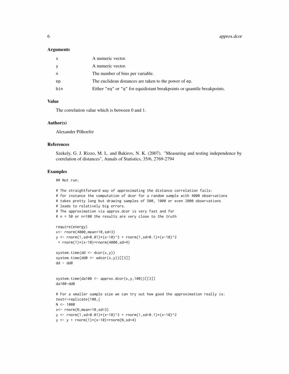
Arguments

x A numeric vector.

y A numeric vector.

n The number of bins per variable.

ep The euclidean distances are taken to the power of ep.

bin Either "eq" or "q" for equidistant breakpoints or quantile breakpoints.

Value

The correlation value which is between 0 and 1.

Author(s)

Alexander Pilhoefer

References

Szekely, G. J. Rizzo, M. L. and Bakirov, N. K. (2007). "Measuring and testing independence bycorrelation of distances", Annals of Statistics, 35/6, 2769-2794

Examples

## Not run:

# The straightforward way of approximating the distance correlation fails:# for instance the computation of dcor for a random sample with 4000 observations# takes pretty long but drawing samples of 500, 1000 or even 2000 observations# leads to relatively big errors.# The approximation via approx.dcor is very fast and for# n = 50 or n=100 the results are very close to the truth

require(energy)x<- rnorm(4000,mean=10,sd=3)y <- rnorm(1,sd=0.01)*(x-10)^3 + rnorm(1,sd=0.1)*(x-10)^2+ rnorm(1)*(x-10)+rnorm(4000,sd=4)

system.time(dd <- dcor(x,y))system.time(dd0 <- wdcor(x,y))[[3]]dd - dd0

system.time(da100 <- approx.dcor(x,y,100))[[3]]da100-dd0

# For a smaller sample size we can try out how good the approximation really is:test<-replicate(100,{N <- 1000x<- rnorm(N,mean=10,sd=3)y <- rnorm(1,sd=0.01)*(x-10)^3 + rnorm(1,sd=0.1)*(x-10)^2y <- y + rnorm(1)*(x-10)+rnorm(N,sd=4)

arsim 7

dd <- wdcor(x,y)dd25 <- approx.dcor(x,y,25)dd50 <- approx.dcor(x,y,50)dd100 <- approx.dcor(x,y,100)dd75 <- approx.dcor(x,y,75)

dd25c <- approx.dcor(x,y,25,correct = TRUE)dd50c <- approx.dcor(x,y,50,correct = TRUE)dd100c <- approx.dcor(x,y,100,correct = TRUE)dd75c <- approx.dcor(x,y,75,correct = TRUE)c(2*dd, dd25, dd50, dd75, dd100, dd25c, dd50c, dd75c, dd100c)-dd})

rm<-apply(test,1,mean)

plot( seq(25,100,25), rm[2:5],type="l",ylim= c(min(rm),abs(min(rm))), xlab = "No. of bins per axis",ylab = "error")

points( seq(25,100,25), rm[2:5],pch=19)points( seq(25,100,25), rm[6:9],type="l", col=2)points( seq(25,100,25), rm[6:9],pch=19,col=2)abline(h=0,lwd=3)legend( 25,abs(min(rm)),legend=c("raw value after binning","corrected value"),col=1:2,lwd=3)

## End(Not run)

arsim block-structured arrays

Description

Generates an array or matrix that includes k fully separated block-clusters.

Usage

arsim(n, dim, k, noise = 0, shuffle = TRUE, v = 0.1, minc = 1,exp.prop = NULL, min.prop = 1/dim/4, noise.type = "s",dimnames=list(LETTERS,1:max(dim)))

Arguments

n The number of observations in the array.

dim The dimension of the array.

k The number of clusters. 1 for no clusters.

noise The proportion of noise among the observations. There are two choices fornoise.type.

shuffle Whether or not to shuffle the original category orders randomly.

8 arsim

v A variability parameter for the assignment of the observations to the block clus-ters. Small values lea

minc The minimum number of categories each cluster must have in each variable.E.g. minc = 2 means, that each block cluster covers at least 2 categories in eachdimension.

exp.prop Optional: expected proportions of the observations which fall into the blockclusters.

min.prop Minimum proportion of observations in each cluster.

noise.type Either "s" or "I". The noise type "s" means that n*noise observations aredrawn at random from the block-diagonal matrix. Then for these observationsthe category labels are permuted at random. "I" adds noise in form of a randomsample from the independence matrix with the same marginal totals as the blockmatrix.

dimnames A list of 2: The first entry defines the variable labels (default: A,B,C,...) and thesecond entry defines the category labels (default 1:k).

Details

Not a very sophisticated way of generating random arrays but it serves for tests and illustrations ofthe other functions.

Value

A simulated data array.

Examples

A <- arsim(1000, c(12,12), 3, shuffle = FALSE)fluctile(A)

A <- arsim(1000, c(12,12), 3, shuffle = FALSE, dimnames = list(NULL,letters))dimnames(A)

A <- arsim(4000, c(11,7,5), 3, shuffle = TRUE, dimnames = list(0:2,letters))dimnames(A)

## Not run:A2<- arsim(1000, c(12,12,12), 3, shuffle = FALSE)fluctile3d(A2, shape ="oct")

## End(Not run)

barysort 9

barysort row and column moment reordering

Description

An iterative row and column reordering procedure based on the barycenter heuristic.

Usage

barysort(x, vs = 1)

Arguments

x The data matrix.

vs version. no effect.

Value

The reordered matrix.

Examples

# a good and quick solution:a <- arsim(2000,c(24,24),6, noise=0.4)fluctile(a2<-barysort(a))BCI(a2)

# which is neara3 <- optile(a, iter=100)BCI(a3)

## Not run:a <- arsim(64000,c(256,256),16, noise=0.4)s1 <- system.time( bci1 <- BCI(a1<-optile(a, fun = "barysort",foreign=".Call", iter = 1)) )[[3]]

s2 <- system.time( bci2 <- BCI(a2<-optile(a, iter=1)) )[[3]]s3 <- system.time( bci3 <- BCI(a3<-optile(a, fun="IBCC",iter=1)) )[[3]]

## End(Not run)

10 BCC

BCC The Bertin Classification Criterion

Description

Computes the Bertin Classification Criterion for a contingency table of any dimensions.

Usage

BCC(x)

Arguments

x A data matrix, table or array.

Details

The BCC counts the number of observation pairs which differ in all variables but are not fullyconcordant, (i.e. neither of the two observations of each pair is larger than the other in all variables).

Value

The criterion value.

Author(s)

Alexander Pilhoefer

See Also

kendalls

Examples

M <-arsim(1000, c(12,12), 3)BCC(M)

M2 <- optile(M, iter = 100)BCC(M2)

BCI 11

BCI The Bertin Classification Index

Description

Computes the Bertin Classification Index for a contingency table of any dimensions.

Usage

BCI(x)

Arguments

x A data matrix, table or array.

Details

The BCI is the Bertin Classification Criterion (BCC) normalized by the BCC value under indepen-dence.

Value


Author(s)

Alexander Pilhoefer

See Also

kendalls

Examples

#for an unoptimized matrix we take the minimum of BCI(M) and BCI(M[,12:1])M <-arsim(1000, c(12,12), 3)min(BCI(M), BCI(M[,12:1]))

#an strongly related alternative (for two-way data)kendalls(M)

M2 <- optile(M, iter = 100)BCI(M2)kendalls(M2)

M3 <-arsim(100000, c(12,13,15), 4,noise=0.2,shuffle=FALSE)BCI(M3)

12 Burt

Burt Burt atrix

Description

The Burt matrix is a quadratic matrix where each row and column corresponds to a category in oneof the variables. The entries of the matrix are the frequencies of the corresponding combination ofcategories.

Usage

Burt(x)

Arguments

x A dataframe with factor variables or a contingency table.

Value

A matrix.

Author(s)

Alexander Pilhoefer

See Also

idat, imat

Examples

require(MASS)Burt(housing)th <- xtabs(Freq~Sat+Infl+Type, data = housing)Burt(th)

carcustomers 13

carcustomers The car customers dataset from 1983

Description

This dataset is taken from the website of the Department of Statistics, University of Munich.The data are based upon a poll from a german car-company. In 1983 questionnaires were sent to2000 customers, who had purchased a new car approximately three months earlier. The point ofinterest was the degree of satisfaction, reasons for the particular choice, consumer profile, etc. Par-ticipation was of course voluntary. Only 1182 persons answered the questions and after removingforms with "missing values" only 793 questionnaires remained. Each form contained 46 questions,which resulted in a dataset of 46 covariates with 793 observations each. Due to the abundance ofordinal and categorical covariates the dataset is particularly suited for generalized linear models.

Usage

data(carcustomers)

Format


model a factor with levels A B C D

gear a factor with levels 4-gear 5-gear (overdrive) 5-gear (sport) Automatic

lease a factor with levels bought leased

usage a factor with levels business private private and business

premod a factor with levels Audi BMW 3er BMW 5er BMW 7er Ford Mercedes Benz Opel other originVolkswagen

other a factor with levels No Yes, both Yes, other manufact Yes, same manufact.

testdrv influence on buying decision: testdrive

promotion influence on buying decision: promotion

exp influence on buying decision: experience

recom influence on buying decision: recommendation

clear influence on buying decision: clearness

eco influence on buying decision: economical aspects

drvchar influence on buying decision: driving character

service influence on buying decision: service

interior influence on buying decision: interior

quality influence on buying decision: overall quality

tech influence on buying decision: technical aspects

evo influence on buying decision: evolution

comfort influence on buying decision: comfort

14 carcustomers

reliab influence on buying decision: reliabilityhandling influence on buying decision: handlingprestige influence on buying decision: prestigeconcept influence on buying decision: overall conceptchar influence on buying decision: characterpower influence on buying decision: engine powervaldecr influence on buying decision:value decreasestyling influence on buying decision: stylingsafety influence on buying decision:safetysport influence on buying decision: sportivefcons influence on buying decision: fuel consumptionspace influence on buying decision: available spacesat overall satisfaction with the car: 1(very satisfied) to 5(not satisfied)adv1 satisfaction with concept and styling: a factor with levels does not suit neither nor

suits

adv2 satisfaction with body/bare essentials: a factor with levels does not suit neither norsuits

adv3 satisfaction with chassis/drive/gearshift: a factor with levels does not suit neither norsuits

adv4 satisfaction with engine/power: a factor with levels does not suit neither nor suits

adv5 satisfaction with electronics: a factor with levels does not suit neither nor suits

adv6 satisfaction with financial aspects: a factor with levels does not suit neither nor suits

adv7 asatisfaction with equipment: a factor with levels does not suit neither nor suits

spoco balance variables: a factor with levels comfort could be better handling could be betterwell balanced

faver usual driving style: a factor with levels economical extreme normal powerful

sspeed usual speed (Autobahn): a factor with levels >110 mph 60-80 mph 81-9g mph 96-110 mph

sfcons satisfaction with fuel consumption: a factor with levels Appropriate Definitely too highJust okay Pleasingly low

sex customer’s gender: a factor with levels Female Male

prof customer’s profession: a factor with levels Employee/Workman Free lanced Self employed

family customers’s family type: a factor with levels >3 persons 1-2 persons

Freq the weighting variable

Source

http://www.stat.uni-muenchen.de/service/datenarchiv/auto/auto_e.html

Examples

data(Autos)## maybe str(Autos) ; plot(Autos) ...

http://www.stat.uni-muenchen.de/service/datenarchiv/auto/auto_e.html

CBCI 15

CBCI The Conditional Independence Bertin Classification Index

Description

Computes the Conditional Independence Bertin Classification Index which uses conditional inde-pendence as a reference for normalization. High values indicate that the BCC is not far from theexpectation if we know the two marginal 2D BBC values.

Usage

CBCI(x, r = 1, joint.order = FALSE)

Arguments

x The 3D table with non-negative entries.

r The index of the conditioning variable, e.g. r = 1 uses the table with variables2 and 3 conditionally independent given 1 for normalization.

joint.order Whether or not to use a joint ordering for all variables. Otherwise the pairwisevalues are computed using separate reorderings.

Details

The BCI of a 3D table but instead of the total independence case the conditional independence caseis used for normalization.

Value

Numeric value in [0,1].

Author(s)

Alexander Pilhoefer

See Also

BCI, JBCI, WBCI

Examples

## Not run:A <- optile(arsim(10000, c(11,12,13), 4,0.1))

BCI(A)

CBCI(A,1,TRUE)CBCI(A,1,FALSE)

16 cfcl

## End(Not run)

cfcl Extract clusters from cfluctile

Description

Extract clusters from cfluctile

Usage

cfcl(x, y = NULL, ll)

Arguments

x vector or dataframe.

y if x is a vector, y needs to be specified.

ll The list with the names of the levels which are combined.

Value

A 2-column dataframe with the cluster factors.

See Also

cfluctile

Examples

a <- arsim(2000, c(12,17),5, noise=0.2,shuffle = FALSE)cfa <- cfluctile(a)

da <- as.data.frame(a)clusters <- cfcl( da, ll = cfa)

dev.new()fluctile(xtabs(da$Freq~clusters[,1] + clusters[,2]))

table(combcl(clusters))

cfluctile 17

cfluctile Pseudo-Diagonal Partitioning for two-way tables

Description

Identifies a diagonal of block-clusters in a two-way table using a top-down-partitioning algorithmthen plots the table and adds the clusters as rectangles.

Usage

cfluctile(x, tau0 = NULL, method = "Kendall", nsplit = NULL,maxsplit = NULL, trafo = I, gap.prop = 0.2, floor = 0,rev.y = FALSE, add = FALSE, shape = "r", just = "c",dir = "b", plot = TRUE, rect.opt = list(), border =NULL, label = TRUE, lab.opt = list(), tile.col =hsv(0.1, 0.1, 0.1, alpha = 0.6),tile.border = NA, bg.col = "lightgrey", ...)

Arguments

x A 2-way table or matrix.

tau0 The minimum acceptable value of Kendall’s tau, Cohen’s Kappa or WBCI. De-faults to the criterion of the input matrix x.

method Either "Kendall" for Kendall’s Tau, "Cohen" for Cohen’s Kappa, "WBCI" forthe Weighted Bertin Classification Criterion and "s" for the minimum residualmethod.

nsplit The number of splits to make. tau0 is ignored.

maxsplit The maximum number of splits.

trafo A transformation of the table entries for the plot, but not for the computation ofthe splits. E.g. trafo = function(z) log(1+z).

gap.prop proportion of the gaps between rows/columns.

floor floor censored zooming: all cases will be plotted but only those with a frequencyof at least floor will be considered for the clustering.

rev.y revert the y axis.

add Whether to make a new plot or to add to an existing one.

shape The shape of the objects. See fluctile.

just See fluctile.

dir See fluctile.

plot Whether or not to create a plot via fluctile.

rect.opt A list with optional parameters for the rectangles. Possible parameters are:

col The rectangle color.lwd The line width. Default is "red".lty The line type. Default is 1 (solid).fill The color to fill the rectangles. Defaults is NULL. A sensible choice is for instance alpha(col, 0.1).

18 cfluctile

border The white margins around the plot which are also used for the labels. Must be avector of length 1, 2 or 4 with values in [0, 1]. Default is border = 0.05.

label Whether or not to draw labels.

lab.opt Label options, see fluctile.

tile.col Color(s) for the tiles, see fluctile.

tile.border Border color for the tiles. Can also be a matrix.

bg.col Color for the background of the cells, see fluctile.

... dots

Details

This function calls fluctile to create a 2-way fluctuation diagram and then adds cluster rectangles toit. The cluster rectangles are computed in the following way:

The algorithm cuts the data matrix once horizontally and once vertically and computes a criterionfor the 2x2 table consisting of the sums of the four parts that resulted from the cuts. This is donefor all possible horizontal and vertical cuts and the best combination is chosen. Then the sameprocedure is applied to the bottom right submatrix and the top left submatrix. The algorithms stopsif no cut yields a better criterion value than tau0.

Value

invisible(TRUE)

Note

This was part of the Google Summer of Code 2011.

Author(s)

Alexander PilhoeferDepartment for Computer Oriented Statistics and Data AnalysisUniversity of AugsburgGermany

See Also

optile, sortandcut, tfluctile

Examples

M <- arsim(10000,c(30,40),8, noise = 0.4)cfluctile( M2 <- optile(M,iter=20) )

cfluctile( M3 <- sortandcut(M) )

cfluctile( M3, nsplit = 4 )

cmat 19

cfluctile( M3, maxsplit = 12 )

cfluctile( M3, tau0 = 0.8 )

cmat pairwise association matrix

Description

Computes pairwise BCI values via qBCI.

Usage

cmat(x, sort = TRUE, crit = BCI, k = 5, iter = 20,p = NULL, jitter = TRUE, freqvar = NULL, diag = NULL,fun = "BCC", foreign = NULL)

Arguments

x A data.frame with factor variables or numeric variables which will be trans-formed to ordinal interval variables via cut. The breakpoints are quantiles of thevariables such that for each pair of numeric variables the expected number ofobservations in each combination of intervals is at least k.

sort Whether or not to sort the pairwise tables via optile.

crit The criterion function, e.g. kendalls, BCI, WBCI or wdcor.

k The minimum expected number for each cell after quantile binning. See alsoqBCI.

iter An optile parameter.

p The quantile distance. See qBCI.

jitter Whether or not to use jittering in order to avoid ties. This is equivalent to arandom assignment of ranks to observations with the same value.

freqvar Optional weights, e.g. a frequency variable.

diag An optional value for the diagonal. Avoids unnecessary function calls for the di-agonal elements. E.g. diag = 0 for crit = BCI or diag = 1 for crit = kendallsmakes sense.

fun See optile.

foreign See optile.

Details

Uses pairwise complete cases only!

20 cohen

Value

A symmetric matrix.

Author(s)

Alexander Pilhoefer

See Also

qBCI, See wdcor.

Examples

## Not run:m1 <- cmat(olives)fluctile(1 - m1,shape="o")

## End(Not run)

cohen Cohens Kappa for rectangular matrices

Description

Cohen’s Kappa for quadratic and non-quadratic matrices using L1-weights.

Usage

cohen(x)

Arguments

x A matrix with non-negative entries.

Value

Cohen’s Kappa

See Also

kendalls, BCI, WBCI

Examples

a <- arsim(2000,c(12,12),6)cohen(a)cohen(optile(a))

combcl 21

combcl Combine categorical variables from cfluctile and cflcl

Description

Combines variables obtained via cfcl and cfluctile to a single factor variable with one level perblock-cluster and one level for the rest.

Usage

combcl(x)

Arguments

x A matrix, table or data.frame. All variables should have the same number ofcategories.

Value

A factor variable with 1 level per diagonal element and 1 level for the rest.

Examples

a <- arsim(2000, c(12,17),5, noise=0.2,shuffle = FALSE)cfa <- cfluctile(a)

da <- as.data.frame(a)clusters <- cfcl( da, ll = cfa)

dev.new()fluctile(xtabs(da$Freq~clusters[,1] + clusters[,2]))

table(combcl(clusters))

CPScluster Clusterings for the US Current Population Survey.

Description

Different hierarchical clusterings and k-means clusterings as well as a model-based clustering havebeen applied to several financial variables for a random sample of ten thousand observations.

Usage

data(CPScluster)

22 CPScluster

Format


Age a numeric vectorSex a factor with levels female maleRace a factor with levels Black WhiteEthnic a factorMarital.Status a factorKind.of.Family a factorClassical a factor with levels All other Classical Husband-Wife family

Family.Type a factorNumber.of.Persons.in.Family a numeric vectorNumber.of.Kids a numeric vectorEducation.of.Head a factorLabor.Status a factorClass.of.Worker a factorWorking.Hours a numeric vectorIncome.of.Head a numeric vectorFamily.Income a numeric vectorTaxable.Income a numeric vectorFederal.tax a numeric vectorFamily.sequence.number a numeric vectorState a factorDivision a factorRegion a factor with levels Midwest North East South West

hc4 a numeric vectorhc6 a numeric vectorhc8 a numeric vectorhc12 a numeric vectorhcs4 a numeric vectorhcs6 a numeric vectorhcs8 a numeric vectorhcs12 a numeric vectorhcw4 a numeric vectorhcw6 a numeric vectorhcw8 a numeric vectorhcw12 a numeric vectorkm4 a numeric vectorkm6 a numeric vectorkm8 a numeric vectorkm12 a numeric vectormc12 a numeric vector

cutbw 23

Examples

data(CPScluster)## maybe str(CPScluster) ; plot(CPScluster) ...

cutbw Active binning

Description

Uses cut with breakpoints derived by getbw.

Usage

cutbw(x, k = NULL, min_n = NULL, warn = FALSE)

Arguments

x A numeric variable.


min_n The minimum number of observations necessary for a bin to count as an activebin. Defaults to min_n = max(log(N/10)/log(10),1).

warn Whether or not to print a warning if the desired number of bins is not possible.

Value

An ordinal factor variable.

Note

Experimental.

Author(s)

Alexander Pilhoefer

See Also

getbw, ahist

Examples

y<-cutbw(c(rnorm(200),rnorm(100,mean=8)),k = 30, min_n = 1)barplot(table(y))

24 dcorMVdata

dcorMVdata Multivariate Distance Correlation for two sets of variables

Description

Computes the distances within two sets of variables and the corresponding distance correlation.

Usage

dcorMVdata(x, ind = 1, method = "euclidean", approx = FALSE)

Arguments

x The data.frame which should only contain non-factor variables. For factorvariables use xtabs in combination with dcorMVtable.

ind The indices for the first set of variables. The second set consists of all remainingvariables.

method The method for dist.

approx FALSE for no approximation via binning or an integer value for the number ofbins.

Value

The distance correlation between 0 and 1 for the distances from the two sets of variables.

Note

This code has not been tested thoroughly and may still contain errors.

Author(s)

Alexander Pilhoefer

See Also

dcorMVtable, wdcor, approx.dcor

Examples

## Not run:so <- scale(olives[,3:8])dcorMVdata(so,ind=1)

p1 <- princomp(so)so1 <- cbind(so,p1$scores[,1])so2 <- cbind(so,p1$scores[,2])so12 <- cbind(so,p1$scores[,1:2])

dcorMVtable 25

dcorMVdata(so1,ind=7)dcorMVdata(so2,ind=7)dcorMVdata(so12,ind=7:8)# how about principal curves?

## End(Not run)

dcorMVtable Multivariate Distance Correlation for two sets of variables

Description

Computes the distances within two sets of variables and the corresponding distance correlation.

Usage

dcorMVtable(x, ind = 1, method = "euclidean")

Arguments

x A contingency table of class table.

ind The indices for the first set of variables. The second set consists of all remainingvariables.

method The method for dist

Value

The distance correlation between 0 and 1 for the distances from the two sets of variables.

Note

This code has not been tested thoroughly and may still contain errors.

Author(s)

Alexander Pilhoefer

See Also

dcorMVdata, wdcor, approx.dcor

26 dendro

Examples

## Not run:A2 <- arsim(2000,c(8,9),5,0.1)A2 <- optile(A2, iter=100)BCI(A2)wdcor(A2)

p1 <- runif(11)+0.1p1 <- p1/sum(p1)A2b <- apply(A2,1:2,function(z) rmultinom(1,z,p1))

# now the first variable is roughly independent from the other two:

dcorMVtable(as.table(A2b),ind = 1)

# here the third variable is NOT independent from the others:A3 <- arsim(2000,c(8,9,11),5,0.1)A3 <- optile(A3, iter=100)BCI(A3)dcorMVtable(A3,ind = 3)

## End(Not run)

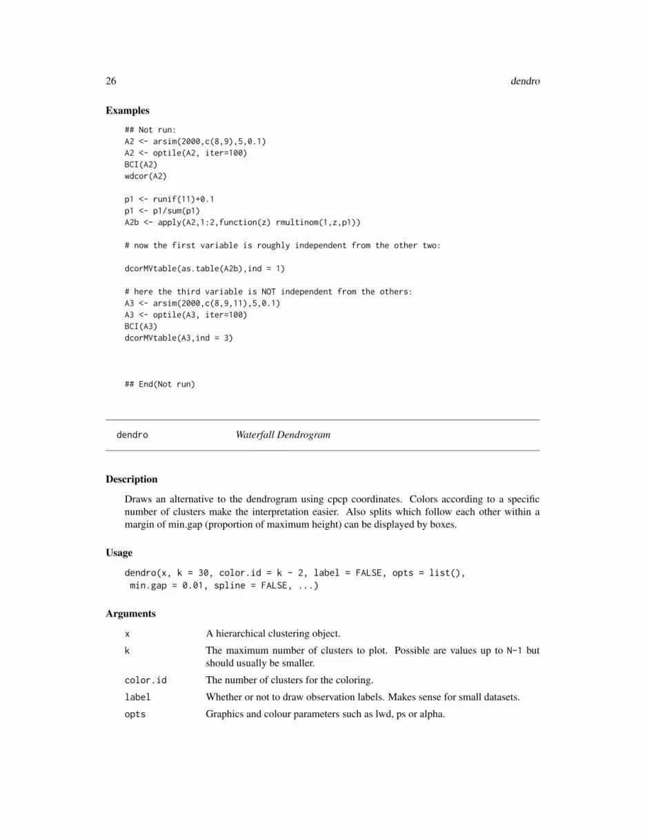
dendro Waterfall Dendrogram

Description

Draws an alternative to the dendrogram using cpcp coordinates. Colors according to a specificnumber of clusters make the interpretation easier. Also splits which follow each other within amargin of min.gap (proportion of maximum height) can be displayed by boxes.

Usage

dendro(x, k = 30, color.id = k - 2, label = FALSE, opts = list(),min.gap = 0.01, spline = FALSE, ...)

Arguments

x A hierarchical clustering object.

k The maximum number of clusters to plot. Possible are values up to N-1 butshould usually be smaller.

color.id The number of clusters for the coloring.

label Whether or not to draw observation labels. Makes sense for small datasets.

opts Graphics and colour parameters such as lwd, ps or alpha.

dmc 27

min.gap Joins which are closer than min.gap from each other will be packed and dis-played as a box.

spline Whether or not to use spline curves instead of straight line connections betweenthe points.

... dots

Value

TRUE

Examples

## Not run:library(amap)hc <- hcluster(USArrests)# the full plot:dendro(hc, k = 24, min.gap = 0.00)

# aggregation splits within 0.02 maximum heightdendro(hc, k = 24, min.gap = 0.02)

# the same graphic with spline curves instead of straight lines.dendro(hc, k = 24, min.gap = 0.02, spline = TRUE)

# olive oil datasx <- scale(olives[,-c(1,2,11)])hc <- hcluster(sx)plot(hc)dendro(hc, 120, color.id = 6, min.gap=0.005)dendro(hc, 120, color.id = 6, min.gap=0.1)

dendro(hc, 120, color.id = 6, min.gap=0.1, spline = TRUE)

## End(Not run)

dmc dmc 2009 insurance variables

Description

five insurance variables from the dmc 2009 dataset, which have a ordinal structure which has beenlost somehow. Can we find it again?

Usage

data(dmc)

28 eco

Format


eiw_scr a factor with levels 5 6 4 3 2 1

eih_scr a factor with levels 6 3 5 1 4 2

ifi_scr a factor with levels 4 3 5 2 1 6

tec_scr a factor with levels 5 1 3 2 4 6

klv_scr a factor with levels 2 5 6 1 3 4

Freq a numeric vector

Details

The Data Mining Cup (dmc) is a competition for students.

Examples

data(dmc)

eco ADAC Eco test data

Description

ADAC Ecotest data with clusterings.

Usage

data("eco")

Format


V1 a factor with levels Hersteller 1 10 100 101 102 103 104 105 106 107 108 109 11 110 111112 113 114 115 116 117 118 119 12 120 121 122 123 124 125 126 127 128 129 13 130 131132 133 134 135 136 137 138 139 14 140 141 142 143 144 145 146 147 148 149 15 150 151152 153 154 155 156 157 158 159 16 160 161 162 163 164 165 166 167 168 169 17 170 171172 173 174 175 176 177 178 179 18 180 181 182 183 184 185 186 187 188 189 19 190 191192 193 194 195 196 197 198 199 2 20 200 201 202 203 204 205 206 207 208 209 21 210211 212 213 214 215 216 217 218 219 22 220 221 222 223 224 225 226 227 228 229 23 230231 232 233 234 235 236 237 238 239 24 240 241 242 243 244 245 246 247 248 249 25 250251 252 253 254 255 256 257 258 259 26 260 261 262 263 264 265 266 267 268 269 27 270271 272 273 274 275 276 277 278 279 28 280 281 282 283 284 285 286 287 288 289 29 290291 292 293 294 295 296 297 298 299 3 30 300 301 302 303 304 305 306 307 308 309 31310 311 312 313 314 315 316 317 318 319 32 320 321 322 323 324 325 326 327 328 329 33330 331 332 333 334 335 336 337 338 339 34 340 341 342 343 344 345 346 347 348 349 35

eco 29

350 351 352 353 354 355 356 357 358 359 36 360 361 362 363 364 365 366 367 368 369 37370 371 372 373 374 375 376 377 378 379 38 380 381 382 383 384 385 386 387 388 389 39390 391 392 393 394 395 396 397 398 399 4 40 400 401 402 403 404 405 406 407 408 40941 410 411 412 413 414 415 416 417 418 419 42 420 421 422 423 424 425 426 427 428 42943 430 431 432 433 434 435 436 437 438 439 44 440 441 442 443 444 445 446 447 448 44945 450 451 452 453 454 455 456 457 458 459 46 460 461 462 463 464 465 466 467 468 46947 470 471 472 473 474 475 476 477 478 479 48 480 481 482 483 484 485 486 487 488 48949 490 491 492 493 494 495 496 497 498 499 5 50 500 501 502 503 504 505 506 507 508509 51 510 511 512 513 514 515 516 517 518 519 52 520 521 522 523 524 525 526 527 528529 53 530 531 532 533 534 535 536 537 538 539 54 540 541 542 543 544 545 546 547 548549 55 550 551 552 553 554 555 556 557 558 559 56 560 561 562 563 564 565 566 567 568569 57 570 571 572 573 574 575 576 577 578 579 58 580 581 582 583 584 585 586 587 588589 59 590 591 592 593 594 595 596 597 598 599 6 60 600 601 602 603 604 605 606 607608 609 61 610 611 612 613 614 615 616 617 618 619 62 620 621 622 623 624 625 626 627628 629 63 630 631 632 633 634 635 636 637 638 639 64 640 641 642 643 644 645 646 647648 649 65 650 651 652 653 654 655 656 657 658 659 66 660 661 662 663 664 665 666 667668 669 67 670 671 672 673 674 675 676 677 678 679 68 680 681 682 683 684 685 686 687688 689 69 690 691 692 693 694 695 696 697 698 699 7 70 700 701 702 703 704 705 706707 708 709 71 710 711 712 713 714 715 716 717 718 719 72 720 721 722 723 724 725 726727 728 729 73 730 731 732 733 734 735 736 737 738 739 74 740 741 742 743 744 745 746747 748 749 75 750 751 752 76 77 78 79 8 80 81 82 83 84 85 86 87 88 89 9 90 91 92 93 9495 96 97 98 99

V2 a factor with levels Alfa Romeo Audi BMW BMW Alpina Brilliance Cadillac ChevroletChevrolet (EU) Chrysler Citroen Dacia Daewoo Daihatsu Dodge Fiat Ford HondaHyundai Jaguar Jiangling Kia KIA Lada Lancia Land Rover Lexus Mazda Mercedes MGMini Mitsubishi Modell Nissan Opel Peugeot Porsche Renault Rover Saab Seat Skodasmart SsangYong Subaru Suzuki Toyota Volvo VW

V3 a factor with levels Alfa Romeo 147 1.9 JTD 16V M-Jet Distinctive Alfa Romeo 159 1.9 JTDM 16V Distinctive (DPF)Alfa Romeo 159 Sportwagon 1.9 JTDM 16V Distinctive (DPF) Alfa Romeo 166 2.4 JTD 20V Multijet DistinctiveAlfa Romeo Brera 2.2 JTS 16V Skyview Alfa Romeo Brera 2.4 JTDM 20V Q-Tronic (DPF)Alfa Romeo GT 1.9 JTD 16V Multijet Progression Alfa Romeo GT 1.9 JTDM 16V Q2 Progression (DPF)Alfa Romeo GT 2.0 16V JTS 16V Distinctive Alfa Romeo Spider 2.2 JTS 16V ExclusiveAlfa Romeo Spider 2.4 JTDM 20V Exclusive (DPF) Audi A2 1.4 TDI Audi A3 1.6 AttractionAudi A3 1.6 FSI Ambiente Audi A3 1.9 TDI Ambition (DPF) Audi A3 1.9 TDI AttractionAudi A3 1.9 TDI e Ambition (DPF) Audi A3 2.0 FSI Ambition Audi A3 2.0 TDI AttractionAudi A3 Cabriolet 1.8 TFSI Ambition Audi A3 Sportback 1.8 TFSI AmbitionAudi A3 Sportback 2.0 TDI Attraction Audi A3 Sportback 2.0 TFSI Ambition S tronic (DSG)Audi A4 1.8 TFSI Ambition Audi A4 2.0 TDI Audi A4 2.0 TDI (DPF) Audi A4 2.0 TDI Ambition (DPF)Audi A4 2.0 TFSI Audi A4 2.7 TDI Ambition multitronic (DPF) Audi A4 3.0 TDI Ambition quattro (DPF)Audi A4 3.2 FSI Ambition quattro tiptronic Audi A4 Avant 1.8 TFSI AmbitionAudi A4 Avant 2.0 TDI Audi A4 Avant 3.0 Audi A4 Avant 3.0 multitronicAudi A5 3.0 TDI quattro (DPF) Audi A5 3.2 FSI multitronic Audi A6 2.0 TDI (DPF)Audi A6 2.4 Audi A8 3.0 TDI quattro tiptronic (DPF) Audi A8 4.2 TDI quattro tiptronic (DPF)Audi Q7 3.0 TDI quattro tiptronic (DPF) Audi R8 Audi S3 Audi TT Roadster 1.8 T tiptronicAudi TT Roadster 2.0 TFSI BMW 116i BMW 118d BMW 118d (DPF) BMW 120d BMW 120d (DPF)BMW 120d Cabriolet (DPF) BMW 120i BMW 123d (DPF) BMW 123d Coup<e9> (DPF)BMW 125i Cabriolet BMW 130i BMW 135i Coup<e9> BMW 318d (DPF) BMW 318d touring (DPF)BMW 318i BMW 318ti compact Edition Lifestyle BMW 320Cd Cabriolet BMW 320Ci Cabriolet

30 eco

BMW 320d (DPF) BMW 320d touring (DPF) BMW 320i touring BMW 325Ci Cabriolet SteptronicBMW 325d (DPF) BMW 330Cd Coup<e9> BMW 330d Cabriolet Steptronic (DPF)BMW 330d Steptronic (DPF) BMW 330i BMW 330i Cabriolet BMW 330i SMG BMW 330i SteptronicBMW 330xi touring Steptronic BMW 335d Coup<e9> Steptronic (DPF) BMW 520d (DPF)BMW 520i Steptronic BMW 525d (DPF) BMW 530d BMW 530d touring Steptronic (DPF)BMW 530i BMW 535d Steptronic (DPF) BMW 630Ci Coup<e9> Steptronic BMW 645Ci CabrioletBMW 730d Steptronic (DPF) BMW 745d Steptronic (DPF) BMW Alpina D3 (DPF)BMW M3 Cabriolet M DKG BMW M3 Coup<e9> BMW M5 touring SMG BMW X3 2.0d Steptronic (DPF)BMW X3 2.5si Steptronic BMW X3 3.0d Automatik BMW X3 3.0sd Steptronic (DPF)BMW X5 3.0d Steptronic BMW X5 3.0d Steptronic (DPF) BMW X5 4.4i SteptronicBMW X6 xDrive35d Sport-Automatic (DPF) BMW Z4 Roadster 2.2i BMW Z4 Roadster 3.0i SteptronicBrilliance BS6 2.0 Deluxe Cadillac BLS Wagon 1.9 TiD Sport Automatik (DPF)Cadillac CTS 2.6 V6 Elegance Automatik Chevrolet (EU) Aveo 1.2 LS Chevrolet (EU) Captiva 2.0 D LT Sport 4WD (7-Sitzer) (DPF)Chevrolet (EU) Captiva 3.2 LT 4WD Automatik (7-Sitzer) Chevrolet (EU) Epica 2.5 LT AutomatikChevrolet (EU) HHR 2.4 LT Chevrolet (EU) Kalos 1.4 16V SX Chevrolet (EU) Matiz 0.8 LPG S (Autogasbetrieb)Chevrolet (EU) Matiz 0.8 LPG S (Benzinbetrieb) Chevrolet (EU) Matiz 1.0 SXChevrolet (EU) Nubira 1.6 SX Chevrolet (EU) Nubira Wagon 1.8 LPG CDX (Autogasbetrieb) (LPG)Chevrolet (EU) Nubira Wagon 1.8 LPG CDX (Benzinbetrieb) Chevrolet (EU) Nubira Wagon 2.0 D CDX (DPF)Chevrolet (EU) Rezzo 2.0 LPG CDX (Autogasbetrieb) Chevrolet (EU) Rezzo 2.0 LPG CDX (Benzinbetrieb)Chrysler 300C 5.7 V8 Automatik Chrysler Crossfire 3.2 V6 Automatik Chrysler Crossfire Roadster 3.2 V6 AutomatikChrysler PT Cruiser Cabrio 2.4 Limited Chrysler Sebring 2.0 CRD LimitedChrysler Sebring Cabrio 2.7 Limited Automatik Chrysler Sebring Cabrio 2.7 LX AutomatikCitroen Berlingo Kombi 1.4 Bivalent Multispace Plus (Benzinbetrieb) Citroen Berlingo Kombi 1.4 Bivalent Multispace Plus (Erdgasbetrieb)Citroen C-Crosser 2.2 HDi FAP Exclusive Citroen C1 1.0 Style Citroen C1 HDi 55 StyleCitroen C2 1.4 16V StopStart SensoDrive Citroen C2 1.4 VTR SensoDriveCitroen C3 1.4 16V Stop Start SensoDrive Citroen C3 HDi 110 FAP ExclusiveCitroen C3 HDi 90 Exclusive Citroen C3 Pluriel 1.6 16V Exclusive SensoDriveCitroen C4 1.6 16V Confort Citroen C4 Coup<e9> 1.6 16V VTR Citroen C4 Coup<e9> HDi 135 FAP VTR Plus AutomatikCitroen C4 HDi 110 FAP Confort Citroen C4 Picasso 1.8 16V Tendance Citroen C4 Picasso HDi 110 FAP Tendance EGS6Citroen C5 2.0 16V Confort Citroen C5 HDi 110 FAP Style Citroen C5 HDi 135 FAP Confort AutomatikCitroen C5 HDi 135 FAP Exclusive Citroen C5 Kombi 1.8 16V Tendance Citroen C5 Kombi 2.0 16V TendanceCitroen C5 Kombi HDi 110 FAP Tendance Citroen C5 Tourer HDi 110 FAP ConfortCitroen C6 HDi 170 Biturbo FAP Pallas Citroen C6 V6 HDi 205 Biturbo FAP Exclusive AutomatikCitroen C8 2.0 16V Tendance Citroen Grand C4 Picasso 1.8 16V TendanceCitroen Grand C4 Picasso HDi 135 FAP Exclusive EGS6 Citroen Jumpy Kombi HDi 135 FAP Club lang (8-Sitzer)Citroen Xsara Kombi 1.4 HDi SX Citroen Xsara Picasso 2.0 16V Exclusive AutomatikCorvette C5 Cabrio Dacia Logan 1.4 Ambiance Dacia Logan 1.5 dCi Laur<e9>ateDacia Logan 1.6 Laur<e9>ate Dacia Logan MCV 1.5 dCi Laur<e9>ate Daewoo Evanda 2.0 CDXDaewoo Lacetti 1.8 CDX Daewoo Matiz 1.0 SE Daewoo Nubira 1.8 CDX Daewoo Nubira Wagon 1.6 SXDaihatsu Copen Daihatsu Cuore 1.0 Top Daihatsu Materia 1.5 Daihatsu Sirion 1.3Daihatsu Trevis 1.0 Dodge Caliber 2.0 CRD SXT (DPF offen) Dodge Nitro 2.8 CRD SXT 4WD Automatik (DPF)Fiat 500 1.3 JTD Multijet 16V Lounge (DPF) Fiat 500 1.4 16V Lounge Fiat 500 1.4 16V SportFiat Bravo 1.4 T-Jet 16V Dynamic Fiat Bravo 1.9 JTD Multijet 8V Emotion (DPF)Fiat Croma 1.9 JTD Multijet 16V Emotion Automatik (DPF) Fiat Dobl<f2> Kombi 1.9 JTD Multijet 8V Dynamic (DPF)Fiat Grande Punto 1.2 8V Dynamic Fiat Grande Punto 1.3 JTD Multijet 16V DynamicFiat Idea 1.3 JTD 70 Multijet 16V Dynamic Fiat Idea 1.9 JTD 100 Multijet 8V EmotionFiat Linea 1.4 T-Jet 16V Emotion Fiat Multipla 1.9 JTD Dynamic Fiat Multipla 1.9 JTD Multijet 8V Dynamic (DPF)Fiat Panda 1.1 8V Active Fiat Panda 1.2 8V Emotion Fiat Panda 1.2 8V Natural Power Panda Panda (Benzinbetrieb)

eco 31

Fiat Panda 1.2 8V Natural Power Panda Panda (Erdgasbetrieb) Fiat Panda 1.3 JTD Multijet 16V Cross 4x4Fiat Panda 1.3 JTD Multijet 16V Emotion Fiat Panda 1.4 16V 100 HP Fiat Punto 1.3 JTD 70 Multijet DynamicFiat Scudo Kombi 140 Multijet DPF Panorama Executive lang Fiat Stilo 1.2 16V ActiveFiat Stilo 1.9 JTD Multijet 16V Dynamic Ford C-MAX 2.0 TDCi DPF TitaniumFord C-MAX 2.0 Titanium Ford Fiesta 1.4 TDCi Ghia Ford Fiesta 1.6 TrendFord Fiesta ST Ford Focus 1.4 Ford Focus 1.6 Futura Ford Focus 1.6 TDCi DPF GhiaFord Focus 1.6 Ti-VCT Trend Ford Focus 1.8 FFV Ambiente (Ethanol-Betrieb)Ford Focus 1.8 Style Ford Focus 2.0 Sport Ford Focus 2.0 TDCi DPF TitaniumFord Focus C-MAX 1.8 Trend Ford Focus C-MAX 2.0 TDCi DPF Ghia Ford Focus C-MAX 2.0 TDCi DPF TrendFord Focus C-MAX 2.0 TDCi Trend Ford Focus Coup<e9>-Cabriolet 2.0 TDCi DPF TitaniumFord Focus Coup<e9>-Cabriolet 2.0 Titanium Ford Focus Turnier 1.6 Ford Focus Turnier 1.8 GhiaFord Focus Turnier 1.8 TDCi Futura Ford Focus Turnier 2.0 TDCi DPF TitaniumFord Galaxy 2.0 Trend Ford Kuga 2.0 TDCi DPF Titanium 4x4 Ford Mondeo 1.6 TrendFord Mondeo 1.8 Futura Ford Mondeo 1.8 SCi Ambiente Ford Mondeo 2.0 TDCi DPF Ghia XFord Mondeo Turnier 2.0 TDCi DPF Titanium Ford Mondeo Turnier 2.0 TDCi Trend (5-Gang)Ford Mondeo Turnier 2.0 Trend Ford Mondeo Turnier 2.5 Turbo Titanium XFord Ranger 2.5 TDCi Doppelkabine XLT Limited Ford S-MAX 2.5 Trend Ford Streetka 1.6 8V EleganceFord Tourneo Connect Kombi 1.8 TDCi kurz Honda Accord 2.0i ExecutiveHonda Accord 2.4 Executive Automatik Honda Accord Tourer 2.2 i-CTDi SportHonda Civic 1.3 DSi IMA Honda Civic 1.3 i-DSi i-VTEC IMA Honda Civic 1.4i LSHonda Civic 1.6i ES Honda Civic 2.2 i-CTDi Type S (DPF) Honda CR-V 2.0i ES AutomatikHonda FR-V 1.8 Executive Automatik Honda FR-V 2.0i Executive Honda FR-V 2.2 i-CTDi Executive (DPF)Honda FR-V 2.2i-CTDi Comfort Honda Jazz 1.4 ES Sport Honda Legend 3.5 V6 AutomatikHonda S2000 Honda Stream 2.0i Sport Hyundai Atos 1.1 ComfortVersion Hyundai Coup<e9> 2.0 GLSHyundai Elantra 2.0 GLS Hyundai Getz 1.1 GL Hyundai Getz 1.4 GLS Hyundai Getz 1.5 CRDi GLSHyundai Grandeur 2.2 CRDi Automatik (DPF) Hyundai Grandeur 3.3 V6 AutomatikHyundai i10 1.1 Classic E Hyundai i10 1.1 CRDi Style Hyundai i30 1.4 ComfortHyundai i30cw 1.6 Comfort Hyundai i30cw 1.6 CRDi Comfort (DPF) Hyundai Matrix 1.5 CRDi VGT GLSHyundai Sonata 2.4 GLS Automatik Hyundai Terracan 2.9 CRDi GLS AutomatikHyundai Trajet 2.0 GLS Hyundai Tucson 2.0 CRDi GLS 4WD Hyundai XG 350 AutomatikJaguar XJ6 3.0 V6 Automatik Jaguar XKR Coup<e9> Automatik Jiangling Landwind 2.4 SC2 4WDKIA Carens 2.0 CWT EX KIA Carnival 2.9 CRDi EX (DPF offen) KIA Carnival II 2.9 CRDi EXKIA cee<b4>d 1.6 CRDi 115 EX (DPF) KIA cee<b4>d 1.6 EX KIA cee<b4>d Sporty Wagon 1.6 CRDi 115 LX (DPF)KIA Cerato 1.6 EX KIA Cerato 2.0 CRDi EX KIA Cerato 2.0 EX KIA Magentis 2.0 CRDi EX (DPF)KIA Opirus 3.8 Automatik KIA Picanto 1.1 Cool KIA Picanto 1.1 EX KIA pro_cee<b4>d 2.0 CRDi TX (DPF)KIA Rio 1.4 EX KIA Rio 1.5 CRDi EX Top KIA Rio 1.5 LS KIA Rio 1.6 EX TopKIA Shuma II 1.8 Active KIA Sorento 3.5 EX Automatik Klasse Lada 1118 Kalina 1.6 8VLancia Musa 1.9 jtd Multijet 8v Oro Lancia Thesis 2.4 jtd Multijet 20v EmblemaLancia Ypsilon 1.3 jtd Multijet 16v Argento D.F.N-System Lancia Ypsilon 1.3 jtd Multijet 16v PlatinoLancia Ypsilon 1.4 16v Oro Land Rover Freelander Td4 SE (DPF) Lexus GS 430 Luxury AutomatikLexus GS 460 Luxury Automatik Lexus IS 220d Luxury (DPF) Lexus IS 250 Luxury AutomatikLexus LS 460 Impression Automatik Lexus LS 600h L Ambience Wellness AutomatikLexus RX 300 Executive Automatik Lexus RX 350 Executive Automatik Lexus RX 400h Luxury AutomatikLexus SC 430 Automatik Mazda 2 1.3 Impression Mazda 2 1.4 Active Mazda 2 1.4 CD ActiveMazda 2 1.4 CD Independence Mazda 2 1.4 Exclusive Mazda 2 1.5 ImpressionMazda 2 1.6 Top Mazda 3 2.0 Top Mazda 3 Sport 1.4 Comfort Mazda 3 Sport 1.6 ExclusiveMazda 3 Sport 1.6 Exclusive Activematik Mazda 3 Sport 2.0 CD DPF ActiveMazda 5 1.8 Exclusive Mazda 5 2.0 CD DPF Top Mazda 5 2.0 Top Mazda 6 1.8 Comfort

32 eco

Mazda 6 1.8 Exclusive Mazda 6 2.0 CD DPF Active Mazda 6 Sport 2.0 ExclusiveMazda 6 Sport 2.3 Top Mazda 6 Sport Kombi 2.0 CD Top (DPF) Mazda 6 Sport Kombi 2.0 ExclusiveMazda BT-50 XL-Cab Toplands Mazda CX-7 2.3 DISI Expression Mazda MPV 2.0 TD Comfort6Mazda MX-5 1.9 Mazda MX-5 Roadster-Coupe 2.0 Expression Mazda RX-8 High-Power RevolutionMazda RX-8 STD-Power Revolution Mercedes A 160 CDI Classic Mercedes A 160 LR EleganceMercedes A 170 Classic Mercedes A 180 CDI Avantgarde (DPF) Mercedes A 200 Classic AutotronicMercedes B 150 Mercedes B 170 Mercedes B 200 CDI Autotronic (DPF) Mercedes B 200 Turbo AutotronicMercedes C 180 Kompressor Elegance Mercedes C 180 Kompressor T-Modell EleganceMercedes C 200 CDI T-Modell Classic Mercedes C 200 Kompressor ClassicMercedes C 200 Kompressor T-Modell Avantgarde Automatik Mercedes C 220 CDI Elegance (DPF)Mercedes C 220 CDI T-Modell Avantgarde (DPF) Mercedes C 220 CDI T-Modell Elegance (DPF)Mercedes C 230 T-Modell Avantgarde Mercedes C 280 Avantgarde Mercedes C 320 CDI Elegance 7G-Tronic (DPF)Mercedes CL 500 7G-Tronic Mercedes CL 500 Automatik Mercedes CLC 220 CDI (DPF)Mercedes CLK 220 CDI Coup<e9> Elegance (DPF) Mercedes CLK 270 CDI Coup<e9> Elegance AutomatikMercedes CLS 320 CDI 7G-Tronic (DPF) Mercedes CLS 63 AMG 7G-Tronic Mercedes E 200 Kompressor ClassicMercedes E 200 Kompressor T-Modell Elegance Mercedes E 220 CDI Classic (DPF)Mercedes E 220 CDI Elegance Automatik Mercedes E 220 CDI Elegance Automatik (DPF)Mercedes E 220 CDI T-Modell Elegance Mercedes E 280 CDI Elegance (DPF)Mercedes E 300 Bluetec Elegance 7G-Tronic Mercedes E 320 CDI Avantgarde AutomatikMercedes E 320 CDI Elegance 7G-Tronic (DPF) Mercedes E 320 CDI Elegance Automatik (DPF)Mercedes E 350 CGI Elegance 7G-Tronic Mercedes GL 320 CDI 4Matic (7G-Tronic) (DPF)Mercedes ML 270 CDI Automatik Mercedes S 320 CDI 7G-Tronic (DPF) Mercedes S 320 CDI Automatik (DPF)Mercedes S 350 7G-Tronic Mercedes S 350 Automatik Mercedes S 420 CDI 7G-Tronic (DPF)Mercedes SL 350 Sportmotor 7G-Tronic Mercedes SL 500 7G-Tronic Mercedes SLK 200 KompressorMercedes SLK 280 Mercedes SLK 350 Mercedes SLK 350 7G-Tronic Mercedes Sprinter Kombi 315 CDI kurz 3.5t Automatik (DPF)Mercedes Viano 2.0 CDI Trend kompakt (DPF) Mercedes Viano 2.2 CDI Fun kompaktMG TF 135 Mini Cooper Mini Cooper Cabrio Mini Cooper D (DPF) Mini Cooper D Clubman (DPF)Mini Cooper S Mini Cooper S Clubman Mini One Cabrio Mini One Seven Mitsubishi Colt 1.5 DI-D InviteMitsubishi Colt 1.5 DI-D Invite Automatik Mitsubishi Colt 1.5 InstyleMitsubishi Colt CZ3 1.3 Invite Mitsubishi Grandis 2.0 DI-D Intense Mitsubishi Grandis 2.4 IntenseMitsubishi L200 2.5 DI-D Double Cab Intense Super Select 4WD Mitsubishi Lancer 1.6 ComfortMitsubishi Lancer 1.8 MPI Invite Mitsubishi Lancer 2.0 DI-D Instyle (DPF)Mitsubishi Lancer Kombi 2.0 Sport Mitsubishi Outlander 2.0 DI-D Instyle (DPF offen)Mitsubishi Outlander 2.2 DI-D Instyle (DPF) Mitsubishi Pajero 3.2 DI-D Intense Automatik (DPF)Mitsubishi Pajero Classic 2.5 TD Nissan 350Z Coup<e9> Premium Pack Nissan 350Z Roadster Premium PackNissan Almera 1.5 acenta Nissan Almera Tino 1.8 acenta plus Nissan Almera Tino 2.2 dCi teknaNissan Micra 1.2 Acenta Nissan Micra 1.2 visia Nissan Micra 1.2 VisiaNissan Micra 1.4 Acenta Sport Nissan Micra 1.5 dCi Tekna Nissan Micra C+C 1.6 PremiumNissan Navara Double Cab 2.5 dCi LE (DPF) Nissan Primera Traveller 1.9 dCi acentaNissan Primera Traveller 2.0 tekna CVT-Automatik Nissan Qashqai 1.5 dCi DPF acenta 4x2Nissan Qashqai 1.6 acenta 4x2 Nissan Qashqai 2.0 tekna 4x4 Nissan Tiida 1.6 teknaNissan Tiida 1.8 tekna Nissan X-Trail 2.0 dCi LE 4x4 (DPF) Nissan X-Trail 2.5 Elegance 4x4Nissan X-Trail 2.5 LE 4x4 CVT-Automatik Opel Agila 1.2 Edition Opel Agila 1.3 CDTI EnjoyOpel Antara 2.0 CDTI Edition (DPF) Opel Astra 1.3 CDTI (DPF) Opel Astra 1.4 Twinport EnjoyOpel Astra 1.6 Opel Astra 1.6 Twinport Enjoy Opel Astra 1.7 CDTI Edition (6-Gang)Opel Astra 1.8 Sport Opel Astra Caravan 1.7 CDTI Cosmo (DPF) Opel Astra Caravan 1.9 CDTI EleganceOpel Astra GTC 1.6 Turbo Cosmo Opel Astra GTC 1.9 CDTI Cosmo (DPF) Opel Combo Combi 1.7 CDTI SportOpel Combo Tour 1.3 CDTI Opel Corsa 1.0 Twinport Catch Me Now Opel Corsa 1.0 Twinport Edition

eco 33

Opel Corsa 1.2 Twinport Edition Opel Corsa 1.3 CDTI Cosmo Opel Corsa 1.7 DTIOpel GT 2.0 Turbo Opel Meriva 1.7 CDTI Cosmo Opel Meriva 1.8 Enjoy Opel Signum 2.2 direct CosmoOpel Tigra TwinTop 1.3 CDTI Enjoy Opel Tigra TwinTop 1.4 Twinport EnjoyOpel Vectra 1.9 CDTI DPF Elegance Opel Vectra Caravan 1.9 CDTI DPF EditionOpel Vectra Caravan 2.2 direct Elegance Opel Vivaro Life 2.5 CDTI Opel Zafira 1.6 CNG Edition (Erdgasbetrieb)Opel Zafira 1.7 CDTI Edition (DPF) Opel Zafira 1.9 CDTI Cosmo (DPF) Opel Zafira 1.9 CDTI Edition Automatik (DPF)Opel Zafira 2.2 DTI Edition Peugeot 1007 110 Sport 2-Tronic Peugeot 1007 75 FilouPeugeot 1007 HDi FAP 110 Sport Peugeot 206 60 Grand Filou Peugeot 206 90 ESP Pr<e9>miumPeugeot 206 CC 135 Roland Garros Peugeot 206 CC HDi FAP 110 TendancePeugeot 206 HDi <e9>co 70 Grand Filou Peugeot 207 110 Sport Peugeot 207 CC 150 THP SportPeugeot 207 CC HDi FAP 110 Sport Peugeot 207 HDi FAP 110 Platinum Peugeot 207 RC CupPeugeot 207 SW 75 Tendance Peugeot 307 110 Grand Filou Cool Peugeot 307 110 TendancePeugeot 307 Break HDi 90 Esplanade Peugeot 307 Break HDi FAP 135 TendancePeugeot 307 Break HDi FAP 90 Tendance Peugeot 307 CC 135 Peugeot 307 CC HDi FAP 135 SportPeugeot 307 HDi FAP 110 Platinum Peugeot 307 HDi FAP 135 Pr<e9>mium Peugeot 307 SW HDi FAP 110 Pr<e9>miumPeugeot 308 120 VTi Sport Peugeot 308 HDi FAP 110 Sport Peugeot 308 SW 120 VTi Sport PlusPeugeot 308 SW HDi FAP 135 Sport Plus Peugeot 4007 HDi FAP 155 Platinum (7-Sitzer)Peugeot 406 Break HDi FAP 135 Pr<e9>mium Peugeot 406 Break HPi 140 SportPeugeot 406 Coup<e9> HDi FAP 135 Platinum Peugeot 407 115 Esplanade Peugeot 407 Coup<e9> V6 HDI FAP 205 Bi-Turbo Platinum AutomatikPeugeot 407 HDi FAP 135 Tendance Peugeot 407 SW HDi FAP 135 PlatinumPeugeot 407 SW V6 HDi FAP 205 Bi-Turbo Platinum Automatik Peugeot 607 V6 HDi FAP 205 Bi-Turbo Platinum AutomatikPeugeot 807 HDi FAP 130 Tendance Peugeot 807 HDi FAP 135 Platinum Peugeot Partner Tepee HDi FAP 110 EscapadePorsche Boxster S 3.4 Porsche Cayman S 3.4 Renault Clio 1.2 16V AuthentiqueRenault Clio 1.2 16V Confort Authentique Renault Clio 1.2 16V Privil<e8>ge QuickshiftRenault Clio 1.5 dCi Confort Dynamique Renault Clio 1.5 dCi DynamiqueRenault Clio 1.5 dCi ESP Edition Dynamique Renault Clio 1.5 dCi InitialeRenault Clio 1.6 16V Edition Dynamique Renault Espace 2.0 dCi FAP Privil<e8>geRenault Grand Espace 3.0 dCi Initiale Automatik Renault Grand Modus 1.5 dCi ESP FAP DynamiqueRenault Grand Sc<e9>nic 2.0 16V Emotion Renault Kangoo 1.6 16V Edition CampusRenault Kangoo 1.6 16V Privil<e8>ge Renault Laguna 2.0 16V ExpressionRenault Laguna 2.0 16V IDE Privil<e8>ge Renault Laguna 2.0 dCi FAP DynamiqueRenault Laguna Grandtour 2.0 16V Dynamique Renault Laguna Grandtour 2.0 dCi FAP GTRenault Laguna Grandtour 2.0 dCi FAP Initiale Renault M<e9>gane 1.5 dCi FAP DynamiqueRenault M<e9>gane 1.5 dCi Luxe Privil<e9>ge Renault M<e9>gane 1.6 16V Luxe Privil<e9>geRenault M<e9>gane 1.9 dCi FAP Dynamique Renault M<e9>gane 2.0 16V Confort Privil<e9>geRenault Modus 1.2 16V Avantage Renault Modus 1.6 16V Dynamique Renault Sc<e9>nic 1.6 16V DynamiqueRenault Sc<e9>nic 1.6 16V Luxe Privil<e8>ge Renault Sc<e9>nic 1.9 dCi Luxe DynamiqueRenault Trafic Passenger 2.0 dCi 115 Privil<e8>ge Renault Twingo 1.2 16V DynamiqueRenault Twingo 1.2 16V TCE GT Renault Twingo 1.2 Authentique Renault Twingo 1.5 dCi DynamiqueRenault Vel Satis 3.0 dCi Privil<e8>ge Automatik Renault Vel Satis 3.5 V6 Initiale AutomatikRover 75 2.0 CDTi Celeste S Saab 9-3 1.8i Vector Saab 9-3 Cabriolet 1.9 TTiD Aero (DPF)Saab 9-3 Cabriolet 2.0t Vector Saab 9-3 SportCombi 1.9 TiD Vector (DPF)Saab 9-3 SportCombi 2.0t Biopower Vector (Ethanol-Betrieb) Saab 9-3 SportCombi 2.0t VectorSaab 9-5 SportCombi 1.9 TiD Vector (DPF) Saab 9-5 SportCombi 2.0t Biopower Vector (Ethanol-Betrieb)Seat Altea 1.6 Reference Seat Altea 1.9 TDI Stylance Seat Altea XL 1.8T FSI StylanceSeat Altea XL 2.0 TDI Stylance (DPF) Seat Ibiza 1.2 12V Signo Seat Ibiza 1.4 TDI SignoSeat Ibiza 1.8 20V T Cupra Seat Le<f3>n 2.0 TDI Stylance (DPF) Seat Le<f3>n Cupra RSeat Toledo 1.9 TDI Signo Seat Toledo 2.0 FSI Stylance Seat Toledo 2.0 TDI Sport Edition DSG

34 eco

Skoda Fabia 1.2 HTP 12V Comfort Skoda Fabia 1.4 16V Elegance Skoda Fabia 1.4 TDI Elegance (DPF)Skoda Fabia 1.9 TDI RS Skoda Fabia Combi 1.4 TDI Ambiente (DPF) Skoda Fabia Combi 1.9 TDI ExtraSkoda Octavia 1.6 FSI Ambiente Skoda Octavia 1.9 TDI Ambiente Skoda Octavia Combi 1.8 Turbo LKSkoda Octavia Combi 1.9 TDI Elegance Skoda Octavia Combi 2.0 FSI EleganceSkoda Octavia Combi 2.0 TDI Elegance DSG (DPF) Skoda Octavia Combi RS TDI (DPF)Skoda Roomster Scout 1.6 16V Skoda Superb 1.9 TDI Elegance Skoda Superb 2.0 TDI LK (DPF)Skoda Superb 2.8 V6 Elegance Tiptronic smart forfour 1.5 cdi pulse smart forfour 1.5 passion softouch plussmart forfour Brabus smart fortwo cabrio 0.8 cdi passion (DPF offen)smart fortwo coup<e9> 0.8 cdi pure (DPF offen) smart fortwo coup<e9> 1.0 mhd pulsesmart fortwo coup<e9> 1.0 passion smart fortwo coup<e9> 1.0 pure smart fortwo coup<e9> 1.0 turbo passionsmart fortwo coup<e9> passion SsangYong Actyon Sports 200 Xdi 4x4 Subaru B9 Tribeca 3.0R Exclusive AutomatikSubaru Forester 2.0X Exclusive Subaru Impreza 2.0R Comfort Subaru Justy 1.0 ActiveSubaru Legacy 3.0R Comfort Navigation Automatik Subaru Legacy Kombi 2.0D Comfort (DPF)Subaru Outback 2.5 ecomatic Comfort Automatik (Autogasbetrieb) (LPG) Subaru Outback 2.5 ecomatic Comfort Automatik (Benzinbetrieb)Suzuki Grand Vitara 1.9 DDiS Comfort+ (DPF) Suzuki Ignis 1.3 DDiS ComfortSuzuki Ignis 1.5 Comfort Suzuki Jimny 1.5 DDiS Comfort Suzuki Jimny Cabrio 1.3 ClassicSuzuki Liana 1.4 DDiS Comfort Suzuki Liana 1.6 Comfort Suzuki Splash 1.0 ComfortSuzuki Splash 1.2 Comfort Suzuki Swift 1300 Comfort Suzuki Swift 1300 DDiS Comfort (DPF)Suzuki Swift 1600 Sport Suzuki Wagon R+ 1.3 DDiS Comfort Toyota Auris 1.6 ExecutiveToyota Auris 2.0 D-4D Executive (DPF) Toyota Auris 2.2 D-CAT Toyota Avensis 2.0 D-CAT ExecutiveToyota Avensis 2.0 Executive Toyota Avensis Combi 2.0 D-4D Executive Toyota Avensis Combi 2.2 D-CAT ExecutiveToyota Avensis Verso 2.0 Executive Toyota Aygo 1.0 City MMT Toyota Aygo 1.0 Club MMTToyota Celica 1.8 TS Toyota Corolla 1.4 D-4D Sol Toyota Corolla 1.6 ExecutiveToyota Corolla 1.6 Sol Automatik Toyota Corolla 2.0 D-4D Sol Toyota Corolla Combi 1.6 SolToyota Corolla Verso 1.8 Executive Toyota Corolla Verso 1.8 Executive (7-Sitzer)Toyota Corolla Verso 1.8 linea sol Toyota Corolla Verso 2.2 D-4D Executive (7-Sitzer) (DPF)Toyota Corolla Verso 2.2 D-CAT Executive Toyota Hilux 3.0 D-4D Double Cab Exexcutive 4x4Toyota Land Cruiser 3.0 D-4D Executive Automatik Toyota MR2 Roadster SMTToyota Previa 2.0 D-4D Sol Toyota Prius 1.5 Hybrid Executive Toyota Prius 1.5 Hybrid SolToyota RAV4 2.0 Sol 4x4 Toyota RAV4 2.2 D-CAT Executive 4x4 Toyota Yaris 1.0 Sol MMTToyota Yaris 1.4 D-4D Executive Toyota Yaris 1.4 D-4D linea sol Toyota Yaris TSVolvo C30 1.6D Momentum (DPF) Volvo C30 1.8F Summum (Ethanol-Betrieb)Volvo C30 D5 Summum Geartronic (DPF) Volvo S40 2.0D Summum (DPF) Volvo S40 2.4i MomentumVolvo S60 D5 Comfort Volvo V50 1.6D Momentum (DPF) Volvo V50 2.0D MomentumVolvo V50 2.0D Summum (DPF) Volvo V70 2.0D Summum (DPF) Volvo V70 2.4 Bi-Fuel CNG Momentum (Benzinbetrieb)Volvo V70 2.4 Bi-Fuel CNG Momentum (Erdgasbetrieb) Volvo V70 T5 SummumVolvo XC90 D5 Executive Geartronic (7-Sitzer) (DPF) VW Caddy Life 1.6VW Caddy Life 1.9 TDI VW Caddy Life 1.9 TDI (DPF) VW CrossGolf 1.4 TSIVW CrossTouran 1.4 TSI VW Eos 2.0 TDI (DPF) VW Fox 1.2 VW Fox 1.4 TDIVW Golf 1.4 VW Golf 1.4 16V Trendline VW Golf 1.4 TSI Comfortline VW Golf 1.4 TSI Comfortline DSG (7-Gang)VW Golf 1.4 TSI GT Sport VW Golf 1.6 FSI Comfortline VW Golf 1.9 TDI ComfortlineVW Golf 1.9 TDI Comfortline (DPF) VW Golf 1.9 TDI Sportline 4Motion VW Golf 2.0 FSI ComfortlineVW Golf BlueMotion Trendline (DPF) VW Golf GTI DSG VW Golf Plus 1.4 TSI ComfortlineVW Golf Plus 1.9 TDI Sportline VW Golf Variant 1.4 TSI Comfortline VW Jetta 2.0 TDI ComfortlineVW Lupo 1.4 VW New Beetle 1.9 TDI VW Passat 2.0 FSI Sportline VW Passat 2.0 TDI Highline DSG (DPF)VW Passat 2.0 TDI Sportline (DPF) VW Passat BlueMotion (DPF) VW Passat CC 1.8 TSIVW Passat Variant 2.0 5V Trendline VW Passat Variant 2.0 TDI Highline DSG (DPF)VW Passat Variant 2.0 TDI Trendline (DPF) VW Passat Variant 2.0 Turbo FSI Highline Tiptronic

eco 35

VW Passat Variant BlueMotion (DPF) VW Phaeton V6 Tiptronic (5-Sitzer)VW Polo 1.2 VW Polo 1.4 FSI Highline VW Polo 1.4 TDI Trendline (DPF)VW Polo 1.6 Trendline VW Polo 1.9 TDI Sportline VW Polo BlueMotion (DPF)VW Polo Fun 1.4 TDI VW Polo Limousine 1.4 Comfortline VW Sharan 2.0 TDI Trendline (DPF)VW Sharan 2.8 V6 Highline Tiptronic VW T5 Caravelle 1.9 TDI Trendline kurz (DPF)VW Tiguan 2.0 TDI Sport Style (DPF) VW Touareg V6 FSI Tiptronic VW Touareg V6 TDI (DPF)VW Touareg V8 Tiptronic VW Touran 1.4 TSI Highline DSG VW Touran 1.9 TDI TrendlineVW Touran 1.9 TDI Trendline DSG (DPF) VW Touran 2.0 FSI Trendline VW Touran EcoFuel Trendline (Erdgasbetrieb)

V4 a factor with levels aktuell Kleinstwagen Kleinwagen Microwagen Mittelklasse Obere MittelklasseOberklasse Untere Mittelklasse

V5 a factor with levels Ja Nein Steuerklasse

V6 a factor with levels Euro3 Euro4 Motor

V7 a factor with levels Diesel Gas Hybrid kW Otto Wankel

V8 a factor with levels 100 103 104 105 106 107 108 110 112 114 115 118 119 120 121 122 124125 126 127 128 129 130 131 132 133 135 136 140 141 142 143 145 147 149 150 153 155160 162 165 169 170 171 173 175 176 177 180 190 191 194 195 196 200 203 206 208 210215 217 225 228 232 235 240 242 245 250 253 255 280 285 306 309 327 33 373 378 38 4043 44 45 46 47 48 49 50 51 52 54 55 56 59 60 61 62 63 64 65 66 67 68 69 70 71 72 73 74 7576 77 78 79 80 81 82 83 84 85 88 89 90 91 92 93 94 95 96 98 99 CCM

V9 a factor with levels 1086 1108 1120 1124 1149 1198 1206 1229 1240 1242 1248 1298 13081328 1332 1339 1348 1349 1360 1364 1368 1386 1388 1390 1396 1398 1399 1422 1461 14681490 1493 1495 1497 1498 1499 1560 1582 1584 1586 1587 1590 1591 1595 1596 1598 15991686 1689 1699 1749 1753 1769 1781 1793 1794 1796 1798 1799 1840 1870 1896 1910 19511968 1970 1975 1984 1985 1991 1992 1994 1995 1997 1998 1999 2034 2148 2171 2172 21792184 2188 2198 2204 2231 2261 2351 2354 2359 2378 2387 2393 2399 2400 2401 2429 24352457 2463 2477 2488 2492 2494 2496 2497 2499 2500 2521 2597 2685 2698 2720 2736 27712777 2792 2902 2958 2967 2976 2979 2982 2987 2993 2995 2996 3000 3189 3195 3197 31993200 3222 3311 3342 3387 3456 3471 3497 3498 3597 3724 3778 3996 3999 4134 4163 41724196 4293 4398 4423 4608 4966 4969 4999 5461 5654 5666 6208 659 698 796 799 989 995996 998 999 Verbrauch

V10 a factor with levels 10.02 10.03 10.05 10.08 10.09 10.12 10.14 10.18 10.19 10.29 10.3310.34 10.41 10.43 10.47 10.55 10.58 10.6 10.62 10.63 10.68 10.69 10.7 10.78 10.810.84 10.89 10.94 10.98 11.13 11.22 11.23 11.24 11.28 11.32 11.33 11.37 11.39 11.411.71 11.9 11.96 12.09 12.14 12.2 12.21 12.22 12.3 12.36 12.4 12.44 12.49 12.8613.43 13.85 14.04 14.13 14.54 4.03 4.38 4.41 4.5 4.54 4.63 4.7 4.71 4.75 4.78 4.814.82 4.83 4.86 4.89 4.93 4.95 4.96 4.97 4.98 4.99 5.02 5.04 5.06 5.07 5.1 5.15 5.175.18 5.19 5.2 5.21 5.22 5.23 5.25 5.26 5.27 5.28 5.29 5.31 5.32 5.33 5.38 5.43 5.445.45 5.46 5.48 5.49 5.5 5.51 5.53 5.54 5.56 5.57 5.58 5.59 5.6 5.62 5.64 5.65 5.665.67 5.68 5.69 5.7 5.71 5.73 5.74 5.75 5.76 5.77 5.78 5.79 5.8 5.81 5.82 5.84 5.855.86 5.87 5.88 5.9 5.91 5.92 5.93 5.94 5.95 5.96 5.97 5.98 5.99 6.0 6.02 6.04 6.056.06 6.07 6.08 6.09 6.1 6.12 6.13 6.14 6.15 6.16 6.18 6.19 6.2 6.21 6.22 6.23 6.246.26 6.27 6.28 6.29 6.3 6.31 6.32 6.34 6.35 6.36 6.38 6.39 6.4 6.41 6.42 6.44 6.456.46 6.49 6.5 6.52 6.53 6.54 6.55 6.56 6.58 6.59 6.6 6.61 6.62 6.63 6.64 6.65 6.676.68 6.69 6.7 6.71 6.72 6.73 6.74 6.75 6.76 6.77 6.78 6.79 6.8 6.81 6.82 6.83 6.846.85 6.86 6.87 6.89 6.9 6.91 6.92 6.94 6.95 6.96 6.97 6.98 6.99 7.0 7.01 7.03 7.047.05 7.06 7.07 7.08 7.09 7.1 7.11 7.14 7.15 7.16 7.19 7.2 7.21 7.23 7.24 7.25 7.277.29 7.3 7.31 7.32 7.33 7.34 7.35 7.36 7.38 7.39 7.41 7.42 7.43 7.44 7.46 7.47 7.48

36 extracat

7.49 7.5 7.51 7.52 7.53 7.54 7.55 7.56 7.57 7.58 7.59 7.6 7.61 7.63 7.64 7.66 7.687.69 7.71 7.73 7.74 7.75 7.76 7.77 7.78 7.8 7.82 7.83 7.84 7.85 7.89 7.9 7.91 7.927.93 7.96 7.98 8.0 8.01 8.02 8.03 8.04 8.07 8.09 8.1 8.11 8.12 8.13 8.14 8.15 8.168.18 8.19 8.2 8.21 8.24 8.26 8.27 8.28 8.31 8.32 8.33 8.34 8.35 8.36 8.37 8.38 8.398.4 8.43 8.44 8.45 8.46 8.47 8.48 8.49 8.5 8.51 8.52 8.53 8.54 8.57 8.58 8.61 8.628.63 8.64 8.65 8.66 8.67 8.68 8.69 8.7 8.71 8.72 8.73 8.74 8.76 8.77 8.78 8.79 8.88.81 8.82 8.83 8.85 8.86 8.88 8.89 8.91 8.92 8.93 8.94 8.95 8.96 8.97 8.98 9.0 9.019.02 9.04 9.06 9.07 9.08 9.1 9.12 9.13 9.15 9.16 9.17 9.21 9.26 9.29 9.3 9.31 9.329.35 9.36 9.4 9.41 9.42 9.44 9.45 9.46 9.47 9.48 9.52 9.53 9.54 9.55 9.59 9.6 9.649.67 9.68 9.71 9.83 9.85 9.86 9.87 9.92 9.95 9.96 9.99 Schadstoffe

V11 a factor with levels 0 11 13 14 16 17 18 19 20 21 22 23 24 25 26 27 28 29 30 31 32 33 34 3536 37 38 39 40 41 42 43 44 45 46 47 48 49 50 CO2

V12 a factor with levels 0 1 10 11 12 13 14 15 16 17 18 19 2 20 21 22 23 24 25 26 27 28 29 3 3031 32 33 34 35 36 37 38 39 4 40 41 43 5 6 7 8 9 gesamt

V13 a factor with levels 19 22 25 27 29 30 32 34 35 36 37 38 39 40 41 44 45 46 47 48 49 50 51 5253 54 55 56 57 58 59 60 61 62 63 64 65 66 67 68 69 70 71 72 73 74 75 76 77 78 79 80 81 8283 87 89 km

V14 a factor with levels 1 10 11 12 2 3 4 5 6 7 8 9 mc

V15 a factor with levels 1 10 11 12 2 3 4 5 6 7 8 9 hc1

V16 a factor with levels 1 10 11 12 2 3 4 5 6 7 8 9 hc2

V17 a factor with levels 1 10 11 12 2 3 4 5 6 7 8 9 kmO

V18 a factor with levels A B C D E F G H I J K L mcO

V19 a factor with levels A B C D E F G H hc1O I J K L

V20 a factor with levels A B C D E F G H hc2O I J K L

V21 a factor with levels A B C D E F G H I J K L

Source

www.adac.de

Examples

data(eco2plus)## maybe str(eco2plus) ; plot(eco2plus) ...

extracat Categorical Data Analysis and Visualization

Description

This package offers a variety of functions that can be used for categorical data analysis or at leasthave to do with categorical data.

Among the most interesting features are

extracat 37

rmb RMB plots visualize contingency tables.The function offers different visualizations of conditional distributions and their corresponding weights (frequencies)including multiple barcharts, spineplots and piecharts. There are different ways of displaying the residuals from statistical models.

scpcp A static version of CPCP plots with labeling and color options.optile The OPTILE interface was developed for the Google Summer of Code 2011.

It offers a variety of reordering techniques for contingency tables.The reordering of the categories not only improves visualizations.

rmbmat A matrix of RMB plots not unlike a Scatterplot matrix (SPLOM) is produced.It uses binning for continuous data.

hexpie After a hexagonal binning of x and y a third categorical target variableis displayed via piecharts (or embedded hexagons) within the hexagons. This avoids problems with overplotting.

quickfechner A very fast implementation of the fechnerian scaling technique,which computes a fechnerian distance matrix from a (dis.)similarity matrix.The technique is equivalent to a shortest path algorithm.

fluctile Offers two- or multidimensional fluctuation diagrams and multiple barcharts.arsim Simulates categorical data arrays of any dimension.

The number of observations, the number of block clusters and the noise level and type can be chosen.

Details

Package: extracatType: PackageVersion: 1.6-4Date: 2013-12-11License: -LazyLoad: yes

Author(s)


Maintainer: Alexander Pilhoefer <[email protected]>

References

Alexander Pilhoefer, Antony Unwin (2013). New Approaches in Visualization of Categorical Data:R Package extracat. Journal of Statistical Software, 53(7), 1-25. URL http://www.jstatsoft.org/v53/i07/

http://www.jstatsoft.org/v53/i07/


38 facetshade

facetshade facetshade

Description

This function makes it possible to create ggplots using facet_grid with a plot of the complete datain the background of each facet. There are two options: If geom is specified then the backgrounddata is put into a separate layer. The original data is stored in the main object. The other option isto not specify a geom. In this case the modified data is stored in the main body. See examples.

Usage

facetshade( data, mapping, f, geom, geom.mapping, bg.all = TRUE, keep.orig = FALSE, ...)

Arguments

data The dataframe used for the background plots in the first layer.

mapping The aesthetic mapping conctructed via aes.

f The formula specifying the grid for facet_grid or a facet/wrap.

geom The geom used for the shade.

geom.mapping Aesthetics for the shade.

bg.all Whether or not to use all data points for each background plot. If FALSE thenthe data for the background is the compleent of the data in the facet.

keep.orig Logical. Whether to keep the original faceting variables defined by f. Those arerenamed by adding orig. as a prefix. For example f = .~variable will workfine with group = orig.variable. See FinCal example.

... Further arguments for the background layer or the main ggplot object.

Value

A ggplot object.

Author(s)

Alexander Pilhoefer

See Also

facet_grid

facetshade 39

Examples

# produces a modified data.frame mdata and returns:# ggplot(data = mdata, mapping, ... ) + facet_grid(f)

require(scales)require(ggplot2)

# facetshade object:fs1 <- facetshade( data = olives, aes(x = palmitoleic, y = oleic),f = .~Region )

# only the background-datafs1 + geom_point( colour = alpha(1, 0.2) )

# the actual data added in a second layer:fs1 + geom_point( colour = alpha(1, 0.2) ) +geom_point( data = olives )

# now again with colours:fs1 + geom_point( colour = alpha(1, 0.2) ) +geom_point( data = olives, aes(colour = Area) )

# a different geom for the background-plot:fs1 + geom_density2d(colour=alpha(1,0.1)) +geom_point( data = olives, aes(colour = Area) )## Not run:# OPTION 2: specify geom in facetshade call:fs1b <- facetshade( data = olives, aes(x = palmitoleic, y = oleic),f = .~Region , geom = geom_point)fs1b + geom_point(aes(colour = Area))

## End(Not run)

# compare with complement:fs2 <- facetshade( data = olives, aes(x = palmitoleic, y = oleic),f = .~Region , bg.all = FALSE)

fs2 + geom_density2d(colour=alpha(1,0.1)) +geom_point( data = olives, aes(colour = Area) )## Not run:# OPTION 2: specify geom in facetshade call:fs2b <- facetshade( data = olives, aes(x = palmitoleic, y = oleic),f = .~Region , geom = geom_density2d, bg.all = FALSE)fs2b + geom_point(aes(colour = Area))

## End(Not run)

# a second dataset:## Not run:

40 facetshade

data(EURO4PlayerSkillsSep11, package="SportsAnalytics")e4 <- subset(EURO4PlayerSkillsSep11,Attack > 0 & Defence > 0)

fs3 <- facetshade( data = e4, aes(x = Attack, y = Defence),f = .~Position , compare.all = TRUE)

fs3 + geom_point( colour = alpha(1, 0.1) ) +geom_point( data = e4, aes(colour = Position) ,alpha=0.3)

fs3 + geom_bin2d( colour = alpha(1, 0.1) ) +geom_point( data = e4, aes(colour = Position) ,alpha=0.3)

# now with two facet variablesfs4 <- facetshade( data = e4, aes(x = Attack, y = Defence),f = Position~Side , compare.all = TRUE)

fs4 + geom_point( colour = alpha(1, 0.1) ) +geom_point( data = e4, aes(colour = Position))

## End(Not run)

## Not run:library(FinCal)sh13 <- get.ohlcs.google(symbols=c("AAPL","GOOG","IBM", "MSFT"),start="2013-01-01",end="2013-12-31")

# OPTION 1 ------------require(reshape2)SH13 <- data.frame(date = as.Date(sh13$AAPL$date),sapply(sh13,"[" ,"close",USE.NAMES=TRUE))

names(SH13) <- c("date",names(sh13))SH13[,-1] <- apply(SH13[,-1], 2, function(x) 100*x/x[1])SH13am <- melt(SH13, id="date")

# OPTION 2 ------------#SH13am <- do.call(rbind,# mapply(function(z,y){# data.frame(# date = as.Date(z$date),# value = 100*z$close/z$close[1],# variable = y)# } , z = sh13, y = names(sh13), SIMPLIFY = FALSE))# ---------------------

# original plot from GDAR:ggplot(SH13am, aes(date, y=value, colour=variable,group=variable)) +geom_line()+ xlab("") + ylab("") +theme(legend.position="bottom") +theme(legend.title=element_blank())

facetshade 41

# facetshade:# compare to "average" of others:facetshade(SH13am,aes(x=date, y=value),f = .~variable, bg.all = FALSE) +geom_smooth(aes(x=date, y=value),method="loess",span = 1/28) +geom_line(data=SH13am,aes(colour=variable),show_guide=FALSE) +xlab("") + ylab("")

# compare to all othersfacetshade(SH13am,aes(x=date, y=value),f = .~variable, bg.all = FALSE,keep.orig = TRUE) +geom_line(aes(x=date, y=value,group=orig.variable),colour = alpha(1,0.3)) +geom_line(data=SH13am,aes(colour=variable),show_guide=FALSE, size = 1.2) +

xlab("") + ylab("")

# --- parallel coordinates --- #

sc <- scale(olives[,3:10])

# OPT: order by varord <- order(apply(sc,2,sd))sc <- sc[,ord]

require(scales)# OPT: align at mediansc <- apply(sc,2,function(z) rescale_mid(z, mid = median(z,na.rm=TRUE)))

require(reshape2)require(ggplot2)

msc <- melt(sc)msc$Area <- olives$Area

f1 <- facetshade(msc,aes(x=Var2,y=value,group=Var1),f=.~Area, bg.all = FALSE)f1+geom_line(alpha=0.05)+geom_line(data=msc,aes(colour=Area),alpha=0.2)+facet_wrap(f=~Area,nrow=3)

## End(Not run)## Not run:# TESTCODE: instead of creating a new object# a shade layer is added to an existing ggplot# NOTE: function CHANGES the object!

# highlighting + alphapp0 <- ggplot()+geom_point(data = olives,aes(x = palmitoleic, y = palmitic), colour = 2) + facet_wrap(~Area, ncol = 3)

extracat:::facetshade2(pp0, alpha = 0.1, colour = 1)

42 fluctile

# colours for both, alpha for shadepp1 <- ggplot()+geom_point(data = olives,aes(x = palmitoleic, y = oleic, colour = Area)) + facet_grid(.~Region)

extracat:::facetshade2(pp1, alpha = 0.1)

# different geom and colour for shadepp2 <- ggplot()+geom_point(data = olives,aes(x = palmitoleic, y = oleic, colour = Area)) + facet_grid(.~Region)

extracat:::facetshade2(pp2, geom = geom_density2d,mapping = aes(colour = NULL), colour = 7)

# smooth over points shade with matching colourspp3 <- ggplot()+geom_smooth(data = olives,aes(x = palmitoleic, y = oleic, colour = Region)) + facet_grid(.~Region)

extracat:::facetshade2(pp3, geom = geom_point,mapping = aes(colour = orig.Region), keep.orig = TRUE)

## End(Not run)

fluctile fluctuation diagrams

Description

Create a fluctuation diagram from a multidimensional table.

Usage

fluctile(tab, dir = "b", just = "c", hsplit = FALSE, shape ="r", gap.prop = 0.1,border = NULL, label = TRUE, lab.opt = list(), add = FALSE, maxv = NULL,tile.col = hsv(0.1,0.1,0.1,alpha=0.6), bg.col = ifelse(add,NA,"lightgrey"),tile.border = NA, vp = NULL, ... )

Arguments

tab The table which is to be plotted.

dir The bar/rectangle direction: "v" and "h" stand for vertical or horizontal bars."b" stands for "both" and leads to standard fluctuation diagrams with quadraticrectangles. Use "n" for a same-binsize-plot

just A shortcut version of the argument used in grid for the anchorpoint of the rect-angles: "rb" is equivalent to c("right", "bottom"), "t" is equivalent to "ct"or c("centre", "top") and so on. See examles.

fluctile 43

hsplit A logical for alternating columns and rows or a vector of logicals with TRUEfor each variable on the x-axis.

shape Instead of rectangles ("r") it is possible to use circles ("c"), diamonds ("d") oroctagons ("o"). The arguments dir and just work for rectangular shapes only.

gap.prop proportion of the gaps between the rows/columns within each block.

border The proportion of the space used for the labels.

label Whether or not to plot labels.

lab.opt A list with options for the labels. Currently lab.cex and abbrev work.

add Whether to create a new plot or add it to an existing one.

maxv The maximum value for the scale. Default is equivalent to maxv = max(x).

tile.col The color of the tiles.

bg.col The background color in each cell.

tile.border The color for the tile border.

vp An optional viewport to plot in. vp = c(i, j) can be used as a shortcut toviewport(layout.pos.row = i, layout.pos.col = j)

... dots

Value

The viewport tree behind the graphic.

Note

This was part of the Google Summer of Code 2011.

Author(s)


See Also

mosaicplot

Examples

M <- arsim(1000, c(12,12), 3)fluctile(M)

M2 <- optile(M)

# the standard fluctuation diagram with centralized rectanglesfluctile(M2)

# the standard fluctuation diagram with centralized octagons

44 fluctile

fluctile(M2, shape = "o")

#another option such as it is used in iplots or MONDRIAN# is to plot the rectangles in the bottom left cornerfluctile(M2, just ="lb")

# a multiple barchartfluctile(M2, just ="b", dir = "h")

# or with vertical barsfluctile(M2, just ="l", dir = "v")

# a same-binsize-plotfluctile(M2, dir = "n")

require(MASS)fluctile(xtabs(Freq~Type+Infl+Cont+Sat,data=housing),dir="h",just="b",lab.opt=list(lab.cex=1))

A <- arsim(2000, c(6,6,4,4), 3, shuffle = FALSE, noise = 0.05)fluctile(A)

## Not run:# airport footprints: Unique Carrier vs. Destinationrequire(grid)iata <- c("ATL","BOS","CLT", "DEN" , "DFW", "DTW","EWR", "IAH", "LAS", "LAX", "MCO", "MSP", "ORD", "PHX", "SFO", "SLC")

mat.layout <- grid.layout(nrow = 4 , ncol = 4 , widths = 1/4, heights=1/4)grid.newpage()vp.mat <- viewport(layout = mat.layout)pushViewport(vp.mat)

for(i in seq_along(iata)){

ap <- assign(iata[i],read.table(paste("http://rosuda.org/lehre/SS09-f/datasets/air07s_",iata[i],".txt",sep=""),sep="\t",quote="",header=T) )

tt <- with(ap, table(UniqueCarrier,Dest))

jj <- ceiling(i/4)ii <- i - (jj-1)*4

fluctile(optile(tt,iter=100),vp=c(ii,jj),lab.opt=list(rot=0,lab.cex=0.5),border=c(0.1,0.02,0.02,0.15),gap.prop=0.2)

pushViewport(viewport(layout.pos.row = ii, layout.pos.col = jj))grid.text(iata[i],0.5,0.8,gp=gpar(col=2))popViewport()}

GeneEx 45

popViewport()rm(ap)

## End(Not run)

GeneEx Gene Expression Data

Description

Gene expression dataset.

Usage

data(GeneEx)

Format

A data frame with 7705 observations (genes) on the following 52 variables (samples).

CLID clinical ID

NAME a numeric vector

shee177 a numeric vector

shfa047 a numeric vector

shfs151 a numeric vector







shet058 a numeric vector




shco045 a numeric vector




46 GeneEx




shfe113 a numeric vector





shcz090 a numeric vector







shdj104 a numeric vector


















Details

See source.

getbw 47

Source

http://seurat.r-forge.r-project.org/

Examples

data(GeneEx)## maybe str(GeneEx) ; plot(GeneEx) ...

getbw Active binning

Description

Computes binwidth and breakpoints for a numeric or integer variable. The binwidth is a multipleof the minimal non-zero distance between two neighboring observations. The binwidth is chosensuch that the number of active bins is as close as possible to a desired number k. An active bin is abin which contains at least min_n observations.

Usage

getbw(x, k = NULL, min_n = NULL, warn = FALSE)

Arguments

x A numeric variable.


min_n The minimum number of observations necessary for a bin to count as an activebin. Defaults to min_n = max(log(N/10)/log(10),1).

warn I don’t want to know about problems.

Value

A vector of breakpoints with attributes "bw", "k" and "outlier". The first one is the binwidth, thesecond one is the number of active bins which is as close as possible to the specified parameter k."outlier" is a logical vector indicating which bins are not active.

Note

Experimental.

Author(s)

Alexander Pilhoefer

http://seurat.r-forge.r-project.org/

48 getbw

See Also

nclass.scott, cutbw, ahist

Examples

require(scales)

hist(x <- rexp(200,1/10),breaks=gb<-getbw(x,24,min_n = 5, warn=TRUE),col = alpha(attr(gb,"outlier")+1,0.3))

hist(x <- rexp(2000,1/10),breaks=gb<-getbw(x,24,min_n = 5,warn=TRUE),col = alpha(attr(gb,"outlier")+1,0.3))

x <- rlnorm(1000,log(10),log(4))x <- c(x, rnorm(500,400,30))

hist(x ,breaks=gb<-getbw(x,24,min_n = 5,warn=TRUE),col = alpha(attr(gb,"outlier")+1,0.3))

x <- rlnorm(1000,log(10),log(4))x <- c(x, rnorm(500,800,30))

hist(x ,breaks=gb<-getbw(x,24,min_n = 5,warn=TRUE),col = alpha(attr(gb,"outlier")+1,0.3))

## Not run:

bws1 <-replicate(1000,{x <- rexp(200,1/10)gb <- getbw(x,20)attr(gb,"bw")

})hist(bws1,breaks=getbw(bws1,30))

bws2 <-replicate(1000,{x <- rnorm(200)x <- x/rnorm(200)gb <- getbw(x,20)attr(gb,"bw")

})hist(bws2,breaks=getbw(bws2,30))

getcolors 49

mov <- read.table("http://www.rosuda.org/lehre/WS1213-f/MovieLens.txt",header=T, sep="\t")

require(extracat)with(mov,plot(MovieVotes,meanMovieRat,pch=19,col=alpha("black",0.2)))with(mov, fluctile(table(cutbw(MovieVotes,30),cutbw(meanMovieRat,30))))

with(USR, fluctile(table(occupation,cutbw(meanUserRat,30)),dir="h",just="b"))

with(USR, fluctile(log(1+table(cutbw(Pct.Animation,50),cutbw(Pct.Children.s,50)))))

with(USR, barplot(table(cutbw(Pct.Animation,50,min_n=5))))

## End(Not run)

getcolors Create a color vector

Description

Creates a color vector using different palettes, e.g. from the colorspace package.

Usage

getcolors(N, palette, col.opt = list(), revert = FALSE)

Arguments

N Number of colors.

palette Palette shortcut:

"rgb","hsv" RGB rainbow colors. See rainbow."hcl" HCL rainbow colors. See rainbow_hcl.

"s","seq","sqt","sqn","sequential" See sequential_hcl"d","div","diverging","diverge" See diverge_hcl

"h","heat","heatcolors" See heat_hcl"t","ter","terrain" See terrain_hcl

"Wijffelaars","w","wijf", "q17" A fixed vector of 17 qualitative colors defined by Wijffelaars (2008).. defined by Wijffelaars (2008).

50 getIs

col.opt Options for the palette. See help pages for the specific palettes.revert Logical. The color vector is returned in reverse order.

Value

A color vector.

References

Martijn Wijffelaars. Synthesis of Color Palettes. PhD thesis, Technische Universiteit Eindhoven,2008.

Examples

## Not run:require(MASS)mat.layout <- grid.layout(nrow = 2 , ncol = 2)vp.mat <- viewport(layout = mat.layout)pushViewport(vp.mat)rmb(formula = ~Type+Infl+Cont+Sat, data = housing, col = "rgb", vp = c(1,1))rmb(formula = ~Type+Infl+Cont+Sat, data = housing, col = "q17", vp = c(1,2))rmb(formula = ~Type+Infl+Cont+Sat, data = housing, col = "hcl", vp = c(2,1))rmb(formula = ~Type+Infl+Cont+Sat, data = housing, col = "seq", vp = c(2,2))popViewport()

## End(Not run)

getIs ME reordering for biclust objects.

Description

Basically this is an auxiliary function used by heattile: It extracts the cluster indices from a biclustobject and optimizes the order of the rows and columns in the data matrix with respect to theseclusters. Uses the Measure of Effectiveness as an optimization criterion. See ME and optME.

Usage

getIs(biclust, dim, nstart = 20, solver = "nn", adjust.dist = TRUE)

Arguments

biclust The biclust object.dim The dimension of the matrix.nstart Number of starting points for the TSP solver in optME.solver The TSP solver to use with optME: See solve_TSP.adjust.dist If TRUE the ME values used as a distance matrix for the TSP are slightly adjusted

by adding a the hamming distance divided by a constant. This keeps identicalcases together and also preserves the orders within such groups.

getIs2 51

Details

The algorithm first computes an indicator matrix for each cluster and then combines these matricesto a 3D table. Then for the first and the second dimension the category orders are optimized withrespect to ME. The optimization is done via optME which uses a TSP solver.

Value

The cluster indices with respect to the optimized row and column orders in form of a list. Theoptimized orders for the data matrix are attached as an attribute attr(x, "orders").

Author(s)

Alexander Pilhoefer

See Also

heattile, getIs2

getIs2 ME reordering for biclust objects.

Description

Basically this is an auxiliary function used by heattile: It extracts the cluster indices from a biclustobject and optimizes the order of the rows and columns in the data matrix with respect to theseclusters. Uses the Measure of Effectiveness as an optimization criterion. See ME and optME.

Usage

getIs2(bic, dim, nstart = 20, solver = "nn", cpr = FALSE,cpc = TRUE, adjust.dist = FALSE)

Arguments

bic The biclust object.

dim The dimension of the matrix.

nstart Number of starting points for the TSP solver in optME.

solver The TSP solver to use with optME: See solve_TSP.

cpr Whether or not to combine identical rows.

cpc Whether or not to combine identical columns.

adjust.dist If TRUE the ME values used as a distance matrix for the TSP are slightly adjustedby adding a the hamming distance divided by a constant. This keeps identicalcases together (which is only necessary if cpr = FALSE or cpc = FALSE) andalso preserves the orders within such groups.

52 getpath

Details

The algorithm first computes an indicator matrix for each cluster and then combines these matricesto a 3D table. Then for the first and the second dimension the category orders are optimized withrespect to ME. The optimization is done via optME which uses a TSP solver.

The difference to getIs is that rows and columns which are identical with respect to the biclustersare combined before the optimization. This keeps identical categories together and also speeds upthe algorithm considerably (depending on the TSP solver).

The TSP solver solver = "nearest_insertion" for instance is inefficient in this case since it hasto add (identical) cases one by one.

Value

The cluster indices with respect to the optimized row and column orders in form of a list. Theoptimized orders for the data matrix are attached as an attribute attr(x, "orders").

Author(s)

Alexander Pilhoefer

See Also

heattile, getIs2

getpath Path extracation from quickfechner objects

Description

Uses the path.matrix to obtain the shortest paths of the quickfechner object.

Usage

getpath(fm, pm = NULL, from = 1, to = nrow(fm))

Arguments

fm A Fechner matrix computed via quickfechner

pm The path.matrix. Only necessary if the corresponding attribute in fm is missing.

from Start index.

to Final index.

Details

The path.matrix is defined as follows: The entry of the i-th row and j-th column is the index of thelast node visited before j on the shortest path from i to j.

gsac 53

Value

A vector of indices defining the shortest path from i to j in the original matrix passed to the quick-fechner function.

Author(s)

Alexander Pilhoefer

Examples

#not a distance matrix, but a similarity matrix in some sensecx <- 1-abs(cor(olives[-c(1,2,11)]))

cx2 <- quickfechner(cx)getpath(cx2,from=1,to=5)

gsac GSAC

Description

The generalized sort-and-cut algorithm. Reordering via optile and partitioning via cfluctile areiteratively combined to a clustering algorithm.

Usage

gsac(x, nc = Inf, maxiter = 40, zero = TRUE, r0 = 0,force.cs = FALSE, force.rs = FALSE, resort = "complete",method = "Kendall", tau0 = 0.5, stack = "max", clean = TRUE,clean.Is = TRUE, cutoff = -20, ... )

Arguments

x The data matrix.

nc The desired maximum number of clusters. Useful to restrict the algorithm fur-ther.

maxiter Maximum number of iterations. Depending on the partitioning method/thresholdand the size of the matrix the number of steps can sometimes become very large.

zero Each partition identifies a sparse part of the table. If zero = TRUE this part isset to 0 or r0 times the expectation from the marginals.

r0 A parameter controlling how sparse areas are handled. Usually left at zero,which means that sparse areas are zeroed.

force.cs Logical. If TRUE clusters may not share columns.

force.rs Logical. If TRUE clusters may not share rows.

54 gsac

resort The reordering variation: "none" for no subtable reordering, "c" for restrictedcommon reordering (the subtables share the orders), "s" for independent/unrestrictedreordering.

method Method used for the partitioning via cfluctile.

tau0 Threshold used for the partitioning via cfluctile.

stack The rule which element (cluster) from the list to use next. "last" is the FILOand "first" uses FIFO. "max" and "min" mean that the largest / the smallestelements will be handled first.

clean Whether or not to clean the results using setcover.

clean.Is Whether or not to check the current list of non-finished clusters for redundan-cies.

cutoff Clusters are pruned by removing rows and columns with an average residualbelow this value.

... Further arguments passed to optile.

Details

The clusters are returned as a 2D list. The first element lists the clusters by their row indices vectors,the seond element lists the corresponding column indices. This can be used with getIs and heattile.

Value

A 2D list: row and column indices of the clusters.

Author(s)

Alexander Pilhoefer

See Also

sortandcut, cfluctile

Examples

## Not run:ss <- sample(1:nrow(plants),500)M <- t( as.matrix(plants[ss,-1]) )

gs <- gsac(M, fun="IBCC", foreign=".Call")

heattile(M, Is = getIs2(gs, dim(M)), fluct = TRUE, hm.palette = 1)

## End(Not run)

# simulated example:

A <- arsim(3000,c(8,5),1)B <- arsim(2000,c(7,6),1)C <- arsim(4000,c(9,9),1)

gsac 55

M <- matrix(0,16,16)

M[1:8,1:5] <- AM[4:10,6:11] <- BM[8:16,8:16] <- C

M <- as.table(optile(M, iter=20))t0 <- 0.6

# no subtable reorderingtest1 <- gsac(M,resort="none",method= "BCI", tau0=t0)

require(scales)heattile(M,Is=test1,hm.palette=alpha(1,0.8),shape="r",fluct = TRUE, label = c(TRUE,TRUE),bg.col=NA, lab.opt = list(rot=c(0,90)))

## Not run:# unrestricted subtable reorderingtest2 <- gsac(M,resort="s", method= "BCI", tau0=t0)

#common reorderingtest3 <- gsac(M,resort="c", method= "BCI", tau0=t0)

# clusters do not share rows, columns, bothtest4 <- gsac(M,resort="s",force.cs=TRUE,method = "BCI", tau0=t0)test5 <- gsac(M,resort="s",force.rs=TRUE,method = "BCI", tau0=t0)test6 <- gsac(M,resort="s",force.rs=TRUE,force.cs=TRUE, tau0=t0)

## End(Not run)

## Not run:heattile(M,Is=test2,hm.palette=alpha(1,0.8),shape="r",fluct = TRUE, label = c(TRUE,TRUE),bg.col=NA, lab.opt = list(rot=c(0,90)))

heattile(M,Is=test3,hm.palette=alpha(1,0.8),shape="r",fluct = TRUE, label = c(TRUE,TRUE),bg.col=NA, lab.opt = list(rot=c(0,90)))




## End(Not run)

56 heattile

heattile Heatmap with Biclusters

Description

Draws a heatmap using fluctile as the workhorse and offers the possibility to add rectangles whichvisualize the biclusters.

Usage

heattile(x, biclust = NULL, Is = NULL, shape = "r", fluct = FALSE, gap.prop = 0,border = c(0.05, 0.03, 0.03, 0.05), label = c(TRUE,FALSE) ,lab.opt = list(abbrev = 24, lab.cex = 1, rot = 0), bg.col = "lightgrey", sym = FALSE,breaks = 20+ 10*sym, clust.col = NULL, clust.palette = "rgb", hm.palette = "div",clust.col.opt = list(), hm.col.opt = list(revert = TRUE))

Arguments

x A two-was data matrix.biclust A biclustering object. The matrix is displayed in its original order.Is Instead of biclust one can define the indices of the clusters as a list where each

element represents a cluster and is itself a list of length 2 containing the rowindices and the column indices respectively. getIs or getIs2 return such lists andthe row and column orders are changed with respect to the clusters.

shape Shape of the tiles, see fluctile.fluct Plots polygons whose sizes are proportional to their corresponding values, see

fluctile. If FALSE (default) a colored same-binsize plot is produced.gap.prop gaps between the tiles, see fluctile.border plot margins, see fluctile.label Whether or not to draw labels, see fluctile.lab.opt Label options, see fluctile.bg.col A background color, see fluctile.sym Whether or not the colors should be on a symmetric scale around zero.breaks The matrix entries are cut into intervals via fluctile. see fluctile.clust.col A color vector for the cluster rectangles.clust.palette If no colors are specified a palette is used to obtain them: Usually a quantita-

tive palette is a reasonable choice, e.g. "rbg" for rainbow and "hcl" for rain-bow_hcl. "seq" and "div" stand for sequential_hcl and diverge_hcl.

hm.palette The color vector for the heatmap or a color palette. Usually "seq" and "div"which stand for sequential_hcl and diverge_hcl respectively will make sense."rgb" for rainbow and "hcl" for rainbow_hcl are useful if the matrix entriesare categorical. "terrain" and "heat" are also available.

clust.col.opt Options for the cluster color palette. See col.opt for rmb.hm.col.opt Options for the heatmap color palette. See col.opt for rmb.

heattile 57

Value

TRUE

Author(s)

Alexander Pilhoefer

See Also

fluctile

Examples

## Not run:

ss <- sample(1:nrow(plants), 500)M <- t(as.matrix(plants[ ss, -1]))M <- optME(M)heattile(M, hm.palette = "seq")

require(biclust)

GE <- t(na.omit(GeneEx[,3:52]))

# draw a sample of 1000 genesss <- sample(1:ncol(GE),1000)

EY <- GE[,ss]SEY <- scale(EY)

# compute sensible initial row and column orders:require(seriation)s1 <- seriate(dist(SEY),method="GW")s2 <- seriate(dist(t(SEY)),method="GW")

o1 <- get_order(s1,1)o2 <- get_order(s2,1)

SEY <- SEY[o1,o2]

# A plaid model with row effectsb1 <- biclust(SEY,method=BCPlaid(),row.release=0.4,col.release=0.4, fit.model = y ~ m + a )

# index sets from b1Is2 <- getIs(b1,dim(SEY), nstart = 1)

58 hexpie

# clusters in seriated matirx:heattile(SEY,biclust=b1,clust.palette="hsv",hm.palette="div",label = TRUE, border = c(0.1,0.01,0.03,0.03))

#clusters in optimized matrixheattile(SEY,Is=Is2,clust.palette="hsv",hm.palette="div",label = TRUE, border = c(0.1,0.01,0.03,0.03))

## End(Not run)

hexpie Hexagonal Binning and Piecharts

Description

This function bins two continuous variables into a hexagonal grid and represents a third variable(which is usually a factor) via piecharts or nested hexagons within the bins. The main idea is to avoidoverplotting and unfortunate effects that emerge from mixing up colors, e.g. with alpha-blending.

Usage

hexpie(x, y = NULL, z = NULL, n = 24, shape = "hex", p.rule = "radial",decr.by.rank = NULL, freq.trans = I, alpha.freq = FALSE, col = "hcl",col.opt = list(), show.hex = TRUE, random = NULL, xlim = range(x),ylim = range(y), label.opt = list(), vp = NULL)

Arguments

x The variable for the horizontal axis. Should be integer or numeric.

y The variable for the vertical axis. Should be integer or numeric.

z The target variable for the colors which is handled as a factor.

n The number of bins into which x is divided. See hexbin.

shape There are two possibilities: "hex", "hexagonal", and "h" lead to hexagonalrepresentations and "pie", "piechart", "circular" and "c" lead to circularrepresentations.

p.rule This controls the rules for the representation of the relative frequencies of thetarget categories. For shape = "hex" this should be one of "rad", "radius","radial" meaning that the probabilities are represented by the radii. For shape = "circular"it is also possible to create piecharts via "angular", "angles" or "ang".

decr.by.rank Whether or not to sort the categories within each hexagon individually by theirfrequencies in decreasing order. Defaults to NULL for no reordering but may beeither TRUE (decreasing order) or FALSE (increasing order).

freq.trans A function which is used to rescale the total counts of the cells. sqrt is a com-mon choice.

hexpie 59

alpha.freq The frequencies may additionally be reflected in terms of the alpha values of thecolors.

col The choice of a color palette. See rmb for further explanations.

col.opt Additional color options to replace the defaults. See rmb for further explana-tions.

show.hex Whether or not to draw the hexagons. Setting col.opt = list(line.col.hex = NA)leaves the lines out and draws the background only.

random If this is not NULL in each bin a random sample of n = random observationswill be drawn (with replacement) from the corresponding data points. The re-sulting frequencies are then used to draw the piechart or hexagon. The mainidea is to use random = 1 with larger numbers of bins such as n = 120 andshow.hex = FALSE.

xlim A vector of length 2 defining the x-limits e.g. computed via innerval .

ylim A vector of length 2 defining the y-limits e.g. computed via innerval .

label.opt Additional labeling options to replace the defaults. Not yet implemented.

vp A viewport to plot in, e.g. for conditional plots.

Value

invisible(TRUE)

Author(s)

Alexander Pilhoefer

See Also

stat_binhex, hexbin

Examples

data(olives)x <- olives$oleicy <- olives$linoleicz <- olives$Region

# the defaulthexpie(x,y,z)

## Not run:# zooming in (transformation of the total number of obs in each bin)hexpie(x,y,z, freq.trans=sqrt)

# circular shapeshexpie(x,y,z, freq.trans=sqrt, shape="pie")

# classical piechartshexpie(x,y,z, freq.trans=sqrt, shape="pie", p.rule ="angles")

60 hexpie

# the total numbers of obs are reflected via alpha-blending,# the grid is not shown and RGB colors are usedhexpie(x,y,z, freq.trans=sqrt, shape="hex", p.rule ="radial",alpha.freq=TRUE, col ="rgb",show.hex=F)

hexpie(x,y,z, freq.trans=NULL, shape="hex", p.rule ="radial",alpha.freq=TRUE, col ="rgb",show.hex=T)

require(ggplot2)data(diamonds)x2 <- diamonds$caraty2 <- diamonds$pricez2 <- diamonds$color

# a standard plot with colors via ggplot2qplot(x2,y2,colour=z2)

# the hexpie versionhexpie(x2,y2,z2,n=36)

# due to the few bins with the majority of observations# it is sensible to zoom inhexpie(x2,y2,z2,n=36,freq.trans=function(s) log(1+s))

# the same, but this time the central color is the most frequent onehexpie(x2,y2,z2,n=36,freq.trans=function(s) log(1+s), decr.by.rank = TRUE)

# this way the difference is more obvious# (although the color palette is better suited for ordinal target variables)

mat.layout <- grid.layout(nrow = 1 , ncol = 2 , widths = c(1/2,1/2), heights=1)grid.newpage()vp.mat <- viewport(layout = mat.layout)pushViewport(vp.mat)

vp1 <- viewport(layout.pos.row = 1, layout.pos.col = 1)pushViewport(vp1)

hexpie(x2,y2,z2,n=18,freq.trans=NULL,decr.by.rank=NULL,col="div", vp = vp1)

vp2 <- viewport(layout.pos.row = 1, layout.pos.col = 2)pushViewport(vp2)

hexpie(x2,y2,z2,n=18,freq.trans=NULL,decr.by.rank=T,col="div", vp = vp1)popViewport()

# random samples from the data (within bins) with many bins# (takes some time)require(scales)grid.newpage()

idat 61

hexpie(x2,y2,z2, freq.trans=function(s) log(1+s),random=1,n=240, show.hex=FALSE, col.opt=list(bg=alpha(1,0.7)),shape="c",col="rgb")

## End(Not run)

idat indicator dataframe

Description

Converts all factor variables in a dataframe to a set of binary variables.

Usage

idat(x, allcat = FALSE, keep = "Freq")

Arguments

x dataframe

allcat Whether or not to keep all categories or leave the last one out.

keep Variables which are kept unchanged such as a frequency variable.

Value

dataframe

See Also

Burt, imat

Examples

require(MASS)idat(housing)

62 innerval

imat indicator variables

Description

converts a single categorical variable into indicator variables

Usage

imat(x, allcat = TRUE)

Arguments

x A factor variable.

allcat Whether or not to keep all categories or leave the last one out.

Value

matrix

Examples

require(MASS)imat(housing$Type)

innerval Interval boundaries

Description

This function computes the boundaries of an interval which is symmetric around the median andincludes a given percentage of the data. If that’s impossible due to ties the interval is chosen tominimize the squared difference between the desired percentage and the actual percentage of theobservations included.

Usage

innerval(x, p = 0.95, data.points = TRUE)

Arguments

x A data vector.

p The percentage of observations inside the interval.

data.points Whether to return the most extreme data points within the interval or the intervalboundaries.

itab 63

Value

A vector with the lower and upper boundaries of the interval.

Author(s)

Alexander Pilhoefer

See Also

quantile

Examples

x1 <- rnorm(200)innerval(x1)quantile(x1, c(0.025, 0.975))

x2 <- rexp(200)innerval(x2, data.points = FALSE)innerval(x2)quantile(x2, c(0.025, 0.975))

itab Independence Table

Description

Computes the independence table for a data table with non-negative entries. The entries of the inde-pendence table are defined by the multiplication of all corresponding marginal relative frequencies.

Usage

itab(x)

Arguments

x A data table of any dimension but with non-negative entries.

Value

A data table of the same dimension as the input table.

Author(s)

Alexander Pilhoefer

64 JBCI

Examples

A <- optile(arsim(4000,c(13,17),4,0.1),iter=10)fluctile(A)fluctile(itab(A))D <- A-itab(A)G <- (D)^2/itab(A)fluctile(G, tile.col = c(2,4)[1+ (D>0)])

JBCI The Joint Bertin Classification Index

Description

Computes the Joint Bertin Classification Criterion which uses joint independence as a reference fornormalization.

Usage

JBCI(x, r = 1)

Arguments

x The 3D table with non-negative entries.

r The index of the variable which is tested for joint independence of the other two.

Details

The BCI of a 3D table but instead of the total independence case the joint independence case is usedfor normalization. With an optimal reordering we have JBCI(x) >= BCI(x).

Value

Numeric value in [0,1].

Author(s)

Alexander Pilhoefer

See Also

BCI, CBCI, WBCI

kendalls 65

Examples

## Not run:A <- optile( arsim(144*5*20,c(12,12),6,0.1) , iter = 1000)

p1 <- 0.1 + runif(5)p1 <- p1/sum(p1)

A2 <- apply(A,1:2,function(z) rmultinom(1,z,p1))A2 <- optile(A2, iter = 1000,return.type="table")

BCI(A)BCI(A2)

DA2 <- subtable(A2,1:3)names(DA2) <- c("X","Y","Z","Freq")

rmb(~Y+Z+X,data=DA2)

JBCI(A2,3)

## End(Not run)

kendalls Kendalls Tau for a matrix

Description

Computes Kendalls Tau for a two-way table or matrix.

Usage

kendalls(x)

Arguments

x A two-way table or matrix.

Details

Kendalls tau is a rank-correlation coefficient.

Value

numeric between -1 and +1.

Author(s)

Alexander Pilhoefer

66 ME

Examples

M <- arsim(300,c(8,8),3)kendalls(M)kendalls(optile(M))

ME Measure of Effectiveness

Description

Computes the measure of effectiveness for a table, a matrix or an array.

Usage

ME(x)

Arguments

x A matrix, table or array.

Value

The ME value.

See Also

optME

Examples

a <- arsim(2000,c(8,9,10),3,0.2)ME(a)a2<-optME(a)ME(a2)

MJnew 67

MJnew Example Matrix Data

Description

US Convictions

Usage

data("MJnew")

Format


Last.Name a factor with levels Aatique Abassi Abdall Abdallah Abdhir Abdi Abdoulah AbdowAbdul-Latif Abdullahu Abdulmutallab Abdulqader Abdur-Raheem Abodayah AbrahamAbshir Abu-Zbaida Abu Ali Abu Baker Abuali Abujihaad Afridi Afzali Ahissou AhmadAhmed Ahmedzay Akhdar Akl al-Aboody al-Aboudy Al-Amoudi al-Arian al-Atabi al-Attasal-Bakri al-Baraa al-Buthe al-Draibi al-Ghazi al-Hachami Al-Hadi al-Hamdan Al-Hamdial-Kassar al-Khaledy al-Maleky al-Marabh al-Marri al-Moayad al-Nalfi al-Obaidial-Qaryuti al-Rababah al-Salmi al-Saraf al-Shiblawy al-Tamimi al-Timimi Al-Uqailyal-Wahaidy Al Delaema Al Khammash Alandon Alazawi Albanna Albred AldawsariAlessa Alferahin Alghamdi Ali Alibrahimi Alishtari Almari Almazaal Almonte AlmosalehAlmutairi Alshomary Alubeidy Alvarez-Duenas Alwan Amawi Aref Arnaout Ashqar AsllaniAtta Augustin Augustine Awad Awada Awan Awde Ayesh Azmath Babar Badri BakarbashatBarrera-De Amaris Basnan Batiste Battle Bautista Martinez Benkahla BenmoumenBerjaoui Berro Biheiri Bilal Bin Osman Boughader-Mucharrafille Bouraima BowmanBoyd Brent Budiman Bujol Butt Carpenter Chandia Chapman Chesser Chhun ChughtaiCleveland Conde Rubio Cromitie Daher Damra Dato Dawe Defreitas Dhafir DhakaneDoudzai Duka Dweikat El-Hanafi el-Hindi el-Mezain el-Najjar El-Sablani el-ShukrijumahEl-Shwehdi El Hage El Ouariachi El Zaatari Elahwal Elashi Elashmouny ElashyiElfgeeh Elgindy Elmaghraby Elshafay Elzahabi Faarax Fall Farhane Farhat FaridFaris Fariz Fawaz Ferrari Fidse Finton Florez-Gomez Foley Ford Galab GaliciaGamarra-Murillo Gamboa Goba Godoy Gonzalez-Neira Gordon Grecula Grinberg GuagniGujar Haddoumi Hafaiedh Hamdan Hameed Hammadi Hammami Hammoud Hansen Harb HaririHasan Hasanoff Hashmi Hassan Hassoun Hatfield Hawash Hayat Haydous Hazime HeadleyHmimssa Hodroj Hossain Hupper Hussain Hussein Hyder Ibrahim Imam Iqbal IsmailIssa Isse Jabarah Jaber Jamal James Jarwan Jayyousi Jensen Johnson Jubara KadirKamran Kandasamy Kane Karaki Kassem Kassir Katz Kaziu Khafagi Khalil Khamis KhanKhatib Kilfat Kishk Kopke Koshak Kourani Kwon Laimeche Lakhani LaRose Lewis LindhLondono Lopez Lopez-Flores Maatouk Maddy Maflahi Mahmood Mahmoud Makki MaldonadoMalike Martinez Martinez-Flores Maruf Masfaka Masri Mazloum Medunjanin MehannaMenepta Mohamed Mohammad Mohamud Moheisen Mora Morales Mosed Mostafa MoussaouiMubayyid Mujahidh Muntasser Murshed Muthana Nabil Naeem Naseer Nasr NasrallahNasser Nguyen Nour Nur Odeh Omar Omian Ouazzani Oulai Padilla Paracha PatpanathanPatterson Paul Paulin-Ramirez Payen Pervez Peters Phanor Pierre Pineda Ponton Caro

68 MJnew

Pratheepan Puerta Qayyum Qazi Qureshi Rahal Rahmani Raja Ranjha Ranson Raza RefaiRehman Reid Reynolds Rizvi Rockwood Rodriguez Rodriguez-Acevedo Romero-PanchanoRouissi Royer Ruiz Rusli Saade Sabaratnam Sabir Sadequee Safadi Salah SalamancaSalat Sallam Samana Samhan Sandhu Sarachandran Sarama Sarsour Sarwer Sattar SedaghatySeif Serrano-Valdez Shah Shahzad Shaikh Shareef Shehadeh Sheikh Sherifi ShishaniShnewer Shorbagi Siddiqui Siraj Smadi Socrates Soedirdja Steitiye Stewart SubandiSubasic Subeh Sudani Suleiman Surratt Taher Talavera Taleb-Jedi Talyi Tapasco RomeroTatar Tauseef Tebbakh Thanigasalam Trabelsi Tumer Ujaama Ulloa Melo Upshur VaratharasaVarela Villalobos Vinas Vinayagamoorthy Wagner Walker Warsame Washington WasilWilliams Wingate Wotulo Wu Yaghi Yograrasa Younes Younis Yousry Yusuf Zayed ZaziZeb

First.Name.s. a factor with levels Aafia Abad Abdel Hameed Abdelhaleem Abdifatah YusufAbdikadir Ali Abdillah Abdisalan Hussein Abdiweli Yassin Abdow Munye AbdulAbdul Halim Abdul Karim Akram Abdul Rahman Abdul Tawala Ibn Ali AbdulamirAbdulghefur Abdul Abdulhakeem Abdulla Kasem Abdullahi Omar Abdulrahman AbdurahmanAbid Abu Khalid Adarus Abdulle Adel Adham Admin Adis Adnan Adriana Gladys AgronAgus Ahmad Ahmad Abeed Ahmad Wais Ahmed Ahmed Abdel Ahmed Abdellatif SherifAhmed Abdulkadir Ahmed Ali Ahmed Hassan Ahmed Ibrahim Ahmed Muhammed Ahmed NawazAhmed Omar Aisha Akeel Akram Akram Abdul Karim Alaa Allia Ahmed Alam Alawi HussainAli Ali Abdul Karim Ali Abdulamir Ali Asad Ali F. Ali Khaled Ali MohamadAli Mohammed Abboud Ali Saleh Kalah Almire Ali-Sadek Amera Amina Amina FarahAmira Ali Amna Amr I. Anes Ansar Antonio Aref Arkan Armoghan Arsalan AbsarArshad Arwah Ashar Iqbal Assam Atif Awais Ayman Bajram Barry Basman Bassam KamelBayan Ben Sami Fathi Bernardo Valdes Betim Bilal Brandy Jo Bryant Neal BursonCabdulaahi Ahmed Carlos Carlos Ali Romero Carlos Eduardo Carmen Maria CaroleCedric Chao Tung Chawki Choudhry Christopher Colleen Corneille Daniel JosephDaniel Patrick David David Coleman Deka Abdalla Derrick Dib Hani Donald ThomasDritan Dylan Earnest James Edgar Fernando Blanco Edizon Ramirez Ehab Ehsanul IslamElias Mohamad Eljvir Elkin Alberto Arroyave Elmeliani Emadeddin Emilio Enaam M.Erick Eyad Fadhil Fadi Fadl Mohammed Faisal Faisal M. Fanny Farida Farooque FawazFaycal Faysal Ferid Francis Sourou Francois G. William Ghassan Gregory HadirHafiz Hafiz Khalil Hafiz Muhammad Sher Ali Haider Haji Hamid Hammad Hammad RaizHamze Haniffa Hasan Ali Hasan Antar Hassan Hassan Moussa Hatef Hatem NajiHawo Mohamed Hazim Hector Helmi Hemant Herbert Hisham Hor Hosam Hosam YousefHossain Houda Mohamad Husam Addelhafiz Hussain Hussein Hussein A. Hysen Ibrahim AhmedIftikhar Ihsan Ilyas Imdad Ullah Imran Imtiaz Irfan Issam Abdul-Hakim Issam HassanIyman Izhar Jalal Saadat Jamal Saadallah James Jamie Jamil Salem Jamshed JarallahJavaid Javed Jawaid Jean Tony Jeffrey Jeffrey Leon Jehad Serwan John EarlJohn Walker Jorge De Los Reyes Jose Jose Guillermo Jose Tito Libio Jude KenanJulio Cesar Juvenal Ovidio Ricardo Palmera Kamal Kamal Said Kamel Kamel MohamedKamran Kareem Karim Karunakaran Kenys Kevin Khaled T. Khaleel Khalid Khalid Ali-MKhalid Mohamud Khwaja Mahmood Kifah Kobie Diallo Kumeit Laguerre Lamont Latif KamelLevar Libardo Lina Lori Luis Luis Alfredo Daza Luis Felipe Moreno Lynn LynneMaher Mofeid Maher Yousef Mahmoud Youssef Mahmud Faruq Majeda Malek MohamadManel Manthena Maodo Mark Robert Marlon Maroune Martin Raouf Marwan OthmanMasoud Ahmad Mazhar Iqbal Michael Michael Curtis Moeen Islam Mohadar MohamadMohamad Abdulamir Mohamad Ahmad Mohamad Ibrahim Mohamad Mustapha Ali MohamedMohamed Abdullahi Mohamed Ahmed Mohamed Mahmood Mohamed Osman Mohammad Mohammad Omar Aly

MJnew 69

Mohammad Salman Farooq Mohammad Zaki Mohammed Mohammed Ali Hassan Mohammed IbrahimMohammed Junaid Mohammed Mohsen Yahya Mohanad Shareef Moinuddeen MonasserMonir Montaser Monzer Moussa Ali Moustafa Habib Mubarek Mufid Muhamed Muhamed NasirMuhammad Hamid Muhammad Ibrahim Muhammed Abid Mujahid Abdul Mukhtar MurugesuMustafa Mustafa Ali Nabi Nabil Nabil Mohamad Nachimuthu Nadarasa Nadia NadimNageeb Abdul Naji Antoine Abi Najibullah Nancy Narseal Nasri Nasser Nemr AliNermine Nima Ali Noura Numan Nuradin M. October Martinique Omar Omar Abdi OmerOmer Abdi Onta Osama Musa Osama Yousef Osameh Oussama Abdullah Parvez MehmoodPatrice Lumumba Patricia Patrick Paul Jr. Pirouz Priscilla Raad Rabi RafilRafiq Abdus Rahmat Randall Todd Rania M. Fawaz Raza Nasir Reinhard RichardRichard David Robert Ronald Rothschild Roxanne Russell Sabah Saber SabirhanSabri Sadek Sadik Sahilal Sahim Said Saifullah Anjum Salah Osman Salam IbrahimSaleh Saleh Ali Saleh Alli Saleh Eldin Ali Salim Salim Nemir Salman Sami AhmadSami Amin Sami Samir Samih Fadl Samir Sathajhan Sayed Abdul Seifullah SerdarShafal Shahawar Matin Shain Shaker Sherif Shiraz Syed Shukri Sofiane SolimanSoliman Hamd Stanley Grant Suhail Syed Syed Gul Mohammad Syed Haris Syed MustajabTarek Tarek Abdelhamid Tareq Mousa Tarik Tariq Tariq Ur Thavaraja ThirunavukarasuThiruthanikan Tomer Traci Troy M. Ulises Umar Farouk Umer Uwe Uzair Victor Victor DanielVijayashanthar Vincente Rafael Vinh Tan Waad Ramadan Wael Walid Walli Wassim I.Wathek Wesam Yahya Yasein Yaser Yasith Yassin Yaudat Mustafa Yehuda Yildirim BeyozitYong Ki Youssef Zacarias Zachary Zakaria Zakariya Zameer Zarein Zeinab ZiyadZubair A. Zuhaier Ben Mohammed Zuhair Hamed

Charge.Date a factor with levels 01/03/2003 01/03/2006 01/04/2002 01/04/2003 01/04/200701/06/2010 01/08/2004 01/08/2010 01/09/2004 01/11/2002 01/14/2002 01/14/200301/16/2002 01/20/2004 01/22/2003 01/22/2010 01/23/2003 01/29/2003 02/03/200302/03/2005 02/03/2010 02/04/2002 02/04/2003 02/05/2002 02/05/2003 02/06/200602/07/2002 02/08/2006 02/09/2005 02/09/2006 02/10/2005 02/11/2009 02/13/200202/13/2003 02/14/2007 02/16/2006 02/17/2005 02/18/2005 02/19/2003 02/19/200902/20/2002 02/21/2002 02/23/2011 02/26/2009 03/02/2010 03/03/2010 03/04/201003/05/2004 03/06/2002 03/08/2006 03/08/2007 03/13/2003 03/16/2004 03/19/200303/20/2003 03/21/2007 03/22/2001 03/22/2011 03/23/2006 03/25/2003 03/26/200303/28/2001 04/02/2007 04/03/2002 04/06/2005 04/07/2003 04/09/2002 04/09/200304/11/2007 04/12/2005 04/19/2010 04/20/2005 04/22/2004 04/24/2003 04/26/200405/01/2003 05/02/2003 05/06/2004 05/07/2007 05/12/2011 05/13/2004 05/16/200305/19/2005 05/20/2002 05/20/2005 05/21/2003 05/21/2004 05/21/2007 05/22/200205/23/2005 05/23/2007 05/24/2006 05/25/2011 05/26/2011 05/29/2007 05/31/200506/02/2009 06/03/2003 06/03/2004 06/03/2010 06/04/2010 06/05/2002 06/07/201006/14/2004 06/16/2004 06/16/2005 06/17/2010 06/21/2006 06/22/2006 06/23/201106/25/2003 06/25/2004 06/26/2003 06/27/2002 06/27/2005 06/28/2007 06/30/201107/01/2003 07/02/2010 07/03/2003 07/06/2010 07/07/2010 07/15/2003 07/18/200507/19/2006 07/20/2010 07/21/2002 07/21/2010 07/23/2004 07/25/2002 07/25/200607/26/2004 07/27/2004 07/28/2004 07/30/2002 07/30/2003 07/31/2006 08/01/200708/03/2006 08/05/2004 08/06/2004 08/08/2003 08/11/2005 08/13/2003 08/16/200408/17/2005 08/18/2004 08/19/2003 08/19/2008 08/27/2004 08/28/2002 08/28/200608/30/2007 08/31/2005 08/31/2006 09/02/2008 09/04/2002 09/04/2003 09/09/200509/10/2004 09/11/2002 09/14/2005 09/14/2006 09/15/2003 09/16/2002 09/17/200409/18/2001 09/18/2009 09/19/2001 09/19/2006 09/22/1999 09/23/2004 09/23/200909/24/2009 09/25/2001 09/25/2007 09/27/2001 09/28/2003 09/28/2006 09/29/2006

70 MJnew

09/29/2010 09/30/2002 10/01/2003 10/01/2009 10/03/2001 10/03/2002 10/03/200610/04/2001 10/05/2005 10/07/2004 10/07/2009 10/09/2001 10/09/2002 10/09/200310/09/2009 10/10/2001 10/11/2009 10/12/2001 10/13/2004 10/13/2009 10/14/201010/16/2001 10/16/2002 10/17/2001 10/18/2001 10/19/2009 10/21/2002 10/21/201010/22/2001 10/23/2001 10/25/2001 10/26/2001 10/26/2010 10/27/2009 10/29/200110/30/2001 10/30/2002 10/31/2001 10/31/2007 11/01/2001 11/02/2001 11/06/200111/07/2005 11/07/2008 11/09/2005 11/10/2004 11/12/2002 11/12/2010 11/13/200111/14/2001 11/14/2008 11/15/2001 11/15/2002 11/15/2006 11/16/2001 11/17/200511/17/2009 11/19/2001 11/19/2003 11/22/2006 11/24/2009 11/24/2010 11/26/201011/28/2001 11/28/2006 11/29/2001 11/30/2001 12/01/2004 12/02/2003 12/03/200312/04/2001 12/04/2002 12/06/2001 12/06/2010 12/08/2010 12/09/2004 12/11/200112/12/2001 12/13/2007 12/16/2003 12/17/2001 12/17/2002 12/18/2003 12/19/200112/19/2003 12/20/2006 12/21/2001

Investigation.Type.s. a factor with levels Agent Provocateur, Informant Agent Provocateur, Informant, StingAgent Provocateur, Sting Informant Informant, Sting Sting

Charges a factor with levels Air piracy, Air safety violations, Explosives, Murder/attempted murder of US officials, Terrorist conspiracy, Weapons of mass destructionAir piracy, Air safety violations, Funding terrorists, Material support for terrorists, Threats against the presidentAir safety violations Air safety violations, Attempted murder, Firearms violations, Weapons of mass destructionAir safety violations, Bombings, Explosives, Terrorist attacks on mass transportAir safety violations, Conspiracy to kill Americans, Firearms violations, Terrorist attacks on mass transport, Weapons of mass destructionAir safety violations, Immigration violations, Making false statementsArms control violations, Criminal conspiracy, Firearms violations, Material support for terrorists, RICO/racketeeringArms control violations, Criminal conspiracy, RICO/racketeering Arms control violations, Drug violations, Firearms violations, Material support for terroristsArms control violations, Material support for terrorists, RICO/racketeering, SmugglingAsset forfeiture, Fraud/financial crimes Bombings, Conspiracy to murder, kidnap, or maim overseas, Killing Americans abroad, Material support for terroristsBombings, Explosives, Terrorist attacks on mass transport Bribery, Contraband tobacco, Criminal conspiracy, Fraud/financial crimes, Immigration violations, Material support for terrorists, RICO/racketeering, Stolen goods/counterfeitsChemical weapons, Conspiracy to murder, kidnap, or maim overseas, Criminal conspiracy, Explosives, Material support for terroristsConspiracy to kill Americans, Conspiracy to murder, Explosives, Making false statements, Murder, Murder of foreign officials, Murder/attempted murder of US officials, Weapons of mass destructionConspiracy to kill Americans, Conspiracy to murder, kidnap, or maim overseas, Material support for terrorists, Receiving terrorist trainingConspiracy to kill Americans, Conspiracy to murder, Material support for terrorists, Murder/attempted murder of US officials, Obtaining missiles to destroy airplanesConspiracy to kill Americans, Conspiracy to murder, Material support for terrorists, Murder/attempted murder of US officials, Obtaining missiles to destroy airplanes, RICO/racketeeringConspiracy to kill Americans, Conspiracy to murder, Military sabotage, Murder/attempted murder of US officialsConspiracy to kill Americans, Explosives, Firearms violations, Funding terrorists, Material support for terroristsConspiracy to kill Americans, Firearms violations, Murder/attempted murder of US officialsConspiracy to kill Americans, Firearms violations, Weapons of mass destructionConspiracy to kill Americans, Killing Americans abroad, Material support for terrorists, Obtaining missiles to destroy airplanes, Weapons of mass destructionConspiracy to murder, Conspiracy to murder, kidnap, or maim overseas, Firearms violations, Making false statements, Material support for terroristsConspiracy to murder, Firearms violations, Murder/attempted murder of US officialsConspiracy to murder, Firearms violations, Murder/attempted murder of US officials, Weapons of mass destructionConspiracy to murder, Firearms violations, RICO/racketeering, Sedititious conspiracyConspiracy to murder, kidnap, or maim overseas Conspiracy to murder, kidnap, or maim overseas, Criminal conspiracy, Criminal solicitation, Making false statements, Material support for terroristsConspiracy to murder, kidnap, or maim overseas, Criminal conspiracy, Drug violations, Firearms violations, Making false statements, Material support for terrorists, Obstruction of justice, PerjuryConspiracy to murder, kidnap, or maim overseas, Criminal conspiracy, Fraud/financial crimes, Material support for terrorists, Terrorist fundraisingConspiracy to murder, kidnap, or maim overseas, Criminal conspiracy, Immigration violations, Material support for terroristsConspiracy to murder, kidnap, or maim overseas, Criminal conspiracy, Immigration violations, Material support for terrorists, Obstruction of justice, RICO/racketeeringConspiracy to murder, kidnap, or maim overseas, Criminal conspiracy, Making false statements, Material support for terroristsConspiracy to murder, kidnap, or maim overseas, Criminal conspiracy, Material support for terroristsConspiracy to murder, kidnap, or maim overseas, Criminal conspiracy, Material support for terrorists, RICO/racketeering

MJnew 71

Conspiracy to murder, kidnap, or maim overseas, Criminal conspiracy, Weapons of mass destructionConspiracy to murder, kidnap, or maim overseas, Criminal solicitation, Firearms violations, Immigration violations, Making false statements, Material support for terroristsConspiracy to murder, kidnap, or maim overseas, Explosives, Making false statements, Material support for terroristsConspiracy to murder, kidnap, or maim overseas, Explosives, Material support for terrorists, Threats against the presidentConspiracy to murder, kidnap, or maim overseas, Firearms violations, Material support for terroristsConspiracy to murder, kidnap, or maim overseas, Firearms violations, Material support for terrorists, Receiving terrorist training, Terrorist conspiracy, Weapons of mass destructionConspiracy to murder, kidnap, or maim overseas, Immigration violations, Making false statements, Material support for terroristsConspiracy to murder, kidnap, or maim overseas, Making false statements, Material support for terroristsConspiracy to murder, kidnap, or maim overseas, Material support for terroristsConspiracy to murder, kidnap, or maim overseas, Material support for terrorists, Terrorist conspiracyConspiracy to murder, kidnap, or maim overseas, Material support for terrorists, Weapons of mass destructionConspiracy to murder, Murder/attempted murder of US officials Conspiracy to murder, Murder/attempted murder of US officials, Obtaining missiles to destroy airplanes, Weapons of mass destructionContraband tobacco, Criminal conspiracy, Drug violations, Obtaining missiles to destroy airplanes, Stolen goods/counterfeitsContraband tobacco, Criminal conspiracy, Fraud/financial crimes, Immigration violations, RICO/racketeeringContraband tobacco, Criminal conspiracy, Stolen goods/counterfeits Contraband tobacco, Drug violations, RICO/racketeeringContraband tobacco, Fraud/financial crimes, Immigration violations, Material support for terrorists, RICO/racketeeringContraband tobacco, Fraud/financial crimes, Material support for terrorists, RICO/racketeering, Terrorist fundraisingContraband tobacco, Fraud/financial crimes, RICO/racketeering, Terrorist fundraisingContraband tobacco, Material support for terrorists, RICO/racketeering, Stolen goods/counterfeitsContraband tobacco, RICO/racketeering Criminal conspiracy Criminal conspiracy, Criminal solicitation, Explosives, Firearms violations, Funding terrorists, Sedititious conspiracyCriminal conspiracy, Criminal solicitation, Making false statements, Material support for terroristsCriminal conspiracy, Drug violations, Firearms violations, Material support for terroristsCriminal conspiracy, Drug violations, Fraud/financial crimes, Immigration violationsCriminal conspiracy, Drug violations, Immigration violations, Making false statements, RICO/racketeeringCriminal conspiracy, Drug violations, Material support for terrorists Criminal conspiracy, Explosives, Firearms violations, Funding terrorists, Material support for terrorists, Plotting expedition against friendly nation, Sedititious conspiracyCriminal conspiracy, Explosives, Firearms violations, Material support for terrorists, Plotting expedition against friendly nationCriminal conspiracy, Explosives, Firearms violations, Material support for terrorists, Receiving terrorist trainingCriminal conspiracy, Export fraud, Funding terrorists Criminal conspiracy, Firearms violationsCriminal conspiracy, Firearms violations, Funding terrorists Criminal conspiracy, Firearms violations, Funding terrorists, Material support for terrorists, Plotting expedition against friendly nation, Sedititious conspiracyCriminal conspiracy, Firearms violations, Immigration violations, Making false statements, Plotting expedition against friendly nationCriminal conspiracy, Firearms violations, Making false statements Criminal conspiracy, Firearms violations, Making false statements, Material support for terrorists, Plotting expedition against friendly nationCriminal conspiracy, Firearms violations, Material support for terrorists, Plotting expedition against friendly nationCriminal conspiracy, Firearms violations, Material support for terrorists, RICO/racketeeringCriminal conspiracy, Firearms violations, Plotting expedition against friendly nationCriminal conspiracy, Fraud/financial crimes Criminal conspiracy, Fraud/financial crimes, Immigration violationsCriminal conspiracy, Fraud/financial crimes, Immigration violations, Making false statementsCriminal conspiracy, Fraud/financial crimes, Immigration violations, Making false statements, RICO/racketeering, Stolen goods/counterfeitsCriminal conspiracy, Fraud/financial crimes, Immigration violations, Making false statements, RICO/racketeering, Tax violationsCriminal conspiracy, Fraud/financial crimes, Making false statements Criminal conspiracy, Fraud/financial crimes, Making false statements, Obstruction of justice, RICO/racketeeringCriminal conspiracy, Fraud/financial crimes, Making false statements, RICO/racketeeringCriminal conspiracy, Fraud/financial crimes, Material support for terrorists, RICO/racketeeringCriminal conspiracy, Fraud/financial crimes, Obstruction of justice, RICO/racketeeringCriminal conspiracy, Fraud/financial crimes, RICO/racketeering Criminal conspiracy, Funding terrorists, Material support for terroristsCriminal conspiracy, Hostage taking Criminal conspiracy, Immigration violationsCriminal conspiracy, Immigration violations, Making false statements Criminal conspiracy, Immigration violations, Making false statements, Material support for terrorists, Stolen goods/counterfeitsCriminal conspiracy, Immigration violations, Making false statements, Obstruction of justiceCriminal conspiracy, Immigration violations, Material support for terroristsCriminal conspiracy, Immigration violations, Material support for terrorists, RICO/racketeering

72 MJnew

Criminal conspiracy, Immigration violations, Stolen goods/counterfeits Criminal conspiracy, Making false statementsCriminal conspiracy, Making false statements, Material support for terroristsCriminal conspiracy, Making false statements, Obstruction of justice Criminal conspiracy, Making false statements, RICO/racketeeringCriminal conspiracy, Making false statements, RICO/racketeering, Stolen goods/counterfeitsCriminal conspiracy, Making false statements, Tax violations Criminal conspiracy, Material support for terroristsCriminal conspiracy, Material support for terrorists, RICO/racketeering, Tax violationsCriminal conspiracy, Material support for terrorists, Weapons of mass destructionCriminal conspiracy, Obstruction of justice, RICO/racketeering Criminal conspiracy, RICO/racketeeringCriminal conspiracy, RICO/racketeering, Stolen goods/counterfeits Criminal conspiracy, Smuggling, Stolen goods/counterfeitsCriminal conspiracy, Stolen goods/counterfeits Criminal conspiracy, Stolen goods/counterfeits, Tax violationsCriminal solicitation, Explosives, Firearms violations, Material support for terroristsDrug violations Drug violations, Firearms violations, Terrorist conspiracyDrug violations, Funding terrorists Drug violations, Funding terrorists, Material support for terroristsDrug violations, Funding terrorists, Material support for terrorists, Obtaining missiles to destroy airplanesDrug violations, Immigration violations Drug violations, Making false statementsDrug violations, Material support for terrorists Explosives Explosives, Firearms violations, Material support for terroristsExplosives, Firearms violations, Terrorist conspiracy, Weapons of mass destructionExplosives, Fraud/financial crimes, Material support for terrorists, Perjury, RICO/racketeeringExplosives, Killing Americans abroad Explosives, Making false statementsExplosives, Material support for terrorists Explosives, Material support for terrorists, Obtaining missiles to destroy airplanesExplosives, Material support for terrorists, Sedititious conspiracy Explosives, Weapons of mass destructionExtortion Firearms violations Firearms violations, Funding terrorists, Material support for terrorists, RICO/racketeering, Sedititious conspiracyFirearms violations, Funding terrorists, Material support for terrorists, Sedititious conspiracyFirearms violations, Immigration violations Firearms violations, Making false statementsFirearms violations, Stolen goods/counterfeits Fraud/financial crimes Fraud/financial crimes, Funding terrorists, Immigration violations, Making false statements, RICO/racketeering, Tax violationsFraud/financial crimes, Funding terrorists, Immigration violations, RICO/racketeeringFraud/financial crimes, Immigration violations Fraud/financial crimes, Immigration violations, Making false statementsFraud/financial crimes, Immigration violations, Material support for terroristsFraud/financial crimes, Making false statements Fraud/financial crimes, Making false statements, Material support for terrorists, RICO/racketeering, Stolen goods/counterfeitsFraud/financial crimes, RICO/racketeering, Stolen goods/counterfeits Fraud/financial crimes, Stolen goods/counterfeitsFraud/financial crimes, Tax violations Funding terrorists Funding terrorists, Immigration violations, Material support for terroristsFunding terrorists, Making false statements, Material support for terroristsFunding terrorists, Material support for terrorists Funding terrorists, Material support for terrorists, RICO/racketeering, Sedititious conspiracyFunding terrorists, Material support for terrorists, Sedititious conspiracyHostage taking, Material support for terrorists Immigration violations Immigration violations, Making false statementsImmigration violations, Making false statements, Material support for terrorists, RICO/racketeeringImmigration violations, Making false statements, Obtaining sensitive defense informationImmigration violations, Making false statements, Perjury Immigration violations, Material support for terroristsImmigration violations, RICO/racketeering Killing Americans abroad, Murder/attempted murder of US officialsMaking false statements Making false statements, Material support for terroristsMaking false statements, Obstruction of justice Making false statements, Obstruction of justice, PerjuryMaterial support for terrorists Material support for terrorists, Obstruction of justice, RICO/racketeeringMaterial support for terrorists, Obtaining missiles to destroy airplanesMaterial support for terrorists, Obtaining sensitive defense informationMaterial support for terrorists, RICO/racketeering Material support for terrorists, Terrorist attacks on mass transportMurder/attempted murder of US officials, Weapons of mass destruction ObscenityObstruction of justice, RICO/racketeering Obtaining missiles to destroy airplanes, Weapons of mass destructionPerjury Receiving terrorist training RICO/racketeering Stolen goods/counterfeits

MJnew 73

Tax violations Terrorist conspiracy Violating trade restrictions Weapons of mass destruction

Outcome a factor with levels Case pending Deported Found guilty Pleaded guilty

Convictions a factor with levels Accessory after the fact Air piracy, Air safety violations, Explosives, Murder/attempted murder of US officials, Terrorist conspiracy, Weapons of mass destructionAir piracy, Air safety violations, Funding terrorists, Material support for terrorists, Threats against the presidentAir safety violations Air safety violations, Bombings, Explosives, Terrorist attacks on mass transportAir safety violations, Conspiracy to kill Americans, Firearms violations, Weapons of mass destructionArms control violations, Material support for terrorists Arms control violations, Material support for terrorists, RICO/racketeeringArms control violations, Material support for terrorists, RICO/racketeering, SmugglingArms control violations, RICO/racketeering Asset forfeiture Bombings, Conspiracy to murder, kidnap, or maim overseas, Killing Americans abroad, Material support for terroristsBombings, Explosives, Terrorist attacks on mass transport Conspiracy to kill AmericansConspiracy to kill Americans, Conspiracy to murder, Explosives, Making false statements, Murder, Murder of foreign officials, Murder/attempted murder of US officials, Weapons of mass destructionConspiracy to kill Americans, Conspiracy to murder, Material support for terrorists, Murder/attempted murder of US officials, Obtaining missiles to destroy airplanes, RICO/racketeeringConspiracy to kill Americans, Material support for terrorists, Receiving terrorist trainingConspiracy to murder Conspiracy to murder, Firearms violations, Murder/attempted murder of US officialsConspiracy to murder, kidnap, or maim overseas, Criminal conspiracy, Criminal solicitation, Making false statements, Material support for terroristsConspiracy to murder, kidnap, or maim overseas, Criminal conspiracy, Explosives, Material support for terroristsConspiracy to murder, kidnap, or maim overseas, Criminal conspiracy, Material support for terroristsConspiracy to murder, kidnap, or maim overseas, Criminal conspiracy, Weapons of mass destructionConspiracy to murder, kidnap, or maim overseas, Explosives, Material support for terroristsConspiracy to murder, kidnap, or maim overseas, Immigration violations, Making false statements, Material support for terroristsConspiracy to murder, kidnap, or maim overseas, Material support for terroristsConspiracy to murder, kidnap, or maim overseas, Material support for terrorists, Weapons of mass destructionConspiracy to murder, Material support for terrorists, Murder/attempted murder of US officials, Obtaining missiles to destroy airplanesConspiracy to murder, Murder/attempted murder of US officials Contraband tobaccoContraband tobacco, Criminal conspiracy, Drug violations, Obtaining missiles to destroy airplanes, Stolen goods/counterfeitsContraband tobacco, Criminal conspiracy, Immigration violations, RICO/racketeeringContraband tobacco, Fraud/financial crimes, Immigration violations, Material support for terrorists, RICO/racketeeringContraband tobacco, RICO/racketeering Criminal conspiracy Criminal conspiracy, Criminal solicitation, Explosives, Firearms violations, Funding terrorists, Sedititious conspiracyCriminal conspiracy, Criminal solicitation, Making false statements, Material support for terroristsCriminal conspiracy, Drug violations, Fraud/financial crimes, Immigration violationsCriminal conspiracy, Firearms violations Criminal conspiracy, Firearms violations, Funding terrorists, Material support for terrorists, Sedititious conspiracyCriminal conspiracy, Firearms violations, Material support for terroristsCriminal conspiracy, Fraud/financial crimes Criminal conspiracy, Fraud/financial crimes, Immigration violations, Making false statements, RICO/racketeering, Stolen goods/counterfeitsCriminal conspiracy, Fraud/financial crimes, Immigration violations, Making false statements, RICO/racketeering, Tax violationsCriminal conspiracy, Fraud/financial crimes, Making false statements Criminal conspiracy, Fraud/financial crimes, Making false statements, RICO/racketeeringCriminal conspiracy, Fraud/financial crimes, Obstruction of justice, RICO/racketeeringCriminal conspiracy, Fraud/financial crimes, RICO/racketeering Criminal conspiracy, Funding terrorists, Material support for terroristsCriminal conspiracy, Hostage taking Criminal conspiracy, Immigration violationsCriminal conspiracy, Immigration violations, Making false statements, Obstruction of justiceCriminal conspiracy, Making false statements Criminal conspiracy, Making false statements, Obstruction of justiceCriminal conspiracy, Making false statements, RICO/racketeering Criminal conspiracy, Making false statements, RICO/racketeering, Stolen goods/counterfeitsCriminal conspiracy, Making false statements, Tax violations Criminal conspiracy, Material support for terroristsCriminal conspiracy, Material support for terrorists, RICO/racketeeringCriminal conspiracy, Material support for terrorists, RICO/racketeering, Tax violationsCriminal conspiracy, Material support for terrorists, Stolen goods/counterfeitsCriminal conspiracy, Perjury, RICO/racketeering Criminal conspiracy, SmugglingCriminal conspiracy, Stolen goods/counterfeits Criminal conspiracy, Tax violationsCriminal conspiracy, Terrorist fundraising Criminal solicitation, Explosives, Firearms violations, Material support for terrorists

74 MJnew

Criminal solicitation, Extortion, Material support for terrorists Drug violationsDrug violations, Immigration violations Drug violations, Material support for terroristsExplosives Explosives, Firearms violations Explosives, Firearms violations, Material support for terroristsExplosives, Funding terrorists Explosives, Material support for terroristsExplosives, Material support for terrorists, Sedititious conspiracy Firearms violationsFirearms violations, Funding terrorists Firearms violations, Material support for terroristsFirearms violations, Murder/attempted murder of US officials, Terrorist actsFirearms violations, Sedititious conspiracy Fraud/financial crimes Fraud/financial crimes, Funding terrorists, Immigration violations, RICO/racketeeringFraud/financial crimes, Immigration violations Fraud/financial crimes, Immigration violations, Making false statementsFraud/financial crimes, Making false statements Fraud/financial crimes, Material support for terrorists, RICO/racketeeringFraud/financial crimes, RICO/racketeering Funding terrorists Funding terrorists, Immigration violations, Material support for terroristsFunding terrorists, Immigration violations, Tax violations Funding terrorists, Material support for terroristsHostage taking Immigration violations Immigration violations, Making false statementsImmigration violations, Making false statements, Obtaining sensitive defense informationKilling Americans abroad Making false statements Making false statements, Material support for terroristsMaking false statements, Material support for terrorists, RICO/racketeeringMaking false statements, Obstruction of justice, Perjury Material support for terroristsMaterial support for terrorists, Obtaining missiles to destroy airplanesMaterial support for terrorists, Obtaining sensitive defense informationMaterial support for terrorists, RICO/racketeering Material support for terrorists, Terrorist attacks on mass transportMilitary sabotage Murder/attempted murder of US officials, Weapons of mass destructionObscenity Obstruction of justice Obtaining missiles to destroy airplanes, Weapons of mass destructionPerjury Receiving terrorist training RICO/racketeering RICO/racketeering, Terrorist fundraisingSedititious conspiracy Stolen goods/counterfeits Tax violations Violating trade restrictionsWeapons of mass destruction

State a factor with levels Alabama Alaska Arizona Arkansas California Colorado ConnecticutDelaware District of Columbia Florida Georgia Illinois Indiana Iowa KentuckyLouisiana Maine Maryland Massachusetts Michigan Minnesota Mississippi MissouriMontana New Jersey New York North Carolina Ohio Oklahoma Oregon PennsylvaniaSouth Carolina Tennessee Texas Virginia Washington Wisconsin

Alleged.Affiliation a factor with levels Abu Sayyaf al-Aqsa Martyrs' Brigades} \code{al-Barakat} \code{al-Fuqra} \code{al-Haramain Islamic Foundation} \code{al-Ittihad al-Islami} \code{al-Shabaab} \code{Al Gamaa al-Islamiyya} \code{Al Qaeda} \code{Al Qaeda, al-Shabaab} \code{Al Qaeda, Hamas} \code{Ansar al-Islam} \code{Free Government of Vietnam} \code{Hamas} \code{Hezbollah} \code{Iraqi insurgency} \code{Jam'iyyat Ul-Islam Is-SaheehJemaah Islamiyah Khalistan Commando Force (KCF) Lashkar-e-Taiba Mujahideen-e-KhalqPalestinian Islamic Jihad Revolutionary Armed Forces of Colombia (FARC)Taliban Tamil Tigers Terrorist training camps in Afghanistan and PakistanUnited Self-Defense Forces of Colombia (AUC)

month a numeric vector

year a numeric vector

day a numeric vector

BCriminal.conspiracy a numeric vector

BFirearms.violations a numeric vector

BImmigration.violations a numeric vector

BMaking.false.statements a numeric vector

BPlotting.expedition.against.friendly.nation a numeric vector

BContraband.tobacco a numeric vector

BStolen.goods.counterfeits a numeric vector

MJnew 75

BFunding.terrorists a numeric vector

BMaterial.support.for.terrorists a numeric vector

BConspiracy.to.murder..kidnap..or.maim.overseas a numeric vector

BFraud.financial.crimes a numeric vector

BCriminal.solicitation a numeric vector

BConspiracy.to.murder a numeric vector

BMurder.attempted.murder.of.US.officials a numeric vector

BWeapons.of.mass.destruction a numeric vector

BAir.safety.violations a numeric vector

BAttempted.murder a numeric vector

BRICO.racketeering a numeric vector

BDrug.violations a numeric vector

BExplosives a numeric vector

BSedititious.conspiracy a numeric vector

BAir.piracy a numeric vector

BThreats.against.the.president a numeric vector

BTax.violations a numeric vector

BObtaining.sensitive.defense.information a numeric vector

BPerjury a numeric vector

BTerrorist.conspiracy a numeric vector

BTerrorist.attacks.on.mass.transport a numeric vector

BObstruction.of.justice a numeric vector

BConspiracy.to.kill.Americans a numeric vector

BObtaining.missiles.to.destroy.airplanes a numeric vector

BMilitary.sabotage a numeric vector

BTerrorist.fundraising a numeric vector

BKilling.Americans.abroad a numeric vector

BArms.control.violations a numeric vector

BBombings a numeric vector

BReceiving.terrorist.training a numeric vector

BAsset.forfeiture a numeric vector

BExport.fraud a numeric vector

BBribery a numeric vector

BMurder a numeric vector

BMurder.of.foreign.officials a numeric vector

BChemical.weapons a numeric vector

BObscenity a numeric vector

76 MJnew

BSmuggling a numeric vector

BHostage.taking a numeric vector

BViolating.trade.restrictions a numeric vector

BExtortion a numeric vector

CFirearms.violations a numeric vector

CFunding.terrorists a numeric vector

CMaking.false.statements a numeric vector

CContraband.tobacco a numeric vector

CMaterial.support.for.terrorists a numeric vector

CStolen.goods.counterfeits a numeric vector

CCriminal.conspiracy a numeric vector

CFraud.financial.crimes a numeric vector

CRICO.racketeering a numeric vector

CDrug.violations a numeric vector

CExplosives a numeric vector

CAir.piracy a numeric vector

CAir.safety.violations a numeric vector

CThreats.against.the.president a numeric vector

CTax.violations a numeric vector

CObtaining.sensitive.defense.information a numeric vector

CImmigration.violations a numeric vector

CConspiracy.to.murder..kidnap..or.maim.overseas a numeric vector

CTerrorist.attacks.on.mass.transport a numeric vector

CWeapons.of.mass.destruction a numeric vector

CConspiracy.to.kill.Americans a numeric vector

CConspiracy.to.murder a numeric vector

CMurder.attempted.murder.of.US.officials a numeric vector

CObtaining.missiles.to.destroy.airplanes a numeric vector

CMilitary.sabotage a numeric vector

CCriminal.solicitation a numeric vector

CSedititious.conspiracy a numeric vector

CPerjury a numeric vector

CTerrorist.fundraising a numeric vector

CObstruction.of.justice a numeric vector

CExtortion a numeric vector

CBombings a numeric vector

CKilling.Americans.abroad a numeric vector

olives 77

CAsset.forfeiture a numeric vector

CArms.control.violations a numeric vector

CMurder a numeric vector

CMurder.of.foreign.officials a numeric vector

CAccessory.after.the.fact a numeric vector

CObscenity a numeric vector

CSmuggling a numeric vector

CReceiving.terrorist.training a numeric vector

CTerrorist.conspiracy a numeric vector

CHostage.taking a numeric vector

CTerrorist.acts a numeric vector

CViolating.trade.restrictions a numeric vector

nrCharges a numeric vector

nrConvs a numeric vector

Examples

data(MJnew)## maybe str(MJnew) ; plot(MJnew) ...

olives olive oil fatty acids

Description

Various fatty acid measurements.

Usage

data(olives)

Format


Area a factor with levels Calabria Coast-Sardinia East-Liguria Inland-Sardinia North-ApuliaSicily South-Apulia Umbria West-Liguria

Region a factor with levels North Sardinia South

palmitic a numeric vector

palmitoleic a numeric vector

stearic a numeric vector

oleic a numeric vector

78 optile

linoleic a numeric vector

linolenic a numeric vector

arachidic a numeric vector

eicosenoic a numeric vector

Test.Training a factor with levels Test Training

Examples

data(olives)

optile Reordering Categorical Data

Description

This function will take a categorical data object (data.frame, table, ftable, matrix, array)and optimize its category orders. Most of the implemented techniques aim for a (pseudo-) diago-nalization of the data matrix or table. This improves graphical representations (e.g. by minimizingcrossings in scpcp plots) and can also be useful to compute clusters (e.g. via cfluctile).

The function offers an interface which will by default return the same type of object that has beenpassed to the function such that it is possible to write myplot( optile(x) ) for an optimizedversion of myplot(x). It is possible to use custom reordering functions (as long as they meet therequirements , see details).

Usage

optile(x, fun = "BCC", foreign = NULL,args = list(), perm.cat = TRUE, method = NULL, iter = 1,freqvar = NULL, return.data = TRUE,return.type = "data.frame", vs = 0, tree = NULL, sym = FALSE, ...)

## S3 method for class 'list'optile(x, fun = "BCC", foreign = NULL,args = list(), perm.cat = TRUE, method = NULL, iter = 1,freqvar = NULL, return.data = TRUE,return.type = "table", vs = 0, tree = NULL,sym = FALSE, k = NULL, h = NULL, ...)

Arguments

x The categorical data of one of the following classes:data.frame, table, ftable, matrix, array

fun The optimization function. Currently available are:BCC, WBCC, CA, csvd , rmca, symmtile, barysort and IBCC. For moreinformation see details.

optile 79

foreign Where to find the optimization function fun. NULL for an R function or forinstance ".Call" and .C for an external function.E.g. barysort needs foreign = ".Call".

args further arguments which will be passed to fun.

perm.cat A logical vector indicating which variables are reordered and which will remainuntouched. For example perm.cat = c(FALSE, TRUE) means that only thesecond variable is reordered. Has no effect if fun = "casort".

method Either NULL, "joint" or "stepwise". method = NULL means that the wholedata table is passed to fun. method = "joint" uses the Burt matrix instead ofthe whole table which only reflects two-way associations not unlike a covariancematrix. method = "stepwise" will repeatedly call fun for 2, 3, 4, and so onvariables.

iter Some optimizations depend on the initial category orders (e.g. "BCC" and "IBCC").If iter > 1 the optimization is repeated for iter random initial category ordersand the best result is returned. In this case fun must return comparable values.

freqvar The name of the frequency variable, if any.

return.data Whether to return the data or just the new orders.

return.type The class of the object which will be returned. Defaults to the input type.

vs An optional version number. "WBCC" is currently equivalent to "BCC" and vs =1

tree A list whose entries are either tree objects (e.g. from hclust) or the string "hc".If the i-th entry is a tree object, the i-th variable is the result from cutting the treeinto dim(x)[i] clusters via subtree. "hc" will compute a hierarchical clusteringfor the rows and columns with arguments specified in args.

sym If fun is BCC or IBCC it is possible to run a symmetric version of the algorithmby setting sym = TRUE.

k A vector of integers specifying the numbers of clusters into which the tree ob-jects shall be cut. See subtree.

h Instead of a number of clusters k the height at which the dendrogram shall becut can be specified. See subtree.

... dots

Details

The optile interface makes it possible to resort the categories in different representations of cate-gorical data.

The most important points to know are

The function by default returns the same type of object as was passed in the function call.It is possible to specify custom optimization functions via fun and foreign.The function is able to handle tree objects which specify a hierarchical tree graph on the categories.The function can pass either multidimensional tables,the corresponding Burt matrix (method = "joint")or a hierarchical series of tables (method = "stepwise") to the optimization functions.

80 optile

How to add a custom optimization function:

It is possible to use custom functions for the optile interface as long as they meet the followingrequirements:

The function should have the formfun( data, dims, perm.cat, ... ) orforeign( "fun", data, dims, perm.cat, ...)where fun is the name of the function and foreign is ".Call", ".C", ...

The function returns a vector of the new category orders (minus 1) and the resulting criterion, e.g.c( 0,2,4,1,3, 4,3,2,1,0,5,6, 0.7612 )

dims is a vector with the number of categories for each variable and perm.cat is a 0/1 vector whichindicates whether or not to change the category order of a variable.

There are three possible types for the data argument of fun which can be set via method:

The argument method can be one of NULL, "stepwise" or "joint". The default method = NULLindicates that fun accepts a multidimensional table as for instance can be produced via xtabs.

If method = "joint" a Burt matrix is computed and passed to fun (c.f. Burt). For instance"fun=casort" uses this data representation.

method = "stepwise" or method = "sw" passes fun, data, foreign as well as any args to afunction called steptile which initially builds a 2-way table of the first pair of variables, passes itto fun and stores the computed category orders. Afterwards the other variables are added one by one.i.e. in a step for the k-th variable the function passes a k-way table to fun and a new category orderfor this variable is computed given the (already fixed) category orders of the variables 1 to k-1. Thisversion is well suited for hierarchical visualizations like classical mosaicplots. A slightly differentimplementation which is not embedded in the optile framework but uses optile as its workhorse issteptile.

CURRENTLY AVAILABLE REORDERING FUNCTIONS:

"BCC" and "WBCC": minimize the Bertin Classification Criterion and the Weighted Bertin Classi-fication Criterion. BCC is the number of observation pairs which are not fully concordant amongall relevant observation pairs (pairs which differ in all variables). A pair of observations a and b isfully concordant if all entries in a are smaller than those in b or vice versa. Full concordance resultsin a so-called pseudo-diagonal. WBCC uses the Hamming distance between the observations asweights for the contradictions to such a diagonal form and also takes pairs within the same row orcolumn into account.

"casort": computes a correspondence analysis (SVD) and sorts by the first coordinate vector ofeach dimension. For more than two dimensions Multiple CA based on the Burt matrix is used.

"rmca": Adopts the idea of CA for k > 2 dimensions without dropping information: For eachdimension d = 1..k with categories d1...dr compute the scaled average k-1 dimensional profile sddand perform an SVD of (sd1...sdr)-sdd. Like in correspondence analysis the first coordinate vectoris used for the reordering.

"csvd": For each variable d in 1..k (iteratively) compute the cumulative sums over the multidimen-sional table for each variable except d. Transform this multidimensional table to an r x s matrixwith r being the number of categories of variable d and s being the product of these numbers forall other variables. Resort the categories of variable d by the first coordinate vector of an SVD ofthat matrix. Repeat this procedure for all variables in turn until a stopping criterion is met. Idea:for any variable h != d we have h1 < h2 < ... < hx due to the cumulative sums. Hence the current

optile 81

order of the categories will (tend to) be the same as in the coordinates of the svd which means thatthe svd computes coordinates for variable d with respect to the current category orders of the othervariables. The algorithm uses casort for an initial solution to start from.

"distcor": Two-way tables or matrices can also be optimized by means of the distance correlation.See wdcor.

"IBCC": Iteratively sorts the categories of one variable at a time. Therefore it computes the averageover the remaining dimensions and scales the profiles of each category as well as the average profile.It then computes the classification criterion between each category profile and the average profilewhich results in one value per category. The categories are then sorted by this criterion. Theprocedure is very quick and yields good results in most cases. It strongly depends on the initialcategory orders as do the BCC or WBCC algorithms. This function is written in C which meansthat foreign =".Call" must be set. Alternatively it can be used to presort the data via the shortcutpresort = TRUE but this is deprecated and not recommended.

"distcor": Two-way tables or matrices can also be optimized by means of the distance correlation.See wdcor.

"barysort": Uses the barycenter heuristic to minimize the number of crossings heuristically. Theheuristic is fast and yields good results but only works for two dimensions. For multiple dimensionsuse either "IBCC" or steptile. In optile the barysort is implemented in C and therefore requiresforeign = ".Call").

Value

The function returns the reordered data. The return type is by default the same as the input type butcan be redefined via return.type.

Note

Some parts of the code have been developed for the Google Summer of Code 2011.

Author(s)


Examples

# simple simulated exampleA <- arsim(2000, c(11,13),3,0.3)

fluctile(A)fluctile(optile(A))fluctile(optile(A, iter = 100))fluctile(optile(A, fun = "CA"))fluctile(optile(A, fun = "barysort", foreign = ".Call"))

# simulated mv example

82 optile

A2 <- arsim(20000, c(6,7,8,9),3,0.1)

scpcp(A2,sel="data[,1]")

scpcp(A3 <- optile(A2,iter=20),sel="data[,1]")

dev.new()fluctile(A3)

## Not run:############ ------------ EXAMPLE I ------------ ############# ----- Cluster results from the Current Population Survey ----- #data(CPScluster)cpsX = subtable(CPScluster,c(5, 26, 34, 38, 39), allfactor=TRUE)

# joint and stepwise optimization of BCCss <- optile(cpsX,presort=TRUE, return.data=TRUE, method="joint")ss2 <- optile(cpsX,presort=TRUE, return.data=TRUE, method="sw")

# original cpcp plotcpcp(cpsX)

# cpcp for joint algorithmcpcp(ss)

# cpcp and fluctuation for the stepwise algorithm# (should be good for pcp plots and hierarchical plots)fluctile(xtabs(Freq~.,data=ss2[,-4]))cpcp(ss2)

# The multivariate algorithmss3 <- optile(cpsX,presort=TRUE, return.data=TRUE, method=NULL)cpcp(ss3)

# cpcp for casort algorithmssca <- optile(cpsX,presort=FALSE, fun = "casort", return.data=TRUE, method="joint")cpcp(ssca)

# cpcp for rmca algorithm results. works better for the dmc datassR <- optile(cpsX,presort=FALSE, fun = "rmca", return.data=TRUE, method=NULL)cpcp(ssR)

# cpcp for csvd algorithmssC <- optile(cpsX,presort=FALSE, fun = "csvd", return.data=TRUE, method=NULL)fluctile(xtabs(Freq~.,data=ssC[,-4]))cpcp(ssC)

# cpcp for presort algorithm with 20 iterationsssP <- optile(cpsX,presort=FALSE, fun = "IBCC",return.data=TRUE, method=NULL, foreign = ".Call",iter=20)cpcp(ssP)

optile 83

############ ------------ EXAMPLE II ------------ ############# ------------------------------- Italian wines ------------------------------ #library(MMST)data(wine)

swine <- scale(wine[,1:13])kmd <- data.frame(wine$class, replicate(9, kmeans(swine, centers = 6)$cluster) )kmd <- subtable(kmd, 1:10, allfactor = TRUE)

cpcp(kmd)

# there is a good joint order and hence the joint result is better than the stepwisekmd2 <- optile(kmd, method = "sw")kmd3 <- optile(kmd, method = "joint")

cpcp(kmd2)cpcp(kmd3)

############ ------------ EXAMPLE III ------------ ############# ---------------- The BicatYeast microarray dataset ---------------- #

# ----- with different clusterings for the genes ----- #library(biclust)data(BicatYeast)

Dby <- dist(BicatYeast)

hc1 <- hclust(Dby, method = "ward")hc2 <- hclust(Dby, method = "average")hc3 <- hclust(Dby, method = "complete")

hcc1 <- cutree(hc1, k = 6)hcc2 <- cutree(hc2, k = 6)hcc3 <- cutree(hc3, k = 6)

km1 <- kmeans(BicatYeast, centers = 6, nstart = 100, iter.max = 30)$cluster

library(mclust)mc1 <- Mclust(BicatYeast, G = 6)$class

clusterings <- data.frame(hcc1,hcc2,hcc3,km1,mc1)clusterings <- subtable(clusterings, 1:5, allfactor = TRUE)

clusterings2 <- optile(clusterings, method = "joint")clusterings3 <- optile(clusterings, fun = "casort")

cpcp(clusterings2)

# a fluctuation diagram of all but the avg. clusteringfluctile(xtabs(Freq~.,data=clusterings2[,-2]))

84 optile

# compute agreement via Fleiss kappa in irr:require(irr)rawdata <- untableSet(clusterings2)for(i in 1:5) levels(rawdata[,i]) <- 1:6(kappam.fleiss(rawdata))(kappam.fleiss(rawdata[,-2]))

## Let's have a look at kmeans with 2:12 clusterslibrary(biclust)data(BicatYeast)

cs <- NULLfor(i in 2:12) cs <- cbind(cs, kmeans(BicatYeast, centers=i,nstart=100)$cluster)cs <- as.data.frame(cs)names(cs) <- paste("V",2:12,sep="")ocs <- optile(cs,method="joint")cpcp(ocs,sort.individual=TRUE)# and set alpha-blending, show.dots = TRUE

# and with hierarchical clusteringscs2 <- NULLlibrary(amap)hc <- hcluster(BicatYeast)for(i in 2:20) cs2 <- cbind(cs2, subtree(hc,k=i)$data)cs2 <- as.data.frame(cs2)names(cs2) <- paste("V",2:20,sep="")cpcp(cs2,sort.individual=TRUE)# and set alpha-blending to about 0.6, show.dots = TRUE, thenss <- iset()ibar(ss$V6)# and VIEW >> Set color (rainbow)# Ideally the axes would be at a distance according to the heights of the cuts.# e.g. for the first 12 clusters (after that there are some cuts at about the same height)

# the complete dendrogram doesn't look too attractive:plot(hc)

# and plotting the top cuts only omits the information# on how many cases are in each node or leaf

xcoords <- rev(tail(hc$height,11))xcoords <- xcoords/max(hc$height)ycoords <- data.matrix(ss[,20:30])ycoords <- apply(ycoords,2,function(s){y <- s - min(s)y <- y/max(y)return(y)})ycoords <- cbind(ycoords, as.integer(as.matrix(ss[,5])))colv <- rainbow_hcl(6)dev.new()

optile 85

par(mfrow=c(1,2))plot(1,pch="", xlim=c(0,1), ylim=c(min(xcoords)-0.007,1))

apply(ycoords,1,function(s){points(x=s[-12], y=xcoords,)points(x=s[-12],y=xcoords,pch=19, col = colv[s[12]])lines(x=s[-12], y=xcoords, col = colv[s[12]])})hc$height <- hc$height/max(hc$height)plclust(subtree(hc,12),hang=0.02)

############ ------------ EXAMPLE IV ------------ ############# ------------------------- The Eisen Yeast data ------------------------- #library(biclust)data(EisenYeast)SEY <- scale(EisenYeast)

Dby2 <- dist(SEY)

hc1 <- hclust(Dby2, method = "ward")hc2 <- hclust(Dby2, method = "complete")

hcc1 <- cutree(hc1, k = 16)km1 <- kmeans(scale(EisenYeast), centers = 16, nstart = 20, iter.max = 30)$clusteroptile( table(hcc1, km1) )

############ ------------ EXAMPLE V ------------ ############# ------------------------- The Bicat Yeast data ------------------------- #

# how many clusters are a good choice for kmeans?# one possible way to find out:# compute kmeans for 100 random initial settings, sort the results (clusters)# and compute their agreement# e.g. via Fleiss' Kappa (available in package irr)

require(biclust)data(BicatYeast)require(irr)

st <- Sys.time()fk <- NULLfor(k in 3:8){test <- subtable(replicate(100,kmeans(BicatYeast, centers = k)$cluster),1:100)test <- optile(test, fun = "casort")test <- optile(test, method="joint")test <- untableSet(test)for(i in 1:100) levels(test[,i]) <- 1:kfk <- c(fk,kappam.fleiss(test)$value)}Sys.time()-st

86 optME

plot(x = 3:8, y = fk, type="l", lwd=2)

############ ------------ EXAMPLE VI ------------ ############# ------------------------- hierarchical clustering ------------------------- #

# A list with hierarchical clustering objects:require(amap)

hc1 <- hcluster(t(plants[,-1]), method="manhattan", link = "ward")hc2 <- hcluster(t(plants[,-1]), method="manhattan", link = "complete")

hclist <- list(hc1, hc2)tfluctile( optile(hclist, k= c(8,8) ) )

# or a table with corresponding tree objects:

tt <- table( subtree(hc1, 12)$data, subtree(hc2, 8)$data )

tfluctile(optile(tt, tree = list(hc1, hc2)))

# only one tree object, the other variable is free:

tt <- table( subtree(hc1, 8)$data, kk <- kmeans(t(plants[,-1]),centers=8)$cluster )

tfluctile(optile(tt, tree = list(hc1, NA)))

## End(Not run)

optME Optimizing ME

Description

Computes optimal category orders for each dimension separately. Uses a TSP solver to achieve thebest ME value.

Usage

optME(x, dims = NULL, nstart = 1,solver = "nearest_insertion",return.table = TRUE, adjust.dist = FALSE)

plants 87

Arguments

x A matrix, table or array.

dims Which dimensions to reorder. The dimensions are reordered independently.

nstart The number of different starting points for the TSP solver. If nstart is greateror equal to the number of cities in a dimension, the solver uses each city once.

solver Should be one of "nn", "nearest_insertion", "cheapest_insertion","farthest_insertion".See solve_TSP.

return.table Whether or not to return the optimized table. If FALSE only the new category or-ders are returned. If TRUE the new orders are attached to the table as an attribute"orders".

adjust.dist If TRUE a small proportion of the euclidean distances between the category pro-files (e.g. rows) is added to the ME distance value. The idea is to keep identicalprofiles together which is otherwise not guaranteed, since the ME values can beidentical even if the profiles aren’t.

Details

Each dimension is optimized separately via a TSP solver.

Value

The passed object as a table with optimized category orders.

See Also

ME

Examples

a <- arsim(2000,c(8,9,10),3,0.2)ME(a)a2<-optME(a)ME(a2)

plants Plants

Description

Binary state variables indicating which of more than 30000 plants grow in that state.

Usage

data(plants)

88 plants

Format


V1 name

ab a numeric vector

ak a numeric vector

ar a numeric vector

az a numeric vector

ca a numeric vector

co a numeric vector

ct a numeric vector

de a numeric vector

dc a numeric vector

fl a numeric vector

ga a numeric vector

hi a numeric vector

id a numeric vector

il a numeric vector

in. a numeric vector

ia a numeric vector

ks a numeric vector

ky a numeric vector

la a numeric vector

me a numeric vector

md a numeric vector

ma a numeric vector

mi a numeric vector

mn a numeric vector

ms a numeric vector

mo a numeric vector

mt a numeric vector

ne a numeric vector

nv a numeric vector

nh a numeric vector

nj a numeric vector

nm a numeric vector

ny a numeric vector

nc a numeric vector

plants 89

nd a numeric vector

oh a numeric vector

ok a numeric vector

or a numeric vector

pa a numeric vector

pr a numeric vector

ri a numeric vector

sc a numeric vector

sd a numeric vector

tn a numeric vector

tx a numeric vector

ut a numeric vector

vt a numeric vector

va a numeric vector

vi a numeric vector

wa a numeric vector

wv a numeric vector

wi a numeric vector

wy a numeric vector

al a numeric vector

bc a numeric vector

mb a numeric vector

nb a numeric vector

lb a numeric vector

nf a numeric vector

nt a numeric vector

ns a numeric vector

nu a numeric vector

on a numeric vector

pe a numeric vector

qc a numeric vector

sk a numeric vector

yt a numeric vector

dengl a numeric vector

fraspm a numeric vector

Source

http://archive.ics.uci.edu/ml/datasets/Plants

http://archive.ics.uci.edu/ml/datasets/Plants

90 qBCI

qBCI Quantile BCI

Description

Bins numeric variables according to their quantiles and computes the Bertin Classification IndexBCI. The data.frame method computes the multivariate qBCI and not the pairwise values (c.f.cmat).

Usage

qBCI(x, ...)## Default S3 method:qBCI(x, y, p = NULL, k = 5, iter=20, ...)## S3 method for class 'data.frame'qBCI(x,p = NULL, k = 5, sort = TRUE, iter=20, ...)

Arguments

x A numeric vector (in this case y needs to be specified) or a data.frame withnumeric or factor variables.

y A numeric vector.

p A percentage to use for the quantiles sequence. See details.

k A minimum expected number of observations in each cell after the binning.

sort Whether or not to compute the BCI for the optimized tables or not. If not,kendalls is usually a better alternative.

iter An optile parameter.

... dots

Details

The breakpoints for the binning are the data quantiles according to equidistant probabilities seq(0,1,p)where p is minimal under the condition that each cell has an expected number of observations of atleast k.

Value

A value between 0 and 1.

Author(s)

Alexander Pilhoefer

See Also

BCI,kendalls, wdcor, cmat

qBCI 91

Examples

## Not run:qBCI(rnorm(100),runif(100))

# non-functional relationship:x1 <- runif(500,0,10)x2 <- runif(500,0,10)y1 <- x1+rnorm(500,sd=1)y2 <- 10-x2+rnorm(500,sd=1)

x <- c(x1,x2)y <- c(y1,y2)

plot(x,y, pch = 19)

wdcor(x,y)1 - qBCI(x,y)

y1 <- x1+rnorm(500,sd=0.1)y2 <- 10-x2+rnorm(500,sd=0.1)

x <- c(x1,x2)y <- c(y1,y2)

plot(x,y, pch = 19)

wdcor(x,y)1 - qBCI(x,y)

# or a quadratic curve:test <- sapply(seq(0,4,0.2),function(s){x <- runif(200,-1,1)y <- 5+12*x^2+rnorm(200,sd=s)return(c(cor(x,y),wdcor(x,y),1 - qBCI(x,y)))})

plot(test[3,],type="l", ylim=c(-0.2,1))lines(test[1,], col = 2, lwd = 2)

lines(test[2,], col = 3, lwd = 2)

## End(Not run)

92 quickfechner

quickfechner fechnerian scaling

Description

This function computes a fechnerian distance matrix from either a similarity matrix or a dissim-ilarity matrix. In addition to the basic procedure which looks for the shortest paths between theobjects in the dissimilarity matrix a second approach is offered which connects similarities in amultiplicative manner.

Usage

quickfechner(x, x.type = "diss", scale ="-", path.op = "+", sym.op = "+",rescale = FALSE, exclude.zero = FALSE, check = TRUE)

Arguments

x A similarity or dissimilarity matrix.

x.type The type of the matrix ('sim' or 'diss').

scale Either divide the similarities by the diagonal entries ('div', '/','*','exp','expected','mult','multiplicative')or subtract the diagonal entries in the dissimilarity matrix ('-', '+', 'add','additive')

path.op Whether to use the similarities to find multiplicative paths ('*','exp','expected','mult','multiplicative')or to use the dissimilarities and find additive paths ('+','add','additive','max','maximum').Note that similarity matrices are simply converted to dissimilarity matrices bysubtraction from 1. Other transitions such as 2M/(1+M) are not yet implementedand have to be done by hand.

sym.op This sets the function which is used to ensure symmetry. "min" uses the minu-mum value, "+", "sum" or "mean" use the sum. "none", NA or FALSE stand forno operation and hence the resulting matrix will not necessarily be symmetric.

rescale Whether or not the original diagonal will be used for a correction of the results.

exclude.zero If TRUE zero-entries are not considered in the updating algorithm.

check Whether or not to check for regular minimality or maximality.

Details

The algorithm first computes a dissimilarity matrix with a zero-diagonal. Then it iteratively tries tofind shorter paths between the items.

Value

The Fechnerian distance matrix.

Author(s)

Alexander Pilhoefer

regmax 93

Examples

data(olives)#not a distance matrix, but a similarity matrix in some sensecx <- 1-abs(cor(olives[-c(1,2,11)]))

cx2 <- quickfechner(cx)

rownames(cx2) <- names(olives)[-c(1,2,11)]plot(hclust(as.dist(cx2)))

dm <- matrix(runif(100),10,10)dm <- dm+t(dm)diag(dm) <- 0dm2 <- quickfechner(dm)

dmS <- 1-dm/max(dm)dmS2 <- quickfechner(dmS, x.type="sim", path.op = "*")

## Not run:# check triangular inequality:extracat:::trinq(dm)extracat:::trinq(dm2)extracat:::trinq(dmS2)

## End(Not run)

regmax Regular maximality

Description

Checks whether or not a matrix fulfills the regular maximality or minimality condition.

Usage

regmax(x)regmin(x)

Arguments

x A symmetric data matrix.

Value

boolean

Author(s)

Alexander Pilhoefer

94 rmb

Examples

x <- replicate(20,rnorm(20))cx <- abs(cor(x))regmax(x)regmin(x)

diag(cx) = runif(20)regmax(x)regmin(x)

rmb Multiple Barchart for relative frequencies and generalized Spineplots

Description

The rmb function basically produces a Multiple Barchart for the relative frequencies of some targetcategories within each combination of the explanatory variables. The weights of those combinations(that is the absolute frequencies) are represented in the total with of the corresponding barchart. Theresult is a graphic which allows to read the conditional target distributions exactly from the graphicwithout losing the information about the importance (in the sense of the number of observations) ofthe different combinations.

Additionally the rmb function allows to draw spineplots instead of the barcharts within each ex-planatory combination. On that score it can be seen as a generalization of Spineplots.

Usage

## S3 method for class 'formula'rmb(formula, data, col.vars = NULL, spine = FALSE,circular = FALSE, eqwidth = FALSE, cat.ord = NULL, cut = NULL,innerval = 1, freq.trans = NULL, num.mode = FALSE, max.scale = 1,use.na = FALSE, expected = NULL, residuals = NULL, model.opt = list(),gap.prop = 0.2, gap.mult = 1.5, col = "hcl",col.opt = list(), label = TRUE,label.opt = list(), vp = NULL, ...)

## S3 method for class 'ftable'rmb(x, col.vars = NULL, spine = FALSE, circular = FALSE,eqwidth = FALSE, cat.ord = NULL, freq.trans = NULL, max.scale = 1,use.na = FALSE, expected = NULL, residuals = NULL, model.opt = list(),gap.prop = 0.2, gap.mult = 1.5, col = "hcl",col.opt = list(), label = TRUE,label.opt = list(), vp = NULL, ...)

Arguments

x Either a table or a model of class "glm" and family "poisson" or "binomial".A table must be either of class table or of class ftable. The latter also implic-itly defines the the order in which the variables will be added to the plot. Thearguments formula and data will be omitted. Please note that the model basedversion is still beta and will be improved in a future release.

rmb 95

formula The formula specifying the variables in their given order with the last variablebeing the target variable. The left hand side defines a weighting variable. If theweights are frequencies in a variable called "Freq" this is detected automaticallyif no other variable is defined.

data The dataset as a data.frame or ftable.

col.vars Logical vector with split directions where TRUE stands for horizontal splitting.The last (target) variable is always arranged on the x-axis.

spine If TRUE a spineplot will be drawn instead of each barchart. This is recommendedfor binary target variables.

circular If TRUE a piechart will be drawn instead of each barchart. spine is set to FALSE.

eqwidth If TRUE the bar length of the multiple barchart in the background no longerrestricts the width of the barcharts/spineplots for the relative frequencies of thetarget variable.

cat.ord A vector specifying the categories of the target variable which will be visualizedin the specified order. The default is to use all categories.

cut Numeric variables will be cut into this number of intervals. May also be a vectorwith specifications for each variable.

innerval The function innerval is used to reduce numeric variables to an interval which issymmetric around the median contains the specified proportion of observations(or as close to this as possible).

freq.trans This parameter allows to transform the absolute frequencies used for the under-lying multiple barchart. Possible values are "log", "sqrt" or list("sqrt",k).The latter stands for the k-th root transformation.

num.mode In the numeric mode the gaps are removed and axes typical for numeric variablesare drawn. Ignored for factor variables.

max.scale The maximum value of the probability (y-axis) scale for each combination. Un-surprisingly the default is 1. The axis will be drawn if yaxis is TRUE.

use.na If TRUE missing values will be changed to a level "N/A" and else (which is thedefault) the function na.omit will be called to reduce the dataset to completecases only.

expected There are three possibilities how to specify this parameter:

1. A list of integer vectors denoting the interaction terms in the poisson or pro-portional odds model, e.g. list( c(1,2,3), c(1,4) ) for all interactionsbetween variables 1,2 and 3 as well as between 1 and 4.2. A logical indicating whether or not to use a model (logit independencemodel).3. A vector with expected values, e.g. from a model. If residuals remainsundefined the response residuals will be plotted.

If undefinded or set to FALSE only the observed values will be plotted.

residuals If expected is a vector with expected values it is also possible to specify resid-uals. This is used internally by rmb.glm.

96 rmb

model.opt A list with optional parameters for model specifications. Possible parametersare:

rmb 97

use.ecpected.values A logical specifying whether or not to use the frequenciespredicted by the model instead of the observed frequencies.

mod.type Either "poisson" or "polr".See glm and polr.

resid.type "pearson", "deviance", working, partialor "response". For polr models only the latter is available.

resid.display One of "values", "color" or "both". "values" will result in barsor wedges for both expected and observed frequencies. Hence the raw residuals are shown in the graphic."color" will set the col argument aside and use colors on a red-blue-scaleto represent (pearson) residuals. "both" does both.

max.rat If a model is specified and resid.display = "both" the x-scaleswill not be reduced to less than 1/max.rat:The x-scales are reduced whenever an observed frequency exceeds the maximal scale.

gap.prop The maximum proportion of the total plot width which is used for the gaps.

gap.mult The incremental multiplier for the gaps of different dimensions. The gaps corre-sponding to any one variable are gap.mult times larger than those correspond-ing to the next variable on the same axis.

col Either a vector defining the colors of the bars or a name specifying a palette:"hsv" and "rgb" for hsv-based rainbow colors, "hcl" for hcl-based rainbowcolors (default), "div" or "diverge" for hcl-based diverging colors and finally"seq" or "sequential" for hcl-based sequential colors.Additional argumentscan be specified via the col.opt argument according to the underlying func-tions in the colorspace package, e.g. rainbow_hcl. For the hsv-based colors seerainbow. Specifying a color or palette has no effect if an expected model isdefined.

col.opt Further options for the color palettes. See e.g. rainbow_hcl or rainbow. Otherparameters are:

col2 for the color of the background/weight bars,line.col for the color of all lines (bars, rectangles),

bg for the background color of the whole graphic,bgs for the background color of each tile

label Either a logical specifying whether or not to draw labels or a numeric vectordefining which variables shall be labelled.

label.opt A list with optional parameters for label specifications. Possible parameters are:

yaxis If TRUE a vertical axis will be drawn at both sides of the plot.This is recommended when changing the max.scale argument.

boxes Should the labels be surrounded by boxes?lab.tv Should the target variable be included in the labeling?

varnames Should the variable names be shown as labels?abbrev An single integer value or a vector of integer values specifying the number

of characters to which the labels will automatically be abbreviated.

98 rmb

lab.cex The fontsize multplier.

vp An optional viewport to plot in. vp = c(i, j) can be used as a shortcut toviewport(layout.pos.row = i, layout.pos.col = j)

... further arguments. Usually not necessary.

Details

A similar way to regard the graphic is the following: A Multiple Barchart of the explanatory vari-ables is drawn with bars in horizontal direction. Then within each of the resulting bars a barchartof the conditional distribution of the target variable is drawn with bars in vertical direction.

Value

invisible(TRUE)

Author(s)


References


See Also

mosaicplot

Examples

require(MASS)# simple examplermb(formula = ~Type+Infl+Cont+Sat, data = housing, gap.mult = 2,

col.vars = c(FALSE,TRUE,TRUE,FALSE), label.opt = list(abbrev = 3))

# with sqrt-transformation and horizontal splits onlyrmb(formula = ~Type+Infl+Cont+Sat, data = housing, gap.mult = 2,

col.vars = c(TRUE,TRUE,TRUE,TRUE), freq.trans = "sqrt",label.opt = list(abbrev = 3) )

# a generalized spineplot with the first category highlightedrmb(formula = ~Type+Infl+Cont+Sat, data = housing, spine = TRUE,

cat.ord = 1, mult = 2, col.vars = c(1,3,4),freq.trans = list("sqrt",3), label.opt = list(abbrev = 2))



rmb 99

## Not run:# a generalized spineplot with all categories highlighted# in a changed orderrmb(formula = ~Type+Infl+Cont+Sat, data = housing, spine = TRUE,

cat.ord = c(3,1,2), gap.mult = 2, col.vars = c(TRUE,FALSE,TRUE,TRUE),freq.trans = "sqrt", label.opt = list(abbrev = 3))

# the barchart version only for categories 1 and 3rmb(formula = ~Type+Infl+Cont+Sat, data = housing,

cat.ord = c(1,3), gap.mult = 2, col.vars = c(TRUE,FALSE,TRUE,TRUE),freq.trans = "sqrt", label.opt = list(abbrev = c(4,1,1,1)))

# with equal widthsrmb(formula = ~Type+Infl+Cont+Sat, data = housing, eqwidth = TRUE,

gap.mult = 2, col.vars = c(TRUE,FALSE,TRUE,TRUE),label.opt = list(abbrev = 2, lab.tv = TRUE))

# ----- models and residuals ----- ## using the logistic model: Sat by Type only

# residual shadings and expected valuesrmb(formula = ~Type+Infl+Cont+Sat, data = housing,

gap.mult = 2, col.vars = c(TRUE,FALSE,TRUE,TRUE),label.opt = list(abbrev = 3), expected = list(c(1,2,3),c(1,4)),model.opt = list(use.expected.values = TRUE, resid.display = "color") )

# residual values without shadingsrmb(formula = ~Type+Infl+Cont+Sat, data = housing,

gap.mult = 2, col.vars = c(TRUE,FALSE,TRUE,TRUE),label.opt = list(abbrev = 3), expected = list(c(1,2,3),c(1,4)),model.opt = list( resid.display = "values") )

# residual shadings and expected valuesrmb(formula = ~Type+Infl+Cont+Sat, data = housing,

gap.mult = 2, col.vars = c(TRUE,FALSE,TRUE,TRUE),label.opt = list(abbrev = 3), expected = list(c(1,2,3),c(1,4)),model.opt = list(use.expected.values = TRUE, resid.display = "color") )

# barcharts with residual shadings and valuesrmb(formula = ~Type+Infl+Cont+Sat, data = housing,

gap.mult = 2, col.vars = c(TRUE,FALSE,TRUE,TRUE),label.opt = list(abbrev = 3), expected = list(c(1,2,3),c(1,4)) )

# spineplots with residual shadings and valuesrmb(formula = ~Type+Infl+Cont+Sat, data = housing, spine = TRUE,


# piecharts with residual shadings and valuesrmb(formula = ~Type+Infl+Cont+Sat, data = housing, circular = TRUE,


100 rmbmat

# ----- using an ftable to create the plot ----- #tt = xtabs(Freq~Type+Cont+Infl+Sat, data = housing)ft = ftable(tt, col.vars= c(1,4))rmb(tt)rmb(ft)

# ----- using a glm model ----- #mod1 <- glm(Freq ~ Type*Infl*Cont + Type*Sat, data = housing, family = poisson)rmb(mod1, circular = TRUE,

gap.mult = 2, col.vars = c(TRUE,FALSE,TRUE,TRUE),label.opt = list(abbrev = 3), model.opt = list(use.expected.values = TRUE) )

# ----- the numeric mode and cuts ----- #data(olives)# only three cuts to show how it worksrmb(~palmitoleic+stearic+Region, data = olives, cut = c(3,3,0))

require(ggplot2)data(diamonds)diamonds$lprice <- log(diamonds$price)# a minority of extreme observations mess the display up:rmb(~depth+table+lprice, data = diamonds, eqwidth = TRUE, spine = TRUE,cut = c(36,36,5), col = "seq", num.mode = TRUE)

# we can zoom in via innerval:rmb(~depth+table+lprice, data = diamonds, circular = TRUE,cut = c(36,36,5), col = "div", innerval = 0.95,num.mode = TRUE, freq.trans ="log")

# price, carat and colordiamonds$lprice <- log(diamonds$price)diamonds$lcarat <- log(diamonds$carat)

rmb(~lcarat+lprice+color, data = diamonds,cut = c(24,24,0), col = "rgb", num.mode = TRUE,freq.trans="sqrt", eqwidth=TRUE, max.scale=0.5)

## End(Not run)

rmbmat Pairwise RMB-Plots

Description

This function generates a matrix with RMB-plots of all pairs of variables with a specified targetvariable. Both categorical and numerical variables are accepted and the latter will be binned. Thismakes the graphic useful for a mixture of variable types and the binning avoids overplotting andcolor mash as it occurs in (colored) scatterplots of large datasets.

rmbmat 101

Usage

rmbmat(x, tv, cut = 20, freqvar = NULL, plot.tv = FALSE, num.mode = TRUE,mode = "circular", eqwidth = FALSE, freq.trans = "sqrt", innerval = 1,allocation = I,max.scale = 1, use.na = FALSE, expected = FALSE,model.opt = list(), gap.prop = 0.2, gap.mult = 1.5, col = "hcl", col.opt = list(),label = FALSE, label.opt = list(), diag.opt = list(), lower.opt = list(),upper.opt = list(), rc.opt = list(), factor.opt = list(), ...)

Arguments

x Anything that can be converted to a data.frame via as.data.frame.

tv The index of the target variable. The target variable will not be plotted unlessplot.tv is TRUE.

cut The number of intervals into which numeric variables will be cut.

freqvar An optional frequency variable. "Freq" is handled automatically.

plot.tv Whether or not to include the target variable(s) in the plot.

num.mode Whether or not to use the numeric mode (no gaps and a numeric axis) for nu-meric variables.

mode One of "circular", "pie", "piechart", "p" or "c" for piecharts, "spine" or"s" for spineplots, "bars", "bar" or "b" for barcharts.NOT YET IMPLEMENTED: "rect" or "r" for nested rectangles. "nested.circles"are abbreviated by "nc" or "ncircles".

eqwidth See rmb.

freq.trans See rmb.

innerval See rmb.

allocation The widths and heights for the plots are proportional to allocation(nlevels(x)).

max.scale See rmb.

use.na See rmb.

expected See rmb.

model.opt See rmb.

gap.prop See rmb.

gap.mult See rmb.

col See rmb.

col.opt See rmb.

label See rmb.

label.opt See rmb and details.

diag.opt A list with rmb parameters. These overwrite the general parameters for all plotson the diagonal.

lower.opt The same as diag.opt but for the lower triangular matrix. Additionally it is pos-sible to define a second target variable, e.g. lower.opt = list(tv2 = 3, ... ).

102 rmbmat

upper.opt The same as diag.opt but for the upper triangular matrix. Additionally it is pos-sible to define a second target variable, e.g. upper.opt = list(tv2 = 3, ... ).

rc.opt A list with which it is possible to define parameters for single matrix cells(plots), columns or rows. This will overwrite all other parameters for the speci-fied plots. It works like this:rc.opt = list( r2c12 = list(spine = FALSE), r1 = list(col="rgb"), c4 = list(col="seq") )

where the plot in row 2 and column 14 is a spineplot, the first row uses RGB col-ors and the fourth column a sequential color palette. Later arguments overwritethe preceding ones. For instance in the example the plot in row 1 and column 4will use the sequential color palette.

factor.opt The same as diag.opt, lower.opt, upper.opt but for all pairs of two categor-ical variables. This overwrites the other option lists.

... Further parameters.

Details

Creates a matrix of all pairwise rmb-plots using all possible rmb parameters except cat.ord,expected =list() and residuals. The parameters are applied to all plots and afterwards possiblyoverwritten by one of the parameter lists.

Value

An environment with the parameter lists and matrices. This can be used to update (parts of) theplot without a complete new construction. The update.rmbmat function is under development.

Author(s)

Alexander Pilhoefer

See Also

rmb, pairs

Examples

data(olives)

## Not run:

# mode = "c" piecharts are currently slow

rmbmat(olives, tv=2, mode = "s")

rmbmat(olives[,1:5], tv=2, col ="div", plot.tv = TRUE,lower.opt = list(tv2 = 1, col ="rgb"))

rmbmat(olives[,c(1:5,11)], tv=2,upper.opt=list(mode="s", eqwidth = TRUE),rc.opt = list( c5 = list(eqwidth=FALSE,mode="s"),

scpcp 103

r5 = list(eqwidth=TRUE, mode="s")),allocation=NULL)

## End(Not run)

scpcp Static Categorical Parallel Coordinates Plot

Description

This function creates a static CPCP plot using base R graphics. The function offers color brush /highlighting and several options for the labels and colors. Efficiency is improved by replacing setsof parallel lines by polygons.

A ggplot version is under construction. A deprecated interactive version based on iplots (withoutlabeling) is still available as extracat:::cpcp.

For reordering of category orders in CPCP plots see steptile.

Usage

scpcp(data, freqvar = "Freq", max.N = 1e6, gap = 0.2,sort.individual = TRUE, level.width = 0.2,polygon = TRUE, base.colour = alpha("black", 0.7), label = TRUE,lab.opt = list(rot = 0, col = 1, bg = TRUE, abbr = FALSE,abbr.var=12,hide.sel=TRUE, var.labels = TRUE),sel = NULL, sel.hide = TRUE, sel.palette = NULL,col.opt = list(), plot = TRUE, return.coords = !plot)

Arguments

data The data.frame which can contain a variable called "Freq".

freqvar Optional specification of a frequency variable.

max.N The plot handles each case as a separate polyline, similar to conventional pcps.This option limits the number of observations.

gap The size of the gaps between the categories as a total proportion.sort.individual

Whether or not the cases (lines) are additionally rearranged according to theneighboring variable. This minimizes crossings.

level.width The width of the rectangles representing the variables/categories.

polygon Whether or not to replace parallel lines by polygons. This improves both effi-ciency and undesirable color effects.

base.colour The standard color used for the cases which are not highlighted via sel.

label Whether or not to draw category labels.

lab.opt A list with options for the labels. See e.g. rmb

104 scpcp

sel A selection defining colors. This can either be an integer vector, a factor or anexpression which returns such a vector. For instance sel="data[,4]" colors bythe fourth variable,sel="sample(1:6,nrow(data),T)") leads to random colors andsel="Sex=='Male' & Survived=='Yes'" selects survivors among the men (inthe titanic data, see examples). The objects (observations/lines) are additionallysorted by their color which brings colors together and makes it possible to seeproportions of the selections.

sel.hide Whether or not to hide the sel variable or plot it as the first variable.

sel.palette The color palette for the selection. See getcolors.

col.opt A list of options for the color palette. See getcolors.

plot Whether or not to plot.

return.coords Whether or not to return the coordinates per observation. plot = FALSE to-gether with return.coords = FALSE is therefore rather stupid. The polygoncoordinates are currently not returned.

Value

Either a logical value or the coordinates defining the polylines per observation.

Note

A grid-based version is still under construction. In polygon mode single cases are still shown as aline rather than a ribbon of width 1/n.

Author(s)

Karin Maria Gehweiler and Alexander Pilhoefer.

References


See Also

steptile

Examples

data(Titanic)titanic <- as.data.frame(Titanic)

scpcp(titanic)

#scpcp(titanic, level.width=0)



setcover 105

#scpcp(titanic, gap=0)

#default with highlightingscpcp(titanic, sel="data[,4]")

# random colors like for instance from a clusteringscpcp(titanic, sel="sample(1:6,nrow(data),T)")

# another one with some formal changesrequire(scales)scpcp(data=titanic,sel="Sex=='Male' & Survived=='Yes'", sel.palette = "w",col.opt=list(alpha=0.7,border=alpha(1,0.3)), gap = 0.5, level.width= 0.3)

## Not run:

# mushroom data from the UCI machine learning repositorydata(agaricus)MR <- agaricus

levels(MR$stalk_root) <- c(levels(MR$stalk_root),"N/A")MR$stalk_root[which(is.na(MR$stalk_root))] <- "N/A"

op <- optile(MR[,1:12], method="joint")

scpcp(op, sel = "odor",sel.palette="w",col.opt = list(border = alpha(1,0.1)), lab.opt=list(rot=45))

# ADAC ecotest data with four clusterings (k-means, mclust, hc Ward, hc complete)data(eco)

# illustrate reordering success using coloringscpcp(eco[,13:16], sel = "data[,1]", sel.palette="d")

scpcp(optile(eco[,13:16]), sel = "data[,1]", sel.palette="d",col.opt = list(border=alpha(1,0.1)))

# car classes (lower to upper class)eco$Klasse <- factor(eco$Klasse, levels = levels(eco$Klasse)[c(3,1,2,7,4,5,6)])

scpcp(eco[,17:20], sel = eco$Klasse, sel.palette="s", col.opt = list(h=140))

# the color variable includedscpcp(eco[,c(3,17:20)], sel = eco$Klasse, sel.palette="s",col.opt = list(h=140),lab.opt = list(abbr=5))

## End(Not run)

setcover greedy setcover optimisation

106 setcover

Description

This function takes an indicator matrix with rows representing objects and columns representingsets and computes a minimal redundancy free set using the greedy setcover optimization algorithm.The aim is to find a minimal set of clusters which covers all objects (or a minimum proportion rat).

Alternatively the number of clusters k can be specified. Then the problem becomes a maximum cov-ergae problem. Both versions also permit weights such as frequencies (weighted setcover/maximumcoverage).

Usage

setcover(x, k = NULL, rat = 1, s = NULL, w = NULL, check = TRUE)

Arguments

x The indicator matrix.

k An optional number of clusters.

rat The minimum proportion of objects that is to be covered by the cluster set. Ifweights are specified in w then those are respected.

s If weights are specified but not all objects are covered by one of the sets it canbe necessary to specify the total weight in order to compute a sensible ratio.

w Optional weights per object.

check Whether or not to check for redundancies.

Value

The indices of the clusters in the minimal redundancy-free set. The result is not always the globallyoptiomal solution since the algorithm is greedy.

Note

This is written supporting the GSAC algorithm.

Author(s)

Alexander Pilhoefer

See Also

gsac

Examples

# compute 100 clusterings with 24 clusters each:sc <- scale(olives[,3:10])km100 <- as.data.frame(replicate(100, kmeans(sc,centers = 24)$cluster))

# convert to indicator matrixI100 <- idat(km100)

sortandcut 107

# select from all clusters a minimum set:scover <- setcover(as.matrix(I100))

cdata <- subtable(as.data.frame(cbind(olives[,1:2],I100[,scover])),1:(length(scover)+2))scpcp(cdata,sel="Area")

sortandcut Sort-and-Cut Reordering

Description

An implementation of the sort-and-cut algorithm which is a mixture of the top-down-partitioningalgorithm used by cfluctile and the reordering techniques available through optile. See details.

Usage

sortandcut(x,iter=20, tau0 = NULL, fun = "BCC", method = "WBCI")

Arguments

x A matrix or 2D table.

iter The number of random initial orderings for optile.

tau0 The minimum criterion value for a new cut. See cfluctile.

fun The reordering function used by optile. Currently "BCC", "barysort" and"preclass" are available.

method The method argument for cfluctile which defines the criterion used to find anoptimal partition.

Details

The algorithm sorts a matrix using optile and cuts the reordered matrix once using cfluctile withnsplit = 1. Then the same procedure is applied to the resulting submatrices at the top left and thebottom right. The partitioning stops when the best cut leads to a criterion below tau0.

Value

The reordered matrix. The row and column order vectors are attached as an attributes attr(x ,"orders").

See Also

cfluctile

108 steptile

Examples

M <- arsim(12000,c(30,40),7,noise=0.3)c1 <- cfluctile(M1<-optile(M, iter = 20))c2 <- cfluctile(M2<-sortandcut(M))

steptile stepwise reordering

Description

Starts with the first k+1 variables and applies optile to the corresponding subtable. Then one ad-ditional variable at a time is reordered using the subtable defined by this variable and the last kvariables. Only the current variable is reordered and the others are fixed since they have beenreordered in the previous steps.

Usage

steptile(x, k = 1, cpcp = FALSE, ...)

Arguments

x The data.frame (which is better for high-dimensional data) or data table.

k The number of preceding variables used for the reordering. E.g. if k = 3 thenvariable 6 is reordered using the variables 3, 4, 5, 6.

cpcp If TRUE a special version of the algorithm which minimizes crossings in CPCPplots (e.g. scpcp ) is used. This modification works with aggregations of the lastk variables and is much faster than the standard procedure if k > 1.

... Arguments passed to optile.

Details

The optile function also offers stepwise reordering via the argument method = "sw" but alwaysstarts with the first pair of variables and then considers the complete past: for the reordering ofvariable i all variables 1...(i-1) are considered. The stepwise algorithms are applicable to high-dimensional problems with a large number of variables where the multivariate techniques fail. Evenif k is high (i.e. the subtables are also high-dimensional) the procedure is very fast since it ca use thefollowing trick: instead of applying optile to the multidimensional table it is applied to a 2D-tablewith one dimension defined by the variable that is reordered and the other dimension defined by the(ordered) combinations of all other variables. This way only combinations which appear at leastonce in the dataset matter and all empty entries (the majority in high-dimensional tables) can be leftaside. The maximum possible size of such a table is therefore N ∗max(ni) when N is the numberof observations and ni is the number of categories in dimension i.

Value

The reordered data either as a table or data.frame depending on the input type.

steptile 109

Author(s)

Alexander Pilhoefer

See Also

optile

Examples

## Not run:

# scaled numeric variables from the olives data# and 20 k-means solutionsso <- scale(olives[,3:10])rr <- replicate(20,{kmeans(so,8)$cluster})

# par(mfrow=c(3,1))

# initial cluster ordersx <- as.data.frame(cbind(olives[,1:2],rr))require(scales)scpcp(x, sel = "data[,1]",sel.palette="rgb", col.opt=list(alpha=0.5))

# reordering using steptile.# optile does not work for the complete table since it has 9*3*2^60 > 3E19 entries# colors by the first unordered example:

x2 <- steptile(x, k = 4)scpcp(x2, sel = "match(data[,1],levels(.GlobalEnv$x[,1]))",sel.palette="rgb", col.opt=list(alpha=0.5))

# additionally reordering the variables ... cmat takes about 20-30 secondsCM <- cmat(x[,3:22])require(seriation)sM <- get_order(seriate(1-CM))

x3 <- steptile(x2[, c(1,2,2+sM,23)], k = 4)

scpcp(x3, sel = "match(data[,1],levels(.GlobalEnv$x[,1]))",sel.palette="rgb", col.opt=list(alpha=0.5))

## End(Not run)

110 subtable

subtable data.frame reduction

Description

Reduces a data.frame into a frequency table with prespecified entries. Uses a modified version ofthe count function which also accepts weights. Zero-entries can be included or excluded and thevariables can be coerced into factors if necessary.

Usage

subtable(data, cols, freqvar = "Freq",keep.zero = FALSE, allfactor = FALSE, return.type = class(data))

Arguments

data The data.frame to reduce.

cols An ordered integer vector containing the indices of the colums to keep.

freqvar Optional name of a frequency variable in V.

keep.zero A logical indicating whether to include zero-cases in the output.

allfactor A logical indicating whether to convert all variables into factor variables. Integervariables will be applied a fitting (non-lexicographic) level order.

return.type The function is able to convert the output to a data.frame or table. The defaultis to use the same type as the input had.

Details

This function uses count as a workhorse and offers additional arguments keep.zero and allfactor.Both raw datasets, datasets with a frequency variable and tables can be handled.

Value

A data.frame including a "Freq" variable.

Author(s)


subtree 111

Examples

require(MASS)hs2 = subtable(housing,c(3,1))summary(hs2)

A <- arsim(33333,c(11,11,11,11),3)subtable(A, c(1,4))

subtree subtrees

Description

Takes a subtree of a dendrogram object such as generated by hclust according to a prespecifiednumber of clusters or a prespecified height.

Usage

subtree(tree, k = NULL, h = NULL)

Arguments

tree The tree object which contains the attributes merge and height in the same wayas an hclust object.

k The number of clusters at which to cut.

h The height at which to cut.

Details

Does the same as cutree with two differences: Firstly it gives back an entire tree object, i.e. an objectwith attributes merge, height, labels and order, as well as data, which contains the cluster ids.Secondly the cluster ids are chosen by the heights at which the clusters were built.

Value

An hclust object.

Author(s)

Alexander Pilhoefer

See Also

cutree

112 tfluctile

Examples

hc <- hclust(dist(USArrests), "ave")

hcs <- subtree(hc, k = 7)hcs2 <- subtree(hc, h= 30)

attributes(hcs)fluctile(table(hcs$data, cutree(hc, k=7)))

par(mfrow=c(1,3))plot(hc)plot(hcs)plot(hcs2)

tfluctile Fluctuation diagram with additional dendrograms

Description

Plots a fluctuation diagram via fluctile and adds dendrograms for the rows and columns to it.

Usage

tfluctile(x, tree = NULL, dims = c(1, 2), tw = 0.2, border = NULL,shape = "r", dir = "b", just = "c",

tile.col = hsv(0.1, 0.1, 0.1, alpha = 0.6), bg.col = "lightgrey", vp = NULL,lab.opt = list(), ...)

Arguments

x The two-way table or matrix with the data.

tree A list with tree objects. This may be NULL or will be disregarded if x has anattribute attr(x, "tree") which should also be a list. The latter way is thestandard for objects returned by optile.list or optile.

dims If x has more than two dimensions this vector of length 2 indicates which vari-ables to plot.

tw The proportion of the total space to the left and at the top which is used for thedendrogram.

border How much space is left white around the dendrogram.

shape Instead of rectangles ("r") it is possible to use circles ("c"), diamonds ("d") oroctagons ("o"). The arguments dir and just work for rectangular shapes only.

dir The bar/rectangle direction: "v" and "h" stand for vertical or horizontal bars."b" stands for "both" and leads to standard fluctuation diagrams with quadraticrectangles. Use "n" for a same-binsize-plot

untableSet 113

just A shortcut version of the argument used in grid for the anchorpoint of the rect-angles: "rb" is equivalent to c("right", "bottom"), "t" is equivalent to "ct"or c("centre", "top") and so on. See examles.

tile.col The tile color.

bg.col A background color for the cells.

vp A viewport to which the plot should be added or NULL.

lab.opt A list with options for the labels. Currently lab.cex and abbrev work. Alsolwd and line.col are the line width and the line color for the dendrogram.

... further args

Value

invisible(TRUE)

Author(s)

Alexander Pilhoefer

See Also

fluctile, cfluctile

Examples

## Not run:library(amap)hc1 <- hcluster(t(plants[,-1]), method="manhattan", link = "ward")hc2 <- hcluster(t(plants[,-1]), method="manhattan", link = "complete")

hclist <- list(hc1, hc2)tfluctile( tt<-optile(hclist, k= c(8,8) ) )

s1 <- subtree(hc1, k = 12)s2 <- subtree(hc2, k = 10)

tfluctile( table(s1$data, s2$data), tree = list(s1,s2))

## End(Not run)

untableSet data.frame conversion

Description

Converts a frequency table into a raw data.frame.

114 USR

Usage

untableSet(data, freqvar = "Freq")

Arguments

data The data.frame including a frequency variable "Freq".

freqvar The name of the frequency/weights variable which is used to expand V.

Value

A data.frame.

Author(s)


References

Alexander Pilhoefer New approaches in visualization of categorical data: R-package extracatJournal of Statistical Software, submitted March 2010

Examples

require(MASS)

hs2 = untableSet(housing)summary(hs2)

USR MovieLens USER data

Description

The user data from the MovieLens 1M data.

Usage

data(USR)

USR 115

Format


UserID a numeric vector

Gender a factor with levels F M

Age a numeric vector

Occupation a numeric vector

Zip.code a factor

occupation a factor

zip1 a numeric vector



UserVotes a numeric vector

meanUserRat a numeric vector

medianUserRat a numeric vector

sdUserRat a numeric vector

minTs a numeric vector

AvgRat a numeric vector

meanDiffRat a numeric vector

meanAbsDiffRat a numeric vector

Pct.Action a numeric vector

Pct.Adventure a numeric vector

Pct.Animation a numeric vector

Pct.Children.s a numeric vector

Pct.Fantasy a numeric vector

Pct.Horror a numeric vector

Pct.Sci.Fi a numeric vector

Pct.Comedy a numeric vector

Source

MovieLens.org

Examples

data(USR)## maybe str(USR) ; plot(USR) ...

116 visid

visid Visualizing Indicator Matrices and Missing Values

Description

This function aggregates a binary dataframe or matrix using subtable and visualizes the combina-tions along with the marginal distributions using fluctile. Options include reordering of rows andcolumns, filtering the most important rows and columns aas well as ceiling censored zooming forthe marginals.

Missing values can be visualized using is.na and datasets with categorical variables can be tran-soformed via idat. visna(x) is a shortcut for visid( is.na(x) + 0 ). visdf(x, freqvar) is ashortcut for visid( idat(x, allcat = TRUE, keep = freqvar) ).

Usage

visid(x, freqvar = "Freq", tp = FALSE, fr = 1, fc = 1, sort = "n",sort.method = "count", col = "w",mar.col = c(alpha("black", 0.7), alpha("darkred", 0.8), "red", "green"),s = Inf, pmax = 1, opts = list(), plot = TRUE, return.data = !plot, ...)

visna(x, freqvar = "Freq", tp = FALSE, fr = 1, fc = 1, sort = "n",sort.method = "count", col = "w",mar.col = c(alpha("black", 0.7), alpha("darkred", 0.8), "red", "green"),s = Inf, pmax = 1, opts = list(), plot = TRUE, return.data = !plot, ...)

visdf(x, freqvar = "Freq", tp = FALSE, fr = 1, fc = 1, sort = "n",sort.method = "count", col = "w",mar.col = c(alpha("black", 0.7), alpha("darkred", 0.8), "red", "green"),s = Inf, pmax = 1, opts = list(), plot = TRUE, return.data = !plot, ...)

Arguments

x A binary dataframe or matrix. is.na and idat can be used to bring in missingvalues and categorical variables.

freqvar An optional frequency variable. If this is not found the data is aggregated us-ingsubtable.

tp Logical. Whether or not to transpose the indicator matrix for the visualization.

fr This controls the row filtering: Only the fr most frequent rows are kept. Valuesbelow 1 are interpreted as proportions and only the minmum number of rowscovering at least fr percent of the observations are kept.

fc See fr.

sort One of "n" (no reordering), "r" (row reordering), "c" (column reordering) or"b" (row and column reordering).

sort.method The default is reordering by frequency (rows) and average (columns). Otheroptions include "ME" for reordering by the measure of effectiveness (see optME)and "optile" which enables all reorderings offered by optile.

visid 117

col The color palette. For the basic indicator case only a single color is meaningful.Transfrmations via idat feature coloring by variable.

mar.col Colors for the marginals: rows, columns, row markers, column markers (see sand pmax).

s Ceiling censored zooming for the rows. The maximum of the scale is s timesthe second largest value.

pmax The maximum for the average/percentage scale used for the column marginalplot.

opts A list of options. Currently:

gap.prop gaps proportion used in fluctile).The default is to use no gaps if more than40 rows or columns are involved.

mar Vector controlling the size of the marginal plots.border Borders around the plot.shape Shape of the symbols. Default is rectangles.

bg.col Background color center/right/bottomabbrev Label abbreviation.

plot Whether or not to draw the plot.

return.data Whether or not to return the data after filtering and reordering took place.

... Further arguments passed to either optME or optile. Can for instance be used tochoose the reordering method.

Value

The filtered and reordered data or invisible(TRUE) (default).

Author(s)

Alexander Pilhoefer

See Also

fluctile, optile, idat

Examples

## Not run:require(reshape2)require(scales)

MJ <- read.table("http://www.rosuda.org/~pilhoefer/MJnew.txt",header=T,sep="\t",quote="")

118 visid

MJS <- MJ[,13:105]

visid(MJS)

# sort by count/percentagevisid(MJS, sort="b")

# sort via MEvisid(MJS, sort = "b", sort.method="ME")

# only rows, only columnsvisid(MJS, sort = "r", sort.method="ME")visid(MJS, sort = "c", sort.method="ME")

# sort via optilevisid(MJS, sort = "b", sort.method="optile")

visid(MJS, sort = "b", sort.method="optile", iter=10)

visid(MJS, sort = "b", sort.method="optile",fun="ca")

# 24 rowsvisid(MJS, sort = "r", sort.method="optile", fr=24)

# 24 rows, >= 40visid(MJS, sort = "r", sort.method="optile", fr=24, fc = 0.4)

# zoom y marginalvisid(MJS, sort = "r", sort.method="optile", fr=24, s=1)

# zoom x marginalvisid(MJS, sort = "r", sort.method="optile", fr=24, pmax=0.1, s =0.5)

## End(Not run)

# NA-example: GeneEx

visna(GeneEx, sort = "b", sort.method="optile", fr=50, pmax=0.05, s = 2)

require(MASS)visdf(housing)visdf(housing,opts=list(var.col="w"))

visdf(housing,opts=list(var.col="w"), sort="r")

WBCI 119

WBCI The Weighted Bertin Classification Index

Description

The weighted Bertin Classification Criterion using weights according to the Hamming distance isnormalized by means of the independence case.

Usage

WBCI(x)

Arguments

x A data matrix.

Value


Author(s)

Alexander Pilhoefer

See Also

kendalls

Examples

M <-arsim(1000, c(12,12), 3)BCI(M)WBCI(M)

M2 <- optile(M, iter = 100)BCI(M2)WBCI(M2)

M3 <- optile(M, fun = "WBCC", iter = 100)BCI(M3)WBCI(M3)

120 wdcor

wdcor Weighted Distance Correlation

Description

An efficient implementation of the distance correlation for two variables with the additional optionto weight the observations. The main application for the weights is to use frequencies according toordinal variables which can be represented by a contingency table (wdcor.table)). Another ideais to make the distance correlation more robust by assigning small weights to observations whichare far from the rest of the data.

For large datasets the distance correlation is often said to be too inefficient to be of any great use.The function approx.dcor offers a pretty good approximation of the distance correlation via binningand wdcor.table).

wdcor.data.frame computes a distance correlation matrix. Factor variables are transformed tointeger via data.matrix.

Usage

wdcor(x,...)## Default S3 method:wdcor(x,y,w = NULL,ep = 1, approx = FALSE, n = 50,na.rm = TRUE, ...)## S3 method for class 'table'wdcor(x,ep = 1,...)## S3 method for class 'data.frame'wdcor(x, w = NULL, ep = 1, approx = FALSE, n = 50, ...)

Arguments

x A data crosstable or a numeric vector.

y A numeric vector.

w Weights, typically frequencies. The default weights all cases the same, whichleads to the standard distance correlation.

ep The euclidean (absolute) distances can be taken to the power of ep.

approx Whether or not to use approx.dcor instead of wdcor. This is automatically cho-sen for vectors with more than 20000 entries.

n The number of bins used by approx.dcor.

na.rm Whether or nor to remove missing values.

... dots.

Value

The correlation value which is between 0 and 1.

wdcor 121

Note

Automatically uses an approximation for vectors larger than 20000 entries!

Author(s)

Alexander Pilhoefer

References

Szekely, G. J. Rizzo, M. L. and Bakirov, N. K. (2007). "Measuring and testing independence bycorrelation of distances", Annals of Statistics, 35/6, 2769-2794

See Also

approx.dcor

Examples

# repeat and change N for different results and computation times.N <- 2000x1 <- rnorm(N,mean=10,sd=3)x2 <- runif(N,0,40)x3 <- rnorm(N,mean=30,sd=4)x <- sample(c(x1,x2,x3),N)

y <- rnorm(1,sd=0.0001)*(x-mean(x))^4+ rnorm(1,sd=0.01)*(x-mean(x))^3y <- y+ rnorm(1,sd=0.1)*(x-mean(x))^2y <- y+ rnorm(1)*(x-mean(x))+rnorm(N,sd=runif(N,3,10))y <- y+ runif(N,0,20)*sin(abs(scale(x))*2*pi)

require(scales)plot(x,y,pch=19,col=alpha("black",0.2))system.time(dd<-wdcor(x,y))

y2 <- runif(2000)system.time(dde<-wdcor(x,y2))dddde

## Not run:y <- diamonds$pricex <- diamonds$carat

length(x) # 53940

# auto approximation via approx.dcorwdcor(x,y)

# the weighted distance correlation is also applicable to# discrete data:

122 wdcor

A <- arsim(2000,c(12,12),4,0.1)wdcor(A)wdcor(optile(A))wdcor(optile(A, fun = "distcor"))

# kernel density weights:kd <- kde2d(x,y,n=50)

xy <- expand.grid(kd$x,kd$y)wdcor(xy[,1],xy[,2], w = kd$z)# this is the approximate distance correlation for the 2D density estimate

## End(Not run)

# a pairwise matrix:D <- wdcor(olives[,3:10])fluctile(D^2, shape="c")

Index

∗Topic \textasciitildekwd1steptile, 108

∗Topic \textasciitildekwd2steptile, 108

∗Topic categoricalextracat, 36

∗Topic datasetsagaricus, 3carcustomers, 13CPScluster, 21dmc, 27eco, 28GeneEx, 45MJnew, 67olives, 77plants, 87USR, 114

∗Topic frequency tableuntableSet, 113

∗Topic interactiveextracat, 36

∗Topic mosaicplotsextracat, 36

∗Topic multiple barchartsextracat, 36

∗Topic parallel coordinatesextracat, 36

aes, 38agaricus, 3ahist, 4, 23, 48approx.dcor, 5, 24, 25, 120, 121arsim, 7, 37

barysort, 9BCC, 10BCI, 11, 15, 20, 64, 90Burt, 12, 61, 79, 80

carcustomers, 13

CBCI, 15, 64cfcl, 16, 21cfluctile, 16, 17, 21, 53, 54, 78, 107, 113cmat, 19, 90cohen, 20combcl, 21count, 110CPScluster, 21cut, 19, 23cutbw, 5, 23, 48cutree, 111

dcorMVdata, 24, 25dcorMVtable, 24, 25dendro, 26dist, 24, 25diverge_hcl, 49, 56dmc, 27

eco, 28extracat, 36

facet_grid, 38facetshade, 38fluctile, 17, 18, 37, 42, 56, 57, 112, 113,

116, 117formula, 95ftable, 95

GeneEx, 45getbw, 4, 5, 23, 47getcolors, 49, 104getIs, 50, 52, 54, 56getIs2, 51, 51, 52, 56getpath, 52ggplot, 38glm, 97gsac, 53, 106

hclust, 79, 111heat_hcl, 49

123

124 INDEX

heattile, 50–52, 54, 56hexbin, 58, 59hexpie, 37, 58

idat, 12, 61, 116, 117imat, 12, 61, 62innerval, 59, 62, 95is.na, 116itab, 63

JBCI, 15, 64

kendalls, 10, 11, 20, 65, 90, 119

ME, 50–52, 66, 87MJnew, 67mosaicplot, 43, 98

na.omit, 95nclass.scott, 48

olives, 77optile, 18, 19, 37, 53, 54, 78, 90, 107–109,

116, 117optME, 50–52, 66, 86, 116, 117

pairs, 102plants, 87polr, 97

qBCI, 19, 20, 90quantile, 63quickfechner, 37, 52, 92

rainbow, 49, 56, 97rainbow_hcl, 49, 56, 97regmax, 93regmin (regmax), 93rmb, 37, 56, 59, 94, 101–103rmbmat, 37, 100

scpcp, 37, 78, 103, 108sequential_hcl, 49, 56setcover, 54, 105solve_TSP, 50, 51, 87sortandcut, 18, 54, 107stat_binhex, 59steptile, 80, 81, 103, 104, 108subtable, 110, 116subtree, 79, 111

terrain_hcl, 49tfluctile, 18, 112

untableSet, 113USR, 114

visdf (visid), 116visid, 116visna (visid), 116

WBCI, 15, 20, 64, 119wdcor, 20, 24, 25, 81, 90, 120, 120wdcor.table, 5

xtabs, 24

package 'extracat

Documents