Package ‘BCA’February 28, 2013

Version 0.9-2

Date 2013/02/27

Title Business and Customer Analytics

Author Dan Putler <putler@yahoo.com>

Maintainer Dan Putler <putler@yahoo.com>

Depends R (>= 2.6.0), car, clv, cluster, class, flexclust, rpart,nnet, rgl, Rcmdr

LazyLoad yes

Description Underlying support functions for RcmdrPlugin.BCA and acompanion to the book Customer and Business Analytics: AppliedData Mining for Business Decision Making Using R by Daniel S. Putler and Robert E. Krider

License GPL (>= 2)

URL http://www.r-project.org, http://www.customeranalyticsbook.com

NeedsCompilation no

Repository CRAN

Date/Publication 2013-02-28 07:27:45

R topics documented:Athletic . . . . . . . . . . . . . . . . . . . . . . . . . . . . . . . . . . . . . . . . . . . 2bootCVD . . . . . . . . . . . . . . . . . . . . . . . . . . . . . . . . . . . . . . . . . . 3bpCent . . . . . . . . . . . . . . . . . . . . . . . . . . . . . . . . . . . . . . . . . . . . 4bpCent3d . . . . . . . . . . . . . . . . . . . . . . . . . . . . . . . . . . . . . . . . . . 6CCS . . . . . . . . . . . . . . . . . . . . . . . . . . . . . . . . . . . . . . . . . . . . . 7create.samples . . . . . . . . . . . . . . . . . . . . . . . . . . . . . . . . . . . . . . . . 9Eggs . . . . . . . . . . . . . . . . . . . . . . . . . . . . . . . . . . . . . . . . . . . . . 10jack.jill . . . . . . . . . . . . . . . . . . . . . . . . . . . . . . . . . . . . . . . . . . . 11lift.chart . . . . . . . . . . . . . . . . . . . . . . . . . . . . . . . . . . . . . . . . . . . 12

1

2 Athletic

Nnet . . . . . . . . . . . . . . . . . . . . . . . . . . . . . . . . . . . . . . . . . . . . . 14relabel.factor . . . . . . . . . . . . . . . . . . . . . . . . . . . . . . . . . . . . . . . . 15scatterplotBCA . . . . . . . . . . . . . . . . . . . . . . . . . . . . . . . . . . . . . . . 15scatterplotMatrixBCA . . . . . . . . . . . . . . . . . . . . . . . . . . . . . . . . . . . . 18score . . . . . . . . . . . . . . . . . . . . . . . . . . . . . . . . . . . . . . . . . . . . . 21SD.clv . . . . . . . . . . . . . . . . . . . . . . . . . . . . . . . . . . . . . . . . . . . . 22SDIndex . . . . . . . . . . . . . . . . . . . . . . . . . . . . . . . . . . . . . . . . . . . 23variable.summary . . . . . . . . . . . . . . . . . . . . . . . . . . . . . . . . . . . . . . 24

Index 25

Athletic Intercollegiate Athletic Program Data Set

Description

The Athletic data set has 168 observations and 7 variables. The data come from a survey ofstakeholders different (students, alumni, faculty, and athletic department employees) of a large USstate university. The variables in the data set are conjoint analysis based relative importance weightsfor seven potential indicators of intercollegiate athletic program success.

Usage

data(Athletic)

Format

This data set contains the following variables:

Win The importance of winning (won/loss record percentage) in determining the respondent’sjudgment of an intercollegiate athletic program’s success.

Grad The importance of student athlete graduation rates in determining the respondent’s judgmentof an intercollegiate athletic program’s success.

Violat The importance of NCAA rule violations in determining the respondent’s judgment of anintercollegiate athletic program’s success.

Attnd The importance of home game attendance in determining the respondent’s judgment of anintercollegiate athletic program’s success.

Fem The importance of gender equity (based on the ratio of female to male student athletes) indetermining the respondent’s judgment of an intercollegiate athletic program’s success.

Teams The importance of the number of different sports teams in determining the respondent’sjudgment of an intercollegiate athletic program’s success.

Finan The importance of the financial success of the program in determining the respondent’sjudgment of an intercollegiate athletic program’s success.

Source

Wolfe, Richard A. and Daniel S. Putler (2002), "How Tight are the Ties that Bind StakeholderGroups?, Organizaton Science, 13(January-February), 64-82.

bootCVD 3

bootCVD Cluster Solution Diagnositics Using Bootstrap Replicates

Description

Provides a plot of both the Rand index and the Calinski-Harabas index for different numbers ofclusters for a common underlying dataset using either the K-Means, K-Medians, or Neural Gasclusting algorithms based on a set of bootstrap replicates of the data.

Usage

bootCVD(x, k, nboot=100, nrep=1, method = c("kmn", "kmd", "neuralgas"),col1, col2, dsname)

bootCH(xdat, k_vals, clstr1, clstr2, cntrs1, cntrs2,method = c("kmn", "kmd", "neuralgas"))

bootPlot(fc, ch, col1="blue", col2="green")

Arguments

x A numeric matrix of the data to be clustered.

k An integer vector giving the set of clustering solutions to be examined.

nboot The number of bootstrap replicates to use for the assessment.

nrep The number of each set of initial cluster seeds on which to base a solution.

method The clustering method, one of "kmn" (K-Means), "kmd" (K-Medians), and"neuralgas" (neural gas).

col1 The color to use for the plot of the Rand index values.

col2 The color to use for the plot of the Calinski-Harabas index values.

dsname The name of the dataset being used (used only for output purposes.

xdat A numeric matrix of the data to be clustered.

k_vals An integer vector giving the set of clustering solutions to be examined.

clstr1 The cluster assignments from a bootFlexclust object for one side of the Randindex paired comparisons.

clstr2 The cluster assignments from a bootFlexclust object for the other side of theRand index paired comparisons.

cntrs1 The cluster centers from a bootFlexclust object for one side of the bootFlexclustRand index paired comparisons.

cntrs2 The cluster centers from a bootFlexclust object for the other side of the boot-Flexclust Rand index paired comparisons.

fc A bootFlexclust object.

ch A matrix of Calinski-Harabas index values from bootCH.

4 bpCent

Details

The Rand index provides a measure of cluster stability, with relatively higher values indicatingrelatively more stable clusters, and the the Calinski-Harabas index gives a ratio of cluster seperationto cluster homogeneity, with higher values of the index being comparatively more preferred. Theuse of bootstrap replicates addresses both potential randomness in both the sample data and theclustering algorithms.

Value

The functions bootCVD and bootPlot return invisibly. Their benefit is the side effect plot producedand the printed summary of the index values. The function bootCH a matrix of Calinski-Harabasindex values, the rows are the replicates, and each column corresponds to a particular number ofclusters for a solution.

Author(s)

Dan Putler

References

S. Dolnicar, F. Leisch (2010), Evaluation of Structure and Reproducibility of Cluster Solution Usingthe Bootstrap. Marketing Letters, 21:1.

F. Leisch (2006), A Toolbox for K-Centroids Cluster Analysis. Computational Statistics and DataAnalysis, 51:2.

See Also

bootFlexclust

bpCent Two Dimensional Biplot of a Clustering Solution

Description

Plot a biplot of a clustering solution on the current graphics device.

Usage

bpCent(pc, clsAsgn, data.pts = TRUE, centroids = TRUE,choices = 1:2, scale = 1, pc.biplot=FALSE, var.axes = TRUE, col,cex = rep(par("cex"), 2), xlabs = NULL, ylabs = NULL, expand=1, xlim = NULL,ylim = NULL, arrow.len = 0.1, main = NULL, sub = NULL, xlab = NULL,ylab = NULL, ...)

bpCent 5

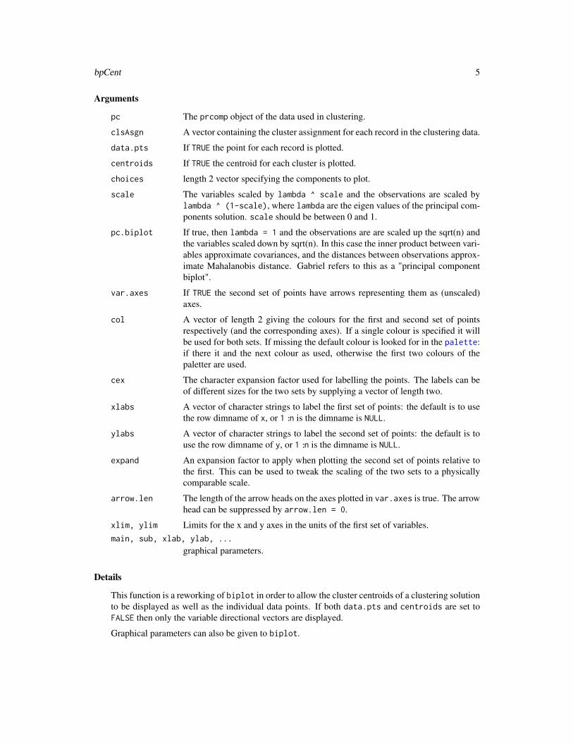
Arguments

pc The prcomp object of the data used in clustering.

clsAsgn A vector containing the cluster assignment for each record in the clustering data.

data.pts If TRUE the point for each record is plotted.

centroids If TRUE the centroid for each cluster is plotted.

choices length 2 vector specifying the components to plot.

scale The variables scaled by lambda ^ scale and the observations are scaled bylambda ^ (1-scale), where lambda are the eigen values of the principal com-ponents solution. scale should be between 0 and 1.

pc.biplot If true, then lambda = 1 and the observations are are scaled up the sqrt(n) andthe variables scaled down by sqrt(n). In this case the inner product between vari-ables approximate covariances, and the distances between observations approx-imate Mahalanobis distance. Gabriel refers to this as a "principal componentbiplot".

var.axes If TRUE the second set of points have arrows representing them as (unscaled)axes.

col A vector of length 2 giving the colours for the first and second set of pointsrespectively (and the corresponding axes). If a single colour is specified it willbe used for both sets. If missing the default colour is looked for in the palette:if there it and the next colour as used, otherwise the first two colours of thepaletter are used.

cex The character expansion factor used for labelling the points. The labels can beof different sizes for the two sets by supplying a vector of length two.

xlabs A vector of character strings to label the first set of points: the default is to usethe row dimname of x, or 1:n is the dimname is NULL.

ylabs A vector of character strings to label the second set of points: the default is touse the row dimname of y, or 1:n is the dimname is NULL.

expand An expansion factor to apply when plotting the second set of points relative tothe first. This can be used to tweak the scaling of the two sets to a physicallycomparable scale.

arrow.len The length of the arrow heads on the axes plotted in var.axes is true. The arrowhead can be suppressed by arrow.len = 0.

xlim, ylim Limits for the x and y axes in the units of the first set of variables.main, sub, xlab, ylab, ...

graphical parameters.

Details

This function is a reworking of biplot in order to allow the cluster centroids of a clustering solutionto be displayed as well as the individual data points. If both data.pts and centroids are set toFALSE then only the variable directional vectors are displayed.

Graphical parameters can also be given to biplot.

6 bpCent3d

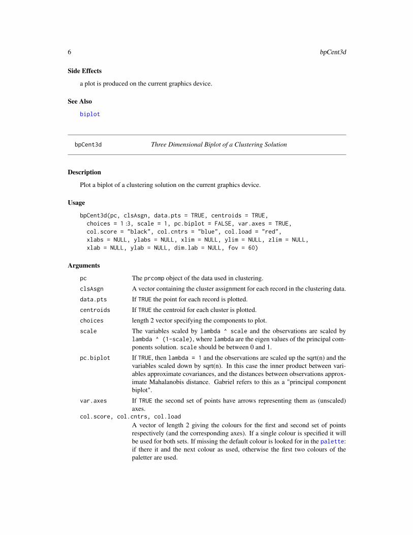
Side Effects

a plot is produced on the current graphics device.

See Also

biplot

bpCent3d Three Dimensional Biplot of a Clustering Solution

Description

Plot a biplot of a clustering solution on the current graphics device.

Usage

bpCent3d(pc, clsAsgn, data.pts = TRUE, centroids = TRUE,choices = 1:3, scale = 1, pc.biplot = FALSE, var.axes = TRUE,col.score = "black", col.cntrs = "blue", col.load = "red",xlabs = NULL, ylabs = NULL, xlim = NULL, ylim = NULL, zlim = NULL,xlab = NULL, ylab = NULL, dim.lab = NULL, fov = 60)

Arguments

pc The prcomp object of the data used in clustering.

clsAsgn A vector containing the cluster assignment for each record in the clustering data.

data.pts If TRUE the point for each record is plotted.

centroids If TRUE the centroid for each cluster is plotted.

choices length 2 vector specifying the components to plot.

scale The variables scaled by lambda ^ scale and the observations are scaled bylambda ^ (1-scale), where lambda are the eigen values of the principal com-ponents solution. scale should be between 0 and 1.

pc.biplot If TRUE, then lambda = 1 and the observations are scaled up the sqrt(n) and thevariables scaled down by sqrt(n). In this case the inner product between vari-ables approximate covariances, and the distances between observations approx-imate Mahalanobis distance. Gabriel refers to this as a "principal componentbiplot".

var.axes If TRUE the second set of points have arrows representing them as (unscaled)axes.

col.score, col.cntrs, col.load

A vector of length 2 giving the colours for the first and second set of pointsrespectively (and the corresponding axes). If a single colour is specified it willbe used for both sets. If missing the default colour is looked for in the palette:if there it and the next colour as used, otherwise the first two colours of thepaletter are used.

CCS 7

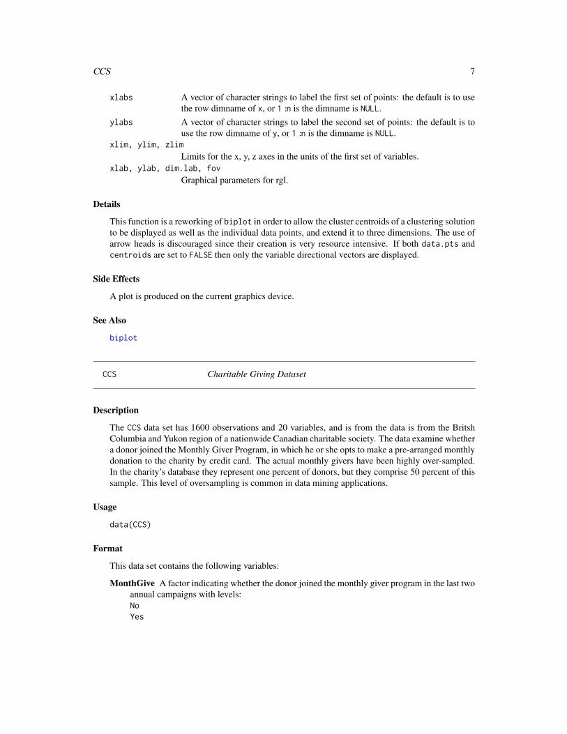
xlabs A vector of character strings to label the first set of points: the default is to usethe row dimname of x, or 1:n is the dimname is NULL.

ylabs A vector of character strings to label the second set of points: the default is touse the row dimname of y, or 1:n is the dimname is NULL.

xlim, ylim, zlim

Limits for the x, y, z axes in the units of the first set of variables.xlab, ylab, dim.lab, fov

Graphical parameters for rgl.

Details

This function is a reworking of biplot in order to allow the cluster centroids of a clustering solutionto be displayed as well as the individual data points, and extend it to three dimensions. The use ofarrow heads is discouraged since their creation is very resource intensive. If both data.pts andcentroids are set to FALSE then only the variable directional vectors are displayed.

Side Effects

A plot is produced on the current graphics device.

See Also

biplot

CCS Charitable Giving Dataset

Description

The CCS data set has 1600 observations and 20 variables, and is from the data is from the BritshColumbia and Yukon region of a nationwide Canadian charitable society. The data examine whethera donor joined the Monthly Giver Program, in which he or she opts to make a pre-arranged monthlydonation to the charity by credit card. The actual monthly givers have been highly over-sampled.In the charity’s database they represent one percent of donors, but they comprise 50 percent of thissample. This level of oversampling is common in data mining applications.

Usage

data(CCS)

Format

This data set contains the following variables:

MonthGive A factor indicating whether the donor joined the monthly giver program in the last twoannual campaigns with levels:NoYes

8 CCS

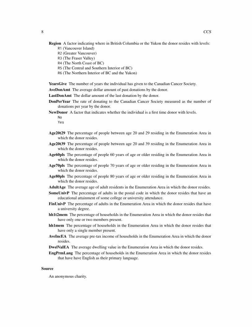
Region A factor indicating where in British Columbia or the Yukon the donor resides with levels:R1 (Vancouver Island)R2 (Greater Vancouver)R3 (The Fraser Valley)R4 (The North Coast of BC)R5 (The Central and Southern Interior of BC)R6 (The Northern Interior of BC and the Yukon)

YearsGive The number of years the individual has given to the Canadian Cancer Society.AveDonAmt The average dollar amount of past donations by the donor.LastDonAmt The dollar amount of the last donation by the donor.DonPerYear The rate of donating to the Canadian Cancer Society measured as the number of

donations per year by the donor.NewDonor A factor that indicates whether the individual is a first time donor with levels.

NoYes

Age20t29 The percentage of people between age 20 and 29 residing in the Enumeration Area inwhich the donor resides.

Age20t39 The percentage of people between age 20 and 39 residing in the Enumeration Area inwhich the donor resides.

Age60pls The percentage of people 60 years of age or older residing in the Enumeration Area inwhich the donor resides.

Age70pls The percentage of people 70 years of age or older residing in the Enumeration Area inwhich the donor resides.

Age80pls The percentage of people 80 years of age or older residing in the Enumeration Area inwhich the donor resides.

AdultAge The average age of adult residents in the Enumeration Area in which the donor resides.SomeUnivP The percentage of adults in the postal code in which the donor resides that have an

educational attainment of some college or university attendance.FinUnivP The percentage of adults in the Enumeration Area in which the donor resides that have

a university degree.hh1t2mem The percentage of households in the Enumeration Area in which the donor resides that

have only one or two members present.hh1mem The percentage of households in the Enumeration Area in which the donor resides that

have only a single member present.AveIncEA The average pre-tax income of households in the Enumeration Area in which the donor

resides.DwelValEA The average dwelling value in the Enumeration Area in which the donor resides.EngPrmLang The percentage of households in the Enumeration Area in which the donor resides

that have have English as their primary language.

Source

An anonymous charity.

create.samples 9

create.samples Create a Sample Membership Character Variable

Description

Provides a character vector with possible values of "Estimation", "Validation" and "Holdout" thatcan then be used to assign observations of a data frame to estimation, validation, or (optionally)holdsout samples using the subset option of a variety of functions.

Usage

create.samples(x, est=0.34, val=0.33, rand.seed=1)

Arguments

x A data frame.

est The percentage of the total sample to allocate to the estimation sample. Thevalue of est should range from zero to one

val The percentage of the total sample to allocate to the validation sample. Thevalue of val should range from zero to one

rand.seed A parameter passed to set.seed for to specify the seed of the random numbergenerator.

Details

The values of est and val should sum to a value between zero and one. If greater than one, anerror is returned. If less than one, the remaining percentage of the sample is allocated to the holdoutsample.

Value

A character vector with possible values of "Estimation", "Validation" and (optionally) "Holdout".The length of the vector equals the number of rows in the original data frame.

Author(s)

Dan Putler

See Also

set.seed

10 Eggs

Examples

data(CCS)# Create a new set of samples with 40 percent in each of the estimation and# validation samples, and 20 percent in the holdout sample.CCS$Sample <- create.samples(CCS, est=0.4, val=0.4)

Eggs Retail Sales of Eggs

Description

The Eggs data set has 105 observations and 10 variables. The data contains information on weeklysales of eggs in Southern California over a two year period.

Usage

data(Eggs)

Format

This data set contains the following variables:

Week The observation week (1 to 105). This variable can be used as a time trend.Month A factor that gives the name of the month in which the observation occured.First.Week A factor indicating whether the observation fell on the first week of the month with

levels:NoYes

Easter A factor that indicates whether the observation fell the week prior to the week containingEaster Sunday, the week containing Easter Sunday, the week following the week containingEaster Sunday, or a non-Easter week with levels:Non EasterPre EasterEasterPost Easter

Cases Retail sales of eggs in cases.Egg.Pr Average retail egg price in cents per dozen.Beef.Pr Average retail price of 7-bone beef roast in cents per pound.Pork.Pr Average retail price of strip bacon in cents per pound.Chicken.Pr Average retail price of whole frying chicken in cents per pound.Cereal.Pr Average retail price of Cheerios breakfast cereal in cents per pound.

Source

Putler (1992)

jack.jill 11

jack.jill Spending on Children’s Apparel

Description

The jack.jill data set has 557 observations and 8 variables. The data contains information onchildren’s apparel spending and household level demographic and socioeconomic information for asample of households residing in Alberta and British Columbia.

Usage

data(jack.jill)

Format

This data set contains the following variables:

SPENDING Dollars spent on children’s apparel over a one-year period.

CHILDREN Pre-tax income given as a factor with levels:1234+

INCOME Pre-tax income given as a factor with levels:$0k-$20k$20k-$30k$30k-$40k$40k-$50k$50k-$60k$60k-$75k$75k-$100k$100k+

EMPOLYMENT The employment status of the female head of household with levels:No female headUnemployedPart-timeFull-time

AGE Age of the female head of household given as a factor with levels:No female head29 and under30 to 3940 to 4950 to 5960 and over

12 lift.chart

EDUCATION The educational attainment of the female head of household given as a factor withlevels:No female headNot statedElementary or lessSome or completed secondarySome post-secondaryPost-secondary diplomaUniversity degree

OCCUPATION The occupation group of the female head of household with levels:No female headBlue collarPink collarWhite collarOtherNon-working or retired

BIRTHCNTRY The birth country of the female head of household with levels:No female headCanadaUS, N&W EuropeS&E EuropeAsia and OceaniaOther (Caribbean, Middle East, and Africa)

Source

Statistics Canada

lift.chart Lift Charts to Compare Binary Predictive Models

Description

Provides either a total cumulative response or incremental response rate lift chart for the purposesof comparing the predictive capability of different binary predictive models.

Usage

lift.chart(modelList, data, targLevel, trueResp, type = "cumulative", sub = "")

Arguments

modelList A character vector containing the names of the different models to be compared.The selected models must have the same y variable that must be a binary factor,and have been estimated using the same data set.

lift.chart 13

data The dataframe that constitues the comparison sample. If this dataframe is notthe same as the dataframe used to estimated models, the dataframe must containall the variables used in the models to be compared.

targLevel The label for the level of the binary factor of interest. For example, in a databasemarketing application, this level could be "Yes" for a variable that takes on thevalues "Yes" and "No" to indicate if a customer responded favorably to a pro-motion offer.

trueResp The true rate of the target level for the master database the estimation and com-parison dataframes were originally drawn from.

type A character string that must either have the value of "cummulative" (to producea total cummaltive response chart) or "incremental" (to produce an incrementalresponse rate chart).

sub A sub-title for the plot, typically to identify the sample used.

Details

Lift charts are a commonly used tool in business data mining applications. They are used to assesshow well a model is able to predict a desirable (from an organization’s point-of-view) responseon the part of a customer compared to alternative estimated models and a benchmark model ofapproaching customers randomly. The total cummulative response chart shows the percentage ofthe total response the organization would receive from only contacting a given percentage (groupedby deciles) of its entire customer base. This chart is best for selecting between alternative models,and in predicting the revenues the organization will receive by contacting a given percentage oftheir customers that the model predicts are most likely to favorably respond. The incrementalresponse rate chart provides the response rate among each of ten decile groups of the organization’scustomers, with the decile groups ordered by their estimated likelihood of a favorable response.

Value

The function returns invisibly. Its benefit is the side effect plot produced.

Author(s)

Dan Putler

Examples

library(rpart)layout(matrix(c(1,2), 2, 1))data(CCS)CCS$Sample <- create.samples(CCS, est=0.4, val=0.4)CCSEst <- CCS[CCS$Sample == "Estimation",]CCS.glm <- glm(MonthGive ~ DonPerYear + LastDonAmt + Region + YearsGive,

family=binomial(logit), data=CCSEst)library(rpart)CCS.rpart <- rpart(MonthGive ~ DonPerYear + LastDonAmt + Region + YearsGive,

data=CCSEst, cp=0.0074)CCSVal <- CCS[CCS$Sample == "Validation",]lift.chart(c("CCS.glm", "CCS.rpart"), data=CCSVal, targLevel="Yes",

14 Nnet

trueResp=0.01, type="cumulative", sub="Validation")lift.chart(c("CCS.glm", "CCS.rpart"), data=CCSVal, targLevel="Yes",

trueResp=0.01, type="incremental", sub="Validation")

Nnet Neural Networks Using Multiple Starting Weights

Description

Estimates a feed forward neural network using multiple intial starting weight vectors using the nnetfunction, and selects as the final model the one that minimizes the criterion function. This functionis designed to be used with the Rcmdrma package. The function nnSub implements subsetting in away more analogous to other R fitting functions.

Usage

Nnet(formula, data, decay, size, subset = "")

nnSub(data, subset)

Arguments

formula The formula to be used by nnet.data The dataframe to be used in the estimation.decay The decay parameter to be used by nnet.size The number of nodes in the hidden layer.subset A subseting expression (given as a quoted character string) for the estimation

data frame.

Value

A set of components identical to those returned by nnet.

Author(s)

Dan Putler

See Also

nnet

Examples

data(iris3)irisDat <- data.frame(rbind(iris3[,,1], iris3[,,2], iris3[,,3]),

species = as.factor(c(rep("s",50), rep("c",50), rep("v",50))))ir.nn2 <- Nnet(species ~ ., irisDat, 0.2, 2)

relabel.factor 15

relabel.factor Relabel Factor Levels

Description

Relabel the levels of factors to provide more descriptive names and reduce the number of factorlevels.

Usage

relabel.factor(x, new.labels, old.labels=levels(x))

Arguments

x A factor.

new.labels The new factor level labels.

old.labels The old factor level labels.

Details

The number of new factor labels/levels must be less than the number of labels/levels than the origi-nal factor.

Value

A factor whose length is equal to the old factor.

Author(s)

Dan Putler

scatterplotBCA Scatterplots with Boxplots

Description

A minor modification of the car package’s scatterplot function that makes enhanced scatterplots,with boxplots in the margins, a lowess smooth, smoothed conditional spread, outlier identification,and a regression line; sp is an abbreviation for scatterplot.

16 scatterplotBCA

Usage

scatterplotBCA(x, ...)

## S3 method for class ’formula’scatterplotBCA(x, data, subset, xlab, ylab, legend.title, legend.coords,labels, ...)

## Default S3 method:scatterplotBCA(x, y, smooth = TRUE, spread = !by.groups,

span = 0.5, loess.threshold = 2, reg.line = lm,boxplots = if (by.groups) "" else "xy", xlab = deparse(substitute(x)),ylab = deparse(substitute(y)), las = par("las"), lwd = 2,lwd.smooth = lwd, lwd.spread = lwd, lty = 1, lty.smooth = lty,lty.spread = 2, labels, id.method = "mahal",id.n = if(id.method[1] == "identify") length(x) else 0, id.cex = 1,id.col = palette()[1], log = "", jitter = list(), xlim = NULL,ylim = NULL, cex = par("cex"), cex.axis = par("cex.axis"),cex.lab = par("cex.lab"), cex.main = par("cex.main"),cex.sub = par("cex.sub"), groups, by.groups = !missing(groups),legend.title = deparse(substitute(groups)), legend.coords,ellipse = FALSE, levels = c(0.5, 0.95), robust = TRUE, col = if(n.groups == 1) palette()[c(2, 1, 3)] else rep(palette(),length = n.groups), pch = 1:n.groups, legend.plot = !missing(groups),reset.par = TRUE, grid = TRUE, ...)

spBCA(...)

Arguments

x vector of horizontal coordinates, or a “model” formula, of the form y ~ x or(to plot by groups) y ~ x | z, where z evaluates to a factor or other variabledividing the data into groups. If x is a factor, then parallel boxplots are producedusing the Boxplot function.

y vector of vertical coordinates.

data data frame within which to evaluate the formula.

subset expression defining a subset of observations.

smooth if TRUE (the default) a loess nonparametric regression line is drawn on the plot.

spread if TRUE (the default when there are no groups), a smoother is applied to theroot-mean-square positive and negative residuals from the loess line to displayconditional spread and asymmetry.

span span for the loess smoother.loess.threshold

suppress the loess smoother if there are fewer than loess.threshold uniquevalues (default, 5) of y.

reg.line function to draw a regression line on the plot or FALSE not to plot a regressionline.

scatterplotBCA 17

boxplots if "x" a boxplot for x is drawn below the plot; if "y" a boxplot for y is drawnto the left of the plot; if "xy" both boxplots are drawn; set to "" or FALSE tosuppress both boxplots.

xlab label for horizontal axis.

ylab label for vertical axis.

las if 0, ticks labels are drawn parallel to the axis; set to 1 for horizontal labels (seepar).

lwd width of linear-regression lines (default 1).

lwd.smooth width for smooth regression lines (default is the same as lwd).

lwd.spread width for lines showing spread (default is the same as lwd).

lty type of linear-regression lines (default 1, solid line).

lty.smooth type of smooth regression lines (default is the same as lty).

lty.spread width for lines showing spread (default is 2, broken line).id.method,id.n,id.cex,id.col

Arguments for the labelling of points. The default is id.n=0 for labeling nopoints. See showLabels for details of these arguments. If the plot uses differentcolors for groups, then the id.col argument is ignored and label colors aredetermined by the col argument.

labels a vector of point labels; if absent, the function tries to determine reasonablelabels, and, failing that, will use observation numbers.

log same as the log argument to plot, to produce log axes.

jitter a list with elements x or y or both, specifying jitter factors for the horizontal andvertical coordinates of the points in the scatterplot. The jitter function is usedto randomly perturb the points; specifying a factor of 1 produces the defaultjitter. Fitted lines are unaffected by the jitter.

xlim the x limits (min, max) of the plot; if NULL, determined from the data.

ylim the y limits (min, max) of the plot; if NULL, determined from the data.

groups a factor or other variable dividing the data into groups; groups are plotted withdifferent colors and plotting characters.

by.groups if TRUE, regression lines are fit by groups.

legend.title title for legend box; defaults to the name of the groups variable.

legend.coords coordinates for placing legend; an be a list with components x and y to specifythe coordinates of the upper-left-hand corner of the legend; or a quoted keyword,such as "topleft", recognized by legend.

ellipse if TRUE data-concentration ellipses are plotted.

levels level or levels at which concentration ellipses are plotted; the default is c(.5, .95).

robust if TRUE (the default) use the cov.trob function in the MASS package to calculatethe center and covariance matrix for the data ellipses.

col colors for lines and points; the default is taken from the color palette, withpalette()[2] for nonparametric regression lines and palette()[1] for lin-ear regression line and points if there are no groups, and successive colors forthe groups if there are groups.

18 scatterplotMatrixBCA

pch plotting characters for points; default is the plotting characters in order (see par).cex, cex.axis, cex.lab, cex.main, cex.sub

set sizes of various graphical elements; (see par).

legend.plot if TRUE then a legend for the groups is plotted in the upper margin.

reset.par if TRUE then plotting parameters are reset to their previous values when scatterplotexits; if FALSE then the mar and mfcol parameters are altered for the current plot-ting device. Set to FALSE if you want to add graphical elements (such as lines)to the plot.

... other arguments passed down and to plot.

grid If TRUE, the default, a light-gray background grid is put on the graph

Value

If points are identified, their labels are returned; otherwise NULL is returned invisibly.

Author(s)

John Fox with modifications made by Dan Putler

See Also

scatterplot

scatterplotMatrixBCA Scatterplot Matrices

Description

A minor modification of the car package’s scatterplotMatrix function that makes enhanced scatter-plot matrices with univariate displays down the diagonal; spmBCA is an abbreviation for scatterplotMatrixBCA.This function just sets up a call to pairs with custom panel functions.

Usage

scatterplotMatrixBCA(x, ...)

## S3 method for class ’formula’scatterplotMatrixBCA(x, data=NULL, subset, labels, ...)

## Default S3 method:scatterplotMatrixBCA(x, var.labels = colnames(x), diagonal = c("density",

"boxplot", "histogram", "oned", "qqplot", "none"),adjust = 1, nclass, plot.points = TRUE, smooth = TRUE,spread = smooth && !by.groups, span = 0.5,loess.threshold = 2, reg.line = lm, transform = FALSE,

scatterplotMatrixBCA 19

family = c("bcPower", "yjPower"), ellipse = FALSE,levels = c(0.5, 0.95), robust = TRUE, groups = NULL,by.groups = FALSE, labels, id.method = "mahal", id.n =0, id.cex = 1, id.col = palette()[1], col = if(n.groups == 1) palette()[c(2, 1, 3)] else rep(palette(),length = n.groups), pch = 1:n.groups, lwd = 2,lwd.smooth = lwd, lwd.spread = lwd, lty = 1,lty.smooth = lty, lty.spread = 2, cex = par("cex"),cex.axis = par("cex.axis"), cex.labels = NULL,cex.main = par("cex.main"), legend.plot =length(levels(groups)) > 1, row1attop = TRUE, ...)

spmBCA(x, ...)

Arguments

x a data matrix, numeric data frame, or a one-sided “model” formula, of the form~ x1 + x2 + ... + xk or ~ x1 + x2 + ... + xk | z where z evaluatesto a factor or other variable to divide the data into groups.

data for scatterplotMatrix.formula, a data frame within which to evaluate theformula.

subset expression defining a subset of observations.

labels,id.method,id.n,id.cex,id.col

Arguments for the labelling of points. The default is id.n=0 for labeling nopoints. See showLabels for details of these arguments. If the plot uses differentcolors for groups, then the id.col argument is ignored and label colors aredetermined by the col argument.

var.labels variable labels (for the diagonal of the plot).

diagonal contents of the diagonal panels of the plot.

adjust relative bandwidth for density estimate, passed to density function.

nclass number of bins for histogram, passed to hist function.

plot.points if TRUE the points are plotted in each off-diagonal panel.

smooth if TRUE a loess smooth is plotted in each off-diagonal panel.

spread if TRUE (the default when not smoothing by groups), a smoother is applied to theroot-mean-square positive and negative residuals from the loess line to displayconditional spread and asymmetry.

span span for loess smoother.

loess.threshold

suppress the loess smoother if there are fewer than loess.threshold uniquevalues (default, 5) of the variable on the vertical axis.

reg.line if not FALSE a line is plotted using the function given by this argument; e.g.,using rlm in package MASS plots a robust-regression line.

20 scatterplotMatrixBCA

transform if TRUE, multivariate normalizing power transformations are computed with powerTransform,rounding the estimated powers to ‘nice’ values for plotting; if a vector of pow-ers, one for each variable, these are applied prior to plotting. If there are groupsand by.groups is TRUE, then the transformations are estimated conditional onthe groups factor.

family family of transformations to estimate: "bcPower" for the Box-Cox family or"yjPower" for the Yeo-Johnson family (see powerTransform).

ellipse if TRUE data-concentration ellipses are plotted in the off-diagonal panels.

levels levels or levels at which concentration ellipses are plotted; the default is c(.5, .9).

robust if TRUE use the cov.trob function in the MASS package to calculate the centerand covariance matrix for the data ellipses.

groups a factor or other variable dividing the data into groups; groups are plotted withdifferent colors and plotting characters.

by.groups if TRUE, regression lines are fit by groups.

pch plotting characters for points; default is the plotting characters in order (see par).

col colors for lines and points; the default is taken from the color palette, withpalette()[2] for nonparametric regression lines and palette()[1] for lin-ear regression lines and points if there are no groups, and successive colors forthe groups if there are groups.

lwd width of linear-regression lines (default 1).

lwd.smooth width for smooth regression lines (default is the same as lwd).

lwd.spread width for lines showing spread (default is the same as lwd).

lty type of linear-regression lines (default 1, solid line).

lty.smooth type of smooth regression lines (default is the same as lty).

lty.spread width for lines showing spread (default is 2, broken line).cex, cex.axis, cex.labels, cex.main

set sizes of various graphical elements (see par).

legend.plot if TRUE then a legend for the groups is plotted in the first diagonal cell.

row1attop If TRUE (the default) the first row is at the top, as in a matrix, as opposed to atthe bottom, as in graph (argument suggested by Richard Heiberger).

... arguments to pass down.

Value

NULL. This function is used for its side effect: producing a plot.

Author(s)

John Fox with minor modifications by Dan Putler

See Also

scatterplotMatrix

score 21

score Score a Database based on a Predictive Model

Description

Provides either an integer vector that contains the "desirability" rank of a case in a data set, the fittedprobability of a desired response, or the fitted probability adjusted for the true response rate basedon the fitted values of a predictive model.

Usage

rankScore(model, data, targLevel)rawProbScore(model, data, targLevel)adjProbScore(model, data, targLevel, trueResp)

Arguments

model A character string containing the name of the model to use to score the database.

data A data frame of the database to be scored. All the predictor variables of themodel need to be amoung the variables of the data frame.

targLevel The "desired" level of the y variable factor as a character string.

trueResp The true "desired" response rate for the overall population of interest.

Details

Only binomial glm, binary rpart, and binary nnet models can be used as the basis of scoring adatabase.

Value

An integer vector that indicates the rank order desirability (a value of 1 means most desirable) ofthe correponding case of the database being scored or a probability measure bounded between zeroand one.

Author(s)

Dan Putler

22 SD.clv

SD.clv A Wrapper Function for the clv.SD Function and its Components

Description

Provides a wrapper to several function calls in the clv package needed to construct the SD indexvalue for a clustering solution. The number of clusters that has the lowest value of the SD indexrepresents the "best" solution under the criteria used to construct the SD index.

Usage

SD.clv(x, clus, alpha)

Arguments

x A numeric matrix of data, or an object that can be coerced to such a matrix (suchas a numeric vector or a dataframe with all numeric columns) used to constructthe clustering solution.

clus The cluster to which each row of x was assigned.

alpha A weight to be placed on the average scattering of the clustering solution.

Details

The SD index corresponds to the weighted sum of the average "scattering" of points within clustersand the inverse of the total seperation between clusters. The average scattering measure is basedon the average sum of the squared differences between a clusters centroid all the points in a cluster,while total seperation is measured by the sum of the squared distance between cluster centroids. Asolution with a low average scattering and a low value of the inverse total seperation is consideredto be better than a solution with higher levels of these two measures.

Value

A scalar SD index value for the clustering solution.

Author(s)

Dan Putler

References

M. Haldiki, Y. Batistakis, M. Vazirgiannis (2001), On Clustering Validation Techniques, Journal ofIntelligent Information Systems, 17:2/3.

See Also

clv.SD

SDIndex 23

Examples

data(iris)iris.data <- iris[,1:4]irisC3 <- kmeans(iris.data, centers=3, nstart=10)SD.clv(iris.data, clus=irisC3$cluster, alpha=0.1)

SDIndex A Plot of SD Index Values for K-Means Clustering Solutions

Description

Provides a plot of SD cluster validation index values for different numbers of k-means clusters fora common underlying dataset. The number of clusters that has the lowest value of the SD indexrepresents the "best" solution under the criteria used to construct the SD index.

Usage

SDIndex(x, minClust, maxClust, iter.max=10, num.seeds=10)

Arguments

x A numeric matrix of data, or an object that can be coerced to such a matrix (suchas a numeric vector or a dataframe with all numeric columns).

minClust The minimum number of clusters to be considered for a solution.

maxClust The maximum number of clusters to be considered for a solution.

iter.max The maximum number of iterations allowed for a solution.

num.seeds The number of different starting random seeds to use for a solution with a givennumber of clusters.

Details

The SD index corresponds to the weighted sum of the average "scattering" of points within clustersand the inverse of the total seperation between clusters. The average scattering measure is basedon the average sum of the squared differences between a clusters centroid all the points in a cluster,while total seperation is measured by the sum of the squared distance between cluster centroids. Asolution with a low average scattering and a low value of the inverse total seperation is consideredto be better than a solution with higher levels of these two measures.

Value

The function returns invisibly. Its benefit is the side effect plot produced.

Author(s)

Dan Putler

24 variable.summary

References

M. Haldiki, Y. Batistakis, M. Vazirgiannis (2001), On Clustering Validation Techniques, Journal ofIntelligent Information Systems, 17:2/3.

See Also

KMeans, SD.clv

Examples

data(iris)iris.data <- iris[,1:4]SDIndex(iris.data, minClust=2, maxClust=6, iter.max=10, num.seeds=10)

variable.summary Basic summary information of the variables of a data frame

Description

The function returns a data frame where, the row names correspond to the variable names, and a setof columns with summary information for each variable. Its purpose is to allow the user to quicklyscan the data frame for potentially problematic variables.

Usage

variable.summary(dframe)

Arguments

dframe A data frame.

Value

The returned data frame contains the variables Class (numeric, integer,factor, or character), missingvalues), Levels (the levels of a factor variable, or NA for non-factor variables), Min.Level.Size (thenumber of cases for the smallest level of a factor, or NA for a non-factor), Mean (the mean of non-missing cases for a numeric or integer variable, or NA for factor and character variables), and SD(the standard deviation of non-missing cases for a numeric or integer variable, or NA for factor andcharacter variables).

Author(s)

Dan Putler

Examples

data(CCS)variable.summary(CCS)

Index

∗Topic clusterbootCVD, 3SD.clv, 22SDIndex, 23

∗Topic datasetsAthletic, 2CCS, 7Eggs, 10jack.jill, 11

∗Topic hplotbpCent, 4bpCent3d, 6scatterplotBCA, 15scatterplotMatrixBCA, 18

∗Topic misccreate.samples, 9lift.chart, 12Nnet, 14relabel.factor, 15score, 21variable.summary, 24

∗Topic multivariatebpCent, 4bpCent3d, 6

adjProbScore (score), 21Athletic, 2

biplot, 6, 7bootCH (bootCVD), 3bootCVD, 3bootFlexclust, 4bootPlot (bootCVD), 3Boxplot, 16bpCent, 4bpCent3d, 6

CCS, 7clv.SD, 22create.samples, 9

Eggs, 10

jack.jill, 11jitter, 17

KMeans, 24

legend, 17lift.chart, 12

Nnet, 14nnet, 14nnSub (Nnet), 14

palette, 5, 6par, 17, 18, 20plot, 17powerTransform, 20

rankScore (score), 21rawProbScore (score), 21relabel.factor, 15

scatterplot, 18scatterplotBCA, 15scatterplotMatrix, 20scatterplotMatrixBCA, 18score, 21SD.clv, 22, 24SDIndex, 23set.seed, 9showLabels, 17, 19spBCA (scatterplotBCA), 15spmBCA (scatterplotMatrixBCA), 18

variable.summary, 24

25