bca 103_mathematical foundation of computer sc_bca.pdf
TRANSCRIPT
MATHEMATICAL FOUNDATIONS OF COMPUTER SCIENCE
VENKATESHWARAOPEN UNIVERSITY
www.vou.ac.in
VENKATESHWARAOPEN UNIVERSITY
www.vou.ac.in
MATHEMATICAL FOUNDATIONS OF COMPUTER SCIENCE
BCA[BCA-103]
MATHEM
ATICAL FOUNDATIONS OF COMPUTER SCIENCE
12 MM
MATHEMATICAL FOUNDATIONSOF COMPUTER SCIENCE
BCA
[BCA-103]
Authors:
Ashish Tayal: Units (1.0-1.2.1, 1.2.7-1.2.9) copyright © Vikas® Publishing House, 2010
S. Mohan Naidu: Units (1.2.2-1.2.6, 1.2.10-1.2.12, 1.4-1.6.4, 1.9-1.16, 4.0-4.4.2) copyright © S. Mohan Naidu, 2010
N Ch SN Iyengar, VM Chandrasekaran, K.A. Venkatesh & P.S. Arunachalam: Units (2.0-2.2.6, 2.2.8-2.11, Unit-3, 4.6-4.6.7,5.6.2) copyright © Vikas® Publishing House, 2010
V.K. Khanna & S.K. Bhambri: Units (5.0-5.4, 5.6-5.6.1) copyright © V.K. Khanna & S.K. Bhambri, 2010
Vikas® Publishing House: Units (1.3-1.3.1, 1.7-1.8,, 2.2.7, 4.6.8-4.12, 5.5, 5.7-5.12) copyright © Vikas® Publishing House,2010
BOARD OF STUDIES
Prof Lalit Kumar SagarVice Chancellor
Dr. S. Raman IyerDirectorDirectorate of Distance Education
SUBJECT EXPERT
Prof. Saurabh Upadhya Dr. Kamal UpretiMr. Animesh Srivastav Hitendranath Bhattacharya
ProfessorAssociate ProfessorAssociate ProfessorAssistant Professor
CO-ORDINATOR
Mr. Tauha KhanRegistrar
All rights reserved. No part of this publication which is material protected by this copyright noticemay be reproduced or transmitted or utilized or stored in any form or by any means now known orhereinafter invented, electronic, digital or mechanical, including photocopying, scanning, recordingor by any information storage or retrieval system, without prior written permission from the Publisher.
Information contained in this book has been published by VIKAS® Publishing House Pvt. Ltd. and hasbeen obtained by its Authors from sources believed to be reliable and are correct to the best of theirknowledge. However, the Publisher and its Authors shall in no event be liable for any errors, omissionsor damages arising out of use of this information and specifically disclaim any implied warranties ormerchantability or fitness for any particular use.
Vikas® is the registered trademark of Vikas® Publishing House Pvt. Ltd.
VIKAS® PUBLISHING HOUSE PVT LTDE-28, Sector-8, Noida - 201301 (UP)Phone: 0120-4078900 Fax: 0120-4078999Regd. Office: A-27, 2nd Floor, Mohan Co-operative Industrial Estate, New Delhi 1100 44Website: www.vikaspublishing.com Email: [email protected]
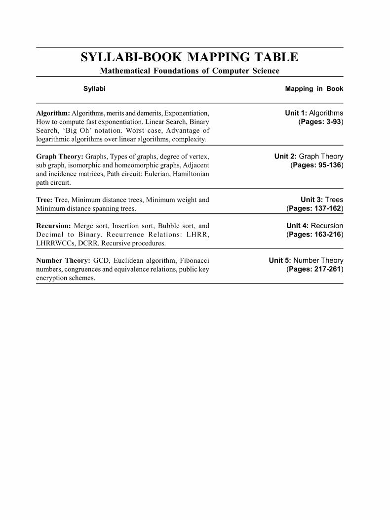
SYLLABI-BOOK MAPPING TABLEMathematical Foundations of Computer Science
Algorithm: Algorithms, merits and demerits, Exponentiation,How to compute fast exponentiation. Linear Search, BinarySearch, ‘Big Oh’ notation. Worst case, Advantage oflogarithmic algorithms over linear algorithms, complexity.
Graph Theory: Graphs, Types of graphs, degree of vertex,sub graph, isomorphic and homeomorphic graphs, Adjacentand incidence matrices, Path circuit: Eulerian, Hamiltonianpath circuit.
Tree: Tree, Minimum distance trees, Minimum weight andMinimum distance spanning trees.
Recursion: Merge sort, Insertion sort, Bubble sort, andDecimal to Binary. Recurrence Relations: LHRR,LHRRWCCs, DCRR. Recursive procedures.
Number Theory: GCD, Euclidean algorithm, Fibonaccinumbers, congruences and equivalence relations, public keyencryption schemes.
Unit 1: Algorithms(Pages: 3-93)
Unit 2: Graph Theory(Pages: 95-136)
Unit 3: Trees(Pages: 137-162)
Unit 4: Recursion(Pages: 163-216)
Unit 5: Number Theory(Pages: 217-261)
Syllabi Mapping in Book

CONTENTS
INTRODUCTION 1
UNIT 1 ALGORITHMS 3-93
1.0 Introduction1.1 Unit Objectives1.2 Algorithms: An Introduction
1.2.1 Definition, Characteristics and Properties of Algorithms1.2.2 Types of Algorithms1.2.3 Areas of Research in the Study of Algorithms1.2.4 Algorithm for Sequential Search1.2.5 Algorithms as Technology1.2.6 Algorithms and Other Technologies1.2.7 Measuring the Running Time of an Algorithm1.2.8 Algorithm Design Strategies1.2.9 Analysis of Algorithms
1.2.10 Merits and Demerits of Algorithm1.2.11 Flowchart and Algorithms1.2.12 Designing an Algorithm using Flowcharts
1.3 Exponentiation1.3.1 How to Compute Exponentiation Fast?
1.4 Linear Search1.4.1 Algorithm for Linear Search1.4.2 Analysis of Linear Search algorithm
1.5 Binary Search1.5.1 The Search Method1.5.2 Algorithm for Binary Search1.5.3 Analysis of Binary Search Algorithm1.5.4 Fibonacci Search
1.6 Big Oh Notation (or Big O Notation)1.6.1 Properties of the Big O Notation1.6.2 General Rules1.6.3 Finding Prime Factor of a Given Number1.6.4 List of Prime Numbers
1.7 Worst Case1.8 Advantage of Logarithmic Algorithms Over Linear Algorithms1.9 Complexity
1.9.1 Space Complexity1.9.2 Time Complexity1.9.3 Practical Complexities1.9.4 Performance Measurement
1.10 Algorithm Representation through a Pseudocode1.10.1 Coding1.10.2 Program Development Steps1.10.3 Software Testing
1.11 Amortized Analysis
1.12 Summary1.13 Key Terms1.14 Answers to ‘Check Your Progress’1.15 Questions and Exercises1.16 Further Reading
UNIT 2 GRAPH THEORY 95-136
2.0 Introduction2.1 Unit Objectives2.2 Graphs: Types and Operations
2.2.1 Bipartite Graphs2.2.2 Subgraph2.2.3 Distance in a Graph2.2.4 Cut-Vertices and Cut-Edges2.2.5 Graph Connectivity2.2.6 Isomorphic Graphs2.2.7 Homeographic Graphs2.2.8 Cut-Sets and Connectivity of Graphs2.2.9 Operations on Graphs
2.3 Degree of Vertex2.4 Adjacent and Incidence Matrices2.5 Path Circuit
2.5.1 Floyd’s and Warshall’s Algorithms2.5.2 Eulerian Path and Circuit2.5.3 Hamiltonian Graphs
2.6 Graph Colouring2.6.1 Four Colour Theorem
2.7 Summary2.8 Key Terms2.9 Answers to ‘Check Your Progress’
2.10 Questions and Exercises2.11 Further Reading
UNIT 3 TREES 137-162
3.0 Introduction3.1 Unit Objectives3.2 Trees: Basics
3.2.1 Trees and Sorting3.3 Minimum Height and Minimum Distance Spanning Trees
3.3.1 Depth-First Search and Breadth-First Search3.3.2 Optimal Spanning Graph
3.4 Planar Graphs3.5 Summary3.6 Key Terms3.7 Answers to ‘Check Your Progress’3.8 Questions and Exercises3.9 Further Reading
UNIT 4 RECURSION 163-216
4.0 Introduction4.1 Unit Objectives4.2 Mergesort4.3 Insertion Sort4.4 Bubble Sort and Selection Sort
4.4.1 Bubble Sort4.4.2 Selection Sort
4.5 Binary and Decimal Numbers4.5.1 Binary Number System4.5.2 Decimal Number System4.5.3 Binary to Decimal Conversion4.5.4 Decimal to Binary Conversion4.5.5 Double-Dabble Method4.5.6 Decimal Fraction to Binary
4.6 Recursion and Recurrence Relations4.6.1 Recursion and Iteration4.6.2 Closed Form Expression4.6.3 Sequence of Integers4.6.4 Recurrence Relations4.6.5 Linear Homogenous Recurrence Relations (LHRR)4.6.6 Solving Linear Homogeneous Recurrence Relations4.6.7 Solving Linear Non-Homogeneous Recurrence Relations4.6.8 Linear Homogeneous Recurrence Relations with Constant Coefficient (LHRRWCC)4.6.9 Divide and Conquer Recurrence Relation (DCRR)
4.7 Recursive Procedures4.7.1 Functional Recursion4.7.2 Recursive Proofs4.7.3 The Recursion Theorem4.7.4 Infinite Sequences4.7.5 Recursive Function and Primitive Recursive Function
4.8 Summary4.9 Key Terms
4.10 Answers to ‘Check Your Progress’4.11 Questions and Exercises4.12 Further Reading
UNIT 5 NUMBER THEORY 217-261
5.0 Introduction5.1 Unit Objectives5.2 Number Theory: Basics
5.2.1 Fundamental Theorem of Arithmetic5.2.2 Prime Numbers5.2.3 Division Algorithms5.2.4 Divisibility5.2.5 Absolute Value5.2.6 Order and Inequalities
5.3 Greatest Common Divisor5.3.1 Linear Diophantine Equation
5.4 Euclidean Algorithm5.5 Fibonacci Numbers
5.6 Congruences and Equivalence Relations5.6.1 Congruences Relations5.6.2 Equivalence Relations
5.7 Public Key Encryption Schemes5.7.1 Message Authentication Code5.7.2 Digital Structure
5.8 Summary5.9 Key Terms
5.10 Answer to ‘Check Your Progress’5.11 Questions and Exercises5.12 Further Reading
Introduction
NOTES
Self-Instructional Material 1
INTRODUCTION
Mathematics is, perhaps, the most important subject for achieving excellence inany field of science or commerce. The book has been structured to define the keymathematical concepts and its formulations by providing helpful and relevantmaterial in lucid, self-explanatory and simple language to help you to understandthe basic concepts and achieve your goals. It can be used by you as an introductionto the underlying ideas of mathematics that are applicable to computer science aswell.
This book, Mathematical Foundations of Computer Science, is dividedinto five units. The first unit introduces the concept of algorithms, its properties andcharacteristics. It also discusses the advantage of logarithmic algorithms over linearalgorithms. The next unit covers the various features of graphs, its types andoperations. The third unit deals with the types of tree structures and the varioussituations in which they are applied. The next unit explains the concept of recursionand the recursive procedures. The last unit discusses the basics of the numbertheory.
The topics are logically organized and explained with related mathematicaltheorems, analysis and formulations to provide a background for statistical thinkingand analysis with good knowledge of calculus. The interactive examples have alsobeen carefully designed so that you can gradually build up your knowledge andunderstanding.
The key features of this book are:
It balances theory with applications.
The theorems and proofs are followed by solved exercises.
Simplified notations and techniques of mathematical methods to make thetext easy to understand.
The book motivates new concepts with the extensive use of examples.
The mathematical applications provided will help you to understandmathematics in action and to contextualize what you are actually learning.
The text facilitates understanding of key mathematical concepts and theirapplication in solving problems.
The book follows the self-instructional mode wherein each unit begins withan Introduction to the topic. The Unit Objectives are then outlined before going onto the presentation of the detailed content in a simple and structured format. CheckYour Progress questions are provided at regular intervals to test the student’sunderstanding of the subject. A Summary, a list of Key Terms and a set of Questionsand Exercises are provided at the end of each unit for recapitulation.

Algorithms
NOTES
Self-Instructional Material 3
UNIT 1 ALGORITHMS
Structure
1.0 Introduction1.1 Unit Objectives1.2 Algorithms: An Introduction
1.2.1 Definition, Characteristics and Properties of Algorithms1.2.2 Types of Algorithms1.2.3 Areas of Research in the Study of Algorithms1.2.4 Algorithm for Sequential Search1.2.5 Algorithms as Technology1.2.6 Algorithms and Other Technologies1.2.7 Measuring the Running Time of an Algorithm1.2.8 Algorithm Design Strategies1.2.9 Analysis of Algorithms
1.2.10 Merits and Demerits of Algorithm1.2.11 Flowchart and Algorithms1.2.12 Designing an Algorithm using Flowcharts
1.3 Exponentiation1.3.1 How to Compute Exponentiation Fast?
1.4 Linear Search1.4.1 Algorithm for Linear Search1.4.2 Analysis of Linear Search algorithm
1.5 Binary Search1.5.1 The Search Method1.5.2 Algorithm for Binary Search1.5.3 Analysis of Binary Search Algorithm1.5.4 Fibonacci Search
1.6 Big Oh Notation (or Big O Notation)1.6.1 Properties of the Big O Notation1.6.2 General Rules1.6.3 Finding Prime Factor of a Given Number1.6.4 List of Prime Numbers
1.7 Worst Case1.8 Advantage of Logarithmic Algorithms Over Linear Algorithms1.9 Complexity
1.9.1 Space Complexity1.9.2 Time Complexity1.9.3 Practical Complexities1.9.4 Performance Measurement
1.10 Algorithm Representation through a Pseudocode1.10.1 Coding1.10.2 Program Development Steps1.10.3 Software Testing
1.11 Amortized Analysis1.12 Summary1.13 Key Terms1.14 Answers to ‘Check Your Progress’1.15 Questions and Exercises1.16 Further Reading
4 Self-Instructional Material
Algorithms
NOTES
1.0 INTRODUCTION
Informally, an algorithm refers to any well-defined computational procedure thattakes some values as ‘input’ and produces some value or set of values as ‘output’.It is composed of a finite set of steps, each of which may require one or moreoperations. Every operation may be characterized as either simple or complex.Operations performed on scalar quantities are termed simple, while those performedon vector data are normally termed as complex. An algorithm can also be viewedas a tool for solving a well-specified ‘computational problem’. The statement ofthe problem specifies, in general terms, the desired input/output relationship.
In simple terms, an algorithm can be defined as a step-by-step procedurefor performing some task in a finite amount of time.
For a given problem, there are several ways of designing an algorithm, butthe best way is the one that executes the algorithm fast. The most commonly useddesign approaches include, incremental approach, divide and conquer approach,dynamic programming, greedy strategy, branch and bound, backtracking andrandomized algorithms.
Algorithms are used in a broad spectrum of computer applications.Algorithms to sort, search and process text, solve graph problems and basicgeometric problems, display graphics and perform common mathematicalcalculations are extensively studied and are considered a necessary component ofcomputer science.
1.1 UNIT OBJECTIVES
After going through this unit, you will be able to:
Describe the basic features of algorithms
Compute exponentiation
Describe the meaning and implementation of linear search
Describe the meaning and implementation of binary search
Understand the functions of Big O notation
Define the best-case, worst-case and average-case situations in an algorithm
Describe the advantages of logarithmic algorithms over linear algorithms
Understand the various types of complexities, such as space complexity,time complexity, practical complexity, etc
Represent an algorithm through a pseudo code
Describe the various techniques used in amortized analysis
Algorithms
NOTES
Self-Instructional Material 5
1.2 ALGORITHMS: AN INTRODUCTION
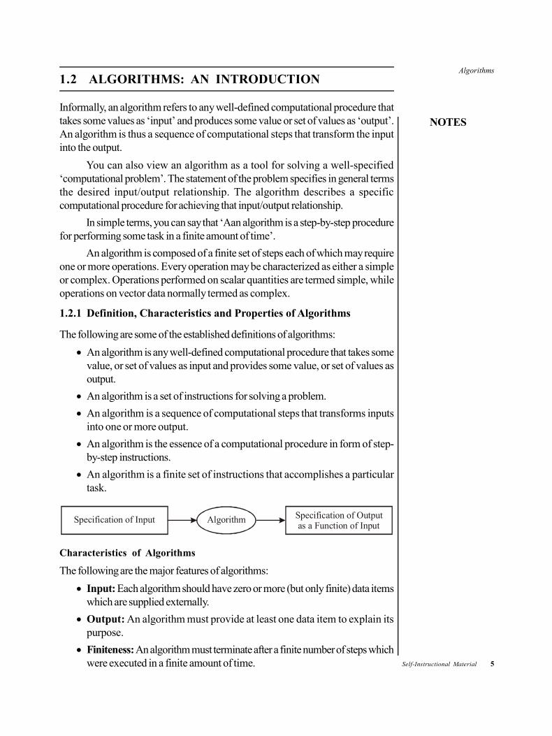
Informally, an algorithm refers to any well-defined computational procedure thattakes some values as ‘input’ and produces some value or set of values as ‘output’.An algorithm is thus a sequence of computational steps that transform the inputinto the output.
You can also view an algorithm as a tool for solving a well-specified‘computational problem’. The statement of the problem specifies in general termsthe desired input/output relationship. The algorithm describes a specificcomputational procedure for achieving that input/output relationship.
In simple terms, you can say that ‘Aan algorithm is a step-by-step procedurefor performing some task in a finite amount of time’.
An algorithm is composed of a finite set of steps each of which may requireone or more operations. Every operation may be characterized as either a simpleor complex. Operations performed on scalar quantities are termed simple, whileoperations on vector data normally termed as complex.
1.2.1 Definition, Characteristics and Properties of Algorithms
The following are some of the established definitions of algorithms:
An algorithm is any well-defined computational procedure that takes somevalue, or set of values as input and provides some value, or set of values asoutput.
An algorithm is a set of instructions for solving a problem.
An algorithm is a sequence of computational steps that transforms inputsinto one or more output.
An algorithm is the essence of a computational procedure in form of step-by-step instructions.
An algorithm is a finite set of instructions that accomplishes a particulartask.
Specification of Input Algorithm Specification of Output as a Function of Input
Characteristics of Algorithms
The following are the major features of algorithms:
Input: Each algorithm should have zero or more (but only finite) data itemswhich are supplied externally.
Output: An algorithm must provide at least one data item to explain itspurpose.
Finiteness: An algorithm must terminate after a finite number of steps whichwere executed in a finite amount of time.
6 Self-Instructional Material
Algorithms
NOTES
Definiteness: Each step must be unambiguously specified and clear, i.e.,each step must be precisely defined.
Effectiveness: Each step should be sufficiently simple and basic.
Algorithms that are definite and effective are also termed as computationalprocedures.
What is a Good Algorithm?
A good algorithm should be efficient in terms of the running time as well as thespace utilized. An algorithm is said to be efficient, if it takes less amount of time toexecute and also utilizes less amount of memory.
Efficiency as a Function of Input Size
Efficiency can be measured in terms of the number of bits in an input number aswell as the number of data elements (numbers, points).
Properties of Algorithm
The following are the five important properties (features) of algorithm:
Finiteness
Definitiveness
Input
Output
Effectiveness
Finiteness: An algorithm must always terminate after a finite number ofsteps. If we trace out the instructions of an algorithm, then for all cases, thealgorithm terminates after a finite number of steps.
Definitiveness: Each operation must have a definite meaning and it mustbe perfectly clear. All steps of an algorithm need to be precisely defined.The actions to be executed in each case should be rigorously and clearlyspecified.
Inputs: An algorithm may have zero or more ‘input’ quantities. These inputsare given to the algorithm either prior to its beginning or dynamically as itruns. An input is taken from a specified set of objects. Also, it is externallysupplied to the algorithm.
Output: An algorithm has one or more ‘output’ quantities. These quantitieshave specified relations to the inputs. An algorithm produces at least oneoutput.
Effectiveness: Each operation should be effective, i.e., the operation mustterminate in a finite amount of time.
An algorithm is usually supposed to be ‘effective’ in the sense that all itsoperations need to be sufficiently basic so that they can in principle be executedexactly the same way in a finite length of time by someone using pencil and paper.
Algorithms
NOTES
Self-Instructional Material 7
1.2.2 Types of Algorithms
(i) Approximate algorithm
(ii) Probabilistic algorithm
(iii) Infinite algorithm
(iv) Heuristic algorithm
(i) Approximate Algorithm
An algorithm is said to approximate if it is infinite and repeating.
For example, 414.12
732.13
14.3 , etc.
(ii) Probabilistic Algorithm
If the solution of a problem is uncertain, then it is called a probabilistic algorithm.
For example, Tossing of a coin
(iii) Infinite Algorithm
An algorithm, which is not finite, is called infinite algorithm.
For example, a complete solution of a chessboard, division by zero
(iv) Heuristic Algorithm
Giving less inputs and getting more outputs is called heuristic algorithm.
1.2.3 Areas of Research in the Study of Algorithms
Several active areas of research are included in the study of algorithms. The followingfour distinct areas can be identified:
1. Devising Algorithms
The creation of an algorithm is an art. It may never be fully automated. Afew design techniques are especially useful in fields other than computerscience, such as operations research and electrical engineering. All of theapproaches we consider have application in diverse areas, includingcomputer science. But some important design techniques such as linear,non-linear and integer programming are not covered here as they aretraditionally covered in other courses.
2. Validating Algorithms
Once you have devised an algorithm, you need to show that it computes thecorrect answer for all possible legal inputs. This process is referred to as‘algorithm validation’. It is not necessary to express the algorithm as aprogram. If it is stated in a precise way, it will do. The objective of thevalidation is to assure the user that the algorithm will work correctly andindependently of the issues concerning the programming language, in whichit will eventually be written. After validity of the method gets checked, is
8 Self-Instructional Material
Algorithms
NOTES
shown, it is possible to write the program. On completion of program writingthe second phase begins. This phase is called ‘program providing’ or‘program verification’. A proof of correctness requires the solution to bestated in two forms. One form is usually a program, which is annotated bya set of assertions about the input and output variables of the program. Thesecond form is called specification and this may also be expressed in thepredicate calculus. A proof shows that these two forms are equivalent forevery given legal input, they describe the same output. A complete proof ofprogram correctness requires that each statement of the programminglanguage is precisely defined and all basic operations are proved correct.All these details may cause a proof to be very much longer than the program.
3. Analysing Algorithms
As an algorithm is executed, it uses computer’s central processing unit (CPU)for performing operations. It also uses the memory for holding the programand its data. Analysis of algorithm is the process of determining the computingtime and storage required by an algorithm.
4. Testing a Program
Testing of a program comprises of two phases: (i) Debugging and (ii) Profiling.(i) Debugging refers to the process of carrying out programs on sample
data sets with the objective of finding faulty results. If any faulty resultoccurs, it is corrected by debugging. A proof of correctness is muchmore valuable than a thousand tests, since it guarantees that the programwill work correctly for a possible input.
(ii) Profiling refers to the process of executing a correct program on datasets and the measurement of the time and space it takes in computingthe results. It is useful in the sense that it confirms a previously doneanalysis and points out logical places for performing useful optimization.
For example,
If you wish to measure the worst-case performance of the sequential searchalgorithm, we need to do the following:
Decide the values of n for which computing time has be obtained
Determine for each of the above value of n the data that exhibits the worst-case behaviour
1.2.4 Algorithm for Sequential Search
1. Algorithm seqsearch (a, x, n)
2. //search for x in a[l: n] . a[0] is used as additionalspace
3. {
4. i := n; a[0] := x;
5. while(a[i] * x) do i := i + 1;
6. return i;
7. }
Algorithms
NOTES
Self-Instructional Material 9
The decision on which the values of n to be used is based on the amount of timingwe wish to perform and also on what we expect to do with the times once they areobtained. Assume that for algorithm, our interest is to simply predict how long itwill take, in the worst case, to search for x, given the size n of a.
1.2.5 Algorithms as Technology
If computers were infinitely fast and computer memory was free, you would be ina position to adopt any correct method to solve a problem. In all likelihood, youwould like your implementation to be adhering to good software engineeringpractice. However, you would use the method which is the easiest to implement.
However, computers may be fast, but they cannot be infinitely fast. Similarly,memory may be cheap, but it cannot be free. Thus, computing time and space inmemory are bounded resources . You need to use these resources wisely. Suchalgorithms which are efficient in terms of time or space will be helpful.
Efficiency
It has been found that algorithm devices used for solving the same problem usuallydiffer considerably in their efficiency. These differences are more significant thanthose due to hardware and software.
1.2.6 Algorithms and Other Technologies
Algorithms are important on contemporary computers which have advancedtechnologies, such as
Hardware with high clock rates, pipelining and super scalar architectures
Easy to use, intuitive Graphical User Interfaces (GUIs)
Local Area Networking (LAN) and Wide Area Networking (WAN)
A truly skilled programmer possesses a solid algorithmic knowledge and technique.It separates him/her from a novice. It is true that with modern computing technology,you can perform some tasks even if you do not have much knowledge of algorithms.However, if you have a good background in algorithms, you can perform muchbetter.
1.2.7 Measuring the Running Time of an Algorithm
Experimental Study
The following steps need to be carried out:
(i) A program should be written in a language which will implement thealgorithm.
(ii) This program should be run with input data which is of varying size andcomposition.
(iii) Methods such as getTime() or System.currentTimemillis() should be employed for obtaining an accurate value of theactual running time required by the algorithm for execution.
10 Self-Instructional Material
Algorithms
NOTES
Limitations of Experimental Study
The experimental studies have the following limitations:
(i) In order to calculate the running time of the algorithm, it must be implementedand tested.
(ii) Since the experiments are carried out only with a few set of inputs, therunning time calculated need not be representative of other inputs whichwere not part of the experimental study.
(iii) The same hardware and software platforms should be used for comparingtwo algorithms.
Theoretical Analysis
The general methodology for analysing the running time of algorithms:
Uses a high-level description of the algorithm instead of testing one of itsimplementations
Takes into account all possible inputs
Enables evaluation of efficiency of any algorithm in a way that is independentof the hardware and software environment.
1.2.8 Algorithm Design Strategies
For a given problem, there are several ways to design algorithms, but the best wayis the one which executes the algorithm fast, such that it operates quickly on inputs.
The following are the descriptions of several design approaches which yieldgood algorithms:
Incremental Approach
This is one of the simplest approaches of algorithm designing. In this case, whenevera new element is inserted into its appropriate place, the index is increased. Youstart moving from the first step executing each step one by one till you reach theend. Here, you do not split your problem.
Example includes insertion sort designed using incremental approach.
Divide and Conquer Approach
Some algorithms have recursion and they call themselves one or more times todeal with sub-problems in order to reach the solution. These types of algorithmsfollow the Divide and Conquer approach.
In this approach, you break the original problem into several sub-problemswhich are similar to the original problem in structure but smaller in size, solve thesub-problems recursively, and then combine these solutions to create a solution ofthe original problem.
Traditionally, an algorithm is referred to as the ‘divide and conquer’ type,only if it contains at least two recursive calls.
Algorithms
NOTES
Self-Instructional Material 11
The following are the three steps involved in this approach:1. Divide: The given problem is divided into several sub-problems2. Conquer: The sub-problems are solved recursively3. Combine: The solutions of the sub-problems are combined to create
a solution of the original problem
Examples include quick sort, merge sort, binary search, etc.
Dynamic Programming
Dynamic programming is the most powerful design technique for optimizationproblems. The divide and conquer approach is applicable where sub-problemsare independent. On the other hand, dynamic programming is applicable wheresub-problems share sub-problems. A dynamic programming algorithm rememberspast results and uses them to find new results.
Dynamic programming is generally used for optimization problems. In theseproblems multiple solutions exist, but we need to find the ‘best’ solution. Thisrequires ‘optimal sub-structure’ and ‘overlapping sub-problems’.
Optimal sub-structure: Optimal solution contains optimal solutionsto sub-problems.
Overlapping sub-problems: Solutions to sub-problems can be storedand reused in a bottom-up fashion.
Examples include assembly line scheduling, matrix chain multiplication and longestcommon sub-sequence.
Greedy Strategy
Greedy algorithms typically applies to optimization problems such as dynamicprogramming algorithms, where a set of choices must be made in order to arrive atan optimal solution. The main idea behind greedy algorithm is to make each choicein a locally optimal manner, i.e., choose the solution which looks best at the momentwithout considering the future results. Greedy approach provides an optimal solutionfor many problems much more quickly than a dynamic programming approach. Ingreedy algorithms, you use optimal sub-structure in a top-down fashion. Insteadof first finding optimal solutions to sub-problems and then making a choice, greedyalgorithms first make a choice—the choice that looks best at the time—and thensolve the resulting sub-problems.
Greedy algorithms do not always guarantee optimal solutions, however,they generally produce solutions that are very close in value to the optimal.
Examples include activity selection problem, Huffman algorithm, fractionalknapsack problem.
Branch and Bound
Branch and Bound algorithm is used for finding optimal solutions of variousoptimization problems, especially discrete and combinational types. In Branchand Bound algorithm, a given problem which cannot be bounded has to be divided
12 Self-Instructional Material
Algorithms
NOTES
into two new restricted problems. Branch and Bound algorithms can be slow, andin worst cases they grow exponentially as the input size grows, but in some casesthese algorithms perform well.
Examples include Knapsack problem, non-linear programming, maximumsatisfiability problem, least cost search, 15-puzzle, and so on.
Backtracking
The term backtrack was first coined by D.H. Lehmer in the 1950s. If a problemhas several possible choices at any stage, then you select any choice and startmoving by considering that choice. If it choice solves your problem then it is good,otherwise, you backtrack, i.e., move backwards and choose some other choiceand repeat the same procedure until the solution is obtained. Some sequence ofchoices may be a solution to your problem.
Examples include N-Queens problem, sum of subsets problem, Hamiltoniancircuit problem, graph colouring, etc.
Randomized Algorithms
An algorithm whose input is determined by the values produced by a randomnumber generator is a randomized or probabilistic algorithm. Such an algorithmemploys a degree of randomness as part of its logic. Various decisions made in thealgorithm depend on the output of the random number generator. As randomnumber generator produces different outputs from run to run, so the output of arandomized algorithm could also differ from run to run for the same input.
The following are the two types of randomized algorithms:
(i) Las Vegas algorithms
(ii) Monte Carlo algorithms
Example includes randomized quicksort.
CHECK YOUR PROGRESS
1. How can efficiency be measured as a function of input size?
2. What is the ‘Incremental approach’ to design algorithms?
3. What are the two main types of randomized algorithms?
1.2.9 Analysis of Algorithms
During analysis, performance of an algorithm should be evaluated by predictinghow much resources the algorithm requires. You usually concentrate on determiningthe running time (worst case) without considering the space requirements, unlessstated. So, to predict the resource requirements, you need a computational model.Popular computational models include RAM (Random Access Model), PARAM,Message Passing Model, Turing Machine, etc.

Algorithms
NOTES
Self-Instructional Material 13
In RAM model, you have to deal with instructions which are executed oneafter the other and there should also be no concurrent operations. Instructionsinclude the following:
Arithmetic: Add, multiply, substract, floor, ceiling, divide Shift left and shift right Data movement: Assignment, load, copy, store Logical: Comparison Control: Conditional/unconditional branching, subroutine call, return
These instructions are called the primitive operations. Primitive operations arelow-level operations which are independent of the programming language. Theycan be identified in the pseudocode.
There is no generally accepted set of rules for the analysis of algorithms.You can perform analysis by counting the number of primitive operations in thealgorithm.
By analysing the pseudocode, you are able to count the number of primitiveoperations executed by an algorithm.
In Example 1.1 the algorithm which determines the maximum elementsfrom a set of elements given in an array of size n is given. Determine the number ofprimitive operations required.
For example,MAXIMUM (A, n)
1. current_max ¬ A[0]
2. for i ¬ 1 to n – 1 do
3. if current_max < A[i]
4. then current_max ¬ A[i]
{increment counter i}
5. return current_max
No. of primitive operations = 2 + 1 + n + 4(n – 1) + 1 = 5n (At least)
= 2 + 1 + n + 6(n – 1) + 1 = 7n – 2 (At most)
Consider the following example for insertion sort, which is a very efficient algorithmfor sorting a small number of elements.
Insertion sort: It is a very good algorithm for sorting or arranging, either in theincreasing or decreasing order for small number of elements.
In this case the sequence of numbers which are to be sorted and output is asorted sequence
Insertion-Sort (A)
1.for i 2 to length A [i] do
2.item A [i]
3.//Insert A [i] into the sorted sequence A [1... i – 1]
4.j i –1
14 Self-Instructional Material
Algorithms
NOTES
5.while j > 0 and A [j] > item do
6.A [j + 1] A [j]
7.j j – 1
8.A [j + 1] item
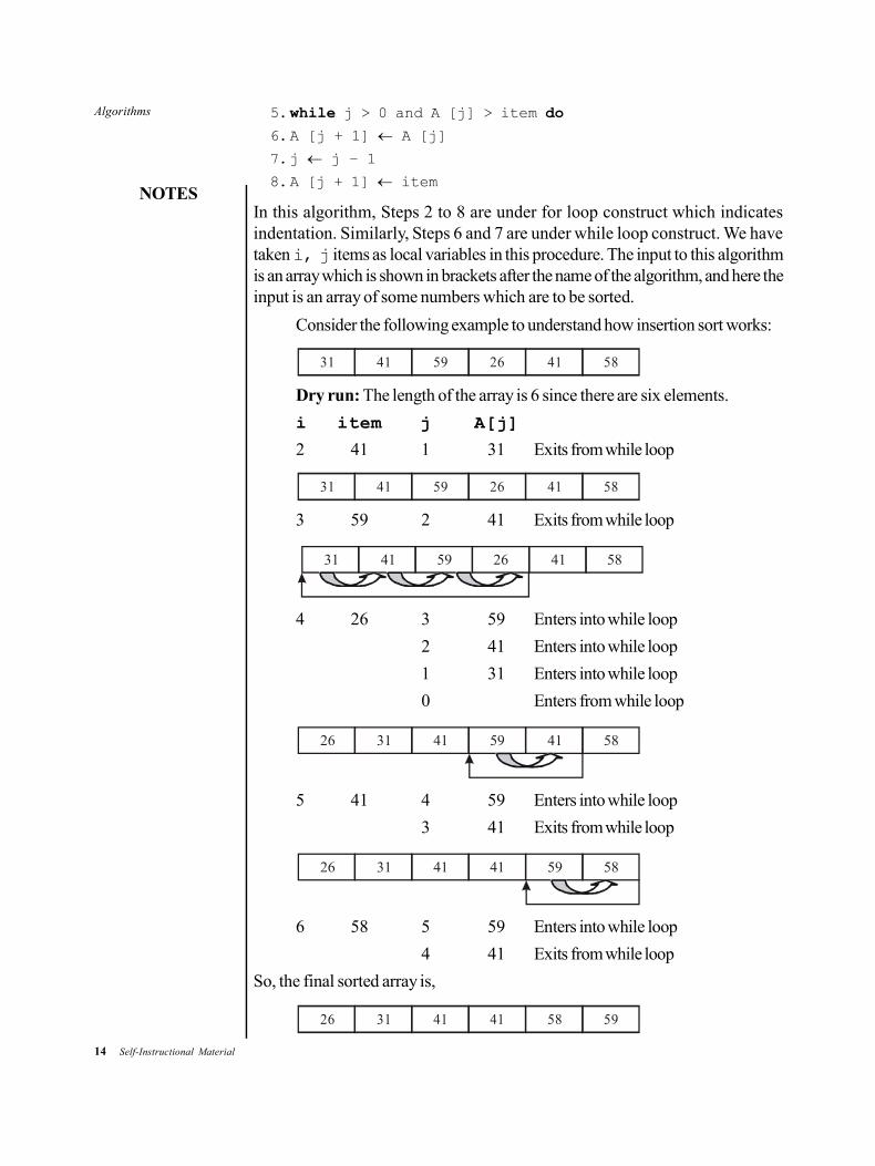
In this algorithm, Steps 2 to 8 are under for loop construct which indicatesindentation. Similarly, Steps 6 and 7 are under while loop construct. We havetaken i, j items as local variables in this procedure. The input to this algorithmis an array which is shown in brackets after the name of the algorithm, and here theinput is an array of some numbers which are to be sorted.
Consider the following example to understand how insertion sort works:
31 41 59 26 41 58
Dry run: The length of the array is 6 since there are six elements.
i item j A[j]
2 41 1 31 Exits from while loop
31 41 59 26 41 58
3 59 2 41 Exits from while loop
31 41 59 26 41 58
4 26 3 59 Enters into while loop
2 41 Enters into while loop
1 31 Enters into while loop
0 Enters from while loop
26 31 41 59 41 58
5 41 4 59 Enters into while loop
3 41 Exits from while loop
26 31 41 41 59 58
6 58 5 59 Enters into while loop
4 41 Exits from while loop
So, the final sorted array is,
26 31 41 41 58 59
Algorithms
NOTES
Self-Instructional Material 15
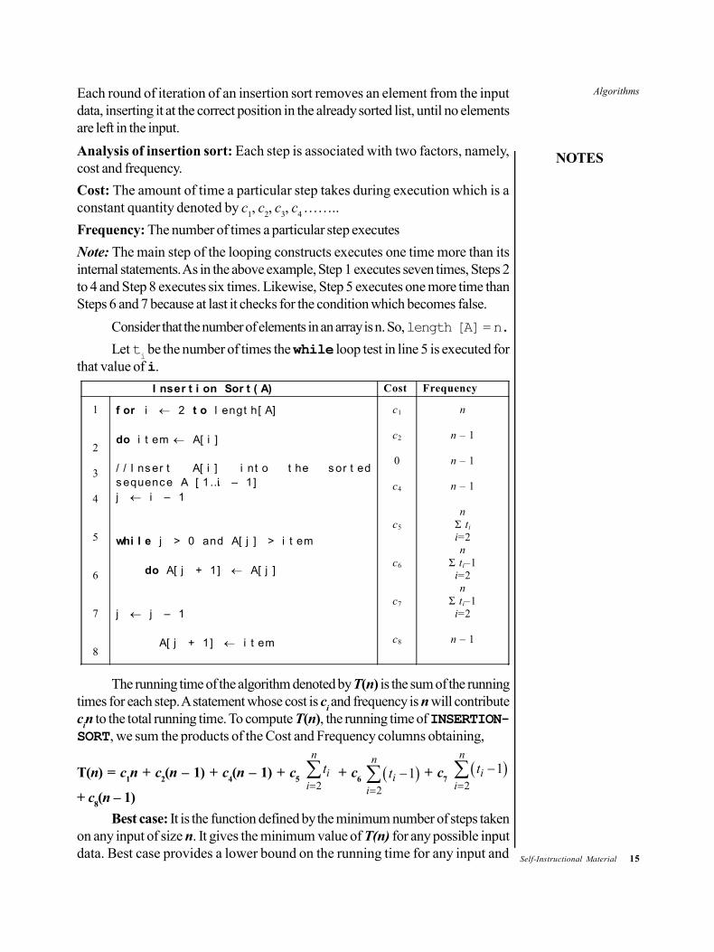
Each round of iteration of an insertion sort removes an element from the inputdata, inserting it at the correct position in the already sorted list, until no elementsare left in the input.
Analysis of insertion sort: Each step is associated with two factors, namely,cost and frequency.
Cost: The amount of time a particular step takes during execution which is aconstant quantity denoted by c
1, c
2, c
3, c
4 ……..
Frequency: The number of times a particular step executes
Note: The main step of the looping constructs executes one time more than itsinternal statements. As in the above example, Step 1 executes seven times, Steps 2to 4 and Step 8 executes six times. Likewise, Step 5 executes one more time thanSteps 6 and 7 because at last it checks for the condition which becomes false.
Consider that the number of elements in an array is n. So, length [A]=n.
Let ti be the number of times the while loop test in line 5 is executed for
that value of i.
I nser t i on Sor t ( A) Cost Frequency
1
2
3
4
5
6
7
8
f or i 2 t o l engt h[ A] do i t em A[ i ] / / I ns er t A[ i ] i nt o t he s or t ed s equenc e A [ 1…i – 1] j i – 1 whi l e j > 0 and A[ j ] > i t em do A[ j + 1] A[ j ] j j – 1 A[ j + 1] i t em
c1
c2
0
c4
c5
c6
c7
c8
n
n – 1
n – 1
n – 1
n Σ ti i=2 n
Σ ti–1 i=2 n
Σ ti–1 i=2
n – 1
The running time of the algorithm denoted by T(n) is the sum of the runningtimes for each step. A statement whose cost is c
i and frequency is n will contribute
cin to the total running time. To compute T(n), the running time of INSERTION-SORT, we sum the products of the Cost and Frequency columns obtaining,
T(n) = c1n + c
2(n – 1) + c
4(n – 1) + c
5
2
n
ii
t + c
6 2
1n
ii
t
+ c
7
2
1n
ii
t
+ c
8(n – 1)
Best case: It is the function defined by the minimum number of steps takenon any input of size n. It gives the minimum value of T(n) for any possible inputdata. Best case provides a lower bound on the running time for any input and
16 Self-Instructional Material
Algorithms
NOTES
occurs when minimum number of steps are executed, i.e., the while loop conditionis always false or the array is already sorted. For that case, t
i = 1.
2
1n
ii
t n
So,
T(n) = c1n + c
2(n – 1) + c
4(n – 1) + c
5(n – 1)
+ c
8(n – 1)
T(n) = (c1 + c
2 + c
4 + c
5 + c
8) n – (c
2 + c
4 + c
5 + c
8)
T(n) = an + b
T(n) = O(n)
For best case, the running time of insertion sort is a linear function in n.
Worst case: It is the function defined by the maximum number of stepstaken on any input size of size n. It gives the maximum value of T(n) for anypossible input data. Worst case provides an upper bound on the running time forany input and gives you a guarantee that the algorithm will never take longer time.
You usually concentrate on finding the worst case running time, i.e., insearching algorithms worst case occurs when you try to find a number but thenumber is not present. Likewise, worst case occurs when the maximum number ofsteps are executed, i.e., the while loop condition always leads to true or the arrayelements are given in decreasing order. For that case, t
i = j.
Hence,
T(n) = c1n + c
2(n – 1) + c
4(n – 1) + c
5 2
n
i
j
+ c
6
2
1n
i
j
+ c7
2
1n
i
j
+ c8(n – 1)
T(n) = c1n + c
2(n – 1) + c
4(n – 1) + c
5((n(n + 1)/2) – 1)
+ c6(n(n – 1)/2) + c
7(n(n – 1)/2) + c
8(n – 1)
T(n) = (c5/2 + c
6/2 + c
7/2)n2 + (c
1 + c
2 + c
4 + c
5/2 – c
6/2
– c7/2 + c
8)n – (c
2 + c
4 + c
5 + c
8)
T(n) = an2 + bn + c
T(n) = O(n2)
For worst case, the running time of insertion sort is a quadratic function in n.
Average case: It is the function defined by the average number of stepstaken on any input of size n. It gives the expected value of T(n). Generally, you donot analyse the average case, because it is often as bad as the worst case. This
Algorithms
NOTES
Self-Instructional Material 17
case lies between the best and worst cases. Hence, in this case, ti = i/2 or (i + 1)/
2 or (i – 1)/2.
T(n) = O(n2)
Note: During analysis we drop the lower contributing terms and the coefficients todo analysis for large n.
Analysis of Some Other Algorithms:
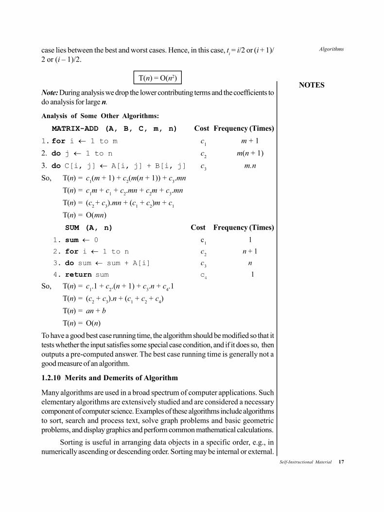
MATRIX-ADD (A, B, C, m, n) Cost Frequency (Times)
1. for i 1 to m c1
m + 1
2. do j 1 to n c2
m(n + 1)
3. do C[i, j] A[i, j] + B[i, j] c3
m.n
So, T(n) = c1(m + 1) + c
2(m(n + 1)) + c
3.mn
T(n) = c1m + c
1 + c
2.mn + c
2m + c
3.mn
T(n) = (c2 + c
3).mn + (c
1 + c
2)m + c
1
T(n) = O(mn)
SUM (A, n) Cost Frequency (Times)
1. sum 0 c1
1
2. for i 1 to n c2
n + 1
3. do sum sum + A[i] c3
n
4. return sum c4
1
So, T(n) = c1.1 + c
2.(n + 1) + c
3.n + c
4.1
T(n) = (c2 + c
3).n + (c
1 + c
2 + c
4)
T(n) = an + b
T(n) = O(n)
To have a good best case running time, the algorithm should be modified so that ittests whether the input satisfies some special case condition, and if it does so, thenoutputs a pre-computed answer. The best case running time is generally not agood measure of an algorithm.
1.2.10 Merits and Demerits of Algorithm
Many algorithms are used in a broad spectrum of computer applications. Suchelementary algorithms are extensively studied and are considered a necessarycomponent of computer science. Examples of these algorithms include algorithmsto sort, search and process text, solve graph problems and basic geometricproblems, and display graphics and perform common mathematical calculations.
Sorting is useful in arranging data objects in a specific order, e.g., innumerically ascending or descending order. Sorting may be internal or external.
18 Self-Instructional Material
Algorithms
NOTES
Using internal sorting, you can arrange data stored internally in a computer’smemory. Simple algorithms for sorting by selection, exchange or insertion are easyto understand and straightforward to code. However, in case the number of objectsto be sorted is large, simple algorithms would not be helpful as they are usuallyvery slow. In such cases, you need a more sophisticated algorithm, such as heapsort or quick sort, to achieve acceptable performance. Using external sorting, youcan arrange data records that are stored.
Searching for data means looking for a desired data object in a group ofdata objects. Elementary searching algorithms comprise of linear search and binarysearch. In linear search, a sequence of data objects is examined one by one. Inbinary search, on the other hand, a more sophisticated strategy for searching datais adopted. While searching a large array, binary search works faster than linearsearch. You can also store the collection of data objects as a tree that need to besearched frequently. If such a tree is properly structured, searching the tree wouldbe very efficient.
A sequence of characters is termed as a text string. In a word processingsystem, efficient algorithms for manipulating text strings, such as algorithms fororganizing text data into lines and paragraphs and searching for occurrences of agiven pattern in a document, are necessary. A source program in a high-levelprogramming language is a text string. Text processing is one of the essential tasksof a compiler. A compiler uses efficient algorithms to perform lexical analysis andparsing. When individual characters are grouped into meaningful words or symbols,it is termed as lexical analysis. When the syntactical structure of a source programis recognized, it is termed as parsing.
A graph is used in modelling a group of interconnected objects. A graphrepresenting a set of locations connected by routes for transportation is a goodexample. Graph algorithms are used to solve such problems which deal with objectsand their connections, such as determining whether or not all locations areconnected, visiting all locations that are accessible from a given location, ordetermining the shortest path from one location to another.
Mathematical algorithms are widely applied in science and engineering.Algorithms to generate random numbers, perform operations on matrices, solvesimultaneous equations and numerical integration, etc., are examples of basicalgorithms for mathematical computations. In the modern programming languages,predefined functions are usually provided for many common computations, suchas random number generation, logarithm, exponentiation and trigonometricfunctions.
There are applications in which a computer program has to adapt to achange in its environment so as to continue performing well. Using a self-organizingdata structure, which gets reorganized at regular intervals, such that thosecomponents which are most likely to be accessed are placed where they can beaccessed most efficiently, is a common approach to make a computer programadaptive. A self-modifying algorithm that adapts itself is also conceivable. In order
Algorithms
NOTES
Self-Instructional Material 19
to develop adaptive computer programs, biological evolution has given impetus toevolutionary computation methods, such as genetic algorithms.
Some applications need a large amount of computations in a timely manner.For saving time, you need to develop a parallel algorithm which uses manyprocessors simultaneously and thus quickly solves a given problem. The basicidea is that the given problem is divided into sub-problems and each processor isused to solve a sub-problem. The processors usually have to communicate amongthemselves so as to facilitate cooperation. For communicating with one another,the processors may share memory. Alternatively, they may be connected bycommunication links into some type of network, such as a hypercube.
1.2.11 Flowchart and Algorithms
In the beginning, the use of flowcharts was restricted to electronic data processingfor representing the conditional logic of computer programs. The1980s witnessedthe emergence of structured programming and structured design. As a result ofthis, in database programming, data flow and structure charts began to replaceflowcharts. With the widespread adoption of such ALGOL-like computer languagesas Pascal, textual models like pseudocode are being used frequently for representingalgorithms. Unified Modeling Language (UML) started the synthesis and codificationthese modelling techniques in the 1990s.
A flowchart refers to a graphical representation of a process which depictsinputs, outputs and units of activity. It represents the whole process at a high ordetailed (depending on your use) level of observation. It serves as an instructionmanual or a tool to facilitate a detailed analysis and optimization of workflow aswell as service delivery.
Flowcharts have been in use since long. Nobody can be specified as the‘father of the flowchart’. It is possible to customize a flowchart according to needor purpose. This is why flowcharts are considered a very unique quality improvementmethod for representing data.
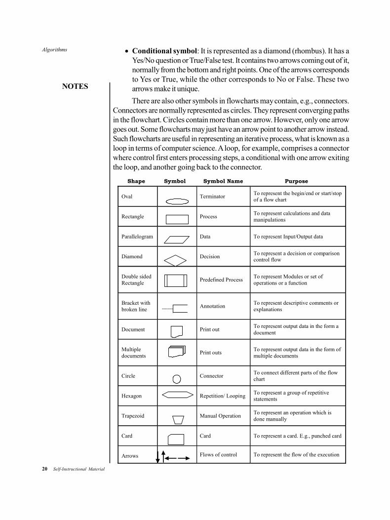
Symbols
A typical flowchart has the following types of symbols:
Start and end symbols: They are represented as ovals or roundedrectangles, normally having the word ‘Start’ or ‘End’.
Arrows: They show the ‘flow of control’ in computer science. An arrowcoming from one symbol and ending at another symbol shows thetransmission of control to the symbol the arrow is pointing to.
Processing steps: They are represented as rectangles.
Example: Add 1 to X.
Input/Output symbol: It is represented as a parallelogram.
Examples: Get X from the user; display X.
20 Self-Instructional Material
Algorithms
NOTES
Conditional symbol: It is represented as a diamond (rhombus). It has aYes/No question or True/False test. It contains two arrows coming out of it,normally from the bottom and right points. One of the arrows correspondsto Yes or True, while the other corresponds to No or False. These twoarrows make it unique.
There are also other symbols in flowcharts may contain, e.g., connectors.Connectors are normally represented as circles. They represent converging pathsin the flowchart. Circles contain more than one arrow. However, only one arrowgoes out. Some flowcharts may just have an arrow point to another arrow instead.Such flowcharts are useful in representing an iterative process, what is known as aloop in terms of computer science. A loop, for example, comprises a connectorwhere control first enters processing steps, a conditional with one arrow exitingthe loop, and another going back to the connector.
Oval
Terminator
To represent the begin/end or start/stop of a flow chart
Rectangle
Process
To represent calculations and data manipulations
Parallelogram
Data To represent Input/Output data
Diamond
Decision
To represent a decision or comparison control flow
Double sided Rectangle
Predefined Process To represent Modules or set of operations or a function
Bracket with broken line
Annotation To represent descriptive comments or explanations
Document
Print out
To represent output data in the form a document
Multiple documents
Print outs To represent output data in the form of multiple documents
Circle
Connector
To connect different parts of the flow chart
Hexagon
Repetition/ Looping
To represent a group of repetitive statements
Trapezoid
Manual Operation
To represent an operation which is done manually
Card
Card To represent a card. E.g., punched card
Arrows
Flows of control To represent the flow of the execution
Shape Symbol Symbol Name Purpose
Algorithms
NOTES
Self-Instructional Material 21
It is now used at the beginning of the next line or page with the same number.Thus, a reader of the chart is able to follow the path.
Instructions
The following is the step-by-step process for developing a flowchart:
Step 1: Information on how the process flows is gathered. For this, the followingtools are used:
Conservation
Experience
Product development codes
Step 2: The trial of process flow is undertaken.
Step 3: Other more familiar personnel are allowed to check for accuracy.
Step 4: If necessary, changes are made.
Step 5: The final actual flow is compared with the best possible flow.
Construction/Interpretation tips for a flowchart
The boundaries of the process should be defined unambiguously.
The simplest symbols should be used.
It should be ensured that each feedback loop contains an escape.
It should be ensured that there is only one output arrow out of a processbox. Otherwise, it would require a decision diamond.
Types of Flowcharts
A flowchart is common type of chart representing an algorithm or a process andshowing the steps as boxes of different kinds and their order by connecting thesewith arrows. We use flowcharts to analyse, design, document or manage a processor program in different fields.
There are many different types of flowcharts. On the one hand, there aredifferent types for different users, such as analysts, designers, engineers, managersor programmers. On the other hand, those flowcharts can represent different typesof objects. Sterneckert (2003) divides four more general types of flowcharts:
Document flowcharts showing a document flow through system
Data flowcharts showing data flows in a system
System flowcharts showing controls at a physical or resource level
Program flowchart showing the controls in a program within a system
However, there are several of these classifications. For example, AndrewVeronis named three basic types of flowcharts: the system flowchart, the generalflowchart, and the detailed flowchart. Marilyn Bohl (1978) stated ‘in practice,
22 Self-Instructional Material
Algorithms
NOTES
two kinds of flowcharts are used in solution planning: system flowcharts andprogram flowcharts...’. More recently, Mark A. Fryman (2001) stated that thereare more differences. Decision flowcharts, logic flowcharts, systems flowcharts,product flowcharts and process flowcharts are just a few of the different types offlowcharts that are used in business and government.
Interpretation
Analyse flowchart of the actual process
Analyse flowchart of the best process
Compare both charts looking for areas where they are different. Most ofthe time, the stages where differences occur are considered to be the problemarea or process.
Take appropriate in-house steps to correct the differences between thetwo separate flows.
Example: Process flowchart—Finding the best way home
This is a simple case of processes and decisions in finding the best route home atthe end of the working day.
A flowchart provides the following:
Communication: Flowcharts are excellent means of communication. Theyquickly and clearly impart ideas and descriptions of algorithms to otherprogrammers, students, computer operators and users.
An overview: Flowcharts provide a clear overview of the entire problemand its algorithm for solution. They show all major elements and theirrelationships.
Algorithm development and experimentation: Flowcharts are a quickmethod of illustrating program flow. It is much easier and faster to try anidea with a flowchart than to write a program and test it on a computer.
Check program logic: Flowcharts show all major parts of a program. Alldetails of program logic must be classified and specified. This is a valuablecheck for maintaining accuracy in logic flow.
Facilitate coding: A programmer can code the programming instructionsin a computer language with more ease with a comprehensive flowchart asa guide. A flowchart specifies all the steps to be coded and helps to preventerrors.
Program documentation: A flowchart provides a permanent recording ofprogram logic. It documents the steps followed in an algorithm.
Advantages of Flowcharts
Clarify the program logic.
Before coding begins, a flowchart assists the programmer in determiningthe type of logic control to be used in a program.

Algorithms
NOTES
Self-Instructional Material 23
Serve as documentation.
Serve as a guide for program coding of program writing.
A flowchart is a pictorial representation that may be useful to thebusinessperson or user who wishes to examine some facts of the logic usedin a program.
Help to detect deficiencies in the problem statement.
Limitations of Flowcharts
Program flowcharts are bulky for the programmer to write. As a resultmany programmers do not write the chart until after the program has beencompleted. This defeats one of its main purposes.
It is sometimes difficult for a business person or user to understand the logicdepicted in a flowchart.
Flowcharts are no longer completely standardized tools. The newerstructured programming techniques have changed the traditional format ofa flowchart.
Differences between Flowcharts and Algorithms
Flowchart
It is the graphical representation of the solution to a problem.
It is connected with the shape of each box indicating the type of operationbeing performed. The actual operation, which is to be performed, is writteninside the symbol. The arrow coming out of symbol indicates which operationto perform next.
Algorithm
It is a process for solving a problem.
It is constructed without boxes in a succession of steps.
Ways to Write an Algorithm
An algorithm can be written in the following three ways:
Straight Sequential: A series of steps that can be performed one after theother
Selection or Transfer of Control: Making a selection of a choice fromtwo alternatives of a group of alternatives
Iteration or Looping: Performing repeated operations
The following are the examples of algorithms and flowcharts for some differentproblems:
24 Self-Instructional Material
Algorithms
NOTES
Examples of Straight Sequential Execution
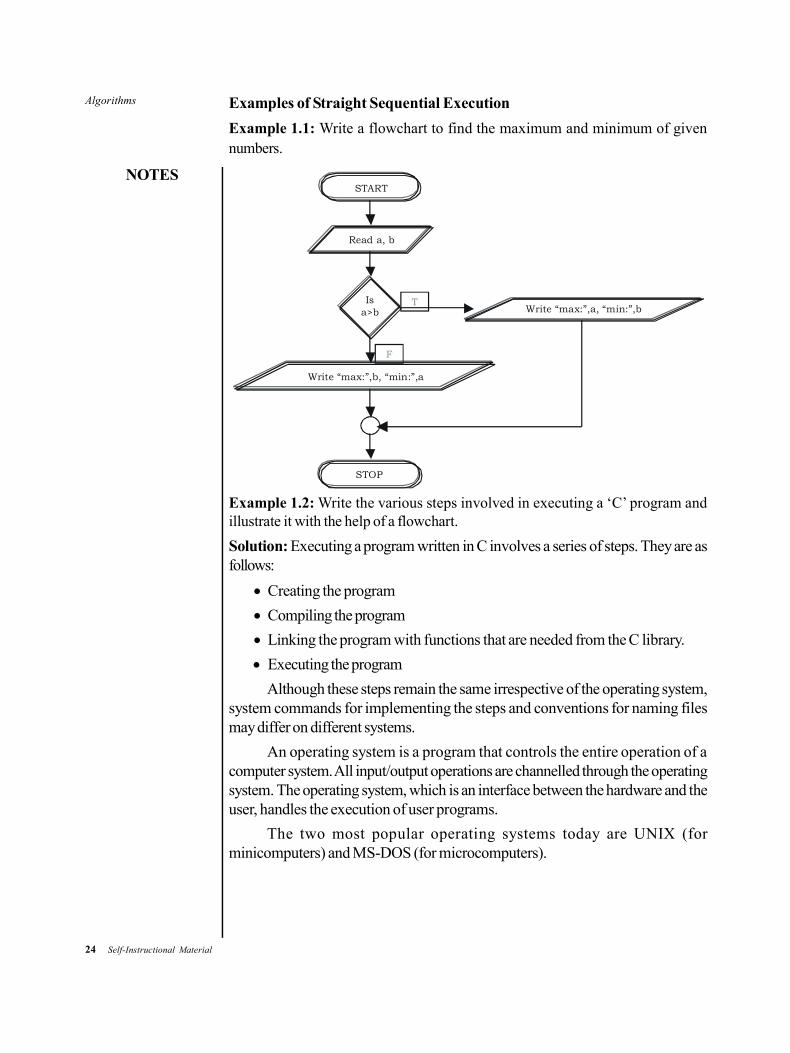
Example 1.1: Write a flowchart to find the maximum and minimum of givennumbers.
Read a, b
Is a>b
Write “max:”,b, “min:”,a
Write “max:”,a, “min:”,b
STOP
T
F
START
Example 1.2: Write the various steps involved in executing a ‘C’ program andillustrate it with the help of a flowchart.
Solution: Executing a program written in C involves a series of steps. They are asfollows:
Creating the program
Compiling the program
Linking the program with functions that are needed from the C library.
Executing the program
Although these steps remain the same irrespective of the operating system,system commands for implementing the steps and conventions for naming filesmay differ on different systems.
An operating system is a program that controls the entire operation of acomputer system. All input/output operations are channelled through the operatingsystem. The operating system, which is an interface between the hardware and theuser, handles the execution of user programs.
The two most popular operating systems today are UNIX (forminicomputers) and MS-DOS (for microcomputers).
Algorithms
NOTES
Self-Instructional Material 25
System Ready
Enter ProgramProgram Code
EditSource Program
CompileSource Program
CCompiler
SyntaxError
?
Link withSystem Library
Object codeNo
SystemLibrary
InputData
ExecuteObject Code
Executable Object code
logic & DataErrors
?
Data Error Logic Error
CORRECT OUTPUT
No Errors
STOP
Yes
Source Program
Examples for Flowcharts with Algorithms
a. Draw a flowchart for adding two numbers and write an algorithm for it.
Start
Read FirstNum
Read SecondNum
Sum = FirstNum + SecondNum
Write Sum
Stop
26 Self-Instructional Material
Algorithms
NOTES
Step 1: Start Step 2: Read FirstNumber Step 3: Read SecondNumber Step 4: Sum= FirstNumber + SecondNumber Step 5: Write (Sum) Step 6: Exit
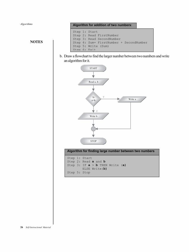
Algorithm for addition of two numbers:
b. Draw a flowchart to find the larger number between two numbers and writean algorithm for it.
Read a, b
Is a>b
Write b
Write a
STOP
T
F
START
Step 1: Start Step 2: Read a and b Step 3: IF a > b THEN Write (a) ELSE Write(b) Step 5: Stop
Algorithm for finding large number between two numbers
Algorithms
NOTES
Self-Instructional Material 27
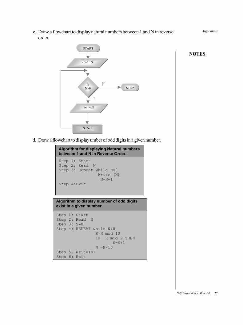
c. Draw a flowchart to display natural numbers between 1 and N in reverseorder.
F
Read N
Is N>0
START
Write N
N=N-1
STOP
T
d. Draw a flowchart to display umber of odd digits in a given number.
Step 1: Start Step 2: Read N Step 3: Repeat while N>0 Write (N) N=N-1 Step 4:Exit
Algorithm for displaying Natural numbers between 1 and N in Reverse Order.
Step 1: Start Step 2: Read N Step 3: S=0 Step 4: REPEAT while N>0 R=N mod 10 IF R mod 2 THEN S=S+1 N =N/10 Step 5. Write(s) Step 6: Exit
Algorithm to display number of odd digits exist in a given number.
28 Self-Instructional Material
Algorithms
NOTES
T
R=N%10
S=S+1
Read N
Is N
START
Write S
STOP
F
Is R%2
N=N/10
T
F
S=0
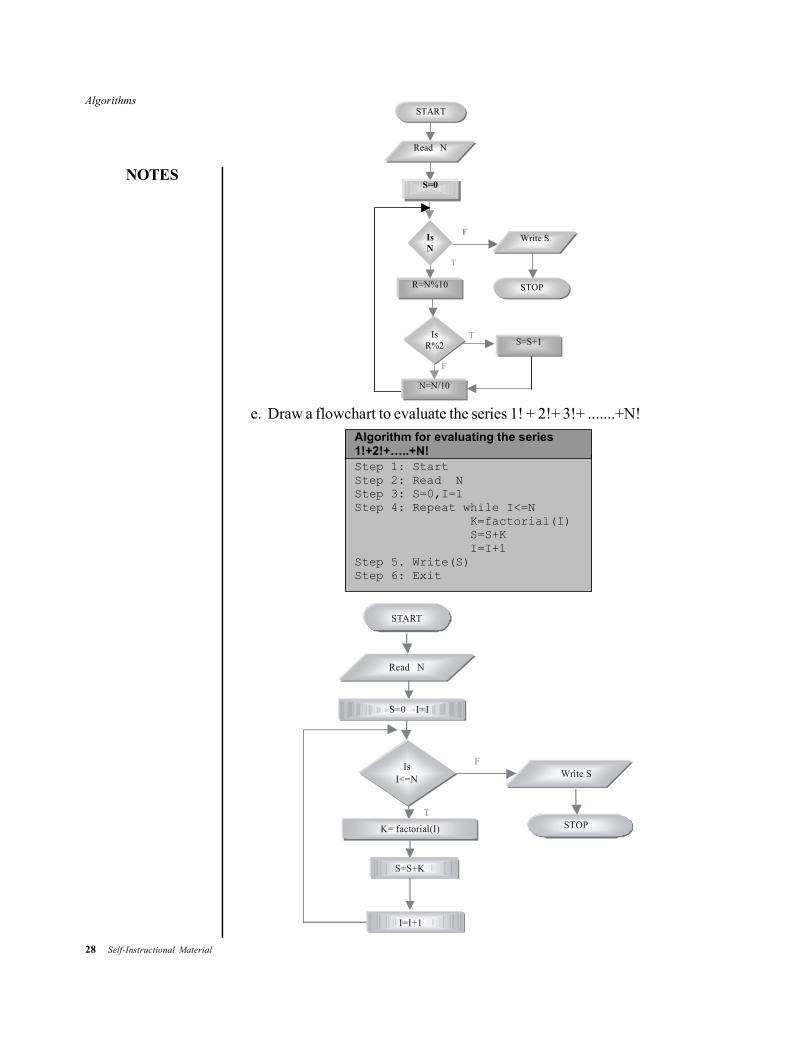
e. Draw a flowchart to evaluate the series 1! + 2!+ 3!+ .......+N!
Step 1: Start Step 2: Read N Step 3: S=0,I=1 Step 4: Repeat while I<=N K=factorial(I) S=S+K I=I+1 Step 5. Write(S) Step 6: Exit
Algorithm for evaluating the series 1!+2!+…..+N!
T
Read N
START
Write S
STOP
F
S=0 I=1
Is I<=N
I=I+1
K= factorial(I)
S=S+K
Algorithms
NOTES
Self-Instructional Material 29
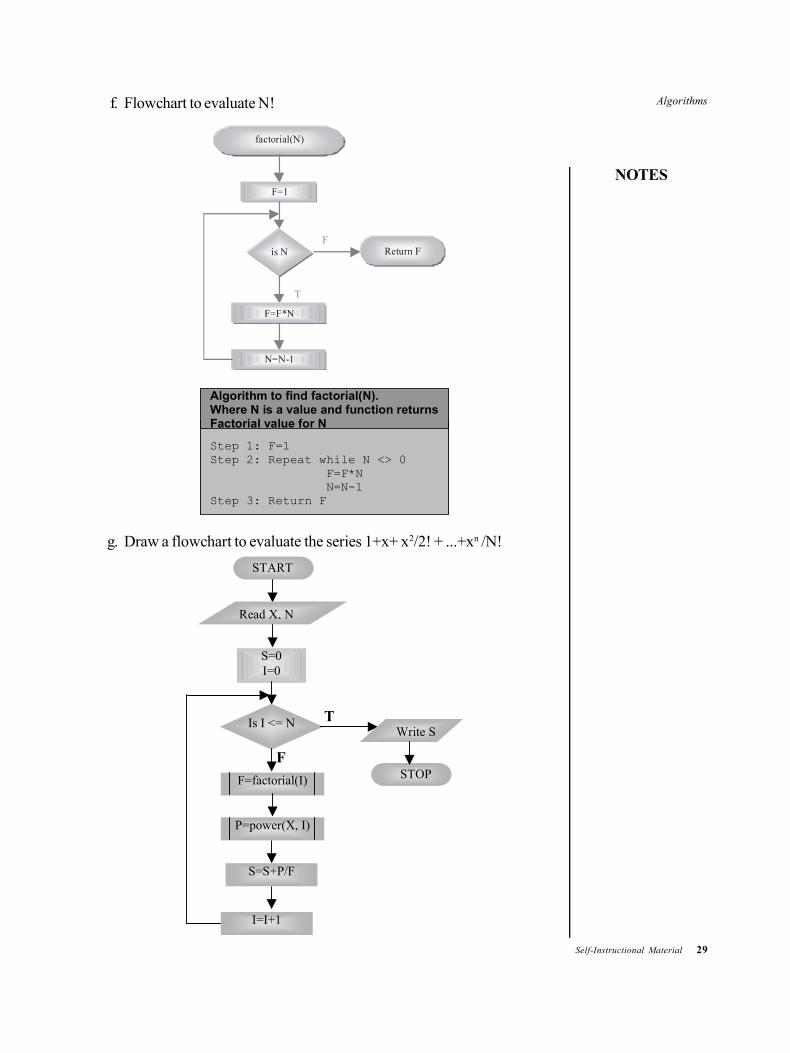
f. Flowchart to evaluate N!
factorial(N)
F=1
is N
F=F*N
N=N-1
F
T
Return F
Step 1: F=1 Step 2: Repeat while N <> 0 F=F*N N=N-1 Step 3: Return F
Algorithm to find factorial(N). Where N is a value and function returns Factorial value for N
g. Draw a flowchart to evaluate the series 1+x+ x2/2! + ...+xn /N!
I=I+1
T
START
Read X, N
S=0 I=0
Is I <= N
F=factorial(I)
P=power(X, I)
S=S+P/F
Write S
STOP F
30 Self-Instructional Material
Algorithms
NOTES
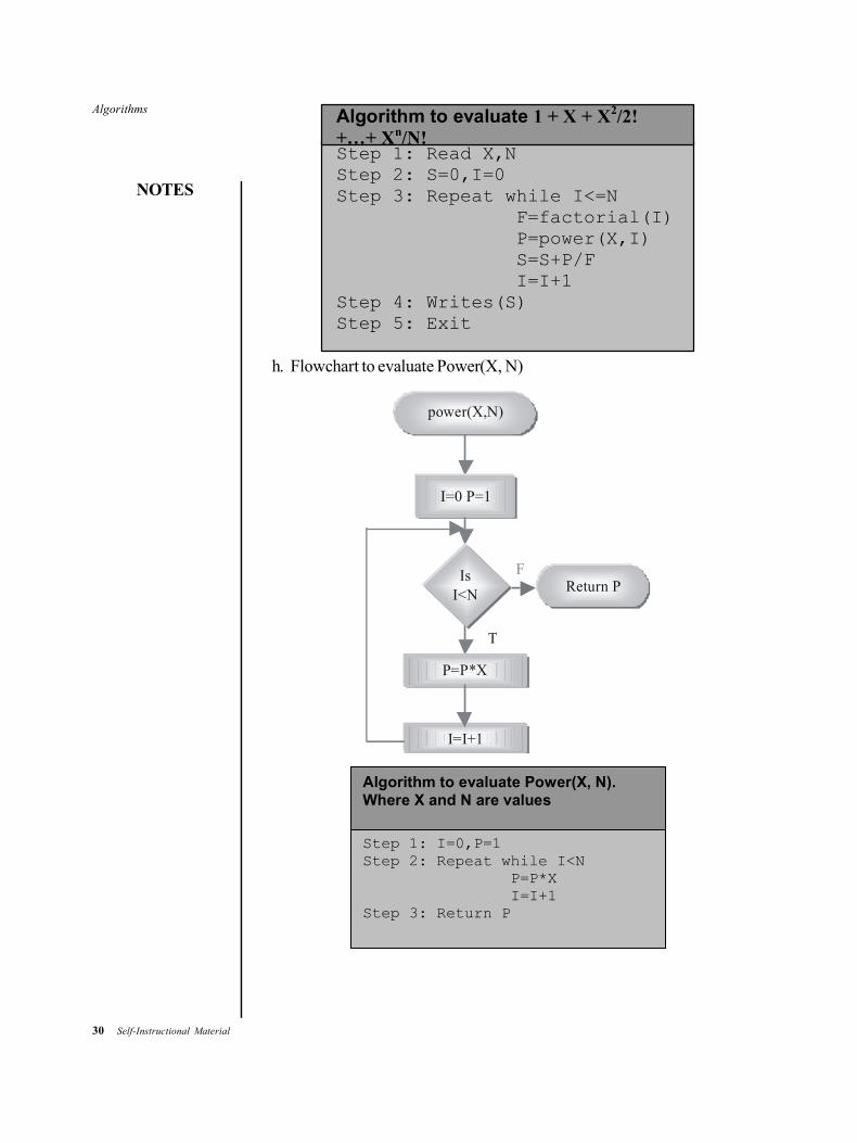
Step 1: Read X,N Step 2: S=0,I=0 Step 3: Repeat while I<=N F=factorial(I) P=power(X,I) S=S+P/F I=I+1 Step 4: Writes(S) Step 5: Exit
Algorithm to evaluate 1 + X + X2/2! +…+ Xn/N!
h. Flowchart to evaluate Power(X, N)
F
power(X,N)
I=0 P=1
Is I<N
P=P*X
I=I+1
Return P
T
Step 1: I=0,P=1 Step 2: Repeat while I<N P=P*X I=I+1 Step 3: Return P
Algorithm to evaluate Power(X, N). Where X and N are values
Algorithms
NOTES
Self-Instructional Material 31
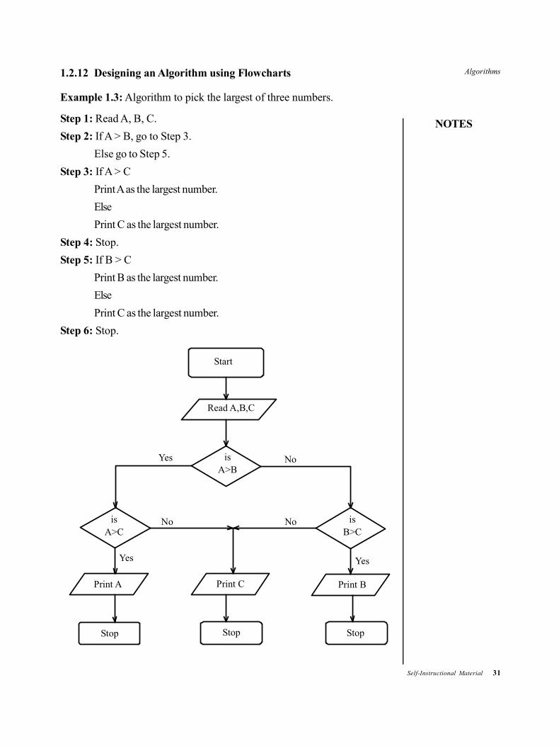
1.2.12 Designing an Algorithm using Flowcharts
Example 1.3: Algorithm to pick the largest of three numbers.
Step 1: Read A, B, C.
Step 2: If A > B, go to Step 3.
Else go to Step 5.
Step 3: If A > C
Print A as the largest number.
Else
Print C as the largest number.
Step 4: Stop.
Step 5: If B > C
Print B as the largest number.
Else
Print C as the largest number.
Step 6: Stop.
Start
Read A,B,C
is A>B
Print A
Stop
is A>C
is B>C
Print C Print B
Stop Stop
Yes No
No No
Yes Yes
32 Self-Instructional Material
Algorithms
NOTES
Explanation: Read the three numbers A, B and C. A is compared with B. If A islarger, then it is compared with C. If A turns out to be the largest number again,then A is the largest number; otherwise, C is the largest number. If in the secondstep, A is less than or equal to be B, then B is compared with C. If B is larger, thenB is the largest number; otherwise, C is the largest number.
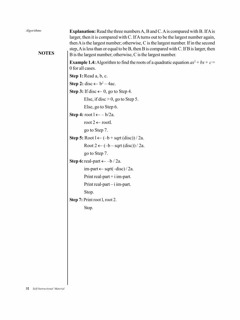
Example 1.4: Algorithm to find the roots of a quadratic equation ax2 + bx + c =0 for all cases.
Step 1:Read a, b, c.
Step 2: disc b2 – 4ac.
Step 3: If disc 0, go to Step 4.
Else, if disc > 0, go to Step 5.
Else, go to Step 6.
Step 4: root l – b/2a.
root 2 rootl.
go to Step 7.
Step 5: Root l (–b + sqrt (disc)) / 2a.
Root 2 (–b – sqrt (disc)) / 2a.
go to Step 7.
Step 6: real-part –b / 2a.
im-part sqrt(–disc) / 2a.
Print real-part + i im-part.
Print real-part – i im-part.
Stop.
Step 7: Print root l, root 2.
Stop.
Algorithms
NOTES
Self-Instructional Material 33
root 1 = (–b + disc) / 2aroot 2 = (–b – disc) / 2a
real-part = b / 2aim-part = disc / 2a
print real-part + i im-part
print real-part + i im-part
root 1 = –b/2aroot 2 = root 1
Print root 1, root 2
Isdisc
d sc = bi – 4ac2
Read A,B,C
Start
Stop Stop
> 0 < 0
= 0
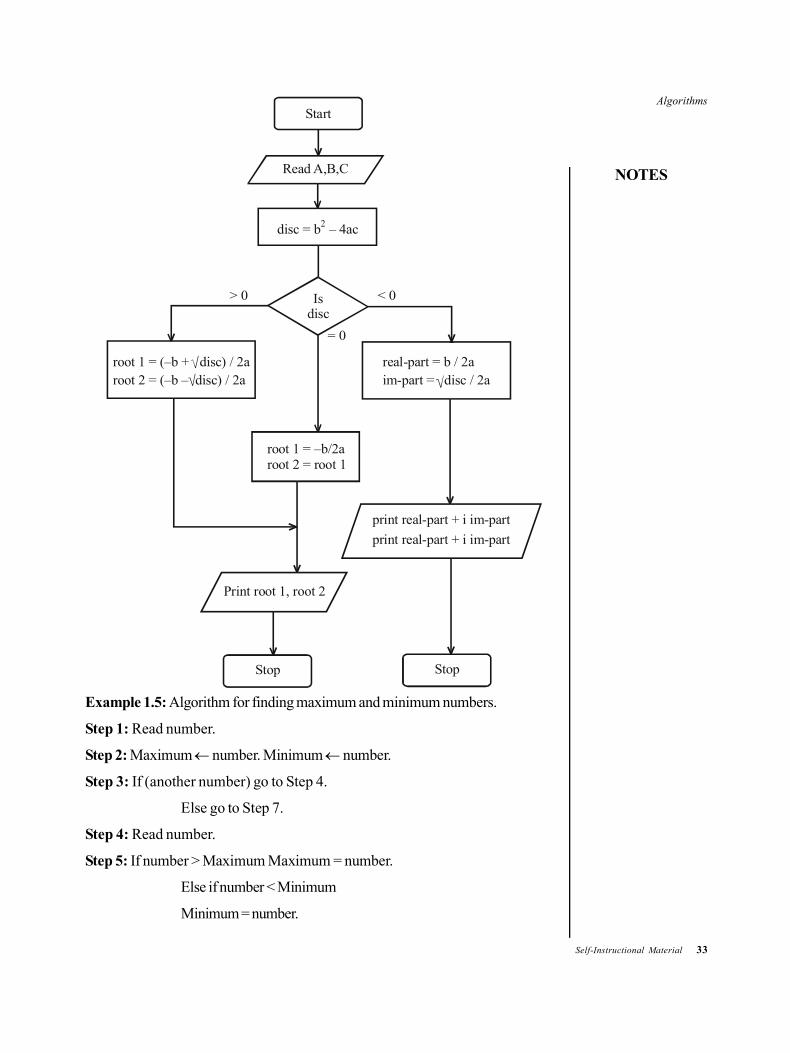
Example 1.5: Algorithm for finding maximum and minimum numbers.
Step 1: Read number.
Step 2: Maximum number. Minimum number.
Step 3: If (another number) go to Step 4.
Else go to Step 7.
Step 4: Read number.
Step 5: If number > Maximum Maximum = number.
Else if number < Minimum
Minimum = number.
34 Self-Instructional Material
Algorithms
NOTES
Step 6: go to Step 3.
Step 7: Print Maximum.
Print Minimum.
Step 8: Stop.
Start
Isanothernumber
Read Number
Maximum = numberMinimum = number
read number
Print maximumprint minimum
maximum = number
minimum = number
Is number >maximum
Isnumber <minimum
stop
No
Yes
Yes
Yes
No
No
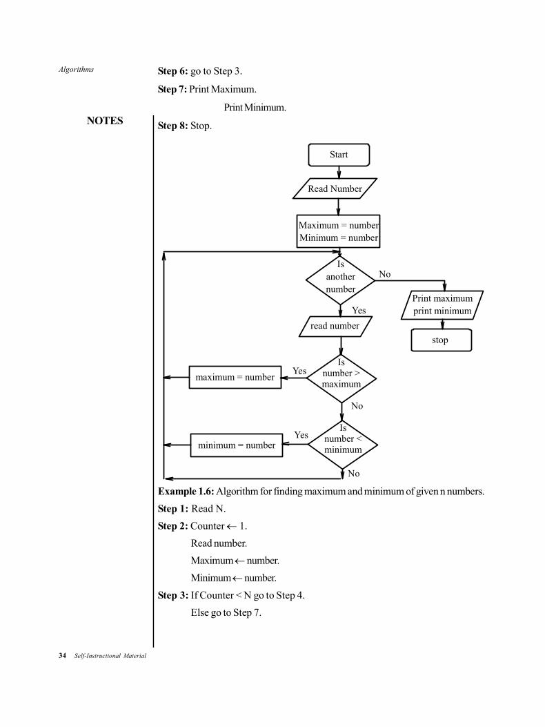
Example 1.6: Algorithm for finding maximum and minimum of given n numbers.
Step 1: Read N.
Step 2: Counter 1.
Read number.
Maximum number.
Minimum number.
Step 3: If Counter < N go to Step 4.
Else go to Step 7.
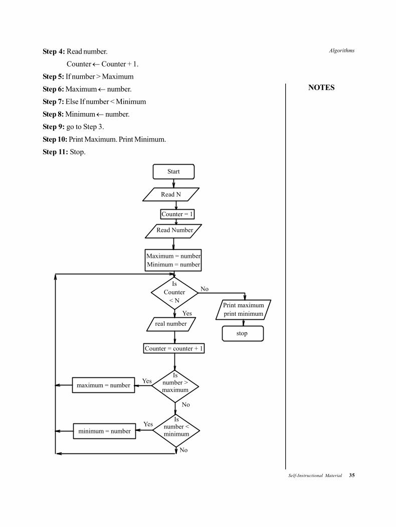
Algorithms
NOTES
Self-Instructional Material 35
Step 4: Read number.
Counter Counter + 1.
Step 5: If number > Maximum
Step 6: Maximum number.
Step 7: Else If number < Minimum
Step 8: Minimum number.
Step 9: go to Step 3.
Step 10: Print Maximum. Print Minimum.
Step 11: Stop.
Start
IsCounter
< N
Read N
Maximum = numberMinimum = number
real number
Print maximumprint minimum
maximum = number
minimum = number
Is number >maximum
Isnumber <minimum
stop
No
Yes
Yes
Yes
No
No
Counter = counter + 1
Counter = 1
Read Number
36 Self-Instructional Material
Algorithms
NOTES
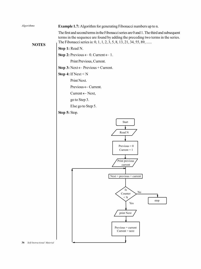
Example 1.7: Algorithm for generating Fibonacci numbers up to n.
The first and second terms in the Fibonacci series are 0 and 1. The third and subsequentterms in the sequence are found by adding the preceding two terms in the series.The Fibonacci series is: 0, 1, 1, 2, 3, 5, 8, 13, 21, 34, 55, 89, ......
Step 1: Read N.
Step 2: Previous 0. Current 1.
Print Previous, Current.
Step 3: Next Previous + Current.
Step 4: If Next < N
Print Next.
Previous Current.
Current Next,
go to Step 3.
Else go to Step 5.
Step 5: Stop.
Start
IsCounter
< N
Read N
Previous = 0Current = 1
print Next
stop
No
Yes
Next = previous + current
Print previouscurrent
Previous = currentCurrent = next
Algorithms
NOTES
Self-Instructional Material 37
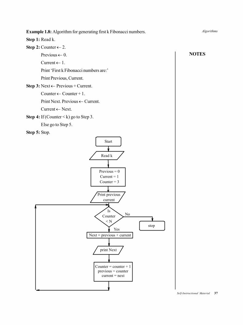
Example 1.8: Algorithm for generating first k Fibonacci numbers.
Step 1: Read k.
Step 2: Counter 2.
Previous 0.
Current 1.
Print ‘First k Fibonacci numbers are:’
Print Previous, Current.
Step 3: Next Previous + Current.
Counter Counter + 1.
Print Next. Previous Current.
Current Next.
Step 4: If (Counter < k) go to Step 3.
Else go to Step 5.
Step 5: Stop.
Start
IsCounter
< N
Read k
Previous = 0Current = 1Counter = 3
print Next
stop
No
Yes
Next = previous + current
Print previouscurrent
Counter = counter + 1previous = counter
current = next
38 Self-Instructional Material
Algorithms
NOTES
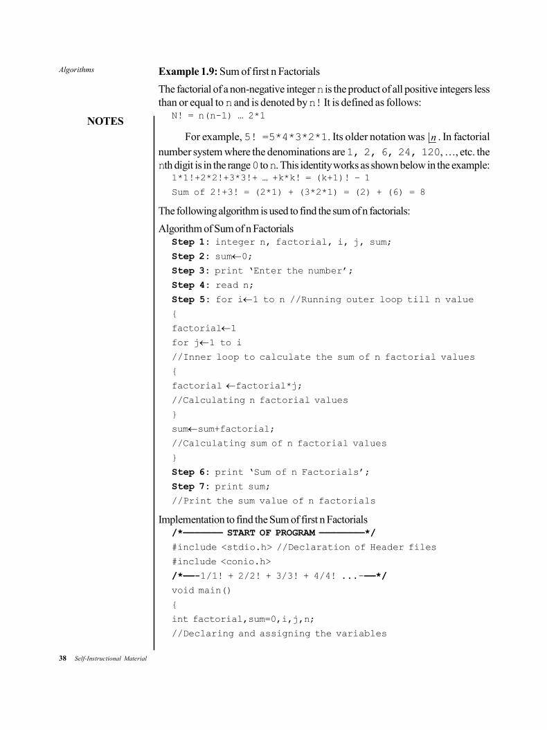
Example 1.9: Sum of first n Factorials
The factorial of a non-negative integer n is the product of all positive integers lessthan or equal to n and is denoted by n! It is defined as follows:
N! = n(n-1) … 2*1
For example, 5! =5*4*3*2*1. Its older notation was n . In factorialnumber system where the denominations are 1, 2, 6, 24, 120, …, etc. thenth digit is in the range 0 to n. This identity works as shown below in the example:
1*1!+2*2!+3*3!+ … +k*k! = (k+1)! – 1
Sum of 2!+3! = (2*1) + (3*2*1) = (2) + (6) = 8
The following algorithm is used to find the sum of n factorials:
Algorithm of Sum of n FactorialsStep 1: integer n, factorial, i, j, sum;
Step 2: sum0;
Step 3: print ‘Enter the number’;
Step 4: read n;
Step 5: for i1 to n //Running outer loop till n value
{
factorial1
for j1 to i
//Inner loop to calculate the sum of n factorial values
{
factorial factorial*j;
//Calculating n factorial values
}
sumsum+factorial;
//Calculating sum of n factorial values
}
Step 6: print ‘Sum of n Factorials’;
Step 7: print sum;
//Print the sum value of n factorials
Implementation to find the Sum of first n Factorials/*——————— START OF PROGRAM ————————*/
#include <stdio.h> //Declaration of Header files
#include <conio.h>
/*——-1/1! + 2/2! + 3/3! + 4/4! ...-——*/
void main()
{
int factorial,sum=0,i,j,n;
//Declaring and assigning the variables
Algorithms
NOTES
Self-Instructional Material 39
printf(“Enter a value for [n] value = “);
scanf(“%d”, &n);
//Accept input value for n term
for(i=1;i<=n;i++) //For outer loop till n value
{
factorial=1;
for(j=1;j<=i;j++)
//Using inner for loop to calculate the sum of n factorial
{
factorial = factorial *j;
}
sum=sum+ factorial;
}
Printf(“\n sum of %d factorial = %d”, n, sum);
}
getch();
}
The result of the above program is as follows:Enter a value for [n] value = 4
sum of 4 factorial = 33
How the above program works it is explained step-wise-step in the followingways:
1!+2!+3!+4! = 33
The value of 1! = 1
The value of 2! = 2
The value of 3! = 6
The value of 4! = 24
1+2+6+24= 33
Example 1.10: To Find Largest Value and Second Largest Value of the List
The largest and second largest values in the given list are determined by arrayimplementation. Array can contain the various elements of the list. The algorithmto find the largest and second largest of given list is as follows:
Algorithm to find the largest value and second largest value of the given listStep 1: integer M, a[M], i, largest, t, second_largest;
Step 2: print ‘Enter a value for array’;
Step 3: read M;
Step 4: for i1 to M
print ‘Enter values:’;

40 Self-Instructional Material
Algorithms
NOTES
read a[i];
Step 5: if i==1
largesttsecond_largesta[i];
Step 6: else if a[i]>largest
second_largestlargest;
largesta[i];
Step 7: else if a[i]>second_largest && a[i]<largest
second_largesta[i];
Step 8: else if a[i]<t
ta[i];
Step 9: print ‘Largest value in the given list =’;
Step 10: print largest;
Step 11: ‘Second largest value in the given list =’;
Step 12: print second_largest;
The result of the above algorithm is as follows:Enter a value for array
5
Then array A[M] is assigned a value 5 as A[5].
The input values are entered in the following way:Enter values
45
90
112
4
35
Largest value in the given list = 112
Second largest value in the given list = 90
The first element of the array is 45 which is assumed to be the largest valueand it is kept in the temporary location where it is temporarily stored in variable t.All the remaining values are checked from this number. Now, the A[i] value isassigned as 45. At second step, the condition is satisfied so largest value is 90.Now, 90 is checked with the next entered value 112. Because the condition isnot satisfied so 112 is assumed as greater value. The values 4 and 35 are lessthan 90, so the condition for less than largest is not satisfied. The checking processof second largest value ‘45’ is done after checking the rest four values anddeclaring 112 as first largest value. Further, the statement‘second_largest=largest’ is used. The first element of the array is againtaken as largest among the four values. Now, 45 is checked step-by-step in ifelse if conditional statement to find the second largest value.
Algorithms
NOTES
Self-Instructional Material 41
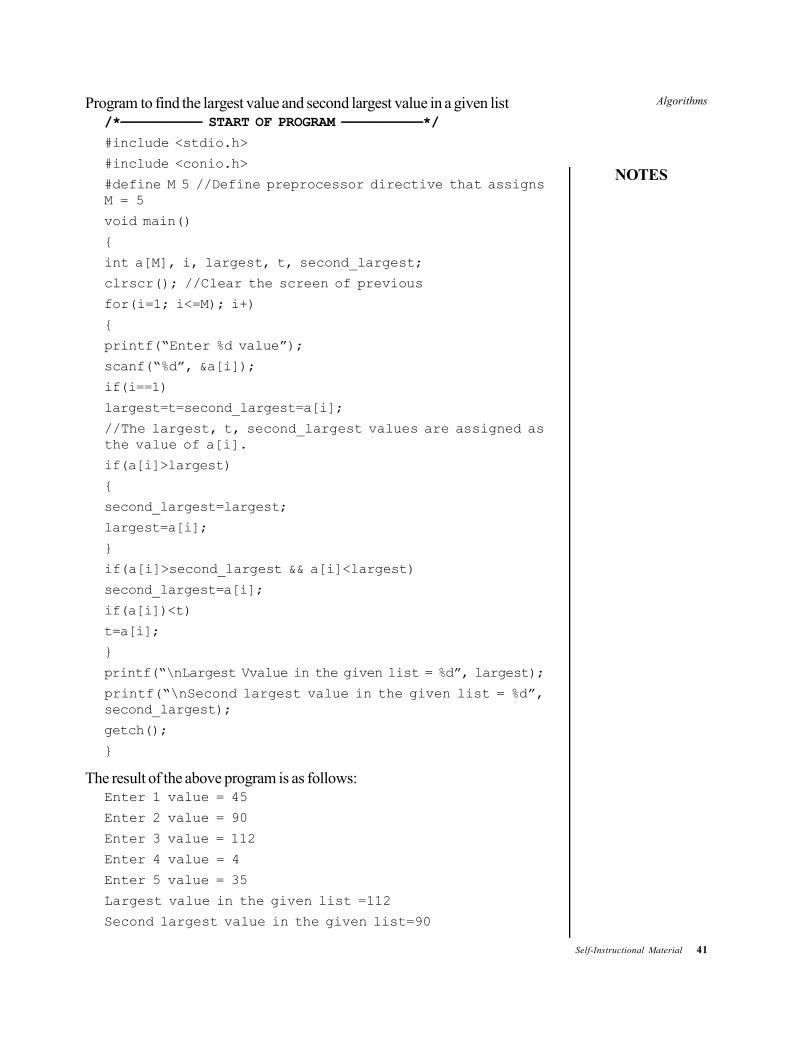
Program to find the largest value and second largest value in a given list/*—————————— START OF PROGRAM ——————————*/
#include <stdio.h>
#include <conio.h>
#define M 5 //Define preprocessor directive that assignsM = 5
void main()
{
int a[M], i, largest, t, second_largest;
clrscr(); //Clear the screen of previous
for(i=1; i<=M); i+)
{
printf(“Enter %d value”);
scanf(“%d”, &a[i]);
if(i==1)
largest=t=second_largest=a[i];
//The largest, t, second_largest values are assigned asthe value of a[i].
if(a[i]>largest)
{
second_largest=largest;
largest=a[i];
}
if(a[i]>second_largest && a[i]<largest)
second_largest=a[i];
if(a[i])<t)
t=a[i];
}
printf(“\nLargest Vvalue in the given list = %d”, largest);
printf(“\nSecond largest value in the given list = %d”,second_largest);
getch();
}
The result of the above program is as follows:Enter 1 value = 45
Enter 2 value = 90
Enter 3 value = 112
Enter 4 value = 4
Enter 5 value = 35
Largest value in the given list =112
Second largest value in the given list=90
42 Self-Instructional Material
Algorithms
NOTES
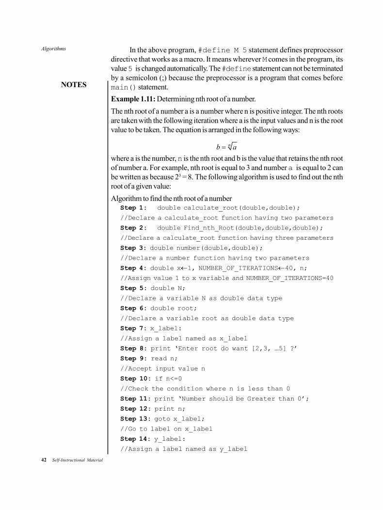
In the above program, #define M 5 statement defines preprocessordirective that works as a macro. It means wherever M comes in the program, itsvalue 5 is changed automatically. The #define statement can not be terminatedby a semicolon (;) because the preprocessor is a program that comes beforemain() statement.
Example 1.11: Determining nth root of a number.
The nth root of a number a is a number where n is positive integer. The nth rootsare taken with the following iteration where a is the input values and n is the rootvalue to be taken. The equation is arranged in the following ways:
nb a
where a is the number, n is the nth root and b is the value that retains the nth rootof number a. For example, nth root is equal to 3 and number a is equal to 2 canbe written as because 23 = 8. The following algorithm is used to find out the nthroot of a given value:
Algorithm to find the nth root of a numberStep 1: double calculate_root(double,double);
//Declare a calculate_root function having two parameters
Step 2: double Find_nth_Root(double,double,double);
//Declare a calculate_root function having three parameters
Step 3: double number(double,double);
//Declare a number function having two parameters
Step 4: double x1, NUMBER_OF_ITERATIONS40, n;
//Assign value 1 to x variable and NUMBER_OF_ITERATIONS=40
Step 5: double N;
//Declare a variable N as double data type
Step 6: double root;
//Declare a variable root as double data type
Step 7: x_label:
//Assign a label named as x_label
Step 8: print ‘Enter root do want [2,3, …5] ?’
Step 9: read n;
//Accept input value n
Step 10: if n<=0
//Check the condition where n is less than 0
Step 11: print ‘Number should be Greater than 0’;
Step 12: print n;
Step 13: goto x_label;
//Go to label on x_label
Step 14: y_label:
//Assign a label named as y_label

Algorithms
NOTES
Self-Instructional Material 43
Step 15: print ‘Enter the number for Root’;
Step 16: read N;
Step 17: if N<=0
Step 18: print ‘Number should be greater than 0’;
Step 19: print ‘PRESS ANY KEY TO ENTER AGAIN’;
Step 20: goto y_label;
//Go to label on y_label
Step 21: xcalulate_root(n,N);
//x retains the returned value of function calculate_root
Step 22: print ‘The first assumed root is’,x;
Step 23: rootFind_nth_Root(N,n,x);
//root retains the Find_nth_Root returned value
Step 24: print ‘Root of n’,n;
Step 25: print N;
Step 26: print root;
Step 27: double calculate_root(double n,double N)
Step 28: integer i,xr;
//integer i and xr are declared
Step 29: xr1;
//xr is assigned as 1
Step 30: double j1;
//double j is assigned as 1
Step 31: while(1)
Step 32: for i0 to n //Running for loop
{
xrxr*j; //xr retains the value of xr*j
}
Step 33: if xr>N
Return j-1; //Returns j-1
Step 34: jj+1; //j value is increased by 1
Step 35: xr1; //xr value is increased by 1
Step 36: double Find_nth_Root(double NUM,double n,doubleX0) //Function Find_nth_Root starts from here.
Step 37: int i;
Step 38: double d1.0;
Step 39: double first_term, second_term, rootX0;
Step 40: for i1 to NUMBER_OF_ITERATIONS
//Body of for loop starts that calculates first term andsecond term value of enter values of NUMBER_OF_ITERATIONS
Step 41: dnumber(root,n);
//d retains the n th value of given number.
44 Self-Instructional Material
Algorithms
NOTES
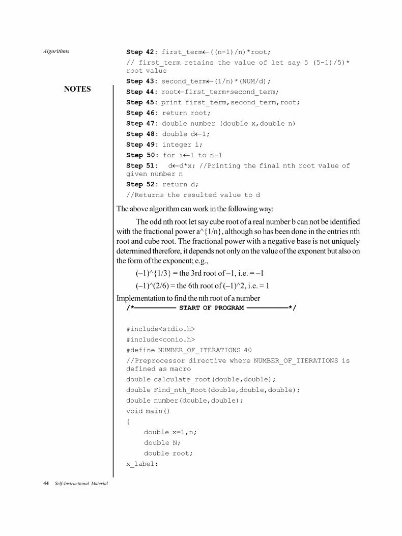
Step 42: first_term((n-1)/n)*root;
// first_term retains the value of let say 5 (5-1)/5)*root value
Step 43: second_term(1/n)*(NUM/d);
Step 44: rootfirst_term+second_term;
Step 45: print first_term,second_term,root;
Step 46: return root;
Step 47: double number (double x,double n)
Step 48: double d1;
Step 49: integer i;
Step 50: for i1 to n-1
Step 51: dd*x; //Printing the final nth root value ofgiven number n
Step 52: return d;
//Returns the resulted value to d
The above algorithm can work in the following way:
The odd nth root let say cube root of a real number b can not be identifiedwith the fractional power a^{1/n}, although so has been done in the entries nthroot and cube root. The fractional power with a negative base is not uniquelydetermined therefore, it depends not only on the value of the exponent but also onthe form of the exponent; e.g.,
(–1)^{1/3} = the 3rd root of –1, i.e. = –1
(–1)^(2/6) = the 6th root of (–1)^2, i.e. = 1
Implementation to find the nth root of a number/*—————————— START OF PROGRAM ——————————*/
#include<stdio.h>
#include<conio.h>
#define NUMBER_OF_ITERATIONS 40
//Preprocessor directive where NUMBER_OF_ITERATIONS isdefined as macro
double calculate_root(double,double);
double Find_nth_Root(double,double,double);
double number(double,double);
void main()
{
double x=1,n;
double N;
double root;
x_label:
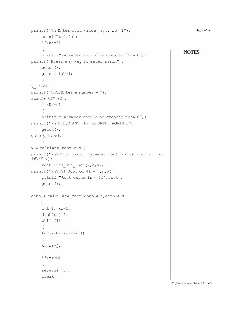
Algorithms
NOTES
Self-Instructional Material 45
printf(“\n Enter root value [2,3, …5] ?”);
scanf(“%f”,&n);
if(n<=0)
{
printf(“\nNumber should be Greater than 0”);
printf(“Press any key to enter again”);
getch();
goto x_label;
}
y_label:
printf(“\n\rEnter a number = “);
scanf(“%f”,&N);
if(N<=0)
{
printf(“\nNumber should be greater than 0”);
printf(“\n PRESS ANY KEY TO ENTER AGAIN …”);
getch();
goto y_label;
}
x = calulate_root(n,N);
printf(“\n\nThe first assumed root is calculated as%f\n”,x);
root=Find_nth_Root(N,n,x);
printf(“\n\n%f Root of %f = “,n,N);
printf(“Root value is = %f”,root);
getch();
}
double calculate_root(double n,double N)
{
int i, xr=1;
double j=1;
while(1)
{
for(i=0;i<n;i=i+1)
{
xr=xr*j;
}
if(xr>N)
{
return(j-1);
break;
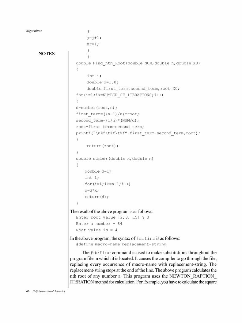
46 Self-Instructional Material
Algorithms
NOTES
}
j=j+1;
xr=1;
}
}
double Find_nth_Root(double NUM,double n,double X0)
{
int i;
double d=1.0;
double first_term,second_term,root=X0;
for(i=1;i<=NUMBER_OF_ITERATIONS;i++)
{
d=number(root,n);
first_term=((n-1)/n)*root;
second_term=(1/n)*(NUM/d);
root=first_term+second_term;
printf(“\n%f\t%f\t%f”,first_term,second_term,root);
}
return(root);
}
double number(double x,double n)
{
double d=1;
int i;
for(i=1;i<=n-1;i++)
d=d*x;
return(d);
}
The result of the above program is as follows:Enter root value [2,3, …5] ? 3
Enter a number = 64
Root value is = 4
In the above program, the syntax of #define is as follows:#define macro-name replacement-string
The #define command is used to make substitutions throughout theprogram file in which it is located. It causes the compiler to go through the file,replacing every occurrence of macro-name with replacement-string. Thereplacement-string stops at the end of the line. The above program calculates thenth root of any number a. This program uses the NEWTON_RAPTION_ITERATION method for calculation. For Example, you have to calculate the square
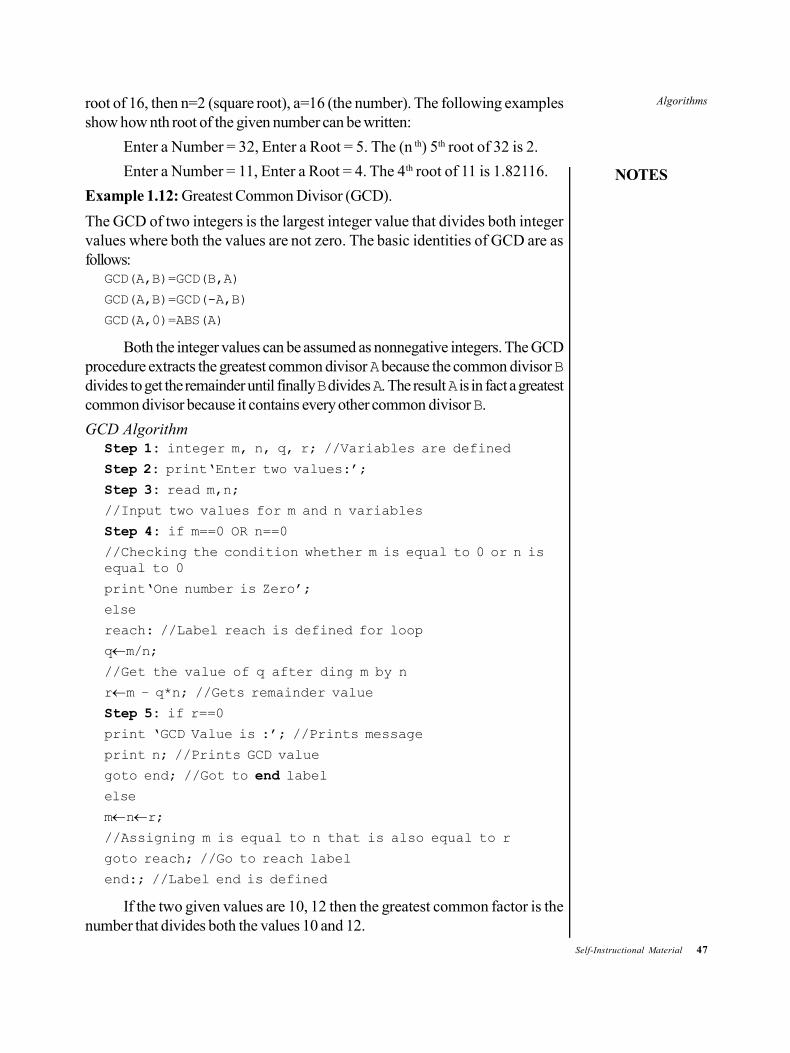
Algorithms
NOTES
Self-Instructional Material 47
root of 16, then n=2 (square root), a=16 (the number). The following examplesshow how nth root of the given number can be written:
Enter a Number = 32, Enter a Root = 5. The (n th) 5th root of 32 is 2.
Enter a Number = 11, Enter a Root = 4. The 4th root of 11 is 1.82116.
Example 1.12: Greatest Common Divisor (GCD).
The GCD of two integers is the largest integer value that divides both integervalues where both the values are not zero. The basic identities of GCD are asfollows:
GCD(A,B)=GCD(B,A)
GCD(A,B)=GCD(-A,B)
GCD(A,0)=ABS(A)
Both the integer values can be assumed as nonnegative integers. The GCDprocedure extracts the greatest common divisor A because the common divisor Bdivides to get the remainder until finally B divides A. The result A is in fact a greatestcommon divisor because it contains every other common divisor B.
GCD AlgorithmStep 1: integer m, n, q, r; //Variables are defined
Step 2: print‘Enter two values:’;
Step 3: read m,n;
//Input two values for m and n variables
Step 4: if m==0 OR n==0
//Checking the condition whether m is equal to 0 or n isequal to 0
print‘One number is Zero’;
else
reach: //Label reach is defined for loop
qm/n;
//Get the value of q after ding m by n
rm – q*n; //Gets remainder value
Step 5: if r==0
print ‘GCD Value is :’; //Prints message
print n; //Prints GCD value
goto end; //Got to end label
else
mnr;
//Assigning m is equal to n that is also equal to r
goto reach; //Go to reach label
end:; //Label end is defined
If the two given values are 10, 12 then the greatest common factor is thenumber that divides both the values 10 and 12.
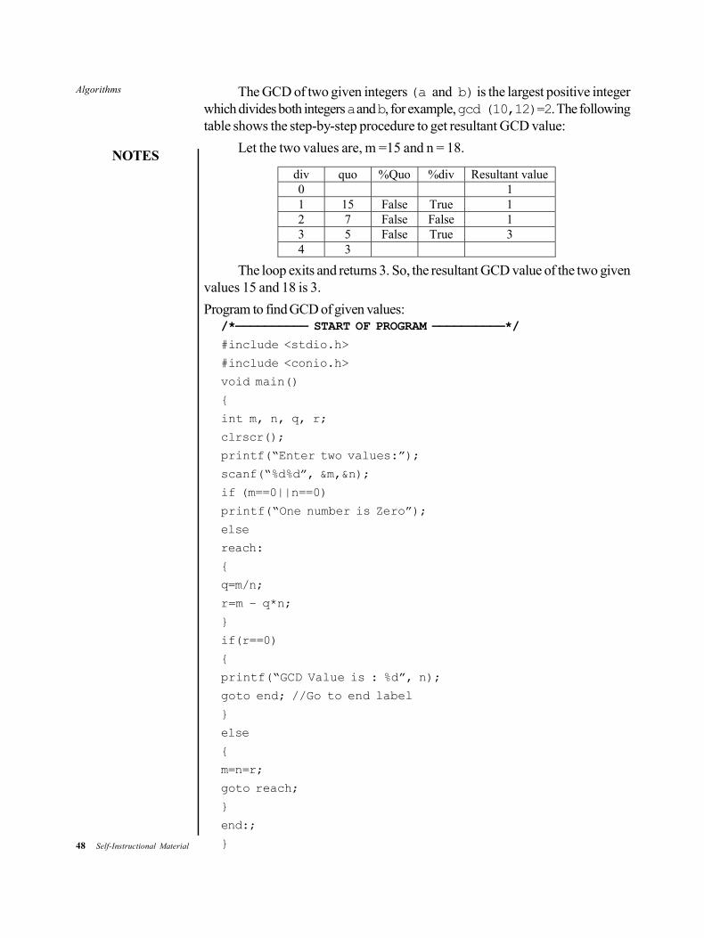
48 Self-Instructional Material
Algorithms
NOTES
The GCD of two given integers (a and b) is the largest positive integerwhich divides both integers a and b, for example, gcd (10,12)=2. The followingtable shows the step-by-step procedure to get resultant GCD value:
Let the two values are, m =15 and n = 18.
div quo %Quo %div Resultant value 0 1 1 15 False True 1 2 7 False False 1 3 5 False True 3 4 3
The loop exits and returns 3. So, the resultant GCD value of the two givenvalues 15 and 18 is 3.
Program to find GCD of given values:/*—————————— START OF PROGRAM ——————————*/
#include <stdio.h>
#include <conio.h>
void main()
{
int m, n, q, r;
clrscr();
printf(“Enter two values:”);
scanf(“%d%d”, &m,&n);
if (m==0||n==0)
printf(“One number is Zero”);
else
reach:
{
q=m/n;
r=m – q*n;
}
if(r==0)
{
printf(“GCD Value is : %d”, n);
goto end; //Go to end label
}
else
{
m=n=r;
goto reach;
}
end:;
}
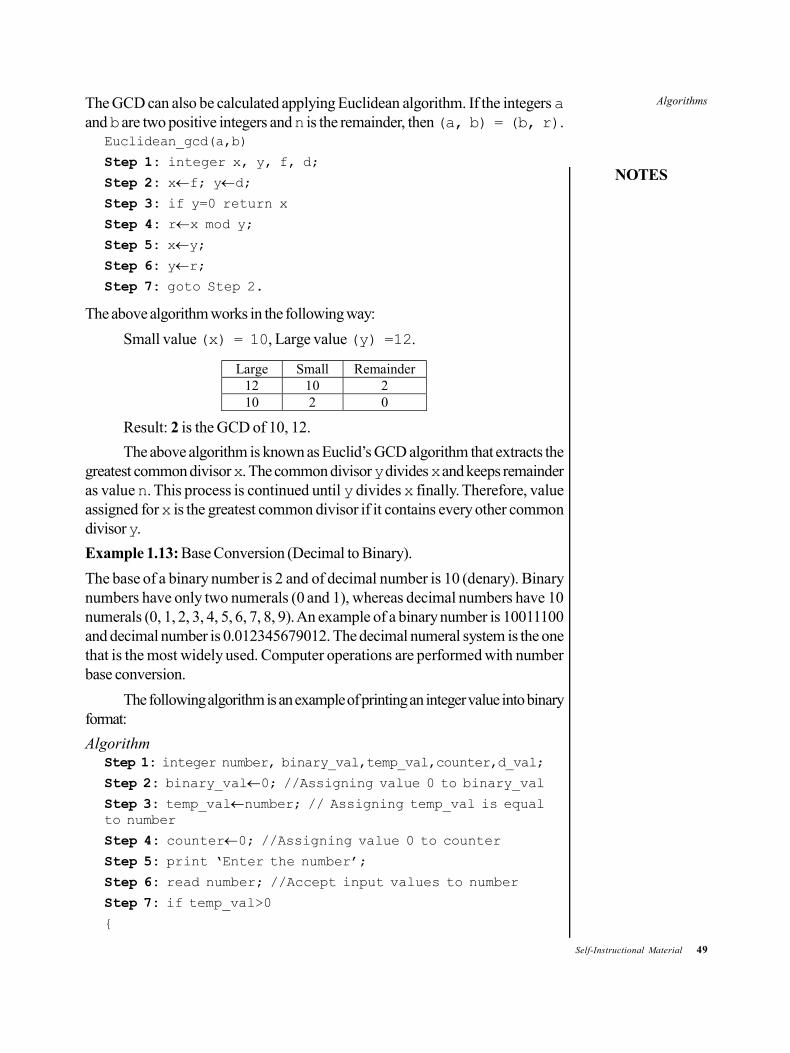
Algorithms
NOTES
Self-Instructional Material 49
The GCD can also be calculated applying Euclidean algorithm. If the integers aand b are two positive integers and n is the remainder, then (a, b) = (b, r).
Euclidean_gcd(a,b)
Step 1: integer x, y, f, d;
Step 2: xf; yd;
Step 3: if y=0 return x
Step 4: rx mod y;
Step 5: xy;
Step 6: yr;
Step 7: goto Step 2.
The above algorithm works in the following way:
Small value (x) = 10, Large value (y) =12.
Large Small Remainder 12 10 2 10 2 0
Result: 2 is the GCD of 10, 12.
The above algorithm is known as Euclid’s GCD algorithm that extracts thegreatest common divisor x. The common divisor y divides x and keeps remainderas value n. This process is continued until y divides x finally. Therefore, valueassigned for x is the greatest common divisor if it contains every other commondivisor y.
Example 1.13: Base Conversion (Decimal to Binary).
The base of a binary number is 2 and of decimal number is 10 (denary). Binarynumbers have only two numerals (0 and 1), whereas decimal numbers have 10numerals (0, 1, 2, 3, 4, 5, 6, 7, 8, 9). An example of a binary number is 10011100and decimal number is 0.012345679012. The decimal numeral system is the onethat is the most widely used. Computer operations are performed with numberbase conversion.
The following algorithm is an example of printing an integer value into binaryformat:
AlgorithmStep 1: integer number, binary_val,temp_val,counter,d_val;
Step 2: binary_val0; //Assigning value 0 to binary_val
Step 3: temp_valnumber; // Assigning temp_val is equalto number
Step 4: counter0; //Assigning value 0 to counter
Step 5: print ‘Enter the number’;
Step 6: read number; //Accept input values to number
Step 7: if temp_val>0
{

50 Self-Instructional Material
Algorithms
NOTES
d_val mod(temp_val,2)
binary_val binary_val + d_val*10^counter;
//10^counter means power(10,counter)
d_val d_val + a_val*p_val;
temp_val int(temp_val/2)
//Change the fraction values as integer data types.
counter counter + 1;
//Increase the counter value by one
}
Step 7: print ‘Binary Value’;
Step 8: print binary_val; // Prints resultant binaryvalue
How the above algorithm works is explained below:
Let us take a decimal value 6.d_val = 6 mod 2 that returns 0
binary value=0+3*10^0 returns 0
d_val = 3 mod 2 returns 1
counter = 0 +1= 1
The decimal number 6 is equal to binary number 110. This conversion isexplained in the following way:
number number/2 number % 2 6 3 0 3 1 1 1 0 1
Implementation of base conversion (decimal to binary)/*—————————— START OF PROGRAM ——————————*/
#include <stdio.h> //Declaring Header files
#include <conio.h>
#include <math.h>
void main() //Start main() function
{
int number, binary_val, temp_val, counter, d_val, p_val;
binary_val=0;
// Declaring integer data types variables
temp_val=number; //Assigning temp_val is equal to number
counter=0; //Initailizing 0 to counter
printf(“\n Enter a number”);
scanf(“%d”, &number); //Accept input value
if (temp_val>0)
{
Algorithms
NOTES
Self-Instructional Material 51
d_val = temp_val%2;
//Returns remainder to d_val
p_val=power(10,counter);
binary_val= binary_val+ d_val*p_val; //The value ofbinary_val is added to d_val by d_val by 10 ‘raise to thepower’ counter value
temp_val = int(temp_val/2)
//if temp_val contains fraction value, int() functionchanges the integer type value
counter = counter +1;
//Counter variable is increased
}
printf(“Binary Value = %d”, binary_val); //Printing thebinary value
getch();
}
Base Conversion (binary to decimal)
AlgorithmStep 1: integer number,d_val,temp_val,counter,a_val;
Step 2: d_val0; //Assigning 0 to d_val
Step 3: temp_valnumber; //Assigning temp_val is equalto number
Step 4: counter0; //Assigning 0 to counter
Step 5: print ‘Enter the number’;
Step 6: read number; //Accept input value for number
Step 7: if temp_val>0 //Body of if control statement
{
a_val mod(temp_val,10);
p_valpower(2,counter);
d_val d_val+ a_val*p_val;
temp_val int(temp_val/10);
counter counter +1;
}
Step 8: print ‘Decimal value’;
Step 9: print d_val;
How the above algorithm works is explained as follows:
Let us take binary number 1011.
=1*23+0+22+1*21+1*20
=8+0+2+1 = 11

52 Self-Instructional Material
Algorithms
NOTES
The binary number 1011 is equal to decimal number 11./*—————————— START OF PROGRAM ——————————*/
#include <stdio.h> //Declaring Header files
#include <conio.h>
#include <math.h>
void main() //Start main() function
{
int number,d_val,temp_val,counter,a_val;
// Declaring integer data types variables
temp_val=number;
//Assigning temp_val is equal to number
d_val=0;
counter=0; //Initailizing 0 to counter
printf(“\n Enter a number”);
scanf(“%d”, &number); //Accept input value
if (temp_val>0)
{
a_val = temp_val%10;
//Returns remainder to d_val
p_val = pow(2,counter);
//Returns counter value raise to the power 2 to p_valvariable
d_val=d_val+ a_val*p_val;
//The value of d_val is added to multiplied value ofa_val and p_val
temp_val = int(temp_val/10)
//if temp_val contains fraction value, int() functionchanges the integer type value
counter = counter +1;
//Counter variable is increased
}
printf(“Decimal Value = %d”, d_val); //Printing the binaryvalue
getch();
//Pressing key to return the program
}
The above program is able to convert the binary number into decimal number.The result of the program is as follows:
Enter a number = 1011
Decimal Value = 11
When a theoretical algorithm design is combined with the real-world data,it is called algorithm engineering. When you take an algorithm and combine it
Algorithms
NOTES
Self-Instructional Material 53
with a hardware device that is connected to the real-world, you can verify andvalidate the algorithm results and behaviour more precisely and accurately. A simpledata acquisition or stimulus device may be considered as the real-world device.Alternatively, you can implement an algorithm on some embedded platform, suchas a field-programmable gate array (FPGA) or microprocessor which can besimilar to the final system design.
The first specific use of the term, ‘algorithm engineering’ was at the inauguralWorkshop on Algorithm Engineering (WAE) in 1997.
It has of late been used for describing the steps in a graphical system design:‘A modern approach to design, prototype and deploy the embedded systemswhich combine open graphical programming with the commercial off-the-shelf(COTS) hardware for dramatically simplifying development, bringing higher-qualitydesigns with a migration to custom design’.
With the help of algorithm engineering, you can transform a pencil-and-paper algorithm into a robust, efficient, well-tested and easily usable implementation.It covers various topics, from modelling cache behaviour to the principles of goodsoftware engineering. However, experimentation is its main focus.
CHECK YOUR PROGRESS
4. List the instructions that are dealt with in RAM model.
5. What are primitive operations?
6. What is a flowchart?
7. Define algorithm engineering.
1.3 EXPONENTIATION
The mathematical operation of the form xn is known as exponentiation. This involvestwo numbers, base and exponent. Here, in xn, x is the base and n is the exponent.For positive integral values of n exponentiation means repeated multiplication asshown below:
xn = x x ……..x x (n times)
This can be compared with mathematical operation of multiplying with a positiveinteger that means repeated addition:
xn = x + x + ……..x + x (n times)
54 Self-Instructional Material
Algorithms
NOTES
Exponentiation is written as a superscript towards the right of the base. Theexponentiation xn is equivalent to saying ‘x raised to the nth power or x raisedto the power n or x raised to the power n’. Some use statements more brief thatthese and say ‘x to the n.’
Negative Exponentiation
The exponentiation xn, is also defined when n is a negative integer and x¹ 0. Thereis no natural extension for all real valued x and n, but for all positive real values ofthe base x , xn is defined for real and even complex exponents n by the exponentialfunction ey. Trigonometric functions are also expressed as a combination of complexexponentiation.
Exponentiation is used in many fields such as physics, chemistry, biology,computer science and economics. Applications such as wave behaviour, chemicalreaction, kinetics, population growth, public key cryptography and compoundinterest are used in these fields.
Exponents One and Zero
Exponentiation is recursive in nature and one and zero are base cases. 51 mean 5only and 55 = 5·54; 54 = 5·53 and continuing like this, we get 51 = 5·50.
Another way of saying this is that when n, m and n – m are positive (and ifx is not equal to zero), one can see by counting the number of occurrences of xthat,
nn m
m
xx
x
Extended to the case that n and m are equal, the equation would read,
01n
n nn
xx x
x
For equal numerator and denominator this gives the definition of x0. Thus,we define 50 = 1 for the equality to hold. This leads to two basic rules ofexponentiation:
(i) Any number to the power 1 is the same number.(ii) Any nonzero number to the power 0 is 1.
Negative Integer Exponents
By definition, when base is a nonzero number and exponent is 1 is used givenegative, reciprocal of that base:
x–1 = 1/x and one may write x–n = 1/xn for x¹ 0 and n I+.
Negative integral exponent to a base means repeated division of 1 by thebase. For example,
5–1 = 1/5 and 5–3 = ((1/5)/5)/5
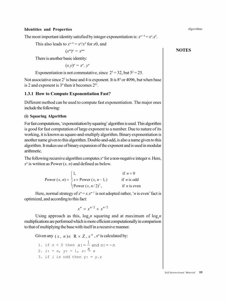
Algorithms
NOTES
Self-Instructional Material 55
Identities and Properties
The most important identity satisfied by integer exponentiation is: xa+ b = xa.xb.
This also leads to xa–b = xa/xb for x0, and
(xm)n = xmn
There is another basic identity:
(x.y)n = xn. yn
Exponentiation is not commutative, since 25 = 32, but 52 = 25.
Not associative since 23 is base and 4 is exponent. It is 84 or 4096, but when baseis 2 and exponent is 34 then it becomes 281.
1.3.1 How to Compute Exponentiation Fast?
Different method can be used to compute fast exponentiation. The major onesinclude the following:
(i) Squaring Algorithm
For fast computations, ‘exponentiation by squaring’ algorithm is used. This algorithmis good for fast computation of large exponent to a number. Due to nature of itsworking, it is known as square-and-multiply algorithm. Binary exponentiation isanother name given to this algorithm. Double-and-add, is also a name given to thisalgorithm. It makes use of binary expansion of the exponent and is used in modulararithmetic.
The following recursive algorithm computes xn for a non-negative integer n. Here,xn is written as Power (x, n) and defined as below.
2
1, if 0
Power ( , ) Power ( , 1, ) if is odd
Power ( , / 2) , if is even
n
x n x x n n
x n n
Here, normal strategy of xn = x.xn–1 is not adopted rather, ‘n is even’ fact isoptimized, and according to this fact:
/ 2 / 2n n nx x x
Using approach as this, log2n squaring and at maximum of log
2n
multiplications are performed which is more efficient computationally in comparisonto that of multiplying the base with itself in a recursive manner.
Given any ( , ) R Z , nx n x , xn is calculated by:
1. if n < 0 then 1
:= and := -x n nx2. i: = n, y: = 1, z: = x
3. if i is odd then y: = y.z
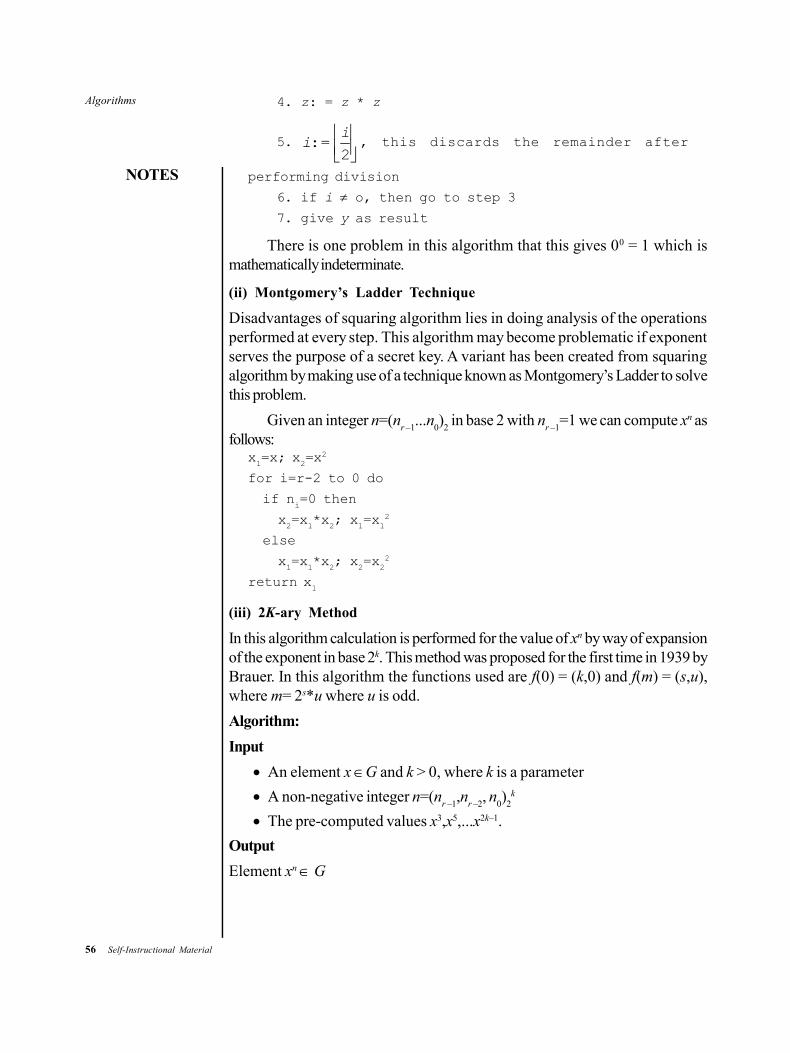
56 Self-Instructional Material
Algorithms
NOTES
4. z: = z * z
5.
:=2i
i , this discards the remainder after
performing division
6. if i o, then go to step 37. give y as result
There is one problem in this algorithm that this gives 00 = 1 which ismathematically indeterminate.
(ii) Montgomery’s Ladder Technique
Disadvantages of squaring algorithm lies in doing analysis of the operationsperformed at every step. This algorithm may become problematic if exponentserves the purpose of a secret key. A variant has been created from squaringalgorithm by making use of a technique known as Montgomery’s Ladder to solvethis problem.
Given an integer n=(nr –1
...n0)
2 in base 2 with n
r –1=1 we can compute xn as
follows:x1=x; x
2=x2
for i=r-2 to 0 do
if ni=0 then
x2=x
1*x
2; x
1=x
12
else
x1=x
1*x
2; x
2=x
22
return x1
(iii) 2K-ary Method
In this algorithm calculation is performed for the value of xn by way of expansionof the exponent in base 2k. This method was proposed for the first time in 1939 byBrauer. In this algorithm the functions used are f(0) = (k,0) and f(m) = (s,u),where m= 2s*u where u is odd.
Algorithm:
Input
An element x G and k > 0, where k is a parameter
A non-negative integer n=(nr –1
,nr –2
, n0)
2k
The pre-computed values x3,x5,...x2k–1.
Output
Element xn G
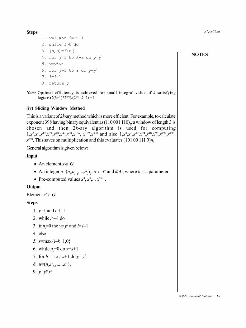
Algorithms
NOTES
Self-Instructional Material 57
Steps1. y=1 and i=r –1
2. while i>0 do
3. (s,u)=f(ni)
4. for j=1 to k-s do y=y2
5. y=y*xu
6. for j=1 to s do y=y2
7. i=i–1
8. return y
Note: Optimal efficiency is achieved for small integral value of k satisfyinglog(n)<(k(k+1)*22*k)/(2k+1–k–2) + 1
(iv) Sliding Window Method
This is a variant of 2k-ary method which is more efficient. For example, to calculateexponent 398 having binary equivalent as (110 001 110)
2, a window of length 3 is
chosen and then 2k-ary algorithm is used for computing1,x3,x6,x12,x24,x48,x49,x98,x196, x199,x398 and also 1,x3,x6,x12,x24,x48,x96,x192,x199,x398. This saves on multiplication and this evaluates (101 00 111 0)n
2.
General algorithm is given below:
Input
An element x G
An integer n=(nl,n
l–1,...,n
0)
2, n I+ and k>0, where k is a parameter
Pre-computed values x3, x5,... x2k–1.
Output
Element xn G
Steps
1. y=1 and i=l–1
2. while i>–1 do
3. if ni=0 the y=y2 and i=i–1
4. else
5. s=max{i–k+1,0}
6. while ns=0 do s=s+1
7. for h=1 to i-s+1 do y=y2
8. u=(ni,n
i–1,....,n
s)
2
9. y=y*xu
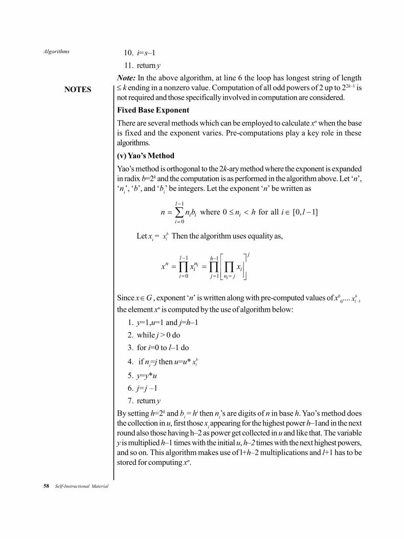
58 Self-Instructional Material
Algorithms
NOTES
10. i=s–1
11. return y
Note: In the above algorithm, at line 6 the loop has longest string of length k ending in a nonzero value. Computation of all odd powers of 2 up to 22k–1 isnot required and those specifically involved in computation are considered.
Fixed Base Exponent
There are several methods which can be employed to calculate xn when the baseis fixed and the exponent varies. Pre-computations play a key role in thesealgorithms.
(v) Yao’s Method
Yao’s method is orthogonal to the 2k-ary method where the exponent is expandedin radix b=2k and the computation is as performed in the algorithm above. Let ‘n’,‘n
i’, ‘b’, and ‘b
i’ be integers. Let the exponent ‘n’ be written as
1
0
where 0 for all [0, 1]l
i i ii
n n b n h i l
Let xi = b
ix Then the algorithm uses equality as,
1 1
0 1
i
i
jl h
nni i
i j n j
x x x
Since x G , exponent ‘n’ is written along with pre-computed values of xb0.... –1
blx
the element xn is computed by the use of algorithm below:
1. y=1,u=1 and j=h–1
2. while j > 0 do
3. for i=0 to l–1 do
4. if ni=j then u=u* b
ix
5. y=y*u
6. j=j –1
7. return y
By setting h=2k and bi = hi then n
i’s are digits of n in base h. Yao’s method does
the collection in u, first those xi appearing for the highest power h–1and in the next
round also those having h–2 as power get collected in u and like that. The variabley is multiplied h–1 times with the initial u, h–2 times with the next highest powers,and so on. This algorithm makes use of l+h–2 multiplications and l+1 has to bestored for computing xn.

Algorithms
NOTES
Self-Instructional Material 59
(vi) Euclidean Method
The Euclidean method was first introduced in ‘efficient exponentiation usingprecomputation and vector addition chains’ by P.D Rooij. The algorithm belowcomputes xn using the following equality recursively:
1 001
( mod )0 10 0 1 01 1( ) . where /n nnn n qx x x x x q n n
If x G and exponent ‘n’ is written the way it is written in Yao’s method havingcomputed values of xb
0....xb
l–1 the element xn is computed by making use of the
algorithm below:
Steps
1. while true do
2. find M such that nM n
i for all i in [0,l–1]
3. find N M such that nN n
i for all i in [0,l–1],i M
4. if nN 0 then
5. *( / ) , and modqM N N N M M NMq n n x x x n n n
6. else break
7. return xM
n
The algorithm first finds the largest value amongst the ni and then the supremum
within the set of {ni : i M }. It raises x
M to the power q, multiplies this value with
xN and then assigns x
N the result of this computation and n
M the value n
M modulo
nN.
Further applications
Using this idea, speedy calculations for large exponents modulo division of a numberis done, that has applications in cryptography. Computation of powers in a ring ofintegers modulo q is very useful and use can be made of this in computing integerpowers in a group. For this following rule is used,
Power(x, –n) = (Power(x, n))–1.
In every semi-group this method works and this is often used for computingpowers of matrices.
For example, in evaluating 13789722341 (mod 2345), if a naïve method isused then it will require very long time and storage space. It involves computing13789722341 and taking remainder after dividing by 2345. Even if more effectivemethods are used it will consume long time as it will first square 13789, thenwould find remainder after dividing by 2345 and further multiply this result by13789. This process will continue involving 722340 modular multiplications. Thesquare-and-multiply algorithm is based on 13789722341 = 13789(137892)361170.So, when 137892 is computed, full computation would consist of 361170 modularmultiplications and there is a gain of a factor of two. As new problem is also the
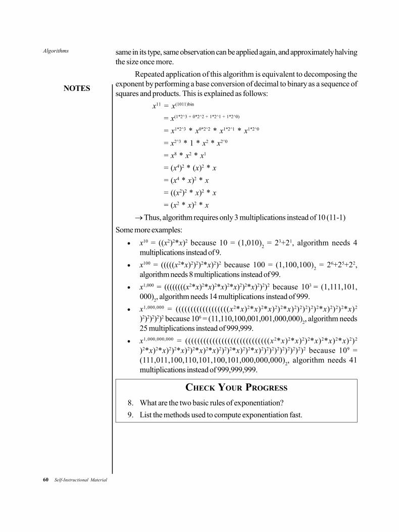
60 Self-Instructional Material
Algorithms
NOTES
same in its type, same observation can be applied again, and approximately halvingthe size once more.
Repeated application of this algorithm is equivalent to decomposing theexponent by performing a base conversion of decimal to binary as a sequence ofsquares and products. This is explained as follows:
x11 = x(1011)bin
= x(1*2^3 + 0*2^2 + 1*2^1 + 1*2^0)
= x1*2^3 * x0*2^2 * x1*2^1 * x1*2^0
= x2^3 * 1 * x2 * x2^0
= x8 * x2 * x1
= (x4)2 * (x)2 * x
= (x4 * x)2 * x
= ((x2)2 * x)2 * x
= (x2 * x)2 * x
Thus, algorithm requires only 3 multiplications instead of 10 (11-1)
Some more examples:
x10 = ((x2)2*x)2 because 10 = (1,010)2 = 23+21, algorithm needs 4
multiplications instead of 9.
x100 = (((((x2*x)2)2)2*x)2)2 because 100 = (1,100,100)2 = 26+25+22,
algorithm needs 8 multiplications instead of 99.
x1,000 = ((((((((x2*x)2*x)2*x)2*x)2)2*x)2)2)2 because 103 = (1,111,101,000)
2, algorithm needs 14 multiplications instead of 999.
x1,000,000 = ((((((((((((((((((x2*x)2*x)2*x)2)2*x)2)2)2)2)2*x)2)2)2*x)2
)2)2)2)2)2 because 106 = (11,110,100,001,001,000,000)2, algorithm needs
25 multiplications instead of 999,999.
x1,000,000,000 = ((((((((((((((((((((((((((((x2*x)2*x)2)2*x)2*x)2*x)2)2
)2*x)2*x)2)2*x)2)2*x)2*x)2)2)2*x)2)2*x)2)2)2)2)2)2)2)2)2 because 109 =(111,011,100,110,101,100,101,000,000,000)
2, algorithm needs 41
multiplications instead of 999,999,999.
CHECK YOUR PROGRESS
8. What are the two basic rules of exponentiation?
9. List the methods used to compute exponentiation fast.
Algorithms
NOTES
Self-Instructional Material 61
1.4 LINEAR SEARCH
Linear search is the easiest and least efficient searching technique. In this technique,the given list of elements is scanned till either the required element is found or thelist is exhausted. This technique is used in direct access media such as magnetictapes.
Example 1.14 illustrutes a linear search.
Example 1.14: Find an element 77 from the given list using linear search. The listof elements is 10, 25, 77, 16, 47 and 98.
Linear search starts by checking the target element (i.e., 77) with the firstelement of the list, i.e., 10, which is not equal to the target element; search continueswith the second element, i.e. 25, which is also not equal to the target element andsearch continues with the third element, i.e. 77, which is equal to the target element(=77). So, the search is stopped.
1.4.1 Algorithm for Linear Search
LINEAR_SEARCH (L, N, E)
1. [Initialization]
loc = 1
L[N + 1] = E
2. [Search the element in the vector]
REPEAT WHILE ( K[loc]<> E ) DO
loc = loc + 1
3. [Check whether the search is successful or not?]
IF loc = N + 1, THEN WRITE (‘UNSUCCESSFUL SEARCH’)
RETURN(0)
ELSE WRITE(‘SUCCESSFUL SEARCH’)
RETURN(loc)
1.4.2 Analysis of Linear Search Algorithm
For N total number of elements, the search time T is proportional to half of N:T = K * N/2 where K is a constant
If K = 2, then T = K*N
The average linear search times are proportional to the size of the array, i.e., O(N)
Note: If an array is twice as big, it will take twice as long to search.
Implementation of Linear Search to Find a String from a String Vector/Array
Program for Linear Search of Strings /*—————————START OF PROGRAM——————————*/
#include<stdio.h>
#define MAXROWS 10
62 Self-Instructional Material
Algorithms
NOTES
#define MAXCOLS 20
#define NOTFOUND -1
typedef char STRINGS[MAXROWS][MAXCOLS];
typedef char STRING[MAXCOLS];
int LSearch(STRINGS s,STRING target,int n)
{
int loc=0;
strcpy(s[n],target);
while(strcmp(s[loc],target))
loc++;
if(loc==n)
return NOTFOUND;
else
return loc;
}
void main()
{
STRINGS a={“MON”,”TUE”,”WED”,”THU”,”FRI”,”SAT”,”SUN”};
int index;
index=LSearch(a,”WED”,7);
if(index==NOTFOUND)
printf(“Record not found”);
else
printf(“Record found at Location:%d”,index+1);
}
/*——————————END OF PROGRAM————————*/
Output: Record found at Location 3
Implementation of linear search to find a value in a vector or array/*————————START OF PROGRAM——————————*/
#include<stdio.h>
#include<conio.h>
#define MAXROWS 10
#define MAXCOLS 20
#define NOTFOUND -1
typedef int VECTOR[MAXCOLS];
int LSearch(VECTOR s,int target,int n)
{
int loc=0;
s[n]=target;
while(s[loc]!=target)
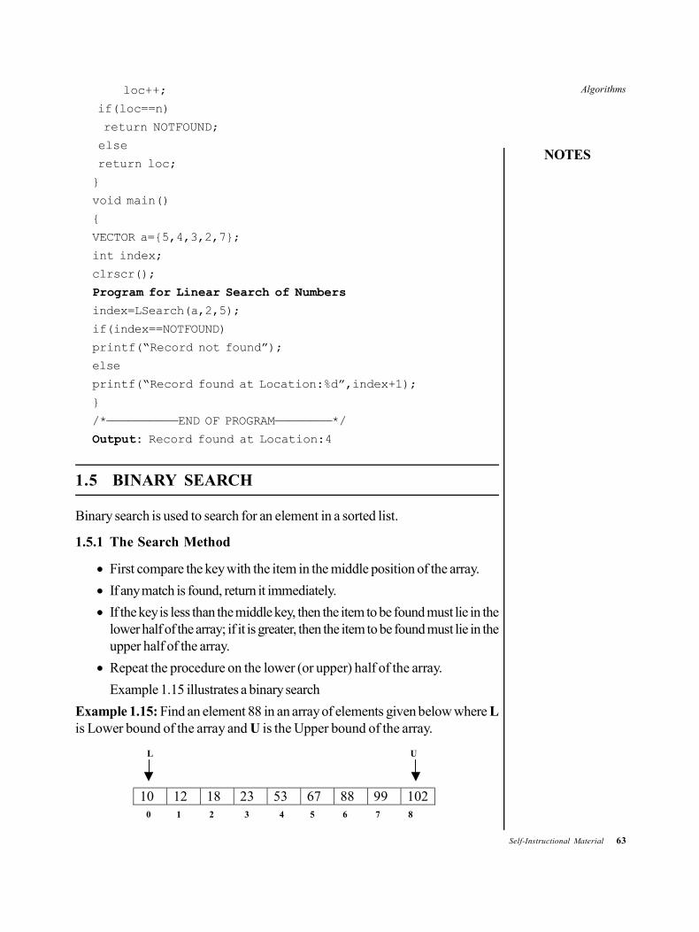
Algorithms
NOTES
Self-Instructional Material 63
loc++;
if(loc==n)
return NOTFOUND;
else
return loc;
}
void main()
{
VECTOR a={5,4,3,2,7};
int index;
clrscr();
Program for Linear Search of Numbers
index=LSearch(a,2,5);
if(index==NOTFOUND)
printf(“Record not found”);
else
printf(“Record found at Location:%d”,index+1);
}
/*——————————END OF PROGRAM————————*/
Output: Record found at Location:4
1.5 BINARY SEARCH
Binary search is used to search for an element in a sorted list.
1.5.1 The Search Method
First compare the key with the item in the middle position of the array.
If any match is found, return it immediately.
If the key is less than the middle key, then the item to be found must lie in thelower half of the array; if it is greater, then the item to be found must lie in theupper half of the array.
Repeat the procedure on the lower (or upper) half of the array.
Example 1.15 illustrates a binary search
Example 1.15: Find an element 88 in an array of elements given below where Lis Lower bound of the array and U is the Upper bound of the array.
10 12 18 23 53 67 88 99 102 0 1 2 3 4 5 6 7 8
L U
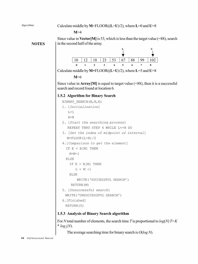
64 Self-Instructional Material
Algorithms
NOTES
Calculate middle by M=FLOOR((L+U)/2), where L=0 and U=8
M=4
Since value in Vector[M] is 53, which is less than the target value (=88), searchin the second half of the array.
10 12 18 23 53 67 88 99 102 0 1 2 3 4 5 6 7 8
L U
Calculate middle by M=FLOOR((L+U)/2), where L=5 and U=8
M=6
Since value in Array[M] is equal to target value (=88), then it is a successfulsearch and record found at location 6.
1.5.2 Algorithm for Binary Search
BINARY_SEARCH(B,N,E)
1. [Initialization]
L=1
H=N
2. [Start the searching process]
REPEAT THRU STEP 4 WHILE L<=H DO
3. [Get the index of midpoint of interval]
M=FLOOR(L+H)/2
4.[Comparison to get the element]
IF E < B[M] THEN
H=M-1
ELSE
IF E > B[M] THEN
L = M +1
ELSE
WRITE(‘SUCCESSFUL SEARCH’)
RETURN(M)
5. [Unsuccessful search]
WRITE(‘UNSUCCESSFUL SEARCH’)
6.[Finished]
RETURN(0)
1.5.3 Analysis of Binary Search algorithm
For N total number of elements, the search time T is proportional to log(N) T=K* log
2(N).
The average searching time for binary search is O(log N).
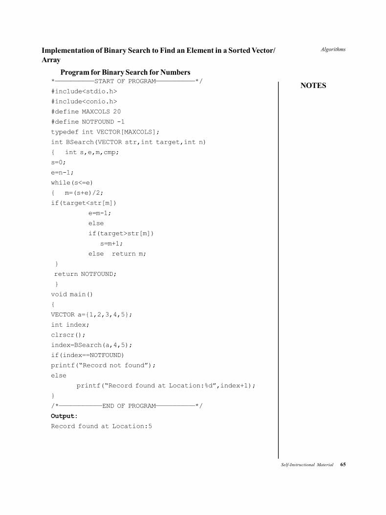
Algorithms
NOTES
Self-Instructional Material 65
Implementation of Binary Search to Find an Element in a Sorted Vector/Array
Program for Binary Search for Numbers*——————————START OF PROGRAM——————————*/
#include<stdio.h>
#include<conio.h>
#define MAXCOLS 20
#define NOTFOUND -1
typedef int VECTOR[MAXCOLS];
int BSearch(VECTOR str,int target,int n)
{ int s,e,m,cmp;
s=0;
e=n-1;
while(s<=e)
{ m=(s+e)/2;
if(target<str[m])
e=m-1;
else
if(target>str[m])
s=m+1;
else return m;
}
return NOTFOUND;
}
void main()
{
VECTOR a={1,2,3,4,5};
int index;
clrscr();
index=BSearch(a,4,5);
if(index==NOTFOUND)
printf(“Record not found”);
else
printf(“Record found at Location:%d”,index+1);
}
/*———————————END OF PROGRAM——————————*/
Output:
Record found at Location:5
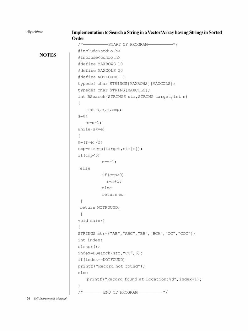
66 Self-Instructional Material
Algorithms
NOTES
Implementation to Search a String in a Vector/Array having Strings in SortedOrder
/*——————————START OF PROGRAM——————————*/
#include<stdio.h>
#include<conio.h>
#define MAXROWS 10
#define MAXCOLS 20
#define NOTFOUND -1
typedef char STRINGS[MAXROWS][MAXCOLS];
typedef char STRING[MAXCOLS];
int BSearch(STRINGS str,STRING target,int n)
{
int s,e,m,cmp;
s=0;
e=n-1;
while(s<=e)
{
m=(s+e)/2;
cmp=strcmp(target,str[m]);
if(cmp<0)
e=m-1;
else
if(cmp>0)
s=m+1;
else
return m;
}
return NOTFOUND;
}
void main()
{
STRINGS str={“AB”,”ABC”,”BB”,”BCA”,”CC”,”CCC”};
int index;
clrscr();
index=BSearch(str,”CC”,6);
if(index==NOTFOUND)
printf(“Record not found”);
else
printf(“Record found at Location:%d”,index+1);
}
/*————————END OF PROGRAM——————————*/
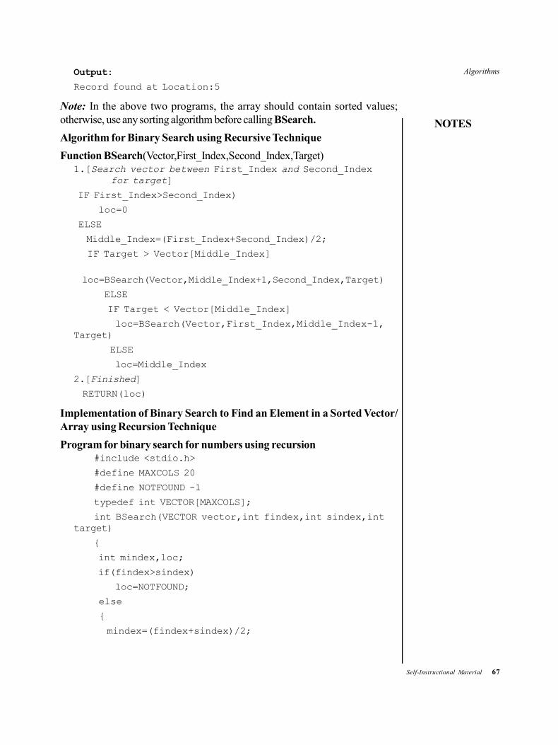
Algorithms
NOTES
Self-Instructional Material 67
Output:
Record found at Location:5
Note: In the above two programs, the array should contain sorted values;otherwise, use any sorting algorithm before calling BSearch.
Algorithm for Binary Search using Recursive Technique
Function BSearch(Vector,First_Index,Second_Index,Target)1.[Search vector between First_Index and Second_Index
for target]
IF First_Index>Second_Index)
loc=0
ELSE
Middle_Index=(First_Index+Second_Index)/2;
IF Target > Vector[Middle_Index]
loc=BSearch(Vector,Middle_Index+1,Second_Index,Target)
ELSE
IF Target < Vector[Middle_Index]
loc=BSearch(Vector,First_Index,Middle_Index-1,Target)
ELSE
loc=Middle_Index
2.[Finished]
RETURN(loc)
Implementation of Binary Search to Find an Element in a Sorted Vector/Array using Recursion Technique
Program for binary search for numbers using recursion#include <stdio.h>
#define MAXCOLS 20
#define NOTFOUND -1
typedef int VECTOR[MAXCOLS];
int BSearch(VECTOR vector,int findex,int sindex,inttarget)
{
int mindex,loc;
if(findex>sindex)
loc=NOTFOUND;
else
{
mindex=(findex+sindex)/2;

68 Self-Instructional Material
Algorithms
NOTES
if(target>vector[mindex])
loc=BSearch(vector,mindex+1,sindex,target);
else
if(target<vector[mindex])
loc=BSearch(vector,findex,mindex-1,target);
else
loc=mindex;
}
return(loc);
}
void main()
{
VECTOR a={10,20,30,40,50,60,70,80,90};
int loc;
loc=BSearch(a,0,8,40);
if(loc==NOTFOUND)
printf(“Target string not found”);
else
printf(“Starting from 0th location target is atlocation:%d”,loc);
}
Output
Starting from 0th location target is at Location:3
Implementation to Search a String in a Vector/Array having Strings in SortedOrder using Recursion Technique
Program for binary search for strings using recursion#include <stdio.h>
#include <string.h>
#define MAXCOLS 20
#define MAXROWS 10
#define NOTFOUND -1
typedef char STRINGS[MAXROWS][MAXCOLS];
typedef char STRING[MAXCOLS];
int BSearch(STRINGS str,int findex,int sindex,STRINGtarget)
{
int mindex,loc,cmp;
if(findex>sindex)
loc=NOTFOUND;
else
{ mindex=(findex+sindex)/2;
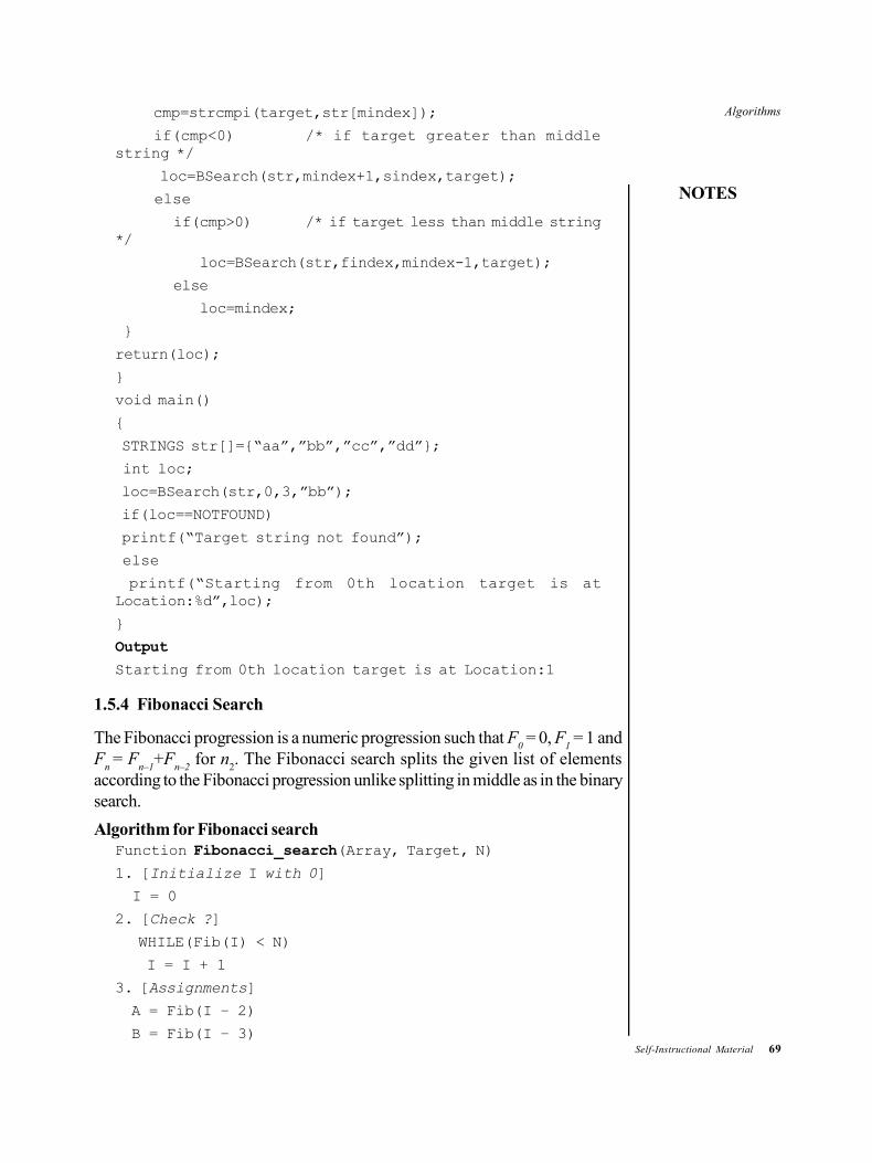
Algorithms
NOTES
Self-Instructional Material 69
cmp=strcmpi(target,str[mindex]);
if(cmp<0) /* if target greater than middlestring */
loc=BSearch(str,mindex+1,sindex,target);
else
if(cmp>0) /* if target less than middle string*/
loc=BSearch(str,findex,mindex-1,target);
else
loc=mindex;
}
return(loc);
}
void main()
{
STRINGS str[]={“aa”,”bb”,”cc”,”dd”};
int loc;
loc=BSearch(str,0,3,”bb”);
if(loc==NOTFOUND)
printf(“Target string not found”);
else
printf(“Starting from 0th location target is atLocation:%d”,loc);
}
Output
Starting from 0th location target is at Location:1
1.5.4 Fibonacci Search
The Fibonacci progression is a numeric progression such that F0 = 0, F
1 = 1 and
Fn = F
n–1+F
n–2 for n
2. The Fibonacci search splits the given list of elements
according to the Fibonacci progression unlike splitting in middle as in the binarysearch.
Algorithm for Fibonacci searchFunction Fibonacci_search(Array, Target, N)
1. [Initialize I with 0]
I = 0
2. [Check ?]
WHILE(Fib(I) < N)
I = I + 1
3. [Assignments]
A = Fib(I – 2)
B = Fib(I – 3)
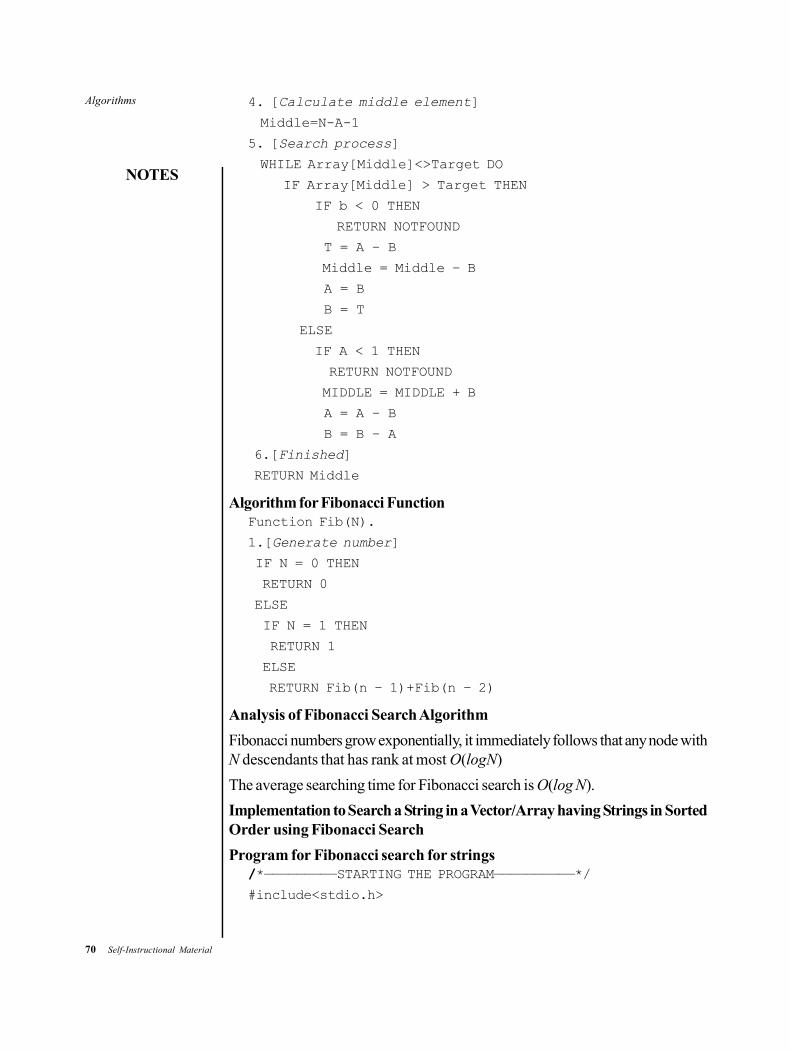
70 Self-Instructional Material
Algorithms
NOTES
4. [Calculate middle element]
Middle=N-A-1
5. [Search process]
WHILE Array[Middle]<>Target DO
IF Array[Middle] > Target THEN
IF b < 0 THEN
RETURN NOTFOUND
T = A – B
Middle = Middle – B
A = B
B = T
ELSE
IF A < 1 THEN
RETURN NOTFOUND
MIDDLE = MIDDLE + B
A = A – B
B = B – A
6.[Finished]
RETURN Middle
Algorithm for Fibonacci FunctionFunction Fib(N).
1.[Generate number]
IF N = 0 THEN
RETURN 0
ELSE
IF N = 1 THEN
RETURN 1
ELSE
RETURN Fib(n – 1)+Fib(n – 2)
Analysis of Fibonacci Search Algorithm
Fibonacci numbers grow exponentially, it immediately follows that any node withN descendants that has rank at most O(logN)
The average searching time for Fibonacci search is O(log N).
Implementation to Search a String in a Vector/Array having Strings in SortedOrder using Fibonacci Search
Program for Fibonacci search for strings/*—————————STARTING THE PROGRAM——————————*/
#include<stdio.h>
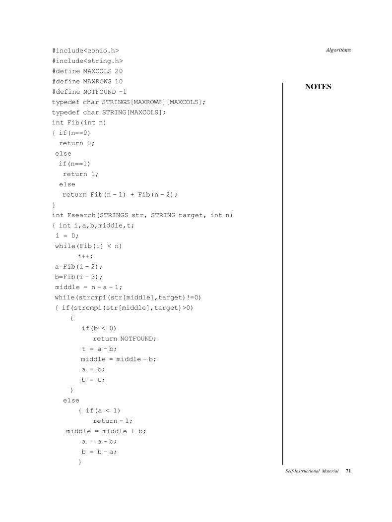
Algorithms
NOTES
Self-Instructional Material 71
#include<conio.h>
#include<string.h>
#define MAXCOLS 20
#define MAXROWS 10
#define NOTFOUND –1
typedef char STRINGS[MAXROWS][MAXCOLS];
typedef char STRING[MAXCOLS];
int Fib(int n)
{ if(n==0)
return 0;
else
if(n==1)
return 1;
else
return Fib(n – 1) + Fib(n – 2);
}
int Fsearch(STRINGS str, STRING target, int n)
{ int i,a,b,middle,t;
i = 0;
while(Fib(i) < n)
i++;
a=Fib(i – 2);
b=Fib(i – 3);
middle = n – a – 1;
while(strcmpi(str[middle],target)!=0)
{ if(strcmpi(str[middle],target)>0)
{
if(b < 0)
return NOTFOUND;
t = a – b;
middle = middle – b;
a = b;
b = t;
}
else
{ if(a < 1)
return – 1;
middle = middle + b;
a = a – b;
b = b – a;
}
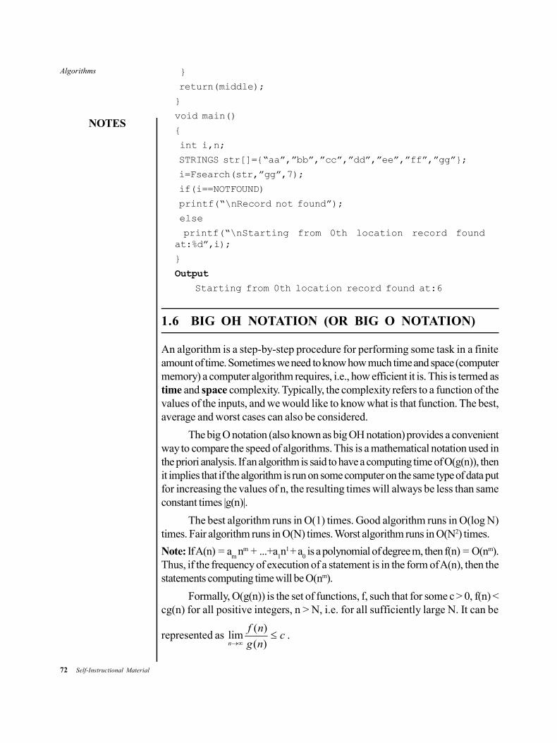
72 Self-Instructional Material
Algorithms
NOTES
}
return(middle);
}
void main()
{
int i,n;
STRINGS str[]={“aa”,”bb”,”cc”,”dd”,”ee”,”ff”,”gg”};
i=Fsearch(str,”gg”,7);
if(i==NOTFOUND)
printf(“\nRecord not found”);
else
printf(“\nStarting from 0th location record foundat:%d”,i);
}
Output
Starting from 0th location record found at:6
1.6 BIG OH NOTATION (OR BIG O NOTATION)
An algorithm is a step-by-step procedure for performing some task in a finiteamount of time. Sometimes we need to know how much time and space (computermemory) a computer algorithm requires, i.e., how efficient it is. This is termed astime and space complexity. Typically, the complexity refers to a function of thevalues of the inputs, and we would like to know what is that function. The best,average and worst cases can also be considered.
The big O notation (also known as big OH notation) provides a convenientway to compare the speed of algorithms. This is a mathematical notation used inthe priori analysis. If an algorithm is said to have a computing time of O(g(n)), thenit implies that if the algorithm is run on some computer on the same type of data putfor increasing the values of n, the resulting times will always be less than sameconstant times |g(n)|.
The best algorithm runs in O(1) times. Good algorithm runs in O(log N)times. Fair algorithm runs in O(N) times. Worst algorithm runs in O(N2) times.
Note: If A(n) = am nm + ...+a
1n1 + a
0 is a polynomial of degree m, then f(n) = O(nm).
Thus, if the frequency of execution of a statement is in the form of A(n), then thestatements computing time will be O(nm).
Formally, O(g(n)) is the set of functions, f, such that for some c > 0, f(n) <cg(n) for all positive integers, n > N, i.e. for all sufficiently large N. It can be
represented as cng
nfn
)(
)(lim .

Algorithms
NOTES
Self-Instructional Material 73
Informally, we say the O(g) is the set of all functions, which grows no fasterthan g. The function g is an upper bound to functions in O(g).
We can analyse any algorithm by the O notation irrespective of theprogramming language and machine.
Consider two other functions: )(g and )(g .
)(g is the set of functions f(n) for which f(n) )(ncg for all positive integers,
n>N, and )()()( gOgg
1.6.1 Properties of the Big O Notation
The following are the properties of big O notation:
Constant factors may be ignored: For all k > 0, kf is O(f).
e.g. cn2 and kn2 are both O(n2).
Higher powers of n grow faster than lower powers: nr is O(n8) if sr 0 .
The growth rate of a sum of terms is the growth rate of its fastest growingterm: If f is O(g), then f+g is O(g).
e.g. an3+bn2 is O(n3).
The growth rate of polynomial is given by the growth rate of its leadingterm: If f is a polynomial of degree d, then f is O(nd).
If f grows faster than g, which grows faster than h, then f grows faster thanh.
The product of upper bounds of functions gives an upper bound for theproduct of the functions: If f is O(g) and h is O(r) , then fh is O(gr).
e.g. If f is O(n2) and g is O(log n), then fg is O(n2 log n).
Exponential functions grow faster than powers: nk is O(bn), for all b > 1, k,
e.g. n4 is O(2n) and n4 is O(exp(n)).
Logarithms grow more slowly than powers: logb n is O(nk) for all b > 1, k >
0
e.g. log2n is O(n0.5).
All logarithms grow at the same rate: logb n is )(log nd for all b, d>1.
The sum of the n rth powers grows as the (r+1)th power:
n
k
rr nisk1
1 )(
e.g. )(2
)1( 2
1nis
nni
n
k
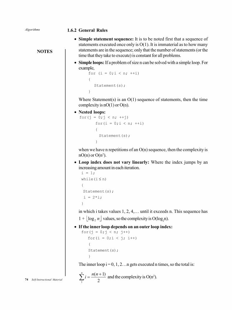
74 Self-Instructional Material
Algorithms
NOTES
1.6.2 General Rules
Simple statement sequence: It is to be noted first that a sequence ofstatements executed once only is O(1). It is immaterial as to how manystatements are in the sequence; only that the number of statements (or thetime that they take to execute) is constant for all problems.
Simple loops: If a problem of size n can be solved with a simple loop. Forexample,
for (i = 0;i < n; ++i)
{
Statement(s);
}
Where Statement(s) is an O(1) sequence of statements, then the timecomplexity is nO(1) or O(n).
Nested loops: for(j = 0;j < n; ++j)
for(i = 0;i < n; ++i)
{
Statement(s);
}
when we have n repetitions of an O(n) sequence, then the complexity isnO(n) or O(n2).
Loop index does not vary linearly: Where the index jumps by anincreasing amount in each iteration.i = 1;
while(i n){
Statement(s);
i = 2*i;
}
in which i takes values 1, 2, 4,… until it exceeds n. This sequence has
1 + n2log values, so the complexity is O(log2n).
If the inner loop depends on an outer loop index:for(j = 0;j < n; j++)
for(i = 0;i < j; i++)
{
Statement(s);
}
The inner loop i = 0, 1, 2…n gets executed n times, so the total is:
n nni
1 2
)1( and the complexity is O(n2).
Algorithms
NOTES
Self-Instructional Material 75
Notice that the above two nested loops also have the same complexity, sothe variable number of iterations of the inner loop does not affect the ‘bigpicture’. However, if the number of iterations of one of the loops decreasesby a constant factor with every iteration as shown below:i = n;
while(i > 0)
{ for(i = 0;i < n; ++i)
{
Statement(s);
}
h = h/2;
}
Then there are log2 n iterations of the outer loop and the inner loop is O(n).
So the overall complexity is O(n log n) .
The most common computing times of algorithms in the big O notation are:
O(1)<O(logn)<O(n)<O(nlogn)<O(n2 ) <O(n3)<O(2n)<=O(n!)
1.6.3 Finding Prime Factor of a Given Number
Finding a prime factor begins with the lowest prime number 2. If 2 divides thenumber completely and leaves no remainder it is marked as the very first primefactor. It continues dividing until it longer divides evenly. Then the control flowmoves to the next lowest prime numbers. The step is repeated until the next primefactor comes. The following algorithm is used to find the prime factor of a givennumber:
Algorithm to Find Prime Factor of a Given NumberStep 1: integer input, divisor, count;
Step 2: print ‘Enter a value:’,
Step 3: read input;
Step 4: count0;
Step 5: Do
Step 6: divisor0;
Step 7: if input mod 2==0 OR input==1
//To remove all the factors of 2
break;
countcount+1; //Increase counter value by 1
print count, divisor;
inputinput/2; //Remove this factor from input
Step 8:End Do
Step 9: divisor3;
Step 10: Do
Step 11: if divisor>input
76 Self-Instructional Material
Algorithms
NOTES
break;
Step 12: Do //Remove the factors repeatedly
Step 13: if input mod divisor ==0 OR input==1
break;
countcount+1;
print count, divisor;
inputinput/divisor;
//Remove factors from input
Step 14: End Do
Step 15: divisor divisor+2;
//Move to next odd number
Step 16: End Do
The above algorithm lists out all prime factors of an n integer >=2.First it sides back all factors of 2. Then, all factors, such as 3, 5, 7 and so on canbe removed. This process is run until all the prime factors are sided back and keptin a temporary location. According to the above algorithm, if the input value is 53,the prime factors of 53 are 1 and 53 itself.
Implementation of Finding Prime Factor of a Given Number/*—————————— START OF PROGRAM ——————————*/
#include <stdio.h>
#include <conio.h>
void main()
{
int number, i, j, k;
clrscr();
printf(“Enter a number:”);
scanf(“%d”, &d);
while(i<=number)
{
k=0;
if (number%i==0)
{
j=1;
while(j<=i)
{
if(i%j==0)
k++; //Value k is increased by 1
j++; //Value j is increased by 1
}
if(k==2)
printf(“\nPrime factors are:”);
printf(“%d”,i);
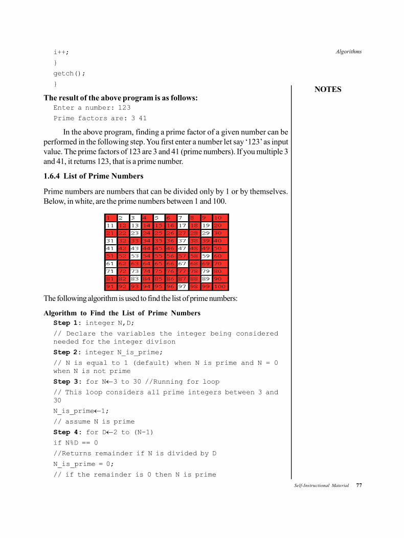
Algorithms
NOTES
Self-Instructional Material 77
i++;
}
getch();
}
The result of the above program is as follows:Enter a number: 123
Prime factors are: 3 41
In the above program, finding a prime factor of a given number can beperformed in the following step. You first enter a number let say ‘123’ as inputvalue. The prime factors of 123 are 3 and 41 (prime numbers). If you multiple 3and 41, it returns 123, that is a prime number.
1.6.4 List of Prime Numbers
Prime numbers are numbers that can be divided only by 1 or by themselves.Below, in white, are the prime numbers between 1 and 100.
The following algorithm is used to find the list of prime numbers:
Algorithm to Find the List of Prime NumbersStep 1: integer N,D;
// Declare the variables the integer being consideredneeded for the integer divison
Step 2: integer N_is_prime;
// N is equal to 1 (default) when N is prime and N = 0when N is not prime
Step 3: for N3 to 30 //Running for loop
// This loop considers all prime integers between 3 and30
N_is_prime1;
// assume N is prime
Step 4: for D2 to (N-1)
if N%D == 0
//Returns remainder if N is divided by D
N_is_prime = 0;
// if the remainder is 0 then N is prime
78 Self-Instructional Material
Algorithms
NOTES
Step 5: if N_is_prime == 0
break; //Exit from loop
// if N is prime do not do any more integer divisions
Step 6: if N_is_prime == 1
print N;
Implementation to find the list of prime numbers/*—————————— START OF PROGRAM ——————————*/
#include<stdio.h>
#include <conio.h>
void main()
{
int N; // the integer being considered
int D; // needed for the integer divison
int N_is_prime; // = 1 (default) when N is prime and = 0when N is not prime
for (N=3;N<=30;N++)
// This loop considers all prime integers between 3 and100
{
N_is_prime = 1; // assume N is prime
for (D=2;D<=N-1;D++)
{
if ( N%D == 0 ) N_is_prime = 0;
// if the remainder is 0 then N is prime
if (N_is_prime == 0)
break;
// if N is prime don’t do any more integer divisions
}
if (N_is_prime == 1)
printf(“%d\n”,N);
}
getch();
}
The result of the above program is as follows:2
3
5
7
11
13
17

Algorithms
NOTES
Self-Instructional Material 79
19
23
29
CHECK YOUR PROGRESS
10. What do you understand by the linear search technique?
11. When is the binary search method used?
12. What is big O notation?
1.7 WORST CASE
In the field of computer science, complexity indicates a measure of resourcesrequired by an algorithm and worst-case complexity is a measure of resourcesrequired by the algorithm to solve a problem in worst case. Here, by ‘resources’we mean time of run and memory required. These are time and space complexity.Worst-case indicates the maximum amount of resource required by the algorithmto solve the problem.
Measured in terms of time required, worst-case time-complexity givesmaximum time required by an algorithm to perform when any input of size n isgiven with a guarantee that algorithm finishes its work within that time. This alsoforms a basis for comparing efficiency of two algorithms.
Best case, worst case and average cases are three situations in which analysisis done for a given algorithm. These terms tell about use of resources in terms of atleast, at most and on average, respectively. Here, resources usually includerunning time and amount of memory space the algorithm occupies. It may meanother resources as well, but mostly time and space complexities are used. Worst-case execution time is of particular importance in real time computing as it is criticalto know the maximum time required to execute instructions with a guarantee thatthe algorithm will always finish within that time.
Worst-case is compared with average performance and is mostly used inalgorithm analysis. In case of a looping statement there is O(n) time complexity. Ifanother loop is put in that loop the complexity increases and it becomes O(n^2),since it has to do n^2 things for an input size of n.
Worst case algorithms are non deterministic.
1.8 ADVANTAGE OF LOGARITHMICALGORITHMS OVER LINEAR ALGORITHMS
An algorithm that takes search time of the order of O(log n) is logarithmic whereasa linear algorithm takes search time of O(kn) to find kth smallest or largest item ina list containing n items. This linear algorithm is not effective when list is large and
80 Self-Instructional Material
Algorithms
NOTES
value of k is large. Such algorithm is suitable only for the cases where value of k issmall. Binary search is an example of logarithmic search.
In linear algorithm, program moves in a sequential manner, whereas a binarysearch adopts the policy of ‘divide and conquer’. For example, if we start searchinga number, say 30, in a list of 100 numbers, and the list is serially arranged then itwill search linearly from 1 to 29 and then come to 30. But in Binary search, itwould divide in two halves and will discard one half and will again search in anotherhalf. This search strategy reduces the number checking by a factor of two eachtime to find the target value, if it is in the list and this will be done in logarithmictime.
Suppose we want to design an algorithm to find whether determinant valueof a particular n n matrix is more than a predetermined value k. Using linearsearch this can be done in O(n2) time whereas using binary search, ceiling of thedeterminant value (d) can be found in O(n2log d) time. Here, d is the size of outputand not of the input.
Algorithm of logarithmic nature always takes less time that of linear search.A linear search has worst case behaviour of N iterations and takes much time as Ngrows. If there are one million items, it will make one million searches. But in caseof logarithmic search such as binary search, time taken in worst case is floor valueof (log
2210 – 1) which is approximately 9. Search is continued even if iteration fails
to find a match at the probed position, with one or other of the two sub-intervals,each with almost halved size. If N, denoting the number items, is odd then bothsub-intervals will have (N –1)/2 elements. But if N is even the two sub-intervalswill have N/2 –1 and N/2 elements.
In a list of N items, after first iteration, remaining items will N/2 items at themaximum and in second iteration, items will get reduced to at most N/4 items, thento N/8 items and so on. This way algorithm continues, iterating until the spanbecomes empty. This will, at the most will take log
2(N) + 1 iterations. Here,
stands for the floor function which neglects the decimal part of the number. Inworst case for any N it takes exactly (log
2 N) + 1 iterations.
Linear search can be applied to a list sorted as well as unsorted, but binarysearch is applied to a list that is already sorted.
1.9 COMPLEXITY
1.9.1 Space Complexity
The space complexity of an algorithm indicates the quantity of temporary storagerequired for running the algorithm, i.e. the amount of memory needed by thealgorithm to run to completion.
Algorithms
NOTES
Self-Instructional Material 81
In most cases, you do not count the storage required for the inputs or theoutputs as part of the space complexity. This is because the space complexity isused to compare different algorithms for the same problem in which case theinput/output requirements are fixed.
Also, you cannot do without the input or the output, and you want to countonly the storage that may be served. You also do not count the storage requiredfor the program itself since it is independent of the size of the input.
Like time complexity, space complexity refers to the worst case, and it isusually denoted as an asymptotic expression in the size of the input. Thus, a o(n)– space algorithm requires a constant amount of space independent of the size ofthe input.
The amount of memory an algorithm needs to run to completion is called itsspace complexity. The space required by an algorithm consists of the followingtwo components:
(i) Fixed or static part: Fixed or static part is not dependent on thecharacteristics (such as number size) of the inputs and outputs. It includesvarious types spaces, such as instruction space (i.e., space for code), spacefor simple variables and fixed-size component variables, space for constants,etc.
(ii) Variable or dynamic part: Variable or dynamic part consists of the spacerequired by component variables whose size is dependent on the particularproblem instance at run-time being solved, the space needed by referencedvariables and the recursion stack space (depends on instance characteristics).
The space requirements S(p) of an algorithm p is S(p) = c + Sp (instancecharacteristics), where ‘c’ is a constant.
We are supposed to concentrate on estimating SP (instance characteristics)since the first part is static.
The problem instances for algorithm are characterized by n, the number ofelements to be summed. The space needed by n is one word since it is of typeinteger. The space needed by a is the space needed by variables of type array offloating-point numbers.
This is at least n words since a must be large enough to hold the n elementsto be summed. So, we obtain S
S(n) = (n + 3) (n for a[ ], one each for n, i, and s).
Iterative function for sumAlgorithm RSum (a, n)
{
if (n 0) then return 0.0;
else return
RSum (a, n – 1) + a[n];
}
82 Self-Instructional Material
Algorithms
NOTES
1.9.2 Time Complexity
The time complexity of an algorithm may be defined as the amount of time thecomputer requires to run to completion.
The time T(P) consumed by a program P is the sum of the compile-time andthe run-time (execution-time). The compile time is independent of the instancecharacteristics. Also, it may be assumed that a compiled program can be run manytimes without recompilation. As a result, we are more interested in the run-time ofa program. This run-time is denoted by t
p (instance characteristics).
Many factors on which tp depend are not known at the time a program is
written; so it is always better to estimate tp. If we happen to know the type of the
compiler used, then we could proceed to find the number of additions, subtractions,multiplications, divisions, compare statements, loads, stores and so on that wouldbe made by a program P.
So we can obtain an expression of the form.
tp(n) = Ca ADD(n) + Cs SUB(n) + Cm MUL(n) + Cd DIV(n) +.........
Where n denotes the instance characteristics, and Ca , C
s, C
m , C
d and so
on denote the time needed for addition, subtraction, multiplication, division, etc.
But here we need to note that the exact amount of time needed for theoperations mentioned here cannot be found exactly; so instead we could onlycount the number of program steps, which means that a program step is counted.
A program step is defined as a syntactically or semantically meaningfulsegment of a program that has an execution time that is independent of the instancecharacteristics.
For example, consider the statement return a + b * c – d % e/f
This can be regarded as a step since its execution time is independent of theinstance characteristics.
The number of steps that are assigned to any program statement depend onthe type of statement. The comments do not count for the program step. A generalassignment statement, which does not call another algorithm, is considered onestep whereas in an iterative statement like for, while and repeat_until, you countthe step only for the control part of the statement.
The general syntax for ‘for’ and ‘while’ statements is as follows:for i = (exprl) to (expr2) do
while(expr) do
Each execution of the control part of a while statement is given step countequal to the number of step counts assignable to <expr>. The step count for eachexecution of the control part of a for statement is one, unless the counts attributableto <expr> and <exprl> are functions of the instance characteristics.
Algorithms
NOTES
Self-Instructional Material 83
1.9.3 Practical Complexities
One of the main reasons to analyse algorithms is to find out the relative performanceof two or more algorithms for the same problem. Consider the problem of sortingan array a[0:n – 1] for which the best known algorithms are bubble sort,selection sort, insertion sort, quick sort, merge sort, etc. The time complexities ofthese algorithms fall in two categories. One set of algorithm have O(n2) and theother set have O(n log n). Unless we analyse and find their complexities, it may bedifficult to say which is faster and which is not.
While comparing the algorithms we must also keep in mind that n is verylarge or sufficiently large. The performance of the algorithms strongly depends onthe size of n too. For instance, quick sort behaves very badly when n is small, i.e.,O(n2), which is same as bubble sort or insertion sort. However, when the size issufficiently large its time complexity is O(n log n).
The aim of this section is to illustrate the practical time calculation of aprogram, what are the timing functions to use (given by the operating system or thecomplier), how to set up the test data, calculate the actual time taken by commonasymptotic functions, f(n) using a real computer executing certain number ofinstructions per second. You will be wondering that certain functions may takeyears of computer time (even on a Pentium III or mainframe machines) for sufficientlylarge values of n.
Typical Examples
(1) Assume that a computer can execute 109 steps/sec and a particular programneeds n10 steps, then:
for n = 10, the time required is = 10 sec
for n = 100, the time required is = 3171 years
for n = 1000, the time required is = 3.17 × 10¹³ years
(2) Assuming that out task needs n2 steps (bubble sort to selection sort) then:
for n = 10, the time required is = 0.1 sec
for n = 100, the time required is = 10 sec
for n = 1000, the time required is = 1msec
for n = 1000000, the time required is = 16.6 min
Looking at the first example, we see that even a polynomial function f(n10) takesenormous amount of time (unimaginable 1013 years). When the function isexponential, (say 2n) imagine what could be the time taken.

84 Self-Instructional Material
Algorithms
NOTES
Table 1.1 shows the run-time on a 1,000,000,000 instructions/sec.
Table 1.1 Run-time for Various Values of n
n n n log n 2n 10n n2
10 s01.0 s03.0 s1.0 10s s1
50 s05.0 s28.0 s5.2 3.1yrs 13 days
100 s01.0 s66.0 s10 3171yrs 4 × 10¹³ yrs
1000 s1 s96.9 1ms 3.17 × 10¹³ yrs 3.17 × 1043 yrs
1000000 1ms 19.92ms 16.67min 3.17 × 1043 yrs -
1.9.4 Performance Measurement
This section explains how the run-time of a function is calculated using specificcomplier options. You will not show the space calculations and the compilationtime in this example. There is of course a small difference between the timecalculation on DOS/Windows 95 or 98 environment and UNIX environment.
Therefore, the reader must be careful in introducing the appropriate statementin his/her program depending on the platform.
The test data is another important aspect of time complexity calculation.For example, when you want to generate the test data for bubble sort (or for thatmatter any sorting or searching program) function, it is better to use a randomnumber generator to populate the array. This will enable you to find the run-timeon an average case or worst case.
Programs need to be tested and in turn, the time complexity need to becalculated. For example, in the case of bubble sort, the best case is to input asorted sequence itself. In case of the searching algorithm, just put the key in the 1stposition.
Example1.16 shows the famous factorial program with statements requiredfor finding the time complexity on DOS platforms. The function gettime () obtainsthe time in a structure with hours, minutes, seconds and hundredth of a second. Inthe program shown, only hundredth of a second is considered assuming that theprogram does not take of the order of seconds. The time before and after callingthe functions is recorded and the difference multiplied by 10 gives the result inmilliseconds. If this program gets tested on a Pentium – III @ 500 MHz computerthen for most of the values of n, you may get the result as 0 as the machine is fastas the program consumes less than a millisecond.
Example 1.16: Run-time Calculation – Factorial Program (DOS version)/* Factorial – Recursive method */
#include<stdio.h>
#include<stdlib.h>
#include<time.h>
#include<dos.h>

Algorithms
NOTES
Self-Instructional Material 85
long Fact(int);
void main()
{
int n;
long f;
struct time t;
long stime, etime;
printf(“Enter n:”);
scanf(“%d”, &n);
gettime(&t);
stime=t.ti_hund;
f=Fact(n);
gettime(&t);
etime=t.ti_hund;
printf(“The Factorial is = %1d\n”, f);
printf(“Time taken = %1d\n”,(etime – stime) * 10);/* time in msec */
}
long Fact(int n)
{
delay(10);
if (n==0) return 1;
else return n* Fact(n-1);
}
On UNIX platform, you must follow the following piece ofcode:
#include<sys/types.h>
#include<sys/times.h>
…………….
…………….
…………….
main()
{
struct tms t; long stime, etime;
………….
…………
stime = times (&t);
f( ); /* function whose run-time to be calculated*/
etime = times(&t);
86 Self-Instructional Material
Algorithms
NOTES
…………../* calculate the difference *10*/
…………../* similar to program 1.11 */
}
1.10 ALGORITHM REPRESENTATION THROUGH APSEUDOCODE
A pseudocode is neither an algorithm nor a program. It is an art of expressing aprogram in simple English that parallels the forms of a computer language. It isbasically useful for working out the logic of a program. Once the logic seems right,you can attend to the details of translating the pseudocode to the actual programmingcode. The advantage of pseudocode is that it lets you concentrate on the logic andorganization of the program while sparing you the efforts of simultaneously worryinghow to express the ideas in a computer language.
A simple example of pseudocode:set highest to 100
set lowest to 1
ask user to choose a number
guess ( highest + lowest ) / 2
while guess is wrong, do the following:
{
if guess is high, set highest to old guess minus 1
if guess is low, set lowest to old guess plus 1
new guess is ( highest + lowest) / 2
}
1.10.1 Coding
In the field of computer programming, the term code refers to instructions to acomputer in a programming language. The terms ‘code’ and ‘to code’ have differentmeanings in computer programming. The noun ‘code’ stands for source code ormachine code. The verb ‘to code’ , on the other hand, means writing source codeto a program. This usage seems to have originated at the time when the first symboliclanguages evolved and were punched onto cards as ‘codes’.
It is a common practice among engineers to use the word ‘code’ to mean asingle program. They may say ‘I wrote a code’ or ‘I have two codes’. This inspireswincing among the literate software engineer or computer scientists. They ratherprefer to say ‘I wrote some code’ or ‘I have two programs’. As in English it ispossible to use virtually any word as a verb, a programmer/coder may also say‘coded a program’; however, since a code is applicable to various concepts, acoder or programmer may say ‘hard-coded it right into the program’ as opposedto the meta-programming model, which might allow multiple reuses of the samepiece of code to achieve multiple goals. As compared to a hard-coded concept, a
Algorithms
NOTES
Self-Instructional Material 87
soft-coded concept has a longer lifespan. This is the reason of soft-coding ofconcept by the coder.
While writing your code, you need to remember the following key points:
Linearity: If you are using a procedural language, you need to ensure thatcode is linear at the first executable statement and continues to a final returnor end of block statement.
If constructs: You would better use several simpler nested ‘if’ constructsrather than a complicated and compound ‘if’ constructs.
Layout: Code layout should be formatted in such a way that it providesclues to the flow of the implementation. Layout is an important part of coding.Thus, before a project starts, there should be agreement on the variouslayout factors, such as indentation, location of brackets, length of lines, useof tabs or spaces, use of white space, line spacing, etc.
External constants: You should define constant values outside the code.It ensures easy maintenance. Changing hard-coded constants takes toomuch time and is prone to human error.
Error handling: Writing some form of error handling into your code isequally important.
Portability: Portable code makes it possible for the source file to becompiled with any compiler. It also allows the source file to be executed onany machine and operating system. However, creating a portable code is afairly complex task. The machine-dependent and machine-independentcodes should be kept in separate files.
1.10.2 Program Development Steps
The following steps are required to develop a program:
Statement of the problem
Analysis
Designing
Implementation
Testing
Documentation
Maintenance
Statement of the problem: A problem should be explained clearly withrequired input/output and objectives of the problem. It makes easy tounderstand the problem to be solved.
Analysis: Analysis is the first technical step in the program developmentprocess. To find a better solution for a problem, an analyst must understandthe problem statement, objectives and required tools for it.
88 Self-Instructional Material
Algorithms
NOTES
Designing: The design phase will begin after the software analysis process.It is a multi-step process. It mainly focuses on data, architecture, userinterfaces and program components. The importance of the designing is toget the quality of the product.
Implementation: A new system will be implemented based on the designingpart. It includes coding and building of new software using a programminglanguage and software tools. Clear and detailed designing greatly helps ingenerating effective code with less implementing time.
Testing: Program testing begins after the implementation. The importanceof the software testing is in finding the uncover errors, assuring softwarequality and reviewing the analysis, design and implementation phases.
1.10.3 Software Testing
Software testing will be performed in the following two technical ways:
Black box tests or Behavioral tests (testing in the large): These typesof techniques focus on the information domain of the software.
Example: Graph-based testing, Equivalence partitioning, Boundary valueanalysis, Comparison testing and Orthogonal array testing.
White box tests or Glass box tests (testing in the small): These types oftechniques focus on the program control structure.
Example: Basis path testing and Condition testing
Documentation: Documentation is descriptive information that explainsthe usage as well as functionality of the software.
Documentation can be in several forms:
Documentation for programmers
Documentation for technical support
Documentation for end-users
Maintenance: Software maintenance starts after the software installation.This activity includes amendments, measurements and tests in the existingsoftware. In this activity, problems are fixed and the software updated tomake the system faster and better.
Programming is the process of devising programs in order to achieve the desiredgoals using computers. A good program has the following qualities:
A program should be correct and designed in accordance with thespecifications so that anyone can understand the design of the program.
A program should be easy to understand. It should be designed thatanyone can understand its logic.
A program should be easy to maintain and update.

Algorithms
NOTES
Self-Instructional Material 89
It should be efficient in terms of the speed and use of computer resourcessuch as primary storage.
It should be reliable.
It should be flexible; that is to say, it should be able to operate with a widerange of inputs.
1.11 AMORTIZED ANALYSIS
Amortized analysis means finding the average running time per operation over aworst-case sequence of operations. While giving the average case complexity,probability is involved. On the other hand, amortized analysis ensures the time peroperation over the worst-case performance.
Amortized analysis assumes the worst-case input and typically disallowsrandom choices.
The average case analysis and amortized analysis are two different concepts.In the former, we average all possible inputs, whereas in the latter, we averagea sequence of operations.
The amortized analysis disallows the random selection of input.
Various techniques are used in amortized analysis. They are discussed as follows:
Aggregate analysis: In this type of analysis, the upper bound T(n) on thetotal cost of a sequence of n operations is decided; then the average cost iscalculated as T(n)/n.
Accounting method: In this method, the individual cost of an operation iscalculated by combining the immediate execution time and its influence onthe run- time of future operations.
Potential method: This method is very much like the accounting method,but overcharges operations early to compensate for undercharges later.
CHECK YOUR PROGRESS
13. What do you understand by worst-case complexity of algorithms?
14. Define space complexity.
15. What is time complexity?
16. What do you understand by a pseudocode?
17. What is amortized analysis?
90 Self-Instructional Material
Algorithms
NOTES
1.12 SUMMARY
In this unit, you have learned that:
An algorithm is a step-by-step procedure for performing some task in afinite amount of time. The five important properties (features) of algorithmare: finiteness, definitiveness, input, output and effectiveness.
Testing of a program comprises two phases: (i) debugging and (ii) profiling.Debugging refers to the process of carrying out programs on sample datasets for finding out faulty results. Profiling refers to the process of executinga correct program on data sets and the measurement of the time and spaceit takes in computing the results.
Algorithms can be classified into four categories: approximate algorithms,probabilistic algorithms, infinite algorithm and heuristic algorithms.
The most commonly used design approaches for designing an algorithminclude: incremental approach, divide and conquer approach, dynamicprogramming approach, greedy strategy, branch and bound algorithmapproach, backtracking and randomized algorithms approach.
The mathematical operation of the form xn is known as exponentiation. Thisinvolves two numbers, base and exponent. Here, in xn, x is the base and nis the exponent.
The methods which can be used to compute exponentiation fast are: squaringalgorithm, Montgomery’s ladder technique, sliding window method, Yao’smethod, and euclidean method.
Linear search is the easiest and least efficient searching technique. In thistechnique, the given list of elements are scanned from the first one till eitherthe required element is found or the list is exhausted. This technique is usedin direct access media, such as magnetic tapes.
Binary search is used to search for an element in a sorted list.
The Fibonacci progression is a numeric progression such that F0 = 0, F
1 =
1, and Fn = F
n–1+F
n–2 for n
2. The Fibonacci search splits the given list of
elements according to the Fibonacci progression unlike splitting in middleas in the binary search.
The amount of memory an algorithm needs to run to completion is called itsspace complexity.
The time complexity of an algorithm may be defined as the amount of timethe computer requires to run to completion.

Algorithms
NOTES
Self-Instructional Material 91
1.13 KEY TERMS
Debugging: It refers to the process of carrying out programs on sampledata sets so as to check for faulty results.
Profiling: It refers to the process of executing a correct program on datasets and the measurement of the time and space it takes in computing theresults.
Randomized algorithm: It refers to an algorithm whose input is determinedby the values produced by a random number generator.
Average case: It is the function defined by the average number of stepstaken on any input of size n.
Space complexity: It refers to the amount of memory an algorithm needsto run to completion.
Time complexity: It refers to the amount of time the computer requires torun to completion.
1.14 ANSWERS TO ‘CHECK YOUR PROGRESS’
1. Efficiency as a function of input size can be measured in terms of the numberof bits in an input number as well as the number of data elements (numbers,points).
2. Incremental approach is one of the simplest approaches to design algorithms.In this approach, whenever a new element is inserted into its appropriateplace, the index is increased. One needs to start moving from the first step,executing each step till he reaches the end. Here, the problem is not split.
3. The following are the two main types of randomized algorithms:(i) Las Vegas algorithms(ii) Monte Carlo algorithms
4. Instructions include the following: Arithmetic: Add, multiply, substract, floor, ceiling, divide Shift left and shift right Data movement: Assignment, load, copy, store Logical: Comparison Control: Conditional/unconditional branching, subroutine call, return
5. Primitive operations are low-level operations which are independent of theprogramming language. They can be identified in the pseudocode.
6. A flowchart refers to a graphical representation of a process which depictsinputs, outputs and units of activity. It represents the whole process at ahigh or detailed (depending on your use) level of observation. It serves as
92 Self-Instructional Material
Algorithms
NOTES
an instruction manual or a tool to facilitate a detailed analysis and optimizationof workflow as well as service delivery.
7. When a theoretical algorithm design is combined with the real-world data,it is called algorithm engineering.
8. This leads to two basic rules of exponentiation:(i) Any number to the power 1 is the same number.(ii) Any nonzero number to the power 0 is 1.
9. The following methods can be used to compute exponentiation fast: Squaring algorithm Montgomery’s ladder technique 2 K-ary method Sliding window method Yao’s method Euclidean method
10. In this technique, the given list of elements is scanned till either the requiredelement is found or the list is exhausted. This technique is used in directaccess media such as magnetic tapes.
11. Binary search is used to search for an element in a sorted list.
12. The big O notation (also known as big OH notation) provides a convenientway to compare the speed of algorithms. This is a mathematical notationused in the priori analysis. If an algorithm is said to have a computing time ofO(g(n)), then it implies that if the algorithm is run on some computer on thesame type of data put for increasing the values of n, the resulting times willalways be less than same constant times |g(n)|.
13. Worst-case complexity of an algorithm refers to the measure of resources itrequires to solve a problem in the worst case. Here, resources include, timeof run and memory required. Worst-case indicates the maximum amount ofresource required by the algorithm to solve the problem.
14. The space complexity of an algorithm indicates the quantity of temporarystorage required for running the algorithm, i.e., the amount of memory neededby the algorithm to run to completion.
15. The time complexity of an algorithm may be defined as the amount of timethe computer requires to run to completion.
16. A pseudocode is neither an algorithm nor a program. It is an art of expressinga program in simple English that parallels the forms of a computer language.It is basically useful for working out the logic of a program.
17. Amortized analysis means finding the average running time per operationover a worst-case sequence of operations.
Algorithms
NOTES
Self-Instructional Material 93
1.15 QUESTIONS AND EXERCISES
Short-Answer Questions
1. Why an algorithm needs to be verified before it gets analysed?
2. Write a short note on Greedy algorithms.
3. Write a short note on squaring algorithm which is used for computingexponentiation fast.
4. Write an algorithm for Fibonacci search.
Long-Answer Questions
1. Explain the different methods used to compute exponentiation fast.
2. Write a program to show the implementation of linear search to find a valuein a vector or array.
3. Write a program to show the implementation of binary search to find anelement in a sorted vector/array using recursion technique.
4. Write a program to show the implementation of Fibonacci search to find astring in a sorted vector/array.
1.16 FURTHER READING
Lipschutz, Seymour and Lipson Marc. Schaum’s Outline of DiscreteMathematics, 3rd edition. New York: McGraw-Hill, 2007.
Horowitz, Ellis, Sartaj Sahni and Sanguthevar Rajasekaran. Fundamentals ofComputer Algorithms. Hyderabad: Orient BlackSwan, 2008.
Cormen, Thomas H., Charles E. Leiserson, Ronald L. Rivest and Clifford Stein.Introduction to Algorithms. The MIT Press, 1990.
Brassard, Gilles and Paul Bratley. Fundamentals of Algorithms. New Delhi: PrenticeHall of India, 1995.
Levitin, Anany. Introduction to the Design and Analysis of Algorithms. NewJersey: Pearson, 2006.
Baase, Sara and Allen Van Gelder. Computer Algorithms – Introduction toDesign and Analysis. New Jersey: Pearson, 2003.
Mott, J.L. Discrete Mathematics for Computer Scientists, 2nd edition. NewDelhi: Prentice-Hall of India Pvt. Ltd., 2007.
Liu, C.L. Elements of Discrete Mathematics. New Delhi: Tata McGraw-HillPublishing Company, 1977.
Rosen, Kenneth. Discrete Mathematics and Its Applications, 6th edition. NewYork: McGraw-Hill Higher Education, 2007.

Graph Theory
NOTES
Self-Instructional Material 95
UNIT 2 GRAPH THEORY
Structure
2.0 Introduction2.1 Unit Objectives2.2 Graphs: Types and Operations
2.2.1 Bipartite Graphs2.2.2 Subgraph2.2.3 Distance in a Graph2.2.4 Cut-Vertices and Cut-Edges2.2.5 Graph Connectivity2.2.6 Isomorphic Graphs2.2.7 Homeographic Graphs2.2.8 Cut-Sets and Connectivity of Graphs2.2.9 Operations on Graphs
2.3 Degree of Vertex2.4 Adjacent and Incidence Matrices2.5 Path Circuit
2.5.1 Floyd’s and Warshall’s Algorithms2.5.2 Eulerian Path and Circuit2.5.3 Hamiltonian Graphs
2.6 Graph Colouring2.6.1 Four Colour Theorem
2.7 Summary2.8 Key Terms2.9 Answers to ‘Check Your Progress’
2.10 Questions and Exercises2.11 Further Reading
2.0 INTRODUCTION
In this unit, you will learn about the various features of graphs. A graph is a depictionin a diagrammatic format of a set of dots for the vertices, joined by lines or curvesfor the edges. Every graph has a diagram associated with it. This diagram is helpfulin understanding the problems involved in the graph. In this unit you will learnabout the various types of graphs and operations involving them. You will alsolearn the difference between a simple graph and pseudograph, and will also cometo know that the degree of a vertex is the number of edges incident with that vertexand that a vertex with degree zero is called an isolated vertex. There are varioustypes of graphs, such as complete graph, bipartite graph and subgraph. The edgeconnectivity of a graph is the minimum cardinality of a set of edges. This unit alsodeals with isomorphic and homeographic graphs.
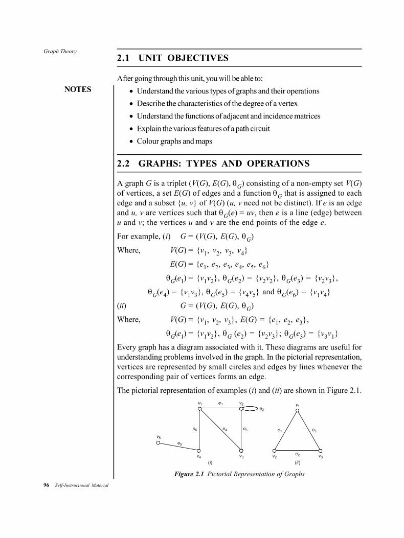
96 Self-Instructional Material
Graph Theory
NOTES
2.1 UNIT OBJECTIVES
After going through this unit, you will be able to:
Understand the various types of graphs and their operations
Describe the characteristics of the degree of a vertex
Understand the functions of adjacent and incidence matrices
Explain the various features of a path circuit
Colour graphs and maps
2.2 GRAPHS: TYPES AND OPERATIONS
A graph G is a triplet (V(G), E(G), G) consisting of a non-empty set V(G)of vertices, a set E(G) of edges and a function G that is assigned to eachedge and a subset {u, v} of V(G) (u, v need not be distinct). If e is an edgeand u, v are vertices such that G(e) = uv, then e is a line (edge) betweenu and v; the vertices u and v are the end points of the edge e.
For example, (i) G = (V(G), E(G), G)
Where, V(G) = {v1, v2, v3, v4}
E(G) = {e1, e2, e3, e4, e5, e6}
G(e1) = {v1v2}, G(e2) = {v2v2}, G(e3) = {v2v3},
G(e4) = {v1v3}, G(e5) = {v4v5} and G(e6) = {v1v4}
(ii) G = (V(G), E(G), G)
Where, V(G) = {v1, v2, v3}, E(G) = {e1, e2, e3},
G(e1) = {v1v2}, G (e2) = {v2v3}; G(e3) = {v3v1}
Every graph has a diagram associated with it. These diagrams are useful forunderstanding problems involved in the graph. In the pictorial representation,vertices are represented by small circles and edges by lines whenever thecorresponding pair of vertices forms an edge.
The pictorial representation of examples (i) and (ii) are shown in Figure 2.1.
v2 v3
e3e1
e2
v1
( )ii
e6 e4 e3
e2
v2e1v1
v4 v3
e5
v5
( )i
Figure 2.1 Pictorial Representation of Graphs
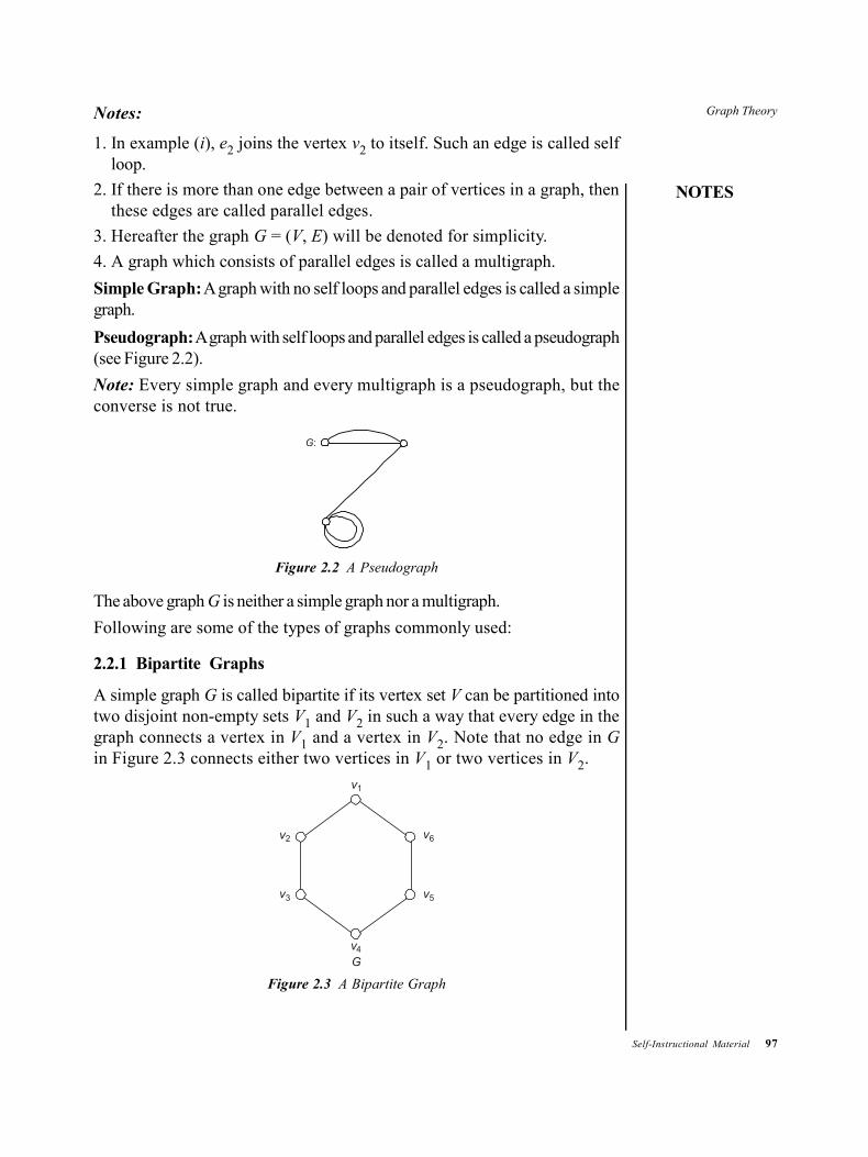
Graph Theory
NOTES
Self-Instructional Material 97
Notes:
1. In example (i), e2 joins the vertex v2 to itself. Such an edge is called selfloop.
2. If there is more than one edge between a pair of vertices in a graph, thenthese edges are called parallel edges.
3. Hereafter the graph G = (V, E) will be denoted for simplicity.
4. A graph which consists of parallel edges is called a multigraph.
Simple Graph: A graph with no self loops and parallel edges is called a simplegraph.
Pseudograph: A graph with self loops and parallel edges is called a pseudograph(see Figure 2.2).
Note: Every simple graph and every multigraph is a pseudograph, but theconverse is not true.
G:
Figure 2.2 A Pseudograph
The above graph G is neither a simple graph nor a multigraph.
Following are some of the types of graphs commonly used:
2.2.1 Bipartite Graphs
A simple graph G is called bipartite if its vertex set V can be partitioned intotwo disjoint non-empty sets V1 and V2 in such a way that every edge in thegraph connects a vertex in V1 and a vertex in V2. Note that no edge in Gin Figure 2.3 connects either two vertices in V1 or two vertices in V2.
v2
v3
v6
v5
v1
v4
G
Figure 2.3 A Bipartite Graph
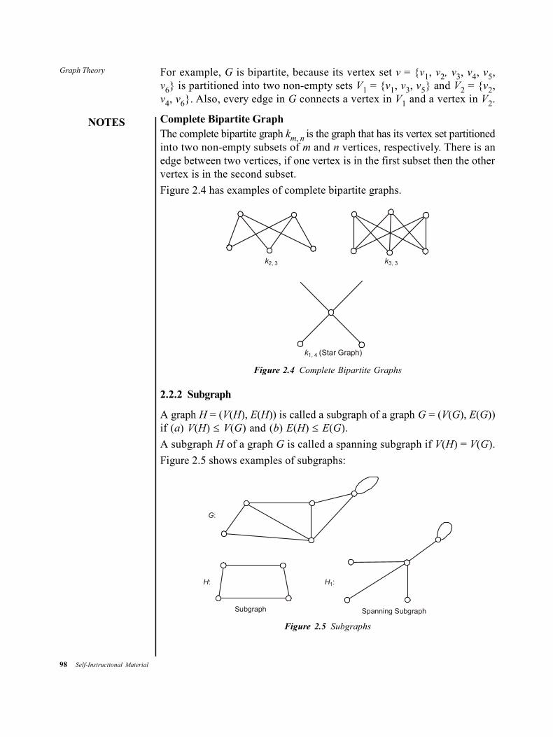
98 Self-Instructional Material
Graph Theory
NOTES
For example, G is bipartite, because its vertex set v = {v1, v2, v3, v4, v5,v6} is partitioned into two non-empty sets V1 = {v1, v3, v5} and V2 = {v2,v4, v6}. Also, every edge in G connects a vertex in V1 and a vertex in V2.
Complete Bipartite GraphThe complete bipartite graph km, n is the graph that has its vertex set partitionedinto two non-empty subsets of m and n vertices, respectively. There is anedge between two vertices, if one vertex is in the first subset then the othervertex is in the second subset.
Figure 2.4 has examples of complete bipartite graphs.
k2, 3 k3, 3
k1, 4 (Star Graph)
Figure 2.4 Complete Bipartite Graphs
2.2.2 Subgraph
A graph H = (V(H), E(H)) is called a subgraph of a graph G = (V(G), E(G))if (a) V(H) V(G) and (b) E(H) E(G).
A subgraph H of a graph G is called a spanning subgraph if V(H) = V(G).
Figure 2.5 shows examples of subgraphs:
G:
H: H1:
Subgraph Spanning Subgraph
Figure 2.5 Subgraphs
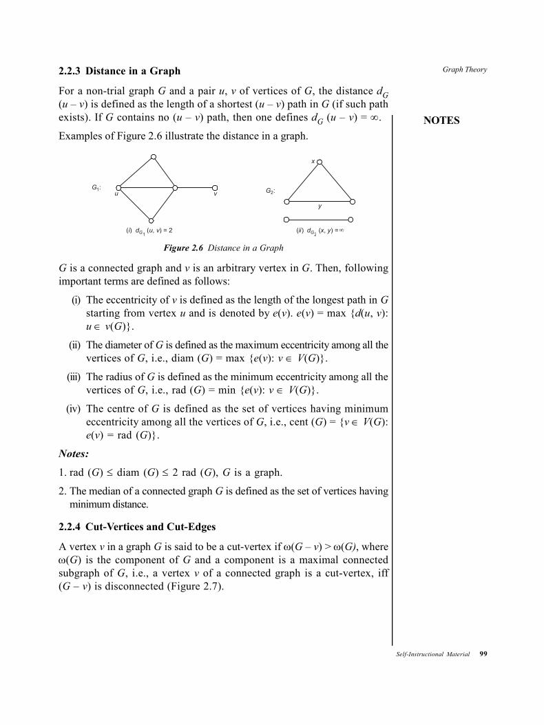
Graph Theory
NOTES
Self-Instructional Material 99
2.2.3 Distance in a Graph
For a non-trial graph G and a pair u, v of vertices of G, the distance dG(u – v) is defined as the length of a shortest (u – v) path in G (if such pathexists). If G contains no (u – v) path, then one defines dG (u – v) = .
Examples of Figure 2.6 illustrate the distance in a graph.
G1:u v
( ) ( , ) = 2i d u vG1
G2:
x
y
( ) ( , ) = ii d x yG2
Figure 2.6 Distance in a Graph
G is a connected graph and v is an arbitrary vertex in G. Then, followingimportant terms are defined as follows:
(i) The eccentricity of v is defined as the length of the longest path in Gstarting from vertex u and is denoted by e(v). e(v) = max {d(u, v):u v(G)}.
(ii) The diameter of G is defined as the maximum eccentricity among all thevertices of G, i.e., diam (G) = max {e(v): v V(G)}.
(iii) The radius of G is defined as the minimum eccentricity among all thevertices of G, i.e., rad (G) = min {e(v): v V(G)}.
(iv) The centre of G is defined as the set of vertices having minimumeccentricity among all the vertices of G, i.e., cent (G) = {v V(G):e(v) = rad (G)}.
Notes:
1. rad (G) diam (G) 2 rad (G), G is a graph.
2. The median of a connected graph G is defined as the set of vertices havingminimum distance.
2.2.4 Cut-Vertices and Cut-Edges
A vertex v in a graph G is said to be a cut-vertex if (G – v) >(G), where(G) is the component of G and a component is a maximal connectedsubgraph of G, i.e., a vertex v of a connected graph is a cut-vertex, iff(G – v) is disconnected (Figure 2.7).

100 Self-Instructional Material
Graph Theory
NOTES
G1:v
G2:
Figure 2.7 Cut-Vertices and Cut-Edges
G1 contains one cut-vertex v and G2 contains no cut-vertices (See Figure2.7).
Theorem 2.1: A vertex v in a connected graph G is a cut-vertex iff verticesu and w exist (both are different from v) in such a way that every pathconnecting u and w contains v.
Proof: Let G be a connected graph and v be a cut-vertex.
Claim: There exist vertices u and w in such a way that every path betweenu and w contains v.
Since v is a cut-vertex, (G – v) is disconnected and (G – v) contains twocomponents say G1 and G2. Let u and w be the vertices of G1 and G2,respectively. Clearly there is no (u – w) path in (G – v). Hence, every pathconnecting u and w must contain v.
Conversely, lets assume that there exist vertices u and w in such a way thatevery (u – w) path contains v.
Claim: v is a cut-vertex.
Suppose v is not a cut-vertex. Then, (G – v) is connected. Since u, w arevertices in G – v, there is a path between u and w in G – v, which does notcontain the vertex v. This is a contradiction. Hence, v is a cut-vertex.
Cut-edge: An edge e in a graph G is said to be a cut-edge, if (G – e) isdisconnected (see Figure 2.8).
For example,
G1:e
G2:
Figure 2.8 G1 containing One Cut-Edge and G
2 with no Cut-edge
As in cut-vertex, a similar result can be furnished.
Theorem 2.2: An edge e in a connected graph G is a cut-edge iff thereexists vertices u and w such that every path connecting u and w must containthe edge ‘e’.
Proof: Let G be a connected graph and e be a cut-edge.
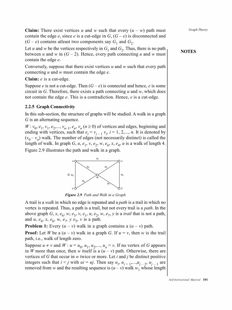
Graph Theory
NOTES
Self-Instructional Material 101
Claim: There exist vertices u and w such that every (u – w) path mustcontain the edge e, since e is a cut-edge in G, (G – e) is disconnected and(G – e) contains atleast two components say G1 and G2.
Let u and w be the vertices respectively in G1 and G2. Thus, there is no pathbetween u and w in (G – 2). Hence, every path connecting u and w mustcontain the edge e.
Conversely, suppose that there exist vertices u and w such that every pathconnecting u and w must contain the edge e.
Claim: e is a cut-edge.
Suppose e is not a cut-edge. Then (G – e) is connected and hence, e is somecircuit in G. Therefore, there exists a path connecting u and w, which doesnot contain the edge e. This is a contradiction. Hence, e is a cut-edge.
2.2.5 Graph Connectivity
In this sub-section, the structure of graphs will be studied. A walk in a graphG is an alternating sequence.
W : v0, e1, v1, e2,..., vn–1, en, vn (n 0) of vertices and edges, beginning andending with vertices, such that ei = vi – 1 vi, i = 1, 2,..., n. It is denoted by(v0 – vn) walk. The number of edges (not necessarily distinct) is called thelength of walk. In graph G, u, e1, v, e2, w, e6, x, e4, u is a walk of length 4.
Figure 2.9 illustrates the path and walk in a graph.
G e: 4
x
u v
y
we6
e7
e5
e3e2
e1
Figure 2.9 Path and Walk in a Graph
A trail is a walk in which no edge is repeated and a path is a trail in which novertex is repeated. Thus, a path is a trail, but not every trail is a path. In theabove graph G, x, e6, w, e3, v, e1, u, e2, w, e7, y is a trail that is not a path,and u, e4, x, e6, w, e7, y e5, v is a path.
Problem 1: Every (u – v) walk in a graph contains a (u – v) path.
Proof: Let W be a (u – v) walk in a graph G. If u = v, then w is the trailpath, i.e., walk of length zero.
Suppose u v and W : u = u0, u1, u2,..., un = v. If no vertex of G appearsin W more than once, then w itself is a (u – v) path. Otherwise, there arevertices of G that occur in w twice or more. Let i and j be distinct positiveintegers such that i < j with ui = uj. Then say ui, ui + 1,...,uj – 2, uj – 1 areremoved from w and the resulting sequence is (u – v) walk w1 whose length

102 Self-Instructional Material
Graph Theory
NOTES
is less than that of w. By induction hypothesis, this w1 contains a (u – v) pathand hence w has a (u – v) path. If no vertex of G appears more than oncein w1, then w1 is a (u – v) path. If not, apply the procedure, until you geta (u – v) path.
Cycle: A cycle is a walk. v0, v1,..., vn is a walk in which n 3, v0 = vn andthe ‘n’-vertices v1, v2,..., vn are distinct. It is said that a (u – v) walk isclosed if u = v and open if u v.
Connection: Let u and v be vertices in a graph G. You say that u is connectedto v if G contains a (u – v) path. The graph G is connected, if u is connectedto v for every pair and u, v are vertices of G.
Disconnection: A graph G is disconnected, if there exists two vertices u andv for which there is no (u – v) path.
Component: A subgraph H of a graph G is called a component of G, if His a maximal connected subgraph of G and component is denoted by (G).
Note: If (G) > 1, then G is disconnected (see Figure 2.10)
( )i ( )ii
Figure 2.10 Connected and Disconnected Graph
Graph (i) is connected and (ii) is disconnected.
Note that graph (ii) has 3 components.
Connectedness in a Directed Graph
Strongly Connected: A directed graph is strongly connected if there is apath from u to v and v to u, whenever u and v are vertices in the graph.
Weakly Connected: A directed graph is weakly connected, if there is apath between any two vertices in the underlying undirected graph.
Unilaterally Connected: A directed graph is said to be unilaterallyconnected, if in the two vertices u and v, there exists a directed path eitherfrom u to v or from v to u. (see Figure 2.11)
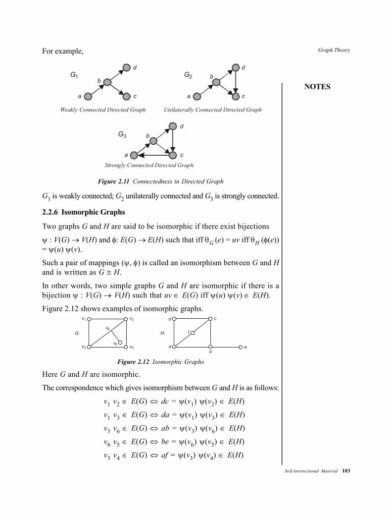
Graph Theory
NOTES
Self-Instructional Material 103
For example,
G1
a
b
d
c a
b
d
c
Weakly Connected Directed Graph Unilaterally Connected Directed Graph
Strongly Connected Directed Graph
a
b
d
c
G2
G3
Figure 2.11 Connectedness in Directed Graph
G1 is weakly connected; G2 unilaterally connected and G3 is strongly connected.
2.2.6 Isomorphic Graphs
Two graphs G and H are said to be isomorphic if there exist bijections
: V(G) V(H) and : E(G) E(H) such that iff G (e) = uv iff H ((e))= (u) (v).
Such a pair of mappings (, ) is called an isomorphism between G and Hand is written as G H.
In other words, two simple graphs G and H are isomorphic if there is abijection : V(G) V(H) such that uv E(G) iff (u) (v) E(H).
Figure 2.12 shows examples of isomorphic graphs.
G:
v3
v1 v2
v4v5
v6
a
H:
d c
b
f
e
Figure 2.12 Isomorphic Graphs
Here G and H are isomorphic.
The correspondence which gives isomorphism between G and H is as follows:
v1 v2 E(G) dc = (v1) (v2) E(H)
v1 v3 E(G) da = (v1) (v3) E(H)
v3 v6 E(G) ab = (v3) (v6) E(H)
v6 v5 E(G) be = (v6) (v5) E(H)
v3 v4 E(G) af = (v3) (v4) E(H)
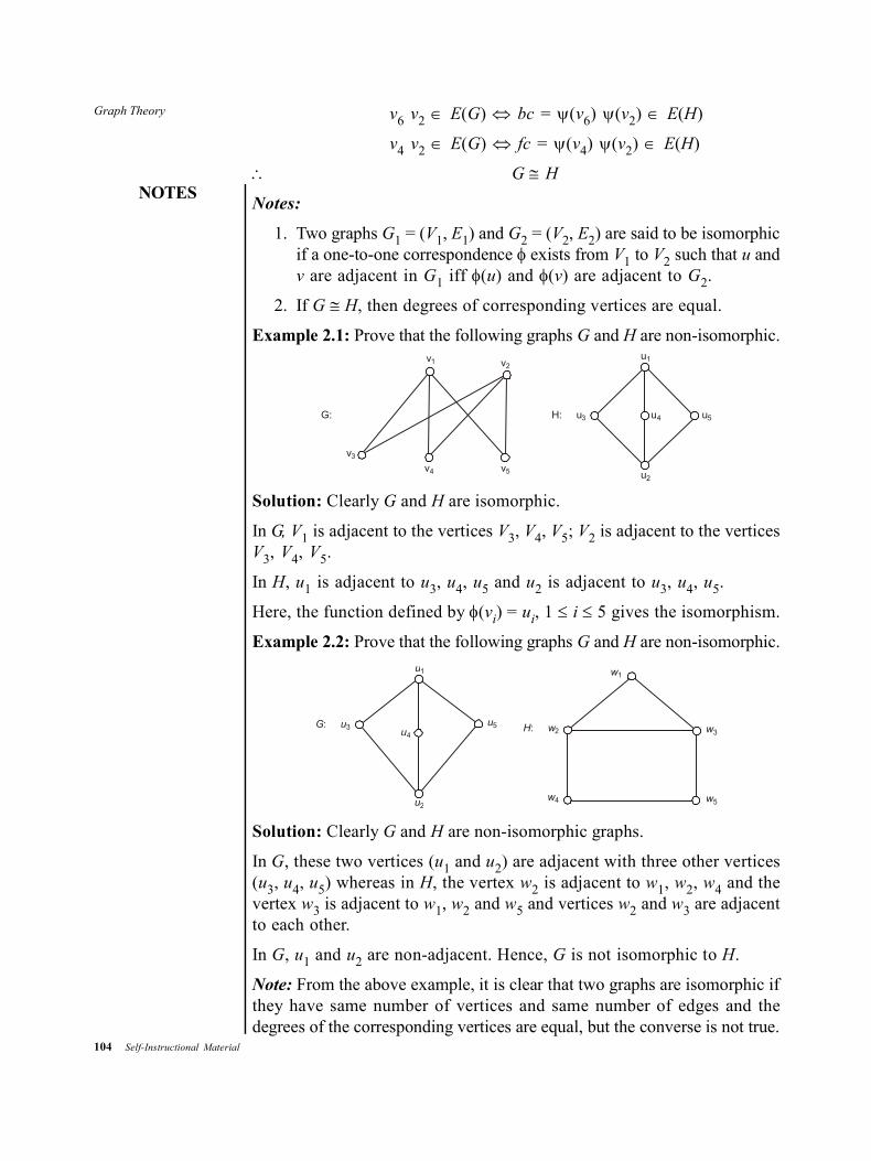
104 Self-Instructional Material
Graph Theory
NOTES
v6 v2 E(G) bc = (v6) (v2) E(H)
v4 v2 E(G) fc = (v4) (v2) E(H)
G H
Notes:
1. Two graphs G1 = (V1, E1) and G2 = (V2, E2) are said to be isomorphicif a one-to-one correspondence exists from V1 to V2 such that u andv are adjacent in G1 iff (u) and (v) are adjacent to G2.
2. If G H, then degrees of corresponding vertices are equal.
Example 2.1: Prove that the following graphs G and H are non-isomorphic.
G:
v3
v4 v5
v2v1
H: u3 u4 u5
u1
u2
Solution: Clearly G and H are isomorphic.
In G, V1 is adjacent to the vertices V3, V4, V5; V2 is adjacent to the verticesV3, V4, V5.
In H, u1 is adjacent to u3, u4, u5 and u2 is adjacent to u3, u4, u5.
Here, the function defined by (vi) = ui, 1 i 5 gives the isomorphism.
Example 2.2: Prove that the following graphs G and H are non-isomorphic.
G u: 3 u5u4
u2
u1 w1
H w: 2
w4
w3
w5
Solution: Clearly G and H are non-isomorphic graphs.
In G, these two vertices (u1 and u2) are adjacent with three other vertices(u3, u4, u5) whereas in H, the vertex w2 is adjacent to w1, w2, w4 and thevertex w3 is adjacent to w1, w2 and w5 and vertices w2 and w3 are adjacentto each other.
In G, u1 and u2 are non-adjacent. Hence, G is not isomorphic to H.
Note: From the above example, it is clear that two graphs are isomorphic ifthey have same number of vertices and same number of edges and thedegrees of the corresponding vertices are equal, but the converse is not true.
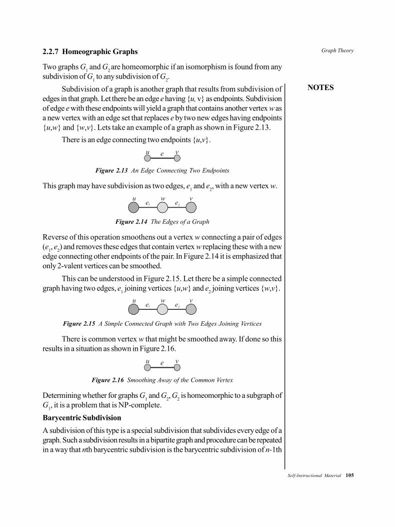
Graph Theory
NOTES
Self-Instructional Material 105
2.2.7 Homeographic Graphs
Two graphs G1 and G
2 are homeomorphic if an isomorphism is found from any
subdivision of G1 to any subdivision of G
2.
Subdivision of a graph is another graph that results from subdivision ofedges in that graph. Let there be an edge e having {u, v} as endpoints. Subdivisionof edge e with these endpoints will yield a graph that contains another vertex w asa new vertex with an edge set that replaces e by two new edges having endpoints{u,w} and {w,v}. Lets take an example of a graph as shown in Figure 2.13.
There is an edge connecting two endpoints {u,v}.
u e v
Figure 2.13 An Edge Connecting Two Endpoints
This graph may have subdivision as two edges, e1 and e
2, with a new vertex w.
u w ve1 e2
Figure 2.14 The Edges of a Graph
Reverse of this operation smoothens out a vertex w connecting a pair of edges(e
1, e
2) and removes these edges that contain vertex w replacing these with a new
edge connecting other endpoints of the pair. In Figure 2.14 it is emphasized thatonly 2-valent vertices can be smoothed.
This can be understood in Figure 2.15. Let there be a simple connectedgraph having two edges, e
1 joining vertices {u,w} and e
2 joining vertices {w,v}.
u w ve1 e2
Figure 2.15 A Simple Connected Graph with Two Edges Joining Vertices
There is common vertex w that might be smoothed away. If done so thisresults in a situation as shown in Figure 2.16.
u e v
Figure 2.16 Smoothing Away of the Common Vertex
Determining whether for graphs G1 and G
2, G
2 is homeomorphic to a subgraph of
G1, it is a problem that is NP-complete.
Barycentric Subdivision
A subdivision of this type is a special subdivision that subdivides every edge of agraph. Such a subdivision results in a bipartite graph and procedure can be repeatedin a way that nth barycentric subdivision is the barycentric subdivision of n-1th
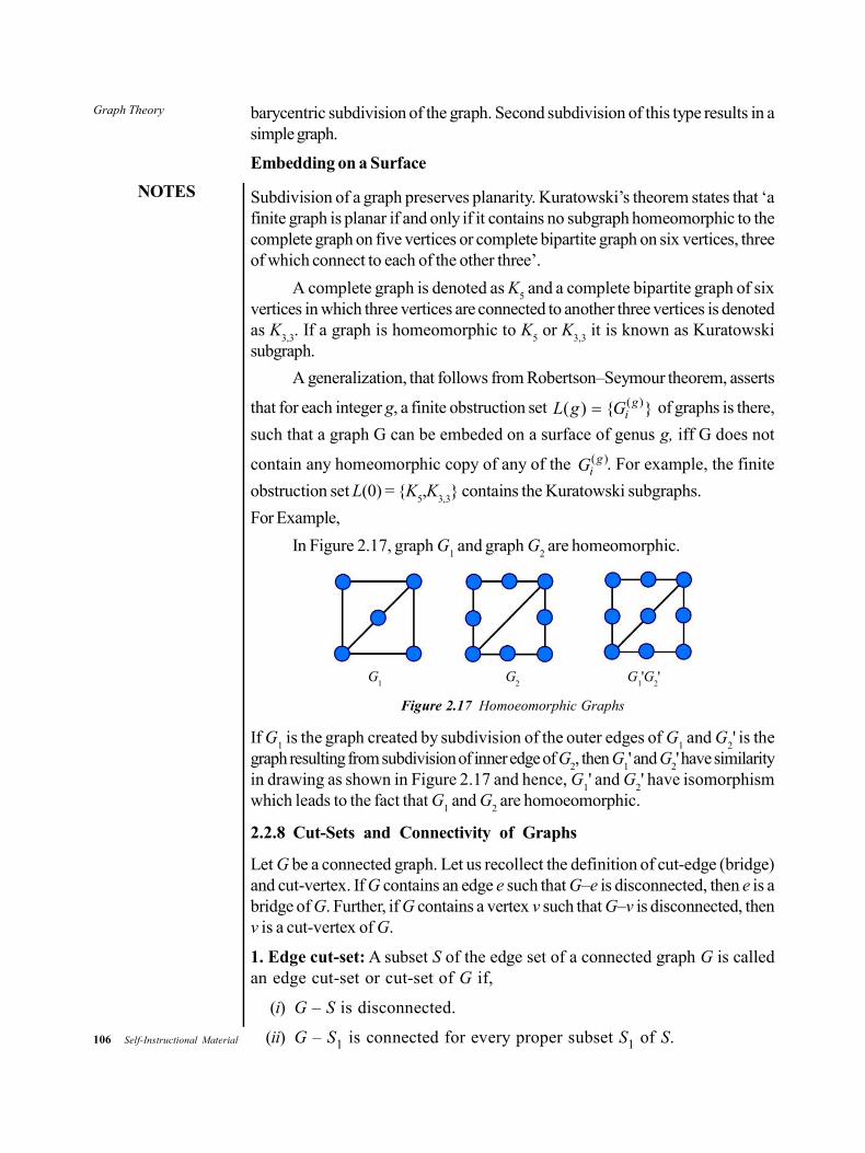
106 Self-Instructional Material
Graph Theory
NOTES
barycentric subdivision of the graph. Second subdivision of this type results in asimple graph.
Embedding on a Surface
Subdivision of a graph preserves planarity. Kuratowski’s theorem states that ‘afinite graph is planar if and only if it contains no subgraph homeomorphic to thecomplete graph on five vertices or complete bipartite graph on six vertices, threeof which connect to each of the other three’.
A complete graph is denoted as K5 and a complete bipartite graph of six
vertices in which three vertices are connected to another three vertices is denotedas K
3,3. If a graph is homeomorphic to K
5 or K
3,3 it is known as Kuratowski
subgraph.
A generalization, that follows from Robertson–Seymour theorem, asserts
that for each integer g, a finite obstruction set ( )( ) { }giL g G of graphs is there,
such that a graph G can be embeded on a surface of genus g, iff G does not
contain any homeomorphic copy of any of the ( )giG . For example, the finite
obstruction set L(0) = {K5,K
3,3} contains the Kuratowski subgraphs.
For Example,
In Figure 2.17, graph G1 and graph G
2 are homeomorphic.
G1
G2
G1'G
2'
Figure 2.17 Homoeomorphic Graphs
If G1 is the graph created by subdivision of the outer edges of G
1 and G
2' is the
graph resulting from subdivision of inner edge of G2, then G
1' and G
2' have similarity
in drawing as shown in Figure 2.17 and hence, G1' and G
2' have isomorphism
which leads to the fact that G1 and G
2 are homoeomorphic.
2.2.8 Cut-Sets and Connectivity of Graphs
Let G be a connected graph. Let us recollect the definition of cut-edge (bridge)and cut-vertex. If G contains an edge e such that G–e is disconnected, then e is abridge of G. Further, if G contains a vertex v such that G–v is disconnected, thenv is a cut-vertex of G.
1. Edge cut-set: A subset S of the edge set of a connected graph G is calledan edge cut-set or cut-set of G if,
(i) G – S is disconnected.
(ii) G – S1 is connected for every proper subset S1 of S.
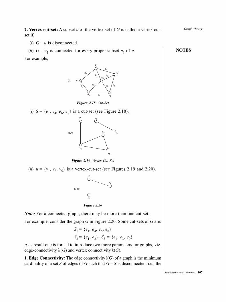
Graph Theory
NOTES
Self-Instructional Material 107
2. Vertex cut-set: A subset u of the vertex set of G is called a vertex cut-set if,
(i) G – u is disconnected.
(ii) G – u1 is connected for every proper subset u1 of u.
For example,
v1
e2
v6 v5
v4
v2
v3
e1
e5
e6e4
e3 e7e8
e9
G:
Figure 2.18 Cut-Set
(i) S = {e1, e4, e6, e8} is a cut-set (see Figure 2.18).
v6
v5
v3
v1 v2
v4G-S:
Figure 2.19 Vertex Cut-Set
(ii) u = {v1, v3, v5} is a vertex-cut-set (see Figures 2.19 and 2.20).
v6
v5
v6
G-U:
Figure 2.20
Note: For a connected graph, there may be more than one cut-set.
For example, consider the graph G in Figure 2.20. Some cut-sets of G are:
S1 = {e1, e4, e6, e8}
S2 = {e1, e2}, S3 = {e1, e3, e9}
As s result one is forced to introduce two more parameters for graphs, viz.edge-connectivity (G) and vertex connectivity k(G).
1. Edge Connectivity: The edge connectivity l(G) of a graph is the minimumcardinality of a set S of edges of G such that G – S is disconnected, i.e., the
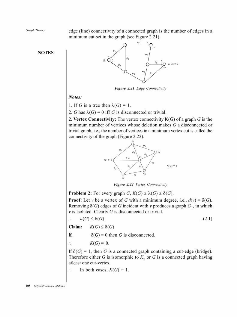
108 Self-Instructional Material
Graph Theory
NOTES
edge (line) connectivity of a connected graph is the number of edges in aminimum cut-set in the graph (see Figure 2.21).
G:
e3
e3
e6
e8
e7e5e4
e1
e2
λ( ) = 2G
Figure 2.21 Edge Connectivity
Notes:
1. If G is a tree then (G) = 1.
2. G has (G) = 0 iff G is disconnected or trivial.
2. Vertex Connectivity: The vertex connectivity K(G) of a graph G is theminimum number of vertices whose deletion makes G a disconnected ortrivial graph, i.e., the number of vertices in a minimum vertex cut is called theconnectivity of the graph (Figure 2.22).
G: v1
e2
v6
e9v5
e8
v4
v2
e5
e6v3
e4
e10
e1
e3 e7K G( ) = 3
Figure 2.22 Vertex Connectivity
Problem 2: For every graph G, K(G) (G) (G).
Proof: Let v be a vertex of G with a minimum degree, i.e., d(v) = (G).Removing (G) edges of G incident with v produces a graph G1, in whichv is isolated. Clearly G is disconnected or trivial.
(G) (G) ...(2.1)
Claim: K(G) (G)
If, (G) = 0 then G is disconnected.
K(G) = 0.
If (G) = 1, then G is a connected graph containing a cut-edge (bridge).Therefore either G is isomorphic to K2 or G is a connected graph havingatleast one cut-vertex.
In both cases, K(G) = 1.
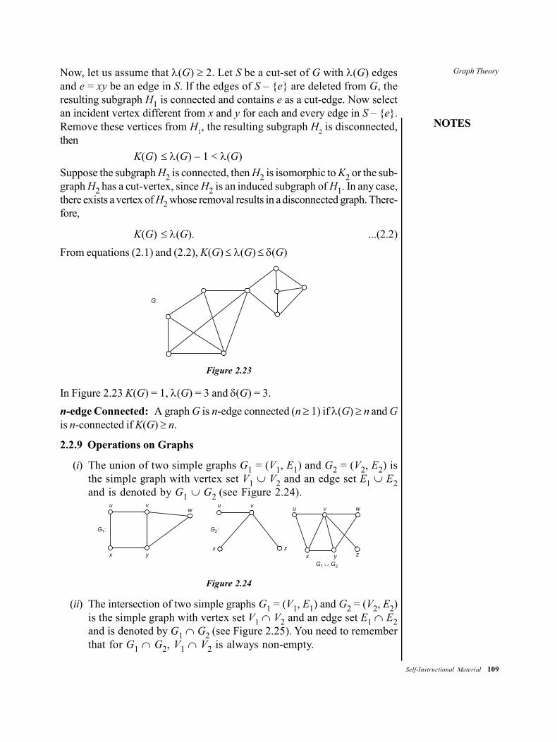
Graph Theory
NOTES
Self-Instructional Material 109
Now, let us assume that (G) 2. Let S be a cut-set of G with (G) edgesand e = xy be an edge in S. If the edges of S – {e} are deleted from G, theresulting subgraph H1 is connected and contains e as a cut-edge. Now selectan incident vertex different from x and y for each and every edge in S – {e}.Remove these vertices from H
1, the resulting subgraph H
2 is disconnected,
then
K(G) (G) – 1 < (G)
Suppose the subgraph H2 is connected, then H2 is isomorphic to K2 or the sub-graph H2 has a cut-vertex, since H2 is an induced subgraph of H1. In any case,there exists a vertex of H2 whose removal results in a disconnected graph. There-fore,
K(G) (G). ...(2.2)
From equations (2.1) and (2.2), K(G) (G) (G)
G:
Figure 2.23
In Figure 2.23 K(G) = 1, (G) = 3 and (G) = 3.
n-edge Connected: A graph G is n-edge connected (n 1) if (G) n and Gis n-connected if K(G) n.
2.2.9 Operations on Graphs
(i) The union of two simple graphs G1 = (V1, E1) and G2 = (V2, E2) isthe simple graph with vertex set V1 V2 and an edge set E1 E2and is denoted by G1 G2 (see Figure 2.24).
G1:
x y
vuw
G2:
u v
x z
G1 G2
x y z
wvu
Figure 2.24
(ii) The intersection of two simple graphs G1 = (V1, E1) and G2 = (V2, E2)is the simple graph with vertex set V1 V2 and an edge set E1 E2and is denoted by G1 G2 (see Figure 2.25). You need to rememberthat for G1 G2, V1 V2 is always non-empty.
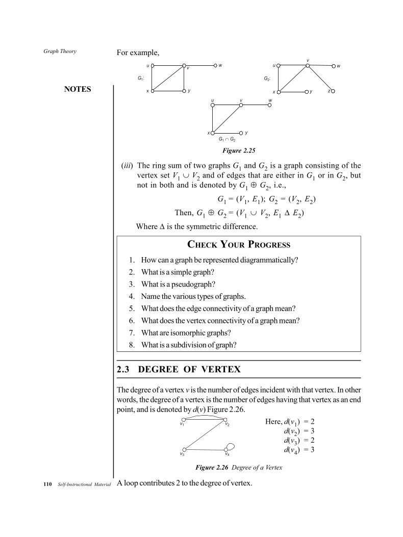
110 Self-Instructional Material
Graph Theory
NOTES
For example,
G1:
u
x y
v w
G2:
u
x y z
wv
x
u v w
yG1 G2
Figure 2.25
(iii) The ring sum of two graphs G1 and G2 is a graph consisting of thevertex set V1 V2 and of edges that are either in G1 or in G2, butnot in both and is denoted by G1 G2, i.e.,
G1 = (V1, E1); G2 = (V2, E2)
Then, G1 G2 = (V1 V2, E1 E2)
Where is the symmetric difference.
CHECK YOUR PROGRESS
1. How can a graph be represented diagrammatically?
2. What is a simple graph?
3. What is a pseudograph?
4. Name the various types of graphs.
5. What does the edge connectivity of a graph mean?
6. What does the vertex connectivity of a graph mean?
7. What are isomorphic graphs?
8. What is a subdivision of graph?
2.3 DEGREE OF VERTEX
The degree of a vertex v is the number of edges incident with that vertex. In otherwords, the degree of a vertex is the number of edges having that vertex as an endpoint, and is denoted by d(v) Figure 2.26.
v1 v2
v3 v4
Here, d(v1) = 2d(v2) = 3d(v3) = 2d(v4) = 3
Figure 2.26 Degree of a Vertex
A loop contributes 2 to the degree of vertex.
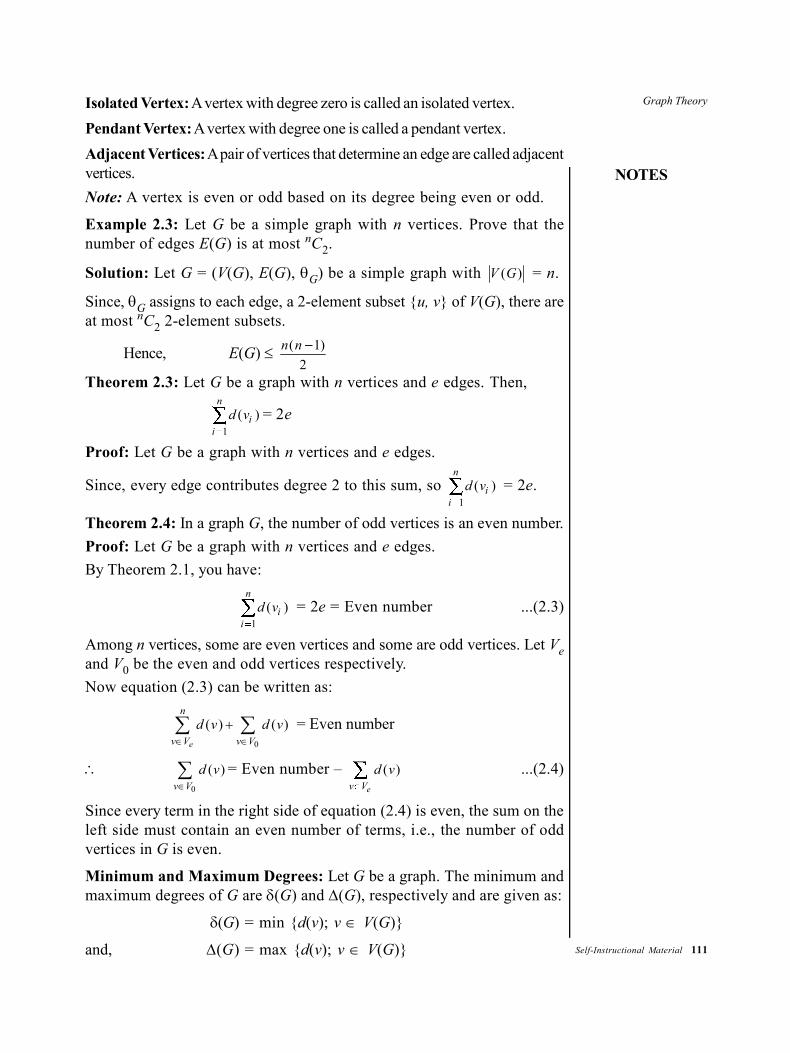
Graph Theory
NOTES
Self-Instructional Material 111
Isolated Vertex: A vertex with degree zero is called an isolated vertex.
Pendant Vertex: A vertex with degree one is called a pendant vertex.
Adjacent Vertices: A pair of vertices that determine an edge are called adjacentvertices.
Note: A vertex is even or odd based on its degree being even or odd.
Example 2.3: Let G be a simple graph with n vertices. Prove that thenumber of edges E(G) is at most nC2.
Solution: Let G = (V(G), E(G), G) be a simple graph with ( )V G = n.
Since, G assigns to each edge, a 2-element subset {u, v} of V(G), there areat most nC2 2-element subsets.
Hence, E(G) ( 1)
2
n n
Theorem 2.3: Let G be a graph with n vertices and e edges. Then,
1
( )n
ii
d v = 2e
Proof: Let G be a graph with n vertices and e edges.
Since, every edge contributes degree 2 to this sum, so 1
( )n
ii
d v = 2e.
Theorem 2.4: In a graph G, the number of odd vertices is an even number.
Proof: Let G be a graph with n vertices and e edges.
By Theorem 2.1, you have:
1
( )n
ii
d v = 2e = Even number ...(2.3)
Among n vertices, some are even vertices and some are odd vertices. Let Veand V0 be the even and odd vertices respectively.
Now equation (2.3) can be written as:
0
( ) ( )
e
n
v V v V
d v d v = Even number
0
( )
v V
d v = Even number – ( )ev V
d v ...(2.4)
Since every term in the right side of equation (2.4) is even, the sum on theleft side must contain an even number of terms, i.e., the number of oddvertices in G is even.
Minimum and Maximum Degrees: Let G be a graph. The minimum andmaximum degrees of G are (G) and (G), respectively and are given as:
(G) = min {d(v); v V(G)}
and, (G) = max {d(v); v V(G)}
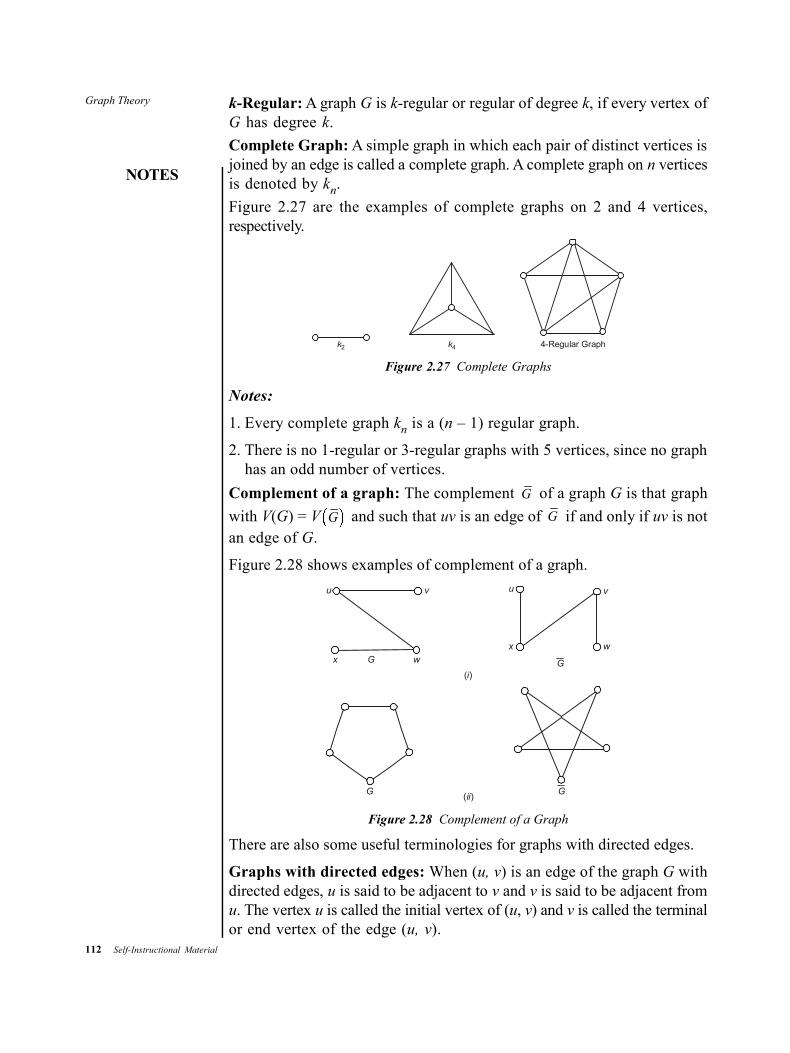
112 Self-Instructional Material
Graph Theory
NOTES
k-Regular: A graph G is k-regular or regular of degree k, if every vertex ofG has degree k.
Complete Graph: A simple graph in which each pair of distinct vertices isjoined by an edge is called a complete graph. A complete graph on n verticesis denoted by kn.
Figure 2.27 are the examples of complete graphs on 2 and 4 vertices,respectively.
k2 k4 4-Regular Graph
Figure 2.27 Complete Graphs
Notes:
1. Every complete graph kn is a (n – 1) regular graph.
2. There is no 1-regular or 3-regular graphs with 5 vertices, since no graphhas an odd number of vertices.
Complement of a graph: The complement G of a graph G is that graph
with V(G) = V G and such that uv is an edge of G if and only if uv is notan edge of G.
Figure 2.28 shows examples of complement of a graph.
u v
wx
x
u v
w
G( )i
G
( )iiGG
Figure 2.28 Complement of a Graph
There are also some useful terminologies for graphs with directed edges.
Graphs with directed edges: When (u, v) is an edge of the graph G withdirected edges, u is said to be adjacent to v and v is said to be adjacent fromu. The vertex u is called the initial vertex of (u, v) and v is called the terminalor end vertex of the edge (u, v).
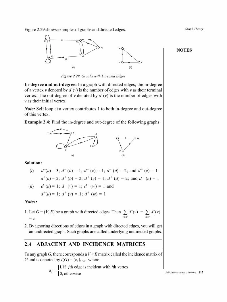
Graph Theory
NOTES
Self-Instructional Material 113
Figure 2.29 shows examples of graphs and directed edges.
u
w
vG
v3
v5
v4
v2
v1
( )i ( )ii
Figure 2.29 Graphs with Directed Edges
In-degree and out-degree: In a graph with directed edges, the in-degreeof a vertex v denoted by d–(v) is the number of edges with v as their terminalvertex. The out-degree of v denoted by d+(v) is the number of edges withv as their initial vertex.
Note: Self loop at a vertex contributes 1 to both in-degree and out-degreeof this vertex.
Example 2.4: Find the in-degree and out-degree of the following graphs.
c b
a
d
e
( )i
u w
v
( )ii
Solution:
(i) d –(a) = 3; d – (b) = 1; d – (c) = 1; d– (d) = 2; and d – (e) = 1
d +(a) = 2; d + (b) = 2; d + (c) = 1; d + (d) = 2; and d + (e) = 1
(ii) d –(u) = 1; d – (v) = 1; d – (w) = 1 and
d +(u) = 1; d + (v) = 1; d + (w) = 1
Notes:
1. Let G = (V, E) be a graph with directed edges. Then ( )
v V
d v = ( )
v V
d v
= e.
2. By ignoring directions of edges in a graph with directed edges, you will getan undirected graph. Such graphs are called underlying undirected graphs.
2.4 ADJACENT AND INCIDENCE MATRICES
To any graph G, there corresponds a V × E matrix called the incidence matrix ofG and is denoted by I(G) = ,][ EVija where
1, if th edge is incident with th vertex
0, otherwiseij
j ia
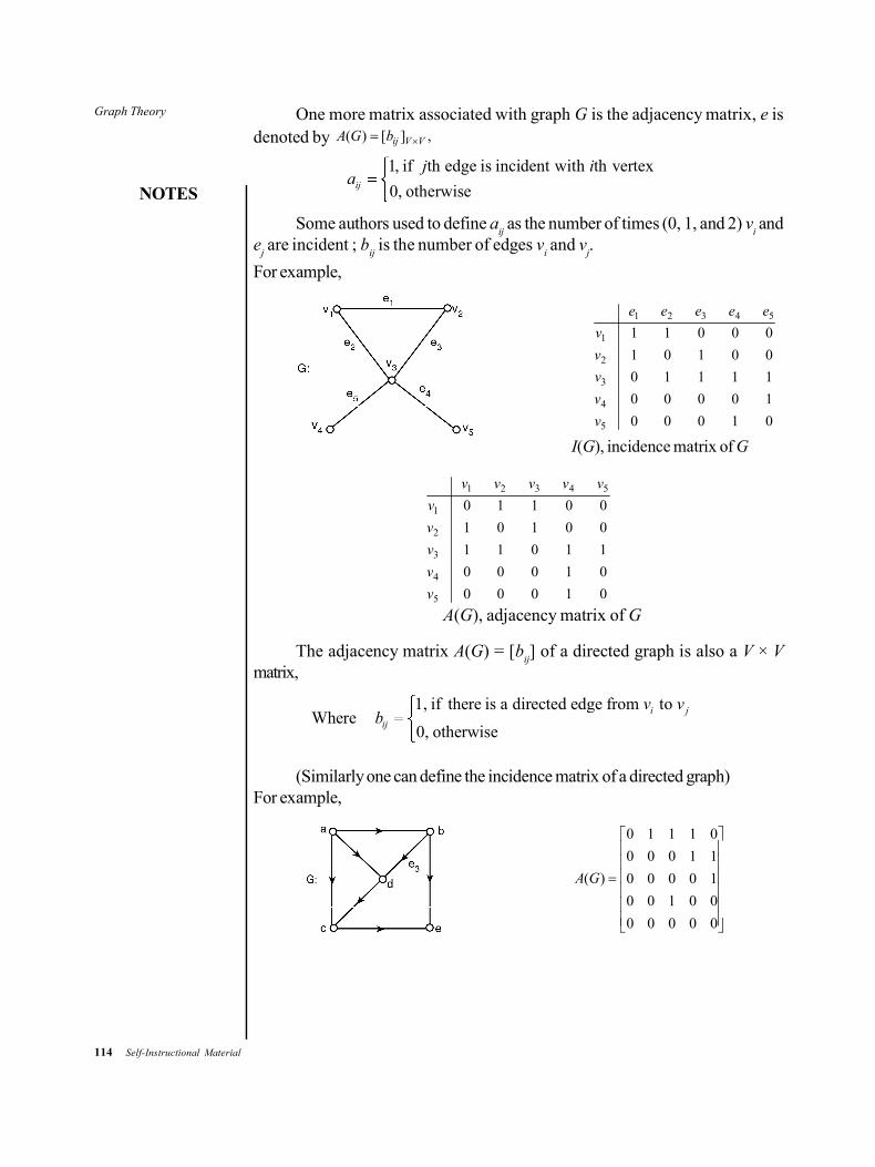
114 Self-Instructional Material
Graph Theory
NOTES
One more matrix associated with graph G is the adjacency matrix, e isdenoted by ,][)( VVijbGA
1, if th edge is incident with th vertex
0, otherwiseij
j ia
Some authors used to define aij as the number of times (0, 1, and 2) v
i and
ej are incident ; b
ij is the number of edges v
i and v
j.
For example,
01000
10000
11110
00101
00011
5
4
3
2
1
54321
v
v
v
v
v
eeeee
I(G), incidence matrix of G
01000
01000
11011
00101
00110
5
4
3
2
1
54321
v
v
v
v
v
vvvvv
A(G), adjacency matrix of G
The adjacency matrix A(G) = [bij] of a directed graph is also a V × V
matrix,
1, if there is a directed edge from toWhere
0, otherwise
i j
ij
v vb
(Similarly one can define the incidence matrix of a directed graph)For example,
0 1 1 1 0
0 0 0 1 1
( ) 0 0 0 0 1
0 0 1 0 0
0 0 0 0 0
A G
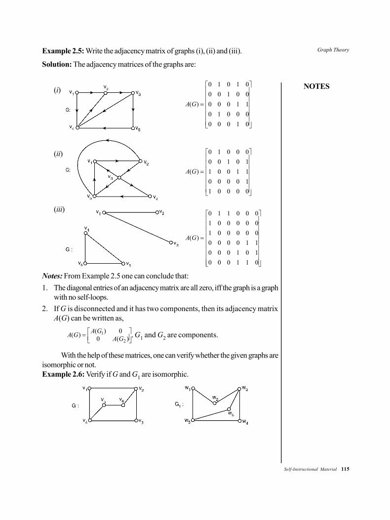
Graph Theory
NOTES
Self-Instructional Material 115
Example 2.5: Write the adjacency matrix of graphs (i), (ii) and (iii).
Solution: The adjacency matrices of the graphs are:
(i)0 1 0 1 0
0 0 1 0 0
( ) 0 0 0 1 1
0 1 0 0 0
0 0 0 1 0
A G
(ii)
00001
10000
11001
10100
00010
)(GA
(iii)
011000
101000
110000
000001
000001
000110
)(GA
Notes: From Example 2.5 one can conclude that:
1. The diagonal entries of an adjacency matrix are all zero, iff the graph is a graphwith no self-loops.
2. If G is disconnected and it has two components, then its adjacency matrixA(G) can be written as,
,)(0
0)()(
2
1
GAGA
GA G1 and G2 are components.
With the help of these matrices, one can verify whether the given graphs areisomorphic or not.Example 2.6: Verify if G and G1 are isomorphic.
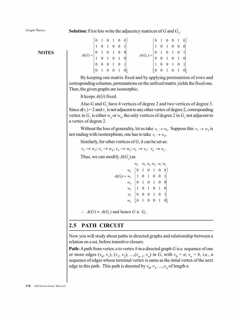
116 Self-Instructional Material
Graph Theory
NOTES
Solution: First lets write the adjacency matrices of G and G1.
010010
101000
010101
001010
100101
001010
)(GA
010100
101001
010100
101010
000101
010010
)( 1GA
By keeping one matrix fixed and by applying permutation of rows andcorresponding columns, permutations on the unfixed matrix yields the fixed one.Then, the given graphs are isomorphic.
It keeps A(G) fixed.
Also G and G1 have 4 vertices of degree 2 and two vertices of degree 3.
Since d(v1) = 2 and v
1 is not adjacent to any other vertex of degree 2, corresponding
vertex in G1 is either w
4 or w
6, the only vertices of degree 2 in G
1 not adjacent to
a vertex of degree 2.
Without the loss of generality, let us take .61 wv Suppose this 61 wv isnot ending with isomorphism, one has to take 41 wv .
Similarly, for other vertices of G, it can be set as:
2 3 3 4 4 5 5 1; ; ; ;v w v w v w v v 6 2v v .
Thus, we can modify A(G1) as
6 3 4 5 1 2
6
1 3
4
5
1
2
0 1 0 1 0 0
( ) 1 0 1 0 0 1
0 1 0 1 0 0
1 0 1 0 1 0
0 0 0 1 0 1
0 1 0 0 1 0
w w w w w w
w
A G w
w
w
w
w
1 1( ) ( ) and hence .A G A G G G
2.5 PATH CIRCUIT
Now you will study about paths in directed graphs and relationship between arelation on a set, before transitive closure.
Path: A path from vertex a to vertex b in a directed graph G is a sequence of oneor more edges (v0, v1), (v1, v2), ...,(vn–1, vn) in G, with v0 = a; vn = b, i.e., asequence of edges whose terminal vertex is same as the intial vertex of the nextedge in this path. This path is denoted by v0, v1, ...,vn of length n.
Graph Theory
NOTES
Self-Instructional Material 117
Let R be a relation on a set A = {1, 2,..,n} and GR be the correspondingrelation graph whose vertices are a = 1, v1 = 2, ...,b = n. There is a path in GRfrom a to b if there is a sequence of vertices a, v1, v2,..., vn–1, b with (a, v1)R,(v1, v2)R, (v2, v3)R,..., (vn–1, b)R.
Problem 3: Let R be a relation on a set A. Then,
(i) R2 = R R, Rn = Rn–1 R(ii) Rn R(iii) In GR, the relational graph of R, there is a path of length n from a to b if
(a,b)Rn.
Connectivity Relation: Let R be a relation on set A. The connectivity relation R*
consists of the pairs (a,b) such that there is a path between a and b in R.
i.e., n
nRR
1
Problem 4: The transitive closure of a relation R equals the connectivity relationR*.
Let R be a relation on a set A.
Claim: R* is the transitive closure of R. To prove that,
(i) R* is transitive.(ii) S is a transitive relation on A with R S. Then R* S.
By definition, i
iRR
1
R* contains R.
(i) If (a,b)R* and (b,c)R*, then there are paths from a to b and from b toc in R. Thus, a path is obtained from a to c by starting with the path a to band following it with the path b to c.
(b,c)R*.
i.e., R* is transitive.
(ii) Let S be a transitive relation containing R.
Since, S is transitive, S* is also transitive.
Further S* S. Since, 1
i
iS S
and Si S, S* S.
Since, any path in R is also a path in S, R* S*, if R S.
Now one gets, R* S* and S* S.
R* S*
i.e., any transitive relation that contains R must also contain R*.
R* is the transitive closure of R.
Transitive Closure: Let MR be the relation matrix of a relation R on the set A ofn elements. Then the transitive closure matrix MR* is given by,
* 2 3 ...R R nR R RM M M M M
118 Self-Instructional Material
Graph Theory
NOTES
Example 2.7:
(i) Find the transitive closure of a relation R on the set {a,b,c}, whose relationmatrix M
R is given as
0 0 1
1 1 0
1 0 1RM
Solution: Let R* be the transitive closure of R. The relation matrix MR* of R* isgiven as,
MR* = MR 2RM
3RM
Now
2 3
1 0 1 1 1 1
1 1 1 ; 1 1 1
1 1 1 1 1 1
0 0 1 1 0 1 1 1 1 1 1 1
1 1 0 1 1 1 1 1 1 1 1 1
1 0 1 1 1 1 1 1 1 1 1 1
R R
R
M M
M
(ii) Find the transitive closure matrix of the relation R whose relation matrix isgiven as
011
010
101
RM
Solution: Let R* be the transitive closure of R and MR* be the correspondingrelation matrix.
we have MR* = MR MR2 MR
3
2 3
1 1 1 1 1 1
Now 0 1 0 ; 0 1 0
1 1 1 1 1 1
1 0 1 1 1 1 1 1 1 1 1 1
0 1 0 0 1 0 0 1 0 0 1 0
1 1 0 1 1 1 1 1 1 1 1 1
R R
R
M M
M
Note: The transitive closure can be obtained by the following algorithm.
Transitive closure (MR; 0 –1 nn matrix)
A MR
B A
for i 2 to n
begin
A A × MR
M
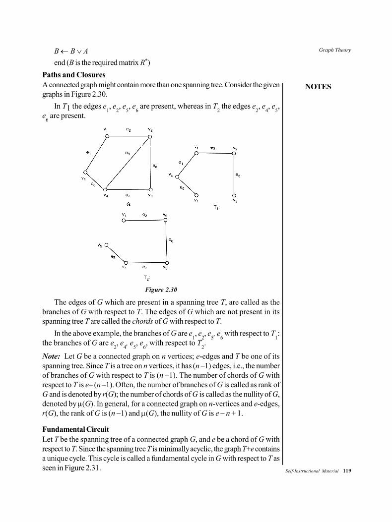
Graph Theory
NOTES
Self-Instructional Material 119
B B Aend (B is the required matrix R*)
Paths and ClosuresA connected graph might contain more than one spanning tree. Consider the givengraphs in Figure 2.30.
In T1 the edges e1, e
2, e
5, e
6 are present, whereas in T
2 the edges e
2, e
4, e
5,
e6 are present.
Figure 2.30
The edges of G which are present in a spanning tree T, are called as thebranches of G with respect to T. The edges of G which are not present in itsspanning tree T are called the chords of G with respect to T.
In the above example, the branches of G are e1, e
2, e
5, e
6 with respect to T
1:
the branches of G are e2, e
4, e
5, e
6, with respect to T
2.
Note: Let G be a connected graph on n vertices; e-edges and T be one of itsspanning tree. Since T is a tree on n vertices, it has (n –1) edges, i.e., the numberof branches of G with respect to T is (n –1). The number of chords of G withrespect to T is e– (n –1). Often, the number of branches of G is called as rank ofG and is denoted by r(G); the number of chords of G is called as the nullity of G,denoted by (G). In general, for a connected graph on n-vertices and e-edges,r(G), the rank of G is (n –1) and (G), the nullity of G is e – n + 1.
Fundamental CircuitLet T be the spanning tree of a connected graph G, and e be a chord of G withrespect to T. Since the spanning tree T is minimally acyclic, the graph T+e containsa unique cycle. This cycle is called a fundamental cycle in G with respect to T asseen in Figure 2.31.
RM
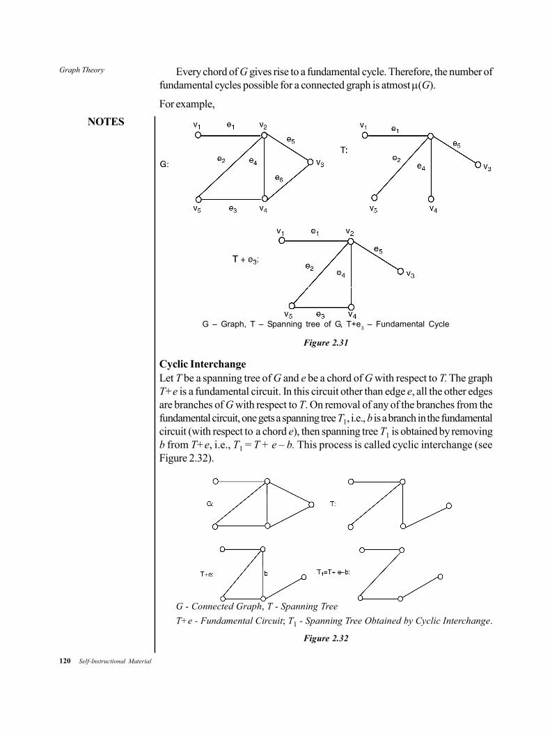
120 Self-Instructional Material
Graph Theory
NOTES
Every chord of G gives rise to a fundamental cycle. Therefore, the number offundamental cycles possible for a connected graph is atmost (G).
For example,
G – Graph, T – Spanning tree of G, T+e3 – Fundamental Cycle
Figure 2.31
Cyclic InterchangeLet T be a spanning tree of G and e be a chord of G with respect to T. The graphT+e is a fundamental circuit. In this circuit other than edge e, all the other edgesare branches of G with respect to T. On removal of any of the branches from thefundamental circuit, one gets a spanning tree T1, i.e., b is a branch in the fundamentalcircuit (with respect to a chord e), then spanning tree T1 is obtained by removingb from T+e, i.e., T1 = T + e – b. This process is called cyclic interchange (seeFigure 2.32).
G - Connected Graph, T - Spanning Tree
T+e - Fundamental Circuit; T1 - Spanning Tree Obtained by Cyclic Interchange.
Figure 2.32
Graph Theory
NOTES
Self-Instructional Material 121
2.5.1 Floyd’s and Warshall’s Algorithms
Floyd’s Algorithm – Shortest Paths
Floyd’s algorithm finds the paths which has least value between all the vertices ofa graph. This requires matrix representation of the graph. The matrix representsthe distance of edges between vertices which normally corresponds to the cost.
To apply this algorithm a matrix has to be made as a two-dimensional array.For a graph of n vertices matrix will be n × n. Every row in the matrix is a ‘starting’vertex, denoted as i and each column is an ‘ending’ point, denoted as j. An edgebetween i and j in the graph, length of this edge is the position (i,j) of the matrix. Incase of undirected graphs, edges are bidirectional, a value is given in position (j,i)of the matrix. If there is no edge as a direct link between two vertices, value isgiven as infinity. Alternatively, very large value is put, to express the impossibility ofmovement from i to j.
For example, in a graph connecting points 2 and 6, bidirectionally and theedge has a length of 24 units, number 24 will be placed into positions (2, 6) and(6, 2) of the matrix.
After setting such a matrix Floyd’s algorithm can be used to find the shortestdistance between every pair of vertices in the graph. The algorithm works forevery non-direct path between pairs of vertices having least value than the way tomove between these vertices. In the event of locating such a path, it is the valuebetween these vertices which are to be tested. Each element of the matrix representsthe least value of traversal between the vertices with respect to its row and column.If the graph is directed, (i,j) and (j,i) may not be equal.
Warshall’s Algorithm
This algorithm is more efficient in determining the access of all pairs of nodes in agraph whether directed or undirected. For a graph G with n nodes, this methodconstructs a sequence of n adjacency matrices, P
1,...,P
n, by using the same set of
nodes. One starts by setting P0 = G.
If Pk is already defined then P
k+1 has all the edges of P
k, and additional
edges, if any, needed to ensure that every pair of nodes joined by an edge of Pk to
node k + 1 are joined by an arc of Pk+1
(in the undirected case) and also for everypath a k + 1 b. The pair (a, b) is an edge of P
k+1 (in the directed case).
The algorithm terminates after n iterations and Pn contains all adjacency
relationships which are shown as edges.
Floyd–Warshall’s algorithm is an algorithm for graph analysis that findsshortest paths in a graph that is weighted and directed. The algorithm computesthe shortest paths between all pairs of vertices. This algorithm is an example ofdynamic programming.
A path in the matrix k is defined in such a way that path k[i][j] is true if andonly if there is a path from node i to node j and there is no node higher than k,

122 Self-Instructional Material
Graph Theory
NOTES
except i and j themselves. For any i and j if path k[i][j] = True, it implies that path(k+1)[i][j] is also true. If there is a situation in which path (k+1)[i][j] is true whilepath k[i][j] it is false, it is possible if there is a path from i to j via node k + 1, butno path from i to j via nodes i through k. This means that there is a path from i tok + 1 through nodes i through k and a similar path from k + 1 to j. This followsthat the path (k+ 1)[i][j] is true if and only if one of the following two conditionsholds:
(i) Path k[i][j] is true.
(ii) (Path k[i][k+1]) (Path k[k+1][j]) is true.
Also, path 0[i][j] = adjacent. This is since, direct path is there from node ito node j with no intermediate node. It can also be noted that, path (MAXNODES-1)[i][j] = Path[i][j], because if a path exists through any node, then any path fromnode i to node j may be selected.
This is Warshall’s algorithm which is named, after its discoverer.
This algorithm compares every possible path between every pair of verticesin the graph. It makes only V
3 comparisons. Maximum number of edges may be
given as V2 in the graph with every combination of edges tested. It estimates the
shortest path between two vertices, by improving it incrementally to find an optimalsolution.
Let there be a graph with a set V, of vertices and each vertex numbered 1through N. Let there be a function defined as shortest path (i, j, k) which returnsthe shortest possible path from i to j using only vertices 1, 2, 3, ….., k as intermediatenodes. The objective is to find the shortest possible path from each i to each j byusing only nodes 1, 2, 3, …., k + 1.
There are two alternative paths:
(i) Shortest path that uses nodes only in the set (1...k).or
(ii) Another path that goes from i to j, via k + 1.
Best path from i to j is the one that uses only nodes 1…. k which is definedby the function. If there was a better path from i to j via k + 1, then the length ofthis path would be the sum total of the shortest path from i to k + 1, traversingvertices 1.....k and the shortest path from k + 1 to j by using same set of vertices,i.e., 1…....k.
One may define shortest path (i, j, k), that is recursive in nature.
This formula is the heart of Floyd Warshall algorithm which works by firstcomputing shortest path (i, j, 1) for all (i, j) pairs, then using that to find shortestpath (i, j, 2) for all (i, j) pairs, and so on and terminates when k = n. This finds theshortest path for all (i, j) pairs by using any intermediate vertices.
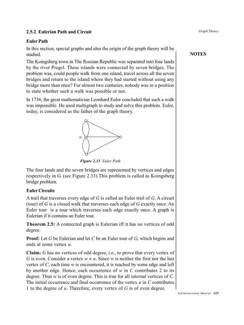
Graph Theory
NOTES
Self-Instructional Material 123
2.5.2 Eulerian Path and Circuit
Euler Path
In this section, special graphs and also the origin of the graph theory will bestudied.
The Koingsberg town in The Russian Republic was separated into four landsby the river Pregel. These islands were connected by seven bridges. Theproblem was, could people walk from one island, travel across all the sevenbridges and return to the island where they had started without using anybridge more than once? For almost two centuries, nobody was in a positionto state whether such a walk was possible or not.
In 1736, the great mathematician Leonhard Euler concluded that such a walkwas impossible. He used multigraph to study and solve this problem. Euler,today, is considered as the father of the graph theory.
G:
Figure 2.33 Euler Path
The four lands and the seven bridges are represented by vertices and edgesrespectively in G. (see Figure 2.33) This problem is called as Koingsbergbridge problem.
Euler Circuits
A trail that traverses every edge of G is called an Euler trail of G. A circuit(tour) of G is a closed walk that traverses each edge of G exactly once. AnEuler tour is a tour which traverses each edge exactly once. A graph isEulerian if it contains an Euler tour.
Theorem 2.5: A connected graph is Eulerian iff it has no vertices of odddegree.
Proof: Let G be Eulerian and let C be an Euler tour of G, which begins andends at some vertex u.
Claim: G has no vertices of odd degree, i.e., to prove that every vertex ofG is even. Consider a vertex w u. Since w is neither the first nor the lastvertex of C, each time w is encountered, it is reached by some edge and leftby another edge. Hence, each occurrence of w in C contributes 2 to itsdegree. Thus w is of even degree. This is true for all internal vertices of C.The initial occurrence and final occurrence of the vertex u in C contributes1 to the degree of u. Therefore, every vertex of G is of even degree.
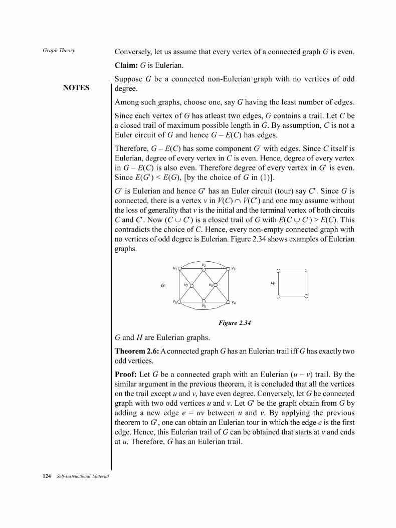
124 Self-Instructional Material
Graph Theory
NOTES
Conversely, let us assume that every vertex of a connected graph G is even.
Claim: G is Eulerian.
Suppose G be a connected non-Eulerian graph with no vertices of odddegree.
Among such graphs, choose one, say G having the least number of edges.
Since each vertex of G has atleast two edges, G contains a trail. Let C bea closed trail of maximum possible length in G. By assumption, C is not aEuler circuit of G and hence G – E(C) has edges.
Therefore, G – E(C) has some component G with edges. Since C itself isEulerian, degree of every vertex in C is even. Hence, degree of every vertexin G – E(C) is also even. Therefore degree of every vertex in G is even.Since E(G) < E(G), [by the choice of G in (1)].
G is Eulerian and hence G has an Euler circuit (tour) say C. Since G isconnected, there is a vertex v in V(C) V(C) and one may assume withoutthe loss of generality that v is the initial and the terminal vertex of both circuitsC and C. Now (C C) is a closed trail of G with E(C C) > E(C). Thiscontradicts the choice of C. Hence, every non-empty connected graph withno vertices of odd degree is Eulerian. Figure 2.34 shows examples of Euleriangraphs.
G:
v6
v1 v3v2
v5v4
v8v7 H:
Figure 2.34
G and H are Eulerian graphs.
Theorem 2.6: A connected graph G has an Eulerian trail iff G has exactly twoodd vertices.
Proof: Let G be a connected graph with an Eulerian (u – v) trail. By thesimilar argument in the previous theorem, it is concluded that all the verticeson the trail except u and v, have even degree. Conversely, let G be connectedgraph with two odd vertices u and v. Let G be the graph obtain from G byadding a new edge e = uv between u and v. By applying the previoustheorem to G, one can obtain an Eulerian tour in which the edge e is the firstedge. Hence, this Eulerian trail of G can be obtained that starts at v and endsat u. Therefore, G has an Eulerian trail.
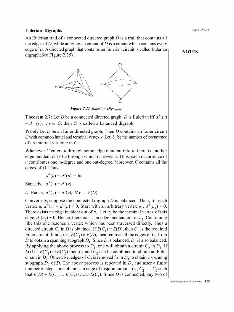
Graph Theory
NOTES
Self-Instructional Material 125
Eulerian Digraphs
An Eulerian trail of a connected directed graph D is a trail that contains allthe edges of D; while an Eulerian circuit of D is a circuit which contains everyedge of D. A directed graph that contains an Eulerian circuit is called Euleriandigraph(See Figure 2.35).
D1:
D2:
Figure 2.35 Eulerian Digraphs
Theorem 2.7: Let D be a connected directed graph. D is Eulerian iff d + (v)= d – (v), v G, then G is called a balanced digraph.
Proof: Let D be an Euler directed graph. Then D contains an Euler circuitC with common initial and terminal vertex v. Let, bu be the number of occurrenceof an internal vertex u in C.
Whenever C enters u through some edge incident into u, there is anotheredge incident out of u through which C leaves u. Thus, each occurrence ofu contributes one in-degree and one out-degree. Moreover, C contains all theedges of D. Thus,
d+(u) = d–(u) = bu
Similarly, d +(v) = d–(v)
Hence, d +(v) = d–(v), v V(D)
Conversely, suppose the connected digraph D is balanced. Then, for eachvertex u, d +(u) = d–(u) 0. Start with an arbitrary vertex u1, d +(u1) 0.There exists an edge incident out of u1. Let u2 be the terminal vertex of thisedge, d+(u2) 0. Hence, there exists an edge incident out of u2. Continuinglike this one reaches a vertex which has been traversed directly. Thus adirected circuit C1 in D is obtained. If E(C1) = E(D), then C1 is the requiredEuler circuit. If not, i.e., E(C1) E(D), then remove all the edges of C1 fromD to obtain a spanning subgraph D1. Since D is balanced, D1 is also balanced.By applying the above process to D1, one will obtain a circuit C2 in D1. IfE(D) = E(C1) E(C2) then C1 and C2 can be combined to obtain an Eulercircuit in D1. Otherwise, edges of C2 is removed from D1 to obtain a spanningsubgraph D2 of D. The above process is repeated in D2 and after a finitenumber of steps, one obtains an edge of disjoint circuits C1, C2, ..., Ck suchthat E(D) = E(C1) E(C2) ...E(Ck). Since D is connected, any two of

126 Self-Instructional Material
Graph Theory
NOTES
these cycles have a common vertex and the circuits C1, C2, ... ,Ck can becombined to obtain an Euler circuit in D. Hence, D is an Euler graph.
2.5.3 Hamiltonian Graphs
In 1857, Sir William Rowan Hamilton invented a game called ‘Around theWorld’. In this game, a solid regular dodecahedron (20 vertices, 30 edgesand 12 faces) and a supply of string is given. Every vertex is given the nameof an important city. The objective of the game is to find a route along theedges of dodecahedron that visits every city exactly once and terminateswhere it started
D
Figure 2.36 Hamiltonian Graphs
The graph D is a dodecahedron.
Another famous problem is ‘The Knight’s Puzzle’. Is it possible for a knightto tour the chess board, i.e., visit each square exactly once and return to itsinitial square?
It can be represented by a graph G, where the vertices ui correspond tosquares Si of the chess board and uj is adjacent to ui iff it is possible for aknight to proceed from Si to Sj in a single move.
To solve ‘Around the World’ and ‘Knight’s Puzzle’, one must determine if thegiven graph is Hamiltonian.
A path that contains every vertex of G is called a Hamilton path of G.Similarly, a Hamilton cycle of G is a cycle that contains every vertex of G inother words spanning cycle. A graph is Hamiltonian if it contains a Hamiltoncycle or a spanning cycle.
Example 2.8: Prove that kn has a Hamiltonian circuit, n 3.
Solution: Let us construct the Hamiltonian circuit in kn (n 3) as follows:
Choose a vertex arbitrarily in kn and begin the Hamiltonian circuit at thisvertex. Such a circuit can be built by traversing vertices in any order, as longas the path begins and terminates at the same vertex and visits other verticesexactly once. This is possible in kn, since every vertex is adjacent to all othervertices. Also k1 and k2 has only Hamiltonian path, not circuit.
Graphical: A sequence d = (d1, d2, ...., dn) is graphical if there exists a simpleundirected graph on n vertices with the degrees of the vertices d1, d2, ..., dnrespectively.

Graph Theory
NOTES
Self-Instructional Material 127
For example, a graph with degree sequence of vertices v1 to v6 (4, 4, 3, 2,2, 1) is shown in the following figure.
v5v6
v4
v2v3
v1
G:
Closure: A closure (CG) of a n-vertex graph G is a graph from G byrecursively joining pairs of non-adjacent vertices whose degree sum is atleastn until no such pair remains.For example,
G:
C G( )
The above figures explain one way of constructing a closure of a graph.
Important TheoremsTheorem 2.8: Let G be a n-vertex graph. Suppose G1 and G2 are twographs obtained from G by recursively joining pairs of non-adjacent verticeswhose degree sum is atleast n. Then G1 = G2. In other words, C(G), theclosure of a graph G is unique.
Proof: Let e1, e2, ..., ek and f1, f2, f3, ..., fe be the edges added to G toobtain G1 and G2, respectively. It has to be proved that every ei (1 i k)is an edge of G2 and fj (1 j l) is an edge of G1. Suppose that some edgein the sequence e1, e2, ..., ek does not belong to G2. Let p be the smallestpositive integer such that ep+1 is not an edge of G2. Let ep+1 = uv and H =G + {e1, e2, ..., ep}. Then, H is a subgraph of G1 and G2. By the constructionof G1, one gets
dH(u) + dH(v) n
Therefore, dG2(u) + dG2
(v) dH(u) + dH(v) n.
This is a contradiction since u and v are non-adjacent in G2. Therefore, eachei is an edge of G2. Similarly, each fj belongs to G1. Hence, G1 = G2.
Theorem 2.9: A graph G is Hamiltonian iff its closure C(G) is Hamiltonian.
Proof: Let e1, e2,...en be edges added to G to obtain its closure C(G). LetGi be the graph obtained from G by adding the edge ei.
By repeated application of Example (2.8).
G is Hamiltonian C(G) is also Hamiltonian.
Corollary 1: Let G be a graph with atleast 3 vertices. If C(G) kn, (n 3) then G is Hamiltonian.
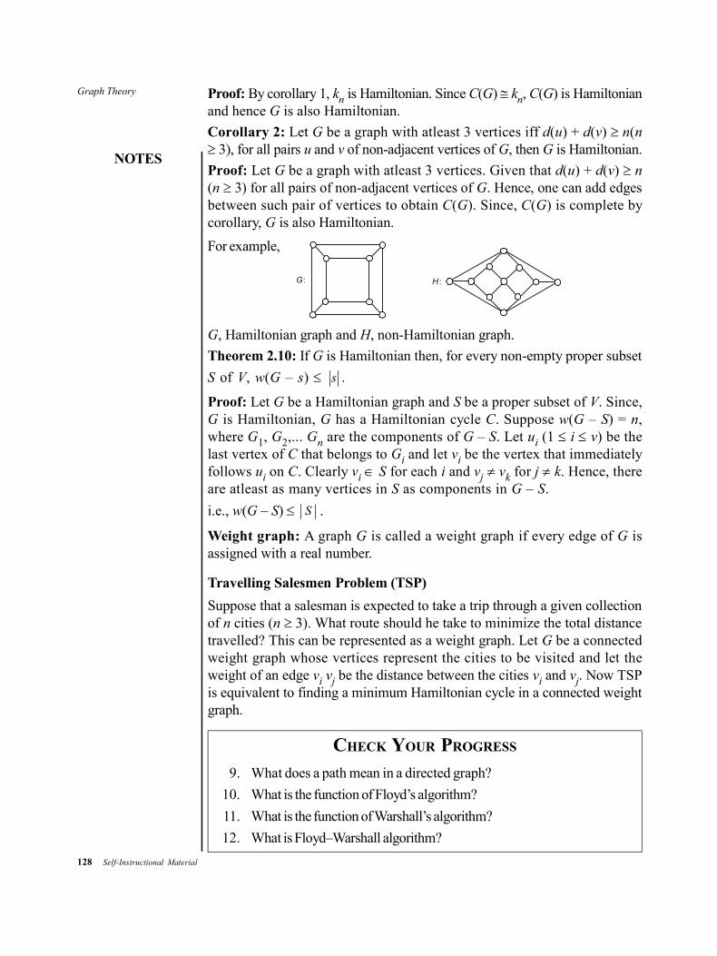
128 Self-Instructional Material
Graph Theory
NOTES
Proof: By corollary 1, kn is Hamiltonian. Since C(G) kn, C(G) is Hamiltonianand hence G is also Hamiltonian.
Corollary 2: Let G be a graph with atleast 3 vertices iff d(u) + d(v) n(n 3), for all pairs u and v of non-adjacent vertices of G, then G is Hamiltonian.
Proof: Let G be a graph with atleast 3 vertices. Given that d(u) + d(v) n(n 3) for all pairs of non-adjacent vertices of G. Hence, one can add edgesbetween such pair of vertices to obtain C(G). Since, C(G) is complete bycorollary, G is also Hamiltonian.
For example,
G : H :
G, Hamiltonian graph and H, non-Hamiltonian graph.
Theorem 2.10: If G is Hamiltonian then, for every non-empty proper subset
S of V, w(G – s) s .
Proof: Let G be a Hamiltonian graph and S be a proper subset of V. Since,G is Hamiltonian, G has a Hamiltonian cycle C. Suppose w(G – S) = n,where G1, G2,... Gn are the components of G – S. Let ui (1 i v) be thelast vertex of C that belongs to Gi and let vi be the vertex that immediatelyfollows ui on C. Clearly vi S for each i and vj vk for j k. Hence, thereare atleast as many vertices in S as components in G – S.
i.e., w(G – S) S .
Weight graph: A graph G is called a weight graph if every edge of G isassigned with a real number.
Travelling Salesmen Problem (TSP)
Suppose that a salesman is expected to take a trip through a given collectionof n cities (n 3). What route should he take to minimize the total distancetravelled? This can be represented as a weight graph. Let G be a connectedweight graph whose vertices represent the cities to be visited and let theweight of an edge vi vj be the distance between the cities vi and vj. Now TSPis equivalent to finding a minimum Hamiltonian cycle in a connected weightgraph.
CHECK YOUR PROGRESS
9. What does a path mean in a directed graph?
10. What is the function of Floyd’s algorithm?
11. What is the function of Warshall’s algorithm?
12. What is Floyd–Warshall algorithm?
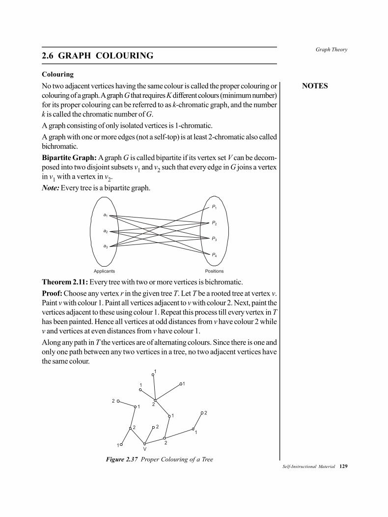
Graph Theory
NOTES
Self-Instructional Material 129
2.6 GRAPH COLOURING
Colouring
No two adjacent vertices having the same colour is called the proper colouring orcolouring of a graph. A graph G that requires K different colours (minimum number)for its proper colouring can be referred to as k-chromatic graph, and the numberk is called the chromatic number of G.
A graph consisting of only isolated vertices is 1-chromatic.
A graph with one or more edges (not a self-top) is at least 2-chromatic also calledbichromatic.
Bipartite Graph: A graph G is called bipartite if its vertex set V can be decom-posed into two disjoint subsets v1 and v2 such that every edge in G joins a vertexin v1 with a vertex in v2.
Note: Every tree is a bipartite graph.
a1
a2
a3
P1
P2
P3
P4
PositionsApplicants
Theorem 2.11: Every tree with two or more vertices is bichromatic.
Proof: Choose any vertex r in the given tree T. Let T be a rooted tree at vertex v.Paint v with colour 1. Paint all vertices adjacent to v with colour 2. Next, paint thevertices adjacent to these using colour 1. Repeat this process till every vertex in Thas been painted. Hence all vertices at odd distances from v have colour 2 whilev and vertices at even distances from v have colour 1.
Along any path in T the vertices are of alternating colours. Since there is one andonly one path between any two vertices in a tree, no two adjacent vertices havethe same colour.
21
2
1V
2
2
1
2
1
1
1
2
1
Figure 2.37 Proper Colouring of a Tree
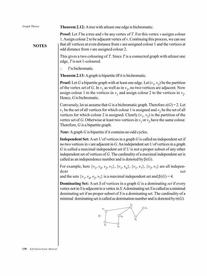
130 Self-Instructional Material
Graph Theory
NOTES
Theorem 2.12: A tree with atleast one edge is bichromatic.
Proof: Let T be a tree and v be any vertex of T. For this vertex v assigns colour1. Assign colour 2 to be adjacent vertex of v. Continuing this process, we can seethat all vertices at even distance from v are assigned colour 1 and the vertices atodd distance from v are assigned colour 2.
This gives a two colouring of T. Since T is a connected graph with atleast oneedge, T is not 1-coloured.
T is bichromatic.
Theorem 2.13: A graph is bipartite iff it is bichromatic.
Proof: Let G a bipartite graph with at least one edge. Let (v1, v2) be the partitionof the vertex set of G. In v1 as well as in v2, no two vertices are adjacent. Nowassign colour 1 to the vertices in v1 and assign colour 2 to the vertices in v2.Hence, G is bichromatic.
Conversely, let us assume that G is a bichromatic graph. Therefore x(G) = 2. Letv1 be the set of all vertices for which colour 1 is assigned and v2 be the set of allvertices for which colour 2 is assigned. Clearly (v1, v2) is the partition of thevertex set of G. Otherwise at least two vertices in v1 or v2 have the same colour.Therefore, G is a bipartite graph.
Note: A graph G is bipartite if it contains no odd cycles.
Independent Set: A set U of vertices in a graph G is called an independent set ifno two vertices in v are adjacent in G. An independent set U of vertices in a graphG is called a maximal independent set if U is not a proper subset of any otherindependent set of vertices of G. The cardinality of a maximal independent set iscalled as an independence number and is denoted by (G).
For example, here {v1, v4, v2, v7}, {v1, v6}, {v1, v7}, {v2, v7} are all indepen-dent setand the sets {v1, v4, v2, v7} is a maximal independent set and (G) = 4.
Dominating Set: A set S of vertices in a graph G is a dominating set if everyvertex not in S is adjacent to a vertex in S. A dominating set S is called as a minimaldominating set if no proper subset of S is a dominating set. The cardinality of aminimal dominating set is called as domination number and is donoted by (G).
G :
v5 v4
v3
v1
v2
v6
v7
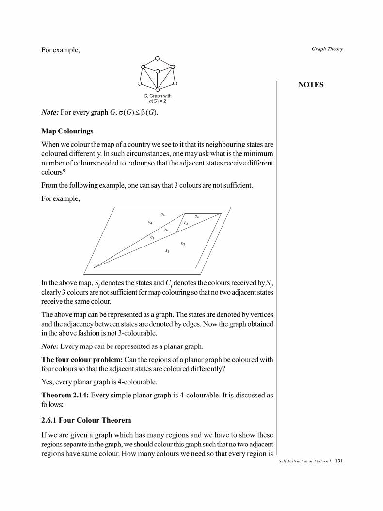
Graph Theory
NOTES
Self-Instructional Material 131
For example,
G, Graph with(G) = 2
Note: For every graph G, (G) (G).
Map Colourings
When we colour the map of a country we see to it that its neighbouring states arecoloured differently. In such circumstances, one may ask what is the minimumnumber of colours needed to colour so that the adjacent states receive differentcolours?
From the following example, one can say that 3 colours are not sufficient.
For example,
s3
c3
s3
c4
c1
s4
s4
c4
In the above map, Si denotes the states and Ci denotes the colours received by Si,clearly 3 colours are not sufficient for map colouring so that no two adjacent statesreceive the same colour.
The above map can be represented as a graph. The states are denoted by verticesand the adjacency between states are denoted by edges. Now the graph obtainedin the above fashion is not 3-colourable.
Note: Every map can be represented as a planar graph.
The four colour problem: Can the regions of a planar graph be coloured withfour colours so that the adjacent states are coloured differently?
Yes, every planar graph is 4-colourable.
Theorem 2.14: Every simple planar graph is 4-colourable. It is discussed asfollows:
2.6.1 Four Colour Theorem
If we are given a graph which has many regions and we have to show theseregions separate in the graph, we should colour this graph such that no two adjacentregions have same colour. How many colours we need so that every region is

132 Self-Instructional Material
Graph Theory
NOTES
shown separate? It has been discovered that four colours are sufficient for thispurpose in case of a planar graph. This is ‘four colour theorem’ which is true forany planar graph. This is also known as ‘four colour map theorem’.
Although it is possible to colour a map by using only three colours, but thisis inadequate when a region is surrounded by three regions. In that case a fourthcolour becomes necessary. Few map-makers make use of fifth colour as an easierapproach, but it is optional as four colours are sufficient for such applications.
In 1976, this theorem was proved. For this computer was used. All mapswere categorized into more than 1900 cases. One special-purpose computerprogram was run and the concept of four colour theorem was tested. But sincethis could not be verified by hand, it was not accepted by all mathematicians.
As per the four colour theorem, every planar map is four colourable.This conclusion was based on the work of Appel and Haken. Although, notaccepted by all, the original work of Kempe has put forward some basic tools,which was used at a later stage, to prove it.
Adding edges to a graph does not decrease its chromatic number. Thus, amaximal planar graph, a kind of triangular graphs, where every face is bounded bythree edges, is to be considered here. Let v, e, and f be the number of vertices,edges, and faces, respectively. We know that each edge is shared by two faces,hence, 2e = 3f. Using this fact with Euler’s formula v – e + f = 2 6v – 2e = 12.Let v
n be the number of vertices of degree n and D be the maximum degree. Then,
1 1 1
6 2 6 (6 ) 12D D D
i i ii i i
v e v iv i v
Here, 12 > 0 and 6 – i 0 and so, i 6. Thus, there is at least one vertexof degree 5 or less. There may be more than one vertex which may have degree 5.
If a maximal planar graph exists that requires 5 colours, then there is aminimal such graph and removing any vertex reduces it to four-colourable. Let ustake a graph G. This graph can not have a vertex having degree 3 or less than 3. Ifd(v) 3, v can be removed from G, we colour the smaller graph using four-colourand then re-add v. After re-adding v, we extend the four-colouring to this graphby selecting a colour different from its neighbours.
Kempe argued that G can have no vertex of degree 4. Once again, weremove a vertex v and apply four colours for remaining vertices.
Figure 2.38 Colouring a Graph
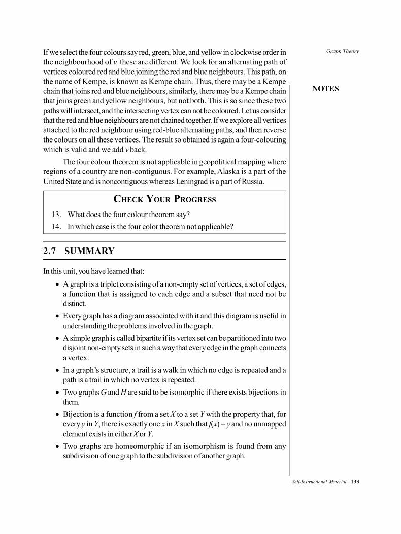
Graph Theory
NOTES
Self-Instructional Material 133
If we select the four colours say red, green, blue, and yellow in clockwise order inthe neighbourhood of v, these are different. We look for an alternating path ofvertices coloured red and blue joining the red and blue neighbours. This path, onthe name of Kempe, is known as Kempe chain. Thus, there may be a Kempechain that joins red and blue neighbours, similarly, there may be a Kempe chainthat joins green and yellow neighbours, but not both. This is so since these twopaths will intersect, and the intersecting vertex can not be coloured. Let us considerthat the red and blue neighbours are not chained together. If we explore all verticesattached to the red neighbour using red-blue alternating paths, and then reversethe colours on all these vertices. The result so obtained is again a four-colouringwhich is valid and we add v back.
The four colour theorem is not applicable in geopolitical mapping whereregions of a country are non-contiguous. For example, Alaska is a part of theUnited State and is noncontiguous whereas Leningrad is a part of Russia.
CHECK YOUR PROGRESS
13. What does the four colour theorem say?
14. In which case is the four color theorem not applicable?
2.7 SUMMARY
In this unit, you have learned that:
A graph is a triplet consisting of a non-empty set of vertices, a set of edges,a function that is assigned to each edge and a subset that need not bedistinct.
Every graph has a diagram associated with it and this diagram is useful inunderstanding the problems involved in the graph.
A simple graph is called bipartite if its vertex set can be partitioned into twodisjoint non-empty sets in such a way that every edge in the graph connectsa vertex.
In a graph’s structure, a trail is a walk in which no edge is repeated and apath is a trail in which no vertex is repeated.
Two graphs G and H are said to be isomorphic if there exists bijections inthem.
Bijection is a function f from a set X to a set Y with the property that, forevery y in Y, there is exactly one x in X such that f(x) = y and no unmappedelement exists in either X or Y.
Two graphs are homeomorphic if an isomorphism is found from anysubdivision of one graph to the subdivision of another graph.
134 Self-Instructional Material
Graph Theory
NOTES
Subdivision of a graph refers to another graph that results from subdivisionof edges in that graph.
Barycentric subdivision is a special subdivision that subdivides every edgeof a graph.
The degree of a vertex is the number of edges having that vertex as an endpoint, and is denoted by d(v).
A vertex with degree zero is called an isolated vertex.
A vertex with degree one is called a pendant vertex.
A path from various vertices in a directed graph is a sequence of one ormore edges.
Floyd’s algorithm finds those paths which have least value between all thevertices of a graph and it requires the matrix representation of the graph.
Floyd’s algorithm works for every non-direct path between pairs of verticeshaving least value than the way to move between these vertices.
Warshall’s algorithm is more efficient in determining the access of all pairsof node in a graph, whether directed or undirected.
2.8 KEY TERMS
Simple graph: A graph with no self loops and parallel edges is called asimple graph.
Pseudograph: A graph with self loops and parallel edges is called apseudograph.
Isolated vertex: A vertex with degree zero is called an isolated vertex.
Pendant vertex: A vertex with degree one is called a pendant vertex.
Adjacent vertices: A pair of vertices that determine an edge are calledadjacent vertices.
Complete graph: A simple graph in which each pair of distinct vertices isjoined by an edge is called a complete graph.
Bipartite graph: A simple graph is called bipartite if its vertex set can bepartitioned into two disjoint non-empty sets.
Floyd’s algorithm: It finds the paths which has least value between all thevertices of a graph.
Floyd–Warshall algorithm: Floyd–Warshall algorithm is an algorithm forgraph analysis that finds shortest paths in a graph that is weighted anddirected.
Graph Theory
NOTES
Self-Instructional Material 135
2.9 ANSWERS TO ‘CHECK YOUR PROGRESS’
1. In the diagrammatic representation of a graph, vertices are represented bysmall circles and edges by lines whenever the corresponding pair of verticesforms an edge.
2. A graph with no self loops and parallel edges is called a simple graph.
3. A graph with self loops and parallel edges is called a pseudograph.
4. The various types of graphs are as follows:(i) Bipartite graphs(ii) Subgraph(iii) Complete graph
5. The edge connectivity l(G) of a graph is the minimum cardinality of a set Sof edges of G such that G – S is disconnected.
6. The vertex connectivity K(G) of a graph G is the minimum number of verticeswhose deletion makes G a disconnected or a trivial graph.
7. Two graphs are said to be isomorphic if there exist bijections (it is a functionf from a set X to a set Y with the property that, for every y in Y, there isexactly one x in X such that f(x) = y and no unmapped element exists ineither X or Y) amongst them.
8. Subdivision of a graph is another graph that results from subdivision ofedges in that graph.
9. A path from various vertices in a directed graph is a sequence of one ormore edges.
10. Floyd’s algorithm finds the paths which have least value between all thevertices of a graph and it requires a matrix representation of the graph.
11. Warshall’s algorithm determines the access of all pairs of nodes in a graph,whether directed or undirected.
12. Floyd–Warshall algorithm is an algorithm for graph analysis that finds theshortest paths in a graph that is weighed and directed.
13. As per the four colour theorem, every planar map is four colourable.
14. The four colour theorem is not applicable in geopolitical mapping whereregions of a country are non-contiguous.
136 Self-Instructional Material
Graph Theory
NOTES
2.10 QUESTIONS AND EXERCISES
Short-Answer Questions
1. What do you understand by the degree of vertex?
2. Differentiate between edge-connectivity and vertex-connectivity.
3. What do you understand by connectivity relation?
4. Write a short note on cyclic interchange.
5. Write a short note on Euler path.
Long-Answer Questions
1. Explain the various types of graphs and their operations.
2. Explain cut-vertices and cut-edges.
3. Explain the structures of various type of graphs.
4. Explain with the help of a diagram the concepts of adjacent and incidencematrices.
5. Discuss the characteristics of Floyd–Warshall algorithm.
6. Describe Euler circuits.
2.11 FURTHER READING
Lipschutz, Seymour and Lipson Marc. Schaum’s Outline of DiscreteMathematics, 3rd edition. New York: McGraw-Hill, 2007.
Horowitz, Ellis, Sartaj Sahni and Sanguthevar Rajasekaran. Fundamentals ofComputer Algorithms. Hyderabad: Orient BlackSwan, 2008.
Cormen, Thomas H., Charles E. Leiserson, Ronald L. Rivest and Clifford Stein.Introduction to Algorithms. The MIT Press, 1990.
Brassard, Gilles and Paul Bratley. Fundamentals of Algorithms. New Delhi:Prentice Hall of India, 1995.
Levitin, Anany. Introduction to the Design and Analysis of Algorithms. NewJersey: Pearson, 2006.
Baase, Sara and Allen Van Gelder. Computer Algorithms – Introduction toDesign and Analysis. New Jersey: Pearson, 2003.
Mott, J.L. Discrete Mathematics for Computer Scientists, 2nd edition. NewDelhi: Prentice-Hall of India Pvt. Ltd., 2007.
Liu, C.L. Elements of Discrete Mathematics. New Delhi: Tata McGraw-HillPublishing Company, 1977.
Rosen, Kenneth. Discrete Mathematics and Its Applications, 6th edition. NewYork: McGraw-Hill Higher Education, 2007.
Trees
NOTES
Self-Instructional Material 137
UNIT 3 TREES
Structure
3.0 Introduction3.1 Unit Objectives3.2 Trees: Basics
3.2.1 Trees and Sorting3.3 Minimum Height and Minimum Distance Spanning Trees
3.3.1 Depth-First Search and Breadth-First Search3.3.2 Optimal Spanning Graph
3.4 Planar Graphs3.5 Summary3.6 Key Terms3.7 Answers to ‘Check Your Progress’3.8 Questions and Exercises3.9 Further Reading
3.0 INTRODUCTION
In this unit, you will learn about the various types of tree structures and theirapplications. In a graph theory, a tree is defined as a graph in which two verticesare connected by one and only one path. Generally, trees are known as opengraphs. An organizational hierarchy is considered to be a very good example of atree structure. In a tree, every edge is a cut-edge. Traversal algorithm is a methodicalway for visiting each and every vertex of an ordered rooted tree. An orderedrooted tree is primarily used for representing any arithmetic expressions andcompound proposition expressions.
You will learn how trees are helpful in merge sort. In addition, you will learnto compute mathematical expressions by using algorithms and formulae and theirgraphical representation by using tree structures.
3.1 UNIT OBJECTIVES
After going through this unit, you will be able to:
Identify the various types of trees
Understand the basics of a tree
Explain the features of minimum height and minimum distance spanning trees
Comprehend the meaning and functions of planar graphs
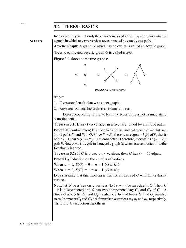
138 Self-Instructional Material
Trees
NOTES
3.2 TREES: BASICS
In this section, you will study the characteristics of a tree. In graph theory, a tree isa graph in which any two vertices are connected by exactly one path.
Acyclic Graph: A graph G, which has no cycles is called an acyclic graph.
Tree: A connected acyclic graph G is called a tree.
Figure 3.1 shows some tree graphs:
G1: G2: G3:
Figure 3.1 Tree Graphs
Notes:
1. Trees are often also known as open graphs.
2. Any organizational hierarchy is an example of tree.
Before proceeding further to learn the types of trees, let us understandsome theorems.
Theorem 3.1: Every two vertices in a tree, are joined by a unique path.
Proof: (By contradiction) let G be a tree and assume that there are two distinct,(v, w) paths P
1 and P
2 in G. Since P
1 P
2, there is an edge e = V
1V
2 of P
1 that is
not in P2. Clearly (P
1 P
2) – e is connected. Therefore, it contains a (V
1 – V
2)
path P. Now P + e is a cycle in the acyclic graph G, which is a contradiction to thefact that G is a tree.
Theorem 3.2: If G is a tree on n vertices, then G has (n – 1) edges.
Proof: By induction on the number of vertices.
When n = 1, E(G) = 0 = n – 1 (G K1)
When n = 2, E(G) = 1 = n – 1 (G K2)
Let us assume that this theorem is true for all trees of G with fewer than nvertices.
Now, let G be a tree on n vertices. Let e = uv be an edge in G. Then G– e is disconnected and G has two components say G1 and G2 of G – e.Since G is acyclic, G1 and G2 are also acyclic and hence G1 and G2 are alsotrees. Moreover G1 and G2 has fewer than n vertices say n1 and n2, respectively.Therefore, by induction hypothesis,

Trees
NOTES
Self-Instructional Material 139
G1 has (n1 – 1) edges and G2 has (n2 – 1) edges.
E(G) = E(G1) + (G2) + 1
(Here, 1 in the sum corresponds to the edge e)
= (n1 – 1) + (n2 – 1) + 1 = n1 + n2 – 1 = n – 1
Therefore, any vertex tree, has (n – 1) edges.
Theorem 3.3: Every tree has at least two vertices of degree one or in a tree,there are atleast two pendant vertices.
Proof: Let G be a tree on n vertices. Then,
d(v) 1, v v(G) ...(3.1)
Already we have, vv(G) d(v) = 2 × E(G) = 2 × e ...(3.2)
Since G is an n-vertex tree, it has (n – 1) edges.
v v(G) d(v) = (2n – 2) ...(3.3)
From equations (3.1) and (3.3), it follows that d(v) = 1 for at least twovertices.
Note: In a tree, every edge is a cut-edge.
Now, let us learn about the various types of trees.
1. Rooted Tree
In a directed tree (every edge assigned with a direction), a particular vertex iscalled a root if that vertex is of degree zero. A tree together with its root producesa graph called a rooted tree as shown in Figure 3.2. Note that in the rooted tree,every edge is directed away from the root.
For example, suppose T is a rooted tree. If a vertex u is a vertex in T otherthan the root then the parent of u is the unique vertex u1 such that there isa directed edge from u1 to u. Here, u is called as a child of u1. Vertices ofthe same parent are called as siblings. A vertex of a rooted tree is called asa leaf if it has no children and those vertices which have children, are calledas internal vertices.
G: u1
u2u3
u4
r
G1:
r
Figure 3.2 Rooted Trees

140 Self-Instructional Material
Trees
NOTES
If v is a vertex in a tree, then a subtree with v as its root is the subgraph ofthe tree consisting of v and its children and all edges incident to these childrenas shown in Figure 3.3:
G:
u
u1
u3 u4
u2v1
v
r
H: u1
u
u2
u3 u4
Rooted Tree T Subtree of T withits Root u.
Figure 3.3 Rooted Tree and Subtree
Level and Height in a Rooted Tree
The level of a vertex v in a rooted tree is the length of the path from the rootto this vertex. The height of a rooted tree is the length of the longest pathfrom the root to any vertex as illustrated in Figure 3.4:
w1 w2 w3
T:
uw
r
v
v1
v3 v3
v1
v5
v4
v6 v7
level 0
level 1
level 2
level 3
level 4
Figure 3.4 Height of a Tree
Rooted Tree T with its different Levels.
Height of T is 4.
2. k-ary Tree
A rooted tree is called a k-ary tree if every internal vertex does not havemore than k-children. The tree is called a full k-ary tree if every internalvertex has exactly k-children. A k-ary tree with k = 2 is called a binary tree.
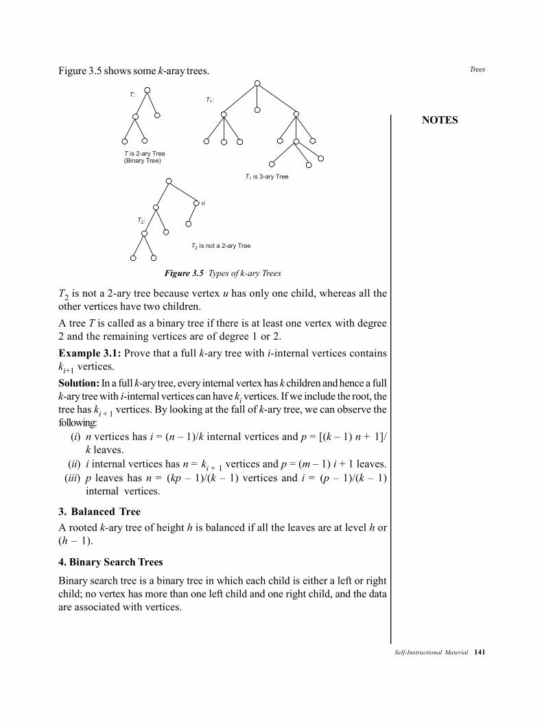
Trees
NOTES
Self-Instructional Material 141
Figure 3.5 shows some k-aray trees.
T2:
u
T:
T is 2-ary Tree(Binary Tree)
T1:
T1 is 3-ary Tree
T2 is not a 2-ary Tree
Figure 3.5 Types of k-ary Trees
T2 is not a 2-ary tree because vertex u has only one child, whereas all theother vertices have two children.
A tree T is called as a binary tree if there is at least one vertex with degree2 and the remaining vertices are of degree 1 or 2.
Example 3.1: Prove that a full k-ary tree with i-internal vertices containski+1 vertices.
Solution: In a full k-ary tree, every internal vertex has k children and hence a fullk-ary tree with i-internal vertices can have ki vertices. If we include the root, thetree has ki + 1 vertices. By looking at the fall of k-ary tree, we can observe thefollowing:
(i) n vertices has i = (n – 1)/k internal vertices and p = [(k – 1) n + 1]/k leaves.
(ii) i internal vertices has n = ki + 1 vertices and p = (m – 1) i + 1 leaves.(iii) p leaves has n = (kp – 1)/(k – 1) vertices and i = (p – 1)/(k – 1)
internal vertices.
3. Balanced Tree
A rooted k-ary tree of height h is balanced if all the leaves are at level h or(h – 1).
4. Binary Search Trees
Binary search tree is a binary tree in which each child is either a left or rightchild; no vertex has more than one left child and one right child, and the dataare associated with vertices.
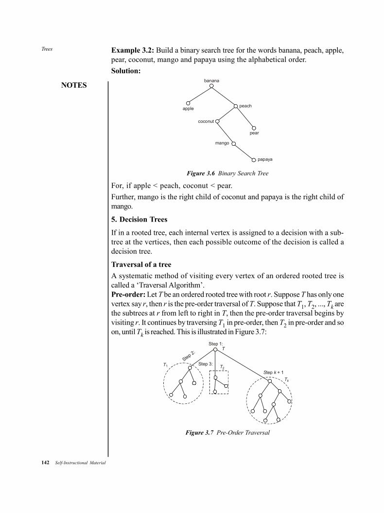
142 Self-Instructional Material
Trees
NOTES
Example 3.2: Build a binary search tree for the words banana, peach, apple,pear, coconut, mango and papaya using the alphabetical order.
Solution:
apple
banana
peach
pear
papaya
mango
coconut
Figure 3.6 Binary Search Tree
For, if apple < peach, coconut < pear.
Further, mango is the right child of coconut and papaya is the right child ofmango.
5. Decision Trees
If in a rooted tree, each internal vertex is assigned to a decision with a sub-tree at the vertices, then each possible outcome of the decision is called adecision tree.
Traversal of a tree
A systematic method of visiting every vertex of an ordered rooted tree iscalled a ‘Traversal Algorithm’.Pre-order: Let T be an ordered rooted tree with root r. Suppose T has only onevertex say r, then r is the pre-order traversal of T. Suppose that T1, T2, ..., Tk arethe subtrees at r from left to right in T, then the pre-order traversal begins byvisiting r. It continues by traversing T1 in pre-order, then T2 in pre-order and soon, until Tk is reached. This is illustrated in Figure 3.7:
T1 T2
Step 2:
Step 1:
Tk
S ktep + 1
Step 3:
T
Figure 3.7 Pre-Order Traversal
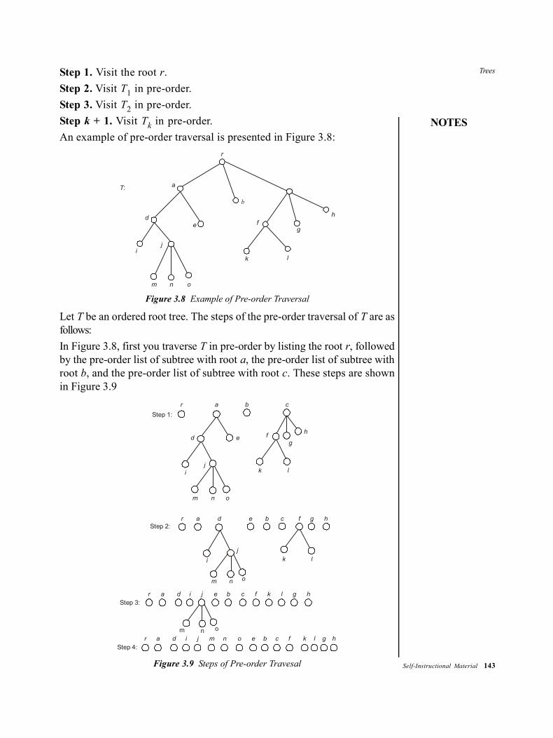
Trees
NOTES
Self-Instructional Material 143
Step 1. Visit the root r.
Step 2. Visit T1 in pre-order.
Step 3. Visit T2 in pre-order.
Step k + 1. Visit Tk in pre-order.
An example of pre-order traversal is presented in Figure 3.8:
T: a
r
d
ij
e
b
f
onm
h
g
lk
Figure 3.8 Example of Pre-order Traversal
Let T be an ordered root tree. The steps of the pre-order traversal of T are asfollows:
In Figure 3.8, first you traverse T in pre-order by listing the root r, followedby the pre-order list of subtree with root a, the pre-order list of subtree withroot b, and the pre-order list of subtree with root c. These steps are shownin Figure 3.9
r a b c
h
gf
k l
ed
ij
m n o
Step 1:
r a d e b c f g h
lk
onm
i
j
Step 2:
Step 3:r a d i j e b c f k l g h
onm
Step 4:r a d i j m n o e b c f k l g h
Figure 3.9 Steps of Pre-order Travesal
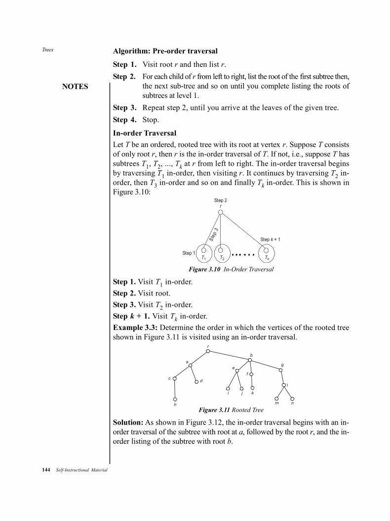
144 Self-Instructional Material
Trees
NOTES
Algorithm: Pre-order traversal
Step 1. Visit root r and then list r.
Step 2. For each child of r from left to right, list the root of the first subtree then,the next sub-tree and so on until you complete listing the roots ofsubtrees at level 1.
Step 3. Repeat step 2, until you arrive at the leaves of the given tree.
Step 4. Stop.
In-order Traversal
Let T be an ordered, rooted tree with its root at vertex r. Suppose T consistsof only root r, then r is the in-order traversal of T. If not, i.e., suppose T hassubtrees T1, T2, ..., Tk at r from left to right. The in-order traversal beginsby traversing T1 in-order, then visiting r. It continues by traversing T2 in-order, then T3 in-order and so on and finally Tk in-order. This is shown inFigure 3.10:
Step 1T1 T2 Tk
Ste
p 3
Step + 1k
Step 2r
Figure 3.10 In-Order Traversal
Step 1. Visit T1 in-order.
Step 2. Visit root.
Step 3. Visit T2 in-order.
Step k + 1. Visit Tk in-order.
Example 3.3: Determine the order in which the vertices of the rooted treeshown in Figure 3.11 is visited using an in-order traversal.
h
c
a
d
r
b
f
e
i j k
m n
l
g
Figure 3.11 Rooted Tree
Solution: As shown in Figure 3.12, the in-order traversal begins with an in-order traversal of the subtree with root at a, followed by the root r, and the in-order listing of the subtree with root b.
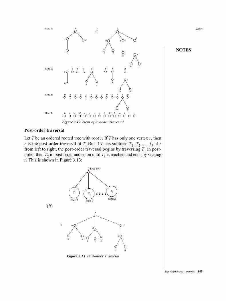
Trees
NOTES
Self-Instructional Material 145
c
h
d
a r b
e
i jk
fg
l
m n
Step 1:
Step 2: a d r e b f g
kjih
c
m n
l
Step 3:
Step 4: h c a d r i e j b k f m l n g
h c a d r i e j b k f l g
m n
Figure 3.12 Steps of In-order Traversal
Post-order traversal
Let T be an ordered rooted tree with root r. If T has only one vertex r, thenr is the post-order traversal of T. But if T has subtrees T1, T2, ..., Tk at rfrom left to right, the post-order traversal begins by traversing T1 in post-order, then T2 in post-order and so on until Tk is reached and ends by visitingr. This is shown in Figure 3.13:
Step kStep 2Step 1
T1 T2
Tk
r k Step +1
(ii)
T : a
d e
b
f g h
c
r
i
j k
Figure 3.13 Post-order Traversal
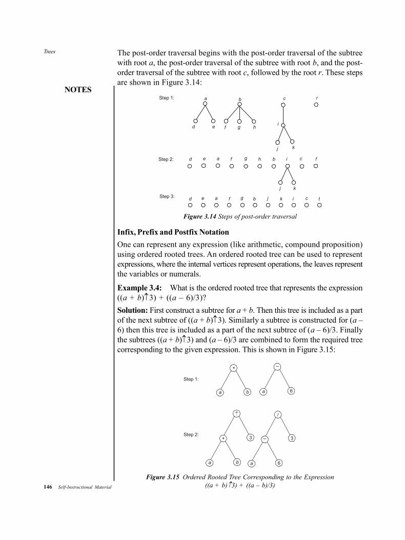
146 Self-Instructional Material
Trees
NOTES
The post-order traversal begins with the post-order traversal of the subtreewith root a, the post-order traversal of the subtree with root b, and the post-order traversal of the subtree with root c, followed by the root r. These stepsare shown in Figure 3.14:
Step 1: a
d e f g h
cb
i
j k
r
Step 2: d e fa g h b i c f
j k
d e a f g b ikj c tStep 3:
Figure 3.14 Steps of post-order traversal
Infix, Prefix and Postfix Notation
One can represent any expression (like arithmetic, compound proposition)using ordered rooted trees. An ordered rooted tree can be used to representexpressions, where the internal vertices represent operations, the leaves representthe variables or numerals.
Example 3.4: What is the ordered rooted tree that represents the expression((a + b)3) + ((a – 6)/3)?
Solution: First construct a subtree for a + b. Then this tree is included as a partof the next subtree of ((a + b)3). Similarly a subtree is constructed for (a –6) then this tree is included as a part of the next subtree of (a – 6)/3. Finallythe subtrees ((a + b)3) and (a – 6)/3 are combined to form the required treecorresponding to the given expression. This is shown in Figure 3.15:
Step 1:
+ –
a b a 6
/
+ 3 – 3
ba a 6
Step 2:
Figure 3.15 Ordered Rooted Tree Corresponding to the Expression((a + b)3) + ((a – b)/3)
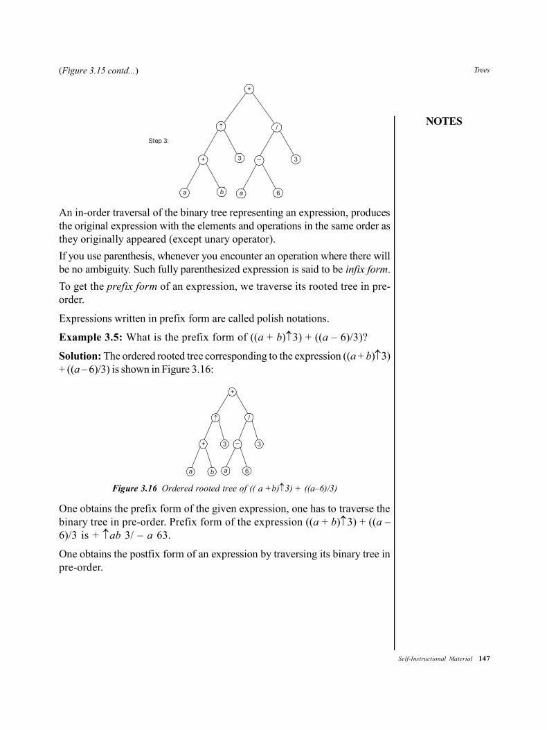
Trees
NOTES
Self-Instructional Material 147
(Figure 3.15 contd...)
Step 3:
+
/
3+ – 3
6aba
An in-order traversal of the binary tree representing an expression, producesthe original expression with the elements and operations in the same order asthey originally appeared (except unary operator).
If you use parenthesis, whenever you encounter an operation where there willbe no ambiguity. Such fully parenthesized expression is said to be infix form.
To get the prefix form of an expression, we traverse its rooted tree in pre-order.
Expressions written in prefix form are called polish notations.
Example 3.5: What is the prefix form of ((a + b)3) + ((a – 6)/3)?
Solution: The ordered rooted tree corresponding to the expression ((a + b)3)+ ((a – 6)/3) is shown in Figure 3.16:
+
/
+ 3 – 3
6aba
Figure 3.16 Ordered rooted tree of (( a +b)3) + ((a–6)/3)
One obtains the prefix form of the given expression, one has to traverse thebinary tree in pre-order. Prefix form of the expression ((a + b)3) + ((a –6)/3 is + ab 3/ – a 63.
One obtains the postfix form of an expression by traversing its binary tree inpre-order.
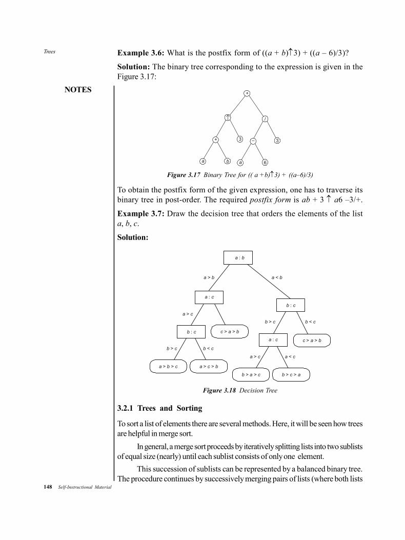
148 Self-Instructional Material
Trees
NOTES
Example 3.6: What is the postfix form of ((a + b)3) + ((a – 6)/3)?
Solution: The binary tree corresponding to the expression is given in theFigure 3.17:
+
–3+ 3
a b a 6
/
Figure 3.17 Binary Tree for (( a +b)3) + ((a–6)/3)
To obtain the postfix form of the given expression, one has to traverse itsbinary tree in post-order. The required postfix form is ab + 3 a6 –3/+.
Example 3.7: Draw the decision tree that orders the elements of the lista, b, c.
Solution:
a b:
a c:
b c :
b c : c a b > >
a c : c a b > >
b c a > > b a c > >
a c b > > a b c > >
a b> a b<
a c >
b c > b c <
b c > b c <
a c > a c <
Figure 3.18 Decision Tree
3.2.1 Trees and Sorting
To sort a list of elements there are several methods. Here, it will be seen how treesare helpful in merge sort.
In general, a merge sort proceeds by iteratively splitting lists into two sublistsof equal size (nearly) until each sublist consists of only one element.
This succession of sublists can be represented by a balanced binary tree.The procedure continues by successively merging pairs of lists (where both lists
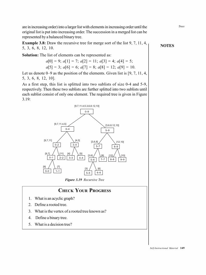
Trees
NOTES
Self-Instructional Material 149
are in increasing order) into a larger list with elements in increasing order until theoriginal list is put into increasing order. The succession in a merged list can berepresented by a balanced binary tree.
Example 3.8: Draw the recursive tree for merge sort of the list 9, 7, 11, 4,5, 3, 6, 8, 12, 10.
Solution: The list of elements can be represented as:
a[0] = 9; a[1] = 7; a[2] = 11; a[3] = 4; a[4] = 5;
a[5] = 3; a[6] = 6; a[7] = 8; a[8] = 12; a[9] = 10.
Let us denote 0–9 as the position of the elements. Given list is [9, 7, 11, 4,5, 3, 6, 8, 12, 10].
As a first step, this list is splitted into two sublists of size 0-4 and 5-9,respectively. Then these two sublists are further splitted into two sublists untileach sublist consist of only one element. The required tree is given in Figure3.19:
[9,7,11,4,5,3,6,8,12,10]
0–9
[9,7,11,4,5]
0–4 5–9
[3,6,8,12,10]
[9,7,11]
0–2 3–4
[4,5] [3,6,8]
5–7
[12,10]
8–9
[9,7]
0–1 2–2 3–3 4–4
[11] [4] [5]
5–6 7–7 8–8 9–9
[3,6] [8] [12] [10]
[9]
0–0 1–1
[7][3] [6]
5–5 6–6
Figure 3.19 Recursive Tree
CHECK YOUR PROGRESS
1. What is an acyclic graph?
2. Define a rooted tree.
3. What is the vertex of a rooted tree known as?
4. Define a binary tree.
5. What is a decision tree?
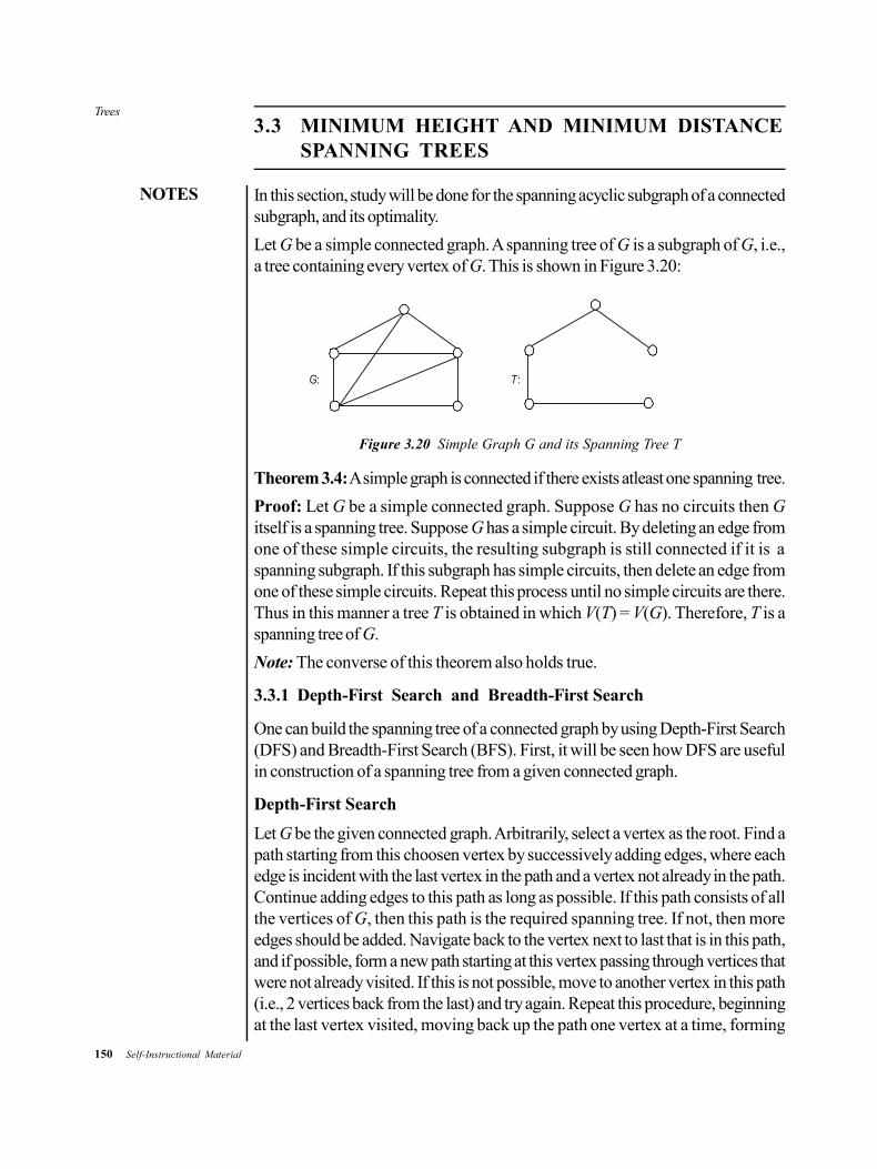
150 Self-Instructional Material
Trees
NOTES
3.3 MINIMUM HEIGHT AND MINIMUM DISTANCESPANNING TREES
In this section, study will be done for the spanning acyclic subgraph of a connectedsubgraph, and its optimality.
Let G be a simple connected graph. A spanning tree of G is a subgraph of G, i.e.,a tree containing every vertex of G. This is shown in Figure 3.20:
G: T :
Figure 3.20 Simple Graph G and its Spanning Tree T
Theorem 3.4: A simple graph is connected if there exists atleast one spanning tree.
Proof: Let G be a simple connected graph. Suppose G has no circuits then Gitself is a spanning tree. Suppose G has a simple circuit. By deleting an edge fromone of these simple circuits, the resulting subgraph is still connected if it is aspanning subgraph. If this subgraph has simple circuits, then delete an edge fromone of these simple circuits. Repeat this process until no simple circuits are there.Thus in this manner a tree T is obtained in which V(T) = V(G). Therefore, T is aspanning tree of G.
Note: The converse of this theorem also holds true.
3.3.1 Depth-First Search and Breadth-First Search
One can build the spanning tree of a connected graph by using Depth-First Search(DFS) and Breadth-First Search (BFS). First, it will be seen how DFS are usefulin construction of a spanning tree from a given connected graph.
Depth-First Search
Let G be the given connected graph. Arbitrarily, select a vertex as the root. Find apath starting from this choosen vertex by successively adding edges, where eachedge is incident with the last vertex in the path and a vertex not already in the path.Continue adding edges to this path as long as possible. If this path consists of allthe vertices of G, then this path is the required spanning tree. If not, then moreedges should be added. Navigate back to the vertex next to last that is in this path,and if possible, form a new path starting at this vertex passing through vertices thatwere not already visited. If this is not possible, move to another vertex in this path(i.e., 2 vertices back from the last) and try again. Repeat this procedure, beginningat the last vertex visited, moving back up the path one vertex at a time, forming

Trees
NOTES
Self-Instructional Material 151
new long paths until no more edges can be added. This process ends with aspanning tree.
When this procedure returns to the vertices previously visited, it is alsocalled as backtracking.
Example 3.9: Construct a spanning tree for the graph G which is shown in Figure3.21.
a b c
d f
e
G:
Figure 3.21 Graph G
Solution: First, arbitrarily choose a vertex, say e as the root. Form a pathat e, i.e., cdf is the path. Backtrack to d. Form a path beginning at d in such a waythat it has to visit the vertices which where not visited in the previous path, d e b a.Since all the vertices of G are visited, this procedure gives the spanning tree T,which is shown in Figure 3.22.
ab
T
c d f
Figure 3.22 Spanning Tree T of Graph G
Breadth-First Search
First, choose a vertex arbitrarily as the root. Add the edges of G which are incidentwith this vertex. The new vertices added at this stage becomes level 1 in thespanning tree. Order these vertices arbitrarily. Next, for each vertex at level 1visited in order, add each edge incident to this vertex to the tree as long as itdoes not- create a simple circuit. Order the children of each vertex at level 1arbitrarily. This produces the vertices at level 2 in the tree. Continue in this manneruntil all the vertices of G have been added. Ultimately a spanning tree, is created.
Example 3.10: Construct a spanning tree of the graph G. Which is shown inFigure 3.23:
e1
a
c e
f
db
e4
e3
e5
e6
e7
e8
e9
e2
Figure 3.23 Graph G
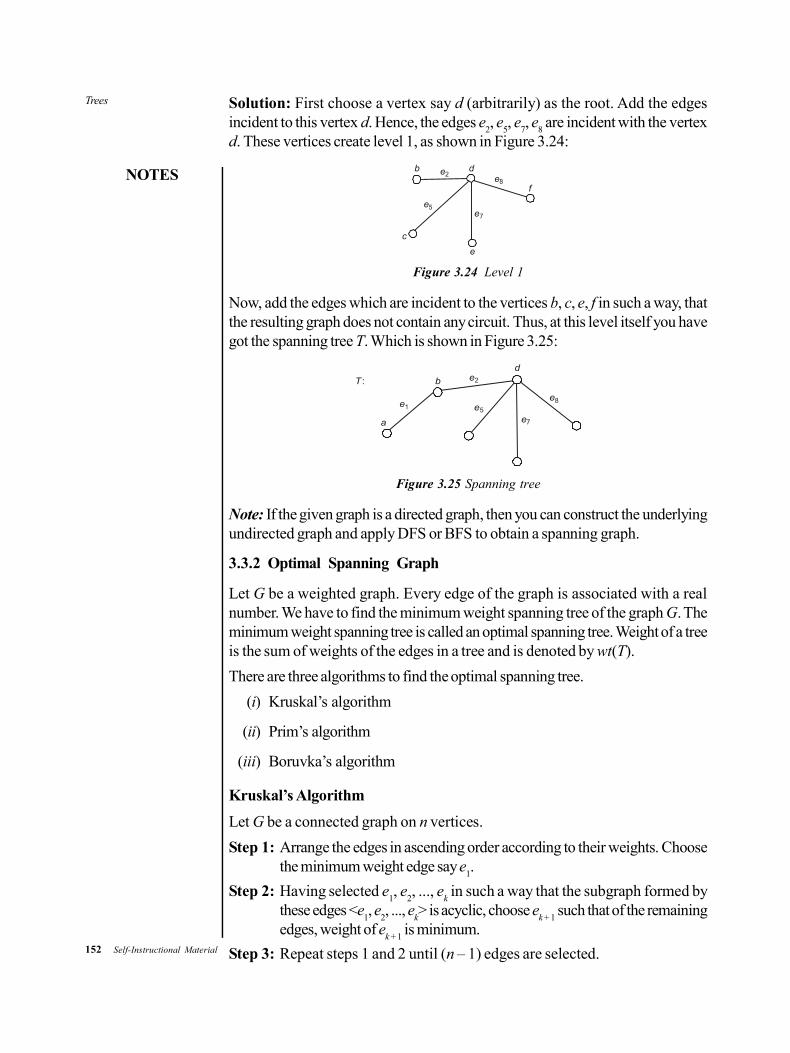
152 Self-Instructional Material
Trees
NOTES
Solution: First choose a vertex say d (arbitrarily) as the root. Add the edgesincident to this vertex d. Hence, the edges e
2, e
5, e
7, e
8 are incident with the vertex
d. These vertices create level 1, as shown in Figure 3.24:
b d
f
e
c
e2
e7
e8
e5
Figure 3.24 Level 1
Now, add the edges which are incident to the vertices b, c, e, f in such a way, thatthe resulting graph does not contain any circuit. Thus, at this level itself you havegot the spanning tree T. Which is shown in Figure 3.25:
a
b
d
e1
e2
e5
e7
e8
T :
Figure 3.25 Spanning tree
Note: If the given graph is a directed graph, then you can construct the underlyingundirected graph and apply DFS or BFS to obtain a spanning graph.
3.3.2 Optimal Spanning Graph
Let G be a weighted graph. Every edge of the graph is associated with a realnumber. We have to find the minimum weight spanning tree of the graph G. Theminimum weight spanning tree is called an optimal spanning tree. Weight of a treeis the sum of weights of the edges in a tree and is denoted by wt(T).
There are three algorithms to find the optimal spanning tree.
(i) Kruskal’s algorithm
(ii) Prim’s algorithm
(iii) Boruvka’s algorithm
Kruskal’s Algorithm
Let G be a connected graph on n vertices.
Step 1: Arrange the edges in ascending order according to their weights. Choosethe minimum weight edge say e
1.
Step 2: Having selected e1, e
2, ..., e
k in such a way that the subgraph formed by
these edges <e1, e
2, ..., e
k> is acyclic, choose e
k + 1 such that of the remaining
edges, weight of ek + 1
is minimum.
Step 3: Repeat steps 1 and 2 until (n – 1) edges are selected.
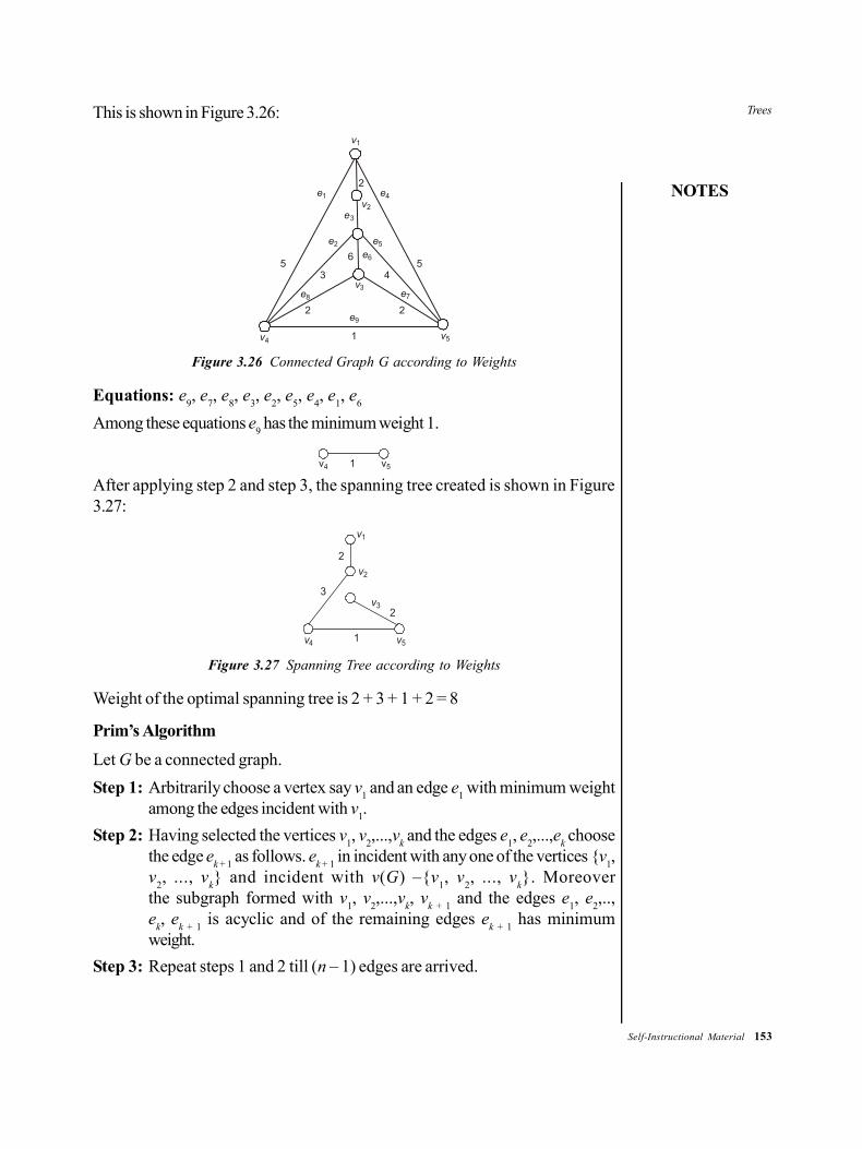
Trees
NOTES
Self-Instructional Material 153
This is shown in Figure 3.26:
v5v4
v1
e4v2
v3
e3
e1
e6
e7e8
e2 e5
5 56
3 4
e9
1
2
2 2
Figure 3.26 Connected Graph G according to Weights
Equations: e9, e
7, e
8, e
3, e
2, e
5, e
4, e
1, e
6
Among these equations e9 has the minimum weight 1.
v4 v51
After applying step 2 and step 3, the spanning tree created is shown in Figure3.27:
v1
v2
v4 v5
v32
1
3
2
Figure 3.27 Spanning Tree according to Weights
Weight of the optimal spanning tree is 2 + 3 + 1 + 2 = 8
Prim’s Algorithm
Let G be a connected graph.
Step 1: Arbitrarily choose a vertex say v1 and an edge e
1 with minimum weight
among the edges incident with v1.
Step 2: Having selected the vertices v1, v
2,...,v
k and the edges e
1, e
2,...,e
k choose
the edge ek + 1
as follows. ek + 1
in incident with any one of the vertices {v1,
v2, ..., v
k} and incident with v(G) –{v
1, v
2, ..., v
k}. Moreover
the subgraph formed with v1, v
2,...,v
k, v
k + 1 and the edges e
1, e
2,..,
ek, e
k + 1 is acyclic and of the remaining edges e
k + 1 has minimum
weight.
Step 3: Repeat steps 1 and 2 till (n – 1) edges are arrived.

154 Self-Instructional Material
Trees
NOTES
This is shown in Figure 3.28:
v1
v2
v3
v4 v51
22
3 4
6
55
Figure 3.28 Connected Graph n according to Prim’s Algorithm
Step 1: Choose arbitrarily vertex v3 and apply step 2 and step 3. Now, you will
get the spanning trees. Which are shown in Figure 3.29:
v4
v2
2
v4 v5
v2
2
1
v4 v5
v3
v2
3
2
1
v1
v2
v3
v5v4
1
23
2
Figure 3.29 Spanning Trees according to Prim’s Algorithm
So the final weight of the spanning tree is 8.
Boruvka’s Algorithm
Boruvka’s algorithm finds a minimum spanning tree in a weighted graph. Boruvkadeveloped this for constructing an efficient electrical network.
Every vertex in the graph finds its lightest edge, and then the vertices at theends of each lightest edge are marked. This process goes and the entire graphcollapses into a single point. The tree consists of all the lightest edges are so found.
The algorithm starts by examining every vertex one-by-one and selectingthe cheapest edge from that vertex to another in the graph, without regard about
Trees
NOTES
Self-Instructional Material 155
the already added edges. It continues joining these groupings in a similar mannerand a tree spanning all vertices is formed.
Every vertex or set of connected vertices is termed as a ‘component’. Thepseudocode for this algorithm is given as follows:
1. Start with a connected graph G containing edges of distinct weights, and anempty set of edges T.
2. While vertices of G connected by T are disjoint, Start with an empty set of edges E. For each edge in the component,
– Start with an empty set of edges S.
For each vertex in the component,
– Add the cheapest edge from the vertex in the component toanother vertex in a disjoint component to S.
– Add the cheapest edge in S to E.
– Add the resulting set of edges E to T.
3. The resulting set of edges T is the minimum spanning tree of G.
Boruvka’s algorithm takes O(log V) iterations of the outer loop beforetermination, and runs in time O(Elog V), where E is the number of edges, and V isthe number of vertices in G.
Faster algorithms can be obtained by combining Prim’s algorithm withBoruvka’s.
CHECK YOUR PROGRESS
6. Define an optimal spanning tree.
7. What is the weight of a tree?
8. What is the working of the Boruvka’s algorithm?
9. Define a ‘component’.
3.4 PLANAR GRAPHS
A graph G is said to be planar if a geometric representation of G exists, whichcan be drawn on a plane such that no two of its edges intersect (‘meeting’ of edgesat a vertex is not considered an intersection). A graph that cannot be drawn on aplane without a cross over between its edges is called a non-planar graph. Adrawing of a geometric representation of a graph on any surface such that noedges intersect is called embedding.
Some planar graphs are presputed in Figure 3.30.
Note: To show a that graph G is nonplanar you have to prove that all the possiblegeometric representations of G, cannot be embedded in a plane.
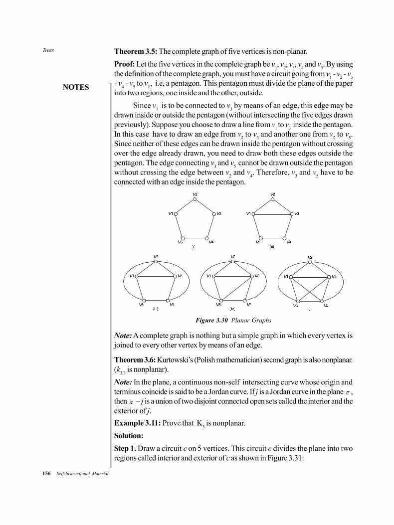
156 Self-Instructional Material
Trees
NOTES
Theorem 3.5: The complete graph of five vertices is non-planar.
Proof: Let the five vertices in the complete graph be v1, v
2, v
3, v
4 and v
5. By using
the definition of the complete graph, you must have a circuit going from v1 - v
2 - v
3
- v4 - v
5 to v
1, i.e, a pentagon. This pentagon must divide the plane of the paper
into two regions, one inside and the other, outside.
Since v1 is to be connected to v
3 by means of an edge, this edge may be
drawn inside or outside the pentagon (without intersecting the five edges drawnpreviously). Suppose you choose to draw a line from v
1 to v
3 inside the pentagon.
In this case have to draw an edge from v2 to v
3 and another one from v
2 to v
5.
Since neither of these edges can be drawn inside the pentagon without crossingover the edge already drawn, you need to draw both these edges outside thepentagon. The edge connecting v
3 and v
5 cannot be drawn outside the pentagon
without crossing the edge between v2 and v
4. Therefore, v
3 and v
5 have to be
connected with an edge inside the pentagon.
v
v v
v v
v
v v
v v
v
v v
v v
v
v v
v v
v
v v
v v
Figure 3.30 Planar Graphs
Note: A complete graph is nothing but a simple graph in which every vertex isjoined to every other vertex by means of an edge.
Theorem 3.6: Kurtowski’s (Polish mathematician) second graph is also nonplanar.(k
3,3 is nonplanar).
Note: In the plane, a continuous non-self intersecting curve whose origin andterminus coincide is said to be a Jordan curve. If j is a Jordan curve in the plane ,then – j is a union of two disjoint connected open sets called the interior and theexterior of j.
Example 3.11: Prove that K5 is nonplanar.
Solution:
Step 1. Draw a circuit c on 5 vertices. This circuit c divides the plane into tworegions called interior and exterior of c as shown in Figure 3.31:

Trees
NOTES
Self-Instructional Material 157
V1
V2 V5
V4V3
Figure 3.31 Circuit C
Step 2. Draw the edges v1v
3, v
1v
4 in the interior as shown in Figure 3.32. You
cannot draw any more edge in the interior of c, without intersecting any edge.V1
V2 V5
V4V3
Figure 3.32 Circuit c with edges in the interior
Now, draw the edges v2v
5, v
2v
4 in the exterior of c as shown in Figure
3.33. But the edge v3v
5 cannot be drawn in the interior or exterior of c, without
intersecting the edge of c.
V1
V2 V5
V3 V4
Figure 3.33 Circuit c with interior and exterior edges
Thus, k5 is nonplanar.
In addition, you can prove that k3, 3 is nonplanar in the following manner:
Assume that k3,3
is planar. Let the vertex of k3,3
is {v1,...,v
6}.
Let
P = {v1, v
3, v
5} and Q = {v
2, v
4, v
6}.
Let C be the cycle v1 v
2 v
3 v
4 v
5 v
6 v
1. It is a Jordan curve. The other three
edges v1v
4, v
2v
5, v
3v
6 are chords of the cycle C. So, either the interior of C or
exterior of C contains two of these three chords. Say there are two chords in Intc. These two chords must cross each other, which is a contradiction, hence k
3,3 is
nonplanar.
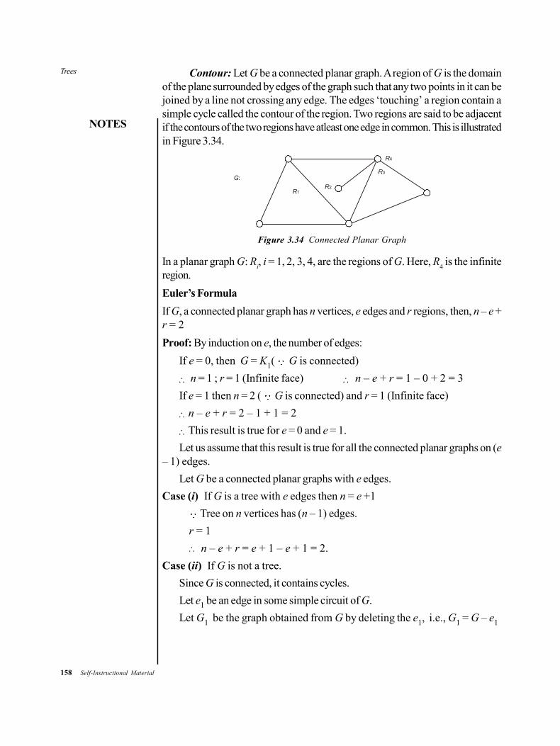
158 Self-Instructional Material
Trees
NOTES
Contour: Let G be a connected planar graph. A region of G is the domainof the plane surrounded by edges of the graph such that any two points in it can bejoined by a line not crossing any edge. The edges ‘touching’ a region contain asimple cycle called the contour of the region. Two regions are said to be adjacentif the contours of the two regions have atleast one edge in common. This is illustratedin Figure 3.34.
R2R1
R3
R4
G:
Figure 3.34 Connected Planar Graph
In a planar graph G: Ri, i = 1, 2, 3, 4, are the regions of G. Here, R
4 is the infinite
region.
Euler’s Formula
If G, a connected planar graph has n vertices, e edges and r regions, then, n – e +r = 2
Proof: By induction on e, the number of edges:
If e = 0, then G = K1( G is connected)
n = 1 ; r = 1 (Infinite face) n – e + r = 1 – 0 + 2 = 3
If e = 1 then n = 2 ( G is connected) and r = 1 (Infinite face)
n – e + r = 2 – 1 + 1 = 2
This result is true for e = 0 and e = 1.
Let us assume that this result is true for all the connected planar graphs on (e– 1) edges.
Let G be a connected planar graphs with e edges.
Case (i) If G is a tree with e edges then n = e +1
Tree on n vertices has (n – 1) edges.
r = 1
n – e + r = e + 1 – e + 1 = 2.
Case (ii) If G is not a tree.
Since G is connected, it contains cycles.
Let e1 be an edge in some simple circuit of G.
Let G1 be the graph obtained from G by deleting the e1, i.e., G1 = G – e1
Trees
NOTES
Self-Instructional Material 159
Now, number of vertices in G1 = n
Number of edges in G1 = e–1
Number of regions in G1 = r–1
Since G1 has less then e edges, the result is true for G1 also.
By induction hypothesis, n1– e1+r1 = 2, where n1 is the number of vertices,e1 is the number of edges and r1 is the number of regions of G1 respectively.
n–(e–1) + r–1 = 2 n – e + r = 2.
In all these cases, the result in true.
Corollary: If G is a connected simple planar graph without loops and has nvertices, e 2 edges and r regions, then 3/2 r e 3n–6.
Proof: If r = 1 then 3/2 e 3n – 6 is true, since e 2.
If r > 1. Let k be the number of edges in the contours of the finite regions.
Since G is simple, each region (finite) is bounded by atleast 3 edges.
Therefore k 3 (r – 1) ...(3.4)
But, in a planar graph, an edge belongs to the contours of atmost two regionsand atleast 3 edges touch the infinite region.
k 2e – 3 ...(3.5)
From equations (3.4) and (3.5), 3r–3 k 2e–3
3r – 3 2e – 3
3r 2e 3/2 r e ...(3.6)
Since G is planar, n – e + r = 2, by Euler’s Formula.
n – e + 2/3 e 2 [ From equation (3.10) r 2/3 e]
3n – 3e + 2e6
– e – 3n + 6
e 3n – 6 ...(3.7)
From equations (3.6) and (3.7), 3/2r e 3n – 6
Example 3.12: Prove that K5 is nonplanar.
Solution: Suppose K5 is planar, then by the above corollory, e 3n – 6. In K5 n= 5, e = 10;
10 3 × 5 – 6 = 9, which is absurd. K5 is nonplanar..
Remark: K5, K3,3 are called Kuratowski’s first graph, second graph respectively.
Corollary: If G is a simple connected planar graph on n vertices, e edges and rregions and does not contain any triangle, then 2r e (2n – 4).

160 Self-Instructional Material
Trees
NOTES
Subdivision: A subdivision of a graph G is obtained by inserting vertices ofdegree 2 into the edges of G, as shown in Figure 3.35:
G: H:
Figure 3.35 Subdivision of Graph G
H is the subdivsision of G.
Kuratowski theorem: A graph is planar if it contains no subgraph that is isomorphicor is a subdivision of K
5 or K
3,3.
CHECK YOUR PROGRESS
10. What is a non-planar graph?
11. Define a complete graph?
3.5 SUMMARY
In this unit, you have learned that:
In graph theory, a tree refers to a graph in which two vertices are attachedby only one path.
Trees are generally open graphs.
In a tree, every edge is a cut-edge.
Traversal algorithm refers to the systematic method for visiting every vertexof an ordered rooted tree.
Arithmetic expression and compound proposition can be represented byusing ordered rooted trees.
A merge sort proceeds by repeatedly splitting lists into two sub-lists ofequal size (nearly) to a point such that each sub-list consists of only oneelement.
A spanning tree of a connected graph using either of the two methods:o Depth-First Search (DFS)o Breadth-First Search (BFS)
A graph G is considered to be planar if there exists some geometricrepresentation of G which can be drawn on a plane in such a manner thatno two of its edges intersect (‘meeting’ of edges at a vertex is not consideredan intersection).
Euler’s Formula states that in case G, a connected planar graph has n vertices,e edges and r regions, then, n – e + r = 2
Trees
NOTES
Self-Instructional Material 161
3.6 KEY TERMS
Tree: A connected acyclic graph G is called a tree.
Vertex: It refers to a point of intersection in any diagram containing two ormore edges.
Rooted tree: In a directed tree a particular vertex is called a root if thatvertex is of degree zero.
Balanced tree: A rooted k-ary tree of height h is balanced if all the leavesare at level h or (h – 1).
3.7 ANSWERS TO ‘CHECK YOUR PROGRESS’
1. A graph G, which has no cycles is called an acyclic graph.
2. A tree together with its root produces a graph called a rooted tree.
3 A vertex of a rooted tree is known as a leaf.
4. A tree is called as a binary tree if there is at least one vertex with degree 2and the remaining vertices are of degree 1 or 2.
5. If in a rooted tree, each internal vertex is assigned to a decision with a sub-tree at the vertices, then each possible outcome of the decision is called adecision tree.
6. The minimum weight spanning tree is called an optimal spanning tree.
7. The weight of a tree is the sum of weights of the edges in the tree and isdenoted by wt(T).
8. Boruvka’s algorithm finds a minimum spanning tree in a weighted graph.
9. Every vertex or set of connected vertices is termed as a ‘component’.
10 A graph that cannot be drawn on a plane without a cross-over between itsedges is called a non-planar graph.
11 A complete graph is nothing but a simple graph in which every vertex isjoined to every other vertex by means of an edge.
3.8 QUESTIONS AND EXERCISES
Short-Answer Questions
1. Briefly explain how trees are helpful in the process of merge sort.
2. State the three types of algorithms used to find the optimal spanning tree.
3. What is a fundamental circuit?
4. Diagrammatically state what a contour.
162 Self-Instructional Material
Trees
NOTES
Long-Answer Questions
1. In a graph theory, prove that G has (n-1) edges, if G is a tree with n numberof vertices.
2. Explain the concept of traversal of a tree.
3. Discuss the algorithms used to find optimal spanning trees.
4. ‘The complete graph of five vertices is non-planar.’ Prove it.
3.9 FURTHER READING
Lipschutz, Seymour and Lipson Marc. Schaum’s Outline of DiscreteMathematics, 3rd edition. New York: McGraw-Hill, 2007.
Horowitz, Ellis, Sartaj Sahni and Sanguthevar Rajasekaran. Fundamentals ofComputer Algorithms. Hyderabad: Orient BlackSwan, 2008.
Cormen, Thomas H., Charles E. Leiserson, Ronald L. Rivest and Clifford Stein.Introduction to Algorithms. The MIT Press, 1990.
Brassard, Gilles and Paul Bratley. Fundamentals of Algorithms. New Delhi:Prentice Hall of India, 1995.
Levitin, Anany. Introduction to the Design and Analysis of Algorithms. NewJersey: Pearson, 2006.
Baase, Sara and Allen Van Gelder. Computer Algorithms – Introduction toDesign and Analysis. New Jersey: Pearson, 2003.
Mott, J.L. Discrete Mathematics for Computer Scientists, 2nd edition. NewDelhi: Prentice-Hall of India Pvt. Ltd., 2007.
Liu, C.L. Elements of Discrete Mathematics. New Delhi: Tata McGraw-HillPublishing Company, 1977.
Rosen, Kenneth. Discrete Mathematics and Its Applications, 6th edition. NewYork: McGraw-Hill Higher Education, 2007.
Recursion
NOTES
Self-Instructional Material 163
UNIT 4 RECURSION
Structure
4.0 Introduction4.1 Unit Objectives4.2 Mergesort4.3 Insertion Sort4.4 Bubble Sort and Selection Sort
4.4.1 Bubble Sort4.4.2 Selection Sort
4.5 Binary and Decimal Numbers4.5.1 Binary Number System4.5.2 Decimal Number System4.5.3 Binary to Decimal Conversion4.5.4 Decimal to Binary Conversion4.5.5 Double-Dabble Method4.5.6 Decimal Fraction to Binary
4.6 Recursion and Recurrence Relations4.6.1 Recursion and Iteration4.6.2 Closed Form Expression4.6.3 Sequence of Integers4.6.4 Recurrence Relations4.6.5 Linear Homogenous Recurrence Relations (LHRR)4.6.6 Solving Linear Homogeneous Recurrence Relations4.6.7 Solving Linear Non-Homogeneous Recurrence Relations4.6.8 Linear Homogeneous Recurrence Relations with Constant Coefficient
(LHRRWCC)4.6.9 Divide and Conquer Recurrence Relation (DCRR)
4.7 Recursive Procedures4.7.1 Functional Recursion4.7.2 Recursive Proofs4.7.3 The Recursion Theorem4.7.4 Infinite Sequences4.7.5 Recursive Function and Primitive Recursive Function
4.8 Summary4.9 Key Terms
4.10 Answers to ‘Check Your Progress’4.11 Questions and Exercises4.12 Further Reading
4.0 INTRODUCTION
Recursion is a concept prevalent in mathematics and computer science. It is amethod of defining functions in which the function being defined is applied withinits own definition. This specifically means defining an infinite statement using finitecomponents. The term is also used more generally to describe a process of repeatingobjects in a self-similar way. For instance, when the surfaces of two mirrors are
164 Self-Instructional Material
Recursion
NOTES
exactly parallel with each other, the nested images that occur are a form of infiniterecursion.
This in plain English means that recursion is the process a procedure goesthrough when one of the steps of that procedure involves re-running the procedure.A procedure that goes through recursion is recursive, that is, if one of the stepsthat makes up the procedure calls for a new running of the procedure. A recursiveprocedure must complete each of all its steps. Even if a new running is called for inone of its steps, each running must run through the remaining steps.
In this unit, you will learn about merge sort, insertion sort, bubble sort andselection sort, binary and decimal numbers, recursion and recurrent relations andrecursive procedures.
4.1 UNIT OBJECTIVES
After going through this unit, you will be able to:
Understand the concepts of merge sort, bubble sort, insertion sort andselection sort
Describe binary and decimal numbers
Convert binary numbers to decimal numbers and vice versa
Explain the concepts of recursion and recurrence relations
Describe the various features of recursive procedures
4.2 MERGESORT
The Mergesort algorithm basically works according to a divide and conquerstrategy in which the sequence is divided into two halves. Each half is independentlysorted and then both halves are merged to make a combine sequence. In thisprocess, the validity of input data required in Mergesort is as follows:
Check the input sequences. If there is only one element then theMergesort operation is not performed.
The input sequences are separated into two halves.
Sort the input sequences.
Merge both sorted input sequences to generate the result.
In the merging process, the elements of two arrays are combined, creatinga new array. The algorithm is based on the merging process where all the elementsare copied in one array and kept in the separate new array. Then it adds thesecond array to the new array. After combining the sorted array a Mergesortarray is created. For example, the two arrays A[5] and B[3] are manipulatedand then merged to create a new array. The newly created array, namely C, willhave 5+3=8 elements. The required steps are as follows:
Recursion
NOTES
Self-Instructional Material 165
Compare the very first elements of both A[0] and B[0]. If A[0] <B[0] then the value of A[0] is shifted to C[0]. Then the size of botharrays [Arrays A and C] current pointers are increased by one.
The elements of array A and array B are compared where the pointers arepointing, that is, the first element of array A and the null element of B, i.e.,A[1] and B [0].
If B[0]<A[1] then B[0] is moved to C[1]. The current pointer of B isincremented to point the next element in array B.
The following algorithm checks the sequences of validation of arrays:Function Mergesort(M1, M2)
{
list A Empty
while (neither M1 nor M2)
{
compare first items of M1 and M2
remove smaller of the M1 and M2 from the list
add to end of A
}
catenate remaining list to end of A
return A
}
Mergesort problem: Sort a sequence of given n elements in a non-decreasingway. It follows the DCC mechanism that represents Divide, Conquer and Combine:
Divide: Divides the n element sequence that is sorted into two subsequences ofn/2 elements.
Conquer: Sorts by using Mergesort the two recursive subsequences.
Combine: Merges both subsequences to produce the sorted result.
The required steps in the Mergesort algorithm are as follows:
Input: Sort a sequence of n numbers that is stored in an array.
Output: Produce an ordered sequence of n numbers.
The following algorithm is applied in mergesort mechanism:Mergesort(A,m,n) //It sorts A[m…n] by divide and conquermethod
Step 1: if m<n
Step 2: then r[(m+n)/2]
Step 3: Mergesort (A,m,r)
Step 4: Mergesort (A, r+1, n)
Step 5: Merge(A,m,n,r) //This step merges A[m…n] withA[r+1…n]
Merge (A,m,n,p)

166 Self-Instructional Material
Recursion
NOTES
Step 1: n1n – m+1
Step 2: n2p – n
Step 3: for i 1 to n1
Step 4: do L[i] A[m+i–1]
Step 5: for j 1 to n2
Step 6: do R[j] A[n+j]
Step 7: L[n1+1] Step 8: R[n2+1] Step 9: i1
Step 10: j1
Step 11: for km to p
Step 12: do if L[i]<=R[j]
Step 13: then A[k]L[i]
Step 14: i i+1
Step 15: else A[k] R[j]
Step 16: j j+1
In the above algorithm, L[i] and R[j] are the smallest elements of L andR that are not copied back into A. Figure 4.1 shows the Mergesort processthat is based on this algorithm:
j
6 8 26 32 1 9 42 43 … … A k
6 8 26 32 1 9 42 43
k k k k k k k
i i i i
i j j j j
6 8 26 32 1 9 42 43
1 6 8 9 26 32 42 43
L R
6 8 26 32 1 9 42 43 … … A 6 8 26 32 1 9 42 43
merge
m
p
Figure 4.1 Elements sorted [1, 6, 8, 9, 26, 32, 42, 43] using Mergesort
Analysis of Mergesort Algorithm
In Figure 4.2, an array A is taken in which there are eight elements. Theoperation of Mergesort on the array A is [5, 2, 4, 7, 1, 3, 2, 6]. The length ofthe sorted sequences is merged as the steps required in algorithm from bottom totop.
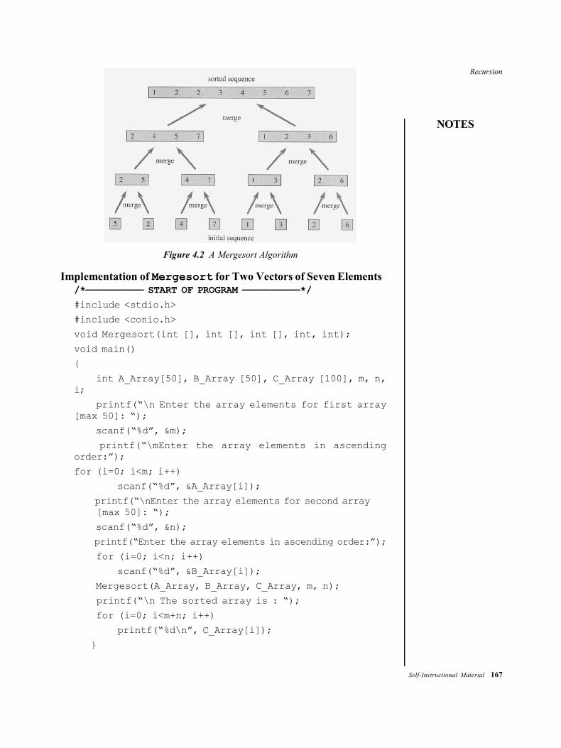
Recursion
NOTES
Self-Instructional Material 167
Figure 4.2 A Mergesort Algorithm
Implementation of Mergesort for Two Vectors of Seven Elements/*—————————— START OF PROGRAM ——————————*/
#include <stdio.h>
#include <conio.h>
void Mergesort(int [], int [], int [], int, int);
void main()
{
int A_Array[50], B_Array [50], C_Array [100], m, n,i;
printf(“\n Enter the array elements for first array[max 50]: “);
scanf(“%d”, &m);
printf(“\mEnter the array elements in ascendingorder:”);
for (i=0; i<m; i++)
scanf(“%d”, &A_Array[i]);
printf(“\nEnter the array elements for second array [max 50]: “);
scanf(“%d”, &n);
printf(“Enter the array elements in ascending order:”);
for (i=0; i<n; i++)
scanf(“%d”, &B_Array[i]);
Mergesort(A_Array, B_Array, C_Array, m, n);
printf(“\n The sorted array is : “);
for (i=0; i<m+n; i++)
printf(“%d\n”, C_Array[i]);
}

168 Self-Instructional Material
Recursion
NOTES
void Mergesort(int A_Array[], int B_Array[], int C_Array[],int m, int n)
{
int a_ele=0, b_ele=0, c_ele=0;
for (a_ele =0, b_ele=0, c_ele =0; a_ele<m && b_ele<n;)
{
if (A_Array[a_ele]< B_Array[b_ele])
//Check the elements of A_Array are less than elements ofB_Array
C_Array[c_ele++] = A_Array[a_ele++];
//Assign the values of C_Array in A_Array otherwise B_Array
else
C_Array[c_ele++] = B_Array [b_ele++];
}
if (a_ele<m)
while (a_ele<m)
C_Array[c_ele++] = A[a_ele++];
else
while (b_ele<n)
C_Array[c_ele++] = B_Array[b_ele++];
}
The arrays A_Array and B_Array are the input arrays that containelements in ascending order. Their sizes are m and n respectively. The C_Arrayis the output array containing the elements from the two combined arrays in sortedorder.
The result comes in the following way:Enter the array elements for first array [max 50]: 3
Enter the array elements in ascending order:
4
8
10
Enter the array elements for second array [max 50]:4
Enter the array elements in ascending order:
3
5
7
9

Recursion
NOTES
Self-Instructional Material 169
Output : The sorted array is:
3
4
5
7
8
9
10
4.3 INSERTION SORT
Insertion sort refers to a simple sorting algorithm. In it, the sorted array (or list) isbuilt one entry at a time. As compared to more advanced algorithms, such asquick sort, heap sort or merge sort, it is less efficient on large lists. However,insertion sort has many advantages, such as:
Its implementation is simple.
It is efficient for (quite) small data sets.
It is efficient for data sets that are already substantially sorted. The timecomplexity is O(n + d), where d is the number of inversions.
It is more efficient in practice as compared to most other simple quadratici.e., O(n2) algorithms, such as selection sort or bubble sort. The averagerunning time of insertion sort is n2/4. Further, in the best case scenario, therunning time is linear.
It is stable. In other words, it does not change the relative order of elementswith equal keys.
It is in place, i.e., it only requires a constant amount O(1) of additionalmemory space.
It is online, i.e., it can sort a list as it receives it.
Most people while sorting—ordering a deck of cards, for example—usethe insertion sort like method.
In abstract terms, each iteration of insertion sort removes an element fromthe input data and then inserts it into the correct position in the list that is alreadysorted. The process continues till all input elements are inserted. The element to beremoved from the input is chosen arbitrarily. Almost any choosen algorithm can beused for this.
Sorting is typically done in-place. The resulting array after k iterations hasthe property where the first k entries are sorted. In each iteration, the first remainingentry of the input is removed, inserted into the result at the correct position, thus
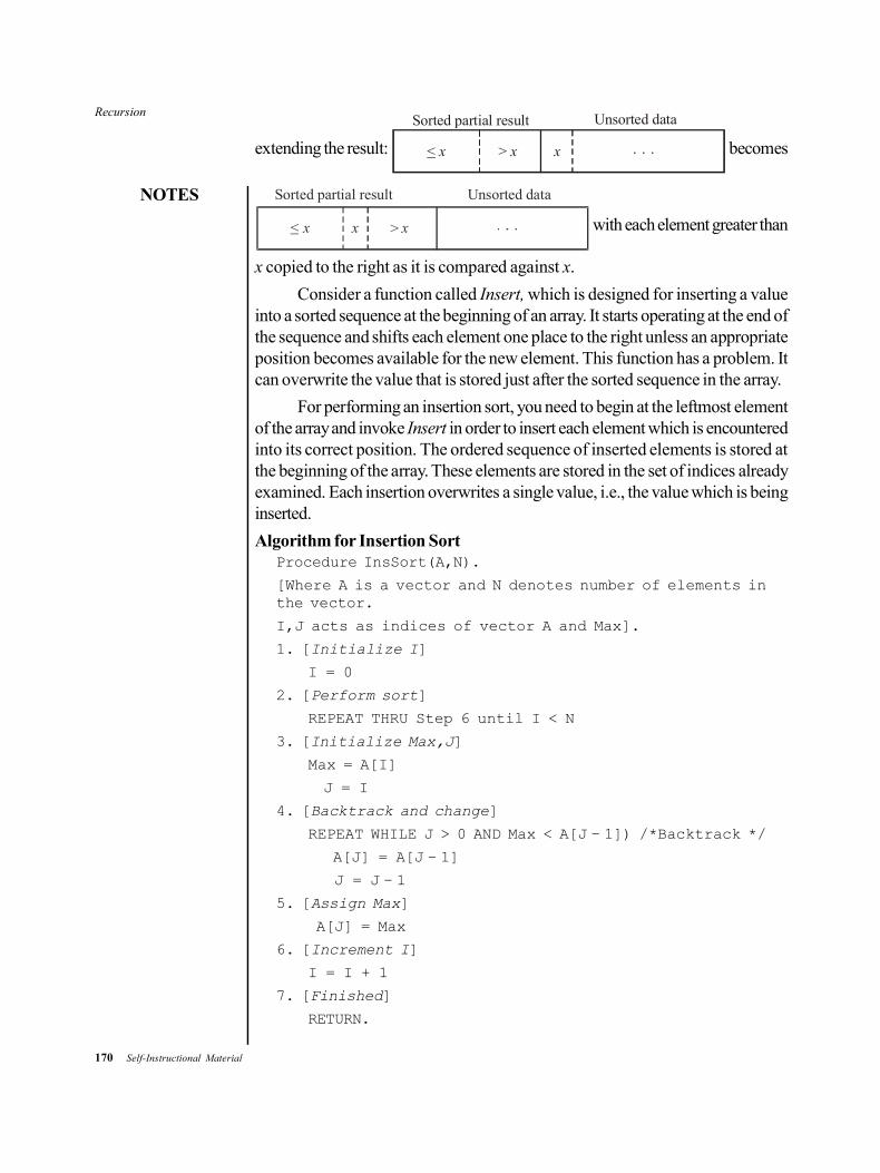
170 Self-Instructional Material
Recursion
NOTES
extending the result: < x > x x
Sorted partial result Unsorted data
becomes
< x > xx
Sorted partial result Unsorted data
with each element greater than
x copied to the right as it is compared against x.
Consider a function called Insert, which is designed for inserting a valueinto a sorted sequence at the beginning of an array. It starts operating at the end ofthe sequence and shifts each element one place to the right unless an appropriateposition becomes available for the new element. This function has a problem. Itcan overwrite the value that is stored just after the sorted sequence in the array.
For performing an insertion sort, you need to begin at the leftmost elementof the array and invoke Insert in order to insert each element which is encounteredinto its correct position. The ordered sequence of inserted elements is stored atthe beginning of the array. These elements are stored in the set of indices alreadyexamined. Each insertion overwrites a single value, i.e., the value which is beinginserted.
Algorithm for Insertion SortProcedure InsSort(A,N).
[Where A is a vector and N denotes number of elements inthe vector.
I,J acts as indices of vector A and Max].
1. [Initialize I]
I = 0
2. [Perform sort]
REPEAT THRU Step 6 until I < N
3. [Initialize Max,J]
Max = A[I]
J = I
4. [Backtrack and change]
REPEAT WHILE J > 0 AND Max < A[J – 1]) /*Backtrack */
A[J] = A[J – 1]
J = J – 1
5. [Assign Max]
A[J] = Max
6. [Increment I]
I = I + 1
7. [Finished]
RETURN.
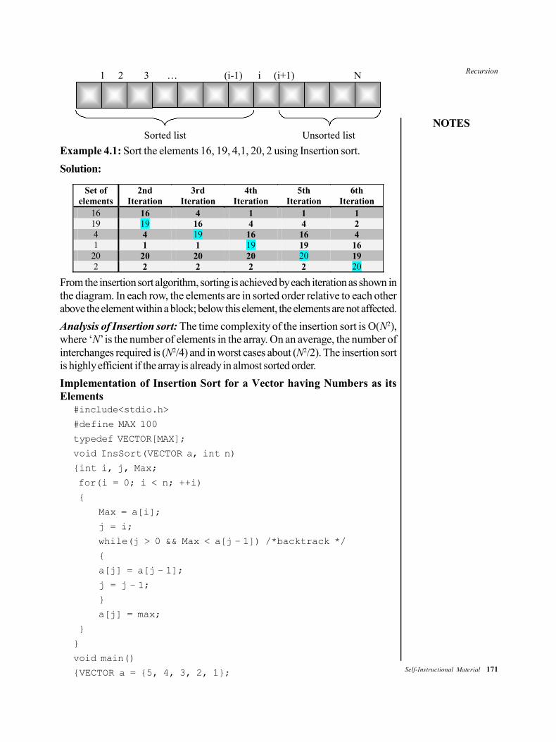
Recursion
NOTES
Self-Instructional Material 171
1 2 3 … (i-1) i (i+1) N
Sorted list Unsorted list
Example 4.1: Sort the elements 16, 19, 4,1, 20, 2 using Insertion sort.
Solution:
Set of elements
2nd Iteration
3rd Iteration
4th Iteration
5th Iteration
6th Iteration
16 16 4 1 1 1 19 19 16 4 4 2 4 4 19 16 16 4 1 1 1 19 19 16
20 20 20 20 20 19 2 2 2 2 2 20
From the insertion sort algorithm, sorting is achieved by each iteration as shown inthe diagram. In each row, the elements are in sorted order relative to each otherabove the element within a block; below this element, the elements are not affected.
Analysis of Insertion sort: The time complexity of the insertion sort is O(N2),where ‘N’ is the number of elements in the array. On an average, the number ofinterchanges required is (N2/4) and in worst cases about (N2/2). The insertion sortis highly efficient if the array is already in almost sorted order.
Implementation of Insertion Sort for a Vector having Numbers as itsElements
#include<stdio.h>
#define MAX 100
typedef VECTOR[MAX];
void InsSort(VECTOR a, int n)
{int i, j, Max;
for(i = 0; i < n; ++i)
{
Max = a[i];
j = i;
while(j > 0 && Max < a[j – 1]) /*backtrack */
{
a[j] = a[j – 1];
j = j – 1;
}
a[j] = max;
}
}
void main()
{VECTOR a = {5, 4, 3, 2, 1};
172 Self-Instructional Material
Recursion
NOTES
int i;
InsSort(a, 5);
for(i = 0; i < 5; ++i)
printf(“%d “, a[i]);
}
Output: 1 2 3 4 5
Implementation of Insertion Sort for a Vector having Strings as its Elements#include<stdio.h>
#include<string.h>
#define MAXROWS 10
#define MAXCOLS 20
typedef char STRINGS[MAXROWS][MAXCOLS];
typedef char STRING[MAXCOLS];
void InsSort(STRINGS A,int N)
{
int I, J;
STRING MaxStr;
for(I = 0; I < N; ++I)
{
strcpy(MaxStr, A[I]);
J = I;
while(J > 0 && strcmp(MaxStr, A[J – 1])<0) /*backtrack*/
{
strcpy(A[J], A[J – 1]);
J = J – 1;
}
strcpy(A[J], MaxStr);
}
}
void main()
{
STRINGS A = {“EE”, “AA”, “BB”, “DD”, “CC”};
int i;
InsSort(A, 5);
for(i = 0; i < 5; ++i)
printf(“%s”, A[i]);
}
OUTPUT: AA BB CC DD EE
The array which is already sorted is considered the best case input. In thegiven case, insertion sort has a linear running time, i.e., O(n). During each iteration,
Recursion
NOTES
Self-Instructional Material 173
the first remaining element of the input would only be compared with the rightmostelement of the sorted subsection of the array.
An array sorted in the reverse order is the worst case input. In the givencase, insertion sort has a quadratic running time, i.e., O(n2). Every iteration of theinner loop scans and shifts the entire sorted subsection of the array before the nextelement is inserted. The average case is also quadratic. That is why the insertionsort is not practical for sorting large arrays. However, for sorting arrays havingless than ten elements, insertion sort is one of the fastest algorithms.
CHECK YOUR PROGRESS
1. What is the Mergesort algorithm based on?
2. List out any two advantages of Insertion sort.
3. What is the role of the insert function?
4.4 BUBBLE SORT AND SELECTION SORT
In the fields of computer science and mathematics, a sorting algorithm refers to analgorithm whose function is to put elements of a list in a certain order. The numericaland lexicographical orders are the most used orders. In order to optimize the useof other algorithms, such as search and merge algorithms, efficient sorting is essential,as these algorithms require sorted lists to work correctly. Sorting is often used tocanonicalize data and to produce human-readable output. The output must meetthe following two conditions:
The output should be in non-decreasing order (each element should not besmaller than the previous element according to the desired total order).
The output should be a permutation or reordering of the input.
Since the beginning of computing, the sorting problem has greatly attractedthe attention of researchers, perhaps due to the complexity of solving it efficientlydespite its simple, familiar statement. For example, the analysis of bubble sort wasdone as early as 1956. Many consider it a solved problem. However, the inventionof new sorting algorithms has not stopped. Library sort, for example, was firstpublished in 2004. Sorting algorithms are taught in introductory computer scienceclasses. Students are introduced to a variety of core algorithm concepts, such asbig O notation, divide and conquer algorithms, data structures, randomizedalgorithms, best, worst and average case analysis, time-space tradeoffs and lowerbounds.
Sorting is a method of arranging keys in a file in the ascending or descendingorder. Sorting makes handling of records in a file easier.
174 Self-Instructional Material
Recursion
NOTES
Sorting can be classified into the following two types:
Internal sorting: Sorting of records in a file, which is stored in the main memory.
External sorting: Sorting of records in a file, which is stored in the secondarymemory. Some sorting techniques are as follows:
Bubble sort
Insertion sort
Selection sort
Quick sort
Tree sort
Arrangement of elements in a list according to the increasing (or decreasing)values of some key field of each element.
Sorting will be useful to search, insert or delete a data item in a list.
There are various methods for sorting explained in the following sections.
4.4.1 Bubble Sort
Bubble sort comes under the category of exchange sort technique.
Consider an array A has n elements A[0] to A[n – 1]. The array is tobe sorted in the ascending order.
Compare A[0] and A[1] and arrange such that A[0] < A[1]. Thencompare A[1] and A[2] and arrange such that A[1] < A[2].Repeat this process till the largest element is bubbled to the nth position.
Since the largest value is now in the last position as required for the ascendingorder, consider the first (n – 1) elements. Repeat the above process as tobubble the next largest value to (n – 1)th position. Then consider the first(n – 2) elements and in this way proceed to bubble till all the elements arebubbled to their respective positions. Then sorting will be completed.
Algorithm for Bubble Sort or Exchange SortBUBBLE_SORT(B,N). Where B is a vector having N elements
1. [Initialization]
Last = N (entire list assumed unsorted at this point)
2. [Loop on I index]
REPEAT THRU STEP 5 FOR I = 1 TO N – 1 DO
3. [Initialize exchanges counter for this pass]
EXS = 0
4. [Compare the unsorted pairs]
REPEAT FOR J = 1 TO Last – 1 DO
IF B[J] < B[J+1] THEN
B[J] = B[J+1]
EXS = EXS + 1
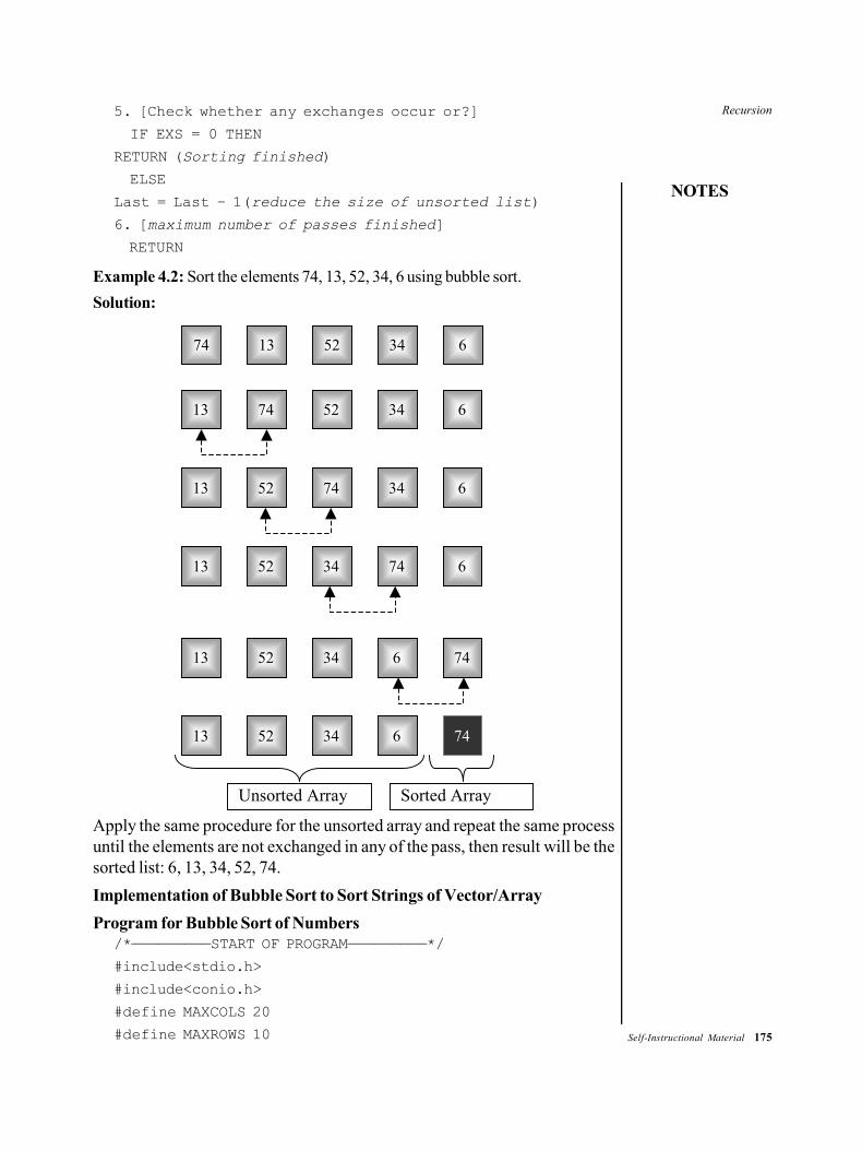
Recursion
NOTES
Self-Instructional Material 175
5. [Check whether any exchanges occur or?]
IF EXS = 0 THEN
RETURN (Sorting finished)
ELSE
Last = Last – 1(reduce the size of unsorted list)
6. [maximum number of passes finished]
RETURN
Example 4.2: Sort the elements 74, 13, 52, 34, 6 using bubble sort.
Solution:
74 13 52 34 6
13 74 52 34 6
13 52 74 34 6
13 52 34 74 6
13 52 34 6 74
13 52 34 6 74
Unsorted Array Sorted Array
Apply the same procedure for the unsorted array and repeat the same processuntil the elements are not exchanged in any of the pass, then result will be thesorted list: 6, 13, 34, 52, 74.
Implementation of Bubble Sort to Sort Strings of Vector/Array
Program for Bubble Sort of Numbers/*—————————START OF PROGRAM—————————*/
#include<stdio.h>
#include<conio.h>
#define MAXCOLS 20
#define MAXROWS 10
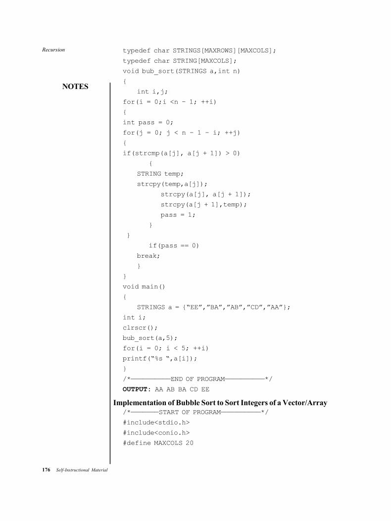
176 Self-Instructional Material
Recursion
NOTES
typedef char STRINGS[MAXROWS][MAXCOLS];
typedef char STRING[MAXCOLS];
void bub_sort(STRINGS a,int n)
{
int i,j;
for(i = 0;i <n – 1; ++i)
{
int pass = 0;
for(j = 0; j < n – 1 – i; ++j)
{
if(strcmp(a[j], a[j + 1]) > 0)
{
STRING temp;
strcpy(temp,a[j]);
strcpy(a[j], a[j + 1]);
strcpy(a[j + 1],temp);
pass = 1;
}
}
if(pass == 0)
break;
}
}
void main()
{
STRINGS a = {“EE”,”BA”,”AB”,”CD”,”AA”};
int i;
clrscr();
bub_sort(a,5);
for(i = 0; i < 5; ++i)
printf(“%s “,a[i]);
}
/*——————————END OF PROGRAM——————————*/
OUTPUT: AA AB BA CD EE
Implementation of Bubble Sort to Sort Integers of a Vector/Array/*———————START OF PROGRAM——————————*/
#include<stdio.h>
#include<conio.h>
#define MAXCOLS 20
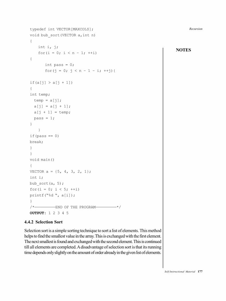
Recursion
NOTES
Self-Instructional Material 177
typedef int VECTOR[MAXCOLS];
void bub_sort(VECTOR a,int n)
{
int i, j;
for(i = 0; i < n – 1; ++i)
{
int pass = 0;
for(j = 0; j < n – 1 – i; ++j){
if(a[j] > a[j + 1])
{
int temp;
temp = a[j];
a[j] = a[j + 1];
a[j + 1] = temp;
pass = 1;
}
}
if(pass == 0)
break;
}
}
void main()
{
VECTOR a = {5, 4, 3, 2, 1};
int i;
bub_sort(a, 5);
for(i = 0; i < 5; ++i)
printf(“%d “, a[i]);
}
/*—————————END OF THE PROGRAM—————————*/
OUTPUT: 1 2 3 4 5
4.4.2 Selection Sort
Selection sort is a simple sorting technique to sort a list of elements. This methodhelps to find the smallest value in the array. This is exchanged with the first element.The next smallest is found and exchanged with the second element. This is continuedtill all elements are completed. A disadvantage of selection sort is that its runningtime depends only slightly on the amount of order already in the given list of elements.
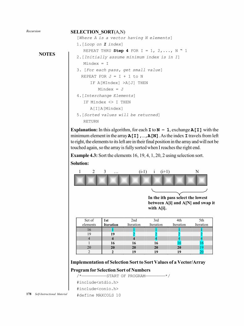
178 Self-Instructional Material
Recursion
NOTES
SELECTION_SORT(A,N)[Where A is a vector having N elements]
1.[Loop on I index]
REPEAT THRU Step 4 FOR I = 1, 2,..., N “ 1
2.[Initially assume minimum index is in I]
Mindex = I
3. [For each pass, get small value]
REPEAT FOR J = I + 1 to N
IF A[MIndex] >A[J] THEN
Mindex = J
4.[Interchange Elements]
IF Mindex <> I THEN
A[I]A[Mindex]
5.[Sorted values will be returned]
RETURN
Explanation: In this algorithm, for each I to N – 1, exchange A[I] with theminimum element in the array A[I],…,A[N]. As the index I travels from leftto right, the elements to its left are in their final position in the array and will not betouched again, so the array is fully sorted when I reaches the right end.
Example 4.3: Sort the elements 16, 19, 4, 1, 20, 2 using selection sort.
Solution:
1 2 3 … (i-1) i (i+1) N
In the ith pass select the lowest between A[i] and A[N] and swap it with A[i].
Set of elements
1st Iteration
2nd Iteration
3rd Iteration
4th Iteration
5th Iteration
16 1 1 1 1 1 19 19 2 2 2 2 4 4 4 4 4 4 1 16 16 16 16 16
20 20 20 20 20 19 2 2 19 19 19 20
Implementation of Selection Sort to Sort Values of a Vector/Array
Program for Selection Sort of Numbers/*——————————START OF PROGRAM————————*/
#include<stdio.h>
#include<conio.h>
#define MAXCOLS 10
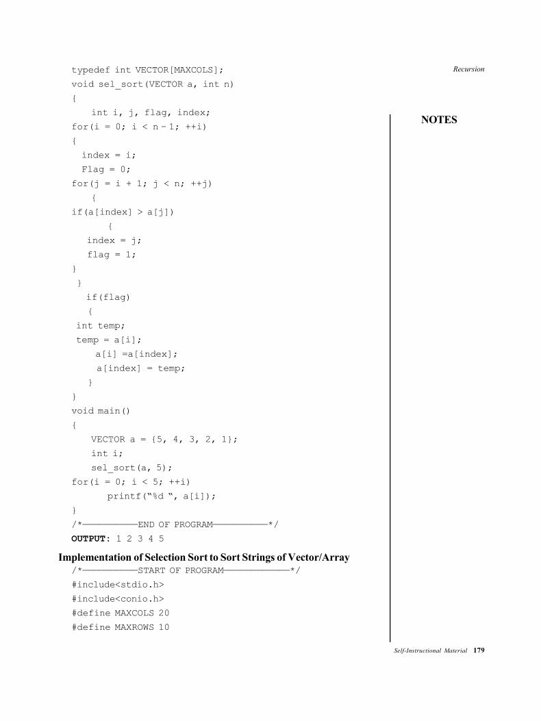
Recursion
NOTES
Self-Instructional Material 179
typedef int VECTOR[MAXCOLS];
void sel_sort(VECTOR a, int n)
{
int i, j, flag, index;
for(i = 0; i < n – 1; ++i)
{
index = i;
Flag = 0;
for(j = i + 1; j < n; ++j)
{
if(a[index] > a[j])
{
index = j;
flag = 1;
}
}
if(flag)
{
int temp;
temp = a[i];
a[i] =a[index];
a[index] = temp;
}
}
void main()
{
VECTOR a = {5, 4, 3, 2, 1};
int i;
sel_sort(a, 5);
for(i = 0; i < 5; ++i)
printf(“%d “, a[i]);
}
/*——————————END OF PROGRAM——————————*/
OUTPUT: 1 2 3 4 5
Implementation of Selection Sort to Sort Strings of Vector/Array/*——————————START OF PROGRAM————————————*/
#include<stdio.h>
#include<conio.h>
#define MAXCOLS 20
#define MAXROWS 10
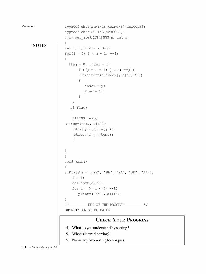
180 Self-Instructional Material
Recursion
NOTES
typedef char STRINGS[MAXROWS][MAXCOLS];
typedef char STRING[MAXCOLS];
void sel_sort(STRINGS a, int n)
{
int i, j, flag, index;
for(i = 0; i < n – 1; ++i)
{
flag = 0, index = i;
for(j = i + 1; j < n; ++j){
if(strcmp(a[index], a[j]) > 0)
{
index = j;
flag = 1;
}
}
if(flag)
{
STRING temp;
strcpy(temp, a[i]);
strcpy(a[i], a[j]);
strcpy(a[j], temp);
}
}
}
void main()
{
STRINGS a = {“EE”, “BB”, “EA”, “DD”, “AA”};
int i;
sel_sort(a, 5);
for(i = 0; i < 5; ++i)
printf(“%s “, a[i]);
}
/*—————————END OF THE PROGRAM—————————*/
OUTPUT: AA BB DD EA EE
CHECK YOUR PROGRESS
4. What do you understand by sorting?
5. What is internal sorting?
6. Name any two sorting techniques.
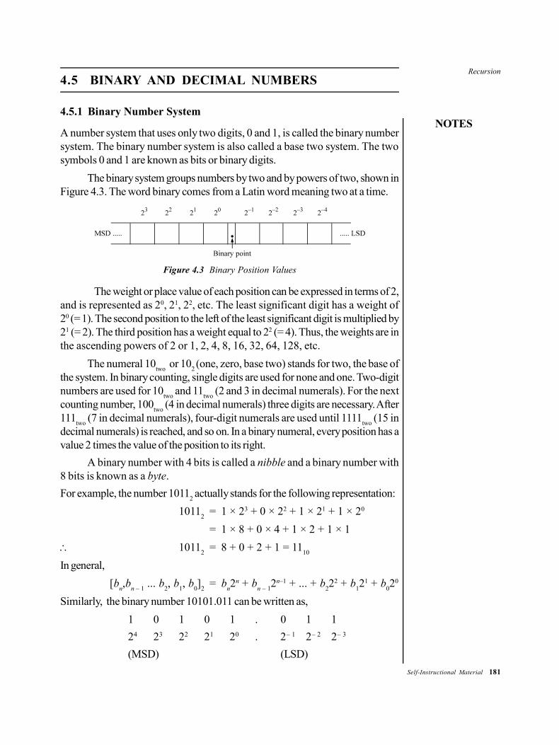
Recursion
NOTES
Self-Instructional Material 181
4.5 BINARY AND DECIMAL NUMBERS
4.5.1 Binary Number System
A number system that uses only two digits, 0 and 1, is called the binary numbersystem. The binary number system is also called a base two system. The twosymbols 0 and 1 are known as bits or binary digits.
The binary system groups numbers by two and by powers of two, shown inFigure 4.3. The word binary comes from a Latin word meaning two at a time.
Figure 4.3 Binary Position Values
The weight or place value of each position can be expressed in terms of 2,and is represented as 20, 21, 22, etc. The least significant digit has a weight of20 (= 1). The second position to the left of the least significant digit is multiplied by21 (= 2). The third position has a weight equal to 22 (= 4). Thus, the weights are inthe ascending powers of 2 or 1, 2, 4, 8, 16, 32, 64, 128, etc.
The numeral 10two
or 102 (one, zero, base two) stands for two, the base of
the system. In binary counting, single digits are used for none and one. Two-digitnumbers are used for 10
two and 11
two (2 and 3 in decimal numerals). For the next
counting number, 100two
(4 in decimal numerals) three digits are necessary. After111
two (7 in decimal numerals), four-digit numerals are used until 1111
two (15 in
decimal numerals) is reached, and so on. In a binary numeral, every position has avalue 2 times the value of the position to its right.
A binary number with 4 bits is called a nibble and a binary number with8 bits is known as a byte.
For example, the number 10112 actually stands for the following representation:
10112
= 1 × 23 + 0 × 22 + 1 × 21 + 1 × 20
= 1 × 8 + 0 × 4 + 1 × 2 + 1 × 1
10112
= 8 + 0 + 2 + 1 = 1110
In general,
[bn,b
n – 1 ... b
2, b
1, b
0]
2= b
n2n + b
n – 12n–1 + ... + b
222 + b
121 + b
020
Similarly, the binary number 10101.011 can be written as,
1 0 1 0 1 . 0 1 1
24 23 22 21 20 . 2– 1 2– 2 2– 3
(MSD) (LSD)
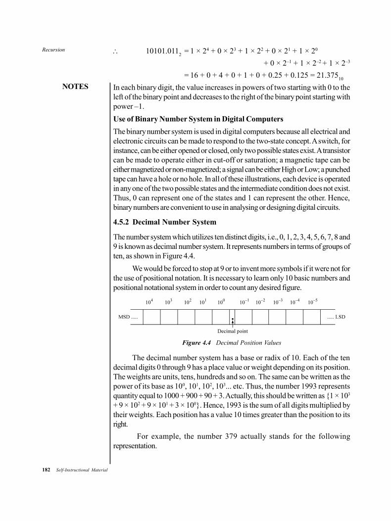
182 Self-Instructional Material
Recursion
NOTES
10101.0112 = 1 × 24 + 0 × 23 + 1 × 22 + 0 × 21 + 1 × 20
+ 0 × 2–1 + 1 × 2–2 + 1 × 2–3
= 16 + 0 + 4 + 0 + 1 + 0 + 0.25 + 0.125 = 21.37510
In each binary digit, the value increases in powers of two starting with 0 to theleft of the binary point and decreases to the right of the binary point starting withpower –1.
Use of Binary Number System in Digital Computers
The binary number system is used in digital computers because all electrical andelectronic circuits can be made to respond to the two-state concept. A switch, forinstance, can be either opened or closed, only two possible states exist. A transistorcan be made to operate either in cut-off or saturation; a magnetic tape can beeither magnetized or non-magnetized; a signal can be either High or Low; a punchedtape can have a hole or no hole. In all of these illustrations, each device is operatedin any one of the two possible states and the intermediate condition does not exist.Thus, 0 can represent one of the states and 1 can represent the other. Hence,binary numbers are convenient to use in analysing or designing digital circuits.
4.5.2 Decimal Number System
The number system which utilizes ten distinct digits, i.e., 0, 1, 2, 3, 4, 5, 6, 7, 8 and9 is known as decimal number system. It represents numbers in terms of groups often, as shown in Figure 4.4.
We would be forced to stop at 9 or to invent more symbols if it were not forthe use of positional notation. It is necessary to learn only 10 basic numbers andpositional notational system in order to count any desired figure.
Figure 4.4 Decimal Position Values
The decimal number system has a base or radix of 10. Each of the tendecimal digits 0 through 9 has a place value or weight depending on its position.The weights are units, tens, hundreds and so on. The same can be written as thepower of its base as 100, 101, 102, 103... etc. Thus, the number 1993 representsquantity equal to 1000 + 900 + 90 + 3. Actually, this should be written as {1 × 10³
+ 9 × 10² + 9 × 101 + 3 × 100}. Hence, 1993 is the sum of all digits multiplied bytheir weights. Each position has a value 10 times greater than the position to itsright.
For example, the number 379 actually stands for the followingrepresentation.

Recursion
NOTES
Self-Instructional Material 183
100 10 1
102 101 100
3 7 9
3 × 100 + 7 × 10 + 9 × 1
37910 = 3 × 100 + 7 × 10 + 9 × 1
= 3 × 10² + 7 × 101 + 9 × 100
In this example, 9 is the least significant digit (LSD) and 3 is the most significantdigit (MSD).
Example 4.4: Write the number 1936.469 using decimal representation.
Solution: 1936.46910
= 1 × 10³ + 9 × 10² + 3 × 101 + 6 × 100 + 4 × 10⁻¹
+ 6 × 10⁻² + 9 × 10–3
= 1000 + 900 + 30 + 6 + 0.4 + 0.06 + 0.009
= 1936.469
It is seen that powers are numbered to the left of the decimal point startingwith 0 and to the right of the decimal point starting with –1.
The general rule for representing numbers in the decimal system by usingpositional notation is as follows:
ana
n – 1 ... a
2a
1a
0 = a
n10n + a
n – 110n–1 + ... a
2102 + a
1101 + a
0100
Where n is the number of digits to the left of the decimal point.
4.5.3 Binary to Decimal Conversion
A binary number can be converted into decimal number by multiplying the binary1 or 0 by the weight corresponding to its position and adding all the values.
Example 4.5: Convert the binary number 110111 to decimal number.
Solution: 1101112
= 1 × 25 + 1 × 24 + 0 × 23 + 1 × 22 + 1 × 21 + 1 × 20
= 1 × 32 + 1 × 16 + 0 × 8 + 1 × 4 + 1 × 2 + 1 × 1
= 32 + 16 + 0 + 4 + 2 + 1
= 5510
We can streamline binary to decimal conversion by the following procedure:
Step 1:Write the binary, i.e., all its bits in a row.
Step 2:Write 1, 2, 4, 8, 16, 32, ..., directly under the binary number workingfrom right to left.
Step 3:Omit the decimal weight which lies under zero bits.
Step 4:Add the remaining weights to obtain the decimal equivalent.
The same method is used for binary fractional number.
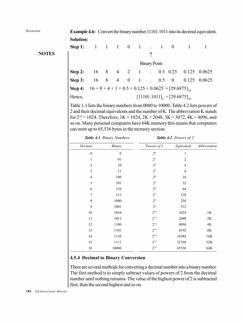
184 Self-Instructional Material
Recursion
NOTES
Example 4.6: Convert the binary number 11101.1011 into its decimal equivalent.
Solution:
Step 1: 1 1 1 0 1 . 1 0 1 1
Binary Point
Step 2: 16 8 4 2 1 . 0.5 0.25 0.125 0.0625
Step 3: 16 8 4 0 1 . 0.5 0 0.125 0.0625
Step 4: 16 + 8 + 4 + 1 + 0.5 + 0.125 + 0.0625 = [29.6875]10
Hence, [11101.1011]2 = [29.6875]10
Table 1.1 lists the binary numbers from 0000 to 10000. Table 4.2 lists powers of2 and their decimal equivalents and the number of K. The abbreviation K standsfor 210 = 1024. Therefore, 1K = 1024, 2K = 2048, 3K = 3072, 4K = 4096, andso on. Many personal computers have 64K memory this means that computerscan store up to 65,536 bytes in the memory section.
Table 4.1 Binary Numbers Table 4.2 Powers of 2
Decimal Binary Powers of 2 Equivalent Abbreviation
0 0 20 1
1 01 21 2
2 10 22 4
3 11 23 8
4 100 24 16
5 101 25 32
6 110 26 64
7 111 27 128
8 1000 28 256
9 1001 29 512
10 1010 210 1024 1K
11 1011 211 2048 2K
12 1100 212 4096 4K
13 1101 213 8192 8K
14 1110 214 16384 16K
15 1111 215 32768 32K
16 10000 216 65536 64K
4.5.4 Decimal to Binary Conversion
There are several methods for converting a decimal number into a binary number.The first method is to simply subtract values of powers of 2 from the decimalnumber until nothing remains. The value of the highest power of 2 is subtractedfirst, then the second highest and so on.
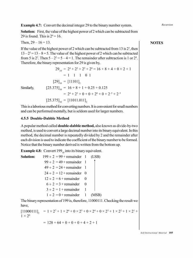
Recursion
NOTES
Self-Instructional Material 185
Example 4.7: Convert the decimal integer 29 to the binary number system.
Solution: First, the value of the highest power of 2 which can be subtracted from29 is found. This is 24 = 16.
Then, 29 – 16 = 13.
If the value of the highest power of 2 which can be subtracted from 13 is 23, then13 – 23 = 13 – 8 = 5. The value of the highest power of 2 which can be subtractedfrom 5 is 22. Then 5 – 22 = 5 – 4 = 1. The remainder after subtraction is 1 or 20.Therefore, the binary representation for 29 is given by,
2910
= 24 + 23 + 22 + 20 = 16 + 8 + 4 + 0 × 2 + 1
= 1 1 1 0 1
[29]10
= [11101]2
Similarly, [25.375]10
= 16 + 8 + 1 + 0.25 + 0.125
= 24 + 23 + 0 + 0 + 20 + 0 + 2–2 + 2–3
[25.375]10
= [11011.011]2
This is a laborious method for converting numbers. It is convenient for small numbersand can be performed mentally, but is seldom used for larger numbers.
4.5.5 Double-Dabble Method
A popular method called double-dabble method, also known as divide-by-twomethod, is used to convert a large decimal number into its binary equivalent. In thismethod, the decimal number is repeatedly divided by 2 and the remainder aftereach division is used to indicate the coefficient of the binary number to be formed.Notice that the binary number derived is written from the bottom up.
Example 4.8: Convert 19910
into its binary equivalent.
Solution: 199 2 = 99 + remainder 1 (LSB)99 2 = 49 + remainder 149 2 = 24 + remainder 1
24 2 = 12 + remainder 0
12 2 = 6 + remainder 06 2 = 3 + remainder 03 2 = 1 + remainder 11 2 = 0 + remainder 1 (MSB)
The binary representation of 199 is, therefore, 11000111. Checking the result wehave,
[11000111]2 = 1 × 27 + 1 × 26 + 0 × 25 + 0 × 24 + 0 × 23 + 1 × 22 + 1 × 21 +1 × 20
= 128 + 64 + 0 + 0 + 0 + 4 + 2 + 1
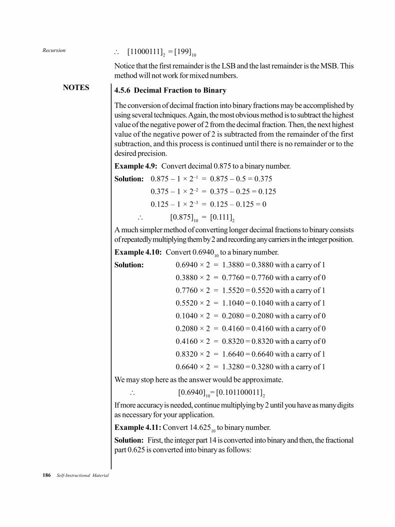
186 Self-Instructional Material
Recursion
NOTES
[11000111]2 = [199]10
Notice that the first remainder is the LSB and the last remainder is the MSB. Thismethod will not work for mixed numbers.
4.5.6 Decimal Fraction to Binary
The conversion of decimal fraction into binary fractions may be accomplished byusing several techniques. Again, the most obvious method is to subtract the highestvalue of the negative power of 2 from the decimal fraction. Then, the next highestvalue of the negative power of 2 is subtracted from the remainder of the firstsubtraction, and this process is continued until there is no remainder or to thedesired precision.
Example 4.9: Convert decimal 0.875 to a binary number.
Solution: 0.875 – 1 × 2–1 = 0.875 – 0.5 = 0.375
0.375 – 1 × 2–2 = 0.375 – 0.25 = 0.125
0.125 – 1 × 2–3 = 0.125 – 0.125 = 0
[0.875]10
= [0.111]2
A much simpler method of converting longer decimal fractions to binary consistsof repeatedly multiplying them by 2 and recording any carriers in the integer position.
Example 4.10: Convert 0.694010
to a binary number.
Solution: 0.6940 × 2 = 1.3880 = 0.3880 with a carry of 1
0.3880 × 2 = 0.7760 = 0.7760 with a carry of 0
0.7760 × 2 = 1.5520 = 0.5520 with a carry of 1
0.5520 × 2 = 1.1040 = 0.1040 with a carry of 1
0.1040 × 2 = 0.2080 = 0.2080 with a carry of 0
0.2080 × 2 = 0.4160 = 0.4160 with a carry of 0
0.4160 × 2 = 0.8320 = 0.8320 with a carry of 0
0.8320 × 2 = 1.6640 = 0.6640 with a carry of 1
0.6640 × 2 = 1.3280 = 0.3280 with a carry of 1
We may stop here as the answer would be approximate.
[0.6940]10
= [0.101100011]2
If more accuracy is needed, continue multiplying by 2 until you have as many digitsas necessary for your application.
Example 4.11: Convert 14.62510
to binary number.
Solution: First, the integer part 14 is converted into binary and then, the fractionalpart 0.625 is converted into binary as follows:
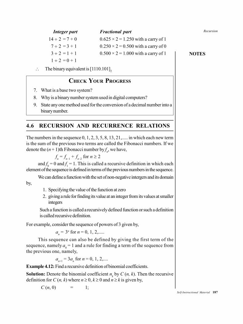
Recursion
NOTES
Self-Instructional Material 187
Integer part Fractional part
14 2 = 7 + 0 0.625 × 2 = 1.250 with a carry of 1
7 2 = 3 + 1 0.250 × 2 = 0.500 with a carry of 0
3 2 = 1 + 1 0.500 × 2 = 1.000 with a carry of 1
1 2 = 0 + 1
The binary equivalent is [1110.101]2
CHECK YOUR PROGRESS
7. What is a base two system?
8. Why is a binary number system used in digital computers?
9. State any one method used for the conversion of a decimal number into abinary number.
4.6 RECURSION AND RECURRENCE RELATIONS
The numbers in the sequence 0, 1, 2, 3, 5, 8, 13, 21,..... in which each new termis the sum of the previous two terms are called the Fibonacci numbers. If wedenote the (n + 1)th Fibonacci number by f
n, we have,
fn = f
n–1 + f
n–2 for n 2
and f0 = 0 and f
1 = 1. This is called a recursive definition in which each
element of the sequence is defined in terms of the previous numbers in the sequence.
We can define a function with the set of non-negative intergers and its domainby,
1. Specifying the value of the function at zero2. giving a rule for finding its value at an integer from its values at smaller
integers
Such a function is called a recursively defined function or such a definitionis called recursive definition.
For example, consider the sequence of powers of 3 given by,
an = 3n for n = 0, 1, 2,.....
This sequence can also be defined by giving the first term of thesequence, namely a
0 = 1 and a rule for finding a term of the sequence from
the previous one, namely,
an+1
= 3an for n = 0, 1, 2,....
Example 4.12: Find a recursive definition of binomial coefficients.
Solution: Denote the binomial coefficient nk by C (n, k). Then the recursive
definition for C (n, k) where n 0, k 0 and n k is given by,
C (n, 0) = 1;
188 Self-Instructional Material
Recursion
NOTES
C (n, n) = 1; and
C (n, k) = C (n – 1, k) + C (n – 1, k – 1) for n > k > 0.
Example 4.13: Suppose that f is recursively defined as follows,
f(0) = 2
f(n + 1) = 3f(n)+2
Find f(1), f(2), f(3) and f(4).
Solution: From the recursive definition, it follows that:f(1) = 3f(0) + 2 = 3.2 + 2 = 8f(2) = 3f(1) + 2 = 3.8 + 2 = 26f(3) = 3f(2) + 2 = 3.26 + 2 = 80f(4) = 3f(3) + 2 = 3.80 + 2 = 242
Example 4.14: Give a recursive definition of f(n) = n!
Solution: Since 0! = 1 and (n + 1)! = (n + 1)n!, the desired rule is,
f(0) = 1
f(n + 1) = (n + 1) f(n)
Example 4.15: Give a recursive definition of an where a is a non-zero numberand n is a non-negative integer.
Solution: It can be stated as,
a0 = 1; and an+1 = a.an for n 0.
Where an uniquely defined is for all non-negative integers n.
Example 4.16: Give a recursive definition for polynomial expression.
Solution: An expression of the form,
f(x) = a0xn + a
1xn–1 + .... + a
n–1x + a
n
Where a’s are constants (a0 0) and n 0, is called polynomial in x of
degree n.
Let S be a set of coefficients. Then, recursive definition for polynomial is,
1. A zeroth degree (constant) polynomial is an element of S.2. For n 1, an nth degree polynomial expression is an expression of
the form q(x)x+a, where q(x) is an (n – 1)th degree polynomial anda S.
Example 4.17: Using recursive definition for polynomial expression prove that
f(n) = 3n3 – 8n2 + 2n + 4 is a third-degree polynomial expression
Solution: Given f(n) = 3n3 – 8n2 + 2n + 4
= (3n2 – 8n + 2) n + 4 = ((3n – 8) n + 2) n + 4
= (((3) n – 8) n + 2) n + 4
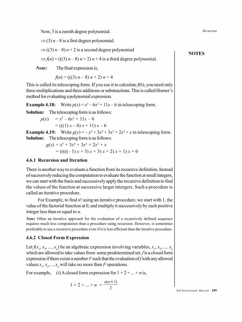
Recursion
NOTES
Self-Instructional Material 189
Now, 3 is a zeroth degree polynomial.
(3) n – 8 is a first degree polynomial.
((3) n – 8) n + 2 is a second degree polynomial
f(n) = (((3) n – 8) n + 2) n + 4 is a third degree polynomial.
Note: The final expression is,
f(n) = (((3) n – 8) n + 2) n + 4
This is called its telescoping form. If you use it to calculate f(6), you need onlythree multiplications and three additions or substractions. This is called Horner’smethod for evaluating a polynomial expression.
Example 4.18: Write p(x) = x3 – 6x2 + 11x – 6 in telescoping form.
Solution: The telescoping form is as follows:p(x) = x3 – 6x2 + 11x – 6
= (((1) x – 6) x + 11) x – 6Example 4.19: Write g(x) = – x5 + 3x4 + 3x3 + 2x2 + x in telescoping form.Solution: The telescoping form is as follows:
g(x) = x5 + 3x4 + 3x3 + 2x2 + x= (((((– 1) x + 3) x + 3) x + 2) x + 1) x + 0
4.6.1 Recursion and Iteration
There is another way to evaluate a function from its recursive definition. Insteadof sucessively reducing the computation to evaluate the function at small integers,we can start with the basis and successively apply the recursive definition to findthe values of the function at successive larger intergers. Such a procedure iscalled an iterative procedure.
For Example, to find n! using an iterative procedure, we start with 1, thevalue of the factorial function at 0, and multiply it successively by each positiveinteger less than or equal to n.
Note: Often an iterative approach for the evaluation of a recursively defined sequencerequires much less computation than a procedure using recursion. However, is sometimespreferable to use a recursive procedure even if it is less efficient than the iterative procedure.
4.6.2 Closed Form Expression
Let f(x1, x
2, .... x
n) be an algebraic expression involving variables, x
1, x
2, .... x
n
which are allowed to take values from some predetermined set. f is a closed formexpression if there exists a number F such that the evaluation of f with any allowedvalues x
1, x
2, ....x
n will take no more than F operations.
For example, (i) A closed form expression for 1 + 2 + ... + n is,
1 + 2 + ... + n = n n( )1
2
190 Self-Instructional Material
Recursion
NOTES
(ii) A closed form expression for 12 + 22 + ... + n2 is,
12 + 22 + ... + n2 = n n n( )( ) 1 2 1
6
4.6.3 Sequence of Integers
A sequence of integers is a function from the natural numbers into integers. That is,if f is a sequence of integers, then f: N Z is a function. We use the notation f
n or
f(n) to denote the image of any natural number n. We call fn and nth term of the
sequence.
Note: A sequence is often called a discrete function.
Example 4.20: Prove by induction that f(k) = 3k + 2, k 0 is a closed formexpression of the sequence f defined recursively by f(0) = 2 and f(k) = f(k – 1) +3 for k 1.
Solution:
1. Basis of induction: If k = 0, then f(0). But f(0) = 3(0) + 2 = 2 as defined.
2. Induction step: Now assume that for some k > 0,
f(k) = 3k + 2 …(1)
We have,
f(k + 1) = f(k) + 3 by the recursive definition
= 3k + 2 + 3 = 3k + 3 + 2
= 3(k + 1) + 2
Therefore, by the principle of mathematical induction the result follows. Hence,f(k) = 3k + 2, k 0 is a closed form expression for the sequence f.
Example 4.21: Define the sequence of numbers f by f0 = 100 and f
n = 1.08
fn–1
for n 1. Prove by induction that fn = 100 (1.08)n, n 0 is a closed form of
expression for the sequence f.
Solution:
1. Basis of induction: If k = 0, then f0 = 100 (1.08)0 = 100 as defined.
2. Induction step: Now assume that for some k > 0
fk
= 100 (1.08)k
Then,
f(k+1)
= (1.08)fk by the recursive definition
= (1.08)100k
= 100 (1.08)k+1
Therefore, by the principle of mathematical induction the result follows. Hence,fn = 100 (1.08)n, n 0 is closed form expression for the sequence f.
Recursion
NOTES
Self-Instructional Material 191
Notes:
1. The sequence f:N Z, defined by f(n) = n3 – n, is a sequence of integers.
2. The sequence f:N Z, defined by f(0) = 1 and f(n) = f(n – 1) + 2 for n 1 is a sequence of integer.
3. The codomain of a sequence can be any set. We use the notation {fn} to
describe the sequence. We describe sequences by listing the terms of thesequence in the order of increasing subscripts.
For example,
(i) Consider the sequence f:N S defined by f(n) = fn =
1
1n. The list of the
terms of this sequence f0, f
1, f
2,... begins with:
1, 1
2, 1
3, 1
4, ....
(ii) Consider the sequence f:N Z defined by fn = 4n. The list of the terms of
the sequence f0, f
1, f
2,... begins with:
1, 4, 16, 64, ....
4.6.4 Recurrence Relations
The expressions for permutations and combinations are one of the most fundamentaltools for counting the elements of finite sets. They often prove to be inadequateand many problems of computer sciences require a different approach. An importantalternative approach uses recurrence relations (often called recurrence equationsor difference equation) to define the terms of a sequence. A formal definition ofrecurrence relations is difficult because of the wide variety of forms in which suchrelations can be written, but the concept is straightforward. You have already seenan example of a recurrence relation in the definition of the Fibonacci sequence,where for n 2, the term f
n is defined by the recurrence relation,
fn
= fn–1
+ fn–2
The salient characteristic of a recurrence relation is the specification of theterm f
n as a function of the terms f
0, f
1, ....., f
n–1. By itself, however, a recurrence
relation is not sufficient to define the terms of a sequence. You must also specifythe values of some initial terms of the sequence. Thus, in our definition of theFibonacci sequence, we set f
0 = 0 and f
1 = 1. These are called the boundary
conditions or initial conditions of the sequence.
Recall that a recursive definition of a sequence specifies one or more initialterms and a rule for determining subsequent terms from those that precede them.Recursive definitions can be used to solve counting problems. When they are, therule for finding terms from those that precede them is called a recurrence relation.
Recurrence relation: A recurrence relation for the sequence {fn} is a formula
that expresses fn in terms of one or more of the previous terms of the sequence,

192 Self-Instructional Material
Recursion
NOTES
namely, f0, f
1, ..... f
n–1, for all integers n with n n
0, when n
0 is a non-negative
integer. A sequence is called a solution of a recurrence relation if its terms satisfythe recurrence relation.
Example 4.22: Determine whether the sequence {fn} is a solution of the
recurrence relation,
fn
= 2fn–1
– fn–2
for n = 2, 3, 4, .... Where fn = 3n for every non-negative integer n.
Solution: Suppose that, fn = 3n for every non-negative integer n. Then for
n 2,
fn
= 2fn–1
– fn–2
= 2[3(n – 1)] – 3(n – 2) since fn = 3n
= 6n – 6 – 3n + 6 = 3n
Therefore, {fn}, where f
n = 3n is a solution of the recurrence relation.
Example 4.23: Show that the sequence {fn} is a solution of the recurrence
relation fn = – 3f
n–1 + 4f
n–2 if f
n = 2(–4)n + 3.
Solution: Suppose that, fn
= 2(– 4)n + 3.
Then fn
= –3fn–1
+ 4fn–2
= – 3 [2(– 4)n–1 + 3] + 4 [2(– 4)n–2 + 3]
= – 6(– 4)n–1 – 9 + 8(– 4)n–2 + 12
= – 6(– 4)n–1 – 2(– 4)n–1 + 3
= – 8(– 4)n–1 + 3
= 2(– 4)n + 3
Therefore {fn} where f
n = 2(– 4)n + 3 is a solution of the recurrence relation.
Now you will study about a class of recurrence relations known as linearrecurrence relations with constant coefficients.
Linear recurrence relation: A recurrence relation of the form
a0 f
n + a
1 f
n–1 + a
2 f
n–2 + ..... + a
k f
n–k = f(n) ...(4.1)
Where a1, a
2 and so on are constants, is called a linear recurrence relation
with constant coefficients. The recurrence relation as shown in Equation 4.1 isknown as a kth-order recurrence relation, provided that both a
0 and a
k are non
zero.
Note: The phrase ‘kth-order’ means that each term in the sequence dependsonly on the previous k terms.
For example, consider the Fibonacci sequence defined by the recurrence relationfn = f
n–1 + f
n–2, n 2 and the initial condition f
0 = 0 and f
1 = 1. The recurrence
relation is called a second-order relation because fn depends on the two previous
terms of f.
Recursion
NOTES
Self-Instructional Material 193
For example, consider the recurrence relation f(k) – 5f(k – 1) + 6f(k – 2) = 4k + 10
defined for k 2, together with the initial condition f(0) = 7
3 and f(1) = 5. Clearly,,
it is a second-order linear recurrence relation.
Homogeneous recurrence: A kth-order linear relation is a homogeneousrecurrence relation if f(n) = 0 for all n. Otherwise, it is called non-homogeneous.
For example, consider the recurrence relation c(k) – 5c (k – 1) + 8c (k – 2) = 0together with the initial condition c(0) = 5 and c(1) = 2. It is a second-orderhomogeneous recurrence relation.
Example 4.24: Which of the recurrence relations of the following arehomogeneous and which are non-homogeneous?
(i) fn = nf
n–2(ii) a
n = a
n–1 + a
n–3
(iii) bn = b
n–1 + 2 (iv) s (n – 2) + s (n – 4)
Solution: The relation fn = nf
n–2, a
n = a
n–1 + a
n–3, s(n) = s(n – 2) + s (n – 4) are
all homogeneous and the relation bn = b
n–1 + 2 is non-homogeneous.
4.6.5 Linear Homogenous Recurrence Relations (LHRR)
Before writing an algorithm for solving a recurrence relations, let us examine a fewrecurrence relations that arise from certain closed form expressions. The procedureis illustrated by the following examples.
Example 4.25: Form the recurrence relation given fn = 3.5n, n 0.
Solution: If, n 1,
Then fn
= 3.5n = 3.5.5n–1
= 5.3.5n–1 = 5fn–1
So, the recurrence relation is fn – 5f
n–1 = 0 with f
0 = 3.
Example 4.26: Find the recurrence relation which satisfies that
yn = A(3)n + B(– 2)n.
Solution: Given, yn
= A(3)n + B(– 2)n
Therefore, yn+1
= A(3)n+1 + B (– 2)n+1 = 3A(3)n – 2B(– 2)n
and yn+2
= A(3)n+2 + B (– 2)n+2 = 9A(3)n + 4B(– 2)n
Eliminating A and B from these equations, we get
yyy
n
n
n
1 139 4
01
2
–2
Or yn+2
– yn+1
– 6yn = 0, which is the required recurrence relation.
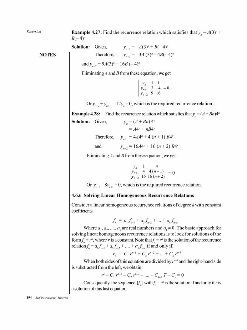
194 Self-Instructional Material
Recursion
NOTES
Example 4.27: Find the recurrence relation which satisfies that yn = A(3)n +
B(– 4)n
Solution: Given, yn+1
= A(3)n + B(– 4)n
Therefore, yn+1
= 3A (3)n – 4B(– 4)n
and yn+2
= 9A(3)n + 16B (– 4)n
Eliminating A and B from these equation, we get
yyy
n
n
n
1 139 16
01
2
–4
Or yn+2
+ yn+1
– 12yn = 0, which is the required recurrence relation.
Example 4.28: Find the recurrence relation which satisfies that yn = (A + Bn)4n
Solution: Given, yn
= (A + Bn) 4n
= A4n + nB4n
Therefore, yn+1
= 4A4n + 4 (n + 1) B4n
and yn+2
= 16A4n + 16 (n + 2) B4n
Eliminating A and B from these equation, we get
y ny ny n
n
n
n
14 4 ( 1)
16 16 ( 2)
1
2
= 0
Or yn+2
– 8yn+1
= 0, which is the required recurrence relation.
4.6.6 Solving Linear Homogeneous Recurrence Relations
Consider a linear homogeneous recurrence relations of degree k with constantcoefficients.
fn
= a1 f
n–1 + a
2 f
n–2 + ... + a
k f
n–k
Where a1, a
2, ...., a
k are real numbers and a
k 0. The basic approach for
solving linear homogeneous recurrence relations is to look for solutions of theform f
n = rn, where r is a constant. Note that f
n = rn is the solution of the recurrence
relation fn = a
1 f
n–1 + a
2 f
n–2 + .... + a
k f
n–k if and only if,
rn
= C1 rn–1 + C
2 rn–2 + ... + C
k rn–k
When both sides of this equation are divided by rn–k and the right-hand sideis substracted from the left, we obtain:
rk – C1 rk–1 – C
2 rk–2 – .... – C
k–1 T – C
k = 0
Consequently, the sequence {fn} with f
n = rn is the solution if and only if r is
a solution of this last equation.

Recursion
NOTES
Self-Instructional Material 195
Characteristic equation: The characteristic equation of the homogeneous kthorder linear relation,
fn + a
1 f
n–1 + a
2 f
n–2 + ... + a
k f
n–k = 0
This is the kth degree polynomial equation
rk + C1 rk–1 + C
2 rk–2 + ... + C
k–1 r + C
k = 0
The solutions of this equation are called the characteristic roots of therecurrence relation.
Example 4.29: What is the characteristic equation of,
Q(k) + 2Q(k – 1) – 3Q(k – 2) – 6Q(k – 4) = 0
Solution: The characteristic equation of the given equation
Q(k) + 2Q(k – 1) – 3Q(k – 2) – 6Q(k – 4) = 0
is r4 + 2r3 – 3r2 – 6 = 0.
Note that the absence of a Q(k – 3) term means that there is no r4–3 = r termin the characteristic equation.
Example 4.30: What is the characteristic equation of T(k) – 7T(k – 2) + 6T(k– 3) = 0?
Solution: The characteristic equation is r3 – 7r + 6 = 0 and 1, 2 and – 3 are thecharacteristic roots.
Algorithm for solving kth-order homogeneous linear recurrence relation
Step 1: If fn + a
1 f
n–1 + a
2 f
n–2 + ... + a
k f
n–k = 0 is a given recurrence relation,
then write its characteristic equation.
It is, rk + C1 rk–1 + C
2 rk–2 + ... + C
k–1 r + C
k = 0.
Step 2: Find all the characteristic roots of this equation.
Step 3: Case (i) If there are k distinct roots, say c1, c
2, ... c
k , then the general
solution of the recurrence relation is,
fn = A
1 c
1k + A
2 c
2k + ... + A
kck
k
Case (ii) Suppose that c1 is a root of multiplicity m. Then the
corresponding solution is,
fn = (A
1 rm–1 + A
2 rm–2 + ... + A
m – 2r2 + A
m–1 T + A
m)cT
1 + ...
Step 4: Use the boundary conditions to determine the constants A1, A
2, .... A
k.
Example 4.31: Solve the Fibonacci sequence {fn} defined by,
fn = f
n–1 + f
n–2 for n 2 with the initial conditions f
0 = 1 and f
1 = 1.
Solution: The first step is to form the characteristic equation corresponding to thegiven difference equation. In this case it is,
r2 – r – 1 = 0
196 Self-Instructional Material
Recursion
NOTES
Solving, we get c1 =
1 5
2 and c
2 =
1 5
2 as the characteristic roots. It
follows that the general solution is,
fn
= A1c
1n + A
2c
2n
Where A1 and A
2 are constants. Since f
0 = 1 and f
1 = 1, we get
0 = A1 + A
2
and 1 = A1c
1 + A
2c
2
1 = A1
1 5
2
FHG
IKJ + A
2
1 5
2
FHG
IKJ
On solving, we get
A1
= 1
5 and A
2 =
1
5
Hence, the solution is,
fn
= 1
5
1 5
2
1 5
2
FHG
IKJ
FHG
IKJ
L
NMM
O
QPP
n n
Example 4.32: If the recurrence relation is un+1
– 2un = 0, then find the closed
form expression (solution) for un.
Solution: The characteristic equation of the given recurrence relation isr – 2 = 0, i.e., r = 2. Therefore, the general solution is u
n = A2n. Hence, u
n = u
0 .
2n is the closed form expression, where the value of u0 is the initial condition.
Example 4.33: Find f(n) if f(n) = 7f(n – 1) – 10f(n – 2), given that f(0) = 4 and f(1) = 17.
Solution: The characteristic equation of the given recurrence relation isr2 – 7r + 10 = 0.
Its characteristic roots are r = 2, 5. So, the general solution of the recurrencerelation is,
f(n) = A1 (2)n + A
2 (5)n
Since, f(0) = 4, 4 = A1 + A
2
Again, f(1) = 17 implies 17 = 2A1 + 5A
2
Solving, we get A1
= 1 and A2 = 3.
Therefore, f(n) = (2)n + 3(5)n
Recursion
NOTES
Self-Instructional Material 197
Example 4.34: Find T(k) if T(k) – 7T(k –2) + 6T(k – 3) = 0, where T(0) = 8,T(1) = 6 and T(2) = 22.
Solution: The characteristic equation is r2 – 7r + 6 = 0
Its roots are 1, 2 and –3.
Therefore, the general solution is T(k) = A1 (1)k + A
2 (2)k + A
3 (– 3)k.
Now,
T(0) = 8 A1 + A
2 + A
3 = 8
T(1) = 6 A1 + 2A
2 – 3A
3 = 6
T(2) = 22 A1 + 4A
2 + 9A
3 = 22
Solving, we get A1
= 5, A2 = 2 and A
3 = 1.
Hence,
T(k) = 5 + 2(2)k + 1 (– 3)k
= 5 + 2k+1 + (– 3)k
Example 4.35: Solve fk – 8f
k–1 + 16f
k–2 = 0, where f
2 = 16 and f
3 = 80.
Solution: The characteristic equation is r2 – 8r + 16 = 0 (or) (r – 4)2 = 0
So, r = 4 is a double characteristic root.
Therefore, the general solution is fk = (A
1 + A
2k) 4k
Now, f2
= 16 (A1 + 2A
2) 16 = 16
And, f3
= 80 (A1 + 3A
2) 64 = 80
Solving, we get A1
=1
2 and A
2 =
1
4
Hence, the solution is,
fk
=1
2
1
4FH
IKk 4k
= (2 + k)4k–1
Example 4.36: Find a solution to the recurrence relation Cn = – 3C
n–1
– 3Cn–2
– Cn–3
for n 3 with initial conditions C0 = 1, C
1 = – 2 and C
2 = 1.
Solution: The characteristic equation is r3 + 3r2 + 3r + 1 = 0 (or) (r + 1)3 = 0.
So r = – 1 is a characteristic root of multiplicity 3. Therefore, the generalsolution is,
Cn
= (A1 + A
2n + A
3n2) (– 1)n
Now, C0
= 1 A1 = 1
198 Self-Instructional Material
Recursion
NOTES
C1
= 2 – (A1 + A
2 + A
3) = – 2
C2
= 1 A1 + 2A
2 + 4A
3 = 1
Solving, we get A1 = 1, A
2 = 2, A
3 = 1.
Hence, the solution is Cn = (1 + 2n – n2) (– 1)n.
4.6.7 Solving Linear Non-Homogeneous Recurrence Relations
The solution of a linear non-homogeneous recurrence relation with constantcoefficient is the sum of the two parts: the homogeneous solution, which satisfiesthe recurrence relation when the right-hand side of the equation is set 1 to 0, andthe particular solution, which satisfies the difference equation with f(n) on theright-hand side.
There is no general procedure for determining the particular solution of adifference equation. However, in simple cases, this solution can be obtained bythe method of inspection. To determine the particular solution, the following rulesare used:
Rule 1: When f(n) is of the form of a polynomial of degree m in n,k
0 + k
1n + k
2n2 + ... + k
m–1nm–1 + k
mnm
Then the corresponding particular solution will be of the form,Q
0 + Q
1n + Q
2n2 + ... + Q
m–1nm–1 + Q
mnm
Rule 2: When f(n) is of the form,(k
0 + k
1n + k
2n2 + ... + k
m+1nm–1 + k
mnm)an
Then the corresponding particular solution is of the form,
(Q0 + Q
1n + Q
2n2 + .... + Q
m–1nm–1 + Q
mnm)an
If a is not a characteristic root of the recurrence relation.
Example 4.37: Solve S(k) – S(k – 1) – 6S(k – 2) = – 30, where S(0) = 20, S(1)= – 5.
Solution: The associated homogeneous relation is S(k) – S(k – 1) – 6S(k – 2) = 0.
The characteristic equation is r2 – r – 6 = 0.
Its characteristic roots are r = – 2, 3.
So, the homogeneous solution is A1 (– 2)k + A
2 (3)k.
Since the right-hand side of S(k) – S(k – 1) – 6S(k – 2) = – 30 is aconstant, by rule 1, the particular solution will also be a constant, say Q into (1).
Thus,
Q – Q – 6Q = – 30 – 6Q = – 30
Q = 5
Therefore, the general solution is
S(k) = A1 (– 2)k + A
2 (3)k + 5

Recursion
NOTES
Self-Instructional Material 199
Using the initial conditions, S(0) = 20, S(1) = – 5
20 = A1 + A
2 + 5
– 5 = – 2A1 + 3A
2 + 5
This will yield A1 = 11 and A
2 = 4.
Hence, the complete solution is S(k) = 11 (– 2)k + 4(3)k + 5.
Rule 3: If a is a characteristic root of multiplicity r – 1, when f(n) is of theform,
(k0 + k
1n + k
2n2 + ... + k
m–1 nm–1 + k
mnm)an
Then the corresponding particular solution is of the form,
nr–1 (Q0 + Q
1n + Q
2n2 + ... + Q
m–1nm–1 + Q
mnm)an.
Note: The general solution of the recurrence relation is the sum of thehomogeneous solution and particular solution. If no initial conditions are given,then you have obtained the solution. If m initial conditions are given, obtain mlinear equations in m unknowns and solve the system, if possible, to get a completesolution.
Example 4.38: Solve the recurrence relation fn – 5f
n–1 + 6f
n–2 = 1. ...(1)
Solution: The associated homogeneous relation is fn – 5f
n–1 + 6f
n–2 = 0.
The characteristic equation is r2 – 5r + 6 = 0.
Its characteristic roots are r = 2, 3 so the homogeneous solution is,
A1 (2)n + A
2(3)n
Since the right-hand side f(n) = 1 is a constant, by rule 1, the particularsolution will also be a constant, say Q. Substituting Q into Equation (1), we obtain:
Q – 5Q + 6Q = 1
This implies that Q = 1
2. Therefore, the complete solution is,
fn
= A1 (2)n + A
2(3)n +
1
2.
Example 4.39: Find the particular solution of the recurrence relation,
f(n) + 5f(n – 1) + 6f(n – 2) = 3n2 – 2n + 1 …(1)
Solution: By rule 1, the particular solution is of the form,
Q0 + Q
1n + Q
2n2 …(2)
Substituting Equation (2) into Equation (1), you obtain:
(Q0 + Q
1n + Q
2n2) + 5 (Q
0 + Q
1 (n – 1) + Q
2 (n – 1)2)
+ 6(Q0 + Q
1 (n – 2) + Q
2 (n – 2)2) = 3n2 – 2n + 1
200 Self-Instructional Material
Recursion
NOTES
Which simplifies to,
(12Q0 – 17Q
1 + 29Q
2) + (12Q
1 – 34Q
2)n + 12Q
2n2 = 3n2 – 2n + 1 (3)
Comparing the two sides of Equation (3), you obtain,
12Q2 = 3; 12Q
1 – 34Q
2 = – 2; 12Q
0 – 17Q
1 + 29Q
2 = 1
Which yields Q2 =
1
4, Q
1 =
13
24, Q
0 =
71
288.
Therefore, the particular solution is 71
288 +
13
24n +
1
4n2.
Example 4.40: Solve ar + 5a
r–1 = 9 with initial condition a
0 = 6.
Solution: The associated homogeneous recurrence relation is ar + 5a
r–1 = 0.
The characteristic equation is r + 5 = 0.
Therefore, r = – 5. So, the homogeneous solution is A1 (– 5)r. Since the
right-hand side of the given relation is a constant, the particular solution will alsobe a constant Q. Substituting in the recurrence relation, we get:
Q + 5Q = 9
So, Q = 3
2. Therefore, the general solution is a
r = A
1 (– 5)r +
3
2.
Using the initial condition a0 = 6, we get
6 = A1 +
3
2 A
1 =
9
2
Hence, the complete solution is,
ar =
9
2 (– 5)r +
3
2
Example 4.41: Solve the recurrence relation f(n) – 7f(n – 1) + 10f(n – 2) = 6
+ 8n with f(0) = 1 and f(1) = 2. …(1)
Solution: The homogeneous solution is A1 (2)n + A (2)n + A
2 (5)n. By rule 1, the
particular solution is of the form Q0 + Q
1n.
Substituting in Equation (1), we get :
(Q0 + Q
1n) – 7(Q
0 + Q
1(n – 1)) + 10(Q
0 + Q
1(n – 2)) = 6 + 8n
Comparing the two sides, you obtain
4Q0 – 13Q
1 = 6 and 4Q
1 = 8
Which yields, Q0 = 8, Q
1 = 2. Therefore, the particular solution is 8 + 2n
and the general solution is,
f(n) = A1 (2)n + A
2 (5)n + 8 + 2n
Now the initial conditions,
f(0) = 1 A1 + A
2 + 8 = 1
Recursion
NOTES
Self-Instructional Material 201
and
f(1) = 2 2A1 + 5A
2 + 10 = 2
Solving, we get A1 = – 9 and A
2 = 2. Hence, the complete solution is,
f(n) = – 9(2)n + 2(5)n + 8 + 2n
Example 4.42: Find the particular solution of the recurrence relationa
n + 5a
n–1 + 6a
n–2 = 42(4)n. …(1)
Solution: Now r2 + r + 6 = 0, r = – 2, – 3 are characteristic roots. Since 4 isnot a characteristic root, by rule 2, you can assume that the general form of theparticular solution is Q (4)n. Substituting in Equation (1), you will obtain
Q.(4)n + 5Q.(4)n–1 + 6Q.(4)n–2 = 42 (4)n
Q.4n–2 [16 + 20 + 6] = 42 (4)n Q.4n–2 (42) = 42 (4)n
Q = 42 = 16
Therefore, the particular solution is 16 (4)n = 4n+2
Example 4.43: Find the particular solution of the recurrence relation,
fn + f
n–1 = 3n2n.
Solution: The characteristic equation is r + 1 = 0. Therefore, r = –1 is acharacteristic root. Since 2 is not a characteristic root, by rule 2, the general formof the particular solution is (Q
0 + Q
1n)2n. Substituting in Equation (1), we obtain:
(Q0 + Q
1n)2n + (Q
0 + Q
1 (n –1))2n – 1 = 3n2n
Which simplifies to,
Q02n + Q
1n2n +
1
2 Q
02n +
1
2Q
1n2n –
1
2 Q
1n2n = 3n2n
(3
2 Q
0 –
1
2 Q
1)2n +
3
2 Q
1n2n = 3n2n
Comparing the two sides, we obtain:
3
2 Q
0 –
1
2 Q
1 = 0
3
2 Q
1 = 3
Thus, Q0 =
3
2 and Q
1 = 2 and the particular solution is (
3
2 + 2n)2n.
Example 4.44: Find the particular solution of the recurrence relation f(n) – 2f(n – 1)= 3.2n
Solution: The characteristic equation is r – 2 = 0. Since, r = 2 is thecharactertistic root of multiplicity 1, by rule 3, the general form of the particularsolution is Qn2n. Substituting in Equation (1), you will obtain:
202 Self-Instructional Material
Recursion
NOTES
Qn2n – 2Q.(n – 1)2n – 1 = 3.2n
Q.2n = 3.2n
Q = 3
Thus, the particular solution is 3n2n.
Example 4.45: Find the general solution of f(n) – 3f(n – 1) – 4f(n – 2) = 4n
…(1)
Solution: The associated homogeneous relation is,
f(n) – 3f(n – 1) – 4f(n – 2) = 0
Its characteristic equation is r2 – 3r – 4 = 0
Solving, we get r = – 1, 4 as characteristic roots. Therefore, thehomogeneous solution is A
1 (– 1)n + A
2 (4)n. Since, 4 is a charactetistic root, by
rule 3, we assume that the general form of the particular solution is Qn4n.
Substituting in Equation (1), we get:
Qn4n – 3Q(n – 1)4n – 1 – 4Q(n – 2)4n – 2 = 4n
Qn4n – 3Qn4n – 1 + 3Q4n – 1 – 4Qn4n – 2 + 8Q4n – 2 = 4n
(16Qn – 12 Qn + 12Q – 4Qn + 8Q)4n – 2 = (16)4n – 2
20Q = 16 Q = 4
5
Therefore, the particular solution is 4
5 n4n. Hence, the general solution of the
recurrence relation of,
f(n) = A1 (– 1)n + A
2(4)n +
4
5 n4n
Note: What if the characteristic equation gives rise to complex roots? Here, themethods are still valid, but the method for expressing the solutions of the recurrencerelations is different. Since an understanding of these representations require somebackground in complex numbers, it is suggested that an interested reader refer toa more advanced treatement of recurrence relations.
4.6.8 Linear Homogeneous Recurrence Relations with ConstantCoefficient (LHRRWCC)
We know that a recurrence relation is an equation defining a sequence recursivelyin which each term of the sequence is defined as a function of the preceding terms.A linear homogeneous recurrence relation of k-order with constant coefficients isa recurrence relation of the form,
an = c
1a
n-1 + c
2a
n-2 + … + c
ka
n-k
Where c1, c
2,…, c
k are real numbers and c
k 0
Recursion
NOTES
Self-Instructional Material 203
The equation is linear since RHS consists of the sum of the previousterms, each multiplied by a function of n.
The equation is homogeneous since there is no term that is not a multipleof a
j s.
The equation is order k as an is expressed in terms of previous k
terms in the sequence. The equation has constant coefficients c
1, c
2,…, c
k.
The relation is recurrence of kth order and has k initial conditions suchas a
0 = c
0, a
1 = c
1, … a
k–1= c
k–1
Thus, the above relation is a linear homogeneous recurrence relation of orderk with constant coefficient. The following is an example on the order of therecurrence relation:
Pn = 2.5 P
n-1Order one
fn = f
n-1 + f
n-2Order two
an = a
n-5 Order five
an = 2a
n-1 +
3a
n-2 + 5a
n-6Order six
Note: Terms in a recurrence relation is written either by subscript notation orfunctional notation.
For example, fn = f
n–1 + f
n–2 is also written as f(n) = f(n-1) + f(n-2).
Theorem 4.1: If and are two distinct (real or complex) solutions of theequation x2 – ax – b = 0, where a, b R and b 0, then every relation ofLHRRWCC a
n = a·a
n–1 +
b·a
n–2 where a
0 = C
0 and a
1 = C
1 is of the form a
n =
An + Bn for some constant A and B.
Proof: This theorem will be proved in two parts:
(i) First it will be proved that an = An + Bn is a solution of recurrence relation
for constants A and B. From initial conditions, given values of A and B isdetermined.
Since and are roots of the equation x2 – ax – b = 0, a2 = aa + b and2 = a + b.
Now, it will be shown that an = An + Bn is the solution of the recurrence relation,
an
= a·an-1
+ b·a
n-2.
a·an-1
+ b·a
n-2= a(An-1 + Bn-1) + b(An-2 + Bn-2)
= An-2(a + b) + Bn-2(a + b)
= An-22 + Bn-22
= An + Bn i
= an
204 Self-Instructional Material
Recursion
NOTES
This proves that an = An + Bn is a solution of recurrence relation,
an = a·a
n–1+
b·a
n–2
If an = An + Bn is a solution of the recurrence relation, then values of A
and B should be calculated. Initial conditions are used to evaluate these two. Initialgiven conditions are:
a0 = C
0 and a
1 = C
1
Using this, you get the following two equations.
C0
= A + B and C1
= A + B.
The values of A and B are as:
A = (C1 C
0)/( ) and B = (C
0 C
1)/( ) and .
After these values are determined, an = An + Bn is the unique solution.
However, this formula to determine A and B can not be applied when = .
Solution is looked for the form an = rn, where r is constant.
Here, an = rn is a solution of recurrence relation given by,
an = c
1a
n-1+ c
2a
n-2 +…+ c
ka
n-k iff rn = c
1rn – 1 + c
2rn – 2 + c
3rn – 3 +….+ c
krn – k
Dividing both sides by rn – k and bringing RHS to the left, a characteristicequation is obtained which is shown as follows:
rk c1rk – 1 c
2rk – 2 c
3rk – 3 …. c
krk – k rk c
1rk – 1 c
2rk – 2 c
3rk – 3
…. ckr
By solving this equation, you get the characteristics roots.
Example 4.46: Solve recurrence relation an= 5a
n–1 – 6a
n–2 where a
0= 4
and a1= 7.
Solution: To solve this problem, we follow the given steps:
To get general solution of the recurrence relation, find the characteristic equationwhich is givn by r2 – 5r + 6 = 0.
r2 – 5r + 6 = (r – 2)( r – 3) = 0 that leads to characteristic roots as 2 and 3.
Hence, general solution is given by an = A·2n + B·3n, where A and B are
constants. These are to be determined from the given initial conditions.
Putting n = 0, you get a0 = A + B = 4 and a
1 = 2A + 3B = 7. Solving
equations A + B = 4 and 2A + 3B = 7, you get A = 5, B = 1.
Thus, solution is given as an = 5·2n 3n
Example 4.47: Solve the recurrence relation an = 6a
n–1 11a
n–2 + 6a
n–3
where a0 = 2, a
1 =5, and a
2 = 15.
Solution: General solution is obtained for the given recurrence relation by findingthe characteristic equation first which is given by r3 – 6r2 + 11r – 6 = 0 (r – 1)( r – 2)( r – 3) = 0. Thus characteristic roots are given as 1, 2 and 3.
/n b
Recursion
NOTES
Self-Instructional Material 205
General solution is given by: an = A·1n + B·2n + C·3n.
Now evaluate constants by using initial conditions.
Get equations a0 = A + B + C = 4; a
1 = A + 2B + 3C = 5 and a
2 = A +
4B + 9C = 15. Solving these three equations you will get values of A B and Cas A = 1, B = 1, C = 2. Thus, the unique solution is:
an = 1 2n + 2·3n for n 0.
Example 4.48: Find f(n) if f(n) = 7f(n – 1) – 10f(n – 2), given that f(0) = 4and f(1) = 17.
Solution: The characteristic equation of the given recurrence relation is r2 – 7r+ 10 = 0
Its characteristic roots are r = 2, 5. So, the general solution of the recurrencerelation is,
f(n) = A1 (2)n + A2 (5)n
Since, f(0) = 4, A1 + A2 = 4
Again, f(1) = 17 implies 2A1 + 5A2 = 17
Solving these two equations, You will get A1=1 and A
2 = 3. Therefore,
unique solution is:
f(n) = (2)n + 3(5)n
Note: If roots of a characteristic equation are equal, i.e., = , then the generalsolution is a bit different in form and this has a form a
n = (A
1 + A
2n) n. This is
illustrated in the following examples.
Example 4.49: Solve fk – 8fk–1 + 16fk–2 = 0, where f2 = 16 and f3 = 80.
Solution: Characteristic equation is r2 – 8r + 16 = 0 (r – 4)2 = 0
So, r = 4 is a double characteristic root. Therefore, the general solution is fk = (A1 + A2k) 4k
Now, f 2 = 16 (A1 + 2A2) 16 = 16
and f 3 = 80 (A1 + 3A2) 64 = 80
Solving, you get A1= 1/2 and A2 = 1/4 and hence, unique solution is,
fk = (1/2 + k/4) 4k = (2 + k)4k–1
Example 4.50: Find a solution to the recurrence relation
Cn = – 3Cn–1 – 3Cn–2 – Cn–3 for n 3 with initial conditions C0 = 1, C1 = – 2 andC2 = 1.
Solution: The characteristic equation is r3 + 3r2 + 3r + 1 = 0 or (r + 1)3 = 0.
So, r = – 1 is a characteristic root of multiplicity 3. Therefore, the generalsolution is,
Cn = (A1 + A2n + A3n2) (– 1)n
Now, C0 = 1 A1 = 1
/n b
206 Self-Instructional Material
Recursion
NOTES
C1 = 2 – (A1 + A2 + A3) = – 2
C2 = 1 A1 + 2A2 + 4A3 = 1
Solving, we get A1 = 1, A2 = 2, A3 = 1. Hence, the solution is,
Cn = (1 + 2n – n2) (– 1)n.
4.6.9 Divide and Conquer Recurrence Relation (DCRR)
There are many recurrence relations that are not linear or are linear with variablecoefficients. Such problems are complex and require some strategy to find a methodor design an algorithm to solve such recurrence relations. This strategy is knownas ‘divide and conquer’ strategy. A problem is divided into many smaller problemsand such reduction is done repeatedly to find solutions of smaller problems quickly.This procedure is called divide and conquer.
Note: We will use functional form of notation for writing recurrence relation thatdescribes a function of time- complexity for an algorithm, and f(n) will be writteninstead of a
n.
Let the given problem be the computation of f(n) and strategy is ‘divide andconquer; so it is divided into b number of small sub-problems of the same type.
Each problem size can be given by floor-function n/b or ceiling-function /n b .
In either case, the result is an integer. The basic idea is to know roughly the timerequired to compute f(n) using a ‘divide and conquer’ algorithm. The process ofsolving the smaller problems may be shown by a function and let this function beh(n). Now, the function f(n) can be written as f(n) = af(n/b) + h(n) to get an ideaof the time that may be required to solve f(n) using such strategy. You will becalculating to get an approximation about the time needed to compute f(n/b) andtime to compute h(n).
For this an O notation is used and is denoted as O(f(n)). It is said thatO(f(n)) is the greater of O(f(n/b)) and O(h(n)). If you do not know O(f(n)), thenyou also do not know O(f(n/b)); hence you cannot compare O(f(n/b)) and O(h(n)).Thus, you need tools to help, you find the answer. You may compute f(n) forn = 1 and find f(1) = c and f(n) = af(n/b)+c, n = bk, k Z+.
The basic idea is find the asymptotic bound for f(n).
Theorem 4.2:
Let f be an increasing function that satisfies the rec. rel. f(n) = af(n/b) + c, whenever
n is divisible by b, where a, b N, b > 1 and c R, c > 0, then f(n) is log( )b aO nif a > 1 and O(logn) if a = 1.
Furthermore, when n = bk, k N, then f(n) = C1 logb an + C
2, where C
1 = f(1) +
c/(a – 1) and C2 = – c/(a – 1).
Recursion
NOTES
Self-Instructional Material 207
1. Binary Search
Binary Search is an example of ‘divide and conquer’ policy. If a function f(n)denotes numbers of comparisons required for searching an element in the list with,size n then let us take n as even. In this, the search list is reduced to two lists eachof size n/2. Then there are two types of comparisons needed, one to check thatpart of the list for use and the other to check whether there is any term remainingin the list. So, f(n)=f(n/2)+2 for even n.
2. Finding Maximum and Minimum in a List
Let {a1, a
2, …, a
n} denote a list. For n = 1, there is a single list a
1 which is both
maximum and minimum for n > 1, and f(n) as total numbers of comparisons forfinding maximum and minimum elements in the list of n elements. If n is even, thenlist is reduced to two lists of equal elements, otherwise if n is odd, one sub-list willhave one element more than the other one. Here also two comparisons are required,one that makes comparison for maximum and another for minimum of the twosub-lists. Hence, the recurrence relation is f(n)=2 f(n/2)+2 for even n.
3. Fast Multiplication of Integers
For this job, ‘divide and conquer’ strategy is used. Suppose a and b are 2n-bitintegers. You split each into two blocks with each block having n-bits. Integers aand b have binary expansions of length 2n. Further,
a = (a2n–1
a2n–2
…a1a
0)
2, b = (b
2n–1b
2n–2…b
1b
0)
2 a = 2nA
1 + A
0, b = 2nB
1 +
B0 and where A
1=(a
2n–1…a
n+1a
n)
2, A
0=(a
n–1…a
1a
0)
2, B
1=(b
2n–1…b
n+1b
n)
2,
B0=(b
n–1…b
1b
0)
2. So, we can write ab = (22n + 2n) A
1B
1 + 2n(A
1 – A
0)(B
0 – B
1)
+ (2n + 1) A0B
0 . Thus multiplication of two 2n-bit integers may be carried by use
of multiplication of three n-bit integers combined by some shifts, subtractions andadditions. Thus, if f(n) stands for total number of bit operations required to multiplytwo n-bit integers, then this can be mathematically denoted as f(2n)=3f(n)+Cn.Here, Cn gives the number of shifts, subtractions and additions required to carryout multiplication of three n-bit integers which is 3f(n).
4. Fast Matrix Multiplication
Matrix multiplications between two n n matrices need n3 multiplications andn2(n –1) additions and such an operation is O(n3). This obviously is high resourceconsuming operation. Adopting ‘divide and conquer’ strategy, multiplication oftwo n n matrices can be reduced to 7 multiplication and 15 additions of two halfsize matrices. This reduction was used by V. Strassen. If f(n) shows the number ofboth the operations, multiplications and additions, then f(n)=7f(n/2)+15 /4 foreven n.
So, in ‘divide and conquer’ strategy, the recurrence relation of the typef(n)=af(n/b)+g(n) appears mostly. Here, instead of g(n), h(n) can also be written.To solve this, let us assume that f satisfies the recurrence relation whenever, n = bk,kN, where kN. Then,
f(n) = a f(n/b) + g(n)
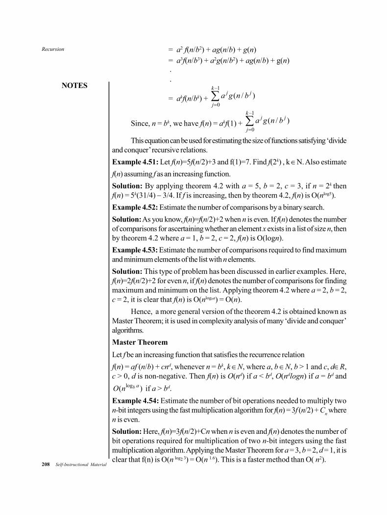
208 Self-Instructional Material
Recursion
NOTES
= a2 f(n/b2) + ag(n/b) + g(n)
= a3f(n/b3) + a2g(n/b2) + ag(n/b) + g(n)..
= akf(n/bk) +
–1
0
( / )k
j j
j
a g n b
Since, n = bk, we have f(n) = akf(1) +
–1
0
( / )k
j j
j
a g n b
This equation can be used for estimating the size of functions satisfying ‘divideand conquer’ recursive relations.
Example 4.51: Let f(n)=5f(n/2)+3 and f(1)=7. Find f(2k) , k N. Also estimate
f(n) assuming f as an increasing function.
Solution: By applying theorem 4.2 with a = 5, b = 2, c = 3, if n = 2k thenf(n) = 5k(31/4) 3/4. If f is increasing, then by theorem 4.2, f(n) is O(nlog5).
Example 4.52: Estimate the number of comparisons by a binary search.
Solution: As you know, f(n)=f(n/2)+2 when n is even. If f(n) denotes the numberof comparisons for ascertaining whether an element x exists in a list of size n, thenby theorem 4.2 where a = 1, b = 2, c = 2, f(n) is O(logn).
Example 4.53: Estimate the number of comparisons required to find maximumand minimum elements of the list with n elements.
Solution: This type of problem has been discussed in earlier examples. Here,f(n)=2f(n/2)+2 for even n, if f(n) denotes the number of comparisons for findingmaximum and minimum on the list. Applying theorem 4.2 where a = 2, b = 2,c = 2, it is clear that f(n) is O(nlogba) = O(n).
Hence, a more general version of the theorem 4.2 is obtained known asMaster Theorem; it is used in complexity analysis of many ‘divide and conquer’algorithms.
Master Theorem
Let f be an increasing function that satisfies the recurrence relation
f(n) = af (n/b) + cnd, whenever n = bk, k N, where a, b N, b > 1 and c, dR,c > 0, d is non-negative. Then f(n) is O(nd) if a < bd, O(ndlogn) if a = bd and
log( )b aO n if a > bd.
Example 4.54: Estimate the number of bit operations needed to multiply twon-bit integers using the fast multiplication algorithm for f(n) = 3f (n/2) + C
n where
n is even.
Solution: Here, f(n)=3f(n/2)+Cn when n is even and f(n) denotes the number ofbit operations required for multiplication of two n-bit integers using the fastmultiplication algorithm. Applying the Master Theorem for a = 3, b = 2, d = 1, it isclear that f(n) is O(n log2 3) = O(n 1.6). This is a faster method than O( n2).
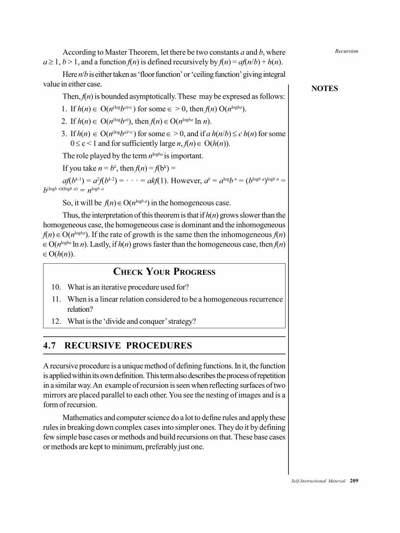
Recursion
NOTES
Self-Instructional Material 209
According to Master Theorem, let there be two constants a and b, wherea 1, b > 1, and a function f(n) is defined recursively by f(n) = af(n/b) + h(n).
Here n/b is either taken as ‘floor function’ or ‘ceiling function’ giving integralvalue in either case.
Then, f(n) is bounded asymptotically. These may be expresed as follows:
1. If h(n) O(n(logba)-) for some > 0, then f(n) O(nlogba).
2. If h(n) O(n(logba)), then f(n) O(nlogba ln n).
3. If h(n) O(n(logba)+) for some > 0, and if a h(n/b) c h(n) for some0 c < 1 and for sufficiently large n, f(n) O(h(n)).
The role played by the term nlogba is important.
If you take n = bk, then f(n) = f(bk) =
af(bk-1) = a2f(bk-2) = · · · = akf(1). However, ak = alogb n = (blogb a)logb n =b(logb n)(logb a) = nlogb a
So, it will be f(n) O(nlogb a) in the homogeneous case.
Thus, the interpretation of this theorem is that if h(n) grows slower than thehomogeneous case, the homogeneous case is dominant and the inhomogeneousf(n) O(nlogba). If the rate of growth is the same then the inhomogeneous f(n)O(nlogba ln n). Lastly, if h(n) grows faster than the homogeneous case, then f(n)O(h(n)).
CHECK YOUR PROGRESS
10. What is an iterative procedure used for?
11. When is a linear relation considered to be a homogeneous recurrencerelation?
12. What is the ‘divide and conquer’ strategy?
4.7 RECURSIVE PROCEDURES
A recursive procedure is a unique method of defining functions. In it, the functionis applied within its own definition. This term also describes the process of repetitionin a similar way. An example of recursion is seen when reflecting surfaces of twomirrors are placed parallel to each other. You see the nesting of images and is aform of recursion.
Mathematics and computer science do a lot to define rules and apply theserules in breaking down complex cases into simpler ones. They do it by definingfew simple base cases or methods and build recursions on that. These base casesor methods are kept to minimum, preferably just one.
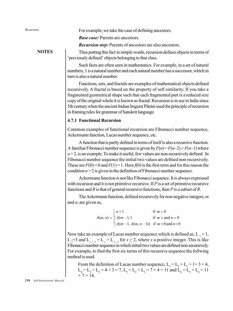
210 Self-Instructional Material
Recursion
NOTES
For example, we take the case of defining ancestors.
Base case: Parents are ancestors.
Recursion step: Parents of ancestors are also ancestors.
Thus putting this fact in simple words, recursion defines objects in terms of‘previously defined’ objects belonging to that class.
Such facts are often seen in mathematics. For example, in a set of naturalnumbers, 1 is a natural number and each natural number has a successor, which inturn is also a natural number.
Functions, sets, and fractals are examples of mathematical objects definedrecursively. A fractal is based on the property of self similarity. If you take afragmented geometrical shape such that each fragmented part is a reduced sizecopy of the original whole it is known as fractal. Recursion is in use in India since5th century when the ancient Indian linguist Pânini used the principle of recursionin framing rules for grammar of Sanskrit language.
4.7.1 Functional Recursion
Common examples of functional recursion are Fibonacci number sequence,Ackermann function, Lucas number sequence, etc.
A function that is partly defined in terms of itself is also a recursive function.A familiar Fibonacci number sequence is given by F(n) = F(n–2) + F(n–1) wheren > 2, is an example. To make it useful, few values are non-recursively defined. InFibonacci number sequence the initial two values are defined non-recursively.These are F(0) = 0 and F(1) = 1. Here f(0) is the first term and for this reason thecondition n > 2 is given in the definition of Fibonacci number sequence.
Ackermann function is not like Fibonacci sequence. It is always expressedwith recursion and it is not primitive recursive. If P is a set of primitive recursivefunctions and R is that of general recursive functions, then P is a subset of R.
The Ackermann function, defined recursively for non-negative integers, mand n, are given as,
1 if 0
( , ) ( – 1,1 if and 0
( –1, ( , – 1)) if 0and 0
n m
A m n A m m n
A m A m n m n
Now take an example of Lucas number sequence which is defined as, L 1 = 1,
L 2=3 and L
x + 1 = L
x + L
x –1 for x > 2, where x a positive integer. This is like
Fibonacci number sequence in which initial two values are defined non-recursively.For example, to find the first six terms of this recursive sequence the follwingmethod is used.
From the definition of Lucas number sequence, L3 = L
2 + L
1 = 1+ 3 = 4,
L4 = L
3 + L
2 = 4 + 3 = 7, L
5 = L
4 + L
3 = 7 + 4 = 11 and L
6 = L
5 + L
4 = 11
+ 7 = 18.
Recursion
NOTES
Self-Instructional Material 211
So the first six terms are 1, 3, 4, 7, 11 and 18.
We now give example of factorial function defined as f(n) = n!.
This leads to n! = n(n – 1)!= n(n – 1)(n – 2)! f(n) = n.f(n – 1 )= n(n – 1).F(n – 2 ). Here, n N, set of natural numbers.
Catalan numbers are another example of recursive functions; it is given as:
C0 = 1, C
n + 1 = (4n + 2)C
n / (n + 2)
Catalan numbers form a sequence of natural numbers that exists in theproblems using recursively defined objects in combinational mathematics.
4.7.2 Recursive Proofs
New systems in mathematics or logical constructs are defined as ‘true’ and ‘false’or ‘all natural numbers’. These are taken as base cases and after this, subsequentcomputations in the system are made according to predefined rules. If base casesand rules as predefined are computable, then any formula can be computed.
4.7.3 The Recursion Theorem
This theorem guarantees the existence of recursively defined functions. Let X bea set whose element is x and a function f: X X. The theorem opines the existenceof a unique function F : N X, where N stands for the set of natural numbers andzero. The function is stated as,
F(0) = x
F(n + 1) = f(F(n)) for any natural number n.
Proof of Uniqueness
Let there be two functions f and g. Domain of f is N and codomain of g is X suchthat,
f(0) = x
g(0) = x
f(n + 1) = F(f(n))
g(n + 1) = F(g(n)), where x is an element of X.
It is required to prove that f = g.
Equality of two functions is possible when they have equal domains/codomains and follow the same curve.
Recursively Defined Functions and Procedures
The basic requirement for a function to be recursive is that at least one value ƒ(x)is defined in terms of another value ƒ(y), when x y. In a similar way, if there is aprocedure P, it is defined recursively only when the action of P(x) is defined interms of another action P(y), provided x y.
212 Self-Instructional Material
Recursion
NOTES
The argument domain is already inductively defined.
Steps in defining recursive functions:
1. A value ƒ(x) or an action P(x) is to be specified for each basis element xof S.
2. Rules for each inductively defined element x in S is to be specified. Valueƒ(x) or action P(x) is to be defined in terms of previously defined values.
Example 4.55: A function ƒ : N N is defined as ƒ(n) = 0 + 3 + 6 + … + 3n.Develop a recursive definition for this function.
Solution: The set N which is inductively defined should be understood first. Thisincludes 0 too, hence 0 N and n N n + 1 N. Now f(0) should be givena value in N and then define ƒ(n + 1) in terms of ƒ(n). As given, set ƒ(0) = 0. Nexta definition for ƒ(n + 1) is obtained. According to definition of f(n),
ƒ(n + 1) = (0 + 3 + 6 + … + 3n) + 3(n + 1) = ƒ(n) + 3(n + 1).
Thus, a recursive definition has been developed as, ƒ(0) = 0 and ƒ(n + 1) =ƒ(n) + 3(n + 1).
This recursive function can be stated in different ways:
• Putting n – 1 in place of n, you get ƒ(0) = 0 and ƒ(n) = ƒ(n – 1) + 3n (n >0).
• It may be expressed as a conditional statement. If n = 0, then ƒ(n) = 0 elseƒ(n) = ƒ(n–1) + 3n.
Example 4.56: A function ƒ : N N is defined recursively as ƒ(0) = 0, ƒ(1) = 0and ƒ(x + 2) = 1 + ƒ(x). This function can be written as a conditional statement. Ifx = 0 or x = 1, then f(x) = 0; else 1 + ƒ(x – 2). What does ƒ do?
Solution: Following the rule of the function, find few values of the function for x = 0 to 9. f(0) = 0, f(1) = 0, f(2) = 1, f(3) = 1… and like that f(8) = 4 and f(9)= 4. Now do the mapping (ƒ(0, 1, 2, 3, 4, 5, 6, 7, 8, 9)) = ( 0, 0, 1, 1, 2, 2, 3,3, 4, 4) and find ƒ(x) = [x/2].
4.7.4 Infinite Sequences
It is possible to define recursive functions for infinite sequences. For this, define avalue ƒ(x) in terms of x and ƒ(y) for some value y in a sequence.
Example 4.57: An infinite sequence ƒ(x) = (x, x2, x4, x8, … ) is to be representedas a recursive function.
Solution: Follow the given definition and develop a solution:
The function is defined as,
ƒ(x) = (x, x2, x4, x8, … ) = (x :: (x2, x4, x8, … )) = x :: ƒ(x2).
So the developed definition is,
ƒ(x) = x :: ƒ(x2).
Recursion
NOTES
Self-Instructional Material 213
Example 4.58: A recursive function is defined as g(x, c) = xc :: g(x, c + 1). Findthe sequence represented by this function.
Solution: According to definition,
g(x, c) = xc :: g(x, c + 1) = xc :: xc+1 :: g(x, c + 2) =… = (xc, xc+1, xc+2, … ).
4.7.5 Recursive Function and Primitive Recursive Function
Consider a function, g(x1, x
2, … x
n) and h(x
1, x
2, … x
n ,y,z) of n and n+2 variables.
Now define a function f(x1, x
2, … x
n, y) of n+1 variables as f(x
1, x
2, … x
n, 0) =
g(x1, x
2, … x
n,) and f(x
1, x
2, … x
n, y + 1) = h(x
1, x
2, … x
n, ,y, f(x
1, x
2, … x
n,
y)); here f is called a recursive function or simply a recursion. A function f isprimitive recursive if it can be obtained from initial functions by a finite number ofoperations of composition and recursion.
CHECK YOUR PROGRESS
13. What do you understand by a recursive procedure?
14. Give some examples of functional recursion.
4.8 SUMMARY
In this unit, you have learned that:
The Mergesort algorithm works according to a ‘divide and conquer’ strategyin which the sequence is divided into two halves.
In the merging process, the elements of two arrays are combined, creatinga new array.
In insertion sorting algorithm, the sorted array is built one entry at a time.
The ordered sequence of inserted elements is stored at the beginning of thearray.
Each iteration of the inner loop scans and shifts the entire sorted subsectionof the array before the next element is inserted.
Sorting can be classified into two types, viz., internal sorting and externalsorting.
A binary system groups numbers by two and by powers of two.
A binary number with 4 bits is called a nibble and a binary number with 8bits is called a byte.
A number system that utilizes ten distinct digits, i.e., 0, 1, 2, 3, 4, 5, 6, 7, 8and 9 is known as a decimal number system.
A binary number can be converted into decimal number by multiplying thebinary 1 or 0 by the weight corresponding to its position and adding all thevalues.
214 Self-Instructional Material
Recursion
NOTES
The numbers in the sequence 0, 1, 2, 3, 5, 8, 13, 21 … in which each newterm is the sum of the previous two terms are called Fibonacci numbers.
A recursive relation is an equation defining a sequence in which each termof the sequence is defined as a function of the preceding terms.
A kth order linear relation is a homogeneous recurrence relation if f(n)=0for all n.
The general solution of the recurrence relation is the sum of the homogeneoussolution and particular solution.
4.9 KEY TERMS
Selection sort: It refers to a simple technique of sorting a list of elementsby finding the smallest value in an array.
Binary number system: It refers to the number system in which only twodigits, viz., 0 and 1, are used.
Nibble: A binary number with 4 bits is called a nibble.
Double-dabble method: It refers to a method that is used to convert alarge decimal number into its binary equivalent by repeatedly dividing itby 2.
Recursive relation: It is an equation defining a sequence in which eachterm of the sequence is defined as a function of the preceding terms.
4.10 ANSWERS TO ‘CHECK YOUR PROGRESS’
1. The Mergesort algorithm is based on the merging process where all theelements are copied in one array and kept in a separate new array.
2. Two advantages of insertion sort are as follows:(i) Its implementation is simple.(ii) It can sort a list even as it receives it.
3. The insert function is designed for inserting a value into a sorted sequence atthe beginning of an array.
4. Sorting is a method of arranging keys in a file in the ascending or descendingorder.
5. Internal sorting occurs when the records in a file that are stored in the mainmemory are sorted.
6. Two common sorting techniques are:(i) Bubble sort(ii) Tree sort
Recursion
NOTES
Self-Instructional Material 215
7. A base two system is another term for a binary number system. Such anumber system uses two digits, 0 and 1, only.
8. A binary number system is used in digital computers because all electricaland electronic circuits can be made to respond to the two-state concept.
9. One method to convert a decimal number into a binary number is to subtractvalues of power of 2 from the decimal number until nothing remains.
10. An iterative procedure is used to evaluate a function from its recursivedefinition.
11. A k-th order linear relation is considered to be a homogeneous recurrencerelation if f(n)=0 for all n.
12. When a problem is divided into many smaller problems and such reductionis done repeatedly to find solutions of smaller problems, such a procedureis called a ‘divide and conquer’ strategy.
13. A recursive procedure is a unique method of defining functions. In it, thefunction is applied within its own definition. This term also describes theprocess of repetition in a similar way.
14. Common examples of functional recursion are Fibonacci number sequence,Ackermann function, Lucas number sequence, etc.
4.11 QUESTIONS AND EXERCISES
Short-Answer Questions
1. Give an algorithm illustrating the use of Mergesort mechanism.
2. Write a short note on the Insertion sort algorithm.
3. What are the different types of sorting algorithms?
4. Differentiate between the binary number system and decimal number system.
5. Write a short note on the double-dabble method.
Long-Answer Questions
1. Write a program illustrating the use of Insertion sort.
2. Explain the functions of Bubble sort and Selection sort. Write one programeach to illustrate their implementation.
3. Explain the various techniques that are used to convert binary numbers intodecimal numbers and vice versa.
4. What do you understand by recursion and recurrence relations? Giveexamples to illustrate both the relations.

216 Self-Instructional Material
Recursion
NOTES
4.12 FURTHER READING
Lipschutz, Seymour and Lipson Marc. Schaum’s Outline of DiscreteMathematics, 3rd edition. New York: McGraw-Hill, 2007.
Horowitz, Ellis, Sartaj Sahni and Sanguthevar Rajasekaran. Fundamentals ofComputer Algorithms. Hyderabad: Orient BlackSwan, 2008.
Cormen, Thomas H., Charles E. Leiserson, Ronald L. Rivest and Clifford Stein.Introduction to Algorithms. The MIT Press, 1990.
Brassard, Gilles and Paul Bratley. Fundamentals of Algorithms. New Delhi:Prentice Hall of India, 1995.
Levitin, Anany. Introduction to the Design and Analysis of Algorithms. NewJersey: Pearson, 2006.
Baase, Sara and Allen Van Gelder. Computer Algorithms – Introduction toDesign and Analysis. New Jersey: Pearson, 2003.
Mott, J.L. Discrete Mathematics for Computer Scientists, 2nd edition. NewDelhi: Prentice-Hall of India Pvt. Ltd., 2007.
Liu, C.L. Elements of Discrete Mathematics. New Delhi: Tata McGraw-HillPublishing Company, 1977.
Rosen, Kenneth. Discrete Mathematics and Its Applications, 6th edition. NewYork: McGraw-Hill Higher Education, 2007.
Number Theory
NOTES
Self-Instructional Material 217
UNIT 5 NUMBER THEORY
Structure
5.0 Introduction5.1 Unit Objectives5.2 Number Theory: Basics
5.2.1 Fundamental Theorem of Arithmetic5.2.2 Prime Numbers5.2.3 Division Algorithms5.2.4 Divisibility5.2.5 Absolute Value5.2.6 Order and Inequalities
5.3 Greatest Common Divisor5.3.1 Linear Diophantine Equation
5.4 Euclidean Algorithm5.5 Fibonacci Numbers5.6 Congruences and Equivalence Relations
5.6.1 Congruences Relations5.6.2 Equivalence Relations
5.7 Public Key Encryption Schemes5.7.1 Message Authentication Code5.7.2 Digital Structure
5.8 Summary5.9 Key Terms
5.10 Answer to ‘Check Your Progress’5.11 Questions and Exercises5.12 Further Reading
5.0 INTRODUCTION
Numbers form the very basis for any type of calculation. There are primarily twotypes of numbers—prime and composite numbers. A prime number refer to thosenumbers which have only 1 and the number itself as its factors and does notcontain any multiple. In this unit, you will learn about the various types of numbers,their properties and their applications.
A common calculation that is used frequently is the finding of the greatestcommon divisor (GCD) and the Euclid’s algorithm. You will learn about theapplication of GCD, least common multiple (LCM), and Euclidean algorithm.
Fibonacci numbers refer to numbers that are a sum of the previous twonumbers. Among other things, this unit will talk about Fibonacci numbers, congruentrelations, equivalence relations and also encryption schemes.

218 Self-Instructional Material
Number Theory
NOTES
5.1 UNIT OBJECTIVES
After going through this unit, you will be able to:
Understand the basics of the number theory
Identify the greatest common divisor (GCD), Euclidean algorithm andFibonacci numbers
Explain the concepts of congruence and equivalent relations
Comprehend the public key encryption schemes and their application
5.2 NUMBER THEORY: BASICS
5.2.1 Fundamental Theorem of Arithmetic
Let a, b be two integers such that a = bc, where b and c are called factors of a anda is called multiple of b and c. If b is a factor of a, this implies that b divides a andit is written as b | a. It is easy to prove that ± 1 are factors of a and every non-zerointegers is a factor of 0.
For example, 6 = (– 2) (– 3) – 2 and – 3 are factors of 6.
Again 7 = 7. 1, so 7 and 1 are factors of 7.
An integer n different from ± 1 is called a prime integer provided its onlyfactors are ± 1 and ± n.
Thus, 2, – 3, 7, 11, – 13 are some prime integers, while – 4, 16, 12 are notprime integers as – 4 = 2 (– 2), 16 = 4 . 4, 12 = 6 . 2
A positive prime integer is called a prime number.
Properties of Prime Numbers(i) If a prime number p divides ab then either p | a or p | b.
(ii) If a prime number p does not divide an integer a then the Highest CommanFactor (HCF) of p and a is 1 (by convention take HCF to be a +ve integer).
Fundamental Theorem of ArithmeticEvery integer n > 1 can be factorized into a product of finite numbers of primenumbers. This expression is unique except for the order in which the prime factorsare written.
For example, 56 = 2 . 2 . 2 . 7 = 23 . 7
72 = 2 . 2 . 2 . 3 . 3 = 23 . 32
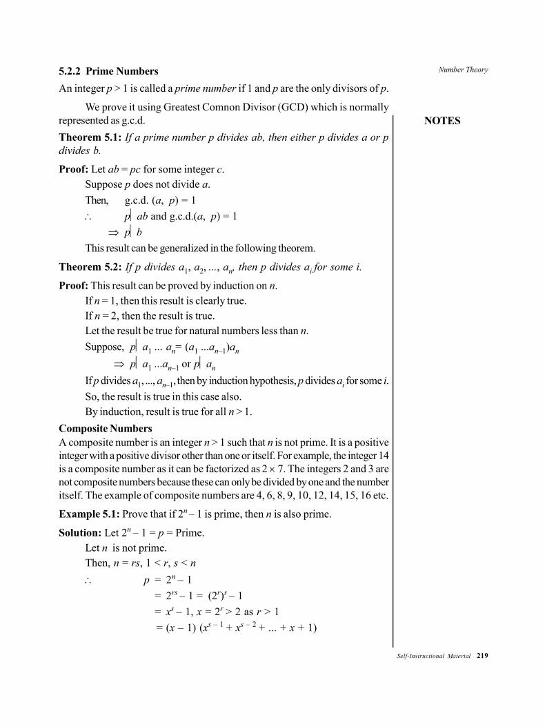
Number Theory
NOTES
Self-Instructional Material 219
5.2.2 Prime Numbers
An integer p > 1 is called a prime number if 1 and p are the only divisors of p.
We prove it using Greatest Comnon Divisor (GCD) which is normallyrepresented as g.c.d.
Theorem 5.1: If a prime number p divides ab, then either p divides a or pdivides b.
Proof: Let ab = pc for some integer c.Suppose p does not divide a.
Then, g.c.d. (a, p) = 1
pab and g.c.d.(a, p) = 1
pb
This result can be generalized in the following theorem.
Theorem 5.2: If p divides a1, a2, ..., an, then p divides ai for some i.
Proof: This result can be proved by induction on n.If n = 1, then this result is clearly true.If n = 2, then the result is true.Let the result be true for natural numbers less than n.
Suppose, pa1 ... an= (a1 ...an–1)an
pa1 ...an–1 or pan
If p divides a1, ..., an–1, then by induction hypothesis, p divides ai for some i.
So, the result is true in this case also.By induction, result is true for all n > 1.
Composite NumbersA composite number is an integer n > 1 such that n is not prime. It is a positiveinteger with a positive divisor other than one or itself. For example, the integer 14is a composite number as it can be factorized as 2 7. The integers 2 and 3 arenot composite numbers because these can only be divided by one and the numberitself. The example of composite numbers are 4, 6, 8, 9, 10, 12, 14, 15, 16 etc.
Example 5.1: Prove that if 2n – 1 is prime, then n is also prime.
Solution: Let 2n – 1 = p = Prime.Let n is not prime.Then, n = rs, 1 < r, s < n
p = 2n – 1
= 2rs – 1 = (2r)s – 1
= xs – 1, x = 2r > 2 as r > 1
= (x – 1) (xs – 1 + xs – 2 + ... + x + 1)
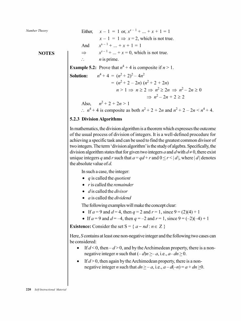
220 Self-Instructional Material
Number Theory
NOTES
Either, x – 1 = 1 or, xs – 1 + ... + x + 1 = 1
x – 1 = 1 x = 2, which is not true.
And xs – 1 + ... + x + 1 = 1
xs – 1 + ... + x = 0, which is not true. n is prime.
Example 5.2: Prove that n4 + 4 is composite if n > 1.
Solution: n4 + 4 = (n2 + 2)2 – 4n2
= (n2 + 2 – 2n) (n2 + 2 + 2n)
n > 1 n 2 n2 2n n2 – 2n 0
n2 – 2n + 2 2Also, n2 + 2 + 2n > 1 n4 + 4 is composite as both n2 + 2 + 2n and n2 + 2 – 2n < n4 + 4.
5.2.3 Division Algorithms
In mathematics, the division algorithm is a theorem which expresses the outcomeof the usual process of division of integers. It is a well-defined procedure forachieving a specific task and can be used to find the greatest common divisor oftwo integers. The term ‘division algorithm’ is the study of algebra. Specifically, thedivision algorithm states that for given two integers a and d with d 0, there existunique integers q and r such that a = qd + r and 0 < r < | d |, where | d | denotesthe absolute value of d.
In such a case, the integer: q is called the quotient r is called the remainder d is called the divisor a is called the dividend
The following examples will make the concept clear: If a = 9 and d = 4, then q = 2 and r = 1, since 9 = (2)(4) + 1 If a = 9 and d = –4, then q = –2 and r = 1, since 9 = (–2)(–4) + 1
Existence: Consider the set S = { a nd : n }
Here, S contains at least one non-negative integer and the following two cases canbe considered:
If d < 0, then – d > 0, and by the Archimedean property, there is a non-negative integer n such that (– d)n >– a, i.e., a– dn > 0.
If d > 0, then again by the Archimedean property, there is a non-negative integer n such that dn > – a, i.e., a – d(–n) = a + dn >0.
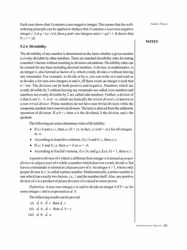
Number Theory
NOTES
Self-Instructional Material 221
Each case shows that S contains a non-negative integer. This means that the well-ordering principle can be applied to deduce that S contains a least non-negativeinteger r. Let q = (a–r)/d, then q and r are integers and a = qd + r. It shows that0 < r < |d|.
5.2.4 Divisibility
The divisibility of any number is determined on the basis whether a given numberis evenly divisible by other numbers. There are standard divisibility rules for testinga number’s factors without resorting to division calculations. Divisibility rules canbe created for any base including decimal numbers. A divisor, in mathematics, isan integer n, also termed as factor of n, which evenly divides n without leavingany remainder. For example, to divide m by n, you can write m/n and read asm divides n for non-zero integers m and n, iff there exists an integer k such thatn = km. The divisors can be both positive and negative. Numbers which areevenly divisible by 2 without leaving any remainder are called even numbers andnumbers not evenly divisible by 2 are called odd numbers. Further, a divisor ofn that is not 1, –1, n or –n, which are basically the trivial divisors, is known asa non-trivial divisor. Prime numbers do not have non-trivial divisors while thecomposite numbers have non-trivial divisors. The term is derived from the arithmeticoperation of division. If a/b = c then a is the dividend, b the divisor, and c thequotient.
The following are some elementary rules of divisibility:
If a | b and a | c, then a | (b + c), in fact, a | (mb + nc) for all integersm, n.
According to transitive relation, if a | b and b | c, then a | c.
If a | b and b | a, then a = b or a = –b.
According to Euclid’s lemma, if a | bc and g.c.d.(a, b) = 1, then a | c.
A positive divisor of n which is different from integer n is termed as properdivisor or aliquot part of n while a number which does not evenly divide n, butleaves a remainder is termed as aliquant part of n. An integer n > 1, whose onlyproper divisor is 1, is called a prime number. Mathematically, a prime number isone which has exactly two factors, i.e., 1 and the number itself. Also, any positivedivisor of n is a product of prime divisors of n raised to some power.
Definition. A non-zero integer a is said to divide an integer b if b = ac forsome integer c and is expressed as ab.
The following results can be proved:
(i) ab, bc then ac
(ii) ab, ac then ab + c
(iii) a0, aa

222 Self-Instructional Material
Number Theory
NOTES
5.2.5 Absolute Value
For any a R, | a | is defined as follows:
| a | = a if a 0
= – a if a < 0
Thus, | – 2 | = 2 , | 0 | = 0, | 5. 7 | = 5. 7
Definition. | a | is called absolute value of a.
Note: It follows from definition that for all x R, | x | 0.
Properties of Absolute Value Function:
(1) For all a R, | a | a.
Proof: If a 0 then, | a | = a. As a a, you get | a | a.
In case a < 0 then, a + (– a) < 0 + (– a) 0 < – a – a > 0
Now – a > 0 and 0 > a – a > a
But for a < 0, | a | = – a. Hence | a | > a. Then, by definition of ‘ ‘, | a | a.
(2) For all a,b R, | a b | = | a | | b |
Proof: The following four cases occur:
Case I.
a 0, b 0
By definition, | a | = a, | b | = b. Further, a 0, b 0 imply ab
Thus, | ab | = ab = | a | | b |
Case II.
a 0, b 0
In this case | a | = – a and | b | = b. But a < 0, b 0 imply ab < 0.
So, | a b | = – a b = | a | | b |
Case III.
a 0, b < 0
This is similar to Case II; There is just an interchange of a and b.
Case IV.
a < 0, b < 0
Here, | a | = – a, | b | = – b and a b > 0 | ab | = ab
So, | a b | = (– a) (– b) = | a | | b |
(3) For all a, b in R, | a + b | | a | + | b |
Proof: For all a, b R, ( | a | + | b | )2 = | a |2 + 2 | a | | b | + | b |2
= a2 + 2 | a | | b | + b2.

Number Theory
NOTES
Self-Instructional Material 223
Since, | a |2 = a2 and | b |2 = b2
= a2 + 2 | a b | + b2
a2 + 2 ab + b2 by Property (1)
Thus, ( | a | + | b | )2 (a + b)2 = | a + b |2
| a | + | b | | a + b |
(4) For a, k R, | a | < k – k < a < k
Proof: Suppose | a | < k. In case a 0, you get a < k.
In case, a < 0, | a | = – a – a < k a > – k
– k < a
Hence, | a | < k implies that – k < a < k.
Conversely, let – k < a < k
If a 0 you get | a | = a < k
If a < 0, then | a | = – a.
But, – k < a k > – a
or, – a < k.
So, | a | < k
5.2.6 Order and Inequalities
In mathematics, an inequality is a statement that defines the relative size or orderof two objects to check whether they are similar or not. The following statementsexplain the order and inequality relationship between integers:
The notation a < b means that a is less than b.
The notation a > b means that a is greater than b.
The notation a b means that a is not equal to b. It does not mean that ais bigger than b or even that they can be compared in size.
In all these cases, a is not equal to b defines that there is inequality in theirrelation. The following relations are known as strict inequality:
The notation a < b means that a is less than or equal to b or in other wordsa is not greater than b.
The notation a > b means that a is greater than or equal to b or in otherwords a is not smaller than b.
When the inequality is same for all the values of the given variables forwhich it is defined, then the inequality is termed as an ‘absolute’ or ‘unconditional’inequality. Similarly, if an inequality holds only for certain values of the variablesinvolved, but is reversed or destroyed for other values of the variables then it istermed as ‘conditional inequality’.
224 Self-Instructional Material
Number Theory
NOTES
Inequalities are governed by the following properties:
Trichotomy: The trichotomy property states that for any real numbers aand b any one of the following is true:
a < b
a = b
a > b
Transitivity: The transitivity of inequalities states that for any real numbersa, b, c, any one of the following case may be true:
If a > b and b > c; then a > c
If a < b and b < c; then a < c
If a > b and b = c; then a > c
If a < b and b = c; then a < c
Addition and subtraction: The properties which deal with addition andsubtraction, state that for any real numbers a, b, c, any one of the following casemay be true:
If a < b, then a + c < b + c and a – c < b – c
If a > b, then a + c > b + c and a – c > b – c
This states that the real numbers are an ordered group.
Multiplication and division: The properties which deal with multiplicationand division, state that for any real numbers a, b, c any one of the following casemay be true:
If c is positive and a < b, then ac < bc
If c is negative and a < b, then ac > bc
This is basically applied to an ordered field.
The next step is to extend N so as to include the solution of the equations ofthe type a + x = b with a, b N. The extended system Z, consists of, ..., – 4, –3, – 2, – 1, 0, 1, 2, 3, ..., etc. Each member of Z is called an integer. To constructan integer with the help of natural numbers, remember a simple fact that everyinteger can be written as m – n for some m, n N, where ‘–’ stands for the usualdifference sign. But, as you have not defined this operation for N, hence tactfullyavoid it and proceed as follows:
Consider N × N = {(m, n) | m, n N}, i.e., the elements of N × N areordered pairs of natural numbers.
Define a relation ~ on N as under,
(m, n) ~ (p, q) if and only if m + q = n + p
For example, (1, 5) ~ (3, 7) as 1 + 7 = 5 + 3 = 8 and (4, 4) ~ (2, 2) as
4 + 2 = 2 + 4 = 6
Number Theory
NOTES
Self-Instructional Material 225
It can be verified that ‘~’ is an equivalence relation on N. By [m, n] it is meantthat all ordered pairs (p, q) such that (m, n) ~ (p, q). This [m, n] will be called aninteger. The set of all [m, n], m, n N is denoted by Z.
Addition and multiplication on Z are defined as follows:
[m, n] + [m1, n1] = [m + m1, n + n1]
[m, n] . [m1, n1] = [mm + nn1, mn1 + m1n]
It can be verified that these operations are well defined, i.e., if
(m, n) ~ (p, q) and (m1, n1) ~ (p1, q1)
Then, [m, n] + [m1, n1] = [p, q] + [p1, q1]
and [m, n] [m1, n1] = [p, q] . [p1, q1]
Addition and multiplication are motivated by the following observations:
Let z and z1 be two integers and z = m – n, z1 = p – q when m, n, p, q N.
Then, z + z1 = (m + p) – (n + q) and zz1 = mp + nq – (mq + np)
For numerical instances of addition and multiplication, consider integers [3, 5]and [4, 1]. [3, 5] + [4, 1] = [3 + 4, 5 + 1] = [ 7, 6]
[3, 5].[4, 1] = [3 . 4 + 5 . 1, 3 . 1 + 5 . 4]
= [17, 23]
Compare this with the facts that [3, 5] is actually – 2 and [4, 1] is 3 then,
– 2 + 3 = 1
Which is same as 7 – 6, whereas (– 2) (3) = – 6 = 17 – 23
The following properties hold for integers:
(i) Addition is associative and commutative.
(ii) Multiplication is associative and commutative.
(iii) Multiplication is distributive over addition.
(iv) The integer [n, n] is called zero element and is denoted by 0.
It can be easily shown that 0 + z = z = z + 0 for all z Z.
(v) For each integer z = [m, n], the integer z¢ = [n, m] is called negative of z.It can be that z + z¢ = z¢ + z = 0
Note: By z – z we mean z + (– z) for any z, zZ.
The integer z = [m, n] is called positive if m > n and is called negative incase n > m.
Let, z, z Z
You define z > zif z = z + u for some positive integer u.
(vi) Given two integers z and z for which one and only one of the followingholds: Either z > z or z = z or z > z.
226 Self-Instructional Material
Number Theory
NOTES
Example 5.3: Show that addition on Z is commutative.
Solution: Let, z = [m, n] and z= [p, q], where m, n, p, q N
Now z + z = [m + p, n + q] = [p + m, q + n]
= [p, q] + [m, n] = z+ z
Example 5.4: Prove that multiplication on Z is associative.
Solution: Let, z = [m, n], z = [p, q] and z = [r, s] where m, n, p, q, r, s N.
(zz) z= [mp + nq, mq + np] [r, s]
= [(mp + nq) r + (mq + np) s, (mp + nq) s + (mq + np) r]
= [mpr + nqr + mqs + nps, mps + nqs + mqr + npr] ... (1)
Further z (zz) = [m, n] [pr + qs, pr + qr]
= [m (pr + qs) + n (ps + qs), m (ps + qr) + n (pr + qs)]
= [(mpn + mqs + nps +nqr, mps + mqr + npr + nqs] ...(2)
Using properties of N, one can easily show that the right sides ofEquations (1) and (2) are same as a consequence.
(zz) z = z (zz)
Example 5.5: Show that for all z Z, z. 0 = 0
Solution: Let z = [m, n], 0 = [p, p]
z 0 = [mp + np, mp + np] = 0
Example 5.6: Prove that if z > z then (i) For any zZ, z + z > z + z
(ii) For any + ve integer k, zk > zk
Solution:
(i) z > z z= z + u, u is a positive integer.
Clearly, z + z = z + u + z
= z + z + u
z + z > z + z
(ii) As zk = (z + u) k = zk + uk, it is sufficient to prove that product of twopositive integers is a positive integer.
Let, u = [m, n] and k = [p, q]
Since u is positive, so m > n. In case n = 1and m > 1, then there exists anatural number t such that m = t*. So (m, n) = (t*, 1)
If n 1, n > 1 n = 1 + k, for some k N.
Then, m > n m = 1 + k + l for some l N.
Thus, [m, n] = [1 + k + l, 1 + k] = [1 + l, 1]
Since, (1 + k + l) + 1 = (1 + k) + (1 + l) (1 + k + l, 1 + k) ~ (1 + l, 1)
This implies that [m, n] = [l*, 1]
So, in each case if z = [m, n], then it is positive.
Number Theory
NOTES
Self-Instructional Material 227
You can write u = [t*, 1] for some t N.
Similarly,
k = [s*, 1] for some s N
Now, uk = [t*s* + 1. t* + s*]
But, t*s* + 1 = (t + 1) (s + 1) + 1 = (t + 1) + (s + 1) + ts
= (t* + s*) + ts and ts N
So, t*s* + 1 > (t* + s*) + ts. In other words, uk is + ve. Hence the assertionis follow.
Notes:
1. It can be shown that z Z is positive if and only if z > 0 and negative if andonly if 0 > z.
2. Let z and zZ , then z > z if and only if z – z > 0.
3. By z z it is shown that either z > z or z = z4. Z+ denotes the set of all positive integers, Z– denotes the set of all negative,
integers. Law of Trichotomy states that Z = Z+ Z– {0} which is a disjointunion.
5. As a convention, 0 is regarded both positive and negative. When we wish tostress upon a non-zero positive integer, then it is called strictly positive.Similarly, the strictly negative integer is defined.
CHECK YOUR PROGRESS
1. State the properties of prime numbers.
2. Define division algorithm.
3. What are even numbers?
4. Define an inequality.
5.3 GREATEST COMMON DIVISOR
The greatest common divisor (g.c.d) is also termed as the greatest common factor(g.c.f.) or highest common factor (h.c.f.). The g.c.d. of two or more non-zerointegers is the largest positive integer that divides a number without leaving aremainder.A special case in Euclid’s algorithm arises when the remainder is zero.
Definition. An integer d > 0 is called g.c.d. of two integers a, b (non-zero) if,
(i) da, db
(ii) If ca, cb then d c
It is written d = g.c.d.(a, b) or simply d = (a, b).
228 Self-Instructional Material
Number Theory
NOTES
Notes:1. (a, 0) = a, (0, b) = b
Clearly, aa, a0
If ca, then ca (a, 0) = aSimilarly (0, b) = b
2. If ab, then (a, b) = aaa, and ab ab
If ca, cb, then ca (a, b) =a
3. The g.c.d. of a and b does not depend on signs of a and b.
i.e., (a, b) = (– a, b) = (a, – b) = (–a, –b)
Let, d = (a, b).
Then, da, db d–a, d b
c–a, cb ca, cb cd
d = (–a, b).
The following theorem will prove the existence and uniqueness of g.c.d. ofintegers a and b.
Theorem 5.3 Let a, b be two integers. Suppose either a 0 or b 0. Thenfor some ), the greatest common divisor d of a, b such that, d = ax + by forsome integers x, y d is uniquely determined by a and b.
Proof: Let S = {au + bv u, v are integers and au + bv > 0}.
If a > 0, then a = a.1 + b.0 > 0 a S.
If a < 0, then –a = a(–1) + b.0 > 0 –a S.
Similarly, if b > 0 then b S and if b < 0 then –b S. Since one of a and bis non-zero, either ±a S or ±b S. In any case S .
By well ordering principle, S has a least element, say d.
Now d S d = ax + by for some integers x and y. Also, d > 0.
Let, a = dq + r, 0 r < d
Let, r 0. Since r = a – dq
= a – (ax + by)q
= a(1 – xq) + b(–yq) > 0
r S
But r < d, which contradicts the fact that d is the least element of S. So, r = 0.
Therefore, a = dq da
Similarly, db
Suppose, ca, cb cax + by = d
Number Theory
NOTES
Self-Instructional Material 229
So, d is the greatest common divisor of a and b.
If d is also the greatest common divisor of a and b, then d a, d b, ddSimilarly, da, db d d. Since d, d > 0, d = d . So, d is uniquely determinedby a and b.
Note: x and y in the preceding theorem need not be unique.
For, d = ax + by
d = a(x – b) + b(a + y)
If x – b = x, a + y = y b = 0 = a, which is not true. So either,
x – b x or a + y y.
Definition: If g.c.d.(a, b) = 1, then a and b are said to be relatively prime orcoprime.
Corollary 1. Two integers a, b are relatively prime, if and only if integers x,y are such that ax + by = 1.
Proof: Suppose, a, b are relatively prime. Then g.c.d.(a, b) = 1. By the precedingtheorem, integers x, y such that ax + by = 1.
Conversely, let ax + by = 1 for some integers x, y.
Let, d = g.c.d.(a, b).
Then, d | a, d | b d | ax, d | by d | ax + by = 1 d = 1.
So, a, b are relatively prime.
Corollary 2. If g.c.d.(a, b) = d, then g.c.d. ,a b
d d = 1.
Proof: Given that g.c.d.(a, b) = d
integers x, y such that,
d = ax + by
1 = a bx y
d d
g.c.d. ,a b
d d = 1, by Corollary 1.
Corollary 3. If abc, with g.c.d.(a, b) = 1, then ac
Proof: As g.c.d.(a, b) = 1 integers x, y such that,
ax + by = 1 acx + bcy = c
Now, aac, abc aacx, abcy
aacx + bcy = c
Corollary 4. If g.c.d.(a, b) = 1 and g.c.d.(a, c) = 1, then g.c.d.(a, bc) = 1.
Proof: Since g.c.d.(a, b) = 1, integers x, y, such that ax + by = 1. Also,g.c.d.(a, c) = 1, integers u, v, such that au + cv = 1.
230 Self-Instructional Material
Number Theory
NOTES
1 = (ax + by) (au + cv)
= a (axu + cxv + byu) + bc (yv)
By Corollary 1, g.c.d.(a, bc) = 1.
The following lemman defines the practical method of finding the greatestcommon divisor of two integers. First, prove the following result:
Lemma. If a = bq + r, then g.c.d.(a, b) = g.c.d.(b, r).
Proof: Let, g.c.d.(a, b) = d.
Then, da, db da, dbq da – bq = r.
Suppose cb, cr.
Then, cbq, cr cbq + r ca, cb cd.
Thus, d = g.c.d. (b, r).
Let a, b be two integers.
Since, g.c.d.(a, b) = g.c.d.(ab), let a b > 0.
Let, a = bq1 + r1, 0 r1 < b.
If r1 = 0, then ba and g.c.d. (a, b) = b.
Let r1 0. Divide b by r1 to get integers q2 and r2 such that,
b = r1q2 + r2, 0 r2 < r1
If r2 = 0, then g.c.d.(b, r1) = r1 and so by above lemma, g.c.d.(a, b) = r1.
If r2 0, then proceed as above till we get remainder as zero,
Given that, a = q1b + r1, 0 < r1 < b
b = q2r1 + r2, 0 < r2 < r1
r1 = q3r2 + r3, 0 < r3 < r2
. . . . . . . . . .
rn–2 = qnrn–1 + rn’ 0 < rn < rn–1
rn–1 = qn+1rn + 0
By above lemma,
g.c.d.(a, b) = g.c.d.(b, r1) = ...... = g.c.d.(rn’ 0) = rn
So, the last remainder nr is g.c.d. of a and b.
For example, to determine g.c.d. (56, 72), divide 72 by 56 to get,
72 = 56 + 16
56 = 16 3 + 8
16 = 8 2 + 0
Number Theory
NOTES
Self-Instructional Material 231
Since the last non-zero remainder is 8 hence g.c.d.(56, 72) = 8.
Also, 8 = 56 – 16 3
= 56 – (72 – 56) 3
= 56 (4) + 72 (–3)
= 56x + 72y where x = 4, y = –3.
Which shows us the way to find x, y such that,
g.c.d. (a, b) = ax + by
Theorem 5.4:Let k > 0. Then g.c.d.(ka, kb) = k g.c.d.(a, b).
Proof: Let, g.c.d.(a, b) = d
Then, da, db kdka, kdkb
Also, integers x, y such that,
d = ax + by
kd = kax + kby
Let, cka, ckb then, ckax, ckby
ckax + kby = kd
g.c.d. (ka, kb) = kd = k g.c.d. (a, b)
Note: As k > 0, d > 0 we get kd > 0
Corollary: For any integer k 0, g.c.d. (ka, kb) = k g.c.d.(a, b).
Proof: For k > 0, the result follows from the preceding theorem.
Let, k < 0. Then, g.c.d.(ka, kb)
= g.c.d.(–ka, –kb)
= – k g.c.d.(a, b) by above theorem.
= k g.c.d.(a, b)
Definition: The least common multiple (l.c.m.) of two non-zero integers a andb, denoted as l.c.m.(a, b) is the positive integer m such that,
(i) am, bm
(ii) If ac, bc, with c > 0, then mc
Theorem 5.5: For positive integers a and b,
g.c.d.(a, b) l.c.m.(a, b) = ab
Proof: Let, d = g.c.d.(a, b)
Now, . asab b ab b
a ad d d d is integer..
Also, . asab a ab a
b bd d d d is integer..
232 Self-Instructional Material
Number Theory
NOTES
Let, m = ab
d, then am and bm.
Suppose now ac, bc. Since (a, b) = d, integers x, y such that,
d = ax + by.
( )c cd c ax by c cx y
m ab ab b aInteger
mc
Thus, m = l.c.m. (a, b), i.e., ab
d = l.c.m. (a, b)
Or, ab = g.c.d. (a, b) l.c.m. (a, b).
Example 5.7: Let g.c.d. (a, b) = 1.
Show that g.c.d.(a + b, a2 – ab + b2) = 1 or 3.
Solution: Let, g.c.d.(a + b, a2 – ab + b2) = d
Then, da + b, da2 – ab + b2
d(a + b)2 = a2 + b2 + 2ab, da2 – ab + b2
d3ab
Let, g.c.d. (d, a) = e
Then, eda + b ea + b and ea
e(a + b) – a = b
So, eg.c.d.(a, b) = 1 e = 1
g.c.d.(d, a) = 1
Similarly, g.c.d.(d, b) = 1
d3 d = 1 or 3.
Example 5.8: Let g.c.d.(a, b) = 1. Show that g.c.d.(an, bn) = 1 for everyinteger n 1.
Solution: Since, g.c.d. (a, b) = 1, integers x, y, such that ax + by = 1.
(ax + by) (ax + by) = 1
a2x2 + 2abxy + by2 = 1
a2x2 + b(2axy + y2) = 1
g.c.d.(a2, b) = 1
In this way you will get,
g.c.d.(an, b) = 1 or g.c.d.(b, an) = 1
Proceeding as above, we get
g.c.d.(bn, an) = 1
Number Theory
NOTES
Self-Instructional Material 233
5.3.1 Linear Diophantine Equation
Definition. Linear Diophantine equation is an equation ax + by = c in twounknowns x and y, where a, b, c are given integers and one of a, b is not zero.The name is due to the mathematician Diophantus. A natural question arises as towhen such an equation would have a solution? The following theorem is helpfulin finding the answer.
Theorem 5.6: The linear Diophantine equation ax + by = c has a solutionif and only if dc, where d = g.c.d. (a, b). If x0, y0 is a particular solution,then the other solutions are given by,
0 0,b a
x x t y y td d
for varying integer t.
Proof: Suppose, ax + by = c has a solution.
Let, x = x0, y = y0 be a solution.
Then, ax0 + by0 = c.
Let, d = g.c.d.(a, b).
da, db dax0, dby0
dax0 + by0 = c
Conversely, let dc. Let, c = dk.
Since, d = g.c.d. (a, b), integers x0, y0 such that
ax0 + by0 = d a(x0k) + b(y0k) = dk = c
ax + by = c has a solution x = x0k, y = y0k
To prove the second assertion, let x0, y0 be a given solution of,
ax + by = c.
Let x, y be any solution of ax + by = c
ax0 + by0 = ax + by = c
a(x0 – x) = b(y – y0)
0( ) ( ),oa b
x x y yd d
where d = g.c.d. (a, b)
0( )b a
x xd d
Since, g.c.d. , 1.a b
d d
0 0b b
x x x xd d
0
bx x t
d, where t is an integer..
234 Self-Instructional Material
Number Theory
NOTES
0 0( )b a b b
x x t t y yd d d d
0 0a a
t y y y y td d
It can be easily seen that for all values of 0 0, ,b a
t x x t y y td d
is a
solution of ax + by = c as,
0 0b a
a x t b y td d
= 0 0ax by c
Example 5.9: Determine all the solutions in the integers of the Diophantine equation56x + 72y = 40.
Solution: First find g.c.d.(56, 72).
Now, 72 = 56 1 + 16
56 = 3 16 + 8
16 = 2 8
Hence, g.c.d.(56, 72) = 8
8 = 56 – 3 16
= 56 – 3 (72 – 56)
= 4 56 – 3 72
40 = 56 20 + 72 (–15)
x = 20, y = – 15, is a solution of 56x + 72y = 40By the preceding theorem, any other solution is given by
72 5620 , 15
8 8t t
= (20 + 9t, – 15 – 7t) for any integer t.
CHECK YOUR PROGRESS
5. What is the greatest common divisor (GCD)?
6. State the linear Diophantine equation.
5.4 EUCLIDEAN ALGORITHM
In number theory, the Euclidean algorithm also termed as Euclid’s algorithm, is avery important algorithm that is used to determine the greatest common divisor oftwo elements of any Euclidean domain. It does not need factoring the two integersand is one of the oldest algorithms known, dating back to the ancient Greeks.

Number Theory
NOTES
Self-Instructional Material 235
These algorithms are used when division with remainder is possible. It also includesrings of polynomials over a field and the ring of Gaussian integers for all Euclideandomains.
Theorem 5.7: Euclid’s algorithmLet k > 0 be an integer and j be any integer. Then unique integers
q and r such that j = kq + r, where 0 r < k.
Proof: Let S = {j – kqq is an integer, j – kq 0}.
Then, S , if you take q = – j.
When, j > 0, then j – kq = j + kj > 0 j – kq S
and if j < 0, then j – kq = j – kj
= j (1 – k)0 j – kq S
If j = 0, then j – kq = j – k.0
= j = 0
j – kq SIn any case, S .
By well ordering principle, S has least element, say r S.
r S r = j – kq for some integer q.
j = kq + r. Also, r 0Suppose, r kThen, j – kq k
j – k (q + 1) 0
j – k (q + 1) S
But, j – k (q + 1) < j – kq as k > 0, contradicts r = j – kq which is least theelement of S.
0 r < k.
Uniqueness: Suppose, j = kq + r = kq + r, 0 r, r < k. Then, k(q–q) = r – r. Suppose, r > r. Then, r– r > 0. But kr– r k r– r.Since, r, r < k, r– r < k, a contradiction.
r >/ r. Similarly r >/ r r = r kq = kq q = q.An important application of this result is the basis representation theorem.
Theorem 5.8: Basis Representation TheoremLet b > 0 be an integer and let N > 1 be also any integer. Then N can
be expressed as,
N = ambm + am–1bm–1 + ... + a1b + a0,
Where m and ais are integers such that m > 0 and 0 ai < b. Also then, theseais are uniquely determined. Here, b is called the base of representation ofN.
236 Self-Instructional Material
Number Theory
NOTES
Proof: If N < b
Then, N = 0bm + 0bm–1 +... + 0b + N is the representation of N asrequired.
Let N b > 0.
By Euclid’s algorithm, integers q, r such that,
N = bq + r, 0 r < b NSince, N – r > 0, bq > 0 q > 0 as b > 0.
If q < b, then N = bq + r is the required representation of n.
If q b > 0, then by Euclid’s algorithm integers q1, r1 such that,
q = bq1 + r1, 0 r1 < b q
Since, q – r1 > 0, bq1 > 0 q1 > 0 as b > 0
Now, N = bq + r = b(bq1 + r1) + r
N = b2q1 + br1 + r
If q1 < b, then it is the required representation of N. In this way after a finitenumber of steps, you get,
N = am bm +am–1b
m–1 + ... +a1b +a0
Where ais are integers such that,
0 ai < b for all i = 1,..., m
Uniqueness of ai s follows as:
Suppose N = cm bm + cm–1 b
m–1 + ... + c1 b + c0 where each ci is an integersuch that 0 ci < b. You can select the same m in both the representations of Nbecause if one representation of N has lesser terms then you can always insertzero coefficients and make the number of terms to be same.
0 = (am – cm)bm + ... + (a1 – c1)b +(a0 – c0)
Let, ai – ci = di
Then, dmbm + ... + d1b + d0 = 0
Show that di = 0 for all i.Suppose for some i, di 0. Let k be the least subscript such that dk 0
Then, dkbk + dk+1b
k+1 + ... + dmbm = 0
dkbk = –(dk+1b
k+1 + ... + dmbm)
dk = –(dk+1b + dk + 2b2 + ... + dmbm – k)
dk = – b(dk+1 + dk+2b ... + dmbm–k–1)
bdk
bdk
b dk
But, ak , ck < b ak – ck< b
dk < b
Number Theory
NOTES
Self-Instructional Material 237
So, The contradiction is as follows:
di = 0 for all i = 1,..., m
ai = ci for all i = 1,..., m
When the integer N is expressed as follows:N = ambm + ... + a1b + a0, 0 ai < b,
It is represented as, N = (am am–1 ... a1a0)b
And say that N is amam–1 ... a0 to the base b.For example,
132 = 1.102 +3.10 + 2. Here base is 10.Then, according the preceding statement
132 = (132)10
So, numbers that you usually write are to the base 10.Again, if you want to write 132 to the base 2, then first you write,
132 = 27 + 22 = 27 + 0.26 + 0.25 + 0.24 + 0.23 + 1.22 + 0.2 + 0By basis representation theorem,
132 = (10000100)2
Example 5.10: If a, b are integers with b 0, show that there exist unique integers
q and r satisfying a = bq + r, where – 1
2b< r 1
2b.
Solution: By Euclid’s algorithm, there exist unique integers q, rsuch that,
a = qb + r, where 0 r< b
(As b> 0 when b 0).
Case 1. 0 < r 1
2b
Take, rrqq (if b > 0),qq (if b < 0)
Since, – 1
2b< 0r 1
2b
– 1
2b< r 1
2b
Also, a = qbrbecomes,a = qb + r if b > 0
And, a = (–q) (–b) + r if b < 0= qb + r
where, 1
2b< r 1
2b
238 Self-Instructional Material
Number Theory
NOTES
Case 2. 1
2b< rb
Take, rr + b
qq – 1 if b > 0
= – q – 1 if b < 0
Now, 1
2b< rr +b
– 1
2b< r
– 1
2b< r < 1
2b
Again, a = b q + r becomes,
a = b(q – 1) + r + b, when b > 0
= bq + r
Also, when b > 0, a = b q + r becomes,
a = –b (–q –1) + r – b
= bq + r
Where, – 1
2b< r 1
2b
5.5 FIBONACCI NUMBERS
In mathematics, the following number sequence is termed as Fibonacci numbers:
0, 1, 1, 2, 3, 5, 8, 13, 21, 34, 55, 89, 144, ………………….
The first two Fibonacci numbers are 0 and 1, and all other numbers are thesum of the previous two numbers.
The Fibonacci number sequence is named after Leonardo of Pisa, whowas famous as Fibonacci.
The Fibonacci sequence has its origin in ancient India and was used in themetrical sciences (prosody). The inspiration came from Sanskrit prosody in whichthe length of long syllables was 2 and the short syllables, 1. Any configuration oflength n was created by simply adding a short syllable to a design of length n –1 ora long syllable to a design of length n –2. Hence, the number of designs of lengthn was the sum of the two previous numbers in the sequence. The first 21 Fibonaccinumbers denoted by F
n are represented in Table 5.1, where n = 0, 1, 2, ......., 20:
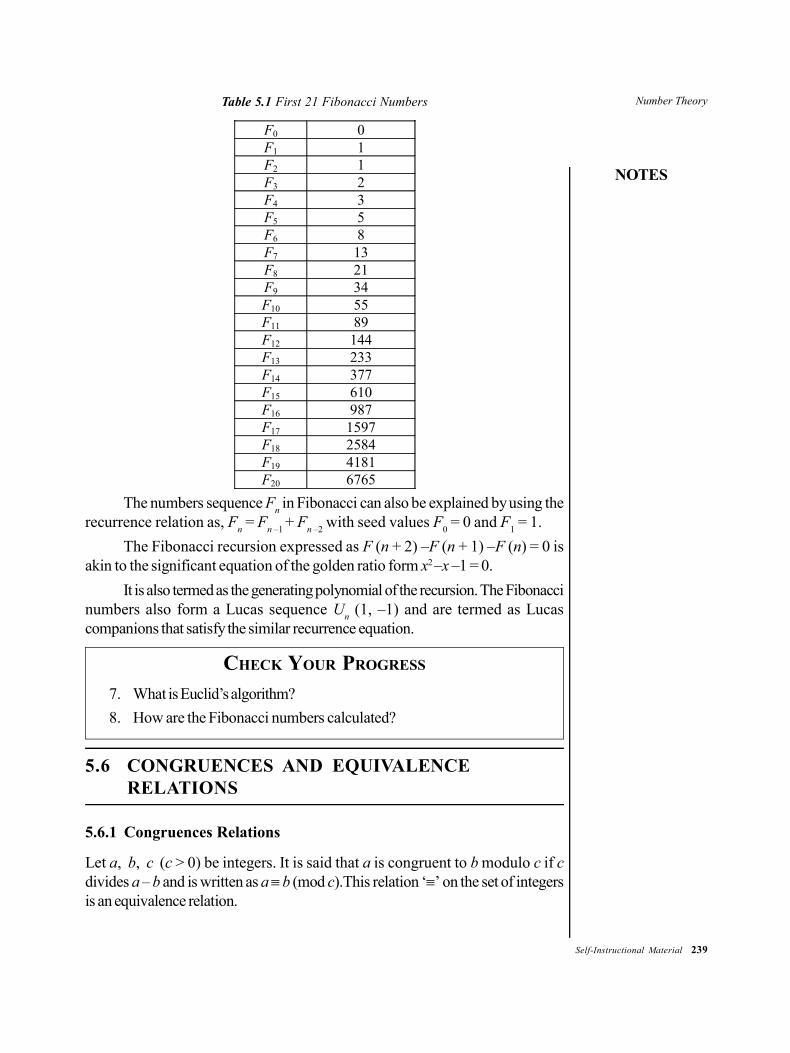
Number Theory
NOTES
Self-Instructional Material 239
Table 5.1 First 21 Fibonacci Numbers
F0 0 F1 1 F2 1 F3 2 F4 3 F5 5 F6 8 F7 13 F8 21 F9 34 F10 55 F11 89 F12 144 F13 233 F14 377 F15 610 F16 987 F17 1597 F18 2584 F19 4181 F20 6765
The numbers sequence Fn in Fibonacci can also be explained by using the
recurrence relation as, Fn = F
n –1 + F
n –2 with seed values F
0 = 0 and F
1 = 1.
The Fibonacci recursion expressed as F (n + 2) –F (n + 1) –F (n) = 0 isakin to the significant equation of the golden ratio form x2 –x –1 = 0.
It is also termed as the generating polynomial of the recursion. The Fibonaccinumbers also form a Lucas sequence U
n (1, –1) and are termed as Lucas
companions that satisfy the similar recurrence equation.
CHECK YOUR PROGRESS
7. What is Euclid’s algorithm?
8. How are the Fibonacci numbers calculated?
5.6 CONGRUENCES AND EQUIVALENCERELATIONS
5.6.1 Congruences Relations
Let a, b, c (c > 0) be integers. It is said that a is congruent to b modulo c if cdivides a – b and is written as a b (mod c).This relation ‘’ on the set of integersis an equivalence relation.
240 Self-Instructional Material
Number Theory
NOTES
Addition, subtraction and multiplication in congruences behave naturally.
Let, a b (mod c)
a1b1 (mod c) ca – b, ca1 – b1
c (a + a1) – (b + b1)
a + a1 b + b1 (mod c)
Similarly, a – a1 b – b1 (mod c)
Also, ca – b, ca1 – b1
caa1 – ba1, cba1 – bb1
c(aa1 – ba1) + (ba1 – bb1)
caa1 – bb1
aa1 bb1 (mod c)
However, it is not possible to achieve the above result in case of division.
Indeed 1 1
ora b
a b may not even be integers.
Again, cancellation in congruences in general may not hold.
i.e., ad bd (mod c) need not essentially imply.
a b (mod c)
For example, 2.2 2.1 (mod 2)
But, 2 1 (mod 2)
However, cancellation holds if g.c.d.(d, c) = 1.
i.e., if ad bd (mod c)
And, g.c.d.(d, c) = 1
Then, a b (mod c)
Proof: ad bd (mod c)
cad – bd
cd (a – b)
ca – b as g.c.d.(c, d) = 1
a b (mod c)
Example 5.11: If a b (mod n), prove that g.c.d.(a, n) = (b, n).
Solution: Let, d = g.c.d.(a, n)
Then, da, dn. But, na – b
da – b, da
da – (a – b) = b
db, dn
Number Theory
NOTES
Self-Instructional Material 241
Let, cb, cn cb, ca – b as na – b
ca – b + b = a
ca, cn
cd as d = g.c.d.(a, n) g.c.d.(b, n) = d
Example 5.12: Establish that if a is an odd integer, then2n
a 1 (mod 2n +2) for any n 1.
Solution: The result can be prove by induction on n.
Let, n = 1.
Then, 2n
a = a2
And 2n + 2 = 23 = 8
Let, a = 2k + 1
Then, a2 = 4k2 + 4k + 1
= 4k (k + 1) + 1
a2 – 1 = 4k (k + 1)
= Multiple of 8, as either k is even or k + 1 is even. a2 1 (mod 8)So, result is true for n = 1.Assume that the result is true for n = k.
Then, a2k 1 (mod 2k + 2)
Now, a2k + 1 – 1 = (a2k)2 – 1
= (a2k – 1) (a2k + 1)
= (Multiple of 2k + 2) (a2k + 1) by induction hypothesis.
But, a = Odd a2k = Odd a2k + 1 = Even
a2k + 1 – 1 = Multiple of 2k + 3
a2k + 1 1 (mod 2k + 3)So, result is true for n = k + 1.By induction, result is true for all n 1.
Example 5.13: Show that for any integer a,
a3 0, 1, or 8 (mod 9)
Solution: Let, a = 3k + r, 0 r < 3
If, r = 0, then a = 3k
a3 = 27k30 (mod 9)
If , r = 1, then a = 3k + 1
a3 = 27k3 + 1 + 9k2 + 9k
242 Self-Instructional Material
Number Theory
NOTES
a3 1 (mod 9)
If , a = 3k + 2, then a3 = 27k3 + 8 + 27k2 + 36k2
a3 8 (mod 9)
a30, 1 or 8 (mod 9)
Example 5.14: If ca cb (mod n), then a b mod ,n
d
where d = g.c.d.
(c, n).
Solution: Given that, d = g.c.d. (c, n)
1 = g.c.d. ,c n
d d
Also, ca cb (mod n)
ca – cb = nk for some integer k.
c ca b
d d =
nk
d
( )n c
a bd d
as g.c.d. ,n c n
a bd d d
= 1
a b mod .n
d
Example 5.15: Find the remainder obtained by dividing 1! + 2! + 3! + 4! + ...+ 100! by 12.
Solution: Each number 4! onwards is a multiple of 12.
1! + 2! + 3! + 4! + ... + 100! 1! + 2! + 3! + 0 + ... + 0 (mod 12)
1! + 2! + 3! + 4! + ... + 100! 9 (mod 12)
9 is the required remainder.
Example 5.16: Find the remainder when 250 is divided by 7.
Solution: Now 23 1 (mod 7)
(23)16116 1 (mod 7)
248 1 (mod 7)
248 22 22 (mod 7)
20 4 (mod 7) 4 is the remainder.
Number Theory
NOTES
Self-Instructional Material 243
Example 5.17: What is the remainder when the sum 15 + 25 + 35 + ... + 995
+ 1005 is divided by 4?
Solution: 1 1 (mod 4) 15 1 (mod 4)
22 0 (mod 4) 25 0 (mod 4)
32 1 (mod 4) 35 3 (mod 4)
35 – 1 (mod 4)
42 0 (mod 4) 45 0 (mod 4)
15 + 25 + 35 + 45 1 + 0 – 1 + 0 0 (mod 4)Any number after these will be of the form 2k + 1, 2k + 2, 2k + 3,
2k + 4, k > 1.Now, (2k + 1)2 1 (mod 4) (2k + 1)5 2k + 1 1 (mod 4)
(2k + 2)2 0 (mod 4) (2k + 2)5 0 (mod 4)
(2k + 3)2 1 (mod 4) (2k + 3)5 2k + 3 – 1 (mod 4)
(2k + 4)2 0 (mod 4 ) (2k + 4)5 0 (mod 4)
15 + 25 + 35 + 45 + ... 995 + 1005 0 (mod 4)
So, remainder is 0 when the given number is divided by 4.
5.6.2 Equivalence Relations
A relation R on a set A is called an equivalence relation if R is reflexive, symmetricand transitive.
For example, let N be set of natural numbers. Define R on N as,
R = {(x,y) : x + y is even, x, yN}
Proof: Let, xN. Now, x + x = 2x.
Clearly 2x is even. Therefore, R is reflexive. Let x, yN and x + y be even.Clearly y + x is also even and hence, R is symmetric.
Now, if x + y is even and y + z is even then prove that x + z is even.
Since, x + y and y + z are even, both (x + y) and (y + z) are divisible by 2.
(x + y) + (y + z) is also divisible by 2, i.e., x + (y + y) + z is divisible by 2.
(x + z) is divisible by 2.
Hence, R is transitive. So, R is an equivalence relation.
Note: From the relation graph or relation matrix the kind of relation can beidentified.
Example 5.18: The relation R on a set is represented by,
110
111
011
RM
Is R reflexive, symmetric or antisymmetric?

244 Self-Instructional Material
Number Theory
NOTES
Solution: In the matrix MR, the diagonal elements are 1. Therefore, R is reflexive.Since, the matrix MR is symmetric hence, the relation R is also symmetric.
Example 5.19: The relation R and R1 on a set is represented by,
(i) MR =
1 0 0
0 1 0
0 0 1(ii) M
R1 =
111101111
Are the relations R and R1 reflexive, symmetric, antisymmetric and/or
transitive?
Solution:
(i) Matrix MR is symmetric. Its diagonal entries are 1. Hence, relation R issymmetric and reflexive. Since R is not antisymmetric, R is transitive.
(ii) The relation R1 is not reflexive as all diagonal entries are not 1.
R1 is symmetric [ MR1 is symmetric] and R1 is transitive.
Example 5.20: Draw the relation graph for the following relations.
(i) R = {(1, 1), (1, 3), (2, 1), (2, 3), (2, 4), (3, 1), (3, 2), (4, 1)}on the setX = {1, 2, 3, 4}.
(ii) R1 = {(1, 1), (1, 2), (1, 3), (2, 2), (2, 3), (3, 3)}on the set Y= {1, 2, 3}.
Solution:
(i) The relation graph GR of R is drawn as follows.
The vertices of GR are 1, 2, 3 and 4.
(ii) The relation graph GR1
of R1 is drawn as:
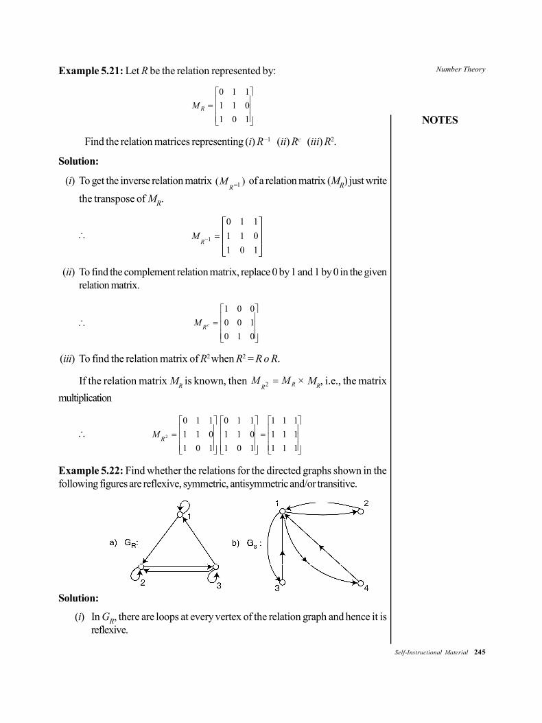
Number Theory
NOTES
Self-Instructional Material 245
Example 5.21: Let R be the relation represented by:
101
011
110
RM
Find the relation matrices representing (i) R –1 (ii) Rc (iii) R2.
Solution:
(i) To get the inverse relation matrix 1( )R
M of a relation matrix (MR) just write
the transpose of MR.
1
0 1 1
1 1 0
1 0 1R
M
(ii) To find the complement relation matrix, replace 0 by 1 and 1 by 0 in the givenrelation matrix.
010
100
001
cRM
(iii) To find the relation matrix of R2 when R2 = R o R.
If the relation matrix MR is known, then 2 RR
M M × MR, i.e., the matrix
multiplication
111
111
111
101
011
110
101
011
110
2RM
Example 5.22: Find whether the relations for the directed graphs shown in thefollowing figures are reflexive, symmetric, antisymmetric and/or transitive.
Solution:
(i) In GR, there are loops at every vertex of the relation graph and hence it isreflexive.
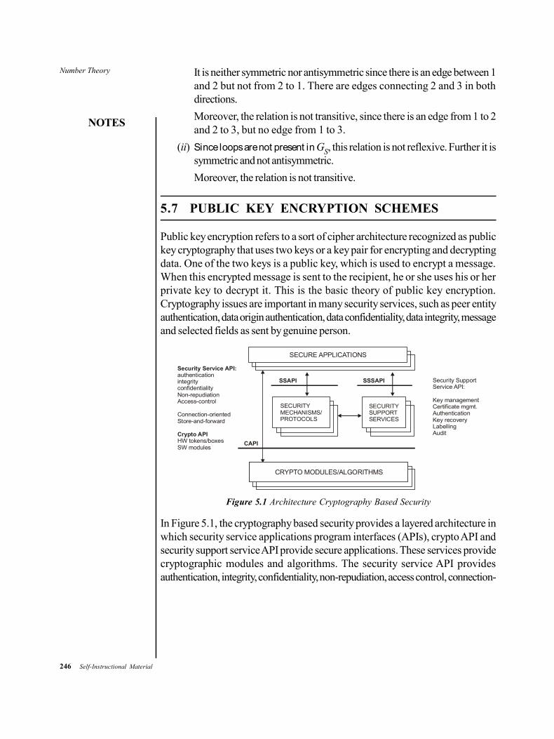
246 Self-Instructional Material
Number Theory
NOTES
It is neither symmetric nor antisymmetric since there is an edge between 1and 2 but not from 2 to 1. There are edges connecting 2 and 3 in bothdirections.
Moreover, the relation is not transitive, since there is an edge from 1 to 2and 2 to 3, but no edge from 1 to 3.
(ii) Since loops are not present in GS, this relation is not reflexive. Further it issymmetric and not antisymmetric.
Moreover, the relation is not transitive.
5.7 PUBLIC KEY ENCRYPTION SCHEMES
Public key encryption refers to a sort of cipher architecture recognized as publickey cryptography that uses two keys or a key pair for encrypting and decryptingdata. One of the two keys is a public key, which is used to encrypt a message.When this encrypted message is sent to the recipient, he or she uses his or herprivate key to decrypt it. This is the basic theory of public key encryption.Cryptography issues are important in many security services, such as peer entityauthentication, data origin authentication, data confidentiality, data integrity, messageand selected fields as sent by genuine person.
SECURE APPLICATIONS
CRYPTO MODULES/ALGORITHMS
SECURITYMECHANISMS/PROTOCOLS
SECURITYSUPPORTSERVICES
SSAPI SSSAPI
CAPI
Security Service API:
Crypto API
authenticationintegrityconfidentialityNon-repudiationAccess-control
Connection-orientedStore-and-forward
HW tokens/boxesSW modules
Security SupportService API:
Key managementCertificate mgmt.AuthenticationKey recoveryLabellingAudit
Figure 5.1 Architecture Cryptography Based Security
In Figure 5.1, the cryptography based security provides a layered architecture inwhich security service applications program interfaces (APIs), crypto API andsecurity support service API provide secure applications. These services providecryptographic modules and algorithms. The security service API providesauthentication, integrity, confidentiality, non-repudiation, access control, connection-

Number Theory
NOTES
Self-Instructional Material 247
oriented method and ‘store and forward’ method. The crypto API provides HWtokens and SW modules. HW tokens are hardware cryptographic services, forexample, accelerator boards and SW modules are kernel modules providingcryptographic services, such as implementation of cryptographic algorithm. Thesecurity support service API provides certificate management authentication, keyrecovery, labelling and auditing. The prime aim of this hierarchy level is to providethe following mechanisms:
This level promotes the development of security services and cryptographicAPI.
This level also identifies the area of security support service APIs along withcertificate management, key management and authentication APIs.
This level demonstrates the uses of cryptographic APIs products andservices.
This level identifies the steps of demonstrations and experiments in the fieldof crypto services.
Table 5.2 shows the relationship between security services and securitymechanisms:
Table 5.2 Relationship between Security Mechanism and Security Services
Service Encipherment Digital Signature
Access Control
Data Integrity
Authentication Exchange
Traffic Padding
Routing Control
Notarization
Peer entity
authentication
Data origin
authentication
Access control
Data integrity
Traffic flow
confidentiality
Nonrepudiation
Availability
5.7.1 Message Authentication Code
Message Authentication Code (MAC) follows the algorithm given as follows:H a s h ( M A C _ w r i t e _ s e c r e t | | p a d _ 2 | |hash(MAC_write_secret||pad_1||seq_num||SSLCompressed.type||SSLCompressed.length||SSLCompressed.fragment))
This code is written and computed over compressed data. A shared secretkey is used for this algorithm. Table 5.3 shows the keywords used in this code:
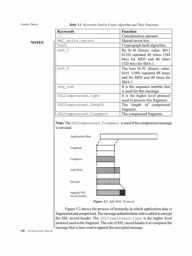
248 Self-Instructional Material
Number Theory
NOTES
Table 5.3 Keywords Used in Crypto Algorithm and Their Functions
Keywords Function || Concatenation operator. MAC_write_secret Shared secret key. hash Cryptograph hash algorithm. pad_1 By 036 (binary value: 0011
0110) repeated 48 times (384 bits) for MD5 and 40 times (320 bits) for SHA-1.
pad_2 The byte 05C (binary value: 0101 1100) repeated 48 times and for MD5 and 40 times for SHA-1.
seq_num It is the sequence number that is used for this message.
SSLCompressed.type It is the higher level protocol used to process this fragment.
SSLCompressed.length The length of compressed fragment.
SSLCompressed.fragment The compressed fragment.
Note: The SSLCompressed.fragment is used if the compression messageis not used.
Application Data
Fragment
Compress
Add MAC
Encrypt
Append SSLrecord header
Figure 5.2 Add MAC Protocol
Figure 5.2 shows the process of hierarchy in which application data isfragmented and compressed. The message authentication code is added to encryptthe SSL record header. The SSLCompressed.type is the higher levelprotocol used in the fragment. The role of SSL record header is to compress themessage that is later used to append the encrypted message.
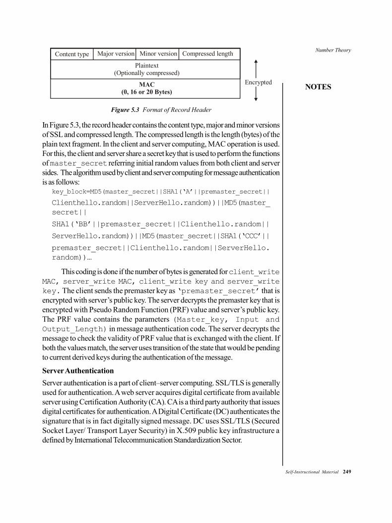
Number Theory
NOTES
Self-Instructional Material 249
Content type Major version Minor version Compressed length
Plaintext(Optionally compressed)
MAC(0, 16 or 20 Bytes)
Encrypted
Figure 5.3 Format of Record Header
In Figure 5.3, the record header contains the content type, major and minor versionsof SSL and compressed length. The compressed length is the length (bytes) of theplain text fragment. In the client and server computing, MAC operation is used.For this, the client and server share a secret key that is used to perform the functionsof master_secret referring initial random values from both client and serversides. The algorithm used by client and server computing for message authenticationis as follows:
key_block=MD5(master_secret||SHA1(‘A’||premaster_secret||
Clienthello.random||ServerHello.random))||MD5(master_secret||
SHA1(‘BB’||premaster_secret||Clienthello.random||
ServerHello.random))||MD5(master_secret||SHA1(‘CCC’||
premaster_secret||Clienthello.random||ServerHello.random))…
This coding is done if the number of bytes is generated for client_writeMAC, server_write MAC, client_write key and server_writekey. The client sends the premaster key as ‘premaster_secret’ that isencrypted with server’s public key. The server decrypts the premaster key that isencrypted with Pseudo Random Function (PRF) value and server’s public key.The PRF value contains the parameters (Master_key, Input andOutput_Length) in message authentication code. The server decrypts themessage to check the validity of PRF value that is exchanged with the client. Ifboth the values match, the server uses transition of the state that would be pendingto current derived keys during the authentication of the message.
Server Authentication
Server authentication is a part of client–server computing. SSL/TLS is generallyused for authentication. A web server acquires digital certificate from availableserver using Certification Authority (CA). CA is a third party authority that issuesdigital certificates for authentication. A Digital Certificate (DC) authenticates thesignature that is in fact digitally signed message. DC uses SSL/TLS (SecuredSocket Layer/ Transport Layer Security) in X.509 public key infrastructure adefined by International Telecommunication Standardization Sector.

250 Self-Instructional Material
Number Theory
NOTES
Certification Authority
ServerCertificate
IssueCertificates
ClientCertificates
ClientPrivate Key
SSL Session
ServerPrivate Key
Figure 5.4 Authentication in SSL/TLS
In Figure 5.4, if client connects to the server using SSL/TLS then both client andserver follow strong cryptographic algorithm. Then, the server sends X.509certificate that contains the server’s public key. The client then generates a 48-byte random number and a premaster secret key after encrypting the number usedby the server’s public key. The encrypted premaster secret key is sent to theserver by the client. After getting premaster secret key, the server decrypts themessage using the private keys. Then, both the client and the server share thesame premaster secret key which is basically symmetric key used to encrypt themessage. Subsequently they start communicating via generated keys. In thismechanism, only server knows the private key that decrypts the encryptedpremaster secret key. Clients know the message after sending the decryptedmessage by server. It proves that the client is talking to the correct server. Thiswhole mechanism represents the complete scenario of authenticating the server.
Client Authentication
In SSL/TSL, client authentication is not required; instead it is optional. A clientstays anonymous while communicating between a web server and a browser inB2B business transaction. Therefore, they use HTTP authentication methods.

Number Theory
NOTES
Self-Instructional Material 251
Client Get/myapps/servlet/order Server
401WWW-Authenticate: Basic realm = “PurchaseOrder”
Get/myapps/servlet/orderAuthorization: Basic QWxhZGRpbjpvcGVulHNlc2FtZQ==
Base64-encoded “user id:password”
Figure 5.5 HTTP Authentication
In Figure 5.5, the HTTP authentication known as RFC 2617, represents the HTTPprotocol in which client and server communicate between each other via HTTPprotocol. It basically considers two factors, user-id and password, to authenticatethe users/clients. Sometimes, user-id might be user’s email-id also. Both valuesare sent to authenticate without encryption and hence they are not considered assecure methods of authentication in cryptography. In this mechanism, client sendsBase64-encoded user-id and password in HTTP header. If data is sent throughSSL/TLS connection, it is not altered or stolen during transmission. A maliciousserver cannot disguise itself as genuine web server and cannot steal the passwordof users. For client authentication, SSL/TLS certificate is used to obtain anappropriate digital certificate before connecting to the server. A client generatesthe private key/public key pair to obtain the client certificate. A private key is keptas the secret key and is protected by passphrase. A passphrase works as thepassword with added security. It is a sequence of words used to control access tothe system. The application does not maintain the database of user-id and password.It verifies the certificate that is signed by trusted CA.
Application A
Application B
Application C
CertificationAuthority
Certificate
Trust
Issue Certificate
Figure 5.6 Uses of Client Certificates
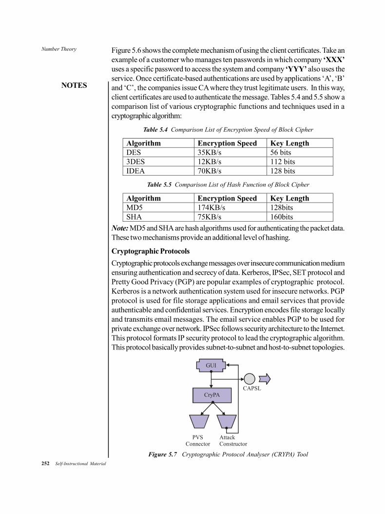
252 Self-Instructional Material
Number Theory
NOTES
Figure 5.6 shows the complete mechanism of using the client certificates. Take anexample of a customer who manages ten passwords in which company ‘XXX’uses a specific password to access the system and company ‘YYY’ also uses theservice. Once certificate-based authentications are used by applications ‘A’, ‘B’and ‘C’, the companies issue CA where they trust legitimate users. In this way,client certificates are used to authenticate the message. Tables 5.4 and 5.5 show acomparison list of various cryptographic functions and techniques used in acryptographic algorithm:
Table 5.4 Comparison List of Encryption Speed of Block Cipher
Algorithm Encryption Speed Key Length DES 35KB/s 56 bits 3DES 12KB/s 112 bits IDEA 70KB/s 128 bits
Table 5.5 Comparison List of Hash Function of Block Cipher
Algorithm Encryption Speed Key Length MD5 174KB/s 128bits SHA 75KB/s 160bits Note: MD5 and SHA are hash algorithms used for authenticating the packet data.
These two mechanisms provide an additional level of hashing.
Cryptographic Protocols
Cryptographic protocols exchange messages over insecure communication mediumensuring authentication and secrecy of data. Kerberos, IPSec, SET protocol andPretty Good Privacy (PGP) are popular examples of cryptographic protocol.Kerberos is a network authentication system used for insecure networks. PGPprotocol is used for file storage applications and email services that provideauthenticable and confidential services. Encryption encodes file storage locallyand transmits email messages. The email service enables PGP to be used forprivate exchange over network. IPSec follows security architecture to the Internet.This protocol formats IP security protocol to lead the cryptographic algorithm.This protocol basically provides subnet-to-subnet and host-to-subnet topologies.
CAPSL
GUI
CryPA
PVSConnector
AttackConstructor
Figure 5.7 Cryptographic Protocol Analyser (CRYPA) Tool
Number Theory
NOTES
Self-Instructional Material 253
Figure 5.7 shows that CRYptographic Protocol Analyser (CRYPA) is based ongraphics user interface specification of cryptographic protocols using constructionof attack on protocol. PGP supports digital signature and encryption. This toolprovides a virtual distributed environment system that provides a secure chain ofhandling and controlling the crypto message.
5.7.2 Digital Signature
Digital Signature (DS) follows authentication mechanism. A code is attached withmessages in DS. Primarily, the signature is generated by hashing the message andlater this message is encrypted with the sender’s private key. DS is based onpublic key encryption. A signature confirms that integrity and source of message iscorrect. NIST (National Institute of Standards and Technology) recognized theDS standard that uses the Secure Hash Algorithm (SHA). Message authenticationprotects digital signature as this way the messages are exchanged by a third party.DS is analogous to manual signature. The characteristics of DS are as follows:
It attaches date and time along with the author of the signature.
It authenticates the contents while the signature is being completed.
It solves the disputes using a third party (generally in online payment byPayPal).
It ensures that the message is not altered. The message can be in the form ofelectronic documents, such as email, text file, spreadsheet, etc.
A person or information is authenticated on the computer by using varioustechniques. Brief descriptions of these techniques are as follows:
Password
User name and password provides authentication. When the user logs on thesystem unit or application, the system asks for user name and password forchecking authentication. Generally, the following type of password authenticationis provided to users in which two prime fields, namely ‘User Name’ and‘Password’ are required to access the system.
User Name:
Password:
Click!
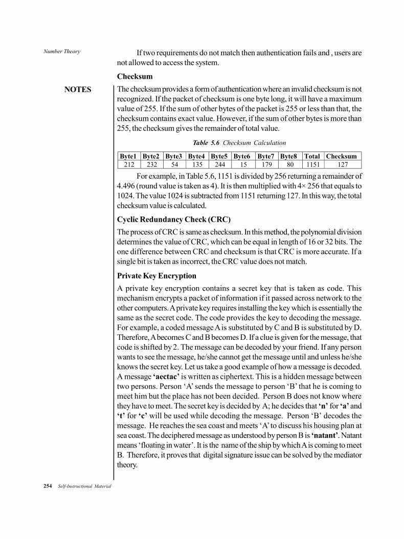
254 Self-Instructional Material
Number Theory
NOTES
If two requirements do not match then authentication fails and , users arenot allowed to access the system.
Checksum
The checksum provides a form of authentication where an invalid checksum is notrecognized. If the packet of checksum is one byte long, it will have a maximumvalue of 255. If the sum of other bytes of the packet is 255 or less than that, thechecksum contains exact value. However, if the sum of other bytes is more than255, the checksum gives the remainder of total value.
Table 5.6 Checksum Calculation
Byte1 Byte2 Byte3 Byte4 Byte5 Byte6 Byte7 Byte8 Total Checksum 212 232 54 135 244 15 179 80 1151 127
For example, in Table 5.6, 1151 is divided by 256 returning a remainder of4.496 (round value is taken as 4). It is then multiplied with 4× 256 that equals to1024. The value 1024 is subtracted from 1151 returning 127. In this way, the totalchecksum value is calculated.
Cyclic Redundancy Check (CRC)
The process of CRC is same as checksum. In this method, the polynomial divisiondetermines the value of CRC, which can be equal in length of 16 or 32 bits. Theone difference between CRC and checksum is that CRC is more accurate. If asingle bit is taken as incorrect, the CRC value does not match.
Private Key Encryption
A private key encryption contains a secret key that is taken as code. Thismechanism encrypts a packet of information if it passed across network to theother computers. A private key requires installing the key which is essentially thesame as the secret code. The code provides the key to decoding the message.For example, a coded message A is substituted by C and B is substituted by D.Therefore, A becomes C and B becomes D. If a clue is given for the message, thatcode is shifted by 2. The message can be decoded by your friend. If any personwants to see the message, he/she cannot get the message until and unless he/sheknows the secret key. Let us take a good example of how a message is decoded.A message ‘aectac’ is written as ciphertext. This is a hidden message betweentwo persons. Person ‘A’ sends the message to person ‘B’ that he is coming tomeet him but the place has not been decided. Person B does not know wherethey have to meet. The secret key is decided by A; he decides that ‘n’ for ‘a’ and‘t’ for ‘c’ will be used while decoding the message. Person ‘B’ decodes themessage. He reaches the sea coast and meets ‘A’ to discuss his housing plan atsea coast. The deciphered message as understood by person B is ‘natant’. Natantmeans ‘floating in water’. It is the name of the ship by which A is coming to meetB. Therefore, it proves that digital signature issue can be solved by the mediatortheory.
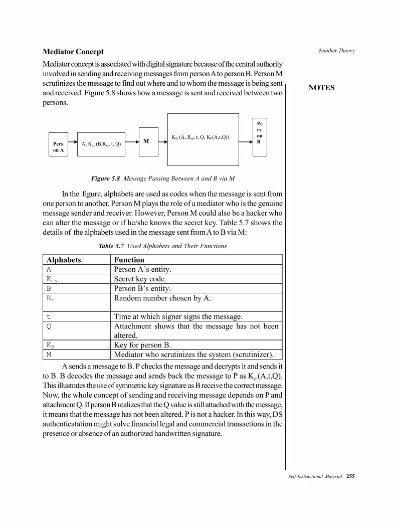
Number Theory
NOTES
Self-Instructional Material 255
Mediator Concept
Mediator concept is associated with digital signature because of the central authorityinvolved in sending and receiving messages from person A to person B. Person Mscrutinizes the message to find out where and to whom the message is being sentand received. Figure 5.8 shows how a message is sent and received between twopersons.
A, Key (B,Rm, t, Q)
M
KB (A, Rm, t, Q, KP(A,t,Q))
Person A
Person B
Figure 5.8 Message Passing Between A and B via M
In the figure, alphabets are used as codes when the message is sent fromone person to another. Person M plays the role of a mediator who is the genuinemessage sender and receiver. However, Person M could also be a hacker whocan alter the message or if he/she knows the secret key. Table 5.7 shows thedetails of the alphabets used in the message sent from A to B via M:
Table 5.7 Used Alphabets and Their Functions
Alphabets Function A Person A’s entity. Key Secret key code. B Person B’s entity. Rm
Random number chosen by A.
t Time at which signer signs the message. Q Attachment shows that the message has not been
altered. KB Key for person B. M Mediator who scrutinizes the system (scrutinizer). A sends a message to B. P checks the message and decrypts it and sends it
to B. B decodes the message and sends back the message to P as KP (A,t,Q).
This illustrates the use of symmetric key signature as B receive the correct message.Now, the whole concept of sending and receiving message depends on P andattachment Q. If person B realizes that the Q value is still attached with the message,it means that the message has not been altered. P is not a hacker. In this way, DSauthenticatation might solve financial legal and commercial transactions in thepresence or absence of an authorized handwritten signature.

256 Self-Instructional Material
Number Theory
NOTES
Public Key Encryption
A public key encryption uses private and public keys. A private key is restricted tothe individual systems, whereas public key can be accessed by any system wheremessage is to be communicated securely with the individual system. Decoding ofan encrypted message can be done by a public key that is provided by the individualsystem as well as its own private key. Basically, the key is based on the hash value.For example, Table 5.8 shows the hash value of input number:
Table 5.8 Hash Value of Input Number
Input Number Hashing Algorithm Hash Value 12421 Input # × 131 1627151 In the table, the value 1627151 is the result of multiplication of 131 and
12421. If the multiplier is 131, the value comes as 1627151. The public key canuse large values to encrypt, such as 40bit and 128bit. The value 128bit can have2128 combinations.
A digital signature follows the following operations:
Key pair generation: In this process, a public and a private key pair is generated.
Generation operation: In this process, a signature is produced for a messagewith private key.
Verification operation: In this process, a signature is checked with the publickey.
Digital signature provides data integrity, signer authenticity, authorization,security, accountability and non-repudiation. These are the mechanisms that arefrequently associated with digital signatures. These mechanisms are inter-relatedwith each other and hence are popular in transaction of digital cash, e-moneytransfer across net, etc.
Non-repudiation
Accountability Security
Authorization
SignerAuthenticity
Data Integrity
Digital Signatures
Figure 5.9 Mechanisms of Digital Signature
Figure 5.9 shows how various mechanisms are associated with digitalsignatures.
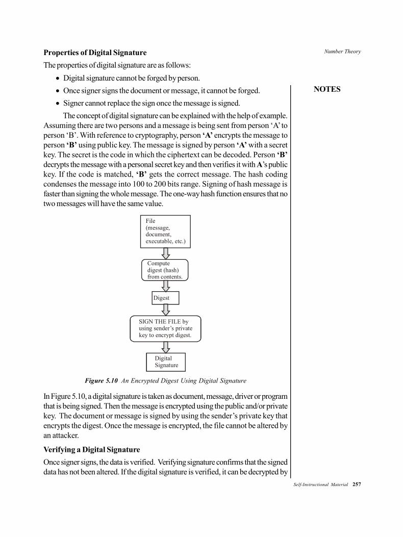
Number Theory
NOTES
Self-Instructional Material 257
Properties of Digital Signature
The properties of digital signature are as follows:
Digital signature cannot be forged by person.
Once signer signs the document or message, it cannot be forged.
Signer cannot replace the sign once the message is signed.
The concept of digital signature can be explained with the help of example.Assuming there are two persons and a message is being sent from person ‘A’ toperson ‘B’. With reference to cryptography, person ‘A’ encrypts the message toperson ‘B’ using public key. The message is signed by person ‘A’ with a secretkey. The secret is the code in which the ciphertext can be decoded. Person ‘B’decrypts the message with a personal secret key and then verifies it with A’s publickey. If the code is matched, ‘B’ gets the correct message. The hash codingcondenses the message into 100 to 200 bits range. Signing of hash message isfaster than signing the whole message. The one-way hash function ensures that notwo messages will have the same value.
File(message,document,executable, etc.)
Computedigest (hash)from contents.
Digest
SIGN THE FILE byusing sender’s privatekey to encrypt digest.
DigitalSignature
Figure 5.10 An Encrypted Digest Using Digital Signature
In Figure 5.10, a digital signature is taken as document, message, driver or programthat is being signed. Then the message is encrypted using the public and/or privatekey. The document or message is signed by using the sender’s private key thatencrypts the digest. Once the message is encrypted, the file cannot be altered byan attacker.
Verifying a Digital Signature
Once signer signs, the data is verified. Verifying signature confirms that the signeddata has not been altered. If the digital signature is verified, it can be decrypted by
258 Self-Instructional Material
Number Theory
NOTES
using a public key that produces the original hash value. If the two hash valuesmatch, the signature is exactly same.
Various software, such as Multilevel Digital Signateure System,MyLiveSignature, Random Signature Changer, SignetSure, SignaturePilot,SignaturePilotPro, 602XMLFormFilter, AzSDK MD5Sum, Signit, etc., are usedby various commercial transaction hubs for signing and verifying the digital signature.
CHECK YOUR PROGRESS
9. What do you understand by an equivalence relation?
10. What do you understand by public key encryption?
11. What role does the certification authority (CA) play in data authentication?
12. What do cryptographic protocols do?
13. How can the decoding of an encrypted message be done?
5.8 SUMMARY
In this unit, you have learned that:
There are two types of numbers: prime numbers and composite numbers.
The division algorithm is a well-defined procedure for achieving a specifictask and can be used to find the greatest common divisor of two integers.
Numbers can be divided into two based on their divisibility by 2:(i) Even numbers: They do not leave any remainder.(ii) Odd numbers: They are not evenly divisible by 2.
An inequality statement identifies the relative size or order of two objects toconfirm whether they are similar or not.
Inequalities are influenced by these properties: trichotomy, transitivity,addition and subtraction and multiplication and division.
The greatest common divisor (G.C.D) is the largest positive integer thatdivides a number entirely, i.e., without leaving any remainder.
Euclid’s algorithm determines the G.C.D of two elements of any Euclideandomain.
The Fibonacci number sequence is named after Leonardo of Pisa, whowas famously known as Fibonacci.
In the Fibonacci series, 0 and 1 are the first two Fibonacci numbers; all theother numbers of the series are the sum of the previous two numbers.
Congruent relation states that if a, b, c (c > 0) are integers, then a is congruentto b modulo c if c divides a – b.
Equivalence relation refers to a relation R on a set A which is in equivalencein case R is reflexive, symmetric and transitive.
Number Theory
NOTES
Self-Instructional Material 259
Public key encryption refers to a sort of cipher architecture recognized aspublic key cryptography that uses two keys, or a key pair for encryptingand decrypting data.
5.9 KEY TERMS
Prime number: An integer p > 1 is called a prime number if 1 and p arethe only divisors of p.
Composite number: A composite number is an integer n > 1 such that n isnot prime.
Divisor: A divisor, in mathematics, is an integer n, also termed as factor ofn, which evenly divides n without leaving any remainder.
5.10 ANSWERS TO ‘CHECK YOUR PROGRESS’
1. Properties of prime numbers are as follows:(i) If a prime number p divides ab, then either p | a or p | b.
(ii) If a prime number p does not divide an integer a, then the highestcomman factor (HCF) of p and a is 1 (by convention HCF is taken tobe a + ve integer).
2. In mathematics, the division algorithm is a theorem which expresses theoutcome of the usual process of division of integers.
3. Numbers which are evenly divisible by 2 without leaving any remainder arecalled even numbers.
4. In mathematics, an inequality is a statement that defines the relative size ororder of two objects to check whether they are similar or not.
5. The GCD of two or more non-zero integers is the largest positive integerthat divides a number without leaving a remainder.
6. Linear Diophantine equation is an equation ax + by = c in two unknowns, xand y, where a, b, c are given integers and one of a, b is not zero.
7. In number theory, the Euclidean algorithm also termed as Euclid’s algorithm,is a very important algorithm that is used to determine the greatest commondivisor of two elements of any Euclidean domain.
8. The first two Fibonacci numbers are 0 and 1, and all other numbers are thesum of the previous two numbers.
9. A relation R on a set A is called an equivalence relation if R is reflexive,symmetric and transitive.
10. Public key inscription refers to a sort of cipher architecture recognized aspublic key cryptography that uses two keys for encrypting and decryptingdata.

260 Self-Instructional Material
Number Theory
NOTES
11. Certification Authority (CA) serves as a third party that issues digitalcertificates for data authentication.
12. Cryptographic protocols exchange messages over insecure communicationmedium ensuring authentication and secrecy of data.
13. Decoding of an encrypted message can be done by a public key that isprovided by the individual system as well as its own private key. Basically,the key is based on the hash value.
5.11 QUESTIONS AND EXERCISES
Short-Answer Questions
1. What does the concept of strict inequality state?
2. Briefly explain the fundamental theorem of arithmetic.
3. What do you understand by prime numbers?
4. Differentiate between trivial and non-trivial divisors.
5. What are the various keywords that are used in crypto algorithm? Alsostate their functions.
6. Write a short note on private key encryption.
Long –Answer questions
1. Explain the properties of inequalities.
2. Prove the Euclidean algorithm.
3. Explain the basis representation theorem.
4. Explain how http authentication is done in business-to-business transactions.
5. Describe the various techniques used for the authentication of data oncomputer.
5.12 FURTHER READING
Lipschutz, Seymour and Lipson Marc. Schaum’s Outline of DiscreteMathematics, 3rd edition. New York: McGraw-Hill, 2007.
Horowitz, Ellis, Sartaj Sahni and Sanguthevar Rajasekaran. Fundamentals ofComputer Algorithms. Hyderabad: Orient BlackSwan, 2008.
Cormen, Thomas H., Charles E. Leiserson, Ronald L. Rivest and Clifford Stein.Introduction to Algorithms. The MIT Press, 1990.
Brassard, Gilles and Paul Bratley. Fundamentals of Algorithms. New Delhi:Prentice Hall of India, 1995.
Levitin, Anany. Introduction to the Design and Analysis of Algorithms. NewJersey: Pearson, 2006.
Number Theory
NOTES
Self-Instructional Material 261
Baase, Sara and Allen Van Gelder. Computer Algorithms – Introduction toDesign and Analysis. New Jersey: Pearson, 2003.
Mott, J.L. Discrete Mathematics for Computer Scientists, 2nd edition. NewDelhi: Prentice-Hall of India Pvt. Ltd., 2007.
Liu, C.L. Elements of Discrete Mathematics. New Delhi: Tata McGraw-HillPublishing Company, 1977.
Rosen, Kenneth. Discrete Mathematics and Its Applications, 6th edition. NewYork: McGraw-Hill Higher Education, 2007.

262 Self-Instructional Material
NOTES

Self-Instructional Material 263
NOTES

264 Self-Instructional Material
NOTES
MATHEMATICAL FOUNDATIONS OF COMPUTER SCIENCE
VENKATESHWARAOPEN UNIVERSITY
www.vou.ac.in
VENKATESHWARAOPEN UNIVERSITY
www.vou.ac.in
MATHEMATICAL FOUNDATIONS OF COMPUTER SCIENCE
BCA[BCA-103]
MATHEM
ATICAL FOUNDATIONS OF COMPUTER SCIENCE
12 MM