the car package

The car Package

October 29, 2007

Version 1.2-7

Date 2007/10/27

Title Companion to Applied Regression

Author John Fox <[email protected]>. I am grateful to Douglas Bates, David Firth, Michael

Friendly, Gregor Gorjanc, Spencer Graves, Richard Heiberger, Georges Monette, Henric Nilsson,

Brian Ripley, Sanford Weisberg, and Achim Zeleis for various suggestions and contributions.

Maintainer John Fox <[email protected]>

Depends R (>= 2.1.1), stats, graphics

Suggests MASS, nnet, leaps

LazyLoad yes

LazyData yes

Description This package accompanies J. Fox, An R and S-PLUS Companion to Applied Regression,

Sage, 2002. The package contains mostly functions for applied regression, linear models, and

generalized linear models, with an emphasis on regression diagnostics, particularly graphical

diagnostic methods. There are also some utility functions. With some exceptions, I have tried not

to duplicate capabilities in the basic distribution of R, nor in widely used packages. Where

relevant, the functions in car are consistent with na.action = na.omit or na.exclude.

License GPL (>= 2)

URL http://www.r-project.org, http://socserv.socsci.mcmaster.ca/jfox/

R topics documented:

Adler . . . . . . . . . . . . . . . . . . . . . . . . . . . . . . . . . . . . . . . . . . . . 3

Angell . . . . . . . . . . . . . . . . . . . . . . . . . . . . . . . . . . . . . . . . . . . . 4

Anova . . . . . . . . . . . . . . . . . . . . . . . . . . . . . . . . . . . . . . . . . . . . 5

Anscombe . . . . . . . . . . . . . . . . . . . . . . . . . . . . . . . . . . . . . . . . . . 12

Ask . . . . . . . . . . . . . . . . . . . . . . . . . . . . . . . . . . . . . . . . . . . . . 13

Baumann . . . . . . . . . . . . . . . . . . . . . . . . . . . . . . . . . . . . . . . . . . 14

1

2 R topics documented:

Bfox . . . . . . . . . . . . . . . . . . . . . . . . . . . . . . . . . . . . . . . . . . . . . 15

Blackmoor . . . . . . . . . . . . . . . . . . . . . . . . . . . . . . . . . . . . . . . . . . 16

Burt . . . . . . . . . . . . . . . . . . . . . . . . . . . . . . . . . . . . . . . . . . . . . 16

Can.pop . . . . . . . . . . . . . . . . . . . . . . . . . . . . . . . . . . . . . . . . . . . 17

Chile . . . . . . . . . . . . . . . . . . . . . . . . . . . . . . . . . . . . . . . . . . . . . 17

Chirot . . . . . . . . . . . . . . . . . . . . . . . . . . . . . . . . . . . . . . . . . . . . 18

Contrasts . . . . . . . . . . . . . . . . . . . . . . . . . . . . . . . . . . . . . . . . . . 19

Cowles . . . . . . . . . . . . . . . . . . . . . . . . . . . . . . . . . . . . . . . . . . . 21

Davis . . . . . . . . . . . . . . . . . . . . . . . . . . . . . . . . . . . . . . . . . . . . 21

DavisThin . . . . . . . . . . . . . . . . . . . . . . . . . . . . . . . . . . . . . . . . . . 22

Duncan . . . . . . . . . . . . . . . . . . . . . . . . . . . . . . . . . . . . . . . . . . . 23

Ellipses . . . . . . . . . . . . . . . . . . . . . . . . . . . . . . . . . . . . . . . . . . . 24

Ericksen . . . . . . . . . . . . . . . . . . . . . . . . . . . . . . . . . . . . . . . . . . . 26

Florida . . . . . . . . . . . . . . . . . . . . . . . . . . . . . . . . . . . . . . . . . . . . 27

Freedman . . . . . . . . . . . . . . . . . . . . . . . . . . . . . . . . . . . . . . . . . . 28

Friendly . . . . . . . . . . . . . . . . . . . . . . . . . . . . . . . . . . . . . . . . . . . 28

Ginzberg . . . . . . . . . . . . . . . . . . . . . . . . . . . . . . . . . . . . . . . . . . 29

Greene . . . . . . . . . . . . . . . . . . . . . . . . . . . . . . . . . . . . . . . . . . . . 30

Guyer . . . . . . . . . . . . . . . . . . . . . . . . . . . . . . . . . . . . . . . . . . . . 31

Hartnagel . . . . . . . . . . . . . . . . . . . . . . . . . . . . . . . . . . . . . . . . . . 31

Leinhardt . . . . . . . . . . . . . . . . . . . . . . . . . . . . . . . . . . . . . . . . . . 32

Mandel . . . . . . . . . . . . . . . . . . . . . . . . . . . . . . . . . . . . . . . . . . . 33

Migration . . . . . . . . . . . . . . . . . . . . . . . . . . . . . . . . . . . . . . . . . . 34

Moore . . . . . . . . . . . . . . . . . . . . . . . . . . . . . . . . . . . . . . . . . . . . 35

Mroz . . . . . . . . . . . . . . . . . . . . . . . . . . . . . . . . . . . . . . . . . . . . . 35

OBrienKaiser . . . . . . . . . . . . . . . . . . . . . . . . . . . . . . . . . . . . . . . . 36

Ornstein . . . . . . . . . . . . . . . . . . . . . . . . . . . . . . . . . . . . . . . . . . . 37

Pottery . . . . . . . . . . . . . . . . . . . . . . . . . . . . . . . . . . . . . . . . . . . . 38

Prestige . . . . . . . . . . . . . . . . . . . . . . . . . . . . . . . . . . . . . . . . . . . 39

Quartet . . . . . . . . . . . . . . . . . . . . . . . . . . . . . . . . . . . . . . . . . . . 40

Robey . . . . . . . . . . . . . . . . . . . . . . . . . . . . . . . . . . . . . . . . . . . . 40

SLID . . . . . . . . . . . . . . . . . . . . . . . . . . . . . . . . . . . . . . . . . . . . 41

Sahlins . . . . . . . . . . . . . . . . . . . . . . . . . . . . . . . . . . . . . . . . . . . . 42

Soils . . . . . . . . . . . . . . . . . . . . . . . . . . . . . . . . . . . . . . . . . . . . . 42

States . . . . . . . . . . . . . . . . . . . . . . . . . . . . . . . . . . . . . . . . . . . . 44

Transformation Axes . . . . . . . . . . . . . . . . . . . . . . . . . . . . . . . . . . . . 45

UN . . . . . . . . . . . . . . . . . . . . . . . . . . . . . . . . . . . . . . . . . . . . . . 47

US.pop . . . . . . . . . . . . . . . . . . . . . . . . . . . . . . . . . . . . . . . . . . . 47

Var . . . . . . . . . . . . . . . . . . . . . . . . . . . . . . . . . . . . . . . . . . . . . . 48

Vocab . . . . . . . . . . . . . . . . . . . . . . . . . . . . . . . . . . . . . . . . . . . . 49

Womenlf . . . . . . . . . . . . . . . . . . . . . . . . . . . . . . . . . . . . . . . . . . . 50

av.plots . . . . . . . . . . . . . . . . . . . . . . . . . . . . . . . . . . . . . . . . . . . 50

box.cox . . . . . . . . . . . . . . . . . . . . . . . . . . . . . . . . . . . . . . . . . . . 52

box.cox.powers . . . . . . . . . . . . . . . . . . . . . . . . . . . . . . . . . . . . . . . 54

box.cox.var . . . . . . . . . . . . . . . . . . . . . . . . . . . . . . . . . . . . . . . . . 56

box.tidwell . . . . . . . . . . . . . . . . . . . . . . . . . . . . . . . . . . . . . . . . . 57

car-internal . . . . . . . . . . . . . . . . . . . . . . . . . . . . . . . . . . . . . . . . . 59

car-package . . . . . . . . . . . . . . . . . . . . . . . . . . . . . . . . . . . . . . . . . 60

Adler 3

ceres.plots . . . . . . . . . . . . . . . . . . . . . . . . . . . . . . . . . . . . . . . . . . 63

Cook’s Distances . . . . . . . . . . . . . . . . . . . . . . . . . . . . . . . . . . . . . . 64

cr.plots . . . . . . . . . . . . . . . . . . . . . . . . . . . . . . . . . . . . . . . . . . . . 65

durbin.watson . . . . . . . . . . . . . . . . . . . . . . . . . . . . . . . . . . . . . . . . 67

hccm . . . . . . . . . . . . . . . . . . . . . . . . . . . . . . . . . . . . . . . . . . . . . 68

influencPlot . . . . . . . . . . . . . . . . . . . . . . . . . . . . . . . . . . . . . . . . . 70

levene.test . . . . . . . . . . . . . . . . . . . . . . . . . . . . . . . . . . . . . . . . . . 71

leverage.plots . . . . . . . . . . . . . . . . . . . . . . . . . . . . . . . . . . . . . . . . 72

linear.hypothesis . . . . . . . . . . . . . . . . . . . . . . . . . . . . . . . . . . . . . . 74

logit . . . . . . . . . . . . . . . . . . . . . . . . . . . . . . . . . . . . . . . . . . . . . 78

n.bins . . . . . . . . . . . . . . . . . . . . . . . . . . . . . . . . . . . . . . . . . . . . 80

ncv.test . . . . . . . . . . . . . . . . . . . . . . . . . . . . . . . . . . . . . . . . . . . 81

outlier.test . . . . . . . . . . . . . . . . . . . . . . . . . . . . . . . . . . . . . . . . . . 82

panel.car . . . . . . . . . . . . . . . . . . . . . . . . . . . . . . . . . . . . . . . . . . . 84

qq.plot . . . . . . . . . . . . . . . . . . . . . . . . . . . . . . . . . . . . . . . . . . . . 85

recode . . . . . . . . . . . . . . . . . . . . . . . . . . . . . . . . . . . . . . . . . . . . 87

reg.line . . . . . . . . . . . . . . . . . . . . . . . . . . . . . . . . . . . . . . . . . . . 88

scatterplot . . . . . . . . . . . . . . . . . . . . . . . . . . . . . . . . . . . . . . . . . . 89

scatterplot.matrix . . . . . . . . . . . . . . . . . . . . . . . . . . . . . . . . . . . . . . 91

some . . . . . . . . . . . . . . . . . . . . . . . . . . . . . . . . . . . . . . . . . . . . . 93

spread.level.plot . . . . . . . . . . . . . . . . . . . . . . . . . . . . . . . . . . . . . . . 94

subsets . . . . . . . . . . . . . . . . . . . . . . . . . . . . . . . . . . . . . . . . . . . . 96

symbox . . . . . . . . . . . . . . . . . . . . . . . . . . . . . . . . . . . . . . . . . . . 98

vif . . . . . . . . . . . . . . . . . . . . . . . . . . . . . . . . . . . . . . . . . . . . . . 99

which.names . . . . . . . . . . . . . . . . . . . . . . . . . . . . . . . . . . . . . . . . 100

Index 101

Adler Experimenter Expectations

Description

The Adler data frame has 97 rows and 3 columns.

The “experimenters” were the actual subjects of the study. They collected ratings of the appar-

ent successfulness of people in pictures who were pre-selected for their average appearance. The

experimenters were told prior to collecting data that the pictures were either high or low in their

appearance of success, and were instructed to get good data, scientific data, or were given no such

instruction. Each experimenter collected ratings from 18 randomly assigned respondents; a few

subjects were deleted at random to produce an unbalanced design.

Usage

Adler

4 Angell

Format

This data frame contains the following columns:

instruction a factor with levels: GOOD, good data; NONE, no stress; SCIENTIFIC, scientific data.

expectation a factor with levels: HIGH, expect high ratings; LOW, expect low ratings.

rating The average rating obtained.

Source

Adler, N. E. (1973) Impact of prior sets given experimenters and subjects on the experimenter

expectancy effect. Sociometry 36, 113–126.

References

Erickson, B. H., and Nosanchuk, T. A. (1977) Understanding Data. McGraw-Hill Ryerson.

Angell Moral Integration of American Cities

Description

The Angell data frame has 43 rows and 4 columns. The observations are 43 U. S. cities around

1950.

Usage

Angell

Format


moral Moral Integration: Composite of crime rate and welfare expenditures.

hetero Ethnic Heterogenity: From percentages of nonwhite and foreign-born white residents.

mobility Geographic Mobility: From percentages of residents moving into and out of the city.

region A factor with levels: E Northeast; MW Midwest; S Southeast; W West.

Source

Angell, R. C. (1951) The moral integration of American Cities. American Journal of Sociology 57

(part 2), 1–140.

References

Fox, J. (1997) Applied Regression, Linear Models, and Related Methods. Sage.

Anova 5

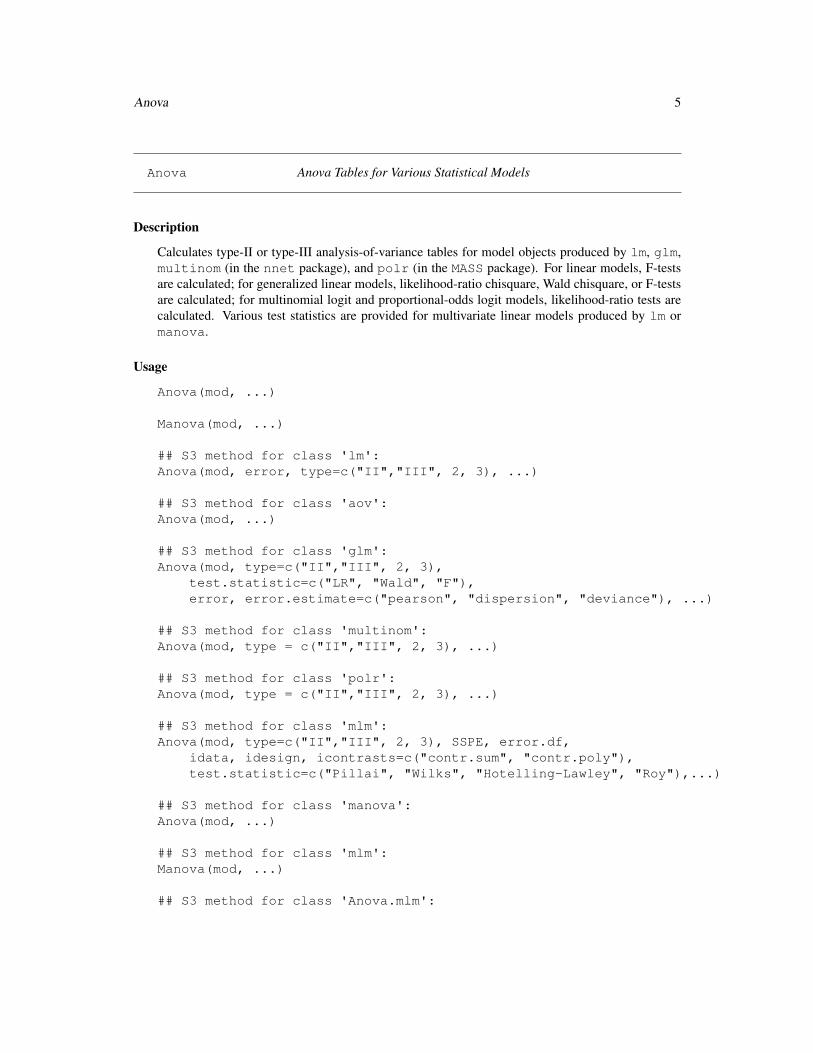
Anova Anova Tables for Various Statistical Models

Description

Calculates type-II or type-III analysis-of-variance tables for model objects produced by lm, glm,

multinom (in the nnet package), and polr (in the MASS package). For linear models, F-tests

are calculated; for generalized linear models, likelihood-ratio chisquare, Wald chisquare, or F-tests

are calculated; for multinomial logit and proportional-odds logit models, likelihood-ratio tests are

calculated. Various test statistics are provided for multivariate linear models produced by lm or

manova.

Usage

Anova(mod, ...)

Manova(mod, ...)

## S3 method for class 'lm':

Anova(mod, error, type=c("II","III", 2, 3), ...)

## S3 method for class 'aov':

Anova(mod, ...)

## S3 method for class 'glm':

Anova(mod, type=c("II","III", 2, 3),

test.statistic=c("LR", "Wald", "F"),

error, error.estimate=c("pearson", "dispersion", "deviance"), ...)

## S3 method for class 'multinom':

Anova(mod, type = c("II","III", 2, 3), ...)

## S3 method for class 'polr':

Anova(mod, type = c("II","III", 2, 3), ...)

## S3 method for class 'mlm':

Anova(mod, type=c("II","III", 2, 3), SSPE, error.df,

idata, idesign, icontrasts=c("contr.sum", "contr.poly"),

test.statistic=c("Pillai", "Wilks", "Hotelling-Lawley", "Roy"),...)

## S3 method for class 'manova':

Anova(mod, ...)


Manova(mod, ...)

## S3 method for class 'Anova.mlm':

6 Anova

print(x, ...)

## S3 method for class 'Anova.mlm':

summary(object, test.statistic, multivariate=TRUE,

univariate=TRUE, digits=unlist(options("digits")), ...)

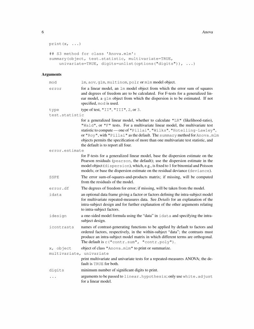
Arguments

mod lm, aov, glm, multinom, polr or mlm model object.

error for a linear model, an lm model object from which the error sum of squares

and degrees of freedom are to be calculated. For F-tests for a generalized lin-

ear model, a glm object from which the dispersion is to be estimated. If not

specified, mod is used.

type type of test, "II", "III", 2, or 3.

test.statistic

for a generalized linear model, whether to calculate "LR" (likelihood-ratio),

"Wald", or "F" tests. For a multivariate linear model, the multivariate test

statistic to compute — one of "Pillai", "Wilks", "Hotelling-Lawley",

or "Roy", with "Pillai" as the default. The summarymethod for Anova.mlm

objects permits the specification of more than one multivariate test statistic, and

the default is to report all four.

error.estimate

for F-tests for a generalized linear model, base the dispersion estimate on the

Pearson residuals (pearson, the default); use the dispersion estimate in the

model object (dispersion), which, e.g., is fixed to 1 for binomial and Poisson

models; or base the dispersion estimate on the residual deviance (deviance).

SSPE The error sum-of-squares-and-products matrix; if missing, will be computed

from the residuals of the model.

error.df The degrees of freedom for error; if missing, will be taken from the model.

idata an optional data frame giving a factor or factors defining the intra-subject model

for multivariate repeated-measures data. See Details for an explanation of the

intra-subject design and for further explanation of the other arguments relating

to intra-subject factors.

idesign a one-sided model formula using the “data” in idata and specifying the intra-

subject design.

icontrasts names of contrast-generating functions to be applied by default to factors and

ordered factors, respectively, in the within-subject “data”; the contrasts must

produce an intra-subject model matrix in which different terms are orthogonal.

The default is c("contr.sum", "contr.poly").

x, object object of class "Anova.mlm" to print or summarize.

multivariate, univariate

print multivariate and univariate tests for a repeated-measures ANOVA; the de-

fault is TRUE for both.

digits minimum number of significant digits to print.

... arguments to be passed to linear.hypothesis; only use white.adjust

for a linear model.

Anova 7

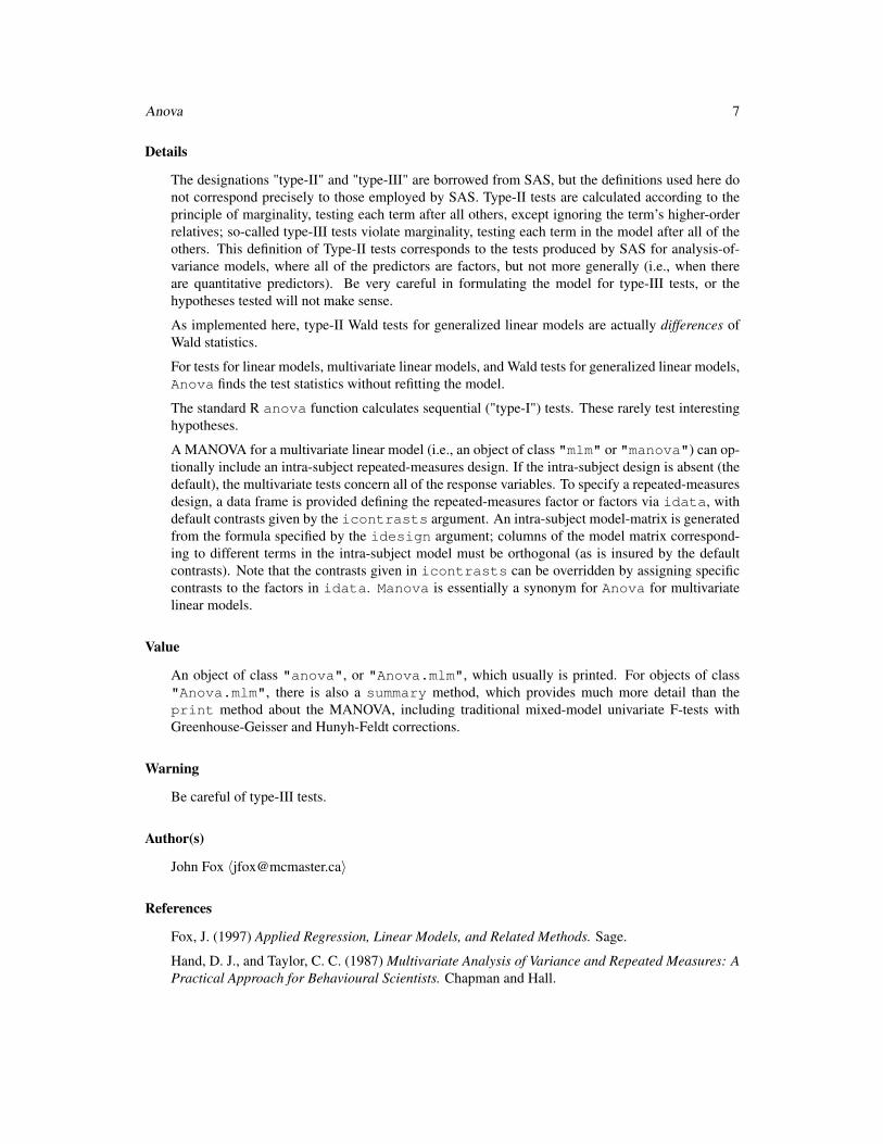
Details

The designations "type-II" and "type-III" are borrowed from SAS, but the definitions used here do

not correspond precisely to those employed by SAS. Type-II tests are calculated according to the

principle of marginality, testing each term after all others, except ignoring the term’s higher-order

relatives; so-called type-III tests violate marginality, testing each term in the model after all of the

others. This definition of Type-II tests corresponds to the tests produced by SAS for analysis-of-

variance models, where all of the predictors are factors, but not more generally (i.e., when there

are quantitative predictors). Be very careful in formulating the model for type-III tests, or the

hypotheses tested will not make sense.

As implemented here, type-II Wald tests for generalized linear models are actually differences of

Wald statistics.

For tests for linear models, multivariate linear models, and Wald tests for generalized linear models,

Anova finds the test statistics without refitting the model.

The standard R anova function calculates sequential ("type-I") tests. These rarely test interesting

hypotheses.

A MANOVA for a multivariate linear model (i.e., an object of class "mlm" or "manova") can op-

tionally include an intra-subject repeated-measures design. If the intra-subject design is absent (the

default), the multivariate tests concern all of the response variables. To specify a repeated-measures

design, a data frame is provided defining the repeated-measures factor or factors via idata, with

default contrasts given by the icontrasts argument. An intra-subject model-matrix is generated

from the formula specified by the idesign argument; columns of the model matrix correspond-

ing to different terms in the intra-subject model must be orthogonal (as is insured by the default

contrasts). Note that the contrasts given in icontrasts can be overridden by assigning specific

contrasts to the factors in idata. Manova is essentially a synonym for Anova for multivariate

linear models.

Value

An object of class "anova", or "Anova.mlm", which usually is printed. For objects of class

"Anova.mlm", there is also a summary method, which provides much more detail than the

print method about the MANOVA, including traditional mixed-model univariate F-tests with

Greenhouse-Geisser and Hunyh-Feldt corrections.

Warning

Be careful of type-III tests.

Author(s)

John Fox 〈[email protected]〉

References


Hand, D. J., and Taylor, C. C. (1987) Multivariate Analysis of Variance and Repeated Measures: A

Practical Approach for Behavioural Scientists. Chapman and Hall.

8 Anova

O’Brien, R. G., and Kaiser, M. K. (1985) MANOVA method for analyzing repeated measures de-

signs: An extensive primer. Psychological Bulletin 97, 316–333.

See Also

linear.hypothesis, anova anova.lm, anova.glm, anova.mlm

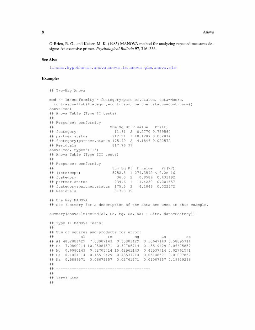
Examples

## Two-Way Anova

mod <- lm(conformity ~ fcategory*partner.status, data=Moore,

contrasts=list(fcategory=contr.sum, partner.status=contr.sum))

Anova(mod)

## Anova Table (Type II tests)

##

## Response: conformity

## Sum Sq Df F value Pr(>F)

## fcategory 11.61 2 0.2770 0.759564

## partner.status 212.21 1 10.1207 0.002874

## fcategory:partner.status 175.49 2 4.1846 0.022572

## Residuals 817.76 39

Anova(mod, type="III")

## Anova Table (Type III tests)

##

## Response: conformity

## Sum Sq Df F value Pr(>F)

## (Intercept) 5752.8 1 274.3592 < 2.2e-16

## fcategory 36.0 2 0.8589 0.431492

## partner.status 239.6 1 11.4250 0.001657

## fcategory:partner.status 175.5 2 4.1846 0.022572

## Residuals 817.8 39

## One-Way MANOVA

## See ?Pottery for a description of the data set used in this example.

summary(Anova(lm(cbind(Al, Fe, Mg, Ca, Na) ~ Site, data=Pottery)))

## Type II MANOVA Tests:

##

## Sum of squares and products for error:

## Al Fe Mg Ca Na

## Al 48.2881429 7.08007143 0.60801429 0.10647143 0.58895714

## Fe 7.0800714 10.95084571 0.52705714 -0.15519429 0.06675857

## Mg 0.6080143 0.52705714 15.42961143 0.43537714 0.02761571

## Ca 0.1064714 -0.15519429 0.43537714 0.05148571 0.01007857

## Na 0.5889571 0.06675857 0.02761571 0.01007857 0.19929286

##

## ------------------------------------------

##

## Term: Site

##

Anova 9

## Sum of squares and products for the hypothesis:

## Al Fe Mg Ca Na

## Al 175.610319 -149.295533 -130.809707 -5.8891637 -5.3722648

## Fe -149.295533 134.221616 117.745035 4.8217866 5.3259491

## Mg -130.809707 117.745035 103.350527 4.2091613 4.7105458

## Ca -5.889164 4.821787 4.209161 0.2047027 0.1547830

## Na -5.372265 5.325949 4.710546 0.1547830 0.2582456

##

## Multivariate Tests: Site

## Df test stat approx F num Df den Df Pr(>F)

## Pillai 3.00000 1.55394 4.29839 15.00000 60.00000 2.4129e-05 ***## Wilks 3.00000 0.01230 13.08854 15.00000 50.09147 1.8404e-12 ***## Hotelling-Lawley 3.00000 35.43875 39.37639 15.00000 50.00000 < 2.22e-16 ***## Roy 3.00000 34.16111 136.64446 5.00000 20.00000 9.4435e-15 ***## ---

## Signif. codes: 0 '***' 0.001 '**' 0.01 '*' 0.05 '.' 0.1 ' ' 1

## MANOVA for a randomized block design (example courtesy of Michael Friendly:

## See ?Soils for description of the data set)

soils.mod <- lm(cbind(pH,N,Dens,P,Ca,Mg,K,Na,Conduc) ~ Block + Contour*Depth,

data=Soils)

Manova(soils.mod)

## Type II MANOVA Tests: Pillai test statistic


## Block 3 1.6758 3.7965 27 81 1.777e-06 ***## Contour 2 1.3386 5.8468 18 52 2.730e-07 ***## Depth 3 1.7951 4.4697 27 81 8.777e-08 ***## Contour:Depth 6 1.2351 0.8640 54 180 0.7311

## ---

## Signif. codes: 0 '***' 0.001 '**' 0.01 '*' 0.05 '.' 0.1 ' ' 1

## a multivariate linear model for repeated-measures data

## See ?OBrienKaiser for a description of the data set used in this example.

phase <- factor(rep(c("pretest", "posttest", "followup"), c(5, 5, 5)),

levels=c("pretest", "posttest", "followup"))

hour <- ordered(rep(1:5, 3))

idata <- data.frame(phase, hour)

idata

## phase hour

## 1 pretest 1

## 2 pretest 2

## 3 pretest 3

## 4 pretest 4

## 5 pretest 5

## 6 posttest 1

## 7 posttest 2

## 8 posttest 3

## 9 posttest 4

## 10 posttest 5

## 11 followup 1

10 Anova

## 12 followup 2

## 13 followup 3

## 14 followup 4

## 15 followup 5

mod.ok <- lm(cbind(pre.1, pre.2, pre.3, pre.4, pre.5,

post.1, post.2, post.3, post.4, post.5,

fup.1, fup.2, fup.3, fup.4, fup.5) ~ treatment*gender,

data=OBrienKaiser)

(av.ok <- Anova(mod.ok, idata=idata, idesign=~phase*hour))

## Type II Repeated Measures MANOVA Tests: Pillai test statistic


## treatment 2 0.4809 4.6323 2 10 0.0376868 *## gender 1 0.2036 2.5558 1 10 0.1409735

## treatment:gender 2 0.3635 2.8555 2 10 0.1044692

## phase 1 0.8505 25.6053 2 9 0.0001930 ***## treatment:phase 2 0.6852 2.6056 4 20 0.0667354 .

## gender:phase 1 0.0431 0.2029 2 9 0.8199968

## treatment:gender:phase 2 0.3106 0.9193 4 20 0.4721498

## hour 1 0.9347 25.0401 4 7 0.0003043 ***## treatment:hour 2 0.3014 0.3549 8 16 0.9295212

## gender:hour 1 0.2927 0.7243 4 7 0.6023742

## treatment:gender:hour 2 0.5702 0.7976 8 16 0.6131884

## phase:hour 1 0.5496 0.4576 8 3 0.8324517

## treatment:phase:hour 2 0.6637 0.2483 16 8 0.9914415

## gender:phase:hour 1 0.6950 0.8547 8 3 0.6202076

## treatment:gender:phase:hour 2 0.7928 0.3283 16 8 0.9723693

## ---

## Signif. codes: 0 '***' 0.001 '**' 0.01 '*' 0.05 '.' 0.1 ' ' 1

summary(av.ok, multivariate=FALSE)

## Univariate Type II Repeated-Measures ANOVA Assuming Sphericity

##

## SS num Df Error SS den Df F Pr(>F)

## treatment 211.286 2 228.056 10 4.6323 0.037687

## gender 58.286 1 228.056 10 2.5558 0.140974

## treatment:gender 130.241 2 228.056 10 2.8555 0.104469

## phase 167.500 2 80.278 20 20.8651 1.274e-05

## treatment:phase 78.668 4 80.278 20 4.8997 0.006426

## gender:phase 1.668 2 80.278 20 0.2078 0.814130

## treatment:gender:phase 10.221 4 80.278 20 0.6366 0.642369

## hour 106.292 4 62.500 40 17.0067 3.191e-08

## treatment:hour 1.161 8 62.500 40 0.0929 0.999257

## gender:hour 2.559 4 62.500 40 0.4094 0.800772

## treatment:gender:hour 7.755 8 62.500 40 0.6204 0.755484

## phase:hour 11.083 8 96.167 80 1.1525 0.338317

## treatment:phase:hour 6.262 16 96.167 80 0.3256 0.992814

## gender:phase:hour 6.636 8 96.167 80 0.6900 0.699124

## treatment:gender:phase:hour 14.155 16 96.167 80 0.7359 0.749562

##

## treatment *## gender

Anova 11

## treatment:gender

## phase ***## treatment:phase **## gender:phase

## treatment:gender:phase

## hour ***## treatment:hour

## gender:hour

## treatment:gender:hour

## phase:hour

## treatment:phase:hour

## gender:phase:hour

## treatment:gender:phase:hour

## ---

## Signif. codes: 0 '***' 0.001 '**' 0.01 '*' 0.05 '.' 0.1 ' ' 1

##

##

## Mauchly Tests for Sphericity

##

## Test statistic p-value

## phase 0.74927 0.27282

## treatment:phase 0.74927 0.27282

## gender:phase 0.74927 0.27282

## treatment:gender:phase 0.74927 0.27282

## hour 0.06607 0.00760

## treatment:hour 0.06607 0.00760

## gender:hour 0.06607 0.00760

## treatment:gender:hour 0.06607 0.00760

## phase:hour 0.00478 0.44939

## treatment:phase:hour 0.00478 0.44939

## gender:phase:hour 0.00478 0.44939

## treatment:gender:phase:hour 0.00478 0.44939

##

##

## Greenhouse-Geisser and Huynh-Feldt Corrections

## for Departure from Sphericity

##

## GG eps Pr(>F[GG])

## phase 0.79953 7.323e-05 ***## treatment:phase 0.79953 0.01223 *## gender:phase 0.79953 0.76616


## hour 0.46028 8.741e-05 ***## treatment:hour 0.46028 0.97879

## gender:hour 0.46028 0.65346


## phase:hour 0.44950 0.34573




## ---

## Signif. codes: 0 '***' 0.001 '**' 0.01 '*' 0.05 '.' 0.1 ' ' 1

##

12 Anscombe

## HF eps Pr(>F[HF])

## phase 0.92786 2.388e-05 ***## treatment:phase 0.92786 0.00809 **## gender:phase 0.92786 0.79845


## hour 0.55928 2.014e-05 ***## treatment:hour 0.55928 0.98877

## gender:hour 0.55928 0.69115


## phase:hour 0.73306 0.34405




## ---

## Signif. codes: 0 '***' 0.001 '**' 0.01 '*' 0.05 '.' 0.1 ' ' 1

Anscombe U. S. State Public-School Expenditures

Description

The Anscombe data frame has 51 rows and 4 columns. The observations are the U. S. states plus

Washington, D. C. in 1970.

Usage

Anscombe

Format


education Per-capita education expenditures, dollars.

income Per-capita income, dollars.

young Proportion under 18, per 1000.

urban Proportion urban, per 1000.

Source

Anscombe, F. J. (1981) Computing in Statistical Science Through APL. Springer-Verlag.

References


Ask 13

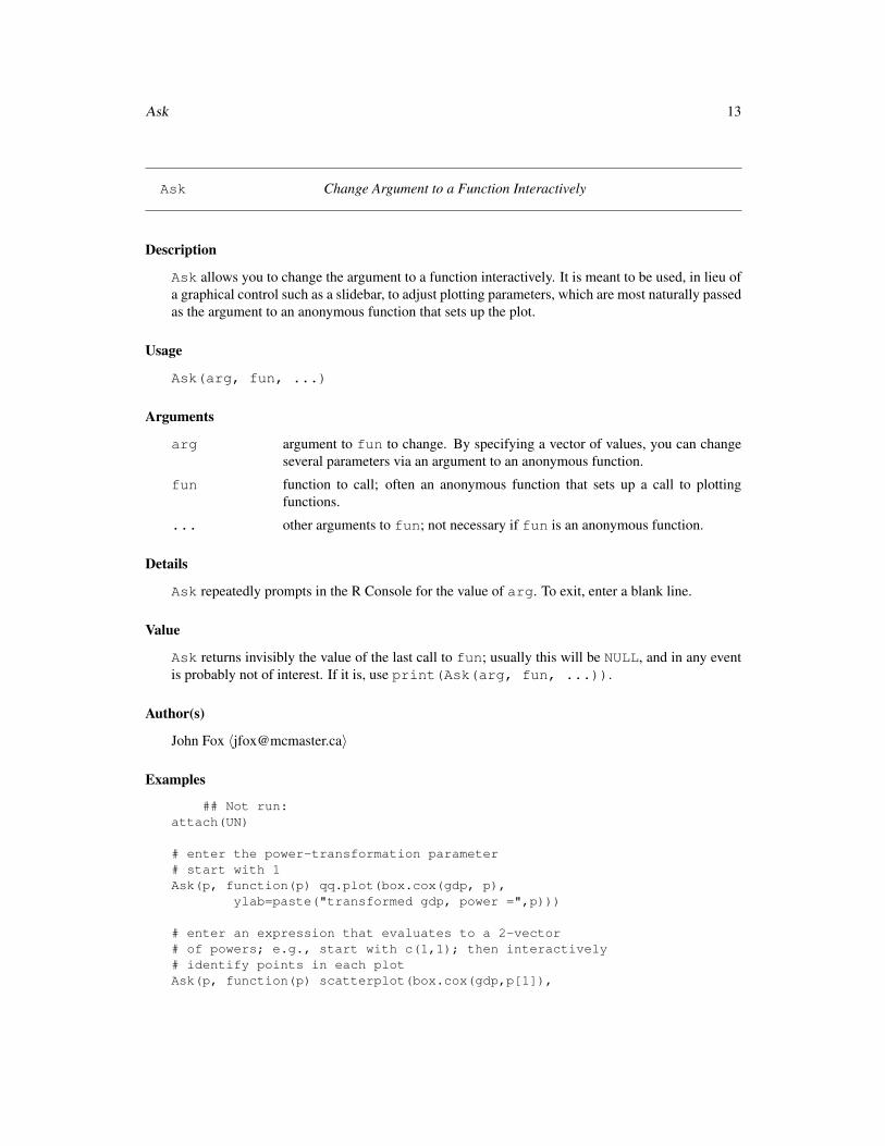
Ask Change Argument to a Function Interactively

Description

Ask allows you to change the argument to a function interactively. It is meant to be used, in lieu of

a graphical control such as a slidebar, to adjust plotting parameters, which are most naturally passed

as the argument to an anonymous function that sets up the plot.

Usage

Ask(arg, fun, ...)

Arguments

arg argument to fun to change. By specifying a vector of values, you can change

several parameters via an argument to an anonymous function.

fun function to call; often an anonymous function that sets up a call to plotting

functions.

... other arguments to fun; not necessary if fun is an anonymous function.

Details

Ask repeatedly prompts in the R Console for the value of arg. To exit, enter a blank line.

Value

Ask returns invisibly the value of the last call to fun; usually this will be NULL, and in any event

is probably not of interest. If it is, use print(Ask(arg, fun, ...)).

Author(s)


Examples

## Not run:

attach(UN)

# enter the power-transformation parameter

# start with 1

Ask(p, function(p) qq.plot(box.cox(gdp, p),

ylab=paste("transformed gdp, power =",p)))

# enter an expression that evaluates to a 2-vector

# of powers; e.g., start with c(1,1); then interactively

# identify points in each plot

Ask(p, function(p) scatterplot(box.cox(gdp,p[1]),

14 Baumann

box.cox(infant.mortality, p[2]),

xlab=paste("transformed GDP/capita, power =",p[1]),

ylab=paste("transformed infant mortality, power =",p[2]),

labels=rownames(UN)))

## End(Not run)

Baumann Methods of Teaching Reading Comprehension

Description

The Baumann data frame has 66 rows and 6 columns. The data are from an experimental study

conducted by Baumann and Jones, as reported by Moore and McCabe (1993). Students were ran-

domly assigned to one of three experimental groups.

Usage

Baumann

Format


group Experimental group; a factor with levels: Basal, traditional method of teaching; DRTA, an

innovative method; Strat, another innovative method.

pretest.1 First pretest.

pretest.2 Second pretest.

post.test.1 First post-test.

post.test.2 Second post-test.

post.test.3 Third post-test.

Source

Moore, D. S. and McCabe, G. P. (1993) Introduction to the Practice of Statistics, Second Edition.

Freeman [pp. 794–795].

Bfox 15

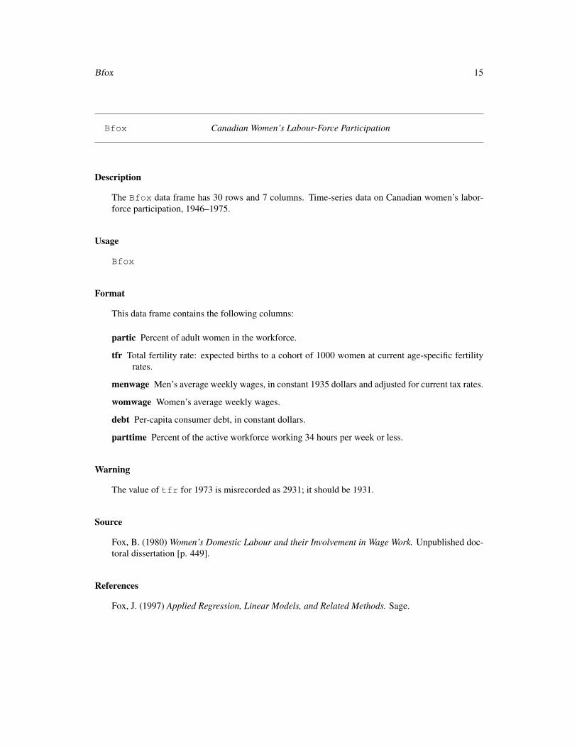
Bfox Canadian Women’s Labour-Force Participation

Description

The Bfox data frame has 30 rows and 7 columns. Time-series data on Canadian women’s labor-

force participation, 1946–1975.

Usage

Bfox

Format


partic Percent of adult women in the workforce.

tfr Total fertility rate: expected births to a cohort of 1000 women at current age-specific fertility

rates.

menwage Men’s average weekly wages, in constant 1935 dollars and adjusted for current tax rates.

womwage Women’s average weekly wages.

debt Per-capita consumer debt, in constant dollars.

parttime Percent of the active workforce working 34 hours per week or less.

Warning

The value of tfr for 1973 is misrecorded as 2931; it should be 1931.

Source

Fox, B. (1980) Women’s Domestic Labour and their Involvement in Wage Work. Unpublished doc-

toral dissertation [p. 449].

References


16 Burt

Blackmoor Exercise Histories of Eating-Disordered and Control Subjects

Description

The Blackmoor data frame has 945 rows and 4 columns. Blackmoor and Davis’s data on exercise

histories of 138 teenaged girls hospitalized for eating disorders and 98 control subjects.

Usage

Blackmoor

Format


subject a factor with subject id codes.

age age in years.

exercise hours per week of exercise.

group a factor with levels: control, Control subjects; patient, Eating-disordered patients.

Source

Personal communication from Elizabeth Blackmoor and Caroline Davis, York University.

Burt Fraudulent Data on IQs of Twins Raised Apart

Description

The Burt data frame has 27 rows and 4 columns. The “data” were simply (and notoriously)

manufactured.

Usage

Burt

Format


IQbio IQ of twin raised by biological parents

IQfoster IQ of twin raised by foster parents

class A factor with levels (note: out of order): high; low; medium.

Can.pop 17

Source

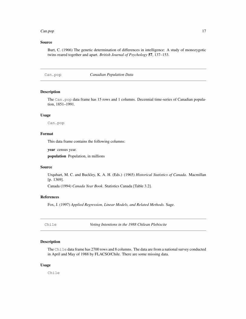
Burt, C. (1966) The genetic determination of differences in intelligence: A study of monozygotic

twins reared together and apart. British Journal of Psychology 57, 137–153.

Can.pop Canadian Population Data

Description

The Can.pop data frame has 15 rows and 1 columns. Decennial time-series of Canadian popula-

tion, 1851–1991.

Usage

Can.pop

Format


year census year.

population Population, in millions

Source

Urquhart, M. C. and Buckley, K. A. H. (Eds.) (1965) Historical Statistics of Canada. Macmillan

[p. 1369].

Canada (1994) Canada Year Book. Statistics Canada [Table 3.2].

References


Chile Voting Intentions in the 1988 Chilean Plebiscite

Description

The Chile data frame has 2700 rows and 8 columns. The data are from a national survey conducted

in April and May of 1988 by FLACSO/Chile. There are some missing data.

Usage

Chile

18 Chirot

Format


region A factor with levels: C, Central; M, Metropolitan Santiago area; N, North; S, South; SA, city

of Santiago.

population Population size of respondent’s community.

sex A factor with levels: F, female; M, male.

age in years.

education A factor with levels (note: out of order): P, Primary; PS, Post-secondary; S, Secondary.

income Monthly income, in Pesos.

statusquo Scale of support for the status-quo.

vote a factor with levels: A, will abstain; N, will vote no (against Pinochet); U, undecided; Y, will

vote yes (for Pinochet).

Source

Personal communication from FLACSO/Chile.

References


Chirot The 1907 Romanian Peasant Rebellion

Description

The Chirot data frame has 32 rows and 5 columns. The observations are counties in Romania.

Usage

Chirot

Format


intensity Intensity of the rebellion

commerce Commercialization of agriculture

tradition Traditionalism

midpeasant Strength of middle peasantry

inequality Inequality of land tenure

Contrasts 19

Source

Chirot, D. and C. Ragin (1975) The market, tradition and peasant rebellion: The case of Romania.

American Sociological Review 40, 428–444 [Table 1].

References


Contrasts Functions to Construct Contrasts

Description

These are substitutes for similarly named functions in the base package (note the uppercase letter

starting the second word in each function name). The only difference is that the contrast functions

from the car package produce easier-to-read names for the contrasts when they are used in statistical

models.

The functions and this documentation are adapted from the base package.

Usage

contr.Treatment(n, base = 1, contrasts = TRUE)

contr.Sum(n, contrasts = TRUE)

contr.Helmert(n, contrasts = TRUE)

Arguments

n a vector of levels for a factor, or the number of levels.

base an integer specifying which level is considered the baseline level. Ignored if

contrasts is FALSE.

contrasts a logical indicating whether contrasts should be computed.

Details

These functions are used for creating contrast matrices for use in fitting analysis of variance and

regression models. The columns of the resulting matrices contain contrasts which can be used for

coding a factor with n levels. The returned value contains the computed contrasts. If the argument

contrasts is FALSE then a square matrix is returned.

Several aspects of these contrast functions are controlled by options set via the options command:

decorate.contrasts This option should be set to a 2-element character vector containing the

prefix and suffix characters to surround contrast names. If the option is not set, then c("[",

"]") is used. For example, setting options(decorate.contrasts=c(".", ""))

produces contrast names that are separated from factor names by a period. Setting options(decorate.contrasts=c("",

"")) reproduces the behaviour of the R base contrast functions.

20 Contrasts

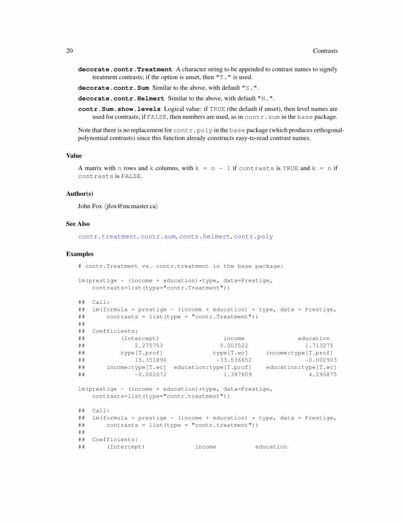
decorate.contr.Treatment A character string to be appended to contrast names to signify

treatment contrasts; if the option is unset, then "T." is used.

decorate.contr.Sum Similar to the above, with default "S.".

decorate.contr.Helmert Similar to the above, with default "H.".

contr.Sum.show.levels Logical value: if TRUE (the default if unset), then level names are

used for contrasts; if FALSE, then numbers are used, as in contr.sum in the base package.

Note that there is no replacement for contr.poly in the base package (which produces orthogonal-

polynomial contrasts) since this function already constructs easy-to-read contrast names.

Value

A matrix with n rows and k columns, with k = n - 1 if contrasts is TRUE and k = n if

contrasts is FALSE.

Author(s)


See Also

contr.treatment, contr.sum, contr.helmert, contr.poly

Examples

# contr.Treatment vs. contr.treatment in the base package:

lm(prestige ~ (income + education)*type, data=Prestige,

contrasts=list(type="contr.Treatment"))

## Call:

## lm(formula = prestige ~ (income + education) * type, data = Prestige,

## contrasts = list(type = "contr.Treatment"))

##

## Coefficients:

## (Intercept) income education

## 2.275753 0.003522 1.713275

## type[T.prof] type[T.wc] income:type[T.prof]

## 15.351896 -33.536652 -0.002903

## income:type[T.wc] education:type[T.prof] education:type[T.wc]

## -0.002072 1.387809 4.290875

lm(prestige ~ (income + education)*type, data=Prestige,

contrasts=list(type="contr.treatment"))

## Call:

## lm(formula = prestige ~ (income + education) * type, data = Prestige,

## contrasts = list(type = "contr.treatment"))

##

## Coefficients:

## (Intercept) income education

Cowles 21

## 2.275753 0.003522 1.713275

## typeprof typewc income:typeprof

## 15.351896 -33.536652 -0.002903

## income:typewc education:typeprof education:typewc

## -0.002072 1.387809 4.290875

Cowles Cowles and Davis’s Data on Volunteering

Description

The Cowles data frame has 1421 rows and 4 columns. These data come from a study of the

personality determinants of volunteering for psychological research.

Usage

Cowles

Format


neuroticism scale from Eysenck personality inventory

extraversion scale from Eysenck personality inventory

sex a factor with levels: female; male

volunteer volunteeing, a factor with levels: no; yes

Source

Cowles, M. and C. Davis (1987) The subject matter of psychology: Volunteers. British Journal of

Social Psychology 26, 97–102.

Davis Self-Reports of Height and Weight

Description

The Davis data frame has 200 rows and 5 columns. The subjects were men and women engaged

in regular exercise. There are some missing data.

Usage

Davis

22 DavisThin

Format


sex A factor with levels: F, female; M, male.

weight Measured weight in kg.

height Measured height in cm.

repwt Reported weight in kg.

repht Reported height in cm.

Source

Personal communication from C. Davis, Departments of Physical Education and Psychology, York

University.

References

Davis, C. (1990) Body image and weight preoccupation: A comparison between exercising and

non-exercising women. Appetite, 15, 13–21.


DavisThin Davis’s Data on Drive for Thinness

Description

The DavisThin data frame has 191 rows and 7 columns. This is part of a larger dataset for a study

of eating disorders. The seven variables in the data frame comprise a "drive for thinness" scale, to

be formed by summing the items.

Usage

DavisThin

Format


DT1 a numeric vector







Duncan 23

Source

Davis, C., G. Claridge, and D. Cerullo (1997) Personality factors predisposing to weight preoccupa-

tion: A continuum approach to the association between eating disorders and personality disorders.

Journal of Psychiatric Research 31, 467–480.

Duncan Duncan’s Occupational Prestige Data

Description

The Duncan data frame has 45 rows and 4 columns. Data on the prestige and other characteristics

of 45 U. S. occupations in 1950.

Usage

Duncan

Format


type Type of occupation. A factor with the following levels: prof, professional and managerial;

wc, white-collar; bc, blue-collar.

income Percent of males in occupation earning $3500 or more in 1950.

education Percent of males in occupation in 1950 who were high-school graduates.

prestige Percent of raters in NORC study rating occupation as excellent or good in prestige.

Source

Duncan, O. D. (1961) A socioeconomic index for all occupations. In Reiss, A. J., Jr. (Ed.) Occu-

pations and Social Status. Free Press [Table VI-1].

References


24 Ellipses

Ellipses Ellipses, Data Ellipses, and Confidence Ellipses

Description

These functions draw ellipses, including data ellipses, and confidence ellipses for linear and gener-

alized linear models.

Usage

ellipse(center, shape, radius, center.pch=19, center.cex=1.5,

segments=51, add=TRUE, xlab="", ylab="",

las=par('las'), col=palette()[2], lwd=2, lty=1, ...)

data.ellipse(x, y, levels=c(0.5, 0.9), center.pch=19, center.cex=1.5,

plot.points=TRUE, add=!plot.points, segments=51, robust=FALSE,

xlab=deparse(substitute(x)),

ylab=deparse(substitute(y)),

las=par('las'), col=palette()[2], pch=1, lwd=2, lty=1, ...)

confidence.ellipse(model, ...)


confidence.ellipse(model, which.coef, levels=0.95, Scheffe=FALSE,

center.pch=19, center.cex=1.5, segments=51, xlab, ylab,



confidence.ellipse(model, which.coef, levels=0.95, Scheffe=FALSE,

center.pch=19, center.cex=1.5, segments=51, xlab, ylab,


Arguments

center 2-element vector with coordinates of center of ellipse.

shape 2 × 2 shape (or covariance) matrix.

radius radius of circle generating the ellipse.

center.pch character for plotting ellipse center.

center.cex relative size of character for plotting ellipse center.

segments number of line-segments used to draw ellipse.

add if TRUE add ellipse to current plot.

xlab label for horizontal axis.

ylab label for vertical axis.

x a numeric vector, or (if y is missing) a 2-column numeric matrix.

Ellipses 25

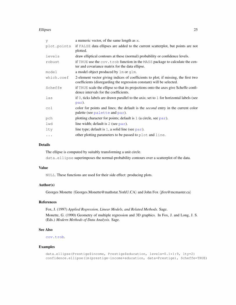
y a numeric vector, of the same length as x.

plot.points if FALSE data ellipses are added to the current scatterplot, but points are not

plotted.

levels draw elliptical contours at these (normal) probability or confidence levels.

robust if TRUE use the cov.trob function in the MASS package to calculate the cen-

ter and covariance matrix for the data ellipse.

model a model object produced by lm or glm.

which.coef 2-element vector giving indices of coefficients to plot; if missing, the first two

coefficients (disregarding the regression constant) will be selected.

Scheffe if TRUE scale the ellipse so that its projections onto the axes give Scheffe confi-

dence intervals for the coefficients.

las if 0, ticks labels are drawn parallel to the axis; set to 1 for horizontal labels (see

par).

col color for points and lines; the default is the second entry in the current color

palette (see palette and par).

pch plotting character for points; default is 1 (a circle, see par).

lwd line width; default is 2 (see par).

lty line type; default is 1, a solid line (see par).

... other plotting parameters to be passed to plot and line.

Details

The ellipse is computed by suitably transforming a unit circle.

data.ellipse superimposes the normal-probability contours over a scatterplot of the data.

Value

NULL. These functions are used for their side effect: producing plots.

Author(s)

Georges Monette 〈[email protected]〉 and John Fox 〈[email protected]〉

References


Monette, G. (1990) Geometry of multiple regression and 3D graphics. In Fox, J. and Long, J. S.

(Eds.) Modern Methods of Data Analysis. Sage.

See Also

cov.trob.

Examples

data.ellipse(Prestige$income, Prestige$education, levels=0.1*1:9, lty=2)

confidence.ellipse(lm(prestige~income+education, data=Prestige), Scheffe=TRUE)

26 Ericksen

Ericksen The 1980 U.S. Census Undercount

Description

The Ericksen data frame has 66 rows and 9 columns. The observations are 16 large cities, the

remaining parts of the states in which these cities are located, and the other U. S. states.

Usage

Ericksen

Format


minority Percentage black or Hispanic.

crime Rate of serious crimes per 1000 population.

poverty Percentage poor.

language Percentage having difficulty speaking or writing English.

highschool Percentage age 25 or older who had not finished highschool.

housing Percentage of housing in small, multiunit buildings.

city A factor with levels: city, major city; state, state or state-remainder.

conventional Percentage of households counted by conventional personal enumeration.

undercount Preliminary estimate of percentage undercount.

Source

Ericksen, E. P., Kadane, J. B. and Tukey, J. W. (1989) Adjusting the 1980 Census of Population and

Housing. Journal of the American Statistical Association 84, 927–944 [Tables 7 and 8].

References


Florida 27

Florida Florida County Voting

Description

The Florida data frame has 67 rows and 11 columns. Vote by county in Florida for President in

the 2000 election.

Usage

Florida

Format


GORE Number of votes for Gore

BUSH Number of votes for Bush.

BUCHANAN Number of votes for Buchanan.

NADER Number of votes for Nader.

BROWNE Number of votes for Browne (whoever that is).

HAGELIN Number of votes for Hagelin (whoever that is).

HARRIS Number of votes for Harris (whoever that is).

MCREYNOLDS Number of votes for McReynolds (whoever that is).

MOOREHEAD Number of votes for Moorehead (whoever that is).

PHILLIPS Number of votes for Phillips (whoever that is).

Total Total number of votes.

Source

Adams, G. D. and Fastnow, C. F. (2000) A note on the voting irregularities in Palm Beach, FL.

http://madison.hss.cmu.edu/.

http://madison.hss.cmu.edu/

28 Friendly

Freedman Crowding and Crime in U. S. Metropolitan Areas

Description

The Freedman data frame has 110 rows and 4 columns. The observations are U. S. metropolitan

areas with 1968 populations of 250,000 or more. There are some missing data.

Usage

Freedman

Format


population Total 1968 population, 1000s.

nonwhite Percent nonwhite population, 1960.

density Population per square mile, 1968.

crime Crime rate per 100,000, 1969.

Source

United States (1970) Statistical Abstract of the United States. Bureau of the Census.

References

Freedman, J. (1975) Crowding and Behavior. Viking.

Friendly Format Effects on Recall

Description

The Friendly data frame has 30 rows and 2 columns. The data are from an experiment on

subjects’ ability to remember words based on the presentation format.

Usage

Friendly

Ginzberg 29

Format


condition A factor with levels: Before, Recalled words presented before others; Meshed, Re-

called words meshed with others; SFR, Standard free recall.

correct Number of words correctly recalled, out of 40 on final trial of the experiment.

Source

Friendly, M. and Franklin, P. (1980) Interactive presentation in multitrial free recall. Memory and

Cognition 8 265–270.

Personal communication from M. Friendly, Department of Psychology, York University.

References


Ginzberg Data on Depression

Description

The Ginzberg data frame has 82 rows and 6 columns. The data are for psychiatric patients

hospitalized for depression.

Usage

Ginzberg

Format


simplicity Measures subject’s need to see the world in black and white.

fatalism Fatalism scale.

depression Beck self-report depression scale.

adjsimp Adjusted Simplicity: Simplicity adjusted (by regression) for other variables thought to

influence depression.

adjfatal Adjusted Fatalism.

adjdep Adjusted Depression.

Source

Personal communication from Georges Monette, Department of Mathematics and Statistics, York

University, with the permission of the original investigator.

30 Greene

References


Greene Refugee Appeals

Description

The Greene data frame has 384 rows and 7 columns. These are cases filed in 1990, in which

refugee claimants rejected by the Canadian Immigration and Refugee Board asked the Federal Court

of Appeal for leave to appeal the negative ruling of the Board.

Usage

Greene

Format


judge Name of judge hearing case. A factor with levels: Desjardins, Heald, Hugessen,

Iacobucci, MacGuigan, Mahoney, Marceau, Pratte, Stone, Urie.

nation Nation of origin of claimant. A factor with levels: Argentina, Bulgaria, China,

Czechoslovakia, El.Salvador, Fiji, Ghana, Guatemala, India, Iran, Lebanon,

Nicaragua, Nigeria, Pakistan, Poland, Somalia, Sri.Lanka.

rater Judgment of independent rater. A factor with levels: no, case has no merit; yes, case has

some merit (leave to appeal should be granted).

decision Judge’s decision. A factor with levels: no, leave to appeal not granted; yes, leave to

appeal granted.

language Language of case. A factor with levels: English, French.

location Location of original refugee claim. A factor with levels: Montreal, other, Toronto.

success Logit of success rate, for all cases from the applicant’s nation.

Source

Personal communication from Ian Greene, Department of Political Science, York University.

References


Guyer 31

Guyer Anonymity and Cooperation

Description

The Guyer data frame has 20 rows and 3 columns. The data are from an experiment in which

four-person groups played a prisoner’s dilemma game for 30 trails, each person making either a

cooperative or competitive choice on each trial. Choices were made either anonymously or in

public; groups were composed either of females or of males. The observations are 20 groups.

Usage

Guyer

Format


cooperation Number of cooperative choices (out of 120 in all).

condition A factor with levels: A, Anonymous; P, Public-Choice.

sex Sex. A factor with levels: F, Female; M, Male.

Source

Fox, J. and Guyer, M. (1978) Public choice and cooperation in n-person prisoner’s dilemma. Jour-

nal of Conflict Resolution 22, 469–481.

References


Hartnagel Canadian Crime-Rates Time Series

Description

The Hartnagel data frame has 38 rows and 7 columns. The data are an annual time-series from

1931 to 1968. There are some missing data.

Usage

Hartnagel

32 Leinhardt

Format


year 1931–1968.

tfr Total fertility rate per 1000 women.

partic Women’s labor-force participation rate per 1000.

degrees Women’s post-secondary degree rate per 10,000.

fconvict Female indictable-offense conviction rate per 100,000.

ftheft Female theft conviction rate per 100,000.

mconvict Male indictable-offense conviction rate per 100,000.

mtheft Male theft conviction rate per 100,000.

Details

The post-1948 crime rates have been adjusted to account for a difference in method of recording.

Some of your results will differ in the last decimal place from those in Table 14.1 of Fox (1997) due

to rounding of the data. Missing values for 1950 were interpolated.

Source

Personal communication from T. Hartnagel, Department of Sociology, University of Alberta.

References

Fox, J., and Hartnagel, T. F (1979) Changing social roles and female crime in Canada: A time series

analysis. Canadian Review of Sociology and Anthroplogy, 16, 96–104.


Leinhardt Data on Infant-Mortality

Description

The Leinhardt data frame has 105 rows and 4 columns. The observations are nations of the

world around 1970.

Usage

Leinhardt

Mandel 33

Format


income Per-capita income in U. S. dollars.

infant Infant-mortality rate per 1000 live births.

region A factor with levels: Africa; Americas; Asia, Asia and Oceania; Europe.

oil Oil-exporting country. A factor with levels: no, yes.

Details

The infant-mortality rate for Jamaica is misprinted in Leinhardt and Wasserman; the correct value

is given here. Some of the values given in Leinhardt and Wasserman do not appear in the original

New York Times table.

Source

Leinhardt, S. and Wasserman, S. S. (1979) Exploratory data analysis: An introduction to selected

methods. In Schuessler, K. (Ed.) Sociological Methodology 1979 Jossey-Bass.

The New York Times, 28 September 1975, p. E-3, Table 3.

References


Mandel Contrived Collinear Data

Description

The Mandel data frame has 8 rows and 3 columns.

Usage

Mandel

Format


x1 first predictor.

x2 second predictor.

y response.

Source

Mandel, J. (1982) Use of the singular value decomposition in regression analysis. The American

Statistician 36, 15–24.

34 Migration

References


Migration Canadian Interprovincial Migration Data

Description

The Migration data frame has 90 rows and 8 columns.

Usage

Migration

Format


source Province of origin (source). A factor with levels: ALTA, Alberta; BC, British Columbia;

MAN, Manitoba; NB, New Brunswick; NFLD, New Foundland; NS, Nova Scotia; ONT, Ontario;

PEI, Prince Edward Island; QUE, Quebec; SASK, Saskatchewan.

destination Province of destination (1971 residence). A factor with levels: ALTA, Alberta; BC,

British Columbia; MAN, Manitoba; NB, New Brunswick; NFLD, New Foundland; NS, Nova

Scotia; ONT, Ontario; PEI, Prince Edward Island; QUE, Quebec; SASK, Saskatchewan.

migrants Number of migrants (from source to destination) in the period 1966–1971.

distance Distance (between principal cities of provinces): NFLD, St. John; PEI, Charlottetown;

NS, Halifax; NB, Fredricton; QUE, Montreal; ONT, Toronto; MAN, Winnipeg; SASK, Regina;

ALTA, Edmonton; BC, Vancouver.

pops66 1966 population of source province.

pops71 1971 population of source province.

popd66 1966 population of destination province.

popd71 1971 population of destination province.

Details

There is one record in the data file for each migration stream. You can average the 1966 and 1971

population figures for each of the source and destination provinces.

Source

Canada (1962) Map. Department of Mines and Technical Surveys.

Canada (1971) Census of Canada. Statistics Canada, Vol. 1, Part 2 [Table 32].

Canada (1972) Canada Year Book. Statistics Canada [p. 1369].

References


Moore 35

Moore Status, Authoritarianism, and Conformity

Description

The Moore data frame has 45 rows and 4 columns. The data are for subjects in a social-psychological

experiment, who were faced with manipulated disagreement from a partner of either of low or high

status. The subjects could either conform to the partner’s judgment or stick with their own judg-

ment.

Usage

Moore

Format


partner.status Partner’s status. A factor with levels: high, low.

conformity Number of conforming responses in 40 critical trials.

fcategory F-Scale Categorized. A factor with levels (note levels out of order): high, low,

medium.

fscore Authoritarianism: F-Scale score.

Source

Moore, J. C., Jr. and Krupat, E. (1971) Relationship between source status, authoritarianism and

conformity in a social setting. Sociometry 34, 122–134.

Personal communication from J. Moore, Department of Sociology, York University.

References


Mroz U.S. Women’s Labor-Force Participation

Description

The Mroz data frame has 753 rows and 8 columns. The observations, from the Panel Study of

Income Dynamics (PSID), are married women.

Usage

Mroz

36 OBrienKaiser

Format


lfp labor-force participation; a factor with levels: no; yes.

k5 number of children 5 years old or younger.

k618 number of children 6 to 18 years old.

age in years.

wc wife’s college attendance; a factor with levels: no; yes.

hc husband’s college attendance; a factor with levels: no; yes.

lwg log expected wage rate; for women in the labor force, the actual wage rate; for women not in

the labor force, an imputed value based on the regression of lwg on the other variables.

inc family income exclusive of wife’s income.

Source

Mroz, T. A. (1987) The sensitivity of an empirical model of married women’s hours of work to

economic and statistical assumptions. Econometrica 55, 765–799.

References

Fox, J. (2000) Multiple and Generalized Nonparametric Regression. Sage.

Long. J. S. (1997) Regression Models for Categorical and Limited Dependent Variables. Sage.

OBrienKaiser O’Brien and Kaiser’s Repeated-Measures Data

Description

These contrived repeate-measures data are taken from Table 7 of O’Brien and Kaiser (1985). The

data are from an imaginary study in which 16 female and male subjects, who are divided into three

treatments, are measured at a pretest, postest, and a follow-up session; during each session, they are

measured at five occasions at intervals of one hour. The design, therefore, has two between-subject

and two within-subject factors.

The contrasts for the treatment factor are set to −2, 1, 1 and 0,−1, 1. The contrasts for the

gender factor are set to contr.sum.

Usage

OBrienKaiser

Ornstein 37

Format

A data frame with 16 observations on the following 17 variables.

treatment a factor with levels control A B

gender a factor with levels F M

pre.1 pretest, hour 1





post.1 posttest, hour 1





fup.1 follow-up, hour 1





Source



Examples

OBrienKaiser

contrasts(OBrienKaiser$treatment)

contrasts(OBrienKaiser$gender)

Ornstein Interlocking Directorates Among Major Canadian Firms

Description

The Ornstein data frame has 248 rows and 4 columns. The observations are the 248 largest

Canadian firms with publicly available information in the mid-1970s. The names of the firms were

not available.

38 Pottery

Usage

Ornstein

Format


assets Assets in millions of dollars.

sector Industrial sector. A factor with levels: AGR, agriculture, food, light industry; BNK, banking;

CON, construction; FIN, other financial; HLD, holding companies; MAN, heavy manufacturing;

MER, merchandizing; MIN, mining, metals, etc.; TRN, transport; WOD, wood and paper.

nation Nation of control. A factor with levels: CAN, Canada; OTH, other foreign; UK, Britain; US,

United States.

interlocks Number of interlocking director and executive positions shared with other major firms.

Source

Ornstein, M. (1976) The boards and executives of the largest Canadian corporations. Canadian

Journal of Sociology 1, 411–437.

Personal communication from M. Ornstein, Department of Sociology, York University.

References


Pottery Chemical Composition of Pottery

Description

The data give the chemical composition of ancient pottery found at four sites in Great Britain. They

appear in Hand, et al. (1994), and are used to illustrate MANOVA in the SAS Manual.

Usage

data(Pottery)

Format

A data frame with 26 observations on the following 6 variables.

Site a factor with levels AshleyRails Caldicot IsleThorns Llanedyrn

Al Aluminum

Fe Iron

Mg Magnesium

Ca Calcium

Na Sodium

Prestige 39

Source

Hand, D. J., Daly, F., Lunn, A. D., McConway, K. J., and E., O. (1994) A Handbook of Small Data

Sets. Chapman and Hall.

Examples

Pottery

Prestige Prestige of Canadian Occupations

Description

The Prestige data frame has 102 rows and 6 columns. The observations are occupations.

Usage

Prestige

Format


education Average education of occupational incumbents, years, in 1971.

income Average income of incumbents, dollars, in 1971.

women Percentage of incumbents who are women.

prestige Pineo-Porter prestige score for occupation, from a social survey conducted in the mid-

1960s.

census Canadian Census occupational code.

type Type of occupation. A factor with levels (note: out of order): bc, Blue Collar; prof, Profes-

sional, Managerial, and Technical; wc, White Collar.

Source

Canada (1971) Census of Canada. Vol. 3, Part 6. Statistics Canada [pp. 19-1–19-21].

Personal communication from B. Blishen, W. Carroll, and C. Moore, Departments of Sociology,

York University and University of Victoria.

References


40 Robey

Quartet Four Regression Datasets

Description

The Quartet data frame has 11 rows and 5 columns. These are contrived data.

Usage

Quartet

Format


x X-values for datasets 1–3.

y1 Y-values for dataset 1.



x4 X-values for dataset 4.


Source

Anscombe, F. J. (1973) Graphs in statistical analysis. American Statistician 27, 17–21.

Robey Fertility and Contraception

Description

The Robey data frame has 50 rows and 3 columns. The observations are developing nations around

1990.

Usage

Robey

Format


region A factor with levels: Africa; Asia, Asia and Pacific; Latin.Amer, Latin America and

Caribbean; Near.East, Near East and North Africa.

tfr Total fertility rate (children per woman).

contraceptors Percent of contraceptors among married women of childbearing age.

SLID 41

Source

Robey, B., Shea, M. A., Rutstein, O. and Morris, L. (1992) The reproductive revolution: New survey

findings. Population Reports. Technical Report M-11.

References


SLID Survey of Labour and Income Dynamics

Description

The SLID data frame has 7425 rows and 5 columns. The data are from the 1994 wave of the

Canadian Survey of Labour and Income Dynamics, for the province of Ontario. There are missing

data, particularly for wages.

Usage

SLID

Format


wages Composite hourly wage rate from all jobs.

education Number of years of schooling.

age in years.

sex A factor with levels: Female, Male.

language A factor with levels: English, French, Other.

Source

The data are taken from the public-use dataset made available by Statistics Canada, and prepared

by the Institute for Social Research, York University.

42 Soils

Sahlins Agricultural Production in Mazulu Village

Description

The Sahlins data frame has 20 rows and 2 columns. The observations are households in a Central

African village.

Usage

Sahlins

Format


consumers Consumers/Gardener, ratio of consumers to productive individuals.

acres Acres/Gardener, amount of land cultivated per gardener.

Source

Sahlins, M. (1972) Stone Age Economics. Aldine [Table 3.1].

References


Soils Soil Compositions of Physical and Chemical Characteristics

Description

Soil characteristics were measured on samples from three types of contours (Top, Slope, and De-

pression) and at four depths (0-10cm, 10-30cm, 30-60cm, and 60-90cm). The area was divided into

4 blocks, in a randomized block design.

Usage

data(Soils)

Soils 43

Format

A data frame with 48 observations on the following 14 variables. There are 3 factors and 9 response

variables.

Group a factor with 12 levels, corresponding to the combinations of Contour and Depth

Contour a factor with 3 levels: Depression Slope Top

Depth a factor with 4 levels: 0-10 10-30 30-60 60-90

Gp a factor with 12 levels, giving abbreviations for the groups: D0 D1 D3 D6 S0 S1 S3 S6 T0 T1

T3 T6

Block a factor with levels 1 2 3 4

pH soil pH

N total nitrogen in %

Dens bulk density in gm/cm3

P total phosphorous in ppm

Ca calcium in me/100 gm.

Mg magnesium in me/100 gm.

K phosphorous in me/100 gm.

Na sodium in me/100 gm.

Conduc conductivity

Details

These data provide good examples of MANOVA and canonical discriminant analysis in a somewhat

complex multivariate setting. They may be treated as a one-way design (ignoring Block), by using

either Group or Gp as the factor, or a two-way randomized block design using Block, Contour

and Depth (quantitative, so orthogonal polynomial contrasts are useful).

Source

Horton, I. F.,Russell, J. S., and Moore, A. W. (1968) Multivariate-covariance and canonical analysis:

A method for selecting the most effective discriminators in a multivariate situation. Biometrics 24,

845–858. http://www.stat.lsu.edu/faculty/moser/exst7037/soils.sas

References

Khattree, R., and Naik, D. N. (2000) Multivariate Data Reduction and Discrimination with SAS

Software. SAS Institute.

Friendly, M. (in press) Data ellipses, HE plots and reduced-rank displays for multivariate linear

models: SAS software and examples. Journal of Statistical Software.

Examples

Soils

http://www.stat.lsu.edu/faculty/moser/exst7037/soils.sas

44 States

States Education and Related Statistics for the U.S. States

Description

The States data frame has 51 rows and 8 columns. The observations are the U. S. states and

Washington, D. C.

Usage

States

Format


region U. S. Census regions. A factor with levels: ENC, East North Central; ESC, East South Cen-

tral; MA, Mid-Atlantic; MTN, Mountain; NE, New England; PAC, Pacific; SA, South Atlantic;

WNC, West North Central; WSC, West South Central.

pop Population: in 1,000s.

SATV Average score of graduating high-school students in the state on the verbal component of

the Scholastic Aptitude Test (a standard university admission exam).

SATM Average score of graduating high-school students in the state on the math component of the

Scholastic Aptitude Test.

percent Percentage of graduating high-school students in the state who took the SAT exam.

dollars State spending on public education, in $1000s per student.

pay Average teacher’s salary in the state, in $1000s.

Source


References

Moore, D. (1995) The Basic Practice of Statistics. Freeman [Table 2.1].

Transformation Axes 45

Transformation Axes

Axes for Transformed Variables

Description

These functions produce axes for the original scale of transformed variables. Typically these would

appear as additional axes to the right or at the top of the plot, but if the plot is produced with

axes=FALSE, then these functions could be used for axes below or to the left of the plot as well.

Usage

power.axis(power, base=exp(1), side=c("right", "above", "left", "below"),

at, grid=FALSE, grid.col=gray(0.5), grid.lty=3,

axis.title="Untransformed Data", cex=1, las=par("las"))

box.cox.axis(power, side=c("right", "above", "left", "below"),

at, grid=FALSE, grid.col=gray(0.5), grid.lty=3,

axis.title="Untransformed Data", cex=1, las=par("las"))

prob.axis(at, side=c("right", "above", "left", "below"), grid=FALSE, grid.lty=3,

grid.col=gray(0.5), axis.title="Probability", interval=0.1, cex=1, las=par("las"))

Arguments

power power for Box-Cox or power transformation.

side side at which the axis is to be drawn; numeric codes are also permitted: side

= 1 for the bottom of the plot, side=2 for the left side, side = 3 for the

top, side = 4 for the right side.

at numeric vector giving location of tick marks on original scale; if missing, the

function will try to pick nice locations for the ticks.

grid if TRUE grid lines for the axis will be drawn.

grid.col color of grid lines.

grid.lty line type for grid lines.

axis.title title for axis.

cex relative character expansion for axis label.


par).

base base of log transformation for power.axis when power = 0.

interval desired interval between tick marks on the probability scale.

46 Transformation Axes

Details

The transformations corresponding to the three functions are as follows:

power.axis: x′ = xp for p 6= 0 and x′ = log x for p = 0.

box.cox.axis: x′ = (xλ − 1)/λ for λ 6= 0 and x′ = log x for λ = 0.

prob.axis: logit = log[p/(1 − p)].

These functions will try to place tick marks at reasonable locations, but producing a good-looking

graph sometimes requires some fiddling with the at argument.

Value

These functions are used for their side effects: to draw axes.

Author(s)


See Also

box.cox, logit

Examples

UN<-na.omit(UN)

attach(UN)

par(mar=c(5, 4, 4, 4)+.1)

plot(log(gdp, 10), log(infant.mortality, 10))

power.axis(0, base=10, side="above",

at=c(50,200,500,2000,5000,20000),grid=TRUE, axis.title="GDP per capita")

power.axis(0, base=10, side="right",

at=c(5,10,20,50,100), grid=TRUE, axis.title="infant mortality rate per 1000")

plot(box.cox(gdp, 0), box.cox(infant.mortality, 0))

box.cox.axis(0, side="above",

grid=TRUE, axis.title="GDP per capita")

box.cox.axis(0, side="right",

grid=TRUE, axis.title="infant mortality rate per 1000")

qq.plot(logit(infant.mortality/1000))

prob.axis()

qq.plot(logit(infant.mortality/1000))

prob.axis(c(.005, .01, .02, .04, .08, .16))

UN 47

UN GDP and Infant Mortality

Description

The UN data frame has 207 rows and 2 columns. The data are for 1998 and are from the United

Nations; the observations are nations of the world. There are some missing data.

Usage

UN

Format


infant.mortality Infant morality rate, infant deaths per 1000 live births.

gdp GDP per capita, in US dollars.

Source

United Nations (1998) Social indicators. http://www.un.org/Depts/unsd/social/main.

htm.

US.pop Population of the United States

Description

The US.pop data frame has 21 rows and 1 columns. This is a decennial time-series, from 1790 to

1990.

Usage

US.pop

Format


year census year.

population Population in millions.

Source


http://www.un.org/Depts/unsd/social/main.htm

http://www.un.org/Depts/unsd/social/main.htm

48 Var

References


Var Variance-Covariance Matrices (deprecated)

Description

Computes variance-covariance matrices or variances for model objects or data. The default method

uses the function var.

These functions are now deprecated; instead, use the vcov function, now in the base package. Note

that vcov has no diagonal argument and no default method.

Usage

Var(object, ...)

## Default S3 method:

Var(object, diagonal=FALSE, ...)





Arguments

object an object for which the covariance matrix is desired.

... arguments to be passed to var (e.g., na.rm).

diagonal if TRUE, return only the variances.

Value

A variance-covariance matrix or a vector of variances.

Author(s)


See Also

var

Vocab 49

Examples

data(Davis)

attach(Davis)

Var(cbind(weight, repwt), na.rm=TRUE)

## weight repwt

## weight 233.8781 176.1014

## repwt 176.1014 189.7966

Var(lm(weight~repwt))

## (Intercept) repwt

## (Intercept) 9.2228211 -0.134640952

## repwt -0.1346410 0.002051736

Vocab Vocabulary and Education

Description

The Vocab data frame has 968 rows and 2 columns. The observations are respondents to the 1989

U. S. General Social Survey.

Usage

Vocab

Format


education Education, in years.

vocabulary Vocabulary test score: number correct on a 10-word test.

Source

National Opinion Research Center (1989) General Social Survey. Distributed by the Inter-University

Consortium for Political and Social Research.

References


50 av.plots

Womenlf Canadian Women’s Labour-Force Participation

Description

The Womenlf data frame has 263 rows and 4 columns. The data are from a 1977 survey of the

Canadian population.

Usage

Womenlf

Format


partic Labour-Force Participation. A factor with levels (note: out of order): fulltime, Working

full-time; not.work, Not working outside the home; parttime, Working part-time.

hincome Husband’s income, $1000s.

children Presence of children in the household. A factor with levels: absent, present.

region A factor with levels: Atlantic, Atlantic Canada; BC, British Columbia; Ontario;

Prairie, Prairie provinces; Quebec.

Source

Social Change in Canada Project. York Institute for Social Research.

References


av.plots Added-Variable Plots

Description

These functions construct added-variable (also called partial-regression) plots for linear and gener-

alized linear models.

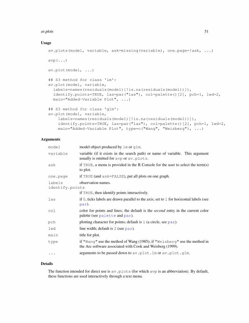
av.plots 51

Usage

av.plots(model, variable, ask=missing(variable), one.page=!ask, ...)

avp(...)

av.plot(model, ...)


av.plot(model, variable,

labels=names(residuals(model)[!is.na(residuals(model))]),

identify.points=TRUE, las=par("las"), col=palette()[2], pch=1, lwd=2,

main="Added-Variable Plot", ...)


av.plot(model, variable,


identify.points=TRUE, las=par("las"), col=palette()[2], pch=1, lwd=2,

main="Added-Variable Plot", type=c("Wang", "Weisberg"), ...)

Arguments

model model object produced by lm or glm.

variable variable (if it exists in the search path) or name of variable. This argument

usually is omitted for avp or av.plots.

ask if TRUE, a menu is provided in the R Console for the user to select the term(s)

to plot.

one.page if TRUE (and ask=FALSE), put all plots on one graph.

labels observation names.identify.points

if TRUE, then identify points interactively.


par).





main title for plot.

type if "Wang" use the method of Wang (1985); if "Weisberg" use the method in

the Arc software associated with Cook and Weisberg (1999).

... arguments to be passed down to av.plot.lm or av.plot.glm.

Details

The function intended for direct use is av.plots (for which avp is an abbreviation). By default,

these functions are used interactively through a text menu.

52 box.cox

The model can contain factors and interactions. An added-variable plot can be drawn for each

column of the model matrix, including the constant.

Value


Author(s)


References

Cook, R. D. and Weisberg, S. (1999) Applied Regression, Including Computing and Graphics.

Wiley.


Wang, P C. (1985) Adding a variable in generalized linear models. Technometrics 27, 273–276.

See Also

cr.plots, ceres.plots, leverage.plots

Examples

## Not run:

av.plots(lm(prestige~income+education+type, data=Duncan))

av.plots(glm(partic != "not.work" ~ hincome + children,

data=Womenlf, family=binomial))

## End(Not run)

box.cox Box-Cox Family of Transformations

Description

Compute the Box-Cox power transformation of a variable.

Usage

box.cox(x, p, start=0)

bc(x, p, ...)

box.cox 53

Arguments

x numeric vector to transform.

p power (0 = log); if p is a vector then a matrix of transformed values with columns

labelled by powers will be returned.

start constant to be added to each value of x prior to transformation.

... argument passed down.

Details

Computes x′ = (xp − 1)/p for p 6= 0 and x′ = log x for p = 0.

The values of x must all be positive; if not, a start should be added to each value to make all

the values positive. The function will automatically compute the start and print a warning, if

necessary.

bc is just an abbreviation for box.cox.

Value

a vector or matrix of transformed values.

Warning

These functions do not compute the maximum-likelihood estimate for a Box-Cox normalizing trans-

formation. See box.cox.powers for estimating unconditional univariate and multivariate Box-

Cox transformations, and boxcox in the MASS package for estimating the Box-Cox transformation

of the response in a linear model.

Author(s)


References

Atkinson, A. C. (1985) Plots, Transformations, and Regression Oxford.

Box, G. E. P. and Cox, D. R. (1964) An analysis of transformations. JRSS B 26, 211–246.


See Also

boxcox, box.cox.var, box.cox.powers, box.cox.axis

Examples

box.cox(1:10, 2)

## [1] 0.0 1.5 4.0 7.5 12.0 17.5 24.0 31.5 40.0 49.5

box.cox(1:5, c(0,2))

## 0 2

## [1,] 0.0000000 0.0

54 box.cox.powers

## [2,] 0.6931472 1.5

## [3,] 1.0986123 4.0

## [4,] 1.3862944 7.5

## [5,] 1.6094379 12.0

box.cox(-5:5, 2)

## [1] 0.0 1.5 4.0 7.5 12.0 17.5 24.0 31.5 40.0 49.5 60.0

## Warning message:

## start = 6 added to data prior to transformation in: box.cox(-5:5, 2)

options(digits=4)

box.cox(-5:5, 0, start=6)

## [1] 0.0000 0.6931 1.0986 1.3863 1.6094 1.7918 1.9459 2.0794 2.1972

## [10] 2.3026 2.3979

box.cox.powers Multivariate Unconditional Box-Cox Transformations

Description

Estimates multivariate unconditional power transformations to multinormality by the method of

maximum likelihood. The univariate case is obtained when only one variable is specified.

Usage

box.cox.powers(X, start=NULL, hypotheses=NULL, ...)

## S3 method for class 'box.cox.powers':

print(x, digits=4, ...)

## S3 method for class 'box.cox.powers':

summary(object, digits=4, ...)

Arguments

X a numeric matrix of variables (or a vector for one variable) to be transformed.

start start values for the power transformation parameters; if NULL (the default), uni-

variate Box-Cox transformations will be computed and used as the start values.

hypotheses if non-NULL, a list of hypotheses to be tested; each hypothesis should be a vector

of values giving the power for each column of X. Note that the hypotheses that

all powers are 1 and that all powers are 0 (log) are always tested.

... optional arguments to be passed to the optim function.

digits number of places to round result.

x, object box.cox.powers object.

box.cox.powers 55

Details

Note that this is unconditional Box-Cox. That is, there is no regression model, and there are no

predictors. The object is to make the distribution of the variable(s) as (multi)normal as possible.

For Box-Cox regression, see the boxcox function in the MASS package.

The function estimates the Box-Cox powers, x′

j = (xλj

j − 1)/λj for λj 6= 0 and x′

j = log xj for

λj = 0. Subsequently using ordinary power transformations (i.e., xp for p 6= 0) achieves the same

result.

Value

returns an object of class box.cox.powers, which may be printed or summarized. the print

and summary methods are now identical; I’ve retained the latter for backwards compatibility.

Author(s)


References

Box, G. E. P. and Cox, D. R. (1964) An analysis of transformations. JRSS B 26 211–246.


Wiley.

See Also

boxcox, box.cox, box.cox.var, box.cox.axis

Examples

attach(Prestige)

box.cox.powers(cbind(income, education))

## Box-Cox Transformations to Multinormality

##

## Est.Power Std.Err. Wald(Power=0) Wald(Power=1)

## income 0.2617 0.1014 2.580 -7.280

## education 0.4242 0.4033 1.052 -1.428

##

## L.R. test, all powers = 0: 7.694 df = 2 p = 0.0213

## L.R. test, all powers = 1: 48.8727 df = 2 p = 0

plot(income, education)

plot(box.cox(income, .26), box.cox(education, .42))

box.cox.powers(income)

## Box-Cox Transformation to Normality

##

## Est.Power Std.Err. Wald(Power=0) Wald(Power=1)

## 0.1793 0.1108 1.618 -7.406

##

## L.R. test, power = 0: 2.7103 df = 1 p = 0.0997

## L.R. test, power = 1: 47.261 df = 1 p = 0

56 box.cox.var

qq.plot(income)

qq.plot(income^.18)

box.cox.var Constructed Variable for Box-Cox Transformation

Description

Computes a constructed variable for the Box-Cox transformation of the response variable in a linear

model.

Usage

box.cox.var(y)

Arguments

y response variable.

Details

The constructed variable is defined as y[log(y/y) − 1], where y is the geometric mean of y.

The constructed variable is meant to be added to the right-hand-side of the linear model. The t-test

for the coefficient of the constructed variable is an approximate score test for whether a transforma-

tion is required.

If b is the coefficient of the constructed variable, then an estimate of the normalizing power trans-

formation based on the score statistic is 1 − b. An added-variable plot for the constructed variable

shows leverage and influence on the decision to transform y.

Value

a numeric vector of the same length as y.

Author(s)


References

Atkinson, A. C. (1985) Plots, Transformations, and Regression. Oxford.

Box, G. E. P. and Cox, D. R. (1964) An analysis of transformations. JRSS B 26 211–246.


See Also

boxcox, box.cox, box.cox.powers, box.cox.axis, av.plots

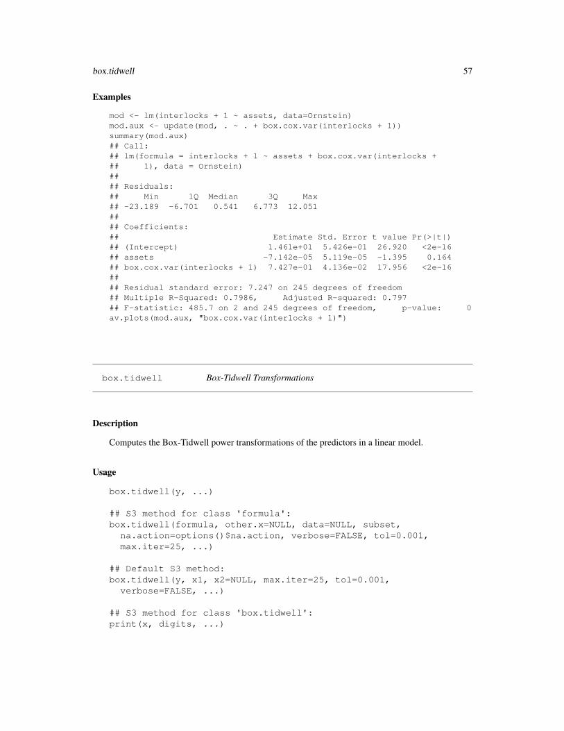
box.tidwell 57

Examples

mod <- lm(interlocks + 1 ~ assets, data=Ornstein)

mod.aux <- update(mod, . ~ . + box.cox.var(interlocks + 1))

summary(mod.aux)

## Call:

## lm(formula = interlocks + 1 ~ assets + box.cox.var(interlocks +

## 1), data = Ornstein)

##

## Residuals:

## Min 1Q Median 3Q Max

## -23.189 -6.701 0.541 6.773 12.051

##

## Coefficients:

## Estimate Std. Error t value Pr(>|t|)

## (Intercept) 1.461e+01 5.426e-01 26.920 <2e-16

## assets -7.142e-05 5.119e-05 -1.395 0.164

## box.cox.var(interlocks + 1) 7.427e-01 4.136e-02 17.956 <2e-16

##

## Residual standard error: 7.247 on 245 degrees of freedom

## Multiple R-Squared: 0.7986, Adjusted R-squared: 0.797

## F-statistic: 485.7 on 2 and 245 degrees of freedom, p-value: 0

av.plots(mod.aux, "box.cox.var(interlocks + 1)")

box.tidwell Box-Tidwell Transformations

Description

Computes the Box-Tidwell power transformations of the predictors in a linear model.

Usage

box.tidwell(y, ...)

## S3 method for class 'formula':

box.tidwell(formula, other.x=NULL, data=NULL, subset,

na.action=options()$na.action, verbose=FALSE, tol=0.001,

max.iter=25, ...)


box.tidwell(y, x1, x2=NULL, max.iter=25, tol=0.001,

verbose=FALSE, ...)

## S3 method for class 'box.tidwell':

print(x, digits, ...)

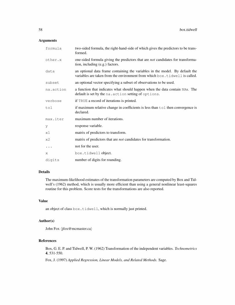
58 box.tidwell

Arguments

formula two-sided formula, the right-hand-side of which gives the predictors to be trans-

formed.

other.x one-sided formula giving the predictors that are not candidates for transforma-

tion, including (e.g.) factors.

data an optional data frame containing the variables in the model. By default the

variables are taken from the environment from which box.tidwell is called.

subset an optional vector specifying a subset of observations to be used.

na.action a function that indicates what should happen when the data contain NAs. The

default is set by the na.action setting of options.

verbose if TRUE a record of iterations is printed.

tol if maximum relative change in coefficients is less than tol then convergence is

declared.

max.iter maximum number of iterations.


x1 matrix of predictors to transform.

x2 matrix of predictors that are not candidates for transformation.

... not for the user.

x box.tidwell object.

digits number of digits for rounding.

Details

The maximum-likelihood estimates of the transformation parameters are computed by Box and Tid-

well’s (1962) method, which is usually more efficient than using a general nonlinear least-squares

routine for this problem. Score tests for the transformations are also reported.

Value

an object of class box.tidwell, which is normally just printed.

Author(s)


References

Box, G. E. P. and Tidwell, P. W. (1962) Transformation of the independent variables. Technometrics

4, 531-550.


car-internal 59

Examples

box.tidwell(prestige~income+education, ~ poly(women,2), data=Prestige)

## income education

## Initial Power -0.91030 2.24354

## Score Statistic -5.30129 2.40556

## p-value 0.00000 0.01615

## MLE of Power -0.03777 2.19283

car-internal Internal car functions

Description

Internal functions for package car.

Usage

df.terms(model, term, ...)



## S3 method for class 'multinom':


## S3 method for class 'polr':


has.intercept(model, ...)


has.intercept(model, ...)

inv(x)

is.aliased(model)

mfrow(n, max.plots=0)

nice(x, direction=c("round", "down", "up"))

predictor.names(model, ...)


predictor.names(model, ...)

relatives(term, names, factors)

responseName(model, ...)

## S3 method for class 'chisq.test':

print(x, ...)


responseName(model, ...)

response(model, ...)


response(model, ...)

term.names(model, ...)


term.names(model, ...)

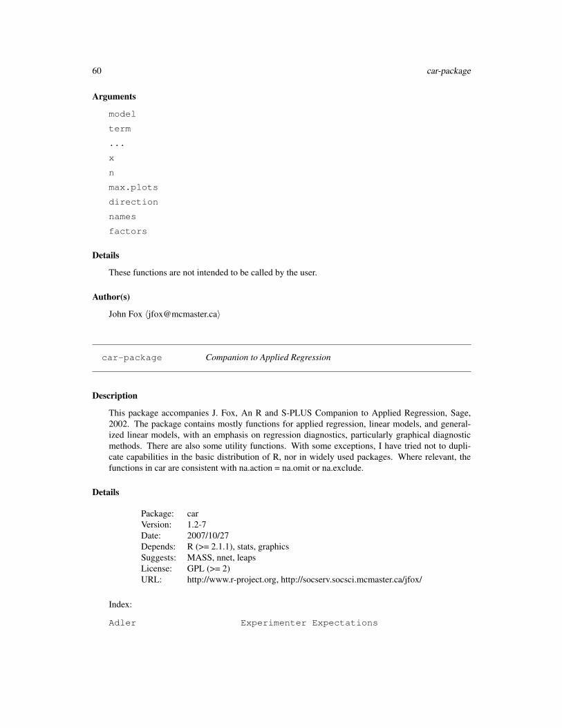
60 car-package

Arguments

model

term

...

x

n

max.plots

direction

names

factors

Details

These functions are not intended to be called by the user.

Author(s)


car-package Companion to Applied Regression

Description

This package accompanies J. Fox, An R and S-PLUS Companion to Applied Regression, Sage,

2002. The package contains mostly functions for applied regression, linear models, and general-

ized linear models, with an emphasis on regression diagnostics, particularly graphical diagnostic

methods. There are also some utility functions. With some exceptions, I have tried not to dupli-

cate capabilities in the basic distribution of R, nor in widely used packages. Where relevant, the

functions in car are consistent with na.action = na.omit or na.exclude.

Details

Package: car

Version: 1.2-7

Date: 2007/10/27

Depends: R (>= 2.1.1), stats, graphics

Suggests: MASS, nnet, leaps

License: GPL (>= 2)

URL: http://www.r-project.org, http://socserv.socsci.mcmaster.ca/jfox/

Index:

Adler Experimenter Expectations

car-package 61

Angell Moral Integration of American Cities

Anova Anova Tables for Various Statistical Models

Anscombe U. S. State Public-School Expenditures

Ask Change Argument to a Function Interactively

Baumann Methods of Teaching Reading Comprehension

Bfox Canadian Women's Labour-Force Participation

Blackmoor Exercise Histories of Eating-Disordered and

Control Subjects

Burt Fraudulent Data on IQs of Twins Raised Apart

Can.pop Canadian Population Data

Chile Voting Intentions in the 1988 Chilean

Plebiscite

Chirot The 1907 Romanian Peasant Rebellion

Contrasts Functions to Construct Contrasts

Cowles Cowles and Davis's Data on Volunteering

Davis Self-Reports of Height and Weight

DavisThin Davis's Data on Drive for Thinness

Duncan Duncan's Occupational Prestige Data

Ericksen The 1980 U.S. Census Undercount

Florida Florida County Voting

Freedman Crowding and Crime in U. S. Metropolitan Areas

Friendly Format Effects on Recall

Ginzberg Data on Depression

Greene Refugee Appeals

Guyer Anonymity and Cooperation

Hartnagel Canadian Crime-Rates Time Series

Leinhardt Data on Infant-Mortality

Mandel Contrived Collinear Data

Migration Canadian Interprovincial Migration Data

Moore Status, Authoritarianism, and Conformity

Mroz U.S. Women's Labor-Force Participation

OBrienKaiser O'Brien and Kaiser's Repeated-Measures Data

Ornstein Interlocking Directorates Among Major Canadian

Firms

Prestige Prestige of Canadian Occupations

Quartet Four Regression Datasets

Robey Fertility and Contraception

SLID Survey of Labour and Income Dynamics

Sahlins Agricultural Production in Mazulu Village

Soils Soil Compositions of Physical and Chemical Characteristics

States Education and Related Statistics for the U.S.

States

UN GDP and Infant Mortality

US.pop Population of the United States

Var Variance-Covariance Matrices (deprecated)

Vocab Vocabulary and Education

Womenlf Canadian Women's Labour-Force Participation

av.plots Added-Variable Plots

62 car-package

box.cox Box-Cox Family of Transformations

box.cox.powers Multivariate Unconditional Box-Cox

Transformations

box.cox.var Constructed Variable for Box-Cox Transformation

box.tidwell Box-Tidwell Transformations

ceres.plots Ceres Plots

cookd Cook's Distances for Linear and Generalized

Linear Models

cr.plots Component+Residual (Partial Residual) Plots

durbin.watson Durbin-Watson Test for Autocorrelated Errors

ellipse Ellipses, Data Ellipses, and Confidence

Ellipses

hccm Heteroscedasticity-Corrected Covariance

Matrices

influencePlot Regression Influence Plot

inv Internal car functions

levene.test Levene's Test

leverage.plots Regression Leverage Plots

linear.hypothesis Test Linear Hypothesis

logit Logit Transformation

n.bins Number of Bins for Histogram

ncv.test Score Test for Non-Constant Error Variance

outlier.test Bonferroni Outlier Test

panel.car Panel Function Coplots

power.axis Axes for Transformed Variables

qq.plot Quantile-Comparison Plots

recode Recode a Variable

reg.line Plot Regression Line

scatterplot Scatterplots with Boxplots

scatterplot.matrix Scatterplot Matrices

some Sample a Few Elements of an Object

spread.level.plot Spread-Level Plots

subsets Plot Output from regsubsets Function in leaps

package

symbox Boxplots for transformations to symmetry

vif Variance Inflation Factors

which.names Position of Row Names

Author(s)

John Fox <[email protected]>. I am grateful to Douglas Bates, David Firth, Michael Friendly,

Gregor Gorjanc, Spencer Graves, Richard Heiberger, Georges Monette, Henric Nilsson, Brian Rip-

ley, Sanford Weisberg, and Achim Zeleis for various suggestions and contributions.

Maintainer: John Fox <[email protected]>

ceres.plots 63

ceres.plots Ceres Plots

Description

These functions calculate Ceres plots for linear and generalized linear model.

Usage

ceres.plots(model, variable, ask=missing(variable), one.page=!ask,

span=0.5, ...)

ceres.plot(model, ...)


ceres.plot(model, variable, line=TRUE, smooth=TRUE, span=0.5, iter,

las=par('las'), col=palette()[2], pch=1, lwd=2, main="Ceres Plot", ...)


ceres.plot(model, ...)

Arguments



usually is omitted for ceres.plots.

ask if TRUE, a menu is provided in the R Console for the user to select the variable(s)

to plot, and to modify the span for the smoother used to draw a nonparametric-

regression line on the plot.


span span for lowess smoother.

iter number of robustness iterations for nonparametric-regression smooth; defaults

to 3 for a linear model and to 0 for a non-Gaussian glm.

line TRUE to plot least-squares line.

smooth TRUE to plot nonparametric-regression (lowess) line.


par).






... pass arguments down.

64 Cook’s Distances

Details

Ceres plots are a generalization of component+residual (partial residual) plots that are less prone to

leakage of nonlinearity among the predictors.

The function intended for direct use is ceres.plots. By default, this function is used interac-

tively through a text menu.

The model cannot contain interactions, but can contain factors. Factors may be present in the model,

but Ceres plots cannot be drawn for them.

Value


Author(s)


References


Wiley.


See Also

cr.plots, av.plots

Examples

## Not run:

ceres.plots(lm(prestige~income+education+type, data=Prestige))

## End(Not run)

Cook’s Distances Cook’s Distances for Linear and Generalized Linear Models

Description

This function now simply calls cooks.distance in the base package.

Usage

cookd(model, ...)

Arguments

model lm or glm model object.

... other arguments to be passed to cooks.distance.

cr.plots 65

Details

Cook’s distances for generalized linear models are approximations, as described in Williams (1987)

(except that the Cook’s distances are scaled as F rather than as chi-square values).

This function is retained primarily for consistency with An R and S-PLUS Companion to Applied

Regression. Other deletion diagnostics formerly in the car package have been rewritten and

moved to the base package; these include influence, rstudent, hatvalues, dfbeta,

and dfbetas.

Value

cookd returns a vector with one entry for each observation.

Author(s)


References

Cook, R. D. and Weisberg, S. (1984) Residuals and Influence in Regression. Wiley.


Williams, D. A. (1987) Generalized linear model diagnostics using the deviance and single case

deletions. Applied Statistics 36, 181–191.

See Also

cooks.distance, influence

Examples

plot(cookd(lm(prestige ~ income + education, data=Duncan)))

cr.plots Component+Residual (Partial Residual) Plots

Description

These functions construct component+residual plots (also called partial-residual plots) for linear

and generalized linear models.

66 cr.plots

Usage

cr.plots(model, variable, ask=missing(variable), one.page=!ask,

span=0.5, ...)

crp(...)

cr.plot(model, ...)


cr.plot(model, variable, order=1, line=TRUE, smooth=TRUE, iter,

span=0.5, las=par('las'), col=palette()[2], pch=1, lwd=2,

main="Component+Residual Plot", ...)


cr.plot(model, ...)

Arguments



usually is omitted for crp or cr.plots.

ask if TRUE, a menu is provided in the R Console for the user to select the variable(s)

to plot, and to modify the span for the smoother used to draw a nonparametric-

regression line on the plot.


order order of polynomial regression performed for predictor to be plotted.

line TRUE to plot least-squares line.

smooth TRUE to plot nonparametric-regression (lowess) line.

iter number of robustness iterations for nonparametric-regression smooth; defaults

to 3 for a linear model and to 0 for a non-Gaussian glm.



par).






... pass arguments down.

Details

The function intended for direct use is cr.plots (for which crp is an abbreviation). By default,

these functions are used interactively through a text menu.

The model cannot contain interactions, but can contain factors. Parallel boxplots of the partial

residuals are drawn for the levels of a factor.

durbin.watson 67

Value


Author(s)


References


Wiley.


See Also

ceres.plots, av.plots

Examples

cr.plots(lm(prestige~income+education, data=Prestige),

variable="income")

## Not run:

cr.plots(glm(partic != "not.work" ~ hincome + children,

data=Womenlf, family=binomial))

## End(Not run)

durbin.watson Durbin-Watson Test for Autocorrelated Errors

Description

Computes residual autocorrelations and generalized Durbin-Watson statistics and their bootstrapped

p-values.

Usage

durbin.watson(model, ...)


durbin.watson(model, max.lag=1, simulate=TRUE, reps=1000,

method=c("resample","normal"),

alternative=c("two.sided", "positive", "negative"), ...)


durbin.watson(model, max.lag=1, ...)

## S3 method for class 'durbin.watson':

print(x, ...)

68 hccm

Arguments

model a linear-model object, or a vector of residuals from a linear model.

max.lag maximum lag to which to compute residual autocorrelations and Durbin-Watson

statistics.

simulate if TRUE p-values will be estimated by bootstrapping.

reps number of bootstrap replications.

method bootstrap method: "resample" to resample from the observed residuals; "normal"

to sample normally distributed errors with 0 mean and standard deviation equal

to the standard error of the regression.

alternative sign of autocorrelation in alternative hypothesis; specify only if max.lag =

1; if max.lag > 1, then alternative is taken to be "two.sided".

... arguments to be passed down to method functions.

x durbin.watson object.

Value

Returns an object of type "durbin.watson".

Author(s)


References


Examples

durbin.watson(lm(fconvict ~ tfr + partic + degrees + mconvict, data=Hartnagel))

## lag Autocorrelation D-W Statistic p-value

## 1 0.688345 0.6168636 0

## Alternative hypothesis: rho != 0

hccm Heteroscedasticity-Corrected Covariance Matrices

Description

Calculates heteroscedasticity-corrected covariance matrices for unweighted linear models. These

are also called “White-corrected” covariance matrices.

hccm 69

Usage

hccm(model, ...)


hccm(model, type=c("hc3", "hc0", "hc1", "hc2", "hc4"), ...)


hccm(model, ...)

Arguments

model an unweighted linear model, produced by lm.

type one of "hc0", "hc1", "hc2", "hc3", or "hc4"; the first of these gives

the classic White correction. The "hc1", "hc2", and "hc3" corrections are

described in Long and Ervin (2000); "hc4" is described in Cribari-Neto (2004).

... arguments to pass to hccm.lm.

Details

The classical White-corrected coefficient covariance matrix ("hc0") is

V (b) = (X ′X)−1X ′diag(e2i )X(X ′X)−1

where e2i are the squared residuals, and X is the model matrix. The other methods represent adjust-

ments to this formula.

The function hccm.default simply catches non-lm objects.

Value

The heteroscedasticity-corrected covariance matrix for the model.

Author(s)


References

Cribari-Neto, F. (2004) Asymptotic inference under heteroskedasticity of unknown form. Compu-

tational Statistics and Data Analysis 45, 215–233.

Long, J. S. and Ervin, L. H. (2000) Using heteroscedasity consistent standard errors in the linear

regression model. The American Statistician 54, 217–224.

White, H. (1980) A heterskedastic consistent covariance matrix estimator and a direct test of het-

eroskedasticity. Econometrica 48, 817–838.

See Also

ncv.test, spread.level.plot

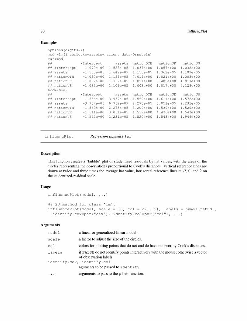
70 influencPlot

Examples

options(digits=4)

mod<-lm(interlocks~assets+nation, data=Ornstein)

Var(mod)

## (Intercept) assets nationOTH nationUK nationUS

## (Intercept) 1.079e+00 -1.588e-05 -1.037e+00 -1.057e+00 -1.032e+00

## assets -1.588e-05 1.642e-09 1.155e-05 1.362e-05 1.109e-05

## nationOTH -1.037e+00 1.155e-05 7.019e+00 1.021e+00 1.003e+00

## nationUK -1.057e+00 1.362e-05 1.021e+00 7.405e+00 1.017e+00

## nationUS -1.032e+00 1.109e-05 1.003e+00 1.017e+00 2.128e+00

hccm(mod)

## (Intercept) assets nationOTH nationUK nationUS

## (Intercept) 1.664e+00 -3.957e-05 -1.569e+00 -1.611e+00 -1.572e+00

## assets -3.957e-05 6.752e-09 2.275e-05 3.051e-05 2.231e-05

## nationOTH -1.569e+00 2.275e-05 8.209e+00 1.539e+00 1.520e+00

## nationUK -1.611e+00 3.051e-05 1.539e+00 4.476e+00 1.543e+00

## nationUS -1.572e+00 2.231e-05 1.520e+00 1.543e+00 1.946e+00

influencPlot Regression Influence Plot

Description

This function creates a "bubble" plot of studentized residuals by hat values, with the areas of the

circles representing the observations proportional to Cook’s distances. Vertical reference lines are

drawn at twice and three times the average hat value, horizontal reference lines at -2, 0, and 2 on

the studentized-residual scale.

Usage

influencePlot(model, ...)


influencePlot(model, scale = 10, col = c(1, 2), labels = names(rstud),

identify.cex=par("cex"), identify.col=par("col"), ...)

Arguments

model a linear or generalized-linear model.

scale a factor to adjust the size of the circles.

col colors for plotting points that do not and do have noteworthy Cook’s distances.

labels if FALSE do not identify points interactively with the mouse; otherwise a vector

of observation labels.identify.cex, identify.col

aguments to be passed to identify.

... arguments to pass to the plot function.

levene.test 71

Value

Returns the indices of identified points.

Note

This function used to be named influence.plot; the name was changed to avoid confusion

with the influence generic function.

Author(s)


References

J. Fox (2002) An R and S-PLUS Companion to Applied Regression. Sage.

See Also

cookd, rstudent, hatvalues

Examples

## Not run:

influencePlot(lm(prestige ~ income + education, data=Duncan))

## End(Not run)

levene.test Levene’s Test

Description

Computes Levene’s test for homeogeneity of variance across groups.

Usage

levene.test(y, group)

Arguments


group factor defining groups.

Value

returns an object meant to be printed showing the results of the test.

72 leverage.plots

Note

adapted from a response posted by Brian Ripley to the R-help email list.

Author(s)


References


Examples

attach(Moore)

levene.test(conformity, fcategory)

## Levene's Test for Homogeneity of Variance

## Df F value Pr(>F)

## group 2 0.046 0.9551

## 42

levene.test(conformity, interaction(fcategory, partner.status))

## Levene's Test for Homogeneity of Variance

## Df F value Pr(>F)

## group 5 1.4694 0.2219

## 39

leverage.plots Regression Leverage Plots

Description

These functions display a generalization, due to Sall (1990), of added-variable plots to multiple-df

terms in a linear model. When a term has just 1 df, the leverage plot is a rescaled version of the

usual added-variable (partial-regression) plot.

Usage

leverage.plots(model, term.name, ask=missing(term.name), ...)

leverage.plot(model, ...)


leverage.plot(model, term.name,


identify.points=TRUE, las=par('las'), col=palette()[2], pch=1, lwd=2,

main="Leverage Plot", ...)


leverage.plot(model, ...)

leverage.plots 73

Arguments

model model object produced by lm

term.name name of term in the model to be plotted; this argument is usually omitted for

leverage.plots.

ask if TRUE, a menu is provided in the R Console for the user to select the term(s)

to plot.

labels observation names.

identify.points

if TRUE, then identify points interactively.


par).






... arguments passed down to method functions.

Details

The function intended for direct use is leverage.plots. By default, this function is used inter-

actively through a text menu.

The model can contain factors and interactions. A leverage plot can be drawn for each term in the

model, including the constant.

leverage.plot.glm is a dummy function, which generates an error message.

Value


Author(s)


References


Sall, J. (1990) Leverage plots for general linear hypotheses. American Statistician 44, 308–315.

See Also

av.plots

74 linear.hypothesis

Examples

## Not run:

leverage.plots(lm(prestige~(income+education)*type, data=Duncan))

## End(Not run)

linear.hypothesis Test Linear Hypothesis

Description

Generic function for testing a linear hypothesis, and methods for linear models, generalized linear

models, multivariate linear models, and other models that have methods for coef and vcov.

Usage

linear.hypothesis(model, ...)

lht(model, ...)


linear.hypothesis(model, hypothesis.matrix, rhs=NULL,

test=c("Chisq", "F"), vcov.=NULL, verbose=FALSE, ...)


linear.hypothesis(model, hypothesis.matrix, rhs=NULL,

test=c("F", "Chisq"), vcov.=NULL, white.adjust=FALSE, ...)


linear.hypothesis(model, ...)


linear.hypothesis(model, hypothesis.matrix, rhs=NULL, SSPE, V,

test, idata, icontrasts=c("contr.sum", "contr.poly"), idesign, iterms,

P=NULL, title="", verbose=FALSE, ...)

## S3 method for class 'linear.hypothesis.mlm':

print(x, SSP=TRUE, SSPE=SSP,

digits=unlist(options("digits")), ...)

Arguments

model fitted model object. The default method works for models for which the esti-

mated parameters can be retrieved by coef and the corresponding estimated

covariance matrix by vcov. See the Details for more information.

linear.hypothesis 75

hypothesis.matrix

matrix (or vector) giving linear combinations of coefficients by rows, or a char-

acter vector giving the hypothesis in symbolic form (see Details).

rhs right-hand-side vector for hypothesis, with as many entries as rows in the hy-

pothesis matrix; can be omitted, in which case it defaults to a vector of zeroes.

For a multivariate linear model, rhs is a matrix, defaulting to 0.

idata an optional data frame giving a factor or factors defining the intra-subject model

for multivariate repeated-measures data. See Details for an explanation of the

intra-subject design and for further explanation of the other arguments relating

to intra-subject factors.

icontrasts names of contrast-generating functions to be applied by default to factors and

ordered factors, respectively, in the within-subject “data”; the contrasts must

produce an intra-subject model matrix in which different terms are orthogonal.

idesign a one-sided model formula using the “data” in idata and specifying the intra-

subject design.

iterms the quoted name of a term, or a vector of quoted names of terms, in the intra-

subject design to be tested.

P transformation matrix to be applied to the repeated measures in multivariate

repeated-measures data; if NULL and no intra-subject model is specified, no

response-transformation is applied; if an intra-subject model is specified via the

idata, idesign, and (optionally) icontrasts arguments, then P is gen-

erated automatically from the iterms argument.

SSPE in linear.hypothesis method for mlm objects: optional error sum-of-

squares-and-products matrix; if missing, it is computed from the model. In

print method for linear.hypothesis.mlm objects: if TRUE, print the

sum-of-squares and cross-products matrix for error.

test character string, "F" or "Chisq", specifying whether to compute the finite-

sample F statistic (with approximate F distribution) or the large-sample Chi-

squared statistic (with asymptotic Chi-squared distribution). For a multivari-

ate linear model, the multivariate test statistic to report — one of "Pillai",

"Wilks", "Hotelling-Lawley", or "Roy", with "Pillai" as the de-

fault.

title an optional character string to label the output.

V inverse of sum of squares and products of the model matrix; if missing it is

computed from the model.

vcov. a function for estimating the covariance matrix of the regression coefficients,

e.g., hccm, or an estimated covariance matrix for model. See also white.adjust.

white.adjust logical or character. Convenience interface to hccm (instead of using the ar-

gument vcov). Can be set either to a character specifying the type argument

of hccm or TRUE, in which case "hc3" is used implicitly. For backwards

compatibility.

verbose If TRUE, the hypothesis matrix and right-hand-side vector (or matrix) are printed

to standard output; if FALSE (the default), the hypothesis is only printed in

symbolic form.

x an object produced by linear.hypothesis.mlm.

76 linear.hypothesis

SSP if TRUE (the default), print the sum-of-squares and cross-products matrix for the

hypothesis and the response-transformation matrix.

digits minimum number of signficiant digits to print.

... aruments to pass down.

Details

Computes either a finite sample F statistic or asymptotic Chi-squared statistic for carrying out a

Wald-test-based comparison between a model and a linearly restricted model. The default method

will work with any model object for which the coefficient vector can be retrieved by coef and the

coefficient-covariance matrix by vcov (otherwise the argument vcov. has to be set explicitely).

For computing the F statistic (but not the Chi-squared statistic) a df.residual method needs to

be available. If a formula method exists, it is used for pretty printing.

The method for "lm" objects calls the default method, but it changes the default test to "F", sup-

ports the convenience argument white.adjust (for backwards compatibility), and enhances the

output by residual sums of squares. For "glm" objects just the default method is called (bypassing

the "lm" method).

The function lht also dispatches to linear.hypothesis.

The hypothesis matrix can be supplied as a numeric matrix (or vector), the rows of which specify

linear combinations of the model coefficients, which are tested equal to the corresponding entries

in the righ-hand-side vector, which defaults to a vector of zeroes.

Alternatively, the hypothesis can be specified symbolically as a character vector with one or more

elements, each of which gives either a linear combination of coefficients, or a linear equation in the

coefficients (i.e., with both a left and right side separated by an equals sign). Components of a linear

expression or linear equation can consist of numeric constants, or numeric constants multiplying

coefficient names (in which case the number precedes the coefficient, and may be separated from

it by spaces or an asterisk); constants of 1 or -1 may be omitted. Spaces are always optional.

Components are separated by plus or minus signs. See the examples below.

A linear hypothesis for a multivariate linear model (i.e., an object of class "mlm") can optionally

include an intra-subject transformation matrix for a repeated-measures design. If the intra-subject

transformation is absent (the default), the multivariate test concerns all of the corresponding coef-

ficients for the response variables. There are two ways to specify the transformation matrix for the

repeated meaures:

1. The transformation matrix can be specified directly via the P argument.

2. A data frame can be provided defining the repeated-measures factor or factors via idata,

with default contrasts given by the icontrasts argument. An intra-subject model-matrix

is generated from the one-sided formula specified by the idesign argument; columns of the

model matrix corresponding to different terms in the intra-subject model must be orthogonal

(as is insured by the default contrasts). Note that the contrasts given in icontrasts can

be overridden by assigning specific contrasts to the factors in idata. The repeated-measures

transformation matrix consists of the columns of the intra-subject model matrix corresponding

to the term or terms in iterms. In most instances, this will be the simpler approach, and

indeed, most tests of interests can be generated automatically via the Anova function.

linear.hypothesis 77

Value

For a univariate model, an object of class "anova" which contains the residual degrees of freedom

in the model, the difference in degrees of freedom, Wald statistic (either "F" or "Chisq") and

corresponding p value.

For a multivariate linear model, an object of class "linear.hypothesis.mlm", which con-

tains sums-of-squares-and-product matrices for the hypothesis and for error, degrees of freedom for

the hypothesis and error, and some other information.

The returned object normally would be printed.

Author(s)

Achim Zeileis and John Fox 〈[email protected]〉

References


Hand, D. J., and Taylor, C. C. (1987) Multivariate Analysis of Variance and Repeated Measures: A

Practical Approach for Behavioural Scientists. Chapman and Hall.



See Also

anova, Anova, waldtest, hccm, vcovHC, vcovHAC, coef, vcov

Examples

mod.davis <- lm(weight ~ repwt, data=Davis)

## the following are equivalent:

linear.hypothesis(mod.davis, diag(2), c(0,1))

linear.hypothesis(mod.davis, c("(Intercept) = 0", "repwt = 1"))

linear.hypothesis(mod.davis, c("(Intercept)", "repwt"), c(0,1))

linear.hypothesis(mod.davis, c("(Intercept)", "repwt = 1"))

## use asymptotic Chi-squared statistic

linear.hypothesis(mod.davis, c("(Intercept) = 0", "repwt = 1"), test = "Chisq")

## the following are equivalent:

## use HC3 standard errors via white.adjust option

linear.hypothesis(mod.davis, c("(Intercept) = 0", "repwt = 1"),

white.adjust = TRUE)

## covariance matrix *function*linear.hypothesis(mod.davis, c("(Intercept) = 0", "repwt = 1"), vcov = hccm)

## covariance matrix *estimate*linear.hypothesis(mod.davis, c("(Intercept) = 0", "repwt = 1"),

vcov = hccm(mod.davis, type = "hc3"))

mod.duncan <- lm(prestige ~ income + education, data=Duncan)

78 logit

## the following are all equivalent:

linear.hypothesis(mod.duncan, "1*income - 1*education = 0")

linear.hypothesis(mod.duncan, "income = education")

linear.hypothesis(mod.duncan, "income - education")

linear.hypothesis(mod.duncan, "1income - 1education = 0")

linear.hypothesis(mod.duncan, "0 = 1*income - 1*education")

linear.hypothesis(mod.duncan, "income-education=0")

linear.hypothesis(mod.duncan, "1*income - 1*education + 1 = 1")

linear.hypothesis(mod.duncan, "2income = 2*education")

mod.duncan.2 <- lm(prestige ~ type*(income + education), data=Duncan)

coefs <- names(coef(mod.duncan.2))

## test against the null model (i.e., only the intercept is not set to 0)

linear.hypothesis(mod.duncan.2, coefs[-1])

## test all interaction coefficients equal to 0

linear.hypothesis(mod.duncan.2, coefs[grep(":", coefs)], verbose=TRUE)

## a multivariate linear model for repeated-measures data

## see ?OBrienKaiser for a description of the data set used in this example.

mod.ok <- lm(cbind(pre.1, pre.2, pre.3, pre.4, pre.5,

post.1, post.2, post.3, post.4, post.5,

fup.1, fup.2, fup.3, fup.4, fup.5) ~ treatment*gender,

data=OBrienKaiser)

coef(mod.ok)

## specify the model for the repeated measures:

phase <- factor(rep(c("pretest", "posttest", "followup"), c(5, 5, 5)),

levels=c("pretest", "posttest", "followup"))

hour <- ordered(rep(1:5, 3))

idata <- data.frame(phase, hour)

idata

## test the four-way interaction among the between-subject factors

## treatment and gender, and the intra-subject factors

## phase and hour

linear.hypothesis(mod.ok, c("treatment1:gender1", "treatment2:gender1"),

title="treatment:gender:phase:hour", idata=idata, idesign=~phase*hour,

iterms="phase:hour")

logit Logit Transformation

Description

Compute the logit transformation of proportions or percentages.

logit 79

Usage

logit(p, percents=max(p, na.rm = TRUE) > 1, adjust)

Arguments

p numeric vector or array of proportions or percentages.

percents TRUE for percentages.

adjust adjustment factor to avoid proportions of 0 or 1; defaults to 0 if there are no

such proportions in the data, and to .025 if there are.

Details

Computes the logit transformation logit = log[p/(1 − p)] for the proportion p.

If p = 0 or 1, then the logit is undefined. logit can remap the proportions to the interval

(adjust, 1 - adjust) prior to the transformation. If it adjusts the data automatically, logit

will print a warning message.

Value

a numeric vector or array of the same shape and size as p.

Author(s)


See Also

prob.axis

Examples

options(digits=4)

logit(.1*0:10)

## [1] -3.6636 -1.9924 -1.2950 -0.8001 -0.3847 0.0000 0.3847

## [8] 0.8001 1.2950 1.9924 3.6636

## Warning message:

## Proportions remapped to (0.025,0.975) in: logit(0.1 * 0:10)

logit(.1*0:10, adjust=0)

## [1] -Inf -2.1972 -1.3863 -0.8473 -0.4055 0.0000 0.4055

## [8] 0.8473 1.3863 2.1972 Inf

80 n.bins

n.bins Number of Bins for Histogram

Description

Several rules for calculating the number of bins to use for a histogram.

Usage

n.bins(x, rule=c("freedman.diaconis", "sturges", "scott", "simple"))

Arguments

x numeric vector, variable for histogram

rule see below.

Details

"freedman.diaconis": n1/3range/2 × IQR.

"sturges": ceiling(log2 n + 1).

"scott": ceiling(n1/3range/3.5s).

"simple": floor(10 log10 n) for n > 100, or floor(2√

n) for n ≤ 100.

where n is the number of observations, range is the range of x, IQR is the inter-quartile range of

x, and s is the standard deviation of x.

Value

the number of bins.

Author(s)


References

Freedman, D. and Diaconis, P. (1981) On the histogram as a density estimator. Zeitschrift fur

Wahrscheinlichkeitstheorie und verwandte Gebiete 57, 453–476.

Scott, D. W. (1979) On optimal and data based-histograms. Biometrika 66, 605–610.

Venables, W. N. and Ripley, B. D. (1999) Modern Applied Statistics with S-PLUS, Third Edition,

Springer.

See Also

hist

ncv.test 81

Examples

attach(UN)

n.bins(gdp)

## [1] 19

n.bins(gdp, "sturges")

## [1] 9

n.bins(gdp, "scott")

## [1] 8

n.bins(gdp, "simple")

## [1] 22

hist(gdp)

hist(gdp, nclass=n.bins(gdp))

ncv.test Score Test for Non-Constant Error Variance

Description

Computes a score test of the hypothesis of constant error variance against the alternative that the

error variance changes with the level of the response (fitted values), or with a linear combination of

predictors.

Usage

ncv.test(model, ...)


ncv.test(model, var.formula, data=NULL, subset, na.action, ...)


ncv.test(model, ...)

Arguments

model a weighted or unweighted linear model, produced by lm.

var.formula a one-sided formula for the error variance; if omitted, the error variance depends

on the fitted values.

data an optional data frame containing the variables in the model. By default the

variables are taken from the environment from which ncv.test is called.




... arguments passed down to methods functions.

82 outlier.test

Details

This test is often called the Breusch-Pagan test; it was independently suggested by Cook and Weis-

berg (1983).

ncv.test.glm is a dummy function to generate an error when a glm model is used.

Value

The function returns a chisq.test object, which is usually just printed.

Author(s)


References

Breusch, T. S. and Pagan, A. R. (1979) A simple test for heteroscedasticity and random coefficient

variation. Econometrica 47, 1287–1294.

Cook, R. D. and Weisberg, S. (1983) Diagnostics for heteroscedasticity in regression. Biometrika

70, 1–10.


See Also

hccm, spread.level.plot

Examples

ncv.test(lm(interlocks~assets+sector+nation, data=Ornstein))

## Non-constant Variance Score Test

## Variance formula: ~ fitted.values

## Chisquare = 46.98537 Df = 1 p = 7.151835e-12

ncv.test(lm(interlocks~assets+sector+nation, data=Ornstein),

~ assets+sector+nation, data=Ornstein)

## Non-constant Variance Score Test

## Variance formula: ~ assets + sector + nation

## Chisquare = 74.73535 Df = 13 p = 1.066320e-10

outlier.test Bonferroni Outlier Test

Description

Reports the Bonferroni p-value for the most extreme observation. At present, there are methods for

studentized residuals in linear and generalized linear models.

outlier.test 83

Usage

outlier.test(model, ...)


outlier.test(model, labels=names(rstud), ...)


outlier.test(model, labels=names(rstud), ...)

## S3 method for class 'outlier.test':

print(x, digits=options("digits")[[1]], ...)

Arguments

model a suitable model object.

labels an optional vector of observation names.

... arguments passed down to methods functions.

x outlier.test object.

digits number of digits for printed output.

Details

For a linear model, the p-value reported is for the largest absolute studentized residual, using the tdistribution with degrees of freedom one less than the residual df for the model. For a generalized

linear model, the largest absolute studentized residual is also used, but with the standard-normal

distribution. The Bonferroni adjustment multiplies the usual two-sided p-value by the number of

observations.

Value

an object of class outlier.test, which is normally just printed.

Author(s)


References

Cook, R. D. and Weisberg, S. (1984) Residuals and Influence in Regression. Wiley.


Williams, D. A. (1987) Generalized linear model diagnostics using the deviance and single case

deletions. Applied Statistics 36, 181–191.

84 panel.car

Examples

outlier.test(lm(prestige~income+education, data=Duncan))

## max|rstudent| df unadjusted p Bonferroni p

## 3.134519 41 0.003177202 0.1429741

##

## Observation: minister

panel.car Panel Function Coplots

Description

a panel function for use with coplot that plots points, a lowess line, and a regression line.

Usage

panel.car(x, y, col, pch, cex=1, span=0.5, lwd=2,

regression.line=lm, lowess.line=TRUE, ...)

Arguments

x vector giving horizontal coordinates.

y vector giving vertical coordinates.

col point color.

pch plotting character for points.

cex character expansion factor for points.


lwd line width, default is 2.

regression.line

function to compute coefficients of regression line, or FALSE for no line.

lowess.line if TRUE plot lowess smooth.

... other arguments to pass to functions lines and reg.line.

Value

NULL. This function is used for its side effect: producing a panel in a coplot.

Author(s)


See Also

coplot, reg.line

qq.plot 85

Examples

coplot(prestige~income|education, panel=panel.car,

col="red", data=Prestige)

qq.plot Quantile-Comparison Plots

Description

Plots empirical quantiles of a variable, or of studentized residuals from a linear model, against

theoretical quantiles of a comparison distribution.

Usage

qq.plot(x, ...)

qqp(...)


qq.plot(x, distribution="norm", ylab=deparse(substitute(x)),

xlab=paste(distribution, "quantiles"), main=NULL, las=par("las"),

envelope=.95, labels=FALSE, col=palette()[2], lwd=2, pch=1, cex=1,

line=c("quartiles", "robust", "none"), ...)


qq.plot(x, main=NULL, xlab=paste(distribution, "Quantiles"),

ylab=paste("Studentized Residuals(", deparse(substitute(x)), ")",

sep = ""),

distribution=c("t", "norm"), line=c("quartiles", "robust", "none"),

las=par('las'), simulate=FALSE, envelope=0.95, labels=names(rstudent),

reps=100, col=palette()[2], lwd=2, pch=1, cex=1, ...)

Arguments

x vector of numeric values or lm object.

distribution root name of comparison distribution – e.g., norm for the normal distribution;

t for the t-distribution.

ylab label for vertical (empirical quantiles) axis.

xlab label for horizontal (comparison quantiles) axis.

main label for plot.

envelope confidence level for point-wise confidence envelope, or FALSE for no envelope.

labels vector of point labels for interactive point identification, or FALSE for no labels.


par).

86 qq.plot




cex factor for expanding the size of plotted symbols; the default is 1.

lwd line width; default is 2 (see par). Confidence envelopes are drawn at half this

line width.

line "quartiles" to pass a line through the quartile-pairs, or "robust" for a

robust-regression line; the latter uses the rlm function in the MASS package.

Specifying line = "none" suppresses the line.

simulate if TRUE calculate confidence envelope by parametric bootstrap; for lm object

only. The method is due to Atkinson (1985).

reps integer; number of bootstrap replications for confidence envelope.

... arguments such as df to be passed to the appropriate quantile function.

Details

Draws theoretical quantile-comparison plots for variables and for studentized residuals from a linear

model. A comparison line is drawn on the plot either through the quartiles of the two distributions,

or by robust regression.

Any distribution for which quantile and density functions exist in R (with prefixes q and d, respec-

tively) may be used. Studentized residuals are plotted against the appropriate t-distribution.

The function qqp is an abbreviation for qq.plot.

Value

NULL. These functions are used only for their side effect (to make a graph).

Author(s)


References


Atkinson, A. C. (1985) Plots, Transformations, and Regression. Oxford.

See Also

qqplot, qqnorm, qqline

Examples

x<-rchisq(100, df=2)

qq.plot(x)

qq.plot(x, dist="chisq", df=2)

qq.plot(lm(interlocks~assets+sector+nation, data=Ornstein), sim=TRUE)

recode 87

recode Recode a Variable

Description

Recodes a numeric vector, character vector, or factor according to simple recode specifications.

Usage

recode(var, recodes, as.factor.result, levels)

Arguments

var numeric vector, character vector, or factor.

recodes character string of recode specifications: see below.

as.factor.result

return a factor; default is TRUE if var is a factor, FALSE otherwise.

levels an optional argument specifying the order of the levels in the returned factor; the

default is to use the sort order of the level names.

Details

Recode specifications appear in a character string, separated by semicolons (see the examples be-

low), of the form input=output. If an input value satisfies more than one specification, then the

first (from left to right) applies. If no specification is satisfied, then the input value is carried over

to the result. NA is allowed on input and output. Several recode specifications are supported:

single value For example, 0=NA.

vector of values For example, c(7,8,9)=’high’.

range of values For example, 7:9=’C’. The special values lo and hi may appear in a range.

For example, lo:10=1.

else everything that does not fit a previous specification. For example, else=NA. Note that

else matches all otherwise unspecified values on input, including NA.

If all of the output values are numeric, and if as.factor.result is FALSE, then a numeric

result is returned.

Value

a recoded vector of the same length as var; if var is a factor, then so is the result.

Author(s)


88 reg.line

See Also

cut, factor

Examples

x<-rep(1:3,3)

x

## [1] 1 2 3 1 2 3 1 2 3

recode(x, "c(1,2)='A'; else='B'")

## [1] "A" "A" "B" "A" "A" "B" "A" "A" "B"

recode(x, "1:2='A'; 3='B'")

## [1] "A" "A" "B" "A" "A" "B" "A" "A" "B"

reg.line Plot Regression Line

Description

Plots a regression line on a scatterplot; the line is plotted between the minimum and maximum

x-values.

Usage

reg.line(mod, col=palette()[2], lwd=2, lty=1,...)

Arguments

mod a model, such as produced by lm, that responds to the coefficients func-

tion by returning a 2-element vector, whose elements are interpreted respectively

as the intercept and slope of a regresison line.




lty line type; default is 1, a solid line (see par).

... optional arguments to be passed to the lines plotting function.

Details

In contrast to abline, this function plots only over the range of the observed x-values. The x-

values are extracted from mod as the second column of the model matrix.

Value

NULL. This function is used for its side effect: adding a line to the plot.

scatterplot 89

Author(s)


See Also

abline, lines

Examples

plot(repwt ~ weight, pch=c(1,2)[sex], data=Davis)

reg.line(lm(repwt~weight, subset=sex=="M", data=Davis))

reg.line(lm(repwt~weight, subset=sex=="F", data=Davis), lty=2)

scatterplot Scatterplots with Boxplots

Description

Makes fancy scatterplots, with boxplots in the margins, a lowess smooth, and a regression line; sp

is an abbreviation for scatterplot.

Usage

scatterplot(x, ...)


scatterplot(formula, data, xlab, ylab, legend.title, subset, labels=FALSE, ...)


scatterplot(x, y, smooth=TRUE, span=0.5, reg.line=lm,

boxplots="xy", xlab=deparse(substitute(x)), ylab=deparse(substitute(y)),

las=par('las'), lwd=1, labels=FALSE, log="", jitter=list(), xlim=NULL, ylim=NULL,

cex=par("cex"), cex.axis=par("cex.axis"), cex.lab=par("cex.lab"),

cex.main=par("cex.main"), cex.sub=par("cex.sub"),

groups=FALSE, by.groups=!(groups[1]==FALSE), legend.title=deparse(substitute(groups)),

ellipse=FALSE, levels=c(.5, .9), robust=FALSE,

col=palette(), pch=1:n.groups, legend.plot=length(levels(groups)) > 1,

reset.par=TRUE, ...)

sp(...)

Arguments

formula “model” formula, of the form y ~ x or (to plot by groups) y ~ x | z, where

z evaluates to a factor or other variable dividing the data into groups.

data data frame within which to evaluate the formula.

subset expression defining a subset of observations.

90 scatterplot

x vector of horizontal coordinates.

y vector of verical coordinates.

smooth if TRUE a lowess nonparametric regression line is drawn on the plot.

span span for the lowess smooth.

reg.line function to draw a regression line on the plot or FALSE not to plot a regression

line.

boxplots if "x" a boxplot for x is drawn above the plot; if "y" a boxplot for y is drawn

to the right of the plot; if "xy" both boxplots are drawn.




par).

lwd width of plotted lines.

labels if not FALSE a vector of point labels, to be used interactively to identify points

on the plot.

log same as the log argument to plot, to produce log axes.

jitter a list with elements x or y or both, specifying jitter factors for the horizontal

and vertical coordinates of the points in the scatterplot. The jitter function

is used to randomly perturb the points; specifying a factor of 1 produces the

default jitter. Fitted lines are unaffected by the jitter.

xlim the x limits (min,max) of the plot; if NULL, determined from the data.

ylim the y limits (min,max) of the plot; if NULL, determined from the data.

groups a factor or other variable dividing the data into groups; groups are plotted with

different colors and plotting characters.

by.groups if TRUE, regression lines are fit by groups.

legend.title title for legend box; defaults to the name of the groups variable.

ellipse if TRUE data-concentration ellipses are plotted.

levels level or levels at which concentration ellipses are plotted; the default is c(.5,

.9).



col colors for points and lines; the default is the current color palette, starting at the

second entry (see palette and par).

pch plotting characters for points; default is the plotting characters in order (see

par).

cex, cex.axis, cex.lab, cex.main, cex.sub

set sizes of various graphical elements; (see par).

legend.plot if TRUE then a legend for the groups is plotted in the upper margin.

reset.par if TRUE then plotting parameters are reset to their previous values when scatterplot

exits; if FALSE then the mar and mfcol parameters are altered for the current

plotting device. Set to FALSE if you want to add graphical elements (such as

lines) to the plot.

... other arguments passed to plot.

scatterplot.matrix 91

Value

NULL. This function is used for its side effect: producing a plot.

Author(s)


See Also

graphics, boxplot, jitter scatterplot.matrix, data.ellipse, par, cov.trob.

Examples

scatterplot(prestige ~ income|type, data=Prestige, span=1)

scatterplot(vocabulary ~ education, jitter=list(x=1, y=1), data=Vocab)

## Not run:

scatterplot(infant.mortality ~ gdp, labels=row.names(UN), data=UN)

scatterplot(infant.mortality ~ gdp, log="xy", labels=row.names(UN), data=UN)

## End(Not run)

scatterplot.matrix Scatterplot Matrices

Description

Scatterplot matrices with univariate displays down the diagonal; spm is an abbreviation for scatterplot.matrix.

This function just sets up a call to pairs.

Usage

scatterplot.matrix(x, ...)


scatterplot.matrix(formula, data=NULL, subset, ...)


scatterplot.matrix(x, labels=colnames(x),

diagonal=c("density", "boxplot", "histogram", "oned", "qqplot", "none"),

adjust=1, nclass, plot.points=TRUE, smooth=TRUE, span=0.5, reg.line=lm,

transform=FALSE, ellipse=FALSE, levels=c(.5, .9), robust=FALSE,

groups=FALSE, by.groups=FALSE, col=palette(),

pch=1:n.groups, lwd=1,

cex=par("cex"), cex.axis=par("cex.axis"), cex.labels=NULL,

cex.main=par("cex.main"),

92 scatterplot.matrix

legend.plot=length(levels(groups)) > 1, ...)

spm(x, ...)

Arguments

x a data matrix, numeric data frame, or formula.

formula a one-side “model” formula, of the form ~ x1 + x2 + ... + xk or ~

x1 + x2 + ... + xk | z where z evaluates to a factor or other vari-

able to divide the data into groups.

data for scatterplot.matrix.formula, a data frame within which to evalu-

ate the formula.

subset expression defining a subset of observations.

labels variable labels (for the diagonal of the plot).

diagonal contents of the diagonal panels of the plot.

adjust relative bandwidth for density estimate, passed to density function.

nclass number of bins for histogram, passed to hist function.

plot.points if TRUE the points are plotted in each off-diagonal panel.

smooth if TRUE a lowess smooth is plotted in each off-diagonal panel.


reg.line if not FALSE a line is plotted using the function given by this argument; e.g.,

using rlm in package MASS plots a robust-regression line.

transform if TRUE, multivariate normalizing Box-Cox transformations are computed and

plotted; if a vector of powers, one for each variable, these are applied as Box-

Cox power transformations prior to plotting.

ellipse if TRUE data-concentration ellipses are plotted in the off-diagonal panels.

levels levels or levels at which concentration ellipses are plotted; the default is c(.5,

.9).



groups a factor or other variable dividing the data into groups; groups are plotted with

different colors and plotting characters.

by.groups if TRUE, regression lines are fit by groups.

pch plotting characters for points; default is the plotting characters in order (see

par).

col colors for points and lines; the default is the in the current color palette, starting

at the second entry (see palette and par).

lwd width for lines.cex, cex.axis, cex.labels, cex.main

set sizes of various graphical elements; (see par).

legend.plot if TRUE then a legend for the groups is plotted in the bottom-right cell.

... arguments to pass down.

some 93

Value

NULL. This function is used for its side effect: producing a plot.

Author(s)


See Also

pairs, scatterplot, data.ellipse, box.cox.powers, box.cox, cov.trob.

Examples

scatterplot.matrix(~income + education + prestige | type, data=Duncan)

scatterplot.matrix(~income + education + prestige,

transform=TRUE, data=Duncan)

some Sample a Few Elements of an Object

Description

Randomly select a few elements of an object, typically a data frame, matrix, vector, or list. If the

object is a data frame or a matrix, then rows are sampled.

Usage

some(x, ...)

## S3 method for class 'data.frame':

some(x, n=10, ...)

## S3 method for class 'matrix':

some(x, n=10, ...)


some(x, n=10, ...)

Arguments

x the object to be sampled.

n number of elements to sample.

... arguments passed down.

Value

Sampled elements or rows.

94 spread.level.plot

Note

These functions are adapted from head and tail in the utils package.

Author(s)


See Also

head, tail.

Examples

some(data.frame(z=rnorm(100), u=runif(100)))

spread.level.plot Spread-Level Plots

Description

Creates plots for examining the possible dependence of spread on level, or an extension of these

plots to the studentized residuals from linear models.

Usage

spread.level.plot(x, ...)

slp(x, ...)


spread.level.plot(formula, data=NULL, subset, na.action,

main=paste("Spread-Level Plot for", varnames[response],

"by", varnames[-response]), ...)


spread.level.plot(x, by,

robust.line=any("MASS"==.packages(all=TRUE)),

start=0, xlab="Median", ylab="Hinge-Spread", point.labels=TRUE, las=par("las"),

main=paste("Spread-Level Plot for", deparse(substitute(x)),

"by", deparse(substitute(by))), col=palette()[2], pch=1, lwd=2, ...)


spread.level.plot(x, start=0,

robust.line=any("MASS"==.packages(all=TRUE)),

xlab="Fitted Values",

ylab="Absolute Studentized Residuals", las=par("las"),

main=paste("Spread-Level Plot for", deparse(substitute(x))),

spread.level.plot 95

pch=1, col=palette()[2], lwd=2, ...)

## S3 method for class 'spread.level.plot':

print(x, ...)

Arguments

x a formula or an lm object to be plotted; alternatively a numeric vector.

formula a formula of the form y~x, where y is a numeric vector and x is a factor.

data an optional data frame containing the variables to be plotted. By default the

variables are taken from the environment from which spread.level.plot

is called.




by a factor, numeric or character vector defining groups.

robust.line if TRUE a robust line is fit using the rlm function in the MASS package; if

FALSE a line is fit using lm.

start add the constant start to each data value.

main title for the plot.



point.labels if TRUE label the points in the plot with group names.


par).





... arguments passed to plotting functions.

Details

Except for linear models, computes the statistics for, and plots, a Tukey spread-level plot of log(hinge-

spread) vs. log(median) for the groups; fits a line to the plot; and calculates a spread-stabilizing

transformation from the slope of the line.

For linear models, plots log(abs(studentized residuals) vs. log(fitted values).

The function slp is an abbreviation for spread.level.plot.

96 subsets

Value

A list containing:

Statistics a matrix with the lower-hinge, median, upper-hinge, and hinge-spread for each

group. (Not for an lm object.)

PowerTransformation

spread-stabilizing power transformation, calculated as 1 – slope of the line fit to

the plot.

Author(s)


References


Hoaglin, D. C., Mosteller, F. and Tukey, J. W. (Eds.) (1983) Understanding Robust and Exploratory

Data Analysis. Wiley.

See Also

hccm, ncv.test

Examples

spread.level.plot(interlocks+1~nation, data=Ornstein)

## Loading required package: MASS

## LowerHinge Median UpperHinge Hinge-Spread

## US 2 6.0 13 11

## UK 4 9.0 14 10

## CAN 6 13.0 30 24

## OTH 4 15.5 24 20

##

## Suggested power transformation: 0.1534487

slp(lm(interlocks ~ assets + sector + nation, data=Ornstein))

## Suggested power transformation: 0.3222165

## Warning message:

## Start = 3 added to fitted values to avoid 0 or negative values. in: spread.level.plot.lm(x,

subsets Plot Output from regsubsets Function in leaps package

Description

The regsubsets function in the leaps package finds optimal subsets of predictors. This func-

tion plots a measure of fit (see the statistic argument below) against subset size).

subsets 97

Usage

subsets(object, ...)

## S3 method for class 'regsubsets':

subsets(object,

names=abbreviate(object$xnames, minlength = abbrev),

abbrev=1, min.size=1, max.size=length(names), legend,

statistic=c("bic", "cp", "adjr2", "rsq", "rss"),

las=par('las'), cex.subsets=1, ...)

Arguments

object a regsubsets object produced by the regsubsets function in the leaps

package.

names a vector of (short) names for the predictors, excluding the regression intercept,

if one is present; if missing, these are derived from the predictor names in

object.

abbrev minimum number of characters to use in abbreviating predictor names.

min.size minimum size subset to plot; default is 1.

max.size maximum size subset to plot; default is number of predictors.

legend TRUE to plot a legend of predictor names; defaults to TRUE if abbreviations

are computed for predictor names. The legend is placed on the plot interactively

with the mouse.

statistic statistic to plot for each predictor subset; one of: "bic", Bayes Information

Criterion; "cp", Mallowss Cp; "adjr2", R2 adjusted for degrees of freedom;

"rsq", unadjusted R2; "rss", residual sum of squares.


par).

cex.subsets can be used to change the relative size of the characters used to plot the regres-

sion subsets; default is 1.

... arguments to be passed down to subsets.regsubsets and plot.

Value

NULL. This function is used for its side effect – to create a plot.

Author(s)

John Fox

See Also

regsubsets

98 symbox

Examples

## Not run:

library(leaps)

subsets(regsubsets(undercount ~ ., data=Ericksen))

## End(Not run)

symbox Boxplots for transformations to symmetry

Description

symbox first transforms x to each of a series of selected powers, with each transformation stan-

dardized to mean 0 and standard deviation 1. The results are then displayed side-by-side in boxplots,

permiting a visual assessment of which power makes the distribution reasonably symmetric.

Usage

symbox(x, powers=c(-1, -.5, 0, .5, 1), start=0)

Arguments

x a numeric vector.

powers a vector of selected powers to which x is to be raised. A power of 0 is taken

to mean log(x). Negative powers are taken to mean −xp, to preserve the order

of the data. For meaningful comparison of powers, 1 should be included in the

vector of powers.

start a constant to be added to x; after adding the start, all data values must be posi-

tive.

Value

as returned by boxplot.

Author(s)

Gregor Gorjanc, John Fox 〈[email protected]〉

References

Friendly, M. (2005) SAS System for Statistical Graphics, 2nd Edition. SAS Institute (In prepara-

tion).

See Also

boxplot, boxcox, box.cox

vif 99

Examples

symbox(Prestige$income)

vif Variance Inflation Factors

Description

Calculates variance-inflation and generalized variance-inflation factors for linear and generalized

linear models.

Usage

vif(mod)


vif(mod)

Arguments

mod an object that inherits from class lm, such as an lm or glm object.

Details

If all terms in an unweighted linear model have 1 df, then the usual variance-inflation factors are

calculated.

If any terms in an unweighted linear model have more than 1 df, then generalized variance-inflation

factors (Fox and Monette, 1992) are calculated. These are interpretable as the inflation in size of

the confidence ellipse or ellipsoid for the coefficients of the term in comparison with what would

be obtained for orthogonal data.

The generalized vifs are invariant with respect to the coding of the terms in the model (as long as

the subspace of the columns of the model matrix pertaining to each term is invariant). To adjust for

the dimension of the confidence ellipsoid, the function also prints GV IF 1/(2×df).

Through a further generalization, the implementation here is applicable as well to other sorts of

models, in particular weighted linear models and generalized linear models, that inherit from class

lm.

Value

A vector of vifs, or a matrix containing one row for each term in the model, and columns for the

GVIF, df, and GV IF 1/(2×df).

Author(s)

Henric Nilsson and John Fox 〈[email protected]〉

100 which.names

References

Fox, J. and Monette, G. (1992) Generalized collinearity diagnostics. JASA, 87, 178–183.


Examples

vif(lm(prestige~income+education, data=Duncan))

## income education

## 2.104900 2.104900

vif(lm(prestige~income+education+type, data=Duncan))

## GVIF Df GVIF^(1/2Df)

## income 2.209178 1 1.486330

## education 5.297584 1 2.301648

## type 5.098592 2 1.502666

which.names Position of Row Names

Description

This function returns the indices of row names in a data frame or a vector of names.

Usage

which.names(names, object)

Arguments

names a name or character vector of names.

object a data frame or character vector of (row) names.

Value

Returns the index or indices of names within object.

Author(s)


Examples

which.names(c('minister', 'conductor'), Duncan)

## [1] 6 16

Index

∗Topic aplotEllipses, 22

panel.car, 82

reg.line, 86

Transformation Axes, 43

∗Topic datasetsAdler, 2

Angell, 2

Anscombe, 10

Baumann, 12

Bfox, 13

Blackmoor, 14

Burt, 14

Can.pop, 15

Chile, 15

Chirot, 16

Cowles, 19

Davis, 19

DavisThin, 20

Duncan, 21

Ericksen, 24

Florida, 25

Freedman, 26

Friendly, 26

Ginzberg, 27

Greene, 28

Guyer, 29

Hartnagel, 29

Leinhardt, 30

Mandel, 31

Migration, 32

Moore, 33

Mroz, 33

OBrienKaiser, 34

Ornstein, 35

Pottery, 36

Prestige, 37

Quartet, 38

Robey, 38

Sahlins, 40

SLID, 39

Soils, 40

States, 42

UN, 45

US.pop, 45

Vocab, 47

Womenlf, 48

∗Topic distributionqq.plot, 83

∗Topic dplotn.bins, 78

∗Topic hplotav.plots, 48

ceres.plots, 61

cr.plots, 63

Ellipses, 22

leverage.plots, 70

scatterplot, 87

scatterplot.matrix, 89

spread.level.plot, 92

subsets, 94

symbox, 96

∗Topic htestAnova, 3

levene.test, 69

linear.hypothesis, 72

ncv.test, 79

outlier.test, 80

∗Topic internalcar-internal, 57

∗Topic iplotAsk, 11

∗Topic manipbox.cox, 50

box.cox.var, 54

logit, 76

recode, 85

∗Topic misc

101

102 INDEX

Ask, 11

Var, 46

∗Topic modelsAnova, 3

box.cox.powers, 52

Contrasts, 17

Cook’s Distances, 62


∗Topic multivariatebox.cox.powers, 52

∗Topic packagecar-package, 58

∗Topic regressionAnova, 3

av.plots, 48

box.cox, 50

box.cox.var, 54

box.tidwell, 55

ceres.plots, 61

Contrasts, 17


cr.plots, 63

durbin.watson, 65

hccm, 66

influencPlot, 68

leverage.plots, 70


ncv.test, 79

outlier.test, 80

qq.plot, 83

spread.level.plot, 92

subsets, 94

vif, 97

∗Topic tsdurbin.watson, 65

∗Topic univarqq.plot, 83

∗Topic utilitiessome, 91

which.names, 98

abline, 87

Adler, 2

Angell, 2

Anova, 3, 74, 75

anova, 6, 75

anova.glm, 6

Anova.II.F.glm (Anova), 3

Anova.II.lm (Anova), 3

Anova.II.LR.glm (Anova), 3

Anova.II.multinom (Anova), 3

Anova.II.polr (Anova), 3

Anova.II.Wald.glm (Anova), 3

Anova.III.F.glm (Anova), 3

Anova.III.lm (Anova), 3

Anova.III.LR.glm (Anova), 3

Anova.III.multinom (Anova), 3

Anova.III.polr (Anova), 3

Anova.III.Wald.glm (Anova), 3

Anova.lm (Anova), 3

anova.lm, 6

Anova.manova (Anova), 3

Anova.mlm (Anova), 3

anova.mlm, 6

Anova.multinom (Anova), 3

Anova.polr (Anova), 3

Anscombe, 10

Ask, 11

av.plot (av.plots), 48

av.plots, 48, 54, 62, 65, 71

avp (av.plots), 48

Baumann, 12

bc (box.cox), 50

Bfox, 13

Blackmoor, 14

box.cox, 44, 50, 53, 54, 91, 96

box.cox.axis, 51, 53, 54

box.cox.axis (Transformation

Axes), 43

box.cox.powers, 51, 52, 54, 91

box.cox.var, 51, 53, 54

box.tidwell, 55

boxcox, 51, 53, 54, 96

boxplot, 89, 96

Burt, 14

Can.pop, 15

car (car-package), 58

car-internal, 57

car-package, 58

ceres.plot (ceres.plots), 61

ceres.plots, 50, 61, 65

Chile, 15

Chirot, 16

coef, 75

confidence.ellipse (Ellipses), 22

contr.Helmert (Contrasts), 17

INDEX 103

contr.helmert, 18

contr.poly, 18

contr.Sum (Contrasts), 17

contr.sum, 18

contr.Treatment (Contrasts), 17

contr.treatment, 18

Contrasts, 17


cookd, 69

cookd (Cook’s Distances), 62

cooks.distance, 63

coplot, 82

cov.trob, 23, 89, 91

Cowles, 19

cr.plot (cr.plots), 63

cr.plots, 50, 62, 63

crp (cr.plots), 63

cut, 86

data.ellipse, 89, 91

data.ellipse (Ellipses), 22

Davis, 19

DavisThin, 20

df.terms (car-internal), 57

Duncan, 21

durbin.watson, 65

ellipse (Ellipses), 22

Ellipses, 22

Ericksen, 24

factor, 86

Florida, 25

Freedman, 26

Friendly, 26

Ginzberg, 27

graphics, 89

Greene, 28

Guyer, 29

Hartnagel, 29

has.intercept (car-internal), 57

hatvalues, 69

hccm, 66, 73, 75, 80, 94

head, 92

hist, 78

influence, 63

influence.plot (influencPlot), 68

influencePlot (influencPlot), 68

influencPlot, 68

inv (car-internal), 57

is.aliased (car-internal), 57

jitter, 88, 89

Leinhardt, 30

levene.test, 69

leverage.plot (leverage.plots), 70

leverage.plots, 50, 70

lht (linear.hypothesis), 72

linear.hypothesis, 6, 72

lines, 87

logit, 44, 76

Mandel, 31

Manova (Anova), 3

mfrow (car-internal), 57

Migration, 32

Moore, 33

Mroz, 33

n.bins, 78

ncv.test, 67, 79, 94

nice (car-internal), 57

OBrienKaiser, 34

Ornstein, 35

outlier.test, 80

pairs, 91

palette, 23, 49, 61, 64, 71, 84, 86, 88, 90,

93

panel.car, 82

par, 23, 43, 49, 61, 64, 71, 83, 84, 86, 88–90,

93, 95

Pottery, 36

power.axis (Transformation Axes),

43

predictor.names (car-internal), 57

Prestige, 37

print.Anova.mlm (Anova), 3

print.box.cox.powers

(box.cox.powers), 52

print.box.tidwell (box.tidwell),

55

print.chisq.test (car-internal),

57

104 INDEX

print.durbin.watson

(durbin.watson), 65

print.linear.hypothesis.mlm

(linear.hypothesis), 72

print.outlier.test

(outlier.test), 80

print.spread.level.plot

(spread.level.plot), 92

prob.axis, 77

prob.axis (Transformation Axes),

43

qq.plot, 83

qqline, 84

qqnorm, 84

qqp (qq.plot), 83

qqplot, 84

Quartet, 38

recode, 85

reg.line, 82, 86

regsubsets, 94, 95

relatives (car-internal), 57

response (car-internal), 57

responseName (car-internal), 57

Robey, 38

rstudent, 69

Sahlins, 40

scatterplot, 87, 91

scatterplot.matrix, 89, 89

SLID, 39

slp (spread.level.plot), 92

Soils, 40

some, 91

sp (scatterplot), 87

spm (scatterplot.matrix), 89

spread.level.plot, 67, 80, 92

States, 42

subsets, 94

summary.Anova.mlm (Anova), 3

summary.box.cox.powers

(box.cox.powers), 52

symbox, 96

tail, 92

term.names (car-internal), 57

Transformation Axes, 43

UN, 45

US.pop, 45

Var, 46

var, 46

vcov, 75

vcovHAC, 75

vcovHC, 75

vif, 97

Vocab, 47

waldtest, 75

which.names, 98

Womenlf, 48

the car package

Documents