OPTIMUM SAFETY LEVELS AND DESIGN RULES FOR THEICELANDIC-TYPE BERM BREAKWATER

Sigurdur Sigurdarson1, Jentsje W. van der Meer2 , Hans F. Burcharth3 andJohn Dalsgaard Sørensen4,

This paper gives first an elaboration of berm recession equations for berm breakwaters and then newdeterministic design rules for the Icelandic-type berm breakwater. Safety optimization calculationshave been performed for a mild depth limited wave climate and for a situation at deep water. Repairstrategies and possible failure with corresponding downtime have been taken into account, as well asactual market prices (in Iceland and Norway) for rock material and construction. Calculations showthat low stability numbers for the largest rock armour layer give the optimal safety level.

INTRODUCTIONGuidance on selection of breakwater types and related design safety levels forbreakwaters are almost non-existent, which is the reason that PIANC hasinitiated working group 47 on the subject “Criteria for the Selection ofBreakwater Types and their Optimum Safety Level”. This paper presentsongoing work, particularly on the Icelandic-type berm breakwater, within thePIANC working group. It will concentrate on design guidance and on theoptimum safety levels for this type of structure.

THE ICELANDIC-TYPE BERM BREAKWATERBerm breakwaters have basically developed in two directions. The first typeuses a few stone classes, which are constructed with an initially unstable bermand where this berm is allowed to reshape into a more gentle statically stableslope. On the other hand, there are more stable structures built of several stoneclasses, where only a few stones on the berm are allowed to move. Thesestructures have been referred to as Icelandic-type berm breakwaters. Thegeneral method for designing an Icelandic-type berm breakwater is to tailor-make the structure around the design wave load, possible quarry yield, availableequipment, transport routes and required functions. Quarry yield prediction ispresented as a tool in breakwater design.

OPTIMUM SAFETY LEVELSIn order to come to optimum safety levels for breakwaters a procedure has to befollowed in numerical simulation for identification of minimum cost safetylevels. Before such a numerical simulation can be performed, design rulesshould be available and also a description of the behaviour of the structureunder (very) extreme wave conditions. The aforementioned procedure in

1Icelandic Maritime Administration, Iceland, sigurdur@sigling.is

2 Van Der Meer Consulting B.V., The Netherlands, jm@vandermeerconsulting.nl3

Aalborg University, Denmark, i5hfb@civil.auc.dk4

Aalborg University, Denmark, jds@civil.aau.dk

numerical simulation (Burcharth and Sørensen, 2005 and 2006) gives amongstothers the following items:

Design of structure geometries by conventional deterministic methodscorresponding to various chosen design wave heights;

Definition of repair policy and related costs of repair;Definition of a model for damage accumulation and consequences of

complete failure.The above procedure has not yet been performed for the Icelandic-type bermbreakwater and this paper is, as a part of the PIANC work, an attempt to fill inthe gaps. The basic report for design of berm breakwaters at present is (PIANCWG 40, 2003).

PROCEDURE FOR CALCULATIONSThe objective is to identify the most economical safety levels over the lifetimeof the structures. The procedure is to calculate the lifetime cost of a number ofstructures, which are deterministically designed to different safety levels and toidentify the safety level corresponding to the lowest cost. The optimisation wasperformed with Monte Carlo simulations. The failure modes considered are therecession of the front of the berm and the rear side erosion (van der Meer andVeldman, 1992). Three limit states are considered: Serviceable limit state (SLS) corresponds to the limit of damage not

affecting the function of the breakwater. Repairable limit state (RLS) corresponds to moderate damage. Ultimate limit state (ULS) corresponds to very severe damage.

BERM RECESSIONMost of the early tests on berm breakwaters were on breakwaters with ahomogenous berm. Tørum (1998) collected data from different tests onhomogenous berms from different laboratories. There was considerable scatterin the test results, both between different tests in the same series of tests from aspecific laboratory and between tests from different laboratories. Tørum, 1998,presented a polynomial formula for the recession of the berm as a function ofrock and hydraulic boundary conditions, HoTo. See Figure 1 for a definition ofberm recession Rec.

Figure 1. Recession of the berm on a berm breakwater

Later Tørum modified the formula to include stone gradation and water depth, toa large extent based on test results for multilayer berm breakwaters, Tørum et al.2003, PIANC WG 40, 2003. The latter PIANC formula is given by:

Rec/Dn50 = 0.0000027(HoTo)3+ 0.000009(HoTo)2+ 0.11HoTo –

(-9.9fg2+ 23.9fg– 10.5) - fd (1)

with: fg = Dn85/Dn15 and fd = -0.16 d/Dn50 +4.0

Without the correction terms of the stone gradation and water depth the formulagoes through the origin. This means that only for zero wave height there will beno damage, but any wave larger than zero will give some recession. This isphysically not correct. There will be a certain wave height below which no rockmovement will occur. Actually the data which the formula is based on, Figure 2,(original Figure 12.1 in the PIANC-report), shows four test cases with HoTo

between 20 and 50 without any damage. The limiting wave condition should bein average somewhere between HoTo = 20 – 40.Furthermore, the influences of grading and water depth on berm recession areassumed to be rather small, certainly given the large overall scatter. Finally, apower function gives a much easier formula than a third order polynomialfunction. Taking HoTo = 20 as the limiting value below which no bermrecession occurs, the following expression can be derived which is quite close tothe original formula of the PIANC-report (Figure 2):

Rec/Dn50 = 0.037 (HoTo – 20)1.34

with Rec/Dn50 = 0 for HoTo < 20 (2)

22

Eq. 2

Eq. 1

22

Eq. 2

Eq. 1

Figure 2. New fit of recession Rec versus HoTo with new confidence intervals

Another remark on the formula is the description of the scatter. The PIANC-report gives a scatter around the berm recession with a variation coefficient of0.337. With this variation coefficient the “2 sigma”-lines have been drawn inFigure 2. This way of describing the scatter may lead to a large over-predictionof scatter for HoTo-values larger than say 120. In reality the scatter of the bermrecession does not really increase with increasing HoTo.Figure 3 (original Figure 12.2 in the PIANC-report) shows that the maximumrelative deviation from the mean value decreases considerably for HoTo-valueslarger than 100, where in fact it should be constant, according to the +/- sigma-lines. Therefore, another description of scatter should be found.

Figure 3. Relative deviation from mean with lines for maximum deviation

A way to describe the scatter is to take the value 20 in equation 2 as a stochasticvariable. Elaboration shows that the scatter can be described by Sc with a meanvalue of 20 and also with a standard deviation of σ(Sc) = 20. The 2 σ-lines havebeen given in Figure 1 and can be compared with the original lines. The right2 σ-line is now much better than the original one. Only the left line gives anover-prediction of recession for small HoTo-values. But this is conservative. Themain reason is that the limiting value of HoTo = 20 is a little conservative andtherefore also the scatter in this area is taken conservative.The final equation for recession of the berm becomes:

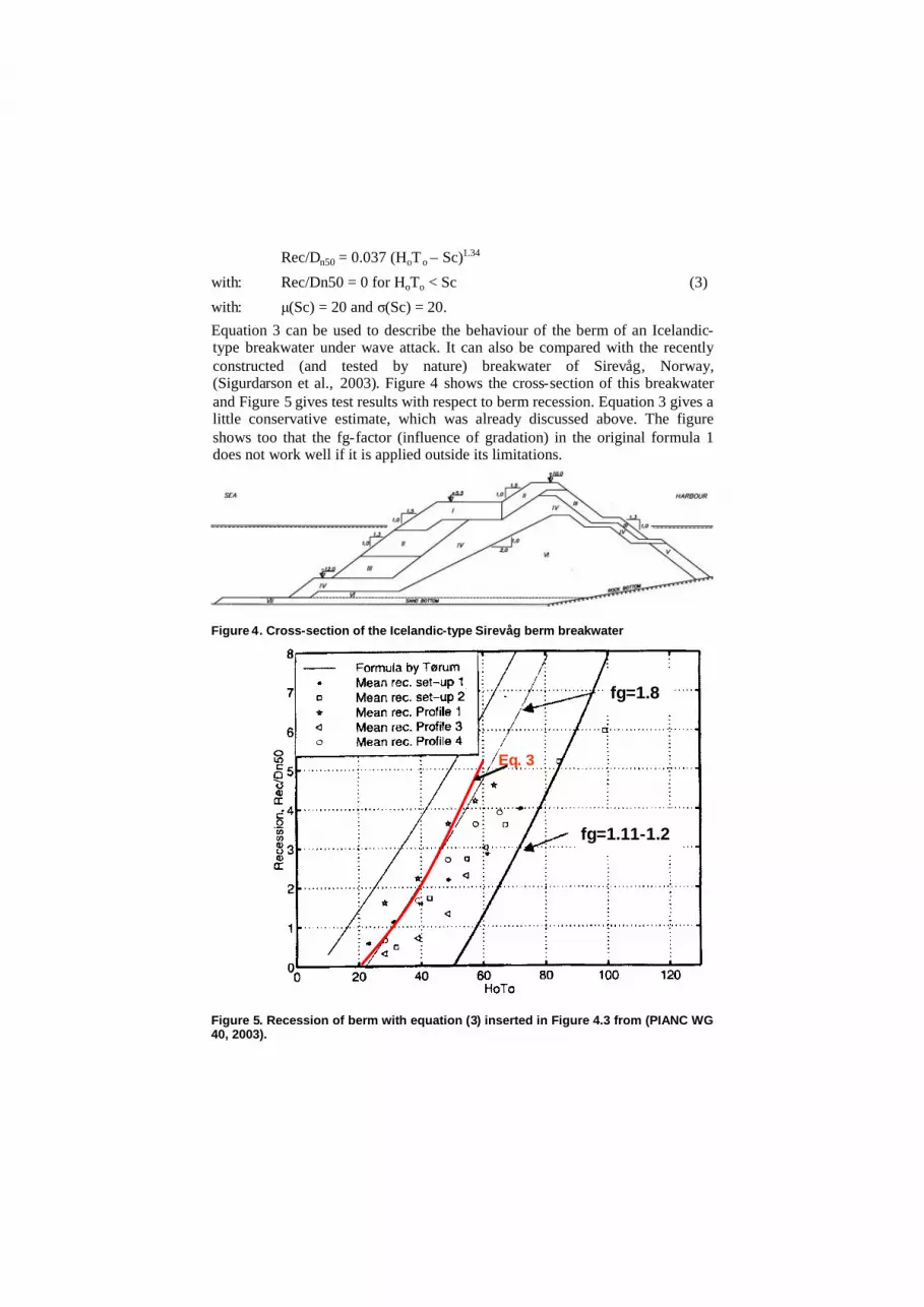
Rec/Dn50 = 0.037 (HoTo – Sc)1.34

with: Rec/Dn50 = 0 for HoTo < Sc (3)

with: μ(Sc) = 20 and σ(Sc) = 20.Equation 3 can be used to describe the behaviour of the berm of an Icelandic-type breakwater under wave attack. It can also be compared with the recentlyconstructed (and tested by nature) breakwater of Sirevåg, Norway,(Sigurdarson et al., 2003). Figure 4 shows the cross-section of this breakwaterand Figure 5 gives test results with respect to berm recession. Equation 3 gives alittle conservative estimate, which was already discussed above. The figureshows too that the fg-factor (influence of gradation) in the original formula 1does not work well if it is applied outside its limitations.

Figure 4. Cross-section of the Icelandic-type Sirevåg berm breakwater

Eq. 3

fg=1.11-1.2

fg=1.8

Eq. 3

fg=1.11-1.2

fg=1.8

Figure 5. Recession of berm with equation (3) inserted in Figure 4.3 from (PIANC WG40, 2003).

CONCEPTUAL DESIGN RULESThe design of an Icelandic-type berm breakwater does not really depend on aformula for the recession of the berm. The main idea is that the biggest rocksfrom a quarry are kept apart to make the upper two layers of the berm and a partof the down slope. From the total quarry output this will only be a few percent.This large and most important layer should be constructed with care. Rocksshould be placed one by one to achieve high interlocking without loosing theporosity. The Sirevåg and Keilisnes berm breakwater in Norway and Icelandrespectively have been chosen here as representative to develop deterministicdesign rules. In summary:

The upper layer of the berm consists of two layers of rock and extents onthe down slope at least to mean sea level;

The rock size of this layer is determined by: Hs/Dn50 = 2.0. Larger rockmay be used too;

Slopes below and above the berm are 1:1.5; The berm width is 3.5*Hs; The berm level is 0.65*Hs above design water level; The crest height is given by Rc/Hs*sop

1/3 =0.35.

REPAIR STRATEGY AND DESIGN LIMIT STATESThe recession, Rec, is calculated for each storm with HoTo > Sc

If in storm n+1 Recn+1>Recn then Recn+1 is used, otherwise Recn+1 is disregarded.

Serviceable limit state (SLS)Repair takes place when total recession in storm n is larger than half of theinitial berm width, i.e. Rec≥1.75*Hs

y. Eroded volume of berm is taken asVr

b=Rec*Hsy and the related cost Cr

b=1.5*Uc1*V r

Repairable limit state (RLS)Repair takes place if the rear side and the crest are eroded in a storm, i.e. whenfor unchanged sop,

1.44 Hsy < H s < 2.12 Hs

y (4)The upper and lower limits in Eq. 4 are the same as presented by van der Meerand Veldman (1992) for stability of the rear of a berm breakwater, where thelower limit corresponds to Rc/Hs*sop

1/3 = 0.25 which stands for start of damageand the upper limit corresponds to 0.17 which stands for severe damage.

Eroded plus extra added volume is taken as V rc=8*Hs

y*D1 and the related costCr

c=1.5*Uc1*Vrc

Ultimate limit stat (ULS)Failure occurs if

Recn+1 > 3.5 Hsy –

n

1Rec (5)

or

Hs > 2.12 Hsy (for unchanged Sop) (6)

In both cases the volume to replace is taken as Vf = V1+0.8*V2, that is the totalvolume of class 1 and 80% of class 2. The related cost is taken as Cf =2.5*Cc1*Vf.

Downtime cost occurs only in case of failure.

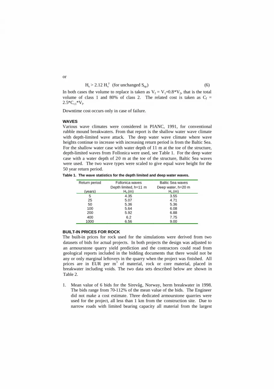
WAVESVarious wave climates were considered in PIANC, 1991, for conventionalrubble mound breakwaters. From that report is the shallow water wave climatewith depth-limited wave attack. The deep water wave climate where waveheights continue to increase with increasing return period is from the Baltic Sea.For the shallow water case with water depth of 11 m at the toe of the structure,depth-limited waves from Follonica were used, see Table 1. For the deep watercase with a water depth of 20 m at the toe of the structure, Baltic Sea waveswere used. The two wave types were scaled to give equal wave height for the50 year return period.Table 1. The wave statistics for the depth limited and deep water waves.

Return period Follonica wavesDepth limited, h=11 m

Baltic Sea wavesDeep water, h=20 m

(years) Hs (m) Hs (m)5 4.35 3.5525 5.07 4.7150 5.36 5.36100 5.64 6.08200 5.92 6.88400 6.2 7.75

1000 6.56 9.00

BUILT-IN PRICES FOR ROCKThe built-in prices for rock used for the simulations were derived from twodatasets of bids for actual projects. In both projects the design was adjusted toan armourstone quarry yield prediction and the contractors could read fromgeological reports included in the bidding documents that there would not beany or only marginal leftovers in the quarry when the project was finished. Allprices are in EUR per m3 of material, rock or core material, placed inbreakwater including voids. The two data sets described below are shown inTable 2.

1. Mean value of 6 bids for the Sirevåg, Norway, berm breakwater in 1998.The bids range from 70-112% of the mean value of the bids. The Engineerdid not make a cost estimate. Three dedicated armourstone quarries wereused for the project, all less than 1 km from the construction site. Due tonarrow roads with limited bearing capacity all material from the largest

quarry had to be sailed to the project site. The prices are regulated to June2007.

2. Mean value of 5 bids for a new berm breakwater in Thorlakshofn, Iceland,in 2003. The bids range from 90-104% of the Engineers cost estimate. Thededicated armourstone quarry for the project is located about 2 km from theconstruction site. As there was a direct access from the quarry to theconstruction site without entering the town it was possible to use miningtrucks for the transport. The prices are regulated to June 2007.

Figure 6 shows the built-in unit prices as a function of weight of the rock as wellas a trend line through the Sirevåg data. It was decided to use only the Sirevågdata for this study.Table 2. Built-in unit prices for rock from biddings on two actual projects.

Sirevåg ThorlakshofnMean mass (t) EUR/m3 Mean mass (t) EUR/m3

0.1 10.1 0.1 11.10.6 14.7 0.53 13.42 15.0 1.7 14.56 18.9 4.7 16.4

13.3 23.5 13.7 17.923.3 27.0

y = 14,8x0,17

0,0

5,0

10,0

15,0

20,0

25,0

30,0

0 5 10 15 20 25 30

Weight of armourstones (tonnes)

EU

R/m

3pl

aced

inbr

eakw

ate

r

Sirevag

Thorlakshofn

Power (Sirevag)

Figure 6. Built-in unit prices for rock as a function of weight

The built-in unit prices for repairs are higher than normal construction prices.The repair mainly needs large stones and less of the smaller stone classes aswell as the quarry run. The mobilization cost is also higher. The repair unitprices for the Serviceability limit state (SLS) and the Repairable limit state(RLS) are taken as 1.5 times the initial unit prices. The unit prices for repair offailure, the Ultimate limit state (ULS), are higher and are taken as 2.5 times theinitial unit prices.

CASE STUDIES

Input dataTwo cases are considered, a shallow water case with 11 m water depth exposedto the Follonica waves and a deep water case with 20 m water depth exposed tothe Baltic Sea waves, Table 1. The breakwaters are designed deterministicallyfor the following data:

Reduced buoyant density of the armour layer: Δ = 1.63 corresponding to ρs = 2.70 t/m3 and ρw = 1.025 t/m3;

Design return periods: y = 5, 25, 50, 100, 200, 400 and 1000 years; Stability number of stone class I: Ho

design= 1.8, 2.0, 2.4, 2.8 and 3.2; Wave steepness sop = 0.035; Dn50 of stone class II = 0.8 * Dn50 of stone class I; Downtime cost = 18,000 EURO/m breakwater for 1 km breakwater; Interest rate 5% p.a. (inflation included); Structure service life time 50 years.

Results of shallow water caseThe results of the cost optimization simulations for the shallow water case areshown in Figure 7. The total cost as a function of the design return period isgiven for various design stability numbers.

3,5

4,5

5,5

6,5

5 25 50 100 200 400 1000Wave return period in year

Tota

lco

sts

in1,

000

Eur

ope

rm

Ho design=1,80

Ho design=2,00

Ho design=2,40

Ho design=2,80

Ho design=3,20

Figure 7. Shallow water case, total cost as a function of design return period forvarious design stability numbers. The arrows point to the minimum values.

The optimum safety level has a flat minimum towards higher return periods, butrather steep increase in cost towards the lower return periods. Design for a lowstability number is more economical than to design for a high stability number.The most economical design corresponds to Ho

design = 1.8 and a design returnperiod of 25 years. But as the minimum is very flat, there is only 3% increase intotal cost if designed for 100 years return period instead of 25 years. For the

stability number of Hodesign = 2.0 the design return period of 50 years is the most

economical, but there is only a 3% increase in total cost if designed for 200years return period. Table 3 shows the split up of the total cost for the designstability number Ho

design = 2.0. It can be seen that there is a slight increase inconstruction cost when designing for higher return period. The repair costincreases towards lower return periods, but the largest changes in cost occur forthe cost of failures for low return periods.Table 3. Split up of total cost for shallow water case designed for Ho = 2.0

Return period(years)

Weight class I(tonnes)

Construction cost(EUR)

Repair cost(EUR)

Cost offailures (EUR)

Total cost(EUR)

5 6 3666 223 4225 811425 10 3888 54 187 4128

50 12 3975 27 33 4035

100 14 4059 10 1 4071

200 16 4141 3 1 4144400 19 4220 0 0 4220

1000 22 4321 0 0 4321

Results of deep water caseThe results for the deep water case are given in Figure 8. This graph shows thesame characteristics as for the shallow water case with flat minimum towardsthe higher stability numbers and steep increase towards the lower stabilitynumbers. The most economical design corresponds to Ho

design = 1.8 for 100years return period and Ho

design = 2.0 for 200 years return period.

3,5

4,5

5,5

6,5

5 25 50 100 200 400 1000Wave return period in year

Tota

lco

sts

in1,

000

Eur

op

erm

Ho design=1,80

Ho design=2,00

Ho design=2,40

Ho design=2,80

Ho design=3,20

Figure 8. Deep water case, total cost as a function of design return period for variousdesign stability numbers. The arrows point to the minimum values.

A comparison of Figures 7 and 8 indicates that the shallow water case is lessexpensive than the deep water case, which can be explained by the higherprobability of extreme wave heights in the deep water case. The optimum safetylevel is reached for lower return period for the shallow water case than for thedeep water case. But the assumption has to be noticed, that in the calculationsall rock sizes are available. For the shallow water case with 50 years returnperiod the stability number of 2.0 corresponds to a mean weight of class I stonesof 12 tonnes, while for the deep water case with 200 years return period thestability number of 2.0 corresponds to a mean weight of class I stones of 25tonnes.

COMPARISON WITH THE DESIGN OF RECENTLY CONSTRUCTEDICELANDIC-TYPE BERM BREAKWATERSTable 4 lists some recent berm breakwater projects in Iceland and Norway(Sigurdarson et al. 2006). In all cases the breakwaters have been designed for awave height with 100 years return period. In four out of six cases the stabilitynumber of the largest stone class has been close to 2.0, or in the range Ho = 1.9to 2.2.Table 4. List of recently constructed Icelandic-type berm breakwaters.

Breakwaterproject

Design returnperiod (y)

Design waveHs (m)

Design waterdepth (m)

Class I(tonnes)

DesignHo

Sirevåg 100 7.0 19 20 – 30 2.1Húsavík 100 6.8 13 16 – 30 1.9

Grindavík* 100 5.1 10 15 – 30 2.0

Hammerfest 100 7.5 25 20 – 35 2.2Thorlákshöfn 100 5.7 9 8 - 25 1.9

* Class I stones on the Grindavik breakwaters are only used on a limited part of thebreakwater heads. The data here corresponds to class II stones used on the mostexposed trunk section.

It is important to be aware of that the design return period and the stabilitynumber are dependent variables. From Table 1 it can be concluded that for thedepth limited case the wave height with 100 years return period is about 5%higher than for 50 years return period and about 11% higher than for 25 yearreturn period. If the Sirevåg berm breakwater had been designed for waves with50 or 25 years return periods instead of 100 years, but with unchanged stoneclasses, the stability number of the largest stone class would be 2.0 and 1.9respectively. That is very close to the optimum safety level for the shallowwater case with Ho

design = 1.8 and design return period of 25 years. For theHammerfest case, on the other hand, which is a more deep water case it wasdifficult to come closer to the optimum safety level of Ho

design = 1.8 for 100years return period as that would have needed a stone class with a mean weightof 46 tonnes instead of the 25 tonnes that were used. However, the simulationsare not valid for such a case because the unit price for such big rocks isunderestimated in the simulations.

It can be concluded that the design of these recent breakwaters follows thegeneral recommendation of this paper. With the required stone sizes available ithas been possible to design the berm breakwaters with low stability numbersclose to the optimum safety levels.

CONCLUSIONSAs a consequence of the rather flat minimum of the optimum safety levels it ispreferable to choose a rather conservative design. The same conclusion wasreached by Burcharth and Sørensen (2006) for conventional rubble moundbreakwaters. This means the Icelandic-type berm breakwater should bedesigned for a low stability number, if possible Ho < 2.0. Optimum safety levelscorrespond to Ho of 1.8 and 2.0 and return periods of 25 and 50 years. Withonly 2% additional cost design for 100 years return period practically avoidsrepair.The conclusion that it is more economical to design for low stability numbersand high return periods presumes that a good quarry, having all required stonesizes should be available. When using natural rock in design the naturallimitation of rock sizes should be taken into account. Sigurdarson et al. 2003,2005 and 2006 have shown how quarry yield prediction is used as an integratedpart of the design process.

REFERENCESBurcharth, H. F. and J.D. Sørensen, 2005. Optimum safety levels for breakwaters. Proc. Coastlines

Structures and Breakwaters 2005, ICE. 483-495.Burcharth, H.F., J.D. Sørensen, 2006. On optimum safety levels of breakwaters. PIANC congress

1996.PIANC WG12, 1991. Analysis of rubble mound breakwaters. PIANC.PIANC WG40, 2003. State-of-the-Art of Designing and Constructing Berm Breakwaters. PIANC.Sigurdarson, S., A. Jacobsen, O.B. Smarason, S. Bjørdal, G. Viggosson, C. Urrang, A. Tørum, 2003.

Sirevåg Berm Breakwater, design, construction and experience after design storm. Proc. CoastalStructures 2004, ASCE, 1212-1224.

Sigurdarson, S., A. Loftsson, A.E. Lothe, E. Bjertness, O.B. Smarason, 2005. Berm BreakwaterProtection for the Hammerfest LNG Plant in Norway - Design and Construction. Proc. Coastlines,Structures and Breakwaters 2005 , ICE. 349-362.

Sigurdarson, S., Smarason, O.B., Viggosson, G. and Bjørdal, S., 2006. Wave height limits for thestatically stable Icelandic-type Berm Breakwater, Proc. ICCE 2006, ASCE, 5046-5058.

Tørum, A., 1998. On the stability of berm breakwaters in shallow and deep water. Proc. 26th Int.Conf. Coastal Eng. , ASCE, 1435–1448.

Tørum, A., F. Kuhnen, A. Menze, 2003. On berm breakwaters. Stability, scour, overtopping.Coastal Eng. 49: 209-238.

Van der Meer, J.W., J.J. Veldman, 1992. Singular points at berm breakwaters: scale effects, rear,roundhead and longshore transport. Journal of Coastal Engineering, 17. 153-171.

KEY WORDS – CSt07

Abstract acceptance number: 60.Paper title: OPTIMUM SAFETY LEVELS AND DESIGN RULES FOR THE

ICELANDIC-TYPE BERM BREAKWATERAuthors: Sigurdur Sigurdarson, Jentsje W. van der Meer, Hans F. Burcharth

and John Dalsgaard Sørensen,

Keywords: Safety levels or optimum safety levelsBreakwaterBerm breakwaterBuilt-in pricesLifetime cost