parametric studies on stability of reshaped berm breakwater with concrete cubes as armor unit
TRANSCRIPT

PARAMETRIC STUDIES ON STABILITY OF
RESHAPED BERM BREAKWATER WITH
CONCRETE CUBES AS ARMOR UNIT
Thesis
Submitted in partial fulfillment of the requirements for the degree of
DOCTOR OF PHILOSOPHY
By
PRASHANTH J.
Register No. 100503, AM10F03
DEPARTMENT OF APPLIED MECHANICS AND HYDRAULICS
NATIONAL INSTITUTE OF TECHNOLOGY KARNATAKA,
SURATHKAL, MANGALORE – 575 025
DECEMBER 2013
D E C L A R A T I O N
I hereby declare that the Research Thesis entitled “Parametric Studies on Stability of
Reshaped Berm Breakwater with Concrete Cubes as Armor Unit” which is being
submitted to the National Institute of Technology Karnataka, Surathkal in partial
fulfillment of the requirements for the award of the Degree of Doctor of Philosophy in
Civil Engineering is a bonafide report of the research work carried out by me. The
material contained in this Research Thesis has not been submitted to any University or
Institution for the award of any degree.
Prashanth J.
Register Number: 100503, AM10F03
Department of Applied Mechanics and Hydraulics
Place: NITK-Surathkal
Date: 31st December, 2013
C E R T I F I C A T E
This is to certify that the Research Thesis entitled “Parametric Studies on Stability of
Reshaped Berm Breakwater with Concrete Cubes as Armor Unit” submitted by
Prashanth J., Register Number: 100503, AM10F03, as the record of the research work
carried out by him is accepted as the Research Thesis submission in partial fulfillment of
the requirements for the award of degree of Doctor of Philosophy.
Prof. Subba Rao Dr. Kiran G. Shirlal
(Research Guide) (Research Guide)
Prof. Subba Rao
(Chairman – DRPC)
DEPARTMENT OF APPLIED MECHANICS AND HYDRAULICS
NATIONAL INSTITUTE OF TECHNOLOGY KARNATAKA
SURATHKAL, MANGALORE – 575 025

ACKNOWLEDGEMENTS
With deep sense of gratitude, I express my heartfelt thanks to two of the imminent
Professors from the Department of Applied Mechanics and Hydraulics, NITK, Surathkal,
Prof. Subba Rao and Prof. Kiran G. Shirlal, for doing a marvelous job at supervising my
research work. Their logical and tactical suggestions have been very valuable and
encouraging during the development of this research. I acknowledge, the time spent in
technical discussions with both my supervising professors in regards to the completion of
this research, as immensely interesting and profoundly knowledge enhancing, to which I
am greatly indebted to. Their moral support and critical guidance have been priceless
which has given me an invaluable opportunity to publish my research work in many
international/national journals/conferences which is a matter of great pride and
satisfaction to me. The easily approachable nature and ever helpful attitude of
Prof. Subba Rao and Prof. Kiran G. Shirlal will always be admired, valued and
cherished.
I thank the former Directors of NITK, Surathkal, Prof. Sandeep Sancheti, and present
Director, Prof. Sawapan Bhattacharya, for granting me the permission to use the
institutional infrastructure facilities, without which this research work would have been
impossible.
I am grateful to Research Progress Committee members, Prof. M. S. Bhat and Prof. Katta
Venkataramana, for their critical evaluation and useful suggestions during the progress of
the work.
I am greatly indebted to Prof. M. K. Nagaraj, the former Head of the Department of
Applied Mechanics and Hydraulics, NITK, Surathkal, and Prof. Subba Rao, the present
Head of the Department, for granting me the permission to use the departmental
computing and laboratory facilities available for necessary research work to the

maximum extent which was very vital for the completion of the computational aspects
relevant to this research.
I sincerely acknowledge the help and support by all the Professors, Associate Professors
and Assistant Professors of Department of Applied Mechanics & Hydraulics.
I gratefully acknowledge the support and all help rendered by the Post-Graduate students
Sri Vishwanath N., Sri Sharath Kumar, Sri Mithun Shetty B. R., Smt. Geetha Kuntoji, Sri
Danny Thomas and Sri Sainath Vaidya during the research work.
I take this opportunity to thank Late Prof. Alf Torum, NTNU, Norway and Dr.
Balakrishna Rao, MIT, Manipal for their valuable suggestions during the research and all
my friends for their support, suggestions and encouragement during my research.
Thanks due to Mr. Jagadish, Foreman, and his supporting staff, Mr. Ananda Devadiga,
Mr. Gopalakrishna, Mr. Padmanabha Achar and Mr. Niranjan, for fabricating the moulds
and casting concrete cubes is gratefully acknowledged.
I thank Mr. Seetharam, Draughtsman, for his help in drawing neat sketches and
Mr. Balakrishna, Literary Assistant, is always remembered for his help in solving
computer snags which cropped up during computations.
I express heart felt gratitude to authors of all those research publications which have been
referred in this thesis.
Finally, I wish to express gratitude, love and affection to my beloved family members,
father Sri. H. R. Janardhana, mother Smt. H. K. Mythily and sister Smt. Shubha J. for
their encouragement, moral support and all their big and small sacrifices on the road to
the completion of my research.
Prashanth J.

i
ABSTRACT
The breakwater construction in deeper waters requires heavier armor units due to larger
wave loads. Such large stones are uneconomical to quarry or transport or may not be
available nearby. Another problem is uncertainty in the design conditions resulting in
breakwater damage due to increased wave loads. The structural stability and economy in
construction of breakwater are the need of hour.
Under these circumstances, berm breakwaters can be a solution. For an optimum
solution, the berm breakwater may be constructed with small size armor units. The
present research work involves a detailed experimental study of influence of various sea
state and structural parameters on the stability of statically stable reshaped berm
breakwater made of concrete cube armor.
Initially, a 0.70 m high of 1:30 scale model of conventional (single) breakwater of
1V:1.5H slope and trapezoidal cross section is constructed on the flume bed with
concrete cube as primary armor of weight 106 g. This is designed for a non-breaking
wave of height 0.1 m. This model is tested for armor stability with regular waves of
heights 0.1 m to 0.16 m and periods 1.6 s to 2.6 s in water depths of 0.3 m, 0.35 m and
0.4 m.
In the second phase, a 1V:1.5H sloped and 0.7 m high berm breakwater with varying size
of concrete armor cubes, berm widths, thickness of primary layer is tested for stability
with same wave conditions in depths varying from 0.30 m to 0.45 m.
Based on the study of reshaped breakwater model the following conclusions are drawn.
The stability of the breakwater is largely influenced by the storm duration. It is observed
that with the decrease in armor weight and berm width the berm recession, wave run-up
and run-down increases. The increase in water depth and wave height increased the
recession of berm, wave run-up and run-down. It is observed that shorter period waves

ii
cause higher berm recession, lower wave run-up and run-down. The surface elevation of
the water in front of the berm influences the recession and eroded area of the berm. Some
of the available equations for berm recession, wave run-up over estimated the values for
the considered conditions. The damage is reduced by about 47% in the present model
when compared to stone armored berm breakwater. The wave run-up and run-down are
reduced by 34% and 49% compared to conventional cube armored breakwater
respectively. The economic analysis showed that the cube armored berm breakwater is
about 8% and 4% economical than the conventional cube armored breakwater and stone
armored berm breakwater for the same design conditions. The design equations for berm
recession, wave run-up and wave run-down are derived.
Finally, it was found that 25% reduction in armor weight with 0.40 m berm width and 3
no. of primary armor layers is safe for the entire conditions considered during the study.
However, for most of the wave climate (excluding extreme waves of 0.16 m height and
1.6 s period) primary layer with 2 armor thickness is safe with a berm width of 0.40 m. In
terms of safety as well as economy 25% reduction with 0.40 m berm width and 2 no. of
primary layer was cheaper compared to the entire models studied.
Keywords: berm breakwater, damage, recession of berm, storm duration, wave run-up,
wave run-down.
iii
CONTENTS
PAGE
NO.
ABSTRACT i
CONTENTS iii
LIST OF TABLES viii
LIST OF FIGURES x
NOMENCLATURE xiv
CHAPTER 1 INTRODUCTION 1-17
1.1 GENERAL 1
1.2 BREAKWATERS AND ITS ARMOR UNITS 2
1.2.1 History of Breakwaters 2
1.2.2 Types of Breakwaters 3
1.2.3 Armor Units 6
1.2.4 Classification of Artificial Armor Units 10
1.3 FAILURE OF RUBBLE MOUND BREAKWATERS 11
1.4 REHABILITATION OF DAMAGED BREAKWATERS 14
1.5 NEED AND SCOPE OF THE PRESENT STUDY 15
1.6 ORGANIZATION OF THE THESIS 16
CHAPTER 2 LITERATURE REVIEW 19 – 76
2.1 GENERAL 19
2.2 RUBBLE MOUND OR HEAP BREAKWATER 19
2.3 BREAKWATER DESIGN METHODS 21
2.3.1 Eqadro Castro formula 22
2.3.2 Hudson formula 23
2.3.3 Van der Meer equations 25
2.3.4 Other design formulas 26
2.3.4.1 Sherbrooke University Formula 26
2.3.4.2 Koev Formula 26

iv
2.3.4.3 Kajima‟s Stability Formula 27
2.3.4.4 Melby and Hughes formula 27
2.3.4.5 Van Gent formulae 28
2.3.5 Improvements in breakwater design 28
2.4 STABILITY OF RUBBLE MOUND BREAKWATER 30
2.4.1 Factors Affecting the Stability of Non-Overtopping
Breakwater 30
2.4.1.1 Wave Characteristics 31
2.4.1.2 Water Depth 33
2.4.1.3 Duration of Wave Attack 33
2.4.1.4 Wave Run-Up and Run-Down 34
2.4.1.5 Geometry of Breakwater 38
2.4.1.6 Permeability of the Structure 38
2.4.1.7 Method of Construction 39
2.4.1.8 Foundation 39
2.5 DAMAGE OF RUBBLE MOUND BREAKWATERS 40
2.6 BERM BREAKWATERS 45
2.6.1 Evolution of berm breakwaters 45
2.6.2 Stability of berm breakwaters 48
2.7 DAMAGE OF BERM BREAKWATERS 54
2.7.1 Statically stable non-reshaped berm breakwaters 54
2.7.2 Statically stable reshaped berm breakwaters 55
2.7.2.1 Berm recession 56
2.7.3 Dynamically stable berm breakwater 61
2.7.3.1 Profile development 61
2.8 WAVE RUN-UP AND WAVE RUN-DOWN IN BERM
BREAKWATERS 63
2.9 DESIGN ASPECTS OF BERM BREAKWATER 66
2.10 ECONOMICAL DESIGN OF BERM BREAKWATERS 71

v
2.11 STUDIES ON ARTIFICIAL ARMOR UNITS 72
2.12 SUMMARY 75
CHAPTER 3 PROBLEM FORMULATION AND
EXPERIMENTAL DETAILS 77 - 96
3.1 GENERAL 77
3.2 PROBLEM FORMULATION 77
3.3 SCOPE OF THE PRESENT WORK 79
3.4 DIMENSIONAL ANALYSIS 79
3.4.1 Predominant variables 80
3.4.2 Details of dimensional analysis 80
3.5 SIMILITUDE AND MODEL SCALE SELECTION 82
3.6 DESIGN CONDITIONS 83
3.7 EXPERIMENTAL SETUP 84
3.7.1 Wave flume 84
3.7.2 Wave Probes 84
3.7.3 Surface profiler system 85
3.7.4 Calibration of test facilities 85
3.7.4.1 Wave Flume 85
3.7.4.2 Wave Probes 86
3.8 BREAKWATER MODEL SECTIONS 86
3.8.1 Conventional breakwater 86
3.8.2 Berm breakwater 88
3.8.3 Model construction 89
3.8.4 Wave characteristics 90
3.9 CASTING OF CONCRETE CUBES AND ITS PROPERTIES 90
3.10 TEST CONDITIONS 92
3.11 TEST PROCEDURE 92
3.11.1 Sources of errors and precautions to minimize error 93
3.11.2 Procedure for experimental study 94

vi
3.12 MEASUREMENTS 94
3.12.1 Measurement of wave heights 94
3.12.2 Measurement of wave run-up and run-down 95
3.12.3 Measurement of breakwater damage 96
3.15 UNCERTAINTY ANALYSIS 96
CHAPTER 4 RESULTS AND DISCUSSION 97-136
4.1 GENERAL 97
4.2 SUMMARY OF MODEL STUDY 97
4.3 STUDIES ON CONVENTIONAL BREAKWATER 100
4.3.1
Effect of deepwater wave steepness (Ho/gT2) on damage
level (S) 100
4.3.2
Effect of deepwater wave steepness (Ho/gT2) on
relative wave run-up (Ru/Ho) 100
4.3.3
Effect of deepwater wave steepness (Ho/gT2) on relative
wave run-down (Rd/Ho) 101
4.4 STUDIES ON BERM BREAKWATER 102
4.4.1 Effect of reduction in armor weight on berm recession,
wave run-up and run-down 102
4.4.2 Effect of different berm widths on berm recession, wave
run-up and run-down 106
4.4.3 Effect of change in thickness of primary layer on berm
recession, wave run-up and run-down 110
4.4.4 Influence of change in water depth on berm recession,
wave run-up and run-down 114
4.4.5 Influence of change in wave height and wave period on
berm recession, wave run-up and run-down 117
4.4.6 Influence of storm duration on berm recession 122
4.5 EQUATIONS DEVELOPED FROM THE PRESENT STUDY 125
4.6 OPTIMUM BERM BREAKWATER CONFIGURATION 127

vii
4.7 COMPARISON OF PRESENT BREAKWATER MODEL
WITH OTHER TYPES OF BREAKWATER 128
4.7.1
Comparison of wave run-up and wave run-down with
conventional breakwater 128
4.7.2
Comparison of berm recession, wave run-up and wave
run-down with berm breakwater armored with natural
stones
129
4.8 COMPARISON OF EXPERIMENTAL BERM RECESSION
WITH DIFFERENT EQUATIONS 131
4.9 COMPARISON OF PRESENT EXPERIMENTAL WAVE
RUN-UP WITH EQUATION 2.44 132
4.10 COST ANALYSIS 134
4.11 SUMMARY 134
CHAPTER 5 CONCLUSIONS 137-139
5.1 GENERAL 137
5.2 CONCLUSIONS ON CONVENTIONAL BREAKWATER
MODEL STUDY 137
5.3 CONCLUSIONS ON RESHAPED BERM BREAKWATER
MODEL STUDY 138
5.4 SCOPE FOR FUTURE WORK 139
APPENDIX I: UNCERTAINTY ANALYSIS 141-147
APPENDIX II: COST ANALYSIS 149-158
APPENDIX III: UNCERTAINTY ANALYSIS 159-161
REFERENCES 163-179
RESUME

viii
LIST OF TABLES
1.1 Summary of historical development of breakwater 3
1.2 Classification of breakwater armor units by shape 10
1.3 Classification of armor units by shape, placement and stability factor 11
2.1 Various stability formulae 22
2.2 Values of wave run-up coefficients for rough slope 36
2.3 Coefficients of wave run-up levels 36
2.4 Damage parameter “D” for two-layer armor 41
2.5 Van der Meer damage criteria 42
2.6 Damage level by Nod for two – layer armor 43
2.7 Best parameter estimates for velocity statistics 67
2.8 Design KD and global safety factors 74
3.1 Predominant variables in the analysis of breakwater stability 80
3.2 Wave parameters of prototype and model 82
3.3 Selection of model scale 83
3.4 Conventional breakwater model characteristics 88
3.5 Berm breakwater model characteristics 89
3.6 Wave characteristics 90
3.7 Results of tests on cement and sand 91
3.8 Sand: Iron ore ratio in 1:3 cement mortar 91
3.9 Statistics of all wave heights recorded 95
3.10 Statistics of all wave run-ups recorded 95
3.11 Statistics of all wave run-downs recorded 96
4.1 Equivalent surf similarity parameter for 0.40 m berm width model 118
4.2 Comparison of results of present study with conventional cube armored and
stone armored berm breakwaters 130
4.3 Summary of results 135
AI-1 Data points with results of 95% confidence band and 95% prediction band 146

ix
AII-1 Quantity estimation of cube armored conventional breakwater for per meter
length 153
AII-2 Quantity estimation of stone armored berm breakwater for per meter length 154
AII-3 Quantity estimation of cube armored berm breakwater for per meter length 154
AII-4 Calculation of unit rates of civil works 155
AII-5 Final unit rates of armor stones of various sizes 156
AII-6 Cost of construction of cube armored conventional breakwater 157
AII-7 Cost of construction of stone armored berm breakwater 157
AII-8 Cost of construction of cube armored berm breakwater 158

x
LIST OF FIGURES
1.1 Rubble mound breakwater at Citavecchia 2
1.2 Different kinds of rubble mound breakwaters 4
1.3 Conventional caisson breakwaters with vertical front 5
1.4 Composite breakwaters 5
1.5 Algeris north breakwater 7
1.6 Marseille breakwater 8
1.7 Examples of Artificial Armor Units 10
2.1 Multilayer rubble mound breakwater with superstructure 20
2.2 Definition sketch of Wave Run-up (Ru) and Wave run-down (Rd) 34
2.3 Failure modes of a rubble mound breakwater 40
2.4 Erosion area and damage level, S 42
2.5 Designed virtual net using Photoshop 44
2.6 Conventional vs. berm breakwaters 45
2.7 Berm breakwater at Rachine, Michigan 47
2.8 Cross-section of the multi-layer berm breakwater under construction
at Sirevag 47
2.9 Seaward profiles for steep, smooth waves acting upon a breakwater
of concrete cube 48
2.10 Different profiles of berm breakwater considered for study 51
2.11 Damage level „S‟ for different thickness of primary layer 55
2.12 Definition of Recession (Rec) 56
2.13 Berm parameters 56
2.14 Recession of a multi layer berm breakwater 58
2.15 Schematized profile of 1:5 initial slope 62
2.16 Parameterization of a generic reshaped profile 63
2.17 Definition of equivalent and average slope 65

xi
2.18 First estimation of berm width as suggested by Van der Meer 69
2.19 Comparison of stability of Rocks, Cubes, Tetrapods and Accropode 72
2.20 Qualitative influence of slope angle on stability of armor units 74
3.1 Details of wave flume facility 84
3.2 Calibration chart for a water depth of 0.35 m 85
3.3 Calibration of wave probes 86
3.4 Details of test model of conventional breakwater 88
3.5 Details of test model of berm breakwater 89
4.1 Influence of deepwater wave steepness (Ho/gT2) on Damage level (S)
for different water depths 100
4.2 Influence of Ho/gT2 on Ru/Ho for different water depths 101
4.3 Influence of Ho/gT2 on Rd/Ho for different water depths 101
4.4 Influence of Ho/gT2 on Rec/B for a 0.35 m berm width and different
water depths 102
4.5 Influence of Ho/gT2 on Rec/B for different water depths and 0.45 m
berm width 103
4.6 Influence of Ho/gT2 on Ru/Ho for different water depths and 0.45 m
berm width 105
4.7 Influence of Ho/gT2 on Rd/Ho for different water depths and 0.45 m
berm width 105
4.8 Influence of Ho/gT2 on Rec/B for 25% reduction in armor weight and
different water depths 107
4.9 Influence of Ho/gT2 on Ru/Ho for 25% reduction in armor weight and
all water depths 108
4.10 Influence of Ho/gT2 on Rd/Ho for 25% reduction in armor weight and
all water depths 110
4.11 Influence of Ho/gT2 on Rec/B for 0.40 m berm width and all water
depths 111
4.12 Influence of Ho/gT2 on Ru/Ho for 0.40 m berm width and all water 112

xii
depths
4.13 Influence of Ho/gT2 on Rd/Ho for 0.40 m berm width and all water
depths 113
4.14 Influence of Ho/gT2 on Rec/B for 0.40 m berm width and 25%
reduction in armor weight 114
4.15 Influence of Ho/gT2 on Ru/Ho for 0.40 m berm width and all water
depths 116
4.16 Influence of Ho/gT2 on Rd/Ho for 0.40 m berm width and all water
depths 117
4.17 Influence of eq on Rec/B for 0.40 m berm width and 25% reduction in
armor weight 119
4.18 Influence of eq on Ru/Ho for 0.40 m berm width and 25% reduction
in armor weight 120
4.19 Influence of eq on Rd/Ho for 0.40 m berm width and 25% reduction
in armor weight 121
4.20 (a) Influence of no. of waves on Rec/B for 0.40 m berm width and 0.45 m
water depth 122
4.20 (b) Influence of no. of waves on Rec/B for 0.40 m berm width and 0.40 m
water depth 123
4.20 (c) Influence of no. of waves on Rec/B for 0.40 m berm width and 0.35 m
water depth 124
4.20 (d) Influence of no. of waves on Rec/B for 0.40 m berm width and 0.30 m
water depth 124
4.21 Stability equation for berm breakwater 125
4.22 Comparison of measured and calculated berm recession 126
4.23 Comparison of measured and calculated wave run-up 126
4.24 Comparison of measured and calculated wave run-down 127
4.25 Comparison of wave run-up between conventional breakwater and
present model 128

xiii
4.26 Comparison of wave run-down between conventional breakwater and
present model 129
4.27 Comparison of berm recession between berm breakwaters armored
with cubes and stones 129
4.28 Comparison of experimental results with Eq. 2.35 and Eq. 2.36 131
4.29 Comparison of experimental results with Eq. 2.39 132
4.30 Comparison of experimental results with Eq. 2.41 and Eq. 2.43 132
4.31 Comparison of experimental wave run-up with Eq. 2.44 for shallow
water condition 133
4.32 Comparison of experimental wave run-up with Eq. 2.44 for
deepwater condition 133
AI-1 Combined specimen graph for 95% confidence and prediction band 142
AI-2 Plot of 95% confidence and prediction bands for the variation of
Rec/Dn50 with Ns 143
AI-3 Plot of 95% confidence and prediction bands for the variation of
Ru/Ho with eq 144
AI-4 Plot of 95% confidence and prediction bands for the variation of
Rd/Ho with eq 145
AII-1 Conventional breakwater section 150
AII-2 Berm breakwater Section 152

xiv
NOMENCLATURE
Ae = Eroded area of sea-ward profile in cross-section
B = Berm width
Dn50 = Nominal diameter of the breakwater armour unit
D15 = 15% of the stones have a diameter less than D15
D85 = 85% of the stones have a diameter less than D85
d = Water depth in front of structure
dB = Water surface above or below the berm horizontal surface
fg = Gradation factor, D85/D15
fd = Depth factor
g = Gravitational acceleration
H = Wave height in front of the structure
Hs = Significant wave height
hb = Berm height above sea bed
Ho = Deep water wave height
HoTo = Wave height- period stability number
KD = Stability coefficient in Hudson formula
kΔ = Armor layer coefficient
Lo = Deep water wave length
N = Number of waves
Ns = Stability number
n = Sample size, number of armor layers
P = Permeability coefficient
Rd = Wave run-down
Ru = Wave run-up
Rui = Run-up level exceeded by „i‟ percent of the incident wave
Re = Reynolds number
Rec = Recession of the reshaped berm
Rc = Crest height of structure

xv
s = Wave steepness
T = Wave period
Tz = Zero up-crossing wave period
t = t-distribution values from statistical table
W50 = 50% value of mass distribution curve of armor units
W15 = 15% value of mass distribution curve of armor units
W85 = 85% value of mass distribution curve of armor units
ta = Thickness of armor layer
xc = Crest width
x = Variable
x = Sample mean
σ = Standard deviation
= Relative mass density, (ρa –ρw)ρw
α = Angle of seaward slope of structure
αeq = Equivalent slope angle of berm breakwater structure
β = Angle of incidence of wave direction
βo = Intercept - regression coefficients
β1 = Slope - regression coefficients
γr = Reduction factor for influence of surface roughness
γb = Reduction factor for influence of a berm
γh = Reduction factor for influence of shallow-water conditions
γβ = Reduction factor for influence of angle of incidence β of the waves
γa = Specific weight of armor unit
a = Mass density of armor unit
w = Mass density of water
ξom = Deep water surf-similarity parameter, Tanα/√(Ho/Lo)
ξeq = Breaking wave surf similarity parameter of an equivalent slope
S = Damage level
Rec/Dn50 = Dimensionless berm recession
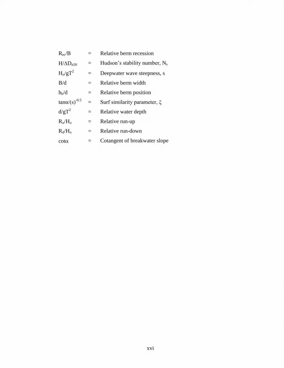
xvi
Rec/B = Relative berm recession
H/Dn50 = Hudson‟s stability number, Ns
Ho/gT2 = Deepwater wave steepness, s
B/d = Relative berm width
hb/d = Relative berm position
tanα/(s)-0.5
= Surf similarity parameter, ξ
d/gT2 = Relative water depth
Ru/Ho = Relative run-up
Rd/Ho = Relative run-down
cot = Cotangent of breakwater slope


1
CHAPTER 1
INTRODUCTION
1.1 GENERAL
The requirement of any port, harbor or marina is a sheltered area free from the sea
waves. In the coastal areas where natural protection from waves is not available, the
development of harbor requires an artificial protection for the creation of calm areas.
For harbors, where perfect tranquility conditions are required, large structures such as
rubble mound breakwaters or vertical wall breakwaters are used. Most of the
breakwaters are used to create tranquil conditions in the lagoon and at the entrance
channel of ports, for maneuvering of ships and port operations. Many a times
breakwaters are also used as berthing structures along with protecting the harbor area.
Sometimes they are used to protect beaches from erosion due to the destructive wave
forces (Verhagen et al. 2009).
The selection of the type of breakwater will be primarily based on the function of the
breakwater, wave climate of that area, depth of water, availability of construction
materials and local labor, geotechnical characteristics of sea bed, environmental
concerns and available contractor potential. Although there are developments in
construction technology, the rubble mound structures remain the most commonly
used among all types of breakwaters worldwide for more than a century now to
protect harbor basins against the wave forces.
Rubble mound breakwater is typically a three layered breakwater of trapezoidal
shape. It is used in relatively shallow water wave conditions only. However, in 1970s
the need for bigger ships and harbors has resulted in construction of breakwaters in
deep water where experience was seldom available. This development resulted in the
failure of several huge rubble mound breakwaters. Further, in order to withstand the
high waves, breakwaters were built with large heavy rocks. But this posed a problem
since the maximum rock size was limited and in some parts of the world no large size
rock or good quality rock was available. Additionally, from the economic point of
view, breakwaters represent a significant portion of a capital investment in the

2
development of a port, and would require regular maintenance to retain their
effectiveness. Hence, an analysis of the total cost over the lifetime of the structure was
also essential. This is another reason that makes it necessary to search for better
solutions and develop economical and safe structures to serve a particular purpose.
1.2 BREAKWATERS AND ITS ARMOR UNITS
1.2.1 History of Breakwaters
The construction of structures on sea dates back to around 5000 BC with the building
of sea link between then India and Srilanka as quoted in the great Indian epic
Ramayana (Bala 2013). The development of breakwater construction is closely
related to the development of ports around the world over the centuries. The first
breakwaters built can be linked to the ancient Egyptian, Phoenician, Greek and
Roman cultures. The structures were simple mound structures, composed of locally
found rock. As early as 2000 BC, mention was made of a stone masonry breakwater
in Alexandria, Egypt (Takahashi 1996). The Roman emperor Trajan (AD 53-117)
initiated the construction of a rubble mound breakwater in Civitavecchia, which still
exists today (Fig. 1.1) (D’Angremond and van Roode 2004).
Fig. 1.1 Rubble mound breakwater at Citavecchia
(D’Angremond and van Roode 2004)
The standards for design and construction of a breakwater remained those developed
primarily by the Romans, later a great leap in technology was achieved through the
development of mechanical equipment and hydraulic sciences including maritime
hydraulics (Franco 1996). De Cessart undertook rather complex work of a breakwater
construction in Cherbourg harbor in comparatively deep waters. The Plymouth
breakwater started in 1811 showed a remarkable similarity of profile with the
Cherbourg breakwater (Bruun 1985). The characteristic feature of these breakwaters
was that they were periodically and partially damaged due to storms. The stable

3
profile of these breakwaters closely resemble the ‘S’ profile adopted for breakwaters
later. The vertical wall breakwater at Dover was constructed in1847 which worked
very well compared to breakwaters built in Cherbourg and Plymouth. The Cherbourg,
Plymouth and Dover breakwaters are considered to be the pioneers of modern-day
breakwater structures (Takahashi 1996). Table 1.1 shows the historical development
of breakwaters along with the development of armor units (Takahashi 1996).
Table 1.1 Summary of historical development of breakwater (Takahashi 1996)
1.2.2 Types of breakwaters
The breakwaters are mainly classified as:
1. Rubble mound or heap breakwaters.
2. Upright or vertical wall breakwaters.
3. Mound with superstructure or composite breakwaters.
4. Special types of breakwaters.
1. Rubble mound breakwaters: It is a heterogeneous assemblage of natural rubble
or undressed stone blocks or in many cases by artificial blocks. It is of trapezoidal
shape with stones or blocks being deposited on its slope without any regard to bond or
bedding. This is the simplest type and is constructed by tipping or dumping of rubble
stones into the sea till the heap or mound emerges out of the water, the mound being
consolidated and its side slopes regulated by the action of the waves.

4
Rubble mound breakwaters are suitable for all types of foundations. They can be
constructed up to 50 m depth economically and can be repaired easily and
periodically. Even though initial and maintenance cost is high, construction does not
necessitate skilled labor or specialized equipments. But the material required might be
of enormous quantity and heavy at locations having large tidal ranges, high waves and
deeper depths. Further, the rubble mound breakwaters can be classified based on its
variation in structural configuration as Multi layer rubble mound breakwater,
submerged breakwaters, berm breakwaters, reef breakwaters and tandem breakwaters
(Refer Fig. 1.2).
Fig. 1.2 Different kinds of rubble mound breakwaters
Multi layer rubble mound breakwaters are made of three layers namely primary layer,
secondary layer and a core. The primary layer is directly exposed to waves and also
acts a protective layer for secondary and core layers. A submerged breakwater is
similar to multi layer breakwater with only its crest at or below sea level. A
breakwater with a horizontal berm at some elevation is called a berm breakwater. The
berm breakwater may be reshaping type or non-reshaping type. The traditional rubble
mound is a reef structure constructed as a heap of bulky stones laid at some stable
slope to resist the wave action. A reef breakwater is a low-crested group of stones
without a filler layer or core. Reef breakwater is allowed to reshape under wave
attack. The concept of rubble mound breakwater and submerged reef breakwater,
operating together as a single unit, is called the tandem breakwater. The submerged
reef reflects and dissipates the wave energy by inducing wave breaking, thereby,
reducing impact of waves on the main breakwater (Shirlal and Rao 2003). A detailed

5
study on rubble mound breakwaters in particular berm breakwater is given in later
chapters.
2. Upright or vertical wall breakwaters: These breakwaters are of types such as
huge concrete blocks, gravity walls, concrete caissons, rock filled timber cribs and
concrete or steel sheet pile walls as indicated in Fig. 1.3. Vertical wall structures are
used as breakwaters, seawalls, and bulkheads in harbors. The main purpose of a
vertical breakwater is to reflect waves, while that for the rubble mound breakwater is
to break them and dissipate wave energy. They are used in relatively moderate wave
conditions but when a critical load value is exceeded, these monolithic breakwaters
lose their stability at once. This catastrophic failure due to loss of stability is one of
the major disadvantages for this type of breakwaters.
Fig. 1.3 Conventional caisson breakwaters with vertical front
3. Mound with superstructure or composite breakwaters: Composite breakwaters
are combination of rubble mound and vertical wall breakwaters. These are used in
locations where either the depth of water is large or there is a large tidal range and in
such situations, the quantity of rubble stone required to construct a breakwater to the
full height would be too large. In such conditions, a composite breakwater is
constructed as a structure with rubble mound base and a super structure of vertical
wall as shown in Fig. 1.4. These breakwaters tend to fail when the waves break near
the mound and then slam against the vertical wall, which damages the structure.
Fig. 1.4 Composite breakwaters

6
4. Special type of breakwaters: These breakwaters are for specific purposes with
special features and are not commonly used. Depending on the site condition these are
designed. Special type of breakwaters can be divided into two types. One is the non-
gravity type breakwaters such as pile type, floating, pneumatic etc. The other is
gravity type which is the conventional breakwater with special features conceived to
improve the functioning and stability of breakwater. Some special breakwaters are as
follows:
• Curtain wall breakwater – commonly used as secondary breakwater to protect
small craft harbors.
• Sheet pile walls – are used to break relatively small waves.
• Horizontal plate breakwater – can reflect and break waves and are supported by a
steel jacket.
• Floating breakwater – Used in deep waters especially in places where the ground
soil is poor for foundation
• The pneumatic breakwater – breaks the wave due to water current induced by air
bubbles.
1.2.3 Armor units
An armor unit is a massive and bulky stone or concrete unit placed as a primary layer
material in rubble mound breakwaters to resist the wave attack. The armor units are
selected to fit specified geometric characteristics and density. The units require
individual placement on the structure since units are very large in size. The choice of
type of unit depends mainly on availability of quarry and the mass of unit required.
The armor units are mainly classified into two categories namely natural armor units
and artificial armor units. The quarried stone is a natural unit and concrete unit is an
artificial armor unit.
In the early days when breakwaters were built in relative shallow waters, natural
stones were used as armor units since the required size and weight were easily
available from quarries nearby. As the construction started moving into deeper waters,
the wave load on armor increased requiring heavier armor units. It became difficult to
procure such heavy weight stones or even to transport them to the site. Sometimes
such heavy weight armor stones were not available in the nearby quarries. This posed

7
a problem as breakwaters constitute the main part of the port from economic point of
view. In order to overcome this disadvantage and with the advancement in the field of
concrete technology new type of armors of various shapes and sizes were developed,
and these were known as artificial armor units. These units can be manufactured/cast
at sites as per the requirement.
The artificial armor units are found to be more advantageous than natural armor units.
The artificial armor units can be of desired shape, size and weight which are relatively
lighter compared to natural armors and can be cast in-situ. Also, they can attain better
interlocking capability, improved hydraulic and structural stability compared to
natural units. Their optimum interlocking capability is balanced between hydraulic
stability and the ease of fabrication.
The usage of concrete blocks dates back to early 19th
century. The historical port of
Algiers which was constructed in 16th
century was protected by rubble mound
breakwater made of stones which was getting continuously damaged. In 1833, a
French engineer, Poirel, carried out reinforcement work using 2 to 3 m3 stones, but
the stones ended up being unstable. The breakwater was later successfully reinforced
using 15 m3 rectangular concrete blocks (Takahashi 1996). Fig. 1.5 shows the north
breakwater of Algiers port armored with 15 m3 concrete blocks with a slope of 1:1.
Further, many breakwaters were built in various ports in Algeris viz. Algeris, Oran,
Philippeville etc. As quoted by Takahashi (1996) these breakwaters also suffered
damage due to steep slope, insufficient weight of blocks, insufficient depth of armor
layer and random placement of blocks.
Fig. 1.5 Algeris north breakwater (Takahashi 1996)

8
A fairly new concept was adopted for the breakwater built in Marseille to overcome
the failure in previous breakwaters. The breakwater was made strong with some
special features. The inner core was included with lighter stones covered by heavier
stones. The primary layer of concrete block was extended to sufficient depth and the
slope above sea level was kept gentle (1:3). The lower slope below sea level was kept
steep (3:4) compared to upper slope and the armor blocks in this region were placed
carefully. Fig. 1.6 shows the Marseille breakwater constructed with the above
features. The breakwaters constructed later followed this concept and they were called
as Marseille type.
Fig. 1.6 Marseille breakwater (Takahashi 1996)
The concrete block unit was very massive and heavy which produced large cross
sections for mild slope above sea level. This made construction difficult and
uneconomical. These disadvantages were overcome with the advent of interlocking
concrete blocks in 1949 by P. Danel. 'Tetrapods' thus developed marked the start of a
long series of similar blocks. Danel (1953) summarized the characteristics of
interlocking blocks as:
1. Porosity: Impermeable layers caused internal pressure in the mound thus disrupting
the structure. Permeable layer tend to dissipate the wave energy thus reducing internal
pressure, wave run-up and also wave run-down.
2. Roughness: The friction between water layer and armor layer helps in reducing the
wave energy. Also, friction between the blocks keeps them in their position reducing
the damage. The above two can be achieved by increasing roughness of the blocks
which is possible by providing interlocking between them with projecting legs.

9
3. Resistance: The block must be strong enough to withstand breakage. If a very long
leg/projection is provided there will be chances of breaking and with a short
projection there will be no adequate resistance and interlocking developed.
In order to achieve all the above characteristics an optimum length of projection was
needed. Thereafter many armor units with different shapes and a number of
projections were developed. The emphasis was mainly on the interlocking of the
units. The slender armor units ‘Dolos’ developed by Merrifield in South Africa in
1968 probably represents the peak of this concept and has a very high degree of
interlocking. The failure of Sines breakwater which was armored with 42T Dolos unit
was a major setback for this unit. This failure led to the development of stronger
complex unit, still with higher hydraulic stability. The result of such development is
Accropode developed by Sogreah in 1980 which brought an end to the rapid
development of interlocking units.
In late 1960's a parallel development of completely different type of armor was in
progress. The armor layer consisting of hollow blocks is placed uniformly in a single
layer where each block is tied to its position by the neighboring blocks. This armor
concept was not based on weight or interlocking but on friction between blocks,
which provided an extremely high degree of hydraulic stability.
Many studies by investigators showed that voids played a very important part in the
stability of armor layers. It was in these voids, created by units in a pack, that the
greatest dissipation of wave energy takes place by relieving fluid pressure trying to
move the blocks. For certain geometric shapes, the percentage of voids in the armor
layer increased drastically as compared to conventional rectangular block armor
layers. Based on this void concept many hollow blocks were developed like Cob,
Shed etc.
Presently, the development of new types of armor block has reduced instead, now
optimization of breakwater structure with a selected armor unit is being done. The
selection of armor unit depends on many factors. Some of commonly used armor units
are shown in Fig. 1.7

10
Fig. 1.7 Examples of Artificial Armor Units (Pilarczyk and Zeidler 1996)
1.2.4 Classification of artificial armor units
Bakker et al. (2003) classified the concrete blocks based on risk of progressive failure
as:
Compact blocks: The armor unit’s own weight is the main stabilizing factor and these
units posses low average hydraulic stability. However, the structural stability is high
and the variation in hydraulic stability is relatively low. Thus, the armor layer can be
considered as a parallel system with a low risk of progressive failure.
Slender Blocks: In these blocks, interlocking is the main stability parameter and the
units have large average hydraulic stability. However, the variation in hydraulic
resistance is also relatively large and the structural stability is low. Therefore, slender
blocks shall be considered as a series system with a large risk of progressive failure.
Further, breakwater armor units can be classified based on their shape as shown in
Table 1.2.
Table 1.2 Classification of breakwater armor units by shape (Bakker et al. 2003)
Shape Armor Blocks
Cubical Cube, Antifer Cube, Modified Cube, Grobbelar, Cob, Shed
Double anchor Dolos, Akmon, Toskane
Thetraeder Tetrapod, Tetrahedron (solid, perforated, hollow), Tripod
Combined bars 2-D: Accropode, Gassho, Core-Loc
3-D: Hexapod, Hexaleg, A-Jack
L-shaped blocks Bipod
Slab type (various shape) Tribar, Trilong, N-Shaped Block, Hollow Square
Others Stabit, Seabee

11
A more general classification based on shape, stability and placement pattern divides
the most commonly used armor units in to 6 categories as shown in Table 1.3 below.
Table 1.3 Classification of armor units by shape, placement and stability factor
(Bakker et al. 2003)
Placement
pattern
No. of
layers
Shape Stability factor
Own weight Interlocking Friction
Random
Double
layer
Simple
(1) Cube, Antifer
Cube, Modified
Cube
Complex
(2) Tetrapod, Akmon, Tribar,
Tripod
(3) Stabit,
Dolos
Single
layer
Simple (5) Cube (4) A-Jack
Accropode,
Core-Loc
Complex
Uniform Single
layer
Simple
(6) Seabee,
Hollow cube,
Diahitis
Complex Cob, Shed
From the above discussions it is observed that the construction of breakwaters was
mainly by trial and error. The failure of earlier breakwaters helped in bringing
modifications in the design of breakwaters that were built later. The development of
artificial armor units brought about larger implementation of rubble mound
breakwater as a protective structure that too in greater depths. Even though the use of
concrete units as armor was found to be more efficient than stones, the failure of the
breakwater could not be avoided. The following section gives a brief account of
failures of some major breakwaters.
1.3 FAILURE OF RUBBLE MOUND BREAKWATERS
If a structure fails to perform its designed function it is considered as failure of the
structure. The rubble mound breakwaters are flexible structures in which the
catastrophic failure is less. The earlier stone armored breakwaters failed gradually and
partially showing visible signs of failure before they failed completely. But, with the
use of artificial armor units which were shape specific and mainly depended on its
12
interlocking property, the failure was very impulsive. These concrete units were
slender and had protruding legs to ensure interlocking. In case of interlocking units
during construction itself some units would develop cracks or get damaged. Under
the wave attack they got further damaged due to rocking or movements. This caused
the units to lose their interlocking ability and the armor unit could then be easily
displaced by wave action. Also these broken units would crash against neighboring
armor units, causing further breakage. This lead in a rapid unraveling of the armor
layer, exposing the under layer and the core to direct wave action. These layers which
were not being designed to resist direct action of waves got degraded very fast
causing a catastrophic failure of the structure. Bruun and Kjelstrup (1983) have given
some common criteria/reasons for the failure of rubble mound breakwaters which
include,
1. ‘Knock-out by plunging waves when
𝜉𝑏 = 𝑡𝑎𝑛𝛼 𝐻𝑏
𝐿𝑜𝑤𝑖𝑡ℎ𝑖𝑛 𝑡ℎ𝑒 𝑟𝑎𝑛𝑔𝑒 0.5− 2.0 ---------------------------------- (1.1)
2. Liftouts (by uprush - downrush) usually resulting from combined velocities in an
arriving plunging wave.
3. Slides of the armor as a whole. This happens in case of steep slopes which are
subjected to higher wave periods close to resonance.
4. Gradual breakdown or failure due to fatigue.
Some of the failures of breakwaters have been explained in following paragraphs.
These breakwaters were built using both natural as well as artificial armor units. The
damaged breakwater have been later rehabilitated by providing an additional structure
or replacing the whole with a new structure depending on the damage to the existing
structure.
The largest and most disastrous failure is that of Sines breakwater in Portugal,
constructed with 42T Dolos, which failed in 1979 when, cyclonic waves ruptured the
slender web portion of armor units resulting in loss of interlocking between them.
This was not the only reason for the failure of this breakwater (Ziedler et al. 1992).
Inadequate wave data collection, insufficient experimental studies and usage of
inadequate armor in deepwater and structurally weak armor units were the other

13
reasons which added up during the cyclonic storm resulting in the catastrophic failure
of this breakwater.
The large port for export of LNG at Arzew El Djeded, Algeria was protected by a 2
km long main breakwater constructed in water depths of about 25 m. The breakwater
was armored with 48T Tetrapods which failed during a storm in 1980. The failure was
mainly attributed to the breakage of large Tetrapods and was not related to the
hydraulic instability. Also the interblock forces formed due to settlement and
compaction of armors during the wave action caused the breakage of the units
(Burcharth 1987).
The Akranes breakwater built with natural stones got severely damaged during a
storm in 1980. Later two other storms during the period of 1980-1984 have hit the
breakwater causing its catastrophic failure. The breakwater head and outermost
section of about 55 m of the breakwater were washed out and down below high water
level (Sigurdarson et al. 1995). The main reason for the failure of this breakwater was
the combined wave actions during the storm. The waves were solitary type which first
lifted the armor blocks from their position by buoyancy and momentum then washed
them during downrush. Also, the shorter wind waves caused the damage by
"pounding effects" which shook the blocks loose of bonds with other blocks thus
weakening the structure (Ziedler et al. 1992).
The failure of breakwaters were not only limited to failure of armor units but also due
to prevailing site conditions and other structural failures which added up in
progressive damage of the breakwaters. Many other breakwaters failed due to similar
conditions encountered along with some site specific conditions leading to the
damage of breakwater. Breakwaters in Humbolt Jetty California (1976), Noyo Harbor
Jetties (1980), El Djedid Port of Arzew (1999), failed due to geotechnical instability
while others like Hirtshals Harbour (1973), Azzawiya Libya (1979), Jalali Oman
(1983), failed due to loss of toe support and morphological changes (Magoon et al.
1974, Davidson and Markle 1976, Maddrell 2005).

14
1.4 REHABILITATION OF DAMAGED BREAKWATERS
The failure of structures gave birth to some safer structures like berm breakwaters,
submerged breakwaters and reef breakwaters. Even the rehabilitation of the damaged
breakwaters and protection of existing breakwater structures were accomplished with
some of such safer structures. The rehabilitation work is mainly undertaken using
berm breakwaters while protection is provided with any of the other two structures
specified above. Some of the rehabilitation and protection works using berm
breakwaters are explained in next few paragraphs.
As quoted by Juhl and Jensen (1995), around seventeen berm type breakwaters were
built in Iceland, since 1983, of which ten were new structures and other seven were
reinforcements or repairs of the existing breakwaters in the form of additional
protection on seaside of caisson breakwaters or modifications of existing conventional
breakwaters.
The failed breakwater of Akranes during 1980-1984 storms, explained earlier, was
rehabilitated with a berm type breakwater with two layers of stones on top of the berm
and one on the slope from berm to the crest (Sigurdarson et al. 1995).
A berm breakwater project on St. George, Alaska, USA was undertaken during 1980s.
Before the completion, project was shut down due to storms in 1986-87 which was
half completed. Survey of breakwater before and after the storm was undertaken
revealed that the half completed breakwater had withstood the storm attack with only
minor changes in profile (Juhl and Jensen 1995).
The Husavik harbor consisted of concrete caisson which was facing large scale
overtopping of waves. A berm type rubble mound breakwater on seaside of the pier
was constructed to protect it and minimize the overtopping (Sigurdarson et al. 1995).
The pier in Blanduos has been protected with the construction of a berm breakwater.
The Tripoli harbor breakwater was re-designed during 1997 with Accropode as
primary armor layer combined with an extended underwater berm. This was adopted
to tackle venting and overtopping problems (Burcharth 1987).
The breakwater at Lajes, Azores located in mid-Atlantic Ocean had deteriorated due
to attack of storms and has been repaired regularly from 1963 till 2003. In 2005 a

15
project to develop a permanent solution to rehabilitate the breakwater was started. A
composite berm structure with Core-Loc in the slope along with a wide reshaping
berm at toe was compared with conventional Core-Loc armored structure. The
composite berm structure was found to perform better than the conventional
breakwater structure (Melby 2005).
An industrial estate built near sea in Gismeroy, a small island in city of Mandal, was
nearly destroyed due to storms in May and October 2000. A berm breakwater
protection structure with 10 Ton cover layer was designed after the storms to protect
the estate from further damage (Lothe and Birkeland 2005).
A damaged breakwater at Codroy, Canada has been rehabilitated with a berm
breakwater with 12 m wide berm (PIANC MarCom 1992). Berm breakwaters have
been used extensively to rehabilitate the existing damaged breakwaters in Iran some
of which are in Aboumusa, Suza, Lengeh and Rishehr (Kheyruri 2005).
Most of the berm breakwaters mentioned above after construction have been hit by
severe storms and were found to be safe without experiencing much damage. It is
clear from the above discussion that berm breakwaters have been successfully
implemented in many projects around the world and are working efficiently. It can
also be observed that even incomplete berm breakwaters are capable of withstanding
storm which gives the impression that a damaged berm breakwater might also
withstand storm up to certain extent without failing catastrophically.
1.5 NEED AND SCOPE OF THE PRESENT STUDY
As explained earlier, there is a need to develop a safe and economical breakwater, as
it represents a significant portion of capital investment in a port. Further, the required
size of stone cannot always be realized due to non-availability of stones or difficulty
in transportation and one may have to think about artificial armor units which can be
cast in-situ or pre-casted. From the previous section it is apparent that the rubble
mound structures with both types of armor units have failed/damaged catastrophically
due to various reasons. It was also observed that berm breakwater could be used as a
new structure or for rehabilitating the damaged breakwater or protecting the existing

16
structure. This demonstrates that the berm breakwater has got potential as a viable
alternative to conventional breakwaters.
Further, Oumeraci (1984) as quoted by Hughes (1993) writes that in the case of
rubble mound breakwaters, the wave structure interaction has not been completely
explained and the stability of these structures cannot be accurately modeled
mathematically. The design of rubble mound breakwater has to be therefore semi-
empirical relying more on laboratory studies and field experience. This has made it
difficult to arrive at a design, which is both, safe from structural standpoint as well as
being favorable from economic point of view. This offers a window of opportunity to
undertake further research in the area of design of berm breakwater.
In this regard, physical model study on the stability of reshaping berm breakwater
constructed with concrete cubes as armor is taken up for the present research work.
The study also involves the evolution of an optimum configuration of berm
breakwater. The shape of armor units considered for present investigations is a cube.
Cubes are selected because of its massive structure which satisfies the requirement of
an armor unit particularly as an alternative to natural armor unit. The production of
cubes is economical than other artificial armor units like Accropode and Core-Loc
(Van der Meer 1999). Also, the damage in case of cube armors is not progressive as it
is for other slender armor units with legs (Bakker et al. 2003).
1.5 ORGANIZATION OF THE THESIS
The information gathered from the work is presented in five chapters.
Chapter 1 introduces the development of breakwaters and artificial armor units.
Further, it includes some examples of breakwater failure along with the scope of the
present work.
Developments in the design, construction and performance of rubble mound
breakwater and berm breakwater are surveyed in Chapter 2 which in turn leads to the
selection of berm breakwater as a topic of the present research work.
Chapter 3 describes the formulation of the present research problem and objectives. It
discusses model scale selection, physical models, and limitations of model testing and
describes the methodology of the present experimental work.

17
Chapter 4 discusses the results obtained from the experiments on the stability of
statically stable reshaped berm breakwater with concrete cube as armor unit.
Chapter 5 constitutes the conclusions drawn from the present study and future
recommendations.
References followed by uncertainty analysis and cost analysis are presented in
appendices I and II respectively. A list of publications based on the present research
work and a brief resume are put at the end of report.


19
CHAPTER 2
LITERATURE REVIEW
2.1 GENERAL
Breakwaters have been built throughout the centuries but their structural development
as well as their design procedure is still under massive change. Breakwater design is
increasingly influenced by environmental, social, aesthetical aspects and new type of
structures are being proposed and built. New ideas and developments are in the
process of being tested regarding breakwater layout for reducing wave loads and
failures. The failure or significant damage of conventional breakwater, due to
onslaught of extreme waves, may have disastrous consequences. The rehabilitation of
damaged breakwater is extremely costly or in some cases impossible to rebuild the
structure.
This chapter covers a comprehensive review of previous studies on various design
concepts, impact of governing parameters, construction and other aspects influencing
breakwater stability of conventional breakwater and berm breakwater.
2.2 RUBBLE MOUND BREAKWATERS
As explained in the previous chapter, rubble mound breakwater is a trapezoidal
shaped heap of rock/concrete units. As per CEM (2006) “A mound randomly placed
stones protected with a cover layer of selected or specially shaped concrete armor
units built to protect shore areas of harbor anchorage or basin from the effects of wave
action is called Rubble Mound Breakwater”.
A rubble-mound breakwater in its most simple shape is a mound of stones. However,
a homogeneous structure of stones large enough to resist displacements due to wave
forces like a reef structure, is very permeable and might cause too much penetration
not only of waves, but also of sediments if present in the area. Moreover, large stones
are expensive because most quarries yield mainly finer material (quarry run) and only
relatively few large stones. As a consequence the conventional rubble-mound
structures consist of a layered structure with core of finer material covered by big

20
blocks forming the so-called secondary and primary armor layers. To prevent finer
material of the core being washed out through the armor layer, a secondary armor
layer called filter layer must be provided. Structures consisting of armor layer,
secondary layer, and core are referred to as multilayer structures. Fig. 2.1 shows a
multilayer rubble mound breakwater with a superstructure.
Fig. 2.1 Multilayer rubble mound breakwater with superstructure (CEM 2006)
The primary armor layer, directly exposed to the severe wave action, is made of
strong and bulky stones. Apart from dissipating the wave energy, it also acts as a
protective cover for secondary layer and core. The core usually consists of quarry run.
The main use of the core material lies in forming a huge mass or heap to act as a
barrier. The secondary layer acts as a cushion between primary layer and the core.
The lower part of the armor layer is usually supported by a toe berm except in cases
of shallow- water structures. Concrete armor units are used as armor blocks in areas
with rough wave climates or at sites where a sufficient amount of large quarry stones
is not available.
All the designers knew that for a breakwater to withstand high wave loads, larger
stones were required. Until about 1930, the design of rubble mound was based only
on general knowledge and experience of site conditions. There was no prevalent
relationship between the heights of waves, slope of breakwater, size and density of
armor stones. The breakwaters were built from the previous design and construction
experience without caring for actual local conditions. The breakwater design was
sometimes under designed or was over safe. Understanding of wave structure
interaction is a primary requirement of any design of any marine structure. First
attempt to relate the armor unit weight and other parameters was done by Spanish

21
Engineer Eqadro Castor in 1933. Although later several formulae were introduced, it
was Hudson (1959) who through several model tests on breakwater sections subjected
to regular waves evolved a simple design formula. Later, several modifications to his
formula were made and other parameters were added. Even then, Hudson formula is
still being used as a first approximation for calculating the armor unit weight because
of its simplicity. The next section describes some of the formulae developed.
2.3 BREAKWATER DESIGN METHODS
In the design of rock armored structures, the median armor size required for stability
constitutes the most important parameter to be determined. The design of rubble
mound breakwaters essentially consists in determining the weight of the primary
armor unit placed on a given slope, to be stable under design wave conditions. The
other dimensions such as secondary armor and individual core material weight, crest
width etc., are determined in terms of the primary armor unit weight and armor size.
Numerous researchers have found from their studies that the armor stability is a
function of water depth, wave characteristics, armor unit weight, structure slope,
porosity and storm duration. Each one of them investigated the structure stability with
respect to different parameters (Hudson 1959, Ahrens 1970, Bruun and Gunbak 1976,
Johnson et al. 1978, Ahrens 1984, Timco et al. 1984, Van der Meer and Pilarczyk
1984, Gadre et al. 1985, Van der Meer 1988, Hegde and Samaga 1996, Belfadhel et
al. 1996). The formulae developed by various researchers are presented in Table 2.1.
These formulae give the required weight of stone as a function of slope angle, wave
height, and specific gravity of stones. CEM (2006, Part VI) provides the standard
guidelines for the design and evaluation of rubble mound breakwaters.
The various formulae developed do not include all the parameters that influence the
stability. Most of the earlier formulae were semi-empirical, developed on the basis of
small-scale model tests conducted using regular waves. Later, with the ability to
generate irregular waves in laboratory paved way for new formulae thereby
representing the field conditions more accurately. Some of the important formulae
developed are explained below.
22
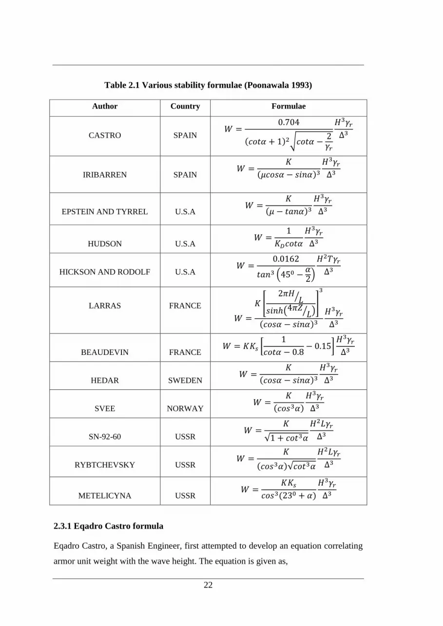
Table 2.1 Various stability formulae (Poonawala 1993)
Author Country Formulae
CASTRO
SPAIN
IRIBARREN
SPAIN
EPSTEIN AND TYRREL
U.S.A
HUDSON
U.S.A
HICKSON AND RODOLF
U.S.A
LARRAS
FRANCE
BEAUDEVIN
FRANCE
HEDAR
SWEDEN
SVEE
NORWAY
SN-92-60
USSR
RYBTCHEVSKY
USSR
METELICYNA
USSR
2.3.1 Eqadro Castro formula
Eqadro Castro, a Spanish Engineer, first attempted to develop an equation correlating
armor unit weight with the wave height. The equation is given as,

23
3
3
2 2cot1cot
704.0
r
r
HW
....................................... (2.1)
Where,
W is weight of individual armor unit in metric tons, H is design wave height in
meters, r is specific weight of armor unit in ton per cubic meter, is angle of
breakwater slope and is relative mass density of armor.
This formula was based on theoretical assumption that destructive action of wave is
proportional to its energy and the stability of units under wave action is inversely
proportional to a function of the angle of slope. This formula yielded very small
values of W and engineers rejected this formula thus it was not used for practical
application.
2.3.2 Hudson formula
Hudson (1959) developed a simple expression for the minimum armor weight
required for a given wave height. The stability formula was developed by equating the
total drag and inertial force of wave to the relevant component of the weight of the
individual unit. This may be written in terms of the armor unit mass (W) and design
wave height (H).
3
3
cot
1
r
D
H
KW
.................................................. (2.2)
Where,
W is weight of individual armor unit in metric tons, KD is stability coefficient which
varies with the type of armor unit and H is design wave height in meters.
A range of wave heights and periods were studied. In each case, the value of KD
corresponds to the wave condition representing worst stability condition. The KD
value mainly depends on the shape of armor unit which includes friction between the
units.

24
Some of Hudson’s conclusions were:
i. The formula could be used more accurately for no damage and no overtopping
criteria. No damage means that a maximum of one percent of armor stones can
only be displaced from their initial position when subjected to wave attack of
design wave height.
ii. KD equal to 3.2 (non-breaking condition) is adequate for angular quarry stone
armor, which includes the safety factor also.
iii. The stability of rubble mound breakwater is not significantly affected by the
variation in relative depth (d/L) and wave steepness (H/L) ratios.
With the improvement in the investigation techniques, better insight into the wave-
structure interaction and the development of measurement instruments, many
investigators have pointed out that certain aspects of Hudson’s formula needed
improvement or updating. These can be briefly put under:
a. Hudson’s formula was developed considering regular waves and does not include
the effect of irregular waves. He also has not specified the wave height of
irregular wave train to be considered for the design.
b. The formula was developed to represent the behavior of natural rock type armor
units which basically depend upon their weight for stability under wave attack.
The validity of the formula for artificial armor units depending primarily on
interlocking for stability (e.g. Dolos) is thus a debatable point.
c. The influence of the variables such as wave period, duration of the storm, degree
of overtopping, damage history, friction, porosity of armor units, permeability of
core and randomness of incident waves were not considered in his stability
equation. Therefore it was argued that the value of KD is too simple to represent
the stability of armor units and should only be accepted as a first approximation
Bruun and Gunbak (1976). Further wave steepness, which has a significant role
in determining the stability, was also neglected by Hudson (1959).
In spite of the above drawbacks, Hudson’s formula is the simplest and widely adopted
means of obtaining a good preliminary estimate of the weight of armor units. It

25
requires only two quantities which need to be estimated, i.e. wave height and KD.
However, the design has to be substantiated by the model testing before finalizing the
cross section of a breakwater.
2.3.3 Van der Meer equations
Van der Meer (1988) derived formulae which include the effect of random waves,
wave periods and a wide range of core / underlayer permeability. The investigations
by Van der Meer showed clear dependence of wave period on erosion damage. Two
design formulae were obtained in terms of Hudson’s stability number considering the
tests performed by him and the results of Thompson and Shuttler (1975).
For plunging waves,
5.0
2.0
18.0
50
2.6
m
n
S
N
SP
D
H ………………...……………...……. (2.3)
For surging waves,
P
m
n
s
N
SP
D
H)(cot0.1
5.0
2.0
13.0
50
…………….….…………… (2.4)
Where, the parameters not previously defined are:
Hs = Significant wave height
Dn50 = Nominal diameter of the armor unit
P = Permeability of the structure
S = Design damage number = Ae/D2n50
Ae = Erosion area from profile
N = Number of waves
m = Iribarren number = tan/ Sm½
Sm = Wave steepness for mean period = 2πHs/gTm2.
Tm = Mean wave period

26
And the transition from plunging to surging waves is calculated using a critical value:
)5.0/(131.0 tan2.6
P
m P …………………………..…..…… (2.5)
These formulae developed by Van der Meer included the parameters such as wave
period, storm duration, random wave conditions and a clearly defined damage level.
The starting level of damage, S = 2 to 3, is equal to the definition of no damage in the
Hudson’s formula. Van der Meer considered storm duration of 5000 to 7000 waves
during his investigations. Van der Meer formulae, though versatile, parameters like
permeability are difficult to evaluate and quantify to a degree of accuracy required for
design. This has limited the use of this new formula for the design of breakwaters.
2.3.4 Other design formulas
2.3.4.1. Sherbrooke University Formula
Sherbrooke University Formula (Belfadhel et al. 1996) is derived from Hudson’s
formula by replacing KD with actual percentage of damage within the active zone.
This was developed for regular waves on both steep (1.5:1) and flat (2.5:1) slopes.
6.031.23
3
50cot
88.1
Pd
HW Dr
............................................... (2.6)
Where, HD is design wave height and Pd is percent damage within the active zone
delimited by an elevation of one wave height below and above the water level.
2.3.4.2 Koev Formula
Koev (1992) derived a stability equation based on statistical analysis of 21 formulas
developed earlier for breakwater armor design using regular waves. This formula is
also similar to Hudson’s formula with KD replaced by wave steepness (H/L).
3843.05667.13
3
50
cot
1421.0
LH
HW Dr
........................................ (2.7)
The equation is valid for wave steepness ranging from 0.04 and 0.1 and slope (cot)
between 1.1 and 20.

27
2.3.4.3 Kajima’s Stability Formula
Kajima (1994) proposed the following expression of stability number applicable to
Tetrapods for horizontally composite breakwaters (Hanzawa et al. 1996).
5.016.05.0
3/1 /5.8 NSDHN ns .............................................. (2.8)
Hanzawa et al. 1996 tested the above equation with their model test results and found
no good agreement. The reasons for the disagreement given by them were, the
equation was formulated to cover a range of relatively high damage level which is
usually not seen in the ordinary design of port structures, and the water depth of the
structure Kajima investigated was greater than their test data which resulted in a
bigger cross section affecting the parameter S.
2.3.4.4 Melby and Hughes formula
Melby and Hughes (2004) used the maximum depth integrated wave momentum flux
(Nm) to describe the armor stability. The new equations explicitly included the effects
of nearshore wave height, wave period, water depth, and storm duration as well as the
characteristics of wave breaking on the structure (Melby, 2005).
cot0.52.0
18.0zm NSPN
sm smc .......................... (2.9)
3/5.02.018.0 cot0.5 P
m
P
zm sNSPN
sm < smc ........................... (2.10)
where smc = – 0.0035 cot + 0.028
50
2/12
max
)1( nr
wFa
mD
h
S
hMKN
.................................................... (2.11)
With Ka = 1. Here MF = wave momentum flux, smc = critical wave steepness on the
structure, P = structure permeability, S = damage level, w = water specific weight, Nz
= t/Tm = number of waves at mean period during event of duration t. Tm = mean wave
period, sm = Hs/Lm = wave steepness, Hs = significant wave height, Lm = wavelength
based on mean wave period, and = seaward structure slope from horizontal.
Also,
1
2
max
2
A
oF
gT
hA
gh
M
.................................................... (2.12)

28
Where,
0256.2
6392.0
h
HAo
and
391.0
1 1804.0
h
HA
2.3.4.5 Van Gent formulae (2003)
Van Gent et al. (2003) gave a single simple stability formula than the Van der Meer
formulas (1988). The influence of wave period was found to be small and hence they
did not consider it in their equation. The permeability parameter is replaced by a
structure parameter i.e., diameter of core material. The equation is given as:
3/2
50
50
2.0
50
1cot75.1
n
coren
n
s
D
D
N
S
D
H ....................................... (2.13)
The influence of filters in considering the permeability was neglected. The equation is
limited to following conditions:
Hs/Dn50 = 0.6 – 4.3; m = 1.0 – 5.0; Dn50core /Dn50 = 0 – 0.3; and slope = 1:2 to 1:4.
2.3.5 Improvements in breakwater design
Along with physical model studies few researchers (Haan 1989, Hegde 1996, Mase et
al. 1995, Melby 2005, Kim et al. 2007, Mandal et al. 2007, Balas et al. 2010, Van
Gent et al. 2011) had started developing mathematical and numerical models for the
design of breakwater structures.
Kobayashi and Jacobs (1985) developed a mathematical model to predict the flow
characteristics in the downrush of regular waves and the critical condition for
initiation of movement of armor units. The effect of bottom friction, permeability,
water depth and wave overtopping were not considered for modeling. They concluded
that the mathematical model could be a supplement for hydraulic model tests and
empirical formulas.
Haan (1989) developed a computer package for optimum design of rubble mound
breakwater. The program included all the parameters required for design and the
armor weight was calculated based on Van der Meer formula.
Mase et al. (1995) examined the applicability of neural network for prediction of
stability of rubble mound breakwaters. They found good agreement between the
predicted and measured stability numbers.

29
Hegde (1996) also developed a mathematical model called DORUB to predict the
armor stone weight of a rubble mound breakwater using the quarry yield optimally.
He used programming language C and Visual basic to draw the cross section.
Yagci et al. (2005) developed three ANN models and a fuzzy logic model to study the
breakwater damage ratio. Damage ratio is defined as the ratio of the displaced armor
to total armor units in the section. It was observed that all the four models predicted
the damage ratio fairly well compared to the experimental values. It was suggested
that ANN performance can be further enhanced with the extension of training data set
by considering the data for all slopes.
Kim et al. (2007) used Probabilistic Neural Network (PNN) to predict the stability
number of breakwater and assess its performance. It was proved that PNN provided
more advanced results than the empirical model and ANN in estimating the stability
number of breakwaters.
Mandal et al. (2007) also have concluded that the neural network can predict the
stability of a breakwater better than the empirical formula with higher correlation
coefficient for ANN models compared to Van der Meer formula. Some upgraded
algorithms like LMA (Levenberg-Marquardt Algorithm), SCG (Scaled Conjugate
Gradient) and GDA (Gradient Descent with Adaptive learning rate) were also tested
for enhancing the prediction capability of stability and found that LMA showed better
improvement compared to other two algorithms. The network developed predicted a
relatively lesser armor weights compared to empirical model.
Etemad-Shahidi and Bonakdar (2009) developed a M50 machine learning method for
designing a rubble mound breakwater. It was observed that the performances of the
proposed model trees were better than those of previous empirical and the soft
computing methods in predicting the stability of rubble mound breakwater.
Artificial neural networks based on principal component analysis, fuzzy systems and
fuzzy neural networks can be adopted for preliminary design of rubble mound
breakwaters as suggested by Balas et al. (2010). However, they have emphasized the
hydraulic model tests for the final design, since; the safety of coastal structures is

30
highly variable and depends upon the unpredictable nature of wave-structure
interaction.
2.4 STABILITY OF RUBBLE MOUND BREAKWATER
The main governing parameter of the armor layer stability is the stability number. The
stability of a breakwater is derived from Hudson’s formula which can be rearranged
to get,
3/1
50
cotD
n
s
s KD
HN
……………….……………. (2.14)
Where, Ns = Hudson’s stability number,
3/1
50
r
n
WD
……………………………………………. (2.15)
The wave height commonly used in this formula is the significant wave height, H1/3 or
Hmo (Hmo is the estimate of significant wave height deduced from spectral
information). The value of Ns is usually established by testing the breakwater until its
damage reaches equilibrium. To attain this equilibrium, the time series of the sea state
may have to be recycled many times. The number of times it is recycled is also an
important parameter to be taken into account.
Van der Meer (1988) gives the examples of types of structures with corresponding
H/ΔD values as:
H/ΔD < 1, Caissons or seawalls
H/ΔD = 1 – 4, Stable breakwaters
H/ΔD = 3 – 6, S- shaped and berm breakwaters
H/ΔD = 6 – 20, Rock slopes / beaches
H/ΔD = 15 – 100, Gravel beaches
H/ΔD > 500, Sand beaches and Dunes
2.4.1 Factors affecting the stability of non-overtopping breakwater
The factors affecting the stability can be classified under environmental conditions
and structural conditions as coined by various authors (Hudson 1959, Van der Meer
1988, Losada 1990, Bruun 1981, CEM 2006). After reviewing the literature on the

31
breakwaters, it is observed that large number of parameters affect the stability and
hence the design of breakwaters. The various factors affecting the stability of
breakwaters are given below.
a) Environmental Variables
i. Wave characteristics
ii. Water depth
iii. Duration of wave attack
iv. Wave run-up and run-down
b) Structural Variables
i. Geometry of the breakwater
ii. Permeability of the structure
iii. Method of construction
iv. Foundation
2.4.1.1 Wave characteristics
Wave characteristics of a wave include wave height and wave period. The important
parameter which affects stability is the wave height. The wave height used in most of
the design formulas is the wave height measured in front of the structure and the
armor stone weight required in conventional breakwater is directly proportional to H3.
The wave forces of higher waves caused instability of armor units thus indicating that
generally damage increases with increasing wave height.
Wave period is another parameter which affects the stability indirectly through some
related parameters like wave steepness, wave breaking characteristics, etc. Wave
period was not considered by Hudson in his formula. The wave period is often
described by a dimensionless variable, wave steepness (s) or surf similarity parameter
(ξ). Wave steepness, s, can be defined by the ratio of deep water wave height to the
deep water wave length and is given as,
2
2
gT
Hs
....................................................................... (2.16)
Iribarren defined the similarity parameter, ξ, relating wave steepness, s to the slope
angle of the structure, tan, given as,
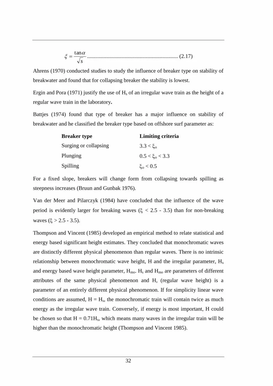
32
s
tan .................................................................. (2.17)
Ahrens (1970) conducted studies to study the influence of breaker type on stability of
breakwater and found that for collapsing breaker the stability is lowest.
Ergin and Pora (1971) justify the use of Hs of an irregular wave train as the height of a
regular wave train in the laboratory.
Battjes (1974) found that type of breaker has a major influence on stability of
breakwater and he classified the breaker type based on offshore surf parameter as:
Breaker type Limiting criteria
Surging or collapsing 3.3 < o
Plunging 0.5 < o < 3.3
Spilling o < 0.5
For a fixed slope, breakers will change form from collapsing towards spilling as
steepness increases (Bruun and Gunbak 1976).
Van der Meer and Pilarczyk (1984) have concluded that the influence of the wave
period is evidently larger for breaking waves ( < 2.5 - 3.5) than for non-breaking
waves ( > 2.5 - 3.5).
Thompson and Vincent (1985) developed an empirical method to relate statistical and
energy based significant height estimates. They concluded that monochromatic waves
are distinctly different physical phenomenon than regular waves. There is no intrinsic
relationship between monochromatic wave height, H and the irregular parameter, Hs
and energy based wave height parameter, Hmo. Hs and Hmo are parameters of different
attributes of the same physical phenomenon and H, (regular wave height) is a
parameter of an entirely different physical phenomenon. If for simplicity linear wave
conditions are assumed, H = Hs, the monochromatic train will contain twice as much
energy as the irregular wave train. Conversely, if energy is most important, H could
be chosen so that H = 0.71Hs, which means many waves in the irregular train will be
higher than the monochromatic height (Thompson and Vincent 1985).

33
The study of Ahrens (1975) as reported by Van der Meer (1988) in large wave tank
showed the importance of the wave period on the stability of riprap. The tests were
performed with the regular waves.
Pilarczyk and Zeidler (1996) gave the critical values of inshore surf similarity
parameter, b for different types of breaker for plane profile as:
Breaker type Limiting criteria
Surging 3.0 – 3.5 < b
Collapsing 2.0 < b < 3.0 – 3.5
Plunging 0.5 < b > 2.0
Spilling b < 0.5
Vidal et al. (2006) based on their experimental study have shown that wave height
parameter H50, defined as the average wave height of the 50 highest wave reaching a
rubble mound breakwater in its useful life, can describe the effect of the wave height
on the history of the armor damage caused by the wave climate during the useful life
of the structure.
2.4.1.2 Water depth
Water depth in front of structure has a major effect on its stability. If depth of water is
small then waves shoal and loose their energy due to bottom friction but deeper water
can sustain higher waves which can break close to the breakwater structure resulting
in increased wave run-up and run-down causing higher damage to the structure.
Weight of armor may be reduced by one-fourth at depth below one-third of the toe
depth and by three-fourth below two-third depth (Palmer and Walker 1976).
As reported by Van der Meer (1998) from Van der Meer (1988) for depth limited
condition it is suggested to use H2% rather than Hs to describe the stability of
breakwater.
2.4.1.3 Duration of wave attack
Font (1968) found that the damage generally increased as the duration of exposure
increased. But, it was also observed that for shorter duration of wave exposure the
amount of damage was high indicating that the shorter exposure might improve the

34
interlocking thus making the structure more resistant to longer exposure of the same
wave.
Van der Meer and Pilarczyk (1984) have concluded that with random waves a stable
profile could not be found with less than 10,000 waves where as for regular waves
equilibrium profile is generally found within 1000 - 2000 waves.
Hall (1994) in his experiments on dynamically stable breakwaters considered a storm
duration of 3000 waves. This was based on the studies previously done by Hall and
Kao (1991).
Hegde (1996) concluded that the conventional breakwater will have a stable profile
after about 3000 waves.
2.4.1.4 Wave run-up and run-down
The wave action and breaking on the slope cause wave run-up and run-down (Fig.
2.1). Run-up and run-down heights are defined as the vertical distance from the still
water level to the crest and trough of the up- and down-rushing wave.
Fig. 2.2 Definition sketch of Wave Run-up (Ru) and Wave run-down (Rd)
The effects of the permeability and the roughness of the rubble-mound face are
important factors in wave run-up (Hudson 1958). For a given structure slope as the
wave steepness decreases, the relative wave run-up increases (CERC 1966).
Saville (1957) suggested an iterative method for calculation of wave run-up on
composite slopes due to regular waves. The method proposed to consider an
equivalent straight slope from the bottom to the point of maximum initial run-up on
the structure. The initial run-up is estimated for the initial bottom slope of the
breakwater. This process is repeated till same values of run-up are obtained between
two successive iterations. Saville limited the application of composite- slope method

35
for berms with a length less than L/4, where L is the design wavelength for the
structure.
As quoted by Bruun and Gunbak (1976), Saville (1953) has concluded that effect of
water depth is negligible when d/H > 3.0 for all wave steepness. Wave run-up
increases with increasing values and trends gets milder at high values. Run-down
also increases with increasing values and becomes nearly constant at high values
( > 4.0). Higher run-down was observed for cot = 3.0 than for cot = 2.0 at the
breaking range when < 3.0 (Bruun and Gunbak 1976). The reason quoted by them is
that the water running up and down on the 1 in 3 slope travels a longer distance than
on the 1 in 2 slope which may cause a higher possibility of penetration of water deep
into the breakwater body and thus cause a deeper run-down on the 1 in 3 slope.
For breakwaters of slope 1:1.5, maximum run-up could be up to 1.8 times depth of
water (Palmer and Walker 1976).
Losada and Gimenez-Curto (1981) gave a general form of wave run-up and run-down
studying the data corresponding to Ahrens and McCartney (1975) and Gunbak (1979).
They found that wave run-up, run-down and surf similarity parameter is exponentially
related as,
.exp1 BAH
Ru ....................................................................... (2.18)
.exp1 BAH
Rd ....................................................................... (2.19)
The coefficients A and B are to be fitted by Least-square method.
Various graphs were provided by Shore Protection Manual (SPM 1984) for
calculation of wave run-up on a slope due to regular waves. For irregular waves a
method suggested by Ahrens (1977) was adopted.
Armor damage due to displacement occur mainly due to run-down for steep slopes
and run-up is damaging for flatter slopes i.e., cot > 3.5 (Sorensen and Jensen 1986).
Leenknecht et al. (1992) mentioned an empirical formula given by Ahrens and
McCartney (1975). The related the run-up and surf similarity parameter by a non-
linear relationship.

36
b
a
H
R
i
u
1....................................................................... (2.20)
Where, a, b are empirical coefficients associated with the type of armor unit. The
values are listed in Table 2.2.
Table 2.2 Values of wave run-up coefficients for rough slope
(Leenknecht et al. 1992)
Armor material a b
Riprap 0.956 0.398
Rubble (Permeable – No core) 0.692 0.504
Rubble (2 layers – Impermeable Core) 0.775 0.361
Modified Cubes 0.950 0.690
Tetrapods 1.010 0.910
Dolosse 0.988 0.703
Van der Meer and Stam (1992) studied the effects of various parameters viz. wave
height, wave period, slope angle, water depth, structure permeability and spectral
shape on wave run-up on smooth and rock slopes. An empirical relationship between
wave run-up and surf similarity parameter was developed given as,
m
s
ux aH
R for m 1.5....................................................................... (2.21)
c
m
s
ux bH
R for m 1.5....................................................................... (2.22)
The coefficients of wave run-up levels are given in Table 2.3.
Table 2.3 Coefficients of wave run-up levels
Level (%) a b C
0.13 1.12 1.34 0.55
1 1.01 1.24 0.48
2 0.96 1.17 0.46
5 0.86 1.05 0.44
10 0.77 0.94 0.42
Significant 0.72 0.88 0.41
Mean 0.47 0.60 0.34

37
Hughes (2004) considered momentum flux parameter and developed an empirical
formula to compute wave run-up for both regular and irregular waves. Hughes stated
that existing wave run-up formulas for regular waves based on Iribarren number
performed well for milder slopes but poorly for steeper slopes.
2/1
2)(
gh
MCF
h
R F
....................................................................... (2.23)
Where, C is an unknown constant, F() is a function of slope angle to be determined
empirically and MF = wave momentum flux.
The Hughes (2004) formula was applied to old regular wave data of Granthem (1953)
and Saville (1955) and following relation was obtained.
2/1
2tan84.3
gh
M
h
R F
................................................................ (2.24)
Influence of scale effect on wave run-up was studied by Schüttrumpf and Oumeraci
(2005) and found that their effect is negligible under usual model conditions.
Muttary et al. (2006) found that wave run-up is closely related to clapotis height in
front of the breakwater. An empirical equation relating wave run-up and reflection
coefficient was developed given by,
)1( ri CaHR ......................................................................... (2.25)
Where, ‘a’ is a coefficient and its value is 1.31 for regular and 1.17 for irregular
waves. Hi is the incident wave height, Hr is the reflected wave height and Cr is
reflection coefficient (Cr = Hr/Hi). The Eq. 2.24 is applicable for non-breaking waves
and little or no-overtopping conditions. The empirical coefficient ‘a’ between 1.2-1.3
is only applicable for 1:1.5 slopes.
Wave run-down on rock slopes, as per CEM (2006), is given by
)60(15.0%2 5.12.1tan1.2 oms
s
d ePH
R ............................... (2.26)
38
2.4.1.5 Geometry of breakwater
The thickness of the structure is important for wave energy absorption as reported by
Hunt (1959). It was found that wave energy absorption by the structure continued up
to a thickness of 2d, where d is the water depth.
Losada & Gimenez-Curto (1981) concluded that for each type of armor unit, an
optimum slope of maximum stability exists. The greater the interlocking among armor
units, the steeper the optimum stability slope.
Van der Meer (1987, 1988) has concluded that if fine material can’t erode through the
armor layer then the stability of the armor layer is not influenced by the grading and
size of filter layer.
Hall (1987) as quoted by Hall and Kao (1991) concluded that thicker armor layer is
very effective in reducing internal differential pressure in a stable breakwater.
The trapezoidal shape was found to be optimum for rubble mound breakwaters
(Pilarczyk and Zeidler 1996).
2.4.1.6 Permeability of the structure
The porosity of the armor layers, underlayers, core and filter materials is an important
factor in the stability of a rubble structures. The permeability/porosity of the structure
has large influence on stability as shown by Hudson (1958), Hedar (1986), Thompson
& Shuttler (1976), Bruun and Gunbak (1977), Van der Meer (1988), Hegde (1996).
Hudson (1958) found that permeability and the roughness of the rubble-mound face
are important factors in wave run-up.
Van Gent (1992) in his report derived some equations to describe the motion of wave
on permeable structures and developed a model based on these equations. The model
developed was tested on permeable and impermeable berm breakwater and
submerged breakwater.
Hegde and Srinivas (1995) experimentally found that core porosity affects stability
and wave run-up of a structure. With the increased porosity the stability was found to
increase and wave run-up was found decreasing. The reasons for such a behavior as

39
quoted by Hegde and Srinivas (1995) were large inflow and high energy dissipation
within the core of the structure.
2.4.1.7 Method of construction
Randomly placed armor stones or pell-mell construction would have less stable
compared to those placed with special care. The method of placing units randomly,
affects the stability and repeatability of tests was proved by Thompson and Shuttler
(1976) during their experiments.
Very often rubble mound breakwater design seems to be a result only of stability
considerations corresponding to design wave conditions. Designers tend to put too
little emphasis on practical problems related to construction, maintenance and repair.
Based on the studies by Burcharth and Rietveld in 1987 on the different methods of
construction process have found that during construction of seaward slope of
breakwater, each armor block takes about the same time to place, independent of its
weight over a fairly wide range, and savings can be achieved by placing fewer and
heavier concrete blocks on a steeper slope than a relatively lighter natural stones over
a gentler slope depending upon the site conditions and wave climate.
Palmer and Walker (1976) investigated type of placement, on the stability. The
required weight of loosely placed stone may be two times that of a well placed stone,
and keyed and fitted armor is several times more stable than loosely placed armor.
2.4.1.8 Foundation
Breakwater over a weak foundation is less stable and has an undue settlement. If the
underlying material is too weak to withstand the superstructure, wedges of material
will be displaced which might result in uneven settlement due to which there will be
instability to the rubble mound. PIANC (1976) suggested some methods to strengthen
the foundation and improve the stability of rubble mounds like, removal of unsuitable
material or replacing it by sand or gravel, increasing the stability by providing sand
columns etc. Many researchers also suggest alternative structures like berm
breakwater, pile breakwater, submerged structure etc.

40
2.5 DAMAGE OF RUBBLE MOUND BREAKWATERS
‘Damage’ quantification is essential for the qualitative and quantitative analysis of
stability of rubble mound structures. There are various types of damage to breakwater
that will lead to its failure. Fig. 2.3 shows the different failure modes of a rubble
mound breakwater. The armor unit instability is the most critical among all the
failures since its causes the disintegration of armor layer and further progressive
failure making the breakwater unstable (Kamali and Hashim 2009). This section is
mainly concentrated on damage of the breakwater due to armor layer instability.
Fig. 2.3 Failure modes of a rubble mound breakwater (Burcharth and Liu 1995)
As quoted by Bruun (1985), Iribarren defined that a rubble mound reached its failure
when the armor units of the secondary layer are exposed. Hudson (1959) defined no
damage condition as maximum 1% of displacement of armor stones from its initial
position. The percentage of damage is the number of displaced stones divided by the
number of stones in the attacked area (SWL + H and SWL – H) times hundred as per
Van de Kreeke (1969).
If the number of units seems to rock and move a distance which was less than the
overall size of the unit, it was considered as stable damage, if the distance was greater
than that size, it was considered as unstable damage according to Ouellet (1972).
Thompson and Shuttler (1976) defined a damage parameter N as ‘the number of Dn50
sized spherical stones eroded from the slope which was obtained by dividing the
product of the bulk density, and the eroded volume by the size of a spherical stone’.

41
350
50
6
9
na
bn
D
AeDN
....................................................................... (2.27)
where, a = mass density of armor units, b = bulk density of armor units, Dn50 =
nominal diameter of the armor units. The damage parameter is independent of the size
of the armor layer (i.e., length above and below water level and thickness) and also
N is directly related to the erosion area and stone size. The measurement of the bulk
density in prototype is one of the major disadvantages of this formula.
‘Damage’ is also represented as damage parameter, D%, defined as percentage of
armor units displaced from the cover layer by the wave action (Hudson 1958). CEM
(2006) revised this definition with respect to rock and concrete armor units. For rock
it is taken as percentage of eroded volume and for concrete units as percentage of
units more than Dn within some restricted area around Still Water Level (SWL). This
specific zone around SWL is also called active zone. In case of emerged breakwaters,
most displacements occur approximately in the area from one Hs below SWL to one
Hs above SWL and the number of units placed in this zone is often used as the
reference number (CEM 2006). The area between the middle of the crest to one Hs
below SWL was considered as active zone in the Shore Protection Manual (SPM
1984). These definitions of active zone are not applicable to Low Crested Structures
or submerged barriers. Moreover, due to different designs, total number of armor
units differs for each structure; and varying definition of damage computed through
various studies cannot be compared. The range of values of damage parameter for
different armor units are given in CEM (2006) are presented in Table 2.4.
Table 2.4 Damage parameter “D” for two-layer armor (CEM 2006)
Unit Slope Initial Damage Intermediate Damage Failure
Rock 1:2 – 1:3 0 – 5% 5 – 10% > 20%
Cube 1:1.5 – 1:2 -- 4% --
Dolosse 1:1.5 0 – 2% -- ≥ 15%
Accropode 1:1.33 0% 1 – 5% ≥ 10%

42
Van der Meer (1988) used a relation to measure the damage in terms of area of
erosion (Refer Fig. 2.4), which is as follows,
Damage level, SA
Dn
50
2
....................................................................... (2.28)
Where, Ae is the erosion area and Dn50 is the nominal diameter of the stones.
The limit of damage (S), for rocks, observed by Van der Meer (1988) is given in
Table 2.5.
Table 2.5 Van der Meer damage criteria
Slope Initial damage Intermediate damage Failure
1:1.5 2 3 – 5 8
1:2 2 4 – 6 8
1:3 2 6 – 9 12
1:4 to 1:6 3 8 – 12 17
Fig. 2.4 Erosion area and damage level, S (Van der Meer 1988)
Relative damage number, Nod, is defined as the number of units displaced within a
vertical strip of width Dn (Dn = equivalent armor size) stretching from the bottom to
the top of the armor layer (Van der Meer 1988). This relative damage number is
generally used to define damage of artificial armor units. This definition of damage
can be easily related to a percentage of damage. Nod gives the actual damage, which is
related to the number of units in a cross section with a width of Dn50. Table 2.6 gives
the limit of the Nod values for initial damage condition and failure of the structure
with different armor units. The disadvantage of Nod is its dependency on the slope
length (CEM 2006).
............................................... (2.29)

43
Table 2.6 Damage level by Nod for two – layer armor (CEM 2006)
Units Slope Initial damage Failure
Cube 1:1.5 0 2
Tetrapods 1:1.5 0 1.5
Accropode 1:1.33 0 0.5
Van der Meer (1988) experimentally determined relationship between Nod and S for
different armor units as,
Cubes, Slope 1:1.5, Nod = (S-0.4)/1.8
Tetrapod, Slope 1:1.5, Nod = (S-1)/2
Accropode, Slope 1:1.33, Nod = (S-1)/2
Since profile measurement is not commonly adopted for damage calculation of
artificial armor units, damage level (S) cannot be used for them to quantify the
damage (Bakker et al. 2009).
Unit movement may take place in different ways and each has different contribution
to damage. Some of the units may displace out of layer and completely fail to perform
their function. While, some units displaced from their original position may still
remain in the eroded area and reach a stable position. In this case, the displaced units
may still contribute effectively to the slope protection by still remaining in the slope
covering the secondary layer. Counting method considers all the displaced units as
damage regardless of their new position, while profile measurement does not take the
units displaced but remains in the eroded area as damage. To reach a conclusion, it
should be considered that any type of unit displacement reduces the layer integrity.
Hence, counting method can lead to damage overestimation on one hand, and
profiling method may gives underestimated damage on the other hand.
Gómez-Martín and Medina (2013) adopted a new method of damage calculation
which was suggested by Gómez-Martín and Medina (2006). The new method was
named as ‘Virtual Net Method’. In the Virtual Net method a virtual net will be
projected over a photographed armor layer (Fig. 2.5). The armor layer will be divided
into strips of a constant width. The width (a=m*Dn) and length (b=k*Dn) of each strip

44
are calculated. The number of armor units within each strip (Ni) is counted, and the
porosity of each strip is estimated using Eq. 2.30, before and after the wave attack.
Next, the dimensionless armor damage in each strip (Di) is calculated using Eq. 2.31.
The overall damage is then calculated using Eq. 2.32. The virtual net method
considers armor unit extraction, armor layer sliding as a whole. The applicability of
the virtual net method in case of berm breakwaters is not viable as projecting a virtual
net over the photographed armor layer is difficult because of presence of berm.
i
2
50nii 1
ab
DN1p .................................................... (2.30)
0
i
i0
ii
p1
p11n1nD
....................................... (2.31)
ie DD ...................................................................... (2.32)
Where, p0 and pi are porosities before and after the wave attack,
Ni is number of armor units in strip ‘i’,
a and b are strip height and strip width
0i and i are packing density before and after the wave attack,
n is times of strip width equivalent to cube size.
Di and De are Dimensionless damage of each strip and equivalent damage
Fig. 2.5 Designed virtual net using Photoshop (Vanhoutte 2009)

45
2.6 BERM BREAKWATERS
2.6.1 Evolution of berm breakwaters
Berm breakwaters are different from the conventional breakwater with the presence of
horizontal berm at or above SWL as shown in Fig. 2.6. The conventional breakwaters
are designed in such a way that no damage or only little damage is allowed on the
structure. This criterion necessitates the use of heavy and bulky rock or artificial
concrete elements for armoring. The availability of large rock is seldom and even
though if they are available transporting and placing them on the structure will be a
problem which requires heavy equipments. The use of artificial armor unit as an
alternative would also be a costly affair, since, the mould for casting and special
equipments for lifting and placing costs come into picture. Thus, an alternative would
be a safe and economical section where smaller size stones could be used.
Fig. 2.6 Conventional vs. berm breakwaters
The berm breakwater which has an advantage of using lighter weight of the armor
stones can be an alternative for the conventional rubble mound breakwater with heavy
rocks or artificial armor units. The main concept of berm breakwater lies in the fact
that the highly porous horizontal berm acts as a sacrificial member absorbing most of
the wave energy thus reducing the impact of waves on the slope which in turn
increases the stability of the structure.
Their natural response to hydrodynamic loads makes them economically attractive
because, rock of lesser weight can be used in these types of breakwaters. The
movement of material which results in sorting and nesting maximizes the inter-
particle interlocking and the subsequent reforming of the profile that increases the
stability of this structure (Van Gent 1993). The berm breakwater can be designed to
optimize the utilization of the available quarry material for the available construction

46
equipment. Berm breakwater performs better than the conventional structures when
exposed to waves exceeding design conditions.
The berm breakwater concept is also relevant to many hot climate port locations
where only relative small size rocks are available due to rock degradation. In many
cases the total construction and repair costs are significantly lower for a berm
breakwater compared to a conventional rubble mound breakwater, especially in hot
climate locations and in large water depths (Andersen 2006).
A berm breakwater is considered to be a very rigid structure as it is very difficult to
destroy, even a dynamically stable berm breakwater, by incoming head-on-waves,
unless the structure is overtopped or the berm is too narrow. A conventional rubble
mound breakwater fails easily and rapidly and repair operations are more difficult.
The highly absorbing porous berm media and a flat slope around the water level gives
very less reflection from a berm breakwater providing a better maneuvering condition
at the entrance and less scour in front of the structure. Further, wave run-up and
overtopping are smaller than that for a conventional straight and steeper breakwater
slope.
One of the many advantages of berm breakwater is that the design is mainly supply
based rather than demand based. The design of berm breakwater is governed by the
available quarry yield in the field rather than computed quarry yield by a designer.
The specifications should therefore be functional specifications, not demand
specifications (CIRIA 2007).
The berm breakwaters may be divided into three categories:
Statically Stable Non- Reshaped: In this condition few stones are allowed to
move, similar to the condition for a conventional rubble mound breakwater. The
H/D value is less than 1.5 for this type of breakwater (PIANC 2003).
Statically Stable Reshaped: In this condition the profile is allowed to reshape into
a profile, which is stable and where the individual stones are also stable. The H/D
value ranges from 1.5-2.7 for a statically stable reshaped breakwater (PIANC
2003).
Dynamically Stable Reshaped: In this condition, the profile is reshaped into a
stable profile, but the individual stones may move up and down the front slope.

47
The H/D value is more than 2.7 for a dynamically stable reshaped berm
breakwater (PIANC 2003).
The first berm breakwaters built were with a homogeneous berm. Fig. 2.7 shows the
cross section of a breakwater built in Racine, Michigan (Montgomery et al. 1988).
This breakwater has a large berm in the front part of the breakwater, though the
quarry stones are not very large. Such a design allows for berm deformation which
will end up forming an equilibrium slope. Berm breakwaters like these have been
built in North America, Europe, and other places, and many studies have been carried
out on them (Baird and Hall 1984; Fournier et al. 1990; Burcharth and Frigaard 1987,
1988).
Fig. 2.7 Berm breakwater at Rachine, Michigan (Montgomery et al. 1988)
Along with the development of reshaping berm breakwater a new type of multilayered
berm breakwater also came into existence in Iceland. This structure, named as
Icelandic-type berm breakwater, consists of number of layers of different weights of
armor placed systematically (Refer Fig. 2.8). Icelandic-type berm breakwater falls
into either of the two categories: statically stable non-reshaped berm breakwater and
statically stable reshaped berm breakwater.
Fig. 2.8 Cross-section of the multi-layer berm breakwater under construction at
Sirevag (Torum et al. 2003)
Various studies conducted on different types of berm breakwater are briefed in next
few paragraphs.

48
Earlier studies (Popov 1961, Priest et al. 1964) have demonstrated that S-shape
profiles are more stable than the original uniform slopes from which they develop. It
was found that the stable profile after reshaping intersect the initial plane face at about
0.2 of the still water depth below the still water surface as shown in Fig. 2.9 (Priest et
al. 1964).
Fig. 2.9 Seaward profiles for steep, smooth waves acting upon a breakwater of
concrete cube (Priest et al. 1964)
Bruun and Johannesson (1976) described the hydraulics of S-shaped breakwater and
recommended the use of S-shaped breakwater geometry, instead of continuous single
slope, for an increased safety and economy.
2.6.2 Stability of berm breakwaters
Naheer and Buslov (1983) from their studies concluded that the composite slope
breakwater showed no improvement over the uniform slope, as far as wave run-up
was concerned. They laid out the advantage of composite slope breakwater as the
increase in the stability of the armor layer compared to uniform slope.
Torum et al. (1988) showed that berm breakwater is less sensitive to the variation in
the significant wave height than the conventional breakwater. There was not a sudden
collapse as normally is the case for a conventional breakwater. This is very useful for
a location where there is a significant uncertainty in the wave climate.
Ergin et al. (1989) conducted a series of tests on three slope composite rubble mound
breakwater, and concluded that under the same test conditions, same wave height,
period range, water depth, and same armor stone, the three slope berm type section

49
produce up to 90% less damage relative to the 1:2 single slope section. Also the
increase in wave height of about 2.3 times the design wave height, the alternate
section received damage ranging between 5 to 12% for the wave period tested.
Kao and Hall (1990) found that for armor stones having the same D50 values, the
wave height is the single most important factor affecting the reshaping process of a
dynamically stable breakwater. They also found that narrowly graded armor stones
are less prone to reshaping and the effect of wave period and wave groupiness was
less on berm width eroded and toe length after reshaping.
The mechanical strength (or quality) of rock has to be considered in prototype
designs, especially for dynamically stable structures with large rock, as berm
breakwaters. The quality of the rock is less important for small scale investigation and
may not be considered (Van der Meer 1992).
Van Gent (1993) from his study on reshaping homogenous berm breakwaters with
stone units concluded that rolling of armor units was the dominant failure mechanism
compared to sliding, lifting and rocking.
Torum (1994) made an unsuccessful attempt to measure wave induced forces on
armor units on berm breakwater using Morison type force method. It was found that
forces on an armor unit were drag dominated.
The mobility of armor stones on berm breakwater was extensively studied by
Lamberti et al. (1994), Lamberti and Tomasicchio (1997) and Archetti and Lamberti
(1999). The research was performed within the range of 1.5 < Ho (= Ns) < 4.5. The
main conclusions are summarized as follows:
• When Ho = ~ 1.5 – 2 the armor units on a berm breakwater attains mobility;
• When 2 < Ho < 3 the mobility of stones is low;
• The mobility increases rapidly when Ho > 3;
• When Ho = ~2.7 a berm breakwater will attain a statically stable profile and when
Ho > ~2.7 it reshapes itself into a dynamically stable profile.
Lissev and Torum (1996) from their studies concluded that the core of a berm
breakwater can be extended into the berm. They suggested that with extending the

50
core into the berm a cheaper berm breakwater structure can be obtained since the core
material is cheaper than armor units.
Many researchers opined that waves of smaller wave steepness have highest wave
force and increases berm reshaping to a larger extent (Archetti and Lamberti 1999 and
Juhl and Sloth 1998).
From the studies of Torum on berm breakwater in shallow water Archetti and
Lamberti (1999) concluded that the force of a wave in shallow water is less compared
to deep water even for same significant wave height. This lesser force caused reduced
recession in the structure for shallow water as compared to deep water.
Juhl and Sloth (1998) compared various profiles of berm breakwater (Fig. 2.10). They
concluded that Profile 3 (an armor layer protecting both top and front of berm) was
more effective than both Profile 4 and Profile 1 (hammerhead and thick layer at top of
berm). They also concluded that by increasing armor stone size a reduction in berm
width can be obtained but if fine materials (reduced permeability) are used in top of
the berm or entire berm an increase in berm recession was observed. Also, with
increased berm freeboard reshaping of berm was found to be decreasing even though
there was an increase in berm volume.
Lissev and Daskalov (2000) carried out tests in the Hydraulic Research Laboratory at
the University of Architecture, Civil Engineering with regard to extension of port of
Burgas, the concept of berm type breakwater was offered as an alternative solution of
conventional rubble mound breakwater covered by Tetrapods. They found that final
profile of breakwater depended mainly on stone gradation.
Experiments on statically stable berm breakwaters have shown that increase in berm
width reduces the damage to a large extent and for the same wave parameters the
armor weight required for a berm breakwater can be reduced than that of a
conventional breakwater (Hegde et al. 2002).
The PIANC (2003), according to the results of laboratory tests, reports that the
recession of the berm (Rec) for Icelandic type of berm breakwater structures is larger
to some extent than for the homogeneous berm breakwater when the Dn50 for the
largest stone class is used to calculate HoTo and Rec /Dn50.

51
Fig. 2.10 Different profiles of berm breakwater considered for study (Juhl and
Sloth 1998)
The most used parameters in relation to the stability of berm breakwaters are the
following: (PIANC 2003)
n50
s
osΔD
HHN
.................................................................. (2.33)

52
n50z
n50
soo
D
gT
ΔD
HTH ........................................................................ (2.34)
Where, = (s / w) – 1.
Hs = Significant wave height,
Dn50 = (W50 / s) 1/3
W50 = Median stone weight,
Tz = Mean wave period
s = Density of stone, w = Density of water.
Torum et al. (2003) have considered berm recession as one of the stability parameter
for berm breakwaters expressed as Rec /Dn50.
Tomasicchio et al. (2003) developed a theoretical model to evaluate the stone
abrasion on reshaping armor slopes. The model forecasts the degradation of rock
within the structure’s lifetime and provides a reasonable prediction of volume loss
caused by armor movements. But they neglected the effect of breakage, weathering
and chemical agents on degradation of armor unit.
Rao et al. (2004) from their study on non-reshaping berm breakwaters found that
increased berm width reduced damage to the structure. They found wave period had
greater influence on stability of berm breakwaters. Increase in berm width was found
to be ineffective in reducing wave run-up.
Fişkin (2004) studied the effect of armor stone gradation on stability of berm type
breakwater and found that for a given berm width with increased reduction in stone
size the cumulative local damage on the berm also increased. He also found that
increased duration of wave attack did not affect the damage level of the structure.
Also, when berm was placed above still water level resulted in lower wave run-up and
water spray compared to models with berm below still water level.
Sigurdarson et al. (2006) in their survey mention that Icelandic type berm breakwater
have been built for a design wave height of 7.5 m and further development to design
for a wave height of 8 m is possible through various adjustments depending on the
site conditions. The various adjustments may be use of high density stones or provide

53
tandem breakwater or use of concrete armor units which reduces the reflection,
overtopping as well as loading due to impact waves.
CEM (2006) states that even a damaged rubble mound berm can provide protection to
primary armor layer and if the damage is severe then only it may be required to
redesign the berm using larger units.
Recently study on prediction of stability of berm breakwater using artificial neural
network was undertaken by Mandal et al. (2008). They have concluded that ANN
models predicted the stability more accurately compared to empirical relationships
and berm width is one major parameter affecting the stability. It was suggested that
back-propagation neural network with Levenberg-Marquardt algorithm could be
effectively used as advanced technique for predicting the stability of berm breakwater.
Dijkstra (2008) conducted exhaustive studies on stability of bermed slope
breakwaters. He found that the berm length has a large influence on the stability of
slopes and with the increase in berm length the stability also increases. It was found
that two dominant forces affecting the stability viz. incident waves and the return of
the current after reflection from the structure. The important role played by water
level on these forces was highlighted. When water level is below berm level then
incident forces will be prominent, when water level equals berm level both the forces
will be in balance and when water level is above berm level the return current will be
more prominent than the incident wave force. He also clearly specified that no design
guidelines are available for a bermed slope breakwater and design is mainly
dependent on past experience and model studies. The reason for not having design
guidelines as told by him is the difficulty in modeling of complex processes related to
the stability of the breakwater mainly the return current which has high impact on the
stability of the structure.
Rao et al. (2008) presented the results of an experimental investigation on stability of
non-reshaped berm breakwaters. From the work it was concluded that damage was
relatively significant for shorter period waves in comparison with longer period
waves, in the range of wave steepness from 0.008 to 0.043. The importance of water
level was highlighted and it was found that the structure to be more stable when water

54
depth above the berm was smaller. They also found mild slopes (1:2) being safer than
steep slopes (1:1.5).
Moghim et al. (2011) carried out series of studies on homogenous berm breakwater to
study the influence of various parameters on its stability. They observed that as wave
height and wave period increases the berm recession also increases. They found most
of the reshaping (90% of final reshaping) occurs within storm duration of 3000 waves.
The demonstration by Andersen (2006) about the water depth in front of the structure
was upheld by these researchers stating that larger water depths require larger
deposition volume to dissipate the wave energy. Further, the effect of wave period
was highlighted suggesting that the influence of wave period is less on the reshaping
process.
Van Gent (2013) carried out tests on berm breakwater to develop a stability equation
and to study influence of various berm parameters on its stability. It was found that
when berm is below still water level (low berm) reduction in armor weight is less and
the reduction increases as berm goes above still water level (high berm). It was
observed damage was more near junction of berm and lower slope and in order to
reduce this localized damage it was suggested to consider rounding off the transition
near that junction rather than providing a sharp transition, in order to reduce the
exposure of armor units.
Shekari and Shafieefar (2013) conducted experimental studies on reshaping berm
breakwaters under irregular wave attack. They also have concluded that with increase
in berm width and higher berm elevation above still water level reduces the berm
recession. They have proposed a formula for estimating berm recession considering
various parameters.
2.7 DAMAGE OF BERM BREAKWATERS
2.7.1 Statically stable non-reshaped berm breakwaters
The damage of a statically stable non-reshaped berm breakwater is similar to that of a
rubble mound breakwater which has been dealt in detail in Section 2.5.

55
2.7.2 Statically stable reshaped berm breakwaters
In case of statically stable reshaped berm breakwater, the berm recession and
exposure of underlayer/ secondary layer can be adopted for measuring the damage to
the structure. Since, the structure is allowed to reshape up to a certain extent the
damage parameters explained earlier for a rubble mound breakwater cannot be
applied. Davies et al. (1994) during their studies on damage prediction of rubble
mound breakwaters have given specific reasons for not adopting damage level ‘S’ in
case of reshaped as well as reshaping berm breakwaters. They have quoted that usage
of damage level ‘S’ would loose its relevance since the berm breakwaters are allowed
to reshape. In order to substantiate their statement, they have explained the damage
level ‘S’ considering different thickness of primary layers as shown in Fig. 2.10. A
value of S = 3, as in the Fig. 2.11, could correspond to a deep hole in the armour
layer, or it could represent shallow damage spread over a wider area. So, the damage
level ‘S’ depends mainly on size of the armor and armor layer thickness.
Fig. 2.11 Damage level ‘S’ for different thickness of primary layer (Davies et al.
1994)
In order to overcome the above disadvantage they have suggested measuring the
depth of cover layer (dc) remaining after the wave attack and the minimum depth of
cover at any point of time must not be less than one ‘Dn50’. If the value of ‘dc’ drops
to zero then the damage is considered severe with the exposure of underlayer.

56
2.7.2.1 Berm recession
An important feature of reshaping is the recession of the berm as shown in Fig. 2.12.
Recession (Rec) is the erosion of horizontal berm due to the attack of wave. Hall and
Kao (1991) investigated the influence of stones on the reshaping of the berm. They
arrived at an equation for the recession of a homogenous berm. Torum (1998) gave a
dimensionless recession equation, Rec/Dn50, which was updated by Torum et al.
(1999) when the waves are approaching the breakwater is almost normal to the
breakwater longitudinal axis as:
8.011.0000009.00000027.023
50
oooooo
n
ec THTHTHD
R
............ (2.35)
Where HoTo > 20-30
Fig. 2.12 Definition of Recession (Rec)
Sayao (1999) defines the stability of berm breakwaters as follows, “A stable,
dynamic, berm breakwater is a structure with Wr/B ≈ 1 for the design storm condition,
where Wr = reshaped portion of the berm width, B = berm width (Refer Fig. 2.13).
Thus, if during testing Wr/B ≤ 1, the berm is considered as stable. If the berm
reshapes more than its design width at berm elevation (Wr/B > 1), then the berm is
considered unstable and new tests are performed with an increased B.
Fig. 2.13 Berm parameters (Sayao 1999)
A
hf
Fig. 2.4 Berm Recession

57
As quoted by Torum et al. (2003), Menze (2000) added some terms to the Eq. 2.35 to
take into account the gradation of the stones and the water depth. The recession
equation arrived at is then:
dgoooooo
n
ec ffTHTHTHD
R 11.0000009.00000027.0
23
50
............ (2.36)
Where, Gradation factor, 5.109.2391.915
85
2
15
85
n
n
n
n
gD
D
D
Df and is valid for
1.3 < Dn85/Dn15 < 1.8.,
Depth factor, 0.416.050
n
dD
df , within the range 12.5 < d/Dn50 < 25
Referring to Fig. 2.11, as an approximation, hf can be obtained as (PIANC 2003):
5.02.05050
nn
f
D
d
D
h, within the range 10 < d/Dn50 < 25 .................. (2.37)
Torum et al. (2003) conducted laboratory tests for multilayer berm breakwaters and
calculated berm recession using equation given by Menze (2000) for homogenous
berm breakwater. Fig. 2.14 shows the dimensionless recession relation v/s HoTo for
multilayer berm breakwaters. Torum et al. (2003) concluded that till then no formula
has been developed for calculating berm recession of a multilayered berm breakwater
and hence the equation by Menze (2000) can be considered for feasibility studies.
Further, it was concluded that the smaller stone size is sufficient for large density
stones compared to small density stones, provided the same absolute recession is
considered.
Sigurdarson et al. (2007) came up with a more simple formula for predicting berm
recession for an Icelandic type of berm breakwater wherein they assumed that the
influence of stone grading and water depth on berm recession is small.
34.1
50
037.0 coo
n
ec STHD
R .................................................................. (2.38)
Where, Sc is the scatter in recession measurements and Rec/Dn50 = 0 for HoTo < Sc.

58
Fig. 2.14 Recession of a multi layer berm breakwater (Torum et al. 2003)
Rao et al. (2010) from their study in reshaping berm breakwater concluded that berm
recession is influenced largely by wave period. Also, they found that with the increase
in equivalent surf similarity parameter and decrease in wave steepness, the berm
recession was found to decrease.
Andersen and Burcharth (2010) developed an equation for calculating berm recession
for a homogenous berm breakwater. They suggested that the equation can also be
adopted where the core is extended into the berm as long as core level is below the
still water level. They found that ‘Rec’ and ‘hf’ are the only good measures for
reshaped profile when berm is above still water level and when berm is below still
water level the damage to the crest was high even with recession being zero. Hence,
recession cannot be considered as damage parameter when berm level is below still
water level.
b
n
d
skewnessgradingN
b
s
Hohb
n
ec hhD
ffffhh
hhff
D
R.
.2
05.1)cot(....
)2.1(2.2
5050
……… (2.39)
Where,
cosf

59
ffsHh Nommos
3.065.0 and 2
012.T
Hs
g
moom
1.0.64.1exp.18.1
1.01
mo
b
mo
b
mo
b
hb
h
hfor
h
h
h
hfor
f
53000
53000
07.0
3.0.046.0
o
o
H
N
forHN
forHN
f
o
50n
mo
oD
HH
and 01
50
TD
gT
n
o
o
omH
oH
sT o
05.0
5.10.exp.8.19 5.008.7
*
*
*5.008.7
5.1005.0
.exp.8.19
oooo
ooomHHo
TforTTH
TforTsf o
2
15.1exp bf skewness
5.243.1
5.25.1355.043.0
5.11
g
gg
g
grading
ffor
fforf
ffor
f
In the absence of wave skewness information the surface skewness can be predicted
from the Ursell number using:
54.0
1 54.0 Urb
2..2 hkh
HUr
p
mo and p
pL
k2
The berm recession of Icelandic type of berm breakwaters cannot be defined by
earlier definitions as suggested by Sigurdarson and Van der Meer (2011). They gave a
more refined definition stating that instead of measuring the recession on top of berm
it can be measured either as the mean or the maximum horizontal recession on the
front slope of the berm. Two new terms ‘Recmax’ and ‘Recav’ were coined by them to
measure the recession. Recmax, the maximum recession distance, is the greatest

60
measured recession on any individual profile and Recav, the average recession
distance, is the recession of the average profile averaged between low water level and
top of the berm. They found that initial recession is largely dependent on wave height
rather than wave period and gave an empirical relation based on this condition as,
2
5050
5.2 cnsn
ec SDHD
R ...................................................... (2.40)
With Rec/Dn50 = 0 for Hs/Dn50 < Sc and Hs/Dn50 < 2.5
Moghim et al. (2011) introduced a new term instead of HoTo which includes
some sea state and structural parameters. The influence of different parameters on
berm recession was first studied individually and then the important influencing
parameters were considered for developing the equation. The equation was then
developed by curve fitting and nonlinear regression analysis considering the important
influencing parameters. The recession estimated using this formula was found to have
a better correlation with experimental data of their study as well as data of other
experiments within the range specified. The dimensionless recession is given by,
56.0
50
2.014.0
50 30002.2exp61.16.134.10
ns
br
oo
n
ec
D
d
H
hNTH
D
R
for 17oo TH ......... (2.41)
56.0
50
2.0
50 30002.2exp61.149.0089.0
ns
br
oo
n
ec
D
d
H
hNTH
D
R
for 17oo TH ......... (2.42)
Within the range of,
7.7 < oo TH <24.4, 500 < N < 6000, 8.0 < d/Dn50 < 16.5
1.2 < fg < 1.5, 0.09 < d/L < 0.25, 0.12 < hbr/Hs < 1.24
Shekari and Shafieefar (2013) have studied the effect of irregular waves on
homogenous reshaping berm breakwater. They observed that increase in berm
elevation above still water level decreases berm recession. Further, they have

61
proposed an equation for the estimation of berm recession considering various
parameters affecting the stability of breakwater.
21.015.0
50
2
50 300019.2exp72.186.959.1016.0
s
b
n
oooo
n
ec
H
h
D
B
NTHTH
D
R
… (2.43)
The Eq. 2.43 is valid within the following conditions
41.2914
11.146.9
57.122.0
6000500
52.2309.7
50
50
n
n
sb
oo
DB
Dd
Hh
N
TH
2.7.3 Dynamically stable berm breakwater
For a dynamically stable berm breakwater the armor units are allowed to move in its
axis even after the structure has attained equilibrium shape. Hence, the damage in this
case is quantified based on its profile development and berm recession. The berm
recession has already been explained in the previous Section 2.7.2.1.
2.7.3.1 Profile development
The dynamic stability is defined by the formation of a profile which can deviate
substantially from the initial profile. In order to describe a dynamically stable profile
the profile has to be schematized into profile parameter.
Van der Meer and Pilarczyk (1986) developed a model for predicting profile
development of dynamically stable rock slopes. The developed model predicted the
profiles of slopes with any arbitrary shape under varying wave conditions. The model
also estimated the length of the gentle part of a dynamically stable berm breakwater
and also its position part below the still water level.
Van der Meer (1988a, 1992) developed a computational model, based on empirical
equations, which can be used to predict profile changes. The model was developed by

62
combining a numerical description of both wave loading and the particulate structure
of breakwater armor layer. The model was then used to develop computational
computer program BREAKWAT. Fig. 2.15 shows a schematized model for a
dynamically profile development on a 1:1.5 uniform slope. Various parameters were
considered for developing a schematized profile. Another model was developed by
Norton and Holmes (1992) on the same lines of Van der Meer (1990), but considering
individual displacements of stones under monochromatic wave attack. The model
provided a good qualitative prediction of profile development. Boundary conditions
for Van der Meer model were,
Applicable within the range of Hs/Dn50 = 3 – 500.
Arbitrary initial slope is essential.
Crest has to be above still water level.
Computation of profiles for a sequence of storms is by using previously
computed profile as initial profile.
Van Gent (1993) from the physical model and numerical studies concluded that as
wave height and period increases, the reshaped profile also lengthens. It was found
that smaller stone units lead to more accretion below still water level. Also, initial
slope hardly influenced reshaping near still water level but further upward or
downward the reshaped profiles evolve towards initial slope. Van Gent (1996)
developed a numerical model for predicting the profile of a dynamically stable
breakwater. He considered drag force, inertia force and lift force for modeling.
Fig. 2.15 Schematized profile of 1:5 initial slope (Van der Meer 1992)

63
Kortenhaus et al. (2004) suggests using Van der Meer method (1992) for computing
the reshaped profiles of a dynamically stable breakwater. A good agreement was
found between the measured and calculated profiles. But, for a statically stable
reshaping breakwater the damage was over predicted by the same method.
Fig. 2.16 Parameterization of a generic reshaped profile (Merli 2009)
Merli (2009) developed a simple numerical model for calculation of reshaped profile.
In his study various parameters were considered for schematizing the reshaped profile
as shown in Fig. 2.16. He concluded from his studies that more graded wide material
is more impermeable, thus reducing the dissipation of wave energy and enhancing the
instability.
2.8 WAVE RUN-UP AND WAVE RUN-DOWN IN BERM BREAKWATERS
Many researchers have concluded that a low berm is very efficient from the run-up
point of view (Torum et al. 1988). As quoted by PIANC (2003), Pilarczyk found that
run-up on slope protection decreases with increasing berm width and the reduction
rapidly falls off once a certain minimum width is exceeded: for B > 0.25 Lo for non
breaking waves and for B > 4 Hs for strong breaking waves i.e., for Hs / Lo > 0.03.
Ahrens and Ward (1991) observed that reduction in run-up as a result of the berm is a
rather modest 20%. In order to estimate the maximum wave run-up on a revetment
fronted by a rubble berm they suggested an empirical equation.
De Waal and Van der Meer (1992) from their studies found that for a berm at SWL
there was large reduction in run-up. They also found that the influence of the berm on
run-up is negligible when the berm is about 1.5 Hs above or below SWL. They
introduced a new term ‘eq’ called equivalent surf similarity parameter calculated

64
considering an equivalent slope (Fig. 2.17). They gave a prediction equation for run-
up considering the influence of roughness, shallow water effect and other parameters
as,
20.3
25.05.1 ,%2
eqhf
eqeqphf
s
u
H
R
..................................... (2.44)
Where, f = influence factor for roughness
h = influence factor for shallow water
influence factor for oblique wave attack
p,eq = breaker parameter based on an equivalent slope = b p
binfluence factor for berm
f = 0.60 for rough slope due to rubble layer of berm
s
hH
H
4.1
%2
For short crested waves, = 1 – 0.0022
For long crested waves,
o
ooo
oo
for
for
for
636.0
6310)10cos(
1000.1
brB (1rdB) with 0.6 b 1.0
Where, rB = reduction of average slope (tan) caused by the berm width B.
rdB = reduction of the influence of a berm caused by the berm depth dB (a berm
at SWL yields rdB = 0)
B
BB
HB
HBr
cot2 and
2
21
s
BdB
H
dr with 0 rdB 1
For a structure without berm ‘rB’ is equal to 0 and when berm is at SWL ‘rdB’ is 0.
The influence factor b has a lower limit of 0.6. This implies that in a situation where
b is 0.6 an increase of berm width will not lead to a further reduction of run-up. They
also found optimum berm width when berm is at SWL and b =0.6 as,

65
cot3
4sHB ......................................................... (2.45)
Fig. 2.17 Definition of equivalent and average slope
(De waal and Van der Meer 1992)
Van der Meer (1998) has proposed the following design formula for estimating wave
run-up due to irregular waves.
Ru2% / Hs = max (1.6 op , 3.2 f ) in the range 0.5 < b op < 4 or 5 ............. (2.46)
where, Ru2% = Run-up level measured vertically above SWL, which is exceeded by
two percent of incoming waves.
= Reduction factor = b f
b = Represents the effect of the presence of the berm
f = Represents the effect of rough surface
= Represents the effect of wave obliquity.
Rao et al. (2004) found that berm width has no influence on wave run-up. The wave
run-up was found to increase with decrease in armor weight from Wo/W = 1 to Wo/W
= 0.9 but for Wo/W = 0.7 the wave run-up remained almost same as that for armor
weight Wo/W = 0.9. This shows that reduction in weight of armor has influence on
wave run-up upto certain extent after which it does not influence it.
Fişkin (2004) found from his study concluded that when berm was constructed above
Still Water Level (SWL), energy dissipation of the waves travelling along the width
of the berm was increased due to the pores between the armor stones forming the
berm. This resulted in lower wave run-up and water spray when compared with the
model investigations done on the berm being below SWL.
Rao et al. (2007) from their study on berm breakwater with reduced armor weight
have found that the maximum run-up and run-down are respectively 1.28 times and

66
1.07 times the deep water wave height. Rao et al. (2008) have found that the slope of
breakwater has a lot of influence on wave run-up and with the change of slope from
1:1.5 to 1:2 the run-up was reduced by 36%. Also with the increase in wave steepness,
the wave run-up was found to decrease. They found that wave run-down was more
significant than the wave run-up when SWL was above the berm and run-down was
less significant than run-up when SWL was below the berm. Studies on statically
stable berm breakwater by Rao et al. (2010) have concluded that the relative wave
run-up and run-down was less when berm level is equal to still water level.
Van Broekhoven (2011) in his study on influence of armor layer and permeability on
run-up for two different slopes of 1:1.5 and 1:2 found that for (regular) surging waves
(ξ > 4.0) the surface roughness has a negligible influence on the reduction of the wave
run-up. For ξ < 4.0 both the surface roughness and the permeability of the armor layer
influences the wave run-up. Also, for values of Dn50/H < 0.7 the stone diameter has no
influence on the reduction of the relative wave run-up. For values of Dn50/H between
0.7 – 1.0 a slight difference is visible, and for Dn50/H > 1.0 large influence of diameter
of stone can be found on wave run-up.
2.9 DESIGN ASPECTS OF BERM BREAKWATER
Different countries follow different design procedure of berm breakwaters. There are
no specific design equation or comprehensive design criteria sets for berm
breakwaters similar to design equations for conventional breakwaters.
Many aspects are to be considered when designing a berm breakwater in addition to
environmental conditions, quarry yield and stone breaking strength. For the final
design the following aspects may also be taken into account:
Reshaping
Lateral transport of stones
Soil stability
Wave overtopping
Construction methods
Scour and scour protection
Cost evaluation.

67
Torum et al. (1999) introduced the limit state design for berm breakwaters and have
discussed various limit states. They have also given a relation between stone velocity
and modified stability number studying previous experimental results of MAST II
project. Preliminary studies on rock strength (drop test) were also conducted.
The stone velocity is given by,
**
** 2/1..
s
o
sstonesN
NgHV
....................................................... (2.47)
Where,
5/2
)5/1(
50
** cos o
mk
mo
nk
k
ss
s
DC
HN
(Lamberti and Tomasicchio 1997)
smk = reference wave steepness = 0.03
smo = actual wave steepness
o = angle between breakwater axis and wave direction
Hk/Ck = Hs for deep water
No**
= value of Ns**
at start of reshaping of berm breakwater
The best estimates for , and are given in Table 2.7 assuming fixed values of
parameters and No**
.
Table 2.7 Best parameter estimates for velocity statistics (Torum et al. 1999)
Fixed
paramaeter
s, , No**
Best estimates
No**
Vmedian 2.0 0.064 0.5 0
Vmean 2.0 0.11 0.5 0.5
Vmax 2.0 3.87 0.5 3
Limit state design on hydraulic stability
The limit state design is an attempt to establish a rational bridge between the three
design philosophies as such “non-reshaped statically stable, reshaping statically stable
or dynamically stable”, by considering the actual block degradation resistance as per
Torum et al. (1999). The different limit states that are used in Norway are:
Serviceability Limit States (SLS): The Serviceability Limit States (SLS) is applied to

68
know the general functional requirements with the change in profile before and after
reshaping. Also, this limit state prohibits the movement of armor blocks under normal
sea states other than severe sea states.
This is to be checked for sea states occurring 50 times during the design lifetime,
requirement:
No significant motions of the stones due to waves
No wave transformation through the breakwater.
Ultimate Limit States (ULS): The Ultimate Limit State (ULS) is adopted to check the
reshaping of breakwater based on the quality of rock.
This is checked for a sea state with a 100 year recurrence period, requirement:
It is acceptable for the berm to reshape. However, the residual berm width should
not be less than 4XDn50. After reshaping the distance from the reshaped profile to
the lower layer with smaller stones, possibly a filter layer should be larger than
1.5Dn50 or at least 2m. The armor stones should be able to withstand the reshaping
without splitting, which reduces Dn50 due to the motion of the stones.
Fatigue Limit States (FLS): This limit state is utilized to check the accumulated
reshaping after all large storms and also the block degradation.
This is usually verified for a sea state of 10 year recurrence period after reshaping in
ULS, requirement:
No significant further reshaping must be allowed. Also, additional splitting and
abrasion of stones must not be allowed.
Accidental Limit States (ALS): This limit state is adopted to check the structural
integrity for the worst credible sea state. It makes sure of the necessary safety and
toughness margins of a breakwater structure.
To be checked for a sea state of 10,000 year recurrence period after reshaping in ULS,
requirement:
The breakwater must be intact even after wave attack.
Van Gent (1993) suggests that erosion of berm to be such that no core has to be

69
exposed. The primary layer above core in any case must be at least two to three stone
diameters thick.
Van der Meer (1998) gave a method to calculate first approximate berm width. As
quoted by him “First draw a straight line from the crest of the structure to the filter
layer at the bottom under a slope of 1:4. This gives more or less the total amount of
rock that is required at the seaward side. Then draw a steep upper slope (around 1:1.5)
until the desired berm level. Redistribution of the required amount of rock will give a
first estimation of the berm width.” This is illustrated in Fig. 2.18.
Fig. 2.18 First estimation of berm width as suggested by Van der Meer (1998)
For practical purpose the berm width can be calculated using equation suggested by
(Fişkin 2004).
r
n
n
n
n
n
s
nb PD
D
D
D
D
HDB 1.65.71.15.04.10
15
85
2
15
85
5.2
50
50
............ (2.48)
Where, Bb = berm width
Pr = fraction of rounded stones
Berm width could be designed between the values as Bb to B=L/4 (Fişkin 2004).
CIRIA (2007) have given some design guidelines for initial dimensions of a berm
breakwater. The berm height (hB) can be taken as 0.5 to 0.9 times Hs above design
water level. The berm height has no significant effect on berm recession within the
range hB/Dn50 = 2 – 4 (Torum 1998). The minimum berm width must be equal to berm
recession due to maximum design waves.
Sigurdarson et al. (2007) listed the design guidelines developed for an Icelandic type
of berm breakwater as:
• The upper layer of the berm must contain two layers of rock and it will extend on
the down slope to at least mean sea level;

70
• The rock size of this layer is determined by Ho = 2.0. Larger rock may be used too;
• Slope of 1:1.5 can be maintained above and below the berm;
• The berm width can be taken equal to 2.5 - 3.0 HS;
• The berm level preferably must be 0.65HS above design water level;
• The crest height can be obtained by RC/HS*sop1/3
= 0.35;
Van Gent (2013) has developed stability equation for berm breakwater focusing the
slope above berm and slope below berm separately. The equation is:
For upper slope:
5
%21.018.05.0
50
1
s
m
n
s
plunging
posbermH
HNP
D
H
cS ..................................... (2.49)
With
5
s
bpos
H
h1cot125.025.0
for 0 pos 1
3.0
15.01
s
mbermH
B for berm 0
For lower slope:
5
%21.018.05.0
50
1
s
m
n
s
plunging
bermH
HNP
D
H
cS
With
s
b
s
bermH
h
H
B12.01 for hb /Hs 0
s
b
s
mbermH
h
H
B
02.01 for hb /Hs 0
The equation can be applied under the following parametric conditions.
Parameter Symbol Value
Slope angle cot 2 and 4
Relative density 1.7
Wave steepness sp 0.015 – 0.040
Berm level w.r.t SWL (m) hb - 0.1 – 0.1
Grading armor material Dn85/Dn15 1.5
Berm width B 0.0 – 0.8
Number of waves N 1000
Stability parameter Hs/Dn50 2 – 8
Damage level S < 20

71
2.10 ECONOMICAL DESIGN OF BERM BREAKWATERS
Baird and Hall (1984) quoted that by building berm breakwaters using smaller stones
and utilizing quarry yield economically, there can be 50% to 70% cost savings for a
site compared to traditional breakwater.
Berm breakwater can be built with armor stones which are 20% to 30% lower in
weight than that required for an equivalent traditional uniform sloped breakwater
(Gadre et al. 1991).
Van Gent (1993) also has quoted that berm breakwater structure requires stone weight
two to ten times less than that required by conventional breakwater.
Hauer et al. (1995) performed a detailed cost comparison analysis between a
conventional and berm breakwater. For a specific harbor they concluded that the cost
of conventional breakwater under all considered circumstances was more than berm
breakwater. Also, deviation in quarry yield may result in more than 100% growth in
total costs of a conventional breakwater whereas berm breakwater would be only
slightly affected.
Different types of breakwaters were considered for cost comparison by Tutuarima and
D’Angremond (1998). From their results it was found that even though berm
breakwaters required large volume of rocks they yield low costs mainly because of
higher efficiency in quarry utilization.
Hegde et al. (2002) have concluded that a more economic section could be a structure
with smaller armor unit, where profile development being allowed in order to reach a
stable profile.
The comparison of hypothetical conventional and berm breakwater by CIRIA (2007)
showed that conventional breakwater required 36% extra cost than that required for
berm breakwater.
Andersen and Burcharth (2010) have suggested that the added stability of multilayer
berm breakwater (Icelandic berm breakwater) should be compared to the extra cost of
the more sorting and the more complicated construction method.

72
2.11 STUDIES ON ARTIFICIAL ARMOR UNITS
The stability of some artificial units under random wave was studied by Van der Meer
(1988b). He compared the stability of rocks, cubes, Tetrapods and Accropode as
shown in Fig. 2.16. He derived some important conclusions from the graph as,
Start of damage is same for both rock and cubes. Initially stability of Accropode
is higher than all other units.
Failure of the slope was first reached by rock, then cubes, Tetrapodes and finally
Accropode.
Van der Meer (1998a) also gave a stability equation for cubes as
1.03.04.0 0.1/7.6
zod
n
s sNND
H
.......................................... (2.50)
Where, Nod is relative damage number, N is number of waves and sz is the wave
steepness.
Van der Meer also made a comparison study between different armor units for two
levels of damage condition: no damage and severe damage. It can be observed from
the graph (Fig. 2.19) that the start of damage for rock and cube armor unit is almost
same and is higher for Tetrapods. Accropode have the highest Hs/Dn values for start
of damage compared to other armor units. The failure of slope is first reached by rock
followed by cube, then Tetrapods and Accropode.
Fig. 2.19 Comparison of stability of Rocks, Cubes, Tetrapods and Accropode
(Van der Meer 1998a)
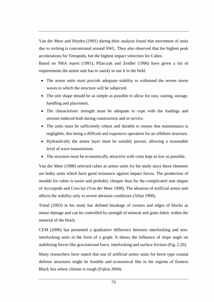
73
Van der Meer and Heydra (1991) during their analysis found that movement of units
due to rocking is concentrated around SWL. They also observed that the highest peak
accelerations for Tetrapods, but the highest impact velocities for Cubes.
Based on NRA report (1991), Pilarczyk and Zeidler (1996) have given a list of
requirements the armor unit has to satisfy to use it in the field.
The armor units must provide adequate stability to withstand the severe storm
waves to which the structure will be subjected.
The unit shape should be as simple as possible to allow for easy casting, storage,
handling and placement.
The characteristic strength must be adequate to cope with the loadings and
stresses induced both during construction and in service.
The units must be sufficiently robust and durable to ensure that maintenance is
negligible, this being a difficult and expensive operation for an offshore structure.
Hydraulically the armor layer must be suitably porous, allowing a reasonable
level of wave transmission.
The structure must be economically attractive with costs kept as low as possible.
Van der Meer (1998) selected cubes as armor units for his study since these elements
are bulky units which have good resistance against impact forces. The production of
moulds for cubes is easier and probably cheaper than for the complicated unit shapes
of Accropode and Core-loc (Van der Meer 1998). The abrasion of artificial armor unit
affects the stability only in severe abrasion conditions (Allen 1998).
Trmal (2003) in his study has defined breakage of corners and edges of blocks as
minor damage and can be controlled by strength of mineral and grain fabric within the
material of the block.
CEM (2006) has presented a qualitative difference between interlocking and non-
interlocking units in the form of a graph. It shows the influence of slope angle on
stabilizing forces like gravitational force, interlocking and surface friction (Fig. 2.20).
Many researchers have stated that use of artificial armor units for berm type coastal
defense structures might be feasible and economical like in the regions of Eastern
Black Sea where climate is rough (Fişkin 2004).

74
Fig. 2.20 Qualitative influence of slope angle on stability of armor units
(CEM 2006)
Medina et al. (2011) compared the various aspects of cube and cubipod armor units.
They found that when the equivalent drop height is lower than a certain threshold
limit (he < he0), the prototypes only showed very low RLM (Relative Loss of Mass)
and local edge damage. The threshold limit is 0.5m for cubes and 1.9m for cubipods.
he is the equivalent drop height and he0 is the equivalent drop height threshold limit.
Medina and Gómez-Martín (2012) suggested considering two safety factors ‘Initiation
of Damage (IDa)’ and ‘Initiation of Destruction (IDe)’. They also suggested
considering different KD values for double and single layered armors. The reason for
different values was explained by them considering massive units which show
tenacious failure for double layer while a brittle failure for single layer. The design KD
values and the factor of safety suggested by them are given in Table 2.8.
Table 2.8 Design KD and global safety factors (Medina and Gómez-Martín 2012)
Initiation of
Destruction (IDe)
Initiation of
Damage (IDa)
Sectio
n
CAU KD layers Slope SF
(IDe5%)
SF
(IDe50%)
SF
(IDa5%)
SF
(IDa50%)
Trunk Cube 6 2 1:1.5 1.05 1.35 0.67 0.86
Cubipod 2 28 2 1:1.5 1.09 1.40 0.82 0.99
Cubipod 1 12 1 1:1.5 1.31 1.64 1.06 1.27
Accropode 15 1 1:1.3 1.05 to
1.40
1.26 to
1.51
0.93 to
1.24
1.15 to
1.38
Xbloc 16 1 1:1.3 1.17 1.68 1.17 1.32
Round
-head
Cube 5 2 1:1.5 1.17 1.40 0.88 1.13
Cubipod 2 7 2 1:1.5 1.19 1.36 0.99 1.18
75
Medina and Gómez-Martín (2012) additionally pointed out the conclusions of
Burcharth and Brejnegaard-Nielsen (1986) stating that stress level in Concrete Armor
Units (CAU) increases linearly with its size for static and hydrodynamic loads and is
proportional to the root of the armor size for impact loads. Therefore, CAUs never
break in small-scale tests; however, there may be chances of breaking at prototype
scale.
Gómez-Martín and Medina (2013) have pointed out several advantages of cubes
which are massive units as: high structural strength, inexpensive molds, high
production rate, easy handling with pressure clamps and efficient stacking in the
block yard. But, they also suggest that when cube is considered as armor, the
Heterogeneous Packing (HeP) failure must be taken into account since, the units tend
to move and adjust themselves in face-to-face arrangements which alter the porosity
of the layer. This change in porosity lead to higher packing density below mean water
level and lower packing density above and near mean water level which are critical
from stability point of view.
The heterogeneous packing of the armor units may lead to block sliding failure.
Davies et al. (1994) have conducted studies on block sliding and have highlighted the
significance of thickness of armor layer in reducing this failure. They have concluded
that thicker the armor layer greater is the resistance to sliding failures and with
increase in layer thickness the sliding failure reduces.
2.12 SUMMARY
In this chapter the studies on stability of conventional rubble mound breakwater and
berm breakwater have been reviewed. The various stability formulae developed by
means of physical and mathematical modeling have been presented. The different
types of damage parameters used for quantifying the stability of a conventional
breakwater and the variables affecting them are also reviewed. The studies on wave
run-up and run-down on a conventional breakwater and berm breakwater and their
estimation using different formulae developed by various researchers have also been
explained.

76
Further, a detailed introduction of berm breakwater and its types are discussed in this
chapter. The stability in terms of berm recession and profile development has also
been highlighted in few sections. Additionally, there are no clear design principles
available for the design of berm breakwater and it is mainly dependent on filed
experience. Therefore, a much detailed study is required in order to understand the
effects of various parameters on stability of berm breakwaters.

77
CHAPTER 3
PROBLEM FORMULATION AND EXPERIMENTAL DETAILS
3.1 GENERAL
Before the commencement of any experiment the details of the setup available,
conditions under which it can be used are essential to be known. The wave flume
facility available in Applied Mechanics Department of National Institute of
Technology Karnataka can be used to generate regular waves. The scale of the model
selected was obtained after conducting series of tests which is explained in detail in
the forthcoming sections. Buckingham- theorem was used for obtained non-
dimensional parameters. Experimental setup consisted of wave generator system,
profiler system and wave probes.
In this chapter, problem formulation and objectives of the present study are briefed
along with the details of laboratory conditions, experimental setup, dimensional
analysis, hydraulic modeling, methodology and procedure adopted for the
experimental investigation.
3.2 PROBLEM FORMULATION
The review of literature in the previous chapter shed light on the various studies
conducted on conventional as well as berm breakwaters. The advantages of berm
breakwaters over conventional breakwater were highlighted. High stability during
changing wave conditions, reduced wave run-up, overtopping and wave reflection
compared to conventional breakwater was also emphasized.
The studies by Priest et al. (1964), Brunn (1985), Van der Meer (1988), Ergin et al.
(1989) have showed S-shaped profiles being more stable than single slope profile.
Brunn (1985) has highlighted that the size of armor block for an S-shaped breakwater
can be reduced to half than that required by a conventional breakwater.
Van der Meer (1988) gave the idea for measurement of damage for a statically stable
and dynamically stable berm breakwater. A model was also developed to compute the
profile changes due to wave attack in a dynamically stable breakwater.

78
The studies by Van Gent (1993) on the movement of armor stones on the slope of a
berm breakwater gave an insight on the failure mechanism of the breakwater. He
observed that rolling of stones was a major factor for failure.
Lissev and Torum (1996) found from their studies that a structure with its core
extended into the berm was stable and they suggested it to be a viable option since, it
would be cheaper compared to a traditional trapezoidal cored berm breakwater.
The stability of a berm breakwater with various profiles was studied by Juhl and Sloth
in 1998. A profile with additional layer of armor protecting the berm and lower slope
of a breakwater was found to be more stable than the other profiles considered for
study.
A detailed report on the berm breakwater was presented by PIANC (2003) giving the
studies conducted by different researchers on the various aspects of berm breakwater
structure.
The breakwater using natural stone armor can’t always be realized due to non-
availability of required sizes of stones in the vicinity and one may have to think about
artificial armor units (Neelamani and Sunderavadivelu 2003).
Joshi et al. (2006) have suggested the wave flume tests using regular waves as a
versatile tool and could be used to compare merits of feasible proposals quickly and
also for visualization of complex wave patterns. However, they have also mentioned
that the results using regular waves would be conservative.
Number of equations to measure berm recession has been developed for a
homogenous as well as layered berm breakwater (Torum et al. (1999), Sigurdarson et
al. (2007), Andersen and Burcharth (2010), Moghim et al. (2011)).
The importance of water level, position of berm and slope of a breakwater was
emphasized by Rao et al. (2008) in their experimental studies on non-reshaped berm
breakwaters.
Torum et al. (2012) have stressed the use of economical optimization for assessing the
risk levels of berm breakwaters which includes loss due to damage of structure and
loss of lives due to its failure.

79
Recent studies by Van Gent et al. (2012) and Van Gent (2013) have suggested usage
of concrete armor units in berm and lower slope of a berm breakwater.
The research on berm breakwater as explained earlier have shown that the studies
were mainly concentrated considering natural rock as armor unit and the equations
developed were also for the same. The equations thus developed are valid under
certain ranges and cannot be used universally. Further, with no definite design
principles available for the design of berm breakwaters, the design is mainly
dependent on the field experience. The alternative numerical and mathematical
models developed have not helped in reducing the physical model studies as
emphasized by many researchers.
In order to arrive at a more realistic knowledge of seaward profiles for which wave
intensity and likelihood of breakwater damage are minimal, a laboratory study of
shallow water wave action on reshaped berm breakwater is proposed in the present
investigation. The present study includes understanding the mechanism and
performance of berm breakwater with artificial armor units and to evolve an optimal
breakwater section.
3.3 SCOPE OF THE PRESENT WORK
In the present research work, the stability of statically stable reshaped berm breakwater
made of concrete cube armor units is investigated using a physical model while varying
the wave and breakwater characteristics.
The scope of the present research is to experimentally investigate the stability of berm
breakwater,
1. With varying Concrete cube armor size.
2. For different water levels in front of the structure.
3. With varying berm widths of the model and
4. To evolve an optimal section of the structure.
3.4 DIMENSIONAL ANALYSIS
The present model study involves a berm breakwater structure made of concrete cube
as primary armor unit. The modeling of wave-structure interaction in the present
study is difficult. The major portion of wave energy will be lost over the berm
portion, before it attacks the upper slope due to breaking of waves. This phenomenon
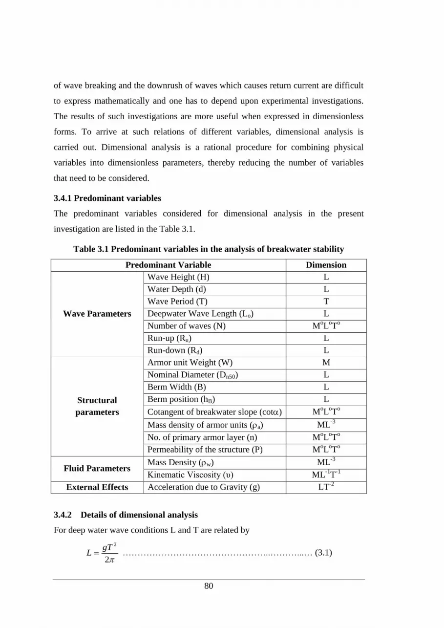
80
of wave breaking and the downrush of waves which causes return current are difficult
to express mathematically and one has to depend upon experimental investigations.
The results of such investigations are more useful when expressed in dimensionless
forms. To arrive at such relations of different variables, dimensional analysis is
carried out. Dimensional analysis is a rational procedure for combining physical
variables into dimensionless parameters, thereby reducing the number of variables
that need to be considered.
3.4.1 Predominant variables
The predominant variables considered for dimensional analysis in the present
investigation are listed in the Table 3.1.
Table 3.1 Predominant variables in the analysis of breakwater stability
Predominant Variable Dimension
Wave Parameters
Wave Height (H) L
Water Depth (d) L
Wave Period (T) T
Deepwater Wave Length (Lo) L
Number of waves (N) MoL
oT
o
Run-up (Ru) L
Run-down (Rd) L
Structural
parameters
Armor unit Weight (W) M
Nominal Diameter (Dn50) L
Berm Width (B) L
Berm position (hB) L
Cotangent of breakwater slope (cot) MoL
oT
o
Mass density of armor units (a) ML-3
No. of primary armor layer (n) MoL
oT
o
Permeability of the structure (P) MoL
oT
o
Fluid Parameters Mass Density (w) ML
-3
Kinematic Viscosity (υ) ML-1
T-1
External Effects Acceleration due to Gravity (g) LT-2
3.4.2 Details of dimensional analysis
For deep water wave conditions L and T are related by
2
2gTL …………………………………………..………...… (3.1)

81
The term gT2
is used to represent the wave length L during dimensional analysis. This
is because if L is used it would be depth specific while gT2 is independent of depth
and represents the deep water wave characteristics which can easily be transformed to
shallow waters depending upon local bathymetry.
The stability of rubble mound breakwaters can be described by static stability or
dynamic stability. The static stability of the breakwater is defined by the term damage
level (S) or damage number (Nod). The dynamic stability is defined by the profile
parameters as length and angles. The stability of berm breakwaters are mainly
characterized based on the erosion in the berm portion which is termed as berm
recession (Rec).
Considering the damage level (S) of the rubble mound breakwater and berm recession
(Rec) of berm breakwater, which is dependent on several parameters, their
relationships can be expressed as,
S = f (W, H, T, d, g, a, w, Dn50, Ru, Rd, cotα, P) …………..…… (3.2)
Rec = f (W, H, T, d, B, hB, g, a, w, Dn50, Ru, Rd, cotα, P)………..….. (3.3)
By the application of Buckingham’s theorem, an equation of the form shown below
is obtained.
S = f{ H/∆Dn50, Ho/gT2, Ru/Ho, Rd/Ho, d/gT
2, cotα) ............................ (3.4)
Rec/Dn50 = f{ H/∆Dn50, Ho/gT2, hB/d, B/d, Ru/Ho, Rd/Ho, d/gT
2, cotα) .... (3.5)
Where,
S Damage level
Rec/Dn50 Dimensionless berm recession
Rec/B Relative berm recession
H/Dn50 Hudson’s stability number, Ns
Ho/gT2
Deepwater wave steepness, s
B/d Relative berm width
hb/d Relative berm position
tanα/(s)-0.5
Surf similarity parameter, ξ
d/gT2 Relative water depth
Ru/Ho Relative run-up

82
Rd/Ho Relative run-down
cot Cotangent of breakwater slope
3.5 SIMILITUDE CRITERIA AND MODEL SCALE SELECTION
The basis of all physical modeling is similitude of the model and prototype.
Similitude is said to be achieved when all factors that influence the phenomenon are
in proportion between the prototype and the model. According to Hughes (1993),
model similitude can be achieved by: i) Calibration ii) Differential equation iii)
Dimensional analysis iv) Scale series
The method of calibration is appropriate for movable bed models. The method of
differential equations is more applicable when the differential equations considered
are reasonably accurate. Scale series is mostly used to establish the scaling criteria for
a complex phenomenon, and one has to be extremely careful in analyzing the results
from the model tests and extrapolating them to prototype.
In the present study, the similitude is achieved by the method of dimensional analysis.
The similitude is achieved between the prototype and the model with the help of non-
dimensional parameters of the phenomenon. These non-dimensional parameters must
be of the same range for both model and the prototype. Considering the wave climate
off Mangalore coast, in the present study similitude is achieved by considering the
non-dimensional parameter, wave steepness H/gT2 as given in Table 3.2. In the
laboratory using the existing facilities of the two-dimensional wave flume, regular
waves of heights ranging from 0.03 m to 0.24 m and periods ranging from 1 s to 3 s
can be produced.
Table 3.2 Wave parameters of prototype and model
Wave Parameters H (m) T (sec) H/gT2
Prototype 1 to 5.4 8 to 12 0.00070 to 0.0086
Model 0.030 to 0.24 1.0 to 3.0 0.00033 to 0.0244
For selecting a model-scale the range of wave heights and wave periods that can be
generated in the wave flume accounting the wave climate off Mangalore coast are
considered. The appropriate length scale range for rubble mound stability tests is
between 1:5 and 1:70 (Hudson et al. 1979). To simulate the field conditions of wave

83
height, period and nominal diameter of armor stone, by the application of Froude’s
law, a geometrically similar scale of 1:30 was selected (Table 3.3). This scale is
within the scale selected for rubble mound breakwater model tests conducted in
majority of the laboratories around the world and is good enough to give reasonable
and satisfactory results compared to those of the prototype (Le Mehaute (1976),
Palmer and Walker (1976), Jensen and Klinting (1983), Stive (1985) and Hughes
(1993)).
Many researchers had observed that there will be scale effect on armor stability for
lower Reynolds number. For many years, it was considered that the Reynolds number
of flow through armor layer must be greater than 3x10⁴ for no modeling errors to
arise. But, Owen and Briggs (1986) from their model studies conducted with different
scales suggested that, the Reynolds number can be as low as 8x10³ or even 3x10
3
before any significant errors can arise. In the present work, effect of Reynolds number
is not considered, because, flow in the primary armor layer is considered to be
turbulent as Re > 3x10³.
Table 3.3 Selection of model scale
Scale H (m) T (sec) D (m)
1 5.4 8 12 1
1:10 0.1 0.54 2.53 3.8 0.1
1:20 0.050 0.27 1.79 2.68 0.05
1:30 0.033 0.18 1.46 2.19 0.03
1:40 0.025 0.135 1.26 1.90 0.025
3.6 DESIGN CONDITIONS
The wave climates off the Mangalore coast as given by KREC Study Team (1994) are
considered while planning the present experimental investigation. During the
monsoon, the maximum recorded wave height off Mangalore coast is about 4.5 m to
5.4 m. During fair weather season wave height hardly exceeds 1 m. Predominant
wave period is 8 s to 11 s. Occasionally, during the fair weather season, wave periods
up to 15 s are observed. Hence, for the design of conventional rubble mound
breakwater model an equivalent of prototype design wave of height 3 m is assumed,

84
while a maximum wave of height up to 4.8 m and period of 8 s to 14 s are considered
for model study.
3.7 EXPERIMENTAL SETUP
3.7.1 Wave flume
The physical model study for regular waves was conducted in a two dimensional
wave flume available in Marine Structures laboratory of Applied Mechanics
Department, National Institute of Technology Karnataka, Surathkal, India. The wave
flume is 50 m long, 0.71 m wide and 1.1 m deep. It has a 41.5 m long smooth
concrete bed. About 15 m length of the flume is provided with glass panels on one
side. It has a 6.3 m long, 1.5 m wide and 1.4 m deep chamber at one end where the
bottom hinged flap (or wave paddle) generates waves.
A ramp is provided between flume bed level and generating chamber for generation
of waves. A series of vertical asbestos cement sheets are provided as wave filter
spaced at about 0.1 m centre to centre parallel to length of the flume. The flap is
controlled by an induction motor of 11 KW power at 1450 rpm. This motor is
regulated by an inverter drive (0 – 50 Hz) rotating in a speed range of 0–155 rpm.
Waves of height ranging from 0.08 m to 0.24 m heights and periods from 0.8 sec to
4.0 sec in a maximum water depth of 0.5 m can be generated with this facility. Fig.
3.1 shows the line diagram of wave flume.
Fig. 3.1 Details of wave flume facility
3.7.2 Wave probes
The capacitance type wave probes are used in the present study. The accuracy of the
measurements is 0.001 m. The probes were used to record the incident wave
characteristics. The spacing of probes and decomposition of incident and reflected
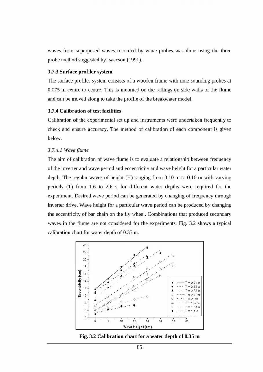
85
waves from superposed waves recorded by wave probes was done using the three
probe method suggested by Isaacson (1991).
3.7.3 Surface profiler system
The surface profiler system consists of a wooden frame with nine sounding probes at
0.075 m centre to centre. This is mounted on the railings on side walls of the flume
and can be moved along to take the profile of the breakwater model.
3.7.4 Calibration of test facilities
Calibration of the experimental set up and instruments were undertaken frequently to
check and ensure accuracy. The method of calibration of each component is given
below.
3.7.4.1 Wave flume
The aim of calibration of wave flume is to evaluate a relationship between frequency
of the inverter and wave period and eccentricity and wave height for a particular water
depth. The regular waves of height (H) ranging from 0.10 m to 0.16 m with varying
periods (T) from 1.6 to 2.6 s for different water depths were required for the
experiment. Desired wave period can be generated by changing of frequency through
inverter drive. Wave height for a particular wave period can be produced by changing
the eccentricity of bar chain on the fly wheel. Combinations that produced secondary
waves in the flume are not considered for the experiments. Fig. 3.2 shows a typical
calibration chart for water depth of 0.35 m.
Fig. 3.2 Calibration chart for a water depth of 0.35 m

86
3.7.4.2 Wave probes
The probes were originally calibrated by the manufacturer. However, the output is
expected to show minor variations depending on the salinity and temperature of the
water used in the flume. Hence, the probes were subjected to static immersion tests
and the relationship between the water level and the output voltage was determined
and recorded. The variation of voltage with water level is shown in Fig. 3.3. The
calibration was undertaken daily before and after the experiments. The free surface of
water is considered as zero mark in x-axis and the probe will be moved from the
bottom tip to the top tip inside the water to record the change in voltage.
Fig. 3.3 Calibration of wave probes
3.8 BREAKWATER MODEL SECTIONS
3.8.1 Conventional breakwater
The conventional breakwater model of trapezoidal section was built with a uniform
slope of 1:1.5. The breakwater was constructed with concrete cubes as primary armor.

87
The KD for the concrete cubes was derived as 5.5 from the following relation
(National River Authority, 1991, as quoted by Pilarczyk and Zeidler, 1996)
𝐾𝐷 𝑜𝑓 𝑇𝑒𝑡𝑟𝑎𝑝𝑜𝑑𝑠
𝐾𝐷 𝑜𝑓 𝐶𝑢𝑏𝑒𝑠= 1.5 ……………………………..…….. (3.6)
The unit weight (W50) of 106 g for primary armor cube was determined using
Hudson’s formula (Eq. 3.7) for a design wave height (H) of 0.10 m.
3
3
cot
1
r
D
H
KW
......................................................... (3.7)
The armor cube size (Dn50) was determined using Eq. 3.8 and for the present case it
was found to be 0.0353 m.
3/1
50
r
n
WD
…………………………………. (3.8)
The weight of the stones in the secondary layer was taken as 10.6 g (W/10). A
minimum crest width of three armor units was maintained which was 0.10 m and crest
height was 0.70 m to avoid wave over topping. The core was designed with quarry
dust of 300 microns size.
The thickness of the primary and secondary layer was determined by the equation
3/1
r
WnKt
…………..…………………. (3.9)
where, t = thickness of armor layers
n = number of layers of the armor units
K = layer coefficient
r = specific weight of armor material (concrete cube=2.4 g/cc)
The average layer thickness of 0.118 m was provided for primary layer and an
average thickness of 0.055 m was provided for secondary layer. Fig. 3.4 shows a
typical cross section of conventional rubble mound breakwater. The model
characteristics are tabulated in Table 3.4.

88
Table 3.4 Conventional breakwater model characteristics
Variable Expression Value
Slope 1V: 1.5H
Armor type -- Concrete cube
Mass Density γr 2.4 g/cc
Stability coefficient KD 5.5
Relative mass density of armor unit 1.4
Nominal size of armor cube Dn50 0.0353 m
Armor cube weight W50 106 g
Layer coefficient K 1.1
Crest width -- 0.10 m
Crest height -- 0.70 m
Thickness of primary armor layer -- 0.118 m
Thickness of secondary armor layer -- 0.055 m
Porosity of primary armor P1 47%
Porosity of secondary armor P2 39%
Porosity of core P3 36%
Fig. 3.4 Details of test model of conventional breakwater
3.8.2 Berm breakwater
Berm breakwater model was also constructed with a slope of 1V: 1.5H with cubes as
armor unit. Various models were constructed with different armor weights. The armor
weights considered were 1.0W, 0.75W, 0.6W and 0.5W, where W represents the
weight of armor obtained using Hudson formula (i.e., 106 g) for a design wave height
of 0.10 m. The armor cube size and thicknesses of primary and secondary armor layer

89
were calculated using Eq. 3.8 and Eq. 3.9, for the reduced armor weights considered.
The crest height and crest width were provided same as conventional breakwater of
0.70 m and 0.10 m respectively. A range of berm widths varying from 0.30 m to 0.45
m was considered in the present study. The berm was maintained at a constant height
of 0.45 m from sea bed. Fig. 3.5 shows the section of berm breakwater. The berm
breakwater characteristics are tabulated in Table 3.5.
Table 3.5 Berm breakwater model characteristics
Variable Expression Value
Slope 1V: 1.5H
Armor type -- Concrete cube
Mass Density γr 2.4 g/cc
Armor cube weight W50 106, 79.5, 63.6, 53 g
Size of armor cube Dn50 0.0353, 0.0325, 0.0298, 0.0285 m
Berm width B 0.30, 0.35, 0.40, 0.45 m
Berm position from sea bed hB 0.45 m
Crest width -- 0.10 m
Crest height -- 0.70 m
Fig. 3.5 Details of test model of berm breakwater
3.8.3 Model construction
The breakwater model was constructed on the flat bed of wave flume at a distance of
32 m from the generator flap. The cross section of breakwater denoting layers was
drawn on the glass panel. The core material was placed and formed to the required
level and after well compacting; the secondary layer and the primary layer were

90
constructed to the marked level. The placement of primary armor units was random
over the secondary layer. The primary armor layers were colored red, white and grey
respectively to reduce the surface roughness (Hughes 1993). Pipes are provided below
the breakwater test section to balance the water levels on seaside and leeside (Diskin
et al. 1970). A same slope of 1:1.5 was maintained on both sides of the breakwater.
3.8.4 Wave characteristics
The breakwater models were tested for varying wave characteristics (test conditions)
as given in Table 3.6. The models were subjected to normal wave attack of height
ranging from 0.10 m to 0.16 m and of periods varying from 1.6 s to 2.6 s in a depth of
water (d) of 0.30 m, 0.35 m, 0.40 m and 0.45 m. Storm duration of 3000 waves
(which is equivalent to an actual storm of 6.67 hours to 10.83 hours) was considered
since more than 80% to 90% of the total damage would have already inflicted by that
time and equilibrium would have established (Van der Meer and Pilarczyk (1984) and
Hegde (1996)).
Table 3.6 Wave characteristics
Variable Expression Value
Wave height H 0.10, 0.12, 0.14, 0.16 m
Wave period T 1.6, 2.0, 2.6 s
Water depth d 0.30, 0.35, 0.40, 0.45 m
Storm duration N 3000 waves
Angle of wave attack - 900
Wave type - Regular
3.9 CASTING OF CONCRETE CUBES AND ITS PROPERTIES
Various tests like standard consistency, initial and final setting time, fineness of
cement and specific gravity of cement were conducted on cement. Similarly, sand was
also tested for its specific gravity and fineness modulus. Compressive strength of 28
days cured cubes was determined. The obtained results are compared with the
standard Indian Standard (IS) code specifications and all of them are within the limits
specified in the code. Table 3.7 shows the different tests performed on cement and
sand, the obtained values and standard limits.

91
Table 3.7 Results of tests on cement and sand
Cement
Test Value obtained IS code value IS code
Standard consistency 30% 28% – 32%
IS: 8112 - 1989
Initial setting time 66 min Not less than 30 min
Final setting time 330 min Not more than 600 min
Fineness of cement 300 m2/Kg > 225 m
2/Kg
Specific gravity 3.1 3.1 – 3.15
Sand
Specific gravity 2.64 Nearer to 2.65 IS: 2720 (Part
III/Sec 1) - 1980
Fineness modulus 3.29 2.3 – 3.5 IS: 2386 (Part I) –
1963
Cube
Compressive strength
of 28 days cured cube 37.5 N/mm
2
> 35 N/mm2
(for M35 grade) IS: 456 - 2000
Concrete cubes were casted using 1:3 cement mortar with a water cement ratio of 0.4.
To maintain the density of concrete as 2.4 g/cc, a part of sand was replaced by iron
ore filings. The Table 3.8 gives the different sand: iron ore filings ratios and its mass
densities. A mass density of 2.396 g/cc was obtained for a ratio of 80: 20 which was
considered for the present study.
Table 3.8 Sand: Iron ore ratio in 1:3 cement mortar
Trial No. Sand: Iron Ore Mass density of cube in
g/cc
1 90:10 2.05
2 87:13 2.178
3 85:15 2.288
4 83:17 2.378
5 80:20 2.396
6 78:22 2.342

92
The cubes were casted with the above parameters and cured for 28 days before
constructing the model. The porosity of the armor layers was determined as per IS
2386 (Part III) - 1963 and the porosity of primary armor, secondary layer and core
were 47%, 39% and 36% respectively.
3.10 TEST CONDITIONS
The present experimental investigations are carried out with the following test
conditions:
1. The sea bed is rigid and horizontal and it is assumed that the sediment movement
does not interfere with the wave motion and do not affect the model performance.
2. The waves are periodic and monochromatic.
3. Waves are generated in short burst of five waves.
4. Between wave bursts there are brief intervals to allow wave energy to dampen
out.
5. Secondary waves generated during the test are not considered.
6. The density difference between freshwater and seawater is not considered.
In the lab, the reflected waves from the breakwater strike the wave paddle and are
almost totally re-reflected and create waves which may not represent the prototype
condition truly. Further, the re-reflected waves may add-up or reduce the incident
wave height and period thus resulting in undesired wave heights and periods. This
results in erroneous output which is not desirable. This problem is eliminated by
conducting experiments with series of wave bursts, such that, each burst of waves
ending before re-reflected waves can again reach the testing section of the wave flume
(Hughes 1993).
3.11 TEST PROCEDURE
To minimize uncertainty the experiment has to be properly planned, experimental
procedures and extrapolation methods should be standardized. Sources of errors and
magnitude of errors have to be minimized.

93
3.11.1 Sources of errors and precautions to minimize error
The following sources are identified which may cause error in the experimental study.
1. Error in linear dimensions: The model is constructed with an accuracy of linear
dimensions up to ±1.0 mm, which may contribute errors in between 0.2% to
0.3%.
2. Error in wave height measurement: The least count of the wave probe is 1.0 mm
and may contribute to an error of 2% to 6% in the incident wave height.
3. Error due to change in water level: The water level is checked at the beginning
and end of every day’s work and maintained within ±2 mm of the required level.
This may contribute to an error of 0.6% to 1.0%.
These errors are expected to be compensative in nature and hence, there is no
significant effect if they are neglected. However, the following precautions are taken
for minimizing the errors:
1. The model is constructed, as per the standard procedure, with a largest possible
model with a scale of 1:30.
2. The depth of water in the flume is maintained exactly at the required level and
was continuously monitored. Average variation of 2 mm was found after a full
day of model testing. Any drop in the water level of more than 2 mm was
immediately corrected.
3. Before the commencement of the experiments, calibration of flume and wave
probes without the placement of model were undertaken to determine the proper
wave height to assign to a particular combination of generator stroke and wave
period. The wave heights used in the test runs are obtained during calibration.
This will exclude the losses due to interference of flume bed, sidewalls and
reflection and therefore, eliminates these error sources.
4. Waves were run in short bursts of five during the tests. Between wave bursts
there will be brief interval to allow reflected wave energy to dampen out.
5. All the wave characteristics were measured with more than 35 readings and were
statistically analyzed. Similar exercise was repeated for other parameters such as
wave run-up and run-down over the breakwater.
6. Tests were started by surveying newly constructed slope with profiler, which
becomes reference survey for comparison of subsequent surveys.

94
3.11.2 Procedure for experimental study
After carefully studying the model test conditions and procedures adopted by various
investigators, the following procedure is adopted for the present study.
1. All the test models were constructed, in the flume, at a distance of 32 m from the
wave generator flap.
2. The wave flume was filled with tap water to required depths of 0.3 m, 0.35 m, 0.4
m and 0.45 m and the entire experimental set up including the wave probes were
calibrated for each depth of water.
3. The breakwater models were constructed and their initial profiles were taken for
comparison of subsequent surveys (final profile).
4. The models were tested for varying wave characteristics as listed in Table 3.6.
Initially the models were tested for smaller wave height of 0.1 m for different
wave periods of 1.6, 2.0 and 2.6 s. The wave heights were then increased by
0.02 m till they reach 0.16 m for all the wave periods. 3000 waves or the
exposure of the secondary layer were run for each trial whichever occurred
earlier.
5. During the initial study of each model wave run-up and run-down were
measured. After each trial the final profile was taken to calculate the damage
expressed in terms of berm recession (Rec).
3.12 MEASUREMENTS
3.12.1 Measurement of wave heights
Three capacitance type wave probes are used during the experimental work to
measure the wave heights. The probes are kept on the seaside of model for acquiring
incident wave heights (Hi). The spacing between probes was kept near to one third of
the wave length. During the experimentation, the signals from wave probes are
verified online and recorded by the computer through the data acquisition system. The
statistics namely, the ranges of standard deviation and coefficient of variation for all
wave heights recorded for all depths of water in the entire model tests of the present
study are listed in Table 3.9.

95
Table 3.9 Statistics of all wave heights recorded
Depth of water
d (m)
Range of statistical parameters of wave heights
Standard deviation (m) Coefficient of variation c
0.45 0.08 – 0.26 0.006 – 0.065
0.40 0.07 – 0.10 0.005 – 0.011
0.35 0.10 – 0.21 0.011 – 0.042
0.30 0.06 – 0.14 0.004 – 0.019
3.14.2 Measurement of wave run-up and run-down
Wave run-up was measured as the vertical distance above the SWL of the maximum
wave up rush when a wave impinges on the breakwater model. The vertical distance
below the SWL up to the minimum elevation attained by wave on the breakwater
slope was taken as the wave run-down. The wave run-up and run-down are measured
over the breakwater on the graduated scale fixed over the glass panels of the flume.
The statistics of all wave run-up and run-down recorded for the entire model tests of
the present study are listed in Table 3.10 and Table 3.11 respectively.
Table 3.10 Statistics of all wave run-ups recorded
Depth of water
d (m)
Range of statistical parameters of wave run-ups
Standard deviation (m) Coefficient of variation c
0.45 0.03 – 0.09 0.0008 – 0.0071
0.40 0.03 – 0.09 0.0006 – 0.0064
0.35 0.03 – 0.11 0.0007 – 0.0072
0.30 0.02 – 0.10 0.0005 – 0.0066

96
Table 3.11 Statistics of all wave run-downs recorded
Depth of water
d (m)
Range of statistical parameters of wave run-downs
Standard deviation (m) Coefficient of variation c
0.45 0.06 – 0.11 0.0033 – 0.0085
0.40 0.05 – 0.11 0.0027 – 0.0087
0.35 0.05 – 0.10 0.0028 – 0.0101
0.30 0.05 – 0.10 0.0021 – 0.0079
3.14.3 Measurement of breakwater damage
The recession of the berm and the exposure of secondary layer on the sea side slope or
the berm reflect the damage of a structure. If Rec/B is less than one then structure is
safe otherwise unsafe. Further, the structure was considered damaged with the
exposure of secondary layer even if Rec/B < 1. Surface profiler system was used for
obtaining profile before and after the test of the breakwater. Intermediate profiles
were also obtained to study the effect of storm duration.
3.15 UNCERTAINTY ANALYSIS
Generally, whenever experimentation is involved, there is a possibility of some errors
creeping in while making measurements. Some of the errors involved in the present
study are already explained in previous sections. Further, it is also observed that the
experimental results as well as extrapolated values for prototype obtained from
different test facilities vary considerably. In such events, it becomes necessary for a
researcher to provide the upper and lower margins of the calculated results with a fair
amount of confidence level. Such a study of providing a confident margin is called as
uncertainty analysis. Uncertainty analysis is the process of calculating uncertainty of a
value that has been calculated from several measured quantities. It describes the
degree of goodness of a measurement or experimentally determined result. With the
help of uncertainty analysis it is possible to conduct experiments in a scientific
manner and predict the accuracy of the result (Misra 2001). The details of the analysis
are illustrated in Appendix I.

97
CHAPTER 4
RESULTS AND DISCUSSION
4.1 GENERAL
After the completion of experiments, the results obtained have to be interpreted
accurately to know the performance of a structure. In this chapter the effect of various
sea state parameters as well as structural parameters on the stability, wave run-up and
run-down of the berm breakwater are analyzed in detail.
A safe and economical structure has to stand and be stable for all the wave conditions
that it is being tested with a minimum cross sectional area. The stability analysis is
carried out to know the vigor of a structure to withstand the onslaught of waves. Wave
run-up studies help in knowing the highest water level a wave reaches and dislocation
of primary armor while wave run-down studies aid us in relating the movement of
armor and hence the stability of the primary layer of the breakwater. Understanding
the effect of various sea and structural parameters is essential in knowing the behavior
of the structure and design an optimized structure which is safe as well as economical
for the wave conditions considered.
4.2 SUMMARY OF MODEL STUDY
The starting point of the experimental studies was the trapezoidal cross section model
made of cube armor constructed with a scale of 1:30 on the flat bed of the flume. A
uniform slope of 1V:1.5H was maintained with primary armor weight of 106 g (i.e.,
nominal diameter, Dn50, of 0.0353 m) for a non-breaking design wave of 0.10 m. Its
crest width was 0.1 m and height 0.70 m. The secondary armor of mean weight of
about 10.6 g and core of size of about 300 microns was designed. The porosities of
the primary armor, secondary armor and core are 43%, 39% and 36% respectively.
The primary armor units were painted with different colors and placed in bands of
heights of 0.2 m to 0.3 m to track their movement during damage. In the first phase
this conventional breakwater model was tested. The breakwater model characteristics
are listed in Table 3.4.

98
The model was constructed at a distance of 32 m from the generator flap. The cross
section of breakwater denoting layers was drawn on the glass panel. Pipes were
placed over the flume bed, at the breakwater test section, to balance the water levels
on seaside and leeside. The core material was placed and formed to the required level
by light compacting with hands. Then, the secondary and primary layers were
constructed to the marked level. The technique adopted in the present work was keyed
and fitted placement. The primary armor layers were painted to reduce the surface
roughness. In the rubble mound breakwater model, the armor units placed around
SWL were painted in white and in the zone above it was painted with red color while
in the zone below the units were painted with grey color to identify the damage zone
after the test. Further, the details of the breakwater model construction are explained
in Chapter 3.
Before the model tests were started, the experimental set up along with the wave
probes was calibrated to find the required wave heights which, were assigned to a
particular combination of generator stroke and wave period, for depths of water of
0.30 m, 0.35 m, 0.40 m and 0.45 m. The model was subjected to regular waves (H) of
height varying from 0.1 m to 0.16 m of a range of period (T) varying from 1.6 s to 2.6
s generated in water depths (d) of 0.30 m to 0.45 m. The model was tested for varying
wave characteristics as shown in Table 3.6. The model was subjected to normal attack
of regular waves. The waves were generated in bursts of five waves with brief
interludes to allow reflected wave energy to dampen out. During the test the number
of incident waves, their heights and periods, wave run-up and run-down over the
breakwater slope and armor unit movements were recorded. Further details of test
procedure are explained in Chapter 3.
In the second phase different berm breakwater models constructed with cube armor
with a slope of 1V:1.5H (above and below the berm) was tested. The experimental
works proceeded with the changes in armor unit sizes and berm widths to see their
effects on the stability of the structure. In each experiment, 12 individual test waves
forming a storm having the significant wave height (0.1 m to 0.16 m) and period (1.6
s to 2.6 s) were generated. The armors in the primary layer were painted similarly as
in the case of conventional breakwater, with red color for units in the upper slope

99
above the berm, grey color for units in the lower slope below the berm and white for
the units in the berm. The berm in berm breakwaters were mostly constructed above
still water level as the construction is much simpler than the ones constructed below
still water level. The breakwater model characteristics are listed in Table 3.5. Initial
and profile of the breakwater structure before and after the tests were also taken
additionally to the wave characteristics readings recorded similar to that of a
conventional breakwater.
Initially, the conventional breakwater was tested for stability and the results obtained
was used to design the statically stable reshaped berm breakwater with design armor
weight, minimum primary layer thickness of 2 and a smallest berm width of 0.30 m.
The model was tested for stability and was found that the structure was safe for a
higher berm width of 0.35 m. Hence, much higher berm widths of 0.40 m and 0.45m
were not tested for this armor weight. Next, the armor weight was reduced by 25% of
the design weight and the stability was analyzed with berm widths varying from
0.30 m to 0.45 m and 3 layers of primary armor. The models with 0.30 m and 0.35 m
berm widths were again not safe but the structure was safe for higher berm widths of
0.40 m and 0.45 m. Further, for the same reduced armor weight, the thickness of
primary armor was reduced by 2 and the stability was tested. Model with berm width
0.45 m was the only safe structure obtained during these tests. Hence, further studies
were conducted with 3 layers of primary armor and 0.45 m berm width for more
reduced armor weight. The model with 40% reduced armor weight was not safe for all
the test conditions. So, the stability was tested with increased primary layer thickness
of 4. Even then the model with 40% reduced armor weight was not safe. Along with
this, model with 50% reduced armor weight were also tested and found unsafe.
During these tests some typical observations were made. It was observed that with the
decrease in armor weight and berm width the berm recession, wave run-up and run-
down was found increasing. Also, the increase in water depth and wave height
increased the recession of berm, wave run-up and run-down. Further, it was observed
that shorter period waves caused higher berm recession, lower wave run-up and run-
down. In the next few sections details of the results are discussed for the some of the
critical test conditions.

100
4.3 STUDIES ON CONVENTIONAL BREAKWATER
4.3.1 Effect of deepwater wave steepness (Ho/gT2) on damage level (S)
Fig. 4.1 Influence of deepwater wave steepness (Ho/gT2) on Damage level (S) for
different water depths
Fig. 4.1 shows the influence of deep water wave steepness (Ho/gT2) on damage level
(S) for different water depths. It is clear from the graph that S increases with the
increase in Ho/gT2 and d/gT
2. The highest S of 11.5 is observed for a water depth of
0.40 m (d/gT2 = 0.00181) and a wave height of 0.16 m for a wave period of 1.6 s
(Ho/gT2 = 0.00778). It is also observed that for a 0.30 m (d/gT
2 = 0.0045 - 0.0136)
depth of water and a wave height of 0.16 m, S is zero for all the wave periods
(Ho/gT2 = 0.00143, 0.00254, 0.00486). The high damage for steeper waves is due to
the dislodging of armor unit from its position by the waves and subsequent pulling
down of them even before they settle. The damage level for lower water depths
ranged from ‘no damage’ to ‘intermediate damage’ while for higher water depths a
complete failure was observed for many of the test conditions.
4.3.2 Effect of deepwater wave steepness (Ho/gT2) on relative wave run-up
(Ru/Ho)
The influence of deep water wave steepness parameter (Ho/gT2), on relative run-up
(Ru/Ho) for increasing ranges of depth parameter (d/gT2) i.e., varying wave climate in
depths of water of 0.3 m, 0.35 m and 0.4 m, is shown in Fig. 4.2.

101
Fig. 4.2 Influence of Ho/gT2 on Ru/Ho for different water depths
The relative run-up decreases with an increase in wave steepness and there is no
significant impact of d/gT2. For 1.1x10⁻³ < Ho/gT2 < 6.7x10⁻³ and all ranges of d/gT2,
Ru/Ho vary from 0.905 to 1.785. In the present study, it is observed that, run-up is
relatively higher for 1.1x10⁻³ < Ho/gT2
< 4x10⁻³, when, 4 < ξ < 4.25. This is because, in
this range of ξ, surging breakers occur. As water depth decreases from 0.40 m to 0.35m
and 0.30 m, the wave run-up decreases by 4.6% to 7.9% and 7.5% to 9.9% respectively.
4.3.3 Effect of deepwater wave steepness (Ho/gT2) on relative wave run-down
(Rd/Ho)
Fig. 4.3 Influence of Ho/gT2 on Rd/Ho for different water depths

102
The influence of deep water wave steepness parameter (Ho/gT2), on relative run-down
(Rd/Ho) for increasing ranges of depth parameter (d/gT2) i.e., varying wave climate in
depths of water of 0.3 m, 0.35 m and 0.4 m, is shown in Fig. 4.3. The relative run-down
decreases with an increase in wave steepness and decreasing d/gT2 similar to relative
wave run-up. For 1.1x10⁻³ < Ho/gT2 < 6.7x10⁻³ and all ranges of d/gT2, Rd/Ho vary from
1.003 to 1.965. As water depth decreases from 0.40 m to 0.35m and 0.30 m, the wave
run-down decreases by 3.8% to 19.4% and 11.2% to 36.3% respectively.
4.4 STUDIES ON BERM BREAKWATER
4.4.1 Effect of reduction in armor weight on berm recession, wave run-up and
run-down
Fig. 4.4 Influence of Ho/gT2 on Rec/B for a 0.35 m berm width and different water
depths
Fig. 4.4 shows the comparison of berm recession for design (Wo = 1.0W) armor
weight and reduced (Wo = 0.75W) armor weight models for a berm width of 0.35 m.
It is observed from the figure that, as the armor weight decreases there is an increase
in relative berm recession (Rec/B) with increasing Ho/gT2
for all conditions
considered. The design armor weight considered for the model was safe for all the

103
conditions, but when the armor weight was reduced by 25%, for water depths 0.45 m
(B/d = 0.78) and 0.40 m (B/d = 0.88) the breakwater was not safe as the wave height
increased by 0.16 m along with the periods. The damage was in the form of complete
erosion of berm with no secondary layer exposure in these models. Shorter wave
periods caused more recession compared to longer wave periods as observed in the
Fig. 4.4. As armor weight is reduced from W to 0.75W, the berm recession increased
by 20% to 100% for all the conditions considered.
Fig. 4.5 Influence of Ho/gT2 on Rec/B for different water depths and 0.45 m berm
width
Fig. 4.5 shows the typical variation of relative berm recession (Rec/B) with deepwater
wave steepness (Ho/gT2) for higher reduced armor weights of 0.25W, 0.6W and 0.5W
in different depths of water (d) for a constant berm width (B) of 0.45. Since, from Fig.
4.4 it is observed that design armor weight models were safe for a berm width of 0.35
m, higher berm width of 0.45 m were not tested with these models. Hence, design
armor weight models are considered for comparison in Fig. 4.5. In Fig. 4.5 also same
trend of increasing Rec/B with decreasing armor weight and B/d ratio can be observed.
It is also observed from figure that for water depths of 0.45 m (B/d = 1.0) and 0.40 m

104
(B/d = 1.13) the Rec/B was found to be greater than one in 0.6W and 0.5W armor
weight models for many of the wave conditions. In these models both types of
damage to the structure have been observed. Secondary layer was exposed in 0.6W
and 0.5W armor weight models for 0.14 m and 0.16 m high wave and almost all the
wave periods. The secondary layer was exposed within short storm duration of 1500
waves. The complete erosion of berm was observed in 0.5W armor weight models for
a wave height of 0.12 m at all the wave periods and 0.6W armor weight model for a
0.12 m wave height at a period of 1.6 s.
The 0.75W armor weight models were completely safe for all the wave conditions
with the berm recession less than berm width (Rec/B < 1) with no exposure of
secondary layer. As the armor weight is reduced from 0.75W to 0.6W and 0.5W, the
Rec/B increases by 26% to 100% and 47% to 100% respectively.
The failure of the structure for higher reduction in armor weight is due to smaller size
of the unit and the reduced porosity in armor layer. Since, cube is a bulky armor, the
wave attack is resisted by its weight and with the reduction in weight, as in the present
case, the resistance also decreases thus inducing higher damage to the structure. Also,
with the reduction in size, the armor units get closely packed thus decreasing the
porosity between the units and subsequently reducing the wave energy dissipation
which increases the damage on the structure. Further, the increased recession for
waves of shorter period is due to the fact that the initial waves floats the armor unit
from its position and before it settles back the remaining waves dislodge them from
their position thus inflicting damage to the structure. Along with this, the decrease in
water depth decreases the berm recession since, the waves carry less energy in lower
depths which is efficiently dissipated by the berm.
The influence of deepwater wave steepness (Ho/gT2) on relative run-up (Ru/Ho) and
relative run-down (Rd/Ho) for different reduced armor weights (Wo) and relative berm
width (B/d) are shown in Figs. 4.6 and 4.7 respectively. These tests were conducted
with a constant berm width of 0.45 m. It is clear from the figures that both Ru/Ho and
Rd/Ho decreases with the increase in Ho/gT2, while, there is no significant impact of B/d
and reduction of armor weight.

105
Fig. 4.6 Influence of Ho/gT2 on Ru/Ho for different water depths and 0.45 m berm
width
Fig. 4.7 Influence of Ho/gT2 on Rd/Ho for different water depths and 0.45 m berm
width

106
From the Fig. 4.6, it is observed that berm absorbs more energy for less steeper waves
and hence the wave run-up converges irrespective of armor weights and water depths.
The reduction in wave run-up and run-down for higher wave steepness is due to the
action of berm as ‘stilling basin’ which controls the inflow and outflow of water
through the structure which reduces the run-up and run-down (Bruun and
Johannesson 1976). The wave run-up and run-down was increased for the reduced
armor weight because of lesser porosity of the armor layer. As the water depth
decreases, both wave run-up and run-down decreases due to the lower energy of the
wave for lesser depths of water.
For all wave steepness and B/d, as armor weight reduces from 0.75W to 0.6W and
0.5W, the relative wave run-up increases by 1.7% to 3.8% and 4.4% to 9.6%
respectively. Similarly, the wave run-down also increases by 5.3% to 9% and 13.3%
to 16.3% respectively with the reduction in armor weight from 0.75W to 0.6W and
0.5W. From the discussions it is observed the reduction in armor weight does have a
significant effect on berm recession while wave run-up and wave-down are not
affected.
4.4.2 Effect of different berm widths on berm recession, wave run-up and run-
down
The influence of deepwater wave steepness (Ho/gT2) on relative berm recession
(Rec/B) for 0.75W armor weight models in different water depths can be observed in
Figs. 4.8 (a) – (d). 25% reduction in armor weight with different berm widths is
considered for the comparison, since, this was the only model tested for all the berm
widths. Rec/B was found to be increasing as the Ho/gT2 increased which was also
observed in section 4.4.1. From the Fig 4.8 it is noticed that larger the width of berm
lower is the berm recession. It is also observed that in all the cases as berm width
increases from 0.40 m to 0.45 m, the reduction in berm recession is less, showing that
further increase in berm width will not be effective.
Fig. 4.8 (a) shows the influence of Ho/gT2 on Rec/B for a water depth of 0.45 m. For
B/d = 0.67 and 0.78 the failure was observed at wave heights of 0.16 m and 0.14 m
for almost all the wave periods. The models with berm widths of 0.45 m (B/d = 1.0)
and 0.40 m (B/d = 0.89) were found safe with Rec/B being less than 1.0 for all the test

107
conditions. The berm recession is least for 0.45 m berm width in comparison with
other berm width models for all the wave steepness considered. In a 0.45 m depth of
water as B/d increased from 0.67 to 0.78, 0.89 and 1.0, the Rec/B decreased from 0 to
18%, 26.8% to 44.5% and 34.6% to 53.7% respectively.
Fig. 4.8 (a) – (d) Influence of Ho/gT2 on Rec/B for 25% reduction in armor weight
and different water depths
In Fig. 4.8 (b), for water depth of 0.40 m, the model with B/d = 0.75 (B = 0.30 m) for
a wave 0.16 m and 1.6 s (Ho/gT2 = 0.0067) showed failure with Rec/B = 1.0. All the
other models were found safe for the considered wave conditions. As B/d increased
from 0.75 to 0.88, 1.0 and 1.13, the Rec/B decreased from 8.1 to 13.3%, 34.3% to
51.2% and 38.8% to 59.3% respectively in 0.40 m water depth.
All the models in Fig. 4.8 (c) were found safe for the entire wave conditions
considered in 0.35 m deep water. A maximum Rec/B of 0.8 was observed for 0.30 m
berm width (B/d = 0.86) model for wave of 0.16 m and 1.6 s (Ho/gT2 = 0.0067). In a
0.35 m depth of water as B/d increased from 0.86, 1.0, 1.14 and 1.29, the Rec/B
decreased from 12.6% to 39.7%, 36.7% to 44.6% and 53.7% to 100% respectively.

108
Fig. 4.8 (d) also shows that Rec/B is less than 1.0 for the wave conditions in a water
depth 0.30 m. Wave height of 0.16 m could not be generated since they were breaking
before reaching the structure. As B/d increased from 1.0, 1.17, 1.33 and 1.50, the
Rec/B decreased from 0 to 0.216, 0 to 0.16, 0 to 0.12 and 0 to 0.1 respectively.
Considering all the water depths, as the berm width increased from 0.30 m to 0.45 m,
there was a maximum reduction berm recession by up to 100%, while, with the
increase in berm width from 0.40 m to 0.45 m, a maximum reduction in berm
recession of 17% was observed, which shows that further increase in berm width
would not help significantly in reducing the erosion of berm. The failure and high
berm recession for smaller berm width in all the cases is due to the reduced area
available for dissipation of wave energy in the berm portion. Also, the reduced berm
width and increased wave height caused the waves to directly attack the upper slope
and dislodge the armor units there by inflicting high damage to the structure.
Fig. 4.9 (a) – (d) Influence of Ho/gT2 on Ru/Ho for 25% reduction in armor weight
and all water depths

109
Fig. 4.9 (a) – (d) and Fig. 4.10 (a) – (d) depict the influence of deepwater wave
steepness (Ho/gT2) on relative wave run-up (Ru/Ho) and relative wave run-down
(Rd/Ho) for 0.75W armor weight models in different water depths. It is observed that
in all the cases wave run-up and run-down reduces with the increase in wave
steepness. Further, in Fig. 4.9 it can be observed that for longer period waves (Ho/gT2
= 0.0013 – 0.00225) the trend line is steeper and the Ru/Ho values converge,
irrespective of berm width, compared to shorter period waves (Ho/gT2 = 0.00425 –
0.00675). In case of wave run-down also there is a similar steep decrease in Rd/Ho for
longer period waves, but, the Rd/Ho values do not converge as in the case of Ru/Ho. As
the berm width was increased, both Ru/Ho and Rd/Ho were found to be decreasing for
all Ho/gT2. This is because as the longer berm width will have increased porosity and
large area for the wave energy dissipation.
For a water depth 0.45 m (Fig. 4.9 (a)), as berm width increases from 0.30 m to 0.35
m, 0.40 m and 0.45 m, the wave run-up decreases by 1% to 1.6%, 2.6% to 3.4% and
6% to 6.5% respectively. For a water depth 0.40 m (Fig. 4.9 (b)), as berm width
increases from 0.30 m to 0.35 m, 0.40 m and 0.45 m, the wave run-up decreases by
1.8% to 2.1%, 3.3% to 4.4% and 6.5% to 7.8% respectively. For a water depth 0.35 m
(Fig. 4.9 (c)), as berm width increases from 0.30 m to 0.35 m, 0.40 m and 0.45 m, the
wave run-up decreases by 1.4% to 2.4%, 3.4% to 5.3% and 6.5% to 8.6%
respectively. For a water depth 0.30 m (Fig. 4.9 (d)), as berm width increases from
0.30 m to 0.35 m, 0.40 m and 0.45 m, the wave run-up decreases by 2% to 2.4%,
2.9% to 4.1% and 6.4% to 6.6% respectively.
For a water depth 0.45 m (Fig. 4.10 (a)), as berm width increases from 0.30 m to 0.35
m, 0.40 m and 0.45 m, the wave run-down decreases by 4.5% to 7.5%, 8.6% to 12.7%
and 19.5% to 17.4% respectively. For a water depth 0.40 m (Fig. 4.10 (b)), as berm
width increases from 0.30 m to 0.35 m, 0.40 m and 0.45 m, the wave run-down
decreases by 5.2% to 8.8%, 12.6% to 13.9% and 19.5% to 23.9% respectively.
Further, For a water depth 0.35 m (Fig. 4.10 (c)), as berm width increases from 0.30
m to 0.35 m, 0.40 m and 0.45 m, the wave run-down decreases by 8.2%, 14.1% to
14.7% and 19.9% to 24.9% respectively. Similarly, For a water depth 0.30 m (Fig.
4.10 (d)), as berm width increases from 0.30 m to 0.35 m, 0.40 m and 0.45 m, the

110
wave run-down decreases by 1.7% to 5.9%, 10.4% to 13.5% and 18.4% to 19.5%
respectively.
Fig. 4.10 (a) – (d) Influence of Ho/gT2 on Rd/Ho for 25% reduction in armor
weight and all water depths
Considering all the water depths and wave steepness, a maximum reduction in wave
run-up and run-down of 9% and 25% respectively was observed in a 0.35 m depth of
water for an increase in berm width from 0.30 m to 0.45 m.
4.4.3 Effect of change in thickness of primary layer on berm recession, wave run-
up and run-down
The influence of deepwater water steepness (Ho/gT2) on relative berm recession
(Rec/B) for a stable berm width (0.40 m) and safe reduction in armor weight (25%) for
different water depths and no. of primary layers (n) are considered for investigation in
this section. The thicknesses of primary layers are represented in terms of number of
layers considered for calculating the thickness using Eq. 3.9. It is observed from the

111
Fig 4.11 that in all the cases a similar increasing trend is followed for both n = 2 and
3.
Fig. 4.11 Influence of Ho/gT2 on Rec/B for 0.40 m berm width and all water
depths
From the Fig. 4.11 the variation in thickness of primary armor layer has a cognizable
effect on berm recession and it reduces with the increase in thickness of primary
layer. A similar increasing trend of berm recession, as in the sections 4.4.2, with the
increase in wave steepness is observed in the Fig. 4.11. This is due to increasing
energy of steeper waves. Also, a parallel trend for the both the thicknesses are
observed for a particular B/d and all wave steepness.
For n = 2 and 3 it is observed that all the models are safe for almost all the considered
wave conditions and water depths. In case of n= 2, for a B/d of 0.89 (d = 0.45 m) and
Ho/gT2 of 0.0064 (H= 0.16 m, T= 1.6 s) failure of structure is observed. For B/d =
1.00, 1.14 and 1.33 all the models are safe for the entire test conditions considered.
Also, it can be observed that with the increase in B/d there is reduction in berm
recession and for the highest B/d of 1.33, a zero recession for wave height of 0.10 m

112
for all wave periods (Ho/gT2 = 0.0014, 0.0025, 0.0042) is observed for both the
thicknesses.
There is a decrease in berm recession with the increase in thickness of primary layer
as shown in the Fig. 4.11. This is because thicker layer of armor with more pores
within the berm portion in the primary layer offers greater opportunity for dissipating
more wave energy. This reduces the erosion of the berm and damage to the structure.
Since, most of the models were safe even with the lesser thickness it can be concluded
that thickness of 2 is sufficient until the berm recession is less than the berm width.
Fig. 4.12 Influence of Ho/gT2 on Ru/Ho for 0.40 m berm width and all water
depths
The influence of deepwater water steepness (Ho/gT2) on relative wave run-up (Ru/Ho)
for a constant berm width (0.40 m) and reduction in armor weight (25%) for different
water depths and thickness of primary layers (n=2 and n=3) can be observed in Fig.
4.12. From the figure it is clear that variation in thickness of primary armor layer has
an effect on wave run-up and it reduces with the increase in thickness of primary
layer. It may also be observed that the trend line deviates away from each other as
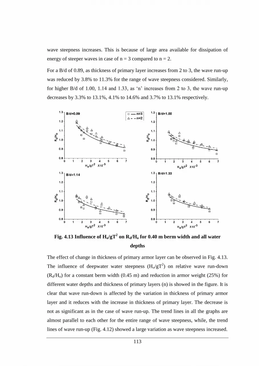
113
wave steepness increases. This is because of large area available for dissipation of
energy of steeper waves in case of n = 3 compared to n = 2.
For a B/d of 0.89, as thickness of primary layer increases from 2 to 3, the wave run-up
was reduced by 3.8% to 11.3% for the range of wave steepness considered. Similarly,
for higher B/d of 1.00, 1.14 and 1.33, as ‘n’ increases from 2 to 3, the wave run-up
decreases by 3.3% to 13.1%, 4.1% to 14.6% and 3.7% to 13.1% respectively.
Fig. 4.13 Influence of Ho/gT2 on Rd/Ho for 0.40 m berm width and all water
depths
The effect of change in thickness of primary armor layer can be observed in Fig. 4.13.
The influence of deepwater water steepness (Ho/gT2) on relative wave run-down
(Rd/Ho) for a constant berm width (0.45 m) and reduction in armor weight (25%) for
different water depths and thickness of primary layers (n) is showed in the figure. It is
clear that wave run-down is affected by the variation in thickness of primary armor
layer and it reduces with the increase in thickness of primary layer. The decrease is
not as significant as in the case of wave run-up. The trend lines in all the graphs are
almost parallel to each other for the entire range of wave steepness, while, the trend
lines of wave run-up (Fig. 4.12) showed a large variation as wave steepness increased.

114
For the entire range of wave steepness and B/d, as the thickness of primary layer is
increased from 2 to 3, the wave run-down decreases by up to 4.6% which is
insignificant compared to wave run-up which is up to 14.6%. The return flow of the
wave run-down is not affected by the increased porosity of the armor layer. Hence,
there is only small impact of variation in thickness of primary layer on wave run-
down.
4.4.4 Influence of change in water depth on berm recession, wave run-up and
run-down
From the section 4.4.3 it was observed that the model with 25% reduced armor weight
and 3 no. of primary layer thickness for 0.40 m berm width is safe for all wave
conditions and water depths. Further tests were conducted only for this condition and
the results and analysis for the same are presented in all the subsequent sections.
Fig. 4.14 Influence of Ho/gT2 on Rec/B for 0.40 m berm width and 25% reduction
in armor weight
Fig. 4.14 depicts the effect of variation in water depth (expressed in terms of relative
berm position, hb/d) on relative berm recession (Rec/B). The position of berm from the
sea bed (hb) was kept constant at a height of 0.45 m. The damage increases with an
increase in depth of water and with a decreasing wave period. As observed in the

115
previous sections 4.4.1 to 4.4.3, the Rec/B increases with an increase in Ho/gT2. For all
the test conditions, the berm recession is less than berm width which indicates the
structure is safe. High berm recession is observed when water level is equal to the
berm position (i.e., hb/d = 1) for all Ho/gT2 considered. Berm recession is reduced as
water level in front of the berm reduces and highest reduction of recession is observed
for hb/d=1.50. A maximum Rec/B of 0.72 is observed for Ho/gT2 of 0.0067 and water
depth of 0.45 m (hb/d = 1.00). As the hb/d increases from 1.00 to 1.13, 1.29 and 1.50,
the berm recession decreases by 8.8% to 37.5%, 58.1% to 76% and 76.1% to 100%
respectively.
The high erosion of berm was observed when its level equals water level. This is
because waves directly attack the upper slope and dislodge the armor units. Further,
the return flow of the water pull down these dislodged armors along with it thus
increasing erosion. But, as water level decreases the berm restricts the movement of
the wave onto the upper reaches and hence, the return flow will also be less thus
reducing the erosion. Even though the waves impinges directly on the lower slope for
lower water depth (hb/d =1.50), the energy within the wave is less and hence does not
cause much damage to the structure. From the stability point of view it may be noted
that when water level is about 0.10 m (hb/d = 1.29) less than the berm level the
reduction in berm recession is high. The large damage for higher water depths and
shorter wave periods is because higher water depths sustain larger waves and short
period waves repeatedly disturb the displaced armor units within a smaller time
interval without allowing them to settle.
Fig. 4.15 shows the obtained relative wave run-up (Ru/Ho) as a function of the
deepwater wave steepness (Ho/gT2) for a constant berm width of 0.40 m and 25%
reduced armor weight models. The water depth is varied from 0.30 m to 0.45 m (hb/d
= 1.50 – 1.00). The berm is placed at a constant height of 0.45 m from the sea bed. It
can be clearly observed that for a higher water depth of 0.45 m and 0.40 m (hb/d = 1.0,
1.13), the wave run-up is high compared to other water depths. A lowest wave run-up
can be observed for a water depth of 0.35 m (hb/d = 1.29). Wave run-up for 0.30 m
water depth (hb/d = 1.50) is more than 0.35 m depth. This is because for lower water
depth the effect of berm is not felt and the wave impinges directly on lower slope thus

116
increasing wave run-up. Same is the case for higher water depth of 0.45 m where the
water impinges on upper slope and hence, an increasing wave run-up. Further, a
decrease in wave run-up with increasing Ho/gT2 is also observed which is similar to
the cases in the previous sections 4.4.1 to 4.4.3. Also, it can be observed in all the
three graphs that the trend line becomes gentle as Ho/gT2 increases.
Fig. 4.15 Influence of Ho/gT2 on Ru/Ho for 0.40 m berm width and all water
depths
As hb/d increases from 1.00 to 1.13, 1.29 and 1.50, the wave run-up decreases by
0.5% to 3.2%, 2.1% to 6.5% and 1.2% to 2.9% respectively for the entire range of
wave steepness considered. It can be observed that the maximum reduction in Ru/Ho is
6.5% for hb/d = 1.29. This implies that highest reduction in wave run-up is possible
when hb/d = 1.29 (d = 0.35m).
Fig. 4.16 shows the variation of relative wave run-down (Rd/Ho) as a function of the
deepwater wave steepness (Ho/gT2) for a constant berm width of 0.40 m and 25%
reduced armor weight models. The water depth is varied from 0.30 m to 0.45 m (hb/d
= 1.50 – 1.00). The berm is placed at a constant height of 0.45 m from the sea bed.
Wave run-down is high for highest water depth tested i.e., 0.45 m (hb/d = 1.00) and
lowest for a water depth of 0.35 m (hb/d = 1.29) similar to that of wave run-up. It is
also observed that as wave steepness increase the slope of trend line gets gentle for all
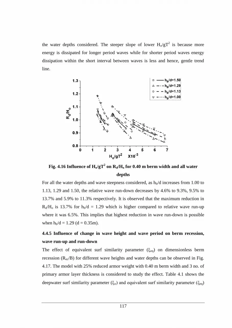
117
the water depths considered. The steeper slope of lower Ho/gT2 is because more
energy is dissipated for longer period waves while for shorter period waves energy
dissipation within the short interval between waves is less and hence, gentle trend
line.
Fig. 4.16 Influence of Ho/gT2 on Rd/Ho for 0.40 m berm width and all water
depths
For all the water depths and wave steepness considered, as hb/d increases from 1.00 to
1.13, 1.29 and 1.50, the relative wave run-down decreases by 4.6% to 9.3%, 9.5% to
13.7% and 5.9% to 11.3% respectively. It is observed that the maximum reduction in
Rd/Ho is 13.7% for hb/d = 1.29 which is higher compared to relative wave run-up
where it was 6.5%. This implies that highest reduction in wave run-down is possible
when hb/d = 1.29 (d = 0.35m).
4.4.5 Influence of change in wave height and wave period on berm recession,
wave run-up and run-down
The effect of equivalent surf similarity parameter (eq) on dimensionless berm
recession (Rec/B) for different wave heights and water depths can be observed in Fig.
4.17. The model with 25% reduced armor weight with 0.40 m berm width and 3 no. of
primary armor layer thickness is considered to study the effect. Table 4.1 shows the
deepwater surf similarity parameter (o) and equivalent surf similarity parameter (ξeq)

118
calculated using the method explained in CEM 2006 (refer Fig. 2.17), for different
wave heights and wave periods considered for the study.
o
o
o
LH
tan ........................................................ (4.1)
o
o
eq
eq
LH
tan ........................................................ (4.2)
Table 4.1 Equivalent surf similarity parameter for 0.40 m berm width model
H (m) T (s) o eq
0.10 1.6 4.070 1.743
0.12 1.6 3.677 1.591
0.14 1.6 3.439 1.473
0.16 1.6 3.202 1.378
0.10 2.0 5.092 2.229
0.12 2.0 4.674 2.035
0.14 2.0 4.383 1.884
0.16 2.0 4.085 1.762
0.10 2.6 7.087 3.021
0.12 2.6 6.507 2.758
0.14 2.6 6.006 2.554
0.16 2.6 5.658 2.389
Fig. 4.17 shows the variation in the berm recession as the equivalent surf similarity
parameter changes from 1.3 to 2.9 for different water depths of 0.35 m, 0.40 m and
0.45 m (B/d= 1.14, 1.00 and 0.89). It is observed that with the increase in eq, the
berm recession decreases, while, with the increase in Ns, berm recession increases.
Also, with the increase in B/d ratio the berm recession is found to decrease for all the
test conditions. For B/d = 0.89, 1.00 and 1.14, the berm recession varies from 0.192 to
0.732, 0.12 to 0.657 and 0.046 to 0.456 respectively. With the increase in B/d from
0.89 to 1.00 and 1.14, there is 8.9% to 37.5% and 36.7% to 76.0% reduction in berm
recession respectively for all the test conditions.

119
Fig. 4.17 Influence of eq on Rec/B for 0.40 m berm width and 25% reduction in
armor weight
For a particular B/d of 0.89, with the increase in eq from 1.6 to 2.9, the Rec/B
decreases by 14.3% to 20%. Similarly, for a particular B/d of 0.89, as Ns decreases
from 3.5 to 2.2, the berm recession also decreases by 66.7% to 72.8%. Comparing the
percentage decrease with respect to wave period (eq) and wave height (Ns), it can be
concluded that the effect of wave period is less on berm recession. The same
observation was also expressed by Moghim et al. (2011).
According to Bruun and Gunbak (1976), the failure of breakwater is caused by
combinations of buoyancy, inertia and drag forces supported by the effect of
hydrostatic pressure from the core. These forces all seem to reach their maximum
value for lowest down rush which occurs at resonance. Bruun and Gunbak (1976)
observed that, this condition was reached for 2.0 < ξo < 3.0. In the present study,
models tested with wave period of 1.6 s (eq = 1.2 – 1.6) have shown greater damage
when compared to the other wave periods studied. This may be due to the nature of
wave breaking, which is of collapsing type when period is 1.6 s and corresponding
value of ξo is 3.2 to 4.0 and ξeq is 1.37 to 1.74. The recession was found decreasing as

120
the wave period increased from 1.6 s to 2.6 s. In model study, during such condition,
it is found that wave run-up is maximum and run-down is relatively high and armor
units are disturbed, dislodged and lifted by run-up and pulled down by the run-down
as stated by Ahrens (1970).
Fig. 4.18 Influence of eq on Ru/Ho for 0.40 m berm width and 25% reduction in
armor weight
The effect of wave period and height on wave run-up can be observed in Fig. 4.18.
The graphs are plotted for a constant berm width of 0.40 m and 25% reduced armor
weight for different water depths. A steep increase in wave run-up with increase in
surf similarity parameter (eq) can be observed in the graphs for all stability numbers.
From the figure, it is clear that Ru/Ho is linearly proportional to the eq for any B/d.
For any selected B/d, it can be seen that, higher wave periods cause increased Ru/Ho.
This observation confirms the similar trend demonstrated in Fig. 4.15 of section 4.4.4.
It is also demonstrated in Fig. 4.18, that B/d has little influence on Ru/Ho Vs eq, since,
the slope of the graphs are almost similar. Also, the relative wave run-up increases
with the increase in stability number which can also be noticed very clearly from the

121
graphs. This graph makes a clear indication of dependence of wave run-up on wave
period and wave height.
As B/d increases from 0.89 to 1.00, 1.14 and 1.33, the wave run-up decreases by 1.3%
to 1.6%, 3.3% to 4.9% and 2.5% to 3.2% respectively. This shows the effect of B/d is
insignificant on Ru/Ho which was also observed in the section 4.4.2. Similarly, for a
B/d of 1.00, as Ns increases from 2.2 to 3.6, the Ru/Ho decreases by 3.6% to 10%.
Further, for a B/d of =1.00 and Ns of 2.2, as eq increases, Ru/Ho also increases by 4%
to 14%.
Fig. 4.19 Influence of eq on Rd/Ho for 0.40 m berm width and 25% reduction in
armor weight
The effect of wave period and height on wave run-down can be observed in Fig. 4.19.
The graphs are plotted for a constant berm width of 0.40 m and 25% reduced armor
weight for different water depths. An increase in wave run-down with increase in surf
similarity parameter (eq) can be observed in the graphs for all stability numbers. For
any selected B/d, it can be seen that, higher wave periods cause increased Rd/Ho. This
observation confirms the similar trend demonstrated in Fig. 4.16 of section 4.6.4. It is
also demonstrated in Fig. 4.19 that B/d has some influence on Rd/Ho Vs eq, since,

122
with the increase in B/d the trend line starts becoming horizontal with increased eq.
Also, the wave run-down increases with the increase in stability number which can
also be noticed very clearly from the graphs. This graph makes a clear indication of
dependence of wave run-down on wave period and wave height.
As B/d increases from 0.89 to 1.00, 1.14 and 1.33, the wave run-down decreases by
4.4% to 8.5%, 8.7% to 12.1% and 5.6% to 10.1% respectively. This shows the effect
of B/d is insignificant on Rd/Ho which was also observed in the section 4.6.4.
Similarly, for a B/d of 1.00, as Ns increases from 2.2 to 3.6, the Rd/Ho decreases by
2.3% to 14.4%. Further, for a B/d of =1.00 and Ns of 2.2, as eq increases, Rd/Ho also
increases by 6.7% to 10%.
4.4.6 Influence of storm duration on berm recession
Figs. 4.20 (a) – (d) illustrate the influence of storm duration on dimensionless berm
recession (Rec/B) for different deepwater wave steepness and water depths. The effect
is shown for 25% reduced armor weight with 0.40 m berm model for 3 layers of
primary armor. It can be observed that as storm duration increases the berm recession
also increases. For all water depths, wave periods and lower wave height (H = 0.10 m)
the berm is almost stabilized and recession was found to be nearly constant after 2000
waves (4.44 hrs to 7.22 hrs). The legend depicting the ‘dash’, ‘dotted’ and ‘solid’
lines represent 1.6, 2.0 and 2.6 s wave period respectively in all the figures.
Fig. 4.20 (a) Influence of no. of waves on Rec/B for 0.40 m berm width and 0.45 m
water depth

123
The effect of storm duration on dimensionless berm recession for a water depth of
0.45 m is observed in Fig. 4.20 (a). It is clear from the graph that most of the
settlement and movement of the armor takes place within 2000 waves. From the
figure it is observed that as wave height increases berm recession increases and it
decreases with the increase in wave period. 90% of the berm recession occurs within
2000 waves (4.44 hrs to 7.22 hrs) and the remaining up to 3000 waves (6.67 hrs to
10.83 hrs) for all the considered wave conditions. This is as suggested by many
researchers (Van der Meer and Pilarczyk (1984), Hall (1984), Hegde (1996), Moghim
et al. (2011)).
Fig. 4.20 (b) Influence of no. of waves on Rec/B for 0.40 m berm width and 0.40 m
water depth
Similarly, from Fig. 4.20 (b), the increase in berm recession with increasing wave
height and decreasing wave period can be observed. Further, 90% of the berm
recession occurred within 2000 waves for higher wave heights (H = 0.14 m, 0.16 m)
and within 1000 waves (2.22 hrs to 3.61 hrs) for lower wave heights (H = 0.10 m,
0.12 m).

124
Fig. 4.20 (c) Influence of no. of waves on Rec/B for 0.40 m berm width and 0.35 m
water depth
In Fig. 4.20 (c) it can be clearly observed that for a wave height of 0.10 m (Ho/gT2 =
0.0042, 0.0026, 0.0014) there was no berm recession up to 2000 waves for all wave
periods. Similarly, for a wave height of 0.12 m (Ho/gT2 = 0.0051, 0.0031, 0.0017), no
berm recession was observed for initial 1000 waves for all wave periods. For waves
of 0.14 m (Ho/gT2 = 0.0059, 0.0036, 0.0019) and 0.16 m (Ho/gT
2 = 0.0068, 0.0041,
0.0022), berm recession was increasing for the entire storm duration.
Fig. 4.20 (d) Influence of no. of waves on Rec/B for 0.40 m berm width and 0.30 m
water depth

125
For a water depth of 0.30 m (Fig. 4.20 (d)) no berm recession occurred for waves of
0.10 m and all wave periods (Ho/gT2 = 0.0042, 0.0026, 0.0014) and for 0.12 m wave
with 2.6 s period (Ho/gT2 = 0.0017) for the entire storm duration. For 0.14 m wave
and all wave periods (Ho/gT2 = 0.0059, 0.0036, 0.0019), for initial 1000 waves no
recession of berm was observed and up to 2000 waves, the reshaping of structure was
observed after which no further erosion was observed.
The decrease in rate of increase in berm recession with the increase in storm duration
is due the reshaping of the breakwater structure into an equilibrium profile during the
wave attack. Once equilibrium profile is attained even with further attack of waves,
no further erosion of berm will takes place. This makes storm duration an important
parameter in case of berm breakwater which helps in knowing after how much
storm/cyclone/depression in sea, an equilibrium profile is achieved for a particular
wave condition.
4.5 EQUATIONS DEVELOPED FROM THE PRESENT STUDY
All the test data for different configurations of berm breakwater were combined into
suitable dimensionless terms and are represented in Fig. 4.21. The figure shows the
experimental data for 540 test runs and the best fit curve with a correlation coefficient
of 0.8251. The curve is fitted using M.S. Excel sheet.
Fig. 4.21 Stability equation for berm breakwater

126
From Fig. 4.21, the equation for berm recession in statically stable reshaped berm
breakwater is derived as:
1.0
s2.0
50nec ANN
DR ------------------------------------------- (7.1)
Where,
1.0
b
32
o
dh*dB*n
10*gTHA
------------------------- (7.2)
Fig. 4.22 shows the comparison between the measured berm recession and the
calculated berm recession. A good R2 of 0.821 is obtained.
Fig. 4.22 Comparison of measured and calculated berm recession
Fig. 4.23 Comparison of measured and calculated wave run-up

127
Fig. 4.24 Comparison of measured and calculated wave run-down
Similarly equations for prediction of wave run-up and run-down are also developed
which are given as:
eq
eq
o
u
H
R
681.11
449.2
------------------------- (7.3)
eq
eq
o
d
H
R
133.11
680.1
------------------------- (7.4)
Fig. 4.23 shows the comparison between the measured wave run-up and the calculated
wave run-up. A better R2 of 0.821 is obtained. Similarly, Fig. 4.24 depicts the
comparison between the measured wave run-down and the calculated wave run-down.
A better R2 of 0.822 is obtained.
4.6 OPTIMUM BERM BREAKWATER CONFIGURATION
Considering the test results, an optimum berm breakwater design is evolved. This
consists of a reduced armor cube weight of 79.5 g (≈0.75W) and lower crest height of
0.6 m (i.e. 14.28% of 0.7 m) with a crest width of 0.1 m. It also consists of a
horizontal berm of 0.40 m width at a height of 0.45 m from sea bed. A slope of
1V:1.5H in the remaining upper and lower faces of the breakwater is provided. A
minimum thickness of 2 primary armor layers has to be provided as it satisfies the
stability of berm breakwater model for most of the test conditions. This model is
tested for the similar wave characteristics as in the earlier investigations. It is found

128
that the breakwater is totally safe with Rec/B < 1 with no exposure of secondary layer
for the entire range of test parameters.
4.7 COMPARISON OF PRESENT BREAKWATER MODEL WITH OTHER
TYPES OF BREAKWATER
4.7.1 Comparison of wave run-up and wave run-down with conventional
breakwater
Fig. 4.25 and 4.26 shows the comparison of wave run-up and run-down for the
present model and a conventional uniform slope breakwater, both, armored with
concrete cubes. The berm breakwater model has a 0.45 m berm, with thickness of
primary layer two and made of 25% reduced weight armor units. The conventional
breakwater consists of design weight armor units placed in three layers in the primary
layer. Both breakwaters are constructed with a same sea side slope of 1:1.5.
Fig. 4.25 Comparison of wave run-up between conventional breakwater and
present model
From Fig. 4.25 it is clear that wave run-up is significantly decreased for berm
breakwater as compared to conventional breakwater. This reduction in wave run-up
can be attributed to the presence of berm which breaks the wave thus reducing run-up.
For the range of wave steepness and water depths considered, the relative wave run-
up in berm breakwater decreases by 1% to 34%.

129
Fig. 4.26 Comparison of wave run-down between conventional breakwater and
present model
Fig. 4.26 shows the comparison of wave run-down and even in this case it is clear that
wave run-down is again significantly decreased for berm breakwater compared to
conventional breakwater. For the range of water depths and wave steepness
considered, relative wave run-down in berm breakwater decreases by 27% to 49%
compared to conventional breakwater.
4.7.2 Comparison of berm recession, wave run-up and wave run-down with berm
breakwater armored with natural stones
Fig. 4.27 Comparison of berm recession between berm breakwaters armored
with cubes and stones

130
The comparison of relative berm recession (Rec/B) between berm breakwaters
armored with cubes and stones are shown in Fig. 4.27. Both the berm breakwater are
built with a constant berm of 0.45 m, 40% reduced armor weight with three layers of
primary armor. The results of the stone armored breakwater were collected from
previous studies carried out by Balakrishna (2009). It is clear from the graph that, for
a water depth of 0.40 m (B/d = 1.13), cube armored breakwater has lesser berm
recession compared to stone armored breakwater. For lower wave height a lower
recession can be observed in case of stone armored breakwater but with the increase
in wave height the berm recession also increases. The reason for lower berm recession
is due to the size of the armor units in primary layer. In stone armored breakwater a
range of weights are considered while in cube armored only one weight of the armor
unit will be used. This affects the porosity of the layer thus increasing berm recession.
For the range of wave steepness considered, Rec/B in cube armored berm breakwater
decreases by 18% to 51%.
In addition these results are also tabulated in Table 4.2 to get a clear idea of reduction
or increase when cube armored berm breakwater is compared with cube armored
conventional breakwater and stone armored berm breakwater.
Table 4.2 Comparison of results of present study with conventional cube
armored and stone armored berm breakwaters
Parameter CCBW* CBBW
# (B = 0.45 m) SBBW
$ (B = 0.45 m)
25% 40% 50% 30% 40%
Max. Ru/Ho 1.785 1.195 1.215 1.248 1.177 1.284
% increase in
Ru/Ho
49.4 -- 1.7 4.4 1.5
(decrease)
7.5
Max. Rd/Ho 1.965 1.071 1.177 1.236 1.195 1.286
% increase in
Rd/Ho
83.5 -- 9.9 15.4 11.6 20.1
Max. Rec/B NA1 0.654 1.00 1.00 1.00 1.00
% increase in
Rec/B
-- 52.9 52.9 52.9 52.9
* – CCBW – Conventional Cube armored Breakwater
# – CBBW – Cube armored Berm Breakwater
$ – SBBW – Stone armored Berm Breakwater
NA1 – Berm recession is not applicable in case of conventional cube armored
breakwater
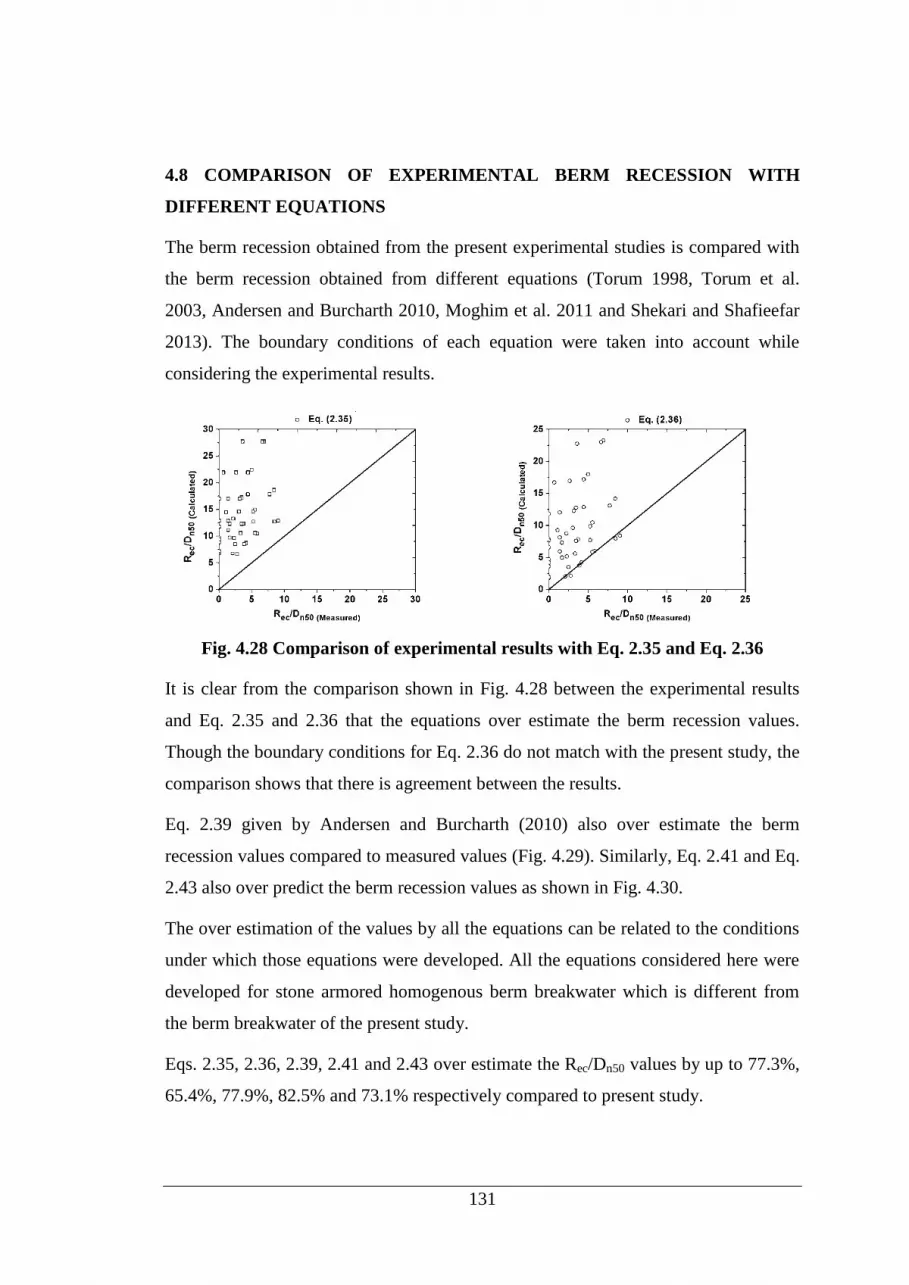
131
4.8 COMPARISON OF EXPERIMENTAL BERM RECESSION WITH
DIFFERENT EQUATIONS
The berm recession obtained from the present experimental studies is compared with
the berm recession obtained from different equations (Torum 1998, Torum et al.
2003, Andersen and Burcharth 2010, Moghim et al. 2011 and Shekari and Shafieefar
2013). The boundary conditions of each equation were taken into account while
considering the experimental results.
Fig. 4.28 Comparison of experimental results with Eq. 2.35 and Eq. 2.36
It is clear from the comparison shown in Fig. 4.28 between the experimental results
and Eq. 2.35 and 2.36 that the equations over estimate the berm recession values.
Though the boundary conditions for Eq. 2.36 do not match with the present study, the
comparison shows that there is agreement between the results.
Eq. 2.39 given by Andersen and Burcharth (2010) also over estimate the berm
recession values compared to measured values (Fig. 4.29). Similarly, Eq. 2.41 and Eq.
2.43 also over predict the berm recession values as shown in Fig. 4.30.
The over estimation of the values by all the equations can be related to the conditions
under which those equations were developed. All the equations considered here were
developed for stone armored homogenous berm breakwater which is different from
the berm breakwater of the present study.
Eqs. 2.35, 2.36, 2.39, 2.41 and 2.43 over estimate the Rec/Dn50 values by up to 77.3%,
65.4%, 77.9%, 82.5% and 73.1% respectively compared to present study.

132
Fig. 4.29 Comparison of experimental results with Eq. 2.39
Fig. 4.30 Comparison of experimental results with Eq. 2.41 and Eq. 2.43
4.9 COMPARISON OF PRESENT EXPERIMENTAL WAVE RUN-UP WITH
EQUATION 2.44
Figs. 4.31 and 4.32 show the comparison of present experimental results with the Eq.
2.44 (De Waal and Van der Meer 1992) which takes into account the influence of the
berm width and water depth (see section 2.8). The equivalent surf similarity (eq)
parameter varies with berm widths. Hence, there are different estimated values of
wave run-up for different berm widths.

133
Fig. 4.31 Comparison of experimental wave run-up with Eq. 2.44 for shallow
water condition
Fig. 4.32 Comparison of experimental wave run-up with Eq. 2.44 for deepwater
condition

134
In the Fig. 4.31, the data related to the equations are calculated corresponding to
shallow water condition, where h, reduction factor for influence of shallow water
conditions is taken as 0.714. From the Fig. 4.31 it can be observed that the prediction
of wave run-up is over-estimated in most of the cases. Also, as berm width decreases,
it can be observed that more and more points starts accumulating at a value of 1.3.
The equation estimates a constant Ru/Ho of 1.3 for eq ≥ 2.0 where as the experimental
values vary.
In the Fig. 4.32, the data related to the equations are calculated corresponding to deep
water condition where h = 1. In this case also the wave run-up is over estimated for
all the conditions considered.
4.10 COST ANALYSIS
The cost analysis of the prototype berm breakwater (details of which are given in
Appendix II) is undertaken. It shows that the cube armored berm breakwater is about
8% and 4% economical than the conventional cube armored breakwater and stone
armored berm breakwater (depending on site condition), both designed for same
operating conditions.
4.11 SUMMARY
The results of various tests conducted on reshaped cube armored berm breakwater
with different sea state and structural parameters were presented in this chapter. The
results obtained were discussed in detail providing relevant details for various
phenomena that occurred during the interaction of the wave with the structure.
It was observed that reduction in armor weight had a serious impact on stability and
damage was found increasing with decrease in armor weight. Berm width also had
some influence in reducing berm recession and it was found that increasing berm
width greatly reduces berm recession. The thickness of primary armor layer also had
its role in reducing berm recession and with increased thickness, higher reduction
could be achieved. The water depth in front of the structure had an impact on berm
recession and with the reduction in water depth, the berm recession also decreased. It
was observed that even though decrease in wave period increased berm recession its
effect compared to wave height was less which incurred higher recession. Finally, the

135
storm duration had a great influence, since; this was the important factor which
reshaped the structure.
The impact of various parameters on wave run-up and run-down was also studied. It
could be noted that many of the parameters had no serious impact on run-up or run-
down. The reduction in armor weight, increase in thickness of primary layer, water
depth fluctuations had no major impact in reducing wave run-up or run-down. The
increasing berm width and change in wave parameters had some notable impact. It
was observed that 0.35 m depth of water (hb/d = 1.29) had the lowest wave run-up and
run-down. The summary of all tests conducted during the study is tabulated in Table
4.3 showing the maximum Rec/B, Ru/Ho and Rd/Ho of all the test models.
Considering all the parameters and the obtained results, it was found that 25%
reduction in armor weight with 0.40 m berm width and 3 no. of primary armor layers
is safe for the entire conditions considered during the study. However, for most of the
wave climate (excluding extreme waves of 0.16 m height and 1.6 s period) primary
layer with 2 armor thickness is safe with a berm width of 0.40 m. In terms of safety as
well as economy 25% reduction with 0.40 m berm width and 2 no. of primary layer
was cheaper compared to the entire models studied.
Table 4.3 Summary of results
Parameters B
(m)
Design
armor
weight
(W)
0.75W 0.6W 0.5W
n = 2 n = 2 n = 3 n = 3 n = 4 n = 4
Max. Ru/Ho
for all
depths
0.45 NA2 1.262 1.195 1.215 1.202 1.248
0.40 NA2 1.284 1.235 NA
4 NA
4 NA
4
0.35 1.274 1.305 1.257 NA4 NA
4 NA
4
0.30 1.292 NA3 1.278 NA
4 NA
4 NA
4
Max. Rd/Ho
for all
depths
0.45 NA2 1.146 1.071 1.177 1.124 1.236
0.40 NA2 1.205 1.185 NA
4 NA
4 NA
4
0.35 1.274 1.267 1.238 NA4 NA
4 NA
4
0.30 1.297 NA3 1.297 NA
4 NA
4 NA
4

136
Max. Rec/B
for all
depths
0.45 NA2 0.78 (S) 0.65 (S) 1.00 (F) 1.00 (F) 1.00 (F)
0.40 NA2 1.00 (F) 0.76 (S) NA
4 NA
4 NA
4
0.35 0.80 (S) 1.00 (F) 1.00 (F) NA4 NA
4 NA
4
0.30 1.00 (F) NA3 1.00 (F) NA
4 NA
4 NA
4
NA2 – Not applicable as the berm breakwater designed with design armor weight and
0.35 m berm width was safe for all test conditions and hence, other berm widths of
0.40 m and 0.45 m are not investigated.
NA3 – Not applicable as the berm breakwater model with 0.35 m berm width and two
layers of primary armor was not safe and hence, smaller berm width of 0.30 m was
not investigated.
NA4 – Not applicable as these berm breakwaters failed for berm widths of 0.45 m.
Hence, shorter berm widths of 0.4 m, 0.35 m and 0.30 m were not investigated.
F indicates berm breakwater failure and S indicates safe berm breakwater structure.

137
CHAPTER 5
CONCLUSIONS
5.1 GENERAL
The stability of conventional and berm breakwater consisting of cube units under
regular wave attack have been investigated with the aid of 1:30 scale physical models.
The study aimed on the evolution of an optimum configuration of statically stable
reshaped berm breakwater with reduced concrete cube amour weight. The
experimental studies were undertaken in Marine Structures Laboratory of Applied
Mechanics Department, National Institute of Technology Karanataka, Surathkal,
India. The conclusions made based on the present experimental work are presented in
this chapter.
5.2 CONCLUSIONS ON CONVENTIONAL BREAKWATER MODEL STUDY
Based on the experimental results of model study on statically stable non-reshaped
berm breakwater, the following conclusions are drawn.
1. Both the relative run-up (Ru/Ho) and the relative run-down (Rd/Ho) decrease with
an increase in deepwater wave steepness (Ho/gT2) depth parameter (d/gT
2).
2. Considering the complete ranges of Ho/gT2 (i.e., 1.43 x 10
-3 ≤ Ho/gT
2 ≤ 7.78x 10
-3)
and d/gT2 (0.006 ≤ d/gT
2 ≤ 0.014), the maximum relative run-up Ru/Ho and
relative run-down Rd/Ho are respectively 1.2 times and 1.25 times the deep water
wave height.
3. The damage level S increases with increase in Ho/gT2, d/gT
2 and Ns.
4. The breakwater damages are in the range of 4.62 to 5.69, 9.75 to 11.46 and 9.46 to
10.22 in the depths of 0.3m, 0.35m and 0.4m respectively
5. Considering all the ranges of d/gT2 (i.e. waves in all depths of water of 0.3m,
0.35m and 0.4m), the increase in damage levels are 9.75 to 11.46 (17.5%), and
9.46 to 10.22 (8%) for waves of periods of 1.6 s and 2.0s respectively. (i.e., ranges
of 4.7x10⁻³
≤ Ho/gT2 ≤ 7.85x10
-3 and 2.5x10
-3 ≤ Ho/gT
2 ≤ 4.0x10
-3 respectively,
and damage are zero for 2.6 s.

138
6. Considering 0.005 ≤ d/gT2 ≤ 0.016, i.e. in depths of 0.35m, the maximum damage
levels increase from 9.46 to 9.76 (i.e. 10.66 %) and for 0.006 ≤ d/gT2 ≤ 0.019 i.e.,
in the depth of 0.4m they increase from 10.22 to 11.46 (i.e., 9.78 %).
5.3 CONCLUSIONS ON RESHAPED BERM BREAKWATER MODEL
STUDY
Based on the experimental results of model study on statically stable reshaped berm
breakwater, the following conclusions are drawn.
1. Berm recession, wave run-up, run-down and exposure of secondary layer are
influenced by armor weight, berm width, wave height, period and depth, and
storm duration.
2. The structure with reduced armor weight by 25% and 0.45 m berm width is safe
for all the parameters considered in the present investigation.
3. For a model with 25% reduced armor weight and 0.40 m berm, increase in
thickness of primary layer from 2 to 3 brought about 15% and 4% reduction in
wave run-up and run-down respectively. However, breakwater with 2 layers of
primary armor is totally safe for almost all the test conditions.
4. As hb/d parameter increases from 1.00 to 1.50, the berm recession decreased by up
to 77%. Also, the wave run-up and run-down decreases by 7% and 14%
respectively.
5. In stone armored berm breakwater, the berm recession increases by 52.9%,
compared to cube armored berm breakwater, and the wave run-up and run-down
also increases by 20.1% and 7.5% respectively for the same wave conditions.
6. A reduction of up to 50.6% and 16.5% in wave run-up and run-down can be
achieved with a cube armored berm breakwater compared to conventional cube
armored breakwater for the same wave conditions.
7. The present cube armored berm breakwater is 8% and 4% economical than the
conventional cube armored breakwater and stone armored berm breakwater.
8. The berm recession equations (Eqs. 2.35, 2.36, 2.39, 2.41 and 2.42 and 2.43) over
estimate the Rec/Dn50 values by up to 83% respectively compared to present study.

139
9. The wave run-up equation given by CEM 2006 also over estimates the wave run-
up compared to the present study.
10. The stability equation of tandem breakwater with reef of natural stones is derived
as:
1.032
2.0
50
**
10*
dhdBn
gTHN
N
DR
b
os
nec
11. The wave run-up and run-down equations based on the present experimental data
are derived as:
eq
eq
o
u
H
R
681.11
449.2
and
eq
eq
o
d
H
R
133.11
680.1
5.4 SCOPE FOR FUTURE WORK
The similar model studies may be undertaken on the reshaped breakwaters with;
1. Varying structure slopes such as 1V:2H, 1V: 2.5H and 1V:3H with higher
reduction in armor weight to get an economical and safe geometry of the berm
breakwater.
2. Studies on the same model with random waves.
3. Berm breakwaters with multi layers of armor unit.


141
APPENDIX I
UNCERTAINTY ANALYSIS
AI-1 GENERAL
There are many ways of expressing the inaccuracies in an experiment. Error
measurement is one of the method which measures of difference between true value
and recorded value. An error is a fixed number and is not a statistical variable.
Uncertainty analysis is another way of expressing an uncertainty which is different
from error. An uncertainty is a possible value that the error might take on in a given
measurement. Since, the uncertainty can take on various values over a range, it is
inherently a statistical variable (Kline 1985). It is also generally agreed that the
inaccuracies can be appropriately expressed by an “uncertainty” and these values
could be obtained by an “Uncertainty analysis”.
The hydrodynamic testing facilities differ from one another with regard to
instrumentation, experimental procedures, scale, etc. Hence, it becomes necessary for
a test facility to provide results with possible lower and upper margins, which can be
accepted with a fair confidence level. The width of confidence intervals is a measure
of the overall quality of the regression line. The 95% confidence interval limits must
always be estimated and this concept of confidence level is fundamental to
uncertainty analysis.
AI-2 CONFIDENCE AND PREDICTION BANDS
The plot of the best-fit curve can include the 95% confidence band of the best-fit
curve, and the 95% prediction band. The two are very different. The Confidence band
tells about the best fit curve. This means, it is 95% sure that the true best fit curve (if
an infinite number of data points are available) lies within the confidence band. The
prediction band tells about the scatter of the data. If data points are considered, 95%
points are expected to fall within the prediction band. Since the prediction band has to
an account for uncertainty in the curve itself as well as scatters around the curve, it is
much wider than the confidence band. As increase in number of data points, the

142
confidence band gets closer and closer to the best fit curve, while the prediction band
doesn’t change predictably.
For example, in Fig. AI-1 shown below, it is noticed that the confidence bands
(shown as solid) contain a minority of data points. That indicates, the confidence
bands have a 95% chance of containing the true best fit curve and with so much of
data, these bands contain far fewer than half the data points. In contrast, the dashed
prediction bands include 95% of the data points. 95% confidence and prediction
bands have been accepted to be reliable enough for usage under the adoption of
uncertainty analysis.
Fig. AI-1 Combined specimen graph for 95% confidence and prediction band
A 100(1-α) percent confidence interval about the mean response at the value of x = x1,
say Y1 is given by Montgomery and Runger (1999):
xx
o
noS
xx
ntYY
2
2
)2,2/(1
1 ……………………. (AI-1)
where, α = significance level used to compute the confidence level, 2 = variance,
n = sample size, x = sample mean, x = variable, Sxx = standard deviation, t (/2, n -2) =
t-distribution values for n – 2 degrees of freedom, and Yo = βo + β1xo is computed
from the fitted regression model.
The prediction is independent of the observations used to develop the regression

143
model. Therefore, the confidence interval for Yo in Eq. AI-1 is inappropriate, since it
is based only on the data used to fit the regression model. The confidence interval
about Yo refers to the true mean response at x = xo, not to future observations.
A 100(1-α) percent prediction interval on a feature observation Yo at given value xo is
given by:
xx
ono
S
xx
ntYY
22
)2,2/(1
11 ………………… (AI-2)
where Yo = βo + β1xo is computed from the regression model.
AI-3 CONFIDENCE INTERVAL AND PREDICTION INTERVAL FOR
DIMENSIONLESS BERM RECESSION WITH STABILITY NUMBER
The 95% confidence and prediction band for variation of recession level with stability
number for reshaped berm breakwater models tested with W50 = 79.5 g, B = 0.45 m,
T = 1.6 to 2.6 s, H = 0.10 to 0.16 m and d = 0.30 to 0.45 m is shown in Fig. AI-2. It
can be observed that more than 90% of experimental data lie within the 95%
confidence bands. The coefficient of determination, R2, is found to be 0.92.
Fig. AI-2 Plot of 95% confidence and prediction bands for the variation of
Rec/Dn50 with Ns

144
From the figure it is observed that the trend line lie within these 95% confidence
bands and data points lie within the 95% prediction bands drawn. From the bands
drawn, the results may be analyzed with 95% confidence i.e. the conclusions drawn
from these graphs are 95% reliable. Also from the figure it may be visualized that
experimental data points are bounded within the 95% prediction bands and this
particular observation strengthen the conclusions derived from this graph.
AI-4 CONFIDENCE INTERVAL AND PREDICTION INTERVAL FOR
RELATIVE RUN-UP WITH SURF SIMILARITY PARAMATER
The 95% confidence interval and prediction interval for variation of relative run-up
with surf similarity parameter for reshaped berm breakwater models tested with W50 =
79.5 g, B = 0.45 m, T = 1.6 to 2.6 s, H = 0.10 to 0.16 m and d = 0.30 to 0.45 m are
shown in Fig. AI-3. It has been observed that around 95% of the experimental data lie
within the 95% confidence bands. The coefficient of determination, R2, is found to be
0.895.
Fig. AI-3 Plot of 95% confidence and prediction bands for the variation of Ru/Ho
with eq

145
AI-5 CONFIDENCE INTERVAL AND PREDICTION INTERVAL FOR
RELATIVE WAVE RUN-DOWN WITH SURF SIMILARITY PARAMETER
The 95% confidence interval and prediction interval for variation of relative run-down
with surf similarity parameter for reshaped berm breakwater models tested with W50 =
79.5 g, B = 0.45 m, T = 1.6 to 2.6 s, H = 0.10 to 0.16 m and d = 0.30 to 0.45 m are
shown in Fig. AI-4. The coefficient of determination, R2, is found to be 0.895.
Fig. AI-4 Plot of 95% confidence and prediction bands for the variation of Rd/Ho
with eq
As it can be observed about 70% data points lie within the confidence band and all the
points are within prediction band. The large scatter is because of different wave
conditions and water depths considered during the study. Also, the wave run-down
includes both down rush of a wave and flow from within the pores of the armor layer
of the breakwater. This combined flow increases the variation in the run-down for
considered parameters.

146
AI-6 SPECIMEN CALCULATION OF CONFIDENCE AND PREDICTION
INTERVALS
Specimen calculation for the plot Ru/Ho vs. eq for different depths of water is shown
in Table AI-1 with the 95% upper and lower confidence band values and 95% upper
and lower prediction band values. The values are computed using Eqs. AI-1 and AI-2.
Table AI-1 Data points with results of 95% confidence band and 95% prediction
band
Xi (eq) Yi (Ru/Ho)
Confidence band Prediction band
LL
Confidence
UL
Prediction
LL
Confidence
UL
Prediction
1.628 1.021 1.018 0.964 1.127 0.855
1.487 1.002 1.000 0.938 1.107 0.832
1.376 0.981 0.987 0.918 1.090 0.814
1.287 0.954 0.977 0.901 1.078 0.800
2.083 1.072 1.084 1.038 1.197 0.925
1.901 1.066 1.056 1.011 1.169 0.898
1.760 1.047 1.035 0.987 1.147 0.876
1.647 1.038 1.020 0.968 1.130 0.858
2.823 1.195 1.221 1.129 1.316 1.034
2.577 1.152 1.174 1.100 1.276 0.999
2.386 1.139 1.138 1.078 1.245 0.971
2.232 1.118 1.110 1.058 1.220 0.948
1.636 1.007 1.019 0.966 1.129 0.856
1.493 0.967 1.001 0.940 1.108 0.833
1.383 0.947 0.988 0.919 1.091 0.815
1.293 0.924 0.977 0.902 1.078 0.801
2.100 1.067 1.087 1.040 1.199 0.928
1.917 1.043 1.058 1.013 1.171 0.900
1.775 1.026 1.037 0.990 1.149 0.878
1.660 1.010 1.022 0.970 1.132 0.860

147
2.855 1.175 1.227 1.132 1.322 1.038
2.606 1.141 1.179 1.104 1.280 1.003
2.413 1.122 1.143 1.081 1.249 0.975
2.257 1.091 1.114 1.061 1.224 0.952
1.647 0.960 1.020 0.968 1.130 0.858
1.503 0.941 1.002 0.941 1.109 0.835
1.392 0.928 0.989 0.921 1.093 0.817
1.302 0.897 0.978 0.903 1.080 0.802
2.122 1.038 1.091 1.043 1.203 0.931
1.937 0.998 1.061 1.016 1.174 0.903
1.793 0.987 1.040 0.993 1.152 0.881
1.677 0.962 1.024 0.973 1.135 0.863
2.891 1.157 1.234 1.136 1.328 1.043
2.639 1.121 1.186 1.108 1.286 1.007
2.443 1.094 1.148 1.085 1.254 0.979
2.285 1.072 1.119 1.065 1.229 0.956


149
APPENDIX II
COST ANALYSIS
AII-1 INTRODUCTION
From the model studies on berm breakwater, it is concluded that the geometry of the
berm breakwater with 25% reduced armor weight with a berm width of 0.45 m is
completely safe. Considering this, the trunk section of a conventional and a berm
breakwater armored with cube units are designed for the same operating conditions.
This chapter explains the details of the analysis and comparison of cost of prototypes
of conventional and berm breakwater.
AII-2 DESIGN OF CONVENTIONAL BREAKWATER
AII-2.1 Armor weight
Based on the investigations conducted in the wave flume, the trunk section of a
conventional non-overtopping breakwater of primary armor weight (W) of 2.9 T is
designed using Hudson formula (1959) with cubes as armor unit. The weight of stones
in the secondary layer is W/10 = 300 kg but stones of 200 kg to 500 kg are used. A
toe of 200 kg to 500 kg stones, of top width 4.8 m and 3.6 m high is provided at the
bottom at both the ends. The weight of core material is W/200 = 15 kg but 10 kg to
100 kg are used.
AII-2.2 Breakwater height
The maximum run-up observed is about 1.75 times the wave height, about 3.0 m, in a
water depth of 12 m. This results in a breakwater height of 17.3 m. However,
breakwater crest elevation is fixed at 21 m.
AII-2.3 Thickness of layers
The thickness of primary and secondary layer is calculated as 3.7 m and 1.6 m
respectively. The minimum crest width should be sufficient to accommodate 3 armor
units and crest width of 3.5 m is provided.

150
AII-2.4 Design parameters of conventional breakwater
Design wave height, H : 3.0 m
Design armor weight, W : 2.9 T
Specific weight of armor, Sr : 2.4
Mass density of armor unit : 2.4 T/cum
Relative mass density of armor unit, a : 1.4 T/cum
Layer coefficient, K : 1.1
Porosity of
Primary layer : 47%
Secondary layer : 39%
Core : 36%
Breakwater slope : 1V : 1.5H
Thickness of Primary layer : 3.5 m
Secondary layer : 1.7 m
Depth of water : 12 m
Breakwater height : 21 m
Crest Width : 3.5 m
Weight of
Secondary layer, W/10 : 200 kg to 500 kg
core, W/200 : 10 kg to 100 kg
Toe, W/10 : 200 kg to 500 kg
Fig. AII-1 gives the dimensions of the conventional breakwater designed.
Fig. AII-1 Conventional breakwater section

151
AII-3 DESIGN OF BERM BREAKWATER
Based on the conclusions of the present study, it is decided to design the trunk section
of a berm breakwater with cube of armor weight reduced by 25% of that of the
conventional breakwater. Hence, the armor weight for berm breakwater is 2.2 T. The
weight of stones in the secondary layer is W/10 = 230 kg but stones of 200 kg to 500
kg are used. A toe of 200 kg to 500 kg stones, of top width 4.8 m and 3.6 m high is
provided at the bottom at both the ends. The weight of core material is W/200 = 12 kg
but 10 kg to 100 kg are used.
The maximum run-up in case of berm breakwater is 1.2 times the wave height in a
water depth of 12 m which will result in breakwater height of 15.6 m. However,
breakwater crest elevation is fixed at 18 m. A berm of width 12 m will be provided at
an elevation of 13.5 m from the sea bed. The thickness of primary and secondary
layer is calculated as 2.2 m and 1.0 m respectively. The minimum crest width should
be sufficient to accommodate 3 armor units and crest width of 3 m is provided.
AII-3.1 Design parameters of berm breakwater
Design wave height, H : 3.0 m
Design armor weight, W : 2.2 T
Specific weight of armor, Sr : 2.4
Mass density of armor unit : 2.4 T/cum
Relative mass density of armor unit, a : 1.4 T/cum
Layer coefficient, K : 1.1
Porosity of
Primary layer : 47%
Secondary layer : 39%
Core : 36%
Breakwater slope : 1V : 1.5H
Berm width, B : 12 m
Position of berm from sea bed, hB : 13.5 m
Thickness of Primary layer : 2.15 m
Secondary layer : 1.0 m
Depth of water, d : 12 m

152
Breakwater height : 18 m
Crest Width : 3 m
Weight of
Secondary layer, W/10 : 200 kg to 500 kg
core, W/200 : 10 kg to 100 kg
Toe, W/10 : 200 kg to 500 kg
Fig. AII-2 gives the dimensions of the berm breakwater designed.
AII-2 Berm breakwater Section
AII-4 QUANTITY ESTIMATION
The density of cube armor for the calculation of their quantity is estimated as follows:
AII-4.1 Sample calculation
Porosity of primary armor layer = 0.47
Taking volume of primary layer = 1 m3
Volume of voids, Vv = 0.47 m3
Volume of cubes in the layer = 0.53 m3
Weight of cubes in 1 m3 of the layer = volume of cubes X mass density of cubes
= 0.53 X 2.4
= 1.3 T
Density of primary layer = 1.3 T/m3
Similarly,
Density of secondary layer = 1.7 T/m3
Density of core = 1.8 T/m3

153
AII-4.1 Quantity Estimation
The quantity of cube armors required for conventional and berm breakwaters are
calculated in this section. The quantity of material of the breakwater section is first
calculated and these are increased by 15% for possible settlement and/or soft clay
conditions due to its large cross section and a heavy load on the foundation.
Table AII-1 gives the estimation of quantity of primary armor, secondary armor and
core as per the design parameters given in section AII-2.4 and with reference to Fig.
AII-1 for conventional breakwater and Table AII-2 gives the same for berm
breakwater as per the design parameters given in section AII-3.1 and with reference to
Fig. AII-2. The area (BXD) is obtained by drawing the breakwater structures to
prototype dimensions in software called “AutoCAD 2009”. The total quantity in the
tables indicates the increased quantity by 15% due to settlement and soft clay
conditions.
Table AII-1 Quantity estimation of cube armored conventional breakwater for
per meter length
Sl.
No
Layer Density
(T/m3)
No Length
(m)
Area
(BXD)
(m2)
Volume
(m3)
Quantity
(T)
Increased
quantity
(by15%)
(T)
1 Filter
Layer
(1 to 5 kg)
1.8 2 1.0 28.70 57.40 103.320 118.818
2 Core Layer
(5 to 100 kg) 1.8 1 1.0 371.16 371.16 668.088 768.301
3 Sec. Layer
(200 to 500
kg)
1.7 1 1.0 90.21 90.21 153.357 176.361
4 Primary
Layer
(2.9 T)
1.3 1 1.0 197.12 197.12 256.256 294.694
5 Toe Layer
(200 to 500
kg)
1.7 2 1.0 33.55 67.10 114.07 131.181
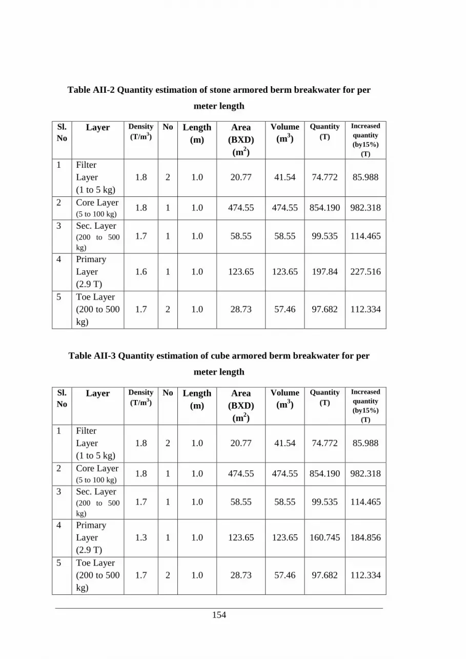
154
Table AII-2 Quantity estimation of stone armored berm breakwater for per
meter length
Sl.
No
Layer Density
(T/m3)
No Length
(m)
Area
(BXD)
(m2)
Volume
(m3)
Quantity
(T)
Increased
quantity
(by15%)
(T)
1 Filter
Layer
(1 to 5 kg)
1.8 2 1.0 20.77 41.54 74.772 85.988
2 Core Layer
(5 to 100 kg) 1.8 1 1.0 474.55 474.55 854.190 982.318
3 Sec. Layer
(200 to 500
kg)
1.7 1 1.0 58.55 58.55 99.535 114.465
4 Primary
Layer
(2.9 T)
1.6 1 1.0 123.65 123.65 197.84 227.516
5 Toe Layer
(200 to 500
kg)
1.7 2 1.0 28.73 57.46 97.682 112.334
Table AII-3 Quantity estimation of cube armored berm breakwater for per
meter length
Sl.
No
Layer Density
(T/m3)
No Length
(m)
Area
(BXD)
(m2)
Volume
(m3)
Quantity
(T)
Increased
quantity
(by15%)
(T)
1 Filter
Layer
(1 to 5 kg)
1.8 2 1.0 20.77 41.54 74.772 85.988
2 Core Layer
(5 to 100 kg) 1.8 1 1.0 474.55 474.55 854.190 982.318
3 Sec. Layer
(200 to 500
kg)
1.7 1 1.0 58.55 58.55 99.535 114.465
4 Primary
Layer
(2.9 T)
1.3 1 1.0 123.65 123.65 160.745 184.856
5 Toe Layer
(200 to 500
kg)
1.7 2 1.0 28.73 57.46 97.682 112.334

155
AII-5 ANALYSIS OF RATES
Unit rates of all items of work are calculated for 10 m3 of material which includes
construction, quarrying, blasting of hard rock, depositing and stacking of useful stones
within a lead of 50 m, transportation, weighing and dumping/placing at specified
location with a lead of 8 km from the quarry as shown in Table AII-4. Finally cost per
ton of armor stone is derived. The cost of 1 m3 of concrete (M35 grade) is Rs. 6500/-
which gives cost per ton equal to Rs. 1,965/-. The cost of preliminaries like
equipments, mobilization, insurance, temporary construction of temporary jetties etc.,
are not included but are to be estimated separately and added to the cost of
breakwaters. Table AII-5 gives the final unit rates of armor stones of various sizes.
Table AII-4 Calculation of unit rates of civil works
Sl.
No. Description of work Quantity
Rate
(Rs.) Per
Amount
(Rs.)
1 Materials
Country blasting powder 4 kg 380/- 1 kg 1,520.00
Country fuse 12 m 200/- 1 m 2,400.00
2 Labor
Quarry men(for boring holes) 15 Nos. 500/- each 7,500.00
Quarry men(charging holes with
Powder and tampering and firing) 2 Nos. 500/- each 1,000.00
Hammer men(Breaking big boulders) 2 Nos. 350/- each 700.00
Men (Removing blasted rock to a
distance of 50 mts) 3 Nos. 350/- each 1,050.00
3 Loading, Unloading and Transporting
charge (8 kms). 2,000.00
16,170.00
4 Royalties @ 10% on Rs 5,097/- 1,617.00
5 Weighing charge Lump sum 275.00
6 Carriage charge of stone up to breakwaters site and placing
Hire charge of boat or any other
transportation upto breakwater
construction site into the sea.
1,200.00
Loading and placing in position the
stones with necessary lifting
equipment.
900.00

156
7 Sundries, wastage – 10% 2,016.00
8 Add contractor‟s overhead and profit
20%. 4,436.00
26,614.00
9 So, cost per cubic meter (for average
size & weight)
26,614
10 2,660.00
10 Cost per Ton
(2660 x 1,000)
2800 950.00
Table AII-5 Final unit rates of armor stones of various sizes
Sl. No. Description of layer Rate per Ton
(Rs.)
1 Filter layer and core stones (1kg to 5kg) 950.00
2
Core and Secondary layer stones
(5kg to 100kg)
(Add 5% extra over „1‟)
998.00
3 Secondary layer stones (100kg to 200kg)
(Add 5% extra over „2‟) 1,048.00
4 Primary layer stones (200kg to 500kg)
(Add 5% extra over „3‟) 1,100.00
5 Primary layer stones (500kg to 700kg)
(Add 5% extra over „4‟) 1,155.00
6 Primary layer stones (700kg to 1000kg)
(Add 5% extra over „5‟) 1,213.00
7 Primary layer stones (1000kg to 2000kg)
(Add 25% extra over „6‟) 1,517.00
8 Primary layer stones ( 2000kg to 3000kg)
(Add 25% extra over „7‟) 1,900.00
AII-6 COST OF CONSTRUCTION
The cost of construction of conventional breakwater is shown in Table AII-6. This is
calculated considering the estimation of armor and other material quantities given in
Table AII-1 and the final unit rates calculated in Table AII-5. The cost of construction
of berm breakwater armored with stone is shown in Table AII-7. This is calculated
considering the estimation of armor and other material quantities given in Table AII-2

157
and the final unit rates calculated in Table AII-5. Similarly, the cost of construction of
berm breakwater armored with cube is shown in Table AII-8. This is calculated
considering the estimation of armor and other materials given in Table AII-2 and the
unit rates given in Section AII-5.
Table AII-6 Cost of construction of cube armored conventional breakwater
Sl. No. Description of work Quantity
Ton
Rate
Rs/Ton.
Amount
Rs.
a) Filter layer (1kg to 5kg) 118.818 950 1,12,877
b) Core stones (10kg to 100kg) 768.301 998 7,66,765
c) Secondary layer (200kg to 500kg ) 176.361 1,100 1,93,997
d) Primary layer (2.9T) (Cube) 294.694 1,965 5,79,074
e) Toe berms (200kg to 500kg) 131.181 1,100 1,44,299
TOTAL COST (Rs.) 17,97,012
Table AII-7 Cost of construction of stone armored berm breakwater
Sl. No. Description of work Quantity
Ton
Rate
Rs/Ton.
Amount
Rs.
a) Filter layer (1kg to 5kg) 85.988 950 81,689
b) Core stones (10kg to 100kg) 982.318 998 9,80,354
c) Secondary layer (200kg to 500kg ) 114.465 1,100 1,25,912
d) Primary layer (2T to 3T) 227.516 1,900 4,32,281
e) Toe berms (200kg to 500kg) 112.334 1,100 1,23,568
TOTAL COST (Rs.) 17,43,804

158
Table AII-8 Cost of construction of cube armored berm breakwater
Sl. No. Description of work Quantity
Ton
Rate
Rs/Ton.
Amount
Rs.
a) Filter layer (1kg to 5kg) 85.988 950 81,689
b) Core stones (10kg to 100kg) 982.318 998 9,80,354
c) Secondary layer (200kg to 500kg ) 114.465 1,100 1,25,912
d) Primary layer (2.2T) (Cube) 184.856 1,965 3,63,242
e) Toe berms (200kg to 500kg) 112.334 1,100 1,23,568
TOTAL COST (Rs.) 16,74,765
159
APPENDIX III
PUBLICATIONS
INTERNATIONAL JOURNAL
1. Prashanth J., Subba Rao, Kiran G. Shirlal, Balakrishna Rao K. & Vishwanath N.,
(2012), “Wave Run-Up, Run-Down studies on reshaped Berm Breakwater with
artificial armor units”, Intl. J. of Earth sciences and Engg., Vol. 5, No. 04 (02),
August, 1052-1056.
NATIONAL JOURNAL
1. Manu, Subba Rao, Kiran G. Shirlal, Prashanth J. & Balakrishna Rao K., (2011),
“Physical Model studies on stability of concrete armored breakwaters”, ISH J. of
Hydraulic Engg., special issue, Vol. 17, No. 3, October, 51-60.
INTERNATIONAL CONFERENCES
1. Subba Rao, Kiran G. Shirlal, Balakrishna Rao K. & Prashanth J., (2011),
“Investigation of Stability of berm breakwater with concrete cubes as armor
units”, Intl. Conf. on Emerging Trends in Engg. (ICETE 2011), NMAM Institute
of Technology, Nitte, Karnataka.
2. Subba Rao, Kiran G. Shirlal, Balakrishna Rao K. & Prashanth J., (2011),
“Concrete cubes as artificial armor units: A laboratory study on berm
breakwaters”, Intl. Conf. on Advances in Materials and Techniques for
Infrastructure Development (AMTID 2011), NIT, Calicut.
3. Subba Rao, Kiran G. shirlal, Balakrishna Rao K. & Prashanth J., (2011), “Wave
run-up, run-down studies on berm breakwater with concrete cubes as armor
units”, 6th
Intl. Conf. on Asian and Pacific Coasts (APAC 2011), University of
Hong Kong, Hong Kong.
4. Subba Rao, Kiran G. Shirlal, Balakrishna Rao K. & Prashanth J., (2012), “Berm
breakwater study with concrete cubes – An experimental approach”, 8th
Intl. Conf.
on Coastal and Port Engineering in Developing Countries (COPEDEC 2012),

160
IIT, Madras, Chennai.
5. Prashanth J., Subba Rao, Kiran G. Shirlal, Balakrishna Rao K. & Vishwanath N.,
(2012), “Wave Run-Up, Run-Down studies on reshaped Berm Breakwater with
artificial armor units”, 2nd
International Engineering Symposium – IES 2012,
Kumamoto University, Japan.
6. Geetha Kuntoji, Subba Rao & Prashanth J. (2013), “Investigation on berm
breakwaters using concrete cubes as armor units.” Intl. Conf. on Hydraulics,
Water Resources, Coastal and Env. Engg. (HYDRO-2013) held at IIT, Madras.
NATIONAL CONFERENCES
1. Subba Rao, Kiran G. Shirlal, Balakrishna Rao K. & Prashanth J., (2010), “An
experimental study on berm breakwater with concrete cubes.” Nat. Conf. on
Hydraulics, Water Resources, Coastal and Env. Engg. (HYDRO-2010), MMU,
Mullana.
2. Subba Rao, Kiran G. Shirlal, Balakrishna Rao K. & Prashanth J., (2011),
“Stability analysis of berm breakwater with concrete cubes as armor units.” Nat.
Conf. on Recent Development in Civil Engg. – RDCE 2011, MIT, Manipal,
Karnataka.
3. Subba Rao, Kiran G. Shirlal, Balakrishna Rao K. & Prashanth J., (2011), “Study
on berm breakwater with concrete cubes as armor unit.” Nat. Seminar on Coastal
Hazards, Resources and Management, Mangalore University, Mangalore.
4. Subba Rao, Kiran G. Shirlal, Balakrishna Rao K. & Prashanth J. and Sharath
kumar, (2011), “Study on stability of berm breakwater with artificial armor units.”
Nat. Conf. on Hydraulics, Water Resources, Coastal and Env. Engg. (HYDRO-
2011), NIT, Surat.
5. Subba Rao, Prashanth J. & Mithun Shetty, (2012), “Performance Characteristics
of Berm Breakwater with Concrete Cube as Armor Units.” Nat. Conf. on
Contemporary Civil Engg. Research and Practices – CCERP 2012, MIT,
Manipal, Karnataka.

161
6. Prashanth J., Subba Rao, Kiran G. shirlal, Geetha Kuntoji & Balakrishna Rao K.
(2012), “Reshaped Berm Breakwater with Artificial Armor Units - Studies on
Wave Run-Up and Run-Down”, Nat. Conf. on Hydraulics, Water Resources,
Coastal and Env. Engg. (HYDRO-2012), IIT, Bombay.
7. Geetha K., Prashanth J. & Subba Rao. (2013). “Investigation on berm breakwaters
using concrete cubes as armor units.” Nat. Seminar on Coastal Env. & their
Management, Mangalore University.
8. Danny Thomas, Prashanth J. & Subba Rao. (2013). “Experimental Analysis on
Berm Breakwater using Artificial Armor Units – Studies on Wave Run-Up and
Run-Down.” Workshop on Disaster Management of Floods and Consequences
thereof in Coastal Region and Food and Water Security, NITK, Surathkal.
9. Prashanth J., Subba Rao, Kiran G Shirlal, Balakrishna Rao K & Danny Thomas
(2013). “Experimental Studies On Reshaping Berm Breakwaters With Artificial
Armor Units.” Nat. Conf. on New Horizons in Civil Engg. – NHCE 2013, MIT,
Manipal, 859-865.
10. Subba Rao, Kiran G. Shirlal, Prashanth J. & Sainath V. (2013). “A Study on
Reshaping Berm Breakwaters.” Nat. Conf. on Emerging Trends in Env. and
Energy Management - NCEEM 2013, Shri Madhwa Vadiraja Institute of
Technology and Management, Udupi, pp. 87-88.
11. Prashanth J., Subba Rao, Kiran G. Shirlal, & K. Balakrishna Rao. (2014).
“Experimental studies on berm breakwater with different armor units”, Fifth
Indian Nat. Conf. on Harbour and Ocean Engg. – INCHOE 2014, NIO, Goa, 5 -7
February 2014. Paper accepted for presentation.
12. Subba Rao, Balakrishna Rao, Madhu M. & Prashanth J., (2011), “Laboratory
investigations on berm breakwater using concrete cubes as artificial armor unit”,
NITK Research Bulletin, Vol. 20, No.1, July 2011, 12-20.


163
REFERENCES
Ahrens, J. P. (1970). "The Influence of Breakwater Type on Rip Rap Stability."
Proc. 12th
ICCE, Washington, 3, 1557 -1566.
Ahrens, J. P. (1975). "Large Wave Tank Tests of Riprap Stability." CERC,
Technical Memorandum No.51, USA.
Ahrens, J. P. (1977). "Prediction of Irregular Wave Runup," CETA 77-4, U.S.
Army Corps of Engineers, Coastal Engineering Research Center, Fort Belvoir,
Va., July.
Ahrens, J. P. (1984). "Reef Type Breakwaters." Proc. 19th
ICCE, Houston, USA,
2648-2662.
Ahrens, J. P., and Ward, D. L. (1991). ―Performance of Bermed Revetments.‖ J.
of Waterway, Port, Coastal, and Ocean Eng., 117(5), 534-540.
Allen R. T. L. (1998). ―Concrete in Coastal Structures.‖ Thomas Telford
Publishing, 1st Edition, London.
Andersen, L. T. (2006). ―Hydraulic Response of Rubble Mound Breakwaters.
Scale Effects–Berm Breakwaters.‖ Doctoral dissertation, Dept. of Civil Eng.,
Aalborg University, Denmark.
Andersen, L. T., and Burcharth, H. F. (2010). ―A New Formula for Front Slope
Recession of Berm Breakwaters.‖ Coastal Eng., 57(4), 359-374.
Archetti, R., and Lamberti, A. (1999). ―Stone Movement and Stresses during the
Reshaping of Berm Breakwaters.‖ Proc 5th
Int. Conf. Coastal Port Eng.
Developing Countries (COPEDEC V), Cape Town, April, pp. 19-23.
Baird, W. F. and Hall, K.R. (1984). "The Design of Breakwaters using Quarried
Stones." Proc., 19th
Int. Conf. on Coastal Eng., 2580-2591.
Bakker, P., van den Berge, A., Hakenberg, R., Klabbers, M., Muttray, M.,
Reedijk, B. and Rovers, I. (2003). ―Development of Concrete Breakwater Armour
Units.‖ 1st Coastal, Estuary and Offshore Eng. Specialty Conf. of the Canadian
Society for Civil Eng., Canada, CSC-395-1 – CSC-395-12.

164
Bakker, S. A., Uijttewaal, W. S. J., Winterwerp, J. C., and Jonkman, S. N. (2009).
―Uncertainty Analysis of the Mud Infill Prediction of the Olokola LNG Approach
Channel.‖ MSc Thesis, Delft University of Technology, 23, 10.
Bala, S. (2013). ―Amazing facts about - Ancient India.‖
http://sarojbala.blogspot.in (July 13, 2013).
Balas, C. E., Koç, M. L., and Tür, R. (2010). ―Artificial Neural Networks based
on Principal Component Analysis, Fuzzy Systems and Fuzzy Neural Networks for
Preliminary Design of Rubble Mound Breakwaters.‖ Applied Ocean Research,
32(4), 425-433.
Battjes, J. A. (1974) ―Surf similarity‖, Proc., 14th
Coastal Eng. Conf. 1, Ch. 26,
Denmark, The Netherlands.
Belfadhel B. M., Lefebvre, G. and Karol Rohan. (1996). "Comparison and
Evaluation of different Riprap Stability Formulas using Field Performance." J.
Waterway, Ports, Coastal and Ocean Eng., ASCE, 122 (1), 8-15.
Bruun, P. (1981). ―Port Engineering.‖ The Gulf Publishing Company, Houston,
USA.
Bruun, P. (1985). ―Design and Construction of Mound for Breakwater and Coastal
Protection.‖ Access Online via Elsevier, 938 p.
Bruun, P. and Gunbak, A. R. (1976). "New design principles for rubble mound
structure", Proc., Coastal Eng. Conf., 3, 2429 -2473.
Bruun, P. and Gunbak, A. R. (1977). "Stability of sloping structures in relation to =
tan /√ (H/Lo) risk criteria in design." J. Coastal Engineering, 1 (4), 287 -322.
Bruun, P. and Kjelstrup, S., (1983). ―Design of Mound Breakwaters.‖ Proc.
Coastal Structures- 83, 9-11 March, 1983, Arlington, Virginia, United States,
122-139.
Bruun, P. M., and Johannesson, P. (1976). ―Parameters Affecting Stability of
Rubble Mounds.‖ J. of the Waterways Harbors and Coastal Eng. Division,
102(2), 141-164.
165
Burcharth, H. F. (1987). ―The Lessons from Recent Breakwater Failures.
Developments in Breakwater Design.” Invited speech presented at World
Federation of Engineering Organizations Technical Congress, Vancouver, May,
pg. 27.
Burcharth, H. F. (1999). ―State of Art in Conceptual Design of Breakwaters.‖
Proc. Coastal Structures '99, Balkema, Rotterdam, 3 -20.
Burcharth, H. F. and Frigaard, P. (1987). "Reshaping Breakwaters: On the
Stability of Roundheads and Trunk Erosion in Oblique waves," Proc. of ASCE
Conf. on Berm Breakwaters, Ottawa, Canada.
Burcharth, H. F. and Frigaard, P. (1988). "On 3-Dimensional Stability of
Reshaping Breakwaters," Proc. of the 21st Coastal Eng. Conf., Malaga, Spain.
Burcharth, H. F., and Brejnegaard-Neilsen, T. (1986). ―The Influence of Waist
Thickness of Dolosse on the Hydraulic Stability of Dolosse Armour.‖ Coastal
Eng. Proc., 1 (20).
Burcharth, H. F., and Liu, Z. (1995). ―Rubble Mound Breakwater Failure Modes.‖
Workshops Proc. of MAST II project, Commission of the European Community,
Directorate General for Science Research and Development. Ed. Aalborg
University Center, DK, December.
Burcharth, H. F., and Rietveld, C. F. W. (1987). ―Construction, Maintenance and
Repair as Elements in Rubble Mound Breakwater Design.‖ 2nd
Int. Conf. on
Coastal and Port Eng. in Developing Countries.
CIRIA, CUR, CETMEF. (2007). ―The Rock Manual: The Use of Rock in
Hydraulic Engineering.‖ 2nd
Ed., CIRIA, London.
Coastal Engineering Manual. (CEM). (2006). "Fundamental of Design." EM
1110-2-1100 (Part-VI), U.S. Anny Corps. of Engineers, Vicksburg, Miss.
Coastal Engineering Research Center. (CERC). (1966). Technical Report No. 4.

166
D’Angremond K., and van Roode, F. C. (2004). ―Positioning the subject.‖
Breakwaters and Closure Dams, Taylor & Francis e-Library, ISBN: 0415332567,
2004 edition, 12-14.
Danel, P. (1953). ―Tetrapods.‖ Proc. Fourth Int. Conf. Coastal Eng., ASCE,
Chicago, USA, 390 – 398.
Davidson, D. D. and Markle, D. G. (1976). ―Effects of Broken DOLOSSE on
Breakwater Stability.‖ Proc., 15th
Conf. Coastal Eng., 3, 2544-2563.
Davies, M. H., Mansard, E. P., & Cornett, A. M. (1994). ―Damage Analysis for
Rubble-Mound Breakwaters.‖ Coastal Eng. Proc., 1 (24).
De Haan, W. (1989). ―Computer Aided Optimum Design of Rubble-Mound
Breakwater Cross-Sections: Manual of the RUMBA Computer Package.‖ Release
1, Delft University of Technology.
De Waal, J. P., and Van der Meer, J. W. (1992). ―Wave Runup and Overtopping
on Coastal Structures.‖ Coastal Eng. Proc., 1 (23).
Dijkstra, O. P. J. (2008). ―Armour Stability on a Bermed Slope Breakwater.‖ M.
Sc. thesis, Delft University of Technology.
Diskin, M. H., Vajda, M. L. and Amir, I. (1970). ―Piling up behind low and
submerged permeable breakwaters.‖ J. of Waterway and Harbour Division,
96(2), 359 – 371.
Ergin, A. and Pora, S. (1971). "Irregular Wave Action on Rubble Mound
Breakwaters." J. Waterways, Port, Coastal, Ocean Eng., ASCE, 97 (WW2), 279-
293.
Ergin, A., Gunbak A. R. and Yanmaz, A. M. (1989). "Rubble Mound
Breakwaters with S-shape Design." J. Waterway, Port, Coastal, Ocean Eng.,
ASCE, 115 (5), 579-593.
Etemad-Shahidi, A., and Bonakdar, L. (2009). ―Design of Rubble-Mound
Breakwaters Using M5′ Machine Learning Method.‖ Applied Ocean Research, 31
(3), 197-201.

167
Fişkin, G. (2004). ―A Case Study on the Stability of Berm Type Coastal Defense
Structures.‖ Doctoral dissertation, Middle East Technical University.
Font, J. B. (1968). ―The Effect of Storm Duration on Rubble Mound Breakwater
Stability.‖ Coastal Eng. Proc., 1 (11).
Fournier, C. P., Sayao, O. J., and Caldas, F. (1990). ―Berm Breakwater
Contamination Study Sergipe Marine Terminal, Brazil.‖ Coastal Eng. Proc., 1
(22).
Franco, L. (1996). ―History of Coastal Engineering in Italy‖, History and Heritage
of Coastal Engineering, ASCE, New York, USA, 275-335.
Gadre, M. R., Poonawala, I. Z. and Kudale, M. D. (1991). "Berm Breakwater
Concept in the Design of Rubble Mound Breakwaters.‖ Proc. 4th
Indian Conf. on
Ocean Eng., Goa, 427-430.
Gadre, M. R., Somayaji, N. and Kale, A. G. (1985). "Stones in Breakwaters and
Seawalls." Proc. 1st Nat. Conf. on Dock and Harbour Eng., IIT Bombay, Dec., 1,
B-107 -B 112.
Gómez-Martín, M. E., and Medina, J. R. (2006). ―Damage Progression on Cube
Armored Breakwaters.‖ Coastal Engineering Conference, ASCE, Vol. 30, No. 5,
p. 5229.
Gómez-Martín, M. E., and Medina, J. R. (2013). ―Heterogeneous Packing and
Hydraulic Stability of Cube and Cubipod Armor Units.‖ J. of Waterway, Port,
Coastal, and Ocean Eng.
Hall, K. R., and Kao, J. S. (1991). ―The Influence of Armour Stone Gradation on
Dynamically Stable Breakwaters.‖ Coastal Eng., 15(4), 333-346.
Hall, K.R. (1994). "Influence of Wave Groups on Stability of Berm Breakwaters."
J. Waterway, Port, Coastal, Ocean Eng., ASCE, 120 (6), 630-636.
Hanzawa, M., Sato, H., Takahashi, S., Shimosako, K., Takayama, T., and
Tanimoto, K. (1996). ―New Stability Formula for Wave-Dissipating Concrete

168
Blocks Covering Horizontally Composite Breakwaters.‖ Coastal Eng. Proc., 1
(25).
Hauer, M., op den Velde, W., Vrijling, J. K., and d'Angremond, K. (1995).
―Comparison between the Construction Costs of Conventional Rubblemound
Breakwaters and Berm Breakwaters.‖ Technical report, Faculty of Civil
Engineering, Delft University of Technology, The Netherlands.
Hedar, P. A. (1986). ―Armor Layer Stability of Rubble-Mound Breakwaters.‖ J. of
Waterway, Port, Coastal, and Ocean Eng., 112(3), 343-350.
Hegde, A. V. (1996). "Studies on deterministic optimum Computer Aided Design
on non-overtopping rubble motmd breakwaters", Doctoral dissertation,
Mangalore University, KREC, Surathkal, India.
Hegde, A. V., and P Srinivas, R. (1995). ―Effect of Core Porosity on Stability and
Run-up of Breakwaters.‖ Ocean Engineering, 22 (6), 519-526.
Hegde, A. V., and Samaga, B. R (1996). "Study on the Effect of Core Porosity on
Rubble Mound Breakwater." Proc., 10th
Congress of the Asian and Pacific
Regional Division of the Int. Assn. for Hydraulic Research, Langkawi, Malaysia,
1, 287-294.
Hegde, A. V., Shirlal, K. G., and Rajaraman, J. (2002). ―Berm Breakwaters-
Effects of Berm Width on Stability‖, Proc. Int. Conf. on Ship and Ocean
Technology SHOT-02., I.I.T, Kharagpur, India, December.
Hudson, R. Y. (1958). ―Design of Quarry-Stone Cover Layers for Rubble-Mound
Breakwaters.‖ Research Report No. 2-2, Army Engineer Waterways Experiment
Station, Vicksburg, Mississippi
Hudson, R. Y. (1959). ―Laboratory Investigation of Rubble Mound Breakwaters.‖
J. Waterway and Harbour Division, 85 (3), 93 – 121.
Hudson, V.Y., Herrmann, F.A., Sager, R.A., Whalin, R.W., Keulegan, G.H.,
Chatham, C.E., Hales, L.Z., (1979). ―Coastal Hydraulic Model.‖ Special Report,
US Army Corps of Engineering, Coastal Engineering Research Centre, No: 5.

169
Hughes, S. A. (1993). ―Physical Models and Laboratory Techniques in Coastal
Engineering.‖ World Scientific, Vol. 7.
Hughes, S. A. (2004). ―Estimation of Wave Run-up on Smooth, Impermeable
Slopes using the Wave Momentum Flux Parameter.‖ Coastal Eng., 51 (11), 1085-
1104.
Hunt, I. A. (1959). "Design of seawalls and breakwaters." J. Waterway and
Harbour Division, 85 (3), 123-152.
Isaacson, M. (1991). ―Measurement of regular wave reflection.‖ J. of Waterway,
Port, Coastal, and Ocean Eng., 117(6), 553-569.
Jensen, O.J. and Klinting, P. (1983). ―Evaluation of scale effects in hydraulic
models by analysis of laminar and turbulent flows.‖ Coastal Eng., 7, 319-329.
Johnson, R. R., Mansard, E. P. D., and Ploeg, J. (1978). ―Effects of Wave
Grouping on Breakwater Stability.‖ Coastal Engineering Proceedings, 1 (16).
Joshi V. B., Jagadeesh, H.B., Chalawadi, A. S. and Purandare U. V. (2006)
―Physical Modelling Studies For Development Of Fisheries Harbour.‖ ISH J. of
Hydraulic Eng., 12:3, 83-94
Juhl, J. and Jensen, O. J. (1995). ―Features of Berm Breakwaters and Practical
Experience.‖ Proc. of Int. Conf. on Coastal and Port Eng. in Developing
Countries, 25-29 September, RJ Brazil, 1307-1320.
Juhl, J., and Sloth, P. (1998). ―Berm Breakwaters-Influence of Stone Gradation
Permeability and Armouring.‖ Coastal Engineering Proceedings, 1 (26).
Kamali, B., and Hashim, R. (2009). ―Recent Advances in Stability Formulae and
Damage Description of Breakwater Armour Layer.‖ Australian Journal of Basic
and Applied Sciences, 3 (3), 2717-2827.
Kao, J. S., and Hall, K. R. (1990). ―Trends in Stability of Dynamically Stable
Breakwaters.‖ Coastal Eng. Proc., 1 (22).
Kheyruri, Z. (2005). ―Berm breakwaters and Jetties Performances in Iran.‖ 2nd
ICS
in Iceland: Höfn the Town of Hornafjörður , Höfn, Iceland , Pg. 9

170
Kim, D. K., Kim, D. H., Chang, S. K., and Chang, S. K. (2007). ―Probabilistic
Neural Network for Predicting the Stability numbers of Breakwater Armor
Blocks.‖ Int. Conf. on Computational & Experimental Eng. and Sciences, Vol. 2,
No. 2, pp 35-40.
Kobayashi, N., and Jacobs, B. K. (1985). ―Riprap Stability Under Wave Action.‖
J. of Waterway, Port, Coastal, and Ocean Eng., 111 (3), 552-566.
Koev, K. N. (1992). ―Statistical Analysis of Formulas for Breakwater Armor
Layer Design.‖ J. of Waterway, Port, Coastal, and Ocean Eng., 118 (2), 213-219.
Kortenhaus, A., Medina, J., González-Escrivá, J. and Garrido, J. (2004).
―Workpackage 4 - Laboratory Measurements on the Zeebrugge Breakwater.‖
Clash Report - EVK3-CT-2001-00058, Version 1.2, November.
KREC Study Team. (1994). ―Study on coastal erosion - Input to environmental
master plan study.‖ DANIDA-DEE-Mangalore, Department of Applied Mechanics
and Hydraulics, KREC, Surathkal, India.
Lamberti, A., and Tomasicchio, G. R. (1997). ―Stone Mobility and Longshore
Transport at Reshaping Breakwaters.‖ Coastal Engineering, 29 (3), 263-289.
Lamberti, A., Tomasicchio, G.R. and Guiducci, F. (1994). ―Reshaping Berm
Breakwaters in Deep and Shallow Water Conditions.‖ Proc. of the 24th
Int. Conf.
on Coastal Eng., Kobe, Japan, ASCE, pp 1343 – 1358.
Le Mehaute, B. (1976). ―Similitude in coastal engineering.‖ J. of Waterway, Port,
Coastal, and Ocean Eng., Division, 102(3), 317-335.
Leenknecht, D.A., Szuwalski, A., and Sherlock, A.R. (1992). ―Automated Coastal
Engineering System.‖ User's Guide, WES, CERC, U S Army Corps of the
Engineers, Vicksburg, MS.
Lissev, N., and Daskalov, K. (2000). ―Berm Type Breakwater—An Alternative
Solution for New East Breakwater for Port of Burgas.‖ Varna conference.
Lissev, N., and Torum, A. (1996). ―Influence of the Core Configuration on the
Stability of Berm Breakwaters.‖ Coastal Eng. Proc., 1 (25).

171
Losada, M. A., and Giménez-Curto, L. A. (1981). ―Flow Characteristics on
Rough, Permeable Slopes under Wave Action.‖ Coastal Eng., 4, 187-206.
Losada, M.A., 1990. ―Recent Development in the Design of Mound Breakwaters.‖
Herbich, J.B. (Ed.), Handbook of Coastal and Ocean Engineerng, vol. I, pp. 939–
1050. Chapter 21.
Lothe, A. E. and Birkeland, T. (2005). ―Rehabilitation and Redesign of the
Gismeroy Industrial Area Sea Wall in Mandal, Norway.‖ Proc. of Int. Conf. on
Coastlines, Structures and Breakwaters, Organized on behalf of the Maritime
Board of the Institution of Civil Engineers and held in London, UK, 20-22 April,
453-467.
Maddrell, R. (2005). ―Lessons Re-Learnt from the Failure of Marine Structures.‖
Coastlines, Structures and Breakwaters Conf., 139-151.
Magoon, O. T., Sloan, R. L. and Foote, G. L. (1974). ―Damages to Coastal
Structures.‖ Coastal Eng. Proc., 1 (14), 1655- 1676.
Mandal, S., Rao, S., and Manjunath, Y. R. (2008). ―Stability Prediction of Berm
Breakwater using Neural Network.‖ Proc. of Seventh Int. Conf. on Coastal and
Port Eng. in Developing Countries-Best Practices in the Coastal Environment,
Dubai Municipality, Dubai, UAE, 24-28 February, 11 pp.
Mandal, S., Rao, S., Manjunath, Y. R., and Kim, D. H. (2007). ―Stability Analysis
of Rubblemound Breakwater Using ANN.‖ Fourth Indian Nat. Conf. on Harbour
and Ocean Eng. (INCHOE-2007), National Institute of Technology, Surathkal,
12-14 December, pp 551-560.
Mase, H., Sakamoto, M., and Sakai, T. (1995). ―Neural Network for Stability
Analysis of Rubble-mound Breakwaters.‖ J. of Waterway, Port, Coastal, and
Ocean Eng., 121 (6), 294-299.
Medina, J. R., and Gómez-Martín, M. E. (2012). ―KD And Safety Factors Of
Concrete Armor Units.‖ Coastal Eng. Proc., 1 (33), Structures-29.

172
Medina, J. R., Gómez-Martín, M. E., and Corredor, A. (2011). ―Influence of
Armor Unit Placement on Armor Porosity and Hydraulic Stability.‖ Coastal Eng.
Proc., 1 (32), Structures-41.
Melby, J. A. (2005). ―Composite-Berm Rubble Mound Breakwater.‖ Proc. of Int.
Conf. on Coastlines, Structures and Breakwaters, Organized on behalf of the
Maritime Board of the Institution of Civil Engineers and held in London, UK, 20-
22 April, 520-529.
Melby, J. A., and Hughes, S. A. (2004). ―Armor Stability based on Wave
Momentum Flux.‖ Proc. of Coastal Structures '03 Conference. ASCE, New York.
Merli, D. 2009. ―Stability of Wide-Graded Rubble Mounds.‖ Msc Thesis,
UNESCO-IHE, Delft.
Misra S. C. (2001). ―Uncertainty Analysis in Hydrodynamics Tests.‖ Int. Conf. in
Ocean Eng., 207-216
Moghim, M. N., Shafieefar, M., Tørum, A., and Chegini, V. (2011). ―A New
Formula for the Sea State and Structural Parameters Influencing the Stability of
Homogeneous Reshaping Berm Breakwaters.‖ Coastal Eng., 58 (8), 706-721.
Montgomery, R, Hofmeister, G. J., and Baird, W F. (1988) "Implementation and
performance of berm breakwater design at Racine, WI." Berm Breakwaters,
ASCE.
Muttray, M., Oumeraci, H., and Oever, E. T. (2006). ―Wave Reflection and Wave
Run-up at Rubble Mound Breakwaters.‖ Coastal Eng. Conf., ASCE, Vol. 30, No.
5, p. 4314.
Naheer, E., and Buslov, V. (1983). ―On Rubble-Mound Breakwaters of Composite
Slope.‖ Coastal Eng., 7 (3), 253-270.
Neelamani, S. and Sunderavadivelu, R. (2003). ―Plans to win back a sandy beach
in Pondicherry, South-East coast of India.‖ Proc. of the 3rd
Int. Surfing Reef
Symposium, June, Raglan, New Zealand, pp 375 – 377.

173
Norton, P. A., and Holmes, P. (1992). ―Armour Displacements on Reshaping
Breakwaters.‖ Coastal Eng. Proc., 1 (23).
Ouellet, Y. (1972). ―Effect of Irregular Wave Trains on Rubble-Mound
Breakwaters.‖ J. of Waterways, Harbors & Coast Eng. Div., 98 (WW1).
Oumeraci, H. (1984). ―Scale Effects in Coastal Hydraulic Models.‖ Symposium on
Scale Effects in Modelling Hydraulic Structures, Technische Akademie Eßlingen,
September.
Owen, M.W. and Briggs, M.G. (1985). ―Limitations of modeling.‖ Proc.
Developments in breakwaters, Institution of Civil Engineers, London, 91-101
Palmer, R. Q. and Walker, J. R. (1976). ―Honolulu reef runway dike.‖ Proc. 15th
ICCE, 3, 1629 – 1646.
PIANC (1976). ―Final Report of the International Commission for the Study of
Waves.‖ Annex to Bulletin No. 25, Vol. III.
PIANC MarCom W. G. 40. (2003). "State-of-the-art of the Design and
Construction of Berm Breakwaters." PIANC, Rep. of Working Group 40 -
MARCOM, Brussels, Belgium.
PIANC Marcom, W. G. 12 (1992). ―Analysis of Rubble Mound Breakwaters.‖
PTC2 Report of Working Group 12.
Pilarczyyk, K. W. and Zeidler, R. B. (1996). "Offshore breakwater and shore
evolution control", A. Balkema Rotterdam, The Netherlands.
Poonawala, L. Z. (1993). "Design of Marine Structures". Lecture notes on training
courses on coastal erosion, protection and coastal zone management, NITK,
Surathkal, India.
Popov, I. J., (1961). ―Experimental Research in Formation by Waves of Stable
Profiles of Upstream Faces of Earth Dams and Reservoir Shores.‖ 7th
Int. Coastal
Eng. Conf., The Hague.

174
Priest, M. S., Pugh, J. W. and Singh, R. (1964). ―Seaward Profile for Rubble
Mound Breakwaters.‖ Proc. 9th
Int. Conf. on Coastal Engineering, ASCE, 553-
559.
Rao S., Rao B. K., and Roy P. K. (2007) ―Influence of Change in Water Depth on
Reshaping of Berm Breakwater.‖ Proc. of Fourth Indian Nat. Conf. on Harbour &
Ocean Eng., 12-14 December, India.
Rao, S., Pramod, C., and Rao, B. (2004). ―Stability of Berm Breakwater with
Reduced Armor stone Weight.‖ Ocean Eng., 31 (11), 1577-1589.
Rao, S., Rao, B. K., and Kamath K. (2010). "Influence of Change in Water
Surface Elevation on Reshaping of Statically Stable Berm Breakwater.", Second
Int. Conf. on Coastal Zone Eng. and Management (Arabian Coast 2010),
November 1-3, Muscat, Oman.
Rao, S., Subrahmanya, K., Rao, B. K., and Chandramohan, V. R. (2008).
―Stability Aspects of Nonreshaped Berm Breakwaters with Reduced Armor
Weight.‖ J. of Waterway, Port, Coastal, and Ocean Eng., 134 (2), 81-87.
Saville, Jr, T. (1955). "Laboratory Data on Wave Run-Up and Over-Topping on
Shore Structures" No. TM64, Coastal Engineering Research Center, Vicksburg,
Mississippi.
Saville, Jr, T. (1957). ―Wave Run-up on Composite Slopes.‖ Coastal Eng.
Proc., 1 (6), 41.
Saville, T., (1953). "Wave and Lake Level Statistics for Lake Erie." U.S. Army
Corps of Engineers, B.E.B. T.M. 37.
Sayao, O. J. (1999). "On the Profile Reshaping of Berm Breakwaters." Coastal
Structures, Vol. 99, pp. 343-351.
Schüttrumpf, H., and Oumeraci, H. (2005). "Layer Thicknesses and Velocities of
Wave Overtopping Flow at Seadikes." Coastal Eng., 52 (6), 473-495.

175
Shekari, M. R., and Shafieefar, M. (2013). "An Experimental Study on the
Reshaping of Berm Breakwaters under Irregular Wave Attacks." Applied Ocean
Research, 42, 16-23.
Shirlal K. G., and Rao S. (2003). ―Laboratory Studies on the Stability of Tandem
Breakwater.‖ ISH Journal of Hydraulic Engineering, 9:1, 36-45.
Sigurdarson, S. and Van der Meer, J. W. (2011). "Front Slope Stability of the
Icelandic-type Berm Breakwater." Proceedings of Coastal Structures, ASCE.
Sigurdarson, S., Smarason, O. B., Viggosson, G., and Bjordal, S. (2006). "Wave
Height Limits for the Statically Stable Icelandic-type Berm Breakwater." Coastal
Eng. Conf., ASCE, Vol. 30, No. 5, p. 5046.
Sigurdarson, S., van der Meer, J.W., Burcharth, H.F., and Soerensen, J. D.,
(2007). "Optimum Safety Levels and Design Rules for the Icelandic-type Berm
Breakwater." Coastal Structures, Venice. ASCE, 53-64.
Sigurdarson, S., Viggosson, G., Benediktsson, S. and Smaraso, O. B. (1995).
―Berm Breakwaters and Quarry Investigations in Iceland.‖ Proc. of Int. Conf. on
Coastal and Port Eng. in Developing Countries, 25-29 September, RJ Brazil,
1204-1218.
Sorensen, T., and Jensen, O. J. (1986). "4. Experience Gained From Breakwater
Failures. In Developments in Breakwaters." Proc. Breakwaters' 85.
SPM (Shore Protection Manual). (1984). Vol. I and II, U.S. Army Coastal
Engineering Research Center, U.S. Government Printing Office, Washington,
D.C.
Stive, M. J. F. (1985). ―A scale comparison of waves breaking on a beach.‖
Coastal Eng., 9(2), 151-158.
Takahashi, S. (1996). ―Design of Vertical Breakwaters‖, Reference Document
no.34, Port and Harbour Research Institute, Ministry of Transport, Yokosuka,
Japan

176
Thompson, D .H and Shuttler, R. M. (1976). "Design of Riprap Slope Protection
against Wind Waves", CIRIA Rep. 61, Hydr. Res. Station, Wallingford, England.
Thompson, D. M., and Shuttler, R. M. (1975). "Riprap design for wind wave
attack. A laboratory study in random waves." Wallingford, EX, 707.
Thompson, E.F. and Vincent, C.L. (1985). "Significant Wave Height for Shallow
Water Design." J. Waterway, Port, Coastal, Ocean Eng., ASCE, 111 (5), 828-841.
Timco, G. W., Mansard, E. P. D., and Ploeg, J. (1984). "Stability of Breakwaters
with Variations in Core Permeability." Coastal Eng. Proc., 1(19).
Tomasicchio, G. R., Lamberti, A., and Archetti, R. (2003). "Armor Stone
Abrasion due to Displacements in Sea Storms." J. of Waterway, Port, Coastal,
and Ocean Eng., 129 (5), 229-232.
Torum, A. (1994). "Wave-induced Forces on Armor Unit on Berm Breakwaters."
J. of Waterway, Port, Coastal, and Ocean Eng., 120 (3), 251-268.
Torum, A. (1998). "On the Stability of Berm Breakwaters in Shallow and Deep
Water." Coastal Eng. Proc., 1 (26).
Torum, A., Franziska K. and Andreas Menze (2003). "On Berm Breakwaters.
Stability, Scour, Overtopping." J. Coastal Eng., 49, 209-238.
Torum, A., Krogh, S.R., Bjordal, S., Fjeld, S., Archetti, R. and Jacobsen, A.
(1999). "Design Criteria and Design Procedure for Berm Breakwaters." Proc.,
Coastal Structures '99, Balkema, Rotterdam, 331-341.
Torum, A., Naess, S., Instanes, A., and Vold, S. (1988). "On Berm Breakwaters."
Coastal Eng. Proc., 1 (21).
Trmal, C. (2003). "Brief Literature Review: Displacements of Rock Armour on
Rubble Mound Breakwaters." Notes, MSc Coastal Engineering, Plymouth
University.
Tutuarima, W. H., and D'Angremond, K. (1998). "Cost Comparison of
Breakwater Types." Coastal Eng. Proc., 1 (26).

177
Van Broekhoven, P. (2011). "The Influence of Armour Layer and Core
Permeability on the Wave Run-up." Master's thesis, Delft University of
Technology.
Van de Kreeke. (1969). "Damage Function of Rubble-mound Breakwaters." J. of
Waterways and Harbors Division. Proc. ASCE, Vol. 95, WW3.
Van der Meer, J. W. (1987). "Stability of Breakwater Armour Layers — Design
Formulae." Coastal Eng., 11 (3), 219-239.
Van der Meer, J. W. (1988a). "Stability of Cubes, Tetrapods and
Accropode." Proc. Breakwaters Conf., London.
Van der Meer, J. W. (1988b). "Deterministic and Probabilistic Design of
Breakwater Armor Layer." J. Waterway, Port, Coastal, Ocean Eng., ASCE,
114,66-80.
Van der Meer, J. W. (1992). "Stability of the Seaward Slope of Berm
Breakwaters." Coastal Eng., 16 (2), 205-234.
Van der Meer, J. W. (1998). "Application and Stability Criteria for Rock and
Artificial Units." Chapter 11, Dikes and Revetments: Design, Maintenance and
Safety Assessment, AA Balkema, Rotterdam, The Netherlands, 191-215.
Van der Meer, J. W. (1988). "Rock Slopes and Gravel Beaches under Random
Wave Attack." Doctorial thesis, Delft University of Technology, The Netherlands.
Van der Meer, J. W. (1998a). "Geometrical Design of Coastal
Structures." Chapter 9, Dikes and Revetments: Design, Maintenance and Safety
Assessment, AA Balkema, Rotterdam, The Netherlands, 161.
Van der Meer, J. W. (1998b). "Wave Run-up and Overtopping." Chapter 8, Dikes
and Revetments: Design, Maintenance and Safety Assessment, AA Balkema,
Rotterdam, The Netherlands, 145-159.
Van der Meer, J. W. (1999). ―Design of concrete armour layers.‖ Proc. of the
Coastal Structures, Vol. 99, June, pp. 213-221.

178
Van der Meer, J. W., and Heydra, G. (1991). "Rocking Armour Units: Number,
Location and Impact Velocity." Coastal Eng., 15 (1), 21-39.
Van der Meer, J. W., and Pilarczyk, K. W. (1984). "Stability of Rubble Mound
Slopes under Random Wave Attack." Coastal Eng. Proc., 1 (19).
Van der Meer, J. W., and Pilarczyk, K. W. (1986). "Dynamic Stability of Rock
Slopes and Gravel Beaches." Coastal Eng. Proc., 1 (20).
Van der Meer, J. W., and Stam, C. J. M. (1992). "Wave Runup on Smooth and
Rock Slopes of Coastal Structures." J. of Waterway, Port, Coastal, and Ocean
Eng., 118 (5), 534-550.
Van Gent, M. R. A. (1992). "Numerical Model for Wave Action on and in Coastal
Structures." Report No. 92-6, Communications on Hydraulic and Geotechnical
Eng., April, Delft University of Technology.
Van Gent, M. R. A. (1993). "Berm Breakwaters: Hydrodynamics, Forces and
Profile-development." Report No. 93-11, Communications on Hydraulic and
Geotechnical Eng., December, Delft University of Technology.
Van Gent, M. R. A. (1996). "Numerical Modelling of Wave Interaction with
Dynamically Stable Structures." Coastal Eng. Proc., 1 (25).
Van Gent, M. R. A. (2013). "Rock Stability of Rubble Mound Breakwaters with a
Berm." Coastal Eng., 78, 35-45.
Van Gent, M. R. A., Smale, A. and Kuiper, C. (2003). "Stability of Rock Slopes
with Shallow Foreshores." Proc. Coastal Structures Conf., Portland, USA.
Van Gent, M. R. A., Smith, G. M. and Van der Werf, I. M. (2011). "Stability of
Rubble Mound Breakwaters with a Berm: The Upper Slope." Proc. Coastal
Structures Conf. 2011, Yokohama, Japan.
Van Gent, M., Smith, G. M., and Van der Werf, I. (2012). ―Stability Of Rubble
Mound Breakwaters with a Berm.‖ Coastal Eng. Proc., 1(33), Structures-10.

179
Verhagen, H. J., d’Angremond, K. and van Roode, F. C. (2009). ―Breakwaters
and Closure Dams.‖ VSSD, Delft, 2nd
edition, ISBN 978-90-6562-173-3. xi, 392
pp.
Vidal, C., Medina, R. and Lomonaco, P. (2006). "Wave Height Parameter for
Damage Description of Rubble Mound Breakwaters." J. Coastal Eng., 53, 711-
722.
Yagci, O., Mercan, D. E., Cigizoglu, H. K., and Kabdasli, M. S. (2005). "Artificial
Intelligence Methods in Breakwater Damage Ratio Estimation." Ocean Eng., 32
(17), 2088-2106.
Zeidler, R. B., Tarnowska, M., Pruszak, Z., and Pilarczyk, K. W. (1992).
―Effectiveness of Coastal Defence Measures.‖ Report prepared for
Rijkswaterstaat and Delft Hydraulics, pg. 581.


RESUME
Name : Prashanth J.
Date of Birth : 27-08-1987
Address : S/o H. R. Janardhana,
Door no. 9, Behind RR School,
Krisnappa Layout,
Doddabommasandra,
Bangalore-5600097
Mobile : (+91) 9844610726
Email(s) : [email protected] / [email protected]
Qualification : B.E. (Civil), M.Tech. (Marine Structures)
Journal Publications : International: 3 National: 1
No. of Conference Presentations : International: 6 National: 14