optimization of outrigger locations in tall buildings
TRANSCRIPT

1
Optimization of Outrigger Locations in Tall
Buildings Subjected to Wind Loads
By Yau Ken Chung
B. Eng. (Hon.)
A thesis submitted in fulfillment of the requirements for the degree of
Master of Engineering Science
Department of Civil and Environmental Engineering
The University of Melbourne
April 2010

2
ABSTRACT
The study of the response of tall buildings to wind has become more critical with the
increase of super tall buildings in major cities around the world. Outrigger-braced tall
building is considered as one of the most popular and efficient tall building design
because they are easier to build, save on costs and provide massive lateral stiffness. Most
importantly, outrigger-braced structures can strengthen a building without disturbing its
aesthetic appearance and this is a significant advantage over other lateral load resisting
systems. Therefore this thesis focuses on the optimum design of multi-outriggers in tall
buildings, based on the standards set out in the Australian wind code AS/NZS 1170.2.
As taller buildings are built, more outriggers are required. Most of the research to date
has included a limited number of outriggers in a building. Some tall buildings require
more outriggers especially for those more than 500m building height. Therefore there is a
need to develop a design that includes many outriggers (e.g. more than 5). In addition,
wind-induced acceleration is not covered in most of the research on outrigger-braced
buildings. The adoption of outrigger-braced systems in tall buildings is very common and
therefore a discussion of wind-induced acceleration will be included in this thesis.
Most of the current standards allow for the adoption of a triangular load distribution in
estimating the wind response of a structure. However, there are only few publications on
the utilization of a triangular load distribution to determine the optimum location of a
limited number of outriggers. This issue will be addressed in this thesis and will be
compared with a uniformly distributed wind load. Further to this, an investigation will be
carried out on the factors affecting the efficiency of an outrigger-braced system in terms
of the core base bending moment and the total drift reduction.
This thesis principally provides a preliminary guide to assess the performance of
outrigger-braced system by estimating the restraining moments at the outrigger locations,
core base bending moment, the total building deflection, along-wind and crosswind

3
acceleration of a tall building. While many computer programs can provide accurate
results for the above, they are time-consuming to run. For designers working on the
preliminary design in the conceptual phase, a quick estimation drawn from a simpler
analysis is preferable. Therefore, as an alternative to computer-generated estimations, a
methodology for an approximate hand calculation of the wind-induced acceleration in an
outrigger-braced structure will be developed.

4
STATEMENT
I hereby certify that:
(a) The thesis is approximately 25000 words in length, exclusive of tables, maps,
bibliographies and appendices,
(b) The thesis comprises only my original work, except where due acknowledgement
has been made in the text of the thesis to all other material used.
Yau Ken Chung
(September 2009)

5
ACKNOWLEDGEMENTS
I would like to give my special thanks to my supervisor Professor Priyan Mendis for his
patience, kindness, encouragement, advice and guidance throughout the course of this
study.
My appreciation is also extended to Dr. Tuan Ngo, Assoc. Professor Nick Haritos, Dr.
Cuong Ngu Yen and my other colleagues for their suggestions in light of this work.
Likewise, I would like to send my gratitude to the senior industrial engineers who
provided ideas and suggestions to improve this thesis — Mr Bao Truong, Mr. Peter
Delphin, Ms Jessey Lee, and others.
Finally, I wish to express my appreciation to my parents for their encouragement and
support, without which this thesis would not be possible.

6
TABLE OF CONTENTS
FIGURES ------------------------------------------- 11
Chapter 1 ------------------------------------------14
1.0 INTRODUCTION -------------------------------------------------------------------------- 14
1.1 Background--------------------------------------------------------------------------- 14
1.2 Motivation and research significance -------------------------------------------- 16
1.3 Objective of research---------------------------------------------------------------- 17
1.4 Scope of study ------------------------------------------------------------------------ 17
1.5 Thesis layout-------------------------------------------------------------------------- 18
Chapter 2 ------------------------------------------19
2.0 DYNAMIC RESPONSE OF TALL BUILDINGS TO WIND ------------------------------- 19
2.1 Introduction -------------------------------------------------------------------------- 19
2.2 Dynamic wind response------------------------------------------------------------- 22
2.3 Introduction to dynamic wind response ------------------------------------------ 26
2.4 Random Vibration Theory---------------------------------------------------------- 28
2.1.1 Along-wind response---------------------------------------------------------- 30
2.1.1.1 Quasi-static assumption---------------------------------------------------- 31
2.1.1.2 Mechanical admittance ---------------------------------------------------- 33
2.1.1.3 Aerodynamic admittance -------------------------------------------------- 35
2.1.1.4 Background and resonant component ----------------------------------- 36

7
2.1.1.5 Gust response factor-------------------------------------------------------- 37
2.1.1.6 Dynamic response factor -------------------------------------------------- 38
2.1.1.7 Peak factor ------------------------------------------------------------------- 38
2.1.1.8 Derivation of along-wind acceleration ---------------------------------- 39
2.1.1.9 Australian Standard AS 1170.2 approach------------------------------- 40
2.1.2 Crosswind response ----------------------------------------------------------- 43
2.1.2.1 Derivation of crosswind acceleration ------------------------------------ 43
2.1.2.2 Australian Standard AS 1170.2 approach------------------------------- 47
2.2 Wind-induced acceleration based on AS 1170.2 2002 ------------------------- 49
2.2.1 Design procedure -------------------------------------------------------------- 49
2.2.2 Parametric studies of wind-induced acceleration ------------------------- 50
Wind-governed parameters--------------------------------------------------------- 50
Building-governed parameters----------------------------------------------------- 50
2.2.2.1 Region------------------------------------------------------------------------ 52
2.2.2.2 Terrain Category------------------------------------------------------------ 53
2.2.2.3 Building Dimensions------------------------------------------------------- 54
2.2.2.4 Building Mass--------------------------------------------------------------- 56
2.2.2.5 Building Periods ------------------------------------------------------------ 57
2.3 Peak versus root-mean-square (r.m.s) acceleration---------------------------- 59
2.4 Human perception threshold------------------------------------------------------- 60
2.4.1 Background--------------------------------------------------------------------- 60
2.4.2 Application of perception curves-------------------------------------------- 60
Chapter 3 ------------------------------------------63
3.0 PERFORMANCE OF AN OUTRIGGER-BRACED STRUCTURE --------------------------- 63
3.1 Introduction -------------------------------------------------------------------------- 63
3.1.1 Outrigger-braced structure --------------------------------------------------- 64
3.2 Method of Analysis ------------------------------------------------------------------ 66
3.2.1 Assumptions for analysis ----------------------------------------------------- 66

8
3.2.2 Uniform wind loading -------------------------------------------------------- 66
3.2.2.1 Restraining Moments ------------------------------------------------------ 72
3.2.2.2 Analysis of horizontal deflection----------------------------------------- 74
3.2.2.3 Optimum locations of outriggers for deflection------------------------ 75
3.2.3 Triangular wind loading ------------------------------------------------------ 79
3.2.3.1 Restraining Moments ------------------------------------------------------ 83
3.2.3.2 Analysis of horizontal deflection----------------------------------------- 85
3.2.3.3 Optimum locations of outriggers for deflection------------------------ 86
3.2.4 Comparison of uniform and triangular form loading--------------------- 89
3.2.5 Generalized solutions for a multi-outrigger system ---------------------- 90
3.2.5.1 Restraining moments------------------------------------------------------- 90
3.2.5.2 Analysis of horizontal deflection----------------------------------------- 93
3.2.5.3 Optimum location of a multi-outrigger system for deflection ------- 93
3.3 Efficiency of outrigger-braced structures ---------------------------------------- 97
3.3.1 Drift reduction efficiency----------------------------------------------------- 97
3.3.2 Moment reduction efficiency ------------------------------------------------ 99
3.3.3 Factors affecting the efficiency of an outrigger-braced structure------101
3.3.3.1 Height of structure---------------------------------------------------------102
3.3.3.2 Core properties-------------------------------------------------------------103
3.3.3.3 Outrigger-braced column properties ------------------------------------105
3.3.3.4 Clear distance between outrigger-braced column---------------------107
3.4 Estimation of wind-induced acceleration ---------------------------------------109
3.4.1 Estimation of building properties ------------------------------------------109
3.4.1.1 Deflected mode shape-----------------------------------------------------109
3.4.1.2 Building mass --------------------------------------------------------------113
3.4.1.3 Building stiffness ----------------------------------------------------------114
3.4.1.4 Building period ------------------------------------------------------------116
3.4.2 Peak along wind acceleration -----------------------------------------------118
3.4.3 Peak cross wind acceleration -----------------------------------------------120

9
Chapter 4 ---------------------------------------- 125
4.0 VERIFICATION THROUGH COMPUTER MODELING ----------------------------------125
4.1 Introduction to ETABS software--------------------------------------------------125
4.2 Wind loading information ---------------------------------------------------------126
4.3 Building properties and configuration ------------------------------------------127
4.4 ETABS analysis ---------------------------------------------------------------------128
4.4.1 Core shear & moment--------------------------------------------------------128
4.4.2 Outrigger-braced column axial force --------------------------------------129
4.4.3 Verification of results --------------------------------------------------------130
4.5 Comparison of manual calculation and the computer model ----------------132
4.5.1 Restraining moment ----------------------------------------------------------132
4.5.2 Deflected mode shape and total deflection -------------------------------134
4.5.3 Building mass -----------------------------------------------------------------135
4.5.4 Building stiffness -------------------------------------------------------------137
4.5.5 Building period ---------------------------------------------------------------138
4.5.6 Along-wind acceleration-----------------------------------------------------139
4.5.7 Crosswind acceleration ------------------------------------------------------142
4.6 Discussion of results ---------------------------------------------------------------143
Chapter 5 ---------------------------------------- 148
5.0 CONCLUSION AND RECOMMENDATIONS FOR FUTURE STUDY ---------------------148
5.1 Conclusions--------------------------------------------------------------------------148
5.2 Recommendations for future study -----------------------------------------------151
5.2.1 Torsional acceleration--------------------------------------------------------151
5.2.2 P-∆ effect ----------------------------------------------------------------------151
5.2.3 Differential shortening of outrigger-braced columns--------------------152
5.2.4 Slab stiffness contribution---------------------------------------------------153

10
Bibliography ------------------------------------ 154
Appendices -------------------------------------- 165
APPENDIX A: PARAMETRIC STUDIES ON WIND-INDUCED ACCELERATIONS --------------165
A.1 Building Information -------------------------------------------------------------------165
A.2 Static Wind Load Analysis-------------------------------------------------------------166
A.3 Dynamic Wind Load Analysis (Ultimate X-direction)-----------------------------168
A.4 Dynamic Wind Load Analysis (Ultimate Y-direction) -----------------------------170
A.5 Dynamic Wind Load Analysis (Serviceability X-direction)-----------------------172
A.6 Dynamic Wind Load Analysis (Serviceability Y-direction) -----------------------174
APPENDIX B: FACTORS AFFECTING EFFICIENCY OF OUTRIGGER-BRACED SYSTEM ------176
A.1 Building Information -------------------------------------------------------------------176
B.2 Static Wind Load Analysis-------------------------------------------------------------177
B.3 Dynamic Wind Load Analysis (Ultimate X-direction)-----------------------------179
B.4 Dynamic Wind Load Analysis (Ultimate Y-direction) -----------------------------181
B.5 Dynamic Wind Load Analysis (Serviceability X-direction)-----------------------183
B.6 Dynamic Wind Load Analysis (Serviceability Y-direction) -----------------------185
B.7 Building Mass ---------------------------------------------------------------------------187
B.8 Building Deflection and Mode Shape ------------------------------------------------189
B.9 Outrigger-braced System Analysis ---------------------------------------------------191
APPENDIX C: MATHEMATICA PROGRAM CALCULATIONS ---------------------------------192
C.1 One-outrigger-braced system ---------------------------------------------------------192
C.2 Two-outrigger-braced system---------------------------------------------------------194
C.3 Three-outrigger-braced system -------------------------------------------------------196
C.4 Four-outrigger-braced system --------------------------------------------------------198
C.5 Five-outrigger-braced system---------------------------------------------------------202
APPENDIX D: ETABS RESULTS ---------------------------------------------------------------211

11
FIGURES
Figure 1.1 Burj Dubai and other skyscrapers.................................................................... 15
Figure 2.1 Multitude of eddies formed when wind flows through an obstacle ................ 20
Figure 2.2 Three-dimensional wind response on a tall structure ..................................... 21
Figure 2.3 Response spectral density for a tall building (Holmes, 2007)......................... 23
Figure 2.4 Time histories of : (a) wind force; (b) response of a structure with high natural
frequency; and (c) response of a structure with a low natural frequency
(Holmes, 2001) ............................................................................................. 24
Figure 2.5 (a) Tacoma Bridge swaying and before collapse; and (b) Collapse of bridge
after resonant response reached the climax (Holmes, 2001) ....................... 25
Figure 2.6 Wind flow around a tall building..................................................................... 26
Figure 2.7 Description of the wind-induced effects on a structure (Kareem et al, 1999). 27
Figure 2.8 The random vibration (frequency domain) approach to resonant dynamic
response (Davenport, 1963) .......................................................................... 29
Figure 2.9 Simple stick model with large mass on top (Cenek, 1990) ............................. 30
Figure 2.10 Mechanical admittance with respect to natural frequency of structure (Cenek,
1990) ............................................................................................................. 33
Figure 2.11 Aerodynamic admittance – experimental data and fitted function (Vickery,
1965) ............................................................................................................. 35
Figure 2.12 Background and resonant components of response (Holmes, 2001) ............ 36
Figure 2.13 Mode generalized crosswind force spectra of tall buildings (Kwok, 1982).. 46
Figure 2.14 Illustrative example of a tall building............................................................ 51
Figure 2.15 Comparison of regional wind speed with along-wind and crosswind response
....................................................................................................................... 52
Figure 2.16 Comparison of terrain categories with along-wind and crosswind response 54
Figure 2.17 Comparison of building dimensions with along-wind and crosswind response
....................................................................................................................... 55
Figure 2.18 Comparison of building mass with along-wind and crosswind response ..... 56
Figure 2.19 Comparison of building periods with along-wind and crosswind response.. 58

12
Figure 2.20 Horizontal acceleration criteria for occupancy comfort in buildings
(Melbourne & Palmer, 1992)........................................................................ 62
Figure 2.21 various perception criteria for occupant comfort (Kareem, 1999) ................ 62
Figure 3.1 3-D view of an outrigger-braced core-to-column structure (left) and the
elevation of the structure (right) extracted from ETABS software............... 65
Figure 3.2 (a) Outrigger structure deformed shape; (b) the deflection of structure; (c) the
total core base bending moment diagram (Stafford Smith, 1991) ................ 67
Figure 3.3 (a) Outrigger connected to edge of core; (b) equivalent outrigger beam
attached to the centroid of core (Stafford Smith, 1991)................................ 69
Figure 3.4 Restraining moments at both outrigger locations............................................ 71
Figure 3.5 Optimum location for two-outrigger structure under uniform wind load ....... 79
Figure 3.6 Optimum location for two-outrigger structure under triangular form wind load
....................................................................................................................... 88
Figure 3.7 Optimum location for a two-outrigger-braced structure under both uniform and
triangular form loading ................................................................................. 89
Figure 3.8 Optimum location for one-outrigger-braced structure .................................... 94
Figure 3.9 Optimum location for three-outrigger-braced structure .................................. 95
Figure 3.10 Optimum location for four-outrigger-braced structure.................................. 95
Figure 3.11 Optimum location for five-outrigger-braced structure .................................. 96
Figure 3.12 Deflection reduction efficiency of an outrigger-braced structure ................. 98
Figure 3.13 Moment reduction efficiency of an outrigger-braced structure..................... 99
Figure 3.14 Moment reduction efficiency with outriggers 10% lower than the optimum
location........................................................................................................ 100
Figure 3.15 Deflection reduction efficiency with outriggers 10% lower than the optimum
location........................................................................................................ 101
Figure 3.16 Deflection reduction efficiency with total height of 500m ......................... 102
Figure 3.17 Moment reduction efficiency with total height of 500m............................. 103
Figure 3.18 Deflection reduction efficiency with different core properties ................... 104
Figure 3.19 Moment reduction efficiency with different core properties....................... 105
Figure 3.20 Deflection reduction efficiency with column changed................................ 106
Figure 3.21 Moment reduction efficiency with column changed ................................... 106

13
Figure 3.22 Drift reduction efficiency with column clear distance changed.................. 107
Figure 3.23 Moment reduction efficiency with column clear distance changed ............ 108
Figure 3.24 Deflected shape of an outrigger-braced structure........................................ 111
Figure 3.25 Mode shape comparison of an outrigger-braced structure .......................... 112
Figure 3.26 Comparison of mode shape factor between manual calculation and AS1170.2
..................................................................................................................... 123
Figure 4.1 General layout of floor plan for the outrigger-braced structure .................... 127
Figure 4.2 Total shear acting on the main core based on ETABS analysis .................... 128
Figure 4.3 Total moment acting on the main core based on ETABS analysis ............... 129
Figure 4.4 Wind-induced axial load acting on outrigger-braced columns...................... 130
Figure 4.5 Core bending moment of an outrigger-braced structure................................ 131
Figure 4.6 Core bending moment from both analyses.................................................... 133
Figure 4.7 Comparison of mode shape factors based on both analyses.......................... 135
Figure 4.8 (a) Deflection predicted in AS1170.2; (b) the realistic building deflection .. 145

14
Chapter 1
1.0 Introduction
1.1 Background
Tall buildings are a common sight in contemporary cities, especially in those countries
where land is scarce, as they offer a high ratio of floor space per area of land. Tall
buildings are also, arguably, a sign of a city’s economic stature. With the aid of new
design concepts and construction technologies, many countries are constructing gigantic
structures in their major cities, such as Petronas Twin Towers in Malaysia, Taipei 101,
Shanghai’s World Finance Center, and the ultimate skyscraper, Burj Dubai, with a final
projected height of more than 800m including the antenna.
With the identified trend towards higher and more lightweight structures, the risk of
increased flexibility and potentially diminished damping can lead buildings to be more
susceptible to wind action. Even though a structure is designed to meet the requirements
of ultimate strength and serviceability drift, it may not escape from levels of motion that
can cause serious discomfort to its occupants. Therefore, it is very important to control

15
the wind-induced vibration of very tall building (Samali et al, 2004). Intensive study and
research has been carried out to quantify a building’s acceleration to ensure that the
building remains serviceable without causing disturbing motions to its occupants.
Additionally, innovative structural design methods are continuously being sought in the
design of super tall structures with the intention of reducing building response due to
wind action without increasing the construction and material costs. Therefore, outrigger-
braced system has been developed and used in some of the world’s tallest towers in the
past few decades. This design concept consists of a reinforced concrete or steel-braced
core that is connected to the exterior columns by a pair of flexurally stiff horizontal walls
at convenient plan locations. These outriggers are usually located at the plant rooms
along the height of the building. While the outrigger system is very effective in providing
lateral flexural resistance to the building, it does not increase the shear stiffness and the
core itself will carry all the lateral shear forces.
Figure 1.1 Burj Dubai and other skyscrapers

16
1.2 Motivation and research significance
As tall buildings have continued to soar skyward, they are inevitably buffeted in the
wind’s complex environment. The responses of tall building to wind clearly become
more critical as the construction becomes taller, less stiff and more lightweight. Given
that tall buildings need to be strengthened, an outrigger-braced structure is preferable due
to the fact that it is easier to build, with associated cost savings, and can provide massive
lateral stiffness. Most importantly, an outrigger-braced system can improve the structural
performance of a structure without changing its architectural appearance, which is a
significant advantage over other lateral load-resisting systems.
As buildings grow taller, more outriggers are required and they are preferred to be
located at plant rooms. However, most research has included a limited number of
outriggers on a building. This might not be sufficient for a very tall building, e.g.
exceeding 500m in height, and therefore design principles for more outriggers need to be
developed. In addition, the wind-induced acceleration becomes critical for a very tall
building and this has not been a substantial focus in most of the research on outrigger-
braced systems. To address this gap in the research, this thesis will discuss the
optimization of outrigger location in terms of core base bending moments, building
deflection and wind-induced accelerations.
This thesis aims to develop a methodology for estimating the best location for outriggers
in terms of the outriggers’ restraining moments, the total building deflection and the
along-wind and crosswind accelerations of an outrigger-braced structure. While a number
of computer programs can provide accurate results for the above, they are time-
consuming to run. For designers working on the preliminary design in the conceptual
phase, a quick estimation drawn from a simpler analysis is preferable.

17
1.3 Objective of research
This research focuses on the optimization of outrigger locations for an outrigger-braced
structure in terms of reducing the building deflection and the wind-induced accelerations
at the top of the building. Firstly, derivations of along and cross wind accelerations will
be presented, leading to a parametric study of wind-induced accelerations based on the
Australian wind code AS/NZS 1170.2. In addition, the acceleration limit criteria will be
discussed based on recently presented graphs and research.
Secondly, this thesis will introduce a method for analyzing an outrigger-braced structure
with the aim of finding the best-fit outrigger locations to obtain the least building
deflection, along-wind and crosswind accelerations, and to determine the outrigger
restraining moments. Further to this, an investigation will be carried out on the factors
affecting the “efficiency” of outrigger-braced systems in terms of the core moment
distribution and total drift reduction.
Finally, the methodology for an approximate method for acquiring the wind-induced
acceleration in an outrigger-braced structure will be developed based on the
aforementioned analysis. Then, a computer program is used to analyze a simple
outrigger-braced structure to verify the results based on the manual analysis that is
performed.
1.4 Scope of study
This thesis is limited to the study of the overall performance of outrigger-braced
reinforced concrete structures and only the issues related to the structural system are
investigated, based on the first and second fundamental sway modes when they are
subjected to wind loadings. Further analysis, such as that of the torsional response of a
structure, second order effects such as p-delta effect and differential shortening of
columns, will not be covered in this thesis. Additionally, the slab stiffness contribution is
not taken into account in this thesis, although this is an important element in contributing

18
to the lateral stiffness of a structure. It is highly recommended that this should be
included in future research in this field.
1.5 Thesis layout
This thesis is divided into 5 main chapters.
Chapter 1 presents an overview of the research, which includes the motivation for the
thesis and the research significance, main objectives and scope of the study.
Chapter 2 presents a literature review of the research into wind-induced accelerations.
This includes a derivation of the formula that is universally adopted in most of the codes
around the world. Also, parametric studies of wind-induced acceleration are performed
and the human perception threshold is also discussed.
Chapter 3 presents an overall review of the performance of outrigger-braced structures.
This includes an optimization of the outriggers’ location in terms of reducing total
building deflection. Factors affecting the efficiency of an outrigger-braced structure are
discussed in terms of the moment and drift reduction. Wind-induced acceleration is
estimated based on the analysis performed.
Chapter 4 is concerned with the computer modeling of a typical tall building. A
comparison of results will be performed based on a manual analysis and the computer
model.
Chapter 5 consists of conclusions and recommendations for future research.

19
Chapter 2
2.0 Dynamic Response of Tall Buildings to Wind
2.1 Introduction
Wind is air movement that is closely related to the earth. It is driven by several different
forces and pressure differences in the atmosphere, which are themselves produced by
differential solar heating or by different elements of the earth’s surface, and by forces
generated by the rotation of the earth. The differences in solar radiation between the poles
are the equator-produced temperatures and the differences in pressure. These, together
with the effects of the earth’s rotation, produce large-scale circulation systems in the
atmosphere, with both horizontal and vertical orientations. Owing to these circulations,
the prevailing wind directions in the tropics and near the poles tend to be easterly.
Westerly winds dominate in the temperate latitudes. Local severe winds may also
originate from local convective effects (Sachs, 1978).

20
Due to the fact that wind is a phenomenon of great complexity that relates to the
fluctuating atmospheric flow, it can induce a variety of wind actions on structures. As
shown in Figure 2.1, the wind consists of a multitude of eddies of different sizes and
rotational characteristics carried along in a general stream of air moving on the ground.
When wind approaches a building, its flow pattern will create large wind pressure
fluctuations. These fluctuations are mainly due to the distortion of the mean flow, the
flow separation, the vortex formation and the wake development. In summary, the wind
vector at a point may be considered as the sum of the mean static wind component and a
dynamic (turbulence) component. Super tall structures are likely to be sensitive to
dynamic response at both along-wind and crosswind directions, as a consequence of
turbulence buffeting, vortex shedding and galloping (Sachs, 1978).
Figure 2.1 Multitude of eddies formed when wind flows through an obstacle
For the convenience of structural design, the worldwide standards set out two ways of
analyzing wind action: static and dynamic analysis. Static analysis is regarded as a quasi-
steady approximation. It assumes that the building is a fixed rigid body under wind
conditions by using a 3 second gust wind speed to calculate the forces, pressures and
moment on the structure. The limitations of static analysis are that it is only appropriate

21
for buildings with a frequency of greater 1 Hz. For tall and slender buildings, dynamic
analysis has to be performed, and this method will be introduced in a later section.
A tall structure is subjected to aerodynamic forces, both the along-wind and crosswind
response, that may be estimated using the available results of aerodynamic theory or
through the code approach. However, if the environmental conditions or the properties of
the structure are unusual, it may be necessary to conduct special wind tunnel tests. Figure
2.2 illustrates both the along-wind and crosswind response in a given flow field. In
addition, if the distance between the shear center of the lateral-load-resisting structural
walls and the center of the wind flow is large, the structure may also be subjected to
torsional moments that can significantly affect the structural design.
Figure 2.2 Three-dimensional wind response on a tall structure
Furthermore, because these aerodynamic forces are dependent on time, the theory of
random vibrations is applied to the current practice of wind analysis. However, in certain
cases, it may be necessary to perform an aeroelastic wind tunnel study to examine the
interaction between the aerodynamic and the inertial, damping, and elastic forces, with

22
the purpose of investigating the aerodynamic stability of the structure. In designing
structures that are subjected to wind action, this requires an ability to adopt the correct
methodology in order to produce a more sensible and accurate analysis.
In the case of tall buildings, serviceability criteria usually govern the structural design.
Even though the design can satisfy the maximum static lateral drift as specified in the
codes, excessive vibration of these buildings during windstorms can still produce a
disturbing motion for the building’s occupants. It is noted that humans are surprisingly
sensitive to vibration, to the extent that motions may feel uncomfortable even if they
correspond to relatively low levels of stress and strain. Hence, wind-induced acceleration
is one of the most important criteria to be satisfied in tall building design.
Although some aspects related to the response of a structure to wind loading is given in
this chapter, this study is limited to an investigation of structural behavior of outrigger-
braced structures.
2.2 Dynamic wind response
Dynamic wind analysis is the analysis of the dynamic response of wind acting on a tall
structure. Unlike the mean flow of the static wind, the dynamic response of wind involves
wind loads associated with rapid changes in gustiness or turbulence, which create effects
much greater than when the same static wind loads are applied. So, dynamic wind load
fluctuates dramatically, due to the turbulent nature of the wind velocities during storm
events. In AS1170.2, to account for an increasing wind force, it is stated that there is the
potential to excite resonant dynamic responses in structures with natural frequencies less
than 1Hz.
Any structure that is exposed to a wind environment is likely to be affected by the time-
history-dependent resonance, in which the wind acting along the structure depends on the
instantaneous wind gust velocities and on the previous time history of the wind gusts.
Under a strong wind event, together with the building’s low natural frequencies and

23
damping, the fluctuating nature of wind pressures and forces may cause the excitation of
significant resonant vibration on the structures. Therefore, this dynamic response has
been distinguished from the background and the resonant response to which all structures
are subjected to.
Figure 2.3 Response spectral density for a tall building (Holmes, 2007)
Figure 2.3 shows the response spectral density of a tall building under a strong wind
event, where the mean response is not included in this plot. The area under the entire
curve represents the total mean-square fluctuating response. The parts that are hatched in
the diagram represent the resonant responses of the first two modes of vibration. The
background response, which is largely made up of low-frequency contributions, is below
the resonant response, and is the largest contributor. However, the resonant components
will become more significant as structures become taller or more flexible, as their size
and natural frequencies become lower.
Figure 2.4 (a) shows the characteristics of the time histories of an along-wind force.
Figure 2.4 (b) shows the structural response of a structure with a high fundamental
natural frequency and it is clearly shown that the response is insignificant, which
generally follows closely the time variation of the exciting forces. The resonant response,

24
shown in Figure 2.4 (c), with a relatively lower natural frequency, is important in the
fundamental mode of vibration.
(a)
(b)
(c)
Figure 2.4 Time histories of : (a) wind force; (b) response of a structure with high natural frequency;
and (c) response of a structure with a low natural frequency (Holmes, 2001)
D(t)
time
time
x(t)
Low n1
time
x(t) High n1

25
A well-known rule of thumb is that the lowest natural frequency should be below 1 Hz
for the resonant response to be significant. However, the amount of resonant response
also depends on the damping that is present, whether aerodynamic or structural. For
example, high-voltage transmission lines usually have fundamental sway frequencies that
are well below 1 Hz. However, the aerodynamic damping is very high (typically around
25% of critical) so that the resonant response is largely damped out. Lattice towers,
because of their low mass, also have high aerodynamic damping ratios. Slip-jointed steel
lighting poles have high structural damping due to friction at the joints and this energy
absorbing mechanism limits their resonant response to the wind. (Holmes, 2007)
Figure 2.5 (a) Tacoma Bridge swaying and before collapse; and (b) Collapse of bridge after resonant
response reached the climax (Holmes, 2001)
Resonant response may occasionally produce complex interactions, especially with
significant aeroelastic forces caused by the movement of the structure itself. An extreme
case is the Tacoma Narrows Bridge failure of 1940, as shown in Figure 2.5 (a) and (b),
which was due to the resonant vibratory response of the bridge under strong wind
currents. This situation may also apply to tall buildings and, therefore, in the majority of
structural design and especially in the case where there is a high likelihood of a
significant resonant dynamic response, dynamic analysis has to be performed based on
the mean and background fluctuating response.

26
2.3 Introduction to dynamic wind response
Wind flow has a very complex pattern and it is dependant on the shape of any structure.
Figure 2.6 illustrates the nature of wind flow around a tall building. When wind is acting
on the windward face, there is a strong downward flow below the stagnation point, which
occurs at a height of 70 to 80% of the overall building height (Holmes, 2001). This high
velocity downward flow can bring about negative effects at the base of tall buildings. On
the rear side, there is a negative pressure region of lower magnitude mean pressures and a
lower level of fluctuating pressures.
Figure 2.6 Wind flow around a tall building
As shown in Figure 2.7, the dynamic wind response can be categorized into three main
fluctuating loadings: along-wind, crosswind and torsional loadings. The along-wind
response leads to a sway of the building in the direction of the wind; it also consists of a
mean component due to the action of the mean wind speed and a fluctuating component
due to wind speed variation from the mean. Therefore, to predict the along-wind response
in a high-rise building, random vibration theory is adopted to calculate the turbulence
properties in the approaching flow, and it is thereby associated with the gust loading
factor and the gust response factor, defined as the ratio of the expected maximum
response of the structure in a limited time period. This will be discussed further later in
this chapter.

27
Figure 2.7 Description of the wind-induced effects on a structure (Kareem et al, 1999)
The crosswind motion is introduced by pressure fluctuations on the sidewalls of a
building, which is mainly due to the fluctuations in the separated, shear layers and wake
dynamics (Kareem, 1988). The crosswind response is unpredictable and is difficult to
measure due to the complexity of the wind flow associated with the vortex shedding.
However, in current practice, it is suggested that the value of the crosswind parameters
are predicted through the empirical information from a wind tunnel test. To perform
dynamic wind analysis on a particular structure, it is crucial to combine both along- and
crosswind responses because they occur simultaneously. These responses create a
resultant acceleration at the top of the building that must be carefully investigated.
Finally, the torsional wind load, which is formed by the imbalance of wind pressure
distribution on the building surface, will affect human sensitivity to angular motion. If the
resultant wind forces do not coincide with the center of stiffness of the structure, an
eccentric wind loading will be responsible for the excitation of the torsional mode of
vibration. However, most of the current codes and standards do not provide any

28
information or equation to estimate the torsion as the fundamental mode of vibration, and
it can only be tested through a wind tunnel study.
2.4 Random Vibration Theory
Random vibration theory is the application of the concept of the stationary random
process to describe wind velocities, pressures and forces. Random vibration theory has
been widely adopted in most of the standards around the world. The assumption is to
apply the theory to the windstorms that cannot be predicted owing to the complexities of
the wind flow. From there, the method used is to obtain averaged quantities, such as
standard deviation, correlations and spectral densities, in order to describe both the
excitation forces and the structural response. In general, spectral density describes the
distribution of turbulence against the frequency, and it is the most important parameter to
be considered in this approach as it is used to perform the final calculations and
prediction of along- and crosswind responses. Alternatively, it is known as the ‘spectral
approach’.
As an introduction to random vibration theory, wind pressures and resulting structural
response can be treated as stationary random processes in which the mean component is
separated from the fluctuating component. This can be expressed as,
)(')( txXtX += (2.1)
• )(tX denotes the overall wind velocity component,
• X is the mean component; and
• )(' tx is the fluctuating component such that 0)(' ≠tx
x is a response variable and )(' tx includes any resonant dynamic response resulting from
excitation of any natural modes of vibration of the structure. Figure 2.8 illustrates the
overall process of the spectral approach. It has gone through three main procedures:
velocity, force and the response. If the response spectrum of wind is provided, then the
main calculations can be completed as shown in the bottom row.

29
Figure 2.8 The random vibration (frequency domain) approach to resonant dynamic response
(Davenport, 1963)
The first graph is the gust spectra density, which is then transformed from the random
velocity function of wind loading into the frequency domain (t). The aerodynamic
admittance transfer function is then required and combined with the first graph to obtain
the third graph, the aerodynamic force spectral density. Mechanical admittance is again
introduced to combine with the third graph to produce the final response, the response
spectral density, which is categorized into the background and resonant component.
Aerodynamic and mechanical admittance are frequency-dependent functions and they act
like form links between these spectra. The amplification at the resonant frequency will
result in a higher mean square fluctuating and peak response. The random vibration
process is appropriate for windstorms, such as gales in temperate latitudes and tropical
cyclones. However, it may not be appropriate for windstorms that have a shorter duration,
such as downbursts or tornadoes associated with thunderstorms (Holmes, 2007).

30
2.1.1 Along-wind response
The derivation of the along-wind response in terms of random vibration theory can be
represented by a simple structure consisting of a large mass supported by a column of
low mass, such as a mast, with a large array of lamps on top that do not disturb the
approaching turbulent flow significantly. The mass is concentrated at the top of structure
and the structure itself is assumed to have negligible mass, such as that of a long and
narrow stick. Figure 2.9 shows the diagram of a pole supporting a large mass on top,
which symbolizes a structure with a considerably stiff core wall and with most of the
mass on top.
Figure 2.9 Simple stick model with large mass on top (Cenek, 1990)
The displacement x(t) of the structure is opposed by a restoring force generated from the
member and a damping force due to the internal friction developed within the system
during the motion. It is then assumed that the restoring force is linear and proportional to
the displacement x(t), and that damping is viscous and proportional to the velocity x’(t).
So, the equation of motion of this system based on Newton’s second law under a given
wind force, P(t), is given by Equation 2.2,
)(tPkxxcxm =++ &&& (2.2)
•••• )(tP is the time-dependent wind force acting on the mass,

31
•••• k is the spring constant of the member; and
•••• c is known as the coefficient of viscous damping
From Equation 2.2, this can be written in terms of frequency,
m
tPxnxnx
)()2()2(2 2
001 =++ ππς &&& (2.3)
•••• Natural frequency, m
kn
π21
0 = ; and
•••• Critical damping ratio, km
c
21 =ς
The quantity km2 is known as the critical damping coefficient and can be shown to be
the value of the damping coefficient beyond which the free motion of the system is non-
oscillatory. The damping ratio is expressed as a percentage of the critical damping.
2.1.1.1 Quasi-static assumption
The quasi-static assumption is widely adopted in many wind-loading standards. The
fluctuating pressure on a structure is assumed to follow the variations in longitudinal
wind velocity upstream (Holmes, 2007). Therefore, it is written as:
2
21 )]([)()(
0tUCtp ap ρ= (2.4)
• 0p
C is a quasi-steady pressure coefficient.
By expanding )(tU in Equation 2.4 into its mean and fluctuating components,
])(')('2[)()]('[)()( 22
212
21
00tutuUUCtuUCtp apap ++=+= ρρ (2.5)
Taking mean values for Equation 2.5 as:
][)()( 22
21
0 uap UCtp σρ += (2.6)

32
For small turbulence intensities, 2
uσ is small in comparison with2
U . Then the quasi-
steady pressure coefficient,0p
C , is approximately equal to the mean pressure, pC and
Equation 2.6 can be rewritten as:
2
21
2
21 )()(
0UCUCp apap ρρ =≅ (2.7)
Subtracting the mean values from both sides of Equations 2.7, the following equation can
be derived as:
])(')('2[)()( 2
21
0tutuUCtp ap += ρ (2.8)
Neglecting the second term in the square brackets of Equation 2.8 (valid for low
turbulence intensities), squaring and taking mean values, the following equation is
obtained.
222222222 ']'4[)4
1(' uUCuUCp apap ρρ =≅ (2.9)
The equation is a quasi-static relationship between mean-square pressure fluctuations and
mean-square longitudinal velocity fluctuations. The quasi-static assumption for small
structures allows the following relationship between the mean-square fluctuating drag
force and the fluctuating longitudinal wind velocity to be written as:
2
2
2
222222222 '4
''' uU
DAuUCAuUCD aDaDo =≅= ρρ (2.10)
Equation 2.10 is analogous to Equation 2.9 for pressures. Writing Equation 2.10 in terms
of spectral density:
)(4
)(2
2
nSU
DnS uD = (2.11)

33
2.1.1.2 Mechanical admittance
Mechanical admittance is known as the dynamic amplification factor. This occurs as the
frequency of applied force, n, approaches the building frequency, no. When a steady state
has been reached the displacement and magnification factors are shown as follows:
Max displacement, K
tmPtX
)()( = (2.12)
Magnification factor, ς21
max =m at 0nn = (2.13)
For lightly damped structures, this resonance occurs over a narrow band of frequencies
with a high resonance magnification factor. Note that, from Figure 2.10, the
magnification tends to infinity as the damping ratio tends to zero. The steady state
response takes some time to build up. A fraction, R, of the steady state response will be
achieved after N cycles of steady excitation where
πς2
)1ln( RN
−−= (2.14)
Figure 2.10 Mechanical admittance with respect to natural frequency of structure (Cenek, 1990)

34
As the applied frequency increases beyond the building frequency, no, the response
amplitude decreases rapidly. The inertia of the system increases its apparent stiffness in
relation to the rapidly alternating forces. The variation of response with frequency, as
shown in Figure 2.10, is known as the mechanical admittance of system or dynamic
amplification factor, 2|)(| nH , and it is mathematically expressed as:
2222
2
)(4])(1[
1|)(|
i
i
i
i
n
n
n
nnH
ς+−= (2.15)
As shown in Equation 2.15, the magnification factor, m, is related to 2|)(| nH by
|)(| nHx
xm
s
== , where sx is the static deflection of system. Therefore, the steady state
solution is expressed as:
|)(|)(
)( nHK
tPtX ×= (2.16)
In conversion of Equation 2.16, the spectral density of the deflection in relation to the
spectral density of the applied force can be written as follows:
2
2|)(|
)()( nH
K
nSnS D
x = (2.17)
Then, by combining Equation 2.11 and 2.17,
)(4
|)(|1
)(2
2
2
2nS
U
DnH
KnS ux = (2.18)
Equation 2.18 is best applied to those structures that have a relatively smaller frontal area
in relation to the length scales of atmospheric turbulence.

35
2.1.1.3 Aerodynamic admittance
For large structures, the velocity fluctuation does not occur simultaneously over the
windward face and their correlation over the whole area must be considered. Therefore,
aerodynamic admittance, )(2 nχ , is introduced to cater for this effect:
)().(.4
|)(|1
)( 2
2
2
2
2nSn
U
DnH
KnS ux χ= (2.19)
•••• )(nχ is aerodynamic admittance and generally obtained experimentally.
For open structures, such as lattice frame towers, those do not disturb the flow greatly;
)(nχ can be determined from the correlation properties of the upwind velocity
fluctuations. However for solid structures, )(nχ has to be obtained experimentally.
Figure 2.11 shows that )(nχ tends towards 1.0 at low frequencies and for small bodies.
The low frequency gusts are nearly fully correlated and fully envelope the face of a
structure. For high frequencies or very large bodies, the gusts are ineffective in producing
total forces on the structure due to their lack of correlation, and the aerodynamic
admittance tends towards zero (Holmes, 2007).
Figure 2.11 Aerodynamic admittance – experimental data and fitted function (Vickery, 1965)
0.01 0.1 1.0 10
1.0
0.1
0.01
( )nχ
U
An

36
2.1.1.4 Background and resonant component
To obtain the mean-square fluctuating deflection, the spectral density of deflection given
by Equation 2.19 is integrated over all the natural frequencies:
∫∫∞∞
==0
2
2
2
2
2
0
2 ).()(.4
|)(|1
).( dnnSnU
XnH
KdnnS uxx χσ (2.20)
•••• xσ is the r.m.s displacement in a specific direction.
From Figure 2.12, the area underneath the integrand, shown in Equation 2.20, is
approximated by two components, B and R, representing background (broad band) and
resonant (or narrow band) responses respectively, with the effect of 2|)(| nH significant
only at resonance.
][41
.)(
)(|)(|41
2
22
2
0
2
22
2
22
2
2 RBU
X
Kdn
nSnnH
U
X
K
u
u
uu
x +== ∫∞ σ
σχσσ (2.21)
•••• Background component, ∫∞
=0
2 .)(
)( dnnS
nBu
u
σχ
•••• Resonant component, ∫∞
=0
22 .|)(|)(
)( dnnHnS
nRu
u
σχ
Figure 2.12 Background and resonant components of response (Holmes, 2001)
37
Equation 2.21 is a good approximation for any structure with low damping that can be
subjected to a highly resonant effect of dynamic wind response. This equation is used
widely in code methods for evaluating the along-wind response in designing structures.
The background factor, B, represents the quasi-static response caused by gusts below the
natural frequency of the structure and, most importantly, it is independent of frequency.
For many structures under wind loading, B is greater than R, where the background
response is dominant in comparison with the resonant response.
2.1.1.5 Gust response factor
Gust response factor or gust loading factor is a very common term in wind engineering
and it is applied in worldwide standards. By definition, it is the ratio of the expected
maximum response of the structure in a defined time period to the mean response in the
same time period. However, it is best applied at stationary wind and also with large-scale
synoptic wind events, such as storms from tropical cyclones.
The expected maximum response of the simple system described can be written as:
xgXX σ+=ˆ (2.22)
•••• g is a peak factor which depends on the time interval for which the
maximum value and the frequency range of the response is calculated.
Hence from Equation 2.22, gust factor, G, can be expressed as:
RBU
gX
gX
XG ux ++=+==
σσ211
ˆ (2.23)
Equation 2.23 is used in many codes and standards for wind loading and for the
prediction of the along wind dynamic loading of structures. The usual approach is to
calculate the gust factor, G (defined differently in most of the codes) for the first mode of
vibration and then to multiply it by the mean wind load on the structure.

38
2.1.1.6 Dynamic response factor
For the wind flow that is subjected to a transient response, such as downbursts from
thunderstorms, the gust response factor is not applicable due to the fact that the mean
response is very small or near zero. In this case, the gust response factor has to be
replaced by the dynamic response factor. This is the approach that has recently been
adopted in some wind loading codes, such as AS1170.2. Generally, the dynamic response
factor is defined as:
Dynamic response factor = (maximum response including resonant and correlation
effects) / (maximum response excluding both resonant and correlation effects)
Ug
RBU
g
Cu
u
dym σ
σ
21
21
+
++= (2.24)
•••• B =1 (reduction due to correlation ignored)
•••• R =0 (resonant effects ignored)
2.1.1.7 Peak factor
The peak factor is the highest value in a probability distribution of the along wind
response of structures that is closest to the peak value. However, as this is unpredictable
in reality, we can estimate the peak responses by adding the extreme values of the
fluctuating components to the mean response.
Therefore, Davenport (1964) derived Equation 2.25 as an expression for the peak factor:
)(log2
577.0)(log2
TTg
e
e νν += (2.25)
•••• v is the ‘cycling rate’ or effective frequency for the response
•••• T is the time interval over which the maximum value is required. Note that
in most codes, T is usually adopted as 600s or 3600s.

39
2.1.1.8 Derivation of along-wind acceleration
For the derivation of along-wind acceleration, it is usually assumed that the along-wind
response is entirely at the resonant frequency of the first fundamental sway mode. So, the
variance of the generalized deflection of a structure can be estimated as shown in
Equation 2.21. However, this equation can be simplified with the following
approximations:
+≈ ∫
∞
s
uuy
nSndnnS
K ςπσ
4
)()(
1 00
0
2
2 (2.26)
If the excitation of the along-wind response is small and the structural damping is low,
usually less than 10%, the resonant band-width would dominate and therefore the first
term in Equation 2.26 can be neglected. Hence, the root-mean-square (r.m.s) resonant
generalized displacement is shown as follows:
s
F
yK
nSn
ςπ
σ ψ
4
)(2
0,0≈ (2.27)
The general stiffness, K, of a structure has a close relationship with the generalized mass
of the structure itself, and these are expressed as:
K = Mn 2
0 )2( π (2.28)
•••• M = mode-generalized mass of structure which can be expressed as
dzzzm i
h
)()( 2
0ψ∫
Substituting Equation 2.28 into Equation 2.27 gives:
s
F
yy
nSn
Mn
ςπ
σπσ ψ
4
)(1)2(
0,02
0 ==&&
(2.29)
•••• )(ziψ = mode shape, can be represented by a power function
k
h
z

40
•••• k = exponential power of the mode shape curve
Hence, the r.m.s along-wind acceleration can be summarized as:
r.m.s along-wind acceleration = 2
0 )2( nπ x (Gust Factor x Mean deflection)
The estimation of r.m.s along-wind acceleration is generally accepted in the worldwide
codes and is expressed as:
∆××== Gnn yy
2
0
2
0 )2()2( πσπσ&&
(2.30)
•••• ∆ , mean deflection of structure, can be obtained from structural analysis;
•••• G is gust factor, can be calculated from codes/standards; and
•••• 0n , the natural frequency of the particular structure.
2.1.1.9 Australian Standard AS 1170.2 approach
To convert Equation 2.30 into the peak value, the r.m.s along-wind response has to
include the peak factor at resonant response, Rg :
Ry gGn ×∆××= 2
0 )2( πσ&&
(2.31)
In AS1170.2, the gust factor is interpreted as:
)21( hvdyn IgC +× (2.32)
The gust factor can be further expressed as:
5.02
221)21(
++=+×=
ςtRs
svhhvdyn
SEgHBgIIgCG (2.33)
•••• hI = turbulence intensity, V
I v
h
σ=
•••• vg is the peak factor for upwind velocity fluctuation taken as 3.7

41
•••• sB is the background factor,
h
sh
s
L
bshB
5.022 ]46.0)(26.0[1
1
+−+
=
•••• s = height of the level at which action effects are calculated for a structure
•••• h = average roof height of a structure above the ground
•••• shb = the average breadth of the structure between heights s and h and Lh
is a measure of the integral turbulence length scale at height h,
25.0)10(85h
bsh =
•••• sH = height factor for the resonant which equals ( )2/1 hs+
•••• Rg = peak factor for resonant response (10 min), )600(log2 aeR ng =
•••• S = a size reduction factor,
++
++
=
θθ ,
0
,
)1(41
)1(5.31
1
des
hvha
des
hva
V
Igbn
V
IghnS
•••• tE = )4/(π times the spectrum of turbulence in the approaching wind
stream )8.701( 2N
NEt +
= π
•••• N = reduced frequency, [ ] θ,/)(1 deshvba VIgLnN +=
•••• ζ = ratio of structural damping to critical damping of a structure.
However, the mean deflection, as defined in AS1170.2, ∆ , is the mean wind force
divided by general stiffness and, again, the mean wind force can be derived
conservatively by assuming the total mean base moment divided by the total height.
Hence:
Kh
M
K
P b==∆ (2.34)
Thus, combining and rearranging Equations 2.31, 2.32, 2.33 and 2.34 gives:

42
h
MC
MKh
MGnGn b
dynb
x ××=××=∆××= 1)2()2( 2
0
2
0 ππσ&&
(2.35)
From Equation 2.35, AS1170.2 has initially adopted k =1 by assuming pure cantilever
action of the structure and therefore:
h
MC
dzh
zm
b
dynh
x ××
=
∫02
1&&
σ (2.36)
In AS1170.2, the mean base bending moment, bM , can be expressed as the peak based
bending moment divided by peak factor:
bM
( )[ ] ( )[ ])21(
0 0
2
,,
2
,,21
hv
h
z
h
z
zdesleewardfigzdeswindardfigair
Ig
zzbhVCzzbzVC
+
∆−∆
=∑ ∑
= =θθρ
(2.37)
For dynC , the resonant component is considered to be the dominant part of the gust
loading factor and hence:
)21(
2
5.02
2
hv
tRs
svh
dynIg
SEgHBgI
C+
+
=ς
(2.38)
As a result of Equation 2.36, 2.37 and 2.38, the peak along wind acceleration, as defined
in AS1170.2, is shown as (Standards Australia International., 2002):
( ) ( )[ ] ( )[ ]
∆−∆
+= ∑ ∑
= =
h
z
h
z
zdesleewardfigzdeswindardfig
hV
ts
hRair
o
x zzbhVCzzbzVCIg
SEHIg
hm 0 0
2
,,
2
,,
2
2 21
3θθ
ζρ
σ&&
(2.39)

43
2.1.2 Crosswind response
The along-wind response is predicted by applying the random vibration theory methods.
In contrast, the cross-wind response is hard to predict because of the vortex shedding, as
the main contributor to the excitation force in the crosswind direction. So wind tunnel test
has been adopted, with the aid of the high-frequency base-balance technique, to measure
the spectral density of the generalized force in a crosswind direction to predict the
building’s response. This method is then applied to an outrigger-braced system to
estimate the crosswind acceleration. This method will be discussed in a Chapter 3.
Generally, slender structures are susceptible to a dynamic wind response in both along-
wind and crosswind directions. Tall chimneys, street lighting standards, and towers and
cables are the best examples, as they often exhibit crosswind oscillation that can be
significant when the structural damping is small. Cross wind excitation of modern tall
buildings and structures can be divided into three main mechanisms (AS/NZ1170.2 2002)
and their higher time derivatives will be described in the following.
2.1.2.1 Derivation of crosswind acceleration
Generally, high-rises are considered to be a cantilever system that is free to move in any
direction. The cantilever system has numerous natural frequencies, jn , and each
represents a particular mode shape )(ziΨ , where z represents the vertical height of the
structure. A structure with a lightly-damped multi-degree of freedom linear system with
some arbitrary excitation x(z,t) per unit length over a time domain t, can be expressed as a
summation of the form (Holmes, 2007):
∑∞
=
Ψ=1
)()(),(i
ii ztatzy (2.40)
For most lightly damped structures, the mean square displacement )(2 zy , or variance of
displacement , assuming for convenience that the mean response is zero, may be
expressed as:

44
∑∞
=
Ψ==1
2222 )()()()(i
iiy ztazyzσ (2.41)
The evaluation of )(2 tai requires the power spectral density function over the frequency
domain of the wind excitation forces, which can be obtained from:
∫∞
∞−
−= ττ τπ deRnS nj
FiFi
2)(2)( (2.42)
•••• )(τFiR is the auto-correlation function,
•••• τ is the time lag and;
•••• j = 1−
However, a thin line structure excited by a distributed wind load ),( tzx per unit height,
)(nSFi , from Equation 2.42, can be expressed into two ways:
τψψτ τπ dedzdzzztzwtzwnS nj
ii
h h
Fi
2
2121
0 0
21 )()(),(),(2)( −∞
∞−
×+= ∫ ∫ ∫ (2.43)
2121
0 0
210 )()(),,()( dzdzzznzzCnS ii
h h
Fi ψψ∫ ∫= (2.44)
),,( 210 nzzC is the co-spectral density function for the fluctuating loads per unit height at
positions 1z and 2z . However, for the excitation/response relationship, where the phase
information is not required, it is adequate to consider the real part only. Hence, the
variance of the modal coefficient may be evaluated as:
∫∫∞∞
==0
24
2
0
2
2
2
)2(
|)(|)(|)(|)(
Mn
dnnHnS
k
dnnHnSa
i
iFi
i
iFi
i π (2.45)
•••• 2222
2
)(4])(1[
1|)(|
i
i
i
i
n
n
n
nnH
ς+−=

45
Therefore, the power spectral density function of the total response ),( tzy is given by the
summation:
∑∞
=
=1
2
)( )()()(i
iazy znSnSi
ψ (2.46)
And finally the cross-wind response can be estimated by:
24
2
)2(
|)(|)()(
ii
iFia
mn
nHnSnS
i π= (2.47)
However, the force spectra of any building can be presented in a normalized form:
22
21 ])([
)(
bhhU
nnSF
ρ (2.48)
This normalized form is a function of reduced velocity nbhU /)( or reduced frequency
)(/ hUnb where:
•••• ρ = air density
•••• U = mean wind velocity
•••• b = width of structure

46
Figure 2.13 Mode generalized crosswind force spectra of tall buildings (Kwok, 1982)
The mode-generalized crosswind force spectra shown in Figure 2.13 apply to any
fundamental sway mode shape. However, for tall buildings in turbulent condition, the
mode shape of a building may be very complex, other than those of a liner mode shape.
Therefore, the crosswind force spectra )(nSF has to be adjusted as follows:
∫=h
FF nSdznh
nS0
2
, )(.)(3
)( ψψ (2.49)
Hence, from Equation 2.49, the variance of the crosswind response for the r.m.s
deflection of a building can be described as follows:
∫ ∫∞ ∞
==0
2
,24
0
,
2 |)(|)()2(
1)( dnnHnS
MndnnS Fyy ψψ π
σ (2.50)

47
However, from Equation 2.50, this can be further simplified by splitting it into
background and resonant components:
+≈ ∫
∞
s
F
Fy
nSndnnS
Mn ςπ
πσ ψ
ψ4
)()(
)2(
1 0,0
0
,24
0
2 (2.51)
If the wind is subjected to an extreme dynamic response and the structural damping is
low, the background component in the equation can usually be neglected. So, the
variance of the crosswind response can be expressed as follows:
s
F
yMn
nSn
ςππ
σ ψ
4)2(
)(24
0
0,02 ≈ (2.52)
And hence, the estimation of crosswind acceleration is summarized as follows:
s
F
yy
nSn
Mn
ςπ
σπσ ψ
4
)(1)2(
0,02
0 ==&&
(2.53)
•••• M = mode-generalized mass specified in Equation 2.28
Hence, the r.m.s crosswind acceleration can be further simplified as:
s
F
hky
nSn
dzh
zm
ςπ
σ ψ
4
)(1 0,0
0
2
∫
=
&& (2.54)
2.1.2.2 Australian Standard AS 1170.2 approach
According to AS1170.2 2002, the peak crosswind acceleration is derived from the
simplified r.m.s crosswind acceleration, as shown in Equation 2.54. However, AS1170.2
has initially adopted k =1 by assuming the cantilever action of the structure and therefore:

48
s
F
s
F
hy
nSn
mh
nSn
dzh
zm
ςπ
ςπ
σ ψψ
4
)(3
4
)(1 0,00,0
0
2=
=
∫&&
(2.55)
As per Equation 2.48, the spectral force, ψ,FS , is replaced by the crosswind force
spectrum coefficient ( FsC ) in AS1170.2. FsC is presented in a series of graphs of FsC
against the reduced frequency with different building dimension ratios, and is defined as:
222
0,0 )(
hbq
nSnC
F
Fs
ψ= (2.56)
•••• q = mean wind pressure = 2
21 Vρ
•••• V = mean wind speed = hv
des
Ig
V
+1,θ
By substituting FsC into Equation 2.55,
s
Fs
hv
des
s
Fs
y
C
Ig
V
m
bhbqC
mh ςπρ
ςπ
σ θ2
,222
14
3
4
)(3
+==
&& (2.57)
Based on AS1170.2, Equation 2.57 can be further improved by including the mode shape
correction factor to the equation:
s
Fs
m
hv
des
y
CK
Ig
V
m
b
ςπρσ θ
2
,
14
3
+=
&& (2.58)
� mK = mode shape correction factor for crosswind acceleration,
= 0.76+0.24k
� k = mode shape power exponent for the fundamental mode and
values of the exponent k should be taken as:
= 1.5 for a uniform cantilever
= 0.5 for a slender framed structure (moment resisting)

49
= 1.0 for a building with a central core and moment resisting
façade
= 2.3 for a tower decreasing in stiffness with height, or with a
large mass at the top
= the value obtained from curve fitting khzz )/()(1 =φ to the
computed modal shape of the structure where )(1 zφ is the first
mode shape as a function of height z, normalized to unity at
z = h.
In order to change the r.m.s crosswind acceleration to peak, the peak value ( Rg ) of the
resonant response has to be included in Equation 2.58. Therefore, the peak crosswind
acceleration, as it is written in AS1170.2, is as follows:
s
Fs
m
hv
desR
y
CK
Ig
V
m
bg
ςπρσ θ
2
,
14
3
+=
&& (2.59)
• rg = peak factor for resonant response = )600(log2 ae n
2.2 Wind-induced acceleration based on AS 1170.2 2002
The design procedure and parametric studies based on the equation of wind-induced
accelerations from AS1170.2 2002 are performed and investigated.
2.2.1 Design procedure
The procedure for determining wind-induced accelerations based on AS 1170.2 is as
follows:
1. Determine the return period for the serviceability wind design of the structure.
2. Basic wind speed will be based on the return period of 1, 5 or 10 years.

50
3. Determine the terrain category (Mz,cat), topographic multiplier (Mt), wind direction
multiplier (Md), shielding multiplier (Ms) and height multiplier (Mh) to obtain
design wind speed for acceleration calculation purposes.
4. Determine the aerodynamic shape factor (Cfig), which includes external and
internal pressures of the building, and the dynamic response factor (Cdyn), which
is based on the building characteristics and its environments. Design wind
pressure is obtained from the aerodynamic shape factor, dynamic response factor
and design wind speed.
5. Peak along wind accelerations can be obtained from Equation 2.40.
6. For cross wind acceleration, Equation 2.61 is adopted for calculation.
7. Finally, it is important to combine both accelerations into a resultant acceleration
and its direction.
2.2.2 Parametric studies of wind-induced acceleration
A parametric study based on AS1170.2 is performed in order to determine the factors
affecting building acceleration at both along-wind and crosswind directions. These
factors are categorized as follows:
Wind-governed parameters
These are the basic parameters in terms of where the building is located that affect the
design wind speed. These parameters are as follows:
a) Region and terrain category type
b) Multipliers (Height, Wind Direction, Shielding, Topography)
Building-governed parameters
These parameters are related to the building size and/or its shape, and can greatly affect
the building acceleration. These parameters are as follows:
a) Building dimensions (length, width, height)
b) Building properties (stiffness, mass)
c) Damping ratio and its mode shape k, depending on the type of structure

51
An illustrative example, as shown in Figure 2.14, of a tall building located at a region
with relatively high wind speeds was adopted for the purpose of this study. The relevant
information about this building is as follows:
• Location at Region B and Terrain category 3
• Dimensions: 46m x 30m x 183m height
• Sway frequencies: na=nc=0.2 Hz
• Average building density of 160 kg/m3 and damping ratio of 1%
Figure 2.14 Illustrative example of a tall building
183m
30m 46m
Along Wind
Response

52
2.2.2.1 Region
Regional wind speeds are based on 3s gust wind data and classified into several regions
— Regions A, W, B, C and D — across Australia. The table below shows a comparison
of the building’s accelerations for the same building at different regional wind speeds of
5-year return period.
Along Wind Response Across Wind Response
Region
Wind
Speed
(m/s)
Base
Shear
(MN)
Base
Moment
(MNm)
Acceleration
(mg)
Base
Shear
(MN)
Base
Moment
(MNm)
Acceleration
(mg)
A 32 15.8 1533 11.1 5.5 670 21.7
B 28 27.6 2676 7.4 9.4 1140 16.6
C 33 42.5 4120 12.1 14.1 1711 23.1
D 35 71.4 6921 14.5 22.8 2769 25.9
W 39 21.3 2061 20.1 7.3 890 32.2
Table 2.1 Comparison of building accelerations against regional wind speed
Regional Wind Speed VS Building Acceleration
0
5
10
15
20
25
30
35
0 1 2 3 4 5 6
Region
Acceleration (mg)
Along Wind Acceleration Across Wind Acceleration
Figure 2.15 Comparison of regional wind speed with along-wind and crosswind response

53
From Figure 2.15, Region W has the highest building acceleration although it has a
relatively lower base shear and moment compared to other regions. This is due to the 5
year average recurrence interval of the highest wind speed, while its lowest wind speed is
at a 1000 years return period. In comparison, Region B has a higher wind speed with a
1000 year return period and a lower wind speed of a 5 year return period, and therefore
has a lower building acceleration than the building located at Region W. Likewise, the
along-wind acceleration has increased/decreased linearly across the wind acceleration
2.2.2.2 Terrain Category
The surroundings are another factor that affects the wind flow towards a structure and,
eventually, the building’s acceleration. According to AS 1170.2, the terrain should be
carefully assessed and classified into 4 types. Category 1 is exposed open terrain;
Category 2 is grassland with few scattered obstructions; Category 3 is terrain with
numerous closely spaced obstructions, such as areas of suburban housing; and category 4
is terrain with closely spaced obstructions, such as large city centers. The table below
shows a comparison of a building located at different regions with parameters set that are
similar to the illustrative example.
Along Wind Response Across Wind Response
TC
Base
Shear
(MN)
Base
Moment
(MNm)
Acceleration
(mg)
Base Shear
(MN)
Base
Moment
(MNm)
Acceleration
(mg)
1 34.9 3276 8.4 14.2 1733 25.2
2 31.9 3034 8.2 12.0 1461 21.3
3 27.6 2676 7.4 9.4 1140 16.6
4 22.0 2162 5.7 6.2 757 11.0
Table 2.2 Comparison of building accelerations against terrain category

54
Terrain Category VS Building Acceleration
0
5
10
15
20
25
30
0 1 2 3 4 5
TC
Acceleration (mg)
Along Wind Acceleration Across Wind Acceleration
Figure 2.16 Comparison of terrain categories with along-wind and crosswind response
Clearly from Figure 2.16, the worst building acceleration may occur at terrain category 1,
which can be well explained by the unobstructed wind flow around the building.
However, the effect is minimal if along wind accelerations across the 4 terrains are
compared. Therefore, it may be concluded that terrain category has a large effect on
building crosswind acceleration.
2.2.2.3 Building Dimensions
The dimensions of a building are another important factor that eventually affect
acceleration as a result of the change of the crosswind force spectrum coefficient (Cfs)
value. A wider or longer building would yield different tip acceleration when compared
to a square building of the same height. Therefore, a series of building dimension ratios
(H:B:D) are applied to compare the building’s accelerations, setting similar parameters
to the illustrative example.

55
Along Wind Response Across Wind Response Building
Ratio
(H:B:D)
Base Shear
(MN)
Base Moment
(MNm)
Acceleration
(mg)
Base Shear
(MN)
Base Moment
(MNm)
Acceleration
(mg)
1 6:2:1 35.6 3456 8.8 7.9 956 19.9
2 6:1.5:1 27.6 2676 7.4 9.4 1140 16.6
3 6:1:1 18.2 1761 4.4 21.3 2589 15.5
4 6:1:1.5 16.6 1614 4.9 15.5 1880 14.5
5 6:1:2 15.1 1479 4.5 11.3 1372 13.7
Table 2.3 Comparison of building accelerations against building dimensions
Building Ratio VS Acceleration
0
5
10
15
20
25
0 1 2 3 4 5 6
Building Ratio
Acceleration (mg)
Along Wind Acceleration Across Wind Acceleration
Figure 2.17 Comparison of building dimensions with along-wind and crosswind response
From Figure 2.17, it can be seen that the highest acceleration may be applied to a
building with a rectangular shape; the narrower the short section of the building where
the crosswind is applied would result in a larger acceleration at both the along- and cross
wind response. The ideal structure would be either a symmetrical or a square building,
providing the least acceleration regardless of the wind directionality.

56
2.2.2.4 Building Mass
In actual fact, building mass is hard to predict because it varies from day-to-day due to
the movable live load within the building. In this case, G+0.4Q is adopted to compare the
along-wind and across-wind responses. The results shown below are a comparison of
building accelerations against ranges of building mass, with the other building parameters
similar to those for the illustrative example. Commonly, a typical concrete residential
building is ranged from 150-200kg/m3, while an office building is from 250-300kg/m
3.
Along Wind Response Across Wind Response
Mass
(kg/m3)
Base Shear
(MN)
Base Moment
(MNm)
Acceleration
(mg)
Base Shear
(MN)
Base Moment
(MNm)
Acceleration
(mg)
100 27.0 2621 9.3 6.2 751 27.2
160 27.6 2676 7.4 9.4 1140 16.6
200 27.9 2707 6.5 6.0 724 13.1
250 28.3 2742 5.8 5.9 716 10.4
300 28.6 2773 5.2 5.8 708 8.6
Table 2.4 Comparison of building mass against building dimensions
Building Mass VS Acceleration
0
5
10
15
20
25
30
0 50 100 150 200 250 300 350 400
Building Mass (kg/m3)
Acceleration (mg)
Along Wind Acceleration Across Wind Acceleration
Figure 2.18 Comparison of building mass with along-wind and crosswind response

57
From Figure 2.18, it is obvious that a building’s mass may have a direct relationship to
along-wind acceleration and an exponential relationship to across-wind acceleration.
Therefore, a lighter building, which is the trend in tall building nowadays, may have an
adverse effect on human comfort, as a result of an exponential increment in the crosswind
acceleration. This has to be specifically taken into consideration in the design of tall
buildings. As yet, however, no code/standard provides a uniform guideline for designers
in terms of reinforcing the acceleration criteria to ensure that the building remains
serviceable during a high windstorm event. This will be discussed later in Chapter 2.4.
2.2.2.5 Building Periods
Theoretically, a building’s period is proportional to its mass and stiffness. By setting the
mass as constant, a building period may vary depending on the stiffness of the structure.
Stiffness of structure plays a crucial part in determining the deflection and acceleration of
buildings, especially in high-rises. Depending upon the structural system adopted in a
building, periods might not be similar, although the building’s width, length, height and
mass are the same. Therefore, in the table below a series of building periods are applied
to compare building accelerations, setting the other parameters similar to those of the
illustrative example.
Along Wind Response Across Wind Response
Periods
(s)
Base Shear
(MN)
Base Moment
(MNm)
Acceleration
(mg)
Base Shear
(MN)
Base Moment
(MNm)
Acceleration
(mg)
10 30.1 2922 13.5 8.7 1055 15.4
7 28.7 2781 10.0 9.0 1100 16.0
5 27.6 2676 7.4 9.4 1140 16.6
3 26.5 2574 4.4 9.9 1200 17.5
1 25.8 2505 1.3 10.8 1318 19.2
Table 2.5 Comparison of building periods against building responses

58
Building Periods VS Acceleration
0
5
10
15
20
25
1 3 5 7 9 11
Period (s)
Acceleration (mg)
Along Wind Acceleration Across Wind Acceleration
Resultant Acceleration
Figure 2.19 Comparison of building periods with along-wind and crosswind response
From Figure 2.19, different building periods may have a great effect on both along-wind
and across-wind acceleration. Along-wind acceleration tends to increase linearly, while
across-wind acceleration decreases slightly with an increasing period. However, the final
resultant acceleration from both along-wind and across-wind is approximately similar, for
periods less than 5s, while the resultant acceleration tends to increase for periods of more
than 5s.

59
2.3 Peak versus root-mean-square (r.m.s) acceleration
Wind-induced acceleration in tall buildings is important for evaluating motion perception
in high-rise design. Traditionally, the method used to evaluate the effect of wind-induced
acceleration on human comfort is based on the root-mean-square (r.m.s.) value; however
in recent trends, the peak value for acceleration has been introduced into the equation and
has been adopted in most of the world-renowned codes. In this context, it is necessary to
differentiate between the peak and r.m.s acceleration so as to select the appropriate
method for predicting the vibration. Unfortunately, until now, there has been no standard
used to codify wind-induced acceleration that can be universally adopted.
The relationship between the peak values, peak-to-peak and r.m.s acceleration is shown
in Table 2.6. The r.m.s acceleration is always preferred because it expresses the severity
by averaging out the maximum and minimum responses. Nevertheless, all of these
acceleration types are generated from the same wind flow, but are shown in different
numerical values. Likewise, both the peak values of acceleration and the r.m.s can be
obtained from experiments using motion simulators, which are subjected to sinusoidal
motion with varying frequencies and amplitudes. Most of the time, peak and r.m.s
acceleration are equally important because of the acceleration criteria limit. However,
some researchers indicate that r.m.s acceleration offers a more accurate means of
combining the response in different directions (Kareem, 1992).
Peak Peak-to-peak r.m.s
Peak Peak = Peak 2
peaktopeakPeak
−−= 2=Peak r.m.s
Peak-to-peak Peak-to-peak = 2 Peak Peak-to-peak = Peak-to-peak Peak-to-peak = 2 2
r.m.s
r.m.s r.m.s = 2
Peak r.m.s =
22
peaktoPeak −− r.m.s = r.m.s
Table 2.6 Conversion between peak, peak-to-peak and r.m.s value (Griffin, 1990)

60
2.4 Human perception threshold
2.4.1 Background
Over the past few decades, there has been intensive research and experimentation carried
out in order to determine perception thresholds against building acceleration. A “moving
room” experiment has been most commonly used, where human subjects are placed
within a room that is subjected to simple harmonics of varying amplitude and the data on
the perception levels is recorded. Assessments of the perception limit have been
conventionally based on the response of individuals to tests using uni-axial motion
simulators (e.g. Chen & Robertson, 1973, Irwin 1981, Goto 1983), and more recently by
adopting bi-directional motion simulation tests (Denoon et al., 2000). Most of these cases
rely on sinusoidal excitations, which are simply quantified by either peak or r.m.s
acceleration limits. Nonetheless, there are obvious discrepancies between the testing
environment and the actual environment, as buildings may experience narrowband,
random motions, that induce biaxial and torsional responses. Likewise, the absence of
visual and audio cues in most of the test environments neglects the critical stimuli,
especially in terms of torsional motions, which are infamous for triggering visual
stimulus. Therefore, there is a need to improve on model testing in order to create more
accurate data or criteria that can be complied with universally.
2.4.2 Application of perception curves
A famous research project conducted in Japan by Yamada and Goto, in 1977, gained
more reliable data by performing sinusoidal motion over extensive ranges of acceleration.
The results, shown in Table 2.7, were then categorized into a number of ranges, from the
perception threshold, to intolerable ranges such as “can not walk” to “induce nausea”. In
addition, this project confirmed the results from Chen and Robertson (1973).
Yamada and Goto carried out three major experiments. The first experiment was in
regard to the human response to vibration. They obtained the average threshold curves by
investigating eleven factors of perception and tolerance with the relationship between

61
period and acceleration. They found that the perception threshold is very sensitive in
respect to the period.
Table 2.7 Human Perception Levels (Yamada &Goto, 1977)
Melbourne and Palmer (1992) studied acceleration and comfort criteria in buildings
undergoing complex motions by dividing wind-induced motion into a variety of
categories, including: the sway motion of the first 2 bending modes — along- and
crosswind motions; a higher mode torsional motion about the vertical axis; and for
buildings with stiffness and mass asymmetries and complex bending and torsion in the
lower modes. The horizontal acceleration criteria for 10 consecutive minutes in a 5-year
return period for buildings is given by Irwin’s E2 curve as shown in Figure 2.20
(Melbourne & Palmer, 1992). Melbourne and Palmer in 1992 provided their own
perception curves, as shown in Figure 2.20, based on the work of Irwin (1986), Reed
(1971) and Robertson & Chen (1973).

62
0.01
0.1
1
0.01 0.1 1 10
Frequency no (Hz)
Hori
zonta
l accele
ration m
/s
RETURN
PERIODS
10 YEARS
5 YEARS
1 YEAR
Irwin’s E2 Curve and ISO 6897 (1984)
Curve 1, maximum standard deviation
horizontal criteria for 10 minutes in 5
years return period for a building.
Melbourne’s (1988) maximum peak horizontal acceleration criteria
based on Irwin (1986) and Chen and Robertson (1973), for T = 600
seconds, and return period R years
<
Figure 2.20 Horizontal acceleration criteria for occupancy comfort in buildings (Melbourne &
Palmer, 1992)
In 1999, Kareem et al. summarized all the curves from Irwin (1981), Reed (1971),
Melbourne (1988) and the AIJ (1991) as shown in Figure 2.21. In this figure, the lines
labeled H1-H4 are taken from the Japanese AIJ standards and represent various levels of
peak acceleration perception, with H-2 typically used for residential applications and H-3
used for office dwellings (Kareem et al., 1999).
Figure 2.21 various perception criteria for occupant comfort (Kareem, 1999)

63
Chapter 3
3.0 Performance of an outrigger-braced structure
3.1 Introduction
Structurally, the primary structural skeleton of a tall building can be visualized as a
vertical cantilever beam with its base fixed in the ground. The structural columns and
core walls have to carry all of the gravity load and the lateral wind and earthquake loads.
The building must therefore have adequate stiffness to resist the applied lateral shear and
bending, in combination with its vertical load-carrying capability. In fact, the increased
height of a building will result in an increase in its total structural material consumption.
Accordingly, column sizes have to increase down to the base of the building as a result of
the accumulated increase in the gravity loads transmitted from the floors above.
Furthermore, the core wall needs to be thickened and more heavily reinforced towards the
base to resist the lateral loads. The net result is that, as the building becomes taller, the
lateral action of the building, such as sway and wind-induced motion, becomes critical.

64
Hence, innovative structural schemes are continuously being sought in the design of
high-rise structures with the intention of improving the building performance and
reducing the wind drift to acceptable limits. Nowadays, the most commonly used lateral-
resisting structural systems for reinforced concrete tall buildings included moment
resisting frame, shear wall-frame system, shear wall-outrigger-braced system, framed-
tube system, tube-in-tube system with interior columns and modular tubes system.
3.1.1 Outrigger-braced structure
An outrigger-braced core-to-column system is created by combining the columns and the
lateral resisting core as a unit through a very stiff beam, as shown in Figure 3.1. Unlike
the traditional method, of adopting columns that serve as supports to gravity loads, the
columns are used to restrain the lateral movement of the building. The core wall is no
longer free to rotate at the top when it is coupled with the exterior columns through the
outriggers. When a building is subjected to lateral force, the outriggers prevent the core
from rotating due to the restraint from the exterior columns.
Following this, the outrigger-braced columns are elongated at one side and compressed at
the other, based on the magnitude of the outrigger rotation. These tensile and
compressive forces produce a partial reversal of rotation of the braced core and the
deflection can result in a flat S-curve with a point of inflection. The net effect of the
coupling action is to reduce the bending moments of the core and thereby reduce
deflections. The amount of reduction in drift depends on the relative stiffness of the core,
outriggers and the size of columns, as will be discussed later in this chapter.
An outrigger-braced system can generally improve on the stiffness of a structure by up to
20% in comparison with other lateral-load-resisting systems. The outrigger-braced
system illustrates the important role of core and pin-connected columns on the exterior of
the building. This system not only provides an efficient mean in resisting the lateral
loads, but also it offers the benefit of equalizing the differential shortening of the exterior
columns which can be affected by the changes in temperature and from the imbalance of
axial loads between the core and exterior columns.

65
Placing a rigid outrigger at the top of the building eliminates the differential movement
between the interior and exterior columns by providing a compressive restraint for the
exterior columns in expansion and a tension restraint when the columns are in
compression (Taranath, 1988). The next sections present an approximate method for the
analysis of uniform outrigger structures with a uniform core, uniform columns, and
similar-sized outriggers at each level. This method of analysis is useful in providing an
estimate of the optimum levels of the outriggers in minimizing the total building drift and
deflections.
Figure 3.1 3-D view of an outrigger-braced core-to-column structure (left) and the elevation of the
structure (right) extracted from ETABS software
Outrigger-
braced
column
Core
wall
Outrigger

66
3.2 Method of Analysis
This section presents a method based on simplifying assumptions for determining the
optimum location of the outriggers. This is an approximate method of analysis for an
outrigger-braced system. The compatibility method is adopted, in which the rotations of
the core at the outrigger levels are matched with the rotations of the corresponding
outriggers. For simplicity, a two-outrigger structure is adopted for the analysis (Stafford
Smith, 1991).
3.2.1 Assumptions for analysis
The method of analysis is based on the following assumptions:
i) The structure is linear elastic;
ii) Only axial forces are induced in the columns;
iii) The outriggers are rigidly attached to the core;
iv) The core is rigidly attached to the foundation;
v) The sectional properties of the core, columns, and outriggers are uniform
throughout their height;
vi) The stiffness provided by the typical floor slab connecting the core and the
perimeter columns is ignored.
In a tall building, the inertia of the core and the sectional area of the columns are reduced
along its height. However, the base shear, moment and axial forces in the core wall and
columns are influenced by the properties of the structure at the lower levels of the
structure. So an analysis of uniform structural properties of the actual structure will
provide results of sufficient accuracy for a preliminary design.
3.2.2 Uniform wind loading
Starting with a statically determinate freestanding core, a one-outrigger structure is once
redundant; a two-outrigger structure is twice redundant and so on. The number of
compatibility equations necessary for a solution corresponds to the degree of redundancy.

67
Hence, the compatibility equations state, for each outrigger level, the equivalence of the
rotation of the core to the rotation of the outrigger. From Figure 3.2 (a) and (b), it is
clearly shown that the rotation of the core is expressed in terms of the bending
deformation for the outrigger, the axial deformations for the columns, and the bending for
the core wall (Stafford Smith, 1991).
Figure 3.2 (a) Outrigger structure deformed shape; (b) the deflection of structure; (c) the total core
base bending moment diagram (Stafford Smith, 1991)
As shown in Figure 3.2 (c), the base bending moment diagram for the core consists of the
reduction from the external moment generated by the outrigger-braced system, which
extends uniformly down to the base. Initially, without any contribution from the
outrigger-braced system, the core base bending moment can be written as:
2
2wxM B = (3.1)
From Equation 3.1, the moment-area method can be adopted to obtain the core rotations
at levels 1 and 2, respectively:
∫∫ −−+−=H
x
x
xdxMM
wx
EIdxM
wx
EI 2
2
1
)2
(1
)2
(1
21
2
1
2
1θ (3.2)
Leeward
column in
compression
Windward column in
tension
Deflection of
structure
without
outrigger
Deflection of
outrigger-
braced
structure
Moment of
outrigger-
braced
structure
Moment of core without
outriggers
θ1
θ2

68
∫ −−=H
xdxMM
wx
EI 2
)2
(1
21
2
2θ (3.3)
• EI = flexural rigidity of the core
• H = total height of core
• w = intensity of horizontal loading per unit height
• 21 , xx = respective heights of outriggers 1 and 2 from the top of the core
• 21 ,MM = respective restraining moments on the core
The rotations of the outriggers at the points where they are connected to the core consist
of two components: one is allowed by the differential axial deformations of the columns;
the other by the outriggers bending under the action of the column forces. The rotation of
the outrigger at level 1 can be expressed as:
occEI
dM
EAd
xHM
EAd
xHM
)(12)(
)(2
)(
)(2 1
2
22
2
111 +
−+
−=θ (3.4)
And the rotation of outrigger at level 2 is:
ocEI
dM
EAd
xHMM
)(12)(
))((2 2
2
2212 +
−+=θ (3.5)
• cEA)( = axial rigidity of column,
• 2
d = horizontal distance of column from the centroid of the core
• oEI )( = effective flexural rigidity of the outrigger
Another major factor that has to be considered is the proportion of the width of the core
wall and the distance between core wall and the exterior outrigger-braced column
measured from centre of core. This is known as wide-column effect and is illustrated and
shown in Figure 3.3 (a) and (b), outrigger flexural stiffness oEI )( therefore can be
expressed as:

69
oo EIb
aEI )'()1()( 3+= (3.6)
• oEI )'( = actual flexural rigidity of outrigger
• a = horizontal distance from the centroid of the core to edge
• b = the net length of the outrigger
Figure 3.3 (a) Outrigger connected to edge of core; (b) equivalent outrigger beam attached to the
centroid of core (Stafford Smith, 1991)
By equating Equation 3.2 and 3.4, the rotation at level 1, 1θ , and both outriggers at 1x
and 2x , provide the compatibility equations as follow:
−−+−=+−+−
∫∫H
x
x
xocc
dxMMwx
dxMwx
EIEI
dM
EAd
xHM
EAd
xHM
2
2
1
)2
()2
(1
)(12)(
)(2
)(
)(221
2
1
2
1
2
22
2
11
(3.7)
And similarly equating Equation 3.3 and 3.5 for rotation at level 2, 2θ :
∫ −−=+−+ H
xoc
dxMMwx
EIEI
dM
EAd
xHMM
2
)2
(1
)(12)(
))((221
2
2
2
221 (3.8)
To elaborate the right hand side of Equation 3.7:
−−+− ∫∫
H
x
x
xdxMM
wxdxM
wx
EI 2
2
1
)2
()2
(1
21
2
1
2
−−+
−=
H
x
x
x
xMxMwx
xMwx
EI2
2
1
21
3
1
3
66
1

70
−−−−
−+
−−
−= )()(
6
)()(
6
)(12221
3
2
3
121
3
1
3
2 xHMxHMxHw
xxMxxw
EI
−−−−
−= )()(
6
)(12211
3
1
3
xHMxHMxHw
EI
Therefore Equation 3.7 can be rewritten as:
occEI
dM
EAd
xHM
EAd
xHM
)(12)(
)(2
)(
)(2 1
2
22
2
11 +−
+−
−−−−
−= )()(
6
)(12211
3
1
3
xHMxHMxHw
EI
EI
xHw
EI
dM
EI
xHM
EAd
xHM
EI
xHM
EAd
xHM
occ6
)(
)(12
)(
)(
)(2)(
)(
)(2 3
1
3
122
2
2211
2
11 −=+
−−
−+
−−
−
(3.9)
To elaborate the right hand side of Equation 3.8:
∫ −−H
xdxMM
wx
EI 2
)2
(1
21
2
H
x
xMxMwx
EI2
21
3
6
1
−−=
−−−−
−= )()(
6
)(12221
3
2
3
xHMxHMxHw
EI
Therefore Equation 3.8 can be rewritten as:
oc EI
dM
EAd
xHMM
)(12)(
))((2 2
2
221 +−+
−−−−
−= )()(
6
)(12221
3
2
3
xHMxHMxHw
EI
EI
xHw
EI
dM
EI
xHM
EAd
xHM
EI
xHM
EAd
xHM
occ6
)(
)(12
)(
)(
)(2)(
)(
)(2 3
2
3
122
2
2221
2
21 −=+
−−
−+
−−
−
(3.10)

71
By defining S and 1S as:
cEAdEIS
)(
212
+≡ (3.11)
oEI
dS
)(121 ≡ (3.12)
By rewriting Equations 3.9 and 3.10, combining Equation 3.11 and 3.12, the following
equations can be derived:
)(6
){)]([ 3
1
3
22111 xHEI
wxHSMxHSSM −=−+−+ (3.13)
)(6
)]{[)( 3
2
3
21221 xHEI
wxHSSMxHSM −=−++− (3.14)
Figure 3.4 Restraining moments at both outrigger locations
Outrigger-braced core-to-
column system
Core bending
moment diagram
Uniform
Wind
Load
Bending
moment without
outriggers
Moment reduction
with restraining
moments
d
Restraining
moment M1
Restraining
moment
M1 + M2
x1
x2

72
3.2.2.1 Restraining Moments
Figure 3.4 shows the bending moment diagram of an outrigger-braced structure with the
restraining moments 1M and 2M acting at a certain height on the structure. From
Equation 3.13, the restraining moment, 1M can be written as follows:
)]([
){)(6
11
22
3
1
3
1xHSS
xHSMxHEI
w
M−+
−−−= (3.15)
By substituting 1M into Equation 3.14:
)(6
)]{[)()]([
){)(6 3
2
3
2122
11
22
3
1
3
xHEI
wxHSSMxHS
xHSS
xHSMxHEI
w
−=−++−
−+
−−−
−+−−
−−=
−+−
−−+)]([
))({)(
6)]([
)]{[)]{[
11
3
1
3
23
2
3
11
2
2212
xHSS
xHxHSxH
EI
w
xHSS
xHSxHSSM
{ }2
211212 )]{[)]()][{[ xHSxHSSxHSSM −−−+−+
[ ]))({)]()[(6
3
1
3
211
3
2
3 xHxHSxHSSxHEI
w −−−−+−=
And by rearranging the result is:
−−+−−+−−−−−+−
=))({)2(
)])({))([()([
6122
2
211
2
1
3
1
3
2
3
2
3
1
3
2
3
12
xxxHSxxHSSS
xHxHxHxHSxHS
EI
wM (3.16)
This can be rewritten, from Equation 3.14, as:
)]([
){)(6
21
21
3
2
3
2xHSS
xHSMxHEI
w
M−+
−−−=

73
By substituting 2M into Equation 3.13:
)(6
){)]([
){)(6)]([ 3
1
3
2
21
21
3
2
3
111 xHEI
wxHS
xHSS
xHSMxHEI
w
xHSSM −=−−+
−−−+−+
−+−−
−−=
−+−
−−+)]([
))({)(
6)]([
)]{[)]{[
21
3
2
3
23
1
3
21
2
2111
xHSS
xHxHSxH
EI
w
xHSS
xHSxHSSM
{ }2
221111 )]{[)]()][{[ xHSxHSSxHSSM −−−+−+
[ ]))({)]()[(6
3
2
3
221
3
1
3 xHxHSxHSSxHEI
w −−−−+−=
And by rearranging the result is:
−−+−−+−−+−
=))({)2(
))(()(
6122
2
211
2
1
3
1
3
22
3
1
3
11
xxxHSxxHSSS
xxxHSxHS
EI
wM (3.17)
The solution of Equations 3.16 and 3.17 gives the restraining moment applied to the core
by the outriggers at 1x and 2x as:
−−+−−+−−+−
=))({)2(
))(()(
6122
2
211
2
1
3
1
3
22
3
1
3
11
xxxHSxxHSSS
xxxHSxHS
EI
wM
−−+−−+−−−−−+−
=))({)2(
)])({))([()([
6122
2
211
2
1
3
1
3
2
3
2
3
1
3
2
3
12
xxxHSxxHSSS
xHxHxHxHSxHS
EI
wM
Having solved the outrigger restraining moments, 1M and 2M , the resulting moment in
the core can be expressed as:
21
2
2MM
wxM x −−= (3.18)
• 1M is included only for 1xx > ; and
• 2M is included only for 2xx >

74
The forces in the columns due to the outrigger action are:
dM /1± for 21 xxx << and dMM /)( 21 + for 2xx ≥
The maximum moment in the outriggers is then dbM /.1 for level 1 and dbM /.2 for
level 2, where b is the net length of the outrigger.
3.2.2.2 Analysis of horizontal deflection
The horizontal deflections of the structure may be determined from the resulting bending
moment diagram for the core by using the moment-area method (Stafford Smith, 1991).
A general expression for deflections throughout the height, with a uniform loading acting
on the core without any restraining moment, can be derived as:
[ ]434
0 34 HxHxEI
w +−=∆ (3.19)
However, for the purpose of optimizing the top drift only, the deflection at the top of
building without any restraining moment in Equation 3.19, can be expressed as:
EI
wH
8
4
0 =∆ (3.20)
While the deflection due to restraining moment at any location along the building is:
EI
xHM iiR
)( 22 −=∆ (3.21)
By combining Equations 3.20 and 3.21, the total deflection may be decreased due to both
restraining moments at 1x and 2x :
[ ])()(2
1
8
2
2
2
2
2
1
2
1
4
0 xHMxHMEIEI
wHRT −+−−=∆−∆=∆ (3.22)

75
The first term on the right-hand side represents the top drift of the core acting as a free
vertical cantilever subjected to the full external loading; while the two parts of the second
term represent the reductions in the top drift due to the outrigger restraining moments 1M
and 2M .
3.2.2.3 Optimum locations of outriggers for deflection
The assessment of the optimum levels of the outriggers to minimize the horizontal top
deflection can be achieved by maximizing the drift reduction; i.e. the second term on the
right-hand side of Equation 3.22. Following the procedure from the analysis of a two-
outrigger structure, the second term of its deflection equation is maximized by
differentiating with respect to first, 1x , and then 2x (Stafford Smith, 1991):
[ ]1
2
2
2
2
2
1
2
1
1
)()(
dx
xHMxHMd
dx
d R −+−=
∆
[ ] [ ]1
2
2
2
2
1
2
1
2
1
1
)()(
dx
xHMd
dx
xHMd
dx
d R −+
−=
∆
11
1
22
2
2
1
12
1
2
1
2)()( Mxdx
dMxH
dx
dMxH
dx
d R −−+−=∆
(3.23)
[ ]2
2
2
2
2
2
1
2
1
2
)()(
dx
xHMxHMd
dx
d R −+−=
∆
[ ] [ ]2
2
2
2
2
2
2
1
2
1
1
)()(
dx
xHMd
dx
xHMd
dx
d R −+
−=
∆
22
2
22
2
2
2
12
1
2
1
2)()( Mxdx
dMxH
dx
dMxH
dx
d R −−+−=∆
(3.24)
In the complete expressions for Equations 3.16 and 3.17, the structural properties were
expressed initially by the parameters S and 1S . Equations 3.23 and 3.24 can be rewritten

76
in terms of more meaningful non-dimensional parameters, α and β , which represent the
core-to column and core-to-outrigger rigidities, respectively, as follows:
)2
()(2dEA
EI
c
=α
H
d
EI
EI
o)(=β
It is then possible to simplify Equations 3.23 and 3.24 further by combining α and β
into a single parameter ω , as defined by:
HS
S1
)1(12=
+=
αβω
The parameterω , which is non-dimensional, is the characteristic structural parameter for
a uniform structure with flexible outriggers. It is useful because it shows the behavior of
the outrigger structures in a very concise form. The locations at 1x and 2x can then be
simplified by introducing a and b :
H
xa 1= and
H
xb 2=
Equations 3.16 & 3.17 can be further expressed in terms of a and b :
−−+−−+−−+−
=))({)2(
))(()(
6122
2
211
2
1
3
1
3
22
3
1
3
11
xxxHSxxHSSS
xxxHSxHS
EI
wM
22
4
122212
3
1
3
22
3
1
1
12
)1(1
6 SH
SH
H
x
H
x
H
x
H
x
H
x
H
x
H
x
H
x
H
x
EI
wM ×
−
−+
−−+
−
−+
−
=ωω
ω
( ) ( )( ) ( )( ) S
H
abbba
abba
EI
wM
2
2
333
112
)1(1
6×
−−+−−+−−+−=
ωωω
(3.25)

77
−−+−−+−−−−−+−
=))({)2(
)])({))([()([
6122
2
211
2
1
3
1
3
2
3
2
3
1
3
2
3
12
xxxHSxxHSSS
xHxHxHxHSxHS
EI
wM
S
H
H
x
H
x
H
x
H
x
H
x
H
x
H
x
H
x
H
x
H
x
EI
wM
2
122212
3
12
3
21
3
2
2
12
11111
6×
−
−+
−−+
−
−−
−
−+
−
=ωω
ω
( ) ( )( ) ( )( )( ) ( )( ) S
H
abbba
abbab
EI
wM
2
2
333
212
11111
6×
−−+−−+−−−−−+−=
ωωω
(3.26)
Equations 3.23 and 3.24 can be changed in terms of a and b :
11
1
22
2
2
1
12
1
2
1
2)()( Mxdx
dMxH
dx
dMxH
dx
d R −−+−=∆
, where
• 1
1
1
1
dx
da
da
dM
dx
dM×= and
H
xa 1=
• Hda
dM
dx
dM 11
1
1 ×=
112
2
21
2
1
1
2111
MH
x
da
dM
H
x
da
dM
H
x
Hdx
d R
−
−+
−=×∆
( ) ( ) 12212
2211
1aM
da
dMb
da
dMa
Hdb
d R −−+−=×∆∴ (3.27)
22
2
22
2
2
2
12
1
2
1
2)()( Mxdx
dMxH
dx
dMxH
dx
d R −−+−=∆
, where
• 2
1
2
1
dx
da
da
dM
dx
dM×= and
H
xb 2=
• Hdb
dM
dx
dM 11
2
1 ×=

78
122
2
21
2
1
2
2111
MH
x
db
dM
H
x
db
dM
H
x
Hdx
d R
−
−+
−=×∆
( ) ( ) 12212
2211
1bM
db
dMb
db
dMa
Hdb
d R −−+−=×∆∴ (3.28)
The optimum location of the outriggers can be determined by minimizing the value of the
top drift, or by maximizing the restraining moment. The optimum solutions can be
obtained from the solutions of Equations 3.25 and 3.26 and Equations 3.27 and 3.28, and
they can be derived by setting the derivatives of R∆ equal to zero:
( ) ( ) 02111
12212
2=−−+−=×∆
aMda
dMb
da
dMa
Hdb
d R ; and
( ) ( ) 02111
12212
2=−−+−=×∆
bMdb
dMb
db
dMa
Hdb
d R , where
• ( ) ( )( ) ( )( ) S
H
abbba
abba
EI
wM
2
2
333
112
)1(1
6×
−−+−−+−−+−=
ωωω
• ( ) ( )( ) ( )( )( ) ( )( ) S
H
abbba
abbab
EI
wM
2
2
333
212
11111
6×
−−+−−+−−−−−+−=
ωωω
A Mathematica-based computer program is adopted to obtain the numerical solutions. It
is then plotted as a graph, as shown in Figure 3.5. Both equations for a and b can be
generalized and expressed in terms of ω :
312.0446.0016.1991.1478.2666.1457.0 23456 +−+−+−= ωωωωωωa
685.008.114.3026.7329.9489.6817.1 23456 +−+−+−= ωωωωωωb
It may be deduced that with all other properties remaining constant, there is a reduction in
ω as the outriggers flexural stiffness is increased, and that ω increases as the axial
stiffness of the columns increases. From the graph, it can be concluded that as ω tends to
increase, the position of both outriggers may have to shift upward in order to optimize the
building performance in terms of reducing deflection and acceleration at the top of
building.

79
2 Outriggers
0
0.1
0.2
0.3
0.4
0.5
0.6
0.7
0.8
0.9
1
0 0.1 0.2 0.3 0.4 0.5 0.6 0.7 0.8 0.9 1w
Location (x/H
)
a=x1/Hb=x2/H
Figure 3.5 Optimum location for two-outrigger structure under uniform wind load
3.2.3 Triangular wind loading
Lateral loads, such as wind loads acting on a tall building structure, are often distributed
in trapezoidal form, meaning that they are a combination of uniformly distributed forces
and triangularly distributed loads over the building height (Chang et al, 2004). Thus, it is
necessary to study the structural performance of multi-level outrigger-braced structures
subjected to these loads. When an outrigger-braced structure is subjected to triangular
horizontal loads, the base bending moment should be changed to:
−=H
xwxM B
31
2
2
(3.29)
From Equation 3.29, the moment-area method is adopted to obtain the core rotations at
levels 1 and 2, given in Equations 3.30 and 3.31 respectively:

80
∫∫
−−
−+
−
−=H
x
x
xdxMM
H
xwx
EIdxM
H
xwx
EI 2
2
121
2
1
2
13
12
1
31
2
1θ (3.30)
∫
−−
−=H
xdxMM
H
xwx
EI 221
2
23
12
1θ (3.31)
• EI = flexural rigidity of the core
• H = total height of core
• w = intensity of horizontal loading
• 21 , xx = respective heights of outriggers 1 and 2 from the top of the core
• 21 ,MM = respective restraining moments on the core
However, the rotation of the inner ends of the outrigger at levels 1 and 2 has the same
equations as in Section 3.2.2: Equations 3.4 and 3.5 respectively. To allow for the wide-
column effect of the core, the actual outrigger flexural stiffness oEI )'( can be expressed
as per Equation 3.6.
By equating the rotation 1θ at level 1 and level 2, and 2θ of the core and outrigger at 1x
and 2x , the compatibility equations are shown in Equations 3.32 and 3.33:
∫∫
−−
−+
−
−=
+−
+−
H
x
x
x
occ
dxMMH
xwx
EIdxM
H
xwx
EI
EI
dM
EAd
xHM
EAd
xHM
2
2
121
2
1
2
1
2
22
2
11
31
2
1
31
2
1
)(12)(
)(2
)(
)(2
(3.32)
∫
−−
−=+−+ H
xoc
dxMMH
xwx
EIEI
dM
EAd
xHMM
221
2
2
2
221
31
2
1
)(12)(
))((2 (3.33)
Elaborating the right-hand side of Equation 3.32, leads to the following equations.

81
−−
−+
−
− ∫∫H
x
x
xdxMM
H
xwxdxM
H
xwx
EI 2
2
121
2
1
2
31
231
2
1
−−−+
−−= ∫∫
H
x
x
xdxMM
H
wxwxdxM
H
wxwx
EI 2
2
121
32
1
32
6262
1
−−−+
−−=
H
x
x
x
xMxMH
wxwxxM
H
wxwx
EI2
2
1
21
43
1
43
246246
1
−−−−
−−
−
+
−−
−−
−
=
)()(24
)(
6
)(
)(24
)(
6
)(
1
2221
4
2
43
2
3
121
4
1
4
2
3
1
3
2
xHMxHMH
xHwxHw
xxMH
xxwxxw
EI
−−−−
−−
−= )()(
24
)(
6
)(12211
4
1
43
1
3
xHMxHMH
xHwxHw
EI
After simplification, Equation 3.32 can be rewritten as follows:
occEI
dM
EAd
xHM
EAd
xHM
)(12)(
)(2
)(
)(2 1
2
22
2
11 +−
+−
−−−−
−−
−= )()(
24
)(
6
)(12211
4
1
43
1
3
xHMxHMH
xHwxHw
EI
occEI
dM
EI
xHM
EAd
xHM
EI
xHM
EAd
xHM
)(12
)(
)(
)(2)(
)(
)(2 122
2
2211
2
11 +−
−−
+−
−−
EIH
xHw
EI
xHw
24
)(
6
)(4
1
43
1
3 −−
−=
EIH
xHxHw
24
)43( 4
1
3
1
3 +−= (3.34)
Similarly, the right-hand side of Equation 3.33 can be expressed as follows:
∫
−−
−H
xdxMM
H
xwx
EI 221
2
31
2
1
∫
−−−=
H
xdxMM
H
wxwx
EI 221
32
62
1H
x
xMxMH
wxwx
EI2
21
43
246
1
−−−=

82
−−−−
−−
−= )()(
24
)(
6
)(12221
4
2
43
2
3
xHMxHMH
xHwxHw
EI
And hence, after simplification, Equation 3.33 can be rewritten as follows:
oc EI
dM
EAd
xHMM
)(12)(
))((2 2
2
221 +−+
−−−−
−−
−= )()(
24
)(
6
)(12221
4
2
43
2
3
xHMxHMH
xHwxHw
EI
occEI
dM
EI
xHM
EAd
xHM
EI
xHM
EAd
xHM
)(12
)(
)(
)(2)(
)(
)(2 122
2
2221
2
21 +−
−−
+−
−−
EIH
xHw
EI
xHw
24
)(
6
)(4
2
43
2
3 −−
−=
EIH
xHxHw
24
)43( 4
2
3
2
4 +−= (3.35)
Defining S and 1S as Equations 3.11 and 3.12, and rewriting Equations 3.34 and 3.35,
the final product can be expressed as follows:
EIH
xHxHwxHSMxHSSM
24
)43(){)]([
4
1
3
1
4
22111
+−=−+−+ (3.36)
EIH
xHxHwxHSSMxHSM
24
)43()]{[)(
4
2
3
2
4
21221
+−=−++− (3.37)

83
3.2.3.1 Restraining Moments
From Equation 3.36, the restraining moment, 1M , can be rearranged as follows:
)]([
)(24
)43(
11
22
4
1
3
1
4
1xHSS
xHSMEIH
xHxHw
M−+
−−+−
=
By substituting 1M into Equation 3.37:
)]{[)()]([
)(24
)43(
2122
11
22
4
1
3
1
4
xHSSMxHSxHSS
xHSMEIH
xHxHw
−++−
−+
−−+−
EIH
xHxHw
24
)43( 4
2
3
2
4 +−=
−+−
−−+)]([
)]([)]{[
11
2
2212
xHSS
xHSxHSSM
−++−−
−+−=)]([
)43)({)43(
24 11
4
1
3
1
4
24
2
3
2
4
xHSS
xHxHxHSxHxH
EIH
w
{ }2
211212 )]{[)]()][([ xHSxHSSxHSSM −−−+−+
[ ])43)({)]()[43(24
4
1
3
1
4
211
4
2
3
2
4 xHxHxHSxHSSxHxHEIH
w +−−−−++−=
And by rearranging the result, the restraining moment, 2M , can be expressed as:
−−−+−++−−−−++−
=2
21121
4
1
3
1
4
211
4
2
3
2
4
2)]{[)]()][{[
)43)({)]()[43(
24 xHSxHSSxHSS
xHxHxHSxHSSxHxH
EIH
wM
(3.38)
Correspondingly, 2M can be obtained from Equation 3.36 by substituting Equation 3.37.
So, the restraining moment, 2M , can be written as follows:
)]([
)(24
)43(
21
21
4
1
3
1
4
2xHSS
xHSMEIH
xHxHw
M−+
−−+−
=

84
Substituting 2M into Equation 3.36:
){)]([
)(24
)43(
)]([ 2
21
21
4
1
3
1
4
111 xHSxHSS
xHSMEIH
xHxHw
xHSSM −
−+
−−+−
+−+
EIH
xHxHw
24
)43( 4
1
3
1
4 +−=
−+−
−−+)]([
)]{[)]([
21
2
2111
xHSS
xHSxHSSM
−++−−
−+−=)]([
)43)({)43(
24 21
4
2
3
2
4
24
1
3
1
4
xHSS
xHxHxHSxHxH
EIH
w
{ }2221111 )]{[)]()][([ xHSxHSSxHSSM −−−+−+
[ ])43)({)]()[43(24
4
2
3
2
4
221
4
1
3
1
4 xHxHxHSxHSSxHxHEIH
w +−−−−++−=
And by rearranging the result:
−−−+−++−−−−++−
=2
22111
4
2
3
2
4
221
4
1
3
1
4
1)]{[)]()][([
)43)({)]()[43(
24 xHSxHSSxHSS
xHxHxHSxHSSxHxH
EIH
wM
(3.39)
The solution of Equations 3.38 and 3.39 gives the restraining moment applied to the core
by the outriggers at 1x and 2x respectively:
−−−+−++−−−−++−
=2
22111
4
2
3
2
4
221
4
1
3
1
4
1)]{[)]()][([
)43)({)]()[43(
24 xHSxHSSxHSS
xHxHxHSxHSSxHxH
EIH
wM
−−−+−++−−−−++−
=2
21121
4
1
3
1
4
211
4
2
3
2
4
2)]{[)]()][{[
)43)({)]()[43(
24 xHSxHSSxHSS
xHxHxHSxHSSxHxH
EIH
wM

85
Having solved the outrigger restraining moments 1M and 2M , the resulting moment in
the core can be expressed as per Equation 3.18. The forces in the columns due to the
outrigger action are:
dM /1± for 21 xxx << and dMM /)( 21 + for 2xx ≥
The maximum moment in the outriggers is then dbM /.1 for level 1 and dbM /.2 for
level 2, where b is the net length of the outrigger (Chang et al, 2004).
3.2.3.2 Analysis of horizontal deflection
The horizontal deflections of the structure may be determined from the resulting bending
moment diagram for the core by using the moment-area method. For a triangular
distributed wind load, the deflection at any point of a building without any restraining
moment is expressed as:
−+−=∆H
xxxHH
EI
w 5434
0 51511120
(3.40)
For the purpose of optimizing the top drift only, the deflection at the top of a building
without any restraining moment, in Equation 3.40 can be further expressed as:
EI
wH 4
0120
11=∆ (3.41)
The restraining moment at any location along the building can be derived as per Equation
3.20. In combination with Equation 3.41 and 3.20 for a two-outrigger-braced core, total
deflection may be decreased due to both restraining moments at 1x and 2x :
[ ])()(2
1
120
11 2
2
2
2
2
1
2
1
4
0 xHMxHMEIEI
wHRT −+−−=∆−∆=∆ (3.42)
The first term on the right-hand side represents the top drift of the core acting as a free
vertical cantilever subjected to the full external wind loading, while the two parts of the

86
second term represent the reductions in the top drift due to the outrigger restraining
moments 1M and 2M .
3.2.3.3 Optimum locations of outriggers for deflection
Similar to the method shown in Section 3.2.2.3, the estimation of the restraining moment
and horizontal deflection can be achieved by maximizing the drift reduction; i.e. the
second term on the right-hand side of Equation 3.42. Equations 3.23 and 3.24 represent
the procedure by continuing to consider a two-outrigger structure. The second term of its
deflection equation is maximized by differentiating with respect to first, 1x , and then 2x .
In addition, the parameters S and 1S , as shown in Equations 3.12 and 3.13, the non-
dimensional parameters, α and β , as shown in Equations 3.25 and 3.26, and the final
parameter ω , as defined in Equation 3.27, are used to simplify the differentiation. The
location at 1x and 2x can then be simplified by introducing a and b :
• H
xa 1= and
H
xb 2=
From Equation 3.38, 1M can be expanded and expressed in terms of ω , a and b :
−−−+−++−−−−++−
=2
22111
4
2
3
2
4
221
4
1
3
1
4
1)]{[)]()][([
)43)({)]()[43(
24 xHSxHSSxHSS
xHxHxHSxHSSxHxH
EIH
wM
−+−+−−+−+−+−++−+
=2
2
2
21
2
212
2
111
22
11
3
112
3
1
4
2
4
1
3
1
3
2
24
11
4
1
4
221
4
12
4)45()(4)(3
24 xSxxSxSSxHSxSSxHSSHSS
xHSxxxxHSxxSHxSxxSxSH
EIH
wM
22
5
2
22122112
3
12
3
1
4
2
4
1
3
1
3
2
4
1
4
1
4
22
1
2
44543
24 SH
SH
H
x
H
x
H
x
H
x
H
x
H
x
H
x
H
x
H
x
H
x
H
x
H
x
H
x
H
x
H
x
H
x
H
x
H
x
EIH
wM ×
−
+
−
+
−
−+
−
+
−
+
−
+
+
−
+
=ωωωω
ωωω
( ) ( ) ( )S
H
babbbaa
ababaabaabb
EIH
wM
3
22
334433444
12
44543
24×
−+−+−−+−+−+−++−+=
ωωωωωωω
(3.43)

87
And from Equation 3.39:
−−−+−++−−−−++−
=2
21121
4
1
3
1
4
211
4
2
3
2
4
2)]{[)]()][{[
)43)({)]()[43(
24 xHSxHSSxHSS
xHxHxHSxHSSxHxH
EIH
wM
−+−+−−+−+−−−−−−++−−=
2
2
2
21
2
212
2
111
22
11
3
21
3
212
3
1
4
1
4
2
3
1
3
2
2
12
44
21
3
1
3
2211
4
22
4)()(4)(3)(3
24 xSxxSxSSxHSxSSxHSSHSS
xHSxxxxxxHSxxSHxxSHxSxxxSxSH
EIH
wM
( ) ( ) ( ) ( )S
H
babbbaa
babbaabababbabab
EIH
wM
3
22
3334433433
22
4433
24×
−+−+−−+−+−−+−−−++−−=
ωωωωωωω
(3.44)
From Equations 3.43 and 3.44, this can be changed in form of a and b :
11
1
22
2
2
1
12
1
2
1
2)()( Mxdx
dMxH
dx
dMxH
dx
d R −−+−=∆
112
2
21
2
1
1
2111
MH
x
da
dM
H
x
da
dM
H
x
Hdx
d R
−
−+
−=×∆
( ) ( ) 12212
2211
1aM
da
dMb
da
dMa
Hdb
d R −−+−=×∆∴ (3.45)
22
2
22
2
2
2
12
1
2
1
2)()( Mxdx
dMxH
dx
dMxH
dx
d R −−+−=∆
122
2
21
2
1
2
2111
MH
x
db
dM
H
x
db
dM
H
x
Hdx
d R
−
−+
−=×∆
( ) ( ) 12212
2211
1bM
db
dMb
db
dMa
Hdb
d R −−+−=×∆∴ (3.46)
The optimum location of outriggers can be determined by minimizing the value of the top
drift or by maximizing the restraining moment. The optimum solutions can be obtained
from the solutions of the following simultaneous equations by setting the derivatives of
R∆ equal to zero:
( ) ( ) 02111
12212
2=−−+−=×∆
aMda
dMb
da
dMa
Hdb
d R

88
( ) ( ) 02111
12212
2=−−+−=×∆
bMdb
dMb
db
dMa
Hdb
d R
( ) ( ) ( )S
H
babbbaa
ababaabaabb
EIH
wM
3
22
334433444
12
44543
24×
−+−+−−+−+−+−++−+=
ωωωωωωω
( ) ( ) ( ) ( )S
H
babbbaa
babbaabababbabab
EIH
wM
3
22
3334433433
22
4433
24×
−+−+−−+−+−−+−−−++−−=
ωωωωωωω
And again, it is hard to obtain the closed-form solutions of the non-linear simultaneous
equations. For this purpose, a Mathematica-based computer program is developed to
obtain the numerical solutions. The graphical result is plotted in Figure 3.6.
2 Outriggers
0
0.1
0.2
0.3
0.4
0.5
0.6
0.7
0.8
0.9
1
0 0.1 0.2 0.3 0.4 0.5 0.6 0.7 0.8 0.9 1
w
Location (x/H
)
a=x1/H
b=x2/H
Figure 3.6 Optimum location for two-outrigger structure under triangular form wind load
Both equations for a and b can be generalized and expressed in terms of ω :
292.0421.0026.1108.2693.2838.1509.0 23456 +−+−+−= ωωωωωωa
663.0059.1049.3764.6939.8201.6733.1 23456 +−+−+−= ωωωωωωb

89
From Figure 3.6, the graph shows a consistent result in comparison with Figure 3.5. It
can be concluded that as ω tends to increase, the position of both outriggers, under a
triangular wind load, may have to shift in an upward location for the best performance in
terms of reducing top deflection and acceleration.
3.2.4 Comparison of uniform and triangular form loading
In AS 1170.2, one can assume the wind pressure to be uniformly distributed and the other
can be triangularly distributed. A comparison between two wind design approaches can
be made, as shown in Figure 3.7, in order to determine the difference between both
approaches in influencing the outrigger –braced structure performance.
Optimum outrigger location for Two-Outrigger
0
0.1
0.2
0.3
0.4
0.5
0.6
0.7
0.8
0.9
1
0 0.1 0.2 0.3 0.4 0.5 0.6 0.7 0.8 0.9 1w
Location
Triangular load Uniform load
Figure 3.7 Optimum location for a two-outrigger-braced structure under both uniform and
triangular form loading
An analysis is performed of outrigger-braced structures subjected to a triangular load
distribution from the top to the base of the structure, as it is useful for not only

90
considering the triangular wind loading, but also in terms of the nature of the static
equivalent earthquake loading. It can be concluded that the optimum outrigger locations
for minimum top drift from the triangular loading were only slightly higher than those
deduced for uniformly distributed loading.
In reality, the wind loading distribution is usually in the form of a trapezoidal shape,
which consists of the superposition of uniform and triangular loading distributions. As
such, it can be concluded that the optimum outrigger location for minimum top deflection
can be taken as approximate to those from a uniformly distributed loading. Clearly, the
outrigger location tends to move up toward the building height with a triangular load
distribution, in comparison with uniform wind load distribution acting on an outrigger-
braced structure. This is due to the difference in the characteristics of the wind action on
the building, and the differences in the basic equations for the base bending moment and
the top deflection of the building.
3.2.5 Generalized solutions for a multi-outrigger system
The same method of analysis can be applied to structures with more than two-outriggers
that are subjected to uniform wind loading (Stafford Smith, 1991).
3.2.5.1 Restraining moments
Using the method described in the previous section, the generalized solutions of the
restraining moment for a multi-level outrigger-braced building structure subjected to
uniformly distributed horizontal loads are obtained as per Equations 3.13 and 3.14.
)(6
){)]([ 3
1
3
22111 xHEI
wxHSMxHSSM −=−+−+
)(6
)]{[)( 3
2
3
21221 xHEI
wxHSSMxHSM −=−++−
Both equations can then be transformed into a matrix to form a solution for a multi-
outrigger-braced structure and can be expressed as follows:

91
−••
−••
−−+
)(
)(
)(
)(
2
11
n
i
xHS
xHS
xHS
xHSS
)(
)(
)(
)(
21
2
n
i
xHS
xHS
xHSS
xHS
−••
−••
−+−
)(
)(
)(
)(
1
2
n
i
i
xHS
xHSS
xHS
xHS
−••
−+••
−−
••
••
−+••
−••
−−
n
i
n
n
i
M
M
M
M
xHSS
xHS
xHS
xHS
2
1
1
2
)(
)(
)(
)(
−••
−
••
−
−
=
33
33
3
2
3
3
1
3
6
n
i
xH
xH
xH
xH
EI
w
(3.47)
• in which n is the number of the levels of the outriggers.
Equation 3.47 can then be transformed and expressed in terms of restraining moment:
=
••
••
n
i
M
M
M
M
2
1
−••
−••
−−+
)(
)(
)(
)(
6
2
11
n
i
xHS
xHS
xHS
xHSS
EI
w
)(
)(
)(
)(
21
2
n
i
xHS
xHS
xHSS
xHS
−••
−••
−+−
)(
)(
)(
)(
1
2
n
i
i
xHS
xHSS
xHS
xHS
−••
−+••
−− 1
1
2
)(
)(
)(
)(−
−+••
−••
−−
n
n
i
xHSS
xHS
xHS
xHS
−••
−••
−
−
33
33
3
2
3
3
1
3
n
i
xH
xH
xH
xH
(3.48)
The base moment in the core is expressed as Equation 3.49, where, in the region between
the top of structure and the first outrigger from the top, the second term on the right-hand
side will be zero:
∑=
−=n
i
iB Mwx
M1
2
2 (3.49)
The restraining moments for a uniform structure subjected to triangular distributed
loading for a two-outrigger-braced structure is derived as Equations 3.50 and 3.51:

92
EIH
xHxHwxHSMxHSSM
24
)43(){)]([
4
1
3
1
4
22111
+−=−+−+ (3.50)
EIH
xHxHwxHSSMxHSM
24
)43()]{[)(
4
2
3
2
4
21221
+−=−++− (3.51)
Both equations can then be transformed into a matrix to form a solution for a multi-
outrigger-braced structure and can be expressed as follows:
−••
−••
−−+
)(
)(
)(
)(
2
11
n
i
xHS
xHS
xHS
xHSS
)(
)(
)(
)(
21
2
n
i
xHS
xHS
xHSS
xHS
−••
−••
−+−
)(
)(
)(
)(
1
2
n
i
i
xHS
xHSS
xHS
xHS
−••
−+••
−−
••
••
−+••
−••
−−
n
i
n
n
i
M
M
M
M
xHSS
xHS
xHS
xHS
2
1
1
2
)(
)(
)(
)(
+−••
+−••
+−
+−
=
434
434
4
2
3
2
4
4
1
3
1
4
43
43
43
43
24
nn
ii
xHxH
xHxH
xHxH
xHxH
EIH
w
(3.52)
Equation 3.52 can then be transformed and expressed in terms of restraining moment:
••
••
n
i
M
M
M
M
2
1
−••
−••
−−+
=
)(
)(
)(
)(
24
2
11
n
i
xHS
xHS
xHS
xHSS
EIH
w
)(
)(
)(
)(
21
2
n
i
xHS
xHS
xHSS
xHS
−••
−••
−+−
)(
)(
)(
)(
1
2
n
i
i
xHS
xHSS
xHS
xHS
−••
−+••
−− 1
1
2
)(
)(
)(
)(−
−+••
−••
−−
n
n
i
xHSS
xHS
xHS
xHS
+−••
+−••
+−
+−
434
434
4
2
3
2
4
4
1
3
1
4
43
43
43
43
nn
ii
xHxH
xHxH
xHxH
xHxH
(3.53)
The base moment in the core is expressed as Equation 3.54, where, in the region between
the top of structure and the first outrigger from the top, the second term on the right-hand
side will be zero:

93
∑=
−−=n
i
iB MH
xwxM
1
2
)3
1(2
. (3.54)
3.2.5.2 Analysis of horizontal deflection
A general expression of the deflection of a two-outrigger-braced structure subjected to
uniform loading is derived as:
[ ])()(2
1
8
2
2
2
2
2
1
2
1
4
0 xHMxHMEIEI
wHRT −+−−=∆−∆=∆
With a multi-outrigger-braced structure, Equation 3.55 shows the top deflection of the
building under uniform distributed wind loading:
[ ]∑=
−−=∆n
i
iiT xHMEIEI
wH
1
224
)(2
1
8 (3.55)
On the other hand, generalization of the triangular load distribution acting on a multi-
outrigger-braced structure, is expressed as Equation 3.56:
[ ]∑=
−−=∆n
i
iiT xHMEIEI
wH
1
224
)(2
1
120
11 (3.56)
The Mathematica computer program is used to perform the numerical solutions for the
equations above and to obtain the best-fit location for optimizing the drift of a structure.
3.2.5.3 Optimum location of a multi-outrigger system for deflection
Although the method of analysis for a two-outrigger-braced structure subjected to
uniform and triangular loads is presented, in order to estimate the best-fit location for the
preliminary design, it is of further value to provide general information as to the most
efficient arrangement of the structure. The following results will show the difference
between the two- and multi-outrigger structures, and will also present the appropriate
number and location for the outriggers under both uniform and triangular form loading.

94
For multi-outrigger analysis, the results are extracted and plotted as follows: for one
outrigger, as shown in Figure 3.8; for two outriggers as per Figure 3.7; for three
outriggers as per Figure 3.9; for four outriggers as per Figure 3.10; and for five outriggers
as per Figure 3.11.
Optimum outrigger location for One-Outrigger
0
0.1
0.2
0.3
0.4
0.5
0.6
0.7
0.8
0.9
1
0 0.1 0.2 0.3 0.4 0.5 0.6 0.7 0.8 0.9 1w
Location
Triangular load Uniform load
Figure 3.8 Optimum location for one-outrigger-braced structure

95
Optimum outrigger location for Three-Outrigger
0
0.1
0.2
0.3
0.4
0.5
0.6
0.7
0.8
0.9
1
0 0.1 0.2 0.3 0.4 0.5 0.6 0.7 0.8 0.9 1w
Location
Triangular load Uniform load
Figure 3.9 Optimum location for three-outrigger-braced structure
Optimum outrigger location for Four-Outrigger
0
0.1
0.2
0.3
0.4
0.5
0.6
0.7
0.8
0.9
1
0 0.1 0.2 0.3 0.4 0.5 0.6 0.7 0.8 0.9 1w
Location
Triangular load Uniform load
Figure 3.10 Optimum location for four-outrigger-braced structure

96
Optimum outrigger location for Five-Outrigger
0
0.1
0.2
0.3
0.4
0.5
0.6
0.7
0.8
0.9
1
0 0.1 0.2 0.3 0.4 0.5 0.6 0.7 0.8 0.9 1w
Location
Triangular load Uniform load
Figure 3.11 Optimum location for five-outrigger-braced structure
When comparing the series of graphs above, in a structure with outriggers that are
flexurally rigid, when ω equals to zero, the curves can lead to the following simple
guidelines to minimize the deflection at top of the building:
• The outrigger in a one-outrigger structure is approximately half-height;
• The outrigger in a two-outrigger structure is approximately one-third and two-
thirds along the height of structure;
• The outrigger in a three-outrigger structure should be at approximately one-
quarter, one-half and three-quarters along the height, and so on.
Generally, for the optimum performance of a multi-outrigger structure, the outrigger
location should be placed at the )1(
1
+n,
)1(
2
+n, up to the
)1( +n
n height locations
(Stafford Smith, 1991).

97
For a uniform structure, the lowest outrigger will induce the maximum restraining
moment, while the outriggers above carry less moment. If the outrigger locations are
optimized, the moment carried by the lowest outrigger can range from twice that carried
by the outrigger above. This could be worse with an additional outrigger at the top of
building, which will marginally carry a portion of restraining moment. This shows the
inefficiency of an outrigger-braced structure that includes an outrigger at the top of the
building (Stafford Smith, 1991).
3.3 Efficiency of outrigger-braced structures
In order to provide a comparison of the efficiency of structures with one-, two-, three,
four or five –outriggers, an illustrative example of a reinforced concrete outrigger-braced
tall building is adopted in this study. The relevant information for this building is as
follows:
• Average roof height: 301m and horizontal dimensions of 36m x 36m;
• Average building mass density: 200 kg/m3;
• Assuming approximate building ratio H:B:L of 8:1:1;
• Average concrete strength is 65MPa and Young’s Modulus is 40GPa;
• Average core moment of inertia of 1000m4 and column size of 1.5m x 3m;
• Outrigger depth equals to two floor levels which is 7m; and
• Columns at both ends of the core are measured to be 36m apart.
3.3.1 Drift reduction efficiency
This is a useful measure of the effectiveness of an outrigger system in reducing the free-
standing core’s lateral deflection and base moment. The resulting reductions as
percentages of the corresponding reductions are critical to show whether the core and
columns behave fully compositely. The fully composite action is achieved when the
stresses in the vertical components are proportional to their distances from their common
centroidal axis, with the structure having an overall flexural rigidity from the core and the
outrigger-braced system.

98
1-Outrigger
2-Outrigger
3-Outrigger
4-Outrigger
5-Outrigger
The graphs are plotted for one- to five- outrigger structures in Figures 3.12 and 3.13
respectively, and they show that the percentage efficiencies for both drift and base
moment reductions can be expressed in terms ofω . Considering a one-outrigger structure
with a flexurally rigid outrigger (when 0=ω ), the maximum efficiency in drift reduction
is 73.7%, and the corresponding efficiency in core base moment reduction is 46.5%. For
two, three, four and five outrigger structures, the respective efficiencies are 80.6%,
82.7%, 83.6%, and 84.1%. Evidently, for structures with very stiff outriggers (i.e. with
low values of ω ) there is little to be gained in drift control in exceeding five outriggers,
which is the reason the graphs are plotted for up to five outriggers only.
Optimum Outrigger Location for Top Drift
0.0
10.0
20.0
30.0
40.0
50.0
60.0
70.0
80.0
90.0
100.0
0 0.2 0.4 0.6 0.8 1
Value of ω
Deflection reduction efficiency %
Figure 3.12 Deflection reduction efficiency of an outrigger-braced structure

99
1-Outrigger
2-Outrigger
3-Outrigger
4-Outrigger
5-Outrigger
Optimum Outrigger Location for Top Drift
0.0
10.0
20.0
30.0
40.0
50.0
60.0
70.0
80.0
90.0
100.0
0 0.2 0.4 0.6 0.8 1
Value of ω
Moment reduction efficiency %
Figure 3.13 Moment reduction efficiency of an outrigger-braced structure
For a structure with a relatively flexible outrigger, the efficiency in terms of drift and
moment reduction is lower. As such, there is no benefit gained from an outrigger-braced
system. Rather, it is suggested that increasing the outrigger wall thickness or increasing
the concrete strength further reduces the top drift and core moment. Alternatively, it is
necessary to adopt other lateral systems for the structure.
3.3.2 Moment reduction efficiency
The optimum outrigger arrangement for the maximum reduction in drift does not induce
the maximum reduction in the core base moment. Therefore, the outriggers should be
located as near as possible towards the base. Considering the one-outrigger structure with
a flexurally rigid outrigger (when 0=ω ), as shown in Figure 3.14, the maximum
efficiency for moment reduction is 46.5%, and the corresponding base moment reduction
efficiency for an outrigger location 10% closer to the base is 51.9 %.

100
1-Outrigger
2-Outrigger
3-Outrigger
4-Outrigger
5-Outrigger
For two, three, four and five outriggers, the respective efficiencies for both optimum
location and for 10% closer to the base are 60.1% and 66.7%; 66.5% and 73.4%; 70.2%
and 77%; and finally, 72.6% and 79%, respectively. The lowering of outrigger locations
will decrease the base moment, and on the other hand, increases the top drift of the
structure. However, the increase in top drift for these two cases will not affect the result
significantly, as it is approximately between 0.5% to 2% of the total top deflection of the
structure, as shown in Figure 3.15.
Optimum Outrigger Location 10% Lower to Base
0.0
10.0
20.0
30.0
40.0
50.0
60.0
70.0
80.0
90.0
100.0
0 0.2 0.4 0.6 0.8 1
Value of ω
Moment reduction efficiency %
Figure 3.14 Moment reduction efficiency with outriggers 10% lower than the optimum location
In conclusion, when the total deflection of a structure is not critical, the design
philosophy could be changed to reduce the core moment by lowering the location of the
outriggers until the deflection limitations are satisfied. The flexibility of relocating the
outrigger is one of the advantages of selecting an outrigger-braced system over other
lateral systems. An outrigger-braced system enables the designer to choose the best

101
1-Outrigger
2-Outrigger
3-Outrigger
4-Outrigger
5-Outrigger
outrigger arrangements to suit the overall design of a building by means of an analysis of
the total deflection of the structure and the core base bending moment.
Optimum Outrigger Location 10% Lower to Base
0.0
10.0
20.0
30.0
40.0
50.0
60.0
70.0
80.0
90.0
100.0
0 0.2 0.4 0.6 0.8 1
Value of ω
Deflection reduction efficiency %
Figure 3.15 Deflection reduction efficiency with outriggers 10% lower than the optimum location
3.3.3 Factors affecting the efficiency of an outrigger-braced structure
A parametric study has been carried out to investigate the factors that affect the efficiency
of an outrigger-braced structure in terms of top drift and moment reduction. In general,
these can be categorized into several main factors, including:
• Building height;
• Core properties, such as size, thickness and concrete strength;
• Outrigger-braced column properties, such as size and concrete strength; and
• Distance between both outrigger-braced columns

102
1-Outrigger
2-Outrigger
3-Outrigger
4-Outrigger
5-Outrigger
3.3.3.1 Height of structure
It is necessary to investigate the height of a structure to show its relationship to the
efficiency of an outrigger-braced system. By adopting the example described in Section
3.3, the height of the structure is changed to 500m while all the other structural
parameters remain the same. Graphs are plotted as per Figure 3.16 to show the deflection
reduction efficiency and per Figure 3.17 to show the moment reduction efficiency.
0.0
10.0
20.0
30.0
40.0
50.0
60.0
70.0
80.0
90.0
100.0
0 0.2 0.4 0.6 0.8 1
Value of ω
Deflection reduction efficiency %
Figure 3.16 Deflection reduction efficiency with total height of 500m
A comparison of Figures 3.12 and 3.16 for the deflection reduction efficiency, and of
Figures 3.13 and 3.17 for the moment reduction efficiency clearly shows that both graphs
give a similar result. There is no change in reduction efficiency in all the graphs and this
leads to the conclusion that height has no relationship to the efficiency of the outrigger
structures.

103
1-Outrigger
2-Outrigger
3-Outrigger
4-Outrigger
5-Outrigger
0.0
10.0
20.0
30.0
40.0
50.0
60.0
70.0
80.0
90.0
100.0
0 0.2 0.4 0.6 0.8 1
Value of ω
Moment reduction efficiency %
Figure 3.17 Moment reduction efficiency with total height of 500m
3.3.3.2 Core properties
Core properties have to be investigated in order to show their relationship to the
efficiency of an outrigger-braced structure. In this case, by adopting the example in
Section 3.3, a stiffer core is required. Therefore, the core moment of inertia is changed
from 1000m4 to 2000m
4 and concrete strength is changed from 65MPa to 80MPa; the
other structural information remains the same. Graphs are plotted as per Figure 3.18 to
show the deflection reduction efficiency, and per Figure 3.19 to show the moment
reduction efficiency.

104
1-Outrigger
2-Outrigger
3-Outrigger
4-Outrigger
5-Outrigger
0.0
10.0
20.0
30.0
40.0
50.0
60.0
70.0
80.0
90.0
100.0
0 0.2 0.4 0.6 0.8 1
Value of ω
Deflection reduction efficiency %
Figure 3.18 Deflection reduction efficiency with different core properties
A comparison of Figures 3.12 and 3.18 for the deflection reduction efficiency, and of
Figures 3.13 and 3.19 for the moment reduction efficiency clearly shows that Figures
3.18 and 3.19 yield lower efficiency in an outrigger-braced system. This may be due to
the fact that the stronger core attracts more forces and moments, causing the smaller
forces to be redistributed to the outrigger-braced core-to-column. Because of this, it can
be concluded that a stiffer core with an increase of core properties or an increase in
concrete strength will decrease the efficiency of the outrigger structures. It is important
for designers to assess the structural performance of a building, in terms of investigating
the core properties and column properties, before choosing an outrigger-braced system as
the lateral system for a structure.

105
1-Outrigger
2-Outrigger
3-Outrigger
4-Outrigger
5-Outrigger
0.0
10.0
20.0
30.0
40.0
50.0
60.0
70.0
80.0
90.0
100.0
0 0.2 0.4 0.6 0.8 1
Value of ω
Deflection reduction efficiency %
Figure 3.19 Moment reduction efficiency with different core properties
3.3.3.3 Outrigger-braced column properties
The structural properties of an outrigger-braced column have a direct relationship with
the performance of an outrigger-braced system in a building. In this case, a weaker
column will be adopted, changing the column size from 1.5m x 3m to 0.5m x 1m, and the
concrete strength from 65MPa to 40Mpa. All other structural information remain the
same. Graphs are plotted as per Figure 3.20 to show the deflection reduction efficiency,
and per Figure 3.21 to show the moment reduction efficiency.
.

106
1-Outrigger
2-Outrigger
3-Outrigger
4-Outrigger
5-Outrigger
1-Outrigger
2-Outrigger
3-Outrigger
4-Outrigger
5-Outrigger
0.0
10.0
20.0
30.0
40.0
50.0
60.0
70.0
80.0
90.0
100.0
0 0.2 0.4 0.6 0.8 1
Value of ω
Deflection reduction efficiency %
Figure 3.20 Deflection reduction efficiency with column changed
0.0
10.0
20.0
30.0
40.0
50.0
60.0
70.0
80.0
90.0
100.0
0 0.2 0.4 0.6 0.8 1
Value of ω
Moment reduction efficiency %
Figure 3.21 Moment reduction efficiency with column changed

107
1-Outrigger
2-Outrigger
3-Outrigger
4-Outrigger
5-Outrigger
Clearly, Figures 3.20 and 3.21 show that the weaker outrigger-braced columns with lower
concrete strength and column size yield lower efficiency of the whole outrigger-braced
system in comparison with Figures 3.12 and 3.13. With a decrease of column size of 50%
and concrete strength of 25%, the drift reduction efficiency has dropped from 85% to
65%, and the moment reduction efficiency has reduced from 72% to 58% if the
outriggers are considered stiff. So, wherever possible, larger or stronger columns are
preferred in this lateral system in order to reduce the top drift and core moment
significantly.
3.3.3.4 Clear distance between outrigger-braced column
A clear distance between outrigger-braced columns is investigated to show its
relationship to the efficiency of an outrigger-braced system. Using the same example as
in Section 3.3.2, the clear distance between outrigger-braced columns will be modified
from 36m to 25m, with an approximate reduction of 30% in terms of the distance. All
other structural information remain the same.
0.0
10.0
20.0
30.0
40.0
50.0
60.0
70.0
80.0
90.0
100.0
0 0.2 0.4 0.6 0.8 1
Value of ω
Deflection reduction efficiency %
Figure 3.22 Drift reduction efficiency with column clear distance changed

108
1-Outrigger
2-Outrigger
3-Outrigger
4-Outrigger
5-Outrigger
0.0
10.0
20.0
30.0
40.0
50.0
60.0
70.0
80.0
90.0
100.0
0 0.2 0.4 0.6 0.8 1
Value of ω
Moment reduction efficiency %
Figure 3.23 Moment reduction efficiency with column clear distance changed
A comparison of Figures 3.12 and 3.22 for the deflection reduction efficiency, and
Figures 3.13 and 3.23 for the moment reduction efficiency, shows that an outrigger-
braced structure with a shorter clear distance between columns would yield lower
efficiency for the whole outrigger-braced system. With a decrease of clear distance
between columns of 30%, the drift reduction efficiency has dropped from 84% to 67%,
and moment reduction efficiency has reduced from 73% to 58% if the outriggers are
considered stiff: i.e. when 0=ω . The clear distance between the outrigger-braced
columns plays an important role in increasing or decreasing the efficiency of an
outrigger-braced system in a structure. It is suggested that enlarging the clear distance
between columns can reduce the top drift and core moment significantly.

109
3.4 Estimation of wind-induced acceleration
After analyzing the outrigger-braced structure in terms of deflection and core moment
reduction efficiency, it is necessary to study how the wind-induced acceleration affects an
outrigger-braced system. However, as described in Chapter 2, several parameters need to
be investigated before predicting the acceleration vibration in an outrigger-braced
structure.
3.4.1 Estimation of building properties
The parameters that are equally important in determining the acceleration include:
• Deflected mode shape;
• Building mass;
• Building period; and
• Crosswind response spectrum
These parameters are basically related to a building’s properties, and will be calculated
through conventional methods. As such, they may not be reliable under certain
circumstances.
3.4.1.1 Deflected mode shape
The mode shape of a structure affects the wind-induced acceleration in terms of its
deflected shape. When the deflection is larger, the mode shape curves further, forming an
exponential curve with a power of k. Generally the deflected mode shape can be
described as:
• )(ziψ = fundamental mode shape represented by a power function
k
h
z
• k = exponential power of the mode shape curve
In fact, )(ziψ can be determined from the deflection curve that is derived in Section
3.2.2 and can be further expressed in terms of the power function,
k
h
z
. For a uniformly

110
distributed wind load, the deflection at any point of a building without any restraining
moment is expressed as per Equation 3.19:
[ ]434
0 3424
HxHxEI
w +−=∆
The deflection due to restraining moment at any location along the building can be
derived as per Equation 3.21, which is as shown as follows:
EI
xHM iiR
)( 22 −=∆
If outriggers are installed at particular levels of the building, the deflection along the
height of a structure should be reduced in accordance with the restraining moments below
it. The equation should be rewritten as:
[ ] ∑=
−−+−=∆
n
i
iiT
EI
xHMHxHx
EI
w
1
22434 )(
3424
(3.57)
For a triangular distributed wind load, the deflection at any point of a building without
any restraining moment is expressed as per Equation 3.40:
−+−=∆H
xxxHH
EI
w 5434
0 51511120
Therefore, if outriggers are installed at particular levels of the building, the deflection
along the height of structure should be reduced at the outrigger locations. The equation
should be expressed as:
∑=
−−
−+−=∆
n
i
ii
TEI
xHM
H
xxxHH
EI
w
1
225434 )(
51511120
(3.58)
Figure 3.24 shows the deflection at any point of a two-outrigger-braced structure with a
triangular distributed wind load:
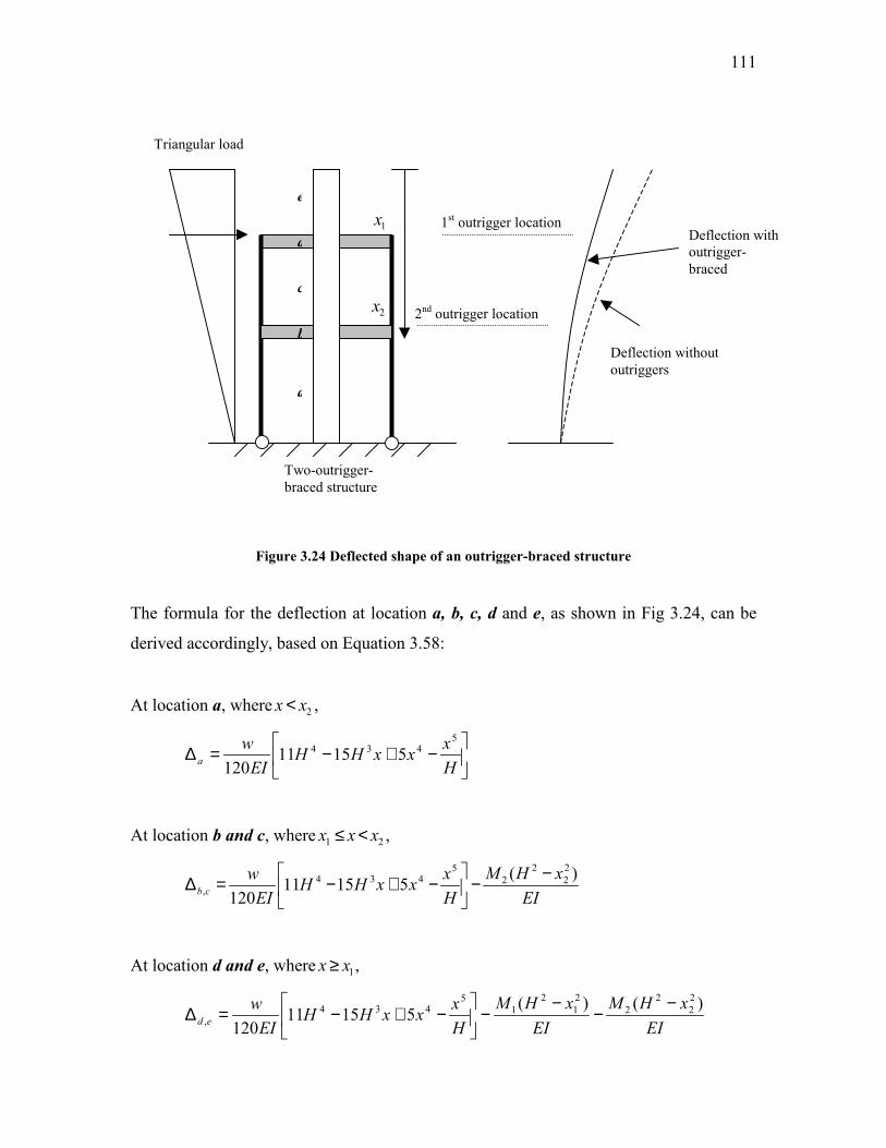
111
Figure 3.24 Deflected shape of an outrigger-braced structure
The formula for the deflection at location a, b, c, d and e, as shown in Fig 3.24, can be
derived accordingly, based on Equation 3.58:
At location a, where 2xx < ,
−+−=∆H
xxxHH
EI
wa
5434 51511
120
At location b and c, where 21 xxx <≤ ,
EI
xHM
H
xxxHH
EI
wcb
)(51511
120
2
2
2
2
5434
,
−−
−+−=∆
At location d and e, where 1xx ≥ ,
EI
xHM
EI
xHM
H
xxxHH
EI
wed
)()(51511
120
2
2
2
2
2
1
2
1
5434
,
−−
−−
−+−=∆
Triangular load
Two-outrigger-
braced structure
Deflection without
outriggers
Deflection with
outrigger-
braced
1st outrigger location
2nd outrigger location 2x
a
b
c
d
e
1x

112
Further from this, the deflected shape of the structure can then be expressed in terms of a
mode shape equation,
k
h
z
. This can be achieved by performing a curve-fitting method
in order to obtain the power of the equation, k . k , in an outrigger-braced structure, can
range from 1 to 2, which depends on the efficiency of the whole outrigger-braced system.
The stronger the outrigger-braced columns and the outriggers, the more the restraining
moments at each outrigger location will be, and therefore the greater the effect of
restrained deflection at those particular points.
In an outrigger-braced structure with stiffer outriggers, k will be smaller and eventually
tends to 1, which can decrease the wind-induced acceleration in both directions. For
2=k , this situation is applicable to the pure cantilever action of the core itself. However,
k can be adopted as 1.5, as is stated in AS 1170.2. Figure 3.25 shows the effect of a total
deflection of an outrigger-braced structure based on the power of the spectrum, k .
Figure 3.25 Mode shape comparison of an outrigger-braced structure
Triangular load
Two-outrigger-
braced structure
2x
a
b
c
d
e
1x
Mode shape with very
strong outrigger-braced
system, k=1
Mode shape with
reasonable outrigger-
braced system, k=1.5
Mode shape with pure
cantilever action from
core, k=2 (can be 1.5 as
stated in AS 1170.2)

113
3.4.1.2 Building mass
In order to estimate the wind-induced acceleration, the generalized building mass can not
be neglected. It can be extracted from Equation 2.36, as shown:
dzzzmM i
h
)()( 2
0ψ∫=
• M = mode-generalized mass of structure
• )(zm = the mass per unit height of the structure
• )(ziψ = fundamental mode shape represented by a power function
k
h
z
In general, )(zm can be estimated by acquiring the total mass of the building divided by
the total height of the structure. However, the total mass of a structure can be predicted
by assuming the total dead load plus a certain percentage of the total live load. In
AS1170.4, the total mass of a structure can be expressed as QG 4.0+ .
Nevertheless, )(zm can further be expressed in terms of mass per floor height, due to the
different masses allocated to each floor, such as in a multi-purpose superstructure with a
basement car-park, a retail podium on the next level, and with apartments and plant
rooms at certain levels on consecutive floors. In order to reduce the complexity of the
equation in this context, it is assumed that mass per unit height is:
=)(zm ( )
H
QG 4.0+ (3.59)
After obtaining the k value from the estimated deflection mode shape and the
simplification of m as per Equation 3.59, the generalized mass can then be integrated as:
dzH
zzmM
kH
2
0)(
= ∫ 12120
2
12
0
2
+=
+=
=+
∫ k
mH
h
z
k
mdz
H
zm
H
k
kH
k
(3.60)

114
For an outrigger-braced structure, k would tend to be 1 if there are very strong outriggers
and the columns are located in the building. Therefore, the generalized mass can be
assumed as per Equation 3.61, where it is one-third of the actual mass of the building:
3
mHM = (3.61)
On the other hand, for a structure with a very low efficiency outrigger-braced system or
that mainly relying on a core system, k would tend to be 2 and the generalized mass can
be further derived as per Equation 3.62, where it is one-fifth of the actual mass of the
building:
5
mHM = (3.62)
Overall, when the power of the mode shape is sitting between 1 and 2, 21 ≤≤ k , the
generalized mass for this purpose can be concluded as:
53
mHM
mH ≤≤ .
3.4.1.3 Building stiffness
Building stiffness is an important factor in estimating the period/frequency of the
structure. There are several methods used to obtain the stiffness of a structure, such as
calculating the core stiffness itself in combination with the effect of an outrigger-braced
system, or in matrix form, where the size of the matrix is determined by the number and
location of the outriggers. However in this context, a simplified method is used for
estimating the building period in Section 3.4.1.4.
The generalized stiffness of the outrigger-braced structure is rearranged from Equation
2.34:
∆= PK

115
For the wind force acting on the structure, P , this can be classified as follows:
For uniform load, HwP uniform=
For triangular load, 2
HwP
triangular=
The estimated tip deflection of the structure, ∆ , can then be classified as per Equations
3.57 and 3.58 respectively:
For uniform load, [ ] ∑=
−−+−=∆
n
i
ii
c
TEI
xHMHxHx
EI
w
1
22434 )(
3424
For triangular load, ∑=
−−
−+−=∆
n
i
ii
c
TEI
xHM
H
xxxHH
EI
w
1
225434 )(
51511120
For verification purposes, the stiffness obtained from the method above should be
compared with the core stiffness. The core stiffness can be calculated manually for a
symmetrical core or, alternatively, a software program can be used if the calculation
becomes complicated. The total stiffness of the outrigger-braced structure calculated
from the method as shown should be no less than the core stiffness itself in all
circumstances: systembracedoutriggercore KK −−≤
However, the generalized stiffness can vary depending on the wind loading type adopted:
For uniform load,
−−
=∆=
∑=
n
i
ii
core
uniform
uniform
uniform
EI
xHM
EI
Hw
HwPK
1
224)(
8
(3.63)
For triangular load,
−−
=∆=
∑=
n
i
ii
core
triangular
triangular
triangular
EI
xHM
EI
Hw
Hw
PK
1
224)(
120
11
2 (3.64)
If the outrigger-braced structure has a very low efficiency and all the lateral forces are
mainly resisted by the core, the restraining moments from the outrigger-braced system

116
will be very small and, therefore, there is not much contribution in reducing the drift. In
this case, the structure would behave as a pure cantilever and the total deflection can be
expressed as per Equation 3.20 for a uniform load and per Equation 3.41 for a triangular
load:
For uniform load, core
uniform
TEI
Hw
8
4
≈∆
For triangular load, core
triangular
TEI
Hw
120
11 4
≈∆
As a result of the pure cantilever action, the total stiffness can be estimated as per
Equation 3.65 and 3.66.
For uniform load, 34
8
8
H
EI
EI
Hw
HwPK core
core
uniform
uniform
uniform =
=∆= (3.65)
For triangular load, 34 11
60
120
11
2
H
EI
EI
Hw
Hw
PK core
core
triangular
triangular
triangular =
=∆= (3.66)
3.4.1.4 Building period
There are several ways to estimate the building period of a structure, which is very much
dependent on its structural system. The energy method can be used to effectively
determine the fundamental vibration period of a tall building when the distributions of
structural stiffness and mass are almost uniform. Taking the average mass along the
building height, m, subjected to a uniformly distributed horizontal load, the elastic
deformation curve can be approximately regarded as the first vibration mode shape. Then
the fundamental vibration period can be estimated. In this context, two methods are used
to estimate the building period of an outrigger-braced structure. The first is the
conventional method of applying a general period equation; the second is using the
equation that is derived by Li (1985).

117
Firstly, the building period through the general equation can be estimated as follows:
K
MT π2= (3.67)
• T = Building period of structure
• M = Generalized mass of structure
• K = Generalized stiffness of structure
The generalized mass is derived from Equation 3.60 and the generalized stiffness is
derived from Equations 3.63 and 3.64; therefore, the building period T from Equation
3.67 can be further expressed by:
For uniform load, Hw
EI
xHM
EI
Hw
k
mH
Tuniform
n
i
ii
core
uniform
−−
+=
∑=1
224)(
8122π (3.68)
For triangular load, Hw
EI
xHM
EI
Hw
k
mH
Ttriangular
n
i
ii
core
triangular
−−×
+=
∑=1
224)(
120
112
122π
(3.69)
If the outrigger-braced system has a weak efficiency, the core of the building will have to
take most of the loading, producing more of the pure cantilever action. Therefore, in
Equations 3.68 and 3.69, the restraining moments can be neglected and k is assumed to be
1.5 for a pure cantilever structure:
For uniform load, corecore EI
mH
EI
mHT
44
66.5
2
322
ππ == (3.70)
For triangular load, corecore EI
mH
EI
mHT
44
67.4
2
240
112
ππ == (3.71)

118
However, according to Li (1985), it is suggested that the fundamental period can be
expressed as follows:
coreEI
mHT
4
555.3
2π= (3.72)
In comparison with a pure cantilever structure with three expressions for fundamental
periods, as above, the period generated from uniform wind load method (Equation 3.70)
gives the smallest building period, while the equation derived by Li yields the highest
period. In fact, the building period is just a basic estimate for representing the stiffness of
a structure. Conservatively, it is advised that the equation derived from Li to be adopted
for wind design. Structures with an outrigger-braced system are expected to have a lesser
period due to an increased stiffness of the structure than that of a pure cantilever
structure.
3.4.2 Peak along wind acceleration
In Section 2.2.1.7, the derivation of a general equation for the r.m.s. along-wind
deflection and acceleration at resonant response is derived as per Equation 2.27 and 2.29
respectively:
r.m.s. deflection, s
F
yK
nSn
ςπ
σ ψ
4
)(2
0,0≈
r.m.s. acceleration, s
F
yy
nSn
Mn
ςπ
σπσ ψ
4
)(1)2(
0,02
0 ==&&
However, the r.m.s. deflection formula from Equation 2.27 is fundamentally a rough
estimate. For an outrigger-braced structure, the r.m.s. top deflection can be enhanced by
adopting the method as discussed in this section, with a uniform distributed wind load or
triangular wind load. In this case, the r.m.s. acceleration, Equation 2.30, can be
substituted from the mean deflection obtained from the analysis, as discussed in Chapter
2:
( )∆××== Gnn yy
2
0
2
0 )2()2( πσπσ&&

119
The gust factor,G , is the ratio of the expected maximum response of the structure in a
defined time period to the mean or time averaged response in the same time period, as is
discussed in Section 2.1.1.6. The gust factor, in AS1170.2, is defined as per Equation
2.32:
)21( hvdyn IgCG +×=
For dynC , as shown in Equation 2.38, the resonant component is the main part in
estimating the acceleration, and hence:
5.02
, 2
=
ςtRs
hresdyn
SEgHIC
For an accurate estimation of the mean deflection of an outrigger-braced structure based
on mean wind pressure, Equations 3.57 and 3.58 are adopted. And for the estimation of
the outrigger-braced building period, Equations 3.68 and 3.69 are used for estimation of
the r.m.s wind-induced acceleration.
From all of the above information, the r.m.s acceleration can be calculated for an
outrigger-braced structure as per Equation 3.73,. Peak factor can be included to acquire
the peak value of acceleration at the top of the building:
TtRs
hyy
SEgHInn ∆×
×==
5.02
2
0
2
0 2)2()2(ς
πσπσ&&
(3.73)
However, the equation provided in AS 1170.2 is shown as per Equation 2.39:
( ) ( )[ ] ( )[ ]
∆−∆
+= ∑ ∑
= =
h
z
h
z
zdesleewardfigzdeswindardfig
hV
ts
hRair
o
x zzbhVCzzbzVCIg
SEHIg
hm 0 0
2
,,
2
,,2 21
3θθ
ζρ
σ&&
This equation is basically derived from Equations 3.26, 3.27 and 3.28:

120
Kh
MIgCn bhvdynx ×+××= )21()2( 2
0πσ&& bhvdyn MIgC
Mh×+××= )21(
1 (3.74)
In comparison, Equation 3.74 is originally derived from the same equation. However, the
only difference between both equations is the estimation of mean deflection. Based on the
equation derived from AS1170.2, the top deflection is conservatively modified by
adopting the maximum point load acting on the tip of the cantilever and the point load is
converted from the total core base moment divided by the total height.
In AS1170.2, 3
2.1170
mHM = and the generalized mass has not included any mode shape
factor. Therefore, the equation can be rewritten as:
bhvdynx MIgCmh
×+××= )21(3
2&&σ (3.75)
However, the problem with this method is that no mode shape correction factor is
included in the equation. The r.m.s. acceleration derived from Equation 3.75 is based on a
conservative approach by converting the base bending moment to a relatively huge point
load and predicting its deflection by treating the structure as a cantilever structure.
However, the mean deflection derived from Equations 3.57 and 3.58 is based on a more
accurate approach. Therefore, it is expected that the peak acceleration obtained from
AS1170.2 will be relatively more conservative than that of the ordinary method.
3.4.3 Peak cross wind acceleration
In Section 2.2.3.4, the derivation of the general equation for the r.m.s crosswind
acceleration can be expressed as per Equation 2.29:
s
F
y
nSn
M ςπ
σ ψ
4
)(1 0,0=&&

121
• Generalized mass, 12
0
+=
k
HmM
• k is the power of mode shape and it is derived by adopting the curve-
fitting method to the deflection curve of an outrigger-braced structure
• 0m is mass per unit height of the structure
• sς is damping in fundamental mode expressed as a fraction of critical,
usually taken as 0.005 to 0.01.
The crosswind force spectrum coefficient ( FsC ), as used in AS 1170.2, is adopted to
replace part of Equation 2.29. This is described in Section 2.1.2.5 and is shown in
Equation 2.58.
222
0,0 )(
hbq
nSnC
F
Fs
ψ=
Rearranging the equation, the r.m.s crosswind acceleration can be expressed as:
( )s
Fs
hv
desair
s
Fs
y
C
Ig
V
m
bkhbqC
mh
k
ςπρ
ςπ
σ θ2
,222
14
12
4
)(12
++
=+=&&
(3.76)
For peak crosswind acceleration, the peak factor must be included in Equation 3.76:
( )s
Fs
hv
desrair
y
C
Ig
V
m
gbk
ςπρ
σ θ2
,
14
12
+×××+
=&&
(3.77)
• rg = peak factor for resonant response (10min period)
= )600(log2 ce n
In AS1170.2, the peak crosswind acceleration is expressed as per Equation 2.61.
s
Fs
m
hv
desairr
y
CK
Ig
V
m
bg
ςπρ
σ θ2
,
14
3
+=
&&

122
A comparison of Equations 2.61 and 3.77 shows that they are almost the same equations,
with the only difference being in the mode shape of the structure. By comparing both
equations, crosswind acceleration can be rewritten into proportional form in relation to
the mode shape of the structure:
For derived equation, ( )12 +∝ ky&&σ (3.78)
For AS 1170.2, my K3∝&&
σ (3.79)
For Equation 2.61, the mode shape factor is modified and replaced by a factor called the
mode shape correction factor:
mK = 0.76+0.24k
• k = mode shape power exponent for the fundamental mode and values of the
exponent k should be taken as:
= 1.5 for a uniform cantilever
= 0.5 for a slender framed structure (moment resisting)
= 1.0 for a building with a central core and moment resisting façade
= 2.3 for a tower decreasing in stiffness with height, or with a large mass
at the top
= the value obtained from curve-fitting khzz )/()(1 =φ to the computed
modal shape of the structure where )(1 zφ is the first mode shape as a
function of height z, normalized to unity at z = h.
An outrigger-braced structure is expected to have a mode shape power of 1 when the
outrigger-braced system is strong and a mode shape of power of 1.5 to 2 when the system
is weak. In conversion,
mK = 1 with a strong outrigger-braced system (ω =0)
mK = 1.12 to 1.24 with a weak outrigger-braced system (ω =1)
In comparison to Equations 3.78 and 3.79, when the mode shape power exponent is equal
to 1, both equations should yield the same outcome:

123
( ) 312 ∝+∝ ky&&σ for manually derived equation and;
33 ∝∝ my K&&
σ for AS1170.2
When the mode shape power exponent is equal to 1.5, the outcome is:
( ) 412 ∝+∝ ky&&σ for manually derived equation and;
36.33 ∝∝ my K&&
σ for AS1170.2
When the mode shape power exponent is equal to 2, the outcome is:
( ) 512 ∝+∝ ky&&σ for the manually derived equation and;
72.33 ∝∝ my K&&
σ for AS1170.2
Comparison of mode shape factor
3
3.5
4
4.5
5
5.5
1 1.2 1.4 1.6 1.8 2 2.2
k
Mode s
hape facto
r
Manual calculation AS1170.2
Figure 3.26 Comparison of mode shape factor between manual calculation and AS1170.2
Figure 3.26 is presented to summarize the difference between mode shape factors in both
equations, as discussed above. AS1170.2 has a lower mode shape factor in comparison

124
with the manually derived equation with the increment of power exponential of mode
shape, k. When k equals 2, the difference in crosswind acceleration between the manually
derived equation and AS1170.2 is almost 35%. It can be concluded that both equations
are applicable when the outrigger-braced structure has a strong outrigger-braced system,
when k =1. However, when the outrigger-braced system has very low efficiency, it is
advised that the manually derived equation for the prediction of crosswind acceleration is
adopted.

125
Chapter 4
4.0 Verification through Computer Modeling
Computer modeling is required to verify the analysis performed in Section 3.0. The
computer software, ETABS, is used to assist in comparing the results.
4.1 Introduction to ETABS software
ETABS is a program that can greatly enhance an engineer's analysis of and design
capabilities for structures. ETABS offers the widest assortment of analysis and design
tools available for the structural engineer working on building structures (ETABS
Manual, 2007). ETABS can easily handle all kinds of structural lateral analysis, such as:
o Tall buildings with all kinds of structural systems
o Buildings with steel, concrete, composite or joist floor framing
o Complex shear walls with arbitrary openings
o P-Delta analysis with static or dynamic analysis
o Construction sequence loading analysis
o Multiple linear and nonlinear time history load cases in any direction

126
For this model, the floors and walls can be modeled as membrane elements with in-plane
stiffness only. The columns are modeled as pin connections that do not take any moment
in any direction; although, in reality, columns contribute a negligible amount of lateral
stiffness. Only the core wall is modeled as a shell element to take all of the lateral load.
The manually calculated lateral wind effects and the requirements of AS1170.2 can then
be input into the program. The three-dimensional mode shapes and frequencies, modal
participation factors, direction factors and participating mass percentages are evaluated
using the eigenvector vector analysis.
4.2 Wind loading information
The estimation of wind load will be based on AS1170.2 for the comparison of the
performance of an outrigger structure using the manual preliminary analyses and the
computer model. The relevant wind load information for the illustrative example of an
outrigger-braced structure is as follows:
• Location: CBD Melbourne, Region A
• Terrain: Category 4
• Topography: Ground slope less than 1 in 20 for greater than 5 km
• Shielding factor assumed to be 1.0 with no other buildings of greater height in
any direction.
• Wind directionality multiplier assumed to be 1.0 where maximum wind occurs
in a north and west direction.
• Ultimate wind: 500 years return period
• Serviceability wind for 20 years return period for deflection and 5 years return
period for acceleration vibration comfort
• Aerodynamic shape factor for the external pressure of structure: windward wall
is 0.8 while leeward wall is -0.5.
• Internal pressure is -0.2 or 0, where it is considered to be effectively sealed.

127
4.3 Building properties and configuration
The relevant building information is summarized as follows:
• Building is served for residential purpose and has an average super-imposed
dead load of 1.5kPa and live load of 1.5kPa
• Building height of 300m and floor-to-floor height of 3.5m
• Horizontal floor dimensions: 36m x 36m
• Reinforced concrete construction with two outrigger-braced core-to-columns
• Floors are based on a post-tensioning band beam system with a 250mm slab
thickness and a band beam of 2400mm in width x 500mm depth
• Core wall is assumed to be 12m x 12m square and 800mm thick on average
• Outrigger-braced columns are assumed to be 1.5m x 3.0m
• All elements are assumed to have a concrete grade of 100MPa
• Damping taken as 0.01 for serviceability deflection and acceleration
calculations and 0.03 for ultimate shear and moment design.
The general layout of the floor plan is illustrated as per Figure 4.1.
Figure 4.1 General layout of floor plan for the outrigger-braced structure
Outrigger-
braced
columns
Outrigger
walls
800mm thick
core wall
Direction of
Wind

128
4.4 ETABS analysis
The general building properties generated from the ETABS analysis are shown as
follows:
• Building period of 8.57s
• Total building mass of 154,000 tonnes
• The deflection due to wind load, which is based on AS1170.2 and a 5-year
return period, is 123mm at the top of the building.
4.4.1 Core shear & moment
The total shear and moment acting on the core, with two outriggers placed at levels 58
and 27, are plotted as follows:
Core Shear - ETABS Analysis
0
50
100
150
200
250
300
350
0 2000 4000 6000 8000
Shear Forcet (kN)
Heig
ht (m
)
Figure 4.2 Total shear acting on the main core based on ETABS analysis

129
Core Moment - ETABS Analysis
0
50
100
150
200
250
300
350
-200 0 200 400 600
Bending Moment (MNm)
Heig
ht (m
)
Figure 4.3 Total moment acting on the main core based on ETABS analysis
From Figure 4.2, it can be seen that there is no change in shear that is due to the effect of
an outrigger system. This is because the outrigger-braced system would not reduce the
total shear of the structure. However, from Figure 4.3, the outrigger-braced system has
made two transitions in the bending moment of the core that are exactly where the two
outriggers are located.
• Core moment reduction of 223MNm at Level 58,
• Core moment reduction of 340MNm at Level 27; and
• Total core moment reduction at base of structure is 563MNm
4.4.2 Outrigger-braced column axial force
From the ETABS analysis, the outrigger-braced columns have taken axial loads that are
transferred by the outrigger-braced system from the wind load specified in Section 4.2.
At the first location of the outrigger, which is located at Level 58, each outrigger-braced
column is taking 3193kN; for the second outrigger location, which is at Level 27, each

130
outrigger-braced column has taken a total axial load of 7916kN. This is purely based on
the uniform wind load. For simplicity, this is illustrated as follows in Figure 4.4.
Figure 4.4 Wind-induced axial load acting on outrigger-braced columns
4.4.3 Verification of results
From the ETABS analysis, the results can be verified from the core moment reduction
and axial loads from the outrigger-braced column. This can be illustrated
diagrammatically as the original core bending moment without an outrigger-braced
system, and as the outrigger-braced core-to-column system. (Figure 4.5)
Outrigger-braced core-to-
column system
Column axial
force diagram
N1=3193kN
N2 = 7916kN
Wind
Load

131
Figure 4.5 Core bending moment of an outrigger-braced structure
The bending moment along the core without an outrigger-braced system can be expressed
as:
• 2
)( 2
0
xHwM
−= , applicable at any height of the structure
• 1081 =M MNm at Level 58; and
• 4792 =M MNm at Level 27
From Figure 4.5, the core moment where the two outriggers are located is as follows:
• Core moment reduction of 223MNm at Level 58; and
• Core moment reduction of 340MNm at Level 27
The core moment reduction should be dissipated to the outrigger-braced columns by
transferring the wind loading through the outrigger-braced system and can be expressed
as follows:
Outrigger-braced core-to-
column system
Core bending
moment diagram
Wind
Load Bending
moment without
outriggers
Moment
reduction with
outriggers
d

132
• dNM RR ×=
• kNmmkNM R 896,22923631931
=××= at Level 58; and
• kNmmkNkNM R 056,340236)31937916(2
=××−= at Level 27
The restraining moment is therefore verified.
4.5 Comparison of manual calculation and the computer model
A manual analysis on the outrigger-braced structure will be performed in order to provide
a comparison with the results obtained from the ETABS analysis. The building properties
and configurations are the same as those in the computer model, as listed in Section 4.3.
In order to obtain the optimum location of the outriggers, it is necessary to acquire the
properties of the building out of the outrigger-braced system, in which the non-
dimensional parameters, S and 1S , which represent the core-to column and core-to-
outrigger rigidities, are:
• 11
21068.2
)(
21 −×=+=cEAdEI
S
• 10
1 1089.3)(12
−×==oEI
dS
• 0048.01 ≈==HS
Sω
The optimum location for both outriggers, a and b , can then be estimated from Figure
3.5 by assuming 0≈ω (a very stiff outrigger-braced system).
• mHa 94312.0 ≈= from the top of the building (Level 58); and
• mHb 206685.0 ≈= from the top of the building (Level 27)
4.5.1 Restraining moment
Substituting the variables into Equations 3.13 and 3.14 gives:

133
• )(6
){)]([ 3
1
3
211 xHEI
wxHSMxHSSM ba −=−+−+
399 1014.2]1053.2[]1093.5[ −−− ×=×+× ba MM
• )(6
)]{[)( 3
2
3
212 xHEI
wxHSSMxHSM ba −=−++−
399 105.1]1092.2[]1053.2[ −−− ×=×+× ba MM
0
50
100
150
200
250
300
350
-200 -100 0 100 200 300 400 500
Bending Moment (MNm)
Heig
ht (m
)
ETABS analysis Manual Analysis
Figure 4.6 Core bending moment from both analyses
By using elimination method to solve the equations above, the restraining moment at
location a and b is calculated as:
• 226=aM MNm; and
• 316=bM MNm

134
Both restraining moments, aM and bM are then compared with the restraining moments
obtained from the ETABS analysis, 2231
=RM MNm and 3402
=RM MNm. The
difference between both results is less than 10%. The core bending moment based on
both the manual and ETABS analysis can be plotted and then compared. From Figure 4.6
it is obvious that there is not a large discrepancy between both analyses. Therefore, the
manual analysis is verified.
4.5.2 Deflected mode shape and total deflection
It is necessary to obtain the mode shape of the structure as this affects the wind-induced
acceleration. With the deflected mode shape forming an exponential curve, the power of
k can be predicted. Generally the deflected mode shape can be manually estimated from
the deflection of the building, as discussed in Section 3.4.1.1. In comparison, the
deflected shape of the structure from both the manual and ETABS analysis can be plotted
as per Figure 4.7.
Figure 4.7 shows the comparison of deflection based on the ETABS analysis, the
outrigger-braced system and the pure cantilever action. The maximum deflection at the
top of the building in each case is summarized as follows:
• ETABS result – 123mm
• Outrigger-braced – 136mm
• Pure cantilever – 498mm
In relation to the three analyses, the power, k, of the exponential curve from the deflected
mode shape can be concluded as:
• 3.1=ETABSk ;
• 35.1=Outriggerk ; and
• 5.1=Cantileverk

135
Comparison of deflection
0
50
100
150
200
250
300
350
0 0.1 0.2 0.3 0.4 0.5
Deflection (m)
Heig
ht (m
)
ETABS Outrigger-braced Pure cantilever
Figure 4.7 Comparison of mode shape factors based on both analyses
Thus it can be concluded that the building with a pure cantilever action from the core will
have a relatively greater power in the exponential curve, which may significantly increase
the effect of the wind-induced acceleration. A comparison between the manual analysis
and the ETABS result shows that the power of the exponential curve of the deflected
mode shape has a difference of less than 5%. Therefore, it is verified.
4.5.3 Building mass
The generalized building mass is important in determining the wind-induced acceleration
and this can be extracted from Equation 2.36 as:
k = 1.5
k = 1.35
k = 1.3

136
• dzzzmM k
i
h
)()( 2
0ψ∫=
In general, )(zm can be estimated by acquiring the total mass of the building and
dividing it by the total height of the structure. However, the total mass of the structure
may also be predicted based on its design. The total mass of a building usually can be
estimated by assuming the total dead load plus a certain percentage of the total live load.
In AS1170.4, total mass of a structure can be expressed as QG 4.0+ . In order to reduce
the complexity of the equation in this context, it is assumed that m represents the total
mass divided by the total height of structure, ( )
H
QG 4.0+.
• For the total mass of this structure, QG 4.0+ =156,800 tonnes
• Therefore, 301/10800,156)( 3×=zm = 521,000 kg/m
After obtaining the k value from the estimated deflection mode shape and simplifying m ,
the equation can be further expressed as:
• dzH
zzmM
kH
ETABS
2
0)(
= ∫ 6.30
)3.1(2mH
dzH
zm
H
=
= ∫
• dzH
zzmM
kH
Outrigger
2
0)(
= ∫ 7.30
)35.1(2mH
dzH
zm
H
=
= ∫
• dzH
zzmM
kH
Cantilever
2
0)(
= ∫ 0.40
)5.1(2mH
dzH
zm
H
=
= ∫
• dzH
zzm
KM
H
m
AS
2
02.1170 )(
1
= ∫ 252.3)]35.1(24.076.0[
1
3
mHmH =+
=
The outrigger-braced system in this building is considered as having relatively strong
outriggers and the columns are located in the building. In comparison, the denominator of
the generalized mass obtained from AS1170.2 is much lower than that in the analyses
obtained manually.

137
4.5.4 Building stiffness
From Equation 2.34 and 3.20, the general stiffness and total deflection of a building can
be expressed as:
• ∆= PK and core
uniform
TEI
Hw
8
4
≈∆
Therefore, the equivalent general stiffness of the structure can be rearranged and
rewritten as:
34
8
8
H
IE
IE
Hw
HwPK totalcore
corecore
uniform
uniform =
=∆= (4.1)
In a comparison of the ETABS and the manual analysis, the equivalent general stiffness
can be estimated by applying Equation 2.34 and the results are shown as follows:
061,55123.0
3015.22 =×=ETABSK kN/m
798,49136.0
3015.22 =×=OutriggerK kN/m
600,13498.0
3015.22 =×=CantileverK kN/m
From the general stiffness, the total I stiffness of the structure can be further modified by
rearranging Equation 4.1:
core
totalE
KHI
8
3
= (4.2)
From Equation 4.2, the equivalent total stiffness of a structure based on the three analyses
can be calculated as follows:
4
9
33
375410508
30110061,55mI ETABS =
××××=

138
4
9
33
339510508
30110798,49mIOutigger =
××××=
4
9
33
92610508
30110600,13mICantilever =
××××=
Note that CantileverI has the same core stiffness as defined originally. A comparison
between equivalent stiffness in the ETABS and manual analysis, the ETABS analysis
yields greater stiffness due to the low deflection and a strong outrigger system. However,
there is less than a 10% difference in the results of both analyses.
For verification purposes, the stiffness obtained from the method above should be
compared with the core stiffness itself. The total stiffness of an outrigger-braced structure
calculated from the method as shown should be no less than the core stiffness itself in all
circumstances, Outriggercore II ≤ . Therefore, the result from both analyses is verified.
4.5.5 Building period
Building period is another factor that cannot be neglected in estimating the wind-induced
acceleration, where, in taking the average mass along the building height, m, as a
uniformly distributed horizontal load, the elastic deformation curve subjected to the
uniform horizontal load can be approximately regarded as the first vibration mode shape.
Then, the fundamental vibration period can be estimated. According to Li (1985), the
building period is estimated by applying Equation 3.72.
EquivalentEI
mHT
4
555.3
2π=
From Section 4.5.3, the generalized mass can then be expressed in a simpler form:
kgmmkgmH
M 63
1038.427.3
301/10521
7.3×=××==
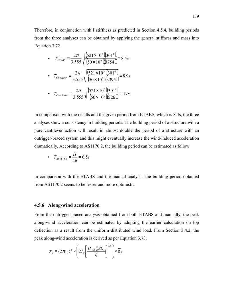
139
Therefore, in conjunction with I stiffness as predicted in Section 4.5.4, building periods
from the three analyses can be obtained by applying the general stiffness and mass into
Equation 3.72.
• ( )( )( )( ) sTETABS 4.8
37541050
30110521
555.3
29
43
=××= π
• ( )( )( )( ) sTOutrigger 9.8
33951050
30110521
555.3
29
43
=××= π
• ( )( )( )( ) sTCantilever 17
9261050
30110521
555.3
29
43
=××= π
In comparison with the results and the given period from ETABS, which is 8.4s, the three
analyses show a consistency in building periods. The building period of a structure with a
pure cantilever action will result in almost double the period of a structure with an
outrigger-braced system and this might eventually increase the wind-induced acceleration
dramatically. According to AS1170.2, the building period can be estimated as follow:
• sH
TAS 5.646
2.1170 ==
In comparison with the ETABS and the manual analysis, the building period obtained
from AS1170.2 seems to be lesser and more optimistic.
4.5.6 Along-wind acceleration
From the outrigger-braced analysis obtained from both ETABS and manually, the peak
along-wind acceleration can be estimated by adopting the earlier calculation on top
deflection as a result from the uniform distributed wind load. From Section 3.4.2, the
peak along-wind acceleration is derived as per Equation 3.73.
TtRs
hy
SEgHIn ∆×
×=
5.02
2
0 2)2(ς
πσ&&

140
However, the building deflection from the analysis is based on the peak wind speed. In
AS 1170.2, the relationship between mean and peak deflection is shown as follows:
∆×+=∆ )21( hvpeal Ig (4.3)
As per Equation 2.39, dynC is defined as:
)21(
2
5.02
2
hv
tRssvh
dynIg
SEgHBgI
C+
+
=ς
Therefore, by combining Equations 4.3 and 2.39 into Equation 3.73, the peak along-wind
acceleration substituted with peak building deflection is expressed as:
∆××= dynx Cn 2
0 )2( πσ&&
(4.4)
However, if excitation by low frequencies is small and the structural damping is low, so
that the excitation band-width is large compared with the resonant band-width, the first
term in the equation above can be neglected.
496.0)21(
2
5.02
=+
=hv
tRs
h
dynIg
SEgHI
Cς
; where
o 121.0=hI
o vg = 3.7
o 562.0]46.0)(26.0[
1
15.022
=+−
+=
h
sh
s
L
bshB
o sH = 1
o 906.2)600(log2 == aeR ng
o 153.0)1(4
1)1(5.3
1
1
,
0
,
=
++
++
=
θθ des
hvha
des
hva
V
Igbn
V
IghnS

141
o 117.0)8.701( 2N
NEt +
= π
o [ ] 651.0/)(1 , =+= θdeshvba VIgLnN
o ζ = 0.01 for serviceability wind acceleration
Peak along wind acceleration can be predicted with the periods and building deflection as
estimated from ETABS and the manual analysis.
0328.0123.0)43.8
12( 2 =×××= dynETABSx Cπσ
&&m/s
2 = 3.4mg
0341.0136.0)87.8
12( 2 =×××= dynOutriggerx Cπσ
&&m/s
2 = 3.5mg
The along-wind acceleration between the ETABS and manual outrigger-braced analysis
shows a very close result and there is less than 5% difference between the two. However,
both results can be compared with the along-wind acceleration equation that is provided
in AS1170.2, as per Equation 2.38, and is shown as:
0514.0=x&&σ m/s2 = 5.2mg
The peak along-wind acceleration calculated from the equation provided by AS1170.2 is
almost 50% more than the acceleration predicted in the analysis. A summary of results is
shown in Table 4.1.
Analysis Generalized
Mass (T)
Period
(s)
Deflection
(mm)
Along-wind
acceleration (mg)
ETABS 43,561 8.4 123 3.4
Manual
calculation 42,384 8.9 136 3.5
AS1170.2 48,223 6.5 - 5.2
Table 4.1 Comparison of building properties and along-wind acceleration based on ETABS analysis,
manual calculation and AS1170.2

142
4.5.7 Crosswind acceleration
Crosswind acceleration can be estimated with the wind and building information as
derived in an earlier section. In Section 3.4.3, the peak crosswind acceleration is derived
as:
( )s
Fs
hv
desrair
y
C
Ig
V
m
gbk
ςπρ
σ θ2
,
14
12
+×××+
=&&
o rg = peak factor for resonant response (10min period)
= )600(log2 ce n
o Crosswind force spectrum, FsC , can be obtained from AS1170.2 with a
series of graphs of FsC against the reduced frequency and different
building dimension ratio, which is presented as:
o airρ = density of air, 33 /102.1 mkg−× ; and
o vg = 3.7
o 121.0=hI
o ζ = 0.001 for serviceability wind acceleration
o )(zm = 521000 kg/m
Normally, the crosswind force spectrum, FsC , has a direct relationship with the period of
the structure. From the building period obtained from both ETABS and manual analyses,
FsC can be estimated as follows:
0134.0=ETABSFsC
0173.0=OutriggerFsC
0041.02.1170
=ASFsC
Peak crosswind acceleration can then be predicted with the periods and building mode
shape factor as estimated from the ETABS and manual analysis.

143
=
+××××+=
01.0
)01339.0(
)121.0)(7.3(1
29.41
5210004
92.22.136]1)3.1(2[2
πσETABSy&& 0.57m/s
2
=
+××××+=
01.0
)01729.0(
)121.0)(7.3(1
29.41
5210004
9.22.136]1)35.1(2[2
πσOutriggery&& 0.66m/s
2
=
+×××××=
01.0
)00409.0(
)121.0)(7.3(1
29.41
5210004
32.136)084.1(32
2.1170
πσASy&& 0.33m/s
2
A comparison of the peak crosswind accelerations between the three different approaches
shows that AS1170.2 has the lowest acceleration. This is due to the low period of the
structure, the small FsC value, and also the lower value of the mode shape correction
factor. Peak crosswind acceleration from both the ETABS and manually calculated
outrigger-braced analysis has shown a relatively close result, with an approximately less
than 15% difference. A summary of result is shown in Table 4.2.
Analysis Period
(s)
Mode shape
correction factor,
k
Crosswind
acceleration
(mg)
ETABS 8.4 1.30 57
Manual
calculation 8.9 1.35 66
AS1170.2 6.6 1.08 33
Table 4.2 Comparison of building properties and crosswind acceleration based on ETABS analysis,
manual calculation and AS1170.2
4.6 Discussion of results
An outrigger-braced structure can be analyzed with ETABS or manually. However, in the
design of tall buildings, it is suggested that both approaches are adopted in two different
stages. For the preliminary stage, it is advised to estimate the outrigger-braced system
through manual calculation as opposed to using time-consuming modeling. For the

144
detailed design phase, ETABS might have to be adopted to increase the accuracy of the
results.
Section 4.5 presents a comparison of results, in terms of the building properties and
lateral deflection and acceleration of a structure, between ETABS analysis, manual
calculation and the equation provided by AS1170.2. The ETABS analysis and manual
calculation show close results in terms of the restraining moments at the outrigger
locations, the building frequencies, and the total deflection at the top of the building.
However, the results obtained from ETABS are more accurate as the program involves a
detailed 3D analysis, including secondary effects on the structure.
Analysis Generalized
Mass (T)
Period
(s)
Deflection
(mm)
Mode shape
correction factor,
k
ETABS 43,561 8.4 123 1.30
Manual
calculation 42,384 8.8 136 1.35
Difference 2.7% 5.2% 10.6% 3.8%
Table 4.3 Difference between ETABS analysis and manual calculation in terms of percentage
From Table 4.3, the ETABS analysis shows a stiffer structure than that in the manually
calculated analysis. From Table 4.1, AS1170.2 shows relatively higher peak along-wind
acceleration than that in the calculated one. This is largely due to the different approach
adopted in AS1170.2 in estimating the top deflection of the structure.
In AS1170.2, the top deflection is conservatively modified by adopting the maximum
point load acting on the tip of the cantilever, and the point load is converted from total
core base moment divided by the total height. By adopting this method, the mean
deflection can be well described as a cantilever with a point load acting on a cantilever.
EI
hM
EI
hP b
33
23
==∆

145
However, the mean deflection of a building should be described as a cantilever with
uniform wind loading acting along the cantilever.
EI
hM
EI
hP b
88
23
==∆
From Figure 4.8, showing both scenarios, the prediction of the mean deflection with the
point load approach is 260% higher than the one with uniform wind loading.
Figure 4.8 (a) Deflection predicted in AS1170.2; (b) the realistic building deflection
In addition, the equation provided by AS1170.2 does not include the mode shape
correction factor. Although the equation is transformed into the generalized mass with an
assumption of 1=k , no additional correction factor, mK , is included to modify the
generalized mass.
=x&&σ
2
3
hmo( ) b
hV
thRair
MIg
SEIg
×+ 21
ζρ
[ ]mK×
EI
hM b
3
2
=∆EI
hM b
8
2
=∆
Lesser deflection due to uniform wind loading
Larger deflection due to
massive point load
(a) (b)
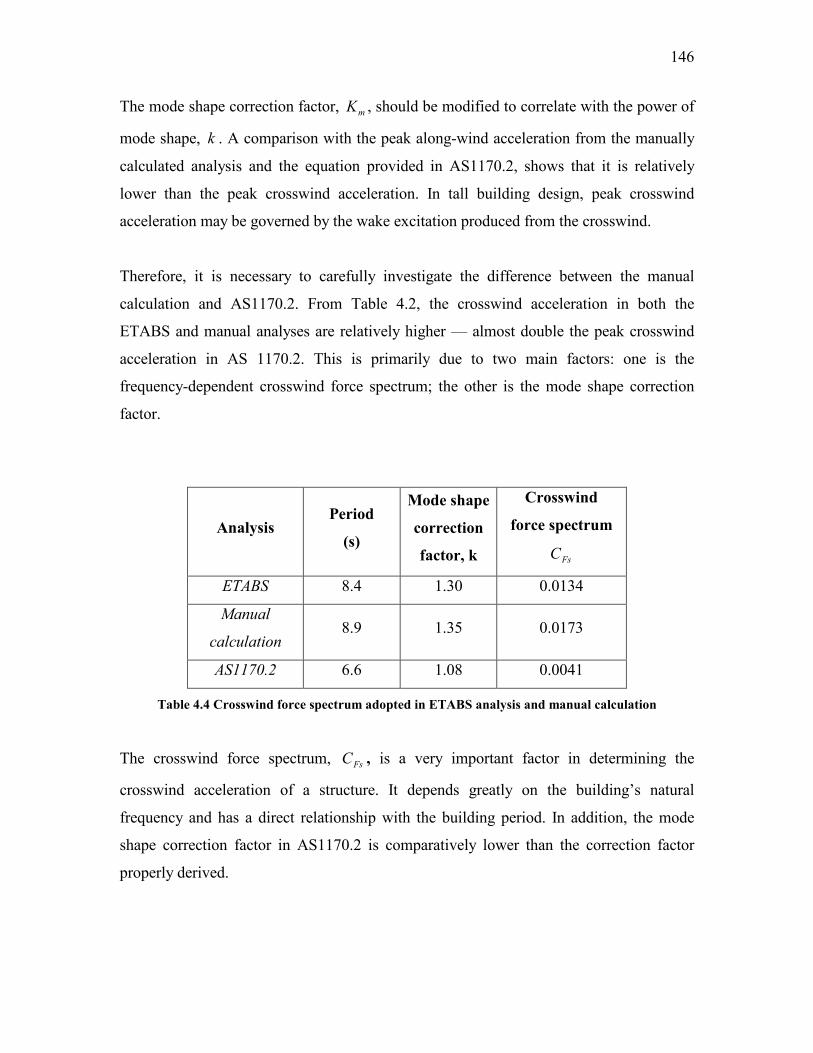
146
The mode shape correction factor, mK , should be modified to correlate with the power of
mode shape, k . A comparison with the peak along-wind acceleration from the manually
calculated analysis and the equation provided in AS1170.2, shows that it is relatively
lower than the peak crosswind acceleration. In tall building design, peak crosswind
acceleration may be governed by the wake excitation produced from the crosswind.
Therefore, it is necessary to carefully investigate the difference between the manual
calculation and AS1170.2. From Table 4.2, the crosswind acceleration in both the
ETABS and manual analyses are relatively higher — almost double the peak crosswind
acceleration in AS 1170.2. This is primarily due to two main factors: one is the
frequency-dependent crosswind force spectrum; the other is the mode shape correction
factor.
Analysis Period
(s)
Mode shape
correction
factor, k
Crosswind
force spectrum
FsC
ETABS 8.4 1.30 0.0134
Manual
calculation 8.9 1.35 0.0173
AS1170.2 6.6 1.08 0.0041
Table 4.4 Crosswind force spectrum adopted in ETABS analysis and manual calculation
The crosswind force spectrum, FsC , is a very important factor in determining the
crosswind acceleration of a structure. It depends greatly on the building’s natural
frequency and has a direct relationship with the building period. In addition, the mode
shape correction factor in AS1170.2 is comparatively lower than the correction factor
properly derived.

147
Therefore, the peak crosswind acceleration is almost half of that in the manually
calculated analysis in respect of the lower estimated period and mode shape correction
factor. However, both the ETABS and manual analysis show closer results.
For combined acceleration, because the along-wind acceleration is a relatively smaller
than the crosswind acceleration, e.g. along-wind acceleration of 3.5mg compare to
crosswind acceleration of 66mg, the combined acceleration is approximately equal to the
crosswind acceleration from the square-root sum of the squares of both accelerations. If
the combined acceleration is to be compared with the horizontal acceleration criteria for
occupancy comfort from Figure 2.20, the building has failed to achieve the acceleration
limit of approximately 20mg under building frequency of 0.1Hz. Hence, there is a need to
review the structure by introducing a few methods to suppress the wind-induced
acceleration such as improving the aerodynamic design of the structure by chamfered
most of the sharp corners, strengthen the structure by improving the building frequency
or increasing the building mass, alternatively introducing auxiliary damping devices to
increase the damping ratio of the structure.
In reality, the building period will be much higher than the manually calculated analysis
because of the stiffness that is not included in the calculation, such as the stiffness
contributed by columns and slabs, by the block partitions and by the retaining wall if
applicable. As such, the peak crosswind acceleration can be lowered.

148
Chapter 5
5.0 Conclusion and recommendations for future
study
5.1 Conclusions
Based on the results and discussions presented in this thesis, several conclusions are
presented in this chapter.
For outrigger-braced structure, the outrigger location for the structure that gives the least
deflection is the optimum location for the least along-wind acceleration as the building’s
acceleration is directly proportional to the deflection. A series of graphs with one to five
outriggers is plotted to show the best location in reducing the building deflection.
Generally, for the optimum performance of a structure with n outriggers, the outriggers
should be placed at height locations of )1(
1
+n,
)1(
2
+n, up to
)1( +n
n. The study shows
that the best location of the outriggers is somewhere at equal distance of the height of the
structure from the base; again, this must be based on the building’s properties. On the
other hand, the outrigger location that gives the least core moment is located as near as

149
possible to the building’s foundation. However, this is generally undesirable, as it is not
efficient in terms of decreasing building deflection and acceleration.
Two types of wind loading are introduced to act as the lateral load on the structure: a
uniformly distributed wind load and a triangular wind load. The results show that the
outrigger location tends to move up the building’s height with a triangular load
distribution in comparison with uniform wind load distribution acting on an outrigger-
braced structure. This is mainly due to the difference in characteristics of wind action on
a building, such as the base bending moment and the top deflection of the building itself.
Additionally, a parametric study has been carried out to investigate the factors that affect
the efficiency of an outrigger-braced structure in terms of top drift and moment reduction.
In the analysis, the height of a structure is investigated and shows no relationship to the
efficiency of the outrigger-braced structures. Similarly, the core properties of an
outrigger-braced structure are studied and it is concluded that the stronger the core, with
an increase in core properties or in concrete strength, there is a decrease in the efficiency
of the outrigger structures. This may be due to the fact that the stronger core attracts more
forces and moments, causing less forces and moments to be redistributed to the outrigger-
braced core-to-column.
The column sizes have a significant effect on the efficiency of an outrigger-braced
system. Deflection and moment reduction efficiency are greatly reduced by increasing the
column sizes, on the basis that the outriggers are considered stiff. In conjunction with the
column sizes, a longer clear distance between columns yields a higher efficiency in the
outrigger-braced system. In short, factors such as the lever arm between outrigger-braced
columns, and the properties of the outrigger-braced columns and outriggers, play an
important role in the efficiency of an outrigger-braced system in a structure.
In terms of peak along-wind and crosswind acceleration, AS1170.2 is adopted to compare
with both analyses. AS1170.2 shows relatively higher peak along-wind acceleration than
that which is manually calculated. This is mainly due to the different approach adopted in

150
AS1170.2 in terms of estimating the top deflection of the structure, which is
conservatively modified by adopting the maximum point load that is acting on the tip of
the cantilever, and the point load is converted from the total core base moment divided by
the total height. In addition, the equation provided by AS1170.2 does not include the
mode shape correction factor. Although the equation is transformed into the generalized
mass with an assumption of 1=k , no additional correction factor, mK , is included to
modify the generalized mass.
For peak crosswind acceleration, both ETABS and manual analyses show relatively
higher acceleration, almost double that of the peak crosswind acceleration in AS 1170.2.
This is primarily due to two main factors: one is the higher value of the frequency-
dependent crosswind force spectrum, FsC , adopted in both the ETABS and manual
analysis. The crosswind force spectrum, FsC , is a very important factor in determining
the crosswind acceleration of the structure and it depends on the building’s natural
frequency. However, there is limited information about FsC provided in AS1170.2, and
most is in terms of the parameters that can be obtained from wind tunnel testing, which
might cause problems during the preliminary building design. The second factor is the
lower mode shape correction factor specified in AS1170.2. In general, the mode shape
correction factor in AS1170.2 is comparatively lower than the correction factor from the
proper derivation.
An example of an outrigger-braced structure is analyzed using both ETABS and manual
calculation. A comparison between the ETABS analysis and manual calculation shows
close results in terms of the restraining moments at the outrigger location, the building
frequencies, and the total deflection at the top of the building. However, the results
obtained from ETABS are more accurate as it involves detailed 3D analysis, including
secondary effects on the structure.
However for tall building design, it is suggested that both approaches are adopted in two
different stages. For the preliminary stage, it is advised that an estimation of the

151
outrigger-braced system through manual calculation is carried out, as opposed to using
time-consuming modeling. For the detailed design phase, computer software such as
ETABS should be adopted to increase the accuracy of the results.
5.2 Recommendations for future study
Based on the literature review and the conclusions made in this thesis, recommendations
for future study are presented in the following sections.
5.2.1 Torsional acceleration
Torsional mode is not considered in this thesis. However, torsional mode in structural
design can be important because of its relation to the architectural and aesthetic
appearance of a building. Often the maximum eccentricity does not occur at the same
wind direction as the maximum shear. If the shear walls are concentrated near the core
then the same torque will produce a much greater shear stress, and the design condition is
more likely to occur in the direction of maximum eccentricity.
Unfortunately, no code or standard has specified the method of analysis to take into
account the torsional deflection and acceleration in a building. For an outrigger-braced
structure, it is likely to have the torsional mode as the fundamental mode of the structure
if the core size is relatively smaller than it should be, due to the fact that the core mainly
takes the torsion of a building. Therefore, it is necessary to include the methodology of
estimating the torsional behavior of an outrigger-braced structure.
5.2.2 P-∆ effect
Assessment of the overall stability of the structure under the action of combined vertical
and lateral loads, or under the action of the vertical load only, is of importance in the
design of building columns. P-∆ analysis plays an important role in an outrigger-braced
structure because it will decrease the performance of the outrigger-braced columns,

152
which therefore decreases the efficiency of the outrigger-braced system. Therefore,
adjustments of the strength of the columns need to be taken into account.
In fundamental analysis, the compensation for not including the P-∆ effect directly in the
analysis is made by multiplying the results of the first-order analysis by the moment
magnifier. However, in reality the axial loads acting through the deflection of the
structure give rise to additional moment at the base, with a consequent increase in the
deflection. By invoking the basic principle that for equilibrium to exist, the change in the
external applied moments must be equal to the change in the internal resisting moment,
this change is considered to be brought about by additional story shears, called sway
forces or P-∆ forces. To account for more iteration and accurate results, it is suggested to
evaluate these with the assistance of computer programs.
5.2.3 Differential shortening of outrigger-braced columns
As the building increases in height, the vertical members are subjected to large axial
displacements because they are intended to carry vertical loads from a large number of
floors. For an outrigger-braced structure, differential shortening of the main columns has
to be assessed thoroughly to avoid unexpected damage in structural and nonstructural
elements. The differential shortening between these vertical members, resulting from
differing stress levels, loading histories, volume-to-surface ratios and other factors in a
high-rise building, must be properly considered in the design process.
In addition, the differential length changes of vertical members arising from elastic,
creep, and shrinkage shortenings are of primary concern, as the differential shortening of
the vertical members causes additional axial forces in the vertical members and additional
bending moments in the slabs. Therefore, the amount of the shortenings, which is based
on the material characteristics, and the design and loading parameters, should be
accurately predicted and properly compensated for, such as pre-cambering the slabs and
re-adjusting the length of the columns during the construction phase.

153
5.2.4 Slab stiffness contribution
Many studies demonstrate the behavior and effectiveness of an outrigger-braced system,
but they do not consider the stiffness of the floor members that link the central core and
the perimeter columns at the typical tower floors. Slab stiffness contributes a significant
amount of stiffness to the structure, which might eventually provide double the stiffness
to the structure without the inclusion of slab stiffness. However, to include slab stiffness,
the effective second moment of are, Ieff, of the slab must be carefully identified in terms
of considering the detailing of reinforcement and the different stages in the building life
cycle.

154
Bibliography
AIJ (2004). ‘Chapter 6: Wind Loads.’ Recommendations and Commentary for Loads on
Buildings, Architectural Institute of Japan, Japan.
Ali M. M. (2007). ‘Structural developments in tall buildings: Current trends and future
prospects.’ Architectural Science Review 50(3): 205-223.
Ambrose J. E. and Vergun D. (1980). Simplified building design for wind and earthquake
forces, New York, Wiley.
Amyot J. R. (1984). ‘Simulation studies of a vibration damper for wind-induced motion
of a tall building.’ Computers in Engineering, Proceedings of the International
Computers in Engineering Conference, pp. 673-681.
AS/NZS 1170.0. (2002) Australian/New Zealand Standard and supplement, Structural
Design Actions : General Principles, Standard Australia, Sydney
AS/NZS 1170.1. (2002) Australian/New Zealand Standard and supplement, Structural
Design Actions – Part 1: Permanent, Imposed and Other Actions, Standard
Australia, Sydney
AS/NZS 1170.2. (2002) Australian/New Zealand Standard and supplement, Structural
Design Actions – Part 2: Wind Actions, Standard Australia, Sydney
Banavalkar P. V. (1995). ‘Ductile outrigger frames for high-rise buildings in a seismic
area.’ Proceedings of the World Congress of the Council on Tall Buildings and
Urban Habitat.

155
Boggs D., Hosoya N. and Cochran L. (2000). ‘Sources of Torsional Wind Loading on
Tall Buildings: Lessons from the Wind Tunnel.’ Advanced Technology in
Structural Engineering, ASCE, 2000.
Boggs D. (2007). Acceleration Indexes for Human Comfort in Tall Buildings – Peak or
RMS, CTBUH Monograph Chapter 13: Motion Perception Tolerance and
Mitigation 1997.
Building Research Establishment. (1994). Wind Around Tall Buildings, Garston,
England, Building Research Establishment.
Burton M. D. (2006). ‘Frequency dependence of human Response to wind-induced
building motion.’ Journal of Structural Engineering, 132(2), pp. 296-303.
Cenek P. D., Wood J. H. (1990). Designing multi-storey buildings for wind effects,
Judgeford [N.Z.], Building Research Association of New Zealand.
Cermak J. E. (1980). Wind engineering: proceedings of the Fifth International
Conference, Fort Collins, Colorado, USA, July 1979. Oxford, New York,
Pergamon Press.
Chang F. K. (1974). ‘Solutions to the wind motion problem in tall building design.’
AGARD Conference Proceedings, pp. 583-588.
Chang F. K. (1981). ‘Motion perception and tolerance.’ Journal of Great Lakes
Research, pp. 803-862.
Chang F. K., Chen C. (2004). Outrigger System Study For Tall Building Structure with
Central Core and Square Floor Plate, CTBUH 2004, October 10-13, Seoul,
Korea.

156
Chen P. W. and Robertson L. E. (1973). ‘Human perception threshold of horizontal
motion.’ Journal of Structural Division, ASCE 98 (8) (1972), pp. 1681–1695.
Chopra A. K. (1995). Dynamics of structures: theory and applications to earthquake
engineering, Upper Saddle River, N.J., Prentice Hall.
Davenport, A. G. (1963). ‘The buffeting of structures by gusts.’ Proceedings,
International Conference on Wind Effects on Building and Structures, Teddington
U.K., 26-8 June, 358-91.
Davenport, A. G. (1967). ‘Gust loading factors.’ ASCE Journal of the Structural
Division, 93: 11-34.
Denoon R.O., Kwok K.C.S., Letchford C.W., and Roberts R.D. (2000). Field
experiments to investigate occupant perception and tolerance of wind-induced
building motion, Research Report No. R803, Department of Civil Engineering,
University of Sydney, Australia.
Denoon R. O. (2000). ‘Effects of wind-induced tall building motion on cognitive
performance.’ Research Report - University of Sydney, Department of Civil
Engineering (804), pp. 1-69.
Denoon, R.O., Kwok, K.C.S., and Roberts, R.D. (2001). ‘The Use of Motion Simulators
in the Investigation of Occupant Response to Wind-Induced Building Motion.’
Proceedings of the Fifth Asia-Pacific Conference on Wind Engineering, Kyoto.
ETABS manual 2007.
Goto T. (1983). ‘Studies on wind-induced motion of tall buildings based on occupants’
reactions.’ Journal of Wind Engineering and Industrial Aerodynamics, 13.

157
Guo J. (1997). ‘Research of displacement and frequency of tall building under wind load
using GPS.’ Proceedings of ION GPS, 2, pp. 1385-1388.
Hansen, R. J. (1973). ‘Human response to wind-induced motion of buildings.’ ASCE J
Struct Div, 99(ST7), pp. 1589-1605.
Haris A. A. K. (1978). ‘Approximate stiffness analysis of high-rise buildings.’ ASCE J
Struct Div, 104(4), pp. 681-696.
Hart G. C. and Wong K. K. F. (2000). Structural Dynamics for Structural Engineers,
New York, Wiley.
HB 212 – 2002. Design Wind Speeds for the Asia-Pacific Region, Standards Australia,
Sydney.
Hoenderkamp J. C. D. (2000). ‘Approximate analysis of high-rise frames with flexible
connections.’ Structural Design of Tall Buildings, 9(3), pp. 233-248.
Hoenderkamp J. C. D. (2000). ‘Simplified analysis of facade rigger braced high-rise
structures.’ Structural Design of Tall Buildings, 9(4), pp. 309-319.
Hoenderkamp J. C. D. (2002). ‘Simplified analysis of asymmetric high-rise structures
with cores.’ Structural Design of Tall Buildings, 11(2), pp. 93-107.
Hoenderkamp J. C. D. (2003). ‘Analysis of high-rise braced frames with outriggers.’
Structural Design of Tall and Special Buildings, 12(4), pp. 335-350.
Hoenderkamp J. C. D. (2003). ‘Preliminary analysis of high-rise braced frames with
facade riggers.’ Journal of Structural Engineering, 129(5), pp. 640-647.
Hoenderkamp J. C. D. (2003). ‘Preliminary design of high-rise outrigger-braced shear
wall structures on flexible foundations.’ Heron, 48(2), pp. 81-98.

158
Hoenderkamp J. C. D. (2004). ‘Shear wall with outrigger trusses on wall and column
foundations.’ Structural Design of Tall and Special Buildings, 13(1), pp. 73-87.
Holmes J. D., Walker G. R.. (1990). A commentary on the Australian standard for wind
loads AS 1170 Part 2, 1989, Melbourne, Australian Wind Engineering Society.
Holmes J. D. (1996). Dynamic Analysis for Wind, N.Z. Structural Engineering Society
Seminars Wind Loading and Analysis, September 1996.
Holmes, J. D. (2001). Wind loading of structures, New York, Spon Press.
Holmes J., King A. (2005). A Guide to AS/NZS 1170.2: 2002: Wind Actions, Mentone,
Vic., Warrreen Publishing.
Holmes J. D. (2007). Wind Loading of Structure, New York, Taylor & Francis.
Irwin A. W. (1981). ‘Perception, comfort and performance criteria for human beings
exposed to whole body pure yaw vibration and vibration containing yaw and
translational components.’ Journal of Sound and Vibration 76 (4) (1981), pp.
481–497
Irwin A. W. (1986). ‘Motion in tall buildings.’ Proceedings of Conference on Tall
Buildings, Second Century of the Skyscraper, Chicago.
ISO 4354. Wind Actions on Structures, International Standard, 1997.
Isyumov N. (1986). ‘Building motion in wind.’ ASCE.

159
Kabeyasawa T. (1986). ‘Ultimate-state seismic deisng of high-rise reinforced concrete
shear wall-frame structures.’ Transactions of the Japan Concrete Institute, 8, pp.
397-404.
Kareem, A. (1988). ‘Wind-induced response of buildings: A serviceability viewpoint.”
Proceedings of National Engineering Conference, American Institute of Steel
Construction, Miami Beach, FL.
Kareem A., Kijewski T., Tamura Y. (1999). Mitigation of Motions of Tall Building with
Specific Examples of Recent Applications, Department of Civil Engineering and
Geological Sciences, University of Notre Dame, Notre Dame.
Kareem A. (2003). ‘Gust loading factor - past, present and future.’ Journal of Wind
Engineering and Industrial Aerodynamics, 91(12-15), pp. 1301-1328.
Katagiri J. (1992). ‘Wind-induced lateral-torsional motion of a tall building.’ Journal of
Wind Engineering and Industrial Aerodynamics, 42(1-3), pp. 1127-1137.
Kijewski T. (1998). ‘Dynamic wind effects: a comparative study of provisions in codes
and standards with wind tunnel data.’ Wind & Structures, An International
Journal, 1(1), pp. 77-109.
Klopp R. (1989). Wind loads on tall buildings, Stuttgart, IRB Verlag.
Kolouek V. R. (1984). Wind Effects on Civil Engineering Structures, Amsterdam; New
York, Elsevier.
Kwok K. C. S. (1982). ‘Crosswind response of tall buildings.’ Eng Struct, V 4(N 4): 256-
262

160
Kwok K. C. S. (1988). ‘Effect of building shape on wind-induced response of tall
building.’ Journal of Wind Engineering and Industrial Aerodynamics, 28 pt 1(1-
3), pp. 381-390.
Li Q. (2005). ‘Serviceability of a 79-storey tall building under typhoon.’ Proceedings of
the Institution of Civil Engineers: Structures and Buildings, 158(4), pp. 219-228.
Liang S., Liu S., Li Q. (2002). ‘Mathematical model of acrosswind dynamic loads on
rectangular tall buildings.’ Journal of Wind Engineering and Industrial
Aerodynamics, 90, pp. 1757-1770.
Liang S. (2005). ‘Simplified formulas for evaluation of acrosswind dynamic responses of
rectangular tall buildings.’ Wind and Structures, An International Journal, 8(3),
pp. 197-212.
Melbourne W. H., Palmer T. R. (1992). “ Acceleration and comfort criteria for buildings
undergoing complex motions.” Journal of Wind Engineering and Industrial
Aerodynamics, 41-44, pp. 105-116.
Melbourne W. H. (1998). Comfort Criteria for Wind-induced motion in Structure,
Structural Eng. Int., 1, pp. 40-44.
Mendis P., Ngo T., Haritos N., Hira A. (2007). ‘Wind loading on tall buildings.’ EJSE
Special Issue: Loading on Structures.
Moudarres F. R. (1984). ‘Outrigger-braced coupled shear walls.’ Journal of structural
engineering – ASCE, 110(12), pp. 2876-2890.
Nigam N. C. and Narayanan S. (1994). Applications of random vibrations, Berlin; New
York.

161
Pandit G. S. (1990). ‘Torsion analysis of high-rise building frames.’ Indian Concrete
Journal, 6(2).
Park H. S. (2003). ‘Optimal compensation of differential column shortening in high-rise
buildings.’ Structural Design of Tall Buildings, 12(1), pp. 49-66.
Reed J. W. (1971). ‘Wind induced motion and human comfort.’ Research Report 71-42,
Massachusetts Institute of Technology.
Rutenberg A. (1986). ‘Free-vibrations of outrigger-braced structures-discussion.’
Proceedings of the Institution of Civil Engineers part 2 – Research and Theory,
81, pp. 149-152.
Sachs P. (1978). Wind forces in engineering, Oxford; New York, Pergamon Press.
Samali, B., Mayol, E, Kwok, KCS, Mack, A. and Hitchcock, P. (2004). ‘Vibration
Control of the Wind Excited 76 Storey Benchmark Building by Liquid Column
Vibration Absorbers’, ASCE Journal of Engineering Mechanics, 130(4), pp. 478-
485.
Shahrooz, B. M. (2004). ‘Outrigger beam-wall connections. I: Component testing and
development of design model.’ Journal of Structural Engineering, 130(2), pp.
253-261.
Shahrooz B. M. (2004). ‘Outrigger beam-wall connections. II: Subassembly testing and
further modeling enhancements.’ Journal of Structural Engineering, 130(2), pp.
262-270.
Simiu, E., and Scanlan, R. H. (1996). Wind Effects on Structures, Third Edition, Wiley
and Sons, New York.

162
Sircovich-Saar O. (2006). Dynamics in the Practice of Structural Design, Southampton,
WIT Press
Smith B. S. (1980). ‘Behavior of multi-outrigger-braced tall building structures.’ Journal
of The American Concrete Institute, 77(4), pp. 290-290.
Smith B. S. (1981). ‘Parameter study of outrigger-braced tall structures.’ Journal of The
Structural Division-ASCE, 107(10), pp. 2001-2014.
Smith B. S. (1983). ‘Formulas for optimum drift resistance of outrigger-braced tall
building structures.’ Computers & Structures, 17(1), pp. 45-50.
Smith B. S. (1984). ‘Generalized method of estimating drift in high-rise structures.’
Journal of Structural Engineering, 110(7), pp. 1549-1562.
Smolira M. (1975). Analysis of tall buildings by the force-displacement method, London;
New York, McGraw-Hill.
Sockel H. and International Centre for Mechanical Sciences. (1994). Wind-Excited
Vibrations of Structures, Wien; New York, Springer-Verlag.
Stafford Smith B. and Coull A. (1991). Tall Building Structures: Analysis and Design,
New York, Wiley.
Tamura Y. (2005). ‘Aspects of the dynamic wind-induced response of structures and
codification.’ Wind and Structures, 8(4), pp. 251-268.
Taranath B. S. (1988). Structural Analysis and Design of Tall Buildings, New York,
McGraw-Hill.

163
Taranath B. S. (1998). Steel, Concrete, and Composite Design of Tall Buildings, New
York, McGraw-Hill.
Thepmongkorn S. (1998). ‘Wind-induced coupled translational-torsional motion of tall
buildings.’ Wind & Structures, An International Journal, 1(1), pp. 43-57.
Tong G. S. (2008). ‘A simplified method for the buckling of outrigger-shear wall braced
structures.’ Advances in Structural Engineering, 11(1), pp. 1-15.
Torkamani M. A. M. (1985). ‘Dynamic response of tall building to wind excitation.’
Journal of Structural Engineering, 111(4), pp. 805-825.
Vickery B. J. (1965). ‘On the flow behind a coarse grid and its use as a model of
atmospheric turbulence in studies related to wind loads on buildings.’ National
Physical Laboratory (U.K.) Aero Report 1143.
Vickery B. J. (1966). ‘On the assessment of wind effects on elastic structure.’ Australian
Civil Engineering Transactions CE8: 183-92.
Wu J. R. (2003). ‘Structural performance of multi-outrigger-braced tall buildings.’
Structural Design of Tall and Special Buildings, 12(2), pp. 155-176.
Xu Y. L. (1990). ‘Wind-induced vibration of tall buildings and its control by tuned mass
dampers.’ National Conference Publication - Institution of Engineers, Australia,
90(9), pp. 73-80.
Xu Y. L. (1993). ‘Mode shape corrections for wind-tunnel tests of tall buildings.’
Engineering Structures, 15(5), pp. 387-392.
Yamada M. and Goto T. (1975). T. The Criteria to Motions in Tall Buildings, Proceeding
Pan Pacific Tall Buildings Conference, Hawaii, pp. 233-244.

164
Yamada M. and Goto T. (1977). ‘Human Response to Tall Building Motion’. Human
Response to Tall Buildings, Dowden Hutchinson & Ross, pp 58-80.
Yang J. N. (1981). ‘Coupled motion of wind-loaded multi-story building.’ ASCE J Eng
Mech Div, 107(6), pp. 1209-1226.
Zeidabadi N. A. (2004). ‘Optimized use of the outrigger system to stiffen the coupled
shear walls in tall buildings.’ Structural Design of Tall and Special Buildings,
13(1), pp. 9-27.
Zhang J. (2007). ‘Safety analysis of optimal outriggers location in high-rise building
structures.’ Journal of Zhejiang University: Science A, 8(2), pp. 264-269.
Zhou Y. (2002). ‘Along-wind load effects on tall buildings: Comparative study of major
international codes and standards.’ Journal of Structural Engineering-ASCE,
128(6), pp. 788-796.
Zhou Y. (2002). ‘Mode shape corrections for wind load effects.’ Journal of Engineering
Mechanics, 128(1), pp. 15-23.
Zhou Y. (2003). ‘Aerodynamic loads on tall buildings: Interactive database.’ Journal of
Structural Engineering –ASCE, 129(3), pp. 394-404.
Zhou Y. and Kareem A. (2001). ‘Gust Loading Factor: New Model.’ Journal of
Structural Engineering, 127(2), pp. 168.
Zhou Y., Kijewski T. and Kareem A. Aerodynamic Loads on Tall Buildings: Interactive
Database, University of Notre Dame.

165
Appendices
Appendix A: Parametric studies on wind-induced
accelerations
A.1 Building Information

166
A.2 Static Wind Load Analysis

167

168
A.3 Dynamic Wind Load Analysis (Ultimate X-direction)

169

170
A.4 Dynamic Wind Load Analysis (Ultimate Y-direction)

171

172
A.5 Dynamic Wind Load Analysis (Serviceability X-direction)

173

174
A.6 Dynamic Wind Load Analysis (Serviceability Y-direction)

175

176
Appendix B: Factors affecting efficiency of
outrigger-braced system
A.1 Building Information

177
B.2 Static Wind Load Analysis

178

179
B.3 Dynamic Wind Load Analysis (Ultimate X-direction)

180

181
B.4 Dynamic Wind Load Analysis (Ultimate Y-direction)

182

183
B.5 Dynamic Wind Load Analysis (Serviceability X-direction)

184

185
B.6 Dynamic Wind Load Analysis (Serviceability Y-direction)

186

187
B.7 Building Mass

188

189
B.8 Building Deflection and Mode Shape

190

191
B.9 Outrigger-braced System Analysis

192
Appendix C: Mathematica Program Calculations
C.1 One-outrigger-braced system
Uniformly distributed wind load (1-Outrigger)

193
Triangular distributed wind load (1-Outrigger)

194
C.2 Two-outrigger-braced system
Uniformly distributed wind load (2-Outrigger)

195
Triangular distributed wind load (2-Outrigger)

196
C.3 Three-outrigger-braced system
Uniformly distributed wind load (3-Outrigger)

197
Triangular distributed wind load (3-Outrigger)

198
C.4 Four-outrigger-braced system
Uniformly distributed wind load (4-Outrigger)

199

200
Triangular distributed wind load (4-Outrigger)

201

202
C.5 Five-outrigger-braced system
Uniformly distributed wind load (5-Outrigger)

203

204

205

206
Triangular distributed wind load (5-Outrigger)

207

208

209

210

211
Appendix D: ETABS Results
Story Height Shear Moment Story Height Shear Moment
(m) (kN) (kNm) (m) (kN) (kNm)
86 301.0 40 140 43 150.5 3421 36596
85 297.5 119 555 42 147.0 3499 48844
84 294.0 197 1246 41 143.5 3578 61367
83 290.5 276 2211 40 140.0 3657 74165
82 287.0 354 3452 39 136.5 3735 87239
81 283.5 433 4968 38 133.0 3814 100588
80 280.0 512 6759 37 129.5 3893 114211
79 276.5 590 8825 36 126.0 3971 128110
78 273.0 669 11167 35 122.5 4050 142285
77 269.5 748 13783 34 119.0 4128 156734
76 266.0 826 16675 33 115.5 4207 171459
75 262.5 905 19842 32 112.0 4286 186458
74 259.0 983 23284 31 108.5 4364 201733
73 255.5 1062 27001 30 105.0 4443 217284
72 252.0 1141 30994 29 101.5 4522 233109
71 248.5 1219 35262 28 98.0 4600 249209
70 245.0 1298 39805 27 94.5 -24601 91546
69 241.5 1377 44623 26 91.0 -24579 -21345
68 238.0 1455 49716 25 87.5 4836 -40878
67 234.5 1534 55084 24 84.0 4915 -23677
66 231.0 1612 60728 23 80.5 4993 -6201
65 227.5 1691 66647 22 77.0 5072 11551
64 224.0 1770 72841 21 73.5 5151 29578
63 220.5 1848 79310 20 70.0 5229 47880
62 217.0 1927 86054 19 66.5 5308 66457
61 213.5 2006 93074 18 63.0 5386 85309
60 210.0 2084 100369 17 59.5 5465 104437
59 206.5 -17207 4713 16 56.0 5544 123839
58 203.0 -17896 -75761 15 52.5 5622 143517
57 199.5 2320 -105982 14 49.0 5701 163470
56 196.0 2399 -97586 13 45.5 5779 183698
55 192.5 2477 -88916 12 42.0 5858 204202
54 189.0 2556 -79970 11 38.5 5937 224980
53 185.5 2635 -70749 10 35.0 6015 246034
52 182.0 2713 -61253 9 31.5 6094 267363
51 178.5 2792 -51481 8 28.0 6173 288967
50 175.0 2870 -41435 7 24.5 6251 310846
49 171.5 2949 -31113 6 21.0 6330 333001
48 168.0 3028 -20516 5 17.5 6408 355431
47 164.5 3106 -9644 4 14.0 6487 378135
46 161.0 3185 1503 3 10.5 6566 401115
45 157.5 3264 12925 2 7.0 6644 424371
44 154.0 3342 24623 1 3.5 6723 447901