optimization of image b-spline interpolation for gpu

Published in Image Processing On Line on 2019–08–02.Submitted on 2019–04–11, accepted on 2019–07–22.ISSN 2105–1232 c© 2019 IPOL & the authors CC–BY–NC–SAThis article is available online with supplementary materials,software, datasets and online demo athttps://doi.org/10.5201/ipol.2019.257

2015/06/16

v0.5.1

IPOL

article

class

Optimization of Image B-spline Interpolation for GPU

Architectures

Thibaud Briand1,2, Axel Davy2

1 Universite Paris-Est, LIGM (UMR CNRS 8049), ENPC, F-77455 Marne-la-Vallee, France([email protected])

2 Universite Paris-Saclay, CMLA (UMR CNRS 8536), France([email protected])

Communicated by Pablo Arias Demo edited by Thibaud Briand and Axel Davy

Abstract

Interpolation is a vital piece of many image processing pipelines. In this document we presenthow to optimize the implementation of image B-spline interpolation for GPU architectures. Theimplementation is based on the one proposed by Briand and Monasse in 2018 and works fororders up to 11. The two main optimizations consist in: (1) transposing the B-spline coefficientsbefore the prefiltering of the rows and (2) dividing columns into subregions in order to use morethreads. We assess the impact of the floating point precision and of using high B-spline orders.

Source Code

The OpenCL implementation of the code that we provide is the one which has been peerreviewed and accepted by IPOL. The source code, the code documentation, and the onlinedemo are accessible at the IPOL web page of the article1. Usage instructions are included inthe README.txt file of the archive.

Keywords: interpolation; splines; linear filtering; GPU; optimization

1 Introduction

Interpolation consists in constructing new data points within the range of a discrete set of knowndata points. In image processing it is commonly expressed as the problem of recovering from adiscrete image u the underlying continuous signal u : R2 → R verifying the interpolation condition

∀(k, l), u(k, l) = uk,l. (1)

A continuous image representation is handy when one wishes to implement numerically an operatorthat is initially defined in the continuous domain. In particular, applying a geometric transformationto an image (like for example a rotation) requires an interpolation method.

1https://doi.org/10.5201/ipol.2019.257

Thibaud Briand, Axel Davy, Optimization of Image B-spline Interpolation for GPU Architectures, Image Processing On Line, 9 (2019),pp. 183–204. https://doi.org/10.5201/ipol.2019.257

Thibaud Briand, Axel Davy

About B-spline interpolation. The spline representation has been widely used since the 1990s.A spline of degree n is a continuous piece-wise polynomial function of degree n of a real variablewith derivatives up to order n− 1. This representation has the advantage of being equally justifiableon a theoretical and practical basis [15]. It can model the physical process of drawing a smoothcurve and it is well adapted to signal processing thanks to its optimality properties. The B-splinerepresentation [12] is particularly handy, as the continuous underlying signal is expressed as theresult of a convolution between the B-spline kernel, that is compactly supported, and the discreteparameters of the representation, namely the B-spline coefficients. One of the strongest argumentsin favor of the B-spline interpolation is that it approaches the Shannon-Whittaker interpolation asthe order increases [1].

The determination of the B-spline coefficients is performed in a prefiltering step that, in general,can be done by solving a band diagonal system of linear equations [7, 9]. For uniformly spaceddata points, which is most of the time the case in signal processing, Unser et al. proposed in [16]an efficient and stable algorithm based on linear filtering that works for any order. More details, inparticular regarding the determination of the interpolator parameters, were provided by the authorsin later publications [17, 18]. All the information, theoretical and practical, required to performefficiently B-spline interpolation for any order and any boundary extension can be found in [4].Two slightly different prefiltering algorithms, whose precision is proven to be controlled thanks to arigorous boundary handling, were proposed.

Choice of the interpolation method and GPU. In practice, the choice of the interpolationmethod, among all the possibilities [6, 14], depends on the context. A compromise is made betweeninterpolation quality and computational efficiency. Although B-spline interpolation (of high-order)provides high-quality results for images, faster but lower quality methods such as bilinear or bicubicinterpolations are usually preferred.

Recently, graphics processing units (GPUs) have been widely used for image processing. Ded-icated GPUs have memory bandwidth that can be an order of magnitude faster than CPU RAM.GPUs are able to perform hardware image bilinear interpolation, though with limited 1/16th pre-cision for the position. Even for integrated GPUs (on laptops typically), the GPU can performsignificantly more floating point operations per second (FLOPS) than the CPU cores combined. SeeTable 1 for some examples of configurations and comparative performance.

Accelerator Description Bandwidth Float ops Double ops0 INTEL i7-6600U CPU (POCL 1.3) 19 GB/s 24 G/s 28 G/s1 INTEL i7-6600U GPU (NEO 18.21.10858) 23 GB/s 380 G/s 95 G/s2 AMD Radeon RX 480 (2766.4) 209 GB/s 5.7 T/s 279 G/s3 NVIDIA TITAN V (384.130) 610 GB/s 13.7 T/s 6.9 T/s

Table 1: Compared configurations: The first accelerator is a 4-core CPU, while the other accelerators are GPUs with differentlevels of performance. The bandwidth and number of operations per second were obtained with Clpeak, which estimatesthe actual peak figures which can be obtained with OpenCL.

While previously some GPU implementations of cubic B-spline interpolation have been publiclyavailable [13, 5, 11], to our knowledge none is able to handle higher orders (except [13] that supportsorders up to 5). Moreover no analysis has been done for the floating-point precision (single ordouble) required for these interpolations. Due to memory bandwidth considerations and doubleprecision computation costs, most GPU programs choose to operate on floats. Besides delivering aGPU implementation for B-spline interpolation from orders 0 to 11, we shall study the impact of thecomputation and storage precision on the results.

184

Optimization of Image B-spline Interpolation for GPU Architectures

Contributions. We propose an efficient GPU implementation of B-spline interpolation for ordersup to 11, which can handle both single and double floating point precision. The two main optimizationtricks to achieve this consist in: (1) transposing the B-spline coefficients before the prefiltering ofthe rows, and (2) dividing columns into subregions in order to use more threads. We compare theimpact of using single or double precision on the accuracy and conclude on the best precision to use.Also, we compare the performance using float or double precision on all supported orders for severalaccelerators. We show that to get an accuracy gain with double precision, all computation andstorage must use double precision, but that using double precision nearly doubles the computationtime.

This article is organized as follows: Section 2 is a short introduction to B-spline interpolation.Section 3 introduces briefly GPU architectures, gives details on our implementation, and compares itto other methods. In Section 4 we compare speed and accuracy for several orders, choices of floatingpoint precision and for different accelerators.

2 Introduction to B-spline Interpolation

In this section we introduce the reader to B-spline interpolation of uniformly spaced data points(such as image pixels). We consider the efficient and stable approach of Unser et al., proposedin [16], that is based on linear filtering and works for any order. This is a two-step interpolationmethod whose first step, namely the prefiltering step, can be decomposed into a cascade of exponentialfilters, themselves separated into two complementary causal and anticausal components. Two slightlydifferent prefiltering algorithms, whose precision is proven to be controlled thanks to a rigorousboundary handling, were introduced in [4] for 1D and 2D finite signals. More precisely, in bothversions the control of the error is guaranteed by the use of adequate truncation indices. Ourproposed GPU implementation, described in Section 3, is based on this method.

Section 2.1 introduces the method of [16] for the B-spline interpolation of one-dimensional infi-nite signals. Section 2.2 proposes a summary of the B-spline interpolation method of [4] for finiteone-dimensional signals. The extension to higher dimensions, and in particular to dimension 2, isdiscussed in Section 2.3. More details, and in particular, proofs, can be found in [4].

2.1 Case of an Infinite Signal

Let n be a non-negative integer. First, we define the B-spline interpolate of order n of an infiniteone-dimensional signal.

Definition 1. The normalized B-spline function of order n, noted β(n), is defined recursively by

β(0)(x) =

1, −12< x < 1

212, x = ±1

2

0, otherwiseand for n ≥ 0, β(n+1) = β(n) ∗ β(0), (2)

where the symbol ∗ denotes the convolution operator.

Definition 2 (B-spline interpolation). The B-spline interpolate of order n of a discrete signal f ∈ℓ∞(Z) is the function ϕ(n) defined for x ∈ R by

ϕ(n)(x) =∑

i∈Z

ciβ(n)(x− i), (3)

where the B-spline coefficients c = (ci)i∈Z are uniquely characterized by the interpolating condition

ϕ(n)(k) = fk, ∀k ∈ Z. (4)

185


Given a bounded signal f and a real x, computing the right hand side of (3) requires two evaluations:the signal c = (ci)i∈Z and the β(n)(x− i). This explains the two steps involved in the computation:

• Step 1 (prefiltering or direct B-spline transform) computes the B-spline coefficients c. Themethod that we consider for the prefiltering step is presented below.

• Step 2 (indirect B-spline transform [16]) reconstructs the signal values. Given the Dirac combof B-spline coefficients c =

∑

i∈Z ciδi the value of ϕ(n)(x) in (3) is computed at any locationx ∈ R as a convolution of c with the finite signal β(n)(x − .). Details about this step can befound in [4].

Prefiltering as a linear filtering. Except in the simplest cases, n = 0 or n = 1, in which caseβ(n)(k − i) = δi(k) and so ci = fi, the determination of the coefficients ci from f so as to satisfy (4)is not straightforward. In the following we summarize how the prefiltering step is rewritten in [16]as a linear filtering process. Proofs and details can be found in [4].

As introduced in [16], the prefiltering step boils down to the discrete convolution

c = (b(n))−1 ∗ f, (5)

where the filter (b(n))−1 denotes the inverse of the filter b(n) for the discrete convolution operator.This filter can be decomposed into a cascade of exponential filters, themselves separated into twocomplementary causal and anticausal components.

Decomposition of (b(n))−1 into exponential filters. The exponential filters involved are parametrizedby negative numbers called the poles of the B-spline interpolation. For order n, the n = ⌊n

2⌋ poles

(zi)1≤i≤n are defined and computed as described in [4], and are arranged so that

−1 < z1 < z2 < · · · < zn < 0. (6)

Let −1 < α < 0, α playing the role of one zi. Denote by k(α) ∈ RZ the causal filter and by l(α) ∈ R

Z

the anticausal filter defined for i ∈ Z by

k(α)i =

{

0 i < 0

αi i ≥ 0and l

(α)i =

{

0 i > 0

α−i i ≤ 0.(7)

Set h(α) = −αl(α) ∗ k(α). The filter h(α) is called exponential filter as it verifies for j ∈ Z,

h(α)j =

α

α2 − 1α|j|. (8)

It can be shown that the filter (b(n))−1 can be decomposed as

(b(n))−1 = γ(n)h(zn) ∗ · · · ∗ h(z1), (9)

where the normalization constant γ(n) is defined by

γ(n) =

{

2nn! n even

n! n odd.(10)

186


Prefiltering algorithm. This provides a new expression for the B-spline coefficients c,

c = γ(n)h(zn) ∗ · · · ∗ h(z1) ∗ f. (11)

To simplify, define recursively the signal c(i) ∈ RZ for i ∈ {0, . . . , n} by

c(0) = f and for i ≥ 1, c(i) = h(zi) ∗ c(i−1). (12)

We have c = γ(n)c(n). Thus the computation of the prefiltering step can be decomposed into n succes-sive filtering steps with exponential filters that can themselves be separated into two complementarycausal and anticausal components. This leads to a theoretical prefiltering algorithm that cannot beused in practice because it requires an infinite input signal. Turning this algorithm into a practicalone, that is, applicable to a finite signal, is the subject of Section 2.2.

2.2 Case of a Finite Signal

In practice the signal f to be interpolated is finite and discrete, i.e., f = (fi)0≤i≤K−1 for a given

positive integerK. An extension of f outside {0, . . . , K−1} is required. B-spline interpolation theorycan then be applied to the extended signal f ∈ ℓ∞(Z). To simplify the notation, in the following nodistinction will be made between the signal f and its extension f when there is no ambiguity.

Extension on a finite domain. Let x ∈ [0, K − 1]. As presented in the following, to com-pute ϕ(n)(x) with a relative precision ε it is sufficient to extend the signal to a finite domain{−L(n,ε), . . . , K − 1 + L(n,ε)} where L(n,ε) is a positive integer that only depends on the B-splineorder n and the desired precision ε. The precision is relative to the values of the signal. A relativeprecision of ε means that the error committed is less than ε supk∈Z |fk| = ε‖f‖∞. In practice theimages are large enough so that L(n,ε) < K and it is possible to express the extension as a bound-ary condition around 0 and K − 1 (otherwise the extension is obtained by iterating the boundarycondition). The most classical boundary condition choices are summarized in Table 2.

Extension Signal abcdeConstant aaa|abcde|eeeHalf-symmetric cba|abcde|edcWhole-symmetric dcb|abcde|dcbPeriodic cde|abcde|abc

Table 2: Classical boundary extensions of the signal abcde by L = 3 values.

Prefiltering computation using the extension. For computing the B-spline coefficients usingthe prefiltering decomposition given in (11), only the first exponential filter h(z1) is applied directlyto f = c(0). Therefore, for i ≥ 1 the intermediate filtered signals c(i) are known a priori only wherethey are computed. Considering this, the two following approaches were proposed in [4] in order toperform the prefiltering.

• Approach 1: extended domain. The intermediate filtered signals c(i) are computed in a largerdomain than {−n, . . . , K − 1 + n}. This works with any extension.

• Approach 2: exact domain. The extension, expressed as a boundary condition, is chosen sothat it is “transmitted” after the application of each exponential filter h(zi). The intermediatefiltered signals c(i) (and the B-spline coefficients c) verify the same boundary condition as theinput f and only need to be computed in {0, . . . , K − 1}.

187


Among the four classical boundary extensions presented in Table 2, the periodic, half-symmetricand whole-symmetric boundary conditions are transmitted after the application of an exponentialfilter. For the periodic extension the filtered signal by any filter always remains periodic. For the half-symmetric and whole-symmetric extensions it is a consequence of the symmetry of the exponentialfilters. However, this property is not satisfied for the constant extension, so that Algorithm 2 is notapplicable in this case. The second approach is more efficient as it requires fewer computations andis the considered approach in the following.

Section 2.2.1 details the general method for computing an exponential filter application on a finitedomain. Then, Section 2.2.2 describes the algorithm for computing the B-spline coefficients of a finitesignal with a given precision when the boundary condition is transmitted. Finally, Section 2.2.3presents the simple algorithm for performing the indirect B-spline transform, i.e., for evaluating theinterpolated values.

2.2.1 Application of the Exponential Filters

Let s ∈ ℓ∞(Z) be an infinite discrete signal and let −1 < α < 0. The application of the exponentialfilter h(α) = −αl(α) ∗ k(α) to the signal s is computed in the domain of interest {0, . . . , K − 1} asfollows. To simplify the notation we set s(α) = k(α) ∗ s so that

h(α) ∗ s = −αl(α) ∗ s(α). (13)

Causal filtering. Given the initialization

s(α)0 =

(

k(α) ∗ s)

0=

+∞∑

i=0

αis−i, (14)

the application of the causal filter k(α) to s can be computed recursively from i = 1 to i = K − 1according to the recursion formula

s(α)i = si + αs

(α)i−1. (15)

Anticausal filtering initialization. As shown in [4, p. 11] the initialization of the renormalizedanticausal filtering −αl(α) ∗ s(α) = h(α) ∗ s is given by

(

h(α) ∗ s)

K−1=

α

α2 − 1

(

s(α)K−1 +

(

l(α) ∗ s)

K−1− sK−1

)

, (16)

where(

l(α) ∗ s)

K−1=

+∞∑

i=0

αisK−1+i. (17)

Anticausal filtering. The renormalized anticausal filtering is computed recursively from i = K−2to i = 0 according to the following formula,

(

h(α) ∗ s)

i= α

(

(

h(α) ∗ s)

i+1− s

(α)i

)

. (18)

Approximation of the initialization values. The two infinite sums in (14) and (17) cannot becomputed numerically. Let N be a non-negative integer. The initialization values are approximatedby truncating the sums at index N so that

(

k(α) ∗ s)

0≃

N∑

i=0

αis−i, (19)

188


and

(

l(α) ∗ s)

K−1≃

N∑

i=0

αisK−1+i. (20)

Algorithm. The general method for computing the application of the exponential filter h(α) to adiscrete signal in a finite domain is summarized in Algorithm 1. Note that it is sufficient to knowthe signal in the domain {−N, . . . ,K − 1 +N}. It consists of 6(N + 1) + 4(K − 1) operations.

Algorithm 1: Application of the exponential filter h(α) to a discrete signal

Input : A pole −1 < α < 0, a truncation index N and a discrete signal s (whose values areknown in {−N, . . . ,K − 1 +N})

Output: The filtered signal h(α) ∗ s at indices {0, . . . , K − 1}

1 Compute s(α)0 using (19)

2 for i = 1 to K − 1 do

3 Compute s(α)i using (15)

4 end

5 Compute(

l(α) ∗ s)

K−1using (20)

6 Compute(

h(α) ∗ s)

K−1using (16)

7 for i = K − 2 to 0 do

8 Compute(

h(α) ∗ s)

iusing (18)

9 end

2.2.2 Prefiltering of a Finite Signal

Let ε > 0. In [4] two algorithms for computing the B-spline coefficients of a finite signal with precisionε were proposed. In this section we present the version where the input signal is extended with aboundary condition that is assumed to be transmitted after the application of the exponential filters.

Truncation indices. Define (µj)1≤j≤n by

µ1 = 0

µk =

(

1 + 1

log |zk|∑

k−1i=1

1log |zi|

)−1

, 2 ≤ k ≤ n.(21)

Define for 1 ≤ i ≤ n the truncation index

N (i,ε) =

log(

ερ(n)(1− zi)(1− µi)∏n

j=i+1 µj

)

log |zi|

+ 1, (22)

where

ρ(n) =

(

n∏

j=1

1 + zj1− zj

)2

. (23)

189


Algorithm. As the boundary condition is transmitted after the application of the exponentialfilters, the c(i) for 0 ≤ i ≤ n share the same boundary condition. Then, c(i) can be computed at anyindex from the values of c(i−1) in {0, . . . , K − 1} using Algorithm 1 (with truncation index N (i,ε)).Indeed, we notice that the initialization values in (19) and (20) only depend on the values of c(i−1)

in {0, . . . , K − 1}. The prefiltering algorithm with a transmitted boundary condition is describedin Algorithm 2. The choice for the truncation indices N (i,ε) guarantees a precision ε for n ≤ 16, asstated in the next theorem [4].

Theorem 1. Let ε > 0 and f be a finite signal of length at least 4. Assume that n ≤ 16 and thatf is extended with a boundary condition that is transmitted after the application of the exponentialfilters.

Then, the computation of the B-spline coefficients of f using Algorithm 2 with the truncationindices (N (i,ε))1≤i≤n has a precision of ε, i.e., the error committed is less than ε‖f‖∞.

Algorithm 2: Prefiltering algorithm (with a transmitted boundary condition)

Input : A finite discrete signal f of length K, a boundary condition that is transmitted, aB-spline interpolation order n ≤ 16 and a precision ε (the poles and thenormalization constant are assumed to be known)

Output: The B-spline coefficients c of order n at indices {0, . . . , K − 1} with precision εPrecomputations

1 for 1 ≤ i ≤ n do

2 Compute the truncation index N (i,ε) using (22)3 end

Prefiltering of the signal:

4 Set c(0)k = fk for k ∈ {0, . . . , K − 1}

5 for i = 1 to n do

6 Compute c(i−1)k for k ∈ {−N (i,ε), . . . ,−1} ∪ {K, . . . ,K − 1 +N (i,ε)} using the boundary

condition7 Compute c

(i)k =

(

h(zi) ∗ c(i−1))

kfor k ∈ {0, . . . , K − 1} using Algorithm 1 with truncation

index N (i,ε)

8 end

9 Renormalize c = γ(n)c(n) using (10) The normalization can be moved to Algorithm 4

Particular cases. For the three boundary conditions that are transmitted, the anticausal initial-ization value in (16) can be computed without using (20). In practice, when one of these threeboundary conditions is used in Algorithm 2, a slightly different version of Algorithm 1 is called inLine 6. The boundary extension is added to the input list and the computation of

(

h(α) ∗ s)

K−1(see

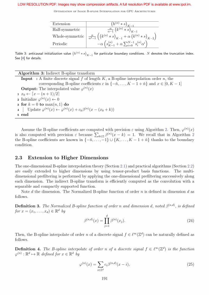
Line 5 and Line 6) is done using the corresponding formula in Table 3.

2.2.3 Indirect B-spline Transform: Computation of the Interpolated Value

The indirect B-spline transform reconstructs the signal values from the B-spline representation. Giventhe B-spline coefficients c in {−n, . . . , K − 1 + n}, the interpolated value ϕ(n)(x) can be computedwith precision ε, using (3), as the convolution of

∑K−1+n

i=−n ciδi with the compactly supported function

β(n). The computation of the indirect B-spline transform at location x ∈ [0, K − 1] is presented inAlgorithm 3.

190


Extension(

h(α) ∗ s)

K−1

Half-symmetric αα−1

(

k(α) ∗ s)

K−1

Whole-symmetric αα2−1

(

(

k(α) ∗ s)

K−1+ α

(

k(α) ∗ s)

K−2

)

Periodic −α(

s(α)K−1 + α

∑N−1i=0 s

(α)i αi

)

Table 3: anticausal initialization value(

h(α) ∗ s)

K−1for particular boundary conditions. N denotes the truncation index.

See [4] for details.

Algorithm 3: Indirect B-spline transform

Input : A finite discrete signal f of length K, a B-spline interpolation order n, thecorresponding B-spline coefficients c in {−n, . . . , K − 1 + n} and x ∈ [0, K − 1]

Output: The interpolated value ϕ(n)(x)1 x0 ← ⌈x− (n+ 1)/2⌉

2 Initialize ϕ(n)(x)← 03 for k = 0 to max(n, 1) do4 Update ϕ(n)(x)← ϕ(n)(x) + ckβ

(n)(x− (x0 + k))5 end

Assume the B-spline coefficients are computed with precision ε using Algorithm 2. Then, ϕ(n)(x)is also computed with precision ε because

∑

k∈Z β(n)(x − k) = 1. We recall that in Algorithm 2

the B-spline coefficients are known in {−n, . . . ,−1} ∪ {K, . . . ,K − 1 + n} thanks to the boundarycondition.

2.3 Extension to Higher Dimensions

The one-dimensional B-spline interpolation theory (Section 2.1) and practical algorithms (Section 2.2)are easily extended to higher dimensions by using tensor-product basis functions. The multi-dimensional prefiltering is performed by applying the one-dimensional prefiltering successively alongeach dimension. The indirect B-spline transform is efficiently computed as the convolution with aseparable and compactly supported function.

Note d the dimension. The Normalized B-spline function of order n is defined in dimension d asfollows.

Definition 3. The Normalized B-spline function of order n and dimension d, noted β(n,d), is definedfor x = (x1, . . . , xd) ∈ R

d by

β(n,d)(x) =d∏

j=1

β(n)(xj). (24)

Then, the B-spline interpolate of order n of a discrete signal f ∈ ℓ∞(Zd) can be naturally defined asfollows.

Definition 4. The B-spline interpolate of order n of a discrete signal f ∈ ℓ∞(Zd) is the functionϕ(n) : Rd 7→ R defined for x ∈ R

d by

ϕ(n)(x) =∑

i∈Zd

ciβ(n,d)(x− i), (25)

191


where the B-spline coefficients c = (ci)i∈Zd are uniquely defined by the interpolation condition

ϕ(n)(k) = fk, ∀k ∈ Zd. (26)

The B-spline interpolation in dimension d is also a two-step interpolation method. The B-spline

coefficients c can be computed by filtering f successively along each dimension by(

b(n))−1

. In otherwords, the multi-dimensional prefiltering is decomposed in successive one-dimensional prefilteringsalong each dimension.

2.3.1 Algorithms in 2D

A particular and interesting case is given by d = 2 where the finite discrete signals to be interpolatedare images.

Separable prefiltering. The B-spline coefficients are obtained by applying successively the one-dimensional prefiltering on the columns and on the rows. More precisely, let g ∈ R

Z2and (i, j) ∈ Z

2.We denote Cj(g) ∈ R

Z the j-th column of g so that Cj(g)i = gi,j. Similarly, we denote Ri(g) ∈ RZ

the i-th row of g so that Ri(g)j = gi,j. Define ccol(f) ∈ RZ2, the one-dimensional prefiltering of the

columns of f , by their columns

Cj(ccol(f)) = Cj(f) ∗ (b(n))−1. (27)

Then, the B-spline coefficients c are given by the one-dimensional prefiltering of the lines of ccol i.e.

Ri(c) = Ri(ccol(f)) ∗ (b(n))−1. (28)

Prefiltering of a finite image. In practice images are finite and an arbitrary extension has to bechosen. Assume that the boundary condition is separable and is transmitted after the application ofthe exponential filters. Let f be an image of size K × L. In order to compute interpolated valuesin [0, K − 1] × [0, L − 1] the B-spline coefficients c of f have to be computed in {0, . . . , K − 1} ×{0, . . . , L − 1}. According to (27) and (28) the prefiltering can be done by applying Algorithm 2

successively on the columns and on the rows. Denote ε′ = ερ(n)

2. Using the truncation indices N (i,ε′)

for both dimensions guarantees a precision ε for n ≤ 16, as stated in the next theorem.

Theorem 2. Assume n ≤ 16. Let ε > 0 and f be a finite image of size at least 4 along eachdimension. Assume that the boundary condition is separable and is transmitted after the application

of the exponential filters. Denote ε′ = ερ(n)

2.

Then, the computation of the B-spline coefficients of f by applying Algorithm 2 successively on thecolumns and on the rows with truncation indices (N (i,ε′))1≤i≤n (as in Algorithm 5) have a precisionof ε.

Computation of interpolated values. The two-dimensional indirect B-spline transform is ef-ficiently performed, as described in Algorithm 4, as a convolution with the separable and com-pactly supported function β(n,2). We recall that the B-spline coefficients are known outside of{0, . . . , K − 1} × {0, . . . , L − 1} thanks to the boundary condition. Finally, the two-dimensionalB-spline interpolation of an image is presented in Algorithm 5. It also has precision ε.

192


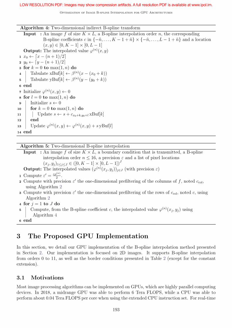
Algorithm 4: Two-dimensional indirect B-spline transform

Input : An image f of size K × L, a B-spline interpolation order n, the correspondingB-spline coefficients c in {−n, . . . , K − 1 + n} × {−n, . . . , L− 1 + n} and a location(x, y) ∈ [0, K − 1]× [0, L− 1]

Output: The interpolated value ϕ(n)(x, y)1 x0 ← ⌈x− (n+ 1)/2⌉2 y0 ← ⌈y − (n+ 1)/2⌉3 for k = 0 to max(1, n) do4 Tabulate xBuf[k]← β(n)(x− (x0 + k))

5 Tabulate yBuf[k]← β(n)(y − (y0 + k))

6 end

7 Initialize ϕ(n)(x, y)← 08 for l = 0 to max(1, n) do9 Initialize s← 0

10 for k = 0 to max(1, n) do11 Update s← s+ cx0+k,y0+l xBuf[k]12 end

13 Update ϕ(n)(x, y)← ϕ(n)(x, y) + s yBuf[l]

14 end

Algorithm 5: Two-dimensional B-spline interpolation

Input : An image f of size K × L, a boundary condition that is transmitted, a B-splineinterpolation order n ≤ 16, a precision ε and a list of pixel locations(xj, yj)1≤j≤J ∈ ([0, K − 1]× [0, L− 1])J

Output: The interpolated values (ϕ(n)(xj, yj))j∈J (with precision ε)

1 Compute ε′ = ερ(n)

2.

2 Compute with precision ε′ the one-dimensional prefiltering of the columns of f , noted ccol,using Algorithm 2

3 Compute with precision ε′ the one-dimensional prefiltering of the rows of ccol, noted c, usingAlgorithm 2

4 for j = 1 to J do

5 Compute, from the B-spline coefficient c, the interpolated value ϕ(n)(xj, yj) usingAlgorithm 4

6 end

3 The Proposed GPU Implementation

In this section, we detail our GPU implementation of the B-spline interpolation method presentedin Section 2. Our implementation is focused on 2D images. It supports B-spline interpolationfrom orders 0 to 11, as well as the border conditions presented in Table 2 (except for the constantextension).

3.1 Motivations

Most image processing algorithms can be implemented on GPUs, which are highly parallel computingdevices. In 2018, a midrange GPU was able to perform 6 Tera FLOPS, while a CPU was able toperform about 0.04 Tera FLOPS per core when using the extended CPU instruction set. For real-time

193


computing, many image processing programs propose to run entirely on GPUs.To get optimal performance, transfers between the GPU and the CPU must be avoided and

thus the whole image processing pipeline must be implemented on GPUs. Interpolation is an im-portant image processing technique for many algorithms. GPUs have native operators for nearestneighbor interpolation and bilinear interpolation, but many algorithms benefit from a more preciseinterpolation algorithm.

Open Computing Language (OpenCL) is a programming language close to C that enables totarget GPUs, CPUs and FPGAs. Special tuning is required for best performance for a given target,but clearly one advantage of OpenCL is that a given code can run on many platforms. While in thispaper we specifically target GPUs, our code will be able to run on CPUs as well (we have not testedour code on FPGAs).

3.2 A Very Short Introduction to GPU Architectures

In order to understand some of the concerns in the following implementation, a short introduction toGPUs is required. Current GPU architectures work on a SIMT model (Single Instruction - MultipleThreads). Essentially threads are grouped together in a “warp” (also named “wavefront”) and willalways be executing the same instructions in lock-steps. GPUs run many of these groups of threadsin parallel and share their computational and memory GPU resources.

Essentially, GPU algorithms are either limited by the available computational resources or by theavailable bandwidth. GPUs run more groups of threads than what the hardware can handle in orderto maximize both resources: some groups will be sleeping, waiting typically for memory commandsto finish, while others use the compute units. To maximize computational use, there must alwaysbe some threads doing computations, while to maximize bandwidth use, there must always be somethreads requesting memory contents. For 2018 GPU architectures, at peak bandwidth (excludingcache) and peak computing, reading a float in memory can cost as much as doing 100 floating pointoperations. Some GPUs can have more than 100K simultaneous threads (though only a small portionwould actually use the computational resources at the same time).

In the case of B-spline interpolation, not many operations are required per memory access, thusthe algorithm will be mainly bandwidth limited. Advanced techniques can be used to maximizebandwidth usage. As we mentioned previously, while groups of threads are waiting on memoryoperations, which can have high latency if the data are not in cache, other groups of threads canbe executed. This enables to reduce the impact of the latency of these memory operations, but insome cases, it is better in addition to interleave computation between the data loading and the use ofthe data. In addition, for optimal bandwidth usage, the threads inside a warp/wavefront must readconsecutive elements in memory, ideally aligned to fit in as few cache lines as possible. Essentially,if one thread needs data inside a cache line, the whole line is loaded (which typically is 64B for thelowest cache, but is higher if loading from the GPU dedicated memory). Thus the cost is minimizedif all threads need the same cache lines. More details can be found in technical documents suchas [8, 2, 10].

3.3 Prefiltering Step

The prefiltering step is heavily bandwidth limited as only a few operations per loaded item are needed.Having an efficient memory access pattern is thus essential. As for each causal or anticausal pass,every image element needs to be read and written once, one could expect a good implementation tobe as fast as a simple image copy, ignoring cache effects. We consider the prefiltering computationintroduced in Section 2.2.2 as it doesn’t require to add border lines. As in [4], the renormalization by(γ(n))2 of the B-spline coefficients is moved to the indirect B-spline transform step (see Section 3.4).

194


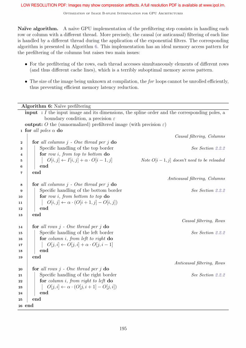
Naıve algorithm. A naıve GPU implementation of the prefiltering step consists in handling eachrow or column with a different thread. More precisely, the causal (or anticausal) filtering of each lineis handled by a different thread during the application of the exponential filters. The correspondingalgorithm is presented in Algorithm 6. This implementation has an ideal memory access pattern forthe prefiltering of the columns but raises two main issues:

• For the prefiltering of the rows, each thread accesses simultaneously elements of different rows(and thus different cache lines), which is a terribly suboptimal memory access pattern.

• The size of the image being unknown at compilation, the for loops cannot be unrolled efficiently,thus preventing efficient memory latency reduction.

Algorithm 6: Naıve prefiltering

input : I the input image and its dimensions, the spline order and the corresponding poles, aboundary condition, a precision ε

output: O the (unnormalized) prefiltered image (with precision ε)1 for all poles α do

Causal filtering, Columns

2 for all columns j - One thread per j do

3 Specific handling of the top border See Section 2.2.2

4 for row i, from top to bottom do

5 O[i, j]← I[i, j] + α ·O[i− 1, j] Note O[i− 1, j] doesn’t need to be reloaded

6 end

7 end

Anticausal filtering, Columns

8 for all columns j - One thread per j do

9 Specific handling of the bottom border See Section 2.2.2

10 for row i, from bottom to top do

11 O[i, j]← α · (O[i+ 1, j]−O[i, j])12 end

13 end

Causal filtering, Rows

14 for all rows j - One thread per j do

15 Specific handling of the left border See Section 2.2.2

16 for column i, from left to right do17 O[j, i]← O[j, i] + α ·O[j, i− 1]18 end

19 end

Anticausal filtering, Rows

20 for all rows j - One thread per j do

21 Specific handling of the right border See Section 2.2.2

22 for column i, from right to left do23 O[j, i]← α · (O[j, i+ 1]−O[j, i])24 end

25 end

26 end

195


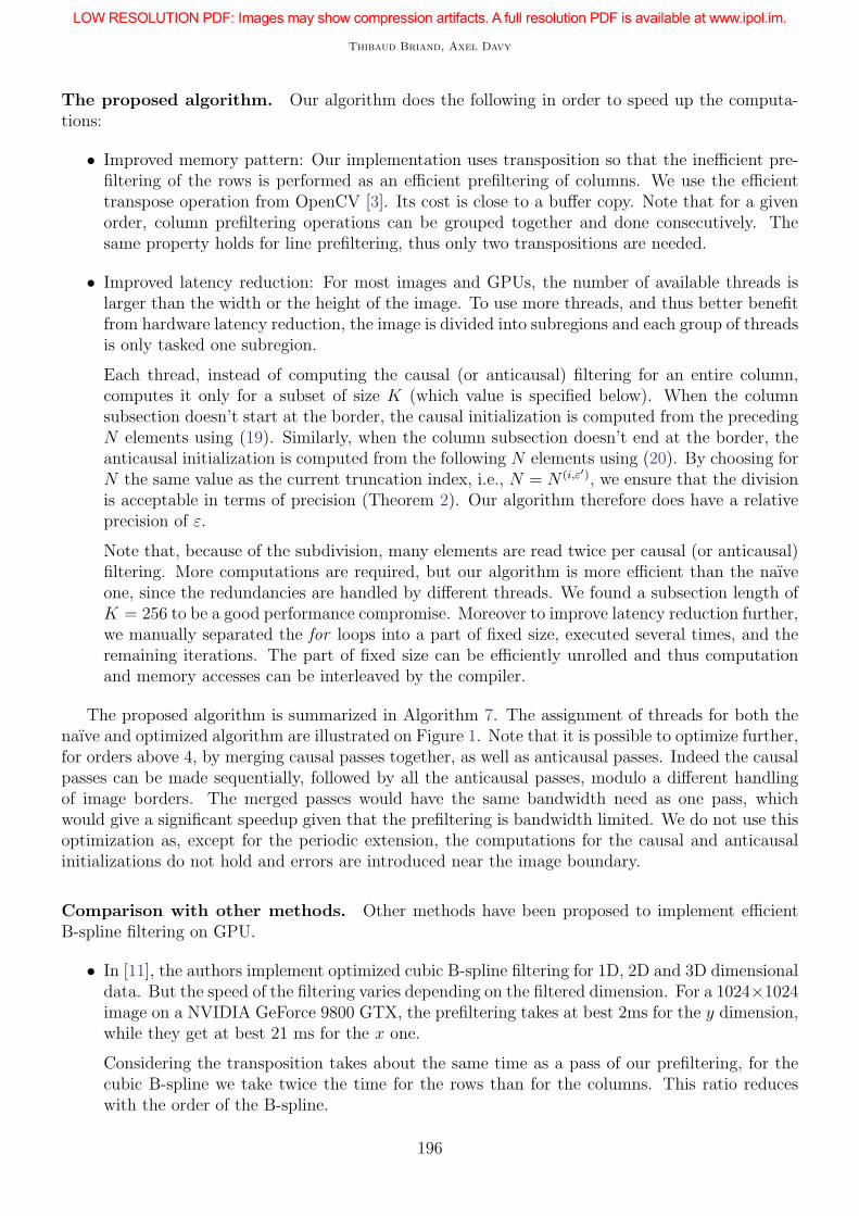
The proposed algorithm. Our algorithm does the following in order to speed up the computa-tions:

• Improved memory pattern: Our implementation uses transposition so that the inefficient pre-filtering of the rows is performed as an efficient prefiltering of columns. We use the efficienttranspose operation from OpenCV [3]. Its cost is close to a buffer copy. Note that for a givenorder, column prefiltering operations can be grouped together and done consecutively. Thesame property holds for line prefiltering, thus only two transpositions are needed.

• Improved latency reduction: For most images and GPUs, the number of available threads islarger than the width or the height of the image. To use more threads, and thus better benefitfrom hardware latency reduction, the image is divided into subregions and each group of threadsis only tasked one subregion.

Each thread, instead of computing the causal (or anticausal) filtering for an entire column,computes it only for a subset of size K (which value is specified below). When the columnsubsection doesn’t start at the border, the causal initialization is computed from the precedingN elements using (19). Similarly, when the column subsection doesn’t end at the border, theanticausal initialization is computed from the following N elements using (20). By choosing forN the same value as the current truncation index, i.e., N = N (i,ε′), we ensure that the divisionis acceptable in terms of precision (Theorem 2). Our algorithm therefore does have a relativeprecision of ε.

Note that, because of the subdivision, many elements are read twice per causal (or anticausal)filtering. More computations are required, but our algorithm is more efficient than the naıveone, since the redundancies are handled by different threads. We found a subsection length ofK = 256 to be a good performance compromise. Moreover to improve latency reduction further,we manually separated the for loops into a part of fixed size, executed several times, and theremaining iterations. The part of fixed size can be efficiently unrolled and thus computationand memory accesses can be interleaved by the compiler.

The proposed algorithm is summarized in Algorithm 7. The assignment of threads for both thenaıve and optimized algorithm are illustrated on Figure 1. Note that it is possible to optimize further,for orders above 4, by merging causal passes together, as well as anticausal passes. Indeed the causalpasses can be made sequentially, followed by all the anticausal passes, modulo a different handlingof image borders. The merged passes would have the same bandwidth need as one pass, whichwould give a significant speedup given that the prefiltering is bandwidth limited. We do not use thisoptimization as, except for the periodic extension, the computations for the causal and anticausalinitializations do not hold and errors are introduced near the image boundary.

Comparison with other methods. Other methods have been proposed to implement efficientB-spline filtering on GPU.

• In [11], the authors implement optimized cubic B-spline filtering for 1D, 2D and 3D dimensionaldata. But the speed of the filtering varies depending on the filtered dimension. For a 1024×1024image on a NVIDIA GeForce 9800 GTX, the prefiltering takes at best 2ms for the y dimension,while they get at best 21 ms for the x one.

Considering the transposition takes about the same time as a pass of our prefiltering, for thecubic B-spline we take twice the time for the rows than for the columns. This ratio reduceswith the order of the B-spline.

196


Algorithm 7: Optimized prefiltering

input : I the input image and its dimensions, the spline order and the corresponding poles, aboundary condition, a precision ε

output: O the (unnormalized) prefiltered image (with precision ε)1 First time we read O from I. Use a buffer O2 to have different source and destination for each

step.2 for all poles α do

Causal filtering, Columns

3 for all columns j - Several threads per j do

4 if Image border then

5 Specific handling of the top border See Section 2.2.2

6 else

7 Initialize first item of the treated region of O2 by accessing rows above from Ousing (19) with the corresponding truncation index

8 end

9 for row i, from top of the region to bottom of the region do

10 O2[i, j]← O[i, j] + α ·O2[i− 1, j]11 end

The above loop is written with manual partial unrolling

12 end

Anticausal filtering, Columns

13 for all columns j - Several threads per j do

14 if Image border then

15 Specific handling of the bottom border See Section 2.2.2

16 else

17 Initialize first item of the treated region of O by accessing rows below from O2

using (20) with the corresponding truncation index18 end

19 for row i, from bottom of the region to top of the region do

20 O[i, j]← α · (O[i+ 1, j]−O2[i, j])21 end

The above loop is written with manual partial unrolling

22 end

23 end

24 Transpose O25 Repeat from Line 2 to Line 2326 Transpose O

• In [5], the authors improve over [11] for the case of 2D images, but still restricting to cubicB-spline. The authors observe the precision of the prefiltering is respected by writing the passesas a 2D 15× 15 convolution, which they implement as two separable convolutions. We expecttheir approach to perform better than our approach, as the transposition is not required forgood performance, and because in one pass of 1D convolution, both a causal and an anticausalpass is implemented, thus reducing the required memory bandwidth. This approach, however,is not scalable to higher orders, or for high precision computation (double), as the size ofthe convolution increases significantly. We note, however, if using periodic or half-symmetricboundary conditions, that one could implement the convolution as a multiplication in the

197


(a) (b)

K

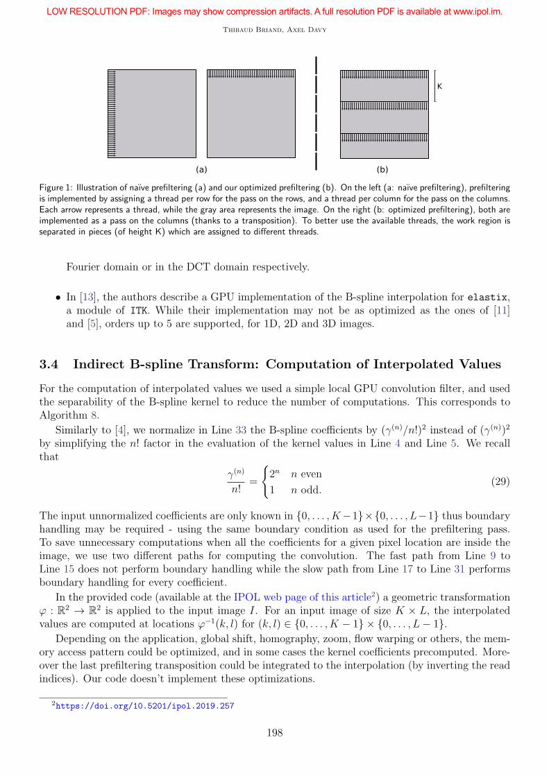
Figure 1: Illustration of naıve prefiltering (a) and our optimized prefiltering (b). On the left (a: naıve prefiltering), prefilteringis implemented by assigning a thread per row for the pass on the rows, and a thread per column for the pass on the columns.Each arrow represents a thread, while the gray area represents the image. On the right (b: optimized prefiltering), both areimplemented as a pass on the columns (thanks to a transposition). To better use the available threads, the work region isseparated in pieces (of height K) which are assigned to different threads.

Fourier domain or in the DCT domain respectively.

• In [13], the authors describe a GPU implementation of the B-spline interpolation for elastix,a module of ITK. While their implementation may not be as optimized as the ones of [11]and [5], orders up to 5 are supported, for 1D, 2D and 3D images.

3.4 Indirect B-spline Transform: Computation of Interpolated Values

For the computation of interpolated values we used a simple local GPU convolution filter, and usedthe separability of the B-spline kernel to reduce the number of computations. This corresponds toAlgorithm 8.

Similarly to [4], we normalize in Line 33 the B-spline coefficients by (γ(n)/n!)2 instead of (γ(n))2

by simplifying the n! factor in the evaluation of the kernel values in Line 4 and Line 5. We recallthat

γ(n)

n!=

{

2n n even

1 n odd.(29)

The input unnormalized coefficients are only known in {0, . . . , K−1}×{0, . . . , L−1} thus boundaryhandling may be required - using the same boundary condition as used for the prefiltering pass.To save unnecessary computations when all the coefficients for a given pixel location are inside theimage, we use two different paths for computing the convolution. The fast path from Line 9 toLine 15 does not perform boundary handling while the slow path from Line 17 to Line 31 performsboundary handling for every coefficient.

In the provided code (available at the IPOL web page of this article2) a geometric transformationϕ : R2 → R

2 is applied to the input image I. For an input image of size K × L, the interpolatedvalues are computed at locations ϕ−1(k, l) for (k, l) ∈ {0, . . . , K − 1} × {0, . . . , L− 1}.

Depending on the application, global shift, homography, zoom, flow warping or others, the mem-ory access pattern could be optimized, and in some cases the kernel coefficients precomputed. More-over the last prefiltering transposition could be integrated to the interpolation (by inverting the readindices). Our code doesn’t implement these optimizations.


198


Algorithm 8: Optimized two-dimensional indirect B-spline transform

Input : An image f of size K × L, a B-spline interpolation order n, the correspondingunnormalized B-spline coefficients c in {0, . . . , K − 1} × {0, . . . , L− 1}, a boundarycondition and a location (x, y) ∈ R

2

Output: The interpolated value ϕ(n)(x, y)1 x0 ← ⌈x− (n+ 1)/2⌉2 y0 ← ⌈y − (n+ 1)/2⌉3 for k = 0 to max(1, n) do4 Tabulate xBuf[k]← n! β(n)(x− (x0 + k))

5 Tabulate yBuf[k]← n! β(n)(y − (y0 + k))

6 end

7 Initialize ϕ(n)(x, y)← 08 if (x0, y0) ∈ {0, . . . , K − 1−max(1, n)} × {0, . . . , L− 1−max(1, n)} then

Fast path without boundary handling

9 for l = 0 to max(1, n) do10 Initialize s← 011 for k = 0 to max(1, n) do12 Update s← s+ cx0+k,y0+l xBuf[k]13 end


15 end

16 else

Slow path with boundary handling

17 for l = 0 to max(1, n) do18 Initialize s← 019 Set l′ = y0 + l20 if l′ /∈ {0, . . . , L− 1} then21 Update l′ with its equivalent position in {0, . . . , L− 1} using the boundary

condition22 end

23 for k = 0 to max(1, n) do24 Set k′ = x0 + k25 if k′ /∈ {0, . . . , K − 1} then26 Update k′ with its equivalent position in {0, . . . , K − 1} using the boundary

condition27 end

28 Update s← s+ ck′,l′ xBuf[k]

29 end


31 end

32 end

33 Update ϕ(n)(x, y)← ϕ(n)(x, y)(

γ(n)

n!

)2

using (29) Renormalization

199


3.5 Online Demo

This article is accompanied by an online demo3 where the user can upload an image and apply to ita shift using B-spline interpolation with a selection of boundary conditions.

4 Experiments

All results (precision and running time) of this section are computed on a reference 4608×3456 image(shown on Figure 2), a shift of (0.5, 0.5) and with half-symmetric border condition. The referenceimage contains flat areas, regions with different levels of textures and sharp edges.

Figure 2: Reference image of size 4608×3456 used for the experiments of Section 4. It contains flat areas, regions withdifferent levels of textures and sharp edges. In all the experiments this image is shifted by (0.5, 0.5) with half-symmetricborder condition.

4.1 Float Versus Double Precision

In this section we would like to answer the following question: Should float precision or doubleprecision be used for B-spline interpolation?

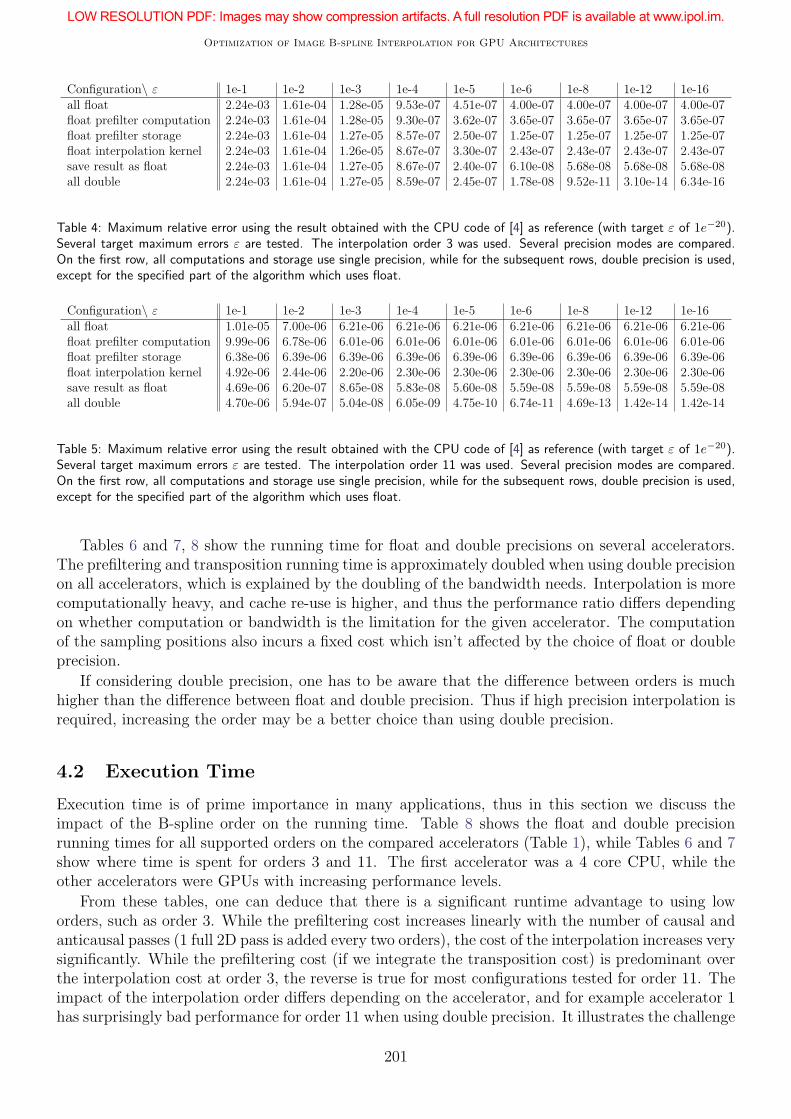
Tables 4 and 5 show experimentally that up to a target precision ε of 1e−6, floats are enough toguarantee the target precision, as the measured maximum relative error is below the target for thetested image. However, for smaller ε, all storage and computations must use double precision. Thetable shows that if any computation or storage uses float precision, the gain of using double precisionfor the other computations and storage is lost. The limit of double precision is reached around ε of1e−13.


200


Configuration\ ε 1e-1 1e-2 1e-3 1e-4 1e-5 1e-6 1e-8 1e-12 1e-16all float 2.24e-03 1.61e-04 1.28e-05 9.53e-07 4.51e-07 4.00e-07 4.00e-07 4.00e-07 4.00e-07float prefilter computation 2.24e-03 1.61e-04 1.28e-05 9.30e-07 3.62e-07 3.65e-07 3.65e-07 3.65e-07 3.65e-07float prefilter storage 2.24e-03 1.61e-04 1.27e-05 8.57e-07 2.50e-07 1.25e-07 1.25e-07 1.25e-07 1.25e-07float interpolation kernel 2.24e-03 1.61e-04 1.26e-05 8.67e-07 3.30e-07 2.43e-07 2.43e-07 2.43e-07 2.43e-07save result as float 2.24e-03 1.61e-04 1.27e-05 8.67e-07 2.40e-07 6.10e-08 5.68e-08 5.68e-08 5.68e-08all double 2.24e-03 1.61e-04 1.27e-05 8.59e-07 2.45e-07 1.78e-08 9.52e-11 3.10e-14 6.34e-16

Table 4: Maximum relative error using the result obtained with the CPU code of [4] as reference (with target ε of 1e−20).Several target maximum errors ε are tested. The interpolation order 3 was used. Several precision modes are compared.On the first row, all computations and storage use single precision, while for the subsequent rows, double precision is used,except for the specified part of the algorithm which uses float.

Configuration\ ε 1e-1 1e-2 1e-3 1e-4 1e-5 1e-6 1e-8 1e-12 1e-16all float 1.01e-05 7.00e-06 6.21e-06 6.21e-06 6.21e-06 6.21e-06 6.21e-06 6.21e-06 6.21e-06float prefilter computation 9.99e-06 6.78e-06 6.01e-06 6.01e-06 6.01e-06 6.01e-06 6.01e-06 6.01e-06 6.01e-06float prefilter storage 6.38e-06 6.39e-06 6.39e-06 6.39e-06 6.39e-06 6.39e-06 6.39e-06 6.39e-06 6.39e-06float interpolation kernel 4.92e-06 2.44e-06 2.20e-06 2.30e-06 2.30e-06 2.30e-06 2.30e-06 2.30e-06 2.30e-06save result as float 4.69e-06 6.20e-07 8.65e-08 5.83e-08 5.60e-08 5.59e-08 5.59e-08 5.59e-08 5.59e-08all double 4.70e-06 5.94e-07 5.04e-08 6.05e-09 4.75e-10 6.74e-11 4.69e-13 1.42e-14 1.42e-14

Table 5: Maximum relative error using the result obtained with the CPU code of [4] as reference (with target ε of 1e−20).Several target maximum errors ε are tested. The interpolation order 11 was used. Several precision modes are compared.On the first row, all computations and storage use single precision, while for the subsequent rows, double precision is used,except for the specified part of the algorithm which uses float.

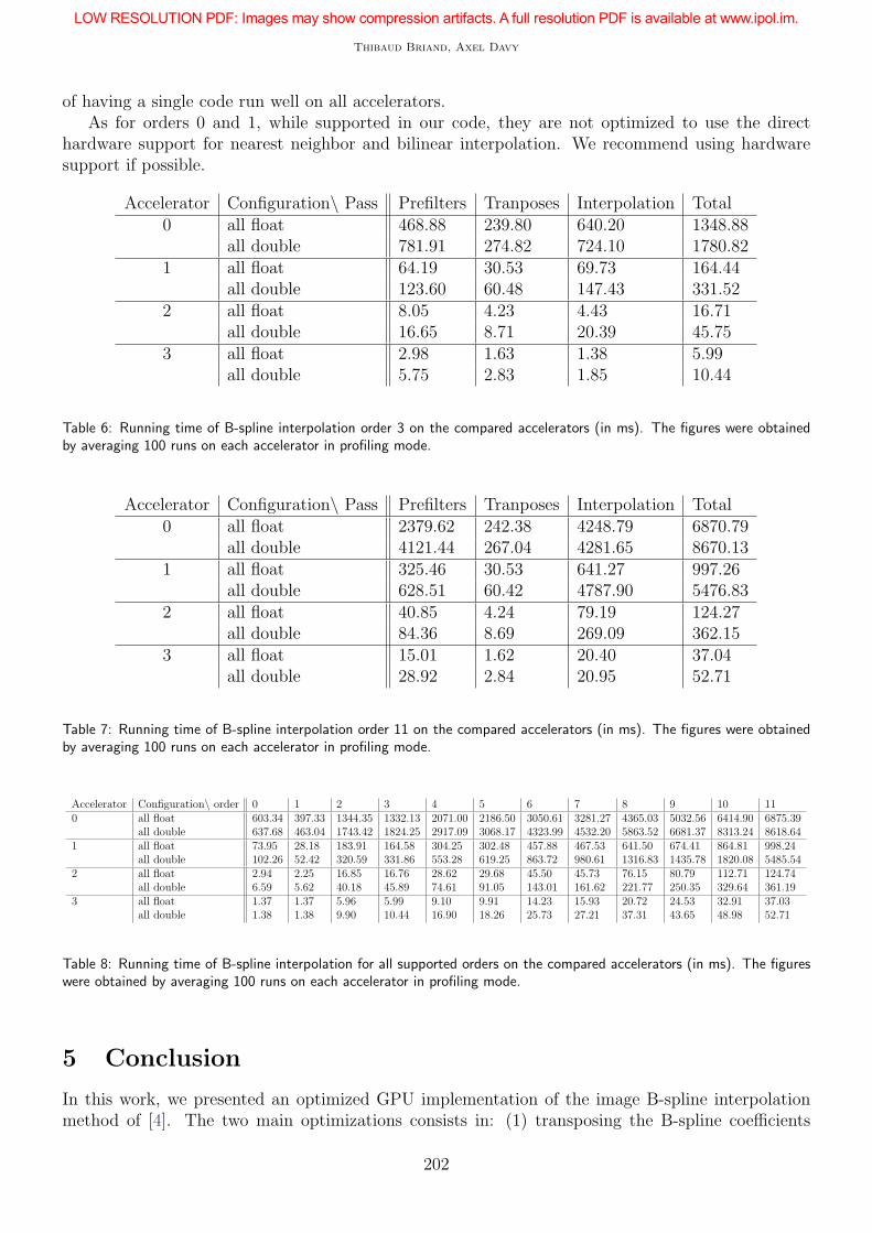
Tables 6 and 7, 8 show the running time for float and double precisions on several accelerators.The prefiltering and transposition running time is approximately doubled when using double precisionon all accelerators, which is explained by the doubling of the bandwidth needs. Interpolation is morecomputationally heavy, and cache re-use is higher, and thus the performance ratio differs dependingon whether computation or bandwidth is the limitation for the given accelerator. The computationof the sampling positions also incurs a fixed cost which isn’t affected by the choice of float or doubleprecision.

If considering double precision, one has to be aware that the difference between orders is muchhigher than the difference between float and double precision. Thus if high precision interpolation isrequired, increasing the order may be a better choice than using double precision.

4.2 Execution Time

Execution time is of prime importance in many applications, thus in this section we discuss theimpact of the B-spline order on the running time. Table 8 shows the float and double precisionrunning times for all supported orders on the compared accelerators (Table 1), while Tables 6 and 7show where time is spent for orders 3 and 11. The first accelerator was a 4 core CPU, while theother accelerators were GPUs with increasing performance levels.

From these tables, one can deduce that there is a significant runtime advantage to using loworders, such as order 3. While the prefiltering cost increases linearly with the number of causal andanticausal passes (1 full 2D pass is added every two orders), the cost of the interpolation increases verysignificantly. While the prefiltering cost (if we integrate the transposition cost) is predominant overthe interpolation cost at order 3, the reverse is true for most configurations tested for order 11. Theimpact of the interpolation order differs depending on the accelerator, and for example accelerator 1has surprisingly bad performance for order 11 when using double precision. It illustrates the challenge

201


of having a single code run well on all accelerators.As for orders 0 and 1, while supported in our code, they are not optimized to use the direct

hardware support for nearest neighbor and bilinear interpolation. We recommend using hardwaresupport if possible.

Accelerator Configuration\ Pass Prefilters Tranposes Interpolation Total0 all float 468.88 239.80 640.20 1348.88

all double 781.91 274.82 724.10 1780.821 all float 64.19 30.53 69.73 164.44



all double 5.75 2.83 1.85 10.44

Table 6: Running time of B-spline interpolation order 3 on the compared accelerators (in ms). The figures were obtainedby averaging 100 runs on each accelerator in profiling mode.

Accelerator Configuration\ Pass Prefilters Tranposes Interpolation Total0 all float 2379.62 242.38 4248.79 6870.79




all double 28.92 2.84 20.95 52.71

Table 7: Running time of B-spline interpolation order 11 on the compared accelerators (in ms). The figures were obtainedby averaging 100 runs on each accelerator in profiling mode.

Accelerator Configuration\ order 0 1 2 3 4 5 6 7 8 9 10 110 all float 603.34 397.33 1344.35 1332.13 2071.00 2186.50 3050.61 3281.27 4365.03 5032.56 6414.90 6875.39

all double 637.68 463.04 1743.42 1824.25 2917.09 3068.17 4323.99 4532.20 5863.52 6681.37 8313.24 8618.641 all float 73.95 28.18 183.91 164.58 304.25 302.48 457.88 467.53 641.50 674.41 864.81 998.24



all double 1.38 1.38 9.90 10.44 16.90 18.26 25.73 27.21 37.31 43.65 48.98 52.71

Table 8: Running time of B-spline interpolation for all supported orders on the compared accelerators (in ms). The figureswere obtained by averaging 100 runs on each accelerator in profiling mode.

5 Conclusion

In this work, we presented an optimized GPU implementation of the image B-spline interpolationmethod of [4]. The two main optimizations consists in: (1) transposing the B-spline coefficients

202


before the prefiltering of the rows, and (2) dividing columns into subregions in order to use morethreads.

In an experimental section we compared the use of float or double precision for the different stepsand found that using double precision increased accuracy only if all the steps and storage use doubleprecision. Float precision met the maximum error target for targets up to 1e-5, and lower errorsrequired double precision. We compared the speed for both precisions and for orders ranging from 0to 11 on several accelerators (a 4 core CPU, and 3 GPUs). Using GPUs enabled significantly betterperformance. For example on two of the compared GPUs, an interpolation of order 11 for the 16Mpxreference image took less than one second for both precision modes. Using double precision wasgenerally about twice slower for the compared GPUs than using float precision, due to the doublingof the bandwidth needs.

While our implementation contains generic optimizations, applications with particular needs couldget further speed boosts by implementing specific optimizations, several of which we mentioned inthis article.

Acknowledgements

The authors would like to thank Prof. Jean-Michel Morel for his support, suggestions, and manyfruitful discussions.

Work partly financed by Office of Naval research grant N00014-17-1-2552, DGA Astrid project“filmer la Terre” no ANR-17-ASTR-0013-01, MENRT and Fondation Mathematique Jacques Hadamard.

Image Credits

Provided by the authors

References

[1] A. Aldroubi, M. Unser, and M. Eden, Cardinal Spline Filters: Stability and Convergenceto the Ideal Sinc Interpolator, Signal Processing, 28 (1992), pp. 127–138. http://dx.doi.org/10.1016/0165-1684(92)90030-Z.

[2] AMD, AMD APP SDK OpenCLTM Optimization Guide, (2015).

[3] G. Bradski, The OpenCV Library, Dr. Dobb’s Journal of Software Tools, (2000).

[4] T. Briand and P. Monasse, Theory and Practice of Image B-spline Interpolation, ImageProcessing On Line, 8 (2018), pp. 99–141. https://doi.org/10.5201/ipol.2018.221.

[5] F. Champagnat and Y. Le Sant, Efficient cubic B-spline image interpolation on a GPU,Journal of Graphics Tools, 16 (2012), pp. 218–232.

[6] P. Getreuer, Linear Methods for Image Interpolation, Image Processing On Line, 1 (2011).http://dx.doi.org/10.5201/ipol.2011.g_lmii.

[7] H. Hou and H. Andrews, Cubic Splines for Image Interpolation and Digital Filtering, IEEETransactions on Acoustics, Speech and Signal Processing, 26 (1978), pp. 508–517. http://dx.doi.org/10.1109/TASSP.1978.1163154.

203


[8] S. Junkins, The compute architecture of Intel R© processor graphics gen9, (2015).

[9] M. Liou, Spline fit made easy, IEEE Transactions on Computers, 100 (1976), pp. 522–527.http://dx.doi.org/10.1109/TC.1976.1674640.

[10] NVIDIA, NVIDIA OpenCL Best Practices Guide, (2009).

[11] D. Ruijters and P. Thevenaz, GPU prefilter for accurate cubic B-spline interpolation, TheComputer Journal, 55 (2012), pp. 15–20.

[12] I.J. Schoenberg, Contributions to the Problem of Approximation of Equidistant Data byAnalytic Functions, in I.J Schoenberg Selected Papers, Springer, 1988, pp. 3–57. http:

//dx.doi.org/10.1007/978-1-4899-0433-1_1.

[13] D. Shamonin and M. Staring, An OpenCL implementation of the Gaussian pyramid andthe resampler, (2012).

[14] P. Thevenaz, T. Blu, and M. Unser, Interpolation Revisited [Medical Images Application],IEEE Transactions on Medical Imaging, 19 (2000), pp. 739–758. http://dx.doi.org/10.1109/42.875199.

[15] M. Unser, Splines: A Perfect Fit for Signal and Image Processing, IEEE Signal ProcessingMagazine, 16 (1999), pp. 22–38. http://dx.doi.org/10.1109/79.799930.

[16] M. Unser, A. Aldroubi, and M. Eden, Fast B-spline Transforms for Continuous ImageRepresentation and Interpolation, IEEE Transactions on Pattern Analysis and Machine Intelli-gence, 13 (1991), pp. 277–285. http://dx.doi.org/10.1109/34.75515.

[17] , B-spline Signal Processing. I. Theory, IEEE Transactions on Signal Processing, 41 (1993),pp. 821–833. http://dx.doi.org/10.1109/78.193220.

[18] , B-spline Signal Processing. II. Efficiency Design and Applications, IEEE Transactions onSignal Processing, 41 (1993), pp. 834–848. http://dx.doi.org/10.1109/78.193221.

204

optimization of image b-spline interpolation for gpu

Documents