a survey on parametric spline function approximation
TRANSCRIPT
Applied Mathematics and Computation 171 (2005) 983–1003
www.elsevier.com/locate/amc
A survey on parametric splinefunction approximation
Arshad Khan a, Islam Khan b,*, Tariq Aziz b
a Department of Mathematics, A.M.U., Aligarh 202 002, Indiab Department of Applied Mathematics, Faculty of Engineering and Technology, A.M.U.,
Aligarh 202 002, India
Abstract
This survey paper contains a large amount of material and indeed can serve as an
introduction to some of the ideas and methods for the solution of ordinary and partial
differential equations starting from Schoenberg�s work [Quart. Appl. Math. 4 (1946)
345–369]. The parametric spline function which depends on a parameter x > 0, is
reduces to the ordinary cubic or quintic spline for x = 0. A note on parametric spline
function approximation, which is special case of this work has been published in [Comp.
Math. Applics. 29 (1995) 67–73]. This article deals with the odd-order parametric spline
relations.
� 2005 Elsevier Inc. All rights reserved.
Keywords: Cubic spline; Parametric cubic spline; Quintic spline; Parametric quintic spline;
Numerov�s method; Spline relations; Diagonally dominant
0096-3003/$ - see front matter � 2005 Elsevier Inc. All rights reserved.
doi:10.1016/j.amc.2005.01.112
* Corresponding author.
E-mail addresses: [email protected] (A. Khan), [email protected] (I. Khan).
984 A. Khan et al. / Appl. Math. Comput. 171 (2005) 983–1003
1. Introduction
This paper is concerned with the development of non-polynomial spline
function approximation methods to obtain numerical solution of ordinary
and partial differential equations. The use of spline functions dates back at
least to the beginning of previous century. Piecewise linear functions had beenused in connection with the Peano�s existence proof for the solution to the
initial value problems of the ordinary differential equations, although these
functions were not called splines. Splines were first identified in the work of
Schoenberg, Sard and others. Usually a spline is a piecewise polynomial func-
tion defined in a region D, such that there exists a decomposition of D into sub-
regions in each of which the function is a polynomial of some degree m. Also
the function, as a rule, is continuous in D, together with its derivatives of order
upto (m � k) [32]. In other words spline function is a piecewise polynomial sat-isfying certain conditions of continuity of the function and its derivatives. The
applications of spline as approximating, interpolating and curve fitting func-
tions have been very successful [1], [18], [37],[34]). It is also interesting to note
that the cubic spline is a close mathematical approximation to the draughts-
man�s spline, which is a widely used manual curve-drawing tool. It has been
shown by Schoenberg [46] that a curve drawn by a mechanical spline to a first
order of approximation is a cubic spline function. Further, the solution of a
variety of problems of �best approximation� are the spline function approxima-tions. Later on, spline functions recieved a considerable amount of attention in
both theoretical and practical studies.
A number of authors have attempted polynomial and non-polynomial
spline approximation methods for the solution of differential equations; De
Boor [12–14], Ahlberg et al. [1], Loscalzo and Talbot [30,31], Bickley [7], Fyfe
[16,17], Albasiny and Hoskins [2], Sakai [43–45], Russell and Shampine [42],
Micula [33,34], Rubin and Khosla [41], Rubin and Graves [40], Daniel and
Swartz [11], Archer [3], Patricio [35,36], Tewarson [51,52], Usmani et al. [53–55], Jain and Aziz [22–24], Surla et al. [47–50], Iyengar and Jain [21], Chawla
and Subramanian [8–10], Irodotou- Ellina and Houstis [20], Rashidinia [39],
Fairweather and Meade [15] and others. Spline functions of maximum smooth-
ness were first considered in the numerical solution of initial value problems in
ordinary differential equations by Loscalzo and Talbot [30,31] and many inter-
esting connections with standard numerical integration techniques have been
established. For example, the trapezoidal rule and the Milne–Simpson predic-
tor–corrector method fall out as special cases of such spline approximations.The main reason why the above mentioned applications of spline functions
to the numerical integration of ordinary differential equations leads to unstable
methods is because the resulting numerical approximations are, in a certain
sense too smooth [56]). Loscalzo and Schoenberg [29] have shown that the
use of Hermite–Splines of lower order smoothness avoids completely the prob-
A. Khan et al. / Appl. Math. Comput. 171 (2005) 983–1003 985
lem of instability. The spline functions have been used by a number of authors
to solve both initial and boundary value problems of ordinary and partial dif-
ferential equations. The use of cubic splines for the solution of linear two point
boundary value problems was first suggested by Bickley [7]. His main idea was
to use the �condition of continuity� as a discretization equation for the linear
two point boundary value problems. Later, Fyfe [16] discussed the applicationof deferred corrections to the method suggested by Bickley by considering
again the case of (regular) linear boundary-value problems.
However, it is well known since then that the cubic spline method of Bickley
gives only O(h2) convergent approximations. But cubic spline itself is a fourth-
order process [37]. It was therefore natural to look for an alternative method
which would give fourth order approximations using cubic splines. We also
find that the applications of the spline functions to the solution of convec-
tion–diffusion problems has not been very encouraging. To be able to dealeffectively with such problems we introduce �spline functions� containing a
parameter x. These are �non-polynomial splines� defined through the solution
of a differential equation in each subinterval. The arbitrary constants being
chosen to satisfy certain smoothness conditions at the joints. These �splines� be-long to the class C2 and reduce into polynomial splines as parameter x ! 0.
The exact form of the spline depends upon the manner in which the parameter
is introduced. We have studied parametric spline functions: spline under com-
pression, spline under tension and adaptive spline. A number of spline relationshave been obtained for subsequent use.
The singular perturbation mathematical model plays an important role in
modelling fluid processes arising in applied mechanics. We have either the stiff
system of initial boundary value problems or the convection-diffusion problems.
It has been realized that when conventional methods are applied to obtain
numerical solution, the step size must be limited to extremely small values.
Any attempt to use a larger step size results in the calculations becoming unsta-
ble and producing completely erroneous results. In recent years, considerableattention has been devoted to the formulation and implementation of, in es-
sence, modified spline methods for the solution of certain classes of elliptic
boundary value problems on rectangles, see for example Houstis et al. [19]. It
is interesting to note that this approach was adopted by Irodotou-Ellina and
Houstis [20], in their quintic spline collocation methods for general linear fourth
order two point boundary value problems. Another quintic spline method
requiring a uniformmesh for a non-linear fourth order boundary value problem
is due to Chawla and Subramanian [10]. This method is based on Bickley�s idea[7] of using the continuity condition to construct a cubic spline approximation,
but here it is used only after some other method (e.g., a finite difference method)
has been used to obtain accurate nodal values. Fairweather andMeade [15] pro-
vide a comprehensive survey of both orthogonal and modified spline collocation
methods for solving ordinary and partial differential equations.
986 A. Khan et al. / Appl. Math. Comput. 171 (2005) 983–1003
2. Spline functions
We consider a mesh D with nodal points xj on [a,b] such that
D:a = x0 < x1 < x2 < � � � < xN�1 < xN = b where hj = xj � xj�1, for j = 1(1)N.
Assume we are given the values fujgNj¼0 of a function u(x), with [a,b] as its do-
main of definition. A spline function of degree m with nodes at the points xj,j = 0,1,2, . . . ,N is a function SD(x) with the following properties:
(a) In each sub interval [xj,xj+1], j = 0,1, . . . ,N � 1, SD(x) is a polynomial of
degree m.
(b) SD(x) and its first (m � 1) derivatives are continuous on [a,b]. If the func-
tion SD(x) has only (m � k) continuous derivatives, then k is defined as
the deficiency of the polynomial spline and is usually denoted by SD
(m,k), see [41]. The cubic spline is a piecewise cubic polynomial of defi-ciency one, e.g. SD (3,1). The cubic spline procedure can be described
as follows.
Consider a function u(x) such that at the mesh points xi,u(xi) = ui. A cubic
polynomial is specified on the interval [xj�1,xj]. The four constants are related
to the function values uj�1, uj as well as certain spline derivatives mj�1, mj or
Mj�1, Mj. The quantities mj, Mj are the spline derivative approximations to
the function derivatives u 0(xj), u00(xj) respectively. Similarly considered on the
interval [xj,xj+1]. The continuity of the derivatives is then specified at xj. The
procedure results in equations for mj, Mj, j = 1,2, . . . ,N � 1. Boundary condi-
tions are required at j = 0 and j = N. The system is closed by the governing dif-
ferential equation for u(xj), where the derivatives are replaced by their spline
approximations mj, Mj.
In this paper, we first give some definitions and basic results on cubic and
quintic spline functions. The definition of the cubic and quintic spline functions
is extended to piecewise non-polynomial functions depending on a parameterx. For x! 0 these (non-polynomial) functions reduce to ordinary cubic or
quintic splines. Depending on the choice of parameter, the spline function is
known as cubic spline in compression, cubic spline in tension or adaptive cubic
spline. Similarly three of the splines derived from quintic spline are termed
�parametric quintic spline-I�, �parametric quintic spline-II� and �adaptive quinticspline�.
3. Cubic spline functions
Definition
A cubic spline function SD(x), of class C2 [a,b], interpolating to a function
u(x) defined on [a,b] is such that
A. Khan et al. / Appl. Math. Comput. 171 (2005) 983–1003 987
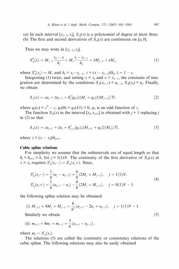
(a) In each interval [xj�1,xj], SD(x) is a polynomial of degree at most three.
(b) The first and second derivatives of SD(x) are continuous on [a,b].
Thus we may write in [xj�1,xj],
S00DðxÞ ¼ Mj�1
xj � xhj
þMjx� xj�1
hj¼ �zMj�1 þ zMj; ð1Þ
where S00DðxjÞ ¼ Mj and hj = xj�xj�1, z = (x � xj�1)/hj, �z ¼ 1� z.
Integrating (1) twice, and setting x = xj and x = xj�1, the constants of inte-gration are determined by the conditions SD(xj�1) = uj�1, SD(xj) = uj. Finally,
we obtain
SDðxÞ ¼ zuj þ �zuj�1 þ h2j ½q3ðzÞMj þ q3ð�zÞMj�1�=3!; ð2Þ
where q3(z) = z3 � z, q3(0) = q3(±1) = 0, q3 is an odd function of z.
The function SD(x) in the interval [xj,xj+1] is obtained with j + 1 replacing j
in (2) so that
SDðxÞ ¼ zujþ1 þ �zuj þ h2jþ1½q3ðzÞMjþ1 þ q3ð�zÞMj�=3!; ð3Þ
where z = (x � xj)/hj+1.
Cubic spline relations
For simplicity we assume that the subintervals are of equal length so that
hj = hj+1 = h, for j = 1(1)N. The continuity of the first derivative of SD(x) at
x = xj requires S0Dðxj�Þ ¼ S0
DðxjþÞ. Since,
S0Dðxj�Þ ¼ 1
hðuj � uj�1Þ þ
h6ð2Mj þMj�1Þ; j ¼ 1ð1ÞN ;
S0DðxjþÞ ¼ 1
hðujþ1 � ujÞ �
h6ð2Mj þMjþ1Þ; j ¼ 0ð1ÞN � 1
ð4Þ
the following spline relation may be obtained:
ðiÞ Mjþ1 þ 4Mj þMj�1 ¼6
h2ðujþ1 � 2uj þ uj�1Þ; j ¼ 1ð1ÞN � 1:
Similarly we obtain
ðiiÞ mjþ1 þ 4mj þ mj�1 ¼3
hðujþ1 � uj�1Þ;
ð5Þ
where mj ¼ S0DðxjÞ.
The relations (5) are called the continuity or consistency relations of thecubic spline. The following relations may also be easily obtained
988 A. Khan et al. / Appl. Math. Comput. 171 (2005) 983–1003
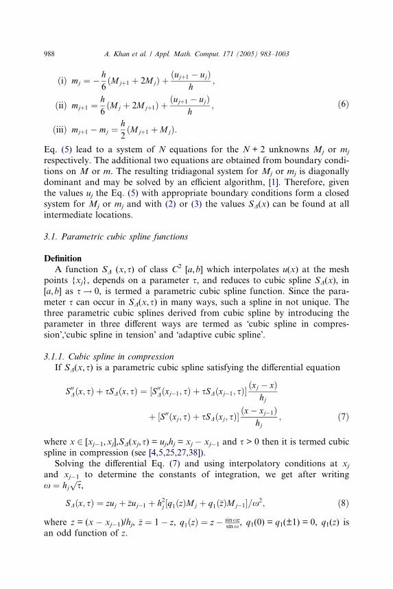
ðiÞ mj ¼ � h6ðMjþ1 þ 2MjÞ þ
ðujþ1 � ujÞh
;
ðiiÞ mjþ1 ¼h6ðMj þ 2Mjþ1Þ þ
ðujþ1 � ujÞh
;
ðiiiÞ mjþ1 � mj ¼h2ðMjþ1 þMjÞ:
ð6Þ
Eq. (5) lead to a system of N equations for the N + 2 unknowns Mj or mj
respectively. The additional two equations are obtained from boundary condi-
tions on M or m. The resulting tridiagonal system for Mj or mj is diagonally
dominant and may be solved by an efficient algorithm, [1]. Therefore, giventhe values uj the Eq. (5) with appropriate boundary conditions form a closed
system for Mj or mj and with (2) or (3) the values SD(x) can be found at all
intermediate locations.
3.1. Parametric cubic spline functions
Definition
A function SD (x,s) of class C2 [a,b] which interpolates u(x) at the meshpoints {xj}, depends on a parameter s, and reduces to cubic spline SD(x), in
[a,b] as s ! 0, is termed a parametric cubic spline function. Since the para-
meter s can occur in SD(x,s) in many ways, such a spline in not unique. The
three parametric cubic splines derived from cubic spline by introducing the
parameter in three different ways are termed as �cubic spline in compres-
sion�,�cubic spline in tension� and �adaptive cubic spline�.
3.1.1. Cubic spline in compression
If SD(x,s) is a parametric cubic spline satisfying the differential equation
S00Dðx; sÞ þ sSDðx; sÞ ¼ ½S00
Dðxj�1; sÞ þ sSDðxj�1; sÞ�ðxj � xÞ
hj
þ ½S00ðxj; sÞ þ sSDðxj; sÞ�ðx� xj�1Þ
hj; ð7Þ
where x 2 [xj�1,xj],SD(xj,s) = uj,hj = xj � xj�1 and s > 0 then it is termed cubic
spline in compression (see [4,5,25,27,38]).
Solving the differential Eq. (7) and using interpolatory conditions at xjand xj�1 to determine the constants of integration, we get after writing
x ¼ hjffiffiffis
p,
SDðx; sÞ ¼ zuj þ �zuj�1 þ h2j ½q1ðzÞMj þ q1ð�zÞMj�1�=x2; ð8Þ
where z = (x � xj�1)/hj, �z ¼ 1� z, q1ðzÞ ¼ z� sinxzsinx , q1(0) = q1(±1) = 0, q1(z) is
an odd function of z.
A. Khan et al. / Appl. Math. Comput. 171 (2005) 983–1003 989
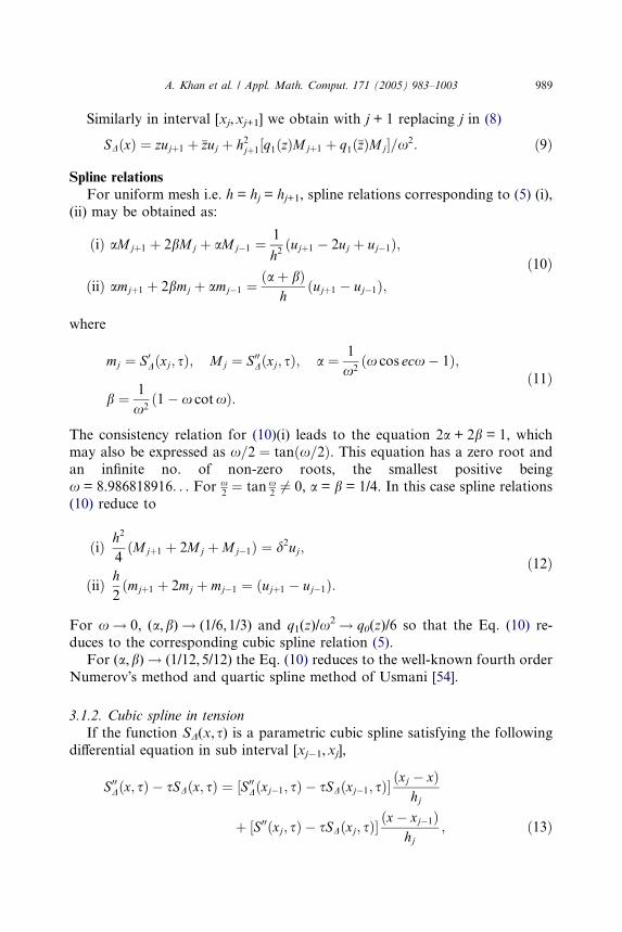
Similarly in interval [xj,xj+1] we obtain with j + 1 replacing j in (8)
SDðxÞ ¼ zujþ1 þ �zuj þ h2jþ1½q1ðzÞMjþ1 þ q1ð�zÞMj�=x2: ð9Þ
Spline relations
For uniform mesh i.e. h = hj = hj+1, spline relations corresponding to (5) (i),
(ii) may be obtained as:
ðiÞ aMjþ1 þ 2bMj þ aMj�1 ¼1
h2ðujþ1 � 2uj þ uj�1Þ;
ðiiÞ amjþ1 þ 2bmj þ amj�1 ¼ðaþ bÞ
hðujþ1 � uj�1Þ;
ð10Þ
where
mj ¼ S0Dðxj; sÞ; Mj ¼ S00
Dðxj; sÞ; a ¼ 1
x2ðx cos ecx� 1Þ;
b ¼ 1
x2ð1� x cotxÞ:
ð11Þ
The consistency relation for (10)(i) leads to the equation 2a + 2b = 1, whichmay also be expressed as x=2 ¼ tanðx=2Þ. This equation has a zero root and
an infinite no. of non-zero roots, the smallest positive being
x = 8.986818916. . . For x2¼ tan x
26¼ 0, a = b = 1/4. In this case spline relations
(10) reduce to
ðiÞ h2
4ðMjþ1 þ 2Mj þMj�1Þ ¼ d2uj;
ðiiÞ h2ðmjþ1 þ 2mj þ mj�1 ¼ ðujþ1 � uj�1Þ:
ð12Þ
For x ! 0, (a,b) ! (1/6,1/3) and q1(z)/x2 ! q0(z)/6 so that the Eq. (10) re-
duces to the corresponding cubic spline relation (5).
For (a,b) ! (1/12,5/12) the Eq. (10) reduces to the well-known fourth order
Numerov�s method and quartic spline method of Usmani [54].
3.1.2. Cubic spline in tension
If the function SD(x,s) is a parametric cubic spline satisfying the following
differential equation in sub interval [xj�1,xj],
S00Dðx; sÞ � sSDðx; sÞ ¼ ½S00
Dðxj�1; sÞ � sSDðxj�1; sÞ�ðxj � xÞ
hj
þ ½S00ðxj; sÞ � sSDðxj; sÞ�ðx� xj�1Þ
hj; ð13Þ
990 A. Khan et al. / Appl. Math. Comput. 171 (2005) 983–1003
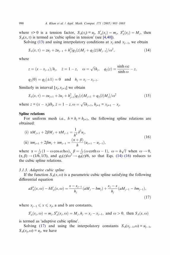
where s> 0 is a tension factor, SD(xj) = uj, S0DðxjÞ ¼ mj, S00
DðxjÞ ¼ Mj, then
SD(x,s) is termed as �cubic spline in tension� (see [4,40]).
Solving (13) and using interpolatory conditions at xj and xj�1, we obtain
SDðx; sÞ ¼ zuj þ �zuj�1 þ h2j ½q2ðzÞMj þ q2ð�zÞMj�1�=x2; ð14Þ
where
z ¼ ðx� xj�1Þ=hj; �z ¼ 1� z; x ¼ffiffiffis
phj; q2ðzÞ ¼
sinhxzsinhx
� z;
q2ð0Þ ¼ q2ð�1Þ ¼ 0 and hj ¼ xj � xj�1:
Similarly in interval [xj,xj+1] we obtain
SDðx; sÞ ¼ zujþ1 þ �zuj þ h2jþ1½q2ðzÞMjþ1 þ q2ð�zÞMj�=x2 ð15Þ
where z = (x � xj)/hj, �z ¼ 1� z;x ¼ffiffiffis
phjþ1, hj+1 = xj+1 � xj.
Spline relations
For uniform mesh i.e., h = hj = hj+1, the following spline relations are
obtained:
ðiÞ aMjþ1 þ 2bMj þ aMj�1 ¼1
h2d2uj;
ðiiÞ amjþ1 þ 2bmj þ amj�1 ¼ðaþ bÞ
hðujþ1 � uj�1Þ;
ð16Þ
where a ¼ 1x2 ð1� x cos echxÞ, b ¼ 1
x2 ðx cothx� 1Þ, x ¼ hffiffiffis
pwhen x! 0,
(a,b) ! (1/6,1/3), and q2(z)/x2 ! q0(z)/6, so that Eqs. (14)–(16) reduces to
the cubic spline relations.
3.1.3. Adaptive cubic spline
If the function SD(x,x) is a parametric cubic spline satisfying the following
differential equation
aS00Dðx;xÞ � bS 0
Dðx;xÞ ¼x� xj�1
hjðaMj � bmjÞ þ
xj � xhj
ðaMj�1 � bmj�1Þ;
ð17Þ
where xj�1 6 x 6 xj, a and b are constants,
S0Dðxj;xÞ ¼ mj; S
00Dðxj;xÞ ¼ Mj; hj ¼ xj � xj�1; and x > 0; then SDðx;xÞ
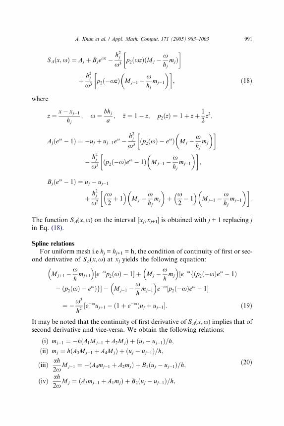
is termed as �adaptive cubic spline�.Solving (17) and using the interpolatory constants SD(xj�1,x) = uj�1,
SD(xj,x) = uj, we have
A. Khan et al. / Appl. Math. Comput. 171 (2005) 983–1003 991
SDðx;xÞ ¼ Aj þ Bjexz �h2jx3
p2ðxzÞðMj �xhjmjÞ
� �
þh2jx3
p2ð�x�zÞ Mj�1 �xhjmj�1
� �� �; ð18Þ
where
z ¼ x� xj�1
hj; x ¼ bhj
a; �z ¼ 1� z; p2ðzÞ ¼ 1þ zþ 1
2z2;
Ajðex � 1Þ ¼ �uj þ uj�1ex �h2jx3
ðp2ðxÞ � exÞ Mj �xhjmj
� �� �
�h2jx3
ðp2ð�xÞex � 1Þ Mj�1 �xhjmj�1
� �� �;
Bjðex � 1Þ ¼ uj � uj�1
þh2jx2
x2þ 1
� �Mj �
xhjmj
� �þ x
2� 1
� �Mj�1 �
xhjmj�1
� �� �:
The function SD(x,x) on the interval [xj,xj+1] is obtained with j + 1 replacing j
in Eq. (18).
Spline relations
For uniform mesh i.e hj = hj+1 = h, the condition of continuity of first or sec-
ond derivative of SD(x,x) at xj yields the following equation:
Mjþ1 �xhmjþ1
� �½e�xp2ðxÞ � 1� þ Mj �
xhmj
� �½e�xfðp2ð�xÞex � 1Þ
� ðp2ðxÞ � exÞg� � Mj�1 �xhmj�1
� �e�x½p2ð�xÞex � 1�
¼ �x3
h2½e�xujþ1 � ð1þ e�xÞuj þ uj�1�: ð19Þ
It may be noted that the continuity of first derivative of SD(x,x) implies that of
second derivative and vice-versa. We obtain the following relations:
ðiÞ mj�1 ¼ �hðA1Mj�1 þ A2MjÞ þ ðuj � uj�1Þ=h;ðiiÞ mj ¼ hðA3Mj�1 þ A4MjÞ þ ðuj � uj�1Þ=h;
ðiiiÞ ah2x
Mj�1 ¼ �ðA4mj�1 þ A2mjÞ þ B1ðuj � uj�1Þ=h;
ðivÞ ah2x
Mj ¼ ðA3mj�1 þ A1mjÞ þ B2ðuj � uj�1Þ=h;
ð20Þ
992 A. Khan et al. / Appl. Math. Comput. 171 (2005) 983–1003
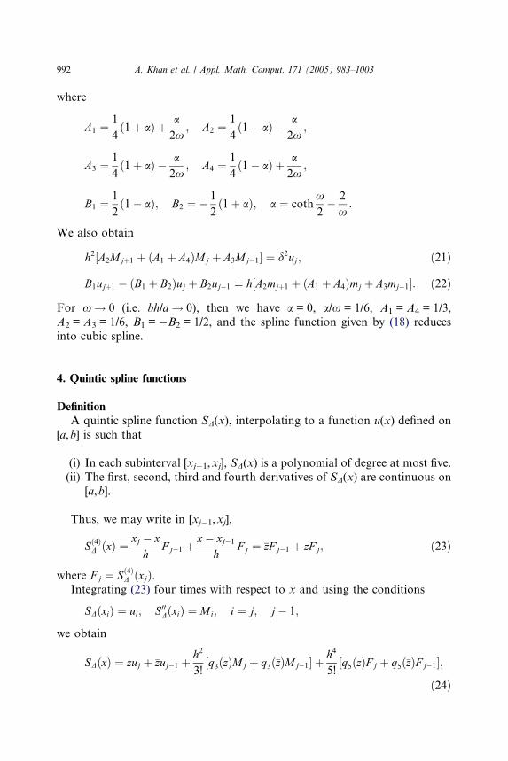
where
A1 ¼1
4ð1þ aÞ þ a
2x; A2 ¼
1
4ð1� aÞ � a
2x;
A3 ¼1
4ð1þ aÞ � a
2x; A4 ¼
1
4ð1� aÞ þ a
2x;
B1 ¼1
2ð1� aÞ; B2 ¼ � 1
2ð1þ aÞ; a ¼ coth
x2� 2
x:
We also obtain
h2½A2Mjþ1 þ ðA1 þ A4ÞMj þ A3Mj�1� ¼ d2uj; ð21Þ
B1ujþ1 � ðB1 þ B2Þuj þ B2uj�1 ¼ h½A2mjþ1 þ ðA1 þ A4Þmj þ A3mj�1�: ð22Þ
For x! 0 (i.e. bh/a ! 0), then we have a = 0, a/x = 1/6, A1 = A4 = 1/3,
A2 = A3 = 1/6, B1 = �B2 = 1/2, and the spline function given by (18) reduces
into cubic spline.
4. Quintic spline functions
DefinitionA quintic spline function SD(x), interpolating to a function u(x) defined on
[a,b] is such that
(i) In each subinterval [xj�1,xj], SD(x) is a polynomial of degree at most five.
(ii) The first, second, third and fourth derivatives of SD(x) are continuous on
[a,b].
Thus, we may write in [xj�1,xj],
Sð4ÞD ðxÞ ¼ xj � x
hF j�1 þ
x� xj�1
hF j ¼ �zF j�1 þ zF j; ð23Þ
where F j ¼ Sð4ÞD ðxjÞ.
Integrating (23) four times with respect to x and using the conditions
SDðxiÞ ¼ ui; S00DðxiÞ ¼ Mi; i ¼ j; j� 1;
we obtain
SDðxÞ ¼ zuj þ �zuj�1 þh2
3!½q3ðzÞMj þ q3ð�zÞMj�1� þ
h4
5!½q5ðzÞF j þ q5ð�zÞF j�1�;
ð24Þ
A. Khan et al. / Appl. Math. Comput. 171 (2005) 983–1003 993
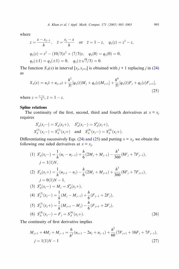
where
z ¼ x� xj�1
h; �z ¼ xj � x
hor �z ¼ 1� z; q3ðzÞ ¼ z3 � z;
q5ðzÞ ¼ z5 � ð10=3Þz3 þ ð7=3Þz; q3ð0Þ ¼ q5ð0Þ ¼ 0;
q3ð�1Þ ¼ q5ð�1Þ ¼ 0; q5ð�ffiffiffi7
p=3Þ ¼ 0:
The function SD(x) in interval [xj,xj+1] is obtained with j + 1 replacing j in (24)
as
SDðxÞ ¼ uj�zþ ujþ1zþh2
3!½q3ð�zÞMj þ q3ðzÞMjþ1� þ
h4
5!½q5ð�zÞF j þ q5ðzÞF jþ1�;
ð25Þwhere z ¼ x�xj
h , �z ¼ 1� z.
Spline relations
The continuity of the first, second, third and fourth derivatives at x = xjrequires
S0Dðxj�Þ ¼ S0
DðxjþÞ; S00Dðxj�Þ ¼ S00
DðxjþÞ;Sð3ÞD ðxj�Þ ¼ Sð3Þ
D ðxjþÞ and Sð4ÞD ðxj�Þ ¼ Sð4Þ
D ðxjþÞ:
Differentiating successively Eqs. (24) and (25) and putting x = xj, we obtain thefollowing one sided derivatives at x = xj.
ð1Þ S0Dðxj�Þ ¼ 1
hðuj � uj�1Þ þ
h6ð2Mj þMj�1Þ �
h3
360ð8F j þ 7F j�1Þ;
j ¼ 1ð1ÞN ;
ð2Þ S0DðxjþÞ ¼ 1
hðujþ1 � ujÞ �
h6ð2Mj þMjþ1Þ þ
h3
360ð8F j þ 7F jþ1Þ;
j ¼ 0ð1ÞN � 1;
ð3Þ S00Dðxj�Þ ¼ Mj ¼ S00
DðxjþÞ;
ð4Þ Sð3ÞD ðxj�Þ ¼ 1
hðMj �Mj�1Þ þ
h6ðF j�1 þ 2F jÞ;
ð5Þ Sð3ÞD ðxjþÞ ¼ 1
hðMjþ1 �MjÞ �
h6ðF jþ1 þ 2F jÞ;
ð6Þ Sð4ÞD ðxj�Þ ¼ F j ¼ Sð4Þ
D ðxjþÞ: ð26Þ
The continuity of first derivative implies
Mjþ1 þ 4Mj þMj�1 ¼6
h2ðujþ1 � 2uj þ uj�1Þ þ
h2
60ð7F jþ1 þ 16F j þ 7F j�1Þ;
j ¼ 1ð1ÞN � 1 ð27Þ
994 A. Khan et al. / Appl. Math. Comput. 171 (2005) 983–1003
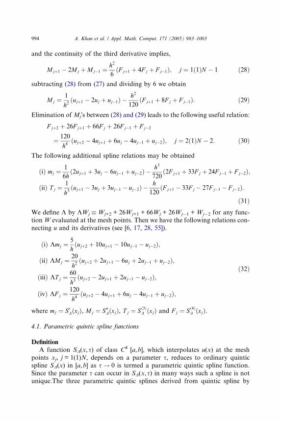
and the continuity of the third derivative implies,
Mjþ1 � 2Mj þMj�1 ¼h2
6ðF jþ1 þ 4F j þ F j�1Þ; j ¼ 1ð1ÞN � 1 ð28Þ
subtracting (28) from (27) and dividing by 6 we obtain
Mj ¼1
h2ðujþ1 � 2uj þ uj�1Þ �
h2
120ðF jþ1 þ 8F j þ F j�1Þ: ð29Þ
Elimination ofMj�s between (28) and (29) leads to the following useful relation:
F jþ2 þ 26F jþ1 þ 66F j þ 26F j�1 þ F j�2
¼ 120
h4ðujþ2 � 4ujþ1 þ 6uj � 4uj�1 þ uj�2Þ; j ¼ 2ð1ÞN � 2: ð30Þ
The following additional spline relations may be obtained
ðiÞ mj ¼1
6hð2ujþ1 þ 3uj � 6uj�1 þ uj�2Þ �
h3
720ð2F jþ1 þ 33F j þ 24F j�1 þ F j�2Þ;
ðiiÞ T j ¼1
h3ðujþ1 � 3uj þ 3uj�1 � uj�2Þ �
h120
ðF jþ1 � 33F j � 27F j�1 � F j�2Þ:
ð31ÞWe define K by KWj � Wj+2 + 26Wj+1 + 66Wj + 26Wj�1 + Wj�2 for any func-
tion W evaluated at the mesh points. Then we have the following relations con-
necting u and its derivatives (see [6, 17, 28, 55]).
ðiÞ Kmj ¼5
hðujþ2 þ 10ujþ1 � 10uj�1 � uj�2Þ;
ðiiÞ KMj ¼20
h2ðujþ2 þ 2ujþ1 � 6uj þ 2uj�1 þ uj�2Þ;
ðiiiÞ KT j ¼60
h3ðujþ2 � 2ujþ1 þ 2uj�1 � uj�2Þ;
ðivÞ KF j ¼120
h4ðujþ2 � 4ujþ1 þ 6uj � 4uj�1 þ uj�2Þ;
ð32Þ
where mj ¼ S0DðxjÞ, Mj ¼ S00
DðxjÞ, T j ¼ Sð3ÞD ðxjÞ and F j ¼ Sð4Þ
D ðxjÞ.
4.1. Parametric quintic spline functions
DefinitionA function SD(x,s) of class C4 [a,b], which interpolates u(x) at the mesh
points xj, j = 1(1)N, depends on a parameter s, reduces to ordinary quintic
spline SD(x) in [a,b] as s ! 0 is termed a parametric quintic spline function.
Since the parameter s can occur in SD(x,s) in many ways such a spline is not
unique.The three parametric quintic splines derived from quintic spline by
A. Khan et al. / Appl. Math. Comput. 171 (2005) 983–1003 995
introducing the parameter in three different ways are termed as �parametric
quintic spline-I�, �parametric quintic spline-II� and �adaptive quintic spline�.
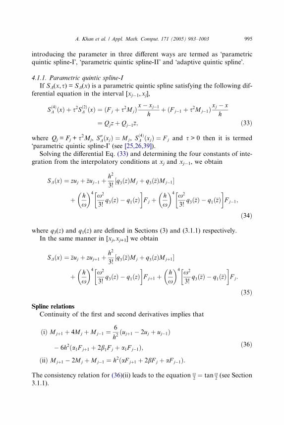
4.1.1. Parametric quintic spline-I
If SD(x,s) = SD(x) is a parametric quintic spline satisfying the following dif-
ferential equation in the interval [xj�1,xj],
Sð4ÞD ðxÞ þ s2Sð2Þ
D ðxÞ ¼ ðF j þ s2MjÞx� xj�1
hþ ðF j�1 þ s2Mj�1Þ
xj � xh
¼ Qjzþ Qj�1�z; ð33Þ
where Qj = Fj + s2Mj, S00DðxjÞ ¼ Mj, S
ð4ÞD ðxjÞ ¼ F j and s > 0 then it is termed
�parametric quintic spline-I� (see [25,26,39]).
Solving the differential Eq. (33) and determining the four constants of inte-
gration from the interpolatory conditions at xj and xj�1, we obtain
SDðxÞ ¼ zuj þ �zuj�1 þh2
3!½q3ðzÞMj þ q3ð�zÞMj�1�
þ hx
� �4 x2
3!q3ðzÞ � q1ðzÞ
� �F j þ
hx
� �4 x2
3!q3ð�zÞ � q1ð�zÞ
� �F j�1;
ð34Þ
where q3(z) and q1(z) are defined in Sections (3) and (3.1.1) respectively.In the same manner in [xj,xj+1] we obtain
SDðxÞ ¼ �zuj þ zujþ1 þh2
3!½q3ð�zÞMj þ q3ðzÞMjþ1�
þ hx
� �4 x2
3!q3ðzÞ � q1ðzÞ
� �F jþ1 þ
hx
� �4 x2
3!q3ð�zÞ � q1ð�zÞ
� �F j:
ð35Þ
Spline relations
Continuity of the first and second derivatives implies that
ðiÞ Mjþ1 þ 4Mj þMj�1 ¼6
h2ðujþ1 � 2uj þ uj�1Þ
� 6h2ða1F jþ1 þ 2b1F j þ a1F j�1Þ;
ðiiÞ Mjþ1 � 2Mj þMj�1 ¼ h2ðaF jþ1 þ 2bF j þ aF j�1Þ:
ð36Þ
The consistency relation for (36)(ii) leads to the equation x2¼ tan x
2(see Section
3.1.1).
996 A. Khan et al. / Appl. Math. Comput. 171 (2005) 983–1003
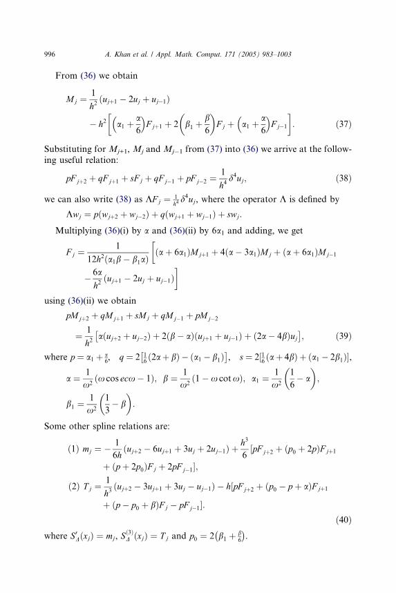
From (36) we obtain
Mj ¼1
h2ðujþ1 � 2uj þ uj�1Þ
� h2 a1 þa6
� �F jþ1 þ 2 b1 þ
b6
� �F j þ a1 þ
a6
� �F j�1
� �: ð37Þ
Substituting for Mj+1, Mj and Mj�1 from (37) into (36) we arrive at the follow-
ing useful relation:
pF jþ2 þ qF jþ1 þ sF j þ qF j�1 þ pF j�2 ¼1
h4d4uj; ð38Þ
we can also write (38) as KF j ¼ 1h4d4uj, where the operator K is defined by
Kwj ¼ pðwjþ2 þ wj�2Þ þ qðwjþ1 þ wj�1Þ þ swj:
Multiplying (36)(i) by a and (36)(ii) by 6a1 and adding, we get
F j ¼1
12h2ða1b� b1aÞ
�ðaþ 6a1ÞMjþ1 þ 4ða� 3a1ÞMj þ ðaþ 6a1ÞMj�1
� 6a
h2ðujþ1 � 2uj þ uj�1Þ
�
using (36)(ii) we obtain
pMjþ2 þ qMjþ1 þ sMj þ qMj�1 þ pMj�2
¼ 1
h2aðujþ2 þ uj�2Þ þ 2ðb� aÞðujþ1 þ uj�1Þ þ ð2a� 4bÞuj�
; ð39Þ
where p ¼ a1 þ a6, q ¼ 2 1
6ð2aþ bÞ � ða1 � b1Þ
� , s ¼ 2½1
6ðaþ 4bÞ þ ða1 � 2b1Þ�,
a ¼ 1
x2ðx cos ecx� 1Þ; b ¼ 1
x2ð1� x cotxÞ; a1 ¼
1
x2
1
6� a
� �;
b1 ¼1
x2
1
3� b
� �:
Some other spline relations are:
ð1Þ mj ¼ � 1
6hðujþ2 � 6ujþ1 þ 3uj þ 2uj�1Þ þ
h3
6½pF jþ2 þ ðp0 þ 2pÞF jþ1
þ ðp þ 2p0ÞF j þ 2pF j�1�;
ð2Þ T j ¼1
h3ðujþ2 � 3ujþ1 þ 3uj � uj�1Þ � h½pF jþ2 þ ðp0 � p þ aÞF jþ1
þ ðp � p0 þ bÞF j � pF j�1�:ð40Þ
where S0DðxjÞ ¼ mj, S
ð3ÞD ðxjÞ ¼ T j and p0 ¼ 2 b1 þ b
6
�.
A. Khan et al. / Appl. Math. Comput. 171 (2005) 983–1003 997
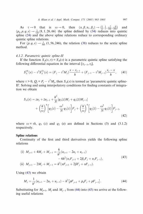
As s ! 0 that is x! 0, then ða; b; a1; b1Þ ! 16; 13; �7360
; �8360
�and
ðp0; p; q; sÞ ! 1120
ð8; 1; 26; 66Þ the spline defined by (34) reduces into quintic
spline (24) and the above spline relations reduce to corresponding ordinary
quintic spline relations.
For ðp; q; sÞ ! 1360
(1,56,246), the relation (38) reduces to the sextic spline
method.
4.1.2. Parametric quintic spline-II
If the function SD(x,s) = SD(x) is a parametric quintic spline satisfying the
following differential equation in the interval [xj�1,xj],
Sð4ÞD ðxÞ � s2Sð2Þ
D ðxÞ ¼ ðF j � s2MjÞx� xj�1
hþ ðF j�1 � s2Mj�1Þ
xj � xh
; ð41Þ
where s > 0, Qj = Fj � s2Mj, then SD(x) is termed as �parametric quintic spline-II�. Solving and using interpolatory conditions for finding constants of integra-
tion we obtain
SDðxÞ ¼ zuj þ �zuj�1 þh2
3!½q3ðzÞMj þ q3ð�zÞMj�1�
þ hx
� �4
q2ðzÞ �x2
3!q3ðzÞ
� �F j þ
hx
� �4
q2ð�zÞ �x2
3!q3ð�zÞ
� �F j�1;
ð42Þ
where x = sh, q3 (z) and q2 (z) are defined in Sections (3) and (3.1.2)respectively.
Spline relations
Continuity of the first and third derivatives yields the following spline
relations
ðiÞ Mjþ1 þ 4Mj þMj�1 ¼6
h2ðujþ1 � 2uj þ uj�1Þ
� 6h2ða1F jþ1 þ 2b1F j þ a1F j�1Þ;ðiiÞ Mjþ1 � 2Mj þMj�1 ¼ h2ðaF jþ1 þ 2bF j þ aF j�1Þ:
ð43Þ
Using (43) we obtain
Mj ¼1
h2ðujþ1 � 2uj þ uj�1Þ � h2 pF jþ1 þ p0F j þ pF j�1
� : ð44Þ
Substituting for Mj+1, Mj and Mj�1 from (44) into (43) we arrive at the follow-
ing useful relations
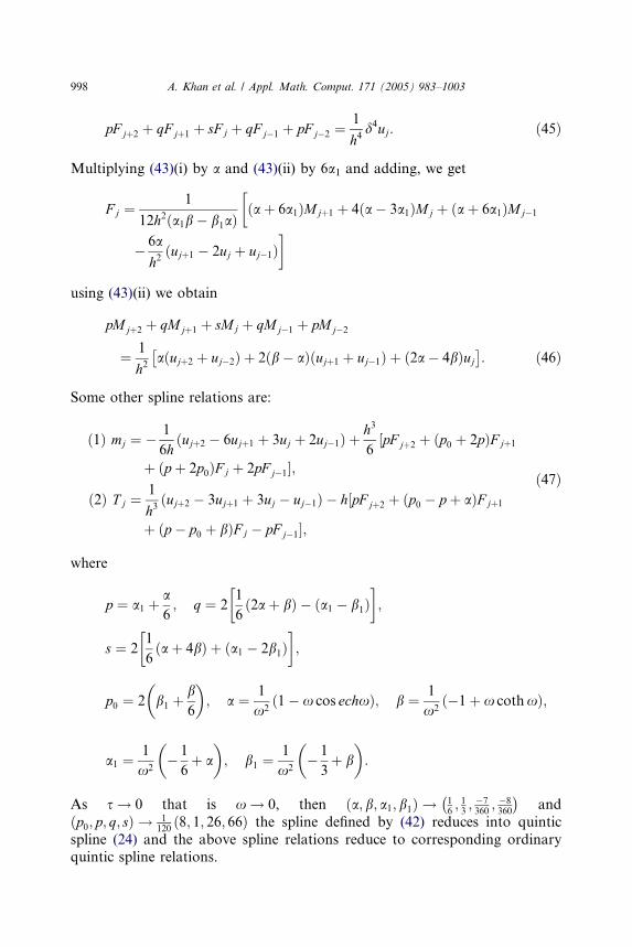
998 A. Khan et al. / Appl. Math. Comput. 171 (2005) 983–1003
pF jþ2 þ qF jþ1 þ sF j þ qF j�1 þ pF j�2 ¼1
h4d4uj: ð45Þ
Multiplying (43)(i) by a and (43)(ii) by 6a1 and adding, we get
F j ¼1
12h2ða1b� b1aÞ
�ðaþ 6a1ÞMjþ1 þ 4ða� 3a1ÞMj þ ðaþ 6a1ÞMj�1
� 6a
h2ðujþ1 � 2uj þ uj�1Þ
�
using (43)(ii) we obtain
pMjþ2 þ qMjþ1 þ sMj þ qMj�1 þ pMj�2
¼ 1
h2aðujþ2 þ uj�2Þ þ 2ðb� aÞðujþ1 þ uj�1Þ þ ð2a� 4bÞuj�
: ð46Þ
Some other spline relations are:
ð1Þ mj ¼ � 1
6hðujþ2 � 6ujþ1 þ 3uj þ 2uj�1Þ þ
h3
6½pF jþ2 þ ðp0 þ 2pÞF jþ1
þ ðp þ 2p0ÞF j þ 2pF j�1�;
ð2Þ T j ¼1
h3ðujþ2 � 3ujþ1 þ 3uj � uj�1Þ � h½pF jþ2 þ ðp0 � p þ aÞF jþ1
þ ðp � p0 þ bÞF j � pF j�1�;
ð47Þ
where
p ¼ a1 þa6; q ¼ 2
1
6ð2aþ bÞ � ða1 � b1Þ
� �;
s ¼ 21
6ðaþ 4bÞ þ ða1 � 2b1Þ
� �;
p0 ¼ 2 b1 þb6
� �; a ¼ 1
x2ð1� x cos echxÞ; b ¼ 1
x2ð�1þ x cothxÞ;
a1 ¼1
x2� 1
6þ a
� �; b1 ¼
1
x2� 1
3þ b
� �:
As s ! 0 that is x ! 0, then ða; b; a1; b1Þ ! 16; 13; �7360
; �8360
�and
ðp0; p; q; sÞ ! 1120
ð8; 1; 26; 66Þ the spline defined by (42) reduces into quintic
spline (24) and the above spline relations reduce to corresponding ordinaryquintic spline relations.
A. Khan et al. / Appl. Math. Comput. 171 (2005) 983–1003 999
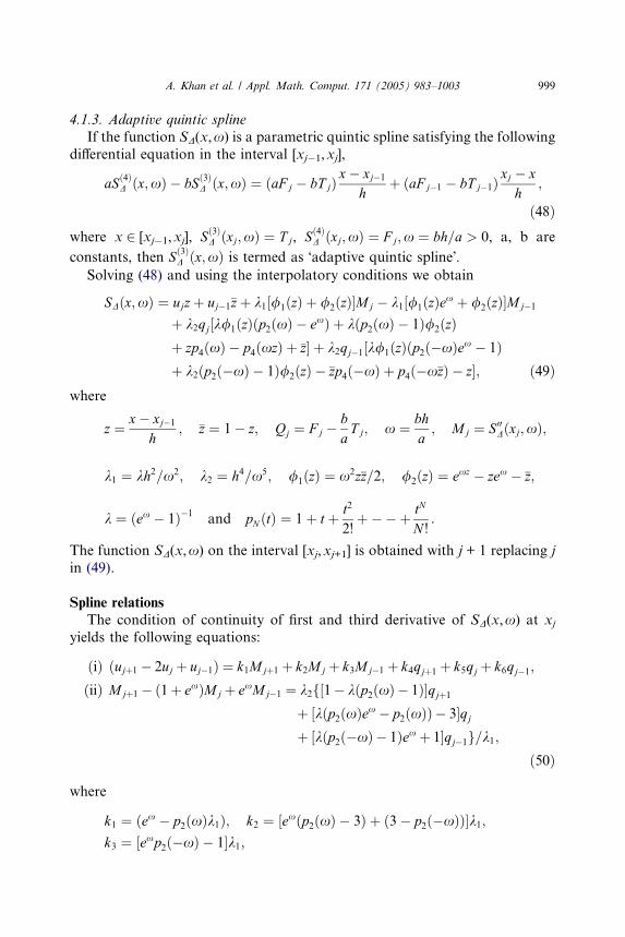
4.1.3. Adaptive quintic spline
If the function SD(x,x) is a parametric quintic spline satisfying the following
differential equation in the interval [xj�1,xj],
aSð4ÞD ðx;xÞ � bSð3Þ
D ðx;xÞ ¼ ðaF j � bT jÞx� xj�1
hþ ðaF j�1 � bT j�1Þ
xj � xh
;
ð48Þwhere x 2 [xj�1,xj], Sð3Þ
D ðxj;xÞ ¼ T j, Sð4ÞD ðxj;xÞ ¼ F j;x ¼ bh=a > 0, a, b are
constants, then Sð3ÞD ðx;xÞ is termed as �adaptive quintic spline�.
Solving (48) and using the interpolatory conditions we obtain
SDðx;xÞ ¼ ujzþ uj�1�zþ k1½/1ðzÞ þ /2ðzÞ�Mj � k1½/1ðzÞex þ /2ðzÞ�Mj�1
þ k2qj½k/1ðzÞðp2ðxÞ � exÞ þ kðp2ðxÞ � 1Þ/2ðzÞþ zp4ðxÞ � p4ðxzÞ þ �z� þ k2qj�1½k/1ðzÞðp2ð�xÞex � 1Þþ k2ðp2ð�xÞ � 1Þ/2ðzÞ � �zp4ð�xÞ þ p4ð�x�zÞ � z�; ð49Þ
where
z ¼ x� xj�1
h; �z ¼ 1� z; Qj ¼ F j �
baT j; x ¼ bh
a; Mj ¼ S00
Dðxj;xÞ;
k1 ¼ kh2=x2; k2 ¼ h4=x5; /1ðzÞ ¼ x2z�z=2; /2ðzÞ ¼ exz � zex � �z;
k ¼ ðex � 1Þ�1and pN ðtÞ ¼ 1þ t þ t2
2!þ��þ tN
N !:
The function SD(x,x) on the interval [xj,xj+1] is obtained with j + 1 replacing j
in (49).
Spline relations
The condition of continuity of first and third derivative of SD(x,x) at xjyields the following equations:
ðiÞ ðujþ1 � 2uj þ uj�1Þ ¼ k1Mjþ1 þ k2Mj þ k3Mj�1 þ k4qjþ1 þ k5qj þ k6qj�1;
ðiiÞ Mjþ1 � ð1þ exÞMj þ exMj�1 ¼ k2f½1� kðp2ðxÞ � 1Þ�qjþ1
þ ½kðp2ðxÞex � p2ðxÞÞ � 3�qjþ ½kðp2ð�xÞ � 1Þex þ 1�qj�1g=k1;
ð50Þ
where
k1 ¼ ðex � p2ðxÞk1Þ; k2 ¼ ½exðp2ðxÞ � 3Þ þ ð3� p2ð�xÞÞ�k1;k3 ¼ ½exp2ð�xÞ � 1�k1;
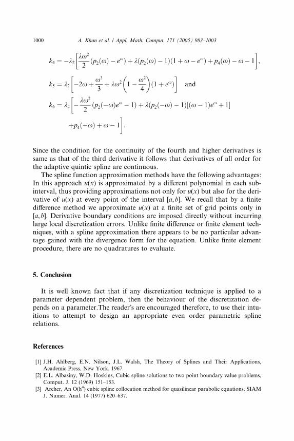
1000 A. Khan et al. / Appl. Math. Comput. 171 (2005) 983–1003
k4 ¼ �k2kx2
2ðp2ðxÞ � exÞ þ kðp2ðxÞ � 1Þð1þx� exÞ þ p4ðxÞ �x� 1
� �;
k5 ¼ k2 �2xþ x3
3þ kx2 1� x2
4
� �ð1þ exÞ
� �and
k6 ¼ k2 � kx2
2ðp2ð�xÞex � 1Þ þ kðp2ð�xÞ � 1Þ½ðx� 1Þex þ 1�
�
þp4ð�xÞ þ x� 1
�:
Since the condition for the continuity of the fourth and higher derivatives is
same as that of the third derivative it follows that derivatives of all order for
the adaptive quintic spline are continuous.The spline function approximation methods have the following advantages:
In this approach u(x) is approximated by a different polynomial in each sub-
interval, thus providing approximations not only for u(x) but also for the deri-
vative of u(x) at every point of the interval [a,b]. We recall that by a finite
difference method we approximate u(x) at a finite set of grid points only in
[a,b]. Derivative boundary conditions are imposed directly without incurring
large local discretization errors. Unlike finite difference or finite element tech-
niques, with a spline approximation there appears to be no particular advan-tage gained with the divergence form for the equation. Unlike finite element
procedure, there are no quadratures to evaluate.
5. Conclusion
It is well known fact that if any discretization technique is applied to a
parameter dependent problem, then the behaviour of the discretization de-pends on a parameter.The reader�s are encouraged therefore, to use their intu-
itions to attempt to design an appropriate even order parametric spline
relations.
References
[1] J.H. Ahlberg, E.N. Nilson, J.L. Walsh, The Theory of Splines and Their Applications,
Academic Press, New York, 1967.
[2] E.L. Albasiny, W.D. Hoskins, Cubic spline solutions to two point boundary value problems,
Comput. J. 12 (1969) 151–153.
[3] Archer, An O(h4) cubic spline collocation method for quasilinear parabolic equations, SIAM
J. Numer. Anal. 14 (1977) 620–637.
A. Khan et al. / Appl. Math. Comput. 171 (2005) 983–1003 1001
[4] T. Aziz, Numerical methods for differential equations using spline function approximations,
Ph.D. Thesis, IIT Delhi, 1983.
[5] T. Aziz, A. Khan, A spline method for second order singularly-perturbed boundary value
problems, J. Comput. Appl. Math. 147 (2) (2002) 445–452.
[6] T. Aziz, A. Khan, Quintic spline approach to the solution of a singularly-perturbed boundary
value problems, J. Opt. Theory Appl. 112 (2002) 517–527.
[7] W.G. Bickley, Piecewise cubic interpolation and two point boundary value problems, Comput.
J. 11 (1968) 206–208.
[8] M. Chawla, R. Subramanian, A new fourth order cubic spline method for non-linear two
point boundary value problems, Int. J. Comput. Math. 22 (1987) 321–341.
[9] M. Chawla, R. Subramanian, A fourth order spline method for singular two point boundary
value problems, J. Comput. Appl. Math. 21 (1988) 189–202.
[10] M. Chawla, R. Subramanian, High accuracy quintic spline solution of fourth order two point
boundary value problems, Int. J. Comput. Math. 31 (1989) 87–94.
[11] J.W. Daniel, B.K. Swartz, Extrapolated collocation for two point boundary value problems
using cubic splines, J. Inst. Math. Appl. 16 (1975) 161–174.
[12] C. De Boor, The method of projections as applied to the numerical solution of two
point boundary value problems using cubic splines, Ph.D. Thesis, University of Michigan,
1966.
[13] C. De Boor, On uniform approximations by splines, J. Approx. Theory 1 (1968) 219–235.
[14] C. De Boor, Practical Guide to Splines, Springer-Verlag, Berlin New York, 1978.
[15] G. Fairweather, D. Meade, A survey of spline collocation methods for the numerical solution
of differential equations, in: Mathematics for Large Scale Computing, in: J.C. Diaz (Ed.),
Lecture Notes in Pure and Applied Maths, 120, Marcel Dekker, New York, 1989, pp. 297–
341.
[16] D.J. Fyfe, The use of cubic splines in the solution of two point boundary- value problems,
Comput. J. 12 (1969) 188–192.
[17] D.J. Fyfe, Linear dependence relations connecting equal interval Nth degree splines and their
derivatives, J. Inst. Math. Appl. 7 (1971) 398–406.
[18] T.N.E. Greville, Introduction to spline functions, in: Theory and Application of Spline
Functions, Academic Press, New York, 1969.
[19] E.N. Houstis, E.A. Vavalis, J.R. Rice, Convergence of O(h2) cubic spline collocation methods
for elliptic partial differential equations, SIAM J. Numer. Anal. 25 (1988).
[20] M. Irodotou-Ellina, E.N. Houstis, An O(h6) quintic spline collocation method for singular
two-point boundary-value problems, BIT 28 (1988) 288–301.
[21] S.R.K. Iyengar, P. Jain, Spline finite difference methods for two-point boundary-value
problems, Numer. Math. 50 (1987) 363–387.
[22] M.K. Jain, T. Aziz, Numerical solution of stiff and convection-diffusion equations using
adaptive spline function approximation, Appl. Math. Model. 7 (1983) 57–63.
[23] M.K. Jain, T. Aziz, Spline function approximation for differential equations, Comput.
Method Appl. Mech. Eng. 26 (1981) 129–143.
[24] M.K. Jain, T. Aziz, Cubic spline solution of two-point boundary-value problems with
significant first derivatives, Comput. Method Appl. Mech. Eng. 39 (1983) 83–91.
[25] A. Khan, Spline solution of differential equations, Ph.D. Thesis, Aligarh Muslim University,
Aligarh, India, 2002.
[26] A. Khan, M.A. Noor, T. Aziz, Parametric quintic spline approach to the solution of a system
of fourth-order boundary-value problems, J Opt. Theory Appl. 122 (2004) 69–82.
[27] A. Khan, T. Aziz, Parametric cubic spline approach to the solution of a system of second order
boundary-value problems, J. Opt. Theory Appl. 118 (1) (2003) 45–54.
[28] A. Khan, T. Aziz, The numerical solution of third order boundary-value problems using
quintic splines, Appl. Math. Comput. 137 (2–3) (2002) 253–260.
1002 A. Khan et al. / Appl. Math. Comput. 171 (2005) 983–1003
[29] F.R. Loscalzo, I.J. Schoenberg, On the use of spline functions for the approximation of
solution of ordinary differential equations, Tech. Summary Report no.723, Math. Research
Centre, University of Wisconsin, Madison, 1967.
[30] F.R. Loscalzo, T.D. Talbot, Spline function approximations for solution of ordinary
differential equations, Bull. Amer. Math. Soc. 73 (1967) 438–442.
[31] F.R. Loscalzo, T.D. Talbot, Spline function approximations for solution of ordinary
differential equations, SIAM J. Numer. Anal. 4 (1967) 433–445.
[32] G.I. Marchuk, Methods of Numerical Mathematics, second ed., Springer- Verlag, New York,
1982.
[33] G. Micula, Approximation solution of the differential equation with spline functions, Math.
Comput. 27 (1973) 807–816.
[34] G. Micula, Sanda Micula, Hand Book of Splines, Kluwer Academic Publisher�s, 1999.[35] F. Patricio, A numerical method for solving initial value problems with spline functions, BIT
19 (1979) 489–494.
[36] F. Patricio, Cubic spline functions and initial value problems, BIT 18 (1978) 342–
347.
[37] P.M. Prenter, Splines and Variational Methods, John Wiley & Sons INC., 1975.
[38] C.V. Raghavarao, S.T.P.T. Srinivas, A note on parametric spline function approximation,
Comp. Math. Applics. 29 (1995) 67–73.
[39] J. Rashidinia, Applications of splines to the numerical solution of differential equations, Ph.D.
Thesis, A.M.U. Aligarh, 1994.
[40] S.G. Rubin, R.A. Graves Jr., Viscous flow solutions with a cubic spline approximation,
Computers and Fluids 3 (1975) 1–36.
[41] S.G. Rubin, P.K. Khosla, Higher order numerical solution using cubic splines, AIAA J. 14
(1976) 851–858.
[42] R.D. Russell, L.F. Shampine, A collocation method for boundary value problems, Numer.
Math. 19 (1972) 1–28.
[43] M. Sakai, Piecewise cubic interpolation and two point boundary value problems, Publ. RIMS.,
Kyoto Univ. 7 (1972) 345–362.
[44] M. Sakai, Numerical solution of boundary-value problems for second order functional
differential equations by the use of cubic splines, Mem. Fac. Sci., Kyushu Univ. 29 (1975) 113–
122.
[45] M. Sakai, Two sided quintic spline approximations for two point boundary-value problems,
Rep. Fac. Sci., Kagoshima Univ., (Math., Phys., Chem.) (10) (1977) 1–17.
[46] I.J. Schoenberg, Contribution to the problem of approximation of equidistant data by analytic
functions, Quart. Appl. Math. 4 (1946) 345–369.
[47] K. Surla, D. Herceg, L. Cvetkovic, A family of exponential spline difference schemes, Univ. u.
Novom Sadu, Zb. Rad. Prirod. Mat. Fak. Ser. Mat. 19 (2) (1991) 12–23.
[48] K. Surla, M. Stojanovic, Solving singularly perturbed boundary value problems by spline in
tension, J. Comput. Appl. Math. 24 (1988) 355–363.
[49] K. Surla, Z. Uzelec, Some uniformly convergent spline difference schemes for singularly
perturbed boundary-value problems, IMA J. Numer. Anal. 10 (1990) 209–222.
[50] K. Surla, V. Vukoslavcevic, A spline difference scheme for boundary -value problems with a
small parameter, Univ. u. Novom Sadu, Zb. Rad. Zb. Rad. Prirod. Mat. Fak. Ser. Mat. 25 (2)
(1995) 159–166.
[51] R.P. Tewarson, On the use of splines for the numerical solution of non linear two point
boundary value problems, BIT 20 (1980) 223–232.
[52] R.P. Tewarson, Y. Zhang, Solution of two point boundary value problems using splines, Int.
J. Numer. Method Engg. 23 (1986) 707–710.
[53] R.A. Usmani, Spline solutions for nonlinear two point boundary value problems, Intern. J.
Math. and Math. Sci. 3 (1980) 151–167.

A. Khan et al. / Appl. Math. Comput. 171 (2005) 983–1003 1003
[54] R.A. Usmani, M. Sakai, A connection between quartic spline solution and Numerov solution
of a boundary value problem, Int. J. Comput. Math. 26 (1989) 263–273.
[55] R.A. Usmani, S.A. Warsi, Quintic spline solution of boundary value problems, Comput.
Math. Appl. 6 (1980) 197–203.
[56] R.S. Varga, Error bounds for spline interpolation, in: I.J. Schoenberg (Ed.), Approximations
with Special Emphasis on Spline Functions, Academic Press, New York, 1969, pp. 367–388.