moment-preserving spline approximation on finite intervals

Numer. Math. 50, 503-518 (1987) Numerische Mathematik �9 Springer-Verlag 1987

Moment-Preserving Spline Approximation on Finite Intervals*

Marco Frontini 1, Walter Gautschi 2, and Gradimir V. Milovanovib s

1 Dipartimento di Matematica, Politecnico di Milano, Piazza Leonardo da Vinci, 32, 1-20133 Milano, Italy

z Department of Computer Sciences, Purdue University, West Lafayette, IN 47907, USA 3 Faculty of Electronic Engineering, Department of Mathematics, P.O. Box 73, Y-18000 Nil,

Yugoslavia

Summary. Continuing previous wotk, we discuss the problem of approximating a function f on the interval [0, 1] by a spline function of degree m, with n (variable) knots, matching as many of the initial moments o f f as possible. Additional constraints on the derivatives of the approximation at one endpoint of [0, 1] may also be imposed. We show that, if the approximations exist, they can be represented in terms of generalized Gauss- Lobat to and Gauss-Radau quadrature rules relative to appropriate moment functionals or measures (depending on f) . Pointwise convergence as n--*oo, for fixed m>0 , is shown for functions f that are completely monotonic on [0, 1], among others. Numerical examples conclude the paper.

Subject Classifications: AMS: Primary 41A15, 65D32; Secondary 33A65; CR: GI.2, GI.4.

1. Introduction

In previous papers [4, 6] two of us dealt with the problem of approximating a given function f on [0, oo] by a spline function of fixed degree (with variable knots) in such a way as to reproduce as many moments of f as possible. Having had in mind applications to physics, our functions f=f(r) were considered functions of the radial distance r = [Ixll of a vector xeP, d, and accordingly the moments were "spherical moments". We now wish to consider the analogous problem on an arbitrary finite interval. In this case, the interpretation of the independent variable as a radial distance is no longer meaningful, and our functions f=f(t), therefore, are now simply functions of a real variable t on some given interval [a, b]. The case of a semi-infinite interval having been treated in our previous work, we restrict attention here to the case of a finite

* The work of the first author was supported by the Ministero della Pubblica Istruzione and by the Consiglio Nazionale delle Ricerche. The work of the second author was supported, in part, by the National Science Foundation under grant DCR-8320561

504 M. Frontini et al.

interval, which can be s tandardized to [a, b] = [0, 1]. The case of the whole real line, [a, b] = ~ , is also of interest, as is the case of periodic splines. Both, however, appea r to be less amenable to the type of analysis we are going to give, and will not be considered here.

2. Spline Approximation on [0, I]

A spline function of degree m > 0 , with n (distinct) knots z-I,'L 2 . . . . . T n in the interior of [0, 1], can be wri t ten in terms of t runcated powers in the form

S,,m(t)=pm(t)+ ~ av(zv--t)+ , 0_<t_<l, (2.1) V = I

where a v are real numbers and p,, is a po lynomia l of degree <m. (Our choice of t runcated powers distinguishes the right endpoint of [0, 1] in the sense that s,,.,(t) =pro(t), t > 1.) We consider two related prob lems:

Problem I. Determine s,,,. in (2.l) such that

1 1

~tJs,,m(t)dt= StJf(t)dt, j = 0 , 1, . . . ,2n+m. (2.2) 0 0

Problem I*. Determine s,,,, in (2.1) such that

S (k) tD=f(k)(1) k = 0 , 1, m, (2.3) L n , m X I J x y~ " ' ' ,

and such that (2.2) holds for j =0 , 1 . . . . . 2 n - 1. Here we must assume that f has m derivatives at t = 1, all being known.

Both p rob lems will be solved in two ways: first in terms of m o m e n t functionals, then in terms of Gauss-Christoffel quadrature . The former ap- proach requires only the existence and knowledge of the momen t s of f in- volved; the latter requires addi t ional regulari ty of f, but lends itself bet ter to stable implementa t ions .

2.1. Solution of Problems I and I* by Moment Functionals

We first consider P rob lem I. Let

( m + j + l ) ! 1 StJf(t)dt, j = 0 , 1 . . . . , 2 n + m , (2.4)

PJ- m!j? o

where the momen t s of f on the right are assumed to exist. (They do, of course, if f is integrable on [-0, 1].) We define a linear functional LP on the set of polynomials of the fo rm t "+1P(0, P~IP2.+m, by

L~a(t "+1 . t J )=pj , j = 0 , 1 . . . . . 2n + m . (2.5)

Moment -P re se rv ing Spline A p p r o x i m a t i o n on Fin i te Intervals 505

Then the inner product

(p, q )= ~(f(t"+ 1(1 _t)m+lp.q) (2.6)

is well defined for any polynomials p, q for which p.q~IP2,_ r In particular, we can define (if it exists) the monic polynomial n , ( - ) = n , ( . ; ~ ) of degree n or thogonal with respect to the inner product (2.6) to all polynomials of lower degree,

d e g ~ , = n , ~ , ( t ) = t " + .... (2.v) (ft., q )=0 , all qelP,_ 1.

Theorem 2.1. There exists a unique spline function on [0, 1],

s,,,.(t)=p,,(t)+ ~ a~(%--t)+, 0 < z ~ < l , z~4:z u for V4:l 2, (2.8) v = l

satisfying the 2 n + m + t moment equations (2.2) of Problem I if and only if the orthogonal polynomial ~ , ( ' ) = n , ( ' ; ~ ) in (2.7) exists uniquely and has n distinct real zeros %~("), v= 1, 2, ..., n, all contained in the open interval (0, 1). The knots % in (2.8) are then precisely these zeros,

% = ~("), v = 1, 2 . . . . . n , ( 2 . 9 )

while the coefficients a~ and the quantities

(which uniquely system

where

( - 1) k bk= m ~ P~)(l),

determine p,, in (2.8))

k =0 , 1 . . . . , m, (2.10)

are obtained uniquely from the linear

~o(t"+ap)=~(tm+lp) all p~IP.+ m,

_(n) ~ o ( g ) = ~ bkg("-k)(1)+ ~ a~g(%), z~=Lv . k=O v = l

(2.11)

(2.12)

Proof. Substituting (2.1) in (2.2), and observing that 0 < % < 1, gives

i n Tv 1

y, j m ~t~p,,(t)dt+ av~t ( % - t ) d t=~tJ f ( t )d t , o ~=1 o o (2.13)

j=O, 1 . . . . , 2 n + m .

Changing variables, t = z %, in the v-th integral of the summation, one obtains

rv 1

tJ(zv- t)" dt = z m +j+1 ~ z j(1 _ z)" dz o o (2.14)

= j ! m ! r

( m + j + l ) ! - v "


Using m integrations by parts in the first integral of (2.13) yields

a j!m! m [ d m - k l + j ] , ! t2pm(t) dt =(m + j + 1)! k~=O bk [d~ W~ tin+ (2.15)

~ t = l

where b k is defined in (2.10). Inserting (2.14) and (2.15) in (2.13) and dividing through by j ! m !/(m + j + 1) ! gives

~o(tm+l.tJ)=#j, j = 0 , 1 . . . . . 2n+m,

where pj is defined by (2.4) and 5('o by (2.12). Therefore, using (2.5) and the linearity of ~o and ~9~,

~o(tm+lp)=Sf(t'+lp), all p~IP2,+m. (2.16)

Thus, the moment equations (2.2) and Eqs. (2.16) are equivalent. Let now 7~, denote the "knot polynomial"

n

~,(t)= 1-[ (t--%) (2.17) v = l

having the knots z~ of the spline (2.8) as zeros. Then, by the definition of the inner product (2.6) we have, for any qeIP,_ 1,

(~,, q)= ~L~~ 1(1-- t )m+l~, 'q)=~o(tm+l(1-- t )"+l~, 'q) , (2.18)

by (2.16), since ( 1 - 0 "+1 ~,.qeIP2,+, .. Therefore, (~,, q)=0 by the definition (2.12) of ~o and the fact that 7r,(zv)=0, v= 1,2 . . . . . n. It follows that the knots % must be the zeros of the orthogonal polynomial ~,(.; 5r of (2.7). This proves the necessity of the condition asserted in Theorem 2.1. Furthermore, the system (2.11) is a trivial consequence of (2.16); with z~= ~t")~ determined, (2.1l) is essentially a confluent Vandermonde system, hence nonsingular.

To prove the sufficiency of the condition, together with (2.11), we must show that they imply (2.16). Thus, let pelP2,+m be an arbitrary polynomial of degree<2n+m. Let q and r be the quotient and remainder of p upon division by ( 1 - 0 "+1 ~,(t), where ~ , ( . )=~, ( . ; ~r

p(t)=(1-t)~+ln,(t)q(t)+r(t), q~IP,_l, r~lP +,,. (2.19) Then,

s 1 p) = ~q(tm+ 1(t _ t)m+ 1 ~ . q) + 5r + 1 r)

= ~( t "+a r) [by (2.7)]

= ~o(t"+~ r) [by (2.11)]

=~o(tm+ip)--~o(t"+l(1--t)m+ln,'q) [by (2.19)]

= ~o(tm+lp) [since ~,(z~) =0] .

This proves (2.16). []

The solution of Problem I* can be effected similarly, if one observes, in view of 0 < % < 1, that

stk) tD--,4k)tl~ k=0, 1, m. (2.20)

Moment-Preserving Spline Approximation on Finite Intervals 507

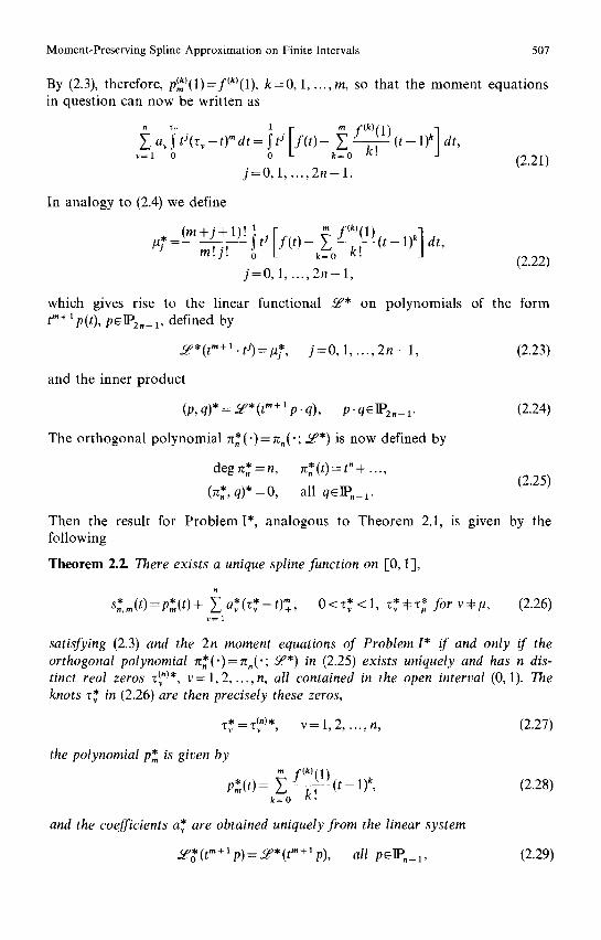
By (2.3), therefore, p~)(1)=f(k)(1), k = 0 , 1 . . . . . m, so that the m o m e n t equat ions in quest ion can now be writ ten as

a~tJ (r~- t )mdt= t ~ | J ( t ) - 2_.~.v ( t - l ) k dt, ~=1 o o L k=O �9 (2.21)

j = 0 , 1 . . . . . 2n - -1 .

In analogy to (2.4) we define

�9 - - ( m + j - - + l ) ! i t ~ [ f ( t ) - - k ~ = o ~ ( t - - 1 ) k l d t , P) m! j! o (2.22)

j = 0 , 1 . . . . . 2 n - - l ,

which gives rise to the linear functional 5r on polynomials of the form tm+ l p(t), pE]P2n_ l, defined by

&v*(t"+ 1. t J ) = p *, j = 0 , 1 . . . . . 2 n - 1 , (2.23)

and the inner product

(p,q)*=~f*(tm+lp.q), p.q~IP2,_ 1. (2.24)

The or thogona l po lynomia l l r* ( . )= lr,(.; 5r is now defined by

deg re* = n, 7r* (t) = t" + .... (2.25)

(~*, q)* = 0 , all q~IP,_l .

Then the result for P rob lem I*, analogous to Theo rem 2.1, is given by the following

Theorem 2.Z There exists a unique spline function on [0, 1],

s*m(t)=p*(t)+ ~ * * " * * * (2.26) a~(%-t )+, 0 < l, % ~v < #-~, for v # p , v = l

satisfying (2.3) and the 2n moment equations of Problem I* if and only if the orthogonal polynomial n * ( ' ) = n , ( ' ; &'~*) in (2.25) exists uniquely and has n dis-

-(")* v= 1,2, n, all contained in the open interval (0, 1). The tinct real zeros % , ..., �9 in (2.26) are then precisely these zeros, knots %

%* -- %-(")*, v = 1, 2 . . . . . n, (2.27)

the polynomial p* is given by

p * ( t ) = k ~ = o ~ ( t - - 1 ) k , (2.28)

and the coefficients a* are obtained uniquely from the linear system

~LP~(tm+Xp)=~*(t"+lp), all p~lP,_ 1, (2.29)


where

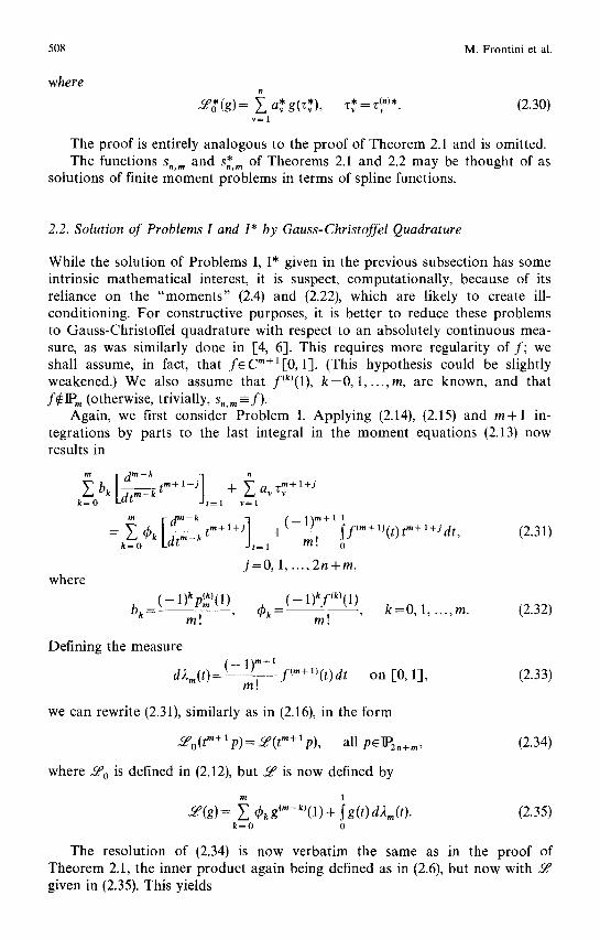
~*(g) ~ * * *- - (")* (2.30) = a~ g(%), % - % . v=l

The proof is entirely analogous to the proof of Theorem 2.1 and is omitted. The functions s,,,, and s,,*,, of Theorems 2.1 and 2.2 may be thought of as

solutions of finite moment problems in terms of spline functions.

2.2. Solution of Problems I and I* by Gauss-Christoffel Quadrature

While the solution of Problems I, I* given in the previous subsection has some intrinsic mathematical interest, it is suspect, computationally, because of its reliance on the "moments" (2.4) and (2.22), which are likely to create ill- conditioning. For constructive purposes, it is better to reduce these problems to Gauss-Christoffel quadrature with respect to an absolutely continuous measure, as was similarly done in [-4, 6]. This requires more regularity of f ; we shall assume, in fact, that f~Cm+l[0,1] . (This hypothesis could be slightly weakened.) We also assume that f(k)(1), k=0, 1 . . . . . m, are known, and that f r m (otherwise, trivially, s,,m= f).

Again, we first consider Problem I. Applying (2.14), (2.15) and m + l integrations by parts to the last integral in the moment equations (2.13) now results in

m r d m-k 1 ~. =~0 "/Tin+ 1 +J / t"+l+J/ + a~ bk Ldt~_~ j,_, ~ = ,

k =

_ [ dm-k l+j] -t m! 1 - ~ ~bk Ldt-~_k t"+ (--1)m+l !f(m+l,(t) tm+l+Jdt, k=O J / = l

j=O, 1 , . . . , 2n+m, where

(2.31)

( _ k (k) 1) Pm (1) ( - 1)kf(k)(1) bk m! ' (Ok-- m! , k=0, 1 . . . . . m. (2.32)

Defining the measure ( - 1 ) " + 1

d;t re(t)= m! f(m+l)(t)dt on [0, 1], (2.33)

we can rewrite (2.31), similarly as in (2.16), in the form

~q~o(tm+lp)=~(t"+ap), all p~IPz,+m, (2.34)

where ~0 is defined in (2.12), but ~qa is now defined by

1 s = Z 4~k g(m-k)(1) + ~ g(t) d2,,(t). (2.35)

k=O 0

The resolution of (2.34) is now verbatim the same as in the proof of Theorem 2.1, the inner product again being defined as in (2.6), but now with given in (2.35). This yields

M o m e n t - P r e s e r v i n g Spl ine A p p r o x i m a t i o n o n F in i te In te rva ls 509

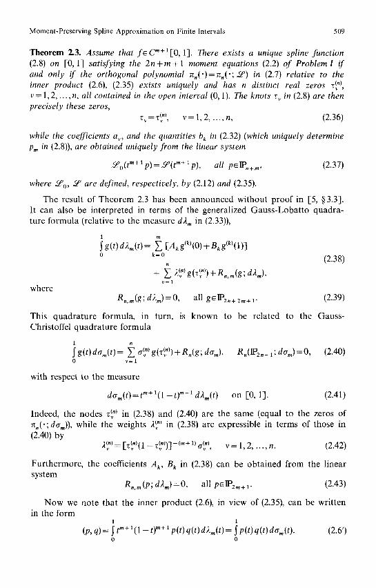
Theorem 2.3. Assume that f e C " + l [ 0 , 1]. There exists a unique spline function (2.8) on [0,1] satisfying the 2 n + m + l moment equations (2.2) of ProblemI if and only if the orthogonal polynomial 7z,( ')=nn('; ~Cf) in (2.7) relative to the inner product (2.6), (2.35) exists uniquely and has n distinct real zeros z(~ "), v = l, 2 . . . . . n, all contained in the open interval (0, 1). The knots z v in (2.8) are then precisely these zeros,

~(") (2.36) r v = . ~ , v= 1 ,2 , . . . ,n ,

while the coefficients av, and the quantities b k in (2.32) (which uniquely determine p,, in (2.8)), are obtained uniquely from the linear system

~o(t"+ l p)==L~(t"+ l p), all p~IP,+m, (2.37)

where ~o, 5P are defined, respectively, by (2.12) and (2.35).

The result of Theorem 2.3 has been announced without proof in [5, w 3.3]. It can also be interpreted in terms of the generalized Gauss-Lobatto quadrature formula (relative to the measure d2 m in (2.33)),

1

S g (t) d2 . (t) = ~ [A k g(k)(0) + B k g(k)(1)] o k=O (2.38)

+ ~ 2~)g(Z~v"))+R,,,.(g; d2,,), v = l

where R.,,.(g; d2m) =0 , all g~]P2n+z,n+l' (2.39)

This quadrature formula, in turn, is known to be related to the Gauss- Christoffel quadrature formula

1

Sg(t)da~(t)= ~ ov-(")g(z~v"))+R,(g;d~,.), Rn(]Pzn_l;d6m)=O, (2.40) 0 v = l

with respect to the measure

dam(t)=t"+l(1 - t ) '+ ld )%( t ) on [0, 1]. (2.41)

Indeed, the nodes -(") in (2.38) and (2.40) are the same (equal to the zeros of "/'V 7t,(';da,,)), while the weights 2~ ) in (2.38) are expressible in terms of those in (2.40) by

2~ ")= [z~")(1 (") -("~+~) (") (2.42) - % )] c%, v= 1,2, . . . ,n .

Furthermore, the coefficients Ak, B k in (2.38) can be obtained from the linear system

R,,,, (p; d2,.) =0 , all p~IP2,,+ ~. (2.43)

Now we note that the inner product (2.6), in view of (2.35), can be written in the form

1 1

(17, q)= ~ t"+a(1 - t )"+lp(t)q(t)d2, , ( t ) = ~p(t)q(t)dtr,,(t). (2.6') O 0

510 M. F r o n t i n i et al.

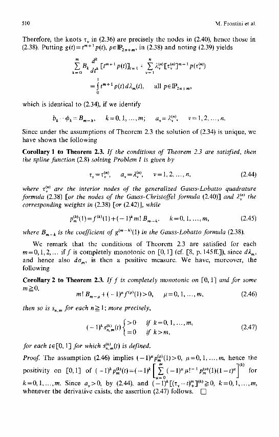
Therefore, the knots % in (2.36) are precisely the nodes in (2.40), hence those in (2.38). Putt ing g(t)= t "+1 p(t), peIP2,+, ,, in (2.38) and noting (2.39) yields

Bk ~ Elm+ x p(t)]t = 1 + 2(,) [Z(,)],~+ 1 p (Z~,)) k = O v = l

1

=~t"+lp(t)d2,.(t), all p~IP2.+~, 0

which is identical to (2.34), if we identify

)(n) bk--C~k=B,,_k, k = 0 , 1 , . . . , m ; av= ~, v = 1 , 2 . . . . . n.

Since under the assumptions of Theorem 2.3 the solution of (2.34) is unique, we have shown the following

Corollary 1 to Theorem 2.3. I f the conditions of Theorem 2.3 are satisfied, then the spline function (2.8) solving Problem I is given by

z v = z~ "), _~,7 = _v~("), v = 1, 2, ..., n, (2.44)

where -(") are the interior nodes of the generalized Gauss-Lobatto quadrature formula (2.38) [or the nodes of the Gauss-Christoffel formula (2.40)] and 2~ ) the corresponding weights in (2.38) [or (2.42)], while

p~(1) =f(k)(1) + ( - 1)kin! Bin_k, k = 0 , 1, ..., m, (2.45)

where B,,_ k is the coefficient of g("-k)(1) in the Gauss-Lobatto formula (2.38).

We remark that the condit ions of Theorem 2.3 are satisfied for each m = 0 , 1,2, ... i f f is completely monotonic on [0, 1] (cf. [8, p. 145 ff.]), since d2,,, and hence also d ~ , is then a positive measure. We have, moreover, the following

Corollary 2 to Theorem 2.3. I f f is completely monotonic on [0, 1-1 and for some m >= O,

m! B,,_u+(-1)uf(u)(1)>O, # = 0 , 1, ..., m, (2.46)

then so is s,.,, for each n > 1; more precisely,

1 k o(k) ~,~ ~" > 0 if k = 0, 1 . . . . , m, (2.47) ( - - ) ~ 1 = 0 if k>m,

for each t6[0, 1] for which s (k) (t~ is defined. n9 my-/

Proof The assumption (2.46) implies ( u (u) - 1 ) p,, (1)>0, p = 0 , 1 . . . . ,m, hence the

positivity on [0,1] o f ( - k (k ) [ ~ 1) p,, ( t )=(--1)k " - o (--1)u/~!-~ P~)(1)(1--t)uJ (k) ]

for # -

k = 0 , 1 , . . . , m . Since a~>0, by (2.44), and (--1)k[(z~--t)+](k)>0, k = 0 , 1 . . . . . m, whenever the derivative exists, the assertion (2.47) follows. [ ]

M o m e n t - P r e s e r v i n g Spl ine A p p r o x i m a t i o n on F in i te In te rva l s 511

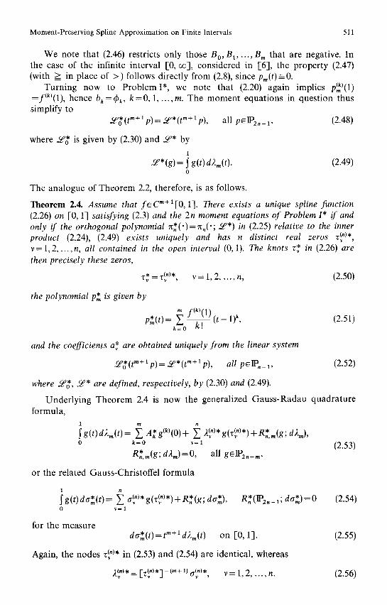
We note that (2.46) restricts only those B 0, B l . . . . . B., that are negative. In the case of the infinite interval [-0, ~ ] , considered in [6], the property (2.47) (with > in place of > ) follows directly from (2.8), since Pm(t)=--O.

Turning now to Problem I*, we note that (2.20) again implies p~)(1) =f(k)(1), hence bk=49k, k=0 , 1 . . . . . m. The moment equations in question thus simplify to

~*(tm+lp)=~*(tm+tp), all p~IPzn_l, (2.48)

where &,q* is given by (2.30) and _~a. by

1

5e*(g) = S g(t) d2,,(t). (2.49) 0

The analogue of Theorem 2.2, therefore, is as follows.

Theorem 2.4. Assume that f ~ C " + a [ 0 , 1]. There exists a unique spline function (2.26) on [0, 1] satisfying (2.3) and the 2n moment equations of Problem I* if and only if the orthogonal polynomial 7z*( ' )=n, ( ' ; ~ * ) in (2.25) relative to the inner product (2.24), (2.49) exists uniquely and has n distinct real zeros z(~ ")*, v= 1,2 . . . . . n, all contained in the open interval (0, 1). The knots z* in (2.26) are then precisely these zeros,

* - ~(")* (2.50) z v - - v , v = l , 2 , . . . , n ,

the polynomial p* is given by

k=O K!

* obtained uniquely from the linear system and the coefficients av are

Lr all p~lP._a, (2.52)

where 5fl~, 5fl* are defined, respectively, by (2.30) and (2.49).

Underlying Theorem 2.4 is now the generalized Gauss-Radau quadra ture formula,

2 v g(% ) + ,,,,(g, d2,,), o k= 0 ~= 1 (2.53)

R * ' ,,.,(g, d2, . )=0, all g~lP2,+, .,

or the related Gauss-Christoffel formula

' i * . fg(t)do*(t)= v v'~(")* ~,~,ot,(.)*~- ,,~,, da*), R. ( l P 2 n _ 1, d a * ) = 0 (2.54)

0 v = l

for the measure da*(t)=tm+~d2m(t) on [0, 1]. (2.55)

Again, the nodes z~ )* in (2.53) and (2.54) are identical, whereas

2~ ")* = L-vrz(")*lJ -(,,+ 1) v,rr(")*, v = 1, 2, ..., n. (2.56)


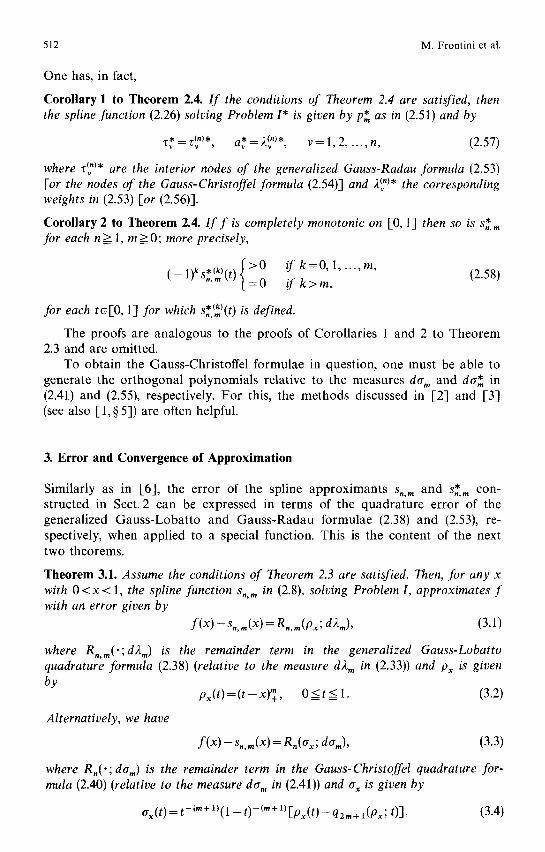
One has, in fact,

Corollary 1 to Theorem 2.4. I f the conditions of Theorem 2.4 are satisfied, then the spline function (2.26) solving Problem I* is given by p* as in (2.51) and by

t* = ~'~")* a* =,~")* v = 1, 2, n, (2.57) v ~ v , - ' v - ' v , " " " ,

where ~-~")* are the interior nodes of the generalized Gauss-Radar formula (2.53) [or the nodes of the Gauss-Christoffel formula (2.54)] and 2~ )* the corresponding weights in (2.53) [or (2.56)].

Corollary 2 to Theorem 2.4. I f f is completely monotonic on [0, I] then so is * S n, ",

for each n__> 1, m>=0; more precisely,

1 ks*(k) t ~ > 0 /f k - 0 , 1 . . . . . m, ( - ) , , " , ( ) (2.58) = 0 if k>m,

for each t e l0 , 1] for which .(k) S.,", (t) is defined.

The proofs are analogous to the proofs of Corollaries 1 and 2 to Theorem 2.3 and are omitted.

To obtain the Gauss-Christoffel formulae in question, one must be able to generate the or thogonal polynomials relative to the measures da", and dcr* in (2.41) and (2.55), respectively. For this, the methods discussed in [2] and [3] (see also [1, w 5]) are often helpful.

3. Error and Convergence of Approximation

Similarly as in [6], the error of the spline approximants s.", and * , S n , " , c o n -

s t r u c t e d in Sect. 2 can be expressed in terms of the quadra ture error of the generalized Gauss-Lobat to and Gauss -Radau formulae (2.38) and (2.53), respectively, when applied to a special function. This is the content of the next two theorems.

Theorem 3.1. Assume the conditions of Theorem 2.3 are satisfied. Then, for any x with 0 < x < l , the spline function s,,", in (2.8), solving Problem I, approximates f with an error given by

f (x ) -s , , " , (x ) = R.,",(px; d2m), (3.1)

where R,,",(';d2,.) is the remainder term in the generalized Gauss-Lobatto quadrature formula (2.38) (relative to the measure d2", in (2.33)) and Px is given by

px( t )=( t -x)+, 0 < t < 1. (3.2)

Alternatively, we have

f (x ) - s.,",(x) = R,(ax; d%), (3.3)

where R,(- ; dam) is the remainder term in the Gauss-Christoffel quadrature formula (2.40) (relative to the measure de., in (2.41)) and ax is given by

ax(t) = t-(",+ 1)( 1 - t) -(",+ n [px(t) - q2",+ l(Px; t)], (3.4)


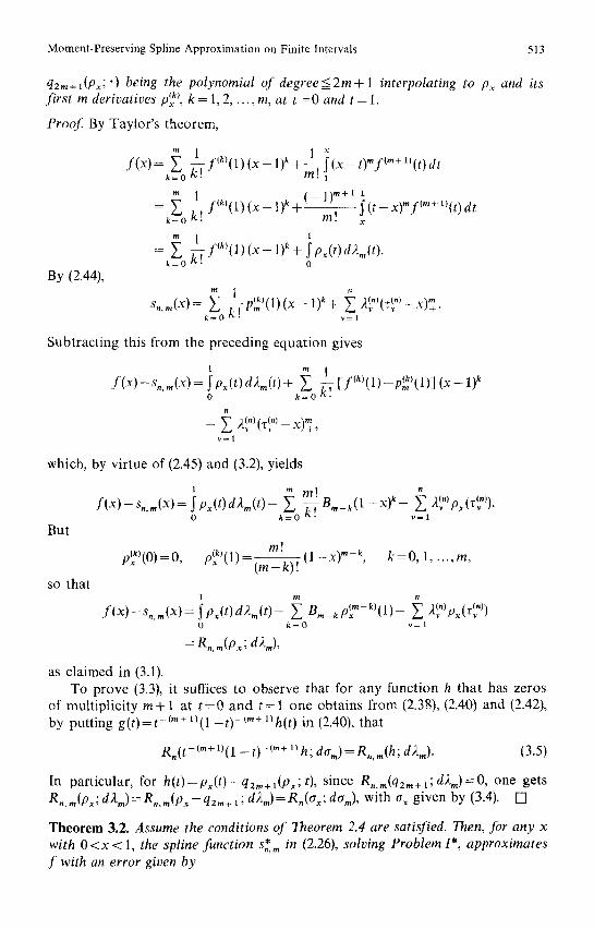
q2m+l(Px; ") being the polynomial of degree<=2m+ 1 interpolating to Px and its first m derivatives #k) k = l 2, ..,re, at t=O and t=1.

Proof By Taylor 's theorem,

By (2.44),

f(X)=k~=O f(k)(1)(X--1)k+~..{(x--t)"f("+l)(t)dt

= ~ ~ f ( k ' (1 ) ( x - - l ) k~ ( - - 1 ) ' + ' i k=O �9 m! (t-x)mf(m+l)(t)dt x

1

= ~ l~f'k)(1)(X--1)k+ Ipx(t)d2m(t). k=O k ! ~ " " 0

s,~(x) ~, l ptmk)(l)(x--1)~+ ~ ~") I,) , = ,~ (~ - x ) + . k = O " v = l

Subtracting this from the preceding equation gives

f(x)--S,,m(X ) = ~p~(t) d2,,(t)+ k.T If(k)(1)--ffd)(1)] (x - 1) k 0 k = O

(n) (n) m - ,~ (~ - x ) + ,

v = l

which, by virtue of (2.45) and (3.2), yields

But

so that

1. ~ m! ~ ,~ p~( ~ ). f(x)--s, ,m(x)= jp~(t)d2m(t)- )_f, ~ .B, . -k(1--X) k - (") Zt,)

0 k = O " v = l

m~ p?'(0)=0, p~)(1)- ( l -x ) m-~, k=0,1 ..... m,

(m-k) !

R ~(m-k)~l ~(n) D (T (n)) f (x)-s , , , . (x)=~Px(t)d)c, , ( t )- ~m-kVx , ' ) - - - . . . . -~ , 0 k = O v = l

= R,,,,(px; d2,,),

as claimed in (3.1). To prove (3.3), it suffices to observe that for any function h that has zeros

of multiplicity m + 1 at t=O and t = 1 one obtains from (2.38), (2.40) and (2.42), by putting g ( t )= t - ("+ ~)(1 - t ) -(m+ 1)h(t) in (2.40), that

R,(t-(,,+ 1)(1 _ t)-(,,+ 1)h; dam) = R,, m(h; d2,.). (3.5)

In particular, for h(t)=px(t)-q2,,+l(p~; t), since R,,,,(qz,~+l;d)~m)=O, one gets R,,m(px; dX,,)=R,,m(px-qz~+l;d2m)=R,(ax; dam), with ax given by (3.4). [ ]

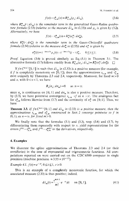
Theorem 3.2. Assume the conditions of Theorem 2.4 are satisfied. Then, for any x with 0 <x < 1, the spline function s,*,,, in (2.26), solving Problem I*, approximates f with an error given by

514 M. Frontini e ta l .

f (x) - s* ,, (x) = R,* m (Px; d2m), (3.6)

, 'here * ." R, , , , ( , d2m) is the remainder term in the generalized Gauss-Radau quadrature formula (2.53) (relative to the measure d). m in (2.33)) and Px is given by (3.2). Alternatively, we have

f ( x ) - - S * m ( X ) = * * * R , (ax ; dam), (3.7)

where * "" R , ( , d a * ) is the remainder tern, in the Gauss-Christoffel quadrature �9 is given by formula (2.54) (relative to the measure da* in (2.55)) and ax

a * ( t ) = t - ( " + l ) p ~ ( t ) = t - { m + l ) ( t - x ) + , 0_<t_< 1. (3.8)

Proof Equat ion (3.6) is proved similarly as Eq.(3.1) in Theorem 3.1. The �9 . " - * * ' d o ' * ) . alternative formula (3.7) follows readily from Rn,m(Px , d z m ) - R n (a x , []

I f f e c m + l [ 0 , 1] is such that d2 m in (2.33) is a positive measure (for example, i f f is completely monoton ic on [0, 1]), then the approximat ions Sn, m and s,, m ~* exist uniquely by Theorems 2.3 and 2.4, respectively. Moreover , for fixed m > 0 and x, with 0 < x < 1, we have

R. (a~ ;da , . )~O as n--*~

since a x is cont inuous on [-0, 1] and da m is also a positive measure. Therefore, by (3.3), we have pointwise convergence s , , m ~ f as n--*~. The analogous fact for s,,* m follows likewise from (3.7) and the continuity of a* on [0, 1]. Thus, we have

Theorem 3.3. I f f ~ c m + l [ O , 1] and d2 m in (2.33) is a positive measure, then the approximations s o,,. and s,,* m constructed in Sect. 2 converge pointwise to f in (0, 1), as n ~ oo for f i x e d m > O.

We finally note that the formulas (3.1) and (3.3), resp. (3.6) and (3.7), by differentiating them repeatedly with respect to x, yield representations for the e r r o r s f ( k ) s.,(k),, and ~f(k)--s*(k)-n,m in the derivatives, respectively.

4. Examples

We illustrate the spline approximat ions of Theorems 2.3 and 2.4 (or their corollaries) in the case of exponential and t r igonometr ic functions. All com- putations reported on were carried out on the CDC 6500 computer in single precision (machine precision ~3.55 x 10-15).

Example 4.1. f ( t ) = e - " , 0 < t < 1, c > 0 .

This is an example of a completely monoton ic function, for which the associated measure (2.33) is thus positive; indeed,

cm+ 1 d 2 m ( t ) = ~ e - " d t on [0, 1]. (4.1)

m ~

M o m e n t - P r e s e r v i n g S p l i n e A p p r o x i m a t i o n o n F i n i t e I n t e r v a l s 515

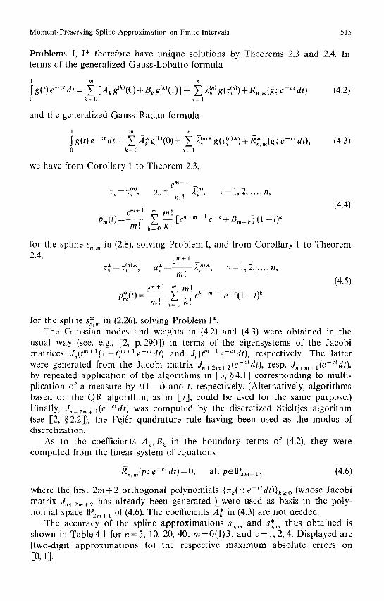
Problems I, I* therefore have unique solutions by Theorems 2.3 and 2.4. In terms of the generalized Gauss-Lobatto formula

1

~g ( t ) e - a d t = ~ [Akg(k)(o)+Bkg'k)(1)] + L y(") (") - " e - a 2 v g(zv )+R,, , , (g, dt) (4.2) 0 k = 0 v = l

and the generalized Gauss-Radau formula

1

g(t)e ct dt ~ A* g(k'(0)+ L 2~Y(")* g(z~(")*)+ -* " = R.,.,(g, e-Ctdt), (4.3) 0 k = 0 v = l

we have from Corollary 1 to Theorem 2.3,

C m + 1

L. = z~ ), a,. = ~ ;~"), v = 1, 2 . . . . , n,

(4.4) c m + 1 m T

5" m:[ck-m- le -C+B, , k](1--t) k p,,(t) = ~ �9 ~ o k ! L

for the spline s,,,, in (2.8), solving Problem I, and from Corollary 1 to Theorem 2.4, c m + 1 _

* : T(n)* , = _ ) ( n ) * z v _,, , a~ m! "~ ' v = l , 2 , . . . , n , (4.5)

c m + l m mt p*(t) = _ _ y """ c k- , . - 1 e - C ( 1 ~ t ~ k

m! k~--o k!

for the spline s.,*,, in (2.26), solving Problem I*. The Gaussian nodes and weights in (4.2) and (4.3) were obtained in the

usual way (see, e.g., [2, p. 290]) in terms of the eigensystems of the Jacobi matrices J,( tm+l(1-t)"+le-~tdt) and J,(tm+le-C~dt), respectively. The latter were generated from the Jacobi matrix Jn+zm+z(e-~'tdt), resp. J,+,,+l(e-Ctdt), by repeated application of the algorithms in [3, w corresponding to multi- plication of a measure by t ( 1 - t ) and t, respectively. (Alternatively, algorithms based on the QR algorithm, as in [-7], could be used for the same purpose.) Finally, Jn+2m+z(e-~tdt) was computed by the discretized Stieltjes algorithm (see [2, w the Fej6r quadrature rule having been used as the modus of discretization.

As to the coefficients Ak, B k in the boundary terms of (4.2), they were computed from the linear system of equations

/~,,m(P; e-~'dt) =0, all pElP2m+l , (4.6)

where the first 2 m + 2 orthogonal polynomials {rCk('; e-~tdt)}k>=O (whose Jacobi matrix J,+2m+2 has already been generated!) were used as basis in the polynomial space IP2,,+ 1 of (4.6). The coefficients 4 " in (4.3) are not needed.

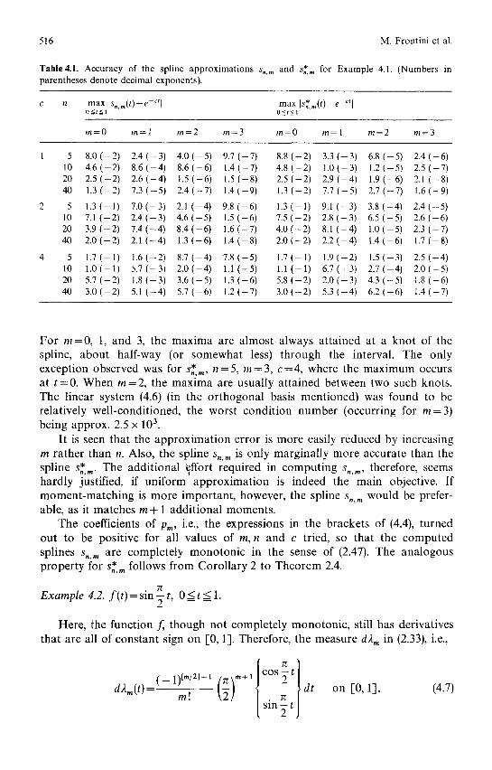
The accuracy of the spline approximations S,,m and S,,*m thus obtained is shown in Table 4.1 for n=5 , 10, 20, 40; m=0(1)3; and c = 1 , 2 , 4 . Displayed are (two-digit approximations to) the respective maximum absolute errors on [o, 13.


Table4.1. Accuracy of the spline approximations s,,~, and s.,,.* for Example 4.1. (Numbers in parentheses denote decimal exponents).

c n max [s,,m(t)-e c,] max Is*m(t)-e ctl O=<t=<l O<t_<l

m=O m=l m=2 m=3 m=O m=l m=2 m=3

1 5 8.0(-2) 2.4(-3) 4.0(-5) 9.7(-7) 8.8(-2) 3.3(-3) 6.8(-5) 2.4(-6) 10 4.6(-2) 8.6(-4) 8.6(-6) 1.4(-7) 4.8(-2) 1.0(-3) 1.2(-5) 2.5(-7) 20 2.5 (-2) 2.6 (-4) 1.5 (-6) 1.5 (-8) 2.5 (-2) 2.9 (-4) 1.9 (--6) 2.1 (-8) 40 1.3(-2) 7.3(-5) 2.4(-7) 1.4[-9) 1.3(-2) 7.7(-5) 2.7(--7) 1.6(-9)

5 1.3(-1) 7.0(-3) 2.1(-4) 9.8(-6) 1.3(-1) 9.1(-3) 3.8(-4) 2.4(-5) 10 7.1(-2) 2.4(-3) 4.6(-5) 1.5(-6) 7.5(-2) 2.8(-3) 6.5(-5) 2.6(-6) 20 3.9(-2) 7.4(-4) 8.4(-6) 1.6(-7) 4.0(-2) 8.1(-4) 1.0(-5) 2.3(-7) 40 2.0(-2) 2.1(-4) 1.3(-6) 1.4(-8) 2.0(-2) 2.2(-4) 1.4(-6) 1.7(-8)

5 1.7(-1) 1.6(-2) 8.7(-4) 7.8(-5) 1.7(-1) 1.9(-2) 1.5(-3) 2.5(-4) 10 1.0(-1) 5.7(-3) 2.0(-4) 1.1(-5) 1.l(-1) 6.7(-3) 2.7(-4) 2.0(-5) 20 5.7(-2) 1.8(-3) 3.6(-5) 1.3(-6) 5.8(-2) 2.0(-3) 4.3(-5) 1.8(-6) 40 3.0(-2) 5.1 (-4) 5.7 (-6) 1.2 (-7) 3.0 (-2) 5.3 (-4) 6.2 (-6) 1.4 (-7)

For m = 0 , 1, and 3, the maxima are almost always attained at a knot of the spline, about half-way (or somewhat less) through the interval. The only exception observed was for s,,,,,* n = 5, m = 3, c =4 , where the maximum occurs at t = 0 . When m--2 , the maxima are usually attained between two such knots. The linear system (4.6) (in the or thogonal basis mentioned) was found to be relatively well-conditioned, the worst condit ion number (occurring for m = 3 ) being approx. 2.5 x 10 3.

It is seen that the approximat ion error is more easily reduced by increasing m rather than n. Also, the spline s,, m is only marginally more accurate than the spline s,*,m. The addit ional ~ffort required in comput ing s,,m, therefore, seems hardly justified, if uniform approximat ion is indeed the main objective. If moment -match ing is more important , however, the spline s,, m would be prefer- able, as it matches m + 1 addit ional moments.

The coefficients of p,~, i.e., the expressions in the brackets of (4.4), turned out to be positive for all values of m,n and c tried, so that the computed splines s,, m are completely mono ton ic in the sense of (2.47). The analogous proper ty for s.,*,, follows from Corol lary 2 to Theorem 2.4.

Example 4.2. f ( t ) = sin 2 t, 0 -< t -< 1.

Here, the function f, though not completely monotonic , still has derivatives that are all of constant sign on [0, 1]. Therefore, the measure d2 m in (2.33), i.e.,

dRm(t)=(-1)tm/21+~ / c ~ m' (2)m+ 1 / T~I dt

[ s i n ~ t ]

on [-0, 1], (4.7)


where the cosine or sine is taken according as m is even or odd, admits a unique system of (monic) or thogonal polynomials , and Problems I and I* both have unique solutions for each m and n. Observing that the subst i tut ion t-+ 1 - t carries the cosine into the sine, and vice versa, it suffices to generate the or thogona l polynomials for one of the t r igonometr ic measures only, say cos((=/2)t)dt. If e~,, fl~,, are the coefficients in the corresponding recurrence relation

lZk+l( t )=( t - -O~k)gk( t ) - - f l k~Zk_l ( t ) , k=O, 1, 2 . . . . . (4.8)

= _ l ( t ) = 0 , rc0(t)=l ,

then the coefficients ~,, fl~, for the s ine-measure are

~, = 1 - ~,, fl~,: fl~,, k = 0, 1, 2, . . . . (4.9)

A similar r emark applies to the generalized Loba t to measures (2.41) [but not to the generalized Radau measures (2.55)]. The constants mult iplying the t r igonometr ic measures in (4.7), of course, simply give rise to analogous multi- plicative constants in the quadra ture rules (2.38) and (2.53).

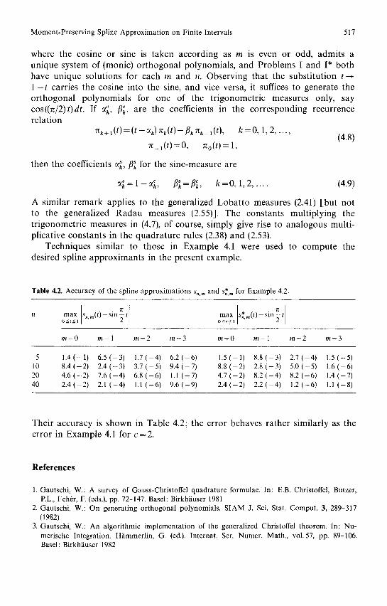
Techniques similar to those in Example 4.1 were used to compute the desired spline approx iman t s in the present example.

Table 4.2. Accuracy of the spline approximations s,, m and s*.,. for Example 4.2.

n max s, ( t ) -s in~- t max s*m( t ) - s i n2 t o-<t<l .m 2 o~,<~ '

m=O m = l m=2 m=3 m=O m = l m=2 m=3

5 1 .4( -1) 6 .5 ( -3 ) 1 .7 ( -4 ) 6 .2 ( -6 ) 1 .5( -1) 8 .8 ( -3 ) 2 .7 ( -4 ) 1 .5( -5) 10 8.4 ( - 2 ) 2 . 4 ( -3 ) 3.7 ( - 5 ) 9.4 ( - 7 ) 8.8 ( - 2 ) 2.8 ( - 3 ) 5.0 ( - 5 ) 1.6 ( - 6 ) 20 4.6 ( - 2 ) 7.6 ( - 4 ) 6.8 ( - 6 ) 1.I ( - 7 ) 4.7 ( - 2 ) 8.2 ( -4 ) 8.2 ( -6 ) 1.4 ( - 7 ) 40 2.4 ( - 2 ) 2.1 ( - 4 ) 1.1 ( - 6 ) 9.6 ( - 9 ) 2.4 ( - 2 ) 2.2 ( - 4 ) 1.2 ( - 6 ) 1.1 ( - 8 )

Their accuracy is shown in Table 4.2; the error behaves rather similarly as the error in Example 4.1 for c = 2.

References

1. Gautschi, W.: A survey of Gauss-Christoffel quadrature formulae. In: E.B. Christoffel, Butzer, EL., Feh6r, F. (eds.), pp. 72-147. Basel: Birkh~iuser 1981

2. Gautschi, W.: On generating orthogonal polynomials. SIAM J. Sci. Stat. Comput. 3, 289-317 (1982)

3. Gautschi, W.: An algorithmic implementation of the generalized Christoffel theorem. In: Nu- merische Integration. HS_mmerlin, G. (ed.). Internat. Set. Numer. Math., vol. 57, pp. 89-106. Basel: Birkh~iuser 1982


4. Gautschi, W.: Discrete approximations to spherically symmetric distributions. Numer. Math. 44, 53-60 (1984)

5. Gautschi, W.: Some new applications of orthogonal polynomials. In: Polyn6mes orthogonaux et applications. Brezinski, C., Draux, A., Magnus, A.P., Maroni, P., Ronveaux, A. (eds.). Lecture Notes Math., vol. 1171, pp. 63-73. Berlin-Heidelberg-New York-Tokyo: Springer 1985

6. Gautschi, W., Milovanovi6, G.V.: Spline approximations to spherically symmetric distributions. Numer. Math. 49, 111-121 (1986)

7. Golub, G.H., Kautsky, J.: Calculation of Gauss quadratures with multiple free and fixed knots. Numer. Math. 41, 147-163 (1983)

8. Widder, D.V.: The Laplace Transform. Princeton: University Press 1941

Received July 21, 1986/November 17, 1986

moment-preserving spline approximation on finite intervals

Documents