Optimal Video Stream Multiplexing through Linear Programming

Helman I Stern* and Ofer Hadar**

*Department of Industrial Engineering and Management

**Department of Communication Systems Engineering

Ben-Gurion University of the Negev

P.O.Box 653, Be’er-Sheeva 84105, ISRAEL

E-mail: (helman,hadar)@bgumail.bgu.ac.il

ABSTRACT

This paper presents a new optimal multiplexing scheme for compressed video streams based on a

piecewise linear approximation of the accumulative data curve of each stream. A linear programming

algorithm is proffered, which takes into account different constraints of each client. It is shown that the

algorithm succeeds in obtaining maximum bandwidth utilization with Quality of Service (QoS) guarantees.

The algorithm takes into account the interaction between the multiplexed streams and the individual

streams, and simultaneously finds the optimum total multiplexed schedule and individual stream schedules

that minimizes the peak transmission rate. In addition, the algorithm, due to the linear programming

formulation, is bounded in polynomial time. Simulation results using 10 real MPEG-1 video sequences are

presented. The optimal multiplexing linear programming results are compared to the PCRTT procedure in

terms of peak transmission bandwidth, P-loss performance, and entropy measures. For several client buffer

sizes, the rate obtained by our LP solution when compared to a previous PCRTT method resulted in a 30

percent reduction.. Therefore, the proposed scheme can allow an increase in the number of simultaneously

served video streams.

Key words: Video rate smoothing, Optimal multiplexing, Statistical multiplexing gain, Network

utilization, Linear programming.

1. Introduction

The main problem of transmitting compressed video over communication networks is its

burstiness. Compressed movies exhibit peak rates that are often significantly larger than their long-term

average rate. One of the suggested solutions for reducing burstiness is to use a playback buffer at the client

site (PC, workstation, or set-top box). In such a system, the video streams are stored at a multimedia server

and transmitted through the network to the client site. The client’s video card then decodes the stream and

forwards it to the video display. The server can significantly reduce the bandwidth requirements for

transmitting stored video streams by prefetching frames into the client playback buffer. In order to

compute an efficient server transmission plan, bandwidth-smoothing algorithms usually require a priori

knowledge of the client buffer size and the length of the transmitted video frames. Many kinds of video

smoothing techniques [1-6] have been developed for reducing the bandwidth variability of video streams

in order to improve network utilization. These techniques exploit client buffering and determine a smooth

rate transmission schedule.

The traffic management schemes for VBR video fall into four main categories [7]: (1)

deterministic without smoothing, (2) deterministic with smoothing, (3) probabilistic, and (4) probabilistic

with collaborative prefetching schemes. In the first scheme [8,9], the original VBR traffic is sent into the

network. Hence, for highly variable VBR traffic this scheme requires large initial delays to achieve

moderate link utilization. The second scheme [10,11], sends a smoothed version of the original VBR

traffic into the network. The video traffic is transmitted at different constant rates over different intervals

according to a specific transmission schedule. The piece-wise constant-rate transmission schedule takes

advantage of the fact that some of the prerecorded video can be prefetched into the client buffer. The

challenge lies in computing those transmission schedules that have the smallest peak rate and rate

variability while ensuring that the client buffer neither over- nor underflows. The probabilistic schemes

send the original VBR encoded video into a non-buffered multiplexer [12]. This scheme introduces

packets loss whenever the aggregate transmission rate exceeds the data link rate. The original traffic can

be first smoothed before it is statistically multiplexed at a non-buffered link. The statistical multiplexing of

the smoothed traffic increases link utilization at the expense of small packet loss probabilities. Reisslein

and Ross [7] present a probabilistic transmission scheme with collaborative prefetching that determines the

transmission schedule of a connection on-line as a function of the buffer contents at all the clients. It is

shown that prefetching protocols with collaborative prefetching have less packet loss than the optimal

smoothing algorithm [13] for the same link utilization.

Using smoothing, one can represent a variable bit rate (VBR) stream as a series of fixed constant

bit rates (CBR), thus simplifying the allocation of network resources and increasing their utilization. This

is the approach used by the PCRTT algorithm found in [1]. The difficulty of the PCRTT approach is that it

treats each stream independently thus providing a sub optimal solution. In this paper we retain the constant

bit rate assumption, but propose an LP algorithm, which treats all video streams collectively to obtain an

optimal solution.

The rest of the paper is organized as follows. In Section 2, the optimal multiplexing problem is

defined. Section 3 presents the notation and the formal description of the problem. The conversion of the

Multiplexed Problem (MP) to an upper bounded linear program is presented in Section 4. Section 5 deals

with the influence of the total buffer size of all clients on the optimal solution as well as, the optimal

buffer allocation. Section 6 presents several small numerical examples using the proposed scheme. Section

7 provides LP solutions using real video streams. The LP and PCRTT solutions are compared using

entropy and a p–loss measure in Sections 8 and 9 , respectively. Section 10 concludes the paper.

2. The Optimal Multiplexing Problem

Many researchers have tried to find the optimal solution for transmitting stored video streams

using smoothing techniques that are applied to each individual stream [1,3,7,13,16]. However, most of

smoothing schemes do not exploit the statistical multiplexing gain that can be obtained before smoothing.

Kang and Yeom [17] proposed a scheme that deals not only with an individual stream, but also with the set

of streams being serviced in order to achieve the optimal network bandwidth utilization and maximize the

number of streams that can be serviced simultaneously. One of the main drawbacks of this approach is its

computational load, since the transmission schedule must be re-calculated for each new request and

applied to the whole set of video streams being serviced.

2.1 The PCRTT and e-PCRTT smoothing algorithms

In this section a smoothing algorithm, which employs CBRs over a series of equal size intervals is

described. This smoothing technique is called a piecewise constant rate transmission and transport

(PCRTT) smoothing technique in the literature [1]. PCRTT determines individually for each video stream

a transmission rate for each time interval by connecting the intersection points of the vertical borderlines

of the time intervals with the accumulative data curve, L (see Section 3). These connections determine a

piecewise linear function. The slope of the jth linear segment, over interval j, corresponds to a rate rj in a

bandwidth transmission plan. To avoid buffer underflow, PCRTT offsets this plan vertically when needed.

This guarantees that the whole run lies above the L curve [1]. Raising the plan corresponds to introducing

an initial playback delay at the client site. Since a PCRTT rate plan consists of fixed-size intervals, the

bandwidth changes occur at constant times. In the PCRTT scheme any increase of the buffer size above a

threshold value will not influence the results of the transmission schedule.

An enhancement to PCRTT, called e-PCRTT, has been proposed in [11]. The idea behind e-PCRTT is

to impose local constraints on the trajectory bandwidth rate plan instead of the global constraints imposed

by the original algorithm. e-PCRTT aims at reducing the required buffer space for the same fixed-size

intervals. This algorithm can increase the length of the smoothing interval while using the same buffer

size. The practical implication of increasing the interval size is that the number of bandwidth changes can

be reduced. This is of crucial importance for ATM networks that allow users to renegotiate their traffic

parameters.

2.2 Collective Stream Smoothing

The PCRTT and e-PCRTT smoothing schemes treat multiple video sources by smoothing the

individual streams independently and not collectively. Thus, they only achieve the optimal solution for an

individual stream but not an optimum solution for the multiplexed stream. In this paper, we propose a new

smoothing scheme that deals with not only the individual streams, but the entire complex of streams being

serviced simultaneously. We call this the Optimal Multiplexing Problem, and offer a linear programming

formulation for its solution.

The advantage of our suggested methodology is not only that it attains the optimum solution, but

also that it allows the possibility of imposing different constraints on each of the clients depending of their

buffer size. With our linear programming scheme it is possible to simultaneously minimize the aggregated

bandwidth of the multiplexed stream. Throughout the paper, we consider only the end nodes behavior,

while assuming the network provides the QoS required by the algorithm, namely guaranteed bandwidth

and no jitter. Hence, data loss is only attributed to decoder buffer overflow and not to network congestion.

There are many ways to determine the starting time of each multiplexed stream. Assuming the

stream arrangement is achieved by enforcing the starting time of the multiplexed video streams, we

describe a possible arrangement for multiplexing smoothed video streams. In what follows we constrain all

the streams to be synchronized in terms of the start time of of the first smoothing interval. By

synchronizing the streams, in a previous paper [16], it was shown that it is possible to bound the number of

bandwidth changes in the multiplexed stream, and also to reduce the variance of the multiplexed stream.

In what follows, we present the globally optimized smoothing scheme, which also consists

of individual smoothing using constant intervals, which maximizes the number of active streams

while providing deterministic service to each client. The proposed scheme is based on a piecewise

linear approximation of the accumulative data curve of each of the compressed video streams.

This approximation allows the optimal multiplexing problem to be formulated as a linear program.

The suggested scheme minimizes the aggregated bandwidth of the multiplexed stream under the

constraint of overall client buffer requirements.

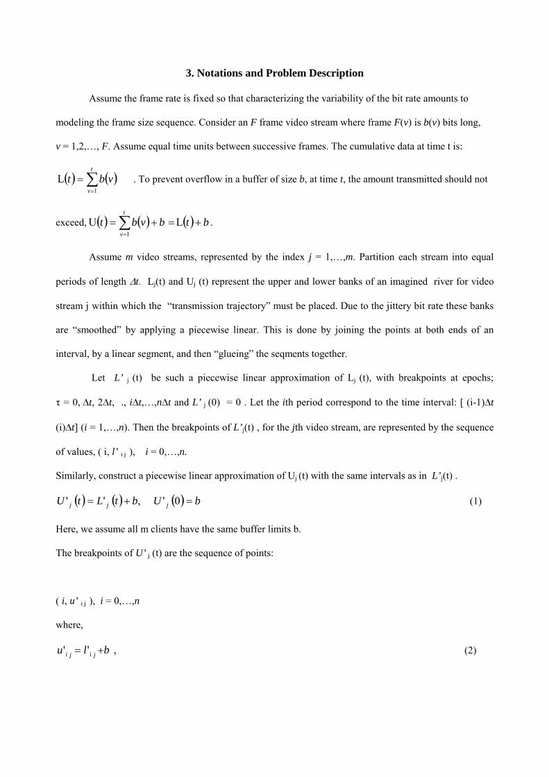
3. Notations and Problem Description

Assume the frame rate is fixed so that characterizing the variability of the bit rate amounts to

modeling the frame size sequence. Consider an F frame video stream where frame F(v) is b(v) bits long,

v = 1,2,…, F. Assume equal time units between successive frames. The cumulative data at time t is:

( ) ( )∑=

=

t

vvbt

1L . To prevent overflow in a buffer of size b, at time t, the amount transmitted should not

exceed, ( ) ( ) ( ) btbvbtt

v+=+=∑

=

LU1

.

Assume m video streams, represented by the index j = 1,…,m. Partition each stream into equal

periods of length ∆t. Lj(t) and Uj (t) represent the upper and lower banks of an imagined river for video

stream j within which the “transmission trajectory” must be placed. Due to the jittery bit rate these banks

are “smoothed” by applying a piecewise linear. This is done by joining the points at both ends of an

interval, by a linear segment, and then “glueing” the seqments together.

Let L’ j (t) be such a piecewise linear approximation of Lj (t), with breakpoints at epochs;

τ = 0, ∆t, 2∆t, ., i∆t,…,n∆t and L’ j (0) = 0 . Let the ith period correspond to the time interval: [ (i-1)∆t

(i)∆t] (i = 1,…,n). Then the breakpoints of L’j(t) , for the jth video stream, are represented by the sequence

of values, ( i, l’ i j ), i = 0,…,n.

Similarly, construct a piecewise linear approximation of Uj (t) with the same intervals as in L’j(t) .

( ) ( ) ( ) bUbtLtU jjj =+= 0','' (1)

Here, we assume all m clients have the same buffer limits b.

The breakpoints of U’ j (t) are the sequence of points:

( i, u’ i j ), i = 0,…,n

where,

,'' blu jiji += (2)

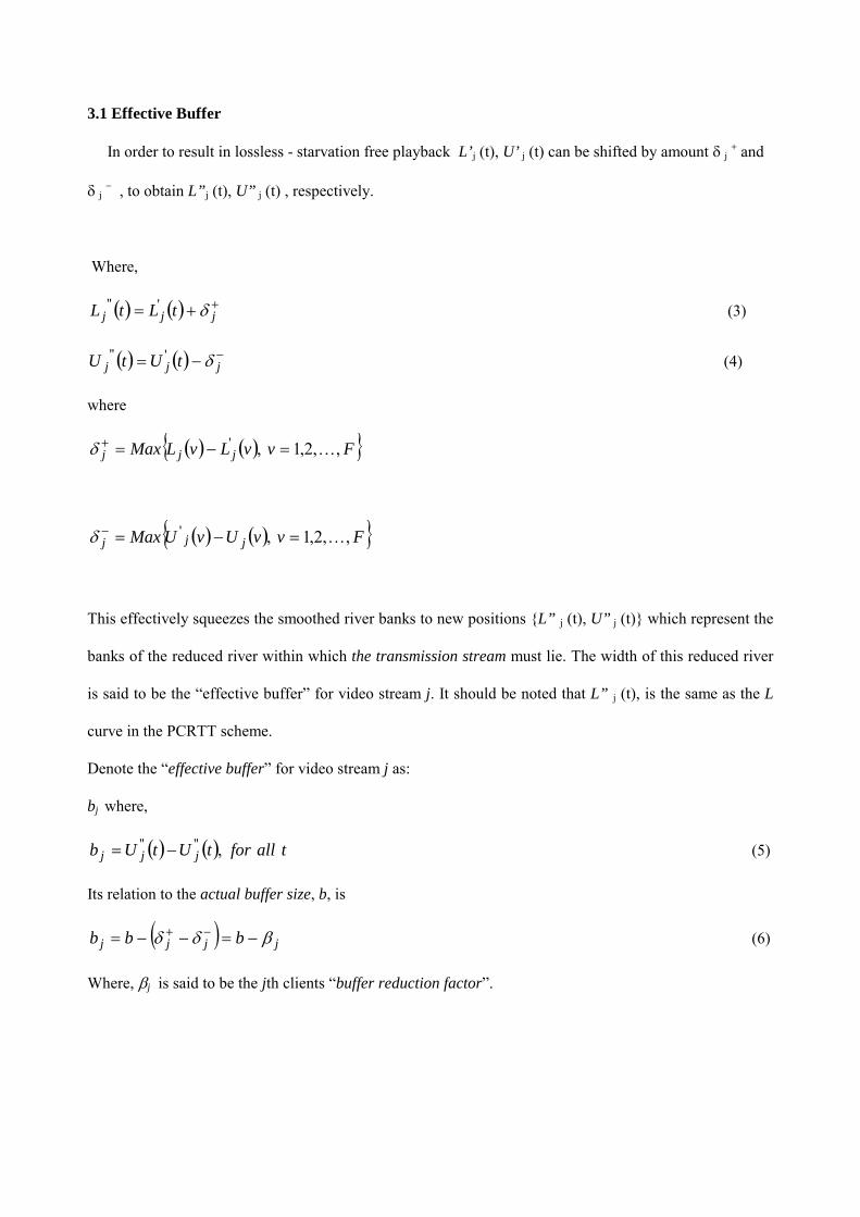
3.1 Effective Buffer

In order to result in lossless - starvation free playback L’j (t), U’ j (t) can be shifted by amount δ j + and

δ j − , to obtain L”j (t), U” j (t) , respectively.

Where,

( ) ( ) ++= jjj tLtL δ

'" (3)

( ) ( ) −

−= jjj tUtU δ'" (4)

where

( ) ( ){ }FvvLvLMax jjj ,,2,1,'l=−=

+δ

( ) ( ){ }FvvUvUMax jjj ,,2,1,'l=−=

−

δ

This effectively squeezes the smoothed river banks to new positions {L” j (t), U” j (t)} which represent the

banks of the reduced river within which the transmission stream must lie. The width of this reduced river

is said to be the “effective buffer” for video stream j. It should be noted that L” j (t), is the same as the L

curve in the PCRTT scheme.

Denote the “effective buffer” for video stream j as:

bj where,

( ) ( ) tallfortUtUb jjj ,""−= (5)

Its relation to the actual buffer size, b, is

( ) jjjj bbb βδδ −=−−=−+ (6)

Where, βj is said to be the jth clients “buffer reduction factor”.

Proposition 1:

Given a real buffer size b for all clients j = 1,…,m, there exist a “critical buffer” value , b*, below which

the combined multiplexed stream is infeasible for the linear approximation.

Proof:

Since the linear approximation defining the reduced river (5) cannot have the upper bank below the lower

bank:

bj = U” j (t) - L”j (t) >= 0

From (6) we see b - βj >=0, j = 1,…,m .

Let the minimum value of b, such that the above is true, be the critical value b*, then

{ }jallforMaxb j ,* β=

We now make a simplifying notational change by letting:

u ij = U” j (i) , i =0,…,n

l ij = l” j (i) , i =0,…,n

The breakpoints for period (i + 1) are shown in Figure 1 below.

A transmission schedule for the jth video stream is represented by the sequence:

{ }niyyS jiijj ,....,0;, 1 ==+

(7)

Such a schedule is said to be a feasible if:

{ }ijijij uyl ≤≤ ,i = 0,…,n (8)

The dash line in the figure 1 shows a feasible transmission schedule. Without loss of generality set ∆t =1.

Let r i j be rate, over segment i, of the jth video stream.

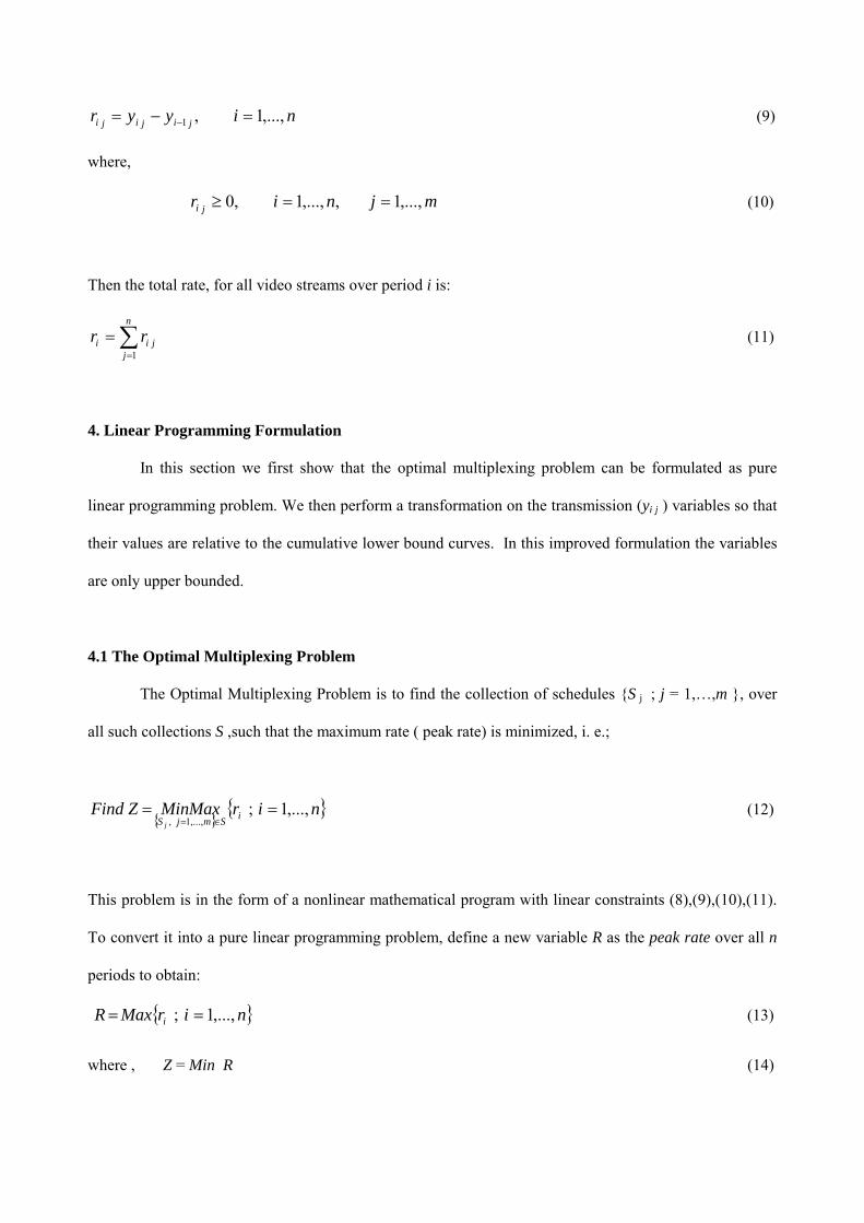
niyyr jijiji ,...,1,1 =−=−

(9)

where,

mjnir ji ,...,1,,...,1,0 ==≥ (10)

Then the total rate, for all video streams over period i is:

∑=

=

n

jjii rr

1

(11)

4. Linear Programming Formulation

In this section we first show that the optimal multiplexing problem can be formulated as pure

linear programming problem. We then perform a transformation on the transmission (yi j ) variables so that

their values are relative to the cumulative lower bound curves. In this improved formulation the variables

are only upper bounded.

4.1 The Optimal Multiplexing Problem

The Optimal Multiplexing Problem is to find the collection of schedules {S j ; j = 1,…,m }, over

all such collections S ,such that the maximum rate ( peak rate) is minimized, i. e.;

{ }{ }nirMinMaxZFind iSmjS j

,...,1;,...,1,

==

∈=

(12)

This problem is in the form of a nonlinear mathematical program with linear constraints (8),(9),(10),(11).

To convert it into a pure linear programming problem, define a new variable R as the peak rate over all n

periods to obtain:

{ }nirMaxR i ,...,1; == (13)

where , Z = Min R (14)

Using (10) and (11) and the fact that nirR i ,...,1; =≥ we obtain:

niRrn

jji ,...,0,

1

=≤∑=

(15)

0≥R (16)

This eliminates the variables r i , so that the basic multiplexing problem (MP) is now:

Problem MP (Linear Programming Formulation)

Z = Min R

subject to: (8),(9),(10),(15),(16)

Constraint (10) is necessary to insure that the rates are nonnegative. The problem size is n(m+1) linear

constraints, (n+1)m upper - lower bounded variables, and nm+1 nonnegative variables. Problem MP

simultaneously solves to peak total rate leveling problem, and the video transmission plans of the

individual video streams. Thus, the solution provides the represents the optimal rate schedules {ri jo ; i =

1,…,n , j = 1,..,m}, for the minimum peak value,Ro, that minimize the peak value of the combined rate

function {r i o ; i = 1,…,n}, as well as, the optimal transmission schedules S j o

= {yi j o , yi+1 j

o ; i = 0,…,n }.

4.2 Conversion of MP to an Upper Bounded Linear Program

We shall perform a transformation on the yi j variables so that their values are relative to the

cumulative lower bound curves. This provides three advantages; (a) it reduces the necessity of dealing

with very large magnitudes of the transmission values which are due to the increasing values of l i j in (8),

(b) it facilitates a parametric analysis of the important factors of the problem and, (c) it reduces the

problem size and consequent search space of the linear programming (LP) problem. The transformation of

the yi j variables converts them to upper bounded variables yi j* by subtracting l i j in (8) to obtain:

mjniuyl ijijij ,...,1,,...,0,***==≤≤ (17)

since, *ijl = 0 and *

iju = ijij ly − the new variables become upper bounded.

mjniby jij ,...,1,,...,0,0 *==≤≤ (18)

The new upper bounded version of problem MP is now:

Problem MP’ (Upper Bounded LP Formulation)

Zmin = Min R

Subject to:

( ) ( ) mjnillyy jiijijji ,...,1,,...,1,1**

1 ==−≤−−−

(19)

nillRyym

j

m

j

m

jjiijij

m

jji ,...,1,

1 1 11

*

1

*1 =

−≥+−∑ ∑ ∑∑

= = =

−

=

−

(20)

Constraint (19) insures that the rates r i j do not become negative. Constraint (20) insures that for each

period the value of the combined rate function does not exceed the peak rate R.

Proposition 2: Problem MP and Problem MP’ are equivalent

(19) in MP’ is equivalent to (9) and (10) in MP. (20) is obtained by summing (9) over j and substituting

in (10). (8) is replace by (18).

After obtaining the optimal solution to MP’, a simple post optimal calculation using,

ijijij lyy −=

* is required to recover the optimal rate schedules {r i j o ; i = 0,…,n , j = 1,..,m} the

combined rate function {r i o ; i = 1,…,n}. The problem size is the same as for MP except the for the fact

that the (n+1)m upper - lower bounded variables are replaced by upper bounded nonnegative variables.

This is important because it allows the use of the more efficient special upper bounded variable technique

for linear programming.

5. Multiplexing - Buffer Allocation Problem

It is of interest to examine the effect of total buffer size on the optimal peak combined rate. To

achieve this a total buffer size constraint may be added to Problem MP’. This also allows the use of the

parametric analysis technique of linear programming to obtain the trade off between the optimal total rate

and the buffer size.

5.1 Inclusion of Buffer Allocation

Let B T be the joint buffer size (a constant), and b j be the buffer size of the jth stream.

T

m

jj Bb =∑

=1

(21)

mjb j ,...,1,0 =≥ (22)

The solution will provide the optimal allocation of the total buffer to all the video streams. In addition, it is

possible to place upper limits on the individual buffer sizes if desired. Let B j equal a given upper bound on

the jth buffer size.

mjBb jj ,...,1, =≤ (23)

Define problem MP-B as the optimal multiplexing - buffer allocation problem.

Problem MP-B (Multiplexing – Buffer Allocation Problem)

Z = Min R

subject to: (19),(20),(18),(16),(21) and (22).

Of course, it is also possible to consider the case of identical individual buffer sizes. One simply solves

MP’ where all bj in (23) are set to the some fixed value B j. Two computational results for a sample

problem of three video streams and four periods are shown in section 6 for case where B j equals 2 and 5 .

5.2 Parametric Analysis – Optimal Total Rate vs Buffer Size

Tradeoffs between various parameters of the problem and the optimal objective value can be

generated using right hand side (RHS) ranging, a well-known technique in linear programming. For

example, it may be of interest to examine the effect of total buffer size on the optimal peak rate R in

problem MP-B. This can be achieved by performing RHS ranging of BT in constraint (21) in MP-B to

obtain the function Min Z(B) = Ro(B). It is known for LP minimization problems that this function will be

a non-increasing piecewise linear convex function in B. A numerical example with all bj in (23) set to

BT/m ,resulted in such a function with breakpoints: [Ro(BT),BT] = [(14,0),(5,9),(0.5,27),(0,30)]. The optimal

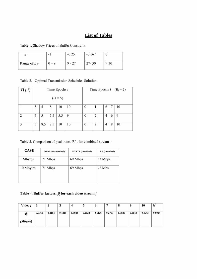
solution of the linear program also provides information on the shadow prices. Shadow prices, π,

corresponding to (17), represent the marginal change in the optimal rate for one additional unit of BT.

These values and the range of BT over which they are valid are shown in the following table.

For example, if the buffer size is very large (over 30 in this case) increasing it by one unit has no

effect on the optimal peak rate. One also sees from the curve that very large buffer sizes result in the

optimal peak rate of zero. In effect we can pre -load the buffer at time zero, and run it down without any

transmission during playback .The decreasing values of π as BT as increased reflects the expected

phenomenon of decreasing returns to scale.

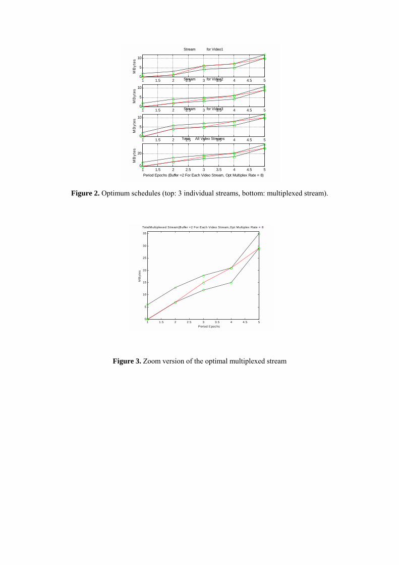
6. Numerical Example

Two small examples are solved with n = 4, m = 3, and buffer sizes fixed at B j = 5 and 2, for each

video stream j. The cumulative data breakpoints at time epochs i are shown below. The optima

transmission schedules are shown in table 2.

( )

109

10

64

5

540320410

,

=ijL

For B j = 5, the total multiplexed schedule and rates are; [15, 18.5, 22, 25.5, 29] and [3.5, 3.5, 3.5, 3.5],

respectively. Note, that the multiplexed rate is flat over all periods. For B j = 2, the total multiplexed

schedule and rates are; [0, 7, 15, 21, 29] and [7, 8, 6, 8], respectively. Here the peak rate has been

increased to 8. For the bj equal 2 case, the results are plotted in Figures 2 and 3.

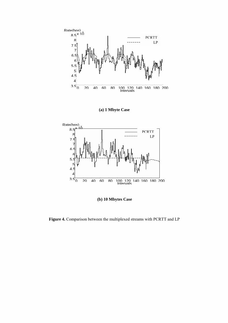
7. Some Results for Real Video Streams

Here we present some results that were obtained from a simulation of real video streams. The

experiments are based on 10 MPEG-1 video traces that have been presented in [1]. These traces were

downloaded from http://www.cis.ohio-state.edu/~wuchi. The video library includes clips with different

lengths and subjects (high activity movies, MTV clips and news) that represent the diversity of

compressed video sources in emerging multimedia services. We used 200 intervals of size 35 frames for

each video stream. The results of the multiplexed stream using the LP formulation (MP) was compared to

those of the PCRTT algorithm. We used PCRTT due to its ease of computation in lieu of e-PCRTT. A

comparison was carried out using several buffer sizes. Due to space constraints, only two cases for client

buffer sizes of 1 and 10 Mbytes are presented here. Figure 4(a) and 4(b) shows a comparison of the ten

streams multiplexed using PCRTT and LP for the 1 and 10 Mbytes cases, respectively. The solid and dash

curves represents PCRTT and LP smoothing, respectively.

Table 3 provides a comparison of the peak rates. LP smoothing reduces the peak PRCTT rate 24%

and 30% percent for the 1 and 10 Mbytes cases, respectively. For comparison purposes, column 2 shows

the peak rate required to transmit the unsmoothed original multiplexed stream. Note, that the LP reduces

the unsmoothed peak rate by 25% and 33% for the 1 and 10 Mbytes cases, respectively.

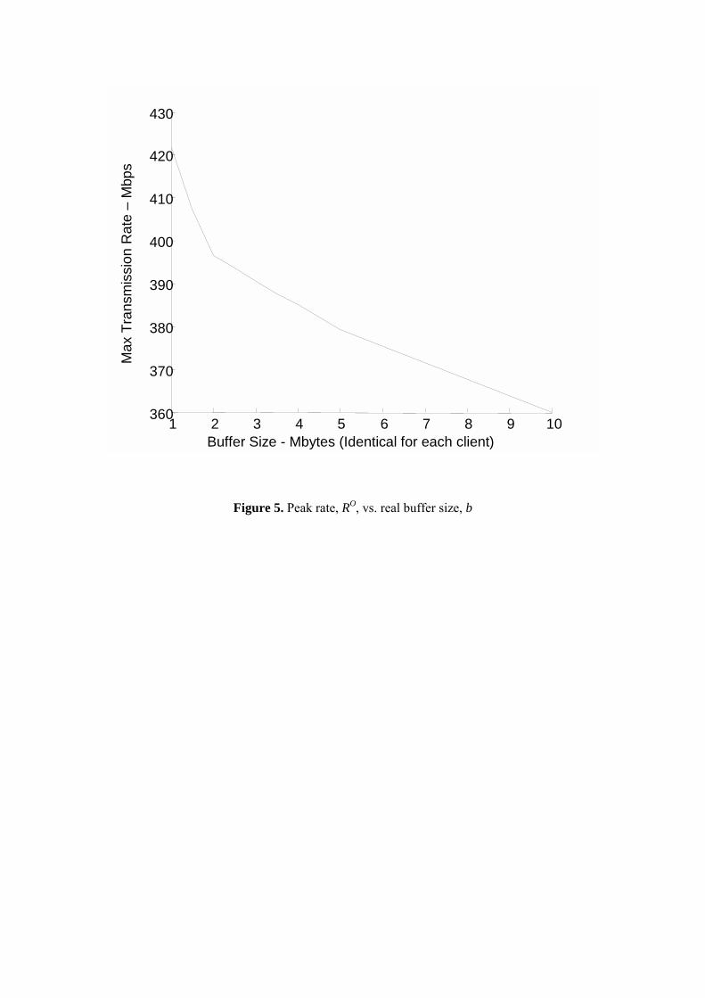
Figure 5 shows the effect of actual buffer size, b, on the peak-multiplexed rate using the LP

procedure. The buffer quantity, b, is identical for each of the 10 streams and varied from 1 to 10 Mbytes.

Table 4 shows the buffer factors used to convert the actual buffer sizes to the effective buffer values used

in constraint (18) of the LP formulation. The function is infeasible for values below b* = 0.993. At this

point at least one client’s linear approximation of the river has an effective buffer size of 0. This occurs at

the critical buffer value b* (shown to be Max {βj, all j} in Proposition 1). As expected from LP theory the

function is a convex non increasing piecewise linear function. One observes the decreasing shadow prices

for the buffer as reflected by the slopes of the RO(b) curve.

8. A Smoothed Entropy Measure

One notes from the graphs in Figure 4 how smoother the LP result becomes when the buffer size is

increased to 10 Mbytes. To quantify the smoothness of the rate step function we propose an entropy

measure. Let the rate step function be represented by the ordered set of rate values, r = {ri, i = 1,..,n).

Normalizing this curve by the total rate converts it into a probability function { }nipP ir ,,1, �== ,

where:

1,,,1,1

1

=∑=

∑

==

=

n

iin

ii

ii pni

r

rp �

The Entropy of Pr is:

( )in

ii ppE 2

1log⋅∑−=

=

A completely flat step function corresponds to the uniform probability density function (PDF) having

equal probalities, p(i) = 1/n , i= 1,2,…, n. Such a function exhibits an maximal entropy value of

( )nE 2log= .

It is important to note, this interpretation of entropy is not the usual one that defines the probability of the

rate as a random variable taking on different values, but instead defines a probability density function over

the intervals of the rate step function.

Denote EORIG , E PCRTT ,and ELP as the entropy of the original unsmoothed stream, PCRTT, and

the optimal LP multiplexed streams, respectively. For the original unsmoothed stream every frame F(v) ,

v = 1,…,F is converted to a rate as follows:

r((v)= rate for frame v = b(v) * 25 where b(v) is the size of frame v in bits and 25 frames per sec is used for

our PAL format videos.

The total data of the stream is:

( ) ( ) 2511

⋅∑=∑==

F

v

F

vvbvr

In order to make a valid entropy comparison of the interval smoothed functions to the original unsmoothed

frame rates we expand all intervals by making q copies of the interval rates, where q is the number of

frames per interval. For our example, for the PCRTT smoothed interval stream, this than corresponds to

rate step functions of length q*n = 7,000 (q = 35 frames per interval, n = 200 intervals).

Each copy has a rate of rci = ri /q . Note , that the amount of data in the ith interval is ri ∆∆∆∆t Were is ∆∆∆∆t =

q/25 = 1.4 sec/interval ( for q=35 ).

The total data in interval i is:

( )∑=+=

q

qvi vbqr

2

125/

So, ( ) 2511

⋅=⋅ ∑∑==

F

v

n

ii vbqrc

From the above, the total rate of the original video stream is equal to the total rates of all intervals of the

smoothed interval.

To obtain some perspective, these entropy values are bounded above by the maximum possible

value for a completely smooth function of 7,000 points. Denote this maximal entropy value as EMAX .

(where, EMAX. = log2(7000)). The relative entropy values for these bit rate combined streams for the two

sample cases are shown in Table 5.

One notes, how the entropy increases for smother versions of the rate step function.

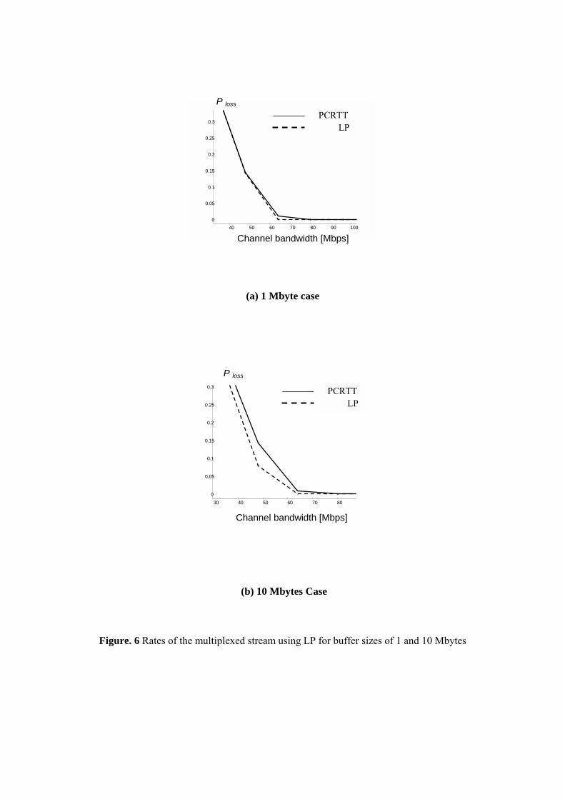
9. P-Loss

We also compared the PCRTT and LP algorithms by investigating the information loss due to

exceeding the constant channel bandwidth by the multiplexed stream. The probability of loss is expressed

by the expected fraction of bits lost from the video streams during transmission over a CBR channel. In

general, to obtain an accurate approximation of Ploss, it becomes necessary to perform a simulation of the

suggested multiplexed scheme during a large number of frame times. In this specific case, however, we

want to compare the optimal linear programming scheme to the multiplexed stream obtained by PCRTT.

Thus, we compute the loss probability Ploss as follows ( see [20]):

TtoupsentbitsofnumbertotalTtouplostbitsofnumberP

Tloss

∞→

= lim

.||

lim

1

0

1

0

∑

∑

=

=

+

∞→

−

= T

ii

T

ii

Tr

Cr (24)

where, | x –y |+ = x-y, if x-y >0, and 0 ,otherwise

Here C is the channel rate and rio is the optimal multiplexed rate during time interval i.

Equation 20 represents the accumulative number of bits above the channel bit rate divided by the total

number of bits in the multiplexed stream. The Ploss is obtained as function of the channel bit rate C, for

decreasing C from the maximum value of the multiplexed stream until zero bit rate.

Figures. 6(a) and 6(b) present the result of Ploss as function of the channel bit rate for client buffer

size cases (all clients have identical buffer sizes) of 1 and 10 Mbytes, respectively. The solid and dashed

lines represent the curves of Ploss for PCRTT and LP. As expected, the Ploss is decreased for both cases as

function of the channel rate. The main difference between the two multiplexing schemes is noticeable for

high channel bit rate, were the performance of the linear programming rates are better than those of the

PCRTT multiplexing scheme. We can also notice that at a certain channel bit rate Ploss is reached to zero,

this bit rate represents the maximum value of the multiplexed stream in both cases. Again the maximum

value of the multiplexed stream is lower for the case of the LP. For example, for the 1 Mbytes buffer size

case (Fig. 6(a)) the maximum bit rates are 84 and 64 Mbps for the PCRTT and LP schemes, respectively.

The results of the 10 Mbytes buffer (Fig. 6(b)) case are 84 and 55 Mbps for the PCRTT and LP schemes,

respectively. Performance of the LP scheme increases as the buffer size increases, and the gap between the

two Ploss curves is more noticeable for larger buffer sizes. This is due to the fact that for a large buffer

there are more possible solutions for the LP, and the range of rates in each smoothing interval is larger.

10. Conclusions and Future Research

In this paper we have proffered a linear programming formulation of the optimal multiplexing

problem. Although there are several other approaches

for solving this problem the advantage of the present approach are many. Linear programming is a well-

known algorithm, easily understood, and readily available without the need for special coding. Our

formulation accepts a linear approximation to the problem, which results in a faster running time, and this

approximation can be progressively increased as desired. It will also accept an initial approximate solution

to the program for further speedup. It is flexible, allowing the addition of constraints without the necessity

of algorithm redesign. For example, if one wishes to add a bandwidth limit for each client, this is easily

done by placing an upper bound on the rate variables, rij. Sensitivity analysis is another advantage. For

example, the shadow price of any individual buffer limit represents the marginal change of the optimal rate

for an additional increment of buffer size. It also allows the investigation of varying selected parameters of

the problem over their entire range through the use of parametric programming. This was demonstrated in

this paper for the total buffer size parameter for both a small numerical example and for real video

streams. It also, provides a framework for the future inclusion of multiple objectives, thus, tapping the

power of multi-objective programming techniques. Finally, linear programming problems have been

proven to belong to the class of polynomial bounded problems.

The optimal LP multiplexing scheme has been applied to real MPEG-1 video sequences. These results

are compared to the PCRTT procedure in terms of peak transmission bandwidth, entropy and P-loss

performance measures. For several client buffer sizes, the rate obtained by PCRTT was reduced by up to

30 percent by the LP solution. Future work includes consideration of the dynamic video on demand

environment, and a study of secondary measures and techniques for further smoothing of the rate function.

In addition we intend to investigate the effect of playback delay, and buffer size modifications to account

for errors induced by the linear approximation.

Acknowledgments

This research was partially supported by the Paul Ivanier Center for Robotics Research & Production

Management, Ben-Gurion University of the Negev, and the Israeli Ministry of Science, Grant No. 2105.

Special thanks are given to Niv Caner and Einat Titkin for their help in coding and running the simulation

software.

References

[1] W. Feng and J. Rexford, “A comparison of bandwidth smoothing techniques for the transmission of

prerecorded compressed video,” In Proceeding. IEEE INFOCOM, Kobe, Japan, Apr. 1997, pp. 58-66.

[2] S. Sen, J. Dey. J. Kurose, J. Stankovic, and D. Towsley, “CBR transmission of VBR stored video,”

SPIE Symposium on Voice Video and Data Communications: Multimedia Networks: Security, Displays,

Terminals, Gateways, (Dallas, Nov. 1997).

[3] W. Feng and S. Sechrest, “Smoothing and buffering for delivery of prerecorded compressed video,” In

Proceeding of the IS&T/ SPIE Symp. on Multimedia Comp. and Networking, Feb. 1995, pp. 234-242.

[4] W. Feng and S. Sechrest, “Critical bandwidth allocation for the delivery of compressed video,”

Comput. Commun., vol. 18, no. 10, Oct. 1995, pp. 709-717.

[5] W. Feng, F. Jahanian, and S. Sechrest, “Optimal buffering for the delivery of compressed prerecorded

video,” In Proceeding. of the IASTED/ISMM Int’l Conf. On Networks, Jan. 1995.

[6] J. D. Salehi, Z. Zhang, J. Kurose, and D. Towsley, “Supporting stored video: reducing rate variability

and end-to-end resource requirements through optimal smoothing,” IEEE/ACM Trans. Networking, Vol. 6,

Aug. 1998, pp. 397-410.

[7] M. Reisslein and K. W. Ross, “High performance prefetching protocols for VBR prerecorded video,”

IEEE Network, 12(6), November 1998, pp. 46-55.

[8] E. W. Knightly and H. Zhang, “D-BIND: an accurate traffic model for providing QoS guarantees to

VBR traffic”, IEEE/ACM Transactions on Networking, 5(2), April 1997, 219-231.

[9] J.Liebeherr and D. Wrege, “Video characterization for multimedia networks with a deterministic

service ”. In Proceeding of IEEE Infocom ’96, San Francisco, CA, March 1996.

[10] W. Feng and J. Rexford, “A comparison of bandwidth smoothing techniques for the transmission

of prerecorded compressed video”, In Proceeding of IEEE Infocom, Kobe, Japan, April 1997, 58-67.

[11] W. Feng and S. Sechrest, “Smoothing and buffering for delivery of prerecorded compressed

video”, In Proceeding of SPIE Multimedia Computation and Networking, February 1995.

[12] M. Grossglaser, S. Keshav and D. N. C. Tse, “RCBR: A simple and efficient service for multiple

time-scale traffic”, IEEE/ACM Trans. Networking, vol.5, Dec. 1997, pp. 741-755.

[13] S. Kang, H. Y. Yeom, “Transmission of video streams with constant bandwidth allocation”,

Computer Communications, 22(1999) pp. 173-180.

[14] J. Salehi, Z. Zhang, J Kurose and D. Towsley, “Supporting stored video: reducing rate variability

and end-to–end resource requirements through optimal smoothing”, In Proceeding of ACM SIGMETRICS

’96, May 1996, pp. 222-231.

[15] S. Kang, H. Y. Yeom, “Aggregated smoothing of VBR video streams”, International Conference

on Information Networking, (ICOIN-14), January, 2000.

[16] O. Hadar and S. Greenberg, ”Video rate smoothing and statistical multiplexing using the e-

PCRTT algorithm,” SPIE Symposium on Voice Video and Data Communications: Multimedia Systems

and Applications II, Boston, MA, Sep. 1999.

[17] O. Hadar and R. Cohen, “PCRTT Enhancement for off-line video smoothing,” in Special Issue on

Adaptive Real Time Multimedia Transmission over Packet Switching Networks in Journal of Real Time

Imaging, Vol. 7, No. 3, pp. 301-314, June, 2001.

[18] O. Hadar and R. Cohen, "PCRTT Enhancement for Off-Line Video Smoothing,"

in Proc. SPIE Vol. 3528, p. 89-100, Multimedia Systems and Applications,Andrew G.

Tescher; Bhaskaran Vasudev; V. Michael Bove; Barbara Derryberry; Eds., November

1998, Boston, MA, USA.

[19] O. Hadar, A. Kazir, and R. Stone, "Prefeteched multiplexing of individually smoothed video

streams," in OptiComm 2001, Optical Networking and Communications Conference, 19 - 24 August 2001,

Denver, CO USA

[20] D. Saparilla, K. W. Ross, and M. Reisslein, “Periodic Broadcasting with VBR-Encoded Video,”

in Proc. IEEE INFOCOM, NY, USA, Apr. 1999, pp. 464-471.

Figure captions

Figure 1. Illustration of the piecewise approximation for period (i+1) showing the effective buffer.

Figure 2. Optimum schedules (top: 3 individual streams, bottom: multiplexed stream).

Figure 3. Zoom version of the optimal multiplexed stream.

Figure 4. Comparison between the multiplexed streams with PCRTT and LP.

Figure 5. Peak rate, RO, vs. real buffer size, b.

Figure 6. Rates of the multiplexed stream using LP for buffer sizes of 1 and 10 Mbytes.

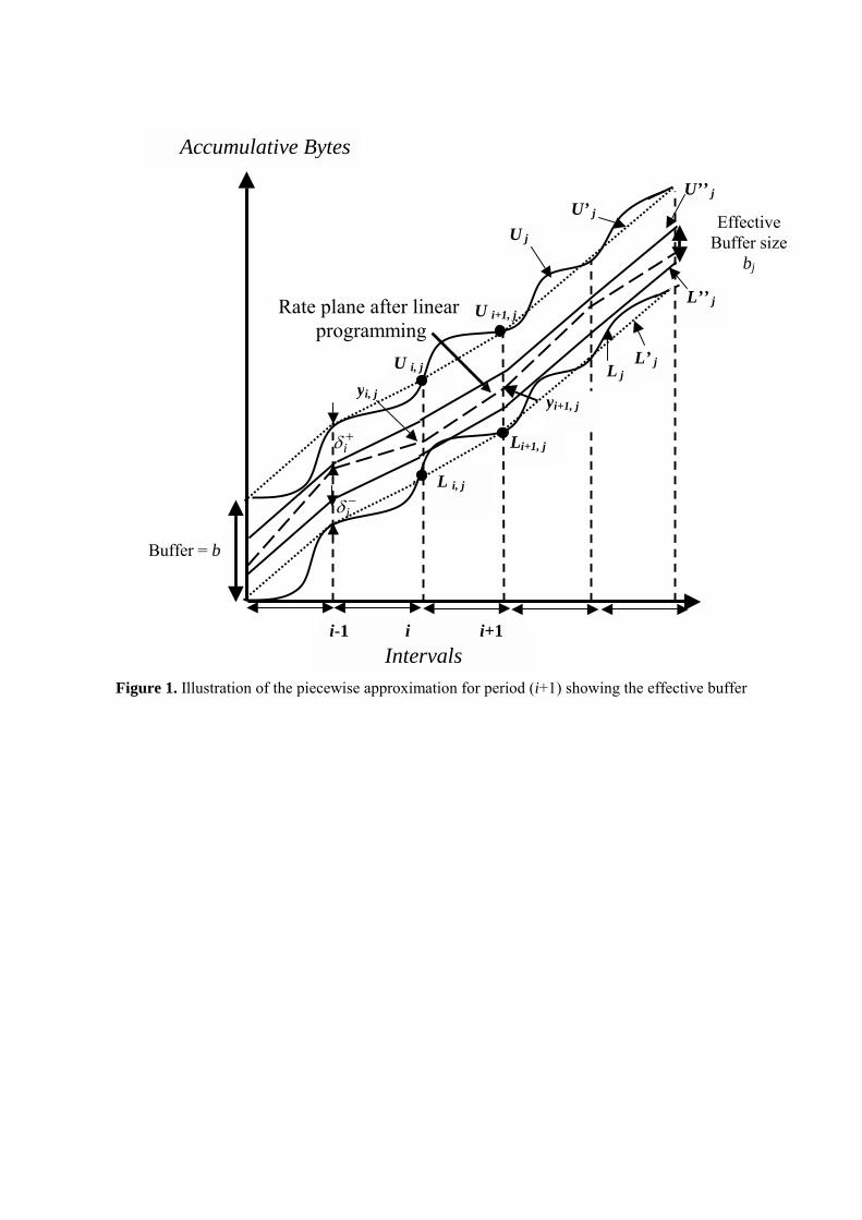
Figure 1. Illustration of the piecewise approximation for period (i+1) showing the effective buffer

Effective Buffer size

bj

U’ j

−

iδ

+

iδ

U i+1, j

U i, j

i-1 i i+1

Rate plane after linear programming

L i, j

Li+1, j

yi+1, jyi, j

Buffer = b

Accumulative Bytes

Intervals

L j L’ j

L’’ j

U j

U’’ j

1 1.5 2 2.5 3 3.5 4 4.5 50

5

10

Stream for Video1

period epochs

MB

ytes

1 1.5 2 2.5 3 3.5 4 4.5 50

5

10

Stream for Video2

period epochs

MB

ytes

1 1.5 2 2.5 3 3.5 4 4.5 50

5

10

Stream for Video3

period epochs

MB

ytes

1 1.5 2 2.5 3 3.5 4 4.5 50

20

Period Epochs (Buffer =2 For Each Video Stream, Opt Multiplex Rate = 8)

Total All Video StreamsM

Byt

es

Figure 2. Optimum schedules (top: 3 individual streams, bottom: multiplexed stream).

1 1.5 2 2.5 3 3.5 4 4.5 50

5

10

15

20

25

30

35

Period Epochs

TotalMultiplexed Stream(Buffer =2 For Each Video Stream,Opt Multiplex Rate = 8

MB

ytes

Figure 3. Zoom version of the optimal multiplexed stream

(a) 1 Mbyte Case

(b) 10 Mbytes Case

Figure 4. Comparison between the multiplexed streams with PCRTT and LP

0 20 40 60 80 100 120 140 160 180 2003.54

4.55

5.56

6.57

7.58

8.5 x 107

Intervals

Rate(bps)

PCRTTLP

0 20 40 60 80 100 120 140 160 180 2003.54

4.55

5.56

6.57

7.58

8.5x 107

Intervals

Rate(bps)

PCRTTLP

1 2 3 4 5 6 7 8 9 10 360

370

380

390

400

410

420

430

Buffer Size - Mbytes (Identical for each client)

Max

Tra

nsm

issi

on R

ate

– M

bps

Figure 5. Peak rate, RO, vs. real buffer size, b

(a) 1 Mbyte case

(b) 10 Mbytes Case

Figure. 6 Rates of the multiplexed stream using LP for buffer sizes of 1 and 10 Mbytes

40 50 60 70 80 90 1000

0.05 0.1

0.15 0.2

0.25 0.3

Channel bandwidth [Mbps]

P loss

PCRTTLP

PCRTTLP

30 40 50 60 70 80

0

0.05

0.1 0.15

0.2 0.25

0.3 P loss

Channel bandwidth [Mbps]

List of Tables

Table 1. Shadow Prices of Buffer Constraint

π -1 -0.25 -0.167 0

Range of B T 0 – 9 9 - 27 27- 30 > 30

Table 2. Optimal Transmission Schedules Solution

( )ijY , Time Epochs i

(Bj = 5)

Time Epochs i (Bj = 2)

1 5 5 8 10 10 0 1 6 7 10

2 5 5 5.5 5.5 9 0 2 4 6 9

3 5 8.5 8.5 10 10 0 2 4 8 10

Table 3. Comparison of peak rates, Ro , for combined streams

Table 4. Buffer factors, ββββj for each video stream j

CASE ORIG (un-smoothed) PCRTT (smoothed) LP (smoothed)

1 Mbytes 71 Mbps 69 Mbps 53 Mbps

10 Mbytes

71 Mbps 69 Mbps 48 Mbs

Video j 1 2 3 4 5 6 7 8 9 10 b*

ββββj

(Mbytes)

0.6361 0.4164 0.4219 0.9924 0.2628 0.6176 0.2793 0.3820 0.8143 0.4643 0.9924

Table 5. Relative Entropy Values for Bit Rate Combined Streams

CASE E ORIG E PCRTT ELP EMAX

1 Mbytes 12.4193 12.7606 12.7681 12.7731

10 Mbytes 12.4193 12.7606 12.7699 12.7731