DOKUZ EYLÜL UNIVERSITY

GRADUATE SCHOOL OF NATURAL AND APPLIED SCIENCES

OPERATIONAL MODAL ANALYSIS AND

FINITE ELEMENT MODEL UPDATING OF AN

IN-SERVICE STEEL RAILROAD BRIDGE

by

Özgür GİRGİN

October, 2019

İZMİR

OPERATIONAL MODAL ANALYSIS AND

FINITE ELEMENT MODEL UPDATING OF AN

IN-SERVICE STEEL RAILROAD BRIDGE

A Thesis Submitted to the

Graduate School of Natural and Applied Sciences of Dokuz Eylül University

In Partial Fulfillment of the Requirements for the Degree of Master of Science

in Civil Engineering, Structure Program

by

Özgür GİRGİN

October, 2019

İZMİR

iii

ACKNOWLEDGMENTS

First and foremost, I would like to thank to my supervisor Assoc. Prof. Dr. Özgür

ÖZÇELİK who believed in me and who was always with me. He did not leave

unanswered any of my questions. His encouragement, support, experience and

guidance helped me during my thesis and my whole life.

I would like to thank to my valuable instructors Prof. Dr. Serap KAHRAMAN,

Prof. Dr. Türkay BARAN, Assoc. Prof. Dr. İbrahim Serkan MISIR, Assistant Prof.

Dr. Sadık Can GİRGİN and Assistant Prof. Dr. Carmen AMADDEO. Their

knowledge, experience and support has an important place in my whole life.

I would like to thank to my valuable friends Civil Engineers Dr. Doruk YORMAZ,

(M.Sc) Umut YÜCEL and (M.Sc) Erkan DURMAZGEZER. Their knowledge,

experience and support has an important place in my whole life.

I would like to thank to my friends Civil Engineers Muhammed Emin

DEMİRKIRAN, Üstün Can MERİÇ, Gülser ERYILMAZ, Onur BAŞKAYA, Dilan

ÇANKAL, Mustafa USLU, and Oğuzcan ŞAHİN for helps to perform our

experiments.

I would like to thank to my family for their endless love, support and guidance.

They were by my side whenever I need. They gave me all kind of opportunity to

become an engineer.

This thesis was supported by TÜBİTAK 214M029 Project. General Directorate of

TCDD and TCDD 3rd Regional Directorate provided their support in carrying out the

study so I would like to thank TÜBİTAK, General Directorate of TCDD and TCDD

3rd Regional Directorate for their supports.

Özgür GİRGİN

iv

OPERATIONAL MODAL ANALYSIS AND FINITE ELEMENT MODEL

UPDATING OF AN IN-SERVICE STEEL RAILROAD BRIDGE

ABSTRACT

In our country Turkey visual inspection techniques are used for health and safety

checks of bridges. Outcomes of such methods are highly dependent on the experience

and the personal skills of the technician, and are most of the times unable to detect

hidden structural damages. Detected damages by these methods are usually too severe

and progressed that most of the times; it is too late to take any precaution. From this

point of view, the vibration based SHM with the potential of detecting small invisible

damage must be included in the standard visual inspection techniques.

The main aim of this thesis is to apply finite element model updating based

structural health monitoring method to 199+325 steel railroad bridge on the route of

Basmane-Dumlupinar which is under service for more than a century. Application of

this technique will eliminate the deficiencies/shortcomings in visual inspection

techniques. With this project, it is targeted to make this technique a part of standard

inspection techniques used by Turkish Republic State Railroads Department.

Ambient vibration data were obtained from the bridge by means of accelerometers

and the modal parameters were determined using operational modal analysis methods.

The modal parameters of the bridge were estimated using dynamic data collected over

the bridge. These estimated modal parameters are useful to detect the existence,

location and amount of damage. In addition, a calibrated finite element model of the

bridge and a database of its modal parameters can be used for comparison purposes in

case of any damaging natural event occurring in the future.

Keywords: Operational modal analysis, finite element model updating, structural

health monitoring, steel railroad bridge

v

KULLANIMDA OLAN BİR ÇELİK DEMİRYOLU KÖPRÜSÜNÜN

OPERASYONEL MODAL ANALİZİ VE SONLU ELEMANLAR

MODELİNİN GÜNCELLENMESİ

ÖZ

Ülkemizde demiryolu köprüleri gibi önemli yapılarda dâhi zorunlu periyodik

muayeneler gözleme dayalı olarak sürdürülmektedir. Sübjektif karar esaslı biçimde

sürdürülen köprü muayenelerinin, gizli hasarları teşhis etmekte yetersiz kalacağı, ya

da ancak hasar ileri boyutlara ulaşmış olduğunda görsel teşhis yapılabileceği açıktır.

Sayısallaşabilir/modellenebilir niteliğiyle yapı sağlığının izlenmesi (YSİ) yöntemleri,

gözleme dayalı değerlendirme sürecinin geliştirecek, değerlendirme sürecini objektif

ölçütlere bağlayacak ve olası gizli hasarların zamanında fark edilerek gerekli

önlemlerin alınmasını sağlayacaktır. Uzun süredir hizmet vermekte olan demiryolu

köprüleri muayenelerinde YSİ yöntemlerinin sürece dâhil edilmesi kritik ve önemli bir

boşluğu dolduracaktır.

Sunulan tezin temel amacı, sonlu elemanlar modeli güncellenmesi tabanlı yapı

sağlığı izleme (YSİ) yönteminin Uşak ili sınırları içerisindeki Türkiye Cumhuriyeti

Devlet Demiryolları (TCDD) tarafından işletilmekte olan; yüz yılı aşkın süredir hizmet

altındaki Basmane–Dumlupınar güzergâhındaki 199+325 çelik demiryolu köprüsüne

uygulanmasıdır. Böylece, hâlen düzenli olarak yapılmakta olan köprü kontrollerinin

daha güvenilir, objektif yöntemlerle iyileştirilmesi; olası gizli hasarların saptanması,

yapının hasar görebilirliği konusundaki mevcut belirsizliğin ortadan kaldırılması

hedeflenmektedir.

Bu tez kapsamında, köprü üzerinden ortamsal titreşim verisi ivmeölçerler

yardımıyla toplanmış ve köprünün modal parametreleri operasyonel modal analiz

yöntemleri kullanılarak belirlenmiştir. Köprüye ait 16 adet mod şekli ve frekans

değerleri operasyonel modal analiz yöntemleri kullanılarak tahmin edilmiştir.

199+325 çelik demiryolu köprüsünün oluşturulan sonlu elemanlar modelinin modal

parametreleri köprü üzerinden toplanan dinamik veriler kullanılarak güncellenmiştir.

vi

Güncellenmiş olan bu modal parametreler hasarın varlığını, yerini ve miktarını tespit

etmek için kullanılabilecektir. Ayrıca gelecekte oluşabilecek köprüye hasar verme

olasılığı bulunan herhangi bir doğa olayı sonrasında kıyaslama amacı ile

kullanılabilecek köprünün kalibre edilmiş sonlu elemanlar modeli ve köprünün modal

parametrelerine ilişkin bir veri tabanına da sahip olunmuştur.

Anahtar kelimeler: Operasyonel modal analiz, sonlu elemanlar model güncellemesi,

yapı sağlığı izleme, çelik demiryolu köprüsü

vii

CONTENTS

Page

M.Sc THESIS EXAMINATION RESULT FORM ..................................................... ii

ACKNOWLEDGEMENTS ........................................................................................ iii

ABSTRACT ................................................................................................................ iv

ÖZ ................................................................................................................................ v

LIST OF FIGURES .................................................................................................... ix

LIST OF TABLES ..................................................................................................... xii

CHAPTER ONE – INTRODUCTION .................................................................... 1

1.1 Motivation and Objectives ................................................................................ 1

1.2 Literature Review .............................................................................................. 4

1.3 Thesis Organization ......................................................................................... 11

CHAPTER TWO - THEORETICAL BACKGROUNDS .................................... 12

2.1 Finite Element Model Updating ...................................................................... 12

2.2 Operational Modal Analysis (OMA) Method ................................................. 12

2.2.1 Enhanced Frequency Domain Decomposition (EFDD) Method ............. 14

2.2.2 Data-Driven Stochastic Subspace Identification (SSI-Data) Method ..... 16

2.3 Modal Assurance Criteria (MAC) ................................................................... 18

CHAPTER THREE - EXPERIMENTAL STUDIES ........................................... 19

3.1 Features of 199+325 Steel Railroad Bridge .................................................... 19

3.2 Experimental Studies of 199+325 Steel Railroad Bridge ............................... 22

3.2.1 Preliminary Studies of the Bridge Tests (Test-1/Winter) ........................ 22

3.2.2 Bridge Tests Studies (Test-1/Winter) ...................................................... 26

3.3 Equipments Used in Test Setups ..................................................................... 28

CHAPTER FOUR - EXPERIMENTAL RESULTS ............................................. 30

viii

4.1 System Identification Studies (Modal Parameter Estimation) ........................ 30

4.2 199+325 Steel Railroad Bridge Test Results (Test-1/Winter) ........................ 31

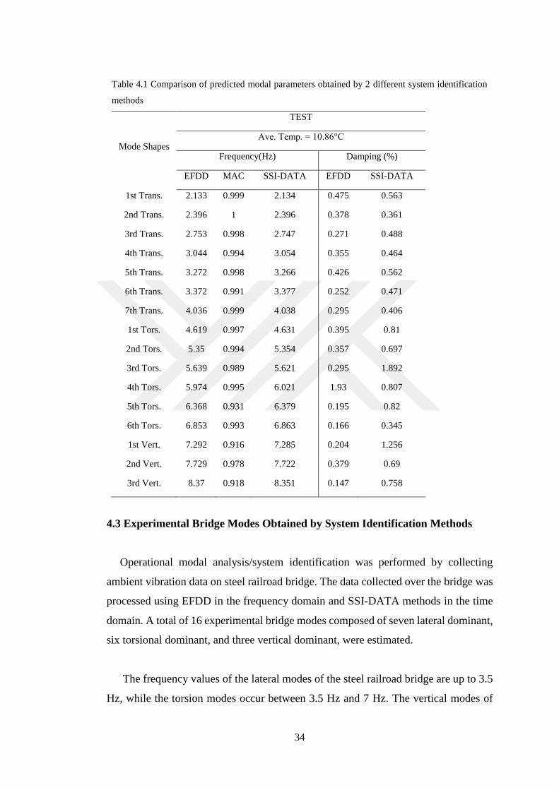
4.3 Experimental Bridge Modes Obtained by System Identification Methods ..... 34

CHAPTER FIVE - NUMERICAL STUDIES ....................................................... 40

5.1 Introduction ..................................................................................................... 40

5.2 Initial Finite Element Model ........................................................................... 48

5.3 Finite Element Model Updating (FEMU) Studies .......................................... 57

5.4 Numerical Results ........................................................................................... 63

5.5 Flow Chart (Discussion) of the Methodology ................................................. 64

CHAPTER SIX - CONCLUSIONS ........................................................................ 67

REFERENCES ......................................................................................................... 70

ix

LIST OF FIGURES

Page

Figure 1.1 199+325 Steel railroad bridge .................................................................... 2

Figure 3.1 The initial project of the steel railroad bridge (1896) ............................... 19

Figure 3.2 The current picture of the 199 + 325 railroad steel bridge ....................... 20

Figure 3.3 Railroad steel bridge element details: (a) support of the trusses on the

column, (b) a span of the bridge between the two abutment, (c) the support

detail of the columns on the masonry foundations, and (d) the rod

anchorage detail in the gallery within the foundation ............................. 21

Figure 3.4 The platform view of 199+325 steel railroad bridge ................................ 22

Figure 3.5 Setup 0 ...................................................................................................... 23

Figure 3.6 Setup1_1 ................................................................................................... 24

Figure 3.7 Setup 1 ...................................................................................................... 25

Figure 3.8 Setup 2 ...................................................................................................... 25

Figure 3.9 Setup 3 ...................................................................................................... 25

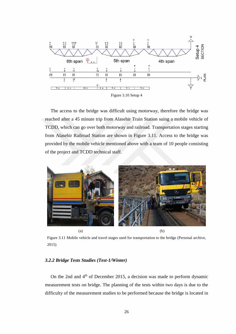
Figure 3.10 Setup 4 .................................................................................................... 26

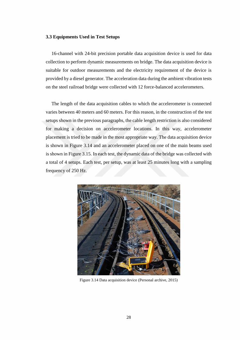
Figure 3.11 Mobile vehicle and travel stages used for transportation to the bridge .. 26

Figure 3.12 Test-1 02.12.2015 (1st Day) ................................................................... 27

Figure 3.13 Test-1 04.12.2015 (2nd Day) .................................................................. 27

Figure 3.14 Data acquisition device ........................................................................... 28

Figure 3.15 An accelerometer mounted on the main lateral beam ............................ 29

Figure 4.1 Representation of reference accelerometers ............................................. 31

Figure 4.2 Lateral dominant modes spectral density singular values graph .............. 32

Figure 4.3 Lateral dominant modes SSI stabilization diagram .................................. 32

Figure 4.4 Vertical / torsional dominant modes spectral density singular values

graph ....................................................................................................... 33

Figure 4.5 Vertical / torsional dominant modes SSI stabilization diagram ............... 33

Figure 4.6 1st Lateral mode ....................................................................................... 35

Figure 4.7 2nd Lateral mode ...................................................................................... 35

Figure 4.8 3rd Lateral mode ....................................................................................... 36

Figure 4.9 4th Lateral mode ....................................................................................... 36

x

Figure 4.10 5th Lateral mode ..................................................................................... 36

Figure 4.11 6th Lateral mode ..................................................................................... 37

Figure 4.12 7th Lateral mode ..................................................................................... 37

Figure 4.13 1st Torsion mode .................................................................................... 37

Figure 4.14 2nd Torsion mode ................................................................................... 37

Figure 4.15 3rd Torsion mode .................................................................................... 38

Figure 4.16 4th Torsion mode .................................................................................... 38

Figure 4.17 5th Torsion mode .................................................................................... 38

Figure 4.18 6th Torsion mode .................................................................................... 38

Figure 4.19 1st Vertical mode .................................................................................... 38

Figure 4.20 2nd Vertical mode................................................................................... 39

Figure 4.21 3rd Vertical mode ................................................................................... 39

Figure 5.1 View of 199+325 steel railroad bridge truss ............................................ 40

Figure 5.2 View of cross-section of 199+325 steel railroad bridge truss elements ... 41

Figure 5.3 Strengthened joint detail ........................................................................... 42

Figure 5.4 Deck cross section .................................................................................... 43

Figure 5.5 Detail of the stringer ................................................................................. 43

Figure 5.6 Rails, footpath and railing......................................................................... 44

Figure 5.7 Sleeper on stringer .................................................................................... 44

Figure 5.8 (a) Simple support and (b) Roller support of the steel railroad bridge ..... 45

Figure 5.9 Anchored rod ............................................................................................ 45

Figure 5.10 Masonry base support ............................................................................. 46

Figure 5.11 Abutment ................................................................................................ 46

Figure 5.12 Horizontal bracing .................................................................................. 47

Figure 5.13 Abutment with vertical, horizontal and diagonal bracing ...................... 47

Figure 5.14 Top frame of abutment ........................................................................... 48

Figure 5.15 Initial finite element model ..................................................................... 50

Figure 5.16 Frame section without strengthening plates and with strengthening

plates ..................................................................................................... 50

Figure 5.17 199 + 325 steel railroad bridge FEM with spring elements ................... 51

Figure 5.18 Abutment numbers.................................................................................. 51

xi

Figure 5.19 Deformed shape of abutments under 10 kN (1 ton) load in x direction: (a)

abutment 1, (b) abutment 2, (c) abutment 3, (d) abutment 4, (e) abutment

5 ............................................................................................................... 53

Figure 5.20 Actual column to support detail .............................................................. 54

Figure 5.21 Platform to simulate the abutment effect (modeling approach) ............. 55

Figure 5.22 1st transversal mode shape and frequency value of FEDEASLab model

(2.000 Hz) ............................................................................................... 55

Figure 5.23 2nd transversal mode shape and frequency value of FEDEASLab model

(2.295 Hz) ............................................................................................... 55

Figure 5.24 3rd transversal mode shape and frequency value of FEDEASLab model

(2.680 Hz) ............................................................................................... 56

Figure 5.25 4th transversal mode shape and frequency value of FEDEASLab model

(3.011 Hz) ............................................................................................... 56

Figure 5.26 3rd vertical mode shape and frequency value of FEDEASLab model

(8.243 Hz) .............................................................................................. 56

Figure 5.27 Representation of elements that have an effect on bridge modal parameters

................................................................................................................. 58

Figure 5.28 Experimentally estimated mode and their numerically modeled and

updated counterpart for 1st transversal mode ....................................... 61

Figure 5.29 Experimentally estimated mode and their numerically modeled and

updated counterpart for 1st vertical mode ............................................ 62

Figure 5.30 Experimentally estimated mode and their numerically modeled and

updated counterpart for 3rd vertical mode ........................................... 63

Figure 5.31 The flow chart of the proposed method .................................................. 66

xii

LIST OF TABLES

Page

Table 4.1 Comparison of predicted modal parameters obtained by 2 different system

identification methods .............................................................................. 34

Table 5.1 Spring stiffnesses representing bridge abutments ...................................... 52

Table 5.2 Vibration frequencies of initial numerical model where the columns are

modeled by springs .................................................................................. 57

Table 5.3 Inıtial and Updated Young’s Moduli ......................................................... 59

Table 5.4 Spring stiffnesses representing abutments: Initial and updated values ...... 59

Table 5.5 Comparison of estimated modal parameters between analytical and

experimental results................................................................................. 60

1

CHAPTER ONE

INTRODUCTION

1.1 Motivation and Objectives

Especially in the rail network, steel bridges are frequently used. Steel bridges are

available in many different forms, such as lattice beam, web-plate girder, arch type

and suspended bridges. In addition, different examples of applications such as whether

the bridge deck slab is in the lower head or the upper head are also seen. Many of the

steel railroad bridges were built long time ago, these bridges have been exposed to

external effects for many years, and increasing load on these bridges; factors such as

the increase in railroad traffic necessitate the establishment of more objective, precise,

and reliable control mechanisms on these bridges.

In our country, even for important structures such as railroad bridges, mandatory

periodic inspections are carried out based on visual observations. It is clear that bridge

inspections, which are carried out in accordance with the personal effort and

experience of the technical personnel performing the visual inspection, will not be

sufficient to diagnose hidden (invisible) damages. When the damage has reached

advanced dimensions, it is possible to make a damage assessment by visual diagnosis.

Therefore, vulnerability of structural systems, loss of structures as a result of damage,

risk of accidents due to structural damage increase. These risks may not only cause

significant economic losses, but also loss of life as a result of possible accidents.

Considering these risks, it is clear that more reliable, non-subjective damage

assessment methods are needed.

As a potential tool for early detection of damage to engineering structures,

vibration-based Structural Health Monitoring (SHM) studies have gained considerable

importance in recent years. SHM methods, which determine information about

structural health by processing dynamic data collected through sensors on structures

in different ways, provide more reliable results for railroad bridges. Since the

parameters required by the method can be determined in a non-destructive manner, it

2

is particularly attractive to use in structures under service. SHM methods, which can

be digitized, will become an integral part of the monitoring process based on visual

observations, will connect the assessment process to objective criteria, and ensure that

possible hidden damages are detected in a timely manner and necessary preventive

measures are taken. In particular, the inclusion of SHM methods in the inspection of

railroad bridges that have been in service for a longer period of time compared to

highway bridges will fill a critical and important gap in routine and periodic

inspections. In this way, SHM methods, which can be digitized / modelable, will

improve the observation-based assessment process, link the assessment process to

objective criteria and ensure that any hidden damages are identified in a timely manner

and necessary actions are taken.

The main aim of this study is to apply a SHM method based upon finite element

model updating (FEMU) on 199+325 steel railroad bridge which is located in the

province of Uşak and operated by The Republic of Turkey State Railroads (TCDD)

(Figure 1.1).

Figure 1.1 199+325 Steel railroad bridge (Personal archive, 2015)

The bridges are constructed with an assumption that their economic life is one

hundred years. In our country, the railroad construction began in the 19th century

during the Ottoman Empire and the Republic of Turkey has rapidly continued the task

in the first period. Bridges, one of the most essential components of the railroad

network, were also built during these periods. There are many bridges within the

3

railroad network that have been in service for more than and a hundred years. These

bridges are exposed to different types of damage during their use due to both increased

axle loads and the deteriorating conditions due environmental changes. Especially in

railroad steel bridges, increased axle loads and train speeds require regular monitoring

of these structures. In addition, these bridges, which have been built long time ago,

cannot meet the current earthquake code specifications. This increases the likelihood

of damage to existing steel railroad bridges and poses a danger to public safety. The

steel railroad bridges under the of The Republic of Turkey State Railroads (TCDD)

are subjected to three different types of regularly performed inspections. These are

public controls performed twice a year, periodic controls every 6 years and post-

disaster controls in case of a natural disaster (Akar, 2009). Most of these controls are

made observationally, in few cases bridge displacement controls with material testing

are performed.

SHM technique based on FEMU is considered as one of the most promising

methods for estimating the damage states and hence the remaining useful lives of

examined structural systems. Therefore it is important to include this technique to the

process of routine bridge control is. Because as a result of FEMU, a finite element

model (FEM) updated by an objective method and therefore reflecting the new state

of the structure can be obtained. Using the changes in the updated parameters in this

model and examining the results of the model simulation, important inferences can be

made about the amount of damage and the remaining life of the structure.

Determination of the presence of damage, which is relatively easier to obtain and the

first objective of the SHM, can be easily done using the updated model. There is no

SHM method to support visual controls within TCDD routine control procedures.

Considering that such a method will complement the regular visual bridge inspections,

the introduction of this method into TCDD reveals the importance of the study.

The SHM-based damage detection method, details of it are given in the later

sections, uses the estimated modal parameters by system identification methods of the

actual structure. Within the scope of this thesis, first of all, modal parameters of the

steel railroad bridge were obtained by vibration based system identification methods.

4

These parameters, which are estimated by using the dynamic data collected over the

bridge, contain valuable information about the dynamic characteristics of the bridge

that may vary significantly depending on the ambient temperature conditions. The

quantitative determination of the impact of temperature effect on modal parameters

will supply important information about the dynamic behavior of the in-service steel

railroad bridge under study.

Damage types likely to occur on a steel bridge that has been in service for over

hundred years are fatigue, reduction in cross-section, deterioration of mechanical

properties of the bridge material, structural defects that may occur after an accident

and possible problems that may arise in the element joining details.

In order to enhance a trustworthy SHM procedure, examining the effects of realistic

damage scenarios on modal parameters is necessary. However performing such a work

will require to damage the actual structure. Inflicting damage on real structure is not

possible for structures that are currently under service, which is the case for the steel

bridge under study. In this case, there is no other choice but to use simulation data

generated from a well calibrated FE model. To do that the modeling capabilities of the

finite element program must be advanced and the FEM of the structure needs to be

detailed enough to study realistic damage scenarios. One of the important objectives

of this thesis is to have a reliable calibrated FEM of the bridge. This is especially

important for the bridge under investigation since the uninterrupted flow of railway

traffic along this line depends on the continuation of service by the bridge.

1.2 Literature Review

There have been many studies on SHM in recent years and these studies are

attracting attention also in our country. Considering that we live on an earthquake

prone country, monitoring the structural health of railroad bridges that have been in

service for a long time must be addressed and examined immediately. 199 + 325 steel

railroad bridge has been a subject of another study where a structural health monitoring

system was developed and in-situ dynamic measurements have been collected by the

5

researchers from Middle East Technical University. The results from this work have

been presented in a master thesis (Akın, 2012). In this study, 2 and 3 dimensional finite

element models are developed without performing any updating work on the model.

Capacity and reliability analyzes were performed by using these models and the

conditions of the structural elements on the bridge under train and earthquake loads

was examined; however, to this date no study has been conducted on this bridge to

update the FEM used for this purpose. In addition, since only a small number of

accelerometers are used in the aforementioned thesis, only very few modal parameters

of vertical modes are obtained. In the thesis, it is stated that the collected acceleration

data is quite noisy. This is a factor that increases the uncertainty in modal parameter

estimation. Wind, temperature and humidity measurements were taken during the

tests; however, effects of these variables on modal parameter estimations were not

examined.

A group of researchers in Turkey was performed often a series of system

identification/operational modal analysis studies on road bridges. Basically, in all

these studies, dynamic measurements were taken with accelerometers placed on

bridges, modal parameters of bridges were estimated by using dynamic measurements,

and then FEM of bridges were updated with trial and error procedure. All bridges

studied are reinforced concrete bridges (Altunışık et al., 2011a; Altunışık et al., 2011b;

Bayraktar el al., 2009). In these studies, effectiveness of the environmental conditions

on modal parameters were not emphasized. However, impact of environmental

conditions on the results of system identification/operational modal analysis cannot be

neglected. In a study conducted in 2014 (Bayraktar et al., 2014), on Gülburnu Bridge,

a reinforced concrete highway bridge, was examined and the effect of the ambient

temperature on the modal parameters was also discussed. For this purpose, data were

collected over two different dates at different ambient temperatures and the modal

parameters were calculated. Obtained results showed that there are differences in

natural vibration frequency values which is one of the modal parameters approaching

to 14%.

6

In a similar study on the steel highway Eynel Bridge (Altunışık et al., 2012), FE

model of this bridge was updated by a trial and error method using the estimated modal

parameters by an OMA method. Based on the results of a dynamic analysis performed

before and after the updating procedure it was found that significant displacement

differences occur between these two models.

In addition to the system identification studies performed on highway bridges in

Turkey, also railroad bridges are examined similarly. A review of these studies is

presented below:

A study on the dynamic evaluation of a steel railroad bridge in Istanbul (Çağlayan

et al., 2011) was conducted. Static and dynamic tests were performed over a steel

railroad bridge with four spans, one of which is damaged. The FEM of the bridge has

been updated according to the field measurements. The difference in the dynamic

parameters of the damaged span was observed and it was proposed to renew the

aperture.

Field measurements and analytical model validation studies were carried out at

Karakaya Steel Railroad Bridge which is 64 meters and consisted of 29 simple

supported spans (Çağlayan et al., 2015). In this study static, environmental, and free

vibration tests were performed on the bridge. Dynamic data from these tests were

collected by using single and biaxial accelerometers. In addition to the accelerometer

data, strain-gage measurements were collected from the bridge elements in order to

obtain strain levels. FEM update was performed with an optimization procedure and

the updated model was also validated by bridge midpoint displacement measurements.

Numerous SHM studies have been carried out on bridge type structures in the last

20 years. Below are some examples of SHM studies on bridge carried out abroad.

For effective bridge management, accurate and reliable assessment is indispensable

to reduce the maintenance, repair or upgrading costs. In current practice, finite element

(FE) modeling is commonly used for analysis and predicting the dynamic behaviour

7

of structures; however, these models are mainly created based upon the uncertain

structural parameters in the sense of boundary conditions, material properties or

geometry. As a result, even refined FE models may not be the best representation of

the actual structural system and cannot predict the dynamic characteristics properly

with a desired level of accuracy. Finite element model updating method (Mottershead

& Frisswell, 1993) has become a popular tool in model calibration studies thanks to

its capability to reduce the discrepancies in numerical models by pairing the estimated

behaviour to the observed structural behaviour obtained by experiments performed by

static measurements based on load tests (Fryba & Pirner, 2001; Marefat et al., 2009)

or ambient/forced vibration measurements (Cunha et al., 2003; Jaishi & Ren, 2005).

Ambient vibration testing in which the structural response obtained over a wide

frequency band, complemented with OMA is the most ideal and effective way to

obtain the experimental modal properties (vibration frequencies, mode shapes,

damping ratios) in civil engineering applications; especially for low frequency ranged

bridge type structures. Although experimental modal data is susceptible to

measurement errors and post-processing operations, it is agreed upon that the structural

behavior is better represented with experimental data than the initial FE model and

therefore these measurements are mostly selected as the main source in the FE model

calibration studies.

Brownjohn & Xia, (2000) established a proper FEM by updating the uncertain

structural parameters for the curved- cable stayed Safti Link Bridge. Sensitivity-based

FEMU scheme was used for this purpose.

Asgari et al., (2013) presented a model updating algorithm for unserviceable cable-

stayed Tatara Bridge. In their study, the design variables were determined based on

sensitivity analysis and the updating was performed by an iteratively manual way.

Difference in natural frequencies calculated between the initial FEM and forced

vibration test were reduced from 29% to 3% for the first six modes after model

calibration study.

8

Banendettini & Gentile, (2011) used manual tuning strategy by choosing

appropriate structural parameters to ensure well-conditioned problem. Together with

the introduction of proper boundary conditions for the column bases, fairly good

correlation is obtained between the experimental and FE modal results.

Hong et al., (2010) updated FE model of a suspension bridge based on the

operational modal analysis results. This calibrated model is later then used in order to

predict the structural response under wind effects numerically.

Enevoldsen, (2002) calibrated the stiffness parameters of joints of a bridge in order

to acquire a numerical model that exhibits a better correspondence with strain

measurements collected during passage of a train. The calibrated FE model was later

then used to predict the fatigue life of the system under higher axle loads.

Hendrik et al., (2009) presented a methodology allows to combine an initial FE

model with dynamic and static measurements. They found that manual model

calibration performed prior to FEMU is essential for more realistic results, as the risk

of compensating the meaningless changes in updating parameters due to modelling

errors is reduced.

In the work conducted on the I-40 Bridge (Farrar & James, 1997), the suitability of

utilizing AV test data to obtain dynamic characteristics of the bridge was investigated.

It was found that the difference between the modal parameters obtained by the

vibration data generated from the traffic on the bridge and obtained by the forced

vibration data created by the vibrators on the bridge was small. In this way, the

suitability of using AV data to extract the dynamic parameters of I-40 Bridge in a non-

destructive manner has been experimentally verified.

A work based on iterative sensitivity based FEMU (Teughels & De Roeck, 2004)

was conducted at the Z24 highway bridge in Switzerland. In this study, finite element

model of the bridge, which is formed by the aid of AV tests, was iteratively updated.

A safe zone strategy has been implemented in order to ensure that FEM update is

9

carried out in a manner that is close to reality. In the damage detection study, the modal

parameters of the bridge were used, and presence of the damage was indicated by

decrements observed in bending and torsional stiffness values.

In the study based on artificial neural networks (Feng et al., 2004), the modal

parameters of two highway bridges were determined with two system identification

methods. These two system identification methods are Frequency Domain

Decomposition (EFDD) and classical peak picking method. The FEM was updated

with the frequency and mode shape values obtained from the bridges.

An experimental and analytical study (Spyrakos et al., 2004) was conducted to

determine the situation of a historic steel railroad bridge. In this study, the seismic and

earthquake load capacities of the bridge were determined. Besides, the initial

numerical model of the bridge was updated according to static and dynamic field

measurements.

In the study conducted on the Vincent Thomas Bridge, a suspension bridge (He et

al., 2008), modal parameters were estimated by data-driven stochastic subspace

identification (SSI-DATA) method by collecting AV data under the influence of wind.

The FEM of the bridge was confirmed by modal parameters extracted from in-situ

measurements. In addition, the effectiveness of measurement noise on system

identification studies was investigated.

Within the scope of the European industrial risk mitigation project, modal

parameter estimation and damage assessment studies were carried out at bridge S101

in Austria (Doehler et al., 2014). In the study, the bridge was gradually damaged and

the changes in the modal parameters were observed by using AV data. In order to

determine the damage state, instead of comparing the modal parameters of the

reference and the damaged states, an algorithm that compares different structural

conditions using the χ2 test was used. Here, the algorithm detects the existence of the

damage by the changes occurred in structural systems.

10

On the purpose of SHM studies, static and dynamic tests were performed on a steel

railroad bridge (Siriwardane, 2015) with a length of 160 meters and 6 spans. In the

dynamic tests, modal parameter estimation was made after the heaviest train passing

over the bridge. The updated FEM was obtained according to the displacement and

stress data collected over the bridge. In the study related to damage detection, modal

parameter estimation was made on the damaged model formed by removing structural

elements which are thought to be damaged from updated FEM. In this way, the change

of the damaged elements on the bridge modal parameters was determined.

SHM is a relatively recent technology that will not eliminate visual controls but

complement it and improve it by providing quantitative knowledge about the dynamic

character of the system. The basis of the vibration-based SHM method is the fact that

the modal parameters of the system are related to its physical parameters (mass,

damping, stiffness). In this case, changes in physical parameters due to damage is

reflected in the modal parameters of the system like frequencies, mode shapes, and

damping ratios (Doebling et al., 1996a; Doebling et al., 1996b; Sohn., 2003). The

ultimate aim of the SHM method is to classify the damage at four levels (increasing

complexity): (i) the presence, (ii) the location, and (iii) the severity of the damage, (iv)

the remnant life of the structure (Rytter, 1993). To determine the remnant life of a

system, a FEM reflecting its damaged condition is essential.

The first step in the method of updating an FE model is to create a preliminary

model using the project information of the structure and the information obtained from

in-situ observations. This initial model is then calibrated using modal parameters

calculated using dynamic data collected over the structure at a reference time (a

specific reference state). Thus, the constituted reference model reflects the actual

condition of the structural system. The reference model corresponds to the undamaged

state of the structure. Dynamic data (modal parameters) collected on the same structure

at oncoming dates is used this time to update this reference model. The differences

between in the physical parameters (model parameters) this newly updated model (s)

and the reference model indicate the change in the structure during this time (this

change may or may not be due to structural damage).

11

1.3 Thesis Organization

This thesis consists of six chapters. A brief introduction on each of on these sections

is given below.

In the Chapter One, the aim of the thesis is explained and reviews of similar studies

in literature are presented.

In the Chapter Two, theoretical background is introduced and details about the

methods used for system identification are given.

In the Chapter Three, details of the tests performed on the bridge are given.

In the Chapter Four, the results related to the estimation of modal parameters

performed in line with the data obtained from the bridge tests are given.

In the Chapter Five, the numerical work on the FEM updating is given.

In the Chapter Six, the conclusions and recommendations are presented.

12

CHAPTER TWO

THEORETICAL BACKGROUNDS

2.1 Finite Element Model Updating

A FEM updating is a non-linear least squares optimization problem. In the

optimization problem, the parameters of the initial FEM (e.g., element stiffness) are

updated to minimize the discrepancies between the experimentally determined modal

parameters and the modal parameters of the finite element model. The fact that the

updated initial model is sufficiently detailed and accurate is critical for the success of

the update process; since the updating procedure cannot compensate for modeling

errors (Zivanovic et al., 2007). In FEMU process, a limited amount of model

parameters are selected for updating purpose during the solution phase of the

optimization problem; in the case of large number of parameters, the optimization

problem becomes difficult and the process takes a lot of time. For this process, high

performance computers that use parallel processing may be required based on the size

of the problem. Therefore, generally, the structure can be subdivided into subsystems,

and a single updating parameter can be assigned to each subsystem. For example, a

bridge structure of hundreds of elements can be divided into smaller number of

subsystems in order to reduce the number of system parameters to be updated. The

system parameters of all elements in one of these subsystems can be aggregated into a

single system parameter. Such a simplification makes it difficult to locate the damage

because the spatial resolution is reduced. However, the efficiency of the calculation is

extremely high.

2.2 Operational Modal Analysis (OMA) Method

The estimation of modal parameters of structural systems by vibration-based

methods has attracted attention in recent decades. These methods are frequently used

in SHM. SHM is an essential tool that can be used for work areas such as assessment

of existing structures, model calibration and damage detection. SHM involves

detecting the current state of the structure continuously and / or at different times by

13

detecting damage-sensitive properties through sensors. In the SHM method, which is

on the strength of FEMU, the experimentally obtained modal parameters of the system

which is SHM are needed. In this section, information about system identification

methods to be used for estimation of modal parameters is presented.

OMA is a method used to estimate the modal parameters of a system exposed to

low-level vibrations. Estimated modal parameters of the structure are natural vibration

frequencies, mode shapes, modal damping ratios and modal participation factors.

There are many difficulties in the field of SHM and therefore in the estimation of

modal parameters. These include nonlinear response of the damaged system,

determination of location and number of sensors, determination of damage sensitive

properties of structures at low vibration levels, removal of changes in these properties

from changes due to environmental factors (temperature and humidity changes, etc.)

and test method (Doebling et al., 1998; Sohn et al., 2003).

It is possible to divide the system identification methods used in the structural health

monitoring into two groups as input-output and output-only methods (Moaveni, 2007).

As civil engineering structures are large-scale structures, it is impractical to excite

these structures with correctly measurable forces. In this case, it is preferred to use

ambient vibration effects such as vibrations (micro tremor, traffic, wind, etc.) resulting

from the normal use of the structure. Therefore, it is more appropriate to use OMA

methods, also called output-only methods, to estimate the modal parameters of

structures.

The report, which was prepared between 1996 and 2001 (Sohn et al., 2003), covers

the system identification and SHM studies, summarizes the methods used, data

collection, signal processing and related engineering applications. The report includes

the stages of structural health monitoring, functional evaluation (building function /

status, necessity of SHM), data collection, data normalization and cleaning operations,

feature selection, feature estimation (system identification), statistical modeling for

selected features. The methods that were considered to be used because they have been

applied to bridge type structures in the past are as follows: Enhanced Frequency

14

Domain Decomposition (EFDD) (Brincker, 2001) and Data-Driven Stochastic

Subspace Identification Method (SSI-Data) (Van Overschee, 1996; Peeters, 2001).

In the thesis, EFDD and SSI-DATA system identification methods are used. The

modal parameter estimation of the bridge is performed by using these methods by

means of ARTEMIS® program.

2.2.1 Enhanced Frequency Domain Decomposition (EFDD) Method

The EFDD method is known as the development of the classical peak picking

method. The method is based on the classical frequency domain method. The classical

method has negative aspects due to difficulties in predicting modes that are close to

each other and the reason that power spectral densities are limited by frequency

resolution. For these reasons, the damping estimates made by the classical method also

yield very uncertain results (Brinckner et al., 2001). In the EFDD method, instead of

selecting the peaks in the power spectral density functions (PSD), spectral matrices are

created using these functions estimated only by the output data and singular value

decomposition (SVD) is applied to these matrices. In cases where the function that

excite the system is broadband, the system has low damping values (engineering

structures are an example of low damping systems), and the close modes are

perpendicular to each other, each individual value is the auto-power spectral density

function (auto-PSD) corresponding to a single mode of the system. If the above

conditions are not fulfilled, the results obtained are sufficiently accurate. The mode

shapes of the system are obtained from singular vectors.

In EFDD method, auto-PSD functions corresponding to single degree of freedom

systems are converted to time domain by discrete Inverse-Fourier transform and

natural vibration frequencies and damping rates are estimated (For this, logarithmic

reduction and zero-crossing - how many times the zero axis crosses during a certain

period of vibration - methods are used). If considered, auto-PSD functions are

estimated in the frequency domain and the Welch-Bartlett method can be used for this

(Manolakis et al., 2000).

15

In EFDD method, the relationship between unknown input and measured output is

shown in Equation 2.1 below (Bendat & Piersol, 2010). The “-“ and “T” signs in

Equation 2.1 indicate the complex conjugate and transpose of the expression,

respectively.

( ) ( ) ( )H(j )T

yy xxG j H j G j (2.1)

( )xxG j = Input signal power spectral density function

( )yyG j = Output signal PSD function

( )H j = Frequency Response Function (FRF)

The frequency response function (FRF) can be arranged in polar and residual forms

as shown in Equation 2.2 and the residual function is shown in Equation 2.3.

1

( )n

k k

k k k

R RH j

j j

(2.2)

n = Mode number

k = Polar function

kR = Residual function

T

k k kR (2.3)

k = Mode vector

k = Modal participation vector

Assuming that the input signal as white noise, Equation 2.1 turns into the form

shown in Equation 2.4 (Brinckner et al., 2001). The expression H in Equation 2.4 refers

to complex conjugate and transpose.

16

1 1

( )

Hn n

k k k kyy

k s k k s s

R R R RG j xC

j j j j

(2.4)

The output PSD can be arranged in polar and residual forms as shown in Equation

2.5 after making certain mathematical adjustments. Output PSD k. residual matrix (Ak)

is shown in Equation 2.6

1

( )n

k k k kyy

k k k k k

A A B RG j

j j j j

(2.5)

2

T

k kk

k

R CRA

(2.6)

The first step in EFDD system identification is the prediction of the PSD matrix.

The output signal considered as = i at discrete frequencies is made by matrix SVD

as shown in Equation 2.7 in PSD estimation.

( ) H

yy i i i iG j U SU (2.7)

iU = Singular values matrix

iS = Scalar singular values diagonal matrix

2.2.2 Data-Driven Stochastic Subspace Identification (SSI-Data) Method

The SSI-DATA method serves directly to obtain a mathematical model in planar

space based solely on output measurements (Van Overschee & De Moor, 1996; Peeters

& De Roeck, 2001). In SSI-DATA method, the structure behavior is expressed as a

linear dynamic system. The expression (t)u in Equation 2.8 indicates the external

force considered white noise.

17

( ) ( ) ( ) (t)MX t CX t KX t (2.8)

M = Mass matrix

C = Damping matrix

K = Stiffness matrix

( )X t = Time dependent acceleration vector

( )X t = Time dependent velocity vector

( )X t = Time dependent displacement vector

The second order differential equation in Equation 2.8 is transformed into the first

order equation as seen in Equation 2.9.

1k k k

k k k

x Ax v

y Cx w

(2.9)

A = State matrix

C = Observation matrix

kx = Discrete-time state vector

ky = Output vector

The method is very effective because it does not require any cross correlation

function or output measurement spectra. Another advantage of the SSI-DATA method

is that it uses reliable numerical techniques such as QR factorization and SVD in the

process of defining modal parameters. SSI-DATA is a time-domain method that does

not require the estimation of spectral density functions unlike the EFDD method. Thus,

problems such as spectral leakage do not occur in SSI-DATA method. The SSI-Data

method is a parametric method that allows the creation of stabilization diagrams for

distinguishing physical modes from non-physical modes.

18

2.3 Modal Assurance Criteria (MAC)

The MAC value is used to determine the similarity between two different modal

vectors. MAC function is used to measure the harmony between modal vectors

(Allemang & Brown, 1982). The formula used in the calculation of the MAC is shown

in Equation 2.10. The calculation results in values between 0 and 1. The value obtained

from the calculation approaches to 1 indicates that the similarity between the two

modes considered is high. The value obtained from the calculation approaches to 0

indicates that the similarity between the two modes considered is small.

T 2

a i d ii a i d i T T

a i a i d i d i

((φ ) (φ ) )MAC ((φ ) ,(φ ) )=

((φ ) (φ ) )((φ ) (φ ) ) (2.10)

( )a i = i. numerical mode shape vector

d( )i = i. experimental mode shape vector

19

CHAPTER THREE

EXPERIMENTAL STUDIES

3.1 Features of 199+325 Steel Railroad Bridge

199+325 steel railroad bridge located on the Basmane-Dumlupınar road and within

the borders of Uşak-Turkey is operated by Republic of Turkey State Railroads

(TCDD). As its name suggests, it is located on the 199th kilometer of the line in

question. This bridge is located in a valley pass where the height is about 50 meters.

199+325 steel railroad bridge was built at the end of the 19th century using the available

technology of its time. The first project of the bridge was made by the French in 1896

and consisted of 5 truss beams of 30 meters and 4 steel column abutment of different

heights. The initial project of the bridge is shown in Figure 3.1.

Figure 3.1 The initial project of the steel railroad bridge (1896)

The steel railroad bridge was damaged during the Turkish War of Independence

and a normal line route with a narrow radius was built into the valley during that time.

The 199 + 325 railroad steel bridge, which was repaired and rehabilitated in the

following period, was constructed with 6 truss beams of 30 meters and 5 steel column

abutment of different heights. The bridge is located in a narrow schist rocky valley and

flood waters pass under the bridge during rainy periods. The bridge, which was

damaged as a result of fire in the 1960s, was renovated in line with the projects carried

out in 1963 and the first two spans in the direction of Afyon and a column pillar were

20

renewed. Afterwards, paint modifications were carried out many times for

maintenance purposes. The current view of the 199 + 325 railroad steel bridge is shown

in Figure 3.2.

Figure 3.2 The current picture of the 199 + 325 railroad steel bridge (Personal archive, 2015)

The horizontal curve radius of the 199 + 325 railroad steel bridge is 300 meters and

the vertical curve has a slope of 2.5%. The total length of the bridge is 180 meters, the

width is 3.2 meters and the height of each truss beam is 4.5 meters. The length of each

span is 30 meters, consisting of two main truss and connected to each other by

transverse beams and diagonal elements (Figure 3.3 (a)). The trusses work like simple

beams and there are fixed supports at one end and roller supports at the other end

(Figure 3.3 (b)). On the transverse beams there are longitudinal beams (stringers)

carrying rail and wooden sleepers. There are 5 steel column abutment of different

heights on the bridge and these are placed on masonry supports at four points (Figure

3.3 (c)). Two of these four points are designed as movable in one direction, one

movable in two directions and one fixed support, and these four points are anchored

vertically with long rods on the masonry foundation (Figure 3.4 (d)).

21

(a)

(b)

(c)

(d)

Figure 3.3 Railroad steel bridge element details: (a) support of the trusses on the column, (b) a span

of the bridge between the two abutment, (c) the support detail of the columns on the masonry

foundations, and (d) the rod anchorage detail in the gallery within the foundation (Personal archive,

2015)

22

There is S46 rail on the bridge and S30 check rail, 6 meters before and 6 meters

after the exit. On each side of the rails, there is a one meter wide diamond embossed

sheet walkway and iron railing. The platform view of the bridge with the above-stated

elements is shown in Figure 3.4.

Figure 3.4 The platform view of 199+325 steel railroad bridge (Personal archive, 2015)

After the fire that occurred on the bridge in the 1960s, the projects of the steel

railroad bridge for the regulation and renovation works are now available. These

projects include the first column on the Esme side of the bridge and the each truss 30

meters long on the left and right of the column abutment. Steel railroad bridge trusses

are formed with reinforced sections like I, H, +, Z using steel gusset and plates. In the

connections, the steel elements are joined to the joining plates using a large amount of

rivets. This information obtained through this project and based on observational

evaluations was used in the stages of the construction of the analytical model of the

bridge.

3.2 Experimental Studies of 199+325 Steel Railroad Bridge

3.2.1 Preliminary Studies of the Bridge Tests (Test-1/Winter)

Before the bridge tests carried out, test setups have been established indicating the

plans for which sensors to be placed at which points on the bridge. These test setups

are based on the mode shapes of the bridge's initial FEM. The most important point

23

here is that the sensors are positioned to capture the movement of as many modes of

the bridge as possible. This way it will be possible to estimate the modal parameters

of the steel railroad bridge. Accelerometers (sensors) to be used in bridge tests can

make uniaxial measurements. For this reason, it has been aimed to plan the most

suitable sensor layout by using different test setups which are structured in such a way

that both horizontal and vertical mode shapes of the bridge can be captured.

It was decided to perform bridge tests within two days. In the first day, Setup 0 and

Setup1_1 test setups were created to test two spans on the Afyon side of the bridge. In

these test setups, Setup 0 is designed to collect data from only the 2nd span of the

bridge, and Setup1_1 is designed to collect data from the 1st and 2nd spans together.

Figure 3.5 and Figure 3.6 show these test setups. Note that these setups are not intended

to collect data from the entire bridge; but was aimed to collect data from only the 2nd

span and only from the 1st and 2nd spans under a highly dense sensor assembly.

Figure 3.5 Setup 0

24

Figure 3.6 Setup1_1

The points indicated by the black boxes in the figures show the sensor stations. Test

setups have been established to collect vertical, transversal, and transversal-vertical

data. The black boxes on the stations show the sensors to be placed to take

measurements in the vertical direction indicated with letter V and in the transverse

direction indicated with letter. In station B2, an accelerometer, which is indicated by

letter L, collects data in the longitudinal direction of the bridge. Since we have 12

accelerometers, 12 sensors are used in each test setup and their numbers are shown

inside the boxes. Since the length of the bridge is 180 meters, it is not possible to

collect the dynamic data of the whole bridge with a single setup with the existing

equipment and cable lengths. Therefore, there is a need for reference sensors for data

connection between different setups. The R marks on the sensor numbers indicate that

the reference sensor. The reference sensors between Setup 0 and Setup 1_1 are shown

in Figure 3.5 and Figure 3.6.

On the first day of the bridge test, after the tests were carried out by means of

collecting data from the first two spans of the bridge, on the second day of the bridge

test, 4 different test setups were used to collect data from the entire bridge. Ambient

vibration data from each of these test setups were collected. Between each test setups,

it was decided to use 2 reference sensors, one of which collects data in the vertical

25

direction and the other one in the transverse direction. These 4 test setups are shown

in Figure 3.7, Figure 3.8, Figure 3.9 and Figure 3.10.

Figure 3.7 Setup 1

Figure 3.8 Setup 2

Figure 3.9 Setup 3

26

Figure 3.10 Setup 4

The access to the bridge was difficult using motorway, therefore the bridge was

reached after a 45 minute trip from Alasehir Train Station suing a mobile vehicle of

TCDD, which can go over both motorway and railroad. Transportation stages starting

from Alasehir Railroad Station are shown in Figure 3.11. Access to the bridge was

provided by the mobile vehicle mentioned above with a team of 10 people consisting

of the project and TCDD technical staff.

(a)

(b)

Figure 3.11 Mobile vehicle and travel stages used for transportation to the bridge (Personal archive,

2015)

3.2.2 Bridge Tests Studies (Test-1/Winter)

On the 2nd and 4th of December 2015, a decision was made to perform dynamic

measurement tests on bridge. The planning of the tests within two days is due to the

difficulty of the measurement studies to be performed because the bridge is located in

27

a steep valley. For this reason, it is aimed to provide adaptation to the measurement

work and it is considered that any problem may occur in the first day tests. TCDD was

informed about the bridge tests to be carried out on 20.11.2015 by Dokuz Eylül

University (DEU) Faculty of Engineering with the letter of application and the required

assistance and support was requested by the protocol signed between DEU and TCDD.

As a result of the negotiations made between TCDD and DEU, the electric generator

was supplied by TCDD and also 2 civil engineers from TCDD 3rd Regional Directorate

were assigned to supervise the bridge tests. The pictures of the tests performed on 02

and 04 December 2015 are presented in Figure 3.12 and Figure 3.13.

Figure 3.12 Test-1 02.12.2015 (1st Day)(Personal archive, 2015)

Figure 3.13 Test-1 04.12.2015 (2nd Day) (Personal archive, 2015)

28

3.3 Equipments Used in Test Setups

16-channel with 24-bit precision portable data acquisition device is used for data

collection to perform dynamic measurements on bridge. The data acquisition device is

suitable for outdoor measurements and the electricity requirement of the device is

provided by a diesel generator. The acceleration data during the ambient vibration tests

on the steel railroad bridge were collected with 12 force-balanced accelerometers.

The length of the data acquisition cables to which the accelerometer is connected

varies between 40 meters and 60 meters. For this reason, in the construction of the test

setups shown in the previous paragraphs, the cable length restriction is also considered

for making a decision on accelerometer locations. In this way, accelerometer

placement is tried to be made in the most appropriate way. The data acquisition device

is shown in Figure 3.14 and an accelerometer placed on one of the main beams used

is shown in Figure 3.15. In each test, the dynamic data of the bridge was collected with

a total of 4 setups. Each test, per setup, was at least 25 minutes long with a sampling

frequency of 250 Hz.

Figure 3.14 Data acquisition device (Personal archive, 2015)

29

Figure 3.15 An accelerometer mounted on the main lateral beam (Personal archive, 2015)

30

CHAPTER FOUR

EXPERIMENTAL RESULTS

4.1 System Identification Studies (Modal Parameter Estimation)

The raw acceleration data collected over the bridge is a metafile with the extension

*.dxx. This raw data file is converted to *.asc files and used for modal parameter

estimation. The data collected from the bridge test was processed using ARTEMIS®

software (ARTEMIS Extractor Pro Software, 2010), a software commonly used in

operational modal analysis (OMA) applications. In ARTEMIS®, firs of all the

geometry of the steel railroad bridge was created using measurement points. The

sensor data obtained from the tests were assigned to the joints according to the

geometry and their horizontal and vertical directions. Afterwards, modal parameters

of the bridge were estimated by using EFDD and SSI-DATA methods. As shown in

Figure 4.1, reference accelerometers are used to provide data connection between the

separate setups performed over the bridge. When moving from one setup to another a

transverse accelerometer and a vertical accelerometer were set as the reference sensors.

As shown in Figure 4.1; R 1-2 accelerometers are the reference accelerometers which

provides the transition from the 1st to the 2nd setup, the R 2-3 from the 2nd to the 3rd

setup, and the R 3-4 from the 3rd to the 4th setup. The raw data was down-sampled to

5 Hz for the lateral dominant modes. For the vertical/torsional dominant modes, the

raw data was down-sampled to 10 Hz, and the processed data was subjected to band-

pass filtering between 4 Hz to 9 Hz. The purpose of filtering is to increase estimation

quality and reduce the prediction uncertainty of modes concentrated in a specific

frequency bandwidth.

31

Figure 4.1 Representation of reference accelerometers

4.2 199+325 Steel Railroad Bridge Test Results (Test-1/Winter)

The data obtained from the first bridge test on 04.12.2015 and collected from the

entire bridge were processed using SSI-Data and EFDD methods. As mentioned in the

previous section, the modes obtained by processing the data are presented in two

groups as lateral dominant modes and vertical/torsional dominant modes.

The spectral density singular values graph of the lateral dominant modes found by

EFDD in the frequency domain from the 1st bridge test is shown in Figure 4.2, and the

stabilization diagram of the lateral dominant modes found by SSI-DATA is shown in

Figure 4.3. Similarly, the spectral density singular values graphs of vertical/torsional

dominant modes found by EFDD in the frequency domain from the 1st bridge test are

shown in Figure 4.4, and the stabilization diagrams of vertical/torsional dominant

modes found by SSI-DATA in the time domain are shown in Figure. 4.5.

The comparison of frequency and damping ratios of the data obtained from the 1st

bridge test in terms of MACs for the estimated bridge modes by EFDD and SSI-DATA

methods are presented in Table 4.1. The given MAC values are calculated between the

modes found by SSI-Data and EFDD methods.

32

Figure 4.2 Lateral dominant modes spectral density singular values graph

Figure 4.3 Lateral dominant modes SSI stabilization diagram

33

Figure 4.4 Vertical / torsional dominant modes spectral density singular values graph

Figure 4.5 Vertical / torsional dominant modes SSI stabilization diagram

34

Table 4.1 Comparison of predicted modal parameters obtained by 2 different system identification

methods

Mode Shapes

TEST

Ave. Temp. = 10.86°C

Frequency(Hz) Damping (%)

EFDD MAC SSI-DATA EFDD SSI-DATA

1st Trans. 2.133 0.999 2.134 0.475 0.563

2nd Trans. 2.396 1 2.396 0.378 0.361

3rd Trans. 2.753 0.998 2.747 0.271 0.488

4th Trans. 3.044 0.994 3.054 0.355 0.464

5th Trans. 3.272 0.998 3.266 0.426 0.562

6th Trans. 3.372 0.991 3.377 0.252 0.471

7th Trans. 4.036 0.999 4.038 0.295 0.406

1st Tors. 4.619 0.997 4.631 0.395 0.81

2nd Tors. 5.35 0.994 5.354 0.357 0.697

3rd Tors. 5.639 0.989 5.621 0.295 1.892

4th Tors. 5.974 0.995 6.021 1.93 0.807

5th Tors. 6.368 0.931 6.379 0.195 0.82

6th Tors. 6.853 0.993 6.863 0.166 0.345

1st Vert. 7.292 0.916 7.285 0.204 1.256

2nd Vert. 7.729 0.978 7.722 0.379 0.69

3rd Vert. 8.37 0.918 8.351 0.147 0.758

4.3 Experimental Bridge Modes Obtained by System Identification Methods

Operational modal analysis/system identification was performed by collecting

ambient vibration data on steel railroad bridge. The data collected over the bridge was

processed using EFDD in the frequency domain and SSI-DATA methods in the time

domain. A total of 16 experimental bridge modes composed of seven lateral dominant,

six torsional dominant, and three vertical dominant, were estimated.

The frequency values of the lateral modes of the steel railroad bridge are up to 3.5

Hz, while the torsion modes occur between 3.5 Hz and 7 Hz. The vertical modes of

35

the bridge are in the range of 7 to 8.5 Hz. Mode shapes estimated by EFDD method

are presented in Figure 4.6 to Figure 4.21. Due to the limited number of accelerometers

used, shapes of some of the estimated modes could not be obtained properly; however,

depending on the interpretation of the stabilization diagram, these modes are

considered to be physical modes and are presented here.

Figure 4.6 1st Lateral mode

Figure 4.7 2nd Lateral mode

36

Figure 4.8 3rd Lateral mode

Figure 4.9 4th Lateral mode

Figure 4.10 5th Lateral mode

37

Figure 4.11 6th Lateral mode

Figure 4.12 7th Lateral mode

Figure 4.13 1st Torsion mode

Figure 4.14 2nd Torsion mode

38

Figure 4.15 3rd Torsion mode

Figure 4.16 4th Torsion mode

Figure 4.17 5th Torsion mode

Figure 4.18 6th Torsion mode

Figure 4.19 1st Vertical mode

39

Figure 4.20 2nd Vertical mode

Figure 4.21 3rd Vertical mode

These modes were obtained separately by two different methods and they were

included in the thesis as physical modes due to their compatibility with the numerical

model results.

40

CHAPTER FIVE

NUMERICAL STUDIES

5.1 Introduction

After the fire on the bridge in the 1960s, new projects were created for the

restoration of the 199+325 Steel Railroad Bridge. These projects include the first

abutment on the Esme side of the bridge and the trusses each 30 meters long on the

left and right of the first column. Figure 5.1 shows the drawing of the symmetrical part

of the bridge truss from the projects prepared in 1963and the cross-sections of the steel

members are shown in Figure 5.2. As it can be seen from the drawings, the truss is

formed with reinforced sections like I, H, +, Z using steel gussets and plates. Each span

of the bridge is consisted of two parallel truss systems connected with bracing

members and with transversal beams supporting the slab. All elements are connected

with rivets and all joints are reinforced with steel plates to increase their stiffness

(Figure 5.3). Since the joints of the steel elements are made with connecting plates by

using a large amount of rivets, it is accepted that these connections exhibit rigid

behavior and classical hinge behavior has not been assigned in any direction in the

numerical model. An example of a connection is presented in Figure 5.3. In addition,

cross-sectional changes due to the joining of more than one element in the connection

are taken into account in the numerical model.

Figure 5.1 View of 199+325 steel railroad bridge truss

41

Figure 5.2 View of cross-section of 199+325 steel railroad bridge truss elements

42

Figure 5.2 continues

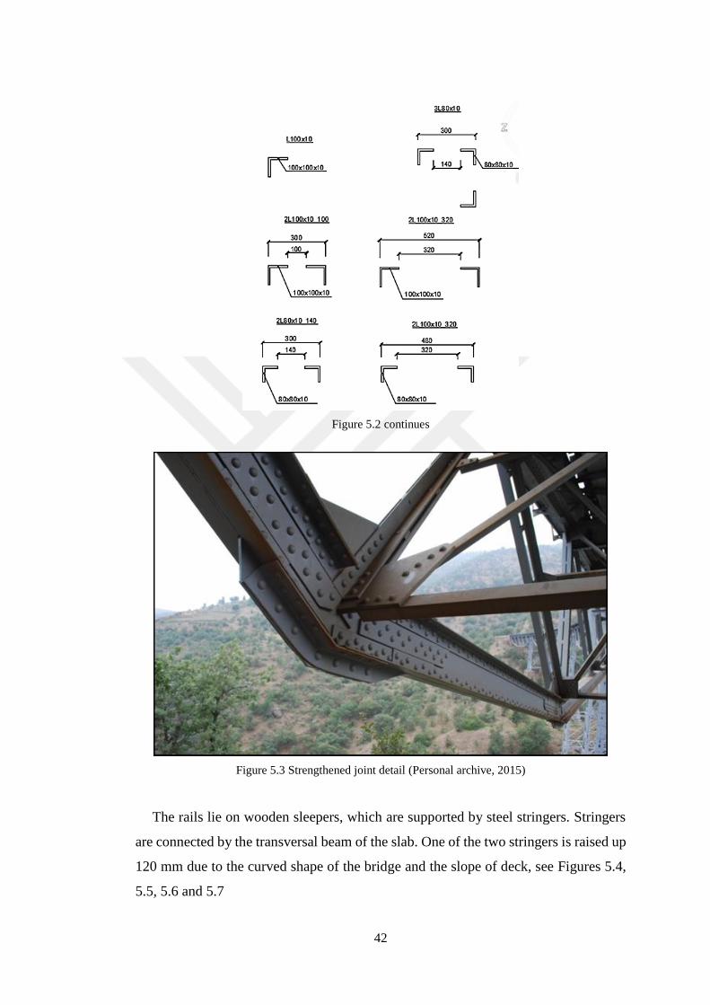
Figure 5.3 Strengthened joint detail (Personal archive, 2015)

The rails lie on wooden sleepers, which are supported by steel stringers. Stringers

are connected by the transversal beam of the slab. One of the two stringers is raised up

120 mm due to the curved shape of the bridge and the slope of deck, see Figures 5.4,

5.5, 5.6 and 5.7

43

Figure 5.4 Deck cross section

Figure 5.5 Detail of the stringer (Personal archive, 2015)

44

Figure 5.6 Rails, footpath and railing (Personal archive, 2015)

Figure 5.7 Sleeper on stringer (Personal archive, 2015)

The footpath on each side of the railroad is realized with a steel sheet of couple of

millimeters, and it has a width of 1120 mm. The footpath is connected with the main

truss system with steel frames. At each side of the footpath there is an open railing

1300 mm height (Figure 5.6). The bridge deck is supported by 5 abutments, each span

is supported by simply (R2=Rotation Y axis) or roller (R2+U1=Translation X axis)

bearing (Figure 5.8).

45

(a)

(b)

Figure 5.8 (a) Simple support and (b) Roller support of the steel railroad bridge (Personal archive,

2015)

Every abutment has a different height and each support is anchored to a masonry

foundation base with rods. Bearings of the pier are just R1, R2 and R3. (Full rotation)

(Figure 5.9 and Figure 5.10)

Figure 5.9 Anchored rod (Personal archive, 2015)

46

Figure 5.10 Masonry base support (Personal archive, 2015)

Abutments are composed of 4 vertical columns connected with vertical, horizontal

and diagonal lateral bracing. Vertical and lateral bracing systems are composed of two

L profiles, which are connected by steel plates (Figure 5.11). For horizontal bracing

system is used a composed L profiles (Figure 5.12 and 5.13). Vertical column is

composed from 4 L profiles and 2 U profiles. On top the pier is composed of 4 L

profiles and 2 plates (Figure 5.14).

Figure 5.11 Abutment (Personal archive, 2015)

47

Figure 5.12 Horizontal bracing (Personal archive, 2015)

Figure 5.13 Abutment with vertical, horizontal and diagonal bracing (Personal archive, 2015)

48

Figure 5.14 Top frame of abutment (Personal archive, 2015)

5.2 Initial Finite Element Model

The data obtained from existing projects of the steel railroad bridge and the

observations made during the exploration trips to the bridge were compiled and the 3D

initial analytical FEM was created using the bridge's FEDEASLab finite element

program. FEDEASLab finite element software in Matlab® (MathWorks, Inc., 2005)

environment is an open-source and non-interface finite element software capable of

performing both static and dynamic linear and nonlinear analysis (Filippou, 2004). The

fact that the program is open-source constitutes an advantageous situation for the study

of updating the FEM by trial-error method. The FEM of the bridge was created by 3-

dimensional frame elements having six degrees of freedom per node, one-dimensional

spring elements to represent column piers, and rigid connection elements that reflect

the support conditions. Since there is no graphical interface to facilitate data entry in

the FEDEASLab program, all parameters required to form a 3-dimensional 6-span

FEM of the steel railroad bridge must be defined individually. These are the coordinate

values (x, y, z) of the nodes of each element, the connectivity matrix required to define

an element to two nodes, the moment of inertia, the torsion constant, the spring

constant, the mass for each node, the Young's modulus, and Poisson values and cross-

sectional properties. All these parameters necessary for the modal analysis of the steel

railroad bridge are defined individually to the nodes or elements. In order to perform

this process quickly and accurately, an Excel file (.xls file) was prepared and all these

parameters were transferred from this prepared Excel file (.xls file) to the FEDEASLab

program and analyzes were performed. It is not practical to manually transfer the

49

bridge model consisting of 1024 nodes and 1610 finite elements to the Excel file (.xls

file) created for the FEDEASLab program and may cause errors. In order to perform

this process faster and accurate, the preliminary FEM of the bridge has been created

in SAP2000 (Computers and Structures, 2010) program and the Excel file (.xls file)

we used for FEDEASLab has been obtained in a more practical and reliable way

(Figure 5.15). The bridge model consisting of 1024 nodes and 1610 finite elements

was created in FEDEASLab with the help of Excel file (.xls file) exported from SAP

2000. The system consists of two side-by-side truss, elements of the bridge lattice

connected to each other by transverse beam and diagonal beams, and elements in the

abutments. In addition, the longitudinal beams (stringers), which sit on the transverse

beams connecting the truss, which are found every six meters, and bearing non-

structural elements such as wooden sleepers and rails, are constituted by 3-dimensional

frame elements. Since the connections of the bridge, which consists of two trusses with

each span, are made with rivets, the joints are involved in the model as rigid

connections. When the joints are modeled, cross-sectional changes have been created

by taking into consideration the dimensions of the connection plates in the joints of

the frame elements. Reinforced and non-reinforced frame element cross-sections are

shown in Figure 5.16. Thus, cross-section increases in the connections are considered

in the bridge FEM.

The bridge is a six spans under-truss system with a total length 180 m, horizontal

radius 300 m and vertical slope 2.5%. Each span is 30 m long, with a maximum width

of 3.2 m and depth of 4.5 m. These geometric parameters are taken into account in the

FEM. Moreover, except the bearing system of the bridge, there are non-structural

elements such as wooden sleepers, rails, jumping cracker, rivets and parapets. The

loads consisting of these non-structural elements have been taken into consideration

by affecting the bearing system as point and distributed load.

50

Figure 5.15 Initial finite element model

Figure 5.16 Frame section without strengthening plates and with strengthening plates

Since the update of the FEM of the bridge will be performed by using the data

obtained from the experimental studies some simplification of the bridge numerical

models has been carried out. Models that are complex and contain too much elements

greatly extend the problem to be updated during the update phase and thus slow down

the processing steps.

To reduce the number of parameters to be updated, it was decided to represent the

bridge abutments only with springs in the analytical model. In this way, only six truss

system and springs between the abutments will be updated. Instead of modeling

abutments of different heights and sizes, one dimensional spring elements were used

in three directions (x, y, z) and the rigidity of the abutments in the bridge system was

obtained in this way (Figure 5.17).

51

Figure 5.17 199 + 325 steel railroad bridge FEM with spring elements

In the determination of the rigidity of the bridge columns, the abutments of different

sizes and heights were modeled separately and the displacements were calculated by

applying 1 ton load in three directions. Displacements of five abutments under 1 ton

force in x, y and z directions were taken into consideration with stiffness = load /

displacement relation and Kx, Ky and Kz stiffness values were found. The spring

stiffness of the abutments used in the FEM obtained in this way is given in Table 5.1.

The abutment numbers are presented in Figure 5.18; Figure 5.19 shows the

displacement of five abutments under 1 ton-force in the x-direction in relation to the

modeling strategy used in the determination of spring stiffness. These abutment

stiffnesses will also constitute one of the update parameters in the bridge system; thus,

changes in spring constants in three different directions used in place of abutments will

represent changes in abutments.

Figure 5.18 Abutment numbers

52

Table 5.1 Spring stiffnesses representing bridge abutments

Initial Spring Stiffnesses

Kx [t/m] Ky [t/m] Kz [t/m]

Abutment 1 2200 5350 106000

Abutment 2 580 1700 55000

Abutment 3 500 1600 50000

Abutment 4 1050 2850 77000

Abutment 5 2850 5600 143000

In order to consider the existence of the abutments they were replaced by a platform

connecting to the bridge deck. The connection between the deck and the platform is

established using two different types of link elements, one that behaves as a roller and

one as a simple. The current state of supports of the bridge is given in Figure 5.20 and

the model approach used for numerical modeling is shown in Figure 5.21. In the first

analytical model, the simple support is modeled to be restrained according to the

translating motion and the roller support is modeled as the link element initial stiffness

is 10000 t / m. Kx, Ky and Kz stiffness values obtained according to the displacement

of the abutments under 1 ton loads were divided into four. These values are assigned

to the springs which under two simple and two roller supports as presented in Figure

5.21. Since there is no remarkable divergence between the bridge model using the

spring and link elements and the initial bridge model, it is assumed that the spring

stiffnesses Kx, Ky and Kz are usable.

In the FEDEASLab program (Figure 5.17), FEM of the bridge was created by using

spring elements and dynamic analyzes were performed. The results of the first five

modes obtained from the dynamic analysis of this FEM are shown in Figure 5.22, 5.23,

5.24, 5.25 and 5.26.

The frequency values of the bridge that achieved from the initial FEM are presented

in Table 5.2. By the reason of the geometric characteristics of the bridge, some of the

first mode shapes of the steel railroad bridge were formed in the lateral direction. The

values obtained in this section belong to the initial model (non-updated), the analytical

53

model is then subjected to the FEM update according to the dynamic parameters

obtained by in-situ tests.

(a) Abutment 1

(b) Abutment 2

(c) Abutment 3

(d) Abutment 4

Figure 5.19 Deformed shape of abutments under 10 kN (1 ton) load in x direction: (a) abutment 1,

(b) abutment 2, (c) abutment 3, (d) abutment 4, (e) abutment 5

54

(e) Abutment 5

Figure 5.19 continues

Figure 5.20 Actual column to support detail (Personal archive, 2015)

55

Figure 5.21 Platform to simulate the abutment effect (modeling approach)

Figure 5.22 1st transversal mode shape and frequency value of FEDEASLab model (2.000 Hz)

Figure 5.23 2nd transversal mode shape and frequency value of FEDEASLab model (2.295 Hz)

56

Figure 5.24 3rd transversal mode shape and frequency value of FEDEASLab model (2.680 Hz)

Figure 5.25 4th transversal mode shape and frequency value of FEDEASLab model (3.011 Hz)

Figure 5.26 3rd vertical mode shape and frequency value of FEDEASLab model (8.243 Hz)

57

Table 5.2 Vibration frequencies of initial numerical model where the columns are modeled by

springs

Mod Shape Frequency [Hz]

1st Transversal 2.000

2nd Transversal 2.295

3rd Transversal 2.680

4th Transversal 3.011

5th Transversal 3.546

1st Torsion 4.795

2nd Torsion 5.588

3rd Torsion 6.089

1st Vertical 7.194

2nd Vertical 8.087

3rd Vertical 8.243

5.3 Finite Element Model Updating (FEMU) Studies

Before the FEMU, sensitivity studies were carried out on the FEM of the bridge to

determine the elements that affect the modal parameters the most. The main objective

of this sensitivity study is to determine the elements that are ineffective on modal

parameter estimations and to update the elements that are sensitive to the modal

parameters in order to obtain the calibrated bridge model. In this way, processing times

are reduced and the possibility of errors is minimized in the update process using less

elements. In these studies, the damage that may occur in red, blue, cyan, magenta, light

green and dark green elements in Figure 5.27 (the elements located in the -y plane and

connecting the two lateral truss of the bridge) is effective on the modal parameter

results. The damage that may occur in the yellow colored elements has no effect on

the results. The different colors in Figure 5.27 represent elements with different cross-

sections.

58

Figure 5.27 Representation of elements that have an effect on bridge modal parameters

Experimental frequency and mode shapes of 199 + 325 Steel Railroad Bridge were

obtained using AV data. The initial FEM was updated using experimental data.

Calibration of the FEM was done by trial-and-error method and the update parameters

are the elements which are the spring stiffness provided by the abutments and sensitive

to the modal parameters of the steel railroad bridge.

In the studies of updating the FEM, FE analysis results were compared with the

frequency values and mode shape vectors obtained from the experimental studies. The

MAC formula shown in Equation 5.1 is applied between analytical and experimental

modes. Experimental modal vectors obtained by applying EFDD technique were used

for MAC calculations.

T 2

a i d ii a i d i T T

a i a i d i d i

((φ ) (φ ) )MAC ((φ ) ,(φ ) )=

((φ ) (φ ) )((φ ) (φ ) ) (5.1)

( )a i = i. analytical mode shape vector

d( )i = i. experimental mode shape vector

All the elements of the bridge and the spring elements representing the abutments

have been updated. The FEM of the steel railroad bridge was updated with trial-and-

59

error method by decreasing the Young's Moduli of all elements by 30% (Table 5.3)

and the obtained spring element stiffness values are given in Table 5.4.

Table 5.3 Inıtial and Updated Young’s Moduli

Initial Young's Modulus Updated Young's Modulus

[N/mm2] [N/mm2]

210000 147000

Table 5.4 Spring stiffnesses representing abutments: Initial and updated values

Initial Spring Stiffnesses

[t/m]

Updated Spring Stiffnesses

[t/m]

Kx Ky Kz Kx Ky Kz

Abutment 1 2200 5350 106000 2200 5350 (0%) 132000 (+25%)

Abutment 2 580 1700 55000 580 2400 (+%41) 68000 (+23%)

Abutment 3 500 1600 50000 500 2200 (+%38) 62000 (+24%)

Abutment 4 1050 2850 77000 1050 4000 (+%40) 96000 (+%25)

Abutment 5 2850 5600 143000 2850 7000 (+25%) 180000 (+%27)

MAC values between experimental mode shape vectors obtained by EFDD method

and updated analytical model mode shape vectors were calculated. MAC comparison

of six different experimental and analytical modes is shown in Table 5.5. As shown in

Table 5.5, three transverse and three vertical modes are obtained in the updated

analytical model, and these values are acceptable MAC values. The visual

representation of the updated analytical model and experimental mode shapes for the

three modes is shown in Figure 5.28 through Figure 5.30. In addition, MAC

information calculated between mode shapes is also given in those figures.

60

Table 5.5 Comparison of estimated modal parameters between analytical and experimental results

Mode Shapes Frequency[Hz] % Difference and MAC Values

Experimentally

Identified

Results

Initial

Numerical

Results

Updated

Numerical

Results

% Difference

(Identified

vs. Initial

FEM)

% Difference

(Identified

vs. Updated

FEM)

MAC

(Identified

vs. Updated

FEM)

1st Transversal 2.133 2.000 2.156 6.24 -1.07 0.97

2nd Transversal 2.396 2.295 2.386 4.22 0.42 0.94

3rd Transversal 2.753 2.680 2.710 2.65 1.56 0.84

1st Vertical 7.292 7.194 7.360 1.34 -0.93 0.88

2nd Vertical 7.729 8.087 7.676 -4.63 0.69 0.76

3rd Vertical 8.370 8.243 8.429 1.52 -0.70 0.92

Although the torsion modes were obtained in the updated analytical model in terms

of frequency values, it was found that the MAC comparison of mode vectors was not

acceptable. It is considered that torsion modes cannot be estimated sufficiently because

only data is collected from the deck plane for safety reasons on the bridge.

61

Figure 5.28 Experimentally estimated mode and their numerically modeled and updated counterpart

for 1st transversal mode

62

Figure 5.29 Experimentally estimated mode and their numerically modeled and updated counterpart

for 1st vertical mode

63

Figure 5.30 Experimentally estimated mode and their numerically modeled and updated counterpart

for 3rd vertical mode

5.4 Numerical Results

In the FEDEASLab program, a simplified steel railroad bridge finite element model

was created for the update process. This simplification was performed using spring

elements instead of abutments and the resulting spring stiffnesses are presented in

Table 5.3. Furthermore, supports of each truss to the platform on the abutments are

represented using link elements (Figure 5.21). The modal analysis of the steel railroad

bridge in FEDEASLab program was performed and obtained the frequency values are

shown in Table 5.2. The frequencies of the transverse modes are in the range of 0-3.6

Hz and the frequency values of the torsion modes are in the range of 3.6-7 Hz. The

vertical modes of the bridge are in the range of 7 to 8.5 Hz.

Young's moduli of all elements and spring stiffness values of spring elements were

selected as update parameters. The FEDEASLab FEM of the steel railroad bridge has

been updated using the trial and error method. The updated Young's Modulus value

64

and the updated spring stiffness values are given in Table 5.3 and Table 5.4,

respectively. A total of 6 experimental and numerical modes, 3 transverse and 3

vertical modes, were matched according to MAC values and these 6 modes were

updated. As shown in Table 5.5, the differences in percentages calculated between the

experimental and numerical frequencies were minimized and MAC values are in

acceptable range. The FEDEASLab FE model of the 199 + 325 steel railroad bridge

was updated using the experimentally modal parameters of the steel railroad bridge,

and this calibrated model is more representative of the actual current state of the bridge.

5.5 Flow Chart (Discussion) of the Methodology

The FE method is a commonly utilized tool for predicting the dynamic behavior of

civil engineering structures, and analyzing and designing them. Depending on the

assumptions made during modeling, the designer performs the analysis by foreseeing

suitable values for parameters containing uncertainties such as material properties,

connections, and boundary conditions. Therefore, it is necessary to calibrate the initial

FEM according to the experimentally obtained modal parameters for more accurate

modeling. Despite the measurement errors likely to occur during experiments, modal

parameters obtained from in-situ measurements are considered to reflect the dynamic

characteristics of the structure better than the initial (not calibrated) FE model.

In this study, the applicability of the SHM method based on the FEMU was studied.

It is recommended that this method become a part of the routine checks of bridges that

have been in-service for many years. The flowchart of the presented method is given

in Figure 5.31 and is detailed below in a step-by-step fashion:

65

1) For the FEM of the structure, data is collected from the existing projects of the

structure. If the projects are not available, field measurements (structure survey)

must be performed and necessary information is obtained for the initial FEM. The

field measurements can also be used to cross check the project values.

2) Initial FEM of the structural system is developed by the data obtained from

the projects and/or field measurements (building survey) of the structure.

3) Test setups are created by considering the mode shapes of the initial FEM, and

AV tests are performed using mainly accelerometers (different type of sensors can

also be used depending on the excitation source).

4) The data collected from ambient vibration tests are processed with operational

modal analysis methods (e.g., EFDD, SSI-Data etc.), and the dynamic parameters

of the structure (frequencies, damping ratios, and mode shapes) are estimated.

5) The model parameters (Young's moduli, mass densities, cross-sectional

dimensions, spring stiffnesses, boundary conditions etc.) of the initial model are

updated and using the experimentally estimated modal parameters (frequency, mode

shape, etc.) by the OMA methods.

6) An FE model, which reflects the current state of the structure (state during the

experiment) is obtained.

7) Ambient vibration tests are performed periodically (or continuously) or after

a natural disaster and modal parameters are re-estimated by OMA methods (e.g.,

EFDD, SSI-Data).

8) The calibrated FE model of the structure is updated once again as described in

step 5 using the new modal parameters.

9) Damage detection is conducted by comparing model parameters of the updated

FEM (step 8) and the reference FEM obtained in step 6.

66

Figure 5.31 The flow chart of the proposed method

67

CHAPTER SIX

CONCLUSIONS

In the scope of this thesis, FEM updating based SHM method was performed on a

steel railroad bridge located on the Basmane-Dumlupınar route in Uşak province near

the city of Eşme. The bridge is operated by Republic of Turkey State Railroads

Department (TCDD). With this work, it is aimed to improve the bridge controls which

are still being done regularly but in a manual manner. This way regularly bridge

controls can become more reliable and objective. Republic of Turkey State Railroads

(TCDD) adapts the proposed method in the routine check procedure. The bridge to be

examined within the scope of the study is a steel railroad bridge. However, the method

is also applicable to other types of bridges.

Two AV tests were conducted on 199+325 Steel Railroad Bridge in winter

(02.12.2015 and 04.12.2015) periods. The data collected on the bridge was processed

by ARTEMIS® using EFDD and SSI-DATA methods. A total of 16 bridge modes

have been identified, seven of which are transverse (lateral), six are torsion, three are

vertical. The frequency values of the bridge transverse modes are in the range of 0-3.5

Hz and the frequency values of the torsion modes are in the range of 3.5-7 Hz. The

vertical modes of the bridge are in the range of 7 to 8.5 Hz.

According to the mode shapes obtained from the initial FEM, the test setups used

on the bridge were planned in terms of sensor layout. By using ambient vibration data,

experimental frequencies and mode shapes of the steel railroad bridge were estimated.

The initial FEM was updated using experimental estimated modal data. Calibration of

the FEM was done by using a trial-error procedure and the truss and spring elements

which are sensitive to the modal parameters are determined from a sensitivity work,

after that the parameters to be updated were selected. The results of the FEMU analysis

and the experimental results obtained from the bridge tests were compared. The

experimental modal shapes obtained by using EFDD technique were used for MAC

for calculations. The three transversal and three vertical numerical mode shapes of the

68

bridge were acceptable considering the MAC values calculated between the numerical

modes and their experimental counterparts.

Because FEDEASLab is an open source software, it is advantageous for FEMU

studies based on the trial and error method compared to other finite element programs.

Since the information about the finite elements is defined individually in FEDEASLab

program, the changes of the element properties can be made in a faster and practical

way.

The FEDEASLab model of the 199+325 steel railroad bridge was updated by a

trial-error procedure using the estimated modal parameters. Thus, a reliable FEM is

obtained which reflects the current state of the bridge. Different damage scenarios can

be applied to this model and FEM updating can be used to predict the inflicted damage

and its extent. More realistic damage detection studies will be possible by monitoring

the bridge's AV data as a result of regular measurements on the bridge. After disasters

with damaging potential, data will be collected again on the bridge and the calibrated

model of the bridge will be updated according to these data and damage detection will

be made more accurately and reliably. In this study, a database on the modal

parameters of the 199+325 steel railroad bridge has been obtained (e.g., a benchmark

state). Regular measurements and maintenance of SHM studies are important for early

detection of possible damage situations. It is considered that it will be beneficial to

carry out more advanced studies to determine the existence of the damage and its

location.

The objective of the thesis is to identify the modal parameters of the bridge and to

create a calibrated reference FE model. Ambient vibration data of the steel railroad

bridge were collected, and 16 modal parameters were estimated by EFDD and SSI-

Data methods. The following findings were observed as a result of the operational

modal analysis of the steel railroad bridge and finite element model updating studies.

69

1. The finite element model of the bridge was created in the FEDEASLab program

and the FEM was updated using a trial-error procedure. In addition, a FEM was

obtained as a reference for sensitivity based finite element model updating studies to

be performed in the future.

2. Transverse modes are more dominant due to the geometry of the bridge.

3. It has been found that sensitivity studies should be performed to determine the

updating parameters to decrease the amount of elements to be updated in a numerical

model containing a large number of elements such as 199+325 steel railroad bridge.

4. As a result of the sensitivity studies, it was concluded that the spring stiffness

values used for modeling the abutments and Young's moduli of the elements were

effective on the modal parameters.

5. In the FEMU studies, reducing the model to a sufficiently simple model makes

the updating procedure faster and more reliable.

6. In this study, the applicability of the structural health monitoring method based

on FEMU was investigated. It is recommended that this method become a part of the

routine checks of bridges that have been in-service for many years.

7. The updated FEM of the bridge can be a useful tool for TCDD to determine the

capacities of the bridge elements.

Future Studies

A calibrated model representing the actual state of the bridge was developed in

FEDEASLab finite element software. In the future, it is planned to carry out damage

detection studies using this calibrated model by applying different damage scenarios

on this model. Also the model can be used with sensitivity based FEM updating

methods to perform model updating in a more objective and systematic way.

70

REFERENCES

Akar, V. (2009). Köprüler bilgisi ders notları. TCDD Yol Dairesi Başkanlığı, Ankara.

Akın, T. (2012). Structural monitoring and analysis of steel truss railroad bridges.

Master Thesis, Orta Doğu Teknik Üniversitesi, Ankara.

Allemang, R. J. & Brown, D. L. (1982). A correlation coefficient for modal vector

analysis. Presented at the 1st International Modal Analysis Conference (IMAC I),

Bethel, CT, USA, 1, 110-116

Altunışık, A. C., & Bayraktar, A., & Sevim, B., & Ateş, Ş. (2011a). Ambient vibration

based seismic evaluation of isolated gülburnu highway bridge. Soil Dynamics and

Earthquake Engineering, 31(11), 1496-1510.

Altunışık, A. C., & Bayraktar, A., & Sevim, B. (2011b). Output-only system

identification of posttensioned segmental concrete highway bridges. Journal of

Bridge Engineering, 16(2), 259-266.

Altunışık, A. C., & Bayraktar, A., & Özdemir, H. (2012). Seismic safety assessment

of eynel highway steel bridge using ambient vibration measurements. Smart

Structures and Systems, 10(2), 131-154.

ARTEMIS Extractor Pro Software, (2010). Structural vibration solutions. Aalborg,

Denmark.

Asgari, B., & Osman, S. A., & Adnan, A. (2013). Sensitivity analysis of the influence

of structural parameters on dynamic behaviour of highly redundant cable-stayed

bridges. Advances in Civil Engineering, 2013, 1-11.

71

Bayraktar, A., & Altunışık, A. C., & Sevim, B., & Türker T., & Domaniç, A., & Taş,

Y. (2009). Vibration characteristics of Kömürhan highway bridge constructed with

balanced cantilever method. Journal of Performance of Constructed Facilities,

23(2), 90-99.

Bayraktar, A., & Altunışık, A. C., & Sevim, B., & Özşahin, T. Ş. (2014).

Environmental effects on the dynamic characteristics of the Gülburnu highway

bridge. Civil Engineering and Environmental Systems, 31(4), 347-366.

Bendat, J. S., & Piersol, A. G. (2010). Random data: Analysis and measurement

procedures (4th ed). USA: John Wiley and Sons.

Benedettini, F., & Gentile, C. (2011). Operational modal testing and FE model tuning

of a cable-stayed bridge. Engineering Structures, 33(6), 2063-2073.

Brincker, R., & Zhang, L., & Andersen, P. (2001). Modal identification of output-only

systems using frequency domain decomposition. Smart Materials and Structures,

10, 441-445.

Brownjohn, J. M., & Xia, P. Q. (2000). Dynamic assessment of curved cable-stayed

bridge by model updating. Journal of Structural Engineering, 126(2), 252-260.

Cunha, A., & Caetano, E., & Calçada, R., & De Roeck, G., & Peeters, B. (2003).

Dynamic measurements on bridges: design, rehabilitation and monitoring. In

Proceedings of the Institution of Civil Engineers-Bridge Engineering 156(3) 135-

148.

Çağlayan O, & Özakgül K., & Tezer Ö., & Uzgider E. (2011). Evaluation of a steel

railway bridge for dynamic and seismic loads. Journal of Constructional Steel

Research, 67, 1198-1211.

72

Çağlayan O, & Özakgül K., & Tezer Ö., & Piroğlu F. (2015). In-situ field

measurements and numerical model identification of a multi-span steel railway

bridge. Journal of Testing and Evaluation, 43(6), 1323-1337.

Doebling, S. W., & Farrar, C. R., & Prime, M. B., & Shevitz, D. W. (1996). Damage

identification and health monitoring of structural and mechanical systems for

changes in their vibration characteristics. Technical Report LA-13070-MS, Los

Alamos National Laboratory.

Doebling, S. W., & Farrar, C. R., & Prime, M. B. (1996). A summary review on

vibration-based damage identification methods. Los Alamos National Laboratory,

Engineering Analysis Group.

Doebling, S.W., & Farrar, C.R., & Prime, M.B. (1998). A summary review of

vibration-based damage identification methods. The Shock and Vibration Digest,

30(2), 91-105.

Doehler, M., & Hille, F. (2014). Subspace-based damage detection on steel frame

structure under changing excitation. Strucutral Health Monitoring, 5, 167-174.

Doehler, M., & Hille, F., & Mevel, L., & Rücker, W. (2014). Structural health

monitoring with statistical methods during progressive damage test of S101 bridge.

Engineering Structures, 69, 183-193.

Enevoldsen, I., & Pedersen, C., & Axhag, F., & Johansson, Ö., & Töyrä, B. (2002).

Assessment and measurement of the Forsmo Bridge, Sweden. Structural

Engineering International, 12(4), 254-257.

Farrar, C.R., & James, G.H. (1997). System identification from ambient vibration

measurements on a bridge. Journal of Sound and Vibration, 205(1), 1-18.

73

Feng, M.Q., & Kim, D. K., & Yi, J. H., & Chen, Y. (2004). Baseline models for bridge

performance monitoring. Journal of Engineering Mechanics, 130(5), 562-569.

Filippou, F. C., & Constantinides, M. (2004). FEDEASLab getting started guide and

simulation examples. Technical Report, NEESgrid.

Frýba, L., & Pirner, M. (2001). Load tests and modal analysis of bridges. Engineering

Structures, 23(1), 102-109.

He, X., & Moaveni, B., & Conte, J. P., & Elgamal A., & Masri, S. F. (2008), Modal

identification study of vincent thomas bridge using simulated wind-induced

ambient vibration data. Journal of Computer-Aided Civil and Infrastructure

Engineering, 23(5), 373-388.

Hong, A. L., & Ubertini, F., & Betti, R. (2010). Wind analysis of a suspension bridge:

identification and finite-element model simulation. Journal of Structural

Engineering, 137(1), 133-142.

Jaishi, B., & Ren, W. X. (2005). Structural finite element model updating using

ambient vibration test results. Journal of Structural Engineering, 131(4), 617-628.

Manolakis, G. M., & Ingle, V. K., & Kogon, S. M. (2000). Statistical and adaptive

signal processing. New York: McGraw Hill.

Moaveni, B. (2007). System identification of civil structures. Phd Thesis, Department

of Structural Engineering, University of California, San Diego, California.

Mottershead, J. E., & Friswell, M. I. (1993). Model updating in structural dynamics: a

survey. Journal of Sound and Vibration, 167(2), 347-375.

74

Peeters, B., & De Roeck, G. (2001). Stochastic system identification for operational

modal analysis: A review. Journal of Dynamic Systems, Measurement, and Control,

123(4), 659-667.

Rytter, A. (1993). Vibration based inspection of civil engineering structures. Phd

Thesis, Department of Building and Technology and Structural Engineering,

Aalborg University, Denmark.

SAP2000, (1998). Integrated finite element analysis and design of structures.

Computers and Structures Inc, Berkeley, California, USA.

Siriwardane, S. C. (2015). Vibration measurement-based simple technique for damage

detection of truss bridges: A case study. Case Studies in Engineering Failure

Analysis, 4, 50-58.

Sohn, H., & Farrar, C. R., & Hemez, F. M., & Shunk, D. D., & Stinemates, D. W., &

Nadler, B. R., & Czarnecki J.J. (2003). A review on structural health monitoring

literature: 1996-2001. Los Alamos National Laboratory, Technical Report annex

to SAMCO Summer Academy, Cambridge.

Spyrakos, C.C., & Raftoyiannis I.G., & Ermopoulos J.C. (2004). Condition assessment

and retrofit of a historic steel-truss railway bridge. Journal of Constructional Steel

Research, 60(8), 1213–1225.

Teughles, A., & De Roeck, G. (2004). Structural damage identification of the highway

bridge Z24 by FE model updating. Journal of Sound and Vibration, 278(3), 589-

610.

Van Overschee, P., & De Moor, B. (1996). Subspace Identification for Linear Systems.

Norwell, Massachusetts: Kluwer Academic Publishers.

75

Zivanovic, S., & Pavic, A., & Reynolds, P. (2007). Finite element model updating and

updating of a lively footbridge: The complete process. Journal of Sound and

Vibration, 301(1-2), 126-145.