Open flexible P-controller designMikulas Huba

Slovak University of Technology in Bratislava, SlovakiaEmail: mikulas.huba@stuba.sk

Abstract—The paper represents first part of two contributionsdealing with simplified modular design of constrained P and dis-turbance observer (DO) based PI control with different filteringproperties illustrated by example of speed servo control. This firstpart is devoted to analysis of the core structure of the P controllertuned for different types of nonmodelled or filter dynamics. Open-ness of the approach means that for approximating additionaldynamics of the P-controller structure different filters may beused without necessity to repeat in the nominal case analysisof the optimal and critical tuning. By simpler means, flexibleapproach enabling to fit requirements of particular loop andsimultaneously offering reasonably better performance than thetraditional controller design based on Luenberger disturbanceobserver for reconstruction of the velocity signal is proposed.Achieved performance is evaluated by newly introduced measuresfor deviations from monotonic and one-pulse shapes of transientstypical for control of plants with dominant 1st order dynamics.

I. INTRODUCTION

The P control design represents one of the simplest andnon-problematic control tasks with long traditions and highnumber of applications. In this paper optimal controller tuningis treated simultaneously with the problem of quantizationnoise filtration that is typical for design of speed control basedon use of incremental encoders for position measurement.Motivation for this work is, however, broader: it is looking foralternatives to traditional PI control that would be able to dealeffectively and reliably with integral and unstable systems,with uncertain systems under measurement noise and highperformance requirements, with systems having long deadtime or with nonlinear systems.

This paper aims to continue in spreading information aboutnew course Constrained PID Control [2] by showing, how aunifying modular combination of P-control with disturbanceobserver (DO) known from advanced mechatronic applicationsmay be extended to a new flexible approach.

II. CONTROL OF LINEAR FIRST ORDER PLANTS

In PID control, two step procedure for the controller designhas been established ( [3]):• by considering firstly the dominant loop dynamics, ap-

propriate controller structure is chosen,and then• controller tuning is fixed by respecting nonmodelled

dynamics, plant uncertainty and measurement noise.In designing P and PI controllers, the dominant first-orderplant dynamics with the output and input disturbances di anddo is considered, x and y being the plant state, or output

dx/dt = Ks(ur + di)− ax ; y = x+ do (1)

0 0.2 0.4 0.6 0.8 10

0.2

0.4

0.6

0.8

1

Ideal Input and Output Pair of Single Integrator

y0

y∞

−−

−>

y(t

)

0 0.2 0.4 0.6 0.8 10

0.2

0.4

0.6

0.8

1

−−−> t

−−

−>

u=

dy/d

t

tm

um

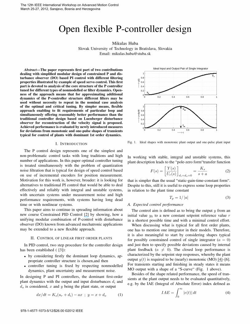
Fig. 1. Ideal shapes with monotonic plant output and one-pulse plant input

In working with stable, integral and unstable systems, thisplant description leads to the “pole-zero form“transfer function

F (s) =

[Y (s)

Ur(s)

]di=do=0

=Ks

s+ a(2)

that is simpler than the usual “static-gain-time-constant form“.Despite to this, still it is useful to express some loop propertiesin relation to the plant time constant

Tp = 1/ |a| (3)

A. Expected control performanceThe control aim is defined as to bring the output y from an

initial value y0 to a new constant setpoint reference value rin a shortest possible time and with a minimal control effort.

When discussing what is typical for all first order plants,one has to mention one integrator in their models. Therefore,it is also meaningful to start by considering shapes typicalfor possibly constrained control of single integrator (a = 0)and just then to specify possible deviations caused by internalplant feedback (a 6= 0). The closed loop performance ischaracterized by the setpoint step responses, whereby the plantoutput y(t) is required to be (nearly) monotonic (MO) [4]–[6].For transients starting and finishing in steady states it meansMO output with a shape of a “S-curve“ (Fig. 1 above).

Besides of the shape related performance, the speed of tran-sients at the plant output needs to be evaluated quantitatively,e.g. by the IAE (Integral of Absolute Error) index defined as

IAE =

∫ ∞0

|e(t)| dt (4)

The 12th IEEE International Workshop on Advanced Motion Control March 25-27, 2012, Sarajevo, Bosnia and Herzegovina

978-1-4577-1073-5/12/$26.00 ©2012 IEEE

For single integrator the input corresponding to the requiredS-shaped output found by its derivation has shape of a one-pulse (1P) function having one extreme point separating twoMO intervals (Fig. 1 below). Under constrained control, in-stead of one extreme point an interval at the saturation limitmay occur separating intervals with MO changing plant input.

For evaluating control effort needed to achieve requiredoutput behavior, Total Variance (TV) was proposed by [7]

TV =

∫ ∞0

∣∣∣∣dudt∣∣∣∣ dt ≈∑

i

|ui+1 − ui| (5)

In Matlab it may be simply computed by the commandsum(abs(diff(u)). Based on TV, new measures for de-viations from MO and 1P shapes may be proposed [4]–[6].Deviations from strictly MO shape of the plant output y(t)with the initial value y0 and the final value y∞ may becharacterized by yTV0 criterion

yTV0 =∑i

|yi+1 − yi| − |y∞ − y0| (6)

yTV0 = 0 just for strictly MO response, else yTV0 > 0.Contribution of the superimposed oscillation in 1P dominant

control are expressed for um = max{u} by

uTV1 =∑i

|ui+1 − ui| − |2um − u∞ − u0| (7)

uTV1 = 0 just for strictly 1P response, else for controlsignals with superimposed higher harmonics uTV1 > 0.

B. Basic controller equation

For a piecewise constant setpoint values r, under poleassignment control of the first order plant one can require thesetpoint-to-output relation with the time constant Tr

Fr(s) =Y (s)

R(s)=

1

Trs+ 1(8)

After substituting for (1) and solving for u one gets

u = KP e+ u∞e = r − y ; KP = (1/Tr − a) /Ks

u∞ = a(r − do)/Ks − di(9)

Thereby, u∞ corresponds to static feedforward control neces-sary for keeping the output in a steady state at the requiredreference value r under influence of constant disturbances.

Closed loop with the P-controller (9) remains stable up tothe moment when its pole s = −1/Tr remains negative and

KPKs + a > 0 (10)

For stable and marginally stable plants (a ≥ 0) this holds forany KPKs > 0 and stability will be satisfied by any 0 <Tr <∞. For unstable plants (a < 0) it must hold

Tr < −1/a = Tp (11)

i.e. the controller gain cannot be arbitrarily decreased (theclosed loop time constant Tr cannot be arbitrarily increased),just to a value fulfilling (11). In tuning P controller this fact

is extremely important: in controlling stable plant the gain de-crease is frequently used both for eliminating effect of controlconstraints, for decreasing influence of the measurement noise,uncertainty in parameters and of the nonmodelled dynamics.Due to this, controller tuning for unstable plants is reasonablydifferent from the prevailing case with stable plants and sothe contemporary research in robust and constrained controlis motivated mainly by these contradictory requirements.

III. NONMODELLED AND FILTER DYNAMICS AND THECONTROLLER TUNING

Plant approximation by the first order model (1) usedfor the P-controller structure design is not sufficient for itsreliable tuning. This should consider additional loop dynamicscomposed from the inherently included nonmodelled dynamicsand the intentionally introduced dynamics of different filters.

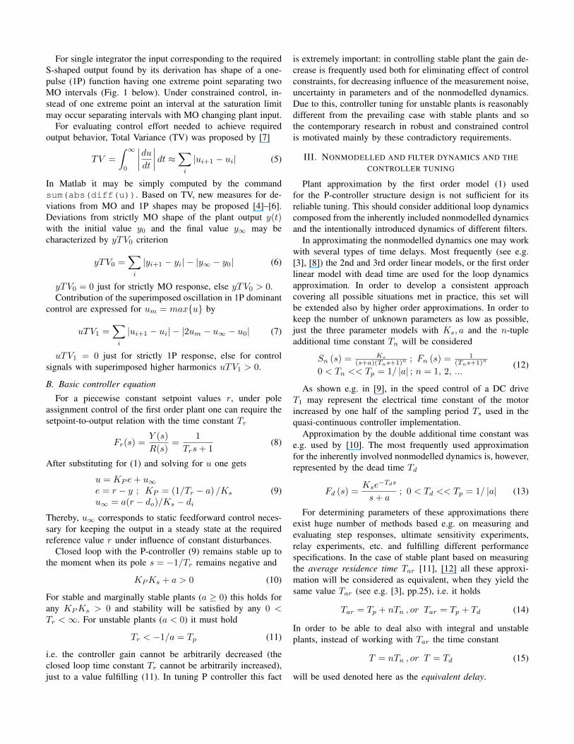
In approximating the nonmodelled dynamics one may workwith several types of time delays. Most frequently (see e.g.[3], [8]) the 2nd and 3rd order linear models, or the first orderlinear model with dead time are used for the loop dynamicsapproximation. In order to develop a consistent approachcovering all possible situations met in practice, this set willbe extended also by higher order approximations. In order tokeep the number of unknown parameters as low as possible,just the three parameter models with Ks, a and the n-tupleadditional time constant Tn will be considered

Sn (s) = Ks

(s+a)(Tns+1)n ; Fn (s) = 1(Tns+1)n

0 < Tn << Tp = 1/ |a| ; n = 1, 2, ...(12)

As shown e.g. in [9], in the speed control of a DC driveT1 may represent the electrical time constant of the motorincreased by one half of the sampling period Ts used in thequasi-continuous controller implementation.

Approximation by the double additional time constant wase.g. used by [10]. The most frequently used approximationfor the inherently involved nonmodelled dynamics is, however,represented by the dead time Td

Fd (s) =Kse

−Tds

s+ a; 0 < Td << Tp = 1/ |a| (13)

For determining parameters of these approximations thereexist huge number of methods based e.g. on measuring andevaluating step responses, ultimate sensitivity experiments,relay experiments, etc. and fulfilling different performancespecifications. In the case of stable plant based on measuringthe average residence time Tar [11], [12] all these approxi-mation will be considered as equivalent, when they yield thesame value Tar (see e.g. [3], pp.25), i.e. it holds

Tar = Tp + nTn , or Tar = Tp + Td (14)

In order to be able to deal also with integral and unstableplants, instead of working with Tar the time constant

T = nTn , or T = Td (15)

will be used denoted here as the equivalent delay.

0 0.5 1 1.5 2 2.5 3 3.5 40

0.1

0.2

0.3

0.4

0.5

0.6

0.7

0.8

0.9

1

−−−> t

−−

−>

y(t

)T

ar=2, T

p=0.75, T

d=1.25, T

1=1.25, T

2=0.625, T

3=0.41667, T

4=0.3125, T

8=0.15625, T

16=0.078125

Td

T1

T2

T3

T4

T8

T16

Fig. 2. Family of approximations (12-15) with the same Tar

A. Gain analysis including nonmodelled dynamics

For a detailed loop characterization, it is firstly importantto derive the closed loop transfer functions from all possibleloop inputs to the output [3]. For Fn in the feedback one gets

Frn (s) = Y (s)R(s) = (KPKs+a)(Tns+1)n

(s+a)(Tns+1)n+KPKs

Fin (s) = Y (s)Di(s)

= Ks(Tns+1)n

(s+a)(Tns+1)n+KPKs

Fon (s) = Y (s)Do(s)

= (s+a)(Tns+1)n

(s+a)(Tns+1)n+KPKs

(16)

Similarly, for Td in the feedback one gets

Frd (s) = Y (s)R(s) = (KPKs+a)e

Tds

(s+a)eTds+KPKs

Fid (s) = Y (s)Di(s)

= KseTds

(s+a)eTds+KPKs

Fod (s) = Y (s)Do(s)

= (s+a)eTds

(s+a)eTds+KPKs

(17)

From KPKs + a 6= 0 it follows Frn (0) = Frd (0) = 1, i.e.in steady states without acting disturbances the output will beequal to the setpoint value. However, since also simultaneouslyFin (0), Fid (0), Fon (0), Fod (0) 6= 0, the steady state outputwill be influenced by possible constant nonzero disturbances.Since the controller gain KP is included in the denominatorof the steady-state gains Fin (0), Fid (0), Fon (0) and Fod (0),suppression of the disturbance influence requires to work withas large as possible values KP .

For determining an appropriate controller tuning in presenceof the nonmodelled dynamics, or additional filters, it is possi-ble to use several approaches. The simplest situation seems tobe in the case of single time constant T1 yielding the closedloop characteristic polynomial A(s) = T1s

2 + (1 + aT1)s +KPKs + a that gives the relative damping

ξ =1 + aT1

2√KPKsT1 + aT1

(18)

By requiring damping ξ ≥√

2 as in [9], one gets

KP ≤(1− aT1)2

2T1(19)

This approach, however, cannot be directly extended to higherorder approximations and is not appropriate to determinestable range of controller gains.

By using the requirement on possibly good disturbancesuppression by possibly large KP values, for a batch of pro-cesses Ziegler and Nichols [13] have determined appropriatetuning experimentally. The achieved performance specified asthe “quarter amplitude damping“ gave ratio of two subse-quent error amplitudes 4 : 1. Later, many authors tried toimprove this method by considering differently specified batchof processes, different performance measures and differentdesign methods [3], [14]–[16]. This experimental approachwas recently automatized by the performance portrait method[4], [5] enabling to look for optimal and robust tuning byspecifying arbitrary performance restraint for given task.

B. Tuning corresponding to double real dominant pole

In analytical controller tuning appropriate for any consid-ered additional dynamics, one of the oldest method for achiev-ing well damped but sufficiently fast dynamics requires doublereal dominant pole [17] of the characteristic polynomials

A (s) = (s+ a)(Tns+ 1)n +KPKs

A (s) = (s+ a)eTds +KPKs(20)

For a double pole so of A(s) it must hold A (so) = 0 andA (so) = 0, what yields

KPn = (1−a)KsTn(n+1)

(n(1−a)n+1

)nKPd = 1

KsTde−(1+aTd)

(21)

so = − 1+nTn aTn (n+1)

so = − (1 + aTd) /Td(22)

The control loop remains stable just for so < 0, i.e. for

anTn = aT > −1aTd > −1

(23)

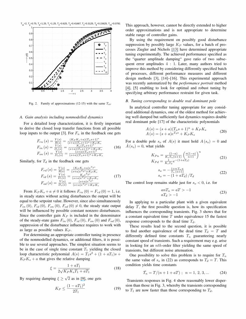
In applying to a particular plant with a given equivalentdelay T , the first possible question is, how its specificationinfluences the corresponding transients. Fig. 3 shows that fora constant equivalent time T under equivalence 15 the fastestresponse corresponds to the dead time Td.

These results lead to the second question, it is possibleto find another equivalence of the dead time Td = T anddifferently defined time constants Tn guaranteeing nearlyconstant speed of transients. Such a requirement may e.g. arisein looking for an nth-order filter yielding the same speed oftransients, but different noise attenuation.

One possibility to solve this problem is to require for Tnthe same value of so in (22) as corresponds to Td = T . Thiscondition yields time constants

Tn = T/(n+ 1 + aT ) ; n = 1, 2, 3, ... (24)

Transients responses in Fig. 4 show reasonably lower disper-sion than those in Fig. 3, whereby the transients correspondingto T1 are now faster than those corresponding to Td.

0 2 4 6 8 100

0.1

0.2

0.3

0.4

0.5

0.6

0.7

0.8

0.9

1

−−−> t

−−

−>

y(t

)

T1

T2

T3

T4

T5

Td

0 2 4 6 8 100

0.05

0.1

0.15

0.2

0.25

0.3

0.35

0.4

−−−> t

−−

−>

u(t

)

T

1

T2

T3

T4

T5

Td

Fig. 3. Transient responses corresponding to approximations (12-15) withthe same equivalent delay T = 1, a = 1

0 2 4 6 8 100

0.1

0.2

0.3

0.4

0.5

0.6

0.7

0.8

0.9

1

−−−> t

−−

−>

y(t

)

T1

T2

T3

T4

T5

Td

0 2 4 6 8 100

0.05

0.1

0.15

0.2

0.25

0.3

0.35

0.4

0.45

0.5

−−−> t

−−

−>

u(t

)

T

1

T2

T3

T4

T5

Td

Fig. 4. Transient responses corresponding to time constants (24), T =Tar − Tp

7 7.1 7.2 7.3 7.4 7.5 7.6 7.70.985

0.99

0.995

−−

−>

y(t

)

m=0

7 7.1 7.2 7.3 7.4 7.5 7.6 7.70.985

0.99

0.995

−−

−>

y(t

)

m=0.11

7 7.1 7.2 7.3 7.4 7.5 7.6 7.70.985

0.99

0.995

−−−> t

−−

−>

y(t

)

m=0.2

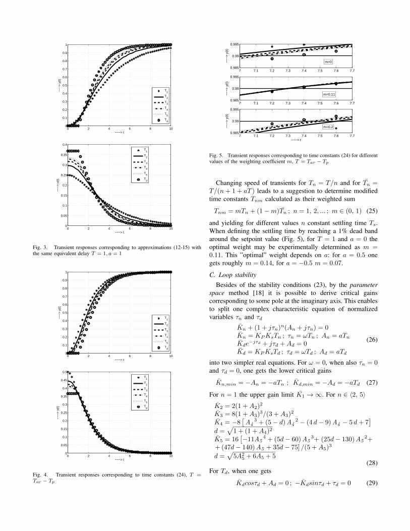
Fig. 5. Transient responses corresponding to time constants (24) for differentvalues of the weighting coefficient m, T = Tar − Tp

Changing speed of transients for Tn = T/n and for Tn =T/(n+ 1 + aT ) leads to a suggestion to determine modifiedtime constants Tnm calculated as their weighted sum

Tnm = mTn + (1−m)Tn ; n = 1, 2, ... ; m ∈ (0, 1) (25)

and yielding for different values n constant settling time Ts.When defining the settling time by reaching a 1% dead bandaround the setpoint value (Fig. 5), for T = 1 and a = 0 theoptimal weight may be experimentally determined as m =0.11. This ”optimal” weight depends on a: for a = 0.5 onegets roughly m = 0.14, for a = −0.5 m = 0.07.

C. Loop stability

Besides of the stability conditions (23), by the parameterspace method [18] it is possible to derive critical gainscorresponding to some pole at the imaginary axis. This enablesto split one complex characteristic equation of normalizedvariables τn and τd

Kn + (1 + jτn)n(An + jτn) = 0Kn = KPKsTn ; τn = ωTn ; An = aTnKde

−jτd + jτd +Ad = 0Kd = KPKsTd ; τd = ωTd ; Ad = aTd

(26)

into two simpler real equations. For ω = 0, when also τn = 0and τd = 0, one gets the lower critical gains

Kn,min = −An = −aTn ; Kd,min = −Ad = −aTd (27)

For n = 1 the upper gain limit K1 →∞. For n ∈ 〈2, 5〉K2 = 2(1 +A2)2

K3 = 8(1 +A3)3/(3 +A3)2

K4 = −8[A4

3 + (5− d)A42 − (4 d− 9)A4 − 5 d+ 7

]d =

√1 + (1 +A4)2

K5 = 16[−11A5

4 + (5d− 60)A53+ (25d− 130)A5

2++ (47d− 140)A5 + 35d− 75] /(5 +A5)3

d =√

5A25 + 6A5 + 5

(28)For Td, when one gets

Kdcosτd +Ad = 0 ; −Kdsinτd + τd = 0 (29)

−1 −0.8 −0.6 −0.4 −0.2 0 0.20

0.1

0.2

0.3

0.4

0.5

0.6

0.7

0.8

0.9

1

−−> A=a*T

−−

> K

P*K

s*T

Optimal and Minimal Gains

opt

min

T=Td

T=T1

T=2T2

T=3T3

T=5T5

−1 −0.8 −0.6 −0.4 −0.2 0 0.21

1.1

1.2

1.3

1.4

1.5

1.6

1.7

1.8

1.9

2

−−> A=a*T

−−

> K

P*K

s*T

Upper Critical Gains

T=Td

T=2T2

T=3T3

T=4T4

T=5T5

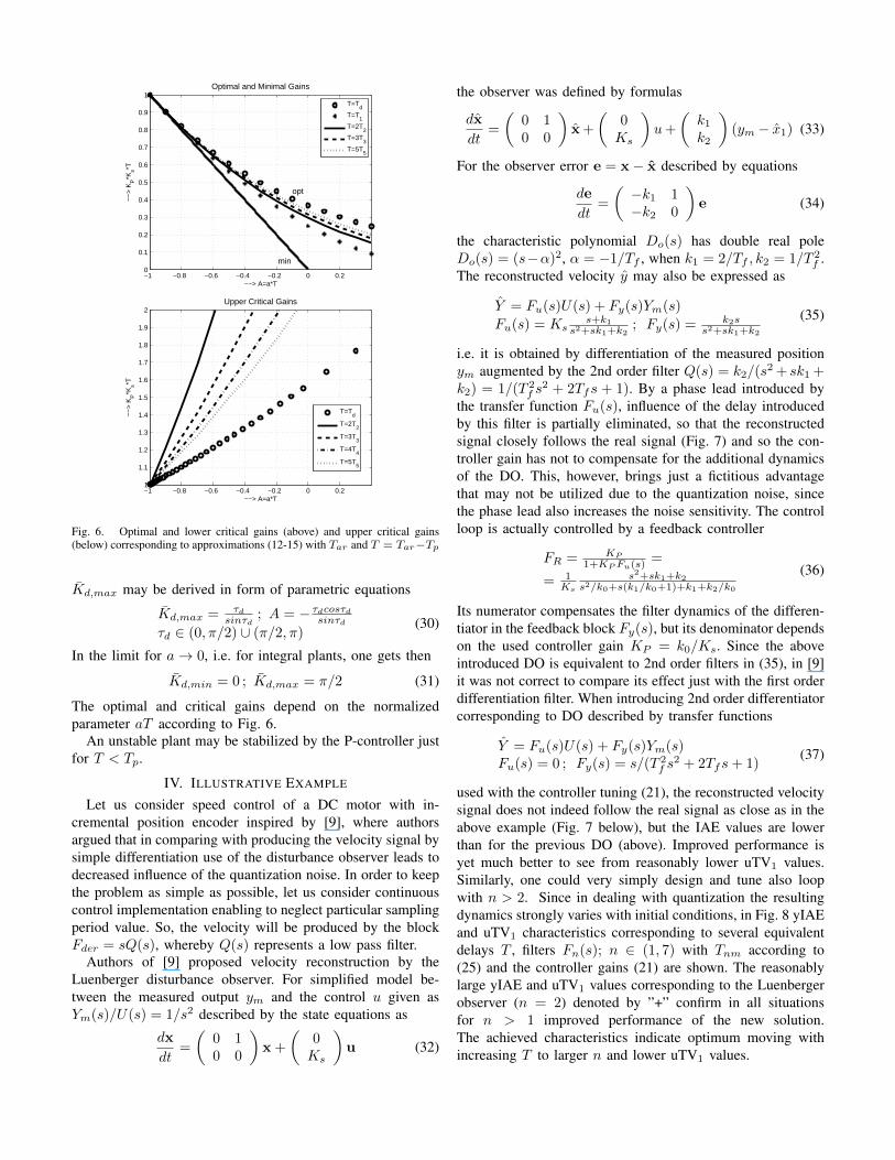
Fig. 6. Optimal and lower critical gains (above) and upper critical gains(below) corresponding to approximations (12-15) with Tar and T = Tar−Tp

Kd,max may be derived in form of parametric equations

Kd,max = τdsinτd

; A = − τdcosτdsinτdτd ∈ (0, π/2) ∪ (π/2, π)

(30)

In the limit for a→ 0, i.e. for integral plants, one gets then

Kd,min = 0 ; Kd,max = π/2 (31)

The optimal and critical gains depend on the normalizedparameter aT according to Fig. 6.

An unstable plant may be stabilized by the P-controller justfor T < Tp.

IV. ILLUSTRATIVE EXAMPLE

Let us consider speed control of a DC motor with in-cremental position encoder inspired by [9], where authorsargued that in comparing with producing the velocity signal bysimple differentiation use of the disturbance observer leads todecreased influence of the quantization noise. In order to keepthe problem as simple as possible, let us consider continuouscontrol implementation enabling to neglect particular samplingperiod value. So, the velocity will be produced by the blockFder = sQ(s), whereby Q(s) represents a low pass filter.

Authors of [9] proposed velocity reconstruction by theLuenberger disturbance observer. For simplified model be-tween the measured output ym and the control u given asYm(s)/U(s) = 1/s2 described by the state equations as

dx

dt=

(0 10 0

)x +

(0Ks

)u (32)

the observer was defined by formulas

dx

dt=

(0 10 0

)x+

(0Ks

)u+

(k1k2

)(ym − x1) (33)

For the observer error e = x− x described by equations

de

dt=

(−k1 1−k2 0

)e (34)

the characteristic polynomial Do(s) has double real poleDo(s) = (s−α)2, α = −1/Tf , when k1 = 2/Tf , k2 = 1/T 2

f .The reconstructed velocity y may also be expressed as

Y = Fu(s)U(s) + Fy(s)Ym(s)

Fu(s) = Kss+k1

s2+sk1+k2; Fy(s) = k2s

s2+sk1+k2

(35)

i.e. it is obtained by differentiation of the measured positionym augmented by the 2nd order filter Q(s) = k2/(s

2 + sk1 +k2) = 1/(T 2

f s2 + 2Tfs + 1). By a phase lead introduced by

the transfer function Fu(s), influence of the delay introducedby this filter is partially eliminated, so that the reconstructedsignal closely follows the real signal (Fig. 7) and so the con-troller gain has not to compensate for the additional dynamicsof the DO. This, however, brings just a fictitious advantagethat may not be utilized due to the quantization noise, sincethe phase lead also increases the noise sensitivity. The controlloop is actually controlled by a feedback controller

FR = KP

1+KPFu(s)=

= 1Ks

s2+sk1+k2s2/k0+s(k1/k0+1)+k1+k2/k0

(36)

Its numerator compensates the filter dynamics of the differen-tiator in the feedback block Fy(s), but its denominator dependson the used controller gain KP = k0/Ks. Since the aboveintroduced DO is equivalent to 2nd order filters in (35), in [9]it was not correct to compare its effect just with the first orderdifferentiation filter. When introducing 2nd order differentiatorcorresponding to DO described by transfer functions

Y = Fu(s)U(s) + Fy(s)Ym(s)Fu(s) = 0 ; Fy(s) = s/(T 2

f s2 + 2Tfs+ 1)

(37)

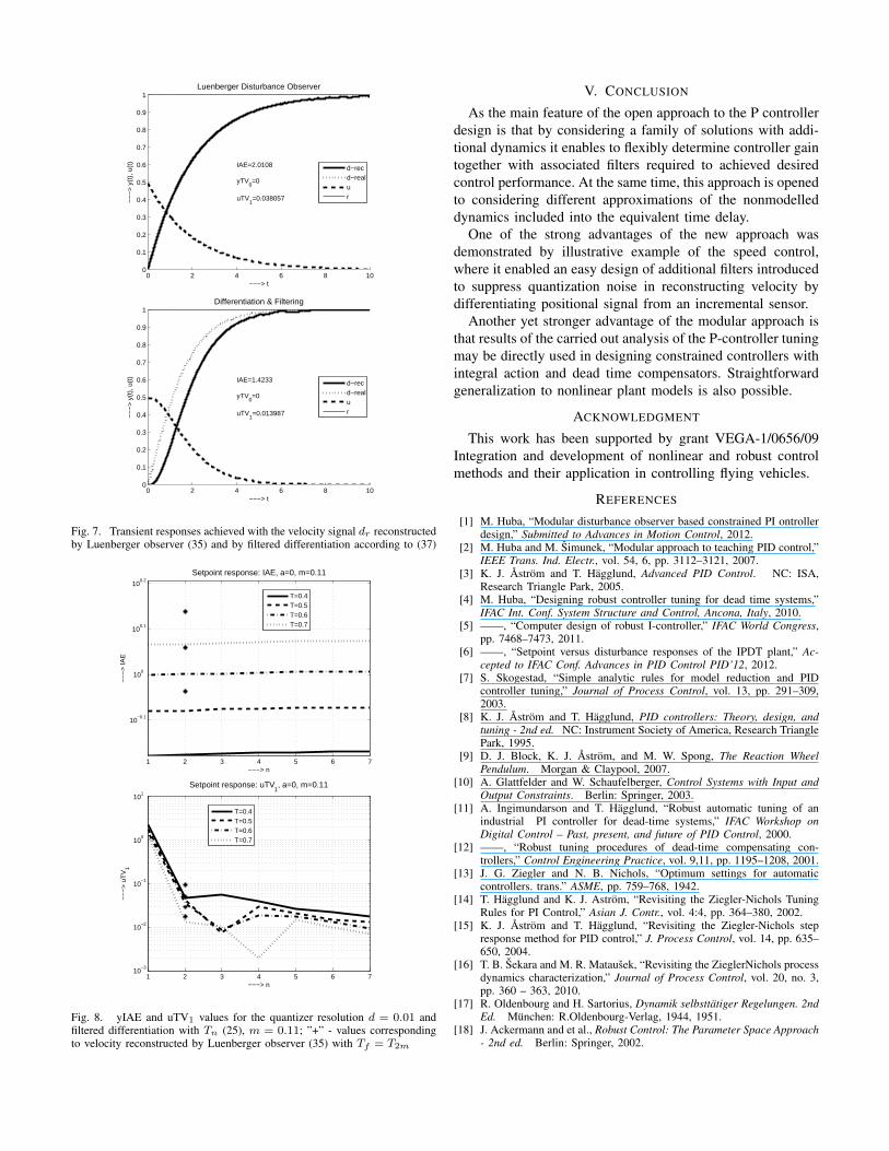
used with the controller tuning (21), the reconstructed velocitysignal does not indeed follow the real signal as close as in theabove example (Fig. 7 below), but the IAE values are lowerthan for the previous DO (above). Improved performance isyet much better to see from reasonably lower uTV1 values.Similarly, one could very simply design and tune also loopwith n > 2. Since in dealing with quantization the resultingdynamics strongly varies with initial conditions, in Fig. 8 yIAEand uTV1 characteristics corresponding to several equivalentdelays T , filters Fn(s); n ∈ (1, 7) with Tnm according to(25) and the controller gains (21) are shown. The reasonablylarge yIAE and uTV1 values corresponding to the Luenbergerobserver (n = 2) denoted by ”+” confirm in all situationsfor n > 1 improved performance of the new solution.The achieved characteristics indicate optimum moving withincreasing T to larger n and lower uTV1 values.

0 2 4 6 8 100

0.1

0.2

0.3

0.4

0.5

0.6

0.7

0.8

0.9

1

−−−> t

−−

−>

y(t

), u

(t)

Luenberger Disturbance Observer

IAE=2.0108

yTV0=0

uTV1=0.038057

d−recd−realur

0 2 4 6 8 100

0.1

0.2

0.3

0.4

0.5

0.6

0.7

0.8

0.9

1

−−−> t

−−

−>

y(t

), u

(t)

Differentiation & Filtering

IAE=1.4233

yTV0=0

uTV1=0.013987

d−recd−realur

Fig. 7. Transient responses achieved with the velocity signal dr reconstructedby Luenberger observer (35) and by filtered differentiation according to (37)

1 2 3 4 5 6 7

10−0.1

100

100.1

100.2

−−−> n

−−

−>

IAE

Setpoint response: IAE, a=0, m=0.11

T=0.4T=0.5T=0.6T=0.7

1 2 3 4 5 6 710

−3

10−2

10−1

100

101

−−−> n

−−

−>

uT

V1

Setpoint response: uTV1, a=0, m=0.11

T=0.4T=0.5T=0.6T=0.7

Fig. 8. yIAE and uTV1 values for the quantizer resolution d = 0.01 andfiltered differentiation with Tn (25), m = 0.11; ”+” - values correspondingto velocity reconstructed by Luenberger observer (35) with Tf = T2m

V. CONCLUSION

As the main feature of the open approach to the P controllerdesign is that by considering a family of solutions with addi-tional dynamics it enables to flexibly determine controller gaintogether with associated filters required to achieved desiredcontrol performance. At the same time, this approach is openedto considering different approximations of the nonmodelleddynamics included into the equivalent time delay.

One of the strong advantages of the new approach wasdemonstrated by illustrative example of the speed control,where it enabled an easy design of additional filters introducedto suppress quantization noise in reconstructing velocity bydifferentiating positional signal from an incremental sensor.

Another yet stronger advantage of the modular approach isthat results of the carried out analysis of the P-controller tuningmay be directly used in designing constrained controllers withintegral action and dead time compensators. Straightforwardgeneralization to nonlinear plant models is also possible.

ACKNOWLEDGMENT

This work has been supported by grant VEGA-1/0656/09Integration and development of nonlinear and robust controlmethods and their application in controlling flying vehicles.

REFERENCES

[1] M. Huba, “Modular disturbance observer based constrained PI ontrollerdesign,” Submitted to Advances in Motion Control, 2012.

[2] M. Huba and M. Simunek, “Modular approach to teaching PID control,”IEEE Trans. Ind. Electr., vol. 54, 6, pp. 3112–3121, 2007.

[3] K. J. Astrom and T. Hagglund, Advanced PID Control. NC: ISA,Research Triangle Park, 2005.

[4] M. Huba, “Designing robust controller tuning for dead time systems,”IFAC Int. Conf. System Structure and Control, Ancona, Italy, 2010.

[5] ——, “Computer design of robust I-controller,” IFAC World Congress,pp. 7468–7473, 2011.

[6] ——, “Setpoint versus disturbance responses of the IPDT plant,” Ac-cepted to IFAC Conf. Advances in PID Control PID’12, 2012.

[7] S. Skogestad, “Simple analytic rules for model reduction and PIDcontroller tuning,” Journal of Process Control, vol. 13, pp. 291–309,2003.

[8] K. J. Astrom and T. Hagglund, PID controllers: Theory, design, andtuning - 2nd ed. NC: Instrument Society of America, Research TrianglePark, 1995.

[9] D. J. Block, K. J. Astrom, and M. W. Spong, The Reaction WheelPendulum. Morgan & Claypool, 2007.

[10] A. Glattfelder and W. Schaufelberger, Control Systems with Input andOutput Constraints. Berlin: Springer, 2003.

[11] A. Ingimundarson and T. Hagglund, “Robust automatic tuning of anindustrial PI controller for dead-time systems,” IFAC Workshop onDigital Control – Past, present, and future of PID Control, 2000.

[12] ——, “Robust tuning procedures of dead-time compensating con-trollers,” Control Engineering Practice, vol. 9,11, pp. 1195–1208, 2001.

[13] J. G. Ziegler and N. B. Nichols, “Optimum settings for automaticcontrollers. trans.” ASME, pp. 759–768, 1942.

[14] T. Hagglund and K. J. Astrom, “Revisiting the Ziegler-Nichols TuningRules for PI Control,” Asian J. Contr., vol. 4:4, pp. 364–380, 2002.

[15] K. J. Astrom and T. Hagglund, “Revisiting the Ziegler-Nichols stepresponse method for PID control,” J. Process Control, vol. 14, pp. 635–650, 2004.

[16] T. B. Sekara and M. R. Matausek, “Revisiting the ZieglerNichols processdynamics characterization,” Journal of Process Control, vol. 20, no. 3,pp. 360 – 363, 2010.

[17] R. Oldenbourg and H. Sartorius, Dynamik selbsttatiger Regelungen. 2ndEd. Munchen: R.Oldenbourg-Verlag, 1944, 1951.

[18] J. Ackermann and et al., Robust Control: The Parameter Space Approach- 2nd ed. Berlin: Springer, 2002.