on bicm receivers for tcm transmission

Chalmers Publication Library

Copyright Notice

©2011 IEEE. Personal use of this material is permitted. However, permission to reprint/republish this material for advertising or promotional purposes or for creating new collective works for resale or redistribution to servers or lists, or to reuse any copyrighted component of this work in other works must be obtained from the IEEE.

This document was downloaded from Chalmers Publication Library (http://publications.lib.chalmers.se/), where it is available in accordance with the IEEE PSPB Operations Manual, amended 19 Nov. 2010, Sec. 8.1.9 (http://www.ieee.org/documents/opsmanual.pdf)

(Article begins on next page)

http://publications.lib.chalmers.se/�

http://www.ieee.org/documents/opsmanual.pdf�

IEEE TRANSACTIONS ONCOMMUNICATIONS, to appear, 2011. 1

On BICM receivers for TCM transmissionAlex Alvarado, Leszek Szczecinski, and Erik Agrell

Abstract—Recent results have shown that the performanceof bit-interleaved coded modulation (BICM) using convolutionalcodes in nonfading channels can be significantly improved whenthe interleaver takes a trivial form (BICM-T), i.e., when it doesnot interleave the bits at all. In this paper, we give a formalexplanation for these results and show that BICM-T is, in fact,the combination of a TCM transmitter and a BICM receiver.To predict the performance of BICM-T, a new type of dis-tance spectrum for convolutional codes is introduced, analyticalbounds based on this spectrum are developed, and asymptoticapproximations are presented. It is shown that the free Hammingdistance of the code is not the relevant optimization criterionfor BICM-T. Asymptotically optimal convolutional codes fordifferent constraint lengths are tabulated and BICM-T is shownto offer asymptotic gains of about 2 dB over traditional BICMdesigns based on random interleavers. The asymptotic gainsoveruncoded transmission are found to be the same as those obtainedby Ungerboeck’s one-dimensional trellis-coded modulation (1D-TCM), and therefore, in nonfading channels, BICM-T is shownto be as good as 1D-TCM.

Index Terms—Bit-interleaved Coded Modulation, Binary Re-flected Gray Code, Coded Modulation, Convolutional Codes,Interleaver, Quadrature Amplitude Modulation, Pulse Ampl itudeModulation, Set Partitioning, Trellis Coded Modulation.

I. I NTRODUCTION

UNGERBOECK’S trellis coded modulation (TCM) [1]and Imai and Hirakawa’s multilevel coding [2] are prob-

ably the most popular coded modulation (CM) schemes forthe AWGN channel. Bit-interleaved coded modulation (BICM)[3]–[5] appeared in 1992 as an alternative for CM in fadingchannels. One particularly appealing feature of BICM is thatall the operations are done at the bit-level, and thus, at thetransmitter’s side, off-the-shelf binary codes are connected tothe modulator via a bit-level interleaver. At the receiver’s side,reliability metrics for the coded bits (L-values) are calculatedby the demapper, de-interleaved, and then fed to a binarydecoder. This structure gives the designer the flexibility tochoose the modulator and the encoder independently, which

Manuscript submitted Aug. 2010; revised Dec. 2010 and Apr. 2011.This work was partially supported by the European Commission under

projects NEWCOM++ (216715) and FP7/2007-2013 (236068), and by theSwedish Research Council, Sweden (2006-5599).

The material in this paper was presented in part at the InternationalConference on Communications (ICC), Kyoto, Japan, June 2011.

A. Alvarado was with the Dept. of Signals and Systems, ChalmersUniv. of Technology, Sweden, and is now with the Dept. of Engineering.University of Cambridge, Cambridge CB2 1PZ, United Kingdom(email:[email protected]).

L. Szczecinski is with the Institut National de la RechercheScientifique,INRS-EMT, 800, Gauchetiere W. Suite 6900 Montreal, H5A 1K6,Canada(e-mail: [email protected]). When this work was submitted for publication,L. Szczecinski was on sabbatical leave with CNRS, Laboratory of Signalsand Systems, Gif-sur-Yvette, France.

E. Agrell is with the Dept. of Signals and Systems, Chalmers Univ. ofTechnology, SE-41296 Goteborg, Sweden (email: [email protected]).

in turn allows, for example, for an easy adaptation of thetransmission to the channel conditions (adaptive modulationand coding). This flexibility is arguably the main advantageof BICM over other CM schemes, and also the reason of whyit is used in almost all of the current wireless communicationsstandards, e.g., HSPA, IEEE 802.11a/g/n, and DVB-T2/S2/C2.

Bit-interleaving before modulation was introduced in Ze-havi’s original paper [3] on BICM. Bit-interleaving is indeedcrucial in fading channels since it guarantees that consecutivecoded bits are sent over symbols affected by independentfades. This results in an increase (compared to TCM) of theso-called code diversity (the suitable performance measurein fading channels), and therefore, BICM is the preferredalternative for CM in fading channels. BICM can also beused in nonfading channels. However, in this scenario, andcompared with TCM, BICM gives a smaller minimum Eu-clidean distance (the proper performance metric in nonfadingchannels), and also a smaller constraint capacity [4]. Despitethat, if a Gray labeling is used, the capacity loss is small, andtherefore, BICM is still considered as a valid option for CMover nonfading channels.

The use of a bit-level interleaver in nonfading channelshas been inherited from the original works on BICM byZehavi [3] and Caireet al. [4]. It simplifies the performanceanalysis of BICM and is implicitly considered mandatoryin the literature. However, the reasons for its presence areseldom discussed. Previously, we have shown in [6] how theperformance of BICM can be improved in nonfading channelsby using multiple interleavers. Recently, however, it has beenshown in [7] that in nonfading channels, considerably largergains (a few decibels) can be obtained if the interleaveris completely removedfrom the tranceiver’s configurations,i.e., BICM without an interleaver performs better than theconventional configurations of [3], [4]. The results presentedin [7] are only numerical and an explanation behind such animprovement is not given (although some intuitive explana-tions and a bit labeling optimization are presented).

In this paper, we present a formal study of BICM with trivialinterleavers (BICM-T) in nonfading channels, i.e., the BICMsystem introduced in [7] where no interleaving is performed.We recognize BICM-T as the combination of a TCM transmit-ter and a BICM receiver and we develop analytical bounds thatgive a formal explanation of why BICM-T with convolutionalcodes (CCs) performs well in nonfading channels. We alsointroduce a new type of distance spectrum for the CCs whichallows us to analytically corroborate the results presentedin [7]. Moreover, we search and tabulate optimum CCs forBICM-T, and we show that the asymptotic gains obtainedby BICM-T are the same obtained by Ungerboeck’s one-dimensional TCM (1D-TCM) demonstrating that a properlydesigned BICM-T system performs asymptotically as well as

2 IEEE TRANSACTIONS ONCOMMUNICATIONS, to appear, 2011.

1D-TCM. The main contribution of this paper is to presentan analytical model for BICM-T which is used to explain theresults presented in [7] and also to design an asymptoticallyoptimum BICM-T system in nonfading channels.

Throughout this paper, we use boldface lettersc to denotelength-L row vectorsct = [ct,1, . . . , ct,L] and also to denotedmatricesc = [cT

1, . . . , cTN ], where(·)T denotes transposition.

The distinction between a matrix and a vector is clear fromthe context in which they are used. Random variables aredenoted by capital lettersC and random vectors/matricesby capital boldface lettersC. We usedH(c) to denote thetotal Hamming weight of the binary matrixc. We denoteprobability byPr(·) and the probability density function (pdf)of a random variableΛ by pΛ(λ). The convolution betweentwo pdfs is denoted bypΛ1

(λ) ∗ pΛ2(λ) and {pΛ(λ)}∗w

denotes thew-fold self-convolution of the pdfpΛ(λ). TheGaussian pdf with mean valueµ and varianceσ2 is denoted byψ(λ;µ, σ) , 1√

2πσexp(−(λ − µ)2/2σ2), and the Q-function

by Q(x) , 1√2π

∫∞x

exp(

−u2/2)

du. Sets are denoted usingcalligraphic lettersC. All the polynomial generators of the CCare given in octal notation and following the notation of [8],the constraint length of the codesK is defined such that thenumber of states in the trellis of the code is2K−1.

II. SYSTEM MODEL AND PRELIMINARIES

A. System Model

The BICM system model under consideration is presented inFig. 1. We use a constraint lengthK, rateR = 1

2 convolutionalcode, connected to a 16-ary quadrature amplitude modulation(16-QAM) labeled by the binary reflected Gray code (BRGC)[9]. This configuration is indeed very simple, yet practical,yielding a spectral efficiency of two information bits percomplex channel use. This example simplifies the presentationof the main ideas related to the fact that the interleaver isremoved. The generalization to other modulations and codingrates is possible but would increase the complexity of nota-tion potentially hindering the main concepts of the analysispresented in this paper.

The input sequence ofN bits i = [i1, . . . , iN ] is fed tothe encoder (ENC) which at each time instantt = 1, . . . , Ngenerates two coded bitsct = [c1,t, c2,t]. We use the matrixc = [cT

1 , . . . , cTN ] of size 2 by N to represent the transmitted

codeword. These coded bits are interleaved byΠ, yieldingcπ = Π(c), where the different interleaving alternatives willbe discussed in detail in Sec. II-B. The coded and interleavedbits are then mapped to 16-QAM symbols, where the 16-QAMconstellation is formed by the direct product of two 4-arypulse amplitude modulation (4-PAM) constellations labeledby the BRGC. Therefore, we analyze the real part of theconstellation only, i.e., one of the constituent 4-PAM constel-lations. The mapper is defined asΦ : {[11], [10], [00], [01]}→{−3∆,−∆,∆, 3∆}, where

∆ ,1√5

(1)

so that the PAM constellation normalized to unit averagesymbol energy, i.e.,Es = 1.

A quick inspection of the BRGC for 4-PAM (cf. Fig. 3)reveals that the BRGC offers unequal error protection (UEP)tothe transmitted bits depending on their position. In particular,the bit at the first position (k = 1) receives higher protection1

than the bit at the second positionk = 2. More detailsabout this can be found in [6]. Moreover, fork = 2 a bitlabeled by zero (inner constellation points) will receive alower protection than a bit labeled by one transmitted in thesame bit position (outer constellation points), and therefore,the binary-input soft-output (BISO) channel fork = 2 isnonsymmetric. To simplify the analysis, we “symmetrize” thechannel by randomly inverting the bits before mapping themto the 4-PAM symbol, i.e.,cπ = cπ ⊕ s = [cπ

1 , . . . , cπN ],

where⊕ represents modulo-2 element-wise addition and theelements of the matrixs = [sT

1 , . . . , sTN ] ∈ {0, 1}2×N , with

st = [s1,t, s2,t], are randomly generated vectors of bits. Sucha scrambling symmetrizes the BISO channel but it does noteliminate the UEP. We note that the scrambling is introducedonly to simplify the analysis, and therefore, it is not showninFig. 1 nor used in the simulations. This symmetrization was infact proposed in [4], and as we will see in Sec. IV, the boundsdeveloped based on this symmetrization perfectly match thenumerical simulations.

We consider transmissions over an additive white Gaussiannoise (AWGN) channel. Assuming an ideal matched filter andperfect synchronization, the equivalent discrete-time basebandreceived signal is given byyt = xt + zt, wherezt is a zero-mean Gaussian noise with varianceN0/2 (with N0/2 beingthe power spectral density of the continuous-time AWGN),xt represents the transmitted symbol, andyt, xt, zt ∈ R. Ateach discrete timet = 1, . . . , N , the coded, interleaved, andscrambled bitscπ

t are mapped to a symbolxt, wherext =Φ(cπ

t ) ∈ X andX is the 4-PAM constellation. The signal-to-noise ratio is defined asγ , Es/N0 = 1/N0.

At the receiver’s side, reliability metrics for the bits arecalculated by the demapperΦ−1 in the form of logarithmic-likelihood ratios (L-values) as

lπk,t = logpYt

(

yt|Cπk,t = 1

)

pYt(yt|Cπ

k,t = 0), (2)

which allows us to write

pYt(yt|Cπ

k,t = u) =exp(

ulπk,t

)

1 + exp(

lπk,t

) , (3)

with u ∈ {0, 1}. Sincecπk,t = cπk,t ⊕ sk,t, it can be shown thatlπk,t passed to the deinterleaver (cf. Fig. 1) can be written as

lπk,t = (−1)sk,t lπk,t, (4)

i.e., after “descrambling”, the sign of the L-values is changedusing (−1)sk,t . These L-values are deinterleaved byΠ−1

yielding the matrixl = Π−1(lπ) of size 2 byN , which isthen passed to the decoder which calculates an estimate of theinformation sequenceı.

1The protection may be defined in different ways, where arguably thesimplest one is the bit error probability per bit position atthe demapper’soutput.


BICM Code BICM Decoder

iENC

c cπ

Π Φx

z

yΦ−1 Π−1

lπ lDEC

ı

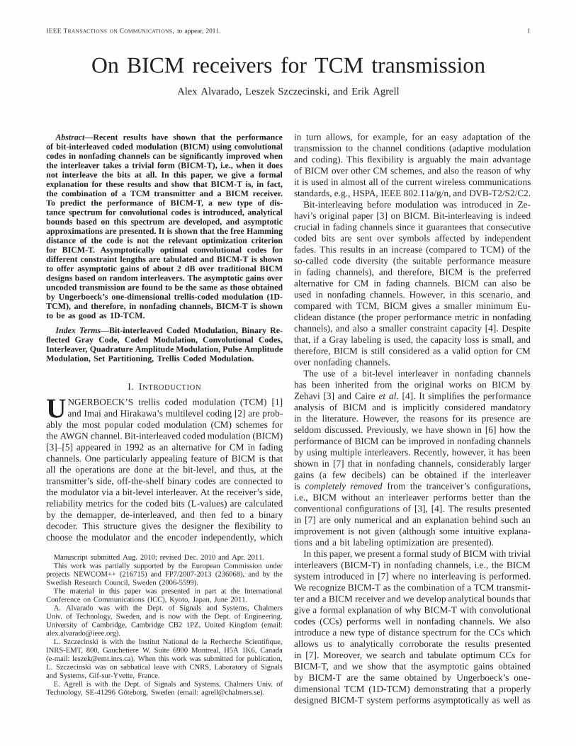
Fig. 1. Model of BICM transmission.

B. The Interleaver

Throughout this paper, three interleaving alternatives (cf. Πin Fig. 1) will be discussed: BICM with a single interleaver(BICM-S), BICM with multiple interleavers (M-interleavers,BICM-M), and BICM with a trivial interleaver (BICM-T). Abrief description of the three interleaving alternatives is givenbelow. This paper focuses on BICM-T.

• BICM-S was introduced in [4] and is the most commonconfiguration analyzed in the literature. It corresponds toan interleaver that randomly permutes the bits inc priorto modulation, where the permutation is random in twodimensions, i.e., it permutes the bits over the bit positionsand over time.

• BICM-M can be seen as a particularization of BICM-S with the following additional constraint: bits from theencoder’skth output must be assigned to the modulator’skth input. BICM-M was formally analyzed in [6] andin fact corresponds to the original model introduced byZehavi in [3] (BICM) and Li in [10] (BICM with iterativedecoding, BICM-ID). Recently, M-interleavers have alsobeen proven to be asymptotically optimum for BICM-ID[11].

• BICM-T was introduced in [7]. In this configuration, theinterleaverΠ in Fig. 1 is not present, i.e.,cπ = c andlπ = l.

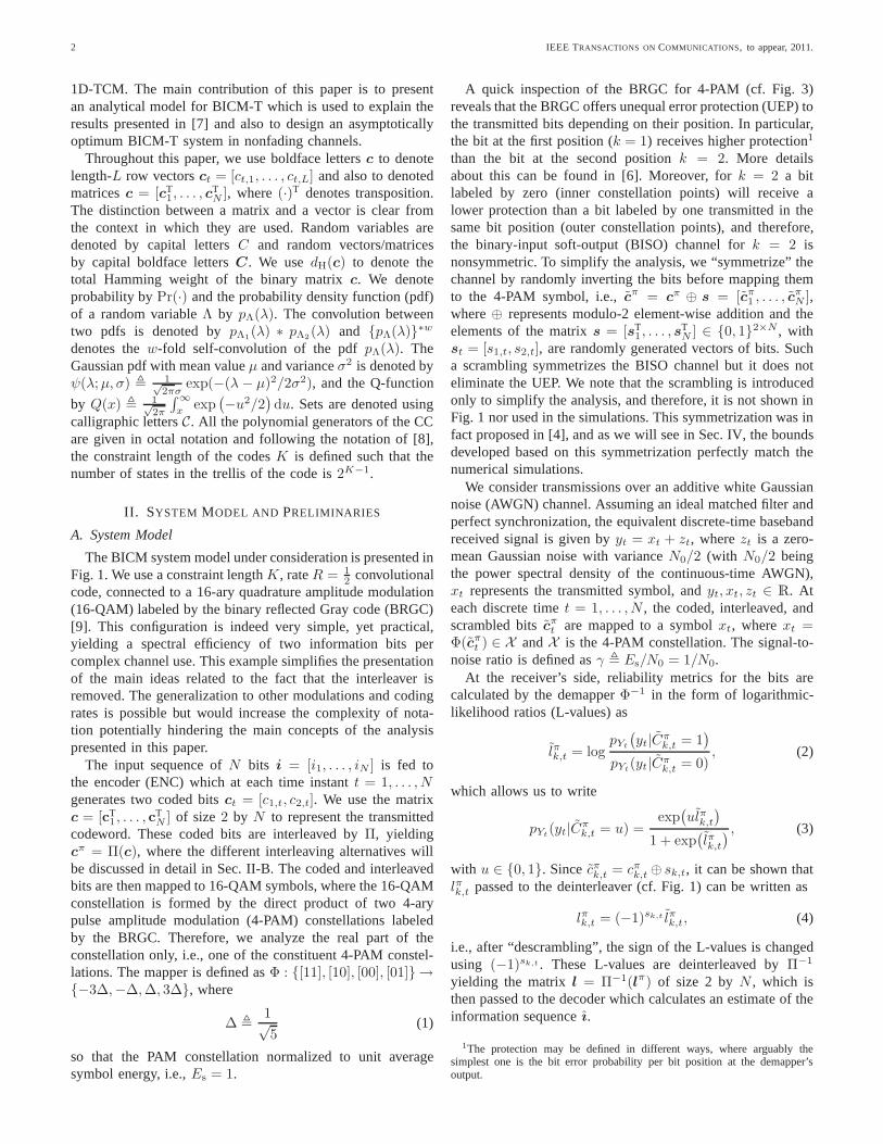
When BICM-T is considered, the resulting system is theone shown in Fig. 2. A careful examination of Fig. 2 revealsthat the structure of the transmitter of BICM-T is the sameas the transmitter of Ungerboeck’s 1D-TCM [1] or the TCMtransmitter in [12, Fig. 4.17]. The transmitter of BICM-T canalso be considered a particular case of the so-called generalTCM [13, Fig. 18.11] whenk = k (using the notation of[13]) and when the BRGC is used instead of Ungerboeck’s set-partitioning (SP). The transmitter of BICM-T is also equivalentto the simplest configuration of the so-called pragmatic TCM[14, Ch. 8] [15] (see also [16], [17, Sec. 9.2.4]), i.e., whentwo bits per symbol are considered.

The receiver of BICM-T in Fig. 2 corresponds to a conven-tional BICM receiver, where L-values for each bit are com-puted and fed to a soft-input Viterbi decoder (VD). The dif-ference between this receiver’s structure and a TCM receiver(one-dimensional or pragmatic) is that bit-level processing isused instead of a symbol-by-symbol VD. In conclusion, theBICM-T system introduced in [7] is a simple TCM transmitterused in conjunction with a BICM receiver. Nevertheless,throughout this paper, we use the name BICM-T to reflect thefact that this transmitter/receiver structure can be consideredas a particular case of BICM-S, where the interleaver takes a

itENC

c1,t

c2,t Φxt

zt

ytΦ−1

l1,t

l2,t DECıt

Fig. 2. BICM-T system analyzed in this paper for any time instant t.

trivial form. Moreover, the concept behind BICM-T might beuseful in adaptive modulation schemes where the interleaverdesign is adapted to the channel conditions, i.e., if fadingispresent, BICM-S is used, and if fading is not present, theinterleaver is dropped (BICM-T).

As explained above, the main difference of the system inFig. 2 and pragmatic TCM is the receiver used. Also, it isimportant to note that if BICM-T with larger constellations(e.g., 8-PAM) is considered, the binary labeling will stillbethe BRGC, which is different than the one used in pragmaticTCM, cf. [14, Fig. 8-30]. A detailed analysis/comparisonof BICM-T and pragmatic TCM for larger constellations is,however, out of the scope of this paper.

C. The Decoder and the decoding errors

A maximum likelihood (ML) sequence decoder chooses themost likely coded sequencec using the vector of channelobservationsy = [y1, . . . , yN ] (cf. Fig. 1), i.e.,

cML = argmax

c∈C{log pY (y|C = c)} (5)

= argmaxc∈C

{log pY (y|Π(C) = Π(c))} (6)

= argmaxc∈C

{

log

N∏

t=1

pYt(yt|Cπ

1,t = cπ1,t, Cπ2,t = cπ2,t)

}

,

(7)

whereC is the transmitted codeword,C is the code, to passfrom (5) to (6) we use the fact that the interleaver is a bijectivemapping, and to pass from (6) to (7) we used the fact that thenoise sampleszt affectingyt are mutually independent.

The striking feature of the BICM decoder shown in Fig. 1is that it replaces the decoding metric used in (7) with the


metric calculated at the bit-level, i.e.,

cBICM = argmax

c∈C

{

log

N∏

t=1

pYt(yt|Cπ

1,t = cπ1,t)

· pYt(yt|Cπ

2,t = cπ2,t)

}

(8)

= argmaxc∈C

{

N∑

t=1

2∑

k=1

log pYt(yt|Cπ

k,t = cπk,t)

}

. (9)

The optimal metric used in (7) is not the same as the one usedin (9), and thus, it is sometimes referred to as a mismatchedmetric [18, Sec. II-B.2].

Using an expression analogous to (3), (9) can be expressedas

cBICM = argmax

c∈C

{

N∑

t=1

2∑

k=1

cπk,tlπk,t

−N∑

t=1

2∑

k=1

log(1 + exp(lπk,t))

}

(10)

= argmaxc∈C

{

N∑

t=1

2∑

k=1

cπk,tlπk,t

}

, (11)

where the second term in (10) being independent ofc isirrelevant to the decision of the decoder.

The decision of the decoder based on the rule (11) iserroneous if it detects a codewordc instead of the transmittedcodeword c. The probability of this event, the so-calledpairwise error probability(PEP), is defined by

PEP(c → c) , Pr

{

N∑

t=1

(c1,tl1,t + c2,tl2,t)

≥N∑

t=1

(c1,tl1,t + c2,tl2,t)

}

(12)

= Pr

{

N∑

t=1

(e1,tl1,t + e2,tl2,t) ≥ 0

}

, (13)

whereek,t are the elements of the “error” codeworde = c−c.The PEP in (13) depends on2N L-values l1, l2, . . . , lN

and its evaluation is, in general, difficult because this sequencecontains pairs of dependent L-values that were calculated fromthe same channel outcome (same noise realization). However,when convolutional codes are considered, the most relevantevents are those involving a relatively small number of errorset, t0 ≤ t ≤ t0 + T − 1, which means that PEP is affectedby the consecutive L-valueslt0 , lt0+1, . . . , lt0+T−1. These2TL-values will be independent if we ensure that all the bitsct0 , ct0+1, . . . , ct0+T−1 are transmitted in2T different timeinstants (and thus, affected by different noise realizations)after interleaving. This condition oflocal independencecanbe obtained by an appropriate design of the interleaver, andis very likely to be satisfied when BICM-S or BICM-M areused.

When BICM-T is considered, for eacht = 1, . . . , N , twobitsct will be transmitted using the same symbolxt, and thus,the two corresponding L-valueslt will be mutually dependent

(because they were obtained from the same observationyt).In the following subsection, we show how to analyze theperformance of such a system.

III. PERFORMANCEEVALUATION

A. BER Analysis

Because of the symmetrization of the channel, we can,without loss of generality, assume that the all-zero codewordwas transmitted. We defineE as the set of codewords cor-responding to paths in the trellis of the code diverging fromthe zero-state at the arbitrarily chosen instantt = t0, andremerging with it afterT trellis stages. We also denote thesecodewords ase , [eT

1 , . . . , eTT ], whereet = [e1,t, e2,t]. Then,

the bit error rate (BER) can be upper-bounded using a unionbound (UB) as

BER ≤ UB ,∑

e∈EPEP(e)dH(ie), (14)

wheredH(ie) is the Hamming weight of the input sequenceie corresponding to the codewordc = e, and the pairwiseerror probability (PEP) is given by (cf. (13))

PEP(e) = Pr

{

t0+T−1∑

t=t0

(

e1,tl1,t + e2,tl2,t

)

> 0

}

. (15)

The general expression for the PEP in (15) and the UB in (14)reduce to well-known cases if simplifying assumptions for thedistribution oflk,t are adopted. To clarify the main differencesbetween BICM-T and BICM-S/BICM-M, in the following, webriefly analyze these well-known cases.

1) Independent and identically distributed L-values (BICM-S): In BICM-S, and because of the interleaver, the L-values lk,t passed to the decoder are locally independent(cf. Sec. II-C) and identically distributed (i.i.d.). Theycan bedescribed using the conditional pdfpL(λ|B) with B ∈ {0, 1}and where the pdf is independent ofk and t. In this case,the PEP in (15) depends only on the Hamming weight of thecodeworde, i.e., the PEP is given by (16) (at the bottom ofnext page). The UB in (14) can be expressed as

UBS =∑

w

PEPS(w)∑

e∈Cw

dH(ie) (17)

=∑

w

PEPS(w)βCw , (18)

where Cw represents the set of codewords with Hammingweightw, i.e.,Cw , {e ∈ E : dH(e) = w}, andC denotes theconvolutional code used for transmission. To pass from (17)to(18) we group the codewordse that have the same Hammingweight and add their contributions, which results in the well-known (input-output) weight distribution spectrum of the codeβCw. The expression in (18) is the most common expression forthe UB for BICM, cf. [4, eq. (26)], [5, eq. (4.12)].

2) Independent but not identically distributed L-values(BICM-M): In BICM-M, the L-values passed to the eachdecoder’s input are locally independent, however, their dis-tributions depend on the bit’s positionk = 1, 2. Therefore, weneed to use the conditional pdfspL1

(λ|B1) and pL2(λ|B2),

whereL1 andL2 are the random variables representing the


L-values at the decoder’s inputs. The PEP in this case is givenby (19) (shown at the bottom of the page), wherewe,k is theHamming weight of thekth row of e. The UB in (14) can beexpressed as

UBM =∑

w1,w2

PEPM(w1, w2)∑

e∈Cw1,w2

dH(ie)

=∑

w1,w2

PEPM(w1, w2)βCw1,w2

, (20)

whereCw1,w2is the set of codewords withgeneralizedHam-

ming weight [w1, w2] (wk in its kth row), i.e., Cw1,w2,

{e ∈ E : w1 = we,1, w2 = we,2}, and βCw1,w2is the

generalized weight distribution spectrum of the code that takesinto account the errors at each encoder’s output separately. TheUB in (20) was shown in [6] to be useful when analyzing theUEP introduced by the binary labeling and also to optimizethe interleaver and the code.

3) BICM without bit-interleaving (BICM-T):For BICM-T,yet a different particularization of (15) must be adopted. LetΛe be the metric associated to the codeworde and assumewithout loss of generality thatt0 = t, cf. (15). This metric isa sum of independent random variables, i.e.,

Λe , Λ(t) + Λ(t+1) + Λ(t+2) + . . . , (21)

whereΛ(t) = e1,tl1,t + e2,tl2,t which corresponds to the L-values defining the PEP in (15). Because the interleaver isremoved,lk,t = lπk,t, and thus, by using (4), we express eachof these metrics as

Λ(t) ≡ Λ(et, st) =

0, if et = [0, 0]

(−1)s1,t lπ1,t, if et = [1, 0]

(−1)s2,t lπ2,t, if et = [0, 1]∑2

k=1(−1)sk,t lπk,t, if et = [1, 1]

,

(22)

where we useΛ(et, st) to show thatΛ(t) depends on thescrambling’s outcomest (through lπk,t) and the error patternat time t, et.

Since lπk,t are random variables (that depend onk andxt),we need three pdfs:pΛ1

(λ|B1), pΛ2(λ|B2), and pΛΣ

(λ|B),for the three relevant cases defined in (22). We note thatpΛΣ

(λ|B) is conditioned not only on one bit, but on the pair oftransmitted bitsB = [B1, B2], whereB1, B2, andB representthe bitsCπ

1,t, Cπ2,t, andCπ

t , respectively. From (21), and due tothe independence of the individual L-values, the PEP in (15)can be expressed as (23) (shown at the bottom of the page)wherewe,1, we,2, andwe,Σ are, respectively, the number of

columns ine being equal toet = [1, 0]T, et = [0, 1]T, andet = [1, 1]T.2 Then, the UB expression in (14) becomes

UBT =∑

w1,w2,wΣ

PEPT(w1, w2, wΣ)∑

e∈Cw1,w2,wΣ

dH(ie)

=∑

w1,w2,wΣ

PEPT(w1, w2, wΣ)βCw1,w2,wΣ, (24)

whereCw1,w2,wΣ, {e ∈ E : w1 = we,1, w2 = we,2, wΣ =

we,Σ} and βCw1,w2,wΣis a new weight distribution spectrum

of the codeC that takes into account the generalized weight[w1, w2, wΣ] of the codewords, i.e., it considers separately thecase whenet = [1, 1]. This is different fromβCw1,w2

, wheresuch a case will increasew1 andw2 in the generalized weight[w1, w2]. Clearly, the following relationships hold

dH(e) = we,1 + we,2 + 2we,Σ (25)

we,1 = we,1 + we,Σ (26)

we,2 = we,1 + we,Σ. (27)

Example 1:Consider the constraint lengthK = 3 optimumdistance spectrum convolutional code (ODSCC) with polyno-mial generators(5, 7) [19, Table I]. The free distance of thecode isdfree

H = 5, andβC5 = 1, i.e., there is one divergent pathat Hamming distance five from the all-zero codeword, and theHamming weight of that path isdH(ie) = 1. Moreover, it ispossible to show that this codeword is given by

e =

[

1 0 11 1 1

]

,

i.e., dH(e) = 5, we,1 = 0, we,2 = 1, andwe,Σ = 2. If BICM-M is considered,we,1 = 2 andwe,2 = 3.

B. PDF of the L-values

In order to calculate the PEP for BICM-T in (23) weneed to compute the conditional pdfspΛ1

(λ|B1), pΛ2(λ|B2),

and pΛΣ(λ|B). In this subsection we show how to find

approximations for these PDFs.The L-values in (2) can be expressed as

lπk,t = log

∑

x∈Xk,1pYt

(yt|Xt = x)∑

x∈Xk,0pYt

(yt|Xt = x), (28)

whereXk,b is the set of constellation symbols labeled withb atbit positionk. Using the fact that the channel is Gaussian and if

2We note that the three argumentswe,1 we,2 andwe,Σ are a consequenceof the code rateR = 1/2 considered in this paper. For other code rates, morearguments will be needed.

PEP(e) = PEPS(dH(e)) =

∫ ∞

0

{pL(λ|b = 0)}∗dH(e) dλ. (16)

PEP(e) = PEPM(we,1, we,2) =

∫ ∞

0

{pL1(λ|B1 = 0)}∗we,1 ∗ {pL2

(λ|B2 = 0)}∗we,2 dλ, (19)

PEP(e) = PEPT(we,1, we,2, we,Σ) =

∫ ∞

0

{pΛ1(λ|B1 = 0)}∗we,1 ∗ {pΛ2

(λ|B2 = 0)}∗we,2 ∗ {pΛΣ(λ|B = [0, 0])}∗we,Σ dλ,

(23)


the so-called max-log approximationlog(exp(a) + exp(b)) ≈max{a, b} is used, the L-values can be expressed as3

lπk,t(yt|st) ≈ γ

[

minx∈Xk,0

(yt − x)2 − minx∈Xk,1

(yt − x)2]

, (29)

where from now on we use the notationlk,t(yt|st) to empha-size that the L-values depend on the received signal and thescrambler’s outcomest. In fact, the L-values depend on thetransmitted symbolxt, however, since the all-zero codewordis transmitted([cπ1,t, c

π2,t] = [0, 0]) and no interleaving is

performed,xt is completely determined byst, i.e., xt =Φ(cπ

t ) = Φ(st).The L-value in (29) is apiece-wise linearfunction of yt.

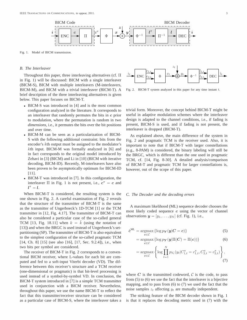
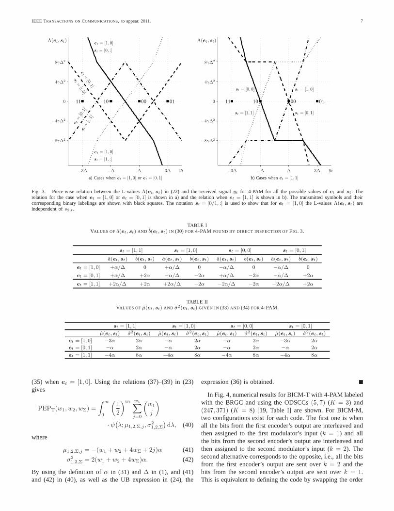
Moreover, the L-valuesΛ(et, st) in (22) are linear combina-tions of lπk,t(yt|st) in (29), and therefore, they are also piece-wise linear functions ofyt. Two cases are of particular interest,namely, whenet = [1, 0] or et = [0, 1], and whenet = [1, 1].The piece-wise linear relationships for the first case are shownin Fig. 3 a). In this figure we also show the constellationsymbols (or equivalently,st) with their binary labelings andwe use the notationst = [0/1, :] and st = [:, 0/1] to showthat for et = [1, 0] andet = [0, 1] the L-valuesΛ(et, st) areindependent ofs2,t ands1,t, respectively. In Fig. 3 b), the fourpossible cases whenet = [1, 1] are shown.

For a given scrambler outcomest (or equivalently, a giventransmitted symbolxt), the received signalyt is a Gaussianrandom variable with meanxt and varianceN0/2. Therefore,each L-valueΛ(et, st) in (22) is a sum of piece-wise Gaussianfunctions.4 In order to obtain expressions that are easy to workwith, we use the so-called zero-crossing approximation of theL-values proposed in [21, Sec. III-C] which replaces all theGaussian pieces required in the max-log model of L-valuesby a single Gaussian function. Intuitively, this approximationstates that

Λ(yt|et, st) ≈ a(et, st)yt + b(et, st), (30)

where a(et, st) and b(et, st) are the slope and the interceptof the closest linear piece to the transmitted symbolxt.

In Table I we show the values ofa(et, st) and b(et, st)defining (30) for 4-PAM, where for notation simplicity wehave defined

α , 4γ∆2. (31)

To clarify how these coefficients are obtained, consider forexampleet = [0, 1]. In this case, forst = [1, 1], whichcorresponds toxt = −3∆, the closest linear piece intersectingthe x-axis is the left-most part of the curve labeled in Fig. 3by et = [0, 1] andst = [:, 1] (dashed-dotted line). This givesa([0, 1], [1, 1]) = +α/∆ (slope) andb([0, 1], [1, 1]) = +2α(intercept), as shown in Table I. If for exampleet = [0, 1] and

3The max-log metric in (29) is suboptimal in terms of BER, however, itis very popular in practical implementations because of itslow complexity.Moreover, when low order constellations are used, the use ofthis simplifica-tion results in a negligible impact on the receiver’s performance [20, Fig. 9].The impact of this approximation, however, becomes more important whenhigher order constellations are considered, as shown in [20, Fig. 9].

4Closed-form expressions for the pdfs ofΛ(et, st) whenet = [1, 0] andet = [0, 1] (cf. Fig. 3 a)) were presented in [21].

st = [0, 0] (xt = ∆), the closest linear piece is the right-mostpiece labeled byet = [0, 1] andst = [:, 0] (dashed line), whichgives a([0, 1], [0, 0]) = +α/∆ and b([0, 1], [0, 0]) = −2α. Allthe other values in Table I can be found by a similar directinspection of Fig. 3.

Using the approximation in (30), the conditional L-values(conditioned onst) can be modeled as Gaussian randomvariables where their mean and variance depend onst, γ, andet, i.e.,

pΛ(λ|St = st) = ψ(

λ; µ(et, st), σ2(et, st)

)

, (32)

where the mean value and variance are given by

µ(st) = xta(et, st) + b(et, st) (33)

σ2(et, st) = [a(et, st)]2N0

2. (34)

In Table II we show the mean values and variances in (33)–(34) for the same cases presented in Table I.

To obtain the (unconditional) pdf ofΛ in (22), we average(32) over the scrambling outcomesst (cf. Table II), whichare assumed to be equiprobable. This results in the followingexpression

pΛ(λ) =

12

[

ψ(

λ;−3α, 2α)

+ ψ(

λ;−α, 2α)]

, if et = [1, 0]

ψ(

λ;−α, 2α)

, if et = [0, 1]

ψ(

λ;−4α, 8α)

, if et = [1, 1]

.

(35)

IV. D ISCUSSION ANDAPPLICATIONS

In the previous section, we developed approximations forthe pdf of the L-values passed to the decoder in BICM-T,cf. (35). In this section we use them to quantify the gainsoffered by BICM-T over BICM-S, to define asymptoticallyoptimum CCs, and to compare BICM-T with Ungerboeck’s1D-TCM.

A. Performance of BICM-T

Theorem 1:The UB for BICM-T is

UBT =∑

w1,w2,wΣ

βCw1,w2,wΣ

(

1

2

)w1 w1∑

j=0

(

w1

j

)

·Q(√

(w1 + w2 + 4wΣ + 2j)2

(w1 + w2 + 4wΣ)

2γ

5

)

. (36)

Proof: Using the pdf of the L-values in (35), the elementsin the integral defining the PEP in (23) can be expressed as

{pΛ1(λ|B1 = 0)}∗w1 =

(

1

2

)w1 w1∑

j=0

(

w1

j

)

·

ψ(

λ;−α(2j + w1), 2αw1

)

(37)

{pΛ2(λ|B2 = 0)}∗w2 =ψ

(

λ;−αw2, 2αw2

)

(38)

{pΛΣ(λ|B = [0, 0])}∗wΣ =ψ

(

λ;−4αwΣ, 8αwΣ

)

, (39)

where we usedψ(λ;µ1, σ21) ∗ . . . ∗ ψ(λ;µJ , σ

2J ) =

ψ(λ;∑J

j=1 µj ,∑J

j=1 σ2j ) and where the binomial coefficient

in (37) comes from the sum of the two Gaussian functions in


∆∆ 3∆3∆ −∆−∆ −3∆−3∆

00

−4γ∆2−4γ∆2

−8γ∆2−8γ∆2

4γ∆24γ∆2

8γ∆28γ∆2

a) Cases whenet = [1, 0] or et = [0, 1] b) Cases whenet = [1, 1]

et = [1, 0]

et = [1, 0]

st = [0, :]

st = [1, :]

et =

[0, 1]

st =

[:, 0]

s t=

[:,1]

e t=

[0, 1

]st = [0, 0]

st = [1, 1]

st = [1, 0]

st = [0, 1]

ytyt

Λ(et, st)Λ(et, st)

1111 1010 0000 0101

Fig. 3. Piece-wise relation between the L-valuesΛ(et, st) in (22) and the received signalyt for 4-PAM for all the possible values ofet and st. Therelation for the case whenet = [1, 0] or et = [0, 1] is shown in a) and the relation whenet = [1, 1] is shown in b). The transmitted symbols and theircorresponding binary labelings are shown with black squares. The notationst = [0/1, :] is used to show that foret = [1, 0] the L-valuesΛ(et, st) areindependent ofs2,t.

TABLE IVALUES OF a(et, st) AND b(et, st) IN (30) FOR 4-PAM FOUND BY DIRECT INSPECTION OFFIG. 3.

st = [1, 1] st = [1, 0] st = [0, 0] st = [0, 1]

a(et, st) b(et, st) a(et, st) b(et, st) a(et, st) b(et, st) a(et, st) b(et, st)

et = [1, 0] +α/∆ 0 +α/∆ 0 −α/∆ 0 −α/∆ 0

et = [0, 1] +α/∆ +2α −α/∆ −2α +α/∆ −2α −α/∆ +2α

et = [1, 1] +2α/∆ +2α +2α/∆ −2α −2α/∆ −2α −2α/∆ +2α

TABLE IIVALUES OF µ(et, st) AND σ2(et, st) GIVEN IN (33) AND (34) FOR 4-PAM.

st = [1, 1] st = [1, 0] st = [0, 0] st = [0, 1]

µ(et, st) σ2(et, st) µ(et, st) σ2(et, st) µ(et, st) σ2(et, st) µ(et, st) σ2(et, st)

et = [1, 0] −3α 2α −α 2α −α 2α −3α 2α

et = [0, 1] −α 2α −α 2α −α 2α −α 2α

et = [1, 1] −4α 8α −4α 8α −4α 8α −4α 8α

(35) whenet = [1, 0]. Using the relations (37)–(39) in (23)gives

PEPT(w1, w2, wΣ) =

∫ ∞

0

(

1

2

)w1 w1∑

j=0

(

w1

j

)

· ψ(

λ;µ1,2,Σ,j , σ21,2,Σ

)

dλ, (40)

where

µ1,2,Σ,j = −(w1 + w2 + 4wΣ + 2j)α (41)

σ21,2,Σ = 2(w1 + w2 + 4wΣ)α. (42)

By using the definition ofα in (31) and∆ in (1), and (41)and (42) in (40), as well as the UB expression in (24), the

expression (36) is obtained.

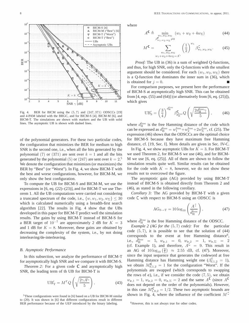
In Fig. 4, numerical results for BICM-T with 4-PAM labeledwith the BRGC and using the ODSCCs(5, 7) (K = 3) and(247, 371) (K = 8) [19, Table I] are shown. For BICM-M,two configurations exist for each code. The first one is whenall the bits from the first encoder’s output are interleaved andthen assigned to the first modulator’s input (k = 1) and allthe bits from the second encoder’s output are interleaved andthen assigned to the second modulator’s input (k = 2). Thesecond alternative corresponds to the opposite, i.e., all the bitsfrom the first encoder’s output are sent overk = 2 and thebits from the second encoder’s output are sent overk = 1.This is equivalent to defining the code by swapping the order


2 3 4 5 6 7 8 9 10 1110

−8

10−7

10−6

10−5

10−4

10−3

10−2

10−1

100

SNR γ [dB]

BE

R

BICM-S [4]BICM-M (“Best”) [6]

BICM-T (“Best”)BICM-T (“Worst”)

UBsAsymptotic UBs

K = 3

K = 8

Fig. 4. BER for BICM using the(5, 7) and (247, 371) ODSCCs [19]and 4-PAM labeled with the BRGC, and for BICM-S [4], BICM-M [6], andBICM-T. The simulations are shown with markers and the UB with solidlines. The asymptotic UB is shown with dashed lines.

of the polynomial generators. For these two particular codes,the configuration that minimizes the BER for medium to highSNR is the second one, i.e., when all the bits generated by thepolynomial(7) or (371) are sent overk = 1 and all the bitsgenerated by the polynomial(5) or (247) are sent overk = 2.5

We denote the configuration that minimizes (or maximizes) theBER by “Best” (or “Worst”). In Fig. 4, we show BICM-T withthe best and worse configurations, however, for BICM-M, weonly show the best configuration.

To compute the UB for BICM-S and BICM-M, we use theexpressions in [6, eq. (22)–(23)], and for BICM-T we use The-orem 1. All the UB computations were carried out consideringa truncated spectrum of the code, i.e.,{w,w1, w2, wΣ} ≤ 30which is calculated numerically using a breadth-first searchalgorithm [22]. The results in Fig. 4 show that the UBsdeveloped in this paper for BICM-T predict well the simulationresults. The gains by using BICM-T instead of BICM-S fora BER target of10−7 are approximately 2 dB forK = 3and 1 dB forK = 8. Moreover, these gains are obtained bydecreasing the complexity of the system, i.e., by not doinginterleaving/de-interleaving.

B. Asymptotic Performance

In this subsection, we analyze the performance of BICM-Tfor asymptotically high SNR and we compare it with BICM-S.

Theorem 2:For a given codeC and asymptotically highSNR, the leading term of th UB for BICM-T is

UB′T = MCQ(√2γAC

5

)

, (43)

5These configurations were found in [6] based on a UB for BICM-Msimilarto (20). It was shown in [6] that different configurations result in differentBER performance because of the UEP introduced by the binary labeling.

where

AC , minw1,w2,wΣ

βCw1,w2,wΣ6=0

(w1 + w2 + 4wΣ) (44)

MC =∑

w1,w2,wΣ

w1+w2+4wΣ=AC(1

2

)w1

βCw1,w2,wΣ. (45)

Proof: The UB in (36) is a sum of weighted Q-functions,and thus, for high SNR, only the Q-functions with the smallestargument should be considered. For each(w1, w2, wΣ) thereis a Q-function that dominates the inner sum in (36), whichis obtained forj = 0.

For comparison purposes, we present here the performanceof BICM-S at asymptotically high SNR. This can be obtainedfrom [4, eqs. (55) and (64)] (or alternatively from [6, eq. (25)]),which gives

UB′S =

(

3

4

)dfree

H

βCdfree

H

Q

(√

2dfreeH γ

5

)

, (46)

wheredfreeH is the free Hamming distance of the code which

can be expressed asdfreeH = wfree

1 +wfree2 +2wfree

Σ , cf. (25). Theexpression (46) shows that the ODSCCs are the optimal choicefor BICM-S because they have maximum free Hammingdistance, cf. [19, Sec. I]. More details are given in Sec. IV-C.

In Fig. 4, we show asymptotic UBs forK = 3. For BICM-Twe used Theorem 2, for BICM-S we use (46), and for BICM-M we use [6, eq. (25)]. All of them are shown to follow thesimulation results quite well. Similar results can be obtainedfor the code withK = 8, however, we do not show theseresults not to overcrowd the figure.

The asymptotic gain (AG) provided by using BICM-Tinstead of BICM-S is obtained directly from Theorem 2 and(46), as stated in the following corollary.

Corollary 3: The AG provided by BICM-T with a givencodeC with respect to BICM-S using an ODSCC is

AGS→T = 10 log10

(

ACdfreeH

)

, (47)

wheredfreeH is the free Hamming distance of the ODSCC.

Example 2 (AG for the(5, 7) code): For the particularcode (5, 7), it is possible to see that the solution of (44)corresponds to the event at free Hamming distance6,i.e., dfree

H = 5, we,1 = 0, we,2 = 1, we,Σ = 2(cf. Example 1), and therefore,AC = 9. This result inan AG of 10 log10

(

95

)

≈ 2.55 dB, cf. (47). Moreover,since the input sequence that generates the codeword at freeHamming distance has Hamming weight one (βC0,1,2 = 1),we obtainMC

0,1,2 = 1 for the configuration “Worst”. If thepolynomials are swapped (which corresponds to swappingthe rows ofe), i.e., if we consider the code(7, 5), we obtainwe,1 = 1, we,2 = 0, we,Σ = 2 and the sameAC (sinceACdoes not depend on the order of the polynomials). However,in this caseMC

1,0,2 = 1/2. These two asymptotic bounds areshown in Fig. 4, where the influence of the coefficientMC

6However, this is not always true for other codes.


(MC0,1,2 = 1 for (5, 7) andMC

1,0,2 = 1/2 for (7, 5)) can beobserved as a weighting coefficient applied to the Q-functionin (43) (this is also visible in the simulation results).

Corollary 4: The AG provided by BICM-T with respect toBICM-S is bounded as

AGS→T ≤ 3 dB. (48)

Proof: For any constraint lengthK, and any codeC, wehave

AC = minw1,w2,wΣ

βCw1,w2,wΣ6=0

(w1 + w2 + 4wΣ)

≤ wfree1 + wfree

2 + 4wfreeΣ (49)

≤ 2wfree1 + 2wfree

2 + 4wfreeΣ , (50)

where we use[wfree1 , wfree

2 , wfreeΣ ] to denote the generalized

weight of the event(s) at free Hamming distance. The in-equality in (49) holds because the event(s) at free Ham-ming distance belong to the elements in the minimization.The inequality in (50) holds becausewfree

1 + wfree2 ≥ 0.

Recognizing2wfree1 + 2wfree

2 + 4wfreeΣ in (50) as twice the

free Hamming distance of the codeC, cf. (25), we obtain2wfree

1 + 2wfree2 + 4wfree

Σ < 2dfreeH , where dfree

H is the freeHamming distance of the ODSCC. Thus,AC ≤ 2dfree

H , whichcombined with (47) completes the proof.

C. Asymptotically Optimum Convolutional Codes

Optimum CCs—in the sense of minimizing the BER forasymptotically high SNR—are usually defined in terms offree Hamming distance, i.e., good CCs are those, which fora given rate and constraint length, have the maximum freedistance (MFD) [23, Sec. 8.2.5]. The MFD criterion can berefined if the multiplicities associated to the different weightsare considered [19], [13, Sec. 12.3]. Based on this refinedoptimality criterion, the ODSCCs were defined, which areoptimal in both binary transmission and in BICM-S, cf. (46).For BICM-M, we have shown in [6] thatdfree

H is still agood indicator of the optimality of the code. If BICM-Tis considered, and as a direct consequence of Theorem 2,asymptotically optimum convolutional codes (AOCCs) can bedefined.

Definition 1 (Asymptotically optimum CCs for BICM-T):For a givenK andR, a CC is said to be an AOCC if it hasthe lowest multiplicityMC among the codes with the highestAC.

We have performed an exhaustive numerical search forAOCCs based on Definition 1, which from now on we denoteby C∗. We considered for constraint lengthsK = 3, 4, . . . , 8and all codes with free distance0 < dfree

H ≤ dfreeH . The

spectrum was truncated asw1 + w2 + 4wΣ ≤ dfreeH + 8 and

the search was performed in lexicographic order. The resultsare shown in Table III, where for comparison we also includethe ODSCCs (with their respective coefficientsAC andMC).If there is more than one AOCC for a givenK, we presentthe first one in the list. These results show that in general thefree Hamming distance of the code is not the proper criterionin BICM-T, i.e., codes that are not MFD codes perform better

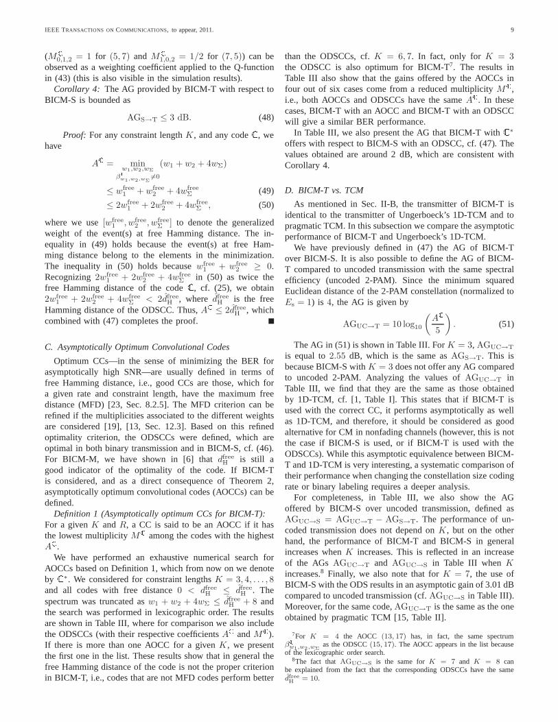
than the ODSCCs, cf.K = 6, 7. In fact, only forK = 3the ODSCC is also optimum for BICM-T7. The results inTable III also show that the gains offered by the AOCCs infour out of six cases come from a reduced multiplicityMC,i.e., both AOCCs and ODSCCs have the sameAC. In thesecases, BICM-T with an AOCC and BICM-T with an ODSCCwill give a similar BER performance.

In Table III, we also present the AG that BICM-T withC∗

offers with respect to BICM-S with an ODSCC, cf. (47). Thevalues obtained are around 2 dB, which are consistent withCorollary 4.

D. BICM-T vs. TCM

As mentioned in Sec. II-B, the transmitter of BICM-T isidentical to the transmitter of Ungerboeck’s 1D-TCM and topragmatic TCM. In this subsection we compare the asymptoticperformance of BICM-T and Ungerboeck’s 1D-TCM.

We have previously defined in (47) the AG of BICM-Tover BICM-S. It is also possible to define the AG of BICM-T compared to uncoded transmission with the same spectralefficiency (uncoded 2-PAM). Since the minimum squaredEuclidean distance of the 2-PAM constellation (normalizedtoEs = 1) is 4, the AG is given by

AGUC→T = 10 log10

(

AC5

)

. (51)

The AG in (51) is shown in Table III. ForK = 3, AGUC→T

is equal to2.55 dB, which is the same asAGS→T. This isbecause BICM-S withK = 3 does not offer any AG comparedto uncoded 2-PAM. Analyzing the values ofAGUC→T inTable III, we find that they are the same as those obtainedby 1D-TCM, cf. [1, Table I]. This states that if BICM-T isused with the correct CC, it performs asymptotically as wellas 1D-TCM, and therefore, it should be considered as goodalternative for CM in nonfading channels (however, this is notthe case if BICM-S is used, or if BICM-T is used with theODSCCs). While this asymptotic equivalence between BICM-T and 1D-TCM is very interesting, a systematic comparison oftheir performance when changing the constellation size codingrate or binary labeling requires a deeper analysis.

For completeness, in Table III, we also show the AGoffered by BICM-S over uncoded transmission, defined asAGUC→S = AGUC→T − AGS→T. The performance of un-coded transmission does not depend onK, but on the otherhand, the performance of BICM-T and BICM-S in generalincreases whenK increases. This is reflected in an increaseof the AGs AGUC→T and AGUC→S in Table III whenKincreases.8 Finally, we also note that forK = 7, the use ofBICM-S with the ODS results in an asymptotic gain of 3.01 dBcompared to uncoded transmission (cf.AGUC→S in Table III).Moreover, for the same code,AGUC→T is the same as the oneobtained by pragmatic TCM [15, Table II].

7For K = 4 the AOCC (13, 17) has, in fact, the same spectrumβCw1,w2,wΣ

as the ODSCC(15, 17). The AOCC appears in the list becauseof the lexicographic order search.

8The fact thatAGUC→S is the same forK = 7 and K = 8 canbe explained from the fact that the corresponding ODSCCs have the samedfree

H= 10.


TABLE IIICOEFFICIENTSAC AND MC FOR AOCCS AND ODSCCS IN BICM-T. THE ASYMPTOTIC GAINS AND THEHAMMING FREE DISTANCES ARE ALSO SHOWN.

KAOCCs ODSCCs AG [dB]

(g1, g2) dfree

H AC∗ MC∗ (g1, g2) dfree

H AC MC AGS→T AGUC→T AGUC→S

3 (7, 5) 5 9 0.50 (7, 5) 5 9 0.50 2.55 2.55 0

4 (13, 17) 6 10 0.50 (15, 17) 6 10 0.50 2.22 3.01 0.79

5 (23, 33) 7 11 0.38 (23, 35) 7 11 0.88 1.96 3.42 1.46

6 (45, 55) 7 13 1.62 (53, 75) 8 12 0.50 2.11 4.15 2.04

7 (107, 135) 9 14 0.50 (133, 171) 10 14 3.09 1.46 4.47 3.01

8 (313, 235) 10 16 8.02 (371, 247) 10 15 0.61 2.04 5.05 3.01

V. CONCLUSIONS

In this paper, we formally explained why the recentlyproposed BICM-T system offers gains over regular BICMin nonfading channels. BICM-T was shown to be a TCMtransmitter used with a BICM receiver. An analytical modelwas developed and a new type of distance spectrum for thecode was introduced, which is the relevant characteristic tooptimize CCs for BICM-T. The analytical model was used tovalidate the numerical results and to show that the use of theODSCCs, which rely on the regular free Hamming distancecriterion, is suboptimal.

The model presented in this paper was also used to analyzethe asymptotic behavior of BICM-T. Optimal convolutionalcodes for BICM-T were tabulated and it was shown that aproperly designed BICM-T system performs asymptotically aswell as Ungerboeck’s TCM. Moreover, it was shown that theasymptotic loss caused by using BICM-S instead of BICM-Tin nonfading channels is never larger than 3 dB.

For notation simplicity and to have a concise explanationof the mechanisms behind BICM-T, the analysis presented inthis paper was done only for a simple BICM configuration(R = 1/2 and 4-PAM). A more general analysis is possible,and very interesting indeed. For example, it is still unknownwhat the performance gains will be in a more general setup,e.g., for different code rates, when the number of encoderoutputs is not the same as the number of modulator inputs,or for different spectral efficiencies. Also, it is unclear whatthe gains offered by the AOCCs for finite SNR values are.All these questions, as well as a general comparison betweenBICM-T and pragmatic TCM, are left for further investigation.

REFERENCES

[1] G. Ungerboeck, “Channel coding with multilevel/phase signals,” IEEETrans. Inf. Theory, vol. 28, no. 1, pp. 55–67, Jan. 1982.

[2] H. Imai and S. Hirakawa, “A new multilevel coding method using error-correcting codes,”IEEE Trans. Inf. Theory, vol. IT-23, no. 3, pp. 371–377, May 1977.

[3] E. Zehavi, “8-PSK trellis codes for a Rayleigh channel,”IEEE Trans.Commun., vol. 40, no. 3, pp. 873–884, May 1992.

[4] G. Caire, G. Taricco, and E. Biglieri, “Bit-interleavedcoded modula-tion,” IEEE Trans. Inf. Theory, vol. 44, no. 3, pp. 927–946, May 1998.

[5] A. Guillen i Fabregas, A. Martinez, and G. Caire, “Bit-interleavedcoded modulation,”Foundations and Trends in Communications andInformation Theory, vol. 5, no. 1–2, pp. 1–153, 2008.

[6] A. Alvarado, E. Agrell, L. Szczecinski, and A. Svensson,“ExploitingUEP in QAM-based BICM: Interleaver and code design,”IEEE Trans.Commun., vol. 58, no. 2, pp. 500–510, Feb. 2010.

[7] C. Stierstorfer, R. F. H. Fischer, and J. B. Huber, “Optimizing BICMwith convolutional codes for transmission over the AWGN channel,” inInternational Zurich Seminar on Communications, Zurich, Switzerland,Mar. 2010.

[8] S. B. Wicker, Error Control Systems for Digital Communication andStorage. Prentice Hall, 1995.

[9] E. Agrell, J. Lassing, E. G. Strom, and T. Ottosson, “On the optimalityof the binary reflected Gray code,”IEEE Trans. Inf. Theory, vol. 50,no. 12, pp. 3170–3182, Dec. 2004.

[10] X. Li and J. Ritcey, “Bit-interleaved coded modulationwith iterativedecoding using soft feedback,”Electronic Letters, vol. 34, no. 10, pp.942–943, May 1998.

[11] A. Alvarado, L. Szczecinski, E. Agrell, and A. Svensson, “On BICM-ID with multiple interleavers,”IEEE Commun. Lett., vol. 14, no. 9, pp.785–787, Sep. 2010.

[12] S. H. Jamali and T. Le-Ngoc,Coded-Modulation Techniques for FadingChannels. Kluwer Academic Publishers, 1994.

[13] S. Lin and D. J. Costello, Jr.,Error Control Coding, 2nd ed. EnglewoodCliffs, NJ, USA: Prentice Hall, 2004.

[14] G. C. Clark Jr. and J. B. Cain,Error-correction coding for digitalcommunications, 2nd ed. Plenum Press, 1981.

[15] A. J. Viterbi, J. K. Wolf, E. Zehavi, and R. Padovani, “A pragmaticapproach to trellis-coded modulation,”IEEE Commun. Mag., vol. 27,no. 7, pp. 11–19, July 1989.

[16] J. K. Wolf and E. Zehavi, “p2 codes: Pragmatic trellis codes utilizingpunctured convolutional codes,”IEEE Commun. Mag., vol. 33, no. 2,pp. 94–99, Feb. 1995.

[17] R. H. Morelos-Zaragoza,The Art of Error Correcting Coding, 2nd ed.John Wiley & Sons, 2002.

[18] A. Martinez, A. Guillen i Fabregas, and G. Caire, “Bit-interleaved codedmodulation revisited: A mismatched decoding perspective,” IEEE Trans.Inf. Theory, vol. 55, no. 6, pp. 2756–2765, June 2009.

[19] P. Frenger, P. Orten, and T. Ottosson, “Convolutional codes with op-timum distance spectrum,”IEEE Trans. Commun., vol. 3, no. 11, pp.317–319, Nov. 1999.

[20] B. Classon, K. Blankenship, and V. Desai, “Channel coding for 4Gsystems with adaptive modulation and coding,”IEEE Wireless Commun.Mag., vol. 9, no. 2, pp. 8–13, Apr. 2002.

[21] A. Alvarado, L. Szczecinski, R. Feick, and L. Ahumada, “Distribution ofL-values in Gray-mappedM2-QAM: Closed-form approximations andapplications,” IEEE Trans. Commun., vol. 57, no. 7, pp. 2071–2079,July 2009.

[22] J. Belzile and D. Haccoun, “Bidirectional breadth-first algorithms forthe decoding of convolutional codes,”IEEE Trans. Commun., vol. 41,no. 2, pp. 370–380, Feb. 1993.

[23] J. G. Proakis,Digital Communications, 4th ed. McGraw-Hill, 2000.

Alex Alvarado (S’06) was born in 1982 in Quellon, on the island ofChiloe, Chile. He received his Electronics Engineer degree (Ingeniero CivilElectronico) and his M.Sc. degree (Magıster en Ciencias de la IngenierıaElectronica) from Universidad Tecnica Federico Santa Marıa, Valparaıso,Chile, in 2003 and 2005, respectively. He obtained the degree of Licentiateof Engineering (Teknologie Licentiatexamen) in 2008 and his PhD degreein 2011, both of them from Chalmers University of Technology, Goteborg,Sweden.


Since 2006, he has been involved in a research collaborationwith theInstitut National de la Recherche Scientifique (INRS), Montreal, QC, Canada,on the analysis and design of BICM systems. In 2008, he was holder of theMerit Scholarship Program for Foreign Students, granted bythe Ministere del’ Education, du Loisir et du Sports du Quebec. His research interests are inthe areas of digital communications, coding, and information theory.

A. Alvarado is currently a Newton International Fellow at the Universityof Cambridge, United Kingdom, funded by The British Academyand TheRoyal Society.

Leszek Szczecinski(M’98-SM’07), obtained M.Eng. degree from the Techni-cal University of Warsaw in 1992, and Ph.D. from INRS-Telecommunications,Montreal in 1997. From 1998 to 2001, he held position of Assistant Professorat the Department of Electrical Engineering, University ofChile. He isnow Associate Professor at INRS-EMT, University of Quebec,Canada, andAdjunct Professor at Electrical and Computer Engineering Department ofMcGill University. His research interests are in the area ofmodulation andcoding, communication theory, wireless communications, and digital signalprocessing.

Erik Agrell received the M.S. degree in electrical engineering in 1989 and thePh.D. degree in information theory in 1997, both from Chalmers Universityof Technology, Sweden.

From 1988 to 1990, he was with Volvo Technical Development asaSystems Analyst, and from 1990 to 1997, with the Department of InformationTheory, Chalmers University of Technology, as a Research Assistant. In 1997–1999, he was a Postdoctoral Researcher with the University of Illinois atUrbana-Champaign and the University of California, San Diego. In 1999,he joined the faculty of Chalmers University of Technology,first as anAssociate Professor and since 2009 as a Professor in Communication Systems.His research interests belong to the fields of information theory, codingtheory, and digital communications, and his favorite applications are found inoptical communications. More specifically, his current research includes bit-interleaved coded modulation and multilevel coding, polarization-multiplexedcoding and modulation, optical intensity modulation, bit-to-symbol mappingsin coded and uncoded systems, lattice theory and sphere decoding, andmultidimensional geometry.

Prof. Agrell served as Publications Editor for IEEE Transactions onInformation Theory from 1999 to 2002.

on bicm receivers for tcm transmission

Documents