detection, receivers, and performance of cpfsk and cpck
TRANSCRIPT
Western UniversityScholarship@Western
Electronic Thesis and Dissertation Repository
April 2013
Detection, Receivers, and Performance of CPFSKand CPCKMohammed ZourobThe University of Western Ontario
SupervisorDr. Raveendra K. RaoThe University of Western Ontario
Graduate Program in Electrical and Computer Engineering
A thesis submitted in partial fulfillment of the requirements for the degree in Master of Science
© Mohammed Zourob 2013
Follow this and additional works at: http://ir.lib.uwo.ca/etd
Part of the Systems and Communications Commons
This Dissertation/Thesis is brought to you for free and open access by Scholarship@Western. It has been accepted for inclusion in Electronic Thesisand Dissertation Repository by an authorized administrator of Scholarship@Western. For more information, please contact [email protected].
Recommended CitationZourob, Mohammed, "Detection, Receivers, and Performance of CPFSK and CPCK" (2013). Electronic Thesis and DissertationRepository. Paper 1179.
Detection, Receivers, and Performance of CPFSK and
CPCK
(Thesis format: Monograph)
by
Mohammed O. M. Zourob
Graduate Program
in
Engineering Science
Electrical and Computer Engineering Department
A thesis submitted in partial fulfillment
of the requirements for the degree of
Master of Engineering Science
The School of Graduate and Postdoctoral Studies
The University of Western Ontario
London, Ontario, Canada
© Mohammed O. M. Zourob 2013
ii
Abstract
Continuous Phase Modulation (CPM) is a power/bandwidth efficient signaling technique for
data transmission. In this thesis, two subclasses of this modulation called Continuous Phase
Frequency Shift Keying (CPFSK) and Continuous Phase Chirp Keying (CPCK) are
considered and their descriptions and properties are discussed in detail and several
illustrations are given. Bayesian Maximum Likelihood Ratio Test (MLRT) is designed for
detection of CPFSK and CPCK in AWGN channel. Based on this test, an optimum receiver
structure, that minimizes the total probability of error, is obtained. Using high- and low-SNR
approximations in the Bayesian test, two receivers, whose performances are analytically
easy-to-evaluate relative to the optimum receiver, are identified. Next, a Maximum
Likelihood Sequence Detection (MLSD) technique for CPFSK and CPCK is considered and
a simplified and easy-to-understand structure of the receiver is presented. Finally, a novel
Decision Aided Receiver (DAR) for detection of CPFSK and CPCK is presented and closed-
form expressions for its Bits Error Rate (BER) performance are derived.
Throughout the thesis, performances of the receivers are presented in terms of probability of
error as a function of Signal-to-Noise Ratio (SNR), modulation parameters and number of
observation intervals of the received waveform. Analytical results wherever possible and, in
general, simulation results are presented. An analysis of numerical results is given from the
viewpoint of the ability of CPFSK and CPCK to operate over AWGN Channel.
Keywords: Continuous phase modulation, Frequency shift keying, Chirp modulation,
Optimum receivers, Sub-optimum receivers, Viterbi receiver, Decision Aided receiver.

iii
Acknowledgments
All praise be to Allah for bestowing upon me His countless blessings.
Words cannot help me in describing my sincere appreciation and gratitude to my supervisor
and mentor Dr. Raveendra K. Rao for giving me the opportunity of working under his
guidance, for his time, unwavering support and imparting not only scientific knowledge, but
also his life experience and wisdom, which have been a priceless inspiration for me. Only by
his enthusiasm, analytical outlook and constructive criticism that this work can be presented
here today.
I am extremely grateful and indebted to my parents for their sacrifice and support in every
possible means and doing their best in pushing me to attain further heights, whether through
helping me through tough times or letting me fight my way through hardships. Without their
hard work and dedication in my upbringing, I would not have been the person who I am
today.
I wish to thank my best friend Saleem Yaghi for all his invaluable encouragement
motivations and support, though far away, throughout the course of my Master’s thesis. I
would like also to thank my dear friend, Abdulafou Kabbani and colleagues, Muhammad
Ajmal Khan, Basil Tarek and Monir Al Hadid. In particular, I appreciate valuable
suggestions and help given by Muhammad Ajmal Khan during the time of difficulties.
Last but not least, I would like to thank the members of the faculty and staff of the
Department of Electrical and Computer Engineering for their support and help, especially
Melissa Harris and Christopher Marriott. It gives me great pleasure in thanking Hydro one
for contributing to my Queen Elizabeth II Graduate Scholarship for pursuing my Master’s
program.
iv
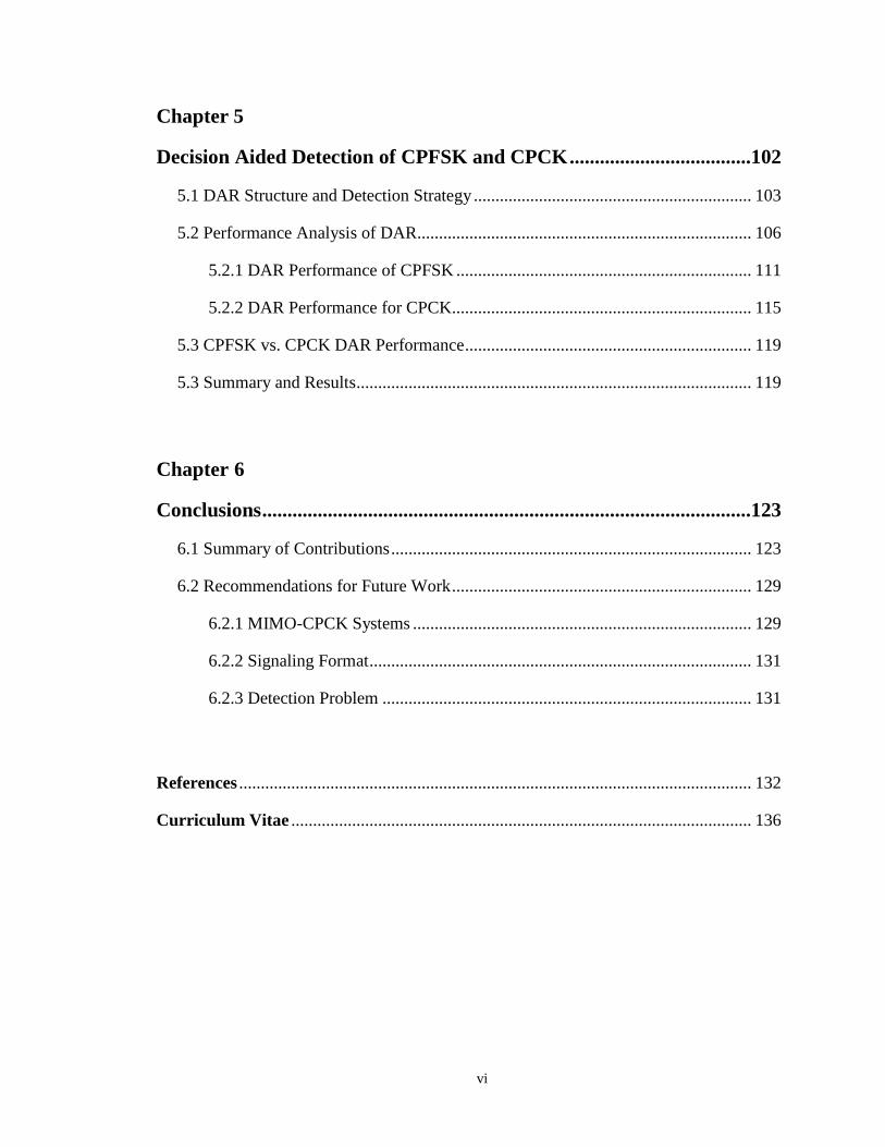
Table of Contents
Abstract .............................................................................................................................. ii
Acknowledgments ............................................................................................................ iii
Table of Contents ............................................................................................................. iv
List of Tables ................................................................................................................... vii
List of Figures ................................................................................................................. viii
Abbreviations ................................................................................................................... xi
Chapter 1
Introduction .................................................................................................... 1
1.1 Digital Communication System (DCS) Overview .................................................. 1
1.2 Modulation Scheme Parameters ............................................................................. 5
1.3 Review of Continuous Phase Modulation (CPM) .................................................. 8
1.4 Problem Statement and Justification ..................................................................... 11
1.5 Thesis Contributions ............................................................................................. 13
1.6 Thesis Organization .............................................................................................. 13
Chapter 2
Continuous Phase Modulation (CPM) .......................................................15
2.1 Description of CPM Signals .................................................................................. 16
2.2 Frequency Pulse Shapes ......................................................................................... 17
2.3 General Schematic of CPM Modulator .................................................................. 18
2.4 Phase States of CPM Signals ................................................................................. 18
2.5 Continuous Phase Frequency Shift Keying (CPFSK) ............................................ 25

v
2.6 Continuous Phase Chirp Keying (CPCK) .............................................................. 32
2.7 Summary ................................................................................................................ 41
Chapter 3
Optimum and Sub-optimum Receivers for CPFSK and CPCK .............42
3.1 Optimum Receiver using Bayesian MLRT ............................................................ 43
3.2 Average Matched Filter (AMF) Receiver .............................................................. 52
3.2.1 CPFSK Performance .................................................................................... 55
3.2.2 CPCK Performance ...................................................................................... 63
3.3 High- Receivers .............................................................................................. 68
3.3.1 CPFSK Performance .................................................................................... 72
3.3.2 CPCK Performance ...................................................................................... 75
3.4 Composite Performance Bounds ............................................................................ 80
3.5 Summary and Results ............................................................................................. 83
Chapter 4
Viterbi Receiver for CPFSK and CPCK ...................................................87
4.1 Minimum Distance Properties for CPFSK and CPCK .......................................... 88
4.1.1 Minimum Distance Properties of CPFSK .................................................... 89
4.1.2 CPCK Minimum Distance Properties .......................................................... 91
4.2 Optimum Viterbi Receiver ..................................................................................... 94
4.3 Summary and Results ............................................................................................. 99
vi
Chapter 5
Decision Aided Detection of CPFSK and CPCK ....................................102
5.1 DAR Structure and Detection Strategy ................................................................ 103
5.2 Performance Analysis of DAR............................................................................. 106
5.2.1 DAR Performance of CPFSK .................................................................... 111
5.2.2 DAR Performance for CPCK..................................................................... 115
5.3 CPFSK vs. CPCK DAR Performance .................................................................. 119
5.3 Summary and Results ........................................................................................... 119
Chapter 6
Conclusions .................................................................................................123
6.1 Summary of Contributions ................................................................................... 123
6.2 Recommendations for Future Work ..................................................................... 129
6.2.1 MIMO-CPCK Systems .............................................................................. 129
6.2.2 Signaling Format ........................................................................................ 131
6.2.3 Detection Problem ..................................................................................... 131
References ...................................................................................................................... 132
Curriculum Vitae .......................................................................................................... 136
vii
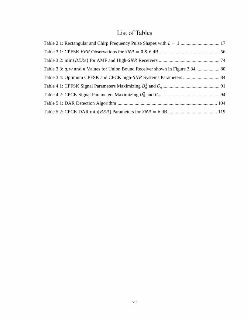
List of Tables
Table 2.1: Rectangular and Chirp Frequency Pulse Shapes with ................................ 17
Table 3.1: CPFSK Observations for dB .................................................. 56
Table 3.2: { s} for AMF and High- Receivers .................................................. 74
Table 3.3: Values for Union Bound Receiver shown in Figure 3.34 ................... 80
Table 3.4: Optimum CPFSK and CPCK high- Systems Parameters .............................. 84
Table 4.1: CPFSK Signal Parameters Maximizing and ............................................... 91
Table 4.2: CPCK Signal Parameters Maximizing and ................................................. 94
Table 5.1: DAR Detection Algorithm ................................................................................... 104
Table 5.2: CPCK DAR Parameters for dB ......................................... 119
viii
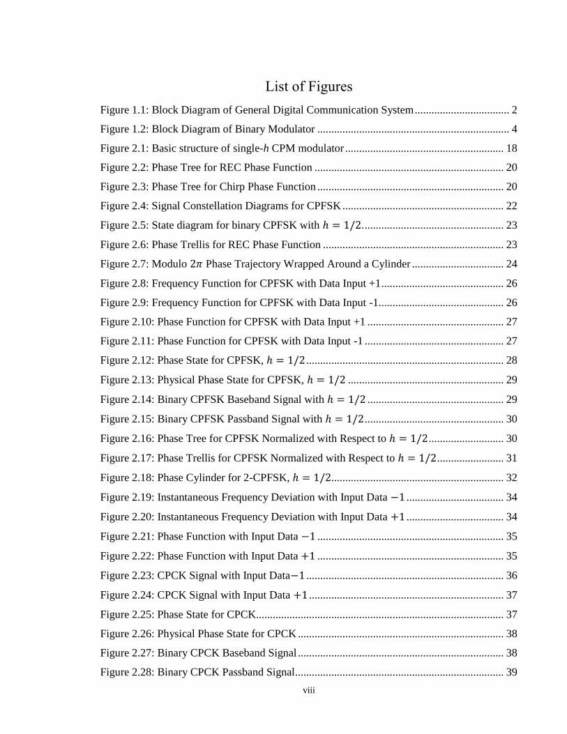
List of Figures
Figure 1.1: Block Diagram of General Digital Communication System .................................. 2
Figure 1.2: Block Diagram of Binary Modulator ..................................................................... 4
Figure 2.1: Basic structure of single-h CPM modulator ......................................................... 18
Figure 2.2: Phase Tree for REC Phase Function .................................................................... 20
Figure 2.3: Phase Tree for Chirp Phase Function ................................................................... 20
Figure 2.4: Signal Constellation Diagrams for CPFSK .......................................................... 22
Figure 2.5: State diagram for binary CPFSK with . .................................................. 23
Figure 2.6: Phase Trellis for REC Phase Function ................................................................. 23
Figure 2.7: Modulo Phase Trajectory Wrapped Around a Cylinder ................................. 24
Figure 2.8: Frequency Function for CPFSK with Data Input +1 ............................................ 26
Figure 2.9: Frequency Function for CPFSK with Data Input -1............................................. 26
Figure 2.10: Phase Function for CPFSK with Data Input +1 ................................................. 27
Figure 2.11: Phase Function for CPFSK with Data Input -1 .................................................. 27
Figure 2.12: Phase State for CPFSK, ....................................................................... 28
Figure 2.13: Physical Phase State for CPFSK, ........................................................ 29
Figure 2.14: Binary CPFSK Baseband Signal with ................................................. 29
Figure 2.15: Binary CPFSK Passband Signal with .................................................. 30
Figure 2.16: Phase Tree for CPFSK Normalized with Respect to ........................... 30
Figure 2.17: Phase Trellis for CPFSK Normalized with Respect to ........................ 31
Figure 2.18: Phase Cylinder for 2-CPFSK, .............................................................. 32
Figure 2.19: Instantaneous Frequency Deviation with Input Data ................................... 34
Figure 2.20: Instantaneous Frequency Deviation with Input Data ................................... 34
Figure 2.21: Phase Function with Input Data ................................................................... 35
Figure 2.22: Phase Function with Input Data ................................................................... 35
Figure 2.23: CPCK Signal with Input Data ....................................................................... 36
Figure 2.24: CPCK Signal with Input Data ...................................................................... 37
Figure 2.25: Phase State for CPCK......................................................................................... 37
Figure 2.26: Physical Phase State for CPCK .......................................................................... 38
Figure 2.27: Binary CPCK Baseband Signal .......................................................................... 38
Figure 2.28: Binary CPCK Passband Signal........................................................................... 39
ix
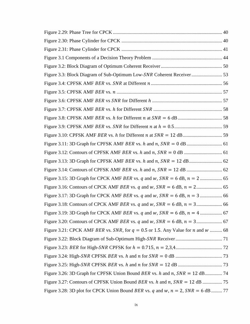
Figure 2.29: Phase Tree for CPCK ......................................................................................... 40
Figure 2.30: Phase Cylinder for CPCK .................................................................................. 40
Figure 2.31: Phase Cylinder for CPCK .................................................................................. 41
Figure 3.1 Components of a Decision Theory Problem ......................................................... 44
Figure 3.2: Block Diagram of Optimum Coherent Receiver .................................................. 50
Figure 3.3: Block Diagram of Sub-Optimum Low- Coherent Receiver ......................... 53
Figure 3.4: CPFSK AMF vs. at Different .......................................................... 56
Figure 3.5: CPFSK AMF vs. ...................................................................................... 57
Figure 3.6: CPFSK AMF vs for Different ......................................................... 57
Figure 3.7: CPFSK AMF vs. for Different ........................................................ 58
Figure 3.8: CPFSK AMF vs. for Different at dB .................................... 58
Figure 3.9: CPFSK AMF vs. for Different at ....................................... 59
Figure 3.10: CPFSK AMF vs. for Different at dB ................................ 59
Figure 3.11: 3D Graph for CPFSK AMF vs. and , dB ............................. 61
Figure 3.12: Contours of CPFSK AMF vs. and , dB ............................... 61
Figure 3.13: 3D Graph for CPFSK AMF vs. and , dB ........................... 62
Figure 3.14: Contours of CPFSK AMF vs. and , dB ............................. 62
Figure 3.15: 3D Graph for CPCK AMF vs. and , dB, .................. 65
Figure 3.16: Contours of CPCK AMF vs. and , dB, ..................... 65
Figure 3.17: 3D Graph for CPCK AMF vs. and , dB, .................. 66
Figure 3.18: Contours of CPCK AMF vs. and , dB, ..................... 66
Figure 3.19: 3D Graph for CPCK AMF vs. and , dB, .................. 67
Figure 3.20: Contours of CPCK AMF vs. and , dB, ..................... 67
Figure 3.21: CPCK AMF vs. , for or . Any Value for and .......... 68
Figure 3.22: Block Diagram of Sub-Optimum High- Receiver ...................................... 71
Figure 3.23: for High- CPFSK for , ...................................... 72
Figure 3.24: High- CPFSK vs. and for dB ...................................... 73
Figure 3.25: High- CPFSK vs. and for dB .................................... 73
Figure 3.26: 3D Graph for CPFSK Union Bound vs. and , dB .............. 74
Figure 3.27: Contours of CPFSK Union Bound vs. and , dB ................ 75
Figure 3.28: 3D plot for CPCK Union Bound vs. and , , dB ......... 77
x
Figure 3.29: Contours of CPCK Union Bound vs. and , dB ........ 77
Figure 3.30: 3D plot for CPCK Union Bound vs. and , , dB ......... 78
Figure 3.31: Contours of CPCK Union Bound vs. and , dB ........ 78
Figure 3.32: 3D plot for CPCK Union Bound vs. and , , dB ......... 79
Figure 3.33: Contours of CPCK Union Bound vs. and , dB ........ 79
Figure 3.34: CPCK Union Bound Receiver ................................................................... 80
Figure 3.35: Composite Bound on CPFSK ............................................................................. 81
Figure 3.36: Composite Bound on CPCK............................................................................... 82
Figure 3.37: CPFSK and CPCK Union Bounds, ......................................................... 82
Figure 3.38: CPFSK and CPCK AMF and Union Bound Receivers Simulation ................... 83
Figure 4.1: Upper Bound on the Minimum Distance Squared for CPFSK at all ................ 89
Figure 4.2: CPFSK Minimum Distance Squared with First Bit Difference Only .................. 90
Figure 4.3: Upper Bound on the Minimum Distance Squared for CPCK for all ........... 92
Figure 4.4: Contours for Upper Bound on Minimum Distance Squared for CPCK ............... 93
Figure 4.5 Basic Quadrature Receiver .................................................................................... 98
Figure 4.6: Upper Bounds on Viterbi Receiver for CPFSK and CPCK ................................. 99
Figure 4.7: Number of Correlations vs. ............................................................................. 101
Figure 5.1: DAR Detection Strategy Flow Chart.................................................................. 105
Figure 5.2: DAR for Obtaining Estimates and ........................ 106
Figure 5.3: DAR for Obtaining Refined Estimates ................................. 106
Figure 5.4: Performance, , of DAR for CPFSK for ...................................... 112
Figure 5.5: Normalized Performance, , of DAR and AMF receiver for CPFSK vs. ... 113
Figure 5.6: Normalized DAR Performance, , vs. for dB ...................... 114
Figure 5.7: Normalized DAR Performance, , vs. for dB .................... 114
Figure 5.8: Performance, , of DAR for optimum CPCK systems, ......... 117
Figure 5.9: Contours of DAR for CPCK, dB .. 118
Figure 5.10: Performance of DAR and AMF for 2-bit Optimum CPCK and CPFSK System ... 120
Figure 6.1: General MIMO System Block Diagram ................................................................... 130
xi
Abbreviations
AWGN Additive White Gaussian Noise
BER Bit Error Rate
BPSK Binary Phase Shift Keying
CDMA Code Division Multiple Access
CPM Continuous Phase Modulation
CPFSK Continuous Phase Frequency Shift Keying
CPCK Continuous Phase Chirp Keying
WCS Wireless Communications Systems
DCS Digital Communications Systems
FM Frequency Modulation
HF High Frequency
MLD Maximum Likelihood Detector
MLSE Maximum Likelihood Sequence Estimation
MLSD Maximum Likelihood Sequence Detection
MLRT Maximum Likelihood Ratio Test
RF Radio Frequency
SNR Signal-to-Noise Ratio
REC Rectangular Pulse
PSK Phase Shift Keying
PSD Power Spectral Density
PDF Probability Distribution Function
MIMO Multiple-Input-Multiple-Output
VA Viterbi Algorithm
DAR Decision Aided Receiver
AMF Average Matched Filter
MSK Minimum Shift Keying
1
Chapter 1
Introduction
In this Chapter, an overview of the functional block diagram of a Digital Communication
System (DCS) is presented with emphasis on digital modulation and demodulation sub-
blocks. Digital modulation techniques and parameters that are used to describe the
performance of the DCS are also given. Transmission and detection strategies,
particularly, those associated with CPFSK and CPCK, are discussed. All in all the
emphasis in this Chapter is mainly on the literature review, problem statements, their
justifications, approaches for their solutions, and organization of the thesis.
1.1 Digital Communication System (DCS) Overview
Digital Communication has become one of the most rapidly growing industries in the
world, and its products cover a wide array of applications and they are exerting a direct
impact on our daily lives. Basically, communication involves implicitly the transmission
of information from one point to another through a succession of processes. The first step
is the generation of a message signal, either analogue (voice, music or picture) or digital
2
(computer data). The second step is to describe that message signal with a certain
measure of precision by using a set of electrical, aural or visual symbols. These symbols
are encoded in a form that is suitable for transmission over the available physical
medium. The encoded symbols are transmitted using a transmission device to a specific
destination. The encoded symbols are received on the other side using a receiver device.
Then, the encoded symbols are decoded to produce an estimate of the original symbols.
Thus, the message signal is re-created with a definable degradation in quality due to
signal fading, system imperfections and the different types of noise (Thermal noise,
Additive White Gaussian Noise (AWGN)…). A typical digital communication system is
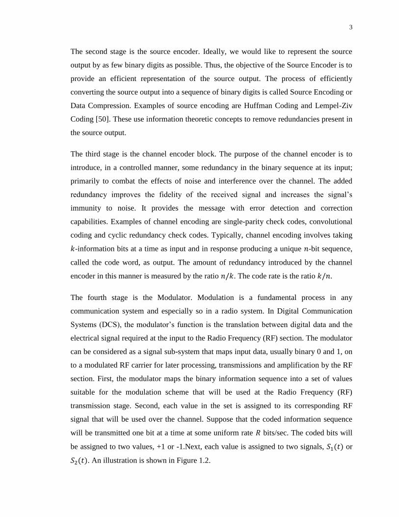
shown in Figure 1.1.
Figure 1.1: Block Diagram of General Digital Communication System
Information source may be either analog (audio or video) or digital (computer output)
signal. In a Digital Communication System, messages produced by source are always
converted to a sequence of binary digits ( ). If source output is analog,
Analogue to Digital conversion (Sampling, Quantization and Encoding) is employed
using Analogue to Digital convertor (ADC).
Input Transducer Source
Encoder
Channel
Encoder Modulator
Channel
Output Transducer Source
Decoder
Channel
Decoder Demodulator
Estimated Message
Information Source Transmitter
Receiver
3
The second stage is the source encoder. Ideally, we would like to represent the source
output by as few binary digits as possible. Thus, the objective of the Source Encoder is to
provide an efficient representation of the source output. The process of efficiently
converting the source output into a sequence of binary digits is called Source Encoding or
Data Compression. Examples of source encoding are Huffman Coding and Lempel-Ziv
Coding [50]. These use information theoretic concepts to remove redundancies present in
the source output.
The third stage is the channel encoder block. The purpose of the channel encoder is to
introduce, in a controlled manner, some redundancy in the binary sequence at its input;
primarily to combat the effects of noise and interference over the channel. The added
redundancy improves the fidelity of the received signal and increases the signal’s
immunity to noise. It provides the message with error detection and correction
capabilities. Examples of channel encoding are single-parity check codes, convolutional
coding and cyclic redundancy check codes. Typically, channel encoding involves taking
-information bits at a time as input and in response producing a unique -bit sequence,
called the code word, as output. The amount of redundancy introduced by the channel
encoder in this manner is measured by the ratio . The code rate is the ratio .
The fourth stage is the Modulator. Modulation is a fundamental process in any
communication system and especially so in a radio system. In Digital Communication
Systems (DCS), the modulator’s function is the translation between digital data and the
electrical signal required at the input to the Radio Frequency (RF) section. The modulator
can be considered as a signal sub-system that maps input data, usually binary 0 and 1, on
to a modulated RF carrier for later processing, transmissions and amplification by the RF
section. First, the modulator maps the binary information sequence into a set of values
suitable for the modulation scheme that will be used at the Radio Frequency (RF)
transmission stage. Second, each value in the set is assigned to its corresponding RF
signal that will be used over the channel. Suppose that the coded information sequence
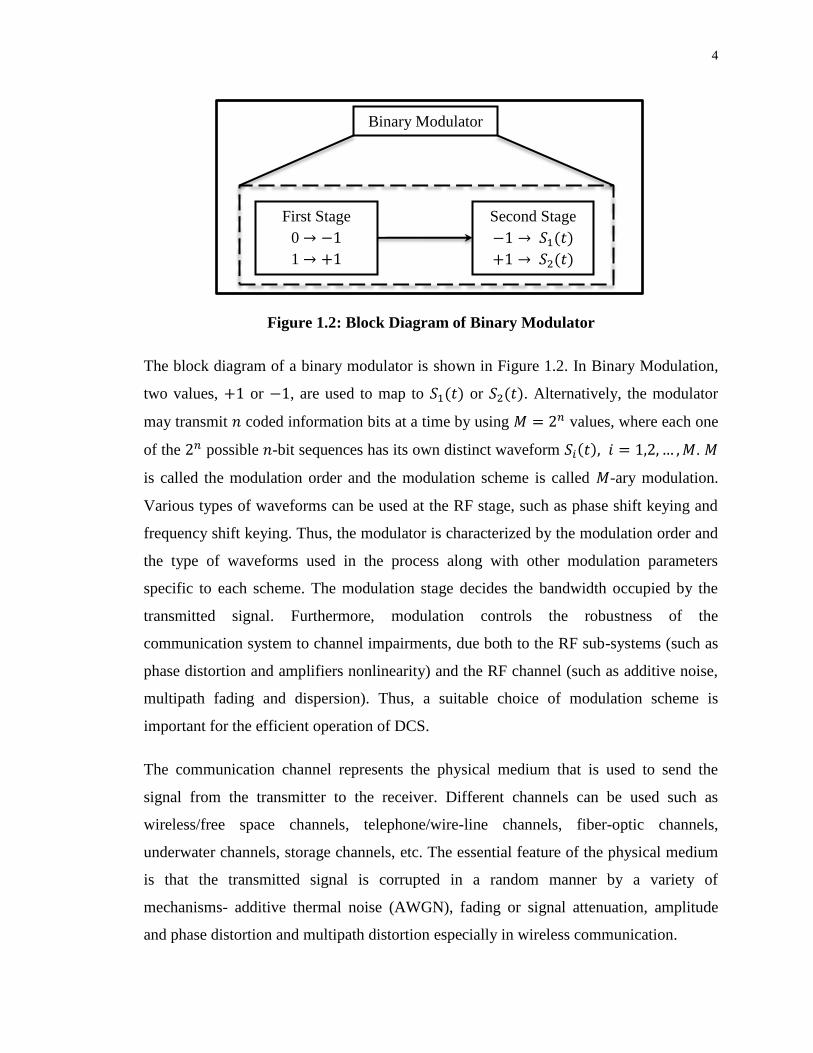
will be transmitted one bit at a time at some uniform rate bits/sec. The coded bits will
be assigned to two values, +1 or -1.Next, each value is assigned to two signals, or
. An illustration is shown in Figure 1.2.
4
Figure 1.2: Block Diagram of Binary Modulator
The block diagram of a binary modulator is shown in Figure 1.2. In Binary Modulation,
two values, or , are used to map to or . Alternatively, the modulator
may transmit coded information bits at a time by using values, where each one
of the possible -bit sequences has its own distinct waveform .
is called the modulation order and the modulation scheme is called -ary modulation.
Various types of waveforms can be used at the RF stage, such as phase shift keying and
frequency shift keying. Thus, the modulator is characterized by the modulation order and
the type of waveforms used in the process along with other modulation parameters
specific to each scheme. The modulation stage decides the bandwidth occupied by the
transmitted signal. Furthermore, modulation controls the robustness of the
communication system to channel impairments, due both to the RF sub-systems (such as
phase distortion and amplifiers nonlinearity) and the RF channel (such as additive noise,
multipath fading and dispersion). Thus, a suitable choice of modulation scheme is
important for the efficient operation of DCS.
The communication channel represents the physical medium that is used to send the
signal from the transmitter to the receiver. Different channels can be used such as
wireless/free space channels, telephone/wire-line channels, fiber-optic channels,
underwater channels, storage channels, etc. The essential feature of the physical medium
is that the transmitted signal is corrupted in a random manner by a variety of
mechanisms- additive thermal noise (AWGN), fading or signal attenuation, amplitude
and phase distortion and multipath distortion especially in wireless communication.
First Stage
0 →
1 →
→ 𝑆 𝑡
→ 𝑆 𝑡
Second Stage
Binary Modulator
5
The Source encoder, channel encoder and modulator form the integral parts of the
transmitter. The reverse of all these processes is taken care of on the destination side by
the receiver, which will typically contain a demodulator, channel decoder and source
decoder. When an analog output is desired, the output of the source decoder is fed to the
Digital to Analogue converter (DAC) to reconstruct the estimated message. Because of
channel conditions and distortions, the message at the destination output is an
approximation to the original source message. Each one of the blocks shown in Figure
1.1 is a research field on its own. In this thesis, our focus is on the
modulation/demodulation sub-blocks of DCS.
1.2 Modulation Scheme Parameters
Radio systems are always strictly limited by the regulating authorities to certain
frequency bands. Usually, each one of those bands is shared among multiple users of the
system by means of Frequency Division Multiple Access (FDMA) and, therefore, the
bandwidth occupied by each user is narrower, and more users can be accommodated.
Moreover, communication system bandwidth requirement is determined by the spectrum
of the modulated signal, which is typically presented as a plot of Power Spectral Density
(PSD) as a function of frequency. Theoretically speaking, the PSD should be zero outside
the occupied band, where in practice, however, this is never the case, and the spectrum
extends to infinity beyond the band’s limit. This is either due to the specific
characteristics associated with the different modulation schemes or due to the
imperfectness of the practical implementation of filters. Therefore, it is essential to set the
bandwidth, , of the modulated signal such that the signal’s power portion falling
beyond the band’s limit is less than a certain threshold. In practical implementation, this
threshold is determined by the system’s tolerance to Adjacent Channel Interference
(ACI), which is also another feature of the modulation scheme. In addition, the
bandwidth or spectral efficiency of a modulation scheme is defined as the channel data
rate per unit bandwidth occupied ( ).
Another parameter used in characterizing a modulation scheme is the Bit-Error-Rate
( ) performance. is defined as the ratio of bits received in error to the total
6
number of bits received. Moreover, is also referred to as the probability of bit error,
, and is frequently plotted logarithmically against Signal-to-Noise-Ratio ( ) in
. For a more system-independent measure, the coordinate of this graph is normally the
-energy-to-noise density ratio . This is due to the fact that noise power spectral
density is a primary feature of a channel and independent of the bandwidth of the
system, unlike the noise power. is dimensionless, since has dimension of
, which is equivalent to .
In addition, modulator and demodulator complexity is another parameter that plays a
major role in determining the choice of a specific modulation scheme for any DCS. The
number of correlators required in the implementation of the demodulator is normally used
as a complexity measure for each modulation scheme. Moreover, all DCS require a
particular degree of synchronization with incoming signals by the receivers, which
further increases the complexity of receivers especially in coherent detection.
Hence, the ultimate choice of one modulation scheme over the others in a DCS depends
on spectral efficiency, performance and receiver complexity. In general, these
parameters can be viewed as a set of basis-functions that can be used to pinpoint DCS as
a point in a three-dimensional space. Following this analogy, trade-offs in the design of a
DCS exist among these three main resources. In practice, two types of modulation
schemes are found, one that is optimized for bandwidth efficiency and the other that is
optimized for power efficiency. The choice of which one to go with depends on the DCS
in question, if it is either power-limited or bandwidth limited. Consequently, different
modulation schemes are referred to as either power-efficient or bandwidth-efficient.
While efficient power and bandwidth utilization is considered an important criteria in the
design of DCS, there are situations where this efficiency is sacrificed in order for other
design objectives to be met, such as providing secure communication in a hostile
environment. A major advantage of such systems is their ability to reject intentional or
unintentional interference. The class of signals that provide this requirement is referred to
as spread-spectrum modulation. In a spread-spectrum system, the transmitted signal is
7
spread over a wide frequency band, usually much wider than the minimum bandwidth
required for information to be conveyed.
Nowadays, indoor wireless communication is of great importance and its market share
has been growing rapidly due to its advantages over cable networks such as users’
mobility, wiring cutoffs and flexibility. Classical applications are cordless phone systems,
Wireless Local Area Networks (WLANs) for office and home applications and flexible
mobile data transmission links between robots, actuators, sensors, and controller units in
industrial environments. Because of the hostile electromagnetic (EM) environment,
which includes severe EM emissions from other devices as well as multipath propagation
distortions [1], communication link robustness is an extremely important feature for
wireless communication system, and here comes in spread-spectrum technology.
Spread-spectrum’s most important ability is its robust data transmission even in very
noisy radio environments [2]. The critical processes in spread spectrum systems are the
spreading and de-spreading functions in the transmitter and receiver. In Frequency
Hopping (FH) and Direct Sequence (DS) systems, the synchronization of the de-
spreading code needs high computational effort and it is difficult. Chirp modulation and
Linear Frequency Modulation (FM) are spread spectrum signaling techniques in which
the carrier frequency is swept over a wideband during a given data pulse interval. In such
systems, the spreading is accomplished solely for combating multi-path distortions,
whereas in Code Division Multiple Access (CDMA), this objective is achieved by using
additional coding [3]. Spreading and de-spreading with chirp signals can be easily
implemented using Surface Acoustic Wave (SAW) technology [4], which offers a rapid
close-to-optimum method for both generation and correlation of wideband chirp pulses
[5]. Moreover, these devices are very compact and can be realized at low cost, due to the
analog correlation process involved in the complex synchronization circuits.
While a variety of modulation techniques exist in the literature, the emphasis in this
thesis is on phase modulations. In particular, two subclasses of phase-continuous signals
referred to as Continuous Phase Frequency Shift Keying (CPFSK) and Continuous Phase
Chirp Keying (CPCK) are considered, in an attempt to arrive at power efficient
8
modulations. In the next Section, an overview of the relevant development in the area of
CPM is provided with particular references to CPFSK and CPCK modulations, detection
techniques, receivers and their performance.
1.3 Review of Continuous Phase Modulation (CPM)
Over the past twenty years or so, research has been intensely focused on finding efficient
Digital Communication Systems, especially modulation techniques that can meet high bit
rate transmissions. Generally speaking, one modulation scheme is chosen over another
based on which one requires the least value of for a specific error rate threshold and
still satisfies the various system constraints [6].
In this context, constant-envelope CPM has emerged as an excellent modulation
technique for applications in satellite communication and global digital radio channels.
CPM offers excellent bandwidth and power efficiency [7]. Moreover, CPM designs are
fairly immune to nonlinear channel effects because of their constant-envelope
characteristic. Although there are many CPM classes with diverse properties and
applications, they are all based on the usage of inherent memory, which is introduced by
the continuous phase. This continuous phase constraint offers enhanced bit error
probability performance [8], sharper spectral roll-off [9], and permits multi-symbol
detection rather than the conventional symbol-by-symbol detection. In general,
performance is improved by increasing the number of observation intervals. However,
the implementation of the corresponding optimal receiver becomes much more complex.
Thus, it is important to examine the class of constant envelope CPM for its ability to offer
tradeoffs among receiver complexity, bandwidth and power.
Osborne and Luntz [10] considered a bandwidth efficient modulation technique,
Continuous Phase Frequency Shift Keying (CPFSK), and showed that Binary CPFSK
with a modulation index of and optimum 3-bit observation receiver can
outperform Binary Phase Shift Keying (BPSK). Later, these results were extended to the
more general case of -ary CPFSK by Schonhoff [11]. In these works, the focus was on
finding optimum modulation parameters that provide least . However, it is important
to examine the loss in performance relative to the optimum if one were to use non-
9
optimum modulation parameters due to bandwidth and receiver complexity constraints. It
is noted that [10, 11] in order to arrive at performance of the optimum receiver,
high-and low- approximations have been employed. Nevertheless, it is not clear as to
the value of that distinguishes high- from that of low- . Thus, an
investigation to answer this question is important.
Moreover, Aulin et. al. have studied CPM using minimum Euclidean distance notion in
the signal space, and have suggested schemes that are efficient in terms of bandwidth and
power compared to PSK [8, 12]. Optimum signaling schemes have been determined
based on maximizing the minimum Euclidean distance in signal-space. Again, it is noted
that an examination of distance properties as a function of modulation parameters is
important to understand the ability of CPM to operate over practical communication
channels.
In addition, Miyakawa’s et. al. have suggested the use of time-varying modulation
indices from one bit interval to the next and have demonstrated that multi-h CPFSK can
outperform single-h CPFSK [13]. Anderson and Taylor [14] generalized Miyakawa’s
work by imposing certain constraints on the modulation indexes employed and have
confirmed that multi-h phase codes can achieve up to dB performance
improvement in approximately the same bandwidth relative to PSK. In another work,
Aulin and Suridberg [15] have thoroughly worked on the distance properties of multi-
signals. In addition, Raveendra and Srinivasan [16] have arrived at optimum multi-h
CPM schemes, which minimize the bit-error-probability. Moreover, they have arrived at
closed-form expressions describing bit error rates of an easy-to-implement multi-h CPM
Average Matched Filter (AMF) receiver.
Later on, Hwang et. al. have introduced the concept of asymmetric modulation indices
[17]. In this technique, the modulation indices were set as a function of the data symbols
and it was demonstrated that performance improvements can be achieved over
conventional multi-h schemes in essentially the same bandwidth. Fonseka and Mao [18]
considered a class of nonlinear asymmetrical multi-h CPFSK with the ability to achieve
higher distance properties relative to other multi-h schemes. By adaptively changing
10
modulation indices in a time-varying manner, it is also possible to obtain an adaptive
multi-h CPFSK signaling [19]. This signaling scheme realizes higher coding gains
compared to the well-known Minimum Shift Keying (MSK) scheme. Further important
works in nonlinear CPFSK has been carried out [20, 21, 22]. Also, Raveendra and
Srinivasan [23] considered a Decision Directed Receiver for coherent demodulation of a
subclass of CPM over AWGN.
Chirp modulation or Linear FM represents a class of spread-spectrum signals. It is useful
in certain communication systems for its abilities such as anti-eavesdrop, low-Doppler
sensitivity and anti-interference [24]. Moreover, there are several applications of chirp
signals in communication such as cordless systems, radio telephony, data communication
in High Frequency (HF) band, air-ground communication via satellite repeaters and
WLANs. Recently, Institute of Electrical and Electronics Engineers (IEEE) introduced
Chirp Spread Spectrum (CSS) physical layer in the new wireless standard 802.15.4a [25],
which uses chirp modulation with no additional coding. The new standard, 802.15.4a,
targets applications in sensor actuator networking, industrial and safety control, medical
and private communication devices.
A combination of chirp modulation [26] with some kind of pseudo-random coding has
been shown to produce significant improvement in anti-jam performance. Among several
applications of chirp signals in communication are cordless systems, data communication
in High Frequency (HF) [27], radiotelephony, WLANs [28] and air-ground
communication via satellite repeaters [29][30].
While majority of chirp signals are employed in radar applications [31], Winkler [32]
first proposed them for data communication, due to their noise immunity property to
intentional interference. Hirt and Pasupathy studied the performance of coherent and non-
coherent binary chirp signals over AWGN channel [33, 34]. Since the optimum receivers
were required to make independent bit-by-bit decisions, it was concluded that chirp
systems did not compare favorably with conventional PSK and FSK systems. By
introducing phase continuity into chirp signals at bit transitions, the use of multiple-bit
detection techniques became possible, which offered power advantages [35]. Thus, Hirt
11
and Pasupathy considered a class of CPM referred to as Continuous Phase Chirp (CPC)
binary signals [33] and showed that an advantage of 1.66 dB at most can be achieved
over conventional PSK. Raveendra extended this work to the more general case of -ary
signaling [36]. It was shown that 4-ary chirp system with five bit observation interval,
when coherently detected, offers an gain that is nearly equal to 3.2 dB compared to
that of the conventional 4-PSK system. Also, Raveendra introduced a class of multi-mode
binary CPC signals [37] that used the concept of time-varying modulation parameters. He
showed that dual-mode phase-continuous chirp signals, with two different sets of
modulation parameters, outperform conventional CPC signals by nearly 0.8 dB. Fonseka
extended these results [38] to include partial response CPC signals. More recently, Bhumi
and Raveendra [39] considered digital asymmetric phase continuous chirp signals. They
showed that it can outperform dual-mode chirp modulation that was considered before
[37]. Wang, Fei, and Li [40] proposed a structure for chirp Binary Orthogonal Keying
(BOK) system. They obtained an expression for the probability of bit error and showed
that chirp BOK performs better than traditional BOK modulation in Additive White
Gaussian Noise (AWGN) channel.
Several other works in this area clearly exhibit the choice of chirp modulation in a variety
of digital communication systems [41, 42, 43, 44, 45 and 46]. In all these works, binary
chirp systems with receivers that are required to make independent bit-by-bit decisions
have been considered.
In the literature, there are several other notable papers, which address the advancement in
CPM over the past 20-30 years [12, 13, 17, 18, 33 and 37].
1.4 Problem Statement and Justification
The optimum coherent receiver which minimizes the bit error probability observes the
received CPM signal contaminated with AWGN, over several bit intervals and makes a
decision on the first bit in this interval. The optimum receiver is complex and its precise
analysis is too complicated to attempt analytically. The complexity of the receiver grows
exponentially as the number of observed symbol intervals. Also, the performance of the
12
optimum receiver is determined in terms of the performance of the sub-optimum
receivers.
These sub-optimum receivers have been arrived at based on high- and low-
approximations. It is not obvious as to the value of that defines the boundary
between high- and low- . Also, most performance analyses have focused on
determining the optimum modulation parameters that achieve minimum . Thus, our
first objective in the thesis is to derive from first principles, the structure of the optimum
receiver and subject it to high- and low- performance analysis. Closed-form
expressions for are then derived and used to find the boundary between high- and
low- s; first using analytical results and then using simulations. Moreover, we
provide a thorough investigation of the effect of modulation parameters on
performance for the subclasses of CPM namely CPFSK and CPCK. This study is carried
out using exhaustive computer search and backed with mathematical analysis, wherever
possible.
It is well-known that the Viterbi Algorithm (VA), a Maximum Likelihood Sequence
Estimation (MLSE) technique, is widely used for estimation and detection problems in
digital communications. In this thesis, we are particularly interested in the application of
VA for detection of CPFSK and CPCK signals. The main issue is to develop VA in
software to examine the performance of specific CPFSK and CPCK signaling.
The problem of finding low-complexity receivers for CPM has received wide spread
attention by researchers. One is particularly interested in arriving at reduced complexity
receivers whose performances are comparable to that of the optimum receiver. In fact, in
all these works, four different types of receivers are considered, of which two are
generally receivers that work for all CPM schemes and the other two work for binary
schemes with a modulation index of 0.5. In this thesis, quite different to the approaches
available in the literature, we introduce a low-complexity receiver, for both CPFSK and
CPCK, which we have called Decision Aided Receiver (DAR). The detection strategy
involves first obtaining coarse estimates and then using these to refine the estimate in a
specific bit in the observation interval. Not only we provide the decision aided detection
13
strategy, but also we obtain closed-form expression for estimating the of such a
receiver.
1.5 Thesis Contributions
The major contributions of the thesis are summarized below:
Two subclasses of constant-envelope phase-continuous signals called CPFSK and
CPCK signals are presented. Mathematical descriptions and properties of these
signals are given and illustrated.
Optimum and sub-optimum receivers are derived based on Bayesian Maximum
Likelihood Ratio Test (MLRT). Performance of these receivers is analyzed and
the effect of the different modulation parameters on is examined in detail for
CPFSK and CPCK modulations.
Minimum Distance Criteria for both CPFSK and CPCK signaling techniques are
provided, and optimum parameters that maximize the minimum distance are
determined through extensive computer search.
Performance of the Maximum Likelihood sequence Estimation (MLSE) receiver,
which is referred to as Viterbi Algorithm (VA) is provided for specific CPFSK
and CPCK modulations.
A novel Decision Aided Receiver (DAR) for CPFSK and CPCK modulations is
presented and closed-form expressions for of the receiver are derived. Best
CPFSK and CPCK systems for DAR have been determined and illustrated.
1.6 Thesis Organization
Chapter 2 provides the concept, mathematical descriptions and properties of CPM
signals. A mathematical frame work required for the understanding of Continuous
Phase Chirp Keying (CPCK) and Continuous Phase Frequency Shift Keying (CPFSK)
signaling techniques is described. We demonstrate the fundamental difference
between CPFSK and CPCK signaling techniques. Illustrations of phase functions,
frequency functions, phase trees and trellises, baseband and passband waveforms for
CPFSK and CPCK as a function of modulation parameters are all provided.
14
In Chapter 3, the problem of detection of CPM in AWGN channel is considered. Using
Maximum Likelihood Ratio Test (MLRT), an optimum receiver is derived for detection
of arbitrary CPM signals in AWGN channel. Also, we discuss the computational
complexity of this optimum receiver for CPFSK and CPCK. Two sub-optimum receivers
for high- and low- values are derived. The low- , sub-optimum, also known as
Average Matched Filter (AMF), receiver is examined thoroughly for CPFSK and CPCK.
At high- , another sub-optimum receiver is provided. A thorough examination of the
relationship among , Signal-to-Noise Ratio ( ), modulation parameters and
detection observation length are provided using number of illustrations. An attempt is
made to answer the question, “What value of separates high- from low-
when studying the effect of the modulation parameters on ?” A composite bound is
provided using the performance of sub-optimum receivers that represents the
performance of the optimum receiver.
In Chapter 4, we present the distance properties of both signaling schemes, CPFSK and
CPCK. This lays the ground work for introducing the MLSE receiver for CPFSK and
CPCK signals, also known as the Viterbi Algorithm (VA) receiver. Advantages of Viterbi
receiver over the MLRT-based receiver are demonstrated and performance of Viterbi
receiver for specific CPFSK and CPCK schemes is illustrated.
In Chapter 5, a Decision Aided Receiver (DAR) for CPFSK and CPCK as an alternative
for the AMF receiver is presented. Decision aided detection strategy is presented and
explicit expressions for computation of are developed for AWGN environment.
Numerical results are reported, and a discussion of the performance of DAR is given.
The thesis is concluded in Chapter 6 by summarizing the work carried out, contributions
made and conclusions from the results obtained. Also, we outline areas for further
research in the light of the needs of modern reliable DCS and the work done in the thesis.
15
Chapter 2
Continuous Phase Modulation (CPM)
Continuous Phase Modulation (CPM) is a memory-type, constant-envelope, nonlinear
modulation, which allows the use of power efficient low cost, nonlinear power amplifiers
without introducing distortion. Digital transmission using constant-envelope CPM has
become important because of its attractive properties. The constant-envelope designs are
fairly immune to nonlinear channel effects. Although constructions of CPM are diverse in
their properties and applications, they all rely upon the use of inherent memory
introduced by the continuous phase. This constraint of continuous phase not only
provides faster spectral roll-off, but also permits multiple symbol detection rather than
the more conventional symbol-by-symbol detection. In this Chapter, two subclasses of
CPM called Continuous Phase Frequency Shift Keying (CPFSK) and Continuous Phase
Chirp Keying (CPCK) are described, although the treatment provided applies, in general,
to any CPM. Concepts, mathematical descriptions and properties of CPM signals are
presented with primary focus on CPFSK and CPCK signaling techniques, which will be
used all through the thesis.
16
2.1 Description of CPM Signals
The general form of a CPM signal is given by
√
where is the symbol energy, is the symbol duration, is the carrier frequency, is
the initial phase offset which is assumed to be zero for coherent detection without any
loss of generality. is a sequence of independent and identically distributed -ary
information symbols each taking one of the — values with an equal
probability of such that
In this work, the focus is binary case, . The information carrying phase, ,
during the symbol interval is given by
∑
where and the phase function is defined as the integral of an
instantaneous frequency pulse and is given by:
∫
The derivative of is the frequency pulse shape . That is
{
where is the frequency response pulse length. The frequency pulse length dictates the
time interval over which a single input data symbol can affect the instantaneous
17
frequency. Depending on the value of , two different schemes of CPM can be defined.
When , the entire pulse extends over one full symbol interval. This type of CPM is
known as full response CPM. When , only a part of the pulse shape extends over a
symbol and is known as partial response CPM signaling. In this work, we are only
interested in full response CPM.
2.2 Frequency Pulse Shapes
One of the reasons for CPM to be a bandwidth efficient scheme is that it uses pulse
shaping. Using various frequency pulse shapes such as Rectangular (REC), Raised
Cosine (RC), Chirp, and Half-Cycle Sinusoid (HCS), various subclasses of CPM have
been constructed. Table 2.1 lists the frequency pulse shaping functions used to describe
CPFSK and CPCK modulations.
Table 2.1: Rectangular and Chirp Frequency Pulse Shapes with
CPFSK (REC) 2
CPCK (Chirp) 2
In CPM, the information carrying phase is continuous all the time for all the
combinations of data symbols. Therefore, memory is introduced into the CPM signal by
means of its continuous phase. The quantity h, in Table 2.1 is the modulation index and
represents the ratio of peak-to-peak frequency deviation and the symbol rate. Ideally, h
can take any real value, but in order to limit the number of phase states, h is chosen a
rational value between and ratio of two prime numbers and , i.e.
. In some cases, the modulation is described using more than one modulation
parameter. Chirp is one such example, which will be explained later.
18
2.3 General Schematic of CPM Modulator
Figure 2.1: Basic structure of single-h CPM modulator
Figure 2.1 represents a conceptual block diagram of the single-h CPM, which is the focus
of this thesis. Data sequence passes through the pulse shaping filter and the multiplier
to form frequency pulse sequence, which is then FM modulated to generate the CPM
signal.
2.4 Phase States of CPM Signals
The phase of CPM can be represented by a tree structure. The tree structure is found by
manipulating the information carrying phase of Equation 2.3. It can be viewed as the sum
of two phase terms: instantaneous phase and accumulated phase. The phase of CPM
signal during the symbol interval to give
∑
∑
where is the instantaneous phase
∑
which represents the changing part of the total phase during and is
determined by the current data symbols and previous — symbols. The first term of
Equation 2.6, is dependent on the sequence of past input data symbols and the
current data input, , and is called the correlative state. There are
𝜋 𝜋𝑓𝑐
𝒂 𝑠 𝑡 𝒂
𝑓 𝑡
Pulse Shaping Filter FM
Modulator
19
possible correlative states. Since we are only interested in full response CPM ,
then
and is the accumulated phase, the phase state, which represents the constant part of the
total phase in the same interval is
∑
The accumulated phase can be interpreted as the sum of the maximum phase changes
contributed by each symbol, accumulated along the time axis up to the symbol
interval. It can be computed recursively as:
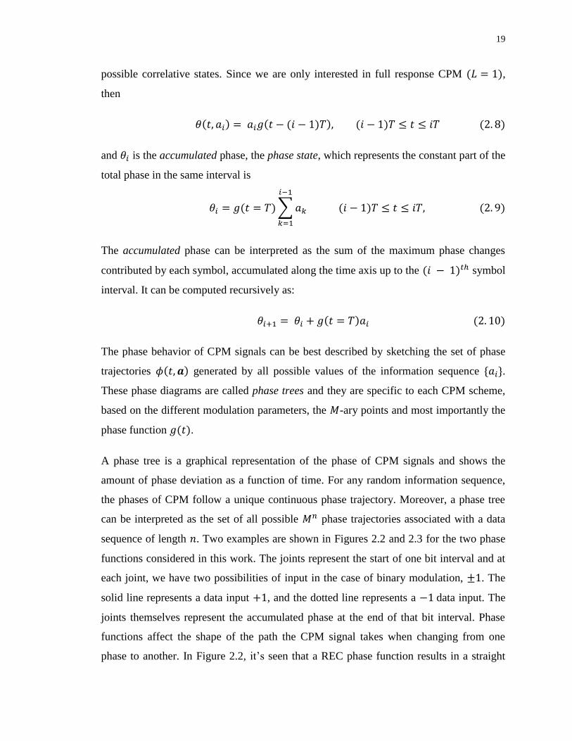
The phase behavior of CPM signals can be best described by sketching the set of phase
trajectories generated by all possible values of the information sequence .
These phase diagrams are called phase trees and they are specific to each CPM scheme,
based on the different modulation parameters, the -ary points and most importantly the
phase function .
A phase tree is a graphical representation of the phase of CPM signals and shows the
amount of phase deviation as a function of time. For any random information sequence,
the phases of CPM follow a unique continuous phase trajectory. Moreover, a phase tree
can be interpreted as the set of all possible phase trajectories associated with a data
sequence of length . Two examples are shown in Figures 2.2 and 2.3 for the two phase
functions considered in this work. The joints represent the start of one bit interval and at
each joint, we have two possibilities of input in the case of binary modulation, . The
solid line represents a data input , and the dotted line represents a data input. The
joints themselves represent the accumulated phase at the end of that bit interval. Phase
functions affect the shape of the path the CPM signal takes when changing from one
phase to another. In Figure 2.2, it’s seen that a REC phase function results in a straight
20
path between one phase and the other. In Figure 2.3, a Chirp phase function results in a
curvy path between one phase and the other. Thus, it is intuitively concluded that
different phase functions will have different performances.
Figure 2.2: Phase Tree for REC Phase Function
Figure 2.3: Phase Tree for Chirp Phase Function
0 0.5 1 1.5 2 2.5 3 3.5 4-8
-6
-4
-2
0
2
4
6
8
Normalized Time with Respect to T in Seconds
Pha
se i
n R
ad
ian
s
Phase Tree For CPM with M = 2, h = 1/2, and REC Phase Function
0 0.5 1 1.5 2 2.5 3 3.5 4 4.5 5-10
-8
-6
-4
-2
0
2
4
6
8
10
Normalized Time with Respect to T in Seconds
Pha
se i
n R
ad
ian
s
Phase Tree For M = 2, q = 0.5, w = 2.25 and Chirp Phase Function
21
Since phase is continuous, it repeats the same pattern over every bit interval. Hence,
the number of phase states increases with an increase in time and the tree becomes more
complex. Thus, in order to reduce complexity in tracking, it is required to restrict this
growth, which can be achieved by plotting the phase trajectory on modulo- scale i.e.
between the range of or . The resultant plot is known as a phase trellis. In
other words, the phase trellis is a modulo- version of the phase tree. The phase trellis is
also a key concept when it comes to applying Maximum Likelihood Sequence Detection
(MLSD) for CPM signals detection, referred to as the Viterbi Algorithm (VA).
The trellis structure is obtained by reducing the phase modulo- . The phase reduced
modulo- is termed the physical phase, and we denote it as . It is impossible to
distinguish between two phases that differ by , and thus, the physical phase is the
phase that is observable.
During the symbol interval, is given by
0 ∑
1
0 ∑
1
0 ∑
1
The , , is given by
0 ∑
1
22
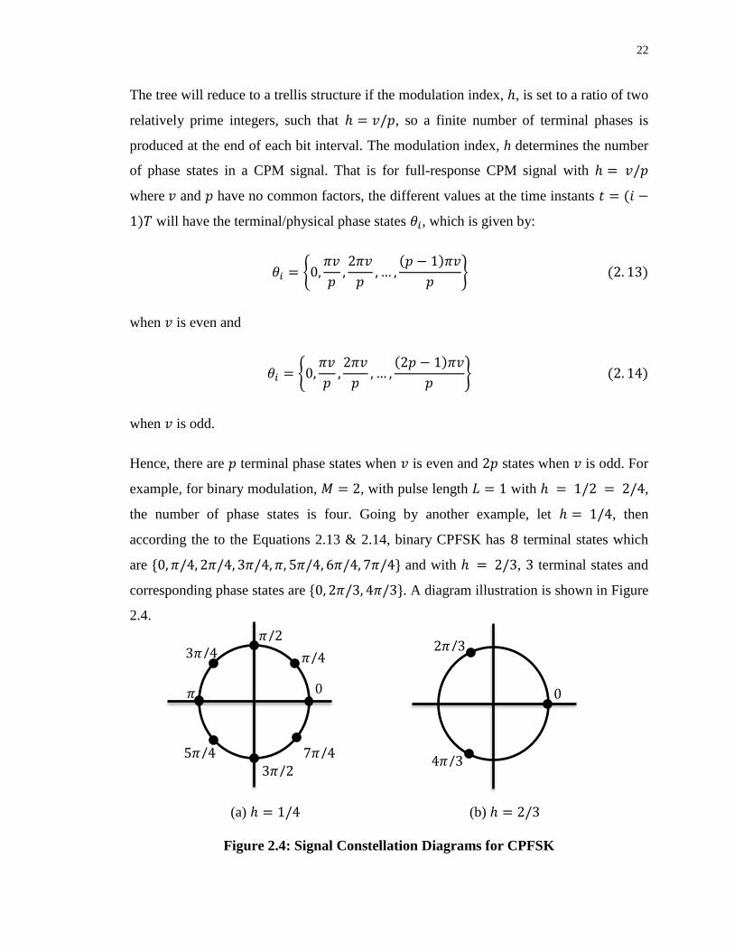
The tree will reduce to a trellis structure if the modulation index, , is set to a ratio of two
relatively prime integers, such that , so a finite number of terminal phases is
produced at the end of each bit interval. The modulation index, h determines the number
of phase states in a CPM signal. That is for full-response CPM signal with
where and have no common factors, the different values at the time instants
will have the terminal/physical phase states , which is given by:
,
-
when is even and
,
-
when is odd.
Hence, there are terminal phase states when is even and states when is odd. For
example, for binary modulation, , with pulse length with ,
the number of phase states is four. Going by another example, let , then
according the to the Equations 2.13 & 2.14, binary CPFSK has terminal states which
are and with , terminal states and
corresponding phase states are . A diagram illustration is shown in Figure
2.4.
(a) (b)
Figure 2.4: Signal Constellation Diagrams for CPFSK
I
R
0
𝜋
𝜋 𝜋
𝜋
𝜋 𝜋
𝜋
I
R
𝜋
𝜋
23
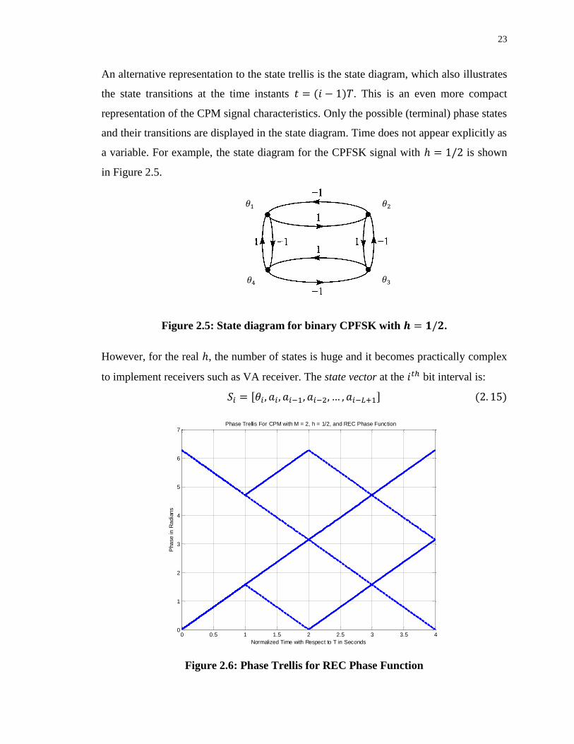
An alternative representation to the state trellis is the state diagram, which also illustrates
the state transitions at the time instants . This is an even more compact
representation of the CPM signal characteristics. Only the possible (terminal) phase states
and their transitions are displayed in the state diagram. Time does not appear explicitly as
a variable. For example, the state diagram for the CPFSK signal with is shown
in Figure 2.5.
Figure 2.5: State diagram for binary CPFSK with .
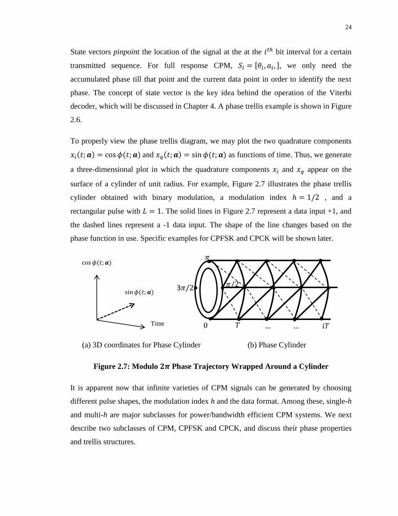
However, for the real , the number of states is huge and it becomes practically complex
to implement receivers such as VA receiver. The state vector at the bit interval is:
Figure 2.6: Phase Trellis for REC Phase Function
0 0.5 1 1.5 2 2.5 3 3.5 40
1
2
3
4
5
6
7
Normalized Time with Respect to T in Seconds
Pha
se i
n R
ad
ian
s
Phase Trellis For CPM with M = 2, h = 1/2, and REC Phase Function
𝜃
𝜃4 𝜃3
𝜃
24
State vectors pinpoint the location of the signal at the at the bit interval for a certain
transmitted sequence. For full response CPM, , we only need the
accumulated phase till that point and the current data point in order to identify the next
phase. The concept of state vector is the key idea behind the operation of the Viterbi
decoder, which will be discussed in Chapter 4. A phase trellis example is shown in Figure
2.6.
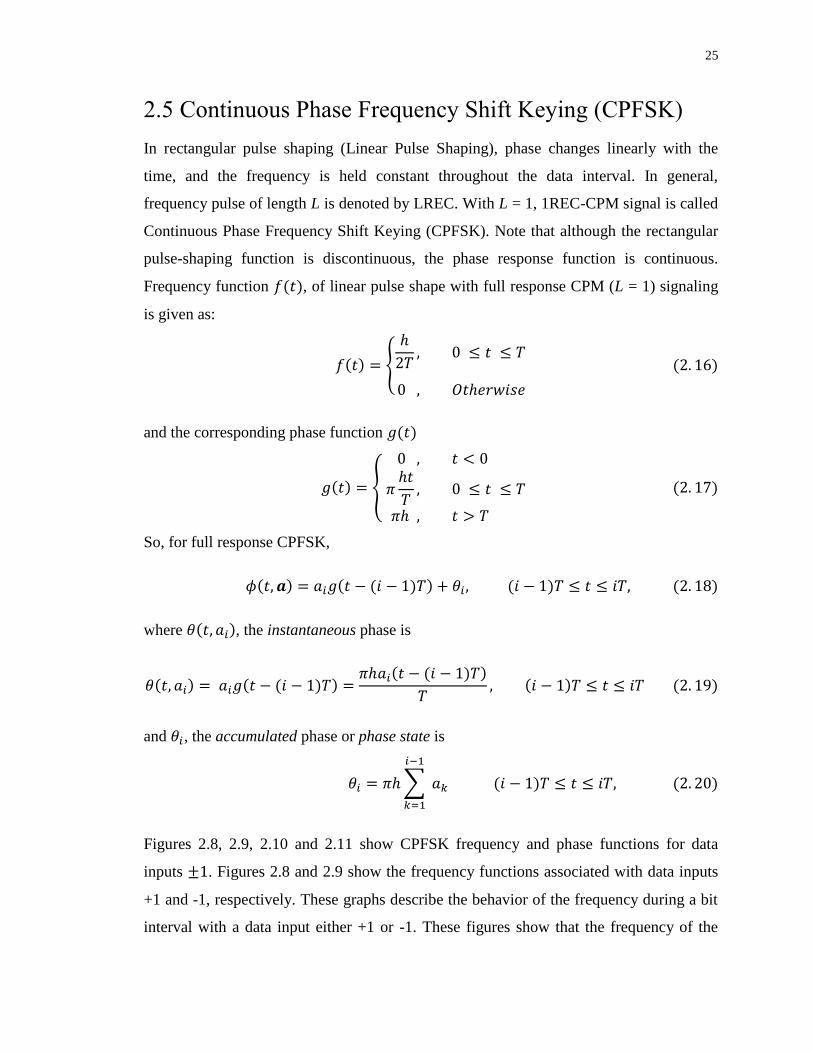
To properly view the phase trellis diagram, we may plot the two quadrature components
and as functions of time. Thus, we generate
a three-dimensional plot in which the quadrature components and appear on the
surface of a cylinder of unit radius. For example, Figure 2.7 illustrates the phase trellis
cylinder obtained with binary modulation, a modulation index , and a
rectangular pulse with . The solid lines in Figure 2.7 represent a data input +1, and
the dashed lines represent a -1 data input. The shape of the line changes based on the
phase function in use. Specific examples for CPFSK and CPCK will be shown later.
(a) 3D coordinates for Phase Cylinder (b) Phase Cylinder
Figure 2.7: Modulo Phase Trajectory Wrapped Around a Cylinder
It is apparent now that infinite varieties of CPM signals can be generated by choosing
different pulse shapes, the modulation index h and the data format. Among these, single-h
and multi-h are major subclasses for power/bandwidth efficient CPM systems. We next
describe two subclasses of CPM, CPFSK and CPCK, and discuss their phase properties
and trellis structures.
𝜋
𝜋
3𝜋
𝑇 𝑖𝑇
𝜙 𝑡 𝒂
𝜙 𝑡 𝒂
Time
25
2.5 Continuous Phase Frequency Shift Keying (CPFSK)
In rectangular pulse shaping (Linear Pulse Shaping), phase changes linearly with the
time, and the frequency is held constant throughout the data interval. In general,
frequency pulse of length L is denoted by LREC. With L = 1, 1REC-CPM signal is called
Continuous Phase Frequency Shift Keying (CPFSK). Note that although the rectangular
pulse-shaping function is discontinuous, the phase response function is continuous.
Frequency function , of linear pulse shape with full response CPM (L = 1) signaling
is given as:
2
and the corresponding phase function
{
So, for full response CPFSK,
where , the instantaneous phase is
and , the accumulated phase or phase state is
∑
Figures 2.8, 2.9, 2.10 and 2.11 show CPFSK frequency and phase functions for data
inputs . Figures 2.8 and 2.9 show the frequency functions associated with data inputs
+1 and -1, respectively. These graphs describe the behavior of the frequency during a bit
interval with a data input either +1 or -1. These figures show that the frequency of the
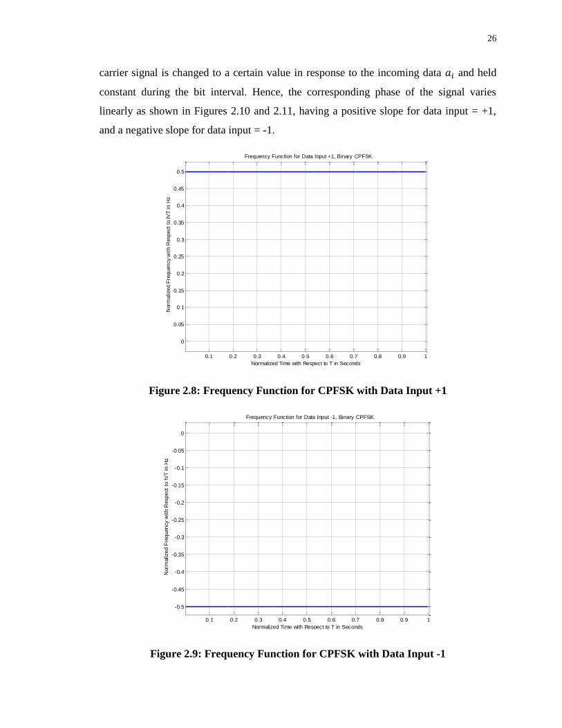
26
carrier signal is changed to a certain value in response to the incoming data and held
constant during the bit interval. Hence, the corresponding phase of the signal varies
linearly as shown in Figures 2.10 and 2.11, having a positive slope for data input = +1,
and a negative slope for data input = -1.
Figure 2.8: Frequency Function for CPFSK with Data Input +1
Figure 2.9: Frequency Function for CPFSK with Data Input -1
0.1 0.2 0.3 0.4 0.5 0.6 0.7 0.8 0.9 1
0
0.05
0.1
0.15
0.2
0.25
0.3
0.35
0.4
0.45
0.5
Normalized Time with Respect to T in Seconds
Norm
alize
d F
req
uen
cy
wit
h R
esp
ect
to
h/T
in
Hz
Frequency Function for Data Input +1, Binary CPFSK
0.1 0.2 0.3 0.4 0.5 0.6 0.7 0.8 0.9 1
-0.5
-0.45
-0.4
-0.35
-0.3
-0.25
-0.2
-0.15
-0.1
-0.05
0
Normalized Time with Respect to T in Seconds
Norm
alize
d F
req
uen
cy
wit
h R
esp
ect
to
h/T
in
Hz
Frequency Function for Data Input -1, Binary CPFSK
27
Figure 2.10: Phase Function for CPFSK with Data Input +1
Figure 2.11: Phase Function for CPFSK with Data Input -1
0 0.1 0.2 0.3 0.4 0.5 0.6 0.7 0.8 0.9 10
0.1
0.2
0.3
0.4
0.5
0.6
0.7
0.8
0.9
1
Normalized Time with Respect to T in Seconds
Norm
alize
d P
ha
se
wit
h R
esp
ect
to
h in
Rad
ians
Phase Function for Data Input +1, Binary CPFSK
0 0.1 0.2 0.3 0.4 0.5 0.6 0.7 0.8 0.9 1-1
-0.9
-0.8
-0.7
-0.6
-0.5
-0.4
-0.3
-0.2
-0.1
0
Normalized Time with Respect to T in Seconds
Norm
alize
d P
ha
se
wit
h R
esp
ect
to
h in
Rad
ians
Phase Function for Data Input -1, Binary CPFSK
28
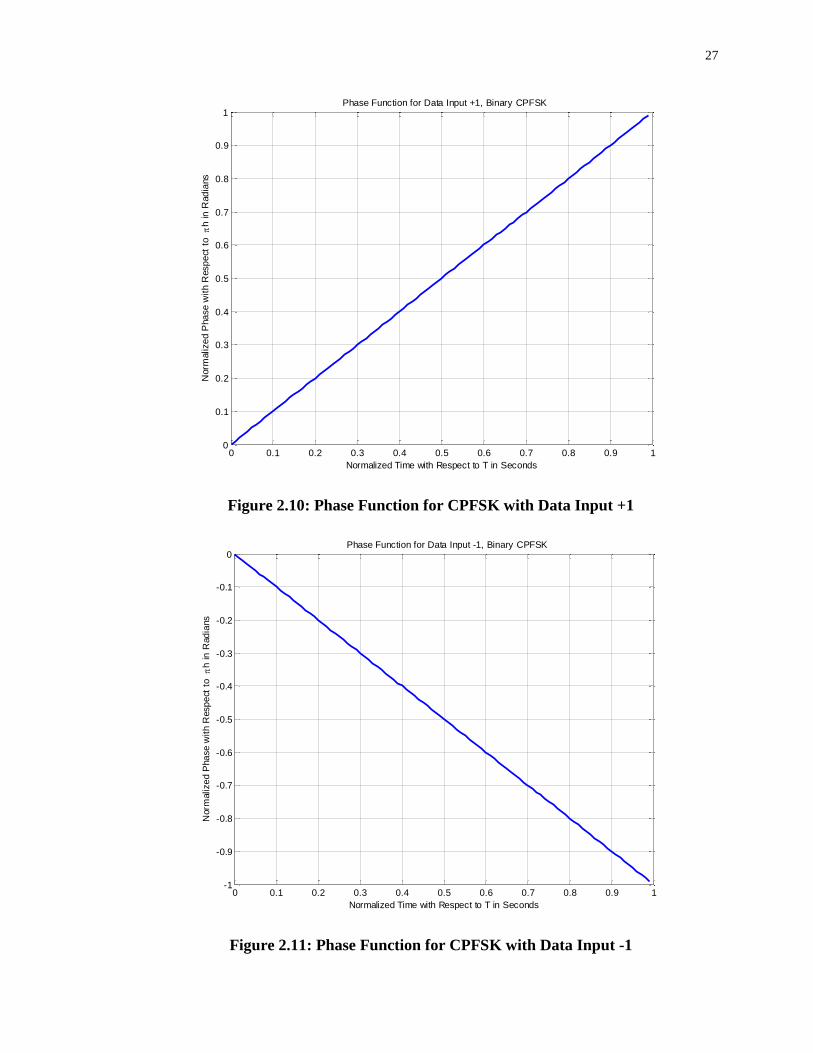
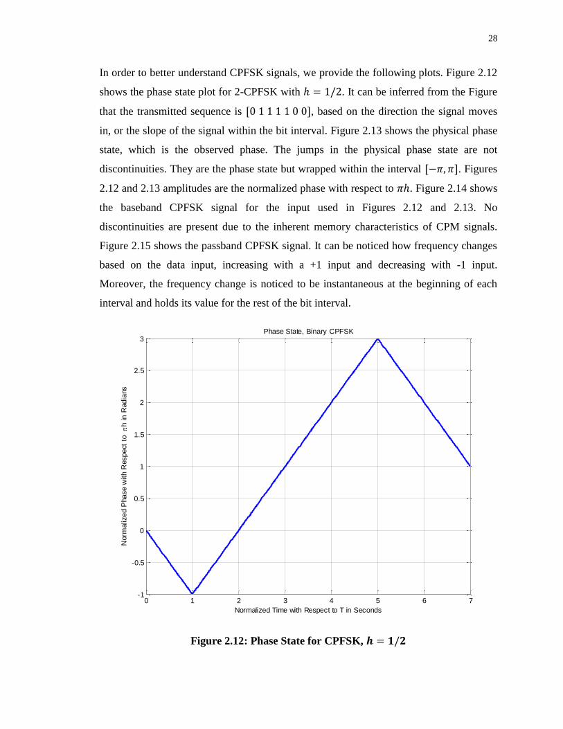
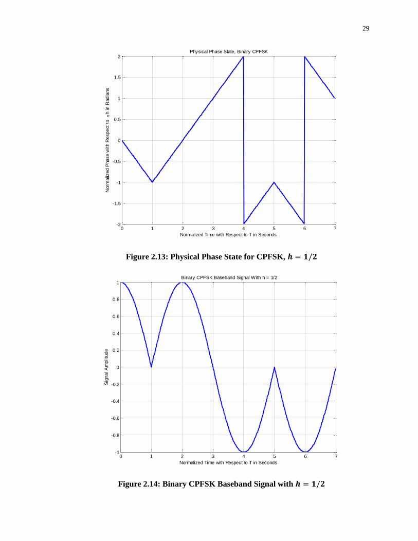
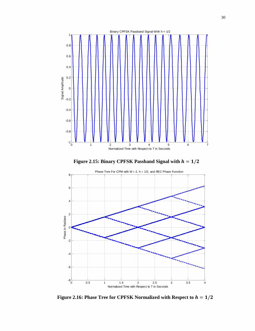
In order to better understand CPFSK signals, we provide the following plots. Figure 2.12
shows the phase state plot for 2-CPFSK with . It can be inferred from the Figure
that the transmitted sequence is , based on the direction the signal moves
in, or the slope of the signal within the bit interval. Figure 2.13 shows the physical phase
state, which is the observed phase. The jumps in the physical phase state are not
discontinuities. They are the phase state but wrapped within the interval . Figures
2.12 and 2.13 amplitudes are the normalized phase with respect to . Figure 2.14 shows
the baseband CPFSK signal for the input used in Figures 2.12 and 2.13. No
discontinuities are present due to the inherent memory characteristics of CPM signals.
Figure 2.15 shows the passband CPFSK signal. It can be noticed how frequency changes
based on the data input, increasing with a +1 input and decreasing with -1 input.
Moreover, the frequency change is noticed to be instantaneous at the beginning of each
interval and holds its value for the rest of the bit interval.
Figure 2.12: Phase State for CPFSK,
0 1 2 3 4 5 6 7-1
-0.5
0
0.5
1
1.5
2
2.5
3
Normalized Time with Respect to T in Seconds
Norm
alize
d P
ha
se
wit
h R
esp
ect
to
h in
Rad
ians
Phase State, Binary CPFSK
29
Figure 2.13: Physical Phase State for CPFSK,
Figure 2.14: Binary CPFSK Baseband Signal with
0 1 2 3 4 5 6 7-2
-1.5
-1
-0.5
0
0.5
1
1.5
2
Normalized Time with Respect to T in Seconds
Norm
alize
d P
ha
se
wit
h R
esp
ect
to
h in
Rad
ians
Physical Phase State, Binary CPFSK
0 1 2 3 4 5 6 7-1
-0.8
-0.6
-0.4
-0.2
0
0.2
0.4
0.6
0.8
1
Normalized Time with Respect to T in Seconds
Sig
na
l A
mp
litu
de
Binary CPFSK Baseband Signal With h = 1/2
30
Figure 2.15: Binary CPFSK Passband Signal with
Figure 2.16: Phase Tree for CPFSK Normalized with Respect to
0 1 2 3 4 5 6 7-1
-0.8
-0.6
-0.4
-0.2
0
0.2
0.4
0.6
0.8
1
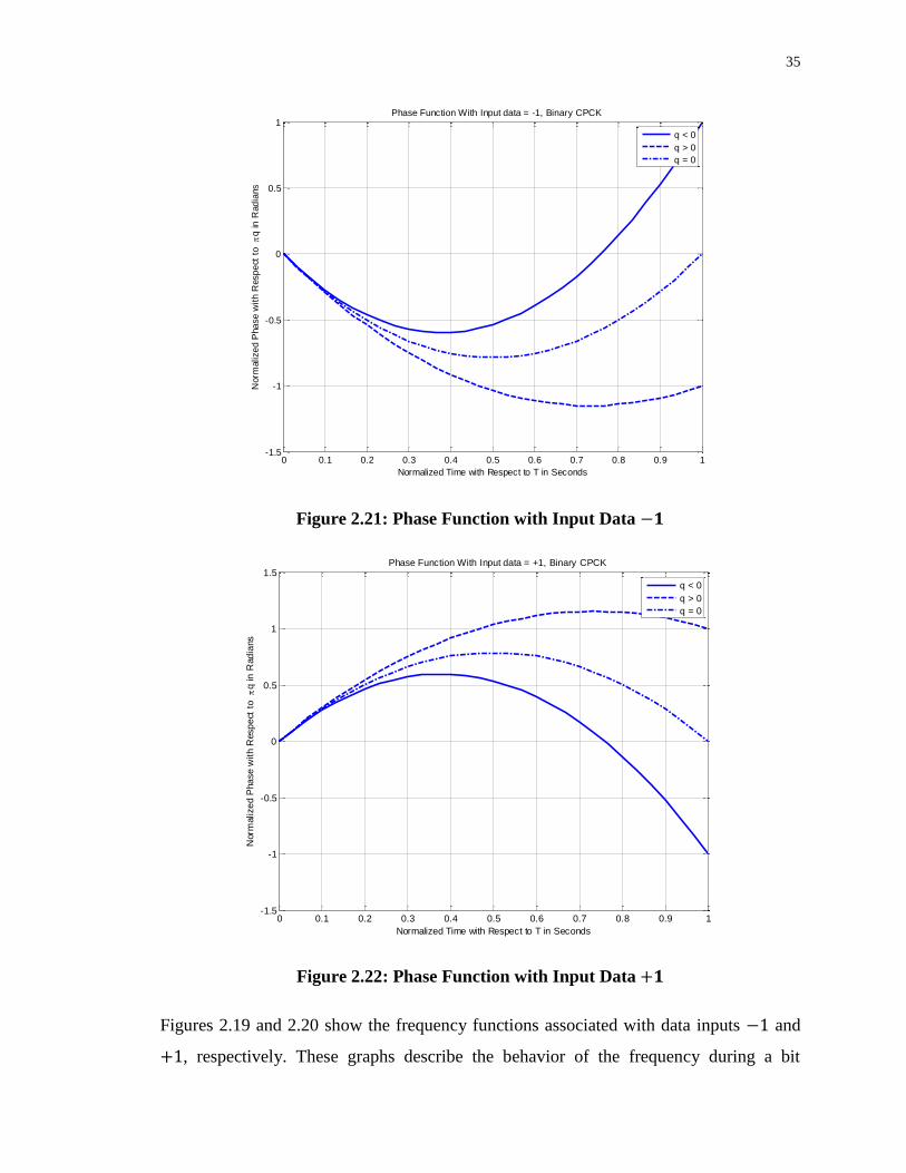
Normalized Time with Respect to T in Seconds
Sig
na
l A
mp
litu
de
Binary CPFSK Passband Signal With h = 1/2
0 0.5 1 1.5 2 2.5 3 3.5 4-8
-6
-4
-2
0
2
4
6
8
Normalized Time with Respect to T in Seconds
Pha
se i
n R
ad
ian
s
Phase Tree For CPM with M = 2, h = 1/2, and REC Phase Function
31
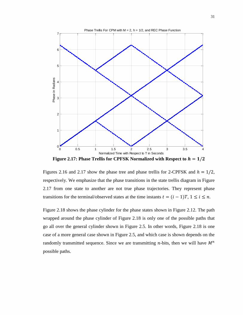
Figure 2.17: Phase Trellis for CPFSK Normalized with Respect to
Figures 2.16 and 2.17 show the phase tree and phase trellis for 2-CPFSK and ,
respectively. We emphasize that the phase transitions in the state trellis diagram in Figure
2.17 from one state to another are not true phase trajectories. They represent phase
transitions for the terminal/observed states at the time instants , .
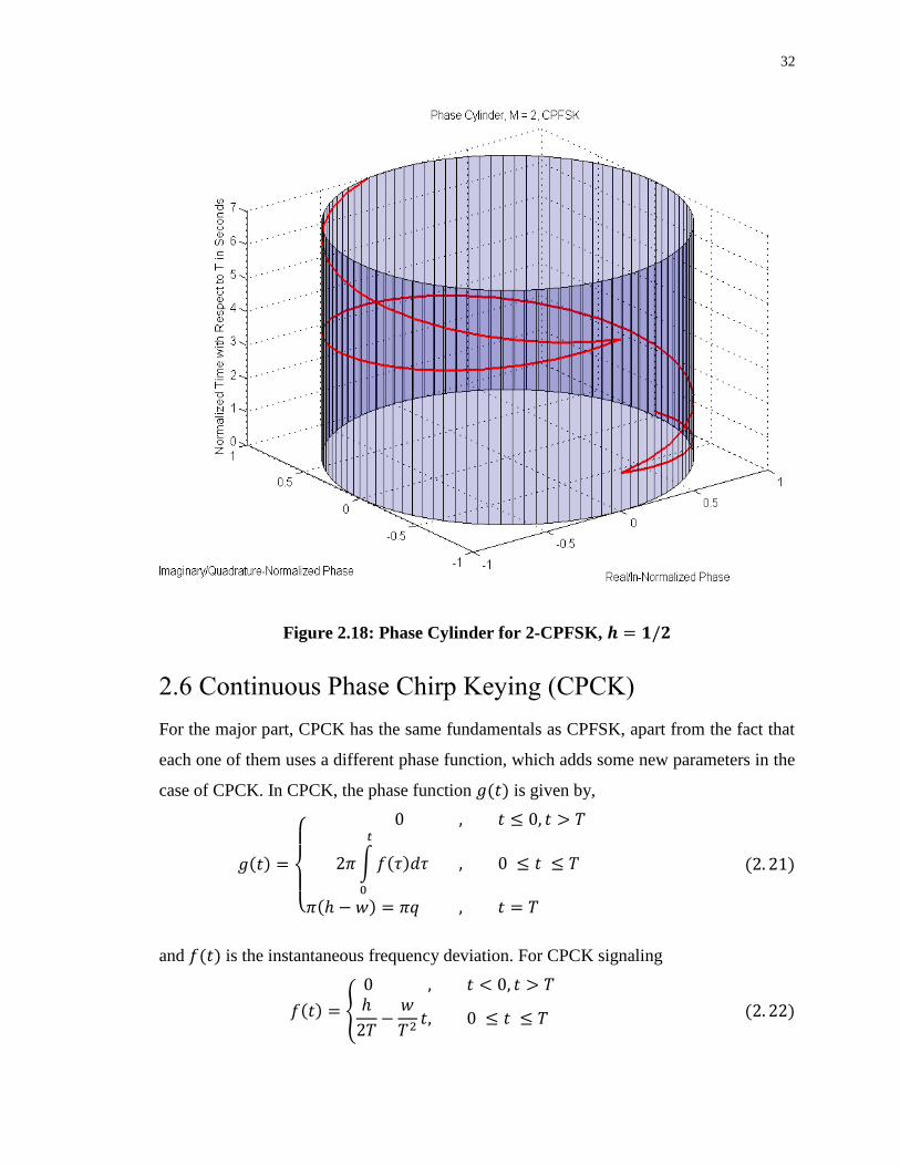
Figure 2.18 shows the phase cylinder for the phase states shown in Figure 2.12. The path
wrapped around the phase cylinder of Figure 2.18 is only one of the possible paths that
go all over the general cylinder shown in Figure 2.5. In other words, Figure 2.18 is one
case of a more general case shown in Figure 2.5, and which case is shown depends on the
randomly transmitted sequence. Since we are transmitting -bits, then we will have
possible paths.
0 0.5 1 1.5 2 2.5 3 3.5 40
1
2
3
4
5
6
7
Normalized Time with Respect to T in Seconds
Pha
se i
n R
ad
ian
s
Phase Trellis For CPM with M = 2, h = 1/2, and REC Phase Function
32
Figure 2.18: Phase Cylinder for 2-CPFSK,
2.6 Continuous Phase Chirp Keying (CPCK)
For the major part, CPCK has the same fundamentals as CPFSK, apart from the fact that
each one of them uses a different phase function, which adds some new parameters in the
case of CPCK. In CPCK, the phase function is given by,
{
∫
and is the instantaneous frequency deviation. For CPCK signaling
2
33
And the CPCK phase function in Equation 2.21 becomes
{
,
(
)
-
where and are dimensionless parameters, represents the initial peak-to-peak
frequency deviation divided by the bit rate , and stands for the frequency sweep
width divided by . We usually express in terms of a third dimensionless parameter,
, where . and are independent signal parameters. Note that gives
the continuous phase frequency shift keying (CPFSK) waveform where and
. Here, is also called the modulation index. Following from Equation 2.21,
2.22 and 2.23, for full response CPCK, the function describing the phase is a little bit
different than the one for CPFSK and is described as follows:
∑
∑
where , the instantaneous phase is
,
(
)
-
and , the accumulated phase or phase state is
∑
∑
For consistency, we show next the same type of plots for CPCK as that for CPFSK.
34
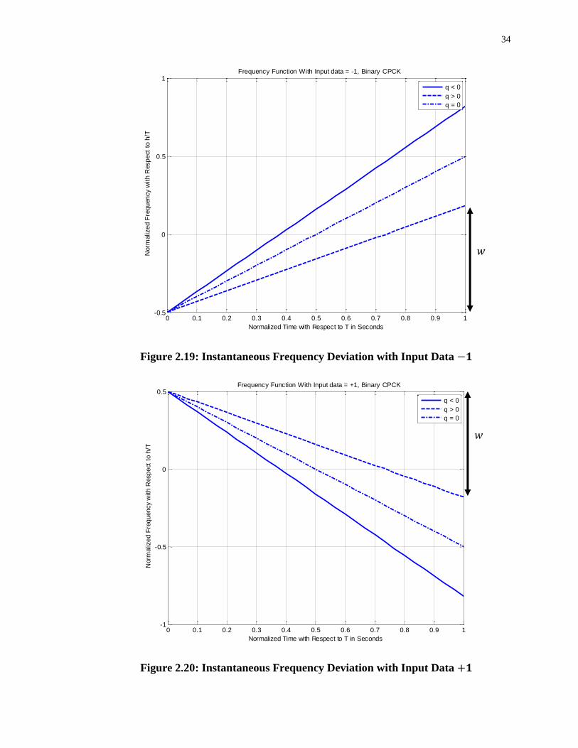
Figure 2.19: Instantaneous Frequency Deviation with Input Data
Figure 2.20: Instantaneous Frequency Deviation with Input Data
0 0.1 0.2 0.3 0.4 0.5 0.6 0.7 0.8 0.9 1-0.5
0
0.5
1
Normalized Time with Respect to T in Seconds
Norm
alize
d F
req
uen
cy
wit
h R
esp
ect
to
h/T
Frequency Function With Input data = -1, Binary CPCK
q < 0
q > 0
q = 0
0 0.1 0.2 0.3 0.4 0.5 0.6 0.7 0.8 0.9 1-1
-0.5
0
0.5
Normalized Time with Respect to T in Seconds
Norm
alize
d F
req
uen
cy
wit
h R
esp
ect
to
h/T
Frequency Function With Input data = +1, Binary CPCK
q < 0
q > 0
q = 0
𝑤
𝑤
35
Figure 2.21: Phase Function with Input Data
Figure 2.22: Phase Function with Input Data
Figures 2.19 and 2.20 show the frequency functions associated with data inputs and
, respectively. These graphs describe the behavior of the frequency during a bit
0 0.1 0.2 0.3 0.4 0.5 0.6 0.7 0.8 0.9 1-1.5
-1
-0.5
0
0.5
1
Normalized Time with Respect to T in Seconds
Norm
alize
d P
ha
se
wit
h R
esp
ect
to
q in
Rad
ians
Phase Function With Input data = -1, Binary CPCK
q < 0
q > 0
q = 0
0 0.1 0.2 0.3 0.4 0.5 0.6 0.7 0.8 0.9 1-1.5
-1
-0.5
0
0.5
1
1.5
Normalized Time with Respect to T in Seconds
Norm
alize
d P
ha
se
wit
h R
esp
ect
to
q in
Rad
ians
Phase Function With Input data = +1, Binary CPCK
q < 0
q > 0
q = 0
36
interval with a data input either or . These Figures show that the frequency of the
carrier signal varies linearly as a function of time, in response to the incoming data ,
and hence, the corresponding phase of the signal varies in a nonlinear manner as shown
in Figures 2.21 and 2.22.The Figures also show the effect of the parameter , and it can
be inferred from the graph that the value of , which is in terms of the modulation index
and the frequency sweep width , dictates the rate at which the frequency changes
during a bit interval. Moreover, the different values of associated with the different
values of can be found through
Figures 2.19 and 2.20 indicate the way to find graphically using the arrows on the side
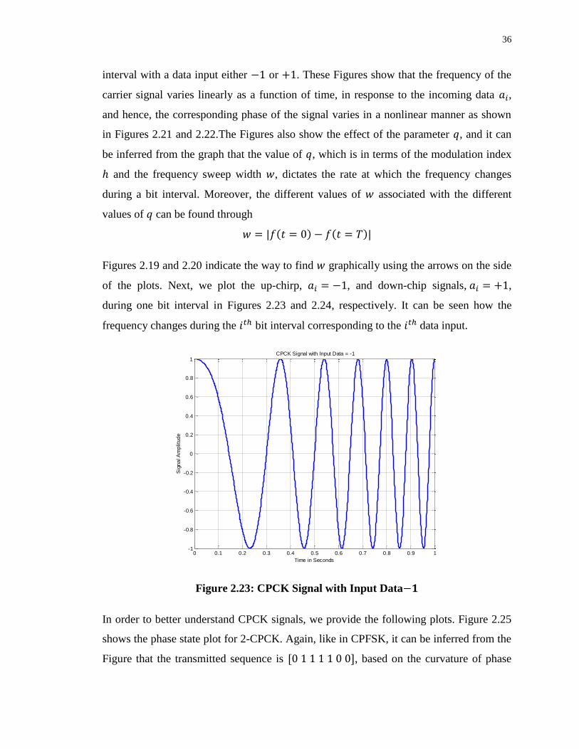
of the plots. Next, we plot the up-chirp, , and down-chip signals, ,
during one bit interval in Figures 2.23 and 2.24, respectively. It can be seen how the
frequency changes during the bit interval corresponding to the data input.
Figure 2.23: CPCK Signal with Input Data
In order to better understand CPCK signals, we provide the following plots. Figure 2.25
shows the phase state plot for 2-CPCK. Again, like in CPFSK, it can be inferred from the
Figure that the transmitted sequence is , based on the curvature of phase
0 0.1 0.2 0.3 0.4 0.5 0.6 0.7 0.8 0.9 1-1
-0.8
-0.6
-0.4
-0.2
0
0.2
0.4
0.6
0.8
1
Time in Seconds
Sig
na
l A
mp
litu
de
CPCK Signal with Input Data = -1
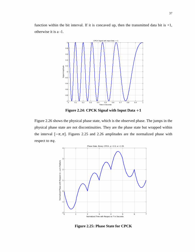
37
function within the bit interval. If it is concaved up, then the transmitted data bit is +1,
otherwise it is a -1.
Figure 2.24: CPCK Signal with Input Data
Figure 2.26 shows the physical phase state, which is the observed phase. The jumps in the
physical phase state are not discontinuities. They are the phase state but wrapped within
the interval . Figures 2.25 and 2.26 amplitudes are the normalized phase with
respect to .
Figure 2.25: Phase State for CPCK
0 0.1 0.2 0.3 0.4 0.5 0.6 0.7 0.8 0.9 1-1
-0.8
-0.6
-0.4
-0.2
0
0.2
0.4
0.6
0.8
1
Time in Seconds
Sig
na
l A
mp
litu
de
CPCK Signal with Input Data = +1
0 1 2 3 4 5 6 7-2
-1
0
1
2
3
4
Normalized Time with Respect to T in Seconds
Norm
alize
d P
ha
se
wit
h R
esp
ect
to
q in
Rad
ians
Phase State, Binary CPCK, q = 0.5, w = 2.25
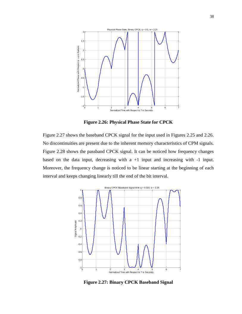
38
Figure 2.26: Physical Phase State for CPCK
Figure 2.27 shows the baseband CPCK signal for the input used in Figures 2.25 and 2.26.
No discontinuities are present due to the inherent memory characteristics of CPM signals.
Figure 2.28 shows the passband CPCK signal. It can be noticed how frequency changes
based on the data input, decreasing with a +1 input and increasing with -1 input.
Moreover, the frequency change is noticed to be linear starting at the beginning of each
interval and keeps changing linearly till the end of the bit interval.
Figure 2.27: Binary CPCK Baseband Signal
0 1 2 3 4 5 6 7-2
-1.5
-1
-0.5
0
0.5
1
1.5
2
Normalized Time with Respect to T in Seconds
Norm
alize
d P
ha
se
wit
h R
esp
ect
to
q in
Rad
ians
Physical Phase State, Binary CPCK, q = 0.5, w = 2.25
0 1 2 3 4 5 6 7-1
-0.8
-0.6
-0.4
-0.2
0
0.2
0.4
0.6
0.8
1
Normalized Time with Respect to T in Seconds
Sig
na
l A
mp
litu
de
Binary CPCK Baseband Signal With q = 0.315, w = 2.25
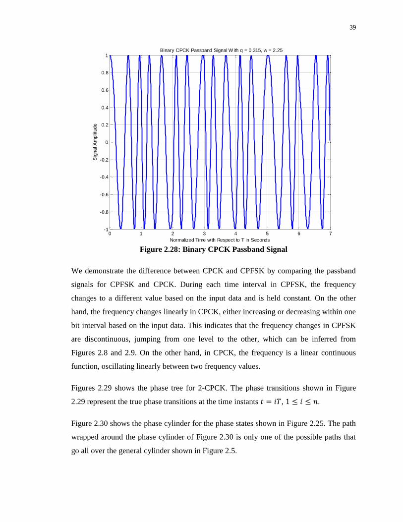
39
Figure 2.28: Binary CPCK Passband Signal
We demonstrate the difference between CPCK and CPFSK by comparing the passband
signals for CPFSK and CPCK. During each time interval in CPFSK, the frequency
changes to a different value based on the input data and is held constant. On the other
hand, the frequency changes linearly in CPCK, either increasing or decreasing within one
bit interval based on the input data. This indicates that the frequency changes in CPFSK
are discontinuous, jumping from one level to the other, which can be inferred from
Figures 2.8 and 2.9. On the other hand, in CPCK, the frequency is a linear continuous
function, oscillating linearly between two frequency values.
Figures 2.29 shows the phase tree for 2-CPCK. The phase transitions shown in Figure
2.29 represent the true phase transitions at the time instants , .
Figure 2.30 shows the phase cylinder for the phase states shown in Figure 2.25. The path
wrapped around the phase cylinder of Figure 2.30 is only one of the possible paths that
go all over the general cylinder shown in Figure 2.5.
0 1 2 3 4 5 6 7-1
-0.8
-0.6
-0.4
-0.2
0
0.2
0.4
0.6
0.8
1
Normalized Time with Respect to T in Seconds
Sig
na
l A
mp
litu
de
Binary CPCK Passband Signal With q = 0.315, w = 2.25
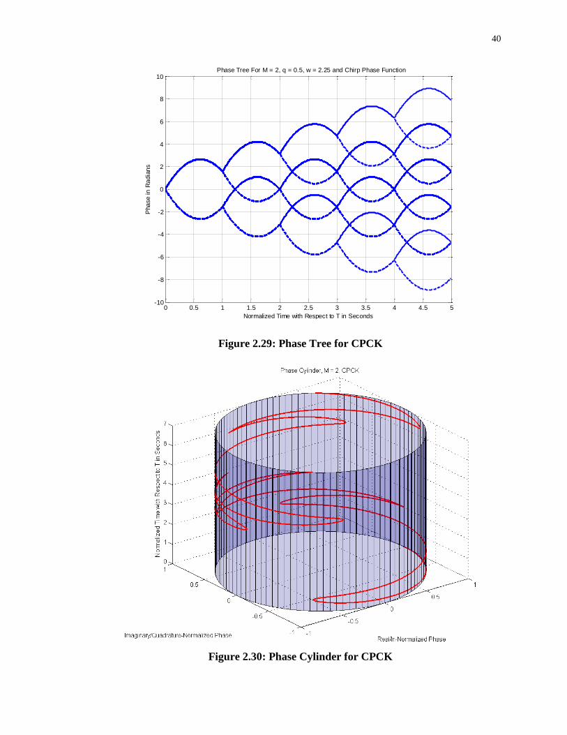
40
Figure 2.29: Phase Tree for CPCK
Figure 2.30: Phase Cylinder for CPCK
0 0.5 1 1.5 2 2.5 3 3.5 4 4.5 5-10
-8
-6
-4
-2
0
2
4
6
8
10
Normalized Time with Respect to T in Seconds
Pha
se i
n R
ad
ian
s
Phase Tree For M = 2, q = 0.5, w = 2.25 and Chirp Phase Function
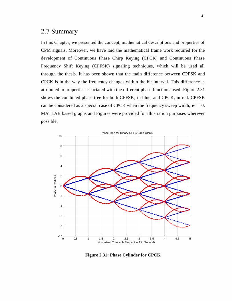
41
2.7 Summary
In this Chapter, we presented the concept, mathematical descriptions and properties of
CPM signals. Moreover, we have laid the mathematical frame work required for the
development of Continuous Phase Chirp Keying (CPCK) and Continuous Phase
Frequency Shift Keying (CPFSK) signaling techniques, which will be used all
through the thesis. It has been shown that the main difference between CPFSK and
CPCK is in the way the frequency changes within the bit interval. This difference is
attributed to properties associated with the different phase functions used. Figure 2.31
shows the combined phase tree for both CPFSK, in blue, and CPCK, in red. CPFSK
can be considered as a special case of CPCK when the frequency sweep width, .
MATLAB based graphs and Figures were provided for illustration purposes wherever
possible.
Figure 2.31: Phase Cylinder for CPCK
0 0.5 1 1.5 2 2.5 3 3.5 4 4.5 5-10
-8
-6
-4
-2
0
2
4
6
8
10
Normalized Time with Respect to T in Seconds
Pha
se i
n R
ad
ian
s
Phase Tree for Binary CPFSK and CPCK
42
Chapter 3
Optimum and Sub-optimum Receivers for
CPFSK and CPCK
When the signal has no memory, the general symbol-by-symbol detector, such as the
ones employed for PSK, FSK, QPSK…etc., is optimum in the sense that it minimizes the
probability of a symbol error. In contrast, for a transmitted signal that has memory, such
as in CPM schemes, the optimum detector bases its decisions on observation of a
sequence of received signals over successive signal intervals. There are mainly two types
of receivers, based on the way the detection technique is applied, however; both of them
are based on minimizing the probability of error using maximum-likelihood theory.
In this Chapter, we derive the structure of the optimum receiver for detection of CPM
buried in AWGN.
The primary focus in this Chapter is to understand the relationship among modulation
parameters, Signal-to-Noise Ratio ( ) and number of observed symbols. The
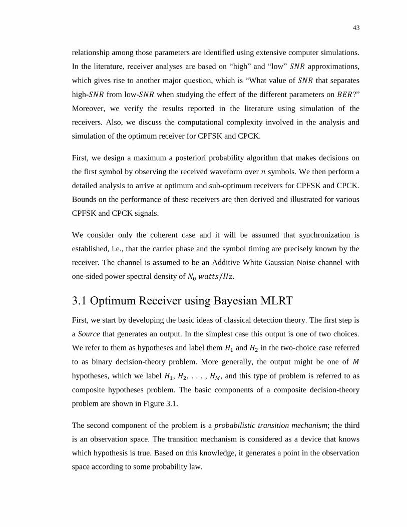
43
relationship among those parameters are identified using extensive computer simulations.
In the literature, receiver analyses are based on “high” and “low” approximations,
which gives rise to another major question, which is “What value of that separates
high- from low- when studying the effect of the different parameters on ?”
Moreover, we verify the results reported in the literature using simulation of the
receivers. Also, we discuss the computational complexity involved in the analysis and
simulation of the optimum receiver for CPFSK and CPCK.
First, we design a maximum a posteriori probability algorithm that makes decisions on
the first symbol by observing the received waveform over symbols. We then perform a
detailed analysis to arrive at optimum and sub-optimum receivers for CPFSK and CPCK.
Bounds on the performance of these receivers are then derived and illustrated for various
CPFSK and CPCK signals.
We consider only the coherent case and it will be assumed that synchronization is
established, i.e., that the carrier phase and the symbol timing are precisely known by the
receiver. The channel is assumed to be an Additive White Gaussian Noise channel with
one-sided power spectral density of .
3.1 Optimum Receiver using Bayesian MLRT
First, we start by developing the basic ideas of classical detection theory. The first step is
a Source that generates an output. In the simplest case this output is one of two choices.
We refer to them as hypotheses and label them and in the two-choice case referred
to as binary decision-theory problem. More generally, the output might be one of
hypotheses, which we label , , . . . , , and this type of problem is referred to as
composite hypotheses problem. The basic components of a composite decision-theory
problem are shown in Figure 3.1.
The second component of the problem is a probabilistic transition mechanism; the third
is an observation space. The transition mechanism is considered as a device that knows
which hypothesis is true. Based on this knowledge, it generates a point in the observation
space according to some probability law.
44
In general, we confine our discussion to problems in which the observation space is
finite-dimensional. In other words, the observations consist of a set of N numbers and can
be represented as a point in an N-dimensional space. This class of problems is referred to
as the classical decision problem.
Figure 3.1 Components of a Decision Theory Problem
The fourth component of the detection problem is a decision rule. After observing the
outcome in the observation space a guess is made on which hypothesis was true, and to
accomplish this a decision rule that assigns each point to one of the hypotheses is
developed.
As mentioned before, CPM signals have better bandwidth and energy performance due to
the phase continuity constraint of CPM. Thus, obtaining this performance requires a
multiple interval observation rather than the symbol-by-symbol decisions in memory-less
modulation schemes.
Source
Probabilistic
Transition
Mechanism
Observation
Space
Decision
𝐻
𝐻𝑀
𝐻
Decision Rule
45
The receivers in this section are quite general and apply to CPM schemes with any pulse
shape and any modulation index, but we will specify them at the end of each section for
CPFSK and CPCK schemes.
This receiver makes a decision about one symbol only, based on observation of a
sequence of consecutive symbols. Once the decision is made, the receiver in principle
starts from scratch again, processing the following symbol by sliding the observation
interval. The received binary CPM signal during the symbol is modeled as
where we use the notations from Chapter 2 for full response CPM
√
where
∑
is the initial phase offset which is assumed to be zero for coherent detection without
any loss of generality. In determining the optimum receiver structure for detecting
symbol , we shall use a shorthand notation developed in [10] for the received signal, so
that Equation 3.1 becomes
where is the first symbol, and is the -tuple where is the
observation interval. This is a classic composite-hypotheses probability theory problem in
which the receiver chooses one hypothesis to be true. We have hypotheses, where
for binary modulation case, under the source output of Figure 3.1, and they are all
corrupted by noise.
46
The hypotheses are
.
.
.
.
where . Since we are only interested on making a decision on the first bit
transmitted , we assume full knowledge about which , has been
transmitted. This reduces the previously stated composite hypotheses to a binary one of
the following form
( )
( )
To establish the likelihood ratio test, we need the Probability Distribution Functions
(PDF) for the previous hypotheses.
( | )
( | )
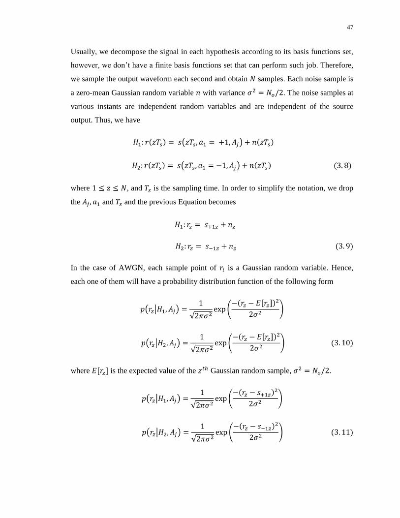
47
Usually, we decompose the signal in each hypothesis according to its basis functions set,
however, we don’t have a finite basis functions set that can perform such job. Therefore,
we sample the output waveform each second and obtain samples. Each noise sample is
a zero-mean Gaussian random variable with variance . The noise samples at
various instants are independent random variables and are independent of the source
output. Thus, we have
( )
( )
where , and is the sampling time. In order to simplify the notation, we drop
the and and the previous Equation becomes
In the case of AWGN, each sample point of is a Gaussian random variable. Hence,
each one of them will have a probability distribution function of the following form
( | )
√ (
)
( | )
√ (
)
where is the expected value of the Gaussian random sample, .
( | )
√ (
)
( | )
√ (
)
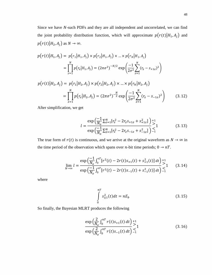
48
Since we have -such PDFs and they are all independent and uncorrelated, we can find
the joint probability distribution function, which will approximate ( | ) and
( | ) as → .
( | ) ( | ) ( | ) ( | )
∏ ( | )
(
∑
)
( | ) ( | ) ( | ) ( | )
∏ ( | )
(
∑
)
After simplification, we get
(
∑
)
(
∑
)
The true form of is continuous, and we arrive at the original waveform as → in
the time period of the observation which spans over -bit time periods; → .
→
(
∫
)
(
∫
)
where
∫
So finally, the Bayesian MLRT produces the following
(
∫
)
(
∫
)
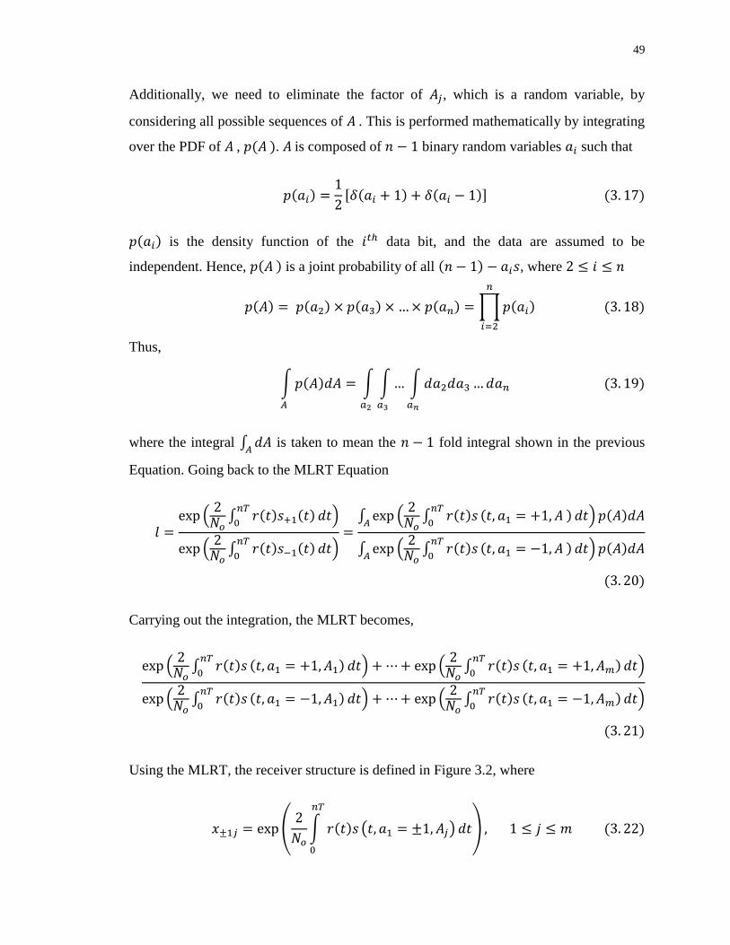
49
Additionally, we need to eliminate the factor of , which is a random variable, by
considering all possible sequences of . This is performed mathematically by integrating
over the PDF of , . is composed of binary random variables such that
is the density function of the data bit, and the data are assumed to be
independent. Hence, is a joint probability of all , where
3 ∏
Thus,
∫
∫ ∫ ∫ 3
where the integral ∫
is taken to mean the fold integral shown in the previous
Equation. Going back to the MLRT Equation
(
∫
)
(
∫
)
∫ (
∫
)
∫ (
∫
)
Carrying out the integration, the MLRT becomes,
(
∫
) (
∫
)
(
∫
) (
∫
)
Using the MLRT, the receiver structure is defined in Figure 3.2, where
.
∫ ( )
/
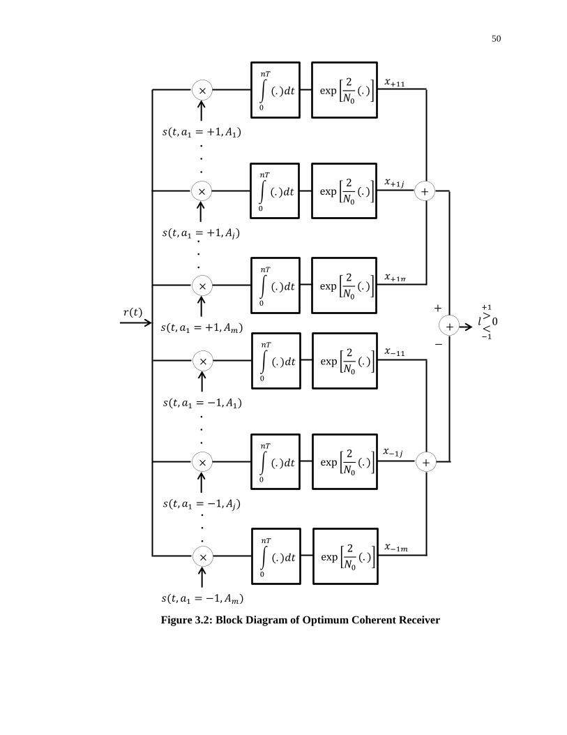
50
Figure 3.2: Block Diagram of Optimum Coherent Receiver
∫ 𝑑𝑡
𝑛𝑇
𝑁
𝑠 𝑡 𝑎 𝐴
𝑥
𝑟 𝑡 𝑙
∫ 𝑑𝑡
𝑛𝑇
𝑁
𝑠 𝑡 𝑎 𝐴𝑗
𝑥 𝑗
∫ 𝑑𝑡
𝑛𝑇
𝑁
𝑠 𝑡 𝑎 𝐴𝑚
𝑥 𝑚
∫ 𝑑𝑡
𝑛𝑇
𝑁
𝑠 𝑡 𝑎 𝐴
𝑥
∫ 𝑑𝑡
𝑛𝑇
𝑁
𝑠 𝑡 𝑎 𝐴𝑗
𝑥 𝑗
∫ 𝑑𝑡
𝑛𝑇
𝑁
𝑠 𝑡 𝑎 𝐴𝑚
𝑥 𝑚
.
.
.
.
.
.
.
.
.
.
.
.
51
The receiver correlates the received waveform with each of the possible transmitted
signals beginning with data , then forms the sum of the
where is the
correlation of the received waveform of the . A similar operation of correlating and
summing for the possible signals with a data is performed and the decision is based
on the polarity of the difference of the two sums.
is a log-normal random variable. When taking [ ], we get the Gaussian
random variable back. The performance of the optimum coherent receiver shown in
Figure 3.2 with the log-normal variable is very complex to be mathematically analyzed.
For Gaussian random variables, finding the joint probability distribution in order to
determine the can be mathematically computed. However, in the CPM optimum
receiver case, that joint probability distribution function passes through the exponential
factor, which is considered as a transformation function, transforming the random
variable and rendering it very complex to be analyzed and computationally exhaustive to
find the joint probability distribution. Even simulating the optimum performance in
MATLAB using the receiver structure in Figure 3.2 is not applicable. This is due to the
problem that the generated Gaussian random variable never have the exact theoretical
values of the mean and variance desired, and can have a difference from the theoretical
value of up to the . That is fine if the decision was to be based before the
exponential stage. However, once it passes through the exponential block and transforms
into a log-normal variable, a small difference of grows exponentially to diverge the
mean of the random variable from the desired theoretical value by a big margin, and it
gets even worse for the variance.
Since the performance of the CPM optimum coherent receiver is very complex to be
computed analytically, we resort to bounding the optimum performance by the
performance of two sub-optimum receivers. One receiver performance is tight at high-
and the other is tight at low- . Both receivers are used together to give a very
reasonable and tight bound at all values.
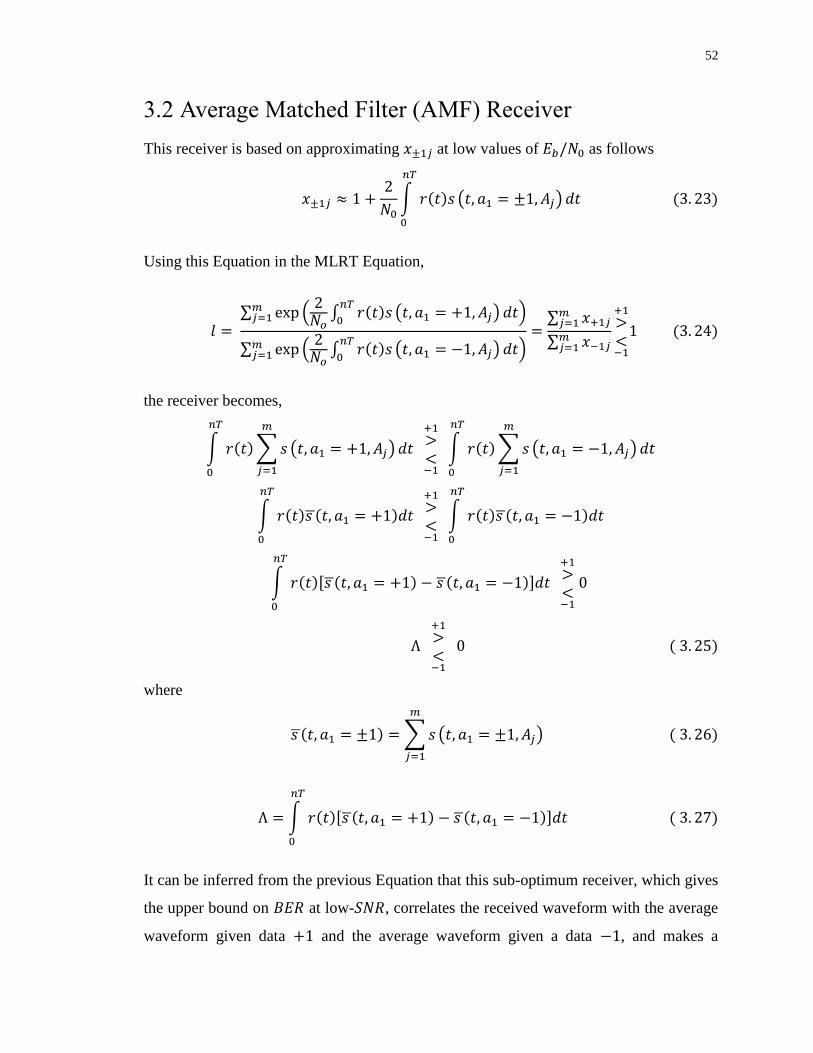
52
3.2 Average Matched Filter (AMF) Receiver
This receiver is based on approximating at low values of as follows
∫ ( )
Using this Equation in the MLRT Equation,
∑ (
∫ ( )
)
∑ (
∫ ( )
)
∑
∑
the receiver becomes,
∫ ∑ ( )
∫ ∑ ( )
∫
∫
∫
where
∑ ( )
∫
It can be inferred from the previous Equation that this sub-optimum receiver, which gives
the upper bound on at low- , correlates the received waveform with the average
waveform given data and the average waveform given a data , and makes a
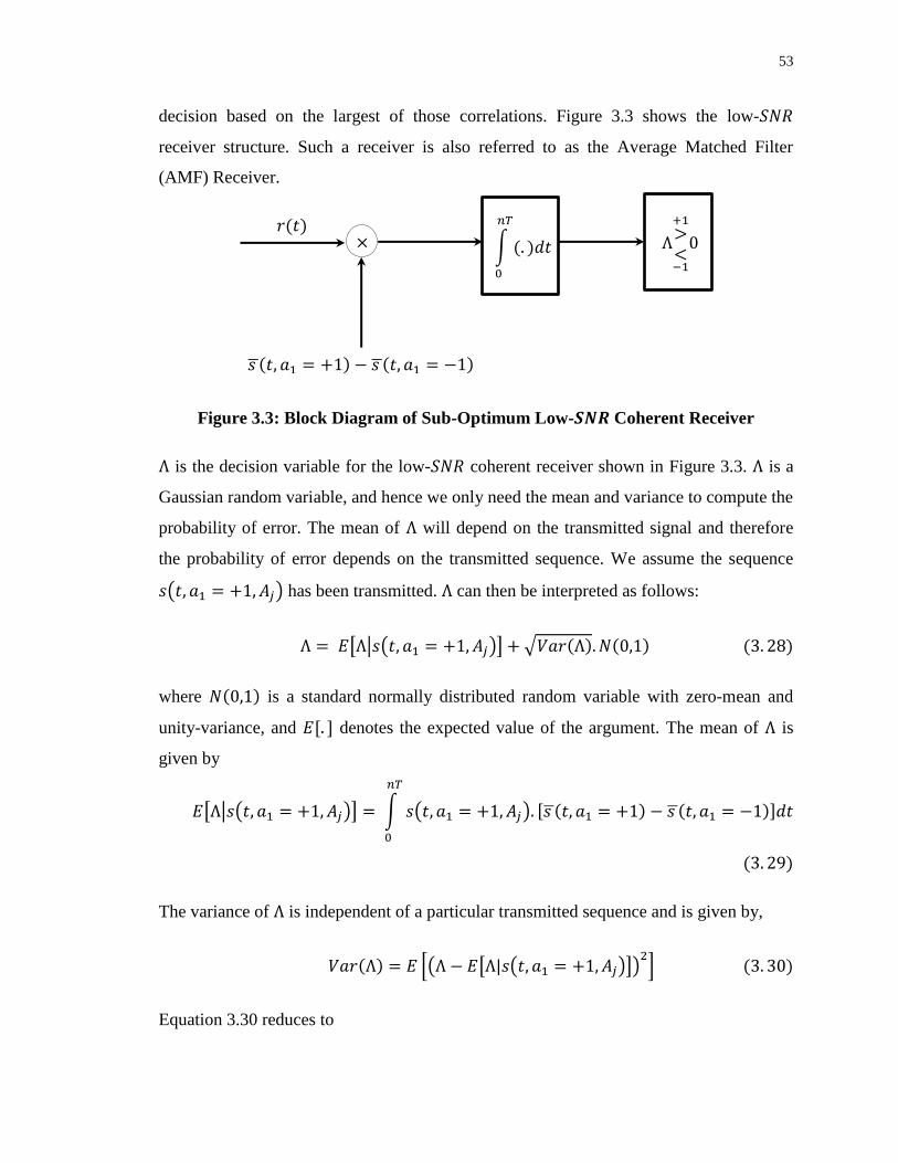
53
decision based on the largest of those correlations. Figure 3.3 shows the low-
receiver structure. Such a receiver is also referred to as the Average Matched Filter
(AMF) Receiver.
Figure 3.3: Block Diagram of Sub-Optimum Low- Coherent Receiver
is the decision variable for the low- coherent receiver shown in Figure 3.3. is a
Gaussian random variable, and hence we only need the mean and variance to compute the
probability of error. The mean of will depend on the transmitted signal and therefore
the probability of error depends on the transmitted sequence. We assume the sequence
( ) has been transmitted. can then be interpreted as follows:
[ | ( )] √
where is a standard normally distributed random variable with zero-mean and
unity-variance, and denotes the expected value of the argument. The mean of is
given by
[ | ( )] ∫ ( )
The variance of is independent of a particular transmitted sequence and is given by,
*( [ ( )]) +
Equation 3.30 reduces to
∫ 𝑑𝑡
𝑛𝑇
Λ
𝑟 𝑡
𝑠 𝑡 𝑎 𝑠 𝑡 𝑎
54
∫ ∫
We know that
∫ ∫
is the auto correlation function for an Gaussian random variable with variance. And
hence the integration will only exist if . Thus
∫
Therefore, the probability of error, given ( ) has been transmitted, is
( | ( )) * [ | ( )]
√ +
where
∫
√ (
)
The probability of error is given by averaging over all the possible transmitted sequences,
∑ ( | ( ))
∑ ( | ( ))
The mean and variance can be found based on the CPM scheme being used, and the
probability of error is affected by the specific modulation parameters for each scheme
and the number of bit-observations . Eventually, after a certain , the does not
show any further improvements and that is set as the optimal observation interval. This is
proved through computer simulations and studying the minimum distance criteria in
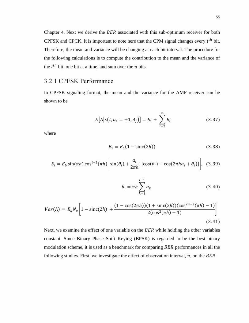
55
Chapter 4. Next we derive the associated with this sub-optimum receiver for both
CPFSK and CPCK. It is important to note here that the CPM signal changes every bit.
Therefore, the mean and variance will be changing at each bit interval. The procedure for
the following calculations is to compute the contribution to the mean and the variance of
the bit, one bit at a time, and sum over the bits.
3.2.1 CPFSK Performance
In CPFSK signaling format, the mean and the variance for the AMF receiver can be
shown to be
[ | ( )] ∑
where
*
+
∑
*
+
Next, we examine the effect of one variable on the while holding the other variables
constant. Since Binary Phase Shift Keying (BPSK) is regarded to be the best binary
modulation scheme, it is used as a benchmark for comparing performances in all the
following studies. First, we investigate the effect of observation interval, , on the .
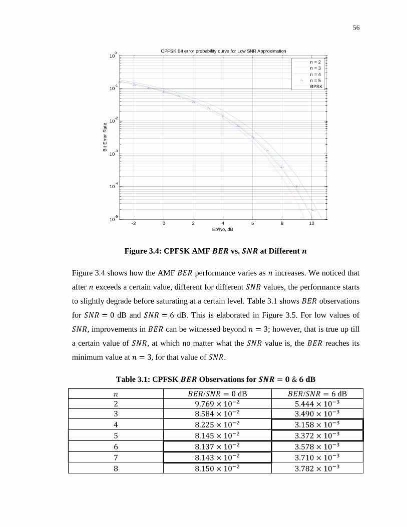
56
Figure 3.4: CPFSK AMF vs. at Different
Figure 3.4 shows how the AMF performance varies as increases. We noticed that
after exceeds a certain value, different for different values, the performance starts
to slightly degrade before saturating at a certain level. Table 3.1 shows observations
for dB and dB. This is elaborated in Figure 3.5. For low values of
, improvements in can be witnessed beyond ; however, that is true up till
a certain value of , at which no matter what the value is, the reaches its
minimum value at for that value of .
Table 3.1: CPFSK Observations for dB
/ dB / dB
3
3
3
3
3
3
3
-2 0 2 4 6 8 1010
-5
10-4
10-3
10-2
10-1
100
Eb/No, dB
Bit E
rro
r R
ate
CPFSK Bit error probability curve for Low SNR Approximation
n = 2
n = 3
n = 4
n = 5
BPSK
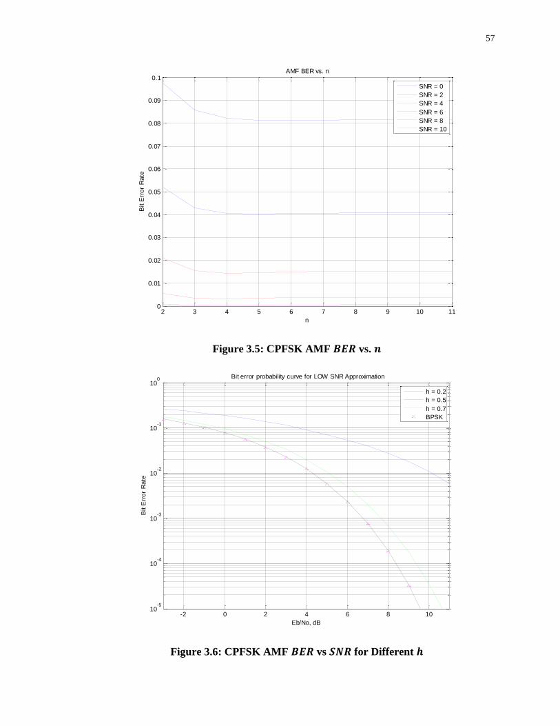
57
Figure 3.5: CPFSK AMF vs.
Figure 3.6: CPFSK AMF vs for Different
2 3 4 5 6 7 8 9 10 110
0.01
0.02
0.03
0.04
0.05
0.06
0.07
0.08
0.09
0.1
n
Bit E
rro
r R
ate
AMF BER vs. n
SNR = 0
SNR = 2
SNR = 4
SNR = 6
SNR = 8
SNR = 10
-2 0 2 4 6 8 1010
-5
10-4
10-3
10-2
10-1
100
Eb/No, dB
Bit E
rro
r R
ate
Bit error probability curve for LOW SNR Approximation
h = 0.2
h = 0.5
h = 0.7
BPSK
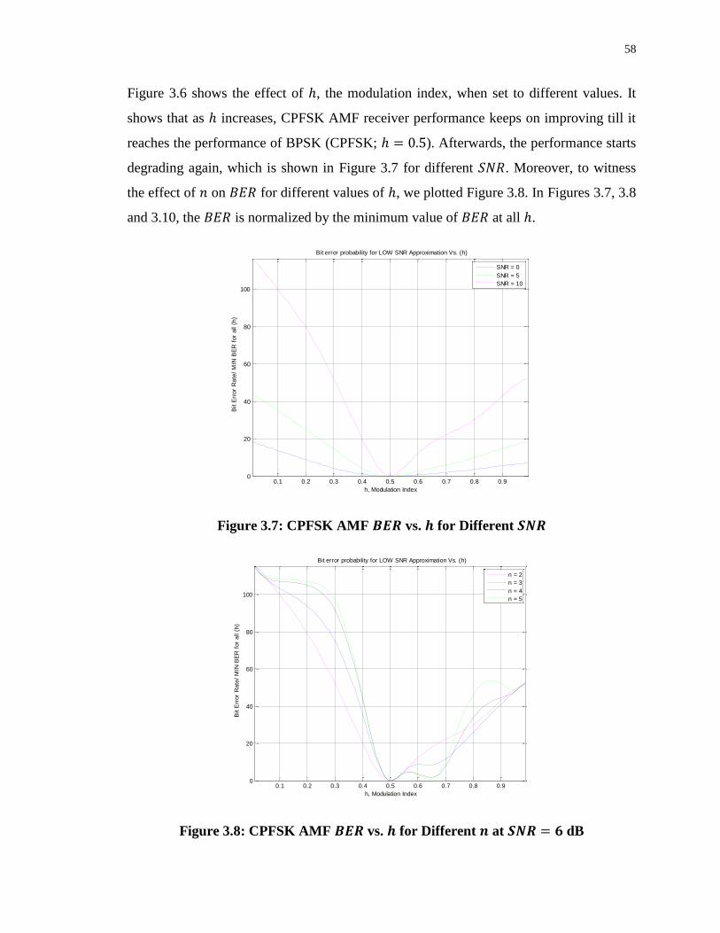
58
Figure 3.6 shows the effect of , the modulation index, when set to different values. It
shows that as increases, CPFSK AMF receiver performance keeps on improving till it
reaches the performance of BPSK (CPFSK; ). Afterwards, the performance starts
degrading again, which is shown in Figure 3.7 for different . Moreover, to witness
the effect of on for different values of , we plotted Figure 3.8. In Figures 3.7, 3.8
and 3.10, the is normalized by the minimum value of at all .
Figure 3.7: CPFSK AMF vs. for Different
Figure 3.8: CPFSK AMF vs. for Different at dB
0.1 0.2 0.3 0.4 0.5 0.6 0.7 0.8 0.90
20
40
60
80
100
h, Modulation Index
Bit E
rro
r R
ate
/ M
IN B
ER
for
all
(h)
Bit error probability for LOW SNR Approximation Vs. (h)
SNR = 0
SNR = 5
SNR = 10
0.1 0.2 0.3 0.4 0.5 0.6 0.7 0.8 0.90
20
40
60
80
100
h, Modulation Index
Bit E
rro
r R
ate
/ M
IN B
ER
for
all
(h)
Bit error probability for LOW SNR Approximation Vs. (h)
n = 2
n = 3
n = 4
n = 5
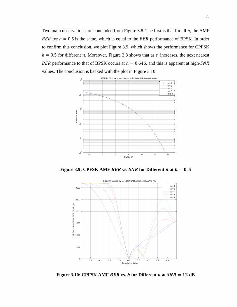
59
Two main observations are concluded from Figure 3.8. The first is that for all , the AMF
for is the same, which is equal to the performance of BPSK. In order
to confirm this conclusion, we plot Figure 3.9, which shows the performance for CPFSK
for different . Moreover, Figure 3.8 shows that as increases, the next nearest
performance to that of BPSK occurs at , and this is apparent at high-
values. The conclusion is backed with the plot in Figure 3.10.
Figure 3.9: CPFSK AMF vs. for Different at
Figure 3.10: CPFSK AMF vs. for Different at dB
-2 0 2 4 6 8 1010
-5
10-4
10-3
10-2
10-1
100
Eb/No, dB
Bit E
rro
r R
ate
CPFSK Bit error probability curve for Low SNR Approximation
n = 2
n = 3
n = 4
n = 5
BPSK
0.1 0.2 0.3 0.4 0.5 0.6 0.7 0.8 0.90
500
1000
1500
2000
2500
3000
h, Modulation Index
Bit E
rro
r R
ate
/ M
IN B
ER
for
all
(h)
Bit error probability for LOW SNR Approximation Vs. (h)
n = 2
n = 3
n = 4
n = 5
n = 6
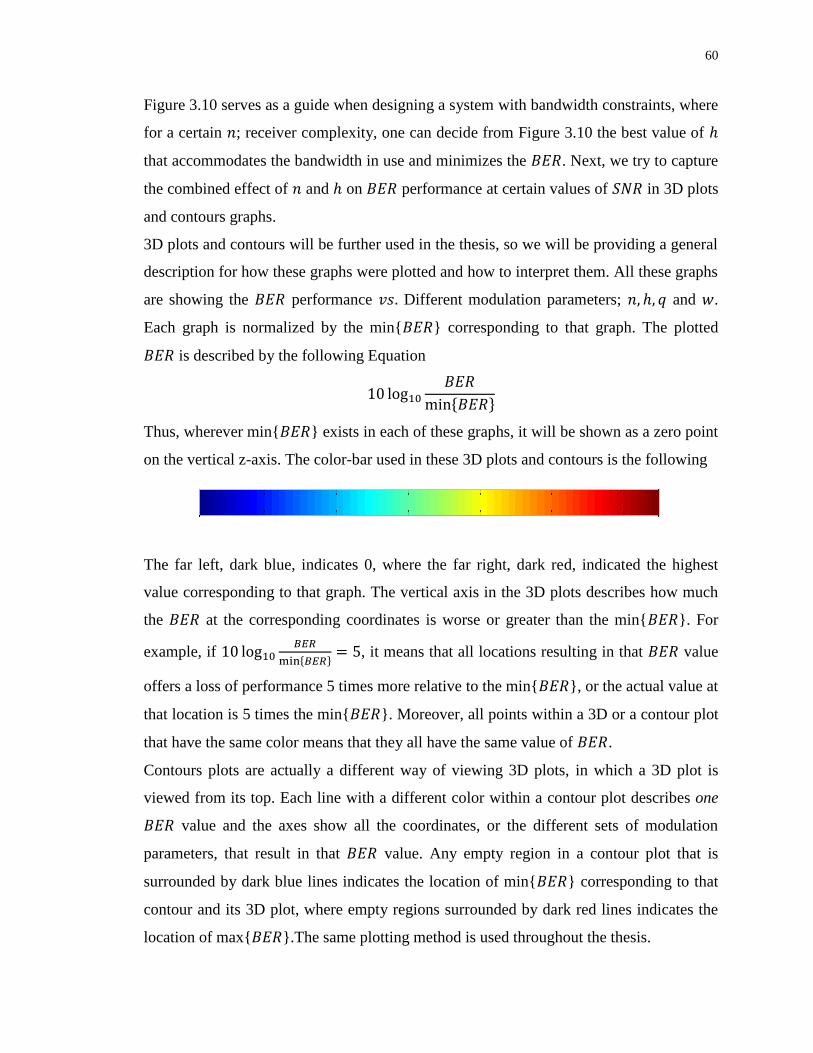
60
Figure 3.10 serves as a guide when designing a system with bandwidth constraints, where
for a certain ; receiver complexity, one can decide from Figure 3.10 the best value of
that accommodates the bandwidth in use and minimizes the . Next, we try to capture
the combined effect of and on performance at certain values of in 3D plots
and contours graphs.
3D plots and contours will be further used in the thesis, so we will be providing a general
description for how these graphs were plotted and how to interpret them. All these graphs
are showing the performance Different modulation parameters; and .
Each graph is normalized by the min{ } corresponding to that graph. The plotted
is described by the following Equation
Thus, wherever min{ } exists in each of these graphs, it will be shown as a zero point
on the vertical z-axis. The color-bar used in these 3D plots and contours is the following
The far left, dark blue, indicates 0, where the far right, dark red, indicated the highest
value corresponding to that graph. The vertical axis in the 3D plots describes how much
the at the corresponding coordinates is worse or greater than the min{ }. For
example, if
, it means that all locations resulting in that value
offers a loss of performance 5 times more relative to the min{ }, or the actual value at
that location is 5 times the min{ }. Moreover, all points within a 3D or a contour plot
that have the same color means that they all have the same value of .
Contours plots are actually a different way of viewing 3D plots, in which a 3D plot is
viewed from its top. Each line with a different color within a contour plot describes one
value and the axes show all the coordinates, or the different sets of modulation
parameters, that result in that value. Any empty region in a contour plot that is
surrounded by dark blue lines indicates the location of min{ } corresponding to that
contour and its 3D plot, where empty regions surrounded by dark red lines indicates the
location of max{ }.The same plotting method is used throughout the thesis.
00
.10
.20
.30
.40
.50
.60
.70
.80
.91
0
0.1
0.2
0.3
0.4
0.5
0.6
0.7
0.8
0.9 1
10
20
30
40
50
60
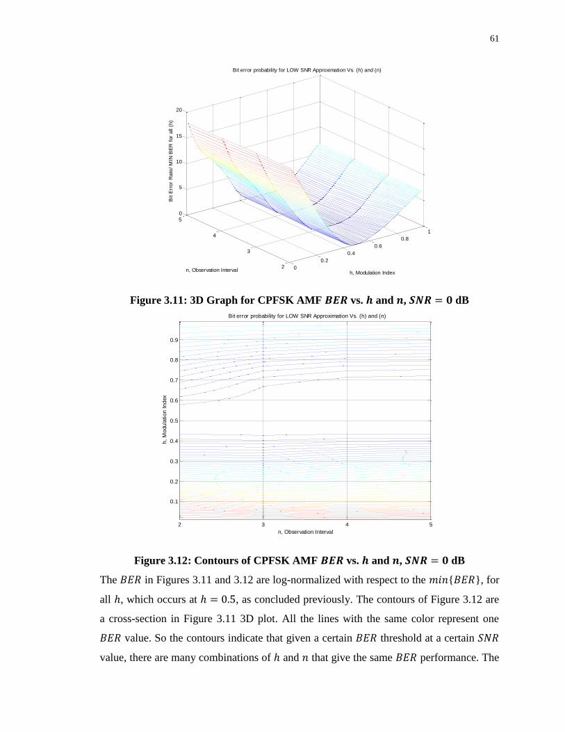
61
Figure 3.11: 3D Graph for CPFSK AMF vs. and , dB
Figure 3.12: Contours of CPFSK AMF vs. and , dB
The in Figures 3.11 and 3.12 are log-normalized with respect to the { }, for
all , which occurs at , as concluded previously. The contours of Figure 3.12 are
a cross-section in Figure 3.11 3D plot. All the lines with the same color represent one
value. So the contours indicate that given a certain threshold at a certain
value, there are many combinations of and that give the same performance. The
0
0.2
0.4
0.6
0.8
1
2
3
4
5
0
5
10
15
20
h, Modulation Index
Bit error probability for LOW SNR Approximation Vs. (h) and (n)
n, Observation Interval
Bit E
rro
r R
ate
/ M
IN B
ER
for
all
(h)
h,
Mo
du
latio
n I
nd
ex
n, Observation Interval
Bit error probability for LOW SNR Approximation Vs. (h) and (n)
2 3 4 5
0.1
0.2
0.3
0.4
0.5
0.6
0.7
0.8
0.9
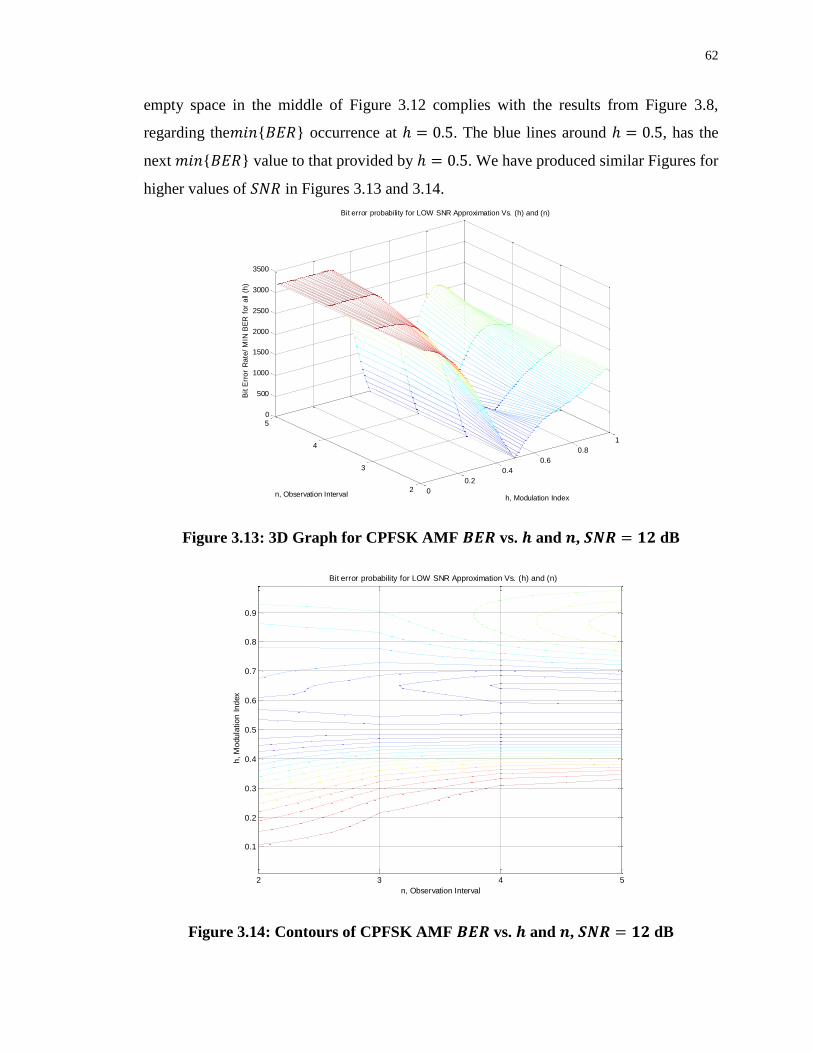
62
empty space in the middle of Figure 3.12 complies with the results from Figure 3.8,
regarding the { } occurrence at . The blue lines around , has the
next { } value to that provided by . We have produced similar Figures for
higher values of in Figures 3.13 and 3.14.
Figure 3.13: 3D Graph for CPFSK AMF vs. and , dB
Figure 3.14: Contours of CPFSK AMF vs. and , dB
0
0.2
0.4
0.6
0.8
1
2
3
4
5
0
500
1000
1500
2000
2500
3000
3500
h, Modulation Index
Bit error probability for LOW SNR Approximation Vs. (h) and (n)
n, Observation Interval
Bit E
rro
r R
ate
/ M
IN B
ER
for
all
(h)
h,
Mo
du
latio
n I
nd
ex
n, Observation Interval
Bit error probability for LOW SNR Approximation Vs. (h) and (n)
2 3 4 5
0.1
0.2
0.3
0.4
0.5
0.6
0.7
0.8
0.9
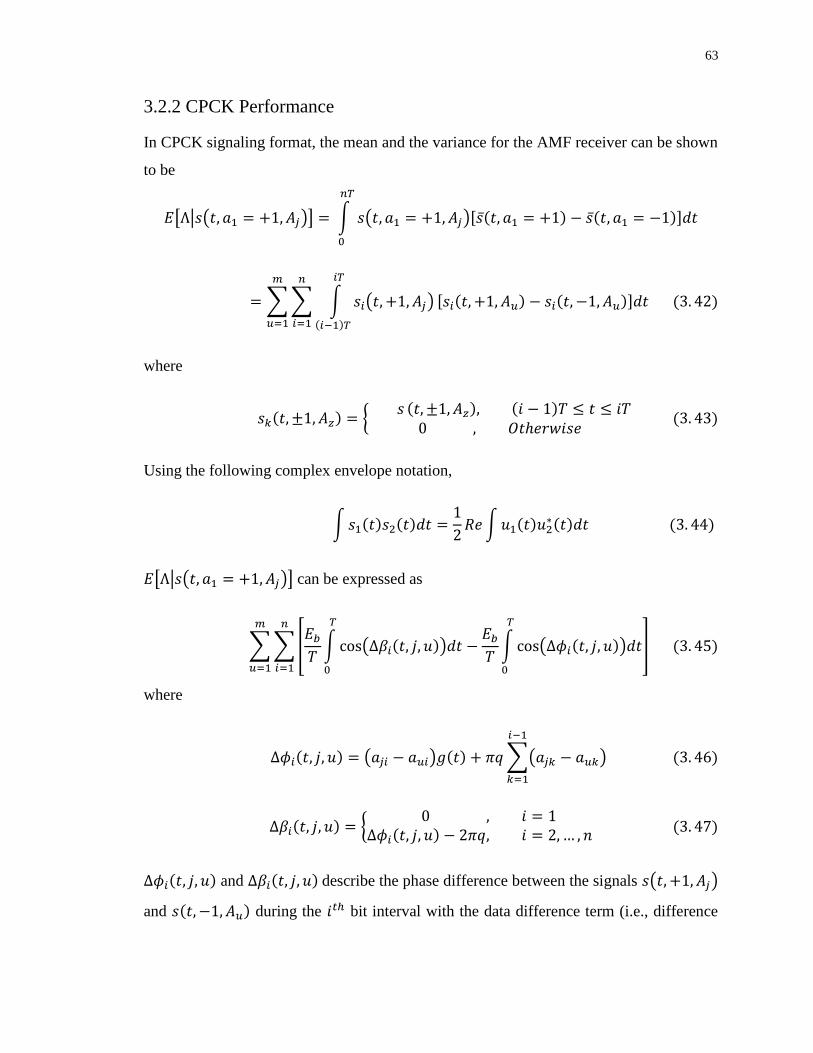
63
3.2.2 CPCK Performance
In CPCK signaling format, the mean and the variance for the AMF receiver can be shown
to be
[ | ( )] ∫ ( )
∑ ∑ ∫ ( )
where
{
Using the following complex envelope notation,
∫
∫
[ | ( )] can be expressed as
∑ ∑0
∫ ( )
∫ ( )
1
where
( ) ∑( )
{
and describe the phase difference between the signals ( )
and during the bit interval with the data difference term (i.e., difference
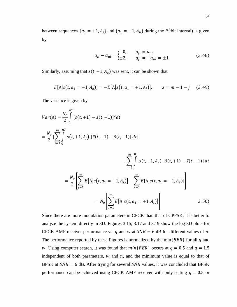
64
between sequences { and during the bit interval) is given
by
{
Similarly, assuming that was sent, it can be shown that
[ | ( )]
The variance is given by
∫
∑∫ ( )
∑∫
0∑ [ | ( )]
∑
1
0∑ [ | ( )]
1
Since there are more modulation parameters in CPCK than that of CPFSK, it is better to
analyze the system directly in 3D. Figures 3.15, 3.17 and 3.19 show the log 3D plots for
CPCK AMF receiver performance vs. and at dB for different values of .
The performance reported by these Figures is normalized by the min{ } for all and
. Using computer search, it was found that { } occurs at and
independent of both parameters, and , and the minimum value is equal to that of
BPSK at dB. After trying for several values, it was concluded that BPSK
performance can be achieved using CPCK AMF receiver with only setting or
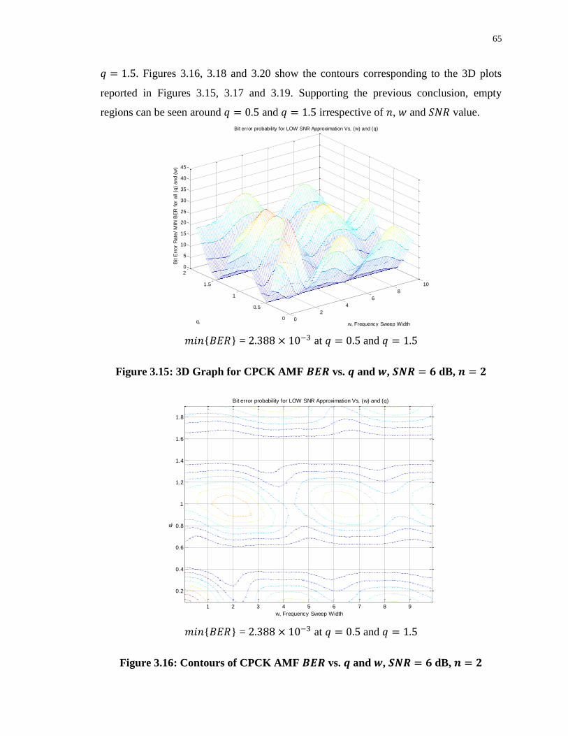
65
. Figures 3.16, 3.18 and 3.20 show the contours corresponding to the 3D plots
reported in Figures 3.15, 3.17 and 3.19. Supporting the previous conclusion, empty
regions can be seen around and irrespective of , and value.
{ } = 3 at and
Figure 3.15: 3D Graph for CPCK AMF vs. and , dB,
{ } = 3 at and
Figure 3.16: Contours of CPCK AMF vs. and , dB,
0
2
4
6
8
10
0
0.5
1
1.5
2
0
5
10
15
20
25
30
35
40
45
w, Frequency Sweep Width
Bit error probability for LOW SNR Approximation Vs. (w) and (q)
q, Modulation Index
Bit E
rro
r R
ate
/ M
IN B
ER
for
all
(q)
an
d (
w)
w, Frequency Sweep Width
q,
Mo
du
latio
n I
nd
ex
Bit error probability for LOW SNR Approximation Vs. (w) and (q)
1 2 3 4 5 6 7 8 9
0.2
0.4
0.6
0.8
1
1.2
1.4
1.6
1.8
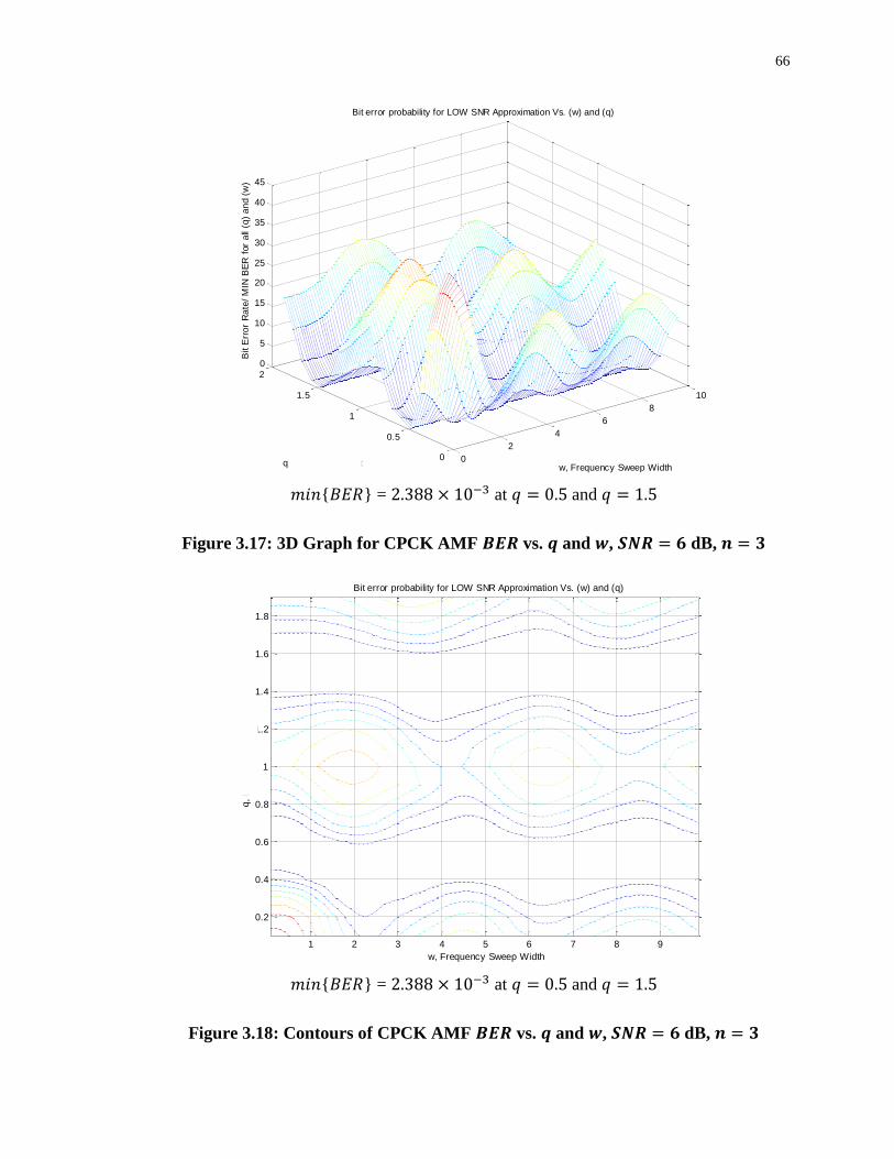
66
{ } = 3 at and
Figure 3.17: 3D Graph for CPCK AMF vs. and , dB,
{ } = 3 at and
Figure 3.18: Contours of CPCK AMF vs. and , dB,
0
2
4
6
8
10
0
0.5
1
1.5
2
0
5
10
15
20
25
30
35
40
45
w, Frequency Sweep Width
Bit error probability for LOW SNR Approximation Vs. (w) and (q)
q, Modulation Index
Bit E
rro
r R
ate
/ M
IN B
ER
for
all
(q)
an
d (
w)
w, Frequency Sweep Width
q,
Mo
du
latio
n I
nd
ex
Bit error probability for LOW SNR Approximation Vs. (w) and (q)
1 2 3 4 5 6 7 8 9
0.2
0.4
0.6
0.8
1
1.2
1.4
1.6
1.8
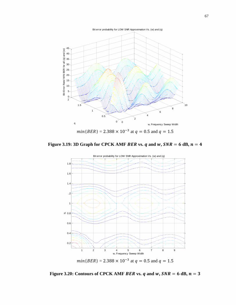
67
{ } = 3 at and
Figure 3.19: 3D Graph for CPCK AMF vs. and , dB,
{ } = 3 at and
Figure 3.20: Contours of CPCK AMF vs. and , dB,
0
2
4
6
8
10
0
0.5
1
1.5
2
0
5
10
15
20
25
30
35
40
45
w, Frequency Sweep Width
Bit error probability for LOW SNR Approximation Vs. (w) and (q)
q, Modulation Index
Bit E
rro
r R
ate
/ M
IN B
ER
for
all
(q)
an
d (
w)
w, Frequency Sweep Width
q,
Mo
du
latio
n I
nd
ex
Bit error probability for LOW SNR Approximation Vs. (w) and (q)
1 2 3 4 5 6 7 8 9
0.2
0.4
0.6
0.8
1
1.2
1.4
1.6
1.8
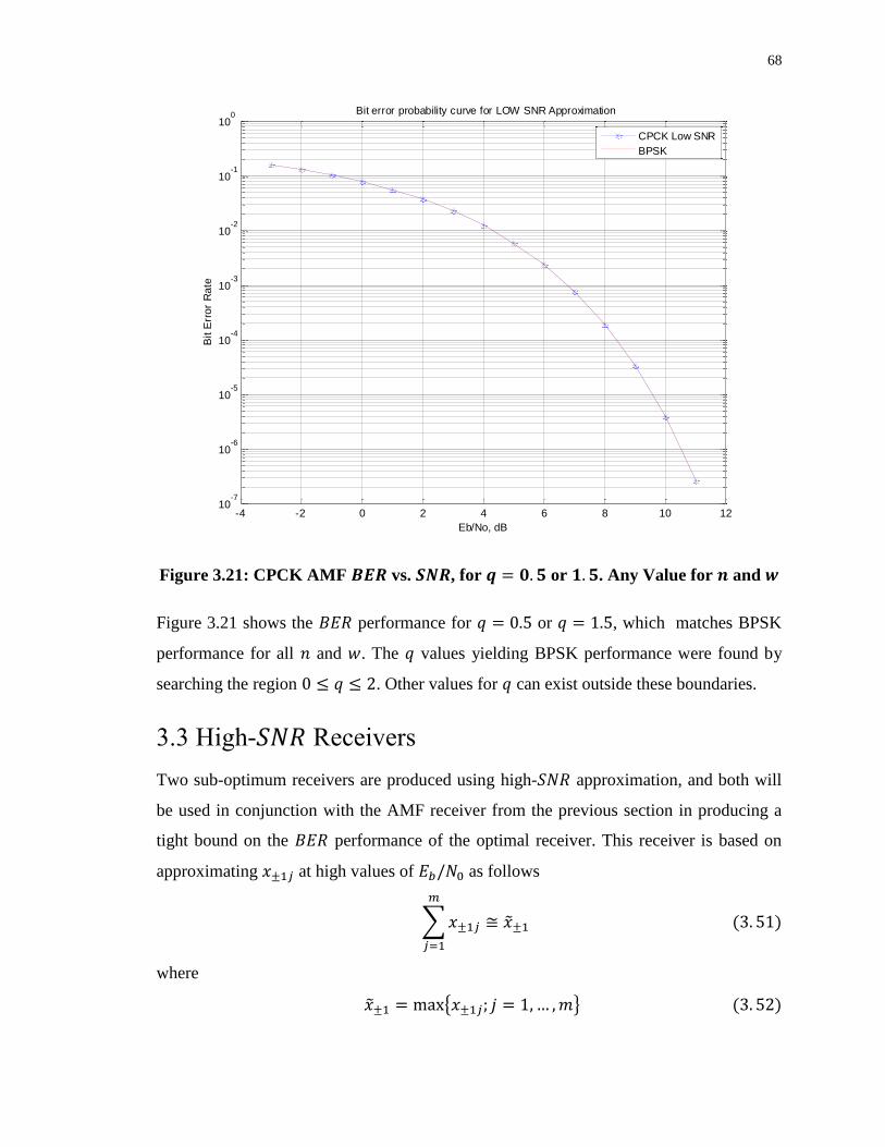
68
Figure 3.21: CPCK AMF vs. , for or . Any Value for and
Figure 3.21 shows the performance for or , which matches BPSK
performance for all and . The values yielding BPSK performance were found by
searching the region . Other values for can exist outside these boundaries.
3.3 High- Receivers
Two sub-optimum receivers are produced using high- approximation, and both will
be used in conjunction with the AMF receiver from the previous section in producing a
tight bound on the performance of the optimal receiver. This receiver is based on
approximating at high values of as follows
∑
where
{ }
-4 -2 0 2 4 6 8 10 1210
-7
10-6
10-5
10-4
10-3
10-2
10-1
100
Eb/No, dB
Bit E
rro
r R
ate
Bit error probability curve for LOW SNR Approximation
CPCK Low SNR
BPSK
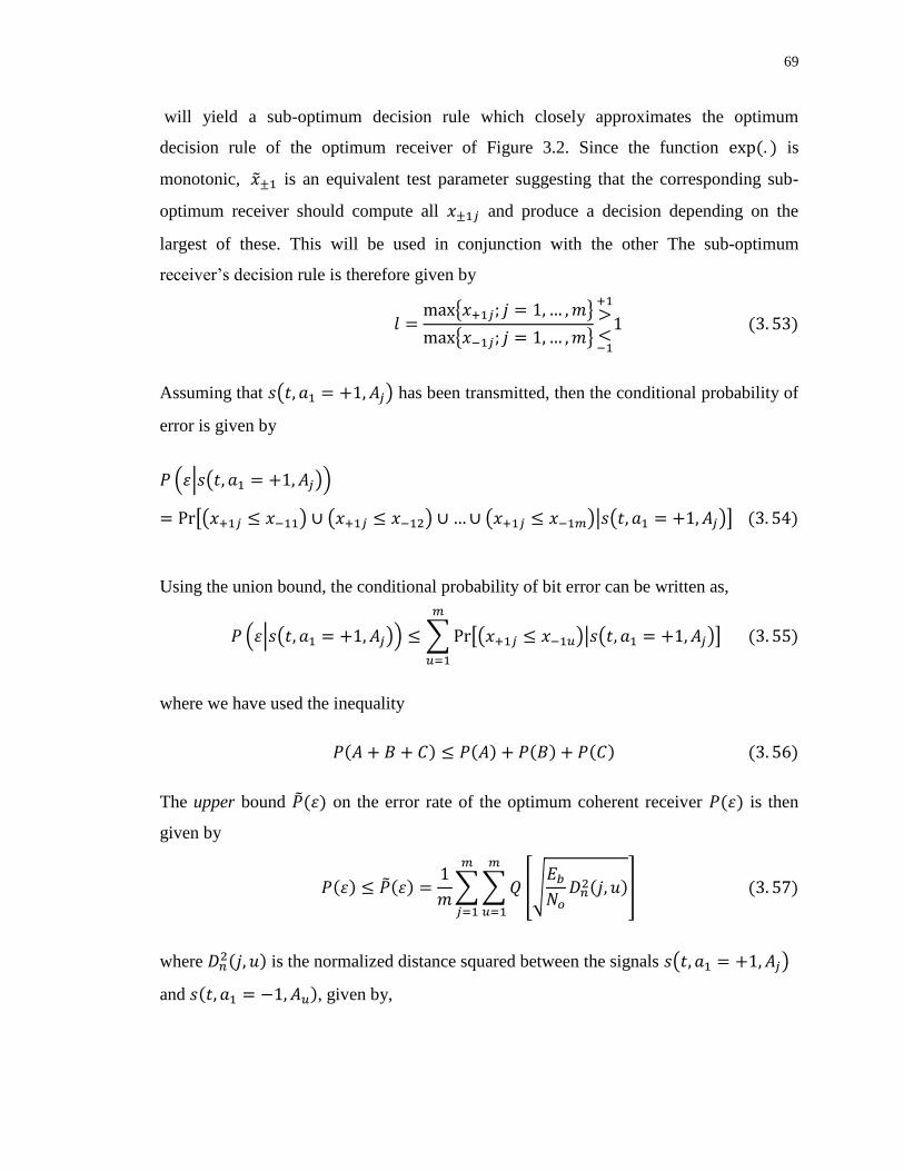
69
will yield a sub-optimum decision rule which closely approximates the optimum
decision rule of the optimum receiver of Figure 3.2. Since the function is
monotonic, is an equivalent test parameter suggesting that the corresponding sub-
optimum receiver should compute all and produce a decision depending on the
largest of these. This will be used in conjunction with the other The sub-optimum
receiver’s decision rule is therefore given by
{ }
{ }
Assuming that ( ) has been transmitted, then the conditional probability of
error is given by
( | ( ))
[( ) ( ) ( )| ( )]
Using the union bound, the conditional probability of bit error can be written as,
( | ( )) ∑ [( )| ( )]
where we have used the inequality
The upper bound on the error rate of the optimum coherent receiver is then
given by
∑ ∑ 0√
1
where is the normalized distance squared between the signals ( )
and , given by,
70
∫ | ( ) |
where
∫ ( )
For large , the error rate is mainly determined by the minimum of all distance-
squared values,
It is possible, therefore, to compare different coherent systems (at high- ) by simply
comparing their respective minimum distances. Using PSK ( ) as a benchmark, an
estimate of the gain (in decibels) relative to PSK is then obtained from
(
)
We will carry out a study of the minimum distance properties of CPM signals in Chapter
4. It is useful to construct a lower bound on the performance of the coherent CPM
receiver in order to test the tightness of the upper bound introduced above. The lower
bound is obtained by supposing that for each transmitted sequence, the receiver needs
only to decide between that sequence and its nearest neighbor. This receiver will perform
at least as well as the receiver which does not know which of two sequences. The
performance of this receiver is a lower bound to the performance of the optimum CPM
receiver presented in section 3.1. This lower bound on the probability of error can be
written as
∑ 0√
1
Figure 3.23 shows the high- approximation receiver.
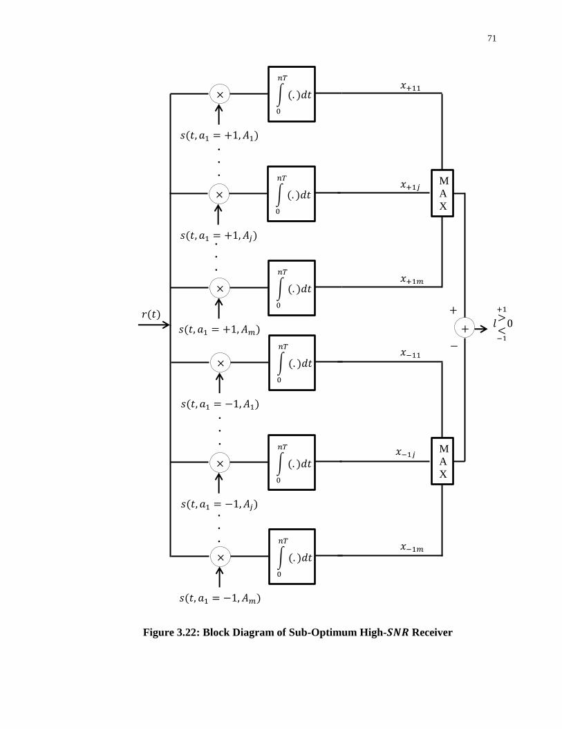
71
Figure 3.22: Block Diagram of Sub-Optimum High- Receiver
∫ 𝑑𝑡
𝑛𝑇
𝑠 𝑡 𝑎 𝐴
𝑥
𝑟 𝑡 𝑙
∫ 𝑑𝑡
𝑛𝑇
𝑠 𝑡 𝑎 𝐴𝑗
𝑥 𝑗
∫ 𝑑𝑡
𝑛𝑇
𝑠 𝑡 𝑎 𝐴𝑚
𝑥 𝑚
∫ 𝑑𝑡
𝑛𝑇
𝑠 𝑡 𝑎 𝐴
𝑥
∫ 𝑑𝑡
𝑛𝑇
𝑠 𝑡 𝑎 𝐴𝑗
𝑥 𝑗
∫ 𝑑𝑡
𝑛𝑇
𝑠 𝑡 𝑎 𝐴𝑚
𝑥 𝑚
M
A
X
M
A
X
.
.
.
.
.
.
.
.
.
.
.
.
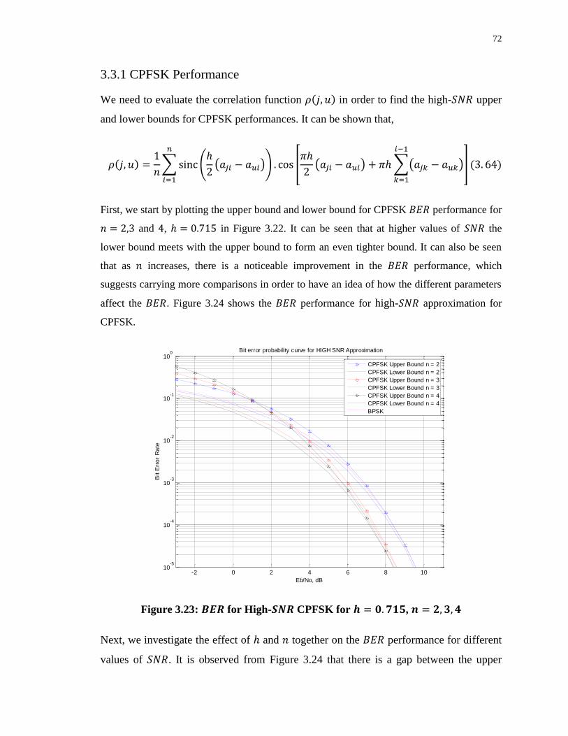
72
3.3.1 CPFSK Performance
We need to evaluate the correlation function in order to find the high- upper
and lower bounds for CPFSK performances. It can be shown that,
∑ (
( )) 0
( ) ∑( )
1
First, we start by plotting the upper bound and lower bound for CPFSK performance for
and , in Figure 3.22. It can be seen that at higher values of the
lower bound meets with the upper bound to form an even tighter bound. It can also be seen
that as increases, there is a noticeable improvement in the performance, which
suggests carrying more comparisons in order to have an idea of how the different parameters
affect the . Figure 3.24 shows the performance for high- approximation for
CPFSK.
Figure 3.23: for High- CPFSK for ,
Next, we investigate the effect of and together on the performance for different
values of . It is observed from Figure 3.24 that there is a gap between the upper
-2 0 2 4 6 8 1010
-5
10-4
10-3
10-2
10-1
100
Eb/No, dB
Bit E
rro
r R
ate
Bit error probability curve for HIGH SNR Approximation
CPFSK Upper Bound n = 2
CPFSK Lower Bound n = 2
CPFSK Upper Bound n = 3
CPFSK Lower Bound n = 3
CPFSK Upper Bound n = 4
CPFSK Lower Bound n = 4
BPSK
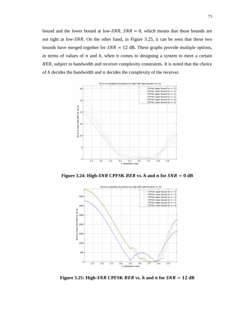
73
bound and the lower bound at low- , , which means that these bounds are
not tight at low- . On the other hand, in Figure 3.25, it can be seen that these two
bounds have merged together for dB. These graphs provide multiple options,
in terms of values of and , when it comes to designing a system to meet a certain
, subject to bandwidth and receiver complexity constraints. It is noted that the choice
of decides the bandwidth and decides the complexity of the receiver.
Figure 3.24: High- CPFSK vs. and for dB
Figure 3.25: High- CPFSK vs. and for dB
0.1 0.2 0.3 0.4 0.5 0.6 0.7 0.8 0.90
5
10
15
20
25
30
h, Modulation Index
Bit E
rro
r R
ate
/ M
IN B
ER
for
all
(h)
Bit error probability Boundaries for High SNR Approximation Vs. (h)
CPFSK Upper Bound for n = 2
CPFSK Lower Bound for n = 2
CPFSK Upper Bound for n = 3
CPFSK Lower Bound for n = 3
CPFSK Upper Bound for n = 4
CPFSK Lower Bound for n = 4
0.1 0.2 0.3 0.4 0.5 0.6 0.7 0.8 0.90
500
1000
1500
2000
2500
3000
3500
h, Modulation Index
Bit E
rro
r R
ate
/ M
IN B
ER
for
all
(h)
Bit error probability Boundaries for High SNR Approximation Vs. (h)
CPFSK Upper Bound for n = 2
CPFSK Lower Bound for n = 2
CPFSK Upper Bound for n = 3
CPFSK Lower Bound for n = 3
CPFSK Upper Bound for n = 4
CPFSK Lower Bound for n = 4
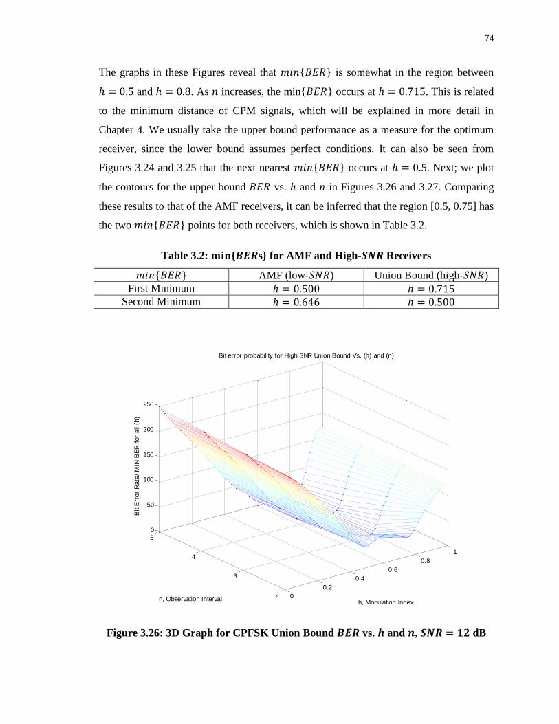
74
The graphs in these Figures reveal that { } is somewhat in the region between
and . As increases, the min{ } occurs at . This is related
to the minimum distance of CPM signals, which will be explained in more detail in
Chapter 4. We usually take the upper bound performance as a measure for the optimum
receiver, since the lower bound assumes perfect conditions. It can also be seen from
Figures 3.24 and 3.25 that the next nearest { } occurs at Next; we plot
the contours for the upper bound vs. and in Figures 3.26 and 3.27. Comparing
these results to that of the AMF receivers, it can be inferred that the region [0.5, 0.75] has
the two { } points for both receivers, which is shown in Table 3.2.
Table 3.2: { s} for AMF and High- Receivers
{ } AMF (low- ) Union Bound (high- )
First Minimum Second Minimum
Figure 3.26: 3D Graph for CPFSK Union Bound vs. and , dB
0
0.2
0.4
0.6
0.8
1
2
3
4
5
0
50
100
150
200
250
h, Modulation Index
Bit error probability for High SNR Union Bound Vs. (h) and (n)
n, Observation Interval
Bit E
rro
r R
ate
/ M
IN B
ER
for
all
(h)
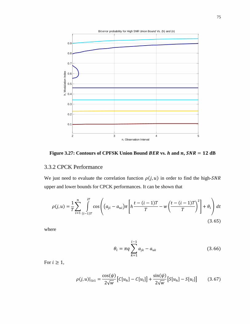
75
Figure 3.27: Contours of CPFSK Union Bound vs. and , dB
3.3.2 CPCK Performance
We just need to evaluate the correlation function in order to find the high-
upper and lower bounds for CPCK performances. It can be shown that
∑ ∫ .( ) [
(
)
] /
where
∑
For ,
√ [ ]
√ [ ]
h,
Mo
du
latio
n I
nd
ex
n, Observation Interval
Bit error probability for High SNR Union Bound Vs. (h) and (n)
2 3 4 5
0.1
0.2
0.3
0.4
0.5
0.6
0.7
0.8
0.9
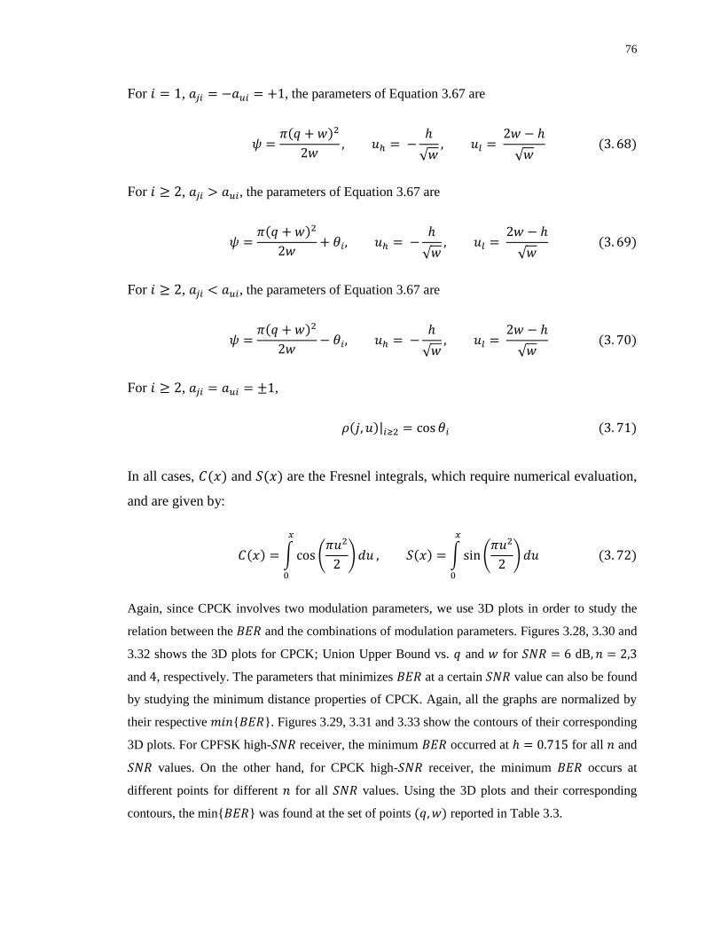
76
For , , the parameters of Equation 3.67 are
√
√
For , , the parameters of Equation 3.67 are
√
√
For , , the parameters of Equation 3.67 are
√
√
For , ,
In all cases, and are the Fresnel integrals, which require numerical evaluation,
and are given by:
∫ (
)
∫ (
)
Again, since CPCK involves two modulation parameters, we use 3D plots in order to study the
relation between the and the combinations of modulation parameters. Figures 3.28, 3.30 and
3.32 shows the 3D plots for CPCK; Union Upper Bound vs. and for dB
and , respectively. The parameters that minimizes at a certain value can also be found
by studying the minimum distance properties of CPCK. Again, all the graphs are normalized by
their respective { }. Figures 3.29, 3.31 and 3.33 show the contours of their corresponding
3D plots. For CPFSK high- receiver, the minimum occurred at for all and
values. On the other hand, for CPCK high- receiver, the minimum occurs at
different points for different for all values. Using the 3D plots and their corresponding
contours, the min{ } was found at the set of points reported in Table 3.3.
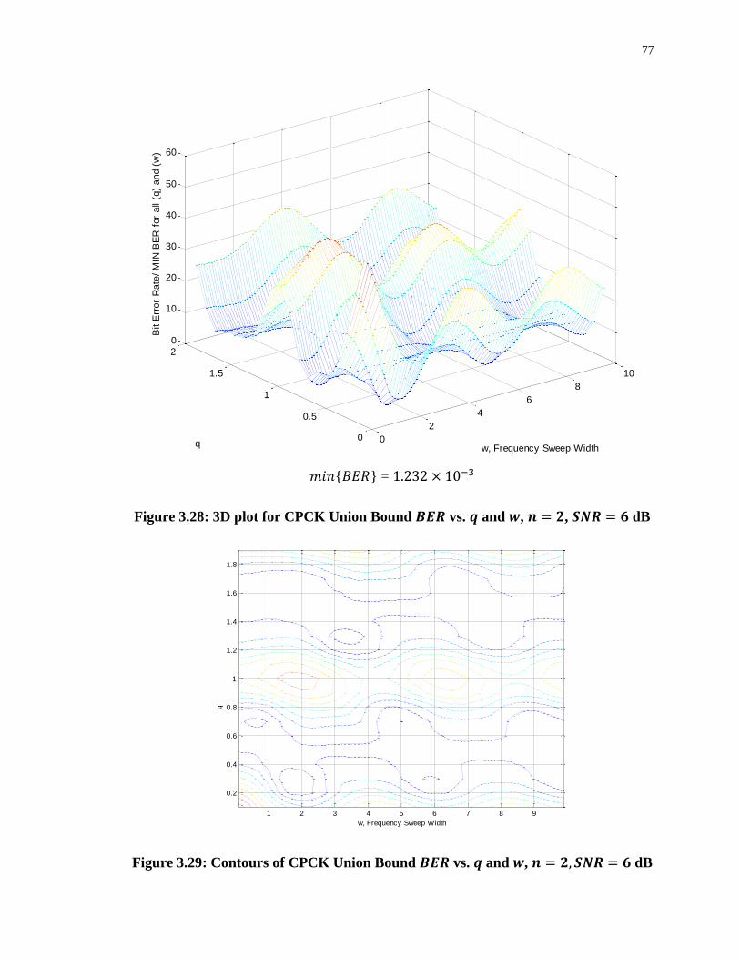
77
{ } = 3
Figure 3.28: 3D plot for CPCK Union Bound vs. and , , dB
Figure 3.29: Contours of CPCK Union Bound vs. and , dB
0
2
4
6
8
10
0
0.5
1
1.5
2
0
10
20
30
40
50
60
w, Frequency Sweep Width
Bit error probability for High SNR Lower Bound Vs. (h) and (n)
q, Modulation Index
Bit E
rro
r R
ate
/ M
IN B
ER
for
all
(q)
an
d (
w)
w, Frequency Sweep Width
q,
Mo
du
latio
n I
nd
ex
Bit error probability for High SNR Lower Bound Vs. (h) and (n)
1 2 3 4 5 6 7 8 9
0.2
0.4
0.6
0.8
1
1.2
1.4
1.6
1.8
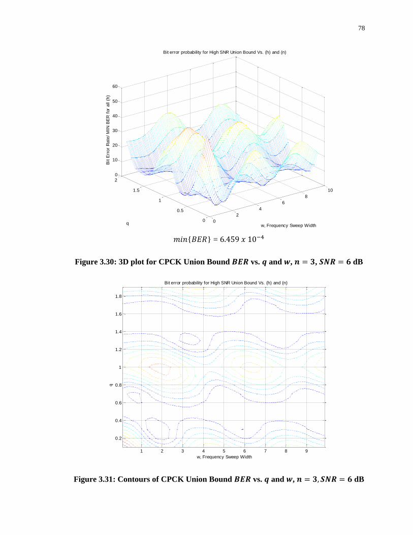
78
{ } = 4
Figure 3.30: 3D plot for CPCK Union Bound vs. and , , dB
Figure 3.31: Contours of CPCK Union Bound vs. and , dB
0
2
4
6
8
10
0
0.5
1
1.5
2
0
10
20
30
40
50
60
w, Frequency Sweep Width
Bit error probability for High SNR Union Bound Vs. (h) and (n)
q, Modulation Index
Bit E
rro
r R
ate
/ M
IN B
ER
for
all
(h)
w, Frequency Sweep Width
q,
Mo
du
latio
n I
nd
ex
Bit error probability for High SNR Union Bound Vs. (h) and (n)
1 2 3 4 5 6 7 8 9
0.2
0.4
0.6
0.8
1
1.2
1.4
1.6
1.8
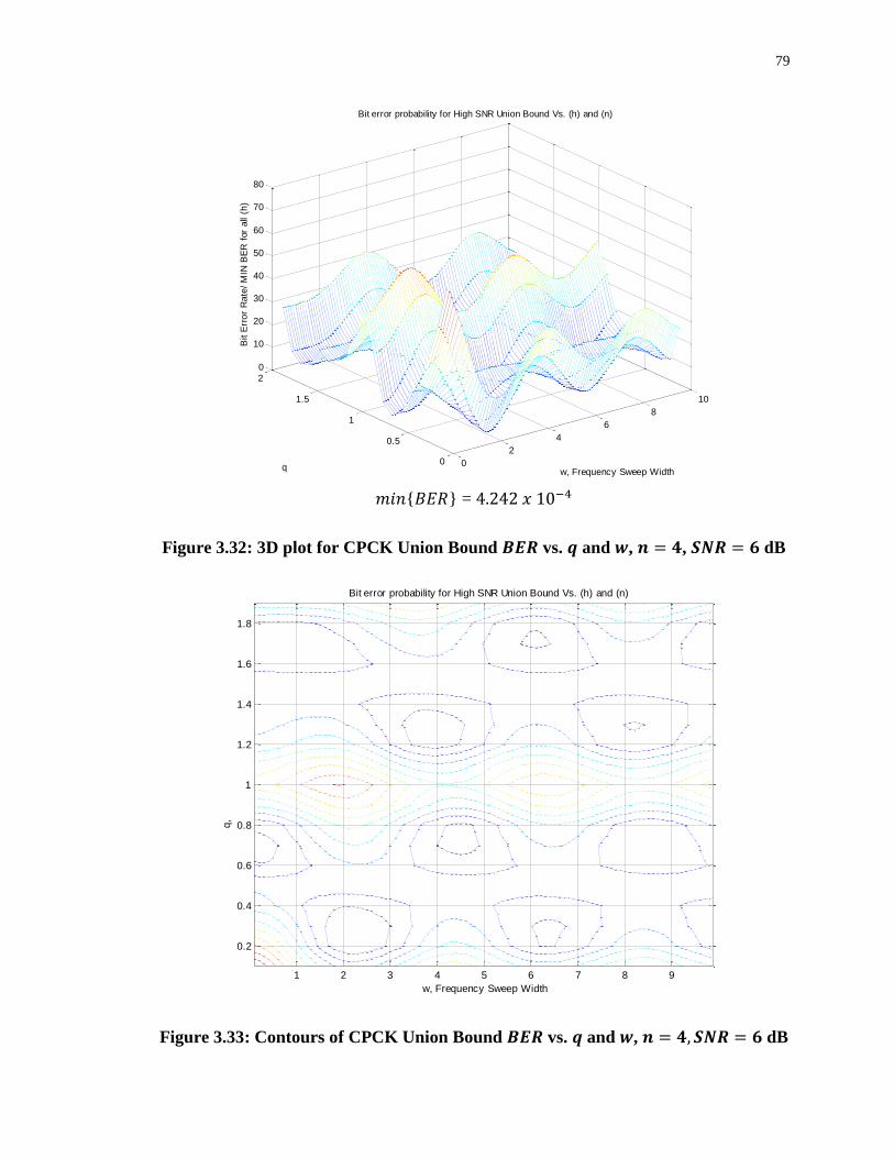
79
{ } = 4
Figure 3.32: 3D plot for CPCK Union Bound vs. and , , dB
Figure 3.33: Contours of CPCK Union Bound vs. and , dB
0
2
4
6
8
10
0
0.5
1
1.5
2
0
10
20
30
40
50
60
70
80
w, Frequency Sweep Width
Bit error probability for High SNR Union Bound Vs. (h) and (n)
q, Modulation Index
Bit E
rro
r R
ate
/ M
IN B
ER
for
all
(h)
w, Frequency Sweep Width
q,
Mo
du
latio
n I
nd
ex
Bit error probability for High SNR Union Bound Vs. (h) and (n)
1 2 3 4 5 6 7 8 9
0.2
0.4
0.6
0.8
1
1.2
1.4
1.6
1.8
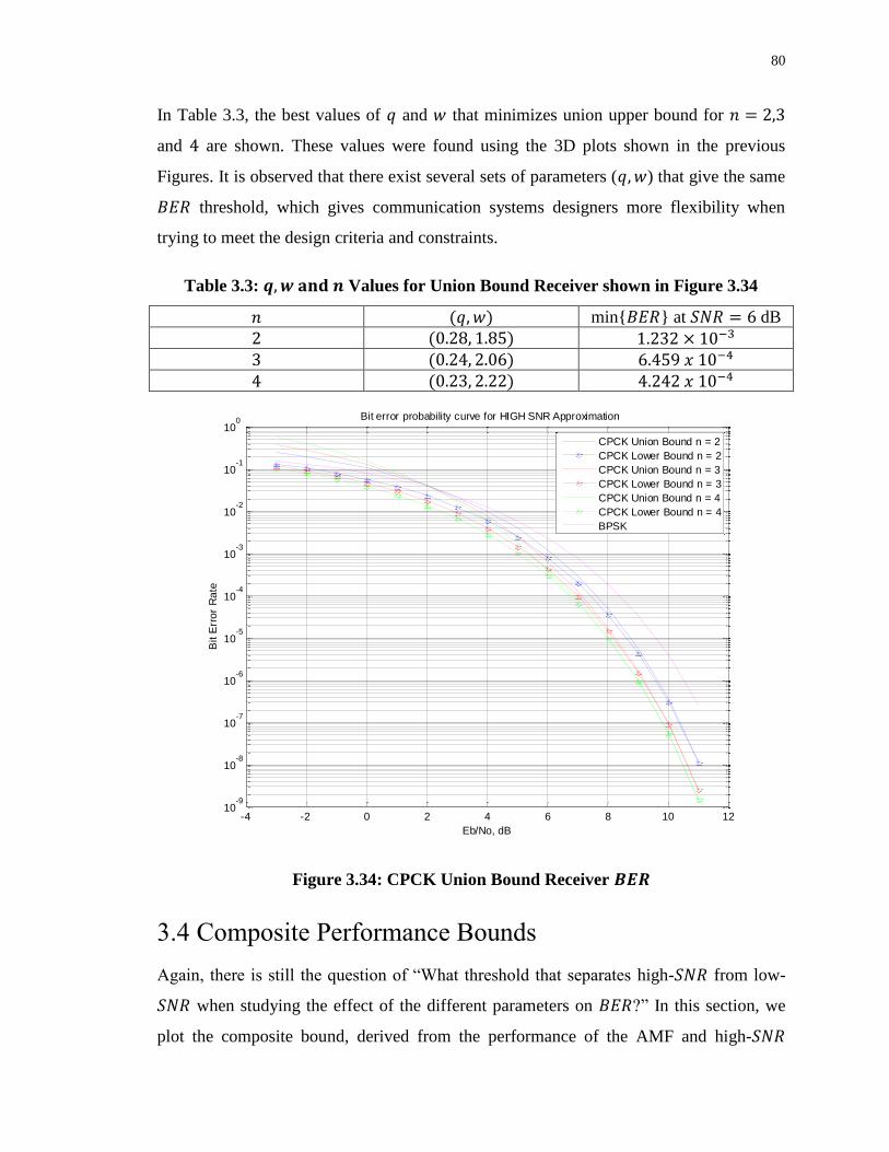
80
In Table 3.3, the best values of and that minimizes union upper bound for
and are shown. These values were found using the 3D plots shown in the previous
Figures. It is observed that there exist several sets of parameters ( ) that give the same
threshold, which gives communication systems designers more flexibility when
trying to meet the design criteria and constraints.
Table 3.3: Values for Union Bound Receiver shown in Figure 3.34
min{ } at dB 3 4 4
Figure 3.34: CPCK Union Bound Receiver
3.4 Composite Performance Bounds
Again, there is still the question of “What threshold that separates high- from low-
when studying the effect of the different parameters on ?” In this section, we
plot the composite bound, derived from the performance of the AMF and high-
-4 -2 0 2 4 6 8 10 1210
-9
10-8
10-7
10-6
10-5
10-4
10-3
10-2
10-1
100
Eb/No, dB
Bit E
rro
r R
ate
Bit error probability curve for HIGH SNR Approximation
CPCK Union Bound n = 2
CPCK Lower Bound n = 2
CPCK Union Bound n = 3
CPCK Lower Bound n = 3
CPCK Union Bound n = 4
CPCK Lower Bound n = 4
BPSK
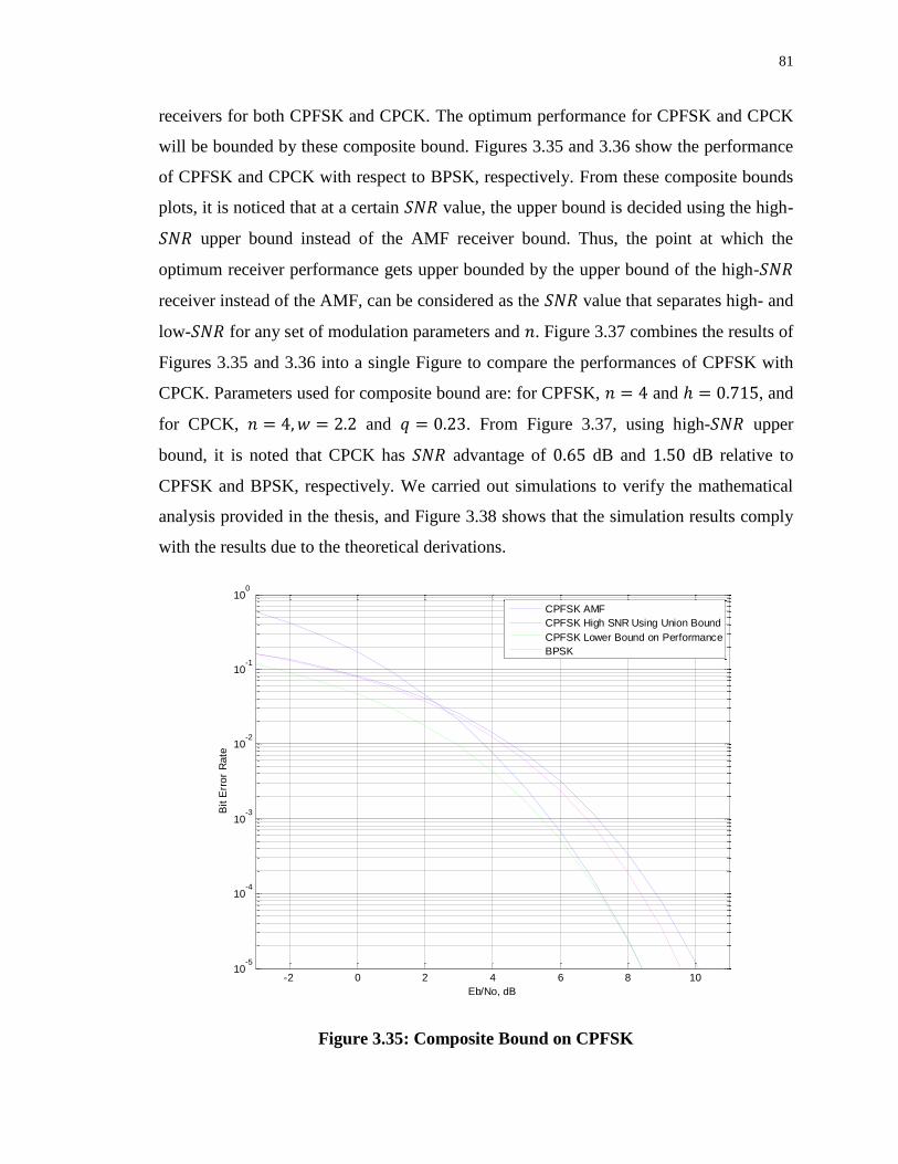
81
receivers for both CPFSK and CPCK. The optimum performance for CPFSK and CPCK
will be bounded by these composite bound. Figures 3.35 and 3.36 show the performance
of CPFSK and CPCK with respect to BPSK, respectively. From these composite bounds
plots, it is noticed that at a certain value, the upper bound is decided using the high-
upper bound instead of the AMF receiver bound. Thus, the point at which the
optimum receiver performance gets upper bounded by the upper bound of the high-
receiver instead of the AMF, can be considered as the value that separates high- and
low- for any set of modulation parameters and . Figure 3.37 combines the results of
Figures 3.35 and 3.36 into a single Figure to compare the performances of CPFSK with
CPCK. Parameters used for composite bound are: for CPFSK, and , and
for CPCK, and . From Figure 3.37, using high- upper
bound, it is noted that CPCK has advantage of dB and dB relative to
CPFSK and BPSK, respectively. We carried out simulations to verify the mathematical
analysis provided in the thesis, and Figure 3.38 shows that the simulation results comply
with the results due to the theoretical derivations.
Figure 3.35: Composite Bound on CPFSK
-2 0 2 4 6 8 1010
-5
10-4
10-3
10-2
10-1
100
Eb/No, dB
Bit E
rro
r R
ate
CPFSK AMF
CPFSK High SNR Using Union Bound
CPFSK Lower Bound on Performance
BPSK
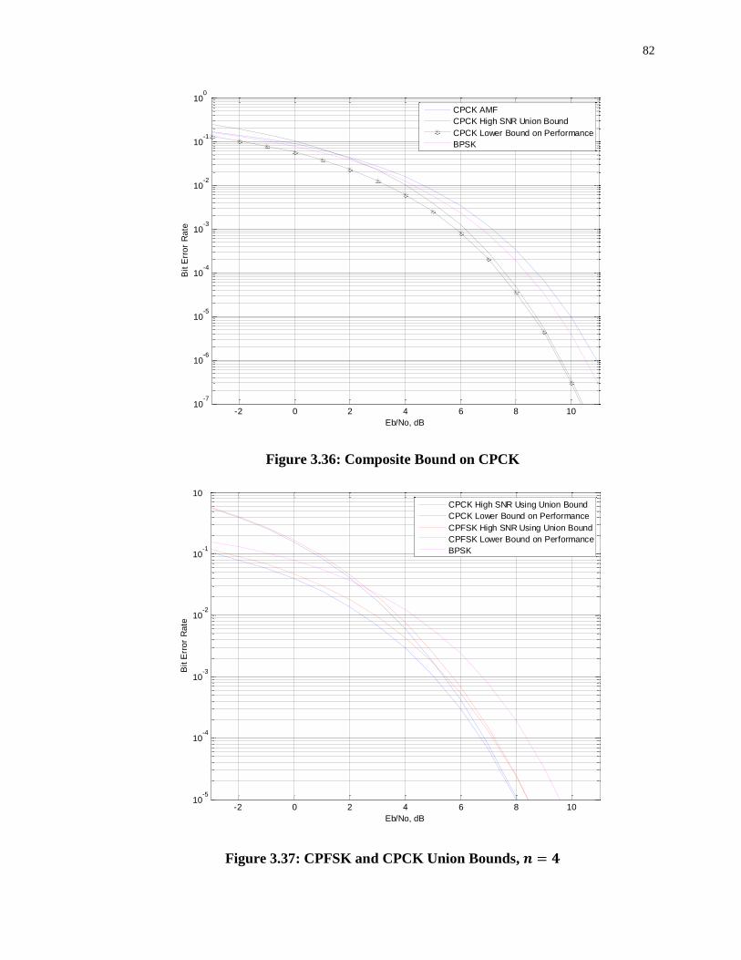
82
Figure 3.36: Composite Bound on CPCK
Figure 3.37: CPFSK and CPCK Union Bounds,
-2 0 2 4 6 8 1010
-7
10-6
10-5
10-4
10-3
10-2
10-1
100
Eb/No, dB
Bit E
rro
r R
ate
CPCK AMF
CPCK High SNR Union Bound
CPCK Lower Bound on Performance
BPSK
-2 0 2 4 6 8 1010
-5
10-4
10-3
10-2
10-1
100
Eb/No, dB
Bit E
rro
r R
ate
Bit error probability curve for HIGH SNR Approximation
CPCK High SNR Using Union Bound
CPCK Lower Bound on Performance
CPFSK High SNR Using Union Bound
CPFSK Lower Bound on Performance
BPSK
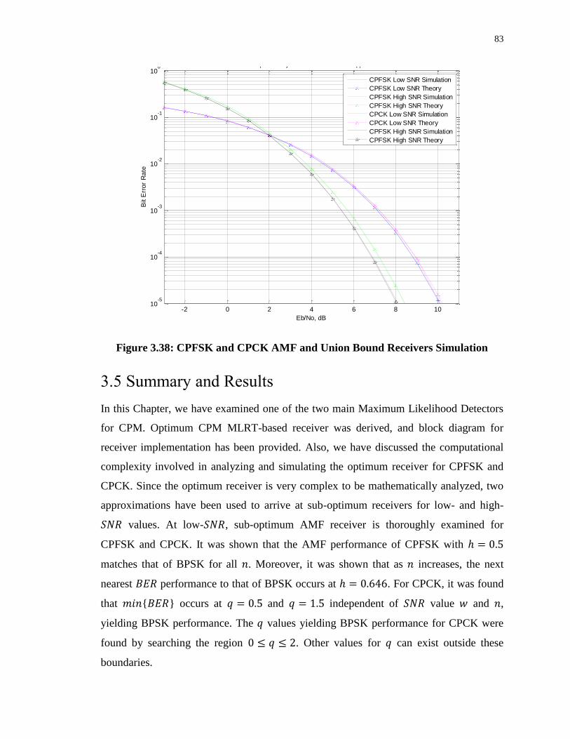
83
Figure 3.38: CPFSK and CPCK AMF and Union Bound Receivers Simulation
3.5 Summary and Results
In this Chapter, we have examined one of the two main Maximum Likelihood Detectors
for CPM. Optimum CPM MLRT-based receiver was derived, and block diagram for
receiver implementation has been provided. Also, we have discussed the computational
complexity involved in analyzing and simulating the optimum receiver for CPFSK and
CPCK. Since the optimum receiver is very complex to be mathematically analyzed, two
approximations have been used to arrive at sub-optimum receivers for low- and high-
values. At low- , sub-optimum AMF receiver is thoroughly examined for
CPFSK and CPCK. It was shown that the AMF performance of CPFSK with
matches that of BPSK for all . Moreover, it was shown that as increases, the next
nearest performance to that of BPSK occurs at . For CPCK, it was found
that { } occurs at and independent of value and ,
yielding BPSK performance. The values yielding BPSK performance for CPCK were
found by searching the region . Other values for can exist outside these
boundaries.
-2 0 2 4 6 8 1010
-5
10-4
10-3
10-2
10-1
100
Eb/No, dB
Bit E
rro
r R
ate
Bit error probability curve for HIGH SNR Approximation
CPFSK Low SNR Simulation
CPFSK Low SNR Theory
CPFSK High SNR Simulation
CPFSK High SNR Theory
CPCK Low SNR Simulation
CPCK Low SNR Theory
CPFSK High SNR Simulation
CPFSK High SNR Theory
84
Using high- approximation, sub-optimum high- receiver has been provided for
CPFSK and CPCK. This receiver has provided two bounds for CPFSK and CPCK
optimum receiver, an upper bound and a lower bound. Different plots and graphs have
been provided in both cases in order to study the relationships between and the
different modulation parameters for both CPFSK and CPCK, such as: vs. ,
vs. , vs. , vs. …etc. In general, for CPFSK and
CPCK, the performance improved as the length of the observation interval
increased. However, that amount of improvement decreased with each increment of the
observation interval length. This indicated that increasing the length of the observation
interval beyond a certain limit provided only marginal improvement and higher
receiver complexity. Moreover, for CPFSK, it has been noted that optimum performance
is achieved at for all , and near optimum performance is achieved at
for all . In addition, the difference in performance between the upper bound and the
lower bound at low- was relatively big, which means that these bounds are not tight
at low- ; however, the performance corresponding to both bounds would meet at
high- values. For CPCK, 3D plots were used in order to study the relation between
and the combinations of modulation parameters. Wherein CPFSK high- receiver the
minimum occurred at for all and values, for CPCK high- receiver,
the minimum occurs at different points for different for all values. Using the 3D
plots and their corresponding contours, the set of points where min{ } occurs were
found. The high- numerical results are best summarized in Table 3.4.
Table 3.4: Optimum CPFSK and CPCK high- Systems Parameters
CPFSK
min{ } at dB
3
4
4
CPCK
min{ } at dB
3
4
4
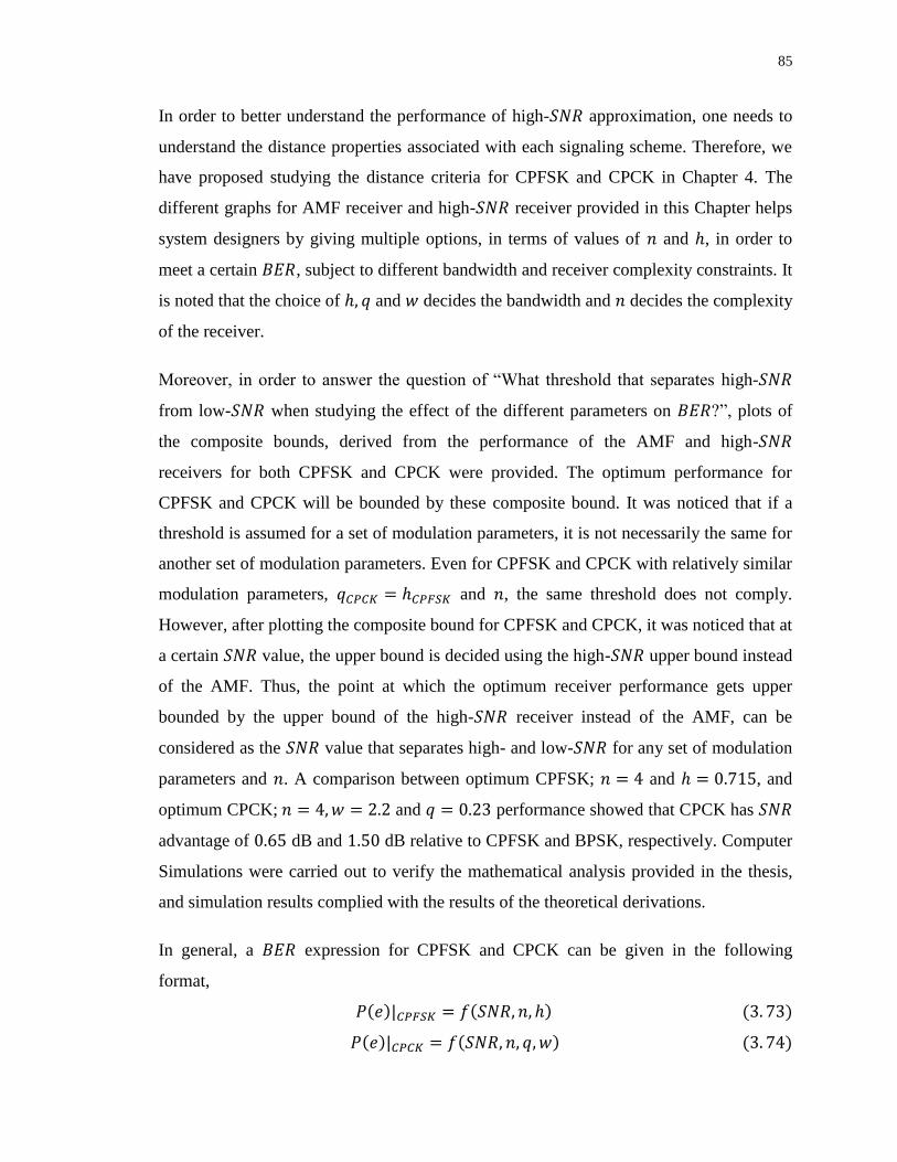
85
In order to better understand the performance of high- approximation, one needs to
understand the distance properties associated with each signaling scheme. Therefore, we
have proposed studying the distance criteria for CPFSK and CPCK in Chapter 4. The
different graphs for AMF receiver and high- receiver provided in this Chapter helps
system designers by giving multiple options, in terms of values of and , in order to
meet a certain , subject to different bandwidth and receiver complexity constraints. It
is noted that the choice of and decides the bandwidth and decides the complexity
of the receiver.
Moreover, in order to answer the question of “What threshold that separates high-
from low- when studying the effect of the different parameters on ?”, plots of
the composite bounds, derived from the performance of the AMF and high-
receivers for both CPFSK and CPCK were provided. The optimum performance for
CPFSK and CPCK will be bounded by these composite bound. It was noticed that if a
threshold is assumed for a set of modulation parameters, it is not necessarily the same for
another set of modulation parameters. Even for CPFSK and CPCK with relatively similar
modulation parameters, and , the same threshold does not comply.
However, after plotting the composite bound for CPFSK and CPCK, it was noticed that at
a certain value, the upper bound is decided using the high- upper bound instead
of the AMF. Thus, the point at which the optimum receiver performance gets upper
bounded by the upper bound of the high- receiver instead of the AMF, can be
considered as the value that separates high- and low- for any set of modulation
parameters and . A comparison between optimum CPFSK; and , and
optimum CPCK; and performance showed that CPCK has
advantage of dB and dB relative to CPFSK and BPSK, respectively. Computer
Simulations were carried out to verify the mathematical analysis provided in the thesis,
and simulation results complied with the results of the theoretical derivations.
In general, a expression for CPFSK and CPCK can be given in the following
format,
86
In addition, CPCK has been found more flexible than CPFSK, from a design point of
view, in the sense that CPCK allowed for the manipulation of more parameters, which
gave better control on the modulation scheme, and this can be inferred from Equations
3.73 and 3.74. In general, CPCK can achieve superior performances to that of
CPFSK.
87
Chapter 4
Viterbi Receiver for CPFSK and CPCK
The immense capabilities of CPM signaling techniques encouraged designers to use CPM
in many real-life communication applications; however, when it comes to demodulation
of CPM, the receiver complexity is always a huge drawback. The complexity associated
with the MLRT-based optimum receiver was examined in Chapter 3. In such a receiver,
frame-by-frame detection strategy is employed. Maximum Likelihood Detection (MLD)
Theory offers another solution for detection of CPM signals by taking advantage of the
inherent memory/sequence characteristics of CPM. Essentially, it operates using a
sequence detection strategy, which is Maximum Likelihood Sequence Estimation
(MLSE). Receivers employing MLSE are referred to as Viterbi receivers. This detection
approach is based on searching for the minimum Euclidean distance path through the
trellis that characterizes the memory in the transmitted signal. Viterbi detector is the
practical implementation of Maximum Likelihood Detection for CPFSK and CPCK
signals.
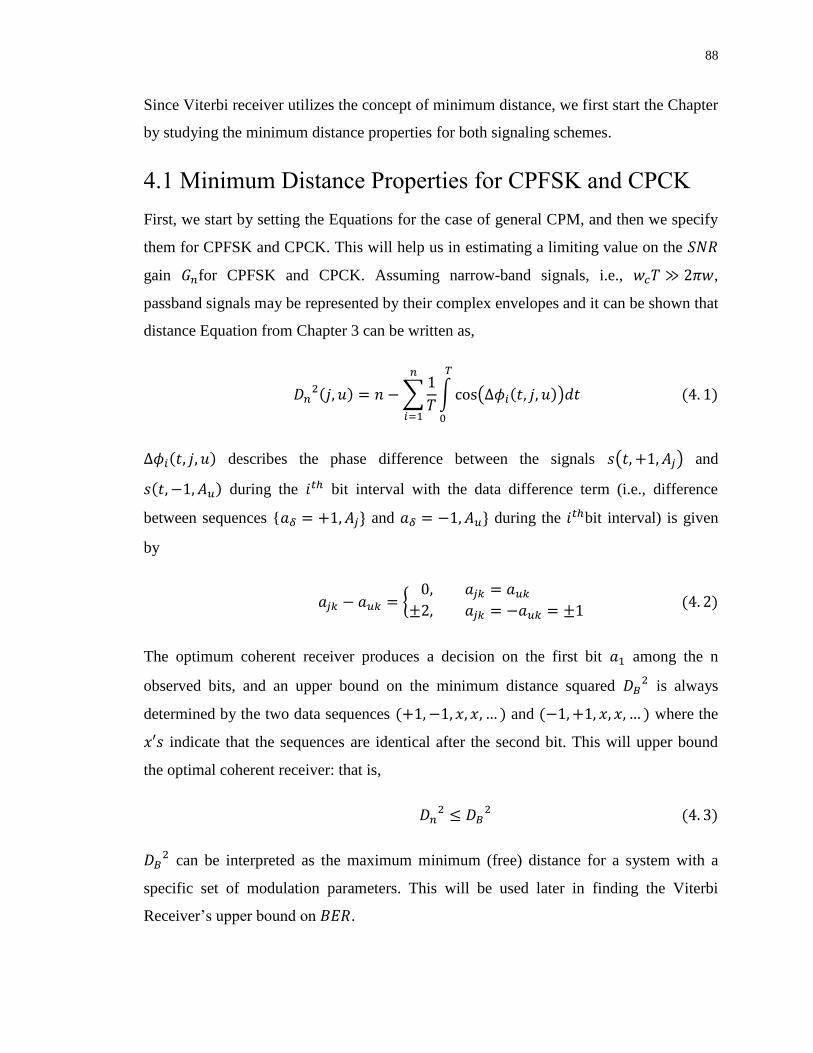
88
Since Viterbi receiver utilizes the concept of minimum distance, we first start the Chapter
by studying the minimum distance properties for both signaling schemes.
4.1 Minimum Distance Properties for CPFSK and CPCK
First, we start by setting the Equations for the case of general CPM, and then we specify
them for CPFSK and CPCK. This will help us in estimating a limiting value on the
gain for CPFSK and CPCK. Assuming narrow-band signals, i.e., ,
passband signals may be represented by their complex envelopes and it can be shown that
distance Equation from Chapter 3 can be written as,
∑
∫ ( )
describes the phase difference between the signals ( ) and
during the bit interval with the data difference term (i.e., difference
between sequences { and during the bit interval) is given
by
{
The optimum coherent receiver produces a decision on the first bit among the n
observed bits, and an upper bound on the minimum distance squared is always
determined by the two data sequences and where the
indicate that the sequences are identical after the second bit. This will upper bound
the optimal coherent receiver: that is,
can be interpreted as the maximum minimum (free) distance for a system with a
specific set of modulation parameters. This will be used later in finding the Viterbi
Receiver’s upper bound on .
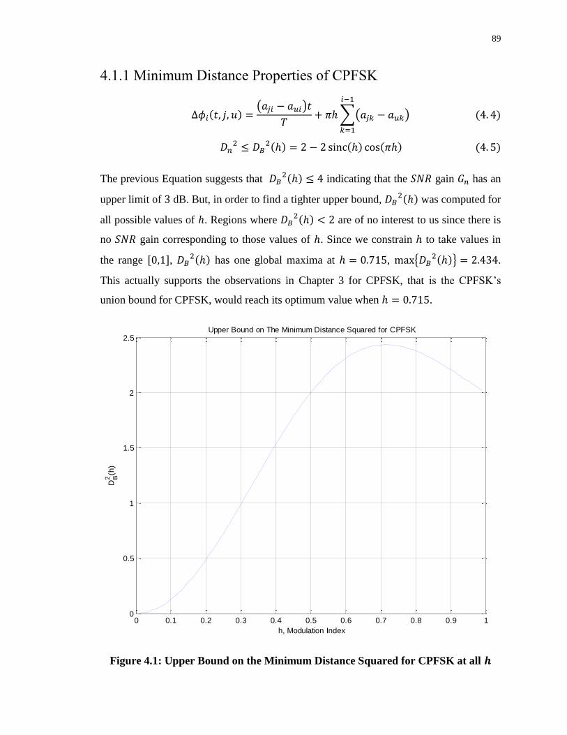
89
4.1.1 Minimum Distance Properties of CPFSK
( )
∑( )
The previous Equation suggests that indicating that the gain has an
upper limit of dB. But, in order to find a tighter upper bound, was computed for
all possible values of . Regions where are of no interest to us since there is
no gain corresponding to those values of . Since we constrain to take values in
the range , has one global maxima at , {
} .
This actually supports the observations in Chapter 3 for CPFSK, that is the CPFSK’s
union bound for CPFSK, would reach its optimum value when .
Figure 4.1: Upper Bound on the Minimum Distance Squared for CPFSK at all
0 0.1 0.2 0.3 0.4 0.5 0.6 0.7 0.8 0.9 10
0.5
1
1.5
2
2.5
h, Modulation Index
DB2
(h)
Upper Bound on The Minimum Distance Squared for CPFSK
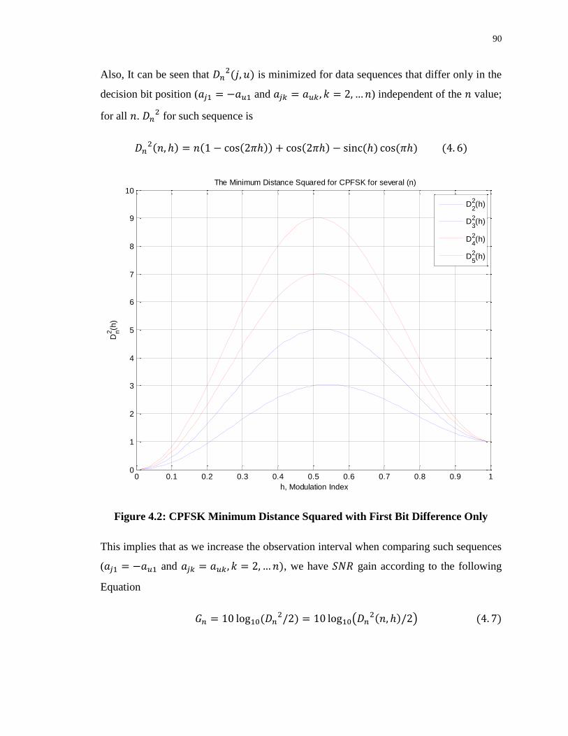
90
Also, It can be seen that is minimized for data sequences that differ only in the
decision bit position ( and ) independent of the value;
for all . for such sequence is
Figure 4.2: CPFSK Minimum Distance Squared with First Bit Difference Only
This implies that as we increase the observation interval when comparing such sequences
( and , we have gain according to the following
Equation
(
)
0 0.1 0.2 0.3 0.4 0.5 0.6 0.7 0.8 0.9 10
1
2
3
4
5
6
7
8
9
10
h, Modulation Index
Dn2(h
)
The Minimum Distance Squared for CPFSK for several (n)
D2
2(h)
D3
2(h)
D4
2(h)
D5
2(h)
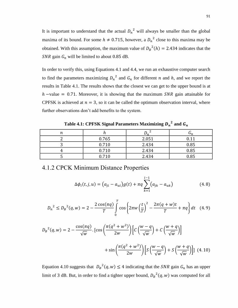
91
It is important to understand that the actual will always be smaller than the global
maxima of its bound. For some , however, a close to this maxima may be
obtained. With this assumption, the maximum value of indicates that the
gain will be limited to about dB.
In order to verify this, using Equations 4.1 and 4.4, we run an exhaustive computer search
to find the parameters maximizing and for different and , and we report the
results in Table 4.1. The results shows that the closest we can get to the upper bound is at
value . Moreover, it is showing that the maximum gain attainable for
CPFSK is achieved at , so it can be called the optimum observation interval, where
further observations don’t add benefits to the system.
Table 4.1: CPFSK Signal Parameters Maximizing and
4.1.2 CPCK Minimum Distance Properties
( ) ∑( )
∫ , (
)
-
√ (
) (
√ ) (
√ )
(
) (
√ ) (
√ )
Equation 4.10 suggests that indicating that the gain has an upper
limit of dB. But, in order to find a tighter upper bound, was computed for all
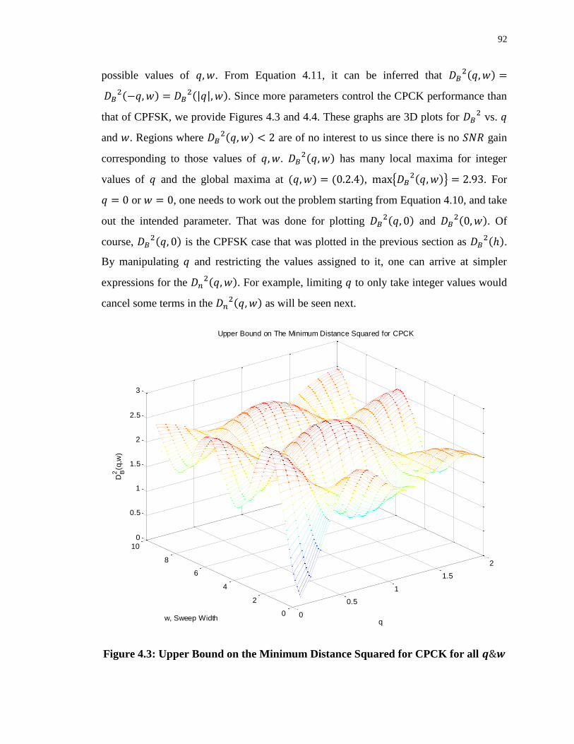
92
possible values of . From Equation 4.11, it can be inferred that
. Since more parameters control the CPCK performance than
that of CPFSK, we provide Figures 4.3 and 4.4. These graphs are 3D plots for vs.
and . Regions where are of no interest to us since there is no gain
corresponding to those values of . has many local maxima for integer
values of and the global maxima at , { } . For
or , one needs to work out the problem starting from Equation 4.10, and take
out the intended parameter. That was done for plotting and
. Of
course, is the CPFSK case that was plotted in the previous section as
.
By manipulating and restricting the values assigned to it, one can arrive at simpler
expressions for the . For example, limiting to only take integer values would
cancel some terms in the as will be seen next.
Figure 4.3: Upper Bound on the Minimum Distance Squared for CPCK for all
0
0.5
1
1.5
2
0
2
4
6
8
10
0
0.5
1
1.5
2
2.5
3
q, Modulation Index
Upper Bound on The Minimum Distance Squared for CPCK
w, Sweep Width
DB2
(q,w
)
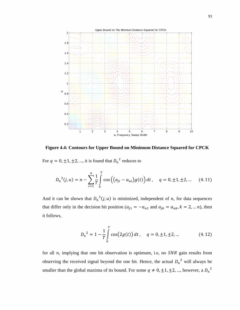
93
Figure 4.4: Contours for Upper Bound on Minimum Distance Squared for CPCK
For it is found that reduces to
∑
∫ (( ) )
And it can be shown that is minimized, independent of , for data sequences
that differ only in the decision bit position ( and ), then
it follows,
∫ ( )
for all , implying that one bit observation is optimum, i.e, no gain results from
observing the received signal beyond the one bit. Hence, the actual will always be
smaller than the global maxima of its bound. For some , however, a
w, Frequency Sweep Width
q,
Mo
du
latio
n I
nd
ex
Upper Bound on The Minimum Distance Squared for CPCK
1 2 3 4 5 6 7 8 9 10
0.2
0.4
0.6
0.8
1
1.2
1.4
1.6
1.8
2
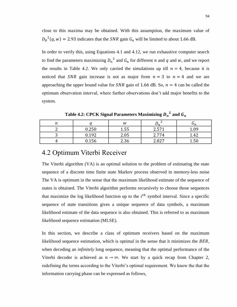
94
close to this maxima may be obtained. With this assumption, the maximum value of
indicates that the gain will be limited to about dB.
In order to verify this, using Equations 4.1 and 4.12, we run exhaustive computer search
to find the parameters maximizing and for different and and , and we report
the results in Table 4.2. We only carried the simulations up till , because it is
noticed that gain increase is not as major from to and we are
approaching the upper bound value for gain of dB. So, can be called the
optimum observation interval, where further observations don’t add major benefits to the
system.
Table 4.2: CPCK Signal Parameters Maximizing and
4.2 Optimum Viterbi Receiver
The Viterbi algorithm (VA) is an optimal solution to the problem of estimating the state
sequence of a discrete time finite state Markov process observed in memory-less noise
The VA is optimum in the sense that the maximum likelihood estimate of the sequence of
states is obtained. The Viterbi algorithm performs recursively to choose those sequences
that maximize the log likelihood function up to the symbol interval. Since a specific
sequence of state transitions gives a unique sequence of data symbols, a maximum
likelihood estimate of the data sequence is also obtained. This is referred to as maximum
likelihood sequence estimation (MLSE).
In this section, we describe a class of optimum receivers based on the maximum
likelihood sequence estimation, which is optimal in the sense that it minimizes the ,
when decoding an infinitely long sequence, meaning that the optimal performance of the
Viterbi decoder is achieved as → . We start by a quick recap from Chapter 2,
redefining the terms according to the Viterbi’s optimal requirement. We know the that the
information carrying phase can be expressed as follows,
95
∑
For and and for any symbol interval , the phase is defined by , the
correlative state vector and the phase state , where
0 ∑
1
The number of correlative states is finite and equal to . Since we are working with
full response CPM, , we don’t have a correlative state vector. For rational
modulation indices the phase tree is reduced to a phase trellis. In this Chapter, we define
the modulation index as follows
( integers) (4.15)
There are different phase states with values *
+. The total state
vector is defined by the -tuple and the number of such states is . All of these
properties are critical to the receiver structures in this section.
Usually, phase states and correlative states are assigned to the nodes in the phase tree.
The root node is arbitrarily given phase state 0. Each node in the tree is labeled with the
state . The state trellis diagram can be derived from the phase tree by viewing the
phases modulo . By folding the phase tree into a cylinder, the so-called phase cylinder
is obtained, which was illustrated in Chapter 2. The receiver observes the signal
, where the noise is AWGN. The maximum likelihood sequence
estimating (MLSE) receiver maximizes the following log likelihood function,
∫
96
with respect to the infinitely long estimated sequence . The maximizing sequence is
the maximum likelihood sequence estimate and is the probability density function
for the observed signal conditioned on the infinitely long sequence . It is equivalent
to maximize the correlation
∫
In principle, Equation 4.18 states the basic principle for a correlation receiver, in which
all possible transmitted signals are correlated with the received signal and the data
sequence maximizing the correlation is chosen as the received data. This is not a
feasible structure in practice, not even with reasonably short data bursts. That is due to
the sheer number of correlations associated with an -bit long sequence, which is
correlations. Now define
∫
Thus, we can write
where
∫
By using the above formulas it is possible to calculate the function recursively
through Equation 4.20 and the metric . This metric can be recognized as a
correlation between the received signal and an estimated signal over the symbol
interval. The possible extensions of those sequences are portrayed in the state trellis
shown in Chapter 2. The receiver computes ( ) for all possible sequences
and all possible . This makes different values of . Rewriting Equation 4.20
using Equation 4.14 yields
97
( ) ∫ [ ]
Now, it can be seen that ( ) is obtained by feeding the signal into a filter and
sampling the output of the filter at ; and that a bank of such filters must be used.
The receiver correlates the received signal over one symbol interval with all possible
transmitted alternatives over that symbol interval. By using the finite state description of
the signals, the correlation receiver can now be implemented without exponential growth
of the number of receiver signal alternatives. The noise can be expressed in the
band-pass form
Using the basic quadrature receiver of Figure 4.5, the received quadrature components
are
0√
1
0√
1
The LP-filters only remove double carrier frequency terms. Thus,
By inserting these components in ( ) and omitting double frequency terms, we
have
( ) ∫
∫
∫
∫
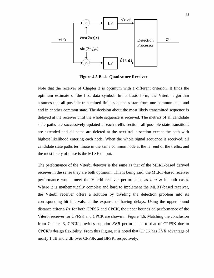
98
Figure 4.5 Basic Quadrature Receiver
Note that the receiver of Chapter 3 is optimum with a different criterion. It finds the
optimum estimate of the first data symbol. In its basic form, the Viterbi algorithm
assumes that all possible transmitted finite sequences start from one common state and
end in another common state. The decision about the most likely transmitted sequence is
delayed at the receiver until the whole sequence is received. The metrics of all candidate
state paths are successively updated at each trellis section; all possible state transitions
are extended and all paths are deleted at the next trellis section except the path with
highest likelihood entering each node. When the whole signal sequence is received, all
candidate state paths terminate in the same common node at the far end of the trellis, and
the most likely of these is the MLSE output.
The performance of the Viterbi detector is the same as that of the MLRT-based derived
receiver in the sense they are both optimum. This is being said, the MLRT-based receiver
performance would meet the Viterbi receiver performance as → in both cases.
Where it is mathematically complex and hard to implement the MLRT-based receiver,
the Viterbi receiver offers a solution by dividing the detection problem into its
corresponding bit intervals, at the expanse of having delays. Using the upper bound
distance criteria for both CPFSK and CPCK, the upper bounds on performance of the
Viterbi receiver for CPFSK and CPCK are shown in Figure 4.6. Matching the conclusion
from Chapter 3, CPCK provides superior performance to that of CPFSK due to
CPCK’s design flexibility. From this Figure, it is noted that CPCK has advantage of
nearly 1 dB and 2 dB over CPFSK and BPSK, respectively.
LP
Detection
Processor
LP
𝑟 𝑡 𝜋𝑓𝑐𝑡
𝜋𝑓𝑐𝑡
��
𝐼 𝑡 ��
�� 𝑡 ��
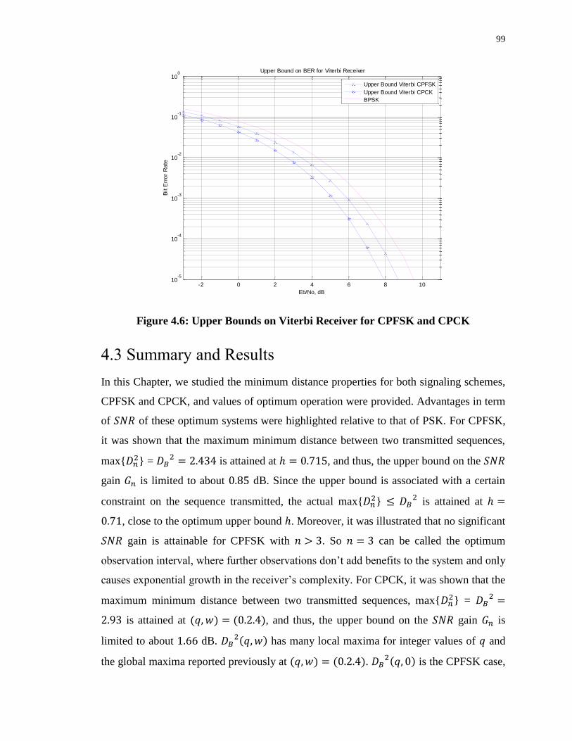
99
Figure 4.6: Upper Bounds on Viterbi Receiver for CPFSK and CPCK
4.3 Summary and Results
In this Chapter, we studied the minimum distance properties for both signaling schemes,
CPFSK and CPCK, and values of optimum operation were provided. Advantages in term
of of these optimum systems were highlighted relative to that of PSK. For CPFSK,
it was shown that the maximum minimum distance between two transmitted sequences,
max{ } =
is attained at , and thus, the upper bound on the
gain is limited to about dB. Since the upper bound is associated with a certain
constraint on the sequence transmitted, the actual max{ }
is attained at
, close to the optimum upper bound . Moreover, it was illustrated that no significant
gain is attainable for CPFSK with . So can be called the optimum
observation interval, where further observations don’t add benefits to the system and only
causes exponential growth in the receiver’s complexity. For CPCK, it was shown that the
maximum minimum distance between two transmitted sequences, max{ } =
is attained at , and thus, the upper bound on the gain is
limited to about dB. has many local maxima for integer values of and
the global maxima reported previously at . is the CPFSK case,
-2 0 2 4 6 8 1010
-5
10-4
10-3
10-2
10-1
100
Eb/No, dB
Bit E
rro
r R
ate
Upper Bound on BER for Viterbi Receiver
Upper Bound Viterbi CPFSK
Upper Bound Viterbi CPCK
BPSK
100
reported previously as . By manipulating and restricting the values assigned to
it, one can arrive at simpler expressions for the . The actual
will always be
smaller than the global maxima of its bound. For some , however, a
close to the global maxima may be obtained. Computer simulations were carried out in
order to find the parameters maximizing and for different , and . It was
noticed that gain increase is not as major from to and we are
approaching the upper bound value for gain of dB. So, was taken as the
optimum observation interval, where further observations didn’t add major benefits to the
system. gains for CPFSK and CPCK were reported at the corresponding sections.
Studying the distance properties for CPFSK and CPCK was necessary in order to prepare
for the discussion of the other type of CPM signals receiver, which is the Viterbi receiver.
The Viterbi receiver is based on the maximum-likelihood sequence estimation (MLSE)
theory, which searches for the minimum Euclidean distance path through the trellis that
characterizes the memory in the transmitted signal. Upper bounds results using Viterbi
receiver were reported for CPFSK and CPCK. Matching the conclusion from Chapter 3,
CPCK provides superior performance to that of CPFSK due to CPCK’s design
flexibility. Using the upper bound distance criteria for both CPFSK and CPCK, the
upper bounds on performance of the Viterbi receiver for optimum CPFSK; ,
and CPCK; , were found. It showed that CPCK provides superior
performance to that of CPFSK due to CPCK’s design flexibility. It was noted that CPCK
has advantage of nearly 1 dB and 2 dB over CPFSK and BPSK, respectively.
To demonstrate the complexity reduction by the Viterbi receiver, we take a simple
example. In an -long sequence, for the MLRT-based receiver, there are possibilities,
where is the modulation order, that needs to correlate the received signal with. And it
is noticed that the growth in complexity is exponential. Where in the Viterbi receiver, the
correlation process is taken down to the bit-interval level instead of the full sequence
duration-level, as in the case of MLRT-based receiver. At each bit duration, there are
correlations, where . So the total number of correlations is -multiple of .
These correlations constitute the distance metric, in which the Viterbi algorithm looks for
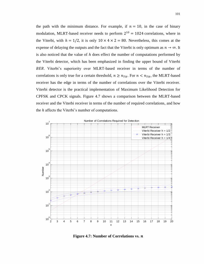
101
the path with the minimum distance. For example, if , in the case of binary
modulation, MLRT-based receiver needs to perform correlations, where in
the Viterbi, with it is only . Nevertheless, this comes at the
expense of delaying the outputs and the fact that the Viterbi is only optimum as → . It
is also noticed that the value of does effect the number of computations performed by
the Viterbi detector, which has been emphasized in finding the upper bound of Viterbi
. Viterbi’s superiority over MLRT-based receiver in terms of the number of
correlations is only true for a certain threshold, . For , the MLRT-based
receiver has the edge in terms of the number of correlations over the Viterbi receiver.
Viterbi detector is the practical implementation of Maximum Likelihood Detection for
CPFSK and CPCK signals. Figure 4.7 shows a comparison between the MLRT-based
receiver and the Viterbi receiver in terms of the number of required correlations, and how
the affects the Viterbi’s number of computations.
Figure 4.7: Number of Correlations vs.
2 3 4 5 6 7 8 9 10 11 12 13 14 15 16 17 18 19 2010
0
101
102
103
104
105
106
107
n
Num
ber
Number of Correlations Required for Detection
MLRT Receiver
Viterbi Receiver h = 1/2
Viterbi Receiver h = 1/3
Viterbi Receiver h = 1/4
102
Chapter 5
Decision Aided Detection of CPFSK and
CPCK
The successful application of CPFSK and CPCK signaling techniques for reliable
transmission of digital data over communication channels requires complex signal
processing techniques. Both CPFSK and CPCK offer tradeoffs among power, bandwidth
and signal processing complexity. It is evident from Chapters 3 and 4 that receivers for
these signaling techniques are quite complex and the complexity grows exponentially
with the number of observed symbols in the detection process. Therefore, it is of interest
to explore alternative receivers that are less complex and yet perform close to that of the
optimum. Thus, the intent of this Chapter is to present a Decision Aided Receiver (DAR)
based on heuristics as an alternative for the AMF receiver that is optimum at low values
of . Decision aided detection strategy is presented and explicit expressions for
computation of are developed for AWGN environment.
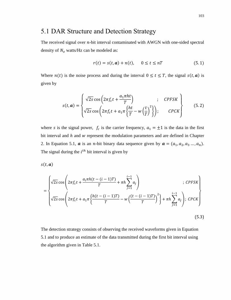
103
5.1 DAR Structure and Detection Strategy
The received signal over -bit interval contaminated with AWGN with one-sided spectral
density of watts/Hz can be modeled as:
Where is the noise process and during the interval , the signal is
given by
{
√ (
)
√ ( ,
(
)
-) }
where is the signal power, is the carrier frequency, is the data in the first
bit interval and and represent the modulation parameters and are defined in Chapter
2. In Equation 5.1, is an -bit binary data sequence given by 3 .
The signal during the bit interval is given by
{
√ .
∑
/
√ . ,
(
)
- ∑
/
}
(5.3)
The detection strategy consists of observing the received waveforms given in Equation
5.1 and to produce an estimate of the data transmitted during the first bit interval using
the algorithm given in Table 5.1.
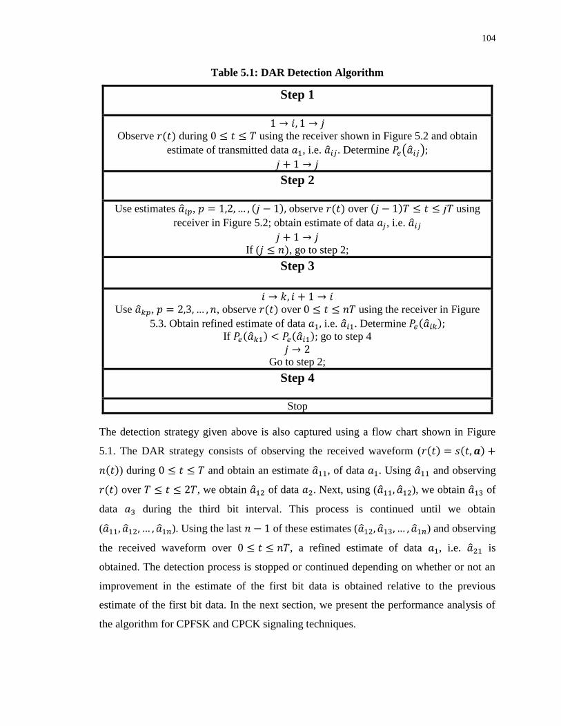
104
Table 5.1: DAR Detection Algorithm
Step 1
→ → Observe during using the receiver shown in Figure 5.2 and obtain
estimate of transmitted data , i.e. . Determine ( )
→
Step 2
Use estimates , observe over using
receiver in Figure 5.2; obtain estimate of data , i.e.
→ If ( , go to step 2;
Step 3
→ → Use , , observe over using the receiver in Figure
5.3. Obtain refined estimate of data i.e. . Determine If go to step 4
→ Go to step 2;
Step 4
Stop
The detection strategy given above is also captured using a flow chart shown in Figure
5.1. The DAR strategy consists of observing the received waveform (
) during and obtain an estimate , of data . Using and observing
over , we obtain of data . Next, using ( ), we obtain 3 of
data 3 during the third bit interval. This process is continued until we obtain
( ). Using the last of these estimates ( 3 ) and observing
the received waveform over , a refined estimate of data , i.e. is
obtained. The detection process is stopped or continued depending on whether or not an
improvement in the estimate of the first bit data is obtained relative to the previous
estimate of the first bit data. In the next section, we present the performance analysis of
the algorithm for CPFSK and CPCK signaling techniques.
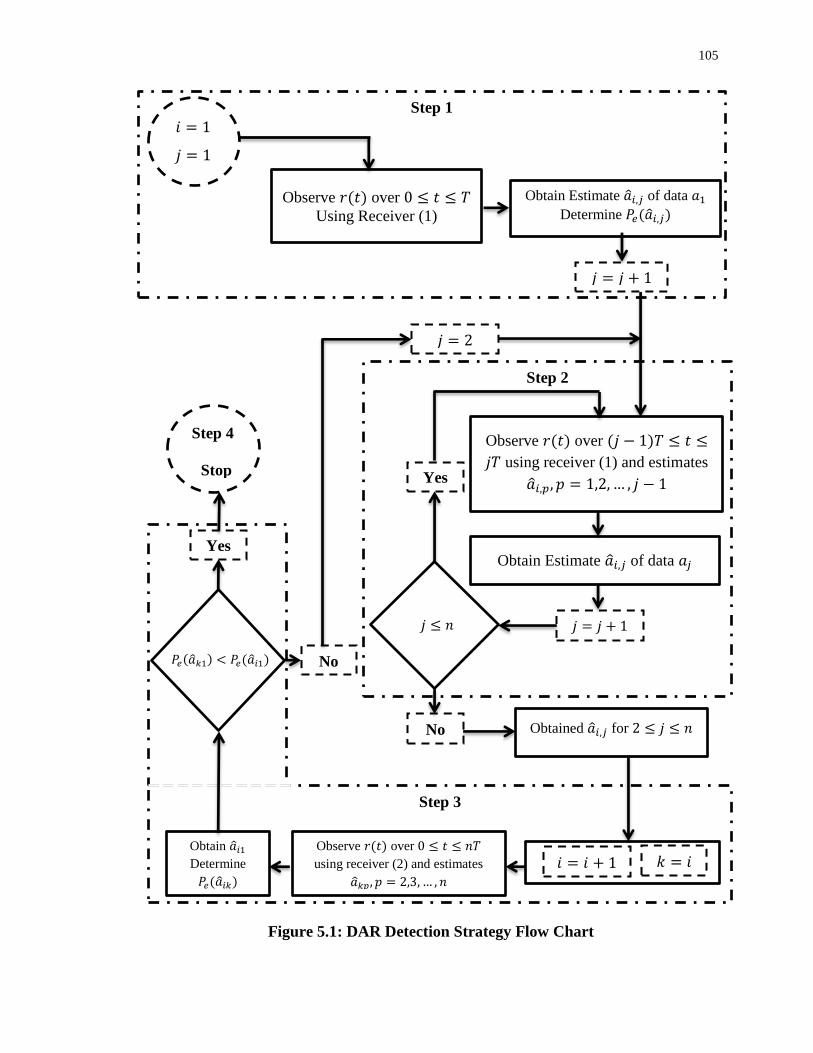
105
Figure 5.1: DAR Detection Strategy Flow Chart
𝑃𝑒 ��𝑘 𝑃𝑒 ��𝑖
Yes
No
��𝑖 𝑝 𝑝 𝑗
Observe 𝑟 𝑡 over 𝑗 𝑇 𝑡
𝑗𝑇 using receiver (1) and estimates
Obtain Estimate ��𝑖 𝑗 of data 𝑎𝑗
𝑗 𝑗 𝑗 𝑛
Yes
Obtained ��𝑖 𝑗 for 𝑗 𝑛 No
𝑘 𝑖 𝑖 𝑖
��𝑘𝑝 𝑝 𝑛
Observe 𝑟 𝑡 over 𝑡 𝑛𝑇
using receiver (2) and estimates
Obtain ��𝑖
Determine
𝑃𝑒 ��𝑖𝑘
Step 2
𝑗 𝑗
Step 1
𝑖
𝑗
Observe 𝑟 𝑡 over 𝑡 𝑇
Using Receiver (1)
Obtain Estimate ��𝑖 𝑗 of data 𝑎
Determine 𝑃𝑒 ��𝑖 𝑗
Step 3
Step 4
𝑗
Stop
106
Figure 5.2: DAR for Obtaining Estimates and
Figure 5.3: DAR for Obtaining Refined Estimates
5.2 Performance Analysis of DAR
The receiver shown in Figure 5.2 is used to obtain the first set of estimates. The
received waveform during the first bit interval is correlated with the reference signal
( for the first bit interval) to generate , which is given by
∫ 𝑑𝑡
𝑗𝑇
𝑗 𝑇
𝑖𝑗
��𝑖𝑗
��𝑖𝑗
𝑟 𝑡
√ 𝑠 ( 𝜋𝑓𝑐𝑡 𝜙 𝑡 ) √ 𝑠 ( 𝜋𝑓𝑐𝑡 𝜙 𝑡 )
𝜙 𝑡 𝑔 𝑡 𝑗 𝑇 𝑔 𝑡 𝑇 ∑ ��𝑞
𝑗
𝑞
∫ 𝑑𝑡
𝑛𝑇
∑
𝑛
𝑗
𝑟 𝑡
𝑠 𝑡 𝑏 ��𝑖 ��𝑖 ��𝑖𝑛
𝑠 𝑡 𝑏 ��𝑖 ��𝑖 ��𝑖𝑛
∫ 𝑑𝑡
𝑛𝑇
∑
𝑛
𝑗
𝑖 ′
��𝑖+1 1
��𝑖+1 1
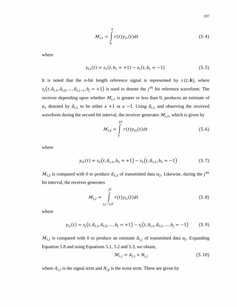
107
∫
where
It is noted that the -bit length reference signal is represented by , where
( ) is used to denote the bit reference waveform. The
receiver depending upon whether is greater or less than 0, produces an estimate of
denoted by to be either a or a . Using and observing the received
waveform during the second bit interval, the receiver generates , which is given by
∫
where
( ) ( )
is compared with 0 to produce of transmitted data . Likewise, during the
bit interval, the receiver generates
∫
where
( ) ( )
is compared with 0 to produce an estimate of transmitted data . Expanding
Equation 5.8 and using Equations 5.1, 5.2 and 5.3, we obtain,
where is the signal term and is the noise term. These are given by
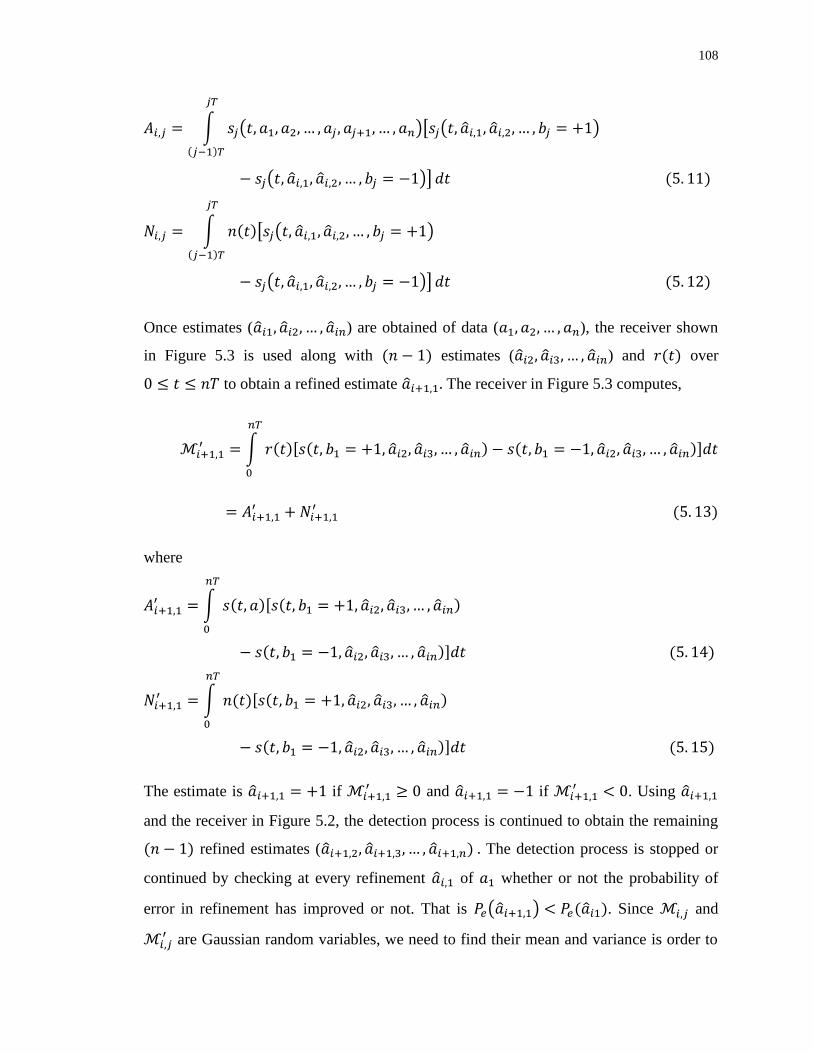
108
∫ ( )[ ( )
( )]
∫ [ ( )
( )]
Once estimates ( ) are obtained of data ( ), the receiver shown
in Figure 5.3 is used along with estimates ( 3 ) and over
to obtain a refined estimate The receiver in Figure 5.3 computes,
′ ∫ 3 3
′
′
where
′ ∫ 3
3
′ ∫ 3
3
The estimate is if ′ and if
′ . Using
and the receiver in Figure 5.2, the detection process is continued to obtain the remaining
refined estimates ( 3 The detection process is stopped or
continued by checking at every refinement of whether or not the probability of
error in refinement has improved or not. That is ( ) . Since and
′ are Gaussian random variables, we need to find their mean and variance is order to
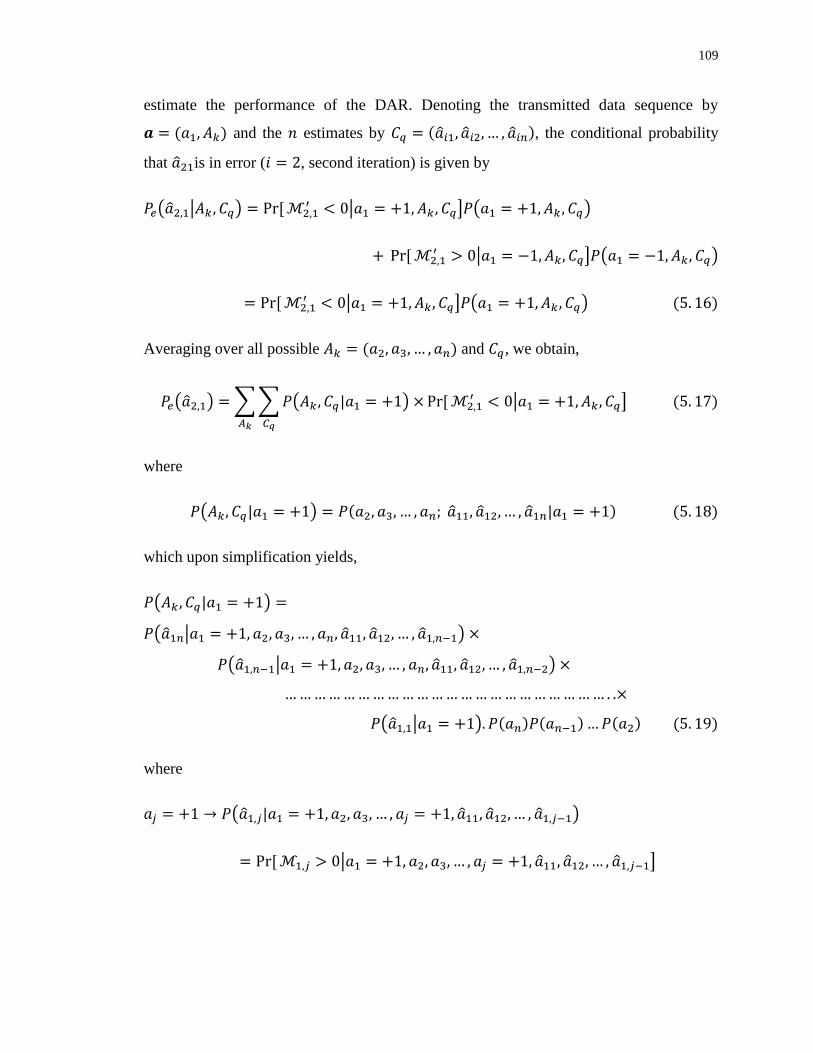
109
estimate the performance of the DAR. Denoting the transmitted data sequence by
and the estimates by , the conditional probability
that is in error ( , second iteration) is given by
( | ) ′ | ] ( )
′ | ] ( )
′ | ] ( )
Averaging over all possible 3 and , we obtain,
( ) ∑ ∑ ( )
′ | ]
where
( ) 3
which upon simplification yields,
( )
( | 3 )
( | 3 )
( | )
where
→ ( 3 )
| 3 ]
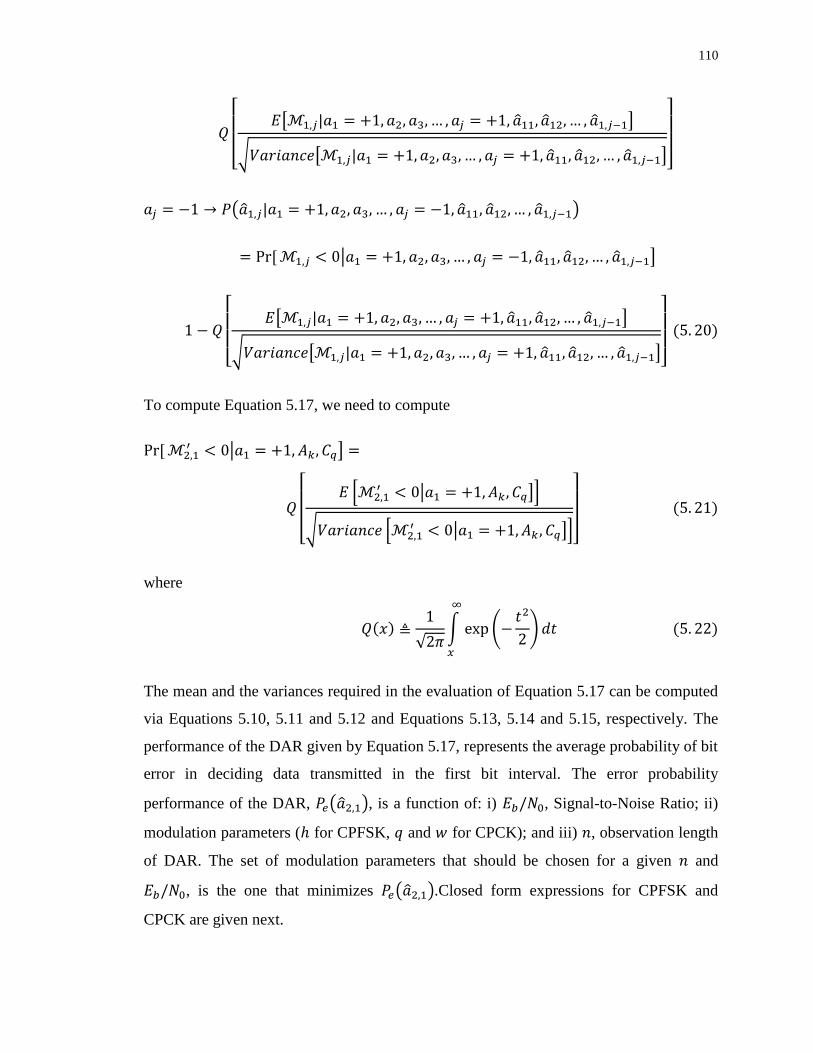
110
[
[ 3 ]
√ [ 3 ]]
→ ( 3 )
| 3 ]
[
[ 3 ]
√ [ 3 ]]
To compute Equation 5.17, we need to compute
′ | ]
[ *
′ | ]+
√ * ′ | ]+]
where
√ ∫ (
)
The mean and the variances required in the evaluation of Equation 5.17 can be computed
via Equations 5.10, 5.11 and 5.12 and Equations 5.13, 5.14 and 5.15, respectively. The
performance of the DAR given by Equation 5.17, represents the average probability of bit
error in deciding data transmitted in the first bit interval. The error probability
performance of the DAR, ( ), is a function of: i) , Signal-to-Noise Ratio; ii)
modulation parameters ( for CPFSK, and for CPCK); and iii) , observation length
of DAR. The set of modulation parameters that should be chosen for a given and
, is the one that minimizes ( ).Closed form expressions for CPFSK and
CPCK are given next.
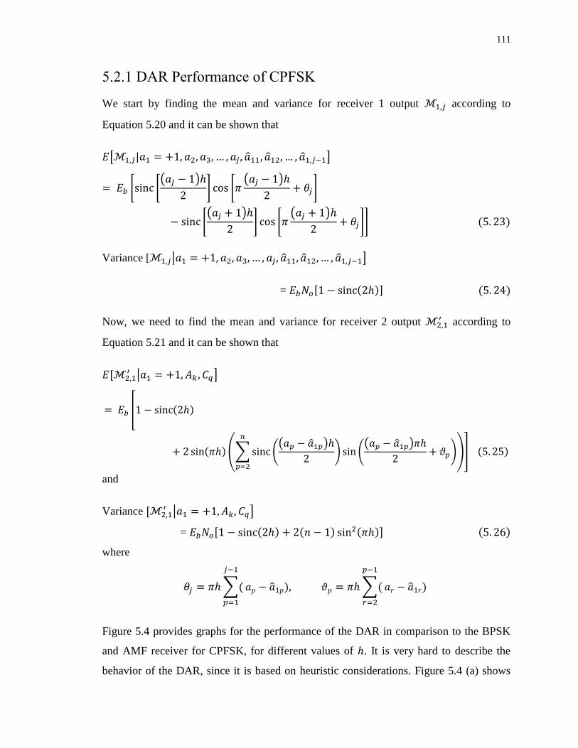
111
5.2.1 DAR Performance of CPFSK
We start by finding the mean and variance for receiver 1 output according to
Equation 5.20 and it can be shown that
[ 3 ]
* *( )
+ *
( )
+
*( )
+ *
( )
++
Variance [ | 3 ]
=
Now, we need to find the mean and variance for receiver 2 output ′ according to
Equation 5.21 and it can be shown that
′ | ]
0
.∑ (( )
) (
( )
)
/1
and
Variance ′ | ]
=
where
∑
∑
Figure 5.4 provides graphs for the performance of the DAR in comparison to the BPSK
and AMF receiver for CPFSK, for different values of . It is very hard to describe the
behavior of the DAR, since it is based on heuristic considerations. Figure 5.4 (a) shows
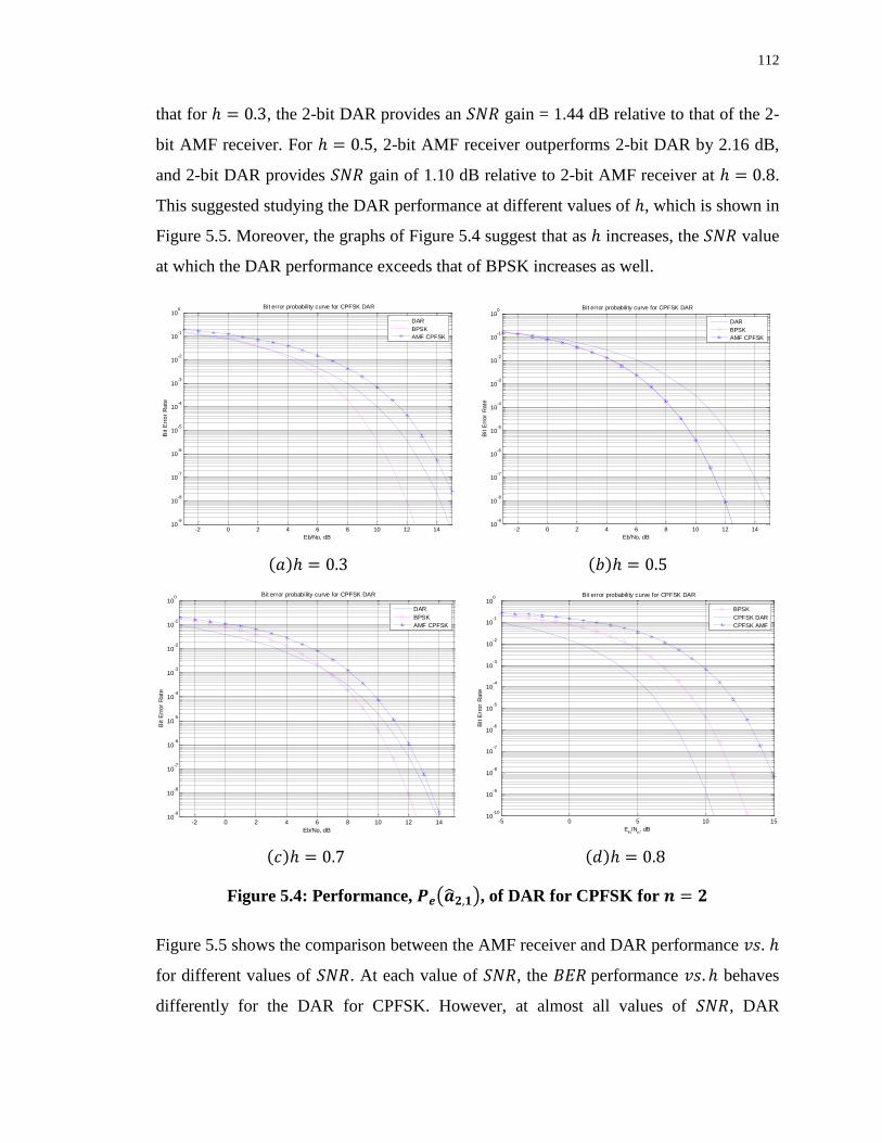
112
that for , the 2-bit DAR provides an gain = 1.44 dB relative to that of the 2-
bit AMF receiver. For , 2-bit AMF receiver outperforms 2-bit DAR by 2.16 dB,
and 2-bit DAR provides gain of 1.10 dB relative to 2-bit AMF receiver at .
This suggested studying the DAR performance at different values of , which is shown in
Figure 5.5. Moreover, the graphs of Figure 5.4 suggest that as increases, the value
at which the DAR performance exceeds that of BPSK increases as well.
Figure 5.4: Performance, ( ), of DAR for CPFSK for
Figure 5.5 shows the comparison between the AMF receiver and DAR performance
for different values of . At each value of , the performance behaves
differently for the DAR for CPFSK. However, at almost all values of , DAR
-2 0 2 4 6 8 10 12 1410
-9
10-8
10-7
10-6
10-5
10-4
10-3
10-2
10-1
100
Eb/No, dB
Bit E
rro
r R
ate
Bit error probability curve for CPFSK DAR
DAR
BPSK
AMF CPFSK
-2 0 2 4 6 8 10 12 1410
-9
10-8
10-7
10-6
10-5
10-4
10-3
10-2
10-1
100
Eb/No, dB
Bit E
rro
r R
ate
Bit error probability curve for CPFSK DAR
DAR
BPSK
AMF CPFSK
-2 0 2 4 6 8 10 12 1410
-9
10-8
10-7
10-6
10-5
10-4
10-3
10-2
10-1
100
Eb/No, dB
Bit E
rro
r R
ate
Bit error probability curve for CPFSK DAR
DAR
BPSK
AMF CPFSK
-5 0 5 10 1510
-10
10-9
10-8
10-7
10-6
10-5
10-4
10-3
10-2
10-1
100 Bit error probability curve for CPFSK DAR
Bit E
rro
r R
ate
Eb/N
o, dB
BPSK
CPFSK DAR
CPFSK AMF
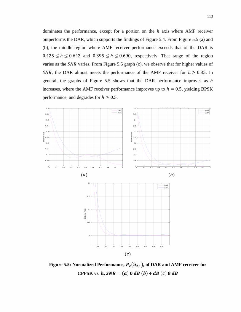
113
dominates the performance, except for a portion on the axis where AMF receiver
outperforms the DAR, which supports the findings of Figure 5.4. From Figure 5.5 (a) and
(b), the middle region where AMF receiver performance exceeds that of the DAR is
and , respectively. That range of the region
varies as the varies. From Figure 5.5 graph (c), we observe that for higher values of
, the DAR almost meets the performance of the AMF receiver for . In
general, the graphs of Figure 5.5 shows that the DAR performance improves as
increases, where the AMF receiver performance improves up to , yielding BPSK
performance, and degrades for
Figure 5.5: Normalized Performance, ( ), of DAR and AMF receiver for
CPFSK vs. ,
0 0.1 0.2 0.3 0.4 0.5 0.6 0.7 0.8 0.9 10
0.05
0.1
0.15
0.2
0.25
0.3
0.35
0.4
0.45
0.5
Eb/No, dB
Bit E
rro
r R
ate
BER for CPFSK DAR and AMV vs h
DAR
AMF
0 0.1 0.2 0.3 0.4 0.5 0.6 0.7 0.8 0.9 10
0.05
0.1
0.15
0.2
0.25
0.3
0.35
0.4
0.45
0.5
Eb/No, dB
Bit E
rro
r R
ate
BER for CPFSK DAR and AMV vs h
DAR
AMF
0.1 0.2 0.3 0.4 0.5 0.6 0.7 0.8 0.9
0
0.05
0.1
0.15
0.2
Eb/No, dB
Bit E
rro
r R
ate
BER for CPFSK DAR and AMV vs h
DAR
AMF
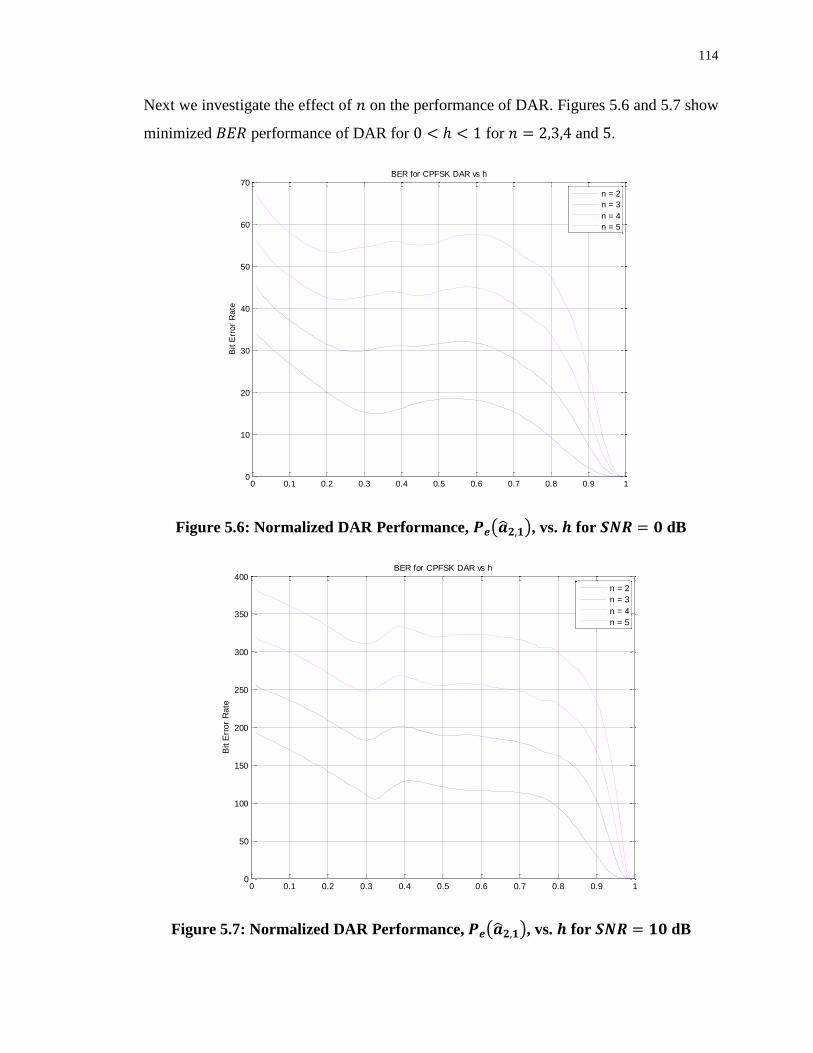
114
Next we investigate the effect of on the performance of DAR. Figures 5.6 and 5.7 show
minimized performance of DAR for for and .
Figure 5.6: Normalized DAR Performance, ( ), vs. for dB
Figure 5.7: Normalized DAR Performance, ( ), vs. for dB
0 0.1 0.2 0.3 0.4 0.5 0.6 0.7 0.8 0.9 10
10
20
30
40
50
60
70
Eb/No, dB
Bit E
rro
r R
ate
BER for CPFSK DAR vs h
n = 2
n = 3
n = 4
n = 5
0 0.1 0.2 0.3 0.4 0.5 0.6 0.7 0.8 0.9 10
50
100
150
200
250
300
350
400
Eb/No, dB
Bit E
rro
r R
ate
BER for CPFSK DAR vs h
n = 2
n = 3
n = 4
n = 5
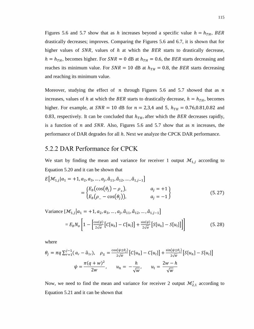
115
Figures 5.6 and 5.7 show that as increases beyond a specific value ,
drastically decreases; improves. Comparing the Figures 5.6 and 6.7, it is shown that for
higher values of , values of at which the starts to drastically decrease,
, becomes higher. For dB at , the starts decreasing and
reaches its minimum value. For dB at , the starts decreasing
and reaching its minimum value.
Moreover, studying the effect of through Figures 5.6 and 5.7 showed that as
increases, values of at which the starts to drastically decrease, , becomes
higher. For example, at dB for and , and
, respectively. It can be concluded that after which the decreases rapidly,
is a function of and . Also, Figures 5.6 and 5.7 show that as increases, the
performance of DAR degrades for all . Next we analyze the CPCK DAR performance.
5.2.2 DAR Performance for CPCK
We start by finding the mean and variance for receiver 1 output according to
Equation 5.20 and it can be shown that
[ 3 ]
, ( ( )
)
( ( ))
-
Variance [ | 3 ]
= *
√ [ ]
√ [ ] +
where
∑ ,
( )
√ [ ]
( )
√ [ ]
√
√
Now, we need to find the mean and variance for receiver 2 output ′ according to
Equation 5.21 and it can be shown that
116
′ | ]
*
√ [ ]
√ [ ] |
+
and
Variance ′ | ]
= *
√ [ ]
√ [ ] +
where
|
∑ ∫ . [
(
)
] /
∑
2
3
|
√ [ ]
√ [ ]
√
√
In all cases, and are the Fresnel integrals, which require numerical evaluation,
and are given by
∫ (
)
∫ (
)
The performance of the DAR for observation lengths , and sec are shown in
Figure 5.8(a), (b) and (c), respectively, for optimum CPCK systems. Also, in the same
figure are shown performances of corresponding AMF receiver for these optimum CPCK
systems. From Fig. 3(a), it is observed that 2-bit DAR provides an gain of 4.57 dB
relative to that of the 2-bit AMF receiver, for optimum CPCK ( ).
However, with the latter receiver, decision about the data is available after secs,
117
whereas with DAR decision is available only after secs. gains of nearly and
dB are observed for and , respectively, when optimum CPCK systems
are employed. By going to and observations from , the performance of the
DAR becomes better, for optimum CPCK systems.
Figure 5.8: Performance, ( ), of DAR for optimum CPCK systems, for (a)
, (b) and (c)
-5 0 5 10 1510
-10
10-9
10-8
10-7
10-6
10-5
10-4
10-3
10-2
10-1
100
Eb/No, dB
Bit E
rro
r R
ate
Bit error probability curve for DAR
AMF CPCK
DAR CPCK
-5 0 5 10 1510
-10
10-9
10-8
10-7
10-6
10-5
10-4
10-3
10-2
10-1
100
Eb/No, dB
Bit E
rro
r R
ate
Bit error probability curve for DAR
AMF CPCK
DAR CPCK
-5 0 5 10 1510
-10
10-9
10-8
10-7
10-6
10-5
10-4
10-3
10-2
10-1
100
Eb/No, dB
Bit E
rro
r R
ate
Bit error probability curve for DAR
AMF CPCK
DAR CPCK
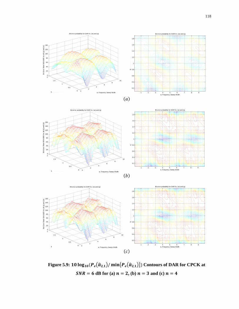
118
Figure 5.9: ( ) { ( )} Contours of DAR for CPCK at
dB for (a) , (b) and (c)
0
2
4
6
8
10
0
0.5
1
1.5
2
0
20
40
60
80
100
120
140
w, Frequency Sweep Width
Bit error probability for DAR Vs. (w) and (q)
q, Modulation Index
Bit E
rro
r R
ate
/ M
IN B
ER
for
all
(q)
an
d (
w)
w, Frequency Sweep Width
q,
Mo
du
latio
n I
nd
ex
Bit error probability for DAR Vs. (w) and (q)
1 2 3 4 5 6 7 8 9
0.2
0.4
0.6
0.8
1
1.2
1.4
1.6
1.8
0
2
4
6
8
10
0
0.5
1
1.5
2
0
20
40
60
80
100
120
140
160
w, Frequency Sweep Width
Bit error probability for DAR Vs. (w) and (q)
q, Modulation Index
Bit E
rro
r R
ate
/ M
IN B
ER
for
all
(q)
an
d (
w)
w, Frequency Sweep Width
q,
Mo
du
latio
n I
nd
ex
Bit error probability for DAR Vs. (w) and (q)
1 2 3 4 5 6 7 8 9
0.2
0.4
0.6
0.8
1
1.2
1.4
1.6
1.8
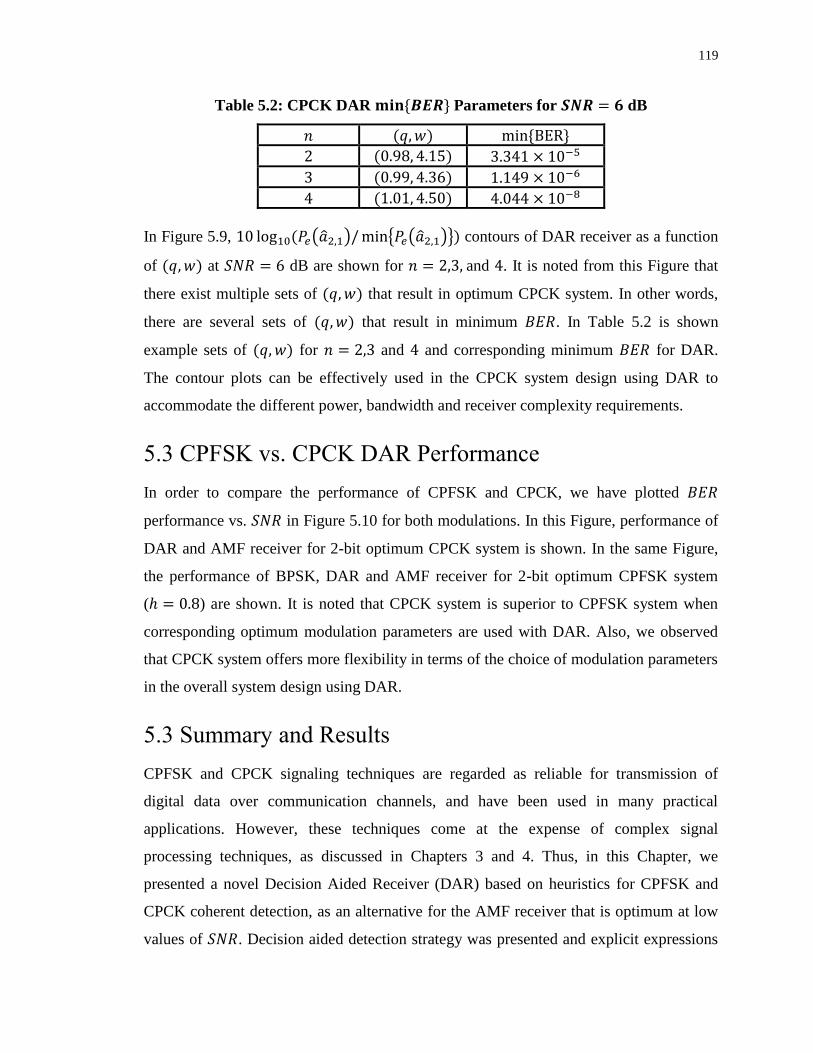
119
Table 5.2: CPCK DAR Parameters for dB
5
6
In Figure 5.9, ( ) { ( )} contours of DAR receiver as a function
of at dB are shown for and . It is noted from this Figure that
there exist multiple sets of that result in optimum CPCK system. In other words,
there are several sets of that result in minimum . In Table 5.2 is shown
example sets of for and and corresponding minimum for DAR.
The contour plots can be effectively used in the CPCK system design using DAR to
accommodate the different power, bandwidth and receiver complexity requirements.
5.3 CPFSK vs. CPCK DAR Performance
In order to compare the performance of CPFSK and CPCK, we have plotted
performance vs. in Figure 5.10 for both modulations. In this Figure, performance of
DAR and AMF receiver for 2-bit optimum CPCK system is shown. In the same Figure,
the performance of BPSK, DAR and AMF receiver for 2-bit optimum CPFSK system
( ) are shown. It is noted that CPCK system is superior to CPFSK system when
corresponding optimum modulation parameters are used with DAR. Also, we observed
that CPCK system offers more flexibility in terms of the choice of modulation parameters
in the overall system design using DAR.
5.3 Summary and Results
CPFSK and CPCK signaling techniques are regarded as reliable for transmission of
digital data over communication channels, and have been used in many practical
applications. However, these techniques come at the expense of complex signal
processing techniques, as discussed in Chapters 3 and 4. Thus, in this Chapter, we
presented a novel Decision Aided Receiver (DAR) based on heuristics for CPFSK and
CPCK coherent detection, as an alternative for the AMF receiver that is optimum at low
values of . Decision aided detection strategy was presented and explicit expressions
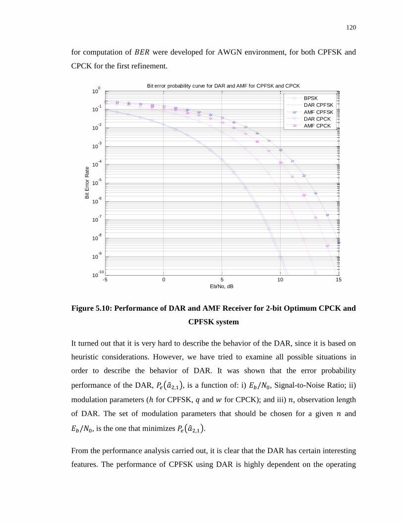
120
for computation of were developed for AWGN environment, for both CPFSK and
CPCK for the first refinement.
Figure 5.10: Performance of DAR and AMF Receiver for 2-bit Optimum CPCK and
CPFSK system
It turned out that it is very hard to describe the behavior of the DAR, since it is based on
heuristic considerations. However, we have tried to examine all possible situations in
order to describe the behavior of DAR. It was shown that the error probability
performance of the DAR, ( ), is a function of: i) , Signal-to-Noise Ratio; ii)
modulation parameters ( for CPFSK, and for CPCK); and iii) , observation length
of DAR. The set of modulation parameters that should be chosen for a given and
, is the one that minimizes ( ).
From the performance analysis carried out, it is clear that the DAR has certain interesting
features. The performance of CPFSK using DAR is highly dependent on the operating
-5 0 5 10 1510
-10
10-9
10-8
10-7
10-6
10-5
10-4
10-3
10-2
10-1
100
Eb/No, dB
Bit E
rro
r R
ate
Bit error probability curve for DAR and AMF for CPFSK and CPCK
BPSK
DAR CPFSK
AMF CPFSK
DAR CPCK
AMF CPCK
121
value of and also is sensitive to the value of . However, at most values of ,
DAR outperforms the corresponding AMF receiver, except for a small range of for
which AMF receiver outperforms DAR. For example, at dB the middle region
where AMF receiver performance exceeds that of the DAR is , and
for dB. That range of the region varies as the varies.
Moreover, it was observed that for higher values of , the DAR almost meets the
performance of the AMF receiver for . In general, the DAR performance
improves as increases, where the AMF receiver performance improves up to ,
yielding BPSK performance, and degrades for
In addition, it was illustrated that as increases beyond a specific value ,
drastically decreases. It was shown that for higher values of , values of at which
the starts to drastically decrease, , becomes higher. For example, the
starts decreasing drastically at dB for , and for
at dB.
Moreover, studying the effect of on the performance showed that as increases,
values of at which the starts to drastically decrease, , becomes higher. For
example, at dB for and , and ,
respectively. So, it was concluded that after which the decreases rapidly, is a
function of and .
Analyzing optimum CPFSK system using DAR showed that 2-bit DAR provides an
gain of 5.63 dB relative to that of the 2-bit AMF receiver, for optimum CPFSK (
). gains of nearly and dB are observed for and , respectively,
when optimum CPFSK systems are employed. By going to and observations from
, the performance of the DAR becomes better, for optimum CPFSK systems.
Analyzing optimum CPCK system using DAR showed that 2-bit DAR provides an
gain of 4.57 dB relative to that of the 2-bit AMF receiver, for optimum CPCK (
). However, with the latter receiver, decision about the data is available
after secs, whereas with DAR decision is available only after secs. gains of
122
nearly and dB are observed for and , respectively, when optimum
CPCK systems are employed. By going to and observations from , the
performance of the DAR becomes better, for optimum CPCK systems.
Contours of DAR receiver as a function of at dB for and
showed that there exist multiple sets of that result in optimum CPCK system. In
other words, there are several sets of that result in minimum . These contour
plots can be effectively used in the CPCK system design using DAR to accommodate the
different power, bandwidth and receiver complexity requirements.
Finally, the Chapter was concluded with a comparison between optimum CPFSK and
CPCK systems. It was noted that CPCK system is superior to CPFSK system when
corresponding optimum modulation parameters are used with DAR. Also, we observed
that CPCK system offers more flexibility in terms of the choice of modulation parameters
in the overall system design using DAR.
In general, it can be concluded that DAR outperforms the corresponding AMF receiver
for both CPFSK and CPCK, but with certain restrictions on the modulation parameters
used.
123
Chapter 6
Conclusions
In this thesis, we investigated the detection strategies, receivers and their performance of
two subclasses of CPM modulation called Continuous Phase Frequency Shift Keying
(CPFSK) and Continuous Phase Chirp Keying (CPCK) for data communication. This
chapter summarizes the contributions made in this thesis and the conclusions from the
results obtained. It also discusses some important issues and the scope for future research
as determined by projected demands of DCS.
6.1 Summary of Contributions
In Chapter 2, the concept, mathematical descriptions and properties of CPM signals
were presented in detail. Moreover, the mathematical frame work required for the
development of Continuous Phase Chirp Keying (CPCK) and Continuous Phase
Frequency Shift Keying (CPFSK) signaling techniques was provided. It has been
demonstrated that the main difference between CPFSK and CPCK is the way the
frequency changes within the bit interval, which is due to the properties associated
124
with the different phase functions used by each signaling technique. Phase functions,
frequency functions, phase trees and trellises, baseband and passband waveforms for
CPFSK and CPCK with different modulation parameters have been illustrated and
verified using MATLAB. CPFSK is considered as a special case of CPCK when the
frequency sweep width, .
In Chapter 3, we have examined one of the two main Maximum Likelihood Detectors for
CPM. Optimum CPM MLRT-based receiver was derived, and block diagram for receiver
implementation has been provided. Also, we have discussed the computational
complexity involved in analyzing and simulating the optimum receiver for CPFSK and
CPCK. Since the optimum receiver is very complex to be mathematically analyzed, two
approximations have been used to arrive at sub-optimum receivers for low- and high-
values. At low- , sub-optimum AMF receiver is thoroughly examined for
CPFSK and CPCK. It was shown that the AMF performance of CPFSK with
matches that of BPSK for all . Moreover, it was shown that as increases, the next
nearest performance to that of BPSK occurs at . For CPCK, it was found
that { } occurs at and independent of value, and ,
yielding BPSK performance. The values yielding BPSK performance for CPCK were
found by searching the region . Other values for can exist outside these
boundaries.
Using high- approximation, sub-optimum high- receiver has been provided for
CPFSK and CPCK. This receiver has provided two bounds for CPFSK and CPCK
optimum receiver, an upper union bound and a lower bound. Different plots and graphs
have been provided in both cases in order to study the relationships between and the
different modulation parameters for both CPFSK and CPCK, such as: vs. ,
vs. and , vs. and , vs. and …etc. In general, for CPFSK
and CPCK, the performance improved as the length of the observation interval
increased. However, that amount of improvement decreased with each increment of the
observation interval length. This indicated that increasing the length of the observation
interval beyond a certain limit provided only marginal improvement and higher
receiver complexity. Moreover, for CPFSK, it has been noted that optimum performance
125
is achieved at for all , and near optimum performance is achieved at .
In addition, the difference in performance between the upper bound and the lower bound
at low- was relatively big, which means that these bounds are not tight at low- ;
however, the performance corresponding to both bounds would meet at high- values.
For CPCK, 3D plots were used in order to study the relation between and the combinations
of modulation parameters. Wherein CPFSK high- receiver the minimum occurred at
for all and values, for CPCK high- receiver, the minimum occurs at
different points for different for all values. Using the 3D plots and their corresponding
contours, the set of points where min{ } occurs were found.
The different graphs for AMF receiver and high- receiver provided in Chapter 3
helps system designers by giving multiple options, in terms of values of and , in order
to meet a certain , subject to different bandwidth and receiver complexity
constraints. It is noted that the choice of and decides the bandwidth and decides
the complexity of the receiver.
Moreover, in order to answer the question of “What threshold that separates high-
from low- when studying the effect of the different parameters on ?”, plots of
the composite bounds, derived from the performance of the AMF and high-
receivers for both CPFSK and CPCK were provided. The optimum performance for
CPFSK and CPCK will be bounded by these composite bounds. It was noticed that at a
certain value, the upper bound is decided using the high- upper bound instead
of the AMF. Thus, the point at which the optimum receiver performance gets upper
bounded by the upper bound of the high- receiver instead of the AMF, can be
considered as the value that separates high- and low- for any set of modulation
parameters and . This value can be thought of as a function of , the modulation
scheme in use and its modulation parameters. Comparing optimum CPFSK and CPCK
using high- receiver showed that CPCK has advantage of dB and dB
relative to CPFSK and BPSK, respectively. Computer Simulations verified the
mathematical analysis provided for the different receivers. In addition, CPCK has been
found more flexible than CPFSK, from a design point of view, in the sense that CPCK
allowed for the manipulation of more parameters, which gave better control on the
126
modulation scheme. In general, CPCK can achieve superior performances to that of
CPFSK.
Chapter 3 suggested that tradeoffs between , power, bandwidth and receiver
complexity can be further explained through studying the minimum distance properties
for both signaling schemes, CPFSK and CPCK. In Chapter 4, we studied the minimum
distance properties for both signaling schemes, CPFSK and CPCK, and values of
optimum operation were provided. Advantages in term of of these optimum systems
were highlighted relative to that of PSK. For CPFSK, it was shown that the maximum
minimum distance between two transmitted sequences, max{ } =
is
attained at , and thus, the upper bound on the gain is limited to about
dB. Moreover, it was illustrated that no significant gain is attainable for
CPFSK with . So can be called the optimum observation interval, where
further observations don’t add benefits to the system and only causes exponential growth
in the receiver’s complexity. For CPCK, it was shown that the maximum minimum
distance between two transmitted sequences, max{ } =
is attained at
, and thus, the upper bound on the gain is limited to about
dB. has many local maxima for integer values of and the global maxima
reported previously at . is the CPFSK case, reported
previously as . Computer simulations were carried out in order to find the
parameters maximizing and for different , and . It was noticed that
gain increase is not as major from to and we are approaching the upper
bound value for gain of dB. So, was taken as the optimum observation
interval, where further observations didn’t add major benefits to the system. gains
for CPFSK and CPCK were reported at the corresponding sections.
Studying the distance properties for CPFSK and CPCK led to the discussion of the other
type of CPM signals receiver, which is the Viterbi receiver. The Viterbi receiver is based
on the maximum-likelihood sequence estimation (MLSE) theory, which searches for the
minimum Euclidean distance path through the trellis that characterizes the memory in the
transmitted signal. Upper bounds results using Viterbi receiver were reported for CPFSK
127
and CPCK. Matching the conclusion from Chapter 3, CPCK provides superior
performance to that of CPFSK due to CPCK’s design flexibility. Using the upper bound
distance criteria for both CPFSK and CPCK, the upper bounds on performance of the
Viterbi receiver for optimum CPFSK; , and CPCK; , were
found. It showed that CPCK provides superior performance to that of CPFSK due to
CPCK’s design flexibility. It was noted that CPCK has advantage of nearly 1 dB
and 2 dB over CPFSK and BPSK, respectively. The complexity reduction introduced by
the Viterbi receiver was illustrated through examples and graphs.
In Chapter 5, we presented a novel Decision Aided Receiver (DAR) based on heuristics
for CPFSK and CPCK coherent detection, as an alternative for the AMF receiver that is
optimum at low values of . Decision aided detection strategy was presented and
explicit expressions for computation of were developed for AWGN environment,
for both CPFSK and CPCK for the first refinement.
It turned out that it is very hard to describe the behavior of the DAR, since it is based on
heuristic considerations. However, we have tried to examine all possible situations in
order to describe the behavior of DAR. It was shown that the error probability
performance of the DAR for the first refinement, ( ), is a function of: i) ,
Signal-to-Noise Ratio; ii) modulation parameters ( for CPFSK, and for CPCK); and
iii) , observation length of DAR. The set of modulation parameters that should be
chosen for a given and , is the one that minimizes ( ).
From the performance analysis carried out, it is clear that the DAR has certain interesting
features. The performance of CPFSK using DAR is highly dependent on the operating
value of and also is sensitive to the value of . However, at most values of ,
DAR outperforms the corresponding AMF receiver, except for a small range of for
which AMF receiver outperforms DAR. For example, at dB the middle region
where AMF receiver performance exceeds that of the DAR is , and
for dB. That range of the region varies as the varies.
Moreover, it was observed that for higher values of , the DAR almost meets the
performance of the AMF receiver for . In general, the DAR performance
128
improves as increases, where the AMF receiver performance improves up to ,
yielding BPSK performance, and degrades for
In addition, it was illustrated that as increases beyond a specific value ,
drastically decreases. It was shown that for higher values of , values of at which
the starts to drastically decrease, , becomes higher. For example, the
starts decreasing drastically at dB for , and for
at dB.
Moreover, studying the effect of on the performance showed that as increases,
values of at which the starts to drastically decrease, , becomes higher. For
example, at dB for and , and ,
respectively. So, it was concluded that after which the decreases rapidly, is a
function of and .
Analyzing optimum CPFSK system using DAR showed that 2-bit DAR provides an
gain of 5.63 dB relative to that of the 2-bit AMF receiver, for optimum CPFSK (
). gains of nearly and dB are observed for and , respectively,
when optimum CPFSK systems are employed. By going to and observations from
, the performance of the DAR becomes better, for optimum CPFSK systems.
Analyzing optimum CPCK system using DAR showed that 2-bit DAR provides an
gain of 4.57 dB relative to that of the 2-bit AMF receiver, for optimum CPCK (
). However, with the latter receiver, decision about the data is available
after secs, whereas with DAR decision is available only after secs. gains of
nearly and dB are observed for and , respectively, when optimum
CPCK systems are employed. By going to and observations from , the
performance of the DAR becomes better, for optimum CPCK systems.
Contours of DAR receiver as a function of at dB for and
showed that there exist multiple sets of that result in optimum CPCK system. In
other words, there are several sets of that result in minimum . These contour
129
plots can be effectively used in the CPCK system design using DAR to accommodate the
different power, bandwidth and receiver complexity requirements.
Finally, the Chapter was concluded with a comparison between optimum CPFSK and
CPCK systems. It was noted that CPCK system is superior to CPFSK system when
corresponding optimum modulation parameters are used with DAR. Also, we observed
that CPCK system offers more flexibility in terms of the choice of modulation parameters
in the overall system design using DAR. In general, it can be concluded that DAR
outperforms the corresponding AMF receiver for both CPFSK and CPCK, but with
certain restrictions on the modulation parameters used.
6.2 Recommendations for Future Work
In light of the work presented in this thesis, there exists a number of areas for further
research and examination. They are as follows:
6.2.1 MIMO-CPCK Systems
With the combination of Internet and multimedia application in next generation wireless
communication, the demand for wide-band high data rate communication services is
increasing. Usually more bandwidth is required for higher data-rate transmission. Due to
spectral limitations, it is often unfeasible or very expensive to increase the bandwidth.
Moreover, another major pitfall of wireless communication systems (WCS) is fading and
multipath propagation.
Most recent developments in information technology proved that spectrally efficient
transmission over wireless channels is realizable with Multiple Input Multiple Output
(MIMO) systems. A key feature of MIMO systems is its ability to turn multipath
propagation, which is usually a hindrance for WCS, into an advantage for the user.
MIMO systems effectively take advantage of random fading [51] and multipath delay
spread [54], for increasing transfer rates. A general block diagram for MIMO systems is
shown in Figure 6.1. The challenge in implementing a MIMO system lies in the efficient
realization of a detector that can separate the spatially multiplexed signals.
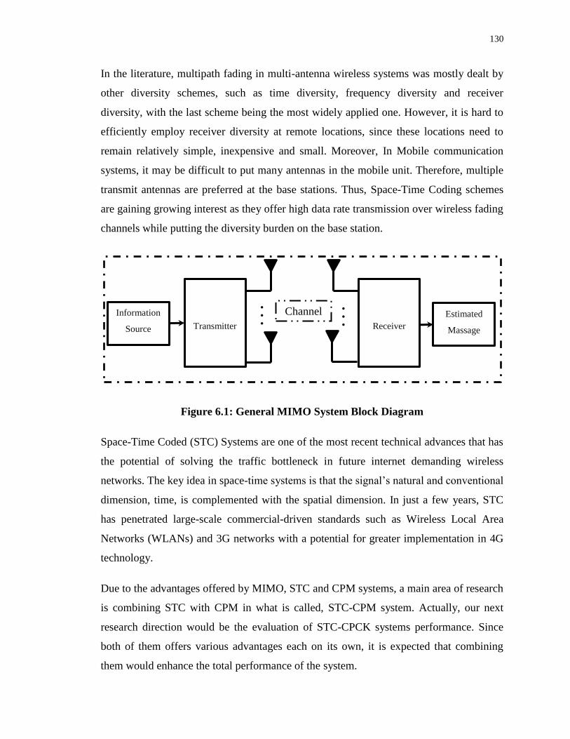
130
In the literature, multipath fading in multi-antenna wireless systems was mostly dealt by
other diversity schemes, such as time diversity, frequency diversity and receiver
diversity, with the last scheme being the most widely applied one. However, it is hard to
efficiently employ receiver diversity at remote locations, since these locations need to
remain relatively simple, inexpensive and small. Moreover, In Mobile communication
systems, it may be difficult to put many antennas in the mobile unit. Therefore, multiple
transmit antennas are preferred at the base stations. Thus, Space-Time Coding schemes
are gaining growing interest as they offer high data rate transmission over wireless fading
channels while putting the diversity burden on the base station.
Figure 6.1: General MIMO System Block Diagram
Space-Time Coded (STC) Systems are one of the most recent technical advances that has
the potential of solving the traffic bottleneck in future internet demanding wireless
networks. The key idea in space-time systems is that the signal’s natural and conventional
dimension, time, is complemented with the spatial dimension. In just a few years, STC
has penetrated large-scale commercial-driven standards such as Wireless Local Area
Networks (WLANs) and 3G networks with a potential for greater implementation in 4G
technology.
Due to the advantages offered by MIMO, STC and CPM systems, a main area of research
is combining STC with CPM in what is called, STC-CPM system. Actually, our next
research direction would be the evaluation of STC-CPCK systems performance. Since
both of them offers various advantages each on its own, it is expected that combining
them would enhance the total performance of the system.
Channel Information
Source Transmitter Receiver
Estimated
Massage
.
.
. . . .
131
6.2.2 Signaling Format
The information carrying phase of CPM signals can be generally viewed as
( )
In our work with the DAR, we have considered single- CPM, yet, this work can be
extended to multi- CPM. Moreover, we have employed two distinct pulse shapes i.e.
REC and Chirp, however, same work can be done employing other pulse shapes such as
Raised cosine (RC), Spectrally Raised Cosine (SRC), Gaussian Minimum Shift Keying
(GMSK) and Half-Cycle Sinusoid (HCS). Another area of future work could be the
extension of DAR algorithm to partial response CPFSK, CPCK and CPM signaling in
general, which usually gives better distance properties relative to full response CPM.
6.2.3 Detection Problem
The DAR receiver we evaluated, assumes ideal conditions such as 100% synchronization,
ideal coherent detection and pure AWGN channel model, however, it is not practically
true, hence, another area of future work could be in testing the proposed CPCK DAR in
non-Gaussian noise. In addition, generalizing the DAR strategy to -ary CPM is an
interesting area of research. Moreover, the MLRT-based optimum receiver still requires
more analysis, in an attempt to find a closed-form expression describing the
performance. It is also desirable to simulate the actual optimum receiver in order to verify
the mathematical analysis and performance of the sub-optimum receivers.
132
References
[1] FEHER, K., 1995. Wireless digital communications :modulation and spread spectrum
applications. Upper Saddle River, N.J.: Prentice-Hall PTR.
[2] MAGILL, D.T., NATALI, F.D. and EDWARDS, G.P., 1994. Spread-spectrum technology
for commercial applications. Proceedings of the IEEE, 82(4), pp. 572-584.
[3] JUNG, P., BAIER, P.W. and STEIL, A., 1993. Advantages of CDMA and spread spectrum
techniques over FDMA and TDMA in cellular mobile radio applications. Vehicular
Technology, IEEE Transactions on, 42(3), pp. 357-364.
[4] MATTHEWS, H., 1977. Surface wave filters :design, construction, and use. New York:
Wiley.
[5] HUEMER, M., KOPPLER, A., RUPPEL, C.C.W., REINDL, L., SPRINGER, A. and
WEIGEL, R., 1999. SAW based chirp Fourier transform for OFDM systems, Ultrasonics
Symposium, 1999. Proceedings. 1999 IEEE 1999, pp. 373-376 vol.1.
[6] BHARGAVA, V.K., 1981. Digital Communications by Satellite: Modulation, Multiple
Access and Coding. New York; Toronto: Wiley.
[7] ANDERSON, J. B., AULIN, T. and SUNDBERG, C.-E., 1986. Digital Phase Modulation.
New York: Plenum Press.
[8] AULIN, T. and SUNDBERG, C.-E., 1981. Continuous Phase Modulation-Part I: Full
Response Signalling. Communications, IEEE Transactions on, 29(3), pp. 196-209.
[9] SKLAR, B., 1988. Digital communications: fundamentals and applications. Englewood
Cliffs, N.J.: Prentice-Hall.
[10] OSBORNE, W. and LUNTZ, M., 1974. Coherent and Noncoherent Detection CPFSK.
Communications, IEEE Transactions on, 22(8), pp. 1023-1036.
[11] SCHONHOFF, T., 1976. Symbol Error Probabilities for M-ary CPFSK: Coherent and
Noncoherent Detection. Communications, IEEE Transactions on, 24(6), pp. 644-652.
[12] AULIN, T., RYDBECK, N. and SUNDBERG, C.-E., 1981. Continuous Phase Modulation--
Part II: Partial Response Signaling. Communications, IEEE Transactions on, 29(3), pp. 210-
225.
[13] MIYAKAWA, H., HARASHIMA, H., TATSUI, N. and TANAKA, Y., 1975. DIGITAL
PHASE-MODULATION SCHEME USING PHASE-CONTINUOUS WAVEFORM.
Electronics and Communications in Japan (English translation of Denshi Tsushin Gakkai
Zasshi), 58(12), pp. 35-42.
133
[14] ANDERSON, J.B. and TAYLOR, D.P., 1978. A bandwidth-efficient class of signal-space
codes. Information Theory, IEEE Transactions on, 24(6), pp. 703-712.
[15] AULIN, T. and SUNDBERG, C.-E., 1982. On the minimum Euclidean distance for a class
of signal space codes. Information Theory, IEEE Transactions on, 28(1), pp. 43-55.
[16] RAVEENDRA, K.R. and SRINIVASAN, R., 1987. Coherent detection of binary multi-h
CPM. Communications, Radar and Signal Processing, IEE Proceedings F, 134(4), pp. 416-
426.
[17] HWANG, H.-K., LEE, L.-S. and CHEN, S.-H., 1989. Multi-H phase-coded modulations
with asymmetric modulation indexes. Selected Areas in Communications, IEEE Journal on,
7(9), pp. 1450-1461.
[18] FONSEKA, J.P. and MAO, R., 1994. Nonlinear continuous phase modulation.
Communications, IEEE Transactions on, 42(9), pp. 2661-2663.
[19] FONSEKA, J.P., 1990. Adaptive CPFSK signaling, Communications, 1990. ICC '90,
Including Supercomm Technical Sessions. SUPERCOMM/ICC '90. Conference Record.,
IEEE International Conference on 1990, pp. 626-630 vol.2.
[20] FONSEKA, J.P., 1991. Nonlinear continuous phase frequency shift keying.
Communications, IEEE Transactions on, 39(10), pp. 1473-1481.
[21] FONSEKA, J.P. and RONGQIANG MAO, 1995. Generalized nonlinear continuous phase
modulation. Communications, IEEE Transactions on, 43(5), pp. 1868-1871.
[22] RONGQIANG MAO and FONSEKA, J.P., 1995. Nonlinear multi-h phase codes for CPFSK
signaling. Communications, IEEE Transactions on, 43(8), pp. 2350-2359.
[23] RAVEENDRA, K.R. and SRINIVASAN, R., 1991. A novel decision-directed receiver for
detection of CPM signals, TENCON '91.1991 IEEE Region 10 International Conference on
EC3-Energy, Computer, Communication and Control Systems 1991, pp. 72-76.
[24] ZAITSEV, D.L. and ZHURAVLEV, V.I., 1968. Noise immunity of digital data transmission
system using linearly frequency-modulated signals. Elektrosvyaz, 22(4), pp. 17-23.
[25] SHEN, H., MACHINENI, S., GUPTA, C. and PAPANDREOU-SUPPAPPOLA, A., 2004.
Time-varying multichirp rate modulation for multiple access systems. Signal Processing
Letters, IEEE, 11(5), pp. 497-500.
[26] DIXON, R.C., 1976. Spread spectrum systems. New York: Wiley.
[27] GOTT, G.F. and NEWSOME, J.P., 1971. H.F. data transmission using chirp signals.
Electrical Engineers, Proceedings of the Institution of, 118(9), pp. 1162-1166.
134
[28] GUGLER, W., SPRINGER, A. and WEIGEL, R., 2000. A chirp-based wideband spread
spectrum modulation technique for WLAN applications, Spread Spectrum Techniques and
Applications, 2000 IEEE Sixth International Symposium on 2000, pp. 83-87 vol.1.
[29] BERNI, A.J. and GREGG, W.D., 1973. On the Utility of Chirp Modulation for Digital
Signaling. Communications, IEEE Transactions on, 21(6), pp. 748-751.
[30] PEEBLES, P.Z., 1998. Radar principles. New York: Wiley.
[31] COOK, C.E. and BERNFELD, M., 1967. Radar signals ;;an introduction to theory and
application. New York: Academic Press.
[32] Winkler, M. R., 1962. Chirp signals for communications, IEEE WESCON Convention
Record, Tech. Rep.
[33] HIRT, W. and PASUPATHY, S., 1981. Continuous Phase Chirp (CPC) Signals for Binary
Data Communication-Part I: Coherent Detection. Communications, IEEE Transactions on,
29(6), pp. 836-847.
[34] HIRT, W. and PASUPATHY, S., 1981. Continuous Phase Chirp (CPC) Signals for Binary
Data Communication--Part II: Noncoherent Detection. Communications, IEEE Transactions
on, 29(6), pp. 848-858.
[35] SUNDBERG, C.-E., 1986. Continuous phase modulation. Communications Magazine,
IEEE, 24(4), pp. 25-38.
[36] Raveendra, K. R., 1987. Continuous phase chirp signals for M-ary data communications. Tel
Aviv, Israel: Proceedings of the XXIInd General Assembly of the URSI, August 1987.
[37] RAVEENDRA, K.R., 1996. Digital transmission using multimode phase-continuous chirp
signals. Communications, IEE Proceedings-, 143(2), pp. 87.
[38] FONSEKA, J.P., 1999. Partial response continuous phase chirp modulation. Electronics
Letters, 35(6), pp. 448-449.
[39] DAVE, B.A. and RAO, R.K., 2005. Data transmission using digital asymmetric phase
continuous chirp signals, Proceedings - 6th World Wireless Congress, WWC, May 25, 2005
- May 27, 2005 2005, Delson Group Inc, pp. 283-288.
[40] XIAOWEI WANG, MINRUI FEI and XIN LI, 2008. Performance of chirp spread spectrum
in wireless communication systems, Communication Systems, 2008. ICCS 2008. 11th IEEE
Singapore International Conference on 2008, pp. 466-469.
[41] HENGSTLER, S., KASILINGAM, D.P. and COSTA, A.H., 2002. A novel chirp modulation
spread spectrum technique for multiple access, Spread Spectrum Techniques and
Applications, 2002 IEEE Seventh International Symposium on 2002, pp. 73-77 vol.1.
135
[42] SPRINGER, A., GUGLER, W., HUEMER, M., KOLLER, R. and WEIGEL, R., 2001. A
wireless spread-spectrum communication system using SAW chirped delay lines.
Microwave Theory and Techniques, IEEE Transactions on, 49(4), pp. 754-760.
[43] HUAPING LIU, 2005. Multi-code ultra-wideband signaling using chirp waveforms,
Military Communications Conference, 2005. MILCOM 2005. IEEE 2005, pp. 1219-1224
Vol. 2.
[44] FANYU, M. and XUEMAI, G., 2011. A combined chirp signal modulation technique for
multiple access system. Information Technology Journal, 10(2), pp. 416-421.
[45] KADRI, A., RAO, R.K. and JIANG, J., 2009. Low-power chirp spread spectrum signals for
wireless communication within nuclear power plants. Nuclear Technology, 166(2), pp. 156-
169.
[46] KADRI, A. and UNIVERSITY OF WESTERN ONTARIO, 2010. Low-power chirp signals
for wireless data communication in industrial environments. PhD Dissertation
[47] VAN TREES, H.L., 1968. Detection, estimation, and modulation theory. New York: Wiley.
[48] SKLAR, B., 1993. Defining, designing, and evaluating digital communication systems.
Communications Magazine, IEEE, 31(11), pp. 91-101.
[49] XIONG, F., 2000. Digital modulation techniques. Boston: Artech House.
[50] PROAKIS, J.G. and SALEHI, M., 2008. Digital communications. 5th edn. Boston:
McGraw-Hill Higher Education.
[51] FOSCHINI, G.J. and GANS, M.J., 1998. On Limits of Wireless Communications in a
Fading Environment when Using Multiple Antennas. Wireless Personal Communications,
6(3), pp. 311-335.
[52] TELATAR, E., 1999. Capacity of multi-antenna Gaussian channels. European Transactions
on Telecommunications, 10(6), pp. 585-596.
[53] ALAMOUTI, S., 1998. A simple transmit diversity technique for wireless communications.
Selected Areas in Communications, IEEE Journal on, 16(8), pp. 1451-1458.
[54] PAULRAJ, A.J., 1997. Space-time processing for wireless communications, Acoustics,
Speech, and Signal Processing, 1997. ICASSP-97., 1997 IEEE International Conference on
1997, pp. 1-4 vol.1.
136
Curriculum Vitae
Name: Mohammed Omar Zourob
Place of Birth: Al Fijaira, United Arab Emirates
Post-secondary American University of Sharjah (AUS)
Education and Sharjah, United Arab Emirates
Degrees: 2007-2011 B.E.Sc.
Western University
London, Ontario, Canada
2011-2013 M.E.Sc.
Professional IEEE Student Member
Affiliation:
Honours and AUS Merit Scholarship
Awards: 2007-2011
Shikha Salama Scholarship for Academic Excellence
2007-2011
AUS Dean’s and Chancellor’s List
2007-2011
Ranked among 610 AUS Fall 2010 graduates
2007-2011
Western University Graduate Research Scholarship
2011-2013
Queen Elizabeth II Graduate Scholarship
2012-2013
Related Work Teaching & Research Assistant
Experience American University of Sharjah
2008-2010
Teaching & Research Assistant
Western University
2011-2013
137
Publications:
K. Assaleh, T. Shanableh, M. Zourob, “Low Complexity Classification System for
Glove-based Arabic Sign Language Recognition”, Lecture Notes in Computer Science
(LNCS) 7665, Part III, pp. 262-268 (2012) Doha, Qatar.
R. K. Rao, M. Zourob, “Decision-Aided Receiver for Continuous Phase Chirp Keying”
Submitted for presentation in the International Symposium on Performance Evaluation of
Computer and Telecommunication Systems(ISPECTS 2013), Toronto, Ontario, Canada.
Publications in Preparation:
R. K. Rao, M. Zourob, “Continuous Phase Chirp Keying based Multiple-Input-Multiple-
Output Communication System: Design, Detection and Performance” Under preparation.