asymptotic performance of adaptive distributed detection over networks
TRANSCRIPT
arX
iv:1
401.
5742
v2 [
cs.IT
] 23
Jan
201
4SUBMITTED FOR PUBLICATION 1
Asymptotic Performance of
Adaptive Distributed Detection over Networks
Paolo Braca, Stefano Marano, Vincenzo Matta, Ali H. Sayed
Abstract
This work examines the close interplay between cooperationand adaptation for distributed detection
schemes over fully decentralized networks. The combined attributes of cooperation and adaptation are
necessary to enable networks of detectors to continually learn from streaming data and to continually
track drifts in the state of nature when deciding in favor of one hypothesis or another. The results in the
paper establish a fundamental scaling law for the probabilities of miss-detection and false-alarm, when
the agents interact with each other according to distributed strategies that employ constant step-sizes. The
latter are critical to enable continuous adaptation and learning. The work establishes three key results.
First, it is shown that the output of the collaborative process at each agent has a steady-state distribution.
Second, it is shown that this distribution is asymptotically Gaussian in the slow adaptation regime of
small step-sizes. And third, by carrying out a detailed large-deviations analysis, closed-form expressions
are derived for the decaying rates of the false-alarm and miss-detection probabilities. Interesting insights
are gained from these expressions. In particular, it is verified that as the step-sizeµ decreases, the error
probabilities are driven to zero exponentially fast as functions of1/µ, and that the exponents governing
the decay increase linearly in the number of agents. It is also verified that the scaling laws governing
errors of detection and errors of estimation over networks behave very differently, with the former having
an exponential decay proportional to1/µ, while the latter scales linearly with decay proportional to
µ. Moreover, and interestingly, it is shown that the cooperative strategy allows each agent to reach the
same detection performance, in terms of detection error exponents, of a centralized stochastic-gradient
P. Braca is with NATO STO Centre for Maritime Research and Experimentation, La Spezia, Italy (e-mail: [email protected]).
S. Marano and V. Matta are with DIEM, University of Salerno, via Giovanni Paolo II 132, I-84084, Fisciano (SA), Italy
(e-mail: [email protected]; [email protected]).
A. H. Sayed is with the Electrical Engineering Department, University of California, Los Angeles, CA 90095 USA (e-mail:
The work of A. H. Sayed was supported in part by the NSF Grant CCF-1011918.
January 24, 2014 DRAFT
SUBMITTED FOR PUBLICATION 2
solution. The results of the paper are illustrated by applying them to canonical distributed detection
problems.
Index Terms
Distributed detection, adaptive network, diffusion strategy, consensus strategy, false-alarm proba-
bility, miss-detection probability, large-deviation analysis.
I. OVERVIEW
Recent advances in the field of distributed inference have produced several useful strategies
aimed at exploiting localcooperationamong network nodes to enhance the performance of each
individual agent. However, the increasing availability ofstreaming data continuously flowing
across the network has added the new and challenging requirement of onlineadaptationto track
drifts in the data. In the adaptive mode of operation, the network agents must be able to enhance
their learning abilities continually in order to produce reliable inference in the presence of
drifting statistical conditions, drifting environmentalconditions, and even changes in the network
topology, among other possibilities. Therefore, concurrent adaptation (i.e., tracking) and learning
(i.e., inference) are key components for the successful operation of distributed networks tasked
to produce reliable inference under dynamically varying conditions and in response to streaming
data.
Several useful distributed implementations based on consensus strategies [1]–[12] and diffusion
strategies [13]–[17] have been developed for this purpose in the literature. The diffusion strategies
have been shown to have superior stability ranges and mean-square performance when constant
step-sizes are used to enable continuous adaptation and learning [18]. For example, while
consensus strategies can lead to unstable growth in the state of adaptive networks even when all
agents are individually stable, this behavior does not occur for diffusion strategies. In addition,
diffusion schemes are robust, scalable, and fully decentralized. Since in this work we focus on
studyingadaptivedistributed inference strategies, we shall therefore focus on diffusion schemes
due to their enhanced mean-square stability properties over adaptive networks.
Now, the interplay between the two fundamental aspects of cooperation and adaptation has
been investigated rather extensively in the context ofestimationproblems. Less explored in the
literature is the same interplay in the context ofdetectionproblems. This is the main theme
January 24, 2014 DRAFT

SUBMITTED FOR PUBLICATION 3
of the present work. Specifically, we shall address the problem of designing and characterizing
the performance of diffusion strategies that reconcile both needs of adaptation and detection in
decentralized systems. The following is a brief description of the scenario of interest.
A network of connected agents is assumed to monitor a certainphenomenon of interest.
As time elapses, the agents collect an increasing amount of streaming data, whose statistical
properties depend upon anunknownstate of nature. The state is formally represented by a pair
of hypotheses, say,H0 andH1. At each time instant, each agent is expected to produce a decision
about the state of nature, based upon its own observations and the exchange of information with
neighboring agents. The emphasis here is onadaptation: we allow the true hypothesis to drift
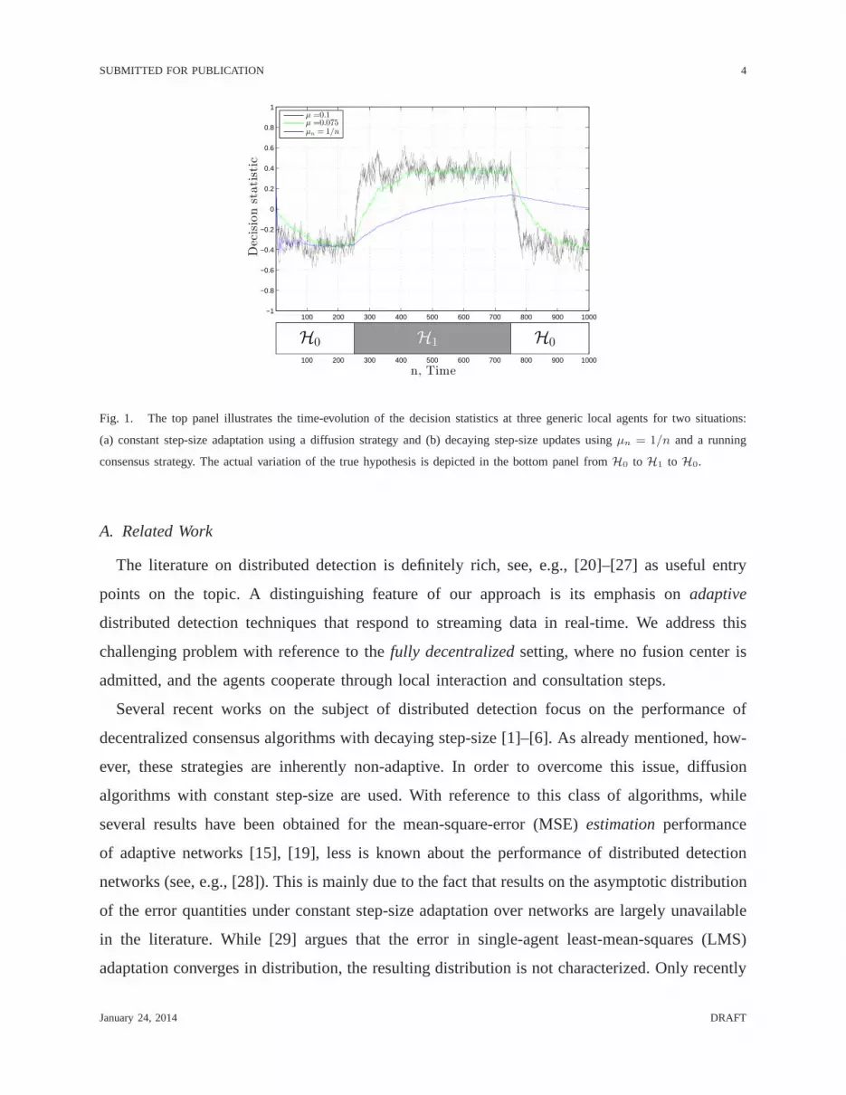
over time, and the network must be able to track the drifting state. This framework is illustrated
in Fig. 1, where we show the time-evolution of the actual realization of the decision statistics
computed by three generic network agents. Two situations are considered. In the first case, the
agents run a constant-step size diffusion strategy [15], [19] and in the second case, the agents
run a consensus strategy with a decaying step-size of the form µn = 1/n [1]–[6]. Note from the
curves in the figure that the statistics computed by different sensors are hardly distinguishable,
emphasizing a certain equivalence in performance among distinct agents, an important feature
that will be extensively commented on in the forthcoming analysis.
Assume that high (positive) values of the statistic correspond to deciding forH1, while low
(negative) values correspond to deciding forH0. The bottom panel in the figure shows how
the true (unknown) hypothesis changes at certain (unknown)epochs following the sequence
H0 → H1 →H0. It is seen in the figure that the adaptive diffusion strategyis more apt in tracking
the drifting state of nature. It is also seen that the decaying step-size consensus implementation
is unable to track the changing conditions. Moreover, the inability to track the drift degrades
further as time progresses since the step-size sequenceµn = 1/n decays to zero asn → ∞.
For this reason, in this work we shall set the step-sizes to constant values to enable continuous
adaptation and learning by the distributed network of detectors. In order to evaluate how well
these adaptive networks perform, we need to be able to assessthe goodness of the inference
performance (reliability of the decisions), so as to exploit the trade-off between adaptation and
learning capabilities. This will be the main focus of the paper.
January 24, 2014 DRAFT
SUBMITTED FOR PUBLICATION 4
100 200 300 400 500 600 700 800 900 1000−1
−0.8
−0.6
−0.4
−0.2
0
0.2
0.4
0.6
0.8
1
Decisionstatistic
µ =0.1µ =0.075µn = 1/n
100 200 300 400 500 600 700 800 900 1000
H0 H1 H0
n, Time
Fig. 1. The top panel illustrates the time-evolution of the decision statistics at three generic local agents for two situations:
(a) constant step-size adaptation using a diffusion strategy and (b) decaying step-size updates usingµn = 1/n and a running
consensus strategy. The actual variation of the true hypothesis is depicted in the bottom panel fromH0 to H1 to H0.
A. Related Work
The literature on distributed detection is definitely rich,see, e.g., [20]–[27] as useful entry
points on the topic. A distinguishing feature of our approach is its emphasis onadaptive
distributed detection techniques that respond to streaming data in real-time. We address this
challenging problem with reference to thefully decentralizedsetting, where no fusion center is
admitted, and the agents cooperate through local interaction and consultation steps.
Several recent works on the subject of distributed detection focus on the performance of
decentralized consensus algorithms with decaying step-size [1]–[6]. As already mentioned, how-
ever, these strategies are inherently non-adaptive. In order to overcome this issue, diffusion
algorithms with constant step-size are used. With reference to this class of algorithms, while
several results have been obtained for the mean-square-error (MSE) estimationperformance
of adaptive networks [15], [19], less is known about the performance of distributed detection
networks (see, e.g., [28]). This is mainly due to the fact that results on the asymptotic distribution
of the error quantities under constant step-size adaptation over networks are largely unavailable
in the literature. While [29] argues that the error in single-agent least-mean-squares (LMS)
adaptation converges in distribution, the resulting distribution is not characterized. Only recently
January 24, 2014 DRAFT
SUBMITTED FOR PUBLICATION 5
these questions have been considered in [30], [31] in the context of distributed estimation over
adaptive networks. Nevertheless, these results on the asymptotic distribution of the errors are still
insufficient to characterize the rate of decay of the probability of error over networks of distributed
detectors. To do so, it is necessary to pursue a large deviations analysis in the constant step-size
regime. Motivated by these remarks, we therefore provide a thorough statistical characterization
of the diffusion network in a manner that enables detector design and analysis.
B. Main Result and Ramifications
Consider a connected network ofS sensors performing distributed detection by means of
adaptive diffusion strategies, as described in the next section. The adaptive nature of the solution
allows the network to track variations in the hypotheses being tested over time. As anticipated,
to enable continuous adaptation and learning, we shall employ distributed strategies with a
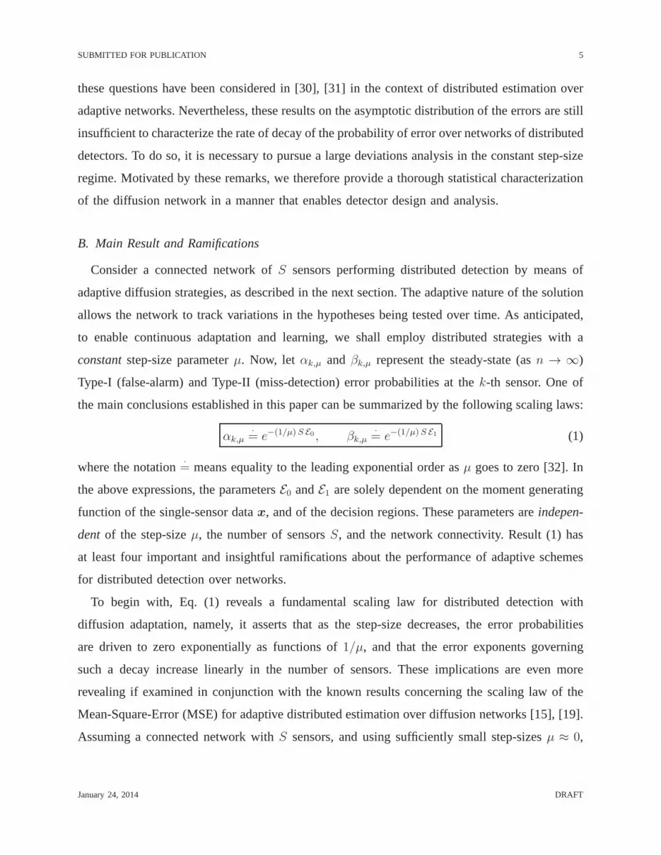
constantstep-size parameterµ. Now, let αk,µ and βk,µ represent the steady-state (asn → ∞)
Type-I (false-alarm) and Type-II (miss-detection) error probabilities at thek-th sensor. One of
the main conclusions established in this paper can be summarized by the following scaling laws:
αk,µ·= e−(1/µ) S E0 , βk,µ
·= e−(1/µ) S E1 (1)
where the notation·= means equality to the leading exponential order asµ goes to zero [32]. In
the above expressions, the parametersE0 andE1 are solely dependent on the moment generating
function of the single-sensor datax, and of the decision regions. These parameters areindepen-
dent of the step-sizeµ, the number of sensorsS, and the network connectivity. Result (1) has
at least four important and insightful ramifications about the performance of adaptive schemes
for distributed detection over networks.
To begin with, Eq. (1) reveals a fundamental scaling law for distributed detection with
diffusion adaptation, namely, it asserts that as the step-size decreases, the error probabilities
are driven to zero exponentially as functions of1/µ, and that the error exponents governing
such a decay increase linearly in the number of sensors. These implications are even more
revealing if examined in conjunction with the known resultsconcerning the scaling law of the
Mean-Square-Error (MSE) for adaptive distributed estimation over diffusion networks [15], [19].
Assuming a connected network withS sensors, and using sufficiently small step-sizesµ ≈ 0,
January 24, 2014 DRAFT
SUBMITTED FOR PUBLICATION 6
the MSE that is attained by sensork obeys (see expression (32) in [15]):
MSEk ∝µ
S, (2)
where the symbol∝ denotes proportionality. Some interesting symmetries areobserved. In the
estimation context, the MSE decreases asµ goes to zero, and the scaling rate improves linearly
in the number of sensors. Recalling that smaller values ofµ mean a lower degree of adaptation,
we observe that reaching a better inference quality costs interms of adaptation speed. This is a
well-known tradeoff in the adaptive estimation literaturebetween tracking speed and estimation
accuracy.
Second, we observe from (1) and (2) that the scaling laws governing errors of detection and
estimation over distributed networks behave very differently, the former exhibiting an exponential
decay proportional to1/µ, while the latter is linear with decay proportional toµ. The significance
and elegance of this result for adaptive distributed networks lie in revealing an intriguing analogy
with other more traditional inferential schemes. As a first example, consider the standard case
of a centralized, non-adaptive inferential system withN i.i.d. data points. It is known that the
error probabilities of the best detector decay exponentially fast to zero withN , while the optimal
estimation error decays as1/N [33], [34]. Another important case is that of rate-constrained
multi-terminal inference [35], [36]. In this case the detection performance scales exponentially
with the bit-rateR while, again, the squared estimation error vanishes as1/R. Thus, at an abstract
level, reducing the step-size corresponds to increasing the number of independent observations in
the first system, or increasing the bit-rate in the second system. The above comparisons furnish
an interesting interpretation for the step-sizeµ as the basic parameter quantifying the cost of
information used by the network for inference purposes, much as the number of dataN or the
bit-rateR in the considered examples.
A third aspect pertaining to the performance of the distributed network relates to the potential
benefits of cooperation. These are already encoded into (1),and we have already implicitly
commented on them. Indeed, note that the error exponents increase linearly in the number of
sensors. This implies that cooperation offersexponential gainsin terms of detection performance.
The fourth and final ramification we would like to highlight relates to how much performance
is lost by thedistributedsolution in comparison to a centralized stochastic gradient solution.
January 24, 2014 DRAFT
SUBMITTED FOR PUBLICATION 7
Again, the answer is contained in (1). Specifically, the centralized solution is equivalent to a
fully connected network, so that (1) applies to the centralized case as well. As already mentioned,
the parametersE0 andE1 do not depend on the network connectivity, which therefore implies that,
as the step-sizeµ decreases, the distributed diffusion solution of the inference problem exhibits a
detection performance governed by thesame error exponentsof the centralized system. This is a
remarkable conclusion and it is also consistent with results in the context of adaptive distributed
estimation over diffusion networks [15].
We now move on to describe the adaptive distributed solutionand to establish result (1) and
the aforementioned properties.
Notation. We use boldface letters to denote random variables, and normal font letters for their
realizations. Capital letters refer to matrices, small letters to both vectors and scalars. Sometimes
we violate this latter convention, for instance, we denote the total number of sensors byS. The
symbolsP andE are used to denote the probability and expectation operators, respectively. The
notationPh andEh, with h = 0, 1, means that the pertinent statistical distribution corresponds
to hypothesisH0 or H1.
II. PROBLEM FORMULATION
The scalar observation collected by thek-th sensor at timen will be denoted byxk(n),
k = 1, 2, . . . , S, which arises from a stationary distribution with meanEx and varianceσ2x.
Data are assumed to be spatially and temporally independentand identically distributed (i.i.d.),
conditionedon the hypothesis that gives rise to them. The distributed network is interested in
making an inference about the true state of nature. As it is well-known, for the i.i.d. data model,
an optimal centralized (and non-adaptive) detection statistic is the sum of the log-likelihoods.
When these are not available, alternative detection statistics obtained as the sum of some suitably
chosen functions of the observations are often employed, ashappens in some specific frameworks,
e.g., in locally optimum detection [37] and in universal hypothesis testing [38]. Accordingly, each
sensor in the network will try to compute, as its own detection statistic, a weighted combination
of some function of the local observations. We assume the symbol xk(n) represents the local
statistic that is available at timen at sensork.
Since we are interested in an adaptive inferential scheme, and given the idea of relying on
weighted averages, we resort to the class of diffusion strategies for adaptation over networks [15],
January 24, 2014 DRAFT
SUBMITTED FOR PUBLICATION 8
[28]. These strategies admit various forms. We consider theATC form due to some inherent
advantages in terms of a slightly improved mean-square-error performance relative to other
forms [15]. In the ATC diffusion implementation, each nodek updates its state fromyk(n− 1)
to yk(n) through local cooperation with its neighbors as follows:
vk(n) = yk(n− 1) + µ[xk(n)− yk(n− 1)], (3)
yk(n) =S∑
ℓ=1
ak,ℓvℓ(n), (4)
where 0 < µ ≪ 1 is a small step-size parameter. In this construction, nodek first uses its
local statistic,xk(n), to update its state fromyk(n − 1) to an intermediate valuevk(n). All
other nodes in the network perform similar updates simultaneously using their local statistics.
Subsequently, nodek aggregates the intermediate states of its neighbors using nonnegative convex
combination weightsak,ℓ that add up to one. Again, all other nodes in the network perform
a similar calculation. If we collect the combination coefficients into a matrixA = [ak,ℓ], thenA
is a right-stochastic matrix in that the entries on each of its rows add up to one:
ak,ℓ ≥ 0, A1 = 1, (5)
with 1 being a column-vector with all entries equal to1.
At time n, the k-th sensor needs to produce a decision based upon its state value yk(n).
To this aim, a decision rule must be designed, by choosing appropriate decision regions. The
performance of the test will be measured according to the Type-I and Type-II error probabilities
defined, respectively, as
αdef= P[chooseH1 whenH0 is true], (6)
βdef= P[chooseH0 whenH1 is true]. (7)
An important remark is needed at this stage. Computation of the exact distribution ofyk(n)
is generally intractable. This implies that the structure of the optimal, or even of a reasonable
test, is unknown. We tackle this difficult problem by pursuing the following approach. First, we
perform a thorough analysis of the statistical properties of yk(n). As standard in the adaptation
literature [15], [39], this will be done with reference toi) the steady-state properties (asn→∞),
and ii) for small values of the step-size (µ → 0). Throughout the paper, the term steady-state
January 24, 2014 DRAFT

SUBMITTED FOR PUBLICATION 9
will refer to the limit as the time-indexn goes to infinity, while the term asymptotic will be used
to refer to the slow adaptation regime whereµ→ 0. Specifically, we will follow these steps:
• We show thatyk(n) has alimiting distribution asn goes to infinity (Theorem 1).
• For small step-sizes, the distribution ofyk(n) approaches a Gaussian, i.e., it isasymptotically
normal (Theorem 2).
• We characterize thelarge deviationsof the steady-state outputyk(n) in the slow adaptation
regime whenµ→ 0 (Theorem 3).
• The results of the above steps will provide a series of tools for designing the detector and
characterizing its performance (Theorem 4).
We would like to mention that the detailed statistical characterization offered by Theorems 1-3
is not confined to the specific detection problems we are dealing with. As a matter of fact, these
results are of independent interest, and might be useful forthe application of adaptive diffusion
strategies in broader contexts.
III. EXISTENCE OFSTEADY-STATE DISTRIBUTION
Let yn denote theS × 1 vector that collects the state variables from across the network at
time n, i.e.,
yn = coly1(n), y2(n), . . . ,yS(n). (8)
Likewise, we collect the local statisticsxk(n) at timen into the vectorxn. It is then straight-
forward to verify from the diffusion strategy (3)–(4) that the vectoryn is given by:
yn = (1− µ)nAny0 +µ
1− µn∑
i=1
(1− µ)n−i+1An−i+1xi (9)
By making the change of variablesi← n− i+ 1, the above equation can be written as
yn = (1− µ)nAny0 +µ
1− µn∑
i=1
(1− µ)iAixn−i+1. (10)
We note that the termxn−i+1 depends on the time indexn in such a way that the most recent
datumxn is assigned the highest scaling weight, in compliance with the adaptive nature of
the algorithm. However, since the vectorsxi are i.i.d. across time, and since we shall be only
concerned with the distribution of partial sums involving these terms, the statistical properties
January 24, 2014 DRAFT

SUBMITTED FOR PUBLICATION 10
of yn are left unchanged if in (10) we replacexn−i+1 with a random vectorx′i, wherex′
i is
a sequence of i.i.d. random vectors distributed similarly to thexn−i+1. Formally, we write
ynd= (1− µ)nAny0 +
µ
1− µn∑
i=1
(1− µ)iAix′i, (11)
whered= denotes equality in distribution.
It follows that the state of thek−th sensor is given by:
yk(n)d= (1− µ)n
S∑
ℓ=1
bk,ℓ(n)yℓ(0)
︸ ︷︷ ︸transient
+µ
1− µn∑
i=1
(1− µ)iS∑
ℓ=1
bk,ℓ(i)x′ℓ(i),
︸ ︷︷ ︸steady-state
(12)
where the scalarsbk,ℓ(n) are the entries of the matrix power:
Bndef= An. (13)
Since we are interested in reaching abalancedfusion of the observations, we shall assume that
A is doubly-stochasticwith second largest eigenvalue magnitude strictly less than one, which
yields [8], [16], [40]:
Bnn→∞−→ 1
S11
T . (14)
In order to reveal the steady-state behavior ofyk(n), let us focus on the RHS of (12). It is
useful to rewrite it as:
yk(n)d= transient+
n∑
i=1
zk(i), (15)
where the definition ofzk(i) should be clear. As a result, we are faced with a sum of independent,
but not identically distributed, random variables. Let us evaluate the first two moments of the
sum:
E
(n∑
i=1
zk(i)
)= Ex
n∑
i=1
µ(1− µ)i−1
S∑
ℓ=1
bk,ℓ(i)
︸ ︷︷ ︸=1
n→∞−→ Ex, (16)
January 24, 2014 DRAFT
SUBMITTED FOR PUBLICATION 11
and (VAR denotes the variance operator):
VAR
(n∑
i=1
zk(i)
)= σ2
x
n∑
i=1
µ2(1− µ)2(i−1)S∑
ℓ=1
b2k,ℓ(i)︸ ︷︷ ︸≤1
≤ σ2x S µ
2− µ <∞. (17)
We have thus shown that the expectation of the sum expressionfrom (15) converges toEx,
and that its variance converges to a finite value. In view of the Infinite Convolution Theorem
— see [41, p. 266], these two conditions are sufficient to conclude that the second term on the
RHS of (15), i.e., the sum of random variableszk(i), converges in distribution asn→∞, and
the first two moments of the limiting distribution are equal to Ex and∑∞
i=1 VAR(zk(i)). The
random variable characterized by the limiting distribution will be denoted byy⋆k,µ, where we
make explicit the dependence upon the step-sizeµ for later use. Since the first term on the RHS
of (12) vanishes withn, by application of Slutsky’s Theorem [33] we have that, at steady-state,
the diffusion outputyk(n) is still distributed asy⋆k,µ.
The above statement can be sharpened to ascertain that the sum of random variableszk(i) ac-
tually converges almost surely (a.s.). This conclusion canbe obtained by applying Kolmogorov’s
Two Series Theorem [41]. In view of the a.s. convergence, it makes sense to define the limiting
random variabley⋆k,µ as:
y⋆k,µdef=
∞∑
i=1
S∑
ℓ=1
µ (1− µ)i−1bk,ℓ(i)x′ℓ(i) (18)
We wish to avoid confusion here. We are not stating that the actual diffusion outputyk(n)
converges almost surely (a behavior that would go against the adaptive nature of the diffusion
algorithm). We are instead claiming thatyk(n) converges in distribution to a random variable
y⋆k,µ that can be conveniently defined in terms of the a.s. limit (18).
The main result about the steady-state behavior of the diffusion output is summarized below
(the symbol means convergence in distribution).
THEOREM 1: (Steady-state distribution ofyk(n)). The state variableyk(n) that is generated by
the diffusion strategy (3)–(4) is asymptotically stable indistribution, namely,
yk(n)n→∞ y⋆k,µ (19)
January 24, 2014 DRAFT

SUBMITTED FOR PUBLICATION 12
It is useful to make explicit the meaning of Theorem 1. By definition of convergence in
distribution (or weak convergence), the result (19) can be formally stated as [34], [42]:
limn→∞
P[yk(n) ∈ Γ] = P[y⋆k,µ ∈ Γ], (20)
for any setΓ such thatP[y⋆k,µ ∈ ∂Γ] = 0, where∂Γ denotes the boundary ofΓ. It is thus
seen that the properties of the steady-state variabley⋆k,µ will play a key role in determining the
steady-state performance of the diffusion output. Accordingly, we state two useful properties of
y⋆k,µ.
First, when the local statisticxk(n) has anabsolutely continuousdistribution (where the
reference measure is the Lebesgue measure over the real line), it is easily verified that the
distribution of y⋆k,µ is absolutely continuous as well. Indeed, note that we can writey⋆k,µ =
zk(1)+∑∞
i=2 zk(i). Now observe thatzk(1), which has an absolutely continuous distribution by
assumption, is independent of the other term. The result follows by the properties of convolution
and from the fact that the distribution of the sum of two independent variables is the convolution
of their respective distributions.
Second, when the local statisticxk(n) is a discreterandom variable, by the Jessen-Wintner
law [43], [44], we can only conclude thaty⋆k,µ is of pure type, namely, its distribution is pure:
absolutely continuous, or discrete, or continuous but singular.
An intriguing case is that of the so-calledBernoulli convolutions, i.e., random variables of the
form∑∞
i=1(1 − µ)i−1x(i), wherex(i) are equiprobable±1. For this case, it is known that if
1/2 < µ < 1, then the limiting distribution is aCantordistribution [45]. This is an example of a
distribution that is neither discrete nor absolutely continuous. Whenµ < 1/2, which is relevant
for our discussion since we shall be concerned with small step-sizes, the situation is markedly
different, and the distribution is absolutely continuous for almost all values ofµ.
Before proceeding, we stress that we have proved that a steady-state distribution foryk(n)
exists, but its form is not known. Accordingly, even in steady-state, the structure of the optimal
test is still unknown. In tackling this issue, and recallingthat the regime of interest is that of
slow adaptation, we now focus on the caseµ≪ 1.
January 24, 2014 DRAFT
SUBMITTED FOR PUBLICATION 13
IV. THE SMALL -µ REGIME.
While the exact form of the steady-state distribution is generally impossible to evaluate, it is
nevertheless possible to approximate it well for small values of the step-size parameter. Indeed,
in this section we prove two results concerning the statistical characterization of the steady-
state distribution forµ → 0. The first one is a result ofasymptotic normality, stating thaty⋆k,µ
approaches a Gaussian random variable with known moments asµ goes to zero (Theorem 2).
The second finding (Theorem 3) provides the complete characterization for thelarge deviations
of y⋆k,µ.
THEOREM 2: (Asymptotic normality ofy⋆k,µ as µ→ 0). Under the assumptionE|xk(n)|3 <∞,
the variabley⋆k,µ fulfills, for all k = 1, 2, . . . , S:
y⋆k,µ − Ex√µ
µ→0 N(0,σ2x
2S
)(21)
Proof: The argument requires dealing with independent but non-identically distributed random
variables, as done in the Lindeberg-Feller CLT (Central Limit Theorem) [41]. This theorem,
however, does not apply to our setting since the asymptotic parameter isnot the number of
samples, but rather the step-size. Some additional effort is needed, and the detailed technical
derivation is deferred to Appendix A.
A. Implications of Asymptotic Normality
Let us now briefly comment on several useful implications that follow from the above theorem:
1) First, note thatall sensorsshare, forµ small enough, thesamedistribution, namely, the
inferential diffusion strategy equalizes the statisticalbehavior of the agents. This finding
complements well results from [15], [19], [31] where the asymptotic equivalence among
the sensors has been proven in the context of mean-square-error estimation. One of the
main differences between the estimation context and the detection context studied in this
article is that in the latter case, the regression data is deterministic and the randomness
arises from the stochastic nature of the statisticsxk(n). For this reason, the steady-state
distribution in (21) is characterized in terms of the moments of these statistics and not in
terms of the moments of regression data, as is the case in the estimation context.
January 24, 2014 DRAFT

SUBMITTED FOR PUBLICATION 14
2) The result of Theorem 2 is valid provided that the connectivity matrix fulfills (14). This
condition is satisfied when the network topology is strongly-connected, i.e., there exists a
path connecting any two arbitrary nodes and at least one nodehasak,k > 0 [16]. Obviously,
condition (14) is also satisfied in the fully connected case when ak,ℓ = bk,ℓ = 1/S for
all k, ℓ = 1, 2, . . . , S. This latter situation would correspond to a representation of the
centralized stochastic gradient algorithm, namely, an implementation of the form
y(c)(n) = y(c)(n− 1) +µ
S
S∑
ℓ=1
[xℓ(n)− y(c)(n− 1)], (22)
wherey(c)(n) denotes the output by the centralized solution at timen. The above algorithm
can be deduced from (3)–(4) by defining
y(c)(n)def=
1
S
S∑
ℓ=1
yℓ(n). (23)
Now, since the moments of the limiting Gaussian distribution in (21) are independent of the
particular connectivity matrix, the net effect is that eachagent of thedistributednetwork
acts, asymptotically, as thecentralizedsystem. This result again complements well results
in the estimation context where the role of the statistics variablesxk(n) is replaced by
that of stochastic regression data [46].
3) The asymptotic normality result is powerful in approximating the steady-state distribution
for relatively small step-sizes, thus enabling the analysis and design of inferential diffusion
networks in many different contexts. With specific reference to the detection application
that is the main focus here, Eq. (21) can be exploited for an accurate threshold setting when
one desires to keep under control one of the two errors, say, the false-alarm probability, as
happens, e.g., in the Neyman-Pearson setting [34]. To show aconcrete example on how
this can be done, let us assume that, without loss of generality, E0x < E1x, and consider
a single-threshold detector for which:
Γ0 = γ ∈ R : γ ≤ ηµ, Γ1 = R \ Γ0, (24)
where the threshold is set as
ηµ = E0x+
√µσ2
x,0
2SQ−1(α). (25)
January 24, 2014 DRAFT
SUBMITTED FOR PUBLICATION 15
Here, σ2x,0 is the variance ofx underH0, Q(·) denotes the complementary CDF for
a standard normal distribution, andα is the prescribed false-alarm level. By (21), it is
straightforward to check that this threshold choice ensures
limµ→0
P0[y⋆k,µ > ηµ] = α. (26)
In summary, Theorem 2 provides an approximation of the diffusion output distribution for
small step-sizes. At first glance, this may seem enough to obtain a complete characterization
of the detection problem. A closer inspection reveals that this is not the case. A good example
to understand why Theorem 2 alone is insufficient for characterizing the detection performance
is obtained by examining the Neyman-Pearson threshold setting just described in (25)–(26)
above. While we have seen that the asymptotic behavior of thefalse-alarm probability in (26) is
completely determined by the application of Theorem 2, the situation is markedly different as
regards the miss-detection probabilityP1[y⋆k,µ ≤ ηµ]. Indeed, by using (25) we can write:
P1[y⋆k,µ ≤ ηµ] = P1
[y⋆k,µ − E1x√
µ≤ ηµ − E1x√
µ
]
= P1
y
⋆k,µ − E1x√
µ≤ E0x− E1x√
µ+
√σ2x,0
2SQ−1(α)
.
(27)
SinceE0x < E1x, the quantityE0x−E1x√µ
diverges to−∞ asµ→ 0. As a consequence, the fact
thaty⋆k,µ
−E1x√µ
is asymptotically normal does not provide much more insightthan revealing that
the miss-detection probability converges to zero asµ → 0. A meaningful asymptotic analysis
would instead require to examine the way this convergence takes place (i.e., the error exponent).
The same kind of problem is found when one letsboth error probabilities vanish exponentially,
such that the Type-I and Type-II detection error exponents furnish a meaningful asymptotic
characterization of the detector. In order to fill these gaps, the study of thelarge deviations of
y⋆k,µ is needed.
B. Large Deviations ofy⋆k,µ.
From (21) we learn that, asµ→ 0, the diffusion output shrinks down to its limiting expectation
Ex and that thesmall (of orderõ) deviations around this value have a Gaussian shape. But
January 24, 2014 DRAFT

SUBMITTED FOR PUBLICATION 16
this conclusion is not helpful when working withlarge deviations, namely, with terms like:
P[|y⋆k,µ − Ex| > δ]µ→0−→ 0, δ > 0, (28)
which play a significant role in detection applications. While the above convergence to zero can
be inferred from (21), it is well known that (21) is not sufficient in general to obtain the rate at
which the above probability vanishes. In order to perform accurate design and characterization
of reliable inference systems [47], [48] it is critical to assess this rate of convergence, which
turns out to be the main purpose of a large-deviation analysis.
Accordingly, we will be showing in the sequel that the process y⋆k,µ obeys a Large Deviation
Principle (LDP), namely, that the following limit exists [47], [48]:
limµ→0
µ lnP[y⋆k,µ ∈ Γ] = − infγ∈Γ
I(γ)def= −IΓ, (29)
for someI(γ) that is called therate function. Equivalently:
P[y⋆k,µ ∈ Γ] = e−(1/µ) IΓ+o(1/µ) ·= e−(1/µ) IΓ, (30)
where o(1/µ) stands for any correction term growing slower than1/µ, namely, such that
µ o(1/µ) → 0 asµ → 0, and the notation·= was introduced in (1). From (30) we see that, in
the large deviations framework, only the dominant exponential term is retained, while discarding
any sub-exponential terms. It is also interesting to note that, according to (30), the probability
thaty⋆k,µ belongs to a given regionΓ is dominated by the infimumIΓ of the rate functionI(γ)
within the regionΓ. In other words, the smallest exponent (⇒ highest probability) dominates,
which is well explained in [48] through the statement: “any large deviation is done in the least
unlikely of all the unlikely ways”.
In summary, the LDP generally implies an exponential scaling law for probabilities, with an
exponent governed by the rate function. Therefore, knowledge of the rate function is enough to
characterize the exponent in (30). We shall determine the expression forI(γ) pertinent to our
problem in Theorem 3 further ahead — see Eq. (37).
In the traditional case where the statistic under consideration is the arithmetic average of i.i.d.
data, the asymptotic parameter is the number of samples and the usual tool for determining the
rate function in the LDP is Cramer’s Theorem [47], [48]. Unfortunately, in our adaptive and
distributed setting, we are dealing with a more general statistic y⋆k,µ, whose dependence is on the
step-size parameter and not on the number of samples. Cramer’s Theorem is not applicable in
January 24, 2014 DRAFT
SUBMITTED FOR PUBLICATION 17
this case, and we must resort to a more powerful tool, known asthe Gartner-Ellis Theorem [47],
[48], stated below in a form that uses directly the set of assumptions relevant for our purposes.
GARTNER-ELLIS THEOREM [48]. Let zµ be a family of random variables with Logarithmic
Moment Generating Function (LMGF)φµ(t) = lnE exptzµ. If
φ(t)def= lim
µ→0µφµ(t/µ) (31)
exists, withφ(t) < ∞ for all t ∈ R, andφ(t) is differentiable inR, thenzµ satisfies the LDP
property (29) with rate function given by the Fenchel-Legendre transform ofφ(t), namely:
Φ(γ)def= sup
t∈R[γt− φ(t)]. (32)
In what follows, we shall use capital letters to denote Fenchel-Legendre transforms, as done
in (32).
We now show how the result allows us to assess the asymptotic performance of the diffusion
output in the inferential network. Let us introduce the LMGFof the dataxk(n), and that of the
steady-state variabley⋆k,µ, respectively:
ψ(t)def= lnE exptxk(n), (33)
φk,µ(t)def= lnE expty⋆k,µ. (34)
THEOREM 3: (Large deviations ofy⋆k,µ asµ→ 0). Assume thatψ(t) < +∞ for all t ∈ R. Then,
for all k = 1, 2, . . . , S:
i)
φ(t)def= lim
µ→0µφk,µ(t/µ) = S ω(t/S) (35)
where
ω(t)def=
∫ t
0
ψ(τ)
τdτ (36)
ii) The steady-state variabley⋆k,µ obeys the LDP with a rate function given by:
I(γ) = S Ω(γ) (37)
that is, by the Fenchel-Legendre transform ofω(t) multiplied by the number of sensorsS.
Proof: See Appendix B.
January 24, 2014 DRAFT
SUBMITTED FOR PUBLICATION 18
ψ(t)
tt*
0
ω(t)
t
xslope =
0
′ω (t) =ψ(t)
t< 0 ′ω (t) =
ψ(t)
t> 0
′ω (0) = ′ψ (0) = E
Ω(γ )
γx 0
slope = E
E
x
t*
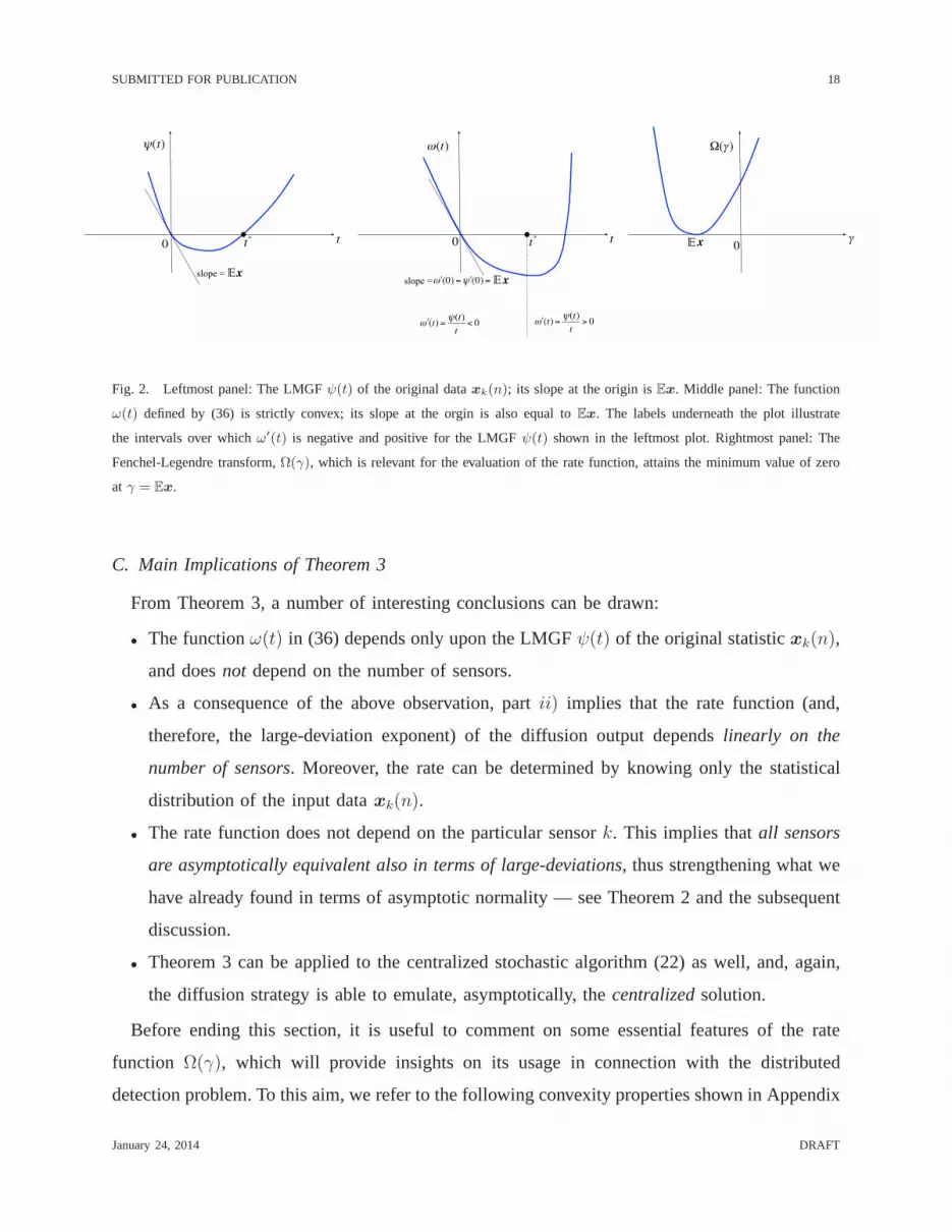
Fig. 2. Leftmost panel: The LMGFψ(t) of the original dataxk(n); its slope at the origin isEx. Middle panel: The function
ω(t) defined by (36) is strictly convex; its slope at the orgin is also equal toEx. The labels underneath the plot illustrate
the intervals over whichω′(t) is negative and positive for the LMGFψ(t) shown in the leftmost plot. Rightmost panel: The
Fenchel-Legendre transform,Ω(γ), which is relevant for the evaluation of the rate function, attains the minimum value of zero
at γ = Ex.
C. Main Implications of Theorem 3
From Theorem 3, a number of interesting conclusions can be drawn:
• The functionω(t) in (36) depends only upon the LMGFψ(t) of the original statisticxk(n),
and doesnot depend on the number of sensors.
• As a consequence of the above observation, partii) implies that the rate function (and,
therefore, the large-deviation exponent) of the diffusionoutput dependslinearly on the
number of sensors. Moreover, the rate can be determined by knowing only the statistical
distribution of the input dataxk(n).
• The rate function does not depend on the particular sensork. This implies thatall sensors
are asymptotically equivalent also in terms of large-deviations, thus strengthening what we
have already found in terms of asymptotic normality — see Theorem 2 and the subsequent
discussion.
• Theorem 3 can be applied to the centralized stochastic algorithm (22) as well, and, again,
the diffusion strategy is able to emulate, asymptotically,the centralizedsolution.
Before ending this section, it is useful to comment on some essential features of the rate
function Ω(γ), which will provide insights on its usage in connection withthe distributed
detection problem. To this aim, we refer to the following convexity properties shown in Appendix
January 24, 2014 DRAFT

SUBMITTED FOR PUBLICATION 19
C (see also [47], Ex. 2.2.24, and [48], Ex. I.16):
i) ω′′(t) > 0 for all t ∈ R, implying thatω(t) is strictly convex.
ii) Ω(γ) is strictly convex in the interior of the set:
DΩ = γ ∈ R : Ω(γ) <∞. (38)
iii) Ω(γ) attains its unique minimum atγ = Ex, with
Ω(Ex) = 0. (39)
In light of these properties, it is possible to provide a geometric interpretation for the main
quantities in Theorem 3, as illustrated in Fig. 2. The leftmost panel shows a typical behavior
of the LMGF of the original dataxk(n). Using the resultω′(t) = ψ(t)/t, and examining the
sign of ψ(t)/t, it is possible to deduce the corresponding typical behavior of ω(t), depicted
in the middle panel. As it can be seen, the slope at the origin is preserved, and is still equal
to the expectation of the original data,Ex. The intersection with thet-axis is changed, and
moves further to the right in the considered example. Starting fromω(t), it is possible to draw a
sketch of its Fenchel-Legendre transformΩ(γ) (rightmost panel), which illustrates its convexity
properties, and the fact that the minimum value of zero is attained only atγ = Ex.
V. THE DISTRIBUTED DETECTION PROBLEM
The tools and results developed so far allow us to address in some detail the detection problem
we are interested in. Let us denote the decision regions in favor of H0 andH1 by Γ0 andΓ1,
respectively. We assume that they are the same at all sensorsbecause, in view of the asymptotic
equivalence among sensors proved in the previous section, there is no particular interest in
making a different choice. Note, however, that all the subsequent development does not rely on
this assumption and applies,mutatis mutandis, to the case of distinct decision regions used by
distinct agents.
The Type-I and Type-II error probabilities at thek-th sensor at timen are defined as:
αk(n)def= P0[yk(n) ∈ Γ1], (40)
βk(n)def= P1[yk(n) ∈ Γ0]. (41)
The steady-state detection performance is:
limn→∞
αk(n), limn→∞
βk(n). (42)
January 24, 2014 DRAFT
SUBMITTED FOR PUBLICATION 20
Some questions arise. Do these limits exist? Do these probabilities vanish asn approaches
infinity? Theorem 1 provides the answers. Indeed, we found that yk(n) stabilizes in distribution
asn goes to infinity. In the sequel, in order to avoid dealing withpathological cases, we shall
assume thatP0[y⋆k,µ ∈ ∂Γ1] = 0 and thatP1[y
⋆k,µ ∈ ∂Γ0] = 0. This is a mild assumption, which
is verified, for instance, when the limiting random variabley⋆k,µ has an absolutely continuous
distribution, and the decision regions are not so convoluted to have boundaries with strictly
positive measure. Accordingly, by invoking the weak convergence result of Theorem 1, and in
view of (20) we can write:
αk,µdef= lim
n→∞αk(n) = P0[y
⋆k,µ ∈ Γ1], (43)
βk,µdef= lim
n→∞βk(n) = P1[y
⋆k,µ ∈ Γ0], (44)
where the dependence uponµ has been made explicit for later use. We notice that, in the above,
we work with decision regions that do not depend onn, which corresponds exactly to the
setup of Theorem 1. Generalizations where the regions are allowed to change withn can be
handled by resorting to known results from asymptotic statistics. To give an example, consider
the meaningful case of a detector with a sequence of thresholds η(n) that converges to a value
η asn→∞. Here,
limn→∞
Ph[yk(n) > η(n)] = Ph[y⋆k,µ > η], (45)
which can be seen, e.g., as an application of Slutsky’s Theorem [33], [34].
From (43)–(44), it turns out that, as time elapses, the errorprobablities do not vanish exponen-
tially. As a matter of fact, they do not vanish at all. This situation is in contrast to what happens
in the case of running consensus strategies with decaying step-size studied in the literature [1]–
[6]. We wish to avoid confusion here. In the decaying step-size case, one does need to examine
the effect of large deviations [4]–[6] for largen, quantifying the rate of decay to zero of the
error probabilitiesas time progresses. In the adaptive context, on the other hand, whereconstant
step-sizes are used to enable continuous adaptation and learning, the large-deviation analysis is
totally different, in that it is aimed at characterizing thedecaying rate of the error probabilities
as the step-sizeµ approaches zero.
Returning to the detection performance evaluation (43)–(44), we stress that the steady-state
values of these error probabilities are unknown, since the distribution of y⋆k,µ is generally
January 24, 2014 DRAFT
SUBMITTED FOR PUBLICATION 21
unknown. However, the large-deviation result offered by Theorem 3 allows us to characterize
the error exponentsin the regime of small step-sizes.
Theorem 3 can be tailored to our detection setup as follows (suffixes 0 and 1 are used to
indicate that the statistical quantities are evaluated underH0 andH1, respectively):
THEOREM 4: (Detection error exponents). Forh ∈ 0, 1, let Γh be the decision regions –
independent ofµ– and assume thatψh(t) <∞ for all t ∈ R, and define:
ωh(t)def=
∫ t
0
ψh(τ)
τdτ. (46)
Then, for allk = 1, 2, . . . , S, Eq.(1) holds true, namely,
limµ→0
µ lnαk,µ = −S E0, limµ→0
µ ln βk,µ = −S E1 (47)
with
E0 = infγ∈Γ1
Ω0(γ), E1 = infγ∈Γ0
Ω1(γ) (48)
whereΩh(γ) is the Fenchel-Legendre transform ofωh(t).
REMARK I. The technical requirement that the LMGFsψ0(t) andψ1(t) are finite is met in many
practical detection problems, as already shown in [5]. In particular, the assumption is clearly
verified when the observations are discrete and supported ona finite alphabet; when they have
compact support; and for shift-in-mean detection problemswhere the data distributions fulfill
mild regularity conditions — see Remark I in [5] for a detailed list.
REMARK II. As typical in large-deviations analysis, we have workedwith regionsΓ0 and Γ1
that do not depend on the step-sizeµ. Generalizations are possible to the case in which these
regions depend onµ. A relevant case where this might be useful is the Neyman-Pearson setup,
where one needs to work with a fixed (non-vanishing) value of the false-alarm probability. An
example of this scenario is provided in Sec. VI-C — see the discussion following (79) — along
with the detailed procedure for the required generalization.
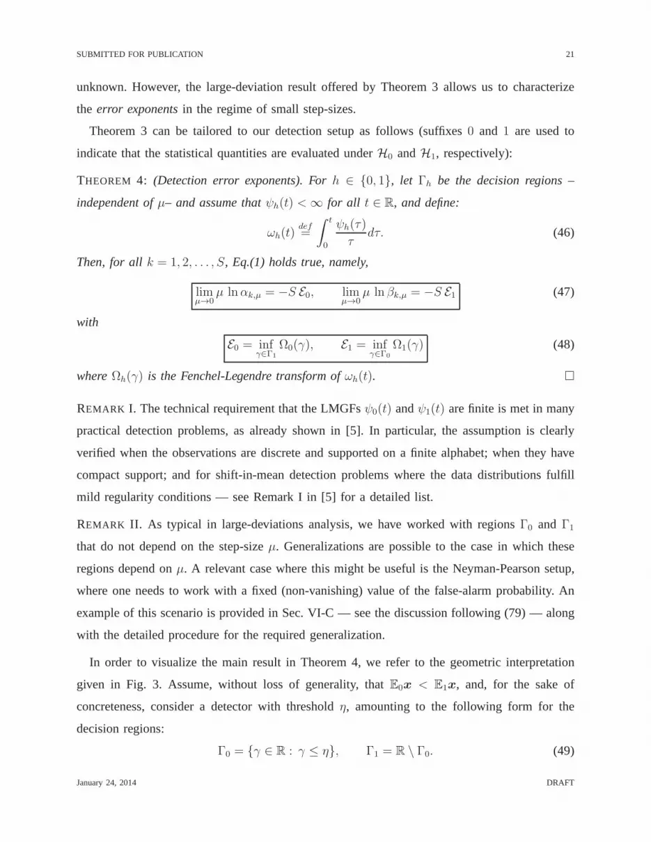
In order to visualize the main result in Theorem 4, we refer tothe geometric interpretation
given in Fig. 3. Assume, without loss of generality, thatE0x < E1x, and, for the sake of
concreteness, consider a detector with thresholdη, amounting to the following form for the
decision regions:
Γ0 = γ ∈ R : γ ≤ η, Γ1 = R \ Γ0. (49)
January 24, 2014 DRAFT
SUBMITTED FOR PUBLICATION 22
Ω0(γ )
γxE0
Ω1(γ )
x
Γ0= γ ∈ R :γ ≤η
infγ∈Γ0
Ω1(γ )
η
infγ∈Γ1
Ω0(γ )
E1
R Γ1= γ ∈ R :γ >η R
Fig. 3. A geometric view of Theorem 4.
Let us setE0x < η < E1x since, as will be clear soon, choosing a threshold outside the
range(E0x,E1x) will always nullify one of the exponents. According to Theorem 4, to evaluate
the exponentE0 (resp.,E1), one must consider the worst-case, i.e., the smallest value of the
functionΩ0(γ) (resp.,Ω1(γ)), within the correspondingerror regionΓ1 (resp.,Γ0). In view of
the convexity properties discussed at the end of Sec. IV-C, and reported in Appendix C, we see
that, for the threshold detector, both minima are attained only atγ = η. Certainly, this shape turns
out to be of great interest in practical applications where,inspired by the optimality properties of
a log-likelihood ratio test in the centralized case, a threshold detector is often an appealing and
reasonable choice. On the other hand, we would like to stressthat different, arbitrary decision
regions can be in general chosen, and that the minima ofΩ0(·) andΩ1(·) in Fig. 3 might be
correspondingly located at two different points.
In summary, Theorem 4 allows us to compute the exponentsE0 andE1 as functions ofi) the
kind of statisticx employed by the sensors, which determines the shape of the LMGFsψh(t) to
be used in (46); andii) of the employed decision regions relevant for the minimizations in (48).
OnceE0 andE1 have been found, the error probabilitiesαk,µ andβk,µ can be approximated using
Eq. (1). This result is then key for both detector design and analysis, so that we are now ready
to illustrate the operation of the adaptive distributed network of detectors.
January 24, 2014 DRAFT
SUBMITTED FOR PUBLICATION 23
1
2
3
45
67
8
9
10
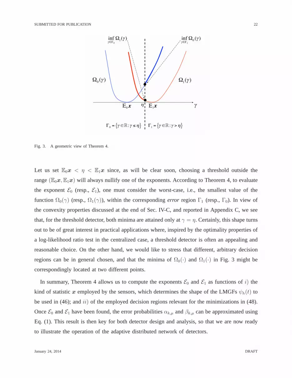
Fig. 4. Network skeleton used for the numerical simulations.
VI. EXAMPLES OF APPLICATION
In this section, we apply the developed theory to four relevant detection problems. We start with
the classical Gaussian shift-in-mean problem. Then, we consider a scenario of specific relevance
for sensor network applications, namely, detection with hardly (one-bit) quantized measurements.
This case amounts to testing two Bernoulli distributions with different parameters under the
different hypotheses. Both the Gaussian and the finite-alphabet assumptions are removed in
the subsequent example, where a problem of relevance to radar applications is addressed, that
is, shift-in-mean with additive noise sampled from a Laplace (double-exponential) distribution.
Finally, we examine a case where the agents have limited knowledge of the underlying data
model, and agree to employ a simple sample-mean detector, inthe presence of noise distributed
as a Gaussian mixture.
Before dwelling on the presentation of the numerical experiments, we provide some essential
details on the strategy that has been implemented for obtaining them:
• The network used for our experiments consists of ten sensors, arranged so as to form the
topology in Fig. 4, with combination weightsak,ℓ following the Laplacian rule [8], [16].
• The decision rule for the detectors is based on comparing thediffusion outputyk(n) to
some thresholdη, namely,
yk(n)H0
⋚H1
η, (50)
where the decision regions are the same as in (49).
January 24, 2014 DRAFT

SUBMITTED FOR PUBLICATION 24
• Selecting the thresholdη in (50) is a critical stage of detector design and implementation.
This choice can be guided by different criteria, which wouldlead to different threshold
settings. In the following examples, we present three relevant cases, namely:i) a threshold
setting that is suited to the Bayesian and the max-min criteria (Sec. VI-B); ii) a Neyman-
Pearson threshold setting (Sec. VI-C);iii) and a threshold setting in the presence of
insufficient information about the underlying statisticalmodels (Sec. VI-D). We would like
to stress that using different threshold setting rules for different statistical models has no
particular meaning. These choices are just meant to illustrate different rules and different
models while avoiding repetition of similar results.
• The diffusion output is obtained after consultation steps involving the exchange of some
local statisticsxk(n). The particular kind of statistic used in the different examples will be
detailed when needed.
A. Shift-in-mean Gaussian Problem
The first hypothesis testing problem we consider is the following:
H0 : dk(n) ∼ N (0, σ2), (51)
H1 : dk(n) ∼ N (θ, σ2), (52)
wheredk(n) denotes the local datum collected by sensork at timen. In the above expression,
N (a, b) is a shortcut for a Gaussian distribution with meana and varianceb, and the symbol
∼ means “distributed as”. We assume the local statisticxk(n) to be shared during the diffusion
process is the log-likelihood ratio of the measurementdk(n):
xk(n) =θ
σ2
(dk(n)−
θ
2
). (53)
Note that in the Gaussian case the log-likelihood ratio is simply a shifted and scaled version of
the collected observationdk(n), such that no substantial differences are expected if the agents
share directly the observations.
In the specific case thatxk(n) is the log-likelihood ratio, the expectationsE0x and E1x
assume a peculiar meaning. Indeed, they can be convenientlyrepresented as:
E0x = −D(H0||H1), E1x = D(H1||H0), (54)
January 24, 2014 DRAFT

SUBMITTED FOR PUBLICATION 25
whereD(Hi||Hj), with i, j ∈ 0, 1, is the Kullback-Leibler (KL) divergence between hypothe-
sesi andj — see [32]. In particular, for the Gaussian shift-in-mean problem the distribution of
the log-likelihood ratio can be expressed in terms of the KL divergences as follows:
xk(n)H0∼ N (−D, 2D), xk(n)
H1∼ N (D, 2D), (55)
where
D def= D(H0||H1) = D(H1||H0) =
θ2
2σ2, (56)
is the KL divergence for the Gaussian shift-in-mean case [32].
Since the LMGF of a Gaussian random variableN (a, b) is at+bt2/2 [34], we deduce from (55)
that
ψ0(t) = Dt(t− 1), ψ1(t) = Dt(t+ 1). (57)
Note thatψ1(t) = ψ0(t+1), a relationship that holds true more generally when workingwith the
LMGFs of the log-likelihood ratio — see, e.g., [47]. Now, applying (46) to (57) readily gives
ω0(t) = Dt(t
2− 1
), ω1(t) = Dt
(t
2+ 1
). (58)
According to its definition (32), in order to find the Fenchel-Legendre transform we should
maximize, with respect tot, the functionγt− ω(t). In view of the convexity properties proved
in Appendix C, this can be done by taking the first derivative and equating it to zero, which is
equivalent to writing
γ = ω′0(t0) =
ψ0(t0)
t0⇒ t0 =
γ
D + 1, (59)
γ = ω′1(t1) =
ψ1(t1)
t1⇒ t1 =
γ
D − 1. (60)
These expressions lead to
Ω0(γ) =(γ +D)2
2D , Ω1(γ) =(γ −D)2
2D . (61)
Selecting the thresholdη within the interval(−D,D), the minimization in (48) is easily per-
formed — refer to Fig. 3 and the related discussion. The final result is:
αk,µ·= e−(1/µ)S (η+D)2
2D , βk,µ·= e−(1/µ) S (η−D)2
2D (62)
These expressions provide the complete asymptotic characterization to the leading exponential
order (i.e., they furnish the detection error exponents) ofthe adaptive distributed network of
January 24, 2014 DRAFT
SUBMITTED FOR PUBLICATION 26
-0.04 0 0.04
0.0
0.5
1.0
1.5
2.0
Γ
Rat
efu
nctio
ns,B
erno
ulli
W0HΓL
W1HΓL
-0.005 Η=0 0.005
Γ
10 100 200 300 400 50010
−2
10−1
100
1/µ
Errorpro
babilityp(e)
k,µ
Sensor 8Sensor 9Sensor 2Sensor 6Sensor 5Sensor 10Sensor 4Sensor 1Sensor 7Sensor 3Fully conn.
10 5000
0.01
0.1
1/µ
−µ
lnp(e)
k,µ
Theor. expon. S E
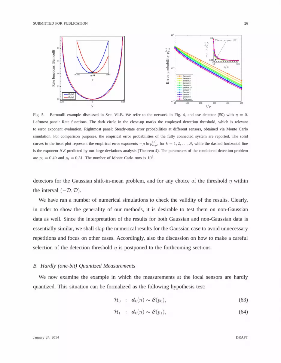
Fig. 5. Bernoulli example discussed in Sec. VI-B. We refer tothe network in Fig. 4, and use detector (50) withη = 0.
Leftmost panel: Rate functions. The dark circle in the close-up marks the employed detection threshold, which is relevant
to error exponent evaluation. Rightmost panel: Steady-state error probabilities at different sensors, obtained via Monte Carlo
simulation. For comparison purposes, the empirical error probabilities of the fully connected system are reported. The solid
curves in the inset plot represent the empirical error exponents−µ ln p(e)k,µ, for k = 1, 2, . . . , S, while the dashed horizontal line
is the exponentS E predicted by our large-deviations analysis (Theorem 4). The parameters of the considered detection problem
arep0 = 0.49 andp1 = 0.51. The number of Monte Carlo runs is105.
detectors for the Gaussian shift-in-mean problem, and for any choice of the thresholdη within
the interval(−D,D).We have run a number of numerical simulations to check the validity of the results. Clearly,
in order to show the generality of our methods, it is desirable to test them on non-Gaussian
data as well. Since the interpretation of the results for both Gaussian and non-Gaussian data is
essentially similar, we shall skip the numerical results for the Gaussian case to avoid unnecessary
repetitions and focus on other cases. Accordingly, also thediscussion on how to make a careful
selection of the detection thresholdη is postponed to the forthcoming sections.
B. Hardly (one-bit) Quantized Measurements
We now examine the example in which the measurements at the local sensors are hardly
quantized. This situation can be formalized as the following hypothesis test:
H0 : dk(n) ∼ B(p0), (63)
H1 : dk(n) ∼ B(p1), (64)
January 24, 2014 DRAFT
SUBMITTED FOR PUBLICATION 27
with B(p) denoting a Bernoulli random variable with success probability p. As in the previous
example, we assume that the local statisticsxk(n) employed by the sensors in the adapta-
tion/combination stages are chosen as the local log-likelihood ratios that, in view of (63)–(64),
can be written as:
xk(n) = dk(n) ln
(p1p0
)+ (1− dk(n)) ln
(q1q0
), (65)
where qh = 1 − ph, with h = 0, 1. Sincedk(n) ∈ 0, 1, we see thatxk(n) is a binary
random variable taking on the valuesln(p1/p0) or ln(q1/q0). The distribution ofxk(n) is then
characterized by:
P0
[xk(n) = ln
(p1p0
)]= p0, P1
[xk(n) = ln
(p1p0
)]= p1, (66)
and, hence, the LMGFs for this example are readily computed:
ψ0(t) = ln
(pt1pt−10
+qt1qt−10
), (67)
ψ1(t) = ln
(pt+11
pt0+qt+11
qt0
). (68)
According to the relationship (46) found in Theorem 4, theseclosed-form expressions are used
for the evaluation ofω0(t) andω1(t), which in turn are needed to compute the rate functions
Ω0(γ) andΩ1(γ). Differently from the Gaussian example, here these tasks need to be performed
numerically. The resulting rate functions are displayed inthe leftmost panel of Fig. 5, and the
observed behavior reproduces what is predicted by the general properties of the rate function —
see also the explanation of Fig. 2.
Let us now examine the adaptive distributed network of detectors in operation. To do so,
we must decide on how to set the detection thresholdη in (50). As a method for selecting
the threshold, in this section we illustrate the asymptoticBayesian criterion that prescribes
maximizing the exponent of the average error probability
p(e)k,µ = π0αk,µ + π1βk,µ, (69)
whereπ0 andπ1 are the prior probabilities of occurrence of hypothesesH0 andH1, respectively.
It is easily envisaged that the exponent of the average errorprobability is determined by the
worst one (slowest decay) between the Type-I and Type-II error exponents — see [48, Eq. (I.2),
p. 4]. As a result, optimizing the Bayesian error exponent isequivalent to a max-min approach
January 24, 2014 DRAFT

SUBMITTED FOR PUBLICATION 28
aimed at maximizing the minimum exponent. We now apply this criterion to the considered
example. To this aim, a close inspection of the rate functions in Fig. 5 is beneficial. First, as it
can be seen by the close-up shown in the inset plot, setting the threshold toη = 0 would imply
E0 = infγ>0
Ω0(γ) = Ω0(0) = Ω1(0) = infγ≤0
Ω1(γ) = E1 def= E . (70)
Moreover, any other choice of the thresholdη 6= 0 makes one of the two exponents smaller
than E . This can be clearly visualized by varying the position ofη in Fig. 3, and computing
the infima over the pertinent decision regions. In summary, according to whether we adopt a
Bayesian or a max-min criterion, an optimal choice for the threshold in this case isη = 0.
In the simulations, we refer to a sufficiently large time horizon, such that the steady-state
assumption applies, and evaluate the error probabilities for different values of the step-size —
see the rightmost panel in Fig. 5. In the considered example,it is easily verified by symmetry
arguments that the error probabilities (and not only the exponents) of first and second kind are
equal, and therefore they equal the average error probability for any prior distribution of the
hypotheses:
αk,µ = βk,µ = p(e)k,µ. (71)
Accordingly, in the following description the terminologies “error probability” and “error expo-
nent” can be equivalently and unambiguously referred to anyof these errors.
In Fig. 5, rightmost panel, the performance of all the agentsis displayed as a function of1/µ,
and different agents are marked with different colors. For comparison purposes, the performance
of the fully connected system is also displayed. All these probability curves have been obtained
by Monte Carlo simulation. Some remarkable features are observed.
First, all the different curves pertaining to different agents stay nearly parallel for sufficiently
small values of the step-sizeµ. This is a way to visualize thati) the detection error probabilities
vanish exponentially at rate1/µ; and ii) the detection errorexponentsat different sensors are
equal, and further equal to that of the fully-connected system corresponding to the centralized
stochastic gradient solution. This is the basic message conveyed by the large deviations analysis.
Indeed, the asymptotic relationships for the error probabilities in (1) express convergenceto the
first leading order in the exponent.
It remains to show that theexponentsof the simulated error probabilities match theexponents
predicted by Theorem 4. This is made in the inset plot of Fig. 5, rightmost panel, where the
January 24, 2014 DRAFT
SUBMITTED FOR PUBLICATION 29
horizontal dashed line depicts the theoretical exponentSE , with E computed using (70), while
the solid curves represent the empirical error exponents seen at different sensors, namely the
quantities−µ ln p(e)k,µ, for k = 1, 2, . . . , S. It is observed that, as the step-size decreases, the
empirical error exponents converge toward the theoreticaloneS E .
A further interesting evidence seems to emerge from the numerical experiments. The error
probability curves in Fig. 5, rightmost panel, are basically ordered. Examining the relationship
between this ordering and the sensor placement in Fig. 4, it is seen that the ordering reflects the
degree of connectivity of each agent. For instance, sensor3 has the highest number of neighbors
(five), and its performance is the closest to the fully connected case. On the other hand, sensor
8 is the most isolated, and its error probability curve appears accordingly the highest one. Note
that, since from the presented theory we learned that each agent reaches asymptotically the same
detection exponent, these differences are related to higher order corrections (i.e., sub-exponential
terms that are neglected in a large deviations analysis) and/or to non-asymptotic effects. A
systematic and thorough analysis of the above features, as well as of their exact interplay with
the network connectivity and more in general with the overall structure of the connectivity matrix
A, requires a refined asymptotic estimate that goes beyond thelarge deviations analysis carried
out here.
C. Shift-in-mean with Laplacian noise
In this section we consider another non-Gaussian example, namely, the case of a shift-in-
mean detection problem with noise distributed according toa Laplace distribution. Denoting by
L(a, b) a (shifted) Laplace distribution with shift parametera and scale parameterb, i.e., having
the probability density function:
fL(ξ) =1
2be−
|ξ−a|b , (72)
the hypothesis test we are now interested in is formulated asfollows:
H0 : dk(n) ∼ L(0, σ), (73)
H1 : dk(n) ∼ L(θ, σ). (74)
We assume again that the local statisticsxk(n) are chosen as the local log-likelihood ratios:
xk(n) =1
σ(|dk(n)| − |dk(n)− θ|). (75)
January 24, 2014 DRAFT
SUBMITTED FOR PUBLICATION 30
-0.05 0 0.05
0.0
0.5
1.0
1.5
2.0
2.5
Γ
Rat
efu
nctio
ns,L
apla
ce
W0HΓL
W1HΓL
-0.005 0 0.005E0x
Γ
10 100 200 300 400 500 600 700 800 900 10000
0.1
0.2
0.3
0.4
0.5
1/µ
Type-Ierro
rpro
babilityα
k,µ
Prescribed Type-I e rror prob. α
Sensor 8Sensor 9Sensor 2Sensor 6Sensor 5Sensor 10Sensor 4Sensor 1Sensor 7Sensor 3Fully conn.Theorem 2
10 100 200 300 400
10−3
10−2
10−1
100
1/µ
Type-II
erro
rpro
babilityβk,µ
Sensor 8Sensor 9Sensor 2Sensor 6Sensor 5Sensor 10Sensor 4Sensor 1Sensor 7Sensor 3Fully conn.
10 4000
0.01
0.1
1/µ
−µ
lnβk,µ
Theor. expon. S E 1
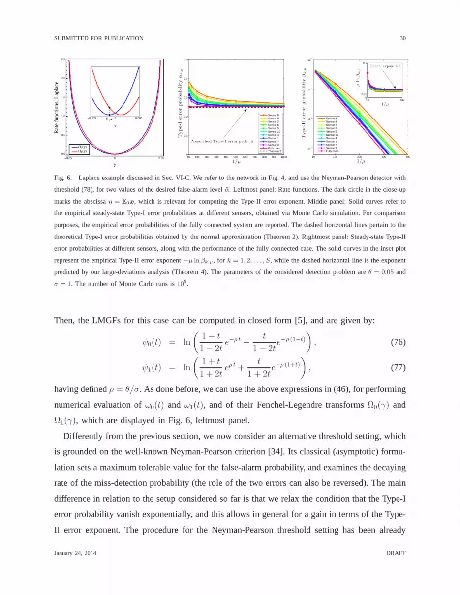
Fig. 6. Laplace example discussed in Sec. VI-C. We refer to the network in Fig. 4, and use the Neyman-Pearson detector with
threshold (78), for two values of the desired false-alarm level α. Leftmost panel: Rate functions. The dark circle in the close-up
marks the abscissaη = E0x, which is relevant for computing the Type-II error exponent. Middle panel: Solid curves refer to
the empirical steady-state Type-I error probabilities at different sensors, obtained via Monte Carlo simulation. Forcomparison
purposes, the empirical error probabilities of the fully connected system are reported. The dashed horizontal lines pertain to the
theoretical Type-I error probabilities obtained by the normal approximation (Theorem 2). Rightmost panel: Steady-state Type-II
error probabilities at different sensors, along with the performance of the fully connected case. The solid curves in the inset plot
represent the empirical Type-II error exponent−µ ln βk,µ, for k = 1, 2, . . . , S, while the dashed horizontal line is the exponent
predicted by our large-deviations analysis (Theorem 4). The parameters of the considered detection problem areθ = 0.05 and
σ = 1. The number of Monte Carlo runs is105.
Then, the LMGFs for this case can be computed in closed form [5], and are given by:
ψ0(t) = ln
(1− t1− 2t
e−ρ t − t
1− 2te−ρ (1−t)
), (76)
ψ1(t) = ln
(1 + t
1 + 2teρ t +
t
1 + 2te−ρ (1+t)
), (77)
having definedρ = θ/σ. As done before, we can use the above expressions in (46), forperforming
numerical evaluation ofω0(t) andω1(t), and of their Fenchel-Legendre transformsΩ0(γ) and
Ω1(γ), which are displayed in Fig. 6, leftmost panel.
Differently from the previous section, we now consider an alternative threshold setting, which
is grounded on the well-known Neyman-Pearson criterion [34]. Its classical (asymptotic) formu-
lation sets a maximum tolerable value for the false-alarm probability, and examines the decaying
rate of the miss-detection probability (the role of the two errors can also be reversed). The main
difference in relation to the setup considered so far is thatwe relax the condition that the Type-I
error probability vanish exponentially, and this allows ingeneral for a gain in terms of the Type-
II error exponent. The procedure for the Neyman-Pearson threshold setting has been already
January 24, 2014 DRAFT
SUBMITTED FOR PUBLICATION 31
described in Sec. IV — see (25)–(26). Accordingly, to achieve a false-alarm probabilityα, we
need a threshold
η = ηµ = E0x+
√µσ2
x,0
2SQ−1(α). (78)
It remains to evaluate the Type-II error probability
βk,µ = P1[y⋆k,µ ≤ ηµ], (79)
or, more precisely, the corresponding exponentE1. For this purpose, we must resort to Theorem
4. Note, however, that the thresholdη = ηµ now depends onµ and, hence, Theorem 4 does not
directly apply. As noted in Remark II, it is instructive to examine how the result of Theorem
4 can be generalized to manage similar situations. Indeed, we can work in terms of the shifted
variables
y⋆k,µ = y⋆k,µ −
√µσ2
x,0
2SQ−1(α), (80)
yielding
βk,µ = P1[y⋆k,µ ≤ E0x]. (81)
By application of the Gartner-Ellis Theorem to the shiftedvariablesy⋆k,µ, it is easy to see that
the added deterministic term (vanishing withµ) does not alter the limiting functionω1(t) in (46),
and consequently the final rate functionΩ1(γ). Accordingly, and based on (81), the Type-II error
exponent is
E1 = infγ≤E0x
Ω1(γ) = Ω1(E0x). (82)
The main implication of the above result can be understood, e.g., by examining the close-up in
the leftmost panel of Fig. 6, where it is seen that:
E1 = Ω1(E0x) > Ω1(0), (83)
the latter value being the Type-II error exponent achieved by the max-min optimal detector with
zero threshold previously described. This immediately shows the gain achieved by relaxing the
constraint thatboth error probabilities must vanish exponentially.
We now present the numerical evidence for the Neyman-Pearson adaptive distributed detec-
tor. The middle panel in Fig. 6 shows the convergence ofαk,µ toward the prescribed Type-I
error probabilityα as the step-sizeµ goes to zero. The rightmost panel refers instead to the
January 24, 2014 DRAFT
SUBMITTED FOR PUBLICATION 32
-2 0 2
0
1
2
3
4
5
6
Γ
Rat
efu
nctio
ns,G
auss
ian
mix
ture
W0HΓL
W1HΓL
-0.05 0 0.05Η
Γ
10 100 200 300 400 500
10−2
10−1
100
1/µ
Type-Ierro
rpro
babilityα
k,µ
Sensor 8Sensor 9Sensor 2Sensor 6Sensor 5Sensor 10Sensor 4Sensor 1Sensor 7Sensor 3Fully conn.
10 5000
0.01
0.1
1/µ
−µ
lnα
k,µ
Theor. expon. S E 0
10 100 200 300 400 500
10−2
10−1
100
1/µ
Type-II
erro
rpro
babilityβk,µ
Sensor 8Sensor 9Sensor 2Sensor 6Sensor 5Sensor 10Sensor 4Sensor 1Sensor 7Sensor 3Fully conn.
10 5000
0.01
0.1
1/µ
−µ
lnβk,µ
Theor. expon. S E 1
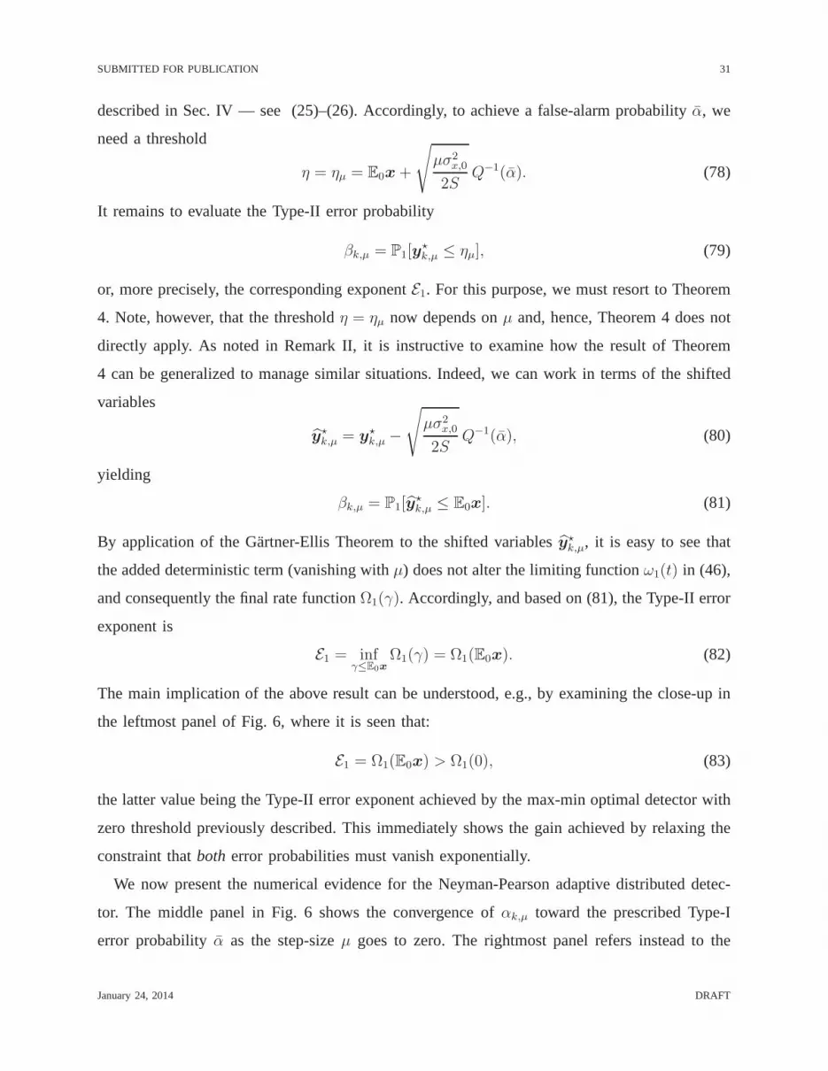
Fig. 7. Gaussian mixture example discussed in Sec. VI-D. We refer to the network in Fig. 4, and use detector (50) withη = θ/3.
Leftmost panel: Rate functions. The dark circle in the close-up marks the employed detection threshold, which is relevant for
evaluating the error exponents. Middle panel: Steady-state Type-I error probabilities at different sensors, obtained via Monte
Carlo simulation. For comparison purposes, the empirical error probabilities of the fully connected system are reported. The
solid curves in the inset plot represent the empirical Type-I error exponent−µ lnαk,µ, for k = 1, 2, . . . , S, while the dashed
horizontal line is the exponent predicted by our large-deviations analysis (Theorem 4). Rightmost panel: Same of middle panel,
but for the Type-II error. The parameters of the considered detection problem areθ = 0.05, θ0 = 1, σ1 = 1, andσ2 = 0.3. The
number of Monte Carlo runs is105.
corresponding Type-II error probability curves. The conclusions that can be drawn are similar
to those discussed in the previous example, confirming the validity of the theoretical analysis. It
is also interesting to note that the ordering of the different curves, for both error probabilities,
is exactly the same obtained in the Bernoulli example. Sincethe network employed for the
simulations is unchanged, this is another clue that the ordering may be related to the structure
of the connectivity matrixA.
D. Shift-in-mean with Gaussian mixture noise
As a final example, we consider the case of a shift-in-mean detection problem with noise
distributed according to a zero-mean Gaussian mixture, having the probability density function
fGM(ξ) =1
2
(1√2πb1
e− (ξ−a0)
2
2b1 +1√2πb2
e− (ξ+a0)
2
2b2
), (84)
namely, a balanced mixture of normal random variables with different variancesb1 and b2,
and symmetric expectations±a0. Denoting byNmix(a, a0, b1, b2) a shifted Gaussian mixture
January 24, 2014 DRAFT

SUBMITTED FOR PUBLICATION 33
distribution with shift parametera, we consider the following hypothesis test:
H0 : dk(n) ∼ Nmix(0, θ0, σ21, σ
22), (85)
H1 : dk(n) ∼ Nmix(θ, θ0, σ21, σ
22). (86)
For this model, we donot assume that the local statisticsxk(n) are chosen as the local log-
likelihood ratios. We assume instead that the agents of the network have scarce knowledge about
the underlying statistical model. They know that it is a shift-in-mean problem, and possess a
rough information about the value ofθ. In these circumstances, the agents decide to implement
a distributed sample-mean detector, namely, they exchangethe local measurementsas they are,
without any additional pre-processing. This amounts to state that
H0 : xk(n) ∼ Nmix(0, θ0, σ21, σ
22), (87)
H1 : xk(n) ∼ Nmix(θ, θ0, σ21, σ
22). (88)
Then, the LMGFs for this case can be computed in closed form [5], and are given by:
ψ0(t) = ln
(1
2eθ0t+
σ21t
2
2 +1
2e−θ0t+
σ22t
2
2
), (89)
ψ1(t) = θt+ ψ0(t). (90)
The above expressions are used in (46) for evaluating numerically ω0(t) andω1(t), and then their
Fenchel-Legendre transformsΩ0(γ) andΩ1(γ). These latter are depicted in the leftmost panel of
Fig. 7. We assume the agents in the network are not able to optimize the choice of the detection
threshold, due to their limited knowledge of the underlyingstatistical models. The particular
value used in the simulations isη = θ/3, which is marked in the close-up of Fig. 7, leftmost
panel. It is seen that, differently from the previous examples, this choice does not correspond to
a balancing of the detection error exponents, such that it isexpected that the Type-I and Type-II
error probabilities behave quite differently in this case.This is clearly observed in the middle
(Type-I error) and rightmost (Type-II error) panels of Fig.7. The numerical evidence confirms
the theoretical predictions, as well as the essential features found in all the previous examples.
Moreover, it is seen that the enhanced decaying rate of the Type-II error probability arising from
the unbalanced threshold setting is paid in terms of a higherType-I error probability.
January 24, 2014 DRAFT
SUBMITTED FOR PUBLICATION 34
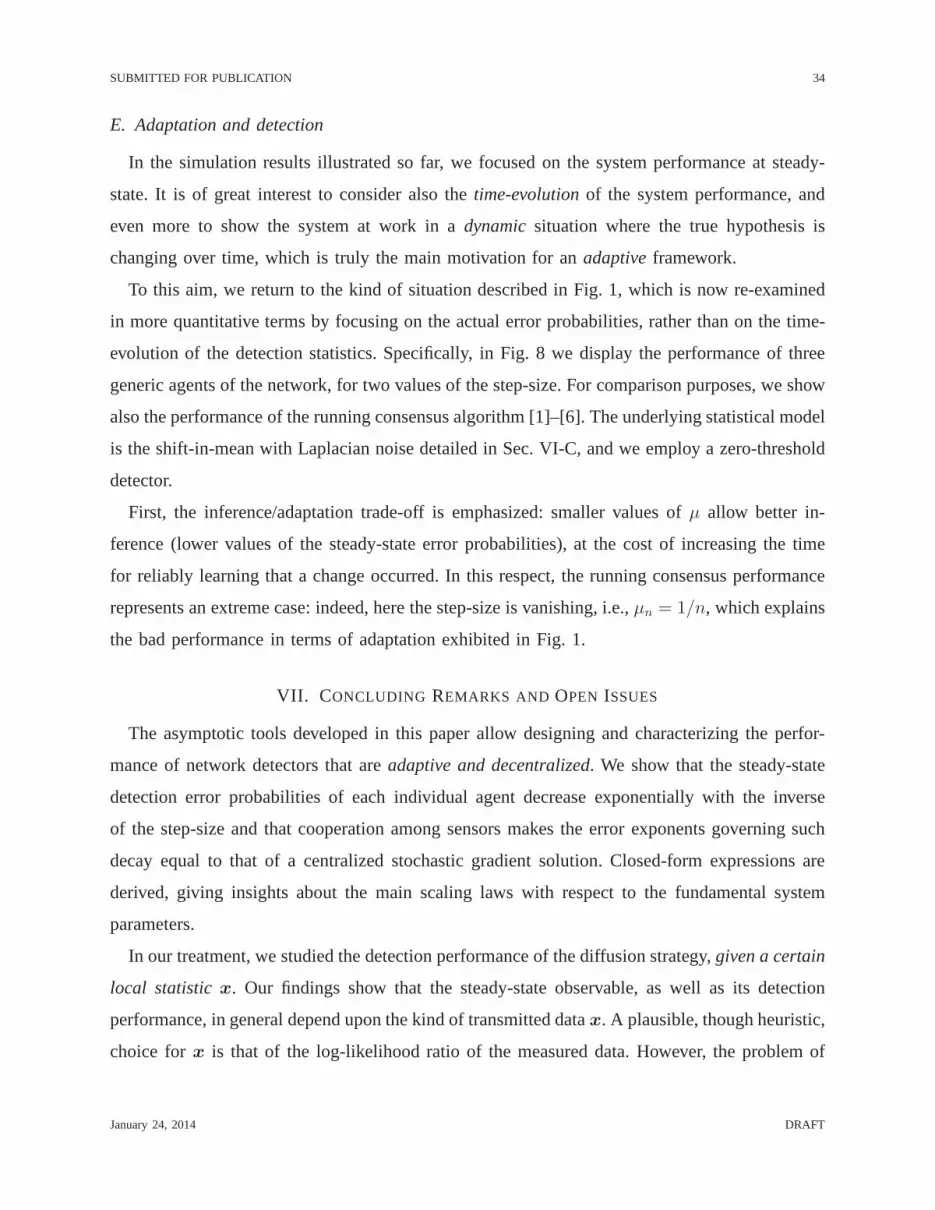
E. Adaptation and detection
In the simulation results illustrated so far, we focused on the system performance at steady-
state. It is of great interest to consider also thetime-evolutionof the system performance, and
even more to show the system at work in adynamicsituation where the true hypothesis is
changing over time, which is truly the main motivation for anadaptiveframework.
To this aim, we return to the kind of situation described in Fig. 1, which is now re-examined
in more quantitative terms by focusing on the actual error probabilities, rather than on the time-
evolution of the detection statistics. Specifically, in Fig. 8 we display the performance of three
generic agents of the network, for two values of the step-size. For comparison purposes, we show
also the performance of the running consensus algorithm [1]–[6]. The underlying statistical model
is the shift-in-mean with Laplacian noise detailed in Sec. VI-C, and we employ a zero-threshold
detector.
First, the inference/adaptation trade-off is emphasized:smaller values ofµ allow better in-
ference (lower values of the steady-state error probabilities), at the cost of increasing the time
for reliably learning that a change occurred. In this respect, the running consensus performance
represents an extreme case: indeed, here the step-size is vanishing, i.e.,µn = 1/n, which explains
the bad performance in terms of adaptation exhibited in Fig.1.
VII. CONCLUDING REMARKS AND OPEN ISSUES
The asymptotic tools developed in this paper allow designing and characterizing the perfor-
mance of network detectors that areadaptive and decentralized. We show that the steady-state
detection error probabilities of each individual agent decrease exponentially with the inverse
of the step-size and that cooperation among sensors makes the error exponents governing such
decay equal to that of a centralized stochastic gradient solution. Closed-form expressions are
derived, giving insights about the main scaling laws with respect to the fundamental system
parameters.
In our treatment, we studied the detection performance of the diffusion strategy,given a certain
local statisticx. Our findings show that the steady-state observable, as wellas its detection
performance, in general depend upon the kind of transmitteddatax. A plausible, though heuristic,
choice forx is that of the log-likelihood ratio of the measured data. However, the problem of
January 24, 2014 DRAFT
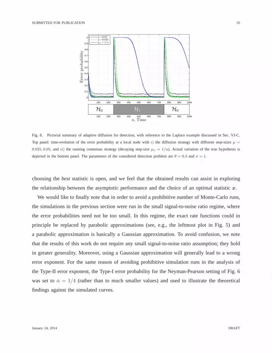
SUBMITTED FOR PUBLICATION 35
100 200 300 400 500 600 700 800 900 1000
0
0.1
0.2
0.3
0.4
0.5
0.6
0.7
0.8
0.9
1
Errorprobability
µ =0.05µ =0.025µn = 1/n
100 200 300 400 500 600 700 800 900 1000
H0 H1 H0
n, Time
Fig. 8. Pictorial summary of adaptive diffusion for detection, with reference to the Laplace example discussed in Sec. VI-C.
Top panel: time-evolution of the error probability at a local node with i) the diffusion strategy with different step-sizesµ =
0.025, 0.05, and ii) the running consensus strategy (decaying step-sizeµn = 1/n). Actual variation of the true hypothesis is
depicted in the bottom panel. The parameters of the considered detection problem areθ = 0.3 andσ = 1.
choosing thebeststatistic is open, and we feel that the obtained results can assist in exploring
the relationship between the asymptotic performance and the choice of an optimal statisticx.
We would like to finally note that in order to avoid a prohibitive number of Monte-Carlo runs,
the simulations in the previous section were run in the smallsignal-to-noise ratio regime, where
the error probabilities need not be too small. In this regime, the exact rate functions could in
principle be replaced by parabolic approximations (see, e.g., the leftmost plot in Fig. 5) and
a parabolic approximation is basically a Gaussian approximation. To avoid confusion, we note
that the results of this work do not require any small signal-to-noise ratio assumption; they hold
in greater generality. Moreover, using a Gaussian approximation will generally lead to a wrong
error exponent. For the same reason of avoiding prohibitivesimulation runs in the analysis of
the Type-II error exponent, the Type-I error probability for the Neyman-Pearson setting of Fig. 6
was set toα = 1/4 (rather than to much smaller values) and used to illustrate the theoretical
findings against the simulated curves.
January 24, 2014 DRAFT

SUBMITTED FOR PUBLICATION 36
APPENDIX A: PROOF OFTHEOREM 2
Motivated by the fact that the transient term in Eq. (12) doesnot affect the limiting behavior
of yk(n), we introduce the following finite-horizon variable:
y⋆k(n)def=
n∑
i=1
zk(i) =n∑
i=1
S∑
ℓ=1
µ(1− µ)i−1bk,ℓ(i)x′ℓ(i). (91)
Sincey⋆k(n) converges in distribution toy⋆k,µ asn→∞, by Levy’s continuity Theorem [41], the
corresponding characteristic functions must converge as well. It is convenient to work in terms
of the normalized variable:
y⋆k,µ =y⋆k,µ − Ex√µ σ2
x/(2S). (92)
Denoting byϕk,µ(t) the characteristic function ofy⋆k,µ, using (91) and (92), and taking the limit
asn→∞, we have:
ϕk,µ(t) = Eejty⋆k,µ =
∞∏
i=1
S∏
ℓ=1
Eejtx′ℓ(i)ζi,ℓ , (93)
defined in terms of the non-random variable
ζi,ℓ =√2Sµ(1− µ)i−1bk,ℓ(i), (94)
and the centered and normalized random variable
x′ℓ(i) =
x′ℓ(i)− Ex
σx. (95)
Now, the claim of asymptotic normality in (21) can be proven by showing the convergence, as
µ → 0, of ϕk,µ(t) towards the characteristic function of the standard normaldistribution,e−t2
2 .
It suffices to work witht > 0 to verify the validity of this latter property. Formally, wewould
like to show that the quantity:∣∣∣ϕk,µ(t)− e−
t2
2
∣∣∣ =∣∣∣∣∣
∞∏
i=1
S∏
ℓ=1
Eejtx′ℓ(i)ζi,ℓ − e− t2
2
∣∣∣∣∣ (96)
converges to zero asµ→ 0. To this aim, we start by working with a finiten, and write:∣∣∣∣∣
n∏
i=1
S∏
ℓ=1
Eejtx′ℓ(i)ζi,ℓ − e− t2
2
∣∣∣∣∣
≤∣∣∣∣∣
n∏
i=1
S∏
ℓ=1
Eejtx′ℓ(i)ζi,ℓ −
n∏
i=1
S∏
ℓ=1
e−t2ζ2
i,ℓ2
∣∣∣∣∣
+
∣∣∣∣∣
n∏
i=1
S∏
ℓ=1
e−t2ζ2
i,ℓ2 − e− t2
2
∣∣∣∣∣ . (97)
January 24, 2014 DRAFT

SUBMITTED FOR PUBLICATION 37
We first focus on the first term on the RHS of (97). For complexwi, zi, with |wi| ≤ 1 and
|zi| ≤ 1, it is known that [41]:∣∣∣∣∣
n∏
i=1
wi −n∏
i=1
zi
∣∣∣∣∣ ≤n∑
i=1
|wi − zi|. (98)
SinceEejtx′ℓ(i)ζi,ℓ is a characteristic function, its magnitude is not greater than one [41], such
that it is legitimate to write, in view of (98):∣∣∣∣∣
n∏
i=1
S∏
ℓ=1
Eejtx′ℓ(i)ζi,ℓ −
n∏
i=1
S∏
ℓ=1
e−t2ζ2
i,ℓ2
∣∣∣∣∣
≤n∑
i=1
S∑
ℓ=1
∣∣∣∣Eejtx′
ℓ(i)ζi,ℓ − e−
t2ζ2i,ℓ2
∣∣∣∣ . (99)
The single summand on the right-hand side of the above expression is upper bounded by∣∣∣∣Ee
jtx′ℓ(i)ζi,ℓ − 1 +
t2ζ2i,ℓ2
∣∣∣∣ +∣∣∣∣e
−t2ζ2
i,ℓ2 − 1 +
t2ζ2i,ℓ2
∣∣∣∣ . (100)
Using the fact thatEx′ℓ(i) = 0 andE[x′
ℓ(i)]2 = 1, we can further bound the first term in the
above expression as∣∣∣∣Ee
jtx′ℓ(i)ζi,ℓ − 1 +
t2ζ2i,ℓ2
∣∣∣∣
=
∣∣∣∣E(ejtx
′ℓ(i)ζi,ℓ − 1− jx′
ℓ(i)tζi,ℓ + [x′ℓ(i)]
2t2ζ2i,ℓ2
)∣∣∣∣
≤ E|x′ℓ(i)|3
t3ζ3i,ℓ6
, (101)
where the last inequality follows from upper bounding the remainder of the Taylor expansion
of the complex exponential:∣∣∣∣ejt − 1− jt
1!− · · · − (jt)n−1
(n− 1)!
∣∣∣∣ ≤|t|nn!. (102)
Likewise, the second term in (100) is upper bounded byt4ζ4
i,ℓ
8since|e−s− 1+ s| ≤ s2/2 for any
s ≥ 0.
January 24, 2014 DRAFT

SUBMITTED FOR PUBLICATION 38
We can accordingly rewrite (97) as:∣∣∣∣∣
n∏
i=1
S∏
ℓ=1
Eejtx′ℓ(i)ζi,ℓ − e− t2
2
∣∣∣∣∣
≤ E|x′ℓ(i)|3
t3
6
n∑
i=1
S∑
ℓ=1
ζ3i,ℓ
+t4
8
n∑
i=1
S∑
ℓ=1
ζ4i,ℓ
+∣∣∣e−
t2
2
∑ni=1
∑Sℓ=1 ζ
2i,ℓ − e− t2
2
∣∣∣ .
(103)
We now take the limit asn → ∞ in the above expression. To this aim, observe that, by the
definition (94), the summation:n∑
i=1
S∑
ℓ=1
ζmi,ℓ, m = 1, 2, . . . (104)
is made of nonnegative terms, and is upper bounded by a convergent geometric series, since
bk,ℓ ≤ 1. This implies the convergence of the series (104) asn → ∞. Accordingly, taking the
limit as n→∞ in (103), and using (96), we have:∣∣∣ϕk,µ(t)− e−
t2
2
∣∣∣ =
∣∣∣∣∣
∞∏
i=1
S∏
ℓ=1
Eejtx′ℓ(i)ζi,ℓ − e− t2
2
∣∣∣∣∣
≤ E|x′ℓ(i)|3
t3
6
∞∑
i=1
S∑
ℓ=1
ζ3i,ℓ
+t4
8
∞∑
i=1
S∑
ℓ=1
ζ4i,ℓ
+∣∣∣e−
t2
2
∑∞i=1
∑Sℓ=1 ζ
2i,ℓ − e− t2
2
∣∣∣ .
(105)
In order to show that the first term on the RHS converges to zeroasµ→ 0, it suffices to verify
that:∞∑
i=1
S∑
ℓ=1
ζmi,ℓµ→0−→ 0, m = 3, 4, (106)
∞∑
i=1
S∑
ℓ=1
ζ2i,ℓµ→0−→ 1. (107)
January 24, 2014 DRAFT

SUBMITTED FOR PUBLICATION 39
The key for proving the above properties is Perron’s Theorem, which provides a uniform bound
on the convergence rate — see [40, Th. 8.5.1]. Letλ2 be the second largest magnitude eigenvalue
of A. For any positiveλ such that|λ2| < λ < 1, there exists a positive constantC = C(λ,A),ensuring for alli, k and ℓ: ∣∣∣∣bk,ℓ(i)−
1
S
∣∣∣∣ ≤ Cλi. (108)
The above result follows by noting that the largest magnitude eigenvalue of the difference matrix
Bn−(1/S)11T is λ2, and by applying the result on the convergence rate in [40, Corollary 5.6.13].
According to the above discussion, let us modify the variables ζi,ℓ by replacing the matrix
entriesbk,ℓ(i) with their limit 1/S, namely,
ζi,ℓ =√2Sµ(1− µ)i−1 1
S, (109)
and introduce, for any integerm ≥ 2, the absolute difference:∣∣∣∣∣
∞∑
i=1
S∑
ℓ=1
ζmi,ℓ −∞∑
i=1
S∑
ℓ=1
ζmi,ℓ
∣∣∣∣∣ ≤∞∑
i=1
S∑
ℓ=1
|ζmi,ℓ − ζmi,ℓ|
= (2Sµ)m/2∞∑
i=1
S∑
ℓ=1
(1− µ)m(i−1)
∣∣∣∣bmk,ℓ(i)−
1
Sm
∣∣∣∣ .
(110)
Recalling the factorization
am − bm = (a− b)m−1∑
k=0
akbm−1−k, (111)
(which can be proved, fora 6= b, by using the geometric sum∑m−1
k=0 rk = 1−rm
1−r , and using
r = a/b), along with the fact thatbk,ℓ(i) and1/S are not greater than one, we conclude that∣∣∣∣bmk,ℓ(i)−
1
Sm
∣∣∣∣ ≤ m
∣∣∣∣bk,ℓ(i)−1
S
∣∣∣∣ , (112)
January 24, 2014 DRAFT

SUBMITTED FOR PUBLICATION 40
yielding∣∣∣∣∣
∞∑
i=1
S∑
ℓ=1
ζmi,ℓ −∞∑
i=1
S∑
ℓ=1
ζmi,ℓ
∣∣∣∣∣
≤ m(2Sµ)m/2∞∑
i=1
S∑
ℓ=1
(1− µ)m(i−1)
∣∣∣∣bk,ℓ(i)−1
S
∣∣∣∣
≤ Cλm(2Sµ)m/2∞∑
i=1
S∑
ℓ=1
(1− µ)m(i−1)λi−1
= Cλm2m/2Sm/2+1 µm/2
1− λ(1− µ)mµ→0−→ 0, (113)
where the second inequality follows from (108), and the limit holds becauseλ < 1. In view of
the above result, in order to establish (106) and (107) it is enough to study the limiting behavior
of the summation:∞∑
i=1
S∑
ℓ=1
ζmi,ℓ =(2µ)m/2
Sm/2−1
∞∑
i=1
(1− µ)m(i−1)
=2m/2
Sm/2−1
µm/2
1− (1− µ)m . (114)
Applying L’Hospital’s rule [49], the limit of the RHS asµ→ 0 is:(2
S
)m/2−1
limµ→0
µm/2−1
(1− µ)m−1, (115)
which converges to1 for m = 2, and to0 otherwise, completing the proof.
APPENDIX B: PROOF OFTHEOREM 3
We first list some regularity properties ofψ(t) that will be applied in the subsequent analysis
— see, e.g., [47], [48]:
1) By assumption,ψ(t) <∞ for all t ∈ R. Since it is a LMGF, it is infinitely differentiable
in R. Also, sincex is a non-degenerate (i.e., non deterministic) random variable, we have
ψ′′(t) > 0, ∀t ∈ R, (116)
and, hence,ψ(t) is strictly convex inR.
2) With reference to the functionψ(t)t
appearing in (36), we note that
limt→0
ψ(t)
t= ψ′(0), (117)
January 24, 2014 DRAFT

SUBMITTED FOR PUBLICATION 41
and, hence,ψ(t)t
is continuous for allt ∈ R, and the integral in (36) is well-posed.
3) For all t 6= 0, we haved
dt
ψ(t)
t=ψ′(t) t− ψ(t)
t2, (118)
with
limt→0
ψ′(t) t− ψ(t)t2
=ψ′′(0)
2, (119)
implying that ddtψ(t)t
is continuous for allt ∈ R. In addition, we have:
d
dt
ψ(t)
t> 0, ∀t ∈ R. (120)
This is immediately verified fort = 0 by using (116) in (119). Fort 6= 0, sinceψ(t) is
strictly convex and differentiable inR, we can apply the first-order condition for strict
convexity — see Eq. (3.3) in [50]:
ψ(a)− ψ(b) > ψ′(b)(a− b), ∀a, b ∈ R, a 6= b. (121)
Settinga = 0, b = t 6= 0, and usingψ(0) = 0, result (120) now follows from (118).
In the following, we denote byφ(c)µ (t) the LMGF of the steady-state variabley⋆k,µ that would
correspond to a fully connected network with uniform weights, ak,ℓ = bk,ℓ = 1/S for all k, ℓ =
1, 2, . . . , S. We start by stating two lemmas (their proofs are given in thesequel).
LEMMA 1 Define an auxiliary functionf1(t) whose values over the negative and positive ranges
of time are scaled as follows:
f1(t) = t2 ×
maxτ∈[0,t]
(d
dτ
ψ(τ)
τ
), t ≥ 0,
maxτ∈[t,0]
(d
dτ
ψ(τ)
τ
), t < 0.
(122)
Then, the LMGF ofy⋆k,µ for the fully connected solution with uniform weights is:
φ(c)µ (t) =
S
µ
[∫ µSt
0
ψ(τ)
τdτ +
∞∑
i=1
ci(t;µ)
](123)
where the functionsci(t;µ) are nonnegative and satisfy∞∑
i=1
ci(t;µ) ≤ f1
(µSt)× µ2
1− (1− µ)2 . (124)
January 24, 2014 DRAFT

SUBMITTED FOR PUBLICATION 42
LEMMA 2 Let λ2 be the second largest eigenvalue ofA in magnitude, and let|λ2| < λ < 1.
Define another auxiliary function as:
f2(t) = |t| ×
maxτ∈[0,t]
|ψ′(τ)|, t ≥ 0,
maxτ∈[t,0]
|ψ′(τ)|, t < 0.(125)
Then, the LMGF of the steady-state diffusion outputy⋆k,µ defined by (19) is:
φk,µ(t) = φ(c)µ (t) +
∞∑
i=1
S∑
ℓ=1
ci,ℓ(t;µ) (126)
where the functionsci,ℓ(t;µ) now satisfy∞∑
i=1
S∑
ℓ=1
|ci.ℓ(t;µ)| ≤ (CλS) f2(µt)
1− λ(1− µ) , (127)
for a positive constantC depending onλ and on the combination matrixA.
We can easily show that:
0 ≤ f1(t) <∞, 0 ≤ f2(t) <∞, ∀t ∈ R. (128)
Indeed,f1(t) ≥ 0 from (120), whilef2(t) ≥ 0 by definition. Finiteness of both functions follows
from Weierstrass extreme value theorem [49] since, by the properties ofψ(t) discussed at the
beginning of this appendix, the maxima appearing in (122) and (125) are maxima of continuous
functions over compact sets for any finitet.
By using the above lemmas (whose proofs will be given soon), it is straightforward to prove
Theorem 3.
Proof of Part i) of Theorem 3:we start by proving that
limµ→0
µφ(c)µ (t/µ) = S
∫ t/S
0
ψ(τ)
τdτ. (129)
From the above Lemma 1 we have:∣∣∣∣∣µφ(c)µ (t/µ)− S
∫ t/S
0
ψ(τ)
τdτ
∣∣∣∣∣
= S
∞∑
i=1
ci(t/µ;µ) ≤ S f1(t/S)×µ2
1− (1− µ)2µ→0
−→ 0 .
(130)
January 24, 2014 DRAFT
SUBMITTED FOR PUBLICATION 43
On the other hand, using Lemma 2,
µ∣∣φk,µ(t/µ)− φ(c)
µ (t/µ)∣∣ = µ
∣∣∣∣∣
∞∑
i=1
S∑
ℓ=1
ci,ℓ(t/µ;µ)
∣∣∣∣∣
≤ (CλS) f2(t)µ
1− λ(1− µ)µ→0
−→ 0, (131)
and claimi) is proven.
Proof of Part ii) of Theorem 3:From the definition ofω(t) in (36) we haveω′(t) = ψ(t)/t,
which follows by continuity ofψ(t)/t for all t ∈ R — see property 2) at the beginning of this
appendix. Then, using the result proven in parti), sinceω(t) is differentiable inR, the Gartner-
Ellis Theorem [48] stated in Sec. IV-B can be applied to conclude thaty⋆k,µ must obey the
LDP (29) with rate function given by the Fenchel-Legendre transform of the functionS ω(t/S).
It is straightforward to verify that the Fenchel-Legendre transform of a function scaled in this
way is simplyS Ω(γ).
We now prove the two lemmas.
Proof of Lemma 1. For the case of a fully connected network with uniform weights, the finite-
horizon variable introduced in (91) reduces to
y⋆k(n) =n∑
i=1
S∑
ℓ=1
µ(1− µ)i−1 1
Sx′ℓ(i). (132)
Now since the LMGF is additive for sums of independent randomvariables, the LMGF ofy⋆k(n)
defined above, for any fixed time instantn, is given by:
Sn∑
i=1
ψ((1− µ)i−1µ
St). (133)
First we notice that, if we were able to show that this quantity converges asn goes to infinity,
the limit will represent the LMGF,φ(c)µ (t), of the steady-state random variabley⋆k,µ in the fully
connected case, in view of the continuity theorem for the moment generating functions [51].
Define g(t) = ψ(t)/t and let us focus initially ont > 0. We introduce the countably infinite
partition of the interval[0, µSt] with endpoints
τi = (1− µ)i−1µ
St, i = 1, 2, . . . ,∞. (134)
January 24, 2014 DRAFT

SUBMITTED FOR PUBLICATION 44
Repeated application of the mean-value theorem [49] then gives:∫ τ1
τn+1
g(τ)dτ =n∑
i=1
∫ τi
τi+1
g(τ)dτ =n∑
i=1
g(ti)δi
=n∑
i=1
g(τi)δi +n∑
i=1
g′(ti)(ti − τi)δi,
(135)
where ti ∈ (τi+1, τi), ti ∈ (ti, τi), and δi = τi − τi+1. Using the explicit expressions forτi and
g(·), we haven∑
i=1
g(τi)δi =
n∑
i=1
ψ(τi)
(1− τi+1
τi
)
= µ
n∑
i=1
ψ((1− µ)i−1 µ
St), (136)
and we conclude that we can write
µ
n∑
i=1
ψ((1− µ)i−1 µ
St)=
∫ τ1
τn+1
g(τ)dτ +
n∑
i=1
ci(t;µ), (137)
whereci(t;µ) is defined as:
ci(t;µ) = g′(ti)(τi − ti)δi > 0. (138)
Positiveness follows sinceti ∈ (τi+1, τi), andg′(t) > 0 for all t ∈ R in view of (120). Now note
thatn∑
i=1
ci(t;µ) ≤∞∑
i=1
δ2i maxτ∈[0,µt/S]
g′(τ), (139)
and recalling the definition ofδi, we have∞∑
i=1
δ2i =(µSt)2 ∞∑
i=1
[(1− µ)i−1 − (1− µ)i]2
=(µSt)2 µ2
1− (1− µ)2 . (140)
The proof for the caset < 0 follows the same line of reasoning. We now obtain∞∑
i=1
ci(t;µ) ≤ f1
(µSt)× µ2
1− (1− µ)2 , (141)
January 24, 2014 DRAFT

SUBMITTED FOR PUBLICATION 45
wheref1(·) is defined in (122). Asn → ∞ in (137), the first term on the RHS converges to∫ µ
St
0g(τ)dτ since theτi’s define a countably infinite partition of[0, µ
St]. The second term is
convergent from what was just proved. Using now (133), and letting n→∞, we finally get
φ(c)µ (t) =
S
µ
[∫ µSt
0
ψ(τ)
τdτ +
∞∑
i=1
ci(t;µ)
]. (142)
Proof of Lemma 2. Using the mean-value theorem again, the LMGF of the variabley⋆k(n) defined
earlier in (91) for diffusion networks using combination weights that are not necessarily uniform
is given by
n∑
i=1
S∑
ℓ=1
ψ(µ(1− µ)i−1bk,ℓ(i)t
)
= S
n∑
i=1
ψ((1− µ)i−1 µ
St)
+n∑
i=1
S∑
ℓ=1
ψ′(ti,ℓ)µ(1− µ)i−1
[bk,ℓ(i)−
1
S
]t
︸ ︷︷ ︸def= ci,ℓ(t;µ)
,
(143)
for an intermediate variableti,ℓ that, focusing first on the caset > 0, must be certainly contained
in the range[0, µt], sincebk,ℓ ≤ 1. This yields:
∞∑
i=1
S∑
ℓ=1
|ci,ℓ(t;µ)| ≤ (CλS) maxτ∈[0,µt]
|ψ′(τ)| µ t
1− λ(1− µ) , (144)
where we used Perron’s Theorem (108). A similar argument holds for t < 0.
APPENDIX C: CONVEXITY PROPERTIES OFω(t) AND Ω(γ)
The following properties hold.
i) ω′′(t) > 0 for all t ∈ R, implying thatω(t) is strictly convex.
ii) Ω(γ) is strictly convex in the interior of the set:
DΩ = γ ∈ R : Ω(γ) <∞. (145)
iii) Ω(γ) attains its unique minimum atγ = Ex, with
Ω(Ex) = 0. (146)
January 24, 2014 DRAFT

SUBMITTED FOR PUBLICATION 46
Proof.
i) In view of (36) we haveω′(t) = ψ(t)/t. Positivity of ω′′(t) follows now from (120).
ii) Consider first the following equation:
γ = ω′(t). (147)
Sinceω′(t) is strictly increasing, it makes sense to define
limt→+∞
ω′(t) = ω+, limt→−∞
ω′(t) = ω−. (148)
Clearly, if ω+ = +∞ andω− = −∞, Eq. (147) will have a solutiont for any γ ∈ R. Consider
the most restrictive situation thatω− andω+ are both finite, and thatγ /∈ (ω−, ω+). The case
that only one of them is finite follows then in a straightforward manner.
Recall that the Fenchel-Legendre transformΩ(γ) of the functionω(t) is defined as:
Ω(γ) = supt∈R
[γt− ω(t)], (149)
and let us introduce the function:
h(t)def= γt− ω(t). (150)
From the first-order condition for strict convexity (121) applied to the strictly convex function
ω(t), we can write, fort 6= 0, ω′(t)t > ω(t), which implies:
h(t) > [γ − ω′(t)] t. (151)
If γ > ω+, the term on the RHS diverges to+∞ as t → +∞. Similarly, if γ < ω−, the term
on the RHS diverges to+∞ as t→ −∞. This yields:
supt∈R
h(t) =∞, (152)
showing, in view of (149) that the conditionγ /∈ (ω−, ω+) implies γ /∈ DΩ.
The proof will be complete if we are able to show thatΩ(γ) <∞ andΩ(γ) is strictly convex
for γ ∈ (ω−, ω+). Now, sinceω(t) is differentiable and strictly convex inR, we have that, for
any γ, the functionh(t) in (150) is differentiable and strictly concave inR, with
h′(t) = γ − ω′(t). (153)
January 24, 2014 DRAFT

SUBMITTED FOR PUBLICATION 47
Moreover, forγ ∈ (ω−, ω+) the stationary-point equation
h′(t) = 0⇔ γ = ω′(t) (154)
admits a unique (sinceω′(t) is strictly increasing) solutiont(γ). The strict concavity ofh(t)
allows us to determine the supremum in (149) as follows:
Ω(γ) = γ t(γ)− ω(t(γ)) <∞, (155)
where finiteness ofΩ(γ) follows by the fact thatt(γ) ∈ R, and by finiteness ofω(t). By further
noting thatω′(t) is differentiable andω′′(t) > 0, the theorem about differentiation of the inverse
function [49, Ex. 2, p. 114] allows concluding that the derivative of the functiont(γ) can be
computed as:d
dγt(γ) =
1
ω′′(t(γ))> 0. (156)
Then we can write
d
dγΩ(γ) = t(γ) + γ
d
dγt(γ)− ω′(t(γ))︸ ︷︷ ︸
γ
d
dγt(γ) = t(γ), (157)
andd2
dγ2Ω(γ) =
d
dγt(γ) > 0, (158)
which completes the proof.
iii) We have
Ω(γ) = supt∈R
[γ t− ω(t)] ≥ γ 0− ω(0) = 0. (159)
Sinceω′(0) = Ex, from (155) we conclude that
Ω(Ex) = (Ex) 0− ω(0) = 0, (160)
and, hence, the minimum allowed value of zero is attained.
January 24, 2014 DRAFT
SUBMITTED FOR PUBLICATION 48
REFERENCES
[1] P. Braca, S. Marano, and V. Matta, “Enforcing consensus while monitoring the environment in wireless sensor networks,”
IEEE Trans. Signal Process., vol. 56, no. 7, pp. 3375–3380, Jul. 2008.
[2] P. Braca, S. Marano, V. Matta, and P. Willett, “Asymptotic optimality of running consensus in testing statistical hypotheses,”
IEEE Trans. Signal Process., vol. 58, no. 2, pp. 814–825, Feb. 2010.
[3] ——, “Consensus-based Page’s test in sensor networks,”Signal Processing, vol. 91, no. 4, pp. 919–930, Apr. 2011.
[4] D. Bajovic, D. Jakovetic, J. Xavier, B. Sinopoli, and J. M. F. Moura, “Distributed detection via Gaussian running consensus:
Large deviations asymptotic analysis,”IEEE Trans. Signal Process., vol. 59, no. 9, pp. 4381–4396, Sep. 2011.
[5] D. Bajovic, D. Jakovetic, J. M. F. Moura, J. Xavier, and B.Sinopoli, “Large deviations performance of consen-
sus+innovations distributed detection with non-Gaussianobservations,”IEEE Trans. Signal Process., vol. 60, no. 11,
pp. 5987–6002, Nov. 2012.
[6] D. Jakovetic, J. M. F. Moura, and J. Xavier, “Distributeddetection over noisy networks: Large deviations analysis,” IEEE
Trans. Signal Process., vol. 60, no. 8, pp. 4306–4320, Aug. 2012.
[7] J. Tsitsiklis, D. Bertsekas, and M. Athans, “Distributed asynchronous deterministic and stochastic gradient optimization
algorithms,” IEEE Trans. Autom. Control, vol. 31, no. 9, pp. 803–812, Sep. 1986.
[8] L. Xiao and S. Boyd, “Fast linear iterations for distributed averaging,”Systems and Control Letters, vol. 53, no. 1, pp.
65–78, Sep. 2004.
[9] S. Boyd, A. Ghosh, B. Prabhakar, and D. Shah “Randomized gossip algorithms,”IEEE Trans. Inf. Theory, vol. 52, no. 6,
pp. 2508–2530, Jun. 2006.
[10] A. Nedic and A. Ozdaglar, “Distributed subgradient methods for multiagent optimization,”IEEE Trans. Autom. Control,
vol. 54, no. 1, pp. 48–61, Jan. 2009.
[11] A. G. Dimakis, S. Kar, J. M. F. Moura, M. G. Rabbat, and A. Scaglione, “Gossip algorithms for distributed signal
processing,” inProc. IEEE, vol. 98, no. 11, pp. 1847–1864, Nov. 2010.
[12] S. Kar and J. M. F. Moura, “Convergence rate analysis of distributed gossip (linear parameter) estimation: Fundamental
limits and tradeoffs,”IEEE J. Sel. Topics Signal Process., vol. 5, no. 4, pp. 674–690, Aug. 2011.
[13] C. G. Lopes and A. H. Sayed, “Diffusion least-mean squares over adaptive networks: Formulation and performance
analysis,”IEEE Trans. Signal Process., vol. 56, no. 7, pp. 3122–3136, Jul. 2008.
[14] F. S. Cattivelli and A. H. Sayed, “Diffusion LMS strategies for distributed estimation,”IEEE Trans. Signal Process., vol. 58,
no. 3, pp. 1035–1048, Mar. 2010.
[15] A. H. Sayed, S.-Y. Tu, J. Chen, X. Zhao, and Z. J. Towfic, “Diffusion strategies for adaptation and learning over networks,”
IEEE Signal Process. Mag., vol. 30, no. 3, pp. 155–171, May 2013.
[16] A. H. Sayed, “Diffusion adaptation over networks,” inAcademic Press Library in Signal Processing, vol. 3, R. Chellapa
and S. Theodoridis,Eds., pp. 323–454, Academic Press, Elsevier, 2014. Also available as arXiv:1205.4220 [cs.MA], May
2012.
[17] J. Chen and A. H. Sayed, “Distributed Pareto optimization via diffusion strategies,”IEEE J. Sel. Topics Signal Process.,
vol. 7, no. 2, pp. 205–220, Apr. 2013.
[18] S.-Y. Tu and A. H. Sayed, “Diffusion strategies outperform consensus strategies for distributed estimation over adaptive
networks,” IEEE Trans. Signal Process., vol. 60, no. 12, pp. 6217–6234, Dec. 2012.
[19] X. Zhao and A. H. Sayed, “Performance limits for distributed estimation over LMS adaptive networks,”IEEE Trans. Signal
Process., vol. 60, no. 10, pp. 5107–5124, Oct. 2012.
January 24, 2014 DRAFT
SUBMITTED FOR PUBLICATION 49
[20] M. Longo, T. D. Lookabaugh, and R. M. Gray, “Quantization for decentralized hypothesis testing under communication
constraints,”IEEE Trans. Inf. Theory, vol. 36, no. 2, pp. 241–255, Mar. 1990.
[21] P. K. Varshney,Distributed Detection and Data Fusion. Springer-Verlag, New York, 1997.
[22] R. Viswanathan and P. K. Varshney, “Distributed detection with multiple sensors: Part I–Fundamentals,” inProc. IEEE,
vol. 85, no. 1, pp. 54–63, Jan. 1997.
[23] R. S. Blum, S. A. Kassam, and H. V. Poor, “Distributed detection with multiple sensors: Part II–Advanced topics,” in
Proc. IEEE, vol. 85, no. 1, pp. 64–79, Jan. 1997.
[24] J. F. Chamberland and V. V. Veeravalli, “Decentralizeddetection in sensor networks,”IEEE Trans. Signal Process., vol. 51,
no. 2, pp. 407–416, Feb. 2003.
[25] J. F. Chamberland and V. V. Veeravalli, “Wireless sensors in distributed detection applications,”IEEE Signal Process.
Mag., vol. 24, no. 3, pp. 16–25, May 2007.
[26] B. Chen, L. Tong, and P. K. Varshney, “Channel-aware distributed detection in wireless sensor networks,”IEEE Signal
Process. Mag., vol. 23, no. 4, pp. 16–26, Jul. 2006.
[27] V. Saligrama, M. Alanyali, and O. Savas, “Distributed detection in sensor networks with packet losses and finite capacity
links,” IEEE Trans. Signal Process., vol. 54, no. 11, pp. 4118–4132, Nov. 2006.
[28] F. S. Cattivelli and A. H. Sayed, “Distributed detection over adaptive networks using diffusion adaptation,”IEEE Trans.
Signal Process., vol. 59, no. 5, pp. 1917–1932, May 2011.
[29] R. R. Bitmead, “Convergence in distribution of LMS-type adaptive parameter estimates,”IEEE Trans. Autom. Control,
vol. 28, no. 1, pp. 54–60, Jan. 1983.
[30] X. Zhao and A. H. Sayed, “Probability distribution of steady-state errors and adaptation over networks,” inProc. IEEE
International Workshop on Statistical Signal Processing (SSP), Nice, France, Jun. 2011, pp. 253–256.
[31] J. Chen and A. H. Sayed, “On the probability distribution of distributed optimization strategies,” inProc. IEEE GlobalSIP,
Austin, TX, USA, Dec. 2013, pp. 1–5.
[32] T. Cover and J. Thomas,Elements of Information Theory. John Wiley & Sons, NY, 1991.
[33] H. Shao,Mathematical Statistics, 2nd ed., Springer, 2003.
[34] E. L. Lehmann and J. P. Romano,Testing Statistical Hypotheses. Springer, 2005.
[35] T. Berger, Z. Zhang, and H. Viswanathan, “The CEO problem,” IEEE Trans. Inf. Theory, vol. 42, no. 3, pp. 887–902, May
1996.
[36] H. Viswanathan and T. Berger, “The quadratic Gaussian CEO problem,” IEEE Trans. Inf. Theory, vol. 43, no. 5, pp.
1549–1559, Sep. 1997.
[37] S. A. Kassam,Signal Detection in Non-Gaussian Noise. Springer-Verlag, 1987.
[38] H. V. Poor,An Introduction to Signal Detection and Estimation. Springer-Verlag, 1988.
[39] A. H. Sayed,Adaptive Filters. Wiley, NJ, 2008.
[40] R. Horn and C. Johnson,Matrix Analysis. Cambridge University Press, Cambridge, UK, 1985.
[41] W. Feller,An Introduction to Probability and Its Applications,vol. 2, Wiley, NY, 1971.
[42] P. Billingsley,Convergence of Probability Measures, 2nd ed., Wiley, 1999.
[43] B. Jessen and A. Wintner, “Distribution functions and the Riemann Zeta function,”Trans. Amer. Math. Soc., vol. 38, pp.
48–88, 1935.
[44] L. Breiman,Probability. SIAM, PA, 1968.
January 24, 2014 DRAFT

SUBMITTED FOR PUBLICATION 50
[45] P. Erdos, “On a family of symmetric Bernoulli convolutions,” American Journal of Mathematics, vol. 61, no. 4, pp.
974–976, 1939.
[46] X. Zhao and A. H. Sayed, “Attaining optimal batch performance via distributed processing over networks,” inProc. IEEE
ICASSP, Vancouver, Canada, May 2013, pp. 5214–5218.
[47] A. Dembo and O. Zeitouni,Large Deviations Techniques and Applications. Springer, 1998.
[48] F. den Hollander,Large Deviations. American Mathematical Society, 2008.
[49] W. Rudin,Principles of Mathematical Analysis. McGraw-Hill, 1976.
[50] S. Boyd and L. Vandenberghe,Convex Optimization. Cambridge University Press, Cambridge, UK, 2004.
[51] J. H. Curtiss, “A note on the theory of moment generatingfunctions,”The Annals of Statistics, vol. 13, no. 4, pp. 430–433,
1942.
January 24, 2014 DRAFT