advanced transmitter and receivers in future wireless
TRANSCRIPT
Departamento de Ciências e Tecnologias de Informação
Advanced Transmitters and Receivers in Future Wireless Networks
João André Correia Batista Conduto
Dissertação submetida como requisito parcial para obtenção do grau de
Mestre em Engenharia de Telecomunicações e Informática
Orientador:
Professor Doutor Nuno Manuel Branco Souto,
Professor Auxiliar, ISCTE - IUL
Setembro, 2011

Advanced Transmitters and Receivers in Future Wireless Networks
João André Correia Batista Conduto

ISCTE - IUL Advanced Transmitter and Receivers in Future Wireless Networks
I
Resumo
O objectivo desta dissertação é aprofundar o estudo de tecnologias que permitam atingir
comunicações mais eficientes e fiáveis nas futuras redes sem fios. Uma das tecnologias
estudadas nesta dissertação e que ainda não existem muitos estudos é o Complex Rotation
Matrix (CRM). Esta tecnologia é bastante útil em sistemas que usem multi-portadoras como o
Orthogonal Frequency Division Multiplexing (OFDM) pois permite dividir a informação
pelas várias sub-portadoras. Caso este sistema use também a tecnologia MIMO ainda
permitirá a divisão da informação por várias antenas. As constelações hierárquicas são outro
dos temas abordados nesta dissertação e são um método eficiente de entregar o mesmo
conteúdo a diferentes utilizadores. Esta técnica poderá ser bastante útil tanto em sistemas de
uma portadora como multi-portadoras. O Single Carrier (SC) é outra das tecnologias
abordadas nesta dissertação.
Um dos standards em que poderia ser utilizado tanto o OFDM com o SC é no Digital Video
Broadcasting – Satellite services to Handhelds (DVB-SH). Este esquema de comunicação
tem com propósito a entrega de conteúdos multimédia aos terminais móveis via comunicação
com estações base ou por satélite. O uso de o OFDM no downlink (DL) e do SC no uplink
(UL) no mesmo standard/protocolo teria repercussões também ao nível dos terminais móveis
pois permitiria uma melhor eficiência na duração das baterias.
Os resultados obtidos nesta tese visam sobretudo o estudo do CRM, estimação de canal e
constelações hierárquicas. Para a obtenção de resultados foram efectuadas simulações com o
método de Monte Carlo e Turbo Códigos. Os simuladores foram desenvolvidos em Matlab.
Palavras-chave: CRM, OFDM, constelações hierárquicas, SC e DVB-SH.
ISCTE - IUL
Advanced Transmitter and Receivers in Future Wireless Networks
II
Abstract
The main purpose of this dissertation is the study of technologies that allow achieving more
reliable and efficient communications in wireless systems. One of the technologies studied in
this dissertation and practically new is the Complex Rotation Matrix (CRM). This technology
is useful in systems that use multi-carrier as the Orthogonal Frequency Division Multiplexing
(OFDM). The hierarchical constellations are other theme approached in this dissertation and it
purpose efficiently is to deliver the same content to different users. Another technology
studied in this dissertation was the Single Carrier (SC) with Frequency Division Equalization.
The SC is a well-know technology and is used in several telecommunications systems. The
goal is the future wireless communications adopt the two technologies in the same system and
use one of them depending of the situation.
The Digital Video Broadcasting – Satellite services to Handhelds (DVB-SH) is one standard
that can take advantage of the using of the OFDM and SC in the same system. The main goal
of the DVB-SH is deliver multimedia content via satellite communications or
communications with base stations to mobile terminals. The mobile terminals can achieve a
more efficiency in their batteries whether in a standard/protocol that uses OFDM in DL and
SC in UL.
The results obtained with this thesis have the purpose to study the CRM, channel estimation
and hierarchical constellation. The simulators were developed in Matlab platform and Turbo
Codes are the codification used, channel estimation is also used and all the simulations were
made with the Monte Carlo method.
Key-words: CRM, OFDM, hierarchical constellations, SC and DVB-SH.

ISCTE - IUL Advanced Transmitter and Receivers in Future Wireless Networks
III
Dedication
The first person I would like to thank you to Professor Doctor Nuno Souto for help me in this
journey since the thesis beginning until the last day. He really made an effort to the success of
this study. Thank you.
I would like to thank you to my parents and all my family for the support over these years. It
was a long journey but now we can see the outcomes. Next I want to thank to my special
friends Genádio Martins, Rui Batalha, Catarina Cruz, João Teixeira and Alexander Machado.
My family and my friends always support me and help me during this thesis, the degree and
the life. Thank you!
ISCTE - IUL
Advanced Transmitter and Receivers in Future Wireless Networks
IV
Index
Resumo ................................................................................................................................................. I
Abstract ............................................................................................................................................... II
Dedication .......................................................................................................................................... III
Index ................................................................................................................................................... IV
Figures Index ...................................................................................................................................... VI
Tables Index ..................................................................................................................................... VIII
Acronyms List .................................................................................................................................... IX
Chapter 1 – Introduction.......................................................................................................................... 1
Introduction ......................................................................................................................................... 1
Motivation ........................................................................................................................................... 4
State of the Art .................................................................................................................................... 6
Objectives ............................................................................................................................................ 7
Chapter 2 – Block Transmission Techniques .......................................................................................... 8
OFDM ................................................................................................................................................. 8
SC-FDE ............................................................................................................................................. 13
MIMO................................................................................................................................................ 17
Channel estimation ............................................................................................................................ 18
Turbo codes ....................................................................................................................................... 22
LTE.................................................................................................................................................... 25
DVB-SH ............................................................................................................................................ 30
WiMAX ............................................................................................................................................. 33
Chapter 3 – Enhancement Techniques .................................................................................................. 37
Hierarchical Constellations ............................................................................................................... 37
CRM .................................................................................................................................................. 45
Chapter 4 – Experimental Results ......................................................................................................... 49
Simulation Results ............................................................................................................................. 49
Chapter 5 – Thesis Conclusions ............................................................................................................ 61
Conclusions ....................................................................................................................................... 61
Future work ....................................................................................................................................... 62
References ............................................................................................................................................. 63

ISCTE - IUL Advanced Transmitter and Receivers in Future Wireless Networks
V
Appendix A ........................................................................................................................................... 65
Appendix B ........................................................................................................................................... 69
ISCTE - IUL
Advanced Transmitter and Receivers in Future Wireless Networks
VI
Figures Index
Figure 1 – Fading Effect [17] .................................................................................................................. 4
Figure 2 - The same signal to different mobile terminals [18] ................................................................ 7
Figure 3 - The area under a sine or cosine wave is always zero (in the same period) [17] ..................... 8
Figure 4 - A fading channel has frequencies that do not allow anything to pass. Data is lost
sporadically. „a‟ and „b‟ are frequencies [17] ........................................................................................ 10
Figure 5 - In an OFDM signal, only a small sub-set of the data is lost due to fading [17] ................... 10
Figure 6 - Cyclic prefix adding ............................................................................................................. 11
Figure 7 – OFDM system representation .............................................................................................. 12
Figure 8 - SC-FDE receiver structure with no space diversity (a) and with an order space diversity
[37] ........................................................................................................................................................ 13
Figure 9 – IB-DFE receiver structure with no diversity (a) and with L-branch space diversity (b)...... 15
Figure 10 – SISO, SIMO, MISO and MIMO techniques [44] .............................................................. 17
Figure 11 – Transmitter chain [40] ........................................................................................................ 19
Figure 12 - Data Multiplexed Pilot frame structure (P – pilot symbol; D – data symbol; – symbol
duration; N – number of carriers;) [40] ................................................................................................. 19
Figure 13 - Implicit Pilot frame structure (P – Pilot symbol; D – Data symbol) [40] ........................... 20
Figure 14 - Turbo Encoder structure for the rate of 1/3. D is the encoders shift registers [41]. 3GPP
specified. ............................................................................................................................................... 22
Figure 15 - Turbo Decoder structure where the two decoders are soft-input soft-output (SISO) [41] . 23
Figure 16 - LTE Carrier Aggregation [9] .............................................................................................. 28
Figure 17 - LTE Advanced CoMP ........................................................................................................ 29
Figure 18 - DVB-SH system [32] .......................................................................................................... 30
Figure 19 – WiMAX Phase 1 upgrade [36]........................................................................................... 35
Figure 20 – WiMAX Phase 2 Upgrade supporting Release 2 functionality [36] .................................. 36
Figure 21 - Signal Constellation for a 16-QAM hierarchical modulation [37] ..................................... 38
Figure 22 - Signal Constellation construction for an 8-PSK hierarchical modulation [37] .................. 41
Figure 23 – Transmitter chain for a MIMO-OFDM [40] ...................................................................... 42
Figure 24 – Iterative receiver structure for data multiplexed pilots [40] ............................................... 42
Figure 25 – Iterative receiver structure for implicit pilots [40] ............................................................. 44
Figure 26 - Transmitter block diagram [43] .......................................................................................... 45
Figure 27 - Receiver Structure [43] ....................................................................................................... 47
Figure 28 – Difference between the several receivers. QPSK and SISO simulation. OFDM system ... 50
Figure 29 – Figure to show the CRM block size impact (rate ½ - QPSK SISO). OFDM system ......... 51
Figure 30 - Figure to show the CRM block size impact (rate 5/6 – QPSK SISO). OFDM system....... 52
Figure 31 – Figure to show the CRM angle impact (QPSK SISO and OFDM system)........................ 53
Figure 32 – Figure to show the impact of the channel estimation (QPSK SISO and OFDM system) .. 54
Figure 33 – Figure to show the impact of channel estimation (CRM size of 16 – QPSK SISO). OFDM
system .................................................................................................................................................... 55
Figure 34 – Different receivers with CRM and without CRM (QPSK MIMO and OFDM system) .... 56
Figure 35 – Figure to show the impact of the number of antennas transmitting/receiving (QPSK
MIMO and OFDM system) ................................................................................................................... 57
Figure 36 – Figure to show the impact of channel estimation (QPSK MIMO and OFDM system) ..... 58
ISCTE - IUL Advanced Transmitter and Receivers in Future Wireless Networks
VII
Figure 37 – Comparison between 8-PSK and 256-QAM blocks (OFDM-SISO) ................................. 59
Figure 38 - SC-FDE system. Comparison between coding and no coding (SISO) ............................... 60
Figure 39 – Figure to show the impact of the reception and turbo iterations ........................................ 65
Figure 40 - Comparison between 16-PSK and 512-QAM blocks ......................................................... 66
Figure 41 – SC-FDE simulations. Comparison between coding and no coding. QPSK SISO ............. 66
Figure 42 - BER figure example ........................................................................................................... 69
Figure 43 - BLER figure example ......................................................................................................... 70
Figure 44 - BLER evolution figure example ......................................................................................... 70
ISCTE - IUL
Advanced Transmitter and Receivers in Future Wireless Networks
VIII
Tables Index
Table 1 - LTE specification overview [20][22] ..................................................................................... 26
Table 2 – Modulation and coding used in WiMAX .............................................................................. 33
Table 3 – Simulation parameters ........................................................................................................... 50
Table 4 – Simulation parameters ........................................................................................................... 51
Table 5 – Simulation parameters ........................................................................................................... 52
Table 6 – Simulation parameters ........................................................................................................... 53
Table 7 – General simulation parameters .............................................................................................. 54
Table 8 – Simulation parameters specified for each simulation developed to build the figure 32 ........ 54
Table 9 – Simulation parameters ........................................................................................................... 55
Table 10 – Simulation parameters ......................................................................................................... 56
Table 11 – Simulation parameters ......................................................................................................... 57
Table 12 – General simulation parameters ............................................................................................ 58
Table 13 - Simulation parameters specified for each simulation developed to build the figure 36 ...... 58
Table 14 – Simulation Parameters ......................................................................................................... 59
Table 15 – Simulation parameters ......................................................................................................... 60
Table 16 – Simulation parameters ......................................................................................................... 65
Table 17 – Turbo and receiver iterations correspondence ..................................................................... 65
Table 18 – Simulation Parameters ......................................................................................................... 67
Table 19 – Simulation parameters ......................................................................................................... 70
ISCTE - IUL Advanced Transmitter and Receivers in Future Wireless Networks
IX
Acronyms List
0G Zero Generation
1G First Generation
2G Second Generation
3G Third Generation
3GPP Third Generation Partnership Project
4G Fourth Generation
ABS Advanced Base Station
AMPS Advanced Mobile Phone System
AMS Advanced Mobile Station
AMTS Advanced Mobile Telephone System
ASN Access Service Network
ASN-GW ASN Gateway
ATM Asynchronous Transfer Mode
AWGN Additive White Gaussian Noise
BER Bit Error Rate
BLER Block Error Rate
BS Base Station
CGC Complementary Ground Component
COFDM Coded OFDM
CoMP Coordinate Multipoint
CRM Complex Rotation Matrix
CSN Connectivity Service Network
DFE Decision Feedback Equalization
DFT Discrete Fourier Transform
DL Downlink
DSL Digital Subscriber Line
DTT Digital Terrestrial Television
DVB-SH Digital Video Broadcasting – Satellite services to Handhelds
DVB-T Digital Video Broadcasting – Terrestrial
EDGE Enhanced Data rates for GSM Evolution
ISCTE - IUL
Advanced Transmitter and Receivers in Future Wireless Networks
X
ETACS European TACS
ETSI European Telecommunication Standards Institute
FDD Frequency Division Duplex
FDE Frequency Domain Equalization
FDMA Frequency Division Multiple Access
FEC Forward Error Correction
FFT Fast Fourier Transform
GPRS General Packet Radio Service
GPS Global Positioning System
GSM Groupe Spécial Mobile
HM Hadamard Matrix
HPA High Power Amplifier
HPSK Hierarchical PSK
HQAM Hierarchical QAM
HSDPA High Speed Downlink Packet Access
HSPA High Speed Packet Access
HSUPA High Speed Uplink Packet Access
IB Iteration Block
IDFT Inverse DFT
IEEE Institute of Electrical and Electronics Engineers
IFFT Inverse FFT
IP Internet Protocol
IPDC IP Datacast
ISI Inter-symbol Interference
LAN Local Area Network
LDPC Low-Density Parity-Check
LLR Log-likelihood Ratio
LTE Long Term Evolution
MAC Media Access Control
MBMS Multimedia Broadcast Multicast Service
MIMO Multiple-input Multiple-output
MISO Multiple-input Single-output
ISCTE - IUL Advanced Transmitter and Receivers in Future Wireless Networks
XI
MLSO Maximum Likelihood Soft Output
MMSE Minimum MSE
MSE Mean Square Error
MU Multi-user
NCRM Non-orthogonal CRM
OCRM Orthogonal CRM
OFDM Orthogonal Frequency Division Multiplexing
OSI Open Systems Interconnections
P/S Parallel to Serial
PAPR Peak to Average Power Ratio
PCCC Parallel Concatenated Convolutional Code
PDF Probability Density Function
PHY Physical Layer
PSAM Pilot Symbol Assisted Modulation
PSK Phase Shift Keying
PtM Point to Multipoint
PtP Point to Point
QAM Quadrature Amplitude Modulation
QPSK Quadrature Phase Shift Keying
RF Radio Frequency
RRM Real Rotation Matrix
S/P Serial to Parallel
SAE System Architecture Evolution
SC Single Carrier
SIMO Single-input Multiple-output
SISO Single-input Single-output
SNR Signal to Noise Ratio
TACS Total Access Communication System
TDD Time Division Duplex
TDM Time Division Multiplexing
TV Television
UE User Equipment
ISCTE - IUL
Advanced Transmitter and Receivers in Future Wireless Networks
XII
UL Uplink
UMTS Universal Mobile Telecommunications System
UTRA Universal Terrestrial Radio Access
W-CDMA Wireless Code Division Multiple Access
WiMAX Worldwide Interoperability for Microwaves Access
ISCTE - IUL Advanced Transmitter and Receivers in Future Wireless Networks
1
Chapter 1 – Introduction
Introduction
In our society, communication is extremely important. All kinds of communications are
important, people talking with each other, newspapers, television, phones, internet and other
kinds of communications. The internet has taken a relevant place in our society. Nowadays is
usual to see people using social networks in their mobile phones. They have access to the
internet in their mobile phones. Using your mobile phones to make a call or even access the
internet fifty years ago were something impossible and unthinkable (fifty years ago the
concept of internet was something unthinkable as well). So in our society to get access to „the
world‟ is a piece vital in everything, in people well-being, economy, military, etc.
Alexander Bell and Charles Tainter made the first wireless conversation using a telephone in
1880. They used a telephone that conducted wireless communications over a modulated light
beams - which are narrow projections of electromagnetic waves. Good weather was required
to perform the communication.
Another important step in wireless communication happened eight years after the experience
of Alexander Bell and Charles Tainter. Heinrich Hertz demonstrated the theory of
electromagnetic waves. Hertz (based on research developed by James Maxwell and Michael
Faraday) demonstrated that electromagnetic waves could be transmitted and transmitted an
electromagnetic wave through space at straight lines and that they were able to be received.
In 1901, Marconi (the inventor of the radio telegraph) established a wireless communication
over the Atlantic Ocean. The distance between the transmitter and receiver was about 3,500
kilometers.
As we can see, wireless communications started in the end of the XIX century and suffered a
tremendous evolution since those days. Nowadays cellular networks are one of the most
important networks for the human kind.
The zero generation (0G) of mobile communications started with the Advanced Mobile
Telephone System (AMTS) in Japan.
ISCTE - IUL
Advanced Transmitter and Receivers in Future Wireless Networks
2
The first generation (1G) of mobile communication took place in 1983. The standard used
was Advanced Mobile Phone System (AMPS) and is an analog mobile phone system
developed by Bell Labs [1]. This standard was used in Americas, Israel and Australia. In
Europe the standard used was Total Access Communication System (TACS). The TACS is a
mostly-obsolete variant of AMPS and in Europe is known as ETACS, in Japan is known as
JTACHong Kong also adopted the TACS.
The main standard of the second generation (2G) was the Groupe Spécial Mobile (GSM)
known in English as Global System for Mobile Communications. This standard was
developed by the European Telecommunication Standards Institute (ETSI). The GSM was
developed to replace the 1G analog cellular networks. After a while the GSM was expanded
to include a first circuit switched data transport (initial design for circuit switched network for
full duplex voice telephony) and after it, a packet data transport via General Packet Radio
Service (GPRS) was adopted. The GPRS is known in the telecommunication world as 2.5G.
The third generation (3G) is the well-known Universal Mobile Telecommunication System
(UMTS). The UMTS was developed by the 3rd
Generation Partnership Project (3GPP) and
employs wideband code division multiplexing (W-CDMA) radio access to achieve good
spectral efficiency and bandwidth to the mobile operators.
The Enhanced Data rates for GSM Evolution (EDGE) were developed to improve the data
transmission rates in GSM and the High Speed Packet Access (HSPA) improves the
performance of the W-CDMA protocol existing in UMTS. The Long Term Evolution (LTE)
is a set of enhancements of the UMTS. This standard is known as the 3.75G and was also
developed by the 3GPP. The LTE is the latest standard in mobile communications that
produce GSM/EDGE and UMTS/HSPA network technologies.
The Worldwide Interoperability for Microwave Access (WiMAX) is another famous
telecommunications protocol of the 3.5G. The purpose of WiMAX is to provide fixed and
mobile Internet access and is described as a standard enabled to deliver wireless broadband
access as an alternative to cable and Digital Subscriber Line (DSL). The standard of the
3.75G is the most advanced that we have in the market in these days.
The 4G is based in the LTE Advanced and the WiMAX-Advanced. Both standards are
evolutions of previously protocols LTE and WiMAX respectively. The standards of the 4G
are the last developed to these days.
ISCTE - IUL Advanced Transmitter and Receivers in Future Wireless Networks
3
The wireless communications are not only about cellular networks. The Global Positioning
System (GPS) is used in several different contexts like airplane industry, military and other
industries/situations. The purpose is always the same to know the location in real-time of an
object. In GPS the communication is by satellite and was developed by the United State
government.
The same device can communicate with different networks. For example a mobile phone can
communicate with a cellular network (2G or 3G mainly), wireless network only to provide
Internet (Local Area network – LAN) and/or communication with satellite to have GPS
services.
It is expected that the wireless communication continue to evolve. These communications are
important because of their importance in our society. So it is important to continue investing
in this sector. It is guaranteed that mobile phones will continue to have more different services
and will continue to improve over the years.
ISCTE - IUL
Advanced Transmitter and Receivers in Future Wireless Networks
4
Motivation
Nowadays the technologies took a huge control over our lives. The mobile phone is like a
wallet. Everybody owns one and carry it everywhere. It is important to deliver to the mobile
phone all kind of content. The mobile is no longer a gadget to make phone calls. You can use
them to send/receive e-mails, use the internet, update your social network profile, etc.
Basically it is a little laptop. So it is extremely important to deliver multimedia content to
them with the need to have a great experience to the users. For example, the digital TV is here
and is important to deliver the best quality of image as we can to the mobile phones.
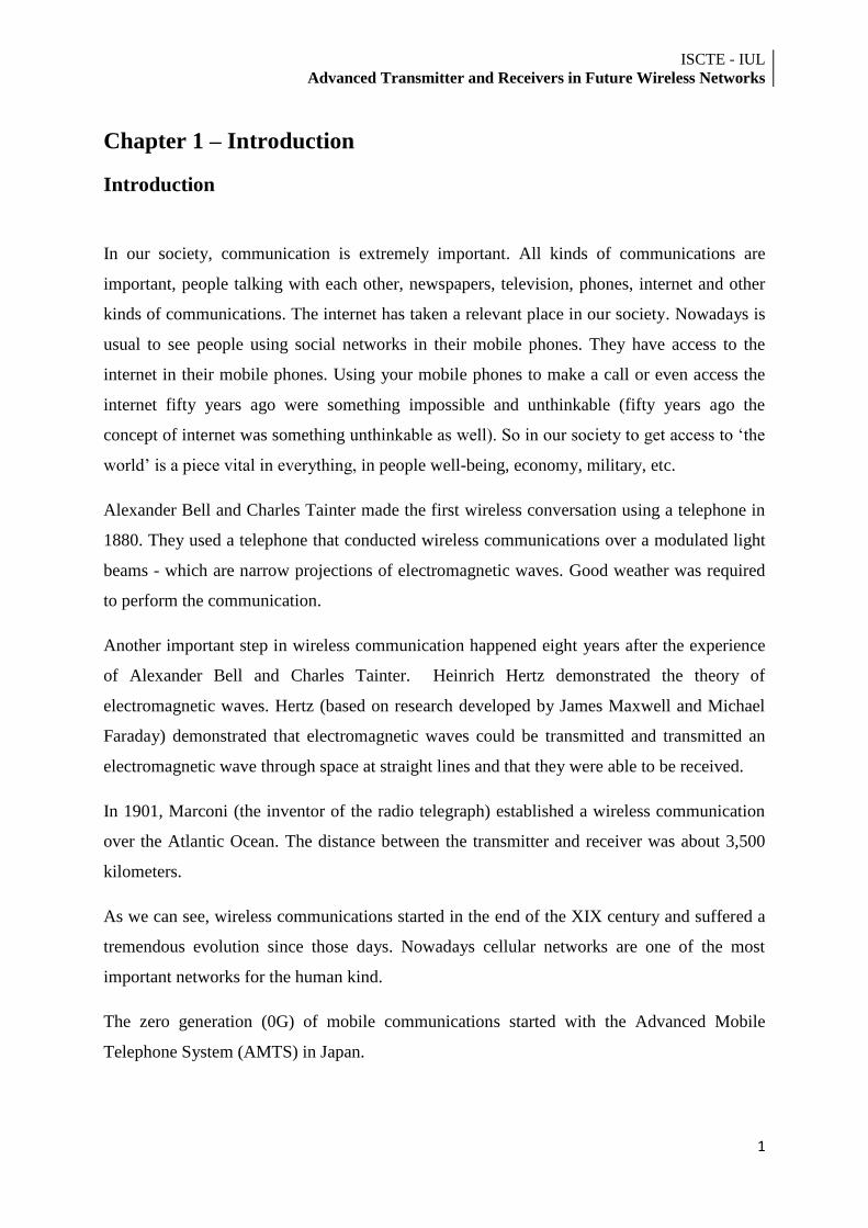
Wireless communications have a few issues. The download velocity is extremely important if
we want to deliver interactive content or watch live events. The fading effects are other of the
biggest problems of wireless communications. Fading effect is explained in the following
figure:
Figure 1 – Fading Effect [17]
This effect only appears when the path from the transmitter to the receiver either has
reflections or obstructions. The signal reaches the receiver from many different routes, each
being a copy of the original (multipath effect). The slightly difference are delay and gain. The
time delays result in phase shifts which added to main signal component causes the signal to
be degraded. This causes the Rayleigh fading. The Rayleigh fading effects assume that the
magnitude of the signal has passed through a transmission medium and will vary randomly.
Rayleigh fading is most applicable when is no dominant along a line of sight between the
ISCTE - IUL Advanced Transmitter and Receivers in Future Wireless Networks
5
transmitter and receiver. Another issue in wireless communications is the poor channel
estimation or imperfect channel estimation.
Sometimes the data information has errors that must be recovered at the receiver.
The study of Complex Rotation Matrix (CRM) and Multiple-input Multiple-output (MIMO)
in the same system is not deeper. It is expect that both technologies working together can
achieve a great performance in wireless communications. It should be introduces techniques
with the purpose of reduce this effects.
ISCTE - IUL
Advanced Transmitter and Receivers in Future Wireless Networks
6
State of the Art
The Orthogonal Frequency Division Multiplexing (OFDM) appeared for the first time in 1966
[4]. Over the years the OFDM evolved and nowadays is a well-known technology used
mostly in wireless communications [5]. The Universal Terrestrial Radio Access (UTRA)
Long-Term Evolution (LTE) was the first technology to mobile communication who adopted
the OFDM [6]. The UTRA LTE has a service which is specialized in delivering Multimedia
content to the mobile terminals. The service is called Multimedia Broadcast Multicast Service
(MBMS) and includes two types of transmission modes: point-to-point (PtP) and point-to-
multipoint (PtM).
Voice and video signals information are scalable and to permit reliable and efficient broadcast
communication using these kind of signals in mobile technologies we can use hierarchical
constellations with different protection bit error in broadcast transmissions[7][8].
Hierarchical constellations [15][16] had already been incorporated into Digital Video
Broadcasting – Terrestrial (DVB-T) [10]. DVB-T is a standard for broadcast transmission of
digital terrestrial television (DTT). It was published in 1997 and the first broadcast was in the
United Kingdom in 1998 [11]. The modulations used in DVB-T were 16 and 64 Quadrature
Amplitude Modulation (QAM). This technology uses OFDM. The hierarchical constellations
are being considered for the UTRA LTE [6].
Another technology for the delivery of multimedia content to mobile terminals is the Digital
Video Broadcasting – Satellite services to Handhelds (DVB-SH). The DVB Project published
this standard in February 2007 [9]. The DVB-SH was designed for frequencies below 3 GHz
and proposes was to support the televisions bands UHF, S and L.
The Complex Rotation Matrix (CRM) is a technique capable of achieving performance gains
in fading channels using OFDM transmission [12]. The CRM is based in spreading the
information over a large number of subcarriers of the OFDM signal.
Multiple-input and multiple-output (MIMO) schemes have emerged as a promising method
for improving the capacity of wireless communication systems [13][14][16]. This technique
consists in the use of multiple antennas at both transmitter and receiver to improve
communication performance.
ISCTE - IUL Advanced Transmitter and Receivers in Future Wireless Networks
7
Objectives
The purpose of this dissertation is to study technologies that can improve the quality of signal
in the receiver and improve communication reliability. The Complex Rotation Matrix (CRM)
is a technique that can improve the quality of the experience especially when used in a multi-
carrier system as Orthogonal Frequency Division Multiplexing (OFDM).
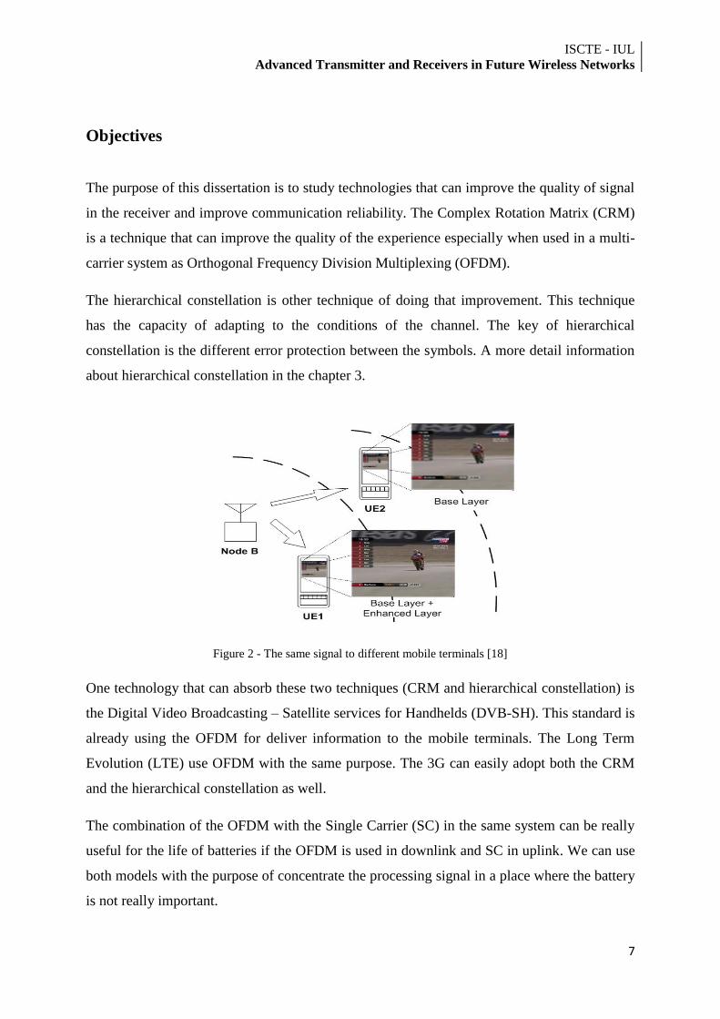
The hierarchical constellation is other technique of doing that improvement. This technique
has the capacity of adapting to the conditions of the channel. The key of hierarchical
constellation is the different error protection between the symbols. A more detail information
about hierarchical constellation in the chapter 3.
Figure 2 - The same signal to different mobile terminals [18]
One technology that can absorb these two techniques (CRM and hierarchical constellation) is
the Digital Video Broadcasting – Satellite services for Handhelds (DVB-SH). This standard is
already using the OFDM for deliver information to the mobile terminals. The Long Term
Evolution (LTE) use OFDM with the same purpose. The 3G can easily adopt both the CRM
and the hierarchical constellation as well.
The combination of the OFDM with the Single Carrier (SC) in the same system can be really
useful for the life of batteries if the OFDM is used in downlink and SC in uplink. We can use
both models with the purpose of concentrate the processing signal in a place where the battery
is not really important.
ISCTE - IUL
Advanced Transmitter and Receivers in Future Wireless Networks
8
Chapter 2 – Block Transmission Techniques
OFDM
The OFDM (Orthogonal Frequency Division Multiplexing) is a transmission technique with
the purpose of improving the spectrally efficiency and to combat the effects of multipath
conditions. It is a one of the most famous techniques which uses a multicarrier solution [19].
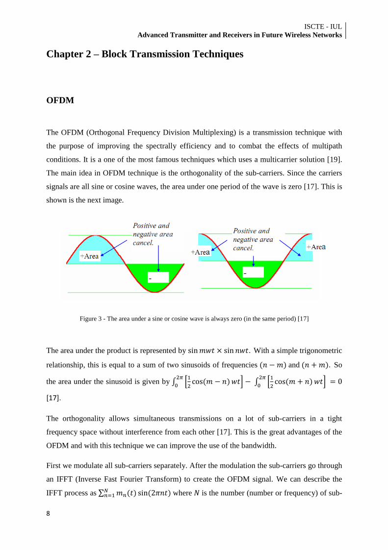
The main idea in OFDM technique is the orthogonality of the sub-carriers. Since the carriers
signals are all sine or cosine waves, the area under one period of the wave is zero [17]. This is
shown is the next image.
Figure 3 - The area under a sine or cosine wave is always zero (in the same period) [17]
The area under the product is represented by . With a simple trigonometric
relationship, this is equal to a sum of two sinusoids of frequencies and . So
the area under the sinusoid is given by
[17].
The orthogonality allows simultaneous transmissions on a lot of sub-carriers in a tight
frequency space without interference from each other [17]. This is the great advantages of the
OFDM and with this technique we can improve the use of the bandwidth.
First we modulate all sub-carriers separately. After the modulation the sub-carriers go through
an IFFT (Inverse Fast Fourier Transform) to create the OFDM signal. We can describe the
IFFT process as where is the number (number or frequency) of sub-
ISCTE - IUL Advanced Transmitter and Receivers in Future Wireless Networks
9
carriers, is the actual sub-carrier and is the sub-carrier signal. The IFFT converts the
signal from the frequency domain to time domain by successively multiplying it by a range of
sinusoids [17]. The equation for IFFT is
(1)
Where is the index of the frequencies over the frequencies and is the time index. is
the value of the spectrum for the frequency [17]. One of the main purposes of the IFFT
block is to change the domain of the signal.
The extraction of the sub-carriers at the receiver is done by applying the FFT (Fast Fourier
Transform) operation. The result of the FFT block in common understanding is a frequency
domain signal. We can write the FFT as
(2)
Where are the coefficients of the sines and cosines of frequency
, is the index of
the frequencies over the frequencies and is the time index. The coefficients by convention
are defined as time domain samples for the FFT and frequency bin values for the
IFFT [17].
After the IFFT block, the system adds a cyclic prefix. The cyclic prefix is a repetition of the
last data symbols in a block. The purpose of the cyclic prefix is to mitigate the ISI (Inter-
Symbol Interference) and the fading effects. The cyclic prefix is discarded at the receiver
because its only purpose is to mitigate the referred last two effects. ISI is a form of distortion
of a signal in which one symbol interferes with the nearest symbols. In wireless
communications, ISI is usually caused by multipath propagation. The presence of ISI in
systems can introduce errors in the decision device at the receiver.
We can get fading effects when the path from the transmitter to the receiver has reflections or
obstructions [17]. This type of effect is common in wireless communications. The problem
arises when the signal reach the receiver from many different paths and each signal is a copy
of the original signal having a different delay and gain. The degradation of the signal appears
due to the sum of the time delays. The reflected signals that are delayed cause either gains in
the signal strength or deep fades and by deep fades we mean that the signal is practically
ISCTE - IUL
Advanced Transmitter and Receivers in Future Wireless Networks
10
wiped out [17]. The delay spread is the maximum time delay that occurs in a certain
environment.
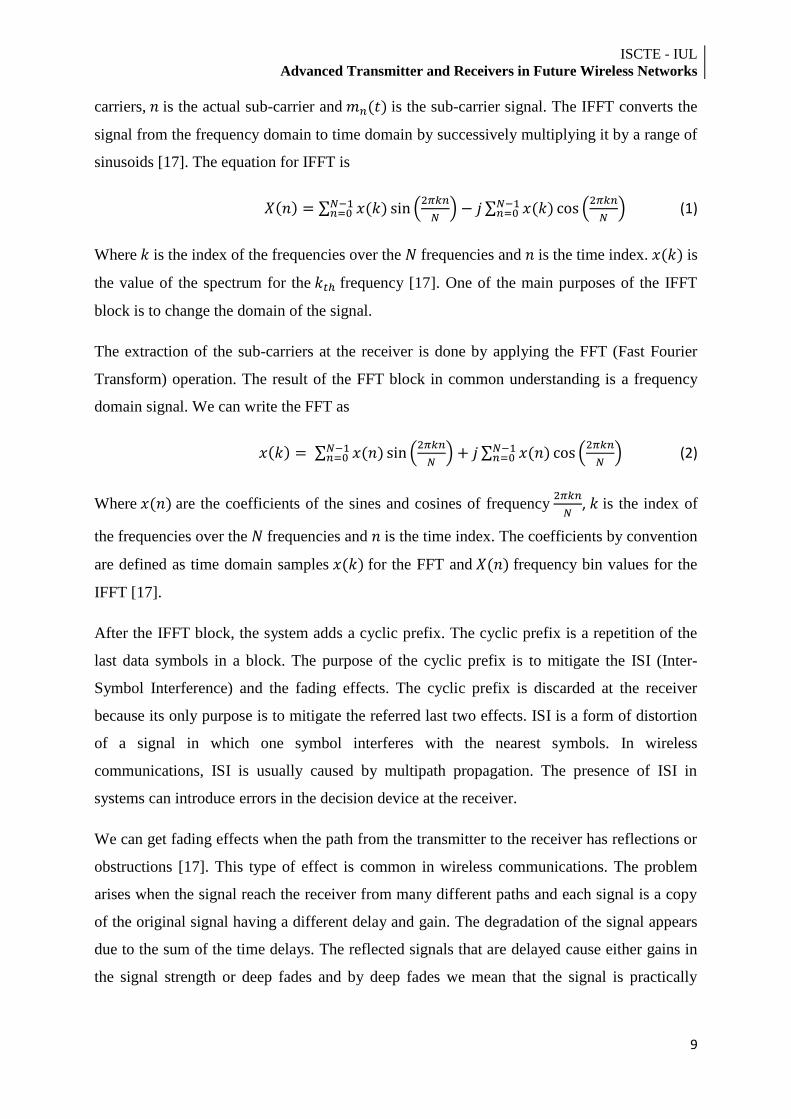
Sometimes the environment cause fading in several frequencies, this type of fading is called
deep fades frequencies. This happens to some frequencies in the band. The channel does not
allow any information to go through in this frequencies and it does not occur uniformly across
the band.
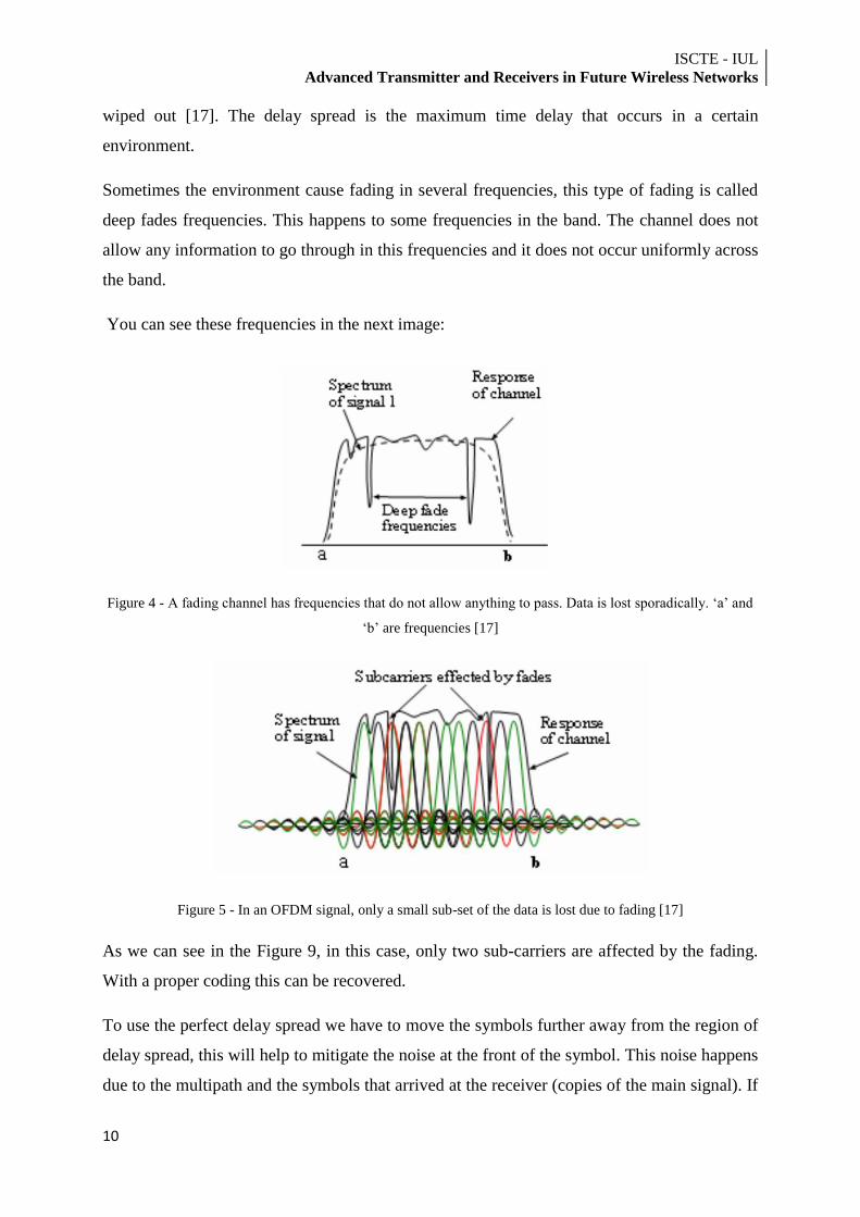
You can see these frequencies in the next image:
Figure 4 - A fading channel has frequencies that do not allow anything to pass. Data is lost sporadically. „a‟ and
„b‟ are frequencies [17]
Figure 5 - In an OFDM signal, only a small sub-set of the data is lost due to fading [17]
As we can see in the Figure 9, in this case, only two sub-carriers are affected by the fading.
With a proper coding this can be recovered.
To use the perfect delay spread we have to move the symbols further away from the region of
delay spread, this will help to mitigate the noise at the front of the symbol. This noise happens
due to the multipath and the symbols that arrived at the receiver (copies of the main signal). If
ISCTE - IUL Advanced Transmitter and Receivers in Future Wireless Networks
11
we are moving the symbols further from each others, blank spaces can appear in the signals.
We cannot have blank spaces in signals because it won‟t work for the hardware which likes to
crank out signals continuously. To resolve this problem we extend the symbol into the empty
space, so the actual symbol is more than one cycle. But now the start of the symbol is still in
the danger zone (zone which copies of the main signal can arrive to the receiver). The start is
the most important about our symbol since the slicer needs it in order to make a decision
about the bit [17]. To avoid the situation where the first part of the symbol falls in this danger
zone, we can slide the symbol backwards and then fill this area with a copy of what turns out
to be the tail end of the symbol.
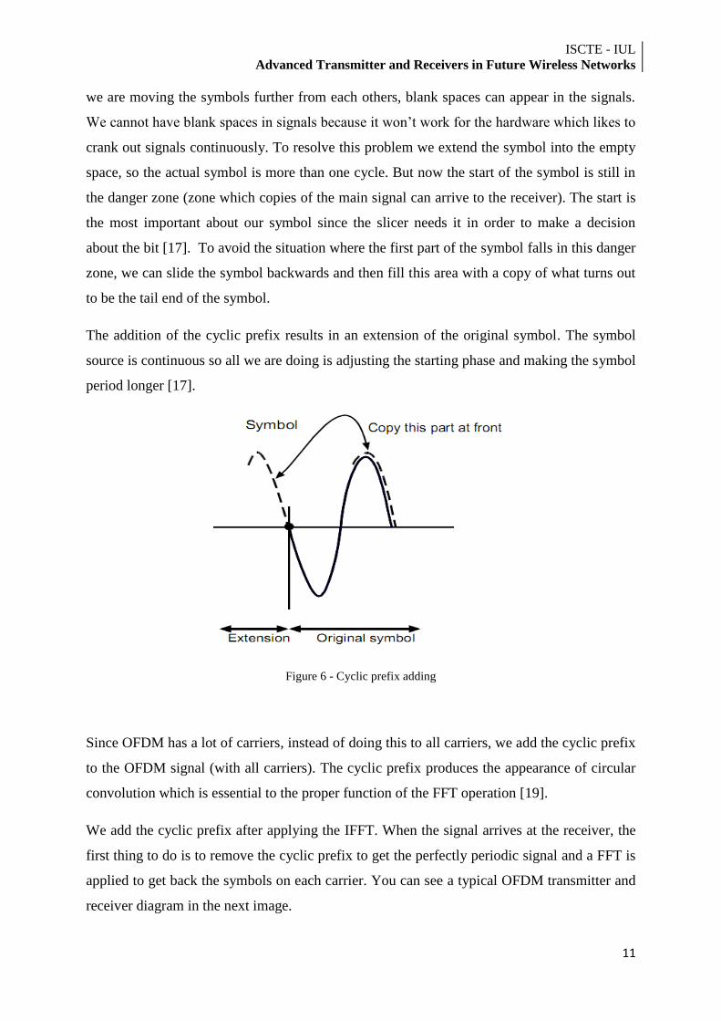
The addition of the cyclic prefix results in an extension of the original symbol. The symbol
source is continuous so all we are doing is adjusting the starting phase and making the symbol
period longer [17].
Figure 6 - Cyclic prefix adding
Since OFDM has a lot of carriers, instead of doing this to all carriers, we add the cyclic prefix
to the OFDM signal (with all carriers). The cyclic prefix produces the appearance of circular
convolution which is essential to the proper function of the FFT operation [19].
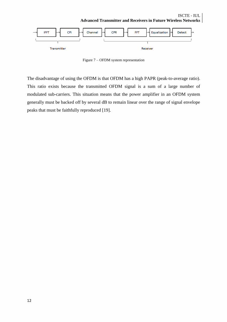
We add the cyclic prefix after applying the IFFT. When the signal arrives at the receiver, the
first thing to do is to remove the cyclic prefix to get the perfectly periodic signal and a FFT is
applied to get back the symbols on each carrier. You can see a typical OFDM transmitter and
receiver diagram in the next image.
ISCTE - IUL
Advanced Transmitter and Receivers in Future Wireless Networks
12
Figure 7 – OFDM system representation
The disadvantage of using the OFDM is that OFDM has a high PAPR (peak-to-average ratio).
This ratio exists because the transmitted OFDM signal is a sum of a large number of
modulated sub-carriers. This situation means that the power amplifier in an OFDM system
generally must be backed off by several dB to remain linear over the range of signal envelope
peaks that must be faithfully reproduced [19].
ISCTE - IUL Advanced Transmitter and Receivers in Future Wireless Networks
13
SC-FDE
Single Carrier (SC) is a frequency division multiple access scheme. It is a scheme of sending
data. SC is used with equalization. There are two types of equalization: Frequency Domain
Equalization (FDE) and Time Domain Equalization (TDE). In this thesis we used the FDE.
FDE has better performance than TDE and the low signal processing is lower as in OFDM.
The major SC-FDE advantage over OFDM is the less sensitive to radio-frequency
impairments such as power amplifier nonlinearities [19]. As Sari [38] [39] pointed out that
when combined Fast Fourier Transform (FFT) processing with SC- FDE, the system can
achieved performance and low complexity as an OFDM system.
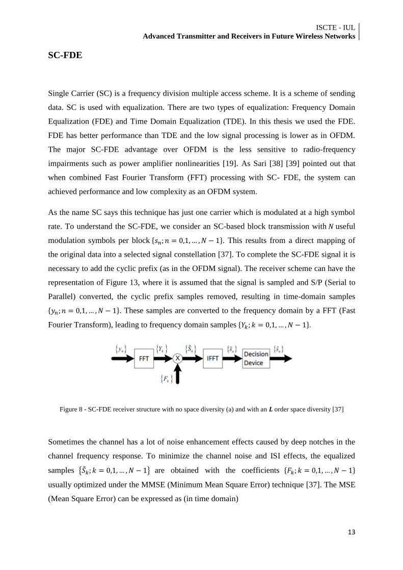
As the name SC says this technique has just one carrier which is modulated at a high symbol
rate. To understand the SC-FDE, we consider an SC-based block transmission with useful
modulation symbols per block . This results from a direct mapping of
the original data into a selected signal constellation [37]. To complete the SC-FDE signal it is
necessary to add the cyclic prefix (as in the OFDM signal). The receiver scheme can have the
representation of Figure 13, where it is assumed that the signal is sampled and S/P (Serial to
Parallel) converted, the cyclic prefix samples removed, resulting in time-domain samples
. These samples are converted to the frequency domain by a FFT (Fast
Fourier Transform), leading to frequency domain samples .
Figure 8 - SC-FDE receiver structure with no space diversity (a) and with an order space diversity [37]
Sometimes the channel has a lot of noise enhancement effects caused by deep notches in the
channel frequency response. To minimize the channel noise and ISI effects, the equalized
samples are obtained with the coefficients
usually optimized under the MMSE (Minimum Mean Square Error) technique [37]. The MSE
(Mean Square Error) can be expressed as (in time domain)
ISCTE - IUL
Advanced Transmitter and Receivers in Future Wireless Networks
14
(3)
and
. (4)
To minimize the MSE, we can minimize in order to , for each separately, i.e.
(5)
which leads to the set of optimized FDE coefficients
(6)
where is the inverse of the SNR (Signal-to-Noise Ratio), given by
(7)
with
(8)
and
. (9)
In SC modulations the data contents are transmitted in the time domain, the equalized samples
are converted back to the time domain by an IFFT operation leading to
the time domain samples. These samples are equalized then will be
used to make decisions on the transmitted symbols.
The attractive features of processing the FFT of the received signal in the frequency domain
are:
The OFDM has a high PAPR (peak-to-average ratio) and the SC modulation reduced
that PAPR. This allows using less costly power amplifiers.
The performance of the two systems (OFDM and SC) when the equalization of SC
modulation is in the frequency domain are similar and codification is used in OFDM.
Even for a very long channel delay spread.
ISCTE - IUL Advanced Transmitter and Receivers in Future Wireless Networks
15
To achieve reliable results in OFDM, coding is a requirement which does not happen
on SC-FDE. In spite of that both technologies are usually combined with coding.
The SC modulation systems are a well proven technology in many existing wireless
systems.
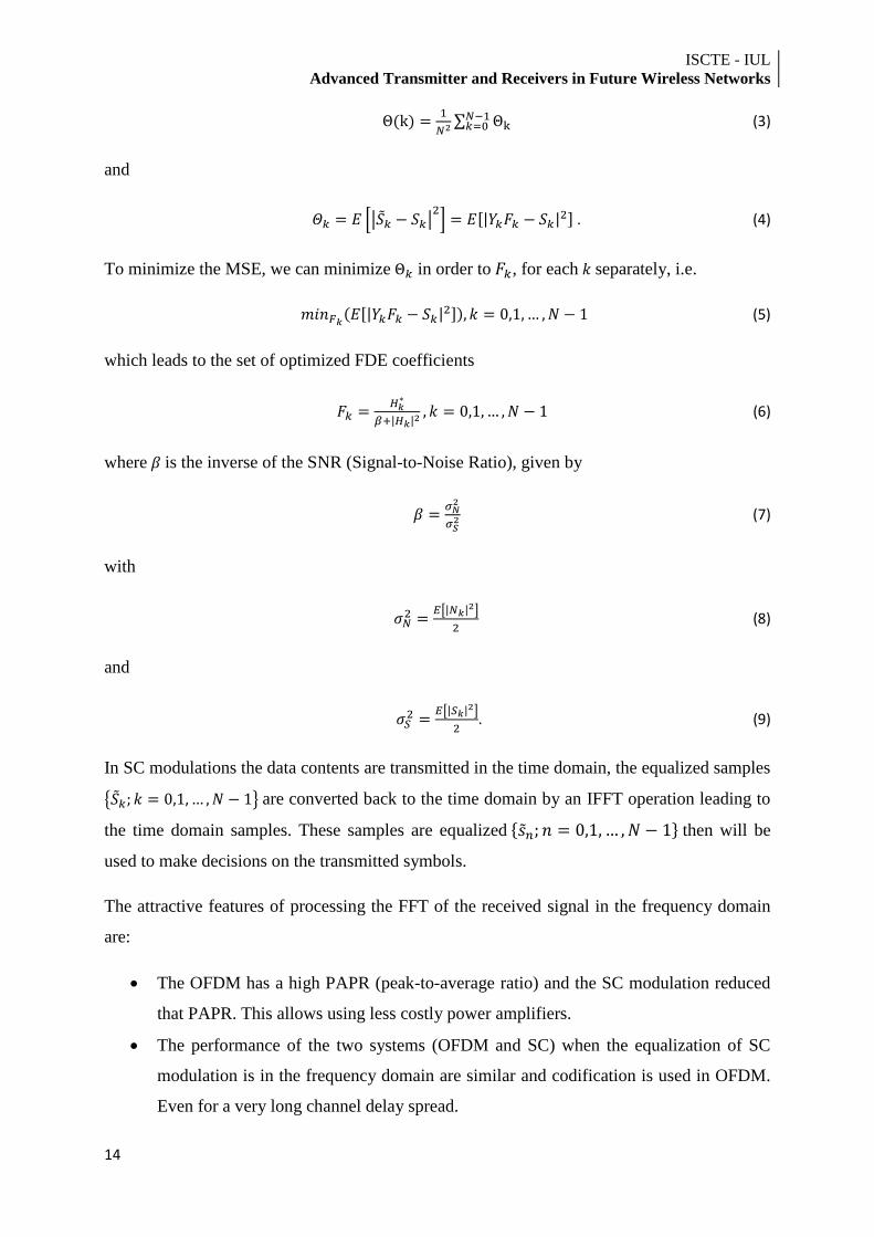
To obtain better performances than the linear equalization we can use a DFE (Decision
Feedback Equalization) in a frequency selective radio channels. The goal of this technique is
to remove the interference effect from subsequently detected symbols. It is achieved when
symbol-by-symbol data symbol decisions are made, filtered and immediately fed back [19].
Due to the inherent delay of the FFT signal processing, this cannot be done in a frequency
domain. To avoid the feedback delay problem, the approach is a hybrid time-frequency
domain DFE to filtering only for the forward filter part of the DFE and a conventional
transversal filtering for the feedback part [19]. Due to multiplications only on data symbols,
this kind of filter is relatively simple.
Figure 9 – IB-DFE receiver structure with no diversity (a) and with L-branch space diversity (b)
ISCTE - IUL
Advanced Transmitter and Receivers in Future Wireless Networks
16
Once per block, the FFT output coefficients ( ) are multiplied by the complex-valued
forward equalizer coefficients . This multiplication has the purpose to compensate the
frequency-selective channel‟s variations of amplitude and phase with frequency. An IFFT is
applied to the weight-equalized complex-valued samples and the resulting time domain
sequence is passed to a data symbol decision device. In the case of the DFE, the estimated ISI
due to previously detected symbols is computed using feedback taps ( and subtracted off
symbol-by-symbol [37].
ISCTE - IUL Advanced Transmitter and Receivers in Future Wireless Networks
17
MIMO
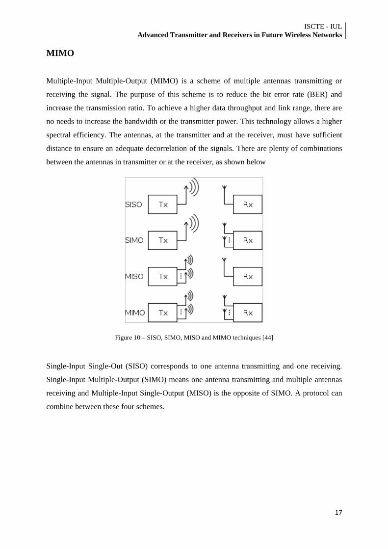
Multiple-Input Multiple-Output (MIMO) is a scheme of multiple antennas transmitting or
receiving the signal. The purpose of this scheme is to reduce the bit error rate (BER) and
increase the transmission ratio. To achieve a higher data throughput and link range, there are
no needs to increase the bandwidth or the transmitter power. This technology allows a higher
spectral efficiency. The antennas, at the transmitter and at the receiver, must have sufficient
distance to ensure an adequate decorrelation of the signals. There are plenty of combinations
between the antennas in transmitter or at the receiver, as shown below
Figure 10 – SISO, SIMO, MISO and MIMO techniques [44]
Single-Input Single-Out (SISO) corresponds to one antenna transmitting and one receiving.
Single-Input Multiple-Output (SIMO) means one antenna transmitting and multiple antennas
receiving and Multiple-Input Single-Output (MISO) is the opposite of SIMO. A protocol can
combine between these four schemes.
ISCTE - IUL
Advanced Transmitter and Receivers in Future Wireless Networks
18
Channel estimation
Channel estimation processing is required for accomplishing coherent detection at the
receiver [40]. This channel estimation is important for the system to work reliably. These
estimates can be obtained with the help of training symbols that are multiplexed with the data.
These training symbols are called pilots. It is desirable to reduce the overheads required for
channel estimation because this approach can result in an inefficient use of bandwidth. There
are two methods of pilot symbols transmission: the data multiplexed method or the implicit
method.
The data multiplexed pilots technique consists in the insertion of pilot symbols into to the
modulated symbols sequence. In the scheme the pilot symbols are randomly introduced with
data symbols in the same structure.
The implicit pilots technique relies on the idea of pilot embedding where a pilot sequence is
summed to the data sequence and both are transmitted at the same time. This technique
demands that some power to be spent on the pilot sequence but allows to increase the pilots‟
density without sacrificing the system capacity [40]. The biggest problem on the technique of
implicit pilots transmission relies on the interference that can occur between data and pilots
which might be high, especially when employing multiple antennas schemes since each pilot
symbol will be affected by interference of several data symbols simultaneously [40]. The
pilots can interfere with the data symbol as well. This can lead to substantial performance
degradation and to irreducible noise.
For both methods, the transmitter chain is the same like we show in figure 16.
ISCTE - IUL Advanced Transmitter and Receivers in Future Wireless Networks
19
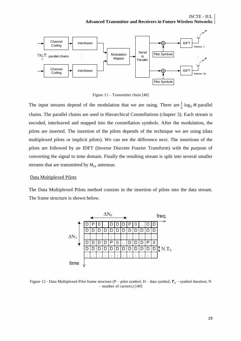
Figure 11 – Transmitter chain [40]
The input streams depend of the modulation that we are using. There are
parallel
chains. The parallel chains are used in Hierarchical Constellations (chapter 3). Each stream is
encoded, interleaved and mapped into the constellation symbols. After the modulation, the
pilots are inserted. The insertion of the pilots depends of the technique we are using (data
multiplexed pilots or implicit pilots). We can see the difference next. The insertions of the
pilots are followed by an IDFT (Inverse Discrete Fourier Transform) with the purpose of
converting the signal to time domain. Finally the resulting stream is split into several smaller
streams that are transmitted by antennas.
Data Multiplexed Pilots
The Data Multiplexed Pilots method consists in the insertion of pilots into the data stream.
The frame structure is shown below.
Figure 12 - Data Multiplexed Pilot frame structure (P – pilot symbol; D – data symbol; – symbol duration; N
– number of carriers;) [40]
Serial
to Parallel
.
.
.
.
.
.
Channel
Coding
.
.
.
Modulation
Mapper
IDFT
.
.
.
2log
2
Mparallel chains
Interleaver
Channel Coding
Interleaver
Antenna 1
Antenna Mtx
IDFT
Pilot Symbols
Pilot Symbols
ISCTE - IUL
Advanced Transmitter and Receivers in Future Wireless Networks
20
If the scheme adopted is a MIMO, to mitigate the interference between pilots of different
transmitting antennas, the pilots are multiplexed in FDM (Frequency Division Multiplexing).
This means that all pilot symbols have a different sub-carrier. Data symbols are not
transmitted on reserved sub-carriers for pilots in any antenna.
Before being transmitted, the sequences of symbols are converted to the time domain
through
, where is the symbol
transmitted by the sub-carrier of the OFDM block using antenna . The transmitted
OFDM signals are then expressed as
(10)
Where is the symbol duration, is the number of samples at the cyclic prefix using
OFDM and is the adopted pulse shaping filter [40].
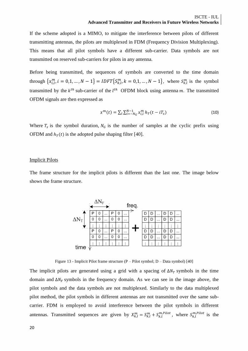
Implicit Pilots
The frame structure for the implicit pilots is different than the last one. The image below
shows the frame structure.
Figure 13 - Implicit Pilot frame structure (P – Pilot symbol; D – Data symbol) [40]
The implicit pilots are generated using a grid with a spacing of symbols in the time
domain and symbols in the frequency domain. As we can see in the image above, the
pilot symbols and the data symbols are not multiplexed. Similarly to the data multiplexed
pilot method, the pilot symbols in different antennas are not transmitted over the same sub-
carrier. FDM is employed to avoid interference between the pilot symbols in different
antennas. Transmitted sequences are given by
, where
is the
ISCTE - IUL Advanced Transmitter and Receivers in Future Wireless Networks
21
implicit pilot transmitted over the sub-carrier in the OFDM block using antenna .
Before being transmitted, the sequence is converted to time domain through the process
. The transmitted OFDM signal is
expressed in the same format as for the data multiplexed pilot,
.
ISCTE - IUL
Advanced Transmitter and Receivers in Future Wireless Networks
22
Turbo codes
The turbo codes are a class of forward error correction1 (FEC) codes. The turbo codes were
designed to achieve reliable communication over a limited bandwidth or latency in the
presence of a channel with a high noise. Turbo codes have been used in satellite
communications and in UMTS where the noise is high. The main characteristic of the turbo
codes is that they almost take full advantage of the channel capacity and they were the first
does it.
Next we will briefly describe the turbo encoder and decoder.
Turbo Encoder
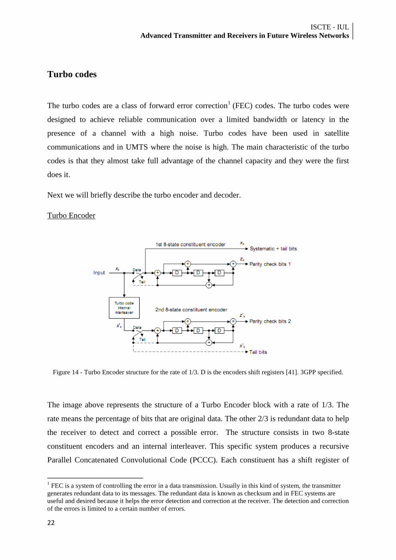
Figure 14 - Turbo Encoder structure for the rate of 1/3. D is the encoders shift registers [41]. 3GPP specified.
The image above represents the structure of a Turbo Encoder block with a rate of 1/3. The
rate means the percentage of bits that are original data. The other 2/3 is redundant data to help
the receiver to detect and correct a possible error. The structure consists in two 8-state
constituent encoders and an internal interleaver. This specific system produces a recursive
Parallel Concatenated Convolutional Code (PCCC). Each constituent has a shift register of
1 FEC is a system of controlling the error in a data transmission. Usually in this kind of system, the transmitter
generates redundant data to its messages. The redundant data is known as checksum and in FEC systems are
useful and desired because it helps the error detection and correction at the receiver. The detection and correction
of the errors is limited to a certain number of errors.
ISCTE - IUL Advanced Transmitter and Receivers in Future Wireless Networks
23
length 3 that can represent 8 different states. Each of the eight states depends on the input bits.
In the first constituent encoder receives input bits directly and the other constituent encoder
receives input bits from the interleaver. For each input, three outputs are generated. This rate
can be altered depending on the puncturing 2of bits and tail bits from the second constituent
encoder. This system is recursive so one error in a bit will result in several error in the parity
check bits.
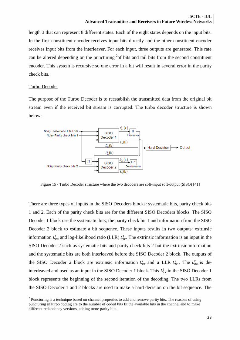
Turbo Decoder
The purpose of the Turbo Decoder is to reestablish the transmitted data from the original bit
stream even if the received bit stream is corrupted. The turbo decoder structure is shown
below:
Figure 15 - Turbo Decoder structure where the two decoders are soft-input soft-output (SISO) [41]
There are three types of inputs in the SISO Decoders blocks: systematic bits, parity check bits
1 and 2. Each of the parity check bits are for the different SISO Decoders blocks. The SISO
Decoder 1 block use the systematic bits, the parity check bit 1 and information from the SISO
Decoder 2 block to estimate a bit sequence. These inputs results in two outputs: extrinsic
information and log-likelihood ratio (LLR)
. The extrinsic information is an input in the
SISO Decoder 2 such as systematic bits and parity check bits 2 but the extrinsic information
and the systematic bits are both interleaved before the SISO Decoder 2 block. The outputs of
the SISO Decoder 2 block are extrinsic information and a LLR
. The is de-
interleaved and used as an input in the SISO Decoder 1 block. This in the SISO Decoder 1
block represents the beginning of the second iteration of the decoding. The two LLRs from
the SISO Decoder 1 and 2 blocks are used to make a hard decision on the bit sequence. The
2 Puncturing is a technique based on channel properties to add and remove parity bits. The reasons of using
puncturing in turbo coding are to the number of coded bits fit the available bits in the channel and to make
different redundancy versions, adding more parity bits.
ISCTE - IUL
Advanced Transmitter and Receivers in Future Wireless Networks
24
hard decision consists in assigning the value 0 or 1 to the LLRs. The number of iterations to
provide a good estimation of the bit sequence depends on the type of the encoder that was
used.
ISCTE - IUL Advanced Transmitter and Receivers in Future Wireless Networks
25
LTE
The Long Term Evolution (LTE) is known as 3.75G of mobile telecommunications networks.
The LTE is a project of the 3rd
Generation Partnership Project (3GPP) and provides an uplink
speed of up 50 Mbps and downlink speed of up to 100 Mbps. The LTE was designed to
carrier needs of high-speed and data and media transport as well as high-capacity voice
support. When we compare LTE with previous technologies, the LTE introduced several new
improvement techniques. The technologies in LTE that permit the system to operate more
efficiently are:
Orthogonal Frequency Division Multiplexing (OFDM).
Multiple-Input Multiple-Output (MIMO).
System Architecture Evolution (SAE).
The OFDM is explained in the beginning of this chapter and is incorporated into LTE with the
purpose of enabling high data bandwidths. LTE uses different access schemes between the
downlink and the uplink. The downlink uses OFDM Access (OFDMA) while Single Carrier
with Frequency Division Multiple Access (SC-FDMA) is used in uplink. The main goal of
using the SC-FDMA in LTE is to improve the battery life of the mobile handsets because the
peak to average power ratio (PAPR) is small in SC-FDMA and the more constant power
enables high radio-frequency (RF) power amplifier efficiency in the mobile terminal. The
choice of the bandwidth is a key parameter associated to the OFDM in LTE. The bandwidth
influences the number of carriers available that can be accommodated in the OFDM signal.
The channel capacity achieves the best performance when the bandwidth is the biggest
available.
The MIMO is the capacity to send and receive data from multiple antennas. This technology
was developed to mitigate the problem of previous telecommunications systems has
encountered multiple signals arising from the many reflections. Using MIMO, these
additional signal paths can be used to advantage and are able to be used to increase the
throughput [22]. To distinguish the different paths it is necessary to use multiple antennas.
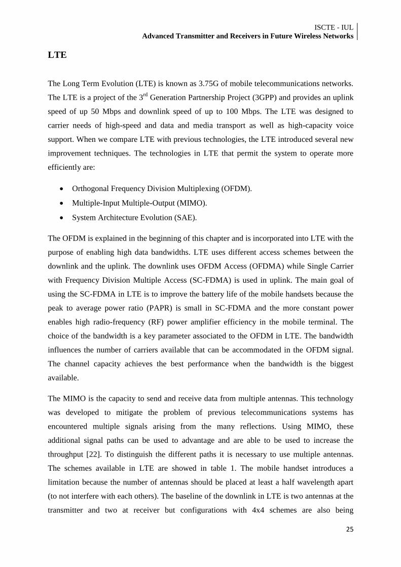
The schemes available in LTE are showed in table 1. The mobile handset introduces a
limitation because the number of antennas should be placed at least a half wavelength apart
(to not interfere with each others). The baseline of the downlink in LTE is two antennas at the
transmitter and two at receiver but configurations with 4x4 schemes are also being
ISCTE - IUL
Advanced Transmitter and Receivers in Future Wireless Networks
26
considered. In uplink is applied a scheme called Multi-User MIMO (MU-MIMO). The MU-
MIMO exploits the availability of multiple independent radio terminals in order to enhance
the communication capabilities of each individual terminal [23].
To improve the LTE performance when compared with previous systems, it was necessary to
evolve the system architecture. The most important change was that a number of functions
previously handled by the core network have been transferred out to the periphery [22]. With
this change latency times were reduced and data can be routed more directly to the
destination.
Table 1 - LTE specification overview [20][22]
Peak downlink speed 64-QAM (Mbps) 100 (SISO), 172 (2x2 MIMO), 326 (4x4
MIMO)
Peak uplink speeds (Mbps) 50 (QPSK), 57 (16QAM), 86 (64QAM)
Data type All packet switched data (voice and data).
Channel bandwidth (MHz) 1.4, 3, 5, 10, 15, 20
Duplex schemes FDD and TDD
Mobility 0 – 15 km/h (optimized)
15 – 120 km/h (high performance)
Latency Idle to active less than 100 ms
Small packets ~10 ms
Spectral efficiency Downlink: 3 – 4 times Rel 6 HSDPA
Uplink: 2 – 3 times Real 6 HSUPA
Access schemes Downlink: OFDMA
Uplink: SC-FDMA
Modulation types supported QPSK, 16-QAM, 64-QAM (Downlink
and uplink)
Antenna configuration supported Downlink: 4x4, 4x2, 2x2, 1x2, 1x1
Uplink: 1x2, 1x1
Coverage Full performance up to 5 km
Slight degradation 5 km – 30 km
Operation up to 100 km should not be
precluded by standard
ISCTE - IUL Advanced Transmitter and Receivers in Future Wireless Networks
27
The schemes employed in this standard vary slightly between the uplink and the downlink.
The reason is to keep the terminal cost low and the complex signal processing should be far
away from the terminals as well.
The LTE is prepared to use Frequency Division Duplex (FDD) or Time Division Duplex
(TDD) with the purpose communicating in both directions simultaneously.
LTE Advanced
The LTE Advanced is a standard which is an evolution of LTE. This new standard belongs to
the fourth generation (4G). LTE Advanced arose to keep the pace of cellular networks
constant evolution. The main headlines of the LTE are:
Speed data rate: downlink – 1 Gbps; uplink – 500 Mbps.
Spectrum efficiency: 3 times greater than LTE.
Peak spectrum efficiency: downlink – 30 bps/Hz; uplink – 15 bps/Hz.
Spectrum use: the ability to support scalable bandwidth use and spectrum aggregation
where non-contiguous spectrum needs to be used.
Latency: from Idle to connected in less than 50 ms and then shorter than 5 ms one way
for individual packet transmission.
Cell edge user throughput to be twice that of LTE.
Average user throughput to be 3 times that of LTE.
Compatibility: LTE Advanced shall be capable of interworking with LTE and 3GPP
legacy systems [24].
Hybrid OFDMA and SC-FDMA in uplink.
Coordinated multipoint (CoMP) transmission and reception.
UE Dual TX antenna solutions for SU-MIMO and diversity MIMO [27].
The three main technologies to achieve the required high data throughput are OFDM, SC-
FDMA and MIMO such as in LTE. The number of antennas used in LTE MIMO increased.
With the number of antennas increasing, techniques such as beamforming3 may be used to
enable the antenna coverage to be focused where it is needed. The core network has to change
3 Beamforming is a signal processing technique used in sensor arrays for directional signal transmission or
reception.
ISCTE - IUL
Advanced Transmitter and Receivers in Future Wireless Networks
28
and the objective is to bring the network closer to the user by adding low power nodes such as
picocells4 and femtocells
5. The network will become optimized and heterogeneous.
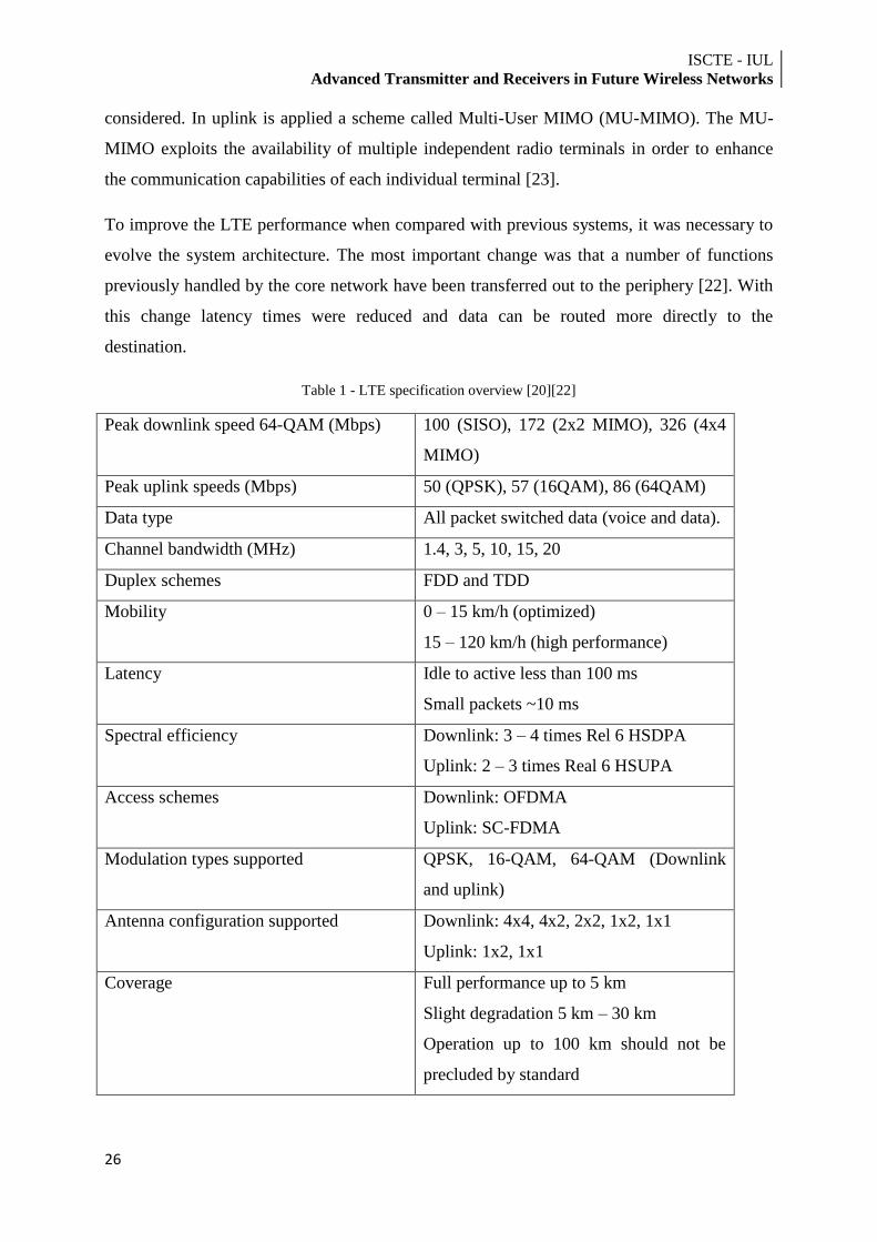
To achieve higher data rates than in the first release of LTE, the method adopted is carrier
aggregations or sometimes channel aggregation. With this method, it is possible to utilize
several carriers and increase the overall transmission bandwidth with it. Using carrier
aggregation means that several carrier will be aggregated on the physical layer to achieve the
required bandwidth.
Figure 16 - LTE Carrier Aggregation [9]
A system that supports LTE Advanced must support LTE first release so in LTE each
component appears as an LTE carrier but in LTE Advanced is processed as an aggregate.
The Coordinated Multipoint (CoMP) is a technology that is being developed to incorporate
the LTE Advanced. This technology consists in transmitting or receiving data from several
base stations. When using CoMP the throughput values are higher than no CoMP is used.
Higher data rates are easy to maintain close to the base station (BS), the problem emerges
when the user is near the edge of the cell. The issue is not only the far distance to the base
station but also the interference of the other BSs. The CoMP requires close coordination
between the BSs. The BSs dynamically coordinate themselves to provide joint scheduling and
processing of the received signals.
4 A picocell is a small cellular base station typically covering a small area, such as in-building (offices, shopping
malls, train stations, etc.), or more recently in-aircraft. In cellular networks, picocells are typically used to extend
coverage to indoor areas where outdoor signals do not reach well, or to add network capacity in areas with very
dense phone usage, such as train stations [25]. 5 Femtocell is a small cellular base station, typically designed for use in a home or small business. It connects to
the service provider‟s network via broadband [26].
ISCTE - IUL Advanced Transmitter and Receivers in Future Wireless Networks
29
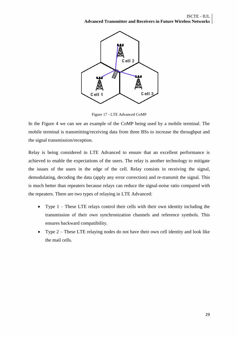
Figure 17 - LTE Advanced CoMP
In the Figure 4 we can see an example of the CoMP being used by a mobile terminal. The
mobile terminal is transmitting/receiving data from three BSs to increase the throughput and
the signal transmission/reception.
Relay is being considered in LTE Advanced to ensure that an excellent performance is
achieved to enable the expectations of the users. The relay is another technology to mitigate
the issues of the users in the edge of the cell. Relay consists in receiving the signal,
demodulating, decoding the data (apply any error correction) and re-transmit the signal. This
is much better than repeaters because relays can reduce the signal-noise ratio compared with
the repeaters. There are two types of relaying in LTE Advanced:
Type 1 – These LTE relays control their cells with their own identity including the
transmission of their own synchronization channels and reference symbols. This
ensures backward compatibility.
Type 2 – These LTE relaying nodes do not have their own cell identity and look like
the mail cells.
ISCTE - IUL
Advanced Transmitter and Receivers in Future Wireless Networks
30
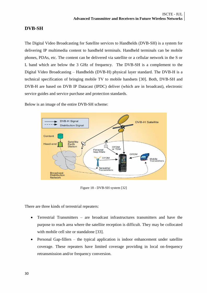
DVB-SH
The Digital Video Broadcasting for Satellite services to Handhelds (DVB-SH) is a system for
delivering IP multimedia content to handheld terminals. Handheld terminals can be mobile
phones, PDAs, etc. The content can be delivered via satellite or a cellular network in the S or
L band which are below the 3 GHz of frequency. The DVB-SH is a complement to the
Digital Video Broadcasting – Handhelds (DVB-H) physical layer standard. The DVB-H is a
technical specification of bringing mobile TV to mobile handsets [30]. Both, DVB-SH and
DVB-H are based on DVB IP Datacast (IPDC) deliver (which are in broadcast), electronic
service guides and service purchase and protection standards.
Below is an image of the entire DVB-SH scheme:
Figure 18 - DVB-SH system [32]
There are three kinds of terrestrial repeaters:
Terrestrial Transmitters – are broadcast infrastructures transmitters and have the
purpose to reach area where the satellite reception is difficult. They may be collocated
with mobile cell site or standalone [33].
Personal Gap-fillers – the typical application is indoor enhancement under satellite
coverage. These repeaters have limited coverage providing in local on-frequency
retransmission and/or frequency conversion.
ISCTE - IUL Advanced Transmitter and Receivers in Future Wireless Networks
31
Mobile transmitters – are mobile broadcast infrastructure transmitters creating a
moving complementary infrastructure. The typical use is for trains, commercial ships
or other environment where the coverage of the satellite transmission and the
terrestrial transmission are not guaranteed.
The DVB-SH ensures a wide area covered by the satellite communication known as Satellite
Component and combined with a Complementary Ground Component (CGC). The Satellite
Component ensures a global coverage while the CGC provides a cellular coverage. There are
two operation modes in this system:
SH-A – use Coded Orthogonal Frequency Division Multiplexing (COFDM)
modulation in satellite and terrestrial links with the possibility of single frequency
network;
SH-B – use Time Division Multiplexing (TDM) in the satellite link and COFDM in
the terrestrial communication.
Two main classes of satellite payloads may be considered:
Single DVB-SH physical layer multiplex per high power amplifier (HPA).
Multiple DVB-SH physical layer multiplex per high power amplifier. This is the case
with multibeam satellite with re-configurable antenna architecture based on large size
reflectors fed by arrays [33].
In the single DVB-SH, the SH-A requires that satellite transponders operated in quasi-linear
mode while the SH-B takes advantage of satellite transponders operated in full saturation. For
the second case, the SH-B provides little or no performance advantage over SH-A.
A choose has to be made between physical layer or link layer techniques to combat long
interruptions of the line of sight typical in satellite receptions with mobile terminals. The
choice is dictated by the cost and required footprint of the memory to implement long
interleaver at physical layer. The combination of a short physical interleaver with a long link
layer interleaver could be advantageous, especially for handheld terminals (battery life). The
long interleaver at physical layer might be better in difficult reception, especially with no
battery life restrictions.
Considering spectrum allocation, SH-B needs a dedicated sub-band for satellite transmission,
completed with a part of the sub-band available for the terrestrial local component to re-
ISCTE - IUL
Advanced Transmitter and Receivers in Future Wireless Networks
32
enforce reception of the satellite programs [33]. The SH-A allows on terrestrial repetition of
the satellite content in the same sub-band. All the remaining sub-bands are available for
terrestrial transmission.
ISCTE - IUL Advanced Transmitter and Receivers in Future Wireless Networks
33
WiMAX
The Worldwide Interoperability for Microwaves Access (WiMAX) is a telecommunications
protocol that provides fixed and mobile Internet access. The first WiMax release provides up
40 Mbit/s of download speed. The WiMax Forum is the creator and this technology which is
based on 802.16 IEEE (Institute of Electrical and Electronics Engineers) standards for the
physical and Media Access Control (MAC) layer.
WiMAX uses Orthogonal Frequency Division Multiplexing (OFDM) and the signal
incorporates multiples of 128 carriers in a bandwidth from 1.25 MHz to 20 MHz. To maintain
orthogonality between the individual carriers the symbol period must be the reciprocal of the
carrier spacing [35]. As a result of the narrow bandwidth, the WiMAX technology has a
longer symbol period. This longer symbols period is an advantage that helps to mitigate the
problem of the multipath interference.
Such as in Long Term Evolution (LTE), the WiMAX adopted Multiple Input Multiple Output
(MIMO) techniques to improve the quality of the system. MIMO provides benefits in
coverage, power consumption, frequency re-use and bandwidth efficiency.
WiMAX modulation and coding is adaptive, enabling it to vary these parameters according to
prevailing conditions. Channel quality feedback indicator is used to determine the modulation
and coding to be used. WiMAX is particularly flexible in channel bandwidth, modulation and
coding schemes, these three factors can significantly vary the data rates that can be achieved.
Table 2 – Modulation and coding used in WiMAX
Parameter Downlink Uplink
Modulation BPSK, QPSK, 16 QAM, 64
QAM; BPSK optional for
OFDMA-PHY
BPSK, 16 QAM; 64 QAM optional
Coding Mandatory: convolutional
codes at rate 1/2, 2/3, 3/4, 5/6
Optional: convolutional turbo
codes at rate 1/2, 2/3, 3/4, 5/6;
Mandatory: convolutional codes at
rate 1/2, 2/3, 3/4, 5/6
Optional: convolutional turbo codes
at rate 1/2, 2/3, 3/4, 5/6; repetition
ISCTE - IUL
Advanced Transmitter and Receivers in Future Wireless Networks
34
repetition codes at rate 1/2, 1/3,
1/6, LDPC, RS-Codes for
OFDM-PHY
codes at rate 1/2, 1/3, 1/6, LDPC
Time Division Duplex (TDD) is the most common in WiMAX systems but Frequency
Division Duplex (FDD) is used as well. TDD allows greater efficiency in the use of the
spectrum.
Multiple frequencies can be used to transmit in WiMAX. The lower the frequency the lower
is the signal attenuation and therefore the multiple frequencies can improve range and better
coverage within buildings.
The MAC layer is an essential element within the overall WiMAX software stack. The MAC
layer is a sub-layer of the Data Link Layer. This is based in the Open Systems
Interconnections architecture (OSI) level 2. The MAC layer provides addressing and channel
access control mechanisms that make it possible for several terminals or network nodes to
communicate within multi-point network [35].
WiMAX Release 2
The WiMAX Release 2 has several improvements to the previous release. Core enhancement
is supported for the Wireless Man-Advanced air interface and the air interface capacity is the
double of the previous release. The objective of the WiMAX for the release 2 was to achieve
better performances without increase the cost of the network. It is important to upgrade the
core network elements but with the aim of spending the less possible.
The upgrading to the Release 2 has two phases. In the first phase, new network elements are
introduced: the Advanced Mobile Station (AMS) and the Advanced Base Station (ABS). The
second phase consists in the upgrading of the other network elements.
ISCTE - IUL Advanced Transmitter and Receivers in Future Wireless Networks
35
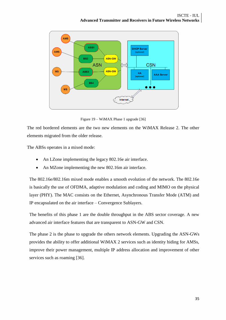
Figure 19 – WiMAX Phase 1 upgrade [36]
The red bordered elements are the two new elements on the WiMAX Release 2. The other
elements migrated from the older release.
The ABSs operates in a mixed mode:
An LZone implementing the legacy 802.16e air interface.
An MZone implementing the new 802.16m air interface.
The 802.16e/802.16m mixed mode enables a smooth evolution of the network. The 802.16e
is basically the use of OFDMA, adaptive modulation and coding and MIMO on the physical
layer (PHY). The MAC consists on the Ethernet, Asynchronous Transfer Mode (ATM) and
IP encapsulated on the air interface – Convergence Sublayers.
The benefits of this phase 1 are the double throughput in the ABS sector coverage. A new
advanced air interface features that are transparent to ASN-GW and CSN.
The phase 2 is the phase to upgrade the others network elements. Upgrading the ASN-GWs
provides the ability to offer additional WiMAX 2 services such as identity hiding for AMSs,
improve their power management, multiple IP address allocation and improvement of other
services such as roaming [36].
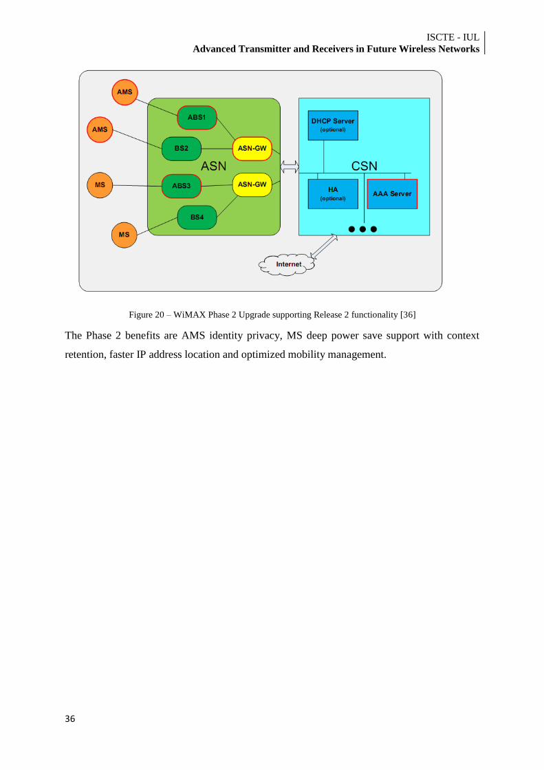
ISCTE - IUL
Advanced Transmitter and Receivers in Future Wireless Networks
36
Figure 20 – WiMAX Phase 2 Upgrade supporting Release 2 functionality [36]
The Phase 2 benefits are AMS identity privacy, MS deep power save support with context
retention, faster IP address location and optimized mobility management.
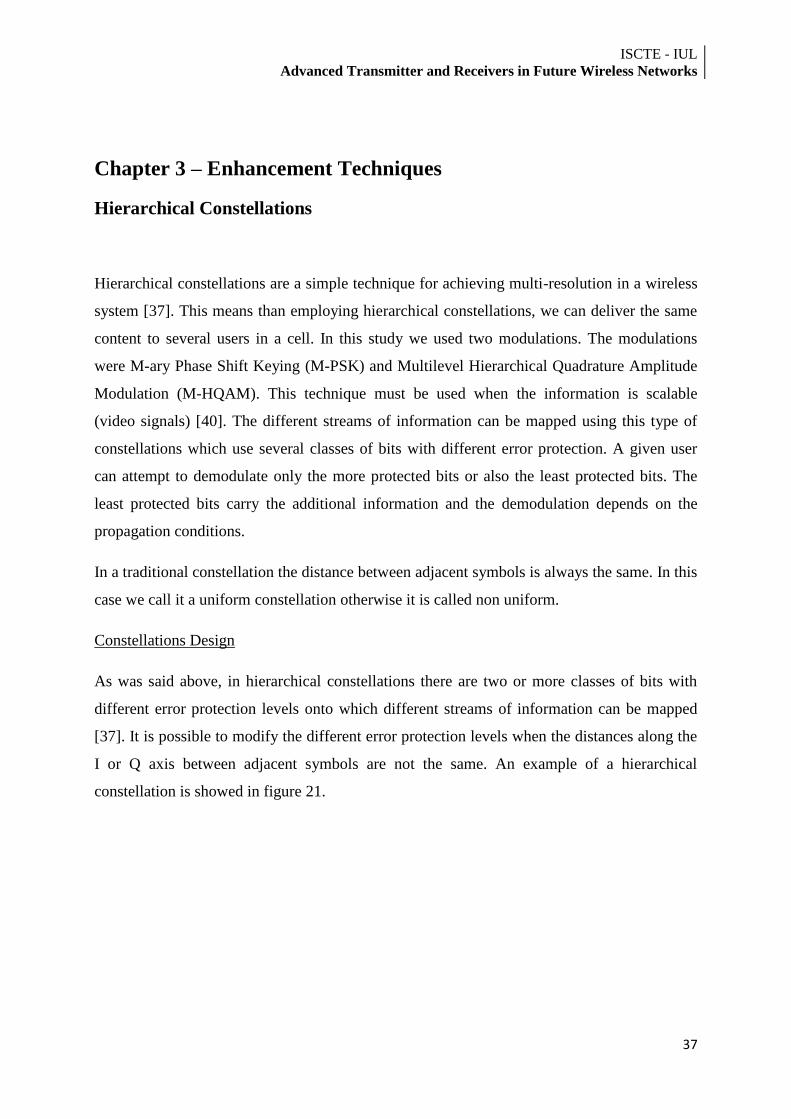
ISCTE - IUL Advanced Transmitter and Receivers in Future Wireless Networks
37
Chapter 3 – Enhancement Techniques
Hierarchical Constellations
Hierarchical constellations are a simple technique for achieving multi-resolution in a wireless
system [37]. This means than employing hierarchical constellations, we can deliver the same
content to several users in a cell. In this study we used two modulations. The modulations
were M-ary Phase Shift Keying (M-PSK) and Multilevel Hierarchical Quadrature Amplitude
Modulation (M-HQAM). This technique must be used when the information is scalable
(video signals) [40]. The different streams of information can be mapped using this type of
constellations which use several classes of bits with different error protection. A given user
can attempt to demodulate only the more protected bits or also the least protected bits. The
least protected bits carry the additional information and the demodulation depends on the
propagation conditions.
In a traditional constellation the distance between adjacent symbols is always the same. In this
case we call it a uniform constellation otherwise it is called non uniform.
Constellations Design
As was said above, in hierarchical constellations there are two or more classes of bits with
different error protection levels onto which different streams of information can be mapped
[37]. It is possible to modify the different error protection levels when the distances along the
I or Q axis between adjacent symbols are not the same. An example of a hierarchical
constellation is showed in figure 21.
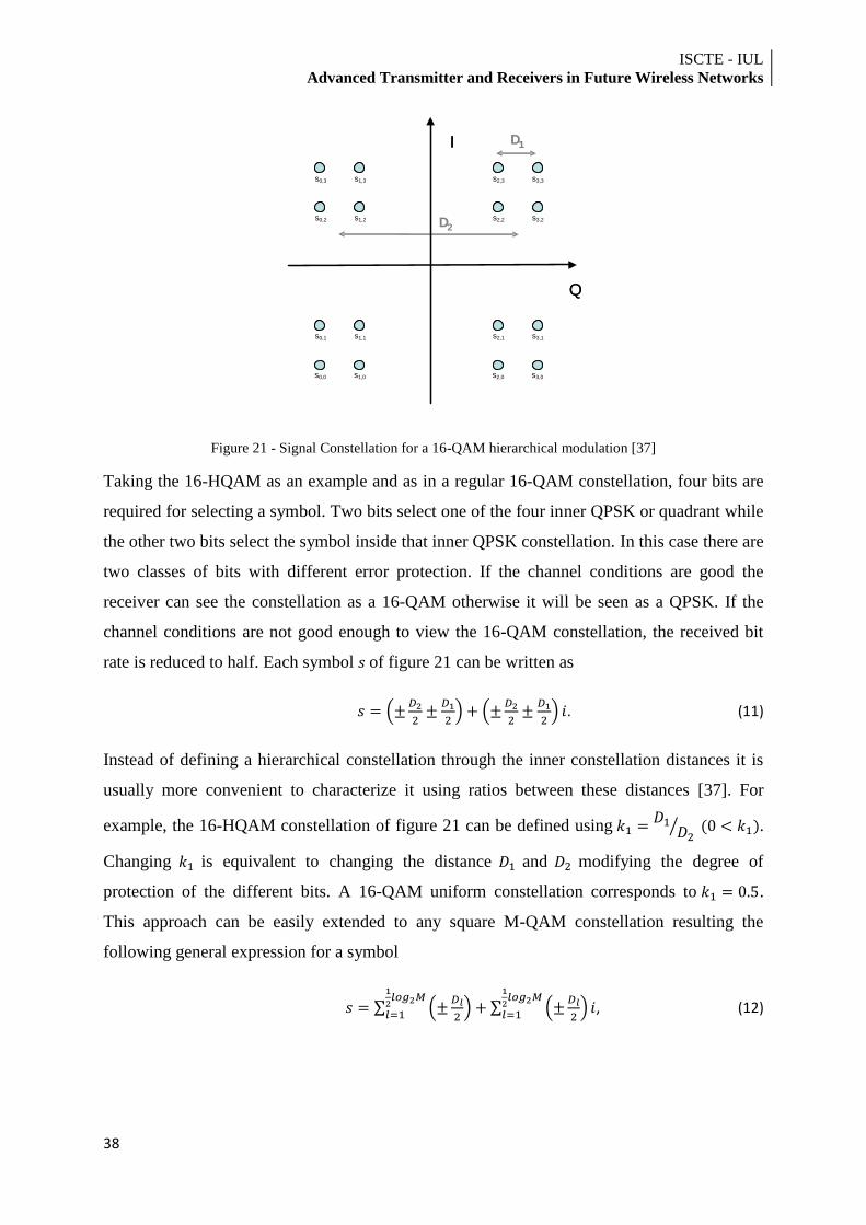
ISCTE - IUL
Advanced Transmitter and Receivers in Future Wireless Networks
38
I
Q
D
D1I
Q
2
1
s0,0 s1,0 s2,0 s3,0
s0,1 s1,1 s2,1 s3,1
s0,2 s1,2 s2,2 s3,2
s0,3 s1,3 s2,3 s3,3
Figure 21 - Signal Constellation for a 16-QAM hierarchical modulation [37]
Taking the 16-HQAM as an example and as in a regular 16-QAM constellation, four bits are
required for selecting a symbol. Two bits select one of the four inner QPSK or quadrant while
the other two bits select the symbol inside that inner QPSK constellation. In this case there are
two classes of bits with different error protection. If the channel conditions are good the
receiver can see the constellation as a 16-QAM otherwise it will be seen as a QPSK. If the
channel conditions are not good enough to view the 16-QAM constellation, the received bit
rate is reduced to half. Each symbol of figure 21 can be written as
. (11)
Instead of defining a hierarchical constellation through the inner constellation distances it is
usually more convenient to characterize it using ratios between these distances [37]. For
example, the 16-HQAM constellation of figure 21 can be defined using
.
Changing is equivalent to changing the distance and modifying the degree of
protection of the different bits. A 16-QAM uniform constellation corresponds to .
This approach can be easily extended to any square M-QAM constellation resulting the
following general expression for a symbol
, (12)
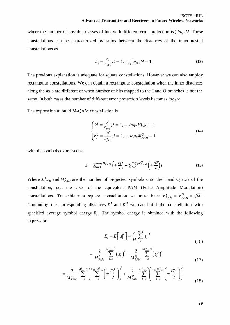
ISCTE - IUL Advanced Transmitter and Receivers in Future Wireless Networks
39
where the number of possible classes of bits with different error protection is
. These
constellations can be characterized by ratios between the distances of the inner nested
constellations as
. (13)
The previous explanation is adequate for square constellations. However we can also employ
rectangular constellations. We can obtain a rectangular constellation when the inner distances
along the axis are different or when number of bits mapped to the I and Q branches is not the
same. In both cases the number of different error protection levels becomes .
The expression to build M-QAM constellation is
(14)
with the symbols expressed as
(15)
Where and
are the number of projected symbols onto the I and Q axis of the
constellation, i.e., the sizes of the equivalent PAM (Pulse Amplitude Modulation)
constellations. To achieve a square constellation we must have
.
Computing the corresponding distances and
we can build the constellation with
specified average symbol energy . The symbol energy is obtained with the following
expression
/42 2
1
4 M
s l
l
E E s sM
(16)
22
2 2
1 1
2 2QI
PAM PAMMMI Q
l lI Ql lPAM PAM
s sM M
(17)
22
222 log2 log
1 1 1 1
2 2
2 2
Q QI IPAM PAM PAM PAMM MI QM M
i i
I Ql i l iPAM PAM
D D
M M
(18)
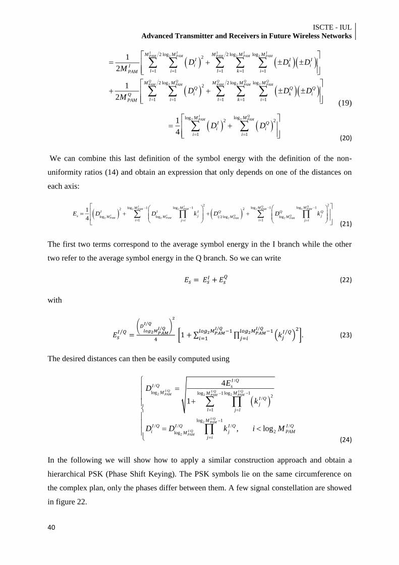
ISCTE - IUL
Advanced Transmitter and Receivers in Future Wireless Networks
40
2 2 2
2 2 2
2 log 2 log log2
1 1 1 1 1
2 log 2 log log2
1 1 1 1 1
1
2
1
2
I I I I IPAM PAM PAM PAM PAM
Q Q Q Q QPAM PAM PAM PAM PAM
M M M M MI I I
i k iIl i l k iPAM
M M M M MQ Q Q
i k iQl i l k iPAM
D D DM
D D DM
(19)
22 loglog
2 2
1 1
1
4
QIPAM PAMMM
I Q
i i
i i
D D
(20)
We can combine this last definition of the symbol energy with the definition of the non-
uniformity ratios (14) and obtain an expression that only depends on one of the distances on
each axis:
2222
2 2 2 2
22log 1log 1log 1log 1 22
log log 1 2 log log1 1
1
4
QQIIPAM PAMPAM PAM
I I Q QPAM PAM PAM PAM
MMMMI I I Q Q Q
s j jM M M Mi ij i j i
E D D k D D k
(21)
The first two terms correspond to the average symbol energy in the I branch while the other
two refer to the average symbol energy in the Q branch. So we can write
(22)
with
(23)
The desired distances can then be easily computed using
/ //
2 22
/2
/2
//
log log 1log 12
/
1
log 1
/ / / /
2log
4
1
, log
I Q I QI QPAM PAMPAM
I QPAM
I QPAM
I QI Q s
M MMI Q
j
l j l
M
I Q I Q I Q I Q
i j PAMMj i
ED
k
D D k i M
(24)
In the following we will show how to apply a similar construction approach and obtain a
hierarchical PSK (Phase Shift Keying). The PSK symbols lie on the same circumference on
the complex plan, only the phases differ between them. A few signal constellation are showed
in figure 22.
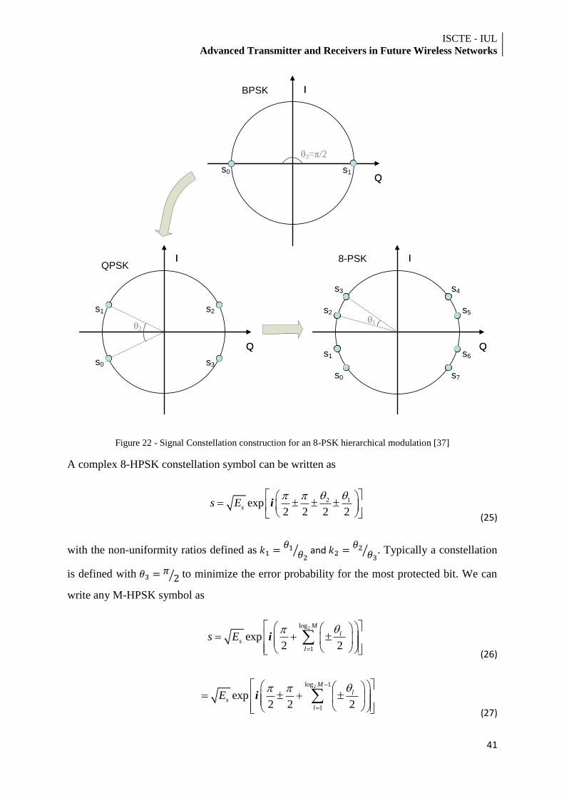
ISCTE - IUL Advanced Transmitter and Receivers in Future Wireless Networks
41
I
Q
I
Qs0 s1
I
Q
I
Q
s1
s0
s2
s3
θ2
I
Q
I
Q
s2
θ1
s3
s5
s4
s6
s7
s1
s0
BPSK
QPSK8-PSK
θ3=π/2
Figure 22 - Signal Constellation construction for an 8-PSK hierarchical modulation [37]
A complex 8-HPSK constellation symbol can be written as
2 1exp2 2 2 2
ss E
i
(25)
with the non-uniformity ratios defined as
and
. Typically a constellation
is defined with to minimize the error probability for the most protected bit. We can
write any M-HPSK symbol as
2log
1
exp2 2
M
ls
l
s E
i
(26)
2log 1
1
exp2 2 2
M
ls
l
E
i
(27)
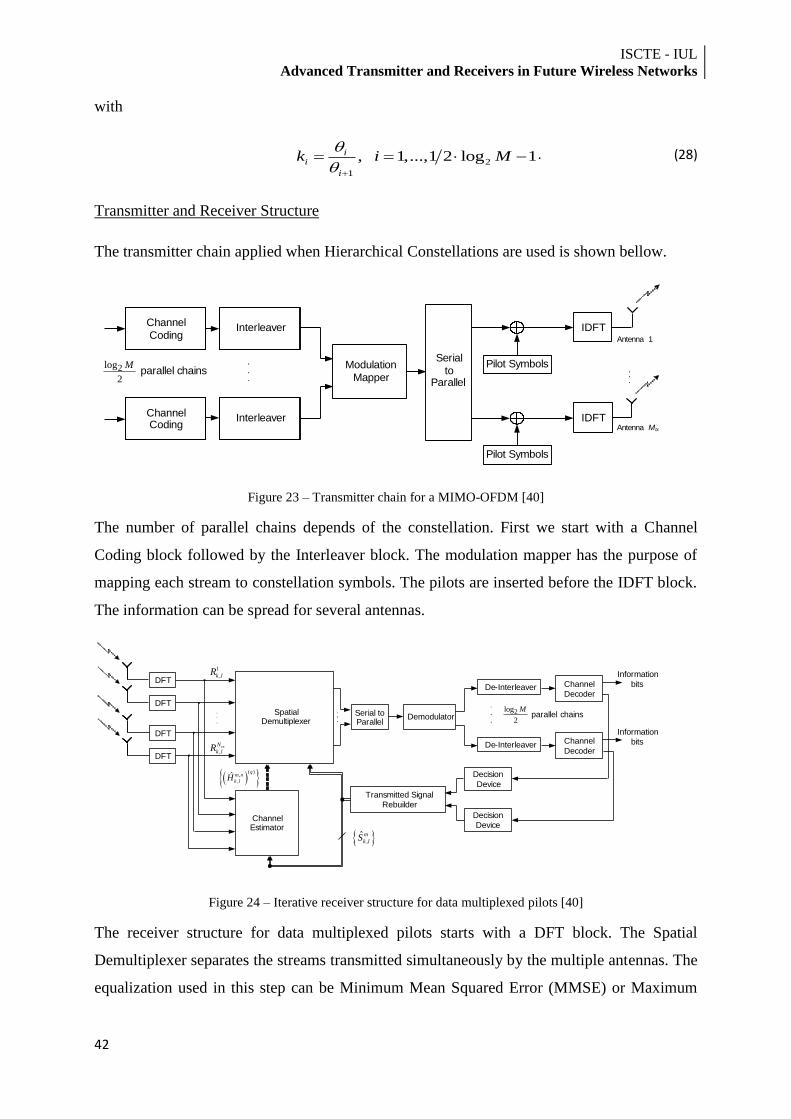
ISCTE - IUL
Advanced Transmitter and Receivers in Future Wireless Networks
42
with
2
1
, 1,...,1 2 log 1ii
i
k i M
. (28)
Transmitter and Receiver Structure
The transmitter chain applied when Hierarchical Constellations are used is shown bellow.
Figure 23 – Transmitter chain for a MIMO-OFDM [40]
The number of parallel chains depends of the constellation. First we start with a Channel
Coding block followed by the Interleaver block. The modulation mapper has the purpose of
mapping each stream to constellation symbols. The pilots are inserted before the IDFT block.
The information can be spread for several antennas.
Figure 24 – Iterative receiver structure for data multiplexed pilots [40]
The receiver structure for data multiplexed pilots starts with a DFT block. The Spatial
Demultiplexer separates the streams transmitted simultaneously by the multiple antennas. The
equalization used in this step can be Minimum Mean Squared Error (MMSE) or Maximum
Serial
to Parallel
.
.
.
.
.
.
Channel
Coding
.
.
.
Modulation
Mapper
IDFT
.
.
.
2log
2
Mparallel chains
Interleaver
Channel Coding
Interleaver
Antenna 1
Antenna Mtx
IDFT
Pilot Symbols
Pilot Symbols
Channel
DecoderDe-Interleaver
Demodulator Spatial
Demultiplexer
Channel Estimator
Transmitted Signal
Rebuilder
Decision
Device
DFT
DFT
DFT
DFT
1
,k lR
,rxN
k lR
.
.
.
( )
,
,ˆ
qm n
k lH
,ˆm
k lS
Serial to Parallel
.
.
.
.
.
Channel
DecoderDe-Interleaver
Decision
Device
.
.
.
.
.
2log
2
Mparallel chains
Information
bits
Information
bits
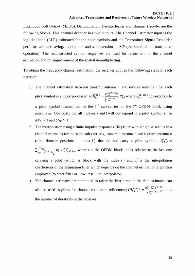
ISCTE - IUL Advanced Transmitter and Receivers in Future Wireless Networks
43
Likelihood Soft Output (MLSO). Demodulation, De-Interleaver and Channel Decoder are the
following blocks. This channel decoder has two outputs. The Channel Estimator input is the
log-likelihood (LLR) estimated for the code symbols and the Transmitter Signal Rebuilder
performs an interleaving, modulation and a conversion of S/P (the same of the transmitter
operation). The reconstructed symbol sequences are used for refinement of the channel
estimation and for improvement of the spatial demultiplexing.
To obtain the frequency channel estimation, the receiver applies the following steps in each
iteration:
1. The channel estimation between transmit antenna and receive antenna for each
pilot symbol is simply processed as
where
corresponds to
a pilot symbol transmitted in the sub-carrier of the OFDM block using
antenna . Obviously not all indexes and will correspond to a pilot symbol since
and .
2. The interpolation using a finite impulse response (FIR) filter with length results in a
channel estimates for the same sub-carrier , transmit antenna and receive antenna
(time domain positions – index ) that do not carry a pilot symbol,
, where is the OFDM block index relative to the last one
carrying a pilot (which is block with the index ) and
is the interpolation
coefficients of the estimation filter which depends on the channel estimation algorithm
employed (Weiner filter or Low Pass Sinc Interpolator).
3. The channel estimates are computed as (after the first iteration the data estimates can
also be used as pilots for channel estimation refinement)
. R is
the number of iterations in the receiver.
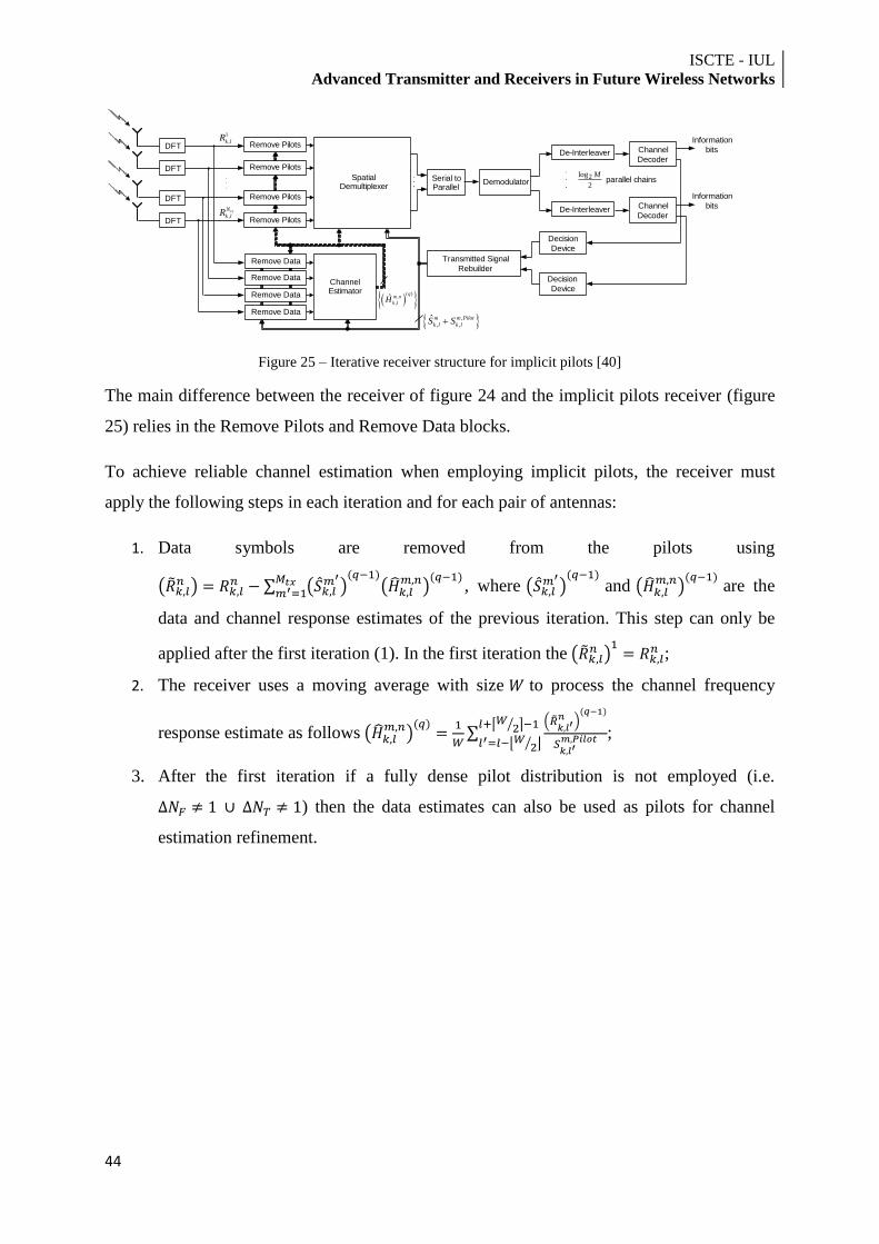
ISCTE - IUL
Advanced Transmitter and Receivers in Future Wireless Networks
44
Figure 25 – Iterative receiver structure for implicit pilots [40]
The main difference between the receiver of figure 24 and the implicit pilots receiver (figure
25) relies in the Remove Pilots and Remove Data blocks.
To achieve reliable channel estimation when employing implicit pilots, the receiver must
apply the following steps in each iteration and for each pair of antennas:
1. Data symbols are removed from the pilots using
, where
and
are the
data and channel response estimates of the previous iteration. This step can only be
applied after the first iteration (1). In the first iteration the
;
2. The receiver uses a moving average with size to process the channel frequency
response estimate as follows
;
3. After the first iteration if a fully dense pilot distribution is not employed (i.e.
) then the data estimates can also be used as pilots for channel
estimation refinement.
Channel
DecoderDe-Interleaver
Demodulator Spatial
Demultiplexer
Channel Estimator
Transmitted Signal
Rebuilder
Decision
Device
DFT
DFT
DFT
DFT
1
,k lR
,rxN
k lR
Remove Pilots
Remove Pilots
Remove Pilots
Remove Pilots
Remove Data
Remove Data
Remove Data
Remove Data
.
.
.
( )
,
,ˆ
qm n
k lH
,
, ,ˆ m m Pilot
k l k lS S
Serial to Parallel
.
.
.
.
.
Channel
DecoderDe-Interleaver
Decision
Device
.
.
.
.
.
2log
2
Mparallel chains
Information
bits
Information
bits
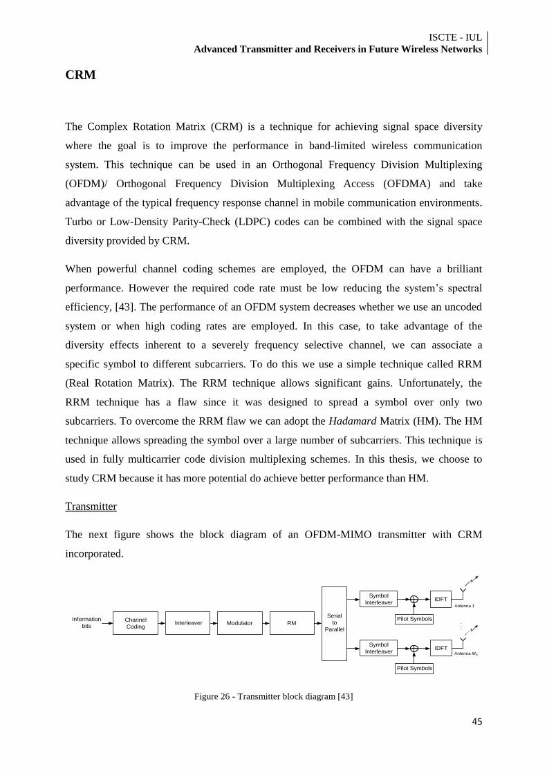
ISCTE - IUL Advanced Transmitter and Receivers in Future Wireless Networks
45
CRM
The Complex Rotation Matrix (CRM) is a technique for achieving signal space diversity
where the goal is to improve the performance in band-limited wireless communication
system. This technique can be used in an Orthogonal Frequency Division Multiplexing
(OFDM)/ Orthogonal Frequency Division Multiplexing Access (OFDMA) and take
advantage of the typical frequency response channel in mobile communication environments.
Turbo or Low-Density Parity-Check (LDPC) codes can be combined with the signal space
diversity provided by CRM.
When powerful channel coding schemes are employed, the OFDM can have a brilliant
performance. However the required code rate must be low reducing the system‟s spectral
efficiency, [43]. The performance of an OFDM system decreases whether we use an uncoded
system or when high coding rates are employed. In this case, to take advantage of the
diversity effects inherent to a severely frequency selective channel, we can associate a
specific symbol to different subcarriers. To do this we use a simple technique called RRM
(Real Rotation Matrix). The RRM technique allows significant gains. Unfortunately, the
RRM technique has a flaw since it was designed to spread a symbol over only two
subcarriers. To overcome the RRM flaw we can adopt the Hadamard Matrix (HM). The HM
technique allows spreading the symbol over a large number of subcarriers. This technique is
used in fully multicarrier code division multiplexing schemes. In this thesis, we choose to
study CRM because it has more potential do achieve better performance than HM.
Transmitter
The next figure shows the block diagram of an OFDM-MIMO transmitter with CRM
incorporated.
Information
bits
Serial
to
Parallel
.
.
.
.
.
.
IDFTAntenna 1
Antenna Mtx
IDFT
Pilot Symbols
Pilot Symbols
Channel
CodingModulatorInterleaver RM
Symbol
Interleaver
Symbol
Interleaver
Figure 26 - Transmitter block diagram [43]
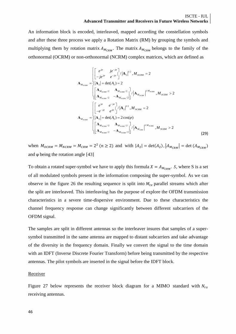
ISCTE - IUL
Advanced Transmitter and Receivers in Future Wireless Networks
46
An information block is encoded, interleaved, mapped according the constellation symbols
and after these three process we apply a Rotation Matrix (RM) by grouping the symbols and
multiplying them by rotation matrix . The matrix
belongs to the family of the
orthonormal (OCRM) or non-orthonormal (NCRM) complex matrices, which are defined as
1/ 2
2
2 2
1//2 /2
/2 /2
1/ 2
2
2 2
/2
/ , 2
det( ) 2
/ , 2
/ , 2
det( ) 2cos( )
OCRM
OCRMOCRM OCRM
OCRM
OCRM OCRM
NCRM
NCRM NC
j j
OCRMj j
M
MM M
M OCRM
M M
j j
NCRMj j
M
M M
e jeM
je e
A
M
e eM
e e
A
A
Α A
Α ΑΑ
Α Α
A
Α A
Α Α 1//2
/2 /2
/ , 2NCRMRM
CRM
NCRM NCRM
M
M NCRM
M M
M
ΑΑ Α
(29)
when and with
and ϕ being the rotation angle [43]
To obtain a rotated super-symbol we have to apply this formula , where S is a set
of all modulated symbols present in the information composing the super-symbol. As we can
observe in the figure 26 the resulting sequence is split into parallel streams which after
the split are interleaved. This interleaving has the purpose of explore the OFDM transmission
characteristics in a severe time-dispersive environment. Due to these characteristics the
channel frequency response can change significantly between different subcarriers of the
OFDM signal.
The samples are split in different antennas so the interleaver insures that samples of a super-
symbol transmitted in the same antenna are mapped to distant subcarriers and take advantage
of the diversity in the frequency domain. Finally we convert the signal to the time domain
with an IDFT (Inverse Discrete Fourier Transform) before being transmitted by the respective
antennas. The pilot symbols are inserted in the signal before the IDFT block.
Receiver
Figure 27 below represents the receiver block diagram for a MIMO standard with
receiving antennas.
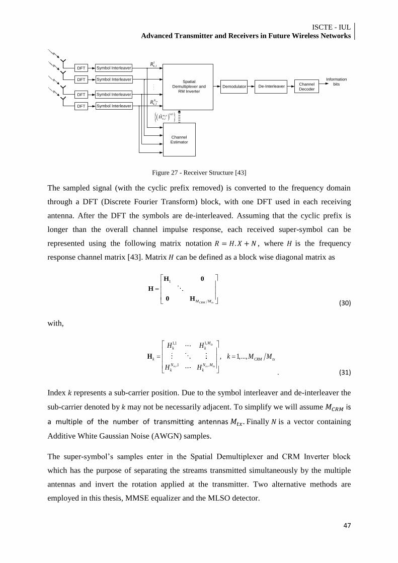
ISCTE - IUL Advanced Transmitter and Receivers in Future Wireless Networks
47
Channel
DecoderDe-InterleaverDemodulator
Spatial
Demultiplexer and
RM Inverter
Channel
Estimator
DFT
DFT
DFT
DFT
1
,k lR
,rxN
k lR
.
.
.
( )
,
,ˆ
qm n
k lH
Information
bits
Symbol Interleaver
Symbol Interleaver
Symbol Interleaver
Symbol Interleaver
Figure 27 - Receiver Structure [43]
The sampled signal (with the cyclic prefix removed) is converted to the frequency domain
through a DFT (Discrete Fourier Transform) block, with one DFT used in each receiving
antenna. After the DFT the symbols are de-interleaved. Assuming that the cyclic prefix is
longer than the overall channel impulse response, each received super-symbol can be
represented using the following matrix notation , where is the frequency
response channel matrix [43]. Matrix can be defined as a block wise diagonal matrix as
1
CRM txM M
H 0
H
0 H (30)
with,
1,1,1
,1 ,
, 1,...,
tx
rx rx tx
M
k k
k CRM tx
N N M
k k
H H
k M M
H H
H
. (31)
Index represents a sub-carrier position. Due to the symbol interleaver and de-interleaver the
sub-carrier denoted by may not be necessarily adjacent. To simplify we will assume is
a multiple of the number of transmitting antennas Finally is a vector containing
Additive White Gaussian Noise (AWGN) samples.
The super-symbol‟s samples enter in the Spatial Demultiplexer and CRM Inverter block
which has the purpose of separating the streams transmitted simultaneously by the multiple
antennas and invert the rotation applied at the transmitter. Two alternative methods are
employed in this thesis, MMSE equalizer and the MLSO detector.
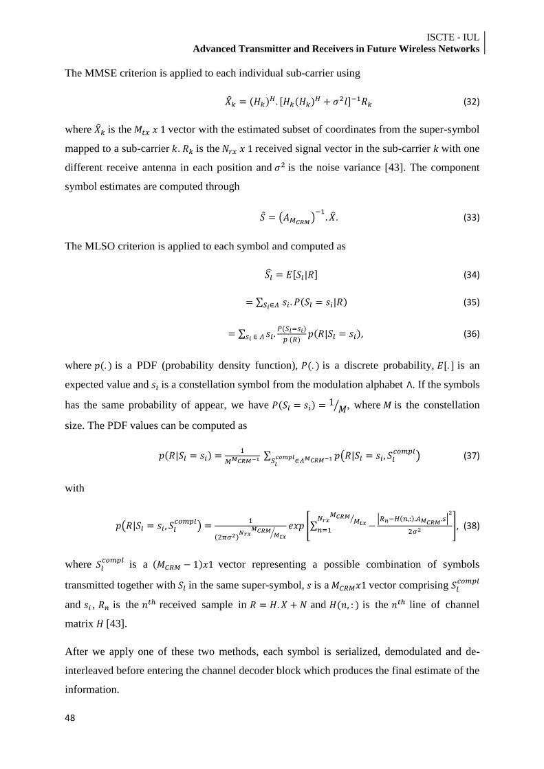
ISCTE - IUL
Advanced Transmitter and Receivers in Future Wireless Networks
48
The MMSE criterion is applied to each individual sub-carrier using
(32)
where is the vector with the estimated subset of coordinates from the super-symbol
mapped to a sub-carrier . is the received signal vector in the sub-carrier with one
different receive antenna in each position and is the noise variance [43]. The component
symbol estimates are computed through
. (33)
The MLSO criterion is applied to each symbol and computed as
(34)
(35)
, (36)
where is a PDF (probability density function), is a discrete probability, is an
expected value and is a constellation symbol from the modulation alphabet Λ. If the symbols
has the same probability of appear, we have , where is the constellation
size. The PDF values can be computed as
(37)
with
, (38)
where
is a vector representing a possible combination of symbols
transmitted together with in the same super-symbol, is a vector comprising
and , is the received sample in and is the line of channel
matrix [43].
After we apply one of these two methods, each symbol is serialized, demodulated and de-
interleaved before entering the channel decoder block which produces the final estimate of the
information.
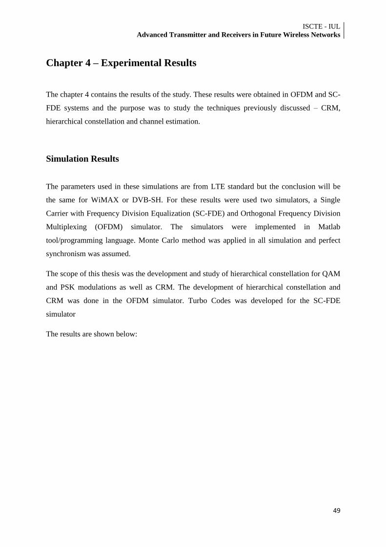
ISCTE - IUL Advanced Transmitter and Receivers in Future Wireless Networks
49
Chapter 4 – Experimental Results
The chapter 4 contains the results of the study. These results were obtained in OFDM and SC-
FDE systems and the purpose was to study the techniques previously discussed – CRM,
hierarchical constellation and channel estimation.
Simulation Results
The parameters used in these simulations are from LTE standard but the conclusion will be
the same for WiMAX or DVB-SH. For these results were used two simulators, a Single
Carrier with Frequency Division Equalization (SC-FDE) and Orthogonal Frequency Division
Multiplexing (OFDM) simulator. The simulators were implemented in Matlab
tool/programming language. Monte Carlo method was applied in all simulation and perfect
synchronism was assumed.
The scope of this thesis was the development and study of hierarchical constellation for QAM
and PSK modulations as well as CRM. The development of hierarchical constellation and
CRM was done in the OFDM simulator. Turbo Codes was developed for the SC-FDE
simulator
The results are shown below:
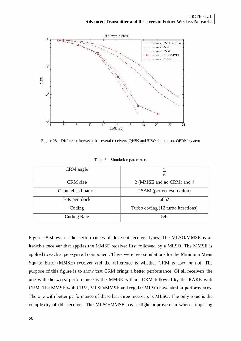
ISCTE - IUL
Advanced Transmitter and Receivers in Future Wireless Networks
50
Figure 28 – Difference between the several receivers. QPSK and SISO simulation. OFDM system
Table 3 – Simulation parameters
CRM angle
CRM size 2 (MMSE and no CRM) and 4
Channel estimation PSAM (perfect estimation)
Bits per block 6662
Coding Turbo coding (12 turbo iterations)
Coding Rate 5/6
Figure 28 shows us the performances of different receiver types. The MLSO/MMSE is an
iterative receiver that applies the MMSE receiver first followed by a MLSO. The MMSE is
applied to each super-symbol component. There were two simulations for the Minimum Mean
Square Error (MMSE) receiver and the difference is whether CRM is used or not. The
purpose of this figure is to show that CRM brings a better performance. Of all receivers the
one with the worst performance is the MMSE without CRM followed by the RAKE with
CRM. The MMSE with CRM, MLSO/MMSE and regular MLSO have similar performances.
The one with better performance of these last three receivers is MLSO. The only issue is the
complexity of this receiver. The MLSO/MMSE has a slight improvement when comparing
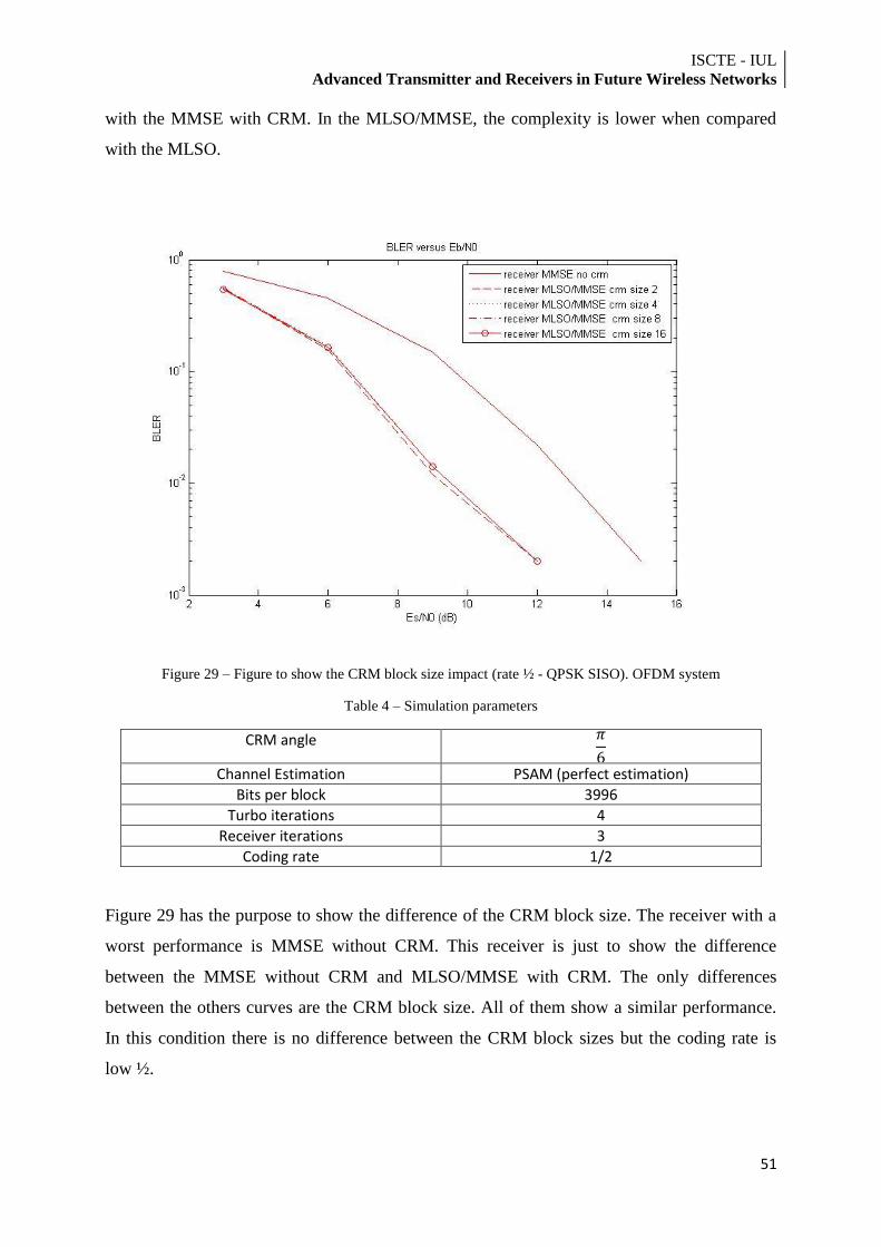
ISCTE - IUL Advanced Transmitter and Receivers in Future Wireless Networks
51
with the MMSE with CRM. In the MLSO/MMSE, the complexity is lower when compared
with the MLSO.
Figure 29 – Figure to show the CRM block size impact (rate ½ - QPSK SISO). OFDM system
Table 4 – Simulation parameters
CRM angle
Channel Estimation PSAM (perfect estimation)
Bits per block 3996
Turbo iterations 4
Receiver iterations 3
Coding rate 1/2
Figure 29 has the purpose to show the difference of the CRM block size. The receiver with a
worst performance is MMSE without CRM. This receiver is just to show the difference
between the MMSE without CRM and MLSO/MMSE with CRM. The only differences
between the others curves are the CRM block size. All of them show a similar performance.
In this condition there is no difference between the CRM block sizes but the coding rate is
low ½.
ISCTE - IUL
Advanced Transmitter and Receivers in Future Wireless Networks
52
Figure 30 - Figure to show the CRM block size impact (rate 5/6 – QPSK SISO). OFDM system
Table 5 – Simulation parameters
CRM angle
Channel estimation PSAM
Bits per block 6662
Coding rate 5/6
Turbo iteration 4
Receiver iteration 3
In this chart, the MMSE without CRM is shown here as reference. The difference between
this figure and figure 29 is the coding rate that in this figure is 5/6. All the MLSO/MMSE
simulations achieve a better performance than the MMSE receiver. The one that achieves a
better performance is with CRM block size of 16. The larger the block size, better the
performance. Of the all MLSO/MMSE simulation, the one with the worst performance is the
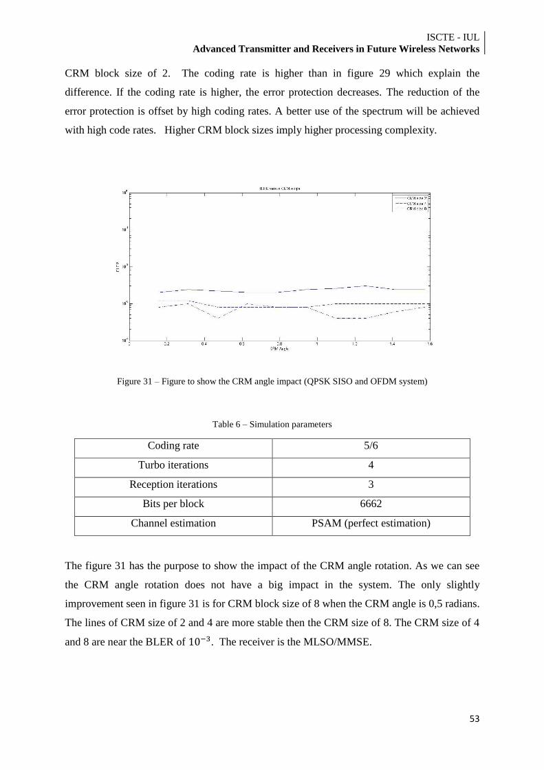
ISCTE - IUL Advanced Transmitter and Receivers in Future Wireless Networks
53
CRM block size of 2. The coding rate is higher than in figure 29 which explain the
difference. If the coding rate is higher, the error protection decreases. The reduction of the
error protection is offset by high coding rates. A better use of the spectrum will be achieved
with high code rates. Higher CRM block sizes imply higher processing complexity.
Figure 31 – Figure to show the CRM angle impact (QPSK SISO and OFDM system)
Table 6 – Simulation parameters
Coding rate 5/6
Turbo iterations 4
Reception iterations 3
Bits per block 6662
Channel estimation PSAM (perfect estimation)
The figure 31 has the purpose to show the impact of the CRM angle rotation. As we can see
the CRM angle rotation does not have a big impact in the system. The only slightly
improvement seen in figure 31 is for CRM block size of 8 when the CRM angle is 0,5 radians.
The lines of CRM size of 2 and 4 are more stable then the CRM size of 8. The CRM size of 4
and 8 are near the BLER of . The receiver is the MLSO/MMSE.
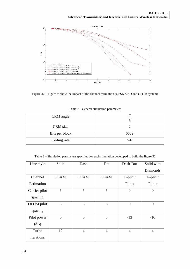
ISCTE - IUL
Advanced Transmitter and Receivers in Future Wireless Networks
54
Figure 32 – Figure to show the impact of the channel estimation (QPSK SISO and OFDM system)
Table 7 – General simulation parameters
CRM angle
CRM size 2
Bits per block 6662
Coding rate 5/6
Table 8 – Simulation parameters specified for each simulation developed to build the figure 32
Line style Solid Dash Dot Dash-Dot Solid with
Diamonds
Channel
Estimation
PSAM PSAM PSAM Implicit
Pilots
Implicit
Pilots
Carrier pilot
spacing
5 5 5 0 0
OFDM pilot
spacing
3 3 6 0 0
Pilot power
(dB)
0 0 0 -13 -16
Turbo
iterations
12 4 4 4 4
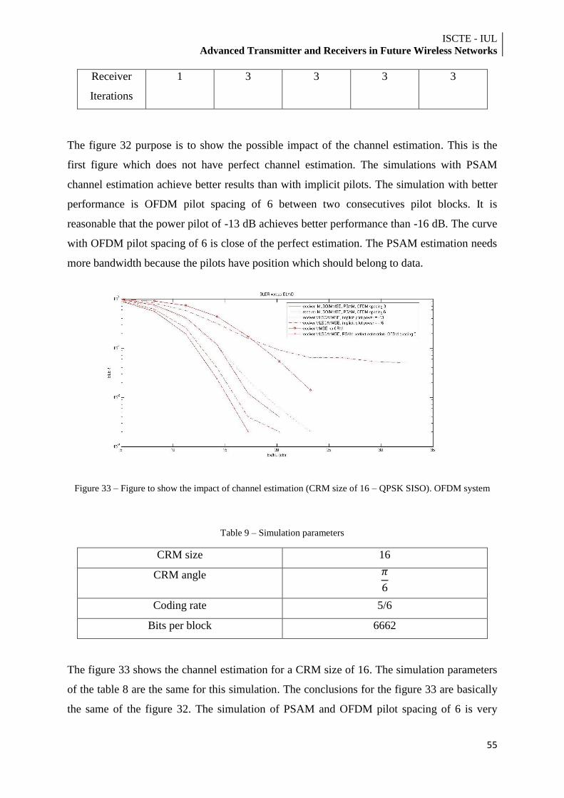
ISCTE - IUL Advanced Transmitter and Receivers in Future Wireless Networks
55
Receiver
Iterations
1 3 3 3 3
The figure 32 purpose is to show the possible impact of the channel estimation. This is the
first figure which does not have perfect channel estimation. The simulations with PSAM
channel estimation achieve better results than with implicit pilots. The simulation with better
performance is OFDM pilot spacing of 6 between two consecutives pilot blocks. It is
reasonable that the power pilot of -13 dB achieves better performance than -16 dB. The curve
with OFDM pilot spacing of 6 is close of the perfect estimation. The PSAM estimation needs
more bandwidth because the pilots have position which should belong to data.
Figure 33 – Figure to show the impact of channel estimation (CRM size of 16 – QPSK SISO). OFDM system
Table 9 – Simulation parameters
CRM size 16
CRM angle
Coding rate 5/6
Bits per block 6662
The figure 33 shows the channel estimation for a CRM size of 16. The simulation parameters
of the table 8 are the same for this simulation. The conclusions for the figure 33 are basically
the same of the figure 32. The simulation of PSAM and OFDM pilot spacing of 6 is very
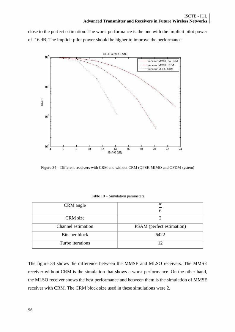
ISCTE - IUL
Advanced Transmitter and Receivers in Future Wireless Networks
56
close to the perfect estimation. The worst performance is the one with the implicit pilot power
of -16 dB. The implicit pilot power should be higher to improve the performance.
Figure 34 – Different receivers with CRM and without CRM (QPSK MIMO and OFDM system)
Table 10 – Simulation parameters
CRM angle
CRM size 2
Channel estimation PSAM (perfect estimation)
Bits per block 6422
Turbo iterations 12
The figure 34 shows the difference between the MMSE and MLSO receivers. The MMSE
receiver without CRM is the simulation that shows a worst performance. On the other hand,
the MLSO receiver shows the best performance and between them is the simulation of MMSE
receiver with CRM. The CRM block size used in these simulations were 2.
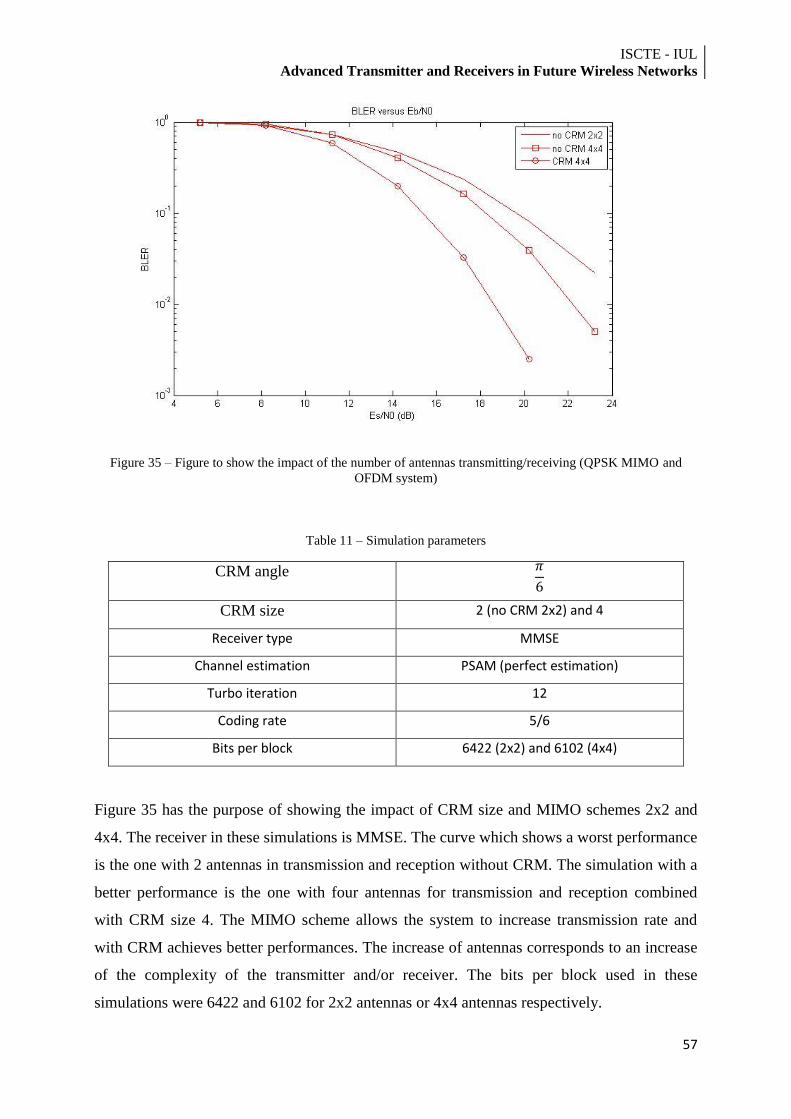
ISCTE - IUL Advanced Transmitter and Receivers in Future Wireless Networks
57
Figure 35 – Figure to show the impact of the number of antennas transmitting/receiving (QPSK MIMO and
OFDM system)
Table 11 – Simulation parameters
CRM angle
CRM size 2 (no CRM 2x2) and 4
Receiver type MMSE
Channel estimation PSAM (perfect estimation)
Turbo iteration 12
Coding rate 5/6
Bits per block 6422 (2x2) and 6102 (4x4)
Figure 35 has the purpose of showing the impact of CRM size and MIMO schemes 2x2 and
4x4. The receiver in these simulations is MMSE. The curve which shows a worst performance
is the one with 2 antennas in transmission and reception without CRM. The simulation with a
better performance is the one with four antennas for transmission and reception combined
with CRM size 4. The MIMO scheme allows the system to increase transmission rate and
with CRM achieves better performances. The increase of antennas corresponds to an increase
of the complexity of the transmitter and/or receiver. The bits per block used in these
simulations were 6422 and 6102 for 2x2 antennas or 4x4 antennas respectively.
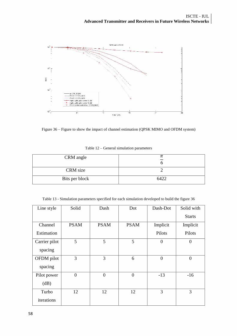
ISCTE - IUL
Advanced Transmitter and Receivers in Future Wireless Networks
58
Figure 36 – Figure to show the impact of channel estimation (QPSK MIMO and OFDM system)
Table 12 – General simulation parameters
CRM angle
CRM size 2
Bits per block 6422
Table 13 - Simulation parameters specified for each simulation developed to build the figure 36
Line style Solid Dash Dot Dash-Dot Solid with
Starts
Channel
Estimation
PSAM PSAM PSAM Implicit
Pilots
Implicit
Pilots
Carrier pilot
spacing
5 5 5 0 0
OFDM pilot
spacing
3 3 6 0 0
Pilot power
(dB)
0 0 0 -13 -16
Turbo
iterations
12 12 12 3 3
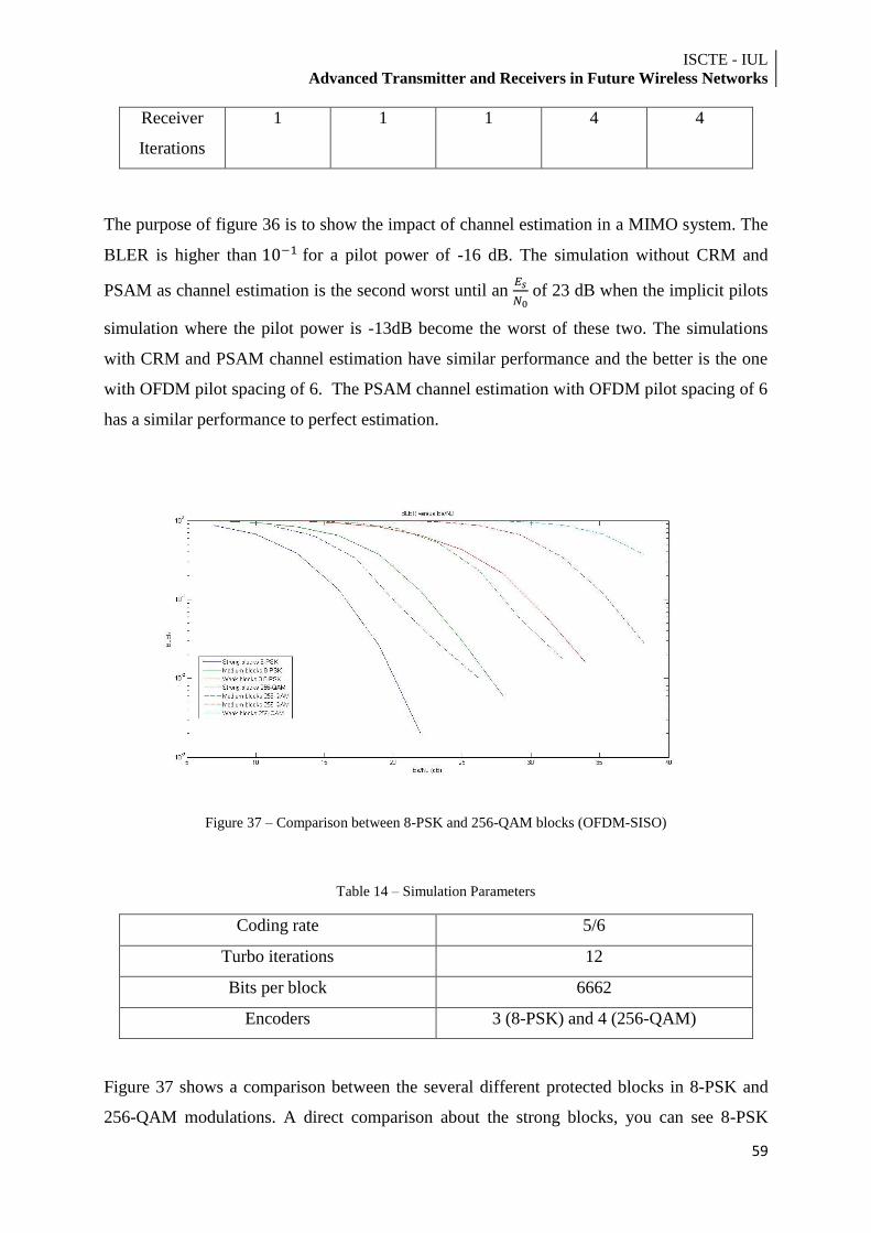
ISCTE - IUL Advanced Transmitter and Receivers in Future Wireless Networks
59
Receiver
Iterations
1 1 1 4 4
The purpose of figure 36 is to show the impact of channel estimation in a MIMO system. The
BLER is higher than for a pilot power of -16 dB. The simulation without CRM and
PSAM as channel estimation is the second worst until an
of 23 dB when the implicit pilots
simulation where the pilot power is -13dB become the worst of these two. The simulations
with CRM and PSAM channel estimation have similar performance and the better is the one
with OFDM pilot spacing of 6. The PSAM channel estimation with OFDM pilot spacing of 6
has a similar performance to perfect estimation.
Figure 37 – Comparison between 8-PSK and 256-QAM blocks (OFDM-SISO)
Table 14 – Simulation Parameters
Coding rate 5/6
Turbo iterations 12
Bits per block 6662
Encoders 3 (8-PSK) and 4 (256-QAM)
Figure 37 shows a comparison between the several different protected blocks in 8-PSK and
256-QAM modulations. A direct comparison about the strong blocks, you can see 8-PSK
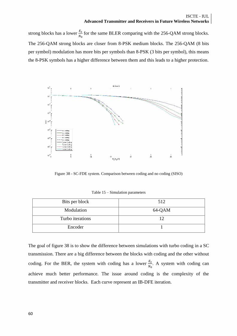
ISCTE - IUL
Advanced Transmitter and Receivers in Future Wireless Networks
60
strong blocks has a lower
for the same BLER comparing with the 256-QAM strong blocks.
The 256-QAM strong blocks are closer from 8-PSK medium blocks. The 256-QAM (8 bits
per symbol) modulation has more bits per symbols than 8-PSK (3 bits per symbol), this means
the 8-PSK symbols has a higher difference between them and this leads to a higher protection.
Figure 38 - SC-FDE system. Comparison between coding and no coding (SISO)
Table 15 – Simulation parameters
Bits per block 512
Modulation 64-QAM
Turbo iterations 12
Encoder 1
The goal of figure 38 is to show the difference between simulations with turbo coding in a SC
transmission. There are a big difference between the blocks with coding and the other without
coding. For the BER, the system with coding has a lower
. A system with coding can
achieve much better performance. The issue around coding is the complexity of the
transmitter and receiver blocks. Each curve represent an IB-DFE iteration.
ISCTE - IUL Advanced Transmitter and Receivers in Future Wireless Networks
61
Chapter 5 – Thesis Conclusions
Conclusions
The first conclusion taken in this study is that the use of CRM can be an advantage. The CRM
can lead the future wireless system to better performance. The CRM is complex and that can
be a problem to terminals.
The CRM block size is useful when the coding rate is high and high coding rates mean least
code protection. If the coding rate is high the efficiency of the spectrum usage will be higher.
The CRM combine with higher coding rates can compensate the issue around high code rates,
the impairment of the code protection. The performance gain is higher in MIMO system when
it is using CRM technique. The advantage of using the MIMO is the higher transmission rate
but the system is more complex.
The different protection error bit can take an important impact combining with CRM. You
can increase the protection when using CRM. The price to pay is the higher complexity of the
system.
The PSAM channel estimation leads to better channel estimation, very close to the perfect
estimation when the OFDM pilot spacing is 6. The PSAM needs a higher bandwidth when
comparing with the implicit pilots.
Hierarchical constellations can be useful especially for high modulation (M>64 for QAM and
M>32 for PSK. These kind of hierarchical constellations are attractive for broadcast
transmissions.
The CRM technologies can lead to a new era in wireless communications. Video and Internet
are very common in mobile phones. Using CRM can lead to a higher quality of the
communications.
ISCTE - IUL
Advanced Transmitter and Receivers in Future Wireless Networks
62
Future work
This thesis has in the scope to develop a simulator with the purpose of study the performance
of CRM, hierarchical constellations and to study the impact of channel estimation. that allows
any kind of modulation. Future studies should be the study of CRM for modulation like M-
PSK (M>8) and M-QAM (M>64), to study the impact of CRM in more complex modulation.
Higher CRM block size must be developed because the higher CRM block size the higher can
be de performance of the system. The issue is the complexity than higher CRM block size
brings.
It would be interesting to develop a receiver with low complexity and a performance similar
to the MLSO.
More studies must be done about the possible impact of MIMO system in CRM.
ISCTE - IUL Advanced Transmitter and Receivers in Future Wireless Networks
63
References
[1] http://en.wikipedia.org/wiki/Wireless - 22/04/2011
[2] http://en.wikipedia.org/wiki/Mobile_phone - 22/04/2011
[3] http://en.wikipedia.org/wiki/Cellular_network - 22/04/2011
[4] “Synthesis of Band-Limited Orthogonal Signals for Multichannel Data
Transmission,” Bell System Technical Journal, 45, pp. 1775-1796, 1970
[5] L.Cimini, ”Analysis and Simulation of a Digital Mobile Channel using Orthogonal
Frequency Division Multiplexing”, IEEE Trans. on Comm., Vol. 33, No. 7, July 1985.
[6] 3GPPP TR 25.814, ”3rd Generation Partenership Project: Technical Specification
Group Radio Access Network; Physical Layers Aspects for Evolved UTRA”, 2006.
[7] T. Cover, “Broadcast channels”, IEEE Trans. On Inform. Theory, vol.IT-18, pp.2-
14, Jan. 1972.
[8] K. Ramchandran, A. Ortega, K. M. Uz, and M. Vetterli, “Multiresolution broadcast
for digital HDTV using joint source/channel coding”, IEEE J. Select. Areas Commun.,
vol. 11, Jan. 1993.
[9] http://www.dvb.org/news_events/news/dvb_approves_dvbsh_specif/index.xml -
22/04/2011
[10] „Digital video broadcasting (DVB) framing structure, channel coding and
modulation for digital terrestrial television (DVB-T)‟, Mar. 1997. ETSI, European
Telecommunication Standard ETS 300 744.
[11]http://www.radio-electronics.com/info/broadcast/digital-video-
broadcasting/what-is-dvb-t-basics-tutorial.php - 29/03/2011
[12] A. Correia, “Optimised Complex Constellations for Transmitter Diversity”,
Wireless Personal Communications Journal, pp. 267-284, 2002
[13] E. Telatar, “Capacity of multiantenna Gaussian channels,” AT&T Bell
Laboratories, Technical Memorandum, June 1995.
[14] G.J. Foschini and M.J. Gans, “On limits of wireless communications in a fading
environment when using multiple antennas,” Wireless Pers.Commun., vol. 6, pp. 311–
335, Mar. 1998
[15] N. Souto, F. Cercas, R. Dinis, J. Silva, "On the BER Performance of Hierarchical
M-QAM Constellations with Diversity and Imperfect Channel Estimation", IEEE
Trans. on Commun. , vol. 55 , no. 10 , pp. 1852 - 1856 , Oct. 2007 .
[16] N. Souto, R. Dinis, F. Cercas J. Silva, A. Correia “An Iterative Receiver for
WCDMA Systems with MIMO Transmissions and Hierarchical Constellations”, Proc.
IEEE International Symposium on Spread Spectrum Techniques and Applications -
ISSSTA 2006, August 2006, Manaus, Brasil.
[17] http://www.complextoreal.com/chapters/ofdm2.pdf - 18/11/2010
[19] Falconer, D., Ariyavisitakul, S., Benyamin-Seeyar, A., Eidson, B., Frequency
Domain Equalization for Single-Carrier Broadband Wireless Systems, Abril 2002,
IEEE Communications Magazine;
[20] J. Zyren, W. McCoy, “Overview of the 3GPP Long Term Evolution Physical
Layer”, Freescale Semiconductor, Inc., white paper, 2007;
[21] http://en.wikipedia.org/wiki/3GPP_Long_Term_Evolution - 22/4/2011
ISCTE - IUL
Advanced Transmitter and Receivers in Future Wireless Networks
64
[22] http://www.radio-electronics.com/info/cellulartelecomms/lte-long-term-
evolution/3g-lte-basics.php - 22/04/2011
[23] http://en.wikipedia.org/wiki/Multi-user_MIMO - 22/04/2011
[24] http://www.radio-electronics.com/info/cellulartelecomms/lte-long-term-
evolution/3gpp-4g-imt-lte-advanced-tutorial.php - 22/04/2011
[25] http://en.wikipedia.org/wiki/Picocell - 14/08/2011
[26] http://en.wikipedia.org/wiki/Femtocell - 14/08/2011
[27] http://en.wikipedia.org/wiki/LTE_Advanced - 14/08/2011
[28] http://www.radio-electronics.com/info/cellulartelecomms/lte-long-term-
evolution/4g-lte-advanced-carrier-channel-aggregation.php - 14/08/2011
[29] http://www.dvb.org/news_events/news/dvb_approves_dvbsh_specif/index.xml -
14/08/2011
[30] http://en.wikipedia.org/wiki/DVB-H - 14/08/2011
[31] http://en.wikipedia.org/wiki/DVB-SH - 14/08/2011
[32] L. Fiens, “Esquemas de Emissão/Recepção Avançados para Transmissões
Broadcast por Satélite”,Master Thesis, September 2010
[33]https://docs.google.com/viewer?a=v&pid=explorer&chrome=true&srcid=0B1rbl
MZdJlB_ZmQ0OWQ1NDItYjA0Ny00NGEzLThkMTgtZTIxMTlmMWIxOTBj&hl=
en - 14/08/2011
[34] http://en.wikipedia.org/wiki/WiMAX - 14/08/2011
[35] http://www.radio-electronics.com/info/wireless/wimax/ieee-802-16-standards.php
- 14/08/2011
[36]http://www.wimaxforum.org/resources/documents/marketing/whitepapers/migrati
on-wimax%C2%AE-release-1-release-2-part-2-air-interface – 14/08/2011
[37] Silva, M.; Correia, A.; Dinis, R.; Souto, N.S.; Silva. J.C.; (eds.); Transmission
Techniques for Emergent Multicast and Broadcast Systems, CRC Press, Boca Raton,
2010.
[38] H. Sari, G. Karam, and I. Jeanclaude, “Frequency-Domain Equalization of
Mobile Radio and Terrestrial Broadcast Channels.” Proc. GLOBECOM ‟94, San
Francisco, CA, Nov.-Dec. 1994, pp. 1-5;
[39] H. Sari, G. Karam, and I. Jeanclaude, “Transmission Techniques for Digital
Terrestrial TV Broadcasting,” IEEE Commun. Mag., vol. 33, no. 2, Feb. 1995, pp.
100-109
[40] N. Souto, R. Dinis, J. C. Silva, A. Correia, “Efficient Transmission Strategies for
Multimedia Broadcast and Multicast Services in Mobile OFDM Based System”
[41] J. Kjeldsen, “Turbo Coding – Hardware Acceleration of an EGPRS-2 Turbo
Decoder on an FPGA”, Master Thesis, June 2009
[42] http://en.wikipedia.org/wiki/Turbo_code - 14/08/2011
[43] J. Seguro, P. Gomes, N. Souto, A. Correia, R. Dinis, “Rotation Matrices for
OFDM Transmission”
[44] - http://en.wikipedia.org/wiki/MIMO - 14/08/2011
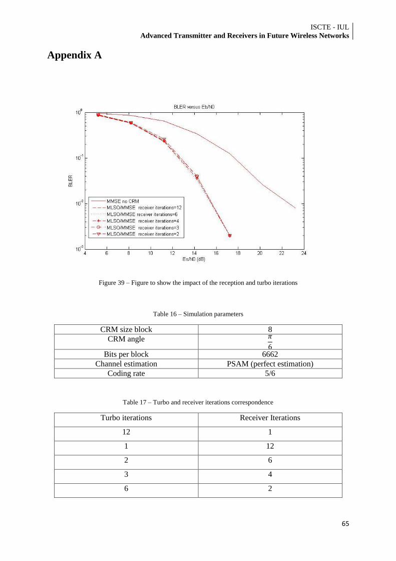
ISCTE - IUL Advanced Transmitter and Receivers in Future Wireless Networks
65
Appendix A
Figure 39 – Figure to show the impact of the reception and turbo iterations
Table 16 – Simulation parameters
CRM size block 8
CRM angle
Bits per block 6662
Channel estimation PSAM (perfect estimation)
Coding rate 5/6
Table 17 – Turbo and receiver iterations correspondence
Turbo iterations Receiver Iterations
12 1
1 12
2 6
3 4
6 2
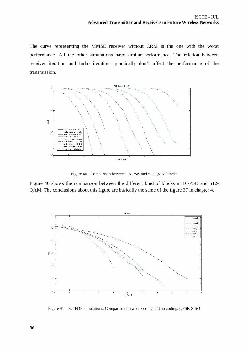
ISCTE - IUL
Advanced Transmitter and Receivers in Future Wireless Networks
66
The curve representing the MMSE receiver without CRM is the one with the worst
performance. All the other simulations have similar performance. The relation between
receiver iteration and turbo iterations practically don‟t affect the performance of the
transmission.
Figure 40 - Comparison between 16-PSK and 512-QAM blocks
Figure 40 shows the comparison between the different kind of blocks in 16-PSK and 512-
QAM. The conclusions about this figure are basically the same of the figure 37 in chapter 4.
Figure 41 – SC-FDE simulations. Comparison between coding and no coding. QPSK SISO
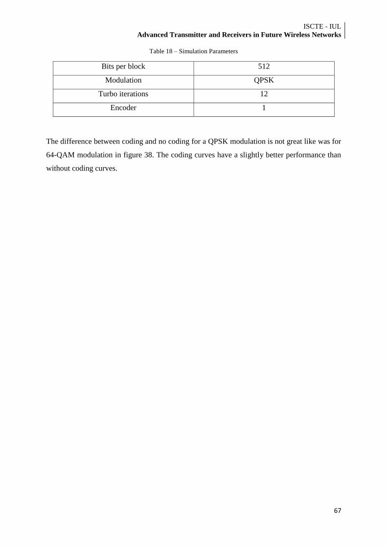
ISCTE - IUL Advanced Transmitter and Receivers in Future Wireless Networks
67
Table 18 – Simulation Parameters
Bits per block 512
Modulation QPSK
Turbo iterations 12
Encoder 1
The difference between coding and no coding for a QPSK modulation is not great like was for
64-QAM modulation in figure 38. The coding curves have a slightly better performance than
without coding curves.

ISCTE - IUL
Advanced Transmitter and Receivers in Future Wireless Networks
68
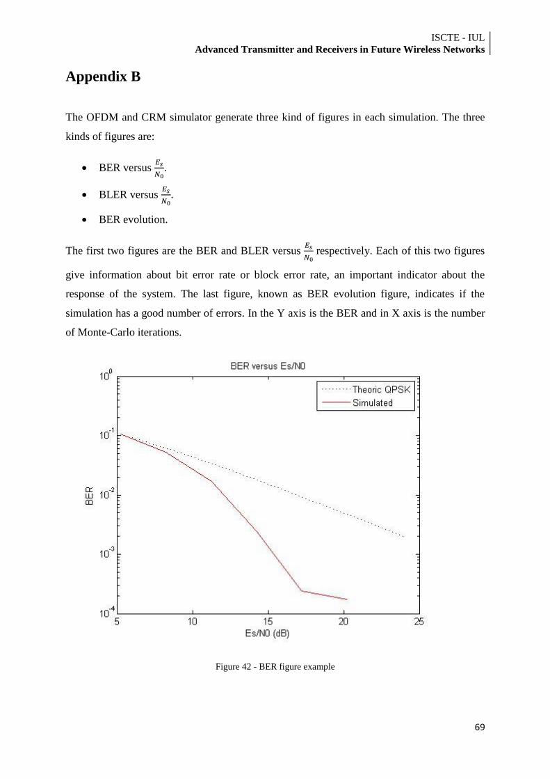
ISCTE - IUL Advanced Transmitter and Receivers in Future Wireless Networks
69
Appendix B
The OFDM and CRM simulator generate three kind of figures in each simulation. The three
kinds of figures are:
BER versus
.
BLER versus
.
BER evolution.
The first two figures are the BER and BLER versus
respectively. Each of this two figures
give information about bit error rate or block error rate, an important indicator about the
response of the system. The last figure, known as BER evolution figure, indicates if the
simulation has a good number of errors. In the Y axis is the BER and in X axis is the number
of Monte-Carlo iterations.
Figure 42 - BER figure example
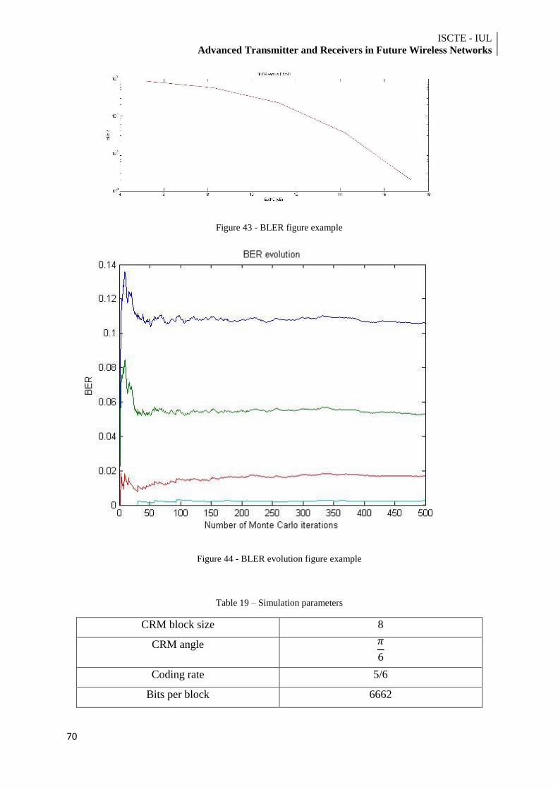
ISCTE - IUL
Advanced Transmitter and Receivers in Future Wireless Networks
70
Figure 43 - BLER figure example
Figure 44 - BLER evolution figure example
Table 19 – Simulation parameters
CRM block size 8
CRM angle
Coding rate 5/6
Bits per block 6662

ISCTE - IUL Advanced Transmitter and Receivers in Future Wireless Networks
71
Channel estimation PSAM (perfect estimation)
Receiver MLSO/MMSE
Turbo iterations 1
Receiver iterations 12