offline learnopengl
TRANSCRIPT

Learn OpenGL
An offline transcript of learnopengl.com
Joey de Vries

Copyright c© 2015 Joey de VriesPUBLISHED BY ME :)
LEARNOPENGL.COM
Licensed under the Creative Commons Attribution-NonCommercial 3.0 Unported License (the“License”). You may not use this file except in compliance with the License. You may obtaina copy of the License at http://creativecommons.org/licenses/by-nc/3.0. Un-less required by applicable law or agreed to in writing, software distributed under the License isdistributed on an “AS IS” BASIS, WITHOUT WARRANTIES OR CONDITIONS OF ANY KIND, eitherexpress or implied. See the License for the specific language governing permissions and limitationsunder the License.
Second printing, July 2015

Contents
1 Introduction . . . . . . . . . . . . . . . . . . . . . . . . . . . . . . . . . . . . . . . . . . . . . . . . . . 14
1.1 Prerequisites 141.2 Structure 151.2.1 Boxes . . . . . . . . . . . . . . . . . . . . . . . . . . . . . . . . . . . . . . . . . . . . . . . . . . . . . . . . . 151.2.2 Code . . . . . . . . . . . . . . . . . . . . . . . . . . . . . . . . . . . . . . . . . . . . . . . . . . . . . . . . . 151.2.3 Color hints . . . . . . . . . . . . . . . . . . . . . . . . . . . . . . . . . . . . . . . . . . . . . . . . . . . . . 151.2.4 OpenGL Function references . . . . . . . . . . . . . . . . . . . . . . . . . . . . . . . . . . . . . . 15
I Getting started
2 OpenGL . . . . . . . . . . . . . . . . . . . . . . . . . . . . . . . . . . . . . . . . . . . . . . . . . . . . . . 17
2.1 Core-profile vs Immediate mode 182.2 Extensions 192.3 State machine 192.4 Objects 202.5 Let’s get started 212.6 Additional resources 21
3 Creating a window . . . . . . . . . . . . . . . . . . . . . . . . . . . . . . . . . . . . . . . . . . . 22
3.1 GLFW 223.2 Building GLFW 233.2.1 CMake . . . . . . . . . . . . . . . . . . . . . . . . . . . . . . . . . . . . . . . . . . . . . . . . . . . . . . . . 233.2.2 Compilation . . . . . . . . . . . . . . . . . . . . . . . . . . . . . . . . . . . . . . . . . . . . . . . . . . . . 24

3.3 Our first project 243.4 Linking 243.4.1 OpenGL library on Windows . . . . . . . . . . . . . . . . . . . . . . . . . . . . . . . . . . . . . . . 253.4.2 OpenGL library on Linux . . . . . . . . . . . . . . . . . . . . . . . . . . . . . . . . . . . . . . . . . . 26
3.5 GLEW 263.5.1 Building and linking GLEW . . . . . . . . . . . . . . . . . . . . . . . . . . . . . . . . . . . . . . . . . 26
3.6 Additional resources 27
4 Hello Window . . . . . . . . . . . . . . . . . . . . . . . . . . . . . . . . . . . . . . . . . . . . . . . . 28
4.1 GLEW 294.2 Viewport 304.3 Ready your engines 304.4 One last thing 314.5 Input 324.6 Rendering 33
5 Hello Triangle . . . . . . . . . . . . . . . . . . . . . . . . . . . . . . . . . . . . . . . . . . . . . . . . . 35
5.1 Vertex input 375.2 Vertex shader 395.3 Compiling a shader 405.4 Fragment shader 415.4.1 Shader program . . . . . . . . . . . . . . . . . . . . . . . . . . . . . . . . . . . . . . . . . . . . . . . . 42
5.5 Linking Vertex Attributes 435.5.1 Vertex Array Object . . . . . . . . . . . . . . . . . . . . . . . . . . . . . . . . . . . . . . . . . . . . . . 455.5.2 The triangle we’ve all been waiting for . . . . . . . . . . . . . . . . . . . . . . . . . . . . . . . 47
5.6 Element Buffer Objects 485.7 Additional resources 515.8 Exercises 51
6 Shaders . . . . . . . . . . . . . . . . . . . . . . . . . . . . . . . . . . . . . . . . . . . . . . . . . . . . . . 52
6.1 GLSL 526.2 Types 536.2.1 Vectors . . . . . . . . . . . . . . . . . . . . . . . . . . . . . . . . . . . . . . . . . . . . . . . . . . . . . . . . 53
6.3 Ins and outs 546.4 Uniforms 566.5 Our own shader class 596.6 Reading from file 606.7 Exercises 62
7 Textures . . . . . . . . . . . . . . . . . . . . . . . . . . . . . . . . . . . . . . . . . . . . . . . . . . . . . . 63
7.1 Texture Wrapping 657.2 Texture Filtering 667.2.1 Mipmaps . . . . . . . . . . . . . . . . . . . . . . . . . . . . . . . . . . . . . . . . . . . . . . . . . . . . . . 67

7.3 Loading and creating textures 687.4 SOIL 697.5 Generating a texture 697.6 Applying textures 707.7 Texture Units 737.8 Exercises 76
8 Transformations . . . . . . . . . . . . . . . . . . . . . . . . . . . . . . . . . . . . . . . . . . . . . . . 77
8.1 Vectors 778.2 Scalar vector operations 788.3 Vector negation 798.4 Addition and subtraction 798.5 Length 808.6 Vector-vector multiplication 818.6.1 Dot product . . . . . . . . . . . . . . . . . . . . . . . . . . . . . . . . . . . . . . . . . . . . . . . . . . . . 818.6.2 Cross product . . . . . . . . . . . . . . . . . . . . . . . . . . . . . . . . . . . . . . . . . . . . . . . . . . 82
8.7 Matrices 828.8 Addition and subtraction 838.9 Matrix-scalar products 848.10 Matrix-matrix multiplication 848.11 Matrix-Vector multiplication 858.12 Identity matrix 868.13 Scaling 868.14 Translation 878.15 Rotation 888.16 Combining matrices 898.17 In practice 908.18 GLM 908.19 Exercises 94
9 Coordinate Systems . . . . . . . . . . . . . . . . . . . . . . . . . . . . . . . . . . . . . . . . . . 95
9.1 The global picture 969.2 Local space 979.3 World space 979.4 View space 979.5 Clip space 979.5.1 Orthographic projection . . . . . . . . . . . . . . . . . . . . . . . . . . . . . . . . . . . . . . . . . . 989.5.2 Perspective projection . . . . . . . . . . . . . . . . . . . . . . . . . . . . . . . . . . . . . . . . . . . . 99
9.6 Putting it all together 1029.7 Going 3D 1029.8 More 3D 1069.8.1 Z-buffer . . . . . . . . . . . . . . . . . . . . . . . . . . . . . . . . . . . . . . . . . . . . . . . . . . . . . . . 107

9.8.2 More cubes! . . . . . . . . . . . . . . . . . . . . . . . . . . . . . . . . . . . . . . . . . . . . . . . . . . . 108
9.9 Exercises 109
10 Camera . . . . . . . . . . . . . . . . . . . . . . . . . . . . . . . . . . . . . . . . . . . . . . . . . . . . . 110
10.1 Camera/View space 11010.1.1 1. Camera position . . . . . . . . . . . . . . . . . . . . . . . . . . . . . . . . . . . . . . . . . . . . . 11110.1.2 2. Camera direction . . . . . . . . . . . . . . . . . . . . . . . . . . . . . . . . . . . . . . . . . . . . 11110.1.3 3. Right axis . . . . . . . . . . . . . . . . . . . . . . . . . . . . . . . . . . . . . . . . . . . . . . . . . . . 11110.1.4 4. Up axis . . . . . . . . . . . . . . . . . . . . . . . . . . . . . . . . . . . . . . . . . . . . . . . . . . . . . 111
10.2 Look At 11210.3 Walk around 11310.4 Movement speed 11510.5 Look around 11610.6 Euler angles 11710.7 Mouse input 11910.8 Zoom 12110.9 Camera class 12210.10 Exercises 123
11 Review . . . . . . . . . . . . . . . . . . . . . . . . . . . . . . . . . . . . . . . . . . . . . . . . . . . . . . 124
11.1 Glossary 124
II Lighting
12 Colors . . . . . . . . . . . . . . . . . . . . . . . . . . . . . . . . . . . . . . . . . . . . . . . . . . . . . . 127
12.1 A lighting scene 129
13 Basic Lighting . . . . . . . . . . . . . . . . . . . . . . . . . . . . . . . . . . . . . . . . . . . . . . . 133
13.1 Ambient lighting 13413.2 Diffuse lighting 13513.3 Normal vectors 13613.4 Calculating the diffuse color 13713.5 One last thing 13913.6 Specular Lighting 14113.7 Exercises 145
14 Materials . . . . . . . . . . . . . . . . . . . . . . . . . . . . . . . . . . . . . . . . . . . . . . . . . . . . 146
14.1 Setting materials 14714.2 Light properties 14914.3 Different light colors 15114.4 Exercises 152

15 Lighting maps . . . . . . . . . . . . . . . . . . . . . . . . . . . . . . . . . . . . . . . . . . . . . . . 154
15.1 Diffuse maps 15415.2 Specular maps 15715.3 Sampling specular maps 15815.4 Exercises 160
16 Light casters . . . . . . . . . . . . . . . . . . . . . . . . . . . . . . . . . . . . . . . . . . . . . . . . . 161
16.1 Directional Light 16116.2 Point lights 16416.3 Attenuation 16516.3.1 Choosing the right values . . . . . . . . . . . . . . . . . . . . . . . . . . . . . . . . . . . . . . . . 16616.3.2 Implementing attenuation . . . . . . . . . . . . . . . . . . . . . . . . . . . . . . . . . . . . . . . 167
16.4 Spotlight 16916.5 Flashlight 16916.6 Smooth/Soft edges 17216.7 Exercises 174
17 Multiple lights . . . . . . . . . . . . . . . . . . . . . . . . . . . . . . . . . . . . . . . . . . . . . . . 175
17.1 Directional light 17617.2 Point light 17717.3 Putting it all together 17817.4 Exercises 181
18 Review . . . . . . . . . . . . . . . . . . . . . . . . . . . . . . . . . . . . . . . . . . . . . . . . . . . . . . 182
18.1 Glossary 182
III Model Loading
19 Assimp . . . . . . . . . . . . . . . . . . . . . . . . . . . . . . . . . . . . . . . . . . . . . . . . . . . . . . 185
19.1 A model loading library 18619.2 Building Assimp 187
20 Mesh . . . . . . . . . . . . . . . . . . . . . . . . . . . . . . . . . . . . . . . . . . . . . . . . . . . . . . . 189
20.1 Initialization 19020.2 Rendering 192
21 Model . . . . . . . . . . . . . . . . . . . . . . . . . . . . . . . . . . . . . . . . . . . . . . . . . . . . . . 194
21.1 Importing a 3D model into OpenGL 19521.1.1 Assimp to Mesh . . . . . . . . . . . . . . . . . . . . . . . . . . . . . . . . . . . . . . . . . . . . . . . . 19721.1.2 Indices . . . . . . . . . . . . . . . . . . . . . . . . . . . . . . . . . . . . . . . . . . . . . . . . . . . . . . . 19921.1.3 Material . . . . . . . . . . . . . . . . . . . . . . . . . . . . . . . . . . . . . . . . . . . . . . . . . . . . . . 199

21.2 A large optimization 20021.3 No more containers! 20221.4 Exercises 203
IV Advanced OpenGL
22 Depth testing . . . . . . . . . . . . . . . . . . . . . . . . . . . . . . . . . . . . . . . . . . . . . . . . 205
22.1 Depth test function 20622.2 Depth value precision 20922.3 Visualizing the depth buffer 21022.4 Z-fighting 21322.4.1 Prevent z-fighting . . . . . . . . . . . . . . . . . . . . . . . . . . . . . . . . . . . . . . . . . . . . . . . 214
23 Stencil testing . . . . . . . . . . . . . . . . . . . . . . . . . . . . . . . . . . . . . . . . . . . . . . . 216
23.1 Stencil functions 21823.2 Object outlining 219
24 Blending . . . . . . . . . . . . . . . . . . . . . . . . . . . . . . . . . . . . . . . . . . . . . . . . . . . . 223
24.1 Discarding fragments 22424.2 Blending 22824.3 Rendering semi-transparent textures 23124.4 Don’t break the order 233
25 Face culling . . . . . . . . . . . . . . . . . . . . . . . . . . . . . . . . . . . . . . . . . . . . . . . . . 235
25.1 Winding order 23525.2 Face culling 23725.3 Exercises 239
26 Framebuffers . . . . . . . . . . . . . . . . . . . . . . . . . . . . . . . . . . . . . . . . . . . . . . . . 240
26.1 Creating a framebuffer 24026.1.1 Texture attachments . . . . . . . . . . . . . . . . . . . . . . . . . . . . . . . . . . . . . . . . . . . . 24226.1.2 Renderbuffer object attachments . . . . . . . . . . . . . . . . . . . . . . . . . . . . . . . . . . 243
26.2 Rendering to a texture 24426.3 Post-processing 24726.3.1 Inversion . . . . . . . . . . . . . . . . . . . . . . . . . . . . . . . . . . . . . . . . . . . . . . . . . . . . . . 24726.3.2 Grayscale . . . . . . . . . . . . . . . . . . . . . . . . . . . . . . . . . . . . . . . . . . . . . . . . . . . . 248
26.4 Kernel effects 24926.4.1 Blur . . . . . . . . . . . . . . . . . . . . . . . . . . . . . . . . . . . . . . . . . . . . . . . . . . . . . . . . . . 25126.4.2 Edge detection . . . . . . . . . . . . . . . . . . . . . . . . . . . . . . . . . . . . . . . . . . . . . . . . 252
26.5 Exercises 253

27 Cubemaps . . . . . . . . . . . . . . . . . . . . . . . . . . . . . . . . . . . . . . . . . . . . . . . . . . 254
27.1 Creating a cubemap 25527.2 Skybox 25627.3 Loading a skybox 25827.4 Displaying a skybox 25927.5 An optimization 26127.6 Environment mapping 26227.7 Reflection 26227.8 Refraction 26627.9 Dynamic environment maps 26727.10 Exercises 268
28 Advanced Data . . . . . . . . . . . . . . . . . . . . . . . . . . . . . . . . . . . . . . . . . . . . . 269
28.1 Batching vertex attributes 27028.2 Copying buffers 271
29 Advanced GLSL . . . . . . . . . . . . . . . . . . . . . . . . . . . . . . . . . . . . . . . . . . . . . 273
29.1 GLSL’s built-in variables 27329.2 Vertex shader variables 27329.2.1 gl_PointSize . . . . . . . . . . . . . . . . . . . . . . . . . . . . . . . . . . . . . . . . . . . . . . . . . . . . 27429.2.2 gl_VertexID . . . . . . . . . . . . . . . . . . . . . . . . . . . . . . . . . . . . . . . . . . . . . . . . . . . . 275
29.3 Fragment shader variables 27529.3.1 gl_FragCoord . . . . . . . . . . . . . . . . . . . . . . . . . . . . . . . . . . . . . . . . . . . . . . . . . . 27529.3.2 gl_FrontFacing . . . . . . . . . . . . . . . . . . . . . . . . . . . . . . . . . . . . . . . . . . . . . . . . . 27629.3.3 gl_FragDepth . . . . . . . . . . . . . . . . . . . . . . . . . . . . . . . . . . . . . . . . . . . . . . . . . . 277
29.4 Interface blocks 27829.5 Uniform buffer objects 27929.6 Uniform block layout 28029.7 Using uniform buffers 28229.8 A simple example 284
30 Geometry Shader . . . . . . . . . . . . . . . . . . . . . . . . . . . . . . . . . . . . . . . . . . . 288
30.1 Using geometry shaders 29130.2 Let’s build some houses 29430.3 Exploding objects 29930.4 Visualizing normal vectors 302
31 Instancing . . . . . . . . . . . . . . . . . . . . . . . . . . . . . . . . . . . . . . . . . . . . . . . . . . . 305
31.1 Instanced arrays 30831.2 An asteroid field 311

32 Anti Aliasing . . . . . . . . . . . . . . . . . . . . . . . . . . . . . . . . . . . . . . . . . . . . . . . . . 317
32.1 Multisampling 31832.2 MSAA in OpenGL 32232.3 Off-screen MSAA 32332.3.1 Multisampled texture attachments . . . . . . . . . . . . . . . . . . . . . . . . . . . . . . . . . 32432.3.2 Multisampled renderbuffer objects . . . . . . . . . . . . . . . . . . . . . . . . . . . . . . . . . 32432.3.3 Render to multisampled framebuffer . . . . . . . . . . . . . . . . . . . . . . . . . . . . . . . . 324
32.4 Custom Anti-Aliasing algorithm 327
V Advanced Lighting
33 Advanced Lighting . . . . . . . . . . . . . . . . . . . . . . . . . . . . . . . . . . . . . . . . . . 329
33.1 Blinn-Phong 329
34 Gamma Correction . . . . . . . . . . . . . . . . . . . . . . . . . . . . . . . . . . . . . . . . . . 334
34.1 Gamma correction 33634.2 sRGB textures 33834.3 Attenuation 33934.4 Additional resources 341
35 Shadow Mapping . . . . . . . . . . . . . . . . . . . . . . . . . . . . . . . . . . . . . . . . . . . 342
35.1 Shadow mapping 34335.2 The depth map 34435.2.1 Light space transform . . . . . . . . . . . . . . . . . . . . . . . . . . . . . . . . . . . . . . . . . . . 34635.2.2 Render to depth map . . . . . . . . . . . . . . . . . . . . . . . . . . . . . . . . . . . . . . . . . . . 346
35.3 Rendering shadows 34835.4 Improving shadow maps 35235.4.1 Shadow acne . . . . . . . . . . . . . . . . . . . . . . . . . . . . . . . . . . . . . . . . . . . . . . . . . 35235.4.2 Peter panning . . . . . . . . . . . . . . . . . . . . . . . . . . . . . . . . . . . . . . . . . . . . . . . . . 35435.4.3 Over sampling . . . . . . . . . . . . . . . . . . . . . . . . . . . . . . . . . . . . . . . . . . . . . . . . . 356
35.5 PCF 35835.6 Orthographic vs projection 36035.7 Additional resources 361
36 Point Shadows . . . . . . . . . . . . . . . . . . . . . . . . . . . . . . . . . . . . . . . . . . . . . . . 362
36.1 Generating the depth cubemap 36336.1.1 Light space transform . . . . . . . . . . . . . . . . . . . . . . . . . . . . . . . . . . . . . . . . . . . 36536.1.2 Depth shaders . . . . . . . . . . . . . . . . . . . . . . . . . . . . . . . . . . . . . . . . . . . . . . . . . 366
36.2 Omnidirectional shadow maps 36736.2.1 Visualizing cubemap depth buffer . . . . . . . . . . . . . . . . . . . . . . . . . . . . . . . . . 371
36.3 PCF 37236.4 Additional resources 375

37 Normal Mapping . . . . . . . . . . . . . . . . . . . . . . . . . . . . . . . . . . . . . . . . . . . . 376
37.1 Normal mapping 37737.2 Tangent space 38137.2.1 Manual calculation of tangents and bitangents . . . . . . . . . . . . . . . . . . . . . . 38337.2.2 Tangent space normal mapping . . . . . . . . . . . . . . . . . . . . . . . . . . . . . . . . . . . 385
37.3 Complex objects 38937.4 One last thing 39137.5 Additional resources 391
38 Parallax Mapping . . . . . . . . . . . . . . . . . . . . . . . . . . . . . . . . . . . . . . . . . . . 392
38.1 Parallax mapping 39538.2 Steep Parallax Mapping 39938.3 Parallax Occlusion Mapping 40338.4 Additional resources 405
39 HDR . . . . . . . . . . . . . . . . . . . . . . . . . . . . . . . . . . . . . . . . . . . . . . . . . . . . . . . . . 406
39.1 Floating point framebuffers 40839.2 Tone mapping 41039.2.1 More HDR . . . . . . . . . . . . . . . . . . . . . . . . . . . . . . . . . . . . . . . . . . . . . . . . . . . . . 412
39.3 Additional resources 412
40 Bloom . . . . . . . . . . . . . . . . . . . . . . . . . . . . . . . . . . . . . . . . . . . . . . . . . . . . . . 413
40.1 Extracting bright color 41640.2 Gaussian blur 41840.3 Blending both textures 42140.4 Additional resources 423
41 Deferred Shading . . . . . . . . . . . . . . . . . . . . . . . . . . . . . . . . . . . . . . . . . . . . 424
41.1 The G-buffer 42641.2 The deferred lighting pass 43041.3 Combining deferred rendering with forward rendering 43241.4 A larger number of lights 43541.4.1 Calculating a light’s volume or radius . . . . . . . . . . . . . . . . . . . . . . . . . . . . . . . 43541.4.2 How we really use light volumes . . . . . . . . . . . . . . . . . . . . . . . . . . . . . . . . . . . 437
41.5 Deferred rendering vs forward rendering 43841.6 Additional resources 439
42 SSAO . . . . . . . . . . . . . . . . . . . . . . . . . . . . . . . . . . . . . . . . . . . . . . . . . . . . . . . 440
42.1 Sample buffers 44342.2 Normal-oriented hemisphere 44542.3 Random kernel rotations 44642.4 The SSAO shader 447

42.5 Ambient occlusion blur 45142.6 Applying ambient occlusion 45342.7 Additional resources 456
VI In Practice
43 Text Rendering . . . . . . . . . . . . . . . . . . . . . . . . . . . . . . . . . . . . . . . . . . . . . . 458
43.1 Classical text rendering: bitmap fonts 45843.2 Modern text rendering: FreeType 45943.2.1 Shaders . . . . . . . . . . . . . . . . . . . . . . . . . . . . . . . . . . . . . . . . . . . . . . . . . . . . . . 46343.2.2 Render line of text . . . . . . . . . . . . . . . . . . . . . . . . . . . . . . . . . . . . . . . . . . . . . . 464
43.3 Going further 467
44 2D Game . . . . . . . . . . . . . . . . . . . . . . . . . . . . . . . . . . . . . . . . . . . . . . . . . . . 468
45 Breakout . . . . . . . . . . . . . . . . . . . . . . . . . . . . . . . . . . . . . . . . . . . . . . . . . . . . 469
45.1 OpenGL Breakout 470
46 Setting up . . . . . . . . . . . . . . . . . . . . . . . . . . . . . . . . . . . . . . . . . . . . . . . . . . . 472
46.1 Utility 47346.2 Resource management 47446.3 Program 474
47 Rendering Sprites . . . . . . . . . . . . . . . . . . . . . . . . . . . . . . . . . . . . . . . . . . . . 476
47.1 2D projection matrix 47647.2 Rendering sprites 47747.2.1 Initialization . . . . . . . . . . . . . . . . . . . . . . . . . . . . . . . . . . . . . . . . . . . . . . . . . . . 47847.2.2 Rendering . . . . . . . . . . . . . . . . . . . . . . . . . . . . . . . . . . . . . . . . . . . . . . . . . . . . 479
47.3 Hello sprite 480
48 Levels . . . . . . . . . . . . . . . . . . . . . . . . . . . . . . . . . . . . . . . . . . . . . . . . . . . . . . . 482
48.1 Within the game 48548.1.1 The player paddle . . . . . . . . . . . . . . . . . . . . . . . . . . . . . . . . . . . . . . . . . . . . . . 487
49 Ball . . . . . . . . . . . . . . . . . . . . . . . . . . . . . . . . . . . . . . . . . . . . . . . . . . . . . . . . . 490
50 Collision detection . . . . . . . . . . . . . . . . . . . . . . . . . . . . . . . . . . . . . . . . . . . 494
50.1 AABB - AABB collisions 49450.2 AABB - Circle collision detection 497
51 Collision resolution . . . . . . . . . . . . . . . . . . . . . . . . . . . . . . . . . . . . . . . . . . . 50151.0.1 Collision repositioning . . . . . . . . . . . . . . . . . . . . . . . . . . . . . . . . . . . . . . . . . . . 50151.0.2 Collision direction . . . . . . . . . . . . . . . . . . . . . . . . . . . . . . . . . . . . . . . . . . . . . . . 50251.0.3 AABB - Circle collision resolution . . . . . . . . . . . . . . . . . . . . . . . . . . . . . . . . . . . 503

51.1 Player - ball collisions 50551.1.1 Sticky paddle . . . . . . . . . . . . . . . . . . . . . . . . . . . . . . . . . . . . . . . . . . . . . . . . . . 50651.1.2 The bottom edge . . . . . . . . . . . . . . . . . . . . . . . . . . . . . . . . . . . . . . . . . . . . . . 506
51.2 A few notes 507
52 Particles . . . . . . . . . . . . . . . . . . . . . . . . . . . . . . . . . . . . . . . . . . . . . . . . . . . . . 508
53 Postprocessing . . . . . . . . . . . . . . . . . . . . . . . . . . . . . . . . . . . . . . . . . . . . . . 51453.0.1 Shake it . . . . . . . . . . . . . . . . . . . . . . . . . . . . . . . . . . . . . . . . . . . . . . . . . . . . . . 517
54 Powerups . . . . . . . . . . . . . . . . . . . . . . . . . . . . . . . . . . . . . . . . . . . . . . . . . . . 51954.0.1 Spawning PowerUps . . . . . . . . . . . . . . . . . . . . . . . . . . . . . . . . . . . . . . . . . . . . 52054.0.2 Activating PowerUps . . . . . . . . . . . . . . . . . . . . . . . . . . . . . . . . . . . . . . . . . . . . 52154.0.3 Updating PowerUps . . . . . . . . . . . . . . . . . . . . . . . . . . . . . . . . . . . . . . . . . . . . . 524
55 Audio . . . . . . . . . . . . . . . . . . . . . . . . . . . . . . . . . . . . . . . . . . . . . . . . . . . . . . . 527
55.1 Irrklang 52755.1.1 Adding music . . . . . . . . . . . . . . . . . . . . . . . . . . . . . . . . . . . . . . . . . . . . . . . . . . 52855.1.2 Adding sounds . . . . . . . . . . . . . . . . . . . . . . . . . . . . . . . . . . . . . . . . . . . . . . . . . 529
56 Render text . . . . . . . . . . . . . . . . . . . . . . . . . . . . . . . . . . . . . . . . . . . . . . . . . . 530
56.1 Player lives 53256.2 Level selection 53356.3 Winning 536
57 Final thoughts . . . . . . . . . . . . . . . . . . . . . . . . . . . . . . . . . . . . . . . . . . . . . . . 539
57.1 Optimizations 53957.2 Get creative 540

1. Introduction
Since you came here you probably want to learn the inner workings of computer graphics and doall the stuff the cool kids do by yourself. Doing things by yourself is extremely fun and resourcefuland gives you a great understanding of graphics programming. However, there are a few items thatneed to be taken into consideration before starting your journey.
1.1 PrerequisitesSince OpenGL is a graphics API and not a platform of its own, it requires a language to operatein and the language of choice is C++, therefore a decent knowledge of the C++ programminglanguage is required for these tutorials. However, I will try to explain most of the concepts used,including advanced C++ topics where required so it is not required to be an expert in C++, butyou should be able to write more than just a ’Hello World’ program. If you don’t have muchexperience with C++ I can recommend the following free tutorials at www.learncpp.com.
Also, we will be using some math (linear algebra, geometry and trigonometry) along theway and I will try to explain all the required concepts of the math required. However, I’m not amathematician by heart so even though my explanations might be easy to understand, they will mostlikely be incomplete. So where necessary I will provide pointers to good resources that explain thematerial in a more complete fashion. Do not be scared about the mathematical knowledge requiredbefore starting your journey into OpenGL; almost all the concepts can be understood with a basicmathematical background and I will try to keep the mathematics to a minimum where possible.Most of the functionality does not even require you to understand all the math as long as you knowhow to use it.

1.2 Structure 15
1.2 StructureLearnOpenGL is broken down into a number of general subjects. Each subject contains severalsections that each explain different concepts in large detail. Each of the subjects can be found at themenu to your left. The subjects are taught in a linear fashion (so it is advised to start from the topto the bottom, unless otherwise instructed) where each page explains the background theory andthe practical aspects.
To make the tutorials easier to follow and give them some added structure the site containsboxes, code blocks, color hints and function references.
1.2.1 Boxes
Green boxes encompasses some notes or useful features/hints about OpenGL or thesubject at hand.
Red boxes will contain warnings or other features you have to be extra careful with.
1.2.2 CodeYou will find plenty of small pieces of code in the website that are located in dark-gray boxes withsyntax-highlighted code as you can see below:
// This box contains code
Since these provide only snippets of code, wherever necessary I will provide a link to the entiresource code required for a given subject.
1.2.3 Color hintsSome words are displayed with a different color to make it extra clear these words portray a specialmeaning:
• Definition: green words specify a definition i.e. an important aspect/name of somethingyou’re likely to hear more often.• Program logic: red words specify function names or class names.• Variables: blue words specify variables including all OpenGL constants.
1.2.4 OpenGL Function referencesA particularly well appreciated feature of LearnOpenGL is the ability to review most of OpenGL’sfunctions wherever they show up in the content. Whenever a function is found in the content that isdocumented at the website, the function will show up with a slightly noticeable underline. You canhover the mouse over the function and after a small interval, a pop-up window will show relevantinformation about this function including a nice overview of what the function actually does. Hoveryour mouse over glEnable to see it in action.
Now that you got a bit of a feel of the structure of the site, hop over to the Getting Startedsection to start your journey in OpenGL!

I2 OpenGL . . . . . . . . . . . . . . . . . . . . . . . . . . . . 17
3 Creating a window . . . . . . . . . . . . . . . . . . 22
4 Hello Window . . . . . . . . . . . . . . . . . . . . . . . 28
5 Hello Triangle . . . . . . . . . . . . . . . . . . . . . . . . 35
6 Shaders . . . . . . . . . . . . . . . . . . . . . . . . . . . . . 52
7 Textures . . . . . . . . . . . . . . . . . . . . . . . . . . . . . 63
8 Transformations . . . . . . . . . . . . . . . . . . . . . . 77
9 Coordinate Systems . . . . . . . . . . . . . . . . . 95
10 Camera . . . . . . . . . . . . . . . . . . . . . . . . . . . 110
11 Review . . . . . . . . . . . . . . . . . . . . . . . . . . . . . 124
Getting started

2. OpenGL
Before starting our journey we should first define what OpenGL actually is. OpenGL is mainlyconsidered an API (an Application Programming Interface) that provides us with a large set offunctions that we can use to manipulate graphics and images. However, OpenGL by itself is not anAPI, but merely a specification, developed and maintained by the Khronos Group.
The OpenGL specification specifies exactly what the result/output of each function shouldbe and how it should perform. It is then up to the developers implementing this specification tocome up with a solution of how this function should operate. Since the OpenGL specification doesnot give us implementation details, the actual developed versions of OpenGL are allowed to havedifferent implementations, as long as their results comply with the specification (and are thus thesame to the user).
The people developing the actual OpenGL libraries are usually the graphics card manufacturers.Each graphics card that you buy supports specific versions of OpenGL which are the versions ofOpenGL developed specifically for that card (series). When using an Apple system the OpenGLlibrary is maintained by Apple themselves and under Linux there exists a combination of graphicsuppliers’ versions and hobbyists’ adaptations of these libraries. This also means that wheneverOpenGL is showing weird behavior that it shouldn’t, this is most likely the fault of the graphicscards manufacturers (or whoever developed/maintained the library).

2.1 Core-profile vs Immediate mode 18
Since most implementations are built by graphics card manufacturers. Whenever thereis a bug in the implementation this is usually solved by updating your video card drivers;those drivers include the newest versions of OpenGL that your card supports. This isone of the reasons why it’s always advised to occasionally update your graphic drivers.
Khronos publicly hosts all specification documents for all the OpenGL versions. The interestedreader can find the OpenGL specification of version 3.3 (which is what we’ll be using) here whichis a good read if you want to delve into the details of OpenGL (note how they mostly just describeresults and not implementations). The specifications also provide a great reference for finding theexact workings of its functions.
2.1 Core-profile vs Immediate modeIn the old days, using OpenGL meant developing in immediate mode (also known as the fixedfunction pipeline) which was an easy-to-use method for drawing graphics. Most of the functionalityof OpenGL was hidden in the library and developers did not have much freedom at how OpenGLdoes its calculations. Developers eventually got hungry for more flexibility and over time thespecifications became more flexible; developers gained more control over their graphics. Theimmediate mode is really easy to use and understand, but it is also extremely inefficient. For thatreason the specification started to deprecate immediate mode functionality from version 3.2 andstarted motivating developers to develop in OpenGL’s core-profile mode which is a division ofOpenGL’s specification that removed all old deprecated functionality.
When using OpenGL’s core-profile, OpenGL forces us to use modern practices. Whenever wetry to use one of OpenGL’s deprecated functions, OpenGL raises an error and stops drawing. Theadvantage of learning the modern approach is that it is very flexible and efficient, but unfortunatelyis also more difficult to learn. The immediate mode abstracted quite a lot from the actual operationsOpenGL performed and while it was easy to learn, it was hard to grasp how OpenGL actuallyoperates. The modern approach requires the developer to truly understand OpenGL and graphicsprogramming and while it is a bit difficult, it allows for much more flexibility, more efficiency andmost importantly a much better understanding of graphics programming.
This is also the reason why our tutorials are geared at Core-Profile OpenGL version 3.3.Although it is more difficult, it is greatly worth the effort.
As of today, much higher versions of OpenGL are published (at the time of writing 4.5) atwhich you might ask: why do I want to learn OpenGL 3.3 when OpenGL 4.5 is out? The answer tothat question is relatively simple. All future versions of OpenGL starting from 3.3 basically addextra useful features to OpenGL without changing OpenGL’s core mechanics; the newer versionsjust introduce slightly more efficient or more useful ways to accomplish the same tasks. The resultis that all concepts and techniques remain the same over the modern OpenGL versions so it isperfectly valid to learn OpenGL 3.3. Whenever you’re ready and/or more experienced you caneasily use specific functionality from more recent OpenGL versions.

2.2 Extensions 19
When using functionality from the most recent version of OpenGL, only the mostmodern graphics cards will be able to run your application. This is often why mostdevelopers generally target lower versions of OpenGL and optionally enable higherversion functionality.
In some tutorials you’ll sometimes find more modern features which are noted down as such.
2.2 ExtensionsA great feature of OpenGL is its support of extensions. Whenever a graphics company comes upwith a new technique or a new large optimization for rendering this is often found in an extensionimplemented in the drivers. If the hardware an application runs on supports such an extensionthe developer can use the functionality provided by the extension for more advanced or efficientgraphics. This way, a graphics developer can still use these new rendering techniques withouthaving to wait for OpenGL to include the functionality in its future versions, simply by checking ifthe extension is supported by the graphics card. Often, when an extension is popular or very usefulit eventually becomes part of future OpenGL versions.
The developer then has to query whether any of these extensions are available (or use anOpenGL extension library). This allows the developer to do things better or more efficient, basedon whether an extension is available:
if(GL_ARB_extension_name){
// Do cool new and modern stuff supported by hardware}else{
// Extension not supported: do it the old way}
With OpenGL version 3.3 we rarely need an extension for most techniques, but wherever it isnecessary proper instructions are provided.
2.3 State machineOpenGL is by itself a large state machine: a collection of variables that define how OpenGL shouldcurrently operate. The state of OpenGL is commonly referred to as the OpenGL context. Whenusing OpenGL, we often change its state by setting some options, manipulating some buffers andthen render using the current context.
Whenever we tell OpenGL that we now want to draw lines instead of triangles for example,we change the state of OpenGL by changing some context variable that sets how OpenGL shoulddraw. As soon as we changed the state by telling OpenGL it should draw lines, the next drawingcommands will now draw lines instead of triangles.
When working in OpenGL we will come across several state-changing functions that changethe context and several state-using functions that perform some operations based on the currentstate of OpenGL. As long as you keep in mind that OpenGL is basically one large state machine,most of its functionality will make more sense.

2.4 Objects 20
2.4 ObjectsThe OpenGL libraries are written in C and allows for many derivations in other languages, but inits core it remains a C-library. Since many of C’s language-constructs do not translate that well toother higher-level languages, OpenGL was developed with several abstractions in mind. One ofthose abstractions are objects in OpenGL.
An object in OpenGL is a collection of options that represents a subset of OpenGL’s state. Forexample, we could have an object that represents the settings of the drawing window; we couldthen set its size, how many colors it supports and so on. One could visualize an object as a C-likestruct:
struct object_name {GLfloat option1;GLuint option2;GLchar[] name;
};
Primitive typesNote that when working in OpenGL it is advised to use the primitive types definedby OpenGL. Instead of writing float we prefix it with GL; the same holds for int,uint, char, bool etc. OpenGL defines the memory-layout of their GL primitives in across-platform manner since some operating systems may have different memory-layoutsfor their primitive types. Using OpenGL’s primitive types helps to ensure that yourapplication works on multiple platforms.
Whenever we want to use objects it generally looks something like this (with OpenGL’s contextvisualized as a large struct):
// The State of OpenGLstruct OpenGL_Context {
...object* object_Window_Target;...
};
// Create objectGLuint objectId = 0;glGenObject(1, &objectId);// Bind object to contextglBindObject(GL_WINDOW_TARGET, objectId);// Set options of object currently bound to GL_WINDOW_TARGETglSetObjectOption(GL_WINDOW_TARGET, GL_OPTION_WINDOW_WIDTH, 800);glSetObjectOption(GL_WINDOW_TARGET, GL_OPTION_WINDOW_HEIGHT, 600);// Set context target back to defaultglBindObject(GL_WINDOW_TARGET, 0);
This little piece of code is a workflow you’ll frequently see when working in OpenGL. We firstcreate an object and store a reference to it as an id (the real object data is stored behind the scenes).Then we bind the object to the target location of the context (the location of the example windowobject target is defined as GL_WINDOW_TARGET). Next we set the window options and finally weun-bind the object by setting the current object id of the window target to 0. The options we set are

2.5 Let’s get started 21
stored in the object referenced by objectId and restored as soon as we bind the object back toGL_WINDOW_TARGET.
The code samples provided so far are only approximations of how OpenGL operates;throughout the tutorial you will come across enough actual examples.
The great thing about using these objects is that we can define more than one object in ourapplication, set their options and whenever we start an operation that uses OpenGL’s state, we bindthe object with our preferred settings. There are objects for example that act as container objectsfor 3D model data (a house or a character) and whenever we want to draw one of them, we bind theobject containing the model data that we want to draw (we first created and set options for theseobjects). Having several objects allows us to specify many models and whenever we want to drawa specific model, we simply bind the corresponding object before drawing without setting all theiroptions again.
2.5 Let’s get startedYou now learned a bit about OpenGL as a specification and a library, how OpenGL approximatelyoperates under the hood and a few custom tricks that OpenGL uses. Don’t worry if you didn’t getall of it; throughout the tutorial we’ll walk through each step and you’ll see enough examples toreally get a grasp of OpenGL. If you’re ready for the next step we can start creating an OpenGLcontext and our first window here.
2.6 Additional resources• opengl.org: official website of OpenGL.• OpenGL registry: hosts the OpenGL specifications and extensions for all OpenGL versions.

3. Creating a window
The first thing we need to do to create stunning graphics is to create an OpenGL context and anapplication window to draw in. However, those operations are specific per operating system andOpenGL purposefully tries to abstract from these operations. This means we have to create awindow, define a context and handle user input all by ourselves.
Luckily, there are quite a few libraries out there that already provide the functionality we seek,some specifically aimed at OpenGL. Those libraries save us all the operation-system specific workand give us a window and an OpenGL context to render in. Some of the more popular libraries areGLUT, SDL, SFML and GLFW. For our tutorials we will be using GLFW.
3.1 GLFWGLFW is a library, written in C, specifically targeted at OpenGL providing the bare necessities re-quired for rendering goodies to the screen. It allows us to create an OpenGL context, define window
parameters and handle user input which is all that we need.
The focus of this and the next tutorial is getting GLFW up and running, making sure it properlycreates an OpenGL context and that it properly displays a window for us to render in. The tutorialwill take a step-by-step approach in retrieving, building and linking the GLFW library. For thistutorial we will use the Microsoft Visual Studio 2012 IDE. If you’re not using Visual Studio (or anolder version) don’t worry, the process will be similar on most other IDEs. Visual Studio 2012 (orany other version) can be downloaded for free from Microsoft by selecting the express version.

3.2 Building GLFW 23
3.2 Building GLFWGLFW can be obtained from their webpage’s download page. GLFW already has pre-compiledbinaries and header files for Visual Studio 2012/2013, but for completeness’ sake we will compileGLFW ourselves from the source code. So let’s download the Source package.
If you’re using their pre-compiled binaries, be sure to download the 32 bit versions andnot the 64 bit versions (unless you know exactly what you’re doing). The 64 bit versionshave reportedly been causing weird errors for most readers.
Once you’ve downloaded the source package, extract it and open its content. We are onlyinterested in a few items:• The resulting library from compilation.• The include folder.
Compiling the library from the source code guarantees that the resulting library is perfectly tailoredfor your CPU/OS, a luxury pre-compiled binaries do not always provide (sometimes, pre-compiledbinaries are not available for your system). The problem with providing source code to the openworld however is that not everyone uses the same IDE for developing their application, whichmeans the project/solution files provided may not be compatible with other people’s IDEs. Sopeople then have to build their own project/solution with the given .c/.cpp and .h/.hpp files, whichis cumbersome. Exactly for those reasons there is a tool called CMake.
3.2.1 CMakeCMake is a tool that can generate project/solution files of the user’s choice (e.g. Visual Studio,Code::Blocks, Eclipse) from a collection of source code files using pre-defined CMake scripts. Thisallows us to generate a Visual Studio 2012 project file from GLFW’s source package which we canuse to compile the library. First we need to download and install CMake that can be found on theirdownload page. I used the Win32 Installer.
Once CMake is installed you can choose to run CMake from the command line or via theirGUI. Since we’re not trying to overcomplicate things we’re going to use the GUI. CMake requiresa source code folder and a destination folder for the binaries. As the source code folder we’re goingto choose the root folder of the downloaded GLFW source package and for the build folder we’recreating a new directory build and then select that directory.
Once the source and destination folders have been set, click the Configure button so CMakecan read the required settings and the source code. We then have to choose the generator for the

3.3 Our first project 24
project and since we’re using Visual Studio 2012 we will choose the Visual Studio 11 option(Visual Studio 2012 is also known as Visual Studio 11). CMake will then display the possiblebuild options to configure the resulting library. We can leave them to their default values and clickConfigure again to store the settings. Once the settings have been set, we can click Generateand the resulting project files will be generated in your build folder.
3.2.2 CompilationIn the build folder a file named GLFW.sln can be found and we open it with Visual Studio 2012.Since CMake generated a project file that already contains the proper configuration settings we canhit the Build Solution button and the resulting compiled library can be found in src/Debugnamed glfw3.lib (note, we’re using version 3).
Once the library is generated we need to make sure the IDE knows where to find the libraryand the include files. There are two approaches in doing this:
1. We find the /lib and /include folders of the IDE/Compiler and add the content ofGLFW’s include folder to the IDE’s /include folder and similarly add glfw3.libto the IDE’s /lib folder. This works, but this is not the recommended approach. It’s hardto keep track of your library/include files and a new installation of your IDE/Compiler willresult in lost files.
2. The recommended approach is to create a new set of directories at a location of your choicethat contains all the header files/libraries from third parties to which you can refer to usingyour IDE/Compiler. I personally use a single folder that contains a Libs and Includefolder where I store all my library and header files respectively for OpenGL projects. Nowall my third party libraries are organized within a single location (that could be shared acrossmultiple computers). The requirement is however, that each time we create a new project wehave to tell the IDE where to find those directories.
Once the required files are stored at a location of your choice, we can start creating our first OpenGLproject with GLFW!
3.3 Our first projectFirst, let’s open up Visual Studio and create a new project. Choose Visual C++ if multiple optionsare given and take the Empty Project (don’t forget to give your project a suitable name). Wenow have a workspace to create our very first OpenGL application!
3.4 LinkingIn order for the project to use GLFW we need to link the library with our project. This can be doneby specifying we want to use glfw3.lib in the linker settings, but our project does not yet knowwhere to find glfw3.lib since we pasted our third party libraries to different directories. Wethus need to add those directories to the project first.
We can add those directories (where VS should search for libraries/include-files) by going tothe project properties (right-click the project name in the solution explorer) and then go to VC++Directories as can be seen in the image below:

3.4 Linking 25
From there on out you can add your own directories to let the project know where to search.This can be done by manually inserting it into the text or clicking the appropriate location stringand selecting the <Edit..> option where you’ll see the following image for the IncludeDirectories case:
Here you can add as many extra directories as you’d like and from that point on the IDE willalso search those directories when searching for header files, so as soon as your Include folderfrom GLFW is included, you will be able to find all the header files for GLFW by including<GLFW/..>. The same applies for the library directories.
Since VS can now find all the required files we can finally link GLFW to the project by goingto the Linker tab and selecting input:
To then link to a library you’d have to specify the name of the library to the linker. Since thelibrary name is glfw3.lib, we add that to the Additional Dependencies field (eithermanually or using the <Edit..> option) and from that point on GLFW will be linked when wecompile. Aside from GLFW you should also add a link entry to the OpenGL library, but this mightdiffer per operating system:
3.4.1 OpenGL library on WindowsIf you’re on Windows the OpenGL library opengl32.lib comes with the Microsoft SDK whichis installed by default when you install Visual Studio. Since this tutorial uses the VS compiler and

3.5 GLEW 26
is on windows we add opengl32.lib to the linker settings.
3.4.2 OpenGL library on LinuxOn Linux systems you need to link to the libGL.so library by adding -lGL to your linkersettings. If you can’t find the library you probably need to install any of the Mesa, NVidia or AMDdev packages, but I won’t delve into the details since this is platform-specific (plus I’m not a Linuxexpert).
Then, once you’ve added both the GLFW and OpenGL library to the linker settings you caninclude the headers of GLFW as follows:
#include <GLFW\glfw3.h>
This concludes the setup and configuration of GLFW.
3.5 GLEWWe’re still not quite there yet, since there is one other thing we still need to do. Since OpenGLis a standard/specification it is up to the driver manufacturer to implement the specification to adriver that the specific graphics card supports. Since there are many different versions of OpenGLdrivers, the location of most of its functions is not known at compile-time and needs to be queriedat run-time. It is then the task of the developer to retrieve the location of the functions he/she needsand store them in function pointers for later use. Retrieving those locations is OS-specific and inWindows it looks something like this:
// Define the function’s prototypetypedef void (*GL_GENBUFFERS) (GLsizei, GLuint*);// Find the function and assign it to a function pointerGL_GENBUFFERS glGenBuffers = (GL_GENBUFFERS)wglGetProcAddress("glGenBuffers
");// Function can now be called as normalGLuint buffer;glGenBuffers(1, &buffer);
As you can see the code looks complex and it’s a cumbersome process to do this for eachfunction you might need that is not yet declared. Thankfully, there are libraries for this purpose aswell where GLEW is the most popular and up-to-date library.
3.5.1 Building and linking GLEWGLEW stands for OpenGL Extension Wrangler Library and manages all that cumbersome work wetalked about. Since GLEW is again a library, we need to build/link it to our project. GLEW can bedownloaded from their download page and you can either choose to use their pre-compiled binariesif your target platform is listed or compile them from the source as we’ve done with GLFW. Again,use GLEW’s 32 bit libraries if you’re not sure what you’re doing.
We will be using the static version of GLEW which is glew32s.lib (notice the séxtension)so add the library to your library folder and also add the include content to your include folder.

3.6 Additional resources 27
Then we can link GLEW to the project by adding glew32s.lib to the linker settings in VS.Note that GLFW3 is also (by default) built as a static library.
Static linking of a library means that during compilation the library will be integrated inyour binary file. This has the advantage that you do not need to keep track of extra files,but only need to release your single binary. The disadvantage is that your executablebecomes larger and when a library has an updated version you need to re-compile yourentire application.Dynamic linking of a library is done via .dll files or .so files and then the library codeand your binary code stays separated, making your binary smaller and updates easier.The disadvantage is that you’d have to release your DLLs with the final application.
If you want to use GLEW via their static library we have to define a pre-processor variableGLEW_STATIC before including GLEW.
#define GLEW_STATIC#include <GL/glew.h>
If you want to link dynamically you can omit the GLEW_STATIC define. Keep in mind that ifyou want to link dynamically you’ll also have to copy the .DLL to the same folder of your binary.
For Linux users compiling with GCC the following command line options might help youcompile the project -lGLEW -lglfw3 -lGL -lX11 -lpthread -lXrandr-lXi. Not correctly linking the corresponding libraries will generate many undefinedreference errors.
Now that we successfully compiled and linked both GLFW and GLEW we’re set to go forthe next tutorial where we’ll discuss how we can actually use GLFW and GLEW to configure anOpenGL context and spawn a window. Be sure to check that all your include and library directoriesare correct and that the library names in the linker settings match with the corresponding libraries.If you’re still stuck, check the comments, check any of the additional resources or ask your questionbelow.
3.6 Additional resources• Building applications: provides great info about the compilation/linking process of your
application and a large list of possible errors (plus solutions) that might come up.• GLFW with Code::Blocks: building GLFW in Code::Blocks IDE.• Running CMake: short overview of how to run CMake on both Windows and Linux.• Writing a build system under Linux: an autotools tutorial by Wouter Verholst on how to write
a build system in Linux, specifically targeted for these tutorials.• Polytonic/Glitter: a simple boilerplate project that comes pre-configured with all relevant
libraries; great for if you want a sample project for the LearnOpenGL tutorials without thehassle of having to compile all the libraries yourself.

4. Hello Window
Let’s see if we can get GLFW up and running. First, create a .cpp file and add the followingincludes to the top of your newly created file. Note that we define GLEW_STATIC since we’reusing the static version of the GLEW library.
// GLEW#define GLEW_STATIC#include <GL/glew.h>// GLFW#include <GLFW/glfw3.h>
Be sure to include GLEW before GLFW. The include file for GLEW contains the correctOpenGL header includes (like GL/gl.h) so including GLEW before other header filesthat require OpenGL does the trick.
Next, we create the main function where we will instantiate the GLFW window:
int main(){
glfwInit();glfwWindowHint(GLFW_CONTEXT_VERSION_MAJOR, 3);glfwWindowHint(GLFW_CONTEXT_VERSION_MINOR, 3);glfwWindowHint(GLFW_OPENGL_PROFILE, GLFW_OPENGL_CORE_PROFILE);glfwWindowHint(GLFW_RESIZABLE, GL_FALSE);
return 0;}
In the main function we first initialize GLFW with glfwInit, after which we can configureGLFW using glfwWindowHint. The first argument of glfwWindowHint tells us what optionwe want to configure, where we can select the option from a large enum of possible options

4.1 GLEW 29
prefixed with GLFW_. The second argument is an integer that sets the value of our option. A list ofall the possible options and its corresponding values can be found at GLFW’s window handlingdocumentation. If you try to run the application now and it gives a lot of undefined reference errorsit means you didn’t successfully link the GLFW library.
Since the focus of this website is on OpenGL version 3.3 we’d like to tell GLFW that 3.3 isthe OpenGL version we want to use. This way GLFW can make the proper arrangements whencreating the OpenGL context. This ensures that when a user does not have the proper OpenGLversion GLFW fails to run. We set the major and minor version both to 3. We also tell GLFWwe want to explicitly use the core-profile and that the window should not be resizable by a user.Telling GLFW explicitly that we want to use the core-profile will result in invalid operationerrors whenever we call one of OpenGL’s legacy functions, which is a nice reminder when weaccidentally use old functionality where we’d rather stay away from. Note that on Mac OS X youalso need to add glfwWindowHint(GLFW_OPENGL_FORWARD_COMPAT, GL_TRUE); toyour initialization code for it to work.
Make sure you have OpenGL versions 3.3 or higher installed on your system/hardwareotherwise the application will crash or display undefined behavior. To find the OpenGLversion on your machine either call glxinfo on Linux machines or use a utility like theOpenGL Extension Viewer for Windows. If your supported version is lower try to checkif your video card supports OpenGL 3.3+ (otherwise it’s really old) and/or update yourdrivers.
Next we’re required to create a window object. This window object holds all the windowingdata and is used quite frequently by GLFW’s other functions.
GLFWwindow* window = glfwCreateWindow(800, 600, "LearnOpenGL", nullptr,nullptr);
if (window == nullptr){
std::cout << "Failed to create GLFW window" << std::endl;glfwTerminate();return -1;
}glfwMakeContextCurrent(window);
The glfwCreateWindow function requires the window width and height as its first twoarguments respectively. The third argument allows us to create a name for the window; for now wecall it "LearnOpenGL" but you’re allowed to name it however you like. We can ignore the last2 parameters. The function returns a GLFWwindow object that we’ll later need for other GLFWoperations. After that we tell GLFW to make the context of our window the main context on thecurrent thread.
4.1 GLEWIn the previous tutorial we mentioned that GLEW manages function pointers for OpenGL so wewant to initialize GLEW before we call any OpenGL functions.
glewExperimental = GL_TRUE;

4.2 Viewport 30
if (glewInit() != GLEW_OK){
std::cout << "Failed to initialize GLEW" << std::endl;return -1;
}
Notice that we set the glewExperimental variable to GL_TRUE before initializing GLEW.Setting glewExperimental to true ensures GLEW uses more modern techniques for managingOpenGL functionality. Leaving it to its default value of GL_FALSE might give issues when usingthe core profile of OpenGL.
4.2 ViewportBefore we can start rendering we have to do one last thing. We have to tell OpenGL the size of therendering window so OpenGL knows how we want to display the data and coordinates with respectto the window. We can set those dimensions via the glViewport function:
glViewport(0, 0, 800, 600);
The first two parameters set the location of the lower left corner of the window. The thirdand fourth parameter set the width and height of the rendering window, which is the same as theGLFW window. We could actually set this at values smaller than the GLFW dimensions; then allthe OpenGL rendering would be displayed in a smaller window and we could for example displayother elements outside the OpenGL viewport.
Behind the scenes OpenGL uses the data specified via glViewport to transform the 2Dcoordinates it processed to coordinates on your screen. For example, a processed point oflocation (-0.5,0.5) would (as its final transformation) be mapped to (200,450)in screen coordinates. Note that processed coordinates in OpenGL are between -1 and 1so we effectively map from the range (-1 to 1) to (0, 800) and (0, 600).
4.3 Ready your enginesWe don’t want the application to draw a single image and then immediately quit and close thewindow. We want the application to keep drawing images and handling user input until the programhas been explicitly told to stop. For this reason we have to create a while loop, that we now call thegame loop, that keeps on running until we tell GLFW to stop. The following code shows a verysimple game loop:
while(!glfwWindowShouldClose(window)){
glfwPollEvents();glfwSwapBuffers(window);
}
The glfwWindowShouldClose function checks at the start of each loop iteration if GLFWhas been instructed to close, if so, the function returns true and the game loop stops running, afterwhich we can close the application.

4.4 One last thing 31
The glfwPollEvents function checks if any events are triggered (like keyboard input ormouse movement events) and calls the corresponding functions (which we can set via callbackmethods). We usually call eventprocessing functions at the start of a loop iteration.
The glfwSwapBuffers will swap the color buffer (a large buffer that contains color valuesfor each pixel in GLFW’s window) that has been used to draw in during this iteration and show itas output to the screen.
Double bufferWhen an application draws in a single buffer the resulting image might display flickeringissues. This is because the resulting output image is not drawn in an instant, but drawnpixel by pixel and usually from left to right and top to bottom. Because these images arenot displayed at an instant to the user, but rather via a step by step generation the resultmay contain quite a few artifacts. To circumvent these issues, windowing applicationsapply a double buffer for rendering. The front buffer contains the final output imagethat is shown at the screen, while all the rendering commands draw to the back buffer.As soon as all the rendering commands are finished we swap the back buffer to the frontbuffer so the image is instantly displayed to the user, removing all the aforementionedartifacts.
4.4 One last thingAs soon as we exit the game loop we would like to properly clean/delete all resources that wereallocated. We can do this via the glfwTerminate function that we call at the end of the mainfunction.
glfwTerminate();return 0;
This will clean up all the resources and properly exit the application. Now try to compile yourapplication and if everything went well you should see the following output:

4.5 Input 32
If it’s a very dull and boring black image, you did things right! If you didn’t get the right imageor you’re confused as to how everything fits together, check the full source code here.
If you have issues compiling the application, first make sure all your linker options are setcorrectly and that you properly included the right directories in your IDE (as explained in theprevious tutorial). Also make sure your code is correct; you can easily verify it by looking at thesource code. If you still have any issues, post a comment below with your issue and me and/or thecommunity will try to help you.
4.5 InputWe also want to have some form of input control in GLFW and we can achieve this using GLFW’scallback functions. A callback function is basically a function pointer that you can set thatGLFW can call at an appropriate time. One of those callback functions that we can set is theKeyCallback function, which should be called whenever the user interacts with the keyboard.The prototype of this function is as follows:
void key_callback(GLFWwindow* window, int key, int scancode, int action,int mode);
The key input function takes a GLFWwindow as its first argument, an integer that specifies thekey pressed, an action that specifies if the key is pressed or released and an integer representingsome bit flags to tell you if shift, control, alt or super keys have been pressed. Whenevera user pressed a key, GLFW calls this function and fills in the proper arguments for you to process.
void key_callback(GLFWwindow* window, int key, int scancode, int action,int mode)
{// When a user presses the escape key, we set the WindowShouldCloseproperty to true,// closing the applicationif(key == GLFW_KEY_ESCAPE && action == GLFW_PRESS)
glfwSetWindowShouldClose(window, GL_TRUE);}
In our (newly created) key_callback function we check if the key pressed equals the escapekey and if it was pressed (not released) we close GLFW by setting its WindowShouldCloseproperty to true using glfwSetwindowShouldClose. The next condition check of the mainwhile loop will then fail and the application closes.
The last thing left to do is register the function with the proper callback via GLFW. This is doneas follows:
glfwSetKeyCallback(window, key_callback);
There are many callbacks functions we can set to register our own functions. For example, wecan make a callback function to process window size changes, to process error messages etc. Weregister the callback functions after we’ve created the window and before the game loop is initiated.

4.6 Rendering 33
4.6 RenderingWe want to place all the rendering commands in the game loop, since we want to execute all therendering commands each iteration of the loop. This would look a bit like this:
// Program loopwhile(!glfwWindowShouldClose(window)){
// Check and call eventsglfwPollEvents();
// Rendering commands here...
// Swap the buffersglfwSwapBuffers(window);
}
Just to test if things actually work we want to clear the screen with a color of our choice.At the start of each render iteration we always want to clear the screen otherwise we wouldstill see the results from the previous iteration (this could be the effect you’re looking for, butusually you don’t). We can clear the screen’s color buffer using the glClear function wherewe pass in buffer bits to specify which buffer we would like to clear. The possible bits we can set areGL_COLOR_BUFFER_BIT, GL_DEPTH_BUFFER_BIT and GL_STENCIL_BUFFER_BIT. Rightnow we only care about the color values so we only clear the color buffer.
glClearColor(0.2f, 0.3f, 0.3f, 1.0f);glClear(GL_COLOR_BUFFER_BIT);
Note that we also set a color via glClearColor to clear the screen with. Whenever wecall glClear and clear the color buffer, the entire colorbuffer will be filled with the color asconfigured by glClearColor. This will result in a dark green-blueish color.
As you might recall from the OpenGL tutorial, the glClearColor function is a state-setting function and glClear is a state-using function in that it uses the current stateto retrieve the clearing color from.

4.6 Rendering 34
The full source code of the application can be found here.
So right now we got everything ready to fill the game loop with lots of rendering calls, butthat’s for the next tutorial. I think we’ve been rambling long enough here.

5. Hello Triangle
In OpenGL everything is in 3D space, but the screen and window are a 2D array of pixels so a largepart of OpenGL’s work is about transforming all 3D coordinates to 2D pixels that fit on your screen.The process of transforming 3D coordinates to 2D coordinates is managed by the graphics pipelineof OpenGL. The graphics pipeline can be divided into two large parts: the first transforms your3D coordinates into 2D coordinates and the second part transforms the 2D coordinates into actualcolored pixels. In this tutorial we’ll briefly discuss the graphics pipeline and how we can use it toour advantage to create some fancy pixels.
There is a difference between a 2D coordinate and a pixel. A 2D coordinate is avery precise representation of where a point is in 2D space, while a 2D pixel is anapproximation of that point limited by the resolution of your screen/window.
The graphics pipeline takes as input a set of 3D coordinates and transforms these to colored2D pixels on your screen. The graphics pipeline can be divided into several steps where each steprequires the output of the previous step as its input. All of these steps are highly specialized (theyhave one specific function) and can easily be executed in parallel. Because of their parallel naturemost graphics cards of today have thousands of small processing cores to quickly process your datawithin the graphics pipeline by running small programs on the GPU for each step of the pipeline.These small programs are called shaders.
Some of these shaders are configurable by the developer which allows us to write our ownshaders to replace the existing default shaders. This gives us much more fine-grained control overspecific parts of the pipeline and because they run on the GPU, they can also save us valuable CPUtime. Shaders are written in the OpenGL Shading Language (GLSL) and we’ll delve more into thatin the next tutorial.
Below you’ll find an abstract representation of all the stages of the graphics pipeline. Note thatthe blue sections represent sections where we can inject our own shaders.

36
As you can see the graphics pipeline contains a large number of sections that each handle onespecific part of converting your vertex data to a fully rendered pixel. We will briefly explain eachpart of the pipeline in a simplified way to give you a good overview of how the pipeline operates.
As input to the graphics pipeline we pass in a list of three 3D coordinates that should form atriangle in an array here called Vertex Data; this vertex data is a collection of vertices. A vertexis basically a collection of data per 3D coordinate. This vertex’s data is represented using vertexattributes that can contain any data we’d like but for simplicity’s sake let’s assume that each vertexconsists of just a 3D position and some color value.
In order for OpenGL to know what to make of your collection of coordinates and colorvalues OpenGL requires you to hint what kind of render types you want to form with thedata. Do we want the data rendered as a collection of points, a collection of triangles orperhaps just one long line? Those hints are called primitives and are given to OpenGLwhile calling any of the drawing commands. Some of these hints are GL_POINTS,GL_TRIANGLES and GL_LINE_STRIP.
The first part of the pipeline is the vertex shader that takes as input a single vertex. The mainpurpose of the vertex shader is to transform 3D coordinates into different 3D coordinates (more onthat later) and the vertex shader allows us to do some basic processing on the vertex attributes.
The primitive assembly stage takes as input all the vertices (or vertex if GL_POINTS is chosen)from the vertex shader that form a primitive and assembles all the point(s) in the primitive shapegiven; in this case a triangle.
The output of the primitive assembly stage is passed to the geometry shader. The geometryshader takes as input a collection of vertices that form a primitive and has the ability to generateother shapes by emitting new vertices to form new (or other) primitive(s). In this example case, itgenerates a second triangle out of the given shape.
The tessellation shaders have the ability to subdivide the given primitive into many smallerprimitives. This allows you to for example create much smoother environments by creating moretriangles the smaller the distance to the player.
The output of the tessellation shaders is then passed on to the rasterization stage where it maps

5.1 Vertex input 37
the resulting primitive to the corresponding pixels on the final screen, resulting in fragments for thefragment shader to use. Before the fragment shaders runs, clipping is performed. Clipping discardsany fragments that are outside your view, increasing performance.
A fragment in OpenGL is all the data required for OpenGL to render a single pixel.
The main purpose of the fragment shader is to calculate the final color of a pixel and thisis usually the stage where all the advanced OpenGL effects occur. Usually the fragment shadercontains data about the 3D scene that it can use to calculate the final pixel color (like lights, shadows,color of the light and so on).
After all the corresponding color values have been determined, the final object will then passthrough one more stage that we call the alpha test and blending stage. This stage checks thecorresponding depth (and stencil) value (we’ll get to those later) of the fragment and uses thoseto check if the resulting fragment is in front or behind other objects and should be discardedaccordingly. The stage also checks for alpha values (alpha values define the opacity of an object)and blends the objects accordingly. So even if a pixel output color is calculated in the fragmentshader, the final pixel color could still be something entirely different when rendering multipletriangles.
As you can see, the graphics pipeline is quite a complex whole and contains many configurableparts. However, for almost all the cases we only have to work with the vertex and fragment shader.The geometry shader and the tessellation shaders are optional and usually left to their defaultshaders.
In Modern OpenGL we are required to define at least a vertex and fragment shader of our own(there are no default vertex/fragment shaders on the GPU). For this reason it is often quite difficultto start learning Modern OpenGL since a great deal of knowledge is required before being able torender your first triangle. Once you do get to finally render your triangle at the end of this chapteryou will end up knowing a lot more about graphics programming.
5.1 Vertex inputTo start drawing something we have to first give OpenGL some input vertex data. OpenGL is a 3Dgraphics library so all coordinates that we specify in OpenGL are in 3D (x, y and z coordinate).OpenGL doesn’t simply transform all your 3D coordinates to 2D pixels on your screen; OpenGLonly processes 3D coordinates when they’re in a specific range between -1.0 and 1.0 on all 3axes (x, y and z). All coordinates within this so called normalized device coordinates range willend up visible on your screen (and all coordinates outside this region won’t).
Because we want to render a single triangle we want to specify a total of three vertices witheach vertex having a 3D position. We define them in normalized device coordinates (the visibleregion of OpenGL) in a GLfloat array:
GLfloat vertices[] = {-0.5f, -0.5f, 0.0f,0.5f, -0.5f, 0.0f,0.0f, 0.5f, 0.0f

5.1 Vertex input 38
};
Because OpenGL works in 3D space we render a 2D triangle with each vertex having a zcoordinate of 0.0. This way the depth of the triangle remains the same making it look like it’s 2D.
Normalized Device Coordinates (NDC)Once your vertex coordinates have been processed in the vertex shader, they shouldbe in normalized device coordinates which is a small space where the x, y and zvalues vary from -1.0 to 1.0. Any coordinates that fall outside this range willbe discarded/clipped and won’t be visible on your screen. Below you can see thetriangle we specified within normalized device coordinates (ignoring the z axis):
Unlike usual screen coordinates the positive y-axis points in the up-direction and the(0,0) coordinates are at the center of the graph, instead of top-left. Eventually youwant all the (transformed) coordinates to end up in this coordinate space, otherwise theywon’t be visible.
Your NDC coordinates will then be transformed to screen-space coordinates via theviewport transform using the data you provided with glViewport. The resultingscreen-space coordinates are then transformed to fragments as inputs to your fragmentshader.
With the vertex data defined we’d like to send it as input to the first process of the graphicspipeline: the vertex shader. This is done by creating memory on the GPU where we store the vertexdata, configure how OpenGL should interpret the memory and specify how to send the data to thegraphics card. The vertex shader then processes as much vertices as we tell it to from its memory.
We manage this memory via so called vertex buffer objects (VBO) that can store a large numberof vertices in the GPU’s memory. The advantage of using those buffer objects is that we can sendlarge batches of data all at once to the graphics card without having to send data a vertex a time.Sending data to the graphics card from the CPU is relatively slow, so wherever we can we try tosend as much data as possible at once. Once the data is in the graphics card’s memory the vertexshader has almost instant access to the vertices making it extremely fast
A vertex buffer object is our first occurrence of an OpenGL object as we’ve discussed in theOpenGL tutorial. Just like any object in OpenGL this buffer has a unique ID corresponding to thatbuffer, so we can generate one with a buffer ID using the glGenBuffers function:
GLuint VBO;glGenBuffers(1, &VBO);

5.2 Vertex shader 39
OpenGL has many types of buffer objects and the buffer type of a vertex buffer object isGL_ARRAY_BUFFER. OpenGL allows us to bind to several buffers at once as long as they havea different buffer type. We can bind the newly created buffer to the GL_ARRAY_BUFFER targetwith the glBindBuffer function:
glBindBuffer(GL_ARRAY_BUFFER, VBO);
From that point on any buffer calls we make (on the GL_ARRAY_BUFFER target) will be usedto configure the currently bound buffer, which is VBO. Then we can make a call to glBufferDatafunction that copies the previously defined vertex data into the buffer’s memory:
glBufferData(GL_ARRAY_BUFFER, sizeof(vertices), vertices, GL_STATIC_DRAW);
glBufferData is a function specifically targeted to copy user-defined data into the currentlybound buffer. Its first argument is the type of the buffer we want to copy data into: the vertex bufferobject currently bound to the GL_ARRAY_BUFFER target. The second argument specifies the sizeof the data (in bytes) we want to pass to the buffer; a simple sizeof of the vertex data suffices.The third parameter is the actual data we want to send.
The fourth parameter specifies how we want the graphics card to manage the given data. Thiscan take 3 forms:
• GL_STATIC_DRAW: the data will most likely not change at all or very rarely.• GL_DYNAMIC_DRAW: the data is likely to change a lot.• GL_STREAM_DRAW: the data will change every time it is drawn.The position data of the triangle does not change and stays the same for every render call so its
usage type should best be GL_STATIC_DRAW. If, for instance, one would have a buffer with datathat is likely to change frequently, a usage type of GL_DYNAMIC_DRAW or GL_STREAM_DRAWensures the graphics card will place the data in memory that allows for faster writes.
As of now we stored the vertex data within memory on the graphics card as managed by avertex buffer object named VBO. Next we want to create a vertex and fragment shader that actuallyprocesses this data, so let’s start building those.
5.2 Vertex shaderThe vertex shader is one of the shaders that are programmable by people like us. Modern OpenGLrequires that we at least set up a vertex and fragment shader if we want to do some rendering so wewill briefly introduce shaders and configure two very simple shaders for drawing our first triangle.In the next tutorial we’ll discuss shaders in more detail.
The first thing we need to do is write the vertex shader in the shader language GLSL (OpenGLShading Language) and then compile this shader so we can use it in our application. Below you’llfind the source code of a very basic vertex shader in GLSL:
#version 330 core
layout (location = 0) in vec3 position;

5.3 Compiling a shader 40
void main(){
gl_Position = vec4(position.x, position.y, position.z, 1.0);}
As you can see, GLSL looks similar to C. Each shader begins with a declaration of its version.Since OpenGL 3.3 and higher the version numbers of GLSL match the version of OpenGL (GLSLversion 420 corresponds to OpenGL version 4.2 for example). We also explicitly mention we’reusing core profile functionality.
Next we declare all the input vertex attributes in the vertex shader with the in keyword. Rightnow we only care about position data so we only need a single vertex attribute. GLSL has a vectordatatype that contains 1 to 4 floats based on its postfix digit. Since each vertex has a 3D coordinatewe create a vec3 input variable with the name position. We also specifically set the locationof the input variable via layout (location = 0) and you’ll later see that why we’re goingto need that location.
VectorIn graphics programming we use the mathematical concept of a vector quite often,since it neatly represents positions/directions in any space and has useful mathematicalproperties. A vector in GLSL has a maximum size of 4 and each of its values can beretrieved via vec.x, vec.y, vec.z and vec.w respectively where each of themrepresents a coordinate in space. Note that the vec.w component is not used as aposition in space (we’re dealing with 3D, not 4D) but is used for something calledperspective division. We’ll discuss vectors in much greater depth in a later tutorial.
To set the output of the vertex shader we have to assign the position data to the predefinedgl_Position variable which is a vec4 behind the scenes. At the end of the main function,whatever we set gl_Position to will be used as the output of the vertex shader. Since our inputis a vector of size 3 we have to cast this to a vector of size 4. We can do this by inserting the vec3values inside the constructor of vec4 and set its w component to 1.0f (we will explain why in alater tutorial).
The current vertex shader is probably the most simple vertex shader we can imagine becausewe did no processing whatsoever on the input data and simply forwarded it to the shader’s output.In real applications the input data is usually not already in normalized device coordinates so wefirst have to transform the input data to coordinates that fall within OpenGL’s visible region
5.3 Compiling a shaderWe wrote the source code for the vertex shader, but in order for OpenGL to use the shader it has todynamically compile it at run-time from its source code.
The first thing we need to do is create a shader object, again referenced by an ID. So we storethe vertex shader as a GLuint and create the shader with glCreateShader:
GLuint vertexShader;vertexShader = glCreateShader(GL_VERTEX_SHADER);

5.4 Fragment shader 41
We provide the type of shader we want to create as an argument to glCreateShader. Sincewe’re creating a vertex shader we pass in GL_VERTEX_SHADER.
Next we attach the shader source code to the shader object and compile the shader:
glShaderSource(vertexShader, 1, &vertexShaderSource, NULL);glCompileShader(vertexShader);
The glShaderSource function takes the shader object to compile to as its first argument.The second argument specifies how many strings we’re passing as source code, which is onlyone. The third parameter is the actual source code of the vertex shader and we can leave the 4thparameter to NULL.
You probably want to check if compilation was successful after the call toglCompileShader and if not, what errors were found so you can fix those. Checkingfor compile-time errors is accomplished as follows:
GLint success;GLchar infoLog[512];glGetShaderiv(vertexShader, GL_COMPILE_STATUS, &success);
First we define an integer to indicate success and a storage container for the error mes-sages (if any). Then we check if compilation was successful with glGetShaderiv. Ifcompilation failed, we should retrieve the error message with glGetShaderInfoLogand print the error message.
if(!success){
glGetShaderInfoLog(vertexShader, 512, NULL, infoLog);std::cout << "ERROR::SHADER::VERTEX::COMPILATION_FAILED\n" <<infoLog << std::endl;
}
If no errors were detected while compiling the vertex shader it is now compiled.
5.4 Fragment shaderThe fragment shader is the second and final shader we’re going to create for rendering a triangle.The fragment shader is all about calculating the color output of your pixels. To keep things simplethe fragment shader will always output an orange-ish color.

5.4 Fragment shader 42
Colors in computer graphics are represented as an array of 4 values: the red, green, blueand alpha (opacity) component, commonly abbreviated to RGBA. When defining a colorin OpenGL or GLSL we set the strength of each component to a value between 0.0and 1.0. If, for example, we would set red to 1.0f and green to 1.0f we would get amixture of both colors and get the color yellow. Given those 3 color components we cangenerate over 16 million different colors!
#version 330 core
out vec4 color;
void main(){
color = vec4(1.0f, 0.5f, 0.2f, 1.0f);}
The fragment shader only requires one output variable and that is a vector of size 4 that definesthe final color output that we should calculate ourselves. We can declare output values with theout keyword, that we here promptly named color. Next we simply assign a vec4 to the coloroutput as an orange color with an alpha value of 1.0 (1.0 being completely opaque).
The process for compiling a fragment shader is similar to the vertex shader, although this timewe use the GL_FRAGMENT_SHADER constant as the shader type:
GLuint fragmentShader;fragmentShader = glCreateShader(GL_FRAGMENT_SHADER);glShaderSource(fragmentShader, 1, &fragmentShaderSource, NULL);glCompileShader(fragmentShader);
Both the shaders are now compiled and the only thing left to do is link both shader objects intoa shader program that we can use for rendering.
5.4.1 Shader programA shader program object is the final linked version of multiple shaders combined. To use therecently compiled shaders we have to link them to a shader program object and then activate thisshader program when rendering objects. The activated shader program’s shaders will be used whenwe issue render calls.
When linking the shaders into a program it links the outputs of each shader to the inputs of thenext shader. This is also where you’ll get linking errors if your outputs and inputs do not match.
Creating a program object is easy:
GLuint shaderProgram;shaderProgram = glCreateProgram();
The glCreateProgram function creates a program and returns the ID reference to the newlycreated program object. Now we need to attach the previously compiled shaders to the programobject and then link them with glLinkProgram:

5.5 Linking Vertex Attributes 43
glAttachShader(shaderProgram, vertexShader);glAttachShader(shaderProgram, fragmentShader);glLinkProgram(shaderProgram);
The code should be pretty self-explanatory, we attach the shaders to the program and link themvia glLinkProgram.
Just like shader compilation we can also check if linking a shader program failedand retrieve the corresponding log. However, instead of using glGetShaderiv andglGetShaderInfoLog we now use:
glGetProgramiv(shaderProgram, GL_LINK_STATUS, &success);if(!success) {
glGetProgramInfoLog(shaderProgram, 512, NULL, infoLog);...
}
The result is a program object that we can activate by calling glUseProgram with the newlycreated program object as its argument:
glUseProgram(shaderProgram);
Every shader and rendering call after glUseProgram will now use this program object (andthus the shaders).
Oh yeah, and don’t forget to delete the shader objects once we’ve linked them into the programobject; we no longer need them anymore:
glDeleteShader(vertexShader);glDeleteShader(fragmentShader);
Right now we sent the input vertex data to the GPU and instructed the GPU how it shouldprocess the vertex data within a vertex and fragment shader. We’re almost there, but not quite yet.OpenGL does not yet know how it should interpret the vertex data in memory and how it shouldconnect the vertex data to the vertex shader’s attributes. We’ll be nice and tell OpenGL how to dothat.
5.5 Linking Vertex AttributesThe vertex shader allows us to specify any input we want in the form of vertex attributes and whilethis allows for great flexibility, it does mean we have to manually specify what part of our input datagoes to which vertex attribute in the vertex shader. This means we have to specify how OpenGLshould interpret the vertex data before rendering.
Our vertex buffer data is formatted as follows:

5.5 Linking Vertex Attributes 44
• The position data is stored as 32-bit (4 byte) floating point values.• Each position is composed of 3 of those values.• There is no space (or other values) between each set of 3 values. The values are tightly
packed in the array.• The first value in the data is at the beginning of the buffer.With this knowledge we can tell OpenGL how it should interpret the vertex data (per vertex
attribute) using glVertexAttribPointer:
glVertexAttribPointer(0, 3, GL_FLOAT, GL_FALSE, 3 * sizeof(GLfloat), (GLvoid*)0);
glEnableVertexAttribArray(0);
The function glVertexAttribPointer has quite a few parameters so let’s carefully walkthrough them:
• The first parameter specifies which vertex attribute we want to configure. Remember that wespecified the location of the position vertex attribute in the vertex shader with layout(location = 0). This sets the location of the vertex attribute to 0 and since we want topass data to this vertex attribute, we pass in 0.• The next argument specifies the size of the vertex attribute. The vertex attribute is a vec3 so
it is composed of 3 values.• The third argument specifies the type of the data which is GL_FLOAT (a vec* in GLSL
consists of floating point values).• The next argument specifies if we want the data to be normalized. If we set this to GL_TRUE
all the data that has a value not between 0 (or -1 for signed data) and 1 will be mapped tothose values. We leave this at GL_FALSE.• The fifth argument is known as the stride and tells us the space between consecutive vertex
attribute sets. Since the next set of position data is located exactly 3 times the size of aGLfloat away we specify that value as the stride. Note that since we know that the array istightly packed (there is no space between the next vertex attribute value) we could’ve alsospecified the stride as 0 to let OpenGL determine the stride (this only works when values aretightly packed). Whenever we have more vertex attributes we have to carefully define thespacing between each vertex attribute but we’ll get to see more examples of that later on.• The last parameter is of type GLvoid* and thus requires that weird cast. This is the offset
of where the position data begins in the buffer. Since the position data is at the start of thedata array this value is just 0. We will explore this parameter in more detail later on

5.5 Linking Vertex Attributes 45
Each vertex attribute takes its data from memory managed by a VBO and which VBO ittakes its data from (one could have multiple VBOs) is determined by the VBO currentlybound to GL_ARRAY_BUFFER when calling glVertexAttribPointer. Sincethe previously defined VBO was bound before calling glVertexAttribPointervertex attribute 0 is now associated with its vertex data.
Now that we specified how OpenGL should interpret the vertex data we should also enablethe vertex attribute with glEnableVertexAttribArray giving the vertex attribute locationas its argument; vertex attributes are disabled by default. From that point on we have everythingset up: we initialized the vertex data in a buffer using a vertex buffer object, set up a vertex andfragment shader and told OpenGL how to link the vertex data to the vertex shader’s vertex attributes.Drawing an object in OpenGL would now look something like this:
// 0. Copy our vertices array in a buffer for OpenGL to useglBindBuffer(GL_ARRAY_BUFFER, VBO);glBufferData(GL_ARRAY_BUFFER, sizeof(vertices), vertices, GL_STATIC_DRAW);// 1. Then set the vertex attributes pointersglVertexAttribPointer(0, 3, GL_FLOAT, GL_FALSE, 3 * sizeof(GLfloat), (
GLvoid*)0);glEnableVertexAttribArray(0);// 2. Use our shader program when we want to render an objectglUseProgram(shaderProgram);// 3. Now draw the objectsomeOpenGLFunctionThatDrawsOurTriangle();
We have to repeat this process every time we want to draw an object. It may not look like thatmuch, but imagine if we have over 5 vertex attributes and perhaps 100s of different objects (whichis not uncommon). Binding the appropriate buffer objects and configuring all vertex attributes foreach of those objects quickly becomes a cumbersome process. What if there was some way wecould store all these state configurations into an object and simply bind this object to restore itsstate?
5.5.1 Vertex Array ObjectA vertex array object (also known as VAO) can be bound just like a vertex buffer object and anysubsequent vertex attribute calls from that point on will be stored inside the VAO. This has theadvantage that when configuring vertex attribute pointers you only have to make those calls onceand whenever we want to draw the object, we can just bind the corresponding VAO. This makesswitching between different vertex data and attribute configurations as easy as binding a differentVAO. All the state we just set is stored inside the VAO.
Core OpenGL requires that we use a VAO so it knows what to do with our vertex inputs.If we fail to bind a VAO, OpenGL will most likely refuse to draw anything.
A vertex array object stores the following:
• Calls to glEnableVertexAttribArray or glDisableVertexAttribArray.• Vertex attribute configurations via glVertexAttribPointer.• Vertex buffer objects associated with vertex attributes by calls to glVertexAttribPointer.

5.5 Linking Vertex Attributes 46
The process to generate a VAO looks simliar to that of a VBO:
GLuint VAO;glGenVertexArrays(1, &VAO);
To use a VAO all you have to do is bind the VAO using glBindVertexArray. From thatpoint on we should bind/configure the corresponding VBO(s) and attribute pointer(s) and thenunbind the VAO for later use. As soon as we want to draw an object, we simply bind the VAO withthe prefered settings before drawing the object and that is it. In code this would look a bit like this:
// ..:: Initialization code (done once (unless your object frequentlychanges)) :: ..
// 1. Bind Vertex Array ObjectglBindVertexArray(VAO);
// 2. Copy our vertices array in a buffer for OpenGL to useglBindBuffer(GL_ARRAY_BUFFER, VBO);glBufferData(GL_ARRAY_BUFFER, sizeof(vertices), vertices,GL_STATIC_DRAW);// 3. Then set our vertex attributes pointersglVertexAttribPointer(0, 3, GL_FLOAT, GL_FALSE, 3 * sizeof(GLfloat), (GLvoid*)0);glEnableVertexAttribArray(0);
//4. Unbind the VAOglBindVertexArray(0);
[...]
// ..:: Drawing code (in Game loop) :: ..// 5. Draw the objectglUseProgram(shaderProgram);glBindVertexArray(VAO);someOpenGLFunctionThatDrawsOurTriangle();glBindVertexArray(0);

5.5 Linking Vertex Attributes 47
It is common practice to unbind OpenGL objects when we’re done configuring them sowe don’t mistakenly (mis)configure them elsewhere.
And that is it! Everything we did the last few million pages led up to this moment, a VAO thatstores our vertex attribute configuration and which VBO to use. Usually when you have multipleobjects you want to draw, you first generate/configure all the VAOs (and thus the required VBO andattribute pointers) and store those for later use. The moment we want to draw one of our objects,we take the corresponding VAO, bind it, then draw the object and unbind the VAO again.
5.5.2 The triangle we’ve all been waiting forTo draw our objects of choice OpenGL provides us with the glDrawArrays function that drawsprimitives using the currently active shader, the previously defined vertex attribute configurationand with the VBO’s vertex data (indirectly bound via the VAO).
glUseProgram(shaderProgram);glBindVertexArray(VAO);glDrawArrays(GL_TRIANGLES, 0, 3);glBindVertexArray(0);
The glDrawArrays function takes as its first argument the OpenGL primitive type we wouldlike to draw. Since we said at the start we wanted to draw a triangle and I don’t like lying to you,we pass in GL_TRIANGLES. The second argument specifies the starting index of the vertex arraywe’d like to draw; we just leave this at 0. The last argument specifies how many vertices we wantto draw, which is 3 (we only render 1 triangle from our data, which is exactly 3 vertices long).
Now try to compile the code and work your way backwards if any errors popped up. As soonas your application compiles, you should see the following result:
The source code for the complete program can be found here.
If your output does not look the same you probably did something wrong along the way so

5.6 Element Buffer Objects 48
check the complete source code, see if you missed anything or ask below in the comments section.
5.6 Element Buffer ObjectsThere is one last thing we’d like to discuss when rendering vertices and that is element buffer objectsabbreviated to EBO. To explain how element buffer objects work it’s best to give an example:suppose we want to draw a rectangle instead of a triangle. We can draw a rectangle using twotriangles (OpenGL mainly works with triangles). This will generate the following set of vertices:
GLfloat vertices[] = {// First triangle0.5f, 0.5f, 0.0f, // Top Right0.5f, -0.5f, 0.0f, // Bottom Right
-0.5f, 0.5f, 0.0f, // Top Left// Second triangle0.5f, -0.5f, 0.0f, // Bottom Right
-0.5f, -0.5f, 0.0f, // Bottom Left-0.5f, 0.5f, 0.0f // Top Left
};
As you can see, there is some overlap on the vertices specified. We specify Bottom Rightand Top Left twice! This is an overhead of 50% since the same rectangle could also be specifiedwith only 4 vertices, instead of 6. This will only get worse as soon as we have more complexmodels that have over 1000s of triangles where there will be large chunks that overlap. What wouldbe a better solution is to store only the unique vertices and then specify the order at which we wantto draw these vertices in. In that case we would only have to store 4 vertices for the rectangle, andthen just specify at which order we’d like to draw them. Wouldn’t it be great if OpenGL providedus with a feature like that?
Thankfully, element buffer objects work exactly like that. An EBO is a buffer, just like a vertexbuffer object, that stores indices that OpenGL uses to decide what vertices to draw. This so calledindexed drawing is exactly the solution to our problem. To get started we first have to specify the(unique) vertices and the indices to draw them as a rectangle:
GLfloat vertices[] = {0.5f, 0.5f, 0.0f, // Top Right0.5f, -0.5f, 0.0f, // Bottom Right
-0.5f, -0.5f, 0.0f, // Bottom Left-0.5f, 0.5f, 0.0f // Top Left
};GLuint indices[] = { // Note that we start from 0!
0, 1, 3, // First Triangle1, 2, 3 // Second Triangle
};
You can see that, when using indices, we only need 4 vertices instead of 6. Next we need tocreate the element buffer object:
GLuint EBO;glGenBuffers(1, &EBO);

5.6 Element Buffer Objects 49
Similar to the VBO we bind the EBO and copy the indices into the buffer with glBufferData.Also, just like the VBO we want to place those calls between a bind and an unbind call, althoughthis time we specify GL_ELEMENT_ARRAY_BUFFER as the buffer type.
glBindBuffer(GL_ELEMENT_ARRAY_BUFFER, EBO);glBufferData(GL_ELEMENT_ARRAY_BUFFER, sizeof(indices), indices,
GL_STATIC_DRAW);
Note that we’re now giving GL_ELEMENT_ARRAY_BUFFER as the buffer target. The lastthing left to do is replace the glDrawArrays call with glDrawElements to indicate we wantto render the triangles from an index buffer. When using glDrawElements we’re going to drawusing indices provided in the element buffer object currently bound:
glBindBuffer(GL_ELEMENT_ARRAY_BUFFER, EBO);glDrawElements(GL_TRIANGLES, 6, GL_UNSIGNED_INT, 0);
The first argument specifies the mode we want to draw in, similar to glDrawArrays. Thesecond argument is the count or number of elements we’d like to draw. We specified 6 indices sowe want to draw 6 vertices in total. The third argument is the type of the indices which is of typeGL_UNSIGNED_INT. The last argument allows us to specify an offset in the EBO (or pass in anindex array, but that is when you’re not using element buffer objects), but we’re just going to leavethis at 0.
The glDrawElements function takes its indices from the EBO currently bound to theGL_ELEMENT_ARRAY_BUFFER target. This means we have to bind the corresponding EBOeach time we want to render an object with indices which seems again a bit cumbersome. It just sohappens that a vertex array object also keeps track of element buffer object bindings. The elementbuffer object currently bound while a VAO is bound, is stored as the VAO’s element buffer object.Binding to a VAO thus also automatically binds its EBO.

5.6 Element Buffer Objects 50
A VAO stores the glBindBuffer calls when the target isGL_ELEMENT_ARRAY_BUFFER. This also means it stores its unbind calls somake sure you don’t unbind the element array buffer before unbinding your VAO,otherwise it doesn’t have an EBO configured.
The resulting initialization and drawing code now looks something like this:
// ..:: Initialization code :: ..// 1. Bind Vertex Array ObjectglBindVertexArray(VAO);
// 2. Copy our vertices array in a vertex buffer for OpenGL to useglBindBuffer(GL_ARRAY_BUFFER, VBO);glBufferData(GL_ARRAY_BUFFER, sizeof(vertices), vertices,GL_STATIC_DRAW);// 3. Copy our index array in a element buffer for OpenGL to useglBindBuffer(GL_ELEMENT_ARRAY_BUFFER, EBO);glBufferData(GL_ELEMENT_ARRAY_BUFFER, sizeof(indices), indices,GL_STATIC_DRAW);// 3. Then set the vertex attributes pointersglVertexAttribPointer(0, 3, GL_FLOAT, GL_FALSE, 3 * sizeof(GLfloat), (GLvoid*)0);glEnableVertexAttribArray(0);
// 4. Unbind VAO (NOT the EBO)glBindVertexArray(0);
[...]
// ..:: Drawing code (in Game loop) :: ..glUseProgram(shaderProgram);glBindVertexArray(VAO);glDrawElements(GL_TRIANGLES, 6, GL_UNSIGNED_INT, 0)glBindVertexArray(0);
Running the program should give an image as depicted below. The left image should lookfamiliar and the right image is the rectangle drawn in wireframe mode. The wireframe rectangleshows that the rectangle indeed consists of two triangles.

5.7 Additional resources 51
Wireframe modeTo draw your triangles in wireframe mode, you can configure how OpenGL draws itsprimitives via glPolygonMode(GL_FRONT_AND_BACK, GL_LINE). The firstargument says we want to apply it to the front and back of all triangles and thesecond line tells us to draw them as lines. Any subsequent drawing calls willrender the triangles in wireframe mode until we set it back to its default usingglPolygonMode(GL_FRONT_AND_BACK, GL_FILL).
If you have any errors, work your way backwards and see if you missed anything. Also, youcan find the complete source code here and feel free to ask any question in the comments sectionbelow.
If you managed to draw a triangle or a rectangle just like we did then congratulations, youmanaged to make it past one of the hardest parts of modern OpenGL: drawing your first triangle.This is a difficult part since there is a large chunk of knowledge required before being able to drawyour first triangle. Thankfully, we now made it past that barrier and the upcoming tutorials willhopefully be much easier to understand.
5.7 Additional resources• antongerdelan.net/hellotriangle: Anton Gerdelan’s take on rendering the first triangle.• open.gl/drawing: Alexander Overvoorde’s take on rendering the first triangle.• antongerdelan.net/vertexbuffers: some extra insights into vertex buffer objects.
5.8 ExercisesTo really get a good grasp of the concepts discussed a few exercises were set up. It is advised towork through them before continuing to the next subject to make sure you get a good grasp ofwhat’s going on.
1. Try to draw 2 triangles next to each other using glDrawArrays by adding more verticesto your data: solution.
2. Now create the same 2 triangles using two different VAOs and VBOs for their data: solution.3. Create two shader programs where the second program uses a different fragment shader
that outputs the color yellow; draw both triangles again where one outputs the color yellow:solution.

6. Shaders
As mentioned in the Hello Triangle tutorial, shaders are little programs that rest on the GPU. Theseprograms are run for each specific section of the graphics pipeline. In a basic sense, shaders arenothing more than programs transforming inputs to outputs. Shaders are also very isolated programsin that they’re not allowed to communicate with each other; the only communication they have isvia their inputs and outputs.
In the previous tutorial we briefly touched the surface of shaders and how to properly use them.We will now explain shaders, and specifically the OpenGL Shading Language, in a more generalfashion.
6.1 GLSLShaders are written in the C-like language GLSL. GLSL is tailored for use with graphics andcontains useful features specifically targeted at vector and matrix manipulation.
Shaders always begin with a version declaration, followed by a list of input and output variables,uniforms and its main function. Each shader’s entry point is at its main function where we processany input variables and output the results in its output variables. Don’t worry if you don’t knowwhat uniforms are, we’ll get to those shortly.
A shader typically has the following structure:
#version version_number
in type in_variable_name;in type in_variable_name;
out type out_variable_name;

6.2 Types 53
uniform type uniform_name;
int main(){// Process input(s) and do some weird graphics stuff...// Output processed stuff to output variableout_variable_name = weird_stuff_we_processed;}
When we’re talking specifically about the vertex shader each input variable is also knownas a vertex attribute. There is a maximum number of vertex attributes we’re allowed to declarelimited by the hardware. OpenGL guarantees there are always at least 16 4-component vertexattributes available, but some hardware might allow for more which you can retrieve by queryingGL_MAX_VERTEX_ATTRIBS:
GLint nrAttributes;glGetIntegerv(GL_MAX_VERTEX_ATTRIBS, &nrAttributes);std::cout << "Maximum nr of vertex attributes supported: " << nrAttributes
<< std::endl;
This often returns the minimum of 16 which should be more than enough for most purposes.
6.2 TypesGLSL has like any other programming language data types for specifying what kind of variable wewant to work with. GLSL has most of the default basic types we know from languages like C: int,float, double, uint and bool. GLSL also features two container types that we’ll be using alot throughout the tutorials, namely vectors and matrices. We’ll discuss matrices in a latertutorial.
6.2.1 VectorsA vector in GLSL is a 1,2,3 or 4 component container for any of the basic types just mentioned.They can take the following form (n represents the number of components):
• vecn: the default vector of n floats.• bvecn: a vector of n booleans.• ivecn: a vector of n integers.• uvecn: a vector of n unsigned integers.• dvecn: a vector of n double components.Most of the time we will be using the basic vecn since floats are sufficient for most of our
purposes.
Components of a vector can be accessed via vec.x where x is the first component of thevector. You can use .x, .y, .z and .w to access their first, second, third and fourth componentrespectively. GLSL also allows you to use rgba for colors or stpq for texture coordinates,accessing the same components.
The vector datatype allows for some interesting and flexible component selection called swiz-zling. Swizzling allows for the following syntax:

6.3 Ins and outs 54
vec2 someVec;vec4 differentVec = someVec.xyxx;vec3 anotherVec = differentVec.zyw;vec4 otherVec = someVec.xxxx + anotherVec.yxzy;
You can use any combination of up to 4 letters to create a new vector (of the same type) aslong as the original vector has those components; it is not allowed to access the .z component ofa vec2 for example. We can also pass vectors as arguments to different vector constructor calls,reducing the number of arguments required:
vec2 vect = vec2(0.5f, 0.7f);vec4 result = vec4(vect, 0.0f, 0.0f);vec4 otherResult = vec4(result.xyz, 1.0f);
Vectors are thus a flexible datatype that we can use for all kinds of input and output. Throughoutthe tutorials you’ll see plenty of examples of how we can creatively manage vectors.
6.3 Ins and outsShaders are nice little programs on their own, but they are part of a whole and for that reason wewant to have inputs and outputs on the individual shaders so that we can move stuff around. GLSLdefined the in and out keywords specifically for that purpose. Each shader can specify inputs andoutputs using those keywords and wherever an output variable matches with an input variable ofthe next shader stage they’re passed along. The vertex and fragment shader differ a bit though.
The vertex shader should receive some form of input otherwise it would be pretty ineffective.The vertex shader differs in its input, in that it receives its input straight from the vertex data. Todefine how the vertex data is organized we specify the input variables with location metadata so wecan configure the vertex attributes on the CPU. We’ve seen this in the previous tutorial as layout(location = 0). The vertex shader thus requires an extra layout specification for its inputs sowe can link it with the vertex data.
It is also possible to omit the layout (location = 0) specifier and query for theattribute locations in your OpenGL code via glGetAttribLocation, but I’d preferto set them in the vertex shader. It is easier to understand and saves you (and OpenGL)some work.
The other exception is that the fragment shader requires a vec4 color output variable, sincethe fragment shaders needs to generate a final output color. If you’d fail to specify an output colorin your fragment shader OpenGL will render your object black (or white).
So if we want to send data from one shader to the other we’d have to declare an output in thesending shader and a similar input in the receiving shader. When the types and the names are equalon both sides OpenGL will link those variables together and then it is possible to send data betweenshaders (this is done when linking a program object). To show you how this works in practice we’regoing to alter the shaders from the previous tutorial to let the vertex shader decide the color for thefragment shader.
Vertex shader

6.3 Ins and outs 55
#version 330 corelayout (location = 0) in vec3 position; // The position variable has
attribute position 0
out vec4 vertexColor; // Specify a color output to the fragment shader
void main(){
gl_Position = vec4(position, 1.0); // See how we directly give a vec3to vec4’s constructorvertexColor = vec4(0.5f, 0.0f, 0.0f, 1.0f); // Set the output variableto a dark-red color
}
Fragment shader
#version 330 corein vec4 vertexColor; // The input variable from the vertex shader (same
name and same type)
out vec4 color;
void main(){
color = vertexColor;}
You can see we declared a vertexColor variable as a vec4 output that we set in thevertex shader and we declare a similar vertexColor input in the fragment shader. Since theyboth have the same type and name, the vertexColor in the fragment shader is linked to thevertexColor in the vertex shader. Because we set the color to a dark-red color in the vertexshader, the resulting fragments should be dark-red as well. The following image shows the output:

6.4 Uniforms 56
There we go! We just managed to send a value from the vertex shader to the fragment shader.Let’s spice it up a bit and see if we can send a color from our application to the fragment shader!
6.4 UniformsUniforms are another way to pass data from our application on the CPU to the shaders on the GPU,but uniforms are slightly different compared to vertex attributes. First of all, uniforms are global.Global, meaning that a uniform variable is unique per shader program object, and can be accessedfrom any shader at any stage in the shader program. Second, whatever you set the uniform value to,uniforms will keep their values until they’re either reset or updated.
To declare a uniform in GLSL we simply add the uniform keyword to a shader with a typeand a name. From that point on we can use the newly declared uniform in the shader. Let’s see ifthis time we can set the color of the triangle via a uniform:
#version 330 core
out vec4 color;
uniform vec4 ourColor; // We set this variable in the OpenGL code.
void main(){
color = ourColor;}

6.4 Uniforms 57
We declared a uniform vec4 ourColor in the fragment shader and set the fragment’s outputcolor to the content of this uniform value. Since uniforms are global variables, we can define themin any shader we’d like so no need to go through the vertex shader again to get something to thefragment shader. We’re not using this uniform in the vertex shader so there’s no need to define itthere.
If you declare a uniform that isn’t used anywhere in your GLSL code the compiler willsilently remove the variable from the compiled version which is the cause for severalfrustrating errors; keep this in mind!
The uniform is currently empty; we haven’t added any data to the uniform yet so let’s try that.We first need to find the index/location of the uniform attribute in our shader. Once we have theindex/location of the uniform, we can update its values. Instead of passing a single color to thefragment shader, let’s spice things up by gradually changing color over time:
GLfloat timeValue = glfwGetTime();GLfloat greenValue = (sin(timeValue) / 2) + 0.5;GLint vertexColorLocation = glGetUniformLocation(shaderProgram, "ourColor")
;glUseProgram(shaderProgram);glUniform4f(vertexColorLocation, 0.0f, greenValue, 0.0f, 1.0f);
First, we retrieve the running time in seconds via glfwGetTime(). Then we vary the colorin the range of 0.0 - 1.0 by using the sin function and store the result in greenValue.
Then we query for the location of the ourColor uniform using glGetUniformLocation.We supply the shader program and the name of the uniform (that we want to retrieve the locationfrom) to the query function. If glGetUniformLocation returns -1, it could not find thelocation. Lastly we can set the uniform value using the glUniform4f function. Note that findingthe uniform location does not require you to use the shader program first, but updating a uniformdoes require you to first use the program (by calling glUseProgram), because it sets the uniformon the currently active shader program.
Because OpenGL is in its core a C library it does not have native support for typeoverloading, so wherever a function can be called with different types OpenGL definesnew functions for each type required; glUniform is a perfect example of this. Thefunction requires a specific postfix for the type of the uniform you want to set. A few ofthe possible postfixes are:• f: the function expects a float as its value• i: the function expects an int as its value• ui: the function expects an unsigned int as its value• 3f: the function expects 3 floats as its value• fv: the function expects a float vector/array as its value
Whenever you want to configure an option of OpenGL simply pick the overloadedfunction that corresponds with your type. In our case we want to set 4 floats of theuniform individually so we pass our data via glUniform4f (note that we also could’veused the fv version).

6.4 Uniforms 58
Now what we know how to set the values of uniform variables, we can use them for rendering.If we want the color to gradually change, we want to update this uniform every game loop iteration(so it changes per-frame) otherwise the triangle would maintain a single solid color if we only set itonce. So we calculate the greenValue and update the uniform each render iteration:
while(!glfwWindowShouldClose(window)){
// Check and call eventsglfwPollEvents();
// Render// Clear the colorbufferglClearColor(0.2f, 0.3f, 0.3f, 1.0f);glClear(GL_COLOR_BUFFER_BIT);
// Be sure to activate the shaderglUseProgram(shaderProgram);
// Update the uniform colorGLfloat timeValue = glfwGetTime();GLfloat greenValue = (sin(timeValue) / 2) + 0.5;GLint vertexColorLocation = glGetUniformLocation(shaderProgram, "ourColor");glUniform4f(vertexColorLocation, 0.0f, greenValue, 0.0f, 1.0f);
// Now draw the triangleglBindVertexArray(VAO);glDrawArrays(GL_TRIANGLES, 0, 3);glBindVertexArray(0);
}
The code is a relatively straightforward adaptation of the previous code. This time, we update auniform value each iteration before drawing the triangle. If you update the uniform correctly youshould see the color of your triangle gradually change from green to black and back to green.

6.5 Our own shader class 59
Check out the source code here if you’re stuck.
The image might not be exactly what you would expect, since we only supplied 3 colors, notthe huge color palette we’re seeing right now. This is all the result of something called fragmentinterpolation in the fragment shader. When rendering a triangle the rasterization stage usuallyresults in a lot more fragments than vertices originally specified. The rasterizer then determines thepositions of each of those fragments based on where they reside on the triangle shape.
Based on these positions, it interpolates all the fragment shader’s input variables. Say forexample we have a line where the upper point has a green color and the lower point a blue color.If the fragment shader is run at a fragment that resides around a position at 70% of the line itsresulting color input attribute would then be a linear combination of green and blue; to be moreprecise: 30% blue and 70% green.
This is exactly what happened at the triangle. We have 3 vertices and thus 3 colors and judgingfrom the triangle’s pixels it probably contains around 50000 fragments, where the fragment shaderinterpolated the colors among those pixels. If you take a good look at the colors you’ll see it allmakes sense: red to blue first gets to purple and then to blue. Fragment interpolation is applied toall the fragment shader’s input attributes.
6.5 Our own shader classWriting, compiling and managing shaders can be quite cumbersome. As a final touch on the shadersubject we’re going to make our life a bit easier by building a shader class that reads shaders fromdisk, compiles and links them, checks for errors and is easy to use. This also gives you a bit of anidea how we can encapsulate some of the knowledge we learned so far into useful abstract objects.

6.6 Reading from file 60
We will create the shader class entirely in a header file, mainly for learning purposes andportability. Let’s start by adding the required includes and by defining the class structure:
#ifndef SHADER_H#define SHADER_H
#include <string>#include <fstream>#include <sstream>#include <iostream>using namespace std;
#include <GL/glew.h>; // Include glew to get all the required OpenGLheaders
class Shader{public:
// The program IDGLuint Program;// Constructor reads and builds the shaderShader(const GLchar* vertexSourcePath, const GLchar* fragmentSourcePath);// Use the programvoid Use();
};
#endif
We used several preprocessor directives at the top of the header file. Using these littlelines of code informs your compiler to only include and compile this header file if ithasn’t been included yet, even if multiple files include the shader header. This preventslinking conflicts.
The shader class holds the ID of the shader program. Its constructor requires the file paths ofthe source code of the vertex and fragment shader respectively that we can store on disk as simpletext files. To add a little extra we also added a utility Use function which is rather trivial, but a nicedisplay of how we could ease our life (albeit a little) with home-made classes.
6.6 Reading from fileWe’re using C++ filestreams to read the content from the file into several string objects:
Shader(const GLchar* vertexPath, const GLchar* fragmentPath){
// 1. Retrieve the vertex/fragment source code from filePathstd::string vertexCode;std::string fragmentCode;std::ifstream vShaderFile;std::ifstream fShaderFile;// ensures ifstream objects can throw exceptions:vShaderFile.exceptions (std::ifstream::failbit | std::ifstream::badbit);

6.6 Reading from file 61
fShaderFile.exceptions (std::ifstream::failbit | std::ifstream::badbit);try{
// Open filesvShaderFile.open(vertexPath);fShaderFile.open(fragmentPath);std::stringstream vShaderStream, fShaderStream;// Read file’s buffer contents into streamsvShaderStream << vShaderFile.rdbuf();fShaderStream << fShaderFile.rdbuf();// close file handlersvShaderFile.close();fShaderFile.close();// Convert stream into GLchar arrayvertexCode = vShaderStream.str();fragmentCode = fShaderStream.str();
}catch(std::ifstream::failure e){
std::cout << "ERROR::SHADER::FILE_NOT_SUCCESFULLY_READ" << std::endl;}const GLchar* vShaderCode = vertexCode.c_str();const GLchar* fShaderCode = fragmentCode.c_str();[...]
Next we need to compile and link the shaders. Note that we’re also reviewing if compilation/link-ing failed and if so, print the compile-time errors which is extremely useful when debugging (youare going to need those error logs eventually):
// 2. Compile shadersGLuint vertex, fragment;GLint success;GLchar infoLog[512];
// Vertex Shadervertex = glCreateShader(GL_VERTEX_SHADER);glShaderSource(vertex, 1, &vShaderCode, NULL);glCompileShader(vertex);// Print compile errors if anyglGetShaderiv(vertex, GL_COMPILE_STATUS, &success);if(!success){
glGetShaderInfoLog(vertex, 512, NULL, infoLog);std::cout << "ERROR::SHADER::VERTEX::COMPILATION_FAILED\n" << infoLog<< std::endl;
};
// Similiar for Fragment Shader[...]
// Shader Programthis->Program = glCreateProgram();glAttachShader(this->Program, vertex);glAttachShader(this->Program, fragment);glLinkProgram(this->Program);// Print linking errors if anyglGetProgramiv(this->Program, GL_LINK_STATUS, &success);if(!success)

6.7 Exercises 62
{glGetProgramInfoLog(this->Program, 512, NULL, infoLog);std::cout << "ERROR::SHADER::PROGRAM::LINKING_FAILED\n" << infoLog <<std::endl;
}
// Delete the shaders as they’re linked into our program now and no longernecessery
glDeleteShader(vertex);glDeleteShader(fragment);
And as a finishing touch we will also implement the Use function:
void Use() { glUseProgram(this->Program); }
And there we have it, a completed shader class. Using the shader class is fairly easy; we createa shader object once and from that point on simply start using it:
Shader ourShader("path/to/shaders/shader.vs", "path/to/shaders/shader.frag");
...while(...){
ourShader.Use();glUniform1f(glGetUniformLocation(ourShader.Program, "someUniform"), 1.0f);DrawStuff();
}
Here we stored the vertex and fragment shader source code in two files called shader.vsand shader.frag. You’re free to name your shader files in any way you like; I personally findthe extensions .vs and .frag quite intuitive.
Source code of the program with new shader class, the shader class, the vertex shader and thefragment shader.
6.7 Exercises1. Adjust the vertex shader so that the triangle is upside down: solution.2. Specify a horizontal offset via a uniform and move the triangle to the right side of the screen
in the vertex shader using this offset value: solution.3. Output the vertex position to the fragment shader using the out keyword and set the
fragment’s color equal to this vertex position (see how even the vertex position values areinterpolated across the triangle). Once you managed to do this; try to answer the followingquestion: why is the bottom-left side of our triangle black?: solution.

7. Textures
We learned that to add more detail to our objects we can use colors for each vertex to create someinteresting images. However, to get a fair bit of realism we’d have to have many vertices so wecould specify a lot of colors. This takes up a considerable amount of extra overhead, since eachmodels needs a lot more vertices and for each vertex a color attribute as well.
What artists and programmers generally prefer is to use a texture. A texture is a 2D image (even1D and 3D textures exist) used to add detail to an object; think of a texture as a piece of paper witha nice brick image (for example) on it neatly folded over your 3D house so it looks like your househas a stone exterior. Because we can insert a lot of detail in a single image, we can give the illusionthe object is extremely detailed without having to specify extra vertices.
Aside from images, textures can also be used to store a large collection of data to send tothe shaders, but we’ll leave that for a different topic.
Below you’ll see a texture image of a brick wall mapped to the triangle from the previoustutorial.

64
In order to map a texture to the triangle we need to tell each vertex of the triangle which part ofthe texture it corresponds to. Each vertex should thus have a texture coordinate associated withthem that specifies what part of the texture image to sample from. Fragment interpolation then doesthe rest for the other fragments.
Texture coordinates range from 0 to 1 in the x and y axis (remember that we use 2D textureimages). Retrieving the texture color using texture coordinates is called sampling. Texturecoordinates start at (0,0) for the lower left corner of a texture image to (1,1) for the upperright corner of a texture image. The following image shows how we map texture coordinates to thetriangle:
We specify 3 texture coordinate points for the triangle. We want the bottom-left side ofthe triangle to correspond with the bottom-left side of the texture so we use the (0,0) texturecoordinate for the triangle’s bottom-left vertex. The same applies to the bottom-right side witha (1,0) texture coordinate. The top of the triangle should correspond with the top-center ofthe texture image so we take (0.5,1.0) as its texture coordinate. We only have to pass 3texture coordinates to the vertex shader, which then passes those to the fragment shader that neatlyinterpolates all the texture coordinates for each fragment.
The resulting texture coordinates would then look like this:
GLfloat texCoords[] = {

7.1 Texture Wrapping 65
0.0f, 0.0f, // Lower-left corner1.0f, 0.0f, // Lower-right corner0.5f, 1.0f // Top-center corner
};
Texture sampling has a loose interpretation and can be done in many different ways. It is thusour job to tell OpenGL how it should sample its textures.
7.1 Texture WrappingTexture coordinates usually range from (0,0) to (1,1) but what happens if we specify coor-dinates outside this range? The default behavior of OpenGL is to repeat the texture images (webasically ignore the integer part of the floating point texture coordinate), but there are more optionsOpenGL offers:• GL_REPEAT: The default behavior for textures. Repeats the texture image.• GL_MIRRORED_REPEAT: Same as GL_REPEAT but mirrors the image with each repeat.• GL_CLAMP_TO_EDGE: Clamps the coordinates between 0 and 1. The result is that higher
coordinates become clamped to the edge, resulting in a stretched edge pattern.• GL_CLAMP_TO_BORDER: Coordinates outside the range are now given a user-specified
border color.Each of the options have a different visual output when using texture coordinates outside the
default range. Let’s see what these look like on a sample texture image:
Each of the aforementioned options can be set per coordinate axis (s, t (and r if you’re using3D textures) equivalent to x,y,z) with the glTexParameter* function:
glTexParameteri(GL_TEXTURE_2D, GL_TEXTURE_WRAP_S, GL_MIRRORED_REPEAT);glTexParameteri(GL_TEXTURE_2D, GL_TEXTURE_WRAP_T, GL_MIRRORED_REPEAT);
The first argument specifies the texture target; we’re working with 2D textures so the texturetarget is GL_TEXTURE_2D. The second argument requires us to tell what option we want toset and for which texture axis. We want to configure the WRAP option and specify it for boththe S and T axis. The last argument requires us to pass in the texture wrapping mode we’d likeand in this case OpenGL will set its texture wrapping option on the currently active texture withGL_MIRRORED_REPEAT.
If we choose the GL_CLAMP_TO_BORDER option we should also specify a border color. Thisis done using the fv equivalent of the glTexParameter function with GL_TEXTURE_BORDER_COLORas its option where we pass in a float array of the border’s color value:

7.2 Texture Filtering 66
float borderColor[] = { 1.0f, 1.0f, 0.0f, 1.0f };glTexParameterfv(GL_TEXTURE_2D, GL_TEXTURE_BORDER_COLOR, borderColor);
7.2 Texture FilteringTexture coordinates do not depend on resolution but can be any floating point value, thus OpenGLhas to figure out which texture pixel (also known as a texel ) to map the texture coordinate to. Thisbecomes especially important if you have a very large object and a low resolution texture. Youprobably guessed by now that OpenGL has options for this texture filtering as well. There areseveral options available but for now we’ll discuss the most important options: GL_NEAREST andGL_LINEAR.
GL_NEAREST (also known as nearest neighbor filtering) is the default texture filtering methodof OpenGL. When set to GL_NEAREST, OpenGL selects the pixel which center is closest tothe texture coordinate. Below you can see 4 pixels where the cross represents the exact texturecoordinate. The upper-left texel has its center closest to the texture coordinate and is thereforechosen as the sampled color:
GL_LINEAR (also known as (bi)linear filtering) takes an interpolated value from the texturecoordinate’s neighboring texels, approximating a color between the texels. The smaller the distancefrom the texture coordinate to a texel’s center, the more that texel’s color contributes to the sampledcolor. Below we can see that a mixed color of the neighboring pixels is returned:
But what is the visual effect of such a texture filtering method? Let’s see how these methodswork when using a texture with a low resolution on a large object (texture is therefore scaledupwards and individual texels are noticeable):

7.2 Texture Filtering 67
GL_NEAREST results in blocked patterns where we can clearly see the pixels that form thetexture while GL_LINEAR produces a smoother pattern where the individual pixels are less visible.GL_LINEAR produces a more realistic output, but some developers prefer a more 8-bit look and asa result pick the GL_NEAREST option.
Texture filtering can be set for magnifying and minifying operations (when scaling up ordownwards) so you could for example use nearest neighbor filtering when textures are scaleddownwards and linear filtering for upscaled textures. We thus have to specify the filtering methodfor both options via glTexParameter*. The code should look similar to setting the wrappingmethod:
glTexParameteri(GL_TEXTURE_2D, GL_TEXTURE_MIN_FILTER, GL_NEAREST);glTexParameteri(GL_TEXTURE_2D, GL_TEXTURE_MAG_FILTER, GL_LINEAR);
7.2.1 MipmapsImagine if we had a large room with thousands of objects, each with an attached texture. There willbe objects far away that have the same high resolution texture attached as the objects close to theviewer. Since the objects are far away and probably only produce a few fragments, OpenGL hasdifficulties retrieving the right color value for its fragment from the high resolution texture, since ithas to pick a texture color for a fragment that spans a large part of the texture. This will producevisible artifacts on small objects, not to mention the waste of memory to use high resolution textureson small objects.
To solve this issue OpenGL uses a concept called mipmaps that is basically a collection oftexture images where each subsequent texture is twice as small compared to the previous one.The idea behind mipmaps should be easy to understand: after a certain distance threshold fromthe viewer, OpenGL will use a different mipmap texture that best suits the distance to the object.Because the object is far away, the smaller resolution will not be noticeable to the user. Also,mipmaps have the added bonus feature that they’re good for performance as well. Let’s take acloser look at what a mipmapped texture looks like:

7.3 Loading and creating textures 68
Creating a collection of mipmapped textures for each texture image is cumbersome to do manu-ally, but luckily OpenGL is able to do all the work for us with a single call to glGenerateMipmapsafter we’ve created a texture. Later in the texture tutorial you’ll see use of this function.
When switching between mipmaps levels during rendering OpenGL might show some artifactslike sharp edges visible between the two mipmap layers. Just like normal texture filtering, it isalso possible to filter between mipmap levels using NEAREST and LINEAR filtering for switchingbetween mipmap levels. To specify the filtering method between mipmap levels we can replace theoriginal filtering methods with one of the following four options:• GL_NEAREST_MIPMAP_NEAREST: takes the nearest mipmap to match the pixel size and
uses nearest neighbor interpolation for texture sampling.• GL_LINEAR_MIPMAP_NEAREST: takes the nearest mipmap level and samples using linear
interpolation.• GL_NEAREST_MIPMAP_LINEAR: linearly interpolates between the two mipmaps that
most closely match the size of a pixel and samples via nearest neighbor interpolation.• GL_LINEAR_MIPMAP_LINEAR: linearly interpolates between the two closest mipmaps
and samples the texture via linear interpolation.Just like texture filtering we can set the filtering method to one of the 4 aforementioned methods
using glTexParameteri:
glTexParameteri(GL_TEXTURE_2D, GL_TEXTURE_MIN_FILTER,GL_LINEAR_MIPMAP_LINEAR);
glTexParameteri(GL_TEXTURE_2D, GL_TEXTURE_MAG_FILTER, GL_LINEAR);
A common mistake is to set one of the mipmap filtering options as the magnification filter.This doesn’t have any effect since mipmaps are primarily used for when textures get downscaled:texture magnification doesn’t use mipmaps and giving it a mipmap filtering option will generate anOpenGL GL_INVALID_ENUM error code.
7.3 Loading and creating texturesThe first thing we need to do to actually use textures is to load them into our application. Textureimages can be stored in dozens of file formats, each with their own structure and ordering of data,so how do we get those images in our application? One solution would be to choose a file formatwe’d like to use, say .PNG and write our own image loader to convert the image format into a largearray of bytes. While it’s not very hard to write your own image loader, it’s still cumbersome andwhat if you want to support more file formats? You’d then have to write an image loader for eachformat you want to support.

7.4 SOIL 69
Another solution, and probably a good one, is to use an image-loading library that supportsseveral popular formats and does all the hard work for us. A library like SOIL.
7.4 SOILSOIL stands for Simple OpenGL Image Library and supports the most popular image formats,is easy to use and can be downloaded from their webpage here. Like most other libraries you’llhave to generate the .lib yourself. You can use one of their solution files in /projects (don’tworry if their visual studio version is older, you can just convert them to your newer version; thisworks almost all the time) to generate your own. Also, add the content of the src folder to yourincludes folder; don’t forget to add SOIL.lib to your linker options and add #include<SOIL.h> at the top of your code.
For the following texture sections we’re going to use an image of a wooden container. To loadan image in SOIL we use its SOIL_load_image function:
int width, height;unsigned char* image = SOIL_load_image("container.jpg", &width, &height, 0,
SOIL_LOAD_RGB);
The function first takes as input the location of an image file. It then expects you to give twoints as its second and third argument that SOIL will fill with the resulting image’s width andheight. We need the image’s width and height for generating textures later on. The 4th argumentspecifies the number of channels the image has, but we’re just going to leave this at 0. The lastargument tells SOIL how it should load the image: we’re only interested in the RGB values of theimage. The result is then stored in a large char/byte array.
7.5 Generating a textureLike any of the previous objects in OpenGL, textures are referenced with an ID; let’s create one:
GLuint texture;glGenTextures(1, &texture);
The glGenTextures function first takes as input how many textures we want to generateand stores them in a GLuint array given as its second argument (in our case just a single GLuint).Just like other objects we need to bind it so any subsequent texture commands will configure thecurrently bound texture:
glBindTexture(GL_TEXTURE_2D, texture);
Now that the texture is bound, we can start generating a texture using the previously loadedimage data. Textures are generated with glTexImage2D:
glTexImage2D(GL_TEXTURE_2D, 0, GL_RGB, width, height, 0, GL_RGB,GL_UNSIGNED_BYTE, image);
glGenerateMipmap(GL_TEXTURE_2D);
This is a large function with quite a few parameters so we’ll walk through them step-by-step:

7.6 Applying textures 70
• The first argument specifies the texture target; setting this to GL_TEXTURE_2D means thisoperation will generate a texture on the currently bound texture object at the same target (soany textures bound to targets GL_TEXTURE_1D or G_TEXTURE_3D will not be affected).• The second argument specifies the mipmap level for which we want to create a texture for if
you want to set each mipmap level manually, but we’ll leave it at the base level which is 0.• The third argument tells OpenGL in what kind of format we want to store the texture. Our
image has only RGB values so we’ll store the texture with RGB values as well.• The 4th and 5th argument sets the width and height of the resulting texture. We stored those
earlier when loading the image so we’ll use the corresponding variables.• The next argument should always be 0 (some legacy stuff).• The 7th and 8th argument specify the format and datatype of the source image. We loaded the
image with RGB values and stored them as chars (bytes) so we’ll pass in the correspondingvalues.• The last argument is the actual image data.
Once glTexImage2D is called, the currently bound texture object now has the texture imageattached to it. However, currently it only has the base-level of the texture image loaded and ifwe want to use mipmaps we have to specify all the different images manually (by continuallyincrementing the second argument) or, we could call glGenerateMipmap after generating thetexture. This will automatically generate all the required mipmaps for the currently bound texture.
After we’re done generating the texture and its corresponding mipmaps, it is good practice tofree the image memory and unbind the texture object:
SOIL_free_image_data(image);glBindTexture(GL_TEXTURE_2D, 0);
The whole process of generating a texture thus looks something like this:
GLuint texture;glGenTextures(1, &texture);glBindTexture(GL_TEXTURE_2D, texture);// Set the texture wrapping/filtering options (on the currently bound
texture object)...// Load and generate the textureint width, height;unsigned char* image = SOIL_load_image("container.jpg", &width, &eight, 0,
SOIL_LOAD_RGB);glTexImage2D(GL_TEXTURE_2D, 0, GL_RGB, width, height, 0, GL_RGB,
GL_UNSIGNED_BYTE, image);glGenerateMipmap(GL_TEXTURE_2D);SOIL_free_image_data(image);glBindTexture(GL_TEXTURE_2D, 0);
7.6 Applying texturesFor the upcoming sections we will use the rectangle shape drawn with glDrawElements fromthe final part of the Hello-Triangle tutorial. We need to inform OpenGL how to sample the textureso we’ll have to update the vertex data with the texture coordinates:

7.6 Applying textures 71
GLfloat vertices[] = {// Positions // Colors // Texture Coords0.5f, 0.5f, 0.0f, 1.0f, 0.0f, 0.0f, 1.0f, 1.0f, // Top Right0.5f, -0.5f, 0.0f, 0.0f, 1.0f, 0.0f, 1.0f, 0.0f, // Bottom Right
-0.5f, -0.5f, 0.0f, 0.0f, 0.0f, 1.0f, 0.0f, 0.0f, // Bottom Left-0.5f, 0.5f, 0.0f, 1.0f, 1.0f, 0.0f, 0.0f, 1.0f // Top Left
};
Since we’ve added an extra vertex attribute we again have to notify OpenGL of the new vertexformat:
glVertexAttribPointer(2, 2, GL_FLOAT,GL_FALSE, 8 * sizeof(GLfloat), (GLvoid
*)(6 * sizeof(GLfloat)));glEnableVertexAttribArray(2);
Note that we have to adjust the stride parameter of the previous two vertex attributes to 8 *sizeof(GLfloat) as well.
Next we need to alter the vertex shader to accept the texture coordinates as a vertex attributeand then forward the coordinates to the fragment shader:
#version 330 corelayout (location = 0) in vec3 position;layout (location = 1) in vec3 color;layout (location = 2) in vec2 texCoord;
out vec3 ourColor;out vec2 TexCoord;
void main(){
gl_Position = vec4(position, 1.0f);ourColor = color;TexCoord = texCoord;
}
The fragment shader should then accept the TexCoord output variable as an input variable.
The fragment shader should also have access to the texture object, but how do we pass thetexture object to the fragment shader? GLSL has a built-in data-type for texture objects calleda sampler that takes as a postfix the texture type we want e.g. sampler1D, sampler3D or in

7.6 Applying textures 72
our case sampler2D. We can then add a texture to the fragment shader by simply declaring auniform sampler2D that we later assign our texture to.
#version 330 corein vec3 ourColor;in vec2 TexCoord;
out vec4 color;
uniform sampler2D ourTexture;
void main(){
color = texture(ourTexture, TexCoord);}
To sample the color of a texture we use GLSL’s built-in texture function that takes as itsfirst argument a texture sampler and as its second argument the corresponding texture coordinate.The texture function then samples the corresponding color value using the texture parameterswe set earlier. The output of this fragment shader is then the (filtered) color of the texture at the(interpolated) texture coordinate.
All that’s left to do now is to bind the texture before calling the glDrawElements and it willthen automatically assign the texture to the fragment shader’s sampler:
glBindTexture(GL_TEXTURE_2D, texture);glBindVertexArray(VAO);glDrawElements(GL_TRIANGLES, 6, GL_UNSIGNED_INT, 0);glBindVertexArray(0);
If you did everything right you should see the following image:
If your rectangle is completely white or black you probably made an error along the way. Checkyour shader logs and try to compare your code with the application’s source code.

7.7 Texture Units 73
To get a little funky we can also mix the resulting texture color with the vertex colors. Wesimply multiply the resulting texture color with the vertex color in the fragment shader to mix bothcolors:
color = texture(ourTexture, TexCoord) * vec4(ourColor, 1.0f);
The result should be a mixture of the vertex’s color and the texture’s color:
I guess you could say our container likes to disco.
7.7 Texture UnitsYou probably wondered why the sampler2D variable is a uniform if we didn’t even assign itsome value with glUniform. Using glUniform1i we can actually assign a location value tothe texture sampler so we can set multiple textures at once in a fragment shader. This location of atexture is more commonly known as a texture unit. The default texture unit for a texture is 0 whichis the default active texture unit so we did not had to assign a location in the previous section.
The main purpose of texture units is to allow us to use more than 1 texture in our shaders. Byassigning texture units to the samplers, we can bind to multiple textures at once as long as weactivate the corresponding texture unit first. Just like glBindTexture we can activate textureunits using glActiveTexture passing in the texture unit we’d like to use:
glActiveTexture(GL_TEXTURE0); // Activate the texture unit first beforebinding texture
glBindTexture(GL_TEXTURE_2D, texture);
After activating a texture unit, a subsequent glBindTexture call will bind that texture tothe currently active texture unit. Texture unit GL_TEXTURE0 is always by default activated, so wedidn’t had to activate any texture units in the previous example when using glBindTexture.

7.7 Texture Units 74
OpenGL should have a at least a minimum of 16 texture units for you to use whichyou can activate using GL_TEXTURE0 to GL_TEXTURE15. They are defined in orderso we could also get GL_TEXTURE8 via GL_TEXTURE0 + 8 for example, which isuseful when we’d have to loop over several texture units.
We still however need to edit the fragment shader to accept another sampler. This should berelatively straightforward now:
#version 330 core...
uniform sampler2D ourTexture1;uniform sampler2D ourTexture2;
void main(){
color = mix(texture(ourTexture1, TexCoord), texture(ourTexture2,TexCoord), 0.2);
}
The final output color is now the combination of two texture lookups. GLSL’s built-in mixfunction takes two values as input and linearly interpolates between them based on its third argument.If the third value is 0.0 it returns the first input; if it’s 1.0 it returns the second input value. Avalue of 0.2 will return 80% of the first input color and 20% of the second input color, resulting ina mixture of both our textures.
We now want to load and create another texture; you should be familiar with the steps now.Make sure to create another texture object, load the image and generate the final texture usingglTexImage2D. For the second texture we’ll use an image of your facial expression whilelearning OpenGL.
To use the second texture (and the first texture) we’d have to change the rendering procedure abit by binding both textures to the corresponding texture unit and specifying which uniform samplercorresponds to which texture unit:
glActiveTexture(GL_TEXTURE0);glBindTexture(GL_TEXTURE_2D, texture1);glUniform1i(glGetUniformLocation(ourShader.Program, "ourTexture1"), 0);glActiveTexture(GL_TEXTURE1);glBindTexture(GL_TEXTURE_2D, texture2);glUniform1i(glGetUniformLocation(ourShader.Program, "ourTexture2"), 1);
glBindVertexArray(VAO);glDrawElements(GL_TRIANGLES, 6, GL_UNSIGNED_INT, 0);glBindVertexArray(0);
Note that we’re using glUniform1i to set the location or texture-unit of the uniform samplers.By setting them via glUniform1i we make sure each uniform sampler corresponds to the propertexture unit. You should get the following result:

7.7 Texture Units 75
You probably noticed that the texture is flipped upside-down! This happens because OpenGL ex-pects the 0.0 coordinate on the y-axis to be on the bottom side of the image, but images usually have0.0 at the top of the y-axis. Some image loaders like DevIL have options to reposition the y-originduring loading, but SOIL doesn’t. SOIL does have a function called SOIL_load_OGL_texturethat loads and generates a texture with a flag called SOIL_FLAG_INVERT_Y that solves ourproblem. This function does however use features that are not available in modern OpenGL sowe’d have to stick with SOIL_load_image for now and do the texture generation ourselves.
So to fix our little issue we have 2 options:1. We can alter the texture coordinates in the vertex data and swap the y values (subtract the y
coordinates from 1).2. We can edit the vertex shader to swap the y-coordinate automatically by replacing the TexCo-
ord assignment with TexCoord = vec2(texCoord.x, 1.0f - texCoord.y);.
The provided solutions are small little hacks to get the picture flipped. This works inmost cases, but is still implementation/texture-dependent so the best solution is to alteryour image loader or edit your texture images in such a way that their y-origin suitsOpenGL’s needs.
Once you’ve either edited the vertex data or swapped the y-coordinate in the vertex shader youshould get the following result:

7.8 Exercises 76
If you see one happy container, you did things right. You can compare it with the source codeand the vertex or fragment shader.
7.8 ExercisesTo get more comfortable with textures it is advised to work through these exercises before continu-ing.• Make sure only the happy face looks in the other/reverse direction by changing the fragment
shader: solution.• Experiment with the different texture wrapping methods by specifying texture coordinates in
the range 0.0f to 2.0f instead of 0.0f to 1.0f. See if you can display 4 smiley faces ona single container image clamped at its edge: solution, result. See if you can experiment withother wrapping methods as well.• Try to display only the center pixels of the texture image on the rectangle in such a way that
the individual pixels are getting visible by changing the texture coordinates. Try to set thetexture filtering method to GL_NEAREST to see the pixels more clearly: solution.• Use a uniform variable as the mix function’s third parameter to vary the amount the two
textures are visible. Use the up and down arrow keys to change how much the container orthe smiley face is visible: solution, fragment shader.

8. Transformations
We now know how to create objects, color them and/or give them a detailed appearance usingtextures, but they’re still not that interesting since they’re all static objects. We could try andmake them move by changing their vertices and re-configuring their buffers each frame, but that’scumbersome and costs quite some processing power. There are much better ways to transform anobject and that’s by using (multiple) matrix objects. This doesn’t mean we’re going to talk aboutkungfu and a large digital artificial world.
Matrices are very powerful mathematical constructs that seem scary at first, but once you’llgrow accustomed to them they’ll prove extremely useful. When discussing matrices, we’ll have tomake a small dive into some mathematics and for the more mathematically inclined readers I’llpost additional resources for further reading.
However, to fully understand transformations we first have to delve a bit deeper into vectorsbefore discussing matrices. The focus of this chapter is to give you a basic mathematical backgroundin topics we will require later on. If the subjects are difficult, try to understand them as much asyou can and come back to this page later to review the concepts whenever you need them.
8.1 VectorsIn its most basic definition, vectors are directions and nothing more. A vector has a direction anda magnitude (also known as its strength or length). You can think of vectors like directions on atreasure map: ’go left 10 steps, now go north 3 steps and go right 5 steps’; here ’left’ is the directionand ’10 steps’ is the magnitude of the vector. The directions for the treasure map thus contains3 vectors. Vectors can have any dimension, but we usually work with dimensions of 2 to 4. If avector has 2 dimensions it represents a direction on a plane (think of 2D graphs) and when it has 3dimensions it can represent any direction in a 3D world.
Below you’ll see 3 vectors where each vector is represented with (x,y) as arrows in a 2D

8.2 Scalar vector operations 78
graph. Because it is more intuitive to display vectors in 2D (than in 3D) you can think of the 2Dvectors as 3D vectors with a z coordinate of 0. Since vectors represent directions, the origin of thevector does not change its value. In the graph below we can see that the vectors v and w are equaleven though their origin is different:
When describing vectors mathematicians generally prefer to describe vectors as charactersymbols with a little bar over their head like v. Also, when displaying vectors in formulas they aregenerally displayed as follows:
v =
xyz
Because vectors are specified as directions it is sometimes hard to visualize them as positions.What we basically visualize is we set the origin of the direction to (0,0,0) and then point towardsa certain direction that specifies the point, making it a position vector (we could also specify adifferent origin and then say: ’this vector points to that point in space from this origin’). Theposition vector (3,5) would then point to (3,5) on the graph with an origin of (0,0). Usingvectors we can thus describe directions and positions in 2D and 3D space.
Just like with normal numbers we can also define several operations on vectors (some of whichyou’ve already seen).
8.2 Scalar vector operationsA scalar is a single digit (or a vector with 1 component if you’d like stay in vector-land). Whenadding/subtracting/multiplying or dividing a vector with a scalar we simply add/subtract/multiplyor divide each element of the vector by the scalar. For addition it would look like this:
123
+ x =
1+ x2+ x3+ x

8.3 Vector negation 79
Where + can be +,−,· or ÷ where · is the multiplication operator. Keep in mind that for the −and ÷ operator order the reverse order is not defined.
8.3 Vector negationNegating a vector results in a vector in the reversed direction. A vector pointing north-east wouldpoint south-west after negation. To negate a vector we add a minus-sign to each component (youcan also represent it as a scalar-vector multiplication with a scalar value of -1):
−v =−
v_xv_yv_z
=
−v_x−v_y−v_z
8.4 Addition and subtractionAddition of two vectors is defined as component-wise addition, that is each component of onevector is added to the same component of the other vector like so:
v =
123
, k =
456
→ v+ k =
1+42+53+6
=
579
Visually, it looks like this on vectors v=(4,2) and k=(1,2):
Just like normal addition and subtraction, vector subtraction is the same as addition with anegated second vector:
v =
123
, k =
456
→ v+−k =
1+(−4)2+(−5)3+(−6)
=
−3−3−3

8.5 Length 80
Subtracting two vectors from each other results in a vector that’s the difference of the positionsboth vectors are pointing at. This proves useful in certain cases where we need to retrieve a vectorthat’s the difference between two points.
8.5 LengthTo retrieve the length/magnitude of a vector we use the Pythagoras theorem that you mightremember from your math classes. A vector forms a triangle when you visualize its individual xand y component as two sides of a triangle:
Since the length of the two sides (x, y) are known and we want to know the length of thetilted side v we can calculate it using the Pythagoras theorem as:
||v||=√
x2 + y2
Where ||v|| is denoted as the length of vector v. This is easily extended to 3D by adding z2 tothe equation.
In this case the length of vector (4, 2) equals:

8.6 Vector-vector multiplication 81
||v||=√
42 +22 =√
16+4 =√
20 = 4.47
Which is 4.47.
There is also a special type of vector that we call a unit vector. A unit vector has one extraproperty and that is that its length is exactly 1. We can calculate a unit vector n from any vector bydividing each of the vector’s components by its length:
n =v||v||
We call this normalizing a vector. Unit vectors are displayed with a little roof over their headand are generally easier to work with, especially when we only care about their directions (thedirection does not change if we change a vector’s length).
8.6 Vector-vector multiplicationMultiplying two vectors is a bit of a weird case. Normal multiplication isn’t really defined onvectors since it has no visual meaning, but we have two specific cases that we could choose fromwhen multiplying: one is the dot product denoted as v · k and the other is the cross product denotedas v× k.
8.6.1 Dot productThe dot product of two vectors is equal to the scalar product of their lengths times the cosine of theangle between them. If this sounds confusing take a look at its formula:
v · k = ||v|| · ||k|| · cosθ
Where the angle between them is represented as theta (θ ). Why is this interesting? Well,imagine if v and k are unit vectors then their length would be equal to 1. This would effectivelyreduce the formula to:
v · k = 1 ·1 · cosθ = cosθ
Now the dot product only defines the angle between both vectors. You might remember thatthe cosine or cos function becomes 0 when the angle is 90 degrees or 1 when the angle is 0. Thisallows us to easily test if the two vectors are orthogonal or parallel to each other using the dotproduct (orthogonal means the vectors are at a right-angle to each other). In case you want to knowmore about the sin or the cosine functions I’d suggest the following Khan Academy videosabout basic trigonometry.
You can also calculate the angle between two non-unit vectors, but then you’d have todivide the lengths of both vectors from the result to be left with cosθ .

8.7 Matrices 82
So how do we calculate the dot product? The dot product is a component-wise multiplicationwhere we add the results together. It looks like this with two unit vectors (you can verify that boththeir lengths are exactly 1):
0.6−0.8
0
·0
10
= (0.6∗0)+(−0.8∗1)+(0∗0) =−0.8
To calculate the degree between both these unit vectors we use the inverse of the cosine functioncos−1 and this results in 143.1 degrees. We now effectively calculated the angle between thesetwo vectors. The dot product proves very useful when doing lighting calculations.
8.6.2 Cross productThe cross product is only defined in 3D space and takes two non-parallel vectors as input andproduces a third vector that is orthogonal to both the input vectors. If both the input vectors areorthogonal to each other as well, a cross product would result in 3 orthogonal vectors. This willprove useful in the upcoming tutorials. The following image shows what this looks like in 3D space:
Unlike the other operations, the cross product isn’t really intuitive without delving into linearalgebra so it’s best to just memorize the formula and you’ll be fine (or don’t, you’ll probably befine as well). Below you’ll see the cross product between two orthogonal vectors A and B:
A_xA_yA_z
×B_x
B_yB_z
=
A_y ·B_z−A_z ·B_yA_z ·B_x−A_x ·B_zA_x ·B_y−A_y ·B_x
As you can see, it doesn’t really seem to make sense. However, if you just follow these steps
you’ll get another vector that is orthogonal to your input vectors.
8.7 MatricesNow that we’ve discussed almost all there is to vectors it is time to enter the matrix! A matrix isbasically a rectangular array of numbers, symbols and/or expressions. Each individual item in amatrix is called an element of the matrix. An example of a 2x3 matrix is shown below:

8.8 Addition and subtraction 83
[1 2 34 5 6
]Matrices are indexed by (i,j) where i is the row and j is the column, that is why the above
matrix is called a 2x3 matrix (3 columns and 2 rows, also known as the dimensions of the matrix).This is the opposite of what you’re used to when indexing 2D graphs as (x,y). To retrieve thevalue 4 we would index it as (2,1) (second row, first column).
Matrices are basically nothing more than that, just rectangular arrays of mathematical expres-sions. They do have a very nice set of mathematical properties and just like vectors we can defineseveral operations on matrices, namely: addition, subtraction and multiplication.
8.8 Addition and subtractionAddition and subtraction between a matrix and a scalar is defined as follows:
[1 23 4
]+3 =
[1+3 2+33+3 4+3
]=
[4 56 7
]The scalar value is basically added to each individual element of the matrix. The same applies
for matrix-scalar subtraction:
[1 23 4
]−3 =
[1−3 2−33−3 4−3
]=
[−2 −10 1
]
Matrix addition and subtraction between two matrices is done on a per-element basis. So thesame general rules apply that we’re familiar with for normal numbers, but done on the elements ofboth matrices with the same index. This does mean that addition and subtraction is only defined formatrices of the same dimensions. A 3x2 matrix and a 2x3 matrix (or a 3x3 matrix and a 4x4 matrix)cannot be added or subtracted together. Let’s see how matrix addition works on two 2x2 matrices:
[1 23 4
]+
[5 67 8
]=
[1+5 2+63+7 4+8
]=
[6 810 12
]The same rules apply for matrix subtraction:
[4 21 6
]−[
2 40 1
]=
[4−2 2−41−0 6−1
]=
[2 −21 5
]

8.9 Matrix-scalar products 84
8.9 Matrix-scalar productsJust like addition and subtraction, a matrix-scalar product multiples each element of the matrix by ascalar. The following example illustrates the multiplication:
2 ·[
1 23 4
]=
[2 ·1 2 ·22 ·3 2 ·4
]=
[2 46 8
]Now it also makes sense as to why those single numbers are called scalars. A scalar basically
scales all the elements of the matrix by its value. In the previous example, all elements were scaledby 2.
So far so good, all of our cases weren’t really too complicated. That is, until we start onmatrix-matrix multiplication.
8.10 Matrix-matrix multiplicationMultiplying matrices is not necessarily complex, but rather difficult to get comfortable with. Matrixmultiplication basically means to follow a set of pre-defined rules when multiplying. There are afew restrictions though:
1. You can only multiply two matrices if the number of columns on the left-hand side matrix isequal to the number of rows on the right-hand side matrix.
2. Matrix multiplication is not commutative that is A ·B 6= B ·A.
Let’s get started with an example of a matrix multiplication of 2 2x2 matrices:
[1 23 4
]·[
5 67 8
]=
[1 ·5+2 ·7 1 ·6+2 ·83 ·5+4 ·7 3 ·6+4 ·8
]=
[19 2243 50
]Right now you’re probably trying to figure out what the hell just happened? Matrix multiplica-
tion is a combination of normal multiplication and addition using the left-matrix’s rows with theright-matrix’s columns. Let’s try discussing this with the following image:
We first take the upper row of the left matrix and then take a column from the right matrix. Therow and column that we picked decides which output value of the resulting 2x2 matrix we’re goingto calculate. If we take the first row of the left matrix the resulting value will end up in the first rowof the result matrix, then we pick a column and if it’s the first column the result value will end upin the first column of the result matrix. This is exactly the case of the red pathway. To calculatethe bottom-right result we take the bottom row of the first matrix and the rightmost column of thesecond matrix.
To calculate the resulting value we multiply the first element of the row and column togetherusing normal multiplication, we do the same for the second elements, third, fourth etc. The resultsof the individual multiplications are then summed up and we have our result. Now it also makes

8.11 Matrix-Vector multiplication 85
sense that one of the requirements is that the size of the left-matrix’s columns and the right-matrix’srows are equal, otherwise we can’t finish the operations!
The result is then a matrix that has dimensions of (n,m) where n is equal to the number ofrows of the left-hand side matrix and m is equal to the columns of the right-hand side matrix.
Don’t worry if you have difficulties imagining the multiplications inside your head. Just keeptrying to do the calculations by hand and return to this page whenever you have difficulties. Overtime, matrix multiplication becomes second nature to you.
Let’s finish the discussion of matrix-matrix multiplication with a larger example. Try tovisualize the pattern using the colors. As a useful exercise, see if you can come up with your ownanswer of the multiplication and then compare them with the resulting matrix (once you try to do amatrix multiplication by hand you’ll quickly get the grasp of them).
4 2 00 8 10 1 0
·4 2 1
2 0 49 4 2
=
4 ·4+2 ·2+0 ·9 4 ·2+2 ·0+0 ·4 4 ·1+2 ·4+0 ·20 ·4+8 ·2+1 ·9 0 ·2+8 ·0+1 ·4 0 ·1+8 ·4+1 ·20 ·4+1 ·2+0 ·9 0 ·2+1 ·0+0 ·4 0 ·1+1 ·4+0 ·2
=
20 8 1225 4 342 0 4
As you can see, matrix-matrix multiplication is quite a cumbersome process and very prone toerrors (which is why we usually let computers do this) and this gets problematic real quick whenthe matrices become larger. If you’re still thirsty for more and you’re curious about some more ofthe mathematical properties of matrices I strongly suggest you take a look at these Khan Academyvideos about matrices.
Anyways, now that we know how to multiply matrices together, we can start getting to the goodstuff.
8.11 Matrix-Vector multiplicationUp until now we’ve had our fair share of vectors these tutorials. We used vectors to representpositions, colors and even texture coordinates. Let’s move a bit further down the rabbit hole andtell you that a vector is basically a Nx1 matrix where N is the vector’s number of components(also known as an N-dimensional vector). If you think about it, it makes a lot of sense. Vectorsare just like matrices an array of numbers, but with only 1 column. So, how does this new pieceof information help us? Well, if we have a MxN matrix we can multiply this matrix by our Nx1vector, since the columns of our matrix are equal to the number of rows of our vector, thus matrixmultiplication is defined.
But why do we care if we can multiply matrices with a vector? Well, it just so happens thatthere are lots of interesting 2D/3D transformations we can place inside a matrix and multiplyingthat matrix with our vector basically transforms our vector. In case you’re still a bit confused, let’sstart with some examples and you’ll soon see what we mean.

8.12 Identity matrix 86
8.12 Identity matrixIn OpenGL we usually work with 4x4 transformation matrices for several reasons and one of themis that most of the vectors are of size 4. The most simple transformation matrix that we can think ofis the identity matrix. The identity matrix is an NxN matrix with only 0s except on its diagonal. Asyou’ll see, this transformation matrix leaves a vector completely unharmed:
1 0 0 00 1 0 00 0 1 00 0 0 1
·
1234
=
1 ·11 ·21 ·31 ·4
=
1234
The vector seems completely untouched. This becomes obvious from the rules of multiplication:
the first result element is each individual element of the first row of the matrix multiplied witheach element of the vector. Since each of the row’s elements are 0 except the first one, we get:1 ·1+0 ·2+0 ·3+0 ·4 = 1 and the same applies for the other 3 elements of the vector.
You might be wondering what the use is of a transformation matrix that does not trans-form? The identity matrix is usually a starting point for generating other transformationmatrices and if we dig even deeper into linear algebra, a very useful matrix for provingtheorems and solving linear equations.
8.13 ScalingWhen we’re scaling a vector we are increasing the length of the arrow by amount we’d like to scale,keeping its direction the same. Since we’re working in either 2 or 3 dimensions we can definescaling by a vector of 2 or 3 scaling variables, each scaling one axis (x, y or z).
Let’s try scaling the vector v = (3,2). We will scale the vector along the x-axis by 0.5, thusmaking it twice as narrow; and we’ll scale the vector by 2 along the y-axis, making it twice as high.Let’s see what it looks like if we scale the vector by (0.5,2) as s:
Keep in mind that OpenGL usually operates in 3D space so for this 2D case we could set thez-axis scale to 1 thus leaving it unharmed. The scaling operation we just performed is a non-uniform

8.14 Translation 87
scale, because the scaling factor is not the same for each axis. If the scalar would be equal on allaxes it would be called a uniform scale.
Let’s start building a transformation matrix that does the scaling for us. We saw from theidentity matrix that each of the diagonal elements were multiplied with its corresponding vectorelement. What if we were to change the 1s in the identity matrix to 3s? In that case, we wouldbe multiplying each of the vector elements by a value of 3 and thus effectively scale the vector by3. If we represent the scaling variables as (S_1,S_2,S_3) we can define a scaling matrix on anyvector (x,y,z) as:
S_1 0 0 0
0 S_2 0 00 0 S_3 00 0 0 1
·
xyz1
=
S_1 · xS_2 · yS_3 · z
1
Note that the 4th scaling vector stays 1, since it’s undefined to scale the w component in a 3D
space. The w component is used for other purposes as we’ll see later on.
8.14 TranslationTranslation is the process of adding another vector on top of the original vector to return a newvector with a different position, thus moving the vector based on a translation vector. We’ve alreadydiscussed vector addition so this shouldn’t be too new.
Just like the scaling matrix there are several locations on a 4-by-4 matrix that we can use toperform certain operations and for translation those are the top-3 values of the 4th column. If werepresent the scaling vector as (T _x,T _y,T _z) we can define the translation matrix by:
1 0 0 T _x0 1 0 T _y0 0 1 T _z0 0 0 1
·
xyz1
=
x+T _xy+T _yz+T _z
1
This works because all of the translation values are multiplied by the vector’s w column and
added to the vector’s original values (remember the matrix-multiplication rules). This wouldn’thave been possible with a 3-by-3 matrix.
Homogeneous coordinatesThe w component of a vector is also known as a homogeneous coordinate. To get the3D vector from a homogeneous vector we divide the x, y and z coordinate by its wcoordinate. We usually do not notice this since the w component is 1.0 most of the time.Using homogeneous coordinates has several advantages: it allows us to do translationson 3D vectors (without a w component we can’t translate vectors) and in the next chapterwe’ll use the w value to create 3D visuals.Also, whenever the homogeneous coordinate is equal to 0 the vector is specificallyknown as a direction vector since a vector with a w coordinate of 0 cannot be translated.

8.15 Rotation 88
With a translation matrix we could move objects in any of the 3 directions (x, y, z) we’d like,making it a very useful transformation matrix for our transformation toolkit.
8.15 RotationThe last few transformations were relatively easy to understand and visualize in 2D or 3D space,but rotations are a bit trickier. If you want to know exactly how these matrices are constructed I’drecommend that you watch the rotation items of Khan Academy’s linear algebra videos.
First let’s define what a rotation of a vector actually is. A rotation in 2D or 3D is representedwith an angle. An angle could be in degrees or radians where a whole circle has 360 degrees or 2PI radians. I personally prefer to work in degrees, since they seem to make more sense to me.
Most rotation functions require an angle in radians, but luckily degrees are easilyconverted to radians:angle in degrees = angle in radians * (180.0f / PI)angle in radians = angle in degrees * (PI / 180.0f)Where PI equals (sort of) 3.14159265359.
Rotating half a circle would rotate us 360/2 = 180 degrees and rotating 1/5th to the right meanswe rotate 360/5 = 72 degrees to the right. This is demonstrated for a basic 2D vector where v isrotated 72 degrees to the right from k:
Rotations in 3D are specified with an angle and a rotation axis. The angle specified will rotatethe object along the rotation axis given. Try to visualize this by spinning your head a certain degreewhile continually looking down a single rotation axis. When rotating 2D vectors in a 3D world forexample, we set the rotation axis to the z-axis (try to visualize this).
Using trigonometry it is possible to transform vectors to new rotated vectors given an angle.This is usually done via a smart combination of the sine and cosine function (commonlyabbreviated to sin and cos). A discussion of how the transformation matrices are generated isout of the scope of this tutorial.
A rotation matrix is defined for each unit axis in 3D space where the angle is represented as thetheta symbol θ .
Rotation around the X-axis:

8.16 Combining matrices 89
1 0 0 00 cosθ −sinθ 00 sinθ cosθ 00 0 0 1
·
xyz1
=
x
cosθ · y− sinθ · zsinθ · y+ cosθ · z
1
Rotation around the Y-axis:
cosθ 0 sinθ 0
0 1 0 0−sinθ 0 cosθ 0
0 0 0 1
·
xyz1
=
cosθ · x+ sinθ · z
y−sinθ · x+ cosθ · z
1
Rotation around the Z-axis:
cosθ −sinθ 0 0sinθ cosθ 0 0
0 0 1 00 0 0 1
·
xyz1
=
cosθ · x− sinθ · ysinθ · x+ cosθ · y
z1
Using the rotation matrices we can transform our position vectors around one of the three unitaxes. It is also possible to combine them by first rotating around the X-axis and then the Y-axis forexample. However, this quickly introduces a problem called Gimbal lock. We won’t discuss thedetails, but a better solution is to rotate around an arbitrary unit axis e.g. (0.662,0.2,0.722)(note that this is a unit vector) right away instead of combining the rotation matrices. Such a (nasty)matrix exists and is given below with (R_x,R_y,R_z) as the arbitrary rotation axis:
cosθ +R_x2(1− cosθ) R_xR_y(1− cosθ)−R_zsinθ R_xR_z(1− cosθ)+R_ysinθ 0
R_yR_x(1− cosθ)+R_zsinθ cosθ +R_y2(1− cosθ) R_yR_z(1− cosθ)−R_xsinθ 0R_zR_x(1− cosθ)−R_ysinθ R_zR_y(1− cosθ)+R_xsinθ cosθ +R_z2(1− cosθ) 0
0 0 0 1
A mathematical discussion of generating such a matrix is out of the scope of this tutorial. Keep
in mind that even this matrix does not completely prevent gimbal lock (although it gets a lot harder).To truly prevent Gimbal locks we have to represent rotations using quaternions, that are not onlysafer, but also more computationally friendly. However, a discussion of quaternions is reserved fora later tutorial.
8.16 Combining matricesThe true power from using matrices for transformations is that we can combine multiple transfor-mations in a single matrix thanks to matrix-matrix multiplication. Let’s see if we can generate atransformation matrix that combines several transformations. Say we have a vector (x,y,z) and

8.17 In practice 90
we want to scale it by 2 and then translate it by (1,2,3). We need a translation and a scalingmatrix for our required steps. The resulting transformation matrix would then look like:
Trans.Scale =
1 0 0 10 1 0 20 0 1 30 0 0 1
.
2 0 0 00 2 0 00 0 2 00 0 0 1
=
2 0 0 10 2 0 20 0 2 30 0 0 1
Note that we first do a translation and then a scale transformation when multiplying matrices.
Matrix multiplication is not commutative, which means their order is important. When multiplyingmatrices the right-most matrix is first multiplied with the vector so you should read the multi-plications from right to left. It is advised to first do scaling operations, then rotations and lastlytranslations when combining matrices otherwise they might (negatively) affect each other. Forexample, if you would first do a translation and then scale, the translation vector would also scale!
Running the final transformation matrix on our vector results in the following vector:
2 0 0 10 2 0 20 0 2 30 0 0 1
.
xyz1
=
2x+12y+22z+3
1
Great! The vector is first scaled by two and then translated by (1,2,3).
8.17 In practiceNow that we’ve explained all the theory behind transformations, it’s time to see how we canactually use this knowledge to our advantage. OpenGL does not have any form of matrix or vectorknowledge built in, so we have to define our own mathematics classes and functions. In the tutorialswe’d rather abstract from all the tiny mathematical details and simply use pre-made mathematicslibraries. Luckily, there is an easy-to-use and tailored-for-OpenGL mathematics library calledGLM.
8.18 GLM
GLM stands for OpenGL Mathematics and is a header-only library, which means that we only haveto include the proper header files and we’re done; no linking and compiling necessary. GLM can bedownloaded from their website. Copy the root directory of the header files into your includes folderand let’s get rolling.
Most of GLM’s functionality that we need can be found in only 3 headers files that we’ll includeas follows:
#include <glm/glm.hpp>#include <glm/gtc/matrix_transform.hpp>#include <glm/gtc/type_ptr.hpp>

8.18 GLM 91
Let’s see if we can put our transformation knowledge to good use by translating a vector of(1,0,0) by (1,1,0) (note that we define it as a glm::vec4 with its homogenous coordinateset to 1.0:
glm::vec4 vec(1.0f, 0.0f, 0.0f, 1.0f);glm::mat4 trans;trans = glm::translate(trans, glm::vec3(1.0f, 1.0f, 0.0f));vec = trans * vec;std::cout << vec.x << vec.y << vec.z << std::endl;
We first define a vector named vec using GLM’s built-in vector class. Next we define a mat4which is a 4-by-4 identity matrix by default. The next step is to create a transformation matrix bypassing our identity matrix to the glm::translate function, together with a translation vector(the given matrix is then multiplied with a translation matrix and the resulting matrix is returned).
Then we multiply our vector by the transformation matrix and output the result. If we stillremember how matrix translation works then the resulting vector should be (1+1,0+1,0+0)which is (2,1,0). This snippet of code outputs 210 so the translation matrix did its job.
Let’s do something more interesting and scale and rotate the container object from the previoustutorial. First we’ll rotate the container by 90 degrees counter-clockwise. Then we scale it by 0.5,thus making it twice as small. Let’s create the transformation matrix first:
glm::mat4 trans;trans = glm::rotate(trans, 90.0f, glm::vec3(0.0, 0.0, 1.0));trans = glm::scale(trans, glm::vec3(0.5, 0.5, 0.5));
First we scale the container by 0.5 on each axis and then rotate the container 90 degreesaround the Z-axis. Note that the textured rectangle is on the XY plane so we want to rotate aroundthe Z-axis. Because we pass the matrix to each of GLM’s functions, GLM automatically multiplesthe matrices together, resulting in a transformation matrix that combines all the transformations.
Some versions of GLM take the angle in radians instead of degrees in which case youcan convert it to radians with glm::radians(90.0f).
The next big question is: how do we get the transformation matrix to the shaders? We shortlymentioned before that GLSL also has a mat4 type. So we’ll adapt the vertex shader to accept amat4 uniform variable and multiply the position vector by the matrix uniform:
#version 330 corelayout (location = 0) in vec3 position;layout (location = 1) in vec3 color;layout (location = 2) in vec2 texCoord;
out vec3 ourColor;out vec2 TexCoord;
uniform mat4 transform;
void main(){
gl_Position = transform * vec4(position, 1.0f);ourColor = color;

8.18 GLM 92
TexCoord = vec2(texCoord.x, 1.0 - texCoord.y);}
GLSL also has mat2 and mat3 types that allow for swizzling-like operations justlike vectors. All the aforementioned math operations (like scalar-matrix multiplication,matrix-vector multiplication and matrix-matrix multiplication) are allowed on the matrixtypes. Wherever special matrix operations are used we’ll be sure to explain what’shappening.
We added the uniform and multiplied the position vector with the transformation matrix beforepassing it to gl_Position. Our container should now be twice as small and rotated 90 degrees(tilted to the left). We still need to pass the transformation matrix to the shader though:
GLuint transformLoc = glGetUniformLocation(ourShader.Program, "transform");glUniformMatrix4fv(transformLoc, 1, GL_FALSE, glm::value_ptr(trans));
We first query the location of the uniform variable and then send the matrix data to the shadersvia glUniform function with Matrix4fv as its postfix. The first argument should be familiarby now which is the uniform’s location. The second argument tells OpenGL how many matriceswe’d like to send, which is 1. The third argument asks us if we want to transpose our matrix, that isto swap the columns and rows. OpenGL uses an internal matrix layout that’s called column-majorordering for their matrices under the hood. GLM already defines its matrices using column-majorordering so there is no need to transpose the matrices, we can keep it at GL_FALSE. The lastparameter is the actual matrix data, but GLM stores their matrices not in the exact way that OpenGLlikes to receive them so we first transform them with GLM’s built-in function value_ptr.
We created a transformation matrix, declared a uniform in the vertex shader and sent the matrixto the shaders where we transform our vertex coordinates. The result should look something likethis:

8.18 GLM 93
Perfect! Our container is indeed tilted to the left and twice as small so the transformation wassuccessful. Let’s get a little more funky and see if we can rotate the container over time and for funwe’ll also reposition the container at the bottom-right side of the window. To rotate the containerover time we have to update the transformation matrix in the game loop because it needs to updateeach render iteration. We use GLFW’s time function to get the angle over time:
glm::mat4 trans;trans = glm::translate(trans, glm::vec3(0.5f, -0.5f, 0.0f));trans = glm::rotate(trans,(GLfloat)glfwGetTime() * 50.0f, glm::vec3(0.0f,
0.0f, 1.0f));
Keep in mind that in the previous case we could declare the transformation matrix anywhere,but now we have to create it every iteration so we continuously update the rotation. This meanswe have to re-create the transformation matrix in each iteration of the game loop. Usually whenrendering scenes we have several transformation matrices that are re-created with new values eachrender iteration.
Here we first rotate the container around the origin (0,0,0) and once it’s rotated, we translateits rotated version to the bottom-right corner of the screen. Remember that the actual transformationorder should be read in reverse: even though in code we first translate and then later rotate, the actualtransformations first apply a rotation and then a translation. Understanding all these combinationsof transformations and how they apply to objects is difficult to understand. Try and experimentwith transformations like these and you’ll quickly get a grasp of it.
If you did things right you should get the following result:

8.19 Exercises 94
And there you have it. A translated container that’s rotated over time, all done by a singletransformation matrix! Now you can see why matrices are such a powerful construct in graphicsland. We can define an infinite amount of transformations and combine them all in a single matrixthat we can re-use as often as we’d like. Using transformations like this in the vertex shader savesus the effort of re-defining the vertex data and saves us some processing time as well, since wedon’t have to re-send our data all the time (which is quite slow).
If you didn’t get the right result or you’re stuck somewhere else. Take a look at the source codetogether with the vertex and fragment shader.
In the next tutorial we’ll discuss how we can use matrices to define different coordinate spacesfor our vertices. This will be our first step into real-time 3D graphics!
8.19 Exercises• Using the last transformation on the container, try switching the order around by first rotating
and then translating. See what happens and try to reason why this happens: solution.• Try drawing a second container with another call to glDrawElements but place it at a
different position using transformations only. Make sure this second container is placed atthe top-left of the window and instead of rotating, scale it over time (using the sin functionis useful here; note that using sin will cause the object to invert as soon as a negative scaleis applied): solution.

9. Coordinate Systems
In the last tutorial we learned how we can use matrices to our advantage by transforming all verticeswith transformation matrices. OpenGL expects all the vertices, that we want to become visible, tobe in normalized device coordinates after each vertex shader run. That is, the x, y and z coordinatesof each vertex should be between -1.0 and 1.0; coordinates outside this range will not be visible.What we usually do, is specify the coordinates in a range we configure ourselves and in the vertexshader transform these coordinates to NDC. These NDC coordinates are then given to the rasterizerto transform them to 2D coordinates/pixels on your screen.
Transforming coordinates to NDC and then to screen coordinates is usually accomplished in astep-by-step fashion where we transform an object’s vertices to several coordinate systems beforefinally transforming them to screen coordinates. The advantage of transforming them to severalintermediate coordinate systems is that some operations/calculations are easier in certain coordinatesystems as will soon become apparent. There are a total of 5 different coordinate systems that areof importance to us:
• Local space (or Object space)• World space• View space (or Eye space)• Clip space• Screen spaceThose are all a different state at which our vertices will be transformed in before finally ending
up as fragments.
You’re probably quite confused by now by what a space or coordinate system actually is sowe’ll explain them in a more understandable fashion by showing the total picture and what eachspecific space actually does.

9.1 The global picture 96
9.1 The global pictureTo transform the coordinates in one space to the next coordinate space we’ll use several transforma-tion matrices of which the most important are the model, view and projection matrix. Our vertexcoordinates first start in local space as local coordinates and are then further processed to worldcoordinates, view coordinates, clip coordinates and eventually end up as screen coordinates. Thefollowing image displays the process and shows what each transformation does:
1. Local coordinates are the coordinates of your object relative to its local origin; they’re thecoordinates your object begins in.
2. The next step is to transform the local coordinates to world-space coordinates which arecoordinates in respect of a larger world. These coordinates are relative to a global origin ofthe world, together with many other objects also placed relative to the world’s origin.
3. Next we transform the world coordinates to view-space coordinates in such a way that eachcoordinate is as seen from the camera or viewer’s point of view.
4. After the coordinates are in view space we want to project them to clip coordinates. Clipcoordinates are processed to the -1.0 and 1.0 range and determine which vertices will endup on the screen.
5. And lastly we transform the clip coordinates to screen coordinates in a process we callviewport transform that transforms the coordinates from -1.0 and 1.0 to the coordinaterange defined by glViewport. The resulting coordinates are then send to the rasterizer toturn them into fragments.
You probably got a slight idea what each individual space is used for. The reason we’retransforming our vertices into all these different spaces is that some operations make more sense orare easier to use in certain coordinate systems. For example, when modifying your object it makesmost sense to do this in local space, while calculating certain operations on the object with respectto the position of other objects makes most sense in world coordinates and so on. If we want, wecould define one transformation matrix that goes from local space to clip space all in one go, butthat leaves us with less flexibility.
We’ll discuss each coordinate system in more detail below.

9.2 Local space 97
9.2 Local spaceLocal space is the coordinate space that is local to your object, i.e. where your object begins in.Imagine that you’ve created your cube in a modeling software package (like Blender). The originof your cube is probably at (0,0,0) even though your cube might end up at a different locationin your final application. Probably all the models you’ve created all have (0,0,0) as their initialposition. All the vertices of your model are therefore in local space: they are all local to your object.
The vertices of the container we’ve been using were specified as coordinates between -0.5and 0.5 with 0.0 as its origin. These are local coordinates.
9.3 World spaceIf we would import all our objects directly in the application they would probably all be somewherestacked on each other around the world’s origin of (0,0,0) which is not what we want. We wantto define a position for each object to position them inside a larger world. The coordinates in worldspace are exactly what they sound like: the coordinates of all your vertices relative to a (game)world. This is the coordinate space where you want your objects transformed to in such a way thatthey’re all scattered around the place (preferably in a realistic fashion). The coordinates of yourobject are transformed from local to world space; this is accomplished with the model matrix.
The model matrix is a transformation matrix that translates, scales and/or rotates your object toplace it in the world at a location/orientation they belong to. Think of it as transforming a house byscaling it down (it was a bit too large in local space), translating it to a suburbia town and rotating ita bit to the left on the y-axis so that it neatly fits with the neighboring houses. You could think ofthe matrix in the previous tutorial to position the container all over the scene as a sort of modelmatrix as well; we transformed the local coordinates of the container to some different place in thescene/world.
9.4 View spaceThe view space is what people usually refer to as the camera of OpenGL (it is sometimes alsoknown as the camera space or eye space). The view space is the result of transforming yourworld-space coordinates to coordinates that are in front of the user’s view. The view space is thusthe space as seen from the camera’s point of view. This is usually accomplished with a combinationof translations and rotations to translate/rotate the scene so that certain items are transformed to thefront of the camera. These combined transformations are generally stored inside a view matrix thattransforms world coordinates to view space. In the next tutorial we’ll extensively discuss how tocreate such a view matrix to simulate a camera.
9.5 Clip spaceAt the end of each vertex shader run, OpenGL expects the coordinates to be within a specificrange and any coordinate that falls outside this range is clipped. Coordinates that are clipped arediscarded, so the remaining coordinates will end up as fragments visible on your screen. This isalso where clip space gets its name from.

9.5 Clip space 98
Because specifying all the visible coordinates to be within the range -1.0 and 1.0 isn’t reallyintuitive, we specify our own coordinate set to work in and convert those back to NDC as OpenGLexpects them.
To transform vertex coordinates from view to clip-space we define a so called projection matrixthat specifies a range of coordinates e.g. -1000 and 1000 in each dimension. The projectionmatrix then transforms coordinates within this specified range to normalized device coordinates(-1.0, 1.0). All coordinates outside this range will not be mapped between -1.0 and 1.0 andtherefore be clipped. With this range we specified in the projection matrix, a coordinate of (1250,500, 750) would not be visible, since the x coordinate is out of range and thus gets converted to acoordinate higher than 1.0 in NDC and is therefore clipped.
Note that if only a part of a primitive e.g. a triangle is outside the clipping volumeOpenGL will reconstruct the triangle as one or more triangles to fit inside the clippingrange.
This viewing box a projection matrix creates is called a frustum and each coordinate that endsup inside this frustum will end up on the user’s screen. The total process to convert coordinateswithin a specified range to NDC that can easily be mapped to 2D view-space coordinates is calledprojection since the projection matrix projects 3D coordinates to the easy-to-map-to-2D normalizeddevice coordinates.
Once all the vertices are transformed to clip space a final operation called perspective divisionis performed where we divide the x, y and z components of the position vectors by the vector’shomogeneous w component; perspective division is what transforms the 4D clip space coordinatesto 3D normalized device coordinates. This step is performed automatically at the end of each vertexshader run.
It is after this stage where the resulting coordinates are mapped to screen coordinates (using thesettings of glViewport) and turned into fragments.
The projection matrix to transform view coordinates to clip coordinates can take two differentforms, where each form defines its own unique frustum. We can either create an orthographicprojection matrix or a perspective projection matrix.
9.5.1 Orthographic projectionAn orthographic projection matrix defines a cube-like frustum box that defines the clipping spacewhere each vertex outside this box is clipped. When creating an orthographic projection matrix wespecify the width, height and length of the visible frustum. All the coordinates that end up insidethis frustum after transforming them to clip space with the orthographic projection matrix won’t beclipped. The frustum looks a bit like a container:

9.5 Clip space 99
The frustum defines the visible coordinates and is specified by a width, a height and a near andfar plane. Any coordinate in front of the near plane is clipped and the same applies to coordinatesbehind the far plane. The orthographic frustum directly maps all coordinates inside the frustumto normalized device coordinates since the w component of each vector is untouched; if the wcomponent is equal to 1.0 perspective division doesn’t change the coordinates.
To create an orthographic projection matrix we make use of GLM’s built-in function glm::ortho:
glm::ortho(0.0f, 800.0f, 0.0f, 600.0f, 0.1f, 100.0f);
The first two parameters specify the left and right coordinate of the frustum and the third andfourth parameter specify the bottom and top part of the frustum. With those 4 points we’ve definedthe size of the near and far planes and the 5th and 6th parameter then define the distances betweenthe near and far plane. This specific projection matrix transforms all coordinates between these x,y and z range values to normalized device coordinates.
An orthographic projection matrix directly maps coordinates to the 2D plane that is yourscreen, but in reality a direct projection produces unrealistic results since the projection doesn’ttake perspective into account. That is something the perspective projection matrix fixes for us.
9.5.2 Perspective projectionIf you ever were to enjoy the graphics the real life has to offer you’ll notice that objects that arefarther away appear much smaller. This weird effect is something we call perspective and it happensbecause we see the world from two different viewports: one eye each. Perspective is especiallynoticeable when looking down the end of an infinite motorway or railway as seen in the followingimage:

9.5 Clip space 100
As you can see, due to perspective the lines seem to coincide the farther they’re away. This isexactly the effect perspective projection tries to mimic and it does so using a perspective projectionmatrix. The projection matrix maps a given frustum range to clip space, but also manipulates the wvalue of each vertex coordinate in such a way that the further away a vertex coordinate is from theviewer, the higher this w component becomes. Once the coordinates are transformed to clip spacethey are in the range -w to w (anything outside this range is clipped). OpenGL requires that thevisible coordinates fall between the range -1.0 and 1.0 as the final vertex shader output, thusonce the coordinates are in clip space, perspective division is applied to the clip space coordinates:
out =
x/wy/wz/w
Each component of the vertex coordinate is divided by its w component giving smaller vertex
coordinates the further away a vertex is from the viewer. This is another reason why the wcomponent is important, since it helps us with perspective projection. The resulting coordinatesare then in normalized device space. If you’re interested to figure out how the orthographic andperspective projection matrices are actually calculated (and aren’t too scared of mathematics) I canrecommend this excellent article by Songho.
A perspective projection matrix can be created in GLM as follows:
glm::mat4 proj = glm::perspective(45.0f, (float)width/(float)height, 0.1f,100.0f);
What glm::perspective does is again create a large frustum that defines the visible space,anything outside the frustum will not end up in the clip space volume and will thus become clipped.A perspective frustum can be visualized as a non-uniformly shaped box from where each coordinateinside this box will be mapped to a point in clip space. An image of a perspective frustum is seenbelow:

9.5 Clip space 101
Its first parameter defines the fov value, that stands for field of view and sets how large theviewspace is. For a realistic view it is usually set at 45.0f, but for more doom-style results youcould set it to a higher value. The second parameter sets the aspect ratio which is calculated bydividing the viewport’s width by its height. The third and fourth parameter set the near and farplane of the frustum. We usually set the near distance to 0.1f and the far distance to 100.0f.All the vertices between the near and far plane and inside the frustum will be rendered.
Whenever the near value of your perspective matrix is set a bit too high (like 10.0f),OpenGL will clip all coordinates close to the camera (between 0.0f and 10.0f),which gives a familiar visual result in videogames in that you can see through certainobjects if you move too close to them.
When using orthographic projection, each of the vertex coordinates are directly mapped to clipspace without any fancy perspective division (it still does perspective division, but the w componentis not manipulated (it stays 1) and thus has no effect). Because the orthographic projection doesn’tuse perspective projection, objects farther away do not seem smaller, which produces a weirdvisual output. For this reason the orthographic projection is mainly used for 2D renderings and forsome architectural or engineering applications where we’d rather not have vertices distorted byperspective. Applications like Blender that are used for 3D modelling sometimes use orthographicprojection for modelling, because it more accurately depicts each object’s dimensions. Below you’llsee a comparison of both projection methods in Blender:

9.6 Putting it all together 102
You can see that with perspective projection, the vertices farther away appear much smaller,while in orthographic projection each vertex has the same distance to the user.
9.6 Putting it all togetherWe create a transformation matrix for each of the aforementioned steps: model, view and projectionmatrix. A vertex coordinate is then transformed to clip coordinates as follows:
V _clip = M_pro jection ·M_view ·M_model ·V _local
Note that the order of matrix multiplication is reversed (remember that we need to read matrixmultiplication from right to left). The resulting vertex should then be assigned to gl_Positionin the vertex shader and OpenGL will then automatically perform perspective division and clipping.
And then?The output of the vertex shader requires the coordinates to be in clip-space which is whatwe just did with the transformation matrices. OpenGL then performs perspective divisionon the clip-space coordinates to transform them to normalized-device coordinates.OpenGL then uses the parameters from glViewPort to map the normalized-devicecoordinates to screen coordinates where each coordinate corresponds to a point on yourscreen (in our case a 800x600 screen). This process is called the viewport transform.
This is a difficult topic to understand so if you’re still not exactly sure about what each spaceis used for you don’t have to worry. Below you’ll see how we can actually put these coordinatespaces to good use and enough examples will follow in these tutorials.
9.7 Going 3DNow that we know how to transform 3D coordinates to 2D coordinates we can start showing ourobjects as real 3D objects instead of a lame 2D plane we’ve been showing so far.

9.7 Going 3D 103
To start drawing in 3D we’ll first create a model matrix. The model matrix consists oftranslations, scaling and/or rotations we’d like to apply to transform all object’s vertices it to theglobal world space. Let’s transform our plane a bit by rotating it on the x-axis so it looks like it’slaying on the floor. The model matrix then looks like this:
glm::mat4 model;model = glm::rotate(model, -55.0f, glm::vec3(1.0f, 0.0f, 0.0f));
By multiplying the vertex coordinates with this model matrix we’re transforming the vertexcoordinates to world coordinates. Our plane that is slightly on the floor thus represents the plane inthe global world.
Next we need to create a view matrix. We want to move slightly backwards in the scene sothe object becomes visible (when in world space we’re located at the origin (0,0,0)). To movearound the scene, think about the following:• To move a camera backwards, is the same as moving the entire scene forward.
That is exactly what a view matrix does, we move the entire scene around inversed to where wewant the camera to move.
Because we want to move backwards and since OpenGL is a right-handed system we have tomove in the positive z-axis. We do this by translating the scene towards the negative z-axis. Thisgives the impression that we are moving backwards.

9.7 Going 3D 104
Right-handed systemBy convention, OpenGL is a right-handed system. What this basically says is thatthe positive x-axis is to your right, the positive y-axis is up and the positive z-axisis backwards. Think of your screen being the center of the 3 axes and the posi-tive z-axis going through your screen towards you. The axes are drawn as follows:
To understand why it’s called right-handed do the following:• Stretch your right-arm along the positive y-axis with your hand up top.• Let your thumb point to the right.• Let your pointing finger point up.• Now bend your middle finger downwards 90 degrees.
If you did things right, your thumb should point towards the positive x-axis, the pointingfinger towards the positive y-axis and your middle finger towards the positive z-axis. Ifyou were to do this with your left-arm you would see the z-axis is reversed. This is knownas a left-handed system and is commonly used by DirectX. Note that in normalizeddevice coordinates OpenGL actually uses a left-handed system (the projection matrixswitches the handedness).
We’ll discuss how to move around the scene in more detail in the next tutorial. For now theview matrix looks like this:
glm::mat4 view;// Note that we’re translating the scene in the reverse direction of where
we want to moveview = glm::translate(view, glm::vec3(0.0f, 0.0f, -3.0f));
The last thing we need to define is the projection matrix. We want to use perspective projectionfor our scene so we’ll declare the projection matrix like this:
glm::mat4 projection;projection = glm::perspective(45.0f, screenWidth / screenHeight, 0.1f,
100.0f);

9.7 Going 3D 105
Again, be careful when specifying degrees in glm. Here we set the fov parameter to 45degrees, but some implementations of GLM take the fov in radians in which case youneed to set it as glm::radians(45.0).
Now that we created the transformation matrices we should pass them to our shaders. First let’sdeclare the transformation matrices as uniforms in the vertex shader and multiply them with thevertex coordinates:
#version 330 corelayout (location = 0) in vec3 position;...uniform mat4 model;uniform mat4 view;uniform mat4 projection;
void main(){
// Note that we read the multiplication from right to leftgl_Position = projection * view * model * vec4(position, 1.0f);...
}
We should also send the matrices to the shader (this is usually done each render iteration sincetransformation matrices tend to change a lot):
GLint modelLoc = glGetUniformLocation(ourShader.Program, "model"));glUniformMatrix4fv(modelLoc, 1, GL_FALSE, glm::value_ptr(model));... // Same for View Matrix and Projection Matrix
Now that our vertex coordinates are transformed via the model, view and projection matrix thefinal object should be:• Tilted backwards to the floor.• A bit farther away from us.• Be displayed with perspective (it should get smaller, the further its vertices are).Let’s check if the result actually does fulfill these requirements:

9.8 More 3D 106
It does indeed look like the plane is a 3D plane that’s resting at some imaginary floor. If you’renot getting the same result check the complete source code and the vertex and fragment shader.
9.8 More 3DSo far we’ve been working with a 2D plane, even in 3D space, so let’s take the adventurous routeand extend our 2D plane to a 3D cube. To render a cube we need a total of 36 vertices (6 faces * 2triangles * 3 vertices each). 36 vertices are a lot to sum up so you can retrieve them from here. Notethat we’re omitting the color values, since we’ll only be using textures to get the final color value.
For fun, we’ll let the cube rotate over time:
model = glm::rotate(model, (GLfloat)glfwGetTime() * 50.0f, glm::vec3(0.5f,1.0f, 0.0f));
And then we’ll draw the cube using glDrawArrays, but this time with a count of 36 vertices.
glDrawArrays(GL_TRIANGLES, 0, 36);
You should get something similar to the following:

9.8 More 3D 107
It does resemble a cube slightly but something’s off. Some sides of the cubes are being drawnover other sides of the cube. This happens because when OpenGL draws your cube triangle-by-triangle, it will overwrite its pixels even though something else might’ve been drawn there before.Because of this, some triangles are drawn on top of each other while they’re not supposed to overlap.
Luckily, OpenGL stores depth information in a buffer called the z-buffer that allows OpenGLto decide when to draw over a pixel and when not to. Using the z-buffer we can configure OpenGLto do depth-testing.
9.8.1 Z-bufferOpenGL stores all its depth information in a z-buffer, also known as a depth buffer. GLFWautomatically creates such a buffer for you (just like it has a color-buffer that stores the colors of theoutput image). The depth is stored within each fragment (as the fragment’s z value) and wheneverthe fragment wants to output its color, OpenGL compares its depth values with the z-buffer andif the current fragment is behind the other fragment it is discarded, otherwise overwritten. Thisprocess is called depth testing and is done automatically by OpenGL.
However, if we want to make sure OpenGL actually performs the depth testing we first need totell OpenGL we want to enable depth testing; it is disabled by default. We can enable depth testingusing glEnable. The glEnable and glDisable functions allow us to enable/disable certainfunctionality in OpenGL. That functionality is then enabled/disabled until another call is made todisable/enable it. Right now we want to enable depth testing by enabling GL_DEPTH_TEST:
glEnable(GL_DEPTH_TEST);

9.8 More 3D 108
Since we’re using a depth buffer we also want to clear the depth buffer before each renderiteration (otherwise the depth information of the previous frame stays in the buffer). Just likeclearing the color buffer, we can clear the depth buffer by specifying the DEPTH_BUFFER_BITbit in the glClear function:
glClear(GL_COLOR_BUFFER_BIT | GL_DEPTH_BUFFER_BIT);
Let’s re-run our program and see if OpenGL now performs depth testing:
See video online
There we go! A fully textured cube with proper depth testing that rotates over time. Check thesource code here.
9.8.2 More cubes!Say we wanted to display 10 of our cubes on screen. Each cube will look the same but will onlydiffer in where it’s located in the world with each a different rotation. The graphical layout of thecube is already defined so we don’t have to change our buffers or attribute arrays when renderingmore objects. The only thing we have to change for each object is its model matrix where wetransform the cubes into the world.
First, let’s define a translation vector for each cube that specifies its position in world space.We’ll define 10 cube positions in a glm::vec3 array:
glm::vec3 cubePositions[] = {glm::vec3( 0.0f, 0.0f, 0.0f),glm::vec3( 2.0f, 5.0f, -15.0f),glm::vec3(-1.5f, -2.2f, -2.5f),glm::vec3(-3.8f, -2.0f, -12.3f),glm::vec3( 2.4f, -0.4f, -3.5f),glm::vec3(-1.7f, 3.0f, -7.5f),glm::vec3( 1.3f, -2.0f, -2.5f),glm::vec3( 1.5f, 2.0f, -2.5f),glm::vec3( 1.5f, 0.2f, -1.5f),glm::vec3(-1.3f, 1.0f, -1.5f)};
Now, within the game loop we want to call the glDrawArrays function 10 times, but thistime send a different model matrix to the vertex shader each time before we render. We will createa small loop within the game loop that renders our object 10 times with a different model matrix.Note that we also add a small rotation to each container.
glBindVertexArray(VAO);for(GLuint i = 0; i < 10; i++){glm::mat4 model;model = glm::translate(model, cubePositions[i]);GLfloat angle = 20.0f * i;model = glm::rotate(model, angle, glm::vec3(1.0f, 0.3f, 0.5f));

9.9 Exercises 109
glUniformMatrix4fv(modelLoc, 1, GL_FALSE, glm::value_ptr(model));
glDrawArrays(GL_TRIANGLES, 0, 36);}glBindVertexArray(0);
This snippet of code will update the model matrix each time a new cube is drawn and do this10 times in total. Right now we should be looking into a world filled with 10 oddly rotated cubes:
Perfect! It looks like our container found some likeminded friends. If you’re stuck see if youcan compare your code with the source code and the vertex and fragment shader before continuing.
9.9 Exercises• Try experimenting with the FoV and aspect-ratio parameters of GLM’s projection
function. See if you can figure out how those affect the perspective frustum.• Play with the view matrix by translating in several directions and see how the scene changes.
Think of the view matrix as a camera object.• Try to make every 3rd container (including the 1st) rotate over time, while leaving the other
containers static using just the model matrix: solution.

10. Camera
In the previous tutorial we discussed the view matrix and how we can use the view matrix to movearound the scene (we moved backwards a little). OpenGL by itself is not familiar with the conceptof a camera, but we can try to simulate one by moving all objects in the scene in the reversedirection, giving the illusion that we are moving.
In this tutorial we’ll discuss how we can set up a camera in OpenGL. We will discuss anFPS-style camera that allows you to freely move around in a 3D scene. In this tutorial we’ll alsodiscuss keyboard and mouse input and finish with a custom camera class.
10.1 Camera/View spaceWhen we’re talking about camera/view space we’re talking about all the vertex coordinates asseen from the camera’s perpective as the origin of the scene: the view matrix transforms all theworld coordinates into view coordinates that are relative to the camera’s position and direction. Todefine a camera we need its position in world space, the direction it’s looking at, a vector pointingto the right and a vector pointing upwards from the camera. A careful reader might notice thatwe’re actually going to create a coordinate system with 3 perpendicular unit axes with the camera’sposition as the origin.

10.1 Camera/View space 111
10.1.1 1. Camera positionGetting a camera position is easy. The camera position is basically a vector in world space thatpoints to the camera’s position. We set the camera at the same position we’ve set the camera in theprevious tutorial:
glm::vec3 cameraPos = glm::vec3(0.0f, 0.0f, 3.0f);
Don’t forget that the positive z-axis is going through your screen towards you so if wewant the camera to move backwards, we move along the positive z-axis.
10.1.2 2. Camera directionThe next vector required is the camera’s direction e.g. at what direction it is pointing at. For nowwe let the camera point to the origin of our scene: (0,0,0). Remember that if we subtract twovectors from each other we get a vector that’s the difference of these two vectors? Subtracting thecamera position vector from the scene’s origin vector thus results in the direction vector. Since weknow that the camera points towards the negative z direction we want the direction vector to pointtowards the camera’s positive z-axis. If we switch the subtraction order around we now get a vectorpointing towards the camera’s positive z-axis:
glm::vec3 cameraTarget = glm::vec3(0.0f, 0.0f, 0.0f);glm::vec3 cameraDirection = glm::normalize(cameraPos - cameraTarget);
The name direction vector is not the best chosen name, since it is actually pointing inthe reverse direction of what it is targeting.
10.1.3 3. Right axisThe next vector that we need is a right vector that represents the positive x-axis of the camera space.To get the right vector we use a little trick by first specifying an up vector that points upwards (inworld space). Then we do a cross product on the up vector and the direction vector from step 2.Since the result of a cross product is a vector perpendicular to both vectors, we will get a vectorthat points in the positive x-axis’s direction (if we would switch the vectors we’d get a vector thatpoints in the negative x-axis):
glm::vec3 up = glm::vec3(0.0f, 1.0f, 0.0f);glm::vec3 cameraRight = glm::normalize(glm::cross(up, cameraDirection));
10.1.4 4. Up axisNow that we have both the x-axis vector and the z-axis vector, retrieving the vector that points inthe camera’s positive y-axis is relatively easy: we take the cross product of the right and directionvector:
glm::vec3 cameraUp = glm::cross(cameraDirection, cameraRight);

10.2 Look At 112
With the help of the cross product and a few tricks we were able to create all the vectors thatform the view/camera space. For the more mathematically inclined readers, this process is knownas the Gram-Schmidt process in linear algebra. Using these camera vectors we can now create aLookAt matrix that proves very useful for creating a camera.
10.2 Look AtA great thing about matrices is that if you define a coordinate space using 3 perpendicular (ornon-linear) axes you can create a matrix with those 3 axes plus a translation vector and you cantransform any vector to that coordinate space by multiplying it with this matrix. This is exactlywhat the LookAt matrix does and now that we have 3 perpendiclar axes and a position vector todefine the camera space we can create our own LookAt matrix:
LookAt =
R_x R_y R_z 0U_x U_y U_z 0D_x D_y D_z 0
0 0 0 1
∗
1 0 0 −P_x0 1 0 −P_y0 0 1 −P_z0 0 0 1
Where R is the right vector, U is the up vector, D is the direction vector and P is the camera’s
position vector. Note that the position vector is inverted since we eventually want to translate theworld in the opposite direction of where we want to move. Using this LookAt matrix as our viewmatrix effectively transforms all the world coordinates to the view space we just defined. TheLookAt matrix then does exactly what it says: it creates a view matrix that looks at a given target.
Luckily for us, GLM already does all this work for us. We only have to specify a cameraposition, a target position and a vector that represents the up vector in world space (the up vectorwe used for calculating the right vector). GLM then creates the LookAt matrix that we can use asour view matrix:
glm::mat4 view;view = glm::lookAt(glm::vec3(0.0f, 0.0f, 3.0f),
glm::vec3(0.0f, 0.0f, 0.0f),glm::vec3(0.0f, 1.0f, 0.0f));
The glm::LookAt function requires a position, target and up vector respectively. This createsa view matrix that is the same as the one used in the previous tutorial.
Before delving into user input, let’s get a little funky first by rotating the camera around ourscene. We keep the target of the scene at (0,0,0).
We use a little bit of trigonometry to create an x and z coordinate each frame that representsa point on a circle and we’ll use these for our camera position. By re-calculating the x and ycoordinate we’re traversing all the points in a circle and thus the camera rotates around the scene.We enlarge this circle by a pre-defined radius and create a new view matrix each render iterationusing GLFW’s glfwGetTime function:
GLfloat radius = 10.0f;GLfloat camX = sin(glfwGetTime()) * radius;GLfloat camZ = cos(glfwGetTime()) * radius;

10.3 Walk around 113
glm::mat4 view;view = glm::lookAt(glm::vec3(camX, 0.0, camZ), glm::vec3(0.0, 0.0, 0.0),
glm::vec3(0.0, 1.0, 0.0));
If you run this code you should get something like this:
With this little snippet of code the camera now circles around the scene over time. Feel freeto experiment with the radius and position/direction parameters to get the feel of how this LookAtmatrix works. Also, check the source code and the vertex and fragment shader if you’re stuck.
10.3 Walk aroundSwinging the camera around a scene is fun, but it’s more fun to do all the movement by ourselves!First we need to set up a camera system, so it is useful to define some camera variables at the top ofour program:
glm::vec3 cameraPos = glm::vec3(0.0f, 0.0f, 3.0f);glm::vec3 cameraFront = glm::vec3(0.0f, 0.0f, -1.0f);glm::vec3 cameraUp = glm::vec3(0.0f, 1.0f, 0.0f);
The LookAt function now becomes:
view = glm::lookAt(cameraPos, cameraPos + cameraFront, cameraUp);
First we set the camera position to the previously defined cameraPos. The direction is thecurrent position + the direction vector we just defined. This ensures that however we move, the

10.3 Walk around 114
camera keeps looking at the target direction. Let’s play a bit with these variables by updating thecameraPos vector when we press some keys.
We already defined a key_callback function for GLFW’s keyboard input so let’s add somenew key commands to check for:
void key_callback(GLFWwindow* window, int key, int scancode, int action,int mode)
{...GLfloat cameraSpeed = 0.05f;if(key == GLFW_KEY_W)
cameraPos += cameraSpeed * cameraFront;if(key == GLFW_KEY_S)
cameraPos -= cameraSpeed * cameraFront;if(key == GLFW_KEY_A)
cameraPos -= glm::normalize(glm::cross(cameraFront, cameraUp)) *cameraSpeed;if(key == GLFW_KEY_D)
cameraPos += glm::normalize(glm::cross(cameraFront, cameraUp)) *cameraSpeed;
}
Whenever we press one of the WASD keys the camera’s position is updated accordingly. If wewant to move forward or backwards we add or subtract the direction vector from the position vector.If we want to move sidewards we do a cross product to create a right vector and we move along theright vector accordingly. This creates the familiar strafe effect when using the camera.
Note that we normalize the resulting right vector. If we wouldn’t normalize this vec-tor, the resulting cross product might return differently sized vectors based on thecameraFront variable. If we would not normalize the vector we would either moveslow or fast based on the camera’s orientation instead of at a consistent movement speed.
If you update the key_callback function with this code fragment you are able to movealong the scene by going forward/backwards or sidewards.
See video online
After fiddling around with this basic camera system you probably noticed that you can’t movein two directions at the same time (diagonal movement) and when you hold down one of the keys,it first bumps a little and after a short break starts moving. This happens because most event-inputsystems can handle only one keypress at a time and their functions are only called whenever weactivate a key. While this works for most GUI systems, it is not very practical for smooth cameramovement. We can solve the issue by showing you a little trick.
The trick is to only keep track of what keys are pressed/released in the callback function. In thegame loop we then read these values to check what keys are active and react accordingly. So we’rebasically storing state information about what keys are pressed/released and react upon that state inthe game loop. First, let’s create a boolean array representing the keys pressed/released:

10.4 Movement speed 115
bool keys[1024];
We then have to set the pressed/released keys to true or false in the key_callbackfunction:
if(action == GLFW_PRESS)keys[key] = true;else if(action == GLFW_RELEASE)keys[key] = false;
And let’s create a new function that we call do_movement where we update the cameravalues based on the keys that were pressed:
void do_movement(){// Camera controlsGLfloat cameraSpeed = 0.01f;if(keys[GLFW_KEY_W])
cameraPos += cameraSpeed * cameraFront;if(keys[GLFW_KEY_S])
cameraPos -= cameraSpeed * cameraFront;if(keys[GLFW_KEY_A])
cameraPos -= glm::normalize(glm::cross(cameraFront, cameraUp)) *cameraSpeed;
if(keys[GLFW_KEY_D])cameraPos += glm::normalize(glm::cross(cameraFront, cameraUp)) *cameraSpeed;
}
The code from the previous section is now moved to the Do_Movement function. Because allGLFW’s key-enums are basically just integers, we can use them to index the array.
Last, but not least, we need to add a call to the new function in the game loop:
while(!glfwWindowShouldClose(window)){// Check and call eventsglfwPollEvents();do_movement();
// Render stuff...}
By now, you should be able to move in both directions at the same time and you should be ableto move instantaneously even while holding down the keys. Feel free to check the source code ifyou’re stuck.
10.4 Movement speedCurrently we used a constant value for movement speed when walking around. In theory this seemsfine, but in practice people have different processing powers and the result of that is that somepeople are able to draw much more frames than others each second. Whenever a user draws more

10.5 Look around 116
frames than another user he also calls do_movement more often. The result is that some peoplemove really fast and some really slow depending on their setup. When shipping your applicationyou want to make sure it runs the same on all kinds of hardware.
Graphics applications and games usually keep track of a deltatime variable that stores the timeit takes to render the last frame. We then multiply all velocities with this deltaTime value. Theresult is that when we have a large deltaTime in a frame, meaning that the last frame took longerthan average, the velocitoy for that frame will also be a bit higher to balance it all out. When usingthis approach it does not matter if you have a very fast or slow pc, the velocity of the camera willbe balanced out accordingly so each user will have the same experience.
To calculate the deltaTime value we keep track of 2 global variables:
GLfloat deltaTime = 0.0f; // Time between current frame and last frameGLfloat lastFrame = 0.0f; // Time of last frame
Within each frame we then calculate the new deltaTime value for later use:
GLfloat currentFrame = glfwGetTime();deltaTime = currentFrame - lastFrame;lastFrame = currentFrame;
Now that we have deltaTime we can take it into account when calculating the velocities:
void Do_Movement(){GLfloat cameraSpeed = 5.0f * deltaTime;...}
Together with the previous section we should now have a much smoother and more consistentcamera system for moving around the scene:
See video online
And now we have a camera that walks and looks equally fast on any system. Again, checkthe source code if you’re stuck. We’ll see the deltaTime value frequently return with anythingmovement related.
10.5 Look aroundOnly using the keyboard keys to move around isn’t that interesting. Especially since we can’t turnaround making the movement rather restricted. That’s where the mouse comes in!
To look around the scene we have to change the cameraFront vector based on the input ofthe mouse. However, changing the direction vector based on mouse rotations is a little complicatedand requires some trigonemetry. If you do not understand the trigonemetry, don’t worry. You canjust skip to the code sections and paste them in your code; you can always come back later if youwant to know more.

10.6 Euler angles 117
10.6 Euler anglesEuler angles are 3 values that can represent any rotation in 3D, defined by Leonhard Euler some-where in the 1700s. There are 3 Euler angles: pitch, yaw and roll. The following image gives thema visual meaning:
The pitch is the angle that depicts how much we’re looking up or down as seen in the firstimage. The second image shows the yaw value which represents the magnitude we’re looking tothe left or to the right. The roll represents how much we roll as mostly used in space-flight cameras.Each of the Euler angles are represented by a single value and with the combination of all 3 of themwe can calculate any rotation vector in 3D.
For our camera system we only care about the yaw and pitch values so we won’t discuss the rollvalue here. Given a pitch and a yaw value we can convert them into a 3D vector that represents anew direction vector. The process of converting yaw and pitch values to a direction vector requiresa bit of trigonemetry and we start with a basic case:
If we define the hypotenuse to be of length 1 we know from trigonometry (soh cah toa) thatthe adjacant side’s length is cos x/h = cos x/1 = cos x and that the opposing side’s length issin y/h = sin y/1 = sin y. This gives us some general formulas for retrieving the length in boththe x and y directions, depending on the given angle. Let’s use this to calculate the components ofthe direction vector:

10.6 Euler angles 118
This triangle looks similar to the previous triangle so if we visualize that we are sitting on thexz plane and look towards the y axis we can calculate the length / strength of the y direction (howmuch we’re looking up or down) based on the first triangle. From the image we can see that theresulting y value for a given pitch equals sin θ :
direction.y = sin(glm::radians(pitch)); // Note that we convert the angleto radians first
Here we only update the y value is affected, but if you look carefully you can also that the xand z components are affected. From the triangle we can see that their values equal:
direction.x = cos(glm::radians(pitch));direction.z = cos(glm::radians(pitch));
Let’s see if we can find the required components for the yaw value as well:
Just like the pitch triangle we can see that the x component depends on the cos(yaw) valueand the z value also depends on the sin of the yaw value. Adding this to the previous valuesresults in a final direction vector based on the pitch and yaw values:
direction.x = cos(glm::radians(pitch)) * cos(glm::radians(yaw));direction.y = sin(glm::radians(pitch));direction.z = cos(glm::radians(pitch)) * sin(glm::radians(yaw));
This gives us a formula to convert yaw and pitch values to a 3-dimensional direction vectorthat we can use for looking around. You probably wondered by now: how do we get these yaw andpitch values?

10.7 Mouse input 119
10.7 Mouse inputThe yaw and pitch values are obtained from mouse (or controller/joystick) movement wherehorizontal mouse-movement affects the yaw and vertical mouse-movement affects the pitch. Theidea is to store the last frame’s mouse positions and in the current frame we calculate how much themouse values changed in comparrison with last frame’s value. The higher the horizontal/verticaldifference, the more we update the pitch or yaw value and thus the more the camera should move.
First we will tell GLFW that it should hide the cursor and capture it. Capturing a cursor meansthat once the application has focus the mouse cursor stays within the window (unless the applicationloses focus or quits). We can do this with one simple configuration call:
glfwSetInputMode(window, GLFW_CURSOR, GLFW_CURSOR_DISABLED);
After this call, wherever we move the mouse it won’t be visible and it should not leave thewindow. This is perfect for an FPS camera system.
To calculate the pitch and yaw values we need to tell GLFW to listen to mouse-movementevents. We do this (simliar to keyboard input) by creating a callback function with the followingprototype:
void mouse_callback(GLFWwindow* window, double xpos, double ypos);
Here xpos and ypos represent the current mouse positions. As soon as we register thecallback function with GLFW each time the mouse moves, the mouse_callback function iscalled:
glfwSetCursorPosCallback(window, mouse_callback);
When handling mouse input for an FPS style camera there are several steps we have to takebefore eventually retrieving the direction vector:
1. Calculate the mouse’s offset since the last frame.2. Add the offset values to the camera’s yaw and pitch values.3. Add some constraints to the maximum/minimum yaw/pitch values4. Calculate the direction vector
The first step is to calculate the offset of the mouse since the last frame. We first have to storethe last mouse positions in the application, which we set to the center of the screen (screen size is800 by 600) initially:
GLfloat lastX = 400, lastY = 300;
Then in the mouse’s callback function we calculate the offset movement between the last andcurrent frame:
GLfloat xoffset = xpos - lastX;GLfloat yoffset = lastY - ypos; // Reversed since y-coordinates range from
bottom to toplastX = xpos;lastY = ypos;

10.7 Mouse input 120
GLfloat sensitivity = 0.05f;xoffset *= sensitivity;yoffset *= sensitivity;
Note that we multiply the offset values by a sensitivity value. If we omit this multiplica-tion the mouse movement would be way too strong; fiddle around with the sensitivity value to yourliking.
Next we add the offset values to globally declared pitch and yaw values:
yaw += xoffset;pitch += yoffset;
In the third step we’d like to add some constraints to the camera so users won’t be able to makeweird camera movements (also prevents a few weird issues). The pitch will be constrained in sucha way that users won’t be able to look higher than 89 degrees (at 90 degrees the view tends toreverse, so we stick to 89 as our limit) and also not below -89 degrees. This ensures the user willbe able to look up to the sky and down to his feet but not further. The constraint works by justreplacing the resulting value with its constraint value whenever it breaches the constraint:
if(pitch > 89.0f)pitch = 89.0f;if(pitch < -89.0f)pitch = -89.0f;
Note that we set no constraint on the yaw value since we don’t want to constrain the user inhorizontal rotation. However, it’s just as easy to add a constraint to the yaw as well if you feel likeit.
The fourth and last step is to calculate the actual direction vector from the resulting yaw andpitch value as discussed in the previous section:
glm::vec3 front;front.x = cos(glm::radians(pitch)) * cos(glm::radians(yaw));front.y = sin(glm::radians(pitch));front.z = cos(glm::radians(pitch)) * sin(glm::radians(yaw));cameraFront = glm::normalize(front);
This computed direction vector then contains all the rotations calculated from the mouse’smovement. Since the cameraFront vector is already included in glm’s lookAt function we’reset to go.
If you would now run the code you will notice that the camera makes a large sudden jumpwhenever the window first receives focus of your mouse cursor. The cause for the sudden jump isthat as soon as your cursor enters the window the mouse callback function is called with an xposand ypos position equal to the location your mouse entered the screen. This is usually a positionthat is quite a distance away from the center of the screen resulting in large offsets and thus a largemovement jump. We can circumvent this issue by simply defining a global bool variable to checkif this is the first time we receive mouse input and if so, we first update the initial mouse positions tothe new xpos and ypos values; the resulting mouse movements will then use the entered mouse’sposition coordinates to calculate its offsets:

10.8 Zoom 121
if(firstMouse) // this bool variable is initially set to true{lastX = xpos;lastY = ypos;firstMouse = false;}
The final code then becomes:
void mouse_callback(GLFWwindow* window, double xpos, double ypos){
if(firstMouse){
lastX = xpos;lastY = ypos;firstMouse = false;
}
GLfloat xoffset = xpos - lastX;GLfloat yoffset = lastY - ypos;lastX = xpos;lastY = ypos;
GLfloat sensitivity = 0.05;xoffset *= sensitivity;yoffset *= sensitivity;
yaw += xoffset;pitch += yoffset;
if(pitch > 89.0f)pitch = 89.0f;
if(pitch < -89.0f)pitch = -89.0f;
glm::vec3 front;front.x = cos(glm::radians(yaw)) * cos(glm::radians(pitch));front.y = sin(glm::radians(pitch));front.z = sin(glm::radians(yaw)) * cos(glm::radians(pitch));cameraFront = glm::normalize(front);
}
There we go! Give it a spin and you’ll see that we can now freely move through our 3D scene!If you’re still stuck somewhere, check the source code.
10.8 ZoomAs a little extra to the camera system we’ll also implement a zooming interface. In the previoustutorial we said the Field of view or fov defines how much we can see of the scene. When the fieldof view becomes smaller the scene’s projected space gets smaller giving the illusion of zoomingin. To zoom in, we’re going to use the mouse’s scroll-wheel. Similar to mouse movement andkeyboard input we have a callback function for mouse-scrolling:
void scroll_callback(GLFWwindow* window, double xoffset, double yoffset){

10.9 Camera class 122
if(fov >= 1.0f && fov <= 45.0f)fov -= yoffset;
if(fov <= 1.0f)fov = 1.0f;
if(fov >= 45.0f)fov = 45.0f;
}
When scrolling, the yoffset value represents the amount we scrolled vertically. Whenthe scroll_callback function is called we change the content of the globally declared fovvariable. Since 45.0f is the default fov value we want to constrain the zoom level between 1.0fand 45.0f.
We now have to upload the perspective projection matrix to the GPU each render iteration butthis time with the fov variable as its field of view:
projection = glm::perspective(fov, (GLfloat)WIDTH/(GLfloat)HEIGHT, 0.1f,100.0f);
And lastly don’t forget to register the scroll callback function:
glfwSetScrollCallback(window, scroll_callback);
And there you have it. We implemented a simple camera system that allows for free movementin a 3D environment.
See video online
Feel free to experiment a little and if you’re stuck compare your code with the source code.
Note that a camera system using Euler angles is still not a perfect system. Depending onyour constraints and your setup you could still introduce a Gimbal lock. The best camerasystem would be developed using quaternions but we’ll leave that to a later topic.
10.9 Camera classIn the upcoming tutorials we will always use a camera to easily look around the scenes and seethe results from all angles. However, since a camera can take up quite some space on each tutorialwe’ll abstract a little from the details and create our own camera object that does most of the workfor us with some neat little extras. Unlike the Shader tutorial we won’t walk you through creatingthe camera class, but just provide you with the (fully commented) source code if you want to knowthe inner workings.
Just like the Shader object we create it entirely in a single header file. You can find the cameraobject here. You should be able to understand all the code by now. It is advised to at least check theclass out once to see how you could create a camera object like this.

10.10 Exercises 123
The camera system we introduced is an FPS-like camera that suits most purposes andworks well with Euler angles, but be careful when creating different camera systemslike a flight simulation camera. Each camera system has its own tricks and quirks so besure to read up on them. For example, this FPS camera doesn’t allow for pitch valueshigher than 90 degrees and a static up vector of (0,1,0) doesn’t work when we takeroll values into account.
The updated version of the source code using the new camera object can be found here.
10.10 Exercises• See if you can transform the camera class in such a way that it becomes a true fps camera
where you cannot fly; you can only look around while staying on the xz plane: solution.• Try to create your own LookAt function where you manually create a view matrix as discussed
at the start of this tutorial. Replace glm’s LookAt function with your own implementationand see if it still acts the same: solution.

11. Review
Congratulations on reaching the end of the Getting started section. By now you should be able tocreate a window, create and compile shaders, send vertex data to your shaders via buffer objectsor uniforms, draw objects, use textures, understand vectors and matrices and combine all thatknowledge to create a full 3D scene with a camera to play around with.
Phew, that is a lot that we learned these last few chapters. Try to play around with the tutorials,experiment a bit or come up with your own ideas and solutions to some of the problems. As soonas you feel you got the hang of all the materials we’ve discussed it’s time to move on to the nexttutorials.
11.1 Glossary• OpenGL: a formal specification of a graphics API that defines the layout and output of each
function.• GLEW: an extension loading library that loads and sets all OpenGL’s function pointers for us
so we can use all (modern) OpenGL’s functions.• Viewport: the window where we render to.• Graphics Pipeline: the entire process a vertex has to walk through before ending up
as a pixel on your screen.• Shader: a small program that runs on the graphics card. Several stages of the graphics
pipeline can use user-made shaders to replace existing functionality.• Vertex: a collection of data that represent a single point.• Normalized Device Coordinates: the coordinate system your vertices end up in
after clipping and perspective division is performed on clip coordinates. All vertex positionsin NDC between -1.0 and 1.0 will not be discarded and end up visible.• Vertex Buffer Object: a buffer object that allocates memory and stores all the vertex
data for the graphics card to use.• Vertex Array Object: stores buffer and vertex attribute state information.

11.1 Glossary 125
• Element Buffer Object: a buffer object that stores indices for indexed drawing.• Uniform: a special type of GLSL variable that is global (each shader in a shader program
can access this uniform variable) and only has to be set once.• Texture: a special type of image wrapped around objects, giving the illusion an object is
extremely detailed.• Texture Wrapping: defines the mode that specifies how OpenGL should sample textures
when texture coordinates are outside the range: (0, 1).• Texture Filtering: defines the mode that specifies how OpenGL should sample the
texture when there are several texels (texture pixels) to choose from. This usually occurswhen a texture is magnified.• Mipmaps: stored smaller versions of a texture where the appropriate sized version is chosen
based on the distance to the viewer.• SOIL: image loading library.• Texture Units: allows for multiple textures on a single object by binding multiple
textures each to a different texture unit.• Vector: a mathematical entity that defines directions and/or positions in any dimension.• Matrix: a rectangular array of mathematical expressions.• GLM: a mathematics library tailored for OpenGL.• Local Space: the space an object begins in. All coordinates relative to an object’s origin.• World Space: all coordinates relative to a global origin.• View Space: all coordinates as viewed from a camera’s perspective.• Clip Space: all coordinates as viewed from the camera’s perspective but with projection
applied. This is the space the vertex coordinates should end up in, as output of the vertexshader. OpenGL does the rest (clipping/perspective division).• Screen Space: all coordinates as viewed from the screen. Coordinates range from 0 to
screen width/height.• LookAt: a special type of view matrix that creates a coordinate system where all coordinates
are rotated and translated in such a way that the user is looking at a given target from a givenposition.• Euler Angles: defined as yaw, pitch and roll that allow us to form any 3D direction
vector from these 3 values.

II
12 Colors . . . . . . . . . . . . . . . . . . . . . . . . . . . . . 127
13 Basic Lighting . . . . . . . . . . . . . . . . . . . . . . 133
14 Materials . . . . . . . . . . . . . . . . . . . . . . . . . . . 146
15 Lighting maps . . . . . . . . . . . . . . . . . . . . . . 154
16 Light casters . . . . . . . . . . . . . . . . . . . . . . . . 161
17 Multiple lights . . . . . . . . . . . . . . . . . . . . . . 175
18 Review . . . . . . . . . . . . . . . . . . . . . . . . . . . . . 182
Lighting

12. Colors
We briefly mentioned how to work with colors in OpenGL in the previous tutorials, but so far onlytouched the surface of colors. Here we’ll extensively discuss what colors are and start building thescene for the upcoming lighting tutorials.
In the real world, colors can take practically any known color value with each object having itsown color(s). In the digital world we need to map the (infinite) real colors to (limited) digital valuesand therefore not all real-world colors can be represented digitally. We can however representso many colors that you probably won’t notice the difference anyways. Colors are digitallyrepresented using a red, green and blue component commonly abbreviated as RGB. Usingdifferent combinations of just those 3 values we can represent almost any color there is. Forexample, to get a coral color we define a color vector as:
glm::vec3 coral(1.0f, 0.5f, 0.31f);
The colors we see in real life are not the colors the objects actually have, but are the colorsreflected from the object; the colors that are not absorbed (rejected) by the objects are the colors weperceive of them. For example, the light of the sun is perceived as a white light that is the combinedsum of many different colors (as you can see in the image). So if we would shine the white lighton a blue toy, it absorbs all the white color’s sub-colors except the blue color. Since the toy doesnot absorb the blue value, it is reflected and this reflected light enters our eye, making it look likethe toy has a blue color. The following image shows this for a coral colored toy where it reflectsseveral colors with varying intensity:

128
You can see that the white sunlight is actually a collection of all the visible colors and the objectabsorbs a large portion of those colors. It only reflects those colors that represent the object’s colorand the combination of those is what we perceive (in this case a coral color).
These rules of color reflection apply directly in graphics-land. When we define a light source inOpenGL we want to give this light source a color. In the previous paragraph we had a white colorso we’ll give the light source a white color as well. If we would then multiply the light source’scolor with an object’s color value, the resulting color is the reflected color of the object (and thusits perceived color). Let’s revisit our toy (this time with a coral value) and see how we wouldcalculate its perceivable color in graphics-land. We retrieve the resulting color vector by doing acomponent-wise multiplication on both color vectors:
glm::vec3 lightColor(1.0f, 1.0f, 1.0f);glm::vec3 toyColor(1.0f, 0.5f, 0.31f);glm::vec3 result = lightColor * toyColor; // = (1.0f, 0.5f, 0.31f);
We can see that the toy’s color absorbs a large portion of the white light, but reflects several red,green and blue values based on its own color value. This is a representation of how colors wouldwork in real life. We can thus define an object’s color as the amount of each color component itreflects from a light source. Now what would happen if we used a green light?
glm::vec3 lightColor(0.0f, 1.0f, 0.0f);glm::vec3 toyColor(1.0f, 0.5f, 0.31f);glm::vec3 result = lightColor * toyColor; // = (0.0f, 0.5f, 0.0f);
As we can see, the toy has no red and blue light to absorb and/or reflect The toy also absorbshalf of the light’s green value, but also still reflects half of the light’s green value. The toy’s colorwe perceive would then be a dark-greenish color. We can see that if we use a green light, only thegreen color components can be reflected and thus perceived; no red and blue colors are perceived.The result is that the coral object suddenly becomes a dark-greenish object. Let’s try one moreexample with a dark olive-green light:
glm::vec3 lightColor(0.33f, 0.42f, 0.18f);glm::vec3 toyColor(1.0f, 0.5f, 0.31f);

12.1 A lighting scene 129
glm::vec3 result = lightColor * toyColor; // = (0.33f, 0.21f, 0.06f);
As you can see, we can get unexpected colors from objects by using different light colors. It’snot hard to get creative with colors.
But enough about colors, let’s start building a scene where we can experiment in.
12.1 A lighting sceneIn the upcoming tutorials we’ll be creating interesting visuals by simulating real-world lightingmaking extensive use of colors. Since now we’ll be using light sources we want to display them asvisual objects in the scene and add at least one object to simulate the lighting on.
The first thing we need is an object to cast the light on and we’ll use the infamous containercube from the previous tutorials. We will also be needing a light object to show where the lightsource is located in the 3D scene. For simplicity’s sake we’ll represent the light source with a cubeas well (we already have the vertex data right?).
So, filling a vertex buffer object, setting vertex attribute pointers and all that weird stuff shouldbe easy for you by now so we won’t walk you through those steps. If you still have difficulties withthose items I suggest you review the previous tutorials and work through the exercises if possiblebefore continuing.
So, the first thing we will actually need is a vertex shader to draw the container. The vertexpositions of the container remain the same (although we won’t be needing texture coordinates thistime) so the code should be nothing new. We’ll be using a stripped down version of the vertexshader from the last tutorials:
#version 330 corelayout (location = 0) in vec3 position;
uniform mat4 model;uniform mat4 view;uniform mat4 projection;
void main(){
gl_Position = projection * view * model * vec4(position, 1.0f);}
Make sure to update your vertex data and attribute pointers to correspond with the new vertexshader (if you want you can actually keep the texture data and attribute pointers active; we’re justnot using them right now, but it’s not a bad idea to start from a fresh start).
Because we are also going to create a lamp cube, we want to generate a new VAO specificallyfor the lamp. We could also represent a lamp using the same VAO and then simply do sometransformations on the model matrix, but in the upcoming tutorials we’ll be changing the vertexdata and attribute pointers of the container object quite often and we don’t want these changes topropagate to the lamp object (we only care about the lamp’s vertex positions), so we’ll create a newVAO:

12.1 A lighting scene 130
GLuint lightVAO;glGenVertexArrays(1, &lightVAO);glBindVertexArray(lightVAO);// We only need to bind to the VBO, the container’s VBO’s data already
contains the correct data.glBindBuffer(GL_ARRAY_BUFFER, VBO);// Set the vertex attributes (only position data for our lamp)glVertexAttribPointer(0, 3, GL_FLOAT, GL_FALSE, 3 * sizeof(GLfloat), (
GLvoid*)0);glEnableVertexAttribArray(0);glBindVertexArray(0);
The code should be relatively straightforward. Now that we created both the container and thelamp cube there is one thing left to define and that is the fragment shader:
#version 330 coreout vec4 color;
uniform vec3 objectColor;uniform vec3 lightColor;
void main(){
color = vec4(lightColor * objectColor, 1.0f);}
The fragment shader accepts both an object color and a light color from a uniform variable.Here we multiply the light’s color with the object’s (reflected) color just like we discussed at thebeginning of this tutorial. Again, this shader should be easy to understand. Let’s set the object’scolor to the last section’s coral color with a white light:
// Don’t forget to ’use’ the corresponding shader program first (to set theuniform)
GLint objectColorLoc = glGetUniformLocation(lightingShader.Program, "objectColor");
GLint lightColorLoc = glGetUniformLocation(lightingShader.Program, "lightColor");
glUniform3f(objectColorLoc, 1.0f, 0.5f, 0.31f);glUniform3f(lightColorLoc, 1.0f, 1.0f, 1.0f); // Also set light’s color (
white)
One thing left to note is that when we start to change the vertex and fragment shaders, the lampcube will change as well and this is not what we want. We don’t want the lamp object’s color to beaffected by the lighting calculations in the upcoming tutorials, but rather keep the lamp isolatedfrom the rest. We want the lamp to have a constant bright color, unaffected by other color changes(this makes it look like the lamp really is the source of the light).
To accomplish this we actually need to create a second set of shaders that we will use to drawthe lamp, thus being safe from any changes to the lighting shaders. The vertex shader is the sameas the current vertex shader so you can simply copy the source code for the lamp’s vertex shader.The fragment shader of the lamp ensures the lamp’s color stays bright by defining a constant whitecolor on the lamp:
#version 330 core

12.1 A lighting scene 131
out vec4 color;
void main(){
color = vec4(1.0f); // Set alle 4 vector values to 1.0f}
When we want to draw our objects, we want to draw the container object (or possibly manyother objects) using the lighting shader we just defined and when we want to draw the lamp, we usethe lamp’s shaders. During the tutorials we’ll gradually be updating the lighting shaders to slowlyachieve more realistic results.
The main purpose of the lamp cube is to show where the light comes from. We usually definea light source’s position somewhere in the scene, but this is simply a position that has no visualmeaning. To show the actual lamp we draw the lamp cube at the same location of the light source.This is accomplished by drawing the lamp object with the lamp shader, ensuring the lamp cubealways stays white, regardless of the light conditions of the scene.
So let’s declare a global vec3 variable that represents the light source’s location in world-spacecoordinates:
glm::vec3 lightPos(1.2f, 1.0f, 2.0f);
We then want to translate the lamp’s cube to the light source’s position before drawing it andwe’ll also scale it down a bit to make sure the lamp isn’t too dominant:
model = glm::mat4();model = glm::translate(model, lightPos);model = glm::scale(model, glm::vec3(0.2f));
The resulting drawing code for the lamp should then look something like this:
lampShader.Use();// Set the model, view and projection matrix uniforms...// Draw the lamp objectglBindVertexArray(lightVAO);glDrawArrays(GL_TRIANGLES, 0, 36);glBindVertexArray(0);
Injecting all the code fragments at their appropriate locations would then result in a cleanOpenGL application properly configured for experimenting with lighting. If everything compiles itshould look like this:

12.1 A lighting scene 132
Not really much to look at right now, but I’ll promise it will get more interesting in the upcomingtutorials.
If you have difficulties finding out where all the code snippets fit together in the application asa whole, check the source code and carefully work your way through the code/comments.
Now that we have a fair bit of knowledge about colors and created a basic scene for some sexylighting stuff we can jump to the next tutorial where the real magic begins.

13. Basic Lighting
Lighting in the real world is extremely complicated and depends on way too many factors, somethingwe can’t afford to calculate on the limited processing power we have. Lighting in OpenGL istherefore based on approximations of reality using simplified models that are much easier to processand look relatively similar. These lighting models are based on the physics of light as we understandit. One of those models is called the Phong lighting model. The major building blocks of the Phongmodel consist of 3 components: ambient, diffuse and specular lighting. Below you can see whatthese lighting components actually look like:
• Ambient lighting: even when it is dark there is usually still some light somewhere in theworld (the moon, a distant light) so objects are almost never completely dark. To simulatethis we use an ambient lighting constant that always gives the object some color.• Diffuse lighting: simulates the directional impact a light object has on an object. This is the
most visually significant component of the lighting model. The more a part of an object facesthe light source, the brighter it becomes.• Specular lighting: simulates the bright spot of a light that appears on shiny objects. Specular
highlights are often more inclined to the color of the light than the color of the object.
To create visually interesting scenes we want to at least simulate these 3 lighting components.We’ll start with the simplest one: ambient lighting.

13.1 Ambient lighting 134
13.1 Ambient lightingLight usually does not come from a single light source, but from many light sources scattered allaround us, even when they’re not immediately visible. One of the properties of light is that it canscatter and bounce in many directions reaching spots that aren’t in its direct vicinity; light can thusreflect on other surfaces and have an indirect impact on the lighting of an object. Algorithms thattake this into consideration are called global illumination algorithms, but these are expensive and/orcomplicated.
Since we’re not big fans of complicated and expensive algorithms we’ll start by using a verysimplistic model of global illumination, namely ambient lighting. As you’ve seen in the previoussection we use a small constant (light) color that we add to the final resulting color of the object’sfragments, thus making it look like there is always some scattered light even when there’s not adirect light source.
Adding ambient lighting to the scene is really easy. We take the light’s color, multiply it witha small constant ambient factor, multiply this with the object’s color and use it as the fragment’scolor:
void main(){
float ambientStrength = 0.1f;vec3 ambient = ambientStrength * lightColor;
vec3 result = ambient * objectColor;color = vec4(result, 1.0f);
}
If you’d now run your program, you’ll notice that the first stage of lighting is now successfullyapplied to your object. The object is quite dark, but not completely since ambient lighting is applied(note that the light cube is unaffected because we use a different shader). It should look somethinglike this:

13.2 Diffuse lighting 135
13.2 Diffuse lightingAmbient lighting by itself does not produce the most interesting results, but diffuse lighting willstart to give a significant visual impact on the object. Diffuse lighting gives the object morebrightness the closer its fragments are aligned to the light rays from a light source. To give you abetter understanding of diffuse lighting take a look at the following image:
To the left we find a light source with a light ray targeted at a single fragment of our object.We then need to measure at what angle the light ray touches the fragment. If the light ray isperpendicular to the object’s surface the light has the greatest impact. To measure the angle between

13.3 Normal vectors 136
the light ray and the fragment we use something called a normal vector that is a vector perpendicularto the fragment’s surface (here depicted as a yellow arrow); we’ll get to that later. The angle betweenthe two vectors can then easily be calculated with the dot product.
You might remember from the transformations tutorial that the lower the angle between twounit vectors, the more the dot product is inclined towards a value of 1. When the angle betweenboth vectors is 90 degrees, the dot product becomes 0. The same applies to θ : the larger θ becomes,the less of an impact the light should have on the fragment’s color.
Note that to get (only) the cosine of the angle between both vectors we will work withunit vectors (vectors of length 1) so we need to make sure all the vectors are normalized,otherwise the dot product returns more than just the cosine (see Transformations).
The resulting dot product thus returns a scalar that we can use to calculate the light’s impact onthe fragment’s color, resulting in differently lit fragments, based on their orientation towards thelight.
So, what do we need to calculate diffuse lighting?• Normal vector: a vector that is perpendicular to the vertex’ surface.• The directed light ray: a direction vector that is the difference vector between the light’s
position and the fragment’s position. To calculate this light ray we need the light’s positionvector and the fragment’s position vector.
13.3 Normal vectorsA normal vector is a (unit) vector that is perpendicular to the surface of a vertex. Since a vertexby itself has no surface (it’s just a single point in space) we retrieve a normal vector by using itssurrounding vertices to figure out the surface of the vertex. We can use a little trick to calculate thenormal vectors for all the cube’s vertices by using the cross product, but since a 3D cube is not acomplicated shape we can simply manually add them to the vertex data. The updated vertex dataarray can be found here. Try to visualize that the normals are indeed vectors perpendicular to theplane’s surfaces of the cube (a cube consists of 6 planes).
Since we added extra data to the vertex array we should update the lighting’s vertex shader:
#version 330 corelayout (location = 0) in vec3 position;layout (location = 1) in vec3 normal;...
Now that we added a normal vector to each of the vertices and updated the vertex shader weshould update the vertex attribute pointers as well. Note that the lamp object uses the same vertexarray for its vertex data, but the lamp shader has no use of the newly added normal vectors. Wedon’t have to update the lamp’s shaders or attribute configurations, but we have to at least modifythe vertex attribute pointers to reflect the new vertex array’s size:
glVertexAttribPointer(0, 3, GL_FLOAT, GL_FALSE, 6 * sizeof(GLfloat), (GLvoid*)0);

13.4 Calculating the diffuse color 137
glEnableVertexAttribArray(0);
We only want to use the first 3 floats of each vertex and ignore the last 3 floats so we only needto update the stride parameter to 6 times the size of a GLfloat and we’re done.
It may look inefficient using vertex data that is not completely used by the lamp shader,but the vertex data is already stored in the GPU’s memory from the container object sowe don’t have to store new data into the GPU’s memory. This actually makes it moreefficient compared to allocating a new VBO specifically for the lamp.
All the lighting calculations are done in the fragment shader so we need to forward the normalvectors from the vertex shader to the fragment shader. Let’s do that:
out vec3 Normal;
void main(){
gl_Position = projection * view * model * vec4(position, 1.0f);Normal = normal;
}
What’s left to do is declare the corresponding input variable in the fragment shader:
in vec3 Normal;
13.4 Calculating the diffuse colorWe now have the normal vector for each vertex, but we still need the light’s position vector and thefragment’s position vector. Since the light’s position is just a single static variable we can simplydeclare it as a uniform in the fragment shader:
uniform vec3 lightPos;
And then update the uniform in the game loop (or outside since it doesn’t change). We use thelightPos vector declared in the previous tutorial as the location of the light source:
GLint lightPosLoc = glGetUniformLocation(lightingShader.Program, "lightPos");
glUniform3f(lightPosLoc, lightPos.x, lightPos.y, lightPos.z);
Then the last thing we need is the actual fragment’s position. We’re going to do all the lightingcalculations in world space so we want a vertex position that is in world space. We can accomplishthis by multiplying the vertex position attribute with the model matrix only (not the view andprojection matrix) to transform it to world space coordinates. This can easily be accomplished inthe vertex shader so let’s declare an output variable and calculate its world space coordinates:
out vec3 FragPos;out vec3 Normal;
void main()

13.4 Calculating the diffuse color 138
{gl_Position = projection * view * model * vec4(position, 1.0f);FragPos = vec3(model * vec4(position, 1.0f));Normal = normal;
}
And lastly add the corresponding input variable to the fragment shader:
in vec3 FragPos;
Now that all the required variables are set we can start with the lighting calculations in thefragment shader.
The first thing we need to calculate is the direction vector between the light source and thefragment’s position. We mentioned that the light’s direction vector is the difference vector betweenthe light’s position vector and the fragment’s position vector. As you might remember from thetransformations tutorial we can easily calculate this difference by subtracting both vectors. We alsowant to make sure all the relevant vectors end up as unit vectors so we normalize both the normaland the resulting direction vector:
vec3 norm = normalize(Normal);vec3 lightDir = normalize(lightPos - FragPos);
When calculating lighting we usually do not care about the magnitude of a vector ortheir position; we only care about their direction. Because we only care about theirdirection almost all the calculations are done with unit vectors since it simplifies mostcalculations (like the dot product). So when doing lighting calculations, make sure youalways normalize the relevant vectors to ensure they’re actual unit vectors. Forgetting tonormalize a vector is a popular mistake.
Next we want to calculate the actual diffuse impact the light has on the current fragment bytaking the dot product of the norm and lightDir vector. The resulting value is then multipliedwith the light’s color to get the diffuse component, resulting in a darker diffuse component thegreater the angle is between both vectors:
float diff = max(dot(norm, lightDir), 0.0);vec3 diffuse = diff * lightColor;
If the angle between both vectors is greater than 90 degrees then the result of the dot productwill actually become negative and we end up with a negative diffuse component. For that reasonwe use the max function that returns the highest of both its parameters to make sure the diffusecomponent (and thus the colors) never become negative. Lighting for negative colors is not reallydefined so it’s best to stay away from that, unless you’re one of those eccentric artists.
Now that we have both an ambient and a diffuse component we add both colors to each otherand then multiply the result with the color of the object to get the resulting fragment’s output color:
vec3 result = (ambient + diffuse) * objectColor;color = vec4(result, 1.0f);

13.5 One last thing 139
If your application (and shaders) compiled successfully you should see something like this:
You can see that with diffuse lighting the cube starts to look like an actual cube again. Tryvisualizing the normal vectors in your head and move around the cube to see that the larger theangle between them and the light’s direction, the darker a fragment becomes.
Feel free to compare your source code with the complete source code here and the fragmentshader’s code here if you’re stuck.
13.5 One last thingAs of now we’ve been passing the normal vectors directly from the vertex shader to the fragmentshader. However, the calculations we’ve been doing in the fragment shader are all done in worldspace coordinates, so shouldn’t we transform the normal vectors to world space coordinates aswell? Basically yes, but it’s not as simple as simply multiplying it with a model matrix.
First of all, normal vectors are only direction vectors and do not represent a specific position inspace. Also, normal vectors do not have a homogeneous coordinate (the w component of a vertexposition). This means that translations do and should not have any effect on the normal vectors. Soif we want to multiply the normal vectors with a model matrix we want to remove the translationpart of the matrix by taking the upper-left 3x3 matrix of the model matrix (note that we couldalso set the w component of a normal vector to 0 and multiply with the 4x4 matrix; this removestranslation as well). The only transformations we want to apply to normal vectors are scale androtation transformations.

13.5 One last thing 140
Second, if the model matrix would perform a non-uniform scale, the vertices would be changedin such a way that the normal vector is not perpendicular to the surface anymore, so we can’ttransform the normal vectors with such a model matrix. The following image shows the effect sucha model matrix (with non-uniform scaling) has on a normal vector:
Whenever we apply a non-uniform scale (note: uniform scales won’t hurt the normals sincetheir directions do not change, just their magnitude which is easily fixed by normalizing them)the normal vectors are not perpendicular to the corresponding surface anymore which distorts thelighting.
The trick of fixing this behavior is to use a different model matrix specifically tailored fornormal vectors. This matrix is called the normal matrix and uses a few linear algebraic operationsto remove the effect of wrongly scaling the normal vectors. If you want to know how this matrix isactually calculated I suggest the following article.
The normal matrix is defined as ’the transpose of the inverse of the upper-left corner of themodel matrix’. Phew, that’s a mouthful and if you don’t really understand what that means, don’tworry; we haven’t discussed inverse and transpose matrices yet. Note that most resources definethe normal matrix as these operations applied to the model-view matrix, but since we’re working inworld space (and not in view space) we only use the model matrix.
In the vertex shader we can generate this normal matrix ourselves by using the inverse andtranspose functions in the vertex shader that work on any matrix type. Note that we also castthe matrix to a 3x3 matrix to ensure it loses its translation properties and that it can multiply withthe vec3 normal vector:
Normal = mat3(transpose(inverse(model))) * normal;
In the diffuse lighting section the lighting was just fine because we did not perform any scalingoperation on the object itself so there was not really a need to use a normal matrix and could’ve justmultiplied the normals with the model matrix. If you are doing a non-uniform scale however, it isessential that you multiply your normal vector with the normal matrix.

13.6 Specular Lighting 141
Inversing matrices is a costly operation even for shaders so wherever possible, try toavoid doing inverse operations in shaders since they have to be done on each vertex ofyour scene. For learning purposes this is fine, but for an efficient application you’ll likelywant to calculate the normal matrix on the CPU and send it to the shaders via a uniformbefore drawing (just like the model matrix).
13.6 Specular LightingIf you’re not already exhausted by all the lighting calculations we can start finishing the Phonglighting model by adding specular highlights.
Just like diffuse lighting, specular lighting is based on the light’s direction vector and theobject’s normal vectors, but this time it is also based on the view direction e.g. from what directionthe player is looking at the fragment. Specular lighting is based on the reflective properties of light.If we think of the object’s surface as a mirror, the specular lighting is the strongest wherever wewould see the light reflected on the surface. You can see this effect in the following image:
We calculate a reflection vector by reflecting the light direction around the normal vector. Thenwe calculate the angular distance between this reflection vector and the view direction and thecloser the angle between them, the greater the impact of the specular light. The resulting effect isthat we see a bit of a highlight when we’re looking at the light’s direction reflected via the object.
The view vector is the one extra variable we need for specular lighting which we can calculateusing the viewer’s world space position and the fragment’s position. Then we calculate thespecular’s intensity, multiply this with the light color and add this to the resulting ambient anddiffuse components.

13.6 Specular Lighting 142
We chose to do the lighting calculations in world space, but most people tend to preferdoing lighting in view space. The added advantage of calculating in view space is thatthe viewer’s position is always at (0,0,0) so you already got the position of the viewerfor free. However, I find calculating lighting in world space more intuitive for learningpurposes. If you still want to calculate lighting in view space you want to transformall the relevant vectors with the view matrix as well (don’t forget to change the normalmatrix too).
To get the world space coordinates of the viewer we simply take the position vector of thecamera object (which is the viewer of course). So let’s add another uniform to the fragment shaderand pass the corresponding camera position vector to the fragment shader:
uniform vec3 viewPos;
GLint viewPosLoc = glGetUniformLocation(lightingShader.Program, "viewPos");glUniform3f(viewPosLoc, camera.Position.x, camera.Position.y, camera.
Position.z);
Now that we have all the required variables we can calculate the specular intensity. First wedefine a specular intensity value to give the specular highlight a medium-bright color so that itdoesn’t have too much of an impact:
float specularStrength = 0.5f;
If we would set this to 1.0f we’d get a really bright specular component which is a bit toomuch for a coral cube. In the next tutorial we’ll talk about properly setting all these lightingintensities and how they affect the objects. Next we calculate the view direction vector and thecorresponding reflect vector along the normal axis:
vec3 viewDir = normalize(viewPos - FragPos);vec3 reflectDir = reflect(-lightDir, norm);
Note that we negate the lightDir vector. The reflect function expects the first vector topoint from the light source towards the fragment’s position, but the lightDir vector is currentlypointing the other way around from the fragment towards the light source (depends on the order ofsubtraction earlier on when we calculated the lightDir vector). To make sure we get the correctreflect vector we reverse its direction by negating the lightDir vector first. The secondargument expects a normal vector so we supply the normalized norm vector.
Then what’s left to do is to actually calculate the specular component. This is accomplishedwith the following formula:
float spec = pow(max(dot(viewDir, reflectDir), 0.0), 32);vec3 specular = specularStrength * spec * lightColor;
We first calculate the dot product between the view direction and the reflect direction (and makesure it’s not negative) and then raise it to the power of 32. This 32 value is the shininess value ofthe highlight. The higher the shininess value of an object, the more it properly reflects the lightinstead of scattering it all around and thus the smaller the highlight becomes. Below you can see animage that shows the visual impact of different shininess values:

13.6 Specular Lighting 143
We don’t want the specular component to be too dominant so we keep the exponent at 32. Theonly thing left to do is to add it to the ambient and diffuse components and multiply the combinedresult with the object’s color:
vec3 result = (ambient + diffuse + specular) * objectColor;color = vec4(result, 1.0f);
We now calculated all the lighting components of the Phong lighting model. Based on yourpoint of view you should see something like this:

13.6 Specular Lighting 144
You can find the complete source code of the application here and the corresponding shadershere: vertex and fragment.
In the earlier days of lighting shaders, developers used to implement the Phong lightingmodel in the vertex shader. The advantage of doing lighting in the vertex shader is that itis a lot more efficient since there are generally a lot less vertices than fragments, so the(expensive) lighting calculations are done less frequently. However, the resulting colorvalue in the vertex shader is the resulting lighting color of that vertex only and the colorvalues of the surrounding fragments are then the result of interpolated lighting colors.The result was that the lighting was not very realistic unless large amounts of verticeswere used:
When the Phong lighting model is implemented in the vertex shader it is called Gouraudshading instead of Phong shading. Note that due to the interpolation the lighting looks abit off. The Phong shading gives much smoother lighting results.

13.7 Exercises 145
By now you should be starting to see just how powerful shaders are. With little informationshaders are able to calculate how lighting affects the fragment’s colors for all our objects. In thenext tutorials we’ll be delving much deeper into what we can do with the lighting model.
13.7 Exercises• Right now the light source is a boring static light source that doesn’t move. Try to move
the light source around the scene over time using either sin or cos. Watching the lightingchange over time gives you a good understanding of Phong’s lighting model: solution.• Play around with different ambient, diffuse and specular strengths and see how they impact
the result. Also experiment with the shininess factor. Try to comprehend why certain valueshave a certain visual output.• Do Phong shading in view space instead of world space: solution.• Implement Gouraud shading instead of Phong shading. If you did things right the lighting
should look a bit off (especially the specular highlights) with the cube object. Try to reasonwhy it looks so weird: solution.

14. Materials
In the real world, each object reacts differently to light. Steel objects are often shinier than a clayvase for example and a wooden container does not react the same to light as a steel container. Eachobject also responds differently to specular highlights. Some objects reflect the light without toomuch scattering resulting in a small highlights and others scatter a lot giving the highlight a largerradius. If we want to simulate several types of objects in OpenGL we have to define materialproperties specific to each object.
In the previous tutorial we specified an object and light color to define the visual output of theobject, combined with an ambient and specular intensity component. When describing objects wecan define a material color for each of the 3 lighting components: ambient, diffuse and specularlighting. By specifying a color for each of the components we have fine-grained control over thecolor output of the object. Now add a shininess component to those 3 colors and we have all thematerial properties we need:
#version 330 corestruct Material {
vec3 ambient;vec3 diffuse;vec3 specular;float shininess;
};
uniform Material material;
In the fragment shader we create a struct to store the material properties of the object.We can also store them as individual uniform values, but storing them as a struct keeps it moreorganized. We first define the layout of the struct and then simply declare a uniform variable withthe newly created struct as its type.
As you can see, we define a color vector for each of the Phong lighting’s components. The

14.1 Setting materials 147
ambient material vector defines what color this object reflects under ambient lighting; this isusually the same as the object’s color. The diffuse material vector defines the color of the objectunder diffuse lighting. The diffuse color is (just like ambient lighting) set to the desired object’scolor. The specular material vector sets the color impact a specular light has on the object (orpossibly even reflect an object-specific specular highlight color). Lastly, the shininess impactsthe scattering/radius of the specular highlight.
With these 4 components that define an object’s material we can simulate many real-worldmaterials. A table as found at devernay.free.fr shows several material properties that simulate realmaterials found in the outside world. The following image shows the effect several of these realworld materials have on our cube:
As you can see, by correctly specifying the material properties of an object it seems to changethe perception we have of the object. The effects are clearly noticeable, but for the most realisticresults we will eventually need more complicated shapes than a cube. In the following tutorialsections we’ll discuss more complicated shapes.
Getting the right materials for an object is a difficult feat that mostly requires experimentationand a lot of experience so it’s not that uncommon to completely destroy the visual quality of anobject by a misplaced material.
Let’s try implementing such a material system in the shaders.
14.1 Setting materialsWe created a uniform material struct in the fragment shader so next we want to change the lightingcalculations to comply with the new material properties. Since all the material variables are storedin a struct we can access them from the material uniform:
void main(){
// Ambient

14.1 Setting materials 148
vec3 ambient = lightColor * material.ambient;
// Diffusevec3 norm = normalize(Normal);vec3 lightDir = normalize(lightPos - FragPos);float diff = max(dot(norm, lightDir), 0.0);vec3 diffuse = lightColor * (diff * material.diffuse);
// Specularvec3 viewDir = normalize(viewPos - FragPos);vec3 reflectDir = reflect(-lightDir, norm);float spec = pow(max(dot(viewDir, reflectDir), 0.0), material.shininess);vec3 specular = lightColor * (spec * material.specular);
vec3 result = ambient + diffuse + specular;color = vec4(result, 1.0f);
}
As you can see we now access all of the material struct’s properties wherever we need themand this time calculate the resulting output color with the help of the material’s colors. Each of theobject’s material attributes are multiplied with their respective lighting components.
We can set the material of the object in the application by setting the appropriate uniforms. Astruct in GLSL however is not special in any regard when setting uniforms. A struct only acts as anencapsulation of uniform variables so if we want to fill the struct we still have to set the individualuniforms, but this time prefixed with the struct’s name:
GLint matAmbientLoc = glGetUniformLocation(lightingShader.Program, "material.ambient");
GLint matDiffuseLoc = glGetUniformLocation(lightingShader.Program, "material.diffuse");
GLint matSpecularLoc = glGetUniformLocation(lightingShader.Program, "material.specular");
GLint matShineLoc = glGetUniformLocation(lightingShader.Program, "material.shininess");
glUniform3f(matAmbientLoc, 1.0f, 0.5f, 0.31f);glUniform3f(matDiffuseLoc, 1.0f, 0.5f, 0.31f);glUniform3f(matSpecularLoc, 0.5f, 0.5f, 0.5f);glUniform1f(matShineLoc, 32.0f);
We set the ambient and diffuse component to the color we’d like the object to have and set thespecular component of the object to a medium-bright color; we don’t want the specular componentto be too strong on this specific object. We also keep the shininess at 32. We can now easilyinfluence the object’s material from the application.
Running the program gives you something like this:

14.2 Light properties 149
It doesn’t really look right though?
14.2 Light propertiesThe object is way too bright. The reason for the object being too bright is that the ambient, diffuseand specular colors are reflected with full force from any light source. Light sources also havedifferent intensities for their ambient, diffuse and specular components respectively. In the previoustutorial we solved this by varying the ambient and specular intensities with a strength value. Wewant to do something similar, but this time by specifying intensity vectors for each of the lightingcomponents. If we’d visualize lightColor as vec3(1.0) the code would look like this:
vec3 ambient = vec3(1.0f) * material.ambient;vec3 diffuse = vec3(1.0f) * (diff * material.diffuse);vec3 specular = vec3(1.0f) * (spec * material.specular);
So each material property of the object is returned with full intensity for each of the light’scomponents. These vec3(1.0) values can be influenced individually as well for each lightsource and this is usually what we want. Right now the ambient component of the object is fullyinfluencing the color of the cube, but the ambient component shouldn’t really have such a bigimpact on the final color so we can restrict the ambient color by setting the light’s ambient intensityto a lower value:
vec3 result = vec3(0.1f) * material.ambient;
We can influence the diffuse and specular intensity of the light source in the same way. This isclosely similar to what we did in the previous previous tutorial; you could say we already created

14.2 Light properties 150
some light properties to influence each lighting component individually. We’ll want to createsomething similar to the material struct for the light properties:
struct Light {vec3 position;
vec3 ambient;vec3 diffuse;vec3 specular;
};
uniform Light light;
A light source has a different intensity for its ambient, diffuse and specular light. Theambient light is usually set to a low intensity because we don’t want the ambient color to be toodominant. The diffuse component of a light source is usually set to the exact color we’d like alight to have; often a bright white color. The specular component is usually kept at vec3(1.0f)shining at full intensity. Note that we also added the light’s position vector to the struct.
Just like with the material uniform we need to update the fragment shader:
vec3 ambient = light.ambient * material.ambient;vec3 diffuse = light.diffuse * (diff * material.diffuse);vec3 specular = light.specular * (spec * material.specular);
We then want to set the light intensities in the application:
GLint lightAmbientLoc = glGetUniformLocation(lightingShader.Program, "light.ambient");
GLint lightDiffuseLoc = glGetUniformLocation(lightingShader.Program, "light.diffuse");
GLint lightSpecularLoc = glGetUniformLocation(lightingShader.Program, "light.specular");
glUniform3f(lightAmbientLoc, 0.2f, 0.2f, 0.2f);glUniform3f(lightDiffuseLoc, 0.5f, 0.5f, 0.5f); // Let’s darken the light a
bit to fit the sceneglUniform3f(lightSpecularLoc, 1.0f, 1.0f, 1.0f);
Now that we modulated how the light influences all the objects’ materials we get a visual outputthat looks much like the output from the previous tutorial. This time however we got full controlover the lighting and the material of the object:

14.3 Different light colors 151
Changing the visual aspects of objects is relatively easy right now. Let’s spice things up a bit!
14.3 Different light colorsSo far we used light colors to only vary the intensity of their individual components by choosingcolors that range from white to gray to black, not affecting the actual colors of the object (only itsintensity). Since we now have easy access to the light’s properties we can change their colors overtime to get some really interesting effects. Since everything is already set up in the fragment shader,changing the light’s colors is easy and immediately creates some funky effects:

14.4 Exercises 152
As you can see, a different light color greatly influences the object’s color output. Since thelight color directly influences what colors the object can reflect (as you might remember from theColors tutorial) it has a significant impact on the visual output.
We can easily change the light’s colors over time by changing the light’s ambient and diffusecolors via sin and glfwGetTime:
glm::vec3 lightColor;lightColor.x = sin(glfwGetTime() * 2.0f);lightColor.y = sin(glfwGetTime() * 0.7f);lightColor.z = sin(glfwGetTime() * 1.3f);
glm::vec3 diffuseColor = lightColor * glm::vec3(0.5f); // Decrease theinfluence
glm::vec3 ambientColor = diffuseColor * glm::vec3(0.2f); // Low influence
glUniform3f(lightAmbientLoc, ambientColor.x, ambientColor.y, ambientColor.z);
glUniform3f(lightDiffuseLoc, diffuseColor.x, diffuseColor.y, diffuseColor.z);
Try and experiment with several lighting and material values and see how they affect the visualoutput. You can find the source code of the application here and the fragment shader here.
14.4 Exercises• Can you simulate some of the real-world objects by defining their respective materials like
we’ve seen at the start of this tutorial? Note that the table’s ambient values are not the same

14.4 Exercises 153
as the diffuse values; they didn’t take light intensities into account. To correctly set theirvalues you’d have to set all the light intensities to vec3(1.0f) to get the same output:solution of cyan plastic container.

15. Lighting maps
In the previous tutorial we discussed the possibility of each object having a unique material of itsown that reacts differently to light. This is great for giving each object a unique look in comparisonwith other objects in a lighted scene, but still doesn’t offer too much flexibility on the visual outputof an object.
In the previous tutorial we defined a material for an entire object as a whole, but objects inthe real world usually do not consist of a single material, but consist of several materials. Thinkof a car: its exterior consists of a shiny fabric, it has windows that partly reflect the surroundingenvironment, its tires are all but shiny so they don’t have specular highlights and it has rims that aresuper shiny (if you actually washed your car alright). The car also has diffuse and ambient colorsthat are not the same for the entire object; a car displays many different ambient/diffuse colors. Allby all, such an object has different material properties for each of its different parts.
So the material system in the previous tutorial isn’t sufficient for all but the simplest models sowe need to extend the previous system by introducing diffuse and specular maps. These allow us toinfluence the diffuse (and indirectly the ambient component since they’re almost always the sameanyways) and the specular component of an object with much more precision.
15.1 Diffuse mapsWhat we want is some way to set the diffuse color of an object for each individual fragment. Somesort of system where we can retrieve a color value based on the fragment’s position on the object?
This should probably all sound extremely familiar and to be honest we’ve been using such asystem for a while now. This sounds a lot like textures we’ve extensively discussed in one of theearlier tutorials and it basically is just that: a texture. We’re just using a different name for the sameunderlying principle: using an image wrapped around an object that we can index for unique color

15.1 Diffuse maps 155
values per fragment. In lighted scenes this is usually called a diffuse map (this is generally how 3Dartists call them) since a texture image represents all of the object’s diffuse colors.
To demonstrate diffuse maps we’re going to use the following image of a wooden containerwith a steel border:
Using a diffuse map in shaders is exactly the same as with the texture tutorials. This timehowever we store the texture as a sampler2D inside the Material struct. We replace the earlierdefined vec3 diffuse color vector with the diffuse map.
Keep in mind that sampler2D is a so called opaque type which means we can’tinstantiate these types, but only define them as uniforms. If we would instantiate thisstruct other than as a uniform (like a function parameter) GLSL could throw strangeerrors; the same thus applies to any struct holding such opaque types.
We also remove the ambient material color vector since the ambient color is in almost all casesequal to the diffuse color so there’s no need to store it separately:
struct Material {sampler2D diffuse;vec3 specular;float shininess;
};...in vec2 TexCoords;
If you’re a bit stubborn and still want to set the ambient colors to a different value (otherthan the diffuse value) you can keep the ambient vec3, but then the ambient colorswould still remain the same for the entire object. To get different ambient values foreach fragment you’d have to use another texture for ambient values alone.

15.1 Diffuse maps 156
Note that we are going to need texture coordinates again in the fragment shader, so we declaredan extra input variable. Then we simply sample from the texture to retrieve the fragment’s diffusecolor value:
vec3 diffuse = light.diffuse * diff * vec3(texture(material.diffuse,TexCoords));
Also, don’t forget to set the ambient material’s color equal to the diffuse material’s color aswell:
vec3 ambient = light.ambient * vec3(texture(material.diffuse, TexCoords));
And that’s all it takes to use a diffuse map. As you can see it is nothing new, but it does providea dramatic increase in visual quality. To get it working we do need to update the vertex data withtexture coordinates, transfer them as vertex attributes to the fragment shader, load the texture andbind the texture to the appropriate texture unit.
The updated vertex data can be found here. The vertex data now includes vertex positions,normal vectors and texture coordinates for each of the cube’s vertices. Let’s update the vertexshader to accept texture coordinates as a vertex attribute and forward them to the fragment shader:
#version 330 corelayout (location = 0) in vec3 position;layout (location = 1) in vec3 normal;layout (location = 2) in vec2 texCoords;...out vec2 TexCoords;
void main(){
...TexCoords = texCoords;
}
Be sure to update the vertex attribute pointers of both VAOs to match the new vertex data andload the container image as a texture. Before drawing the container we want to assign the preferredtexture unit to the material.diffuse uniform sampler and bind the container texture to thistexture unit:
glUniform1i(glGetUniformLocation(lightingShader.Program, "material.diffuse"), 0);
...glActiveTexture(GL_TEXTURE0);glBindTexture(GL_TEXTURE_2D, diffuseMap);
Now using a diffuse map we get an enormous boost in detail again and this time with addedlighting the container really starts to shine (quite literally). Your container now probably lookssomething like this:

15.2 Specular maps 157
You can find the full source code of the application here.
15.2 Specular mapsYou probably noticed that the specular highlight looks a bit off since our object is a container thatmostly consists of wood and we know that wood doesn’t give such specular highlights. We can fixthis by setting the specular material of the object to vec3(0.0f) but that would mean that thesteel borders of the container would stop showing specular highlights as well and we also knowthat steel should show some specular highlights. Again, we would like to control what parts of theobject should show a specular highlight with varying intensity. This is a problem that looks reallyfamiliar to the diffuse maps discussion. Coincidence? I think not.
We can also use a texture map just for specular highlights. This means we need to generate ablack and white (or colors if you feel like it) texture that defines the specular intensities of each partof the object. An example of a specular map is the following image:

15.3 Sampling specular maps 158
The intensity of a specular highlight is retrieved by the brightness of each pixel in the image.Each pixel of the specular map can be displayed as a color vector where black represents the colorvector vec3(0.0f) and gray the color vector vec3(0.5f) for example. In the fragment shaderwe then sample the corresponding color value and multiply this value with the light’s specularintensity. The more ’white’ a pixel thus is, the higher the result of the multiplication and thus thebrighter the specular component of an object becomes.
Because the container mostly consists of wood, and wood as a material should have no specularhighlights, the entire wooden section of the diffuse texture was converted to black: black sectionsdo not have any specular highlight. The steel border of the container has varying specular intensitieswith the steel itself being relatively susceptible to specular highlights while the cracks are not.
Technically wood also has specular highlights although with a much lower shininessvalue (more light scattering) and less impact, but for learning purposes we can justpretend wood doesn’t have any reaction to specular light.
Using tools like Photoshop or Gimp it is relatively easy to transform a diffuse texture to aspecular image like this by cutting out some parts, transforming it to black and white and increasingthe brightness/contrast.
15.3 Sampling specular mapsA specular map is just like any other texture so the code is similar to the diffuse map code. Makesure to properly load the image and generate a texture object. Since we’re using another texturesampler in the same fragment shader we have to use a different texture unit (see Textures) for thespecular map so let’s bind it to the appropriate texture unit before rendering:
glUniform1i(glGetUniformLocation(lightingShader.Program, "material.specular"), 1);

15.3 Sampling specular maps 159
...glActiveTexture(GL_TEXTURE1);glBindTexture(GL_TEXTURE_2D, specularMap);
Then update the material properties of the fragment shader to accept a sampler2D as itsspecular component instead of a vec3:
struct Material {sampler2D diffuse;sampler2D specular;float shininess;
};
And lastly we want to sample the specular map to retrieve the fragment’s corresponding specularintensity:
vec3 ambient = light.ambient * vec3(texture(material.diffuse, TexCoords));vec3 diffuse = light.diffuse * diff * vec3(texture(material.diffuse,
TexCoords));vec3 specular = light.specular * spec * vec3(texture(material.specular,
TexCoords));color = vec4(ambient + diffuse + specular, 1.0f);
By using a specular map we can specify with enormous detail what parts of an object actuallyhave shiny properties and we can even set their corresponding intensity. Specular maps thus give usan added layer of control on top of the diffuse map.
If you don’t want to be too mainstream you could also use actual colors in the specularmap to not only set the specular intensity of each fragment, but also the color of thespecular highlight. Realistically, however, the color of the specular highlight is mostly(to completely) determined by the light source itself so it wouldn’t generate realisticvisuals (that’s why the images are usually black and white: we only care about theintensity).
If you would now run the application you can clearly see that the container’s material nowclosely resembles that of an actual wooden container with steel frames:
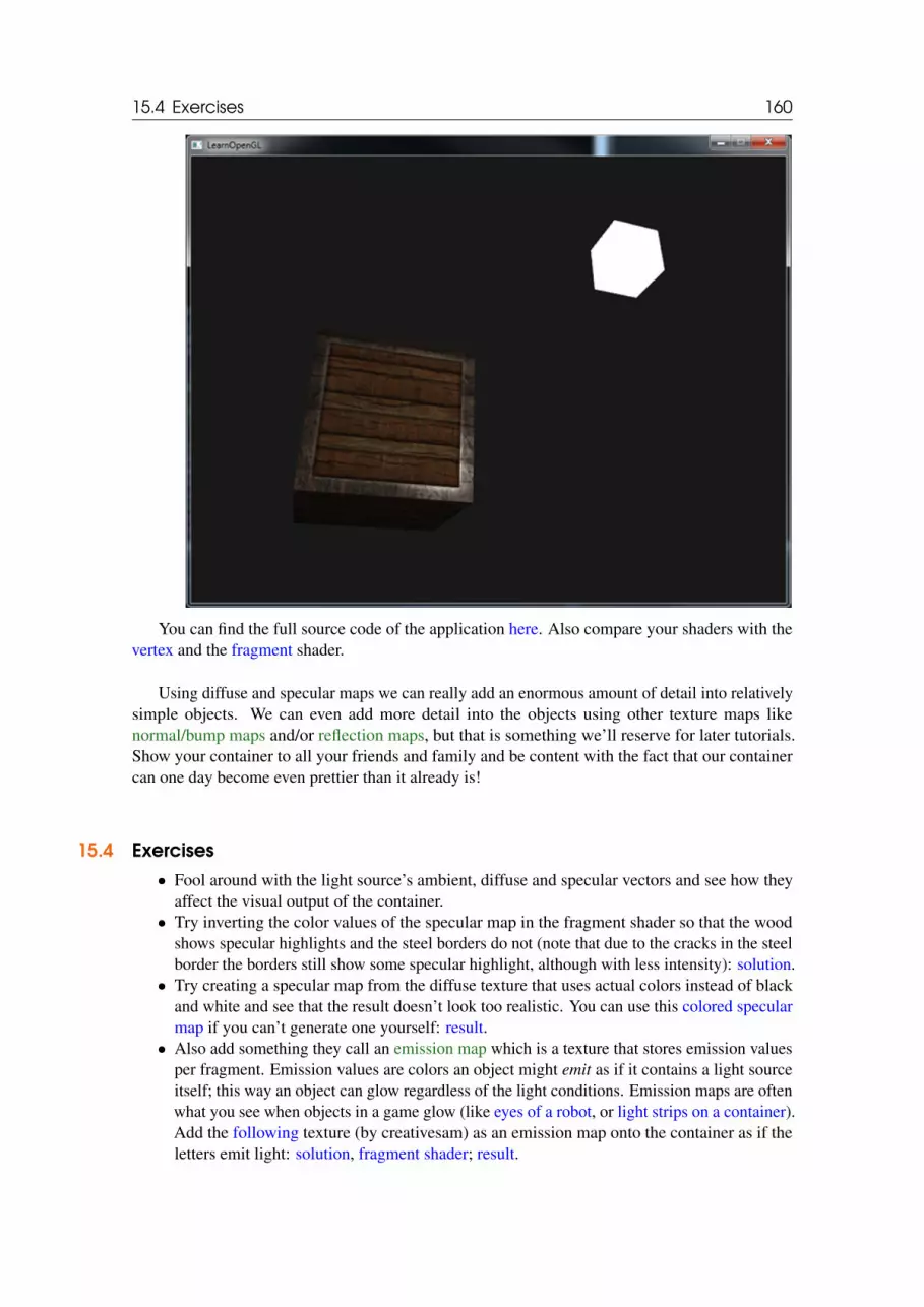
15.4 Exercises 160
You can find the full source code of the application here. Also compare your shaders with thevertex and the fragment shader.
Using diffuse and specular maps we can really add an enormous amount of detail into relativelysimple objects. We can even add more detail into the objects using other texture maps likenormal/bump maps and/or reflection maps, but that is something we’ll reserve for later tutorials.Show your container to all your friends and family and be content with the fact that our containercan one day become even prettier than it already is!
15.4 Exercises• Fool around with the light source’s ambient, diffuse and specular vectors and see how they
affect the visual output of the container.• Try inverting the color values of the specular map in the fragment shader so that the wood
shows specular highlights and the steel borders do not (note that due to the cracks in the steelborder the borders still show some specular highlight, although with less intensity): solution.• Try creating a specular map from the diffuse texture that uses actual colors instead of black
and white and see that the result doesn’t look too realistic. You can use this colored specularmap if you can’t generate one yourself: result.• Also add something they call an emission map which is a texture that stores emission values
per fragment. Emission values are colors an object might emit as if it contains a light sourceitself; this way an object can glow regardless of the light conditions. Emission maps are oftenwhat you see when objects in a game glow (like eyes of a robot, or light strips on a container).Add the following texture (by creativesam) as an emission map onto the container as if theletters emit light: solution, fragment shader; result.

16. Light casters
All the lighting we’ve used so far came from a single source that is a single point in space. It givesgood results, but in the real world we have several types of light that each act different. A lightsource that casts light upon objects is called a light caster. In this tutorial we’ll discuss severaldifferent types of light casters. Learning to simulate different light sources is yet another tool inyour toolbox to further enrich your environments.
We’ll first discuss a directional light, then a point light which is an extension of what wehad before and lastly we’ll discuss spotlights. In the next tutorial we’ll combine several of thesedifferent light types into one scene.
16.1 Directional LightWhen a light source is far away the light rays coming from the light source are close to parallel toeach other. It looks like all the light rays are coming from the same direction, regardless of wherethe object and/or the viewer is. When a light source is modeled to be infinitely far away it is calleda directional light since all its light rays have the same direction; it is independent of the location ofthe light source.
A fine example of a directional light source is the sun as we know it. The sun is not infinitelyfar away from us, but it is so far away that we can perceive it as being infinitely far away in thelighting calculations. All the light rays from the sun are then modelled as parallel light rays as wecan see in the following image:

16.1 Directional Light 162
Because all the light rays are parallel it does not matter how each object relates to the lightsource’s position since the light direction remains the same for each object in the scene. Becausethe light’s direction vector stays the same, the lighting calculations will be similar for each objectin the scene.
We can model such a directional light by defining a light direction vector instead of a positionvector. The shader calculations remain mostly the same except this time we directly use the light’sdirection vector instead of calculating the lightDir vector with the light’s positionvector:
struct Light {// vec3 position; // No longer necessery when using directional lights.vec3 direction;
vec3 ambient;vec3 diffuse;vec3 specular;
};...void main(){vec3 lightDir = normalize(-light.direction);...}
Note that we first negate the light.direction vector. The lighting calculations we usedso far expect the light direction to be a direction from the fragment towards the light source, butpeople generally prefer to specify a directional light as a global direction pointing from the lightsource. Therefore we have to negate the global light direction vector to switch its direction; it’s nowa direction vector pointing towards the light source. Also, be sure to normalize the vector since it isunwise to assume the input vector to be a unit vector.
The resulting lightDir vector is then used as before in the diffuse and specular computations.
To clearly demonstrate that a directional light has the same effect on all multiple objects we

16.1 Directional Light 163
revisit the container party scene from the end of the Coordinate systems tutorial. In case you missedthe party we first defined 10 different container positions and generated a different model matrixper container where each model matrix contained the appropriate local-to-world transformations:
for(GLuint i = 0; i < 10; i++){model = glm::mat4();model = glm::translate(model, cubePositions[i]);GLfloat angle = 20.0f * i;model = glm::rotate(model, angle, glm::vec3(1.0f, 0.3f, 0.5f));glUniformMatrix4fv(modelLoc, 1, GL_FALSE, glm::value_ptr(model));
glDrawArrays(GL_TRIANGLES, 0, 36);}
Also, don’t forget to actually specify the direction of the light source (note that we define thedirection as a direction from the light source; you can quickly see the light’s direction is pointingdownwards):
GLint lightDirPos = glGetUniformLocation(lightingShader.Program, "light.direction");
glUniform3f(lightDirPos, -0.2f, -1.0f, -0.3f);
We’ve been passing the light’s position and direction vectors as vec3s for a while now,but some people tend to prefer to keep all the vectors defined as vec4. When definingposition vectors as a vec4 it is important to set the w component to 1.0 so translationand projections are properly applied. However, when defining a direction vector as avec4 we don’t want translations to have an effect (since they just represent directions,nothing more) so then we define the w component to be 0.0.
Direction vectors are then represented like: vec4(0.2f, 1.0f, 0.3f, 0.0f).This can also function as an easy check for light types: you could check if the wcomponent is equal to 1.0 to see that we now have a light’s position vector and if w isequal to 0.0 we have a light’s direction vector so adjust the calculations based on that:
if(lightVector.w == 0.0) // Note: be careful for floating point errors// Do directional light calculationselse if(lightVector.w == 1.0)// Do light calculations using the light’s position (like last
tutorial)
Fun fact: this is actually how the old OpenGL (fixed-functionality) determined if a lightsource was a directional light or a positional light source and adjusted its lighting basedon that.
If you’d now compile the application and fly through the scene it looks like there is a sun-likelight source casting light on all the objects. Can you see that the diffuse and specular componentsall react as if there was a light source somewhere in the sky? It’ll look something like this:

16.2 Point lights 164
You can find the full source code of the application here together with the vertex and fragmentshader’s code.
16.2 Point lightsDirectional lights are great for global lights that illuminate the entire scene, but aside from adirectional light we usually also want several point lights scattered throughout the scene. A pointlight is a light source with a given position somewhere in a world that illuminates in all directionswhere the light rays fade out over distance. Think of light bulbs and torches as light casters that actas a point light.

16.3 Attenuation 165
In the earlier tutorials we’ve been working with a (simplistic) point light all along. We had alight source at a given position that scatters light in all directions from that given light position.However, the light source we defined simulated light rays that never fade out thus making it looklike the light source is extremely strong. In most 3D simulations we’d like to simulate a light sourcethat only illuminates a certain area close to the light source and not the entire scene.
If you’d add the 10 containers to the lighting scene of the previous tutorial you’d notice that thecontainer all the way in the back is lit with the same intensity as the container in front of the lamp;there is no formula defined that diminishes light over distance. We want the container in the backto only be slightly lit in comparison to the containers close to the light source.
16.3 AttenuationTo reduce the intensity of light, over the distance a light ray travels, is generally called attenuation.One way to reduce the light intensity over distance is to simply use a linear equation. Such anequation would linearly reduce the light intensity over the distance thus making sure that objects ata distance are less bright. However, such a linear function tends to look a bit fake. In the real world,lights are generally quite bright standing close by, but the brightness of a light source diminishesquickly at the start and the remaining light intensity more slowly diminishes over distance. We arethus in need of a different formula for reducing the light’s intensity.
Luckily some smart people already figured this out for us. The following formula divides thelight’s intensity of a fragment by a calculated attenuation value based on the distance to the lightsource:
F_att =I
K_c+K_l ∗d +K_q∗d2 (16.1)
Here I is the intensity of the light at the current fragment and d represents the distance fromthe fragment to the light source. Then to calculate the attenuation value we define 3 (configurable)terms: a constant term K_c, a linear term K_l and a quadratic term K_q.

16.3 Attenuation 166
• The constant term is usually kept at 1.0 which is mainly there to make sure the resultingdenominator never gets smaller than 1 since it would otherwise boost the intensity withcertain distances, which is not the effect we’re looking for.• The linear term is multiplied with the distance value that reduces the intensity in a linear
fashion.• The quadratic term is multiplied with the quadrant of the distance and sets a quadratic decrease
of intensity for the light source. The quadratic term will be less significant compared tothe linear term when the distance is small, but gets much larger than the linear term as thedistance grows.
Due to the quadratic term the light will diminish mostly at a linear fashion until the distancebecomes large enough for the quadratic term to surpass the linear term and then the light intensitywill decrease a lot faster. The resulting effect is that the light is quite intense when at a close range,but quickly loses it brightness over distance and eventually loses its brightness at a more slowerpace. The following graph shows the effect such an attenuation has over a distance of 100:
You can see that the light has the highest intensity when the distance is small, but as soon asthe distance grows its intensity is significantly reduced and slowly reaches 0 intensity at around adistance of 100. This is exactly what we want.
16.3.1 Choosing the right valuesBut at what values do we set those 3 terms? Setting the right values depends on many factors: theenvironment, the distance you want a light to cover, the type of light etc. In most cases, it simply isa question of experience and a moderate amount of tweaking. The following table shows some ofthe values these terms could take to simulate a realistic (sort of) light source that covers a specificradius (distance). The first column specifies the distance a light will cover with the given terms.These values are good starting points for most lights, with courtesy of Ogre3D’s wiki:

16.3 Attenuation 167
Distance Constant Linear Quadratic7 1.0 0.7 1.813 1.0 0.35 0.4420 1.0 0.22 0.2032 1.0 0.14 0.0750 1.0 0.09 0.03265 1.0 0.07 0.017100 1.0 0.045 0.0075160 1.0 0.027 0.0028200 1.0 0.022 0.0019325 1.0 0.014 0.0007600 1.0 0.007 0.00023250 1.0 0.0014 0.000007
As you can see, the constant term K_c is kept at 1.0 in all cases. The linear term K_l is usuallyquite small to cover larger distances and the quadratic term K_q is even smaller. Try to experimenta bit with these values to see their effect in your implementation. In our environment a distance of32 to 100 is generally enough for most lights.
16.3.2 Implementing attenuationTo implement attenuation we’ll be needing 3 extra values in the fragment shader: namely theconstant, linear and quadratic terms of the formula. These are best stored in the Light struct wedefined earlier. Note that we calculate lightDir as we did in the previous tutorial and not as inthe earlier Directional Light section.
struct Light {vec3 position;
vec3 ambient;vec3 diffuse;vec3 specular;
float constant;float linear;float quadratic;
};
Then we set the terms in OpenGL: we want the light to cover a distance of 50 so we’ll use theappropriate constant, linear and quadratic terms from the table:
glUniform1f(glGetUniformLocation(lightingShader.Program, "light.constant"),1.0f);
glUniform1f(glGetUniformLocation(lightingShader.Program, "light.linear"),0.09);
glUniform1f(glGetUniformLocation(lightingShader.Program, "light.quadratic"), 0.032);
Implementing attenuation in the fragment shader is relatively straightforward: we simplycalculate an attenuation value based on the formula and multiply this with the ambient, diffuse andspecular components.

16.3 Attenuation 168
We do need the distance to the light source for the formula to work though; remember how wecan calculate the length of a vector? We can retrieve the distance term by retrieving the differencevector between the fragment and the light source and take the resulting vector’s length. We can useGLSL’s built-in length function for that purpose:
float distance = length(light.position - Position);float attenuation = 1.0f / (light.constant + light.linear * distance +
light.quadratic * (distance * distance));
Then we include this attenuation value in the lighting calculations by multiplying the attenuationvalue with the ambient, diffuse and specular colors.
We could leave the ambient component alone so ambient lighting is not decreased overdistance, but if we were to use more than 1 light source all the ambient components willstart to stack up so in that case we want to attenuate ambient lighting as well. Simplyplay around with what’s best for your environment.
ambient *= attenuation;diffuse *= attenuation;specular *= attenuation;
If you’d run the application you’d get something like this:
You can see that right now only the front containers are lit with the closest container being thebrightest. The containers in the back are not lit at all since they’re too far from the light source.You can find the source code of the application here and the fragment’s code here.

16.4 Spotlight 169
A point light is thus a light source with a configurable location and attenuation applied to itslighting calculations. Yet another type of light for our lighting arsenal.
16.4 SpotlightThe last type of light we’re going to discuss is a spotlight. A spotlight is a light source that islocated somewhere in the environment that, instead of shooting light rays in all directions, onlyshoots them in a specific direction. The result is that only the objects within a certain radius of thespotlight’s direction are lit and everything else stays dark. A good example of a spotlight would bea street lamp or a flashlight.
A spotlight in OpenGL is represented by a world-space position, a direction and a cutoff anglethat specifies the radius of the spotlight. For each fragment we calculate if the fragment is betweenthe spotlight’s cutoff directions (thus in its cone) and if so, we lit the fragment accordingly. Thefollowing image gives you an idea of how a spotlight works:
• LightDir: the vector pointing from the fragment to the light source.• SpotDir: the direction the spotlight is aiming at.• Phi φ : the cutoff angle that specifies the spotlight’s radius. Everything outside this angle is
not lit by the spotlight.• Theta θ : the angle between the LightDir vector and the SpotDir vector. The θ value
should be smaller than the Φ value to be inside the spotlight.
So what we basically need to do, is calculate the dot product (returns the cosine of the anglebetween two unit vectors remember?) between the LightDir vector and the SpotDir vectorand compare this with the cutoff angle φ . Now that you (sort of) understand what a spotlight is allabout we’re going to create one in the form of a flashlight.
16.5 FlashlightA flashlight is a spotlight located at the viewer’s position and usually aimed straight ahead from theplayer’s perspective. Basically a flashlight is a normal spotlight, but with its position and direction

16.5 Flashlight 170
continually updated based on the player’s position and orientation.
So, the values we’re going to need for the fragment shader are the spotlight’s position vector (tocalculate the light’s direction vector), the spotlight’s direction vector and the cutoff angle. We canstore these values in the Light struct:
struct Light {vec3 position;vec3 direction;float cutOff;...
};
Next we pass the appropriate values to the shaders:
glUniform3f(lightPosLoc, camera.Position.x, camera.Position.y,camera.Position.z);
glUniform3f(lightSpotdirLoc, camera.Front.x, camera.Front.y, camera.Front.z);
glUniform1f(lightSpotCutOffLoc, glm::cos(glm::radians(12.5f)));
As you can see we’re not setting an angle for the cutoff value but calculate the cosine valuebased on an angle and pass the cosine result to the fragment shader. The reason for this is that inthe fragment shader we’re calculating the dot product between the LightDir and the SpotDirvector and the dot product returns a cosine value and not an angle so we can’t directly compare anangle with a cosine value. To retrieve the angle we then have to calculate the inverse cosine of thedot product’s result which is an expensive operation. So to save some performance we calculate thecosine value of a given cutoff angle and pass this result to the fragment shader. Since both anglesare now represented as cosines, we can directly compare between them without any expensiveoperations.
Now what’s left to do is calculate the theta θ value and compare this with the cutoff φ value todetermine if we’re in or outside the spotlight:
float theta = dot(lightDir, normalize(-light.direction));
if(theta > light.cutOff){// Do lighting calculations}else // else, use ambient light so scene isn’t completely dark outside the
spotlight.color = vec4(light.ambient * vec3(texture(material.diffuse, TexCoords)),
1.0f);
We first calculate the dot product between the lightDir vector and the negated directionvector (negated, because we want the vectors to point towards the light source, instead of from). Besure to normalize all the relevant vectors.

16.5 Flashlight 171
You might be wondering why there is a > sign instead of a < sign in the if guard.Shouldn’t theta be smaller than the light’s cutoff value to be inside the spotlight? Thatis right, but don’t forget angle values are represented as cosine values and an angle of 0is represented as the cosine value of 1.0 while an angle of 90 degrees is represented asthe cosine value of 0.0 as you can see here:
You can now see that the closer the cosine value is to 1.0 the smaller its angle. Now itmakes sense why theta needs to be larger than the cutoff value. The cutoff value iscurrently set at the cosine of 12.5 which is equal to 0.9978 so a cosine theta valuebetween 0.9979 and 1.0 would result in the fragment being lit as inside the spotlight.
Running the application results in a spotlight that only lights the fragments that are directlyinside the cone of the spotlight. It’ll look something like this:

16.6 Smooth/Soft edges 172
You can find the full source code here and the fragment shader’s source code here.
It still looks a bit fake though, mostly because the spotlight has hard edges. Wherever a fragmentreaches the edge of the spotlight’s cone it is shut down completely instead of with a nice smoothfade. A realistic spotlight would reduce the light gradually around its edges.
16.6 Smooth/Soft edgesTo create the effect of a smoothly-edged spotlight we want to simulate a spotlight having an innerand an outer cone. We can set the inner cone as the cone defined in the previous section, but wealso want an outer cone that gradually dims the light from the inner to the edges of the outer cone.
To create an outer cone we simply define another cosine value that represents the angle betweenthe spotlight’s direction vector and the outer cone’s vector (equal to its radius). Then, if a fragmentis between the inner and the outer cone it should calculate an intensity value between 0.0 and1.0. If the fragment is inside the inner cone its intensity is equal to 1.0 and 0.0 if the fragmentis outside the outer cone.
We can calculate such a value using the following formula:
I =θ − γ
ε(16.2)
Here ε (epsilon) is the cosine difference between the inner (φ ) and the outer cone (γ) (ε = φ−γ).The resulting I value is then the intensity of the spotlight at the current fragment.

16.6 Smooth/Soft edges 173
It is a bit hard to visualize how this formula actually works so let’s try it out with a few samplevalues:
θ
θ inde-
grees
φ
(innercut-off)
φ inde-
grees
γ
(outercut-off)
γ inde-
greesε I
0.87 30 0.91 25 0.82 350.91 - 0.82
= 0.090.87 - 0.82 /0.09 = 0.56
0.9 26 0.91 25 0.82 350.91 - 0.82
= 0.090.9 - 0.82 /0.09 = 0.89
0.97 14 0.91 25 0.82 350.91 - 0.82
= 0.090.97 - 0.82 /0.09 = 1.67
0.97 14 0.91 25 0.82 350.91 - 0.82
= 0.090.97 - 0.82 /0.09 = 1.67
0.83 34 0.91 25 0.82 350.91 - 0.82
= 0.090.83 - 0.82 /0.09 = 0.11
0.64 50 0.91 25 0.82 350.91 - 0.82
= 0.090.64 - 0.82 /0.09 = -2.0
0.966 15 0.9978 12.5 0.953 17.50.966 -0.953 =0.0448
0.966 -0.953 /0.0448 =0.29
As you can see we’re basically interpolating between the outer cosine and the inner cosinebased on the θ value. If you still don’t really see what’s going on, don’t worry, you can simply takethe formula for granted and return here when you’re much older and wiser.
Since we now have an intensity value that is either negative when outside the spotlight, higherthan 1.0 when inside the inner cone and somewhere in between around the edges. If we properlyclamp the values we don’t need an if-else in the fragment shader anymore and we can simplymultiply the light components with the calculated intensity value:
float theta = dot(lightDir, normalize(-light.direction));float epsilon = light.cutOff - light.outerCutOff;float intensity = clamp((theta - light.outerCutOff) / epsilon, 0.0, 1.0);...// We’ll leave ambient unaffected so we always have a little light.diffuse *= intensity;specular *= intensity;...
Note that we use the clamp function that clamps its first argument between the values 0.0and 1.0. This makes sure the intensity values won’t end up outside the [0, 1] interval.
Make sure you add the outerCutOff value to the Light struct and set its uniform value inthe application. For the following image an inner cutoff angle of 12.5f and an outer cutoff angleof 17.5f was used:

16.7 Exercises 174
Ahhh, that’s much better. Play around with the inner and outer cutoff angles and try to create aspotlight that better suits your needs. You can find the source code of the application here and thefragment’s source code here.
Such a flashlight/spotlight type of lamp is perfect for horror games and combined with direc-tional and point lights the environment will really start to light up. In the next tutorial we’ll combineall the lights and tricks we’ve discussed so far.
16.7 Exercises• Try experimenting with all the different light types and their fragment shaders. Try inverting
some vectors and/or using < instead of >. Try to explain the different visual outcomes.

17. Multiple lights
In the previous tutorials we learned quite a lot about lighting in OpenGL. We learned about Phongshading, materials, lighting maps and different types of light casters. In this tutorial we’re goingto combine all the previously obtained knowledge by creating a fully lit scene with 6 active lightsources. We are going to simulate a sun-like light as a directional light source, 4 point lightsscattered throughout the scene and we’ll be adding a flashlight as well.
To use more than one light source in the scene we want to encapsulate the lighting calculationsinto GLSL functions. The reason for that is that the code quickly gets nasty when we want to dolighting computations with multiple lights with each light type requiring different computations. Ifwe were to do all these calculations in the main function only, the code quickly becomes difficultto understand.
Functions in GLSL are just like C-functions. We have a function name, a return type and we’dhave to declare a prototype at the top of the code file if the function hasn’t been declared before themain function yet. We’ll create a different function for each of the light types: directional lights,point lights and spotlights.
When using multiple lights in a scene the approach is usually as follows: we have a single colorvector that represents the fragment’s output color. For each light, the light’s contribution color ofthe fragment is added to the fragment’s output color vector. So each light in the scene will calculateits individual impact on the aforementioned fragment and contribute to the final output color. Ageneral structure would look something like this:
out vec4 color;
void main(){// define an output color valuevec3 output;

17.1 Directional light 176
// add the directional light’s contribution to the outputoutput += someFunctionToCalculateDirectionalLight();// Do the same for all point lightsfor(int i = 0; i < nr_of_point_lights; i++)
output += someFunctionToCalculatePointLight();// And add others lights as well (like spotlights)output += someFunctionToCalculateSpotLight();
color = vec4(output, 1.0);}
The actual code will likely differ per implementation, but the general structure remains thesame. We define several functions that calculate the impact per light source and add its resultingcolor to an output color vector. If for example two light sources are close to the fragment, theircombined contribution would result in a more brightly lit fragment than the fragment being lit by asingle light source.
17.1 Directional lightWhat we want to do is define a function in the fragment shader that calculates the contribution adirectional light has on the corresponding fragment: a function that takes a few parameters andreturns the calculated directional lighting color.
First we need to set the required variables that we minimally need for a directional light source.We can store the variables in a struct called DirLight and define it as a uniform. The requiredvariables should be familiar from the previous tutorial:
struct DirLight {vec3 direction;
vec3 ambient;vec3 diffuse;vec3 specular;
};uniform DirLight dirLight;
We can then pass the dirLight uniform to a function with the following prototype:
vec3 CalcDirLight(DirLight light, vec3 normal, vec3 viewDir);
Just like C and C++ if we want to call a function (in this case inside the main function)the function should be defined somewhere before the caller’s line number. In thiscase we’d prefer to define the functions below the main function so this requirementdoesn’t hold. Therefore we declare the function’s prototypes somewhere above themain function, just like we would in C.
You can see that the function requires a DirLight struct and two other vectors required for itscomputation. If you successfully completed the previous tutorial then the content of this functionshould come as no surprise:

17.2 Point light 177
vec3 CalcDirLight(DirLight light, vec3 normal, vec3 viewDir){
vec3 lightDir = normalize(-light.direction);// Diffuse shadingfloat diff = max(dot(normal, lightDir), 0.0);// Specular shadingvec3 reflectDir = reflect(-lightDir, normal);float spec = pow(max(dot(viewDir, reflectDir), 0.0), material.shininess);// Combine resultsvec3 ambient = light.ambient * vec3(texture(material.diffuse, TexCoords));vec3 diffuse = light.diffuse * diff * vec3(texture(material.diffuse,TexCoords));vec3 specular = light.specular * spec * vec3(texture(material.specular,TexCoords));return (ambient + diffuse + specular);
}
We basically copied the code from the previous tutorial and used the vectors given as functionarguments to calculate the directional light’s contribution vector. The resulting ambient, diffuse andspecular contributions are then returned as a single color vector.
17.2 Point lightJust like with directional lights we also want to define a function that calculates the contribution apoint light has on the given fragment, including its attenuation. Just like directional lights we wantto define a struct that specifies all the variables required for a point light:
struct PointLight {vec3 position;
float constant;float linear;float quadratic;
vec3 ambient;vec3 diffuse;vec3 specular;
};#define NR_POINT_LIGHTS 4uniform PointLight pointLights[NR_POINT_LIGHTS];
As you can see we used a pre-processor directive in GLSL to define the number of point lightswe want to have in our scene. We then use this NR_POINT_LIGHTS constant to create an arrayof PointLight structs. Arrays in GLSL are just like C arrays and can be created by the use oftwo square brackets. Right now we have 4 PointLight structs to fill with data.
We could also simply define one large struct (instead of different structs per light type)that contains all the necessary variables for all the different light types and use that structfor each function, and simply ignore the variables we don’t need. However, I personallyfind the current approach more intuitive and aside from a few extra lines of code it couldsave up some memory since not all light types need all variables.

17.3 Putting it all together 178
The prototype of the point light’s function is as follows:
vec3 CalcPointLight(PointLight light, vec3 normal, vec3 fragPos, vec3viewDir);
The function takes all the data it needs as its arguments and returns a vec3 that representsthe color contribution that this specific point light has on the fragment. Again, some intelligentcopy-and-pasting results in the following function:
// Calculates the color when using a point light.vec3 CalcPointLight(PointLight light, vec3 normal, vec3 fragPos, vec3
viewDir){
vec3 lightDir = normalize(light.position - fragPos);// Diffuse shadingfloat diff = max(dot(normal, lightDir), 0.0);// Specular shadingvec3 reflectDir = reflect(-lightDir, normal);float spec = pow(max(dot(viewDir, reflectDir), 0.0), material.shininess);// Attenuationfloat distance = length(light.position - fragPos);float attenuation = 1.0f / (light.constant + light.linear * distance +
light.quadratic * (distance * distance));// Combine resultsvec3 ambient = light.ambient * vec3(texture(material.diffuse, TexCoords));vec3 diffuse = light.diffuse * diff * vec3(texture(material.diffuse,TexCoords));vec3 specular = light.specular * spec * vec3(texture(material.specular,TexCoords));ambient *= attenuation;diffuse *= attenuation;specular *= attenuation;return (ambient + diffuse + specular);
}
Abstracting this functionality away in a function like this has the advantage that we caneasily calculate the lighting for multiple point lights without the need for nasty duplicated code.In the main function we simply create a loop that iterates over the point light array that callsCalcPointLight for each point light.
17.3 Putting it all togetherNow that we defined both a function for directional lights and a function for point lights we can putit all together in the main function.
void main(){
// Propertiesvec3 norm = normalize(Normal);vec3 viewDir = normalize(viewPos - FragPos);
// Phase 1: Directional lightingvec3 result = CalcDirLight(dirLight, norm, viewDir);

17.3 Putting it all together 179
// Phase 2: Point lightsfor(int i = 0; i < NR_POINT_LIGHTS; i++)
result += CalcPointLight(pointLights[i], norm, FragPos, viewDir);// Phase 3: Spot light//result += CalcSpotLight(spotLight, norm, FragPos, viewDir);
color = vec4(result, 1.0);}
Each light type adds its contribution to the resulting output color until all light sources areprocessed. The resulting color contains the color impact of all the light sources in the scenecombined. If you want you could also implement a spotlight and add its effect to the output coloras well. We leave the CalcSpotLight function as an exercise for the reader.
Setting the uniforms for the directional light struct shouldn’t be too unfamiliar, but you mightbe wondering how we could set the uniform values of the point lights since the point light uniformis now an array of PointLight structs. This isn’t something we’ve discussed before.
Luckily for us, it isn’t too complicated. To set the uniform of an array of structs works just likesetting the uniforms of a single struct, although this time we also have to define the appropriateindex when retrieving the uniform’s location:
glUniform1f(glGetUniformLocation(lightingShader.Program, "pointLights[0].constant"), 1.0f);
Here we index the first PointLight struct in the pointLights array and retrieve thelocation of its constant variable. This does mean unfortunately that we have to manually set allthe uniforms for each of the 4 point lights, which leads up to 28 uniform calls for the point lightsalone which is a bit tedious. You could try to abstract a bit away from this by defining a point lightclass that sets the uniforms for you, but in the end you’d still have to set the all the lights’ uniformvalues this way.
Let’s not forget that we also need to define a position vector for each of the point lights so let’sspread them up a bit around the scene. We’ll define another glm::vec3 array that contains thepointlights’ positions:
glm::vec3 pointLightPositions[] = {glm::vec3( 0.7f, 0.2f, 2.0f),glm::vec3( 2.3f, -3.3f, -4.0f),glm::vec3(-4.0f, 2.0f, -12.0f),glm::vec3( 0.0f, 0.0f, -3.0f)
};
Then index the corresponding PointLight struct from the pointLights array and setits position attribute as one of the positions we just defined. Also be sure to now draw 4 lightcubes instead of just 1. Simply create a different model matrix for each of the light objects just likewe did with the containers.
If you’d also use a flashlight the result of all the combined lights looks something like this:

17.3 Putting it all together 180
As you can see there appears to be some form of a global light (like a sun) somewhere in thesky, we have 4 lights scattered throughout the scene and a flashlight is visible from the player’sperspective. Looks pretty neat doesn’t it?
You can find the full source code of the final application here together with the vertex andfragment shader’s source code here.
The image shows all the light sources set with the default light properties we’ve used in all theprevious tutorials, but if you’d play around with these values you can get pretty interesting results.Artists and level editors generally tweak all these lighting variables in a large editor to make surethe lighting matches the environment. Using the simple lighted environment we just created youcan create some interesting visuals by simply tweaking the lights their attributes:

17.4 Exercises 181
We also changed the clear color to better reflect the lighting. You can see that by simplyadjusting some of the lighting parameters you can create completely different atmospheres.
By now you should have a pretty good understanding of lighting in OpenGL. With the knowl-edge so far we can already create interesting and visually rich environments and atmospheres. Tryplaying around with all the different values to create your own atmospheres.
17.4 Exercises• Create a struct for a spotlight, implement the CalcSpotLight(...) function and set the
appropriate uniform values in your application: solution.• Can you (sort of) re-create the different atmospheres of the last image by tweaking the light’s
attribute values? solution.

18. Review
Congratulations on making it this far! I’m not sure if you noticed, but over all the lighting tutorialswe basically learned nothing new about OpenGL itself except a few minor items like accessinguniform arrays. All of the tutorials so far were all about manipulating shaders using techniquesand formulas to achieve realistic lighting results. This again shows you the power of shaders.Shaders are extremely flexible and you witnessed firsthand that with just a few 3D vectors andsome configurable variables we were able to create amazing graphics with just that!
The last few tutorials you learned about colors, the Phong lighting model (that includes ambient,diffuse and specular lighting), object materials, configurable light properties, diffuse and specularmaps, different types of lights and how to combine all the knowledge into a single application. Besure to experiment with different lights, material colors, light properties and try to create your ownenvironments with the help of a little bit of creativity.
In the next tutorials we’ll be adding more advanced shapes to our scene that look really well inthe lighting models we’ve discussed.
18.1 Glossary• Color vector: a vector portraying most of the real world colors via a combination of
red, green and blue components (abbreviated to RGB). The color of an object is actually thereflected color components that an object did not absorb.• Phong lighting model: a model for approximating real-world lighting by computing
an ambient, diffuse and specular component.• Ambient lighting: approximation of global illumination by giving each object a small
brightness so that objects aren’t completely dark if not lit.• Diffuse shading: lighting that gets stronger the more a vertex/fragment is aligned to a
light source. Makes use of normal vectors to calculate the angles.• Normal vector: a (unit) vector that is perpendicular to a surface.

18.1 Glossary 183
• Normal matrix: a 3x3 matrix that is the model (or model-view) matrix without transla-tion. It is also modified in such a way (inverse-transpose) that it keeps normal vectors facingin the correct direction when applying non-uniform scaling. Otherwise normal vectors getdistorted when using non-uniform scaling.• Specular lighting: sets a specular highlight the closer the viewer is looking at the
reflection of a light source on a surface. Based on the viewer’s direction, the light’s directionand a shininess value that sets the amount of scattering of the highlight.• Phong shading: the Phong lighting model applied in the fragment shader.• Gouraud shading: the Phong lighting model applied in the vertex shader. Produces
noticeable artifacts when using a small number of vertices. Gains efficiency for loss of visualquality.• GLSL struct: a C-like struct that acts as a container for shader variables. Mostly used for
organizing input/output/uniforms.• Material: the ambient, diffuse and specular color an object reflects. These set the colors
an object has.• Light (properties): the ambient, diffuse and specular intensity of a light. These can
take any color value and define at what color/intensity a light source shines for each specificPhong component.• Diffuse map: a texture image that sets the diffuse color per fragment.• Specular map: a texture map that sets the specular intensity/color per fragment. Allows
for specular highlights only on certain areas of an object.• Directional light: a light source with only a direction. It is modeled to be at an
infinite distance which has the effect that all its light rays seem parallel and its directionvector thus stays the same over the entire scene.• Point light: a light source with a location in a scene with light that fades out over
distance.• Attenuation: the process of light reducing its intensity over distance, used in point lights
and spotlights.• Spotlight: a light source that is defined by a cone in one specific direction.• Flashlight: a spotlight positioned from the viewer’s perspective.• GLSL uniform array: an array of uniform values. Work just like a C-array, except that
they can’t be dynamically allocated.

III
19 Assimp . . . . . . . . . . . . . . . . . . . . . . . . . . . . . 185
20 Mesh . . . . . . . . . . . . . . . . . . . . . . . . . . . . . . 189
21 Model . . . . . . . . . . . . . . . . . . . . . . . . . . . . . 194
Model Loading

19. Assimp
In all the scenes so far we’ve been extensively abusing our little container friend in many ways,but over time even our best friends could get a little boring. In practical graphics applicationsthere are usually lots of complicated and interesting models that are much prettier to look at thana static container. However, unlike the container object, we can’t really manually define all thevertices, normals and texture coordinates of complicated shapes like houses, vehicles or human-likecharacters. What we want instead is to import these models into the application; models that werecarefully designed by 3D artists in tools like Blender, 3DS Max or Maya.
These so called 3D modeling tools allow artists to create complicated shapes and apply texturesto them via a process called uv-mapping. The tools then automatically generate all the vertexcoordinates, vertex normals and texture coordinates while exporting them to a model file format.This way, artists have an extensive toolkit to create high quality models without having to care toomuch about the technical details. All the technical aspects are hidden in the exported model file.We, as graphics programmers, do have to care about these technical details though.
It is thus our job to parse these exported model files and extract all the relevant information sowe can store them in a format that OpenGL understands. A common issue is however that there aredozens of different file formats where each exports the model data in its own unique way. Modelformats like the Wavefront .obj only contains model data with minor material information likemodel colors and diffuse/specular maps, while model formats like the XML-based Collada fileformat are extremely extensive and contain models, lights, many types of materials, animation data,cameras, complete scene information and much more. The wavefront object format is generallyconsidered to be an easy-to-parse model format. It is recommended to visit the Wavefront’s wikipage at least once to see how such a file format’s data is structured. This should give you a basicperception of how model file formats are generally structured.
All by all, there are many different file formats where a common general structure betweenthem usually does not exist. So if we want to import a model from these file formats we’d have to

19.1 A model loading library 186
write an importer ourselves for each of the file formats we want to import. Luckily for us, there justhappens to be a library for this.
19.1 A model loading libraryA very popular model importing library out there is called Assimp that stands for Open Asset ImportLibrary. Assimp is able to import dozens of different model file formats (and export to some aswell) by loading all the model’s data into Assimp’s generalized data structures. As soon as Assimphas loaded the model, we can retrieve all the data we need from Assimp’s data structures. Becausethe data structure of Assimp stays the same, regardless of the type of file format we imported, itabstracts us from all the different file formats out there.
When importing a model via Assimp it loads the entire model into a scene object that containsall the data of the imported model/scene. Assimp then has a collection of nodes where each nodecontains indices to data stored in the scene object where each node can have any number of children.A (simplistic) model of Assimp’s structure is shown below:
• All the data of the scene/model is contained in the Scene object like all the materials and themeshes. It also contains a reference to the root node of the scene.• The Root node of the scene may contain children nodes (like all other nodes) and could have
a set of indices that point to mesh data in the scene object’s mMeshes array. The root node’smMeshes array contains the actual Mesh objects, the values in the mMeshes array of anode are only indices for the scene’s meshes array.• A Mesh object itself contains all the relevant data required for rendering, think of vertex
positions, normal vectors, texture coordinates, faces and the material of the object.• A mesh contains several faces. A Face represents a render primitive of the object (triangles,
squares, points). A face contains the indices of the vertices that form a primitive. Becausethe vertices and the indices are separated, this makes it easy for us to render via an indexbuffer (see Hello Triangle).• Finally a mesh also contains a Material object that hosts several functions to retrieve the
material properties of an object. Think of colors and/or texture maps (like diffuse and specular

19.2 Building Assimp 187
maps).
So what we want to do is first load an object into a Scene object, recursively retrieve thecorresponding Mesh objects from each of the nodes (we recursively search each node’s children)and process each Mesh object to retrieve the vertex data, indices and its material properties. Theresult is then a collection of mesh data that we want to contain in a single Model object.
MeshWhen modelling objects in modelling toolkits, artists generally do not create an entiremodel out of a single shape. Usually each model has several sub-models/shapes that itconsists of. Each of those single shapes that a model is composed of is called a mesh.Think of a human-like character: artists usually model the head, limbs, clothes, weaponsall as separate components and the combined result of all these meshes represents thefinal model. A single mesh is the minimal representation of what we need to draw anobject in OpenGL (vertex data, indices and material properties). A model (usually)consists of several meshes.
In the next tutorials we’ll create our own Model and Mesh class that load and store theimported models using the structure we’ve just described. If we then want to draw a model wedo not render the model as a whole but we render all of the individual meshes that the model iscomposed of. However, before we can start importing models we first need to actually includeAssimp in our project.
19.2 Building AssimpYou can download Assimp from their download page and choose the corresponding version. Asof this writing the newest Assimp version used was version 3.1.1. It is advised to compile thelibraries by yourself, since their pre-compiled libraries aren’t working on most systems. Reviewthe Creating a window tutorial if you forgot how to compile a library by yourself via CMake.
A few issues came up though while building Assimp so I’ll note them down here with theirsolutions in case any of you get the same errors:• CMake continually gave errors while retrieving the configuration list about DirectX libraries
missing, messages like:
Could not locate DirectXCMake Error at cmake-modules/FindPkgMacros.cmake:110 (message):Required library DirectX not found! Install the library (including dev
packages)and try again. If the library is already installed, set the missing
variablesmanually in cmake.
The solution here is to install the DirectX SDK in case you haven’t installed this before. Youcan download the SDK from here.• While installing the DirectX SDK a possible error code of s1023 could pop up. In that case
you first want to de-install the C++ Redistributable package(s) before installing the SDK asexplained here.• Once the configuration is completed you can generate a solution file, open it and compile the
libraries (either as a release version or a debug version, whatever floats your boat).

19.2 Building Assimp 188
• The default configuration builds Assimp as a dynamic library so we need to include theresulting DLL named assimp.dll alongside the application’s binaries. You can simplycopy the DLL to the same folder where your application’s executable is located.• After compilation of Assimp the resulting library and DLL file are located in the code/Debug
or code/Release folder.• Then simply move the lib and DLL to their appropriate locations, link them from your
solution and be sure not to forget to copy Assimp’s headers to your include directory aswell (the header files are found in the include folder in the files downloaded from Assimp).
If you still received any unreported error, feel free to ask for help in the comments below.
If you want Assimp to use multi-threading for faster performance you could compileAssimp with Boost. You can find the full installation instructions at their installationpage.
By now you should have compiled Assimp and linked it to your application. Next step:importing fancy 3D stuff!

20. Mesh
Using Assimp we can load many different models into the application, but once loaded they’re allstored in Assimp’s data structures. What we eventually want is transform that data to a format thatOpenGL understands so that we can render the objects. We learned from the previous tutorial that amesh represents a single drawable entity so let’s start by defining a mesh class of our own.
Let’s review a bit of what we’ve learned so far to think about what a mesh should minimallyhave as its data. A mesh should at least need a set of vertices where each vertex contains a positionvector, a normal vector and a texture coordinate vector. A mesh should also contain indices forindexed drawing and material data in the form of textures (diffuse/specular maps).
Now that we set the minimal requirements for a mesh class we can define a vertex in OpenGL:
struct Vertex {glm::vec3 Position;glm::vec3 Normal;glm::vec2 TexCoords;
};
We store each of the required vectors in a struct called Vertex that we can use to index eachof the vertex attributes. Aside from a Vertex struct we also want to organize the texture data in aTexture struct:
struct Texture {GLuint id;string type;
};
We store the id of the texture and its type e.g. a diffuse texture or a specular texture.
Knowing the actual representation of a vertex and a texture we can start defining the structure

20.1 Initialization 190
of the mesh class:
class Mesh {public:
/* Mesh Data */vector<Vertex> vertices;vector<GLuint> indices;vector<Texture> textures;/* Functions */Mesh(vector<Vertex> vertices, vector<GLuint> indices, vector<
Texture> textures);void Draw(Shader shader);
private:/* Render data */GLuint VAO, VBO, EBO;/* Functions */void setupMesh();
};
As you can see the class isn’t too complicated. In the constructor we give the mesh all thenecessary data, we initialize the buffers in the setupMesh function and finally draw the mesh viathe Draw function. Note that we give a shader to the Draw function; by passing the shader to themesh we can set several uniforms before drawing (like linking samplers to texture units).
The function content of the constructor is pretty straightforward. We simply set the class’s publicvariables with the constructor’s corresponding argument variables. We also call the setupMeshfunction in the constructor:
Mesh(vector<Vertex> vertices, vector<GLuint> indices, vector<Texture>textures)
{this->vertices = vertices;this->indices = indices;this->textures = textures;
this->setupMesh();}
Nothing special going on here. Let’s delve right into the setupMesh function now.
20.1 InitializationThanks to the constructor we now have large lists of mesh data that we can use for rendering. Wedo need to setup the appropriate buffers though and specify the vertex shader layout via vertexattribute pointers. By now you should have no trouble with these concepts, but we’ve spiced it up abit this time with the introduction of vertex data in structs:
void setupMesh(){
glGenVertexArrays(1, &this->VAO);glGenBuffers(1, &this->VBO);glGenBuffers(1, &this->EBO);
glBindVertexArray(this->VAO);

20.1 Initialization 191
glBindBuffer(GL_ARRAY_BUFFER, this->VBO);
glBufferData(GL_ARRAY_BUFFER, this->vertices.size() * sizeof(Vertex),&this->vertices[0], GL_STATIC_DRAW);
glBindBuffer(GL_ELEMENT_ARRAY_BUFFER, this->EBO);glBufferData(GL_ELEMENT_ARRAY_BUFFER, this->indices.size() * sizeof(GLuint),
&this->indices[0], GL_STATIC_DRAW);
// Vertex PositionsglEnableVertexAttribArray(0);glVertexAttribPointer(0, 3, GL_FLOAT, GL_FALSE, sizeof(Vertex),
(GLvoid*)0);// Vertex NormalsglEnableVertexAttribArray(1);glVertexAttribPointer(1, 3, GL_FLOAT, GL_FALSE, sizeof(Vertex),
(GLvoid*)offsetof(Vertex, Normal));// Vertex Texture CoordsglEnableVertexAttribArray(2);glVertexAttribPointer(2, 2, GL_FLOAT, GL_FALSE, sizeof(Vertex),
(GLvoid*)offsetof(Vertex, TexCoords));
glBindVertexArray(0);}
The code is not much different than what you’d expect, but a few little tricks were used withthe help of the Vertex struct.
Structs have a great property in C++ that their memory layout is sequential. That is if we wereto represent a struct as an array of data it would only contain the struct’s variables in sequentialorder which directly translates to a float (actually byte) array that we want for an array buffer. Forexample, if we have a filled Vertex struct its memory layout would be equal to:
Vertex vertex;vertex.Position = glm::vec3(0.2f, 0.4f, 0.6f);vertex.Normal = glm::vec3(0.0f, 1.0f, 0.0f);vertex.TexCoords = glm::vec2(1.0f, 0.0f);// = [0.2f, 0.4f, 0.6f, 0.0f, 1.0f, 0.0f, 1.0f, 0.0f];
Thanks to this useful property we can directly pass a pointer to a large list of Vertex structsas the buffer’s data and they translate perfectly to what glBufferData expects as its argument:
glBufferData(GL_ARRAY_BUFFER, this->vertices.size() * sizeof(Vertex),&this->vertices[0], GL_STATIC_DRAW);
Naturally the sizeof operator can also be used on the struct for the appropriate size in bytes.This should be 32 bytes (8 floats * 4 bytes each).
Another great use of structs is a preprocessor directive called offsetof(s,m) that takesas its first argument a struct and as its second argument a variable name of the struct. The macroreturns the byte offset of that variable from the start of the struct. This is perfect for defining theoffset parameter of the glVertexAttribPointer function:
glVertexAttribPointer(1, 3, GL_FLOAT, GL_FALSE, sizeof(Vertex),

20.2 Rendering 192
(GLvoid*)offsetof(Vertex, Normal));
The offset is now defined using the offsetof macro that, in this case, sets the byte offset ofthe normal vector equal to the byte offset of the normal vector in the struct which is 3 floats andthus 12 bytes. Note that we also set the stride parameter equal to the size of the Vertex struct.
Using a struct like this does not only provide more readable code but also allows us to easilyextend the structure. If we want another vertex attribute we can simply add it to the struct and dueto its flexible nature, the rendering code won’t break.
20.2 RenderingThe last function we need to define for the Mesh class to be complete is its Draw function. Beforeactually rendering the mesh though we first want to bind the appropriate textures before callingglDrawElements. However, this is actually slightly difficult since we don’t know from the starthow many (if any) textures the mesh has and what type they might have. So how do we set thetexture units and samplers in the shaders?
To solve the issue we’re going to assume a certain naming convention: each diffuse texture isnamed texture_diffuseN and each specular texture should be named texture_specularNwhere N is any number ranging from 1 to the maximum number of texture samplers allowed. Let’ssay we have 3 diffuse textures and 2 specular textures for a particular mesh, their texture samplersshould then be called:
uniform sampler2D texture_diffuse1;uniform sampler2D texture_diffuse2;uniform sampler2D texture_diffuse3;uniform sampler2D texture_specular1;uniform sampler2D texture_specular2;
By this convention we can define as many texture samplers as we want in the shaders and if amesh actually does contain (so many) textures we know what their names are going to be. By thisconvention we can process any amount of textures on a single mesh and the developer is free to useas many of those as he wants by simply defining the proper samplers (although defining less wouldbe a bit of a waste of bind and uniform calls).
There are many solutions to problems like this and if you don’t like this particularsolution it is up to you to get creative and come up with your own solution.
The resulting drawing code then becomes:
void Draw(Shader shader){
GLuint diffuseNr = 1;GLuint specularNr = 1;for(GLuint i = 0; i < this->textures.size(); i++){
glActiveTexture(GL_TEXTURE0 + i); // Activate proper texture unitbefore binding
// Retrieve texture number (the N in diffuse_textureN)

20.2 Rendering 193
stringstream ss;string number;string name = this->textures[i].type;if(name == "texture_diffuse")
ss << diffuseNr++; // Transfer GLuint to streamelse if(name == "texture_specular")
ss << specularNr++; // Transfer GLuint to streamnumber = ss.str();
glUniform1f(glGetUniformLocation(shader.Program, ("material." +name + number).c_str()), i);
glBindTexture(GL_TEXTURE_2D, this->textures[i].id);}glActiveTexture(GL_TEXTURE0);
// Draw meshglBindVertexArray(this->VAO);glDrawElements(GL_TRIANGLES, this->indices.size(), GL_UNSIGNED_INT, 0);glBindVertexArray(0);
}
It’s not the most beautiful code but that is partly to blame to how ugly C++ is when convertingtypes like ints to strings. We first calculate the N-component per texture type and concatenate itto the texture’s type string to get the appropriate uniform name. We then locate the appropriatesampler, give it the location value to correspond with the currently active texture unit and bind thetexture. This is also the reason we need the shader in the Draw function.
We also added "material." to the resulting uniform name because we usually store thetextures in a material struct (this might differ per implementation).
Note that we increment the diffuse and specular counters the moment we transferthem to the stringstream. In C++ the increment call: variable++ returns thevariable as is and then increments the variable while ++variable first incrementsthe variable and then returns it. In our case we first pass the original counter value to thestringstream and then increment it for the next round #TheMoreYouKnow.
You can find the full source code of the Mesh class here.
The Mesh class we just defined is a neat abstraction for many of the topics we’ve discussed inthe early tutorials. In the next tutorial we’ll create a model that acts as a container for several meshobjects and actually implement Assimp’s loading interface.

21. Model
Now it is time to get our hands dirty with Assimp and start creating the actual loading and translationcode. The goal of this tutorial is to create another class that represents a model in its entirety, thatis, a model that contains multiple meshes, possibly with multiple objects. A house, that containsa wooden balcony, a tower and perhaps a swimming pool could still be loaded as a single model.We’ll load the model via Assimp and translate it to multiple Mesh objects we’ve created in the lasttutorial.
Without further ado, I present you the class structure of the Model class:
class Model{
public:/* Functions */Model(GLchar* path){
this->loadModel(path);}void Draw(Shader shader);
private:/* Model Data */vector<Mesh> meshes;string directory;/* Functions */void loadModel(string path);void processNode(aiNode* node, const aiScene* scene);Mesh processMesh(aiMesh* mesh, const aiScene* scene);vector<Texture> loadMaterialTextures(aiMaterial* mat, aiTextureType
type,string typeName);
};
The Model class contains a vector of Mesh objects and requires us to give it a file location

21.1 Importing a 3D model into OpenGL 195
in its constructor. It then loads the file right away via the loadModel function that is called inthe constructor. The private functions are all designed to process a part of Assimp’s import routineand we’ll cover them shortly. We also store the directory of the file path that we’ll later need whenloading textures.
The Draw function is nothing special and basically loops over each of the meshes to call theirrespective Draw function:
void Draw(Shader shader){
for(GLuint i = 0; i < this->meshes.size(); i++)this->meshes[i].Draw(shader);
}
21.1 Importing a 3D model into OpenGLTo import a model and translate it to our own structure we first need to include the appropriateheaders of Assimp so the compiler won’t complain to us:
#include <assimp/Importer.hpp>#include <assimp/scene.h>#include <assimp/postprocess.h>
The first function we’re calling is loadModel that’s directly called from the constructor.Within loadModel we use Assimp to load the model into a data structure of Assimp called ascene object. You might remember from the first tutorial of the model loading series that this is theroot object of Assimp’s data interface. Once we have the scene object we can access all the data weneed from the loaded model.
The great thing about Assimp is that it neatly abstracts from all the technical details of loadingall the different file formats and does all this with a single one-liner:
Assimp::Importer importer;const aiScene* scene = importer.ReadFile(path, aiProcess_Triangulate |
aiProcess_FlipUVs);
We first declare an actual Importer object from Assimp’s namespace and then call itsReadFile function. The function expects a file path and as its second argument several post-processing options. Aside from simply loading the file, Assimp allows us to specify several optionsthat forces Assimp to do some extra calculations/operations on the imported data. By settingaiProcess_Triangulate we tell Assimp that if the model does not (entirely) consist of trian-gles it should transform all the model’s primitive shapes to triangles. The aiPorcess_FlipUVsflips the texture coordinates on the y-axis where necessary during processing (you might rememberfrom the Textures tutorial that most images in OpenGL were reversed around the y-axis so this littlepostprocessing option fixes that for us). A few other useful options are:• aiProcess_GenNormals : actually creates normals for each vertex if the model didn’t
contain normal vectors.• aiProcess_SplitLargeMeshes : splits large meshes into smaller sub-meshes which
is useful if your rendering has a maximum number of vertices allowed and can only processsmaller meshes.

21.1 Importing a 3D model into OpenGL 196
• aiProcess_OptimizeMeshes : actually does the reverse by trying to join severalmeshes into one larger mesh, reducing drawing calls for optimization.
Assimp provides a great set of postprocessing instructions and you can find all of them here.Actually loading a model via Assimp is (as you can see) surprisingly easy. The hard work lies inusing the returned scene object to translate the loaded data to an array of Mesh objects.
The complete loadModel function is listed here:
void loadModel(string path){
Assimp::Importer import;const aiScene* scene = import.ReadFile(path, aiProcess_Triangulate |aiProcess_FlipUVs);
if(!scene || scene->mFlags == AI_SCENE_FLAGS_INCOMPLETE || !scene->mRootNode){
cout << "ERROR::ASSIMP::" << import.GetErrorString() << endl;return;
}this->directory = path.substr(0, path.find_last_of(’/’));
this->processNode(scene->mRootNode, scene);}
After we load the model, we check if the scene and the root node of the scene are not null andcheck one of its flags to see if the returned data is incomplete. If any of these error conditionsare met, we report an error via the importer’s GetErrorString function and return. We alsoretrieve the directory path of the given file path.
If nothing went wrong we want to process al of the scene’s nodes so we pass the first node(root node) to the recursive processNode function. Because each node (possibly) contains aset of children we want to first process the node in question, and then continue processing all thenode’s children and so on. This fits a recursive structure so we’ll be defining a recursive function.A recursive function is a function that does some processing and recursively calls the same functionwith different parameters until a certain condition is met. In our case the exit condition is met whenall nodes have been processed.
As you might remember from Assimp’s structure each node contains a set of mesh indiceswhere each index points to a specific mesh located in the scene object. We thus want to retrievethese mesh indices, retrieve each mesh, process each mesh and then do this all again for each of thenode’s children nodes. The content of the processNode function is shown below:
void processNode(aiNode* node, const aiScene* scene){
// Process all the node’s meshes (if any)for(GLuint i = 0; i < node->mNumMeshes; i++){
aiMesh* mesh = scene->mMeshes[node->mMeshes[i]];this->meshes.push_back(this->processMesh(mesh, scene));
}// Then do the same for each of its childrenfor(GLuint i = 0; i < node->mNumChildren; i++){
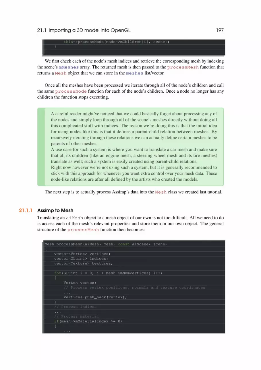
21.1 Importing a 3D model into OpenGL 197
this->processNode(node->mChildren[i], scene);}
}
We first check each of the node’s mesh indices and retrieve the corresponding mesh by indexingthe scene’s mMeshes array. The returned mesh is then passed to the processMesh function thatreturns a Mesh object that we can store in the meshes list/vector.
Once all the meshes have been processed we iterate through all of the node’s children and callthe same processNode function for each of the node’s children. Once a node no longer has anychildren the function stops executing.
A careful reader might’ve noticed that we could basically forget about processing any ofthe nodes and simply loop through all of the scene’s meshes directly without doing allthis complicated stuff with indices. The reason we’re doing this is that the initial ideafor using nodes like this is that it defines a parent-child relation between meshes. Byrecursively iterating through these relations we can actually define certain meshes to beparents of other meshes.A use case for such a system is where you want to translate a car mesh and make surethat all its children (like an engine mesh, a steering wheel mesh and its tire meshes)translate as well; such a system is easily created using parent-child relations.Right now however we’re not using such a system, but it is generally recommended tostick with this approach for whenever you want extra control over your mesh data. Thesenode-like relations are after all defined by the artists who created the models.
The next step is to actually process Assimp’s data into the Mesh class we created last tutorial.
21.1.1 Assimp to MeshTranslating an aiMesh object to a mesh object of our own is not too difficult. All we need to dois access each of the mesh’s relevant properties and store them in our own object. The generalstructure of the processMesh function then becomes:
Mesh processMesh(aiMesh* mesh, const aiScene* scene){
vector<Vertex> vertices;vector<GLuint> indices;vector<Texture> textures;
for(GLuint i = 0; i < mesh->mNumVertices; i++){
Vertex vertex;// Process vertex positions, normals and texture coordinates...vertices.push_back(vertex);
}// Process indices...// Process materialif(mesh->mMaterialIndex >= 0){
...

21.1 Importing a 3D model into OpenGL 198
}
return Mesh(vertices, indices, textures);}
Processing a mesh basically consists of 3 sections: retrieving all the vertex data, retrieving themesh’s indices and finally retrieving the relevant material data. The processed data is stored in oneof the 3 vectors and from those a Mesh is created and returned to the function’s caller.
Retrieving the vertex data is pretty simple: we define a Vertex struct that we add to thevertices array after each iteration. We loop for as much vertices there exist within the mesh(retrieved via mesh->mNumVertices). Within the iteration we then want to fill this struct withall the relevant data. For vertex positions this is done as follows:
glm::vec3 vector;vector.x = mesh->mVertices[i].x;vector.y = mesh->mVertices[i].y;vector.z = mesh->mVertices[i].z;vertex.Position = vector;
Note that we define a placeholder vec3 for transferring Assimp’s data to. We need theplaceholder since Assimp maintains its own data types for vector, matrices, strings etc. and theydon’t convert really well to glm’s data types.
Assimp calls their vertex position array mVertices which isn’t really too intuitive.
The procedure for normals should come as no surprise now:
vector.x = mesh->mNormals[i].x;vector.y = mesh->mNormals[i].y;vector.z = mesh->mNormals[i].z;vertex.Normal = vector;
Texture coordinates are roughly the same, but Assimp allows a model to have up to 8 differenttexture coordinates per vertex which we’re not going to use so we only care about the first set oftexture coordinates. We’ll also want to check if the mesh actually contains texture coordinates(which might not be always the case):
if(mesh->mTextureCoords[0]) // Does the mesh contain texture coordinates?{
glm::vec2 vec;vec.x = mesh->mTextureCoords[0][i].x;vec.y = mesh->mTextureCoords[0][i].y;vertex.TexCoords = vec;
}else
vertex.TexCoords = glm::vec2(0.0f, 0.0f);
The vertex struct is now completely filled with the required vertex attributes and we canpush it to the back of the vertices vector at the end of the iteration. This process is repeated foreach of the mesh’s vertices.

21.1 Importing a 3D model into OpenGL 199
21.1.2 IndicesAssimp’s interface defined each mesh having an array of faces where each face represents a singleprimitive, which in our case (due to the aiProcess_Triangulate option) are always triangles.A face contains the indices that define which vertices we need to draw in what order for eachprimitive so if we iterate over all the faces and store all the face’s indices in the indices vectorwe’re all set:
for(GLuint i = 0; i < mesh->mNumFaces; i++){
aiFace face = mesh->mFaces[i];for(GLuint j = 0; j < face.mNumIndices; j++)
indices.push_back(face.mIndices[j]);}
After the outer loop has finished we now have a complete set of vertices and index data fordrawing the mesh via glDrawElements. However, to finish the discussion and to add somedetail to the mesh we want to process the mesh’s material as well.
21.1.3 MaterialJust like with nodes, a mesh only contains an index to a material object and to retrieve the actualmaterial of a mesh we need to index the scene’s mMaterials array. The mesh’s material indexis set in its mMaterialIndex property which we can also query to check if the mesh actuallycontains a material or not:
if(mesh->mMaterialIndex >= 0){
aiMaterial* material = scene->mMaterials[mesh->mMaterialIndex];vector<Texture> diffuseMaps = this->loadMaterialTextures(material,
aiTextureType_DIFFUSE, "texture_diffuse");textures.insert(textures.end(), diffuseMaps.begin(), diffuseMaps.end());vector<Texture> specularMaps = this->loadMaterialTextures(material,
aiTextureType_SPECULAR, "texture_specular");textures.insert(textures.end(), specularMaps.begin(), specularMaps.end());
}
We first retrieve the aiMaterial object from the scene’s mMaterials array. Then wewant to load the mesh’s diffuse and/or specular textures. A material object internally stores anarray of texture locations for each texture type. The different texture types are all prefixed withaiTextureType_. We use a helper function called loadMaterialTextures to retrievethe textures from the material. The function returns a vector of Texture structs that we then storeat the end of the model’s textures vector.
The loadMaterialTextures function iterates over all the texture locations of the giventexture type, retrieves the texture’s file location and then loads and generates the texture and storesthe information in a Vertex struct. It looks like this:

21.2 A large optimization 200
vector<Texture> loadMaterialTextures(aiMaterial* mat, aiTextureType type,string typeName)
{vector<Texture> textures;for(GLuint i = 0; i < mat->GetTextureCount(type); i++){
aiString str;mat->GetTexture(type, i, &str);Texture texture;texture.id = TextureFromFile(str.C_Str(), this->directory);texture.type = typeName;texture.path = str;textures.push_back(texture);
}return textures;
}
We first check the amount of textures stored in the material via its GetTextureCountfunction that expects one of the texture types we’ve given. We then retrieve each of the texture’sfile locations via the GetTexture function that stores the result in an aiString. We then useanother helper function called TextureFromFile that loads a texture (with SOIL) for us andreturns the texture’s ID. You can check the complete code listing at the end for its content if you’renot sure how such a function is written.
Note that we make the assumption that texture file paths in model files are local to theactual model object e.g. in the same directory as the location of the model itself. We canthen simply concatenate the texture location string and the directory string we retrievedearlier (in the loadModel function) to get the complete texture path (that’s why theGetTexture function also needs the directory string).Some models found over the internet still use absolute paths for their texture locationswhich won’t work on each machine. In that case you probably want to manually edit thefile to use local paths for the textures (if possible).
And that is all there is to importing a model using Assimp. You can find the complete sourcecode of the Model class here.
21.2 A large optimizationWe’re not completely done yet, since there is still a large (but not completely necessary) optimizationwe want to make. Most scenes re-use several of their textures onto several meshes; think of a houseagain that has a granite texture for its walls. This texture could also be applied to the floor, itsceilings, the staircase, perhaps a table and maybe even a small well close by. Loading textures isnot a cheap operation and in our current implementation a new texture is loaded and generated foreach mesh even though the exact same texture has been loaded several times before. This quicklybecomes the bottleneck of your model loading implementation.
So we’re going to add one small tweak to the model code by storing all of the loaded texturesglobally and wherever we want to load a texture we first check if it hasn’t been loaded already. Ifso, we take that texture and skip the entire loading routine saving us lots of processing power. Tobe able to actually compare textures we need to store their path as well:

21.2 A large optimization 201
struct Texture {GLuint id;string type;aiString path; // We store the path of the texture to compare withother textures
};
Then we store all the loaded textures in another vector declared at the top of the model’s classfile as a private variable:
vector<Texture> textures_loaded;
Then in the loadMaterialTextures function we want to compare the texture path withall the textures in the textures_loaded vector to see if the current texture path is similar toany of those. If so, we skip the texture loading/generation part and simply use the located texturestruct as the mesh’s texture. The (updated) function is shown below:
vector<Texture> loadMaterialTextures(aiMaterial* mat, aiTextureType type,string typeName)
{vector<Texture> textures;for(GLuint i = 0; i < mat->GetTextureCount(type); i++){
aiString str;mat->GetTexture(type, i, &str);GLboolean skip = false;for(GLuint j = 0; j < textures_loaded.size(); j++){
if(textures_loaded[j].path == str){
textures.push_back(textures_loaded[j]);skip = true;break;
}}if(!skip){ // If texture hasn’t been loaded already, load it
Texture texture;texture.id = TextureFromFile(str.C_Str(), this->directory);texture.type = typeName;texture.path = str;textures.push_back(texture);this->textures_loaded.push_back(texture); // Add to loaded
textures}
}return textures;
}
So now we do not only have an extremely versatile model loading system, but we also have anoptimized one that loads objects quite fast.
Some versions of Assimp tend to load models quite slow when using the debug versionand/or the debug mode of your IDE so be sure to test it out with release versions as wellif you run into slow loading times.

21.3 No more containers! 202
You can find the complete source code of the optimized Model class here.
21.3 No more containers!So let’s give our implementation a spin by actually importing a model created by genuine artists, notsomething done by the creative genius that I am (you got to admit, those containers were probablyone of the most beautiful cubical shapes you’ve seen). Because I don’t want to give myself toomuch credit I’ll occasionally allow some other artists to join the ranks and this time we’re going toload the original nanosuit used by Crytek’s game Crysis. The model is exported as a .obj filetogether with a .mtl file that contains the model’s diffuse, specular and normal maps (more aboutthose later). You can download the model here, note that all the textures and the model files shouldbe located in the same directory for the textures to load.
The version you can download from this website is a modified version where each texturefile path was modified to a local relative path instead of an absolute path if downloadedfrom the original source.
Now in the code, declare a Model object and pass in the model’s file location. The modelshould then automatically load and (if there were no errors) draw the object in the game loopusing its Draw function and that is it. No more buffer allocations, attribute pointers and rendercommands, just a simple one-liner. Then if you create a simple set of shaders where the fragmentshader only outputs the object’s diffuse texture color the result looks a bit like this:
You can find the complete source code here together with its vertex and fragment shader.
We could also get more creative and introduce two point lights to the render equation as welearned from the Lighting tutorials and together with specular maps get amazing results:

21.4 Exercises 203
Even I have to admit that this is maybe a bit more fancy than the containers we’ve used so far.Using Assimp you can load tons of models found over the internet. There are quite a few resourcewebsites that offer free 3D models for you to download in several file formats. Do note that somemodels still won’t load properly, have texture paths that won’t work or might simply be exported ina format even Assimp can’t read.
21.4 Exercises• Can you re-create the last scene with the two point lights?: solution, shaders.

IV22 Depth testing . . . . . . . . . . . . . . . . . . . . . . . 205
23 Stencil testing . . . . . . . . . . . . . . . . . . . . . . 216
24 Blending . . . . . . . . . . . . . . . . . . . . . . . . . . . 223
25 Face culling . . . . . . . . . . . . . . . . . . . . . . . . 235
26 Framebuffers . . . . . . . . . . . . . . . . . . . . . . . 240
27 Cubemaps . . . . . . . . . . . . . . . . . . . . . . . . . 254
28 Advanced Data . . . . . . . . . . . . . . . . . . . . 269
29 Advanced GLSL . . . . . . . . . . . . . . . . . . . . 273
30 Geometry Shader . . . . . . . . . . . . . . . . . . 288
31 Instancing . . . . . . . . . . . . . . . . . . . . . . . . . 305
32 Anti Aliasing . . . . . . . . . . . . . . . . . . . . . . . . 317
Advanced OpenGL

22. Depth testing
In the coordinate systems tutorial we’ve rendered a 3D container and made use of a depth buffer toprevent faces rendering to the front while they’re behind other faces. In this tutorial we’re goingto elaborate a bit more on these depth values the depth buffer (or z-buffer) is storing and how itactually determines if a fragment is indeed behind other fragments.
The depth-buffer is a buffer that, just like the color buffer (that stores all the fragment colors:the visual output), stores information per fragment and (usually) has the same width and height asthe color buffer. The depth buffer is automatically created by the windowing system and stores itsdepth values as 16, 24 or 32 bit floats. In most systems you’ll see a depth buffer with a precisionof 24 bits.
When depth testing is enabled OpenGL tests the depth value of a fragment against the contentof the depth buffer. OpenGL performs a depth test and if this test passes, the depth buffer is updatedwith the new depth value. If the depth test fails, the fragment is discarded.
Depth testing is done in screen space after the fragment shader has run (and after stenciltesting has run which we’ll discuss in the next tutorial). The screen space coordinates relatedirectly to the viewport defined by OpenGL’s glViewport function and can be accessed viaGLSL’s built-in gl_FragCoord variable in the fragment shader. The x and y components ofgl_FragCoord represent the fragment’s screen-space coordinates (with (0,0) being the bottom-left corner). The gl_FragCoord also contains a z-component which contains the actual depthvalue of the fragment. This z value is the value that is compared to the depth buffer’s content.

22.1 Depth test function 206
Today most GPUs support a hardware feature called early depth testing. Early depthtesting allows the depth test to run before the fragment shader runs. Wherever it is cleara fragment is never going to be visible (it is behind other objects) we can prematurelydiscard the fragment.Fragment shaders are usually quite expensive so wherever we can avoid running them weshould. A restriction on the fragment shader for early depth testing is that you shouldn’twrite to the fragment’s depth value. If a fragment shader would write to its depth value,early depth testing is impossible; OpenGL won’t be able to figure out the depth valuebeforehand.
Depth testing is disabled by default so to enable depth testing we need to enable it with theGL_DEPTH_TEST option:
glEnable(GL_DEPTH_TEST);
Once enabled OpenGL automatically stores fragments their z-values in the depth buffer if theypassed the depth test and discards fragments if they failed the depth test accordingly. If you havedepth testing enabled you should also clear the depth buffer before each render iteration using theGL_DEPTH_BUFFER_BIT, otherwise you’re stuck with the written depth values from last renderiteration:
glClear(GL_COLOR_BUFFER_BIT | GL_DEPTH_BUFFER_BIT);
There are certain scenarios imaginable where you want to perform the depth test on all fragmentsand discard them accordingly, but not update the depth buffer. Basically, you’re using a read-onlydepth buffer. OpenGL allows us to disable writing to the depth buffer by setting its depth mask toGL_FALSE:
glDepthMask(GL_FALSE);
Note that this only has effect if depth testing is enabled.
22.1 Depth test functionOpenGL allows us to modify the comparison operators it uses for the depth test. This allows us tocontrol when OpenGL should pass or discard fragments and when to update the depth buffer. Wecan set the comparison operator (or depth function) by calling glDepthFunc:
glDepthFunc(GL_LESS);
The function accepts several comparison operators that are listed in the table below:

22.1 Depth test function 207
Function DescriptionGL_ALWAYS The depth test always passes.GL_NEVER The depth test never passes.GL_LESS Passes if the fragment’s depth value is less than the stored depth value.GL_EQUAL Passes if the fragment’s depth value is equal to the stored depth value.
GL_LEQUALPasses if the fragment’s depth value is less than or equal to the stored depth
value.GL_GREATER Passes if the fragment’s depth value is greater than the stored depth value.GL_NOTEQUAL Passes if the fragment’s depth value is not equal to the stored depth value.
GL_GEQUALPasses if the fragment’s depth value is greater than or equal to the stored depth
value.
By default the depth function GL_LESS is used that discards all the fragments that have adepth value higher than or equal to the current depth buffer’s value.
Let’s show the effect that changing the depth function has on the visual output. We’ll use afresh code setup that displays a basic scene with two textured cubes sitting on a textured floor withno lighting. You can find the source code here and its shaders here.
Within the source code we changed the depth function to GL_ALWAYS:
glEnable(GL_DEPTH_TEST);glDepthFunc(GL_ALWAYS);
This simulates the same behavior we get if we didn’t enable depth testing. The depth test simplyalways passes so the fragments that are drawn last are rendered in front of the fragments that weredrawn before, even though they should’ve been at the front. Since we’ve drawn the floor plane aslast the plane’s fragments overwrite each of the container’s fragments:

22.1 Depth test function 208
Setting it all back to GL_LESS gives us the type of scene we’re used to:

22.2 Depth value precision 209
22.2 Depth value precisionThe depth buffer contains depth values between 0.0 and 1.0 and it compares its content withz-value of all the objects in the scene as seen from the viewer. These z-values in view space canbe any value between the projection frustum’s near and far value. We thus need some way totransform these view-space z-values to the range of [0,1] and one way is to linearly transformthem to the [0,1] range. The following (linear) equation then transforms the z-value to a depthvalue between 0.0 and 1.0:
F_depth =z−near
f ar−near(22.1)
Here near and f ar are the near and far values we used to provide to the projection matrix to setthe visible frustum (see coordinate Systems). The equation takes a depth value z within the frustumand transforms it to the range [0,1]. The relation between the z-value and its correspondingdepth value is presented in the following graph:
Note that all equations give a depth value close to 0.0 when the object is close by and adepth value close to 1.0 when the object is close to the far plane.
In practice however, a linear depth buffer like this is almost never used. For correct projectionproperties a non-linear depth equation is used that is proportional to 1/z. What this basically doesis give us enormous precision when z is small and much less precision when z is far away. Thinkabout this for a second: do we really want the depth values that are 1000 units away to have thesame precision as highly-detailed objects at a distance of 1? The linear equation doesn’t take thisinto account.
Since the non-linear function is proportional to 1/z, z-values between 1.0 and 2.0 for examplewould result in depth values between 1.0 and 0.5 which is half of the precision a float providesus, giving us enormous precision at small z-values. Z-values between 50.0 and 100.0 wouldaccount for only 2% of the float’s precision, this is exactly what we want. Such an equation, thatalso takes near and far distances into account, is given below:

22.3 Visualizing the depth buffer 210
F_depth =1/z−1/near
1/ f ar−1/near(22.2)
Don’t worry if you don’t know exactly what is going on with this equation. The important thingto remember is that the values in the depth buffer are not linear in screen-space (they are linear inview-space before the projection matrix is applied). A value of 0.5 in the depth buffer does notmean the object’s z-values are halfway in the frustum; the z-value of the vertex is actually quiteclose to the near plane! You can see the non-linear relation between the z-value and the resultingdepth buffer’s value in the following graph:
As you can see, the depth values are greatly determined by the small z-values thus givingus enormous depth precision to the objects close by. The equation to transform z-values (fromthe viewer’s perspective) is embedded within the projection matrix so when we transform vertexcoordinates from view to clip and then to screen-space the non-linear equation is applied. If you’recurious as to what the projection matrix actually does in detail I suggest the following great article
The effect of this non-linear equation quickly becomes apparent when we try to visualize thedepth buffer.
22.3 Visualizing the depth bufferWe know that the z-value of the built-in gl_FragCoord vector in the fragment shader containsthe depth value of that particular fragment. If we were to output this depth value of the fragmentas a color we could display the depth values of all the fragments in the scene. We can do this byreturning a color vector based on the fragment’s depth value:
void main(){
color = vec4(vec3(gl_FragCoord.z), 1.0f);}

22.3 Visualizing the depth buffer 211
If you’d then run the same program again you’ll probably notice that everything is white,making it look like all of our depth values are 1.0 which is the maximum depth value. So whyaren’t any of the depth values closer to 0.0 and thus darker?
You might remember from the previous section that the depth values in screen space are non-linear e.g. they have a very high precision for small z-values and a low precision for large z-values.The depth value of the fragment increases rapidly over distance so almost all the vertices havevalues close to 1.0. If we were to carefully move really close to objects you might eventually seethe colors getting darker, showing that their z-values are becoming smaller:
This clearly shows the non-linearity of the depth value. Objects close by have a much largereffect on the depth value than objects far away. Only moving a few inches results in the colorsgoing from dark to completely white.
We can however, transform the non-linear depth values of the fragment back to their linearsiblings. To achieve this we basically need to reverse the process of projection for the depthvalues alone. This means we have to first re-transform the depth values from the range [0,1]to normalized device coordinates in the range [-1,1] (clip space). Then we want to reverse thenon-linear equation (equation 2) as done in the projection matrix and apply this inversed equationto the resulting depth value. The result is then a linear depth value. Sounds do-able right?
First we want to transform the depth value to NDC which is not too difficult:
float z = depth * 2.0 - 1.0;
We then take the resulting z value and apply the inverse transformation to retrieve the linear

22.3 Visualizing the depth buffer 212
depth value:
float linearDepth = (2.0 * near) / (far + near - z * (far - near));
Note that this equation is not precisely the inverse of equation 2. This equation is derived fromthe projection matrix that again uses equation 2 to non-linearize the depth values. This equationalso takes into account that the z-values are supplied in the range [0,1] instead of [near,far].This math-heavy article explains the projection matrix in enormous detail for the interested reader;it also shows where the equations come from.
This is not the exact equation as derived from the projection matrix; this equation is theresult of a division by far. The depth values range all the way to the far plane whichdoesn’t fit nicely as a color value between 0.0 and 1.0. Dividing by far maps thedepth values to 0.0 and 1.0 which is better suited for demonstration purposes.
The complete fragment shader that transforms the non-linear depth in screen-space to a lineardepth value is then as follows:
#version 330 core
out vec4 color;
float LinearizeDepth(float depth){
float near = 0.1;float far = 100.0;float z = depth * 2.0 - 1.0; // Back to NDCreturn (2.0 * near) / (far + near - z * (far - near));
}
void main(){
float depth = LinearizeDepth(gl_FragCoord.z);color = vec4(vec3(depth), 1.0f);
}
If we’d now run the application we get depth values that are actually linear over distance. Trymoving around the scene to see the depth values change in a linear fashion.

22.4 Z-fighting 213
The colors are mostly black because the depth values range linearly from the near plane whichis 0.1 to the far plane which is 100 that is still quite far away from us. The result is that we’rerelatively close to the near plane and thus get lower (darker) depth values.
22.4 Z-fightingA common visual artifact might occur when two planes or triangles are so closely aligned to eachother that the depth buffer does not have enough precision to figure out which one of the two shapesis in front of the other. The result is that the two shapes continually seem to switch order whichcauses weird glitchy patterns. This is called z-fighting, because it looks like the shapes are fightingover who gets on top.
In the scene we’ve been using so far there are a few spots where z-fighting is quite noticeable.The containers were placed at the exact height that the floor was placed which means the bottomplane of the container is coplanar with the floor plane. The depth values of both planes are then thesame so the resulting depth test has no way of figuring out which is the right one.
If you move the camera inside one of the containers the effects are clearly visible, the bottompart of the container is constantly switching between the container’s plane and the floor’s plane in azigzag pattern:

22.4 Z-fighting 214
Z-fighting is a common problem with depth buffers and is generally stronger when objects areat a further distance (because the depth buffer has less precision at larger z-values). Z-fighting can’tbe completely prevented, but there are generally a few tricks that will help to mitigate or completelyprevent z-fighting in your scene.
22.4.1 Prevent z-fightingThe first and most important trick is never place objects too close to each other in a way that someof their triangles closely overlap. By creating a small offset between two objects that is hardlynoticeable by a user you’ll completely remove z-fighting between the two objects. In the case ofthe containers and the plane we could’ve easily moved the containers slightly in the positive ydirection. The small change of the container’s positions would probably not be noticeable at all andcompletely reduce the z-fighting. However, this requires manual intervention of each of the objectsand thorough testing to make sure no objects in a scene produce z-fighting.
A second trick is to set the near plane as far as possible. In one of the previous sections we’vediscussed that precision is extremely large when close to the near plane so if we move the nearplane farther from the viewer, we’ll have significantly greater precision over the entire frustumrange. However, setting the near plane too far could cause clipping of near objects so it is usuallya matter of tweaking and experimentation to figure out the best near distance for your scene.
Another great trick at the cost of some performance is to use a higher precision depth buffer.Most depth buffers have a precision of 24 bits, but most cards nowadays support 32 bit depthbuffers which increases the precision by a significant amount. So at the cost of some performanceyou’ll get much more precision with depth testing, reducing z-fighting.

22.4 Z-fighting 215
The 3 techniques we’ve discussed are the most common and easy-to-implement anti z-fightingtechniques. There are some other techniques out there that require a lot more work and still won’tcompletely disable z-fighting. Z-fighting is a common issue, but if you use the proper combinationof the listed techniques you probably won’t really need to deal with z-fighting.

23. Stencil testing
Once the fragment shader has processed the fragment a so called stencil test is executed that, justlike the depth test, has the possibility of discarding fragments. Then the remaining fragments getpassed to the depth test that could possibly discard even more fragments. The stencil test is basedon the content of yet another buffer called the stencil buffer that we’re allowed to update duringrendering to achieve interesting effects.
A stencil buffer (usually) contains 8 bits per stencil value that amounts to a total of 256different stencil values per pixel/fragment. We can then set these stencil values to values of ourliking and then we can discard or keep fragments whenever a particular fragment has a certainstencil value.
Each windowing library needs to set up a stencil buffer for you. GLFW does thisautomatically so we don’t have to tell GLFW to create one, but other windowinglibraries might not create a stencil library by default so be sure to check your library’sdocumentation.
A simple example of a stencil buffer is shown below:

217
The stencil buffer is first cleared with zeros and then an open rectangle of 1s is set in the stencilbuffer. The fragments of the scene are then only rendered (the others are discarded) wherever thestencil value of that fragment contains a 1.
Stencil buffer operations allow us to set the stencil buffer at specific values wherever we’rerendering fragments. By changing the content of the stencil buffer while we’re rendering, we’rewriting to the stencil buffer. In the same (or following) render iteration(s) we can then read thesevalues to discard or pass certain fragments. When using stencil buffers you can get as crazy as youlike, but the general outline is usually as follows:
• Enable writing to the stencil buffer.• Render objects, updating the content of the stencil buffer.• Disable writing to the stencil buffer.• Render (other) objects, this time discarding certain fragments based on the content of the
stencil buffer.By using the stencil buffer we can thus discard certain fragments based on the fragments of
other drawn objects in the scene.
You can enable stencil testing by enabling GL_STENCIL_TEST. From that point on, allrendering calls will influence the stencil buffer in one way or another.
glEnable(GL_STENCIL_TEST);
Note that you also need to clear the stencil buffer each iteration just like the color and depthbuffer:
glClear(GL_COLOR_BUFFER_BIT | GL_DEPTH_BUFFER_BIT | GL_STENCIL_BUFFER_BIT);
Also, just like the depth testing’s glDepthMask function, there is an equivalent functionfor the stencil buffer. The function glStencilMask allows us to set a bitmask that is ANDedwith the stencil value about to be written to the buffer. By default this is set to a bitmask of all 1sunaffecting the output, but if we were to set this to 0x00 all the stencil values written to the bufferend up as 0s. This is equivalent to depth testing’s glDepthMask(GL_FALSE):
glStencilMask(0xFF); // Each bit is written to the stencil buffer as isglStencilMask(0x00); // Each bit ends up as 0 in the stencil buffer (
disabling writes)

23.1 Stencil functions 218
Most of the cases you’ll just be writing 0x00 or 0xFF as the stencil mask, but it’s good toknow there are options to set custom bit-masks.
23.1 Stencil functionsJust like with depth testing, we have a certain amount of control over when a stencil test shouldpass or fail and how it should affect the stencil buffer. There are a total of two functions we can useto configure stencil testing: glStencilFunc and glStencilOp.
The glStencilFunc(GLenum func, GLint ref, GLuint mask) has three pa-rameters:
• func: sets the stencil test function. This test function is applied to the stored sten-cil value and the glStencilFunc’s ref value. Possible options are: GL_NEVER,GL_LESS, GL_LEQUAL, GL_GREATER, GL_GEQUAL, GL_EQUAL, GL_NOTEQUAL andGL_ALWAYS. The semantic meaning of these is similar to the depth buffer’s functions.• ref: specifies the reference value for the stencil test. The stencil buffer’s content is compared
to this value.• mask: specifies a mask that is ANDed with both the reference value and the stored stencil
value before the test compares them. Initially set to all 1s.So in the case of the simple stencil example we’ve shown at the start the function would be set
to:
glStencilFunc(GL_EQUAL, 1, 0xFF)
This tells OpenGL that whenever the stencil value of a fragment is equal (GL_EQUAL) to thereference value 1 the fragment passes the test and is drawn, otherwise discarded.
But glStencilFunc only described what OpenGL should do with the content of the stencilbuffer, not how we can actually update the buffer. That is where glStencilOp comes in.
The glStencilOp(GLenum sfail, GLenum dpfail, GLenum dppass) containsthree options of which we can specify for each option what action to take:
• sfail: action to take if the stencil test fails.• dpfail: action to take if the stencil test passes, but the depth test fails.• dppass: action to take if both the stencil and the depth test pass.Then for each of the options you can take any of the following actions:

23.2 Object outlining 219
Action DescriptionGL_KEEP The currently stored stencil value is kept.GL_ZERO The stencil value is set to 0.
GL_REPLACEThe stencil value is replaced with the reference value set with
glStencilFunc.GL_INCR The stencil value is increased by 1 if it is lower than the maximum value.
GL_INCR_WRAPSame as GL_INCR, but wraps it back to 0 as soon as the maximum value is
exceeded.GL_DECR The stencil value is decreased by 1 if it is higher than the minimum value.
GL_DECR_WRAPSame as GL_DECR, but wraps it to the maximum value if it ends up lower
than 0.GL_INVERT Bitwise inverts the current stencil buffer value.
By default the glStencilOp function is set to (GL_KEEP, GL_KEEP, GL_KEEP) sowhatever the outcome of any of the tests, the stencil buffer keeps its values. The default behaviordoes not update the stencil buffer, so if you want to write to the stencil buffer you need to specify atleast one different action for any of the options.
So using glStencilFunc and glStencilOp we can precisely specify when and how wewant to update the stencil buffer and we can also specify when the stencil test should pass or note.g. when fragments should be discarded.
23.2 Object outliningIt would be unlikely if you completely understood how stencil testing works from the previoussections alone so we’re going to demonstrate a particular useful feature that can be implementedwith stencil testing alone called object outlining.
Object outlining does exactly what it says it does. For each object (or only one) we’re creatinga small colored border around the (combined) objects. This is a particular useful effect when youwant to select units in a strategy game for example and need to show the user which of the unitswere selected. The routine for outlining your objects is as follows:

23.2 Object outlining 220
1. Set the stencil func to GL_ALWAYS before drawing the (to be outlined) objects, updating thestencil buffer with 1s wherever the objects’ fragments are rendered.
2. Render the objects.3. Disable stencil writing and depth testing.4. Scale each of the objects by a small amount.5. Use a different fragment shader that outputs a single (border) color.6. Draw the objects again, but only if their fragments’ stencil values are not equal to 1.7. Enable stencil writing and depth testing again.This process sets the content of the stencil buffer to 1s for each of the object’s fragments
and when we want to draw the borders, we basically draw scaled-up versions of the objects andwherever the stencil test passes, the scaled-up version is drawn which is around the borders of theobject. We’re basically discarding all the fragments of the scaled-up versions that are not part ofthe original objects’ fragments using the stencil buffer.
So we’re first going to create a very basic fragment shader that outputs a border color. Wesimply set a hardcoded color value and call the shader shaderSingleColor:
void main(){
outColor = vec4(0.04, 0.28, 0.26, 1.0);}
We’re only going to add object outlining to the two containers so we’ll leave the floor out of it.We thus want to first draw the floor, then the two containers (while writing to the stencil buffer)and then we draw the scaled-up containers (while discarding the fragments that write over thepreviously drawn container fragments).
We first want to enable stencil testing and set the actions to take whenever any of the testssucceed or fail:
glEnable(GL_DEPTH_TEST);glStencilOp(GL_KEEP, GL_KEEP, GL_REPLACE);
If any of the tests fail we do nothing, we simply keep the currently stored value that is in thestencil buffer. If both the stencil test and the depth test succeed however, we want to replace thestored stencil value with the reference value set via glStencilFunc which we later set to 1.
We clear the stencil buffer to 0s and for the containers we update the stencil buffer to 1 foreach fragment drawn:
glStencilFunc(GL_ALWAYS, 1, 0xFF); // All fragments should update thestencil buffer
glStencilMask(0xFF); // Enable writing to the stencil buffernormalShader.Use();DrawTwoContainers();
By using the GL_ALWAYS stencil testing function we make sure that each of the containers’fragments update the stencil buffer with a stencil value of 1. Because the fragments always passthe stencil test, the stencil buffer is updated with the reference value wherever we’ve drawn them.

23.2 Object outlining 221
Now that the stencil buffer is updated with 1s where the containers were drawn we’re going todraw the upscaled containers, but this time disabling writes to the stencil buffer:
glStencilFunc(GL_NOTEQUAL, 1, 0xFF);glStencilMask(0x00); // Disable writing to the stencil bufferglDisable(GL_DEPTH_TEST);shaderSingleColor.Use();DrawTwoScaledUpContainers();
We set the stencil function to GL_NOTEQUAL which makes sure that we’re only drawing partsof the containers that are not equal to 1 thus only draw the part of the containers that are outsidethe previously drawn containers. Note that we also disable depth testing so the scaled up containerse.g. the borders do not get overwritten by the floor.
Also make sure to enable the depth buffer again once you’re done.
The total object outlining routine for our scene will then look something like this:
glEnable(GL_DEPTH_TEST);glStencilOp(GL_KEEP, GL_KEEP, GL_REPLACE);
glClear(GL_COLOR_BUFFER_BIT | GL_DEPTH_BUFFER_BIT | GL_STENCIL_BUFFER_BIT);
glStencilMask(0x00); // Make sure we don’t update the stencil buffer whiledrawing the floor
normalShader.Use();DrawFloor()
glStencilFunc(GL_ALWAYS, 1, 0xFF);glStencilMask(0xFF);DrawTwoContainers();
glStencilFunc(GL_NOTEQUAL, 1, 0xFF);glStencilMask(0x00);glDisable(GL_DEPTH_TEST);shaderSingleColor.Use();DrawTwoScaledUpContainers();glStencilMask(0xFF);glEnable(GL_DEPTH_TEST);
As long as you understand the general idea behind stencil testing this fragment of code shouldn’tbe too hard to understand. Otherwise try to carefully read the previous sections again and try tocompletely understand what each of the functions does now that you’ve seen an example of itsusage.
The result of this outlining algorithm, in the scene from the depth testing tutorial, then lookslike this:

23.2 Object outlining 222
Check the source code here together with the shaders to see the complete code of the objectoutlining algorithm.
You can see that the borders overlap between both containers which is usually the effectthat we want (think of strategy games where we want to select 10 units; merging bordersis usually what we want). If you want a complete border per object you’d have to clearthe stencil buffer per object and get a little creative with the depth buffer.
The object outlining algorithm you’ve seen is quite commonly used in several games to visualizeselected objects (think of strategy games) and such an algorithm can easily be implemented withina model class. You could then simply set a boolean flag within the model class to draw with bordersor without. If you want to be creative you could even give the borders a more natural look with thehelp of post-processing filters like Gaussian Blur.
Stencil testing has many more purposes, beside outlining objects, like drawing textures inside arear-view mirror so it neatly fits into the mirror shape or rendering real-time shadows with a stencilbuffer technique called shadow volumes. Stencil buffers provide us with yet another nice tool inour already extensive OpenGL toolkit.

24. Blending
Blending in OpenGL is also commonly known as the technique to implement transparency withinobjects. Transparency is all about objects (or parts of them) not having a solid color, but having acombination of colors from the object itself and any other object behind it with varying intensity. Acolored glass window is a transparent object; the glass has a color of its own, but the resulting colorcontains the colors of all the objects behind the glass as well. This is also where the name blendingcomes from, since we blend several colors (of different objects) to a single color. Transparencythus allows us to see through objects.
Transparent objects can be completely transparent (it lets all colors through) or partially trans-parent (it lets colors through, but also shows some of its own colors). The amount of transparencyof an object is defined by its color’s alpha value. The alpha color value is the 4th component of acolor vector that you’ve probably seen quite often now. Until this tutorial, we’ve always kept this4th component at a value of 1.0 giving the object 0.0 transparency, while an alpha value of 0.0

24.1 Discarding fragments 224
would result in the object having complete transparency. An alpha value of 0.5 tells us the object’scolor consist of 50% of its own color and 50% of the colors behind the object.
The textures we’ve used so far all consisted of 3 color components: red, green and blue, butsome textures also have an embedded alpha channel that contains an alpha value per texel. Thisalpha value tells us exactly which parts of the texture have transparency and by how much. Forexample, the following window texture has an alpha value of 0.25 at its glass part (it wouldnormally be completely red, but since it has 75% transparency it largely shows the website’sbackground through it, making it seem a lot less red) and an alpha value of 0.0 at its corners:
We’ll soon be adding this windowed texture to the scene, but first we’ll discuss an easiertechnique to implement transparency for textures that are either fully transparent or fully opaque.
24.1 Discarding fragmentsSome images do not care about partial transparency, but either want to show something or nothingat all based on the color value of a texture. Think of grass; to create something like grass withlittle effort you generally paste a grass texture onto a 2D quad and place that quad into your scene.However, grass isn’t exactly shaped like a 2D square so you only want to display some parts of thegrass texture and ignore the others.
The following texture is exactly such a texture where it either is full opaque (an alpha value of1.0) or it is fully transparent (an alpha value of 0.0) and nothing in between. You can see thatwherever there is no grass, the image shows the website’s background color instead of its own.

24.1 Discarding fragments 225
So when adding vegetation like grass to your scene we don’t want to see a square image ofgrass, but rather only show the actual grass and be able to see through the rest of the image. Wewant to discard the fragments that show the transparent parts of the texture, not storing the fragmentinto the color buffer. Before we get into that we first need to learn how to load a transparent texture.
To load textures with alpha values we need to tell SOIL to load the RGBA components of theimage instead of the RGB components. Note that SOIL will still load most alpha-less textures justfine, it simply stores an alpha value of 1.0 wherever one is omitted.
unsigned char* image = SOIL_load_image(path, &width, &height, 0,SOIL_LOAD_RGBA);
Don’t forget to change the texture generation procedure as well:
glTexImage2D(GL_TEXTURE_2D, 0, GL_RGBA, width, height, 0, GL_RGBA,GL_UNSIGNED_BYTE, image);
Also make sure that you retrieve all 4 color components of the texture in the fragment shader,not just the RGB components:
void main(){
// color = vec4(vec3(texture(texture1, TexCoords)), 1.0);color = texture(texture1, TexCoords);

24.1 Discarding fragments 226
}
Now that we know how to load transparent textures it’s time to put it to the test by addingseveral of these leaves of grass throughout the basic scene introduced in the depth testing tutorial.
We create a small vector where we add several glm::vec3 variables to represent the locationof the grass leaves:
vector<glm::vec3> vegetation;vegetation.push_back(glm::vec3(-1.5f, 0.0f, -0.48f));vegetation.push_back(glm::vec3( 1.5f, 0.0f, 0.51f));vegetation.push_back(glm::vec3( 0.0f, 0.0f, 0.7f));vegetation.push_back(glm::vec3(-0.3f, 0.0f, -2.3f));vegetation.push_back(glm::vec3( 0.5f, 0.0f, -0.6f));
Each of the grass objects is rendered as a single quad with the grass texture attached to it. It’snot a perfect 3D representation of grass, but it’s a lot more efficient than actually loading complexmodels. With a few tricks, like adding several more rotated grass quads at the same position, youcan still get good results.
Because the grass texture is added to a quad object we’ll need to create another VAO again, fillthe VBO and set the appropriate vertex attribute pointers. Then after we’ve drawn the floor and thetwo cubes we’re going to draw the grass leaves:
glBindVertexArray(vegetationVAO);glBindTexture(GL_TEXTURE_2D, grassTexture);for(GLuint i = 0; i < vegetation.size(); i++){
model = glm::mat4();model = glm::translate(model, vegetation[i]);glUniformMatrix4fv(modelLoc, 1, GL_FALSE, glm::value_ptr(model));glDrawArrays(GL_TRIANGLES, 0, 6);
}glBindVertexArray(0);
Running your application will now probably look a bit like this:
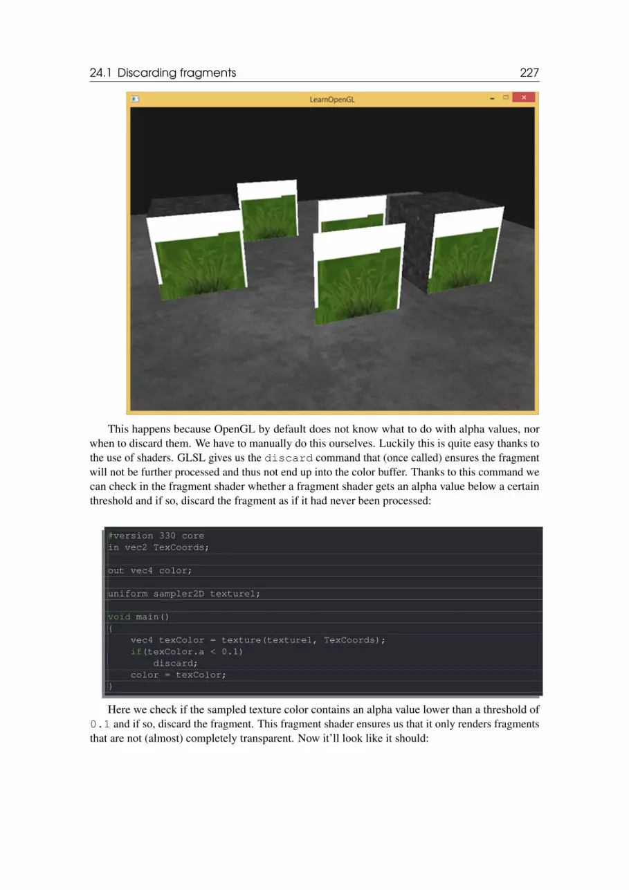
24.1 Discarding fragments 227
This happens because OpenGL by default does not know what to do with alpha values, norwhen to discard them. We have to manually do this ourselves. Luckily this is quite easy thanks tothe use of shaders. GLSL gives us the discard command that (once called) ensures the fragmentwill not be further processed and thus not end up into the color buffer. Thanks to this command wecan check in the fragment shader whether a fragment shader gets an alpha value below a certainthreshold and if so, discard the fragment as if it had never been processed:
#version 330 corein vec2 TexCoords;
out vec4 color;
uniform sampler2D texture1;
void main(){
vec4 texColor = texture(texture1, TexCoords);if(texColor.a < 0.1)
discard;color = texColor;
}
Here we check if the sampled texture color contains an alpha value lower than a threshold of0.1 and if so, discard the fragment. This fragment shader ensures us that it only renders fragmentsthat are not (almost) completely transparent. Now it’ll look like it should:

24.2 Blending 228
Note that when sampling textures at their borders, OpenGL interpolates the border valueswith the next repeated value of the texture (because we set its wrapping parameters toGL_REPEAT). This is usually okay, but since we’re using transparent values, the top ofthe texture image gets its transparent value interpolated with the bottom border’s solidcolor value. The result is then a slightly semi-transparent colored border you might seewrapped around your textured quad. To prevent this, set the texture wrapping method toGL_CLAMP_TO_EDGE whenever you use alpha textures:
glTexParameteri( GL_TEXTURE_2D, GL_TEXTURE_WRAP_S, GL_CLAMP_TO_EDGE);glTexParameteri( GL_TEXTURE_2D, GL_TEXTURE_WRAP_T, GL_CLAMP_TO_EDGE);
You can find the source code here.
24.2 BlendingWhile discarding fragments is great and all, it doesn’t give us the flexibility to render semi-transparent images; we either render the fragment or completely discard it. To render images withdifferent levels of transparency we have to enable blending. Like most of OpenGL’s functionalitywe can enable blending by enabling GL_BLEND:
glEnable(GL_BLEND);
Now that we’ve enabled blending we need to tell OpenGL how it should actually blend.
Blending in OpenGL is done with the following equation:

24.2 Blending 229
C_result = C_source∗F_source+C_destination∗F_destination (24.1)
• C_source: the source color vector. This is the color vector that originates from the texture.• C_destination: the destination color vector. This is the color vector that is currently stored
in the color buffer.• F_source: the source factor value. Sets the impact of the alpha value on the source color.• F_destination: the destination factor value. Sets the impact of the alpha value on the
destination color.After the fragment shader has run and all the tests have passed, this blend equation is let loose
on the fragment’s color output and with whatever is currently in the color buffer (previous fragmentcolor stored before the current fragment). The source and destination colors will automatically beset by OpenGL, but the source and destination factor can be set to a value of our choosing. Let’sstart with a simple example:
We have two squares where we want to draw the semi-transparent green square on top of thered square. The red square will be the destination color (and thus should be first in the color buffer)and we are now going to draw the green square over the red square.
The question then arises: what do we set the factor values to? Well, we at least want to multiplythe green square with its alpha value so we want to set the F_src equal to the alpha value ofthe source color vector which is 0.6. Then it makes sense to let the destination square have acontribution equal to the remainder of the alpha value. If the green square contributes 60% to thefinal color we want the red square to contribute 40% of the final color e.g. 1.0 - 0.6. So we setthe F_destination equal to one minus the alpha value of the source color vector. The equation thusbecomes:
C_result =
0.01.00.00.6
∗0.6+
1.00.00.01.0
∗ (1−0.6) (24.2)
The result is that the combined square fragments contain a color that is 60% green and 40% redgiving a dirty color:

24.2 Blending 230
The resulting color is then stored in the color buffer, replacing the previous color.
So this is great and all, but how do we actually tell OpenGL to use factors like these? Well itjust so happens that there is a function for this called glBlendFunc.
The glBlendFunc(GLenum sfactor, GLenum dfactor) function expects two pa-rameters that set the option for the source and destination factor. OpenGL defined quite a fewoptions for us to set of which we’ll list the most common options below. Note that the constantcolor vector C_constant can be separately set via the glBlendColor function.
Option ValueGL_ZERO Factor is equal to 0.GL_ONE Factor is equal to 1.
GL_SRC_COLOR Factor is equal to the source color vector C_source.
GL_ONE_MINUS_SRC_COLORFactor is equal to 1 minus the source color vector:
1−C_source.
GL_DST_COLORFactor is equal to the destination color vector
C_destination
GL_ONE_MINUS_DST_COLORFactor is equal to 1 minus the destination color vector:
1−C_destination.
GL_SRC_ALPHAFactor is equal to the al pha component of the source
color vector C_source.
GL_ONE_MINUS_SRC_ALPHAFactor is equal to 1−al pha of the source color vector
C_source.
GL_DST_ALPHAFactor is equal to the al pha component of the
destination color vector C_destination.
GL_ONE_MINUS_DST_ALPHAFactor is equal to 1−al pha of the destination color
vector C_destination.GL_CONSTANT_COLOR Factor is equal to the constant color vector C_constant.
GL_ONE_MINUS_CONSTANT_COLORFactor is equal to 1 - the constant color vector
C_constant.
GL_CONSTANT_ALPHAFactor is equal to the al pha component of the constant
color vector C_constant.
GL_ONE_MINUS_CONSTANT_ALPHAFactor is equal to 1−al pha of the constant color vector
C_constant.
To get the blending result we had from the two squares earlier, we want to take the al pha of the

24.3 Rendering semi-transparent textures 231
source color vector for the source factor and 1−al pha for the destination factor. This translates tothe glBlendFunc as follows:
glBlendFunc(GL_SRC_ALPHA, GL_ONE_MINUS_SRC_ALPHA);
It is also possible to set different options for the RGB and alpha channel individually usingglBlendFuncSeperate:
glBlendFuncSeperate(GL_SRC_ALPHA, GL_ONE_MINUS_SRC_ALPHA, GL_ONE, GL_ZERO);
This function sets the RGB components as we’ve set them previously, but only lets the resultingalpha component be influenced by the source’s alpha value.
OpenGL gives us even more flexibility by allowing us to change the operator between thesource and destination part of the equation. Right now, the source and destination componentsare added together, but we could also subtract them if we want. glBlendEquation(GLenummode) allows us to set this operation and has 3 possible options:
• GL_FUNC_ADD: the default, adds both components to each other: C_result = Src+Dst.• GL_FUNC_SUBTRACT: subtracts both components from each other: C_result = Src−Dst.• GL_FUNC_REVERSE_SUBTRACT: subtracts both components, but reverses order: C_result =
Dst−Src.Usually we can simply omit a call to glBlendEquation because GL_FUNC_ADD is the
preferred blending equation for most operations, but if you’re really trying your best to break themainstream circuit any of the other equations might suit your needs.
24.3 Rendering semi-transparent texturesNow that we know how OpenGL works with regards to blending it’s time to put our knowledgeto the test by adding several semi-transparent windows. We’ll be using the same scene as in thestart of this tutorial, but instead of rendering a grass texture we’re now going to use the transparentwindow texture from the start of this tutorial.
First, during initialization we enable blending and set the appropriate blending function:
glEnable(GL_BLEND);glBlendFunc(GL_SRC_ALPHA, GL_ONE_MINUS_SRC_ALPHA);
Since we enabled blending there is no need to discard fragments so we’ll reset the fragmentshader to its original version:
#version 330 corein vec2 TexCoords;
out vec4 color;
uniform sampler2D texture1;
void main(){

24.3 Rendering semi-transparent textures 232
color = texture(texture1, TexCoords);}
This time (whenever OpenGL renders a fragment) it combines the current fragment’s colorwith the fragment color currently in the color buffer based on its alpha value. Since the glass partof the window texture is semi-transparent we should be able to see the rest of the scene by lookingthrough this window.
If you take a closer look however, you might notice something is off. The transparent parts ofthe front window are occluding the windows in the background. Why is this happening?
The reason for this is that depth testing works a bit tricky combined with blending. Whenwriting to the depth buffer, the depth test does not care if the fragment has transparency or notso the transparent parts are written to the depth buffer as any other value. The result is that theentire quad of the window is checked for depth testing regardless of transparency. Even though thetransparent part should show the windows behind it, the depth test discards them.
So we cannot simply render the windows however we want and expect the depth buffer to solveall our issues for us; this is also where blending gets a little nasty. To make sure the windows showthe windows behind them, we have to draw the windows in the background first. This means wehave to manually sort the windows from furthest to nearest and draw them accordingly ourselves.
Note that with fully transparent objects like the grass leaves we have the option to simplydiscard the transparent fragments instead of blending them, saving us a few of theseheadaches (no depth issues).

24.4 Don’t break the order 233
24.4 Don’t break the orderTo make blending work for multiple objects we have to draw the farthest object first and the closestobject as last. The normal non-blended objects can still be drawn as normal using the depth bufferso they don’t have to be sorted. We do have to make sure those are drawn first before drawing the(sorted) transparent objects. When drawing a scene with non-transparent and transparent objectsthe general outline is usually as follows:
1. Draw all opaque objects first.2. Sort all the transparent objects.3. Draw all the transparent objects in sorted order.One way of sorting the transparent objects is to retrieve the distance of an object from the
viewer’s perspective. This can be achieved by taking the distance between the camera’s positionvector and the object’s position vector. We then store this distance together with the correspondingposition vector in a map data structure from the STL library. A map automatically sorts itsvalues based on its keys, so once we’ve added all positions with their distance as the key they’reautomatically sorted on their distance value:
std::map<float, glm::vec3> sorted;for (GLuint i = 0; i < windows.size(); i++) // windows contains all window
positions{
GLfloat distance = glm::length(camera.Position - windows[i]);sorted[distance] = windows[i];
}
The result is a sorted container object that stores each of the window positions based on theirdistance key value from lowest to highest distance.
Then, this time when rendering, we take each of the map’s values in reverse order (from farthestto nearest) and then draw the corresponding windows in correct order:
for(std::map<float,glm::vec3>::reverse_iterator it = sorted.rbegin(); it !=sorted.rend(); ++it)
{model = glm::mat4();model = glm::translate(model, it->second);glUniformMatrix4fv(modelLoc, 1, GL_FALSE, glm::value_ptr(model));glDrawArrays(GL_TRIANGLES, 0, 6);
}
We take a reverse iterator from the map to iterate through each of the items in reverse orderand then translate each window quad to the corresponding window position. This relatively simpleapproach to sorting transparent objects fixes the previous problem and now the scene looks likethis:
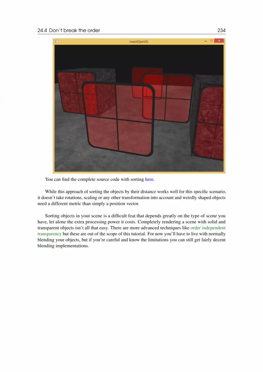
24.4 Don’t break the order 234
You can find the complete source code with sorting here.
While this approach of sorting the objects by their distance works well for this specific scenario,it doesn’t take rotations, scaling or any other transformation into account and weirdly shaped objectsneed a different metric than simply a position vector.
Sorting objects in your scene is a difficult feat that depends greatly on the type of scene youhave, let alone the extra processing power it costs. Completely rendering a scene with solid andtransparent objects isn’t all that easy. There are more advanced techniques like order independenttransparency but these are out of the scope of this tutorial. For now you’ll have to live with normallyblending your objects, but if you’re careful and know the limitations you can still get fairly decentblending implementations.

25. Face culling
Try mentally visualizing a 3D cube and count the maximum number of faces you’ll be able to seefrom any direction. If your imagination is not too creative you probably ended up with a maximumnumber of 3. You can view a cube from any position and/or direction, but you would never be ableto see more than 3 faces. So why would we waste the effort of actually drawing those other 3 facesthat we can’t even see. If we could discard those in some way we would save more than 50% offragment shader runs!
We say more than 50% instead of 50%, because from certain angles only 2 or even 1face could be visible. In that case we’d save more than 50%.
This is a really great idea, but there’s one problem we need to solve: how do we know if a faceof an object is not visible from the viewer’s point of view? If we imagine any closed shape, each ofits faces has two sides. Each side would either face the user or show its back to the user. What ifwe could only render the faces that are facing the viewer?
This is exactly what face culling does. OpenGL checks all the faces that are front facing towardsthe viewer and renders those while discarding all the faces that are back facing saving us a lot offragment shader calls (those are expensive!). We do need to tell OpenGL which of the faces we useare actually the front faces and which faces are the back faces. OpenGL uses a clever trick for thisby analyzing the winding order of the vertex data.
25.1 Winding orderWhen we define a set of triangle vertices we’re defining them in a certain winding order that iseither clockwise or counter-clockwise. Each triangle consists of 3 vertices and we specify those 3vertices in a winding order as seen from the center of the triangle.

25.1 Winding order 236
As you can see in the image we first define the vertex 1 and then we can either define vertex 2or 3 and this choice defines the winding order of this triangle. The following code illustrates this:
GLfloat vertices[] = {// Clockwisevertices[0], // vertex 1vertices[1], // vertex 2vertices[2], // vertex 3// Counter-clockwisevertices[0], // vertex 1vertices[2], // vertex 3vertices[1] // vertex 2
};
Each set of 3 vertices that form a triangle primitive thus contain a winding order. OpenGL usesthis information when rendering your primitives to determine if a triangle is a front-facing or aback-facing triangle. By default, triangles defined with counter-clockwise vertices are processed asfront-facing triangles.
When defining your vertex order you visualize the corresponding triangle as if it was facingyou, so each triangle that you’re specifying should be counter-clockwise as if you’re directly facingthat triangle. The cool thing about specifying all your vertices like this is that the actual windingorder is calculated at the rasterization stage, so when the vertex shader has already run. The verticesare then seen as from the viewer’s point of view.
All the triangle vertices that the viewer is then facing are indeed in the correct winding order aswe specified them, but the vertices of the triangles at the other side of the cube are now rendered insuch a way that their winding order becomes reversed. The result is that the triangles we’re facingare seen as front-facing triangles and the triangles at the back are seen as back-facing triangles. Thefollowing image shows this effect:

25.2 Face culling 237
In the vertex data we would’ve defined both triangles in counter-clockwise order (the fronttriangle as 1, 2, 3 and the back triangle as 1, 2 and 3 as well (if we’d see the triangle from thefront)). However, from the viewer’s direction the back triangle is rendered clockwise if we draw itin the order of 1, 2 and 3 from the viewer’s current point of view. Even though we specified theback triangle in counter-clockwise order, it is now rendered in a clockwise order. This is exactlywhat we want to cull (discard) non-visible faces!
25.2 Face cullingAt the start of the tutorial we said that OpenGL is able to discard triangle primitives if they’rerendered as back-facing triangles. Now that we know how to set the winding order of the verticeswe can start using OpenGL’s face culling option which is disabled by default.
The cube vertex data we used in the last tutorials wasn’t defined with the counter-clockwisewinding order in mind, so I updated the vertex data to reflect a counter-clockwise winding orderwhich you can copy from here. It’s a good practice to try and visualize that these vertices are indeedall defined in a counter-clockwise order for each triangle.
To enable face culling we only have to enable OpenGL’s GL_CULL_FACE option:
glEnable(GL_CULL_FACE);
From this point on, all the faces that are not front-faces are discarded (try flying inside the cubeto see that all inner faces are indeed discarded). Currently we save over 50% of performance onrendering fragments, but do note that this only works with closed shapes like a cube. We’ll have todisable face culling again when we draw the grass leaves from the previous tutorial for example,since their front and back face should be visible.
OpenGL allows us to change the type of face we want to cull as well. What if we want to cullfront faces and not the back faces? We can define this behavior by calling glCullFace:
glCullFace(GL_BACK);

25.2 Face culling 238
The glCullFace function has three possible options:
• GL_BACK: Culls only the back faces.• GL_FRONT: Culls only the front faces.• GL_FRONT_AND_BACK: Culls both the front and back faces.The initial value of glCullFace is GL_BACK. Aside from the faces to cull we can also tell
OpenGL we’d rather prefer clockwise faces as the front-faces instead of counter-clockwise facesvia glFrontFace:
glFrontFace(GL_CCW);
The default value is GL_CCW that stands for counter-clockwise ordering with the other optionbeing GL_CW which (obviously) stands for clockwise ordering.
As a simple test we could reverse the winding order by telling OpenGL that the front-faces arenow determined by a clockwise ordering instead of a counter-clockwise ordering:
glEnable(GL_CULL_FACE);glCullFace(GL_BACK);glFrontFace(GL_CW);
The result is that only the back faces are rendered:
Note that you can create the same effect by culling front faces with the default counter-clockwisewinding order:

25.3 Exercises 239
glEnable(GL_CULL_FACE);glCullFace(GL_FRONT);
As you can see, face culling is a great tool for increasing performance of your OpenGLapplications with minimal effort. You do have to keep track of which objects will actually benefitfrom face culling and which objects shouldn’t be culled.
25.3 Exercises• Can you re-define the vertex data by specifying each triangle in clockwise order and then
render the scene with clockwise triangles set as the front faces: solution

26. Framebuffers
So far we’ve used several types of screen buffers: a color buffer for writing color values, a depthbuffer to write depth information and finally a stencil buffer that allows us to discard certainfragments based on some condition. The combination of these buffers is called a framebuffer and isstored somewhere in memory. OpenGL gives us the flexibility to define our own framebuffers andthus define our own color and optionally a depth and stencil buffer.
The rendering operations we’ve done so far were all done on top of the render buffers attachedto the default framebuffer. The default framebuffer is created and configured when you create yourwindow (GLFW does this for us). By creating our own framebuffer we can get an additional meansto render to.
The application of framebuffers might not immediately make sense, but rendering your sceneto a different framebuffer allows us to create mirrors in a scene or do cool post-processing effectsfor example. First we’ll discuss how they actually work and then we’ll use them by implementingthose cool post-processing effects.
26.1 Creating a framebufferJust like any other object in OpenGL we can create a framebuffer object (abbreviated to FBO) byusing a function called glGenFramebuffers:
GLuint fbo;glGenFramebuffers(1, &fbo);
This pattern of object creation and usage is something we’ve seen dozens of times now sotheir usage functions are similar to all the other object’s we’ve seen; first we create a framebufferobject, bind it as the active framebuffer, do some operations and unbind the framebuffer. To bindthe framebuffer we use glBindFramebuffer:

26.1 Creating a framebuffer 241
glBindFramebuffer(GL_FRAMEBUFFER, fbo);
By binding to the GL_FRAMEBUFFER target all the next read and write framebuffer operationswill affect the currently bound framebuffer. It is also possible to bind a framebuffer to a read orwrite target specifically by binding to GL_READ_FRAMEBUFFER or GL_DRAW_FRAMEBUFFERrespectively. The framebuffer bound to GL_READ_FRAMEBUFFER is then used for all readoperations like glReadPixels and the framebuffer bound to GL_DRAW_FRAMEBUFFER isused as the destination for rendering, clearing and other write operations. Most of the times youwon’t need to make this distinction though and you generally bind to both with GL_FRAMEBUFFER.
Unfortunately, we can’t use our framebuffer yet because it is not complete. For a framebufferto be complete the following requirements have to be satisfied:
• We have to attach at least one buffer (color, depth or stencil buffer).• There should be at least one color attachment.• All attachments should be complete as well (reserved memory).• Each buffer should have the same number of samples.Don’t worry if you don’t know what samples are, we’ll get to those in a later tutorial.
From the requirements it should be clear that we need to create some kind of attachmentfor the framebuffer and attach this attachment to the framebuffer. After we’ve completed allrequirements we can check if we actually successfully completed the framebuffer by callingglCheckFramebufferStatus with GL_FRAMEBUFFER. It then checks the currently boundframebuffer and returns any of these values found in the specification. If it returns GL_FRAMEBUFFER_COMPLETEwe’re good to go:
if(glCheckFramebufferStatus(GL_FRAMEBUFFER) == GL_FRAMEBUFFER_COMPLETE)// Execute victory dance
All subsequent rendering operations will now render to the attachments of the currently boundframebuffer. Since our framebuffer is not the default framebuffer, the rendering commands willhave no impact on the visual output of your window. For this reason it is called off-screen renderingwhile rendering to a different framebuffer. To make sure all rendering operations will have a visualimpact on the main window we need to make the default framebuffer active again by binding to 0:
glBindFramebuffer(GL_FRAMEBUFFER, 0);
When we’re done with all framebuffer operations, do not forget to delete the framebuffer object:
glDeleteFramebuffers(1, &fbo);
Now before the completeness check is executed we need to attach one or more attachments tothe framebuffer. An attachment is a memory location that can act as a buffer for the framebuffer,think of it as an image. When creating an attachment we have two options to take: textures orrenderbuffer objects.

26.1 Creating a framebuffer 242
26.1.1 Texture attachmentsWhen attaching a texture to a framebuffer, all rendering commands will write to the texture as if itwas a normal color/depth or stencil buffer. The advantage of using textures is that the result of allrendering operations will be stored as a texture image that we can then easily use in our shaders.
Creating a texture for a framebuffer is roughly the same as a normal texture:
GLuint texture;glGenTextures(1, &texture);glBindTexture(GL_TEXTURE_2D, texture);
glTexImage2D(GL_TEXTURE_2D, 0, GL_RGB, 800, 600, 0, GL_RGB,GL_UNSIGNED_BYTE, NULL);
glTexParameteri(GL_TEXTURE_2D, GL_TEXTURE_MIN_FILTER, GL_LINEAR);glTexParameteri(GL_TEXTURE_2D, GL_TEXTURE_MAG_FILTER, GL_LINEAR);
The main differences here is that we set the dimensions equal to the screen size (although thisis not required) and we pass NULL as the texture’s data parameter. For this texture, we’re onlyallocating memory and not actually filling it. Filling the texture will happen as soon as we render tothe framebuffer. Also note that we do not care about any of the wrapping methods or mipmappingsince we won’t be needing those in most cases.
If you want to render your whole screen to a texture of a smaller or larger size youneed to call glViewport again (before rendering to your framebuffer) with the newdimensions of your texture, otherwise only a small part of the texture or screen would bedrawn onto the texture.
Now that we’ve created a texture the last thing we need to do is actually attach it to theframebuffer:
glFramebufferTexture2D(GL_FRAMEBUFFER, GL_COLOR_ATTACHMENT0, GL_TEXTURE_2D,texture, 0);
The glFrameBufferTexture2D has the following parameters:
• target: the framebuffer type we’re targeting (draw, read or both).• attachment: the type of attachment we’re going to attach. Right now we’re attaching
a color attachment. Note that the 0 at the end suggests we can attach more than 1 colorattachment. We’ll get to that in a later tutorial.• textarget: the type of the texture you want to attach.• texture: the actual texture to attach.• level: the mipmap level. We keep this at 0.Aside from the color attachments we can also attach a depth and a stencil texture to the frame-
buffer object. To attach a depth attachment we specify the attachment type as GL_DEPTH_ATTACHMENT.Note that the texture’s format and internalformat type should then become GL_DEPTH_COMPONENTto reflect the depth buffer’s storage format. To attach a stencil buffer you use GL_STENCIL_ATTACHMENTas the second argument and specify the texture’s formats as GL_STENCIL_INDEX.
It is also possible to attach both a depth buffer and a stencil buffer as a single texture. Each 32 bitvalue of the texture then consists for 24 bits of depth information and 8 bits of stencil information. To

26.1 Creating a framebuffer 243
attach a depth and stencil buffer as one texture we use the GL_DEPTH_STENCIL_ATTACHMENTtype and configure the texture’s formats to contain combined depth and stencil values. An exampleof attaching a depth and stencil buffer as one texture to the framebuffer is given below:
glTexImage2D(GL_TEXTURE_2D, 0, GL_DEPTH24_STENCIL8, 800, 600, 0,GL_DEPTH_STENCIL, GL_UNSIGNED_INT_24_8, NULL);
glFramebufferTexture2D(GL_FRAMEBUFFER, GL_DEPTH_STENCIL_ATTACHMENT,GL_TEXTURE_2D, texture, 0);
26.1.2 Renderbuffer object attachmentsRenderbuffer objects were introduced to OpenGL after textures as a possible type of framebufferattachments, so textures were the only attachments used in the good old days. Just like a textureimage, a renderbuffer object is an actual buffer e.g. an array of bytes, integers, pixels or whatever.A renderbuffer object has the added advantage though that it stores its data in OpenGL’s nativerendering format making it optimized for off-screen rendering to a framebuffer.
Renderbuffer objects store all the render data directly into their buffer without any conversionsto texture-specific formats, thus making them faster as a writeable storage medium. However,renderbuffer objects are generally write-only, thus you cannot read from them (like with texture-access). It is possible to read from them via glReadPixels though that returns a specified areaof pixels from the currently bound framebuffer, but not directly from the attachment itself.
Because their data is already in its native format they are quite fast when writing data or simplycopying their data to other buffers. Operations like switching buffers are thus quite fast whenusing renderbuffer objects. The glfwSwapBuffers function we’ve been using at the end ofeach render iteration might as well be implemented with renderbuffer objects: we simply write to arenderbuffer image, and swap to the other one at the end. Renderbuffer objects are perfect for thesekind of operations.
Creating a renderbuffer object looks similar to the framebuffer’s code:
GLuint rbo;glGenRenderbuffers(1, &rbo);
And similarly we want to bind the renderbuffer object so all subsequent renderbuffer operationsaffect the current rbo:
glBindRenderbuffer(GL_RENDERBUFFER, rbo);
Since renderbuffer objects are generally write-only they are often used as depth and stencilattachments, since most of the time we don’t really need to read values from the depth and stencilbuffers but still care about depth and stencil testing. We need the depth and stencil values fortesting, but don’t need to sample these values so a renderbuffer object suits this perfectly. Whenwe’re not sampling from these buffers, a renderbuffer object is generally preferred since it’s moreoptimized.

26.2 Rendering to a texture 244
Creating a depth and stencil renderbuffer object is done by calling the glRenderbufferStoragefunction:
glRenderbufferStorage(GL_RENDERBUFFER, GL_DEPTH24_STENCIL8, 800, 600);
Creating a renderbuffer object is similar to texture objects, the difference being that this objectis specifically designed to be used as an image, instead of a general purpose data buffer like atexture. Here we’ve chosen the GL_DEPTH24_STENCIL8 as the internal format, which holdsboth the depth and stencil buffer with 24 and 8 bits respectively.
Last thing left to do is actually attach the renderbuffer object:
glFramebufferRenderbuffer(GL_FRAMEBUFFER, GL_DEPTH_STENCIL_ATTACHMENT,GL_RENDERBUFFER, rbo);
Renderbuffer objects could provide some optimizations in your framebuffer projects, but it isimportant to realize when to use renderbuffer objects and when to use textures. The general rule isthat if you never need to sample data from a specific buffer, it is wise to use a renderbuffer objectfor that specific buffer. If you need to someday sample data from a specific buffer like colors ordepth values, you should use a texture attachment instead. Performance-wise it doesn’t have anenormous impact though.
26.2 Rendering to a textureNow that we know how framebuffers (sort of) work it’s time to put them to good use. We’re goingto render the scene into a color texture attached to a framebuffer object we created and then drawthis texture over a simple quad that spans the whole screen. The visual output is then exactly thesame as without a framebuffer, but this time it’s all printed on top of a single quad. Now why is thisuseful? In the next section we’ll see why.
First thing to do is to create an actual framebuffer object and bind it, this is all relativelystraightforward:
GLuint framebuffer;glGenFramebuffers(1, &framebuffer);glBindFramebuffer(GL_FRAMEBUFFER, framebuffer);
Next we create a texture image that we attach as a color attachment to the framebuffer. We setthe texture’s dimensions equal to the width and height of the window and keep its data uninitialized:
// Generate textureGLuint texColorBuffer;glGenTextures(1, &texColorBuffer);glBindTexture(GL_TEXTURE_2D, texColorBuffer);glTexImage2D(GL_TEXTURE_2D, 0, GL_RGB, 800, 600, 0, GL_RGB,
GL_UNSIGNED_BYTE, NULL);glTexParameteri(GL_TEXTURE_2D, GL_TEXTURE_MIN_FILTER, GL_LINEAR );glTexParameteri(GL_TEXTURE_2D, GL_TEXTURE_MAG_FILTER, GL_LINEAR);glBindTexture(GL_TEXTURE_2D, 0);

26.2 Rendering to a texture 245
// Attach it to currently bound framebuffer objectglFramebufferTexture2D(GL_FRAMEBUFFER, GL_COLOR_ATTACHMENT0, GL_TEXTURE_2D,
texColorBuffer, 0);
We also want to make sure OpenGL is able to do depth testing (and optionally stencil testing ifyou’re into that) so we have to make sure to add a depth (and stencil) attachment to the framebufferas well. Since we’ll only be sampling the color buffer and not the other buffers we can create arenderbuffer object for this purpose. Remember that they’re a good choice when you’re not goingto sample from the specific buffer(s)?
Creating a renderbuffer object isn’t too hard. The only thing we have to remember is that we’recreating it as a depth and stencil attachment renderbuffer object. We set its internal format toGL_DEPTH24_STENCIL8 which is enough precision for our purposes.
GLuint rbo;glGenRenderbuffers(1, &rbo);glBindRenderbuffer(GL_RENDERBUFFER, rbo);glRenderbufferStorage(GL_RENDERBUFFER, GL_DEPTH24_STENCIL8, 800, 600);glBindRenderbuffer(GL_RENDERBUFFER, 0);
Once we’ve allocated enough memory for the renderbuffer object we can unbind the render-buffer.
Then, as a final step before we can complete the framebuffer, we attach the renderbuffer objectto the depth and stencil attachment of the framebuffer:
glFramebufferRenderbuffer(GL_FRAMEBUFFER, GL_DEPTH_STENCIL_ATTACHMENT,GL_RENDERBUFFER, rbo);
Then as a final measure we want to check if the framebuffer is actually complete and if it’s not,we print an error message.
if(glCheckFramebufferStatus(GL_FRAMEBUFFER) != GL_FRAMEBUFFER_COMPLETE)cout << "ERROR::FRAMEBUFFER:: Framebuffer is not complete!" << endl;
glBindFramebuffer(GL_FRAMEBUFFER, 0);
Then also be sure to unbind the framebuffer to make sure we’re not accidentally rendering tothe wrong framebuffer.
Now that the framebuffer is complete all we need to do to render to the framebuffer’s buffersinstead of the default framebuffers is simply bind to the framebuffer object. All subsequentrendering commands will then influence the currently bound framebuffer. All the depth and stenciloperations will also read from the currently bound framebuffer’s depth and stencil attachments ifthey’re available. If you were to omit a depth buffer for example, all depth testing operations willno longer work, because there’s not a depth buffer present in the currently bound framebuffer.
So, to draw the scene to a single texture we’ll have to take the following steps:
1. Render the scene as usual with the new framebuffer bound as the active framebuffer.2. Bind to the default framebuffer.

26.2 Rendering to a texture 246
3. Draw a quad that spans the entire screen with the new framebuffer’s color buffer as its texture.We’ll draw the same scene we’ve used in the depth testing tutorial, but this time with the
old-school container texture.
To draw the quad we’re going to create a fresh set of simple shaders. We’re not going to includeany fancy matrix transformations since we’ll just be supplying the vertex coordinates as normalizeddevice coordinates so we can directly specify them as the output of the vertex shader. The vertexshader looks like this:
#version 330 corelayout (location = 0) in vec2 position;layout (location = 1) in vec2 texCoords;
out vec2 TexCoords;
void main(){
gl_Position = vec4(position.x, position.y, 0.0f, 1.0f);TexCoords = texCoords;
}
Nothing too fancy. The fragment shader will be even more basic since the only thing we haveto do is sample from a texture:
#version 330 corein vec2 TexCoords;out vec4 color;
uniform sampler2D screenTexture;
void main(){
color = texture(screenTexture, TexCoords);}
It is then up to you to create and configure a VAO for the screen quad. A render iteration of theframebuffer procedure then has the following structure:
// First passglBindFramebuffer(GL_FRAMEBUFFER, framebuffer);glClearColor(0.1f, 0.1f, 0.1f, 1.0f);glClear(GL_COLOR_BUFFER_BIT | GL_DEPTH_BUFFER_BIT); // We’re not using
stencil buffer nowglEnable(GL_DEPTH_TEST);DrawScene();
// Second passglBindFramebuffer(GL_FRAMEBUFFER, 0); // back to defaultglClearColor(1.0f, 1.0f, 1.0f, 1.0f);glClear(GL_COLOR_BUFFER_BIT);
screenShader.Use();glBindVertexArray(quadVAO);glDisable(GL_DEPTH_TEST);glBindTexture(GL_TEXTURE_2D, textureColorbuffer);glDrawArrays(GL_TRIANGLES, 0, 6);

26.3 Post-processing 247
glBindVertexArray(0);
There are a few things to note. First, since each framebuffer we’re using has its own set ofbuffers, we want to clear each of those buffers with the appropriate bits set by calling glClear.Second, when drawing the quad, we’re disabling depth testing since we don’t really care aboutdepth testing because we’re drawing a simple quad; we’ll have to enable depth testing again whenwe draw the normal scene though.
There are quite some steps that could go wrong here, so if you have no output, try to debug wherepossible and re-read the relevant sections of the tutorial. If everything did work out successfullyyou’ll get a visual result that looks like this:
The left shows the visual output which is exactly the same as we’ve seen in the depth testingtutorial, but this time, rendered to a simple quad. If we render the scene in wireframe it becomesobvious we’ve only drawn a single quad in the default framebuffer.
You can find the source code of the application here.
So what was the use of this again? Because we can now freely access each of the pixels of thecompletely rendered scene as a single texture image, we can create some interesting effects in thefragment shader. The combination of all these interesting effects are called post-processing effects.
26.3 Post-processingNow that the entire scene is rendered to a single texture we can create some interesting effectssimply by manipulating the texture data. In this section we’ll show you some of the more popularpost-processing effects and how you might create your own with some added creativity.
Let’s start with one of the simplest post-processing effects.
26.3.1 InversionWe have access to each of the colors of the render output so it’s not so hard to return the inverse ofthese colors in the fragment shader. We’re taking the color of the screen texture and inverse it bysubtracting it from 1.0:

26.3 Post-processing 248
void main(){
color = vec4(vec3(1.0 - texture(screenTexture, TexCoords)), 1.0);}
While inversion is a relatively simple post-processing effect it already creates funky results:
The entire scene now has all its colors inversed with a single line of code in the fragment shader.Pretty cool huh?
26.3.2 GrayscaleAnother interesting effect is to remove all colors from the scene except the white, gray and blackcolors effectively grayscaling the entire image. An easy way to do this is simply by taking all thecolor components and averaging their results:
void main(){
color = texture(screenTexture, TexCoords);float average = (color.r + color.g + color.b) / 3.0;color = vec4(average, average, average, 1.0);
}
This already creates pretty good results, but the human eye tends to be more sensitive to greencolors and the least to blue, so to get the most physically accurate results we’ll need to use weightedchannels:

26.4 Kernel effects 249
void main(){
color = texture(screenTexture, TexCoords);float average = 0.2126 * color.r + 0.7152 * color.g + 0.0722 * color.b;color = vec4(average, average, average, 1.0);
}
You probably won’t notice the difference right away, but with more complicated scenes, such aweighted grayscaling effect tends to be more realistic.
26.4 Kernel effectsAnother advantage about doing post-processing on a single texture image is that we can actuallysample color values from other parts of the texture. We could for example take a small area aroundthe current texture coordinate and sample multiple texture values around the current texture value.We can then create interesting effects by combining them in creative ways.
A kernel (or convolution matrix) is a small matrix-like array of values centered on the currentpixel that multiplies surrounding pixel values by its kernel values and adds them all together to forma single value. So basically we’re adding a small offset to the texture coordinates in surroundingdirections of the current pixel and combine the results based on the kernel. An example of a kernelis given below:

26.4 Kernel effects 250
2 2 22 −15 22 2 2
This kernel takes 8 surrounding pixel values and multiplies them by 2 and the current pixel by
-15. This example kernel basically multiplies the surrounding pixels by a weight determined in thekernel and balances the result by multiplying the current pixel by a large negative weight.
Most kernels you’ll find over the internet all sum up to 1 if you add all the weightstogether. If they don’t add up to 1 it means that the resulting texture color ends brighteror darker than the original texture value.
Kernels are an extremely useful tool for post-processing since they’re quite easy to use, experi-ment with and a lot of examples can be found online. We do have to slightly adapt the fragmentshader a bit to actually support kernels. We make the assumption that each kernel we’ll be using isa 3x3 kernel (which most kernels are):
const float offset = 1.0 / 300;
void main(){
vec2 offsets[9] = vec2[](vec2(-offset, offset), // top-leftvec2(0.0f, offset), // top-centervec2(offset, offset), // top-rightvec2(-offset, 0.0f), // center-leftvec2(0.0f, 0.0f), // center-centervec2(offset, 0.0f), // center-rightvec2(-offset, -offset), // bottom-leftvec2(0.0f, -offset), // bottom-centervec2(offset, -offset) // bottom-right
);
float kernel[9] = float[](-1, -1, -1,-1, 9, -1,-1, -1, -1
);
vec3 sampleTex[9];for(int i = 0; i < 9; i++){
sampleTex[i] = vec3(texture(screenTexture, TexCoords.st + offsets[i]));}vec3 col;for(int i = 0; i < 9; i++)
col += sampleTex[i] * kernel[i];
color = vec4(col, 1.0);}
In the fragment shader we first create an array of 9 vec2 offsets for each surrounding texturecoordinate. The offset is simply a constant value that you could customize to your liking. Then

26.4 Kernel effects 251
we define the kernel, which in this case is a sharpen kernel that sharpens each color value bysampling all surrounding pixels in an interesting way. Lastly, we add each offset to the currenttexture coordinate when sampling and then multiply these texture values with the weighted kernelvalues that we add together.
This particular sharpen kernel looks like this:
This could create some interesting effects of where your player might be on a narcotic adventure.
26.4.1 BlurA kernel that creates a blur effect is defined as follows:
1 2 12 4 21 2 1
/16
Because all values add up to 16, simply returning the combined sampled colors would result inan extremely bright color so we have to divide each value of the kernel by 16. The resulting kernelarray would then become:
float kernel[9] = float[](1.0 / 16, 2.0 / 16, 1.0 / 16,2.0 / 16, 4.0 / 16, 2.0 / 16,

26.4 Kernel effects 252
1.0 / 16, 2.0 / 16, 1.0 / 16);
By changing the kernel float array in the fragment shader we’re completely changing thepost-processing effect we’re after. It now looks something like this:
Such a blur effect creates interesting possibilities. We could vary the blur amount over timefor example to create the effect of someone being drunk, or increase the blur whenever the maincharacter is not wearing glasses. Blurring also give us a useful utility to smooth color values whichwe will use in later tutorials.
You can see that once we have such a little kernel implementation in place it is quite easy tocreate cool post-processing effects. Let’s show you a last popular effect to finish this discussion.
26.4.2 Edge detectionBelow you can find an edge-detection kernel that is similar to the sharpen kernel:
1 1 11 −8 11 1 1
This kernel highlights all edges and darkens the rest, which is quite useful when we only care
about edges in an image.

26.5 Exercises 253
It probably does not come as a surprise that kernels like this are used as image-manipulatingtools/filters in tools like Photoshop. Because of a graphic card’s ability to process fragments withextreme parallel capabilities, we can manipulate images on a per-pixel basis in real-time with relativeease. Image-editing tools therefore tend to use graphics cards more often for image-processing.
26.5 Exercises• Can you use framebuffers to create a rear-view mirror? For this you’ll have to draw your
scene twice: one with the camera rotated 180 degrees and the other as normal. Try to createa small quad on the top of your screen to apply the mirror texture on: solution and visualresult.• Play around with the kernel values and create your own interesting post-processing effects.
Try searching the internet as well for other interesting kernels.

27. Cubemaps
We’ve been using 2D textures for a while now, but there are even more texture types we haven’texplored yet and in this tutorial we’ll discuss a texture type that is actually a combination of multipletextures mapped into a single texture: a cube map.
A cubemap is basically a texture that contains 6 individual 2D textures that each form one sideof a cube: a textured cube. You might be wondering what’s the point of such a cube? Why botherwith combining 6 individual textures into a single entity instead of just using 6 individual textures?Well, cube maps have the useful property that they can be indexed/sampled using a direction vector.Imagine we have a 1x1x1 unit cube with the origin of a direction vector residing at its center.Sampling a texture value from the cube map with an orange direction vector looks a bit like this:

27.1 Creating a cubemap 255
The magnitude of the direction vector doesn’t matter. As long as a direction is supplied,OpenGL retrieves the corresponding texels that the direction hits (eventually) and returnsthe properly sampled texture value.
If we image we have a cube shape that we attach such a cubemap to, the direction vector tosample the cubemap would be similar to the (interpolated) vertex position of the cube. This waywe can sample the cubemap using the cube’s actual position vectors as long as the cube is centeredon the origin. We can then retrieve the texture coordinates of all vertices as the vertex positions ofthe cube. The result is a texture coordinate that accesses the proper individual face texture of thecubemap.
27.1 Creating a cubemapA cubemap is a texture like any other texture so to create one we generate a texture and bindit to the proper texture target before we do any further texture operations. This time binding toGL_TEXTURE_CUBE_MAP:
GLuint textureID;glGenTextures(1, &textureID);glBindTexture(GL_TEXTURE_CUBE_MAP, textureID);
Because a cubemap consists of 6 textures, one for each face, we have to call glTexImage2Dsix times with their parameters set to values similar to the previous tutorials. This time however,we have to set the texture target parameter to a specific face of the cubemap, basically tellingOpenGL which side of the cubemap we’re creating a texture for. This means we have to callglTexImage2D once for each face of the cubemap.
Since we have 6 faces OpenGL provides us with 6 special texture targets specifically fortargeting a face of the cubemap:
Texture target OrientationGL_TEXTURE_CUBE_MAP_POSITIVE_X RightGL_TEXTURE_CUBE_MAP_NEGATIVE_X LeftGL_TEXTURE_CUBE_MAP_POSITIVE_Y TopGL_TEXTURE_CUBE_MAP_NEGATIVE_Y BottomGL_TEXTURE_CUBE_MAP_POSITIVE_Z BackGL_TEXTURE_CUBE_MAP_NEGATIVE_Z Front
Like many of OpenGL’s enums, their behind-the-scenes int value is linearly incrementedso if we were to have an array or vector of texture locations we could loop over them by startingwith GL_TEXTURE_CUBE_MAP_POSITIVE_X and incrementing the enum by 1 each iteration,effectively looping through all the texture targets:
int width,height;unsigned char* image;for(GLuint i = 0; i < textures_faces.size(); i++){

27.2 Skybox 256
image = SOIL_load_image(textures_faces[i], &width, &height, 0,SOIL_LOAD_RGB);glTexImage2D(
GL_TEXTURE_CUBE_MAP_POSITIVE_X + i,0, GL_RGB, width, height, 0, GL_RGB, GL_UNSIGNED_BYTE, image
);}
Here we have a vector called textures_faces that contain the locations of all thetextures required for the cubemap in the order as given in the table. This generates a texture foreach face of the currently bound cubemap.
Because a cubemap is a texture like any other texture we will also specify its wrapping andfiltering methods:
glTexParameteri(GL_TEXTURE_CUBE_MAP, GL_TEXTURE_MAG_FILTER, GL_LINEAR);glTexParameteri(GL_TEXTURE_CUBE_MAP, GL_TEXTURE_MIN_FILTER, GL_LINEAR);glTexParameteri(GL_TEXTURE_CUBE_MAP, GL_TEXTURE_WRAP_S, GL_CLAMP_TO_EDGE);glTexParameteri(GL_TEXTURE_CUBE_MAP, GL_TEXTURE_WRAP_T, GL_CLAMP_TO_EDGE);glTexParameteri(GL_TEXTURE_CUBE_MAP, GL_TEXTURE_WRAP_R, GL_CLAMP_TO_EDGE);
Don’t be scared by the GL_TEXTURE_WRAP_R, this simply sets the wrapping method for thetexture’s R coordinate which corresponds to the texture’s 3rd dimension (like the z for positions).We set the wrapping method to GL_CLAMP_TO_EDGE since texture coordinates that are exactlybetween two faces might not hit an exact face (due to some hardware limitations) so by usingGL_CLAMP_TO_EDGE OpenGL always return their edge values whenever we sample betweenfaces.
Then before drawing the objects that will use the cubemap, we activate the correspondingtexture unit and bind the cubemap before rendering, not much of a difference compared to normal2D textures.
Within the fragment shader we also have to use a different sampler of the type samplerCubethat we sample from using the texture function, but this time using a vec3 direction vectorinstead of a vec2. An example of fragment shader using a cubemap looks like this:
in vec3 textureDir; // Direction vector representing a 3D texturecoordinate
uniform samplerCube cubemap; // Cubemap texture sampler
void main(){
color = texture(cubemap, textureDir);}
That is still great and all, but why bother? Well, it just so happens that there are quite a fewinteresting techniques that are a lot easier to implement with a cubemap. One of those techniques iscreating a skybox.
27.2 SkyboxA skybox is a (large) cube that encompasses the entire scene and contains 6 images of a surroundingenvironment, giving the player the illusion that the environment he’s in is actually much larger than

27.2 Skybox 257
it actually is. Some examples of skyboxes used in videogames are images of mountains, of cloudsor of a starry night sky. An example of a skybox, using starry night sky images, can be seen in thefollowing screenshot of the third elder scrolls game:
You probably guessed by now that skyboxes like this suit cubemaps perfectly: we have a cubethat has 6 faces and needs to be textured per face. In the previous image they used several imagesof a night sky to give the illusion the player is in some large universe while he’s actually inside atiny little box.
There are usually enough resources online where you could find skyboxes like these. Thiswebsite for example has plenty of skyboxes. These skybox images usually have the followingpattern:

27.3 Loading a skybox 258
If you would fold those 6 sides into a cube you’d get the completely textured cube that simulatesa large landscape. Some resources provide the skyboxes in a format like this in which case you’dhave to manually extract the 6 face images, but in most cases they’re provided as 6 single textureimages.
This particular (high-quality) skybox is what we’ll use for our scene and can be downloadedhere.
27.3 Loading a skyboxSince a skybox is by itself just a cubemap, loading a skybox isn’t too different from what we’veseen before. To load the skybox we’re going to use the following function that accepts a vectorof 6 texture locations:
GLuint loadCubemap(vector<const GLchar*> faces){
GLuint textureID;glGenTextures(1, &textureID);glActiveTexture(GL_TEXTURE0);
int width,height;unsigned char* image;
glBindTexture(GL_TEXTURE_CUBE_MAP, textureID);for(GLuint i = 0; i < faces.size(); i++){

27.4 Displaying a skybox 259
image = SOIL_load_image(faces[i], &width, &height, 0, SOIL_LOAD_RGB);
glTexImage2D(GL_TEXTURE_CUBE_MAP_POSITIVE_X + i, 0,GL_RGB, width, height, 0, GL_RGB, GL_UNSIGNED_BYTE, image
);}glTexParameteri(GL_TEXTURE_CUBE_MAP, GL_TEXTURE_MAG_FILTER, GL_LINEAR);glTexParameteri(GL_TEXTURE_CUBE_MAP, GL_TEXTURE_MIN_FILTER, GL_LINEAR);glTexParameteri(GL_TEXTURE_CUBE_MAP, GL_TEXTURE_WRAP_S,GL_CLAMP_TO_EDGE);glTexParameteri(GL_TEXTURE_CUBE_MAP, GL_TEXTURE_WRAP_T,GL_CLAMP_TO_EDGE);glTexParameteri(GL_TEXTURE_CUBE_MAP, GL_TEXTURE_WRAP_R,GL_CLAMP_TO_EDGE);glBindTexture(GL_TEXTURE_CUBE_MAP, 0);
return textureID;}
The function itself shouldn’t be too surprising. It is basically all the cubemap code we’ve seenin the previous section, but combined in a single manageable function.
Then before we call this function we’ll load the appropriate texture paths in a vector in theorder as specified by the cubemap enums:
vector<const GLchar*> faces;faces.push_back("right.jpg");faces.push_back("left.jpg");faces.push_back("top.jpg");faces.push_back("bottom.jpg");faces.push_back("back.jpg");faces.push_back("front.jpg");GLuint cubemapTexture = loadCubemap(faces);
We now loaded the skybox as a cubemap with cubemapTexture as its id. We can now bindit to a cube to finally replace the lame clear color we’ve been using as the background all this time.
27.4 Displaying a skyboxBecause a skybox is drawn on a cube we’ll need another VAO, VBO and a fresh set of vertices likeany other object. You can get its vertex data here.
A cubemap used to texture a 3D cube can be sampled using the positions of the cube as thetexture coordinates. When a cube is centered on the origin (0,0,0) each of its position vectors isalso a direction vector from the origin. This direction vector is exactly what we need to get thecorresponding texture value at that specific cube’s position. For this reason we only need to supplyposition vectors and don’t need texture coordinates.
To render the skybox we’ll need a new set of shaders which aren’t too complicated. Becausewe only have one vertex attribute the vertex shader is quite simple:
#version 330 core

27.4 Displaying a skybox 260
layout (location = 0) in vec3 position;out vec3 TexCoords;
uniform mat4 projection;uniform mat4 view;
void main(){
gl_Position = projection * view * vec4(position, 1.0);TexCoords = position;
}
Note that the interesting part of the vertex shader is that we set the incoming position vectors asthe outcoming texture coordinates for the fragment shader. The fragment shader then takes these asinput to sample a samplerCube:
#version 330 corein vec3 TexCoords;out vec4 color;
uniform samplerCube skybox;
void main(){
color = texture(skybox, TexCoords);}
The fragment shader is all relatively straightforward. We take the vertex attribute’s positionvectors as the texture’s direction vector and use those to sample the texture values from the cubemap.
Rendering the skybox is easy now that we have a cubemap texture, we simply bind the cubemaptexture and the skybox sampler is automatically filled with the skybox cubemap. To draw theskybox we’re going to draw it as the first object in the scene and disable depth writing. This waythe skybox will always be drawn at the background of all the other objects.
glDepthMask(GL_FALSE);skyboxShader.Use();// ... Set view and projection matrixglBindVertexArray(skyboxVAO);glBindTexture(GL_TEXTURE_CUBE_MAP, cubemapTexture);glDrawArrays(GL_TRIANGLES, 0, 36);glBindVertexArray(0);glDepthMask(GL_TRUE);// ... Draw rest of the scene
If you run this you will get into difficulties though. We want the skybox to be centered aroundthe player so that no matter how far the player moves, the skybox won’t get any closer givingthe impression the surrounding environment is extremely large. The current view matrix howevertransforms all the skybox’s positions by rotating, scaling and translating them, so if the playermoves, the cubemap moves as well! We want to remove the translation part of the view matrix somovement doesn’t affect the skybox’s position vectors.
You might remember from the basic lighting tutorial that we could remove the translation

27.5 An optimization 261
section of transformation matrices by taking the upper-left 3x3 matrix of the 4x4 matrix, effectivelyremoving the translation components. We can achieve this by simply converting the view matrix toa 3x3 matrix (removing translation) and converting it back to a 4x4 matrix:
glm::mat4 view = glm::mat4(glm::mat3(camera.GetViewMatrix()));
This removes any translation, but keeps all rotation transformations so the user can still lookaround the scene.
The result is a scene that instantly looks enormous due to our skybox. If you’d fly around thebasic container you immediately get a sense of scale which dramatically improves the realism ofthe scene. The result looks something like this:
You can find the complete source code here in case you’re stuck or you’d like to compare thesource code with your own.
Try experimenting with different skyboxes and see how they can have an enormous impact onthe look and feel of your scene.
27.5 An optimizationRight now we’ve rendered the skybox first before we rendered all the other objects in the scene.This works great, but isn’t too efficient. If we render the skybox first we’re running the fragmentshader for each pixel on the screen even though only a small part of the skybox will eventually bevisible; fragments that could have easily been discarded using early depth testing saving us valuablebandwidth.

27.6 Environment mapping 262
So to give us a slight performance boost we’re going to render the skybox last. This way, thedepth buffer is completely filled with all the objects’ depth values so we only have to render theskybox’s fragments wherever the early depth test passes, greatly reducing the calls to the fragmentshader. The problem is that the skybox will most likely fail to render since it’s only a 1x1x1 cube,failing most depth tests. Simply rendering it without depth testing is not a solution since the skyboxwill then overwrite all the other objects in the scene. We need to trick the depth buffer into believingthat the skybox has the maximum depth value of 1.0 so that it fails the depth test wherever there’sa different object in front of it.
In the coordinate systems tutorial we said that perspective division is performed after the vertexshader has run, dividing the gl_Position’s xyz coordinates by its w component. We also knowfrom the depth testing tutorial that the z component of the resulting division is equal to that vertex’sdepth value. Using this information we can set the z component of the output position equal to itsw component which will result in a z component that is always equal to 1.0, because when theperspective division is applied its z component translates to w / w = 1.0:
void main(){
vec4 pos = projection * view * vec4(position, 1.0);gl_Position = pos.xyww;TexCoords = position;
}
The resulting normalized device coordinates will then always have a z value equal to 1.0: themaximum depth value. The skybox will as a result only be rendered wherever there are no objectsvisible (only then it will pass the depth test, everything else is in front of the skybox).
We do have to change the depth function a little by setting it to GL_LEQUAL instead of thedefault GL_LESS. The depth buffer will be filled with values of 1.0 for the skybox, so we needto make sure the skybox passes the depth tests with values less than or equal to the depth bufferinstead of less than.
You can find the more optimized version of the source code here.
27.6 Environment mappingWe now have the entire surrounding environment mapped in a single texture object and we coulduse that information for more than just a skybox. Using a cubemap with an environment, we couldgive objects reflective or refractive properties. Techniques that use an environment cubemap likethis are called environment mapping techniques and the two most popular ones are reflection andrefraction.
27.7 ReflectionReflection is the property that an object (or part of an object) reflects its surrounding environmente.g. the object’s colors are more or less equal to its environment based on the angle of the viewer.A mirror for example is a reflective object: it reflects its surroundings based on the viewer’s angle.

27.7 Reflection 263
The basics of reflection are not that difficult. The following image shows how we can calculatea reflection vector and use that vector to sample from a cubemap:
We calculate a reflection vector R around the object’s normal vector N based on the viewdirection vector I. We can calculate this reflection vector using GLSL’s built-in reflect function.The resulting vector R is then used as a direction vector to index/sample the cubemap returning acolor value of the environment. The resulting effect is that the object seems to reflect the skybox.
Since we already have a skybox setup in our scene, creating reflections isn’t too difficult. We’llchange the fragment shader used by the container to give the container reflective properties:
#version 330 corein vec3 Normal;in vec3 Position;out vec4 color;
uniform vec3 cameraPos;uniform samplerCube skybox;
void main(){
vec3 I = normalize(Position - cameraPos);vec3 R = reflect(I, normalize(Normal));color = texture(skybox, R);
}
We first calculate the view/camera direction vector I and use this to calculate the reflect vectorR which we then use to sample from the skybox cubemap. Note that we have the fragment’sinterpolated Normal and Position variable again so we’ll need to adjust the vertex shader aswell.
#version 330 core

27.7 Reflection 264
layout (location = 0) in vec3 position;layout (location = 1) in vec3 normal;
out vec3 Normal;out vec3 Position;
uniform mat4 model;uniform mat4 view;uniform mat4 projection;
void main(){
gl_Position = projection * view * model * vec4(position, 1.0f);Normal = mat3(transpose(inverse(model))) * normal;Position = vec3(model * vec4(position, 1.0f));
}
We’re using normal vectors so we’ll want to transform them with a normal matrix again. ThePosition output vector is a world-space position vector. This Position output of the vertexshader is used to calculate the view direction vector in the fragment shader.
Because we’re using normals you’ll want to update the vertex data and update the attributepointers as well. Also make sure to set the cameraPos uniform.
Then we also want to bind the cubemap texture before rendering the container:
glBindVertexArray(cubeVAO);glBindTexture(GL_TEXTURE_CUBE_MAP, skyboxTexture);glDrawArrays(GL_TRIANGLES, 0, 36);glBindVertexArray(0);
Compiling and running your code gives you a container that acts like a perfect mirror. Thesurrounding skybox is perfectly reflected on the container:

27.7 Reflection 265
You can find the full source code here.
When reflection is applied to an entire object (like the container) the object looks as if it has ahigh reflective material like steel or chrome. If we were to load the nanosuit model we used in themodel loading tutorials we’d get the effect that the suit looks to be entirely made out of chrome:
This looks quite awesome, but in reality most models aren’t all completely reflective. We couldfor example introduce reflection maps that give the models another extra level of detail. Just likediffuse and specular maps, reflection maps are texture images that we can sample to determine thereflectivity of a fragment. Using these reflection maps we can determine which parts of the modelshow reflection and by what intensity. In the exercise of this tutorial it’s up to you to introducereflection maps in the model loader we created earlier, significantly boosting the detail of the

27.8 Refraction 266
nanosuit model.
27.8 RefractionAnother form of environment mapping is called refraction and is similar to reflection. Refraction isthe change in direction of light due to the change of the material the light flows through. Refractionis what we commonly see with water-like surfaces where the light doesn’t enter straight through,but bends a little. It’s like looking at your arm when it’s halfway in the water.
Refraction is described by Snell’s law that with environment maps looks a bit like this:
Again, we have a view vector I, a normal vector N and this time a resulting refraction vector R.As you can see, the direction of the view vector is slightly bend. This resulting bended vector R isthen used to sample from the cubemap.
Refraction can easily be implemented by using GLSL’s built-in refract function that expectsa normal vector, a view direction and a ratio between both materials’ refractive indices.
The refractive index determines the amount light distorts/bends of a material where eachmaterial has its own refractive index. A list of the most common refractive indices are given in thefollowing table:
Material Refractive indexAir 1.00
Water 1.33Ice 1.309
Glass 1.52Diamond 2.42
We use these refractive indices to calculate the ratio between both materials the light passes

27.9 Dynamic environment maps 267
through. In our case, the light/view ray goes from air to glass (if we assume the container is madeof glass) so the ratio becomes 1.00
1.52 = 0.658.
We already have the cubemap bound, supplied the vertex data with normals and set the cameraposition as a uniform. The only thing we have to change is the fragment shader:
void main(){
float ratio = 1.00 / 1.52;vec3 I = normalize(Position - cameraPos);vec3 R = refract(I, normalize(Normal), ratio);color = texture(skybox, R);
}
By changing the refractive indices you can create completely different visual results. Compilingthe application and running the results is not so interesting though since we’re simply using abasic container, which doesn’t really show the effect refraction has aside that it acts slightly as amagnifying glass right now. Using the same shaders on the nanosuit model however does show usthe effect we’re looking for: a glass-like object.
You can imagine that with the right combination of lighting, reflection, refraction and vertexmovement you can create pretty neat water graphics. Do note that for physically accurate resultswe also should refract the light again when it leaves the object; now we simply used single-siderefraction which is fine for most purposes.
27.9 Dynamic environment mapsRight now we’ve been using a static combination of images as the skybox, which looks great, butdoesn’t include the actual scene with possibly moving objects. We didn’t really notice this so far,because we only used a single object. If we had a mirror-like objects with multiple surroundingobjects, only the skybox would be visible in the mirror as if it was the only object in the scene.
Using framebuffers it is possible to create a texture of the scene for all 6 different angles fromthe object in question and store those in a cubemap each render iteration. We can then use this(dynamically generated) cubemap to create realistic reflection and refractive surfaces that includeall other objects. This is called dynamic environment mapping, because we dynamically create a

27.10 Exercises 268
cubemap of an object’s surroundings and use that as its environment map.
While it looks great, it has one enormous disadvantage: we have to render the scene 6 times perobject using an environment map, which is an enormous performance penalty on your application.Modern applications try to use the skybox as much as possible and where possible pre-compilecubemaps wherever they can to still sort-of create dynamic environment maps. While dynamicenvironment mapping is a great technique, it requires a lot of clever tricks and hacks to get itworking in an actual rendering application without too many performance drops.
27.10 Exercises• Try to introduce reflection maps into the model loader we created in the model loading
tutorials. You can find the upgraded nanosuit model with reflection maps included here.There are a few things to note though:
– Assimp doesn’t really seem to like reflection maps in most object formats so we cheateda little by storing the reflection maps as ambient maps. You can then load the reflectionmaps by specifying aiTextureType_AMBIENT as the texture type when loadingmaterials.
– I sort of hastily created reflection map textures from the specular texture images, so thereflection maps won’t map exactly to the model in some places :).
– Since the model loader by itself already takes up 3 texture units in the shader, you’llhave to bind the skybox to a 4th texture unit since we’ll also sample from the skybox inthe same shader.
• You can find the solution source code here together with the updated model and mesh class.The shaders used for rendering the reflection maps can be found here: vertex shader andfragment shader.If you did things right it’ll look something like this.

28. Advanced Data
We’ve been extensively using buffers in OpenGL to store data for quite some time now. Thereare more interesting ways to manipulate buffers and also other interesting methods to pass largeamounts of data to the shaders via textures. This tutorial we’ll discuss some more interesting bufferfunctions and how we can use texture objects to store large amounts of data (the texture part of thetutorial has not yet been written).
A buffer in OpenGL is only an object that manages a certain piece of memory and nothingmore. We give a meaning to a buffer when binding it to a specific buffer target. A buffer is only avertex array buffer when we bind it to GL_ARRAY_BUFFER, but we could just as easily bind it toGL_ELEMENT_ARRAY_BUFFER. OpenGL internally stores a buffer per target and based on thetarget, processes the buffers differently.
So far we’ve been filling the memory managed by the buffer objects by calling glBufferDatawhich allocates a piece of memory and adds data into this memory. If we were to pass NULL as itsdata argument, the function would only allocate memory and not fill it. This is useful if we firstwant to reserve a specific amount of memory and later come back to this buffer to fill it piece bypiece.
Instead of filling the entire buffer with one function call we can also fill specific regions of thebuffer by calling glBufferSubData. This function expects a buffer target, an offset, the size ofthe data and the actual data as its arguments. What’s new with this function is that we can now givean offset that specifies from where we want to fill the buffer. This allows us to insert/update onlycertain parts of the buffer’s memory. Do note that the buffer should have enough allocated memoryso a call to glBufferData is necessary before calling glBufferSubData on the buffer.
glBufferSubData(GL_ARRAY_BUFFER, 24, sizeof(data), &data); // Range: [24,24 + sizeof(data)]

28.1 Batching vertex attributes 270
Yet another method for getting data into a buffer is to ask for a pointer to the buffer’s memoryand directly copy the data to the buffer by yourself. By calling glMapBuffer OpenGL returns apointer to the currently bound buffer’s memory for us to operate on:
float data[] = {0.5f, 1.0f, -0.35f...};glBindBuffer(GL_ARRAY_BUFFER, buffer);// Get pointervoid* ptr = glMapBuffer(GL_ARRAY_BUFFER, GL_WRITE_ONLY);// Now copy data into memorymemcpy(ptr, data, sizeof(data));// Make sure to tell OpenGL we’re done with the pointerglUnmapBuffer(GL_ARRAY_BUFFER);
By telling OpenGL we’re finished with the pointer operations via glUnmapBuffer OpenGLknows you’re done. By unmapping, the pointer becomes invalid and the function returns GL_TRUEif OpenGL was able to map your data successfully to the buffer.
Using glMapBuffer is useful to directly map data to a buffer, without first storing it intemporary memory. Think of directly reading data from file and copying into the buffer’s memory.
28.1 Batching vertex attributesUsing glVertexAttribPointer we were able to specify the attribute layout of the vertexarray buffer’s content. Within the vertex array buffer we interleaved the attributes; that is, we placedthe position, normal and/or texture coordinates next to each other for each vertex. Now that weknow a bit more about buffers we could take a different approach.
What we could also do is batch all the vector data into large chunks per attribute type instead ofinterleaving them. Instead of an interleaved layout 123123123123 we take a batched approach111122223333.
When loading vertex data from file you generally retrieve an array of positions, an array ofnormals and/or an array of texture coordinates. It might cost some effort to combine these arraysinto one large array of interleaved data. Taking the batching approach is then an easier solution thatwe can easily implement using glBufferSubData:
GLfloat positions[] = { ... };GLfloat normals[] = { ... };GLfloat tex[] = { ... };// Fill bufferglBufferSubData(GL_ARRAY_BUFFER, 0, sizeof(positions), &positions);glBufferSubData(GL_ARRAY_BUFFER, sizeof(positions), sizeof(normals), &
normals);glBufferSubData(GL_ARRAY_BUFFER, sizeof(positions) + sizeof(normals),
sizeof(tex), &tex);
This way we can directly transfer the attribute arrays as a whole into the buffer without firsthaving to process them. We could have also combined them in one large array and fill the buffer

28.2 Copying buffers 271
right away using glBufferData, but using glBufferSubData lends itself perfectly for taskslike these.
We’ll also have to update the vertex attribute pointers to reflect these changes:
glVertexAttribPointer(0, 3, GL_FLOAT, GL_FALSE, 3 * sizeof(GLfloat), 0);glVertexAttribPointer(1, 3, GL_FLOAT, GL_FALSE, 3 * sizeof(GLfloat), (
GLvoid*)(sizeof(positions)));glVertexAttribPointer(2, 2, GL_FLOAT, GL_FALSE, 2 * sizeof(GLfloat), (GLvoid*)(sizeof(positions)
+ sizeof(normals)));
Note that the stride parameter is equal to the size of the vertex attribute, since the next vertexattribute vector can be found directly after its 3 (or 2) components.
This gives us yet another approach of setting and specifying vertex attributes. Using eitherapproach has no immediate benefit to OpenGL, it is mostly a more organized way to set vertexattributes. The approach you want to use is purely based on your preference and the type ofapplication.
28.2 Copying buffersOnce your buffers are filled with your data you could want to share that data with other buffers orperhaps copy the buffer’s content into another buffer. The function glCopyBufferSubDataallows us to copy the data from one buffer to another buffer with relative ease. The function’sprototype is as follows:
void glCopyBufferSubData(GLenum readtarget, GLenum writetarget, GLintptrreadoffset,
GLintptr writeoffset, GLsizeiptr size);
The readtarget and writetarget parameters expect to give the buffer targets that wewant to copy from and to. We could for example copy from a VERTEX_ARRAY_BUFFER buffer toa VERTEX_ELEMENT_ARRAY_BUFFER buffer by specifying those buffer targets as the read andwrite targets respectively. The buffers currently bound to those buffer targets will then be affected.
But what if we wanted to read and write data into two different buffers that are both vertex arraybuffers? We can’t bind two buffers at the same time to the same buffer target. For this reason, andthis reason alone, OpenGL gives us two more buffer targets called GL_COPY_READ_BUFFER andGL_COPY_WRITE_BUFFER. We then bind the buffers of our choice to these new buffer targetsand set those targets as the readtarget and writetarget argument.
glCopyBufferSubData then reads data of a given size from a given readoffset andwrites it into the writetarget buffer at writeoffset. An example of copying the content oftwo vertex array buffers is shown below:
GLfloat vertexData[] = { ... };glBindBuffer(GL_COPY_READ_BUFFER, vbo1);glBindBuffer(GL_COPY_WRITE_BUFFER, vbo2);

28.2 Copying buffers 272
glCopyBufferSubData(GL_COPY_READ_BUFFER, GL_COPY_WRITE_BUFFER, 0, 0, sizeof(vertexData));
We could’ve also done this by only binding the writetarget buffer to one of the new buffertarget types:
GLfloat vertexData[] = { ... };glBindBuffer(GL_ARRAY_BUFFER, vbo1);glBindBuffer(GL_COPY_WRITE_BUFFER, vbo2);glCopyBufferSubData(GL_ARRAY_BUFFER, GL_COPY_WRITE_BUFFER, 0, 0, sizeof(
vertexData));
With some extra knowledge about how to manipulate buffers we can already use them in moreinteresting ways. The further you get in OpenGL the more useful these new buffer methods start tobecome. In the next tutorial where we’ll discuss uniform buffer objects we’ll make good use ofglBufferSubData.

29. Advanced GLSL
This tutorial won’t really show you super advanced cool new features that give an enormous boostto your scene’s visual quality. This tutorial goes more or less into some interesting aspects of GLSLand some nice tricks that might help you in your future endeavors. Basically some good to knowsand features that might make your life easier when creating OpenGL applications in combinationwith GLSL.
We’ll discuss some interesting built-in variables, new ways to organize shader’s input andoutput and a very useful tool called uniform buffer objects.
29.1 GLSL’s built-in variablesShaders are minimal, if we need data from any other source outside the current shader we’ll have topass data around. We learned to do this via vertex attributes, uniforms and samplers. There arehowever a few extra variables defined by GLSL prefixed with gl_ that give us an extra means togather and/or write data. We’ve already seen two of them in the tutorials so far: gl_Positionthat is the output vector of the vertex shader and the fragment shader’s gl_FragCoord.
We’ll discuss a few interesting built-in input and output variables that are built-in in GLSL andexplain how they might benefit us. Note that we won’t discuss all built-in variables that exist inGLSL so if you want to see all built-in variables you can check OpenGL’s wiki.
29.2 Vertex shader variablesWe’ve already seen gl_Position which is the clip-space output position vector of the vertexshader. Setting gl_Position in the vertex shader is a strict requirement if you want to renderanything on the screen. Nothing we haven’t seen before.

29.2 Vertex shader variables 274
29.2.1 gl_PointSizeOne of the render primitives we’re able to choose from is GL_POINTS in which case each singlevertex is a primitive and rendered as a point. It is possible to set the size of the points being renderedvia OpenGL’s glPointSize function, but we can also influence this value in the vertex shader.
An output variable defined by GLSL is called gl_PointSize that is a float variable whereyou can set the point’s width and height in pixels. By describing the point’s size in the vertex shaderyou can influence this point value per vertex.
Influencing the point sizes in the vertex shader is disabled by default, but if you want to enablethis you’ll have to enable OpenGL’s GL_PROGRAM_POINT_SIZE:
glEnable(GL_PROGRAM_POINT_SIZE);
A simple example of influencing the point sizes is by setting the point size equal to the clip-space position’s z value which is equal to the vertex’s distance to the viewer. The point size shouldthen increase the further we are from the vertices as the viewer.
void main(){
gl_Position = projection * view * model * vec4(position, 1.0f);gl_PointSize = gl_Position.z;
}
The result is that the points we’ve drawn are rendered larger the more we move away fromthem:

29.3 Fragment shader variables 275
You can imagine that varying the point size per vertex is interesting for techniques like particlegeneration.
29.2.2 gl_VertexIDThe gl_Position and gl_PointSize are output variables since their value is read as outputfrom the vertex shader; we can influence the result by writing to them. The vertex shader also givesus an interesting input variable, that we can only read from, called gl_VertexID.
The integer variable gl_VertexID holds the current ID of the vertex we’re drawing. Whendoing indexed rendering (with glDrawElements) this variable holds the current index of thevertex we’re drawing. When drawing without indices (via glDrawArrays) this variable holdsthe number of the currently processed vertex since the start of the render call.
Although not particularly useful right now, it’s good to know that we have access to info likethis.
29.3 Fragment shader variablesWithin the fragment shader we also have access to some interesting variables. GLSL gives us twointeresting input variables called gl_FragCoord and gl_FrontFacing.
29.3.1 gl_FragCoordWe’ve seen the gl_FragCoord a couple of times during the discussion of depth testing, becausethe z component of the gl_FragCoord vector is equal to the depth value of that particularfragment. However, we can also use the x and y component of the vector for some interestingeffects.
The gl_FragCoord’s x and y component are the window-space coordinates of the fragment,originating from the bottom-left of the window. We have a window of 800x600 so the window-spacecoordinates of the fragment will have x values between 0 and 800, and y values between 0 and 600.
Using the fragment shader we can calculate a different color value based on the windowcoordinate of the fragment. A common usage for the gl_FragCoord variable is for comparingvisual output of different fragment calculations, as usually seen in tech demos. We could forexample split the screen in two by rendering one output to the left side of the window and anotheroutput to the right side of the window. An example fragment shader that outputs a different colorbased on the fragment’s window coordinates is given below:
void main(){
if(gl_FragCoord.x < 400)color = vec4(1.0f, 0.0f, 0.0f, 1.0f);
elsecolor = vec4(0.0f, 1.0f, 0.0f, 1.0f);
}

29.3 Fragment shader variables 276
Because the width of the window is equal to 800, whenever a pixel’s x-coordinate is less than400 it must be at the left side of the window and thus we give the object a different color.
We can now calculate two completely different fragment shader results and display each ofthem on a different side of the window. This is great for testing out different lighting techniques forexample.
29.3.2 gl_FrontFacingAnother interesting input variable in the fragment shader is the gl_FrontFacing variable. Inthe face culling tutorial we mentioned that OpenGL is able to figure out if a face is a front orback face due to the winding order of the vertices. If we’re not using face culling (by enablingGL_FACE_CULL) then the gl_FrontFacing variable tells us if the current fragment is part ofa front-facing or a back-facing face. We could then decide to calculate different colors for frontfaces for example.
The gl_FrontFacing variable is a bool that is true if the fragment is part of a front faceand else false. We could for example create a cube this way with a different texture on the insidethan on the outside:
#version 330 coreout vec4 color;in vec2 TexCoords;
uniform sampler2D frontTexture;uniform sampler2D backTexture;

29.3 Fragment shader variables 277
void main(){
if(gl_FrontFacing)color = texture(frontTexture, TexCoords);
elsecolor = texture(backTexture, TexCoords);
}
So if we take a peek inside the container we can now see a different texture being used.
Note that if you enabled face culling you won’t be able to see any faces inside the containerand using gl_FrontFacing would then be pointless.
29.3.3 gl_FragDepthThe input variable gl_FragCoord is an input variable that allows us to read window-spacecoordinates and get the depth value of the current fragment, but it is a read-only variable. We can’tinfluence the window-space coordinates of the fragment, but it is possible to actually set the depthvalue of the fragment. GLSL gives us an output variable called gl_FragDepth that we can useto set the depth value of the fragment within the shader.
To actually set the depth value in the shader we simply write a float value between 0.0 and1.0 to the output variable:
gl_FragDepth = 0.0f; // This fragment now has a depth value of 0.0f
If the shader does not write a value to gl_FragDepth the variable will automatically take itsvalue from gl_FragCoord.z.

29.4 Interface blocks 278
Setting the depth value by our self has a major disadvantage however, because OpenGLdisables all early depth testing (as discussed in the depth testing tutorial) as soon as we write togl_FragDepth in the fragment shader. It is disabled, because OpenGL cannot know what depthvalue the fragment will have before we run the fragment shader, since the fragment shader mightcompletely change this depth value.
By writing to gl_FragDepth you should take this performance penalty into consideration.From OpenGL 4.2 however, we can still sort of mediate between both sides by redeclaring thegl_FragDepth variable at the top of the fragment shader with a depth condition:
layout (depth_<condition>) out float gl_FragDepth;
This condition can take the following values:
Condition Descriptionany The default value. Early depth testing is disabled and you lose most performance.
greater You can only make the depth value larger compared to gl_FragCoord.z.less You can only make the depth value smaller compared to gl_FragCoord.z.
unchanged If you write to gl_FragDepth, you will write exactly gl_FragCoord.z.
By specifying greater or less as the depth condition OpenGL can make the assumptionthat you’ll only write depth values larger or greater than the fragment’s depth value. This wayOpenGL is still able to do an early depth test in cases where the depth value is smaller than thefragment’s depth value.
An example of where we increment the depth value in the fragment shader, but still want topreserve some of the early depth testing is shown in the fragment shader below:
#version 330 corelayout (depth_greater) out float gl_FragDepth;out vec4 color;
void main(){
color = vec4(1.0f);gl_FragDepth = gl_FragCoord.z + 0.1f;
}
Do note that this feature is only available from OpenGL version 4.2 or higher.
29.4 Interface blocksSo far, every time we wanted to send data from the vertex to the fragment shader we declaredseveral matching input/output variables. Declaring these one at a time is the easiest way to senddata from one shader to another, but as applications become larger you probably want to send morethan a few variables over which may include arrays and/or structs.
To help us organize these variables GLSL offers us something called interface blocks thatallows us to group together those variables. The declaration of such an interface block looks a lot

29.5 Uniform buffer objects 279
like a struct declaration, except that it is now declared using an in or out keyword based onthe block being an input or an output block.
#version 330 corelayout (location = 0) in vec3 position;layout (location = 1) in vec2 texCoords;
uniform mat4 model;uniform mat4 view;uniform mat4 projection;
out VS_OUT{
vec2 TexCoords;} vs_out;
void main(){
gl_Position = projection * view * model * vec4(position, 1.0f);vs_out.TexCoords = texCoords;
}
This time we declared an interface block called vs_out that groups together all the outputvariables we want to send to the next shader. This is kind of a trivial example, but you can imaginethat this helps organize your shaders’ inputs/outputs. It is also useful when we want to group shaderinput/output into arrays as we’ll see in the next tutorial about geometry shaders.
Then we also need to declare an input interface block in the next shader which is the fragmentshader. The block name (VS_OUT) should be the same in the fragment shader, but the instancename (vs_out as used in the vertex shader) can be anything we like - avoiding confusing nameslike vs_out that actually contains input variables.
#version 330 coreout vec4 color;
in VS_OUT{
vec2 TexCoords;} fs_in;
uniform sampler2D texture;
void main(){
color = texture(texture, fs_in.TexCoords);}
As long as both interface block names are equal, their corresponding input and output ismatched together. This is another useful feature that helps organize your code and proves usefulwhen crossing between certain shader stages like the geometry shader.
29.5 Uniform buffer objectsWe’ve been using OpenGL for quite a while now and learned some pretty cool tricks, but also afew annoyances. For example, when using more than 1 shader we continually have to set uniform

29.6 Uniform block layout 280
variables where most of them are exactly the same for each shader - so why bother to even set themagain?
OpenGL gives us a tool called uniform buffer objects that allow us to declare a set of globaluniform variables that remain the same over several shader programs. When using uniform bufferobjects we thus have to set the relevant uniforms only once. We do still have to manually set theuniforms that are unique per shader. Creating and configuring a uniform buffer object requires a bitof work though.
Because a uniform buffer object is a buffer like any other buffer we can create one viaglGenBuffers, bind it to the GL_UNIFORM_BUFFER buffer target and store all the relevantuniform data into the buffer. There are certain rules as to how the data for uniform buffer objectsshould be stored and we’ll get to that later. First, we’ll take a simple vertex shader and store ourprojection and view matrix in a so called uniform block:
#version 330 corelayout (location = 0) in vec3 position;
layout (std140) uniform Matrices{
mat4 projection;mat4 view;
};
uniform mat4 model;
void main(){
gl_Position = projection * view * model * vec4(position, 1.0);}
In most of our samples we set a projection and view uniform matrix each render iteration foreach shader we’re using. This is a perfect example of where uniform buffer objects become usefulsince now we only have to store these matrices once.
Here we declared a uniform block called Matrices that stores two 4x4 matrices. Variablesin a uniform block can be directly accessed without the block name as a prefix. Then we storethese matrix values in a buffer somewhere in the OpenGL code and each shader that declared thisuniform block has access to the matrices.
You’re probably wondering right now what the layout (std140) statement means. Whatthis says is that the currently defined uniform block uses a specific memory layout for its content;this statement sets the uniform block layout.
29.6 Uniform block layoutThe content of a uniform block is stored in a buffer object which is basically nothing more than areserved piece of memory. Because this piece of memory holds no information on what kind ofdata it holds, we need to tell OpenGL what parts of the memory corresponds to which uniformvariables in the shader.

29.6 Uniform block layout 281
Imagine the following uniform block in a shader:
layout (std140) uniform ExampleBlock{
float value;vec3 vector;mat4 matrix;float values[3];bool boolean;int integer;
};
What we want to know is the size (in bytes) and the offset (from the start of the block) of eachof these variables so we can place them in the buffer in their respective order. The size of each ofthe elements is clearly stated in OpenGL and directly corresponds to C++ data types; vectors andmatrices being (large) arrays of floats. What OpenGL doesn’t clearly state is the spacing betweenthe variables. This allows the hardware to position variables as it sees fit. Some hardware is ableto place a vec3 adjacent to a float for example. Not all hardware can handle this and pads thevec3 to an array of 4 floats before appending the float. A great feature, but inconvenient for us.
By default GLSL uses a uniform memory layout called a shared layout - shared because oncethe offsets are defined by the hardware, they are consistently shared between multiple programs.With a shared layout GLSL is allowed to reposition the uniform variables for optimization as longas the variables’ order remains intact. Because we don’t know at what offset each uniform variablewill be we don’t know how to precisely fill our uniform buffer. We can query this information withfunctions like glGetUniformIndices, but that is out of the scope of this tutorial.
While a shared layout gives us some space-saving optimizations, we’d need to query each offsetfor each uniform variable which translates to a lot of work. The general practice is however to notuse the shared layout, but to use the std140 layout. The std140 layout explicitly states the memorylayout for each variable type by stating their respective offsets governed by a set of rules. Since thisis explicitly mentioned we can manually figure out the offsets for each variable.
Each variable has a base alignment which is equal to the space a variable takes (includingpadding) within a uniform block - this base alignment is calculated using the std140 layout rules.Then, for each variable, we calculate its aligned offset which is the byte offset of a variable fromthe start of the block. The aligned byte offset of a variable must be equal to a multiple of its basealignment.
The exact layout rules can be found at OpenGL’s uniform buffer specification here, but we’lllist the most common rules below. Each variable type in GLSL such as int, float and boolare defined to be four-byte quantities with each entity of 4 bytes being represented as N.
Like most of OpenGL’s specifications it’s easier to understand with an example. We’re takingthe uniform block called ExampleBlock we introduced earlier and calculate the aligned offsetfor each of its members using the std140 layout:
layout (std140) uniform ExampleBlock{
// // base alignment // aligned offsetfloat value; // 4 // 0

29.7 Using uniform buffers 282
Type Layout ruleScalar e.g. int or
boolEach scalar has a base alignment of N.
Vector Either 2N or4N.
This means that a vec3 has a base alignment of 4N.
Array of scalars orvectors
Each element has a base alignment equal to that of a vec4.
MatricesStored as a large array of column vectors, where each of those vectors
has a base alignment of vec4.
StructEqual to the computed size of its elements according to the previous
rules, but padded to a multiple of the size of a vec4.
vec3 vector; // 16 // 16 (must be multiple of 16 so4->16)mat4 matrix; // 16 // 32 (column 0)
// 16 // 48 (column 1)// 16 // 64 (column 2)// 16 // 80 (column 3)
float values[3]; // 16 // 96 (values[0])// 16 // 112 (values[1])// 16 // 128 (values[2])
bool boolean; // 4 // 144int integer; // 4 // 148
};
As an exercise, try to calculate the offset values yourself and compare them to this table. Withthe calculated offset values, based on the rules of the std140 layout, we can fill the buffer withthe variable data at each offset using functions like glBufferSubData. While not the mostefficient, the std140 layout does guarantee us that the memory layout remains the same over eachprogram that declared this uniform block.
By adding the statement layout (std140) before the definition of the uniform block wetell OpenGL that this uniform block uses the std140 layout. There are two other layouts to choosefrom that require us to query each offset before filling the buffers. We’ve already seen the sharedlayout and the other remaining layout being packed. When using the packed layout, there is noguarantee that the layout remains the same between programs (not shared) because it allows thecompiler to optimize uniform variables away from the uniform block which might differ per shader.
29.7 Using uniform buffersWe’ve discussed defining uniform blocks in the shaders and specifying their memory layout, butwe haven’t discussed how to actually use them yet.
First we need to create a uniform buffer object which is done via glGenBuffers. Once wehave a buffer object we bind it to the GL_UNIFORM_BUFFER target and allocate enough memoryby calling glBufferData.
GLuint uboExampleBlock;glGenBuffers(1, &uboExampleBlock);

29.7 Using uniform buffers 283
glBindBuffer(GL_UNIFORM_BUFFER, uboExampleBlock);glBufferData(GL_UNIFORM_BUFFER, 150, NULL, GL_STATIC_DRAW); // allocate 150
bytes of memoryglBindBuffer(GL_UNIFORM_BUFFER, 0);
Now whenever we want to update or insert data into the buffer, we bind to uboExampleBlockand use glBufferSubData to update its memory. We only have to update this uniform bufferonce, and all shaders that use this buffer now use its updated data. But, how does OpenGL knowwhat uniform buffers correspond to which uniform blocks?
In the OpenGL context there is a number of binding points defined where we can link a uniformbuffer to. Once we created a uniform buffer we link it to one of those binding points and we alsolink the uniform block in the shader to the same binding point, effectively linking those to eachother. The following diagram illustrates this:
As you can see we can bind multiple uniform buffers to different binding points. Because shaderA and shader B both have a uniform block linked to the same binding point 0 their uniform blocksshare the same uniform data found in uboMatrices; a requirement being that both shadersdefined the same Matrices uniform block.
To set the uniform block to a specific binding point we call glUniformBlockBindingthat takes a program object as its first argument, a uniform block index and the binding point to linkto. The uniform block index is a location index of the defined uniform block in the shader. This canbe retrieved via a call to glGetUniformBlockIndex that accepts a program object and thename of the uniform block. We can set the Lights uniform block from the diagram to bindingpoint 2 as follows:
GLuint lights_index = glGetUniformBlockIndex(shaderA.Program, "Lights");glUniformBlockBinding(shaderA.Program, lights_index, 2);
Note that we have to repeat this process for each shader.

29.8 A simple example 284
From OpenGL version 4.2 and onwards it is also possible to store the binding point ofa uniform block explicitly in the shader by adding another layout specifier, saving usthe calls to glGetUniformBlockIndex and glUniformBlockBinding. Thefollowing code sets the binding point of the Lights uniform block explicitly:
layout(std140, binding = 2) uniform Lights { ... };
Then we also need to bind the uniform buffer object to the same binding point and this can beaccomplished with either glBindBufferBase or glBindBufferRange.
glBindBufferBase(GL_UNIFORM_BUFFER, 2, uboExampleBlock);// orglBindBufferRange(GL_UNIFORM_BUFFER, 2, uboExampleBlock, 0, 150);
The function glBindbufferBase expects a target, a binding point index and a uniformbuffer object as its arguments. This function links uboExampleBlock to binding point 2 andfrom this point on both sides of the binding point are linked. You can also use the glBindBufferRangefunction that expects an extra offset and size parameter - this way you can bind only a specificrange of the uniform buffer to a binding point. Using glBindBufferRange you could havemultiple different uniform blocks linked to a single uniform buffer object.
Now that everything is set up, we can start adding data to the uniform buffer. We could addall the data as a single byte array or update parts of the buffer whenever we feel like it usingglBufferSubData. To update the uniform variable boolean we could update the uniformbuffer object as follows:
glBindBuffer(GL_UNIFORM_BUFFER, uboExampleBlock);GLint b = true; // bools in GLSL are represented as 4 bytes, so we store it
in an integerglBufferSubData(GL_UNIFORM_BUFFER, 142, 4, &b);glBindBuffer(GL_UNIFORM_BUFFER, 0);
And the same procedure applies for all the other uniform variables inside the uniform block,but with different range arguments.
29.8 A simple exampleSo let’s demonstrate a real useful example of using uniform buffer objects. If we look back at allthe previous code samples we’ve continually been using 3 matrices: the projection, view and modelmatrices. Of all those matrices, only the model matrix changes frequently. If we have multipleshaders that use this same set of matrices, we’d probably be better off using uniform buffer objects.
We’re going to store the projection and view matrix in a uniform block called Matrices.We’re not going to store the model matrix in there, since the model matrix tends to change quitefrequently between shaders so we wouldn’t really benefit from uniform buffer objects then.
#version 330 corelayout (location = 0) in vec3 position;

29.8 A simple example 285
layout (std140) uniform Matrices{
mat4 projection;mat4 view;
};uniform mat4 model;
void main(){
gl_Position = projection * view * model * vec4(position, 1.0);}
Not much special going on here, except that we now use a uniform block with a std140 layout.What we’re going to do in our sample application is display 4 cubes where each cube is displayedusing a different shader program. Each of the 4 shader programs uses the same vertex shader, buthas a different fragment shader that only outputs a single color that differs per shader.
First, we set the uniform block of the vertex shaders equal to binding point 0. Note that wehave to do this for each shader.
GLuint uniformBlockIndexRed = glGetUniformBlockIndex(shaderRed.Program, "Matrices");
GLuint uniformBlockIndexGreen = glGetUniformBlockIndex(shaderGreen.Program,"Matrices");
GLuint uniformBlockIndexBlue = glGetUniformBlockIndex(shaderBlue.Program, "Matrices");
GLuint uniformBlockIndexYellow = glGetUniformBlockIndex(shaderYellow.Program, "Matrices");
glUniformBlockBinding(shaderRed.Program, uniformBlockIndexRed, 0);glUniformBlockBinding(shaderGreen.Program, uniformBlockIndexGreen, 0);glUniformBlockBinding(shaderBlue.Program, uniformBlockIndexBlue, 0);glUniformBlockBinding(shaderYellow.Program, uniformBlockIndexYellow, 0);
Next we create the actual uniform buffer object and also bind the buffer to binding point 0:
GLuint uboMatricesglGenBuffers(1, &uboMatrices);
glBindBuffer(GL_UNIFORM_BUFFER, uboMatrices);glBufferData(GL_UNIFORM_BUFFER, 2 * sizeof(glm::mat4), NULL, GL_STATIC_DRAW
);glBindBuffer(GL_UNIFORM_BUFFER, 0);
glBindBufferRange(GL_UNIFORM_BUFFER, 0, uboMatrices, 0, 2 * sizeof(glm::mat4));
First we allocate enough memory for our buffer which is equal to 2 times the size of glm::mat4.The size of GLM’s matrix types correspond directly to mat4 in GLSL. Then we link a specificrange of the buffer wich in this case is the entire buffer, to binding point 0.
Now all that’s left to do is actually fill the buffer. If we keep the field of view value constant of theprojection matrix (so no more camera zoom) we only have to define it once in our application - thismeans we only have to insert this into the buffer only once as well. Because we already allocatedenough memory in the buffer object we can use glBufferSubData to store the projectionmatrix before we enter the game loop:

29.8 A simple example 286
glm::mat4 projection = glm::perspective(45.0f, (float)width/(float)height,0.1f, 100.0f);
glBindBuffer(GL_UNIFORM_BUFFER, uboMatrices);glBufferSubData(GL_UNIFORM_BUFFER, 0, sizeof(glm::mat4), glm::value_ptr(
projection));glBindBuffer(GL_UNIFORM_BUFFER, 0);
Here we store the first half of the uniform buffer with the projection matrix. Before we drawthe objects each render iteration we then update the second half of the buffer with the view matrix:
glm::mat4 view = camera.GetViewMatrix();glBindBuffer(GL_UNIFORM_BUFFER, uboMatrices);glBufferSubData(GL_UNIFORM_BUFFER, sizeof(glm::mat4), sizeof(glm::mat4), glm::value_ptr(
view));glBindBuffer(GL_UNIFORM_BUFFER, 0);
And that’s it for uniform buffer objects. Each vertex shader that contains a Matrices uniformblock will now contain the data stored in uboMatrices. So if we now were to draw 4 cubesusing 4 different shaders their projection and view matrix should remain the same:
glBindVertexArray(cubeVAO);shaderRed.Use();glm::mat4 model;model = glm::translate(model, glm::vec3(-0.75f, 0.75f, 0.0f)); // Move
top-leftglUniformMatrix4fv(modelLoc, 1, GL_FALSE, glm::value_ptr(model));glDrawArrays(GL_TRIANGLES, 0, 36);// ... Draw Green Cube// ... Draw Blue Cube// ... Draw Yellow CubeglBindVertexArray(0);
The only uniform we still need to set is the model uniform. Using uniform buffer objects in ascenario like this saves us from quite a few uniform calls per shader. The result looks somethinglike this:

29.8 A simple example 287
Each of the cube is moved to one side of the window by altering the model matrix and dueto the different fragment shaders their object colors differ. This is a relatively simple scenario ofwhere we might use uniform buffer objects, but any large rendering application could have overhundreds of shader programs active; this is where uniform buffer objects really start to shine.
You can find the full source code of the uniform example application here.
Uniform buffer objects have several advantages over single uniforms. First, setting a lot ofuniforms at once is faster than setting multiple uniforms one at a time. Second, if you want tochange the same uniform over several shaders, it is much easier to change a uniform once in auniform buffer. One last advantage that is not immediately apparent is that you can use a lot moreuniforms in shaders using uniform buffer objects. OpenGL has a limit to how much uniform data itcan handle that can be queried with GL_MAX_VERTEX_UNIFORM_COMPONENTS. When usinguniform buffer objects, this limit is much higher. So whenever you reach a maximum number ofuniforms (when doing skeletal animation for example) you could always use uniform buffer objects.

30. Geometry Shader
Between the vertex and the fragment shader there is an optional shader stage called the geometryshader. A geometry shader takes as input a set of vertices that form a single primitive e.g. a pointor a triangle. The geometry shader can then transform these vertices as it sees fit before sendingthem to the next shader stage. What makes the geometry shader interesting however is that it isable to transform the (set of) vertices to completely different primitives possibly generating muchmore vertices than were initially given.
We’re going to throw you right into the deep by showing you an example of a geometry shader:
#version 330 corelayout (points) in;layout (line_strip, max_vertices = 2) out;
void main() {gl_Position = gl_in[0].gl_Position + vec4(-0.1, 0.0, 0.0, 0.0);EmitVertex();
gl_Position = gl_in[0].gl_Position + vec4(0.1, 0.0, 0.0, 0.0);EmitVertex();
EndPrimitive();}
At the start of every geometry shader we need to declare the type of primitive input we’rereceiving from the vertex shader. We do this by declaring a layout specifier in front of the inkeyword. This input layout qualifier can take any of the following primitive values from a vertexshader:
• points: when drawing GL_POINTS primitives (1).• lines: when drawing GL_LINES or GL_LINE_STRIP (2).• lines_adjacency: GL_LINES_ADJACENCY or GL_LINE_STRIP_ADJACENCY (4).

289
• triangles: GL_TRIANGLES, GL_TRIANGLE_STRIP or GL_TRIANGLE_FAN (3).• triangles_adjacency : GL_TRIANGLES_ADJACENCY or GL_TRIANGLE_STRIP_ADJACENCY
(6).These are almost all the rendering primitives we’re able to give to rendering calls like glDrawArrays.
If we’d chosen to draw vertices as GL_TRIANGLESwe should set the input qualifier to triangles.The number within the parenthesis represents the minimal number of vertices a single primitivecontains.
Then we also need to specify a primitive type that the geometry shader will actually output andwe do this via a layout specifier in front of the out keyword. Like the input layout qualifier, theoutput layout qualifier can also take several primitive values:
• points• line_strip• triangle_stripWith just these 3 output specifiers we can create almost any shape we want from the input
primitives. To generate a single triangle for example we’d specify triangle_strip as theoutput and then output 3 vertices.
The geometry shader also expects us to set a maximum number of vertices it outputs (if youexceed this number, OpenGL won’t draw the extra vertices) which we can also do within the layoutqualifier of the out keyword. In this particular case we’re going to output a line_strip with amaximum number of 2 vertices.
In case you are wondering what a line strip is: a line strip binds together a set of points toform one continuous line between them with a minimum of 2 points. Each extra point given to therendering call results in a new line between the new point and the previous point as you can see inthe image below where we have 5 point vertices:
With the current shader we’ll only output a single line since the maximum number of verticesis equal to 2.
To generate meaningful results we need some way to retrieve the output from the previousshader stage. GLSL gives us a built-in variable called gl_in that internally (probably) lookssomething like this:
in gl_Vertex{
vec4 gl_Position;float gl_PointSize;float gl_ClipDistance[];

290
} gl_in[];
Here it is declared as an interface block (as discussed in the previous tutorial) that contains afew interesting variables of which the most interesting one is gl_Position that contains thesimilar vector we set as the vertex shader’s output.
Note that it is declared as an array, because most render primitives consist of more than 1 vertexand the geometry shader receives all vertices of a primitive as its input.
Using the vertex data from the previous vertex shader stage we can start to generate new datawhich is done via 2 geometry shader functions called EmitVertex and EndPrimitive. Thegeometry shader expects you to generate/output at least one of the primitives you specified asoutput. In our case we want to at least generate one line strip primitive.
void main() {gl_Position = gl_in[0].gl_Position + vec4(-0.1, 0.0, 0.0, 0.0);EmitVertex();
gl_Position = gl_in[0].gl_Position + vec4(0.1, 0.0, 0.0, 0.0);EmitVertex();
EndPrimitive();}
Each time we call EmitVertex the vector currently set to gl_Position is added to theprimitive. Whenever EndPrimitive is called, all emitted vertices for this primitive are combinedinto the specified output render primitive. By repeatedly calling EndPrimitive after one ormore EmitVertex calls multiple primitives can be generated. This particular case emits twovertices that were translated by a small offset from the original vertex position and then callsEndPrimitive, combining these two vertices into a single line strip of 2 vertices.
Now that you (sort of) know how geometry shaders work you can probably guess what thisgeometry shader does. This geometry shader takes a point primitive as its input and creates ahorizontal line primitive with the input point at its center. If we were to render this it lookssomething like this:

30.1 Using geometry shaders 291
Not very impressive yet, but it’s interesting to consider that this output was generated using justthe following render call:
glDrawArrays(GL_POINTS, 0, 4);
While this is a relatively simple example, it does show you how we can use geometry shadersto (dynamically) generate new shapes on the fly. Later in this tutorial we’ll discuss some interestingeffects that we can achieve using geometry shaders, but for now we’re going to start by creating asimple geometry shader.
30.1 Using geometry shadersTo demonstrate the use of a geometry shader we’re going to render a really simple scene where wejust draw 4 points on the z-plane in normalized device coordinates. The coordinates of the pointsare:
GLfloat points[] = {-0.5f, 0.5f, // Top-left0.5f, 0.5f, // Top-right0.5f, -0.5f, // Bottom-right
-0.5f, -0.5f // Bottom-left};
The vertex shader only needs to draw the points on the z-plane so we’ll only need a basic vertexshader:

30.1 Using geometry shaders 292
#version 330 corelayout (location = 0) in vec2 position;
void main(){
gl_Position = vec4(position.x, position.y, 0.0f, 1.0f);}
And we’ll simply output the color green for all points which we hardcode in the fragmentshader:
#version 330 coreout vec4 color;
void main(){
color = vec4(0.0f, 1.0f, 0.0f, 1.0f);}
Generate a VAO and a VBO for the points’ vertex data and then draw them via glDrawArrays:
shader.Use();glBindVertexArray(VAO);glDrawArrays(GL_POINTS, 0, 4);glBindVertexArray(0);
The result is a dark scene with 4 (difficult to see) green points:

30.1 Using geometry shaders 293
But didn’t we already learn to do all this? Yes, and now we’re going to spice this little scene upby adding a geometry shader to the scene.
For learning purposes we’re going to create what is called a pass-through geometry shader thattakes a point primitive as its input and passes it to the next shader unmodified:
#version 330 corelayout (points) in;layout (points, max_vertices = 1) out;
void main() {gl_Position = gl_in[0].gl_Position;EmitVertex();EndPrimitive();
}
By now this geometry shader should be fairly easy to understand. It simply emits the unmodifiedvertex position it received as input and generates a point primitive.
A geometry shader needs to be compiled and linked to a program just like the vertex andfragment shader, but this time we’ll create the shader using GL_GEOMETRY_SHADER as theshader type:
geometryShader = glCreateShader(GL_GEOMETRY_SHADER);glShaderSource(geometryShader, 1, &gShaderCode, NULL);glCompileShader(geometryShader);...glAttachShader(program, geometryShader);glLinkProgram(program);
The shader compilation code is basically the same as the vertex and fragment shader code. Besure to check for compile or linking errors!
If you’d now compile and run you should be looking at a result similar to the following:

30.2 Let’s build some houses 294
It’s exactly the same as without the geometry shader! It’s a bit dull, I’ll admit that, but the factthat we were still able to draw the points means that the geometry shader works, so now it’s timefor the more funky stuff!
30.2 Let’s build some housesDrawing points and lines isn’t that interesting so we’re going to get a little creative by using thegeometry shader to draw a house for us at the location of each point. We can achieve this by settingthe output of the geometry shader to triangle_strip and draw a total of three triangles: two for asquare and one for the roof.
A triangle strip in OpenGL is a more efficient way to draw triangles using less vertices. Afterthe first triangle is drawn, each subsequent vertex will generate another triangle next to the firsttriangle: every 3 adjacent vertices will form a triangle. If we have a total of 6 vertices that form atriangle strip we’d get the following triangles: (1,2,3), (2,3,4), (3,4,5) and (4,5,6) forming a total of4 triangles. A triangle strip needs at least 3 vertices and will generate N-2 triangles; with 6 verticeswe created 6-2 = 4 triangles. The following image illustrates this:

30.2 Let’s build some houses 295
Using a triangle strip as the output of the geometry shader we can easily create the house shapewe’re after by generating 3 adjacent triangles in the correct order. The following image shows inwhat order we need to draw what vertices to get the triangles we need with the blue dot being theinput point:
This translates to the following geometry shader:
#version 330 corelayout (points) in;layout (triangle_strip, max_vertices = 5) out;
void build_house(vec4 position){
gl_Position = position + vec4(-0.2f, -0.2f, 0.0f, 0.0f); // 1:bottom-leftEmitVertex();gl_Position = position + vec4( 0.2f, -0.2f, 0.0f, 0.0f); // 2:bottom-rightEmitVertex();

30.2 Let’s build some houses 296
gl_Position = position + vec4(-0.2f, 0.2f, 0.0f, 0.0f); // 3:top-leftEmitVertex();gl_Position = position + vec4( 0.2f, 0.2f, 0.0f, 0.0f); // 4:top-rightEmitVertex();gl_Position = position + vec4( 0.0f, 0.4f, 0.0f, 0.0f); // 5:topEmitVertex();EndPrimitive();
}
void main() {build_house(gl_in[0].gl_Position);
}
This geometry shader generates 5 vertices, with each vertex being the point’s position plus anoffset, to form one large triangle strip. The resulting primitive is then rasterized and the fragmentshader runs on the entire triangle strip, resulting in a green house for each point we’ve drawn:
You can see that each house indeed consists of 3 triangles - all drawn using just a single point inspace. The green houses do look a bit boring though so let’s liven it up a bit by giving each housea unique color. To do this we’re going to add an extra vertex attribute with color information pervertex in the vertex shader, direct it to the geometry shader that further forwards it to the fragmentshader.
The updated vertex data is given below:
GLfloat points[] = {-0.5f, 0.5f, 1.0f, 0.0f, 0.0f, // Top-left

30.2 Let’s build some houses 297
0.5f, 0.5f, 0.0f, 1.0f, 0.0f, // Top-right0.5f, -0.5f, 0.0f, 0.0f, 1.0f, // Bottom-right
-0.5f, -0.5f, 1.0f, 1.0f, 0.0f // Bottom-left};
Then we update the vertex shader to forward the color attribute to the geometry shader using aninterface block:
#version 330 corelayout (location = 0) in vec2 position;layout (location = 1) in vec3 color;
out VS_OUT {vec3 color;
} vs_out;
void main(){
gl_Position = vec4(position.x, position.y, 0.0f, 1.0f);vs_out.color = color;
}
Then we also need to declare the same interface block (with a different interface name) in thegeometry shader:
in VS_OUT {vec3 color;
} gs_in[];
Because the geometry shader acts on a set of vertices as its input, its input data from the vertexshader is always represented as arrays of data even though we only have a single vertex right now.
We don’t necessarily have to use interface blocks to transfer data to the geometry shader.We could have also written it as:
in vec3 vColor[];
If the vertex shader forwarded the color vector as out vec3 vColor. However,interface blocks are much easier to work with in shaders like the geometry shader. Inpractice, geometry shader inputs can get quite large and grouping them in one largeinterface block array makes a lot more sense.
Then we should also declare an output color vector for the next fragment shader stage:
out vec3 fColor;
Because the fragment shader expects only a single (interpolated) color it doesn’t make senseto forward multiple colors. The fColor vector is thus not an array, but a single vector. Whenemitting a vertex, each vertex will store the last stored value in fColor for its fragment shader run.For the houses, we can thus only fill fColor once with the color from the vertex shader before thefirst vertex is emitted to color the entire house:

30.2 Let’s build some houses 298
fColor = gs_in[0].color; // gs_in[0] since there’s only one input vertexgl_Position = position + vec4(-0.2f, -0.2f, 0.0f, 0.0f); // 1:bottom-
leftEmitVertex();gl_Position = position + vec4( 0.2f, -0.2f, 0.0f, 0.0f); // 2:bottom-
rightEmitVertex();gl_Position = position + vec4(-0.2f, 0.2f, 0.0f, 0.0f); // 3:top-leftEmitVertex();gl_Position = position + vec4( 0.2f, 0.2f, 0.0f, 0.0f); // 4:top-rightEmitVertex();gl_Position = position + vec4( 0.0f, 0.4f, 0.0f, 0.0f); // 5:topEmitVertex();EndPrimitive();
All the emitted vertices will have the last stored value in fColor embedded into their datathat is equal to the vertex’s color as we defined in their attributes. All the houses will now have acolor of their own:
Just for fun we could also pretend it’s winter and give their roofs a little snow by giving the lastvertex a color of its own: white.
fColor = gs_in[0].color;gl_Position = position + vec4(-0.2f, -0.2f, 0.0f, 0.0f); // 1:bottom-
leftEmitVertex();gl_Position = position + vec4( 0.2f, -0.2f, 0.0f, 0.0f); // 2:bottom-
rightEmitVertex();gl_Position = position + vec4(-0.2f, 0.2f, 0.0f, 0.0f); // 3:top-left

30.3 Exploding objects 299
EmitVertex();gl_Position = position + vec4( 0.2f, 0.2f, 0.0f, 0.0f); // 4:top-rightEmitVertex();gl_Position = position + vec4( 0.0f, 0.4f, 0.0f, 0.0f); // 5:topfColor = vec3(1.0f, 1.0f, 1.0f);EmitVertex();EndPrimitive();
The result now looks something like this:
You can compare your source code with the OpenGL code here together with the shaders used.
You can see that with geometry shaders you can get pretty creative even with the simplestprimitives. Because the shapes are generated dynamically on the ultra-fast hardware of your GPUthis is a lot more efficient than defining these shapes yourself within vertex buffers. Geometrybuffers are therefore a great tool for optimization on simple often-repeating shapes like cubes in avoxel world or grass leaves on a large outdoor field.
30.3 Exploding objectsWhile drawing houses is fun and all, it’s not something we’re going to use that much. That’s whywe’re now going to take it up one notch and explode objects! That is something we’re also probablynot going to use that much either, but it does show you some of the powers of geometry shaders.
When we say exploding an object we’re not actually going to blow up our precious bundledsets of vertices, but we’re going to move each triangle along the direction of their normal vectorover a small period of time. The effect is that the entire object’s triangles seem to explode along the

30.3 Exploding objects 300
direction of each of the triangle’s normal vectors. The effect of exploding triangles on the nanosuitmodel looks a bit like this:
The great thing about such a geometry shader effect is that it works on all objects, regardless oftheir complexity.
Because we’re going to translate each vertex into the direction of the triangle’s normal vectorwe first need to calculate this normal vector. What we need to do is calculate a vector that isperpendicular to the surface of a triangle, using just the 3 vertices we have access to. You mightremember from the transformations tutorial that we can retrieve a vector perpendicular to two othervectors using the cross product. If we were to retrieve two vectors a and b that are parallel to thesurface of the triangle we can retrieve the normal vector by doing a cross product on those vectors.The following geometry shader function does exactly this to retrieve the normal vector using 3input vertex coordinates:
vec3 GetNormal(){vec3 a = vec3(gl_in[0].gl_Position) - vec3(gl_in[1].gl_Position);vec3 b = vec3(gl_in[2].gl_Position) - vec3(gl_in[1].gl_Position);return normalize(cross(a, b));}
Here we retrieve two vectors a and b that are parallel to the surface of the triangle usingsubtraction. Subtracting two vectors from each other results in a vector that is the difference of thetwo vectors and since all 3 points lie on the triangle plane, subtracting any of its vectors from eachother results in a vector parallel to the plane. Do note that if we switched a and b in the crossfunction we’d get a normal vector that points in the opposite direction - order is important here!

30.3 Exploding objects 301
Now that we know how to calculate a normal vector we can create an explode function thattakes this normal vector along with a vertex position vector. The function returns a new vector thattranslates the position vector along the direction of the normal vector:
vec4 explode(vec4 position, vec3 normal){
float magnitude = 2.0f;vec3 direction = normal * ((sin(time) + 1.0f) / 2.0f) * magnitude;return position + vec4(direction, 0.0f);
}
The function itself shouldn’t be too complicated. The sin function receives a time variableas its argument that based on the time returns a value between -1.0 and 1.0. Because we don’twant to implode the object we transform the sin values to the [0,1] range. The resulting valueis then multiplied by the normal vector and the resulting direction vector is added to theposition vector.
The complete geometry shader for the explode effect while drawing a model loaded using ourmodel loader then looks like this:
#version 330 corelayout (triangles) in;layout (triangle_strip, max_vertices = 3) out;
in VS_OUT {vec2 texCoords;
} gs_in[];
out vec2 TexCoords;
uniform float time;
vec4 explode(vec4 position, vec3 normal) { ... }
vec3 GetNormal() { ... }
void main() {vec3 normal = GetNormal();
gl_Position = explode(gl_in[0].gl_Position, normal);TexCoords = gs_in[0].texCoords;EmitVertex();gl_Position = explode(gl_in[1].gl_Position, normal);TexCoords = gs_in[1].texCoords;EmitVertex();gl_Position = explode(gl_in[2].gl_Position, normal);TexCoords = gs_in[2].texCoords;EmitVertex();EndPrimitive();
}
Note that we’re also outputting the appropriate texture coordinates before emitting a vertex.
Also don’t forget to actually set the time variable in your OpenGL code:
glUniform1f(glGetUniformLocation(shader.Program, "time"), glfwGetTime());
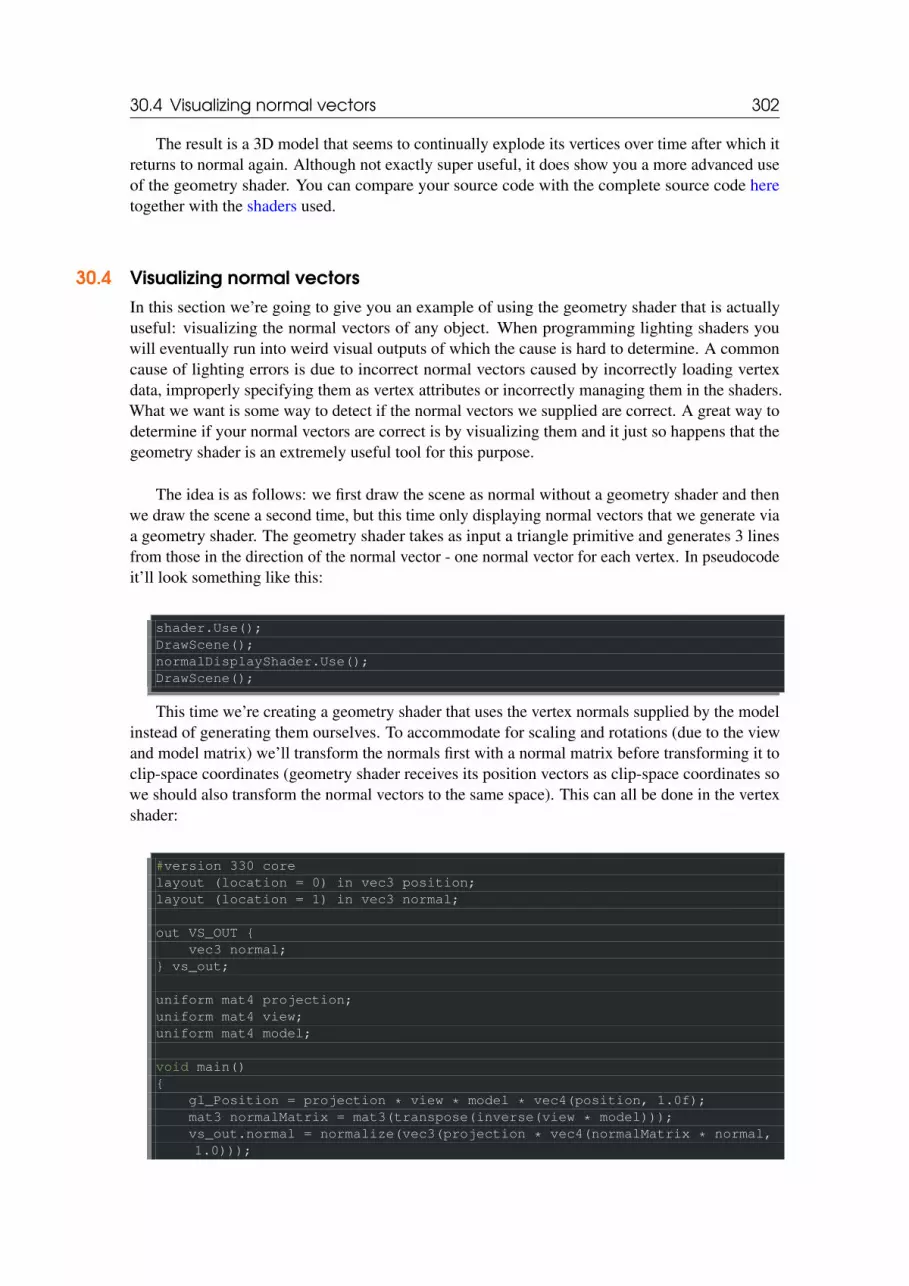
30.4 Visualizing normal vectors 302
The result is a 3D model that seems to continually explode its vertices over time after which itreturns to normal again. Although not exactly super useful, it does show you a more advanced useof the geometry shader. You can compare your source code with the complete source code heretogether with the shaders used.
30.4 Visualizing normal vectorsIn this section we’re going to give you an example of using the geometry shader that is actuallyuseful: visualizing the normal vectors of any object. When programming lighting shaders youwill eventually run into weird visual outputs of which the cause is hard to determine. A commoncause of lighting errors is due to incorrect normal vectors caused by incorrectly loading vertexdata, improperly specifying them as vertex attributes or incorrectly managing them in the shaders.What we want is some way to detect if the normal vectors we supplied are correct. A great way todetermine if your normal vectors are correct is by visualizing them and it just so happens that thegeometry shader is an extremely useful tool for this purpose.
The idea is as follows: we first draw the scene as normal without a geometry shader and thenwe draw the scene a second time, but this time only displaying normal vectors that we generate viaa geometry shader. The geometry shader takes as input a triangle primitive and generates 3 linesfrom those in the direction of the normal vector - one normal vector for each vertex. In pseudocodeit’ll look something like this:
shader.Use();DrawScene();normalDisplayShader.Use();DrawScene();
This time we’re creating a geometry shader that uses the vertex normals supplied by the modelinstead of generating them ourselves. To accommodate for scaling and rotations (due to the viewand model matrix) we’ll transform the normals first with a normal matrix before transforming it toclip-space coordinates (geometry shader receives its position vectors as clip-space coordinates sowe should also transform the normal vectors to the same space). This can all be done in the vertexshader:
#version 330 corelayout (location = 0) in vec3 position;layout (location = 1) in vec3 normal;
out VS_OUT {vec3 normal;
} vs_out;
uniform mat4 projection;uniform mat4 view;uniform mat4 model;
void main(){
gl_Position = projection * view * model * vec4(position, 1.0f);mat3 normalMatrix = mat3(transpose(inverse(view * model)));vs_out.normal = normalize(vec3(projection * vec4(normalMatrix * normal,1.0)));

30.4 Visualizing normal vectors 303
}
The transformed clip-space normal vector is then passed to the next shader stage via an interfaceblock. The geometry shader then takes each vertex (with a position and a normal vector) and drawsa normal vector from each position vector:
#version 330 corelayout (triangles) in;layout (line_strip, max_vertices = 6) out;
in VS_OUT {vec3 normal;
} gs_in[];
const float MAGNITUDE = 0.4f;
void GenerateLine(int index){
gl_Position = gl_in[index].gl_Position;EmitVertex();gl_Position = gl_in[index].gl_Position + vec4(gs_in[index].normal, 0.0f) * MAGNITUDE;EmitVertex();EndPrimitive();
}
void main(){
GenerateLine(0); // First vertex normalGenerateLine(1); // Second vertex normalGenerateLine(2); // Third vertex normal
}
The contents of geometry shaders like these should be self-explanatory by now. Note that we’remultiplying the normal vector by a MAGNITUDE vector to restrain the size of the displayed normalvectors (otherwise they’d be a bit too large).
Since visualizing normals are mostly used for debugging purposes we can just display them asmono-colored lines (or super-fancy lines if you feel like it) with the help of the fragment shader:
#version 330 coreout vec4 color;
void main(){
color = vec4(1.0f, 1.0f, 0.0f, 1.0f);}
Now rendering your model with normal shaders first and then with the special normal-visualizing shader you’ll see something like this:

30.4 Visualizing normal vectors 304
Apart from the fact that our nanosuit now looks like a hairy guy with kitchen mittens on, itgives us a really useful method for determining if the normal vectors of a model are indeed correct.You can imagine that geometry shaders like this are also frequently used for adding fur to objects.
You can find the OpenGL’s source code here together with its normal-displaying shaders.

31. Instancing
Say you have a scene where you’re drawing a lot of models where most of these models containthe same set of vertex data, but with different world transformations. Think of a scene filled withgrass leaves: each grass leave is a small model consisting of only a few triangles. You’ll probablywant to draw quite a few of them and your scene might end up with thousands or maybe tens ofthousands of grass leaves that you need to render each frame. Because each leaf consists of onlya few triangles the leaf is rendered almost instantly, but all those thousands of render calls you’llhave to make will drastically reduce performance.
If we were to actually render such a large amount of objects it will look a bit like this in code:
for(GLuint i = 0; i < amount_of_models_to_draw; i++){
DoSomePreparations(); // bind VAO, bind Textures, set uniforms etc.glDrawArrays(GL_TRIANGLES, 0, amount_of_vertices);
}
When drawing many instances of your model like this you’ll quickly reach a performancebottleneck because of the many drawing calls. Compared to rendering the actual vertices, tellingthe GPU to render your vertex data with functions like glDrawArrays or glDrawElementseats up quite some performance since OpenGL must make necessary preparations before it candraw your vertex data (like telling the GPU which buffer to read data from, where to find vertexattributes and all this over the relatively slow CPU to GPU bus). So even though rendering yourvertices is super fast, giving your GPU the commands to render them isn’t.
It would be much more convenient if we could send some data over to the GPU once and thentell OpenGL to draw multiple objects with a single drawing call using this data. Enter instancing.
Instancing is a technique where we draw many objects at once with a single render call, saving usall the CPU -> GPU communications each time we need to render an object; this only has to be done

306
once. To render using instancing all we need to do is change the render calls glDrawArrays andglDrawElements to glDrawArraysInstanced and glDrawElementsInstanced re-spectively. These instanced versions of the classic rendering functions take an extra parametercalled the instance count that sets the number of instances we want to render. We thus sent all the re-quired data to the GPU only once, and then tell the GPU how it should draw all these instances witha single call. The GPU then renders all these instances without having to continually communicatewith the CPU.
By itself this function is a bit useless. Rendering the same object a thousand times is of no useto us since each of the rendered objects are rendered exactly the same and thus also at the samelocation; we would only see one object! For this reason GLSL embedded another built-in variablein the vertex shader called gl_InstanceID.
When drawing via one of the instanced rendering calls, gl_InstanceID is incremented foreach instance being rendered starting from 0. If we were to render the 43th instance for example,gl_InstanceID would have the value 42 in the vertex shader. Having a unique value perinstance means we could now for example index into a large array of position values to positioneach instance at a different location in the world.
To get a feel for instanced drawing we’re going to demonstrate a simple example that renders ahundred 2D quads in normalized device coordinates with just one render call. We accomplish thisby adding a small offset to each instanced quad by indexing a uniform array of 100 offset vectors.The result is a neatly organized grid of quads that fill the entire window:
Each quad consists of 2 triangles with a total of 6 vertices. Each vertex contains a 2D NDCposition vector and a color vector. Below is the vertex data used for this example - the triangles are

307
quite small to properly fit the screen in large quantities:
GLfloat quadVertices[] = {// Positions // Colors-0.05f, 0.05f, 1.0f, 0.0f, 0.0f,0.05f, -0.05f, 0.0f, 1.0f, 0.0f,
-0.05f, -0.05f, 0.0f, 0.0f, 1.0f,
-0.05f, 0.05f, 1.0f, 0.0f, 0.0f,0.05f, -0.05f, 0.0f, 1.0f, 0.0f,0.05f, 0.05f, 0.0f, 1.0f, 1.0f
};
The colors of the quads are accomplished with the fragment shader that receives a forwardedcolor vector from the vertex shader and sets it as its color output:
#version 330 corein vec3 fColor;out vec4 color;
void main(){
color = vec4(fColor, 1.0f);}
Nothing new so far, but at the vertex shader it’s starting to get interesting:
#version 330 corelayout (location = 0) in vec2 position;layout (location = 1) in vec3 color;
out vec3 fColor;
uniform vec2 offsets[100];
void main(){
vec2 offset = offsets[gl_InstanceID];gl_Position = vec4(position + offset, 0.0f, 1.0f);fColor = color;
}
Here we defined a uniform array called offsets that contain a total of 100 offset vectors.Within the vertex shader we then retrieve an offset vector for each instance by indexing theoffsets array using gl_InstanceID. If we were to draw 100 quads using instanced drawingwe’d get 100 quads located at different positions with just this vertex shader.
We do need to actually set the offset positions that we calculate in a nested for-loop before weenter the game loop:
glm::vec2 translations[100];int index = 0;GLfloat offset = 0.1f;for(GLint y = -10; y < 10; y += 2){
for(GLint x = -10; x < 10; x += 2)

31.1 Instanced arrays 308
{glm::vec2 translation;translation.x = (GLfloat)x / 10.0f + offset;translation.y = (GLfloat)y / 10.0f + offset;translations[index++] = translation;
}}
Here we create a set of 100 translation vectors that contains a translation vector for all positionsin a 10x10 grid. Aside from generating the translations array we’d also need to transfer thedata to the vertex shader’s uniform array:
shader.Use();for(GLuint i = 0; i < 100; i++){
stringstream ss;string index;ss << i;index = ss.str();GLint location = glGetUniformLocation(shader.Program, ("offsets[" +index + "]").c_str())glUniform2f(location, translations[i].x, translations[i].y);
}
Within this snippet of code we transform the for-loop counter i to a string that we then useto dynamically create a location string for querying the uniform location. For each item in theoffsets uniform array we then set the corresponding translation vector.
Now that all the preparations are finished we can start rendering the quads. To draw viainstanced rendering we call glDrawArraysInstanced or glDrawElementsInstanced.Since we’re not using an element index buffer we’re going to call the glDrawArrays version:
glBindVertexArray(quadVAO);glDrawArraysInstanced(GL_TRIANGLES, 0, 6, 100);glBindVertexArray(0);
The parameters of glDrawArraysInstanced are exactly the same as glDrawArraysexcept the last parameter that sets the number of instances we want to draw. Since we want todisplay 100 quads in a 10x10 grid we set it equal to 100. Running the code should now give youthe familiar image of 100 colorful quads.
31.1 Instanced arraysWhile the previous implementation works fine for this specific use case, whenever we are renderinga lot more than 100 instances (which is quite common) we will eventually hit a limit on the amountof uniform data we can send to the shaders. Another alternative is called instanced arrays that isdefined as a vertex attribute (allowing us to store much more data) that is only updated wheneverthe vertex shader renders a new instance.
With vertex attributes, each run of the vertex shader will cause GLSL to retrieve the next set ofvertex attributes that belong to the current vertex. When defining a vertex attribute as an instancedarray however, the vertex shader only updates the content of the vertex attribute per instance instead

31.1 Instanced arrays 309
of per vertex. This allows us to use the standard vertex attributes for data per vertex and use theinstanced array for storing data that is unique per instance.
To give you an example of an instanced array we’re going to take the previous example andrepresent the offset uniform array as an instanced array. We’ll have to update the vertex shader byadding another vertex attribute:
#version 330 corelayout (location = 0) in vec2 position;layout (location = 1) in vec3 color;layout (location = 2) in vec2 offset;
out vec3 fColor;
void main(){
gl_Position = vec4(position + offset, 0.0f, 1.0f);fColor = color;
}
We no longer use gl_InstanceID and can directly use the offset attribute without firstindexing into a large uniform array.
Because an instanced array is a vertex attribute, just like the position and color variables,we also need to store its content in a vertex buffer object and configure its attribute pointer. We’refirst going to store the translations array (from the previous section) in a new buffer object:
GLuint instanceVBO;glGenBuffers(1, &instanceVBO);glBindBuffer(GL_ARRAY_BUFFER, instanceVBO);glBufferData(GL_ARRAY_BUFFER, sizeof(glm::vec2) * 100, &translations[0],
GL_STATIC_DRAW);glBindBuffer(GL_ARRAY_BUFFER, 0);
Then we also need to set its vertex attribute pointer and enable the vertex attribute:
glEnableVertexAttribArray(2);glBindBuffer(GL_ARRAY_BUFFER, instanceVBO);glVertexAttribPointer(2, 2, GL_FLOAT, GL_FALSE, 2 * sizeof(GLfloat), (
GLvoid*)0);glBindBuffer(GL_ARRAY_BUFFER, 0);glVertexAttribDivisor(2, 1);
What makes this code interesting is the last line where we call glVertexAttribDivisor.This function tells OpenGL when to update the content of a vertex attribute to the next element. Itsfirst parameter is the vertex attribute in question and the second parameter the attribute divisor. Bydefault the attribute divisor is 0 which tells OpenGL to update the content of the vertex attributeeach iteration of the vertex shader. By setting this attribute to 1 we’re telling OpenGL that we wantto update the content of the vertex attribute when we start to render a new instance. By setting it to2 we’d update the content every 2 instances and so on. By setting the attribute divisor to 1 we’reeffectively telling OpenGL that the vertex attribute at attribute location 2 is an instanced array.
If we now were to render the quads again using glDrawArraysInstanced we’d get thefollowing output:

31.1 Instanced arrays 310
This is exactly the same as the previous example, but this time accomplished using instancedarrays, which allows us to pass a lot more data (as much as memory allows us to) to the vertexshader for instanced drawing.
For fun we could also slowly downscale each quad from top-right to bottom-left usinggl_InstanceID again, because why not?
void main(){
vec2 pos = position * (gl_InstanceID / 100.0f);gl_Position = vec4(pos + offset, 0.0f, 1.0f);fColor = color;
}
The result is that the first instances of the quads are drawn extremely small and the furtherwe’re in the process of drawing the instances, the closer gl_InstanceID gets to 100 and thusthe more the quads regain their original size. It’s perfectly legal to use instanced arrays togetherwith gl_InstanceID like this.

31.2 An asteroid field 311
If you’re still a bit unsure about how instanced rendering works or want to see how everythingfits together you can find the full source code of the application here.
While fun and all, these examples aren’t really good examples of instancing. Yes, they do giveyou an easy overview of how instancing works, but instancing is extremely useful when drawing anenormous amount of similar objects which we haven’t really been doing so far. For that reasonwe’re going to venture into space in the next section to see the real power of instanced rendering.
31.2 An asteroid fieldImagine a scene where we have one large planet that’s at the center of a large asteroid ring. Suchan asteroid ring could contain thousands or tens of thousands of rock formations and quicklybecomes un-renderable on any decent graphics card. This scenario proves itself particularly usefulfor instanced rendering, since all the asteroids can be represented using a single model. Each singleasteroid then contains minor variations using a transformation matrix unique to each asteroid.
To demonstrate the impact of instanced rendering we’re first going to render a scene of asteroidsflying around a planet without instanced rendering. The scene will contain a large planet model thatcan be downloaded from here and a large set of asteroid rocks that we properly position around theplanet. The asteroid rock model can be downloaded here.
Within the code samples we load the models using the model loader we’ve previously definedin the model loading tutorials.
To achieve the effect we’re looking for we’ll be generating a transformation matrix for each

31.2 An asteroid field 312
asteroid that we’ll use as their model matrix. The transformation matrix is created by first translatingthe rock somewhere in the asteroid ring - we’ll also add a small random displacement value tothis offset to make the ring look more natural. Then we apply a random scale and a randomrotation around a rotation vector. The result is a transformation matrix that transforms each asteroidsomewhere around the planet while also giving it a more natural and unique look compared to otherasteroids. The result is a ring full of asteroids where each asteroid looks different to the other.
GLuint amount = 1000;glm::mat4* modelMatrices;modelMatrices = new glm::mat4[amount];srand(glfwGetTime()); // initialize random seedGLfloat radius = 50.0;GLfloat offset = 2.5f;for(GLuint i = 0; i < amount; i++){
glm::mat4 model;// 1. Translation: displace along circle with ’radius’ in range [-offset, offset]GLfloat angle = (GLfloat)i / (GLfloat)amount * 360.0f;GLfloat displacement = (rand() \% (GLint)(2 * offset * 100)) / 100.0f -offset;GLfloat x = sin(angle) * radius + displacement;displacement = (rand() \% (GLint)(2 * offset * 100)) / 100.0f - offset;GLfloat y = displacement * 0.4f; // y value has smaller displacementdisplacement = (rand() \% (GLint)(2 * offset * 100)) / 100.0f - offset;GLfloat z = cos(angle) * radius + displacement;model = glm::translate(model, glm::vec3(x, y, z));// 2. Scale: Scale between 0.05 and 0.25fGLfloat scale = (rand() \% 20) / 100.0f + 0.05;model = glm::scale(model, glm::vec3(scale));// 3. Rotation: add random rotation around a (semi)randomly pickedrotation axis vectorGLfloat rotAngle = (rand() \% 360);model = glm::rotate(model, rotAngle, glm::vec3(0.4f, 0.6f, 0.8f));// 4. Now add to list of matricesmodelMatrices[i] = model;
}
This piece of code might look a little daunting, but we basically transform the x and z positionof the asteroid along a circle with a radius defined by radius and randomly displace each asteroida little around the circle by -offset and offset. We give the y displacement less of an impactto create a more flat asteroid ring. Then we apply scale and rotation transformations and store theresulting transformation matrix in modelMatrices that is of size amount. Here we generate atotal of 1000 model matrices, one per asteroid.
After loading the planet and rock models and compiling a set of shaders, the rendering codethen looks a bit like this:
// Draw Planetshader.Use();glm::mat4 model;model = glm::translate(model, glm::vec3(0.0f, -5.0f, 0.0f));model = glm::scale(model, glm::vec3(4.0f, 4.0f, 4.0f));glUniformMatrix4fv(modelLoc, 1, GL_FALSE, glm::value_ptr(model));planet.Draw(shader);

31.2 An asteroid field 313
// Draw Asteroid circlefor(GLuint i = 0; i < amount; i++){
glUniformMatrix4fv(modelLoc, 1, GL_FALSE, glm::value_ptr(modelMatrices[i]));rock.Draw(shader);
}
First we draw the planet model that we translate and scale a bit to accommodate to the sceneand then we draw a number of rock models equal to the amount of transformations we calculated.Before we draw each rock however, we first set the corresponding model transformation matrixwithin the shader.
The result is then a space-like scene where we can see a natural-looking asteroid ring around aplanet:
This scene contains a total of 1001 rendering calls per frame of which 1000 are of the rockmodel. You can find the source code for this scene here together with the vertex and fragmentshader.
As soon as we start to increase this number we will quickly notice that the scene stops runningsmoothly and the number of frames we’re able to render per second reduces drastically. As soon aswe set amount to 2000 the scene already becomes so slow, it’s difficult to move around.
Let’s now try to render the same scene, but this time using instanced rendering. We first need toadapt the vertex shader a little:

31.2 An asteroid field 314
#version 330 corelayout (location = 0) in vec3 position;layout (location = 2) in vec2 texCoords;layout (location = 3) in mat4 instanceMatrix;
out vec2 TexCoords;
uniform mat4 projection;uniform mat4 view;
void main(){
gl_Position = projection * view * instanceMatrix * vec4(position, 1.0f);TexCoords = texCoords;
}
We’re no longer using a model uniform variable, but instead declare a mat4 as a vertex attributeso we can store an instanced array of transformation matrices. However, when we declare a datatypeas a vertex attribute that is greater than a vec4 things work a bit differently. The maximum amountof data allowed as a vertex attribute is equal to a vec4. Because a mat4 is basically 4 vec4s, wehave to reserve 4 vertex attributes for this specific matrix. Because we assigned it a location of 3,the columns of the matrix will have vertex attribute locations of 3, 4, 5 and 6.
We then have to set each of the attribute pointers of those 4 vertex attributes and configure themas instanced arrays:
for(GLuint i = 0; i < rock.meshes.size(); i++){
GLuint VAO = rock.meshes[i].VAO;// Vertex Buffer ObjectGLuint buffer;glBindVertexArray(VAO);glGenBuffers(1, &buffer);glBindBuffer(GL_ARRAY_BUFFER, buffer);glBufferData(GL_ARRAY_BUFFER, amount * sizeof(glm::mat4), &modelMatrices[0], GL_STATIC_DRAW);// Vertex AttributesGLsizei vec4Size = sizeof(glm::vec4);glEnableVertexAttribArray(3);glVertexAttribPointer(3, 4, GL_FLOAT, GL_FALSE, 4 * vec4Size, (GLvoid*)0);glEnableVertexAttribArray(4);glVertexAttribPointer(4, 4, GL_FLOAT, GL_FALSE, 4 * vec4Size, (GLvoid*)(vec4Size));glEnableVertexAttribArray(5);glVertexAttribPointer(5, 4, GL_FLOAT, GL_FALSE, 4 * vec4Size, (GLvoid*)(2 * vec4Size));glEnableVertexAttribArray(6);glVertexAttribPointer(6, 4, GL_FLOAT, GL_FALSE, 4 * vec4Size, (GLvoid*)(3 * vec4Size));
glVertexAttribDivisor(3, 1);glVertexAttribDivisor(4, 1);glVertexAttribDivisor(5, 1);glVertexAttribDivisor(6, 1);
glBindVertexArray(0);

31.2 An asteroid field 315
}
Note that we cheated a little by declaring the VAO variable of the Mesh as a public variableinstead of a private variable so we could access its vertex array object. This is not the cleanestsolution, but just a simple modification to suit this tutorial. Aside from the little hack, this codeshould be clear. We’re basically declaring how OpenGL should interpret the buffer for each of thematrix’s vertex attributes and that each of those vertex attributes is an instanced array.
Next we take the VAO of the mesh(es) again and this time draw using glDrawElementsInstanced:
// Draw meteoritesinstanceShader.Use();for(GLuint i = 0; i < rock.meshes.size(); i++){
glBindVertexArray(rock.meshes[i].VAO);glDrawElementsInstanced(
GL_TRIANGLES, rock.meshes[i].vertices.size(), GL_UNSIGNED_INT, 0,amount);glBindVertexArray(0);
}
Here we draw the same amount of asteroids as the earlier example, but this time usinginstanced rendering. The results should be similar, but you’ll start to really see the effect ofinstanced rendering when we start to increase this amount variable. Without instanced renderingwe were able to smoothly render around 1000 to 1500 asteroids. With instanced rendering wecan now set this value to 100000 that, with the rock model having 576 vertices, equals around57 million vertices drawn each frame without any performance drops!

31.2 An asteroid field 316
This image was rendered with 100000 asteroids with a radius of 150.0f and an offset equalto 25.0f. You can find the source code of the instanced rendering demo here.
On different machines an asteroid count of 100000 might be a bit too high, so trytweaking the values till you reach an acceptable framerate.
As you can see, with the right type of environments instanced rendering can make an enormousdifference to the rendering capabilities of your graphics card. For this reason, instanced renderingis commonly used for grass, flora, particles and scenes like this - basically any scene with manyrepeating shapes can benefit from instanced rendering.

32. Anti Aliasing
Somewhere in your adventurous rendering journey you probably came across some jagged saw-likepatterns along the edges of your models. The reason these jagged edges appear is due to how therasterizer transforms the vertex data into actual fragments behind the scene. An example of whatthese jagged edges look like can already be seen when drawing a simple cube:
While not immediately visible, if you take a closer look at the edges of the cube you’ll see ajagged pattern. If we zoom in you’d see the following:

32.1 Multisampling 318
This is clearly not something we want in a final version of an application. This effect, ofclearly seeing the pixel formations an edge is composed of, is called aliasing. There are quite afew techniques out there called anti-aliasing techniques that fight exactly this aliasing behavior toproduce more smooth edges.
At first we had a technique called super sample anti-aliasing (SSAA) that temporarily useda much higher resolution to render the scene in (super sampling) and when the visual output isupdated in the framebuffer, the resolution was downsampled back to the normal resolution. Thisextra resolution was used to prevent these jagged edges. While it did provide us with a solution tothe aliasing problem, it came with a major performance drawback since we had to draw a lot morefragments than usual. This technique therefore only had a short glory moment.
This technique did gave birth to a more modern technique called multisample anti-aliasing orMSAA that borrows from the concepts behind SSAA while implementing a much more efficientapproach. In this tutorial we’ll be extensively discussing this MSAA technique that is built-in inOpenGL.
32.1 MultisamplingTo understand what multisampling is and how it works into solving the aliasing problem we firstneed to delve a bit further into the inner workings of OpenGL’s rasterizer.
The rasterizer is the combination of all algorithms and processes that sit between your finalprocessed vertices and the fragment shader. The rasterizer takes all vertices belonging to a singleprimitive and transforms this to a set of fragments. Vertex coordinates can theoretically have anycoordinate, but fragments can’t since they are bound by the resolution of your window. There willalmost never be a one-on-one mapping between vertex coordinates and fragments, so the rasterizerhas to determine in some way at what fragment/screen-coordinate each specific vertex will end upat.

32.1 Multisampling 319
Here we see a grid of screen pixels where the center of each pixel contains a sample point thatis used to determine if a pixel is covered by the triangle. The red sample points are covered by thetriangle and a fragment will be generated for that covered pixel. Even though some parts of thetriangle edges still enter certain screen pixels, the pixel’s sample point is not covered by the insideof the triangle so this pixel won’t be influenced by any fragment shader.
You can probably already figure out the origin of aliasing right now. The complete renderedversion of the triangle would look like this on your screen:
Due to the limited amount of screen pixels, some pixels will be rendered along an edge andsome won’t. The result is that we’re rendering primitives with non-smooth edges giving rise to thejagged edges we’ve seen before.
What multisampling does is not use a single sampling point for determining coverage of thetriangle, but use multiple sample points (guess where it got its name from). Instead of a singlesample point at the center of each pixel we’re going to place 4 subsamples in a general patternand use those to determine pixel coverage. This does mean that the size of the color buffer is alsoincreased by the number of subsamples we’re using per pixel.

32.1 Multisampling 320
The left side of the image shows how we would normally determine the coverage of a triangle.This specific pixel won’t run a fragment shader (and thus remains blank) since its sample pointwasn’t covered by the triangle. The right side of the image shows a multisampled version whereeach pixel contains 4 sample points. Here we can see that only 2 of the sample points cover thetriangle.
The amount of sample points can be any number we’d like with more samples giving usbetter coverage precision.
This is where multisampling becomes interesting. We determined that 2 subsamples werecovered by the triangle so the next step is to determine a color for this specific pixel. Our initialguess would be that we run the fragment shader for each covered subsample and later averagethe colors of each subsample per pixel. In this case we’d run the fragment shader twice on theinterpolated vertex data at each subsample and store the resulting color in those sample points. Thisis (fortunately) not how it works, because this basically means we need to run a lot more fragmentshaders than without multisampling, drastically reducing performance.
How MSAA really works is that the fragment shader is only run once per pixel (for eachprimitive) regardless of how many subsamples the triangle covers. The fragment shader is run withthe vertex data interpolated to the center of the pixel and the resulting color is then stored insideeach of the covered subsamples. Once the color buffer’s subsamples are filled with all the colors ofthe primitives we’ve rendered, all these colors are then averaged per pixel resulting in a single colorper pixel. Because only two of the 4 samples were covered in the previous image, the color of thepixel was averaged with the triangle’s color and the color stored at the other 2 sample points (inthis case: the clear color) resulting in a light blue-ish color.
The result is a color buffer where all the primitive edges now produce a smoother pattern. Let’ssee what multisampling looks like when we again determine the coverage of the earlier triangle:

32.1 Multisampling 321
Here each pixel contains 4 subsamples (the irrelevant samples were hidden) where the bluesubsamples are covered by the triangle and the gray sample points aren’t. Within the inner regionof the triangle all pixels will run the fragment shader once where its color output it is stored in all4 subsamples. At the edges of the triangle not all subsamples will be covered so the result of thefragment shader is only stored at some subsamples. Based on the amount of subsamples covered,the resulting pixel color is determined by the triangle color and the other subsample’s stored colors.
Basically, the more sample points are covered by the triangle, the more the eventual pixel color isthat of the triangle. If we then fill the pixel colors just like we did earlier with the non-multisampledtriangle we get the following image:

32.2 MSAA in OpenGL 322
For each pixel, the less subsamples are part of the triangle, the less it takes the color of thetriangle as you can see in the image. The hard edges of the triangle are now surrounded by colorsslightly lighter than the actual edge color, which causes the edge to appear smooth when viewedfrom a distance.
Not only color values are affected by the multisampling, but also the depth and stencil test nowmake use of the multiple sample points. For depth testing, the vertex’s depth value is interpolatedto each subsample before running the depth test and for stencil testing we store stencil values persubsample, instead of per pixel. This does mean that the size of the depth and stencil buffer arenow also increased by the amount of subsamples per pixel.
What we’ve discussed so far is a basic overview of how multisampled anti-aliasing worksbehind the scenes. The actual logic behind the rasterizer is a bit more complicated than we’vediscussed here, but you should be able to understand the concept and logic behind multisampledanti-aliasing now.
32.2 MSAA in OpenGLIf we want to use MSAA in OpenGL we need to use a color buffer that is able to store more thanone color value per pixel (since multisampling requires us to store a color per sample point). Wethus need a new type of buffer that can store a given amount of multisamples and this is called amultisample buffer.
Most windowing systems are able to provide us a multisample buffer instead of a defaultcolor buffer. GLFW also gives us this functionality and all we need to do is hint GLFW thatwe’d like to use a multisample buffer with N samples instead of a normal color buffer by callingglfwWindowHint before creating the window:

32.3 Off-screen MSAA 323
glfwWindowHint(GLFW_SAMPLES, 4);
When we now call glfwCreateWindow the rendering window is created, this time with acolor buffer containing 4 subsamples per screen coordinate. GLFW also automatically creates adepth and stencil buffer with 4 subsamples per pixel. This does mean that the size of all the buffersis increased by 4.
Now that we asked GLFW for multisampled buffers we need to enable multisampling bycalling glEnable and enabling GL_MULTISAMPLE. On most OpenGL drivers, multisamplingis enabled by default so this call is then a bit redundant, but it’s usually a good idea to enable itanyways. This way all OpenGL implementations have multisampling enabled.
glEnable(GL_MULTISAMPLE);
Once the default framebuffer has multisampled buffer attachments, all we need to do to enablemultisampling is just call glEnable and we’re done. Because the actual multisampling algorithmsare implemented in the rasterizer in your OpenGL drivers there’s not much else we need to do. Ifwe now were to render the green cube from the start of this tutorial we should see much smootheredges:
This container does indeed look a lot smoother and the same will apply for any other objectyou’re drawing in your scene. You can find the source code for this simple example here.
32.3 Off-screen MSAABecause GLFW takes care of creating the multisampled buffers, enabling MSAA is quite easy. Ifwe want to use our own framebuffers however, for some off-screen rendering, we have to generatethe multisampled buffers ourselves; now we do need to take care of creating multisampled buffers.

32.3 Off-screen MSAA 324
There are two ways we can create multisampled buffers to act as attachments for framebuffers:texture attachments and renderbuffer attachments, similar to normal attachments like we’ve dis-cussed in the framebuffers tutorial.
32.3.1 Multisampled texture attachmentsTo create a texture that supports storage of multiple sample points we use glTexImage2DMultisampleinstead of glTexImage2D that accepts GL_TEXTURE_2D_MULTISAPLE as its texture target:
glBindTexture(GL_TEXTURE_2D_MULTISAMPLE, tex);glTexImage2DMultisample(GL_TEXTURE_2D_MULTISAMPLE, samples, GL_RGB, width,
height, GL_TRUE);glBindTexture(GL_TEXTURE_2D_MULTISAMPLE, 0);
The second argument now sets the number of samples we’d like the texture to have. If the lastargument is equal to GL_TRUE the image will use identical sample locations and the same numberof subsamples for each texel.
To attach a multisampled texture to a framebuffer we use glFramebufferTexture2D, butthis time with GL_TEXTURE_2D_MULTISAMPLE as the texture type:
glFramebufferTexture2D(GL_FRAMEBUFFER, GL_COLOR_ATTACHMENT0,GL_TEXTURE_2D_MULTISAMPLE, tex, 0);
The currently bound framebuffer now has a multisampled color buffer in the form of a textureimage.
32.3.2 Multisampled renderbuffer objectsLike textures, creating a multisampled renderbuffer object isn’t difficult. It is even quite easy sinceall we need to change is the call to glRenderbufferStorage that is now glRenderbufferStorageMultisamplewhen we specify the (currently bound) renderbuffer’s memory storage:
glRenderbufferStorageMultisample(GL_RENDERBUFFER, 4, GL_DEPTH24_STENCIL8,width, height);
The one thing that changed here is the extra parameter after the renderbuffer target where weset the amount of samples we’d like to have which is 4 in this particular case.
32.3.3 Render to multisampled framebufferRendering to a multisampled framebuffer object goes automatically. Whenever we draw anythingwhile the framebuffer object is bound, the rasterizer will take care of all the multisample operations.We then end up with a multisampled color buffer and/or depth and stencil buffer. Because amultisampled buffer is a bit special we can’t directly use their buffer images for other operationslike sampling them in a shader.
A multisampled image contains much more information than a normal image so what we needto do is downscale or resolve the image. Resolving a multisampled framebuffer is generally done

32.3 Off-screen MSAA 325
via glBlitFramebuffer that copies a region from one framebuffer to the other while alsoresolving any multisampled buffers.
glBlitFramebuffer transfers a given source region defined by 4 screen-space coordinatesto a given target region also defined by 4 screen-space coordinates. You might remember fromthe framebuffers tutorial that if we bind to GL_FRAMEBUFFER we’re binding to both the readand draw framebuffer targets. We could also bind to those targets individually by binding theframebuffers to GL_READ_FRAMEBUFFER and GL_DRAW_FRAMEBUFFER respectively. TheglBlitFramebuffer function reads from those two targets to determine which is the sourceand which is the target framebuffer. We could then transfer the multisampled framebuffer output tothe actual screen by blitting the image to the default framebuffer like so:
glBindFramebuffer(GL_READ_FRAMEBUFFER, multisampledFBO);glBindFramebuffer(GL_DRAW_FRAMEBUFFER, 0);glBlitFramebuffer(0, 0, width, height, 0, 0, width, height,
GL_COLOR_BUFFER_BIT, GL_NEAREST);
If we then were to render the application we’d get the same output as without a framebuffer: alime-green cube that is displayed using MSAA and thus shows significantly less jagged edges:
You can find the source code here.
But what if we wanted to use the texture result of a multisampled framebuffer to do stuff likepost-processing? We can’t directly use the multisampled texture(s) in the fragment shader. Whatwe could do is blit the multisampled buffer(s) to a different FBO with a non-multisampled textureattachment. We then use this ordinary color attachment texture for post-processing, effectivelypost-processing an image rendered via multisampling. This does mean we have to generate anew FBO that acts solely as an intermediate framebuffer object to resolve the multisampled bufferinto a normal 2D texture we can use in the fragment shader. This process looks a bit like this inpseudocode:

32.3 Off-screen MSAA 326
GLuint msFBO = CreateFBOWithMultiSampledAttachments();// Then create another FBO with a normal texture color attachment...glFramebufferTexture2D(GL_FRAMEBUFFER, GL_COLOR_ATTACHMENT0, GL_TEXTURE_2D,
screenTexture, 0);...while(!glfwWindowShouldClose(window)){
...
glBindFramebuffer(msFBO);ClearFrameBuffer();DrawScene();// Now resolve multisampled buffer(s) into intermediate FBOglBindFramebuffer(GL_READ_FRAMEBUFFER, msFBO);glBindFramebuffer(GL_DRAW_FRAMEBUFFER, intermediateFBO);glBlitFramebuffer(0, 0, width, height, 0, 0, width, height,GL_COLOR_BUFFER_BIT, GL_NEAREST);// Now scene is stored as 2D texture image, so use that image for post-processingglBindFramebuffer(GL_FRAMEBUFFER, 0);ClearFramebuffer();glBindTexture(GL_TEXTURE_2D, screenTexture);DrawPostProcessingQuad();
...}
If we’d then implement this into the post-processing code of the framebuffers tutorial we’reable to create all kinds of cool post-processing effects on a texture of a scene with (almost) nojagged edges. With the blur kernel filter applied it’ll look something like this:
You can find the full source code of the MSAA version of post-processing here.

32.4 Custom Anti-Aliasing algorithm 327
Because the screen texture is a normal texture again with just a single sample point,some post-processing filters like edge-detection will introduce jagged edges again. Toaccommodate for this you could blur the texture afterwards or create your own anti-aliasing algorithm.
You can see that when we want to combine multisampling with off-screen rendering we’d needto take care of some extra details. All the details are worth the extra effort though since multisam-pling significantly boosts the visual quality of your scene. Do note that enabling multisampling cannoticeably reduce performance of your application the more samples you use. As of this writing,using MSAA with 4 samples is commonly preferred.
32.4 Custom Anti-Aliasing algorithmIt is also possible to directly pass a multisampled texture image to the shaders instead of firstresolving them. GLSL then gives us the option to sample the texture images per subsample so wecan create our own anti-aliasing algorithms which is commonly done by large graphics applications.
To retrieve the color value per subsample you’d have to define the texture uniform sampler as asampler2DMS instead of the usual sampler2D:
uniform sampler2DMS screenTextureMS;
Using the texelFetch function it is then possible to retrieve the color value per sample:
vec4 colorSample = texelFetch(screenTextureMS, TexCoords, 3); // 4thsubsample
We won’t go into the details of creating custom anti-aliasing techniques, but merely providedsome pointers as to how you might implement a feature like this.

V33 Advanced Lighting . . . . . . . . . . . . . . . . . 329
34 Gamma Correction . . . . . . . . . . . . . . . . . 334
35 Shadow Mapping . . . . . . . . . . . . . . . . . . 342
36 Point Shadows . . . . . . . . . . . . . . . . . . . . . . 362
37 Normal Mapping . . . . . . . . . . . . . . . . . . . 376
38 Parallax Mapping . . . . . . . . . . . . . . . . . . 392
39 HDR . . . . . . . . . . . . . . . . . . . . . . . . . . . . . . . . 406
40 Bloom . . . . . . . . . . . . . . . . . . . . . . . . . . . . . 413
41 Deferred Shading . . . . . . . . . . . . . . . . . . . 424
42 SSAO . . . . . . . . . . . . . . . . . . . . . . . . . . . . . . 440
Advanced Lighting

33. Advanced Lighting
In the lighting tutorials we briefly introduced the Phong lighting model to bring a basic amount ofrealism into our scenes. The Phong model looks quite nice, but has a few nuances we’ll focus on inthis tutorial.
33.1 Blinn-PhongPhong lighting is a great and very efficient approximation of lighting, but its specular reflectionsbreak down in certain conditions, specifically when the shininess property is low resulting in a large(rough) specular area. The image below shows what happens when we use a specular shininessexponent of 1.0 on a flat textured plane:
You can see at the edges that the specular area is immediately cut off. The reason this happens

33.1 Blinn-Phong 330
is that the angle between the view vector and the reflection vector is not allowed to go higher than90 degrees. If the angle is larger than 90 degrees the resulting dot product becomes negative andthis results in specular exponents of 0.0. You’re probably thinking this won’t be a problem sincewe shouldn’t get any light with angles higher than 90 degrees anyways, right?
Wrong, this only applies to the diffuse component where an angle higher than 90 degreesbetween the normal and light source means the light source is below the lighted surface and thus thelight’s diffuse contribution should equal 0.0. However, with specular lighting we’re not measuringthe angle between the light source and the normal, but between the view and reflection directionvector. Take a look at the following two images:
Here the issue should become apparent. The left image shows Phong reflections as familiarwith θ being less than 90 degrees. In the right image we can see that the angle θ between the viewand reflection direction is larger than 90 degrees and as a result nullifies the specular contribution.This generally isn’t a problem since the view direction is far from the reflection direction, but if weuse a low specular exponent the specular radius is large enough to have a contribution under theseconditions. In that case we’re nullifying this contribution at angles larger than 90 degrees (as seenin the first image).
In 1977 the Blinn-Phong shading model was introduced by James F. Blinn as an extension tothe Phong shading we’ve used so far. The Blinn-Phong model is largely similar, but approachesthe specular model slightly different which as a result overcomes our problem. Instead of relyingon a reflection vector we’re using a so called halfway vector that is a unit vector exactly halfwaybetween the view direction and the light direction. The closer this halfway vector aligns with thesurface’s normal vector, the higher the specular contribution.

33.1 Blinn-Phong 331
When the view direction is perfectly aligned with the (now imaginary) reflection vector, thehalfway vector aligns perfectly with the normal vector. Thus the closer the viewer looks in theoriginal reflection direction, the stronger the specular highlight becomes.
Here you can see that whatever direction the viewer is look from, the angle between the halfwayvector and the surface normal never exceeds 90 degrees (unless the light is far below the surface ofcourse). This produces slightly different results compared to Phong reflections, but mostly looksslightly more visually plausible, especially with low specular exponents. The Blinn-Phong shadingmodel is also the exact shading model used in the earlier fixed function pipeline of OpenGL.
Getting the halfway vector is easy, we add the light’s direction vector and view vector togetherand normalize the result:
H =L+V||L+V ||
This translates to GLSL code as follows:
vec3 lightDir = normalize(lightPos - FragPos);vec3 viewDir = normalize(viewPos - FragPos);vec3 halfwayDir = normalize(lightDir + viewDir);
Then the actual calculation of the specular term basically becomes a clamped dot productbetween the surface normal and the halfway vector to get the cosine angle between them that weagain raise to a specular shininess exponent:
float spec = pow(max(dot(normal, halfwayDir), 0.0), shininess);vec3 specular = lightColor * spec;
And there is nothing more to Blinn-Phong than what we just described. The only differencebetween Blinn-Phong and Phong specular reflection is that we now measure the angle between thenormal and the halfway vector compared to the angle between the view direction and the reflectionvector.

33.1 Blinn-Phong 332
An interesting side-effect of Blinn-Phong shading is that it is also more efficient com-pared to Phong shading as we no longer have to compute the computationaly moreexpensive reflection vector.
With the introduction of the halfway vector for calculating the specular highlights we should nolonger have the specular cutoff issue of Phong shading. The image below shows the specular areaof both methods with a specular exponent of 0.5:
Another subtle difference between Phong and Blinn-Phong shading is that the angle betweenthe halfway vector and the surface normal is often shorter than the angle between the view andreflection vector. As a result, to get similar results to Phong shading the specular shininess exponenthas to be set a bit higher. A general rule of thumb is to set it between 2 and 4 times the Phongshininess exponent.
Below is a comparison between both specular reflection models with the Phong exponent set to8.0 and the Blinn-Phong component set to 32.0:
You can see that the Blinn-Phong specular exponent is bit sharper compared to Phong. Itusually requires a bit of tweaking to get similar results as to what you previously had set withPhong shading, but the Blinn-Phong shading gives generally a bit more plausible results comparedto default Phong shading.
Here we used a simple fragment shader that switches between regular Phong reflections andBlinn-Phong reflections:

33.1 Blinn-Phong 333
void main(){
[...]float spec = 0.0;if(blinn){
vec3 halfwayDir = normalize(lightDir + viewDir);spec = pow(max(dot(normal, halfwayDir), 0.0), 16.0);
}else{
vec3 reflectDir = reflect(-lightDir, normal);spec = pow(max(dot(viewDir, reflectDir), 0.0), 8.0);
}
You can find the source code for the simple demo here together with its vertex and fragmentshader. By pressing the b key the demo switches from Phong to Blinn-Phong lighting and vicaversa.

34. Gamma Correction
As soon as we computed all the final pixel colors of the scene we will have to display them on amonitor. In the old days of digital imaging most monitors were cathode-ray tube (CRT) monitors.These monitors had the physical property that twice the input voltage did not result in twicethe amount of brightness. Doubling the input voltage resulted in a brightness equal to a powerrelationship of roughly 2.2 also known as the gamma of a monitor. This happens to (coincidently)also closely match how human beings measure brightness as brightness is also displayed with asimilar (inverse) power relationship. To better understand what this all means take a look at thefollowing illustration:
The top line looks like the correct brightness scale to the human eye, doubling the brightness(from 0.1 to 0.2 for example) does indeed look like it’s twice as bright with nice consistentdifferences. However, when we’re talking about the physical brightness of light e.g. amount ofphotons leaving a light source the bottom scale actually displays the correct brightness. At thebottom scale, doubling the brightness returns the correct physical brightness, but since our eyesperceive brightness differently (more susceptible to changes in dark colors) it looks weird.
Because the human eyes prefer to see brightness colors according to the top scale, monitors(still today) use a power relationship for displaying output colors so that the original physicalbrightness colors are mapped to the non-linear brightness colors in the top scale; basically becauseit looks better.
This non-linear mapping of monitors does indeed make the brightness look better in our eyes,but when it comes to rendering graphics there is one issue: all the color and brightness options

335
we configure in our applications are based on what we perceive from the monitor and thus all theoptions are actually non-linear brightness/color options. Take a look at the graph below:
The dotted line represents color/light values in linear space and the solid line represents thecolor space that monitors display. If we double a color in linear space, its result is indeed doublethe value. For instance, take a light’s color vector L = (0.5,0.0,0.0) which represents a semi-darkred light. If we would double this light in linear space it would become (1.0,0.0,0.0) as you cansee in the graph. However, because the colors we defined still have to output to the monitor display,the color gets displayed on the monitor as (0.218,0.0,0.0) as you can see from the graph. Here’swhere the issues starts to rise: once we double the dark-red light in linear space, it actually becomesmore than 4.5 times as bright on the monitor!
Up until this tutorial we have assumed we were working in linear space, but we’ve been actuallyworking in the color space defined by the monitor’s output color space so all colors and lightingvariables we configured weren’t physically correct, but merely looked just right on our monitor. Forthis reason, we (and artists) generally set lighting values way brighter than they should be (sincethe monitor darkens them) which as a result makes most linear-space calculations incorrect. Alsonote that the monitor graph and the linear graph both start and end up at the same position; it is theintermediate colors that get darkened by the display.
Because colors are configured based on the monitor’s display all intermediate (lighting) cal-culations in linear-space are physically incorrect. This becomes more and more obvious as moreadvanced lighting algorithms are used, as you can see in the image below:

34.1 Gamma correction 336
You can see that with gamma correction, the (updated) color values work more nicely togetherand the darker areas are less dark and thus show more details. Overall, a much better image qualitywith only small modifications.
Without properly correcting this monitor gamma the lighting just looks wrong and artists willhave a hard time getting realistic and good-looking results because incorrectly rendered imagescannot simply be corrected by a nice post-processing step. The solution is to apply gammacorrection.
34.1 Gamma correctionThe idea of gamma correction is to apply the inverse of the monitor’s gamma to the final outputcolor before displaying to the monitor. Looking back at the gamma curve graph earlier this sectionwe see another dashed line that is the inverse of the monitor’s gamma curve. We multiply each ofthe linear output colors by this inverse gamma curve (making them brighter) and as soon as thecolors are displayed on the monitor, the monitor’s gamma curve is applied and the resulting colorsbecome linear. Basically we make the intermediate colors brighter so that as soon as the monitordarkens them, it balances all out.
Let’s give another example. Say we again have the dark-red color (0.5,0.0,0.0). Beforedisplaying this color to the monitor we first apply the gamma correction curve to the color value.Linear colors displayed by a monitor are roughly scaled to a power of 2.2 so the inverse requiresscaling the colors by a power of 1/2.2. The gamma-corrected dark-red color thus becomes(0.5,0.0,0.0)1/2.2 = (0.5,0.0,0.0)0.45 = (0.73,0.0,0.0). The corrected colors are then fed to themonitor and as a result the color is displayed as (0.73,0.0,0.0)2.2 = (0.5,0.0,0.0). You can seethat by using gamma-correction, the monitor now finally displays the colors as we linearly set themin the application.
A gamma value of 2.2 is a default gamma value that roughly estimates the averagegamma of most displays. The color space as a result of this gamma of 2.2 is called thesRGB color space. Each monitor has their own gamma curves, but a gamma value of2.2 gives good results on most monitors. For this reason, games often allow players tochange the game’s gamma setting as it varies slightly per monitor.
There are two ways to apply gamma correction to your scenes:

34.1 Gamma correction 337
• By using OpenGL’s built-in sRGB framebuffer support.• Or by doing the gamma correction ourselves in the fragment shaders.The first option is probably the easiest, but also gives you less control. By enabling GL_FRAMEBUFFER_SRGB
you tell OpenGL that each subsequent drawing commands should first gamma correct colors fromthe sRGB color space before storing them in color buffer(s). The sRGB is a color space thatroughly corresponds to a gamma of 2.2 and a standard for most home devices. After enablingGL_FRAMEBUFFER_SRGB OpenGL will automatically perform gamma correction after eachfragment shader run to all subsequent framebuffers, including the default framebuffer.
Enabling GL_FRAMEBUFFER_SRGB is as simple as calling glEnable:
glEnable(GL_FRAMEBUFFER_SRGB);
From now on your rendered images will be gamma corrected and as this is done by thehardware it is completely free. Something you should keep in mind with this approach (andthe other approach) is that gamma correction (also) transforms the colors from linear space tonon-linear space so it is very important you only do gamma correction at the last and final step. Ifyou gamma-correct your colors before the final output, all subsequent operations on those colorswill operate on incorrect values. For instance, if you use multiple framebuffers you probably wantintermediate results passed in between framebuffers to remain in linear-space and only have the lastframebuffer apply gamma correction before being sent to the monitor.
The second approach requires a bit more work, but also gives us complete control over thegamma operations. We apply gamma correction at the end of each relevant fragment shader run sothe final colors end up gamma corrected before being sent out to the monitor:
void main(){
// do super fancy lighting[...]// apply gamma correctionfloat gamma = 2.2;fragColor.rgb = pow(fragColor.rgb, vec3(1.0/gamma));
}
The last line of code effectively raises each individual color component of fragColor to1.0/gamma correcting the output color of this fragment shader run.
An issue with this approach is that in order to be consistent you have to apply gamma correctionto each fragment shader that contributes to the final output so if you have a dozen fragment shadersfor multiple objects, you have to add the gamma correction code to each of these shaders. Aneasier solution would be to introduce a post-processing stage in your render loop and apply gammacorrection on the post-processed quad as a final step which you’d only have to do once.
These one-liners represent the technical implementation of gamma correction. Not all tooimpressive, but there are a few extra things you have to consider when doing gamma correction.

34.2 sRGB textures 338
34.2 sRGB texturesBecause monitors always display colors with gamma applied in sRGB space, whenever you draw,edit or paint a picture on your computer you are picking colors based on what you see on themonitor. This effectively means all the pictures you create or edit are not in linear space, but insRGB space e.g. doubling a dark-red color on your screen based on your perceived brightness, doesnot equal double the red component.
As a result, texture artists create all your textures in sRGB space so if we use those textures asthey are in our rendering application we have to take this into account. Before we applied gammacorrection this was not an issue, because the textures looked good in sRGB space and withoutgamma correction we also worked in sRGB space so the textures were displayed exactly as they arewhich was fine. However, now that we’re displaying everything in linear space the texture colorswill be off as the following image shows:
The texture images are way too bright and this happens because they are actually gammacorrected twice! Think about it, when we create an image based on what we see on the monitor,we effectively gamma correct the color values of an image so that it looks right on the monitor.Because we then again gamma correct in the renderer, the images will be way too bright.
To fix this issue we have to make sure texture artists work in linear space. However, since mosttexture artists don’t even know what gamma correction is and it’s easier to work in sRGB space thisis probably not the preferred solution.
The other solution is to re-correct or transform these sRGB textures back to linear space beforedoing any calculations on their color values. We can do this as follows:
float gamma = 2.2;vec3 diffuseColor = pow(texture(diffuse, texCoords).rgb, vec3(gamma));
To do this for each texture in sRGB space is quite troublesome though. Luckily OpenGL givesus yet another solution to our problems by giving us the GL_SRGB and GL_SRGB_ALPHA internaltexture formats.
If we create a texture in OpenGL with any of these two sRGB texture formats specified, OpenGLwill automatically correct the colors to linear-space as soon as we use them, allowing us to properlywork in linear space with all color values extracted. We can specify a texture as an sRGB texture asfollows:

34.3 Attenuation 339
glTexImage2D(GL_TEXTURE_2D, 0, GL_SRGB, width, height, 0, GL_RGB,GL_UNSIGNED_BYTE, image);
If you also want to include alpha components in your texture you’ll have to specify the texture’sinternal format as GL_SRGB_ALPHA.
You should be careful when specifying your textures in sRGB space as not all textures willactually be in sRGB space. Textures used for coloring objects like diffuse textures are almostalways in sRGB space. Textures used for retrieving lighting parameters like specular maps andnormal maps are almost always in linear space so if you were to configure these as sRGB texturesas well, the lighting will break down. Be careful in which textures you specify as sRGB.
With our diffuse textures specified as sRGB textures you get the visual output you’d expectagain, but this time everything is gamma corrected only once.
34.3 AttenuationAnother thing that will be different with gamma correction is lighting attenuation. In the realphysical world, lighting attenuates closely inversely proportional to the squared distance from alight source. In normal English it simply means that the light strength is reduced over the distanceto the light source squared like below:
float attenuation = 1.0 / (distance * distance);
However, when using this attenuation equation the attenuation effect is always way too strong,giving lights a small radius that didn’t look physically right. For that reason other attenuationfunctions were used like we discussed in the basic lighting tutorials that give much more control, orthe linear equivalent is used:
float attenuation = 1.0 / distance;
The linear equivalent gives much more plausible results than its quadratic variant withoutgamma correction, but when we enable gamma correction the linear attenuation looks too weakand the physically correct quadratic attenuation suddenly gives the better results. The image belowshows the differences:

34.3 Attenuation 340
The cause of this difference is that light attenuation functions change brightness, and as weweren’t visualizing our scene in linear space, we chose the attenuation functions that looked beston our monitor, but weren’t physically correct. Think of the squared attenuation function, if wewere to use this function without gamma correction the attenuation function effectively becomes:(1.0/distance2)2.2 when displayed on a monitor. This creates a much larger attenuation effectwithout gamma correction. This also explains why the linear equivalent makes much more sensewithout gamma correction as this effectively becomes (1.0/distance)2.2 = 1.0/distance2.2 whichresembles its physical equivalent a lot more.
The more advanced attenuation function we discussed in the basic lighting is still usefulin gamma corrected scenes as it gives much more control over the exact attenuation (butof course requires different parameters in a gamma corrected scene).
I created a simple demo scene of which you can find its source code here together with itsvertex and fragment shader. By pressing the spacebar we switch between a gamma corrected andun-corrected scene with both scenes using their texture and attenuation equivalents. It’s not themost impressive demo, but it does show how to actually apply all techniques.
To summarize, gamma correction allows you to work/visualize your renders in linear space.Because linear space makes sense in the physical world, most physical equations now actually givegood results like real light attenuation. The more advanced your lighting becomes, the easier it is toget good looking (and realistic) results with gamma correction. That is also why it’s advised toonly really tweak your lighting parameters as soon as you have gamma correction in place.

34.4 Additional resources 341
34.4 Additional resources• www.cambridgeincolour.com: more about gamma and gamma correction.• blog.wolfire.com: blog post by David Rosen about the benefit of gamma correction in
graphics rendering.• renderwonk.com: some extra practical considerations.

35. Shadow Mapping
Shadows are a result of the absence of light due to occlusion; when a light source’s light rays donot hit an object because it gets occluded by some other object the object is in shadow. Shadowsadd a great deal of realism to a lighted scene and make it easier for a viewer to observe spatialrelationships between objects. They give a greater sense of depth to our scene and objects. Forexample, take a look at the following image of a scene with and without shadows:
You can see that with shadows it becomes much more obvious how the objects relate to eachother. For instance, the fact that one of the cubes is floating above the others is much morenoticeable when we have shadows.
Shadows are a bit tricky to implement though, specifically because in current real-time research aperfect shadow algorithm hasn’t been developed yet. There are several good shadow approximationtechniques, but they all have their little quirks and annoyances which we have to take into account.
One technique used by most videogames that gives decent results and is relatively easy toimplement is shadow mapping. Shadow mapping is not too difficult to understand, doesn’t

35.1 Shadow mapping 343
cost too much in performance and is quite easily extended into more advanced algorithms (likeOmnidirectional Shadow Maps and Cascaded Shadow Maps).
35.1 Shadow mappingThe idea behind shadow mapping is quite simple: we render the scene from the light’s point ofview and everything we see from the light’s perspective is lit and everything we can’t see must bein shadow. Imagine a floor section with a large box between itself and a light source. Since thelight source will see this box and not the floor section when looking in its direction that specificfloor section should be in shadow.
Here all the blue lines represent the fragments that the light source can see. The occludedfragments are shown as black lines: these are rendered as being shadowed. If we were to draw aline or ray from the light source to a fragment on the right-most box we can see the ray first hitsthe floating container before hitting the right-most container. As a result, the floating container’sfragment is lit and the right-most container’s fragment is not lit and thus in shadow.
We want to get a point on the ray where it first hit an object and compare this closest point toother points on this ray. We then do a basic test to see if a test point’s ray position is further downthe ray than the closest point and if so, the test point must be in shadow. Iterating through possiblythousands of light rays from such a light source is an extremely inefficient approach and doesn’tlend itself too well for real-time rendering. We can do something similar, but without casting lightrays. Instead, we use something we’re quite familiar with: the depth buffer.
You probably remember from the depth testing tutorial that a value in the depth buffer cor-responds to the depth of a fragment clamped to [0,1] from the camera’s point of view. What ifwe were to render the scene from the light’s perspective and store the resulting depth values ina texture? This way we can sample the closest depth values as seen from the light’s perspective.After all, the depth values show the first fragment visible from the light’s perspective. We store allthese depth values in a texture that we call a depth map or shadow map.

35.2 The depth map 344
The left image shows a directional light source (all light rays are parallel) casting a shadow onthe surface below the cube. Using the depth values stored in the depth map we find the closest pointand use that to determine whether fragments are in shadow. We create the depth map by renderingthe scene (from the light’s perspective) using a view and projection matrix specific to that lightsource. This projection and view matrix together form a transformation T that transforms any 3Dposition to the light’s visible coordinate space.
A directional light doesn’t have a position as it’s modelled to be infinitely far away.However, for the sake of shadow mapping we need to render the scene from a light’sperspective and thus render the scene from a position somewhere along the lines of thelight direction.
In the right image we see the same directional light and the viewer. We render a fragment atpoint P for which we have to determine whether it is in shadow. To do this, we first transform pointP to the light’s coordinate space using T . Since point P is now as seen from the light’s perspective,its z coordinate corresponds to its depth which in this example is 0.9. Using point P we can alsoindex the depth map to obtain the closest visible depth from the light’s perspective which is at pointC with a sampled depth of 0.4. Since indexing the depth map returned a depth smaller than thedepth at point P we can conclude point P is occluded and thus in shadow.
Shadow mapping consists of two passes: first we render the depth map and in the second passwe render the scene as normal and use the generated depth map to calculate whether fragmentsare in shadow. It might sound a bit complicated, but as soon as we walk through the techniquestep-by-step it’ll likely start to make sense.
35.2 The depth mapThe first pass requires us to generate a depth map. The depth map is the depth texture as renderedfrom the light’s perspective that we’ll be using for calculating shadows. Because we need to storethe rendered result of a scene into a texture we’re going to need framebuffers again.
First we’ll create a framebuffer object for rendering the depth map:
GLuint depthMapFBO;

35.2 The depth map 345
glGenFramebuffers(1, &depthMapFBO);
Next we create a 2D texture that we’ll use as the framebuffer’s depth buffer:
const GLuint SHADOW_WIDTH = 1024, SHADOW_HEIGHT = 1024;
GLuint depthMap;glGenTextures(1, &depthMap);glBindTexture(GL_TEXTURE_2D, depthMap);glTexImage2D(GL_TEXTURE_2D, 0, GL_DEPTH_COMPONENT,
SHADOW_WIDTH, SHADOW_HEIGHT, 0, GL_DEPTH_COMPONENT, GL_FLOAT,NULL);
glTexParameteri(GL_TEXTURE_2D, GL_TEXTURE_MIN_FILTER, GL_NEAREST);glTexParameteri(GL_TEXTURE_2D, GL_TEXTURE_MAG_FILTER, GL_NEAREST);glTexParameteri(GL_TEXTURE_2D, GL_TEXTURE_WRAP_S, GL_REPEAT);glTexParameteri(GL_TEXTURE_2D, GL_TEXTURE_WRAP_T, GL_REPEAT);
Generating the depth map shouldn’t look too complicated. Because we only care about depthvalues we specify the texture’s formats as GL_DEPTH_COMPONENT. We also give the texture awidth and height of 1024: this is the resolution of the depth map.
With the generated depth texture we can attach it as the framebuffer’s depth buffer:
glBindFramebuffer(GL_FRAMEBUFFER, depthMapFBO);glFramebufferTexture2D(GL_FRAMEBUFFER, GL_DEPTH_ATTACHMENT, GL_TEXTURE_2D,
depthMap, 0);glDrawBuffer(GL_NONE);glReadBuffer(GL_NONE);glBindFramebuffer(GL_FRAMEBUFFER, 0);
We only need the depth information when rendering the scene from the light’s perspective sothere is no need for a color buffer. A framebuffer object however is not complete without a colorbuffer so we need to explicitly tell OpenGL we’re not going to render any color data. We do this bysetting both the read and draw buffer to GL_NONE with glDrawBuffer and glReadbuffer.
With a properly configured framebuffer that renders depth values to a texture we can start thefirst pass: generating the depth map. The complete rendering stage of both passes will looks a bitlike this:
// 1. first render to depth mapglViewport(0, 0, SHADOW_WIDTH, SHADOW_HEIGHT);glBindFramebuffer(GL_FRAMEBUFFER, depthMapFBO);
glClear(GL_DEPTH_BUFFER_BIT);ConfigureShaderAndMatrices();RenderScene();
glBindFramebuffer(GL_FRAMEBUFFER, 0);// 2. then render scene as normal with shadow mapping (using depth map)glViewport(0, 0, SCR_WIDTH, SCR_HEIGHT);glClear(GL_COLOR_BUFFER_BIT | GL_DEPTH_BUFFER_BIT);ConfigureShaderAndMatrices();glBindTexture(GL_TEXTURE_2D, depthMap);RenderScene();
This code left out some details, but it’ll give you the general idea of shadow mapping. What isimportant to note here are the calls to glViewport. Because shadow maps often have a different

35.2 The depth map 346
resolution compared to what we originally render the scene in (usually the window resolution) weneed to change the viewport parameters to accommodate for the size of the shadow map. If weforget to update the viewport parameters, the resulting depth map will be either incomplete or toosmall.
35.2.1 Light space transformAn unknown in the previous snippet of code is the ConfigureShaderAndMatrices function.In the second pass this is business as usual: make sure proper projection and view matrices are setand the relevant model matrices per object. However, in the first pass we use a different projectionand view matrix to render the scene from the light’s point of view.
Because we’re modelling a directional light source all its light rays are parallel. For thisreason we’re going to use an orthographic projection matrix for the light source where there is noperspective deform:
GLfloat near_plane = 1.0f, far_plane = 7.5f;glm::mat4 lightProjection = glm::ortho(-10.0f, 10.0f, -10.0f, 10.0f,
near_plane, far_plane);
Here is an example orthographic projection matrix as used in this tutorial’s demo scene. Becausea projection matrix indirectly determines the range of what is visible e.g. what is not clipped youwant to make sure the size of the projection frustum correctly contains the objects you want to be inthe depth map. When objects or fragments are not in the depth map they will not produce shadows.
To create a view matrix to transform each object so they’re visible from the light’s point ofview we’re going to use the infamous glm::lookAt function; this time with the light source’sposition looking at the scene’s center.
glm::mat4 lightView = glm::lookAt(glm::vec(-2.0f, 4.0f, -1.0f), glm::vec3(0.0f), glm::vec3(1.0));
Combining these two gives us a light space transformation matrix that transforms each world-space vector into the space as visible from the light source; exactly what we need to render thedepth map.
glm::mat4 lightSpaceMatrix = lightProjection * lightView;
This lightSpaceMatrix is the transformation matrix that we earlier denoted as T . Withthis lightSpaceMatrix we can render the scene as usual as long as we give the shader thelight-space equivalents of the projection and view matrices. However, we only care about depthvalues and not all the expensive fragment calculations in our main shader. To save performancewe’re going to use a different, but much simpler shader for rendering to the depth map.
35.2.2 Render to depth mapWhen we render the scene from the light’s perspective we’d much rather use a simple shader thatonly transforms the vertices to light space and not much more. For such a simple shader calledsimpleDepthShader we’ll use the following vertex shader:

35.2 The depth map 347
#version 330 corelayout (location = 0) in vec3 position;
uniform mat4 lightSpaceMatrix;uniform mat4 model;
void main(){
gl_Position = lightSpaceMatrix * model * vec4(position, 1.0f);}
This vertex shader takes a per-object model, a vertex and transforms all vertices to light spaceusing lightSpaceMatrix.
Since we have no color buffer the resulting fragments do not require any processing, so we cansimply use an empty fragment shader:
#version 330 core
void main(){
// gl_FragDepth = gl_FragCoord.z;}
The empty fragment shader does no processing whatsoever and at the end of its run the depthbuffer is updated. We could explicitly set the depth by uncommenting its one line, but this iseffectively what happens behind the scene anyways.
Rendering the depth buffer now effectively becomes:
simpleDepthShader.Use();glUniformMatrix4fv(lightSpaceMatrixLocation, 1, GL_FALSE, glm::value_ptr(
lightSpaceMatrix));
glViewport(0, 0, SHADOW_WIDTH, SHADOW_HEIGHT);glBindFramebuffer(GL_FRAMEBUFFER, depthMapFBO);
glClear(GL_DEPTH_BUFFER_BIT);RenderScene(simpleDepthShader);
glBindFramebuffer(GL_FRAMEBUFFER, 0);
Here the RenderScene function takes a shader program, calls all relevant drawing functionsand sets the corresponding model matrices where necessary.
The result is a nicely filled depth buffer holding the closest depth of each visible fragment fromthe light’s perspective. By projecting this texture onto a 2D quad that fills the screen (similar towhat we did in the post-processing section at the end of the framebuffers tutorial) we get somethinglike this:

35.3 Rendering shadows 348
For rendering the depth map onto a quad we used the following fragment shader:
#version 330 coreout vec4 color;in vec2 TexCoords;
uniform sampler2D depthMap;
void main(){
float depthValue = texture(depthMap, TexCoords).r;color = vec4(vec3(depthValue), 1.0);
}
Note that there are some subtle changes when displaying depth using a perspective projectionmatrix instead of an orthographic projection matrix as depth is non-linear when using perspectiveprojection. At the end of this tutorial we’ll discuss some of these subtle differences.
You can find the source code for rendering a scene to a depth map here.
35.3 Rendering shadowsWith a properly generated depth map we can start generating the actual shadows. The code tocheck if a fragment is in shadow is (quite obviously) executed in the fragment shader, but we do thelight-space transformation in the vertex shader:
#version 330 core

35.3 Rendering shadows 349
layout (location = 0) in vec3 position;layout (location = 1) in vec3 normal;layout (location = 2) in vec2 texCoords;
out vec2 TexCoords;
out VS_OUT {vec3 FragPos;vec3 Normal;vec2 TexCoords;vec4 FragPosLightSpace;
} vs_out;
uniform mat4 projection;uniform mat4 view;uniform mat4 model;uniform mat4 lightSpaceMatrix;
void main(){
gl_Position = projection * view * model * vec4(position, 1.0f);vs_out.FragPos = vec3(model * vec4(position, 1.0));vs_out.Normal = transpose(inverse(mat3(model))) * normal;vs_out.TexCoords = texCoords;vs_out.FragPosLightSpace = lightSpaceMatrix * vec4(vs_out.FragPos, 1.0);
}
What is new here is the extra output vector FragPosLightSpace. We take the samelightSpaceMatrix (used to transform vertices to light space in the depth map stage) and trans-form the world-space vertex position to light space. The vertex shader passes a normally transformedworld-space vertex position vs_out.FragPos and a light-space transformed vs_out.FragPosLightSpaceto the fragment shader.
The fragment shader we’ll use to render the scene uses the Blinn-Phong lighting model. Withinthe fragment shader we then calculate a shadow value that is either 1.0 when the fragment isin shadow or 0.0 when not in shadow. The resulting diffuse and specular colors are thenmultiplied by this shadow component. Because shadows are rarely completely dark due to lightscattering we leave the ambient color out of the shadow multiplications.
#version 330 coreout vec4 FragColor;
in VS_OUT {vec3 FragPos;vec3 Normal;vec2 TexCoords;vec4 FragPosLightSpace;
} fs_in;
uniform sampler2D diffuseTexture;uniform sampler2D shadowMap;
uniform vec3 lightPos;uniform vec3 viewPos;
float ShadowCalculation(vec4 fragPosLightSpace){

35.3 Rendering shadows 350
[...]}
void main(){
vec3 color = texture(diffuseTexture, fs_in.TexCoords).rgb;vec3 normal = normalize(fs_in.Normal);vec3 lightColor = vec3(1.0);// Ambientvec3 ambient = 0.15 * color;// Diffusevec3 lightDir = normalize(lightPos - fs_in.FragPos);float diff = max(dot(lightDir, normal), 0.0);vec3 diffuse = diff * lightColor;// Specularvec3 viewDir = normalize(viewPos - fs_in.FragPos);vec3 reflectDir = reflect(-lightDir, normal);float spec = 0.0;vec3 halfwayDir = normalize(lightDir + viewDir);spec = pow(max(dot(normal, halfwayDir), 0.0), 64.0);vec3 specular = spec * lightColor;// Calculate shadowfloat shadow = ShadowCalculation(fs_in.FragPosLightSpace);vec3 lighting = (ambient + (1.0 - shadow) * (diffuse + specular)) *color;
FragColor = vec4(lighting, 1.0f);}
The fragment shader is largely a copy of what we used in the advanced lighting tutorial, butwith an added shadow calculation. We declared a function ShadowCalculation that doesmost of the shadow work. At the end of the fragment shader we multiply the diffuse and specularcontributions by the inverse of the shadow component e.g. how much the fragment is not inshadow. This fragment shader takes as extra input the light-space fragment position and the depthmap generated from the first render pass.
The first thing to do to check whether a fragment is in shadow is transform the light-spacefragment position in clip-space to normalized device coordinates. When we output a clip-spacevertex position to gl_Position in the vertex shader, OpenGL automatically does a perspectivedivide e.g. transform clip-space coordinates in the range [-w,w] to [-1,1] by dividing the x, yand z component by the vector’s w component. As the clip-space FragPosLightSpace is notpassed to the fragment shader via gl_Position we have to do this perspective divide ourselves:
float ShadowCalculation(vec4 fragPosLightSpace){
// perform perspective dividevec3 projCoords = fragPosLightSpace.xyz / fragPosLightSpace.w;[...]
}
This returns the fragment’s light-space position in the range [-1,1].

35.3 Rendering shadows 351
When using an orthographic projection matrix the w component of a vertex remainsuntouched so this step is actually quite meaningless. However, it is necessary whenusing perspective projection so keeping this line ensures it works with both projectionmatrices.
Because the depth from the depth map is in the range [0,1] and we also want to use projCoordsto sample from the depth map so we transform the NDC coordinates to the range [0,1]:
projCoords = projCoords * 0.5 + 0.5;
With these projected coordinates we can sample the depth map as the resulting [0,1] coordinatesfrom projCoords directly correspond to the transformed NDC coordinates from the first renderpass. This gives us the closest depth from the light’s point of view:
float closestDepth = texture(shadowMap, projCoords.xy).r;
To get the current depth at the fragment we simply retrieve the projected vector’s z coordinatewhich equals the depth of the fragment from the light’s perspective.
float currentDepth = projCoords.z;
The actual comparison is then simply a check whether currentDepth is higher thanclosestDepth and if so, the fragment is in shadow.
float shadow = currentDepth > closestDepth ? 1.0 : 0.0;
The complete ShadowCalculation function then becomes:
float ShadowCalculation(vec4 fragPosLightSpace){
// perform perspective dividevec3 projCoords = fragPosLightSpace.xyz / fragPosLightSpace.w;// Transform to [0,1] rangeprojCoords = projCoords * 0.5 + 0.5;// Get closest depth value from light’s perspective (using [0,1] rangefragPosLight as coords)float closestDepth = texture(shadowMap, projCoords.xy).r;// Get depth of current fragment from light’s perspectivefloat currentDepth = projCoords.z;// Check whether current frag pos is in shadowfloat shadow = currentDepth > closestDepth ? 1.0 : 0.0;
return shadow;}
Activating this shader, binding the proper textures and activating the default projection andview matrices in the second render pass should give you a result similar to the image below:

35.4 Improving shadow maps 352
If you did things right you should indeed see (albeit with quite a few artifacts) shadows on thefloor and the cubes. You can find the source code of the demo application here.
35.4 Improving shadow mapsWe managed to get the basics of shadow mapping working, but as you can see there are still a fewartifacts related to shadow mapping that we’d like to fix for better results, which we’ll focus on inthe next sections.
35.4.1 Shadow acneIt is obvious something is wrong from the previous image. A closer zoom shows us a very obviousMoiré-like pattern:
We can see a large part of the floor quad rendered with obvious black lines in an alternating

35.4 Improving shadow maps 353
fashion. This shadow mapping artifact is called shadow acne and can be explained by a simpleimage:
Because the shadow map is limited by resolution, multiple fragments can sample the samevalue from the depth map when they’re relatively far away from the light source. The image showsthe floor where each tilted panel represents a single texel of the depth map. As you can see, severalfragments sample the same depth sample.
While this is generally okay it becomes an issue when the light source looks at an angle towardsthe surface as in that case the depth map is also rendered from an angle. Several fragments thenaccess the same tilted depth texel while some are above and some below the floor; we get a shadowdiscrepancy. Because of this some fragments are deemed in shadow and some are not, giving thestriped pattern from the image.
We can solve this issue with a small little hack called a shadow bias where we simply offsetthe depth of the surface (or the shadow map) by a small bias amount such that fragments are notincorrectly considered below the surface.
With the bias applied all the samples get a depth smaller than the surface’s depth and thus theentire surface is correctly lit without any shadows. We can implement such a bias as follows:
float bias = 0.005;float shadow = currentDepth - bias > closestDepth ? 1.0 : 0.0;
A shadow bias of 0.005 solves the issues of our scene by a large extent, but some surfacesthat have a steep angle to the light source might still produce shadow acne. A more solid approachwould be to change the amount of bias based on the surface angle towards the light: something wecan solve with the dot product:
float bias = max(0.05 * (1.0 - dot(normal, lightDir)), 0.005);

35.4 Improving shadow maps 354
Here we have a maximum bias of 0.05 and a minimum of 0.005 based on the surface’snormal and light direction. This way surfaces like the floor that are almost perpendicular to thelight source get a small bias, while surfaces like the cube’s side-faces get a much larger bias. Thefollowing image shows the same scene but now with a shadow bias: much better results.
Choosing the correct bias value(s) requires some tweaking as this will be different in eachscene, but most of the time it’s simply a matter of incrementing the bias until all acne is removed.
35.4.2 Peter panningA disadvantage of using a shadow bias is that you’re applying an offset to the actual depth ofobjects. As a result the bias might become large enough to see a visible offset of shadows comparedto the actual object locations as you can see below (with an exaggerated bias value):

35.4 Improving shadow maps 355
This shadow artifact is called peter panning since objects seem to slightly hover above thesurface. We can use a little trick to solve most of the peter panning issue by using front face cullingwhen rendering the depth map. You might remember from the face culling tutorial that OpenGL bydefault culls back-faces. By telling OpenGL we want to cull front faces we’re switching that orderaround.
Because we only need depth values for the depth map it shouldn’t matter for solid objectswhether we take the depth of their front faces or their back faces. Using their back face depthsdoesn’t give wrong results as it doesn’t matter if we have shadows inside objects; we can’t see thereanyways.
To mostly fix peter panning we cull front faces. Note that you need to enable GL_CULL_FACEfirst.
glCullFace(GL_FRONT);RenderSceneToDepthMap();glCullFace(GL_BACK); // don’t forget to reset original culling face
This effectively solves the peter panning issues, but only for solid objects that actually have aninside without openings. In our scene for example, this works perfectly fine on the cubes, but won’twork on the floor as culling the front face completely removes the floor from the equation. The

35.4 Improving shadow maps 356
floor is a single plane and would thus completely be culled. If one wants to solve peter panningwith this trick care has to be taken to only cull the front faces of objects where it makes sense.
Another consideration is that objects that are close to the shadow receiver (like the distant cube)might still give incorrect results. Care should be taken to use front face culling on objects where itmakes sense. However, with normal bias values one can generally avoid peter panning.
35.4.3 Over samplingAnother visual discrepancy which you might like or dislike is that some regions outside the light’svisible frustum are considered to be in shadow while they’re not. This happens because projectedcoordinates outside the light’s frustum are higher than 1.0 and will thus sample the depth textureoutside its default range of [0,1]. Based on the texture’s wrapping method we will get incorrectdepth results not based on the real depth values from the light source.
You can see in the image that there is some sort of imaginary region of light and a large partoutside this area is in shadow; this area represents the size of the depth map projected onto the floor.The reason this happens is that we earlier set the depth map’s wrapping options to GL_REPEAT.
What we’d rather have is that all coordinates outside the depth map’s range have a depth of1.0 which as a result means these coordinates will never be in shadow (as no object will havea depth larger than 1.0). We can achieve this by storing a border color and set the depth map’stexture wrap options to GL_CLAMP_TO_BORDER:
glTexParameteri(GL_TEXTURE_2D, GL_TEXTURE_WRAP_S, GL_CLAMP_TO_BORDER);glTexParameteri(GL_TEXTURE_2D, GL_TEXTURE_WRAP_T, GL_CLAMP_TO_BORDER);

35.4 Improving shadow maps 357
GLfloat borderColor[] = { 1.0, 1.0, 1.0, 1.0 };glTexParameterfv(GL_TEXTURE_2D, GL_TEXTURE_BORDER_COLOR, borderColor);
Now whenever we sample outside the depth map’s [0,1] coordinate range the texturefunction will always return a depth of 1.0, returning a shadow value of 0.0. The result nowlooks a lot more plausible:
There still seems to be one part still showing a dark region. Those are the coordinates outsidethe far plane of the light’s orthographic frustum. You can see that this dark region always occurs atthe far end of the light source’s frustum by looking at the shadow directions.
A projected coordinate is further than the light’s far plane when its z coordinate is larger than1.0. In that case the GL_CLAMP_TO_BORDER wrapping method doesn’t work anymore as wecompare the coordinate’s z component with the depth map values; this always returns true for zlarger than 1.0.
The fix for this is also relatively easy as we simply force the shadow value to 0.0 wheneverthe projected vector’s z coordinate is larger than 1.0:
float ShadowCalculation(vec4 fragPosLightSpace){
[...]if(projCoords.z > 1.0)
shadow = 0.0;
return shadow;}
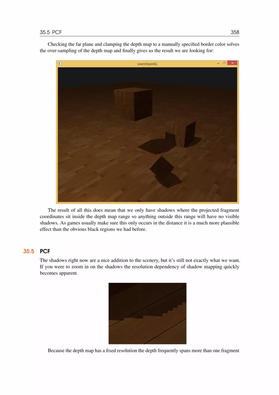
35.5 PCF 358
Checking the far plane and clamping the depth map to a manually specified border color solvesthe over-sampling of the depth map and finally gives us the result we are looking for:
The result of all this does mean that we only have shadows where the projected fragmentcoordinates sit inside the depth map range so anything outside this range will have no visibleshadows. As games usually make sure this only occurs in the distance it is a much more plausibleeffect than the obvious black regions we had before.
35.5 PCFThe shadows right now are a nice addition to the scenery, but it’s still not exactly what we want.If you were to zoom in on the shadows the resolution dependency of shadow mapping quicklybecomes apparent.
Because the depth map has a fixed resolution the depth frequently spans more than one fragment

35.5 PCF 359
per texel. As a result multiple fragments sample the same depth value from the depth map andcome to the same shadow conclusions, which produces these jagged blocky edges.
You can reduce these blocky shadows by increasing the depth map resolution or by trying to fitthe light frustum as closely to the scene as possible.
Another (partial) solution to these jagged edges is called PCF or percentage-closer filteringwhich is a term that hosts many different filtering functions that produce softer shadows, makingthem appear less blocky or hard. The idea is to sample more than once from the depth map, eachtime with slightly different texture coordinates. For each individual sample we check whether itis in shadow or not. All the sub-results are then combined and averaged and we get a nice softlooking shadow.
One simple implementation of PCF is to simply sample the surrounding texels of the depth mapand average the results:
float shadow = 0.0;vec2 texelSize = 1.0 / textureSize(shadowMap, 0);for(int x = -1; x <= 1; ++x){
for(int y = -1; y <= 1; ++y){
float pcfDepth = texture(shadowMap, projCoords.xy + vec2(x, y) *texelSize).r;
shadow += currentDepth - bias > pcfDepth ? 1.0 : 0.0;}
}shadow /= 9.0;
Here textureSize returns a vec2 of the width and height of the given sampler texture atmipmap level 0. Divided over 1 this returns the size of a single texel that we use to offset thetexture coordinates, making sure each new sample samples a different depth value. Here we sample9 values around the projected coordinate’s x and y value, test for shadow occlusion and finallyaverage the results by the total number of samples taken.
By using more samples and/or varying the texelSize variable you can increase the qualityof the soft shadows. Below you can see the shadows with simple PCF applied:
From a distance the shadows look a lot better and less hard. If you zoom in you can still see the

35.6 Orthographic vs projection 360
resolution artifacts of shadow mapping, but in general this gives good results for most applications.
You can find the complete source code of the example here together with the second stage’svertex and fragment shader.
There is actually much more to PCF and quite a few techniques to considerably improve thequality of soft shadows, but for the sake of this tutorial’s length we’ll leave that for a later discussion.
35.6 Orthographic vs projectionThere is a difference between rendering the depth map with an orthographic or a projection matrix.An orthographic projection matrix does not deform the scene with perspective so all view/light raysare parallel which makes it a great projection matrix for directional lights. A perspective projectionmatrix however does deform all vertices based on perspective which gives different results. Thefollowing image shows the different shadow regions of both projection methods:
Perspective projections make more sense for light sources that have actual locations unlikedirectional lights. Perspective projections are thus most often used with spotlights and point lightswhile orthographic projections are used for directional lights.
Another subtle difference with using a perspective projection matrix is that visualizing the depthbuffer will often give an almost completely white result. This happens because with perspectiveprojection the depth is transformed to non-linear depth values with most of its noticeable rangeclose to the near plane. To be able to properly view the depth values as we did with the orthographicprojection you first want to transform the non-linear depth values to linear as we discussed in thedepth testing tutorial.
#version 330 coreout vec4 color;in vec2 TexCoords;
uniform sampler2D depthMap;uniform float near_plane;uniform float far_plane;
float LinearizeDepth(float depth){
float z = depth * 2.0 - 1.0; // Back to NDCreturn (2.0 * near_plane * far_plane) / (far_plane + near_plane - z * (far_plane - near_plane));

35.7 Additional resources 361
}
void main(){
float depthValue = texture(depthMap, TexCoords).r;color = vec4(vec3(LinearizeDepth(depthValue) / far_plane), 1.0); //perspective// color = vec4(vec3(depthValue), 1.0); // orthographic
}
This shows depth values similar to what we’ve seen with orthographic projection. Note thatthis is only useful for debugging; the depth checks remain the same with orthographic or projectionmatrices as the relative depths do not change.
35.7 Additional resources• Tutorial 16 : Shadow mapping: similar shadow mapping tutorial by opengl-tutorial.org with
a few extra notes.• Shadow Mapping - Part 1: another shadow mapping tutorial by ogldev.• How Shadow Mapping Works: a 3-part YouTube tutorial by TheBennyBox on shadow
mapping and its implementation.• Common Techniques to Improve Shadow Depth Maps: a great article by Microsoft listing a
large number of techniques to improve the quality of shadow maps.

36. Point Shadows
In the last tutorial we learned to create dynamic shadows with shadow mapping. It works great, butit’s only suited for directional lights as the shadows are only generated in a single direction of thelight source. It is therefore also known as directional shadow mapping as the depth (or shadow)map is generated from just the direction the light is looking at.
What this tutorial will focus on is the generation of dynamic shadows in all surroundingdirections. The technique we’re using is perfect for point lights as a real point light would castshadows in all directions. This technique is known as point (light) shadows or more formerly asomnidirectional shadow maps.
This tutorial builds upon the previous shadow mapping tutorial so unless you’re familiarwith traditional shadow mapping it is advised to read the shadow mapping tutorial first.
The algorithm remains mostly the same to directional shadow mapping: we generate a depthmap from the light’s perspective(s), sample the depth map based on the current fragment positionand compare each fragment with the stored depth value to see whether it is in shadow. The maindifference between directional shadow mapping and omnidirectional shadow mapping is the depthmap used.
The depth map we need requires rendering a scene from all surrounding directions of a pointlight and as such a normal 2D depth map won’t work; what if we were to use a cubemap instead?Because a cubemap can store environment data with only 6 faces it is possible to render the entirescene to each of the faces of a cubemap and sample these as the point light’s surrounding depthvalues.

36.1 Generating the depth cubemap 363
The generated depth cubemap is then passed to the lighting fragment shader that samples thecubemap with a direction vector to obtain the depth (from the light’s perspective) at that fragment.Most of the complicated stuff we already discussed in the shadow mapping tutorial. What makesthis algorithm slightly more difficult is the depth cubemap generation.
36.1 Generating the depth cubemapTo create a cubemap of a light’s surrounding depth values we have to render the scene 6 times: oncefor each face. One (quite obvious) way to do this is render the scene 6 times with 6 different viewmatrices, each time attaching a different cubemap face to a framebuffer object. This would looksomething like this:
for(int i = 0; i < 6; i++){
GLuint face = GL_TEXTURE_CUBE_MAP_POSITIVE_X + i;glFramebufferTexture2D(GL_FRAMEBUFFER, GL_DEPTH_ATTACHMENT, face,depthCubemap, 0);BindViewMatrix(lightViewMatrices[i]);RenderScene();
}
This can be quite expensive though as a lot of render calls are necessary for just a single depthmap. In this tutorial we’re going to use an alternative (more organized) approach using a little trickin the geometry shader that allows us to build the depth cubemap with just a single render pass.
First, we’ll need to create a cubemap:
GLuint depthCubemap;glGenTextures(1, &depthCubemap);
And generate each of the single cubemap faces as 2D depth-valued texture images:
const GLuint SHADOW_WIDTH = 1024, SHADOW_HEIGHT = 1024;

36.1 Generating the depth cubemap 364
glBindTexture(GL_TEXTURE_CUBE_MAP, depthCubemap);for (GLuint i = 0; i < 6; ++i)
glTexImage2D(GL_TEXTURE_CUBE_MAP_POSITIVE_X + i, 0,GL_DEPTH_COMPONENT,
SHADOW_WIDTH, SHADOW_HEIGHT, 0, GL_DEPTH_COMPONENT,GL_FLOAT, NULL);
Also don’t forget to set the suitable texture parameters:
glTexParameteri(GL_TEXTURE_CUBE_MAP, GL_TEXTURE_MAG_FILTER, GL_NEAREST);glTexParameteri(GL_TEXTURE_CUBE_MAP, GL_TEXTURE_MIN_FILTER, GL_NEAREST);glTexParameteri(GL_TEXTURE_CUBE_MAP, GL_TEXTURE_WRAP_S, GL_CLAMP_TO_EDGE);glTexParameteri(GL_TEXTURE_CUBE_MAP, GL_TEXTURE_WRAP_T, GL_CLAMP_TO_EDGE);glTexParameteri(GL_TEXTURE_CUBE_MAP, GL_TEXTURE_WRAP_R, GL_CLAMP_TO_EDGE);
Normally we’d attach a single face of a cubemap texture to the framebuffer object and renderthe scene 6 times, each time switching the depth buffer target of the framebuffer to a differentcubemap face. Since we’re going to use a geometry shader that allows us to render to all facesin a single pass we can directly attach the cubemap as a framebuffer’s depth attachment usingglFramebufferTexture:
glBindFramebuffer(GL_FRAMEBUFFER, depthMapFBO);glFramebufferTexture(GL_FRAMEBUFFER, GL_DEPTH_ATTACHMENT, depthCubemap, 0);glDrawBuffer(GL_NONE);glReadBuffer(GL_NONE);glBindFramebuffer(GL_FRAMEBUFFER, 0);
Again, note the call to glDrawBuffer and glReadBuffer: we only care about depthvalues when generating a depth cubemap so we have to explicitly tell OpenGL this framebufferobject does not render to a color buffer.
With omnidirectional shadow maps we have two render passes: first we generate the depth mapand second, we use the depth map in the normal render pass to create shadows in the scene. Withthe framebuffer object and the cubemap this process looks a bit like this:
// 1. first render to depth cubemapglViewport(0, 0, SHADOW_WIDTH, SHADOW_HEIGHT);glBindFramebuffer(GL_FRAMEBUFFER, depthMapFBO);
glClear(GL_DEPTH_BUFFER_BIT);ConfigureShaderAndMatrices();RenderScene();
glBindFramebuffer(GL_FRAMEBUFFER, 0);// 2. then render scene as normal with shadow mapping (using depth cubemap)glViewport(0, 0, SCR_WIDTH, SCR_HEIGHT);glClear(GL_COLOR_BUFFER_BIT | GL_DEPTH_BUFFER_BIT);ConfigureShaderAndMatrices();glBindTexture(GL_TEXTURE_CUBE_MAP, depthCubemap);RenderScene();
The process is exactly the same as with default shadow mapping, although this time we renderto and use a cubemap depth texture compared to a 2D depth texture. Before we actually render thescene from all of the light’s viewing directions we first have to calculate the proper transformationmatrices.

36.1 Generating the depth cubemap 365
36.1.1 Light space transformWith the framebuffer and cubemap set we need some way to transform all the scene’s geometryto the relevant light spaces in all 6 directions of the light. Similar to the shadow mapping tutorialwe’re going to need a light space transformation matrix T , but this time one for each face.
Each light space transformation matrix contains both a projection and a view matrix. For theprojection matrix we’re going to use a perspective projection matrix; the light source represents apoint in space so perspective projection makes most sense. Each light space transformation matrixuses the same projection matrix:
GLfloat aspect = (GLfloat)SHADOW_WIDTH/(GLfloat)SHADOW_HEIGHT;GLfloat near = 1.0f;GLfloat far = 25.0f;glm::mat4 shadowProj = glm::perspective(90.0f, aspect, near, far);
Important to note here is the field of view parameter of glm::perspective that we set to90 degrees. By setting this to 90 degrees we make sure the viewing field is exactly large enoughto properly fill a single face of the cubemap such that all faces align correctly to each other at theedges.
As the projection matrix does not change per direction we can re-use it for each of the 6transformation matrices. We do need a different view matrix per direction. With glm::lookAtwe create 6 view directions, each looking at a single direction of the cubemap in the order: right,left, top, bottom, near and far.
std::vector<glm::mat4> shadowTransforms;shadowTransforms.push_back(shadowProj *
glm::lookAt(lightPos, lightPos + glm::vec3(1.0,0.0,0.0),glm::vec3(0.0,-1.0,0.0));
shadowTransforms.push_back(shadowProj *glm::lookAt(lightPos, lightPos + glm::vec3(-1.0,0.0,0.0),
glm::vec3(0.0,-1.0,0.0));shadowTransforms.push_back(shadowProj *
glm::lookAt(lightPos, lightPos + glm::vec3(0.0,1.0,0.0),glm::vec3(0.0,0.0,1.0));
shadowTransforms.push_back(shadowProj *glm::lookAt(lightPos, lightPos + glm::vec3(0.0,-1.0,0.0),
glm::vec3(0.0,0.0,-1.0));shadowTransforms.push_back(shadowProj *
glm::lookAt(lightPos, lightPos + glm::vec3(0.0,0.0,1.0),glm::vec3(0.0,-1.0,0.0));
shadowTransforms.push_back(shadowProj *glm::lookAt(lightPos, lightPos + glm::vec3(0.0,0.0,-1.0),
glm::vec3(0.0,-1.0,0.0));
Here we create 6 view matrices and multiply them with the projection matrix to get a total of6 different light space transformation matrices. The target parameter of glm::lookAt eachlooks into the direction of a single cubemap face.
These transformation matrices are send to the shaders that render the depth into the cubemap.

36.1 Generating the depth cubemap 366
36.1.2 Depth shadersTo render depth values to a depth cubemap we’re going to need a total of three shaders: a vertexand fragment shader and a geometry shader in between.
The geometry shader will be the shader responsible for transforming all world-space vertices to6 different light spaces. Therefore the vertex shader simply transforms vertices to world-space anddirects them to the geometry shader:
#version 330 corelayout (location = 0) in vec3 position;
uniform mat4 model;
void main(){
gl_Position = model * vec4(position, 1.0);}
The geometry shader then takes as input 3 triangle vertices and a uniform array of light spacetransformation matrices. The geometry shader is then responsible for transforming the vertices tothe light spaces; this is also where it gets interesting.
The geometry shader has a built-in variable called gl_Layer that specifies which cubemapface to emit a primitive to. When left alone the geometry shader just sends its primitives furtherdown the pipeline as usual, but when we update this variable we can control to which cubemapface we render to for each primitive. This of course only works when we have a cubemap textureattached to the active framebuffer.
#version 330 corelayout (triangles) in;layout (triangle_strip, max_vertices=18) out;
uniform mat4 shadowMatrices[6];
out vec4 FragPos; // FragPos from GS (output per emitvertex)
void main(){
for(int face = 0; face < 6; ++face){
gl_Layer = face; // built-in variable that specifies to which facewe render.
for(int i = 0; i < 3; ++i) // for each triangle’s vertices{
FragPos = gl_in[i].gl_Position;gl_Position = shadowMatrices[face] * FragPos;EmitVertex();
}EndPrimitive();
}}
This geometry shader should be relatively straightforward. We take as input a triangle andoutput a total of 6 triangles (6 * 3 vertices each equals 18 vertices). In the main function we iterateover 6 cubemap faces where we specify each face as the output face by storing the face integer

36.2 Omnidirectional shadow maps 367
into gl_Layer. Then we generate each triangle by transforming each world-space vertex to therelevant light space by multiplying FragPos with the face’s light-space transformation matrix.Note that we also sent the resulting FragPos variable to the fragment shader that we’ll need tocalculate a depth value.
In the last tutorial we used an empty fragment shader and let OpenGL figure out the depthvalues of the depth map. This time we’re going to calculate our own (linear) depth as the lineardistance between each fragment position and the light source’s position. Calculating our own depthvalues makes the later shadow calculations a bit more intuitive.
#version 330 corein vec4 FragPos;
uniform vec3 lightPos;uniform float far_plane;
void main(){
// get distance between fragment and light sourcefloat lightDistance = length(FragPos.xyz - lightPos);
// map to [0;1] range by dividing by far_planelightDistance = lightDistance / far_plane;
// Write this as modified depthgl_FragDepth = gl_FragCoord.z;
}
The fragment shader takes as input the FragPos from the geometry shader, the light’s positionvector and the frustum’s far plane value. Here we take the distance between the fragment and thelight source, map it to the [0,1] range and write it as the fragment’s depth value.
Rendering the scene with these shaders and the cubemap-attached framebuffer object activeshould give you a completely filled depth cubemap for the second pass’s shadow calculations.
36.2 Omnidirectional shadow mapsWith everything set up it is time to render the actual omnidirectional shadows. The procedure issimilar to the directional shadow mapping tutorial although this time we bind a cubemap textureinstead of a 2D texture as the depth map and also pass the light projection’s far plane variable to theshaders.
glViewport(0, 0, SCR_WIDTH, SCR_HEIGHT);glClear(GL_COLOR_BUFFER_BIT | GL_DEPTH_BUFFER_BIT);shader.Use();// ... send uniforms to shader (including light’s far_plane value)glActiveTexture(GL_TEXTURE0);glBindTexture(GL_TEXTURE_CUBE_MAP, depthCubemap);// ... bind other texturesRenderScene();
Here the renderScene function renders some cubes in a large cube room scattered around alight source at the center of the scene.

36.2 Omnidirectional shadow maps 368
The vertex shader and fragment shader are largely similar to the original shadow mappingshaders: the differences being that the fragment shader no longer requires a fragment position inlight space as we can now sample the depth values using a direction vector.
Because of this the vertex shader no longer needs to transform its position vectors to light spaceso we can exclude the FragPosLightSpace variable:
#version 330 corelayout (location = 0) in vec3 position;layout (location = 1) in vec3 normal;layout (location = 2) in vec2 texCoords;
out vec2 TexCoords;
out VS_OUT {vec3 FragPos;vec3 Normal;vec2 TexCoords;
} vs_out;
uniform mat4 projection;uniform mat4 view;uniform mat4 model;
void main(){
gl_Position = projection * view * model * vec4(position, 1.0f);vs_out.FragPos = vec3(model * vec4(position, 1.0));vs_out.Normal = transpose(inverse(mat3(model))) * normal;vs_out.TexCoords = texCoords;
}
The fragment shader’s Blinn-Phong lighting code is exactly the same as we had before with ashadow multiplication at the end:
#version 330 coreout vec4 FragColor;
in VS_OUT {vec3 FragPos;vec3 Normal;vec2 TexCoords;
} fs_in;
uniform sampler2D diffuseTexture;uniform samplerCube depthMap;
uniform vec3 lightPos;uniform vec3 viewPos;
uniform float far_plane;
float ShadowCalculation(vec3 fragPos){
[...]}
void main()

36.2 Omnidirectional shadow maps 369
{vec3 color = texture(diffuseTexture, fs_in.TexCoords).rgb;vec3 normal = normalize(fs_in.Normal);vec3 lightColor = vec3(0.3);// Ambientvec3 ambient = 0.3 * color;// Diffusevec3 lightDir = normalize(lightPos - fs_in.FragPos);float diff = max(dot(lightDir, normal), 0.0);vec3 diffuse = diff * lightColor;// Specularvec3 viewDir = normalize(viewPos - fs_in.FragPos);vec3 reflectDir = reflect(-lightDir, normal);float spec = 0.0;vec3 halfwayDir = normalize(lightDir + viewDir);spec = pow(max(dot(normal, halfwayDir), 0.0), 64.0);vec3 specular = spec * lightColor;// Calculate shadowfloat shadow = ShadowCalculation(fs_in.FragPos);vec3 lighting = (ambient + (1.0 - shadow) * (diffuse + specular)) *color;
FragColor = vec4(lighting, 1.0f);}
There are a few subtle differences: the lighting code is the same, but we now have a samplerCubeuniform and the ShadowCalculation function takes the fragment’s position as its parameter in-stead of the fragment position in light space. We now also include the light frustum’s far_planevalue that we’ll later need. At the end of the fragment shader run we calculate the shadow compo-nent which is 1.0 when the fragment is in shadow or 0.0 when it’s not. We use the calculatedshadow component to influence the lighting’s diffuse and specular components.
What is largely different is the content of the ShadowCalculation function that nowsamples depth values from a cubemap instead of a 2D texture. Let’s discuss its content step by step.
The first thing we have to do is retrieve the depth of the cubemap. As you might rememberfrom the cubemap section of this tutorial is that we stored the depth as the linear distance betweena fragment and the light position; we’re taking a similar approach here:
float ShadowCalculation(vec3 fragPos){
vec3 fragToLight = fragPos - lightPos;float closestDepth = texture(depthMap, fragToLight).r;
}
Here we take the difference vector between the fragment’s position and the light’s position anduse that vector as a direction vector to sample the cubemap. The direction vector doesn’t needto be a unit vector to sample from a cubemap so there’s no need to normalize it. The resultingclosestDepth is the normalized depth value between the light source and its closest visiblefragment.
The closestDepth value is currently in the range [0,1] so we first transform it back to[0,far_plane] by multiplying it with far_plane.

36.2 Omnidirectional shadow maps 370
closestDepth *= far_plane;
Next we retrieve the depth value between the current fragment and the light source which wecan easily obtain by taking the length of fragToLight due to how we calculated depth values inthe cubemap:
float currentDepth = length(fragToLight);
This returns a depth value in the same (or larger) range as closestDepth.
Now we can compare both depth values to see which is closer than the other and determinewhether the current fragment is in shadow. We also include a shadow bias so we don’t get shadowacne as discussed in the previous tutorial.
float bias = 0.05;float shadow = currentDepth - bias > closestDepth ? 1.0 : 0.0;
The complete ShadowCalculation then becomes:
float ShadowCalculation(vec3 fragPos){
// Get vector between fragment position and light positionvec3 fragToLight = fragPos - lightPos;// Use the light to fragment vector to sample from the depth mapfloat closestDepth = texture(depthMap, fragToLight).r;// It is currently in linear range between [0,1]. Re-transform back tooriginal valueclosestDepth *= far_plane;// Now get current linear depth as the length between the fragment andlight positionfloat currentDepth = length(fragToLight);// Now test for shadowsfloat bias = 0.05;float shadow = currentDepth - bias > closestDepth ? 1.0 : 0.0;
return shadow;}
With these shaders we already get pretty good shadows and this time in all surroundingdirections from a point light. With a point light positioned at the center of a simple scene it’ll looka bit like this:

36.2 Omnidirectional shadow maps 371
You can find the source code of this demo here together with its vertex and fragment shader.
36.2.1 Visualizing cubemap depth bufferIf you’re somewhat like me you probably didn’t get this right on the first try so it makes sense todo some debugging with one of the obvious checks being validating whether the depth map wasbuilt correctly. Because we don’t have a 2D depth map texture anymore visualizing the depth mapbecomes a bit less obvious.
A simple trick to visualize the depth buffer is to take the normalized (in the range [0,1])closestDepth variable in the ShadowCalculation function and display that variable as:
FragColor = vec4(vec3(closestDepth / far_plane), 1.0);
The result is a grayed out scene where each color represents the linear depth values of the scene:

36.3 PCF 372
You can also see the to-be shadowed regions on the outside wall. If it looks somewhat similaryou know the depth cubemap was properly generated. Otherwise you probably did somethingwrong or used the closestDepth still in the [0,far_plane] range.
36.3 PCFSince omnidirectional shadow maps are based on the same principles of traditional shadow mappingit also has the same resolution dependent artifacts. If you zoom in closely you can again see jaggededges. Percentage-closer filtering or PCF allows us to smooth out these jagged edges by filteringmultiple samples around the fragment position and average the results.
If we take the same simple PCF filter of the previous tutorial and add a third dimension (becausewe need 3D direction vectors to sample from a cubemap) we get:
float shadow = 0.0;float bias = 0.05;float samples = 4.0;float offset = 0.1;for(float x = -offset; x < offset; x += offset / (samples * 0.5)){
for(float y = -offset; y < offset; y += offset / (samples * 0.5)){
for(float z = -offset; z < offset; z += offset / (samples * 0.5)){
float closestDepth = texture(depthMap, fragToLight + vec3(x, y,z)).r;
closestDepth *= far_plane; // Undo mapping [0;1]if(currentDepth - bias > closestDepth)

36.3 PCF 373
shadow += 1.0;}
}}shadow /= (samples * samples * samples);
The code isn’t too different from what we had in traditional shadow mapping. Here we calculatethe texture offsets dynamically based on the number of samples we’d like to take in each axis andtake 3 times sample the amount of sub-samples that we then average at the end.
The shadows now look a lot more soft and smooth and gives much more plausible results.
However, with samples set to 4.0 we take a total of 64 samples each fragment which is alot!
As most of these samples are redundant in that they sample close to the original direction vectorit might make more sense to only sample in perpendicular directions of the sample direction vector.However as there is no (easy) way to figure out which sub-directions are redundant this becomesdifficult. One trick we can use is to take an array of offset directions that are all roughly separablee.g. each of them points in completely different directions, reducing the number of sub-directionsthat are close together. Below we have such an array of a maximum of 20 offset directions:
vec3 sampleOffsetDirections[20] = vec3[](vec3( 1, 1, 1), vec3( 1, -1, 1), vec3(-1, -1, 1), vec3(-1, 1, 1),vec3( 1, 1, -1), vec3( 1, -1, -1), vec3(-1, -1, -1), vec3(-1, 1, -1),vec3( 1, 1, 0), vec3( 1, -1, 0), vec3(-1, -1, 0), vec3(-1, 1, 0),vec3( 1, 0, 1), vec3(-1, 0, 1), vec3( 1, 0, -1), vec3(-1, 0, -1),

36.3 PCF 374
vec3( 0, 1, 1), vec3( 0, -1, 1), vec3( 0, -1, -1), vec3( 0, 1, -1));
Then we can adapt the PCF algorithm to take a fixed amount of samples from sampleOffsetDirectionsand use these to sample the cubemap. The advantage is that we need a lot less samples to getvisually similar results to the first PCF algorithm.
float shadow = 0.0;float bias = 0.15;int samples = 20;float viewDistance = length(viewPos - fragPos);float diskRadius = 0.05;for(int i = 0; i < samples; ++i){
float closestDepth = texture(depthMap, fragToLight +sampleOffsetDirections[i] * diskRadius).r;closestDepth *= far_plane; // Undo mapping [0;1]if(currentDepth - bias > closestDepth)
shadow += 1.0;}shadow /= float(samples);
Here we add offsets to a specific diskRadius around the original fragToLight directionvector to sample from the cubemap.
Another interesting trick we can apply here is that we can change the diskRadius basedon how far the viewer is away from a fragment; this way we can increase the offset radius by thedistance to the viewer, making the shadows softer when far away and sharper when close by.
float diskRadius = (1.0 + (viewDistance / far_plane)) / 25.0;
The results of this PCF algorithm gives just as good, if not better, results of soft shadows:

36.4 Additional resources 375
Of course, the bias we add to each sample is highly based on context and will always requiretweaking based on the scene you’re working with. Play around with all the values and see how theyaffect the scene.
You can find the final shaders here: vertex and fragment.
I should mention that using geometry shaders to generate a depth map isn’t necessarily fasterthan rendering the scene 6 times for each face. Using a geometry shader like this has its ownperformance penalties that might outweigh the performance gain of using one in the first place. Thisof course depends on the type of environment, the specific video card drivers and more so if youreally care about performance, make sure to profile both methods and select the more efficient onefor your scene. I personally prefer using geometry shaders for shadow mapping, simply because Ifind them more intuitive to use.
36.4 Additional resources• Shadow Mapping for point light sources in OpenGL: omnidirectional shadow mapping
tutorial by sunandblackcat.• Multipass Shadow Mapping With Point Lights: omnidirectional shadow mapping tutorial by
ogldev.• Omni-directional Shadows: a nice set of slides about omnidirectional shadow mapping by
Peter Houska.

37. Normal Mapping
All our scenes are filled with polygons, each consisting of hundreds or maybe thousands of flattriangles. We boosted the realism by pasting 2D textures on these flat triangles to give them extradetails, hiding the fact that the polygons actually consist of tiny flat triangles. Textures help, butwhen you take a good close look at them it is still quite easy to see the underlying flat surfaces.Most real-life surface are not flat however and exhibit a lot of (bumpy) details.
For instance, take a brick surface. A brick surface is quite a rough surface and obviously notcompletely flat: it contains sunken cement stripes and a lot of detailed little holes and cracks. If wewere to view such a brick surface in a lighted scene the immersion gets easily broken. Below wecan see a brick texture applied to a flat surface lighted by a point light.
The lighting does not take any of the small cracks and holes into account and completelyignores the deep stripes between the bricks; the surface looks perfectly flat. We can partly solve the

37.1 Normal mapping 377
flatness by using a specular map to pretend some surfaces are less lit due to depth or other details,but that’s more of a hack than a real solution. What we need is some way to inform the lightingsystem about all the little depth-like details of the surface.
If we think about this from a light’s perspective: how comes the surface is lit as a completelyflat surface? The answer is the surface’s normal vector. From the lighting algorithm’s point of viewthe only way it determines the shape of an object is by its perpendicular normal vector. The bricksurface only has a single normal vector and as a result the surface is uniformly lit based on thisnormal vector’s direction. What if we, instead of a per-surface normal that is the same for eachfragment, use a per-fragment normal that is different for each fragment? This way we can slightlydeviate the normal vector based on a surface’s little details; as a result this gives the illusion thesurface is a lot more complex:
By using per-fragment normals we can trick the lighting into believing a surface consists of tinylittle planes (perpendicular to the normal vectors) giving the surface an enormous boost in detail.This technique to use per-fragment normals compared to per-surface normals is called normalmapping or bump mapping. Applied to the brick plane it looks a bit like this:
As you can see it gives an enormous boost in detail and for a relatively low cost. Because weonly change the normal vectors per fragment there is no need to change any lighting equation. Wenow pass a per-fragment normal instead of an interpolated surface normal to the lighting algorithm.The lighting is then what gives a surface its detail.
37.1 Normal mappingTo get normal mapping to work we’re going to need a per-fragment normal. Similar to what we didwith diffuse maps and specular maps we can use a 2D texture to store per-fragment data. Asidefrom color and lighting data we can also store normal vectors in a 2D texture. This way we cansample from a 2D texture to get a normal vector for that specific fragment.
While normal vectors are geometric entities and textures are generally only used for color

37.1 Normal mapping 378
information storing normal vectors in a texture might not be immediately obvious. If you thinkabout color vectors in a texture they are represented as a 3D vector with an r, g and b component.We can similarly store a normal vector’s x, y and z component in the respective color components.Normal vectors range between -1 and 1 so they’re first mapped to [0,1]:
vec3 rgb_normal = normal * 0.5 - 0.5; // transforms from [-1,1] to [0,1]
With normal vectors transformed to an RGB color component like this we can store a per-fragment normal derived from the shape of a surface onto a 2D texture. An example normal map ofthe brick surface at the start of this tutorial is shown below:
This (and almost all normal maps you find online) will have a blue-ish tint. This is becauseall the normals are all closely pointing outwards towards the positive z-axis which is (0,0,1): ablue-ish color. The slight deviations in color represent normal vectors that are slightly offset fromthe general positive z direction, giving a sense of depth to the texture. For example, you can seethat at the top of each brick the color tends to get more green which makes sense as the top side ofa brick would have normals pointing more in the positive y direction (0,1,0) which happens to bethe color green!
With a simple plane looking at the positive z-axis we can take this diffuse texture and thisnormal map to render the image from the previous section. Note that the linked normal map isdifferent from the one shown above. The reason for this is that OpenGL reads texture coordinateswith the y (or V) coordinates reversed from how textures are generally created. The linked normalmap thus has its y (or green) component reversed (you can see the green colors are now pointingdownwards); if you fail to take this into account the lighting will be incorrect. Load both textures,bind them to the proper texture units and render a plane with the following changes in a lightingfragment shader:
uniform sampler2D normalMap;
void main(){
// Obtain normal from normal map in range [0,1]

37.1 Normal mapping 379
normal = texture(normalMap, fs_in.TexCoords).rgb;// Transform normal vector to range [-1,1]normal = normalize(normal * 2.0 - 1.0);
[...]// proceed with lighting as normal
}
Here we reverse the process of mapping normals to RGB colors by remapping the samplednormal color from [0,1] back to [-1,1] and then use the sampled normal vectors for the upcominglighting calculations. In this case we used a Blinn-Phong shader.
By slowly moving the light source over time you really get a sense of depth using the normalmap. Running this normal mapping example gives the exact results as shown at the start of thistutorial:
You can find the full source code of this simple demo here together with its vertex and fragmentshader.
There is one issue however that greatly limits this use of normal maps. The normal map weused had normal vectors that all roughly pointed in the positive z direction. This worked becausethe plane’s surface normal was also pointing in the positive z direction. However, what wouldhappen if we used the same normal map on a plane laying on the ground with a surface normalvector pointing in the positive y direction?

37.1 Normal mapping 380
The lighting doesn’t look right! This happens because the sampled normals of this plane stillpoint roughly in the positive z direction even though they should point somewhat in the positive ydirection of the surface normal. As a result the lighting thinks the surface’s normals are the same asbefore when the surface was still looking in the positive z direction; the lighting is incorrect. Theimage below shows what the sampled normals approximately look like on this surface:
You can see that all the normals roughly point in the positive z direction while they shouldbe pointing alongside the surface normal in the positive y direction. A possible solution to this

37.2 Tangent space 381
problem is to define a normal map for each possible direction of a surface. In the case of a cubewe would need 6 normal maps, but with advanced models that can have more than hundreds ofpossible surface directions this becomes an infeasible approach.
A different and also slightly more difficult solution works by doing lighting in a differentcoordinate space: a coordinate space where the normal map vectors always point roughly in thepositive z direction; all other lighting vectors are then transformed relative to this positive z direction.This way we can always use the same normal map, regardless of orientation. This coordinate spaceis called tangent space.
37.2 Tangent spaceNormal vectors in a normal map are expressed in tangent space where normals always point roughlyin the positive z direction. Tangent space is a space that’s local to the surface of a triangle: thenormals are relative to the local reference frame of the individual triangles. Think of it as the localspace of the normal map’s vectors; they’re all defined pointing in the positive z direction regardlessof the final transformed direction. Using a specific matrix we can then transform normal vectorsfrom this local tangent space to world or view coordinates, orienting them along the final mappedsurface’s direction.
Let’s say we have the incorrect normal mapped surface from the previous section looking in thepositive y direction. The normal map is defined in tangent space, so one way to solve the problem isto calculate a matrix to transform normals from tangent space to a different space such that they’realigned with the surface’s normal direction: the normal vectors are then all pointing roughly in thepositive y direction. The great thing about tangent space is that we can calculate such a matrix forany type of surface so that we can properly align the tangent space’s z direction to the surface’snormal direction.
Such a matrix is called a TBN matrix where the letters depict a tangent, bitangent and normalvector. These are the vectors we need to construct this matrix. To construct such a change-of-basis matrix that transforms a tangent-space vector to a different coordinate space we need threeperpendicular vectors that are aligned along the surface of a normal map: an up, right and forwardvector; similar to what we did in the camera tutorial.
We already know the up vector which is the surface’s normal vector. The right and forwardvector are the tangent and bitangent vector respectively. The following image of a surface shows allthree vectors on a surface:

37.2 Tangent space 382
Calculating the tangent and bitangent vectors is not as straightforward as the normal vector. Wecan see from the image that the direction of the normal map’s tangent and bitangent vector alignwith the direction in which we define a surface’s texture coordinates. We’ll use this fact to calculatetangent and bitangent vectors for each surface. Retrieving them does require a bit of math; take alook at the following image:
From the image we can see that the texture coordinate differences of an edge E_2 of a triangledenotes as ∆U_2 and ∆V _2 are expressed in the same direction as the tangent vector T and bitangentvector B. Because of this we can write both displayed edges E_1 and E_2 of the triangle as a linearcombination of the tangent vector T and the bitangent vector B:
E_1 = ∆U_1T +∆V _1B
E_2 = ∆U_2T +∆V _2B
Which we can also write as:

37.2 Tangent space 383
(E_1x,E_1y,E_1z) = ∆U_1(T _x,T _y,T _z)+∆V _1(B_x,B_y,B_z)
(E_2x,E_2y,E_2z) = ∆U_2(T _x,T _y,T _z)+∆V _2(B_x,B_y,B_z)
We can calculate E as the difference vector between two vector positions and ∆U and ∆V asthe texture coordinate differences. We’re then left with two unknowns (tangent T and bitangent B)and two equations. You might remember from your algebra classes that this allows us to solve forT and B.
The last equations allow us to write it in a different form: that of matrix multiplication:
[E_1x E_1y E_1zE_2x E_2y E_2z
]=
[∆U_1 ∆V _1∆U_2 ∆V _2
][T _x T _y T _zB_x B_y B_z
]Try to visualize the matrix multiplications in your head and confirm that this is indeed the
same equation. An advantage of rewriting the equations in matrix form is that solving for T andB becomes much more obvious. If we multiply both sides of the equations by the inverse of the∆U∆V matrix we get:
[∆U_1 ∆V _1∆U_2 ∆V _2
]−1[E_1x E_1y E_1zE_2x E_2y E_2z
]=
[T _x T _y T _zB_x B_y B_z
]This allows us to solve for T and B. This does require us to calculate the inverse of the delta
texture coordinate matrix. I won’t go into the mathematical details of calculating a matrix’ inverse,but it roughly translates to 1 over the determinant of the matrix multiplied by its adjugate matrix:
[T _x T _y T _zB_x B_y B_z
]=
1∆U_1∆V _2−∆U_2∆V _1
[∆V _2 −∆V _1−∆U_2 ∆U_1
][E_1x E_1y E_1zE_2x E_2y E_2z
]This final equation gives us a formula for calculating the tangent vector T and bitangent vector
B from a triangle’s two edges and its texture coordinates.
Don’t worry if you don’t really understand the mathematics behind this. As long as youunderstand that we can calculate tangents and bitangents from a triangle’s vertices and its texturecoordinates (since texture coordinates are in the same space as tangent vectors) you’re halfwaythere.
37.2.1 Manual calculation of tangents and bitangentsIn the tutorial’s demo scene we had a simple 2D plane looking at the positive z direction. This timewe’d like to implement normal mapping using tangent space so we can orient this plane howeverwe want and normal mapping would still work. Using the previously discussed mathematics we’regoing to manually calculate this surface’s tangent and bitangent vectors.
Assuming the plane is built up from the following vectors (with 1, 2, 3 and 1, 3, 4 as its twotriangles):

37.2 Tangent space 384
// positionsglm::vec3 pos1(-1.0, 1.0, 0.0);glm::vec3 pos2(-1.0, -1.0, 0.0);glm::vec3 pos3(1.0, -1.0, 0.0);glm::vec3 pos4(1.0, 1.0, 0.0);// texture coordinatesglm::vec2 uv1(0.0, 1.0);glm::vec2 uv2(0.0, 0.0);glm::vec2 uv3(1.0, 0.0);glm::vec2 uv4(1.0, 1.0);// normal vectorglm::vec3 nm(0.0, 0.0, 1.0);
We first calculate the first triangle’s edges and delta UV coordinates:
glm::vec3 edge1 = pos2 - pos1;glm::vec3 edge2 = pos3 - pos1;glm::vec2 deltaUV1 = uv2 - uv1;glm::vec2 deltaUV2 = uv3 - uv1;
With the required data for calculating tangents and bitangents we can start following theequation from the previous section:
GLfloat f = 1.0f / (deltaUV1.x * deltaUV2.y - deltaUV2.x * deltaUV1.y);
tangent1.x = f * (deltaUV2.y * edge1.x - deltaUV1.y * edge2.x);tangent1.y = f * (deltaUV2.y * edge1.y - deltaUV1.y * edge2.y);tangent1.z = f * (deltaUV2.y * edge1.z - deltaUV1.y * edge2.z);tangent1 = glm::normalize(tangent1);
bitangent1.x = f * (-deltaUV2.x * edge1.x + deltaUV1.x * edge2.x);bitangent1.y = f * (-deltaUV2.x * edge1.y + deltaUV1.x * edge2.y);bitangent1.z = f * (-deltaUV2.x * edge1.z + deltaUV1.x * edge2.z);bitangent1 = glm::normalize(bitangent1);
[...] // similar procedure for calculating tangent/bitangent for plane’ssecond triangle
Here we first pre-calculate the fractional part of the equation as f and then for each vectorcomponent we do the corresponding matrix multiplication multiplied by f. If you compare this codewith the final equation you can see it is a direct translation. At the end we also do a normalizationto make sure the tangent/bitangent vectors end up as unit vectors.
Because a triangle is always a flat shape we only need to calculate a single tangent/bitangentpair per triangle as they will be the same for each of the triangle’s vertices. It should be noted thatmost implementations (e.g. model loaders and terrain generators) generally have triangles thatshare vertices with other triangles. In that case developers usually average the vertex properties likenormals and tangents/bitangents for each vertex to get a more smooth result. Our plane’s trianglesalso shares some vertices, but since both triangles are parallel to each other there’s no need toaverage results, but it’s good to keep this in mind whenever you encounter such a situation.
The resulting tangent and bitangent vector should have a value of (1,0,0) and (0,1,0) respec-tively that together with the normal (0,0,1) forms an orthogonal TBN matrix. Visualized on theplane the TBN vectors would look like this:

37.2 Tangent space 385
With tangent and bitangent vectors defined per vertex we can start implementing proper normalmapping.
37.2.2 Tangent space normal mappingTo get normal mapping working we first have to create a TBN matrix in the shaders. To do that wepass the earlier calculated tangent and bitangent vectors to the vertex shader as vertex attributes:
#version 330 corelayout (location = 0) in vec3 position;layout (location = 1) in vec3 normal;layout (location = 2) in vec2 texCoords;layout (location = 3) in vec3 tangent;layout (location = 4) in vec3 bitangent;
Then within the vertex shader’s main function we create the TBN matrix:
void main(){[...]vec3 T = normalize(vec3(model * vec4(tangent, 0.0)));vec3 B = normalize(vec3(model * vec4(bitangent, 0.0)));vec3 N = normalize(vec3(model * vec4(normal, 0.0)));mat3 TBN = mat3(T, B, N)}
Here we first transform all the TBN vectors to the coordinate system we’d like to work in,which in this case is world-space as we multiply with just the model matrix. Then we create theactual TBN matrix by directly supplying mat3’s constructor with the relevant vectors. Note that if

37.2 Tangent space 386
we want to really be precise we wouldn’t multiply the TBN vectors with the model matrix, butwith the normal matrix as we only care about the orientation of the vectors and not translationand/or scaling transformations.
Technically there is no need for the bitangent variable in the vertex shader. Allthree TBN vectors are perpendicular to each other so we can calculate the bitangentourselves in the vertex shader by simply taking the cross product of the T and N vector:vec3 B = cross(T, N);
So now that we have a TBN matrix, how are we going to use it? There are basically two wayswe can use a TBN matrix for normal mapping and we’ll demonstrate both of them:
1. We take a TBN matrix that transforms any vector from tangent to world space, give it to thefragment shader and transform the sampled normal from tangent space to world space usingthe TBN matrix; the normal is then in the same space as the other lighting variables.
2. We take the inverse of the TBN matrix that transforms any vector from world space to tangentspace and use this matrix to transform not the normal, but the other relevant lighting variablesto tangent space; the normal is then again in the same space as the other lighting variables.
Let’s review the first case. The normal vector we sample from the normal map is expressedin tangent space whereas the other lighting vectors (light and view pos) are expressed in worldspace. By passing the TBN matrix to the fragment shader we can multiply the sampled tangentspace normal with this TBN matrix to transform the normal vector to the same reference space asthe other lighting vectors. This way all the lighting calculations (specifically the dot product) makesense.
Sending the TBN matrix to the fragment shader is easy:
out VS_OUT {vec3 FragPos;vec2 TexCoords;mat3 TBN;
} vs_out;
void main(){
[...]vs_out.TBN = mat3(T, B, N);
}
In the fragment shader we similarly take a mat3 as an input variable:
in VS_OUT {vec3 FragPos;vec2 TexCoords;mat3 TBN;
} fs_in;
With the TBN matrix we can now update the normal mapping code to include the tangent-to-world space transformation:
normal = texture(normalMap, fs_in.TexCoords).rgb;

37.2 Tangent space 387
normal = normalize(normal * 2.0 - 1.0);normal = normalize(fs_in.TBN * normal);
Because the resulting normal is now in world space there is no need to change any of theother fragment shader code as the lighting code assumes the normal vector to be in world space.
Let’s also review the second case, where we take the inverse of the TBN matrix to transform allrelevant world-space vectors to the space the sampled normal vectors are in: tangent space. Theconstruction of the TBN matrix remains the same, but we first inverse the matrix before sending itto the fragment shader:
vs_out.TBN = transpose(mat3(T, B, N));
Note that we use the transpose function instead of the inverse function here. A greatproperty of orthogonal matrices (each axis is a perpendicular unit vector) is that the transpose of anorthogonal matrix is equal to its inverse. This is a great property as inverses are quite expensive anda transpose isn’t; the results are the same.
Within the fragment shader we then do not transform the normal vector, but we transform theother relevant vectors to tangent space, namely the lightDir and viewDir vectors. That wayeach vector is again in the same coordinate system: tangent space.
void main(){
vec3 normal = texture(normalMap, fs_in.TexCoords).rgb;normal = normalize(normal * 2.0 - 1.0);
vec3 lightDir = fs_in.TBN * normalize(lightPos - fs_in.FragPos);vec3 viewDir = fs_in.TBN * normalize(viewPos - fs_in.FragPos);[...]
}
The second approach seems like more work and also requires more matrix multiplications in thefragment shader (which are slightly expensive) so why would we bother with the second approach?
Well, transforming vectors from world to tangent space has an added advantage in that we cantransform all the relevant vectors to tangent space in the vertex shader instead of in the fragmentshader. This works, because lightPos and viewPos do not change each fragment run and forfs_in.FragPos we can also calculate its tangent-space position in the vertex shader and letfragment interpolation do its work. Basically, there is no need to transform any vector to tangentspace in the fragment shader, while it is necessary with the first approach as sampled normal vectorsare specific to each fragment shader run.
So instead of sending the inverse of the TBN matrix to the fragment shader, we send a tangent-space light position, view position and vertex position to the fragment shader. This saves us frommatrix multiplications in the fragment shader. This is a nice optimization as the vertex shader runsconsiderably less often than the fragment shader. This is also the reason why this approach is oftenthe preferred approach.
out VS_OUT {

37.2 Tangent space 388
vec3 FragPos;vec2 TexCoords;vec3 TangentLightPos;vec3 TangentViewPos;vec3 TangentFragPos;
} vs_out;
uniform vec3 lightPos;uniform vec3 viewPos;
[...]
void main(){
[...]mat3 TBN = transpose(mat3(T, B, N));vs_out.TangentLightPos = TBN * lightPos;vs_out.TangentViewPos = TBN * viewPos;vs_out.TangentFragPos = TBN * vec3(model * vec4(position, 0.0));
}
In the fragment shader we then use these new input variables to calculate lighting in tangentspace. As the normal vector is already in tangent space the lighting makes sense.
With normal mapping applied in tangent space we should get similar results to what we had atthe start of this tutorial, but this time we can orient our plane in any way we’d like and the lightingwould still be correct:
glm::mat4 model;model = glm::rotate(model, (GLfloat)glfwGetTime() * -10, glm::normalize(glm
::vec3(1.0, 0.0, 1.0)));glUniformMatrix4fv(modelLoc 1, GL_FALSE, glm::value_ptr(model));RenderQuad();
Which indeed looks like proper normal mapping:

37.3 Complex objects 389
You can find the source code here together with its vertex and fragment shader.
37.3 Complex objectsWe’ve demonstrated how we can use normal mapping together with tangent space transformationsby manually calculating the tangent and bitangent vectors. Luckily for us, having to manuallycalculate these tangent and bitangent vectors is not something you do too often; most of the timeyou implement it once in a custom model loader or in our case use a model loader using Assimp.
Assimp has a very useful configuration bit we can set when loading a model called aiProcess_CalcTangentSpace.When the aiProcess_CalcTangentSpace bit is supplied to Assimp’s ReadFile functionAssimp calculates smooth tangent and bitangent vectors for each of the loaded vertices, similarly tohow we did it in this tutorial.
const aiScene* scene = importer.ReadFile(path, aiProcess_Triangulate | aiProcess_FlipUVs |aiProcess_CalcTangentSpace
);
Within Assimp we can then retrieve the calculated tangents via:
vector.x = mesh->mTangents[i].x;vector.y = mesh->mTangents[i].y;vector.z = mesh->mTangents[i].z;vertex.Tangent = vector;

37.3 Complex objects 390
Then you’ll also have to update the model loader to also load normal maps from a texturedmodel. The wavefront object format (.obj) exports normal maps slightly different as Assimp’saiTextureType_NORMAL doesn’t load its normal maps while aiTextureType_HEIGHTdoes so I often load them as:
vector<Texture> specularMaps = this->loadMaterialTextures(material, aiTextureType_HEIGHT, "texture_normal"
);
Of course this is different for each type of loaded model and file format. Also important torealize is that aiProcess_CalcTangentSpace doesn’t always work. Calculating tangentsis based on texture coordinates and some model artists do certain texture tricks like mirroring atexture surface over a model by also mirroring half of the texture coordinates; this gives incorrectresults when the mirroring is not taken into account (which Assimp doesn’t).
Running the application on a model that is properly texture mapped with specular and normalmaps using an updated model loader gives a result a bit like this:
As you can see normal mapping boosts the detail of an object by an incredible amount withouttoo much extra cost.
Using normal maps is also a great way to boost the performance of your scene. Before normalmapping you had to use a large number of vertices to present a high number of detail on a mesh,but with normal mapping we can present the same level of detail on a mesh using a lot less vertices.The image below from Paolo Cignoni shows a nice comparison of both methods:

37.4 One last thing 391
The details on both the high-vertex mesh and the low-vertex mesh with normal mapping arealmost indistinguishable. So normal mapping doesn’t only look nice, it is also a great tool to replacehigh-vertex polygons with low-vertex polygons without losing detail.
37.4 One last thingThere is one last trick I’d like to discuss with regards to normal mapping that slightly improves itsquality without too much extra cost.
When tangent vectors are calculated on larger meshes that share a considerable amount ofvertices the tangent vectors are generally averaged to give nice and smooth results when normalmapping is applied to these surfaces. A problem with this approach is that the three TBN vectorscould end up non-perpendicular to each other which means the resulting TBN matrix would nolonger be orthogonal. Normal mapping will be only slightly off with a non-orthogonal TBN matrix,but it’s still something we can improve.
Using a mathematical trick called the Gram-Schmidt process we can re-orthogonalize the TBNvectors such that each vector is again perpendicular to the other vectors. Within the vertex shaderwe would do it like this:
vec3 T = normalize(vec3(model * vec4(tangent, 0.0)));vec3 N = normalize(vec3(model * vec4(tangent, 0.0)));// re-orthogonalize T with respect to NT = normalize(T - dot(T, N) * N);// then retrieve perpendicular vector B with the cross product of T and Nvec3 B = cross(T, N);
mat3 TBN = mat3(T, B, N)
This, albeit by a little, generally improves the normal mapping results with a little extra cost.Take a look at the end of the Normal Mapping Mathematics video referenced below this tutorial fora great explanation of how this process actually works.
37.5 Additional resources• Tutorial 26: Normal Mapping: normal mapping tutorial by ogldev.• How Normal Mapping Works: a nice video tutorial of how normal mapping works by
TheBennyBox.• Normal Mapping Mathematics: a similar video by TheBennyBox about the mathematics
behind normal mapping.• Tutorial 13: Normal Mapping: normal mapping tutorial by opengl-tutorial.org.

38. Parallax Mapping
Parallax mapping is a technique similar to normal mapping, but based on different principles.Similar to normal mapping it is a technique that significantly boosts a textured surface’s detail andgives it a sense of depth. While also an illusion, parallax mapping is a lot better in conveying asense of depth and together with normal mapping gives incredibly realistic results. While parallaxmapping isn’t necessarily a technique directly related to (advanced) lighting, I’ll still discuss it hereas the technique is a logical follow-up of normal mapping. Note that getting an understanding ofnormal mapping, specifically tangent space, is strongly advised before learning parallax mapping.
Parallax mapping belongs to the family of displacement mapping techniques that displace oroffset vertices based on geometrical information stored inside a texture. One way to do this isto take a plane with roughly 1000 vertices and displace each of these vertices based on a valuein a texture that tells us the height of the plane at a specific area. Such a texture that containsheight values per texel is called a height map. An example height map derived from the geometricproperties of a simple brick surface looks a bit like this:
When spanned over a plane each vertex is displaced based on the sampled height value in theheight map, transforming a flat plane to a rough bumpy surface based on a material’s geometricproperties. For instance, taking a flat plane displaced with the above heightmap results in thefollowing image:

393
A problem with displacing vertices is that a plane needs to consist of a large amount of trianglesto get a realistic displacement otherwise the displacement looks too blocky. As each flat surfacecould then require over 1000 vertices this quickly becomes computationally infeasible. What if wecould somehow achieve similar realism without the need of extra vertices? In fact, what if I were totell you that the above displaced surface is actually rendered with only 6 vertices (or 2 triangles)?This brick surface shown is rendered with parallax mapping, a displacement mapping techniquethat doesn’t require extra vertex data to convey depth, but similar to normal mapping uses a clevertechnique to trick the user.
The idea behind parallax mapping is to alter the texture coordinates in such a way that it lookslike a fragment’s surface is higher or lower than it actually is, all based on the view direction and aheightmap. To understand how it works, take a look at the following image of our brick surface:
Here the rough red line represents the values in the heightmap as the geometric surfacerepresentation of the brick surface and the vector V represents the surface to view direction(viewDir). If the plane would have actual displacement the viewer would see the surface at point

394
B. However, as our plane has no actual displacement the view direction hits the flat plane at point Aas we’d expect. Parallax mapping aims to offset the texture coordinates at fragment position A insuch a way that we get texture coordinates at point B. We then use the texture coordinates at pointB for all subsequent texture samples, making it look like the viewer is actually looking at point B.
The trick is to figure out how to get the texture coordinates at point B from point A. Parallaxmapping tries to solve this by scaling the fragment-to-view direction vector V by the height atfragment A. So we’re scaling the length of V to be equal to a sampled value from the heightmapH(A) at fragment position A. The image below shows this scaled vector P:
We then take this vector P and take its vector coordinates that align with the plane as thetexture coordinate offset. This works because vector P is calculated using a height value from theheightmap so the higher a fragment’s height, the more it effectively gets displaced.
This little trick gives good results most of the time, but is however a really crude approximationto get to point B. When heights change rapidly over a surface the results tend to look unrealistic asthe vector P will not end up close to B as you can see below:
Another issue with parallax mapping is that it’s difficult to figure out which coordinates toretrieve from P when the surface is arbitrarily rotated in some way. What we’d rather do is parallaxmapping in a different coordinate space where the x and y component of vector P always alignswith the texture’s surface. If you’ve followed along in the normal mapping tutorial you probablyguessed how we can accomplish this and yes, we would like to do parallax mapping in tangentspace.
By transforming the fragment-to-view direction vector V to tangent space the transformed

38.1 Parallax mapping 395
P vector will have its x and y component aligned to the surface’s tangent and bitangent vectors.As the tangent and bitangent vectors are pointing in the same direction as the surface’s texturecoordinates we can take the x and y components of P as the texture coordinate offset, regardless ofthe surface’s direction.
But enough about the theory, let’s get our feet wet and start implementing actual parallaxmapping.
38.1 Parallax mappingFor parallax mapping we’re going to use a simple 2D plane of which we calculate its tangent andbitangent vectors before sending it to the GPU; similar to what we did in the normal mappingtutorial. Onto the plane we’re going to attach a diffuse texture, a normal map and a displacementmap that you can download yourself by clicking the respective links. For this example we’re goingto use parallax mapping in conjunction with normal mapping. Because parallax mapping gives theillusion that it displaces a surface, the illusion breaks when the lighting doesn’t match. As normalmaps are often generated from heightmaps, using a normal map together with the heightmap makessure the lighting is in place with the displacement.
You might’ve already noted that the displacement map linked above is the inverse of theheightmap shown at the start of this tutorial. With parallax mapping it makes more sense to use theinverse of the heightmap (also known as a depthmap) as it’s easier to fake depth than height on flatsurfaces. This slightly changes how we perceive parallax mapping as shown below:
We again have a points A and B, but this time we obtain vector P by subtracting vector Vfrom the texture coordinates at point A. We can obtain depth values instead of height values bysubtracting the sampled heightmap values from 1.0 in the shaders, or by simply inversing itstexture values in image-editing software as we did with the depthmap linked above.
Parallax mapping is implemented in the fragment shader as the displacement effect differsall over a triangle’s surface. In the fragment shader we’re then going to need to calculate thefragment-to-view direction vector V so we need the view position and a fragment position in

38.1 Parallax mapping 396
tangent space. In the normal mapping tutorial we already had a vertex shader that sends thesevectors in tangent space so we can take an exact copy of that tutorial’s vertex shader:
#version 330 corelayout (location = 0) in vec3 position;layout (location = 1) in vec3 normal;layout (location = 2) in vec2 texCoords;layout (location = 3) in vec3 tangent;layout (location = 4) in vec3 bitangent;
out VS_OUT {vec3 FragPos;vec2 TexCoords;vec3 TangentLightPos;vec3 TangentViewPos;vec3 TangentFragPos;
} vs_out;
uniform mat4 projection;uniform mat4 view;uniform mat4 model;
uniform vec3 lightPos;uniform vec3 viewPos;
void main(){
gl_Position = projection * view * model * vec4(position, 1.0f);vs_out.FragPos = vec3(model * vec4(position, 1.0));vs_out.TexCoords = texCoords;
vec3 T = normalize(mat3(model) * tangent);vec3 B = normalize(mat3(model) * bitangent);vec3 N = normalize(mat3(model) * normal);mat3 TBN = transpose(mat3(T, B, N));
vs_out.TangentLightPos = TBN * lightPos;vs_out.TangentViewPos = TBN * viewPos;vs_out.TangentFragPos = TBN * vs_out.FragPos;
}
What’s important to note here is that for parallax mapping we specifically need to send theposition and viewer’s position viewPos in tangent space to the fragment shader.
Within the fragment shader we then implement the parallax mapping logic. The fragmentshader looks a bit like this:
#version 330 coreout vec4 FragColor;
in VS_OUT {vec3 FragPos;vec2 TexCoords;vec3 TangentLightPos;vec3 TangentViewPos;vec3 TangentFragPos;
} fs_in;

38.1 Parallax mapping 397
uniform sampler2D diffuseMap;uniform sampler2D normalMap;uniform sampler2D depthMap;
uniform float height_scale;
vec2 ParallaxMapping(vec2 texCoords, vec3 viewDir);
void main(){
// Offset texture coordinates with Parallax Mappingvec3 viewDir = normalize(fs_in.TangentViewPos - fs_in.TangentFragPos);vec2 texCoords = ParallaxMapping(fs_in.TexCoords, viewDir);
// then sample textures with new texture coordsvec3 diffuse = texture(diffuseMap, texCoords);vec3 normal = texture(normalMap, texCoords);normal = normalize(normal * 2.0 - 1.0);// proceed with lighting code[...]
}
We defined a function called ParallaxMapping that takes as input the fragment’s texturecoordinates and the fragment-to-view direction V in tangent space. The function returns thedisplaced texture coordinates. We then use these displaced texture coordinates as the texturecoordinates for sampling the diffuse and normal map. As a result the fragment’s diffuse color andnormal vector correctly corresponds to the surface’s displaced geometry.
Let’s take a look inside the ParallaxMapping function:
vec2 ParallaxMapping(vec2 texCoords, vec3 viewDir){
float height = texture(depthMap, texCoords).r;vec3 p = viewDir.xy / viewDir.z * (height * height_scale);return texCoords - p;
}
This relatively simple function is a direct translation of what we’ve discussed so far. We takethe original texture coordinates texCoords and use these to sample the height (or depth) fromthe depthMap at the current fragment H(A). We then calculate P as the x and y component of thetangent-space viewDir vector divided by its z component and scale it by the fragment’s height.We also introduced a height_scale uniform for some extra control as the parallax effect isusually too strong without an extra scale parameter. We then subtract this vector P from the texturecoordinates to get the final displaced texture coordinates.
What is interesting to note here is the division of viewDir.xy by viewDir.z. As theviewDir vector is normalized viewDir.z will be somewhere in the range between 0.0 and1.0. When viewDir is largely parallel to the surface its z component is close to 0.0 and thedivision returns a much larger vector P compared to when viewDir is largely perpendicular tothe surface. So basically we’re increasing the size of P in such a way that it offsets the texturecoordinates at a larger scale when looking at a surface from an angle compared to when looking atit from the top; this gives more realistic results at angles.
Some people prefer to leave the division by viewDir.z out of the equation as normal ParallaxMapping could produce undesirable results at angles; the technique is then called Parallax Mapping

38.1 Parallax mapping 398
with Offset Limiting. Choosing which technique to pick is usually a matter of personal preference,but I often tend to side with normal Parallax Mapping.
The resulting texture coordinates are then used to sample the other textures (diffuse and normal)and this gives a very neat displaced effect as you can see below with a height_scale of roughly0.1:
Here you can see the difference between normal mapping and parallax mapping combined withnormal mapping. Because parallax mapping tries to simulate depth it is actually possible to havebricks overlap other bricks based on the direction you view them.
You can still see some weird border artifacts at the edge of the parallax mapped plane. Thishappens because at the edges of the plane, the displaced texture coordinates could oversampleoutside the range [0, 1] and this gives unrealistic results based on the texture’s wrapping mode(s).A cool trick to solve this issue is to discard the fragment whenever it samples outside the defaulttexture coordinate range:
texCoords = ParallaxMapping(fs_in.TexCoords, viewDir);if(texCoords.x > 1.0 || texCoords.y > 1.0 || texCoords.x < 0.0 || texCoords
.y < 0.0)discard;
All fragments with (displaced) texture coordinates outside the default range get discarded andParallax Mapping then gives proper result around the edges of a surface. Note that this trick doesn’twork properly on all types of surfaces, but when applied to a plane it gives great results making itlook like the plane is now actually displaced:

38.2 Steep Parallax Mapping 399
You can find the source code here together with its vertex and fragment shader.
It looks great and is quite fast as well as we only need a single extra texture sample for parallaxmapping to work. It does come with a few issues though as it sort of breaks down when looking atit from an angle (similar to normal mapping) and gives incorrect results with steep height changes,as you can see below:
The reason that it doesn’t work properly at times is that it’s just a crude approximation ofdisplacement mapping. There are some extra tricks however that still allows us to get almost perfectresults with steep height changes, even when looking at an angle. For instance, what if we insteadof one sample, take multiple samples to find the closest point to B?
38.2 Steep Parallax MappingSteep Parallax Mapping is an extension on top of Parallax Mapping in that it uses the sameprinciples, but instead of 1 sample it takes multiple samples to better pinpoint vector P to B. Thisgives much better results, even with steep height changes as the accuracy of the technique is

38.2 Steep Parallax Mapping 400
improved by the number of samples.
The general idea of Steep Parallax Mapping is that it divides the total depth range into multiplelayers of the same height/depth. For each of these layers we sample the depthmap shifting thetexture coordinates along the direction of P until we find a sampled depth value that is below thedepth value of the current layer. Take a look at the following image:
We traverse the depth layers from the top down and for each layer we compare its depth valueto the depth value stored in the depthmap. If the layer’s depth value is less than the depthmap’svalue it means this layer’s part of vector P is not below the surface. We continue this processuntil the layer’s depth is higher than the value stored in the depthmap: this point is then below the(displaced) geometric surface.
In this example we can see that the depthmap value at the second layer (D(2) = 0.73) is stilllower than the second layer’s depth value 0.4 so we continue. In the next iteration the layer’s depthvalue 0.6 does become higher than the depthmap’s sampled depth value (D(3) = 0.37). We canthus assume vector P at the third layer to be the most viable position of the displaced geometry. Wecan then take the texture coordinate offset T _3 from vector ¯P_3 to displace the fragment’s texturecoordinates. You can see how the accuracy increases with more depth layers.
To implement this technique we only have to change the ParallaxMapping function as wealready have all the variables we need:
vec2 ParallaxMapping(vec2 texCoords, vec3 viewDir){
// number of depth layersconst float numLayers = 10;// calculate the size of each layerfloat layerDepth = 1.0 / numLayers;// depth of current layerfloat currentLayerDepth = 0.0;// the amount to shift the texture coordinates per layer (from vector P)vec2 P = viewDir.xy * height_scale;float deltaTexCoords = P / numLayers;

38.2 Steep Parallax Mapping 401
[...]}
Here we first set things up: we specify the number of layers, calculate the depth of each layerand finally calculate the texture coordinate offset that we have to shift along the direction of P perlayer.
We then iterate through all the layers, starting from the top, until we find a depthmap value lessthan the layer’s depth value:
// get initial valuesvec2 currentTexCoords = texCoords;float currentDepthMapValue = texture(depthMap, currentTexCoords).r;
while(currentLayerDepth < currentDepthMapValue){
// shift texture coordinates along direction of PcurrentTexCoords -= deltaTexCoords;// get depthmap value at current texture coordinatescurrentDepthMapValue = texture(depthMap, currentTexCoords).r;// get depth of next layercurrentLayerDepth += layerDepth;
}
return texCoords - currentTexCoords;
Here we loop over each depth layer and stop until we find the texture coordinate offset alongvector P that first returns a depth that’s below the (displaced) surface. The resulting offset issubtracted from the fragment’s texture coordinates to get a final displaced texture coordinate vector,this time with much more accuracy compared to traditional parallax mapping.
With around 10 samples the brick surface already looks more viable even when looking at itfrom an angle, but steep parallax mapping really shines when having a complex surface with steepheight changes like the earlier displayed wooden toy surface:

38.2 Steep Parallax Mapping 402
We can improve the algorithm a bit by exploiting one of Parallax Mapping’s properties. Whenlooking straight onto a surface there isn’t much texture displacement going on while there is a lot ofdisplacement when looking at a surface from an angle (visualize the view direction on both cases).By taking less samples when looking straight at a surface and more samples when looking at anangle we only sample the necessary amount:
const float minLayers = 8;const float maxLayers = 32;float numLayers = mix(maxLayers, minLayers, abs(dot(vec3(0.0, 0.0, 1.0),
viewDir)));
Here we take the dot product of viewDir and the positive z direction and use its result to alignthe number of samples more to minLayers or maxLayers based on the angle we’re lookingtowards a surface (note that the positive z direction is equal to the surface’s normal vector in tangentspace). If we were to look at a direction parallel to the surface we’d use a total of 32 layers.
You can find the updated fragment shader code here. You can also find the wooden toy boxsurface here: diffuse, normal and depth.
Steep Parallax Mapping also comes with its problems though. Because the technique is basedon a finite number of samples we get aliasing effects and the clear distinctions between layers caneasily be spotted:

38.3 Parallax Occlusion Mapping 403
We can reduce the issue by taking a larger number of samples, but this quickly becomes tooheavy a burden on performance. There are several approaches that aim to fix this issue by not takingthe first position that’s below the (displaced) surface, but by interpolating between the position’stwo closest depth layers to find a much closer match to B.
Two of the more popular of these approaches are called Relief Parallax Mapping and ParallaxOcclusion Mapping of which Relief Parallax Mapping gives the most accurate results, but is alsomore performance heavy compared to Parallax Occlusion Mapping. Because Parallax OcclusionMapping gives almost the same results as Relief Parallax Mapping and is also more efficient it isoften the preferred approach and also the last type of Parallax Mapping we’re going to discuss.
38.3 Parallax Occlusion MappingParallax Occlusion Mapping is based on the same principles as Steep Parallax Mapping, but insteadof taking the texture coordinates of the first depth layer after a collision, we’re going to linearlyinterpolate between the depth layer after and before the collision. We base the weight of the linearinterpolation on how far the surface’s height is from the depth layer’s value of both layers. Take alook at the following picture to get a grasp of how it works:

38.3 Parallax Occlusion Mapping 404
As you can see it’s largely similar to Steep Parallax Mapping with as an extra step the linearinterpolation between the two depth layers’ texture coordinates surrounding the intersected point.This is again an approximation, but significantly more accurate than Steep Parallax Mapping.
The code for Parallax Occlusion Mapping is an extension on top of Steep Parallax Mappingand not too difficult:
[...] // steep parallax mapping code here
// get texture coordinates before collision (reverse operations)vec2 prevTexCoords = currentTexCoords + deltaTexCoords;
// get depth after and before collision for linear interpolationfloat afterDepth = currentDepthMapValue - currentLayerDepth;float beforeDepth = texture(depthMap, prevTexCoords).r - currentLayerDepth
+ layerDepth;
// interpolation of texture coordinatesfloat weight = afterDepth / (afterDepth - beforeDepth);vec2 finalTexCoords = prevTexCoords * weight + currentTexCoords * (1.0 -
weight);
return finalTexCoords;
After we found the depth layer after intersecting the (displaced) surface geometry we alsoretrieve the texture coordinates of the depth layer before intersection. Next we calculate the distanceof the (displaced) geometry’s depth from the corresponding depth layers and interpolate betweenthese two values. The linear interpolation is a basic interpolation between both layer’s texturecoordinates. The function then finally returns the final interpolated texture coordinates.
Parallax Occlusion Mapping gives surprisingly good results and although some slight artifactsand aliasing issues are still visible it’s a generally a good trade-off and only really visible whenheavily zoomed in or looking at very steep angles.

38.4 Additional resources 405
You can find the (same) source code here together with its vertex and (updated) fragment shader.
Parallax Mapping is a great technique to boost the detail of your scene, but does come with afew artifacts you’ll have to consider when using it. Most often parallax mapping is used on floor orwall-like surfaces where it’s not as easy to determine the surface’s outline and the viewing angle ismost often roughly perpendicular to the surface. This way the artifacts of Parallax Mapping aren’tas noticeable and makes it an incredibly interesting technique for boosting your objects’ details.
38.4 Additional resources• Parallax Occlusion Mapping in GLSL: great parallax mapping tutorial by sunandblack-
cat.com.• How Parallax Displacement Mapping Works: a nice video tutorial of how parallax mapping
works by TheBennyBox.

39. HDR
Brightness and color values by default are clamped between 0.0 and 1.0 when stored into aframebuffer. This at first seemingly innocent statement caused us to always specify light and colorvalues somewhere in this range trying to make them fit into the scene. This works oké and givesdecent results, but what happens if we walk in a specifically bright area with multiple bright lightsources that as a total sum exceed 1.0? The answer is that all fragments that have a brightness orcolor sum over 1.0 get clamped to 1.0 which isn’t pretty to look at:
Due to a large number of fragments’ color values getting clamped to 1.0 each of the brightfragments have the exact same white color in a large region, losing a significant amount of detailand giving it a fake look.

407
A solution to this problem would be to reduce the strength of the light sources and ensure noarea of fragments in your scene ends up brighter than 1.0; this is not a good solution as this forcesyou to use unrealistic lighting parameters. A better approach is to allow color values to temporarilyexceed 1.0 and transform them back to the original range of 0.0 and 1.0 as a final step, butwithout losing detail.
Monitors are limited to display colors in the range of 0.0 and 1.0, but there is no suchlimitation in lighting equations. By allowing fragment colors to exceed 1.0 we have a much higherrange of color values available to work in known as high dynamic range (HDR). With high dynamicrange bright things can be really bright, dark things can be really dark, and details can be seen inboth.
High dynamic range was originally only used for photography where a photographer takesmultiple pictures of the same scene with varying exposure levels, capturing a large range of colorvalues. These combined images form a HDR image where a large range of details are visible basedon the combined exposure levels or a specific exposure it is viewed with. For instance, the imagebelow shows a lot of detail at brightly lit regions with a high exposure (look at the window), butthese details are gone with a low exposure. However, a high exposure now reveals a great amountof detail at darker regions that weren’t previously visible.
This is also very similar to how the human eye works and the basis of high dynamic rangerendering. When there is little light the human eye adapts itself so the darker parts are much bettervisible and similarly for bright areas, it’s like the human eye has an automatic exposure slider basedon the scene’s brightness.
High dynamic range rendering works a bit like that. We allow for a much larger range of colorvalues to render to collecting a large range of dark and bright details of a scene, and at the end wetransform all the HDR values back to the low dynamic range (LDR) of [0.0, 1.0]. This processof converting HDR values to LDR values is called tone mapping and a large collection of tonemapping algorithms exist that aim to preserve most HDR details during the conversion process.These tone mapping algorithms often involve an exposure parameter that selectively favors dark orbright regions.
When it comes to real-time rendering high dynamic range allows us not only to exceed theLDR range of [0.0, 1.0] and preserve more detail, but also gives us the ability to specify a lightsource’s intensity by their real intensities. For instance, the sun has a much higher intensity thansomething like a flashlight so why not configure the sun as such (like a diffuse brightness of 10.0).This allows us to more properly configure a scene’s lighting with more realistic lighting parameters,something that wouldn’t be possible with LDR rendering as they’d then directly get clamped to1.0.
As monitors only display colors in the range between 0.0 and 1.0 we do need to transform the

39.1 Floating point framebuffers 408
currently high dynamic range of color values back to the monitor’s range. Simply re-transformingthe colors back with a simple average still wouldn’t do us too much good as brighter areas thenbecome a lot more dominant. What we can do however, is use different equations and/or curves totransform the HDR values back to LDR that give us complete control over the scene’s brightness.This is the process earlier denoted as tone mapping and the final step of HDR rendering.
39.1 Floating point framebuffersTo implement high dynamic range rendering we need some way to prevent color values gettingclamped after each fragment shader run. When framebuffers use a normalized fixed-point colorformat (like GL_RGB) as their colorbuffer’s internal format OpenGL automatically clamps thevalues between 0.0 and 1.0 before storing them in the framebuffer. This operation holds formost types of framebuffer formats, except for floating point formats that are used for their extendedrange of values.
When the internal format of a framebuffer’s colorbuffer is specified as GL_RGB16F, GL_RGBA16F,GL_RGB32F or GL_RGBA32F the framebuffer is known as a floating point framebuffer that canstore floating point values outside the default range of 0.0 and 1.0. This is perfect for renderingin high dynamic range!
To create a floating point framebuffer the only thing we need to change is its colorbuffer’sinternal format parameter:
glBindTexture(GL_TEXTURE_2D, colorBuffer);glTexImage2D(GL_TEXTURE_2D, 0, GL_RGB16F, SCR_WIDTH, SCR_HEIGHT, 0, GL_RGB,
GL_FLOAT, NULL);
The default framebuffer of OpenGL (by default) only takes up 8 bits per color component.With a floating point framebuffer with 32 bits per color component (when using GL_RGB32F orGL_RGBA32F) we’re using 4 times more memory for storing color values. As 32 bits isn’t reallynecessary unless you need a high level of precision using GL_RGB16F will suffice.
With a floating point colorbuffer attached to a framebuffer we can now render the scene intothis framebuffer knowing color values won’t get clamped between 0.0 and 1.0. In this tutorial’sexample demo we first render a lighted scene into the floating point framebuffer and then displaythe framebuffer’s colorbuffer on a screen-filled quad; it’ll look a bit like this:
glBindFramebuffer(GL_FRAMEBUFFER, hdrFBO);glClear(GL_COLOR_BUFFER_BIT | GL_DEPTH_BUFFER_BIT);// [...] Render (lighted) scene
glBindFramebuffer(GL_FRAMEBUFFER, 0);
// now render hdr colorbuffer to 2D screen-filling quad with differentshader
hdrShader.Use();glActiveTexture(GL_TEXTURE0);glBindTexture(GL_TEXTURE_2D, hdrColorBufferTexture);RenderQuad();
Here a scene’s color values are filled into a floating point colorbuffer which can contain anyarbitrary color value, possibly exceeding 1.0. For this tutorial a simple demo scene was created

39.1 Floating point framebuffers 409
with a large stretched cube acting as a tunnel with four point lights, one being extremely brightpositioned at the tunnel’s end:
std::vector<glm::vec3> lightColors;lightColors.push_back(glm::vec3(200.0f, 200.0f, 200.0f));lightColors.push_back(glm::vec3(0.1f, 0.0f, 0.0f));lightColors.push_back(glm::vec3(0.0f, 0.0f, 0.2f));lightColors.push_back(glm::vec3(0.0f, 0.1f, 0.0f));
Rendering into the floating point framebuffer is exactly the same as we would normally renderinto a framebuffer. What is new is hdrShader’s fragment shader that renders the final 2D quadwith the floating point colorbuffer texture attached. Let’s first define a simple pass-through fragmentshader:
#version 330 coreout vec4 color;in vec2 TexCoords;
uniform sampler2D hdrBuffer;
void main(){
vec3 hdrColor = texture(hdrBuffer, TexCoords).rgb;color = vec4(hdrColor, 1.0);
}
Here we directly sample the floating point colorbuffer and use its color value as the fragmentshader’s output. However, as the 2D quad’s output is directly rendered into the default framebuffer,all the fragment shader’s output values will be clamped between 0.0 and 1.0 even though wehave several values in the floating point color texture exceeding 1.0.
It becomes clear the intense light values at the end of the tunnel are clamped to 1.0 as a largeportion of it is completely white, effectively losing all lighting details in the process that exceed1.0. As we directly transform HDR values to LDR values it is as if we have no HDR enabled inthe first place. What we need to do to fix this is to transform all the floating point color values backinto the 0.0 - 1.0 range without losing any of its details. We need to apply a process called tonemapping.

39.2 Tone mapping 410
39.2 Tone mappingTone mapping is the process of transforming floating point color values to the expected [0.0, 1.0]range known as low dynamic range without losing too much detail, often accompanied with aspecific stylistic color balance.
The simplest tone mapping algorithm is known as Reinhard tone mapping and involves dividingthe entire HDR color values to LDR color values evenly balancing them all out. The Reinhardtone mapping algorithm evenly spreads out all brightness values onto LDR. We include Reinhardtone mapping into the previous fragment shader and also add a gamma correction filter for goodmeasure (including the use of SRGB textures):
void main(){
const float gamma = 2.2;vec3 hdrColor = texture(hdrBuffer, TexCoords).rgb;
// Reinhard tone mappingvec3 mapped = hdrColor / (hdrColor + vec3(1.0));// Gamma correctionmapped = pow(mapped, vec3(1.0 / gamma));
color = vec4(mapped, 1.0);}
With Reinhard tone mapping applied we no longer lose any detail at the bright areas of ourscene. It does tend to slightly favor brighter areas, making darker regions seem less detailed anddistinct:

39.2 Tone mapping 411
Here you can again see details at the end of the tunnel as the wood texture pattern becomesvisible again. With this relatively simple tone mapping algorithm we can properly see the entirerange of HDR values stored in the floating point framebuffer, giving us precise control over thescene’s lighting without losing details.
Another interesting use of tone mapping is to allow the use of an exposure parameter. Youprobably remember from the introduction that HDR images contain a lot of details visible atdifferent exposure levels. If we have a scene that features a day and night cycle it makes sense touse a lower exposure at daylight and a higher exposure at night time, similar to how the human eyeadapts. With such an exposure parameter it allows us to configure lighting parameters that workboth at day and night under different lighting conditions as we only have to change the exposureparameter.
A relatively simple exposure tone mapping algorithm looks as follows:
uniform float exposure;
void main(){
const float gamma = 2.2;vec3 hdrColor = texture(hdrBuffer, TexCoords).rgb;
// Exposure tone mappingvec3 mapped = vec3(1.0) - exp(-hdrColor * exposure);// Gamma correctionmapped = pow(mapped, vec3(1.0 / gamma));
color = vec4(mapped, 1.0);}
Here we defined an exposure uniform that defaults at 1.0 and allows us to more preciselyspecify whether we’d like to focus more on dark or bright regions of the HDR color values. Forinstance, with high exposure values the darker areas of the tunnel show significantly more detail. Incontrast, a low exposure largely removes the dark region details, but allows us to see more detail inthe bright areas of a scene. Take a look at the image below to see the tunnel at multiple exposurelevels:
This image clearly shows the benefit of high dynamic range rendering. By changing theexposure level we get to see a lot of details of our scene, that would’ve been otherwise lost with lowdynamic range rendering. Take the end of the tunnel for example, with a normal exposure the woodstructure is barely visible, but with a low exposure the detailed wooden patterns are clearly visible.The same holds for the wooden patterns close by that are much better visible with a high exposure.

39.3 Additional resources 412
You can find the source code of the demo here together with the HDR’s vertex and fragmentshader.
39.2.1 More HDRThe two tone mapping algorithms shown are only a few of a large collection of (more advanced)tone mapping algorithms of which each has their own strengths and weaknesses. Some tonemapping algorithms favor certain colors/intensities above others and some algorithms display boththe low and high exposure colors at the same time to create more colorful and detailed images.There is also a collection of techniques known as automatic exposure adjustment or eye adaptationtechniques that determine the brightness of the scene in the previous frame and (slowly) adaptthe exposure parameter such that the scene gets brighter in dark areas or darker in bright areasmimicking the human eye.
The real benefit of HDR rendering really shows itself in large and complex scenes with heavylighting algorithms. As it is difficult to create such a complex demo scene for teaching purposesscene while keeping it accessible the tutorial’s demo scene is small and lacks detail. While relativelysimple it does show some of the benefits of HDR rendering: no details are lost in high and darkregions as they can be regained with tone mapping, the addition of multiple lights doesn’t causeclamped regions and light values can be specified by their original brightness values not beinglimited by LDR values. Furthermore, HDR rendering also makes several interesting effects morefeasible and realistic; one of these effects is bloom that we discuss in the next next tutorial.
39.3 Additional resources• Does HDR rendering have any benefits if bloom won’t be applied?: a stackexchange question
that features a great lengthy answer describing some of the benefits of HDR rendering.• What is tone mapping? How does it relate to HDR?: another interesting answer with great
reference images to explain tone mapping.

40. Bloom
Bright light sources and brightly lit regions are often difficult to convey to the viewer as the intensityrange of a monitor is limited. One way to distinguish bright light sources on a monitor is by makingthem glow, their light bleeds around the light source. This effectively gives the viewer the illusionthese light sources or bright regions are intensily bright.
This light bleeding or glow effect is achieved with a post-processing effect called bloom. Bloomgives all brightly lit regions of a scene a glow-like effect. An example of a scene with and withoutglow can be seen below (image courtesy of Unreal):
Bloom gives noticeable visual cues about the brightness of objects as bloom tends to give theillusion objects are really bright. When done in a subtle fashion (which some games drastically failto do) bloom significantly boosts the lighting of your scene and allows for a large range of dramaticeffects.
Bloom works best in combination with HDR rendering. A common misconception is that HDRis the same as bloom as many people use the terms interchangeably. They are however completelydifferent techniques used for different purposes. It is possible to implement bloom with default8-bit precision framebuffers just as it is possible to use HDR without the bloom effect. It is simplythat HDR makes bloom more effective to implement (as we’ll later see).

414
To implement Bloom we render a lighted scene as usual and extract both the scene’s HDRcolorbuffer and an image of the scene with only its bright regions visible. The extracted brightnessimage is then blurred and the result added on top of the original HDR scene image.
Let’s illustrate this process in a step by step fashion. We render a scene filled with 4 bright lightsources visualized as colored cubes. The colored light cubes have a brightness values between 1.5and 15.0. If we were to render this to an HDR colorbuffer the scene looks as follows:
We take this HDR colorbuffer texture and extract all the fragments that exceed a certainbrightness. This gives us an image that only shows the bright colored regions as their fragmentintensities exceeded a certain threshold:
We then take this thresholded brightness texture and blur the result. The strength of the bloomeffect is largely determined by the range and the strength of the blur filter used.

415
The resulting blurred texture is what we use to get the glow or light-bleeding effect. Thisblurred texture is added on top of the original HDR scene texture. Because the bright regions areextended in both width and height due to the blur filter the bright regions of the scene appear toglow or bleed light.
Bloom by itself isn’t a complicated technique, but difficult to get exactly right. Most of itsvisual quality is determined by the quality and type of blur filter used for blurring the extractedbrightness regions. Simply tweaking the blur filter can drastically change the quality of the bloomeffect.
Following these steps give us the bloom post-processing effect. The image below brieflysummarizes the required steps for implementing bloom.

40.1 Extracting bright color 416
The first step requires us to extract all the bright colors of a scene based on some threshold.Let’s first delve into that.
40.1 Extracting bright colorThe first step requires us to extract two images from a rendered scene. We could render the scenetwice, both rendering to a different framebuffer with different shaders, but we can also use a neatlittle trick called Multiple Render Targets (MRT) that allows us to specify more than one fragmentshader output; this gives us the option to extract the first two images in a single render pass. Byspecifying a layout location specifier before a fragment shader’s output we can control to whichcolorbuffer a fragment shader writes to:
layout (location = 0) out vec4 FragColor;layout (location = 1) out vec4 BrightColor;
This only works however if we actually have multiple places to write to. As a requirement forusing multiple fragment shader outputs we need multiple colorbuffers attached to the currentlybound framebuffer object. You might remember from the framebuffers tutorial that we can specify acolor attachment when linking a texture as a framebuffer’s colorbuffer. Up until now we’ve alwaysused GL_COLOR_ATTACHMENT0, but by also using GL_COLOR_ATTACHMENT1 we can havehave two colorbuffers attached to a framebuffer object:
// Set up floating point framebuffer to render scene toGLuint hdrFBO;glGenFramebuffers(1, &hdrFBO);glBindFramebuffer(GL_FRAMEBUFFER, hdrFBO);GLuint colorBuffers[2];glGenTextures(2, colorBuffers);for (GLuint i = 0; i < 2; i++){
glBindTexture(GL_TEXTURE_2D, colorBuffers[i]);glTexImage2D(
GL_TEXTURE_2D, 0, GL_RGB16F, SCR_WIDTH, SCR_HEIGHT, 0, GL_RGB,GL_FLOAT, NULL);glTexParameteri(GL_TEXTURE_2D, GL_TEXTURE_MIN_FILTER, GL_LINEAR);glTexParameteri(GL_TEXTURE_2D, GL_TEXTURE_MAG_FILTER, GL_LINEAR);glTexParameteri(GL_TEXTURE_2D, GL_TEXTURE_WRAP_S, GL_CLAMP_TO_EDGE);glTexParameteri(GL_TEXTURE_2D, GL_TEXTURE_WRAP_T, GL_CLAMP_TO_EDGE);

40.1 Extracting bright color 417
// attach texture to framebufferglFramebufferTexture2D(
GL_FRAMEBUFFER, GL_COLOR_ATTACHMENT0 + i, GL_TEXTURE_2D,colorBuffers[i], 0);
}
We do have to explicitly tell OpenGL we’re rendering to multiple colorbuffers via glDrawBuffersas otherwise OpenGL only renders to a framebuffer’s first color attachment ignoring all others. Wecan do this by passing an array of color attachment enums that we’d like to render to in subsequentoperations:
GLuint attachments[2] = { GL_COLOR_ATTACHMENT0, GL_COLOR_ATTACHMENT1 };glDrawBuffers(2, attachments);
When rendering into this framebuffer, whenever a fragment shader uses the layout locationspecifier the respective colorbuffer is used to render the fragments to. This is great as this savesus an extra render pass for extracting bright regions as we can now directly extract them from theto-be-rendered fragment:
#version 330 corelayout (location = 0) out vec4 FragColor;layout (location = 1) out vec4 BrightColor;
[...]
void main(){
[...] // first do normal lighting calculations and output resultsFragColor = vec4(lighting, 1.0f);// Check whether fragment output is higher than threshold, if so outputas brightness colorfloat brightness = dot(FragColor.rgb, vec3(0.2126, 0.7152, 0.0722));if(brightness > 1.0)
BrightColor = vec4(FragColor.rgb, 1.0);}
Here we first calculate lighting as normal and pass it to the first fragment shader’s outputvariable FragColor. Then we use what is currently stored in FragColor to determine if itsbrightness exceeds a certain thtreshold. We calculate the brightness of a fragment by properlytransforming it to grayscale first (by taking the dot product of both vectors we effectively multiplyeach individual component of both vectors and add the results together) and if it exceeds a certainthreshold, we output the color to the second colorbuffer that holds all bright regions; similarly forrendering the light cubes.
This also shows why bloom works incredibly well with HDR rendering. Because we render inhigh dynamic range, color values can exceed 1.0 which allows us to specify a brightness thresholdoutside the default range, giving us much more control over what of an image is considered asbright. Without HDR we’d have to set the threshold lower than 1.0 which is still possible, butregions are much quicker considered as bright which sometimes leads to the glow effect becomingtoo dominant (think of white glowing snow for example).
Within the two colorbuffers we then have an image of the scene as normal, and an image of theextracted bright regions; all obtained in a single render pass.

40.2 Gaussian blur 418
With an image of the extracted bright regions we now need to blur the image. We can do thiswith a simple box filter as we’ve done in the post-processing section of the framebufers tutorial, butwe’d rather use a more advanced and better-looking blur filter called Gaussian blur.
40.2 Gaussian blurIn the post-processing blur we simply took the average of all surrounding pixels of an image andwhile it does give us an easy blur it doesn’t give the best results. A Gaussian blur is based on theGaussian curve which is commonly described as a bell-shaped curve giving high values close to itscenter that gradually wear off over distance. The Gaussian curve can be mathematically representedin different forms, but generally has the following shape:
As the Gaussian curve has a larger area close to its center, using its values as weights to blur animage gives great results as samples close by have a higher precedence. If we for instance sample a32x32 box around a fragment we use progressively smaller weights the larger the distance to thefragment; this generally gives a better and more realistic blur which is known as a Gaussian blur.
To implement a Gaussian blur filter we’d need a two-dimensional box of weights that we canobtain from a 2 dimensional Gaussian curve equation. The problem with this approach howeveris that it quickly becomes extremely heavy on performance. Take a blur kernel of 32 by 32 forexample, this would require us to sample a texture a total of 1024 times for each fragment!
Luckily for us, the Gaussian equation has a very neat property that allows us to seperate the

40.2 Gaussian blur 419
two dimensional equation into two smaller equations: one that describes the horizontal weights andthe other that describes the vertical weights. We’d then first do a horizontal blur with the horizontalweights on an entire texture and then on the resulting texture do a vertical blur. Due to this propertythe results are exactly the same, but save us an incredible amount of performance as we’d now onlyhave to do 32 + 32 samples compared to 1024! This is known as two-pass Gaussian blur.
This does mean we need to blur an image at least two times and this works best with again theuse of framebuffer objects. Specifically for implementing a Gaussian blur we’re going to implementping-pong framebuffers. That is a pair of framebuffers where we render a given number of timesthe other framebuffer’s colorbuffer into the current framebuffer’s colorbuffer with some alternatingshader effect. We basically contiously switch the framebuffer to draw in and also the texture todraw with. This allows us to first blur the scene’s texture in the first framebuffer, then blur the firstframebuffer’s colorbuffer into the second framebuffer and then the second framebuffer’s colorbufferinto the first and so on.
Before we delve into the framebuffers let’s first discuss the Gaussian blur’s fragment shader:
#version 330 coreout vec4 FragColor;in vec2 TexCoords;
uniform sampler2D image;
uniform bool horizontal;
uniform float weight[5] = float[] (0.227027, 0.1945946, 0.1216216,0.054054, 0.016216);
void main(){
vec2 tex_offset = 1.0 / textureSize(image, 0); // gets size of singletexelvec3 result = texture(image, TexCoords).rgb * weight[0]; // currentfragment’s contributionif(horizontal){
for(int i = 1; i < 5; ++i){
result += texture(image, TexCoords + vec2(tex_offset.x * i,0.0)).rgb * weight[i];
result += texture(image, TexCoords - vec2(tex_offset.x * i,0.0)).rgb * weight[i];
}}else{
for(int i = 1; i < 5; ++i){

40.2 Gaussian blur 420
result += texture(image, TexCoords + vec2(0.0, tex_offset.y * i)).rgb * weight[i];
result += texture(image, TexCoords - vec2(0.0, tex_offset.y * i)).rgb * weight[i];
}}FragColor = vec4(result, 1.0);
}
Here we take a relatively small sample of Gaussian weights that we each use to assign a specificweight to the horizontal or vertical samples around the current fragment. You can see that webasically split the blur filter into a horizontal and vertical section based on whatever value we setthe horizontal uniform. We based the offset distance on the exact size of a texel obtained bythe division of 1.0 over the size of the texture (obtained as a vec2 from textureSize).
For blurring an image we create two basic framebuffers, each with only a colorbuffer texture:
GLuint pingpongFBO[2];GLuint pingpongBuffer[2];glGenFramebuffers(2, pingpongFBO);glGenTextures(2, pingpongColorbuffers);for (GLuint i = 0; i < 2; i++){
glBindFramebuffer(GL_FRAMEBUFFER, pingpongFBO[i]);glBindTexture(GL_TEXTURE_2D, pingpongBuffer[i]);glTexImage2D(
GL_TEXTURE_2D, 0, GL_RGB16F, SCR_WIDTH, SCR_HEIGHT, 0, GL_RGB,GL_FLOAT, NULL);glTexParameteri(GL_TEXTURE_2D, GL_TEXTURE_MIN_FILTER, GL_LINEAR);glTexParameteri(GL_TEXTURE_2D, GL_TEXTURE_MAG_FILTER, GL_LINEAR);glTexParameteri(GL_TEXTURE_2D, GL_TEXTURE_WRAP_S, GL_CLAMP_TO_EDGE);glTexParameteri(GL_TEXTURE_2D, GL_TEXTURE_WRAP_T, GL_CLAMP_TO_EDGE);glFramebufferTexture2D(
GL_FRAMEBUFFER, GL_COLOR_ATTACHMENT0, GL_TEXTURE_2D, pingpongBuffer[i], 0);
}
Then after we’ve obtained an HDR texture and an extracted brightness texture we first fill oneof the ping-pong framebuffers with the brightness texture and then blur the image 10 times (5 timeshorizontally and 5 times vertically):
GLboolean horizontal = true, first_iteration = true;GLuint amount = 10;shaderBlur.Use();for (GLuint i = 0; i < amount; i++){
glBindFramebuffer(GL_FRAMEBUFFER, pingpongFBO[horizontal]);glUniform1i(glGetUniformLocation(shaderBlur.Program, "horizontal"),horizontal);glBindTexture(
GL_TEXTURE_2D, first_iteration ? colorBuffers[1] : pingpongBuffers[!horizontal]);RenderQuad();horizontal = !horizontal;

40.3 Blending both textures 421
if (first_iteration)first_iteration = false;
}glBindFramebuffer(GL_FRAMEBUFFER, 0);
Each iteration we bind one of the two framebuffers based on whether we want to blur hor-izontally or vertically and bind the other framebuffer’s colorbuffer as the texture to blur. Thefirst iteration we specifically bind the texture we’d like to blur (brightnessTexture) as bothcolorbuffers would else end up empty. By repeating this process 10 times the brightness imageends up with a complete Gaussian blur that was repeated 5 times. This construct allows us to blurany image as often as we’d like; the more Gaussian blur iterations, the stronger the blur.
By blurring the extracted brigtness texture 5 times we get a properly blurred image of all brightregions of a scene.
The last step to complete the bloom effect is to combine this blurred brightness texture with theoriginal scene’s HDR texture.
40.3 Blending both texturesWith the scene’s HDR texture and a blurred brightness texture of the scene we only need to combinethe two to achieve the imfamous bloom or glow effect. In the final fragment shader (largely similarto the one we used in the HDR tutorial) we additively blend both textures:
#version 330 coreout vec4 FragColor;in vec2 TexCoords;
uniform sampler2D scene;uniform sampler2D bloomBlur;uniform float exposure;

40.3 Blending both textures 422
void main(){
const float gamma = 2.2;vec3 hdrColor = texture(scene, TexCoords).rgb;vec3 bloomColor = texture(bloomBlur, TexCoords).rgb;hdrColor += bloomColor; // additive blending// tone mappingvec3 result = vec3(1.0) - exp(-hdrColor * exposure);// also gamma correct while we’re at itresult = pow(result, vec3(1.0 / gamma));FragColor = vec4(result, 1.0f);
}
Interesting to note here is that we add the bloom effect before we apply tone mapping. Thisway the added brightness of bloom is also softly transformed to LDR range witih better relativelighting as a result.
With both textures added together all bright areas of our scene now get a proper glow effect:
The colored cubes now appear much more bright and give a better illusion as light emittingobjects. This is a relatively simple scene so the bloom effect isn’t too impressive here, but in welllit scenes it can make a significant difference when properly configured. You can find the sourcecode of this simple demo here together with the blur’s vertex and fragment shader, the light cube’sfragment shader, and the post-processing vertex and fragment shader.
For this tutorial we used a relatively simple Gaussian blur filter where we only take 5 samplesin each direction. By taking more samples along a larger radius or repeating the blur filter an extranumber of times we can improve the blur effect. As the quality of the blur directly correlates to the

40.4 Additional resources 423
quality of the bloom effect improving the blur step can make a significant improvement. Some ofthese improvements combine blur filters with varying sized blur kernels or use multiple Gaussiancurves to selectively combine weights. The additional resources from Kalogirou and EpicGamesbelow discuss how to significantly improve the bloom effect by improving the Gaussian blur.
40.4 Additional resources• Efficient Gaussian Blur with linear sampling: descirbes the Gaussian blur very well and how
to improve its performance using OpenGL’s bilinear texture sampling.• Bloom Post Process Effect: article from Epic Games about improving the bloom effect by
combining multiple Gaussian curves for its weights.• How to do good bloom for HDR rendering: Article from Kalogirou that describes how to
improve the bloom effect using a better Gaussian blur method.

41. Deferred Shading
The way we did lighting so far was called forward rendering or forward shading, a straightforwardapproach where we render an object, light it according to all light sources in a scene and thenrender the next object, and so on for each object in the scene. While quite easy to understand andimplement it is also quite heavy on performance as each rendered object has to iterate over eachlight source for every rendered fragment which is a lot! Forward rendering also tends to waste a lotof fragment shader runs in scenes with a high depth complexity (multiple objects cover the samescreen pixel) as most fragment shader outputs are overwritten.
Deferred shading or deferred rendering tries to overcome these issues which drastically changesthe way we render objects. This gives us several new options to significantly optimize sceneswith large numbers of lights, allowing us to render hundreds or even thousands of lights with anacceptable framerate. Below is an image of a scene with 1847 point lights rendered with deferredshading (image courtesy of Hannes Nevalainen); something that wouldn’t be possible with forwardrendering.

425
Deferred shading is based on the idea that we defer or postpone most of the heavy rendering(like lighting) to a later stage. Deferred shading consists of two passes: in the first pass called thegeometry pass we render the scene once and retrieve all kinds of geometrical information from theobjects that we store in a collection of textures called the G-buffer; think of position vectors, colorvectors, normal vectors and/or specular values. The geometric information of a scene stored inthe G-buffer is then later used for (more complex) lighting calculations. Below is the content of aG-buffer of a single frame:
We use the textures from the G-buffer in a second pass called the lighting pass where we rendera screen-filled quad and calculate the scene’s lighting for each fragment using the geometrical

41.1 The G-buffer 426
information stored in the G-buffer; pixel by pixel we iterate over the G-buffer. Instead of takingeach object all the way from the vertex shader to the fragment shader we decouple its advancedfragment processes to a later stage. The lighting calculations remain exactly the same to what we’reused to, but this time we take all required input variables from the corresponding G-buffer texturesinstead of the vertex shader (plus some uniform variables).
The image below nicely illustrates the total process of deferred shading.
A major advantage of this approach is that whatever fragment ends up in the G-buffer is theactual fragment information that ends up as a screen pixel, as the depth test already concluded thisfragment information as the top-most fragment. This ensures that for each pixel we process inthe lighting pass we only do this once; saving us from a lot of unused render calls. Furthermore,deferred rendering opens up the possibility for further optimizations that allow us to render a muchlarger amount of light sources than we’d be able to use with forward rendering.
It also comes with a few disadvantages as the G-buffer requires us to store a relatively largeamount of scene data in its texture colorbuffers which eats memory, especially since scene data likeposition vectors require a high precision. Another disadvantage is that it doesn’t support blending(as we only have information of the topmost fragment) and MSAA no longer works. There areseveral workarounds for these disadvantages that we’ll get to at the end of the tutorial.
Filling the G-buffer in the geometry pass is quite efficient as we directly store object informationlike position, color or normals into a framebuffer with a small or zero amount of processing. Byalso using multiple render targets (MRT) we can even do all this in a single render pass.
41.1 The G-bufferThe G-buffer is the collective term of all textures used to store lighting-relevant data for the finallighting pass. Let’s take this moment to briefly review all the data we need to light a fragment withforward rendering:
• A 3D position vector to calculate the (interpolated) fragment position variable used forlightDir and viewDir.• An RGB diffuse color vector also known as albedo.• A 3D normal vector for determining a surface’s slope.

41.1 The G-buffer 427
• A specular intensity float.• All light source position and color vectors.• The player or viewer’s position vector.With these (per-fragment) variables at our disposal we are able to calculate the (Blinn-)Phong
lighting we’re accustomed to. The light source positions and colors, and the player’s view positioncan be configured using uniform variables, but the other variables are all specific to each of anobject’s fragments. If we can somehow pass the exact same data to the final deferred lighting passwe can calculate the same lighting effects, even though we’re rendering fragments of a 2D quad.
There is no limit in OpenGL to what we can store in a texture so it makes sense to store allper-fragment data in one or multiple screen-filled textures called the G-buffer and use these later inthe lighting pass. As the G-buffer textures will have the same size as the lighting pass’s 2D quadwe get the exact same fragment data we’d had in a forward rendering setting, but this time in thelighting pass; there is a one on one mapping.
In pseudocode the entire process will look a bit like this:
while(...) // game loop{
// 1. Geometry pass: render all geometric/color data to g-bufferglBindFramebuffer(GL_FRAMEBUFFER, gBuffer);glClear(GL_COLOR_BUFFER_BIT | GL_DEPTH_BUFFER_BIT);gBufferShader.Use();for(Object obj : Objects){
ConfigureShaderTransformsAndUniforms();obj.Draw();
}// 2. Lighting pass: use g-buffer to calculate the scene’s lightingglBindFramebuffer(GL_FRAMEBUFFER, 0);glClear(GL_COLOR_BUFFER_BIT);lightingPassShader.Use();BindAllGBufferTextures();SetLightingUniforms();RenderQuad();
}
The data we’ll need to store of each fragment is a position vector, a normal vector, a colorvector and a specular intensity value. In the geometry pass we thus need to render all objects ofthe scene and store these data components in the G-buffer. We can again use multiple render targetsto render to multiple colorbuffers in a single render pass; this was briefly discussed in the bloomtutorial.
For the geometry pass we’ll need to initialize a framebuffer object that we’ll intuitively callgBuffer that has multiple colorbuffers attached and a single depth renderbuffer object. For theposition and normal texture we’d preferably use a high-precision texture (16 or 32-bit float percomponent) and albedo and specular values we’ll be fine with a default texture (8-bit precision percomponent).
GLuint gBuffer;glGenFramebuffers(1, &gBuffer);glBindFramebuffer(GL_FRAMEBUFFER, gBuffer);GLuint gPosition, gNormal, gColorSpec;

41.1 The G-buffer 428
// - Position color bufferglGenTextures(1, &gPosition);glBindTexture(GL_TEXTURE_2D, gPosition);glTexImage2D(GL_TEXTURE_2D, 0, GL_RGB16F, SCR_WIDTH, SCR_HEIGHT, 0, GL_RGB,
GL_FLOAT, NULL);glTexParameteri(GL_TEXTURE_2D, GL_TEXTURE_MIN_FILTER, GL_NEAREST);glTexParameteri(GL_TEXTURE_2D, GL_TEXTURE_MAG_FILTER, GL_NEAREST);glFramebufferTexture2D(GL_FRAMEBUFFER, GL_COLOR_ATTACHMENT0, GL_TEXTURE_2D,
gPosition, 0
// - Normal color bufferglGenTextures(1, &gNormal);glBindTexture(GL_TEXTURE_2D, gNormal);glTexImage2D(GL_TEXTURE_2D, 0, GL_RGB16F, SCR_WIDTH, SCR_HEIGHT, 0, GL_RGB,
GL_FLOAT, NULL);glTexParameteri(GL_TEXTURE_2D, GL_TEXTURE_MIN_FILTER, GL_NEAREST);glTexParameteri(GL_TEXTURE_2D, GL_TEXTURE_MAG_FILTER, GL_NEAREST);glFramebufferTexture2D(GL_FRAMEBUFFER, GL_COLOR_ATTACHMENT1, GL_TEXTURE_2D,
gNormal, 0);
// - Color + Specular color bufferglGenTextures(1, &gAlbedoSpec);glBindTexture(GL_TEXTURE_2D, gAlbedoSpec);glTexImage2D(GL_TEXTURE_2D, 0, GL_RGBA, SCR_WIDTH, SCR_HEIGHT, 0, GL_RGBA,
GL_FLOAT, NULL);glTexParameteri(GL_TEXTURE_2D, GL_TEXTURE_MIN_FILTER, GL_NEAREST);glTexParameteri(GL_TEXTURE_2D, GL_TEXTURE_MAG_FILTER, GL_NEAREST);glFramebufferTexture2D(GL_FRAMEBUFFER, GL_COLOR_ATTACHMENT2, GL_TEXTURE_2D,
gAlbedoSpec, 0);
// - Tell OpenGL which color attachments we’ll use (of this framebuffer)for rendering
GLuint attachments[3] = { GL_COLOR_ATTACHMENT0, GL_COLOR_ATTACHMENT1,GL_COLOR_ATTACHMENT2 };
glDrawBuffers(3, attachments);
// Then also add render buffer object as depth buffer and check forcompleteness.
[...]
Since we use multiple render targets we have to explicitly tell OpenGL which of the colorbuffersassociated with GBuffer we’d like to render to with glDrawBuffers. Also interesting to notehere is that we store position and normal data in an RGB texture as we have 3 components each, butwe store color and specular intensity data combined in a single RGBA texture; this saves us fromhaving to declare an additional colorbuffer texture. As your deferred shading pipeline gets morecomplex and needs more data you’ll quickly find new ways to combine data in individual textures.
Next we need to render into the G-buffer. Assuming each object has a diffuse, a normal and aspecular intensity texture we’d use something like the following fragment shader to render into theG-buffer:
#version 330 corelayout (location = 0) out vec3 gPosition;layout (location = 1) out vec3 gNormal;layout (location = 2) out vec4 gAlbedoSpec;
in vec2 TexCoords;

41.1 The G-buffer 429
in vec3 FragPos;in vec3 Normal;
uniform sampler2D texture_diffuse1;uniform sampler2D texture_specular1;
void main(){
// Store the fragment position vector in the first gbuffer texturegPosition = FragPos;// Also store the per-fragment normals into the gbuffergNormal = normalize(Normal);// And the diffuse per-fragment colorgAlbedoSpec.rgb = texture(texture_diffuse1, TexCoords).rgb;// Store specular intensity in gAlbedoSpec’s alpha componentgAlbedoSpec.a = texture(texture_specular1, TexCoords).r;
}
As we use multiple render targets, the layout specifier tells OpenGL to which colorbuffer of thecurrently active framebuffer we render to. Note that we do not store the specular intensity into asingle colorbuffer texture as we can store its single float value in the alpha component of one of theother colorbuffer textures.
Keep in mind that with lighting calculations it is extremely important to keep all variablesin the same coordinate space; in this case we store (and calculate) all variables in world-space.
If we’d now were to render a large collection of nanosuit objects into the gBuffer framebufferand visualize its content by projecting its colorbuffers one by one onto a screen-filled quad we’dsee something like this:

41.2 The deferred lighting pass 430
Try to visualize that the world-space position and normal vectors are indeed correct. Forinstance, the normal vectors pointing to the right would be more aligned to a red color, similar forposition vectors that point from the scene’s origin to the right. As soon as you’re satisfied with thecontent of the G-buffer it’s time to move to the next step: the lighting pass.
41.2 The deferred lighting passWith a large collection of fragment data in the G-Buffer at our disposal we have the option tocompletely calculate the scene’s final lighted colors by iterating over each of the G-Buffer texturespixel by pixel and use their content as input to the lighting algorithms. Because the G-buffer texturevalues all represent the final transformed fragment values we only have to do the expensive lightingoperations once per pixel. This makes deferred shading quite efficient, especially in complex sceneswhere we’d easily invoke multiple expensive fragment shader calls per pixel in a forward renderingsetting.
For the lighting pass we’re going to render a 2D screen-filled quad (a bit like a post-processingeffect) and execute an expensive lighting fragment shader on each pixel:
glClear(GL_COLOR_BUFFER_BIT | GL_DEPTH_BUFFER_BIT);shaderLightingPass.Use();glActiveTexture(GL_TEXTURE0);glBindTexture(GL_TEXTURE_2D, gPosition);glActiveTexture(GL_TEXTURE1);glBindTexture(GL_TEXTURE_2D, gNormal);glActiveTexture(GL_TEXTURE2);glBindTexture(GL_TEXTURE_2D, gAlbedoSpec);// Also send light relevant uniformsSendAllLightUniformsToShader(shaderLightingPass);

41.2 The deferred lighting pass 431
glUniform3fv(glGetUniformLocation(shaderLightingPass.Program, "viewPos"),1, &camera.Position[0]);
RenderQuad();
We bind all relevant textures of the G-buffer before rendering and also send the lighting-relevantuniform variables to the shader.
The fragment shader of the lighting pass is largely similar to the lighting tutorial shaders we’veused so far. What is new is the method in which we obtain the lighting’s input variables which wenow directly sample from the G-buffer:
#version 330 coreout vec4 FragColor;in vec2 TexCoords;
uniform sampler2D gPosition;uniform sampler2D gNormal;uniform sampler2D gAlbedoSpec;
struct Light {vec3 Position;vec3 Color;
};const int NR_LIGHTS = 32;uniform Light lights[NR_LIGHTS];uniform vec3 viewPos;
void main(){
// Retrieve data from G-buffervec3 FragPos = texture(gPosition, TexCoords).rgb;vec3 Normal = texture(gNormal, TexCoords).rgb;vec3 Albedo = texture(gAlbedoSpec, TexCoords).rgb;float Specular = texture(gAlbedoSpec, TexCoords).a;
// Then calculate lighting as usualvec3 lighting = Albedo * 0.1; // hard-coded ambient componentvec3 viewDir = normalize(viewPos - FragPos);for(int i = 0; i < NR_LIGHTS; ++i){
// Diffusevec3 lightDir = normalize(lights[i].Position - FragPos);vec3 diffuse = max(dot(Normal, lightDir), 0.0) * Albedo * lights[i
].Color;lighting += diffuse;
}
FragColor = vec4(lighting, 1.0);}
The lighting pass shader accepts 3 uniform textures that represent the G-buffer and hold all thedata we’ve stored in the geometry pass. If we were to sample these with the current fragment’stexture coordinates we’d get the exact same fragment values as if we were rendering the geometrydirectly. At the start of the fragment shader we retrieve the lighting-relevant variables from theG-buffer textures by a simple texture lookup. Note that we retrieve both the Albedo color and theSpecular intensity from the single gAlbedoSpec texture.

41.3 Combining deferred rendering with forward rendering 432
As we now have the per-fragment variables necessary (and the relevant uniform variables) tocalculate Blinn-Phong lighting we don’t have to make any changes to the lighting code. The onlything we change in deferred shading is the method of obtaining lighting input variables.
Running a simple demo with a total of 32 small lights looks a bit like this:
You can find the full source code of the demo here together with the geometry pass’s vertex andfragment shader, and the lighting pass’s vertex and fragment shader.
One of the disadvantages of deferred shading is that it is not possible to do blending as all valuesin the G-buffer are from single fragments, and blending operates on the combination of multiplefragments. Another disadvantage is that deferred shading forces you to use the same lightingalgorithm for most of your scene’s lighting; you can somehow alleviate this a bit by including morematerial-specific data in the G-buffer.
To overcome these disadvantages (especially blending) we often split the renderer into twoparts: one deferred rendering part, and the other a forward rendering part specifically meant forblending or special shader effects not suited for a deferred rendering pipeline. To illustrate howthis works we’ll render the light sources as small cubes using a forward renderer as the light cubesrequire a special shader (simply output a single light color).
41.3 Combining deferred rendering with forward renderingSay we want to render each of the light sources as a 3D cube positioned at the light source’s positionemitting the color of the light alongside the deferred renderer. A first idea that comes to mind is to

41.3 Combining deferred rendering with forward rendering 433
simply forward render all the light sources on top of the deferred lighting quad at the end of thedeferred shading pipeline. So basically render the cubes as we’d normally do, but only after we’vefinished the deferred rendering operations. In code this will look a bit like this:
// Deferred lighting pass[...]RenderQuad();
// Now render all light cubes with forward rendering as we’d normally doshaderLightBox.Use();glUniformMatrix4fv(locProjection, 1, GL_FALSE, glm::value_ptr(projection));glUniformMatrix4fv(locView, 1, GL_FALSE, glm::value_ptr(view));for (GLuint i = 0; i < lightPositions.size(); i++){
model = glm::mat4();model = glm::translate(model, lightPositions[i]);model = glm::scale(model, glm::vec3(0.25f));glUniformMatrix4fv(locModel, 1, GL_FALSE, glm::value_ptr(model));glUniform3fv(locLightcolor, 1, &lightColors[i][0]);RenderCube();
}
However, these rendered cubes do not take any of the stored geometry depth of the deferredrenderer into account and are, as a result, always rendered on top of the previously rendered objects;this isn’t the result we were looking for.
What we need to do is first copy the depth information stored in the geometry pass into thedefault framebuffer’s depth buffer and only then render the light cubes. This way the light cubes’fragments are only rendered when on top of the previously rendered geometry.

41.3 Combining deferred rendering with forward rendering 434
We can copy the content of a framebuffer to the content of another framebuffer with thehelp of glBlitFramebuffer, a function we also used at the anti-aliasing tutorial to resolvemultisampled framebuffers. The glBlitFramebuffer function allows us to copy a user-definedregion of a framebuffer to a user-defined region of another framebuffer.
We stored the depth of all the objects rendered in the deferred shading pass in the gBufferFBO. If we were to simply copy the content of its depth buffer to the depth buffer of the defaultframebuffer, the light cubes would then render as if all of the scene’s geometry was rendered withforward rendering. As briefly explained in the anti-aliasing tutorial we have to specify a framebufferas the read framebuffer and similarly specify a framebuffer as the write framebuffer:
glBindFramebuffer(GL_READ_FRAMEBUFFER, gBuffer);glBindFramebuffer(GL_DRAW_FRAMEBUFFER, 0); // Write to default framebufferglBlitFramebuffer(0, 0, SCR_WIDTH, SCR_HEIGHT, 0, 0, SCR_WIDTH, SCR_HEIGHT,
GL_DEPTH_BUFFER_BIT, GL_NEAREST);glBindFramebuffer(GL_FRAMEBUFFER, 0);// Now render light cubes as before[...]
Here we copy the entire read framebuffer’s depth buffer content to the default framebuffer’sdepth buffer; this can similarly be done for colorbuffers and stencil buffers. Now if we then renderthe light cubes, the cubes indeed act as if the scene’s geometry is real and not simply pasted on topof a 2D quad:
You can find the full source code of the demo here together with the light cube’s vertex andfragment shader.

41.4 A larger number of lights 435
With this approach we can easily combine deferred shading with forward shading. This is greatas we can now still apply blending and render objects that require special shader effects, somethingthat isn’t possible in a deferred rendering context.
41.4 A larger number of lightsWhat deferred rendering is often praised for is its ability to render an enormous amount of lightsources without a heavy cost on performance. Deferred rendering by itself doesn’t allow for a verylarge amount of light sources as we’d still have to calculate each fragment’s lighting component foreach of the scene’s light sources. What makes a large amount of light sources possible is a veryneat optimization we can apply to the deferred rendering pipeline: that of light volumes.
Normally when we’d render a fragment in a large lighted scene we’d calculate the contributionof each light source in a scene, regardless of their distance to the fragment. A large portion of theselight sources will never reach the fragment so why waste all the lighting computations?
The idea behind light volumes is to calculate the radius or volume of a light source i.e. the areawhere its light is able to reach fragments. As most light sources use some form of attenuation wecan use that to calculate the maximum distance or radius their light is able to reach. We then onlydo the expensive lighting calculations if a fragment is inside one or more of these light volumes.This can save us a considerable amount of computation as we now only calculate lighting whereit’s necessary.
The trick to this approach is mostly figuring out the size or radius of the light volume of a lightsource.
41.4.1 Calculating a light’s volume or radiusTo obtain a light’s volume radius we’d basically have to solve the attenuation equation for abrightness we deem as dark, this can be 0.0 or something slightly more lit but still considered darklike 0.03. To demonstrate how we can calculate a light’s volume radius we’ll use one of the moredifficult, but extensive attenuation functions that we’ve introduced in the light casters tutorial:
F_light =I
K_c+K_l ∗d +K_q∗d2
What we want to do is solve this equation for when F_light is 0.0, when the light is completelydark at that distance. However, this equation will never exactly reach the value 0.0 so there won’tbe a solution. What we can do however is not solve the equation for 0.0, but solve it for abrightness value that is close to 0.0 but still perceived as dark. The brightness value we choose asacceptable for this tutorial’s demo scene is 5/256; divided by 256 as the default 8-bit framebuffercan display that many intensities per component.

41.4 A larger number of lights 436
The attenuation function used is mostly dark in its visible range so if we were to limit itto an even darker brightness than 5/256 the light volume would become too large andthus less effective. As long as a user cannot see a sudden cut-off of a light source at itsvolume borders we’ll be fine. Of course this always depends on the type of scene; ahigher brightness threshold results in smaller light volumes and thus a better efficiency,but can produce noticeable artifacts where lighting seems to break at a volume’s borders.
The attenuation equation we have to solve becomes:
5256
=I_max
Attenuation
Here I_max is the light source’s brightest color component. We use a light source’s brightestcolor component, as solving the equation for a light’s brightest intensity value best reflects the ideallight volume radius.
From here on we continue solving the equation:
5256∗Attenuation = I_max
5∗Attenuation = I_max∗256
Attenuation = I_max∗ 2565
K_c+K_l ∗d +K_q∗d2 = I_max∗ 2565
K_q∗d2 +K_l ∗d +K_c− I_max∗ 2565
= 0
The last equation is an equation of the form ax2 + bx+ c = 0 which we can solve using thequadratic equation:
x =−K_l +
√K_l2−4∗K_q∗ (K_c− I_max∗ 256
5 )
2∗K_q
This gives us a general equation that allows us to calculate x i.e. the light volume’s radius forthe light source given a constant, linear and quadratic parameter:

41.4 A larger number of lights 437
GLfloat constant = 1.0;GLfloat linear = 0.7;GLfloat quadratic = 1.8;GLfloat lightMax = std::fmaxf(std::fmaxf(lightColor.r, lightColor.g),
lightColor.b);GLfloat radius =(-linear + std::sqrtf(linear * linear - 4 * quadratic * (constant - (256.0
/ 5.0) * lightMax)))/ (2 * quadratic);
This returns a radius between roughly 1.0 and 5.0 based on the light’s maximum intensity.
We calculate this radius for each light source of the scene and use it to only calculate lightingfor that light source if a fragment is inside the light source’s volume. Below is the updated lightingpass fragment shader that takes into account the calculated light volumes. Note that this approachis merely done for teaching purposes and not viable in a practical setting as we’ll soon discuss:
struct Light {[...]float Radius;
};
void main(){
[...]for(int i = 0; i < NR_LIGHTS; ++i){
// Calculate distance between light source and current fragmentfloat distance = length(lights[i].Position - FragPos);if(distance < lights[i].Radius){
// do expensive lighting[...]
}}
}
The results are exactly the same as before, but this time each light only calculates lighting forthe light sources in which volume it resides.
You can find the final source code of the demo here together with the lighting pass’s updatedfragment shader.
41.4.2 How we really use light volumesThe fragment shader shown above doesn’t really work in practice and only illustrates how we cansort of use a light’s volume to reduce the lighting calculations. The reality is that your GPU andGLSL are really bad at optimizing loops and branches. The reason for this is that shader executionon the GPU is highly parallel and most architectures have a requirement that for large collection ofthreads they need to run the exact same shader code for it to be efficient. This often means that ashader is run that always executes all branches of an if statement to ensure the shader runs arethe same, making our previous radius check optimization completely useless; we’d still calculatelighting for all light sources!

41.5 Deferred rendering vs forward rendering 438
The appropriate approach to using light volumes is to render actual spheres, scaled by the lightvolume radius. The center of these spheres are positioned at the light source’s position and as it isscaled by the light volume radius the sphere exactly encompasses the light’s visible volume. Thisis where the trick comes in: we use largely the same deferred fragment shader for rendering thesphere. As the rendered sphere produces fragment shader invocations that exactly match the pixelsthe light source affects, we only render the relevant pixels and skip all other pixels. The imagebelow illustrates this:
This is done for each light source in the scene and the resulting fragments are additively blendedtogether. The result is then the exact same scene as before, but this time rendering only the relevantfragments per light source. This effectively reduces the computations from nr_objects *nr_lights to nr_objects + nr_lights which makes it incredibly efficient in sceneswith a large number of lights. This approach is what makes deferred rendering so suitable forrendering a large number of lights.
There is still an issue with this approach: face culling should be enabled (otherwise we’d rendera light’s effect twice) and when it is enabled the user might enter a light source’s volume afterwhich the volume isn’t rendered anymore (due to back-face culling), removing the light source’sinfluence; this can be solved with a neat stencil buffer trick.
Rendering light volumes does take a heavy toll on performance and while it is generally fasterthan normal deferred shading it’s not the best optimization. Two other popular extensions on top ofdeferred shading exist called deferred lighting and tile-based deferred shading. These are incrediblyefficient at rendering large amounts of light and also allow for relatively efficient MSAA. However,for the sake of this tutorial’s length I’ll leave these optimizations for a later tutorial (take a look atthe OGLDev tutorials and the slides by Andrew Lauritzen at the end).
41.5 Deferred rendering vs forward renderingBy itself (without light volumes) deferred shading is already a large optimization as each pixel onlyruns a single fragment shader, compared to forward rendering where we’d often run the fragmentshader multiple times per pixel. Deferred rendering does come with a few disadvantages though: alarge memory overhead, no MSAA and blending still has to be done with forward rendering.
When you have a small scene and not too many lights, deferred rendering is not necessarilyfaster and sometimes even slower as the overhead then outweighs the benefits of deferred rendering.In more complex scenes deferred rendering quickly becomes a significant optimization; especiallywhen rendering with light volumes.

41.6 Additional resources 439
As a final note I’d also like to mention that basically all effects that can be accomplished withforward rendering can also be implemented in a deferred rendering context; this often only requiresa small translation step. For instance, if we want to use normal mapping in a deferred renderer,we’d change the geometry pass shaders to output a world-space normal extracted from a normalmap (using a TBN matrix) instead of the surface normal; the lighting calculations in the lightingpass don’t need to change at all. And if you want parallax mapping to work, you’d want to firstdisplace the texture coordinates in the geometry pass before sampling an object’s diffuse, specularor normal textures. Once you understand the idea behind deferred rendering, it’s not too difficult toget creative.
41.6 Additional resources• Tutorial 35: Deferred Shading - Part 1: a three-part deferred shading tutorial by OGLDev. In
part 2 and 3 the topic of rendering light volumes is discussed.• Deferred Rendering for Current and Future Rendering Pipelines: slides by Andrew Lauritzen
discussing high-level tile-based deferred shading and deferred lighting.

42. SSAO
We’ve briefly touched on it in the basic lighting tutorial: ambient lighting. Ambient lighting is afixed light constant we add to the overall lighting of a scene to simulate the scattering of light. Inreality, light scatters in all kinds of directions with varying intensities so the indirectly lit parts ofa scene should also have varying intensities, instead of a constant ambient component. One typeof indirect lighting approximation is called ambient occlusion that tries to approximate indirectlighting by darkening creases, holes and surfaces that are close to each other. These areas arelargely occluded by surrounding geometry and thus light rays have less places to escape, hence theareas appear darker. Take a look at the corners and creases of your room to see that light seems justa little darker.
Below is an example image of a scene with and without SSAO. Notice how especially betweenthe creases the (ambient) light is more occluded:
While not an incredibly obvious effect, the image with SSAO enabled does feel a lot morerealistic due to these small occlusion-like details, giving the entire scene a greater feel of depth.

441
Ambient occlusion techniques are expensive as they have to take surrounding geometry intoaccount. One could shoot a large number of rays for each point in space to determine its amount ofocclusion, but that quickly becomes computationally infeasible for real-time solutions. In 2007Crytek published a technique called screen-space ambient occlusion (SSAO) for use in their titleCrysis. The technique uses a scene’s depth in screen-space to determine the amount of occlusioninstead of real geometrical data. This approach is incredibly fast compared to real ambient occlusionand gives plausible results, making it the de-facto standard for approximating real-time ambientocclusion.
The basics behind screen-space ambient occlusion are simple: for each fragment on a screen-filled quad we calculate an occlusion factor based on the fragment’s surrounding depth values. Theocclusion factor is then used to reduce or nullify the fragment’s ambient lighting component. Theocclusion factor is obtained by taking multiple depth samples in a sphere sample kernel surroundingthe fragment position and compare each of the samples with the current fragment’s depth value.The number of samples that have a higher depth value than the fragment’s depth represents theocclusion factor.
Each of the gray depth samples that are inside geometry contribute to the total occlusion factor;the more samples we find inside geometry, the less ambient lighting the fragment should eventuallyreceive.
It is clear the quality and precision of the effect directly relates to the number of surroundingsamples we take. If the sample count is too low the precision drastically reduces and we get anartifact called banding; if it is too high we lose performance. We can reduce the amount of sampleswe have to test by introducing some randomness into the sample kernel. By randomly rotatingthe sample kernel each fragment we can get high quality results with a much smaller amount ofsamples. This does come at a price as the randomness introduces a noticeable noise pattern thatwe’ll have to fix by blurring the results. Below is an image (courtesy of John Chapman) showcasingthe banding effect and the effect randomness has on the results:
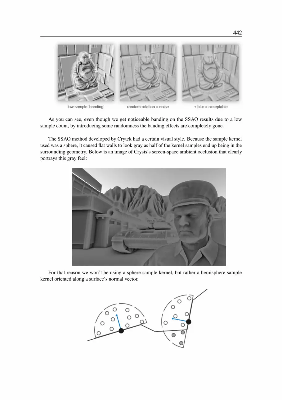
442
As you can see, even though we get noticeable banding on the SSAO results due to a lowsample count, by introducing some randomness the banding effects are completely gone.
The SSAO method developed by Crytek had a certain visual style. Because the sample kernelused was a sphere, it caused flat walls to look gray as half of the kernel samples end up being in thesurrounding geometry. Below is an image of Crysis’s screen-space ambient occlusion that clearlyportrays this gray feel:
For that reason we won’t be using a sphere sample kernel, but rather a hemisphere samplekernel oriented along a surface’s normal vector.

42.1 Sample buffers 443
By sampling around this normal-oriented hemisphere we do not consider the fragment’sunderlying geometry as contribution to the occlusion factor. This removes the gray-feel of ambientocclusion and generally produces more realistic results. This SSAO tutorial is based on this normal-oriented hemisphere method and a slightly modified version of John Chapman’s brilliant SSAOtutorial.
42.1 Sample buffersSSAO requires geometrical info as we need some way to determine the occlusion factor of afragment. For each fragment, we’re going to need the following data:
• A per-fragment position vector.• A per-fragment normal vector.• A linear depth texture.• A sample kernel.• A per-fragment random rotation vector used to rotate the sample kernel.Using a per-fragment view-space position we can orient a sample hemisphere kernel around
the fragment’s view-space surface normal and for each kernel sample we sample the linear depthtexture to compare the results. The sample kernel is slightly rotated based on a per-fragment rotationvector; the resulting occlusion factor is then used to limit the final ambient lighting component.
As SSAO is a screen-space technique we calculate its effect on each fragment on a screen-filled2D quad; we thus have no geometrical information of the scene. What we can do is render thegeometrical per-fragment data into screen-space textures that we then later send to the SSAO shaderso we have access to the per-fragment geometrical data. If you’ve followed along with the previoustutorial you’ll realize this looks largely similar to deferred rendering and for that reason SSAO isperfectly suited in combination with deferred rendering as we already have the position and normalvectors in the G-buffer.
In this tutorial we’re going to implement SSAO on top of a slightly simplified versionof the deferred renderer from the deferred shading tutorial so if you’re not sure whatdeferred shading is be sure to first read up on that.
As we already have per-fragment position and normal data available from the G-buffer we’llonly need to update the geometry shader to also include the linear depth of each fragment.

42.1 Sample buffers 444
As we’ve already learned from the depth testing tutorial we can extract the linear depth fromgl_FragCoord.z as follows:
#version 330 corelayout (location = 0) out vec4 gPositionDepth;layout (location = 1) out vec3 gNormal;layout (location = 2) out vec4 gAlbedoSpec;
in vec2 TexCoords;in vec3 FragPos;in vec3 Normal;
const float NEAR = 0.1; // projection matrix’s near planeconst float FAR = 50.0f; // projection matrix’s far planefloat LinearizeDepth(float depth){
float z = depth * 2.0 - 1.0; // Back to NDCreturn (2.0 * NEAR * FAR) / (FAR + NEAR - z * (FAR - NEAR));
}
void main(){
// Store the fragment position vector in the first gbuffer texturegPositionDepth.xyz = FragPos;// And store linear depth into gPositionDepth’s alpha componentgPositionDepth.a = LinearizeDepth(gl_FragCoord.z);// Also store the per-fragment normals into the gbuffergNormal = normalize(Normal);// And the diffuse per-fragment colorgAlbedoSpec.rgb = vec3(0.95);
}
The extracted linear depth is in view space so all further calculations are in view-space as well.Make sure the G-buffer’s positions and normals are in view-space (multiplied by the view matrix aswell). The view-space linear depth value is then stored as the gPositionDepth colorbuffer’salpha component to save us from having to declare another colorbuffer texture.
It is possible to reconstruct the actual position vectors from depth values alone usingsome clever tricks as Matt Pettineo described in his blog. This requires some extracalculations in the shaders, but saves us from having to store position data in the G-buffer which costs a lot of memory. For the sake of a simple example, we’ll leave theseoptimizations out of the tutorial.
The gPositionDepth colorbuffer texture is now configured as follows:
glGenTextures(1, &gPositionDepth);glBindTexture(GL_TEXTURE_2D, gPositionDepth);glTexImage2D(GL_TEXTURE_2D, 0, GL_RGBA16F, SCR_WIDTH, SCR_HEIGHT, 0,
GL_RGBA, GL_FLOAT, NULL);glTexParameteri(GL_TEXTURE_2D, GL_TEXTURE_MIN_FILTER, GL_NEAREST);glTexParameteri(GL_TEXTURE_2D, GL_TEXTURE_MAG_FILTER, GL_NEAREST);glTexParameteri(GL_TEXTURE_2D, GL_TEXTURE_WRAP_S, GL_CLAMP_TO_EDGE);glTexParameteri(GL_TEXTURE_2D, GL_TEXTURE_WRAP_T, GL_CLAMP_TO_EDGE);

42.2 Normal-oriented hemisphere 445
This gives us a linear depth texture that we can use to obtain depth values for each of the kernelsamples. Note that we store the linear depth values in a floating point data-format; this way thedepth values between 0.1 and 50.0 aren’t clamped to [0.0,1.0]. If you’re not using a floatingpoint format to store depth values, be sure to first normalize them before storing them into thegPositionDepth texture by dividing its values by FAR, and similarly re-construct them in alater shader. Also note the texture wrapping method of GL_CLAMP_TO_EDGE. This ensures wedon’t accidentally oversample depth values in screen-space outside the texture’s default coordinateregion.
Next we need the actual hemisphere sample kernel and some method to randomly rotate it.
42.2 Normal-oriented hemisphereWe need to generate a number of samples oriented along the normal of a surface. As we brieflydiscussed at the start of this tutorial we want to generate samples that form a hemisphere. As it isdifficult nor plausible to generate a sample kernel for each surface normal direction we’re goingto generate a sample kernel in tangent space, with the normal vector pointing in the positive zdirection.
Assuming we have a unit hemisphere we can obtain a sample kernel with a maximum of 64sample values as follows:
std::uniform_real_distribution<GLfloat> randomFloats(0.0, 1.0); // randomfloats between 0.0 - 1.0
std::default_random_engine generator;std::vector<glm::vec3> ssaoKernel;for (GLuint i = 0; i < 64; ++i){
glm::vec3 sample(randomFloats(generator) * 2.0 - 1.0,randomFloats(generator) * 2.0 - 1.0,randomFloats(generator)
);sample = glm::normalize(sample);sample *= randomFloats(generator);GLfloat scale = GLfloat(i) / 64.0;ssaoKernel.push_back(sample);
}
We vary the x and y direction in tangent space between -1.0 and 1.0 and vary the z directionof the samples between 0.0 and 1.0 (if we varied the z direction between -1.0 and 1.0 as well

42.3 Random kernel rotations 446
we’d have a sphere sample kernel). As the sample kernel will be oriented along the surface normal,the resulting sample vectors will all end up in the hemisphere.
Currently, all samples are evenly distributed in the sample kernel, but we’d rather place a largerweight on occlusions close to the actual fragment as to distribute the kernel samples closer to theorigin. We can do this with an accelerating interpolation function:
scale = lerp(0.1f, 1.0f, scale * scale);sample *= scale;ssaoKernel.push_back(sample);}
Where lerp is defined as:
GLfloat lerp(GLfloat a, GLfloat b, GLfloat f){
return a + f * (b - a);}
This gives us kernel distribution that places most samples closer to its origin.
Each of the kernel samples will be used to offset the view-space fragment position to samplesurrounding geometry. We saw at the start of this tutorial that without varying the sample kerneleach fragment we’ll need quite a few samples to get realistic results. By introducing a randomrotation to the sample kernel each fragment we can significantly reduce the number of samplesrequired.
42.3 Random kernel rotationsBy introducing some randomness onto the sample kernels we largely reduce the number of samplesnecessary to get good results. We could create a random rotation vector for each fragment of ascene, but that quickly eats up memory. It makes more sense to create a small texture of randomrotation vectors that we tile over the screen.
We create a 4x4 array of random rotation vectors oriented around the tangent-space surfacenormal:
std::vector<glm::vec3> ssaoNoise;for (GLuint i = 0; i < 16; i++){
glm::vec3 noise(

42.4 The SSAO shader 447
randomFloats(generator) * 2.0 - 1.0,randomFloats(generator) * 2.0 - 1.0,0.0f);
ssaoNoise.push_back(noise);}
As the sample kernel is oriented along the positive z direction in tangent space we leave the zcomponent at 0.0 so we rotate around the z axis.
We then create a 4x4 texture that holds the random rotation vectors; make sure to set itswrapping method to GL_REPEAT so it properly tiles over the screen.
GLuint noiseTexture;glGenTextures(1, &noiseTexture);glBindTexture(GL_TEXTURE_2D, noiseTexture);glTexImage2D(GL_TEXTURE_2D, 0, GL_RGB16F, 4, 4, 0, GL_RGB, GL_FLOAT, &
ssaoNoise[0]);glTexParameteri(GL_TEXTURE_2D, GL_TEXTURE_MIN_FILTER, GL_NEAREST);glTexParameteri(GL_TEXTURE_2D, GL_TEXTURE_MAG_FILTER, GL_NEAREST);glTexParameteri(GL_TEXTURE_2D, GL_TEXTURE_WRAP_S, GL_REPEAT);glTexParameteri(GL_TEXTURE_2D, GL_TEXTURE_WRAP_T, GL_REPEAT);
We now have all the relevant input data we need to implement SSAO.
42.4 The SSAO shaderThe SSAO shader runs on a 2D screen-filled quad that calculates the occlusion value for each ofthe generated fragments (for use in the final lighting shader). As we need to store the result of theSSAO stage we create yet another framebuffer object:
GLuint ssaoFBO;glGenFramebuffers(1, &ssaoFBO);glBindFramebuffer(GL_FRAMEBUFFER, ssaoFBO);GLuint ssaoColorBuffer;
glGenTextures(1, &ssaoColorBuffer);glBindTexture(GL_TEXTURE_2D, ssaoColorBuffer);glTexImage2D(GL_TEXTURE_2D, 0, GL_RED, SCR_WIDTH, SCR_HEIGHT, 0, GL_RGB,
GL_FLOAT, NULL);glTexParameteri(GL_TEXTURE_2D, GL_TEXTURE_MIN_FILTER, GL_NEAREST);glTexParameteri(GL_TEXTURE_2D, GL_TEXTURE_MAG_FILTER, GL_NEAREST);glFramebufferTexture2D(GL_FRAMEBUFFER, GL_COLOR_ATTACHMENT0, GL_TEXTURE_2D,
ssaoColorBuffer, 0);
As the ambient occlusion result is a single grayscale value we’ll only need a texture’s redcomponent thus we set the colorbuffer’s internal format to GL_RED.
The complete process for rendering SSAO then looks a bit like this:
// geometry pass: render stuff into G-bufferglBindFramebuffer(GL_FRAMEBUFFER, gBuffer);
[...]glBindFramebuffer(GL_FRAMEBUFFER, 0);

42.4 The SSAO shader 448
// use G-buffer to render SSAO textureglBindFramebuffer(GL_FRAMEBUFFER, ssaoFBO);
glClear(GL_COLOR_BUFFER_BIT);shaderSSAO.Use();glActiveTexture(GL_TEXTURE0);glBindTexture(GL_TEXTURE_2D, gPositionDepth);glActiveTexture(GL_TEXTURE1);glBindTexture(GL_TEXTURE_2D, gNormal);glActiveTexture(GL_TEXTURE2);glBindTexture(GL_TEXTURE_2D, noiseTexture);SendKernelSamplesToShader();glUniformMatrix4fv(projLocation, 1, GL_FALSE, glm::value_ptr(projection));RenderQuad();
glBindFramebuffer(GL_FRAMEBUFFER, 0);
// lighting pass: render scene lightingglClear(GL_COLOR_BUFFER_BIT | GL_DEPTH_BUFFER_BIT);shaderLightingPass.Use();[...]glActiveTexture(GL_TEXTURE3);glBindTexture(GL_TEXTURE_2D, ssaoColorBuffer);[...]RenderQuad();
The shaderSSAO shader takes as input the relevant G-buffer textures (including the lineardepth), the noise texture and the normal-oriented hemisphere kernel samples:
#version 330 coreout float FragColor;in vec2 TexCoords;
uniform sampler2D gPositionDepth;uniform sampler2D gNormal;uniform sampler2D texNoise;
uniform vec3 samples[64];uniform mat4 projection;
// tile noise texture over screen based on screen dimensions divided bynoise size
const vec2 noiseScale = vec2(800.0/4.0, 600.0/4.0); // screen = 800x600
void main(){
}
Interesting to note here is the noiseScale variable. We want to tile the noise texture all overthe screen, but as the TexCoords vary between 0.0 and 1.0 the texNoise texture wouldn’ttile at all. So we’ll calculate by how much we’ll have to scale the TexCoords coordinates bydividing the screen’s dimensions by the noise texture size; that we then use when we retrieve therelevant input vectors:
vec3 fragPos = texture(gPositionDepth, TexCoords).xyz;vec3 normal = texture(gNormal, TexCoords).rgb;vec3 randomVec = texture(texNoise, TexCoords * noiseScale).xyz;

42.4 The SSAO shader 449
As we set the tiling parameters of texNoise to GL_REPEAT the random values will berepeated all over the screen. Together with the fragPog and normal vector we then have enoughdata to create a TBN matrix that transforms any vector from tangent-space to view-space:
vec3 tangent = normalize(randomVec - normal * dot(randomVec, normal));vec3 bitangent = cross(normal, tangent);mat3 TBN = mat3(tangent, bitangent, normal);
Using a process called the Gramm-Schmidt process we create an orthogonal basis, each timeslightly tilted based on the value of randomVec. Note that because we use a random vector forconstructing the tangent vector, there is no need to have the TBN matrix exactly aligned to thegeometry’s surface, thus no need for per-vertex tangent (and bitangent) vectors.
Next we iterate over each of the kernel samples, transform the samples from tangent to view-space, add them to the current fragment position and compare the fragment position’s depth withthe sample depth stored in the original depth buffer. Let’s discuss it in a step-by-step fashion:
float occlusion = 0.0;for(int i = 0; i < kernelSize; ++i){
// get sample positionvec3 sample = TBN * samples[i]; // From tangent to view-spacesample = fragPos + sample * radius;
[...]}
Here kernelSize and radius are variables that we can use to tweak the effect; in this casekept to their default values of 64 and 1.0 respectively. For each iteration we first transform therespective sample to view-space. We then add the view-space kernel offset sample to the view-spacefragment position; we multiply the offset sample by radius to increase (or decrease) the effectivesample radius of SSAO.
Next we transform sample to screen-space so we can sample the (linear) depth value ofsample as if we were rendering its position directly to the screen. As the vector is currently inview-space, we’ll transform it to clip-space first using the projection matrix uniform:
vec4 offset = vec4(sample, 1.0);offset = projection * offset; // from view to clip-spaceoffset.xyz /= offset.w; // perspective divideoffset.xyz = offset.xyz * 0.5 + 0.5; // transform to range 0.0 - 1.0
After the variable is transformed to clip-space we perform the perspective divide step bydividing its xyz components with its w component. The resulting normalized device coordinatesare then transformed to the [0.0, 1.0] range so we can use them to sample the depth texture:
float sampleDepth = -texture(gPositionDepth, offset.xy).w;
We use the offset vector’s x and y component to sample the linear depth texture to get thedepth value of the sample position as seen from the viewer’s perspective (so the first non-occludedvisible fragment). We then check if the sample’s current depth value is larger than the stored depthvalue and if so, we add to the final contribution factor:

42.4 The SSAO shader 450
occlusion += (sampleDepth >= sample.z ? 1.0 : 0.0);
We’re not completely finished as there is still a small issue we have to take into account.Whenever a fragment is tested for ambient occlusion that is aligned close to the edge of a surface,it will also consider the depth values of surfaces far behind the test surface; these values will(incorrectly) contribute to the occlusion factor. We can solve this by introducing a range check asthe following image (courtesy of John Chapman) illustrates:
We introduce a range check that makes sure we only contribute to the occlusion factor if thedepth values to test are within the sample’s radius. We change the last line by:
float rangeCheck = smoothstep(0.0, 1.0, radius / abs(fragPos.z -sampleDepth));
occlusion += (sampleDepth >= sample.z ? 1.0 : 0.0) * rangeCheck;
Here we used GLSL’s smoothstep function that smoothly interpolates its third parameterbetween the first and second parameter’s range. If the depth difference thus ends up betweenradius their value gets smoothly interpolated between 0.0 and 1.0 by the following curve:
If we used a hard cut-off range check that abruptly removes occlusion contributions if the depthvalues are outside the radius we’d see obvious (unattractive) borders at where the range check isapplied.

42.5 Ambient occlusion blur 451
As a final step we’d normalize the occlusion contribution by the size of the kernel and output theresults. Note that we subtract the occlusion factor from 1.0 so we can directly use the occlusionfactor to scale the ambient lighting component.
}occlusion = 1.0 - (occlusion / kernelSize);FragColor = occlusion;
If we’d imagine a scene where our favorite nanosuit model is taking a little nap, the ambientocclusion shader produces the following texture:
As we can see, ambient occlusion gives a great sense of depth. With just the ambient occlusiontexture we can already clearly see the model is indeed laying on the floor instead of hoveringslightly above it.
It still doesn’t look perfect as the repeating pattern of the noise texture is clearly visible. Tocreate a smooth ambient occlusion result we need to blur the ambient occlusion texture.
42.5 Ambient occlusion blurBetween the SSAO pass and the lighting pass we first want to blur the SSAO texture, so let’s createyet another framebuffer object for storing the blur result:
GLuint ssaoBlurFBO, ssaoColorBufferBlur;glGenFramebuffers(1, &ssaoBlurFBO);glBindFramebuffer(GL_FRAMEBUFFER, ssaoBlurFBO);

42.5 Ambient occlusion blur 452
glGenTextures(1, &ssaoColorBufferBlur);glBindTexture(GL_TEXTURE_2D, ssaoColorBufferBlur);glTexImage2D(GL_TEXTURE_2D, 0, GL_RED, SCR_WIDTH, SCR_HEIGHT, 0, GL_RGB,
GL_FLOAT, NULL);glTexParameteri(GL_TEXTURE_2D, GL_TEXTURE_MIN_FILTER, GL_NEAREST);glTexParameteri(GL_TEXTURE_2D, GL_TEXTURE_MAG_FILTER, GL_NEAREST);glFramebufferTexture2D(GL_FRAMEBUFFER, GL_COLOR_ATTACHMENT0, GL_TEXTURE_2D,
ssaoColorBufferBlur, 0);
Because the tiled random vector texture keeps a consistent randomness we can use this propertyto our advantage to create a very simple blur shader:
#version 330 corein vec2 TexCoords;out float fragColor;
uniform sampler2D ssaoInput;
void main() {vec2 texelSize = 1.0 / vec2(textureSize(ssaoInput, 0));float result = 0.0;for (int x = -2; x < 2; ++x){
for (int y = -2; y < 2; ++y){
vec2 offset = vec2(float(x), float(y)) * texelSize;result += texture(ssaoInput, TexCoords + offset).r;
}}fragColor = result / (4.0 * 4.0);
}
Here we traverse the surrounding SSAO texels between -2.0 and 2.0 sampling the SSAOtexture the identical amount as the noise texture’s dimensions. We offset each texture coordinateby the exact size of a single texel using textureSize that returns a vec2 of the given texture’sdimensions. We average the obtained results to get a simple, but effective blur:

42.6 Applying ambient occlusion 453
And there we go, a texture with per-fragment ambient occlusion data; ready for use in thelighting pass.
42.6 Applying ambient occlusionApplying the occlusion factors to the lighting equation is incredibly easy: all we have to do ismultiply the per-fragment ambient occlusion factor to the lighting’s ambient component and we’redone. If we take the Blinn-Phong deferred lighting shader of the previous tutorial and adjust it a bitwe get the following fragment shader:
#version 330 coreout vec4 FragColor;in vec2 TexCoords;
uniform sampler2D gPositionDepth;uniform sampler2D gNormal;uniform sampler2D gAlbedo;uniform sampler2D ssao;
struct Light {vec3 Position;vec3 Color;
float Linear;float Quadratic;float Radius;
};uniform Light light;

42.6 Applying ambient occlusion 454
void main(){
// Retrieve data from gbuffervec3 FragPos = texture(gPositionDepth, TexCoords).rgb;vec3 Normal = texture(gNormal, TexCoords).rgb;vec3 Diffuse = texture(gAlbedo, TexCoords).rgb;float AmbientOcclusion = texture(ssao, TexCoords).r;
// Blinn-Phong (in view-space)vec3 ambient = vec3(0.3 * AmbientOcclusion); // Here we add occlusionfactorvec3 lighting = ambient;vec3 viewDir = normalize(-FragPos); // Viewpos is (0.0.0) in view-space// Diffusevec3 lightDir = normalize(light.Position - FragPos);vec3 diffuse = max(dot(Normal, lightDir), 0.0) * Diffuse * light.Color;// Specularvec3 halfwayDir = normalize(lightDir + viewDir);float spec = pow(max(dot(Normal, halfwayDir), 0.0), 8.0);vec3 specular = light.Color * spec;// Attenuationfloat dist = length(light.Position - FragPos);float attenuation = 1.0 / (1.0 + light.Linear * dist + light.Quadratic
* dist * dist);diffuse *= attenuation;specular *= attenuation;lighting += diffuse + specular;
FragColor = vec4(lighting, 1.0);}
The only thing (besides changing it to view-space) we really changed compared to previ-ous lighting implementations is the multiplication of the scene’s ambient component by theAmbientOcclusion value. With a single point blue-ish light in the scene we’d get the followingresult:

42.6 Applying ambient occlusion 455
You can find the full source code here together with the following shaders:
• geometry: vertex, fragment.• SSAO: vertex, fragment.• blur: vertex, fragment.• lighting: vertex, fragment.Screen-space ambient occlusion is a highly customizable effect that relies heavily on tweaking
its parameters based on the type of scene. There is no perfect combination of parameters for everytype of scene; some scenes only work with a small radius, while some scenes require a larger radiusand a larger sample count for it to look realistic. The current demo uses 64 samples which is a bitmuch, play around with a smaller kernel size and try to get good results.
Some parameters you can tweak (by using uniforms for example): kernel size, radius and/orsize of noise kernel. You can also raise the final occlusion value to a user-defined power to increaseits strength:
occlusion = 1.0 - (occlusion / kernelSize);FragColor = pow(occlusion, power);
Play around with different scenes and different parameters to appreciate the customizability ofSSAO.
Even though SSAO is a subtle effect that isn’t too clearly noticeable it adds a great deal ofrealism to properly lighted scenes and is definitely a technique you’d want to have in your toolkit.

42.7 Additional resources 456
42.7 Additional resources• SSAO Tutorial: excellent SSAO tutorial by John Chapman; a large portion of this tutorial’s
code and techniques are based of his article.• Know your SSAO artifacts: great article about improving SSAO specific artifacts.• SSAO With Depth Reconstruction: extension tutorial on top of SSAO from OGLDev about
reconstructing position vectors from depth alone, saving us from storing the expensiveposition vectors in the G-buffer.

VI43 Text Rendering . . . . . . . . . . . . . . . . . . . . . 458
44 2D Game . . . . . . . . . . . . . . . . . . . . . . . . . . 468
45 Breakout . . . . . . . . . . . . . . . . . . . . . . . . . . . 469
46 Setting up . . . . . . . . . . . . . . . . . . . . . . . . . . 472
47 Rendering Sprites . . . . . . . . . . . . . . . . . . . 476
48 Levels . . . . . . . . . . . . . . . . . . . . . . . . . . . . . . 482
49 Ball . . . . . . . . . . . . . . . . . . . . . . . . . . . . . . . . 490
50 Collision detection . . . . . . . . . . . . . . . . . 494
51 Collision resolution . . . . . . . . . . . . . . . . . 501
52 Particles . . . . . . . . . . . . . . . . . . . . . . . . . . . 508
53 Postprocessing . . . . . . . . . . . . . . . . . . . . . 514
54 Powerups . . . . . . . . . . . . . . . . . . . . . . . . . . 519
55 Audio . . . . . . . . . . . . . . . . . . . . . . . . . . . . . . 527
56 Render text . . . . . . . . . . . . . . . . . . . . . . . . 530
57 Final thoughts . . . . . . . . . . . . . . . . . . . . . . 539
In Practice

43. Text Rendering
At some stage of your graphics adventures you will want to draw text in OpenGL. Contrary towhat you might expect, getting a simple string to render on screen is quite difficult with a low-levellibrary like OpenGL. If you don’t care about rendering more than 128 different characters, thenit’s probably not too difficult. Things are getting more difficult as soon as each character has adifferent width, height and margin. Based on where you live, you might also need more than 128characters, and what if you want to express special symbols for like mathematical expressions orsheet music symbols, and what about rendering text from top to bottom? Once you think about allthese complicated matters of text, it wouldn’t surprise you that this probably doesn’t belong in alow-level API like OpenGL.
Since there is no support for any text capabilities within OpenGL it is up to us to define a systemfor rendering text to the screen. Since there are no graphical primitives for text characters, we haveto get creative. Some example techniques are: drawing letter shapes via GL_LINES, create 3Dmeshes of letters or render character textures to 2D quads in a 3D environment.
Most often developers choose to render character textures onto quads. Rendering these texturedquads by itself shouldn’t be too difficult, but getting the relevant character(s) onto a texture couldprove challenging. In this tutorial we’ll explore several methods and implement a more advanced,but flexible technique for rendering text using the FreeType library.
43.1 Classical text rendering: bitmap fontsIn the early days rendering text involved selecting a font (or create one yourself) you’d like for yourapplication and extracting all relevant characters out of this font to paste them all within a singlelarge texture. Such a texture, that we from now on call a bitmap font, contains all character symbolswe want to use in predefined regions of the texture. These character symbols of the font are knownas glyphs. Each glyph has a specific region of texture coordinates associated with them. Wheneveryou want to render a character, you select the corresponding glyph by rendering this section of the

43.2 Modern text rendering: FreeType 459
bitmap font to a 2D quad.
Here you can see how we would render the text ’OpenGL’ by taking a bitmap font and samplingthe corresponding glyphs from the texture (by carefully choosing the texture coordinates) that werender on top of several quads. By enabling blending and keeping the background transparent, wewill end up with just a string of characters rendered to the screen. This particular bitmap font wasgenerated using Codehead’s Bitmap Font Generator.
This approach has several advantages and disadvantages. First, it is relatively easy to implementand because bitmap fonts are pre-rasterized they’re quite efficient. However, it is not particularflexible. When you want to use a different font, you need to recompile a complete new bitmapfont and the system is limited to a single resolution; zooming will quickly show pixelated edges.Furthermore, it is often limited to a small character set so Extended or Unicode characters are oftenout of the question.
This approach was quite popular back in the day since it is fast and works on any platform,but as of today more flexible approaches exist. One of these approaches is loading TrueType fontsusing the FreeType library.
43.2 Modern text rendering: FreeTypeFreeType is a software development library that is able to load fonts, render them to bitmaps andprovide support for several font-related operations. It is a popular library used by Mac OS X,Java, PlayStation Consoles, Linux and Android to name a few. What makes FreeType particularlyattractive is that it is able to load TrueType fonts.
A TrueType font is a collection of character glyphs not defined by pixels or any other non-scalable solution, but by mathematical equations (combinations of splines). Similar to vectorimages, the rasterized font images can be procedurally generated based on the preferred font heightyou’d like to obtain them in. By using TrueType fonts you can easily render character glyphs ofvarious sizes without any loss of quality.
FreeType can be downloaded from their website. You can choose to compile the library yourself

43.2 Modern text rendering: FreeType 460
from their source code or use one of their precompiled libraries if your target platform is listed. Besure to link to freetype.lib and make sure your compiler knows where to find the header files.
Then be sure to include the appropriate headers:
#include <ft2build.h>#include FT_FREETYPE_H
Due to how FreeType is developed (at least at the time of this writing), you cannot puttheir header files in a new directory; they should be located at the root of your includedirectories. Including FreeType like #include <FreeType/ft2build.h> willlikely cause several header conflicts.
What FreeType does is load these TrueType fonts and for each glyph generates a bitmap imageand calculates several metrics. We can extract these bitmap images for generating textures andposition each character glyph appropriately using the loaded metrics.
To load a font, all we have to do is initialize the FreeType library and load the font as a face asFreeType likes to call it. Here we load the arial.ttf TrueType font file that was copied fromthe Windows/Fonts directory.
FT_Library ft;if (FT_Init_FreeType(&ft))
std::cout << "ERROR::FREETYPE: Could not init FreeType Library" << std::endl;
FT_Face face;if (FT_New_Face(ft, "fonts/arial.ttf", 0, &face))
std::cout << "ERROR::FREETYPE: Failed to load font" << std::endl;
Each of these FreeType functions returns a non-zero integer whenever an error occurred.
Once we’ve loaded the face, we should define the font size we’d like to extract from this face:
FT_Set_Pixel_Sizes(face, 0, 48);
The function sets the font’s width and height parameters. Setting the width to 0 lets the facedynamically calculate the width based on the given height.
A FreeType face hosts a collection of glyphs. We can set one of those glyphs as the active glyphby calling FT_Load_Char. Here we choose to load the character glyph ’X’:
if (FT_Load_Char(face, ’X’, FT_LOAD_RENDER))std::cout << "ERROR::FREETYTPE: Failed to load Glyph" << std::endl;
By setting FT_LOAD_RENDER as one of the loading flags, we tell FreeType to create an 8-bitgrayscale bitmap image for us that we can access via face->glyph->bitmap.
Each of the glyphs we load with FreeType however do not have the same size (as we had withbitmap fonts). The bitmap image generated by FreeType is just large enough to contain the visible

43.2 Modern text rendering: FreeType 461
part of a character. For example, the bitmap image of the dot character ’.’ is much smaller thanthe bitmap image of the character ’X’. For this reason, FreeType also loads several metrics thatspecify how large each character should be and how to properly position them. Below is an imageby FreeType that shows all of the metrics it calculates for each character glyph.
Each of the glyphs reside on a horizontal baseline (as depicted by the horizontal arrow) wheresome glyphs sit exactly on top of this baseline (like ’X’) or some slightly below the baseline (like’g’ or ’p’). These metrics define exactly the offsets to properly position each glyph on the baseline,how large each glyph should be and how many pixels we need to advance to render the next glyph.Below is a small list of these properties we’ll be needing.
• width: the width (in pixels) of the bitmap accessed via face->glyph->bitmap.width.• height: the height (in pixels) of the bitmap accessed via face->glyph->bitmap.rows.• bearingX: the horizontal bearing e.g. the horizontal position (in pixels) of the bitmap relative
to the origin accessed via face->glyph->bitmap_left.• bearingY: the vertical bearing e.g. the vertical position (in pixels) of the bitmap relative to
the baseline accessed via face->glyph->bitmap_top.• advance: the horizontal advance e.g. the horizontal distance (in 1/64th pixels) from the
origin to the origin of the next glyph. Accessed via face->glyph->advance.x.We could load a character glyph, retrieve its metrics and generate a texture each time we want
to render a character to the screen, but it would be inefficient to do this each frame. We’d ratherstore the generated data somewhere in the application and query it whenever we want to render acharacter. We’ll define a convenient struct that we’ll store in a map.
struct Character {GLuint TextureID; // ID handle of the glyph textureglm::ivec2 Size; // Size of glyphglm::ivec2 Bearing; // Offset from baseline to left/top of glyphGLuint Advance; // Offset to advance to next glyph
};
std::map<GLchar, Character> Characters;
For this tutorial we’ll keep things simple by restricting ourselves to the first 128 characters ofthe ASCII character set. For each character, we generate a texture and store its relevant data into aCharacter struct that we add to the Characters map. This way, all data required to rendereach character is stored for later use.

43.2 Modern text rendering: FreeType 462
glPixelStorei(GL_UNPACK_ALIGNMENT, 1); // Disable byte-alignmentrestriction
for (GLubyte c = 0; c < 128; c++){
// Load character glyphif (FT_Load_Char(face, c, FT_LOAD_RENDER)){
std::cout << "ERROR::FREETYTPE: Failed to load Glyph" << std::endl;continue;
}// Generate textureGLuint texture;glGenTextures(1, &texture);glBindTexture(GL_TEXTURE_2D, texture);glTexImage2D(
GL_TEXTURE_2D,0,GL_RED,face->glyph->bitmap.width,face->glyph->bitmap.rows,0,GL_RED,GL_UNSIGNED_BYTE,face->glyph->bitmap.buffer
);// Set texture optionsglTexParameteri(GL_TEXTURE_2D, GL_TEXTURE_WRAP_S, GL_CLAMP_TO_EDGE);glTexParameteri(GL_TEXTURE_2D, GL_TEXTURE_WRAP_T, GL_CLAMP_TO_EDGE);glTexParameteri(GL_TEXTURE_2D, GL_TEXTURE_MIN_FILTER, GL_LINEAR);glTexParameteri(GL_TEXTURE_2D, GL_TEXTURE_MAG_FILTER, GL_LINEAR);// Now store character for later useCharacter character = {
texture,glm::ivec2(face->glyph->bitmap.width, face->glyph->bitmap.rows),glm::ivec2(face->glyph->bitmap_left, face->glyph->bitmap_top),face->glyph->advance.x
};Characters.insert(std::pair<GLchar, Character>(c, character));
}
Within the for loop we list over all the 128 characters of the ASCII set and retrieve their corre-sponding character glyphs. For each character, we generate a texture, set its options and store its met-rics. What is interesting to note here is that we use GL_RED as the texture’s internalFormatand format arguments. The bitmap generated from the glyph is a grayscale 8-bit image whereeach color is represented by a single byte. For this reason we’d like to store each byte of thebitmap buffer as a texture’s color value. We accomplish this by creating a texture where each bytecorresponds to the texture color’s red component (first byte of its color vector). If we use a singlebyte to represent the colors of a texture we do need to take care of a restriction of OpenGL:
glPixelStorei(GL_UNPACK_ALIGNMENT, 1);
OpenGL requires that textures all have a 4-byte alignment e.g. their size is always a multiple of4 bytes. Normally this won’t be a problem since most textures have a width that is a multiple of 4and/or use 4 bytes per pixel, but since we now only use a single byte per pixel they can have anypossible width. By setting its unpack alignment equal to 1 we ensure there are no alignment issues(which could cause segmentation faults).

43.2 Modern text rendering: FreeType 463
Also be sure to clear FreeType’s resources once you’re finished processing the glyphs:
FT_Done_Face(face);FT_Done_FreeType(ft);
43.2.1 ShadersTo render the actual glyphs we’ll be using the following vertex shader:
#version 330 corelayout (location = 0) in vec4 vertex; // <vec2 pos, vec2 tex>out vec2 TexCoords;
uniform mat4 projection;
void main(){
gl_Position = projection * vec4(vertex.xy, 0.0, 1.0);TexCoords = vertex.zw;
}
We combine both the position and texture coordinate data into one vec4. The vertex shadermultiplies the coordinates with a projection matrix and forwards the texture coordinates to thefragment shader:
#version 330 corein vec2 TexCoords;out vec4 color;
uniform sampler2D text;uniform vec3 textColor;
void main(){
vec4 sampled = vec4(1.0, 1.0, 1.0, texture(text, TexCoords).r);color = vec4(textColor, 1.0) * sampled;
}
The fragment shader takes two uniforms: one is the mono-colored bitmap image of the glyphand the other is a color uniform for adjusting the text’s final color. We first sample the color valueof the bitmap texture. Because the texture’s data is stored in just its red component, we samplethe r component of the texture as the sampled alpha value. By varying the color’s alpha value theresulting color will be transparent for all the glyph’s background colors and non-transparent for theactual character pixels. We also multiply the RGB colors by the textColor uniform to vary thetext color.
We do need to enable blending for this to work though:
glEnable(GL_BLEND);glBlendFunc(GL_SRC_ALPHA, GL_ONE_MINUS_SRC_ALPHA);
For the projection matrix we’ll be using an orthographic projection matrix. For rendering textwe (usually) do not need perspective and using an orthographic projection matrix also allows us tospecify all vertex coordinates in screen coordinates if we set it up as follows:

43.2 Modern text rendering: FreeType 464
glm::mat4 projection = glm::ortho(0.0f, 800.0f, 0.0f, 600.0f);
We set the projection matrix’s bottom parameter to 0.0f and its top parameter equal to thewindow’s height. The result is that we specify coordinates with y values ranging from the bottompart of the screen (0.0f) to the top part of the screen (600.0f). This means that the point (0.0,0.0) now corresponds to the bottom-left corner.
Last up is creating a VBO and VAO for rendering the quads. For now we reserve enoughmemory when initiating the VBO so that we can later update the VBO’s memory when renderingcharacters.
GLuint VAO, VBO;glGenVertexArrays(1, &VAO);glGenBuffers(1, &VBO);glBindVertexArray(VAO);glBindBuffer(GL_ARRAY_BUFFER, VBO);glBufferData(GL_ARRAY_BUFFER, sizeof(GLfloat) * 6 * 4, NULL,
GL_DYNAMIC_DRAW);glEnableVertexAttribArray(0);glVertexAttribPointer(0, 4, GL_FLOAT, GL_FALSE, 4 * sizeof(GLfloat), 0);glBindBuffer(GL_ARRAY_BUFFER, 0);glBindVertexArray(0);
The 2D quad requires 6 vertices of 4 floats each so we reserve 6 * 4 floats of memory.Because we’ll be updating the content of the VBO’s memory quite often we’ll allocate the memorywith GL_DYNAMIC_DRAW.
43.2.2 Render line of textTo render a character we extract the corresponding Character struct of the Characters mapand calculate the quad’s dimensions using the character’s metrics. With the quad’s calculateddimensions we dynamically generate a set of 6 vertices that we use to update the content of thememory managed by the VBO using glBufferSubData.
We create a function called RenderText that renders a string of characters:
void RenderText(Shader &s, std::string text, GLfloat x, GLfloat y, GLfloatscale, glm::vec3 color)
{// Activate corresponding render states.Use();glUniform3f(glGetUniformLocation(s.Program, "textColor"), color.x,color.y, color.z);glActiveTexture(GL_TEXTURE0);glBindVertexArray(VAO);
// Iterate through all charactersstd::string::const_iterator c;for (c = text.begin(); c != text.end(); c++){
Character ch = Characters[*c];
GLfloat xpos = x + ch.Bearing.x * scale;GLfloat ypos = y - (ch.Size.y - ch.Bearing.y) * scale;

43.2 Modern text rendering: FreeType 465
GLfloat w = ch.Size.x * scale;GLfloat h = ch.Size.y * scale;// Update VBO for each characterGLfloat vertices[6][4] = {
{ xpos, ypos + h, 0.0, 0.0 },{ xpos, ypos, 0.0, 1.0 },{ xpos + w, ypos, 1.0, 1.0 },
{ xpos, ypos + h, 0.0, 0.0 },{ xpos + w, ypos, 1.0, 1.0 },{ xpos + w, ypos + h, 1.0, 0.0 }
};// Render glyph texture over quadglBindTexture(GL_TEXTURE_2D, ch.textureID);// Update content of VBO memoryglBindBuffer(GL_ARRAY_BUFFER, VBO);glBufferSubData(GL_ARRAY_BUFFER, 0, sizeof(vertices), vertices);glBindBuffer(GL_ARRAY_BUFFER, 0);// Render quadglDrawArrays(GL_TRIANGLES, 0, 6);// Now advance cursors for next glyph (note that advance is number
of 1/64 pixels)x += (ch.Advance >> 6) * scale; // Bitshift by 6 to get value in
pixels (2^6 = 64)}glBindVertexArray(0);glBindTexture(GL_TEXTURE_2D, 0);
}
The content of the function should be relatively self-explanatory: we first calculate the originposition of the quad (as xpos and ypos) and the quad’s size (as w and h) and generate a set of 6vertices to form the 2D quad; note that we scale each metric by scale. We then update the contentof the VBO and render the quad.
The following line of code requires some extra attention though:
GLfloat ypos = y - (ch.Size.y - ch.Bearing.y);
Some characters (like ’p’ or ’g’) are rendered slightly below the baseline so the quad shouldalso be positioned slightly below RenderText’s y value. The exact amount we need to offsetypos below the baseline can be figured out from the glyph metrics:

43.2 Modern text rendering: FreeType 466
To calculate this distance e.g. offset we need to figure out the distance a glyph extends belowthe baseline; this distance is indicated by the red arrow. As you can see from the glyph metrics wecan calculate the length of this vector by subtracting bearingY from the glyph’s (bitmap) height.This value is then 0.0 for characters that rest on the baseline (like ’X’) and positive for charactersthat reside slightly below the baseline (like ’g’ or ’j’).
If you did everything correct you should now be able to successfully render strings of text withthe following statements:
RenderText(shader, "This is sample text", 25.0f, 25.0f, 1.0f, glm::vec3(0.5, 0.8f, 0.2f));
RenderText(shader, "(C) LearnOpenGL.com", 540.0f, 570.0f, 0.5f, glm::vec3(0.3, 0.7f, 0.9f));
This should then look similar to the following image:
You can find the code of this example here.
To give you a feel of how we calculated the quad’s vertices we can disable blending to see whatthe actual rendered quads look like:

43.3 Going further 467
Here you can clearly see most quads resting on the (imaginary) baseline while the quads thatcorresponds to glyphs like ’p’ or ’(’ are shifted downwards.
43.3 Going furtherThis tutorial demonstrated a text rendering technique with TrueType fonts using the FreeTypelibrary. The approach is flexible, scalable and works with many character encodings. However, itmight be overkill for your application and performance-wise bitmap fonts might be preferable. Youcould of course combine the two approaches by dynamically generating a bitmap font featuring allcharacters glyphs as loaded with FreeType. This saves the renderer from a significant amount oftexture switches and based on how tightly each glyph is packed could save quite some performance.
Another issue with FreeType fonts is that the glyph textures are stored with a fixed font size soa significant amount of scaling might be required that will introduce jagged edges. Furthermore,rotations applied to the glyphs will cause them to appear blurry. This can be mitigated by, insteadof storing the actual rasterized pixel color, storing the distance to the closest glyph outline per pixel.This technique is called signed distance fields and Valve published a paper a few years ago abouttheir implementation of this technique which works surprisingly well for 3D rendering applications.

44. 2D Game
The following chapters discuss the step-by-step development of a simple Breakout game in OpenGLas to give you some sense how to actually use OpenGL to create something meaningful instead ofjust a few relatively simple tech demos.

45. Breakout
Over these tutorials we learned a fair share about OpenGL’s inner workings and how we can usethem to create fancy graphics. However, aside from a few tech demos, we haven’t really created apractical application with OpenGL. This is the introduction of a larger tutorial series about creatinga relatively simple 2D game using OpenGL. The tutorial series will demonstrate how we can useOpenGL in a larger, more complicated, setting. Note that the series does not necessarily introducenew OpenGL concepts but more or less show how we can apply these concepts to a larger whole.
Because we rather keep things simple we ’re going to base our 2D game on an already existing2D arcade game. Introducing Breakout, a classic 2D game released in 1976 on the Atari 2600console. Breakout requires the player, who controls a small horizontal paddle, to destroy all thebricks by bouncing a small ball against each brick without allowing the ball to reach the bottomedge. Once the player destroyed all bricks, he completes the game.
Below we can see how Breakout originally looked on the Atari 2600:

45.1 OpenGL Breakout 470
The game has the following mechanics:
• A small paddle is controlled by the player and can only move within the bounds of the screen;either left or right.• The ball travels across the screen and each collision results in the ball changing its direction
based on where it hit; this applies to the screen bounds, the bricks and the paddle.• If the ball reaches the bottom edge of the screen, the player is either game over or loses a life.• As soon as a brick touches the ball, it is destroyed.• The player wins as soon as all bricks are destroyed.• The direction of the ball can be manipulated by how far the ball bounces from the paddle’s
center.Because from time to time the ball might find a small gap reaching the area above the brick
wall, it will continue to bounce up and forth between the top edge of the level and the top edge ofthe brick layer. The ball keeps this up, until it eventually finds a gap again. This is logically wherethe game obtained its name from, since the ball has to break out.
45.1 OpenGL BreakoutWe’re going to take this classic arcade game as the basis of a 2D game that we’ll completelyimplement with OpenGL. This version of Breakout will run on the graphics card which gives us theability to enhance the classical Breakout game with some nice extra features.
Aside from the classical mechanics, our version of Breakout will feature:
• Best graphics you’ve ever seen• Particles• Advanced text rendering• PowerUps

45.1 OpenGL Breakout 471
• Postprocessing effects• Multiple (customizable) levelsTo get you excited you can see what the game will look like below after you’ve finished the
tutorial series:
These tutorials will combine a large number of concepts as discussed in previous tutorials anddemonstrate how they can work together as a whole. Therefore, it is important to have at leastfinished the Getting started section before working your way through these tutorials.
Also, several tutorials will require concepts from other tutorials (for example Framebuffersfrom the Advanced OpenGL section) so where necessary, the required tutorials are listed.
If you believe you’re ready to get your hands dirty then move on to the next tutorial.

46. Setting up
Before we get started with the actual game mechanics we first need to set up a simple frameworkfor the game to reside in. The game will use several third party libraries of which most of themwere introduced in the earlier tutorials. Wherever a new library is required, it will be properlyintroduced.
First, we define a so called uber game class that contains all relevant render and gameplay code.The idea of such a game class is that it (sort of) organizes your game code while also decoupling allwindowing code from the game. This way, you could use the same class in a completely differentwindowing library (like SDL or SFML for example) without much effort.
There are thousands of ways of trying to abstract and generalize game/graphics codeinto classes and objects. What you will see in this tutorials is just one approach to solvethese problems. If you feel there is a better approach, try to come up with your ownimprovement of the implementation.
The game class hosts an initialization function, an update function, a function to process inputand a render function:
class Game{
public:// Game stateGameState State;GLboolean Keys[1024];GLuint Width, Height;// Constructor/DestructorGame(GLuint width, GLuint height);~Game();// Initialize game state (load all shaders/textures/levels)

46.1 Utility 473
void Init();// GameLoopvoid ProcessInput(GLfloat dt);void Update(GLfloat dt);void Render();
};
The class hosts what you might expect from a game class. We initialize the game by giving awidth and height (corresponding to the resolution you want to play the game in) and use the Initfunction to load shaders, textures and initialize all gameplay state. We can process the input asstored within the Keys array by calling ProcessInput and update all gameplay events (likeplayer/ball movement) in the Update function. Last, we can render the game by calling Render.Note that we split the movement logic from the render logic.
The Game class also hosts a variable called State which is of type GameState as definedbelow:
// Represents the current state of the gameenum GameState {
GAME_ACTIVE,GAME_MENU,GAME_WIN
};
This allows us to keep track of what state the game is currently in. This way we can decide torender and/or process different items based on the current state of the game (we probably renderand process diferent items when we’re in the game’s menu for example).
As of now, the functions of the game class are completely empty since we have yet to write theactual game code, but here are the Game class’s header and code file.
46.1 UtilitySince we’re creating a large application we’ll frequently have to re-use several OpenGL concepts,like textures and shaders. It thus makes sense to create a more easy-to-use interface for these twoitems as similarly done in one of the earlier tutorials where we created a shader class.
A shader class is defined that generates a compiled shader (or generates error messages if itfails) from two or three strings (if a geometry shader is present). The shader class also containsa lot of useful utility functions to quickly set uniform values. A texture class is also defined thatgenerates a 2D texture image (based on its properties) from a byte array and a given width andheight. Again, the texture class also hosts utility functions.
We won’t delve into the details of the classes since by now you should easily understand howthey work. For this reason you can find the header and code files, fully commented, below:
• Shader: header, code.• Texture: header, code.Note that the current texture class is solely designed for 2D textures only, but could easily be
extended for alternative texture types.

46.2 Resource management 474
46.2 Resource managementWhile the shader and texture classes function great by themselves, they do require either a bytearray or several strings to initialize them. We could easily embed file loading code within theclasses themselves, but this slightly violates the single responsibility principle in that the classesshould only focus on either textures or shaders respectively and not necessarily their file-loadingmechanics.
For this reason it is often considered a more organized approach to create a single entity designedfor loading game-related resources called a resource manager. There are several approaches tocreating a resource manager; for this tutorial we chose to use a singleton static resource managerthat is (due to its static nature) always available throughout the project hosting all loaded resourcesand its relevant loading functionality.
Using a singleton class with static functionality has several advantages and disadvantages withits disadvantages mostly being losing OOP properties and losing control over construction/destruc-tion. However, for relative small projects like these it is easy to work with.
Like the other class files, the resource manager is listed below:
• Resource Manager: header, code.Using the resource manager we can easily load shaders into the program like:
Shader shader = ResourceManager::LoadShader("vertex.vs", "fragment.vs",nullptr, "test");
// then use itshader.Use();// orResourceManager::GetShader("test").Use();
The defined Game class together with the resource manager and the easily manageable Shaderand Texture2D classes form the basis for the next tutorials as we’ll be extensively using theseclasses to implement the Breakout game.
46.3 ProgramWe still need a window for the game and set some initial OpenGL state. We make use of OpenGL’sface-culling functionality and of its blending functionality. We do not use depth testing; since thegame is entirely in 2D, all vertices are defined with the same z-values, so enabling depth testingwould be of no use and likely cause z-fighting.
The startup code of the Breakout game is relatively simple: we create a window with GLFW,register a few callback functions, create the Game object and propagate all relevant functionality tothe game class. The code is given below:
• Program: code.Running the code should give you the following output:

46.3 Program 475
By now we have a solid framework for the upcoming tutorials; we’ll be continuously extendingthe game class to host new functionality. Hop over to the next tutorial once you’re ready.

47. Rendering Sprites
To bring some life to the currently black abyss of our game world, we will render sprites to fill thevoid. A sprite has many definitions, but basically it is a 2D image used together with some data toposition it in a larger world like a position, a rotation angle and a two dimensional size. Basically,sprites are the render-able image/texture objects we use in a 2D game.
We can, just like we did with most of the tutorials, create some 2D shape out of vertex data,pass all data to the GPU and transform it all by hand. However, in a larger application like this werather have some abstractions on rendering 2D shapes. If we were to manually define these shapesand transformations for each object, it’ll quickly get messy.
In this tutorial we’ll define a rendering class that allows us to render a large amount of spriteswith a minimal amount of code. This way, we’re abstracting the gameplay code from the grittyOpenGL rendering code as is commonly done in larger projects. First we have to set up a properprojection matrix though.
47.1 2D projection matrixWe know from the coordinate systems tutorial that the projection matrix converts all view-spacecoordinates to normalized device coordinates. By generating the appropriate projection matrixwe can work with different coordinates, that are likely easier to work with compared to directlyspecifying all coordinates as normalized device coordinates.
We don’t need any perspective applied to the coordinates since the game is entirely in 2D soan orthographic projection matrix would suit the rendering quite well. Because an orthographicprojection matrix almost directly transforms all coordinates to clip space we can choose to specifythe world coordinates as screen coordinates by defining the projection matrix as follows:

47.2 Rendering sprites 477
glm::mat4 projection = glm::ortho(0.0f, 800.0f, 600.0f, 0.0f, -1.0f, 1.0f);
The first four arguments specify in order the left, right, bottom and top part of the projectionfrustum. This projection matrix transforms all x coordinates between 0 and 800 to -1 and 1 andall y coordinates between 0 and 600 to -1 and 1. Here we specified that the top of the frustum hasan y coordinate of 0 while the bottom has an y coordinate of 600. The result is that the top-leftcoordinate of the scene will be at (0,0) and the bottom-right part of the screen is at coordinate(800,600) just like screen coordinates; the view-space coordinates directly correspond to theresulting pixel coordinates.
This allows us to specify all vertex coordinates equal to the pixel coordinates they end up in onthe screen, which is rather intuitive for 2D games.
47.2 Rendering spritesRendering an actual sprite shouldn’t be too complicated. We create a textured quad that we cantransform with a model matrix after which we project it using the previously defined orthographicprojection matrix.
Since Breakout is a static game, there is no need for a view/camera matrix so using theprojection matrix we can directly transform the world-space coordinates to clip-spacecoordinates.
To transform a sprite we use the following vertex shader:
#version 330 corelayout (location = 0) in vec4 vertex; // <vec2 position, vec2 texCoords>
out vec2 TexCoords;
uniform mat4 model;uniform mat4 projection;
void main(){

47.2 Rendering sprites 478
TexCoords = vertex.zw;gl_Position = projection * model * vec4(vertex.xy, 0.0, 1.0);
}
Note that we store both the position and texture-coordinate data in a single vec4 variable.Because both the position and texture coordinates contain two floats we can combine them into asingle vertex attribute.
The fragment shader is relatively straightforward as well. We take a texture and a color vectorthat both affect the final color of the fragment. By also having a uniform color vector we can easilychange the color of sprites from the game-code.
#version 330 corein vec2 TexCoords;out vec4 color;
uniform sampler2D image;uniform vec3 spriteColor;
void main(){
color = vec4(spriteColor, 1.0) * texture(image, TexCoords);}
To make the rendering of sprites more organized we defined a SpriteRenderer class thatis able to render a sprite with just a single function. Its definition is as follows:
class SpriteRenderer{
public:SpriteRenderer(Shader &shader);~SpriteRenderer();
void DrawSprite(Texture2D &texture, glm::vec2 position,glm::vec2 size = glm::vec2(10, 10), GLfloat rotate = 0.0f,glm::vec3 color = glm::vec3(1.0f));
private:Shader shader;GLuint quadVAO;
void initRenderData();};
The SpriteRenderer class hosts a shader object, a single vertex array object and a rendering andinitialization function. Its constructor takes a shader object that it uses for all future rendering.
47.2.1 InitializationFirst, let’s delve into the initRenderData function that configures the quadVAO:
void SpriteRenderer::initRenderData(){
// Configure VAO/VBOGLuint VBO;GLfloat vertices[] = {

47.2 Rendering sprites 479
// Pos // Tex0.0f, 1.0f, 0.0f, 1.0f,1.0f, 0.0f, 1.0f, 0.0f,0.0f, 0.0f, 0.0f, 0.0f,
0.0f, 1.0f, 0.0f, 1.0f,1.0f, 1.0f, 1.0f, 1.0f,1.0f, 0.0f, 1.0f, 0.0f
};
glGenVertexArrays(1, &this->quadVAO);glGenBuffers(1, &VBO);
glBindBuffer(GL_ARRAY_BUFFER, VBO);glBufferData(GL_ARRAY_BUFFER, sizeof(vertices), vertices,GL_STATIC_DRAW);
glBindVertexArray(this->quadVAO);glEnableVertexAttribArray(0);glVertexAttribPointer(0, 4, GL_FLOAT, GL_FALSE, 4 * sizeof(GLfloat), (GLvoid*)0);glBindBuffer(GL_ARRAY_BUFFER, 0);glBindVertexArray(0);
}
Here we first define a set of vertices with the (0,0) coordinate being the top-left corner of thequad. This means that when we apply translation or scaling transformations onto the quad, they’retransformed from the top-left position of the quad. This is commonly accepted in 2D graphicsand/or GUI systems where elements’ positions correspond to the top-left corner of the elements.
Next we simply sent the vertices to the GPU and configure the vertex attributes, which in thiscase is a single vertex attribute. We only have to define a single VAO for the sprite renderer sinceall sprites share the same vertex data.
47.2.2 RenderingRendering sprites is not too difficult; we use the sprite renderer’s shader, configure a model matrixand set the relevant uniforms. What is important here is the order of transformations:
void SpriteRenderer::DrawSprite(Texture2D &texture, glm::vec2 position,glm::vec2 size, GLfloat rotate, glm::vec3 color){
// Prepare transformationsthis->shader.Use();glm::mat4 model;model = glm::translate(model, glm::vec3(position, 0.0f));
model = glm::translate(model, glm::vec3(0.5f * size.x, 0.5f * size.y,0.0f));model = glm::rotate(model, rotate, glm::vec3(0.0f, 0.0f, 1.0f));model = glm::translate(model, glm::vec3(-0.5f * size.x, -0.5f * size.y,0.0f));
model = glm::scale(model, glm::vec3(size, 1.0f));
glActiveTexture(GL_TEXTURE0);texture.Bind();

47.3 Hello sprite 480
glBindVertexArray(this->quadVAO);glDrawArrays(GL_TRIANGLES, 0, 6);glBindVertexArray(0);
}
When trying to position objects somewhere in a scene with rotation and scaling transformationsit is advised to first scale, then rotate and finally translate the object. Because multiplying matricesoccurs from right to left we transform the matrix in reverse order: translate, rotate and then scale.
The rotation transformation might seem slightly daunting at first. We know from the transfor-mations tutorial that rotations always revolve around the origin (0,0). Because we specified thequad’s vertices with (0,0) as the top-left coordinate of the quad, all rotations will rotate aroundthis point of (0,0). Basically, the origin of rotation is at the top-left of the quad which producesundesirable results. What we want to do, is move the origin of rotation to the center of the quad sothe quad neatly rotates around this origin, instead of rotating around the top-left of the quad. Wesolve this by translating the quad so its center is at coordinate (0,0) before rotating.
Since we first scale the quad, we have to take the size of the sprite into account when translatingto the sprite’s center (which is why we multiply with the sprite’s size vector). Once the rotationtransformation is applied, we reverse the previous translation.
Combining all these transformations we can position, scale and rotate each sprite in any waywe like. Below you can find the complete source code of the sprite renderer:
• SpriteRenderer: header, code
47.3 Hello spriteWith the SpriteRenderer class we finally have the ability to render actual images to the screen!Let’s initialize one within the game code and load our favorite texture while we’re at it:
SpriteRenderer *Renderer;
void Game::Init(){
// Load shadersResourceManager::LoadShader("shaders/sprite.vs", "shaders/sprite.frag",nullptr, "sprite");// Configure shadersglm::mat4 projection = glm::ortho(0.0f, static_cast<GLfloat>(this->Width),
static_cast<GLfloat>(this->Height), 0.0f, -1.0f, 1.0f);ResourceManager::GetShader("sprite").Use().SetInteger("image", 0);

47.3 Hello sprite 481
ResourceManager::GetShader("sprite").SetMatrix4("projection",projection);// Set render-specific controlsRenderer = new SpriteRenderer(ResourceManager::GetShader("sprite"));// Load texturesResourceManager::LoadTexture("textures/awesomeface.png", GL_TRUE, "face");
}
Then within the render function we can render our beloved mascot to see if everything worksas it should:
void Game::Render(){
Renderer->DrawSprite(ResourceManager::GetTexture("face"),glm::vec2(200, 200), glm::vec2(300, 400), 45.0f, glm::vec3(0.0f,
1.0f, 0.0f));}
Here we position the sprite somewhat close to the center of the screen with its height beingslightly larger than its width. We also rotate it by 45 degrees and give it a green color. Note that theposition we give the sprite is equal to the top-left vertex of the sprite’s quad.
If you did everything right you should get the following output:
You can find the updated game class’s source code here.
Now that we got the rendering systems working, we can put it to good use in the next tutorialwhere we’ll work on building the game’s levels.

48. Levels
Breakout is unfortunately not just about a single happy green face, but contains complete levels witha lot of playfully colored bricks. We want these levels to be flexible such that they can support anynumber of rows and/or columns, we want the levels to have solid bricks (that cannot be destroyed),we want the levels to support multiple brick colors and we want them to be stored externally in(text) files.
In this tutorial we’ll briefly walk through the code of a game level object that is used to managea large amount of bricks. We first have to define what an actual brick is though.
We create a component called a game object that acts as the base representation of an objectinside the game. Such a game object holds state data like its position, size and velocity. It holds acolor, a rotation component, whether it is solid and/or destroyed and it also stores a Texture2Dvariable as its sprite.
Each object in the game is represented as a GameObject or a derivative of this class. You canfind the code of the GameObject class below:
• GameObject: header, codeA level in Breakout basically consists entirely of bricks so we can represent a level by exactly
that: a collection of bricks. Because a brick requires almost all of the same state as a game objectwe’re going to represent each brick of the level as a GameObject. The layout of the GameLevelclass then looks as follows:
class GameLevel{public:
std::vector<GameObject> Bricks;
GameLevel() { }

483
// Loads level from filevoid Load(const GLchar *file, GLuint levelWidth, GLuint levelHeight);// Render levelvoid Draw(SpriteRenderer &renderer);// Check if the level is completed (all non-solid tiles are destroyed)GLboolean IsCompleted();
private:// Initialize level from tile datavoid init(std::vector<std::vector<GLuint>> tileData, GLuint levelWidth,GLuint levelHeight);
};
Since a level is loaded from an external (text) file we need to propose some kind of levelstructure. Below is an example of what a game level might look like in a text file:
1 1 1 1 1 12 2 0 0 2 23 3 4 4 3 3
Here a level is stored in a matrix-like structure where each number represents a type of brick,each one separated by a space. Within the level code we could assign what each number represents.We have chosen the following representation:
• A number of 0: no brick, an empty space within the level.• A number of 1: a solid brick, a brick that cannot be destroyed.• A number higher than 1: a destroyable brick; each number only differs in color.The example level listed above would, after being processed by GameLevel, look like this:
The GameLevel class uses two functions to generate a level from file. It first loads all thenumbers in a two-dimensional vector within its Load function that then processes these numbers(to create all game objects) in its init function.
void GameLevel::Load(const GLchar *file, GLuint levelWidth, GLuintlevelHeight)
{// Clear old datathis->Bricks.clear();

484
// Load from fileGLuint tileCode;GameLevel level;std::string line;std::ifstream fstream(file);std::vector<std::vector<GLuint>> tileData;if (fstream){
while (std::getline(fstream, line)) // Read each line from levelfile
{std::istringstream sstream(line);std::vector<GLuint> row;while (sstream >> tileCode) // Read each word seperated by
spacesrow.push_back(tileCode);
tileData.push_back(row);}if (tileData.size() > 0)
this->init(tileData, levelWidth, levelHeight);}
}
The loaded tileData is then passed to the game level’s init function:
void GameLevel::init(std::vector<std::vector<GLuint>> tileData, GLuintlvlWidth, GLuint lvlHeight)
{// Calculate dimensionsGLuint height = tileData.size();GLuint width = tileData[0].size();GLfloat unit_width = lvlWidth / static_cast<GLfloat>(width);GLfloat unit_height = lvlHeight / height;// Initialize level tiles based on tileDatafor (GLuint y = 0; y < height; ++y){
for (GLuint x = 0; x < width; ++x){
// Check block type from level data (2D level array)if (tileData[y][x] == 1) // Solid{
glm::vec2 pos(unit_width * x, unit_height * y);glm::vec2 size(unit_width, unit_height);GameObject obj(pos, size,
ResourceManager::GetTexture("block_solid"),glm::vec3(0.8f, 0.8f, 0.7f)
);obj.IsSolid = GL_TRUE;this->Bricks.push_back(obj);
}else if (tileData[y][x] > 1){
glm::vec3 color = glm::vec3(1.0f); // original: whiteif (tileData[y][x] == 2)
color = glm::vec3(0.2f, 0.6f, 1.0f);else if (tileData[y][x] == 3)
color = glm::vec3(0.0f, 0.7f, 0.0f);else if (tileData[y][x] == 4)
color = glm::vec3(0.8f, 0.8f, 0.4f);else if (tileData[y][x] == 5)

48.1 Within the game 485
color = glm::vec3(1.0f, 0.5f, 0.0f);
glm::vec2 pos(unit_width * x, unit_height * y);glm::vec2 size(unit_width, unit_height);this->Bricks.push_back(
GameObject(pos, size, ResourceManager::GetTexture("block"), color)
);}
}}
}
The init function iterates through each of the loaded numbers and adds a GameObject tothe level’s Bricks vector based on the processed number. The size of each brick is automaticallycalculated (unit_width and unit_height) based on the total number of bricks so that eachbrick perfectly fits within the screen bounds.
Here we load the game objects with two new textures, namely a block texture and a solid blocktexture.
A nice little trick here is that these textures are completely in gray-scale. The effect is that wecan neatly manipulate their colors within the game-code by multiplying their grayscale colors witha defined color vector; exactly as we did within the SpriteRenderer. This way, customizingthe appearance of their colors doesn’t look too weird or unbalanced.
The GameLevel class also houses a few other functions like rendering all non-destroyedbricks or validating if all non-solid bricks are destroyed. You can find the source code of theGameLevel class below:
• GameLevel: header, codeThe game level class gives us a lot of flexibility since any amount of rows and columns are
supported and a user could easily create his/her own levels by modifying the level files.
48.1 Within the gameWe would like to support multiple levels in the Breakout game so we’ll have to extend the gameclass a little by adding a vector that holds variables of type GameLevel. We’ll also store thecurrently active level while we’re at it:
class Game{
[...]std::vector<GameLevel> Levels;GLuint Level;

48.1 Within the game 486
[...]};
This tutorial version of the Breakout game features a total of 4 levels:
• Standard• A few small gaps• Space invader• Bounce galoreEach of the textures and levels are then initialized within the game class’s Init function:
void Game::Init(){
[...]// Load texturesResourceManager::LoadTexture("textures/background.jpg", GL_FALSE, "background");ResourceManager::LoadTexture("textures/awesomeface.png", GL_TRUE, "face");ResourceManager::LoadTexture("textures/block.png", GL_FALSE, "block");ResourceManager::LoadTexture("textures/block_solid.png", GL_FALSE, "block_solid");// Load levelsGameLevel one; one.Load("levels/one.lvl", this->Width, this->Height *0.5);GameLevel two; two.Load("levels/two.lvl", this->Width, this->Height *0.5);GameLevel three; three.Load("levels/three.lvl", this->Width, this->Height * 0.5);GameLevel four; four.Load("levels/four.lvl", this->Width, this->Height
* 0.5);this->Levels.push_back(one);this->Levels.push_back(two);this->Levels.push_back(three);this->Levels.push_back(four);this->Level = 1;
}
Now all that is left to do is actually render the level which we accomplish by calling thecurrently active level’s Draw function that in turn calls each GameObject’s Draw function usingthe given sprite renderer. Aside from the level, we’ll also render the scene with a nice backgroundimage (courtesy of Tenha):
void Game::Render(){
if(this->State == GAME_ACTIVE){
// Draw backgroundRenderer->DrawSprite(ResourceManager::GetTexture("background"),
glm::vec2(0, 0), glm::vec2(this->Width, this->Height), 0.0f);// Draw levelthis->Levels[this->Level].Draw(*Renderer);
}}
The result is then a nicely rendered level that really starts to make the game feel more alive:

48.1 Within the game 487
48.1.1 The player paddleWhile we’re at it, we might just as well introduce a paddle at the bottom of the scene that iscontrolled by the player. The paddle only allows for horizontal movement and whenever it touchesany of the scene’s edges, its movement should halt. For the player paddle we’re going to use thefollowing texture:
A paddle object will have a position, a size and a sprite texture, so it makes sense to define thepaddle as a GameObject as well.
// Initial size of the player paddleconst glm::vec2 PLAYER_SIZE(100, 20);// Initial velocity of the player paddleconst GLfloat PLAYER_VELOCITY(500.0f);
GameObject *Player;
void Game::Init(){
[...]ResourceManager::LoadTexture("textures/paddle.png", true, "paddle");

48.1 Within the game 488
[...]glm::vec2 playerPos = glm::vec2(
this->Width / 2 - PLAYER_SIZE.x / 2,this->Height - PLAYER_SIZE.y
);Player = new GameObject(playerPos, PLAYER_SIZE, ResourceManager::GetTexture("paddle"));
}
Here we defined several constant values that define the paddle’s size and speed. Within theGame’s Init functions we calculate the starting position of the paddle within the scene. We makesure the player paddle’s center is aligned to the horizontal center of the scene.
With the player paddle initialized, we also need to add a statement to the Game’s Renderfunction:
Player->Draw(*Renderer);
If you’d start the game now you would not only see the level, but also a fancy player paddlealigned to the bottom edge of the scene. As of now, it doesn’t really do anything besides juststatically sitting there so we’re also going to delve into the Game’s ProcessInput function tohorizontally move the paddle whenever the user pressed the A or D key.
void Game::ProcessInput(GLfloat dt){
if (this->State == GAME_ACTIVE){
GLfloat velocity = PLAYER_VELOCITY * dt;// Move playerboardif (this->Keys[GLFW_KEY_A]){
if (Player->Position.x >= 0)Player->Position.x -= velocity;
}if (this->Keys[GLFW_KEY_D]){
if (Player->Position.x <= this->Width - Player->Size.x)Player->Position.x += velocity;
}}
}
Here we move the player paddle either in the left or right direction based on which key the userpressed (note how we multiply the velocity with the deltatime variable). If the paddle’s x valuewould be less than 0 it would’ve moved outside the left edge so we only move the paddle to the leftif the paddle’s x value is higher than the left edge’s x position (0.0). We do the same for when thepaddle breaches the right edge, but we have to compare the right edge’s position with the right edgeof the paddle (subtract the paddle’s width from the right edge’s x position).
Now running the game gives us a player paddle that we can move all across the bottom edge.

48.1 Within the game 489
You can find the updated code of the Game class below:
• Game: header, code

49. Ball
At this moment we have a level full of bricks and a movable player paddle. The only thing missingfrom the classic Breakout recipe is the ball. The objective is to let the ball collide with all the bricksuntil each of the destroyable bricks are destroyed, but this all within the condition that the ball isnot allowed to reach the bottom edge of the screen.
Aside from the general game object components, a ball has a radius and an extra boolean valueindicating whether the ball is stuck on the player paddle or its allowed free movement. Whenthe game starts, the ball is initially stuck on the player paddle until the player starts the game bypressing some arbitrary key.
Because the ball is basically a GameObject with a few extra properties it makes sense tocreate a BallObject class as a subclass of GameObject:
class BallObject : public GameObject{
public:// Ball stateGLfloat Radius;GLboolean Stuck;
BallObject();BallObject(glm::vec2 pos, GLfloat radius, glm::vec2 velocity,
Texture2D sprite);
glm::vec2 Move(GLfloat dt, GLuint window_width);void Reset(glm::vec2 position, glm::vec2 velocity);
};
The constructor of BallObject initializes its own values, but also initializes the underlyingGameObject. The BallObject class hosts a Move function that moves the ball based on its

491
velocity and checks if it reaches any of the scene’s edges and if so reverses the ball’s velocity:
glm::vec2 BallObject::Move(GLfloat dt, GLuint window_width){
// If not stuck to player boardif (!this->Stuck){
// Move the ballthis->Position += this->Velocity * dt;// Check if outside window bounds; if so, reverse velocity and
restore at correct positionif (this->Position.x <= 0.0f){
this->Velocity.x = -this->Velocity.x;this->Position.x = 0.0f;
}else if (this->Position.x + this->Size.x >= window_width){
this->Velocity.x = -this->Velocity.x;this->Position.x = window_width - this->Size.x;
}if (this->Position.y <= 0.0f){
this->Velocity.y = -this->Velocity.y;this->Position.y = 0.0f;
}
}return this->Position;
}
Aside from reversing the ball’s velocity we also want relocate the ball back along the edge. Theball is only able to move if it isn’t stuck.
Because the player is game over (or loses a life) if the ball reaches the bottom edge thereis no code to let the ball bounce of the bottom edge. We do need to later implement thislogic somewhere in the game code though.
You can find the code for the ball object below:
• BallObject: header, codeFirst let’s add the ball to the game. Similar to the player paddle, we create a BallObject
and define two constants that we use to initialize the ball. As the texture of the ball, we’re going touse an image that makes perfect sense in a LearnOpenGL Breakout game: ball texture.
// Initial velocity of the Ballconst glm::vec2 INITIAL_BALL_VELOCITY(100.0f, -350.0f);// Radius of the ball objectconst GLfloat BALL_RADIUS = 12.5f;
BallObject *Ball;
void Game::Init(){
[...]

492
glm::vec2 ballPos = playerPos + glm::vec2(PLAYER_SIZE.x / 2 -BALL_RADIUS, -BALL_RADIUS * 2);Ball = new BallObject(ballPos, BALL_RADIUS, INITIAL_BALL_VELOCITY,
ResourceManager::GetTexture("face"));}
Then we have to update the position of the ball each frame by calling its Move function withinthe game code’s Update function:
void Game::Update(GLfloat dt){
Ball->Move(dt, this->Width);}
Furthermore, because the ball is initially stuck to the paddle, we have to give the player theability to remove it from its stuck position. We select the space key for freeing the ball from thepaddle. This means we have to change the processInput function a little:
void Game::ProcessInput(GLfloat dt){
if (this->State == GAME_ACTIVE){
GLfloat velocity = PLAYER_VELOCITY * dt;// Move playerboardif (this->Keys[GLFW_KEY_A]){
if (Player->Position.x >= 0){
Player->Position.x -= velocity;if (Ball->Stuck)
Ball->Position.x -= velocity;}
}if (this->Keys[GLFW_KEY_D]){
if (Player->Position.x <= this->Width - Player->Size.x){
Player->Position.x += velocity;if (Ball->Stuck)
Ball->Position.x += velocity;}
}if (this->Keys[GLFW_KEY_SPACE])
Ball->Stuck = false;}
}
Here, if the user presses the space bar, the ball’s Stuck variable is set to false. We alsoupdated the ProcessInput function to move the position of the ball alongside the paddle’sposition whenever the ball is stuck.
Last, we need to render the ball which by now should be fairly obvious:
void Game::Render(){
if (this->State == GAME_ACTIVE)

493
{[...]Ball->Draw(*Renderer);
}}
The result is a ball that follows the paddle and roams freely whenever we press the spacebar.The ball also properly bounces of the left, right and top edge, but it doesn’t yet seem to collide withany of the bricks as we can see in the following video:
See video online
What we want is to create one or several function(s) that check if the ball object is collidingwith any of the bricks in the level and if so, destroy this brick. These so called collision detectionfunctions is what we’ll focus on in the next tutorial.

50. Collision detection
When trying to determine if a collision occurs between two objects, we generally do not use thedata of the objects themselves since these objects are often quite complicated; this in turn alsomakes the collision detection complicated. For this reason, it is a common practice to use moresimple shapes (that usually have a nice mathematical definition) for collision detection that weoverlay on top of the original object. We then check for collisions based on these simple shapeswhich makes the code easier and saves a lot of performance. Several examples of such collisionshapes are circles, spheres, rectangles and boxes; these are a lot simpler to work with compared tomeshes with hundreds of triangles.
While they do give us easier and more efficient collision detection algorithms, the simplercollision shapes share a common disadvantage in that these shapes usually do not fully surroundthe object. The effect is that a collision might be detected that didn’t really collide with the actualobject; one should always keep in mind that these shapes are just approximations of the real shapes.
50.1 AABB - AABB collisionsAABB stands for axis-aligned bounding box which is a rectangular collision shape aligned to thebase axes of the scene, which in 2D aligns to the x and y axis. Being axis-aligned means therectangular box is not rotated and its edges are parallel to the base axes of the scene (e.g. left andright edge are parallel to the y axis). The fact that these boxes are always aligned to the axes of thescene makes all calculations easier. Here we surround the ball object with an AABB:

50.1 AABB - AABB collisions 495
Almost all the objects in Breakout are rectangular based objects so it makes perfect sense touse axis aligned bounding boxes for detecting collisions. This is exactly what we’re going to do.
Axis aligned bounding boxes can be defined in several ways. One of the ways to define anAABB is by having a top-left position and a bottom-right position. The GameObject class thatwe defined already contains a top-left position (its Position vector) and we can easily calculateits bottom-right position by adding its size to the top-left position vector (Position + Size).Effectively, each GameObject contains an AABB that we can use for collisions.
So how do we determine collisions? A collision occurs when two collision shapes enter eachother’s regions e.g. the shape that determines the first object is in some way inside the shape of thesecond object. For AABBs this is quite easy to determine due to the fact that they’re aligned to thescene’s axes: we check for each axis if the two object’ edges on that axis overlap. So basically wecheck if the horizontal edges overlap and if the vertical edges overlap of both objects. If both thehorizontal and vertical edges overlap we have a collision.
Translating this concept to code is quite straightforward. We check for overlap on both axesand if so, return a collision:
GLboolean CheckCollision(GameObject &one, GameObject &two) // AABB - AABBcollision
{// Collision x-axis?bool collisionX = one.Position.x + one.Size.x >= two.Position.x &&
two.Position.x + two.Size.x >= one.Position.x;

50.1 AABB - AABB collisions 496
// Collision y-axis?bool collisionY = one.Position.y + one.Size.y >= two.Position.y &&
two.Position.y + two.Size.y >= one.Position.y;// Collision only if on both axesreturn collisionX && collisionY;
}
We check if the right side of the first object is greater than the left side of the second object andif the second object’s right side is greater than the first object’s left side; similarly for the verticalaxis. If you have trouble visualizing this, try to draw the edges/rectangles on paper and determinethis for yourself.
To keep the collision code a bit more organized we add an extra function to the Game class:
class Game{
public:[...]void DoCollisions();
};
Within DoCollisions we check for collisions between the ball object and each brick ofthe level. If we detect a collision, we set the brick’s Destroyed property to true which alsoinstantly stops the level from rendering this brick.
void Game::DoCollisions(){
for (GameObject &box : this->Levels[this->Level].Bricks){
if (!box.Destroyed){
if (CheckCollision(*Ball, box)){
if (!box.IsSolid)box.Destroyed = GL_TRUE;
}}
}}
Then we also need to update the game’s Update function:
void Game::Update(GLfloat dt){
// Update objectsBall->Move(dt, this->Width);// Check for collisionsthis->DoCollisions();
}
If we run the code now, the ball should detect collisions with each of the bricks and if the brickis not solid, the brick is destroyed. If you run the game now it’ll look something like this:
See video online
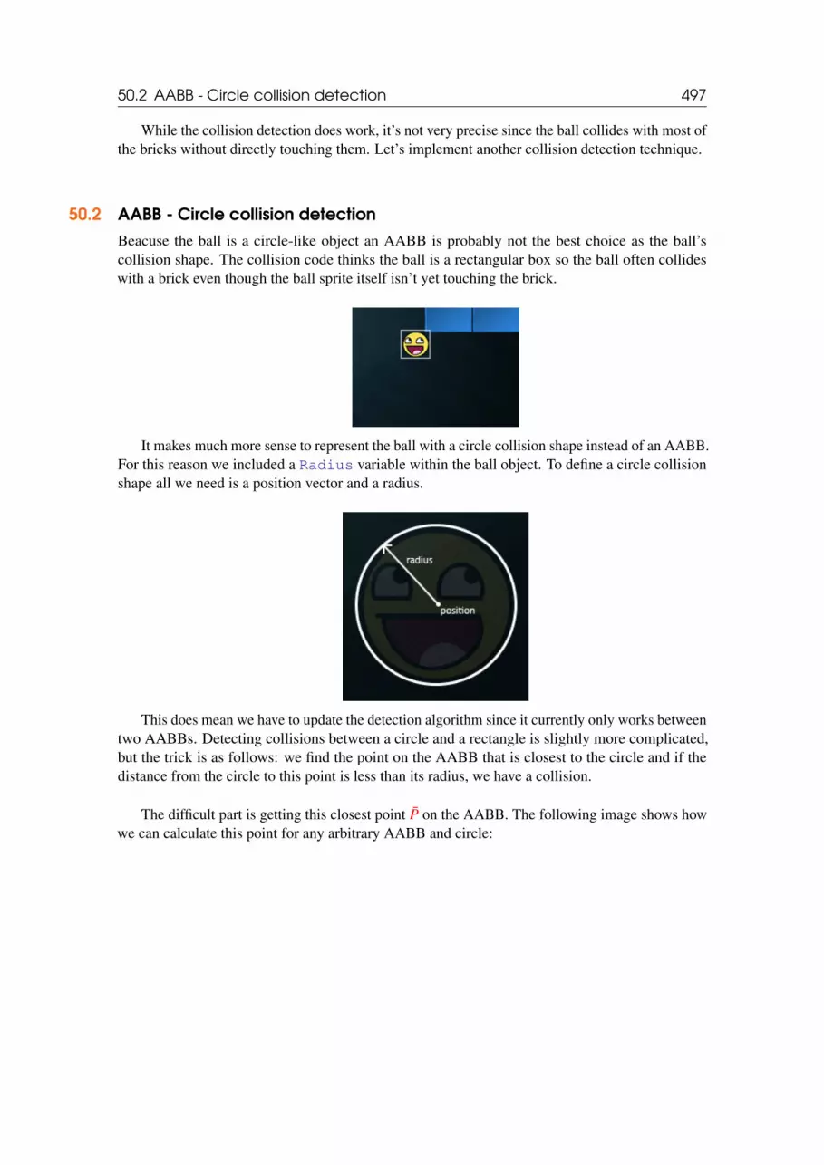
50.2 AABB - Circle collision detection 497
While the collision detection does work, it’s not very precise since the ball collides with most ofthe bricks without directly touching them. Let’s implement another collision detection technique.
50.2 AABB - Circle collision detectionBeacuse the ball is a circle-like object an AABB is probably not the best choice as the ball’scollision shape. The collision code thinks the ball is a rectangular box so the ball often collideswith a brick even though the ball sprite itself isn’t yet touching the brick.
It makes much more sense to represent the ball with a circle collision shape instead of an AABB.For this reason we included a Radius variable within the ball object. To define a circle collisionshape all we need is a position vector and a radius.
This does mean we have to update the detection algorithm since it currently only works betweentwo AABBs. Detecting collisions between a circle and a rectangle is slightly more complicated,but the trick is as follows: we find the point on the AABB that is closest to the circle and if thedistance from the circle to this point is less than its radius, we have a collision.
The difficult part is getting this closest point P on the AABB. The following image shows howwe can calculate this point for any arbitrary AABB and circle:

50.2 AABB - Circle collision detection 498
We first need to get the difference vector between the ball’s center C and the AABB’s centerB to obtain D. What we then need to do is clamp this vector D to the AABB’s half-extents w andh. The half-extents of a rectangle are the distances between the rectangle’s center and its edges;basically its size divided by two. This returns a position vector that is always located somewhere atthe edge of the AABB (unless the circle’s center is inside the AABB).
A clamp operation clamps a value to a value within a given range. This is often expressedas:
float clamp(float value, float min, float max) {return std::max(min, std::min(max, value));
}
For example, a value of 42.0f is clamped as 6.0f between 3.0f and 6.0f and avalue of 4.20f would be clamped to 4.20f.Clamping a 2D vector means we clamp both its x and its y component within the givenrange.
This clamped vector P is then the closest point from the AABB to the circle. What we thenneed to do is calculate a new difference vector D′ that is the difference between the circle’s centerC and the vector P.

50.2 AABB - Circle collision detection 499
Now that we have the vector D′ we can compare its length to the radius of the circle to determineif we have a collision.
This is all expressed in code as follows:
GLboolean CheckCollision(BallObject &one, GameObject &two) // AABB - Circlecollision
{// Get center point circle firstglm::vec2 center(one.Position + one.Radius);// Calculate AABB info (center, half-extents)glm::vec2 aabb_half_extents(two.Size.x / 2, two.Size.y / 2);glm::vec2 aabb_center(
two.Position.x + aabb_half_extents.x,two.Position.y + aabb_half_extents.y
);// Get difference vector between both centersglm::vec2 difference = center - aabb_center;glm::vec2 clamped = glm::clamp(difference, -aabb_half_extents,aabb_half_extents);// Add clamped value to AABB_center and we get the value of box closestto circleglm::vec2 closest = aabb_center + clamped;// Retrieve vector between center circle and closest point AABB andcheck if length <= radiusdifference = closest - center;return glm::length(difference) < one.Radius;
}
An overloaded function for CheckCollision was created that specifically deals with thecase between a BallObject and a GameObject. Because we did not store the collision shapeinformation in the objects themselves we have to calculate them: first the center of the ball iscalculated, then the AABB’s half-extents and its center.
Using these collision shape attributes we calculate vector D as difference that we thenclamp to clamped and add to the AABB’s center to get point P as closest. Then we calculatethe difference vector D′ between center and closest and return whether the two shapescollided or not.
Since we previously called CheckCollision with the ball object as its first argument, we donot have to change any code since the overloaded variant of CheckCollision now automaticallyapplies. The result is now a much more precise collision detection algorithm.

50.2 AABB - Circle collision detection 500
See video online
It seems to work, but still something is off. We properly do all the collision detection, but theball does not react in any way to the collisions. We need to react to the collisions e.g. update theball’s position and/or velocity whenever a collision occurs. This is the topic of the next tutorial.

51. Collision resolution
At the end of the last tutorial we had a working collision detection scheme. However, the ball doesnot react in any way to the detected collisions; it just moves straight through all the bricks. Wewant the ball to bounce of the collided bricks. This tutorial discusses how we can accomplish thisso called collision resolution within the AABB - circle collision detection scheme.
Whenever a collision occurs we want two things to happen: we want to reposition the ball soit is no longer inside the other object and second, we want to change the direction of the ball’svelocity so it looks like its bouncing of the object.
51.0.1 Collision repositioningTo position the ball object outside the collided AABB we have to figure out the distance the ballpenetrated the bounding box. For this we’ll revisit the diagrams from the previous tutorial:

502
Here the ball moved slightly into the AABB and a collision was detected. We now want tomove the ball out of the shape so that it merely touches the AABB as if no collision occurred. Tofigure out how much we need to move the ball out of the AABB we need to retrieve the vector Rwhich is the level of penetration into the AABB. To get this vector R we subtract V from the ball’sradius. Vector V is the difference between closest point P and the ball’s center C.
Knowing R we offset the ball’s position by R and position the ball directly alongside the AABB;the ball is now properly positioned.
51.0.2 Collision directionNext we need to figure out how to update the ball’s velocity after a collision. For Breakout we usethe following rules to change the ball’s velocity:
1. If the ball collides with the right or left side of an AABB, its horizontal velocity (x) isreversed.
2. If the ball collides with the bottom or top side of an AABB, its vertical velocity (y) isreversed.
But how do we figure out the direction the ball hit the AABB? There are several approaches tothis problem and one of them is that instead of 1 AABB we use 4 AABBs for each brick that weposition each at one of its edges. This way we can determine which AABB and thus which edgewas hit. However, a simpler approach exists with the help of the dot product.
You probably still remember from the transformations tutorial that the dot product gives usthe angle between two normalized vectors. What if we were to define four vectors pointing north,south, west or east and calculate the dot product between them and a given vector? The resultingdot product between these four direction vectors and the given vector that is highest (dot product’smaximum value is 1.0f which represents a 0 degree angle) is then the direction of the vector.
This procedure looks as follows in code:
Direction VectorDirection(glm::vec2 target){
glm::vec2 compass[] = {

503
glm::vec2(0.0f, 1.0f), // upglm::vec2(1.0f, 0.0f), // rightglm::vec2(0.0f, -1.0f), // downglm::vec2(-1.0f, 0.0f) // left
};GLfloat max = 0.0f;GLuint best_match = -1;for (GLuint i = 0; i < 4; i++){
GLfloat dot_product = glm::dot(glm::normalize(target), compass[i]);if (dot_product > max){
max = dot_product;best_match = i;
}}return (Direction)best_match;
}
The function compares target to each of the direction vectors in the compass array. Thecompass vector target is closest to in angle, is the direction returned to the function caller. HereDirection is part of an enum defined in the game class’s header file:
enum Direction {UP,RIGHT,DOWN,LEFT
};
Now that we know how to get vector R and how to determine the direction the ball hit theAABB we can start writing the collision resolution code.
51.0.3 AABB - Circle collision resolutionTo calculate the required values for collision resolution we need a bit more information from thecollision function(s) than just a true or false so we’re going to return a tuple of information,namely if a collision occurred, what direction it occurred and the difference vector (R). You canfind the tuple container in the <tuple> header.
To keep the code slightly more organized we’ll typedef the collision relevant data as Collision:
typedef std::tuple<GLboolean, Direction, glm::vec2> Collision;
Then we also have to change the code of the CheckCollision function to not only returntrue or false, but also the direction and difference vector:
Collision CheckCollision(BallObject &one, GameObject &two) // AABB - AABBcollision
{[...]if (glm::length(difference) <= one.Radius)
return std::make_tuple(GL_TRUE, VectorDirection(difference),difference);

504
elsereturn std::make_tuple(GL_FALSE, UP, glm::vec2(0, 0));
}
The game’s DoCollision function now doesn’t just check if a collision occurred, butalso acts appropriately whenever a collision did occur. The function now calculates the level ofpenetration (as shown in the diagram at the start of this tutorial) and adds or subtracts it from theball’s position based on the direction of the collision.
void Game::DoCollisions(){
for (GameObject &box : this->Levels[this->Level].Bricks){
if (!box.Destroyed){
Collision collision = CheckCollision(*Ball, box);if (std::get<0>(collision)) // If collision is true{
// Destroy block if not solidif (!box.IsSolid)
box.Destroyed = GL_TRUE;// Collision resolutionDirection dir = std::get<1>(collision);glm::vec2 diff_vector = std::get<2>(collision);if (dir == LEFT || dir == RIGHT) // Horizontal collision{
Ball->Velocity.x = -Ball->Velocity.x; // Reversehorizontal velocity
// RelocateGLfloat penetration = Ball->Radius - std::abs(
diff_vector.x);if (dir == LEFT)
Ball->Position.x += penetration; // Move ball toright
elseBall->Position.x -= penetration; // Move ball to
left;}else // Vertical collision{
Ball->Velocity.y = -Ball->Velocity.y; // Reversevertical velocity
// RelocateGLfloat penetration = Ball->Radius - std::abs(
diff_vector.y);if (dir == UP)
Ball->Position.y -= penetration; // Move ball backup
elseBall->Position.y += penetration; // Move ball back
down}
}}
}}
Don’t get too scared by the function’s complexity since it is basically a direct translation ofthe concepts introduced so far. First we check for a collision and if so we destroy the block if it is

51.1 Player - ball collisions 505
non-solid. Then we obtain the collision direction dir and the vector V as diff_vector fromthe tuple and finally do the collision resolution.
We first check if the collision direction is either horizontal or vertical and then reverse thevelocity accordingly. If horizontal, we calculate the penetration value R from the diff_vector’sx component and either add or subtract this from the ball’s position based on its direction. The sameapplies to the vertical collisions, but this time we operate on the y component of all the vectors.
Running your application should now give you a working collision scheme, but it’s probablydifficult to really see its effect since the ball will bounce towards the bottom edge as soon as you hita single block and be lost forever. We can fix this by also handling player paddle collisions.
51.1 Player - ball collisionsCollisions between the ball and the player are slightly different than what we’ve previously discussedsince this time the ball’s horizontal velocity should be updated based on how far it hit the paddlefrom its center. The further the ball hits the paddle from its center, the stronger its horizontalvelocity should be.
void Game::DoCollisions(){
[...]Collision result = CheckCollision(*Ball, *Player);if (!Ball->Stuck && std::get<0>(result)){
// Check where it hit the board, and change velocity based on whereit hit the board
GLfloat centerBoard = Player->Position.x + Player->Size.x / 2;GLfloat distance = (Ball->Position.x + Ball->Radius) - centerBoard;GLfloat percentage = distance / (Player->Size.x / 2);// Then move accordinglyGLfloat strength = 2.0f;glm::vec2 oldVelocity = Ball->Velocity;Ball->Velocity.x = INITIAL_BALL_VELOCITY.x * percentage * strength;Ball->Velocity.y = -Ball->Velocity.y;Ball->Velocity = glm::normalize(Ball->Velocity) * glm::length(
oldVelocity);}
}
After we checked collisions between the ball and each brick, we’ll check if the ball collidedwith the player paddle. If so (and the ball is not stuck to the paddle) we calculate the percentage ofhow far the ball’s center is removed from the paddle’s center compared to the half-extent of thepaddle. The horizontal velocity of the ball is then updated based on the distance it hit the paddlefrom its center. Aside from updating the horizontal velocity we also have to reverse the y velocity.
Note that the old velocity is stored as oldVelocity. The reason for storing the old velocityis that we only update the horizontal velocity of the ball’s velocity vector while keeping its yvelocity constant. This would mean that the length of the vector constantly changes which has theeffect that the ball’s velocity vector is much larger (and thus stronger) if the ball hit the edge of thepaddle compared to if the ball would hit the center of the paddle. For this reason the new velocity

51.1 Player - ball collisions 506
vector is normalized and multiplied by the length of the old velocity vector. This way, the strengthand thus the velocity of the ball is always consistent, regardless of where it hits the paddle.
51.1.1 Sticky paddleYou may or may not have noticed it when you ran the code, but there is still a large issue with theplayer and ball collision resolution. The following video clearly shows what might happen:
See video online
This issue is called the sticky paddle issue which happens because the player paddle moveswith a high velocity towards the ball that results in the ball’s center ending up inside the playerpaddle. Since we did not account for the case where the ball’s center is inside an AABB the gametries to continuously react to all the collisions and once it finally breaks free it will have reversed itsy velocity so much that it’s unsure whether it goes up or down after breaking free.
We can easily fix this behavior by introducing a small hack which is possible due to the factthat the we can assume we always have a collision at the top of the paddle. Instead of reversingthe y velocity we simply always return a positive y direction so whenever it does get stuck, it willimmediately break free.
//Ball->Velocity.y = -Ball->Velocity.y;Ball->Velocity.y = -1 * abs(Ball->Velocity.y);
If you try hard enough the effect is still noticeable, but I personally find it an acceptable trade-off.
51.1.2 The bottom edgeThe only thing that is still missing from the classic Breakout recipe is some loss condition thatresets the level and the player. Within the game class’s Update function we want to check if theball reached the bottom edge, and if so, reset the game.
void Game::Update(GLfloat dt){
[...]if (Ball->Position.y >= this->Height) // Did ball reach bottom edge?{
this->ResetLevel();this->ResetPlayer();
}}
The ResetLevel and ResetPlayer functions simply re-load the level and reset the objects’values to their original starting values. The game should now look a bit like this:
See video online
And there you have it, we just finished creating a clone of the classical Breakout game withsimilar mechanics. You can find the game class’ source code here: header, code.

51.2 A few notes 507
51.2 A few notesCollision detection is a difficult topic of video game development and possibly its most challenging.Most collision detection and resolution schemes are combined with physics engines as found inmost modern-day games. The collision scheme we used for the Breakout game is a very simplescheme and one specialized specifically for this type of game.
It should be stressed that this type of collision detection and resolution is not perfect. Itcalculates possible collisions only per frame and only for the positions exactly as they are at thattimestep; this means that if an object would have such a velocity that it would pass over anotherobject within a single frame, it would look like it never collided with this object. So if there areframedrops or you reach high enough velocities, this collision detection scheme will not hold.
Several of the issues that can still occur:
• If the ball goes too fast, it might skip over an object entirely within a single frame, notdetecting any collisions.• If the ball hits more than one object within a single frame, it will have detected two collisions
and reverse its velocity twice; not affecting its original velocity.• Hitting a corner of a brick could reverse the ball’s velocity in the wrong direction since the
distance it travels in a single frame could make the difference between VectorDirectionreturning a vertical or horizontal direction.
These tutorials are however aimed to teach the readers the basics of several aspects of graphicsand game-development. For this reason, this collision scheme serves its purpose; its understandableand works quite well in normal scenarios. Just keep in mind that there exist better (more compli-cated) collision schemes that work quite well in almost all scenarios (including movable objects)like the separating axis theorem.
Thankfully, there exist large, practical and often quite efficient physics engines (with timestep-independent collision schemes) for use in your own games. If you wish to delve further into suchsystems or need more advanced physics and have trouble figuring out the mathematics, Box2D is aperfect 2D physics library for implementing physics and collision detection in your applications.

52. Particles
A particle, as seen from OpenGL’s perspective, is a tiny 2D quad that is always faced at the camera(billboarding) and (usually) contains a texture with large parts of the sprite being transparent. Aparticle by itself is basically just a sprite as we’ve been extensively using so far, but when you puttogether hundreds or even thousands of these particles together you can create amazing effects.
When working with particles, there is usually an object called a particle emitter or particlegenerator that, from its location, continously spawns new particles that decay over time. If sucha particle emitter would for example spawn tiny particles with a smoke-like texture, color themless bright the larger the distance from the emitter and give them a glowy appearance you’d get afire-like effect:

509
A single particle often has a life variable that slowly decays once it is spawned. Once its life isless than a certain threshold (usually 0) we kill the particle so it can be replaced with a new particleobject when the next particle spawns. A particle emitter controls all its spawned particles andchanges their behavior based on their attributes. A particle generally has the following attributes:
struct Particle {glm::vec2 Position, Velocity;glm::vec4 Color;GLfloat Life;
Particle(): Position(0.0f), Velocity(0.0f), Color(1.0f), Life(0.0f) { }
};
Looking at the fire example, the particle emitter probably spawns each particle with a positionclose to the emitter and with an upwards velocity so each particle moves in the positive y direction.It seems to have 3 different regions so it probably gives some particles a higher velocity than others.We can also see that the higher the y position of the particle, the less yellow or bright its colorbecomes. After the particles have reached a certain height, their life is depleted and the particlesare killed; never reaching the stars.
You can imagine that with systems like these we can create interesting effects like fire, smoke,fog, magic effects, gunfire residue etc. In Breakout we’re going to add a simple particle generatorfollowing the ball to make it all look more interesting. It’ll look a bit like this:
See video online
Here the particle generator spawns each particle at the ball’s position, gives it a velocity equalto a fraction of the ball’s velocity and changes the color of the particle based on how long it lived.
For rendering the particles we’ll be using a different set of shaders:

510
#version 330 corelayout (location = 0) in vec4 vertex; // <vec2 position, vec2 texCoords>
out vec2 TexCoords;out vec4 ParticleColor;
uniform mat4 projection;uniform vec2 offset;uniform vec4 color;
void main(){
float scale = 10.0f;TexCoords = vertex.zw;ParticleColor = color;gl_Position = projection * vec4((vertex.xy * scale) + offset, 0.0, 1.0);
}
And the fragment shader:
#version 330 corein vec2 TexCoords;in vec4 ParticleColor;out vec4 color;
uniform sampler2D sprite;
void main(){
color = (texture(sprite, TexCoords) * ParticleColor);}
We take the standard position and texture attributes per particle and also accept an offset anda color uniform for changing the outcome per particle. Note that in the vertex shader we scalethe particle quad by 10.0f; you could also set the scale as a uniform and control this individuallyper particle.
First, we need a list of particles that we then instantiate with default Particle structs.
GLuint nr_particles = 500;std::vector<Particle> particles;
for (GLuint i = 0; i < nr_particles; ++i)particles.push_back(Particle());
Then in each frame, we spawn several new particles with starting values and then for eachparticle that is (still) alive we update their values.
GLuint nr_new_particles = 2;// Add new particlesfor (GLuint i = 0; i < nr_new_particles; ++i){
int unusedParticle = FirstUnusedParticle();RespawnParticle(particles[unusedParticle], object, offset);
}

511
// Uupdate all particlesfor (GLuint i = 0; i < nr_particles; ++i){
Particle &p = particles[i];p.Life -= dt; // reduce lifeif (p.Life > 0.0f){ // particle is alive, thus update
p.Position -= p.Velocity * dt;p.Color.a -= dt * 2.5;
}}
The first loop might look a little daunting. Because particles die over time we want to spawnnr_new_particles particles each frame, but since we’ve decided from the start that the totalamount of particles we’ll be using is nr_particles we can’t simply push the new particles tothe end of the list. This way we’ll quickly get a list filled with thousands of particles which isn’treally efficient considering only a small portion of that list has particles that are alive.
What we want is to find the first particle that is dead (life < 0.0f) and update that particle as anew respawned particle.
The function FirstUnusedParticle tries to find the first particle that is dead and returnsits index to the caller.
GLuint lastUsedParticle = 0;GLuint FirstUnusedParticle(){
// Search from last used particle, this will usually return almostinstantlyfor (GLuint i = lastUsedParticle; i < nr_particles; ++i){
if (particles[i].Life <= 0.0f){lastUsedParticle = i;return i;
}}// Otherwise, do a linear searchfor (GLuint i = 0; i < lastUsedParticle; ++i){
if (particles[i].Life <= 0.0f){lastUsedParticle = i;return i;
}}// Override first particle if all others are alivelastUsedParticle = 0;return 0;
}
The function stores the index of the last dead particle it found, since the next dead particle willmost likely be right after this last particle index so we first search from this stored index. If we didnot find any dead particles, we simply do a slower linear search. If no particles are dead it willreturn the index 0 which results in the first particle being overwritten. Note that if it reaches thislast case, it means your particles are alive for too long, you need to spawn less particles per frameand/or you simply don’t have enough particles reserved.
Then, once the first dead particle in the list is found, we update its values by calling RespawnParticlethat takes the particle, a GameObject and an offset vector:

512
void RespawnParticle(Particle &particle, GameObject &object, glm::vec2offset)
{GLfloat random = ((rand() \% 100) - 50) / 10.0f;GLfloat rColor = 0.5 + ((rand() \% 100) / 100.0f);particle.Position = object.Position + random + offset;particle.Color = glm::vec4(rColor, rColor, rColor, 1.0f);particle.Life = 1.0f;particle.Velocity = object.Velocity * 0.1f;
}
This function simply resets the particle’s life to 1.0f, randomly gives it a brightness (via thecolor vector) starting from 0.5 and assigns a (slightly random) position and velocity based on thegame object.
The second loop within the update function loops through all the particles and for each particlereduces its life by the delta time variable; this way each particle’s life corresponds to exactly thesecond(s) it’s allowed to live. Then we check if the particle is alive and if so, update its positionand color attributes. Here we slowly reduce the alpha component of each particle so it looks likethey’re slowly disappearing over time.
Then what’s left is to actually render the particles:
glBlendFunc(GL_SRC_ALPHA, GL_ONE);particleShader.Use();for (Particle particle : particles){
if (particle.Life > 0.0f){
particleShader.SetVector2f("offset", particle.Position);particleShader.SetVector4f("color", particle.Color);particleTexture.Bind();glBindVertexArray(particleVAO);glDrawArrays(GL_TRIANGLES, 0, 6);glBindVertexArray(0);
}}glBlendFunc(GL_SRC_ALPHA, GL_ONE_MINUS_SRC_ALPHA);
Here, for each particle, we set their offset and color uniform values, bind the texture and renderthe 2D quad. What is interesting to see here are the two calls to glBlendFunc. When renderingthe particles, instead of the default destination blending mode of GL_ONE_MINUS_SRC_ALPHAwe use the GL_ONE blending mode that gives the particles a very neat glow effect when stackedupon each other. This is also likely the blending mode used when rendering the fire at the top of thetutorial, since the fire got glowy at the center where most of its particles were.
Because we (like most other parts of the tutorial series) like to keep things organized, anotherclass called ParticleGenerator was created that hosts all the functionality we just talkedabout. You can find the source code below:
• header, codeThen within the game code, we create such a particle generator and initialize it with this texture.

513
ParticleGenerator *Particles;
void Game::Init(){
[...]ResourceManager::LoadShader("shaders/particle.vs", "shaders/particle.frag", nullptr, "particle");[...]ResourceManager::LoadTexture("textures/particle.png", GL_TRUE, "particle");[...]Particles = new ParticleGenerator(
ResourceManager::GetShader("particle"),ResourceManager::GetTexture("particle"),500
);}
Then we change the game class’s Update function by adding an update statement for theparticle generator:
void Game::Update(GLfloat dt){
[...]// Update particlesParticles->Update(dt, *Ball, 2, glm::vec2(Ball->Radius / 2));[...]
}
Each of the particles will use the game object properties from the ball object, spawn 2 particleseach frame and their positions will be offset towards the center of the ball. Last up is rendering theparticles:
void Game::Render(){
if (this->State == GAME_ACTIVE){
[...]// Draw playerPlayer->Draw(*Renderer);// Draw particlesParticles->Draw();// Draw ballBall->Draw(*Renderer);
}}
Note that we render the particles before the ball is rendered and after the other item are renderedso the particles will end up in front of all other objects, but stay behind the ball. You can find theupdated game class code here.
If you’d now compile and run your application you should see a trail of particles following theball, just like at the beginning of this tutorial, giving the game a more modern look. The system canalso easily be extended to host more advanced effects so feel free to experiment with the particlegeneration and see if you can come up with your own creative effects.

53. Postprocessing
Wouldn’t it be fun if we could completely spice up the visuals of the Breakout game with just a fewpostprocessing effects? We could create a blurry shake effect, inverse all the colors of the scene, docrazy vertex movement and/or make use of other interesting effects with relative ease thanks toOpenGL’s framebuffers.
This tutorial makes extensive use of concepts from the framebuffers and anti-aliasingtutorials.
In the framebuffers tutorial we demonstrated how one could use postprocessing effects toachieve interesting effects using just a single texture. In Breakout we’re going to do somethingsimilar: we’re going to create a framebuffer object with a multisampled renderbuffer object attachedas its color attachment. All the game’s render code should render to this multisampled framebufferthat then blits its content to a different framebuffer with a texture attachment as its color buffer.This texture contains the rendered anti-aliased image of the game that we’ll render to a large 2Dquad with zero or more postprocessing effects applied.
So to summarize these rendering steps:
1. Bind to multisampled framebuffer2. Render game as normal3. Blit multisampled framebuffer to normal framebuffer4. Unbind framebuffers (use default framebuffer)5. Use color buffer texture from normal framebuffer in postprocessing shader6. Render quad of screen-size as output of postprocessing shaderThe postprocessing shader allows for three type of effects: shake, confuse and chaos.
• shake: slightly shakes the scene with a small blur.• confuse: inverses the colors of the scene, but also the x and y axis.

515
• chaos: makes use of an edge detection kernel to create interesting visuals and also moves thetextured image in a circular fashion for an interesting chaotic effect.
Below is a glimpse of what these effects are going to look like:
Operating on a 2D quad, the vertex shader looks as follows:
#version 330 corelayout (location = 0) in vec4 vertex; // <vec2 position, vec2 texCoords>
out vec2 TexCoords;
uniform bool chaos;uniform bool confuse;uniform bool shake;uniform float time;
void main(){
gl_Position = vec4(vertex.xy, 0.0f, 1.0f);vec2 texture = vertex.zw;if(chaos){
float strength = 0.3;vec2 pos = vec2(texture.x + sin(time) * strength, texture.y + cos(
time) * strength);TexCoords = pos;
}else if(confuse){
TexCoords = vec2(1.0 - texture.x, 1.0 - texture.y);}else{
TexCoords = texture;}if (shake){
float strength = 0.01;gl_Position.x += cos(time * 10) * strength;gl_Position.y += cos(time * 15) * strength;
}}
Based on whatever uniform is set to true the vertex shader can take different paths. If eitherchaos or confuse is set to true the vertex shader will manipulate the texture coordinates tomove the scene around (either translate texture coordinates in a circle-like fashion or inverse thetexture coordinates). Because we set the texture wrapping methods to GL_REPEAT the chaoseffect will cause the scene to repeat itself at various parts of the quad. Additionally if shake is set

516
to true it will move the vertex positions around by only a small amount. Note that chaos andconfuse shouldn’t be true at the same time while shake is able to work with any of the othereffects on.
Aside from offsetting the vertex positions or texture coordinates, we’d also like to create asignificant visual impact as soon as any of the effects are active. We can accomplish this within thefragment shader:
#version 330 corein vec2 TexCoords;out vec4 color;
uniform sampler2D scene;uniform vec2 offsets[9];uniform int edge_kernel[9];uniform float blur_kernel[9];
uniform bool chaos;uniform bool confuse;uniform bool shake;
void main(){
vec3 sample[9];// sample from texture offsets if using convolution matrixif(chaos || shake)
for(int i = 0; i < 9; i++)sample[i] = vec3(texture(scene, TexCoords.st + offsets[i]));
// process effectsif(chaos){
for(int i = 0; i < 9; i++)color += vec4(sample[i] * edge_kernel[i], 0.0f);
color.a = 1.0f;}else if(confuse){
color = vec4(1.0 - texture(scene, TexCoords).rgb, 1.0);}else if(shake){
for(int i = 0; i < 9; i++)color += vec4(sample[i] * blur_kernel[i], 0.0f);
color.a = 1.0f;}else{
color = texture(scene, TexCoords);}
}
This long shader almost directly builds upon the fragment shader from the framebuffers tutorialand processes a postprocessing effects based on the effect type activated. This time though, theoffset matrix and convolution kernels are defined as a uniform that we set from the application code.The advantage is that we only have to set this once, instead of recalculating these matrices in eachfragment shader run. For example, the offsets matrix is configured as follows:

517
GLfloat offset = 1.0f / 300.0f;GLfloat offsets[9][2] = {
{ -offset, offset }, // top-left{ 0.0f, offset }, // top-center{ offset, offset }, // top-right{ -offset, 0.0f }, // center-left{ 0.0f, 0.0f }, // center-center{ offset, 0.0f }, // center - right{ -offset, -offset }, // bottom-left{ 0.0f, -offset }, // bottom-center{ offset, -offset } // bottom-right
};glUniform2fv(glGetUniformLocation(shader.ID, "offsets"), 9, (GLfloat*)
offsets);
Since all of the concepts of managing (multisampled) framebuffers were already extensivelydiscussed in earlier tutorials I won’t delve into the details this time. Below you’ll find the codeof a PostProcessor class that manages initialization, writing/reading the framebuffers andrendering a screen quad. You should be able to completely understand the code if you understoodthe framebuffers and anti-aliasing tutorials.
• PostProcessor: header, code.What is interesting to note are the BeginRender and EndRender functions. Since we have
to render the entire game scene into the framebuffer we can conventiently call BeginRender()and EndRender() before and after the scene’s rendering code respectively. The class will thenhandle the behind-the-scenes framebuffer operations. For example, using the PostProcessorclass then looks like this within the game’s Render function:
PostProcessor *Effects;
void Game::Render(){
if (this->State == GAME_ACTIVE){
Effects->BeginRender();// Draw background// Draw level// Draw player// Draw particles// Draw ball
Effects->EndRender();Effects->Render(glfwGetTime());
}}
Wherever we want we can now conveniently set the required effect property of the postprocess-ing class to true and its effect will be immediately visible.
53.0.1 Shake itAs a (practical) demonstration of these effects we’ll emulate the visual impact of a ball when ithits a solid concrete block. By enabling the shake effect for a short period of time wherever a solidcollision occurs, it’ll look like the collision had a stronger impact.

518
We want to enable the shake effect only over a small period of time. We can get this to work bycreating a variable called ShakeTime that holds the duration the shake effect is supposed to beactive. Wherever a solid collision occurs, we reset this variable to a specific duration:
GLfloat ShakeTime = 0.0f;
void Game::DoCollisions(){
for (GameObject &box : this->Levels[this->Level].Bricks){
if (!box.Destroyed){
Collision collision = CheckCollision(*Ball, box);if (std::get<0>(collision)) // If collision is true{
// Destroy block if not solidif (!box.IsSolid)
box.Destroyed = GL_TRUE;else{ // if block is solid, enable shake effect
ShakeTime = 0.05f;Effects->Shake = true;
}[...]
}}
}[...]
}
Then within the game’s Update function we decrease this ShakeTime variable until it’s0.0 after which we disable the shake effect:
void Game::Update(GLfloat dt){
[...]if (ShakeTime > 0.0f){
ShakeTime -= dt;if (ShakeTime <= 0.0f)
Effects->Shake = false;}
}
Then each time we hit a solid block the screen briefly starts to shake and blur, giving the playersome visual feedback the ball collided with a solid object.
See video online
You can find the updated source code of the game class here.
In the next tutorial about powerups we’ll bring the other two postprocessing effects to good use.

54. Powerups
Breakout is close to finished, but it would be cool to at least add one more gameplay mechanic soit’s not your average standard Breakout clone; what about powerups?
The idea is that whenever a brick is destroyed, the brick has a small chance of spawning apowerup block. Such a block will slowly fall downwards and if it collides with the player paddle,an interesting effect occurs based on the type of powerup. For example, one powerup makes thepaddle larger and another powerup allows the ball to pass through objects. We also include severalnegative powerups that affect the player in a negative way.
We can model a powerup as basically a GameObject with a few extra properties. That’s whywe define a class PowerUp that inherits from GameObject and adds these extra properties tothe object:
const glm::vec2 SIZE(60, 20);const glm::vec2 VELOCITY(0.0f, 150.0f);
class PowerUp : public GameObject{public:
// PowerUp Statestd::string Type;GLfloat Duration;GLboolean Activated;// ConstructorPowerUp(std::string type, glm::vec3 color, GLfloat duration,
glm::vec2 position, Texture2D texture): GameObject(position, SIZE, texture, color, VELOCITY),Type(type), Duration(duration), Activated()
{ }};

520
A PowerUp is just a GameObject with extra state, so we can simply define it in a singleheader file which you can find here.
Each powerup defines its type as a string, has a duration of how long it is active and whether itis currently activated. Within Breakout we’re going to feature a total of 4 positive powerups and 2negative powerups:
• Speed: increases the velocity of the ball by 20%.• Sticky: when the ball collides with the paddle, the ball remains stuck to the paddle unless the
spacebar is pressed again. This allows the player to better position the ball before releasing it.• Pass-Through: collision resolution is disabled for non-solid blocks allowing the ball to pass
through multiple blocks.• Pad-Size-Increase: increases the width of the paddle by 50 pixels.• Confuse: activates the confuse postprocessing effect for a short period of time, confusing
the user.• Chaos: activates the chaos postprocessing effect for a short period of time, heavily disorient-
ing the user.You can find the high-quality textures below:
• Textures: Speed, Sticky, Pass-Through, Pad-Size-Increase, Confuse, Chaos.Similar to the level block textures, each of the powerup textures is completely grayscale. This
makes sure the color of the powerups remain balanced whenever we multiply it with a color vector.
Because powerups have state, a duration and certain effects associated with them we would liketo keep track of all the powerups currently active in the game; we store them in a vector:
class Game {public:
[...]std::vector<PowerUp> PowerUps;[...]void SpawnPowerUps(GameObject &block);void UpdatePowerUps(GLfloat dt);
};
We’ve also defined two functions for managing powerups. SpawnPowerUps spawns apowerups at the location of a given block and UpdatePowerUps manages all powerups currentlyactive within the game.
54.0.1 Spawning PowerUpsEach time a block is destroyed we would like to, given a small chance, spawn a powerup. Thisfunctionality is found inside the game’s SpawnPowerUps function:
GLboolean ShouldSpawn(GLuint chance){
GLuint random = rand() \% chance;

521
return random == 0;}void Game::SpawnPowerUps(GameObject &block){
if (ShouldSpawn(75)) // 1 in 75 chancethis->PowerUps.push_back(
PowerUp("speed", glm::vec3(0.5f, 0.5f, 1.0f), 0.0f, block.Position, tex_speed
));if (ShouldSpawn(75))
this->PowerUps.push_back(PowerUp("sticky", glm::vec3(1.0f, 0.5f, 1.0f), 20.0f, block.
Position, tex_sticky);
if (ShouldSpawn(75))this->PowerUps.push_back(
PowerUp("pass-through", glm::vec3(0.5f, 1.0f, 0.5f), 10.0f,block.Position, tex_pass
));if (ShouldSpawn(75))
this->PowerUps.push_back(PowerUp("pad-size-increase", glm::vec3(1.0f, 0.6f, 0.4), 0.0f,
block.Position, tex_size));
if (ShouldSpawn(15)) // Negative powerups should spawn more oftenthis->PowerUps.push_back(
PowerUp("confuse", glm::vec3(1.0f, 0.3f, 0.3f), 15.0f, block.Position, tex_confuse
));if (ShouldSpawn(15))
this->PowerUps.push_back(PowerUp("chaos", glm::vec3(0.9f, 0.25f, 0.25f), 15.0f, block.
Position, tex_chaos));
}
The SpawnPowerUps function creates a new PowerUp object based on a given chance (1in 75 for normal powerups and 1 in 15 for negative powerups) and sets their properties. Eachpowerup is given a specific color to make them more recognizable for the user and a duration inseconds based on its type; here a duration of 0.0f means its duration is infinite. Additionally, eachpowerup is given the position of the destroyed block and one of the textures of the previous section.
54.0.2 Activating PowerUpsThen we update the game’s DoCollisions function to not only check for brick and paddlecollisions, but also all collisions between the paddle and each non-destroyed PowerUp. Note thatwe call the SpawnPowerUps function as soon as a block is destroyed.
void Game::DoCollisions(){
for (GameObject &box : this->Levels[this->Level].Bricks){
if (!box.Destroyed){
Collision collision = CheckCollision(*Ball, box);if (std::get<0>(collision)) // If collision is true

522
{// Destroy block if not solidif (!box.IsSolid){
box.Destroyed = GL_TRUE;this->SpawnPowerUps(box);
}[...]
}}
}[...]for (PowerUp &powerUp : this->PowerUps){
if (!powerUp.Destroyed){
if (powerUp.Position.y >= this->Height)powerUp.Destroyed = GL_TRUE;
if (CheckCollision(*Player, powerUp)){ // Collided with player, now activate powerup
ActivatePowerUp(powerUp);powerUp.Destroyed = GL_TRUE;powerUp.Activated = GL_TRUE;
}}
}}
For all powerups not yet destroyed, we check if the powerup either reached the bottom edge ofthe screen or collided with the paddle. In both cases, the powerup is destroyed, but when collidedwith the paddle, it is also activated.
Activating a powerup is accomplished by settings its Activated property to true andenabling the powerup’s effect by giving it to the ActivatePowerUp function:
void ActivatePowerUp(PowerUp &powerUp){
// Initiate a powerup based type of powerupif (powerUp.Type == "speed"){
Ball->Velocity *= 1.2;}else if (powerUp.Type == "sticky"){
Ball->Sticky = GL_TRUE;Player->Color = glm::vec3(1.0f, 0.5f, 1.0f);
}else if (powerUp.Type == "pass-through"){
Ball->PassThrough = GL_TRUE;Ball->Color = glm::vec3(1.0f, 0.5f, 0.5f);
}else if (powerUp.Type == "pad-size-increase"){
Player->Size.x += 50;}else if (powerUp.Type == "confuse"){
if (!Effects->Chaos)

523
Effects->Confuse = GL_TRUE; // Only activate if chaos wasn’talready active}else if (powerUp.Type == "chaos"){
if (!Effects->Confuse)Effects->Chaos = GL_TRUE;
}}
The purpose of ActivatePowerUp is exactly as it sounds: it activates the effect of a powerupas we’ve described somewhere at the start of this tutorial. We check the type of the powerup andchange the game state accordingly. For the "sticky" and "pass-through" effect we alsochange the color of the paddle and the ball respectively to give the user some feedback as to whicheffect is currently active.
Because the sticky and pass-through effects slightly change the game logic we store their effectas a property of the ball object; this way we can change the game logic based on whatever effect onthe ball is currently active. The only thing we change in the BallObject header is the additionof these two properties, but for completeness’ sake its updated code is listed below:
• BallObject: header, code.We can then easily implement the sticky effect by slightly updating the DoCollisions
function at the collision code between the ball and the paddle:
if (!Ball->Stuck && std::get<0>(result)){
[...]Ball->Stuck = Ball->Sticky;
}
Here we set the ball’s Stuck property equal to the ball’s Sticky property. If the sticky effectis activated, the ball will end up stuck to the player paddle whenever it collides; the user then has topress the spacebar again to release the ball.
A similar small change is made for the pass-through effect within the same DoCollisionsfunction. When the ball’s PassThrough property is set to true we do not perform any collisionresolution on the non-solid bricks.
Direction dir = std::get<1>(collision);glm::vec2 diff_vector = std::get<2>(collision);if (!(Ball->PassThrough && !box.IsSolid)){
if (dir == LEFT || dir == RIGHT) // Horizontal collision{
[...]}else{
[...]}
}
The other effects are activated by simply modifying a part of the game’s state like the ball’svelocity, the paddle’s size or an effect of the PostProcesser object.

524
54.0.3 Updating PowerUpsNow all that is left to do is make sure that powerups are actually able to move once they’ve spawnedand that they’re deactivated as soon as their duration runs out; otherwise powerups will stay activeforever.
Within the game’s UpdatePowerUps function we move the powerups based on their velocityand decrease the active powerups their duration. Whenever a powerup’s duration is decreased to0.0f its effect is deactivated and the relevant variables are set to their original state.
void Game::UpdatePowerUps(GLfloat dt){
for (PowerUp &powerUp : this->PowerUps){
powerUp.Position += powerUp.Velocity * dt;if (powerUp.Activated){
powerUp.Duration -= dt;
if (powerUp.Duration <= 0.0f){
// Remove powerup from list (will later be removed)powerUp.Activated = GL_FALSE;// Deactivate effectsif (powerUp.Type == "sticky"){
if (!isOtherPowerUpActive(this->PowerUps, "sticky")){ // Only reset if no other PowerUp of type sticky
is activeBall->Sticky = GL_FALSE;Player->Color = glm::vec3(1.0f);
}}else if (powerUp.Type == "pass-through"){
if (!isOtherPowerUpActive(this->PowerUps, "pass-through"))
{ // Only reset if no other PowerUp of type pass-through is active
Ball->PassThrough = GL_FALSE;Ball->Color = glm::vec3(1.0f);
}}else if (powerUp.Type == "confuse"){
if (!isOtherPowerUpActive(this->PowerUps, "confuse")){ // Only reset if no other PowerUp of type confuse
is activeEffects->Confuse = GL_FALSE;
}}else if (powerUp.Type == "chaos"){
if (!isOtherPowerUpActive(this->PowerUps, "chaos")){ // Only reset if no other PowerUp of type chaos is
activeEffects->Chaos = GL_FALSE;
}}
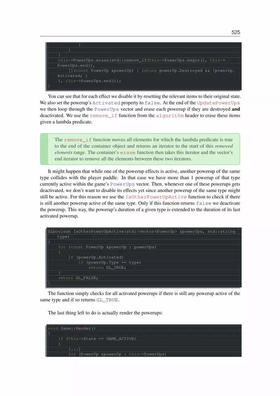
525
}}
}this->PowerUps.erase(std::remove_if(this->PowerUps.begin(), this->PowerUps.end(),
[](const PowerUp &powerUp) { return powerUp.Destroyed && !powerUp.Activated; }), this->PowerUps.end());
}
You can see that for each effect we disable it by resetting the relevant items to their original state.We also set the powerup’s Activated property to false. At the end of the UpdatePowerUpswe then loop through the PowerUps vector and erase each powerup if they are destroyed anddeactivated. We use the remove_if function from the algorithm header to erase these itemsgiven a lambda predicate.
The remove_if function moves all elements for which the lambda predicate is trueto the end of the container object and returns an iterator to the start of this removedelements range. The container’s erase function then takes this iterator and the vector’send iterator to remove all the elements between these two iterators.
It might happen that while one of the powerup effects is active, another powerup of the sametype collides with the player paddle. In that case we have more than 1 powerup of that typecurrently active within the game’s PowerUps vector. Then, whenever one of these powerups getsdeactivated, we don’t want to disable its effects yet since another powerup of the same type mightstill be active. For this reason we use the IsOtherPowerUpActive function to check if thereis still another powerup active of the same type. Only if this function returns false we deactivatethe powerup. This way, the powerup’s duration of a given type is extended to the duration of its lastactivated powerup.
GLboolean IsOtherPowerUpActive(std::vector<PowerUp> &powerUps, std::stringtype)
{for (const PowerUp &powerUp : powerUps){
if (powerUp.Activated)if (powerUp.Type == type)
return GL_TRUE;}return GL_FALSE;
}
The function simply checks for all activated powerups if there is still any powerup active of thesame type and if so returns GL_TRUE.
The last thing left to do is actually render the powerups:
void Game::Render(){
if (this->State == GAME_ACTIVE){
[...]for (PowerUp &powerUp : this->PowerUps)

526
if (!powerUp.Destroyed)powerUp.Draw(*Renderer);
[...]}
}
Combine all this functionality and we have a working powerup system that not only makes thegame more fun, but also a lot more challenging. It’ll look a bit like this:
See video online
You can find the updated game code below (there we also reset all powerup effects wheneverthe level is reset):
• Game: header, code.

55. Audio
No matter how hard we turn up the game’s volume we most likely won’t hear any audio from thegame; we already have so much to show for, but without any audio the game still feels a bit empty.In this tutorial we’re going to fix that.
OpenGL does not offer us any support for audio capabilities (like many other aspects of gamedevelopment). We have to manually load audio files into a collection of bytes, process and convertthem to an audio stream and manage multiple audio streams appropriately for use in our game.This is however slightly complicated and requires some low-level knowledge of audio engineering.
If it is your cup of tea then feel free to manually load audio streams from several audio fileextensions. We are, however, going to make use of library for audio management called irrKlang.
55.1 Irrklang
IrrKlang is a high level 2D and 3D cross platform (Windows, Mac OS X, Linux) sound engineand audio library that plays WAV, MP3, OGG, and FLAC files to name a few. It also featuresseveral audio effects like reverb, delay and distortion that can be extensively tweaked.
3D audio means that an audio source can have a 3D position that will attenuate itsvolume based on the camera’s distance to the audio source, making it feel natural in a3D world (think of gunfire in a 3D world; most often you’ll be able to hear where itcame from just by the direction/location of the sound).

55.1 Irrklang 528
IrrKlang is an easy-to-use audio library that can play most audio files with just a few linesof code, making it a perfect candidate for our Breakout game. Note that irrKlang has a slightlyrestrictive license: you are allowed to use irrKlang as you see fit for non-commercial purposes,but you have to pay for their pro version whenever you want to use irrKlang commercially. SinceBreakout and this tutorial series are non-commercial, we’re freely allowed to use their standardlibrary.
You can download irrKlang from their download page; we’re going to use version 1.5. BecauseirrKlang is closed-source we cannot compile the library ourselves so we’ll have to do with whateverirrKlang provided for us. Luckily they have plenty of precompiled library files so most of youshould be just fine.
Once you included the header files of irrKlang, added their library (irrKlang.lib) to thelinker settings and copied their dll files to the appropriate locations (usually the same locationwhere the .exe resides) we’re set to go. Note that if you want to load MP3 files you’ll also have toinclude the ikpMP3.dll file.
55.1.1 Adding musicSpecifically for this game I created a small little audio track so the game feels slightly more alive.You can find the audio track here that we’ll use as the game’s background music. This track is whatwe’ll play whenever the game starts and that continuously loops until the player closes the game.Feel free to replace it with your own tracks or use it in any way you like.
You can find the audio online
Adding this to the Breakout game is extremely easy with the irrKlang library. We include the cor-responding header files, create an irrKlang::ISoundEngine, initialize it with createIrrKlangDeviceand then use the engine to load and play audio files:
#include <irrklang/irrKlang.h>using namespace irrklang;
ISoundEngine *SoundEngine = createIrrKlangDevice();
void Game::Init(){
[...]SoundEngine->play2D("audio/breakout.mp3", GL_TRUE);
}
Here we created a SoundEngine that we use for all audio-related code. Once we’ve initializedthe sound engine all we need to do to play audio is simply call its play2D function. Its firstparameter is the filename and the second parameter whether we want the file to loop (play againonce it’s finished).
And that is all there is to it! Running the game should now cause your speakers or headset toviolently blast out sound waves.

55.1 Irrklang 529
55.1.2 Adding soundsWe’re not there yet, since music by itself is not enough to make the game completely feel alive. Wewant to play sounds whenever something interesting happens in the game, as some extra feedbackto the player. Like when we hit a brick, or when we activate a powerup and so on. Below you canfind all the sounds we’re going to use (courtesy of freesound.org):
bleep.mp3: the sound for when the ball hit a non-solid block.
You can find the audio online
solid.wav: the sound for when the ball hit a solid block.
You can find the audio online
powerup.wav: the sound for when we the player paddle collided with a powerup block.
You can find the audio online
bleep.wav: the sound for when we the ball bounces of the player paddle.
You can find the audio online
Wherever a collision occurs, we play the corresponding sound. I won’t walk through each ofthe lines of code where this is supposed to happen, but simply list the updated game code here. Youshould easily be able to add the sound effects at their corresponding locations.
Putting it all together gives us a game that feels a lot more complete. All together it looks (andsounds) like this:
See video online
IrrKlang allows for much more fine-grained control of audio controls like advanced memorymanagement, audio effects or sound event callbacks. Check out their simple C++ tutorials and tryto experiment with its features.

56. Render text
In this tutorial we’re adding the final enhancements to the game by adding a life system, a wincondition and feedback in the form of rendered text. This tutorial heavily builds upon the earlierintroduced Text Rendering tutorial so it is highly advised to first work your way through that tutorialif you haven’t already.
In Breakout all text rendering code is encapsulated within a class called TextRenderer thatfeatures the initialization of the FreeType library, render configuration and the actual render code.You can find the code of the TextRenderer class below:
• TextRenderer: header, code.The content of the text renderer’s functions is almost exactly the same as the code from the text
rendering tutorial. However, the code for rendering glyphs onto the screen is slightly different:
void TextRenderer::RenderText(std::string text, GLfloat x, GLfloat y,GLfloat scale,glm::vec3 color)
{[...]for (c = text.begin(); c != text.end(); c++){
GLfloat xpos = x + ch.Bearing.x * scale;GLfloat ypos = y + (this->Characters[’H’].Bearing.y - ch.Bearing.y)
* scale;
GLfloat w = ch.Size.x * scale;GLfloat h = ch.Size.y * scale;// Update VBO for each characterGLfloat vertices[6][4] = {
{ xpos, ypos + h, 0.0, 1.0 },{ xpos + w, ypos, 1.0, 0.0 },{ xpos, ypos, 0.0, 0.0 },
{ xpos, ypos + h, 0.0, 1.0 },

531
{ xpos + w, ypos + h, 1.0, 1.0 },{ xpos + w, ypos, 1.0, 0.0 }
};[...]
}}
The reason for it being slightly different is that we use a different orthographic projection matrixthan the one we’ve used in the text rendering tutorial. In the text rendering tutorial, all y valuesranged from bottom to top while in the Breakout game all y values range from top to bottom with ay coordinate of 0.0 corresponding to the top edge of the screen. This means we have to slightlymodify how we calculate the vertical offset.
Since we now render downwards from RenderText’s y parameter we calculate the verticaloffset as the distance a glyph is pushed downwards from the top of the glyph space. Looking backat the glyph metrics image from FreeType this is indicated by the red arrow:
To calculate this vertical offset we need to get the top of the glyph space (basically the lengthof the black vertical arrow from the origin). Unfortunately, FreeType has no such metric for us.What we do know is that that some glyphs always touch this top edge; characters like ’H’, ’T’ or’X’. So what if we calculate the length of this red vector by subtracting bearingY from any ofthese top-reaching glyphs by bearingY of the glyph in question. This way, we push the glyphdown based on how far its top point differs from the top edge.
GLfloat ypos = y + (this->Characters[’H’].Bearing.y - ch.Bearing.y) * scale;
Aside from updating the ypos calculation we also switched the order of the vertices a bit aroundto make sure all the vertices are still front facing when multiplied with the current orthographicprojection matrix (as discussed in the face culling tutorial).
Adding the TextRenderer to the game is easy:
TextRenderer *Text;
void Game::Init(){
[...]Text = new TextRenderer(this->Width, this->Height);

56.1 Player lives 532
Text->Load("fonts/ocraext.TTF", 24);}
The text renderer is initialized with a font called OCR A Extended that you can download fromhere. If the font is not to your liking feel free to use a different font.
Now that we have a text renderer, let’s finish the gameplay mechanics.
56.1 Player livesInstead of immediately resetting the game as soon as the ball reaches the bottom edge, we’d like togive the player a few extra chances. We do this in the form of player lives, where the player beginswith an initial number of lives (say 3) and each time the ball touches the bottom edge the player’slife total is decreased by 1. Only when the player’s life total becomes 0 we reset the game. Thismakes it easier for the player to finish a level while also building tension.
We keep count of the lives of a player by adding it to the game class (initialized within theconstructor to a value of 3):
class Game{
[...]public:
GLuint Lives;}
We then modify the game’s Update function to, instead of resetting the game, decrease theplayer’s life total and only reset the game once the life total reached 0:
void Game::Update(GLfloat dt){
[...]if (Ball->Position.y >= this->Height) // Did ball reach bottom edge?{
--this->Lives;// Did the player lose all his lives? : Game overif (this->Lives == 0){
this->ResetLevel();this->State = GAME_MENU;
}this->ResetPlayer();
}}
As soon as the player is game over (lives equal to 0) we reset the level and change the gamestate to GAME_MENU which we’ll get to later.
Don’t forget to reset the player’s life total as soon as we reset the game/level:
void Game::ResetLevel(){
[...]

56.2 Level selection 533
this->Lives = 3;}
The player now has a working life total, but has no way of seeing how many lives he currentlyhas while playing the game. That’s where the text renderer comes in.
void Game::Render(){
if (this->State == GAME_ACTIVE){
[...]std::stringstream ss; ss << this->Lives;Text->RenderText("Lives:" + ss.str(), 5.0f, 5.0f, 1.0f);
}}
Here we convert the number of lives to a string and display it at the top-left of the screen. It’llnow look a bit like this:
As soon as the ball touches the bottom edge, the player’s life total is decreased which is instantlyvisible at the top-left of the screen.
56.2 Level selectionWhenever the user is in the game state GAME_MENU we’d like to give the player the control toselect the level he’d like to play in. With either the ’w’ or ’s’ key the player should be able to scrollthrough any of the levels we loaded. Whenever the player feels like the chosen level is indeed the

56.2 Level selection 534
level he’d like to play in he can press the enter key to switch from the game’s GAME_MENU state tothe GAME_ACTIVE state.
Allowing the player to choose a level is not too difficult. All we have to do is increase ordecrease the game class’s Level variable based on whether he pressed ’w’ or ’s’ respectively:
if (this->State == GAME_MENU){
if (this->Keys[GLFW_KEY_ENTER])this->State = GAME_ACTIVE;
if (this->Keys[GLFW_KEY_W])this->Level = (this->Level + 1) \% 4;
if (this->Keys[GLFW_KEY_S])this->Level = (this->Level - 1) \% 4;
}
We use the modulus operator (%) to make sure the Level variable remains within the acceptablelevel range (between 0 and 3). Aside from switching levels we also want to define what we want torender when we’re in the menu state. We’d like to give the player some instructions in the form oftext and also display the selected level in the background.
void Game::Render(){
if (this->State == GAME_ACTIVE || this->State == GAME_MENU){
[...] // Game state’s rendering code}if (this->State == GAME_MENU){
Text->RenderText("Press ENTER to start", 250.0f, Height / 2, 1.0f);Text->RenderText("Press W or S to select level", 245.0f, Height / 2
+ 20.0f, 0.75f);}
}
Here we render the game whenever we’re in either the GAME_ACTIVE state or the GAME_MENUstate and whenever we’re in the GAME_MENU state we also render two lines of text to inform theplayer to select a level and/or accept his choice. Note that for this to work when launching the gameyou do have to set the game’s state as GAME_MENU by default.

56.2 Level selection 535
It looks great, but once you try to run the code you’ll probably notice that as soon as you presseither the ’w’ or the ’s’ key the game rapidly scrolls through the levels making it difficult to selectthe level you want to play in. This happens because the game records the key press for multipleframes until we release the key. This causes the ProcessInput function to process the pressedkey more than once.
We can solve this issue with a little trick commonly found within GUI systems. The trick isto not only record the keys currently pressed, but also storing the keys that have been processedonce, until released again. We then check (before processing) whether the key has not yet beenprocessed, and if so, process this key after which we store this key as being processed. Once wewant to process the same key again without the key having been released, we do not process the key.This probably sounds slightly confusing, but as soon as you see it in practice it (probably) starts tomake sense.
First we have to create another array of bool values to indicate which keys have been processed.We define this within the game class:
class Game{
[...]public:
GLboolean KeysProcessed[1024];}
We then set the relevant key(s) to true as soon as they’re processed and make sure to onlyprocess the key if it wasn’t processed before (until released):

56.3 Winning 536
void Game::ProcessInput(GLfloat dt){
if (this->State == GAME_MENU){
if (this->Keys[GLFW_KEY_ENTER] && !this->KeysPressed[GLFW_KEY_ENTER])
{this->State = GAME_ACTIVE;this->KeysProcessed[GLFW_KEY_ENTER] = GL_TRUE;
}if (this->Keys[GLFW_KEY_W] && !this->KeysProcessed[GLFW_KEY_W]){
this->Level = (this->Level + 1) \% 4;this->KeysProcessed[GLFW_KEY_W] = GL_TRUE;
}if (this->Keys[GLFW_KEY_S] && !this->KeysProcessed[GLFW_KEY_S]){
this->Level = (this->Level - 1) \% 4;this->KeysProcessed[GLFW_KEY_S] = GL_TRUE;
}}[...]
}
Now as soon as the key’s value in the KeysProcessed array has not yet been set, we processthe key and set its value to true. Next time we reach the if condition of the same key, it willhave been processed so we’ll pretend we never pressed the button until it’s released again.
Within GLFW’s key callback function we then need to reset the key’s processed value as soonas its released so we can process it again the next time it’s pressed:
void key_callback(GLFWwindow* window, int key, int scancode, int action,int mode)
{[...]if (key >= 0 && key < 1024){
if (action == GLFW_PRESS)Breakout.Keys[key] = GL_TRUE;
else if (action == GLFW_RELEASE){
Breakout.Keys[key] = GL_FALSE;Breakout.KeysProcessed[key] = GL_FALSE;
}}
}
Launching the game gives us a neat level select screen that now precisely selects a single levelper key press no matter how long we press he key.
56.3 WinningCurrently the player is able to select levels, play the game and fail in doing so to lose. It is kind ofunfortunate if the player finds out after destroying all the bricks he cannot in any way win the game.So let’s fix that.

56.3 Winning 537
The player wins when all of the non-solid blocks have been destroyed. We already created afunction to check for this condition with the GameLevel class:
GLboolean GameLevel::IsCompleted(){
for (GameObject &tile : this->Bricks)if (!tile.IsSolid && !tile.Destroyed)
return GL_FALSE;return GL_TRUE;
}
We check all bricks in the game level and if a single non-solid brick is not destroyed we returnfalse. All we have to do is check for this condition in the game’s Update function and as soonas it returns true we change the game state to GAME_WIN:
void Game::Update(GLfloat dt){
[...]if (this->State == GAME_ACTIVE && this->Levels[this->Level].IsCompleted()){
this->ResetLevel();this->ResetPlayer();Effects->Chaos = GL_TRUE;this->State = GAME_WIN;
}}
Whenever the level is completed while the game is active we reset the game and display asmall victory message in the GAME_WIN state. For fun we’ll enable the chaos effect while in theGAME_WIN screen. In the Render function we’ll congratulate the player and ask him to eitherrestart or quit the game:
void Game::Render(){
[...]if (this->State == GAME_WIN){
Text->RenderText("You WON!!!", 320.0, Height / 2 - 20.0, 1.0, glm::vec3(0.0,
1.0, 0.0));Text->RenderText(
"Press ENTER to retry or ESC to quit", 130.0, Height / 2, 1.0,glm::vec3(1.0, 1.0, 0.0)
);}
}
Then we of course have to actually catch the mentioned keys:
void Game::ProcessInput(GLfloat dt){
[...]if (this->State == GAME_WIN){

56.3 Winning 538
if (this->Keys[GLFW_KEY_ENTER]){
this->KeysProcessed[GLFW_KEY_ENTER] = GL_TRUE;Effects->Chaos = GL_FALSE;this->State = GAME_MENU;
}}
}
If you can then actually manage to win the game you’d get the following image:
And that is it! The final piece of the puzzle of the Breakout game we’ve been working on. Tryit out, customize it to your liking and show it to all your family and friends!
You can find the final version of the game’s code below:
• Game: header, code.

57. Final thoughts
These last tutorials gave a glimpse of what it’s like to create something more than just a techdemo in OpenGL. We created a complete 2D game from scratch and learned how to abstract fromcertain low-level graphics concepts, use basic collision detection techniques, create particles andwe’ve shown a practical scenario for an orthographic projection matrix. All this using conceptswe’ve discussed in the previous tutorial series. We did not really learn new and exciting graphicstechniques using OpenGL, but more as to how to combine all the knowledge so far into a largerwhole.
Creating a simple game like Breakout can be accomplished in thousands of different ways ofwhich this approach is just one of many. The larger a game becomes, the more you start applyingabstractions and design patterns. For further reading you can find most of these abstractions anddesign patterns in the wonderful game programming patterns website.
Keep in mind that it is a difficult feat to create a game with extremely clean and well-thoughtout code (often close to impossible). Simply make your game in whatever way you think feels rightat the time. The more you practice video-game development the more you learn new and betterapproaches to solve problems. Don’t let the struggle to want to create perfect code demotivate you;keep on coding!
57.1 OptimizationsThe content of these tutorials and the finished game code were all focused on explaining conceptsas simple as possible without delving much into optimization details. Therefore, many performanceconsiderations were left out of the tutorials. We’ll list some of the more common improvementsyou’ll find in modern 2D OpenGL games to boost performance for when your framerate starts todrop:

57.2 Get creative 540
• Sprite sheet / Texture atlas: instead of rendering a sprite with a single texture at a time wecombine all required textures into a single large texture (like bitmap fonts) and select theappropriate sprite texture with a targeted set of texture coordinates. Switching texture statescan be expensive so a sprite sheet makes sure we rarely have to switch between textures; thisalso allows the GPU to more efficiently cache the texture in memory for faster lookups.• Instanced rendering: instead of rendering a quad at a time, we could’ve also batched all the
quads we want to render and then with an instanced renderer render all the batched spriteswith just a single draw call. This is easily possible since each sprite is composed of thesame vertices, but differs in only a model matrix; something that we can easily include inan instanced array. This allows OpenGL to render a lot more sprites per frame. Instancedrendering can also be used to render particles and/or characters glyphs.• Triangle strips: instead of rendering each quad as two triangles, we could’ve rendered them
with OpenGL’s TRIANGLE_STRIP render primitive that takes only 4 vertices instead of 6to render a quad. This saves a third of the data sent to the GPU.• Space partitioning algorithms: when checking possible collisions we compare the ball
object to each of the bricks in the active level which is a bit of a waste of CPU resourcessince we can easily tell that most of the bricks won’t even come close to the ball withinthis frame. Using space partitioning algorithms like BSP, Octrees or k-d trees we partitionthe visible space into several smaller regions and determine in which region(s) the ball isin. We then only check collisions between other bricks in whatever region(s) the ball is in,saving us a significant amount of collision checks. For a simple game like Breakout this willlikely be overkill, but for more complicated games with more complicated collision detectionalgorithms this will significantly increase performance.• Minimize state changes: state changes (like binding textures or switching shaders) are
generally quite expensive in OpenGL so you want to avoid doing a large amount of statechanges. One approach to minimize state changes is to create your own state manager thatstores the current value of an OpenGL state (like which texture is bound) and only switchif this value needs to change; this prevents unnecessary state changes. Another approachis to sort all the renderable objects by state change: first render all the objects with shaderone, then all objects with shader two and so on; this can all of course be extended to shaders,texture binds, framebuffer switches etc.
These should give you some hints as to what kind of advanced tricks we can apply to furtherboost the performance of a 2D game. This also gives you a glimpse of the power of OpenGL: bydoing most rendering by hand we have full control over how we accomplish the entire process andthus also complete power over how to optimize the process. If you’re not satisfied with Breakout’sperformance then feel free to take any of these as an exercise.
57.2 Get creativeNow that you’ve seen how to create a simple game in OpenGL it is up to you to create your ownrendering/game applications. Many of the techniques that we’ve discussed so far can be used inmost 2D games like sprite rendering, basic collision detection, postprocessing, text rendering andparticles. It is now up to you to take these techniques and combine/modify them in whichever wayyou think is right and develop your own handcrafted game.