of the us. geological survey - usgs publications
TRANSCRIPT
OF THE US. GEOLOGICAL SURVEY
MARCH-APRIL 1978 VOLUME 6, NUMBER 2
Scientific notes and summaries of investigations in geology, hydrology, and related fields
U.S. DEPARTMENT OF THE INTERIOR
UNITED STATES DEPARTMENT OF THE INTERIOR
CECIL D. ANDRUS, Secretary
GEOLOGICAL SURVEY
W. A. Radlinski, Acting Director
For sale by Superintendent of Documents, U.S. Government Printing Office, Washington, DC 20402. Annual subscription rate, $18.90 (plus $4.75 for foreign mailing). Make check or money order payable to Superintendent of Documents. Send all subscrip tion inquiries and address changes to Superintendent of Documents at above address.
Purchase single copy ($3.15) from Branch of Distribution, U.S. Geological Survey, 1200 South Eads Street, Arlington, VA 22202. Make check or money order payable to U.S. Geological Survey.
Library of Congress Catalog- card No. 72-600241.
The Journal of Research is published every 2 months by the U.S. Geological Survey. It con tains papers by members of the Geological Survey and their pro fessional colleagues on geologic, hydrologic, topographic, and other scientific and technical subjects.
Correspondence and inquiries concerning the Journal (other than subscription inquiries and address changes) should be directed to Anna M. Orellana, Managing Editor, Journal of Research, Publications Division, U.S. Geological Survey, 321 National Center, Reston, VA 22092.
Papers for the Journal should be submitted through regular Division publication channels.
The Secretary of the Interior has determined that the publication of this periodi cal is necessary in the transaction of the public business required by law of this Department. Use of funds for printing this periodical has been approved by the Director of the Office of Management and Budget through June 30, 1980.
REMOTE SENSING Remote-sensing methods for
monitoring surface coal min ing in the northern Great Plains
GEOLOGYStable isotope studies of bed
ded barite at East Northum berland Canyon in Toquima Range, central Nevada
GEOLOGYOccurrence and formation of av-
icennite, TfcOa, as a secon dary mineral at the Carlin gold deposit. Nevada
GEOLOGYFactors contributing to the for
mation of ferfomanganese nodules in Oneida Lake, N. Y,
GEOLOGYHeavy-mineral variability in the
Baltimore Canypn. Trough ^ area
GEOLOGY Blue Ribbon lineament, an
east-trending structural zone within the Pioche mineral belt of southwestern Utah and eastern Nevada
GEOLOGYA tuya in Togiak Valley, south
west Alaska
HYDROLOGY ^i ; \ Impact of sewerage systems on
1 ' stream base flow andground-water recharge on
HYDROLOGY Long Island, N. Y.Hydraulic characteristics of the
White River stream- \ "bed and glacial-outwash ,deposits at a site nearX^ Indianapolis, Ind.
GEOLOGY, Origin of two clay-mineral
facies of the Potomac Group ' (Cretaceous) in the Middle
Atlantic States
GEOGRAPHY J 1 Accuracy of selected land use' '
and land cover maps in the Greater Atlanta Re gion, Ga.
GEOGRAPHIC INDEX TO ARTICLESSee "Contents" for articles concerning areas outside the United States and
articles without geographic orientation.
JOURNAL OF RESEARCHof the
U.S. Geological Survey
Vol. 6 No. 2 Mar.-Apr. 1978
CONTENTS
SI units and U.S. customary equivalents____ ___ ___ II
APPLICATIONS OF REMOTELY SENSED DATA
Eemote-sensing methods for monitoring surface coal mining in the northern Great Plains_________________________________Ned Mamula, Jr. 149
An "optimal" filter for maps showing nominal data_____________ S. C. Guptill 161Accuracy of selected land use and land cover maps in the Greater Atlanta Kegion,
Ga______________________________Katherine Fitzpatrick-Lins 169
GEOLOGIC STUDIES
Blue Ribbon lineament, an east-trending structural zone within the Pioche mineral belt of southwestern Utah and eastern Nevada P. D. Rowley, P. W. Lipman, H. H. Mehnert, D. A. Liridsey, and J. J. Anderson 175
A tuya in Togiak Valley, southwest Alaska ____/. M. Hoare and W. L. Coonrad 193Origin of two clay-mineral facies of the Potomac Group (Cretaceous) in the Middle
Atlantic States___________________L. M. Force and G. K. Moncure 203Heavy-mineral variability in the Baltimore Canyon Trough area
____________________________H. J. Knelel and D. 0. Twichell 215Stable isotope studies of bedded barite at East Northumberland Canyon in Toquima
Range, central Nevada___________R. 0. Rye, D. R. Sliawe, and F. G. Poole 221Factors contributing to the formation of ferromanganese nodules in Oneida Lake,
N.Y ____________________________W. E. Dean and S. K. Glwsli 231Occurrence and formation of avicennite, T12O3 , as a secondary mineral at the Carlin
gold deposit, Nevada______A. S. Radtke, F. W. Dickinson, and J. F. /Slack 241Models for calculating density and vapor pressure of geothermal brines _____
___________________________R. W. Potter II and J. L. Haas, Jr. 247Spectrochemical determination of submicrogram amounts of tungsten in geologic ma
terials _________________ _____R. W. Lemz and D. J. Grimes 259
HYDROLOGIC STUDIES
Impact of sewerage systems on stream base flow and ground-water recharge on LongIsland, N.Y ___________________E. J. Pluhowski and A. G. Spinello 263
Hydraulic characteristics of the White River streambed and glacial-outwash depositsat a site near Indianapolis, Ind____________________ -William Meyer 273
Recent publications of the U.S. Geological Survey ______________ Inside of back cover
SI UNITS AND U.S. CUSTOMARY EQUIVALENTS['SI, International System of Units, a modernized metric system of measurement. All values have been rounded to four significant digits ex
cept 0.01 bar, which is the exact equivalent of 1 kPa. Use of hectare (ha) as as alternative name for square hectometer (hm2 ) is restricted to measurement of land or water areas. Use of liter (L) as a special name for cubic decimeter (dm3 ) is restricted to the measurement of liquids and gases; no prefix other than milli should be used with liter. Metric ton (t) as a name for megagram (Mg) should be restricted to commercial usage, and no prefixes should be used with it. Note that the style of meter2 rather than square meter has been used for con venience in finding units in this table. Where the units are spelled out in text, Survey style is to use square meter]
SI unit U.S. customary equivalent
Length
millimeter (mm) meter (m)
kilometer (km)
= 0.039 37 = 3.281 = 1.094 = 0.621 4 = 0.540 0
inch (in) feet (ft) yards (yd) mile (mi) mile, nautical (nmi)
Area
centimeter3 (cm2 ) meter2 (m2 )
hectometer3 (hm2 )
kilometer2 (km2 )
- 0.1550 = 10.76 - 1.196= 0.000 247 1 = 2.471 = 0.003 861
= 0.3861
inch2 (in") feet2 (ft2 ) yards2 (yd2 ) acre acres section (640 acres or
1 mi2 ) mile2 (mi2 )
Volume
centimeter3 (cm3 ) decimeter3 (dm3 )
meter3 (m3 )
hectometer3 (hm3 ) kilometer3 (km3 )
= 0.061 02 61.02 = 2.113 = 1.057 - 0.264 2= 0'.035 31 = 35.31
. oUo= 264.2 = 6.290
= 0.000 810 7 = 810.7 = 0.2399
inch3 (in3 ) inches3 (in3 ) pints (pt) quarts (qt) gallon (gal) foot3 (ft3 ) feet3 (ft3 ) yards3 (yd3 ) gallons (gal) barrels (bhl) (petro
leum, 1 bbl = 42 gal) acre-foot (acre-ft) acre-feet (acre-ft) mile3 (mi3 )
Volume per unit time (includes flow)decimeter'' per second
(dm3/s)= 0.035 31
= 2.119
foot3 per second (ft3 /s)
feet3 per minute (ft3/ min)
SI unit U.S. customary equivalent
Volume per unit time (includes
decimeter3 per second (dmVs)
meter1 per second (m3 /s)
= 15.85
= 543,4
Q'f\ 31
= 15 850
flow) Continued
gallons per minute (gal/min)
barrels per day (bbl/d) (petroleum, 1 bbl-42 gal)
feet3 per second (ft3 /s) gallons per minute
(gal/min)
Mass
gram (g)
kilogram (kg)
megagram (Mg)
= 0.035 27
= 2.205
- 1,102= 0.984 2
ounce avoirdupois (oz avdp)
pounds avoirdupois (Ib avdp)
tons, short (2 000 Ib) ton, long (2 240 Ib)
Mass per unit volume (includes density)
kilogram per meter3 (kg/m3 )
= 0.062 43 pound per foot3 (lb/ft3 )
Pressure
kilopascal (kPa) = 0.1450 pound-force per inch2 (Ibf/in2)
= 0.009 869 atmosphere, standard (atm)
= 0.01 bar = 0.296 1 inch of mercury at
60°F (in Hg)
Temperature
temp kelvin (K) temp deg Celsius (°C)
= [temp deg Fahrenheit (°F) +459.67] /1. 8 = [temp deg Fahrenheit (°F) 32]/1.8
The policy of the "Journal of Research of the U.S. Geological Survey" is to use SI metric units of measurement except for the following circumstance:
When a paper describes either field equipment or laboratory apparatus dimen sioned or calibrated in U.S. customary units and provides information on the physical features of the components and operational characteristics of the equip ment or apparatus, then dual units may be used. For example, if a pressure gage is calibrated and available only in U.S. customary units of measure, then the gage may be described using SI units in the dominant position with the equiva lent U.S. customary unit immediately following in parentheses. This also ap plies to the description of tubing, piping, vessels, and other items of field and laboratory equipment that normally are described in catalogs in U.S. customary dimensions.
S. M. LANG, Metrics Coordinator, U.S. Geological Survey
Any use of trade names and trademarks in this publication is for descriptive purposes only and does not constitute endorsement by the U.S. Geological Survey.
II
Jour. Research U.S. Geol. Survey Vol. 0, No. 2, Mar.-Apr. 1978, p. 14»-160
REMOTE-SENSING METHODS FOR MONITORING SURFACE COAL MININGIN THE NORTHERN GREAT PLAINS
By NED MAMULA, Jr., 1 Reston, Va.
Abstract. Recent studies at a large surface coal mine in southern Montana confirm that remote sensing is both feasible and effective for gathering land-use and environmental data (spatial, dynamic, and seasonal) for large-scale surface mines in the northern Great Plains. The Western Energy Co.'s Rose bud mine near Colstrip, Mont., was selected as a test site be cause it typifies surface operations in the Powder River Basin of Montana and Wyoming and elsewhere in the northern Great Plains. Several basic interpretive and analytical remote-sen sing techniques were used to identify and delineate various categories of surface-mining operations and concurrent stages of reclamation that characterize most, if not all, such min ing operations. Color infrared and black-and-white aerial photographs and a black-and-white band 5 Landsat image were used to identify (1) high wall and bench areas, (2) un graded spoils, (3) graded and recontoured areas, (4) revege- tated recontoured areas, (5) natural and impounded surface water, and (6) miscellaneous areas. Over the lifespan of an extensive surface mine, cultural and natural processes and cumulative environmental effects can be monitored by capi talizing on the close correlation between enhanced satellite imagery, infrared and (or) black-and-white aerial photog raphy, standard large-scale topographic maps (such as U.S. Geological Survey 7^-minute quadrangle maps), and results of onsite inspection of mining and reclamation by Federal or State agencies.
An investigation, using small-scale remotely sensed data, was made to determine land-use and environ mental conditions within large areas of the public do main in the northern Great Plains which have been leased by the Federal Government for surface mining of coal. The investigation evaluated the feasibility of monitoring changes in surface-mining areas by using multispectral scanner (MSS) imagery from the Land- sat-1 and -2 spacecraft and similar data. Coupled with aerial photography, MSS imagery allows changes of surface features caused by strip mining to be identified, interpreted, and mapped and, thereby, can assist certain Federal and State agencies to supervise producing mineral leases. Characteristics of special environmental interest are (1) spatial the size of the area that is
1 Present address: Department of Geosciences, Pennsylvania State University, University Park, Pa.
affected directly or indirectly by surface mining and related activities, (2) dynamic the rate of change in surface morphology as a result of mining and reclama tion, and (3) seasonal time-dependent aspects, such as the density, distribution, and health of native local vegetation, thus providing a measure of the rate and success of future reclamation efforts. The value of such assessments depends on the quality and availability of remotely sensed data, field observations, and the extent of development of the surface mine(s) at the time. Re cent aerial photographs (low-, medium-, and high- altitude) , topographic maps, and field observations are necessary to confirm the accuracy and precision of in terpretation of repetitive satellite data. Numerous studies of remotely sensed data of surface mining op erations confirm, however, that once the diagnostic criteria are established from repeated analysis of the Landsat imagery, subsequent analysis can be made solely on the basis of such imagery (Russell and others, 1973; Petty John and others, 1974; Rehder, 1976).
PREVIOUS RESEARCH AND RELATED STUDIESMost of the strip-mine areas which have been studied
with Landsat imagery are in the Eastern Interior Coal Basin and the Appalachian Coal Basin. Petty John, Rogers, and Reed (1974) used computer-processed Landsat imagery to investigate the five counties (7500 square kilometers) in eastern Ohio that have been disrupted by surface coal mining. Strip-mine maps generated in that study have a classification accuracy ranging from 95.5 to 100 percent. The technique is rapid and inexpensive and demonstrates definite feasi bility and precision. Anderson, Schultz, and Buchman (1975) investigated and mapped strip-mine areas in Garrett and Allegheny Counties in western Maryland, with an average accuracy of 93 percent; the accuracy was even higher for mines covering more than 100 acres (40 hectares). The U.S. Geological Survey, in cooperation with other Federal and State agencies, is
149
150 MONITORING SURFACE COAL MINING, NORTHERN GREAT PLAINS
assessing the effect of coal mining on water quality, sedimentation, and streamflow in eastern Tennessee. Aerial thermal infrared imagery (aerial thermog- raphy) is used to delineate ground-water outflow, ponding on strip-mining benches, storm runoff, surface- water flow, and acid drainage from mines. Digitally processed Landsat imagery is used to delineate land- cover categories, including forested areas, agricultural land, and bare earth caused by strip mining (U.S. Geo logical Survey, 1975).
The Landsat analyses are especially useful for up dating maps to show current surface-mining activity and for direct comparison with the status of mining in the late 1960's, when the geologic field mapping was done. An analysis was made for the dates of February 19, 1973, March 23, 1974, October 10, 1974, and March 26,1975, for the Duncan Flats quadrangle in Anderson and Campbell Counties, Tenn., at a scale of 1:24000 (Coker and others, 1975). The resulting maps show both active and inactive strip mines, the extensions of bare-earth areas, regrowth of vegetation, and the effects of strip mining on sedimentation in streams. Using Landsat band 5 negative prints, Eehder (1976) pro duced a map of strip-mining landscape changes in the Cumberland Plateau region of eastern Tennessee. To facilitate the determination of landscape changes, his map was prepared at a scale of 1:120 000, the same as the aerial photography used for comparison of ac curacy. Russell and others (1973), using band 7 Land- sat imagery, prepared a mined-land inventory map which shows the status of surface mining in Pike, Warrick, and Gibson Counties in southwestern In diana. Band 1 black-and-white Landsat imagery en largements were by Wobber and Martin (1974) to as sess strip-mine operations in northwestern Belmont County, Ohio. An enlarged part of a Landsat image was used in conjunction with a NASA high-altitude- aircraft color-infrared photograph. The image and photography, reproduced at a scale of 1:100000, il lustrated the utility of the Landsat image for identify ing and classifying recent disturbance caused by area and contour mining, status of reclamation, surface water conditions, and vegetation density.
Landsat imagery has been used in several studies of large surface mines in the West and the northern Great Plains. Computer-enhanced Landsat imagery has previously been used to determine the land-use status and environmental effects of surface mining at more than 30 large and small coal mines scattered throughout the northern Great Plains (National Field Investigations Center, 1975). The computer classffica- tion subdivided mine areas into active-mining areas, ungraded spoils, and revegetated land and also identi
fied certain other features such as ponds, roads, rail roads, and cropland.
A U.S. Geological Survey study during 1973-75 of phosphate-mining areas in southeastern Idaho demon strated the usefulness of aircraft and spacecraft re motely sensed data for assessing environmental effects of existing and proposed strip mining on range re sources and wildlife habitat and established both the specific remote-sensing methods and the analysis pro cedures appropriate for monitoring environmental ef fects. Digital analysis of Landsat data produced maps accurately delineating broad land-cover categories and detected changes in the environment during the 2-year period (Carneggie, 1977).
Some studies utilized standard Landsat film prod ucts, whereas others relied on computer-compatible tapes (CCT's) to present Landsat imagery digitally. Each technique has advantages and disadvantages. Both formats can be produced at various scales for use with standard topographic maps. Landsat film products are available in a variety of image formats and are significantly cheaper than the computer tapes, although their preparation takes much longer. Land- sat film products which cover the same area at different times (seasonal or longer time intervals) can be ac curately compared by an analyst, with or without the use of computer processing. Landsat film products are very versatile and satisfy most needs if orders for Landsat imagery are tailored to the uses planned. Com puter processing of Landsat imagery is more accurate in the mined-land-use classification and can provide exact acreage data for each land-use category. If so desired, cadastral boundaries can be programed for display on computer images (Torbert and Hemphill, 1976).
CURRENT STUDY OF THE ROSEBUD MINE AREA
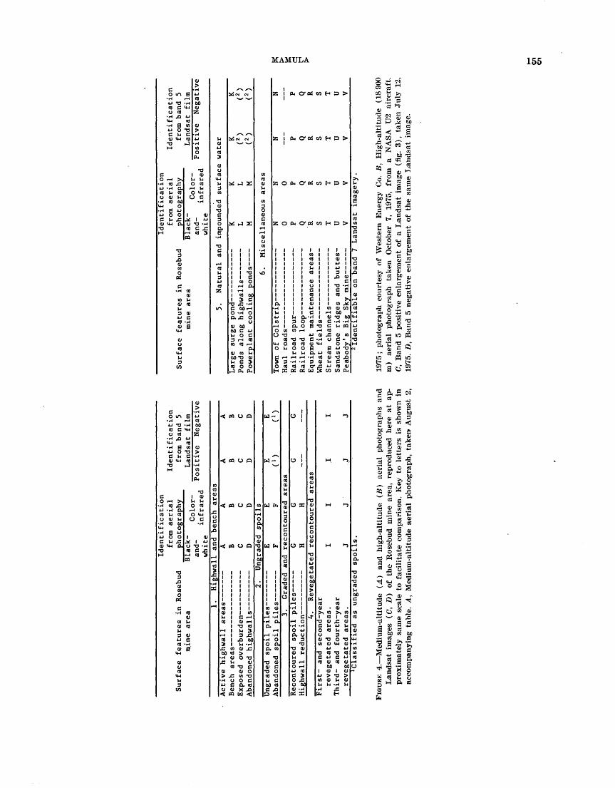
In the current study, standard Landsat film products, together with recent high-altitude aerial photographs and other data, were used to identify and delineate the following six major land-use categories related to mining and reclamation in large surface-mining areas: (1) highwall and bench areas, (2) ungraded spoils, (3) graded and recontoured areas, (4) revegetated re- contoured areas, (5) natural and impounded surface water, and (6) miscellaneous areas.
Western Energy Co.'s Rosebud mine, near Colstrip, Mont., was chosen for this study because it is the larg est surface-coal-mining operation in the northern Great
151
50 I
100 KILOMETERS_I
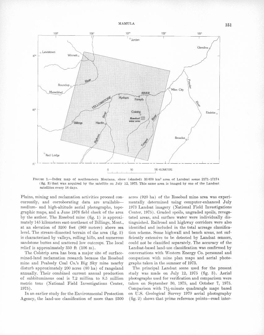
FIGURE 1. Index map of southeastern Montana, show (shaded) 33670 km2 area of Landsat scene 2171-17174 (fig. 3) that was acquired by the satellite on July 12, 1975. This same area is imaged by one of the Landsat satellites every 18 days.
Plains, mining and reclamation activities proceed con currently, and corroborating data are available medium- and high-altitude aerial photographs, topo graphic maps, and a June 1976 field check of the area by the author. The Kosebud mine (fig. 1) is approxi mately 145 kilometers east-northeast of Billings, Mont., at an elevation of 3200 feet (969 meters) above sea level. The stream-dissected terrain of the area (fig. 2) is characterized by valleys, rolling hills, and numerous sandstone buttes and scattered low outcrops. The local relief is approximately 350 ft (106 m).
The Colstrip area has been a major site of surface- mined-land reclamation research because the Rosebud mine and Peabody Coal Co.'s Big Sky mine nearby disturb approximately 200 acres (80 ha) of rangeland annually. Their combined current annual production of subbituminous coal is 7.2 million to 8.5 million metric tons (National Field Investigations Center, 1975).
In an earlier study for the Environmental Protection Agency, the land-use classification of more than 2300
acres (920 ha) of the Rosebud mine area was experi mentally determined using computer-enhanced July 1973 Landsat imagery (National Field Investigations Center, 1975). Graded spoils, ungraded spoils, revege- tated areas, and surface water were individually dis tinguished. Railroad and highway corridors were also identified and included in the total acreage classifica tion scheme. Some highwall and bench areas, not suf ficiently extensive to be detected by Landsat sensors, could not be classified separately. The accuracy of the Landsat^based land-use classification was confirmed by conversations with Western Energy Co. personnel and comparison with mine plan maps and aerial photo graphs taken in the summer of 1973.
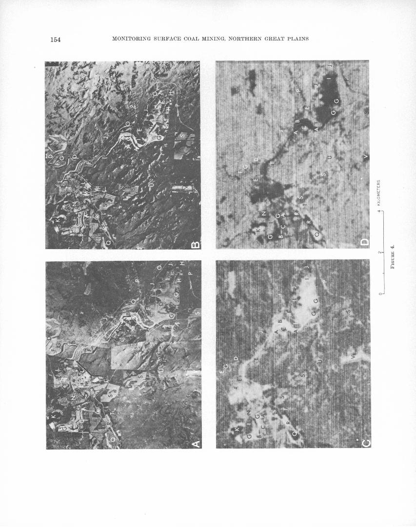
The principal Landsat scene used for the present study was made on July 12, 1975 (fig. 3). Aerial photographs used for verification and comparison were taken on September 30, 1975, and October 7, 1975. Comparison with 71^-minute quadrangle maps based on U.S. Geological Survey 1970 aerial photography (fig. 2) shows that prime reference points road inter-
152 MONITORING SURFACE COAL MINING, NORTHERN GREAT PLAINS
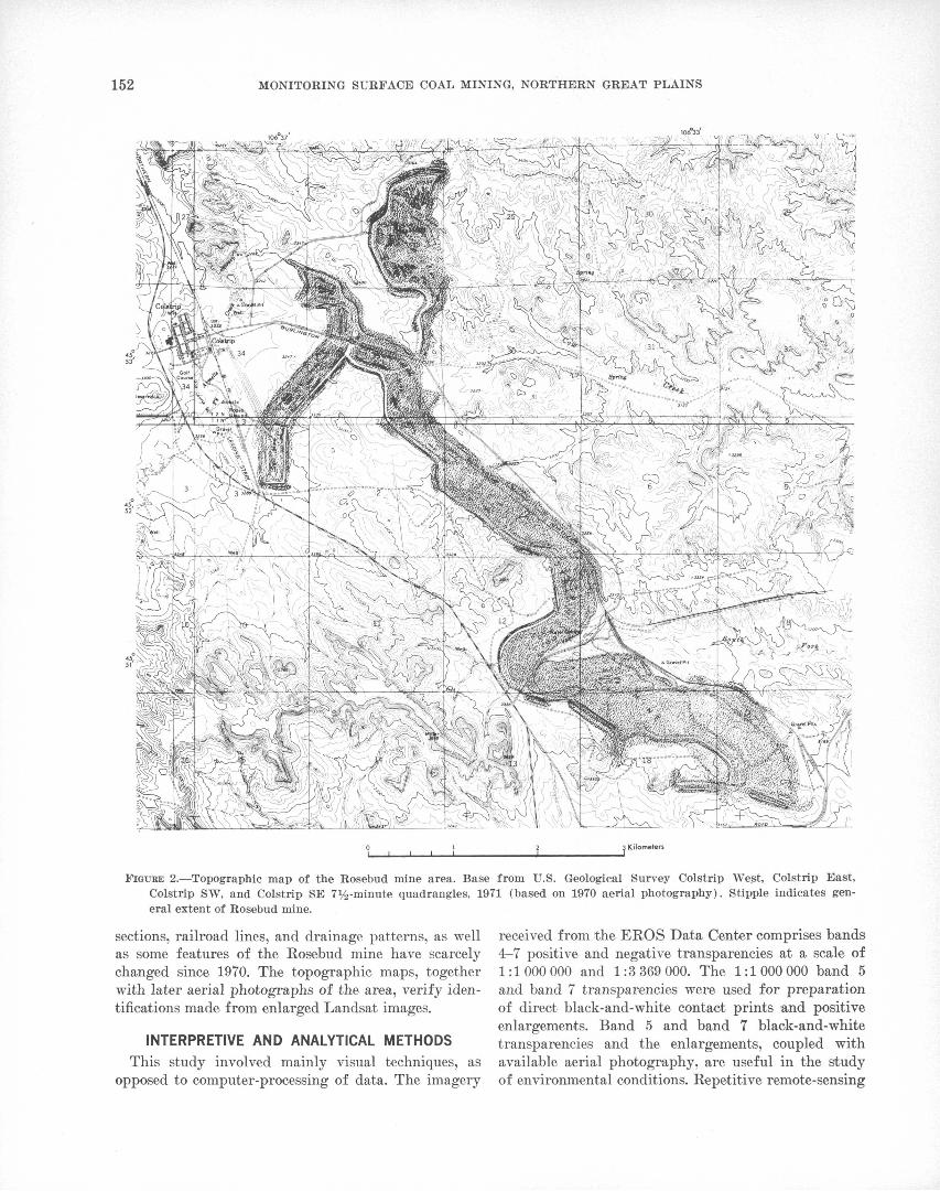
FIGURE 2. Topographic map of the Rosebud mine area. Base from U.S. Geological Survey Colstrip West, Colstrip East, Colstrip S\V, and Colstrip SB 7y2 -minute quadrangles, 1971 (based on 1970 aerial photography). Stipple indicates gen eral extent of Rosebud mine.
sections, railroad lines, and drainage patterns, as well received from the EROS Data Center comprises bandsas some features of the Rosebud mine have scarcely 4-7 positive and negative transparencies at a scale ofchanged since 1970. The topographic maps, together 1:1000000 and 1:3369000. The 1:1000000 band 5with later aerial photographs of the area, verify iden- and band 7 transparencies were used for preparationtifications made from enlarged Landsat images. of direct black-and-white contact prints and positive
enlargements. Band 5 and band 7 black-and-whiteINTERPRETIVE AND ANALYTICAL METHODS transparencies and the enlargements, coupled with
This study involved mainly visual techniques, as available aerial photography, are useful in the studyopposed to computer-processing of data. The imagery of environmental conditions. Repetitive remote-sensing
MAMULA 153
IMH7-W IWI87-3e IUIB7-
I
Colstrip.Rosebud mine
Billings
I2JUL7^%?M/HI87-I6 N rlSS 5 D SUM EL56W ' !32-238«-0- 1 -N-D-a.' E-ZI7I - 17174-5 81
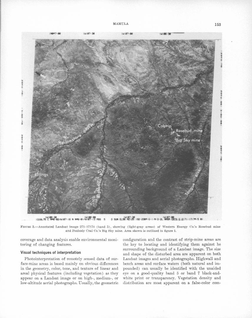
FIGURE 3. Annotated Landsat image 271-17174 (band 5), showing (light-gray areas) of Western Energy Co.'s Rosebud mineand Peabody Coal Co.'s Big Sky mine. Area shown is outlined in figure 1.
coverage and data analysis enable environmental moni toring of changing features.
Visual techniques of interpretation
Photointerpretation of remotely sensed data of sur face-mine areas is based mainly on obvious differences in the geometry, color, tone, and texture of linear and areal physical features (including vegetation) as they appear on a Landsat image or on high-, medium-, or low-altitude aerial photographs. Usually, the geometric
configuration and the contrast of strip-mine areas are the key to locating and identifying them against he surrounding background of a Landsat image. The size and shape of the disturbed area are apparent on both Landsat images and aerial photographs. Highwall and bench areas and surface waters (both natural and im pounded) can usually be identified with the unaided eye on a good-quality band 5 or band 7 black-and- white print or transparency. Vegetation density and distribution are most apparent on a false-color com-
154 MONITORING SURFACE COAL MINING, NORTHERN GREAT PLAINS
Surface
features in Rosebud
mine area
Identification
from
ae
rial
ph
otog
raph
yBlac
k-
_ ,
. Color-
and-
.
, . .
in
frar
ed
whit
e
Identification
from
ban
d 5
Landsat
film
Posi
tive
Ne
gati
ve
1.
High
wall
an
d be
nch
areas
DD
f\ DD
2.
Ungraded sp
oils
Ungraded
sp
oil piles
Abandoned spoil
pile
s-E C1
)
3.
Gra
ded
an
d
reco
nto
ure
d
are
as
Reco
nto
ure
d sp
oil
pil
es
GG
GG
4.
Revegeta
ted
reco
nto
ure
d
are
as
First- an
d se
cond
-yea
rrevegetated
area
s.Third- and
fourth-year
revegetated
areas.
I J
I J
I J
I J'C
lassif
ied
as
un
gra
ded
sp
oil
s.
Surf
ace
features
in Rosebud
mine area
Identification
from
ae
rial
ph
otog
raph
yBlack-
- Co
lor-
an
d-
. c
, .
. infrared
white
Identification
from ban
d 5
Landsat
film
Posi
tive
Ne
gati
ve
5.
Natural
and
impounded
surf
ace
water
Large
surg
e pond
K
K Po
nds
along highwalls
L L
Powerplant co
olin
g ponds __ M______M
6.
Misc
ella
neou
s ar
eas
Town of
Cols trip
Equipment
main
tena
nce
area
s-
h?tr
eam cnanneis
Sand
ston
e ri
dges
and
buttes-
N 0 P Q R S T U V
N 0 P Q R
S T
U V
N P Q R S T U V
N P Q R
S T
U V2Id
enti
fiable
on
ban
d
7 L
an
dsa
t im
ager
y.
FIG
URE
4.
Med
ium
-alt
itu
de
(A)
and
high
-alt
itud
e (K
) ae
rial
ph
otog
raph
s an
d
Lan
dsa
t im
ages
(G
, D
) of
the
Ros
ebud
min
e ar
ea,
repr
oduc
ed h
ere
at a
p
prox
imat
ely
sam
e sc
ale
to f
acil
itat
e co
mpa
riso
n. K
ey t
o le
tter
s is
sho
wn
in
acco
mpa
nyin
g ta
hle.
A,
Med
ium
-alt
itud
e ae
rial
pho
togr
aph,
tak
en-
Aug
ust
2,
1975
; ph
otog
raph
cou
rtes
y of
Wes
tern
Ene
rgy
Co.
B
, H
igh-
alti
tude
(1
8900
m
) ae
rial
ph
otog
raph
ta
ken
Oct
ober
7,
19
75,
from
a
NA
SA
TJ
2 ai
rcra
ft.
C,
Ban
d 5
posi
tive
enl
arge
men
t of
a L
andsa
t im
age
(fig
. 3),
tak
en J
uly
12,
1975
. D
, B
and
5 ne
gati
ve e
nlar
gem
ent
of t
he s
ame
Lan
dsa
t im
age.
cn
en
156 MONITORING SURFACE COAL MINING, NORTHERN GREAT PLAINS
posite image. Such false-color composites are created by exposing three of the four black-and-white bands (bands 4-7) through different color filters onto color film. On false-color images, healthy vegetation appears bright red; diseased, dead, or dormant vegetation is green; clear water appears black; sediment-laden water is powder blue; and surface-coal-mine areas are me dium and dark blue.
By means of a Bausch and Lomb stereomicroscope (zoom binocular) the image transparencies were studied closely. Optical enlargement, though facilitating the identification of features not discernible at 1:1 000 000 scale, sacrifices some resolution. The amount of resolu tion loss caused by increasing magnification depends on the initial quality and the type of transparency furnished by the EEOS Data Center. Once the opti mum magnification-resolution balance was established, the small area of interest was optically enlarged for black-and-white positives; and negatives from the en largement were set aside for density-slicing study.
A comparison of the identifiable surface features on the medium- and high-altitude aerial photographs and the Landsat imagery is presented in figure 4. Despite variation in tone, texture, and clarity of print, a gen eral land-use identification and classification is possible. Enlarging the 1:1 000 000-scale Landsat image (fig. 3) enables much greater precision in identification of sur face mine features. Furthermore, an experienced ana lyst who is familiar with the mining area as represented on Landsat images can derive far more information than the inexperienced user can. Nevertheless, owing to resolution limitations, visual methods alone cannot be relied upon in the identification of certain features on Landsat films. Landsat CCT data, displayed at a scale of 1:24000, can complement or replace visual analysis. For detailed investigations of complex sur face-mining situations, an analyst now may have to rely solely on any available recent medium- or high- altitude aerial photography. Forthcoming Landsat missions are expected to provide improved resolution.
More precise areal comparisons of aerial photo graphs and Landsat enlargements is possible after both are gridded (Chapman, 1974) an'd identical fixed refer ence points located. '
Enlargement to high magnification may necessitate mosaicking of individual images (McEwen and Schoonmaker, 1975).
Good-quality aerial photographs or mosaics of en larged Landsat images can be periodically restudied and compared with later data. Features that pertain to mining and reclamation can be transferred from, imagery or photographs to topographic or mine maps,
yielding a usable, current, and valuable land-use map of the surface mine site.
Densitometric analysis
Films can also be analyzed by density slicing, or densitometry a quantitative measurement of the mag nitude and frequency of change in tonal values, from either film transparencies or prints. Using tone in the interpretation of remotely sensed data requires the interpreter to make a qualitative judgment. The in terpreter must avoid basing his determination solely on results of density slicing because tonal variations on different images of an area may be caused by a change of the sun angle, different reflectance properties of the same surface features (caused, for example, by rain, snow, shadows from cloud cover), a change of vegeta tion appearance due to seasonal variations, or different film-processing techniques.
In this study, density slicing was done on black-and- white positives and negatives of the optically enlarged parts of Landsat images. Positive transparencies were deemed better suited for use in the DATACOLOR Model 703 density slicer. The density slicer employs a television camera that scans the surface of the trans parency, which is illuminated by a light source. The various shades of gray detected by the television camera are electronically "read" by a color-analyzer that assigns ranges of color to particular levels of the gray scale. The interpreter, by means of a color key board, can assign as many as 32 various hues (4 hues for each of 8 distinct chromatic colors) so as to clearly discriminate the numerous shades of gray on the posi tive transparency. The analysis of the image trans parency is then electronically displayed on a color television monitor. The electronic image displayed on the television monitor can be conveniently resolved at a scale of 1:24000.
For densitometric analysis, the loss in resolution with increasing magnification was negligible; identification of the six land-use categories used generally depends not on spatial resolution but on each category's distinc tive reflectance. In theory, each land-use category (fig. 4, table) has a particular level of spectral reflectance. In remote sensing of strip-mined areas from high alti tude or from satellite orbit, the variations of spectral reflections from different surface features are repre sented on black-and-white transparencies by numerous shades of gray that then appear on the processed film. Through manipulation of the densitometer, the distri bution of general and certain specific land-use areas is displayed in color on the television monitor. The moni tor displays (fig. 5) of the July 12, 1975, Landsat
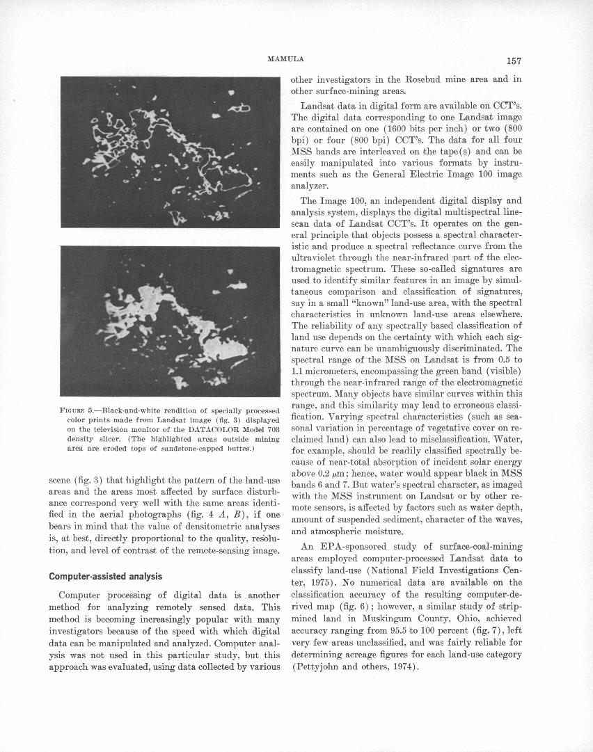
MAMULA 157
FIGURE 5. Black-and-white rendition of specially processed color prints made from Landsat image (fig. 3) displayed on the television monitor of the DATACOLOR Model 703 density slicer. (The highlighted areas outside mining area are eroded tops of sandstone-capped buttes.)
scene (fig. 3) that highlight the pattern of the land-use areas and the areas most affected by surface disturb ance correspond very well with the same areas identi fied in the aerial photographs (fig. 4 A, 5), if one bears in mind that the value of densitometric analyses is, at best, directly proportional to the quality, resolu tion, and level of contrast of the remote-sensing image.
Computer-assisted analysis
Computer processing of digital data is another method for analyzing remotely sensed data. This method is becoming increasingly popular with many investigators because of the speed with which digital data can be manipulated and analyzed. Computer anal ysis was not used in this particular study, but this approach was evaluated, using data collected by various
other investigators in the Rosebud mine area and in other surface-mining areas.
Landsat data in digital form are available on CCT's. The digital data corresponding to one Landsat image are contained on one (1600 bits per inch) or two (800 bpi) or four (800 bpi) CCT's. The data for all four MSS bands are interleaved on the tape(s) and can be easily manipulated into various formats by instru ments such as the General Electric Image 100 image analyzer.
The Image 100, an independent digital display and analysis system, displays the digital multispectral line- scan data of Landsat CCT's. It operates on the gen eral principle that objects possess a spectral character istic and produce a spectral reflectance curve from the ultraviolet through the near-infrared part of the elec tromagnetic spectrum. These so-called signatures are used to identify similar features in an image by simul taneous comparison and classification of signatures, say in a small "known" land-use area, with the spectral characteristics in unknown land-use areas elsewhere. The reliability of any spectrally based classification of land use depends on the certainty with which each sig nature curve can be unambiguously discriminated. The spectral range of the MSS on Landsat is from 0.5 to 1.1 micrometers, encompassing the green band (visible) through the near-infrared range of the electromagnetic spectrum. Many objects have similar curves within this range, and this similarity may lead to erroneous classi fication. Varying spectral characteristics (such as sea sonal variation in percentage of vegetative cover on re claimed land) can also lead to misclassification. Water, for example, should be readily classified spectrally be cause of near-total absorption of incident solar energy above 0.2 /*m; hence, water would appear black in MSS bands 6 and 7. But water's spectral character, as imaged with the MSS instrument on Landsat or by other re mote sensors, is affected by factors such as water depth, amount of suspended sediment, character of the waves, and atmospheric moisture.
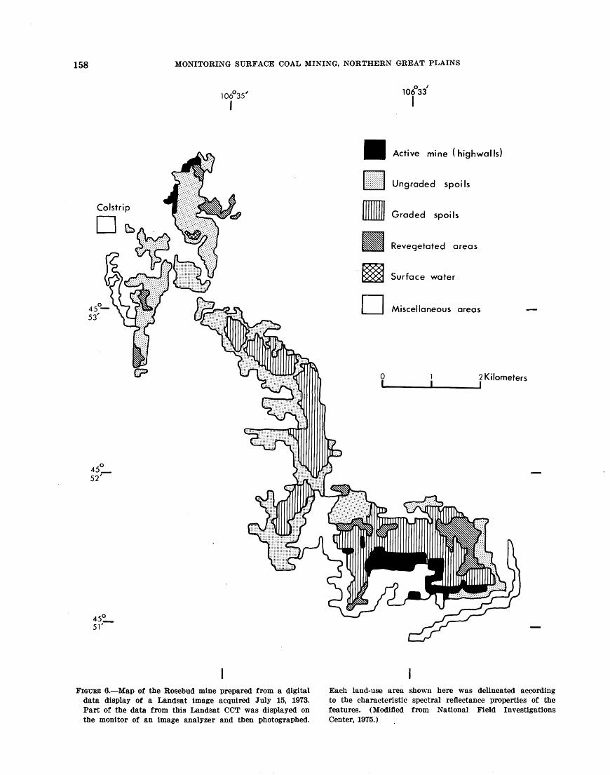
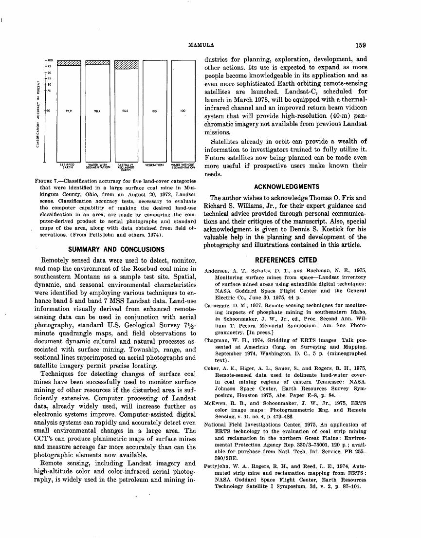
An EPA-sponsored study of surface-coal-mining areas employed computer-processed Landsat data to classify land-use (National Field Investigations Cen ter, 1975). No numerical data are available on the classification accuracy of the resulting computer-de rived map (fig. 6) ; however, a similar study of strip- mined land in Muskingum County, Ohio, achieved accuracy ranging from 95.5 to 100 percent (fig. 7), left very few areas unclassified, and was fairly reliable for determining acreage figures for each land-use category (PettyJohn and others, 1974).
158
106°35'106°33'
Active mine (highwalls)
Ungraded spoils
Graded spoils
Revegetated areas
Surface water
Miscellaneous areas
2 Kilometers
45°_ 52'
51'
FIGUBE 6. Map of the Rosebud mine prepared from a digital data display of a Landsat image acquired July 15, 1973. Part of the data from this Landsat CCT was displayed on the monitor of an image analyzer and then photographed.
Each land-use area shown here was delineated according to the characteristic spectral reflectance properties of the features. (Modified from National Field Investigations Center, 1975.)
MAMULA 159
z ..so
STRIPPED WATER WITH PABTIALIJ VEGETATION EARTH SEDIMENTATION RECLAIMED
FIGURE 7. Classification accuracy for five land-cover categories that were identified in a large surface coal mine in Mus- kinguon County, Ohio, from an August 20, 1972, Landsat scene. Classification accuracy tests, necessary to evaluate the computer capability of making the desired land-use classification in an area, are made by comparing the com puter-derived product to aerial photographs and standard maps of the area, along with data obtained from field ob servations. (From Petty John and others, 1974).
SUMMARY AND CONCLUSIONS
Remotely sensed data were used to detect, monitor, and map the environment of the Rosebud coal mine in southeastern Montana as a sample test site. Spatial, dynamic, and seasonal environmental characteristics were identified by employing various techniques to en hance band 5 and band 7 MSS Landsat data. Land-use information visually derived from enhanced remote- sensing data can be used in conjunction with aerial photography, standard U.S. Geological Survey 71/£- minute quadrangle maps, and field observations to document dynamic cultural and natural processes as sociated with surface mining. Township, range, and sectional lines superimposed on aerial photographs and satellite imagery permit precise locating.
Techniques for detecting changes of surface coal mines have been successfully used to monitor surface mining of other resources if the disturbed area is suf ficiently extensive. Computer processing of Landsat data, already widely used, will increase further as electronic systems improve. Computer-assisted digital analysis systems can rapidly and accurately detect even small environmental changes in a large area. The OCT's can produce planimetric maps of surface mines and measure acreage far more accurately than can the photographic elements now available.
Remote sensing, including Landsat imagery and high-altitude color and color-infrared aerial photog raphy, is widely used in the petroleum and mining in
dustries for planning, exploration, development, and other actions. Its use is expected to expand as more people become knowledgeable in its application and as even more sophisticated Earth-orbiting remote-sensing satellites are launched. Landsat-C, scheduled for launch in March 1978, will be equipped with a thermal- infrared channel and an improved return beam vidicon system that will provide high-resolution (40-m) pan chromatic imagery not available from previous Landsat missions.
Satellites already in orbit can provide a wealth of information to investigators trained to fully utilize it. Future satellites now being planned can be made even more useful if prospective users make known their needs.
ACKNOWLEDGMENTS
The author wishes to acknowledge Thomas 0. Friz and Richard S. Williams, Jr., for their expert guidance and technical advice provided through personal communica tions and their critiques of the manuscript. Also, special acknowledgment is given to Dennis S. Kostick for his valuable help in the planning and development of the photography and illustrations contained in this article.
REFERENCES CITEDAnderson, A. T., Schultz, D. T., and Buchman, N. E., 1975,
Monitoring surface mines from space Landsat inventory of surface mined areas \ising extendible digital techniques: NASA Goddard Space Flight Center and the General Electric Co., June 30, 1975, 44 p.
Carneggie, D. M., 1977, Remote sensing techniques for monitor ing impacts of phosphate mining in southeastern Idaho, in Schoonmaker, J. W., Jr., ed., Proc. Second Ann. Wil liam T. Pecora Memorial Symposium: Am. Soc. Photo- grammetry. [In press.]
Chapman, W. H., 1974, Gridding of ERTS images: Talk pre sented at American Cong. on Surveying and Mapping, September 1974, Washington, D. C., 5 p. (mimeographed text).
Coker, A. E., Higer, A. L., Sauer, S., and Rogers, R. H., 1975, Remote-sensed data used to delineate land-water cover- in coal mining regions of eastern Tennessee: NASA. Johnson Space Center, Earth Resources Survey Sym posium, Houston 1975, Abs. Paper E-8, p. 84.
McEwen, R. B., and Schoonmaker, J. W., Jr., 1975, ERTS color image maps: Photogrammetric Eng. and Remote Sensing, v. 41, no. 4, p. 479-486.
National Field Investigations Center, 1975, An application of ERTS technology to the evaluation of coal strip mining and reclamation in the northern Great Plains: Environ mental Protection Agency Rep. 330/3-75001, 120 p.; avail able for purchase from Natl. Tech. Inf. Service, PB 255- 590/2BE.
Pettyjohn, W. A., Rogers, R. H., and Reed, L. E., 1974, Auto mated strip mine and reclamation mapping from ERTS: NASA Goddard Space Flight Center, Earth Resources Technology Satellite I Symposium, 3d, v. 2, p. 87-101.
160 MONITORING SURFACE COAL MINING, NORTHERN GREAT PLAINS
Rehder, J. B., 1976, Changes in landscape due to strip mining, in Williams, R. S., Jr., and Carter, W. D., eds., ERTS-1, A new window on our planet: U.S. Geol. Survey Prof. Paper 929, p. 254-257.
Russell, O. R., Wobber, F. J., Weir, C. E., and Amato, Roger, 1973, Applications of ERTS-1 and aircraft imagery to mined land investigations: Tullahoma, Tennessee Univ. Space Inst, Remote Sensing of Earth Resources Sympo sium, p. 1095-1105.
Torbert, Grover, and Hemphill, W. R., 1976, Cadastral bound aries on ERTS images, in Williams, R. S., Jr., and Carter, W. D., eds., ERTS-1, A new window on our planet: U.S. Geol. Survey Prof. Paper 929, p. 44-i6.
U.S. Geological Survey, 1975, Status and plans of the Depart ment of the Interior EROS Program: U.S. Geol. Survey Open-File Rept. 75-376, 91 p.
Wobber, F. J., and Martin, K. R., 1974, ERTS monitoring of surface mining operations: World Mining, v. 27, no. 3, p. 56-57.
Jour. Research U.S. Geol. Survey Vol. 0, No. 2, Mar.-Apr. 1978, p. 161-167
AN "OPTIMAL" FILTER FOR MAPS SHOWING NOMINAL DATA
By STEPHEN C. GUPTI1L, Reston, Va.
Abstract. An "optimal" filtering technique for use with nominal data, such as land use and land cover categories, has been developed. This method is based on the conditional prob ability joins of neighboring data elements. In addition to its use in performing filtering, the method can be used to cal culate the likelihood of each data element being properly classified.
The technique was tested on a land use data set for an area in Walnut Valley, Calif. The computer program perform ing the filtering process proved to be computationally efficient and produced satisfactory results. Useful statistics of the error estimation process were also generated. Future applica tions of the method to spectrally classified Landsat data are being explored.
Filtering separates homogeneous components from a mixture of elements. In filtering, one may be concerned with the elements that pass through the filter, as in the case of filtering a bottle of wine to remove the sedi ment, or one may desire the components that is re moved by the filter andmot'the effluent (for example, the insoluble precipitate of a reaction in an aqueous solution). Analogies to these physical filtering pro cesses have been developed to treat analog impulse data and subsequently digitally coded data.
Many of the filtering procedures that can be applied to spatial data have evolved from one-dimensional techniques first used in electrical engineering and com munications science. Researchers in these fields are con cerned with the recovery of a pure signal from a trans mission consisting of both signal and random noise. Although scientists in these fields have dealt pri marily with electronic analog methods to perform the filtering, they were among the first to develop mathe matical ways to describe signals and noise. Works such as Rowe's (1965) provide some useful insights into this field.
The digital equivalent of filtering an electronic sig- n'al is the filtering of a times series of scalar data. One purpose of filtering such data is to attenuate the amp litudes of the high-frequency components in the data without affecting the low-frequency parts. The high- frequency variations are assumed to be noise or are
oscillations not relevant to the type of analysis being applied to the data (for example, the separation of weekly temperature fluctuations from a time series of hourly temperature data). The filtered value is merely an estimate of what the value would be if the "noise" were not present. Holloway (1958) and Rayner (1971) discussed these topics in detail.
The extension of such techniques to two-dimensional data is relatively simple. Generally the filtering func tion applied to two-dimensional data can be considered a composite of two functions applied in orthogonal directions. The specific processes that perform filtering operations are many and varied. Common techniques include the use of weighted moving averages, Fourier transformations, and empirical functions. Tobler (1969) elaborated on these processes.
Although the discussion thus far has dealt with scalar data, some analogous techniques exist for work ing with nominal data, and others need to be developed. To create such techniques, one can substitute simple counting measures (that is, determining the presence or absence of a category) and decision functions for the arithmetic operations that are used on scalar data. Work wiith nominal data has largely concerned binary- valued functions such as those encountered in picture processing. Rosenfeld (1969) and Andrews (1970) dealt with these topics in great detail. Fewer attempts have been made to deal with the filtering of multi- category nominal data, although MacDougall (1972), Strong and Rosenfeld (1973) and Guptill (1975) con ducted research in this field.
One of the problems associated with filtering trans formations is the determination of the correct amount of filtering. Because filters can be applied in an itera tive fashion, with various "strengths," how can one ascertain when a data set has been "sufficiently" fil tered? One approach is to monitor the filtering proc ess by qualitative and quantitative (techniques. A second, more direct approach is to construct an "opti mal" filter that yields results filtered in the proper amount and manner according to a set of predeter mined standards. For example, Thompson (1956) de-
161
162 "OPTIMAL" FILTER FOR MAPS SHOWING NOMINAL DATA
vised an "optimal linear smoothing process" for use on barometric pressure maps. His process is "optimum" in that the root-niean-squared difference between the true and smoothed fields is the least. Similarly, an optimal smoothing filter can be devised for use with nominal data.
DEFINING AN OPTIMAL TRANSFORMATION
The first step in the construction of an optimal trans formation process is to define "optimal." One formula tion is as follows.
Consider a map represented by a geographical mat rix with N rows and M columns and with K possible states. The object is to determine the conditional prob ability between the state (land use category) of a center cell (C) and the state of each neighbor cell (N). Each cell in ithe geographical matrix is taken in turn as a center cell that is surrounded by as many as eight neighbors. The first step is to count the number of transitions between the category of each center cell of the geographical matrix and the categories of the neighbor cells. Once the results are tallied in a matrix, the frequency of the transmissions between the cate gories may be computed by dividing each row entry by the sum of row values. If the number of transitions in a matrix cell is large enough, the frequency of oc currence satisfactorily approximates a conditional probability P(C/N).
The conditional probability of the state of each cell on the map is represented by
(1)
that is, the probability of the center cell being in state k, given that the itn neighbor cell is in state j. This pro cedure permits one to determine the probability of oc currence of the center category, G^ from the categories of the neighbors. If the center cell is not an edge cell and if the categories of the neighbors are denoted by
N (that is, each of the N\) , then the total conditionalprobability of the Ck center category as determined by the neighbor is
-» 8
These conditional probabilities should be normalized to sum to 1; thus for n categories,
P'(C /N)= n*" ' '. - K ' } ' I «=i 1=1 N K' ]' '
(3)
where P'(Ck/N) is the normalized conditional prob ability. This equation provides an estimate of the like-
lihood of a center cell being in a certain state, given the states of its neighbors. When this procedure is applied to each cell and its associated neighborhood, a probability surface is produced that provides informa tion as to where, in geographical space, the state of a cell is probably in error.
An approximation of the total error in the map, as well as the error within each category, is provided by a simple loss function. Define a symmetrical, zero-one loss function as follows:
where c is the number of categories, ak is the category observed at location #, and ftp is the "true" state of the cell at location x. If ak is not the same as the most likely occurrence /3P , then \(ak/(3p )=l. A total measure of error in the map can be compiled by applying the loss function over the entire map :
Total error = (5)
This specialized definition of error only slightly re sembles error as defined by a field check, but it is a defensible definition. In this case, an "optimal" trans formation is defined as the operation that minimizes the total map error.
This transformation, or filtering operation, is performed by selecting the category, &, which maximizes
-» the a posteriori probability P((3P/N). That is, in determining the cell states in the transformed (filtered) map, decide
fl k if P(/3k/N)>P((3p/N) for all k^p (6)
where /3 fc , (3P represent possible states of the central cell and N represents the categories of the neighbors of the central cell.
This method is similar to the techniques used in de termining nominal classifications in pattern recogni tion work. For example, Latham (1974), in classifying land use categories from remotely sensed data, used a method in which the category chosen for a site was the one in the most probable state, as determined by the characteristics of nearby sites.
EXAMPLES
The calculations described in the previous section were made using a Fortran IV computer program written for experimentation with various data sets. The data set in these examples was taken from a 1971 land use map of the Walnut Valley area of California (lo-
GUPTILL 163
X
^
Z
A
X
X
A
I
CD
\
\
/
RESIDENTIAL
INDUSTRIAL
COMMERCIAL
INSTITUTIONAL
RECREATIONAL
URBAN AGRICULTURAL
URBAN VACANT
FREEWAY UNDER CONSTRUCTION
COMPLETED FREEWAY
FIELD CROPS
ROW CROPS
ORCHARDS
MOWN GRASSES
GRAZING
VACANT
CATEGORY NO. 1
CATEGORY NO. 2
CATEGORY NO. 3
CATEGORY NO. 4
CATEGORY NO. .5
CATEGORY NO. 6
CATEGORY NO. 7
CATEGORY NO. 8
CATEGORY NO. 9
CATEGORY NO. 10
CATEGORY NO. 11
CATEGORY NO. 12
CATEGORY NO. 13
CATEGORY NO. 14
CATEGORY NO. 15
Land Use/Land Use Change Legend
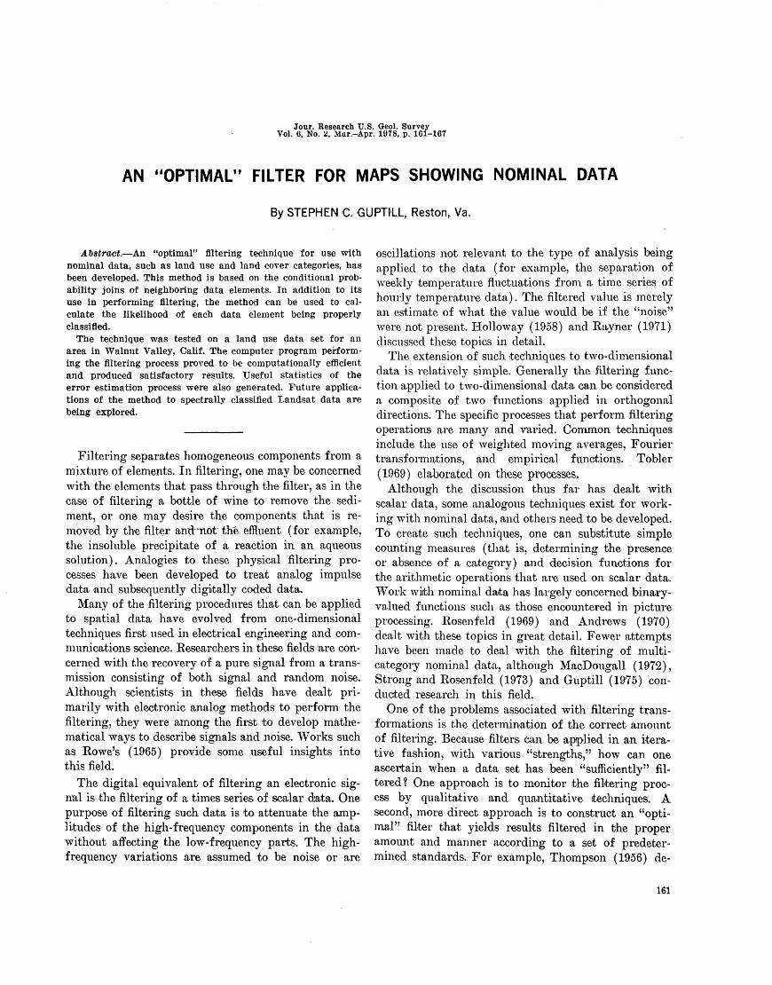
FIGURE 1. Symbols for different categories of land use.
cated east of Los Angeles). The original polygon map of this area, compiled by Goehring (1971), was digi tized and converted to a grid-cell form, with each grid cell measuring 91.4 meters (300 feet) on a side. An explanation of the symbols used on these maps is shown in figure 1.
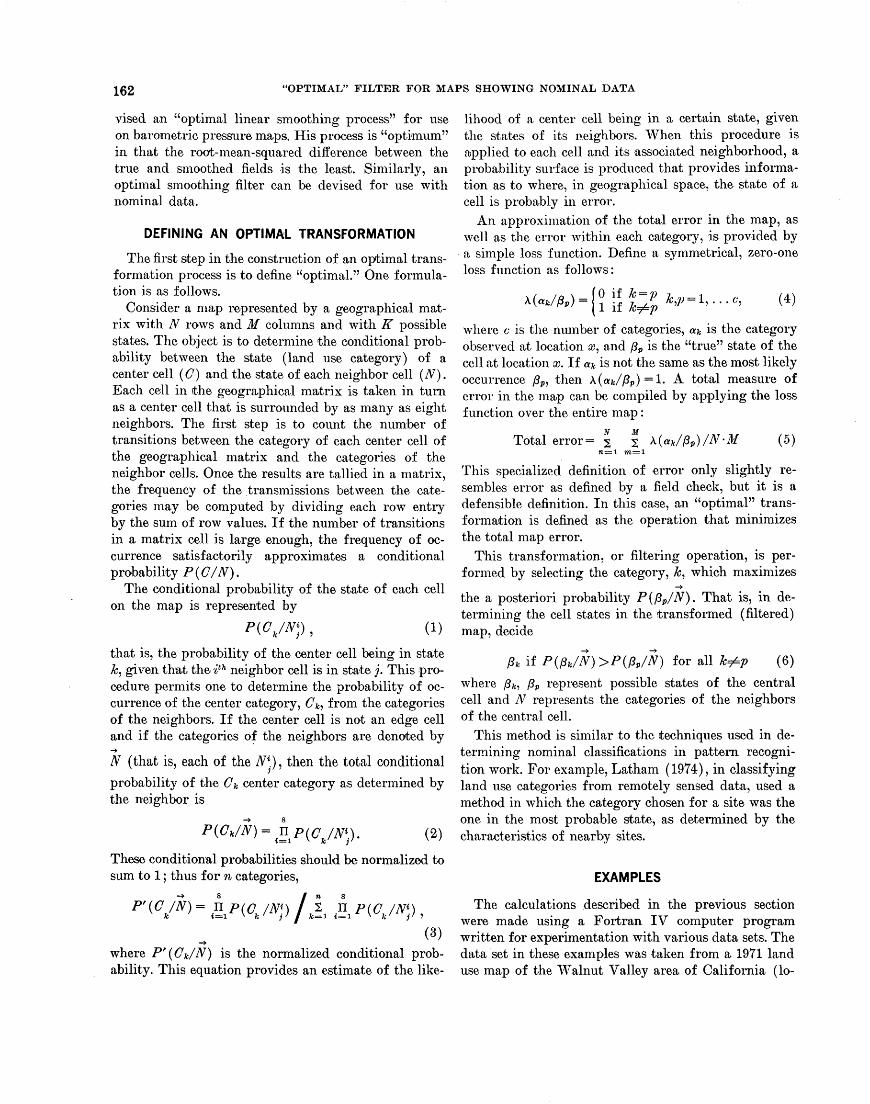
A 1600-cell portion (a 40 by 40 matrix of cells) of the map was tested first. This portion is shown infigure 2. The probability of occurrence of a given
-» category in each cell, P'(Ck/N) of this data set wascalculated as shown in equation 3. An error estimation parameter Ek was then computed by
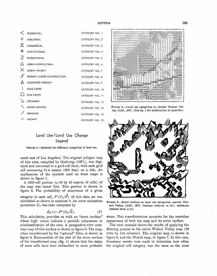
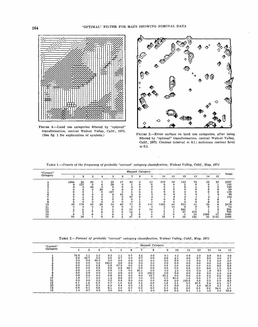
Ek =l-P'(Ck/N). (7) This calculation provides us with an "error surface" where high values indicate a possible uniqueness or misclassification of the area. A perspective-view cont- tour map of this surface is shown in figure 3. The map, when transformed by the "optimal" filter, is shown in figure 4. Examination of the plot of the error surface of the transformed map (fig. 5) shows that the states of some cells have been reclassified to more probable
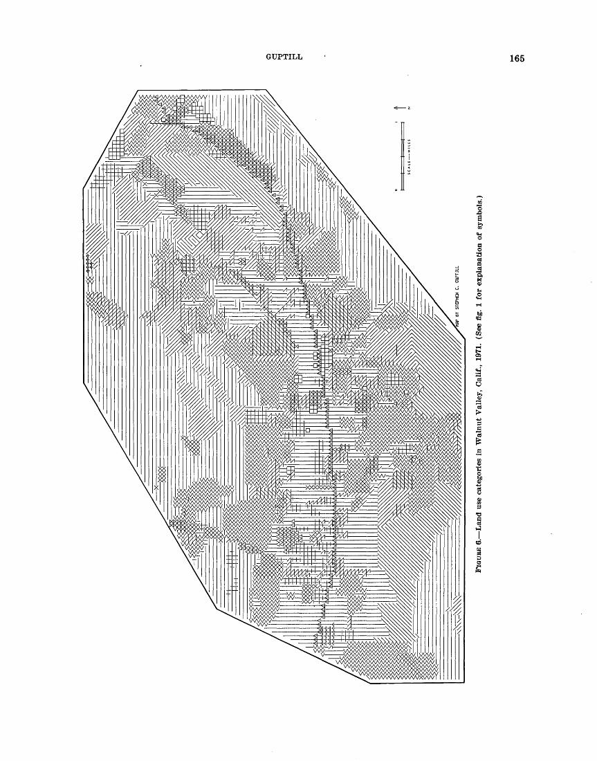
FIGURE 2. Land use categories in central Walnut Val ley, Calif., 1971. (See fig. 1 for explanation of symbols.)
FIGURE 3. Error surface on land use categories, central Wal nut Valley, Calif., 1971. Contour interval = 0.1; minimum contour level = 0.1.
states. This transformation accounts for the smoother appearance of both the map and its error surface.
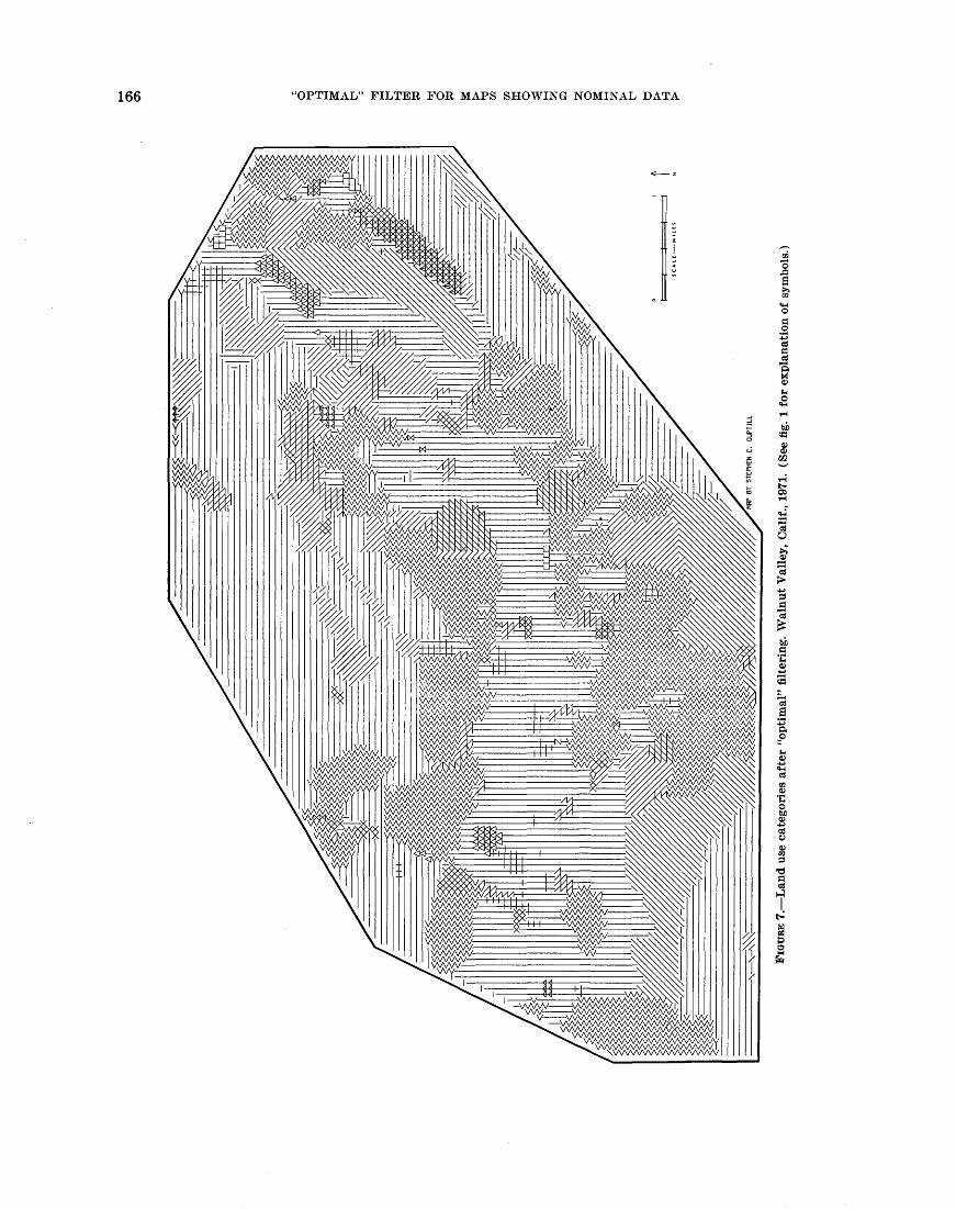
The next example shows the results of applying the filtering process to the entire Walnut Valley map (99 rows by 154 columns). The original map is shown in figure 6, and the filtered map, in figure 7. In this case, frequency counts were made to determine how often the original cell category was the same as the most
164 "OPTIMAL" FILTER FOR MAPS SHOWING NOMINAL DATA
FIGURE 4. Land use categories filtered by "optimal" transformation, central Walnut Valley, Calif., 1971. (See fig. 1 for explanation of symbols.) FIGURE 5. Error surface on land use categories, after being
filtered by "optimal" transformation, central Walnut Valley, Calif., 1971. Contour interval = 0.1; minimum contour level = 0.1.
TABLE 1. Counts of the frequency of probable "correct" category classification, Walnut Valley, Calif., Map, 1971
"Correct" Category
123456789
101112131415
Mapped Category
1
199400000000
480278
50
2
29127
0000100
1760423
26
3
30090010000
5001701
4
700
2000000
2902410
5
292900
1270100
1403300
6
170000
65000
4900032
7
8010010
9700
730
10142
47
8
000000011000100
9
1308010005
1100
14480
10
11060000100
1582:0775
28
11
1601000000
44151104
12
15210000000
2230
240275
38
13
7501000100
4107
67610
125
14
2200001000
25012
100836
15
23100001006025
173142
Total
25971651002013066
10216
247015
294760
10653499
TABLE 2. Percent of probable "correct" category classification, Walnut Valley, Calif., Map, 1971
"Correct" Category
1234567&9
101112131415
Mapped Category
1
76.80.00.00.00.00.00.00.00.01.90.00.70.90.81.4
2
1.192.7
0.00.00.00.01.00.00.07.10.01.40.30.30.7
3
1.20.0
90.00.00.80.00.00.00.02.00.00.30.90.00.0
4
0.30.00.0
100.00.00.00.00.00.01.20.00.70.50.10.0
5
1.10.70.00.0
97.00.01.00.00.00.60.01.00.40.00.0
6
0.70.00.00.00.0
98.50.00.00.02.00.00.00.00.30.1
7
3.10.70.00.00.80.0
95.10.00.03.00.03.41.80.21.3
8
0.00.00.00.00.00.00.0
100.016.7
0.00.00.00.10.00.0
9
0.50.08.00.00.80.00.00.0
83.34.50.04.80.50.30.0
10
4.24.40.00.00.00.01.00.00.0
64.00.02.40.90.50.8
11
0.60.01.00.00.00.00.00.00.01.8
100.00.30.10.00.1
12
5.9'0.7
0.00.00.00.00.00.00.09.00.0
81.63.60.51.1
13
2.90.01.0O'.O0.00.01.00.00.01.70.02.4
8S.90.93.6
14
O.S0.00.00.0O'.O1.50.00.00.01.00.00.30.3
94.61.0
15
0.90.70.00.00.00.01.00.00.00.20.00.70.71.6
89.8
EPHE
N C
. G
UP
TILL
Q d
Fiot
JBE
6. L
and u
se c
ateg
orie
s in
Wal
nut
Val
ley,
Cal
if.,
1971
. (S
ee f
ig.
1 fo
r ex
plan
atio
n of
sym
bols
.)
Ol
166 "OPTIMAL" FILTER FOR MAPS SHOWING NOMINAL DATA
-Wv\A/ WVWV
WNAA'VVW: A'V
WWW NAAA/VVVVVVV
V NAAAAAAAAAAAA/-NAAAAAAAAAAAAAA/
a
1ti a
OJ'C
8.
GUPTILL 167
probable (or "correct") cell state (see eq 4). The fre quency counts are shown in table 1, and the same fig ures expressed as percentages are shown in table 2. Using these figures, one can estimate the total "error" in the map (eq 5). On the entire map, 86.4 percent of the categories were mapped "correctly." The filtering and error estimation process required 13.6 seconds of CPU time on an IBM 370/168.
The "optimal" filtering transformation is a useful technique for nominal data. It offers the advantages of high efficiency and satisfactory plots of the data coupled with the added benefits of producing statistics of the error estimation process.
Researchers are presently testing this technique for use in postprocessing Landsat images in which the pixels have been classified into land use and land cover categories. A statistical clustering technique is being used to classify pixel values derived from scalar radio- metric data. Variations in spectral response cause im perfect separation of cover types, which, in turn, re sults in cluster overlap and the misclassification of some pixels. The use of the "optimal" filtering algo rithm to change the pixel classifications from unlikely states to more probable states based on the states of their neighbors improves the appearance and accuracy of the map.
REFERENCES CITED
Andrews, H. C., 1970, Computer techniques in image proces sing: New York, Academic Press, 187 p.
Goehring, Darryl R., 1971, Monitoring the evolving land use patterns on the Los Angeles metropolitan, fringe using remote sensing: Riverside, California Univ. of, Dept. Geography, Technical Rept. T-71-5,107 p.
Guptill, S. C., 1975, Spatial filtering of nominal data: an ex ploration : Ann Arbor, Michigan Univ. of, unpublished Ph.D. dissert., 210 p.
Holloway, J. L., Jr., 1958, Smoothing and filtering of time series and space fields: Advances in Geophysics, v. 4, New York, Academic Press, p. 351-89.
Latham, J. P., 1974, Urban pattern recognition and image color discrimination with TV waveforms and computerized matrix analysis and mapping: Florida Atlantic Univ., Dept. Geography, Office of Naval Research Rept. NR 389- 151, p. 3-1-3-14.
MacDougall, E. B., 1972, Optimal generalization of mosaic maps: Geog. Analysis, v. 4, no. 4, p. 416-423.
Rayner, ,T. N., 1971, An introduction to spectral analysis: London, Pion Limited, 174 p.
Rosenfeld, Azriel, 1969, Picture processing by computer: New York, Academic Press, 196 p.
Rowe, H. E., 1965, Signals and noise in communication sys tems: Princeton, N.J., D. Van Nostrand Co., Inc., 257 p.
Strong III, J. P., and Rosenfeld, Azriel, 1973, A region color ing technique for scene analysis: Commun. ACM, v. 16, n. 4, p. 237-246.
Thompson, P. D., 1956, Optimum smoothing of two-dimensional fields: Tellus, v. 8, no. 3, p. 384-393.
Tobler, W. R., 1969, Geographic filters and their inverses: Geog. Analysis, v. 1, no. 3, p. 234-252.

Jour. Research U.S. Geol. Survey Vol. 6, No. 2, Mar.-Apr. 1978, p. 169-173
ACCURACY OF SELECTED LAND USE AND LAND COVER MAPS IN THE GREATER ATLANTA REGION, GEORGIA
by KATHERINE FITZPATRICK-LINS, Reston, Va.
Abstract. The land use and land cover maps at 1:100000 scale and at 1:24 000 scale in the Greater Atlanta Region were tested for accuracy. At 1:100 000 scale, 381 points were selected using a stratified systematic nnalined sampling tech nique. Of these 381 points, 343 points or 90 percent were found to be correct. At 1:24 000 scale, 71 points were tested for accuracy. Of these 71 points, 62 points or 87 percent were found to be accurate. Confidence intervals were determined based on the assumption that the data exhibited a binomial distribution. With 95-percent confidence the accuracy of the 1:100 000-scale maps was between 87 and 93 percent, and the accuracy of the 1:24 000-scale maps was between 79 and 96 percent. The accuracy of the interpretations was consistent from category to category.
Level II land use and land cover maps (Anderson and others, 1976) at a scale of 1:250 000 and 1:100 000 are prepared by the U.S. Geological Survey using high-altitude photographs and stable base copies of the black-and-blue line topographic map plates as a mapping base. The mapping criteria adhered to, speci fied by Anderson and others (1976), states that: (1) the land use and land cover maps must be at least 85 percent accurate; (2) the accuracy of the interpretation will be about equal for several cate gories; and, (3) the results must be repeatable from interpreter to interpreter and from one time to an other. Once the maps are compiled, field verification is conducted to assure correct interpretation, and the maps are made available to local users for review. Additional corrections are then incorporated.
For this study, land use and land cover maps of the Greater Atlanta Region were chosen to test quan titatively the accuracy of the Level II land use and land cover maps and to ascertain objectively if the criterion of 85 percent classification accuracy is being met. The set of land use and land cover maps for the Atlanta area are the first in the nationwide land use and land cover program to be tested for accuracy. The procedures utilized for this study establish the method ology to be used for further research on the accuracy of the Geological Survey's land use and land cover maps.
Land use and land cover maps were compiled at 1:100000 for the entire Greater Atlanta Region and for twelve 7.5-minute quadrangles at 1:24 000 scale for parts of the same area in cooperation with the Georgia State Geological Survey. In addition, six 7.5-min quadrangles were selected for compilation at the scale of 1:24000 for a river quality study by the U.S. Geological Survey. These eighteen 7.5-min quad rangles were compiled using the 1:24 000-scale ortho- photoquads as a base and were mapped with a mini mum mapping unit of 1 hectare.
The land use and land cover data were generalizedo
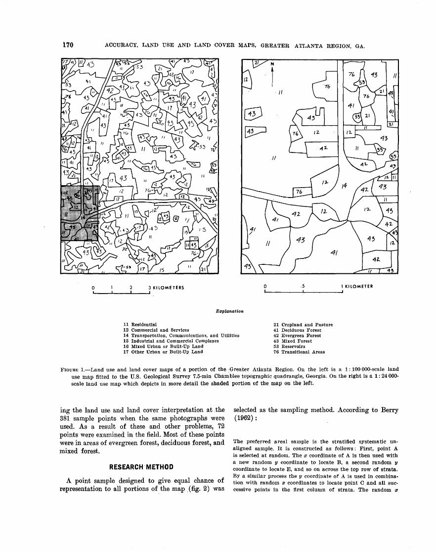
from the 1:24 000-scale map to the 1:100 000 scale for that portion of the Greater Atlanta Region land use and land cover map originally compiled at 1:24 000 scale. The minimum mapping unit for the 1:100 000- scale land use and land cover maps was increased from 1 ha at 1:24 000 scale to 4 or 16 ha at 1:100 000 scale, according to the specifications (Anderson and others, 1976). The remaining 1:100 000-scale land use and land cover map was compiled to a stable base copy of the black-and-blue line print by using black-and- white high-altitude photographs at a contact scale of 1:76000 and at a reduced scale of 1:100000. An ex ample of the land use and land cover maps of the Atlanta area is shown on figure 1.
The compilers experienced the greatest difficulties in interpretation of the forest land categories. The black-and-white aerial photographs were obtained in 3 different months, February, April, and May, and the degree of foliation varied with the time of photog raphy. For this reason the shades of gray on the photo graphs varied for evergreen and deciduous trees from month to month, so that there was no consistent sig nature for forest types. The interpreters had the great est difficulty separating evergreen and deciduous for ests on the May photographs, as both forest types had similar gray tones. This problem was as difficult to resolve at 1:24 000 scale as it Avas at 1:100 000 scale.
These same difficulties were experienced in verify-169
170 ACCURACY, LAND USE AND LAND COVER MAPS, GREATER ATLANTA REGION, GA.
3 KILOMETERS 1 KILOMETER
Explanation
11 Residential12 Commercial and Services14 Transportation, Communications, and Utilities15 Industrial and Commercial Complexes16 Mixed Urban or Bullt-Up Land17 Other Urban or Built-Up Land
21 Cropland and Pasture41 Deciduous Forest42 Evergreen Forest43 Mixed Forest53 Reservoirs76 Transitional Areas
FIGURE 1. Land use and land cover maps of a portion of the Greater Atlanta Region. On the left is a 1:100 000-scale land use map fitted to the U.S. Geological Survey 7.5-min Chamblee topographic quadrangle, Georgia. On the right is a 1:24 000- scale land use map which depicts in more detail the shaded portion of the map on the left.
ing the land use and land cover interpretation at the 381 sample points when the same photographs were used. As a result of these and other problems, 72 points were examined in the field. Most of these points were in areas of evergreen forest, deciduous forest, and mixed forest.
RESEARCH METHOD
A point sample designed to give equal chance of representation to all portions of the map (fig. 2) was
selected as the sampling method. According to Berry (1962):
The preferred areal sample is the stratified systematic un- aligned sample. It is constructed as follows: First, point A is selected at random. The x coordinate of A is then used with a new random y coordinate to locate B, a second random y coordinate to locate E, and so on across the top row of strata. By a similar process the y coordinate of A is used in combina tion with random x coordinates to locate point C and all suc cessive points in the first column of strata. The random a>
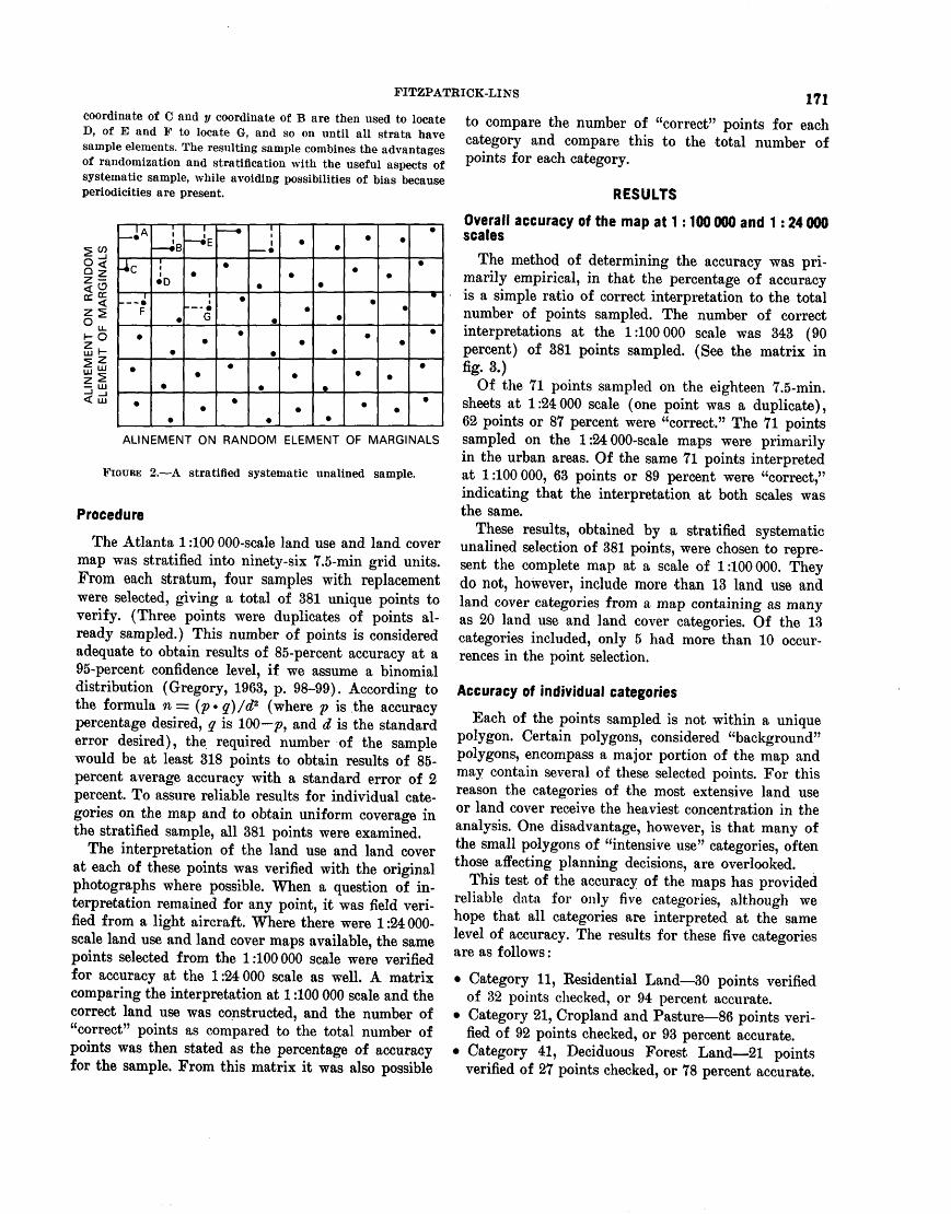
FITZPATRICK-LINS 171coordinate of C and y coordinate of B are then used to locate to compare the number of "correct" points for eachD. Of E and F t.0 lnr>ntA fi nnH on «n iiYiHl oil C.4-.04-0 V.«,.~ _ JT " " *"* ^"^"D, of E and F to locate G, and so on until all strata have sample elements. The resulting sample combines the advantages of randomization and stratification with the useful aspects of systematic sample, while avoiding possibilities of bias because periodicities are present.
o^ -Ic
< LLJ
ALINEMENT ON RANDOM ELEMENT OF MARGINALS
FIGURE 2. A stratified systematic unalined sample.
Procedure
The Atlanta 1:100 000-scale land use and land cover map was stratified into ninety-six 7.5-min grid units. From each stratum, four samples with replacement were selected, giving a total of 381 unique points to verify. (Three points were duplicates of points al ready sampled.) This number of points is considered adequate to obtain results of 85-percent accuracy at a 95-percent confidence level, if we assume a binomial distribution (Gregory, 1963, p. 98-99). According to the formula n = (p» q)/d2 (where p is the accuracy percentage desired, q is 100 p, and d is the standard error desired), the required number of the sample would be at least 318 points to obtain results of 85- percent average accuracy with a standard error of 2 percent. To assure reliable results for individual cate gories on the map and to obtain uniform coverage in the stratified sample, all 381 points were examined.
The interpretation of the land use and land cover at each of these points was verified with the original photographs where possible. When a question of in terpretation remained for any point, it was field veri fied from a light aircraft. Where there were 1:24 000- scale land use and land cover maps available, the same points selected from the 1:100 000 scale were verified for accuracy at the 1:24000 scale as well. A matrix comparing the interpretation at 1:100 000 scale and the correct land use was constructed, and the number of "correct" points as compared to the total number of points was then stated as the percentage of accuracy for the sample. From this matrix it was also possible
category and compare this to the total number of points for each category.
RESULTS
Overall accuracy of the map at 1:100 000 and 1:24 000 scales
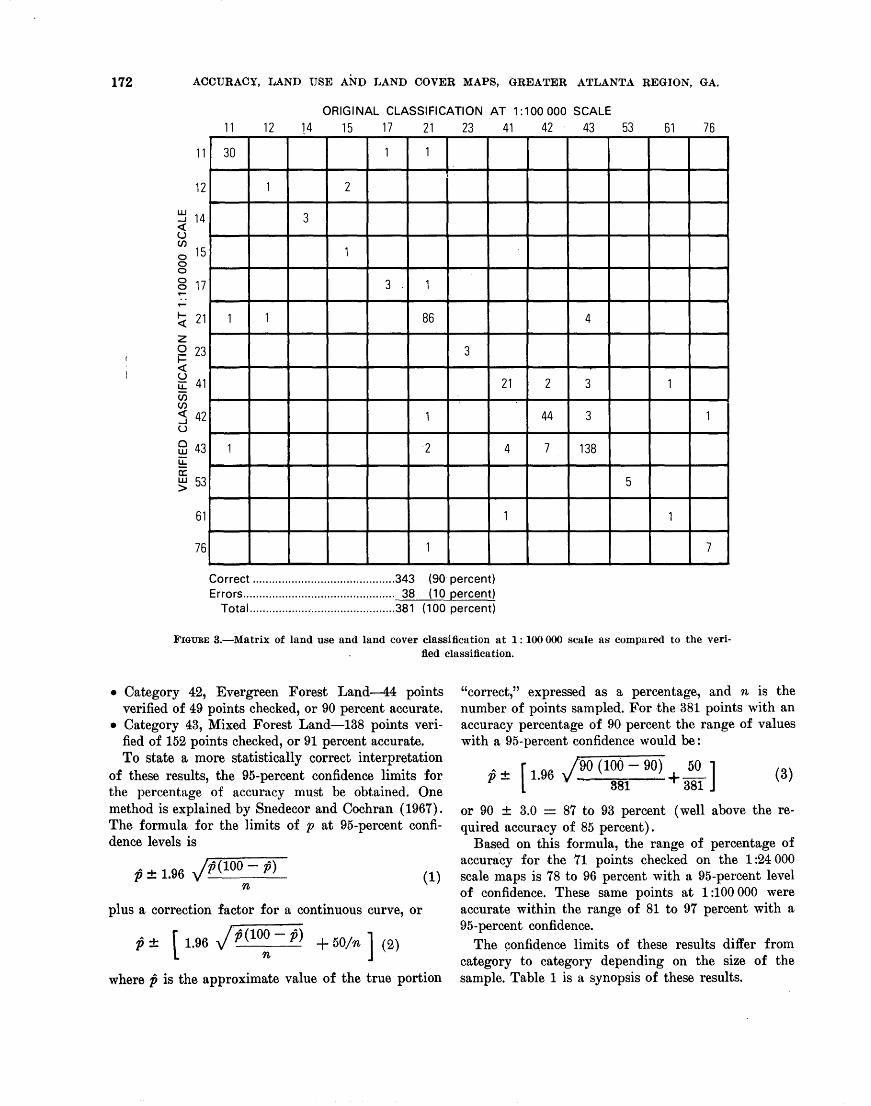
The method of determining the accuracy was pri marily empirical, in that the percentage of accuracy is a simple ratio of correct interpretation to the total number of points sampled. The number of correct interpretations at the 1:100000 scale was 343 (90 percent) of 381 points sampled. (See the matrix in fig. 3.)
Of the 71 points sampled on the eighteen 7.5-min. sheets at 1:24000 scale (one point was a duplicate), 62 points or 87 percent were "correct." The 71 points sampled on the 1:24 000-scale maps were primarily in the urban areas. Of the same 71 points interpreted at 1:100000, 63 points or 89 percent were "correct," indicating that the interpretation at both scales was the same.
These results, obtained by a stratified systematic unalined selection of 381 points, were chosen to repre sent the complete map at a scale of 1:100000. They do not, however, include more than 13 land use and land cover categories from a map containing as many as 20 land use and land cover categories. Of the 13 categories included, only 5 had more than 10 occur rences in the point selection.
Accuracy of individual categories
Each of the points sampled is not within a unique polygon. Certain polygons, considered "background" polygons, encompass a major portion of the map and may contain several of these selected points. For this reason the categories of the most extensive land use or land cover receive the heaviest concentration in the analysis. One disadvantage, however, is that many of the small polygons of "intensive use" categories, often those affecting planning decisions, are overlooked.
This test of the accuracy of the maps has provided reliable data for only five categories, although we hope that all categories are interpreted at the same level of accuracy. The results for these five categories are as follows:
Category 11, Residential Land 30 points verified of 32 points checked, or 94 percent accurate.
Category 21, Cropland and Pasture 86 points veri fied of 92 points checked, or 93 percent accurate.
Category 41, Deciduous Forest Land 21 points verified of 27 points checked, or 78 percent accurate.
172 ACCURACY, LAND USE AND LAND COVER MAPS, GREATER ATLANTA REGION, GA.
61 7611 12ORIGINAL CLASSIFICATION AT 1:100000 SCALE
14 15 17 21 23 41 42 43 53
11
12
LU , . i 14 < oCOo 15 o o0 ,-, O 1 /
t- 91 < Zl
Z 0 23
< o ., LI 41CO CO< 42 o
g 43LL.
CC.g 53
61
76
30
1
1
1
1
3
2
1
1
3 .
1
1
86
1
2
1
3
21
4
1
2
44
7
4
3
3
138
5
1
1
1
7
Correct ............................................343 (90 percent)Errors............................................... 38 (10 percent)
Total.............................................381 (100 percent)
FIGURE 3. Matrix of land use and land cover classification at 1:100 000 scale as compared to the veri fied classification.
Category 42, Evergreen Forest Land 44 points verified of 49 points checked, or 90 percent accurate.
Category 43, Mixed Forest Land 138 points veri fied of 152 points checked, or 91 percent accurate. To state a more statistically correct interpretation
of these results, the 95-percent confidence limits for the percentage of accuracy must be obtained. One method is explained by Snedecor and Cochran (1967). The formula for the limits of p at 95-percent confi dence levels is
p±l.i- p)
n (1)
plus a correction factor for a continuous curve, or
p ± 1.96 + 60/n ] (2)
where p is the approximate value of the true portion
"correct," expressed as a percentage, and n is the number of points sampled. For the 381 points with an accuracy percentage of 90 percent the range of values with a 95-percent confidence would be :
381 381
or 90 ± 3.0 = 87 to 93 percent (well above the re quired accuracy of 85 percent).
Based on this formula, the range of percentage of accuracy for the 71 points checked on the 1:24000 scale maps is 78 to 96 percent with a 95-percent level of confidence. These same points at 1:100000 were accurate within the range of 81 to 97 percent with a 95-percent confidence.
The confidence limits of these results differ from category to category depending on the size of the sample. Table 1 is a synopsis of these results.
FITZPATRICK-LINS 173TABLE 1. Accuracy percentages at the 95-percent confidence
interval for five major categoriesCONCLUSION
Land use and Pointsland cover categories checked
Residential (11) 32Cropland and
Pasture (21) _ 92Deciduous Forest
Land (41) .. 27Evergreen Forest
Land (42) _ 49Mixed Forest
Land (43) __ - 152
Pointsverified
30
86
21
44
138
Accuracypercentage
94
93
78
90
91
95-percentconfidence
limits »
"94-100
87- 99
61- 95
81- 99
86- 96
n Formula from Snedecor and Cochran (1967) :(100 0) / n + 50/n ]
b Calculates to 104 percent by the equation.
In the case of category 11, the 95-percent confidence limits based on formula 2 are 84 to 100 percent. The 95-percent confidence limits for the accuracy of cate gory 21 is 87 to 99 percent. The accuracy of category 42 has 95-percent confidence limits of 81 to 99 per cent. The accuracy of category 43 is between 86 and 96 percent with a 95-percent confidence.
From these results it appears that the accuracies of four of these categories are similar and approach or exceed the criterion of 85-percent accuracy. Category 41 is less accurate, yet the range in accuracy is so great that it would be necessary to test several more points for more precise results. For 78-percent accur acy with a standard error of 5 percent, and therefore an estimate of the true proportion at the 95-percent probability level to within ± 10 percent, at least 69 points should be checked. This required sample size is determined from the formula n=(p-q)/d2 given in "Procedure" section (Gregory 1963, p. 98-99). For a smaller standard error, a much greater sample size would be required.
The overall accuracy of the land use and land cover maps of the Greater Atlanta Region is between 87 and 93 percent with a 95-percent level of confidence, if we assume a binomial distribution. This level of ac curacy is based primarily on categories of Residential Land, Cropland and Pasture, Evergreen Forest Land, Deciduous Forest Land, and Mixed Forest Land which constitute the major portion of the map.
Category 41, Deciduous Forest Land, was mapped with the least accuracy. The 27 points of Deciduous Forest Land checked are insufficient to give a reliable measure of the true accuracy of category 41 at the 95- percent probability level.
The accuracy of the 71 points sampled on the eighteen 1:24 000-scale Level II land use and land cover maps was between 78 and 96 percent with a 95- percent confidence, as compared to an accuracy of 81 to 97 percent at the 1:100 000 scale.
According to the results, the overall accuracy of the land use and land cover maps exceeds the criteria of 85-percent accuracy at the scale of 1:100 000, and the mapping results seem to be consistent from one scale to the next.
REFERENCES CITED
Anderson, J. R., Hardy, E. B., Roach, J. T., and Witmer, R. E.,1976, A land use and land cover classification system foruse with remote sensor data: U.S. Geol. Survey Prof.Paper 964, 28 p.
Berry, B. J. L., 1962, Sampling, coding, and storing flood plaindata: U.S. Dept. Agriculture Handb. 237, 27 p.
Gregory, S., 1963, Statistical methods and the geographer[2d ed.] : Atlantic Highlands, N.J., Humanities Press,p. 82-100.
Snedecor, G. W., and Cochran, W. F., 1967, Statistical methods:Ames, Iowa State Univ. Press, p. 202-211.

Jour. Research U.S. Geol. Survey Vol. 6, No. 2, Mar.-Apr. 1978, p. 175-192
BLUE RIBBON LINEAMENT, AN EAST-TRENDING STRUCTURAL ZONE WITHIN THE PIOCHE MINERAL BELT OF SOUTHWESTERN UTAH AND
EASTERN NEVADA
By PETER D. ROWLEY; PETER W. LIPMAN; HARALD H. MEHNERT,
DAVID A. LINDSEY; and JOHN J. ANDERSON, 1 Denver, Colo.;
Hawaii Volcano Observatory, Hawaii; Denver, Colo.; Kent, Ohio
Abstract. The Blue Ribbon lineament is an east-west struc tural zone that is about 25 kilometers wide and passes through the Pioche mineral belt at about 38°10' N. It is best known in Utah, where it is at least 190 km long, and extends from the southern Sevier Plateau in the High Plateaus westward and across southern Mountain Home (Needle) Range in the Great Basin. It probably continues westward an additional 170 km into Nevada, where it connects with the eastern end of the 230-km Warm Springs lineament. The Blue Ribbon lineament is defined by range terminations and east-trending valleys, alinement of eruptive centers of middle Miocene (20 million years) to Pliocene(?) (5-1.8 m.y.) alkalic rhyolite, alinement of areas of middle Miocene to Pliocene mineralized rocks (mostly fluorine, uranium, tungsten) and hydrothermally altered rocks, east-trending magnetic highs and interruptions of magnetic anomalies, and east-striking basin-range faults of late Tertiary and Quaternary age. Mountains south of the lineament are topographically and structurally lower than those to the north. North-striking Quaternary basin-range faults, the Thermo hot springs area, several warm springs and former hot springs, and numerous dacitic to andesitic volcanic centers of early to middle Miocene age (26-20 m.y.) occur along the lineament. The Blue Ribbon lineament is believed to be a deep crustal fault zone dating from at least middle Miocene time and possibly much earlier. It thus developed generally coincident with northerly trending classical basin-range faults. Its fracture system was an important, long-lived conduit for mineralizing fluids, and it should be an attractive target for minerals exploration in the future. The lineament could be due to an east-trending warp in the subducting mantle plate, or it could be part of a past or present intracontinental trans form fault that locally gets younger eastward and dies out eastward in the western Colorado Plateaus province.
This report is an outgrowth of various studies on the geology of southwestern Utah. One of these studies was a detailed geologic mapping of the southwestern part of the High Plateaus subprovince of the Colorado Plateaus and mapping of the nearby Black Mountains of the eastern Great Basin (Anderson and Rowley, 1975). Other studies were conducted farther west in
1 Kent State University.
the Great Basin and consisted of an investigation of the Staats (Monarch) mine-Blawn Mountain area in the southern Wah Wah Mountains by D. A. Lindsey (unpub. data, 1976) and reconnaissance geochemical studies in the southern parts of the Wah Wah Moun tains and Mountain Home Kange (formerly called Needle Range) by D. R. Shawe and D. A. Lindsey (unpub. data, 1976). During these studies it became apparent that Tertiary volcanic centers, Tertiary min eralized and hydrothermally altered rock, geophysical anomalies, topographic features, and Tertiary and Quaternary basin-range faults defined an east-trending structural belt that passed through all the previously studied areas.
In 1975 an opportunity arose to investigate the hot springs and associated rhyolite centers along this east- trending structural feature, as well as those hot springs and rhyolites north of the feature, as part of a pro gram of reconnaissance and detailed mapping of young rhyolite centers around the rim of the Colorado Plateaus province for their geothermal potential (for example, Lipman and others, 1975; 1978; Rowley and Lipman, 1975). A major phase of this program was the determination of K-Ar ages of alkalic rhyolite (Mehnert and others, 1977). These ages indicated that the rhyolite centers were 20 million years old and younger, generally coincident with the broad episode of basin-range faulting in this part of Utah. The youngest K-Ar age of four rhyolites was from a dome at Blue Ribbon Summit, which gives its name to the structural feature described here.
This report describes the nature of the Blue Ribbon lineament, a through-going structural feature at about 38° 10' N., that crosses the Wasatch Front and the dom inant trend of basin-range faults nearly at right angles. The Blue Ribbon lineament is about 25 kilometers wide
175
176 BLUE RIBBON LINEAMENT, SOUTHWESTERN UTAH AND EASTERN NEVADA
and extends about 190 km through the Great Basin and Colorado Pleateaus .of southwestern Utah and probably an additional 170 km westward through east ern Nevada. The lineament appears to be collinear at about 116° W., in Nevada, with the 230-km east-trend ing Warm Springs lineament (Ekren and others, 1976) of similar characteristics, which extends to the western edge of the Great Basin. In Utah, where de tailed data are available and where we are most fanii- lar with the geology, the lineament is traced from southwest of Indian Peak in the Mountain Home Range near the Nevada border east to the Antimony mining district, which is east of the southern Sevier Plateau (fig. L4). The southern edge of the lineament is several kilometers south of the latitude of Antimony, and the northern edge is near the latitude of Beaver.
The Blue Ribbon lineament as here defined lies within the southern half of the broad Wah Wah- Tushar mineral belt (fig. 2) of Hilpert and Roberts (1964) and just north of the Pioche mineral belt of Roberts (1964). It crosses the axis of the "Pioche min eral belt" as redefined by Shawe and Stewart (1976) but, because of the overall coincidence with the Pioche mineral belt in Utah, the Blue Ribbon lineament is here considered to be a distinctive zone within the broader feature as defined by Shawe and Stewart (1976).
Acknowledgments. Recognition and analysis of the Blue Ribbon lineament is due partly to discussions with T. A. Steven, G. P. Eaton, D. R. Shawe, and E. B. Ekren. We are grateful to E. B. Ekren, J. H. Stewart, and D. R. Shawe for making available much unpub lished data on east-trending features in the Great Basin. R. K. Glanzman, G. L. Galyardt, and P. L. Wil liams provided information on some areas in the Great Basin with which they are familiar. J. S. Pallister as sisted with collecting specimens for K-Ar study and made most mineral separations.
PREVIOUSLY DESCRIBED EAST-TRENDING BELTS IN GREAT BASIN
East-trending belts of mineral occurrences, geophys ical anomalies, structural features, and patterns of Cenozoic igneous rocks in the Great Basin have been observed and described by many geologists, starting with Butler and others (1920). Various geologists and geophysicists have placed belt axes differently, as de scribed in the following paragraphs and shown on figure 2; none of these axes are mutually exclusive because the authors used different scales and different criteria for plotting them. Most of the lineaments probably reflect in one way or another the effects of deep east-trending fault systems in the Great Basin,
apparently of an age coincident with classical basin- range structure but perhaps controlled by features that are partly older than basin-range structure.
Hilpert and Roberts (1964) summarized previous work and described three broad belts of intrusive rocks and metal mining districts in western Utah (fig. 2), from north to south the Oquirrh-Uinta, Deep Creek- Tintic, and Wah Wah-Tushar belts. The mining dis tricts on the belts account for 95 percent of Utah's copper, lead, silver, gold, and zinc. Erickson (1974) discussed the northernmost belt, which he renamed the Uinta-Gold Hill trend and which he extended farther eastward. The southern two belts continue into Nevada as the Cherry Creek belt and the Pioche belt (Roberts, 1964); Roberts (1966) later described the broad curving Cortez-Uinta axis, which connects with the Oquirrh-Uinta belt, and the Hamilton-Ely belt at about 39°10' N. Callaghan (1973) also called attention to east-trending mineral belts. Zietz and others (1969) noted east-trending aeromagnetic patterns in the Oquirrh-Uinta, Deep Creek-Tintic, and Cortez-Uinta belts. Cook and his coworkers (for example, Cook and Montgomery, 1974) postulated three broad east-trend ing zones in Utah defined by gravity data. The axes of these zones are at 40°40' N., 40° N., and 38°40' N., within the mineral belts of Hilpert and Roberts (1964).
Shawe and Stewart (1976) discussed the three ma jor Utah mineral belts as well as Nevada mineral belts. Their Pioche mineral belt, which extends east-north eastward from Nevada into Utah, contains the Wah Wah-Tushar belt of Hilpert and Roberts (1964) and the Pioche belt of Roberts (1964). The axes of their belts generally are defined by alined Cretaceous and Tertiary plutons, zones of faults that are transverse to the northerly basin-range faults, gross aeromagnetic patterns, and major mineral occurrences. To the three major belts they added another, smaller belt south of the Pioche belt, which they called the Delamar-Iron Springs mineral belt (fig. 2). Stewart, Moore, and Zeitz (1977) discussed the belts in terms of distribution of igneous rocks; they observed that broad east-trend ing zones of volcanic rocks in Nevada and western Utah decrease in age from north to south. The axes of their volcanic belts correspond to the axes of the belts of Shawe and Stewart (1976).
Eaton (1975, 1976; unpub. data, 1976) described a major east-trending cfustal boundary that crosses Nevada at about 37° N. (fig. 2), thence gently swings northeasterly into southern Utah, coincident with the Intermountain Seismic Belt. This zone, which is de fined largely by gravity and magnetic data, seismicity, and depth to the M-discontinuity, marks the southern
38° 30' -
38° 15' -
ROWLEY AND OTHERS
113° 00'
38° 00'
112° 00'
CONTOUR INTERVAL X 1000
BFIGURE 1. Index maps showing topographic and aeromagnetic
expression of most of the Utah part of the Blue Ribbon lineament. A, Raised relief map showing location of geo graphic and geologic features near the Blue Ribbon linea ment as well as location of areas of figures 3 and 4. Ap proximate boundaries of Blue Ribbon lineament shown by dashed hachured lines. Wasatch Front shown by dashed line. Occurrence of alkalic rhyolite, stippled. B. Aeromagnetic
map, from Zeitz, Shuey, and Kirby (1976). Blue Ribbon lineament shown by lined ruling. Outlines of aeromagnetic ridge of Pioche mineral belt, modified from Stewart, Moore, and Zeitz (1977, fig. 5), is shown by heavy solid line. Con tour intervals are 20 and 100 gammas. I. Indian Park; S, Staats (Monarch) mine; F, Frisco; T. Thermo hot springs; M, Milford ; Mi, Minersville; B. Beaver; Co, Cove Fort; C. Circleville; Ma, Marysvale; and A. Antimony.
178 BLUE RIBBON LINEAMENT, SOUTHWESTERN UTAH AND EASTERN NEVADA
116°
41
80 120 160 KILOMETERSi i i
Boundary of aeromagnetic ridge of Pioche mineral belt, from Stewart and others (1977)
Axis of east-trending mineral belts of Shawe and Stewart (1976)
OU, DT, PI, Dl-Oquirrh-Uinta; Deep Creek-Tintic; Pioche; Delmar-lron Springs
Axis of eastern parts of lineaments of Ekren and others (1976) WS, Tl-Warm Springs; Timpahute
Axis of southern part of Intermountain Seismic Belt andapproximate transverse crystal boundary of Eaton (1975)
H Mineral belts of Hilpert and Roberts (1964) and Roberts (1966)
Axes of east-trending mineral belts of Roberts (1964, 1966)
FIGURE 2. Index map of eastern Nevada and western Utah showing location of the Blue Ribbon lineament and other east-trending structural, mineral, and geophysical belts de scribed in the published literature. S (Salt Lake City),Pr (Prove), N (Nephi), F (Fillmore) ; Co (Cove Fort); B (Beaver), C (Cedar City), and H (Hurricane) mark the
extreme eastern edge (Wasatch Front) of the Great Basin. T (Tempiute) ; P (Pioche) ; St (Stateline mining district), SF, (San Francisco mining district), M (Milford), and Ma (Marysvale) occur at sites of major mining activity in the east-trending Pioche mineral belt of Shawe and Stewart (1976).
BOWLEY AND OTHERS 179
edge of volcanic rocks and mining districts in the Great Basin. In Utah, this belt coincides with faults of the same strike and with strings of plutons and volcanic centers (Cook, 1960, maps 1-21; Blank and Mackin, 1967, pi. 1).
Ekren and others (1976) documented four linea ments between lat 37°40' and 39° N. in south-central Nevada, each of which ranges in length from 200 to 300 km (fig. 2). Their evidence consists mostly of topo graphic discontinuities and disruptions, terminations and alinements of aeromagnetic anomalies, alinements of plutons and volcanic centers, and other structural features. Their northern lineament may connect with a similar lineament in west-central Nevada described by Bingler (1971). The southern two lineaments of Ekren and others (1976) were called the Warm Springs linea ment and Timpahute lineament. The Warm Springs lineament probably connects with the Blue Ribbon lineament, and the Timpahute lineament extends into Utah as the northern edge of the 'Clover Mountains and Bull Valley Mountains and into the Iron Springs mining district, which owurs at the intersection be tween the Timpahute lineament and Baton's crustal boundary (1975, 1976; unpub. data, 1976).
PIOCHE MINERAL BELT
The Pioche mineral belt, as defined by Shawe and Stewart (1976), is a broad zone more than 50 km wide that extends more than 300 km from the Tempiute mining district in Nevada east through the Marysvale volcanic pile in Utah (fig, 2). As Shawe and Stewart noted, considerable commodities have been produced along the belt, such as gold, silver, lead, zinc, tungsten, uranium, fluorine, manganese, copper, and alujiite. Some mining districts in the belt are shown on figure 2. Those along the Blue Ribbon lineament are described in the following discussion.
In addition to the features enumerated by Shawe and Stewart (1976), other characteristics of the min eral belt are noteworthy. The easterly to east-north easterly trends of occurrences of fluorine, tungsten, gold, copper, molybdenum, lead-zinc-silver, manganese, uranium, and barium minerals are apparent from pub lished compilations (for example, Walker and Oster- wald, 1963; U.S. Geological Survey, Utah Geological and Mineralogical'Survey, 1964; U.S. Geological Sur vey, Nevada Bureau of Mines, 1964); occurrences of iron, beryllium, alunite, sulfur, and other minerals have a less well defined but nontheless general east- trending distribution. Many mineral occurrences, no tably those of fluorine, beryllium, uranium, tungsten, and sulfur, are young and commonly occur near centers
of alkalic rhyolites that range in age from middle Mio cene (20 m.y.) to Pleistocene. At Marysvale, for ex ample, uranium deposits (Kerr and others, 1957; Kerr, 1968) were dated at about 13 m.y. by Bassett and others (1963). Steven and others (1977) concluded that much alunite, uranium, fluorine, and molybdenite at Marysvale are 16-9 m.y. old, but that other deposits of alunite and base and precious metals are early to mid dle Miocene in age. Most other mineral deposits of the Piocihe mineral belt are of middle to late Tertiary age, and some, as at Tempiute and Pioche (Krueger and Schilling, 1971; Johnston, 1972), may be totally Cre taceous in age. In the Pioche mineral belt, many hot spring areas occur, including known geothermal re source areas (KGRA's) that may provide geothermal energy in future years such as the Roosevelt area just west of the Mineral Mountains and the Cove Fort- Sulfurdale area just northeast of the Mineral Moun tains. Clearly the overall Pioche mineral belt has been in existence at least from middle Tertiary to Holocene time and perhaps even longer.
The Pioche mineral belt of Shawe and Stewart (1976) includes the topographically highest mountains in southern Utah and is also structurally high. East- striking faults occur in the mineral belt. Callaghan and Parker (1962), Kennedy (1963), and Oallaghan (1973) noted that the Tushar Mountains probably oc cupy part of an east-trending arch that is bounded on its northern side (in the major east-trending valley of Clear Creek near the northern edge of the mineral belt) by a parallel downwarp. The arch occurs in the same area where an east-trending highland of probable Late Cretaceous or early Tertiary age extended both east and west of the Tushar Mountains (Butler and others, 1920; Callaghan, 1973; Anderson and Rowley,1975). Because of the highland, lacustrine and fluvial rocks of early Tertiary age in the northern High Pla teaus are different in lithology from lacustrine and fluvial rocks of the same age in the southern High Plateaus, and sedimentary rocks of early Tertiary age in the Tushar Mountains are absent or are thin and of different character from beds of the same age to the north and south.
As noted :by Shawe and Stewart (1976, fig. 2), the Pioche mineral belt is characterized by plutons and volcanic rocks mostly of Cenozoic age. One of these is the granitic batholith of the Mineral Mountains (Liese, 1957; Earll, 1957), which is in the first range west of the Wasatch Front (fig. 1), and is the largest pluton in Utah; published K-Ar ages of 15-9 m.y. (Park, 1968; Armstrong, 1970) have received some confirma tion from Rb-Sr dating (C. E. Hedge, unpub. data,1976). Lava and tuff fields of alkalic rhyolite are
180 BLUE RIBBON LINEAMENT, SOUTHWESTERN UTAH AND EASTERN NEVADA
abundant in the Pioche mineral belt. The largest such field is the Mount Belknap Rhyolite, about 21-17 m.y. old (Bassett and others, 1963; Cunningham and Steven, 1977; Steven and others, 1977), and the related Joe Lott Tuff (Callaghan, 1939) in the Tushar Moun tains. Alkalic rhyolite is exposed at several places south of the San Francisco Mountains (P.L. Williams, oral commun., 1976). Alkalic rhyolite of Pleistocene age overlies the Mineral Mountains batholith (Liese, 1957; Earll, 1957; Lipman and others, 1975, 1978). A large province of Quaternary basalt and minor rhyolite oc curs north of the Mineral Mountains on the northern side of the Pioche mineral belt (Mehnert and others, 1977). Upper Cenozoic alkalic rhyolites are extensive in the southern parts of the Mountain Home Range and the Wah Wah Mountains (D. A. Lindsey and D. R. Shawe, oral commun., 1975).
The mineralized and hydrothermally altered rocks in the Pioche mineral belt are closely outlined by a broad aeromagnetic ridge (fig. 2; Stewart and others, 1977, fig. 5). The overall magnetic high (fig. IB) con tains numerous high-amplitude (that is, shallow crustal) hills and depressions (Zietz and others, 1976) that mostly reflect the presence of plutons (Hilpert and Roberts, 1964) and volcanic centers (Stewart and others, 1977). In contrast, the areas north and south of the ridge are magnetically low and contain few superimposed magnetic hills and depressions. The aero- magnetic ridge extends from about 115° W. east to about 111° 45' W.; the west end is terminated by a broad north-trending "quiet" aeromagnetic belt that bisects the Great Basin (Eaton, 1976; Stewart and others, 1977; G. P. Eaton, unpub. data, 1976). In de tail (fig. IB), the aeromagnetic ridge consists of both east- and east-northeast-trending components. One ef fect of the two trends within the magnetic1 ridge is that the western half of the ridge is forked, containing a branch that continues west and a branch extending from about 113°30' W. south-southwest to the western end of the Delamar-Iron Springs mineral belt.
The Pioche mineral belt has striking similarities to the Deep Creek-Tintic mineral 'belt. For example, the Deep Creek-Tintic mineral belt contains major occur rences of beryllium, fluorine, lead-zinc-silver, copper, manganese, gold, uranium, tungsten, and other min erals. Most of these mineral occurrences clearly show a general east-trending distribution (U.S. Geological Survey, Utah Geological and Mineral Survey, 1964; U.S. Geological Survey, Nevada Bureau of Mines, 1964; 'Cohenour, 1963; Park, 1968; Lindsey and others, 1973,1975; Van Alstine, 1976) or a northeast-trending distribution (Shawe, 1966). The Deep Creek-Tintic belt contains numerous centers of young (10-3 m.y.)
alkalic rhyolite (Lindsey and others, 1975; Armstrong, 1970; Mehnert and others, 1977), numerous plutons (Hilpert and Roberts, 1964), and numerous east-strik ing faults (Stokes, 1963; Loring, 1972). It is axial to a broad zone of Cenozoic volcanic rocks and is the site of a broad east-trending magnetic ridge, with superim posed highs and lows, that extends into Nevada (Zietz and others, 1969; Zietz, Shuey, and Kirby, 1976; Stewart and others, 1977). The 'Crater Springs hot springs area occurs along its southern edge. Like the Pioche belt, the eastern end of the Deep Creek-Tintic belt contains a base 'metal and precious metal mining district (Tintic) near the Wasatch Front, while just west of this district the young, 17- to 16-m.y.-old (Armstrong, 1970; Cohenour, 1970; D. A. Lindsey, unpub. data, 1976) granite of Sheeprock Mountains is exposed in a configuration similar to that of the Marys- vale mining district and Mineral Mountains batholith of the Pioche belt.
BLUE RIBBON LINEAMENT IN UTAH
The Blue Ribbon lineament in Utah occupies an east- trending zone, about 25 km wide and 190 km long (fig. 1A), that is defined by magnetic highs and interrup tions of magnetic anomalies, alinement of Tertiary centers of alkalic rhyolite and dacitic to andesitic rocks, range terminations and valleys, Tertiary and Quater nary basin-range faults, and Tertiary mineralized (mostly fluorine, uranium, and tungsten) and hydro thermally altered rock. Several 'hot springs also occur along the lineament, and their presence suggests that hot water circulation along the lineament, which in Tertiary time produced altered rock and carried min erals, is remarkably long lived.
The lineament concentrates many diverse features, but not exclusively so with respect to those in other parts of the Pioche mineral belt; the lineament is only one of several controls of such features within the broad mineral belt. Another such feature is a second, less clearly defined east-west lineament that occurs along the northern edge of the Pioche belt, mostly be tween the latitudes of Cove Fort and Marysvale (cen tered on 38°30' N.) and extending from at least 30 km west of Frisco to at least Marysvale. Parts of this fea ture were recognized by G. L. Galyardt (oral commun., 1976), who observed east-trending geophysical patterns in the Cove Fort-Sulfurdale area, and T. A. Steven (oral commun., 1977) who observed east-trending aline- ments of published mineral occurrences (U.S. Geologi cal Survey, Utah Geological and Mineralogical Survey, 1964). The lineament also is defined by folds and faults (especially in the Clear Creek area west of Cove Fort),
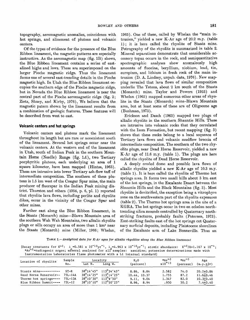
ROWLBY AND OTHERS 181
topography, aeromagiietic anomalies, coincidence with hot springs, and alinement of plutons and volcanic centers.
Of the types of evidence for the presence of the Blue Ribbon lineament, the magnetic patterns are especially instructive. As the aeromagnetic map (fig. IB) shows, the Blue Ribbon lineament contains a series of east- alined highs and lows. These are superimposed on the larger Pioche magnetic ridge. Thus the lineament forms one of several east-trending details in the Pioche magnetic high. In Utah the Blue Ribbon lineament oc cupies the southern edge of the Pioche magnetic ridge, but in Nevada the Blue Ribbon lineament is near the central part of the Pioche aeromagnetic ridge (fig. 2; Zietz, Shuey, and Kirby, 19Y6), We believe that the magnetic patern shown by the lineament results from a combination of geologic features. These features will be described from west to east.
Volcanic centers and hot springs
Volcanic centers and plutons mark the lineament throughout its length but are rare or nonexistent south of the lineament. Several hot springs occur near the volcanic centers. At the western end of the lineament in Utah, south of Indian Peak in the southern Moun tain Home (Needle) Range (fig. L4), two Tertiary porphyritic plutons, each underlying an area of 1 square kilometer, have been mapped (Hintze, 1963). These are intrusive into lower Tertiary ash-flow tuff of intermediate composition. The southern of these plu tons is 1.5 km west of the Cougar Spar mine, the main producer of fluorspar in the Indian Peak mining dis trict. Thurston and others (1954, p. 6, pi. 1) reported that rhyolite lava flows, including perlite and rhyolite dikes, occur in the vicinity of the Cougar Spar and other mines.
Farther east along the Blue Ribbon lineament, in the Staats (Monarch) mine Blawn Mountain area of the southern Wah Wah Mountains, two alkalic rhyolite plugs or sills occupy an area of more than 1 km2 near the Staats (Monarch) mine (Miller, 1966; Whelan,
1965). One of these, called by Whelan the "main in trusion," yielded a new K-Ar age of 20.2 m.y. (table 1); it is here called the rhyolite of Staats mine. Petrography of the rhyolite is summarized in table 2. Mineral separations demonstrate that considerable ac cessory topaz occurs in the rock, and semiquantitative spectrographic analyses show anomalously high amounts of fluorine, beryllium, niobium, lead, tin, europium, and lithium in fresh rock of the main in trusion (D. A. Lindsey, unpub. data, 1976). New map ping revealed that lava flows of similar composition underlie The Tetons, about '2 km south of the Staats (Monarch) mine. Taylor and Powers (1953) and Whelan (1965) mapped numerous other areas of rhyo lite in the Staats (Monarch) mine-Blawn Mountain area, but at least some of these are of Oligocene age (Bushman, 1973).
Erickson and Dasch (1963) mapped two plugs of alkalic rhyolite in the southern Shauntie Hills. These are intrusive into volcanic rocks that they correlated with the Isom Formation, but recent mapping (fig. 3) shows that these rocks belong to a local sequence of Tertiary lava flows and volcanic mudflow breccia of intermediate 'composition. The southern of the two rhy olite plugs, near Dead Horse Reservoir, yielded a new K-Ar age of 11.6 m.y. (table 1). The plugs are here called the rhyolite of Dead Horse Resorvoir.
A deeply eroded dome and possible lava flows of alkalic rhyolite yielded a new K-Ar age of 10.3 m.y. (table 1). It is here called the rhyolite of Thermo hot springs area. It forms two small hills about 3 km east of the hot springs, in the Escalante Desert between the Shauntie Hills and the Black Mountains (fig. 3). Most rhyolite is devitrified, the exception being a vitrophyre zone on the southwestern part of the rhyolite exposures (table 2). The Thermo hot springs area is the site of a KGRA. The hot springs occur in two en echelon north- trending silica mounds controlled by Quaternary north- striking fractures, probably faults (Petersen, 1973). East-striking faults east of the hot springs cut Quater nary surficial deposits, including Pleistocene shorelines of the Escalante arm of Lake Bonneville. Thus an
TABLE 1. Analytical data for K-Ar ages for alkalic rhyolites along the Blue Ribbon lineament
X =0.581 x lO^Oyr' 1 , X =4.963[Decay constants for K40 : X £ =0.581 x ICT^yr" 1 , X =4.963 x 10"^yr" 1 ; atomic abundance: K 40 /K=1.167 x lO *Ar40 =radiogenic argon; mineral analyzed for all samples: sanidine; potassium determinations made with Instrumentation Laboratories flame photometer with a Li internal standard]
Staats mineDead HorseThermo hotBlue Ribbon
Reservoir springs Summit
SampleNo.
ST-R75L-14A75L-13A75L-12
LocalityLat N
38°14'38°14'38°10'38°10'
45"25"30".10"
Long W.
113°34'45"113°14'25"113°9'50"112°50'25"
K2 0(percent)
8.86,10.44,9.11,8.96,
8.8410.379.048.94
*Ar" 0x!0~ 10
2.5821.7551.347.950
*Ar"°
(percent) (m.
74.087.282.050.2
20.11.10.7.
Agey.+20)
2+0.866-1-0.46
3+0.404+0.40
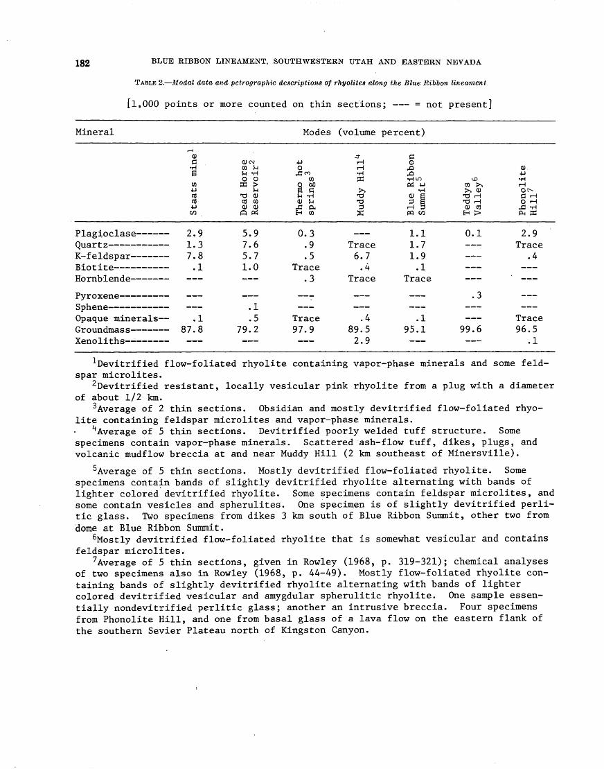
182 BLUE RIBBON LINEAMENT, SOUTHWESTERN UTAH AND EASTERN NEVADA
TABLE 2. Modal data and petrographic descriptions of rhyolites along the Blue Ribbon lineament
[l,000 points or more counted on thin sections; = not present]
Mineral Modes (volume percent)
t J_d£2-LUl~ J_dO C
K-feldspar Biotite Hornblende
Sphene Opaque minerals
Xenoliths -
r-H
CUc HeCO4_lCOCO4-1C/l
2.91.37.8.1
.1ft7 QO / . O
0)C\ICOMO
S3T3
CO0)Q
5751
79
M HO>MCUCO0)&
.9
.6
.7
.0
.1
.5
.2
4-JO
4300CO
0 60P Cft «HCU M
43 frH CO
0.3.9.5
TVoppX J. d^C>
.3
Trace97.9
rHrH Hpr]
^>'O"Dj3S
Trace6.7
.4TvarpX I. dl~C
.489.52.9
c04343 Hio
PCS -P H§ i_3 SrH PPQ en
1.1
1.71.9
.1TTappX L O.L.C
.1
95.1
IDCO >>>, cu
*X3 rH'O rH
CU COH >
0.1
.3
QQ AJ J . U
CU.4-1 HrHOr-Ci rH0 rH.
42 iHPH 33
2.9Trace
.4
___
Trace96.5
.1
Devitrified flow-foliated rhyolite containing vapor-phase minerals and some feld spar microlites.
2Devitrified resistant, locally vesicular pink rhyolite from a plug with a diameter of about 1/2 km.
3Average of 2 thin sections. Obsidian and mostly devitrified flow-foliated rhyo lite containing feldspar microlites and vapor-phase minerals.
4Average of 5 thin sections. Devitrified poorly welded tuff structure. Some specimens contain vapor-phase minerals. Scattered ash-flow tuff, dikes, plugs, and volcanic mudflow breccia at and near Muddy Hill (2 km southeast of Minersville).
5Average of 5 thin sections. Mostly devitrified flow-foliated rhyolite. Some specimens contain bands of slightly devitrified rhyolite alternating with bands of lighter colored devitrified rhyolite. Some specimens contain feldspar microlites, and some contain vesicles and spherulites. One specimen is of slightly devitrified perli- tic glass. Two specimens from dikes 3 km south of Blue Ribbon Summit, other two from dome at Blue Ribbon Summit.
6Mostly devitrified flow-foliated rhyolite that is somewhat vesicular and contains feldspar microlites.
7Average of 5 thin sections, given in Rowley (1968, p. 319-321); chemical analyses of two specimens also in Rowley (1968, p. 44-49). Mostly flow-foliated rhyolite con taining bands of slightly devitrified rhyolite alternating with bands of lighter colored devitrified vesicular and amygdular spherulitic rhyolite. One sample essen tially nondevitrified perlitic glass; another an intrusive breccia. Four specimens from Phonolite Hill, and one from basal glass of a lava flow on the eastern flank of the southern Sevier Plateau north of Kingston Canyon.
ROWLEY AND OTHERS 183
EXPLANATION CORRELATION OF MAP UNITS
Holocene
Of Ol
UNCONFORMITY
J Miocene and
Oligocene(?)
Pleistocene
Pleistocene or Pliocene
Miocene
Miocene and Oligocene
QUATERNARY
QUATERNARY OR TERTIARY
TERTIARY
DESCRIPTION OF MAP UNITS
Travertine hot spring deposits (Holocene)
Alluvium, fan deposits, pediment deposits (Holocene and Pleistocene)
Lake Bonneville sediments (Pleistocene)--Lake deposits and alluvium in Escalante arm of Lake Bonneville
Basaltic lava flows (Pleistocene or Pliocene)
Rhyolite of Dead Horse Reservoir (Miocene)
Rhyolite of Thermo hot springs (Miocene)
Horse Valley Formation (Miocene)--Lava flows, plugs, and volcanic mudflow breccia of rhyodacitic composition. About 22-19 m. y. old
Mount Dutton Formation (Miocene and Oligocene)--Volcanic mudflow breccia
Volcanics of Shauntie Hills (Miocene and Oligocene ?)--Volcanic mudflow breccia and lava flows of intermediate composition
CONTACT
FAULT--Dashed where approximately located, dotted where concealed. Bar and ball on downthrown side
38 STRIKE AND DIP OF BEDS
R. 12 W. R. 11 W.
4 KILOMETERS
FIGURE 3. Preliminary geologic map of Thermo hot springs area and southern Shauntie Hills (P. D. Rowley, unpub. data, 1975) showing distribution of alkalic rhyolite (Trd, Trt). Note east-trending faults at the latitude of the hot
orthogonal system of faults appears to control the hot springs (Rowley and Lipman, 1975); this interpreta tion is supported by geophysical studies by the Univer sity of Utah (Robert Sawyer, oral commun., 1977).
About 10-15 km south and southeast of the Thermo hot springs area, in the northwestern Black Mountains (Anderson and Rowley, 1975), stratovolcano sources for rhyodacitic volcanic mudflow breccia, plugs, and lava flows of the Horse Valley Formation (22-19 m.y. old) are exposed.
Most volcanic rocks (volcanic mudflow breccia and lava flows) lying north of the canyon east of Miners- ville and extending south through the Black Moun tains belong to the Mount Dutton Formation (26-20 m.y. old). One source for these volcanic rocks of in termediate composition is a dacitic(?) plug, the ap parent core of a stratovolcano, at Black Mountain, about 4 km southeast of Minersville. A major N. 10° W.-striking fault that passes through Minersville and
springs and of the rhyolite of Thermo hot springs. See An derson and Rowley (1975) and Fleck, Anderson. and Rowley (1975) for additional details.
partly coincides with several centers of silicic tuff south and southeast of Minersville postdates the Miocene dacitic to andesitic rocks; this silicic tuff here is called the rhyolite(?) of Muddy Hill (table 2). Dotsons warm spring (Mundorff, 1970, p. 43) on the eastern outskirts of Minersville lies along a major north-trend ing fault zone. Lee (1908) noted silica mounds, indica tive of former hot springs, near North Spring about 5.5 km north of Minersville, and Earll (1957) recorded sulfurous fumes and warm water at Oak Spring nearly 1 km northeast of North Spring.
Blue Ribbon Summit, in the northern Black Moun tains about 9 km southeast of Minersville, is underlain by a dome and lava flows of alkalic rhyolite (fig. 4) that are partly covered by basalt lava flows (Anderson and Rowley, 1975, p. 37). The rhyolite yielded a new K-Ar age of 7.4 m.y. (table 1). Alkalic rhyolite also is exposed less than 3 km. south-southeast of Blue Ribbon Summit. These rocks, here called the rhyolite of Blue
184 BLUE RIBBON LINEAMENT, SOUTHWESTERN UTAH AND EASTERN NEVADA
1 12° 50'
QTb
Tn
Tc
QTb
Tm
Tma
Tn
Tc
EXPLANATIONCORRELATION OF MAP UNITS
Pleistocene or 1 QUATERNARY OR Pliocene ' TERTIARY
Miocene
Miocene and
Oligocene
Miocene or - TERTIARY Oligocene
Oligocene
Oligocene and
Eocene
DESCRIPTION OF MAP UNITS
Basaltic lava flows (Pleistocene or Pliocene)
Rhyolite of Blue Ribbon Summit (Miocene)
Mostly volcanic mudflow breccia of Mount Dutton
Formation (Miocene and Oligocene)
Ash-flow tuff member of Mount Dutton Formation(Miocene and Oligocene)
Isom Formation (Miocene or Oligocene)--Ash-flow
tuff about 26 m. y. old
Needles Range Formation (Oligocene) --Ash-flowtuff about 29 m. y. old
Claron Formation (Oligocene and Eocene)--Sandstoneand limestone
,'6
3 KILOMETERS
CONTACT
FAULT--Dashed where approximately located.Bar and ball on downthrown side
STRIKE AND DIP OF BEDSInclinedVerticalHorizontal
HYDROTHERMALLY ALTERED ROCK
FIGURE 4. Preliminary geologic map of the Blue Ribbon Summit area, northern Black Mountains (P. D. Rowley, unpub. data, 1975), showing distribution of alkalic rhyolite (Tr). See Anderson and Rowley (1975) and Fleck, Anderson, and Rowley (1975) for additional details.
Eibbon Summit, are mostly perlite and devitrified rhy olite; obsidian is rare (table 2). Vents of alkalic basalt lie 1-2 km east of Blue Ribbon Summit. The rhyolite and basalt are cut by north-northeast-striking faults, most with displacements of less than 50 m.
A dissected rhyolite dome, the rhyolite of Teddys Valley, occurs in a similar geologic setting, and of an assumed similar age, 10 km east of Blue Ribbon Sum mit (table 2). It covers an area of about 0.2 km2 just north of Teddys Valley and is partly covered by basalt that is transected by north-northeast-striking faults.
Nevershine Hollow, draining north, and Fremont Wash, draining south, separate the Black Mountains on the west from the Tushar Mountains and Marka- gunt Plateau on the east. Dacitic, coarsely porphyritic lava flows of the Beaver Member (25 m.y. old) of the Mount Dutton Formation and their probable plutonic source were mapped by Anderson and Rowley (1975)
east and west, respectively, of Nevershine Hollow. East of Nevershine Hollow, J. J. Anderson (unpub. data, 1976) mapped a small caldera less than 3 km in longest diameter that erupted a green poorly welded to non- welded silicic ash-flow tuff (Rowley and Anderson, 1975, p. 12). This rock is crystal poor except for abundant tiny hornblende crystals. The tuff, as well as caldera breccia and landslide breccia, occupies the in ner sides of the caldera and the low grassy valley in the interior of the caldera. Some tuff also occurs in Nevershine Hollow. The caldera is cut by numerous youthful basin-range faults of relatively small dis placement. The topographic expression of the caldera and the presence of the tuff exhumed from Nevershine Hollow argue that the caldera and tuff are young, probably Pliocene or late Miocene, and thus the tuff is roughly correlative in age with other rhyolites along the lineament.
ROWLEY AND OTHERS 185
A very large positive magnetic anomaly (Eppich, 1973; Zietz, Shuey, and Kirby, 1976) underlies the southern Tushar Mountains, on line with the Blue Ribbon lineament. Major vents of the Mount Dutton Formation, the Dry Hollow Formation (22 m.y. old), older basalt flows (22 m.y. old.), and perhaps younger (upper Oenozoic) basalt flows (Anderson and Rowley, 1975) occur on the lineament in the southern Tushar Mountains. The largest of these vent structures is iden tified by the presence of a large arcuate fault, convex southward, that was mapped by J. J. Anderson (un- pub. data, 1974) on the southern side of Birch Creek Mountain near the southwestern side of the large posi tive magnetic anomaly. The fault is of major dis placement that is down on the northern side and is considered to reflect collapse due to eruption of magma of the Mount Dutton Formation. The fault probably is the partial surface trace of a deeply eroded caldera, about 6 km in diameter, that is concealed on the west ern, northern, and eastern sides by basin-range faults and younger rocks. Locations of other nearby major vent complexes (J. J. Anderson, unpub. data, 1976) of the Mount Dutton Formation marked by dike swarms and autoclastic flows and locally by hydrothermally altered rocks include the following areas: Circleville Canyon (Rowley and Anderson, 1975, p. 2'5), two places about 4 km west and west-southwest of Circle ville, two places about 12 km east of Nevershine Hol low, and several places on the southeastern flank of the Tushar Mountains (Circleville Mountain and north) between the latitudes of Junction and Circleville (Douglas Kohout, unpub. data, 1972). A dike swarm vent area for older basalt flows occurs in Little Dog Valley about 14 km south-southwest of Circleville. A large laccolith of Oligocene age, the Spry pluton, and several inferred laccoliths of Miocene age occur in the northern Markagunt Plateau along the southern side df the Blue Ribbon lineament (Anderson and Rowley, 1975, p. 16-17, 38-39); the Spry pluton, in particular, forms a large positive aeromagnetic anomaly (Eppich, 1973, p. 38-39).
At the extreme eastern end of the lineament, exten sive alkalic rhyolite occurs in the eastern Kingston Canyon area of the southern Sevier Plateau. Here three plugs of alkalic rhyolite underlie an area of 1 km2 near the bottom of the canyon, and lava flows of alkalic rhyolite about 300 m thick underlie an area of 36 km2 on the 'Sevier Plateau north of the canyon and in Grass Valley east of the plateau (Rowley, 1968, pi. 1; Rowley and Anderson, 1975, p. 27). A pro nounced positive anomaly, shown on the aeromagnetic map (fig. 1A ), under the rhyolite suggests the presence of a shallow intrusive body beneath the anomaly. The
possibility of a shallow intrusive body is suggested be cause rhyolite lavas, in general, are magnetically benign and rarely give rise to pronounced magnetic anomalies (G. D. Bath, oral commun., 1976). The largest rhyolite plug in Kingston Canyon, probably a main vent for the lava flows, was pictured by Dutton (1880) in his classic report and the rock was named phonolite, although Dutton noted fhat the samples he collected were too altered for microscopic examination. Chemistry and petrography clearly show that the plugs and flows are mostly devitrified rhyolite (table 2); minor obsidian at the intrusive contacts of the plug and at the base of the flows, as well as perlite, composes some of the rock. On the basis of petro- graphic similarity, the rhyolite in Kingston Canyon was correlated (Rowley, 1968; Anderson and Rowley, 1975) with the Mount Belknap Rhyolite, which has a K-Ar age of about 21-17 m.y. (Bassett and others, 1963; Cunningham and Steven, 1977; Steven and others, 1977). The rhyolite in Kingston Canyon may be considerably younger than the Mount Belknap Rhyolite, however. The rhyolite of the plugs and lava flows is here called informally the rhyolite of Phono lite Hill.
Most dacitic to andesitic volcanic centers along the Blue Ribbon lineament probably are late Oligocene to middle Miocene (27-20 m.y.) in age, in keeping with the middle Tertiary volcanic sequence that character izes this part of Utah (Anderson and Rowley, 1975). The four dated centers of alkalic rhyolite along the Blue Ribbon lineament, however, are revealed to be middle to late Miocene (20-7 m.y.) in age, generally correlative in age with the upper Tertiary and Qua ternary sequence that roughly coincides with basin- range faulting (Anderson and Rowley, 1975; Rowley and others, 1977). The four rhyolite centers get progressively younger toward the east. Hamblin and Best (1975) and Best and Brimhall (1974), among other workers, observed a similar eastward progression of ages in upper Cenozoic basalt centers in extreme southwestern Utah and northwestern Arizona. They attributed the progression to an eastward migration of basin-range block faulting.
Topographic and structural features
The Blue Ribbon lineament is marked by gross east- trending topographic and structural patterns. The mountains are both topographically and structurally higher on the northern side of the lineament than on the southern side. In fact, the south-facing step in to pography is similar in trend, amplitude, and facing direction to that of the lineament at 37° N. (G. P.
186 BLUE RIBBON LINEAMENT, SOUTHWESTERN UTAH AND EASTERN NEVADA
Eaton, written commun., 1976). East-striking faults, rare in this part of the Great Basin where most faults strike north-northwest to north-northeast, also char acterize the lineament. South of the lineament, east- striking faults are rare or nonexistent. Topographic and structural features are discussed from west to east.
The long linear north-trending Mountain Home Kange and Wah Wah Mountains and intervening Pine Valley are broken up within and south of the linea ment into a series of scattered hills with no clear trend and with no major valley separating them (fig. 1A). However, these hills form a block of east-trending high ground that is nearly continuous with the Black Moun tains and High Plateaus to the east (fig. I A). Paleo zoic rocks are exposed widely in the Mountain Home Range and Wah Wah Mountains north of the linea ment, but are exposed only sparsely south of it; this suggests that the northern area is structurally higher than the southern area. Taylor and Powers (1953) and Hintze (1963) mapped east-striking faults in the mountains north of Indian Peak and north of the Staats (Monarch) mine-Blawn Mountain area. Land- sat images clearly show large east-trending linear fea tures, presumably faults, just south of Indian Peak and the Staats (Monarch) mine-Blawn Mountain area.
The Shauntie Hills and other hills forming the southern end of the San Francisco Mountains termi nate abruptly on the northern side of the lineament (fig. I A). Paleozoic rocks are widely exposed in these areas. Many east-striking faults are mapped (Hintze, 1963) through these hills, and are considered by Baer (1962) to be younger than the faults with northerly trends, even though younger (?) uplift of these hills seems to be more strongly influenced by north-striking faults.
A deep east-trending canyon along the lineament east of Minersville separates the low Black Mountains to the south from the high Mineral Mountains to the north. The northern edge of the Black Mountains has an easterly trend for over 50 km. A major north- trending fault zone, which terminates the western side of the Mineral Mountains, offsets the easterly trend of the northern Bladk Mountains at Minersville; the northern flank of the eastern Black Mountains is 6 km north of the northern flank of the western Black Moun tains. The southern part of the Mineral Mountains has a general plunge to the south, and Paleozoic and Meso- zoic rocks, abundant to the north, are exposed in only a few small areas in the northernmost Black Moun tains. The southern Mineral Mountains and northern Black Mountains are broken into scores of small blocks by the intersection of northerly and easterly faults. Numerous east-striking faults occur in the southern
Mineral Mountains and northern Black Mountains (Hintze, 1963; P. D. Rowley, unpub. data, 1976). They are confined to an east-trending zone that extends from about 10 km north to about 6 km south of Minersville. A major east-striking fault zone (Earll, 1957; Hintze, 1963) passes through the Mineral Mountains about 10 km north of Minersville, at the northern side of the lineament. The area north of the fault zone has been uplifted more than 350 m (Earll, 1957, p. 67) relative to the southern side. The huge, young Mineral Moun tains batholith is on the northern side of the fault zone. At least some east-striking faults, as in the Escalante Desert north of the western Black Mountains, are clearly Quaternary (fig. 3). A swarm of north-striking faults, extending eastward in the valley between Minersville Reservoir and Beaver, are also Quaternary (J. J. Anderson and P. D. Rowley, unpub. data, 1976).
The lineament crosses the Wasatch Front near Beaver and passes along the southern edge of the Tushar Mountains, which range in altitude from 3000 to more than 3400 meters, and along the northern edge of the lower Markagunt Plateau, which ranges in alti tude from 2100 to 2600 m. The Tushar Mountains are much higher structurally than the Markagunt Plateau; Mesozoic rocks are exposed in the former but not the latter area. The abrupt south-facing scarp between the southern Tushar Mountains and northern Markagunt Plateau (at the southern side of the lineament) prob ably was not caused by east-striking faults. For the Tushar Mountains, however, vertical offset along northerly striking faults certainly was much greater and the type of faulting was different; horsts and grabens characterize the northern Markagunt Plateau, but a single giant horst forms the Tushar Mountains. Intersecting north-northeast- and north-northwest- striking faults produce rhombic blocks along the south-facing mountain front; these are believed to re flect twisting due to different senses of tilting between the Markagunt Plateau and Tushar Mountains (P. D. Rowley and J. J. Anderson, unpub. data, 1976), along the Blue Ribbon lineament. On the southern side of the lineament, Anderson (1965, 1971) mapped major east-striking faults, about 24 m.y. old, that controlled part of the distribution of rocks of the lower Miocene Buckskin Breccia and Bear Valley Formation.
Near its eastern end, the lineament underlies the 1200-m-deep Kingston Canyon, where an east-flowing antecedent stream crosses the Sevier Plateau. The Sevier Plateau is slightly higher north of Kingston Canyon than it is south of the canyon. The western end of the canyon is incised in fault blocks of the Sevier fault zone. The Sevier fault zone, along which the western side of the Sevier Plateau is uplifted, consists
ROWLEY AND OTHERS 187
of en echelon faults that strike north-nort'heast south of the Blue Ribbon lineament and north-northwest north of the lineament (Rowley, 1968). These two sets of faults intersect and produce a rhombic pattern of fault blocks in the eastern Kingston Canyon region. A similar, but mirror image, zone of intersecting faults occurs 40 km to the north (P. D. Rowley and J. J. Anderson, unpub. data, 1976) at the eastern end of the canyon of Clear Creek and the northern edge of the Pioche mineral belt and on the east-trending lineament at lat 38°30' N. Just west of Clear Creek, Crosby (1973) and Cook and Montgomery (1974) postulated right-lateral offset of the Wasatch Front along a hy pothetical east-trending transverse fault.
Mineralized and hydrothermally altered areas
Mineralized and hydrothermally altered rocks are the major features in several areas along the Blue Ribbon lineament in Utah. Fluorine, uranium, and tungsten minerals are the most important additions. Many mineral occurrences along the lineament are in the youngest rocks and commonly occur near centers of relatively young alkalic rhyolite. In contrast, mineral ized and hydrothermally altered rocks are essentially unknown south of the lineament in the Black Moun tains, Markagunt Plateau, and Sevier Plateau. There is a good possibility that additional deposits of these or other minerals may be present at shallow depth along the lineament. For this reason the deposits and altered rock will be described in detail.
Indian Peak mining district and vicinity. The In dian Peak mining district (also called Washington District) in the southern Mountain Home Range (fig. 1A ) was a leading producer of fluorspar in southwest ern Utah (Thurston and others, 1954) but now is largely inactive; uranium has also been reported in the district. The Cougar Spar mine is the main pro ducer (Whelan, 1973). The rooks in the district consist largely of faulted and hydrothermally altered ash-flow tuff of the Oligocene Needles Range Formation (Bul lock, 1976). Most fluorspar occurs as veins in and near breccia zones (Thurston and others, 1954). The de posits may accompany or postdate rhyolite or one or more Tertiary porphyritic plutons that have been mapped in the area (Thurston and others, 1954; Hintze, 1963; Bullock, 1976).
Staats (Monarch) mine-Blawn Mountain area. The Staats (Monarch) mine and Blawn Mountain area, also known as the Pine Grove mining district, in the southern Wah Wah Mountains (fig. L4), has been an intermittent minor producer of fluorspar and lesser uranium and base metals for many years. Fluorspar at the Staats (Monarch) mine occurs as lenticular shoots
in the faulted, brecciated, and hydrothermally altered contact between alkalic rhyolite and lower Paleozoic carbonates (Thurston and others, 1954; Whelan, 1965, 1973; Bullock, 1976). Uranium (uraninite, autunite, uranophane, and metatorbernite) occurs as impregna tions and coatings on fluorite (Whelan, 1965). At Blawn Mountain, Whelan (1965) mapped intensely hydrothermally altered rock (kaolinite, alumite, silica) and minor mineralized rock (iron, uranium, fluorine) at the contact between Tertiary rhyolite and lower Paleozoic carbonates and quartzites. Alunite resources, perhaps related to ancient hot springs, recently have been discovered in and north of the Blawn Mountain area (William Walker, Earth Sciences, Inc., oral com- mun., 1976). Intensely hydrothermally altered rocks occur about 1'5 km east-southeast of the Staats (Mon arch) mine (R. K. Glanzman, oral commun., 1976).
Shauntie Hills. All rocks in the southern Shauntie Hills (fig. 3) are hydrothermally altered and silicified to some degree, and the most intensely altered rocks are adjacent to plugs of the rhyolite of Dead Horse Re servoir, prompting Erickson and Dasch (1963) to sug gest that at least some alteration is due to emplacement of the plugs. No detailed work has been done on the types and amounts of mineralized and altered rocks.
Significant mineralized and altered rocks are ex posed elsewhere in the Shauntie Hills and areas to the north (Hintze and Whelan, 1973). For example, 7 km north of tihe rhyolite of Dead Horse Reservoir, String- ham (1963) mapped an 11- by 2-km east-trending belt of mineralized rocks (sulfur related to former hot- spring activity, uranium minerals, and hematite) and hydrothermally altered rocks (mostly alunite, kaolin ite, and silica). Undated rhyolite plugs occur north of the belt (Stringham, 1963, pi. 4; Eriokson, 1973; P. L. Williams, oral commun., 1976) and may have produced some of the mineralized and altered rocks; mineraliza tion postdates rock of the 24- to 21-m.y.-old Quichapa Group.
Northern Black Mountains and southern Mineral Mountains. Local areas of intense hydrothermally altered rocks occur along the northern edge of the Black Mountains (Erickson and Dasch, 1963,1968) but few introduced metals other than minor iron have been recorded. The Jarloose mining district (Erickson and Dasch, 1968), several kilometers southeast of Miners- ville, has several mines, but the type of mineral deposit is not known and apparently no ore was produced. The area is broadly hydrothermally altered at and outward from Black Mountain, which is underlain by a Ter tiary dacitic plug. Probably this plug was a main vent for lava flows and volcanic mudflow breccia of the Mount Dutton Formation in this area, and the vent
188 BLUB RIBBON LINEAMENT, SOUTHWESTERN UTAH AND EASTERN NEVADA
area likely was the source of altered and sparsely min eralized rocks.
Most rocks near Minersville are mineralized and hydrothermally altered to some degree, and, as its name suggests, the town was a mining center during its early days. Copper staining is visible in rocks ex posed below a dissected pediment about 1 km northeast of Minersville. Lincoln mining district, in the southern Mineral Mountains about 5 km north of Minersville, produced mostly lead, silver, and zinc. Bradshaw dis trict, 8 km north of Minersville, produced tungsten, gold, silver, and lead. Granite district, about 13 km northeast of Minersville and continuing farther north along the eastern side of the Mineral Mountains, pro duced mostly tungsten (Hobbs, 1945; Earll, 1957); the beryllium mineral helvite was discovered in this dis trict by Sainsbury (1962). Minor fluorspar also occurs in the Bradshaw and Granite districts (Bullock, 1976). Most minerals north of Minersville are contact-meta- morpihic and fissure-vein deposits that formed during intrusion of the young Mineral Mountains batholith.
Southern Tushar Mountains and vicinity. Mineral ized and hydrothermally altered rocks occur in most of the Tushar Mountains, including the southern end. One of these, in the southern Birch Creek Mountain area, was mentioned by Anderson and Rowley (1975, p. 28); it consists of intense hydrothermally altered rock, including silicified sandstone, in a north-north west-trending zone at least 4 km long, and it postdates rooks of the Mount Dutton Formation. On the south ern side of the Blue Ribbon lineament, cinnabar de posits, silicified rock, argillic altered rock, fluorspar, and other minerals have been reported (Doelling, 1975, p. 139-143) on the northwestern side of the Spry pluton.
Eastern Kingston Canyon and vicinity. Kingston Canyon, cut in the southern Sevier Plateau, contains scattered patches of intense hydrothermally altered rocks, at least some of which are associated with rhyo- lite plugs (Rowley, 1968). Antimony and arsenic have been mined east of the town of Antimony (Doelling, 1975).
BLUE RIBBON LINEAMENT IN NEVADA
Because of our lack of firsthand knowledge of the geology of eastern Nevada and because of the absence of a detailed aeromagnetic map of this region, the extension of the Blue Ribbon lineament into Nevada is more speculative, and the discussion brief. At 113°30' W., in Utah, the southern branch of the Pioche mag netic ridge crosses the Blue Ribbon lineament and extends west-southwesterly into Nevada, where it terminates at the north-trending "quiet" magnetic zone
(Eaton, 1976; Stewart and others, 1977; Eaton, unpub. data, 1976) and at the western end of the Delamar- Iron Springs mineral belt of Shawe and Stewart (1976).
The northern branch of the aeromagnetic expression of the Pioche mineral belt (fig. 1), as shown on the generalized aeromagnetic map of Stewart, Moore, and Zietz (1977, fig. 5), extends westward into Nevada as far as 115° W., where it terminates at the quiet zone. The Blue Ribbon lineament coincides with the crest of this northern branch and is centered at about 38° 10' N. A large east-trending magnetic high at 38° 10' N. un derlies the White Rock Mountains and Wilson Creek Mountains. The crest of this high, in the Wilson Creek Mountains, is overlain by a large area of rhyolite (Stewart and Carlson, 1975); the area has not been mapped in detail, but Tschanz and Pampeyan (1970) noted that glassy flows and significant reserves of per- lite occur there, near the Hollinger mine. The mag netic high may reflect a pluton at depth.
The lineament passes through the southern edge of the next two ranges to the west, the Fairview and the Schell Creek; the area is underlain by a circular mag netic high, and rhyolites and east-striking faults are known at the surface (Tschanz and Pampeyan, 1970; Stewart and Carlson, 1974). The largest exposures of rhyolite are in the southern Fairview Range; here the rhyolite is described as perlitic pitchstone (Westgate and Knopf, 1932, p. 32) and is the site of one of Nevada's largest perlite mines (Tschanz and Pam peyan, 1970. A Tertiary granodiorite pluton is mapped in the southern Schell Creek Range (Tschanz and Pampeyan, 1970).
The north-trending magnetic quiet zone is just west of these ranges, from about 115° to 116° W. and no expression of the lineament can be seen on the gross aeromagnetic maps available. Even though aeromag netic expression is not evident, the geology at the surface suggests that the lineament passes through the quiet zone. Thus large rhyolitic intrusive and extrusive masses underlie the Q.uinn Canyon Range at about 38° N. (Stewart and Carlson, 1974), and, from 38° to 38°25' N., the range is dotted by numerous mines which have produced fluorine, uranium, and tung sten, and w^hich contain occurrences of beryllium (U.S. Geological Survey, Nevada Bureau of Mines, 1964; Shawe, 1966; Sainsbury and Kleinhampl, 1969; Tschanz and Pampeyan, 1970). Just west of the Quinn Canyon Range, at 38° 10' N., is the eastern end of the Warm Springs lineament of Ekmen and others (1976); here the Warm Springs lineament exhibits interrup tions of aeromagnetic anomalies (U.S. Geological Sur vey, 1968).
ROWLEY AND OTHERS 189
CONCLUSIONS
Although the genesis of east-trending mineralized structural belts in the eastern Great Basin is poorly known, it is possible to draw a modest set of conclu sions from the observations on the Blue Ribbon linea ment. The lineament is a fault zone, as indicated by alinement of topographic features, alinement with aeromagnetic contours, and coincidence with major high-angle faults. Although at least some major faults of the Warm Springs lineament have strike-slip move ment (Ekren and others, 1976), only dip-slip move ment is known for major faults along the Utah por tion of the Blue Ribbon lineament. The lower topog raphy and structure south of the lineament indicates that cumulative throw is down to the south. Major post basin-range transcurrent movement is not indi cated along the lineament in Utah because the basins and ranges and related structures are not known to be offset laterally. Strike-slip movement along the linea ment might have occurred prior to about 20 m.y. ago, however. Alternately, the Blue Ribbon lineament in Utah may be an incipient strike-slip fault. This is suggested by a general similarity between the fault patterns along the Blue Ribbon lineament and those Riedel shear patterns of "peak structure" illustrated by Tchalenko (1970, fig. 9). East-striking faults of the Blue Ribbon lineament are rare east of the Wasatch Front, indicating that the fault system dies out eastward.
The age of the lineament is unknown, but igneous and (or) hydrothermal activity along the lineament started 20 m.y. ago or earlier and continued to at least as late as 7 m.y. ago, as indicated by new K-Ar ages of rhyolites, and probably to as young as Holo- cene, as suggested by the presence of past and present hot springs. Thus it has been a persistent geologic feature. Furthermore, it is generally coincident with extensional rifting of the eastern Great Basin. Rhyo- lite and basalt along the lineament, for example, are correlated with Anderson and Rowley's (1975) upper Tertiary and Quaternary sequence (20 m.y. to present), which is generally synchronous with basin-range de velopment in this part of Utah (Rowley and others, 1977) and with young extensional tectonics in the western United States (Christiansen and Lipman, 1972). Some features on the lineament, however, belong to the middle Tertiary sequence (Anderson and Row- ley, 1975), and still others may date to early Tertiary or older.
The lineament fracture system extends to a depth where partial melting and fractionation of the rhyo- lite magma occurred. As the magma rose along the
fracture system and the pressure decreased, metal- laden hydrothermal fluids were released. Thus the lineament should serve as a guide to mineral explora tion because it marks the locus of a fracture system that controlled the migration of mineralizing solutions.
The larger mechanism of control of such faults is open to question, but Stewart, Moore, and Zietz (1977) hypothesized that east-trending features may be due to east-trending warps in the subducting mantle plate, and credited one of us (Lipman) with preliminary suggestion of the idea. Another possible explanation is that the Blue lineament was or is part of an intracontinental transform fault, which extends from a zone of clear strike-slip faulting (Warm Springs lineament) eastward along strike to the forerunning fracture zone and from there to die out in the Colorado Plateaus province. The K-Ar ages of rhyolites sug gest that at least some parts of the fault system are younger eastward, in keeping with recent ideas on the eastward expansion of the eastern Great Basin (Best and Hamblin, 1977) The Blue Ribbon linea ment is parallel with the general worldwide pattern of transform faults (Moore, 19,73). At right angles to the lineament, classical northerly trending basin- range faults of the same age as the lineament occur in the extension direction, analogous to the trend in the extension direction of spreading lines in an ocean basin and rifts on a continent where they are parallel to and above the typical (Moore, 1973) north-trending spreading ocean ridge. Both 'hypotheses need consid erable further testing, however, and resolution of the genesis of east-trending features in the Great Basin imust await new studies.
REFERENCES CITED
Anderson, J. J., 1965, Geology of northern Markagunt Plateau, Utah: Austin, Texas Univ., Ph. D. dissert., 194 p.
1971, Geology of the southwestern High Plateaus of Utah; Bear Valley Formation, an Oligocene-Miocene vol canic arenite: Geol. Soc. America Bull., v. 82, no. 5, p. 1179-1205.
Anderson, J. J., and Rowley, P. D., 1975, Cenozoic stratigraphy of southwestern High Plateaus of Utah, in Anderson, J. J., Rowley, P. D., Fleck, R. J., and Nairn, A. E. M., Cenozoic geology of southwestern High Plateaus of Utah: Geol. Soc. America Spec. Paper 160, p. 1-52.
Armstrong, R. L., 1970, Geochronology of Tertiary igneous rocks, eastern Basin and Range Province, western Utah, eastern Nevada, and vicinity, U.S.A.: Geochim. et Cos- mochim. Acta, v. 34, no. 2, p. 203-232.
Baer, J. L., 1962, Geology of the Star Range, Beaver County, Utah: Brigham Young Univ. Geology Studies, v. 9, pt. 2, p. 29-52.
Bassett, W. A., Kerr, P. F., Schaeffer, O. A., and Stoenner, R. W., 1963, Potassium-argon dating of the late Tertiary
190 BLUE RIBBON LINEAMENT, SOUTHWESTERN UTAH AND EASTERN NEVADA
volcanic rocks and mineralization of Marysvale, Utah: Geol. Soc. America Bull., v. 74, p. 213-220.
Best, M. G., and Brimhall, W. H., 1974, Late Cenozoic alkalic basaltic magmas in the western Colorado Plateaus and the Basin and Range transition zone, U.S.A., and their bearing on mantle dynamics: Geol. Soc. America Bull., v. 85, no. 11, p. 1677-1690.
Best, M. G., and Hamblin, W. K., 1977, Origin of the Basin Range-implications from the geology of its eastern bound ary, in Smith, R. B., and Eaton, G. P., eds., Cenozoic tectonics and regional geophysics of the western United States: Geol. Soc. America Mem. (In press.)
Biugler, E. C., 1971, Major east-west lineament in west-central Nevada: Geol. Soc. America Abs. with Programs, v. 3, no. 2, p. 83. -
Blank, H. R., Jr., and Mackin, J. H., 1967, Geologic interpre tation of an aeromagnetic survey of the Iron Springs district, Utah: U.S. Geol. Survey Prof. Paper 516-B, 14 p.
Bullock, K. C., 1976, Fluorite occurrences in Utah: Utah Geol. and Mineral Survey Bull. 110, 89 p.
Bushman, A. V., 1973, Pre-Needles Range silicic volcanism, Tunnel Spring Tuff (Oligocene), west-central Utah: Brigham Young Univ. Geol. Studies, v. 20, pt. 4, p. 159-190.
Butler, B. S., Loughlin, G. F., Heikes, V. C., and others, 1920, The ore deposits of Utah: U.S. Geol. Survey Prof. Paper 111, 672 p.
Callaghan, Eugene, 1939, Volcanic sequence in the Marysvale region in southwest-central Utah: Am. Geophys. Union Trans., 20th Ann. Mtg., Washington 1939, pt. 3, p. 438-452.
1973, Mineral resources potential of Piute County, Utah and adjoining area: Utah Geol. and Mineralog. Survey Bull. 102, 135 p.
Callaghan, Eugene, and Parker, R. L., 1962, Geology of the Sevier quadrangle Utah: U.S. Geol. Survey Geol. Quad. Map GQ-156.
Christiansen, R. L., and Lipman, P. W., 1972, Cenozoic vol canism and paleo-tectonic evolution of the Western United States pt. 2, Late Cenozoic: Royal Soc. London Philos. Trans. A, v. 271, p. 249-284.
Cohenour, R. E., 1963, The beryllium of western Utah, in Beryllium and uranium mineralization in western Jaub County, Utah: Utah Geol. Soc. Guidebook to the Geology of Utah, no. 17, p. 4-7.
1970, Sheeprock granite, in Whelan, J. A., compiler. Radioactive and isotopic age determinations of Utah rocks: Utah Geol. and Mineralog. Survey Bull. 81, p. 31.
Cook, E. F., 1960, Geologic atlas of Utah Washington County: Utah Geol. and Mineralog. Survey Bull. 70, 119 p.
Cook, K. L., and Montgomery, J. R., 1974, Crustal structure and east-west transverse structural trends in eastern Basin and Range province as indicated by gravity data: Geol. Soc. America Abs. with Programs, v. 6, no. 3, p. 158.
Crosby, G. W., 1973, Regional structure in southwestern Utah, in Hintze, L. F., and Whelan, J. A., eds, Geology of the Milford area, 1973: Utah Geol. Assoc. Pub. 3, 27-32.
Cunningham, C. G., and Steven, T. A., 1977, Mount Belknap and Red Hills calderas and associated rocks, Marysvale volcanic field, west-central Utah: U.S. Geol. Survey Open- File Rept. 77-568, 40 p.
Doelling, H. H., 1975, Geology and mineral resources of Gar- field County, Utah: Utah. Geol. Mineral Survey Bull., 107 p.
Dutton, C. E., 1880, Report on the geology of the highplateaus of Utah: U.S. Geog. Geol. Survey, Rocky Mtn.Region (Powell), 307 p.
Earll, F. N., 1957, Geology of the central Mineral Range, BeaverCounty, Utah: Salt Lake City, Utah Univ., Ph. D. thesis,112 p.
Eaton, G. P., 1975, Characteristics of .a transverse crustalboundary in the Basin and Range Province of southernNevada: Geol. Soc. America Abs. with Programs, v. 7, no.7, p. 1062.
1976, Fundamental bilateral symmetry of the western Basin and Range Province: Geol. Soc. America Abs. with Programs, v. 8, no. 5, p. 583.
Ekren, E. B., Bucknam, R. C., Carr, W. J., Dixon, G. L., and Quinlivan, W. D., 1976 East-trending structural linea ments in central Nevada: U.S. Geol. Survey Prof. Paper 986, 16 p.
Eppich, G. K., 1973, Aeromagnetic survey of south-central Utah: Salt Lake City, Utah Univ., M.S. thesis, 78 p.
Erickson, A. J., 1974, The Uinta-Gold Hill trend an econom ically important lineament, in Hodgson, R. A., Gay, S. P., Jr., and Benjamins, J. Y., eds., Proceedings of the First International Conference on the New Basement Tectonics: Utah Geol. Assoc. Pub. 5, p. 126-138.
Erickson, M. P., 1973, Volcanic rocks of the Milford area, Beaver County, Utah, in Geology of the Milford area: Utah Geol. Assoc. Pub. 3, p. 13-21.
Erickson, M. P., and Dasch, E. J., 1963, Geology and hydro- thermal alteration in northwestern Black Mountains and southern Shauntie Hills, Beaver and Iron Counties, Utah: Utah Geol. and Mineralog. Survey Spec. Studies, no. 6, 32 p.
1968, Volcanic stratigraphy, magnetic data and altera tion, geologic map, and sections of the Jarloose mining district southeast of Minersville, Beaver County, Utah: Utah Geol. Mineralog. Survey, Map 26.
Fleck, R. J., Anderson, J. J., and Rowley, P. D., 1975, Chron ology of mid-Tertiary volcanism in High Plateaus region of Utah, in Anderson, ,T. J., Rowley, P. D., Fleck, R. J., and Nairn, A. E. M., Cenozoic geology of southwestern High Plateaus of Utah: Geol. Soc. America Spec. Paper 160, p. 53-62.
Hamblin, W. K., and Best, M. G., 1975, The geologic boundary between the Colorado Plateau and the Basin Range Province: Geol. Soc. America Abs. with Programs, v. 7, no. 7, p. 1097.
Hilpert, L. S., and Roberts, R. J., 1964, Geology Economic geology, in U.S. Geological Survey, Mineral and water re sources of Utah: U.S. 88th Cong., 2d sess., p. 28-38.
Hintze, L. F., 1963, Geologic map of southwestern Utah: Salt Lake City, Utah Geol. and Mineralog. Survey.
Hintze, L. F., and Whelan, J. A., eds., 1973, Geology of the Milford area, 1973: Utah Geol. Assoc. Pub. 3, 94 p.
Hobbs, S. W., 1945, Tungsten deposits in Beaver County, Utah: U.S. Geol. Survey Bull. 945-D, p. 81-111.
Johnston, W. P., 1972, K-Ar ages of the Blind Mountain stock and Yuba dike, Lincoln County, Nevada: Isochron/ West, no. 3, p. 30.
Kennedy, R. R., 1963, Geology of Piute County, Utah: Tucson, Arizona Univ., Ph.D. thesis, 282 p.
Kerr, P. F., 1968, The Marysvale, Utah, uranium deposits, in Ore deposits of the United States, 1933-1967 (Graton-
ROWLEY AND OTHERS 191
Sales Volume) : Am. Inst. Mining, Metall. and Petroleum Engineers, v. 2, p. 1020-1042.
Kerr, P. F., Brophy, G. P., Dahl, H. M., Green, Jack, and Woolard, L. E., 1957, Marysvale, Utah, uranium area Geology, volcanic relations, and hydrothermal alteration: Geol. Soc. America Spec. Paper 64, 212 p.
Krueger, H. W., and Schilling, ,T. H., 1971, Geochron/Nevada Bureau of Mines K/Ar age determinations list 1: Iso- chron/West, no 71-1, p. 9-14.
Lee, W. T., 1908, Water resources of Beaver Valley, Utah: U.S. Geol. Survey Water Supply Paper 217, 57 p.
Liese, H. C., 1957, Geology of the northern Mineral Range, Millard and Beaver Counties, Utah: Salt Lake City, Utah Univ. M.S. thesis, 88 p.
Lindsey, D. A., Ganovv, Harold, and Mountjoy, Wayne, 1973, Hydrothermal alteration associated with beryllium de posits at Spor Mountain, Utah: U.S. Geol. Survey Prof. Paper 818-A, 20 p.
Lindsey, D. A., Naeser, C. W., and Shawe, D. R., 1975, Age of volcanism, intrusion, and mineralization in the Thomas Range, Keg Mountain, and Desert Mountain, western Utah: U.S. Geol. Survey Jour. Research, v. 3, no. 5, p. 597-604.
Lipman, P. W., Rowley, P. D., and Pallister, J. S., 1975, Pleistocene rhyolite of the Mineral Range, Utah geo- thermal and archeological significance: Geol. Soc. Amer ica Abs. with Programs, v. 7, no. 7, p. 1173.
Lipman, P. W., Rowley, P. D., Mehnert, H. H., Evans, S. H., Jr. Nash, W. P., and Brown, F. H., 1978, Pleistocene rhyolite of the Mineral Mountains, Utah Geothermal and arche ological significance: U.S. Geol. Survey Jour. Research, v. 6, no. 1, p. 133-147.
Loring, A. K., 1972, Temporal and spatial distribution of basin-range faulting in Nevada and Utah: Los Angeles, Southern California Univ., M.S. thesis, 163 p.
Mehnert, H. H., Rowley, P. D., and Lipman, P. W., 1977, K-Ar ages and geothermal implications of young rhyo- lites in west-central Utah: Isochron/West. (In press.)
Miller, G. M., 1966, Structure and stratigraphy of southern part of Wah Wah Mountains, southwest Utah: Am. Assoc. Petroleum Geol. Bull., v. 50, p. 858-900.
Moore, G. W., 1973, Westward tidal lag as the driving force of plate tectonics: Geology, v. 1, no. 3, p. 99-100.
Mundorff, J. C., 1970, Major thermal springs of Utah: Utah Geol. and Mineralog. Survey Water-Resources Bull. 13, 60 p.
Park, G. H., 1968, Some geochemical and geochronologic studiesof the beryllium deposits in western Utah: Salt Lake City,Utah Univ., M. S. thesis, 91 p.
Petersen, C. A., 1973, Roosevelt and Thermo hot springs,Beaver County, Utah, in Hintze, L. F., and Whelan, J. A.,eds., Geology of the Milford area, 1973: Utah Geol.Assoc. Pub. 3, p. 73-74.
Roberts, R. J., 1964, Economic geology, in Mineral and waterresources of Nevada: U.S. 88th Cong., 2d sess., SenateDoc. 87, p. 39-48.
1966, Metallogenic provinces and mineral belts inNevada, in AIME Pacific Southwest Mineral IndustryConf., Sparks, Nev., 1965, Papers, pt. A: Nevada Bur MinesRept. 13, pt. A, p. 47-72.
Rowley, P. D., 1968, Geology of the southern Sevier Plateau,Utah: Austin, Texas Univ. Ph.D. thesis, 385 p.
Rowley, P. D., and Anderson, J. J., 1975, Guidebook to the Cenozoic structural and volcanic evolution of the southern Marysvale volcanic center, Iron Springs mining district, and adjacent areas, southwestern Utah Geol. Soc. Amer ica Ann. Mtg., Salt Lake City, Utah, 1975, Field Trip 2: Gamma Zeta Chapter, Sigma Gamma Epsilon, Kent State Univ., Kent, Ohio, 37 p.
Rowley, P. D., and Lipman, P. W., 1975, Geologic setting of the Thermo KGRA (known geothermal resource area), Beaver County, Utah: Geol. Soc. America Abs. with Programs, v. 7, no. 7, p. 1254.
Rowley, P. D., Anderson, J. J., Williams, P. L., and Fleck, R. J., 1977, Age of structural differentiation between the Colorado Plateaus and Basin and Range provinces in southwestern Utah: Geology (In press).
Sainsbury, C. L., 1962, Helvite near Beaver, Utah: Am. Mineralogist, v. 47, nos. 3-4, p. 395-398.
Sainsbury, C. L., and Kleinhampl, F. J., 1969, Fluorite de posits of the Quinn Canyon Range, Nevada: U.S. Geol. Survey Bull. 1272-C, 22 p.
Shawe, D. R., 1966, Arizona-New Mexico and Nevada-Utah beryllium belts, in Geological Survey research 1966: U.S. Geol. Survey Prof. Paper 550-C, p. C206-C213.
Shawe, D. R., and Stewart, J. H., 1976, Ore deposits as related to tectonics and magmatism, Nevada and Utah: Am. Inst. Mining, Metall., and Petroleum Engineers Trans., v. 260, p. 225-232.
Steven, T. A., Cunningham, C. G., Naeser, C. W., and Mehnert, H. H., 1977, Revised stratigraphy and radiometric ages of volcanic rocks and mineral deposits in the Marysvale area, west-central Utah: U. S. Geol. Survey Open-File Rept. 77-569, 45 p.
Stewart, J. H., and Carlson, J. E., 1974, Preliminary geologic map of Nevada: U.S. Geol. Survey Misc. Field Studies Map MF-609.
Stewart, J. H., Moore, W. J., and Zietz, Isidore, 1977, East- west patterns of Cenozoic igneous rocks, aeromagnetic anomalies, and mineral deposits, Nevada and Utah: Geol. Soc. America Bull., v. 88, no. 1, p. 67-77.
Stokes, W. L., 1963, Geologic map of northwestern Utah: Salt Lake City, Utah Geol. and Mineralog. Survey.
Stringham, Bronson, 1963, Hydrothermal alteration in thesoutheast part of the Frisco quadrangle, Beaver County,Utah: Utah Geol. and Mineralog. Survey Spec. Studies,no. 4, 21 p.
Taylor, A. O., and Powers, J. F., 1953, Reconnaissance geologicmap of the Wah Wah Range, Beaver County, Utah: U.S.Geological Survey, open-file map.
Tchalenko, J. S., 1970, Similarities between shear zones ofdifferent magnitudes: Geol. Soc. America Bull., v. 81,no. 6, p. 1625-1640.
Thurston, W. R., Staatz, M. H., Cox, D. C., and others, 1954, Fluorspar deposits of Utah: U.S. Geol. Survey Bull. 1005, 53 p.
Tschanz, Ci M., and Pampeyan, E. H., 1970, Geology and mineral deposits of Lincoln County, Nevada: Nevada Bur. Mines Bull. 73, 188 p.
U.S. Geological Survey, 1968, Aeromagnetic map of the Hot Creek Range region, south-central Nevada: U.S. Geol. Surveys Geophys. Inv. Map GP-637.
192 BLUE RIBBON LINEAMENT, SOUTHWESTERN UTAH AND EASTERN NEVADA
U.S. Geological Survey, Utah Geological and Mineralogical Survey, 1964, Mineral and water resources of Utah: U.S. 88th Cong., 2d sess., Comm. rept, (Utah Geol. and Min- eralog. Survey Bull. 73) 275 p.
U.S. Geological Survey, Nevada Bureau of Mines, 1964, Min eral and water resources of Nevada: U.S. 88th Cong., 2d sess., Senate Doc. 87 (Nevada Bur. Mines Bull. 65), 314 p.
Van Alstine, R. E., 1976, Continental rifts and lineaments associated with major fluorspar districts: Econ. Geology, v. 71, no. 6, p. 977-987.
Walker, G. W., and Osterwald, F. W., 1963, Introduction to the geology of uranium-bearing veins in the conterminous United States, including sections on geographic distri bution and classification of veins: U. S. Geol. Survey Prof. Paper 455-A, p. A1-A28.
Westgate, L. G., and Knopf, Adolph, 1932, Geology and ore
deposits of the Pioche district, Nevada: U.S. Geol. Survey Prof. Paper 171, 79 p.
Whelan, J. A., 1965, Hydrothermal alteration and mineraliza tion, Staats mine and Blawn Mountain areas, central Wah Wah Range, Beaver County, Utah: Utah Geol. and Mineralog. Survey Spec. Studies 12, 31 p.
1973, Mineral resources of the Milford area, Beaver County, Utah, in Hintze, L. F., and Whelan, J. A., eds., Geology of the Milford area, 1973: Utah Geol. Assoc. Pub. 3, p. 1-3.
Zietz, Isidore, Batemant, P. C., Case, J. E., Crittenden, M. D., Jr. Grissom, Andrew, King, E. R., Roberts R. J., and Lorentzen, G. R., 1969, Aeromagnetic investigation of crustal structure for a strip across the western United States: Geol. Soc. America Bull., v. 80, no. 9, p. 1703- 1714.
Zietz, Isidore, Shuey, R. T., and Kirby, J. R., 1976, Aeromag netic map of Utah: U.S. Geol. Surveys Geophys. Inv. Map GP-907.

Jour. Research U.S. Qeol. Survey Vol. 6, No. 2, Mar-Apr. 1978, p. 103-201
A TUYA IN TOGIAK VALLEY, SOUTHWEST ALASKA
By J. M. HOARE and W. L. COONRAD, Menlo Park, Calif.
Abstract. The shape, composition, structure, and location of a conspicuous flat-topped mountain in the lower Togiak Valley, southwest Alaska, all indicate that it formed by a subglacial volcanic eruption of olivine basalt. Volcanoes of this type are known as "tuyas." The Togiak tuya erupted into an intraglacial lake in a hole thawed through a glacier that occupied Togiak Valley in Pleistocene time. The eruption was localized along the Togiak fault, which defines the east side of a shallow graben that is floored by older olivine basalt flows. The tuya, which has an area of 15 square kilometers, is a parallelogram. The flat summit, about 300 meters above the valley floor, is capped by glassy, fine-grained subaerial flows of alkali olivine basalt. To the north, the capping flows overlie palagonitized glassy tuffs; to the south, they overlie pillow basalts and breccia. The elevation of the pillow basalts indicates that surface of the melt-water lake was at least 250 m above present-day sea level. Basalt xenoliths in the tuffs and comparison with other better exposed tuyas suggest that the tuffs probably overlie an older pile of subaqueous pillow basalts that erupted beneath the intraglacial lake. The tuya overlies and is much younger than the preglacial flows on valley floor that yielded a potassium-argon age of 0.758±0.2 million years.
In the course of reconnaissance mapping of the Goodnews and Hagemeister Island 1:250 000-scale quadrangles in southwest Alaska (Hoare and Coon- rad, 1961a, b), we found that much of the lower Togiak Valley was underlain by basalt flows of late Cenozoic age. The widespread flows are obviously preglacial be cause they are overlain by glacial deposits. We as sumed that a prominent volcanic table-mountain near the east side of the valley was a glacially truncated vol cano and that it was the same age as the flows and a major source of the flows on the valley floor.
A recent investigation of the mineral resource poten tial of the same area afforded an opportunity to reex- amine the volcanic rocks in greater detail. We found that the volcano is younger than and petrologically unlike the flows on the valley floor. The occurrence, shape, gross structure, and composition of the volcano show that it was formed by a subglacial volcanic erup tion. Similar volcanoes have been described in Iceland (Sigvaldason, 1968; Jones, 1969, 1970, and in British
Columbia, where Mathews (1947) suggested that such volcanic features be called "tuyas." A short prelimi nary description of the Togiak tuya has already been published (Coonrad and Hoare, 1976, p. 44-45). The present report, which is based upon additional field- work, laboratory data, and search of the literature, describes the composition, structure, and history of the tuya in greater detail and corrects or supplements the previously published report. However, additional field study of the brush-covered lower slopes and sides of the tuya might yield more information on this un usual type of volcano.
LOCATION AND PHYSICAL DESCRIPTION
The Togiak tuya (fig. 1) is located near the lower end of Togiak Valley about 3 kilometers from the east side of the valley on the boundary between the Good- news A-3 and A-4 1:63 360-scale quadrangles. It is a parallelogram 6 km long and 2.5 km wide and elongate northwestward parallel to the regional strike and to the flow of ice in Togiak Valley.
The tuya rises abruptly above the valley floor to a maximum elevation of 353 meters. The summit is near ly planar, sloping a little more than 1° southwestward. The sides of the tuya are steep and locally precipitous except at the south end, which is overlain and flanked by low ridges of glacial drift.
The sides of the tuya are almost everywhere covered by dense alder growth, and there are few visible bed rock exposures on the northwest and southeast sides. On the northeast end, a few ledges of north-dipping tuff are visible among the alders at least 130 m below the summit. Fortunately, the rim of the tuya is cut by small valleys and steep gullies in which bedrock ex posures reveal the composition and structure of the upper part of the tuya. The truncated edges of numer ous flows crop out on the flat top of the tuya, but most of the summit is covered by tundra and fields of frost- rived boulders.
193
194 A TUYA IN TOGIAK VALLEY, SOUTHWEST ALASKA
I60°07'30"
EXPLANATION
Sub-aerial copping flows
Pillow bosolf and breccia
Contact
Strike and dip of beds _
Volcanic vent
Concealed volcanic vent Inferred
Headless volley Cut by glacial stream
iMILE I___
0 CONTOUR INTERVAL 250 FEET 2 KILOMETERS
SEA LEVEL
FIGURE 1. Geologic map and section of the Togiak tuya.
HOARE AND COONRAD 195
161° 160° 159°
Lower Cenozoic volcanic rocks
Mesozoic volcanic and sedimentary rocks
Fault
0 Tuya
»
Pre-glacial volcanic vent
FIGURE 2. Generalized geologic map of Togiak Valley and vicinity showing the geologic setting of the Togiak tuya. (Plutonic rocks and unconsolidated deposits omitted.)
GEOLOGIC SETTING
The Togiak Valley is eroded in highly deformed strata of Mesozoic age that form the mountains on either side and are overlain by glacial deposits and lava flows on the valley floor (fig. 2). The trend and shape of the valley are, to a large degree, controlled by two or more northeast-trending faults that are part of the Denali fault system (Hoare, 1961, p. 608, fig. 3). The valley has been highly modified by glacial ice because it was a major channel down which a number of gla ciers advanced in Pleistocene time. The upper valley, a deep glacial trough that was excavated along the Togiak fault, widens abruptly westward where it joins the lower valley, which is rectangular in plan. The lower Togiak Valley is 25 km wide from east to west and 40 km long. A fault trending about N. 70° E. prob ably separates the upper and lower valleys.
The lower valley east of the Togiak Biver is mostly underlain by horizontal basalt flows of late Cenozoic age. We believe this part of the lower valley to be a graben. The course of the Togiak River in the lower
valley is apparently fault controlled. We infer the existence of this concealed fault from the alinement of the river with the southeast coast of Hagemeister Is land, which is clearly a fault scarp (Hoare and Coon- rad, 1961b; Hoare, 1961). Also, contours on the mag netic map of the Goodnews quadrangle (Alaska Divi sion of Geological and Geophysical Surveys, 1973) are offset along a line that coincides with the river course. The fault is apparently upthrown on the west side because rocks of Mesozoic age underlie the valley west of the river but are overlain by horizontal lava flows east of the river. The high east wall of the lower valley is alined with the upper valley and is considered to be a fault scarp developed along the Togiak fault.
The widespread flows on. the valley floor are pre- glacial in age. They apparently erupted from vents that were localized along the faults. Most of the older volcanic vents were probably destroyed by glacial ice, and only one of them has been identified. It is located about 11 km northeast of the tuya on a small shelf that projects out from the valley wall about 170 m above the valley floor (fig. 2). The shelf is underlain by highly oxidized vesicular breccia, the probable remnant of an old preglacial cone. The location and elevation of the cone remnant suggest vertical uplift on the Togiak fault. A second, larger shelf at about the same elevation projects out from the valley wall east of the tuya. This shelf is underlain by horizontal flows. The flows and shelf can be traced up a tributary valley where the flows overlie highly deformed rocks of Mesozoic (Jurassic?) age. We conclude that there has been about 170 in of vertical movement on the Togiak fault since the flows erupted on the valley floor.
The radiometric age of a flow on the valley floor 20 km north of the tuya was determined by the potas sium-argon method to be 0.76 ±0.2 million years (J. G. Smith, written commun., 1976).
We determined the magnetic polarity of the flows on the valley floor and on the tuya at several places and found that all of the flows are normally magne tized. The polarity of the flows and the radiometric age determination indicate that the flows on the valley floor erupted near the beginning of the present (Brunhes) polarity epoch, which began approximately 700 000 years ago (Cox and others, 1963).
The tuya is clearly younger than the flows on the valley floor because it overlies them. Because the struc ture and composition of the tuya indicate that it re sulted from a subglacial eruption, it must have erupted when the valley was filled with ice. The last two major ice advances occurred about 15 000 years ago and somewhat over 35 000 years ago (Hopkins, 1959, p. 1525). The tuya probably erupted before the last major
196 A TUYA IN TOGIAK VALLEY, SOUTHWEST ALASKA
ice advance because the northeast end and the sides of the tuya have been strongly eroded by glacial ice. The location of the tuya near the east side of the valley suggests that it erupted on or near the Togiak fault. This was the last volcanic eruption in Togiak Valley.
COMPOSITION AND STRUCTURE
The tuya consists of olivine basalt in the form, of glassy tuffs, fine-grained flows, pillow lava, and pillow breccia. The northeast end of the tuya is chiefly pala- gonitized black glassy tuffs (fig. 34, B). The altered tuffs are yellow-brown and contain as much as 25 percent unaltered black glass. Most of the tuff, par ticularly on the northeast rim of the tuya, consists of fragments of vesicular glass less than 20 millimeters in size. Layers of sand-sized accretionary lapilli and volcanic dust are locally interbedded with the coarser material. In thin section, tiny olivine, augite, and plagioclase crystals are visible in the altered and un altered glass. The small areas of clear unaltered glass are generally less than 5 mm in diameter and are embayed by the yellow-brown palagonite.
The palagonitization of glassy tuffs has been ex plained in two different ways. In Iceland, the develop ment of palagonite is attributed to short-term hydro- thermal reaction. Sigvaldason (1968, p. 12-15) sug gested that the necessary heat comes from pillow basalts that characteristically underlie the altered tuffs. On the island of Surtsey, hydrothermal palagonite de veloped in 1-2 years in tuffs that erupted in 1963 and 1964 (Friedman and others, 1976, p. 652-653). The al tered tuffs are restricted to a relatively small area of high heat flow. They were altered by hydrothermal vapor made from marine and meteoric water at tem peratures ranging from 60°-100°C.
However, in Hawaii, the development of palagonite is attributed to weathering (Macdonald, 1972, p. 194) or to long-term, low-temperature hydrochemical reac tions that take place above the water table (Hay and lijima, 1968, p. 374). It is now evident that palagonite develops by both rapid hydrothermal reaction and by slow weathering reactions. The warm climate and high rate of precipitation in Hawaii provide a favorable environment for palagonite formed by weathering, and most of the palagonite probably formed in this man ner. In Iceland, however, the cool climate and low rate of precipitation do not favor weathering, and most of the palagonite probably formed by short-term hydro- thermal reaction. The climate in southwest Alaska is similar to that of Iceland, and it seems likely that the palagonitization of the tuffs on the Togiak tuya is due to short-term hydrothermal reaction rather than to weathering.
No pillow basalts have been found beneath the pala- gonitized tuffs on the Togiak tuya, but the base of the tuya is concealed by vegetation and glacial drift. The tuffs, however, contain abundant xenolithic fragments of dense black basalt that presumably come from pre existing flows. Comparison with better exposed tuyas in Iceland (Jones, 1969, p. 201-205; Sigvaldason, 1968, p. 6-7) suggests that the xenoliths are probably frag ments derived from underlying pillow basalts.
The dip of the tuff at various places suggests that it erupted from two separate vents and formed two cones. The known location of one vent and the in ferred location of the other (fig. 1) suggest that the cones are alined northeastward approximately parallel the long dimension of the tuya. The northern cone is probably larger and younger than the southern cone. The structural apex of the northern cone is near the northeast rim of the tuya. On the tuya rim, about 400 m northeast of the highest point on the tuya (ele vation, 353 m), the dip of the tuff changes from 30° N. to 20° S. The dip angle diminishes to the south and southwest, and, on the high point, the tuffs dip 10° S.
Between the high point and the northeast rim is a shallow saucer-shaped depression that we previously interpreted (Coonrad and Hoare, 1976, p. 44) as a crater remnant in the top of the northern cone. How ever, additional study suggests that a large amount of tuff has been eroded off the top and northeast side of the cone. It now seems likely that the depression is probably an erosional feature whose shape was con trolled by the dip of the tuffs rather than a remnant crater.
The character of the tuffs changes southwestward be tween the vent area on the northeast rim and a gully on the northwest rim. The tuffs on the northeast rim are relatively coarse grained and poorly sorted; the beds are thick to massive and poorly defined (fig. 3A). The truncated west side of the northern cone is ex posed in a steep gully 900 m west of the high point. The tuffs dip very gently westward and are overlain by about 50 m of fine-grained basalt flows (fig. 3(7). Most of the tuffs in the gully are finer grained, better sorted, and thinner bedded. Many of the well-defined beds grade upward from coarse to fine. No examples of reversely graded beds were noted, but the rocks were not examined in detail. In general, the tuffs in the gully are less vesicular than those on the northeast rim. They include earthy-looking beds of silt-sized ma terial as well as beds of sand-sized accretionary lapilli.
The tuffs in the gully are apparently water-deposited air-fall material, whereas the tuffs on the northeast rim were probably deposited subaerially around the erupting vent.
HOARE AND COONRAD 197
FIGTJKE 3. Palagonitized tuffs. A, Thick-bedded, poorly sorted palagonitized tuff near center of the northern cone on the northeast rim of the tuya. Outcrop is about 4 m high. B, Thin-bedded, well-sorted, mostly fine- to medium-grained palagonitized tuff overlying poorly sorted coarser grained tuff in gully, northeast rim of the tuya. Height of exposure is about 15 m. C, Contact between well- sorted palagonitized tuffs and subaerial capping flows, in gully northwest rim of tuya. The valley-floor flows are ex posed on the floor of Togiak Valley in the background. View is west.
Tuffs exposed in a small valley on the southeast side of the tuya about 1200 m south of the high point dip 25° NE. The attitude of the tuffs at this point suggests that they were probably deposited northeastward from a second volcanic vent that is now concealed by overly ing flows some distance to the southwest (fig. 1).
198 A TUYA IN TOGIAK VALLEY, SOUTHWEST ALASKA
The flat top of the tuya is capped by a number of flows that dip gently southward (fig. 4A). The in ferred southern tuff cone is largely concealed by these flows, and most of the capping flows probably came from the northern cone, which was larger and young er. The individual flows are fine grained and generally less than 10 m thick. They contain scattered vesicles throughout and are capped by a relatively thin layer of vesicular rock. Truncated flow margins have a very rough, hackly surface because the rock is broken by many closely spaced irregular fractures (fig. 4Z?, C). Some flows have poorly developed columnar structure. The small ill-formed columns are generally less than 0.3 m in diameter and are broken by many irregular cross fractures. The crude columnar structure is gen erally more easily recognized from a distance.
The structure and general character of the capping flows indicate that they erupted subaerially. In the northeastern part of the tuya, they overlie palagoni-
FIGUBE 4. Subaerial capping flows. A, View southward across frost-jumbled top of capping flows on the tuya summit. The lake-pocked coastal plain in the background is underlain by tholeiite and alkaline-olivine flows that form the low sea cliffs farther south. B, Truncated edge of a subaerial cap ping flow showing the irregular fracture pattern. (7, Con tact between two subaerial capping flows. Note the vesicular top of the lower flow and the curved conchoidal fracture in the massive base of the upper flow.
tized tuffs; farther south, they overlie pillow basalts and breccia.
The base of the capping flows is exposed in a steep gully in the northwest rim of the tuya where about 40- 50 m of subaerial flows overly a thick section of well- bedded tuffs. The tuffs in the gully dip very gently westward and are on the southwest side of the northern cone.
Basalts with pillow structure (fig. 5) crop out below the northwest rim of the tuya approximately 1.6 km southwest of the gully. The small exposure is on a steep slope about 25 m below the rim and 200 m above the valley floor. The pillows are rimmed by partly palagonitized glass and are surrounded by fragmental basalt that we interpret as pillow breccia.
The stratigraphic relation of the pillow basalts is uncertain because their contact with the overlying sub- aerial flows is concealed, and the nearest tuff exposures are 1.6 km to the north. In Iceland, the elevated occur rence of pillow basalts and pillow breccia high on the
HOARE AND COONRAD 199
FIGURE 5. Pillow structure in basalt, approximately 25 m be low the tuya rim on the northwest side a short distance south of the valley that opens northwestward near the mid dle of the tuya. The structure is about 1 m across. The part ly palagonitized glassy rim is visible bottom right. The in dividual pillows are separated by fragmental basalt that is probably pillow breccia.
sides of tuyas has been interpreted in two different ways. Sigvaldason (1968, p. 2-6) pictured them as being part of the initial subaqueous eruption which began with the eruption of pillow basalts and culmi nated with the eruption of glassy tuffs. The mixture of pillows and breccia was interpreted as being transi tional between underlying pillows and overlying tuffs. However, Jones (1969, p. 201-204) found that the pil low-breccia mixture overlies the glassy tuffs. He inter preted it as having formed where subaerial flows entered the intraglacial lake that surrounded the grow ing tuya. On the Togiak tuya, the relative location of the tuffs, subaerial capping flows, and pillow basalts seem to accord best with Jones' interpretation. In other words, if the pillow basalt could be traced updip (northward), it would presumably grade into one of the subaerial capping flows.
It is interesting to compare the subaerial flows on the tuya with the older subaerial flows on the valley floor that underlie the tuya. From, a chemical stand point, the tuya and valley floor basalts are similar (table 1), but, from a physical standpoint, they are very different (compare fig. 4.5, C and fig. 6A, B). The tuya flows are highly fractured, black, fine-grained rock with scattered olivine phenocrysts and 10-20 percent interstitial glass, whereas the flows on the valley floor are gray, medium-grained, nonporphyritic rock with a loose diktytaxitic texture and little or no glass. They contain large, well-shaped columns and many vesicle cylinders (Goff, 1976) consisting of fine grained glassy vesicular rock. The general character of the valley flows shows that they were a fluid holocrys-
TABLE 1. Chemical analysis of basalts in Togiak Valley
[Rapid-rock analysis by method of Shapiro (1975, p. 43-54). Analyst: Hezekiah Smith]
Sample 1
Si02 -
A1 20 3
Fe20 3
FeO
MgO
CaO
Na 20
K20
H 20+
H 20-
Ti0 2
P20 5 -
MnO
C02
51.7
15. A
1.3
8.7
8.5
8.6
3.7
0.67 0.2k 0.06
2.0
0.36
0.12
0.03
48.6
14.9
1.7
8.7
9.2
9-0
3.5
1.40.930.42
2.4
0.48
0.14
0.03
49.5
14.7
1.0
9-610.0
8.03.81.0
0.27
0.13
2.2
0.42
0.13
0.02
Total 101 101 101
Tholeiite from valley-floor flow form ing sea cliffs on east side of Tog- iak Bay (M124635W).
Alkali-olivine basalt from capping flow on southeast rim of Togiak tuya (M124638W).
Alkali-olivine basalt from valley floor 20 km north of tuya (M124639W).
talline mush when they froze, but the tuya flows were a glassy melt that froze before it became completely crystalline.
A major factor that helps to explain the physical difference in the two groups of flows is their respective environments of eruption. The valley flows erupted on the wide, gently sloping floor of Togiak Valley in pre- glacial time, but the tuya flows erupted in a deep hole that had melted through the Togiak glacier. In this cold wet environment, they cooled quickly, froze while incompletely crystalline, and fractured in a highly ir regular fashion.
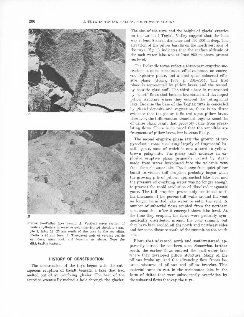
200 A TUYA IN TOGIAK VALLEY, SOUTHWEST ALASKA
t
FIGTJBE 6. Valley floor basalt. A, Vertical cross section of vesicle cylinders in massive columnar-jointed tholeiite (sam ple 1, table 1), 25 km south of the tuya in the sea cliffs. Knife is 90 mm long. B, Truncated ends of several vesicle cylinders, same rock and location as above. Note the diktytaxitic texture.
HISTORY OF CONSTRUCTION
The construction of the tuya began with the sub aqueous eruption of basalt beneath a lake that had melted out of an overlying glacier. The heat of the eruption eventually melted a hole through the glacier.
The size of the tuya and the height of glacial erratics on the walls of Togiak Valley suggest that the hole was at least 8 km in diameter and 330-500 m deep. The elevation of the pillow basalts on the northwest side of the tuya (fig. 1) indicates that the surface altitude of the melt-water lake was at least 250 m above present sea level. ''.;.. ; . .<' .'.' '
The Icelandic tuyas reflect a three-part eruptive suc cession a quiet subaqueous effusive phase, an emerg ent explosive phase, and a final quiet subaerial effu sive phase (Jones, 1969, p. 201-205). The first phase is represented by pillow lavas, and the second, by basaltic glass tuff. The third phase is represented by "sheet" flows that became brecciated and developed pillow structure where they entered the intraglacial lake. Because the base of the Togiak tuya is concealed by glacial deposits and vegetation, there is no direct evidence that the glassy tuffs rest upon pillow lavas. However, the tuffs contain abundant angular xenoliths of dense black basalt that probably came from preex isting flows. There is no proof that the xenoliths are fragments of pillow lavas, but it seems likely.
The second eruptive phase saw the growth of two pyroclastic cones consisting largely of fragmental ba saltic glass, most of which is now altered to yellow- brown palagonite. The glassy tuffs indicate an ex plosive eruptive phase primarily caused by steam made from water introduced into the volcanic vent from the melt-water lake. The change from quiet pillow basalt to violent tuff eruption probably began when the growing pile of pillows approached lake level and the pressure of overlying water was no longer enough to prevent the rapid exsolution of dissolved magmatic gases. The tuff eruption presumably continued until the thickness of the porous tuff walls around the vent no longer permitted lake water to enter the vent. A number of subaerial flows erupted from the northern cone some time after it emerged above lake level. At the time they erupted, the flows were probably sym metrically distributed around the cone summit, but they have been eroded off the north and northeast sides and for some distance south of the summit on the south side.
Flows that advanced south and southwestward ap parently buried the southern cone. Somewhat farther south, the earlier flows entered the melt-water lake where they developed pillow structure. Many of the pillows broke up, and the advancing flow fronts be came mixtures of pillows and pillow breccias. This material came to rest in the melt-water lake in the form of deltas that were subsequently overridden by the subaerial flows that cap the tuya.
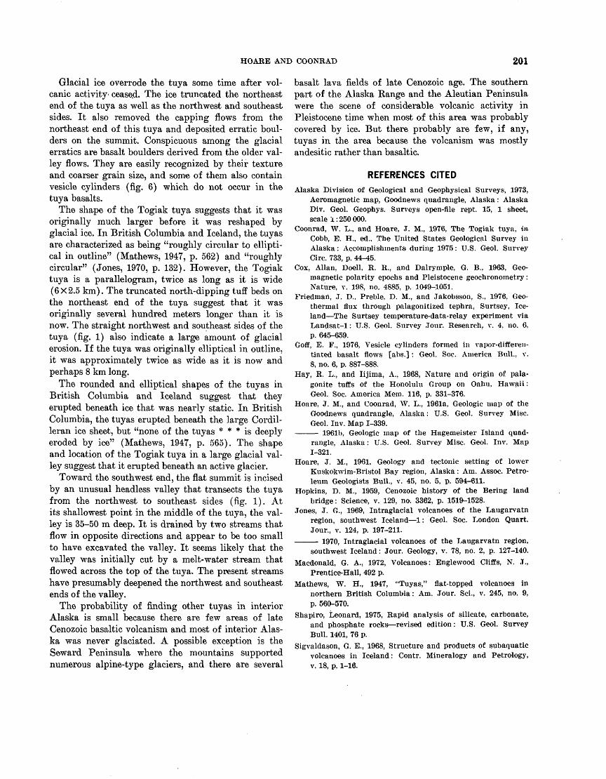
HOARE AND COONRAD 201
Glacial ice overrode the tuya some time after vol canic activity-cease.d. The ice truncated the northeast end of the tuya as well as the northwest and southeast sides. It also removed the capping flows from the northeast end of this tuya and deposited erratic boul ders on the summit. Conspicuous among the glacial erratics are basalt boulders derived from the older val ley flows. They are easily recognized by their texture and coarser grain size, and some of them also contain vesicle cylinders (fig. 6) which do not occur in the tuya basalts.
The shape of the Togiak tuya suggests that it was originally much larger before it was reshaped by glacial ice. In British Columbia and Iceland, the tuyas are characterized as being "roughly circular to ellipti cal in outline" (Mathews, 1947, p. 562) and "roughly circular" (Jones, 1970, p. 132). However, the Togiak tuya is a parallelogram, twice as long as it is wide (6X2.5 km). The truncated north-dipping tuff beds on the northeast end of the tuya suggest that it was originally several hundred meters longer than it is now. The straight northwest and southeast sides of the tuya (fig. 1) also indicate a large amount of glacial erosion. If the tuya was originally elliptical in outline, it was approximately twice as wide as it is now and perhaps 8 km long.
The rounded and elliptical shapes of the tuyas in British Columbia and Iceland suggest that they erupted beneath ice that was nearly static. In British Columbia, the tuyas erupted beneath the large Cordil- leran ice sheet, but "none of the tuyas * * * is deeply eroded by ice" (Mathews, 1947, p. 565). The shape and location of the Togiak tuya in a large glacial val ley suggest that it erupted beneath an active glacier.
Toward the southwest end, the flat summit is incised by an unusual headless valley that transects the tuya from the northwest to southeast sides (fig. 1). At its shallowest point in the middle of the tuya, the val ley is 35-50 m deep. It is drained by two streams that flow in opposite directions and appear to be too small to have excavated the valley. It seems likely that the valley was initially cut by a melt-water stream that flowed across the top of the tuya. The present streams have presumably deepened the northwest and southeast ends of the valley.
The probability of finding other tuyas in interior Alaska is small because there are few areas of late Cenozoic basaltic volcanism and most of interior Alas ka was never glaciated. A possible exception is the Seward Peninsula where the mountains supported numerous alpine-type glaciers, and there are several
basalt lava fields of late Cenozoic age. The southern part of the Alaska Kange and the Aleutian Peninsula were the scene of considerable volcanic activity in Pleistocene time when most of this area was probably covered by ice. But there probably are few, if any, tuyas in the area because the volcanism was mostly andesitic rather than basaltic.
REFERENCES CITED
Alaska Division of Geological and Geophysical Surveys, 1973, Aeromagnetic map, Goodnews quadrangle, Alaska: Alaska Div. Geol. Geophys. Surveys open-file rept. 15, 1 sheet, scale 1:250000.
Coonrad, W. L., and Hoare, J. M., 1976, The Togiak tuya, in Cobb, E. H., ed., The United States Geological Survey in Alaska: Accomplishments during 1975: U.S. Geol. Survey Circ. 733, p. 44-45.
Cox, Allan, Doell, R. R., and Dalrymple, G. B., 1963, Geo magnetic polarity epochs and Pleistocene geochronometry: Nature, v. 198, no. 4885, p. 1049-1051.
Friedmari, J. D., Preble. D. M., and Jakobsson, S., 1976, Geo- thermal flux through palagonitized tephra, Surtsey, Ice land The Surtsey temperature-data-relay experiment via Landsat-1: U.S. Geol. Survey Jour. Research, v. 4, no. 6, p. 645-659.
Goff, E. F., 1976, Vesicle cylinders formed in vapor-differen tiated basalt flows [abs.] : Geol. Soc. America Bull., v. 8, no. 6, p. 887-888.
Hay, R. L., and lijima, A., 1968, Nature and origin of pala- gonite tuffs of the Honolulu Group on Oahu, Hawaii: Geol. Soc. America Mem. 116, p. 331-376.
Hoare, J. M., and Coonrad, W. L., 1961a, Geologic map of the Goodnews quadrangle, Alaska: U.S. Geol. Survey Misc. Geol. Inv. Map 1-339.
19611), Geologic map of the Hagemeister Island quad rangle, Alaska: U.S. Geol. Survey Misc. Geol. Inv. Map 1-321.
Hoare, J. M., 1961, Geology and tectonic setting of lower Kuskokwim-Bristol Bay region, Alaska: Am. Assoc. Petro leum Geologists Bull., v. 45, no. 5, p. 594-611.
Hopkins, D. M., 1959, Cenozoic history of the Bering land bridge: Science, v. 129, no. 3362, p. 1519-1528.
.Tones, J. G., 1969, Intraglacial volcanoes of the Laugarvatn region, southwest Iceland 1: Geol. Soc. London Quart. Jour., v. 124, p. 197-211.
1970, Intraglacial volcanoes of the Laugarvatn region,southwest Iceland: Jour. Geology, v. 78, no. 2, p. 127-140.
Macdonald, G. A., 1972, Volcanoes: Englewood Cliffs, N. J.,Prentice-Hall, 492 p.
Mathews, W. H., 1947, "Tuyas," flat-topped volcanoes innorthern British Columbia: Am. Jour. Sci., v. 245, no. 9,p. 560-570.
Shapiro, Leonard, 1975, Rapid analysis of silicate, carbonate,and phosphate rocks revised edition: U.S. Geol. SurveyBull. 1401, 76 p.
Sigvaldason, G. E., 1968, Structure and products of subaquaticvolcanoes in Iceland: Contr. Mineralogy and Petrology,v. 18, p. 1-16.

Jour. Research U.S. Qeol. Survey Vol. 0, No. 2, Mar.-Apr. 1978, p. 203-214
ORIGIN OF TWO CLAY-MINERAL FACIES OF THE POTOMAC GROUP (CRETACEOUS) IN THE MIDDLE ATLANTIC STATES
By LUCY M. FORCE and GEORGE K. MONCURE,1
Reston, Va., and Laramie, Wyo.
Abstract. Sedimentary clay that crops out in the coastal plains of New Jersey, Delaware, the part of Maryland north and east of Washington, B.C., and the northeast half of Washington, D.C., in the nonmarine Cretaceous Potomac Group is predominantly kaolinite and illite. In contrast, in part of southeastern Maryland, the southwest half of Wash ington, D.C., and most of eastern Virginia, Potomac Group clay is predominantly montmorillonite.
Kaolinite and illite were probably derived by intense acid weathering of metamorphic and granitic rocks to the west during the Cretaceous and were deposited in a well-drained basin. Montmorillonite was most likely produced by deep weathering of a mainly granitic source. Poor drainage and alkaline surface- and ground-water conditions probably ac companied the production, transportation, deposition, and burial of the montmorillonite. Kaolinization of the mont morillonite is taking place now at the surface in northern Virginia.
Previous petrologic studies of the Potomac Group (Glaser, 1969; Owens, 1969) resulted in the discovery of two regional sedimentary facies: orthoquartzitic sand interbedded with kaolinite and illite clay beds north of Washington, D.C. (northern facies of this paper), and arkosic sand with montmorillonite2 and mixed layer clay to the south (southern facies of this paper; fig. 1). We find that the abrupt change in clay mineralogy is accompanied by differences in coarse sediment characteristics, ground-water chem istry, and stratigraphy.
The purpose of the present study is to determine the origin of the two sedimentary facies and to investigate the relationship between the sedimentary facies and the ground-water ion-concentration pattern. We present new stratigraphic details as well as a brief summary of previously published information to provide a depositional framework. Our discussions of prov enance, primary weathering reactions, and postde-
1 Department of Geology, University of Wyoming.- In this paper, montmorillonite is the term used for a clay with a
14- to 15-angstrom d-spacing In air-dried samples, which typically expands to 17 A with ethylene glycolatlon, and which collapses to 10 1 after heating to 300°C for an hour. It is found both as a discrete phase and, more commonly, as layers in mixed-layer clay.
positional changes are based on published data on source rocks, Potomac Group mineralogy and ground- water chemistry, and new mineralogic analyses of the Potomac Group sediments.
Acknowledgments. For samples outside northern Virginia and for unpublished data, we thank J. P. Owens, L. C. Conant, James Kankin, R. B. Mixon, D. J. Fanning, A. J. Froelich, and Deleuw, Gather and Co.
REGIONAL GEOLOGY
The middle Atlantic Coastal Plain extends from the Fall Line to the edge of the Continental Shelf. The Coastal Plain consists of a wedge of continental and marine sediments, deposited in Jurassic(?) through Quaternary time, which thins landward from a thick ness of roughly 9000 m (Minard and others, 1974) at the continental break. Exposed Cretaceous sediments range in age from Early Cretaceous (Barremian) through earliest Late Cretaceous (earliest Cenomani- an; Doyle and others, 1975).
The basal beds, which constitute the lower two-thirds of the sedimentary wedge beneath the emerged Coastal Plain, were assigned to the Potomac Group by McGee (1888). They consist of interbedded continental clay, silt, sand, and gravel deposited on a slightly irregular surface of Precambrian to lower Paleozoic rocks. The Potomac Group is as much as 1,500 m thick along the Atlantic shoreline (Weed and others, 1974) and is apparently considerably thicker farther east. Its beds crop out in an arc 550 km long along the edge of the Salisbury Embayment from central New Jersey to southern Virginia (fig. 1).
The Potomac Group sediments were subsequently subdivided by Brenner (1963) on the basis of pollen age zones. From southern Virginia to the head of the Chesapeake Bay, beds of pollen Zone I (mostly Aptian) occupy the western and northern part of the Potomac Group outcrop belt and beds of Zone II (Albian, 100-108 million years), the seaweed part
203
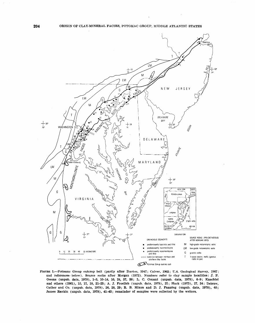
204 ORIGIN OF CLAY-MINERAL FACIES, POTOMAC GROUP, MIDDLE ATLANTIC STATES
+ =
X NEW YORK I MASS
~f " " \ '.CONN0' PENNSYLVANIA
EXPLANATION
CRETACEOUS SEDIMENTS
predominantly kaolinite and illite
predominantly montmorillonite
A predominantly montmorilloniteand illite
1111 transition between northern and southern clay facies
^£s Potomac Group outcrop belt
M
LM
G
T
SOURCE ROCKS (PRE-CRETACEOUSI AFTER MORGAN (1972)
high-grade metamorphic rocks
low-grade metamorphic rocks
granitic rocks
Triassic basins: mafic igneous rocks in part
FIGUBE 1. Potomac Group outcrop belt (partly after Darton, 1947; Calver, 1963; U.S. Geological Survey, 1967; and references below). Source rocks after Morgan (1972). Numbers refer to clay sample localities: J". P. Owens (unpub. data, 1978), 1-5, 10-14, 16; 24, 37, 38; L. C. Conant (unpub. data, 1978), 6-9; Knechtel and others (1961), 15, 17, 18, 21-23; A. J. Froelich (unpub. data, 1978), 25; Hack (1975), 27, 34; Deleuw, Gather and Co. (unpub. data, 1978), 26, 28, 29; R. B. Mixon and D. J. Fanning (unpub. data, 1978), 40; James Rankin (unpub. data, 1978), 41-43; remainder of samples were collected by the writers.
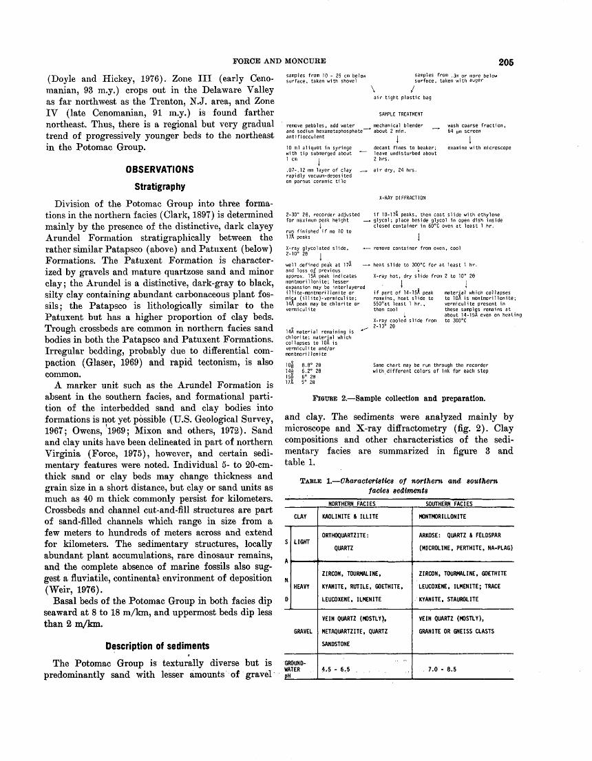
FORCE AND MONCURE 205
(Doyle and Hickey, 1976). Zone III (early Ceno- manian, 93 m.y.) crops out in the Delaware Valley as far northwest as the Trenton, N.J. area, and Zone IV (late Cenomanian, 91 m.y.) is found farther northeast. Thus, there is a regional but very gradual trend of progressively younger beds to the northeast in the Potomac Group.
OBSERVATIONS
Stratigraphy
Division of the Potomac Group into three forma tions in the northern facies (Clark, 1897) is determined mainly by the presence of the distinctive, dark clayey Arundel Formation stratigraphically between the rather similar Patapsco (above) and Patuxent (below) Formations. The Patuxent Formation is character ized by gravels and mature quartzose sand and minor clay; the Arundel is a distinctive, dark-gray to black, silty clay containing abundant carbonaceous plant fos sils; the Patapsco is lithologically similar to the Patuxent but has a higher proportion of clay beds. Trough crossbeds are common in northern facies sand bodies in both the Patapsco and Patuxent Formations. Irregular bedding, probably due to differential com paction (Glaser, 1969) and rapid tectonism, is also common.
A marker unit such as the Arundel Formation is absent in the southern facies, and formational parti tion of the interbedded sand and clay bodies into formations is not yet possible (U.S. Geological Survey, 1967; Owens, ^1969; Mixon and others, 1972). Sand and clay units have been delineated in part of northern Virginia (Force, 1975), however, and certain sedi mentary features were noted. Individual 5- to 20-cm- thick sand or clay beds may change thickness and grain size in a short distance, but clay or sand units as much as 40 m thick commonly persist for kilometers. Crossbeds and channel cut-and-fill structures are part of sand-filled channels which range in size from a few meters to hundreds of meters across and extend for kilometers. The sedimentary structures, locally abundant plant accumulations, rare dinosaur remains, and the complete absence of marine fossils also sug gest a fluviatile, continental environment of deposition (Weir, 1976).
Basal beds of the Potomac Group in both facies dip seaward at 8 to 18 m/km, and uppermost beds dip less than 2 m/km.
Description of sediments
The Potomac Group is texturally diverse but is predominantly sand with lesser amounts of gravel
samples from 10 - 25 cm below surface, taken with shovel
remove pebbles, add water and sodium hexametaphosphate" antiflocculent
10 ml aliquot in syringe with tip submerged about "*~~ 1 cm I
.07-.12 mm layer of clay rapidly vacuum-deposited on porous ceramic tile
2-30° 29, recorder adjusted for maximum peak height
Irun finished if no 10 to 17ft peaks
X-ray glycolated slide, «- 2-10° 28 I
well defined peak at 17& and loss of previous approx. ISA peak indicates montmorillonite; lesser expansion may be interlayered illite-montmorillonite or mica (illite)-vermiculite; 14A peak may be chlorite or vermiculite
14A material remaining is chlorite; material which collapses to 10A is vermiculite and/or montmorillonite
10§ 8.8° 2814A 6.2° 28ISA 6° 2817A 5° 28
samples from .3m or more below surface, taken with auger
wash coarse fraction, 64 pm screen
examine with microscope
\ /air tight plastic bag
SAMPLE TREATMENT
mechanical blender about 2 min.
decant fines to beaker; leave undisturbed about 2 hrs.
air dry, 24 hrs.
X-RAY DIFFRACTION
if 10-17& peaks, then coat slide with ethylene glycol; place beside glycol in open dish inside closed container in 60°C oven at least 1 hr.
remove container from oven, cool
heat slide to 300°C for at least 1 hr.I
X-ray hot, dry slide from 2 to 10° 28
if part of 14-15^ peak remains, heat slide to 550°at least 1 hr., then cool
IX-ray cooled slide from 2-13° 28
material which collapses to 10A is montmorillonite; vermiculite present in these samplgs remains at about 14-15A even on heating to 300°C
Same chart may be run through the recorder with different colors of ink for each step
FIQUBE 2. Sample collection and preparation.
and clay. The sediments were analyzed mainly by microscope and X-ray diffractometry (fig. 2). Clay compositions and other characteristics of the sedi mentary facies are summarized in figure 3 and table 1.
TABLE 1. Characteristics of northern and southern facies sediments
NORTHERN FACIES SOUTHERN FACIES
CLAY
LIGHT
HEAVY
GRAVEL
OUND- TER .
KAOLINITE & ILLITE
ORTHOQUARTZITE:
QUARTZ
ZIRCON, TOURMALINE,
KYANITE, RUTILE, GOETHITE,
LEUCOXENE, ILMENITE
VEIN QUARTZ (MOSTLY),
METAQUARTZITE, QUARTZ
SANDSTONE
4<5 - 6,5 . .
MONTMORILLONITE
ARKOSE: QUARTZ & FELDSPAR
(MICROLINE. PERTHITE. NA-PLAG)
ZIRCON. TOURMALINE. GOETHITE
LEUCOXENE. ILMENITE; TRACE
KYANITE, STAUROLITE
VEIN QUARTZ (MOSTLY),
GRANITE OR GNEISS CLASTS
7.0 - 8.5
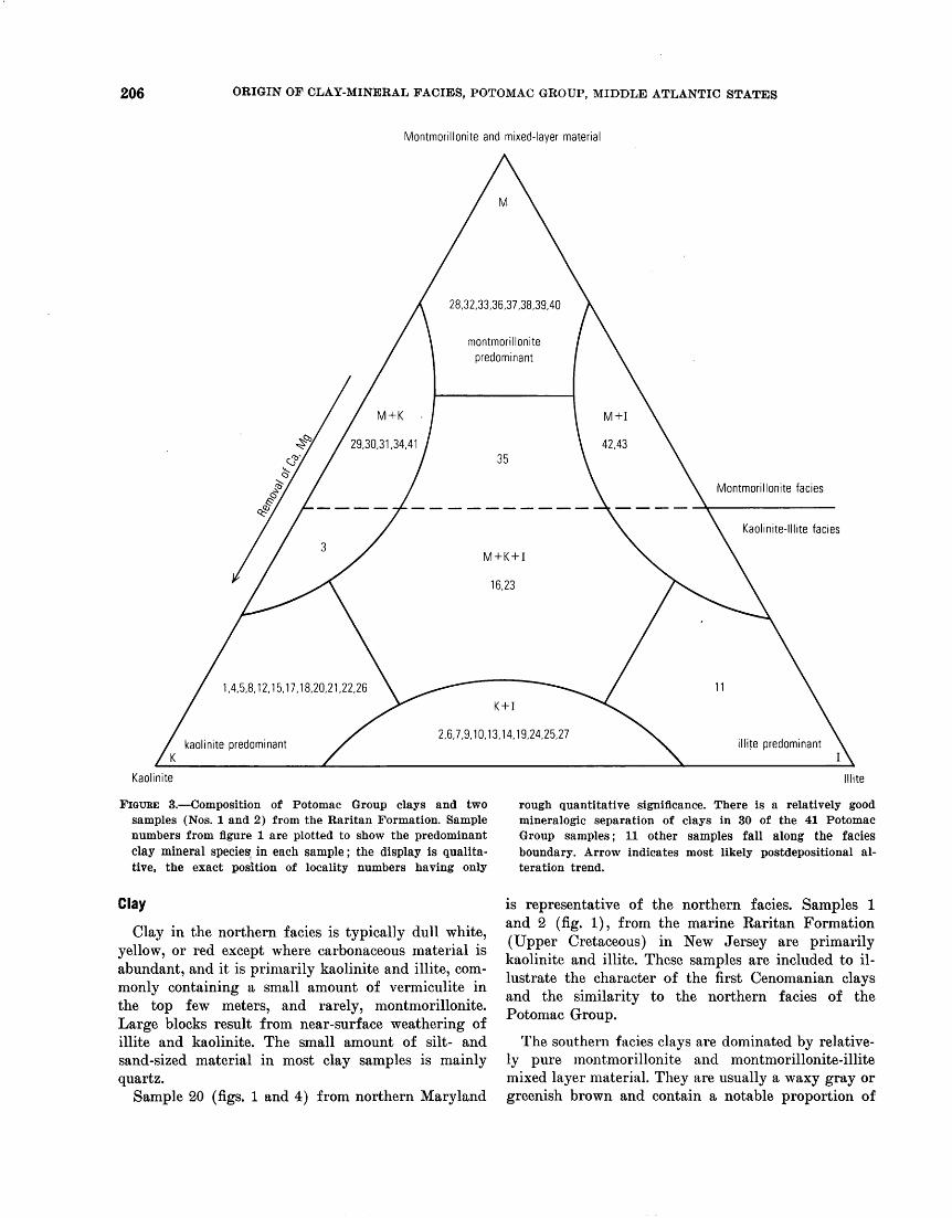
206 ORIGIN OF CLAY-MINERAL FACIES, POTOMAC GROUP, MIDDLE ATLANTIC STATES
Montmorillonite and mixed-layer material
1,4,5,8,12,15,17,18,20,21,22,26
Kaolinite
FIGUBE 3. Composition of Potomac Group clays and two samples (Nos. 1 and 2) from the Raritan Formation. Sample numbers from figure 1 are plotted to show the predominant clay mineral species, in each sample; the display is qualita tive, the exact position of locality numbers having only
Clay
Clay in the northern facies is typically dull white, yellow, or red except where carbonaceous material is abundant, and it is primarily kaolinite and illite, com monly containing a small amount of vermiculite in the top few meters, and rarely, montmorillonite. Large blocks result from near-surface weathering of illite and kaolinite. The small amount of silt- and sand-sized material in most clay samples is mainly quartz.
Sample 20 (figs. 1 and 4) from northern Maryland
Illite
rough quantitative significance. There is a relatively good mineralogic separation of clays in 30 of the 41 Potomac Group samples; 11 other samples fall along the facies boundary. Arrow indicates most likely postdepositional al teration trend.
is representative of the northern facies. Samples 1 and 2 (fig. 1), from the marine Raritan Formation (Upper Cretaceous) in New Jersey are primarily kaolinite and illite. These samples are included to il lustrate the character of the first Cenomanian clays and the similarity to the northern facies of the Potomac Group.
The southern facies clays are dominated by relative ly pure montmorillonite and montmorillonite-illite mixed layer material. They are usually a waxy gray or greenish brown and contain a notable proportion of
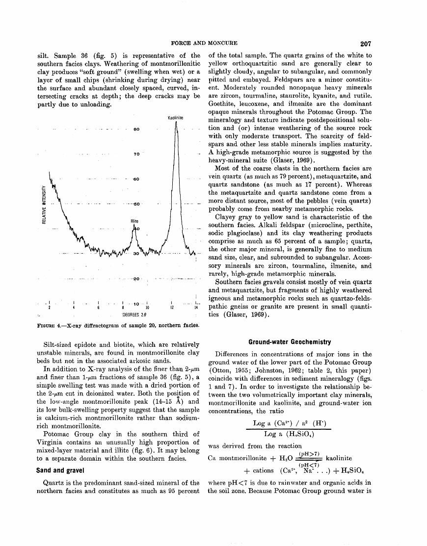
FORCE AND MONCURE 207
silt. Sample 36 (fig. 5) is representative of the southern facies clays. Weathering of montmorillonitic clay produces "soft ground" (swelling when wet) or a layer of small chips (shrinking during drying) near the surface and abundant closely spaced, curved, in tersecting cracks at depth; the deep cracks may be partly due to unloading.
Kaolinite
ao
2
. . 'DEGREES 20
FIGURE 4. X-ray diffractogram of sample 20, northern facies.
Silt-sized epidote and biotite, which are relatively unstable minerals, are found in montmorillonite clay beds but not in the associated arkosic sands.
In addition to X-ray analysis of the finer than 2-/xm and finer than l-/mi fractions of sample 36 (fig. 5), a simple swelling test was made with a dried portion of the 2-/xin cut in deionized water. Both the position of the low-angle montmorillonite peak (14-15 A) and its low bulk-swelling property suggest that the sample is calcium-rich montmorillonite rather than sodium- rich montmorillonite.
Potomac Group clay in the southern third of Virginia contains an unusually high proportion of mixed-layer material and illite (fig. 6). It may belong to a separate domain within the southern facies.
Sand and gravel
Quartz is the predominant sand-sized mineral of the northern facies and constitutes as much as 95 percent
of the total sample. The quartz grains of the white to yellow orthoquartzitic sand are generally clear to slightly cloudy, angular to subangular, and commonly pitted and embayed. Feldspars are a minor constitu ent. Moderately rounded nonopaque heavy minerals are zircon, tourmaline, staurolite, kyanite, and rutile. Goethite, leucoxene, and ilmenite are the dominant opaque minerals throughout the Potomac Group. The mineralogy and texture indicate postdepositional solu tion and (or) intense weathering of the source rock with only moderate transport. The scarcity of feld spars and other less stable minerals implies maturity. A high-grade metamorphic source is suggested by the heavy-mineral suite (Glaser, 1969).
Most of the coarse clasts in the northern facies are vein quartz (as much as 79 percent), metaquartzite, and quartz sandstone (as much as 17 percent). Whereas the metaquartzite and quartz sandstone come from a more distant source, most of the pebbles (vein quartz) probably come from nearby metamorphic rocks.
Clayey gray to yellow sand is characteristic of the southern facies. Alkali feldspar (microcline, perthite, sodic plagioclase) and its clay weathering products comprise as much as 65 percent of a sample; quartz, the other major mineral, is generally fine to medium sand size, clear, and subrounded to subangular. Acces sory minerals are zircon, tourmaline, ilmenite, and rarely, high-grade metamorphic minerals.
Southern facies gravels consist mostly of vein quartz and metaquartzite, but fragments of highly weathered igneous and metamorphic rocks such as quartzo-felds- pathic gneiss or granite are present in small quanti ties (Glaser, 1969).
Ground-water Geochemistry
Differences in concentrations of major ions in the ground water of the lower part of the Potomac Group (Otton, 1955; Johnston, 1962; table 2, this paper) coincide with differences in sediment mineralogy (figs. 1 and 7). In order to investigate the relationship be tween the two volumetrically important clay minerals, montmorillonite and kaolinite, and ground-water ion concentrations, the ratio
Log a (Ca2+ ) / a2 (H+ )
Log a (H4Si04 )
was derived from the reaction
Ca montmorillonite -f- H2O *' - ^ kaolinite(PH<7)
+ cations (Ca2+ , Na+ . . .) -f H4Si04
where pH<7 is due to rainwater and organic acids in the soil zone. Because Potomac Group ground water is
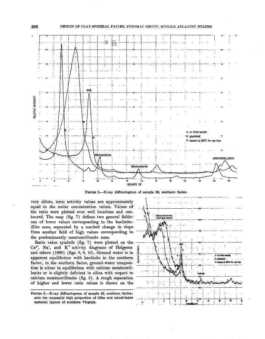
208 ORIGIN OF CLAY-MINERAL FACIES, POTOMAC GROUP, MIDDLE ATLANTIC STATES
A-air dried sample G~gtycol3te[! ~ " H-heated tci 300°C for onp hour
4 U 16
DEGREES 26
FIGURE 5. X-ray diffractogram of sample 36, southern facies.
very dilute, ionic activity values are approximately equal to the molar concentration values. Values of the ratio were plotted over well locations and con toured. The map (fig. 7) defines two general fields: one of lower values corresponding to the kaolinite- illite zone, separated by a marked change in slope from another field of high values corresponding to the predominantly montmorillonite zone.
Ratio value symbols (fig. 7) were plotted on the Ca2+, Na+, and K + activity diagrams of Helgeson and others (1969) (figs. 8, 9, 10). Ground water is in apparent equilibrium with kaolinite in the northern facies; in the southern facies, ground-water composi tion is either hi equilibrium with calcium montmoril lonite or is slightly deficient in silica with respect to calcium montmorillonite (fig. 8). A rough separation of higher and lower ratio values is shown on the
FIGTJBE 6. X-ray diffractogram of sample 42, southern facies; note the unusually, high proportion of illite and mixed4ayer material typical of southern Virginia.
A-aJfldriedtimph, > fi-ttofen*) - - - - - H-hettBd:«f WOta owrhcu
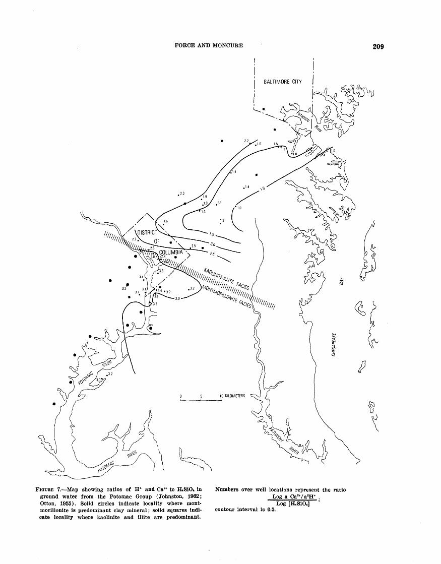
FORCE AND MONCURE 209
FIGURE 7. Map showing ratios of H+ and Ca2* to H4SiO4 in ground water from the Potomac Group (Johnston, 1962; Otton, 1955). Solid circles indicate locality where mont- morillonite is predominant clay mineral; solid squares indi cate locality where kaolinite and illite are predominant.
Numbers over well locations represent the ratio Log a Ca2Va2H* .
Logcontour interval is 0.5.
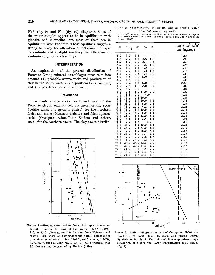
210 ORIGIN OF CLAY-MINERAL FACIES, POTOMAC GROUP, MIDDLE ATLANTIC STATES
Na+ (fig. 9) and K+ (fig. 10) diagrams. Some of the water samples appear to be in equilibrium with gibbsite and microcline, but most of them are in equilibrium with kaolinite. These equilibria suggest a strong tendency for alteration of potassium feldspar to kaolinite and a slight tendency for alteration of kaolinite to gibbsite (leaching).
INTERPRETATION
An explanation of the present distribution of Potomac Group mineral assemblages must take into account (1) probable source rocks and production of clay in the source area, (2) depositional environment, and (3) postdepositional environment.
Provenance
The likely source rocks north and west of the Potomac Group outcrop belt are metamorphic rocks (pelitic schist and granitic gneiss) for the northern facies and mafic (Mesozoic diabase) and felsic igneous rocks (Occoquan Adamellite; Seiders and others, 1975) for the southern facies. The clay facies distribu-
12 -
10 -
Gibbsite
-5 -4 -3
Log [H4SiO/il
-2
FIGURE 8. Ground-water values from this report shown on activity diagram for part of the system H2O-Al2O3-CaO- SiO2 at 25°C. (Format for this diagram from Helgeson and others, 1969, based on thermodynamic data.) Symbols for ground-water values are plus, 1.0-1.5; solid square, 1.5-2.0; no samples, 2.0-2.5; solid circle, 2.5-3.0; solid triangle, over 3.0. Dashed line determined by Norton (1974).
TABLE 2. Concentrations of certain ions in (/round icater from Potomac Group wells
[ Except pH. units are parts per million. Ratio values plotted on figure 7. Starred entries are from .Tohnston (1962) ; remainder are from Otton (1955)]
PH
6.06.45.24.75.04.15.15.25.37.36.04.75.34.77.57.88.17.7
*7.8*7.7*7.8*5.9*5.27.77.87.9
*7.3*6.7*6.6*6.4*5.8*7.3*8.3*8.0
6.0
5.0
i~̂*~zro
§
4.0
3.0
Si02
1.010.06.3
11.08.09.07.28.55.43.77.44.73.18.8
19.013.032.013.013.010.021.0
7.19.9
34.027.019.023.019.014.033.030.021.012.024.0
K-
Gibbsite
-
0
+
-
-4.5
Ca Na
1.1.0.0.1.1.0.0.0.5.1.0.1.0.0.3.2.
29.3.
17.1.2.1.1.0.5.
16.
1 8 2.69 2.19 1.51 1.28 1.35 1.43 5.93 6 6.00 2.03 0 14.09 4.8 30.04 50.08 6.00 4.24 50.00 5.93 53.05 2.47 181 60.05 77.09 88.00 7.1
10.0 2.822.0 7.332.0 13.030.0 11.018.0 9.40.4 80.01. 2 60.0
g2
1
e
K Log a Ca2+/a2HHLog [H4Si04 ]
1.561.0 1.980.5 1.501.0 1.250.3 1.401.6 1.140.3 1.350.3 1.36
1.353.8 2.550.4 1.89
1.042.3 1.39
0 1.231.37
4.8 1.110.6 1.279.2 3.314.8 3.151.6 3.252.4 3.211.1 1.94
.0 1.582.1 3.342.8 3.197.6 3.576.5 3.274.7 2.802.6 2.735.6 2.979.5 2.575.5 3.062.6 3.130.8 3.38
1 \ 1 ' ^v Low\ Na-Montmorillonite N-Albite
\ ' ^V\ 1 ^
1 \ 1
.--'
++ + M +
fA
^
^ ^'**
4A
Kaolinite
-4.0
\ *
\ 1A \ "1 \ 1 ^' + \ 2-
*'£. \ °
Vk tl \
A" A A \
1 , 1 l\
-3.5 -3.0 -2.5 -2.
Log [HtS'tQi]
FIGURE 9. Activity diagram for part of the systemNa2O-SiO2 at 25°C (from Helgeson and others, 1969). Symbols as for fig. 8. Short dashed line emphasizes rough separation of higher and lower concentration ratio values (fig. 8).
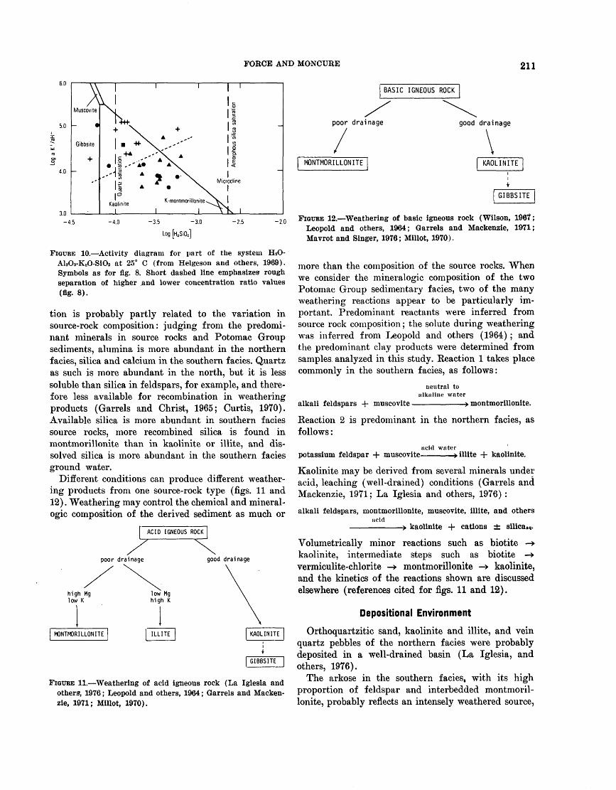
FORCE AND MONCURE 211
-4.5 -4.0 -3.5 -3.0 -2.5 -2.0
Log
FIGURE 10. Activity diagram for part of the system H2O- AlaOa-KaO-SiOa at 25° C (from Helgeson and others, 1969). Symbols as for fig. 8. Short dashed line emphasizes rough separation of higher and lower concentration ratio values (fig. 8).
tion is probably partly related to the variation in source-rock composition: judging from the predomi nant minerals in source rocks and Potomac Group sediments, alumina is more abundant in the northern f acies, silica and calcium in the southern f acies. Quartz as such is more abundant in the north, but it is less soluble than silica in feldspars, for example, and there fore less available for recombination in weathering products (Garrels and Christ, 1965; Curtis, 1970). Available silica is more abundant in southern facies source rocks, more recombined silica is found in montmorillonite than in kaolinite or illite, and dis solved silica is more abundant in the southern facies ground water.
Different conditions can produce different weather ing products from one source-rock type (figs. 11 and 12). Weathering may control the chemical and mineral- ogic composition of the derived sediment as much or
FIQUBE 11. Weathering of acid igneous rock (La Iglesia and others', 1976; Leopold and others, 1964; Garrels and Macken zie, 1971; Millot, 1970).
BASIC IGNEOUS ROCK
poor drainage good drainage
MONTMORILLONITE
FIQUBE 12. Weathering of basic igneous rock (Wilson, 1967; Leopold and others, 1964; Garrels and Mackenzie, 1971; Mavrot and Singer, 1976; Millot, 1970).
more than the composition of the source rocks. When we consider the mineralogic composition of the two Potomac Group sedimentary facies, two of the many weathering reactions appear to be particularly im portant. Predominant reactants were inferred from source rock composition; the solute during weathering was inferred from Leopold and others (1964); and the predominant clay products were determined from samples analyzed in this study. Reaction 1 takes place commonly in the southern facies, as follows:
neutral to alkaline water
alkali feldspars + muscovite montmorillonite.
Reaction 2 is predominant in the northern facies, as follows:
acid waterpotassium feldspar -f muscovite »illite + kaolinite.
Kaolinite may be derived from several minerals under acid, leaching (well-drained) conditions (Garrels and Mackenzie, 1971; La Iglesia and others, 1976) :
alkali feldspars, montmorillonite, muscovite, illite, and othersacid
-> kaolinite + cations ± silica.q.
Volumetrically minor reactions such as biotite -> kaolinite, intermediate steps such as biotite -» vermiculite-chlorite -» montmorillonite -> kaolinite, and the kinetics of the reactions shown are discussed elsewhere (references cited for figs. 11 and 12).
Depositional Environment
Orthoquartzitic sand, kaolinite and illite, and vein quartz pebbles of the northern facies were probably deposited in a well-drained basin (La Iglesia, and others, 1976).
The arkose in the southern facies, with its high proportion of feldspar and interbedded montmoril lonite, probably reflects an intensely weathered source,
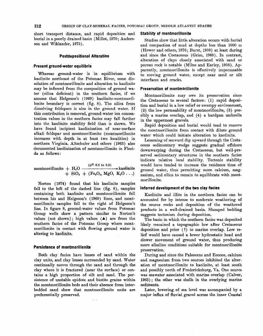
212 ORIGIN OF CLAY-MINERAL FACIES, POTOMAC GROUP, MIDDLE ATLANTIC STATES
short transport distance, and rapid deposition and burial in a poorly drained basin (Millot, 1970; Anders- son and Wiklander, 1975).
Postdepositional Alteration
Present ground-water equilibria
Whereas ground-water is in equilibrium with kaolinite northeast of the Potomac River, some dis solution of montmorillonite and alteration to kaolinite may be inferred from the composition of ground wa ter (silica deficient) in the southern facies, if we assume that Helgeson's (1969) kaolinite-montmoril- lonite boundary is correct (fig. 8). The silica from dissolving feldspars is also in the ground water. If this contribution is removed, ground-water ion concen tration values in the southern facies may fall farther into the kaolinite stability field than is shown. We have found incipient kaolinization of near-surface alkali feldspar and montmorillonite (montmorillonite increases with depth in at least two localities) in northern Virginia. Altschuler and others (1963) also documented kaolinization of montmorillonite in Flori da as follows:
(pH 6.5 to 5.0)montmorillonite -f H2O »kaolinite
+ Si02 + (Fe2O3 , MgO, K2O . . .)
Norton (1974) found that his kaolinite samples fell to the left of the dashed line (fig. 8), samples containing both kaolinite and montmorillonite fell between his and Helgeson's (1969) lines, and mont morillonite samples fell to the right of Helgeson's line. In figure 8, ground-water values from Potomac Group wells show a pattern similar to Norton's values (not shown); high values (A) are from the southern facies of the Potomac Group where mont morillonite in contact with flowing ground water is altering to kaolinite.
Persistence of montmorillonite
Both clay facies have lenses of sand within the clay units, and clay lenses surrounded by sand. Water continually moves through the sand and through the clay where it is fractured (near the surface) or con tains a high proportion of silt and sand. The per sistence of unstable epidote and biotite grains within the montmorillonite beds and their absence from inter- bedded sand show that montmorillonite units are preferentially preserved.
Stability of montmorillonite
Studies show that little alteration occurs with burial and compaction of mud at depths less than 1000 m (Hower and others, 1976; Burst, 1959) at least during and since the Cretaceous (Grim, 1968). In contrast, alteration of clays closely associated with sand or porous rock is notable (Milne and Earley, 1958). Ap parently, montmorillonite is effectively impermeable to moving ground water, except near sand or silt interfaces and cracks.
Preservation of montmorillonite
Montmorillonite may owe its preservation since the Cretaceous to several factors: (1) rapid deposi tion and burial in a low relief or swampy environment, (2) the low permeability of montmorillonite, (3) pos sibly a marine overlap, and (4) a hardpan umbrella in the uppermost gravels.
Rapid deposition and burial would tend to remove the montmorillonite from contact with dilute ground water which could initiate alteration to kaolinite.
Lessening of seaward dip upward through the Creta ceous sedimentary wedge suggests gradual offshore downwarping during the Cretaceous, but well-pre served sedimentary structures in the southern facies indicate relative local stability. Tectonic stability would have tended to increase the residence time of ground water, thus permitting more calcium, mag nesium, and silica to remain to equilibrate with mont morillonite.
Inferred development of the two clay facies
Kaolinite and illite in the northern facies can be accounted for by intense to moderate weathering of the source rocks and deposition of the weathered products in a well-drained basin. Slumped bedding suggests tectonism during deposition.
The basin in which the southern facies was deposited likely remained a topographic low after Cretaceous deposition and prior (?) to marine overlap. Low re lief would have caused a lower hydrostatic head and slower movement of ground water, thus producing more alkaline conditions suitable for montmorillonite preservation.
During and since the Paleocene and Eocene, calcium and magnesium from two sources inhibited the alter ation of montmorillonite to kaolinite, at least south and possibly north of Fredericksburg, Va. One source was sea water associated with marine overlap (Calver, 1963); the other was shells in the overlying marine sediments.
Later, lowering of sea level was accompanied by a major influx of fluvial gravel across the inner Coastal
FORCE AND MONCURE 213
Plain. Impermeable clay hardpans formed in the up per part of the gravel sheets and protected the under lying clays fi^om intense degradation. Major dissection of the gravel sheet* began in the Pleistocene.
Today, some montmorillonite in northern Virginia is altering to kaolinite because of reaction with acidic ground water; the alteration front is within a few feet of the surface.
Summary
The kaolinite-illite clay accompanied by orthoquart- zitic sand and a varied but mature heavy-mineral suite of the northern f acies suggests deep weathering in the Piedmont and Appalachian metamorphic source areas to the west during the Cretaceous (Glaser, 1969). Montmorillonite clay with arkosic sand and a restrict ed, mature heavy-mineral suite of the southern f acies reflects a nearby youthful granite source with few heavy minerals.
The clays in each facies represent primary sedi ments which survived change through time. Kaolinite and illite in the northern facies appear to have been stable since the Cretaceous. Persistence of montmoril lonite in the southern facies is probably due to deposi tion under alkaline, nonleaching conditions with relatively abundant calcium and silica, and subsequent exclusion of acidic ground water because of the im permeability of montmorillonitic clay bodies.
References Cited
Altschuler, Z. S., Dwornik, E. J"., and Kramer, H., 1963, Trans formation of montmorillonite to kaolinite during weather ing: Science, v. 141, p. 148-152.
Andersson, A., and Wiklander, L., 1975, Release of crystal constituents by chemical weathering of some minerals: Soil Science, v. 120, p. 13-19.
Brenner, G. J., 1963, The spores and pollen of the Potomac Group of Maryland: Maryland Dept. Geology, Mines and Water Resources Bull. 27, 215 p.
Burst, J. F., Jr., 1959, Postdiagenetic clay mineral environ mental relationships in the Gulf Coast Eocene: Clays and Clay Minerals, v. 6,p. 327-341.
Calver, J. L., 1963, Geologic map of Virginia, 1: 500,000: Vir ginia Dept. of Conserv. and Econ. Devel.
Clark, W. B., 1897, Outline of present knowledge of the physical features of Maryland, embracing an account of the physiography, geology, and natural resources: Mary land Geol. Survey Repts1., v. 1, p. 139-228.
Curtis, C. D., 1970, Differences between lateritic and podzolic weathering: Geochim. et Cosmochim. Acta, v. 34, p. 1351- 1353.
Darton, N. H., 1947, Sedimentary formations of Washington, D.C., and vicinity: U.S. Geol. Survey Map»scale 1:31,680.
Doyle, J. A., and Hickey, L. J., 1976, Pollen and leaves from the midrCretaceous Potomac. Group and their bearing.on,
early angiospenn evolution, in Beck, C. B., ed., Origin and early evolution of angiosperms: Columbia Univ. Press, p. 139-206.
Doyle, J. A., Van Campo, M., and Lugarden, B., 1975, Observa tions on exine structures in Eucommiidites and Lower Cretaceous- angiosperm pollen: Pollen et Spores, v. 17, p. 429-486.
Force, L. M., 1975, Preliminary geologic map of the Coastal Plain of Fairfax County, Va.: U.S. Geol. Survey Open- File Rep. 76-415.
Garrels, R. M., and Christ, C. L., 1965, Solutions, minerals, and equilibria: New York, Harper and Row, 450 p.
Garrels, R. M., and Mackenzie, F. T., 1971, Evolution of sedi mentary rocks: New York, Norton, 397 p.
Glaser, J. D., 1969, Petrology and origin of Potomac and Magothy (Cretaceous) sediments, Middle Atlantic Coastal Plain: Maryland Geol. Survey Rept. Inv., no. 11, 101 p.
Grim, R. E., 1968, Clay mineralogy [2d ed.]: New York, McGraw-Hill, 596 p.
Hack, J. T., 1975, Prince Georges County geologic map for land use planning: U.S. Geol. Survey Open-File Map 75-208.
Helgeson, H. C., Brown, T. H., and Leeper, R. H., 1969, Handbook of theoretical activity diagrams depicting chemi cal equilibria in geologic systems involving an aqueous phase at one atm. and 0° to 300°C: New York, Freeman, Cooper & Co., 253 p.
Hower, J., Eslinger, E. V., Hower, M. E., and Perry, E. A., 1976, Mechanism of burial metamorphism of argil laceous sediments: 1. Mineralogical and chemical evidence: Geol. Soc. Amer. Bull., v. 87, p. 725-737.
Johnston, P. M., 1962, Geology and groundwater resources of Washington, D.C. and vicinity: U.S. Geol. Survey Water- Supply Paper 1776, 97 p.
Knechtel, M. M., Hamlin, H. P., Hosterman, J. W., and Carroll, Dorothy, 1961, Physical properties of nonmarine Cretaceous clays in the Maryland Coastal Plain: Mary land Dept. Geology, Mines and Water Resources Bull. 23, 11 p.
La Iglesia, A., Martin-Vivaldi, J. L., Jr., and Aguayo, F. L., 1976, Kaolinite crystallization at room temperature by homogeneous precipitation III: Hydrolysis of feldspars: Clays and Clay Minerals, v. 24, p. 36-42.
Leopold, L. B., Wolman, M. G., and Miller, J. P., 1964, Fluvial processes in geomorphology: San Francisco, Freeman and Co., 522 p.
McGee, W. J., 1888, Three formations of the middle Atlantic slope: Am. Jour. Sci., 3d ser., v. 35, p. 120-143, 328-388, 448-466.
Millot, G., 1970, Geology of clays; translated by Farrand, W. R., and Paquet, H.: New York, Springer-Verlag, 429 p.
Milne, I. H., and Barley, J. W., 1958, Effect of source and environment on clay minerals: Am. Assoc. Petroleum Geologists Bull., v. 42, p. 328-338.
Minard, J. P., Perry, W. J., Weed, E. G. A., Rhodehamel, E. C., Robbins, E. I., and Mixon, R. B., 1974, Preliminary report on geology along the Atlantic continental margin of the northeastern United States: Am. Assoc. Petroleum Geologists Bull. v. 58, p. 1169-1178.
Mixon, R. B., Southwick, D. L., and Reed, J. C., Jr., 1972, Geologic map of the Quantico quadrangle, Prince William and Stafford Counties, Va., and Charles County, Md., U.S. Geol. Survey Geol. Quad. Map GQ-^1044 [1973].
214 ORIGIN OF CLAY-MINERAL FACIES, POTOMAC GROUP, MIDDLE ATLANTIC STATES
Morgan, B. A., 1972, Metamorphic map of the Appalachians: U.S. Geol. Survey Misc. Geol. Inv. Map 1-724.
Navrot, J. and Singer, A., 1976, Geochemical changes accom panying basic igneous rocks clay transition in a humid Mediterranean climate: Soil Sci., v. 121, p. 337-345.
Norton, D., 1974, Chemical mass transfer in the Rio Tanama system, west-central Puerto Rico; Geochim. et Cosmochim. Acta, v. 38, p. 267-277.
Otton, E. G., 1955, Groundwater resources of southern Mary land Coastal Plain: Maryland Dept. Geology Mines and Water Resources Bull. 15, 347 p.
Owens, J. P., 1969, Coastal Plain rocks of Harford County, in Southwick, D. L., Owens, J. P., and Edwards, Jonathan, Jr., The geology of Harford County, Maryland: Baltimore, Maryland Geol. Survey, p. 77-103.
Seiders, V. M., Mixon, R. B., Stern, T. W., Newell, M. F., and Thomas, C. B., Jr., 1975, Age of plutonism and tectonism and a new minimum age limit on the Glenarm series in
the northeast Virginia Piedmont near Occoquan: Am. Jour. Sci., v. 275, p.481-511.
U.S. Geological Survey, 1967, Engineering geology of the Northeast Corridor, Washington, D.C., to Boston, Massa chusetts Coastal Plain and surficial deposits: U.S. Geol. Survey Misc. Geol. Inv. Map I-514-B, 8 sheets, scale 1,: 500,000.
Weed, E. G. A., Minard, J. P., Perry, W. J.,Jr., Rhodehamel, E. C., and Robbins, E. I., 1974, Generalized pre-Pleistocene geologic map of the northern United States Atlantic con tinental margin: U.S. Geol. Survey Misc. Inv. Map 1-861, 2 sheets, scale 1:1,000,000.
Weir, G. W., 1976, Crossbedding of the Potomac Formation in Fairfax County, Virginia: U.S. Geol. Survey Open- File Rept. 76-193.
Wilson, M. J., 1967, The clay mineralogy of some soils derived from a biotite-rich quartz-gabbro in the Strathdon area, Aberdeenshire: Clay Minerals, v. 7, p. 91-100.
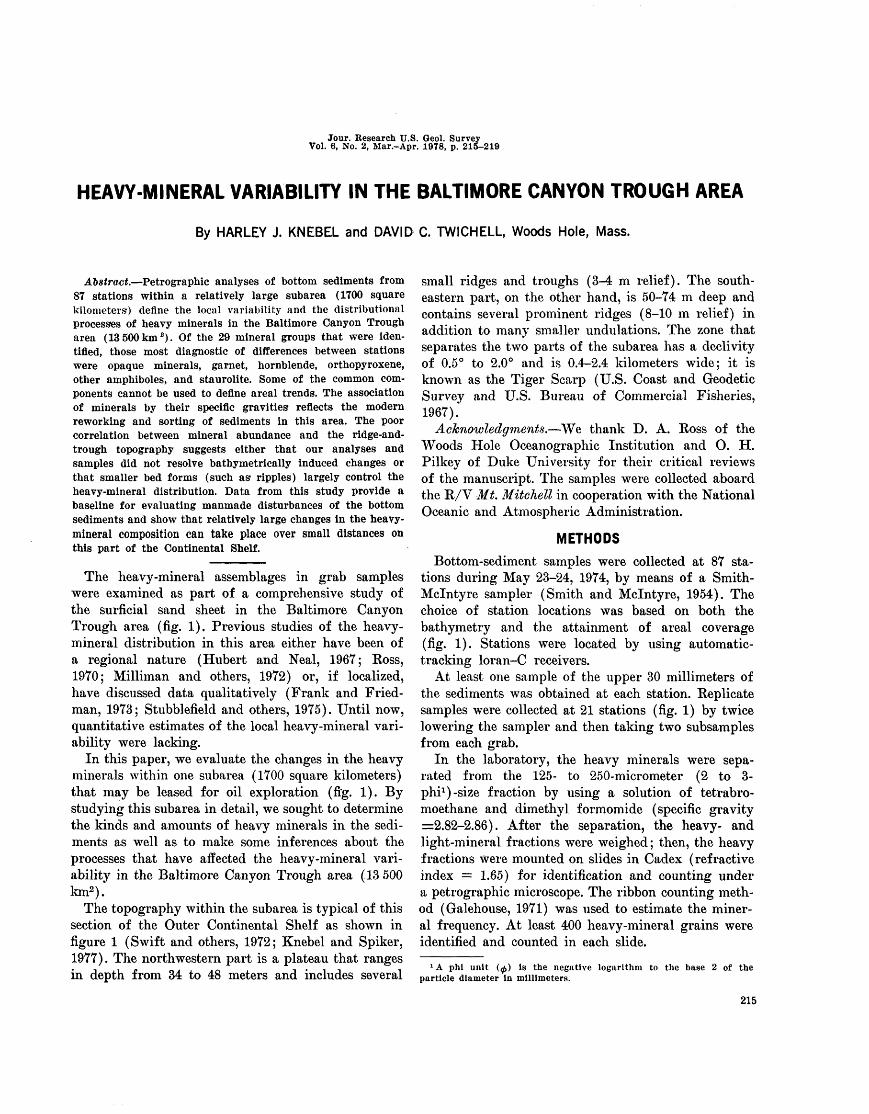
Jour. Research U.S. Geol. Survey Vol. 6, No. 2, Mar.-Apr. 1978, p. 215-219
HEAVY-MINERAL VARIABILITY IN THE BALTIMORE CANYON TROUGH AREA
By HARLEY J. KNEBEL and DAVID C. TWICHELL, Woods Hole, Mass.
Abstract. Petrographic analyses of bottom sediments from 87 stations within a relatively large subarea (1700 square kilometers) define the local variability and the distributional processes of heavy minerals in the Baltimore Canyon Trough area (13500km 8 ). Of the 29 mineral groups that were iden tified, those most diagnostic of differences between stations were opaque minerals, garnet, hornblende, orthopyroxene, other amphiboles, and staurolite. Some of the common com ponents cannot be used to define areal trends. The association of minerals by their specific gravities reflects the modern reworking and sorting of sediments in this area. The poor correlation between mineral abundance and the ridge-and- trough topography suggests either that our analyses and samples did not resolve bathymetrically induced changes or that smaller bed forms (such as ripples) largely control the heavy-mineral distribution. Data from this study provide a baseline for evaluating manmade disturbances of the bottom sediments and show that relatively large changes in the heavy- mineral composition can take place over small distances on this part of the Continental Shelf.
The heavy-mineral assemblages in grab samples were examined as part of a comprehensive study of the surficial sand sheet in the Baltimore Canyon Trough area (fig. 1). Previous studies of the heavy- mineral distribution in this area either have been of a regional nature (Hubert and Neal, 1967; Ross, 1970; Milliman and others, 1972) or, if localized, have discussed data qualitatively (Frank and Fried- man, 1973; Stubblefield and others, 1975). Until now, quantitative estimates of the local heavy-mineral vari ability were lacking.
In this paper, we evaluate the changes in the heavy minerals within one subarea (1700 square kilometers) that may be leased for oil exploration (fig. 1). By studying this subarea in detail, we sought to determine the kinds and amounts of heavy minerals in the sedi ments as well as to make some inferences about the processes that have affected the heavy-mineral vari ability in the Baltimore Canyon Trough area (13 500 km2 ).
The topography within the subarea is typical of this section of the Outer Continental Shelf as shown in figure 1 (Swift and others, 1972; Knebel and Spiker, 1977). The northwestern part is a plateau that ranges in depth from 34 to 48 meters and includes several
small ridges and troughs (3-4 m relief). The south eastern part, on the other hand, is 50-74 m deep and contains several prominent ridges (8-10 m relief) in addition to many smaller undulations. The zone that separates the two parts of the subarea has a declivity of 0.5° to 2.0° and is 0.4-2.4 kilometers wide; it is known as the Tiger Scarp (U.S. Coast and Geodetic Survey and U.S. Bureau of Commercial Fisheries, 1967).
Acknowledgments. We thank D. A. Ross of the Woods Hole Oceanographic Institution and O. H. Pilkey of Duke University for their critical reviews of the manuscript. The samples were collected aboard the R/V Mt. Mitchell in cooperation with the National Oceanic and Atmospheric Administration.
METHODS
Bottom-sediment samples were collected at 87 sta tions during May 23-24, 1974, by means of a Smith- Mclntyre sampler (Smith and Mclntyre, 1954). The choice of station locations was based on both the bathymetry and the attainment of areal coverage (fig. 1). Stations were located by using automatic- tracking loran-C receivers.
At least one sample of the upper 30 millimeters of the sediments was obtained at each station. Replicate samples were collected at 21 stations (fig. 1) by twice lowering the sampler and then taking two subsamples from each grab.
In the laboratory, the heavy minerals were sepa rated from the 125- to 250-micrometer (2 to 3- phi1 )-size fraction by using a solution of tetrabro- moethane and dimethyl formomide (specific gravity =2.82-2.86). After the separation, the heavy- and light-mineral fractions were weighed; then, the heavy fractions were mounted on slides in Cadex (refractive index = 1.65) for identification and counting under a petrographic microscope. The ribbon counting meth od (Galehouse, 1971) was used to estimate the miner al frequency. At least 400 heavy-mineral grains were identified and counted in each slide.
1 A phi unit (0) Is the negative logarithm to the base 2 of the particle diameter In millimeters.
215
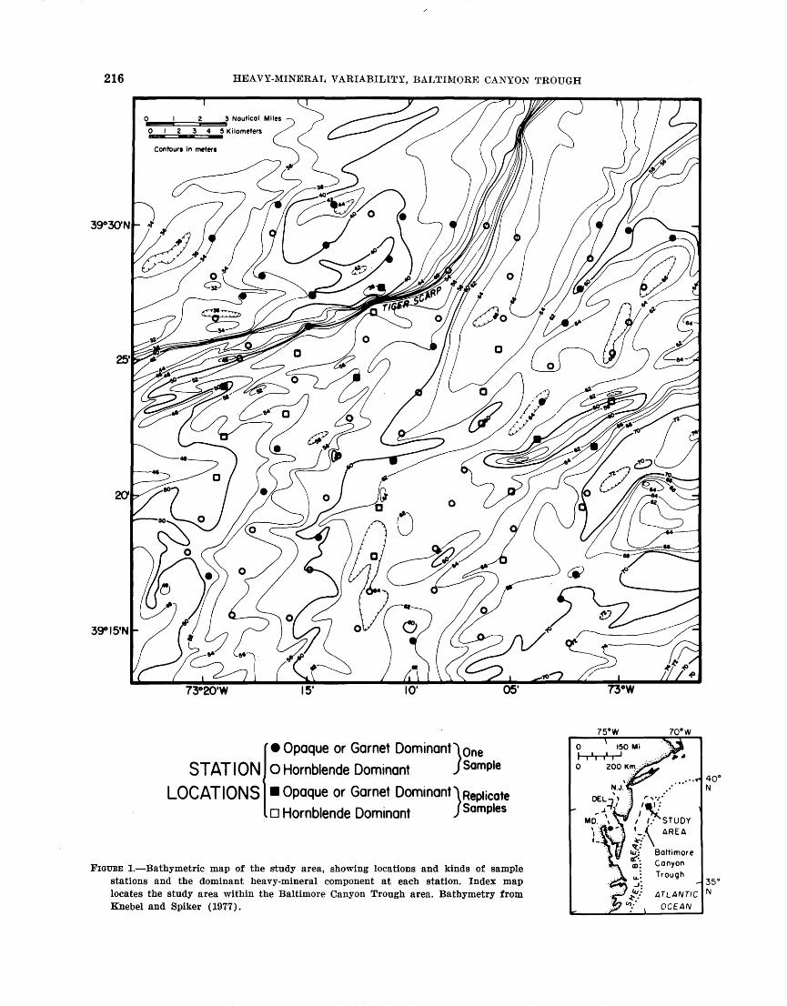
216 HEAVY-MINERAL VARIABILITY, BALTIMORE CANYON TROUGH
0123 Nouticol Miles
01 23 4 5 Kilometers
Contours in meters
39°30'N
25'
201
39°I5'N
73°20'W 15' 10' 05' 73eW
75°W 70° W
STATION LOCATIONS
Opaque or Garnet DominanHone O Hornblende Dominant j Sample
Opaque or Garnet Dominant ̂ 1 Replicate I a Hornblende Dominant ) Samples
FIGURE 1. Bathymetric map of the study area, showing locations and kinds of sample stations and the dominant heavy-mineral component at each station. Index map locates the study area within the Baltimore Canyon Trough area. Bathymetry from Knebel and Spiker (1977).
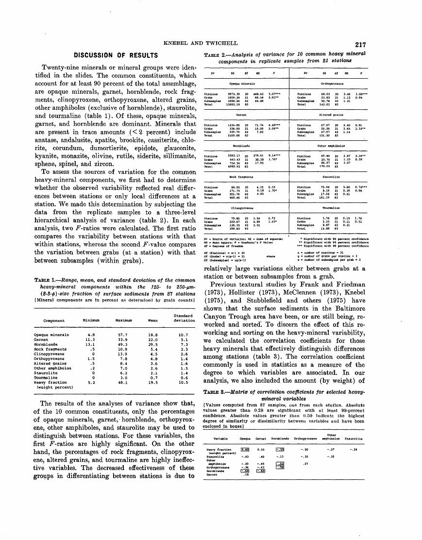
KNEBEL AND TWICHELL 217
DISCUSSION OF RESULTS
Twenty-nine minerals or mineral groups were iden tified in the slides. The common constituents, which account for at least 90 percent of the total assemblage, are opaque minerals, garnet, hornblende, rock frag ments, clinopyroxene, orthopyroxene, altered grains, other amphiboles (exclusive of hornblende), staurolite, and tourmaline (table 1). Of these, opaque minerals, garnet, and hornblende are dominant. Minerals that are present in trace amounts (<2 percent) include anatase, andalusite, apatite, brookite, cassiterite, chlo- rite, corundum, dumortierite, epidote, glauconite, kyanite, monazite, olivine, rutile, siderite, sillimanite, sphene, spinel, and zircon.
To assess the sources of variation for the common heavy-mineral components, we first had to determine whether the observed variability reflected real differ ences between stations or only local differences at a station. We made this determination by subjecting the data from the replicate samples to a three-level hierarchical analysis of variance (table 2). In each analysis, two F-ratios were calculated. The first ratio compares the variability between stations with that within stations, whereas the second F-value compares the variation between grabs (at a station) with that between subsamples (within grabs).
TABLE 1. Range, mean, and standard deviation of the common heavy-mineral components ivithin the 125- to 250-fim- (2-3-<f>)-size fraction of surface sediments from 87 stations
[Mineral components are In percent as determined by grain counts]
TABLE 2. Analysis of variance for 10 common heavy mineral components in replicate samples from 21 stations
Component
Opaque minerals.GarnetHornblendeRock fragmentsClinopyroxeneOrthopyroxeneAltered grainsOther amphibolesStauroliteTourmalineHeavy fraction(weight percent)
Minimum
4.811.313.1
.50
1.5.5.200
5.2
Maximum
57.733.949.310.913.97.88.47.06.23.0
48.1
Mean
18.822.029.55.44.54.83.62.62.10.719.5
Standard deviation
10.75.17.32.32.61.41.61.51.40.610.5
The results of the analyses of variance show that, of the 10 common constituents, only the percentages of opaque minerals, garnet, hornblende, orthopyrox ene, other amphiboles, and staurolite may be used to distinguish between stations. For these variables, the first F-raiios are highly significant. On the other hand, the percentages of rock fragments, clinopyrox ene, altered grains, and tourmaline are highly ineffec tive variables. The decreased effectiveness of these groups in differentiating between stations is due to
sv
Graba Subsamples Total
Grabs Subsamples Total
Stations Grabs Subsamples Total
Stations Grabs Subsamples Total
Grabs
Total
SV - Source a MS - Mean equ at - Degrees
df (Stations) it (Grabs) - df (Subsample
SS df MS t
Opaque minerals
1859.34 21 88.54 2.01** 1850.46 42 44.06
12682.19 83
Garnet
336.09 21 16.00 2.04** .329.70 42 7.85 2100.68 83
Hornblende
5592.13 20 279.61 9.14*** 642.43 21 30.59 1.70* 754.36 42 17.96 6988.92 83
Rock fragments
86.95 20 4.35 0.53 171.75 21 8.18 1.70* 201.76 42 4.80 460.46 83
Clinopyroxene
102.67 21 4.89 1.63*
299.82 83
f variationi SS - Sums of squares i are; P - Snedecor's P Valuei of freedom
- n-1 - 20 n(g-l) - 21 where s) - ng(s-l)
SV SS df MS P
Orthopyroxene
Grabs 23.82 21 1.13 0.94 Subsamples 50.76 42 1.21 Total 142.61 83
Altered grains
Graba 55.56 21 2.65 2.32" Subsamples 47.97 42 1.14 Total 151.50 83
Other amphiboles
Stations 87.40 20 2.87 2.34**' Grabs 25.75 21 1.23 O.S9 Subsamples 86.87 42 2.07 Total 170.02 83
Staurolite
Stations 75.94 20 3.80 9.74*** Graba 8.19 21 0.39 0.96 Subsamples 17.06 42 0.41 Total 101.19 83
Tourmaline
Grabs 2.25 21 0.11 O.S1
Total 14.88 83
Significant with 90 percent confidence Significant with 95 percent confidence
* Significant with 99 percent confidence
n number of stations 21 g number of grabs per station 2 s number of subsamplea per grab 2
relatively large variations either between grabs at a station or between subsamples from a grab.
Previous textural studies by Frank and Friedman (1973), Hollister (1973), McClennen (1973), Knebel (1975), and Stubblefield and others (1975) have shown that the surface sediments in the Baltimore Canyon Trough area have been, or are still being, re worked and sorted'. To discern the effect of this re working and sorting on the heavy-mineral variability, we calculated the correlation coefficients for those heavy minerals that effectively distinguish differences among stations (table 3). The correlation coefficient commonly is used in statistics as a measure of the degree to which variables are associated. In our analysis, we also included the amount (by weight) of
TABLE 3. Matrix of correlation coefficients for selected heavy- mineral variables
[Values computed from 87 samples, one from each station. Absolute values greater than 0.28 are significant with at least 99-percent confidence. Absolute values greater than 0.50 Indicate the highest degree of similarity or dissimilarity between variables and have been enclosed in boxes]
Variable
Heavy fraction(weight percent)
StauroliteOtheranphlbole*
OrthopyroxeneHornblendeGarnet
Opaque
rosi-.43
-.20-.36
F^51.18
OtherGarnet Hornblende Orthopyroxene amphiboles
0.25 FTSSl -.20 -.27
.40 -.13 -.30 -.35
-.45 1 .521 .27-.43 1 .561
PT351
Staurolite
-.24
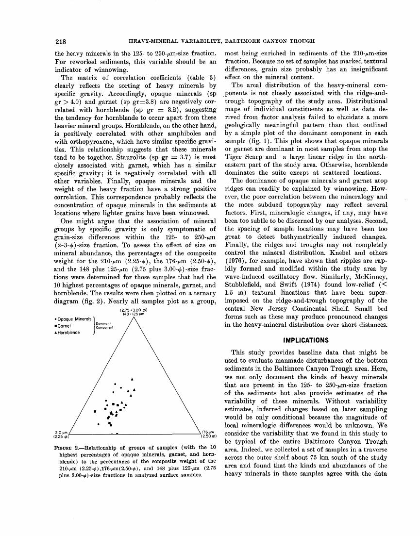
218 HEAVY-MINERAL VARIABILITY, BALTIMORE CANYON TROUGH
the heavy minerals in the 125- to 250-ju.m-size fraction. For reworked sediments, this variable should be an indicator of winnowing.
The matrix of correlation coefficients (table 3) clearly reflects the sorting of heavy minerals by specific gravity. Accordingly, opaque minerals (sp gr > 4.0) and garnet (sp gr=3.8) are negatively cor related with hornblende (sp gr = 3.2), suggesting the tendency for hornblende to occur apart from these heavier mineral groups. Hornblende, on the other hand, is positively correlated with other amphiboles and with orthopyroxene, which have similar specific gravi ties. This relationship suggests that these minerals tend to be together. Staurolite (sp gr = 3.7) is most closely associated with garnet, which has a similar specific gravity; it is negatively correlated with all other variables. Finally, opaque minerals and the weight of the heavy fraction have a strong positive correlation. This correspondence probably reflects the concentration of opaque minerals in the sediments at locations where lighter grains have been winnowed.
One might argue that the association of mineral groups by specific gravity is only symptomatic of grain-size differences within the 125- to 250-/*m (2-3 -</>) -size fraction. To assess the effect of size on mineral abundance, the percentages of the composite weight for the 210-^m (2.25-</>), the 176-/xm (2.50-<£), and the 148 plus 125-jU.m (2.75 plus 3.00-0)-size frac tions were determined for those samples that had the 10 highest percentages of opaque minerals, garnet, and hornblende. The results were then plotted on a ternary diagram (fig. 2). Nearly all samples plot as a group,
Opaque Minerals ] Garnet A Hornblende
(275 + 3.00 0) 148 +125 ym
210 ym (2.25 0)
FIGURE 2. Relationship of groups of samples (with the 10 highest percentages of opaque minerals, garnet, and horn blende) to the percentages of the composite weight of the 210-Aon (2.25-0 ),176-Mm(2.50-0), and 148 plus 125-/tm (2.75 plus 3.00-0)-size fractions in analyzed surface samples.
most being enriched in sediments of the 210-/xm-size fraction. Because no set of samples has marked textural differences, grain size probably has an insignificant effect on the mineral content.
The areal distribution of the heavy-mineral com ponents is not closely associated with the ridge-and- trough topography of the study area. Distributional maps of individual constituents as well as data de rived from factor analysis failed to elucidate a more geologically meaningful pattern than that outlined by a simple plot of the dominant component in each sample (fig. 1). This plot shows that opaque minerals or garnet are dominant in most samples from atop the Tiger Scarp and a large linear ridge in the north eastern part of the study area. Otherwise, hornblende dominates the suite except at scattered locations.
The dominance of opaque minerals and garnet atop ridges can readily be explained by winnowing. How ever, the poor correlation between the mineralogy and the more subdued topography may reflect several factors. First, mineralogic changes, if any, may have been too subtle to be discerned by our analyses. Second, the spacing of sample locations may have been too great to detect bathymetrically induced changes. Finally, the ridges and troughs may not completely control the mineral distribution. Knebel and others (1976), for example, have shown that ripples are rap idly formed and modified within the study area by wave-induced oscillatory flow. Similarly, McKinney, Stubblefield, and Swift (1974) found low-relief (< 1.5 m) textural lineations that have been super imposed on the ridge-and-trough topography of the central New Jersey Continental Shelf. Small bed forms such as these may produce pronounced changes in the heavy-mineral distribution over short distances.
This study provides baseline data that might be used to evaluate manmade disturbances of the bottom sediments in the Baltimore Canyon Trough area. Here, we not only document the kinds of heavy minerals that are present in the 125- to 250-//,m-size fraction of the sediments but also provide estimates of the variability of these minerals. Without variability estimates, inferred changes based on later sampling would be only conditional because the magnitude of local mineralogic differences would be unknown. We consider the variability that we found in this study to be typical of the entire Baltimore Canyon Trough area. Indeed, we collected a set of samples in a traverse across the outer shelf about 75 km south of the study area and found that the kinds and abundances of the heavy minerals in these samples agree with the data
KNEBEL AND TWICHELL 219
presented here. Disturbances of the bottom sediments in the Baltimore Canyon Trough area may arise from such activities as the emplacement of structures and pipelines, sand-mining operations, and waste dis posal.
The kinds, amounts, and variability of the heavy minerals are also characteristic of the modern sedi mentary environment in the Baltimore Canyon Trough area. In particular, the sorting of heavy minerals by specific gravity reflects the modern reworking of the sediments on this part of the shelf. By comparing the heavy minerals present at the surface with those present in subsurface samples (from drilling and coring), one might be able to distinguish between relict and modern deposits.
Estimates of the within-station variance indicate which heavy-mineral variables provide the best dis crimination between stations. The present study shows that some variables are ineffective because the differ ences between samples at a station are large. How ever, those variables that are diagnostic of between- station differences can reliably be used as indicators of regional mineralogic changes. A determination of the effectiveness of variables is useful in any areal study of heavy minerals, but it is crucial for those components of interest that have small regional dif ferences.
Finally, this study demonstrates that relatively large changes in the heavy-mineral composition can occur within a small area of the shelf (table 1). Often, in regional surveys, one or perhaps a few samples may represent an area the size of the study area, yet the range of values that we found for some components in this study is so large that no single sample could be considered typical of the entire area. Local variations, therefore, should be kept in mind when interpreting the results of regional surveys.
REFERENCES CITED
Frank, W. M., and Friedman, G. M., 1973, Continental-shelf sediments off New Jersey: Jour. Sed. Petrology, v. 43, no. 1, p. 224-237.
Galehouse, .T. S., 1971, Point counting, in Carver, R. E., ed., Procedures in sedimentary petrology: New York, Wiley- Interscience, p. 385-407.
Hollister, C. D., 1973, Atlantic Continental Shelf and Slope of the United States Texture of surface sediments from New Jersey to southern Florida: U.S. Geol. Survey Prof. Paper 529-M, 23 p.
Hubert, J. F., and Neal, W. F., 1967, Mineral composition and dispersal patterns of deep-sea sands in the western North Atlantic petrologic province: Geol. Soc. America Bull., v. 78, no. 6, p. 749-771.
Knebel, H. J., 1975, Significance of textural variations, Balti more Canyon Trough area: Jour. Sed. Petrology, v. 45, no. 4, p. 845-851.
Knebel, H. J., and Spiker, Elliott, 1977, Thickness and age of the surflcial sand sheet, Baltimore Canyon Trough area: Am. Assoc. Petroleum Geologists Bull., v. 61, no. 6, p. 861-871.
Knebel, H. J., Butman, Bradford, Folger, D. W., Cousins, P. W., and McGirr, R. R., 1976, Maps and graphic data related to geologic hazards in the Baltimore Canyon Trough area: U.S. Geol. Survey Misc. Field Studies Map MF-828, 3 sheets.
McClennen, C. E., 1973, Nature and origin of the New Jersey continental shelf topographic ridges and depressions: Rhode Island Univ., Kingston, Ph.D. thesis, 94 p.
McKinney, T. F., Stubblefield, W. L., and Swift, D. J. P., 1974, Large-scale current lineations on the central New Jersey shelf Investigations by side-scan sonar: Marine Geology, v. 17, no. 2, p. 79-102.
Milliman, J. D., Pilkey, 0. H., and Boss, D. A., 1972, Sedi ments of the continental margin off the Eastern United States: Geol. Soc. America Bull., v. 83, no. 5, p. 1315-1334.
Ross, D. A., 1970, Atlantic Continental Shelf and Slope of the United States Heavy minerals of the continental margin from southern Nova Scotia to northern New Jersey: U.S. Geol. Survey Prof. Paper 529-G, 40 p.
Smith, W., and Mclntyre, A. D., 1954, A spring-loaded bottom sampler: Jour. Marine Biol. Assoc., v. 33, p. 257-264.
Stubblefield, W. L., Lavelle, J. W., and Swift, D. J. P., 1975, Sediment response to the present hydraulic regime on the central New Jersey shelf: Jour. Sed. Petrology, v. 45, no. 1, p. 337-358.
Swift, D. J. P., Kofoed, J. W., Saulsbury, F. P., and Sears, Phillip, 1972, Holocene evolution of the shelf surface, central and southern Atlantic shelf of North America, in Swift, D. J. P., Duane, D. B., and Pilkey, O. H., eds., Shelf sediment transport Process and pattern: Strouds- burg, Pa., Dowden, Hutchinson, and Ross, Inc., p. 499-574.
U.S. Coast and Geodetic Survey and U.S. Bureau of Com mercial Fisheries, 1967, Bathymetric map, Hudson Canyon (0807N-52) : Washington, D.C., U.S. Coast and Geod. Survey, scale 1:125 000.

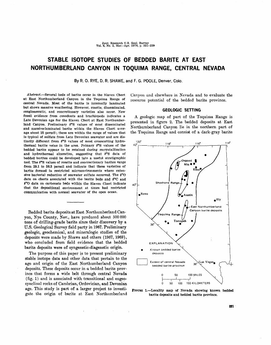
Jour. Research U.S. Qeol. Survey Vol. 6, No. 2, Mar.-Apr. 1978, p. 221-229
By R. 0. RYE, D. R. SHAWE, and F. G. POOLE, Denver, Colo.
Abstract. Several beds of barite occur in the Slaven Chert at East Northumberland Canyon in the Toquima Range of central Nevada. Most of the barite is internally laminated but shows massive weathering. However, rosette, disseminated, conglomeratic, and concretionary varieties also occur. New fossil evidence from conodonts and brachiopods indicates a Late Devonian age for the Slaven Chert at East Northumber land Canyon. Preliminary S^S values of most disseminated and massive-laminated barite within the Slaven Chert aver age about 25 permil; these are within the range of values that is typical of sulfate from Late Devonian seawater and are dis tinctly different from J^S values of most crosscutting hydro- thermal barite veins in the area. Primary S^S values of the bedded barite appear to be retained during recrystallization and hydrothermal alteration, suggesting that 5MS data of bedded barites could be developed into a useful stratigraphic tool. The fiMS values of rosette and concrectionary barites range from 29.1 to 56.3 permil and indicate that these varieties of barite formed in restricted microenvironments where exten sive bacterial reduction of seawater sulfate occurred. The 5180 data on cherts associated with the barite beds and SVC and a18O data on carbonate beds within the Slaven Chert indicate that the depositional environment at tames had restricted communication with normal seawater of the open ocean.
Bedded barite deposits at East Northumberland Can yon, Nye County, Nev., have produced about 500000 tons of drilling-grade barite since their discovery by a U.S. Geological Survey field party in 1967. Preliminary geologic, geochemical, and mineralogic studies of the deposits were made by Shawe and others (1967,1969), who concluded from field evidence that the bedded barite deposits were of syngenetic-diagenetic origin.
The purpose of this paper is to present preliminary stable isotope data and other data that pertain to the age and origin of the East Northumberland Canyon deposits. These deposits occur in -a bedded barite prov ince that forms a wide belt through central Nevada (fig. 1) and is associated with transitional and eugeo- synclinal rocks of Cambrian, Ordovician, and Devonian age. This study is part of a larger project to investi gate the origin of barite at East Northumberland
Canyon and elsewhere in Nevada and to evaluate the resource potential of the bedded barite province.
GEOLOGIC SETTING
A geologic map of part of the Toquima Range is presented in figure 2. The bedded deposits at East Northumberland Canyon lie in the northern part of the Toquima Range and consist of a dark-gray barite
120'118' 116°
/ / Canyon barite deposits
oquima Range-1 /
Tonopah38'
EXPLANATION
Known bedded barite deposits
Extent of central Nevada bedded barite province
50 100 MILESI
50 100 150 KILOMETERS
FIGURE 1. Locality map of Nevada showing known bedded barite deposits and bedded barite province.
221
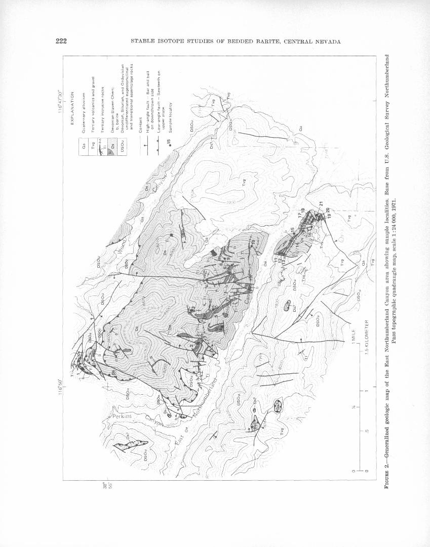
116° 50'
116° 47'3
0"
38
°55'
EX
PL
AN
AT
ION
Qu
ate
rna
ry a
llu
viu
m
Tert
iary
volc
anic
s a
nd
gra
ve
l
Tert
iary
in
trusiv
e r
ocks
De
vo
nia
n S
lave
n C
hert
; b,
barite
De
vo
nia
n,
Silurian,
an
d O
rdovic
ian
undiffe
rentiate
d e
ug
eo
syn
clin
al
an
d t
ransitio
nal
assem
bla
ge r
ocks
Hig
h-a
ngle
fa
ult
Ba
r and ball
on
do
wn
thro
wn
sid
e
Low
-angle
fa
ult S
aw
tee
th o
n
up
pe
r pla
te
OQ I f H M
02 o H
O
*D
H CO H
c! d t-H H 02 w H d a H a td t> S H
H O
H 2!
H
FIG
URE
2. G
ener
aliz
ed g
eolo
gic
map
of
the
Eas
t N
orth
umbe
rlan
d C
anyo
n ar
ea s
how
ing
sam
ple
loca
liti
es.
Bas
e fr
om U
.S.
Geo
logi
cal
Surv
ey N
orth
umbe
rlan
dP
ass
topo
grap
hic
quad
rang
le m
ap,
scal
e 1:
24 0
00,
1971
.
RYE, SHAWB, AND POOLE 223
unit approximately 18 meters thick and thinner barite units, which contain some intercalated chert and shaly mudstone and which are part of an allochthonous eugeo- synclinal sequence composed principally of dark-gray and black chert and siliceous mudstone of the Devonian Slaven Chert. Deposits which are believed to be equiv alent occur on both the north and south sides of the can yon near its mouth. Other bedded barite deposits are found at the Lost Soldier property in the upper drainage area of West Northumberland Canyon on the west side of the Toquima Kange. These deposits, which are probably equivalent to those near the mouth of East Northumberland Canyon, have been slightly re- crystallized in places due to the thermal effect of a nearby Jurassic pluton. Between the East and West Northumberland bedded barite deposits, clear barite crystals occur as fracture fillings near the Northumber land gold deposit south of Northumberland Pass. All of these barite occurrences were analyzed in this study.
The marine beds that contain bedded barite in East Northumberland Canyon were assigned to Ordovician strata by Kay and Crawford (1964). Since then, these beds have been recognized as the Slaven Chert of Middle and Late( ?) Devonian age. However, new fos sil evidence now indicates the age of the Slaven spans much of the Devonian (J. T. Dutro, Jr., written com- mun., 1977). A conodont fauna of very late Devonian age has been obtained from a thin impure cherty lime stone layer near the base of the allochthonous eugeo- synclinal sequence in the canyon (Poole and Sand- berg, 1975). In addition, a fragmentary brachiopod valve possibly belonging to the Famennian (late Late Devonian) rhychonelloid genus Dzieduszyckia has been found in a conglomeratic barite bed (Poole and Sandberg, 1975). Numerous attached pedicle and brachial valves of Dzieduszyckia were seen in a single horizon in bedded barite of the Slaven Chert in the Shoshone Eange, north-central Nevada. Many of the brachiopod shells, which are well preserved and simi larly oriented, appear to have been buried at or near their normal habitat. Cloud and Boucot (1971) re ported Dzieduszyckia in the Slaven Chert at several localities in the Shoshone Range. The Slaven Chert in this area is in part a sedimentary facies and is the time equivalent of the barite-bearing section at East Northumberland Canyon.
Eugeosynclinal siliceous rocks several hundred meters thick were deposited in northern California and western Nevada during the late Devonian; then, in latest Devonian time (during the Antler orogeny), they were tectonically transported eastward into thrust contact with transitional and miogeosynclinal, domi- nantly carbonate rocks of comparable (locally greater)
thickness (Poole and others, 1967). The Antler orogeny may have resulted from a possible increased subduc- tion rate beneath an offshore island arc along the western margin of the eugeosynclinal basin near the end of Devonian time. If this inferred plate-tectonic model is correct, the Late Devonian eugeosyncline would have occupied a marginal ocean basin between the continental edge and the island arc (Poole, 1974). The absence of recognizable Antler orogenic sediment in the Upper Devonian eugeosynclinal deposits indicates that initial downwarping of the marginal ocean basin was mild and that only a small volume, if any, of orogenic sediments was deposited in the Slaven Chert. The Upper Devonian carbonate shelf or miogeosyn- cline east of the eugeosyncline was characterized by a marked north-northeast-trending belt of thick car bonate deposits (Poole and others, 1967, figs. 9, 10). The eugeosynclinal facies are being further evaluated to provide a better understanding of the depositional setting and origin of the bedded barite and chert de posits.
EVIDENCE OF A SYNGENETIC-DIAGENETIC ORIGIN
A syngenetic-diagenetic origin of the bedded barite at East Northumberland Canyon is indicated by sev eral lines of evidence. The bedded barite, consisting of several varieties including massive-laminated,1 dissemi nated, rosette, conglomeratic, and concrectionary barite, displays features of primary sedimentation and early diagenesis. The barite rosettes were formed by growth of radiating barite blades and commonly nucleated on radiolarian tests, which suggests they were formed on the sea floor or in soft pelagic sediments. Graded bedding in barite beds is evident where bedding layers of rosettes decrease in size upward and grade into fine-grained massive-laminated barite. Conglomeratic barite that contains angular and rounded clasts of broken barite rock and chert, fragmental large barite rosettes, and phosphatic nodules is intercalated with beds of massive-laminated and rosette barite; this re lationship attests to erosion and resedimentation dur ing barite deposition. Barite concretions in mudstone may have been segregated during early diagenesis from mudstone containing disseminated barium and sulf ate.
A 87Sr/86Sr ratio of 0.7083 for a massive-laminated dark-gray barite sample from the south side of East Northumberland Canyon is consistent with a marine origin for the barite, although the ratio is also within the range of ratios for Cenozoic volcanic rocks in the region (C. E. Hedge, written commun., 1974).
Internally laminated massive weathering.
224 STABLE ISOTOPE STUDIES OF BEDDED BARITE, CENTRAL NEVADA
Late Devonian conodonts recovered from the cherty limestone layer in the eugeosynclinal section at East Northumberland Canyon are dark yellowish brown in color and indicate a moderate postdepositional tem perature history (Poole and Sandberg, 1975), judged from the method of Epstein, Epstein, and Harris (1975). The dark-yellowish-brown color of the cono donts indicates that they have not been subjected to prolonged temperatures above 200°C.
Madsen (1974) described "spongy-surface" chert from Devonian (reported by Madsen as Ordovician) chert layers interbedded with bedded barite rock at East Northumberland Canyon. The chert's texture was inherited from authigenic cristobalite forming bedded porcelanite. Bedded porcelanite was considered by Madsen to be of sedimentary origin. Metamorphosed chert consists of quartz that has an equigranular tex ture unlike that of the spongy-surface chert. Madsen pointed out that experiments by Ernst and Calvert (1969) on porcelanite from the upper Tertiary Mon- terey Formation of California showed that in rela tively pure water the fine-grained cristobalite would recrystallize to quartz in about 180 million years at 20°C and in about 4-5 m.y. at 50° C. The occurrence of spongy-surface chert at East Northumberland Can yon, therefore, suggests that the beds have not been subjected to prolonged high temperatures since deposi tion, and this finding is compatible with the moderate temperature history inferred from the conodont altera tion color.
Table 1 presents S 34S data on bedded and vein barites occurring in East and West Northumberland Canyons and on occurrences of barite crystals in veins near the Northumberland gold deposit. Table 2 presents 8180 data on cherts and 818O and 813C data on carbonates from the Slaven Chert at East Northumberland Can yon. The locations of most of the samples are shown in figure 2. Samples DRS-28-67A, B, C, and D were collected at the Northumberland gold deposit 5.5 kilo meters N. 5° W. of the junction of Perkins and East Northumberland Canyons, and samples 67FP-46 and 67FP^5 were collected 1.6 km N. 21° W. and 7.5 km N. 26° W., respectively, of the junction of Perkins and East Northumberland Canyons.
The 834S values were determined -by the technique described by Thode, Monster, and Dunford (1961). This method was used because total sulfate can be extracted from the impure barites without special puri fication procedures. The 8180 values in cherts were de termined by BrF5 extraction (Clayton and Mayeda,
1963) after boiling in aqua regia to remove organic material. Isotope data on carbonates were determined as described by McCrea (1950). All measurements were made on a modified Nuclide 6-60-RMS mass spectro meter. The isotope data are presented in the familiar 8 notation relative to international standards for each isotope: the oxygen isotope data are relative to SMOW (Craig, 1961), the carbon isotope data are relative to PDB (Craig, 1957), and the sulfur isotope data are relative to Canon Diablo troilite (Ault and Jensen, 1962). Analytical precision for all measurements was ±0.1 permil or better.
Sulfur isotope data and barite
Most of the bedded barite at East Northumberland Canyon is massive-laminated. The 834S values of 10 samples of the massive-laminated barite range from 20.9 to 28.6 permil, while 7 of the 10 samples have 834S values near 25 permil. The 834S values of oceanic sul fate have varied from about 10 to 33 permil through out geologic time, as indicated by analyses of marine evaporites (Holser and Kaplan, 1966; Thode and Monster, 1965; Claypool and others, 1972). During the Devonian, the 834S of seawater underwent large systematic variations and was between 24 and 30 permil during the Late Devonian. Values in this range are fairly rare for the 834S of seawater sulfate throughout geologic time. Available data on recent marine barites have 834S values similar to present-day seawater sulfate (Goldberg and others, 1969). The 834S data on the massive-laminated barite at East Northumberland thus strongly suggest a Late Devonian marine origin for the sulfate in the bedded barite.
Even though most of the 834S values of the massive- laminated barites cluster near 25 permil, a consider able range of values was obtained for individual beds. This is in contrast to published data on individual evaporites, which normally show very small ranges in 834S values for an entire formation (Holser and Kaplan, 1966).
Samples from measured sections on both the north and south sides of East Northumberland Canyon were analyzed (table 1). There appear to be no general systematics to the distribution of 834S values of the massive-laminated barites, although the values de crease toward the top of the section at locality 11. There is also no apparent correlation between 834S values and the silica, carbon, iron, organic, or clay content of the barites when the data are compared with the chemical data reported by Shawe and others, (1967). Furthermore, the iron (pyrite) content of the barites is apparently very low. Barite deposition ob-
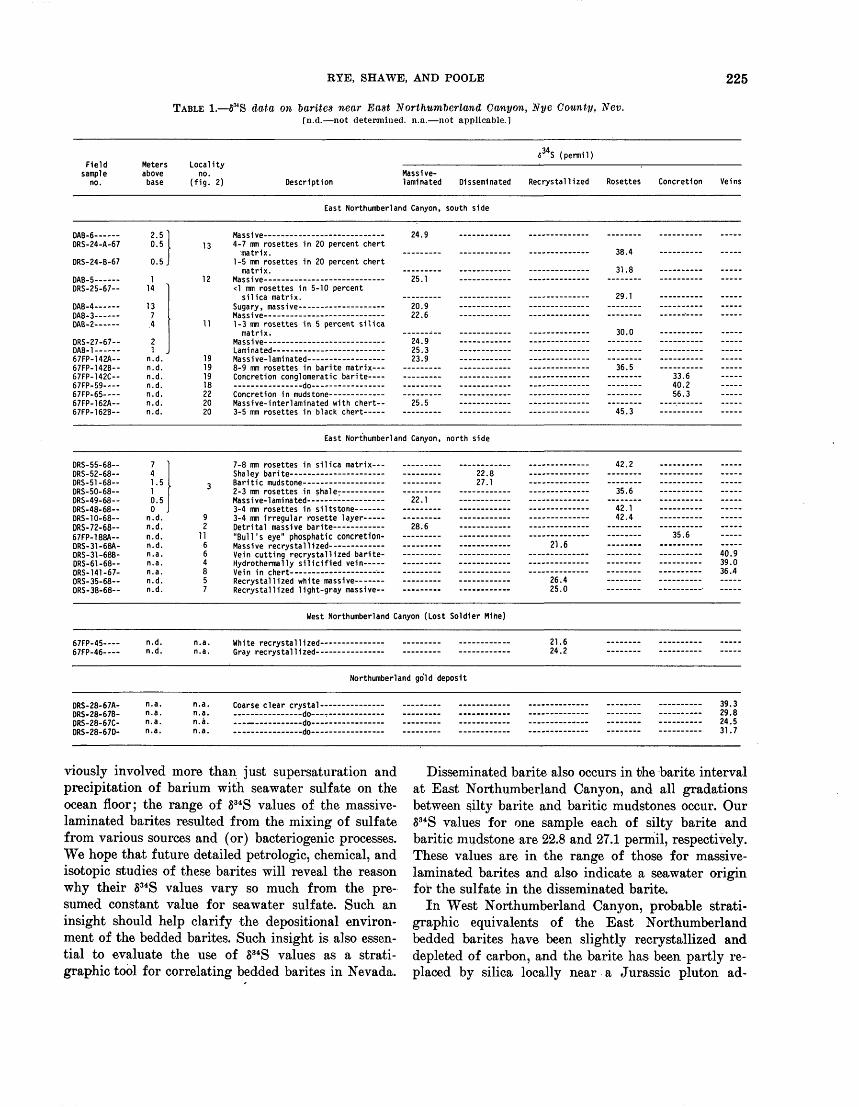
RYE, SHAWE, AND POOLE 225
TABLE 1. 5MS data on barites near East Northumberland Canyon, Nye County, Nev.[n.d. not determined, n.a. not applicable.]
Fieldsample
no.
Metersabove
base
Localityno.
(fig. 2)
(S 34 S (permil)
DescriptionMassive- laminated Disseminated RecrystalUzed Rosettes Concretion Veins
East Northumberland Canyon, south side
DAB-6 DRS-24-A-67
DRS-24-B-67
DAB-5 DRS-25-67-
DAB-4- DAB-3- DAB-2-
DRS-27-67- DAB-1 67FP-142A- 67FP-142B- 67FP-142C- 67FP-59 67FP-65 67FP-162A- 67FP-162B-
DRS-55-68-- DRS-52-68 DRS-51-68-- DRS-50-68 DRS-49-68-- DRS-48-68-- DRS-10-68-- DRS-72-68- 67FP-188A-- DRS-31-68A- DRS-31-68B- DRS-61-68-- DRS-141-67- DRS-35-68-- DRS-38-68-
2.50.5
0.5
114
137.4
21
n.d. n.d. n.d. n.d. n.d. n.d. n.d.
741.510.50
n.d. n.d. n.d. n.d. n.a. n.a. n.a. n.d. n.d.
Massive 24.9 13 4-7 mm rosettes in 20 percent chert
matrix. 38.4 1-5 mm rosettes in 20 percent chertmatr1x. 31.8 -
12 Massive - 25.1 -- ~ - . -<1 mm rosettes in 5-10 percent
silica matrix. 29.1 -Sugary, massive-- 20.9 - - - -----Massive-- 22.6 v -
11 1-3 mm rosettes in 5 percent silicamatrix. 30.0 -
Massive 24.9 -Laminated 25.3
19 Massive-laminated 23.9 -- 19 8-9 mm rosettes in barite matrix 36.5 19 Concretion conglomeratic barite 33.6 -----18 do 40.2 -22 Concretion in mudstone- - 56.3 .....20 Massive-interlaminated with chert-- 25.5 . 20 3-5 mm rosettes in black chert 45.3
East Northumberland Canyon, north side
7-8 mm rosettes in silica matrix -- 42.2 ...Shaley barite 22.8 -
3 Baritic mudstone 27.1 2-3 mm rosettes in shale 35.6 --------Massive-laminated 22.1 -3-4 mm rosettes in slltstone 42.1
9 3-4 mm irregular rosette layer- 42.4 --2 Detrital massive barite 28.6
11 "Bull's eye" phosphatic concretion- 35.6 6 Massive recrystallized- 21.6 - -6 Vein cutting recrystallized barite- 40.94 Hydrothermally silicified vein 39.08 Vein in chert -- 36.45 Recrystallized white massive 26.4 7 Recrystallized light-gray massive-- 25.0 - -----
nd Canyon (Lost Soldier Mine)
n.a. White recrystalllzed 21.6 n.a. Gray recrystallized 24.2
Northumberland gold deposit
n.a. Coarse clear crystal 39.3n.a. do r 29.8n.a. do 24.5n.a. do 31.7
67FP-45 67FP-46 -
DRS-28-67A- DRS-28-67B- DRS-28-67C- DRS-28-67D-
n.d. n.d.
n.a. n.a. n.a. n.a.
viously involved more than just supersaturation and precipitation of barium with seawater sulfate on the ocean floor; the range of 834S values of the massive- laminated barites resulted from the mixing of sulfate from various sources and (or) bacteriogenic processes. We hope that future detailed petrologic, chemical, and isotopic studies of these barites will reveal the reason why their 834S values vary so much from the pre sumed constant value for seawater sulfate. Such an insight should help clarify the depositional environ ment of the bedded barites. Such insight is also essen tial to evaluate the use of 834S values as a strati- graphic tool for correlating bedded barites in Nevada.
Disseminated barite also occurs in the barite interval at East Northumberland Canyon, and all gradations between silty barite and baritic mudstones occur. Our 834S values for one sample each of silty barite and baritic mudstone are 22.8 and 27.1 permil, respectively. These values are in the range of those for massive- laminated barites and also indicate a seawater origin for the sulfate in the disseminated barite.
In West Northumberland Canyon, probable strati- graphic equivalents of the East Northumberland bedded barites have been slightly recrystallized and depleted of carbon, and the barite has been partly re placed by silica locally near a Jurassic pluton ad-
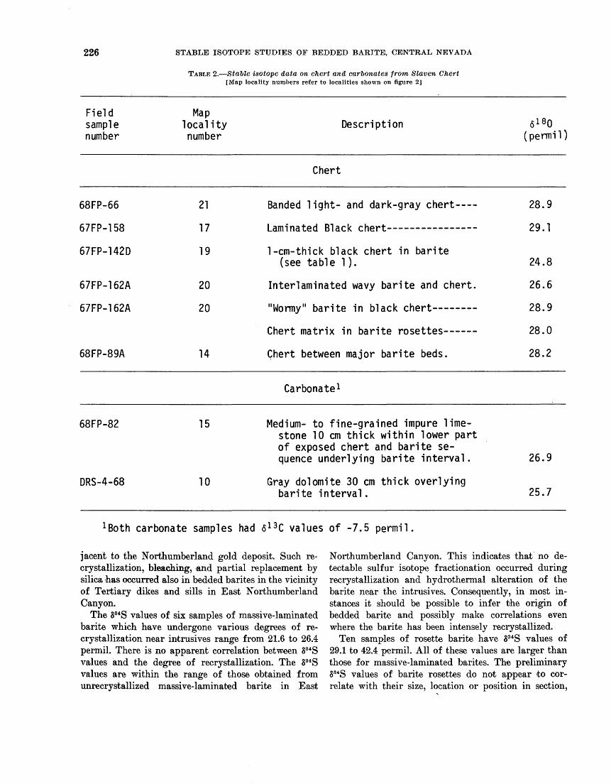
226 STABLE ISOTOPE STUDIES OF BEDDED BARITE, CENTRAL NEVADA
TABLE 2. Stable isotope data on chert and carbonates from Slaven Chert [Map locality numbers refer to localities shown on figure 2]
Fieldsamplenumber
Maplocalitynumber
Description 6 18 0(permil)
Chert
68FP-66
67FP-158
67FP-142D
67FP-162A
67FP-162A
68FP-89A
21
17
19
20
20
14
Banded light- and dark-gray chert
Laminated Black chert ----------------
1 -cm- thick black chert in barite (see table 1 ).
Inter! ami nated wavy barite and chert.
"Wormy" barite in black chert
vsiici i iiid ur IA in u«r i uc IUJCLLCO
Chert between major barite beds.
28.9
29.1
24.8
26.6
28.9
28.0
28.2
Carbonate 1
68FP-82
DRS-4-68
15
10
Medium- to fine-grained impure lime stone 10 cm thick within lower part of exposed chert and barite se quence underlying barite interval.
Gray dolomite 30 cm thick overlying barite interval.
26.9
25.7
carbonate samples had 6 13 C values of -7.5 permil.
jacent to the Northumberland gold deposit. Such re- crystallization, bleaching, and partial replacement by silica has occurred also in bedded barites in the vicinity of Tertiary dikes and sills in East Northumberland Canyon.
The 884S values of six samples of massive-laminated barite which have undergone various degrees of re- crystallization near intrusives range from 21.6 to 26.4 permil. There is no apparent correlation between 834S values and the degree of recrystallization. The 834S values are within the range of those obtained from unrecrystallized massive-laminated barite in East
Northumberland Canyon. This indicates that no de tectable sulfur isotope fractionation occurred during recrystallization and hydrothermal alteration of the barite near the intrusives. Consequently, in most in stances it should be possible to infer the origin of bedded barite and possibly make correlations even where the barite has been intensely recrystallized.
Ten samples of rosette barite have 834S values of 29.1 to 42.4 permil. All of these values are larger than those for massive-laminated barites. The preliminary 834S values of barite rosettes do not appear to cor relate with their size, location or position in section,
RYE, SHAWE, AND POOLE 227
or the nature of their matrix (mudstone, chert, or barite).
The rosettes presumably formed during a period of slow sedimentation on the sea floor or diagenetically below the sediment-water interface. The large 834S values for the rosettes are typical of values that result from partial reduction of seawater sulfate by micro organisms in a closed system (Nakai and Jensen, 1964). A critical test of whether this process occurred would be a comparison of 834S with with corresponding 8180 data. Mizutani and Rafter (1969) showed ex perimentally that the rate of 18O enrichment of S04 remaining in solution is about one-fourth of that of 34S enrichment during bacteriogenic reduction of sea- water sulfate. Sakai (1971) used this fact to conclude that bacteriogenic reduction of seawater sulfate was involved in the formation of Tertiary barite concre tions obtained off the west coast of Japan.
Two samples of barite concretions in mudstone have 834S values of 35.6 and 33.6 permil, and two samples of barite matrix from conglomeratic barite which is com posed of clasts of barite, chert, baritic to phosphatic nodules, and barite rosettes have 8 34S values of 33.6 and 40.2 permil. These values are similar to those for the rosettes and to those obtained from Tertiary barite concretions off the coasts of New Zealand (Kafter and Mizutani, 1967), California (Goldberg and others, 1969), and Japan (Sakai, 1971) and suggest that the nodules and conglomeratic matrix also formed in local closed chemical systems either on the sea floor or in the directly underlying sediments where bacterial re duction of seawater sulfate took place.
Barite occurs as crosscutting veins in two forms in the Northumberland area: as veins in chert and bedded barite and in breccia zones on both sides of East North umberland canyon and as crystals in open fractures near the Northumberland gold deposits. The 834S values of these occurrences range from 31.2 to 40.9 permil and are distinctly larger than those observed for the massive-laminated barite. Especially interesting is sample DRS-31-68, in which the vein barite has 8 34S of 40.9 permil and the recrystallized host bedded barite has 8 34S of only 21.6 permil.
The 834S values of large clear barite crystals near the Northumberland gold mine range from 24.5 to 39.3 permil. However, the 834S values of hydrothermal sulfates must be interpreted in terms of the 834S values of the hydrothermal fluid before inferences can be made about the origin of sulfur in these sulfates (Ohmoto, 1972; Rye and Ohmoto, 1974). Such inter pretation requires a knowledge of the physical-chem ical environment of vein barite deposition. We have
not been able to collect sulfides occurring with the vein barites nor do we have enough information on our samples to evaluate the chemical environment of vein barite deposition. Furthermore, the veins are probably low-temperature, and kinetic factors often dominate low-temperature systems when aqueous sulfate is present. However, all of the vein data could be ex plained if the sulfate were derived from massive bedded barite in the area having an average 834S value of 25 permil and redeposited from hydrothermal fluids at low temperatures under a range of /o2 conditions. Such a variation of /o2 conditions would not be un likely in an area that has both bedded barite and organic-rich cherts and mudstones.
Carbon and oxygen isotope data on cherts and carbonates
The 8180 and 813C values for various cherts and carbonates from the Devonian Slaven Chert are pre sented in table 2. The formation as a whole is pre- dominantely impure chert and mudstone, whereas the barite interval is relatively free of chert but in places contains thin chert layers with chert in various pro portions to barite. Carbonates are sparse in the Slaven Chert. A 10-cm-thick layer of impure limestone occurs at the base of the exposed Slaven Chert, and a 30-cm- thick layer of dolomite occurs higher in the section.
The 818O values of cherts range from 24.8 to 28.9 permil. The values for most samples are near 28 permil, which is within the lower part of the range commonly observed for "unaltered" Devonian marine cherts (Perry, 1967; Knauth and Epstein, 1976). Samples 67FP-142D and 67FP-162A and B are intimately associated with barite, and their low 818O values may reflect changes during diagenesis. The 8180 values of the carbonates are also typical of unaltered Devonian marine carbonates (Keith and Weber, 1964).
However, 813C values of the carbonates (-7.5 permil) are considerably lower than those of most marine carbonates, which normally have 813C values within the range ±4 permil as far back as 3X10⁹ years (Becker and Clayton, 1972). Similar 13C depletions have been observed in marine carbonates associated with Precambrian iron formations and have been in terpreted to indicate that the carbonate precipitated in organic-rich environments which were not open to the larger oceanic carbon reservoir. Such an interpre tation for the East Northumberland 813C data is con sistent with the 834S data on the barite rosettes, which suggests that, at least locally, the environment of depo sition was restricted and may have involved organic matter.
228 STABLE ISOTOPE STUDIES OF BEDDED BARITE, CENTRAL NEVADA
CONCLUSIONS
1. The 8 34S values of bedded, massive-laminated barite in the Slaven Chert from East Northum berland Canyon range from 20.9 to 28.6 per- mil, with most values near 25.0 permil, a value typical of Upper Devonian marine sulfate. A Late Devonian age for the Slaven Chert at East Northumberland Canyon is indicated by new fossil evidence. Although both the sulfate and barium must have come from the Devonian ocean, the ultimate source of the barium is not clear.
2. The fact that 8 34S value of the massive-laminated barite vary almost 8 permil, whereas these values in individual marine evaporites in other areas are nearly constant, suggests that either bacteria and (or) mixing of sulfur from two sources was locally involved in barite deposi tion or diagenesis.
3. The initial sedimentary S34S values of massive- laminated barite were apparently retained dur ing recrystallization, replacement by silica, and the loss of organic carbon associated with hydro- thermal alteration.
4. Once the cause of 8 34S variations in massive-lami nated barites is determined, it may be possible to use 834S as a stratigraphic tool in dating barites in the Nevada barite province.
5. Barite rosettes and concretions have 834 S values ranging from 29.1 to 56.3 permil, suggesting that they formed in a partially closed system either on the ocean floor or within the sediments, where bacterial reduction of seawater sulfate occurred.
6. The 8 34S values on crosscutting vein barites in the area, including those from the Northumberland gold deposit, are much larger than those for bedded barites and, considering the local isotope geochemistry, are consistent with the possibility that the sulfur in the veins was derived from bedded barites.
7. The 8 1&O data on most cherts and carbonates in the bedded barite interval in the Slaven Chert are typical of Devonian marine cherts and car bonates, while 813C values of the carbonates suggest they were deposited in organic-rich en vironments that had restricted communication with the carbon reservoir of the open ocean.
8. Evidence from conodont color alteration and chert textures indicates that the barite-bearing inter val at East Northumberland Canyon did not experience prolonged high temperatures or deep
burial and that the eugeosynclinal allochthon emplaced during the Antler orogeny was a "thin-skinned" feature which apparently re sulted from surficial thrusting during tectonic emplacement above transitional and miogeosyn- clinal rocks of the lower and middle Paleozoic outer continental shelf.
REFERENCES CITED
Ault, W. U., and Jensen, M. L., 1962, Summary of sulfur iso tope standards, in Jensen, M. L., ed., Biogeochemistry of sulfur isotopes: Natl. Sci. Found., Symposium Proc., New Haven, Conn., Yale Univ., Apr. 12-14, 1962, p. 16-29 [1963].
Becker, R. H., and Clayton, R. N., 1972, Carbon isotopic evi dence for the origin of a banded iron formation in West ern Australia: Geochim. et Cosmochim. Acta, v. 36, no. 5, p. 577-596.
Claypool, G. E., Holser, W. T., Kaplau, I. R., Sakai, H., and Zak, I., 1972, Sulfur and oxygen geochemistry of evaporite sulfates: Geol. Soc. America Abs. with Programs, v. 4, no. 7, p. 473.
Clayton, R. N., and Mayeda, T. K., 1963, The use of bromine pentafluoride in the extraction of oxygen from oxides and silicates for isotopic analysis: Geochim. ,et Cosmochim. Acta, v. 27, p. 43-52.
Cloud, P. E., Jr., and Boucot, A. J., 1971, Dzieduszyckia in Nevada, in Dutro, J. T., Jr, ed., Paleozoic perspectives a paleontological tribute to G. Arthur Cooper: Smithsonian Contr. Paleobiology, no. 3, p. 175-180.
Craig, Harmon, 1957, Isotopic standards for carbon and oxygen and correction factors for mass-spectrometric analysis of carbon dioxide: Geochim. et Cosmochim. Acta, v. 12, nos. 1-2, p. 133-149.
1961, Standard for reporting concentrations of deu terium and oxygen-18 in natural waters: Science, v. 133, no. 3467, p. 1833-1834.
Epstein, A. G., Epstein, J. B., and Harris, L. D., 1975, Conodont color alteration an index to organic inetamorphism: U.S. Geol. Survey Open-File Report 75-379, 54 p.
Ernst, W. G., and Calvert, S. E., 1969, An experimental study of the recrystallization of porcelanite and its bearing on the origin of some bedded cherts: Am. Jour. Sci., v. 267- A (Schairer Volume), p. 114-133.
Goldberg, E. D., Somayajulu, B. L. K., Galloway, James, Kaplan, I. R.. and Faure, Gunter, 1969, Differences between barites of marine continental origins: Geochim. et Cosmochim. Acta, v. 33, p. 287-289.
Holser, W. T., and Kaplan, I. R., 1966, Isotope geochemistry of sedimentary sulfates: Chem. Geology, v. 1, no. 2, p. 93-135.
Kay, Marshall, and Crawford, J. P., 1964, Paleozoic facies from the miogeosynclinal to the eugeosynclinal belt in thrust slices, central Nevada: Geol. Soc. America Bull., v. 75, no. 5, p. 426-454.
Keith, M. L., and Weber, J. N., 1964, Carbon and oxygen iso topic composition of selected limestones and fossils: Geo chim. et Cosmochim. Acta, v. 28, p. 1787-1816.
Knauth, P. L., and Epstein, Samuel, 1976, Hydrogen and oxygen isotope ratios in nodular and bedded cherts: Geochim. et Cosmochim. Acta, v. 40, p. 1095-1108.
RYE. SHAWE, AND POOLE 229
Madsen, B. M., 1974, Origin of spongy cherts: U.S. Geol. Sur vey Jour. Research, v. 2, no. 6, p. 685-687.
McCrea, J. M., 1950, On the isotopic chemistry of carbonates and paieotemperature scale: Jour. Chem. Physics, v. 18, p. 849-857.
Mizutani, Y., and Rafter, T. A., 1969. Oxygen isotopic com position of sulphates, pt. 4, Bacterial fractionation of oxygen isotopes in the reduction of sulphate and in the oxidation of sulphur: New Zealand Jour. Sci., v. 12, p. 60- 68.
Nakai, Nobuyaki, and Jensen, M. L., 1964, The kinetic isotope effect in the bacterial reduction and oxidation of sulfur: Geochim. et Cosmochim. Acta, v. 28, p. 1893-1912.
Ohmoto, Hiroshi, 1972, Systematics of sulfur and carbon iso topes in hydrothermal ore deposits: Econ. Geol., v. 67, p. 551-578.
Perry, E. C., Jr., 1967, The oxygen isotope chemistry of an cient cherts: Earth and Planetary Sci. Letters, v. 3, p. 62-66.
Poole, F. G., 1974, Flysch deposits of the Antler foreland basin, western United States, in Dickinson, W. R., ed., Tectonics and sedimentation: Soc. Econ. Paleontologists and Mineralogists Spec. Pub. 22, p. 58-82.
Poole, F. G., Baars, D. L., Drewes, Harald, Hayes, P. T., Ketner, K. B., McKee, E. D., Teichert, Curt, and Williams, J. S., 1967, Devonian of the southwestern United States, in Oswald, D. H., ed., Internat. symposium on the Devon ian System, Calgary, Alberta, Canada, Sept. 1967: Alberta Soc. Petroleum Geologists, v. 1, p. 879-912.
Poole, F. G., and Sandberg, C. A., 1975, Allochthonous Devon ian eugeosynclinal rocks in Toquima Range, central Nevada: Geol. Soc. America Abs. with Programs, v. 7, no. 3, p. 361.
Rafter, T. A., and Mitzutani, Y., 1967, Oxygen isotopic com position of sulphates, pt. 2, Preliminary results on oxygen isotopic variation in sulphates and the relationship to their environment and to their S^S values: New Zealand Jour. Sci., v. 10, p. 816-840.
Rye, R. O., and Ohmoto, Hiroshi, 1974, Sulfur and carbon isotopes and ore genesis A review: Econ. Geol., v. 69, p. 826-842.
Sakai, Hitoshi, 1971, Sulfur and oxygen isotopic study of barite concretions from banks in the Japan Sea off the Northeast Honshu, Japan: Geochemical Journal, v. 5, p. 79-93.
Shawe, D. R., Poole, F. G., and Brobst, D. A., 1967, Bedded barite in East Northumberland Canyon, Nye County, Nevada: U.S. Geol. Survey Circ. 555, 8 p.
, 1969, Newly discovered bedded barite deposits in East Northumberland Canyon, Nye County, Nevada: Econ. Geology, v. 64, no. 3, p. 245-254.
Thode, H. G., and Monster, Jan, 1965, Sulfur-isotope geochem istry of petroleum, evaporites, and ancient seas, in Fluids in subsurface environments: Am. Assoc. Petroleum Geo logists Mem., no. 4, p. 367-377.
Thode, H. G., Monster, Jan, and Dunford, H. B., 1961. Sul phur isotope geochemistry: Geochim. et Cosmochim. Acta, v. 25, p. 159-174.

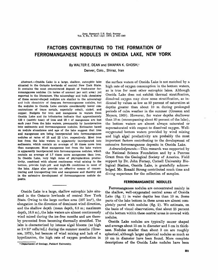
Jour. Research U.S. Qeol. Survey Vol. 6, No. 2, Mar.-Apr. 1978, p. 231-240
FACTORS CONTRIBUTING TO THE FORMATION OF FERROMANGANESE NODULES IN ONEIDA LAKE, NEW YORK
By WALTER E. DEAN and SWAPAN K. GHOSH, 1
Denver, Colo., Shiraz, Iran
Abstract. Oneida Lake is a large, shallow, eutrophic lake situated in the Ontario lowlands of central New York State. It contains the most concentrated deposit of freshwater fer romanganese nodules (in terms of amount per unit area) yet reported in the literature. The mineralogy and bulk chemistry of these saucer-shaped nodules are similar to the mineralogy and bulk chemistry of deep-sea ferromanganese nodules, but the nodules in Oneida Lake contain considerably lower con centrations of trace metals, especially cobalt, nickel, and copper. Budgets for iron and manganese in waters from Oneida Lake and its tributaries indicate that approximately 122 t (metric tons) of iron and 23 t of manganese are lost each year from the lake waters, presumably by incorporation into sediments and ferromanganese nodules. Estimates based on nodule abundance and age of the lake suggest that iron and manganese are being incorporated into ferromanganese nodules at rates of 13 and 22 t/yr, respectively. Most iron lost from the lake waters is apparently incorporated into sediments, which contain an average of 10 times more iron than manganese. Most manganese lost from the lake waters is apparently incorporated into ferromanganese nodules, which contain an average of 1.7 times more manganese than iron. In Oneida Lake, very high rates of phytoplankton produc tivity, combined with almost continuous wind mixing to the bottom, provide high-pH and high-Eh conditions in most of the lake. Algae also provide an effective means of concen trating and transporting iron and manganese and thereby aid in the extensive development of ferromanganese nodule de posits.
Oneida Lake is a large, shallow eutrophic lake situ ated in 'the Ontario lowlands of central New York State. Owing to the large surface area (207 km2 ), the elongation in the direction of dominant wind direction, and the shallow depth (mean depth, 6.8 m; maximum depth, 16.8 m), the lake waters are almost continuously wind mixed during the ice-free months and are there by prevented from becoming thermally stratified. The lake is characterized by intense algal blooms (as high as 2X10⁵ cells/mL) during the summer months (Gree- son, 1972), but because of wind mixing and lack of a hypolimnion, the high rate of oxygen production in
1 Department of Geology, Pahlavl University.
the surface waters of Oneida Lake is not matched by a high rate of oxygen consumption in the bottom waters, as is true for most other eutrophic lakes. Although Oneida Lake does not exhibit thermal stratification, dissolved oxygen may show some stratification, as in dicated by values as low as 50 percent of saturation at depths greater than about 10 m during prolonged periods of calm weather in the summer (Greeson and Meyers, 1969). However, for water depths shallower than 10 m (encompassing about 60 percent of the lake), the bottom waters are almost always saturated or supersaturated with respect to dissolved oxygen. Well- oxygenated bottom waters provided by wind mixing and high algal productivity are probably the most important factors contributing to the development of extensive ferromanganese deposits in Oneida Lake.
Acknowledgments. This research was supported by the National Science Foundation and by a Penrose Grant from the Geological Society of America. Field support by Dr. John Forney, Cornell University Bio logical Station, Oneida Lake, is gratefully acknow ledged. Mr. Ronald Strong contributed much time and diving experience for the collection of samples.
FERROMANGANESE NODULES
Ferromanganese nodules are concentrated mainly in the shallow, well-oxygenated central areas of Oneida Lake (fig. 1) in water depths less than 10 m. Some parts of the lake bottom in these areas are almost com pletely paved with nodules (fig. 2). We estimate, on the basis of visual observations, that about 25 percent of the bottom within these central areas is covered with nodules.
Oneida Lake nodules are typically saucer shaped and average about 15 cm in diameter and 5 cm in thick ness. Nodules smaller than about 3 cm are roughly spherical, although larger spherical nodules as much as 10 cm in diameter have been found. More complete descriptions of the Oneida Lake nodules have been
231
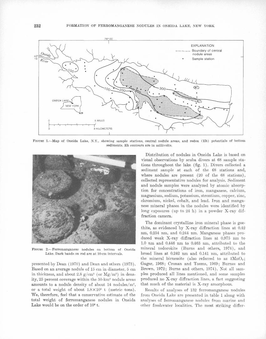
232 FORMATION OP FERROMANGANESE NODULES IN ONEIDA LAKE, NEW YORK
43' 15
EXPLANATION
Boundary of central nodule areas
Sample station
ONEIDA LAKE
NEW YORK
5 MILES
8 KILOMETERS
_________I
FIGURE 1. Map of Oneida Lake, N.Y., showing sample stations, central nodule areas, and redox (Eh) potentials of bottomsediments. Eh contours are in millivolts.
Distribution of nodules in Oneida Lake is based on visual observations by scuba divers at 68 sample sta tions throughout the lake (fig. 1). Divers collected a sediment sample at each of the 68 stations and, where nodules are present (20 of the 68 stations), collected representative nodules for analysis. Sediment and nodule samples were analyzed by atomic absorp tion for concentrations of iron, manganese, calcium, magnesium, sodium, potassium, strontium, copper, zinc, chromium, nickel, cobalt, and lead. Iron and manga nese mineral phases in the nodules were identified by long exposures (up to 24 h) in a powder X-ray dif fraction camera.
The dominant crystalline iron mineral phase is goe- thite, as evidenced by X-ray diffraction lines at 0.42 nm, 0.254 nm, and 0.244 nm. Manganese phases pro duced weak X-ray diffraction lines at 0.975 nm to 1.0 nm and 0.446 nm to 0.463 nm, attributed to the mineral todorokite (Burns and others, 1074), and broad lines at 0.242 nm and 0.141 nm, attributed to the mineral birnessite (also referred to as SMnO2 ; Gager, 1968; Cronan and Tooms, 1969; Burnes and Brown, 1972; Burns and others, 1974). Not all sam ples produced all lines mentioned, and some samples produced no X-ray diffraction lines, a fact suggesting that much of the material is X-ray amorphous.
Results of analyses of 132 ferromanganese nodules from Oneida Lake are presented in table 1 along with analyses of ferromanganese nodules from marine and other freshwater localities. The most striking differ-
FIOUBE 2. Ferromanganese nodules on bottom of Oneida Lake. Dark bands on rod are at 10-cm intervals.
presented by Dean (1970) and Dean and others (1973). Based on an average nodule of 15 cm in diameter, 5 cm in thickness, and about 2.8 g/cm3 (or Mg/m3 ) in dens ity, 25 percent coverage within the 50-km2 nodule areas amounts to a nodule density of about 14 nodules/m2 , or a total weight of about 1.8X10° t (metric tons). We, therefore, feel that a conservative estimate of the total weight of ferromanganese nodules in Oneida Lake would be on the order of 106 1.
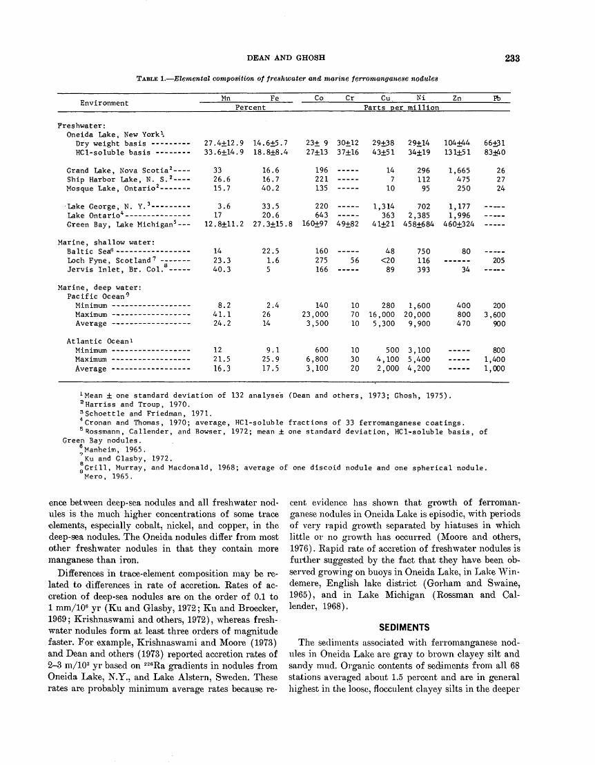
DEAN AND GHOSH 233
TABLE 1. Elemental composition of freshwater and marine ferromanganese nodules
EnvironmentMn Fe Co Cr Cu Ni Zn
Percent Parts per millionPb
Freshwater:Oneida Lake, New York 1.
Dry weight basis ---- HCl-soluble basis ---
Grand Lake, Nova Scotia 2 -- Ship Harbor Lake, N. S. 2 -- Mosque Lake, Ontario 2 -----
Lake George, N. Y. 3 -----Lake Ontario4 -------------Green Bay, Lake Michigan 5 -
Marine, shallow water:Baltic Sea6 -------------Loch Fyne, Scotland 7 -----Jervis Inlet, Br. Col.
27.4±12.9 33.6+14.9
3326.615.7
3.6 17
12.8±11.2
1423.340.3
14.6±5.7 18.8+8.4
16.616.740.2
33.520.6
27 .3+15 . i
22.51.65
23± 9 30±12 29±38 29+14 27±13 37±16 43+51 34±19
196221135
147
10
29611295
104+44 131±51
1,665475250
220 643
160+97 49+82
1,314 702 1,177363 2,385 1,996
41+21 458±684 460±324
160275166
5648
<2089
750116393
80
34
66+31 83+40
262724
205
Marine, deep water: Pacific Ocean 9
Atlantic Ocean*
41.O 7
1221.16.
212
53
2O£
14
92517
.4
.1
.9
.5
233
63
140,000,500
600,800,100
107010
103020
OQA
16,0005,300
5004,1002,000
120
9
354
,600,000,900
,100,400,200
400 200800 3,600 470 900
800
L , HU v
1,000
x Mean ± one standard deviation of 132 analyses (Dean and others, 1973; Ghosh, 1975). 2 Harriss and Troup, 1970. 3 Schoettle and Friedman, 1971.Cronan and Thomas, 1970; average, HCl-soluble fractions of 33 ferromanganese coatings.
5 Rossmann, Callender, and Bowser, 1972; mean ± one standard deviation, HCl-soluble basis, of Green Bay nodules.
Manheim, 1965. 7 Ku and Glasby, 1972. 9 Grill, Murray, and Macdonald, 1968; average of one discoid nodule and one spherical nodule.Mero, 1965.
ence between deep-sea nodules and all freshwater nod ules is the much higher concentrations of some trace elements, especially cobalt, nickel, and copper, in the deep-sea nodules. The Oneida nodules differ from most other freshwater nodules in that they contain more manganese than iron.
Differences in trace-element composition may be re lated to differences in rate of accretion. Rates of ac cretion of deep-sea nodules are on the order of 0.1 to 1 mm/106 yr (Ku and Glasby, 1972; Ku and Broecker, 1969; Krishnaswami and others, 1972), whereas fresh water nodules form at least three orders of magnitude faster. For example, Krishnaswami and Moore (1973) and Dean and others (1973) reported accretion rates of 2-3 m/103 yr based on 226Ra gradients in nodules from Oneida Lake, N.Y., and Lake Alstern, Sweden. These rates are probably minimum average rates because re
cent evidence has shown that growth of ferroman ganese nodules in Oneida Lake is episodic, with periods of very rapid growth separated by hiatuses in which little or no growth has occurred (Moore and others, 1976). Rapid rate of accretion of freshwater nodules is further suggested by the fact that they have been ob served growing on buoys in Oneida Lake, in Lake Win- demere, English lake district (Gorham and Swaine, 1965), and in Lake Michigan (Rossman and Cal lender, 1968).
SEDIMENTS
The sediments associated with ferromanganese nod ules in Oneida Lake are gray to brown clayey silt and sandy mud. Organic contents of sediments from all 68 stations averaged about 1.5 percent and are in general highest in the loose, flocculent clayey silts in the deeper
234 FORMATION OF FERROMANGANESE NODULES IN ONEIDA LAKE, NEW YORK
parts of the lake below the depth of wind mixing and summer oxygen stratification. Shoal areas in the center of the lake are probably drumlins or drumlinoid fea tures and consist of coarse glacial till wiith much, of the sand fraction winnowed out. The hard sand areas sur rounding the shoals are strewn with cobbles and boul ders from the shoals and provide the most common nuclei for ferromanganese nodules that have obvious core materials. The hard bottom areas adjacent to the shoals contain the most abundant nodules, and, in some areas, almost every cobble and boulder is enclosed in a rim of ferromanganese material at the sediment-water interface. Results of analyses of sediments from all 68 stations are summarized in table 2.
Concentrations of major elements in sediment inter stitial (pore) waters are typically several times higher than in average lake water of Oneida Lake (table 3). Iron concentrations in interstitial waters are about the same as the average in the lake water, but manganese concentrations in interstitial water are typically sev eral orders of magnitude higher than those in the lake water. Sediment Eh values range from about 40 to 400 mV and are highest in the central part of the lake (fig.l).
TABLE 2. Concentration of strontium, calcium, mag nesium, sodium, potassium, copper, mine, iron, and man ganese in sediments from Oneida Lake
[Values are in percent dry weight of sediment, averaged for 68 sampling stations]
Element
O-.
Mg IN d
K ----Cu -7n ---------oil
Fe Mn __________
Mean concentration
0.10.48.54na
.25
.003
.012.05
17
TABLE 3. Ratios of concentrations of six elements in sediment interstitial (pore) waters from a nodule-oc curring area and a nonnodule area to the average con centration of each element in Oneida Lake surface water
Ratio of concentration of element in sediment pore water to average concen tration of element in lake water
pfl -----__.Mg
K ______^iMn -
Nodule area
2 1
2.14.1.5
40
Nonnodule area
1.43 /!
2.14.6.7
117
Budgets of iron and manganese
Abundant data on the water chemistry of Oneida Lake and its tributaries have been reported by Gree- son (1972). Greeson's data show that the most impor tant sources of dissolved solids in Oneida Lake are the southern tributaries draining areas of Silurian and Devonian carbonate bedrock. A budget of total dis solved solids indicates an average input of 1120 metric tons per day, an output of 996 t/d, with a net loss to the sediments of 124 t/d. Net losses of major elements range from 0.09 t/d for potassium to 32 t/d for cal cium (Greeson, 1972).
Although there are not as many data for trace ele ments in tributaries to Oneida Lake as there are for major elements and macronutrients, we have calculated approximate budgets for iron and manganese (table 4). Concentrations of iron and manganese given in table 4 are based' on analyses of two water samples from each tributary, one collected in the spring (April 29-30, 1969) and one collected in the fall (October 1-2, 1969). Discharge values in table 4 are based on a standard 30-yr period from 1931 to 1960. Discharges for 1969, the year in which the water samples were collected for trace-element analyses, were slightly higher than the 30-yr averages, but this should have little effect on the budgets. The budgets in table 4 in dicate that an average of 122 t of iron and 23 t of manganese are removed from the lake water each year, presumably by incorporation into sediments and ferromanganese nodules.
Element concentrations for Oneida Lake nodules listed in table 1 are arithmetric means based on anal yses-of 132 nodules. Arithmetic means and standard deviations were used in table 1 for ease of comparison with arithmetic mean concentrations reported for nod ules from other localities. However, actual distribu tions of iron, manganese, and minor elements in Oneida Lake nodules are closer to lognormal than normal, and we feel that geometric means would be more appropriate measures of central tendency for budget calculations. Geometric mean concentrations of iron and manganese in 132 nodules are 13 and 22 t, respec tively. This amounts to an average of 13 t of iron and 22 t of manganese added to nodules each year, if we assume that the estimated total of 109 t of nodules formed over the entire 104-yr postglacial history of Oneida Lake. Comparison of these figures with annual losses of iron and manganese from lake water (table 4) suggests that almost all of manganese loss from the lake water can be explained by incorporation of manganese into ferromanganese nodules. However,
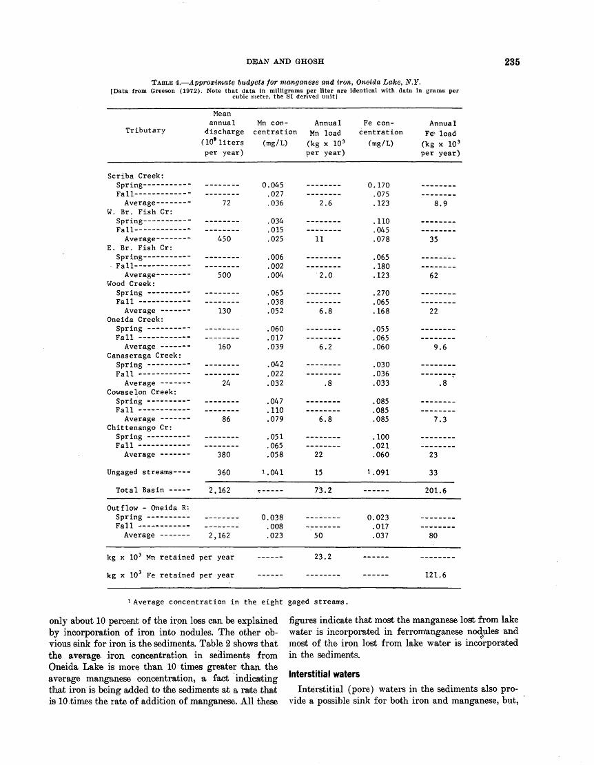
DEAN AND GHOSH 235
TABLE 4. Approximate budgets for manganese and iron, Oneida Lake, N.Y.[Data from Greeson (1972). Note that data in milligrams per liter are identical with data in grams per
cubic meter, the SI derived unit]
Tributary
Scriba Creek:Spring ---Fall Average --------
W. Br. Fish Cr:Spring------ ----T7 fl 11 -------------
Average------- -E. Br. Fish Cr:
Spring-- ---Fall----- ------Average- -------
Wood Creek:Spring --- -------Fall ------------Average - --
Oneida Creek:Spring -Fall
Average -------Canaseraga Creek:
Spring --
Average -------Cowaselon Creek:
Spring - -17-11 ____________
Average -------Chittenango Cr:
Spring --- ----Fall - ---------Average -------
Ungaged streams--- -
Total Basin -----
Outflow - Oneida R:Spring -- -Fall Average -- -
kg x 10 3 Mn retained
kg x 10 3 Fe retained
Meanannual
discharge(10* litersper year)
72
450
500
130
160
24
86
380
360
2,162
2,162
per year
per year
Mn con- Annualcentration Mn ioad
(mg/L) (kg x 10 3per year)
0.045 .027 .036 2.6
.034
.015
.025 11
.006
.002
.004 2.0
.065 mo
.052 6.8
.060
.017
.039 6.2
.042
.022
.032 .8
.047
.no ........
.079 6.8
.051
.065 ...._
.058 22
1.041 15
r 73.2
O nto.008 .........023 50
23.2
Fe con- Annualcentration Fe"1 load
(mg/L) (kg x 10 3per year)
0.170 ....075 ..123 8.9
.110 ........C\L. 5 ________
.078 35
.065 i Qn
.123 62
.270 nc.<z
.168 22
.055 ........
.065 -----
.060 9.6
.030
.036 r
.033 .8
no^noc
.085 7.3
.100 -------
.021 .-..._
.060 23
1.091 33
201.6
0.023 ~.017 .......037 80
121.6
Average concentration in the eight gaged streams.
only about 10 percent of the iron loss can be explained by incorporation of iron into nodules. The other ob vious sink for iron is the sediments. Table 2 shows that the average iron concentration in sediments from Oneida Lake is more than 10 times greater than the average manganese concentration, a fact indicating tlhat iron is being added to tihe sediments at a rate that is 10 times the rate of addition of manganese. All these
figures indicate that most the manganese losit from lake water is incorporated in ferrom'anganese nodules' and most of the iron lost from lake water is incorporated in the sediments.
Interstitial watersInterstitial (pore) waters in the sediments also pro
vide a possible sink for both iron and manganese, but,
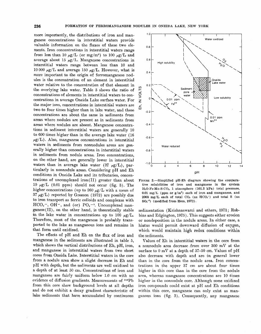
236 FORMATION OF FERROMANGANESE NODULES IN ONEIDA LAKE, NEW YORK
more importantly, the distributions of iron and man ganese concentrations in interstitial waters provide valuable information on the fluxes of these two ele ments. Iron concentrations in interstitial waters range from less than 10 /*g/L (or mg/m3 ) to 100 /ig/L and average about 15 /*g/L. Manganese concentrations in interstitial waters range between less than 10 and 10 000 /Ag/L and average 150 fig/L. However, what is more important to the origin of ferromanganese nod ules is the concentration of an element in interstitial water relative to the concentration of that element in the overlying lake water. Table 3 shows the ratio of concentrations of elements in interstitial waters to con centrations in average Oneida Lake surface water. For the major ions, concentrations in interstitial waters are two to four times higher than in lake water, and these concentrations are about the same in sediments from areas where nodules are present as in sediments from areas where nodules are absent. Manganese concentra tions in sediment interstitial waters are generally 10 to 600 times higher than in the average lake water (16 /*g/L). Also, manganese concentrations in interstitial waters in sediments from nonnodules areas are gen erally higher than concentrations in interstitial waters in sediments from nodule areas. Iron concentrations, on the other hand, are generally lower in interstitial waters than in average lake water (37 /xg/L), par ticularly in nonnodule areas. Considering pH and Eh conditions in Oneida Lake and its tributaries, concen trations of uncomplexed iron (II) greater than about 10 ^g/L (0.01 ppm) should not occur (fig. 3). The higher concentrations (up to 260 /*g/L with a mean of 37 /xg/L) reported by Greeson (1972) are possibly due to iron transport as ferric colloids and complexes with HC03 ~, OH~, and (or) P04 ~ 3 . Uncomplexed man ganese (II), on the other hand, is theoretically stable in the lake water in concentrations up to 100 yug/L. Therefore, most of the manganese is probably trans ported to the lake as manganous ions and remains in that form until oxidized.
The effects of pH and Eh on the flux of iron and manganese in the sediments are illustrated in table 5, which shows the vertical distributions of Eh, pH, iron, and manganese in interstitial waters from two short cores from Oneida Lake. Interstitial waters in the core from a nodule area show a slight decrease in Eh and pH with depth, but the sediments are well oxidized to a depth of at least 50 cm. Concentrations of iron and manganese are fairly uniform below 1.0 cm with no evidence of diffusion gradients. Measurements of 210Pb from this core show background levels at all depths and do not exhibit a decay gradient characteristic of lake sediments that have accumulated by continuous
COi-
d >zs£ LU
1.0
0.8
0.6
0.4
0.2
-0.2
-0.4
-0.6
-0.8
-1.0
I I I Water oxidized
\ Sediment \ pore
water
Water reduced
10 12 14
pH
FIGURE 3. Simplified pH-Eh diagram showing the compara tive solubilities of iron and manganese in the system H2O-Fe-Mn-S-CO2, 1 atmosphere (101.3 kPa) total pressure, 0.01 mg/L (ppm or g/m3 ) each of iron and manganese, and 2000 mg/L each of total CO2 (as HCO3') and total S (as SOr2 ) (modified from Hem, 1972).
sedimentation (Krishnaswami and others, 1971; Rob- bins and Edgington, 1975). This suggests either erosion or nondeposition in the nodule areas. In either case, a hiatus would permit downward diffusion of oxygen, which would maintain high redox conditions within the sediments.
Values of Eh in interstitial waters in the core from a nonnodule area decrease .from over 300 mV at the surface to 0 mV at a depth of 37-50 cm. Values of pH also decrease with depth and are lin general lower than in the core from the nodule area. Iron concen trations in the upper 37 cm are about four times higher in this core than in the core from the nodule area, whereas manganese concentrations are 10 times higher in the nonnodule core. Although some oxidized iron compounds could exist at pH and Eh conditions within this core, manganese can only exist as man ganous ions (fig. 3). Consequently, any manganese
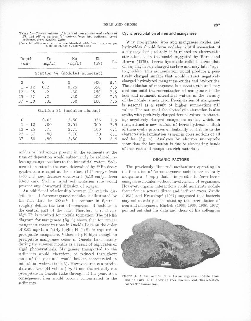
DEAN AND GHOSH 237
TABLE 5. Concentrations of iron and manganese and values of Eh and pH of interstitial waters from two sediment cores collected from Oneida Lake
[Data in milligrams per liter are identical with data in grams per cubic meter, the SI derived unit]
Depth (cm)
Fe (mg/L)
Mn (mg/L)
Eh (mV) PH
Station 44 (nodules abundant)
01
122537
- 12- 25- 37- 50
00.2.2.2.35
00.25.30.30.30
300350250206100
8.47.57.57.57.5
Station 21 (nodules absent)
01 -
12 -25 -37 -
12253750
0.03.80.75.80.80
2.502.552.752.702.80
356300100500
7.97.56.16.16.5
oxides or hydroxides present in the sediments at the time of deposition would subsequently be reduced, re leasing manganous ions to the interstitial waters. Sedi mentation rates in the core, determined by 210Pb decay gradients, are rapid at the surface (1.45 cm/yr from 1-30 cm) and decrease downward (0.13 cm/yr from 30-50 cm). Such a rapid sedimentation rate would prevent any downward diffusion of oxygen.
An additional relationship between Eh and the dis tribution of ferromanganese nodules is illustrated by the fact that the 300-mV Eh contour in figure 1 roughly defines the area of occurence of nodules in the central part of the lake. Therefore, a relatively high Eh is required for nodule formation. The pH-Eh diagram for manganese (fig. 3) shows that for typical manganese concentrations in Oneida Lake on the order of 0.01 mg/L, a fairly high pH (>8) is required to precipitate manganese. Values of pH high enough to precipitate manganese occur in Oneida Lake mainly during the summer months as a result of high rates of algal photosynthesis. Manganese transported to the sediments would, therefore, be reduced throughout most of the year and would become concentrated in interstitial waters (table 3). However, iron can precip itate at lower pH values (fig. 3) and theoretically can precipitate in Oneida Lake throughout the year. As a consequence, iron would become concentrated in the sediments.
Cyclic precipitation of iron and manganese
Why precipitated iron and manganese oxides and hydroxides should form nodules is still somewhat of a mystery, but probably it is related to electrostatic attraction, as in the model suggested by Burns and Brown (1972). Ferric hydroxide colloids accumulate on any negatively charged surface and may later "age" to goethito. This accumulation would produce a posi tively charged surface that would attract negatively charged hydrolyzed manganese oxides and hydroxides. The oxidation of manganese is autocatalytic and may continue until the concentration of manganese in the lake and sediment interstitial waters in the vicinity of the nodule is near zero. Precipitation of manganese is seasonal as a result of higher summertime pH values. The nature of the electrolytic attraction is also cyclic, with positively charged ferric hydroxide attract ing negatively charged manganese oxides, which, in turn, attract a new surface of ferric hydroxide. Both of these cyclic processes undoubtedly contribute to the characteristic lamination as seen in cross sections of all nodules (fig. 4). Analyses by electron microprobe show that the lamination is due to alternating bands of iron-rich and manganese-rich materials.
ORGANIC FACTORS
The previously discussed mechanisms operating in the formation of ferromanganese nodules are basically inorganic and imply that it is possible to form ferro manganese nodules without involvement of organisms. However, organic interactions could accelerate nodule formation in several direct and indirect ways. Zapffe (1931) and Krauskopf (1957) suggested that bacteria may act as catalysts in initiating the precipitation of iron and manganese. Ehrlich (1963; 1966; 1968; 1972) pointed out that his data and those of his colleagues
FIGURE 4. Cross section of a ferromanganese nodule from Oneida Lake. N.Y., showing rock nucleus and characteristic concentric lamination.
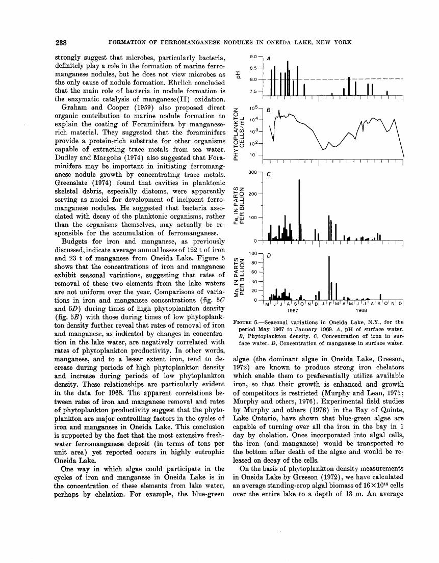
238 FORMATION OF FERROMANGANESE NODULES IN ONEIDA LAKE, NEW YORK
strongly suggest that microbes, particularly bacteria, definitely play a role in the formation of marine ferro- manganese nodules, but he does not view microbes as the only cause of nodule formation. Ehrlich concluded that the main role of bacteria in nodule formation is the enzymatic catalysis of manganese (II) oxidation.
Graham and Cooper (1959) also proposed direct organic contribution to marine nodule formation to explain the coating of Foraminifera by manganese- rich material. They suggested that the foraminifers provide a protein:rich substrate for other organisms capable of extracting trace metals from sea water. Dudley and Margolis (1974) also suggested that Fora minifera may be important in initiating ferromang- anese nodule growth by concentrating trace metals. Greenslate (1974) found that cavities in planktonic skeletal debris, especially diatoms, were apparently serving as nuclei for development of incipient ferro- manganese nodules. He suggested that bacteria asso ciated with decay of the planktonic organisms, rather than the organisms themselves, may actually be re sponsible for the accumulation of ferromanganese.
Budgets for iron and manganese, as previously discussed, indicate average annual losses of 122 t of iron and 23 t of manganese from Oneida Lake. Figure 5 shows that the concentrations of iron and manganese exhibit seasonal variations, suggesting that rates of removal of these two elements from the lake waters are not uniform over the year. Comparisons of varia tions in iron and manganese concentrations (fig. 5C and 5Z>) during times of high phytoplankton density (fig. 5Z?) with those during times of low phytoplank ton density further reveal that rates of removal of iron and manganese, as indicated by changes in concentra tion in the lake water, are negatively correlated with rates of phytoplankton productivity. In other words, manganese, and to a lesser extent iron, tend to de crease during periods of high phytoplankton density and increase during periods of low phytoplankton density. These relationships are particularly evident in the data for 1968. The apparent correlations be tween rates of iron and manganese removal and rates of phytoplankton productivity suggest that the phyto plankton are major controlling factors in the cycles of iron and manganese in Oneida Lake. This conclusion is supported by the fact that the most extensive fresh water ferromanganese deposit (in terms of tons per unit area) yet reported occurs in highly eutrophic Oneida Lake.
One way in which algae could participate in the cycles of iron and manganese in Oneida Lake is in the concentration of these elements from lake water, perhaps by chelation. For example, the blue-green
i i i i f r i i i i i i i i i i
2 m DC Oj-LU U.Q-
old2 CQ oc
300 1
200
100
0
100 ]
80
60
40
20
0
IT I I I T
M' J' J ' A.i, 1
S 1 O 1 N 1 D
67
1 Ik . -. W
j ' F' M' A'M' J ' J1968
A 1 S 1 O 1 N 1 D
FIGURE 5. Seasonal variations in Oneida Lake, N.Y., for the period May 1967 to January 1969. A, pH of surface water. B, Phytoplankton density. C, Concentration of iron in sur face water. D, Concentration of manganese in surface water.
algae (the dominant algae in Oneida Lake, Greeson, 1972) are known to produce strong iron chelators which enable them to preferentially utilize available iron, so that their growth is enhanced and growth of competitors is restricted (Murphy and Lean, 1975; Murphy and others, 1976). Experimental field studies by Murphy and others (1976) in the Bay of Quinte, Lake Ontario, have shown that blue-green algae are capable of turning over all the iron in the bay in 1 day by chelation. Once incorporated into algal cells, the iron (and manganese) would be transported to the bottom after death of the algae and would be re leased on decay of the cells.
On the basis of phytoplankton density measurements in Oneida Lake by Greeson (1972), we have calculated an average standing-crop algal biomass of 16 X1018 cells over the entire lake to a depth of 13 m. An average
DEAN AND GHOSH 239
annual standing-crop biomass of 16 XlO18 cells has a dry-weight equivalent of 1.6 XlO7 kg, on the assump tion of an average cell density of 1.0 g/cm3 , an average cell volume of 2XlO-8 cm3 (estimate based on data compiled by Wetzel, 1975, and measured in sediment trap studies by Braidech and others, 1972), and an average cell content of 95 percent water. A semi- quantitative spectrographic analysis of a mixed assem blage of algae, collected during a blue-green algal bloom in Oneida Lake in July 1975, shows 500 ppm iron and 200 ppm manganese on a dry-weight basis. On the assumption that these are average concentra tions of iron and manganese in Oneida Lake algae, an average standing-crop of 1.6 X10⁷ kg contains 8000 kg iron and 3200 kg manganese. Explanation of the losses from Oneida Lake of 122 t/yr iron and 23 t/yr manga nese would require about 15 standing-crop doublings to remove that much iron and about seven standing- crop doublings to remove that much manganese, if we assume that none of the iron and manganese was re cycled back into the lake's hydrologic system. The assumption of no recycling is not really a practical consideration, but if the iron and manganese are re leased under oxidizing conditions with a relatively high pH (greater than about 8.0, fig. 3), then most of the iron and manganese would probably not be re cycled.
Another important contribution by algae to the cycles of iron and manganese in Oneida Lake is in the production of a well oxygenated, high-pH environ ment. Figure 5A shows a seasonal variation in pH of lake surface waters which corresponds to seasonal variation in algal productivity (fig. 5B). The pH of surface waters in Oneida Lake averages about 8.0, but may reach values greater than 9.0 during the summer months owing to rapid removal of C02 by photo synthesis (Greeson, 1972). The high pH, well-oxy genated environment created near the surface of Oneida Lake is maintained throughout most of the lake volume by almost continual wind mixing during the ice-free months. An abundance of oxygen at the bottom of Oneida Lake is also indicated by the high Eh values of interstitial waters of surface sediments over most of the lake bottom (fig. 1).
REFERENCES CITED
Braidech, T., Gehring, P., and Klevend, C., 1972, Biological studies related to oxygen depletion and nutrient regenera tion processes in the Lake Erie central basin, in Burns, N. M., and Ross, C., eds., Project hypo ... an intensive study of the Lake Erie central basin hypolimnion and re lated water phenomena: Canada Centre for Inland Waters Paper 6 (U.S. Environmental Protection Agency Tech. Kept. TS-05-71-208-24), 182 p.
Burns, R. B., and Brown, B. A., 1972, Nucleation and rnin- eralogical controls on the composition of manganese nodules, in Horn, D. R., ed., Papers from a Conference on Ferromanganese Deposits on the Ocean Floor, NSF- IDOE: Washington, D.C., p. 51-62.
Burns, R. B., Burns, V. M., and Sung, W., 1974, Ferroman ganese nodule mineralogy Suggested terminology of the principal manganese oxide phases: Geol. Soc. America Abs. with Programs, v. 6, p. 1029- 1031.
Cronan, D. S., and Tooms, T. S., 1969, The geochemistry of manganese nodules and associated pelagic deposits from the Pacific and Indian Oceans: Deep-Sea Research, v. 16, p. 335-359.
Cronan, D. S., and Thomas, R. L., 1970, Ferromanganese con cretions on Lake Ontario: Canadian Jour. Earth Sci., v. 7, p. 1346-1349.
Dean, W. E., 1970, Fe-Mn oxidate crusts in Oneida Lake, New York: Great Lakes Research Conf., 13th, Proc., p. 1094- 1100.
Dean, W. E., Ghosh, S. K., Krishnaswami, S., and Moore, W. S., 1973, Geochemistry and accretion rates of freshwater ferromanganese nodules, in Morgenstein, M., eel., The origin and distribution of manganese nodules in the Pacific and prospects for exploration, NSF-IDOE: Washington, D.C., p. 13-20.
Dudley, W. C., and Margolis, S. V., 1974, Iron and trace ele ment concentration in marine manganese nodules by benthic agglutinated foraminifera: Geol. Soc. America Abs. with Programs, v. 6, p. 716.
Ehrlich, H. L., 1963, Bacteriology of manganese nodoles. I. Bacterial action on manganese in nodule enrichment: Appl. Microbiology, v. 11, p. 15-19.
1966, Reaction with manganese by bacteria from marine ferromanganese nodules: Devel. Indus. Micro biology, v. 7, p. 43-60.
1968, Bacteriology of manganese nodules. II. Manganese oxidation by cell-free extract from a manganese nodule bacterium: Appl. Microbiology, v. 16, p. 197-202.
1972, The role of microbes in manganese nodule genesisand degradation, in Horn, D. R.. ed., Papers from a Con ference on Ferromanganese Deposits on the Ocean Floor, NSF-IDOE: Washington, D.C., p. 63-70.
Gager, H. M., 1968, Mossbauer spectra of deep-sea iron-man ganese nodules: Nature, v. 220, p. 1012-1023.
Ghosh, S. K., 1975, The origin and geochemistry of ferroman ganese nodules in Oneida Lake, New York: Syracuse, N.Y., Syracuse Univ., Ph. D. dissert., 222 p.
Gorham, E., and Swaine, D. J., 1965, The influence of oxidizing and reducing conditions upon the distribution of some ele ments in lake sediments: Limnology and Oceanography, v. 10, p. 268-279.
Graham, J. W., and Cooper, S. C., 1959, Biological origin of manganese-rich deposits of the sea floor: Nature, v. 183, 1050-1051.
Greenslate, J., 1974, Manganese and biotic debris associations in some deep-sea sediments: Science, v. 186, p. 529-531.
Greeson, P. E., 1972, Limnology of Oneida Lake with em phasis on factors contributing to algal blooms: U.S. Geol. Survey open-file rept, 255 p.
Greeson, P. E., and Meyers, G. S., 1969, The limnology of Oneida Lake, an interim report: New York State Water Resources Comm. Rept. Inv. RI-8, 64 p.
240 FORMATION OF FERROMANGANESE NODULES IN ONEIDA LAKE, NEW YORK
Grill, E. V., Murray, J. W., and Macdonald, R. D., 1968, Todorokite in manganese nodules from a British Columbia fjord: Nature, v. 219, p. 358-359.
Harriss, R. C., and Troup, A. G., 1970, Chemistry and origin of freshwater ferromanganese concretions: Limnology and Oceanography, v. 15, no. 5, p. 702-712.
Hem. J. D., 1972, Chemical factors that influence the avail ability of iron and manganese in aqueous systems: Geol. Soc. America Bull. v. 83 no. 2, 443-450.
Krauskopf, K. B., 1957, Separation of manganese from iron in sedimentary processes: Geochim. et Cosmochim. Acta., v. 12, p. 61-84.
Krishnaswami, S., Lal, D., Martin, J. M., and Meybeck, M., 1971, Geochronology of lake sediments: Earth and Plane tary Sci. Letters, v. 11, p. 407-414.
Krishnaswami, S., and Moore, W. S., 1973, Accretion rates of freshwater manganese deposits: Nature, v. 243, p. 114- 116.
Krishnaswami, S., Somayajulu, B. L. K., and Moore, W. S., 1972, Dating of manganese nodules using beryIlium-10, in Horn, D. R., ed., Papers from a Conference on Ferroman- ganese Deposits on the Ocean Floor, NSF-IDOE: Wash ington, D.C., p. 117-122.
Ku, Teh-Lung., and Broecker, W. S., 1969, Radiochemical studies on manganese nodules of deep-sea origin: Deep- Sea Research, v. 16, no. 6, p. 625-637.
Ku, Teh-Lung., and Glasby, G. P., 1972 Radiometric evidence for the rapid growth rate of shallow-water continental margin manganese nodules: Geochim. et Cosmochim. Acta. v. 36, no. 6, p. 699-703.
Manheim, F. T., 1965, Manganese-iron accumulations in the shallow marine environment, in Symposium on marine
geochemistry, 1964: Rhode Island Univ. Narragansett Marine Lab. Occasional Pub. 3, p. 217-276.
Mero, J. L., 1965, The mineral resources of the sea: Amster dam, Elsevier Press, 312 p.
Moore, W. S., Dean, W. E., and Krishnaswami, S., 1976, Episodic growth of ferromanganese nodules in Oneida Lake, New York: Geol. Soc. America Abs. with Programs, v. 8, no. 6, p. 1016-1017.
Murphy, T. P., and Lean, D. R. S., 1975, The distribution of iron in a closed ecosystem: Ver. Internal. Verein. Lim- nologie, v. 19, p. 258-266.
Murphy, T. P., Lean, D. R. S., Nalewajko, C., 1976, Blue- green algae: their excretion of iron-selective chelators enables them to dominate other algae: Science, v. 192, p. 900-902.
Robbins, J. A. and Edgington, D. N., 1975, Determination of recent sedimentation rates in Lake Michigan using Pb- 210 and Cs-137: Geochim. et Cosmochim. Acta, v. 39, no. 3, p. 285-304.
Rossmann, Ronald, and Callender, Edward, 1968, Manganese nodules in Lake Michigan: Science, v. 162, p. 1123-1124.
Rossmann, Ronald, Callender, Edward, and Bowser, C. J., 1972, Interelement geochemistry of Lake Michigan fer romanganese nodules: Internat. Geol. Congress, 24th, Proc., sec. 10, p. 336-341.
Schoettle, Manfred, and Friedman, G. M., 1971, Freshwater iron-manganese nodules in Lake George, New York: Geol. Soc. America Bull., v. 82, no. 1, p. 101-110.
Wetzel, R. G., 1975, Limnology: Philadelphia, W. B. Saunders Co., 743 p.
Zapffe, Carl, 1931, Deposition of manganese: Econ. Geology, v. 26, no. 8, p. 799-832.
Jour. Research U.S. Qeol. Survey Vol. 6, No. 2, Mar.-Apr. 1978, p. 241-246
OCCURRENCE AND FORMATION OF AVICENNITE, TI 203 > AS A
SECONDARY MINERAL AT THE CARLIN GOLD DEPOSIT, NEVADA
By ARTHURS. RADTKE, FRANK W. DICKSON, 1 and JOHN F. SLACK,
Menlo Park, Calif., Stanford, Calif., Reston, Va.
Abstract, Avicennite, Tl2Os, occurs as grains disseminated in silicified limestones in the upper part of the East ore zone of the Carlin gold deposit, Nevada. The avicennite is formed by the oxidation of carlinite, T12S, found in primary unoxi- dized carbonaceous ore immediately below the avicennite. The grains of avicennite closely resemble carlinite in size and shape. Some avicennite occurs as thin coatings on carlinite, but the time of its formation is unclear. Avicennite grains are polycrystalline, porous, dark gray to black, with a hackly fracture but no discernible cleavage. The Mohs hardness is 2.0±0.5; Vickers hardness ranges from 46.0 to 80.5 kg mm"2. Measured density is distinctly low, 8.9 g cm-" (or Mg m-s), relative to the calculated density, 10.34 g cm-3. The mineral is isometric, space group 7a3. a=10.5468±0.0003 angstroms or 1.05468±0.00003 nm, Z=16, and the volume of the unit cell is 1173.17±0.04 A3 or 1.17317±0.00004 nin3. The most intense X- ray diffraction peaks are 3.044 (100), 1.864 (38), 2.637 (37), and 1.590 (30). In reflected light, avicennite is pale to medium gray and isotropic and lacks discernible bireflectance. Re flectance in air ranges from 10.6 to 13.0 percent. Avicennite is nearly pure T12O3, containing 89.6 weight percent Tl and 10.5 weight percent O by microprobe analysis. Other elements present, detected by emission spectrographic analysis, are: Pb, 300 ppm; Ca, 100 ppm; and Si, Al, Fe, Mg, Ag, Cr, Cu, Ni, and Ti, all <50 ppm.
Avicennite was discovered in oxidized gold ores from the Carlin mine, Nevada, during investigations of epithermal gold deposits of the Western United States. Thallium minerals are rare, but thallium be longs to a suite of elements known to be present in Carlin-type epithermal gold deposits (Weissberg, 1969; Radtke and others, 1972; Radtke and Dickson, 1974; Raidtke, Dickson, and Rytuba, 1974). In most de posits, the thallium is present in forms not yet identi fied. Small amounts of thallium also form a geochemi- cal halo in surrounding country rocks. The Carlin deposit is one of the few places where discrete thallium or thallium-bearing minerals have been found. These include lorandite, TlAsS2 (Radtke and others, 1973); thallium-bearing orpiment, As2 S3 (Radtke, Taylor,
Department of Geology, Stanford University.
and Dickson, 1974); carlinite, T12S (Radtke and Dick- son, 1975); christite, TlHgAsS 3 (Radtke and others, 1977); and weissbergite, TlSbS2 (F. W. Dickson and A. 'S. Radtke, unpub. data, 1977). All the thallium minerals except avicennite occur in unoxidized primary ores.
Avicennite was first found by Karpova and others (1958) at Zirabulakh, U.S.S.R., where it occurs as tiny black cubic crystals associated with hematite and cal- cite in veins in silicified limestone adjacent to an in trusive. The small amount available, about 20 mg, permitted only a semiquantitative analysis, from which the composition FeTl7 Oi2 was deduced. The X-ray powder diffraction pattern resembled the pattern of synthetic T1 2O3 , but many additional lines were pres ent, explained as being caused by unknown admixed minerals. Karpova and others (1958) did not deter mine whether iron was present as an essential con stituent in a compound of fixed composition or whether iron and thallium oxides formed a solid solution. Fleischer (1959) listed avicennite as T1 203 rather than FeTl7 Oi2 because of the similarity of the df-spacings of avicennite to those of pure T1 203 reported by Zaohariasen (1926) and Swanson and Fuyat (1953). The identification was clarified by Konkova and Save- lev (1960), who studied avicennite from the original locality and reported that iron was present in im purities and that avicennite was essentially pure T12O3 . The mode of formation of avicennite at the original locality remains unclear.
Thallium oxides have been reported as secondary minerals at other localities. Ruiz and others (1965) found thin black coatings of T1 2O3 on uranium ores from Vizarron, Mexico. Semenov and others (1967) detected dusty disseminations, possibly of avicennite, in chalcothallite (Cu8TlS2 ) along with inclusions of native silver, chalcocite, and vrbaite, from Greenland.
Avicennite from Carlin occurs in amounts sufficient for detailed study in a geologic setting that permits
241
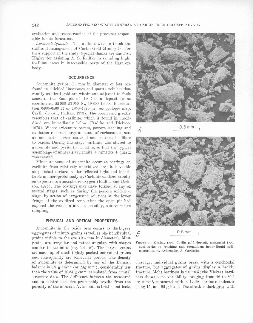
242 AVICENNITE, SECONDARY MINERAL AT CARLIN GOLD DEPOSIT, NEVADA
evaluation and reconstruction of the processes respon sible for its formation.
Acknowledgments. The authors wish to thank the staff and management of Carlin Gold Mining Co. for their support in the study. Special thanks are due Dan Higley for assisting A. S. Radtke in sampling high- thallium areas in inaccessible parts of the East ore body.
OCCURRENCE
Avicennite grains, 0.5 mm in diameter or less, are found in silicified limestones and quartz veinlets that ramify oxidized gold ore within and adjacent to fault zones in the East pit of the Carlin deposit (mine coordinates, 22 900-23 050 X., 19 800-19 900 E., eleva tion 6400-6460 ft or 1950-1970 m; see geologic map, Carlin deposit, Radtke, 1973). The occurrence greatly resembles that of carlinite, which is found in unoxi- dized ore immediately below (Radtke and Dickson, 1975). Where avicennite occurs, postore leaching and oxidation removed large amounts of carbonate miner als and carbonaceous material and converted sulfides to oxides. During this stage, carlinite was altered to avicennite and pyrite to hematite, so that the typical assemblage of minerals avicennite + hematite + quartz was created.
Minor amounts of avicennite occur as coatings on carlinite from relatively unoxidized ore; it is visible on polished surfaces under reflected light and identi fiable in microprobe analysis. Carlinite oxidizes rapidly on exposure to atmospheric oxygen (Radtke and Dick- son, 1975). The coatings may have formed at any of several stages, such as during the postore oxidation stage, by action of oxygenated solutions at the lower fringe of the oxidized zone, after the open pit had exposed the rocks to air, or, possibly, subsequent to sampling.
PHYSICAL AND OPTICAL PROPERTIES
Avicennite in the oxide ores occurs as dark-gray aggregates of minute grains as well as black individual grains visible to the eye (0.5 mm in diameter). Most grains are irregular and rather angular, with shapes similar to carlinite (fig. 1A, B). The larger grains are made up of small tightly packed individual grains and consequently are somewhat porous. The density of avicennite as determined by use of the Berman balance is 8.9 g cm.- 3 (or Mg m~ 3 ), considerably less than the value of 10.34 g cm~ 3 calculated from crystal structure data. The difference between the measured and calculated densities presumably results from the porosity of the mineral. Avicennite is brittle and lacks
A0.5 mm
B I 0.5 mm
FIGURE 1. Grains, from Carlin gold deposit, separated host rocks by crushing and bromoform heavy-liquid mentation. A, Avicennite. B, Carlinite.
from sedi-
cleavage; individual grains break with a conchoidal fracture, but aggregates of grains display a hackly fracture, Mohs hardness is 2.0 ±0.5; the Tickers hard ness shows some variability, ranging from 46 to 80.5 kg mm.- 2 , measured with a Leitz hardness indentor using 15- and 25-g loads. The streak is dark gray with
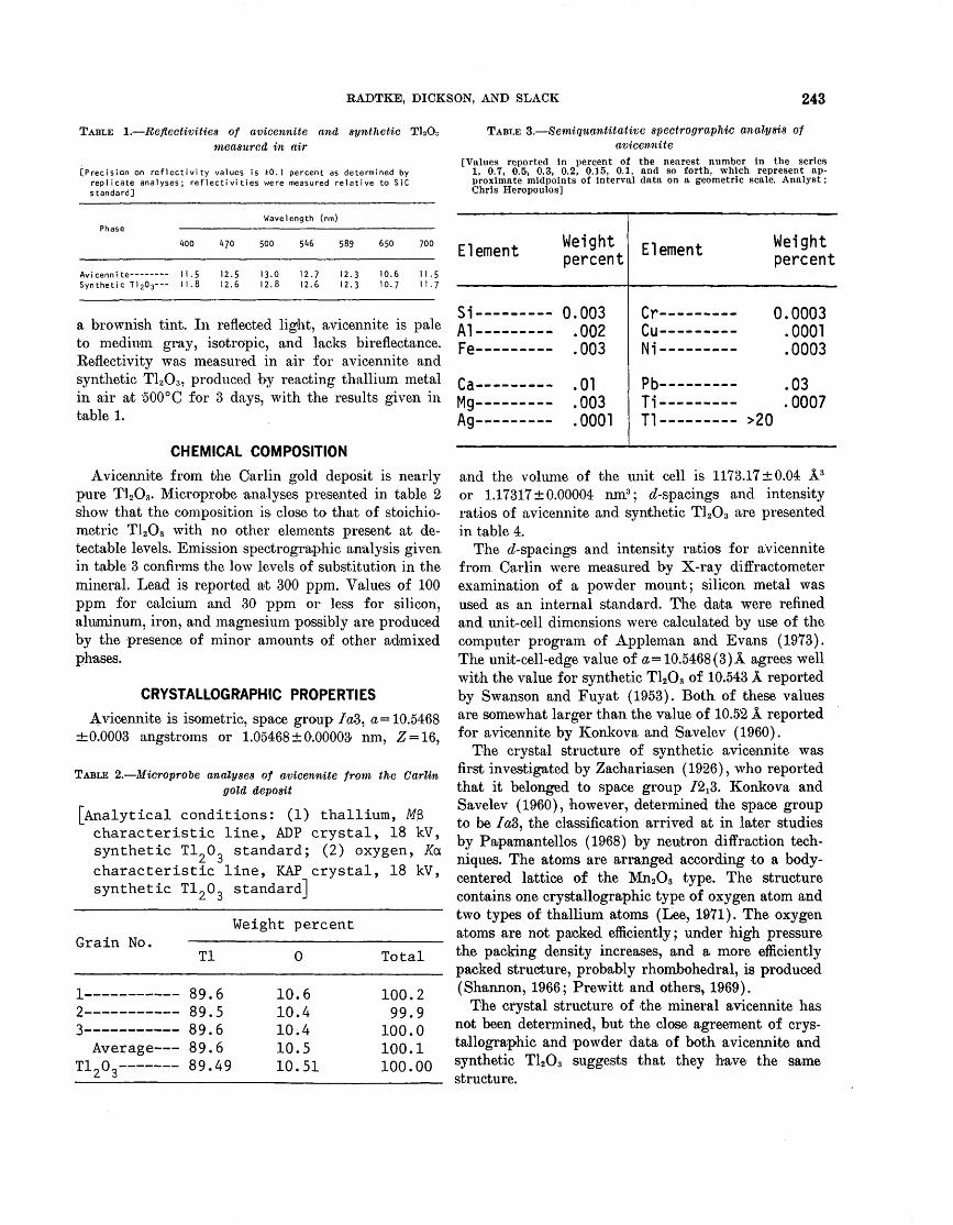
RADTKE, DICKSON, AND SLACK 243
TABLE 1. Reflectivities of avicennite and synthetic T12O3 measured in air
[Precision on reflectivity values is ±0.1 percent as determined by replicate analyses; reflectivities were measured relative to SiC standard]
TABLE 3. Semiquantitative spectrographic analysis of avicennite
[Values reported In percent of the nearest number in the series 1, 0.7, 0.5, 0.3, 0.2, 0.15, 0.1, and so forth, which represent ap proximate midpoints of interval data on a geometric scale. Analyst; Chris Heropoulos]
Wavelength (nm)
1*00 1)70 500 5*16 589 650 700
Avicennite 11.5 12.5 13.0 12.7 12.3 10.6 11.5 Synthetic T1 2 0 3 11.8 12.6 12.8 12.6 12.3 10.7 11.7
a brownish tint. In reflected light, avicennite is pale to medium gray, isotropic, and lacks bireflectance. Reflectivity was measured in air for avicennite and synthetic T1203 , produced by reacting thallium metal in air at '500 °C for 3 days, with the results given in table 1.
Element
Si ----*J I
AT ____ .Fe -
C a -Mg -
9
Weight percent
- 0.003- .002- .003
- .01- .003- .0001
Element
r r _____ .C U - -
Pb- Ti -Tl
Weight percent
0.0003.0001.0003
03. \j*j .0007
- >20
Avicennite from the Carlin gold deposit is nearly pure T12O3 . Microprobe analyses presented in table 2 show that the composition is close to that of stoichio- metric T12O3 with no other elements present at de tectable levels. Emission spectrographic analysis given, in table 3 confirms the low levels of substitution in the mineral. Lead is reported at 300 ppm. Values of 100 ppm for calcium and 30 ppm or less for silicon, aluminum, iron, and magnesium possibly are produced by the presence of minor amounts of other admixed phases.
CRYSTALLOGRAPHIC PROPERTIES
Avicennite is isometric, space group 7o3, a =10.5468 ±0.0003 angstroms or 1.05468±0.00003 nm, Z = 16,
TABLE 2. Microprobe analyses of avicennite from the Carlin gold deposit
[Analytical conditions: (1) thallium, A/3 characteristic line, ADP crystal, 18 kV, synthetic Tl () standard; (2) oxygen, Ka. characteristic line, KAP crystal, 18 kV, synthetic Tl^CL standard]
Weight percentGrain No.
Tl 0 Total
1 89.6 10.6 100.22 89.5 10.4 99.93 89.6 10.4 100.0Average 89.6 10.5 100.1
T120 3 89.49 10.51 100.00
and the volume of the unit cell is 1173.17 ±0.04 A3 or 1.17317±0.00004 nm3 ; d-spacings and intensity ratios of avicennite and synthetic T1203 are presented in table 4.
The d-spacings and intensity ratios for avicennite from Carlin were measured by X-ray diffractometer examination of a powder mount; silicon metal was used as an internal standard. The data were refined and unit-cell dimensions were calculated by use of the computer program of Appleman and Evans (1973). The unit-cell-edge value of a =10.5468 (3) A agrees well with the value for synthetic T1203 of 10.543 A reported by Swanson and Fuyat (1953). Both of these values are somewhat larger than the value of 10.52 A reported for avicennite by Konkova and Savelev (1960).
The crystal structure of synthetic avicennite was first investigated by Zachariasen (1926), who reported that it belonged to space group 12$. Konkova and Savelev (1960), however, determined the space group to be 7o3, the classification arrived at in later studies by Papamantellos (1968) by neutron diffraction tech niques. The atoms are arranged according to a body- centered lattice of the Mn203 type. The structure contains one crystallographic type of oxygen atom and two types of thallium atoms (Lee, 1971). The oxygen atoms are not packed efficiently; under high pressure the packing density increases, and a more efficiently packed structure, probably rhombohedral, is produced (Shannon, 1966; Prewitt and others, 1969).
The crystal structure of the mineral avicennite has not been determined, but the close agreement of crys tallographic and powder data of both avicennite and synthetic T1203 suggests that they have the same structure.
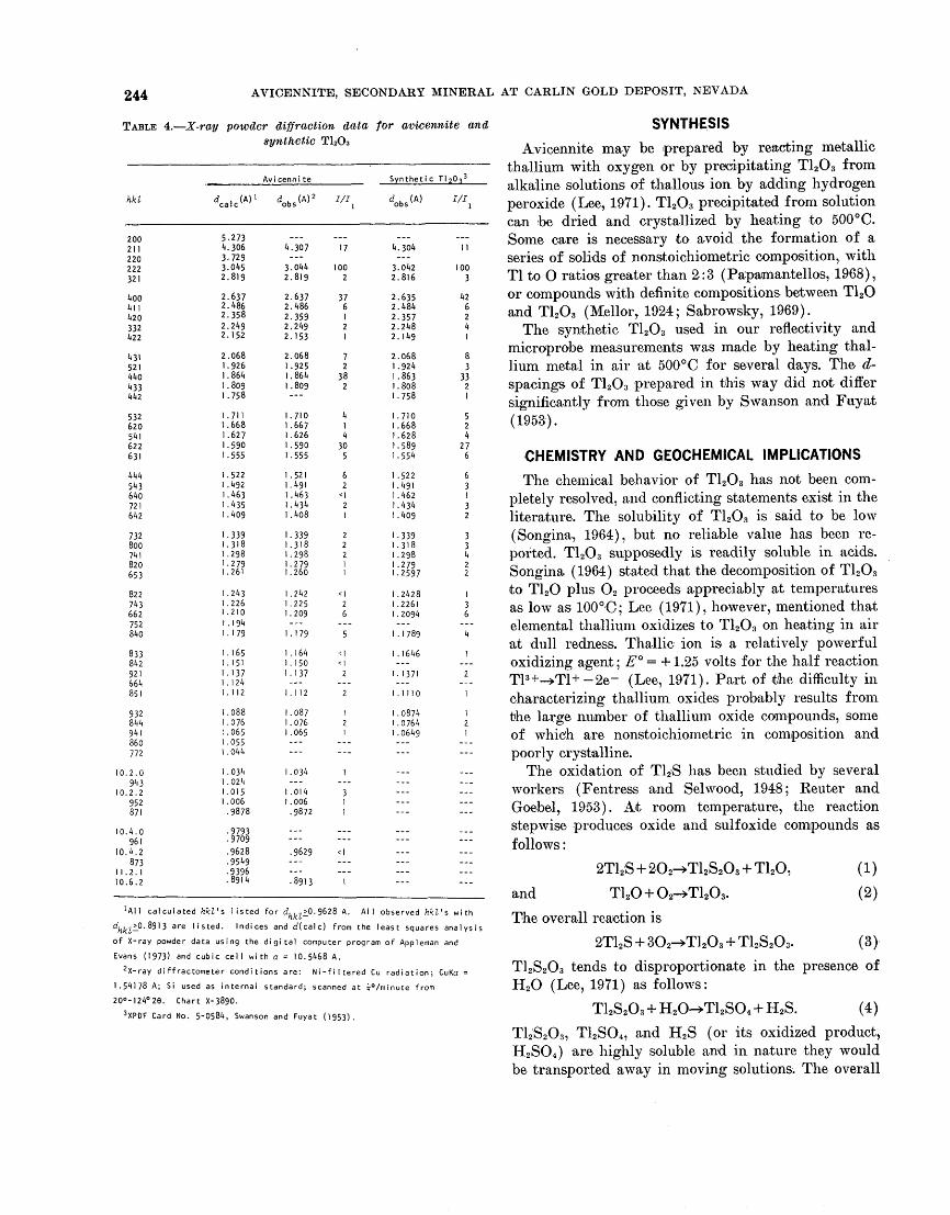
244 AVICENNITE, SECONDARY MINERAL AT CARLIN GOLD DEPOSIT, NEVADA
TABLE 4. X-ray powder diffraction data for avicennite and synthetic T12O3
hkl dc
200211220222321
400411420332422
431521440433442
532620541622631
444543640721642
732800741820653
822743662752840
833842921664851
932844941860772
10.2.0943
10.2.2952871
10.4.0961
10.4.2873
11.2.110.6.2
..«< >
5.273I). 3063-7293-0452.819
2.6372.4862.3582.2492.152
2.068.926.864.809.758
.711
.668
.627
.590
.555
.522
.492
.463
.435
.409
.339
.318
.298
.279
.261
.243
.226
.210.194.179
.165
.151
.137
. 124. 112
.088
.076
.065
.055
.044
.034
.024
.015
.006
.9878
.9793
.9709
.9628
.9549
.9396
.8914
Avi cenni te
^.""
..-
4.307
3.0442.819
2.6372.4862.3592.2492.153
2.0681.9251.8641 .809---
1.7101.6671.6261.5901.555
1.5211.4911.4631.4341.408
1.3391.3181.2981.2791.260
1.2421 .2251.209---1.179
1.1641 . 1501.137-..1.112
1.0871.0761 .065------
1 .034---
1 .0141 .006.9872
...---
.9629
..-
._-
.8913
S
I/I a i
...17
1002
376121
72382
414
305
62
<121
22211
<|26
...
5
<l<\2
...
2
121
-__
1...
311
--.---
<l...-__
1
yntheti c ~\
ob,<A >
..-[(.304-..3.0422.816
2.6352.4842.3572.2482.149
2.068.924.863.808.758
.710
.668
.628
.589
.554
.522
.491
.462
.434
.409
339.318.298 279.2597
.2428
.2261
.2094
...
.1789
.1646... 1371....1110
.0874
.0764
.0649-__---
-..-..-.-...
-_.---......
---
inS
I/I \
---
11
1003
42624I
83
3321
524
276
63132
33422
136...4
1...2
...1
121
--. -
--..-..-_... -
...---
-._ ._-
'All calculated hkl's listed for d,,,>_0.9628 A. All observed hkl's with
^hkl-"-^9'3 are listed. Indices and d(calc) from the least squares analysis
of X-ray powder data using the digital computer program of Appleman and
Evans (1973) and cubic cell with a = 10.5468 A.
2 X-ray diffractometer conditions are: Ni-filtered Cu radiation; CuKa =
1.54178 A; Si used as internal standard; scanned at i°/minute from
20°-I24°26. Chart X-3890.
3 XPDF Card No. 5-0584, Swanson and Fuyat (1953).
SYNTHESIS
Avicennite may be (prepared by reacting metallic thallium with oxygen or by precipitating T12O3 from alkaline solutions of thallous ion by adding hydrogen peroxide (Lee, 1971). T12O3 precipitated from solution can be dried and crystallized by heating to 500 °C. Some care is necessary to avoid the formation of a series of solids of nonstoichiometric composition, with Tl to O ratios greater than 2:3 (Papamantellos, 1968), or compounds with definite compositions between T12O and T12O3 (Mellor, 1924; Sabrowsky, 1969).
The synthetic T12O3 used in our reflectivity and microprobe measurements was made by heating thal lium metal in air at 500°C for several days. The d- spacings of T12O3 prepared in this way did not differ significantly from those given by Swanson and Fuyat (1953).
CHEMISTRY AND GEOCHEMICAL IMPLICATIONS
The chemical behavior of T1 2O3 has not been com pletely resolved, and conflicting statements exist in the literature. The solubility of T12O3 is said to be low ('Songina., 1964), but no reliable value has been re ported. T12O3 supposedly is readily soluble in acids. Songina (1964) stated that the decomposition of T12O3 to T1 2O plus O2 proceeds appreciably at temperatures as low as 100°C; Lee (1971), however, mentioned that elemental thallium oxidizes to T12O3 on heating in air at dull redness. Thallic ion is a relatively powerful oxidizing agent; E° = + 1.25 volts for the half reaction Tl3 +->Tl+-2e- (Lee, 1971). Part of the difficulty in characterizing thallium oxides probably results from the large number of thallium oxide compounds, some of which are nonstoichiometric in composition and poorly crystalline.
The oxidation of T1 2'S has been studied by several workers (Fentress and Selwood, 1948; Keuter and Goebel, 1953). At room temperature, the reaction stepwise produces oxide and sulfoxide compounds as follows:
2T12 S + 2O2^T12S203 + T12O, (1)
and T120 + O2-»T1203 . (2)
The overall reaction is
2T12S + 3O2-»T12O3 + T12S203 . (3)
T1 2 S2O3 tends to disproportionate in the presence of H2O (Lee, 1971) as follows:
T12S2O3 + H2O-»T12SO4 + H2S. (4)
T1 2 S2O3 , T12SO4 , and H2 S (or its oxidized product, H2 SO4 ) are highly soluble and in nature they would be transported away in moving solutions. The overall
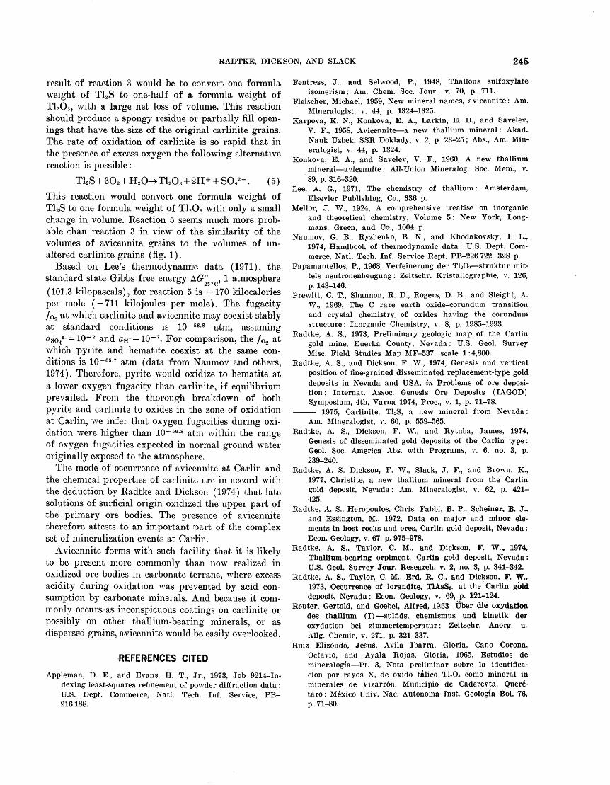
RADTKE, DICKSON, AND SLACK 245
result of reaction 3 would be to convert one formula weight of T12S to one-half of a formula weight of T1 203 , with a large net loss of volume. This reaction should produce a spongy residue or partially fill open ings that have the size of the original carlinite grains. The rate of oxidation of carlinite is so rapid that in the presence of excess oxygen the following alternative reaction is possible:
T12S + 302 + H20-»T12 O3 + 2H+ + S(V-. (5)
This reaction would convert one formula weight of T12 S to one formula weight of T12O3 with only a small change in volume. Reaction 5 seems much more prob able than reaction 3 in view of the similarity of the volumes of avicennite grains to the volumes of un altered carlinite grains (fig. 1).
Based on Lee's thermodynamic data (1971), the standard state Gibbs free energy A#° e , I atmosphere (101.3 kilopascals), for reaction 5 is 170 kilocalories per mole ( 711 kilo joules per mole). The fugacity /o9 at which carlinite and avicennite may coexist stably at standard conditions is 10~ 56 - 8 atm, assuming #so42~ = 10~"2 and &H+ = 10~ 7 . For comparison, the /o2 at which pyrite and hematite coexist at the same con ditions is 10~ 65 - 7 atm (data from Naumov and others, 1974). Therefore, pyrite would oxidize to hematite at a lower oxygen fugacity than carlinite, if equilibrium prevailed. From the thorough breakdown of both pyrite and carlinite to oxides in the zone of oxidation at Carlin, we infer that oxygen fugacities during oxi dation were higher than 10~ 56 - 8 atm within the range of oxygen fugacities expected in normal ground water originally exposed to the atmosphere.
The mode of occurrence of avicennite at Carlin and the chemical properties of carlinite are in accord with the deduction by Radtke and Dickson (1974) that late solutions of surficial origin oxidized the upper part of the primary ore bodies. The presence of avicennite therefore attests to an important part of the complex set of mineralization events at Oarlin.
Avicennite forms with such facility that it is likely to be present more commonly than now realized in oxidized ore bodies in carbonate terrane, where excess acidity during oxidation was prevented by acid con sumption by carbonate minerals. And because it com monly occurs as inconspicuous coatings on carlinite or possibly on other thallium-bearing minerals, or as dispersed grains, avicennite would be easily overlooked.
REFERENCES CITED
Appleman, D. E., and Evans, H. T., Jr., 1973, Job 9214-In- dexing least-squares refinement of powder diffraction data : U.S. Dept. Commerce, Natl. Tech.. Inf. Service, PB- 216188.
Fentress, J., and Selwood, P., 1948, Thallous sulfoxylate isomerism: Am. Chem. Soc. Jour., v. 70, p. 711.
Fleischer, Michael, 1959, New mineral names, aviceunite: Am. Mineralogist, v. 44, p. 1324-1325.
Karpova, K. N., Konkova, E. A., Larkin, E. D., and Savelev, V. F., 1958, Avicennite a new thallium mineral: Akad. Nauk Uzbek, SSR Doklady, v. 2, p. 23-25; Abs., Am. Min eralogist, v. 44, p. 1324.
Konkova, E. A., and Savelev, V. F., 1960, A new thallium mineral avicennite: Ail-Union Mineralog. Soc. Mem., v. 89, p. 316-320.
Lee, A. G., 1971, The chemistry of thallium: Amsterdam, Elsevier Publishing, Co., 336 p.
Mellor, J. W., 1924, A comprehensive treatise on inorganic and theoretical chemistry, Volume 5: New York, Long mans, Green, and Co., 1004 p.
Naumov, G. B., Ryzhenko, B. N., and Khodakovsky, I. L., 1974, Handbook of thermodynamic data: U.S. Dept. Com merce, Natl. Tech. Inf. Service Kept. PB-226 722, 328 p.
Papamantellos, P., 1968, Verfeinerung der Tl2O:i struktur mit- tels neutronenbeugung: Zeitschr. Kristallographie, v. 126, p. 143-146.
Prewitt, C. T., Shannon, R. D., Rogers, D. B., and Sleight, A. W., 1969, The C rare earth oxide-corundum transition and crystal chemistry, of oxides having the corundum structure: Inorganic Chemistry, v. 8, p. 1985-1993.
Radtke, A. S., 1973, Preliminary geologic map of the Carlin gold mine, Euerka County, Nevada: U.S. Geol. Survey Misc. Field Studies Map MF-537, scale 1:4,800.
Radtke, A. S., and Dickson, F. W., 1974, Genesis and vertical position of fine-grained disseminated replacement-type gold deposits in Nevada and USA, in Problems of ore deposi tion: Internat. Assoc. Genesis Ore Deposits (IAGOD) Symposium, 4th, Varna 1974, Proc., v. 1, p. 71-78.
1975, Carlinite, T12S, a new mineral from Nevada: Am. Mineralogist, v. 60, p. 559-565.
Radtke, A. S., Dickson, F. W., and Rytuba, James, 1974, Genesis of disseminated gold deposits of the Carlin type: Geol. Soc. America Abs. with Programs, v. 6, no. 3, p. 239-240.
Radtke, A. S. Dickson, F. W., Slack, J. F., and Brown, K., 1977, Christite, a new thallium mineral from the Carlin gold deposit, Nevada: Am. Mineralogist, v. 62, p. 421- 425.
Radtke, A. S., Heropoulos, Chris, Fabbi, B. P., Scheiner, B. J., and Essington, M., 1972, Data on major and minor ele ments in host rocks and ores, Carlin gold deposit, Nevada: Econ. Geology, v. 67, p. 975-978.
Radtke, A. S., Taylor, C. M., and Dickson, F. W.,, 1974, Thallium-bearing orpiment, Carlin gold deposit, Nevada: U.S. Geol. Survey Jour. Research, v. 2, no. 3, p. 341-342.
Radtke, A. S., Taylor, C. M., Erd, R. C., and Dickson, F. W., 1973, Occurrence of lorandite, TIAsSa. at the Carlin gold deposit, Nevada: Econ. Geology, v. 69, p. 121-124.
Renter, Gertold, and Goebel, Alfred, 19i53 Uber die oxydation des thallium (I) sulfids, chemismus und kinetik der oxydation bei zimrnertemperatur: Zeitschr. Anorg. u. Allg. Chemie, v. 271, p. 321-337.
Ruiz Elizondo, Jesus, Avila Ibarra, Gloria, Cano Corona, Octavio, and Ayala Rojas, Gloria, 1965, Estudios de mineralogia Pt. 3, Nota preliminar sobre la identifica- cion por rayos X, de oxido talico Tl2O:i como mineral in minerales de Vizarr6n, Municipio de Cadereyta, Quer6- taro: Mexico Univ. Nac. Autonoma Inst. Geologia Bol. 76, p. 71-80.
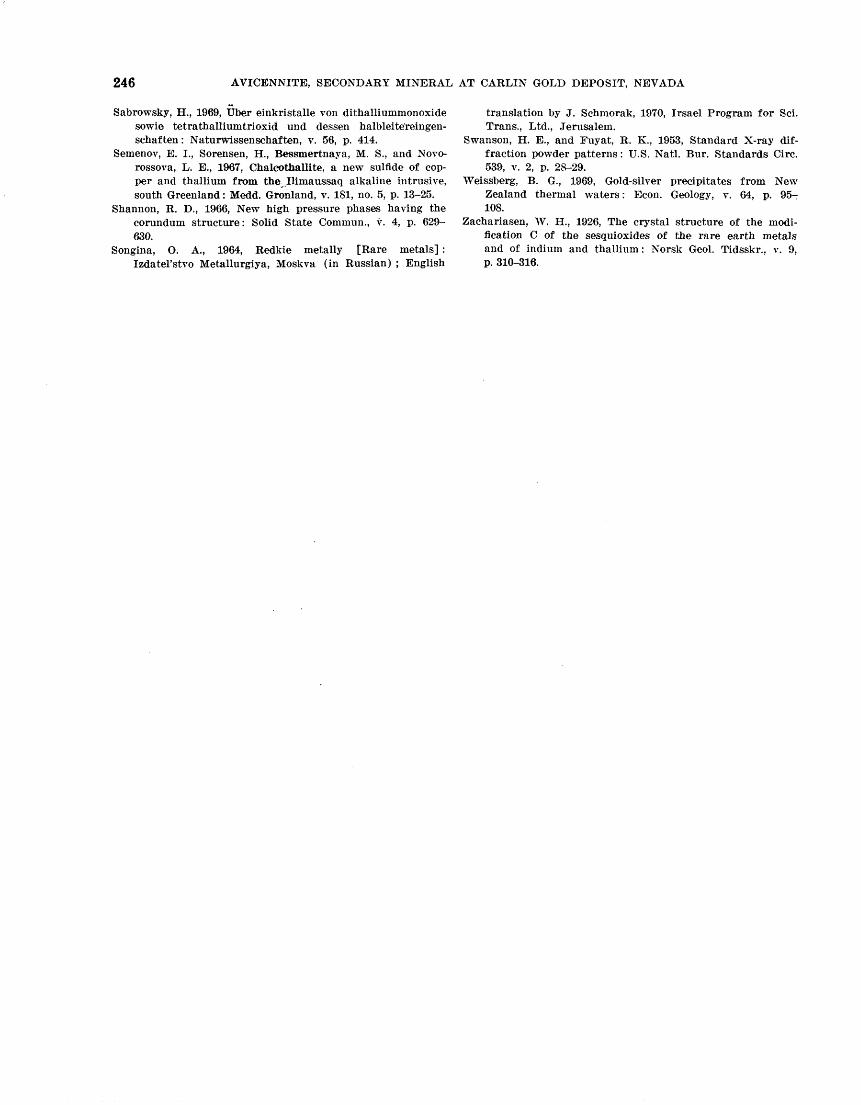
246 AVICENNITE, SECONDARY MINERAL AT CARLIN GOLD DEPOSIT, NEVADA
Sabrowsky, H., 1969, Uber einkristalle von dithalliummonoxide sowie tetrathalliumtrioxid und dessen halbleitereingen- schaften: Naturwissenschaften, v. 56, p. 414.
Semenov, E. I., Sorensen, H., Bessmertnaya, M. S., and Novo- rossova, L. E., 1967, Chalcothallite, a new sulflde of cop per and thallium from the. Ilimaussaq alkaline intrusive, south Greenland: Medd. Gronland, v. 181, no. 5, p. 13-25.
Shannon, R. D., 1966, New high pressure phases having the corundum structure: Solid State Commun., v. 4, p. 629- 630.
Songina, O. A., 1964, Redkie metally [Rare metals] : Izdatel'stvo Metallurgiya, Moskva (in Russian) ; English
translation by J. Schmorak, 1970, Irsael Program for Sci. Trans., Ltd., Jerusalem.
Swanson, H. E., and Fuyat, R. K., 1953, Standard X-ray dif fraction powder patterns: U.S. Natl. Bur. Standards Circ. 539, v. 2, p. 28-29.
Weissberg, B. G., 1969, Gold-silver precipitates from New Zealand thermal waters: Econ. Geology, v. 64, p. 95- 108.
Zachariasen, W. H., 1926, The crystal structure of the modi fication C of the sesquioxides of the rare earth metals and of indium and thallium: Norsk Geol. Tidsskr., v. 9, p. 310-316.
Jour. Research U.S. Qeol. Survey Vol. 6, No. 2, Mar.-Apr. 1978, p. 247-257
MODELS FOR CALCULATING DENSITY AND VAPOR PRESSURE OFGEOTHERMAL BRINES
By ROBERT W. POTTER II and JOHN L. HAAS, Jr.,
Menlo Park, Calif., and Reston, Va.
Abstract. In a model for estimating density of a brine, the density of a natural brine at a known temperature, pres sure, and composition can be calculated from the densities of the component salt solutions in the complex brine. A model for estimating vapor pressure requires two direct or indirect estimates of the vapor pressure and uses a published "ref erence-substance principle" i to extrapolate,; these data 200° to 300° above the temperature of the highest observation. The methods can be used to estimate the partial molal volume and partial molal enthalpy of H2O in the natural brine and the partial molal volume change and partial molal heat change for the H2O component in the vaporization process. The equations for density and vapor pressure and the de rived thermochemical properties will help in designing tur bines for operation with geothermal and geopressured brines, in optimizing production conditions, and in physical and chemical modeling of a geothermal reservoir.
The effective use of saline geothermal fluids in the production of electricity requires precise pressure- volume-temperature-composition (P-V-T-X) data. These data are required to minimize scaling and cor rosion, to design turbines intelligently, and to establish the optimum operating temperatures, pressures, and flow rates. Also, a set of accurate P-V-T-X data for the fluids involved is an important prerequisite to the modeling of the chemical and physical behavior of geothermal reservoirs, which contain highly saline fluids. Despite the critical importance of the P-V-T-X data in the utilization of saline geothermal resources, very limited data at the temperatures and pressures encountered in the geothermal systems are available (Potter, 1976). In this research, we present relatively simple, workable methods that can be used to accu rately predict the density and vapor pressure of com plex brines at elevated temperatures. Our approach was to develop a predictive equation for the density of the liquid and to adapt the reference-substance principle of Othmer and Yu (1968) for calculating the vapor pressure of the liquid. Together, these meth ods give a parametric equation of state for the vapor- saturated liquid.
In this report the application explicitly discussed is the prediction of the liquid properties in a geo thermal reservoir. Obviously, these methods can be used to calculate the properties of any brine within the limitations discussed below.
DENSITY OF A BRINE
Methods of estimation
The available published volumetric data for fluids of geothermal interest have been compiled in an anno tated bibliography by Potter, Shaw, and Haas (1975). A modest amount of volumetric data for binary sys tems (such as NaCl-H20) is available and has been critically evaluated and regressed to a "best" set of values for NaCl-H20, KC1-H2O, Na2SO4-H2O, K2 SO4-H20, and CaCl2-H2O (Potter and Brown, 1975, 1976a, b, c; Potter and Clynne, 1976). Data for car bonate-water systems are available as a set of smoothed data in the International Critical Tables (National Research Council, 1928). Internally consistent data for other than binary systems in the temperature-pressure range of geothermal systems are almost nonexistent. The following table lists the temperature ranges over which internally consistent volumetric data for the binary systems are available:
Salt
NaClKC1Na2S04CaClaKsSO*Na2CO3K2CO3
Temperature range
0-500 0-400 0-325 0-300 0-200 0-100 0-100
Because the necessary experimental data are not available, a model or method capable of predicting the P-V-T-X properties of saline geothermal fluids would prove exceedingly useful. There have been sev eral attempts to erect theoretical models for calculating the density of mixed brines, particularly seawater
247
248 CALCULATING DENSITY AND VAPOR PRESSURE OF GEOTHERMAL BRINES
(Millero, 1973). All of these models are based on the premise that the mean ionic activity coefficient of any strong electrolyte is the same in all solutions of the same ionic strength (Lewis and Randall, 1921), from whence it follows that
vs ^ v^ (1)
where <f>V8 is the apparent molal volume of the dissolved salts, fi is the mole fraction of component «', and <£ ; is the apparent molal volume of component i. Equation 1 is generally referred to as Young's Rule (Young and Smith, 1954) and has been subsequently modified (Wood and Anderson, 1966; Reilly and Wood, 1969; Reilly and others, 1971). These modifications were tested by Millero (1973) and found to give reliable estimates for (f>vs for sea water over the range of 0° to 40°C. Despite the success in calculating the properties of seawater (Millero, 1973), there are drawbacks that effectively preclude the use of the modified Young's Rule:
1. Young's Rule, as modified, defines components as ionic species and sums all the possible combina tions of anions and cations. However, it is not possible to define the speculation accurately in a highly saline fluid at a high temperature.
2. In order to apply the rule, precise molal volume data are required for all the species. However, densities of the required accuracy are generally known only for temperatures less than 50° C.
3. The modified Young's Rule as used by Millero (1973) assumes the additivity of the infinite- dilution volume properties. Although this addi tivity holds fairly well for chlorides, it has not been generally documented for carbonates and sulfates. Furthermore, predictions based on such assumptions may not work for highly saline fluids such as the Salton Sea, Calif., geothermal fluids.
In addition to the calculations based on the modified Young's Rule, an empirical approach utilizing a similar principle has been used to calculate densities in the system Na2CO3-K2CO3-H20 (Ginzburg, 1965). The empirical relation, which adequately describes the density of the carbonate solution, is
d = d + s k
Wn-
c, + c k n(2)
where da is the density of the solution, dk is the density of a K2 CO3 solution with a concentration equal to <?k + tfn , dn is the density of a Na2CO3 solution with a concentration of <?k + <V <?n is the weight percent
Na2CO3 , and ck is the weight percent K2CO3 . If a small amount of an additional component is added, such as K2SO4 , its effect on the density can be calcu lated by treating it as if ck has increased. (If a sodium-bearing salt were added, cn would be increased.) The major difficulty of this model in calculating den sities is that it is limited to ternary carbonate solutions.
Ideally, a calculation model for saline geothermal fluids should be one which (1) is not heavily dependent on ionic equilibria, (2) requires density data of mod erate precision (±0.005 grams per cubic centimeter) for binary systems, and (3) should be flexible enough to allow calculation of the density even if data are not available for minor constituents. A model with these attributes would be useful in developing saline geothermal resources in the most economic and efficient way.
Note that density values throughout this report are given in grams per cubic centimeter, which are identi cal with megagrams per cubic meter, the SI derived unit.
Principles of the density calculation model
Millero (1973) has convincingly shown that the apparent molal volume of a solution is the same as the weighted sum of the apparent molal volumes of the components at the same ionic strength. Hence it follows that
+ (dn - (3)
where ds is the density of the solution, d0 is the density of H2O, di,dz , ... dn are the same densities of the binary salt-water systems of the same molality as the total molality of the solution, and /i,/2 ,. . . fn are the concen trations (molality) of the respective salts divided by the total molality of the solution.
Equation 3 has an important drawback in that the density of pure H2 O at the temperature and pressure of interest is required. At temperatures greater than 374.136°C, the critical point of H2O, or at pressures below the liquid-vapor coexistence, it becomes very difficult to define the density of pure water at the pressure of the saline fluid. However, because water is simply one component of each binary solution, we can redefine the reference point so that
l = d. s 1 (d ~
(4)
POTTER AND HAAS 249
where d1 <d2 <d3 <. . .<dn for computational conven ience. To test this relation, the density of a ternary solution NaCKKCl-H20 at 25°C was calculated using both equations 3 and 4, as well as defining for equation 4 ^1 >c?2>^3 >. . .>dn (table 1). All three methods yield the same result, 1.1272 g/cm3 , which is in good agreement with the measured value of 1.1274 g/cm3 . Both the calculated value and the measured value have uncertainties of ±0.0003 g/cm3 ; hence, within the experimental errors, the numbers are the same.
Density calculations on ternary and quaternary systems
We made a number of representative density calcu lations using equation 4 for ternary solutions (table 2). To avoid systematic errors in measurements of the densities by the various investigators, the density data for the component solutions were taken, where possible, from the same source as the density data for the ter nary solutions. The limited Na2 SO4 data of Fabuss and Korosi (1968) were not extensive enough for the calculations; therefore, we used the data of Potter and Brown (1976c) instead. This in part, explains why deviations for NaCl-Na2SO4 are greater than those for NaCl-KCl. The Nad, KC1, HCl, and MgCl2 density data used in calculating densities for the mixed solutions of Volz-Fladrich (1962) are from Potter and Brown (1975, 1976a) and the International Criti cal Tables (National Research Council, 1928). The
TABLE 1. Composition of calculated and observed solutiondensities
[Observed solution density from Fabuss and Korosi (1968). dn , density of salt n in g/cm3 ; fm , molal proportion of salt n in the solution!
No. n
0
1
2
3
Equation
Component
H 0
NaCl
KC1
solution
3: d =d +(d, sol
Molality
__
2.4034
1.1311
3.5345
d )f,+(d o 1
d n
0.9970
1.1226
1.1369
1.1274
2-do )/2=l.
fn
__
0.6800
0.3200
1272
Equation 4, d.<d~<d'. d =d- + (d -d. )/,=!. 1272JL^-3 S J_ ZJLZ
Equation 4, d->d~>d'. d =1.1272j. £ 3 S
calculated densities (table 2) are in moderately good agreement with the observed densities. The error bands on the experimental and calculated densities overlap in all cases except one, NaCl (0.1601 molal) -CaCl2 (0.4966 m) (Lee, 1966). As the concentration of CaCl2 increases in Lee's solution, the error in the calculated density also increases. The error is a linear function of the square root of the molality of chloride at the 92.5-percent confidence level and can be related to the formation of associated species, and, hence, with the appropriate density data for the associated species, the calculated density can be corrected to agree with the experimental density. Despite the systematic devia tion, the calculated densities are still precise enough for calculations for industrial purposes.
Few data for quaternary systems are available. Some sample calculations from two sets of data are listed in table 3. The density measurements of Nicolai, Ernst, and Wegkamp (1951) have a precision of ±0.003 g/cms , and Ginzburg (1965) reported that his numbers had a scatter of ±0.002 g/cm3 , although his data were reported to four decimal places. The calculated and experimental densities all overlap within their respec tive uncertainties.
Density calculations on more complex systems
The only data of sufficient accuracy at elevated temperatures with which to test the density model are the density data for a synthetic seawater obtained by Fabuss and Korosi (1968) up to 150°C. Fabuss and Korosi have also measured the densities of Na'Cl-H20, KC1-H2O and MgSO4-H2O up to 150°C. The CaCl2- H2O data in the calculations were taken from Potter an'd Clynne (1976), and the density data for KBr-H2O and MgCl 2-H20 at 100°C were obtained from the International Critical Tables (National Kesearch Council, 1928). Data for all the components were available up to 100°C. However, no data were available for KBr and MgCl2 at 150° C; for the purposes of the calculations, they were calculated as KC1 and CaCl2 , respectively. Even using this approximation, the experimental and calculated densities agree re markably well (table 4).
White (1965) listed analyses for a Salton Sea, Calif., brine sample whose density at 20°C was reported to be 1.264 ±0.005 g/cm3 (the error is high because the den sity had to be determined at a higher temperature and corrected to 20°C owing to the presence of solid NaCl). The analyses show the brine to be 2.592 m NaCl, 0.953 m KC1, and 2.2155 in Ca'Cl2 . The other components have been lumped into the above concentrations. Using this composition and the data from Potter and Brown
250 CALCULATING DENSITY AND VAPOR PRESSURE OF GEOTHERMAL BRINES
TABLE 2. Calculated and observed densities for ternary systems
Source of data Salt
Fabuss and Korosi (1968) NaCl
NaCl
NaCl
NaCl
NaCl
NaCl
NaCl
NaCl
NaCl
NaCl
Lee (1966) NaCl
NaCl
NaCl
NaCl
Volz-Fladrich (1962) NaCl
NaCl
NaCl
MgCl2
KC1
Concen tration
2.4034 m
2.4078
2.4144
2.4274
2.4512
2.7569
2.7621
2.7698
2.7849
2.8126
.1601
.1601
.1601
.1601
11.93%
18.04
2.76
18.5
19.99
Salt
KC1
KC1
KC1
KC1
KC1
Na^SOt).
Na2SO^
Na2SOt(.
Na2SOjj
N32SOI+
CaCl2
CaCl2
CaCl2
CaCl2
HC1
HC1
HC1
HC1
HC1
Concen tration
1.1311 m
1.1332
1.1363
1.1424
1.1536
.2591
.2596
.2603
.2618
.2644
.0375
.0871
.1459
.4966
10.11%
5.56
20.08
17.99
6.97
Temp . , °C
25
75
100
125
150
25
75
100
125
150
25
25
25
25
25
25
25
25
25
DensityObserved
1.1274
1.1014
1.0859
1.0692
1.0517
1.1239
1.0980
1.0822
1.0654
1.0476
1.00698
1.01141
1.01659
1.04688
1.1356
1.1594
1.1160
1.257
1.135
(g/cm )Calculated^
1.1272
1.1016
1.0863
1.0696
1.0522
1.1232
1.0989
1.0818
1.0645
1.0457
1.00696
1.01135
1.01651
1.04655
1.1360
1.1598
1.1172
1.257
1.136
Density data for Na2S04 from Potter and Brown (1976c); density data for all salts in Volz-Fladrich 1 s solutions from Potter and Brown (1975, 1976a) and National Research Council (1928).
"Calculated using equation 4 of this report.
(1975, 1976a) and Potter and Clynne (1976), the The following equation describes the data as follows: density of the brine as a function of temperature was calculated and is tabulated as follows: dc n = 1.2730 - 3.771x10 Sol
-4
Temperature (°0)
255075
100 200 300
Density (g/cm*) 1.264 1.249 1.237 1.221 1.142 1.033
- 1.407x10 6T2 ±0.002. (5)
This equation yields a solution density at 20°C of 1.265 ±0.002 g/cm3 . which is in excellent agreement with the measured density, particularly in view of the assumptions made for the calculation.
POTTER AND HAAS
TABLE 3. Calculated densities for quaternary systems
251
Source of data Salt
Nicolai and others (1951) NaCl
NaCl
NaCl
NaCl
NaCl
NaCl
Glnzburg (1965) Na2 C0 3
Concen tration
5.766 m
5.612
5.493
5.321
5.321
5.185
23.31%
Salt
KC1
KC1
KC1
KC1
KC1
KC1
K2C0 3
Concen tration
0.308 m
.617
.617
.925
.617
.925
12.01%
Salt
Na2 S0lt
Na^Ot,
Na2 S(\
Na2 SOit
Na2 S04
Na2 SO[+
K2 S0 3
Concen tration
0.162 m
.162
.324
.324
.486
.486
1.80%
Temp . , °C
25
25
25
25
25
25
25
DensityObserved
1.213
1.218
1.228
1.232
1.237
1.242
1.3911
(g/cm )Calculated
1.211
1.216
1.227
1.232
1.237
1.243
1.3924
TABLE 4. Calculation of the density of Fabuss and KorosVs (1968) synthetic scawater using equation 4
Salts and concentrations
NaCl
KC1
KBr
0.4756 m
.00923
.00084
CaCl2
MgCl2
MgSO,
0.01034 m
.0244
.02973
Temp., °C
Density (g/cm )Observed Calculated
100
150
0.9838 ±.0005
.9451 ±.0010
0.9838 ±.0015
.9838 ±.0015
VAPOR PRESSURE OF A BRINE
Estimating the vapor pressure of a strong brine is almost always impractical. Most techniques are based on estimation of the osmotic coefficient of the brine. By iteration, the vapor pressure of H2O can be calcu lated. Such functions work well where there are suf ficient data and where these data cover a large range in pressure, temperature, and composition. Under these conditions, the formulas are used, generally, to interpo late between the data points. Because the formulas always depend in part on empirical functions, extrapo lation is not possible.
Reference-substance principle
One technique to extrapolate data from lower tem peratures to as much as 200° to 300 °C above the tem perature range of the observations, however, has proved to be fairly accurate. The technique was first suggested by Othmer in 1940 and was developed by Othmer and Yu (1968). The technique is based upon the reference-substance principle (Othmer, 1940; Oth mer and Chen, 1968), where the unknown properties of a liquid are derived by comparison with those of another liquid. Othmer and his coworkers were most interested in organic liquids and solutions. However, Haas (1971a, b; 1976a, b) has used the technique, with a slight modification, to derive a function for the vapor pressure of the H20-NaCl system from the freezing temperatures to 300°C with a precision of 0.32 percent of the observed vapor pressure. In those studies, liquid water was the reference substance.
From the Clapeyron equation for the vaporization, of two liquids, Othmer and Yu (1968) have shown that the temperature Tx of a brine (or other liquid where more data are needed) and the temperature T0 of the reference substance at the same pressure can be related by the equation
In T + In T + c o x(6)
where m is the slope and c is the intercept. (Eefer to figure 1 for a graphical description of the relation between Tx and T0 at constant pressure.) In the pre vious work by Haas on the H2O-NaCl system, it was found that one can improve the calculation by setting c = 0 and m= (a+bTx)- 1 . Equation 6 can be rewritten as
252 CALCULATING DENSITY AND VAPOR PRESSURE OF GEOTHERMAL BRINES
LJ
T 0 ' X
TEMPERATURE, ABSOLUTE SCALE
FIGURE l.^Schematic representation of the relation between Tx and T0 . Tx is the temperature of the brine, x molal, and To is the temperature of liquid water, 0 molal, at the same pressure. The relation between Tx and T0 is given in the text.
In T = (a + bT ) o x-1
In Tx (7)
Knowing the vapor pressure for liquid water at T0 gives us the same pressure for the brine at Tx. In the applications described in this report, both the solvent and the reference substance is liquid water. Therefore, the assumption that c is small is valid because the differences between In T0 and In Tx at constant pressure will be nil at In T0 = 0 (or at T0 = l K).
Equation 6 was derived from the differential equation O In TQ)p3 x
(3 In T )x p3 x (6a)
where (&H/&V) 0 and (bfi/AV), are the ratios of partial molal heat to partial molal volume for the vaporization of H2O from the reference liquid and brine, respectively. In the derivation of equation 6 from equation 6a, as a first approximation, Othmer and Yu (1968) assumed that the ratio of the two ratios was independent of temperature. This assump tion must be invalid; therefore, a linear function, a' + VTX, was used. (Haas (1971a, b; 1976a, b) used the reciprocal, (a+~bTx }-*', however, either expression is valid, and, hence, the form of equation 7.)
H 20-NaCI system
Figures 2, 3, and 4 demonstrate the application of the principle by using the data for a 1-m NaCl solution. In figure 2, the function (In Tx/\&T0) \ is plotted as a function of T^ the temperature of the brine. Using least-squares regression, the constants a and b
50 100 150TEMPERATURE OF BRINE T,
200 250 300IN DEGREES CELSIUS
350
FIGURE 2. Plot of the function ((In Tx/ln T0 ) 1) against Tx , the temperature of the brine. T0 is the temperature of liquid water that has the same vapor pressure as the brine at Tx.
+ 0.004
o.o
-0.004 100
f.i -
0 50 100 150 200 250 300 350
TEMPERATURE OF BRINE T X ,IN DEGREES CELSIUS
FIGURE 3. Plot of the vapor pressure of a 1-m XaCl solution as a function of temperature. Solid circles are the published experimental data; solid line was derived by using the function In T0 = (a+& T*)"1 In Tz and the vapor pressure data for liquid water at T0 . The error plot at the top shows the relative error (observed-calculated)/observed) for each observation. The data were taken from Smith (1939), Smith and Hirtle (1939), Gardner, Jones, and deNordwall. (1963). Lindsay and Liu (1968), Liu and Lindsay (1971), Gardner (1969), Robinson and Stokes (1959), and Bain (1964).
POTTER AND HAAS 253
3.0
50 100 150
TEMPERATURE OF BRINE TV200 250 300
IN DEGREES CELSIUS
FIGURE 4. Plot of the boiling point elevation of a 1-wi NaCl solution as a function of temperature. Solid circles are de rived from published experimental data (see fig. 3) ; solid line was calculated using the function In T0 =
(eq 7) were found to be 0.99984279 and 1.5668108 X 10 ~ 6 , respectively. Because the properties of H2O in the reference substance and in the brine are being compared, a minimum of six digits to the right of the decimal is needed. To avoid introducing error due to rounding off of a and Z>, we carry eight digits.
These constants were used to calculate the vapor pressure of the 1-ra NaCl solution (fig. 3). At the top of figure 3 is an error plot where the relative error is plotted as a function of the brine temperature Tx. Figure 4 shows the elevation of the boiling point Tx T0 plotted as a function of the brine temperature Tx.
Complex brines
The previous section demonstrates the success of the method in modeling a simple brine. In that case, all available data were used to obtain the constants a and b. However, equation 7 is a single-valued function and, in principle, requires as few as two well-defined data points to determine a and &. Figure 5 shows the vapor pressure of selected brines in the system H2O-Na20- A1 2O3 (Dibrov and others, 1964). The vapor pressure of liquid water is also plotted (curve 1) for reference. The data at 75° and 300° C were used to calculate the constants a and 6. The reported experimental precision for the measurement of vapor pressure of H2O in the apparatus is 1 percent. Judging from the error plots given at the top of Dibrov, Mal'tsev, and Mashovets' (1964) figure 1, the experimental precision for the
+0.05
: 0.00
-0.05 140
120
100
80
60
40
20
ERROR =PnDC -P,CflLC / rOBS
VAPOR PRESSURE SYSTEM No 2 0-AI 2 0 3 -H 2 0
DATA (FROM DIBROV AND OTHERS, 1964):
1. H 2 0
2. I5WT PERCENT Na 2 0 [6.00 MOLAL NoOH]
3. 25WT PERCENT Na 2 0+5.9 WT PERCENT
[11.77 MOLAL NoOH-f 1.97 MOLAL NoAI(OH) ]
B 50 100 150 200 250
TEMPERATURE (°C)300 350
FIGURE 5. Observed and calculated vapor pressure of some complex brines in the system NaaO-AUOa-HaO. For refer ence, curve 1 is the vapor pressure of liquid water. Ob served data were taken from Dibrov, Mal'tsev, and Masho vets (1964).
NaOH-H20 and NaOH-NaAl(OH) 4-H2O systems must be somewhat greater.
Another complex brine for which more accurate data are available is simulated seawater. Liu and Lindsay (1971) reported smoothed boiling-point eleva tions for concentrations of a simulated seawater con sisting of 0.42663 m NaCl, 0.02976 m NaSO4 , and 0.06726 in MgCL. The constants a and & were calcu lated using the values for a fourfold concentrate of the above solution at 75° and 100°C. Figure 6 graphi cally compares. the predicted values (solid line) with the tabulated data. The error at 300°C is 0.47° or 0.05 megapascal if vapor pressure were calculated. These errors are small when the magnitude of the extrapolation is considered. If a and & were determined from data points farther apart than 25°, these errors would be smaller.
Procedures for calculations
In the last example above, data at two temperatures 25 °C apart were used to estimate the boiling-point elevation. It is obvious that the greater the spread in the known data, the better the estimation, because errors in the known data have correspondingly less
254 CALCULATING DENSITY AND VAPOR PRESSURE OF GEOTHERMAL BRINES
tod ^o ^m o:
oU_ LJO Q
o -.
50 100 150 200 250 300 350TEMPERATURE OF CONCENTRATE T x , IN
DEGREES CELSIUS
FIGURE 6. Plot of boiling-point elevation (Tx T,) for a con centrate of a simulated seawater against temperature. Data from Liu and Lindsay (1971).. Solid line was calculated using equation 7 and observations at 75° and 100° C only.
effect. Commonly available data for solutions are (1) depression of the freezing point (for dilute solutions), (2) the normal boiling-point elevation where the vapor pressure of the brine is 101.3 kilopascals (1 atmos phere), and (3) osmotic coefficients near room tem perature. From any two of these or from directly observed vapor pressures of the brine of interest, the constants a and b of equation 7 may be estimated.
From the freezing-point depression T, the tempera ture of the freezing point Tf is calculated.
~ = 0.01 .- T (8)
Then, reference tables are used to determine the vapor pressure of ice at Tf (= Tx } and 770 , the temperature at which metastable liquid water has the same vapor pressure.
Data for the boiling-point elevation 6 are less com plicated to use because T0 is given. The temperature of the brine Tx at the same pressure as liquid water at T0 is
T = T X 0
+ e (9)
The osmotic coefficient <£ for a brine is used to obtain Tx and T0 at the same pressure, given T^ by relating the osmotic coefficient and the activity of H2O, a, in the equation
In a = - (10)
10
where Snif is the sum of all the ionic molalities, and Wi is the molecular weight of H2O. At temperatures of and below 100°C, the fugacity coefficient for vapor-
saturated liquid is near unity (Haas, 1970). Therefore we can make the approximation
P = a P(saturated) (ID
where P is the vapor pressure of the brine at Tx and P (saturated) is the vapor pressure of liquid water at the same temperature Tx. Reference tables are used to determine the temperature T0 of liquid water at the pressure P.
The constants a and b of the 1-m NaCl solution were found to be 0.99992323 and 1.3667426 X 10~ 6 , re spectively, when the freezing-point depression (Mom- icchiolo and others, 1970) and boiling-point elevation (Smith, 1939) were used. The vapor pressures for liquid water and ice came from Bain (1964) and Goff (1963), respectively. Figure 7 shows the new equation (solid line) compared to the available data and the equation derived from the least-squares analysis (dashed line). Figure 8 gives the observed vapor pres sures of the 1-m solution and the calculated fit using these two observations (solid line). The error plot is at the top of the figure. When compared with figure 3, divergence occurs near 300°C, an extrapolation of 200° above the normal boiling point.
APPLICATIONS
The two models described in this report have been shown to describe adequately the density (or specific
50 100 150 200 250 300TEMPERATURE OF BRINE T x> IN DEGREES CELSIUS
350
FIGURE 7. Comparison of the function ((In T^/ln T») 1) as estimated from freezing-point depression and boiling-point elevation (solid line) of 1-m NaCl solution with observa tions (solid circles) and least-squares regression of the data (dashed line). References for observations are given in legend for figure 3. Freezing-point depression was inter polated from data in Momicchioli and others, (1970) and boiling-point elevation from Smith (1939).
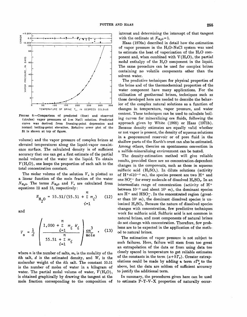
POTTER AND HAAS 255
+ 0.004
0.0
UJ -0.004 100
0 50 100 150 200 250 300 350
TEMPERATURE OF BRINE T x , IN DEGREES CELSIUS
FIGURE 8. Comparison of predicted (line) and observed (circles) vapor pressures of 1-m NaCl solution. Predicted curve was derived from freezing-point depression and normal boiling-point elevation. Relative error plot of the fit is shown at top of figure.
volume) and the vapor pressure of complex brines at elevated temperatures along the liquid-vapor coexist ence surface. The calculated density is of sufficient accuracy that one can get a first estimate of the partial molal volume of the water in the liquid. To obtain T(H2O), one keeps the proportion of each salt to the total concentration constant.
The molar volume of the solution F8 is plotted as a linear function of the mole fraction of the water -A^H2o. The terms Nn2o and F8 are calculated from equations 12 and 13, respectively:
nNu = 55.517(55.51 + I m.) (12) n_0 ^
and
7 = ±1d
I n 1,000 + £ m. W.
n 55.51 + Z m.. '-1 t'
3cmmole
(13)
where n is the number of salts, m^ is the molality of the eth salt, d is the estimated density, and Wt is the molecular weight of the ith salt. The constant 55.51 is the number of moles of water in a kilogram of water. The partial molal volume of water, F(H2O), is obtained graphically by drawing the tangent at the mole fraction corresponding to the composition of
interest and determining the intercept of that tangent with the ordinate at N-aZQ = 1..
Haas (1976a) described in detail how the estimation of vapor pressure in the H20-NaCl system was used to estimate the heat of vaporization of the H2O com ponent and, when combined with V(H2O), the partial molal enthalpy of the H2O component in the liquid. The same procedure can be used for complex brines containing no volatile components other than the solvent water.
The predictive techniques for physical properties of the brine and of the thermochemical properties of the water component have many applications. For the utilization of geothermal brines, techniques such as those developed here are needed to describe the behav ior of the complex natural solutions as a function of changes in temperature, vapor pressure, and water content. These techniques can be used to calculate boil ing curves for mineralizing ore fluids, following the approach given by White (1968) or Haas (197lb). Because density estimates are equally valid whether or not vapor is present, the density of aqueous solutions in a geopressured reservoir or of pore fluid in the shallow parts of the Earth's crust can also be estimated. Among others, theories on spontaneous convection in a sulfide-mineralizing environment can be tested.
The density-estimation method will give reliable results, provided there are no concentration-dependent changes in the components, such as those in aqueous sulfuric acid (H2 SO4 ). In dilute solutions (activity of H+^10~ 2 m), the species present are two H+ and one SO;;- for every molecule of dissolved H2SO4. In an intermediate range of concentration (activity of H+ between 1Q-2 and about 101 m) , the dominant species are H+ and HSO~. In the concentrated region (great er than 101 m), the dominant dissolved species is un ionized H2S04 . Because the nature of dissolved species changes with concentration, few predictive techniques work for sulfuric acid. Sulfuric acid is not common in natural brines, and most components of natural brines do not change with concentration. Therefore, few prob lems are to be expected in the application of the meth od to natural brines.
The estimation of vapor pressure is not subject to such failures. Here, failure will stem from too great an extrapolation of the data or from using data too closely spaced in temperature to get reliable estimates of the constants in the term (a+bTg,). Greater extrap olations could be made by adding a term cT* to the above, but the data are seldom of sufficient accuracy to justify the additional term.
In summary, the procedures given here can be used to estimate P-T-V-X properties of naturally occur-
256 CALCULATING DENSITY AND VAPOR PRESSURE OF GEOTHERMAL BRINES
ring aqueous liquids. They will also permit the esti mation of the partial molal volume and partial molal enthalpy of the H2O component in the liquids. The easy calculation of these parameters should contribute significantly to the study of geochemical and geophysi cal processes where water is a significant component.
REFERENCES CITED
Bain, R. W., 1964, Steam tables 1964: Edinburgh, Her Majesty's Stationery Office, 147 p.
Dibrov, I. A., Mal'tsev, G. Z., and Mashovets, V. P., 1964, Saturated vapor pressure of caustic soda and sodium aluminate solutions in the 25-350° temperature range over a wide range in concentrations: Jour. Applied Chem. USSR, v. 37, p. 1907-1915.
Fabuss, B. M., and Korosi, Alexander, 1968, Properties of sea water and solutions containing sodium chloride, potasium chloride, sodium sulfate, and magnesium sulfate: U.S. Office Saline Water Research Development Progress Rept. No. 384, 133 p.
Gardner, E. R., 1969, Osmotic coefficients of some aqueous sodium chloride solutions at high temperature: Faraday Soc. Trans., v. 65, p. 91-97.
Gardner, E. R., Jones, P. J., and deNordwall, H. J., 1963, Osmotic coefficients of some aqueous sodium chloride solu tions at high temperature: Faraday Soc. Trans., v. 59, p. 1994-2000.
Ginzburg, D. M., 1965, [The density and vapor pressure of sodium and potassium carbonate solutions] : zhur. Prik- ladnaya Khim., v. 38, p. 55-58 (in Russian).
Goff, J. A., 1963, Saturation pressure of water on the new Kelvin scale: Humidity moisture, Papers, Intern, Symp., Washington, D. C., 1963, Proc., v. 3, p. 289-292.
Haas, J. L., Jr., 1970 Fugacity of H2O from 0° to 350° C at the liquid-vapor eqilibrium and at 1 atmosphere: Geo- chim. Cosmochim. Acta, v. 34, p. 929-932.
1971a, Thermodynamic correlations for brines: NaCl- H2O liquid-vapor equilibria [abs.] : Am. Geophys. Union Trans., V. 52, p. 379.
1971b, The effect of salinity on the maximum thermal gradient of a hydrothermal system at hydrostatic pres sure: Econ. Geology, v. 66, p. 940-946.
1976a, Physical properties of the coexisting phases and thennochemical properties of the H2O component in boil ing NaCl solutions: U.S. Geol. Survey Bull. 1421-A, 73 p.
1976b, Thermodynamic properties of the coexistingphases and thermochemical properties of the NaCl com ponent in boiling NaCl solutions: U.S. Geol. Survey Bull. 1421-B, 71 p.
Lee, Shiu, 1966, The apparent and partial molal volumes of electrolytes in water and in aqueous sodium chloride solu tions : Yale Univ., Ph. D. thesis, 141 p.; Univ. Micro films, Order No. 66-4906; Dissertation Abs., v. B27, p. 131.
Lewis, G. N., and Randall, M., 1921, The activity coefficient of strong electrolytes: Jour. Am. Chem. Soc., v. 43, p. 1112- 1154.
Lindsay, W. T., Jr., and Liu, C.-T., 1968, Vapor pressure lower ing of aqueous solutions at elevated temperatures: U.S. Office Saline Water Research Development Rept. 347, 235 p.
Liu-C.-T., and Lindsay, AV. T., Jr., 1971, Thermodynamic properties of aqueous solutions at high temperatures: U.S. Office Saline Water Research Development Rept. 722, 124 p.
Millero, F. J., 1973, Seawater A test of multicomponent electrolyte solution theories, pt. 1, Apparent equivalent volume, expansibility, and compressibility of artificial sea- water: Jour. Solution Chemistry, v. 2, p. 1-22.
Momicchioli, F., Devoto, O., Grandi, G., and Cocco, G., 1970, Thermodynamic properties of concentrated solutions of strong electrolytes, pt. 1, Activity coefficients of water from freezing-point depressions for alkali chlorides: Ber. Bunsen-Gesell, phys. Chemie, v. 74, p. 59-66.
National Research Council, 1928, International critical tables of numerical data, physics, chemistry and technology: New York, McGraw-Hill Book Co., v. 3, 444 p.
Nicolai, H. W., Ernst, W., and Wegkamp, H., 1951, [Viscosity as an analytical method for electrolyte solutions] : Chem. Weeblad, v. 47, p. 88-90 (in Dutch).
Othmer, D. R., 1940, Correlating vapor-pressure and latent- heat data, a new plot: Industrial Eng. Chemistry, v. 32, p. 841-856.
Othmer, D. R., and Chen, H-T., 1968, Correlating and predict ing thermodynamic data: Industrial Eng. Chemistry, v. 60, no. 4, p. 39-61; reprinted in Am. Chem. Soc., 1968, Applied thermodynamics: Washington, D.C., Am. Chem. Soc. Pubs., p. 115-139.
Othmer, D. F., and Yu, E. S., 1968, Correlating vapor pres sures and vapor volumes Use of reference substance equations: Industrial Eng. Chemistry, v. 60, no. 1, p. 22-35.
Potter, R. W., II, 1976, An assessment of the status of the available data on the P-V-T properties for the major components in geothermal brines: United Nations sym posium on the development and use of geothermal re sources, San Francisco 1975, Proc., 1975, v. 1, p. 827-829.
Potter, R. W., II, and Brown, D. L., 1975, The volumetric properties of aqueous sodium chloride solutions for 0° to 500°C at pressures up to 2000 bars based on a regression of the available literature data: U.S. Geol. Survey Open- File Rept. 75-636, 31 p.
1976a, The volumetric properties of vapor saturated aqueous saturated aqueous potassium chloride solutions from 0° to 400°C based on a regression of the available literature data: U.S. Geol. Survey Open-File Rept. 76- 243, 6 p.
19761), The volumetric properties of vapor saturated aqueous sodium sulfate solutions from 0° to 325° C based on a regression of the available literature data: U.S. Geol. Survey Open-File Rept. 76-255, 6 p.
1976c, The volumetric properties of vapor saturatedaqueous potassium sulfate solutions from 0° to 200°C based on a regression of the available literature data: U.S. Geol. Survey Open-File Rept. 76-501, 7 p.
Potter, R. W., II, and Clynne, M. A., 1976, The volumetric properties of vapor saturated aqueous calcium chloride solutions from 0° to 300° C based on a regression of the available literature data: U.S. Geol. Survey Open-File Rept. 76-365, 7 p.
Potter, R. W., II, Shaw, D. R., and Haas, J. L., Jr., 1975, Annotated bibliography of studies on the density and other volumetric properties for major components in geo thermal waters 1928-74: U.S. Geol. Survey Bull. 1417, 78 p.
POTTER AND HAAS 257
Reilly, P. J., and Wood, R. H., 1969, The prediction of the properties of mixed electrolytes from measurements on common ion mixtures: Jour. Phys. Chemistry, v. 73, p. 4292-4302.
Reilly, P. J., Wood., R. H., and Robinson, R. A., 1971, The prediction of osmotic and activity coefficients in mixed- electrolyte solutions: Jour. Phys. Chemistry, v. 75, p. 1305-1315.
Robinson, R. A., and Stokes, R. H., 1959, Electrolyte solutions: London, Butterworths, 2d ed., 571 p.
Smith, R. P., 1939, The boiling point elevation, pt. 2, Sodium chloride 0.05 to 1.0 M and 60 to 100°: Am. Chem. Soc. Jour., v. 61, p. 500-503.
Smith, R. P., and Hirtle, D. S., 1939, The boiling point ele vation, pt. 3, Sodium chloride 1.0 to 4.0 M and 60 to 100°: Am. Chem. Soc. Jour., v. 61, p. 1123-1126.
Volz-Fladrich, H., 1962, [Physical-chemical examinations on the systems MgClr-HCl-HaO, NaCl-HCl-H2O, and KC1- HCl-HzO] : Freiberger Forschunghschefte, v. 134, p. 1-85 (in German).
White, D. E., 1965, Saline waters of sedimentary rocks, in Fluids in subsurface environments A symposium: Am. Assoc. Petroleum Geologists Mem. No. 4, p. 342-366.
1968, Hydrology, activity, and heat f\o\v of the Steam boat Springs thermal system, Washoe County, Nevada: U.S. Geol. Survey Prof. Paper 458-C, 109 p.
Wood, R. H., and Anderson, H. L., 1966, Heats of mixing of aqueous electrolytes, pt. 3, A test of the general equations with quaternary mixtures: Jour. Phys. Chemistry, v. 70, p. 1877-1879.
Young, T. F., and Smith, M. B., 1954, Thermoclynamic prop erties of mixtures of electrolytes in aqueous solutions: Jour. Phys. Chemistry, v. 58, p. 716-724.

Jour. Research U.S. Geol. Survey Vol. 6, No. 2, Mar.-Apr. 1978, p. 259-262
SPECTROCHEMICAL DETERMINATION OF SUBMICROGRAM AMOUNTS OFTUNGSTEN IN GEOLOGIC MATERIALS
By REINHARD W. LEINZ and DAVID J. GRIMES, Denver, Colo.
Abstract. A rapid, sensitive, emission spectrographic meth od for the determination of tungsten in geologic materials has been developed. Sample fusion with potassium hydroxide followed by a hot-water leach renders the tungsten soluble. Acidification of the solution, reduction with titanium tri chloride, complexing with thiocyanate, and ether extraction separate and concentrate the tungsten. An aliquot of the ether solution is pipetted into the cavity of a preformed graphite electrode containing 6 milligrams of sodium carbonate and is evaporated. The carbonate flux prevents formation of refrac tory tungsten carbide during arcing, resulting in nearly com plete volatilization of tungsten during a short exposure period. Spectra from direct-current arc excitation of the tungsten are recorded on film and visually compared to standard spec tra. A determination limit of 0.2-part-per-million tungsten is obtained from a 0.5-gram sample with a sample completion average of 30-50 samples per man-day.
Analytical methods for the determination of tung sten in geologic samples, if not lengthy and tedious, often suffer the lack of sensitivity required in geo- chemical investigations. Gair, Windolph, and Wright (1975) noted in a survey of the Hamme tungsten dis trict, North Carolina, that the tungsten values reported in soils over mineralized quartz veins were not much higher than the detection limit of the analytical method. Hobbs and Elliott (1973, p. 677) pointed out that in tungsten geochemical research, "One of the key restraints . . . has been the inability to analyze with accuracy for small amounts of tungsten."
To date, analysts have relied heavily on spectro- photometric determinations of tungsten after complex- ing it with one of several reagents. Ward's method (1951) utilizes visual estimation of the yellow-green tungsten thiocyanate complex. Lillie and Greenland (1973) made use of this complex in their isotope-dilu tion procedure. .The tungsten dithiol complex is the measured species in methods developed by Jeffery (1956), Chan and Eiley (1967a), Stanton (1970), and Quin and Brooks (1972).
Tungsten is routinely determined down to 50 parts per million in the 30-element spectrographic analysis
described by Grimes and Marranzino (1968) and to submicrogram levels by the neutron-activation tech nique of Simon and Rollinson (1975).
This report describes a chemical preparation con sisting of a rigorous alkali fusion, a hot-water leach, tungsten reduction, complexing with thiocyanate and ether extraction followed by a direct-current arc emis sion spectrographic determination that employs a sodium carbonate flux. The determination limit of this method (0.2 ppm) is below the average crustal abun dance for tungsten (1-1.3 ppm) as given by Hobbs and Elliott (1973). No interelement interferences have been found, and the precision is more than adequate for most geochemical exploration investigations. Thirty to fifty samples can be analyzed per man-day and sim plicity of the method allows for determinations to be made in existing U.S. Geological Survey mobile field laboratories.
REAGENTS AND APPARATUS FOR CHEMICAL PREPARATION
All reagents are reagent grade, except for the tita nium trichloride (20 percent solution) which is tech nical grade, and are listed as follows:
Potassium hydroxide, pellet form.Hydrochloric acid, concentrated.Titanium trichloride, 20 percent solution.Potassium thiocyanate solution, 25 percent (weight per
volume) in water, prepared daily. Isopropyl ether.
The apparatus is listed as follows: Nickel crucibles, 50 milliliter capacity. Muffle furnace. Vortex mixer. Centrifuge, with heads for 16-millimeter and 25-mm-
diameter tubes.Micropipette, 60 microliter capacity. Test tubes, 16 by 150 mm disposable and 25- by 150-mm
screwcap.
259
260 SPECTROCHEMICAL DETERMINATION OF TUNGSTEN IN GEOLOGIC MATERIALS
PROCEDURE
Weigh 0.5 gram of the powdered sample (ground or sieved to at least -80 mesh) into a 75-mL nickel crucible. Add 2.5 g pelletized potassium hydroxide and distribute evenly with the sample on the bottom of the crucible. Fuse in a muffle furnace by increasing the temperature slowly from room temperature to 450°C. Alternatively, heat gently over an open flame until the sample is thoroughly wetted with molten potassium hydroxide and then heat an additional 2 minutes.
Cool the crucible and carefully add 7 mL hot water to dissolve the soluble fusion products. Use a glass stirring rod to break up the melt and with the aid of a funnel transfer the solution and residue to a 16- by 150-mm test tube. Einse the crucible with 1 mL water and transfer as above. Centrifuge and decant the liquid into a 25- by 150-mm screwcap test tube. Einse the residue with 3 mL water, centrifuge, and add the liquid to the same tube. The residue may now be discarded.
With caution, add 12mL concentrated hydrochloric acid to the highly basic solution in the screwcap tube. Cool the tube in a water bath, add 4 mL of the 20 per cent titanium trichloride solution and vortex. Add 1 mL of the 25 percent potassium thiocyanate solution and 1 mL of isopropyl ether, capping and shaking the tube for 2 min after each addition. Centrifuge the tube so that a sufficient amount of ether layer is ob tained for pipetting with the 60-/*L micropipette. The final two-phase solution is stable under refrigeration in the capped tube for at least 2 weeks.
SPECTROGRAPHIC INSTRUMENTATION AND MATERIALS
Spectrograph, 1.5-meters Wadsworth-mounted, with a dispersion of 5.4 angstroms per millimeter over the spectral range of 2100-4800 A in the second order.
Source, spark-ignited direct-current arc 220 volts with arc current variable in steps from 2 to 15 amperes.
Comparator, 20 X magnification.Electrodes, anode 6.15-mm-diameter undercut graph
ite electrode [Utra carbon No. 100-L (U-7) ] ; cath ode 4.57-mm-diameter graphite rod [Ultra carbon No. 105 (U-7)].
Film, 35-rnm spectrum analysis No. 1 emulsion.Sodium carbonate, Johnson Matthey Spec-Pure.
Analytical gap, 4 mm. Slit, 20 microns.
Hartmann diaphram, 1.0 mm. Current, 15 A. Exposure, 30 seconds.Processing, Kodak D-19 20°C 2 min; Kodak fixer
20°C 5 min.
SPECTROGRAPHIC DETERMINATIONWeight 6 millgrams of spectrographically pure
sodium carbonate powder and transfer it to the cavity of the graphite electrode with the aid of an aluminum funnel. Carefully pipet 60 /*L of the ether layer into the electrode crater that contains the sodium carbonate and oven dry at 110°C for 10 min. (Avoid pipetting any of the acid layer into the electrode because the ensuing reaction with the sodium carbonate will pro duce low tungsten results).
After cooling, clamp the sample and counter elec trodes into the arc stand of the spectrograph, set the electrode gap at 4 mm, and arc the sample for 30 sec at 15 A. When Hartmann diaphram is set at 1.0 mm, 24 samples can be recorded on each length of film. Process the exposed film in developer at 20°C for 2 min, in fixer at 20°C for 5 min, wash in cold water, and air dry. Visually compare the resultant spectra with standard spectra by means of a 20 X comparator. A concentration range from 0.2 to 500 ppm is obtained by use of the tungsten line at the wavelength of 2946.9 A. .
STANDARDSTungsten stock solutions are as follows:
1000 micrograms per milliliter: Dissolve 0.8973 gsodium tungstate dihydrate (Na2WO4'2H2O) in 500mL of 0.1 molar KOH.
100 /tg/mL: Dilute 10 mL of the 1000 /tg/mL to 100mL with 0.1 molar KOH.
Prepare solutions of 10 /*g/mL and 1.0 /tg/mL in asimilar manner.To twelve 25- by 150-mm screwcap test tubes, add
2.5 g potassium hydroxide and dissolve with 10 mL water. Using the above stock solutions, and 0, 0.2, 0.5, 1.0, 2.0, 5.0, 10, 20, 50, 100, 200, and 500 micrograms of tungsten to the tubes. Cautiously add 12 mL concen trated hydrochloric acid and cool in a water bath. Add 4 mL titanium trichloride and vortex. Add 1 mL of 25-percent potassium thiocyanate and 2 mL isopropyl ether (extractions of the standards into 2 mL ether and samples (0.5 g) into 1 mL ether allow direct tungsten measurements in micrograms per milliliter or parts per million to be made), capping and shaking the tubes for 2 min after each addition. Allow the phases to separate.
Weigh 6 mg sodium carbonate into the cavities of
LEINZ AND GRIMES 261
12 graphite electrodes, then carefully add 60 /xL from the ether layer of successive standards. Continue as in a procedure for spectrographic determination.
The range of the prepared standards on film is from 0.2 to 500 ppm (excluding the blank) with three standards or steps between each order of magnitude. For semiquantitative analysis, the density and width of an appropriate tungsten line in the spectrum of the sample is visually compared with the tungsten line at the same wavelength in the standard spectrum. An estimate of the tungsten concentration in the sample is based on directly matching densities or the sample line density falling between the densities of two ad jacent standard lines. Thus, values for tungsten are reported in six concentration steps between each order of magnitude in the following series: 0.2, 0.3, 0.5, 0.7, 1.0, 1.5, 2.0, 3.0, 5.0, 7.0, 10.0, 15, 20, 30, 50, 70, 100, 150, 200, 300, and 500 ppm.
DISCUSSION OF PROCEDURE
Fusing the sample with potassium hydroxide and leaching the melt with water solubilize any tungstate minerals present as potassium tungstate. Potentially troublesome iron is simultaneously precipitated as hy droxide and discarded. Acidification of the super natant solution with hydrochloric acid and addition of the reducing agent, titanium trichloride, produce a "genutypic" compound ("one having the same basic structure, but differing in the charges on cations and anions") known as tungsten blue (Cotton and Wilkin- son, 1972). In greater than 4 N hydrochloric acid and in the presence of excess titanium trichloride, tung sten blue appears to react with thiocyanate ions to yield a yellow-green to green complex whose structure is uncertain (perhaps an oxoanion) and whose stability is certain only in solution. This complex is quantita tively extractable from the acidic aqueous layer into the nonpolar isopropyl ether. More than 95-percent extraction is attained into 1 mL of ether at the 250-/xg level.
Formation and extraction of metallic thiocyanates other than tungsten is minimal and does not affect extraction or spectral determination of the tungsten. Molybdenum, for example, complexes only to a slight extent under the highly acidic and reducing-reaction conditions.
Aside from solubilizing tungsten minerals present in the sample, the fusion and leaching also put silica into solution. Upon acidification, the silica forms silicic acid which may form a gel in the ether phase. Centri- fuging is often necessary to clear a sufficient amount of ether for pipetting.
During high-temperature arcing in emission spectro graphic analysis, tungsten species are usually reduced to refractory tungsten carbide (boiling point, 6000°C) when singularly present in the graphite electrode crater. This often necessitates a long burn time, filtered emitted light, and a narrow entrance slit, all of which decrease sensitivity.
The authors found that sodium carbonate present in the crater during arcing inhibits formation of the car bide and allows tungsten to volatilize in a more oxi dized and lower boiling form, probably as the trioide W03 (bp. about 1400°C). The presence of sodium vapor in the arc also lowers the arc temperature which minimizes the ionization of tungsten atoms. In con trast, the much higher temperature of a carbon vapor arc increases the percentage of tungsten atoms ionized. Neutral and ionized atoms of the same element emit different spectra, the intensities of which are propor tional to the population of each species present in the arc. The 2946.9-A tungsten line is produced by excita tion of neutral atoms; therefore, its intensity is in creased by the presence of sodium vapor in the arc. A comparison of tungsten emission with and without the presence of sodium carbonate is shown in figure 1. The graphical data presented in figure 1 was obtained from a 15-sec interval moving-plate study of 60 /*L of a 200- ng/mL tungsten standard pipetted into two electrodes, one of which contained 6 mg of the sodium carbonate flux.
Lower detection limits may be obtained by pipetting additional aliquots of the ether phase into the electrode crater. However, because the ether does contain some dissolved acidic aqueous phase that reacts with the carbonate flux, a new set of spectrographic standards must be prepared. For reliable analysis an equal quan tity of ether must be pipetted for both sample and standard.
PRECISION AND ACCURACY
The precision of this method was established from data of 12 repeat analyses of 12 different samples (table 1). The samples were various geologic materials and contained several different tungsten minerals such as scheelite (CaW04 ) in skarns I and II and hueb- nerite (MnW04 ) in soils I and II. The coefficient of variation ranged from 10 to 27 percent, with all or most values from any one sample falling within one spectrographic reporting step of the mean.
Accuracy was approximated by comparison of the mean of the 12 replicate analysis of the granite G-2 standard and the glass standards GSB, GSC, GSD, and GSE with values found in the literature (table 1).
262 SPECTROCHEMICAL DETERMINATION OF TUNGSTEN IN GEOLOGIC MATERIALS
Without flux
TIME, IN SECONDS
FIGURE 1. A comparison of tungsten emission with and with out sodium carbonate flux (6 mg Na2CO3 ).
Both precision and accuracy are well within an ac ceptable range for most geochemical exploration inves tigations involving tungsten. If a more quantitative analysis was required, incorporation of an internal standard with the flux as well as plots of emulsion calibration and working curves obtained from densio- metric measurements of spectral lines would be necessary.
TABLE 1. Summary of tungsten precision and accuracy studies on 12 repeat analyses for various sample types
Sample type
High Fe-Mn marble
Skarn II
Granite (G-2) ------ Soil I -Soil II -
Porphyry copperOre (sulfide)-
Glass standards:
GSD-
Range (ppm)
15100
7
0.
150
30
100
30300
- 30-150- 15
15- 0.2 - 5200
- 70
-150
,5 - 1
-500
Mean (ppm)
20
9.4
.18 2.9
192
48
CO
400
Standard deviation
5,
2,
19
10
104
.2
.4
.3
.03
.3
70
Coefficient Literature of values (ppm)
variation (percent)
261024
1 217 0.1+0.3; 0.4 27
21
19
17 3 5026 420
Simon and Rollinson (1975).
Chan and Riley (1967b).
Myers and others (1976).
SUMMARY
The proposed method combines a chemical separa tion and preconcentration with an emission spectre- graphic determination and enables tungsten measure ments to be made in geologic materials in amounts below crustal abundance. Interelement interferences, which pose problems in many of the colorimetric pro cedures, such as the interference from molybdenum, are virtually eliminated. The method's precision and accuracy are more than adequate for most geochemical exploration studies, its simplicity allows for adapta tion to the mobile laboratories of the U.S. Geological Survey, and its rapidity permits an average of 30-50 sample analyses per man-day.
REFERENCES CITED
Chan, K. M., and Riley, J. P., 1967a, Determination of tung sten in silicates and natural waters: Anal. Chim. Acta, v. 39, p. 103-113.
1967b, Determinations of vanadium, molybdenum, and tungsten in the new series of U.S. Geological Survey analyzed samples: Chem. Geology, v. 2, p. 171-172.
Cotton, F. A., and Wilkinson, Geoffrey, 1972, Advanced inor ganic chemistry: New York, John Wiley & Sons, 947 p.
Gair, J. E., Windolph, J. F., Jr., and Wright, N. A., 1975. Preliminary results of geochemical soil survey, Hamme tungsten district, North Carolina: U.S. Geol. Survey Circ. 711, 19 p.
Grimes, D. J., and Marranzino, A. P., 1968, Direct-current are and alternating-current spark emission spectrographic field methods for the semiquantitative analysis of geologic materials: U.S. Geol. Survey Circ. 591, 6 p.
Hobbs, S. W., Elliott, J. E., 1973, Tungsten, in Brobst, D. A., and Pratt, W. P., eds., United States mineral resources: U.E. Geol. Survey Prof. Paper 820, p. 667-678.
Jeffrey, P. G., 1956, The simultaneous photometric determina tion of molybdenum and tungsten in silicate rocks: Analyst, v. 81, no. 959, p. 104-109.
Lillie, E. G., and Greenland, L. P., 1973, Spectrophotometric determination of tungsten in rocks by an isotope dilution procedure: U.S. Geol. Survey Jour. Research, v. 1, no. 5, p. 555-558.
Myers, A. T., Havens, R. G., Connor, J. J., Conklin, N. M., and Rose, H. J., 1976, Glass reference standards for the trace-element analysis of geological materials Compila tion of interlaboratory data: U.S. Geol. Survey Prof. Paper 1013, 29 p.
Quin, B. F., and Brooks, R. R., 1972, The rapid determination of tungsten in soils, stream sediments, rocks and vegeta tion: Anal. Chim. Acta, v. 58, p. 301-309.
Simon, F. O., and Rollinson, C. L., 1975, Determination of tungsten in geologic materials by neutron activation anal ysis: U.S. Geol. Survey Jour. Research, v. 3, no. 4. p. 475-478.
Stanton, R. E.. 1970, The colorimetric determination of tung sten in soils, sediments, and rocks by zinc dithiol: Aus tralasian Inst. Mining and Metallurgy Proc.. no. 236. p. 59-60.
Ward, F. N., 1951, A field method for the determination of tungsten in soils: U.S. Geol. Survey Circ. 119, 4 p.
Jour. Research U.S. Qeol. Survey Vol. 6, No. 2, Mar.-Apr. 1978, p. 263-271
IMPACT OF SEWERAGE SYSTEMS ON STREAM BASE FLOW AND GROUND- WATER RECHARGE ON LONG ISLAND, NEW YORK
By E. J. PLUHOWSKil and A. G. SPINELLO, Reston, Va., Syosset, N. Y.
Abstract. Statistically significant decreases in the ratio of base flow to total flow of streams along the south shore of Long Island, N.Y., are due to the use of expanding storm- sewer and sanitary-sewer networks. Base-flow losses due to sewering ranging from virtually none at Connetquot River (largely unaffected by urban development) to 211 liters per second, or a 60-percent decrease below natural levels, during 1965-74 at East Meadow Brook (which drains part of highly urbanized Nassau County). Nearly 75 percent of the base- flow loss at East Meadow Brook during 1965-74 was caused by a network of sanitary sewers west of the stream; the remainder resulted from loss of recharge in areas serviced by stream-directed storm sewers. In areas of the Carlls River basin serviced by stream-directed storm sewers, recharge depletion averaged only about 4 liter per second per square kilometer whereas in the more intensely urbanized East Meadow Brook basin, recharge depletion in such areas aver aged 18 (L/s)/knr.
The eastward spread of urbanization across Long Island has been accompanied by increasingly complex sewerage systems. The large-scale conversion of open land areas to paved, impervious surfaces, concurrent with the redirection, of surface runoff to streams and the disposal of waste water to the oceans through sewer systems, has resulted in a loss of recharge to thje ground-water reservoir. The purpose of this investiga tion is to define and evaluate the impact of the sewer age systems on stream base flow and ground-water recharge.
PREVIOUS RESEARCH
The effects of the installation of a sanitary-sewer system in western Nassau County on ground-water levels, which were lowered by 2.1 meters during 1953- 72, were described by Garber and Sulam (1976). Con tamination of the upper glacial aquifer by cesspools, septic tanks, and sewage lagoons in developed areas of Nassau and Suffolk Counties was described by Plu- howski and Kantrowitz (1964) and Cohen, Franke, and Foxworthy (1968). The alteration of flood-peak characteristics of East Meadow Brook in south-central Nassau County as a result of the diversion of urban runoff to storm sewers has been described by Seaburn (1969).
DEVELOPMENT OF WASTE-WATER DISPOSAL SYSTEMS
Before World War I, when extensive parts of Nassau and Suffolk Counties were devoted to agricul ture, wells were dug or driven into the upper glacial aquifer to provide much of the water supply for do mestic use, and waste water was returned to the aquifer through cesspools and septic tanks (Heath and others, 1966). Storm runoff was channeled to low-lying areas, watercourses, or ponds. Thus, except for small con sumptive losses, virtually all ground water pumped for water supply was returned to the upper glacial aqui fer. After World War I, a slow but steady urban ex pansion began in western Nassau County and along railroad trunklines in central and southern Nassau County and southwestern Suffolk County. In 1927, the village of Freeport built a sanitary sewerage system servicing 11 square kilometers. The system processed domestic and industrial waste water and discharged its effluent to tidewater south of the village.
To cope with ever-increasing amounts of storm run off, as urban development reduced infiltration area, and to conserve ground-water reserves, Nassau County officials approved construction of several experimental storm-water collection basins in 1935 (Welsch, 1935). These excavations, known as recharge basins, were de signed to allow rapid infiltration of runoff conveyed to them by storm sewers. More than 2100 recharge basins had been constructed on Long Island by 1969 (Seaburn and Aronson, 1974), principally in the central part of Nassau and Suffolk Counties. However, the construc tion of storm sewers has continued at a steady rate, especially in southern Nassau County and southwest ern Suffolk County, where they convey the bulk of storm runoff directly to streams rather than to ponds or recharge basins.
Although the system of recharge basins combined with cesspools, septic tanks, and diffusion wells serves to conserve ground water, increasing contamination of the upper glacial aquifer prompted officials of both counties to adopt plans for treating sanitary sewage at
263
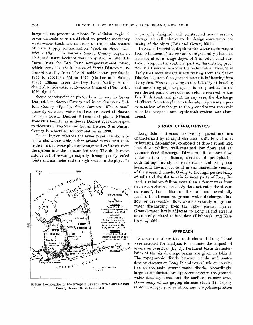
264 IMPACT OF SEWERAGE SYSTEMS, LONG ISLAND, NEW YORK
large-volume processing plants. In addition, regional sewer districts were established to provide secondary waste-water treatment in order to reduce the chance of water-supply contamination. Work on Sewer Dis trict 2 (fig. 1) in western Nassau County began in 1953, iand sewer hookups were completed in 1964. Ef fluent from the Bay Park sewage-treatment plant, which serves the 181-km2 area of Sewer District 2, in creased steadily from 2.2 XlO4 cubic meters per clay in 1953 to 26X10* m3/d in 1972 (Garber and Sulam, 1976). Effluent from the Bay Park facility is dis charged to tidewater ait Keynolds Channel (Pluhowski, 1972, fig. 11).
Sewer construction is presently underway in Sewer District 3 in Nassau County and in southwestern Suf folk County (fig. 1). Since January 1974, a small quantity of waste water has been processed at Nassau County's Sewer District 3 treatment plant. Effluent from this facility, as in Sewer District 2, is discharged to tidewater. The 272-km2 Sewer District 3 in Nassau County is scheduled for completion in 1990.
Depending on whether the sewer pipes are above or below the water table, either ground water will infil trate into the sewer pipes or sewage will exfiltrate from the system into the unsaturated zone. The fluids move into or out of sewers principally through poorly sealed joints and manholes and through cracks in the pipes. In
73°45'
Sewer District 2Sanitary sewer system fully
operational since 1964
Sewer District 3Sanitary sewer system
under construction -- notin operation during thestudy period (1944-74)
Freeport Sewer DistrictSanitary sewer system fully
operational since 19272
ay ParkSewage Freeport Treatment Plant.
FREEPORT SEWER DISTRICT
-^
FIGURE 1. Location of the Freeport Sewer District and Nassau County Sewer Districts 2 and 3.
a properly designed and constructed sewer system, leakage is small relative to the design conveyance ca pacity of the pipes (Fair and Geyer, 1954).
In Sewer District 2, depth to the water table ranges from 0 to about 45 m. Sewers were generally placed in trenches at an average depth, of 3 m below land sur face. Except in the southern part of the district, prac tically all sewers lie above the water table. Thus, it is Hkely that more sewage is exfiltrating from the Sewer District 2 system than ground water is infiltrating into the system. However, owing to the difficulty of locating and measuring pipe seepage, it is not practical to as sess the net gain or loss of fluid volume received by the Bay Park treatment plant. In any case, the discharge of effluent from the plant to tidewater represents a per manent loss of recharge to the ground-water reservoir since the cesspool- and septic-tank system was aban doned.
STREAM CHARACTERISTICS
Long Island streams are widely spaced and are characterized by straight channels, with few, if any, tributaries. Streamflow, composed of direct runoff and base flow, exhibits well-sustained low flows and at tenuated flood discharges. Direct runoff, or storm flow, under natural conditions, consists of precipitation both falling directly on the streams and contiguous lakes, and flowing overland in the immediate vicinity of the stream channels. Owing to the high permeability of soils and the flat terrain in most parts of Long Is land, a raindrop falling more than a few meters from the stream channel probably does not enter the stream as runoff, but infiltrates the soil and eventually reaches the streams as ground-water discharge. Base flow, or dry-weather flow, consists entirely of ground water discharging from the upper glacial aquifer. Ground-water levels adjacent to Long Island streams are directly related to base flow (Pluhowski and Kan- trowitz, 1964).
APPROACH
Six streams along the south shore of Long Island were selected for analysis to evaluate the impact of sewers on base flow (fig. 2). Pertinent basin character istics of the six drainage basins are given in table 1. The topographic divide between north- and south- flowing streams on Long Island bears little or no rela tion to the main ground-water divide. Accordingly, large dissimilarities are apparent between the ground- water drainage areas and the surface-drainage areas above many of the gaging stations (table 1). Topog raphy, geology, precipitation, and evapotranspiration
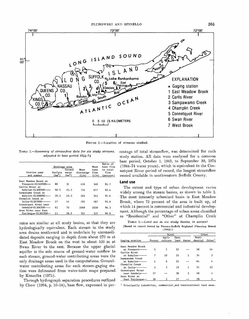
74°00'
PLUHOWSKI AND SPINELLO
73°00'
26572°00'
41 °| 00'
NASSAU , QUEENS ) CO. V. CO.
KINGSCO.(vA°
ATtA NT ' C
5 10 15 KILOMETERS i i i
EXPLANATION
Gaging station1 East Meadow Brook2 Carlls River3 Sampawams Creek4 Champlin Creek5 Connetquot River6 Swan River7 West Brook
FIGURE 2. Location of streams studied.
TABLE 1.- -Summary of streamflow data for six study streams, adjusted to base period 1944-14
Station nameand number
East Meadow Brook atFreeport-01310500
Carlls River atBabylon-01308500
Sampawams Creek atBabylon-01308000
Champlin Creek atIslip-01307000
Connetquot River nearOakdale-01306500
Swan River near EastPatchogue-01305500
Drainage
Surface(km2 )
80
90.5
59.5
17
62
23
areaGroundwater(km2 )
31
45.5
19.5
14
70
28.5
Meandischarge
(L/s)
416
733
263
195
1068
351
Meanbaseflow(L/s)
340
677
241
1 Q7lo /
1028
337
Ratio ofbase flowto total
flow(percent)
81.7
92.4
91.6
95.9
96.3
96.0
rates are similar at all study basins, so that they are hydrologically equivalent. Each stream in the study area drains southward and is underlain by unconsoli- dated deposits ranging in depth from about 270 m at East Meadow Brook on the west to about 520 m at Swan River to the east. Because the upper glacial aquifer is the sole source of ground-water outflow to each stream, ground-water contributing areas were the only drainage areas used in the computations. Ground- water contributing arenas for each stream-gaging sta tion were delineated from water-table maps prepared by Koszalka (1975).
Through hydrograph separation procedures outlined by Ohow (1964, p. 10-14), base flow, expressed in per
centage of total streamflow, was determined for eachO '
study station. All data were analyzed for a common base period, October 1, 1943, to September 30, 1974 (1944-74 water years), which is equivalent to the Con netquot River period of record, the longest streamflow record available in southwestern Suffolk County.
Land useThe extent and type of urban development varies
widely among the stream basins, as shown in table 2. The most intensely urbanized basin is East Meadow Brook, where 72 percent of the area is built up, of which 14 percent is commercial and industrial develop ment. Although the percentage of urban areas classified as "Residential" and "Other" at Champlin Creek
TABLE 2. Lund use in six study basins, in percent [Based on report issued by Nassau-Suffolk Regional Planning Board
(iocs)]Rural
Gaging station
East Meadow Brook
Carlls River
Sampawams Creek
Champlin Creek
Connetquot River near Oakdale
Swan River at East Patchoque
Forest
5
7
1
5
27
39
Agri culture
1
10
6
2
2
Open land
22
25
25
19
30
27
UrbanResi-
Water dential
58
1 54
64
1 51
2 40
28
Other 1
14
3
4
22
1
4
Principally industrial, commercial,and institutional land uses.

266 IMPACT OF SEWERAGE SYSTEMS, LONG ISLAND, NEW YORK
slightly exceeds the percentage for East Meadow Brook, 22 percent of the land classified as "Other" in the Champlin Creek basin is institutional. The bulk of this category consists mainly of a large State hos pital surrounded by extensive grassy areas and parks. Thus, the total pervious area in the Champlin Creek basin is greater than that in the East Meadow Brook basin. .
Both the Connetquot River and Swan River basins are primarily rural, and large parts of both basins are forested, unlike the four study basins to the west. The Connetquot River flows through a State forest pre serve that extends to the drainage-area boundaries along much of the perennial part of the river. This large undeveloped area forms a buffer zone between the river and eastward-spreading urban development. The Connetquot River basin is one of the few areas on Long Island in which undisturbed stramflow condi tions are preserved.
Statistical analysis of base flow
The homogeneity of base flow among the six streams was analyzed statistically. A sampling scheme using the ratio of base flow to total streamflow for each stream at 5-year intervals, beginning with the 1949 water year, was prepared (table 3). This approach minimizes the number of estimates required to fill in missing data resulting from varying periods of rec ord, yet includes an adequate number of sample events. A one-way analysis of variance (Duncan, 1959) was used to test the hypothesis that no difference in the base-flow characteristics exists among the study streams and that variations among the sampled data were due solely to chance.
ResultsThe results of the test are given in table 4. The vari
ance ratio of 13.6 among the streams exceeds the F- distribution value of 3.70 at the 1-percent level. There is less than 1 chance in 100 that the computed variance ratio could have been attained if the homogeneity hy pothesis was correct. Therefore, the hypothesis that the
TABLE 3. Ratio of base flow to total streamflow for six study streams, in percent
TABLE 4. One-way analysis of variance of data in table 3
Water year
194919541959196419691974
Swan River
98.296.697.695.495.993.1
Connet quot River
96.695.397.395.096.096.4
Champ lin
Creek
96.394.195.794.993.2^4.5
Sampa- wams Creek
95.289.392.690.288.592.7
Carlls River
95.793.492.992.484.288.4
East Meadow Brook
91.281.183.277.966.164.8
Source of variation
Error Total
Sum ofsquares
1 C 1 O O
668.82,181.6
Degreesof
freedom
5 3035
Meansquare
302.6 22.3
Varianceratio
'13.6
Estimated, based on correlation analyses with nearby streams.
1 Significant at the 99-percent level.
base-flow characteristics of the streams are similar was rejected. Moreover, it is concluded that some factor has significantly altered the base-flow characteristics of some of the study basins.
In order to identify the principal source of variation in the data, the 'five degrees of freedom assigned to the streams (table 4) were tested by an individual degree- of-freedom analysis. Comparisons were made by first testing the two easternmost, rural streams (Swan River and Connetquot River) and then introducing into the analyses, in succession, eadh of the four urbanized streams to the west. Five analyses were made, in which the final analysis consisted of a comparison of East Meadow Brook (stream farthest west) contrasted with the combined effect of all five streams to the east. Re sults showed that about 90 percent of the variance in table 4 was due to the inclusion of East Meadow Brook in the analysis.
Discussion
The most obvious factor affecting the hydrology of the study basins is the extent to which the surface in filtration capacity of the well-drained soils common to all the basins has been reduced. Storm water from im pervious roads, roof tops, sidewalks, and parking lots is now channeled through storm sewers to recharge basins or watercourses. Seaburn and Aronson (1974) found that where recharge basins are used to dispose of storm water, ground-water recharge from precipita tion is about equal to recharge under natural condi tions. Thus, storm sewers that discharge into recharge basins have little, if any, effect on ground-water levels or on base flow. However, storm, sewers that empty into channels, in effect, speed the delivery of runoff to streams. Precipitation that would have infiltrated the ground and recharged the water-table aquifer under natural conditions is instead conveyed rapidly to a stream as direct runoff. Although the overall impact of tihis process on total volume of streamflow is probably small, its effect on the ratio of base flow to storm flow in the affected watercourses may be considerable.
Storm sewers, ranging from 380 to 1400 millimeters in diameter, carry storm water to all six study streams (Pluhowski, 19TO). Extensive storm-sewer networks
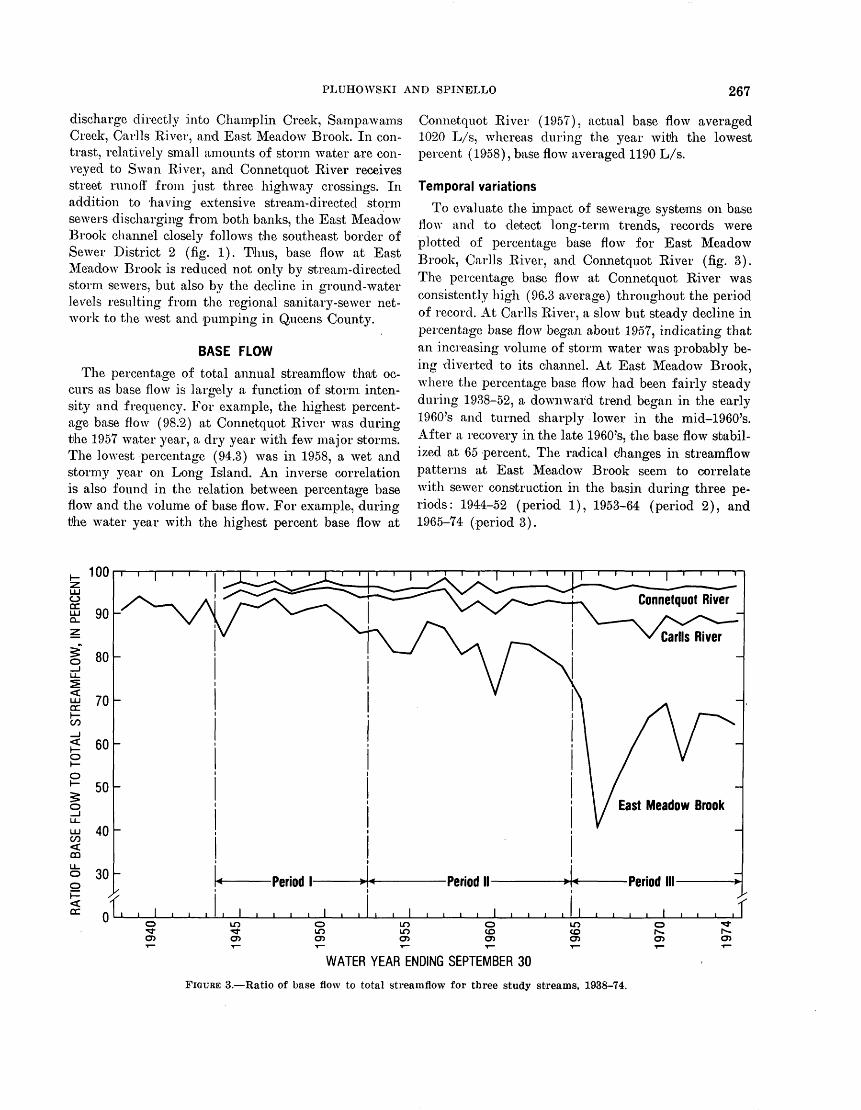
PLUHOWSKI AND SPINELLO 267
discharge directly into Champlin Creek, Saimpawams Creek, Carlls River, and East Meadow Brook. In con trast, relatively small amounts of storm water are con veyed to Swan River, and Connetquot River receives street runoff from just three highway crossings. In addition to having extensive stream-directed storm sewers discharging from both banks, the East Meadow Brook channel closely follows the southeast border of Sewer District 2 (fig. 1). Thus, base flow at East Meadow Brook is reduced not only by stream-directed storm sewers, but also by the decline in ground-water levels resulting from the regional sanitary-sewer net work to the west and pumping in Queens County.
BASE FLOW
The percentage of total annual streamflow that oc curs as base flow is largely a function of storm inten sity and frequency. For example, the highest percent age base flow (98.2) at Connetquot River was during the 1957 water year, a dry year with few major storms. The lowest percentage (94.3) was in 1958, a wet and stormy year on Long Island. An inverse correlation is also found in the relation between percentage base flow and the volume of base flow. For example, during the water year with the highest percent base flow at
Connetquot River (1957), actual base flow averaged 1020 L/s, whereas during the year with the lowest percent (1958), base flow averaged 1190 L/s.
Temporal variations
To evaluate the impact of sewerage systems on base flow and to detect long-term trends, records were plotted of percentage base flow for East Meadow Brook, Carlls River, and Connetquot River (fig. 3). The percentage base flow at Connetquot River was consistently high (96.3 average) throughout the period of record. At Carlls River, a slow but steady decline in percentage base flow began about 1957, indicating that an increasing volume of storm water was probably be ing diverted to its channel. At East Meadow Brook, where the percentage base flow had been fairly steady during 1938-52, a downward trend began in the early 1960's and turned sharply lower in the mid-1960's. After a recovery in the late 1960's, the base flow stabil ized at 65 percent. The radical changes in streamflow patterns at East Meadow Brook seem to correlate with sewer construction in the basin during three pe riods: 1944-52 (period 1), 1953-64 (period 2), and 1965-74 (period 3).
WATER YEAR ENDING SEPTEMBER 30
FIGURE 3. Ratio of base flow to total streamflow for three study streams, 1938-74.
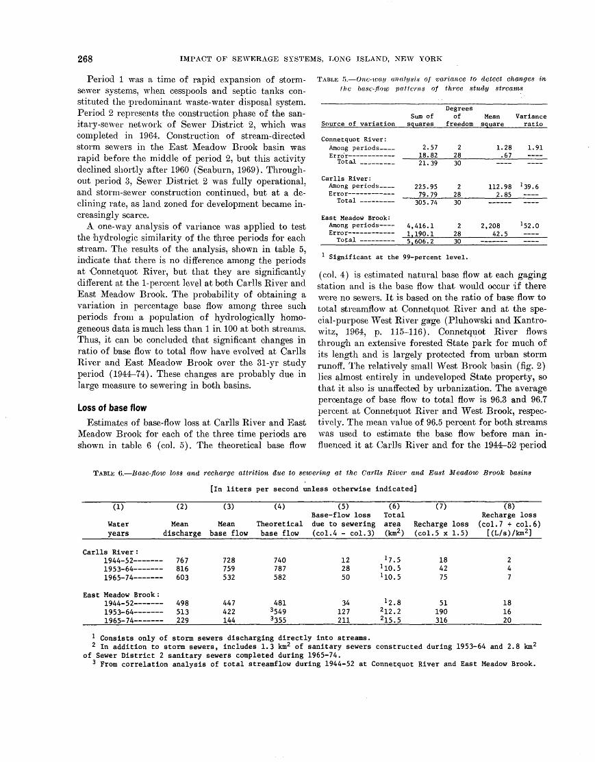
268 IMPACT OF SEWERAGE SYSTEMS, LONG ISLAND, NEW YORK
Period 1 was a time of rapid expansion of storm- sewer systems, when cesspools and septic tanks con stituted the predominant waste-water disposal system. Period 2 represents the construction phase of the san- itary-seAver network of Sewer District 2, which was completed in 1964. Construction of stream-directed storm sewers in the East Meadow Brook basin was rapid before the middle of period 2, but this activity declined shortly after 1960 (Seaburn, 1969). Through out period 3, Sewer District 2 was fully operational, and storm-sewer construction continued, but at a de clining rate, as land zoned for development became in creasingly scarce.
A one-way analysis of variance was applied to test the hydrologic similarity of the three periods for each stream. The results of the analysis, shown in table 5, indicate that there is no difference among the periods at Connetquot River, but that they are significantly different at the 1-percent level at both Carlls River and East Meadow Brook. The probability of obtaining a variation in percentage base flow among three such periods from a population of hydrologically homo geneous data is much less than 1 in 100 at both streams. Thus, it can be concluded that significant changes in ratio of base flow to total flow have evolved at Carlls River and East Meadow Brook over the 31-yr study period (1944-74). These changes are probably due in large measure to sewering in both basins.
Loss of base flowEstimates of base-flow loss at Carlls River and East
Meadow Brook for each of the three time periods are Shown in table 6 (col. 5). The theoretical base flow
TABLE 5. One-wan analysis of variance to detect changes in flic l>asc-fl.ow patterns of three study streams
Source of variation
Connetquot River:Among periods ____Error
Total __ _
Carlls River:Among periods ____
Total _________
East Meadow Brook:Among periods -
Sum ofsquares
2.5718.8221.39
225.9579.79
305.74
4,416.1_!, 190.15,606.2
Degreesof
freedom
22830
2/O
30
2f.O
30
Meansquare
1.28.67
112.98. O J
______
2,20842.5
Varianceratio
1.91
J 39.6_. ____
1 52.0 _
1 Significant at the 99-percent level.
(col. 4) is estimated natural base flow at each gaging station and is the base flow that would occur if there were no sewers. It is based on the ratio of base flow to total streamflow at Connetquot River and at the spe cial-purpose West River gage (Pluhowski and Kantro- witz, 1964, p. 115-116). Connetquot River flows through an extensive forested 'State park for much of its length and is largely protected from urban storm runoff. The relatively small West Brook basin (fig. 2) lies almost entirely in undeveloped State property, so that it also is unaffected by urbanization. The average percentage of base flow to total flow is 96.3 and 96.7 percent at Connetquot River and West Brook, respec tively. The mean value of 96.5 percent for both streams was used to estimate the base flow before man in fluenced it at Carlls River and for the 1944-52 period
TABLE 6. Base-flow loss and recharge attrition due to sewering at the Carlls River and East Meadow Brook basins
[in liters per second unless otherwise indicated]
(1)Water years
Carlls River :j. -»^^ -/ *
1953-64 -1965-74 -
East Meadow Brook :1944-52 -1953-64 -1965-74 -
(2)
Mean discharge
767Q1 £
tno
- 498513229
(3)
Mean base flow
79ft
759532
447
144
(4)
Theoretical base flow
7407Q"7
coo
48135493 355
(5) Base-flow loss due to sewering (col. 4 - col. 3)
12OQ
50
34127211
(6) Total area (km2 )
lj.51 IQ.51 10.5
1 2.82 12.2215.5
(7)
Recharge loss (col. 5 x 1.5)
i ft/ i
75
51190316
(8) Recharge loss (col. 7 T col. 6)
[(L/s)/km2 ]
247
i ft1620
1 Consists only of storm sewers discharging directly into streams.2 In addition to storm sewers, includes 1.3 km2 of sanitary sewers constructed during 1953-64 and 2.8 km 2
of Sewer District 2 sanitary sewers completed during 1965-74.3 From correlation analysis of total streamflow during 1944-52 at Connetquot River and East Meadow Brook.
PLUHOWSKI AND SPINELLO 269
at East Meadow Brook. For example, during 1965-74 at Carlls River, the theoretical base flow of 582 L/s (table 6, col. 4) was computed as the product of meain discharge (col. 2) for the period (603 L/s) and 0.965. By subtracting "measured" mean base flow (col. 3), obtained by hydrograph separation procedures, from the theoretical base flow (col. 4), values of base-flow depletion (col. 5) were computed.
During 1944-52 at tlhe East Meadow Brook basin and throughout the study period (1944-74) at Carlls River, storm sewers were used to dispose of surface run off, whereas cesspools and septic tanks were used to process sanitary sewage. Because cesspools and septic tanks have little, if any, net effect on regional water balances, the loss of base flow during the three study periods at Carlls River and during 1944-52 at East Meadow Brook was probably due in. large measure to the 'present network of stream-directed storm sewers. For a stream basin having storm-water sewers but no sanitary sewers, the total volume of streamflow is not changed; only the ratio of base flow to storm flow is altered. The theoretical base flow for unsewered con ditions can be estimated by multiplying total stream- flow by 0.965, the previously determined ratio of base flow to total streamflow in undisturbed streams. The loss of base flow in the study area during 1944-52 ranged from 12 L/s at Carlls River to 34 L/s in the more highly urbanized East Meadow Brook basin. Chving to an expanding network of storm sewers dis charging into Carlls River, base-flow losses increased to 28 L/s during 1953-64 and to 50 L/s during 1965-74.
Installation of a sanitary-sewer system effectively diverts potential recharge away from the upper glacial aquifer, where the sewers are above the water table. As a result, iboth ground-water levels and the base flow of streams decline, and, because no additional stormflow is added, the total volume of streamflow dwindles. Of the six streams analyzed, only East Meadow Brook was affected by a regional sanitary sewer system during the study period (1944-74). Thus, to estimate the theoretical base flow of that stream dur ing sewer construction, which began in 1953, it was necessary to correlate mean annual discharge of East Meadow Brook with concurrent values for Connetquot River during the preconstruction years (1944 52). Es timates of mean annual discharge at East Meadow Brook were then obtained for the 1953-64 sewer con struction period and the 1965-74 postconstruction pe riod, based on the largely undisturbed Connetquot River basin. These estimated mean annual discharges were multiplied by 0.965 to obtain theoretical base- flow discharges of 549. L/s and 355 L/s at East Meadow Brook 'during 1953-64 and 1965-74, respectively (table
6, col. 4). Base flow decreased dramatically at East Meadow Brook during and after construction of the sanitary sewage system, as potential recharge was diverted from the basin. A base-flow loss of 34 L/s dur ing 1944-52 was followed by losses of 127 L/s in the 1953-64 construction period and 211 L/s in the 1965- 74 postconstruction period (table 6, col. 5). During 1965-74 estimated theoretical base flow exceeded the actual measured mean total discharge by 126 L/s. Clearly, the significant reduction in the sustained flow of the stream 'has been caused principally by the sanitary sewer system associated with Sewer District 2.
Impact of Sewer District 2
Within 5 yr after completion of Sewer District 2 in 1964, the base flow of East Meadow Brook stabilized at 65 percent of total streamflow (fig. 3). Mean esti mated base-flow loss due to separate storm and sanitary sewer systems during the postconstruction period (1964-74) was 211 L/s. To estimate the base-flow losses due to each type of sewage system, it was necessary to examine the preconstruction period (1944-52) and the early years of the construction phase when the impact of Sewer District 2 on streamflow was minimal.
Base flow at East Meadow Brook averaged 89 per cent of total streamflow during 1944-52, but this dropped to 85 percent during 1953-58 as the storm- sewer network discharging direct runoff to the stream expanded rapidly (Seaburn, 1969, table 3). Construc tion of Sewer District 2 during 1953-58 had little if any effect on base flow in East Meadow Brook because ground-water levels adjacent to the stream declined only slightly through 1958 (Franke, 1968, table 1). Thus, the decline of percentage base flow from. 1953-58 was due to storm sewers rather than the combined ef fect of storm and sanitary sewers. Ground-water levels declined steadily after 1959, as an increasing number of sanitary sewer hookups were completed. As a direct result, ground-water discharge declined, and the ratio of base flow to total streamflow dwindled.
The theoretical base flow of East Meadow Brook for the postconstruction period was computed to be 355 L/s. This is the base flow that would have occurred if the basin was left undisturbed. It is estimated that dur ing 1965-74, base flow at East Meadow Brook would have declined to 84 percent of total streamflow had Sewer District 2 not been constructed. Thus, the base flow of the stream would have been about 300 L/s, or 55 L/s below theoretical level. Actual base flow for the postconstruction period was 144 L/s, or 211 L/s below theoretical level. The base-flow loss at East Meadow Brook due to the sanitary sewer network of Sewer Dis-
270 IMPACT OF SEWERAGE SYSTEMS, LONG ISLAND, NEW YORK
trict 2 is estimated to be 211 L/s minus 55 L/s, or 156 L/s. Thus, nearly 75 percent of the loss of base flow of East Meadow Brook during the postconstruction period was due to the 'District 2 sanitary sewer system west of the basin.
Only a small part of the area contributing ground- water discharge to East Meadow Brook underlies Sewer District 2. Throughout the study period, much of the base flow entering East Meadow Brook orig inated in imsewered areas east and northeast of the stream. Thus, it seems that the loss of base flow re sulted from a gradual lowering of ground-water levels that spread from Sewer District 2 to unsewered areas to the east.
RECHARGE DEPLETION
The recharge area of a gaging station, as used in this study, is the area upstream, from, the gage, bordered on the north by the main east-west ground-water divide across Long Island and on the east and west by in- terstream ground-water divides that separate the gaged stream from adjoining basins. Thus, "recharge area" as used herein is coincident with the ground-water con tributing area above the gaging station.
Recharge to the ground-water systems a'bove the gaging stations may be separated into three compo nents, in terms of its path of discharge: (1) ground water seeping into the streams and measured as base flow, ('2) ground water moving under and past the lower basin boundary as underflow, and (3) ground water evaporated and transpired. The bulk of the ground-water evapotranspiration on Long Island oc curs along the marshes and wetlands at or near the shore. Owing to the small amount of wetland areas flanking streams above the gages and because ground- water evapotranspiration is estimated to be only about 10 mm annually on Long Island (Cohen and others, 1968, p. 46), ground-water evapotranspiration was as sumed to be negligible in this analysis. Accordingly, recharge depletion is assumed to be equivalent to the sum of base-flow losses and underflow losses.
At the gaging stations, about two-thirds of the total outflow from the ground-water contributing area is base flow, and one-third is underflow (Phihowski and Kantrowitz, 1964, p. 54). By proportionally adjusting base-flow losses (table 6, col. 5), it is possible to esti mate the loss of recharge resulting from sewering. The assumption of concurrently proportional base flow and underflow losses is reasonable with reference to the upper glacial aquifer in view of the multiyear time frame (table 6, col. 1) used for each of the study pe riods. This assumption may be less acceptable with regard to underflow deep within the ground-water re
servoir; however, the adjustment was made as the best available method of estimating the overall effect of the regional sanitary-sewer system on ground-water out flow.
Recharge losses (table 6, col. 7) were estimated by multiplying column 5 (base-flow loss) by 1.5 to ac count for reduced underflow from the recharge area. Recharge losses, in liters per second per square kilo meter (col. 8), were estimated by dividing column 7 by the area serviced by stream-directed storm sewers in each basin. Averaged over the entire study period (1944-74). the loss of recharge in the Carlls River basin in areas serviced by stream-directed storm sewers was only about 4 (L/s)/km2 . By way of contrast, re charge depletion in the more highly urbanized East Meadow Brook basin was about 18 (L/s)/km2 . These losses were sustained principally in the interstream zone near the south shore, where storm waters are frequently conveyed directly to streams. The heavy re charge depletion in parts of the East Meadow Brook basin serviced by stream-directed storm sewers is due to the interception of runoff by an extensive network of storm drains and to the sanitary sewers of Sewer District 2, which effectively convey potential recharge into tidal Reynolds Channel (fig. 1).
CONCLUSIONS
Significant decreases in the ratio of base flow to total discharge of streams along the south shore of Long Is land have been caused by storm-sewer systems dis charging runoff directly to watercourses and to the completed sanitary sewer network of Sewer District 2 in Nassau County. The general lowering of ground- water levels in Sewer District 2 has diminished the base flow of East Meadow Brook by 60 percent since 1953. Nearly 75 percent of the base-flow loss is attributed to the sanitary sewer network of Sewer District 2, and the remainder is attributed to stream-directed sewers. The Carlls River basin in southwestern Suffolk County sustained base-flow losses that are estimated to have ranged from 12 L/s during 1944-52 to 50 L/s during 1965-74. There were no sanitary sewers in the Carlls River basin during the study period (1944-74) ; there fore, the loss of base flow was due principally to storm sewers conveying runoff to the stream. Base-flow losses at Carlls River were less than 10 percent of the esti mated base flow under undisturbed conditions, whereas similar losses at East Meadow Brook after completion of Sewer District 2 averaged 35-40 percent of the esti mated undisturbed base flow under a no-sewer regime. Little or no loss of base flow was detected at Connet- quot River or Swan River, where urban development is much less intense than in the four other study basins.
PLUHOWSKI AND SPINELLO 271
It is predicted that completion of Nassau County Sewer District 3, east of East Meadow Brook, in 1990 will result in further losses of sustained streamflow. Within 5 years of the completion of Sewer District 2, the ratio of base flow to total flow at East Meadow Brook stabilized in the range of 60-65 percent, down from 85-89 percent before the full sanitary-sewer de velopment. Base flow is expected to diminish further in Carlls River and in other streams draining south western Suffolk County after competion of a sanitary- sewer system currently being constructed in that area.
Recharge depletion in. Carlls River basin areas serv iced by stream-directed storm sewers averaged only about 4 (L/s)/km2 , whereas in the more urbanized East Meadow Brook basin reoharge-depletion rates in simi lar areas averaged about 18 (L/s)/km2 .
REFERENCES CITED
Chow, V. T., 1964, Handbook of applied hydrology: New York, McGraw-Hill Book Co., p. 14-2-14-12.
Cohen, Philip, Franke, O. L., and Foxworthy, B. L., 1968, An atlas of Long Island's water resources: New York Water Resources Bull. 67, 117 p.
Duncan, A. J., 1959, Quality control and industrial statistics: Homewood, 111., Richard D. Irwin, Inc., p. 519-535.
Fair, G. M., and Geyer, J. C., 1954, Water supply and waste- water disposal: New York, John Wiley & Sons, Inc., p. 325.
Franke, O. L., 1968, Double-mass-curve analysis of the effects of sewering on ground-water levels on Long Island, New
York: U.S. Geol. Survey Prof. Paper 600-B, p. B205- B-209.
Garber, M. S., and Sulam, D. J., 1976, Factors affecting de clining water levels in a sewered area of Nassau County, New York: U.S. Geol. Survey Jour. Research, v. 4, no. 3, p. 255-265.
Heath, R. C., Foxworthy, B. L., and Cohen, Philip, 1966, The changing pattern of ground-water development on Long Island, New York: U.S. Geol. Survey Circ. 524, 10 p.
Koszalka, E. J., 1975, The water table on Long Island, New York, in March 1974: Long Island Water Resources Bull. LIWR-5, 7 p., 3 pis.
Nassau-Suffolk Regional Planning Board, 1968, Existing land use: Nassau-Suffolk Regional Comprehensive Plan Series, 30 p.
Pluhowski, E. J., 1970, Urbanization and its effect on the temperature of streams on Long Island, New York: U.S. Geol. Survey Prof. Paper 627-D, 110 p.
1972, Hydrologic interpretation based on infrared im agery of Long Island, New York: U.S. Geol. Survey Water-Supply Paper 2009-B, 20 p.
Pluhowski, E. J., and Kantrowitz, I. H., 1964, Hydrology of the Babylon-Islip area, Suffolk County, Long Island, New York: U.S. Geol. Survey Water-Supply Paper 1768, 119 p.
Seaburn, G. E., 1969, Effects of urban development on direct runoff to East Meadow Brook, Nassau County, Long Island, New York: U.S. Geol. Survey Prof. Paper 627-B, table 3, p. B6.
Seaburn, G. E., and Aaronson, D. A., 1974, Influence of re charge basins on the hydrology of Nassau and Suffolk Counties, Long Island, New York: U.S. Geol. Survey Water-Supply Paper 2031, 66 p.
Welsch, W. F., 1935. Comprehensive drainage plan for Nassau County, New York Summary report: Nassau County Sanitation Comm., 23 p.

Jour. Research U.S. Qeol. Survey Vol. 6, No. 2, Mar.-Apr. 1978, p. 273-283
HYDRAULIC CHARACTERISTICS OF THE WHITE RIVER STREAMBED AND GLACIAL-OUTWASH DEPOSITS AT A SITE NEAR INDIANAPOLIS, INDIANA
By WILLIAM MEYER, Indianapolis, Indiana
Prepared in cooperation icith the State of Indiana, Department of Natural Resources
Abstract. An aquifer test was made in the glacial-outwash aquifer along the course of the White River in Marion County, Ind., to establish the hydraulic characteristics of this unit and the hydraulic conductivity of the White River streambed at a site 11 kilometers south of the center of downtown Indian apolis. In the immediate vicinity of the site, at a depth of about 15 meters below land surface, a clay lens separates the outwash aquifer into an upper sand and gravel unit 12 m thick and a lower unit 8.5 m thick. At the site of the test well, the clay lens is 3.0 m thick. The test was made in the upper sand and gravel unit, and data were analyzed for an assumed condition of no, or at least negligible, transient leak age from the clay lens underlying this unit. As no observa tion wells were installed in the clay lens, this assumption cannot be directly substantiated. However, observation wells beneath the clay lens indicated that a head loss was not in duced below the clay lens by the test well, and the closeness of the values obtained for transmissivity of the upper unit by three different methods strongly supports the assumption. Results of the test include for the upper unit: lateral hy draulic conductivity, 108 meters per day; range of transmissiv ity (determined by three techniques), from 1400 to 1670 meters squared per day; specific yield, 0.08; and vertical hydraulic conductivity of the streambed, 2.2 m/d. These results should be of use in assessing the potential supply and in developing one of Indiana's major aquifer systems because a knpwledge of aquifer characteristics is essential for proper design and spacing of wells.
A cooperative study between the State, of Indiana, Department of Natural Resources, and the U.S. Geo logical Survey to determine the availability of ground water in Marion County (Meyer and others, 1975) included determination of the hydraulic characteristics of the sand and gravel aquifer underlying the White River and Fall Creek and definition of the hydraulic connection between these streams and the aquifer. The aquifer is of glacial-outwash origin and consists of a mixture of sand, sand and gravel, and gravel deposits interspersed with clay lenses. Water in ttfie deposits is generally unconfined, although water in deposits be neath the clay lenses in some local areas is confined.
The major part of ground water presently (1976) pumped in the county is withdrawn from the outwash aquifer, and the potential for additional development in it is greater than for any other aquifer in the county (Meyer and others, 1975). Areal extent of the outwash deposits within the county is shown in figure 1.
White River and Fall Creek are gaining streams throughout their respective reaches in Marion County, and the response of observation wells in the outwash aquifer to changes in stream stage indicate a hydraulic connection between these streams and the aquifer. To help define this connection and determine the hydraulic characteristics of the aquifer, the aquifer was tested at a point 11 kilometers south of the center of down town Indianapolis and along the White River where the characteristics of the streambed are fairly represen tative of the lower 9.6-km reach of the river in Marion County. This report summarizes the test pro cedure and the results of the aquifer test, which were assimilated into the larger overall ground-water study of the county.
The data are significant in their own right, however, as they provide detailed information on the hydrologic conditions in the immediate vicinity of the test site and thus are of potential use to engineers and planners concerned with developing ground water in this area. A knowledge of aquifer characteristics and streambed permeability is essential for proper design and spacing of wells.
GENERAL GEOHYDROLOGIC CONDITIONS OF THE TEST-SITE AREA
The location of the test-site area is shown in figure 2. The outwash aquifer is divided into upper and lower units of sand and gravel by a clay lens, which is about 15 meters below the land surface throughout the im mediate area. An east-west section of the outwash in the test area is shown in figure 3. As can be seen from
273
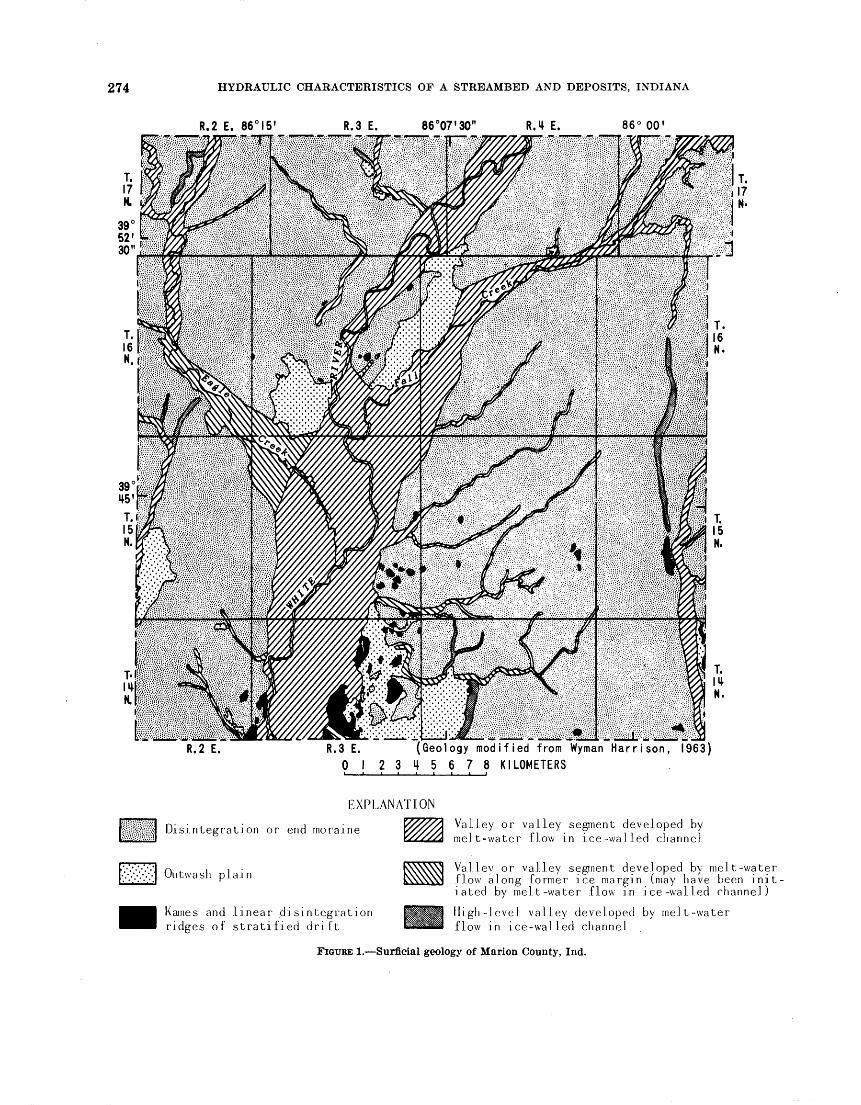
274 HYDRAULIC CHARACTERISTICS OF A STREAMBED AND DEPOSITS, INDIANA
R.2 E. 86°I5' R.3 E. 86°07'30 ? R.4 E. 86° 00'
R.2 E. R.3 E. (Geology modified from Wyman Harrison, 1963) 0 I 2 3 il 5 6 7 8 KILOMETERS
EXPLANATION
Disintegration or end moraine
Outwash p.la.m
Kaines and Linear disintegration ridges of stratified dri ft
Valley or valley segment developed by melt-water flow in ice-walled channel
Valley or valley segment developed by melt-water flow along former ice margin (may have been init iated by melt-water flow in ice-walled channel)
High-level valley developed by melt-water flow in ice-walled channel
FIGURE 1. Surficial geology of Marion County, Ind.
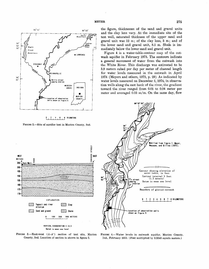
MEYER 275
02468 KILOMETERS
FIGURE 2. Site of aquifer test in Marion County, Ind.
WEST
EXPLANATION
Topsoil and river alluviumSand and gravel
0 100
[ill Clay
C-I-U Shale
200 300 METERS
VERTICAL EXAGGERATION X 12.5
Datum is mean sea level
the figure, thicknesses of the sand and gravel units and the clay lens vary. At the immediate site of the test well, saturated thickness of the upper sand and gravel unit was 12 m; of the clay lens, 3 m; and of the lower sand and gravel unit, 8.5 m. Shale is im mediately below the lower sand and gravel unit.
Figure 4 is a water-table-contour map of the out- wash aquifer in February 1975. The contours indicate a general movement of water from the outwash into the White River. This discharge was estimated to be 3.9 meters cubed per day per meter of channel length for water levels measured in the outwash in April 1974 (Meyers and others, 1975, p. 29) As indicated by water levels measured on December 5, 1974, in observa tion wells along the east bank of the river, the gradient toward the river ranged from 0.01 to 0.04 meter per meter and averaged 0.03 m/m. On the same day, flow
86°07'30"
Modifltd from figure 7, Meyer, Riussow, and Gil lies (1975).
Contour showing elevation of water table, in feet
Contour interval 5 feet .MorTT. street (1 ' 5 met"s)
I gag Ing Datum is mean sea level station
Boundary of glacial-outwash
0 12345678 KILOMETERS
Location of observation wells shown on figure 5
FIGURE 3. East-west (A~A f ) section of test site, Marion FIGURE 4. Water levels in outwash aquifer, Marion County, County, Ind. Location of section is shown in figure 5. Ind., February 1975. (Feet multiplied by 0.3048 equals meters.)
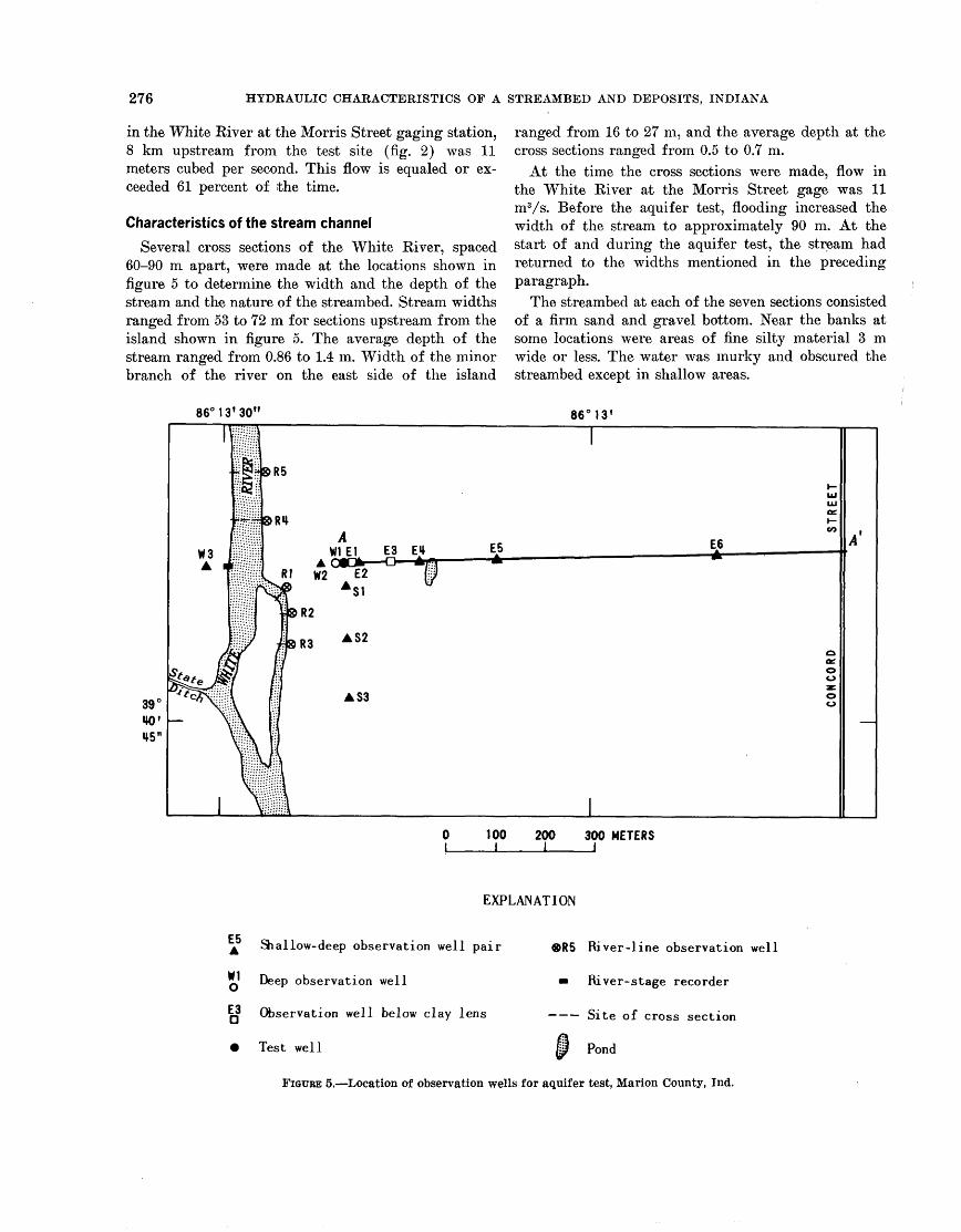
276 HYDRAULIC CHARACTERISTICS OF A STREAMBED AND DEPOSITS, INDIANA
in the White River at the Morris Street gaging station, 8 km upstream from the test site (fig. 2) was 11 meters cubed per second. This flow is equaled or ex ceeded 61 percent of the time.
Characteristics of the stream channel
Several cross sections of the White River, spaced 60-90 m apart, were made at the locations shown in figure 5 to determine the width and the depth of the stream and the nature of the streambed. Stream widths ranged from 53 to 72 m for sections upstream from the island shown in figure 5. The average depth of the stream ranged from 0.86 to 1.4 m. Width of the minor branch of the river on the east side of the island
86° 13'30"
ranged from 16 to 27 m, and the average depth at the cross sections ranged from 0.5 to 0.7 m.
At the time the cross sections were made, flow in the White River at the Morris Street gage was 11 m3/s. Before the aquifer test, flooding increased the width of the stream to approximately 90 m. At the start of and during the aquifer test, the stream had returned to the widths mentioned in the preceding paragraph.
The streambed at each of the seven sections consisted of a firm sand and gravel bottom. Near the banks at some locations were areas of fine silty material 3 m wide or less. The water was murky and obscured the streambed except in shallow areas.
86°13'
39
W1E1 E3 EH E5 E6
R1 W2 E2 A S1
AS2
A S3
100 200 300 METERS I____I____I
EXPLANATION
A Shallow-deep observation well pair ®R5 River-line observation well
Q Deep observation well River-stage recorder
^ Observation well below clay lens Site of cross section
Test well p Pond
FIGURE 5. Location of observation wells for aquifer test, Marion County, Ind.
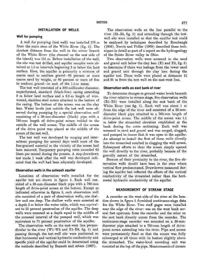
MEYER 277
INSTALLATION OF WELLS
Well for pumping
A well for pumping (test well) was installed 179 m from the main stem of the White Eiver (fig. 5). The shortest distance from the well to the minor branch of the White River (the channel on the east side of the island) was 131 m. Before installation of the well, the site was test drilled, and aquifer samples were ob tained at 1.5-m intervals beginning 3 m below the land surface. Here, the aquifer is primarily a mixture of coarse sand to medium gravel 93 percent or more coarse sand by weight, or 80 percent or more of fine to medium gravel in each of the 1.5-m zones.
The test well consisted of a 300-millimeter-diameter. unperforated, standard (black-line) casing extending 9 m below land surface and a 6.1-m length of wire- wound, stainless steel screen attached to the bottom of the casing. The bottom of the screen was on the clay lens. Water levels just outside the test well were ob served during pumping by a special observation well consisting of a 38-mm-diameter (black) pipe with a 760-mm length of drive-point screen welded to the outside of the well screen. The middle of the screen of the drive point was placed at the middle of the screen of the test well.
The test well was developed by surging and inter mittent pumping for several days until most of the fine-grained material in the vicinity of the screen had been removed. Temporary pumping rates exceeded 63 liters per second during the process. A step-drawdown test made 1 week after the well was developed indi cated that the well had been adquately developed.
Observation wells in the outwash aquifer
Locations of observation wells installed for the aquifer test are shown in figure 5. Each well con sisted of a 38-mm-diameter black pipe with a 760-mm length of drive-point screen at the bottom. Except as indicated otherwise in figure 5, each observation well site consisted of a pair of observation wells, one shal low and one deep. The shallow wells were screened at a depth 3 m below the water table, which was equival ent to 25 percent penetration of the aquifer. The deep wells were screened at a depth equal to the middle of the screened interval of the pumped well, which was equivalent to 75 percent penetration of the aquifer.
The observation wells on the east-west line perpen dicular to the river (W1-W3 and E1-E6, fig. 5) and passing through the test-well site were positioned so that horizontal and vertical hydraulic conductivity and specific yield of the aquifer could be determined using the methods described by Bennett and others (1967).
The observation wells on the line parallel to the river (S1-S3, fig. 5) and extending through the test- well site were installed so that the aquifer test could be analyzed by techniques described by Rorabaugh (1956). Norris and Fidler (1969) described these tech niques in detail as part of a report on the hydrogeology of the Scioto River valley in Ohio.
Two observation wells were screened in the sand and gravel unit below the clay lens (El and E3, fig. 5) to determine if there was leakage from the lower sand and gravel unit through the clay lens during the aquifer test. These wells were placed at distances 15 and 91 m from the test well on the east-west line.
Observation wells on east bank of river
To determine changes in ground-water levels beneath the river relative to stream stage, five observation wells (R1-R5) were installed along the east bank of the White River (see fig. 5). Each well was about 1 m from the edge of the river and consisted of a 38-mm- diameter black pipe attached to a 760-mm length of drive-point screen. The middle of the screen was 1.1 m below the streambed elevation established at the bank during the cross sectioning. Each well was screened in sand and gravel and was surged, slugged, and pumped to insure that it was open to the aquifer. An attempt to install the first of these wells directly into the streambed resulted in clogging the well screen. Subsequent efforts to clear the screen simply opened the well directly to the river, probably because of the gravelly nature of the streambed.
Because of their proximity to the river, the five ob servation wells should have been in the zone where vertical flow predominated. Drawdowns measured dur ing the aquifer test reflected the effects of the vertical conductivity of the streambed rather than the hori zontal hydraulic conductivity of the aquifer.
MEASUREMENT OF STREAM STAGE
A recorder on the west side of the river at the loca tion shown in figure 5 furnished continuous-stage data for the White River. Two staff gages were installed near the edge of the river: one on the west bank sev eral feet upstream from the recorder and the other on the east bank directly across from the recorder. The continuous-stage recorder was mounted on a 38-mm- diameter pipe attached to a 760-mm length of drive- point screen extending into the river. Pipe and screen were permanently fixed so that the screen was fully submerged at all times with its bottom slightly above the streambed. The water-level recording unit was mounted at the top of the pipe. Measurements of stream
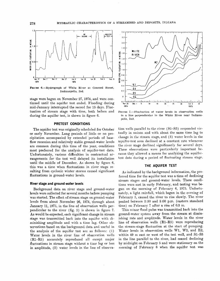
278 HYDRAULIC CHARACTERISTICS OF A STREAMBED AND DEPOSITS, INDIANA
1.5
1.0
£ 0.5
I N0 I RECORD I AQUIFER L-TEST-
J____LNo* 27 Dec 7 Dec 17 Dec 27 I an 6 lan 16 lan 26 Feb 5 Feb IS 1974 1975
FIGIJBE 6. Hydrograph of White River at Concord Street, Indianapolis, Ind.
stage were begun on November 27, 1974, and were con tinued until the aquifer test ended. Flooding during mid-January interrupted the record for 13 days. Fluc tuation of stream stage with time, both before and during the aquifer test, is shown in figure 6.
PRETEST CONDITIONS
The aquifer test was originally scheduled for October or early November. Long periods of little or no pre cipitation accompanied by extended periods of base- flow recession and relatively stable ground-water levels are common during this time of the year, conditions most preferred for the analysis of aquifer-test data. Unfortunately, various difficulties in contractual ar rangements for the test well delayed its installation until the middle of December. As shown by figure 6, this was a time when fluctuations in river stage re sulting from cyclonic winter storms caused significant fluctuations in ground-water levels.
River stage and ground-water levelsBackground data on river stage and ground-water
levels were collected for several months before pumping was started. The effect of stream stage on ground-water levels from about November 26, 1974, through about January 11, 1975, in the line of observation wells per pendicular to the river (fig. 5) is shown in figure 7. As would be expected, each significant change in stream stage was transmitted back into the aquifer with di minishing amplitude and with a time lag. Other ob servations based on the background data and useful in the analysis of the aquifer test are as follows: (1) Water levels in the river line of observation wells (R1-R5) accurately reproduced all except, major fluctuations in stream stage without a time lag or loss in amplitude, (2) water levels in the line of observa-
Nov 25 Dec 15 ID 15 20 25 30 lan 5 10
FIGURE 7. Fluctuation of water levels in observation wells in a line perpendicular to the White River near Indiana polis, Ind.
tioii wells parallel to the river (S1-S3) responded vir tually in unison and with about the same time lag to change in the stream stage, and (3) water levels in the aquifer-test area declined at a constant rate whenever the river stage declined significantly for several days. These obserA^ations were particularly important be cause they allowed a means for analyzing the aquifer- test data during a period of fluctuating stream stngo.
THE AQUIFER TEST
As indicated by the background information, the pre ferred time for the aquifer test was a time of declining stream stages and ground-water levels. These condi tions were met in -early February, and testing was be gun on the morning of February 6, 1975. Unfortu nately, a light rainfall, which begun in the evening of
*/ 7 O ' / C-1
February 5, caused the river to rise slowly. The river peaked between 2:30 and 3:00 p.m. (eastern standard time) on February 7 after a rise of 0.3 m.
This minor flood pulse was transmitted back into the ground-water system away from the stream at dimin ishing rate and amplitude. Water levels in the river line of observation wells (R1-R5) were reproducing the stream-stage fluctuation at the start of pumping. Water levels in observation wells Wl, W2, and E2, within 49 m east or west of the test well, and S1-S3 in the line parallel to the river, had ceased declining by midnight on February 5 and were stationary on the morning of February 6 when the aquifer test was
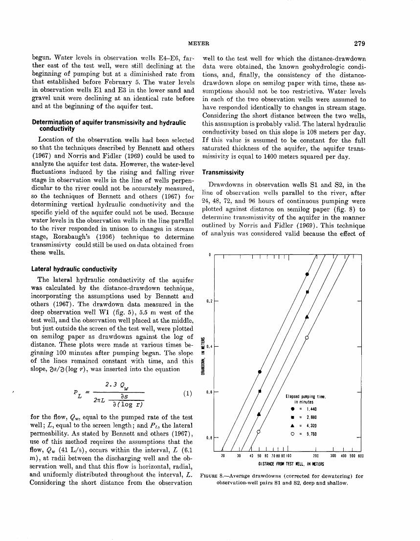
MEYER 279
begun. Water levels in observation wells E4-E6, far ther east of the test well, were still declining at the beginning of pumping but at a diminished rate from that established before February 5. The water levels in observation wells El and E3 in the lower sand and gravel unit were declining at an identical rate before and at the beginning of the aquifer test.
Determination of aquifer transmissivity and hydraulic conductivity
Location of the observation wells had been selected so that the techniques described by Bennett and others (1967) and Norris and Fidler (1969) could be used to analyze the aquifer test data. However, the water-level fluctuations induced by the rising and falling river stage in observation wells in the line of wells perpen dicular to the river could not be accurately measured, so the techniques of Bennett and others (1967) for determining vertical hydraulic conductivity and the specific yield of the aquifer could not be used. Because water levels in the observation wells in the line parallel to the river responded in unison to changes in stream stage, Rorabaugh's (1956) technique to determine transmissivty could still be used on data obtained from these wells.
Lateral hydraulic conductivity
The lateral hydraulic conductivity of the aquifer was calculated by the distance-drawdown technique, incorporating the assumptions used by Bennett and others (1967). The drawdown data measured in the deep observation well Wl (fig. 5), 5.5 m west of the test well, and the observation well placed at the middle, but just outside the screen of the test well, were plotted on semilog paper as drawdowns against the log of distance. These plots were made at various times be ginning 100 minutes after pumping began. The slope of the lines remained constant with time, and this slope, 3<s/3(log r1 ), was inserted into the equation
2.3 Ow
27TL(1)
3 dog r)
for the flow, Qw, equal to the pumped rate of the test well; Z, equal to the screen length; and PL , the lateral permeability. As stated by Bennett and others (1967), use of this method requires the assumptions that the flow, Qw (41 L/s), occurs within the interval, Z (6.1 m), at radii between the discharging well and the ob servation well, and that this flow is horizontal, radial, and uniformly distributed throughout the interval, Z. Considering the short distance from the observation
well to the test well for which the distance-drawdown data were obtained, the known geohydrologic condi tions, and, finally, the consistency of the distance- drawdown slope on semilog paper with time, these as sumptions should not be too restrictive. Water levels in each of the two observation wells were assumed to have responded identically to changes in stream stage. Considering the short distance between the two wells, this assumption is probably valid. The lateral hydraulic conductivity based on this slope is 108 meters per day. If this value is assumed to be constant for the full saturated thickness of the aquifer, the aquifer trans missivity is equal to 1400 meters squared per day.
Transmissivity
Drawdowns in observation wells Si and S2, in the line of observation wells parallel to the river, after 24, 48, 72, and 96 hours of continuous pumping were plotted against distance on semilog paper (fig. 8) to determine transmissivity of the aquifer in the manner outlined by Norris and Fidler (1969). This technique of analysis was considered valid because the effect of
0.2
0.4
o.e
0.6
II I III
Elapsed pumping time, in minutes
= 1,440
= 2,880
A = 4,320
I__
= 5,760
I I50 60 708090100 200
DISTANCE FROM TEST WELL, IN METERS
300 400 500 600
FIGURE 8. Average drawdowns (corrected for dewatering) for observation-well pairs SI and S2, deep and shallow.
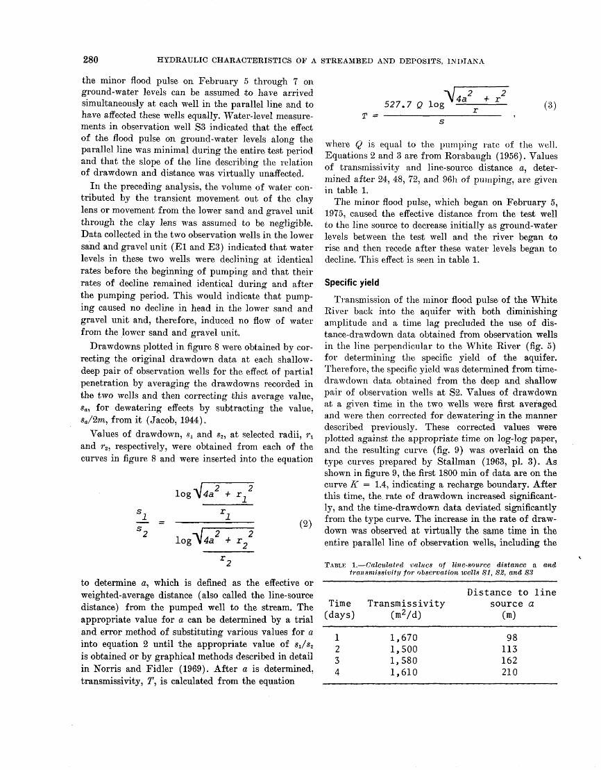
280 HYDRAULIC CHARACTERISTICS OF A STREAMBED AND DEPOSITS, INDIANA
the minor flood pulse on February 5 through 7 on ground-water levels can be assumed to have arrived simultaneously at each well in the parallel line and to have affected these wells equally. Water-level measure ments in observation well S3 indicated that the effect of the flood pulse on ground-water levels along the parallel line was minimal during the entire test period and that the slope of the line describing the relation of drawdown and distance was virtually unaffected.
In the preceding analysis, the volume of water con tributed by the transient movement out of the clay lens or movement from the lower sand and gravel unit through the clay lens was assumed to be negligible. Data collected in the two observation wells in the lower sand and gravel unit (El and E3) indicated that water- levels in these two wells were declining at identical rates before the beginning of pumping and that their rates of decline remained identical during and after the pumping period. This would indicate that pump ing caused no decline in head in the lower sand and gravel unit and, therefore, induced no flow of water from the lower sand and gravel unit.
Drawdowns plotted in figure 8 were obtained by cor recting the original drawdown data at each shallow- deep pair of observation wells for the effect of partial penetration by averaging the drawdowns recorded in the two wells and then correcting this average value, sa, for dewatering effects by subtracting the value, s0/2m, from it (Jacob, 1944).
Values of drawdown, s^ and s2 , at selected radii, rv and r2 , respectively, were obtained from each of the curves in figure 8 and were inserted into the equation
log \4a2 +
to determine <z, which is defined as the effective or weighted-average distance (also called the line-source distance) from the pumped well to the stream. The appropriate value for a can be determined by a trial and error method of substituting various values for ainto equation 2 until the appropriate value of is obtained or by graphical methods described in detail in Norris and Fidler (1969). After a is determined, transmissivity, T7, is calculated from the equation
527.7 Q log* 2 -L 24a -f- r
(3)T
where Q is equal to the pumping rate of the well. Equations 2 and 3 are from Rorabaugh (1956). Values of transmissivity and line-source distance #, deter mined after 24, 48, 72, and 96h of pumping, are given in table 1.
The minor flood pulse, which began on February 5, 1975, caused the effective distance from the test well to the line source to decrease initially as ground-water levels between the test well and the river began to rise and then recede after these water levels began to decline. This effect is seen in table 1.
Specific yield
Transmission of the minor flood pulse of the White River back into the aquifer with both diminishing amplitude and a time lag precluded the use of dis tance-drawdown data obtained from observation wells in the line perpendicular to the White River (fig. 5) for determining the specific yield of the aquifer. Therefore, the specific yield was determined from time- drawdown data obtained from the deep and shallow pair of observation wells at S2. Values of drawdown at a given time in the two wells were first averaged and were then corrected for dewatering in the manner described previously. These corrected values were plotted against the appropriate time on log-log paper, and the resulting curve (fig. 9) was overlaid on the type curves prepared by Stallman (1963, pi. 3). As shown in figure 9, the first 1800 min of data are on the curve K = 1.4, indicating a recharge boundary. After this time, the rate of drawdown increased significant ly, and the time-drawdown data deviated significantly from the type curve. The increase in the rate of draw down was observed at virtually the same time in the entire parallel line of observation wells, including the
TABLE 1. Calculated values of line-source distance a and transmissivily for observation wells 8.1, 82, and S3
Time (days)
1234
Transmissivity O2/d)
1,6701,5001,5801,610
Distance to linesource a
(m)
98113162210
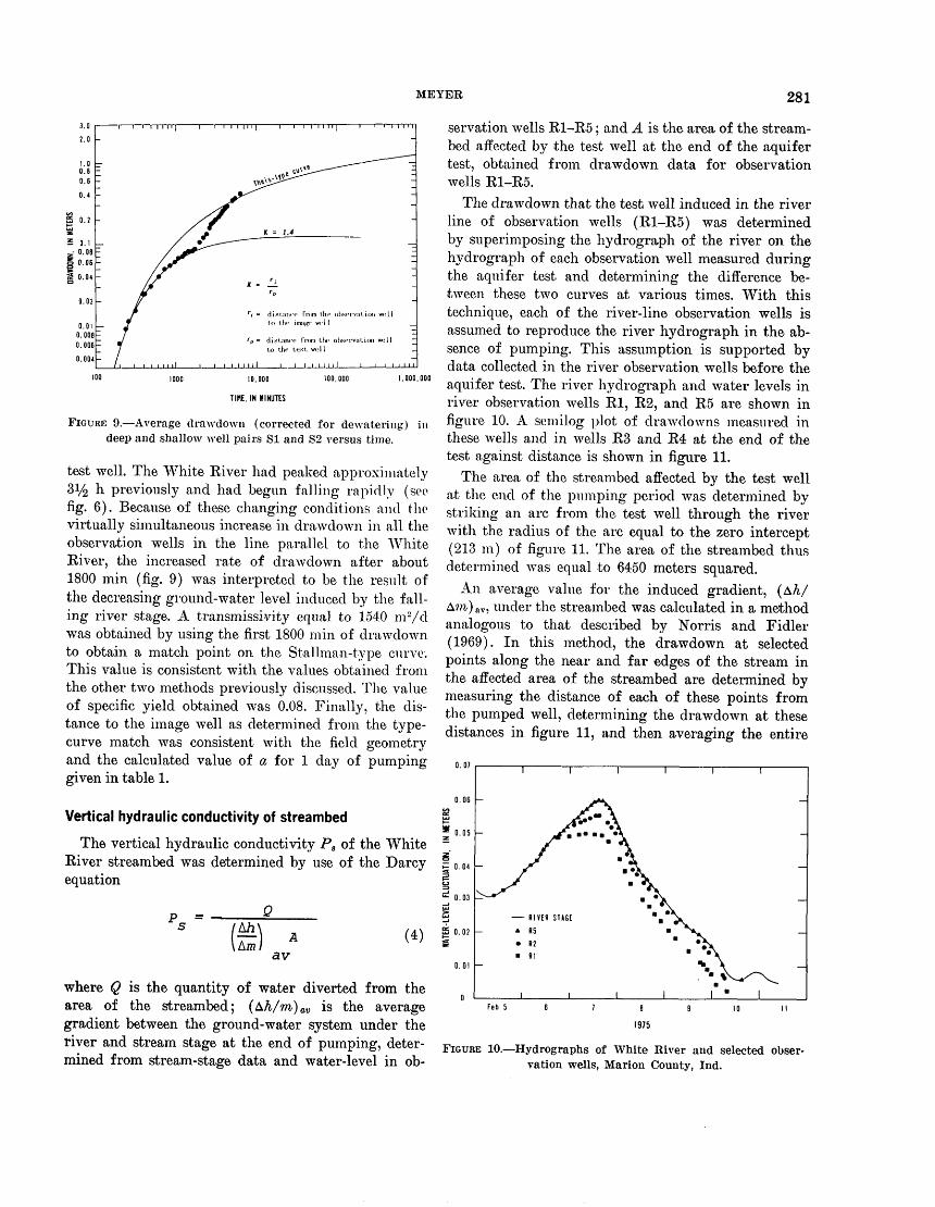
MEYER 281
10.000
TINE,IN MINUTES
100.000 1,000.000
FIGURE 9. Average drawdown (corrected for dewatering) in deep and shallow well pairs SI and S2 versus time.
test well. The White River had peaked approximately 31/2 h previously and had begun falling rapidly (see fig. 6). Because of these changing conditions and the virtually simultaneous increase in drawdown in all the observation wells in the line parallel to the White River, the increased rate of drawdown after about 1800 min (fig. 9) was interpreted to be the result of the decreasing ground-water level induced by the fall ing river stage. A transmissivity equal to 1540 m2/d was obtained by using the first 1800 min of drawdown to obtain a match point on the Stall man-type curve. This value is consistent with the values obtained from the other two methods previously discussed. The value of specific yield obtained was 0.08. Finally, the dis tance to the image well as determined from the type- curve match was consistent with the field geometry and the calculated value of a for 1 day of pumping given in table 1.
Vertical hydraulic conductivity of streambed
The vertical hydraulic conductivity P8 of the White River streambed was determined by use of the Darcy equation
(4)av
where Q is the quantity of water diverted from the area of the streambed; (A/t/m) ov is the average gradient between the ground-water system under the river and stream stage at the end of pumping, deter mined from stream-stage data and water-level in ob
servation wells R1-R5; and A is the area of the stream- bed affected by the test well at the end of the aquifer test, obtained from drawdown data for observation wells R1-R5.
The drawdown that the test well induced in the river line of observation wells (R1-R5) was determined by superimposing the hydrograph of the river on the hydrograph of each observation well measured during the aquifer test and determining the difference be tween these two curves at various times. With this technique, each of the river-line observation wells is assumed to reproduce the river hydrograph in the ab sence of pumping. This assumption is supported by data collected in the river observation wells before the aquifer test. The river hydrograph and water levels in river observation wells Rl, R2, and R5 are shown in figure 10. A semilog plot of drawdowns measured in these wells and in wells R3 and R4 at the end of the test against distance is shown in figure 11.
The area of the streambed affected by the test well at the end of the pumping period was determined by striking an arc from the test well through the river with the radius of the arc equal to the zero intercept (213 m) of figure 11. The area of the streambed thus determined was equal to 6450 meters squared.
An average value for the induced gradient, (A/I/ Aw)nv, under the streambed was calculated in a method analogous to that described by Norris and Fidler (1969). In this method, the drawdown at selected points along the near and far edges of the stream in the affected area of the streambed are determined by measuring the distance of each of these points from the pumped well, determining the drawdown at these distances in figure 11, and then averaging the entire
0.07
0.05
0.03
25 0.022
0.01
Feb 5
1975
FIGURE 10. Hydrographs of White River and selected obser vation wells, Marion County, Ind.
282 HYDRAULIC CHARACTERISTICS OF A STREAMBED AND DEPOSITS, INDIANA
0. 1
0. 2
0.3
R3<
R2
R5
40 50 60 7080 100 200 300
DISTANCE FROM TEST WELL, IN METERS
FIGURE 11. Relation of drawdown in observation wells R1-R5 and distance from test well, Marion County, Ind.
set of values obtained. The average value for draw down under the river (0.05 m) thus determined was converted to an average gradient under the affected streambed area (AA/Am) av by dividing the average drawdown by 1.1 m (the distance between the screens in the river line of observation wells and the stream- bed).
The quantity of wa;ter being diverted from the river at the end of the pumping period was obtained by the technique presented by Theis (1941) for determining the percentage of water diverted from a source of re charge at a given time as a result of pumping. This percentage is determined by calculating a variable, /, which is equal to Tt/azS, and entering a curve pre sented by Theis (1941), where / is the abscissa and the percentage of water diverted from the recharge source is the ordinate. The value of / was calculated for t equal to the toal time of pumping and for values of T7, a, and S that were previously determined for the aquifer. The quantiy of water being diverted from the river was 65 percent (using / = 0.14) of the 41 L/s pumping rate.
From the values of Q, (A^/Aw) av, and A thus deter mined, the value for vertical hydraulic conductivity of the streambed calculated from equation 4 was 2.2 m/d.
SUMMARY AND CONCLUSIONS
Lateral hydraulic conductivity of the upper sand and gravel unit at the aquifer test site was determined to be 108 m/d. Transmissivity of the unit (determined by three different techniques) ranged from 1500 to 1670 m2/d. The specific yield of this upper unit was de termined to be 0.08. Finally, the vertical hydraulic conductivity of the streambed was calculated to be 2.2 m/d.
The test was made in the upper sand and gravel unit, and data were analyzed for an assumed condition of no, or at least negligible, transient leakage from the clay lens underlying this unit. Because no observation wells were installed in the clay lens, this assumption cannot be directly substantiated. However, observation wells beneath the clay lens indicated that a head loss was not induced below the clay lens by the test well, and the closeness of the values obtained for transmis- sivity by three different methods strongly supports this assumption.
The analysis of the test data was complicated by the minor flood pulse on the White River, which began the night before pumping began. Background data collected on the stream stage and ground-water levels had indicated that changes in stream stage could in- 'duce ground-water-level changes far greater than those that would be induced during the aquifer test. These background data also ?proved useful in the sub sequent analysis of the 'aquifer-test data.
Results of the study should be of use in assessing the potential supply and in developing one of Indiana's major aquifer systems.
REFERENCES CITED
Bennett, G. D., Ata-TJr-Rehman, Ijaz Ahmed Sheikh, and Sabir Ali, 1967. Analysis of aquifer tests in the Punjab region of West Pakistan: U.S. Geol. Survey Water-Sup ply Paper 160S-G, p. G1-G56.
Harrison, Wyman, 1963, Geology of Marion County, Indiana: Indiana Dept. Conserv., Geol. Survey Bull. 28, 78 p.
Jacob, C. E., 1944, Notes on determining permeability by pump ing tests under water-table conditions: U.S. Geol. Sur vey open-file rept., 25 p.
Meyer, William, Reussow, J. P., and Gillies, D. C., 1975, Avail ability of ground water in Marion County, Indiana: U.S. Geol. Survey Open-File Rept. 75-312, 87 p.
Norris, S. E., and Fidler, R. E., 1969, Hydrogeology of the Scioto River Valley Near Piketon, south-central Ohio: U.S. Geol. Survey Water-Supply Paper 1872, 70 p.
MEYER 283
Rorabaugh, M. I., 1956, Ground water in northeastern Louis- and special problems in aquifer tests: U.S. Geol. Surveyville, Kentucky, with reference to induced infiltration: U.S. Water-Supply Paper 1545-C, p. C45-C47.Geol. Survey Water-Supply Paper 1360-B, p. B101-B169. Theis, C. V., 1941, The effect of a well on the flow of a nearby
Stallman, R. W., 1963, Type curves for the solution of single stream: Am. Geophys. Union Trans., 22d Ann. Mtg., pt.boundary problems, in Bentall, Ray, compiler. Shortcuts 2, p. 734-738.
.S .GOVERNMENT PRINTING OFFICE: 1 978--2 6 I - I 9 8/3

CHANGE OF ADDRESS FORMNAME FIRST. LAST
I I I I I I I I I I I I I I I I I I I I I I I I I I I I
COMPANY NAME OR ADDITIONAL ADDRESS LINE
I I I I I I I I I I I I I I I I I I I I I I I I I I I I
STREET ADDRESS
I I I I I I I I I I I I I I I I I I I I I I I I I I I ICITY STATE ZIP CODE
PLEASE PRINT OR TYPE
Mail this form to: NEW ADDRESS
Superintendent of Documents Government Printing Office SSOM Washington, D.C. 20402
(or) COUNTRY
Attach last subscription | label here. |
SUBSCRIPTION ORDER FORM
SUBSCRIPTION ORDER FORM
ENTER MY SUBSCRIPTION TO:
@ $18.90 Domestic; @ $23.65 Foreign.
IIII
I
I I
I
I
J I
cOMPA
I
I
crI
INY N
I
I
FY
I
AM
MA
E (
ST
4E
DR
'RE
FIRST.
f I
ADDITIC
I I
ET ADD)
I I
I I
PLEASE PRINT OR TYPE (
L/
NA
RES
kST
IL ADDRI
| |
S I
or) CO JN
I
:s
ST/
PRY
S L
VTE
INE
I
;
III
'.\P C
I3D E
Remittance Enclosed (Make checks payable to Superin tendent of Documents)
Charge to my Deposit Account No. ........................
MAIL ORDER FORM TO: Superintendent of Documents Government Printing Office Washington. D.C. 20402

RECENT PUBLICATIONS OF THE U.S. GEOLOGICAL SURVEYThe following books may be ordered from the Branch of
Distribution, U.S. Geological Survey, 1200 South Eads Street, Arlington, VA 22202 (an authorized agent of the Superin tendent of Documents, Government Printing Office). Pre payment is required. Remittances should be sent by check or money order payable to U.S. Geological Survey. Give series designation and number, such as Bulletin 1368-A, and the full title. Prices of Government publications are subject to change. Increases in costs make it necessary for the Superintendent of Documents to increase the selling prices of many publications offered. As it is not feasible for the Superintendent of Documents to correct the prices manually in all the previous announcements and publications stocked,
the prices charged on your order may differ from the prices printed in the announcements and publications1.
In addition to the publications mentioned below, other professional papers, water-supply papers, bulletins, circulars, single copies of the periodical "Earthquake Information Bulletin," maps, and items of general interest, such as leaflets, pamphlets, and booklets, are available at the above address. All new Survey publications are listed in a, free monthly catalog, "New Publications of the Geological Sur vey"; to subscribe, send name and address to U.S. Geological Survey, 329 National Center, Reston, VA 22092. (Some reports that are now out of print at the Superintendent of Documents can also be obtained at the Branch of Distribution address.)
Professional PapersP 533. Cenozoic fossil mollusks from western Pacific islands;
Gastropods (Eratoidae through Harpidae), by H. S. Ladd. 1977. 84 p., 23 plates. $3.25.
P 751-D. Geochemical effects of recharging the Magothy aquifer, Bay Park, New York, with tertiary-treated sew age, by S. E. Ragone. 1977. p. D1-D22. $1.40.
P 759-C. Distribution of bottom sediments on the continental shelf, northern Bering Sea, by D. A. McManus, D. M. Plopkins, and C. H. Nelson. 1977. p. C1-C31. $1.60.
P 813-G. Summary appraisals of the Nation's ground-water resources Great Basin region, by T. E. Eakin, Don Price, and J. R. Harrill. 1976. p. G1-G37; plate in pocket. $2.40.
P 881. Geologic evaluation of waste-storage potential In selected segments of the Mesozoic aquifer system below the zone of fresh water, Atlantic Coastal Plain, North Carolina through New Jersey, by P. M. Brown and M. S. Reid. 1976 (1977). 47 p.; plates in pocket. $11.
P 999. Stillwater Complex, Montana : Rock succession, meta- morphism and structure of the complex and adjacent rocks, by N. J Page, 1977. 79 p., plates in pocket. $4.50.
P 1002. The Guatemalan earthquake of February 4, 1976, a preliminary report, by A. F. Espinosa, editor. 1976. 90 p. $2.50.
P 1007. Stratigraphy, petrology, and depositional environ ment of the Kenwood Siltstone Member, Borden Forma tion (Mississippian), Kentucky and Indiana, by R. C. Kepferle. 1977. 49 p. $2.30.
P 1026. Revisions of Ulmus and Zclkova in the middle and late Tertiary of western North America, by Toshimasa Tanai and J. A. Wolfe. 1977. 14 p., 4 plates. $2.
P 1027. Paleozoic-Mesozoic boundary in the Berry Creek quadrangle, northwestern Sierra Nevada, California, by Anna Hietanen. 1977. 22 p., plate in pocket. $1.90.
P 1059. GIRAS: A geographic information retrieval and analysis system for handling land use and land cover data, by W. B. Mitchell, S. C. Guptill, K. E. Anderson, R. G. Fegeas, and C. A. Hallam. 1977. 16 p. $1.80
Bulletins
B 1416. Mineral resources of the Joyce Kilmer-Slickrock Wilderness, North Carolina-Tennessee, by F. G. Lesure, E. R. Force, J. F. Windolph, and J. J. Hill. 1977. 89 p.; plates in pocket. $3.15.
B 1422-C Triassic stratigraphy in the northern part of the Culpeper Basin, Virginia and Maryland, by K. Y. Lee. 1977. p. C1-C17; plate in pocket. $1.20.
B 1431. Mineral resources of the Bradwell Bay Wilderness and the Sopchoppy River Study Area, Wakulla County, Florida, by C. C. Cameron and P. C. Mory, with sections on Phosphate, by J. B. Cathcart, and Sand, by P. J. Geraci. 1977. 37 p.; plate in pocket. $1.60.
B 1435-B. The Rio Abajo, Pitahaya, and Daguao Forma tions in eastern Puerto Rico, by J. W. M'Gonigle. 1977. p. B1-B10. $1.
B 1436. Geology of the Yreka quadrangle, Siskiyou County, California, by P. E. Hotz. 1977. 72 p.; plate in pocket. $2.75.
Water-Supply Papers
W 1757-N. Geohydrology of North Eastern Province, Kenya, by W. V. Swarzenski and M. J. Mundorff. 1977. p. Nl- N68, plates in pocket. $3.30.
ANNOUNCEMENTDIRECT-MAIL SALES OF
USGS OPEN-FILE REPORTS
By the
U.S. Geological Survey
Purpose of Program
To furnish microfiche or paper-duplicate copies of open- file reports from a single, centrally located facility.
« To provide faster order-filling service to the public for copies of open-file reports.
To increase the availability of earth-science information to the scientific community.
Order USGS Open-File Reports From:Open-File Services Section, Branch of Distribution, U.S.
Geological Survey, Box 25425, Federal Center, Denver, CO 80225. (Telephone: 303-234-5888.)
Price information will be published in the monthly listing "New Publications of the Geological Survey."
This facility will stock open-file reports only. Please do not mix orders for open-file reports with orders for any other USGS products. Checks or money orders, in exact amount for open-file reports ordered, should be made payable to U.S. Geological Survey. Prepayment is required.
Order by series and number (such as Open-File Report 77-123) and complete title.
Inquiries concerning this new program should be sent to the address given above.

U.S. GOVERNMENT PRINTING OFFICEPUBLIC DOCUMENTS DEPARTMENT
WASHINGTON, D C 20402
OFFICIAL BUSINESS
PENALTY FOR PRIVATE USE S300
FOURTH-CLASS MAIL
POSTAGE & FEES PAID
USGS
PERMIT No. G23