No. 22

Regional Workshop on Techniques

of Analysis of World Fertility Survey Data

MARCH 1980

OCCASIONAi PAPf RS

INTERNATIONAL STATISTICAL INSTITUTE WORLD FERTILITY SURVEY

Permanent Office. Director: E. Lunenberg 428 Prinses Beatrixlaan, P.O . Box 950 2270 AZ Voorburg Netherlands

Project Director: Sir Maurice Kendall, Sc. D., F.B.A. 35-37 Grosvenor Gardens London SWlW OBS

The World Fertility Survey is an international research programme whose purpose is to

assess the current state of human fertility throughout the world. This is being done principally

through promoting and supporting nationally representative, internationally comparable,

and scientifically designed and conducted &ample surveys of fertility behaviour in as many

countries as possible.

The WFS is being undertaken, with the collaboration of the United Nations, by the Inter­

national Statistical Institute in cooperation with the International Union for the Scientific

Study of Population. Financial support is provided principally by the United Nations Fund

for Population Activities and the United States Agency for International Development.

This publication is part of the WFS Publications Programme which includes the WFS Basic

Documentation, Occasional Papers and auxiliary publications. For further information on

the WFS, write to the Information Office, International Statistical Institute, 428 Prinses

Beatrixlaan, Voorburg, The Hague, Netherlands.

The views expressed in the Occasional Papers are solely the responsibility of the authors.

Regional Workshop on Techniques of Analysis· of World Fertility Survey Data

Report and Selected Papers

The workshop was organised by the ECONOMIC AND SOCIAL COMMISSION FOR ASIA AND THE PACIFIC in co-operation with the WORLD FERTILITY SURVEY and the INTERNATIONAL INSTITUTE FOR POPULATION STUDIES

Contents

FOREWORD 5

PART ONE - REPORT 1 BACKGROUND 9 1.1 Introduction 9 1.2 Objectives 9 1.3 Institutional Framework 10 1.4 Participation 10

2 ORGANIZATION OF THE WORKSHOP 11 2.1 Opening Session 11 2.2 Topics 12

3. AN OVERVIEW OF THE TECHNIQUES DISCUSSED 13 3.1 Analysis of the Maternity History Data 13

4 EVALUATION OF THE WORKSHOP 19 4.1 Views of the Participants 19 4.2 Recommendations for Future Workshops 20

APPENDICES I Workshop Programme 21 II List of Documents Distributed at the Workshop 23 III List of Participants 24

3

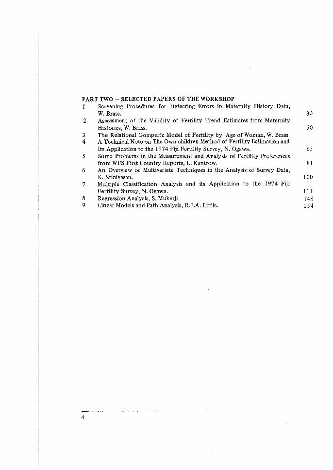
PART TWO - SELECTED PAPERS OF THE WORKSHOP 1 Screening Procedures for Detecting Errors in Maternity History Data,

W. Brass. 30 2 Assessment of the Validity of Fertility Trend Estimates from Maternity

Histories, W. Brass. 50 3 The Relational Gompertz Model of Fertility by Age of Woman, W. Brass. 4 A Technical Note on The Own-children Method of Fertility Estimation and

Its Application to the 1974 Fiji Fertility Survey, N. Ogawa. 65 5 Some Problems in the Measurement and Analysis of Fertility Preferences

from WFS First Country Reports, L. Kantrow. · 81 6 An Overview of Multivariate Techniques in the Analysis of Survey Data,

K. Srinivasan. 100 7 Multiple Classification Analysis and its Application to the 197 4 Fiji

Fertility Survey, N. Ogawa. 111 8 Regression Analysis, S. Mukerji. 148 9 Linear Models and Path Analysis, R.J.A. Little. 154

4

Foreword

At the Second Regional Meeting of the World Fertility Survey for Asia and the Pacific, held in Bangkok in 1977, the National Directors of the fertility surveys emphasised the need for organising regional workshops with a view to enhancing the analytical capabilities of the national researchers involved in the analysis of the survey data. The Regional Workshop on Techniques of Analysis of WFS Data held in December 197 8 was organised in response to this request.

The Workshop was indeed a collaborative exercise between the UN Economic and Social Commission for Asia and the Pacific, the Wor1d Fertility Survey, and the International Institute for Population Studies.

A report of the Workshop has already been published by the UNESCAP. However, in view of the need for wider dissemination of the important documents prepared for the Workshop we felt it .useful to reprint the report, and this was agreed to by ESCAP. This document is essentially a reprint of 'Asian Population Studies Series, No. 44', of the ESCAP, with editorial changes to conform to WFS format and style. We hope this will make another addition to WFS's continuing efforts in assisting the countries in the analysis of their survey data.

I also wish to take this opportunity to express our gratitude to Professor William Brass whose participation and guidance made a significant contribution to the success of the Workshop.

V.C. Chidambaram Deputy Director for Data Analysis

5

PART ONE REPORT OF THE REGIONAL WORKSHOP

1 Background

1.1 INTRODUCTION

The World Fertility Survey (WPS), a large-scale research programme for the study of human fertility, particularly in the developing world, is being conducted by the Inter­national Statistical Institute (ISI) with the collaboration of the United Nations and in co-operation with the International Union for the Scientific Study of Population (IUSSP), with financial support mainly from the United Nations Fund for Population Activities (UNFP A) and the United States Agency for International Development (USAID). In the ESCAP region, 13 countries are participating in this world-wide research programme. All countries except for Burma and Afghanistan have completed their field work; because the majority of them had also published their first country reports, they are ready to undertake the second-stage analysis of their country data.

It was recognized that, among most of those ESCAP countries participating in WFS a proper in-depth analysis of their data was seriously hampered by the lack of availability of adequately trained personnel to plan and implement the analysis. In view of this, at the Second Meeting of the World Fertility Survey for the Asian Region, held at Bangkok in March 1977, a number of directors of the national fertility surveys stressed the urgent need for additional training in techniques of analysis and thus enhance the analytical capability of those responsible for further analysis of WFS data in their own countries. As a solution to the expressed need, it was strongly recommended at the Meeting that, in close collaboration with both WFS and the International Institute for Population Studies (IIPS), ESCAP co-ordinate and execute a training-oriented regional workshop for national staff actually involved in the second-stage analysis of their WPS data.

In accordance with the commendations of the Meeting, ESCAP conducted a Regional Workshop on Techniques of Analysis of World Fertility Survey Data, utilizing the facilities of IIPS, from 27 November to 8 December 1978, at Bombay, India.

One of the primary objectives of the Workshop was to give the national staff, directly responsible for future analysis of their WPS and related data, intensive training in the techniques required for the fulfilment of such advanced research work. In order to achieve that objective, the Workshop involved (a) a series of lectures on theoretical and methodological aspects of the techniques related to the evaluation data, the estimation of fertility and multivariate analysis, and (b) laboratory exercises in the application of those techniques to real data.

9

In the long run, it was anticipated that after the completion of the Workshop each participant would be able to train other demographers in their own countries who would also be involved in-depth analyses of their country data. At the same time, a series of subregional workshops were scheduled in the 1980-1981 work programme of the ESCAP secretariat, at which participants in the Regional Workshop, as key resource persons, would be expected to play a vital role.

1.3 INSTITUTIONAL FRAMEWORK

The Workshop was financially supported by a grant from UNFPA to ESCAP. The ESCAP secretariat provided one staff member to serve as liaison officer for the Workshop and to lecture on assigned topics. ESCAP also invited two staff members from WFS and two from the United Nations Division to lecture on selected topics. WFS, in turn, provided one consultant to deliver a considerable number of lectures. In addition, the Technical Adviser for the World Fertility Survey in Asia contributed to the teaching programme. IIPS provided host facilities and the services of its staff for all local arrangements and contributed three of its staff members to share part of the teaching workload.

1.4 PARTICIPATION

A list of participants is given in Appendix III. Twenty-five government officials from 12 ES.CAP members and associate members participated in the two-week Regional Work­shop. These were Afghanistan, Bangladesh, Hong Kong, India, Indonesia, Nepal, Pakistan, the Philippines, the Republic of Korea, Singapore, Sri Lanka and Thailand. Although ESCAP extended invitations to Fiji, Iran and Malaysia, no representatives from those countries were able to attend. The participants varied in degrees of involvement in the second-stage analysis of their WFS country data. Furthermore, they had a wide range of experiences in the analysis of demographic and population data. Besides the 25 participants, two staff members of ESCAP and the Technical Adviser for the World Fertility Survey from the United Nations Population Division in New York attended the Workshop as observers.

10

2 Organization of the Workshop

2.1 OPENING SESSION

The Workshop opened on 27 November 1978 with a welcoming address by Dr. K. Srinivasan, Director of IIPS. In his statement, he emphasized an urgent need to obtain scientifically valid data on fertility and associated factors, nationally representative and internationally comparative, with a view to formulating proper population policies in the ESCAP region. More importantly, one of the major objectives of WFS was to develop national capabilities for conducting fertility and other demographic surveys in parti­cipating countries, particularly in the developing world. He concluded. by saying that it was fitting that the Workshop be conducted at IIPS, in view of the Institute's long experience in demographic training.

A message from Mr. J.B.P. Maramis, the Executive Secretary of ESCAP was read out by Mr. S.T. Quah of the ESCAP Population and Social Affairs Division. The Executive Secretary stressed that, as recommended at the Second Meeting of the World Fertility Survey for the Asian Region, the Workshop was expected to be the beginning of a regional programme of activities to increase the capability of the WPS-related national staff involved in their national surveys in evaluating and analysing present and future fertility data. The Workshop would helpsparticipants to train other demographers in their respective countries.

Dr. R.0. Carleton, Technical Adviser for the World Fertility Survey (New York) emphasized the significance of the Workshop from the standpoint of promoting the second-stage analysis of WFS data collected in the ESCAP region. He mentioned that a training-oriented workshop of this nature was scheduled for 1979 in the Latin American region.

Mr. V.C. Chidambaram, Assistant Director for Data Analysis, WFS, presented an over­all view on recent WFS activity and future plans with regard to data analysis. He described briefly the current status of first country reports in the participating countries, which, in some cases, had taken a longer time to complete than originally envisaged. Those which had already published their reports were Fiji, Hong Kong, Japan, Malaysia, Nepal, Pakistan, the Republic of Korea, Sri Lanka and Thailand. Reports from Bang­ladesh and Indonesia were in press. In order to facilitate the second-stage analysis, WFS had provided technical assistance by means of publishing technical bulletins on metho­dology and work on selected topics for further analysis, and by means of conducting (a) illustrative analysis done by WFS or its consultants on selected topics, (b) national-level seminars held after the publication of the first country reports to disseminate findings

11

and to identify topics for further analysis, and (c) regional workshops on analysis. This Regional Workshop, a salient example of possible technical assistance by WFS, was the first of a series.

After giving details of their backgrounds and affiliations, the participants made brief presentations regarding the current status of their own country survey and, where available, their future research strategies for second-stage analysis.

2.2 TOPICS

The Workshop was conducted in a series of morning and afternoon sessions. During the morning sessions, the technical aspects of detailed analysis were presented to the participants through lectures, while the afternoon meetings were utilized for doing computational exercises and reading relevant materials. Both ESCAP and WFS prepared the Workshop programme outline in close cooperation with the IIPS staff concerned. The contents covered the following three areas: (a) evaluation of data, (b) estimation of fertility, and (c) multivariate analysis. A considerable amount of time was spent on the parity/fertility (P/F) ratio and its application to the Bangladesh and Sri Lanka WFS data. The discussion on techniques for evaluating the maternity history data was followed by a presentation of fertility estimation methods which included the four-parameter Coale­Trussell model, the three-parameter Gompertz model, the own-children method, and stable population models. Although multivariate analysis was included in the Workshop programme, very limited time was allocated to that topic compared with the two other major topics. The Workshop programme and a list of materials distributed at the Work­shop are contained in Appendix I and Appendix II, respectively.

12

3 An Overview of the Techniques Discussed at The Workshop

3.1 ANALYSIS OF THE MATERNITY HISTORY DATA

The major portion of the demographic techniques pre1>ented at the Workshop have related to the maternity history data collected in the individual interview. Professor Brass presented a variety of methods for the evaluation of the quality of these data and the estimation of levels and trends in fertility.

The basic data used by Professor Brass were the following:

a) From the household schedule:

i) The proportion of women ever married by age;

'b) From the individual interview:

ii) Current age of respondent; iii) Current parity of respondent; iv) Dates of births of all live-born children.

From these data a set of two-way cross-tabulations of the fertility data can be calculated. They take the basic form given in the figure below. The columns represent periods before the survey date, which are conventionally grouped into five-year intervals, although shorter intervals may be considered. The rows represent birth cohorts identified by groupings of current age.

The cells for which data exist are marked by crosses. Within these cells, we can imagine a count of the number of women1, and a distribution of live births for these women, classified by birth order. The entries in any particular table consist of statistics derived from this distribution. The following statistics are used:

a) Mean birth rate; b) Mean birth rate of first order, or, in other words, the proportion of women having

their first child; c) Mean birth rate of parity 4 or more.

In addition, rates for other birth orders may be calculated if necessary. Finally, similar cross-tabulations can be formed for subgroups of the samples such as educational level.2

1 Calculated by dividing the number of ever-married women in required age group from the individual questionnaire by the proportion of women ever-married from the household schedule. 2 If the subgroup marked is not ,coded in the household schedule, then some indirect estimate of the proportions of women' ever-married is required.

13

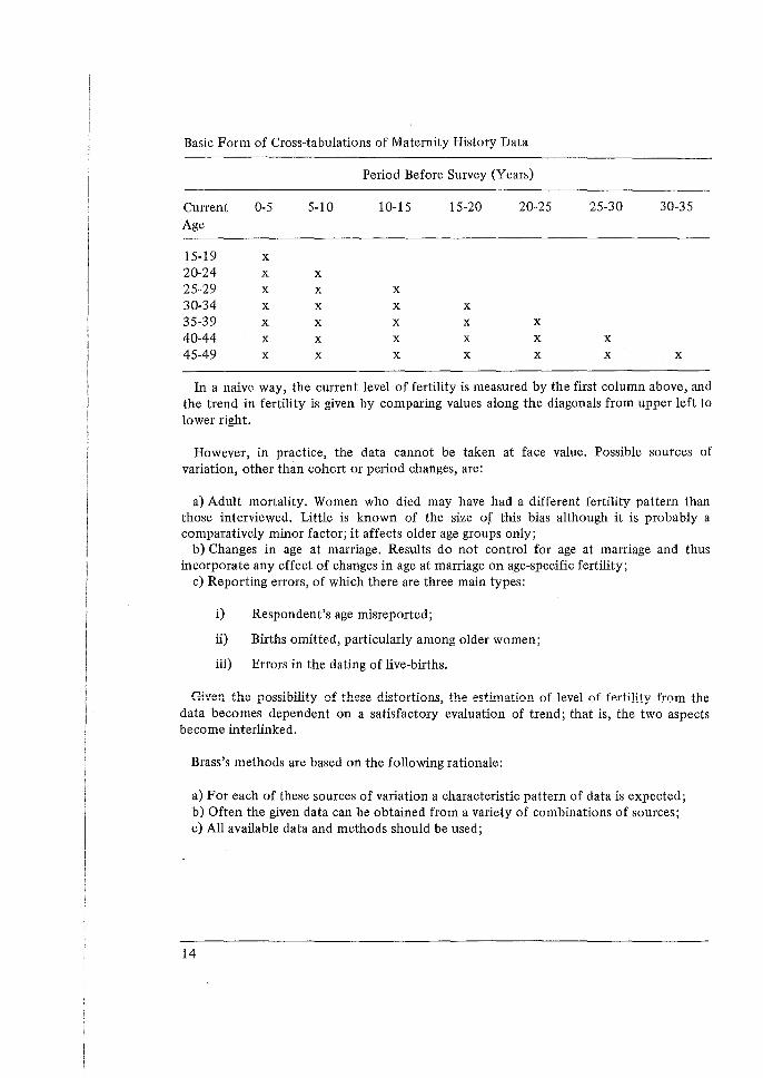
Basic Form of Cross-tabulations of Maternity History Data

Period Before Survey (Years)

Cunent 0-5 5-10 10-15 15-20 20-25 25-30 30-35 Age

15-19 x 20-24 x x 25-29 x x x 30-34 x x x x 35-39 x x x x x 40-44 x x x x x x 45-49 x x x x x x x

In a naive way, the current level of fertility is measured by the first column above, and the trend in fertility is given by comparing values along the diagonals from upper left to lower right.

However, in practice, the data cannot be taken at face value. Possible sources of variation, other than cohcrt or period changes, are:

a) Adult mortality. Women who died may have had a different fertility pattern than those interviewed. Little is known of the size of this bias although it is probably a comparatively minor factor; it affects older age groups only;

b) Changes in age at maniage. Results do not control for age at maniage and thus incorporate any effect of changes in age at marriage on age-specific fertility;

c) Reporting errors, of which there are three main types:

i) Respondent's age misreported;

ii) Births omitted, particularly among older women;

iii) Errors in the dating of live-births.

Given the possibility of these distortions, the estimation of level of fertility from the data becomes dependent on a satisfactory evaluation of trend; that is, the two aspects become interlinked.

Brass's methods are based on the following rationale:

a) For each of these sources of variation a characteristic pattern of data is expected; b) Often the given data can be obtained from a variety of combinations of sources; c) All available data and methods should be used;

14

d) Eventually a subjective choice must be made as to which combination of sources of variation is the most plausible. Often the proportionate contributions of the sources of variation cannot be exactly assessed; then the estimates of level and trend will be subject to bounds of uncertainty.

METHODS OF LIMITED POWER

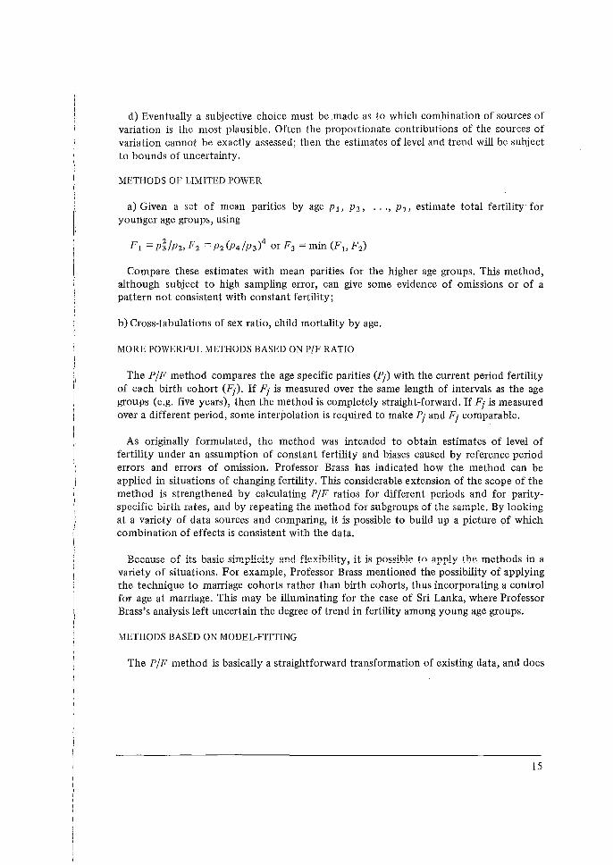
a) Given a set of mean parities by age p 1 , p 2 , •.• , p 7 , estimate total fertility for younger age groups, using

Compare these estimates with mean parities for the higher age groups. This method, although subject to high sampling error, can give some evidence of omissions or of a pattern not consistent with constant fertility;

b) Cross-tabulations of sex ratio, child mortality by age.

MORE POWERFUL METHODS BASED ON P/F RATIO

The P/F method compares the age specific parities (Pj) with the current period fertility of each birth cohort (Fj). If Fj is measured over the same length of intervals as the age groups (e.g. five years), then the method is completely straight-forward. If Fj is measured over a different period, some interpolation is required to make Pj and Fj comparable.

As originally formulated, the method was intended to obtain estimates of level of fertility under an assumption of constant fertility and biases caused by reference period errors and errors of omission. Professor Brass has indicated how the method can be applied in situations of changing fertility. This considerable extension of the scope of the method is strengthened by calculating P/F ratios for different periods and for parity­specific birth rates, and by repeating the method for subgroups of the sample. By looking at a variety of data sources and comparing, it is possible to build up a picture of which combination of effects is consistent with the data.

Because of its basic simplicity and flexibility, it is possible to apply the methods in a variety of situations. For example, Professor Brass mentioned the possibility of applying the technique to marriage cohorts rather than birth cohorts, thus incorporating a control for age at marriage. This may be illuminating for the case of Sri Lanka, where Professor Brass's analysis left uncertain the degree of trend in fertility among young age groups.

METHODS BASED ON MODEL-FITTING

The P/F method is basically a straightforward transformation of existing data, and does

15

not impose any predetermined pattern on the age-specific fertility rates.

Perhaps the most powerful analytical techniques discussed by Professor Brass are methods based on an underlying model. These are attempts to stretch the available data by imposing an underlying model on the fertility rates and using this model to improve existing data and to extrapolate values for which no data are available. A crucial factor in such models is the number of parameters needed to define the pattern. Two models are discussed.

METHODS USED ON MODEL-FITTING

The P/F method is a straightforward transformation of existing data, and does not impose any pattern on age-specific fertility rates. Perhaps the most powerful analytic techniques discussed are the model-based techniques. These attempt to stretch the available data by imposing an underlying pattern to the data and using this pattern to improve existing data values or extrapolate to values for which no data exist. A crucial factor in such models is the number of parameters needed to define the pattern and the interpolation of those parameters. Two models were discussed for age-specific fertility rates:

a) The Coale-Trussel four-parameter model. This involves the combination of a two­parameter model for age at marriage with a two-parameter model of marital fertility. Professor Brass considers the combined four-parameter model for age-specific fertility rates to have too many parameters. An alternative approach is to estimate each component of the model separately, using data on age at marriage and marital fertility;

b) The three-parameter relational Gompertz 'model. The Gompertz model for cumulated age-specific fertility has three parameters: F = total fertility rate, A = proportion of fertility achieved by a certain fixed age, and b = a measure of speed over which fertility cumulates. The model fits the data quite well, but not well enough. Professor Brass has shown an ingenious method for improving the fit at low and high ages without increasing the number of parameters. Empirical research indicates that departures from the Gompertz model tend to have the same character in a wide variety of data sets. From these a fixed transformation of the age scale has been derived and the Gompertz n1odel can be fitted to this transformed age scale. This modified model may be termed the relational Gompertz model. Fitting procedures are developed which are based on the fact that the Gompertz function is linear with age on the - log (-log) scale.

METHODS BASED ON HOUSEHOLD DATA

The methods discussed by Professor Brass are particularly relevant to the detailed maternity histories collected in WFS surveys. Methods have been discussed which are applicable to household data. These were originally designed for census data, where there

16

is no sampling and less detail and reliability. Thus, although these methods may well have a useful role in the analysis. The household data are collected primarily to identify eligible women, and the amount of time spent in data collection and editing is much more limited than for the individual questionnaires.

THE OWN-CHILDREN METHOD

This method uses the ages of children listed in the household schedule who are not living away from home. By projecting back to the birth dates of these children, and making adjustments for the mortality of children and mothers, the degree of under­enumeration and the proportion of children living away from home, age-specific fertility can be calculated.

Broadly speaking, the estimates differ from age-specific fertility rates calculated directly from maternity history data in the following ways:

a) The births of own children are taken from the household questionnaire rather than the individual interview;

b).The children who lived away or have died are estimated indirectly from other sources, rather than directly from the respondent's answers in the individual ques­tionnaire.

The comparative validity of the two methods depends on which of these alternatives is more trustworthy.

Of course, alternative estimates can be calculated and compared. However, the own­children method works best when the adjustment factors are not large. In such cases estimates by the two methods have an unknown but probably high correlation, unless an expanded household schedule is involved. Thus similar estimates cannot be considered as enhancing significantly belief in the reliability of the data, as would be the case if two independent estimates gave the same value. There are considerable dangers in gathering strength from different estimates based on largely similar underlying data. On the other hand, if the two estimates differ, further investigation of the cause of the difference would be desirable.

QUASI-STABLE ESTIMATES

The estimates discussed by the Technical Adviser for WFS (Bangkok) are in a sense even more indirect than those obtained by the own-children method since they use only the sex and age distribution of the household sample. The stable population theory predicts a fixed age distribution from any given level of birth and death rates; conversely the theory enables estimates of birth and death rates from paramters of the age distribution and the growth rate, using the Coale-Demeny life-tables. Here, crude birth and death rates are

17

calculated from a different set of parameters, the child-woman ratio and the life expectancy. Evidence has been provided that these estimates are less sensitive to changes in the level of fertility and child mortality.

QUESTIONS ON FAMILY SIZE PREFERENCE

With regard to the extent to which policy-making inferences can be made on the basis of answers to family size preferences asked in the WFS questionnaire. These questionnaires are subject to a lack of test-retest reliability and to biases caused by the skip procedures designed to filter out women who might find the questions offensive. Also, the meaning of the questions is sometimes unclear, and is subject to formidable translation problems in certain countries. Report writers should therefore be careful to

. state clearly the limitations of any inferences based on these data. To use the classic phrase, they should be treated with great caution.

The subject of the wording and meaning of attitudinal questions is a hornet's nest, and the problems may be fundamentally intractable. This statistician's plea is not to change the wording of questions from survey to survey, since then at least some evidence of changes in attitudes may be believable.

18

4 Evaluation of the Workshop

4.1 VIEWS OF THE PARTICIPANTS

At the closing session, the participants completed a questionnaire in which they were asked to evaluate (a) the overall usefulness of the Workshop, (b) the relevance of topics in terms of the analysis of their country data, (c) the appropriateness of coverage, comprehensiveness of topics and the adequacy of laboratory exercises, and (d) the need for a future ESCAP-sponsored workshop of that nature. The following is a summary of their evaluative comments on these questions.

'On the whole, did you find this Workshop very useful, useful, not very useful, or not us.eful at all?' Of the 23 respondents, 12 participants felt that the Workshop had been very useful: 11, useful; and none, either not very useful or not useful at all. All agreed that the Workshop was, at least, useful. Several of them responded to the question with the remark that new techniques of analysis had been introduced and the ramification of old methods had been presented to make them more suitable in the analysis of WFS data.

'Do you consider the topics covered at the Workshop relevant for use in the analysis of WFS data in your country?' Almost all the participants found the topics relevant to their future research work in the analysis of WFS data. Those participants who made no comment were from countries which were not participating in the WFS programme. Most of the respondents felt that lectures on the evaluation of data and the estimation of fertility had been extremely relevant to their research work. At the same time, a considerable number found lectures on multivariate analysis, such as multiple classi­fication analysis (MCA), path analysis and regression, very relevant to their analysis work.

'Please comment on the course contents of this Workshop in terms of coverage, comprehensiveness of topics covered as well as the adequacy of laboratory assignments'. The majority of the participants agreed that, given such limited time, the Workshop had efficiently covered a wide range of topics on a comprehensive basis. There were various con1ments, however, on the adequacy of laboratory exercises" For instance; a few participants found them rather elementary. The others, on the other hand, felt them to be quite adequate although the time allocated was too short to undertake any in-depth analysis of practice questions. It was also suggested by a few participants that the laboratory sessions could have been better used if all participants had brought their own WFS country data so that they could actually attempt to undertake analyses based on techniques covered at the Workshop, by using some computer statistical package programmes. Furthermore, some participants, commented that additional WFS country data should have been utilized for laboratory questions.

19

'Please give any other comments you may have'. All but a few thought that the duration of the Workshop had been too short, and that it should have lasted from three to six weeks. It was almost unanimously agreed upon that much more time should have been allocated to multivariate analysis. Most of the participants found the quality of lectures and handouts excellent. It should be noted, however, that a number of participants suggested that the papers and handouts should have been distributed at least a few days prior to their presentation, in order to allow each participant sufficient time for careful reading.

'Do you think it is worthwhile for ESCAP to organize another workshop of this nature? If so, please indicate the topics in order of priority?' All of the participants supported the ideas that ESCAP should organize another such workshop. As for topics, a number of participants suggested that multivariate analysis, including MCA, path analysis and factor analysis, should be definitely included in the programme. Other areas indicated were sampling methods, birth interval analysis, analysis of the interrelationship between mortality and fertility, lifectable techniques for the measurement of the effectiveness of various contraceptive methods, the Guttman scale in the analysis of attitudinal responses, etc. Notwithstanding these many diversified topics, many of the participants commented that in the next workshop the number of topics must be limited, so that each could be more intensively dealt with.

4.2 RECOMMENDATIONS FOR FUTURE WORKSHOPS

In order that future WFS workshops are more effective and useful, the following suggestions and comments were made by the participants for consideration:

a) The duration of a workshop should be substantially prolonged from three to six weeks;

b) Participants' qualifications should be more precisely defined in order to facilitate a more suitable selection, thus making workshops more efficient and rewarding;

c) The usefulness of workshops would be considerably enhanced if papers and handouts could be disseminated for perusal at least a few days prior to lecturing;

d) More time should be given to lectures on multivariate analysis: e) Laboratory sessions would be more effective if VIFS country data could be n1ore

extensively used for the interpretation of computional results.

20

Appendix 1 - Workshop Programme

Date Time Period Session Topic Speaker

OPENING SESSION

27 November 10.00 a.m. - Welcoming Address Mr. Srinivasan 12.45 p.m. Opening Remarks by ESCAP Mr. Quah

Overview of WFS Analysis Mr. Chidambaram Plans

2.00 p.m. - Country Presentations Participants 4.00 p.m.

EVALUATION OF DATA

28 November 9.45 - Overview of Screening Mr. Brass 12.45 p.m. Procedures

The P /F Ratio Method Mr. Brass

2.00 p.m. - Laboratory Mr. Pathak 4.00 p.m.

29 November 9.45 a.m. - Indirect Evidence of Mr. Brass 12.45 p.m. Errors

Director Tests for Mr. Brass Omission

2.00 p.m. - Laboratory Mr. Pathak 4.00 p.m.

30 November 9.45 a.m. - Illustrative Analysis: Mr. Brass 12.45 p.m. Bangladesh

Illustrative Analysis: Mr. Brass Sri Lanka

2.00 p.m. - Discussion and summary Mr. Chidambaram 3.00 p.m.

21

ESTIMATION OF FERTILITY

1 December 9.45 a.m. - Overview of Estimation Mr. Brass 12.45 p.m. Procedures

Maternity History Estimates Mr. Brass

2.00 p.m. - Laboratory Mr. Pathak 4.00 p.m.

4 December 9.45 a.m. - Parity-specific Estimates Mr. Brass 12.45 p.m. Own-children Technique Mr. Ogawa

2.00 p.m. - Fertility Preferences-Problems Ms. Kantrow 3.00 p.m. in Measurement and Analysis

3.00 p.m. - Laboratory Mr. Quah 4.30 p.m.

5 December 9.45 a.m. - Quasi-stable Estimates Mr. Rele

4.00 p.m. Discussion and Summary Mr. Little

MULTIVARIATE ANALYSIS

6 December 9.45 a.m. - Overview of Analysis Techniques Mr. Srinivasan 12.45 p.m. Standardisation Mr. Chidambaram

Multiple Classification Analysis Mr. Ogawa

2.00 p.m. - Laboratory Mr. Chidambaram 4.00 p.m. and Mr. Ogawa

7 December 9.45 a.m. - Regression Analysis Mr. Mukerji 12.45 p.m. Linear Models and Path Analysis Mr. Little

"'l ()(\ .................. u.vv .l:'•lU, - Laboratory tvfr. Little 4.00 p.m. Discussion and Summary Mr. Chidambaram

CLOSING SESSION

8 December 9.45 a.m. - Discussion of Problems in Participants 12.45 p.m. Further Analysis

Concluding Statements

22

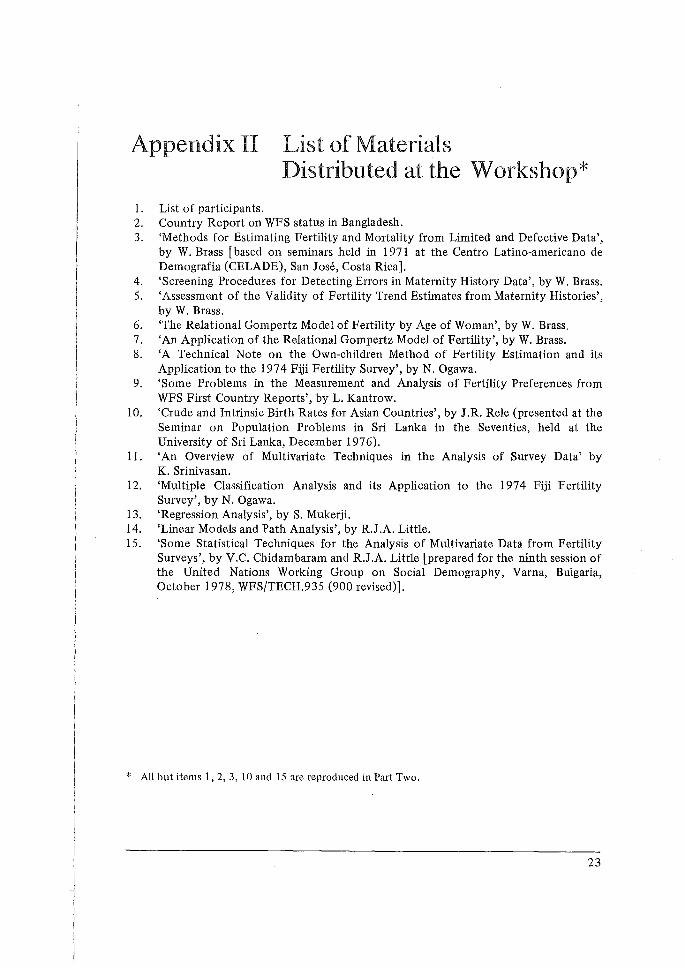
Appendix II List of Materials Distributed at the Workshop*

1. List of participants. 2. Country Report on WFS status in Bangladesh. 3. 'Methods for Estimating Fertility and Mortality from Limited and Defective Data',

by W. Brass [based on seminars held in 1971 at the Centro Latino-americano de Demografia (CELADE), San Jose, Costa Rica].

4. 'Screening Procedures for Detecting Errors in Maternity History Data', by W. Brass. 5. 'Assessment of the Validity of Fertility Trend Estimates from Maternity Histories',

by W. Brass. 6. 'The Relational Gompertz Model of Fertility by Age of Woman', by W. Brass. 7. 'An Application of the Relational Gompertz Model of Fertility', by W. Brass. 8. 'A Technical Note on the Own-children Method of Fertility Estimation and its

Application to the 1974 Fiji Fertility Survey', by N. Ogawa. 9. 'Some Problems in the Measurement and Analysis of Fertility Preferences from

WFS First Country Reports', by L. Kantrow. 10. 'Crude and Intrinsic Birth Rates for Asian Countries', by J.R. Rele (presented at the

Seminar on Population Problems in Sri Lanka in the Seventies, held at the University of Sri Lanka, December 1976).

11. 'An Overview of Multivariate Techniques in the Analysis of Survey Data' by K. Srinivasan.

12. 'Multiple Classification Analysis and its Application to the 1974 Fiji Fertility Survey', by N. Ogawa.

13. 'Regression Analysis', by S. Mukerji. 14. 'Linear Models and Path Analysis', by R.J.A. Little. 15. 'Some Statistical Techniques for the Analysis of Multivariate Data from Fertility

Surveys', by V.C. Chidambaram and R.J.A. Little [prepared for the ninth session of the United Nations Working Group on Social Demography, Varna, Bulgaria, October 1978, WFS/TECH.935 (900 revised)].

* All but items 1, 2, 3, 10 and 15 are reproduced in Part Two.

23

Appendix III List of P~rticipants

AFGHANISTAN

Mr. Yar Mohammad Rad, Director, Provincial Office Census Project of Bamian, Central Statistics Office, Kabul.

Mr. Abdul Wahab Fanahi, Director, Analysis and Evaluation of the Demographic Division, Central Statistics Office, Kabul.

BANGLADESH

Mr. Riazuddin Ahmad, Joint Director, Statistics Division, Ministry of Planning, Dacca.

Mr. Abdul Rashid, Statistician (RESP), Directorate of Population Control and Family Planning, Dacca.

HONGKONG

Mr. Moon-cheong Leong, Statistician, Demographic Statistics Section, Social Statistics Division, Census and Statistics Department, Hong Kong.

INDIA

Mr. B.R. Dohare, Research Officer, Ministry of Health and Family Welfare, Government of India, New Delhi.

Ms. L.V. Chavan, Demographer, Urban Development and Public Health Department, Mantralaya, State Family Welfare Bureau, Government of Maharashtra, Bombay.

Mr. P.S. Gopinathan Nair, Deputy Director, Bureau of Economic and Statistics, Government of Kerala, Kerala.

24

Mr. A.K. Mukherjee, Demographer, State Family Welfare Bureau, Government of West Bengal, Calcutta.

Mr. S.K. Dhawan, Research Officer, Department of Family Welfare, Government of India, New Delhi.

INDONESIA

Ms. Azwini Kartoyo, Lembaga Demografi Fakultas' Ekonomi, Universitas Indonesia, Salemba Raya 4, Jakarta.

Mr. Budi Soeradji, Central Bureau of Statistics, Jakarta.

KOREA, REPUBLIC OF

Mr. Tae Yoon Jun, Officer, National Bureau of Statistics, Economic Planning Board, Seoul.

Mr. Byung Tae Park, Researcher, Korean Institute for Family Planning, Seoul.

NEPAL

Mr. B.B. Gubhaju, Demographer, Nepal Family Planning and MCH Project, Kathmandu.

Mr. Y.S. Thapa, Research Officer, Centre for Economic Development and Administration, Kathmandu.

PAKISTAN

Mr. Nasim Sadiq, Deputy Director General, St\ltistics Division, Ministry of Finance, Planning and Economic Affairs, Karachi.

Ms. Jamila Naeem, Director, Demographic Policies and Implementation Research Centre (DPIRC), Population Planning Division, Lahore.

PHILIPPINES

Miss Remedios V. Sabino, Supervising Statistician, National Family Planning Office, Ministry of Health, Manila.

Mr. Eliseo A. de Guzman, Instructor, Population Institute, University of the Philippines, Manila.

25

SINGAPORE

Ms. Lynda Chiang Shih Chen, Registrar, Research and Statistics, Unit, Ministry of Health, Singapore.

SRI LANKA

Mr. A.T.P.L. Abeykoon, Planning Officer, Planning Division, Ministry of Finance and Planning, Colombo.

Ms. S.S.S. Pereira, Statistician, Department of Census and Statistics, Colombo.

THAILAND

Miss Suvathana Vibulsresth, Assistant Professor, Institute of Population Studies, Chulalongkorn University, Bangkok.

Miss Chintana Pejaranonda, Statistician, Population Survey Division, National Statistical Office, Bangkok.

UNITED NATIONS

Mr. R.O. Carleton

Ms. Louise Kantrow

WORLD FERTILITY SURVEY

Mr. V.C. Chidambaram

Mr. R. Little

ESCAP SECRETARIAT

Mr. B.B. Aromin

Mr. S.T. Quah

Mr. N. Ogawa

26

Technical Adviser for the World Fertility Survey

Fertility and Family Planning Studies Section, Population Division

Assistant Director for Data Analysis

Analysis Division, WPS Central Staff

Chief, General Demography Section, Division of Population and Social Affairs

Population Officer, Fertility and Family Planning Section, Division of Population and Social Affairs

Population Officer, General Demography Section, Division of Population and Social Affairs

Mr. A. Lery

IIPS

Mr. K. Srinivasan Mr. S. Mukerji Mr. K.B. Pathak (Mrs.) M. Karkal Mr. T.K. Roy Mr. S. Lahiri (Mrs.) A.K. Wadia

RESOURCE PERSONS

Mr. William Brass

Mr. J.R. Rele

Expert on Demographic and Population Statistics, Division of Statistics

Director Professor Professor Reader Reader Administrative Officer P.A. to Director

Director, Professor of Medical Demography, Centre for Population Studies, London School of Hygiene and Tropical Medicine, London

Technical Adivser for World Fertility Survey in Asia, ES CAP, Bangkok

27

PART TWO SELECTED PAPERS OF THE WORKSHOP

SCREENING PROCEDURES FOR DETECTING ERRORS IN MATERNITY HISTORY DATA

W. Brass*

A. INTRODUCTION

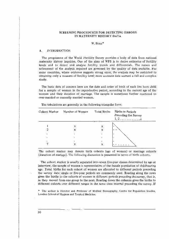
The programme of the World Fertility Survey provides a body of data from national maternity history inquiries. One of the aims of WFS is to derive estimates of fertility levels and to detect and analyse fertility trends and differentials. The nature and refinement of the analysis required are governed by the quality of data available. For some countries, where evidence suggests strong error, the analysis may be restricted to obtaining only a measure of fertility level; more accurate data warrant a full and complex study.

The basic data of concern here are the date and order of birth of each live born child for a sample of women in the reproductive period, according to the current age of the women and their duration of marriage. The sample is sometimes further restricted to ever-married or currently married women.

The tabulations are generally in the following triangular form:

Cohort Marker

1 2

7

Number of Women

x x

x

Total Births Births in Periods Preceding the Survey

x x

x

1, 2 ............ /l

The cohort marker may denote birth cohorts (age of women) or marriage cohorts (duiation of mariage). The following discussion is presented ·in terms of birth cohorts.

The cohort marker is usually separated into seven five-year classes determined by age at interview; the sample of women is representative of the female population of childbearing age. Total births for each cohort of women are allocated to different periods preceding the survey date; single or five-year periods are commonly used. Reading along the rows gives the births to the cohorts of women in different periods preceding the survey, that is, as they moved from one group to the next. Reading down the columns gives the births to different cohorts over different ranges in the same time interval preceding the survey. If

* The author is Director and Professor of Medical Demography, Centre for Population Studies, London School of Hygiene and Tropical Medicine.

30

the periods preceding the survey cover five-year intervals, then reading downward diagonals from the left show the births to women from different cohorts over the same ages.

If the basic data are reported accurately, a reliable picture of the current fertility situation and variations with time among groups may be obtained to the extent that women in the reproductive range in a given past period are represented by the iiving. The upper limit of the fiftieth birthday for the women in the sample leads to progressively lower truncation points of reproductive experience as time recedes. The only important assumption required for such an analysis is that the fertility of the survivors is representative of the fertility of all those exposed to risk at any given time.

The main problems associated with the analysis of maternity history data, at least for less developed countries, concern the accuracy of reporting. Different errors may affect the data and lead to considerable bias. The direction on this bias, especially in the analysis of trends, differs according to the type of error prevailing. Thus, before any detailed analysis of the data, it is essential to check the reliability of recording and to assess the degree and direction of bias likely to affect the estimates.

This report discusses the general procedures for detecting errors in maternity history data and provides a set of tests. Illustrations of the methods are presented using data from the Bangladesh and Sri Lanka fertility surveys. The basic minimum tabulations required in order that these tests may be performed are outlined.

B. ERRORS IN RETROSPECTIVE REPORTS OF BIRTHS

A type of error that may occur is in the definition of the cohort. Misstatement of current age may have important implications for fertility measurements. The direction and magnitude of the error involved in estimating the level and trend in fertility are influenced by the number of women displaced from one age group to the other and their fertility.

Another widely recognized possible error is that the total number of children ever born may be understated. The tendency for the omitted briths to increase with the age of women is well established. This tendency is related to the effect on memory of longer intervals and larger numbers of births and to the likelihood that children who moved away or died are more often omitted. Other factors leading to a higher probability of omission include illegitimacy and female sex of births.

The detailed questioning in the WFS inquiries on surviving births and children who died or moved away is likely to improve the quality of reporting. Also, the restriction of the data collection to women under 50 avoids the most faulty responses, usually from older women. Unfortunately the restriction complicates the detection of omissions.

31

The general effect of omission is an understatement of the level of fertility, expecially for older cohorts and earlier periods. Also, a bias in the measurement of the trend in fertility is present. This bias is usually a deviation towards an increase in fertility on,_a period and cohort basis (certain less common types of omissions, such as of young infants, which do not increase the older the cohorts, may suggest a false decline in fertility).

A more complicated type of error occurs in the allocation of births to the different time intervals before the survey. The simplest specification of this error was proposed by Brass in terms of a distortion of the time scale. Reported births during a certain year may actually refer to births occurring in a period of 9 or 15 months; thus births are allocated on average to a shorter or a longer interval than that in which they actually took place. If this distortion - called reference size error - is the same for all age groups of women, its effect on fertility analysis is straightforward. The level of period fertility is overstated or understated according to a longer or shorter reference size bias. The trend in fertility between two periods depends on the type of reference size error in both. For example, a downwards reference size bias preceded by an upwards or zero one results in the false conclusion of a decline in fertility. The assumption of equal reference error for all age groups of women is more likely to hold for recent short periods preceding the survey.

The more complicated type of misplacement error occurs when the distortion of the timing of births is related to the age of the mother. Brass (197 5) discusses a tendency for older women to exaggerate the interval from when the births took place, placing them further back in time than they occurred. This error results in an overestimation of the level of fertility for the earliest periods preceding the survey and implies a change in the age pattern owing to a false decline in fertility in young age groups for more recent cohorts.

Another equally plausible type of error, which introduces an opposite bias, is discussed by Potter (1975). In an attempt to provide an explanation of timing distortions he presents a model in which the allocation of the time of birth of the nth child is affected by the reported time of birth of the (n-J)th child and the interval between births as well as the number of years before the survey that the event occurred. Specifically, Potter considers there is a tendency to bring earlier events closer to the date of the interview and to exaggerate the length of interval between births. He also assumes that very recent events are correctly reported. In effect, the results of this model is an underestimation of the level of fertility corresponding to the most distant periods preceding the survey (shorter reference error not necessarily equal for all ages and all orders of births), while the most recent period rates are nearly correct and these correspond to the period before the most recent are exaggerated. Evidently the Potter model leads to a false conclusion of a decline in fertility in the most recent period.

It is relevant to note that the effect of omissions on the age pattern of birth-order-

32

specific fertility rate is similar to the type of event misplacement considered by Potter. Omission of the nth child results in the (n+J)th child being stated as the nth; if the date of birth of the (n+ l)th child is assigned to the nth child, an older pattern of the nth order fertility rates occurs. The level of the nth order fertility is only affected by omission by women with only n births in total.

The complexity of the timing error (misplacement) consequences arises from the fact that different errors have a variety of effects on conclusions about fertility change. It is also difficult to conceptualize the possible influences of less structured types of error, and there is a lack of experience on the nature of the timing distortion in developing countries. That experience can only come from a combination of planned field experiments and detailed investigation of the data from many maternity history enquiries. The level of cohort fertility (cumulative fertility rates up to the current ages) is not affected by misplacement error but great care must be exercised in drawing inferences about the level and trends in period fertility.

C. SCREENING PROCEDURE FOR DETECTING ERRORS

The procedures adopted for detecting errors in maternity history~data are divided into three sections.

In the first section, the reportedslevel of fertility is compared with an estimated level and the deviation between the estimated and reported level is used as an indication of error. A comparison between the estimate of the total fertility rate and the reported current period total fertility rate (using births in the year preceding the survey) checks for error in recent period data. As previously pointed out, the major cause of error in the recent period data is usually reference size bias. Furthermore, if fertility has remained constant, the estimated period fertility may be compared with the reported cohort total fertility (using the average parity of women aged 45-49) to indicate omission of births.

Several methods are available for estimating fertility levels. They range from very simple formulae to complicated models. For the preliminary analysis of the data, it was felt that the extra effort required in fitting the more sophisticated models would not be justified and this is more suitable for a later stage (when attempts are made to correct the data by adjusting the reported levels to more plausible estimates). The reasons for this decision are summarized in the following paragraphs.

The final conclusions are based on an accumulation of evidence rather than the result of one test; several methods of estimation are used and a great deal of effort is directed towards checking the 'plausibility of these estimates. The use of elaborate techniques complicates this approach and makes it inappropriate for preliminary screening.

33

Fitting sophisticated models to the data requires familiarity with the general charactelistics of the materials to specify measures least affected by error for the estimation of the parameters. It is the purpose of this study to indicate such measures. It should be pointed out that even if a good model for the pattern of fertility is defined, the estimated levels may not be very precise since an element of extrapolation is usually involved.

Some of the simple formulae depend upon the same underlying pattern of fertility as the more complicated formulations. Thus, it is believed that the estimates of the level of fertility by the simpler methods will not differ much from those obtained from the elaborated models.

In the second section a critical examination, with emphasis on features likely to characterize the data in case of error, is described.

In the third section, several direct tests for omission of certain events are discussed.

Finally, it should be noted that if external data are available, a comparison between measures from the different sources of information may provide valuable test for error. The present report does not deal with this last situation.

METHODS FOR ESTIMATING FERTILITY LEVELS

The techniques used all depend to a greater or lesser extent on regularities in the patterns of age-specific fertility rates. A brief reference is, therefore, made to the more relevant codifications of these regularities as models.

Different fertility models are available. They may be used for the estimation of the total fertility rate from measures for incomplete age ranges of women. In addition a general study of the nature of deviations of the reported fertility rates from the model values may help to indicate the type of distortions affecting the data.

Murphy and Nagnur (1972) discuss the Gompertz function as a representation of cumulated fertility rates; the parameters of this model are the total fertility rate, the proportion of the total attained by a fixed age· and a measure related to the degree to which fertility is concentrated about the peak age.

Romaniuk (1973) applies a Pearsonian type 1 curve; total fertility and the mean and model ages are the parameters of this model.

Coale and Trussell (197 4) developed a more complicated system representing the age pattern of fertility as a combination of two separate models of nuptiality and marital fertility rates. The three parameters specifying the pattern are the age at which marriages

34

begin to take place, a scale factor expressing the interval in which nuptiality in the population is equivalent to that in one year in a standard and the degree of control by family planning. More recently, Coale, Hill and Trussell (197 5) discuss the use of this model in estimating fertility measures from data on children ever born tabulated by duration of marriage.

Brass (1977) modified the Gompertz function model by introducing a fixed empirical transformation of the age scale. This greatly improved the fit to observations at ages early and late in the reproductive period. The model was applied for the detection of birth reporting errors in maternity history analysis.

Coale and Demeny (1967), by using empirical study, showed that the period total fertility rate (TFR) may be approximated as:

TFR=PVP2

where P2 and P3 denote the mean numbers of children ever born to the cohort of women in the age groups 20-24 and 25-29 respectively. P2 and P3 are not affected by mis­placement error and generally least biased by omission error as they pertain to younger women for whom reporting is better.

On the other hand, mis-statement of age and deviations from the basic assumptions may bias the resulting estimate of TFR. The assumptions are that fertility at ages 15-29 has been constant in the recent past (this assumption enables us to replace the period cumulative rates by the cohort cumulative rates, P2 and P3 and that the age pattern of fertility conforms to the typical form in populations practising little birth control.

Brass showed that, if the pattern of fertility can be described by a Gompertz function

P44

of the proportion experienced by each age, then P2 (p3

) is a better estimate of TFR than

P~/P2 provided that good reporting of ages and births extends to age 35 years. Constant fertility over the recent past at age 15-3 5 is assumed. In the two formulae an indication of the level of fertility is obtained using the cumulated experience of young (P2 , P3 and P 4 ).

The two approaches can be combined to obtain an estimate for the total fertility rate.

Brass (see 197 5 exposition) in the P/F ratio method utilizes the data for the most recent period to specify the age pattern of fertility but not necessarily the level. On the assumptions that fertility has been unchanged for some time and that errors in the period data are not age selective, i.e. constant reference size bias, the relation between the cohort measures and the corresponding cumulated period rates (Pi/Fi) is an indication of reference size error. The period fertility rates are adjusted accordingly (for a detailed discussion see Appendix I).

35

As previously, the cumulated cohort measures for younger women are taken as the least affected by birth omissions. Age errors may distort the ratios (Pi/F;), but the effect of such mis-statement is reduced by the fact that the two types of data are derived from the same ~ource and tend to be similarly distorted. Also, some freedom may be exercised in the choice of the correction factor by the avoidance of ages strongly influenced by error (P2 /F2 is generally used). The technique may be applied separately by birth order; special attention is given to the study of first births as the data on these are less likely to be affected by omission and small changes in fertility.

DISCUSSION AND EXTENSION OF THE METHODS

The methods provide estimates of the total fertility rate; a comparison between these estimates and the reported period and cohort measures checks for error in the data. How­ever, the detection of errors is not as straightforward as the preceding paragraphs imply. The differences between reported and estimated rates are not always due to errors in data. Deviations from the underlying assumptions - constant fertility over time and a model pattern of fertility - and age errors may result in erroneous estimates of the total fertility rate. Thus, the first concern is to assess the plausibility of the estimates.

p2 p 4

A critical study of the first two formulae suggests the following rule; if ~ < P 2 ( ~) P2 P3

then it is more likely that the Gompertz model does not provide a good fit for the reported mean parities of cohorts and the estimate of TFR using the first formula is

p 4 p2 recommended. On the other hand, if P 2 ~ < _}, the Brass formula is likely to provide a

P3 P2

better estimate of TFR. In addition, if the estimate of the total fertility is less than the mean parities of the older age cohorts (P7 at ages 45-49 and P6 at 40-44), there is an indication that the underlying assumptions are not met and the formulae should not be used.

The P/F ratio method does not impose a pattern of fertility and is simple to apply. A critical examination of the nature of variations in the P/F ratio with age is important as a check that the underlying assumptions are met, for example, if it is suspected that fertility decline rather than error in the data is the cause of the variation in the ratios; a comparison between the pattern of change in the ratios when the method is applied to lower and higher order births and to differen.t categories of women may substantiate the existence of errors. Fertility decline is more likely to affect higher order births than lower order ones and also certain categories of women. If variations in the ratios are not consistent with this expectation, the case for errors is strengthened.

Nevertheless, it may be that recent changes in fertility affecting young cohorts will produce a different effect on the ordered P/F ratios. For example, recent postponement

36

of first births - whether through a change in the tempo of marital fertility or a change in marriage patterns - is likely to result in high P/F ratios for young ages and lower order births. A study of changes in marriage patterns may be helpful in explaining the behaviour of the P/F ratios.

Generally it should be stated that the effect of recent abrupt movements in fertility are extremely hard to separate from the effects of error on the behaviour of the P/F ratios. On the other hand, the consequences of sustained systematic trends in fertility are more easily defined and therefore differentiated from error.

A further step toward the detection of error may be attempted by successive applications of the P/F method for periods preceding the survey. The successive application may be helpful not only in highlighting the type of distortion affecting the data in earlier periods but also for confirming whether a change in fertility has occurred.

The basic idea of the method is that the impact of fertility change and various kinds of error are typically different, and while the indications from one application of the P/F method for the most recent period may not be enough to draw firm conclusions, several applications will differentiate among the factors. This idea may be better explained by considering a specific situation.

The simplest case occurs if fertility has been constant and reference error is the same for all ages in recent periods. Then the P/F ratios, using the data for 0-1 year preceding the survey are constant or show a systematic decline with age (owing to omission). If the P/F ratios are greater than 1 and show a decline with age, it may be assumed that either shorter reference size error and omission at older ages bias the data, or omission and also fertility decline occurred (fertility decline usually has a stronger effect on the rates at old ages causing an increasing trend ill the ratios). Successive application of the P/F method to previous periods, under the second hypothesis, may suggest that fertility decline was preceded by an increase in fertility, which is unlikely. On the other hand, under the first assumption, an indication that the shorter reference size was preceded by a longer one (not necessarily equal for all age groups) is quite acceptable. Thus, the consistencies of the patterns are evidence of their plausibility. Note that the first hypothesis implies constant fertility with reference size error in period data. Thus, in reapplying the P/F ratio method for different periods preceding the survey, the cumulated measures for cohorts may be taken up to the time of survey; or alternatively they need to be adjusted for reference size error in the omitted interval if they are cumulated up to a point in time preceding the survey. On the other hand, under the second assumption of declining fertility, in the reapplication of the technique to earlier periods, one is forced to use the cumulated cohort rate up to the end of each period considered only. (The values of the multiplying factors, Ki, required to adjust the period cumulated fertility to correspondent to different cohort age groups for intervals preceding the survey are presented in Appendix II.)

37

In the more complicated situations when age errors are significant or misplacement of births is not the same for all ages or fertility is changing, it is hoped that the pattern of the P/F ratios will be an indicator of the type of error or fertility change which has occurred. For example, if the P/F ratios show no systematic trend, one may proceed by assuming that the erratic fluctuations in P/F are caused by misplacement errors and by successive applications of the method extract information on the likely pattern of this misplacement. For example, does it fit the Potter model or does it conform with any other systematic bias? If no pattern of misplacement emerges, the next step is to attempt to find justification for the irregularities in terms of real fertility change.

To simplify the assessment of the successive applications of the method, a flow chart indicating some of the possible factors affecting the data and the expected pattern of P/F ratios in recent and earlier years, under both the assumptions of constant and declining fertility, is presented in Appendix II. The chart covers only specific situations, such as constant reference size error at all ages or steady continuous decline in fertility. Thus, in consulting it, allowances should be made for the fact that errors are not expected to conform exactly to a theoretical model and that changes in fertility may be erratic; in addition, of course, sample errors and demographic factors such as migration will contribute to the variability.

It is difficult to assess beforehand whether the successive applications of the P/ F ratios will be rewarding or whether the interaction of errors will reduce its discriminatory power seriously. Until further suitable surveys are available to extend experience the suggestions remain tentative.

CRITICAL EXAMINATION OF THE DAT A

A simple and effective approach is to look for features that are likely to characterize the data when there is error. If there are no plausible justifications for these features, the balance of judgement is that errors are the explanation. As previously pointed out, fertility rates corresponding to young ages (15-, 20- and 25-) for older cohorts (35+) are, usually, most affected by omission. These rates are also likely to be distorted by event misplacement. If event misplacement is towards pushing the dates of births forward, the bias from both errors is to\vards under-reporting of these rates. Also, since the older the cohort the more the influence of both errors, these rates are expected to decrease with rising current age of women. If event misplacement is towards pushing the dates of births to earlier periods, the biases may cancel and these rates appear to have a normal pattern. Regardless of what type of event misplacement is present, the cumulated rates up to the highest ages for cohorts are under-reported if omission exists. Thus, first, if cumulated fertility rates up to the highest ages for cohorts which are currently 35-, 40-, and 45-49 years do not show an increasing trend for older cohorts, and if an increase in fertility with time is a priori unlikely, evidence of omission exists.

38

This test may also be applied to first order births. If the cumulated rates also show a tendency to decrease for the older cohorts it can be taken as a strong indication of omission. The reasons for this conclusion are twofold. Firstly, the proportions of women who become mothers are less likely to change significantly with moderate trends in fertility in developing countries. Secondly, omissions by women with more than one birth only affect this proportion if all children are unreported. Thus, the change in the proportions who become mothers reflects largely omissions by women with only one child; this is generally small as compared to other types of omission.

Secondly, if fertility rates corresponding to young ages (15-, 20- and 25-) for older cohorts are generally low compared to the corresponding measures for younger cohorts, the presence of error is indicated.

Thirdly, if cumulated - to offset erratic variations - fertility up to fixed early ages (20-, 25-, 30-) for older women increases the younger the cohort, the presence of error is indicated. A further sign occurs if the trend in the cumulated tenility for the young cohorts is the reverse of the previous trend since it is probably that the direction of change for the younger women, characterized by better reporting, is valid and the opposite movement for older women even less plausible. The trend in the size of deviations between corresponding cumulated rates for successive cohorts, may help to differentiate between omission and event misplacement. If the deviations tend to diminish as age increases, event misplacement is the more likely. If they are almost constant, omission is the more plausible. Note that the effect of omission on ordered births is similar to that of event misplacement because some of the events reported will wrongly refer to later orders and times. The three preceding features may, in some cases, be accounted for by a decrease in the age at marriage, and/or a faster pace of marriage, and/or decreases in the proportions remaining single. Thus, it is advisable to study these marriage characteristics across cohorts. If the nuptiality changes do not explain the previous features, there is good justification for concluding that they reflect errors in the reporting.

Further critical examinations of the data include the following: if comparisons between adjacent period fertility in short intervals - single years, for example - reveal big changes, biases are suggested. In addition, a general cumulation of the rates by periods and cohorts is revealing for the detection of distortions. For example, a comparison between cumulated rates up to age 40 for the two oldest cohorts may reveal that fertility is declining. Note that these rates are very slightly affected by event misplacement and omissions will normally bias towards an increase rather than a decrease in fertility.

There is always the possibility that the last feature may be mimicked by real changes in the tempo or level of fertility, particularly when there is also some misplacement. No test can claim to prove beyond any doubt the existence of error. Nevert1'eless, if it is suspected that real changes are the causes of the significant features, further

39

classifications of the data may help. For example, if they are only apparent in the reporting by women with no schooling, while women with higher education show different characteristics, it is more plausible that enor rather than real changes are the cause. The hypothesis that the reports for the better educated will be more accurate and that fertility trends which appear only for the less educated must, therefore, be highly suspect seems to be on a secure basis.

DIRECT TESTS FOR OMISSION

As pointed out before, omission of certain events has a higher probability of occunence; thus the following tests may be used to detect such errors:

a) Check the overall sex ratio and the sex ratios by periods; b) Examine the trends of infant mortality by cohorts and periods. Omission of births

which did not survive affects both the numerator and denominator of the ratio resulting in an underestimation of infant mortality; when omission increases the older the cohort and earlier the period, a false impression of a rise in mortality with time is created. This test is more revealing when first order births only are considered. In this case the numerator is much more reduced by omission than the denominator and the infant mortality rate for first order births may be greatly understated;

c) A large excess of male mortality over female will indicate poor reporting of dead female children and/or of sex (a not uncommon finding);

d) From data on age of mother and number of surviving children at the survey and estimates of mortality level, the numbers of births at earlier periods may be estimated. A comparison between the estimated and reported numbers provides an assessment of omitted deaths, i.e. of births which failed to survive.

Estimates of mortality - in the absence of external information - may be made from the deaths in a recent period (0-5 years before the survey) least influenced by omission. These estimates may be distorted by age errors - whether of the deceased or survivors -and are generally an underestimation of mortality in earlier periods.

A better estimate may be reached from data on the number of children ever born in a recent period (e.g. 0-5 years before the survey) and the number and age of survivors at the time of survey for a given cohort of women. Under the assumption that the pattern of mortality may be approximated by a model, a suitable life-table may be estimated using the following relation:

Na = ~ aSi/Pi where, Na children ever born for cohort whose current age (a-) aSi surviving children whose current age (i-) Pi probability of surviving from birth to age (i-)

The choice of the length of the recent period and the proper grouping of survivors (i-)

40

serve to minimize the effect of event misplacement and omission on the estimated life­table. Once a suitable life-table is determined, an estimate of children ever born in earlier periods preceding the survey (15+) may be reached from the number of surviving children and the life-table. Comparisons between the estimated and reported children ever born provide indications of omission. The procedure assumes that the level of mortality prevailing in recent periods is the same as at earlier times. Since it is more likely that recent periods show lower mortality, an underestimation of birth in earlier periods is expected. Consequently, if the reported births are less than the estimated, the evidence for omissions is strong. This procedure is expected to perform effectively when mortality is high and omission of dead children common.

41

APPENDIX I - P/F RATIO METHOD

In this appendix a detailed discussion of the P /F ratio method is presented. The multiplying factors required to adjust the cumulated annual age-specific fertility rates, for different petiods preceding the survey, so that they may be compared to the average parity for different cohorts of females are given in tables 1 to 5.

The basic idea of this method may be stated as follows. First the synthetic measures of cumulated fertility are derived by summing over the annual age-specific fertility rates, up to different ages, in a certain period preceding the survey. Then, these measures are compared with the average number of children ever born to cohorts of women in corresponding ages.

If fertility remained constant and the data are accurate, the ratios of the retrospective to the synthetic measures are close to unity. If these ratios show a gradual decline with age, a possible explanation is the effect of omission of births by older women. If the ratios at young ages are not close to unity, this may be due to reference size error in the period data. Suppose period data reflect accurately the shape of the fertility curve but underestimate (or overestimate) the level of fertility; births in a year may refer to a shorter (or longer) duration than the year. In this case, the ratios at young ages are greater (or smaller) than one. If no omission affects the data at older ages the ratios are constant for all age groups. Otherwise, a gradual decline in the ratios appears.

Under the assumptions of constant fertility, correct reporting of mean number of children ever born by younger women and equal reference size error for all ages in period data, the ratio P/F1 obtained from younger ages are used as a correction factor for birth omissions at old ages and as indicators of the type of reference error. (Pi/F1 , where the suffix 1 denotes the first age group 15-19, should not be used as it is sensitive to both sampling errors and problems associated with age patterns of fertility.)

In certain situations, the application of the P/F ratio is not appropriate. For example, if birth omission affects the data for young women or if serious error exists, the values of P; for early age groups are distorted. Similarly, misplacement error which is not the same for all age groups or the existence of a fertility trend affects the ratios P;/F;. An examination of the pattern of change of P;/F; before applying a correction is essential as it may indicate deviations from the basic assumptions of the method. Sudden jumps in the ratios or a rapid increase with age are clear signs of the inadequacy of the data.

This technique may be r~applied using data for each parity. The study of first births is is particularly important as the basic assumptions of the method are most likely to hold.

1 Where P denotes the mean number of children ever born to a cohort of women in a certain age group, F denotes the cumulated annual age specific fertility rate for a specific cohort (period measure) up to a corresponding age.

42

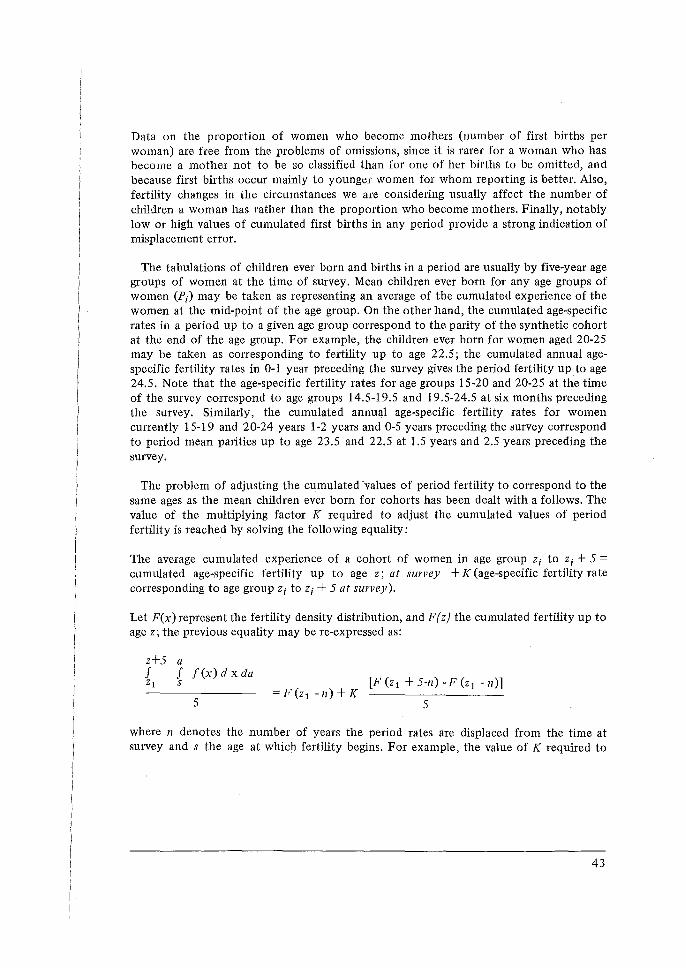
Data on the proportion of women who become mothers (number of first births per woman) are free from the problems of omissions, since it is rarer for a woman who has become a mother not to be so classified than for one of her births to be omitted, and because first births occur mainly to younger women for whom reporting is better. Also, fertility changes in the circumstances we are considering usually affect the number of children a woman has rather than the proportion who become mothers. Finally, notably low or high values of cumulated first births in any period provide a strong indication of misplacement error.

The tabulations of children ever born and births in a period are usually by five-year age groups of women at the time of survey. Mean children ever born for any age groups of women (Pi) may be taken as representing an average of the cumulated experience of the women at the mid-point of the age group. On the other hand, the cumulated age-specific rates in a period up to a given age group correspond to the parity of the synthetic cohort at the end of the age group. For example, the children ever born for women aged 20-25 may be taken as corresponding to fertility up to age 22.5; the cumulated annual age­specific fertility rates in 0-1 year preceding the survey gives the period fertility up to age 24.5. Note that the age-specific fertility rates for age groups 15-20 and 20-25 at the time of the survey correspond to age groups 14.5-19.5 and 19.5-24.5 at six months preceding the survey. Similarly, the cumulated annual age-specific fertility rates for women currently 15-19 and 20-24 years 1-2 years and 0-5 years preceding the survey correspond to period mean parities up to age 23.5 and 22.5 at 1.5 years and 2.5 years preceding the survey.

The problem of adjusting the cumulated -values of period fertility to correspond to the same ages as the mean children ever born for cohorts has been dealt with a follows. The value of the multiplying factor K required to adjust the cumulated values of period fertility is reached by solving the following equality:

The average cumulated experience of a cohort of women in age group zi to zi + 5 = cumulated age-specific fertility up to age z; at s11rJ1ey + K (age-specific fertility rate corresponding to age group zi to zi + 5 at s11rJ1ey ).

Let F(x) represent the fertility density distribution, and F(z) the cumulated fertility up to age z; the previous equality may be re-expressed as:

a f f (x) d x da s

5

[F(z 1 +5-n)-F(z1 -n)] =F(z1 -n) + K

5

where n denotes the number of years the period rates are displaced from the time at survey and s the age at which fertility begins. For example, the value of K required to

43

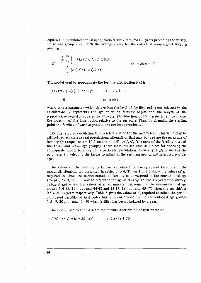
equate the cumulated annual age-specific fertility rate, for 0-1 years preceding the survey, up to age group 20-25 with the average parity for the cohort of women aged 20-25 is given as:

K

1 25 a f f (f (x) d x da - F (19.5)

5 20 s

4 [F(24.5)-F(l9.5)]

(z 1 = 20,n = .5)

The model used to approximate the fertility distribution f(x) is

f (x) = c (x-s) (s + 33 -x)2 s<x<s+33

=O otherwise

where c is a parameter which determines the level of fertility and is not relevant in the calculations, s represents the age at which fertility begins and the length of the reproductive period is equated to 33 years. The function of the parameters is to change the location of the distribution relative to the age scale. Thus, by changing the starting point the fertility of various populations can be approximated.

The first step in calculating K is to select a value for the parameter s. This value may be difficult to estimate in real populations, alternatives that may be used are the mean age of fertility (m) (equal to s + 13.2 on the model), or f 1 /f2 (the ratio of the fertility rates of the 15-19 and 20-24 age groups). These measures are used as indices for choosing the appropriate model to apply for a particular population. Generally, fi/12 is used as the parameter for selecting the factor to adjust in the early age groups and m is used at older ages.

The values of the multiplying factors, calculated for evenly spread locations of the model distribution, are presented i)1 tables 1 to 4. Tables 1 and 2 show the values of Ki required to adjust the period cumulated fertility to correspond to the conventional age groups (15-19, 20-, ... and 45-49) when the age shift is by 0.5 and 1.5 years respectively. Tables 3 and 4 give the values of Ki to make adjustments for the unconventional age groups (14-18, 19-, ... and 44-48 and 13-17, 18-, ... and 43-47) when the age shift is 0.5 and 1.5 years respectively. Table 5 gives the values of Ki required to adjust the period cumulated fertility of first order births to correspond to the conventional age groups (15-19, 20-, ... and 45-49) when fertility has been displaced by a year.

The model used to approximate the fertility distribution of first births is:

f (x) = (x-s) ~ (s + 20 - x)2 s<x<s+20

44

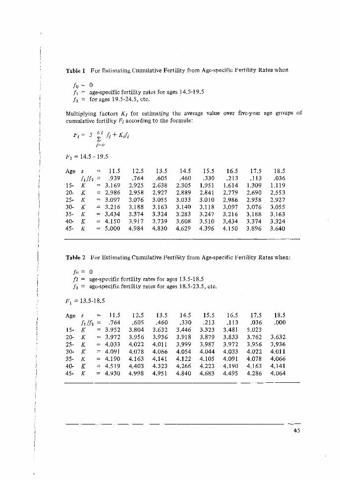
Table 1 For Estimating Cumulative Fertility from Age-specific Fertility Rates when

fo = 0 f 1 = age-specific fertility rates for ages 14.5-19.5 f 2 = for ages 19.5-24.5, etc.

Multiplying factors Ki for estimating the average value over five-year age groups of cumulative fertility Fi according to the formula:

F; = 5 ~1 f; + Kifi

j=o

F1 = 14.5 - 19.5

Age s 11.5 12.5 13.5 14.5 15.5 16.5 17.5 18.5 filfz = .939 .764 .605 .460 .330 .213 .113 .036

15- K 3.169 2.925 2.638 2.305 1.951 1.614 1.309 1.119 20- K 2.986 2.958 2.927 2.889 2.841 2.779 2.690 2.553 25- K 3.097 3.076 3.055 3.033 3.010 2.986 2.958 2.927 30- K 3.216 3.188 3.163 3.140 3.118 3.097 3.076 3.055 35- K 3.434 3.374 3.324 3.283 3.247 3.216 3.188 3.163 40- K 4.150 3.917 3.739 3.608 3.510 3.434 3.374 3.324 45- K 5.000 4.984 4.830 4.629 4.396 4.150 3.896 3.640

Table 2 For Estimating Cumulative Fertility from Age-specific Fertility Rates when:

fo = 0 fl= age-specific fertility rates for ages 13.5-18.5 !2 = age-specific fertility rates for ages 18.5-23.5, etc.

F 1 =13.5-18.5

Age s 11.5 12.5 13.5 14.5 15.5 16.5 17.5 18.5 !1 /!2 = .764 .605 .460 .330 .213 .113 .036 .000

15- K 3.952 3.804 3.632 3.446 3.323 3.481 5.023 20- K 3.972 3.956 3.936 3.918 3.879 3.833 3.762 3.632 25- K 4.033 4.022 4.011 3.999 3.987 3.972 3.956 3.936 30- K 4.091 4.078 4.066 4.054 4.044 4.033 4.022 4.011 35- K 4.190 4.163 4.141 4.122 4.105 4.091 4.078 4.066 40- K 4.519 4.403 4.323 4.266 4.223 4.190 4.163 4.141 45- K 4.930 4.998 4.951 4.840 4.683 4.495 4.286 4.064

45

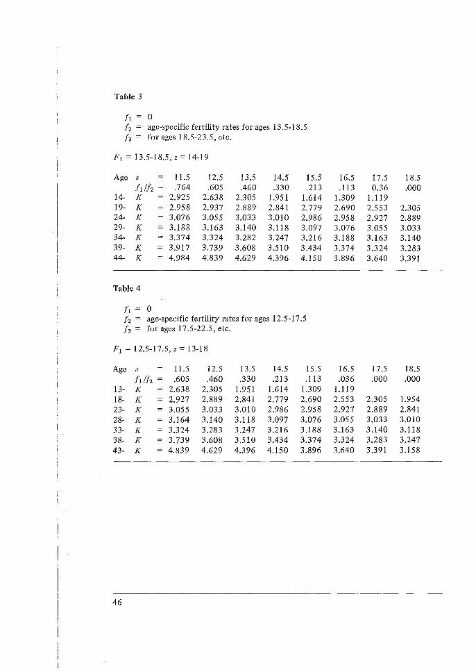
Table 3

!1 = 0 !2 = age-specific fertility rates for ages 13.5-18.5 f3 = for ages 18.5-23.5, etc.

F 1 = 13.5-18.5, z = 14-19

Age s 11.5 12.5 13.5 14.5 15.5 16.5 17.5 18.5 f1!l2 = .764 .605 .460 .330 .213 .113 0.36 .000

14- K 2.925 2.638 2.305 1.951 1.614 1.309 1.119 19- K 2.958 2.937 2.889 2.841 2.779 2.690 2.553 2.305 24- K 3.076 3.055 3.033 3.010 2.986 2.958 2.927 2.889 29- K 3.188 3.163 3.140 3.118 3.097 3.076 3.055 3.033 34- K 3.374 3.324 3.282 3.247 3.216 3.188 3.163 3.140 39- K 3.917 3.739 3.608 3.510 3.434 3.374 3.324 3.283 44- K 4.984 4.839 4.629 4.396 4.150 3.896 3.640 3.391

Table 4

!1 = 0 !2 = age-specific fertility rates for ages 12.5-17 .5 !J= for ages 17 .5-22.5, etc.

F 1 =12.5-17.5, z = 13-18

Age s 11.5 12.5 13.5 14.5 15.5 16.5 17.5 18.5 fili2 = .605 .460 .330 .213 .113 .036 .000 .000

13- K 2.638 2.305 1.951 1.614 1.309 1.119 18- K 2.927 2.889 2.841 2.779 2.690 2.553 2.305 1.954 23- K 3.055 3.033 3.010 2.986 2.958 2.927 2.889 2.841 28- K 3.164 3.140 3.118 3.097 3.076 3.055 3.033 3.010 33- K 3.324 3.283 3.247 3.216 3.188 3.163 3.140 3.118 38- K 3.739 3.608 3.510 3.434 3.374 3.324 3.283 3.247 43- K 4.839 4.629 4.396 4.150 3.896 3.640 3.391 3.158

46

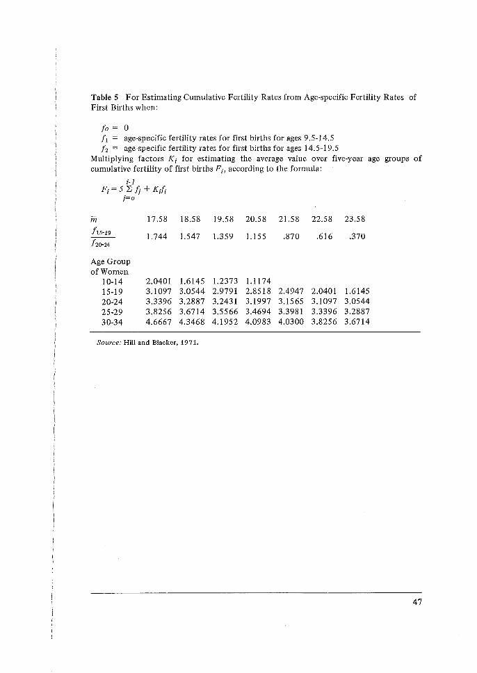
Table 5 For Estimating Cumulative Fertility Rates from Age-specific Fertility Rates of First Births when:

fo = 0 f 1 = age-specific fertility rates for first births for ages 9.5-14.5 f 2 = age-specific fertility rates for first births for ages 14.5-19.5

Multiplying factors K; for estimating the average value over five-year age groups of cumulative fertility of first births F;, according to the formula:

i-1 F; = 5 ~ fj + K;f;

j=o

m

f1s-19

fw-24

17.58 18.58 19.58 20.58 21.58 22.58 23.58

1.744 1.547 1.359 1.155 .870 .616 .370

Age Group of Women

10-14 15-19 20-24 25-29 30-34

2.0401 3.1097 3.3396 3.8256 4.6667

1.6145 3.0544 3.2887 3.6714 4.3468

Source: Hill and Blacker, 1971.

1.2373 2.9791 3.2431 3.5566 4.1952

1.1174 2.8518 2.4947 2.0401 1.6145 3.1997 3.1565 3.1097 3.0544 3.4694 3.3981 3.3396 3.2887 4.0983 4.0300 3.8256 3.6714

47

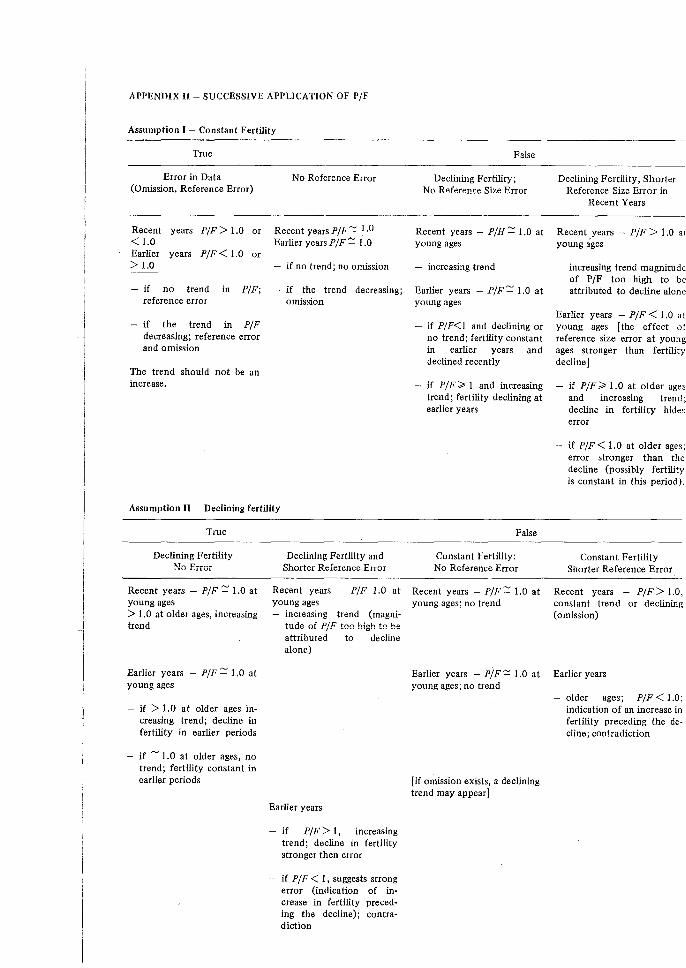
APPENDIX II - SUCCESSIVE APPLICATION OF P/F

Assumption I - Constant Fertility

True

Error in Data (Omission, Reference Error)

Recent years P/F> 1.0 or < 1.0 Earlier years P/F< 1.0 or > l.O

No Reference Error

Recent years P/F'::'. l .U Earlier years P/F ~ 1.0

if no trend; no omission

False

Declining Fertility; No Reference Size Error

Declining Fertility; Shorter Reference Size Error in

Recent Years

Recent years - P/H ~ 1.0 at Recent years - P/F > 1.0 el young ages young ages

- increasing trend

if no trend in P/F; reference error

if the trend decreasing; Earlier years - P/F '::::. 1.0 at

increasing trend magnitude of P /F too high to be attributed to decline alone

omission young ages

if the trend in P/ F decreasing; reference error and omission

The trend should not be an increase.

Assumption II - Declining fertility

True

Declining Fertility No Error

Recent years - P/F ~ 1.0 at young ages > 1.0 at older ages, increasing trend

Earlier years - P/F '::::. 1.0 at young ages

if > 1.0 at older ages in­creasing trend; decline in fertility in earlier periods

if '::::. 1.0 at older ages, no trend; fertility constant in earlier periods

Declining Fertility and Shorter Reference Error

Recent years - P/F 1.0 at young ages

increasing trend (magni­tude of P/ F too high to be attributed to decline alone)

Earlier years

if P/F> I, increasing trend; decline in fertility stronger then error

if P/ F < 1, suggests strong error (indication of in­crease in fertility preced­ing the decline); contra­diction

if P/F<l and declining or no trend; fertility constant in earlier years and declined recently

if P/F> 1 and increasing trend; fertility declining at earlier years

False

Constant Fertility: No Reference Error

Recent years - P/ F '::::. 1.0 at young ages; no trend

Earlier years - P/F < 1.0 at young ages [the effect o 1 reference size error at young ages stronger than fertility decline]

if P/F > 1.0 at older ages and increasing trend; decline in fertility hides error

if P/F < 1.0 at older ages; error stronger than the decline (possibly fertility is constant in this period).

Constant Fertility Shorter Reference Error

Recent years - P/F> 1.0, constant trend or declining (omission)

Earlier years - P/F'::'. 1.0 at Earlier years young ages; no trend

(if omission exists, a declining trend may appear J

older ages; P/F < 1.0; indication of an increase in fertility preceding the de­cline; contradiction

BIBLIOGRAPHY

Brass, W., The Analysis of Maternity Histories to Detect Changes in Fertility. United Nations. Department of Economic and Social Affairs (E/CN.9/AC.12/R.l 1). 1971.

Brass, W., Methods for Estimating Fertility and Mortality from Limited and Defective Data. Laboratories for Population Statistics (POPLABS), Chapel Hill, North Carolina, United States. 197 5.

Brass, W., 'A Note or the Choice of Fertility Measures from Maternity History Data'. Paper Prepared for World Fertility Survey Working Party on Report No. 2. 1976.

Brass, W., 'The Assessment of the Validity of Fertility Trend Estimates from Maternity Histories'. Proceedings of the International Population Conference, Mexico. IUSSP. 1977.

Coale, A.J. and P. Demeny, Regional Model Life Tables and Stable Populations. Princeton, New Jersey, Princeton University Press. 1966.

Coale, A.J. and J. Trussell, 'Model Fertility Schedules: Variations in the Structure of Childbearing in Human Populations', Population Index. 1974.

Coale, A.J., A. Hill and J. Trussell, 'A New Method Estimating Standard Fertility Measures from Incomplete Data', Population Index. 1975.

Hill, K.H. and J.G.C. Blacker, 'Some Problems of African Demographic Analysis', Report on Discussions Held in London in 1971 with W. Brass at the London School of Hygiene and Tropical Medicine. Unpublished.

Murphy, E.M. and D.N. Nagnur, 'A Gompertz Fit that Fits: Application to Canadian Fertility Patterns', Demography, vol. 9. 1972.

Potter, J.E., 'The Validity of Measuring Change in Fertility by Analysing Birth Histories Obtained in Surveys', Ph.D. thesis. University Microfilms, Ann Arbor. 1975

Potter, J.E., 'Methods of Detecting Errors in WFS Data: An Application to the Fiji Fertility Survey', Proceedings of the International Population Conference, Mexico. IUSSP. 1977.

Romaniuk, A., 'A Three-parameter Model for Birth Projections, Population Studies, 27, No. 3. 1973.

Som, Ranjan Kumar, 'Recall Lapse in Demographic Enquiries. Asia Publishing House, Bon1bay. 1973.

United Nations. Methods of Estimating Basic Demographic Measures for Incomplete Data, Manual IV (Population Studies No. 42). 1967.

49

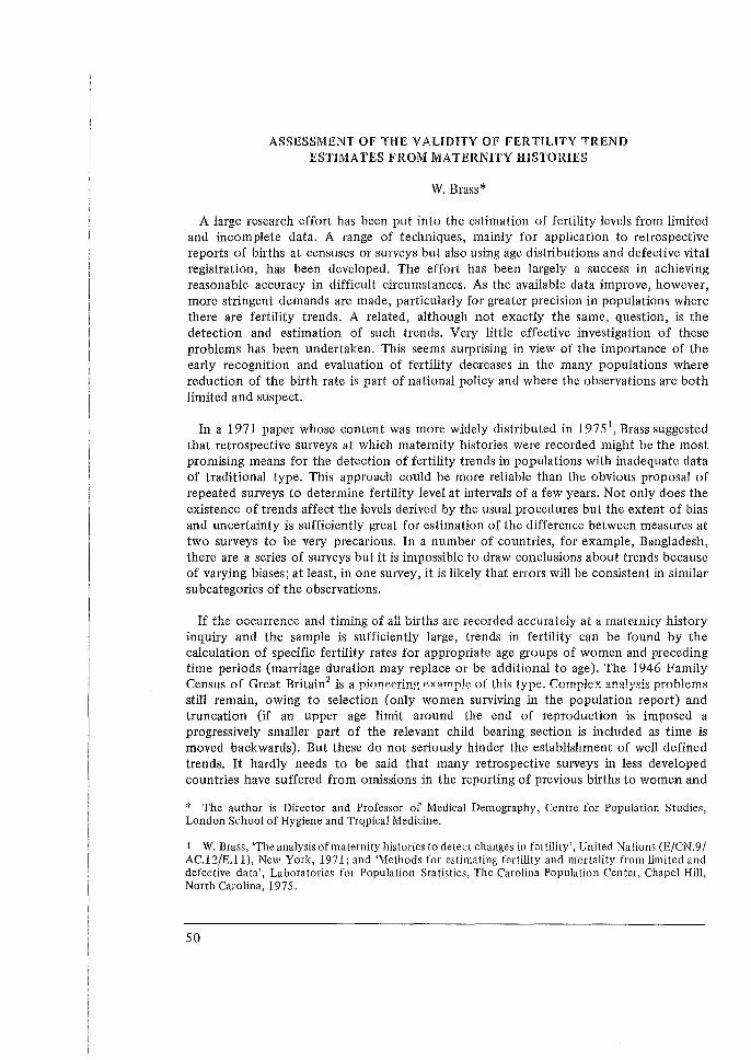
ASSESSMENT OF THE VALIDITY OF FERTILITY TREND ESTIMATES FROM MATERNITY HISTORIES

W. Brass*

A large research effort has been put into the estimation of fertility levels from limited and incomplete data. A range of techniques, mainly for application to retrospective reports of births at censuses or surveys but also using age distributions and defective vital registration, has been developed. The effort has been largely a success in achieving reasonable accuracy in difficult circumstances. As the available data improve, however, more stringent demands are made, particularly for greater precision in populations where there are fertility trends. A related, although not exactly the same, question, is the detection and estimation of such trends. Very little effective investigation of these problems has been undertaken. This seems surprising in view of the importance of the early recognition and evaluation of fertility decreases in the many populations where reduction of the birth rate is part of national policy and where the observations are both limited and suspect.

In a 1971 paper whose content was more widely distributed in 197 51, Brass suggested that retrospective surveys at which maternity histories were recorded might be the most promising means for the detection of fertility trends in populations with inadequate data of traditional type. This approach could be more reliable than the obvious proposal of repeated surveys to determine fertility level at intervals of a few years. Not only does the existence of trends affect the levels derived by the usual procedures but the extent of bias and uncertainty is sufficiently great for estimation of the difference between measures at two surveys to be very precarious. In a number of countries, for example, Bangladesh, there are a series of surveys but it is impossible to draw conclusions about trends because of varying biases; at least, in one survey, it is likely that errors will be consistent in similar subcategories of the observations.

If the occurrence and timing of all births are recorded accurately at a maternity history inquiry and the sample is sufficiently large, trends in fertility can be found by the calculation of specific fertility rates for appropriate age groups of women and preceding time periods (marriage duration may replace or be additional to age). The 1946 Family Census of Great Rritain2 is a pioneering example of this type. Complex analysis problems still remain, owing to selection (only women surviving in the population report) and truncation (if an upper age limit around the end of reproduction is imposed a progressively smaller part of the relevant child bearing section is included as time is moved backwards). But these do not seriously hinder the establishment of well defined trends. It hardly needs to be said that many retrospective surveys in less developed countries have suffered from omissions in the reporting of previous births to women and

* The author is Director and Professor of Medical Demography, Centre for Population Studies, London School of Hygiene and Trqpical Medicine.

1 W. Brass, 'The analysis of maternity histories to detect changes in fertility', United Nations (E/CN .9 / AC.12/E.1 l), New York, 1971; and 'Methods for estimating fertility and mortality from limited and defective data', Laboratories for Population Statistics, The Carolina Population Center, Chapel Hill, North Carolina, 1975.

50

errors in the timing of even the last birth which are so large that the estimate of fertility level is highly doubtful. In other cases the total births may be reasonably counted but the times of occurrence suspect. Many examples could be listed.

The programme of the World Fertility Survey will provide a body of national maternity history inquiries; the estimation of fertility trends from these is one of the main aims, and other objectives would be hard to meet without good success in the former. No doubt the accuracy of the data will cover a wide spectrum since many of the populations included have the characteristics of low educational experience and lack of date awareness which have been significant in past studies. Methods for assessing the importance of birth omissions exist but the evaluation of timing-error distortion of trends needs more research. It can be argued that the most effective way of validating the observations is to carry out the full, detailed analysis which would be appropriate for highly accurate data. Biases will then become apparent from discrepancies, anomalies and implausibilities in the resulting set of estimates. This argument has substance and the approach may be the only suitable one in surveys where the accuracy is reasonably good for the main elements and the bulk of the respondents; even then distortion in trends is possible. This strategy, by itself, implies a long and laborious investigation, nor does it necessarily give guidance on adjustment methods. There is a case for the development of direct screening procedures.

In the presentation cited, Brass (197 5) distinguished two types of birthtiming error. One is reference-period size and the other reference period slippage. In the first, births are allocated on average to a shorter or longer interval than that in which they actually took place but the bias is the same for all age groups of women, e.g. the reports for the period 5-10 years previously might properly relate to 5 .3 to 9 .6 years. The second allows for a translation in which births are pushed further into the past (or brought forward) in a fairly systematic way a women become older. A method was devised by which these errors could be corrected by relation to first births, on certain assumptions. The procedure was rather cumbersome but later has been improved and simplified. Meanwhile Potter3 in his doctorate research at Princeton had put forward the view timing enors in the location of births were more complicated than specified above. In particular, he produced a model which incorporated particular types of slippage operating in different directions at the two ends of the memory range (from the present to the first birth). This might be called a birth concentration or reference-period dispersion enor. Potter has presented strong evidence that a pattern of this kind was operating in maternity history surveys of Bangladesh and El Salvador. Among its consequences are a critical bias in the estimation of fertility trends. The 'first birth' procedure of Brass would not be effective for detecting and adjusting biases of this type. On the other hand there are indications that reference-period dispersion error is not the only way in which memory biases can occur; there may be reference-period concentration or even less structured effects.

An approach to the problem of screening maternity history data for enors in the timing of births, using the minimum of assumptions, will be described and illustrated. The

2 D.V. Glass and E. Grebenik, The Trend and Pattem of Fertility in Great Britain: A Report on the Family Census of 1946, Papers of the Royal Commission on Population, vol. VI (London, Her Majesty's Stationery Office, 1954).

3 J.E. Potter, The Validity of Measuring Change in Fertility by Analysing Birth Histories Obtained in Surveys (University Microfilms, Ann Arbor, 1975).

51

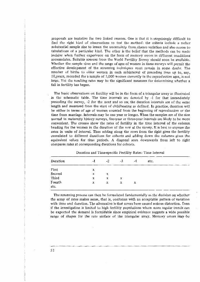
proposals are tentative for two linked reasons. One is that it is surprisingly difficult to find the right kind of observations to test the method: the criteria include a rather substantial sample size to lessen the uncertainty from chance variation and also access to tabulations of a particular kind. The other is the belief that the methods can be made incisive when further experience on the form of memory errors in different conditions accumulates. Suitable sources from the World Fertility Survey should soon be available. Whether the sample sizes and the range of ages of women in these surveys will permit the effective development of the screening techniques must remain in some doubt. The number of births to older women in each subinterval of preceding time up to, say, 10,years, recorded for a sample of 5,000 women currently in the reproductive ages, is not large. Yet the resulting rates may be the significant measures for determining whether a fall in fertility has begun.

The basic observations on fertility will be in the form of a triangular array as illustrated in the schematic table. The time intervals are denoted by -1 for that immediately preceding the survey, -2 for the next and so on; the duration intervals are of the same length and measured from the start of childbearing as defined. In practice, duration will be either in terms of age of women counted from the beginning of reproduction or the time from marriage. Intervals may be one year or longer. When the samples are of the size normal in maternity history surveys, five-year or three-year intervals are likely to be more convenient. The crosses show the rates of fertility in the time interval of the column heading for the women in the duration of the row at the survey. It is best to express the rates in units of interval. Thus adding along the rows from the right gives the fertility cumulated to different durations for cohorts and adding down the columns gives the equivalent values for time periods. A diagonal scan downwards from left to right compares rates at corresponding durations for cohorts.

Duration and Time-specific Fertility Rates: Time Interval

Duration -1 -2 -3 -4 etc.

First x Second x x Third x x x Fourth x v x x etc.

The screening process can then be formulated fundamentally as the decision on whether the array of rates makes sense, that is, conforms with an acceptable pattern of variation with time and duration. The alternative is that errors have caused serious distortion. Even if the investigation is limited to high fertility populations where more regular trends can be expected the demand is formidable since empirical evidence suggests a wide possible range of shapes for the rate surface of the triangular array. Memory errors lnay-be

52

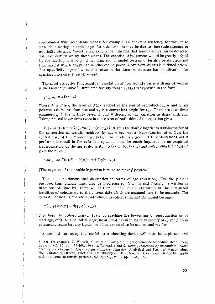
i I

confounded with acceptable trends; for example, an apparent tendency for women to start childbearing at earlier ages for older cohorts may be due to time-scale slippage or nuptiality changes. Nevertheless, experience indicates that serious errors can be detected with fair confidence by these means. The exercise of judgement would be greatly helped by the development of good two-dimensional model systems of fertility by duration and time against which arrays can be checked. A partial move towards this is outlined below. For specificity, age of woman is taken as the duration measure but modification for marriage interval is straightforward.

The most attractive functional representation of how fertility varies with age of woman is the Gompertz curve. 4 Cumulated fertility to age x, F(x) is expressed in the form

F (x)/F = AB(x-xo)

Where F is F(W), the level of F(x) reached at the end of reproduction, A and B are positive values less than one and x 0 is a convenient origin for age. There are thus three parameters, F for fertility level, A and B describing the variation in shape with age. Taking natural logarithms twice in succession of both sides of the equation gives

Qn[ - QnF(x)/F] = Qn( - .QnA) + (x - x 0 ) QnB.Thus the double logarithm transformation of the proportion of fertility achieved by age x becomes a linear function of x. Over the central part of the reproductive period the model is a good fit to observations but it performs less well in the tails. The agreement can be much improved by an empirical transformation of the age scale. Writing¢ (x-x 0 ) for (x-x 0 ) and simplifying the notation gives the model,

- Qn [ - Qn F(x)/F] = Y(x) =a+~ </J(x - x 0 )

[The negative of the double logarithm is taken to make~ positive.]

This is a one-dimensional description in terms of age (duration). For the present purpose, time change must also be incorporated. Y(x), a and ~ could be written as functions of time but there would then be inadequate utilization of the cumulated fertilities of cohorts up to the current date which are assumed here to be accurate. The extra dilnension, is, therefore, introduced in cohort form and the model becomes

Y(x, T) = a(T) + ~(T) </J(x - x 0 )

T is here the cohort marker (date of reaching the lowest age of reproduction or of marriage, etc). At this initial stage, no attempt has been made to specify a(T) and ~(T) in parametric terms but any trends would be expected to be modest and regular.

A method for using the model as a checking device will now be explained and

4 See, for example, G. Wunsch, 'Courbes de Gompertz et perspectives de fecondite', Rech, Econ, Louvain, vol. 32, pp. 457468, 1966; A. Romaniuk and S. Tawny, Projection of Incomplete Cohort Fertility for Canada by Means of the Gompertz Function, Analytical and Technical Memorandum No. 1, Statistics, Ottawa, 1969; and E.M. Murphy and D.N. Nagnur, 'A Gompertz fit that fits: appli­cation to Canadian fertility patterns', Demography, vol. 9, pp. 35-50, 1972.

53

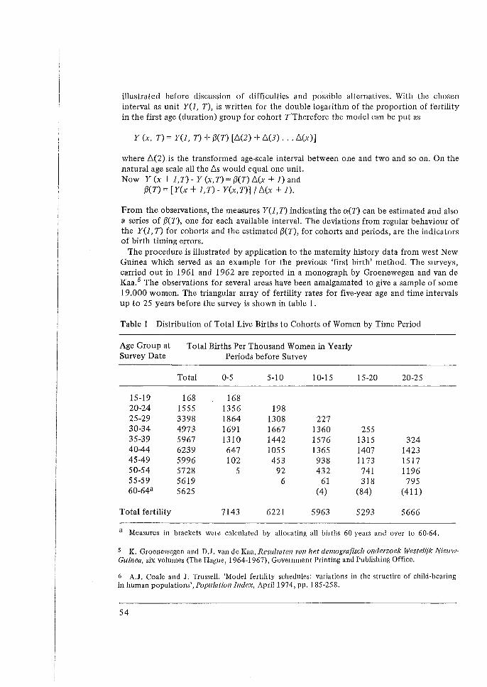
illustrated before discussion of difficulties and possible alternatives. With the chosen interval as unit Y(l, T), is written for the double logarithm of the proportion of fertility in the first age (duration) group for cohort T'Therefore the model can be put as

Y (x, T) = Y(l, T) + {3(T) [6(2) + 6(3) . .. 6(x)]

where 6(2) is the transformed age-scale interval between one and two and so on. On the natural age scale all the 6s would equal one unit. Now Y (x + l,T)- Y (x,T) = {3(T) 6(x + 1) and

{3(T) = [ Y(x + 1, T) - Y(x, T)] / 6(x + 1).

From the observations, the measures Y(l,T) indicating the cx(T) can be estimated and also a series of {3(T), one. for each available interval. The deviations from regular behaviour of the Y{l, T) for cohorts and the estimated {3(T), for cohorts and periods, are the indicators of birth timing errors.

The procedure is illustrated by application to the maternity history data from west New Guinea which served as an example for the previous 'first birth' method. The surveys, carried out in 1961 and 1962 are reported in a monograph by Groenewegen and van de Kaa. 5 The observations for several areas have been amalgamated to give a sample of some 19.000 women. The triangular array of fertility rates for five-year age and time intervals up to 25 years before the survey is shown in table 1.

Table 1 Distribution of Total Live Births to Cohorts of Women by Time Period

Age Group at Total Births Per Thousand Women in Yearly Survey Date Periods before Survey

Total 0-5 5-10 10-15 15-20 20-25

15-19 168 168 20-24 1555 1356 198 25-29 3398 1864 1308 227 30-34 4973 1691 1667 1360 255 35-39 5967 1310 1442 1576 1315 324 40-44 6239 647 1055 1365 1407 1423 45-49 5996 102 453 938 1173 1517 50-54 5728 5 92 432 741 1196 55-59 5619 6 61 318 795 60-64a 5625 (4) (84) (411)

Total fertility 7143 6221 5963 5293 5666

a Measures in brackets were calculated by allocating all births 60 years and over to 60-64.

s K. Groenewegen and D.J. van de Kaa, Resultaten van het demografisch onderzoek Westelijk Nieuw­Guinea, six volumes (The Hague, 1964-1967), Government Printing and Publishing Office.

6 A.J. Coale and J. Trussell, 'Model fertility schedules: variations in the structire of child-bearing in human populations', Population Index, April 1974, pp. 185-258.

54

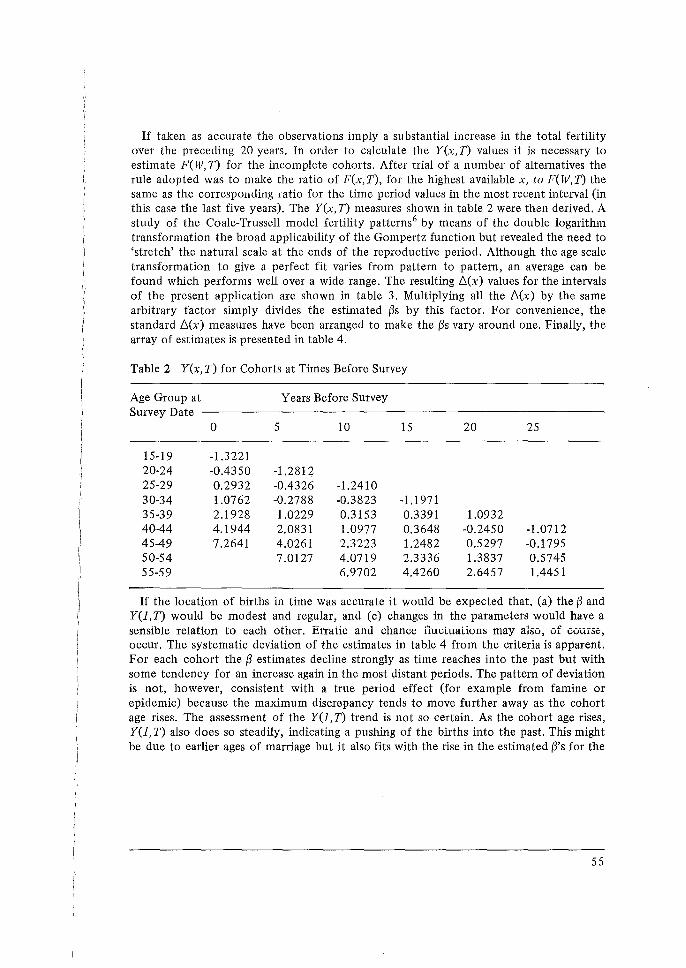
If taken as accurate the observations imply a substantial increase in the total fertility over the preceding 20 years. In order to calculate the Y(x, T) values it is necessary to estimate F(W, T) for the incomplete cohorts. After trial of a number of alternatives the rule adopted was to make the ratio of F(x, T), for the highest available x, to F(W,T) the same as the corresponding ratio for the time period values in the most recent interval (in this case the last five years). The Y(x, T) measures shown in table 2 were then derived. A study of the Coale-Trussell model fertility patterns6 by means of the double logarithm transformation the broad applicability of the Gompertz function but revealed the need to 'stretch' the natural scale at the ends of the reproductive period. Although the age scale transformation to give a perfect fit varies from pattern to pattern, an average can be found which performs well over a wide range. The resulting L(x) values for the intervals of the present application are shown in table 3. Multiplying all the L(x) by the same arbitrary factor simply divides the estimated ~s by this factor. For convenience, the standard L(x) measures have been arranged to make the ~s vary around one. Finally, the array of estimates is presented in table 4.

Table 2 Y(x, T) for Cohorts at Times Before Survey

Age Group at Years Before Survey Survey Date

0 5 10 15 20 2S

lS-19 -1.3221 20-24 -0.43SO -1.2812 2S-29 0.2932 -0.4326 -1.2410 30-34 1.0762 -0.2788 -0.3823 -1.1971 3S-39 2.1928 1.0229 0.31S3 0.3391 1.0932 40-44 4.1944 2.0831 1.0977 0.3648 -0.24SO -1.0712 4S-49 7.2641 4.0261 2.3223 1.2482 0.S297 -0.179S SO-S4 7.0127 4.0719 2.3336 1.3837 0.S74S SS-S9 6.9702 4.4260 2.64S7 l.44S 1

If the location of births in time was accurate it would be expected that, (a) the~ and Y(l,T) would be modest and regular, and (c) changes in the parameters would have a sensible relation to each other. Erratic and chance fiuctualiun~ may also, of course, occur. The systematic deviation of the estimates in table 4 from the criteria is apparent. For each cohort the ~ estimates decline strongly as time reaches into the past but with some tendency for an increase again in the most <,listant periods. The pattern of deviation is not, however, consistent with a true period effect (for example from famine or epidemic) because the maximum discrepancy tends to move further away as the cohort age rises. The assessment of the Y(l, T) trend is not so certain. As the cohort age rises, Y(l, T) also does so steadily, indicating a pushing of the births into the past. This might be due to earlier ages of marriage but it also fits with the rise in the estimated Ws for the

SS

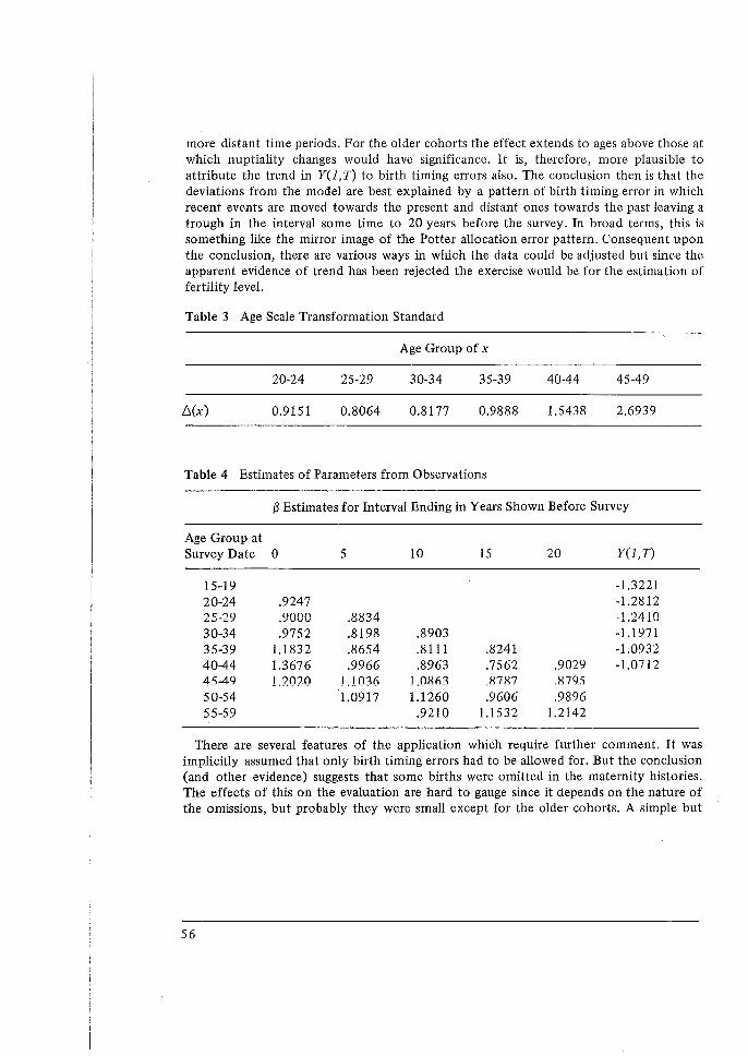
more distant time periods. For the older cohorts the effect extends to ages above those at which nuptiality changes would have significance. It is, therefore, more plausible to attribute the trend in Y(l, T) to birth timing errors also. The conclusion then is that the deviations from the model are best explained by a pattern of birth timing error in which recent events are moved towards the present and distant ones towards the past leaving a trough in the interval some time to 20 years before the survey. In broad terms, this is something like the mirror image of the Potter allocation en-or pattern. Consequent upon the conclusion, there are various ways in which the data could be adjusted but since the apparent evidence of trend has been rejected the exercise would be for the estimation of fertility level.

Table 3 Age Scale Transformation Standard

Age Group of x

20-24 25-29 30-34 35-39 40-44 45-49

L(x) 0.9151 0.8064 0.8177 0.9888 1.5438 2.6939

Table 4 Estimates of Parameters from Observations

~ Estimates for Interval Ending in Years Shown Before Survey

Age Group at Survey Date 0 5 10 15 20 Y(l,T)

15-19 -1.3221 20-24 .9247 -1.2812 25-29 .9000 .8834 -1.2410 30-34 .9752 .8198 .8903 -1.1971 35-39 1.1832 .8654 .8111 .8241 -1.0932 40-44 1.3676 .9966 .8963 .7562 .9029 -1.0712 45-49 l,2020 Ll036 L0863 ,8787 ,8795 50-54 1.0917 1.1260 .9606 .9896 55-59 .9210 1.1532 1.2142

There are several features of the application which require further comment. It was implicitly assumed that only birth timing errors had to be allowed for. But the conclusion (and other evidence) suggests that some births were omitted in the maternity histories. The effects of this on the evaluation are hard to gauge since it depends on the nature of the omissions, but probably they were small except for the older cohorts. A simple but

56

potentially biased method was adopted for the estimation of the F(W,T), the total fertilities of the cohorts. If there are birth timing distortions, varying with cohorts, the proportion of fertility beyond a given age for the last time interval will clearly be affected. The forecast will then rest on an insecure base. However, the influence of this on the technique of screening seems to be small. If a further stage of adjustment in which the ~(T) and cx(T) were estimated was introduced, the F(W,T) measures would have to be recalculated in accord with the assumptions on which the fitting of the model was based.

The age scale transformation was derived from an 'average' Coale-Trussell fertility model pattern. An alternative would be to use an internal standard derived from the fertility distribution of the last time period. However, the liability of the latter to be distorted by both age errors and differentials in the time allocation of births by cohorts makes it less attractive. It is worth noting, however, that the use of this internal standard for the New Guinea surveys leads to a similar structure of deviation from the model and, therefore, the same conclusions. Perhaps better results could be achieved by the selection of a Coale-Trussell fertility pattern as a standard, taking into account some characteristics of the observations. This possibility is being investigated.

57

THE RELATIONAL GOMPERTZ MODEL OF FERTILITY BY AGE OF WOMAN

W. Brasst

A THEMODEL

The Gompertz model was used to represent age-specific fertility rates by Wunsch and Martin in the 1960s. Later, the Canadian Bureau of Statistics explored its characteristics. Murphy and Negnur and Fared applied it to cohort data in the context of forecasting. It is a model with powerful advantages although some limitations. Its potential for indirect estimation from defective and restricted data has not been adequately exploited.

The advantages are that the function describes the age patterns of fertility quite well by the use of three parameters (one less than the Coale-Trussell models) and that a simple transformations leads to a linear relation of fertility with age. The parameters in the linear relation have simple properties. The model is most easily expressed as Y(x) = -Qn(-Qn[F(x)/F]) = l\' + ~x where F(x) and Fare the cumulated age-specific fertility rates to age x and the end of childbearing respectively and a, ~ the two parameters which fix a particular pattern of the system. Cl'. is a location and ~ a dispersal parameter. Thus, Cl'.+ ~(x-x0 ) = (a - ~x0 ) + ~x = al\'* + ~x. Changing Cl'. is then equivalent to changing the age from which x is measured, i.e. sliding the distribution along the age axis l\' + ~x = l\' + (~/k )(kx) = l\' + ~ Y when Y = kx. Changing the value of ~ is then equivalent to multiplying the scale by a constant, i.e. altering the spread of the distribution while keeping its shape the same.

The linear property of the transform makes interpolating, graduation and fitting very simple and elementary. These operations are the ones frequently needed in the analysis of poor, incomplete and unorthodox data. Even if linearity on the transformed scale is far from perfect (see below), applications in which interpolation is between successive five-yearly points, or fitting is required only over the central part of the age range can be made easily and effectively.

The major criticism of the Gompertz model is that the fit to observations at the tails of the distribution is much poorer than that over the central range. For some purposes this does not matter, but for others it is of critical importance, e.g. the extrapolation of values of F(X), for ages below the end of childbearing, to subsequent ages. A further difficulty is that if Fis not known -Qn (-.Qn) linearity transformation cannot be carried out directly, but there are devices for handling this and the problem is not fundamental.

The accuracy of the Gompertz model at the tails of the distribution can be much improved by using the relational device which has proved powerful in the logit system of

t The author is Director and Professor of Medical Demography, Centre for Population Studies, London School of Hygiene and Tropical Medicine.

58

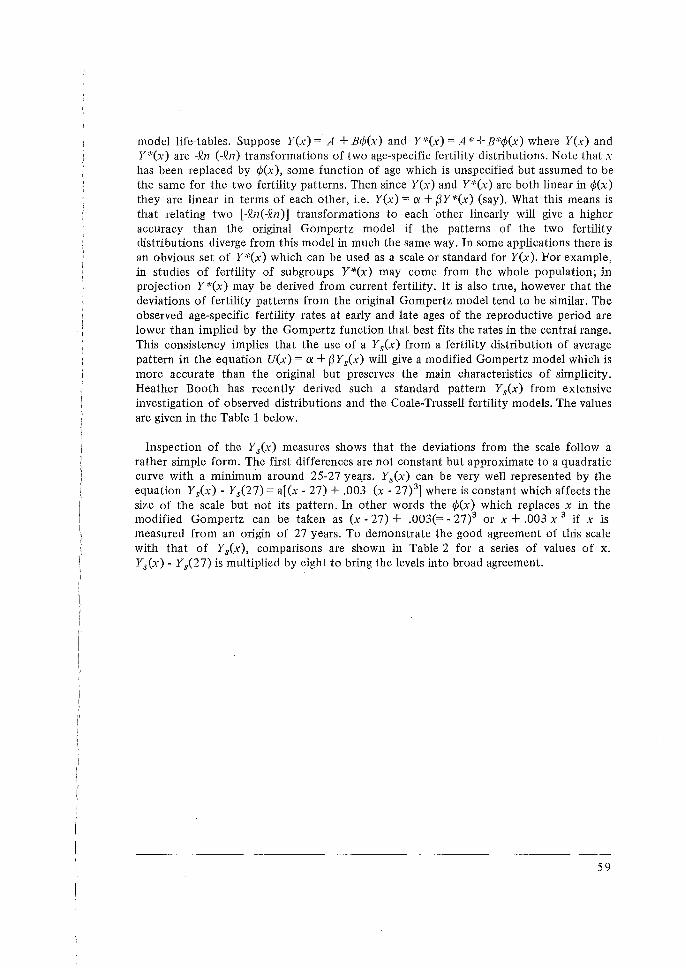
model life-tables. Suppose Y(x) = A + Brp(x) and Y *(x) =A*+ B*rp(x) where Y(x) and Y *(x) are -Qn (-Qn) transformations of two age-specific fertility distributions. Note that x has been replaced by rp(x ), some function of age which is unspecified but assumed to be the same for the two fertility patterns. Then since Y(x) and Y*(x) are both linear in rp(x) they are linear in terms of each other, i.e. Y(x) = O' + {3Y*(x) (say). What this means is that relating two [-Qn(-Qn)] transformations to each other linearly will give a higher accuracy than the original Gompertz model if the patterns of the two fertility distributions diverge from this model in much the same way. In some applications there is an obvious set of Y*(x) which can be used as a scale or standard for Y(x). For example, in studies of fertility of subgroups Y*(x) may come from the whole population; in projection Y*(x) may be derived from current fertility. It is also true, however that the deviations of fertility patterns from the original Gompertz model tend to be similar. The observed age-specific fertility rates at early and late ages of the reproductive period are lower than implied by the Gompertz function that best fits the rates in the central range. This consistency implies that the use of a Ys(x) from a fertility distribution of average pattern in the equation U(x) = O' + f3Ys(x) will give a modified Gompertz model which is more accurate than the original but preserves the main characteristics of simplicity. Heather Booth has recently derived such a standard pattern Ys(x) from extensive investigation of observed distributions and the Coale-Trussell fertility models. The values are given in the Table 1 below.

Inspection of the Ys(x) measures shows that the deviations from the scale follow a rather simple form. The first differences are not constant but approximate to a quadratic curve with a minimum around 25-27 yeass. Ys(x) can be very well represented by the equation Ys(x) - Ys(27) = a[(x - 27) + .003 (x - 27)3

] where is constant which affects the size of the scale but not its pattern. In other words the ¢(x) which replaces x in the modified Gompertz can be taken as (x - 27) + .003(= - 27)3 or x + .003 x 3 if x is measured from an origin of 27 years. To demonstrate the good agreement of this scale with that of Ys(x), comparisons are shown in Table 2 for a series of values of x. Y8 (x) - Ys(27) is multiplied by eight to bring the levels into broad agreement.

59

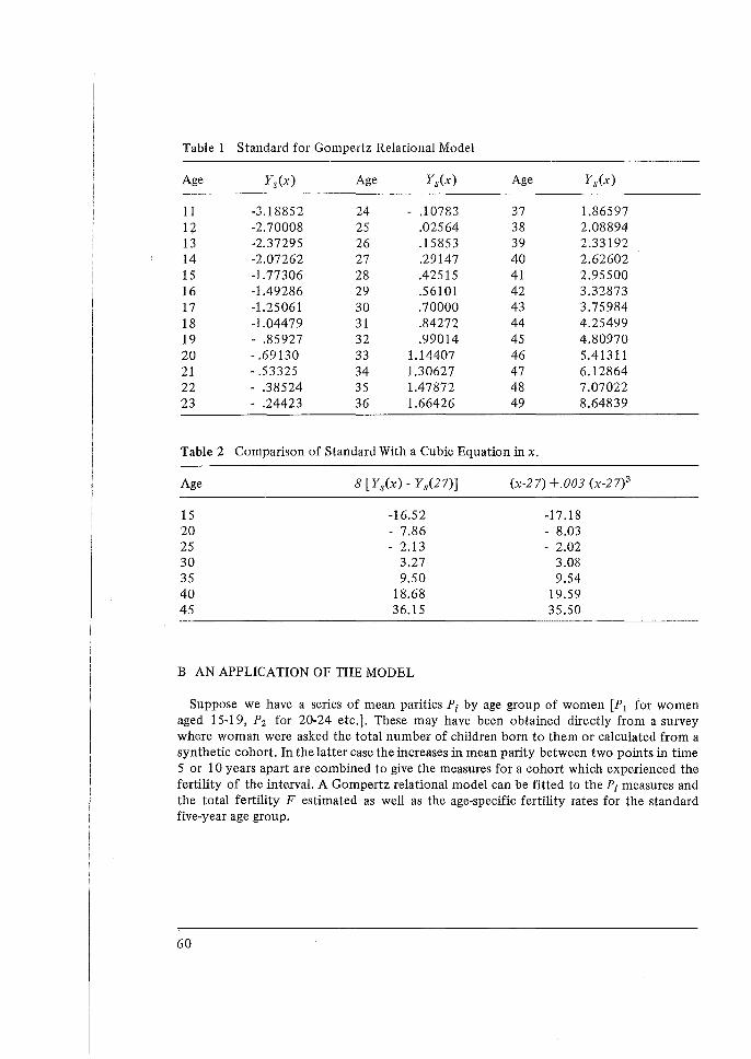
Table 1 Standard for Gompertz Relational Model

Age Y8(x) Age Y8(x) Age Y8 (x)

11 -3.18852 24 - .10783 37 1.86597 1+ -2.70008 25 .02564 38 2.08894 13 -2.37295 26 .15853 39 2.33192 14 -2.07262 27 .29147 40 2.62602 15 -1.77306 28 .42515 41 2.95500 16 -1.49286 29 .56101 42 3.32873 17 -1.25061 30 .70000 43 3.75984 18 -1.04479 31 .84272 44 4.25499 19 - .85927 32 .99014 45 4.80970 20 - .69130 33 1.14407 46 5.41311 21 -.53325 34 1.30627 47 6.12864 22 - .38524 35 1.47872 48 7.07022 23 - .24423 36 1.66426 49 8.64839

Table 2 Comparison of Standard With a Cubic Equation in x.

Age 8 [Ys(x) - Ys(27)] (x-27) +.003 (x-27)3

15 -16.52 -17.18 20 - 7.86 - 8.03 25 - 2.13 - 2.02 30 3.27 3.08 35 9.50 9.54 40 18.68 19.59 45 36.15 35.50

B AN APPLICATION OF THE MODEL

Suppose we have a series of mean parities P; by age group of women [P1 for women aged 15-19, P2 for 20-24 etc.]. These may have been obtained directly from a survey where woman were asked the total number of children born to them or calculated from a synthetic cohort. In the latter case the increases in mean parity between two points in time 5 or 10 years apart are combined to give the measures for a cohort which experienced the fertility of the interval. A Gompertz relational model can be fitted to the P; measures and the total fertility F estimated as well as the age-specific fertility rates for the standard five-year age group.

60

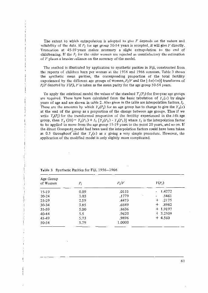
The extent to which extrapolation is adopted to give F depends on the nature and reliability of the data. If Pi for age group 50-5 4 years is accepted, it will give F directly. Truncation at 45-59 years makes necessary a slight extrapolation to the end of childbearing. If the P; for the older women are rejected as unsatisfactory the estimation of F places a heayier reliance on the accuracy of the model.

The method is illustrated by application to synthetic parities in Fiji, constructed from the reports of children born per woman at the 1956 and 1966 censuses, Table 3 shows the synthetic mean parities, the corresponding proportion of the total fertility experienced by the different age groups ofwomen,Pi/F and the [-ln(-ln)] transforms of P;/F denoted by Y(P;), Fis taken as the mean parity for the age group 50-54 years.

To apply the relational model the values of the standard Ys(P;) for five-year age groups are required. These have been calculated from the basic tabulation of Ys(x) by single years of age and are shown in table 2. Also given in the table are interpolation factors, h These are the amounts by which Ys(P;) for an age group has to change to give the Ys(x) at the end of the group as a proportion of the change between age groups. Thus if we

. write Ys(P;) for the transformed proportion of the fertility experienced in the i-th age group, then Ys (20) = Ys(P 1 ) + 11 [Ys(P2 ) - Ys(P1 )] where 11 is the interpolation factor to be applied to move from the age group 15-19 years to the point 20 years, and so on. If the direct Gompertz model had been used the interpolation factors could have been taken as 0.5 throughouf;md the Ys(x) as x giving a very simple procedure. However, the application of the modified model is only slightly more complicated.

Table 3 Synthetic Parities for Fiji, 1956-1966

Age Group of Women

15-19 20-24 25-29 30-34 35-39 40-44 45-49 50-54

0.09 1.03 2.59 3.85 5.00 5.5 5.73 5.79

.0155

.1779

.4473

.6649

.8636

.9620

.9896 1.0000

1.4272 .5461

+ .2175 + .8962 + 1.9197 + 3.2509 + 4.560

61

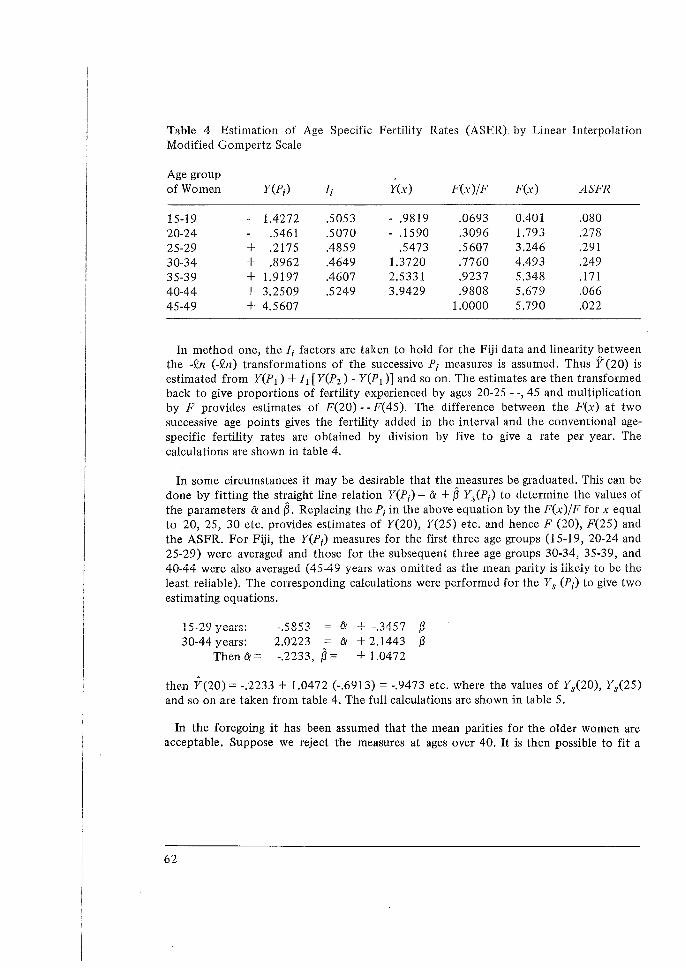
Table 4 Estimation of Age Specific Fertility Rates (ASFR) by Linear Interpolation Modified Gompertz Scale

Age group of Women Y(Pi) Ii Y(x) F(x)/F F(x) ASFR

15-19 1.4272 .5053 - .9819 .0693 0.401 .080 20-24 .5461 .5070 - .1590 .3096 l.793 .278 25-29 + .2175 .4859 .5473 .5607 3.246 .291 30-34 + .8962 .4649 1.3720 .7760 4.493 .249 35-39 + 1.9197 .4607 2.5331 .9237 5.348 .171 40-44 + 3.2509 .5249 3.9429 .9808 5.679 .066 45-49 + 4.5607 1.0000 5.790 .022

In method one, the I; factors are taken to hold for the Fiji data and linearity between the -Qn (-Qn) transformations of the successive P; measures is assumed. Thus Y(20) is estimated from Y(P1 ) + 11 [Y(P2 ) - Y(P 1 )] and so on. The estimates are then transformed back to give proportions of fertility experienced by ages 20-25 - -, 45 and multiplication by F provides estimates of F(20) - - F( 45). The difference between the F(x) at two successive age points gives the fertility added in the interval and the conventional age­specific fertility rates are obtained by division by five to give a rate per year. The calculations are shown in table 4.

In some circumstances it may be desirable that the measures be graduated. This can be done by fitting the straight line relation Y(P;) =a + S Ys(P;) to determine the values of the parameters a and S. Replacing the P; in the above equation by the F(x)/F for x equal to 20, 25, 30 etc. provides estimates of Y(20), Y(25) etc. and hence F (20), F(25) and the ASFR. For Fiji, the Y(P;) measures for the first three age groups (15-19, 20-24 and 25-29) were averaged and those for the subsequent three age groups 30-34, 35-39, and 40-44 were also averaged ( 45-49 years was omitted as the mean parity is likely to be the least reliable). The corresponding calculations were performed for the Ys (P;) to give two estimating equations.

1 <'. '10 n~n~n• =.5853 fr + -.3457 a .1..J-L.J./ ~vcu .. 0. I"

30-44 years: 2.0223 a + 2.1443 ~ Then a= -.2233, S= + 1.0472

then Y{20) = -.2233 + 1.0472 (-.6913) = -.9473 etc. where the values of Ys(20), Ys(25) and so on are taken from table 4. The full calculations are shown in table 5.

In the foregoing it has been assumed that the mean parities for the older women are acceptable. Suppose we reject the measures at ages over 40. It is then possible to fit a

62

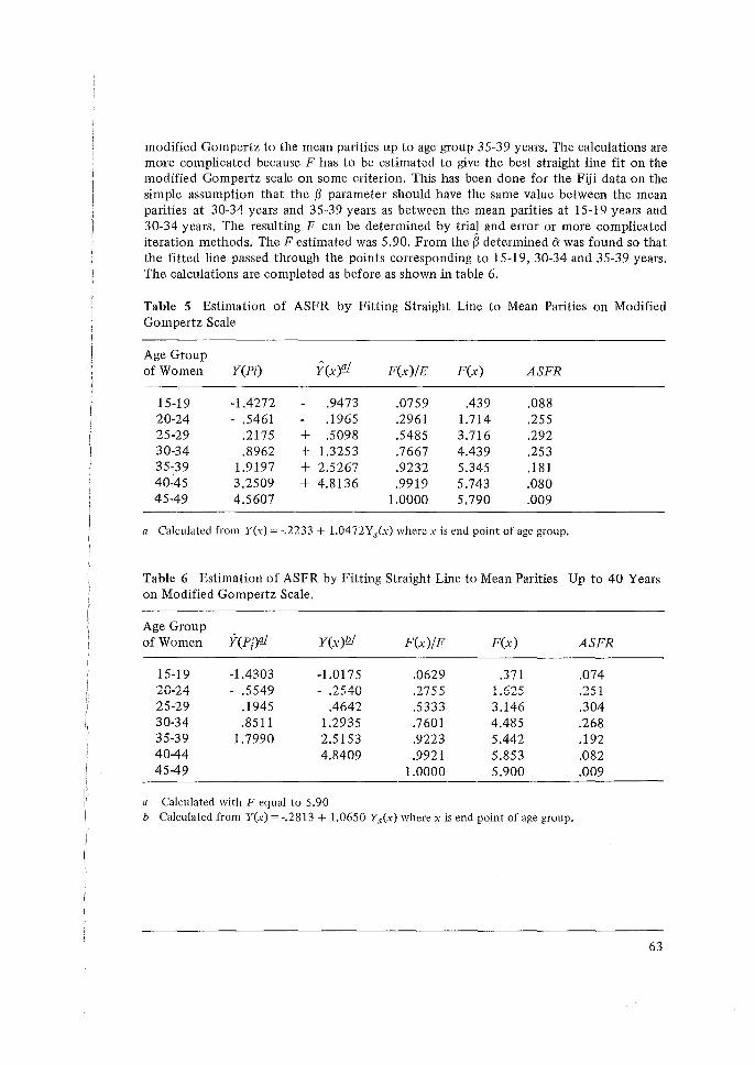
j ,,

modified Gompertz to the mean parities up to age group 35-39 years. The calculations are more complicated because F has to be estimated to give the best straight line fit on the modified Gompertz scale on some criterion. This has been done for the Fiji data on the simple assumption that the ~ parameter should have the same value between the mean parities at 30-34 years and 35-39 years as between the mean parities at 15-19 years and 30-34 years. The resulting F can be determined by trial and error or more complicated iteration methods. The F estimated was 5.90. From the S determined Cl'. was found so that the fitted line passed through the points corresponding to 15-19, 30-34 and 35-39 years. The calculations are completed as before as shown in table 6.

Table S Estimation of ASFR by Fitting Straight Line to Mean Parities on Modified Gompertz Scale

Age Group f(x)aJ of Women Y(Pi) F(x)/E F(x) ASFR

15-19 -1.4272 .9473 .0759 .439 .088 20-24 - .5461 .1965 .2961 1.714 .255 25-29 .2175 + .5098 .5485 3.716 .292 30-34 .8962 + 1.3253 .7667 4.439 .253 35-39 1.9197 + 2.5267 .9232 5.345 .181 40~45 3.2509 + 4.8136 .9919 5.743 .080 45-49 4.5607 1.0000 5.790 .009

a Calculated from Y(x) = -.2233 + 1.04 72Ys(x) where xis end point of age group.

Table 6 Estimation of ASFR by Fitting Straight Line to Mean Parities Up to 40 Years on Modified Gompertz Scale.

Age Group of Women Y(Pf)qj Y(x)Q/ F(x)/F F(x) ASFR

15-19 -1.4303 -1.0175 .0629 .371 .074 ,..,,A ,.... A c C' AO f"\ C' Af\ .2755 1 t::'lt:: 'l<:l .<.v-L-'+ - .JJ'"t7 - ,.£.J""tV .1.,V,l.,.J o"-'.J.L

25-29 .1945 .4642 .5333 3.146 .304 30-34 .8511 1.2935 .7601 4.485 .268 35-39 1.7990 2.5153 .9223 5.442 .192 40-44 4.8409 .9921 5.853 .082 45-49 1.0000 5.900 .009

a Calculated with F equal to 5.90 b Calculated from Y(x) = -.2813 + 1.0650 Ys(x) where xis end point of age group.

63

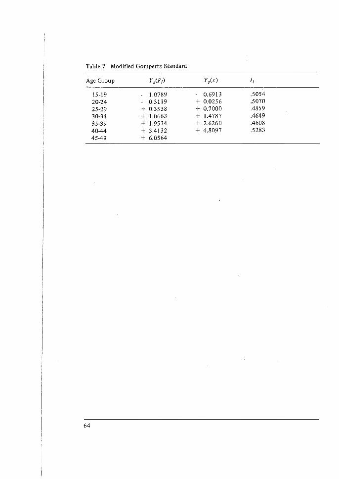
Table 7 Modified Gompertz Standard

Age Group Ys(Pi) Y 8 (x) Ii

15-19 - 1.0789 - 0.6913 .5054 20-24 - 0.3119 + 0.0256 .5070 25-29 + 0.3538 + 0.7000 .4859 30-34 + 1.0663 + 1.4787 .4649 35-39 + 1.9534 + 2.6260 .4608 40-44 + 3.4132 + 4.8097 .5283 45-49 + 6.0564

64

A TECHNICAL NOTE ON THE OWN-CHILDREN METHOD OF FERTILITY ESTIMATION AND ITS APPLICATION TO

THE 1974 FIJI FERTILITY SURVEY

N. Ogawa*

A. INTRODUCTION

In a number of the countries in the ESCAP region, fertility statistics derived from vital registration are unreliable primarily owing to the incompleteness of vital records. In these countries, however, population censuses and surveys have been conducted to improve the reliability of fertility estimates, and to outline fertility trends in recent years. The fertility surveys conducted in conjunction with the World Fertility Survey (WFS) programme are a salient example of such surveys.

Among the most useful fertility estimation techniques in demography is the own­children method, which is applied to census or survey data to provide estimates of fertility levels and trends in years prior to enumeration. Fertility rates are usually computed for each of the 10 to 15 years preceding enumeration. Since the late 1960s, the own-children method has been applied to data from several ESCAP countries, such as the Republic of Korea, Malaysia, the Philippines, Pakistan, Indonesia and Thailand.

One of the pronounced advantages of this method over other fertility estimation techniques is that it does not usually require any additional data collection, only a set of simple tabulations of young children by age of mother. More importantly, such tabulations can be used in computing fertility rates by socio-economic and cultural charac.teristics included in the interview questionnaire. This statistical manipulation is not feasible with vital registration records. Age-specific fertility can be computed by ethnicity, education, religion, region and so forth. Therefore, fertility estimates by the own-children method are extremely useful for the analysis of differential fertility. For instance, in the case of the Philippines, fertility rates were estimated for both urban and rural areas in the 11 census regions over the period 1960-1968, based on a 5 per cent sample from the 1970 census of population (Engracia et al., 1977). The estimates lend themseives to regional developn1ent plai1ning as well as to the evaluation of family

1 planning programmes. It should be noted, however, that the fertility rates are tabulated I\ only by characteristics at the time of enumeration, not at the time of each birth: Never-' theless, if more than one census or survey is available, factors affecting the trend in

fertility can be studied.

The primary objective of this paper is to describe briefly the methodology of the own-children method and its application to the 197 4 Fiji Fertility Survey (FPS) data. Technical aspects of the methodology of the own-children method has been presented in

* At time of writing, the author was a member of the ESCAP secretariat. From January 1980 his address will be: The Population Research Institute of Nikon University, Tokyo, Japan.

65

great detail elsewhere (Cho and Feeney, 1978; Retherford and Cho, 1978).

B. METHODOLOGY

The own-children method of fertility estimation is a survey or census-based reverse­survival method. Enumerated children are computer-matched to mothers within households by means of data on relation to the head of household, age, sex, marital status, and number of living children. The 'match' procedure, which is applied to all children under age 15, has several problems in matching a child to a mother. For instance, the age difference between a mother and a child is within a period of 1 S to 49 years. With this constraint imposed, children born to women after 49 years old are excluded from computations. Moreover, it is not possible to match more children to a woman than she reports are still surviving. This criterion encounters serious difficulties when a woman has stepchildren or adopted children who are older than her natural children. For this reason, in countries where adoption, ramarriage and other factors which complicate mother-child relationships are widely observed, fertility estimates by the own-children method may become less reliable. These are only a few 'match' problems, and a detailed discussion on the 'match' problem has been presented elsewhere (Ho and Choe, 1976).

These matched- or own-children by own age and mother's age are used in estimating, by the reverse-survival technique, births by mother's age in prior years. The technique is also applied to women by age in estimating the age-specific population at risk. Age-specific birth rates and birth probabilities are calculated as suitably adjusted quotients of these two basic quantities. ·

The computation requires several data requirements and simplifying assumptions in order for the own-children method to produce accurate results. Retherford and Cho (1978) have pointed out the following list of major data requirements and computational assumptions:

a) Children's ages are reasonably accurate; b) Most of the children live with their mothers; c) The relationship of each child to the head of the family is clearly specified; d) Mortality levels are relatively low dur1.~g the estimation period prior to enu111eratlon ..

In addition to the above four data requirements, application of the own-children method normally entails the following five simplifying assumptions:

a) Children aged x to x + 1 are underenumerated to the same degree, regardless of age and other characteristics of mother;

b) Women aged a to a+ 1 are underenumerated to the same extent, regardless of their characteristics except age;

66

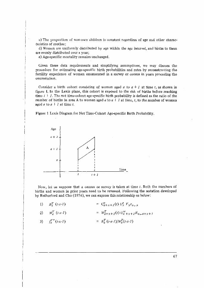
c) The proportion of non-own children is constant regardless of age and other charac­teristics of mother;

d) Women are uniformly distributed by age within the age interval, and births to them are evenly distributed over a year;

e) Age-specific mortality remains unchanged.

Given these data requirements and simplifying assumptions, we may discuss the procedure for estimating age-specific birth probabilities and rates by reconstructing the fertility experience of women enumerated in a survey or census in years proceding the enumeration.

Consider a birth cohort consisting of women aged a to a+ 1 at time t, as shown in figure I. In the Lexis plane, this cohort is exposed to the risk of births before reaching time t + 1. The net time-cohort age-specific birth probability is defined as the ratio of the number of births in area A to women aged a to a+ 1 at time, t, to the number of women aged a to a + 1 at time t.

Figure 1 Lexis Diagram for Net Time-Cohort Age-specific Birth Probability.

Age

a+2

~ a+l

a I I I I

Time

t + 1

l~ow, let u~ suppose that a census or survey is taken at time t. Both the numbers of births and women in prior years need to be reversed. Following the notation developed by Retherford and Cho (1976), we can express this relationship as below:

1)

2)

3)

B'[ (t-x-1)

wI (t-x-1)

tI* (t-x-n BI (t-x-1 )/WI (t-x-1)

67

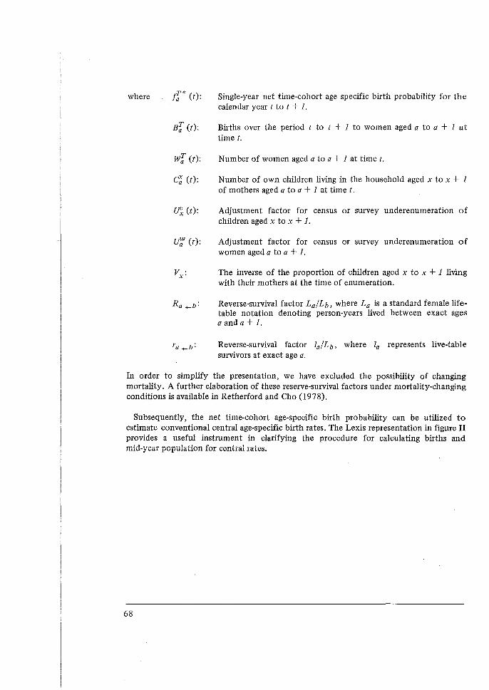
where /[;* (t):

Br (t):

wr (t):

~ (t):

if;; (t):

U-;;' (t):

Single-year net time-cohort age specific birth probability for the calendar year t to t + 1.

Births over the period t to t + 1 to women aged a to a + 1 at time t.

Number of women aged a to a + 1 at time t.

Number of own children living in the household aged x to x + 1 of mothers aged a to a+ 1 at time t.

Adjustment factor for census or survey underenumeration of children aged x to x + 1.

Adjustment factor for census or survey underenumeration of women aged a to a+ 1.

The inverse of the proportion of children aged x to x + 1 living with their mothers at the time of enumeration.

Reverse-survival factor La/Lb, where La is a standard female life­table notation denoting person-years lived between exact ages a and a+ 1.

Reverse-survival factor la/Lb, where la represents live-table survivors at exact age a.

In order to simplify the presentation, we have excluded the possibility of changing mortality. A further elaboration of these reserve-survival factors under mortality-changing conditions is available in Retherford and Cho (1978).

Subsequently, the net time-cohort age-specific birth probability can be utilized to estimate conventional central age-specific birth rates. The Lexis representation in figure II provides a useful instrument in clarifying the procedure for calculating births and mid-year population for central rates.

68

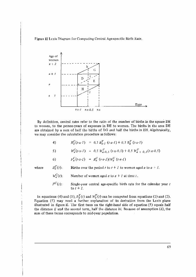
Figure II Lexis Diagram for Computing Central Age-specific Birth Rate.

Age of t women I a+2 --------------

h G

a+ 1 -- - - - -· I I i ,,

D ,, ,,. ,,. I E

a -- - - - - -H

I J 1 I a- -- - - ---

t-x-1 t-x-0.5 t-x

Time

By definition, central rates refer to the ratio of the number of births in the square DE to women, to the person-years of exposure in DE to women. The births in the area DE are obtained by a sum of half the births of DG and half the births in EH. Algebraically, we may consider the calculation procedure as follows:

4)

5)

6)

where Bf (t):

wf (t):

~(t):

B~(t-x-1)

w;(t-x-1)

Fi (t-x-1)

0.5 Br-1 (t-x-1) + 0.5 B'[; (t-x-1)

0.5 w:I0•5 (t-x-0.5) + 0.5 wI + 0 , 5 (t-x-0.5)

Bf (t-x-1)/Wf (t-x-1)

Births over the period t to t + 1 to women aged a to a + 1.

Number of women aged a to a+ 1 at time t.

Single-year central age-specific birth rate for the calendar year t tot+ 1.

In equations (4) and (5), B'[;(t) and W'{;(t) can be computed from equations (1) and (2). Equation (5) may need a further explanation of its derivation from the Lexis plane illustrated in figure II. The first term on the right-hand side of equation (5) equals half the distance ij and the second term, half the distance hi. Because of assumption (d), the sum of these terms corresponds to mid-year population.

69

As shown by the computational steps for the central age-specific birth rate, the fertility estimation by the own-children method is fairly simple and straightforward. However, in a recent article, Retherford and Cho (1978) have extended the own-children method to obtain age-parity-specific fertility estimates. Carried further, Cho and Feeney (1978) have elaborated the methodology of the own-children technique by using more advanced mathematical concepts. Nevertheless, discussion of these refined presentations falls outside the objective of the present paper.

C. REVERSE SURVIVORSHIP RATIOS

One of the distinct features of the own-children method is that fertility rates can be estimated from census or survey data without having recourse to independent mortality data from external sources. Census or survey data on the survival of children ever born by age of mother can be utilized to estimate mortality adjustment factors, utilizing the Brass technique (1968).

The Brass method for estimating child mortality is based on the assumption that fertility is constant for the age range and time period in question, fitting the Brass model fertility schedule. More importantly, in the Brass technique, child mortality estimates are directly influenced by the distribution of fertility by age of woman but are not affected by the level of fertility. In most of the ESCAP countries, however, the age pattern of fertility has recently been changing. Thus, this assumption often appears to be invalid. Nevertheless, there is some empirical evidence that, without any adjustment for changing fertility, the Brass estimates of childhood mortality are reasonably close to other independent estimates of mortality (Cho, 1977).

By the Brass technique, the life-table probabilities of death by exact age one, q(2), and by exact age two, q(3), are obtained, which are used to estimate the life-table Lx values required by equations (1) and (2). The values q(2) and q(3) may be compared with the corresponding values in the Coale-Demeny model life-table for the selection of appropriate model life-table levels.

D. DISCUSSION OF DATA REQUIREMENTS, STATISTICAL ADJUSTMENTS AND ASSUMPTIONS

Based upon past empirical studies on the fertility estimation by the own-children method, the validity of data requirements and simplifying assumptions, and some difficulties arising from statistical adjustments referred to in the previous section will be discussed.

70

a) Mortality

The own-children method requires moderately low mortality during the estimation period prior to enumeration. This requirement is needed partly because the proportion of non-own children should be low. Also, the assumption of low mortality prevents violation of the preceding assumption (e), which would lead to gross error.

If mortality is controlled at a relatively low level, additional changes in mortality adjustments will make little difference. For instance, one of the studies on the Republic of Korea shows that the difference in life expectancy of 10 years in the .estimation of 1965 fertility rates makes total fertility rates differ by less than 5 per cent (Cho, 1977).

b) Age misreporting

The requirement for accurate age classification is specially important in the estimation of fertility rates. Age data in most of the developing countries in the ESCAP region are far from accurate. Age-heaping is a problem very common in Asian census and survey figures. Although age-heaping of women is relatively severe, it affects, to a minimum extent, own-children birth rate estimates for a given year. However, age-heaping of children directly affects fertility estimates, namely overestimates in certain years and . underestimates in others. For instance the own-children estimates from the 1970 Philippine census have suffered from the problem of age-heaping. Consequently, the estimates for the first two years prior to the census have been omitted (Engracia et al., 1977).

In the case of the Republic of Korea, the calculation based upon the censuses of 1966 and 1970 has shown that there is a negligible degree of age misstatement. For children from ages 2 to 9 in 1966, the adjustment of at most 5 per cent was necessary (Cho, 1977). If age misreporting of children is severe, it is recommended that fertility rates be computed for broader age groups, e.g., two-, three-, four-, for five-year age groups.

c) Underenumeration factor

In the own-children estimation, underenumeration of children often poses se1ious problems. For example, if children under age 2 are considerably underenumerated, the result will show a false rapid decline in fertility in the last year or two prior to enumeration.

The completeness of census or survey enumeration is usually evaluated by the data collected in the post-enumeration survey. However, the quality of the postenumeration survey is often questionable. For instance, in the 1966 census in the Republic of Korea, age group 0-4 had no discrepancy between the census count and the post-enumeration survey estimate. However, for age. group 5-9, the census count was slightly less than the

71

post-enumeration survey estimate. If the post-enumeration survey estimate were to be applied for adjustment, fertility estimates for the period five to nine years prior to enumeration would be inflated.

Because both children and women tend to be underenumerated in a census or survey, underenumeration of children and women often offsets each other in the fertility estimate. 'Thus, if the underenumeration of the children is only slightly greater than that of the women, the adjustment factor underenumeration will have little effect on the estimated fertility rate.' (Cho and Feeney, 1978: 17).

In relation to the adjustment of underenumeration, an attempt has been made recently partially to relax one of the simplifying assumptions (Retherford et al., 1978). In the conventional own-children method, the number of enumerated own-children in a certain age group are adjusted for omissions and age misreporting by multiplying by the factor U'f.:, regardless of age and other characteristics of mothers. In this recent experiment, the adjustment factor u<;;a, which is specified by both child's age and mother's age, has been utilized in the fertility estimation based :on the 1970 census of Thailand, and the result has shown a more reasonable pattern. This new procedure takes account of the impact of the factor u~v for women uponthe number of children matched to those women.

d) Non-own children factor

When children are matched with their mothers, there are many possibilities for errors. The child of the head of a household is very likely to be the child of the wife of the head if she is present in the household. This can be vertified by taking into account the numper of children living in the household and the number of children ever born to the women. Because matching is usually performed by computers, its accuracy is sometimes limited. For instance, computers are unable to check reported surnames. Moreover, if there are two or more eligible mothers, the child will be assigned to the one directly prior to it. Despite these limitations in the matching process, unmatched children are grouped by age. These unmatched or non-own children are proportionately distributed among women by age. It is generally considered that if the non-own children exceed more than 20 per cent, the resulting estimates are likely to be biased (Choe, 1978). However, this problem is not very critical in Asia, where parents and children tend to live in the same househol<l. In the 1966 census of the Republic of Korea, 98.2 per cent of children ·aged 5 years old and 95.3 per cen of children aged 5 to 9 were living with their parents (Cho, 1977). In Asia the impact of this adjustment upon estimated fertility is relatively small.

E. APPLICATION OF THE OWN-CHILDREN METHOD TO THE 1974 FIJI FERTILITY SURVEY: PRELIMINARY RESULTS

This section examines preliminary fertility estimates for Fiji by the own-children

72

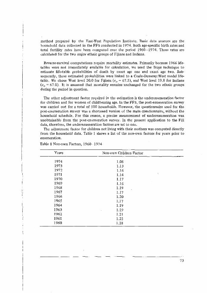
method prepared by the East-West Population Institute. Basic data sources are the household data collected in the FPS conducted in 197 4. Both age-specific birth rates and total fertility rates have been computed over the period 1960-1974. These rates are calculated for the two major ethnic groups of Fijians and Indians.

Reverse-survival computations require mortality estimates. Primarily because 1966 life­tables were not immediately available for calculation, we used the Bra~s technique to estimate life-table probabilities of death by exact age one and exact age two. Sub­sequently, these estimated probabilities were linked to a Coale-Demeny.~West model life­table. We chose West level 20.0 for Fijians (ea= 67.5), and West level 19.8 for Indians (ea= 67.0). It is assumed that mortality remains unchanged for the two ethnic groups during the period in question.

The other adjustment factor required in the estimation is the underenumeration factor for children and for women of childbearing age. In the FPS, the post-enumeration survey was carried out for a total of 500 households. However, the questionnaire used for the post-enumeration survey was a shortened version of the main questionnaire, without the household schedule. For this reason, a precise measurement of underenumeration was unobtainable from the post-enumeration survey. In the present application to the Fiji data, therefore, the underenumeration factors are set to one.

The adjustment factor for children not living with their mothers was computed directly from the household data. Table 1 shows a list of the non-own factors for years prior to enumeration.

Table 1 Non-own Factors, 1960-1974

Years

1974 1973 1972 1971 1970 1969 1968 1967 1966 1965 1964 1963 1962 1961 1960

Non-own Children Factor

1.08 1.13 1.16 1.14 1.17 1.16 1.19 1.17 1.20 1.17 1.19 1.19 1.21 1.22 1.28

73

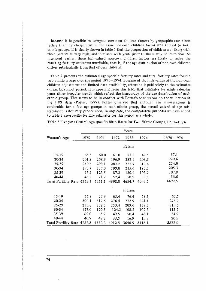
Because it is possible to compute non-own children factors by geographic area alone rather than by characteristics, the same non-own children factor was applied to both ethnic groups. It is clearly shown in table 1 thal the proportion of children not living with their parents is very high, and increases with years prior to the survey enumeration. As discussed earlier, these high-valued non-own children factors are likely to make the resulting fertility estimates unreliable, that is, if the age distribution of non-own children differs substantially from that of own children.

Table 2 presents the estimated age-specific fertility rates and total fertility rates for the two ethnic groups over the period 1970-1974. Because of the high values of the non-own children adjustment and limited data availability, attention is paid solely to the estimates during this short period. It is apparent from this table that estimates for single calendar years show irregular trends which reflect the inaccuracy of the age distribution of each ethnic group. This seems to be in conflict with Potter's conclusions on the validation of the FPS data (Potter, 1977). Potter observed that although age mis-statement is noticeable for a few age groups in each ethnic group, the overall extent of age mis­statement is not very pronounced. In any case, for comparative purposes we have added to table 2 age-specific fertility estimates for this period as a whole.

Table 2 Five-year Central Age-specific Birth Rates for Two Ethnic Groups, 1970-197 4

Women's Age 1970 1971

15-19 65.5 60.0 20-24 201.9 268.9 25-29 250.6 299.1 30-34 193.7 227.0 35-39 93.9 123.5 40-44 46.9 71.7

Total Fertility Rate 4262.5 5251.1

15-19 66.8 77.9 20-24 300.1 317.6 25-29 233.8 232.5 30-34 127.0 120.5 35-39 62.0 65.7 40-44 40.7 48.2

Total Fertility Rate 4152.3 4312.2

74

Years

1972 1973

Fijians

61.0 51.3 196.9 232.2 282.2 225.7 199.8 215.6

87.3 130.4 52.4 58.9

4398.0 4684.7

Indians

65.4 76.4 276.4 273.9 253.4 203.6 124.3 108.2 49.5 50.4 33.5 16.9

4012.8 3646.9

1974

49.5 203.6 219.6 190.7 103.7

39.8 4049.2

53.5 221.1 178.2 102.3, 48.1 19.9

3116.1

1970-1974

57.1 220.6 254.0 205.3 107.9

53.6 4492.5

67.7 275.7 219.5 115.7 54.9 30.9

3822.0

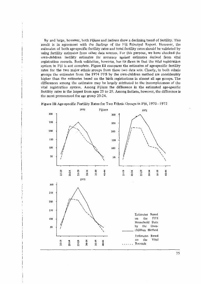
By and large, however, both Fijians and Indians show a declining trend of fertility. This result is in agreement with the findings of the Fiji Principal Report. However, the estimates of both age-specific fertility rates and total fertility rates should be validated by using fertility estimates from other data sources. For this purpose, we have checked the own-children fertility estimates for accuracy against estimates derived from vital registration records. Such validation, however, has its flaws in that the vital registration system in Fiji is not complete. Figure III compares the estimates of age-specific fertility rates for the two major ethnic groups from these two data sets. Clearly, in both ethnic groups the estimates from the 1974 FFS by the own-children method are considerably higher than the estimates based on the birth registrations in almost all age groups. The differences among the estimates may be largely attrituted to the incompleteness of the vital registration system. Among Fijians the difference in the estimated age-specific fertility rates is the largest from ages 25 to 29. Among Indians, however, the difference is the most pronounced for age group 20-24.

Figure III Age-specific Fertility Rates for Two Ethnic Groups in Fiji, 1970-1972

1970 Fijians 1971

300 300

2SO 2SO -

1---, 200 200 I \

' I \ \

I ' \

' \ I lSO \

lSO \

\ I \ '-..., I \

100 I \.._

' 100 --, \ I

I ' I \

' so ~ so I ' ' I \ \ \

~ ... "' ... "' ... ~ ... "' ... "' I 6 <;' "' ~ i 6 <;' "' ~

~ .,., 6 .,.,

~ .,., 0 .,., N N "' "' ... N N "' "' ...

1972

300

2SO

200 r --, I ' I ' ' h \

lSO \ ', ' Estimates Based

' ' the FFS 100 on 7 Household Data I by the Own-so I

___ children Method

Estimates Based

~ ... "' ... "' ... on the Vital 6 <;' "' ~ '1

~ .,., 0 .,., 0 Records N N "' "' ...

75

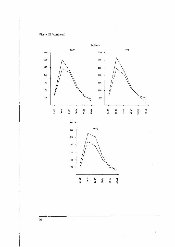
Figure III (continued)

Indians

1970 1971 350 350

300 300

250 2SO (' .......... I .........

200 I \ 200 I \ I \ I \

lSO I \ lSO I \ I \

I \ 100 I ' 100 I

f',, I ' I ' I \

I \ I \ I \ I \ I \

I \ I

1 I I

50 so

3SO

300 1972

2SO

200

lSO

100

so

76

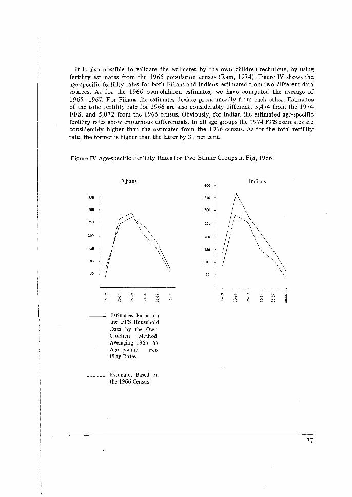
It is also possible to validate the estimates by the own children technique, by using fertility estimates from the 1966 population census (Ram, 1974). Figure IV shows the age-specific fertility rates for both Fijians and Indians, estimated from two different data sources. As for the 1966 own-children estimates, we have computed the average of 1965-1967. For Fijians the estimates deviate pronouncedly from each other. Estimates of the total fertility rate for 1966 are also considerably different: 5,474 from the 1974 FFS, and 5,072 from the 1966 census. Obviously, for Indian the estimated age-specific fertility rates show enournous differentials. In all age groups the 197 4 FPS estimates are considerably higher than the estimates from the 1966 census. As for the total fertility rate, the former is higher than the latter by 31 per cent.

Figure IV Age-specific Fertility Rates for Two Ethnic Groups in Fiji, 1966.

350

300

250

200

150

JOO

50

i I I I

I

Fijians

Estimates Based on the FPS Household Data by the Own­Children Method, Averaging 1965-67 Age-specific Fer­tility Rates

Estimates Based on the 1966 Census

400

350

300

250

200

150

JOO

50

Indians

,.., I ', I ', I \ I ' I I

I \ I \ I \ I \ I ', I ', I \ I \

\ \

77

It is generally considered that the 1966 population census suffers, to a considerable degree, from the undercount of children. For this reason, it may be worth while to compare the fertility estimates compute·d from the FFS household data by the own­children method with those calculated from the FFS individual maternal history data. First, to avoid complicated sampling problems, births between 1971and1973 have been aggregated to form the numerator of the rates. Second, the number of women has been counted from the household schedule. The 'person-years lived' by all women for each age group during this period have also~been calculated directly from the FFS data (World Fertility Survey, 1976: 67).

Figure V depicts the age-specific fertility rates estimated from two different data sources in the 197 4 FFS. It is clear that although in almost all age groups the own­children estimates are still higher than those from the individual questionnaire data, discrepancies between them are considerably smaller than other cases mentioned earlier. In view of the fact that the FFS has given far greater emphasis on the individual maternity and pregnancy history data than on the household schedule, the age-specific fertility rates based on the individual data might be more reliable than the own-children estimates derived from the household data.

Figure V Age-specific Fertility Rates for Two Ethnic Groups in Fiji, 1971-1973

78

300

2SO

200

ISO

100

so

"' "'

Fijians

__ , ,.,.- ' / ..... ,

I \ I '\ I ~

I I

I 1 I

__ Estimates Based on the FFS Household Data by the Own­Children Method

Estimates Based on the FFS Individual Maternity History Data

'\ \

'

300

2SO

200

ISO

100

so

"' "'

Indians

,, / ',,

I \ I \ / \

I \ I \

\ \

' '\

The identification of sources of the gaps among these several estimates is a formidable task, thus falling outside the scope of this paper. However, the following factors may be examined thoroughly in order to fill in such gaps:

a) We should carefully assess the. validity of statistical adjustment involved in the own-children estimation technique. For instance, in Fiji, non-own-children factors are so large that the applicability of the own-children method to the FFS data should be questioned. Furthermore, the application of the same non-own-children factors to the different ethnic groups is also questionable. It is unrealistic to assume that mortality remains constant during the period of estimation. Technically, changing mortality can be handled by a method recently developed by Feeney, which is a modification of the Brass method (Feeney, 1977). It may also be important to examine whether the mortality level selected for each ethnic group is correct;

b) Notwithstanding Potter's observations, the single-year age distribution remains inaccurate, as evidenced by the irregular trends in table 2. For this reason, the 1974 Fiji Fertility Survey data may need more detailed evaluation of its quality and completeness;

c) The degree of the undercount of children in the 1966 census and vital registration for each ethnic group needs to be accurately measured. These are only a few of the factors on the check list.

F. CONCLUDING REMARKS

In recent years the own-children method has been increasingly used among the ESCAP countries. The primary reason for this growing trend is that the quality of vital statistics in these countries is poor.

The own-children method is a very powerful fertility estimation technique, using existing population censuses or surveys. This method requires: (a) reasonably accurate age classification, (b) low proportion of non-own children in the household, (c) clearly specified relationship between a child and the head of household, and (d) relatively low mortality during the estimation period prior to enumeration. The result of sensitivity tests shows that these requirements can be flexible to a certain extent without influencing ultimate fertility estimates.

The own-children approach to fertility estimation can be utilized for estimation from different data sets fertility rates in the overlapping period so as to obtain reliable fertility levels and trends. Therefore, fertility estimates by the own-children method from one consus or survey alone should not be regarded as accurate.

Such careful consideration is applicable to the fertility estimates for Fiji presented in this paper. Although the FFS estimates by the own-children method exhibit a declining trend for both Fijians and Indians, the validation of these estimates needs further detailed work. In any case, the estimates are preliminary, and have been presented here in the hope of providing stimulating discussion material for this Workshop.

79

BIBLIOGRAPHY

Brass, W. and others, The Demography of Tropical Africa. Princeton University Press (pp. 104-132). 1968.

Cho, Lee-Jay, 'The Own-children Approach to Fertility Estimation: An Elaboration', International Population Conference, Mexico (pp. 263-279). 1977.

Cho, Lee-Jay and Griffith Feeney, Fertility Estimation by the Own-Children Method: A Methodological Elaboration, Laboratories for Population Statistics. Reprint Series No. 20. May 1978.

Choe, Minja Kim, 'Census Data for Fertility Analysis', A lecture note prepared for the Seminar on Tabulation and Analytical Processing of Population Census Data. Tokyo. 1978.

Engracia, Luisa T. and others, Estimates of Fertility in the Philippines Derived by the Own-Children Method: 1960-1968, UNFPA-NCSO Population Research Project. National Census and Statistics Office, Manila. Monograph No. 9. 1977.

Feeney, Griffith, 'The Own-children Method of Estimating Age-specific Fertility Rates' Lecture notes prepared for a Demographic Analysis and Data Evaluation Workshop, Kuala Lumpur. 1975.

Feeney, Griffith, 'Estimation of Demographic Parameters from Census and Vital Regis­tration Data', International Population Conference, Mexico (pp. 349-370). 1977.

Ho, Victoria and Minja Choe, 'Evaluation of the Algorithm to Match'-ehildren to Mothers in the Own-children Method of Fertility Estimation', Paper presented at the Second Own-Children Workshop, East-West Center. 1976.

Ogawa, Naohiro and Robert Retherford, 'Decomposition of the Change in the Total Fertility Rate in the Republic of Korea, 1966-70', Paper presented at the Seventh Summer Seminar in Population, East-West Center. June 1976.

Ram, Ganga, 'An Appraisal of the Family Planning Programme in Fiji with Reference to Population Problems, Food, and Population Growth, and Socio-Economic Aspects of the Programme' (mimeo). 1974.

Retherford, Robert and Lee-Jay Cho. 'Age-parity-specific Birth Rates, Birth Expectation, and Birth Probabilities from Census or Survey Data on Own Children', Paper presented at the Second Own-Children Conference. East-'\Vest Center. 1976.

Retherford, Robert, 'Age-parity-specific Birth Rates and Birth Probalities From Census or Survey Data on Own Children:', Population Studies (32(3): 567-582. November 1978.

Retherford, Robert and others. 'An Improved Procedure for Adjusting for Omissions and Age Misreporting Children in the Own-Children Method of Fertility Estimation', Asian and Pacific Census Newsletter (4(4): 5-7. May 1978.

World Fertility Survey, Fiji Fertility Survey 1974: Principal Report, Bureau of Statistics, Fiji. 1976.

80

SOME PROBLEMS IN THE MEASUREMENT AND ANALYSIS OF FERTILITY PREFERENCES FROM V/FS FIRST COUNTRY REPORTS

Louise Kantrow*

A. INTRODUCTION

Levels, patterns and trends of fertility are influenced by a variety of factors, many of which are intricately interrelated. Reliable information on these factors has rarely been available for developing countries. Consequently, little is known of the ways in which reproductive behaviour in these countries is affected by social, cultural and demographic factors or by the unique structure of their interrelationship. The World Fertility Survey provides the first opportunity to determine levels of fertility and analyse the factors affecting fertility and fertility preferences of married women in several developing countries. The first country reports are first stage analyses prepared by the national survey staffs according to guidelines provided by WFS as to the statistical tables which should be prepared. 1 The core questionnaire2 was designed for use in interviewing ever­married women in the childbearing years residing in households. It contains seven sections, including a detailed maternity history, marriage history and segments on contraceptive knowledge and use and fertility preferences. From the pregnancy history, information was obtained on the date, sex and survival status of each birth for each woman interviewed. Data from the first eight published reports are analysed here with a view to throwing light upon problems encountered in the measurement and analysis of fertility preferences from the WFS first country reports. The countries for which data are included in the present study are: Fiji, Malaysia, Nepal, Pakistan, Republic of Korea, Thailand, and, outside the ESCAP region, Colombia and the Dominican Republic.3

B. FERTILITY PREFERENCES AND DESIRED FAMILY SIZE

Since the early 1960s, there has been considerable research interest L11 fertility preferences in relation to knowledge and use of contraception among women in developing countries, because of the assumed usefulness of such information to those concerned with altering rates of population growth by reducing fertility. It is believed by

1 'Guidelines for Country Report No. 1 ', Basic Documentation, World Fertility Survey (London, 1977). 2 'Core Questionnaires', Basic Documentation, World Fertility Survey (London, 1975). 3 World Fertility Survey, Fiji Fertility Survey 1974, Principal Report (Suva, Bureau of Statistics, 1976); The Survey of Fertility in Thailand: Country Report, vols. I and II (Bangkok, Institute of Population Studies, Chulalongkorn University and Population Survey Division, National Statistical Office, 1977); Nepal Fertility Survey 1976, First Report (Kathmandu, His Majesty's Government, Health Ministry, Nepal Family Planning and Maternal Child Health Project, 1977); The Republic of Korea National Fertility Survey 1974, First Country Report (Seoul, Korean Institute for Family Plan­ning, 1977); Malaysian Fertility and Family Survey-1974, First Country Report (Kuala Lumpur, National Family Planning Board, 1977); Pakistan Fertility Survey, First Report (Lahore, Population Planning Council of Pakistan, 1976); Encuesta Nacional de Fecundidad-Infonne General (Santo Domingo, Consejo Nacional de Poblacion y Familia, 1976); Encuesta National de Fecundidad de Colombia, 1976, Resultades Generales (Bogota, Instituto Internacional de Estadistics, 1977). * The author is a staffmember of the Population Division, United Nations, New York.

81

many of those who advocate family planning that, based on findings of fertility surveys, family size desires in developing countries are low. In their view, motivational problems are minimal and population growth could be reduced by preventing the pregnancies which respondents claim were unwanted. Others maintain that family size desires are still high in most developing countries. Although this group also favours providing contraceptive services, it is argued that family size desires are resistant to change and can be reduced only through basic change in social and economic institutions which provide prenatal support.4

Considerable effort has been devoted to the measurement of fertility preferences of women from sample surveys, the goal being to gain knowledge of women's attitudes toward future childbearing, desired completed family size and use of contraception. The underlying assumption was that expressed attitudes on any of these variables relating to future childbearing would determine actual behaviour. However, with few exceptions, the record has not supported this assumption. 5 Instead, most research relating fertility attitudes to behaviour has shown that attitudes make little contribution to the deter­mination of behaviour. Although cohort studies and analyses of aggregate data suggest a strong relation between measures of desired family size and fertility in the developed world, responses of individuals are poor indicators of subsequent actual fertility. Many researchers have begun to question the predictive value of statements regarding future childbearing and question whether such responses have any meaning at all. 6

In response, an important methodological issue has emerged surrounding the reliability ·of the measurement instrument. 7 There are various dimensions to this issue and each has important implications. First, do the attitude questions elicit a consistent response at a single testing, or in a test-retest situation? With data from Thailand, Knodel and Piampiti have shown that test-retest reliability of many survey variables 'is so low that is should be considered a matter of great concern, not only in interpreting results of past surveys, but in planning future ones'.8 And second, is it possible to gauge levels of intensity for any given attitude? Finally, what factors account for the gap between an expressed attitude and subsequent behaviour which is seemingly inconsistent from the researcher's vantage?

Fertility preferences are measured by two sets of questions in the WFS surveys. One concerns the desire for more children, the other concerns the total number of children desired, Particular attention is frequently focused on the group of women who reported

4 Measures, Policies and Programmes Affecting Fertility, with Particular Reference to National Family Planning Programmes (United Nations publication, Sales No. E.72.XIIl.2), pp. 1-16. s R. Freedman, A.I. Hermalin and M.C. Chang, 'Do Statements About Desired Family Size Predict Fertility?', 1975. 6 See N.B. Ryder and C.F. Westoff, 'Relationships Amont Intended, Expected, Desired, and Ideal Family Size: United States 1965', in Population Research (Center for Population Research, National Institute of Child Health and Human Development, Department of Health, Education and Welfare, 1969; and P.M. Hauser, 'Family Planning and Population programs', Demography, 4 :397, 1967. 7 Lolagene Coombs, 'How Many Children do Couples Really Want?' Family Planning Perspecthies, Vol. 10, No. 5, September/October 1978, pp. 303-308; Paul D. Werner, 'Implications of Attitude­behaviour Studies for Population Research and Action', Studies in Family Pla1111i11g, Vol. 8, No. 11, pp. 294-299. s J. Knodel and S. Piampiti, 'Response Reliability in a Longitudinal Survey in Thailand', Studies in Family Planning, Vol. 8, 1977, pp. 64-65.

82

that they did not want more children. This is an important group of women because they are presumably potential candidates for family planning. It has been reported that results from the WFS surveys support the view that there is a large unmet need for family planning services based on the evidence that a large proportion of respondents report having more children thatn they want and a high proportion want to cease childbearing.9

There are at least two issues to be considered concerning the question of wanting more children. How has the group reporting they want no more children been defined, and does the proportion of women reporting they do not want more children accurately reflect a desire or intent to cease childbearing? In addition, how meaningful is the question on desire for more children? Previous investigations into this area have shown that inconsistencies in results from the same data set cast doubt· on the meaning of the responses of women to questions of the desire for more children. 10

Regarding the first issue of defining the group of women who want no more children, in the fertility regulation section of the core questionnaire women were asked if they would like to have another child sometime. In this section a filtering procedure was employed so that certain groups of women were not asked the question on the desire for more children. Specifically, women who had been sterilized, or whose husbands has been sterilized for medical or contraceptive reasons, were not asked the question, but were assumed to have responded negatively to it. Also, women who subjectively felt they were infecund (for unspecified reasons) and women who were not currently married were not asked about their desire for more children. Thus the questionnaire omits the group of women who might desire more children but for whom it would be difficult or impossible.

The percentage of currently married, fecund women who do not want more children by number of livirlg children as reported irl the first country reports is given in table 1. There is no doubt that the desire to cease childbearing as presented here is surprisingly high, ranging from 30 per cent in Nepal to 72 per cent irl the Republic of Korea. A majority of the women with four living children irl all countries report they do not want any more. However, the range is substantial, from 52 per cent in Malaysia to 92 per cent in the Republic of Korea.

The background characteristics of these women (presented in tables 2 and 3) also indicate that high proportions of women with no education and with rural backgrounds report wanting no more children. However, at this stage of analysis it is impossible to determirle the extent to which these results are an artifact of the different demographic characteristics of the women who did not want more children. In Fiji, Malaysia, Nepal; Pakistan, Thailand and the Dominican Republic more than 65 per cent of the women who have been married 0-9 years wanted more children, while more than 65 per cent of those married 20 years of more did not want more children (table 4).

In addition, an upward bias results from the manner in which currently pregnant women were processed. Because currently pregnant women were treated as if they had

9 L.J. Cho, 'Fertility Preferences in Five Asian Countries', International Family Planning Perspectives and Digest, 4(1), Spring 1978. 10 See V. Prachuabmoh and J. Knodel, 'Ideal Family Size in Thailand: Are the Responses Meaning­ful?', Demography, 10(4), November 1973, pp. 619-<i37; and J. Stoeckel and M.A. Choudhury, Fertility, Infant Mortality and Family Planning in Rural Bangladesh (Bangladesh, Oxford University Press, 1973).

83

already achieved the next parity, the desire to cease childbearing is exaggerated, especially for women with 0-3 children, where the largest proportion of currently pregnant women are located. The procedure of mixing currently pregnant women (Parity X-1) with women who already have X number of living children (Parity X) assumes there will be no spontaneous or induced abortions, or still-births among those currently pregnant women. In addition, among currently pregnant women who experience either foetal loss or an infant death, a certain proportion would want to replace that loss and countinue child­bearing. Although infant mortality has been declining in these countries, it should not be ignored. In considering the desire for more children among the currently pregnant women, it may have been just as logical not to ask these women the question directly (as with the sterilized women) but to assume a positive response.

The second issue concerns the ability to measure a desire or intent to cease childbearing from responses to the question 'do you want any more children?'. Doubt in this area stems from several sources. There is evidence which indicates that the question on future childbearing intentions was not easily or universally understood. In a critical review of the Fiji survey, it was noted that the most frequent problems of comprehension occurred around the questions of desires, intentions and opinions regarding the last and future pregnancies. In particular, problems relating to time reference were most numerous. Questions which contained the phrase 'before your last pregnancy' were too abstract for respondents to grasp. There was confusion between the past and the future, and respondents tended to think in terms of their current preference and found it difficult to relate their feelings in the past. 11

Similar problems of time references were noticed with the question on desire for children in the future. Frequently it was found that women who responded negatively to this question interpreted the question to mean the near future, and with probing it was revealed that many women did want more children.12

Beyond the issue of comprehension of the question, there is the issue of the relationship between a woman's desire to have no more children and her actually having a strong inclination or ability to act upon this desire. Does the question on the desire for no more children measure an intent to cease childbearing? A major deficiency of the question regarding future childbearing desires is the failure to obtain any measure of the intensity of the opinion or attitude. It may be that the wife's desire for no additional children is not equal to that of her husband or some otl;er significant family member and if the woman occupies an inferior position within the family there will be little connexion between desire and future behaviour.

Some doubt concerning the meaningfulness of the question on future childbearing intentions arises from the fact that responses to other sets of questions from the core questionnaire are inconsistent with the response to the question on future childbearing desires. In all of the WFS first country reports it is reported that fairly high proportions

11 M.A. Sahib and others, The Fiji Fertility Survey: A Critical Commentary, Occasional Papers, World Fertility Survey (London, 1975), p. 45. 12 See Helen Ware, Language Problems in Demographic Field Work in Africa: The Case of the Cameroon Fertility Survey, Scientific Reports, World Fertility Survey (London, 1977).

84

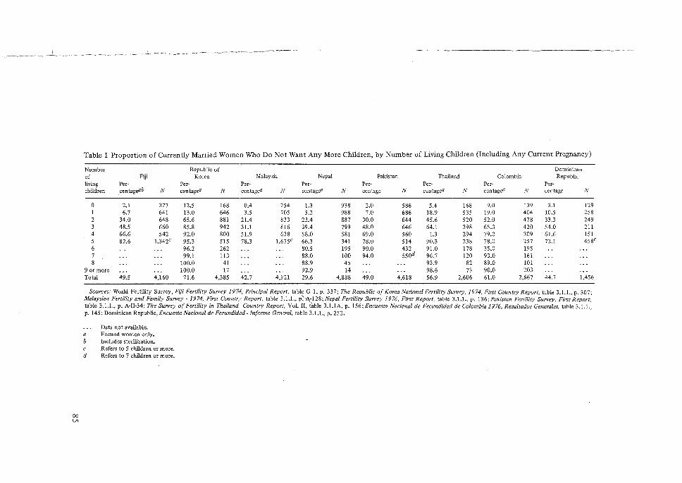
00 V1

Table 1 Proportion of Currently Married Women Who Do Not Want Any More Children, by Number of Living Children (Including Any Current Pregnancy)

Number of living children

0 1 2 3 4 5 6 7 8

9 or more Total

Fiji Per­centag&b

2.1 6.7

34.0 48.5 66.6 82.6

49.5

N

327 641 648 660 542

1.342C

4,160

Republic of Korea

Per­centage"

12.5 13.0 65.6 85.8 92.0 95.3 96.2 99.1

100.0 100.0

71.6

N

168 646 881 942 800 515 262 113 41 17

4,385

Malaysia Per­

centage"

0.4 3.5

21.4 31.l 51.9 78.3

42.7

N

254 705 833 816 638

1.675c

4,921

Nepal Per­

centag&

1.3 5.2

23.4 39.4 58.0 66.3 80.5 88.0 88.9 92.9 29.6

N

938 988 887 799 581 341 195 100 45 14

4,888

Pakistan Per­

centage

2.0 7.0

30.0 48.0 69.0 78.0 90.0 94.0

49.0

N

586 686 644 646 560 514 432 55od

4,618

Thailand Per­

centage"

5.4 18.9 45.6 64.1

1.3 90.3 91.0 96.7 93.9 98.6 56.9

N

168 535 520 398 294 238 178 120

82 73

2,606

Colombia Per­

centage" N

139 404.

478 420 309 257 195 161 101 203

9.0 19.0 52.0 65.0 79.0 78.0 35.0 93.0 89.0 90.0 61.0 2,667

Dominican Republic

Per­centage

3.1 10.5 33.3 54.0 61.6 72.1

N

129 258 249 211 151 453c

44.7 1,456

Sources: World Fertility Survey, Fiji Fertility Survey 1974, Principal Report. table G 1, p. 337; The Republic of Korea National Fertility Survey. 1974, First Country Report, table 3.1.1., p. 307; Malaysian Fertility and Family Survey · 1974, First Country Report, table 3.1.1., P~_::l28; Nepal Fertility Survey 1976, First Report, table 3.1.1., p. 136; Pakistan Fertility Survey, First Report, table 3.1.1., p. A-ll-34; The Survey of Fertility in Thailand: Country Report, Vol. II, table 3.1.lA, p. 156; Encuesta Nacional de Fecundidad de Colombia 1976, Resultados Genera/es, table 3.1.1., p. 145; Dominican Republic, Encuesta Nacional de Fecundzil,zd • Informe General, table 3.1.1., p. 252.

Data not available. a Fecund women only. b Includes sterilization. c Refers to 5 children or more. d Refers to 7 children or more.

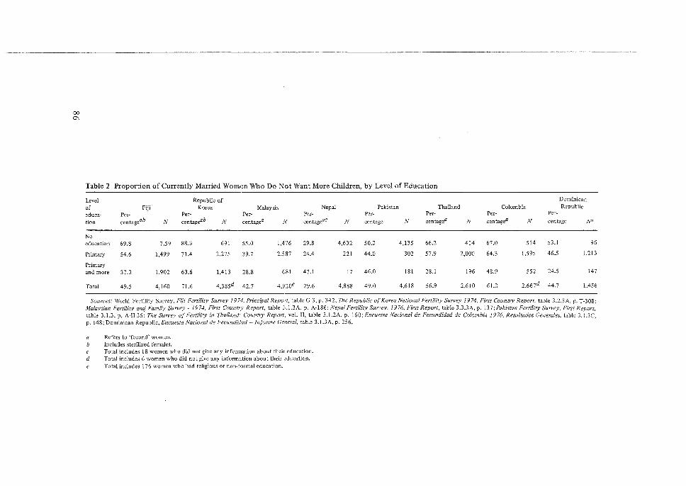
00 Cl\

Table 2 Proportion of Currently Married Women Who Do Not Want More Children, by Level of Education

Level Republic of Dominican

of Fiji Korea Malaysia Nepal Pakistan Thailand Colombia Republic

educa- Per- Per- Per- Per- Per- Per- Per- Per-

ti on centageab N centageab N centagea N centageac N centage N centagea N centagea N centage JV"

No education 69.8 7.59 88.3 691 55.0 1,476 29.8 4.632 50.0 4.135 66.2 414 67.0 514 53.1 96

Primary 54.6 1,499 71.4 2,275 39.7 2,587 24.4 221 44.0 302 57.9 2,000 64.3 1.595 46.5 1.213

Primary and more 37.3 1,902 63.6 1,413 28.8 681 47.1 17 46.0 181 28.1 196 48.9 552 24.5 147

Total 49.5 4,160 71.6 4,385d 42.7 4,noe 29.6 4,888 49.0 4,618 56.9 2,610 61.0 2.667d 44.7 1,456

Sources: World Fertility Survey, Fiji Fertility Survey 1974, Principal Repo,t, table G 3, p. 342; The Republic of Korea National Fertility Survey 1974, First Country Report table 3.2.3A. p. T-308; Malaysian Fertility and Family Survey - 1974, First Country Report, table 3.1.3A, p. A-186; Nepal Fertility Survey, 1976, First Report, table 3.3.3A, p. 137;Pakistan Fertility Survey, First Report, table 3.1.3, p. A-11-35; The Survey of Fertility in Thailand: Country Report, vol. II, table 3.l.2A, p. 160; Encuesta Nacional de Fecundidad de Colombia 1976, Resu/tados Genera/es, table 3.l.3C, p. 148: Dominican Republic. Encuesta Nacional de Fecundidad - Jnforme General, table 3.L3A, p. 256.

a Refers to 'fecund' women. b Includes sterilized females.

Total includes 18 women who did not give any information about their education. d Total includes 6 women who did not give any inform:::.tion about their education.

Total includes 176 women who had religious or non-formal education.

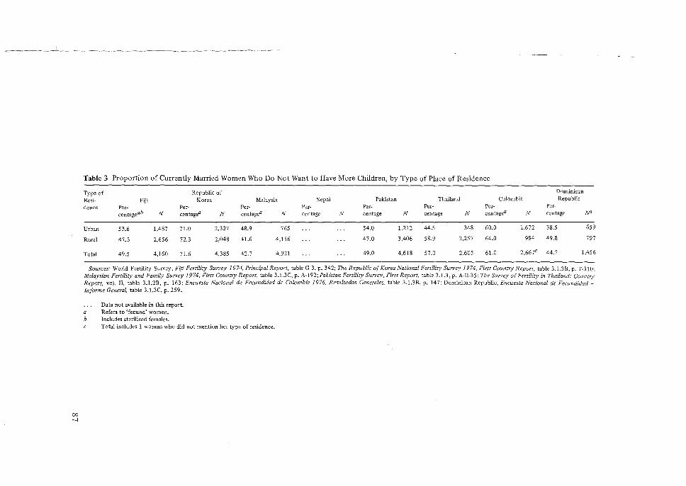
00 -J

Table 3 Proportion of Currently Married Women Who Do Not Want to Have More Children, by Type of Place of Residence

Type of Republic of Dorninkan

Resi- Fiji Korea Malaysia Nepal Pakistan Thailand Colombia Republic

dence Per- Per- Per- Per- Per- Per- Per- Per-centageab N centagea N eentagea Iv centage N centage N centage N centagea N centage N"

Urban 53.6 1,487 71.0 2,337 48.9 765 54.0 1,212 44,5 348 60.0 1.672 38.5 659

Rural 47.3 2,656 72.3 2,048 41.6 4,156 47.0 3,406 58.9 2,257 64.0 994 49.8 797

Total 49.5 4,160 71.6 4,385 42.7 4,921 49.0 4,618 57.0 2,605 61.0 2,667c 44.7 1.456

Sources: World Fertility Survey, Fiji Fertility Survey 197•1, Principal Report, table G 3, p. 342; The Republic of Korea National Fertility Survey 1974, First Country Report, table 3.l.3B, p. T-310; Malaysian Fertility and Family Survey 1974, First Country Report, table 3.l.3C, p. A-192; Pakistan Fertility Survey, First Report, table 3.1.3, p. A·Il·35; The Survey of Fertility in Thailand: Country Report, vol. II, table 3.l.2B, p. 163; Encuesta Nacional d,, Fecundidad de Colombia 1976, Resultados Genera/es, table 3.1.3B, p. 147; Dominican Republic, Encuesta Nacional de Fecundidad -lnforme General, table 3.1.3C, p. 259.

Data not available in this report. Refers to 'fecund' women.

b Includes sterilized females. Total includes 1 woman who did not mention her type of residence.

-------------------·----------------------------·---··--·-·····--·

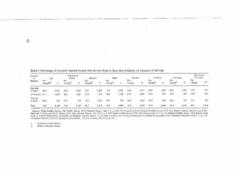
00 00

Table 4 Percentage of Currently Married Worn en Who Do Not Want to Have More Children, by Duration of Marriage

Duration Republic of Dominican

of Fiji Korea Malaysia Nepal Pakistan Thailand Colombia Republic

Marriage Per- Per- Per- Per- Per- Per- Per- Per-

centageab N centageb N centageb N centageb N centage N centageb N centageb N centage Nb

Less than 10 years 24.4 1,912 50.2 2,169 16.6 2,224 8.4 2,169 16.0 1,817 35.0 1,342 42.0 1,263 28.9 724

10-19 years 61.7 1,416 90.1 1,461 57.0 1,550 36.9 1,766 57.0 1,444 76.3 826 76.0 887 58.4 445

20 years or more 86.4 832 97.5 755 74.3 1,142 64.2 953 85.0 1,357 87.8 436 82.4 517 63.4 287

Total 49.5 4,160 71.6 4,385 42.7 4,916 29.6 4,888 49.0 4,618 57.0 2,604 61.0 2,667 44.7 1,456

Sources: World Fertility Survey, Fiji Fertilit_v Survey 19 74, Principal Report, table G 2, p. 339; The Republic of Korea National Fertility Survey 1974, First Country Report, table 3.1.2, p. T-307; Malaysian Fertility and Family Survey 1974, First Country Report, table 3.1.2, p. A 183; Nepal Fertility Survey 1976, First Report, table 3.1.2, p. 136; Pakistan Fertility Survey, First Report, table 3.1.2, p. A·Il-34; Table Survey of Fertility in Thailand: Country Report, vol. II, table 3.1.IB, p. 157;Encuesta Nacional de Fecundidad de Colombia 1976, Resultados Genera/es, table 3.1.2, p. 145; Dominican Republic, Encuesta Nacional de Fecundidad - Informe General, table 3.1.2. p. 253.

a Includes sterilized females. b Refers to 'fecund' women.

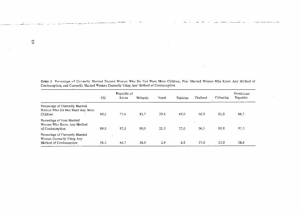
Table 5 Percentage of Currently Married Fecund Women Who Do Not Want More Children, Ever Married Women Who Know Any Method of Contraception, and Currently Married Women Currently Using Any Method of Contraception

Republic of Dominican Fiji Korea Malaysia Nepal Pakistan Thailand Colombia Republic

Percentage of Currently Married Women Who Do Not Want Any More Children 49.5 71.6 42.7 29.6 49.0 56.9 61.0 44.7

Percentage of Ever Married Women Who Know Any Method of Contraception 99.8 97.0 90.0 21.3 75.0 96.1 95.8 97.3

Percentage of Currently Married Women Currently Using Any Method of Contraception 56.2 45.7 38.0 2.9 6.0 37.0 52.0 38.4

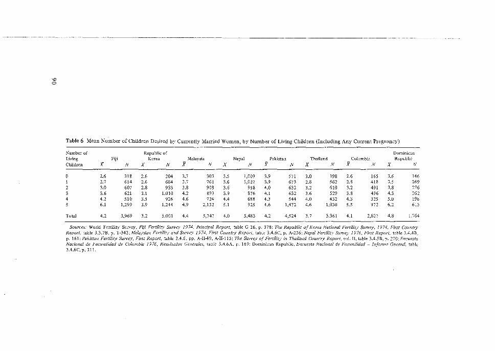
\0 0

Table 6 Mean Number of Children Desired by Currently Married Women, by Number of Living Children (Including Any Current Pregnancy)

Number of Republic of Dominican Living Fiji Korea Malaysia Nepal Pakistan Thailand Colombia Republic Children x N x N x N x N x N x N x N x N

0 2.6 318 2.6 204 3.7 303 3.5 1,009 3.9 571 3.0 198 2.6 165 3.6 146 2.7 614 2.6 684 3.7 761 3.6 1,027 3.9 673 2.8 562 2.8 418 3.5 269

2 3.0 607 2.8 933 3.8 908 3.6 958 4.0 632 3.2 610 3.2 491 3.8 276 3 3.6 621 3.1 1,010 4.2 899 3.9 876 4.1 632 3.6 529 3.8 436 4.3 262 4 4.2 510 3.5 926 4.6 724 4.4 688 4.3 544 4.0 432 4.3 325 5.0 198 5 6.1 1,299 3.9 1,244 4.9 2,152 5.1 925 4.6 1,472 4.6 1,030 5.5 972 6,2 613

Total 4.2 3,969 3.2 5,001 4.4 5,747 4.0 5,483 4.2 4,524 3.7 3,361 4.1 2,807 4.8 1,764

Sources: World Fertility Survey, Fiji Fertility Survey 1974, Principal Report, table G 26, p. 378; The Republic of Korea National Fertility Survey, 1974, First Country Report, table 3.3.7B, p. T-342; Malaysian Fertility aod Survey 1974. First Country Report, table 3.4.6C, p. A-256; Nepal Fertility Survey 1976, First Report, table 3.4.4B. p. 161; Pakistan Fertility Survey, First Report, table 3.4.6, pp. A-II-49, A-Il-115; The Survey of Fertility in Thailand Country Report, vol. II, table 3.4.5B, p. 270; Encuesta Nacional de Fecundidad de Colombia 1976, Resultados Genera/es. table 3.4.6A, p. 169; Dominican Republic, Encuesta Nacional de Fecundidad - Jnforme General, table 3.4.6C, p. 311.

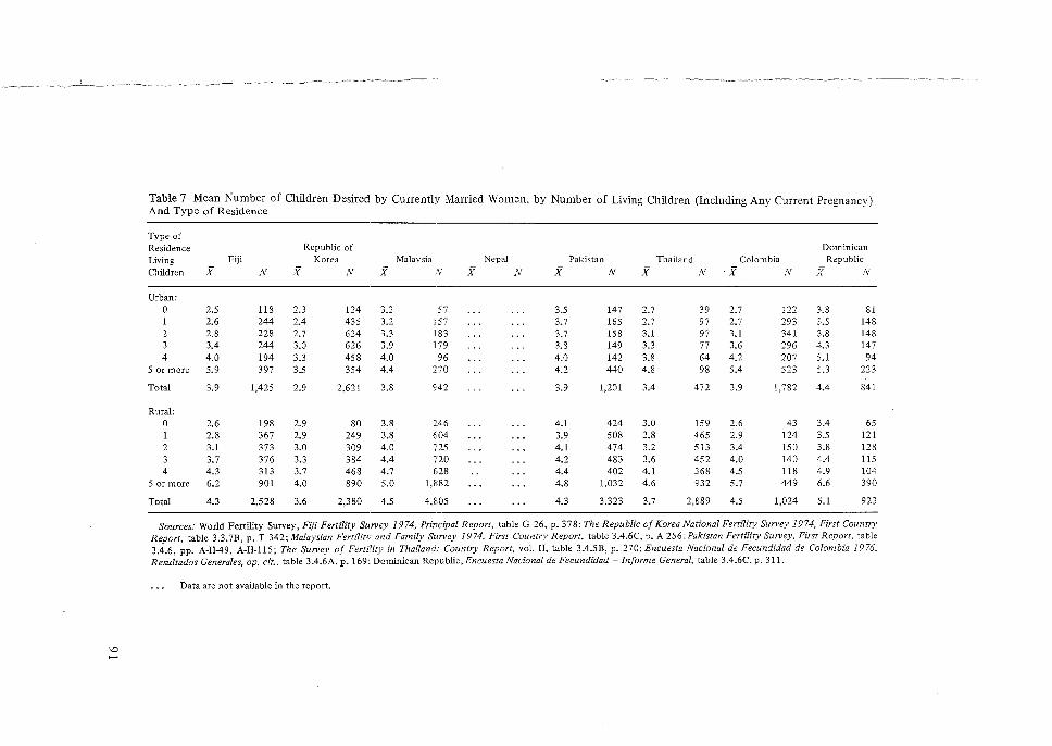
Table 7 Mean Number of Children Desired by Currently Married Women, by Number of Living Children (Including Any Current Pregnancy) And Type of Residence .

Type of Residence Republic of Dominican Living Fiji Korea Malaysia Nepal Pakistan Thailand Colombia Republic Children x N x N x N x N x N x N x N x N

Urban: 0 2.5 118 2.3 124 3.2 57 3.5 147 2.7 39 2.7 122 3.8 81

2.6 244 2.4 435 3.2 157 3.7 165 2.7 97 2.7 293 3.5 148 2 2.8 228 2.7 624 3.3 183 3.7 158 3.1 97 3.1 341 3.8 148

3.4 244 3.0 626 3.9 179 3.8 149 3.3 77 3.6 296 4.3 147 4 4.0 194 3.3 458 4.0 96 4.0 142 3.8 64 4.2 207 5.1 94

5 or more 5.9 397 3.5 354 4.4 270 4.2 440 4.8 98 5.4 523 5.3 223

Total 3.9 1,425 2.9 2,621 3.8 942 3.9 1,201 3.4 472 3.9 1.782 4.4 841

Rural: 0 2.6 198 2.9 80 3.8 246 4.1 424 3.0 159 2.6 43 3.4 65 1 2.8 367 2.9 249 3.8 604 3.9 508 2.8 465 2.9 124 3.5 121 2 3.1 373 3.0 309 4.0 725 4.1 474 3.2 513 3.4 150 3.8 128

3.7 376 3.3 384 4.4 720 4.2 483 3.6 452 4.0 140 L.4 115 4 4.3 313 3.7 468 4.7 628 4.4 402 4.1 368 4.5 118 4.9 104

5 or more 6.2 901 4.0 890 5.0 1,882 4.8 1,032 4.6 932 5.7 449 6.6 390

Total 4.3 2,528 3.6 2,380 4.5 4,805 4.3 3,323 3.7 2,889 4.5 1,024 5.1 923

Sources: World Fertility Survey, Fiji Fertility Survey 1974, Principal Report, table G 26, p. 378; The Republic of Korea National Fertility Survey 1974, First Country Report. table 3.3.7B, p. T 342; Malaysian FertilitJ' and Family Survey 1974, First Country Report, table 3.4.6C, p. A 256:Pakistan Fertility Survey. First Report, table 3.4.6, pp. A·Il-49, A-Il-115; The Survey of Ferti1ity in Thailand: Country Report. vol. II, table 3.4.5B, p. 270: Encuesta Nacional de Fecundidad de Colombia 1976, Resultados Genera/es, op. cit., table 3.4.6A, p. 169: Dominican Republic,Encuesta Nacional de Fecundidad -Informe General, table 3.4.6C, p. 311.

Data are not available in the report.

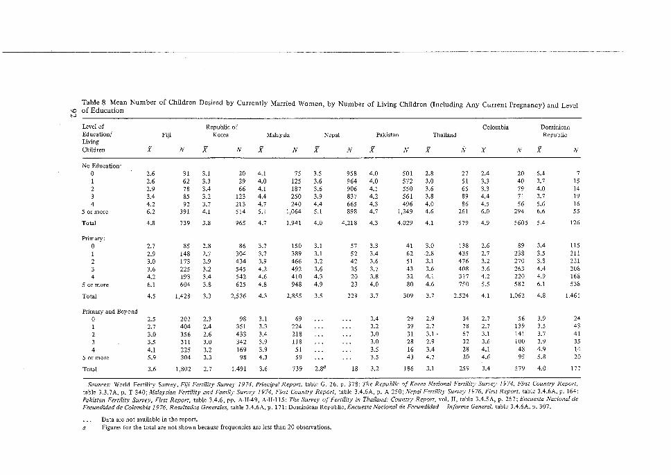
Table 8 1!ean Number of Children Desired by Currently Married Women, by Number of Living Children (Including Any Current Pregnancy) and Level 'Cl of Education N

Level of Republic of Colombia Dominican Education/ Fiji Korea Malaysia Nepal Pakistan Thailand Republic Living Children x N x N x N x N x N x ff x N x N

No Education: 0 2.6 31 3.1 20 4.1 75 3.5 958 4.0 501 2.8 27 2.4 20 6.4 7 1 2.6 62 3.3 29 4.0 125 3.6 964 4.0 572 3.0 51 3.3 40 3.7 15 2 2.9 78 3.4 66 4.1 187 3.6 906 4.1 550 3.6 65 3.3 79 4.0 14 3 3.4 85 3.2 123 4.4 250 3.9 837 4.2 561 3.8 89 4.4 71 3.7 19 4 4.2 92 3.7 213 4.7 240 4.4 665 4.3 496 4.0 86 4.5 56 5.6 16

5 or more 6.2 391 4.1 514 5.1 1,064 5.1 898 4.7 1,349 4.6 261 6.0 294- 6.6 55

Total 4.8 739 3.8 965 4.7 1,941 4.0 4,218 4.3 4,029 4.1 579 4.9 5605 5.4 126

Primary: 0 2.7 85 2.8 86 3.7 150 3.1 57 3.3 41 3.0 138 2.6 89 3.4 115 1 2.9 148 2.7 304 3.7 389 3.1 52 3.4 62 2.8 435 2.7 238 3.5 211 2 3.0 173 2.9 434 3.9 466 3.2 42 3.6 51 3.1 476 3.2 270 3.8 221 3 3.6 225 3.2 545 4.2 492 3.6 35 3.7 43 3.6 408 3.6 263 4.4 208 4 4.2 193 3.4 542 4.6 410 4.3 20 3.8 32 4.1 317 4.2 220 4.9 168

5 or more 6.1 604 3.8 625 4.8 948 4.9 23 4.0 80 4.6 750 5.5 582 6.1 538

Total 4.5 1,428 3.3 2,536 4.3 2,855 3.5 229 3.7 309 3.7 2,524 4.1 1,062 4.8 1,461

Primary and Beyond 0 2.5 202 2.3 98 3.1 69 3.4 29 2.9 34 2.7 56 3.9 24 1 2.7 404 2.4 351 3.3 224 3.2 39 2.7 78 2.7 139 3.5 43 2 3.0 356 2.6 433 3.4 218 3.0 31 3.1. 67 3.1 141 3.7 41 3 3.5 311 3.0 342 3.9 118 3.0 28 2.9 32 3.6 100 3.9 35 4 4.1 225 3.2 169 3.9 51 3.5 16 3.4 28 4.1 48 4.9 14

5 or more 5.9 304 3.3 98 4.3 59 3.5 43 4.7 20 4.6 95 5.8 20

Total 3.6 1,802 2.7 1.491 3.6 739 2.8a 18 3.2 186 3.1 259 3.4 579 4.0 177

Sources: World Fertility Survey, Fiji Fertility Survey 1974, Principal Report, table G. 26, p. 378: The Republic of Korea National Fertility Survey 1974, First Country Report, table 3.3.7 A, p. T 340; Malaysian Fertility and Family Survey 1974, First Country Report, table 3.4.6A, p. A 250; Nepal Fertility Survey 1976, First Report, table 3.4.6A, p. 164: Pakistan Fertility Survey, First Report, table 3.4.6, pp. A-11-49, A·Il·l 15: The Survey of Fertility in Thailand: Country Report, vol. II, table 3.4.5A, p. 267: Encuesta Nacional de Fecundidad de Colombia 1976, Resultados Genera/es, table 3.4.6A, p. 1 71; Dominican Republic, Encuesta Nacional de Fecundidad - Informe General, table 3.4.EA, p. 307.

Data are not available in the report. a Figures for the total are not shown because frequencies are less than 20 observations.

of women want no more children, and high proportions report knowledge of some method of contraception. This, however, does not coincide with the low proportions of current contreaceptive use as shown in table 5. It is possible that the desire for no additional children is high and that the practice of family planning is low if, for example, the wife's desire is not equal to her husband's. Again, there appears to be a large gap between expressed desires and behaviour.

In the WFS questionnaire, fertility preferences were also probed with another question. All currently married women were asked the question: 'If you could choose exactly the number of children to have in your whole life, how many children would that be?' The results to this question, according to number of living children, wife's level of education and urban-rural residence, are given in tables 6-8. In every country desired family size increases with number of living children. In part, this might reflect a decline in family size preferences, and to some extent it might reflect a bias that achieved fertility influences desired family size. If younger women, who are in the early stages of the reproductive career, express a desired family size which is less than that expressed by women at the end of their reproductive careers, this could be supporting evidence that fertility norms are declining. However, it could also be the case that women with large families may rationalize unwanted fertility. Inquiry to estimate the impact of rationalization of stated desired family size has been limited. However, using data from Thailand, Knodel and Prachuabmoh13 suggest that if rationalization of the existing number of children is a factor influencing the choice of the desired number, then the probability of giving a particular number as the desired family size should be greater for women with that particular number of living children than for women with either more or less than that number. The authors calculate and compare these two sets of probabilities and conclude that the differences in probabilities by parity are not large. Only among women with four or more children is there some substantial difference. Yet even for these women, the authors believe that rationalization cannot account for more than one fourth of their responses. Knodel and Prachuabmoh suggest that rationalization has an even weaker effect on the family size desires of women with higher parities ' ... perhaps it is more difficult for women who exceed their "true" preference by a large number of children to rationalize their entire current family size than for women who have only one or two more than they might otherwise want'. 14 As can be seen from table 6, with the exception of the Republic of Korea, women with 0-4 living children consistently report an average desired family size v:hich exceeds acl1Jeved family size.

Desired family size for all currently married women (table 6) ranges from a low of 3.2 in the Republic of Korea to 4.8 in the Dominican Republic. In Fiji, Malaysia, Nepal, Pakistan, Colombia and the Dominican Republic, currently married women desire an average of 4 or more children.

When desired family size by number of living children and background variables is presented graphically (see figure below) it becomes apparent that, except for the

13 J. Knodel and V. Prachuabmoh, 'Desired Family Size in Thailand: Are the Responses Meaning­ful', Demography, Vol. 10, No. 4, pp. 619-637. 14 Ibid., pp. 629-630.

93

Republic of Korea and Thailand, there are few categories of women for whom achieved fertility has surpassed fertility desires. The diagonal indicates the state where actual family size equals desired family size; women above the diagonal have not reached desired parity, women below have surpassed that level. In the Republic of Korea, where the fertility decline has been most pronounced, desired family size is also lowest regardless of number of living children. Fertility has shown little decline in Pakistan and Nepal and, in these countries, desired family size is high and differences associated with number of living children are small. In other words, women who are beginning their reproductive careers in Nepal and Pakistan desire almost as many children as women who have already has five or more. A similar, but less pronounced pattern exists in Malaysia, where the crnde birth rate has declined by 26 per cent since 1965.

One pattern that exists for all countries, regardless of the average desired family size, is that the fertility preferences of childless women or those with one living child are almost identical. With the exception of Nepal and Pakistan, larger differences in fertility preferences begin to emerge for women who have two, three and four living children. This is another indication that fertility preferences are altered as women proceed through their reproductive careers.

Even though a higher proportion of rural than urban woman report not wanting more children, from table 7 it can be seen that the number of children desired by rural women still exceeds that desired by urban women. Also, in every country except Thailand there is an inverse relation between family size and level of education (table 8).

In addition to information from the direct question on the desire for more children, it is possible to measure the desired to cease childbearing indirectly by using the question on total number of children desired. A comparison of these two measures reveals large differences, especially among women in the early stages of their reproductive careers. The results of responses to this question classified by number of living children for the Republic of Korea are presented in table 9. From the first country reports, it was possible to present the following analysis for the Repubfic of Korea only. The women along the diagonal have had exactly the number of children they desire, the women below the diagonal have had more children than they desire and those above the diagonal have not yet reached their desired number. Presumably the women along and below the diagonal are those who do not want more children; they are the women who have had 'exactly the number of children desired' and 'more than the number of children desired'. When measured this way, the proportion of all women who do not want more children in the Republic of Korea is 61 per cent rather than 72 per cent. The difference in the two measures of the desire to cease childbearing is most pronounced for women with 0-3 living children. For women who have two living children, the proportion not wanting any more, measured this way, is 38 per cent compared with 66 per cent. In contrast to the unusually high proportion of zero-parity women who want no more children (12.5 per cent), as calculated from table 9, less than 1 per cent of these women have exactly the

94

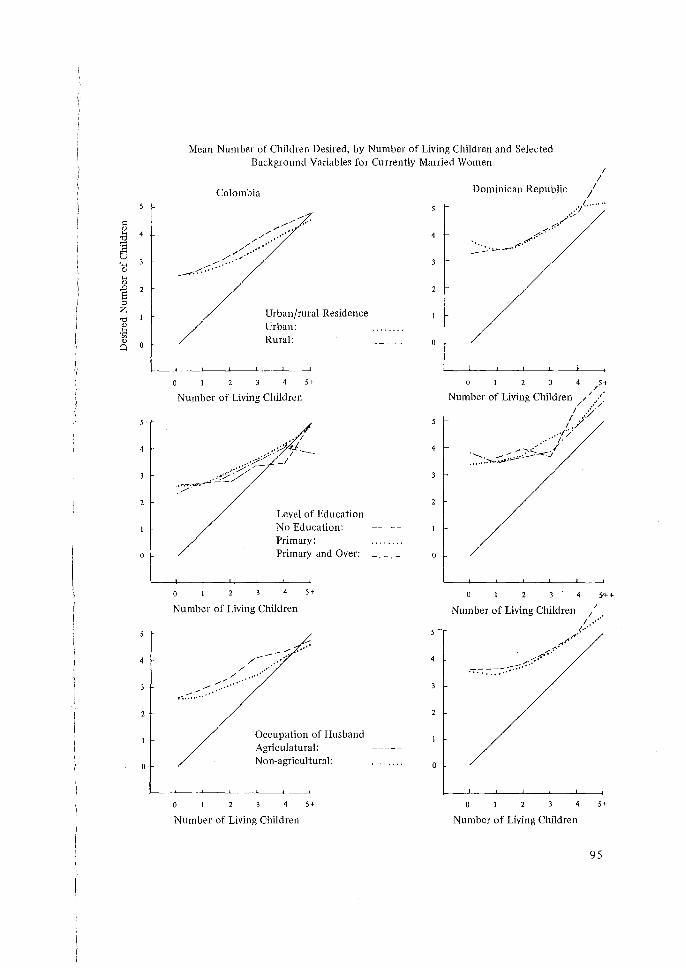
H <l)

..0 s "' z

't:l <l)

·~ <l)

Q

S·

Mean Number of Children Desired, by Number of Living Children and Selected Background Variables for Currently Married Women

Colombia

Urban/rural Residence Urban: Rural:

5+

Number of Living Children

Level of Education No Education: Primary: Primary and Over:

S+

Number of Living Children

····· /--,.. // ·"

-~.-:..~········ <,,-:-; ....

Occupation of Husband Agriculatural: Non-agricultural:

0 5+

Number of Living Children

I I

Dominican Republic /

.. :::/·""" ,.,,,,.,,

/,·;.··· ,..,. .. ·::..·~-,.<·

0 1 2 5+ /

Number of Living Children / ~.,;:

/ ,.;;/ . . h/

""!· ~ --..:..:·' ./

~::::::--~;~~·---·~.../

Number of Living Children /

,,,./~ .. ·" ~""

,7:: -:-.-::;.-::.-:::.·"',..-:"

0 5+

Number of Living Children

95

~

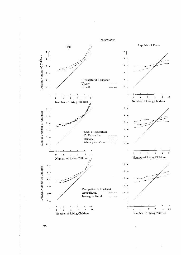
"' -t3 ] u "" 0 .... "' .<:> s i 'O

"' ·iil "' 0 Ci

5 l

4

2

0

96

F'1'J'1' I ;/ ;/

;/ 1.: I'

/.' /,.'

/,•' /,•'

......... ~:.:.:···· roo ;:-: ;;; ••••

(Continued)

Urban/Rural Residence Urban: Urban:

0 1 2 3 4 5+

Number of Living Children

I l .:# ,..:,.:.·

... -;?' ····~~ ::;:,:....:-...:..-

Level of Education No Education: Primary: Primary and Over:

0 1 2 3 5+

Number of Living Children /

/ ;/ ~/

f." f'

.,,,...~ ,........-;.·

/.•· ........................ · ...- .. :-:-::-:::·····

Occupation of Husband Agricultural: Non-agricultural

0 1 2 3 4 5+

Number of Living Children

0

5 I-

4

3 .

0

Republic of Korea

-------- ............. . ---.... ····· .... . ...

0 2 3 4 5+

Number of Living Children

-­.......... ~ ... ···

--------.-::~ ~:::.:..._._ ................ ....--·-·-

5+

Number of Living Children

/

-­,.,--- .... ········· - _,,__, - ····· ····· . ····· ...

0 1 2 3 5+

Number of Living Children

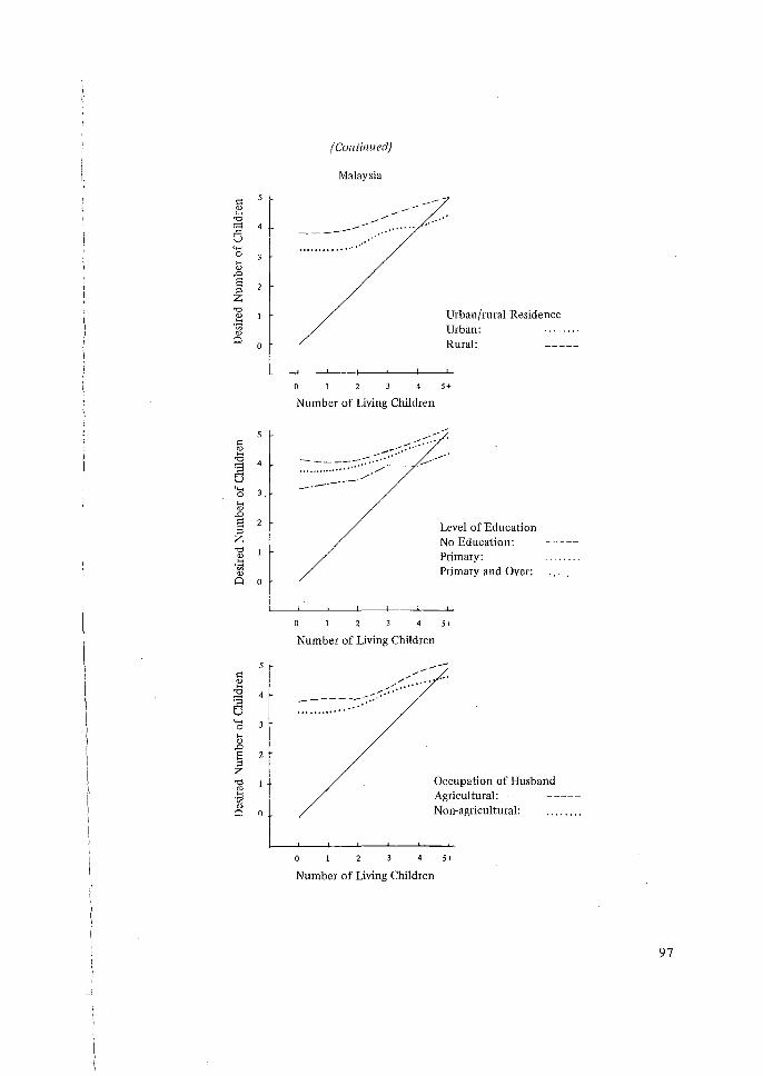
3,

2

0

~ : [ <]) I-<

'O a '-'""< 0 I-<

"' ,0

s ::; z 'O <]) I-<

·~ <])

Q

(Continued)

Malaysia

-------- ...... . ··················

0

... ...

Urban/rural Residence Urban: Rural:

5+

Number of Living Children

Level of Education No Education: Primary: Primary and Over:

4 5+

Number of Living Children

_,/-_:;. ___ :--;;.-;'····"/

-----~.···· ....

Occupation of Husband Agricultural: Non-agricultural:

5+

Number of Living Children

97

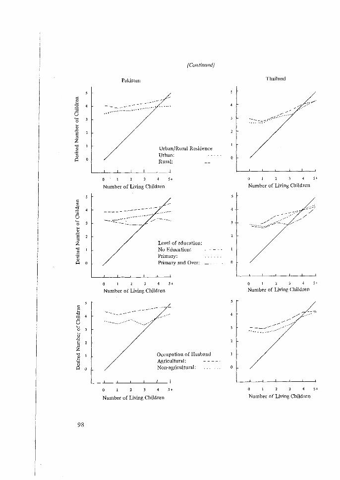
i:: ., .tJ ] u """' 0 ... ., ,D s ;; z "" ., ... ..... "' ., A 0

98

·····

Pakistan

--- ------ ········ ...............

(Co11ti11ued)

Urban/Rural Residence Urban: Rural:

0 3 4 5+

Number of Living Children

---------.:..::::_·.

....

Level of education: No Education: Primary: Primary and Over:

0 1 2 3 4 5+

Number of Living Children

________

............... - - ---- --/--

. ........ · ....

Occupation of Husband Agricultural: Non-agricultural:

0 5+

Number of Living Children

Thailand

...-"".··;."·-r,,,..'

0 I 2 5+

Number of Living Children

4 .

,/

3 . :~:;;:.~~<--'.

0 I 2 3 $+

Number of Living Children

//+. ,,..,,..

_....- ... ____ ,....., .. ·· ... .... ·····

0 2 3 4 5+

Number of Living Children

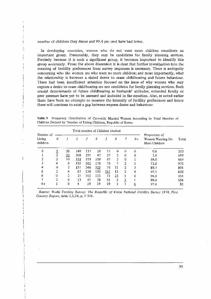
number of children they desire and 99.4 per cent have had fewer.

In developing countries, women who do not want more children constitute an important group. Presumably, they may be candidates for family planning services. Precisely because it is such a significant group, it becomes imp01tant to identify this group accurately. From the above discussion it is dear that further investigation into the meaning of fertility preferences from survey responses is necessary. There is ambiguity concerning who the women are who want no more children; and more importantly, what the relationship is between a stated desire to cease childbearing and future behaviour. There had been insufficient attention focused on the issue of why women who may express a desire to cease childbearing are not candidates for family planning services. Such crucial determinants of future childbearing as husbands' attitudes, extended family or peer pressure have yet to be assessed and included in the equation. Also, as noted earlier there have been no attempts to measure the intensity of fertility preferences and hence there will continue to exist a gap between express desire and behaviour.

Table 9 Frequency Distribution of Currently Married Women According to Total Number of Children Desired by Number of Living Children, Republic of Korea

Total number of Children Desired Number of Proportion of Living 0 1 2 3 4 5 6 7 8+ Women Wanting No Total children More Children

0 2 26 149 137 28 11 0 0 0 0.6 353 1 2 22 308 291 47 27 2 0 0 3.4 699 2 2 10 318 379 109 47 3 0 1 38.0 869 3 4 8 195 502 178 75 7 2 1 72.8 972 4 0 2 131 346 325 75 11 2 3 89.7 895 5 2 4 67 238 130 161 12 2 4 97.1 620 6 0 2 21 i02 125 71 21 5 6 96.9 355 7 2 0 13 47 38 51 2 1 1 99.4 156 8+ 1 0 4 19 19 29 3 1 Q_ 97.6 82

Source: World Fertility Survey: The Republic of Korea National Fertility Survey 1974, Ftrst Count1y Report, table 3.3.3B, p. T 334.

99

AN OVERVIEW OF MULTIVARIATE TECHNIQUES IN THE ANALYSIS OF SURVEY DATA

K. Srinivasan*

A. INTRODUCTION

Multivariate analysis is the branch of statistics concerned with analysing multiple measurements that have been made on one or several samples of individuals. Specifically it has come to be regarded as applicable to a situation involving two or more predictor variables with one or more dependent variables. For example, in the World Fertility Survey, information has been collected on different characteristics of households and individual couples along with data on the fertility of the couples. It may be noted that fertility of any woman depends on a number of factors, such as her fecundability, age at marriage, marital duration, contraceptive practice, incidence of foetal loss, lactation period, sex and survivorship of children already born. A multivariate analysis can be applied in order to find out the contribution of different socio-economic characteristics on the fertility of a woman (say, defined as children ever born) after taking account of biological variables. The simultaneous consideration of several predictor variables (also mentioned in the literature as independent variables) for which data are available in their relationships to a dependent variable is an important aspect of any multivariate analysis.

Sometimes it is desired to know how well all the variables taken together explain the variation in the dependent variable. The.criterion used is how closely a known function of the predictor variables could predict the dependent variable. At other times, interest may lie in examining the effect of a predictor variable, separately, to study how it relates to the dependent variable either considering or neglecting the effects of other predictor variables. A criterion used generally is its contribution to reduction in the unexplained variance or 'error'. Leading from this one may wish to exclude from a given set of predictor variables, irrelevant variables or variables which have very little effect on the dependent variable. Sometimes the researcher's concern may be the question of deriving optimum predictive relations. Knowing that some variables do influence a dependent variable, the issue 1nay be raised as to what type of functional form w·ould best predict the dependent variable. Incidentally, it may also be of interest to know whether the ability to predict under any analysis scheme is significantly better than chance. Tests of significance (F, t) are the usual criteria. Thus some of the major questions at which multivariate analytic techniques are directed are the following.

Given information on a set 'p' predictor variables (say socio-economic and biological variables) x 1, x 2 • •• Xp and a dependent variable (say cumulative fertility) Y on 'N' individuals:

* Director, International Institute for Population Studies, Bombay.

100

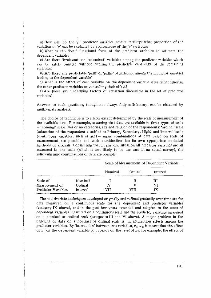
a) How well do the 'p' predictor variables predict fertility? What proportion of the variation of 'y' can be explained by a knowledge of the 'p' variables?

b) What is the 'best' functional form of the predictor variables to estimate the dependent variable?

c) Are there 'irrelevant' or 'redundant' variables among the predictor va1iables which can be safely omitted without altering the predictive capability of the remaining v\l,riables? 'd~re there any predictable 'path' or 'paths' of mfluence among the predictor variables

leading to the dependent variable? e) What is the effect of each variable on the dependent variable after either ignoring

the other predictor varjables or controlling their effect? f) Are there any underlying factors of causation discernible in the set of predictor

variables?

Answers to such questions, though not always fully satisfactory, can be obtained by multivariate analysis.

The choice of technique is to a large extent determined by the scale of measurement of the available data. For example, assuming that data are available in three types of scale - 'nominal' scale (yes or no categories, sex and religion of the respondent); 'ordinal' scale (education of the respondent classified as Primary, Secondary, High); and 'interval' scale (continuous variables, such as age) - many combinations of data based on scale of measurement are possible and each combination has its own appropriate statistical methods of analysis. Considering that in any one situation all predictor variables are all measured in one scale (which is not likely to be the case in an actual survey), the following nine combinations of data are possible.

Scale of Measurement of Predictor Variables

Nominal Ordinal Interval

Scale of Measurement of Dependent Variable

Nominal

I IV

VII

Ordinal

II v

VIII

Interval

III VI IX

The multivariate techniques developed originally and refined gradually over time are for data measured on a continuous scale for the dependent and predictor variables (category IX above), and in the past few years extended and adapted to the cases of dependent variables measured on a continuous scale and the predictor variables measured on a nominal or ordinal sc~le (categories III and VI above). A major problem in the handling of data on a nominal or ordinal scale is the interaction effects among the predictor variables. By 'interaction' between two variables, xl> x 2, is meant that the effect of x 1 on the dependent variable y, depends on the level of x 2 : for example, the effect of

101

'religion' on fertility may depend on the level of education, and in such a case it is said that there is an interaction between religion and education. This problem of interaction is one of the most difficult to handle in~ any multivariate analysis and is also usually encountered in the analysis of survey data.

B. METHODS OF ANALYSIS

In any situation where a multivariate problem is encountered, the method of analysis should proceed from simple to complex in an orderly manner. The simple methods include computation of the mean (and, if needed, variances) of the dependent variable in a series of two-way tabulations, classified by each of the predictor variables. Does the mean number of children born differ by religion, education of women etc.? Usually such simple two-way tabulations of data give good insight into the interrelationships among variables, which can later be tested by more rigorous statistical techniques. A unique advantage of such analysis is that it can be done irrespective of the scale of measurement of data and in many cases applications of more refined statistical techniques call for assumptions of the nature of the underlying distribution of variables and interactions among variables which can hardly be tested.

Thus, construction and study of the data in a series of two-way tables is an essential prerequisite before proceeding with any complex multivariate analytic techniques.

For example, for a subsample of 135 women from a fertility survey conducted in Goa in 1970, five variables were of interest: number of children ever born (y ); age of mother at the time of survey (x 1); duration of married life in years (x2); level of education (x 3); and religion (x 4). While the dependent variable and the first two predictor variables are in interval scale (or can be assumed continuous), education is given codes on an ordinal scale and religion is coded on a nominal scale. In order to study the effect of education of fertility, first a one-way cross-tabulation of mean fertility by education is prepared. This table reveals that the mean number of children ever born (y) for illiterates is 3.69; for literates below Standard III, 3.15; for Standards IV to X, 3.26; and for women with education at matriculation level and above, 2.04. Thus women of matriculation standard and above have clearly lower fertility than other education groups. Can this be due to the possibility that such educated v:omen are relatively younger than other 'Nomen because women's education is a recent phenomenon; or because their marital duation is less than other groups because educated women marry later.

Again preliminary analysis reveals that women with matriculation and above qualifi­cations have a mean age of 31.85, compared with a mean age of 30 for other groups of women; also they have a mean duration of marriage of 10.60, compared with 12.8 for other grouys. Thus it does not appear that the lower fertility of these groups can be explained by these factors.

102

However, the sample considered is small, the total being 135 women, 28 of whom had an attainment of matriculation level and above. In order to exclude the possibility of differences being attributable to chance factors, and to assess the joint effects of regressors on the dependent variable, more complex multivariate analyses such as analysis of variance and multiple regression are required.

In any such detailed statistical analysis, the analyst is as much interested in p(p + 1 )/2 different co-variances, among the (p + 1) variates, i.e. the 'p' predictor variables and the one dependent variable, as much as he or she is interested in (p +I) means and the (p +I) variances. In fact, the three types of statistics, namely, means, variances and co-variances, are the basic parameters of the multivatiate normal distribution assumed by most multivariate techniques. In various text books on multivariate analysis the following multivatiate analysis techniques have been listed.

a) Multiple regression analysis; b) Path analysis; c) Analysis of variance (ANOVA); d) Factor analysis; e) Cluster analysis

A short description of each method is given in the sections below. Details can be found in standard statistical text books, some of which are also referred to in each section. 1

MULTIPLE REGRESSION ANALYSIS

As before, given measurements on a set xv x 2 •.. Xp of predictor variables and one dependent variable, y, all in interval scale for a group of N individuals, the problem of multiple regression is to construct a linear function.

having the property that the sum of squared errors

is as small as possible for the data on hand. More specifically, the problem is to determine values of a, b1 b 2 • •• bp by using the least square method.

Historically, multiple regression analysis arose in the biological and behavioural sciences around the turn of the century in the study of the natural co-variation of observed charactetistics of samples of subjects. Somewhat later, analysis of variance and analysis of co-variance grew out of the analysis of agronomic data produced by the controlled variation of the treatment conditions in manipulative experiments.

1 .For example, a brier overview of these techniques and their application to survey data can be had from Overall and Klett (1972), Harris (1975) and Kendall (1976).

103

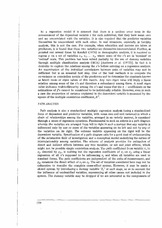
In a regression model it is assumed that there is a random enor term in the measurement of the dependent variable y for each individual, that they have mean zero and are uncorrelated with the variables. It is also required that the predictor variables themselves be unconelated with each other. In real situations, especially in fertility analysis, this is not the case. For example, when education and income are taken as predictors, it is found that these two variables are themselves intercorrelated. Further, as pointed out several times by Kendall (1976) in demographic analysis, it is required to regress y on a set of variables xv x 2 • •• Xp where some of the x's are in 'nominal' or 'ordinal' scale. This problem has been solved partially by the use of dummy variables through multiple classification analysis (MCA) [Andrews et al. (1973)]. In fact it is desirable to explore the relations among the x's before entering on a regression analysis. An examination of the individual correlations between pairs of variables may not be sufficient but is an essential first step. One of the best methods is to compute the co-variance or correlation matrix of the predictors and to determine the constants known as latent roots or eigen values of this matrix. Any zero eigen value will imply a linear relation among some of the x's and therefore a redundancy among them. A small eigen value indicates multicollinearity among the x's and warns that the b - coefficients or the estimations of {J's cannot be considered to be individually reliable. However, even in such a case the proportion of variance explained in the dependent variable is measured by the square of the multiple correlation coefficient, R 2 •

PATH ANALYSIS

Path analysis is also a standardized multiple regression analysis (using a standardized form of dependent and predictor variables, with mean zero and unit variance) in which a chain of relationships among the variables, arranged in an orderly manner, is examined through a series of regression equations. Fundamental to such an anlysis is a path diagram wherein the variables are arranged from left to right in such a manner that any variable is influenced only by one or more of the variables appearing on its left and not by any of the variables on its right. The extreme variable appearing on the right will be the dependent variable. Specification of a path diagram calls for a good deal of understanding of the substantive field of investigation and a conceptual model underlying the nature of interrelationship among variables. The scheme of analysis provides for estimation of direct and indirect efforts between any two variables, or net and joint effects, which might not be possible simple correlation analysis. The path coefficient from variable xi to xi, denoted by Pji> is nothing but the regression coefficient of xi on xi, using a linear regression of all x's supposed to be influencing Xj and when all variables are used in standard forms. The path coefficients are independent of the units of measurement, and Pji measures the direct effect of xi on xi. The set of variables considered here may not be exhaustive to describe the complete cause-effect system. However, it may be made a closed system by introducing a dummy variable 'Xr' at each stage, so as to account for the influence of unidentified variables, representing all other causes not included in the system. The dummy variable may be dropped if we are interested in the components of

104

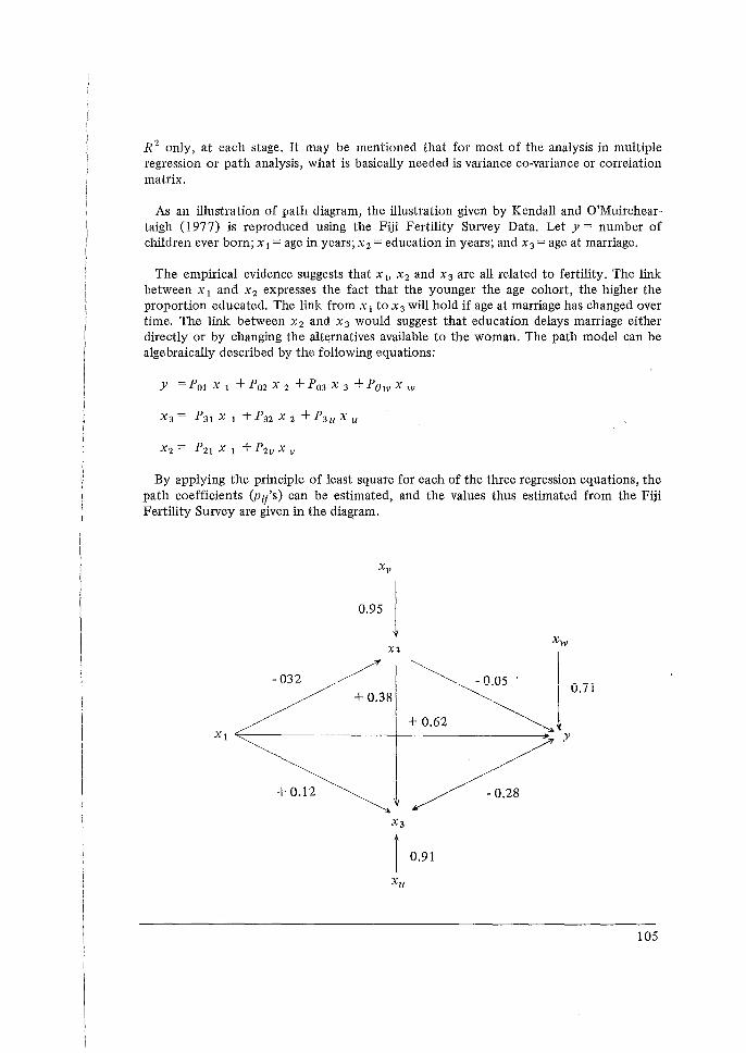
R 2 only, at each stage. It may be mentioned that for most of the analysis in multiple regression or path analysis, what is basically needed is variance co-variance or correlation matrix.

As an illustration of path diagram, the illustration given by Kendall and O'Muirchear­taigh (1977) is reproduced using the Fiji Fertility Survey Data. Let y = number of children ever born; x 1 =age in years; x 2 =education in years; and x 3 =age at marriage.

The empirical evidence suggests that xi> x 2 and x 3 are all related to fertility. The link between x 1 and x 2 expresses the fact that the younger the age cohort, the higher the proportion educated. The link from x 1 to x 3 will hold if age at marriage has changed over time. The link between x2 and x 3 would suggest that education delays marriage either directly or by changing the alternatives available to the woman. The path model can be algebraically described by the following equations:

y = P01 x 1 + P02 x 2 + Po3 x 3 +Pow x w

By applying the principle of least square for each of the three regression equations, the path coefficients (pi/s) can be estimated, and the values thus estimated from the Fiji Fertility Survey are given in the dia~am.

- 032

+ 0.12

0.95 I t

Xl

+ 0.38

X3

~ -OO<;· I __ _ +0.62 ~l U./l

y

-0.28

1 0.91

Xu

105

The predictive model y is as

y 0.62X1 - 0.05 X2 - 0.28 X3

direct effect of age"" 0.62

indirect effect of age through education= 0.02

indirect effect of age working through age at marriage= -0.03.

indirect effect of age working through education, in turn working through age at marriage= 0.03

The four effects add up to r01 = 0.64.

For a detailed descussion of path analysis, see Duncan (1966), Blalock, Jr. (1967), Wright (1960) and Kendall and O'Muircheartaigh (1977).

ANALYSIS OF VARIANCE

Analysis of variance, as a statistical technique, was originally developed in the analysis and interpretation of data compiled from agricultural experiments. Randomness of the observations and replication of experiments were considered essential in the application of the techniques. However, in recent years the technique is also being extensively used in disciplines in which experimental designs are not possible, such as social sciences. For example, in the analysis of human fertility, researchers rely more heavily on data of a non-experimental nature, observations made under different conditions as they occur, and the basic assumption of randomness and replicability are not fully met in this case. Even then the method is applied since the underlying principles are central to some of the logic of methods like correlation and regression analysis. The assumptions made in the analysis of variance are: (a) the populations from which the samples are drawn are normally distributed (or at least similar in distribution); (b) the samples are randomly drawn; (c) the observations in each sample are independent (hence the test is not appropriate for paired observations; and (d) common varianctJ exisls among the populations from which the samples are drawn (this is also called homoscedasticity). For some models of analysis of variance, the first assumption may be violated if the samples are large, and also the fourth assumption, if the number of cases in each sample is the same. But in general, if the assumptions are not clearly met, the ANOV A test will yield false results. As mentioned in the section A above, the purpose of the analysis is to partition the variance of the dependent variable into component units attributable to each of the influencing variables. Details can be obtained from Harris (1975) and other standard works by Anderson (1958).

106

FACTOR ANALYSIS

It has been mentioned earlier that it is difficult to sort out the contribution of each predictor vatiable under conditions of multicollinearity, where the predictor variables are highly correlated among themselves. Analysis of variance is a method which is more appropriate to data from expetimental designs, especially when there are two or more than two nominal scale variables with the dependent vatiable in the interval scale. In the analysis of variance it is also possible to test for the existence of interaction between vatiables.

When there is interaction or multicollinearity, factor analysis can be used in order to find out whether a number of predictor vatiables together can be considered as a measure of an underlying common factor, the factor being a specified linear combination of some vatiables. All the 'p' predictor variables can be reduced to a smaller number (say k) of 'factors' (Z's) which are independent among themselves and hence the regression equation of y on Z's instead of X's becomes more meaningful and the regression coefficients more reliable. Factor analysis begins with the correlation matrix of the predictor variables and attempts to explore the possibility that the phenomenon being studied could be expressed in terms of a smaller number of underlying factors.

Thus the method of factor analysis involves deriving new factor variates as linear transformations of the original correlated predictive variables (X's). Rather than deriving the desired transformation from direct analysis of the otiginal variables, it is compu­tationally more efficient to detive the factor matrix as a simple transformation of the matrix of intercorrelations among the otiginal vatiables. Factors are conceived as primary dimensions of individual differences. Desirable properties of a good factor solution (transformation) include (a) parsimony; (b) orthogonality, or at least approximate independence; and (c) conceptual meaningfulness. These objectives are sought by judicious choice of the transformation matrices.

There are several methods of extracting factors. The basic model of factor analysis may be written as

x{j = a;1 x i + a;2 x~ + ..... a;n x~ +a; v[ +a; er

That is, the variance associated with any particular observation x;; is composed of variance common to some of the other vatiables in the matrix, plus variance unique to the particular variable, plus error valiance. The basic problem of factor analysis is to deter­mine the coefficients ail, a;2, a;11 of the common factors in the variance.

There are several methods of factor analysis discussed in literature. These include the diagonal method, the centroid method, principal axes factor analysis, orthogonal-powered vector factor analysis [for details, see Overall and Kleet (1972)].

107

Factors so obtained can be used for regression analysis. The contribution of each factor towards variation in the explained variable can easily be obtained.

CLUSTER ANALYSIS

Cluster analysis may be used to determine which of the predictor variables can be clustered into groups, such that the variables within each cluster have maximum inter­correlations and variables between two different clusters have minimum intercorrelations. When the variables are not correlated among themselves, each variable is a cluster unto itself and also a factor by the factor analysis. There are various methods of cluster analysis, but the method that seems most useful is called Tyron's coefficient of belonging, or the B-coefficient method. Since the objective is to find the variables that form groups with maximum intercorrelation, the first group is formed with the two variables that correlate highest. This group is then added to the variable that correlates the highest with each of the first two, and then a fourth, and so on, until a point is reached where the newest variable added is not more highly correlated with the variables in the group than with the remaining variables. This means that it does not belong to that group any more but belongs to the group of other variables. This is what the B-coefficient measures. B is defined as

where G is the sum of correlations in a group, ng is the number of variables in the group, T is the sum of the correlation of the variables in the group with all the remaining variables, and nr the number of remaining variables (nr ).

Cluster analysis, however, does not provide a method of uniquely determining the minimum number of factors that express a correlation matrix unless the variables are factorily pure. But it can help demonstrate which variables could be grouped on the basis of communality measured in terms of high correlations.

C. SUMMARY AND CONCLUSION

There have been, during the past three decades, remarkable developments in statistical methods to deal with the analysis and interpretation of data arising out of multiple observations on individuals chosen at random from a population. Each of these multi­variate techniques, as they are called, has underlying it a host of assumptions mostly regarding the nature of distribution of the characteristics in the population, correlations among the variables, interaction with regard to their effects on a particular variable designated as the dependent variable, and causal mechanisms underlying the interrelation­ships. The assumptions vary not only by the method but also by the procedure of

108

collection of data, by scientific experimentation, or observation of phenomena as they occurred naturally, such as in sample surveys of population with regard to social, economic and demographic variables, and also the scale of measurement of the variables. All the analytic methods developed are relatively more valid for data collected through experimental designs where the principles of randomization and replication fundamental to most of the analytic methods could be preserved. The limitations i'l the generaliza­bility of the findings obtained from these methods to data collected from sample surveys, in social sciences, should be kept constantly in mind and towards this purpose the other lectures on specific methods deserve careful attention.

109

BIBLIOGRAPHY

Anderson, T.W., frltroduction to Multivariate Statistical Analysis, New York, John Wiley and Sons, 1958

Andrews, F.M. and others, Multiple Classification Analysis, Survey Research Centre, Institute for Social Research, University of Michigan, Ann Arbor, 1973.

Blalock, H.M. Jr., 'Path Coefficients Versus Regression Coefficients', The American Journal of Sociology, vol. 72, No. 6 {pp. 675-676), 1967.

Draper, N.R. and H. Smith, Applied Regression Analysis, New York, John Wiley and Sons, 1966.

Duncan, O.D. 'Path Analysis: Sociological Examples', The American Journal of Socio­logy, vol. 72, No. 1{pp.1-16), 1966.

Fruchter, B., Introduction to Factor Analysis, van Nostrand, New York, 1954. Harmen, H.H., Modern Factor Analysis (revised edition), University of Chicago, Chicago,

1967. Kendall, M.G., 'Some Notes on Statistical Problems Likely to Arise in the Analysis of

WFS, Survey', World Fertility Survey, Technical Bulletin, No. 11, 197 6. Kendall, M.G. and C.A. O'Muircheartaigh.,'Path Analysis and Model Building', World

Fertility Survey, Technical Bulletin, No. 2/Tech. 414, March 1977. Overall, J.E. and J.C. Klett., Applied Multivariate Analysis, New York, McGraw Hill Book

Co., 1972. Palumbo, T.D., 'Simple Linear Correlation and Regression', and 'Partial and Multiple

Correlation and Regression', Statistics in Political and Behavioral Science, Appleton - Century - Croffs, Educational Division, New York {pp. 177-217), 1969.

Snedecor, W.G. and W.G. Cochran, 'Multiple Regression and Covariance', Statistical Methods, The Lowa State College Press {pp. 413-447), 1966.

Werts, C.E., G.J. Karl and L.L. Robert, 'Identification and Estimation of Path Analysis with Unmeasured Variables', American Journal of Sociology, Vol. 78, No. 6 (pp. 1469-1484), 1973.

Wright, S. 'Path Coefficients and Path Regression: Alternative or Complementary Concept?', Biometrics: 16, no. 2 {pp. 189-202), 1960.

110

MULTIPLE CLASSIFICATION ANALYSIS AND ITS APPLICATION TO THE 1974 FIJI FERTILITY SURVEY

N. Ogawa*

A. INTRODUCTION

There is no doubt that human behaviour is of great complexity with numerous unknown causal links. In most cases, it involves a simultaneous reaction of an almost infinite num­ber of variables. In other cases, it induces a causal chain of a set of many variables. Obvi­ously, the present state of knowledge of social sciences is still far from the stage where it can account for the complex variations in human behaviour in any satisfactory and accu­rate manner. In contemporary social sciences, therefore, much effort is being directed to­ward the clarification and, if possible, quantification of the complex causal links of the variables operating in the phenomenon in question.

In order to facilitate such exploratory research, social scientists are conducting in their own disciplines a number of modern sample surveys. These scientifically-designed surveys­generate a vast amount of data for a wide range of variables. The collected data, used for multipurposes, ranges from mere reporting of descriptive statistics to more sophisticated statistical analyses. Existing social science theory provides only a crude indication of probable relationships of variables. This prevents analysts, first, from deducing specific hypotheses from theory, and, second, from testing their validity on the basis of the data gathered. For these reasons, analysts most frequently work back and forth between theory and data. A close examination of data may reveal observable regularities, which suggest a new behavioural pattern to be used for simplifying or improving existing concep­tual frameworks. These empirical regularities can be further extended, first, to the induc­tion fo theoretical models, and then to deductive model-testing. In the inductive process, relationships observed within the data may lend themselves to forming a set of proposi­tions, consequently leading to the formulation of specific functional hypotheses relating to a specific aspect of a social system. Then in the model-testing phase, these newly­formed hypotheses are tested and verified in other data sets and their relationships within a social system are statistically estimated. Repeated verification of the validity of these hypotheses leads to the construction of more formal predictive models and subsequently suggest a new behavioural pattern to be used for simplifying or improving existing concep­tional mechanism of the social system, and essentially the major objective of many con­temporary research activities is to estimate statistically the linkages in the social system.

B. PROBLEMS RELATED TO SURVEY DATA ANALYSIS

The statistical estimation is usually a two-step process: the selection of variables signifi-

* At time of writing, the author was a member of the ESCAP secretariat. From January 1980 his address will be: the Population Research Institute of Nikon University, Tokyo, Japan,

111

cantly related to the hypotheses in question and the specification of functional relation­ships of the appropriate variables. Not many theories suggest a definite set of variables with well-specified functional relationships. Because of this drawback, it is not an easy task to choose one correct form.

In order to facilitate the following discussion, a sample survey model is expressed in a simple functional notation:

Where 1) Y denotes a dependent variable which is either dichotomous or continous or equal interval,

2) X 1, X 2, •••• X 11 are a set of predictors which are as weak as nominal scales, and

3) e represents a stochastic (error or disturbance) term. Given this functional specification, analysts attempt to compute coefficients of the predictors which give the minimum value of the stochastic error term, thus maximizing the predictability of the estimated function.

It is important to note that the inclusion of a stochastic error term is rationalized by three types of consideration. First, it represents the effect of all of the exluded variables. It is virtually impossible to gather all the necessary data for an infinite number of factors responsible for variations in Y. Secondly, it captures unpredictable, random elements in human behaviour. It can be assumed that the random variable is conveniently grouped into a set of the above-mentioned excludes variables, although an additional term for randomness can be technically incorporated. Thirdly, a disturbance term is included to allow for all measurement errors. In order to avoid possible complications of analysis, it is common practice to assume that the stochastic disturbance term has constant variance with the mean equal to zero; and the various values of the disturbance term are indepen­dent of each other. Given these constraints, if the function is incorrectly specified, dis­turbance terms are excessively large or not random.

In the above, from the standpoint of research designs, we have discussed the problem of functional form in the analysis of data in general. Let us now consider technical diffi­culties relating to functional forms in terms of data gathered in modern surveys such as the World Fertility Survey. As noted earlier, the primary objective of such large-scale surveys lies in analyses of social situations in which numerous variables are interrelated in a complex manner. Such intricate interactive links in human behaviour necessitate multi­variate techniques. In sample survey models, however, an analysis of the joint effect of X 8 upon Y by multivariate techniques encounters several vexing problems (Morgan and Sonquist, 1963).

112

One of the most common problems facing the analyst is that many of the data used as predictors are classifications rather than genuinely continuous variables with normal dis­tributions. Even in the case of continous variables, if their effects are non-linear, class intervals may be more appropriate.

Secondly, large-scale survey data tend to contain measurement errors in all the variables included in the function. Multivariate techniques do not usually deal with the measure­ment problem in any explicit sense. For instance, no exploration into the size and distri­bution of the errors is attempted in multivariate techniques.

Thirdly, modern sample surveys are, by and large, well designed on a scientific basis. Complex sampling is conducted by the use of clustering and stratification techniques, which violate the assumption of simple random sampling underlying conventional signifi­cance tests. Strictly speaking, these complex samples prevent the analyst from applying conventional significance tests to collected data, although such tests can still be useful if the significance levels are not interpreted too literally.

The fourth difficulty in multivariate techniques in the analysis of survey data centres around the problem of intercorrelations among predictors. Apparently, the principal objective of multivariate techniques is the evaluation of the relative importance of pre­dictors simultaneously affecting each other. Technically, this objective is fulfilled by assessing one strategic variable while holding all others constant. However, higher degree of intercorrelations make such assessments more difficult. It should also be noted that in multivariate analysis, classificatory data is more likely to present a more serious multi­collenearity problem than continuous variables.

The fifth point, somewhat more troublesome than the problems discussed so far, is related to the problems of interaction effects. A salient example of interaction is provided by the variables related to family life-cycle, namely, age, marital status, age of children, etc. (Kish and Lansing, 1957). In spite of their importance, interaction effects are one of the most neglected aspects of data analysis. Unfortunately, Ln. most current survey research data analyses, the analyst applies an additive least squares procedures to his data set, assuming no interaction effect. This statistical assumption contributes to a great reduction in computational complexity.

The sixth and last problem, associated with chains of causation, has increasingly con­cerned analysts in the recent past. The question of logical priorities arises when variables are considered on a simultaneous basis in data analysis. In practice, the analyst either restricts his analysis to one level or conducts a sequential analysis.

At present, there are several relatively efficient multivariate techniques developed. These techniques include analysis of variance, factor analysis, multiple regression, path analysis and multiple classification analysis. However, it is important tot note that each of

113

these techniques has its own limitations, thus being at a different level of efficiency in its analysis precedures. In fact, none of these techniques can perfectly deal with all of the above-mentioned statistical difficulties in the analysis of survey data. Among these multi­variate techniques, we will discuss in detail the basic feature of multiple classification analysis and its usefulness and limitations in the following few sections.

C. MULTIPLE CLASSIFICATION ANALYSIS: ITS BASIC FORMULATION AND PROPERTIES

Multiple classification analysis (MCA) techniques were originally developed by Yates (1934) and elaborated by Anderson and Bancroft (1952). In 1963, the computerized MCA programme was prepared by a group of researchers at the Survey Research Center of the University of Michigan. Since then, the MCA programme has been widely used in social science research.

MCA techniques are applicable to one dependent variable and two or more predictor (or independent) variables. The dependent variable should be either an interval scale or a dichotomous classification. The latter case is equivalent to a form of two-group dis­criminant function analysis. Moreover, because observed values of a dependent variable affect the means and variance, both of which are required for the computation of other statistics, they should not be unduly skewed. If a collected data set for the dependent variable shows such irregularities, transformations by its square root or logarithm should be attempted. If the dependent variable is dichotomous in nature, other statistical pro­cedures including a logistic analysis are also recommended.

Predictor variables being as weak as nominal measurements, is one of the most distin­guished advantages of MCA. Most of the multivariate methods require predictors stronger than nominal variables. Furthermore, MCA deals not only with linear but also non-linear relationships among predictors and the dependent variables.

Technically, the MCA prediction model can be described as having the overall mean as its constant term and main effects, or a series of additive coefficients for the category. The additivity assumption implies that differences according to one predictor are the same for all values of the other predictors included in the model. The model can be expressed by the following equation:

where Yijk score of a particular individual who falls into i-th category of predictor A, j-th category of predictor B, etc,

Y grand mean of Y,

114

ai added effect of i-th category of predictor A (= difference between Y and the mean of its cat­egory of predictor A),

bj added effect of j-th category of predictor B (= difference between Y and the mean of j-th cat­egory of predictor B).

The coefficients for a certain predictor estimated by solving the normal equation system are called adjusted or net effects of the predictor. These effects measure those of the predictor alone after taking into account the effects of all other predictors. Should there be no intercorrelation among predictors, the unadjusted or gross effects would be identical with the adjusted or net effects.

Besides the adjusted and unadjusted effects, we will now consider other computed statistics, which reveal the closeness of the relationship between the predictors and the dependent variable. For instance, the eta (ri) coefficient is a correlation ratio, which shows how well a given predictor can explain the variation in the dependent variable, while the eta2 (77)2 coefficient indicates the proportion of the variation explained by the predictor alone. These statistics are applicable to the unadjusted means. On the other hand, the beta (~) coefficient measures, on the basis of the adjusted means, the ability of a given predictor to account for variations in the dependent variable. The beta coefficient is often compared to the partial correlation coefficient in multiple regression analysis. Although these two indices are not, in general, equal to each other, the relative magnitudes of the betas for different predictors will, in most cases, be comparable to the correspond­ing partial correlation coefficient (Morgan, 1971). Similarly, the beta2 (~)2 coefficient shows what proportion of the variation is explained by the predictor, after taking into account the proportion explained by other predictors. The interpretation of beta and beta2 requires greater caution, because they refer to the adjusted means which allow for intercorrelations among the predictors. Both beta and beta2 coefficients are frequently regarded as summary statistics indicating the relative importance of each predictor. In recent years, however, there have been numerous views against the use of these statistics for this particular purpose. Because the beta2 coefficient is expressed in terms of the weighted sum of squares of the adjusted deviations to the standard deviation of the de-pendent variable, it cannot be interpreted as the proportion of variance cxplah"1.cd, unless the predictors are totally uncorrelated with each other. Often enough, a total of the beta2

coefficients for the various predictors exceeds a unity. In order to avoid confusion, there­fore, some research analysts use different statistics. An example is the percentage of the variance in the dependent variable explained by a certain predictor, net of other predictors (Blau and Duncan, 1967; Palmore et al., 1975).

'R 2 unadjusted is the actual proportion of variance in the dependent variable explained by using the obtained coefficients in an additive model applied to the

115

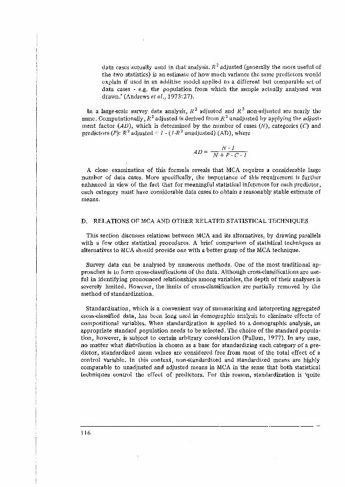
data cases actually used in that analysis. R 2 adjusted (generally the more useful of the two statistics) is an estimate of how much variance the same predictors would explain if used in an additive model applied to a different but comparable set of data cases - e.g. the population from which the sample actually analysed was drawn.' (Andrews et al., 1973:27).

In a large-scale survey data analysis, R 2 adjusted and R 2 non-adjusted are nearly the same. Computationally, R 2 adjusted is derived from R 2 unadjusted by applying the adjust­ment factor (AD), which is determined by the number of cases (N), categories (C) and predictors (P): R 2 adjusted= 1 -(l-R 2 unadjusted) (AD), where

N-1 AD= N+P-C-1

A close examination of this formula reveals that MCA requires a considerable large number of data cases. More specifically, the importance of this requirement is further enhanced in view of the fact that for meaningful statistical inferences for each predictor, each category must have considerable data cases to obtain a reasonably stable estimate of means.

D. RELATIONS OF MCA AND OTHER RELATED STATISTICAL TECHNIQUES

This section discusses relations between MCA and its alternatives, by drawing parallels with a few other statistical procedures. A brief comparison of statistical techniques as alternatives to MCA should provide one with a better grasp of the MCA technique.

Survey data can be analysed by numerous methods. One of the most traditional ap­proaches is to form cross-classifications of the data. Although cross-classifications are use­ful in identifying pronounced relationships among variables, the depth of their analyses is severely limited. However, the limits of cross-classification are partially removed by the method of standardization.

Standardization, which is a convenient way of summarizing and interpreting aggregated cross-classified data, has been long used in demographic analysis to eli...111inate effects of compositional variables. When standardization is applied to a demographic analysis, an appropriate standard population needs to be selected. The choice of the standard popula­tion, however, is subject to certain arbitrary consideration (Pullum, 1977). In any case, no matter what distribution is chosen as a base for standardizing each category of a pre­dictor, standardized mean values are considered free from most of the total effect of a control variable. In this context, non-standardized and standardized means are highly comparable to unadjusted and adjusted means in MCA in the sense that both statistical techniques control the effect of predictors. For this reason, standardization is 'quite

116

analogous to MCA, and when appropriate, should give very nearly the same conclusion' (Pullum, 1977:49). Nevertheless, it is clear that the standardized quantities should not be over-emphasized because they would be substantially different if other standard popula­tions were used. As compared with standardization, MCA is a more sophisticated tech­nique with controls simultaneously a number of variables within the framework of an additive model fitted by the method of least squares. Hence, standardization may be considered as a supplementary technique for cross-classification analysis when analytic recources required for a more refined analysis are limited.

It is important to note that standardized mean values are not completely free from the total effect of the control variable. Its compositional effect is observed not only in the between-category sum of squares but also in the within-category sum of squares. Standard­ization dealing only with the between-category effect excludes the within-category effect from its analysis. This statistical limitation, however, is also applicable to the MCA tech­nique. Furthermore, similar to MCA, standardization contributes to the reduction of the variability of the mean values in all the categories of the control variable, unless the control variable acts as a 'suppressor'. The degree of such variability indicates the im­portance of the control variable.

Another point to be stressed relates to the limitation of additivity. Both standardization and MCA assume an additive structure or a struchue where higher order interactions among the variables are ignored. When non-addivity is present in the data, all the standard­ized values are biased, consequently nullifying the validity of the standardization tech­nique.

As mentioned earlier, MCA is considered to be as an extension of standardization because the observed means can be adjusted by fitting additive models. Other examples of these models include analysis of variance and the 'dummy variable' in regression analysis. First, let us consider analysis of variance. It is a well-known fact that in a two-way analysis of variance, factor effects are orthogonal (or non-correlated) if each cell of cross-classifi­cations of both factors has the same number of observations. If the frequencies in each cell are not equal but are proportional to the marginal frequencies of the factors, main effects are still orthogonal, but both interaction effects and main effects tend to be inter­<lepentlent with each otheI. When cases in each.cell are not proportional to the margL1al frequencies of the factors, the analysis of variance becomes somewhat complex; the com­ponent sums of squares do ·not add to the total sum of squares because the main effects are usually intercorrelated with each other and the interaction effects are not indepen­dent of the main effects. However, whatever frequencies each cell of the factors may have, in the classic two-way experimental approach, the total sum of squares can be divided into three parts: (1) sum of squares owing to additive effects of the two factors; (2) sum of squares cwing to the interaction effects; and (3) sum of squares owing to errors. Based upon the three sums of squares, significance tests are applied to the data.

117

It should be noted, however, that significance tests do not provide specific information about the pattern of effects. When examining the pattern of effects, a general statistical model for the two-way analysis of variance can be specified as follows:

where Zij denotes the effect of interaction between i-th category of factor A and j-th category of factor B.

Essentially, if there is no interaction between the two factors, the term Zif vanishes, and consequently this two-way analysis of variance becomes an additive model. In fact, it is within this additive model that the MCA method applies. Therefore, MCA is a special case of the analysis of variance and can be used as a method of displaying results of the ana­lysis of variance where significant interaction effects are absent. Obviously, the analysis of variance has an advantage over MCA in dealing with data sets where interaction is expected.

In addition to the additive analysis of variance, MCA can be compared with another statistical technique which performs equally well, called the 'dummy variable' in re­gression analysis. In ordinary regression computations, a dummy variable either takes zero, or if the observation falls on a particular class of a certain characteristic, the value one. The estimated regression coefficients of the dummy variables correspond to deviations from the means of the omitted reference class. Similarly, the coefficients com­puted by MCA techniques represent deviations from the grand mean. Although the numerical results produced by both MCA and dummy variable regression techniques are identical after simple mathematical operations, the use of MCA seems to be more prefer­able for purposes of exposition. Furthermore, in handling a data set, MCA necessitates 'no conversion of the basic data, no creation on card or input tape of a dummy variable. Each class of each predicting characteristic becomes, in essence, a dummy variable. Most regression programmes would require a separate recording to create the variables.' (Andrews et al., 1973:50). It should be stressed, however, that MCA may have some operational advantages although no theoretical virtues of the multivariate regression analysis with dummy variables.

A shnple numerical example may further clarify the relations of ~v1CA and its alter­natives. For such illustrative purposes, table I contains computational results of standard­ization, dummy regression and MCA, based upon the 1974 Fiji Fertility Survey data. The variables uses are the number of children ever born as the dependent variable, and both duration of marriage and childhood types of place of residence as predictors.

118

---------------------------------- -------- ------ -

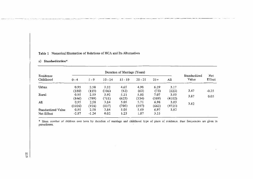
...... \0

Table 1 Numerical Illustration of Relations of MCA and Its Alternatives

a) Standardization*

Duration of Marriage (Years) Residence Standardized Net Childhood 0-4 5-9 10 -14 15 - 19 20 -25 25+ All Value Effect

Urban 0.95 2.50 3.32 4.65 4.98 6.29 3.17 (180) (119) (106) (82) (63) (73) (623) 3.47 -0.35

Rural 0.95 2.59 3.92 5 .11 5.80 7.07 3.93 3.87 0.05 (846) (799) (711) (623) (534) (589) (4102)

All 0.95 2.58 3.84 5.05 5.71 6.98 3.83 3.82 (1026) (918) (817) (705) (597) (662) (4725)

Standardized Value 0.95 2.58 3.84 5.05 5.69 6.97 3.82 Net Effect -2.87 -1.24 0.02 1.23 1.87 3.15

* Mean number of children ever born by duration of marriage and childhood type of place of residence. Base frequencies are given in parentheses .

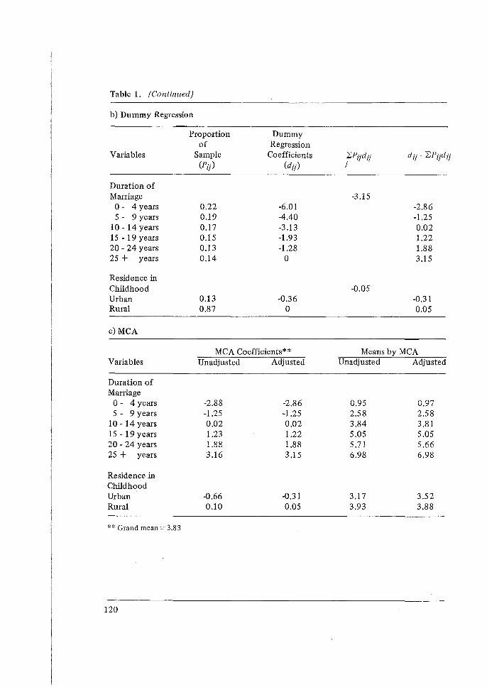
Table 1. (Continued)

b) Dummy Regression

Proportion Dummy of Regression

Variables Sample Coefficients ~Pijdij dij - L.P;jdij (Pij) (dij) J

Duration of Marriage -3.15

0 - 4 years 0.22 -6.01 -2.86 5 - 9 years 0.19 -4.40 -1.25

10 - 14 years 0.17 -3.13 0.02 15 - 19 years 0.15 -1.93 1.22 20 - 24 years 0.13 -1.28 1.88 25 + years 0.14 0 3.15

Residence in Childhood -0.05 Urban 0.13 -0.36 -0.31 Rural 0.87 0 0.05

c)MCA

MCA Coefficients** Means by MCA Variables Unadjusted Adjusted Unadjusted Adjusted

Duration of Marriage 0- 4 years -2.88 -2.86 0.95 0.97 5 - 9 years -1.25 -1.25 2.58 2.58

10 - 14 years 0.02 0.02 3.84 3.81 15 -19 years 1.23 1.22 5.05 5.05 '1() - '"lA ,,ranf'('I ~v-.w-.:1...,u....o 1.88 1.88 5.71 5.66 25 + years 3.16 3.15 6.98 6.98

Residence in Childhood Urban -0.66 -0.31 3.17 3.52 Rural 0.10 0.05 3.93 3.88

**Grand mean= 3.83

120

As for standardization, it is logical that the non-standardized means are identical with MCA unadjusted means. On the other hand, in the absence of serious interaction effects the standardized means are nut exactly identical but highly comparable to adjusted means obtained by MCA. Furthermore, the coefficients computed by MCA can be converted to those computed by dummy regression, by using the following relationship:

where 111ij

dtj

Pij

111/j = dtj - ~ Pij dtj I

MCA coefficient for j-th category of predictor i, dummy regression coefficient for j-th category of variable i, proportion of observed cases in j-th category of predictor i.

It is clear from these numerical results that MCA is parallel with standardization and is identical with dummy variable regression analysis.

E. LIMITATIONS OF MULTIPLE CLASSIFICATION ANALYSIS

Similar to other widely used statistical methods, the noted advantages of MCA techniques are partially depreciated by a few limitations in their use. As noted previously, an analysis by MCA techniques requires a substantial number of observations for obtaining reliable estimates of means. Moreover, there are two severe problems in connexion with intercorrelation. First, excessively close intercorrelation among predictors causes serious difficulties in computing the values for their coefficients. Although categories variables may explain more of total variance than a linear regression using continuous variables, categoried variables are more likely to overlap too closely with each other. (A more detailed discussion on this multicollinearity problem is available in the annex.) Second, unless predictors are statistically independent of each other, the total of sums of squares for gross effects would be either more or less than, but not equal to, the sum of squares for the additive model. Because of 'positive' or 'negative' overlap there is no unique answer to the question of how much variation is explained by a particular predictor when predictors are intercorrelated (Blau and Duncan, 1967: 133).

Besided these weaknesses, the use of MCA techniques has been seriously contended with regard to the relevance of its additivity assumption. In general, the formulation of models is to be parsimonious; the structure of models is to be as simple as it is consisfont with minimum variance of the error terms. To achieve this goal, the analyst applies long­known assertions that additivity is a good initial approximation of reality. However, according to Blalock (1965), although additive models approximate reality well in many cases, common-sense judgements often call for non-additive models as an alternative. Referring to various likely sources of interaction, Sonquist (1970) insists that 'additivity does not seem to be the rule in real life. An examination of much recent sociological research reveals that in fact interaction terms appear with such frequency that one is led to suspect that simple additivity may actually be the exception.' (Sonquist, 1970:30).

121

Theoretically, if the additive assumption is applicable to the data with interaction effects present, this statistical model commits the specification error, thus producing biased estimates of coefficients. Often enough, the presence of interaction effects makes the concept of main effects void. Furthermore, because the exclusion of interaction terms from the model specification leads to large error terms which are scattered randomly, careful exawination of residuals helps the analyst to identify such patterns.

Although MCA assumes that the effects of the category variables are additive, it is possible to incorporate interactions into the analysis by defining composite variables. To inplement this, considerable prior knowledge is needed; one must acquire detailed information such as what portion of data cases is subject to interaction effects and what functional form should be applied to capture such effects accurately. In reality, however, it is extremely difficult to obtain such information. Even if one could identify interaction effects and incorporate composite variables, the number of distinct category effects would be as many as the product of the categories. Therefore, an inclusion of composite variables in MCA might lead to insufficient data cases for each category of the composite variable. In view of this drawback, one may tend to accept an additive model as a sufficiently proper analytic framework for the data, although it is not totally correct.

In search of a more proper solution to the problem of model specification, the automatic interaction detection technique (AID) was developed by Morgan and Sonquist (1970). Basically, this technique is a step-wise application of oneway analysis of variance; it partitions the sample into a series of non-overlapping subgroups, the means of which account for the variation in the dependent variable more than any other subgroup. The computational results are shown by a treelike pattern. Repeated experiments essentially indicate that additivity in the data results in a symmetric tree structure, while interaction effects form an asymmetric tree structure.

It is important to note, however, that the AID analysis, primarily designed for locating interacting variables, shows its limitations in its reported information about models when additivity applies. Because it fails to deal with intercorrelated predictors as precisely and efficiently as MCA techniques, MCA becomes a judicious choice for additive models. AID, on the other hand, should be used to obtain information on functional forms applicable to the data and locate interaction terms to be included in subsequent analyses by MCA. If AID cannot detect any interaction terms, then it provides a cogent basis for introducing additivity assumptions into analysis. Hence, both MCA and AID can be jointly utilized, being supplementary to each other in survey data research.

In the above, we have discussed (a) a variety of the statistical problems arising from analyses of the data generated by contemporary surveys, (b) the basic features of MCA techniques, (c) MCA and its alternative techniques and (d) both advantages and dis­advantages of application of MCA to survey data. In the sections that follow, we will actually apply MCA techniques to the data collected in the Fiji Fertility Survey, a salient example of present-day research surveys.

122

F. FIJI FERTILITY SURVEY, 1974: BACKGROUND

In 1974, the Fiji Fertility Survey (FFS) was conducted as the first survey completed in conjunction with the World Fertility Survey programme. FFS covered, on a random­sampling basis, more than 5 ,000 households corresponding to 9 5 per cent of the population of Fiji. After gathering information on the composition of each household and other household-related matters, survey interviewers carried out an intensive interview with a total of 4,928 ever-married women aged 15 to 49. The term 'ever­married' refers to both legal and consensual marriages.

Geographically, Fiji is located in the Pacific Ocean, compnsmg over 300 islands scattered across 164,000 square miles. Nearly two thirds of the population resides in rural areas while the remaining third resides in urban or peri-urban areas including the largest urban centre, Suva, which is the capital city of Fiji.

The ethnic composition of Fiji is clearly divided into two major groups: the Fijians (242,000 or 44 per cent of the total) and the Indians (281,000 or 51 per cent of the total). It is important to note that Indians were brought to Fiji between 1879 and 1916, as indentured labourers in the agricultural sector. Since then, the population of Indians has grown rapidly and even exceeded that of Fijians. Accordingly, an analysis of past fertility trends in Fiji requires adequate knowledge of the historical background and socio-economic and cultural characteristics of both ethnic groups.

Records of the birth registrations, although approximately 10 per cent of births are presumably unreported, shows that Fiji's crude birth rate dropped substantially from 40 per thousand in the 1950s to 28 per thousand in 1973. This dramatic decline in fertility is attributable principally to rapid fertility reduction of the Indians in the last two decades or so. The Fijians also registered a considerable decline in the crude birth rate, although their fertility level since the 1950s had already been at a relatively low level. In line with Fiji's rapid fertility reduction, many development-related factors have indicated improve­ments. For example, in the last 20 years, Fiji's educational coverage has been expanding at a remarkable rate. Children in the primary school age span are almost universally enrolled. At higher educational levels, enrolment rates have increased distinctively. Interestingly enough, Fiji's economy is complex, ranging from subsistence agriculture to rapidly growing non-agricultural sectors, However, more than half of the labour force is engaged in non-agricultural production.

In the next section, a few selected FFS findings with regard to the birth cohort fertility and the set of factors influencing it will be highlighted in order to formulate a theoretical framework for the use of MCA techniques.

123

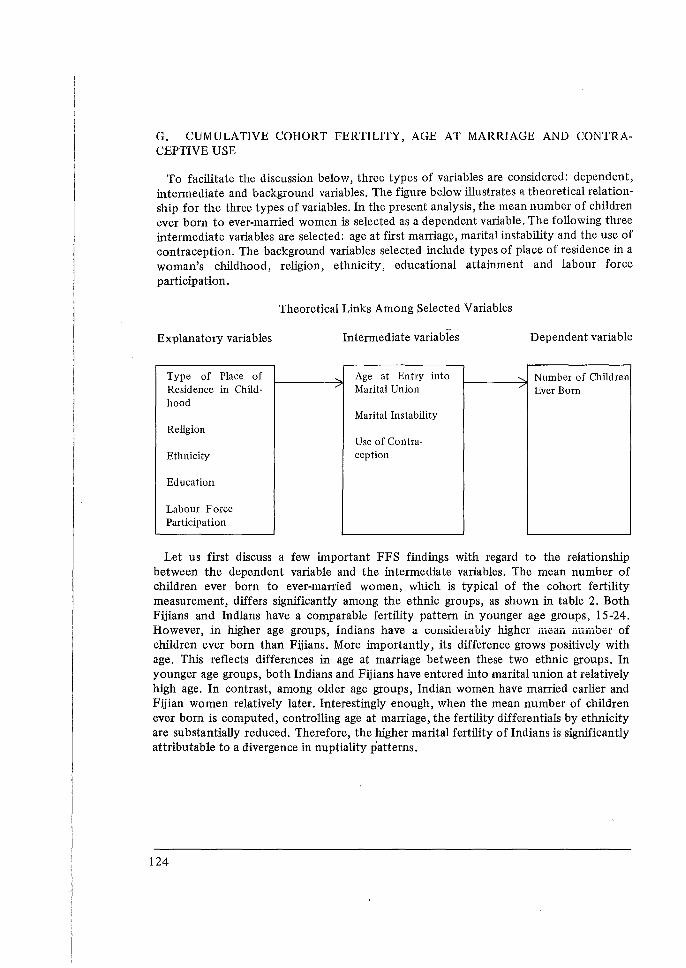
G. CUMULATIVE COHORT FERTILITY, AGE AT MARRIAGE AND CONTRA­CEPTIVE USE

To facilitate the discussion below, three types of variables are considered: dependent, intermediate and background variables. The figure below illustrates a theoretical relation­ship for the three types of variables. In the present analysis, the mean number of children ever born to ever-married women is selected as a dependent variable. The following three intermediate variables are selected: age at first marriage, marital instability and the use of contraception. The background variables selected include types of place of residence in a woman's childhood, religion, ethnicity, educational attainment and labour force participation.

Theoretical Links Among Selected Variables

Explanatory variables Intermediate variables Dependent variable

Type of Place of ..... Age at Entry into ...... Number of Children Residence in Child- / Marital Union / Ever Born hood

Marital Instability Religion

Use of Contra-Ethnicity ception

Education

Labour Force Participation

Let us first discuss a few important FFS findings with regard to the relationship between the dependent variable and the intermediate variables. The mean number of children ever born to ever-manied women, which is typical of the cohort fertility measurement, differs significantly among the ethnic groups, as shown in table 2. Both Fijians and Indians have a comparable fertility pattern in younger age groups, 15-24. However, in higher age groups, Indians have a wnsiderably higher mean number of children ever born than Fijians. More inipo1iantly, its difference grows positively with age. This reflects differences in age at marriage between these two ethnic groups. In younger age groups, both Indians and Fijians have entered into marital union at relatively high age. In contrast, among older age groups, Indian women have married earlier and Fijian women relatively later. Interestingly enough, when the mean number of children ever born is computed, controlling age at marriage, the fertility differentials by ethnicity are substantially reduced. Therefore, the higher marital fertility of Indians is significantly attributable to a divergence in nuptiality patterns.

124

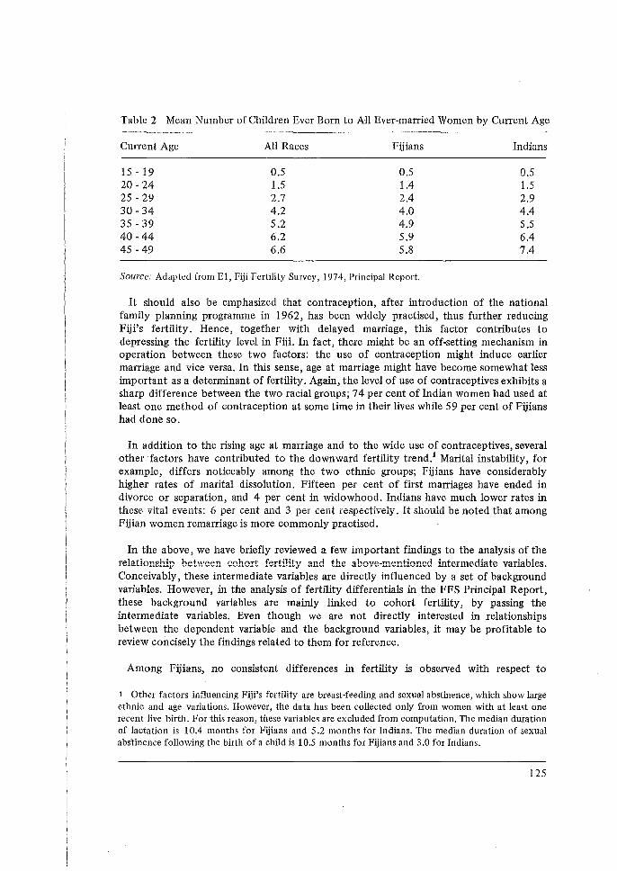
Table 2 Mean Number of Children Ever Born to All Ever-married Women by Current Age

CuITent Age All Races Fijians Indians

15 - 19 0.5 0.5 0.5 20 - 24 1.5 1.4 1.5 25 - 29 2.7 2.4 2.9 30 - 34 4.2 4.0 4.4 35 - 39 5.2 4.9 5.5 40-44 6.2 5.9 6.4 45 -49 6.6 5.8 7.4

Source: Adapted from El, Fiji Fertility Survey, 1974, Principal Report.

It should also be emphasized that contraception, after introduction of the national family planning programme in 1962, has been widely practised, thus further reducing Fiji's fertility. Hence, together with delayed marriage, this factor contributes to depressing the fertility level in Fiii. In fact, there might be an off-setting mechanism in operation between these two factors: the use of contraception might induce earlier maITiage and vice versa. In this sense, age at marriage might have become somewhat less important as a determinant of fertility. Again, the level of use of contraceptives exhibits a sharp difference between the two racial groups; 74 per cent of Indian women had used at least one method of contraception at some time in their lives while 5 9 per cent of Fijians had done so.

In addition to the rising age at marriage and to the wide use of contraceptives, several other factors have contributed to the downward fertility trend.1 Marital instability, for example, differs noticeably among the two ethnic groups; Fijians have considerably higher rates of marital dissolution. Fifteen per cent of first marriages have ended in divorce or separation, and 4 per cent in widowhood. Indians have much lower rates in these vital events: 6 per cent and 3 per cent respectively. It should be noted that among Fijian women remarriage is more commonly practised.

In the above, we have briefly reviewed a few important findings to the analysis of the relations!iJp beti.veen cohort fertility and the above-mentioned intermediate variables. Conceivably, these intermediate variables are directly influenced by a set of background variables. However, in the analysis of fertility differentials in the FFS Principal Report, these background variables are mainly linked to cohort fertility, by passing the intermediate variables. Even though we are not directly interested in relationships between the dependent variable and the background variables, it may be profitable to review concisely the findings related to them for reference.

Among Fijians, no consistent differences in fertility is observed with respect to

1 Other factors influencing Fiji's fertility are breast-feeding and sexual abstinence, which show large ethnic and age variations. However, the data has been collected only from women with at least one recent Jive birth. For this reason, these variables are excluded from computation. The median duration of lactation is 10.4 months for Fijians and 5 .2 months for Indians. The median duration of sexual abstinence following the birth of a child is 10.5 months for Fijians and 3.0 for Indians.

125

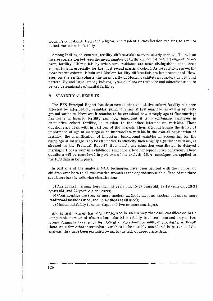
women's educational levels and religion. The residential classification explains, to a minor extent, variations in fertility.

Among Indians, in contrast, fertility differentials are more clearly marked. There is an inverse correlation between the mean number of births and educational attainment. More­over, fertility differentials by urban-rural residence are more distinguished than those among Fijians, especially for the most recent marriage cohort. As for religion, among the more recent cohorts, Hindu and Moslem fertility differentials are less pronounced. How­ever, for the earlier cohorts, the mean parity of Moslems exhibits a considerably different pattern. By and large, among Indians, types of place or residence and education seem to be key determinants of marital fertility.

H. STATISTICAL RESULTS

The FFS Principal Report has documented that cumulative cohort fertility has been affected by intermediate variables, principally age at first marriage, as well as by back­ground variables. However, it remains to be examined how strongly age at first marriage has really influenced fertility and how important it is in explaining variations in cumulative cohort fertility, in relation to the other intermediate variables. These questions are dealt with in part one of the analysis. Then, after measuring the degree of importance of age at marriage as an intermediate variable in the over-all explanation of fertility, the identification of important background variables in accounting for the rising age at marriage is to be attempted. Is ethnicity such a highly significant variable, as stressed in the Principal Report? How much has education contributed to delayed marriage? Does a woman's childhood residence affect her reproductive behaviour? These questions will be considered in part two of the analysis. MCA techniques are applied to the FFS data in both parts.

In part one of the analysis, MCA techniques have been utilized with the number of children ever born to all ever-married women as the dependent variable. Each of the three predictors has the following classifications:

a) Age at first marriage (less than 15 years old, 15-17 years old, 18-19 years old, 20-21 years old, and 22 years old and over);

b) Contraceptive use (one or n1ore niodern methods used, no modern but one or mere traditional methods used, and no methods at all used);

c) Marital instability (one marriage, and two or more marriages).

Age at first marriage has been categorized in such a way that each classification has a comparable number of observations. Marital instability has been measured only in two groups primarily because of insufficient observations for multiple marriages. Although there are a few other intermediate variables to be possibly considered in part one of the analysis, they have been excluded owing to the lack of appropriate data.

126

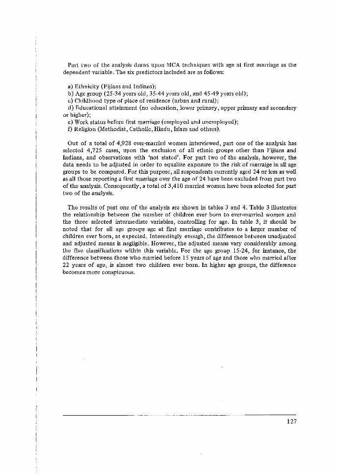
Part two of the analysis draws upon MCA techniques with age at first marriage as the dependent variable. The six predictors included are as follows:

a) Ethnicity (Fijians and Indians); b) Age group (25-34 years old, 35-44 years old, and 45-49 years old); c) Childhood type of place of residence (urban and rural); d) Educational attainment (no education, lower primary, upper primary and secondary

or higher); e) Work status before first marriage (employed and unemployed); f) Religion (Methodist, Catholic, Hindu, Islam and others).

Out of a total of 4,928 ever-married women interviewed, part one of the analysis has selected 4,725 cases, upon the exclusion of all ethnic groups other than Fijians and Indians, and observations with 'not stated'. For part two of the analysis, however, the data needs to be adjusted in order to equalize exposure to the risk -0f marraige in all age groups to be compared. For this purpose, all respondents currently aged 24 or less as well as all those reporting a first marriage over the age of 24 have been excluded from part two of the analysis. Consequently, a total of 3 ,410 married women have been selected for part two of the analysis.

The results of part one of the analysis are shown in tables 3 and 4. Table 3 illustrates the relationship between the number of children ever born to ever-married women and the three selected intermediate variables, controlling for age. In table 3, it should be noted that for all age groups age at first marriage contributes to a larger number of children ever born, as expected. Interestingly enough, the difference between unadjusted and adjusted means is negligible. However, the adjusted means vary considerably among the five classifications within this variable. For the age group 15-24, for instance, the difference between those who married before 15 years of age and those who married after 22 years of age, is almost two children ever born. In higher age groups, the difference becomes more conspicuous.

127

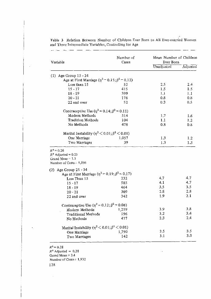
Table 3 Relation Between Number of Children Ever Born to All Ever-married Women and Three Intermediate Variables, Controlling for Age

Variable Number of

Cases

(1) Age Group 15 - 24 Age at First Marriage (r/2 = 0.15; ~2 = 0.12)

Less than 15 52 15-17 415 18-19 399 20-21 178 22 and over 52

Contraceptive Use (r/2 = 0.14; ~2 = 0.11) Modern Methods 514 Tradition Methods 104 No Methods 478

Marital Instability (r/2 < 0.01; ~2 < 0.01) One Marriage 1.057 Two Marriages 39

R 2 ==0.26 R 2 Adjusted== 0.25 Grand Mean== 1.3 Number of Cases= 1,096

(2) Age Group 25 - 34 Age at First Marriage (112 = 0, 19; ~2 = 0 .17)

Less Than 15 232 15-17 585 18 - 19 464 20 - 21 309 22 and over 342

Contraceptive Use (r/2 = 0.12; ~2 = 0.08) Modern Methods 1,259 Traditional Methods 196 No Methods 477

Marital Instability (r/ 2 < 0.01; ~2 < 0.01) One Marriage 1, 7 9 0 Two Marriages 142

R 2 == 0.28 R 2 Adjusted = 0.28 Grand Mean = 3 .4 Number of Cases== 1,932

128

Mean Number of Children Ever Born

Unadjusted Adjusted

2.5 2.4 LS 1.5 1.1 1.1 0.8 0.8 0.3 0.5

1.7 1.6 1.1 1.2 0.8 0.8

1.3 1.2 1.3 1.3

4.7 4.7 4.1 4.7 3.5 3.5 2.8 2.8 1.9 2.1

3.9 3.8 3.2 3.4 2.3 2.4

3.5 3.5 3.1 3.0

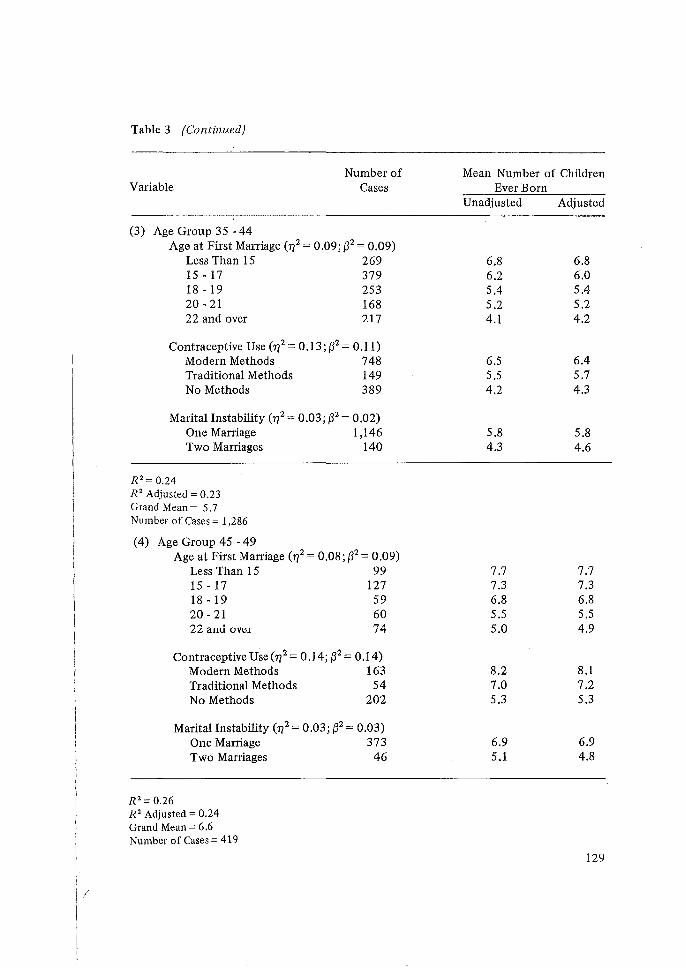
Table 3 (Continued)

Variable Number of

Cases

(3) Age Group 35 - 44 Age at First Marriage (ri2 = 0.09; (3 2 = 0.09)

Less Than 15 269 15-17 379 18 - 19 20 -21 22 and over

253 168 ?17

Contraceptive Use (ri2 = 0.13; {32 = 0.11) Modern Methods 7 48 Traditional Methods 149 No Methods 389

Marital Instability (ri2 c-= 0.03; (3 2 = 0.02)

One Marriage 1,146 Two Marriages 140

R 2 = 0.24 R 2 Adjusted= 0.23 Grand Mean= 5. 7 Number of Cases= 1,286

(4) Age Group 45 - 49 Age at First Marriage (ri2 = 0.08; {32 = 0.09)

Less Than 15 99 15-17 127 18-19 59 20 - 21 60 22 aml uver ,.., A

/ 'T

Contraceptive Use (ri 2 = 0.14; {3 2 = 0.14) Modern Methods 163 Traditional Methods 54 No Methods 202

Marital Instability (ri2 = 0 .03; (32 = 0.03) One Marriage 373 Two Marriages 46

R 2 = 0.26 R 2 Adjusted= 0.24 Grand Mean= 6.6 Number of Cases= 419

Mean Number of Children Ever Born

Unadjusted Adjusted

6.8 6.8 6.2 6.0 5.4 5.4 5.2 5.2 4.1 4.2

6.5 6.4 5.5 5.7 4.2 4.3

5.8 5.8 4.3 4.6

7.7 7.7 7.3 7.3 6.8 6.8 5.5 5.5 ,. " A 0 J,U 'T,7

8.2 8.1 7.0 7.2 5.3 5.3

6.9 6.9 5.1 4.8

129

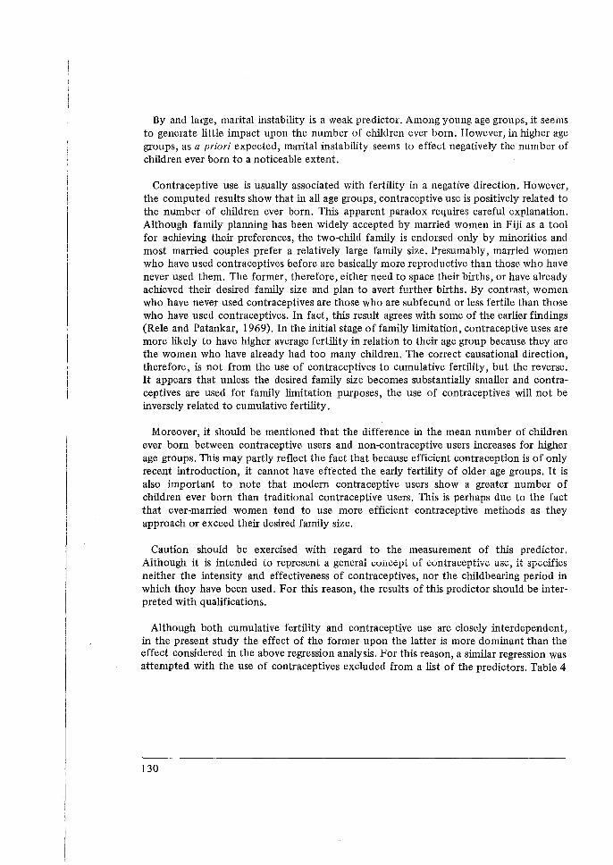
By and large, marital instability is a weak predictor. Among young age groups, it seems to generate little impact upon the number of children ever born. However, in higher age groups, as a priori expected, marital instability seems to effect negatively the number of children ever born to a noticeable extent.

Contraceptive use is usually associated with fertility in a negative direction. However, the computed results show that in all age groups, contraceptive use is positively related to the number of children ever born. This apparent paradox requires careful explanation. Although family planning has been widely accepted by married women in Fiji as a tool for achieving their preferences, the two-child family is endorsed only by minorities and most married couples prefer a relatively large family size. Presumably, married women who have used contraceptives before are basically more reproductive than those who have never used them. The former, therefore, either need to space their births, or have already achieved their desired family size and plan to avert further births. By contrast, women who have never used contraceptives are those who are subfecund or less fertile than those who have used contraceptives. In fact, this result agrees with some of the earlier findings (Rele and Patankar, 1969). In the initial stage of family limitation, contraceptive uses are more likely to have higher average fertility in relation to their age group because they are the women who have already had too many children. The correct causational direction, therefore, is not from the use of contraceptives to cumulative fertility, but the reverse. It appears that unless the desired family size becomes substantially smaller and contra­ceptives are used for family limitation purposes, the use of contraceptives will not be inversely related to cumulative fertility.

Moreover, it should be mentioned that the difference in the mean number of children ever born between contraceptive users and non-contraceptive users increases for higher age groups. This may partly reflect the fact that because efficient contraception is of only recent introduction, it cannot have effected the early fertility of older age groups. It is also important to note that modern contraceptive users show a greater number of children ever born than traditional contraceptive users. This is perhaps due to the fact that ever-married women tend to use more efficient contracepiive methods as they approach or exceed their desired family size.

Caution should be exercised with regard to the measurement of this predictor. Aithough it is intended to represent a gem:ral concept of contraceptive use, it specifics neither the intensity and effectiveness of contraceptives, nor the childbearing period in which they have been used. For this reason, the results of this predictor should be inter­preted with qualifications.

Although both cumulative fertility and contraceptive use are closely interdependent, in the present study the effect of the former upon the latter is more dominant than the effect considered in the above regression analysis. For this reason, a similar regression was attempted with the use of contraceptives excluded from a list of the predictors. Table 4

130

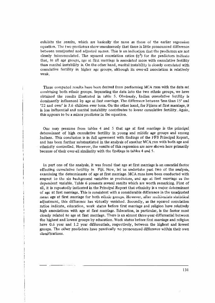
exhibits the results, which are basically the same as those of the earlier regression equation. The two predictors show unanimously that there is little pronounced difference between unadjusted and adjusted means. This is an indication that the predictors are not closely intercorrelated. The squared correlation ratios (11 2

) for the predictors indicate that, in all age groups, age at first marriage is associated more with cumulative fertility than marital instability is. On the other hand, marital instability is closely correlated with cumulative fertility in higher age groups, although its over-all association is relatively weak.

These computed results have been derived from performing MCA runs with the data set combining both ethnic groups. Separating the data into the two ethnic groups, we have obtained the results illustrated in table 5. Obviously, Indian cumulative fertility is dominantly influenced by age at first marriage, The difference between 'less than 15' and '22 and over' is 3.6 children ever born. On the other hand, for Fijians at first marriage, it is less influential and marital instability contributes to lower cumulative fertility. Again, this appears to be a minor predictor in the equation.

One may presume from tables 4 and 5 that age at first marriage is the principal. determinant of high cumulative fertility in young and middle age groups and among Indians. This conclusion is in full agreement with findings of the FFS Principal Report, and has been further substantiated in the analysis of another MCA run with both age and ethnicity controlled. However, the results of this regression are now shown here primarily because of their over-all similarity with the findings in tables 4 and 5.

In part one of the analysis, it was found that age at first marriage is an essential factor effecting cumulative fertility in Fiji. Now, let us undertake part two of the analysis, examining the determinants of age at first marriage. MCA runs have been conducted with respect to the six background variables as predictors, and age at first marriage as the dependent variable. Table 6 presents several results which are worth remarking. First of all, it is repeatedly indicated in the Principal Report that ethnicity is a major determinant of age at first marriage. This is consistent with a considerable difference in the unadjusted mean age at first maniage for both ethnic groups. However, after 1nultivariate statistfoal adjustment, this difference has virtually vanished. Secondly, as the squared correlation ratios indicate, education, work status before first marriage and religion have relatively high associations with age at first marriage. Education, in particular, is the factor most closely related to age at first marriage. There is an almost three-year differential between the highest and lowest groups by education. Work status before first marriage and religion have 0.6 year and 1.2 year differentials, respectively, between the highest and lowest groups. The other predictors have practically no pronounced difference within their own classifications.

131

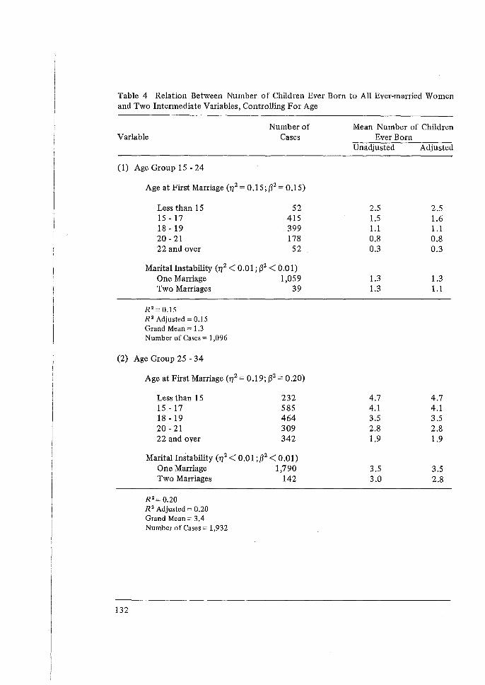
Table 4 Relation Between Number of Children Ever Born to All Ever-married Women and Two Intermediate Variables, Controlling For Age

Variable Number of

Cases

(1) Age Group 15 - 24

Age at First Marriage (ri2 = 0.15; ~2 = 0.15)

Less than 15 15 - 17 18 - 19 20 -21 22 and over

52 415 399 178

52

Marital Instability (ri2 < 0.01; ~2 < 0.01) One Marriage 1,059 Two Marriages 39

R 2 =0.15 R 2 Adjusted= 0.15 Grand Mean= 1.3 Number of Cases= 1,096

(2) Age Group 25 - 34

132

Age at First Marriage (ri2 = 0.19; ~2 = 0.20)

Less than 15 15 - 17 18 - 19 20- 21 22 and over

232 585 464 309 342

Marital Instability (ri2 < 0.01 ;~2 < O.Ol) One Marriage 1,790 Two Marriages 142

R 2 = 0.20 R 2 Adjusted= 0.20 Grand Mean= 3.4 Number of Cases= 1,932

Mean Number of Children Ever Born

Unadjusted Adjusted

2.5 2.5 1.5 1.6 1.1 1.1 0.8 0.8 0.3 0.3

1.3 1.3 1.3 1.1

4.7 4.7 4.1 4.1 3.5 3.5 2.8 2.8 1.9 1.9

3.5 3.5 3.0 2.8

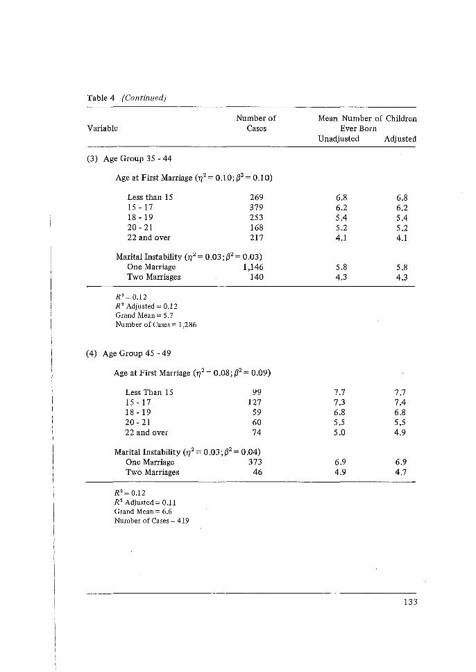
Table 4 (Continued)

Variable

(3) Age Group 35 - 44

Number of Cases

Age at First Marriage (ri2 = 0.10;~2 = 0.10)

Less than 15 269 15 - 17 379 18 - 19 253 20 - 21 168 22 and over 217

Marital Instability (ri2 = 0.03; ~2 = 0.03) One Marriage 1,146 Two Marriages 140

R 2 = 0.12 R 2 Adjusted= 0.12 Grand Mean= 5.7 Number of Cases= 1,286

(4) Age Group 45 - 49

Age at First Marriage (ri2 = 0.08; ~2 = 0.09)

Less Than 15 15 - 17 18 - 19 20- 21 22 and over

99 127

59 60 74

Marital Instability (ri2 = 0.03; ~2 = 0.04) One Marriage 373 Two Marriages 46

R 2 = 0.12 R 2 Adjusted= 0.11 Grand Mean= 6.6 Number of Cases= 419

Mean Number of Children Ever Born

Unadjusted Adjusted

6.8 6.8 6.2 6.2 5.4 5.4 5.2 5.2 4.1 4.1

5.8 5.8 4.3 4.3

7.7 7.7 7.3 7.4 6.8 6.8 5.5 5.5 5.0 4.9

6.9 6.9 4.9 4.7

133

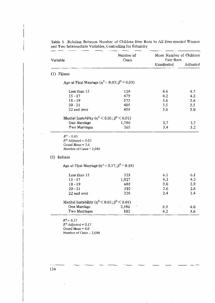
Table 5 Relation Between Number of Children Ever Born to All Ever-married Women and Two Intermediate Variables, Controlling for Ethnicity

Variable Number of

Cases

(1) Fijians

Age at First Marriage (71 2 == 0 .03; ~2 == 0 .03)

Less than 15 15 - 17 18 - 19 20 - 21 22 and over

129 479 573 405 459

Marital Instability (712 < 0.01; ~2 < 0.01) One Marriage 1, 7 8 0 Two Marriages 265

R 2 = 0.03 R 2 Adjusted= 0.03 Grand Mean= 3.6 Number of Cases= 2,045

(2) Indians

134

Age at First Marriage (71-.i == 0.17; ~2 == 0.18)

Less than 15 523 15 - 17 1,027 18 - 19 602 20 -21 310 22 and over 226

Marital Instability (71 2 < 0.01; ~2 < 0.01) One Marriage 2,586 Two Marriages 102

R 2 = 0.17 R 2 Adjusted= 0.17 Grand Mean= 4.0 Number of Cases= 2,688

Mean Number of Children Ever Born

Unadjusted Adjusted

4.6 4.7 4.2 4.2 3.6 3.6 3.5 3.5 3.0 3.0

3.7 3.7 3.4 3.2

6.1 6.1 4.2 4.2 3,0 2.9 2.6 2.6 2.4 2.4

3.9 4.0 4.2 3.6

Although both ethnicity and age have been dealt with as predictors in the above analysis, they can also be treated as control variables. Table 7 indicates the effect of the five predictors, controlling for ethnicity. In both ethnic groups, educational attainment affects considerably age at first marriage, although its effect is more substantial among Indians than among Fijians. There is a differential of 2.2 years among Fijians and 3.4 years among Indians. Work status before first marriage is also influential on age at first marriage. However, its relative impact on age at marriase is rather limited. Moreover, it is clear that among Indians age is a relatively important explanatory variable, with a differential of 0.7 years between the highest and lowest age groups. In contrast, age shows little difference among Fijians. These results account for the insignificanc;.e of age in table 6. It is also noted that the proportion of the variance explained is only 4 per cent among Fijians but 17 per cent among Indians.

Table 8 illustrates the relationships between age at first marriage and the five selected predictors controlling for age. Similar to other cases, the adjusted means indicate that educational attainment contributes to delayed marriage in all age groups. Moreover, at ages 3544 and 4549, ethnic background shows a substantial difference in age at first marriage. Work status considerably affects age at first marriage in age groups 25-34 and 3544. Religion also is an important factor in explaining the variation in age at marriage in age groups 25-34 and 4549.

A similar regression was run with the same dependent variable, controlling for both ethnicity and age simultaneously. Although the results are not shown here, it can be briefly summarized that in every age group, for each ethnic group, education is very powerful in accounting for the variation in age at first marriage. Female labour force participation is an important predictor for age group 4549. By and large, the selected predictors explain the variance in age at marriage more efficiently among Indians than among Fijians.

In both part one and part two of the analysis, we have identified a few important variables in explaining the variance of each dependent variable. Nevertheless, the relative importance of each predictor remains to be discussed. Consequently, the following two indices have been computed for this purpose: the squared beta-coefficient, and the percentage of variance explained by each of the predictors net of the others. The squared beta-coefficient for each predictor is listed in each tabie, while the percentage of variance explained is included in tables 9 and 10. A brief comparison of these tables shows that the results derived from both squared beta-coefficients and the percentage or variance explained by each predictor net of the others are entirely comparable. In particular, according to table 9, at age.s 15-24 and 25-34 the effect of first marriage net of the other predictors upon cumulative fertility is far more dominant than that of marital instability. At other ages, differences in the effect of age at first marriage and marital instability are less pronounced. Furthermore, in both ethnic groups the effect of age at first marriage upon cumulative fertility is, again, the most crucial factor. However, Indian fertility is

135

considerably more sensitive to age at first marriage than Fijian's. As for part two of the analysis, table 10 shows that not only does education explain the greatest amount of variance alone, it also explains the largest percentage of the variance net of the other predictors upon cumulative fertility is far more dominant than that of marital instability. At other ages, differences in the effect of age at first marriage and marital instability arc less pronounced. Furthermore, in both ethnic groups the effect of age at first marriage upon cumulative fertility is, again, the most crucial factor. However, Indian fertility is considerably more sensitive to age at first marriage than Fijian's. As for part two of the analysis, table 10 shows that not only does education explain the greatest amount of variance alone, it also explains the largest percentage of the variance net of the other variables. Religion and work status before first marriage are also important but to a considerable lesser extent.

I. INCORPORATION OF INTERACTION EFFECTS

The above statistical results have been obtained from the MCA additive models. As dis­cussed earlier, MCA is a useful statistical method on the following two grounds: (a) it can handle independent variables on an interval scale, an ordinal, or even a nominal scale; and (b) it can handle non-linear relationships such as the effect of education upon fertility. Nevertheless, these advantages of MCA are often handicapped by its assumption of addi­tivity. In some cases, the exclusion of interaction effects from analysis nullifies the vali­dity of MCA results. When interaction effects are indentified, they can be included in MCA by combining predictors.

In order to detect interaction effects, we have applied analysis of variance techniques to both part one and part two of the analyses. For part one of the analysis, no significant interaction effect was found. For part two of the analysis, however, we have discovered significant three-way interactions among age, ethnicity and education. This implies that part two of the analysis based on the additive linear models have suffered from a specifi­cation error. Therefore, we have performed another MCA run with the three predictor variables, together with a 24-category composite variable based on age, ethnicity and edu­cation.

Table 11 presents its computational results. We should note that work status before marriage has become less important while religion is still a significant predictor. On the other hand, childhood type of place of residence is the least influential in both old and new regression runs.

More importantly, there is a differential of 3.3 years between Indians at ages 45-59 with no education and those at ages 35-44 with 'second or higher' education. In general, those who have higher levels of education tend to marry at higher ages while those who have lower levels of education marry at younger ages. In addition, table 11 shows that Indians

136

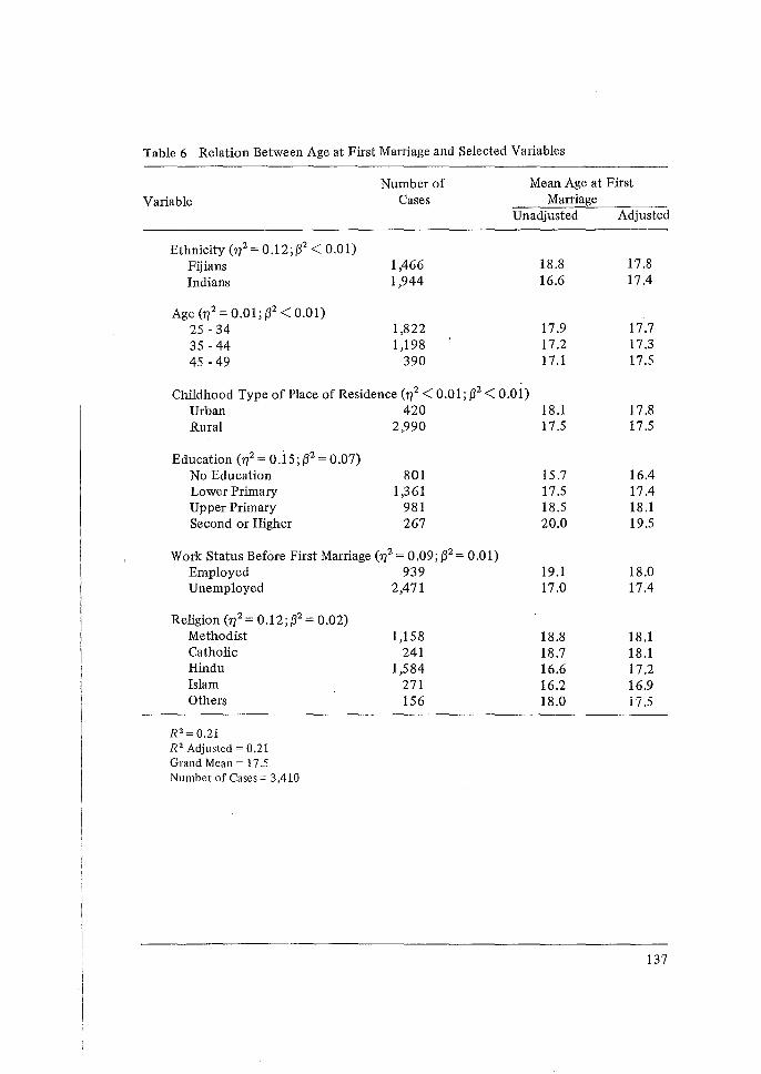
Table 6 Relation Between Age at First Marriage and Selected Variables

Variable

Ethnicity (ri2 = 0 .12; ~2 < 0.01) Fijians Indians

Age (ri 2 = 0.01; ~2 < 0.01) 25 - 34 35 - 44 45 - 49

Number of Cases

1,466 1,944

1,822 1,198

390

Mean Age at First Marriage

Unadjusted Adjusted

18.8 17.8 16.6 17.4

17 .9 17.7 17.2 17.3 17 .1 17.5

Childhood Type of Place of Residence (772 < 0.01; ~2 < 0.0l) Urban 420 18.1 17.8 Rural 2,990 17.5 17.5

Education (772 = 0.15; ~2 = 0.07) No Education 801 15.7 16.4 Lower Primary 1,361 17.5 17.4 Upper Primary 981 18.5 18.1 Second or Higher 267 20.0 19.5

Work Status Before First Marriage (ri2 = 0.09; ~2 = 0.01) Employed 939 19.l 18.0 Unemployed 2,471 17.0 17.4

Religion (ri2 = 0.12; ~2 = 0.02) Methodist 1,158 18.8 18.l Catholic 241 18.7 18.1 Hindu 1,584 16.6 17.2 Islam 271 16.2 16.9 Others 156 18.0 17.5

R 2 = 0.21 R 2 Adjusted= 0.21 Grand Mean= 17 .5 Number of Cases= 3,410

137

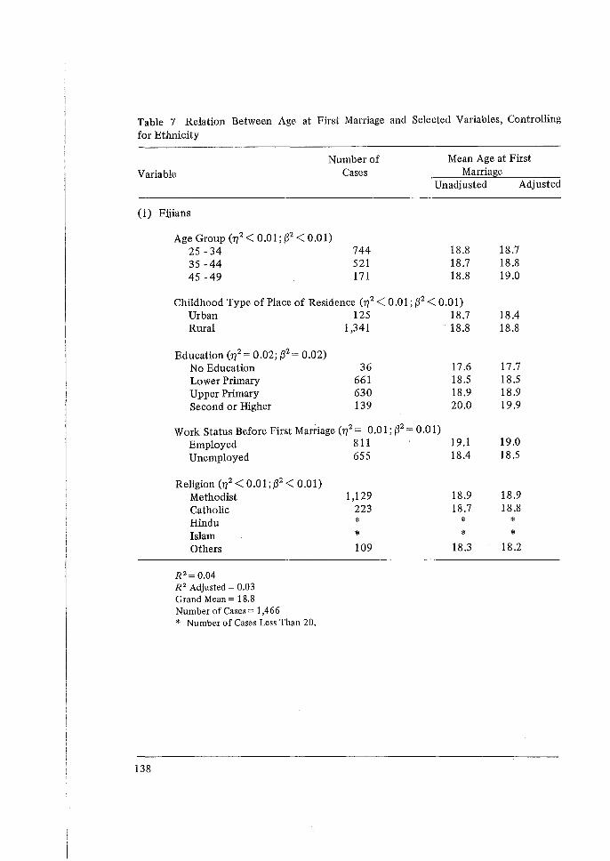
Table 7 Relation Between Age at First Marriage and Selected Variables, Controlling for Ethnicity

Variable Number of

Cases Mean Age at First

Marriage Unadjusted Adjusted

(1) Fijians

138

Age Group (ri2 < 0.01; ~2 < 0.01) 25 - 34 35 -44 45 -49

744 521 171

18.8 18.7 18.8

Childhood Type of Place of Residence (ri2 < 0.01; ~2 < 0.01)

18.7 18.8 19.0

Urban 125 18.7 18.4 Rural 1,341 18.8 18.8

Education (ri2 = 0.02; ~2 = 0.02) No Education Lower Primary Upper Primary Second or Higher

36 661 630 139

Work Status Before First Marriage (ri2 = 0.01; ~2 =0.01)

17.6 18.5 18.9 20.0

17.7 18.5 18.9 19.9

Employed 811 19 .1 19 .0 Unemployed 655 18.4 18.5

Religion (ri2 < 0.01; ~2 < 0.01) Methodist Catholic Hindu Islam Others

R 2 = 0.04 R 2 Adjusted= 0.03 Grand Mean= 18.8 Number of Cases= 1,466 * Number of Cases Less Than 20.

1,129 223

* * 109

18.9 18.7

* *

18.3

18.9 18.8

* *

18.2

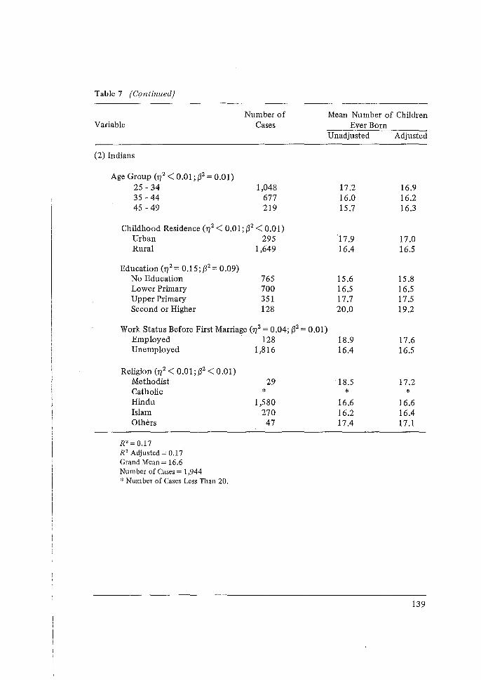
Table 7 (Continued)

Variable

(2) Indians

Age Group (ri2 < O.Ql; ~2 = 0.01) 25 - 34 35 - 44 45 - 49

Number of Cases

1,048 677 219

Childhood Residence (ri2 < 0.01; ~2 < 0.01) Urban 295 Rural 1,649

Education (ri 2 = 0.15; ~2 = 0.09) No Education Lower Primary Upper Primary Second or Higher

765 700 351 128

Work Status Before First Marriage (ri2 = 0.04; ~2 = 0.01)

Mean Number of Children Ever Born

Unadjusted Adjusted

17 :2 16.0 15.7

17.9 16.4

15.6 16.5 17.7 20.0

16.9 16.2 16.3

17.0 16.5

15.8 16.5 17.5 19.2

Employed · 128 18.9 17.6 16.5 Unemployed 1,816 16 .4

Religion (ri 2 < O.Ql; ~2 < 0.01) Methodist Catholic Hindu Islam Others

R'= 0.17 R 2 Adjusted= 0.17 Grand Mean= 16.6 Number of Cases= 1,944 *Number of Cases Less Than 20.

29

* 1,580

270 47

18.5

* 16.6 16.2 17.4

17.2

* 16.6 16.4 17.1

139

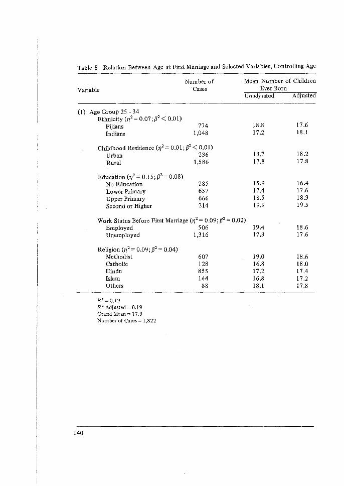
Table 8 Relation Between Age at First Marriage and Selected Variables, Controlling Age

Variable

(1) Age Group 25 - 34 Ethnicity (ri2 = 0.07; ~2 <0.01)

Fijians Indians

Number of , Cases

774 1,048

Childhood Residence (ri2 = 0.01; ~2 < 0.01) Urban 236 Rural 1,586

Education (ri2 = 0.15; ~2 = 0.08) No Education 285 Lower Primary 657 Upper Primary 666 Second or Higher 214

Mean Number of Children Ever Born

Unadjusted Adjusted

18.8 17.6 17.2 18.1

18.7 18.2 17.8 17 .8

15.9 16.4 17.4 17 .6 18.5 18.3 19.9 19.5

Work Status Before First Marriage (ri2 = 0.09; ~2 = 0.02) Employed 506 19.4 18.6 Unemployed 1,316 17.3 17.6

Religion (ri2 = 0.09; ~2 = 0.04) Methodist 607 19.0 18.6 Catholic 128 16.8 18.0 Hindu 855 17.2 17.4 Islam 144 16.8 17.2 Others 88 18.1 17 .8

R 2 = 0.19 R 2 Adjusted= 0.19 Grand Mean~ 1 7 .9 Number of Cases= 1,822

140

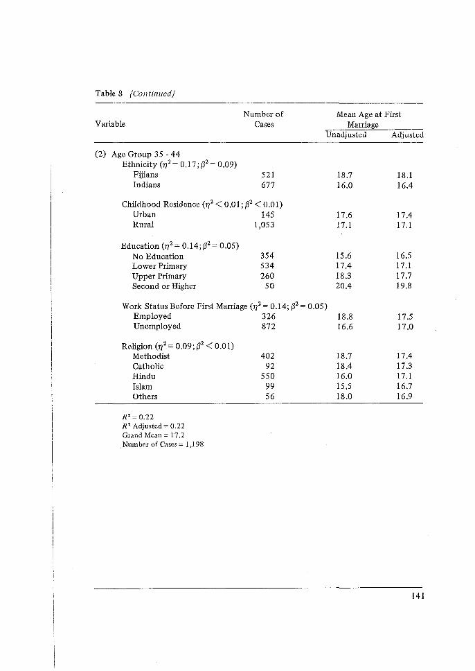
Table 8 (Continued)

Variable

(2) Age Group 35 - 44 Ethnicity (ri2 = 0.17;132 = 0.09)

Fijians Indians

Number of Cases

521 677

Childhood Residence (ri2 <0.01;132 < 0.01) Urban 145 Rm;al 1,053

Education (ri2 =0.14;132 = 0.05) No Education Lower Primary Upper Primary Second or Higher

354 534 260

50

Mean Age at First Marriage

Unadjusted Adjusted

18.7 16.0

17.6 17.l

15.6 17.4 18.3 20.4

18.1 16.4

17.4 17.l

16.5 17.l 17.7 19.8

Work Status Before First Marriage (ri2 =0.14;132 = 0.05) Employed 326 18.8 Unemployed 872 16.6

Religion (ri2 = 0.09;132 < 0.01) Methodist Catholic Hindu Islam Others

R 2 = 0.22 R 2 Adjusted= 0.22 Grand 1-fean = 17.2

,Number of Cases= 1,198

402 92

550 99 56

18.7 18.4 16.0 15.5 18.0

17.5 17.0

17.4 17.3 17.1 16.7 16.9

141

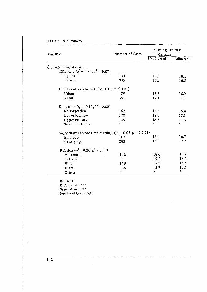
Table 8 (Continued)

Variable

(3) Age group 45 - 49 Ethnicity (ri2 = 0.21; (3 2 = 0.07)

Fijians Indians

Number of Cases

171 219

Childhood Residence (ri2 < 0.01; (32 < 0.01) Urban 39 Rural 351

Education (ri2 = 0.15; (32 = 0.03) No Education Lower Primary Upper Primary Second or Higher

162 170 55

*

Mean Age at First Marriage

Unadjusted Adjusted

18.8 15.7

16.6 17.1

15.5 18.0 18.5

*

18.1 16.3

16.9 17.1

16.4 17 .5 17.6

* Work Status before First Marriage (ri2 = 0.06; (3 2 < 0.01)

142

Employed 107 18 .4 Unemployed 283 16.6

Religion (ri2 = 0.20; (32 = 0.02) Methodist Catholic Hindu Islam Others

R 2 = 0.24 R 2 Adjusted== 0.22 Grand ivfean::::: 17 .1 Number of Cases== 390

150 21

179 28

*

18.6 19.2 15.7 15.7

*

16.7 17.2

17.4 18.1 16.6 16.7

*

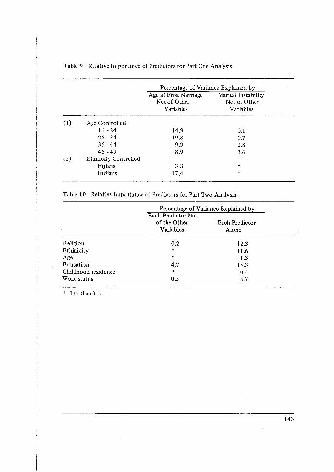
Table 9 Relative Importance of Predictors for Part One Analysis

Percentage of Variance Explained by Age at First Maniage Marital Instability

Net of Other Net of Other Variables Variables

(1) Age Controlled 14 - 24 14.9 0.1 25 - 34 19.8 0.7 35 -44 9.9 2.8 45 -49 8.9 3.6

(2) Ethnicity Controlled Fijians 3.3 * Indians 17.4 *

Table 10 Relative Importance of Predictors for Part Two Analysis

Percentage of Variance Explained by Each Predictor Net

of the Other Each Predictor Variables Alone

Religion 0.2 12.3 Ethinicity * 11.6 Age * 1.3 Education 4.7 15.3 Childhood residence * 0.4 Work status 0.5 8.7

* Less than 0.1.

143

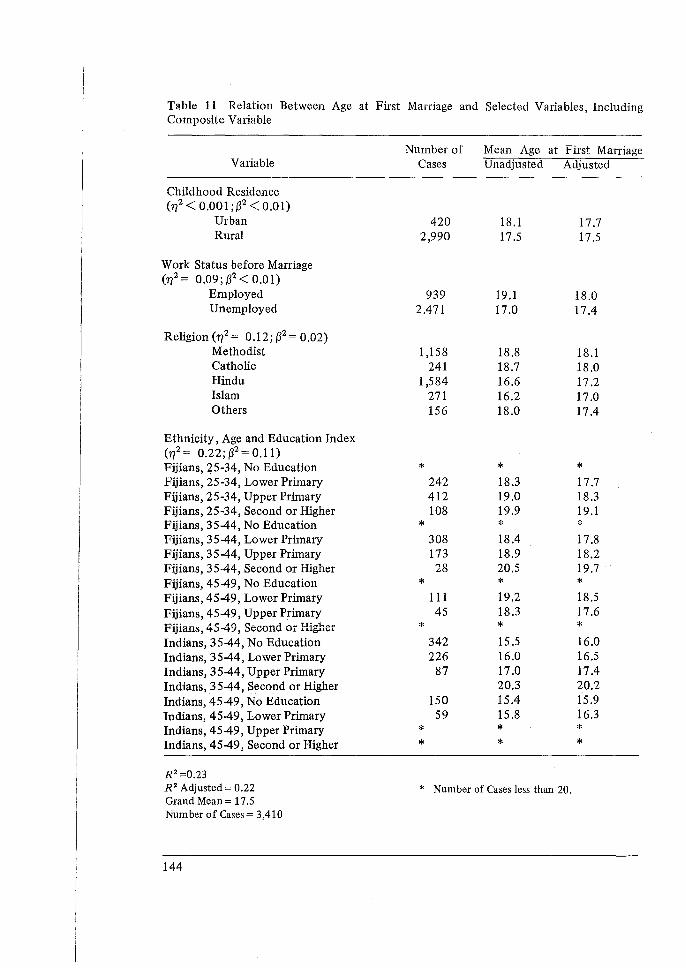
Table 11 Relation Between Age at First Marriage and Selected Variables, Including Composite Variable

Variable

Childhood Residence (112 < 0.001;(32 <0.01)

Urban Rural

Work Status before Marriage (112 = 0.09; (32 < 0.01)

Employed Unemployed

Religion(112 = 0.12;(32 =0.02) Methodist Catholic Hindu Islam Others

Ethnicity, Age and Education Index (112 = 0.22;(32 =0.11) Fijians, 25-34, No Education Fijians, 25-34, Lower Primary Fijians, 25-34, Upper Primary Fijians, 25-34, Second or Higher Fijians, 35-44, No Education Fijians, 35-44, Lower Primary Fijians, 35-44, Upper Primary Fijians, 35-44, Second or Higher Fijians, 45-49, No Education Fijians, 45-49, Lower Primary Fijians, 45-49, Upper Primary Fijians, 45-49, Second or Higher Indians, 35-44, No Education Indians, 35-44, Lower Primary Indians, 35-44, Upper Primary Indians,35-44, Second or Higher Indians, 45-49, No Education Indians, 45-49, Lower Primary Indians, 45-49, Upper Primary Indians, 45-49, Second or Higher

R 2 ==0.23 R 2 Adjusted== 0.22 Grand Mean== 17 .5 Number of Cases== 3,410

144

Number of Mean Age at First Marriage Cases Unadjusted Adjusted

420 2,990

939 2.471

1,158 241

1,584 271 156

* 242 412 108

* 308 173 28

* 111 45

* 342 226

87

150 59

* *

18.1 17.5

19.1 17.0

18.8 18.7 16.6 16.2 18.0

* 18.3 19.0 19.9

* 18.4 18.9 20.5

* 19.2 18.3

* 15.5 16.0 17.0 20.3 15.4 15.8

* *

* Number of Cases less than 20.

17.7 17 .5

18.0 17.4

18.l 18.0 17.2 17.0 17.4

* 17.7 18.3 19.1

* 17.8 18.2 19.7

* 18.5 17.6

* 16.0 16.5 17.4 20.2 15.9 16.3

* *

are more heterogeneous in educational attainment than Fijians. This is indicated by the number of cases falling into each category of the composite variable. As discussed in the Fiji Principal Report, historically, Fijians have been much better educated than Indians. In the past two decades, however, an increasing number of Indians have been educated as a result of the rapid expansion of Fiji's educational system. In other words, although educational effects are rather striking in old age groups between these two ethnic groups, in young age groups the two ethnic groups have become more homogeneous in educa­tional levels. Moreover, in the 'lower primary' education category, Fijians at ages 25-34 have married 0.3 year higher than their Indian counterparts. For the 'upper primary' education category, there is virtually no differential between them. Interestingly enough, in the 'second or higher' category, Indians have married one year higher than Fijians. Marital patterns similar to these found for the age group '25-34 hold for the age group 35-44. Each ethnic group, therefore, has been exposed to different levels of education over time. For the above reasons, these three variables constitute interaction effect.

J. CONCLUDING REMARKS

In this study, we have found support for the argument that, in Fiji, delayed marriage contributes to reduction of cumulative fertility. This argument holds true particularly for both young and middle age groups and among Indians. Marital instability, accounting for only a modest proportion of the variance in cumulative fertility solely in high age groups, has produced no conspicuous difference in cumulative fertility between the two ethnic groups.

We have also found that age at first marriage is closely correlated with the three expla­natory variables, i.e. education, religion and work status before marriage. In particular, education interacts with age and ethnicity. This composite variable seems to be the most dominant factor affecting age at first marriage in Fiji.

145

APPENDIX

Because an elaboration of the mathematical procedure for solving the normal equations is available elsewhere (Anderson and Bancroft, 1952), only a brief sketch of the pro­cedure is nevessary. In the case of two predictors, the following constraints are required in order to make the general constant (m) equal to Y:

(1) I I; n;a; = 0,

i = 1

J I; njbj=O,

j = 1

Given these constraints, an attempt is made to determine m, a; and bj, utilizing

Yu= nii (m + ai + bj)

where Yij stands for all estimated value of Yij for the (iij) subclass with nij entries. Furthermore, since Y11· - Y;j = e;j, the following equation, V, can be formulated:

I J I J V= I; I; e'ij= I; I; [Yij-llij(m + a;+bj)]2

i=l ]j=J i=l i=l

We, then, take derivatives of V with respect to m, a; and bj, and set each of them equal to zero. By rearranging, we have

I J m: nm + I; ni.ai + I; n.jbj G

i = 1 j=l

J n- a· l. l + I; llijbj

i=l

+

where Ai and Bj arn classificatory totals, while G is the grand total. By utilizing (1), we have

m = G/n = Y. Obviously, the two-predictor case can be easily extended to cases with more predictors.

As used in the MCA computerized programme developed by the Survey Research Center, the normal equations are solved by the iterative procedure called the sweep-out method (Anderson and Bancroft, 1952). An alternative is, of course, to use a matrix inversion technique which is usually applied to computer programmes for multiple regression analysis. No matter which method is used, a problem might arise if categories too closely overlap each other. In the case of the inverse matrix method, the data matrix is singular, which in trun makes an inversion of the matrix impossible. If the iterative techniques were to be employed, it would never converge.

146

BIBLIOGRAPHY

Anderson, R.L., and T.A. Bancroft, Statistical Theory in Research. New York, McGraw­Hill. 1952.

Andrews, Frank M., James N. Morgan, John A. Sonquist, and Laura Klem, Multiple Clas­sification Analysis (second edition). Institute for Social Research, University of Michigan. 1973.

Arnold, Fred and Chintana Pejaranonda, Economic Factors in Family Size Decisions in Thailand, World Fertility Survey/Survey of Fertility in Thailand Report No. 2. Bang­kok, 1977.

Blalock, H.M. Jr. 'Theory Building and the Concept of Interactions', American Sociol­ogical Review, Vol. 30, No. 3 (pp. 374-380). 1965.

Blau, P.M. and 0.D. Duncan, The American Occupational Structure. New York, Wiley. 1967.

Kish, L., and M. Frankel, Standard Errors of MCA Multivariate Regression Coefficients and Deviations. Survey Research Center, University of Michigan (mimeo). 1967.

Kish, L. and J.B. Lansing. 'The Family Life Cycle as an Independent Variable', American Sociological Review, Vol. 22 (pp. 512-519). 1957.

Kish, L., and J .A. Sonquist, 'Problems in the Analysis of Survey Data: A Proposal', Jour­nal of the American Statistical Association, Vol. 5 8 (pp. 415-434).

Morgan, James, 'One Assessing the Contribution of One Predictor in a Multivariate Ana­lysis' (memorandum) University of Michigan. 1971.

Palmore, James and others, 'Family Planning Opinion Leadership in Korea: 1971',Jour­nal of East and West Studies, Vof. 4, No. 2 (pp. 27-41). November 1975.

Ram, Bali, 'Regional Sub-cultural Explanations of Black Fertility in the United States', Population Studies, Vol. 30, No. 3 (pp. 553-559). November 1976.

Rele, J.R. and Tava Patankar, 'Differential Fertility of Contraceptors and Non-contra­ceptors', International Population Conference, London, Vol. 1 (pp. 448-45 5). 1969.

Sonquist, John, Multivariate Model Building. Institute for Social Research, University of Michigan. 1970.

Srinivan, K., 'Retrospective Surveys', in Measuring the Effect of Family Planning Pro­gru1n1nes on Fertility, edited by C. Chandrasekran and Albert Hern1alin. International Union for the Scientific Study of Population (pp. 301-350).

Suits, Daniel, 'Use of Dummy Variables in Regression Equations', Journal of the American Statistical Association, Vol. 52 (pp. 548-5 51). 1957.

World Fertility Survey. Fiji Fertility Survey 1974: Principal Report. Bureau of Statistics, Suva, Fiji. 1976.

Yates, F. 'The Analysis of Variance With Unequal Numbers in the Different Classes', Jour­nal of the American Statistical Association, Vol. 29 (pp. 51-66). 1934.

147

REGRESSION ANALYSIS

S. Mukerji*

Measurement of association between two or more variables is of considerable interest in Demographic Research. For example, it may be wished to know if fertility depends on education, income, occupation and other such determinants, in addition to the usual demographic factors such as age at marriage, vaiiations in natural fertility with age and prevalence of contraception. Regression analysis has been found to be of great use in drawing such inferences.

A. SIMPLE AND MULTIPLE REGRESSION EQUATIONS

A simple regression equation has two variables - one called the dependent variable, usually denoted by (Y), and the other called the independent variable, usually denoted by the symbol (X). If the number of independent variables is more than one, the the re­gression equation is called a multiple regression equation. In symbolic form, simple and multiple regression equations can be written as:

Y=A +BX+e Y=A + BiX1 + B 2 X 2 + ..... + BpXp + e

..... (1)

..... (2)

The parameters A and Bi are determined by the principle of least squares (PLS). n

In PLS, the residual sum of squares (RSS) ~ e} is minimized with respect to the para-i=J

meters A and Bi, where n is the number of observations on Y and X;. If the residuals are independently distributed with zero mean and the same variance, then the least squares estimates of A and Bi are the best linear unbiased estimators of the parameters. If it is further assumed that the residuals follow normal distribution; then the so-called 't' statis­tics can be used for the test of significance of estimated regression coefficients. For detals on derivation of the regression coefficients and tests of significance for the coefficient and RSS, see Kendall and Stuart (1967).

If the correlation between observed values of the dependent variable and its estimate from the regression equation is high, the equation is said to have a good fit. r;x in the case of a simple regression equation and R}x

1x; . ... x in the case of a multiple re­

gression equation measure the proportion of variabilitypin the dependent variable ex­plained by the regression equation. This squared correlation coefficient is called the coefficient of determination. Obviously, a high value of coefficient of determination will indicate a good fit. Relation between the multiple correlation coefficient and partial correlation coefficients is:

* Professor, International Institute for Population Studies, Bombay.

148

1 - R;2, " x " = (1 - r;21x· ) (I - r;2'" " ) (I - r;~ x x x ) ... (I - r;~ x x x ) •-"' 1" '.i ' • A p " 1 A 2 •-" 1 " 3' 1 2 ' 1 2' ' {J - 1

(3) Here Ry.x

1x

2 ••• x P denotes the multiple correlation coefficient when the variables

x 1x2 ••••• Xp are included in the regression equation and ryx k·X 1x

2 ••••• x k-l indicates

the correlation between the dependent variable and the variable Xk, given that xi,

X 2 ••• Xk-l are already included. Thus, if (ryxk.x1

x2

••• Xk_ 1 )2 is high then only Xk

should be included in the regression equation. This procedure is useful in deciding whether a new variable should be included in the regression equation. It is also obvious that if Xk is strongly correlated with one of the variables x1 , x 2 •••• Xk-1 already included in the regression equation, then this test procedure will indicate that inclusion of Xk will not lead to substantial improvement in the multiple correlation coefficient. However, in social research total dependence on partial and multiple correlation coefficients for the selection of variables may not be advisable. The objective of the regression model and data availability should be given proper weight.

B. MICRO- AND MACRO-LEVEL ANALYSIS

Available literature on the application of regression analysis in demography is extensive. The studies can be broadly classified into two groups, namely, micro-level studies and macro-level studies. In micro-level studies the effort is to examine the fertility behaviour of women at family or household level in relation to such socio-economic factors as religion, education, occupation, rural-urban residence, age at marriage, family income, etc. Sample surveys usually supply the basic data; some areal characteristics can also be taken from other sources. Some of the factors, for example, religion and rural-urban resi­dence, are not variables in the sense in which x; is defined in the regression models. In such cases dummy variable regression equations may be used to analyse variance and co­variance into their components. Suppose from the survey data is available on the number of children born (Y), and years of schooling (X) for two religion groups - Christians and others - in rural and urban areas ot the country. Three dummy variabies can be defined as follows:

D 1 == 1 for Christians, 0 for others D 2 = 1 for rural, 0 for urban D 3 = 1 for rural Christians and urban others, 0 for others.

Using the data on Y and X we can construct three regression equations:

149

Y=A + B1D1 + BYJ2 + B~3 + e Y=A +B1D1 +B2D2+B~3+B¥+e Y=A1 + B1D1 + B'lfJ2 + B~3 + B¥+ Bs(D1X) + B6(D2X) + B2(D?7) + e

... (4)

... (5)

... (6)

A comparison of the regression coefficients in (4) and (5) will show the effect of years of schooling on the number of children born. From (6), F test for B1 = 0 = B 5 will show the effect of religion; F test for B 2 = 0 = B 6 will show the effect of rural-urban residence, and F test for B 3 = 0 = B7 will show the interaction effect. For further details, see Maddala (1977).

From the survey data, regression euqations can be constructed for separate socio­economic groups and under certain assumptions all the groups can be combined into a single regression equation. For example, suppose fertility and other related data are available for two broad income groups. Two regression equations are constructed for the two groups and then a third regression equation combining the two groups; RSS is calculated in each case. The sum of the group RSS gives the unrestricted sum of squares, and the RSS from the pooled data gives the restricted sum of squares, as it assumes that the regression coefficients for the two groups are the same. The following can now be calculated:

... (7)

Where S 2 and S 1 are the restricted and unrestricted RSS respectively, df 2 denotes the number of restrictions on the regression coefficients and df 1 is the degree of freedom on which the unrestricted RSS is based. If in (7) Fis significant, it indicates that the factors affect fertility differently in the two groups. In this case pooling of the data should be avoided.

An important advantage of using survey data is that the distribution aspect of the independent variables can be taken into consideration. Suppose, for example, that the model includes female education as one of the independent variables. Now, if the proportion of females in the 1549 age group who are literate is included as the variable measuring education, some valuable information which the survey data normally provide is ignored. It is easy to visualize tv:o populations v.rith the same level of proportion literate but having quite different levels of formal education. In this case effect of education on, say, fertility will also be substantially different and, therefore, use of a summary measure such as proportion literate will be wrong. An index of the form l;WJ/l;Wi can be used in the place of proportion literate. Here summation is taken over-all literacy groups and Wi denotes the number of women in the i group. If the data has been tabulated by age of women and number of years of formal education it may be advisable to use that information rather than proportion literate. The same logic applies for income, consumption expenditure and a number of other so-called independent

150

variables in the regression equation. This advantage is usually not available in macro­level analysis. The summary items such as proportion educated, number of doctors, nurses or dispensaries per 1,000 population, etc., do not take into consideration the distribution aspects which may hold the key as far as effect of the variable on the dependent variable is concerned.

Micro-level information is of great use in determining the structure of the variables. However, there are certain factors which are available at areal level only; in some cases a micro-level equivalent may not even exist. Studies by Hermalin (1975), Srikantan (1977) and Mauldin and Berelson (1978) are examples for excellent use of regression models in the analysis of fertility change using data at macro level. Judicious mixture of both approaches is likely to give the best result.

C. DIFFICULTIES IN THE APPLICATION OF REGRESSION MODELS IN DEMOGRAPHY

Prediction and policy decisions are two important uses of a regression model. In prediction, the effort is to find the estimate of the dependent variable given the values of the independent variables. The method of least squares is suitable for this purpose as it estimates the best conditional expectation of Y for given values of Xi. In policy decision­making, the regression coefficients are important. These coefficients measure the direction and amount of change in the dependent variable for changes in individual Xi. In a regression model, it is assumed that the independent variables are not strongly correlated among themselves. This assumption is usually invalid in demographic research and the likely result will be that the estimated regression equation may be good for the purpose of prediction but individual regression coefficients may not be reliable. This is usually called the problem of multicollinearity, and to minimize the effect of multi­collinearity the best course is to select the variables carefully. Klein (1962) has given a rule of thumb for assessing the importance of multicollinearity. According to this rule, if R~.x 1x 2 · ••• xk is less than R~, other x's, then multicollinearity is a problem. There are sophisticated estimation procedures which will reduce the error owing to multi­collinearity but additonal information is necessary for their application.

Errors of observation in the independent variables will result in biased estimation of the regression coefficients. Similarly, if there is simultaneous relationship between the dependent and the independent variables or if some important independent variable is not included in the model, the result will be that functions of the regression coefficients will be estimated rather than their true values in the population. Goldberger (1973) has illustrated the type of errors that may enter owing to violation of the basic conditions which a regression model assumes. It was mentioned earlier that the principle of least squares will yield best linear unbiased estimators (BLUE) if residuals have zero mean, they are uncorrelated among themselves and with the independent variables, and also

151

have the same variance. Unfortunately, in social research such conditions are not always satisfied. A typical problem is that a/ is positively correlated with X[. fo this case the expected value of the estimated variance is likely to be smaller than the true variance so the confidence interval for the regression coefficient will be shortened. Thus, we are likely to infer that the independent variable has significant effect when, in fact, in the population the relationship is poor. On the hypothesis a/ = a2 (A+BX)2 Prais and Houthakker (1955) have suggested that (Y/a+bx) should be regressed on (l/a+bx) and (x/a+bx)iteratively, till a stable value of 'a' and 'b' is reached.

Another problem with the residual errors may be that the errors are autocorrelated instead of being independent. This problem is more important in the analysis of time series data. Survey data being cross-sectional, the problem may not arise. However, if lagged correlation analysis is attempted it will be advisable to test the residual for the presence of autocorrelation. Durbin and Watson (1950) have given a test procedure for the detection of autocorrelation in the residuals. If autocorrelation is present it will be advisable to make appropriate variate transformation which will make the residuals independent.

Formal conditions which the variables and residuals should satisfy for correct application of a regression model are rarely satisfied by the demographic and socio­economic variables. A fair amount of research has been done on the effect of violations of conditions on the estimated regression equations. After examining various aspects, Bohranstedt and Carter (1971) reached the conclusion that a regression model is fairly robust unless the departures from standard assumptions are serious.

Almost all medium-size computer systems have package programmes for regression analysis. So the actual computational work has been simplified a lot. However, it is advisable and instructive to tabulate the data in simple contingency tables before going in for a large-scale regression model.

152

BIBLIOGRAPHY

Mauldin, W.P. and B. Berelson, 'Conditions of Fertility Decline in Developing Countries, 1965-75', Studies in Family Planning, 9(5), 1978.

Maddala, G.S., Econometrics, McGraw-Hill Book Company, 1977. Srikantan, K.S., The Family Planning Program in Socio-economic Context, The

Population Council, New York, 1977. Hermalin, A.I., 'Regression Analysis of Area Data', in Measuring the Effect of Family

Planning Programmes on Fertility, C. Chandrasekaran and A.T. Hermalin (ed.), Ordina Edition, Belgium, 197 5.

Goldberger, A.S., 'Structural Equation Models: An Overview' jn Structural Equation Models in the Social Sciences. A.S. Goldberger and 0.D. Duncan (eds.), Seminar Press, New York, 1973.

Bohrnstedt, G.W. and M.T. Carter, 'Robustness in Regression Analysis', Social Method­ology, San Francisco, Jossey-Bass, 1971.

Kendall, M.G. and A. Stuart, The Advanced Theory of Statistics, Vol. 2, Charles Griffin and Co., Ltd., London, 1967.

Klein, L.R., An Introduction to Econometrics, Prentice-Hall, 1962. Prais, S.J. and H.S. Houthakker, The Analysis of Family Budget, Cambridge University

Press, New York, 1955. Durbin, J. and G.S. Watson, 'Testing for Serial Correlation in Least Square Regression',

Biometrics, 1950 and 1951.

153

LINEAR MODELS AND PATH ANALYSIS

R.J .A. Little*

A. LINEAR MODELS: BASIC CONCEPTS**

PRELIMINARIES

The statistical methods considered here concern the relationship between a response variable Y, and a set of regress or variables X 1 , ... X k. More specifically, they concern the way in which the mean of Yvaries over different sets of values of the regressor variables.

The response variable Y is assumed to be an interval scale variable (for example, parity) or a dichotomous variable (for example, current use of contraception); in the latter case we can conveniently define the two values of the dichotomy as one and zero, and then the mean of Y for any subgroup is simply the proportion of cases with Y equal to one. Multichotomous responses with c categories can be treated by forming a set of c-1 dichotomous response variables which take value 1 for one category and zero otherwise. The single category not characterized by such a dichotomy is called the reference category.

The regressor variables X 1 .. ., Xk may be interval-scaled or categorical. For example, the demographic control marital duration may be a single interval scaled variable, years since first marriage, or a categorical variable formed by the set of five-year marriage groups. The variable education may be an interval variable such as years of education, or a categorical variable defining levels of education (e.g. no education, primary, secondary, university). These variables are ordinal in nature, that is the values can be ordered according to a scale; other categorical variables such as religion have no such ordering, that is, are nominal in nature.

The traditional demographic method for assessing the relationship of Y to a set of regressors is to convert all the regressors into categorical variables, and then to cross­tabulate the mean of Y for each cell formed by joint levels of the categories. Cross­tabulation is an indispensable way uf investigating the character of the data. Nevertheless, the limitations of tabulation with more than, say, two regressors are well known, particularly for observational studies where the sample sizes do not distribute evenly over the cells. A variety of 'statistical' methods provide alternative ways of forming summaries of the data, including direct standardization, analysis of variance, multiple classification analysis, analysis of covariance and multiple regression.

In discussing these techniques, the following concepts recur frequently, and since they are very important it is worth while distinguishing carefully between them:

* The author is a staff member of the World Fertility Survey.

** In the interests of completeness, the paper as a whole includes some material not presented at the Workshop.

154

association, independence, interaction, additivity and linearity.

Association

Association and independence refer to the joint distribution of the regressor variables X 1 , _ .. X c, and thus have nothLng to do with the response variable Y. Two regressors X 1 and X 2 are associated if the distribution of one variable (say X 2 ) changes according to the value of the other variable (X1 ). Two variables are independent if there is no association between them.

For two interval-scaled regressors, such as years of education and years since first marriage, the correlation is a measure of association. If these variables have the bivariate normal distribution, then the correlation in a sense captures all the association between the variables,1 but in other cases other measures may be necessary. For categorical variables, there is no single recognized measure of association, and again this reflects the fact that often there is more than one dimension of association involved.

In experimental studies, where the regressor variables are subject to control by the experimenter, values of the regressors are often deliberately chosen to achieve independence between them, which in this context is called orthogonality. This greatly simplifies the analysis of the results. However, in observational data independence is rarely the case, and indeed the associations between the regressors are themselves aspects of the data which have to be taken into account in any analysis. For example, in WFS data, positive associations between education and age at marriage and between education and age are common, and reflect the fact that educated women tend to marry later, and also are younger because of historical increases in educational levels. Not all our variables are associated, however. For example, often the age composition of women by region is not markedly different; this implies that the variables age and region can be considered approximately independent.

In this paper we are not directly concerned with the measurement of association between regressors, since we wish to measure the relationship of regressors to the re­sponse. However, the presence of association becomes very important when we attempt to quantify the effect of any single variable Xj (or more generally, subsets of variables) on the response. We shall see that unless regressors are orthogonal, such an allocation is impossible without a path analytical model.

Interaction

The term interaction, which is often confused with association, concerns the relation­ship between the regressor variables and the response (or, more formally, the conditional distribution of Y given Xv ... , Xk). Two variables,X1 and X 2 , interact in their effect on a response if the effect of one variable on Y with the other variable fixed varies according

155

to the value of the other variable. Two variables are additive in their effect on Y if there is no interaction.

Categorical regressors

For a categorical variable, the 'effect' on Y can be taken as meaning the differences be­tween the means of Y between the categories.2 For example, suppose that X 2 is the variable level of education, with levels None, Primary and Secondary, that X 1 is the demo­graphic control years since first marriage, and that Y is current parity. For any given value of marital duration, we can calculate the mean parity for each educational level among women with that marital duration. The differences between these means represent the 'effect' of education specific to that marital duration. The variables education and marital duration are additive in their effect on parity if the differences between education means are the same for all levels of marital duration. A little thought will convince the reader that such a situation is unlikely if educational differences in parity exist, since these are likely to irlcrease with marital duration. Thus we are led to expect a form of interaction for these regressors and response.

It is useful to express these ideas ill symbols. In the above example, let Yjk be the mean parity for marriage duration group j and education group k, and assume that no samplirlg of the population is involved. Then the effects of education and marriage duration are additive if and only if Yjk can be written in the form

Yjk = µ + CX-j + ~k for all j and k, (1.1)

where µ represents the mean parity for the population, CX.j represents the deviation of the mean parity of marriage duration group j from the mean, and ~k represents the deviation of the mean parity of education group k from the mean. To see that this model reflects the assumption of additivity, take two educational levels k = 1 and k = 2. For marriage duration level j, the difference in the mean parities between these levels is Yh - Yh. From (1.1), this can be written

and this difference is the same for all values of j, as required.

The incorporation of interactions into (1.1) is achieved by adding a term with the double subscript (jk), viz

Yjk = µ + CX.j + ~k + 5/k for all j and k. (1.2)

In that case the difference between education groups 1 and 2 for marriage duration j is

2 More generally, differences in the distribution of Y between the categories.

156

and this difference depends on the level of j. These ideas readily extend to more than two regressors.

Additivity

The concept of additivity underlies techniques for controlling categorical regressor variables such as direct standardization and multiple classification analysis. The tech­niques aim at assessing the effect of one regressor on Y with a set of other regressors con­trolled, or held fixed. For example, in the example given above we may wish to estimate the effects of education on parity, controlling marital duration. Since these effects can always be written as deviations from an overall mean parity, this exercise is formally identical to estimating the quantities O'j,~k in the additive model.(1.7). These estimates are simply the deviations in standardized means from the over-all mean in direct standard­ization, or the adjusted effects of multiple classification analysis. As regards the estima­tion of the effect of education, the techniques differ only in the degree of statistical efficiency.

The validity of multiple classification analysis can be assessed within the framework of analysis of variance. Indeed, (1.1) and (1.2) are particular cases of models for analysis of variance. An analysis of variance taNe can be constructed which expresses the contri­bution of the following factors to variation between the group means:

a) Main effects of duration; b) Main effects of education, controlling duration; c) Interactions between duration and education, controlling (a) and (b).

Then the sum of squares for (c) can be used to evaluate the validity of the additive model, and the sum of squares for (b) to evaluate the statistical significance of the effects of education, controlling duration.

Interval-scaled Regressors

We have noted that standardization and multiple classification analysis are based on an additive model for the effect of categorical regressors on the response. If we have interval­scaled regressors X 1 .. • ,Xk and wish to take into account their ordinal nature, we can cal­culate the multiple linear regression of X 1, .• . ,Xk on Y, using individual level data.

For example, suppose that the response is again parity, X 1 is the interval variable years since first marriage and X 2 is the interval variable education in years. Then a multiple regression of Y on X 1 and X 2 is in a sense analogous to the multiple classification analysis

157

of Y on the corresponding categorical predictors. The model underlying the regression expresses the mean of Y for each value of X 1 and X 2 as

(1.3)

where ~ 1 and ~2 are slopes or regression coefficient, and (assuming X 1 and X 2 are measured about their means),µ is again the overall mean parity.

A comparison of (1.1) and (1.3) reveals the similarities and differences between the two approaches. Firstly, note that ( 1.3), like ( 1.1) assumes that the effects of X 1 and X 2 are additive. For, given XI>~ represents the effect of X 2 on Y as the increase in the mean of Y when X 2 is increased by one unit, and this effect is assumed to be the same for all values of X 1• Thus additivity is common to both models.

Clearly the methods differ in the way in which the effect of each regressor is measured. For multiple classification analysis, the effect of a variable is represented by a set of deviations of category means from an overall mean; in regression, the effect is repre­sented by a single number representing the average slope of the variable on the response. In effect, the regression model abstracts a particular component of the deviations of multiple classification analysis, namely, a component of average trends in the mean of Y across the ordered categories. The extent to which this component captures all the effect of a regressor depends on whether the relationship with the response is a straight line, or is curvilinear. In the latter case, polynominal terms can be added to augment the picture.

We have noted that the usual regression model (1.3) expresses additivity between the regressors. However, just as interaction terms can be incorporated in the additive analysis of variance model (1.1), they can be included in the regression model as well. The simplest form of interaction is to form a joint variable X 1X2 by multiplying the individual values of X 1 and X 2, and incorporating this product variable in the regression. This leads to the model

(1.4)

where the parameter 8 measures a specific type of interaction between the regressors,' namely, the average change in the slope on one variable per unit increase of the other variable. Again, extensions to more than two regressors are straight-forward.

Mixed Interval-scaled And Categorical Regressors

The most common situation encountered in WFS data is a mixture of interval-scaled regressors (such as age, age at marriage, income) and categorical regressors, which may be ordinal (such as educational level) or nominal (such as region or religion). Thus there is a need for methods which handle all types of variable. This leads to analysis of covariance

158

models. To use the well-worn example of previous sections, suppose that Y is parity, X 1 is the interval-scaled variable years since first marriage and X 2 is the categorical variable level of education. Then analysis of covariance is based on the hybrid model

E(Y) =µ + aX1 + f310 (1.5)

where E(Y) is the mean parity for a respondent in educational group k and years since first marriage X 1. Again this is an additive model, and again interaction terms can be in­cluded, this time by replacing the single regression coefficient a: by a different coefficient O:k for each educational level k.

Analysis of covariance can be viewed as an extension of the analysis of variance models for categorical regressors or of the regression models for interval-scaled regressors. Some analysis of variance programmes, such as the ANOVA (analysis of variance) programme in SPSS (statistical package for the social sciences), allow interval-scaled covariates to be in­cluded and thus become programmes for analysis of covariance. However, analysis of covariance can also be carried out using a multiple linear regression programme. This requires some recoding of the categorical variables but is more flexible, since interactions between the interval-scaled and categorical regressors can be calculated.

The recoding of categorical variables for regression is quite well known, and we include only a brief outline here. Dichotomous variables are included in the regression in the usual way, and their regression coefficients measure differences in the mean response between the two categories. Variables with more than two, say, k categories are treated by calculating k-1 dummy or indicator variables and including these in the regression. For example, in the example just given the variable education has k = 3 levels, no education, primary education and secondary education. One of these is chosen as the reference cate­gory, say no ,education, and then dichotomous indicator variables are defined to identify observations in the other categories. In this case two variables are required:

1, Primary education, 0, Otherwise

1, Secondary education, X22 =

0, Otherwise

Clearly each education category can be indentified by the joint levels of X 21 and X 22• No education corresponds to X 21 = X 22 = 0, primary education to X 21 = 1, X 22 = 0 and secondary education to X 21 = 0, X 22 = 1.

The model for the regression of Yon X 1, X 21 and X 22 is

(1.6)

159

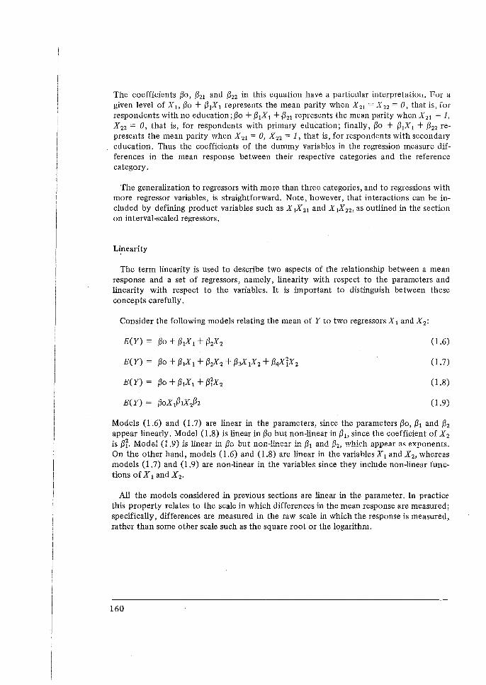
The coefficients {30, {321 and {322 in this equation have a particular interpretation. For a given level of X 1, {30 + {3 1X 1 represents the mean parity when X21 = X 22 = 0, that is, for respondents with no education; {30 + {3 1X 1 + {321 represents the mean parity when X 21 = 1, X 22 = 0, that is, for respondents with primary education; finally, {30 + {31X 1 + {3 22 re­presents the mean parity when X21 = 0, X 22 = 1, that is, for respondents with secondary education. Thus the coefficients of the dummy variables in the regression measure dif­ferences in the mean response between their respective categories and the reference category.

The generalization to regressors with more than three categories, and to regressions with more regressor variables, is straightforward. Note, however, that interactions can be in­cluded by defining product variables such as X 1X 21 and X 1X 22 , as outlined in the section on interval-scaled regressors.

Li,nearity

The term linearity is used to describe two aspects of the relationship between a mean response and a set of regressors, namely, linearity with respect to the parameters and linearity with respect to the variables. It is important to distinguish between these concepts carefully.

Consider the following models relating the mean of Y to two regressors X 1 and X 2 :

E(Y) = {30 + f31X1 + f3i%2

E(Y) = {30 + f31X1 + f3i%2 + f3:71X2 + f3¥IX2

E(Y) = {30 + f31X1 + f3IX2

H(Y) = {30X1f3tX2f32

(1.6)

(1.7)

(1.8)

(1.9)

Models (1.6) and (1.7) are linear in the parameters, since the parameters {30, {31 and {32 appear linearly. Model (1.8) is linear in {30 but non-linear in {3i, since the coefficient of X 2 ls {3f. ~viodel (1.9) is linear in {30 but nan-linear i.11 ~1 and {32, which appear as exponents. On the other hand, models (1.6) and (1.8) are linear in the variables X 1 and X 2 , whereas models (1.7) and (1.9) are non-linear in the variables since they include non-linear func­tions of X 1 and X 2 .•

All the models considered in previous sections are linear in the parameter. In practice this property relates to the scale in which differences in the mean response are measured; specifically, differences are measured in the raw scale in which the response is measured, rather than some other scale such as the square root or the logarithm.

160

The concept of additivity is specific to the scale in which differences are measured, and is thus related to linearity. When we considered additivity in the section on interaction, we were in fact defining additivity on a linear scale. It is possible for variables to be non­additive on the linear scale but additive on some other scale. For example, consider once again the effects of marital duration and education on parity. We have seen that it is un­realistic to suppose that differences in mean parity by educational level are the same for all levels of marital duration. However, it may be reasonable to suppose that ratios (or percentage differences) in mean parity between educational levels are the same for all marital durations. Since the logarithms of ratios are the differences of logarithms this cor­responds to additivity on the logarithmic scale. This leads to multiplicative or log-linear additive models such as (1.9), which are discussed in WFS Technical Bulletin No. 5 (Little, 1978).

Linearity with respect to a variable X refers to the assumption that the relationship between X and the response is linear, that is, that the means of Y for each value of X lie on a straight line. In cases where the relationship is non-linear, linearity may be achieved by a transformation of the regressor variable. If this does not remove the curvilinearity, then polynominal terms (X2

, X3, ... ) may be introduced into the regression model or,

alternatively, the values of the regressor variable may be grouped into categories and treated as a categorical regressor.

B. PATH ANALYSIS: GENERAL PRINCIPLES

In section A we outlined some statistical techniques for assessing the joint effects of a set or regressors on a response, based on linear models. Path analysis is not a statistical technique like regression or MCA. It is an interpretational technique for determining appropriate sets of regressors and predictors in a statistical analysis, and for understanding the output from the statistical analysis. In section C we consider a special form of ana­lyses for multivariate normal data, which entails some further arithmetical operations on the coefficients from multiple regressions. However in this section we consider path ana­lysis in a broader context, as a method of formalizing intuitive ideas about which effects of variables have substantive meaning.

ASSESSING THE EFFECT OF INDIVIDUAL VARIABLES

We again consider the relationship between a set of regressor variables X 1, ••• X k and a response are additive on some scale, that is, that there are no interactions. In section C we shall consider the case where significant interactions are present.

We have noted that the effect of a categorical variable on the response can be repre­sented as deviations between the category means and the overall mean of Y; the effect of

161

an interval-scaled variable in a multiple regression is represented by its regression coefficient. In either case, it is well known that the magnitude of this effect in general depends on which other regressor variables are controlled by inclusion in the analysis. In the simple example of the previous section, the effect of education on parity is usually reduced when marital duration is controlled. More generally, the effect of a variable X 1

on Y changes when another variable X 2 is controlled if X 1 and X 2 are associated and the effect of X 2 on Y con trolling X 1 is not zero.

In practice we may have a large number of potential regressor variables which are associated and have an effect on the response. Suppose we wish to assess the effect of each individual variable. The question is, which other regressor variables should be con­trolled when the effect of any given variable is calculated?

One obvious solution is to calculate the marginal effect of each regressor, without con­trolling any other variables. That is, consider the effect of Xj by simply regressing or cross-classifying Y by Xi. This turns out to be unsatisfactory, for sound substantive reasons. For example, consider the effects of education and age on parity, and suppose that education is negatively associated with both parity and age. If the relationship between education and parity disappears when age is controlled, then the relationship is a spurious consequence of the different age composition of the educational groups. In such situations the substantive effect of education would correctly be assessed after control­ling age, and not from the unadjusted means.

An alternative procedure, often encountered in applications of multiple regression, is to assess the effect of each variable with all other variables controlled. In the context of multiple regression, this corresponds to calculating the regression equation with all regressor variables included, and interpreting the regression coefficient of each variable as the effect of that variable. This also proves unsatisfactory, particularly when there is a high association between the regressors. For example, suppose we include the variables respondent's level of education and husband's level of education as regressors on parity. If these variables are highly associated, their joint effects may easily prove statistically in­significant even though when taken separately their effects are significantly large. In general, the magnitude of effects diminishes as positively associated predictors are introduced, and this can lead to very misleading conclusions. [See, for example, Gordon (i968)].

The fact is that without some additional information independent of the data, there is no unique way of representing the effect of a variable on a response. Any effect is specific to the set of other variables controlled in the analysis. Path analysis, in its general form, can be seen as an attempt to attribute causal interpretations to certain of these control­specific effects. Also, it leads to one particular effect, the total effect of the variable, which has the clearest substantive interpretation, and this may be considered a partial answer to the problem of which variables to control in an analysis.

162

The key concept of path analysis is the determination of a causal ordering between a set of variables. In a general sense this leads to a set of rules concerning which variables should be controlled in any analysis. For the specific application to multivariate normal data, it determines the order in which a set of regressions should be canied out. We now discuss these ideas in more detail.

THE CAUSAL ORDERING AND TOTAL EFFECTS

We suppose that the regressor and response variables can be placed in a causal ordering

(2.1)

such that chan_ges in the values ot any variable can affect a variable later in the chain, but do no affect variables earlier in the chain. Two points require special emphasis here:

a) The causal ordering cannot be decided by an empirical analysis of the data, but must be based on prior theoretical knowledge of the population;

b) The specification of a causal ordering in effect rules out the possibility of circular causation between variables, where one variable both affects and is affected by another variable in the series. In the examples, we shall proceed under the assumption that at least a predominant direction of causal ordering can be established. In cases where this is not possible the interpretation of the data is much more difficult, and more complex ana­lytical techniques than those discussed in section A are required to disentangle relation­ships between the variables. See, for example, the non-recursive models discussed by Hood and Koopmans (1953). In this paper we shall illustrate situations where circular causation does exist, but we shall not provide a quantitative analysis for these cases.

Two general rules of path analysis stem from this ·causal ordering:

Rule 1. The response variable, Y, must be the last variable in the causal chain. In other words, variables causally posterior to the response should not be controlled.

Rule 2. In assessing the effect of any regressor variable X on a response, Y, all variables causally prior to X should be controlled.

To clarify these rules, consider a particular regressor variable X. We can represent the position of X in the causal chain as follows:

where Xb are the set of regressor variables prior to X, Xa are the set of regressor variables posterior to X, and the response Y is by rule 1 the last variable in the chain. Then rule 2 states that the variables Xb should be controlled when calculating the effect of X on Y.

163

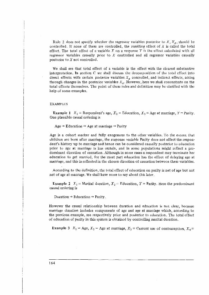
Rule 2 does not specify whether the regressor variables posterior to X, Xa, should be controlled. If none of these are controlled, the resulting effect of Xis called the total effect. The total effect of a variable X on a response Y is the effect calculated with all regressor variables causally prior to X controlled and all regressor variables causally posterior to X not controlled.

We shall see that total effect of a variable is the effect with the clearest substantive interpretation. In section C we shall discuss the decomposition of the total effect into direct effects with certain posterior variables Xa controlled, and indirect effects, acting through changes in the posterior variables Xa. However, here we shall concentrate on the total effects themselves. The point of these rules and definition may be clarified with the help of some examples.

EXAMPLES

Example 1 X 1 = Respondent's age, X 2 = Education, X 3 = Age at marriage, Y =Parity. One plausible causal ordering is

Age -r Education -r Age at marriage -r Parity

Age is a cohort marker and fully exogenous to the other variables. To the extent that children are born after marriage, the response variable Parity does not affect the respon­dent's history up to marriage and hence can be considered causally posterior to education prior to age at marriage is less certain, and in some populations might reflect a pre­dominant direction of causation. Although in some cases a respondent may terminate her education to get married, for the most part education has the effect of delaying age at marriage, and this is reflected in the chosen direction of causation between these variables.

According to the definition, the total effect of education on parity is net of age but not net of age at marriage. We shall have more to say about this later.

Example 2 X 1 = Marital duration, X 2 =Education, Y =Parity. Here the predominant causal ordering is

Duration -r Education -r Parity.

However the causal relationship between duration and education is not clear, because marriage duration includes components of age and age at marriage which, according to the previous example, are respectively prior and posterior to education. The total effect of education of parity in this system is obtained by controlling marital duration.

Example 3 X1 = Age, X 2 = Age at marriage, X 3 = Current use of contraception, X 4 =

164

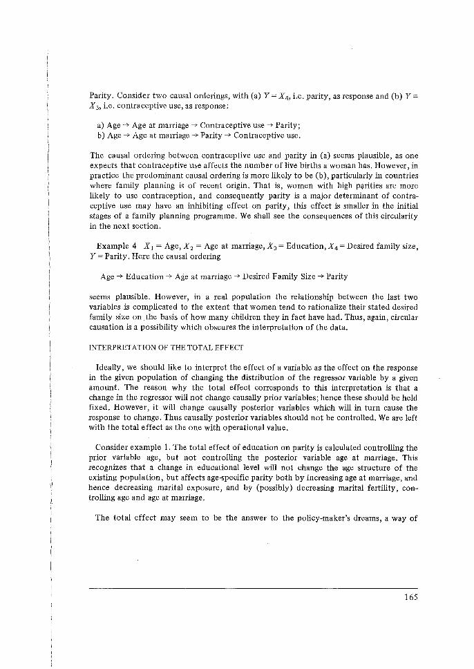
Parity. Consider two causal orde1ings, with (a) Y = X4, i.e. parity, as response and (b) Y = X 3, i.e. contraceptive use, as response:

a) Age-+ Age at marriage-+ Contraceptive use-+ Parity; b) Age-+ Age at marriage-+ Parity-+ Contraceptive use.

The causal ordering between contraceptive use and parity in (a) seems plausible, as one expects that contraceptive use affects the number of live births a woman has. However, in practice the predominant causal ordering is more likely to be (b), particularly in countries where family planning is of recent origin. That is, women with high pi;irities are more likely to use contraception, and consequently parity is a major determinant of contra­ceptive use may have an inhibiting effect on parity, this effect is smaller in the initial stages of a family planning programme. We shall see the consequences of this circularity in the next section.

Example 4 X 1 = Age, X 2 = Age at marriage, X 3 = Education, X 4 = Desired family size, Y = Parity. Here the causal ordering

Age-+ Education-+ Age at marriage-+ Desired Family Size-+ Parity

seems plausible. However, in a real population the relationship between the last two variables is complicated to the extent that women tend to rationalize their stated desired family size on the basis of how many children they in fact have had. Thus, again, circular causation is a possibility which obscures the interpretation of the data.

INTERPRETATION OF THE TOTAL EFFECT

Ideally, we should like to interpret the effect of a variable as the effect on the response in the given population of changing the distribution of the regressor variable by a given amount. The reason why the total effect corresponds to this interpretation is that a change in the regressor will not change causally prior variables; hence these should be held fixed. However, it will change causally posterior variables which will in turn cause the response to change. Thus causally posterior variables should not be controlled. We are left with the total effect as the one with operational value.

Consider example 1. The total effect of education on parity is calculated controlling the prior variable age, but not controlling the posterior variable age at marriage. This recognizes that a change in educational level will not change the age structure of the existing population, but affects age-specific parity both by increasing age at marriage, and hence decreasing marital exposure, and by (possibly) decreasing marital fertility, con­trolling age and age at marriage.

The total effect may seem to be the answer to the policy-maker's dreams, a way of

165

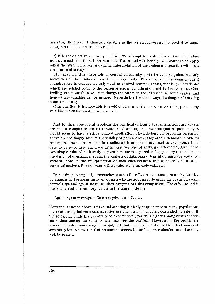
assessing the effect of changing variables in the system. However, this predictive causal interpretation has serious limitations:

a) It is retrospective and not predictive. We attempt to explain the system of variables as they stand, and there is no guarantee that causal relationships will continue to apply when the system changes. A dynamic interpretation of the system is impossible without a time series of surveys;

b) In practice, it is impossible to control all causally posterior variables, since we only measure a finite number of variables in any study. This is not quite as damaging as it sounds, since in practice we only need to control common causes, that is, prior variables which are related both to the regressor under consideration and to the response. Con­trolling other variables will not change the effect of the regressor, as noted earlier, and hence these variables can be ignored. Nevertheless there is always the danger of omitting common causes;

c) In practice, it is impossible to avoid circular causation between variables, particularly variables which have not been measured.

And to these conceptual problems the practical difficulty that interactions are always present to complicate the interpretation of effects, and the principals of path analysis would seem to have a rather limited application. Nevertheless, the problems presented above do not simply restrict the validity of path analysis; they are fundamental problems concerning the nature of the data collected from a cross-sectional survey. Hence they have to be recognized and lived with, whatever type of analysis is attempted. Also, if the two simple rules of path analysis given here are recognized and applied by researchers in the design of questionnaires and the analysis of data, many elementary mistakes would be avoided, both in the interpretation of cross-classifications and in more sophisticated statistical analysis. For this reason these rules are immensely valuable.

To continue example 3, a researcher assesses the effect of contraceptive use by fertility by comparing the mean parity of women who are not currentiy using. He or she correctly controls age and age at marriage when carrying out this comparison. The effect found is the total effect of contraceptive use in the causal ordering

Age -7 Age at marriage_,. Contraceptive;: u~e;: -7 Parity.

However, as noted above, this causal ordering is highly suspect since in many populations the relationship between contraceptive use and parity is circular, contradicting rule 1. If the researcher finds that, contrary to expectations, parity is higher among contraceptive users than among users, he or she may see the problem. However, if the results are reversed the difference may be happily attributed in mean parities to the effectiveness of contraception, whereas in fact no such inference is justified, since circular causation may well be present.

166

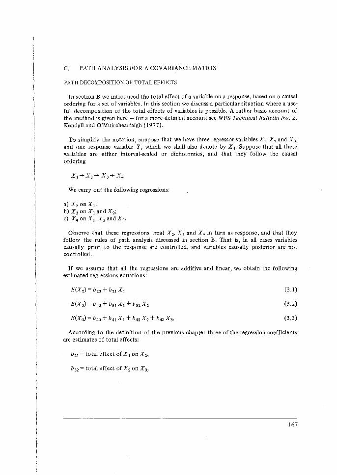
C. PATH ANALYSIS FOR A COVARIANCE MATRIX

PATH DECOMPOSITION OF TOTAL EFFECTS

In section B we introduced the total effect of a variable on a response, based on a causal ordering for a set of variables. In this section we discuss a particular situation where a use­ful decomposition of the total effects of variables is possible. A rather basic account of the method is given here - for a more detailed account see WFS Technical Bulletin No. 2, Kendall and O'Muircheartaigh (1977).

To simplify the notation, suppose that we have three regressor variables X 1, X 2 and X 3,

and one response variable Y, which we shall also denote by X4. Suppose that all these variables are either interval-scaled or dichotomies, and that they follow the causal ordering

We carry out the following regressions:

a) X 2 onX1 ;

b) X 3 on X 1 and X 2 ;

c) X 4 onXi,X2 andX3•

Observe that these regressions treat X 2, X 3 and X4 in turn as response, and that they follow the rules of path analysis discussed in section B. That is, in all cases variables causally prior to the response are controlled, and variables causally posterior are not controlled.

If we assume that all the regressions are additive and linear, we obtain the following estimated regressions equations:

(3.1)

(3.2)

(3.3)

According to the definition of the previous chapter three of the regression coefficients are estimates of total effects:

b21 = total effect of X 1 on X 2,

b32 = total effect of X 2 on X 3,

167

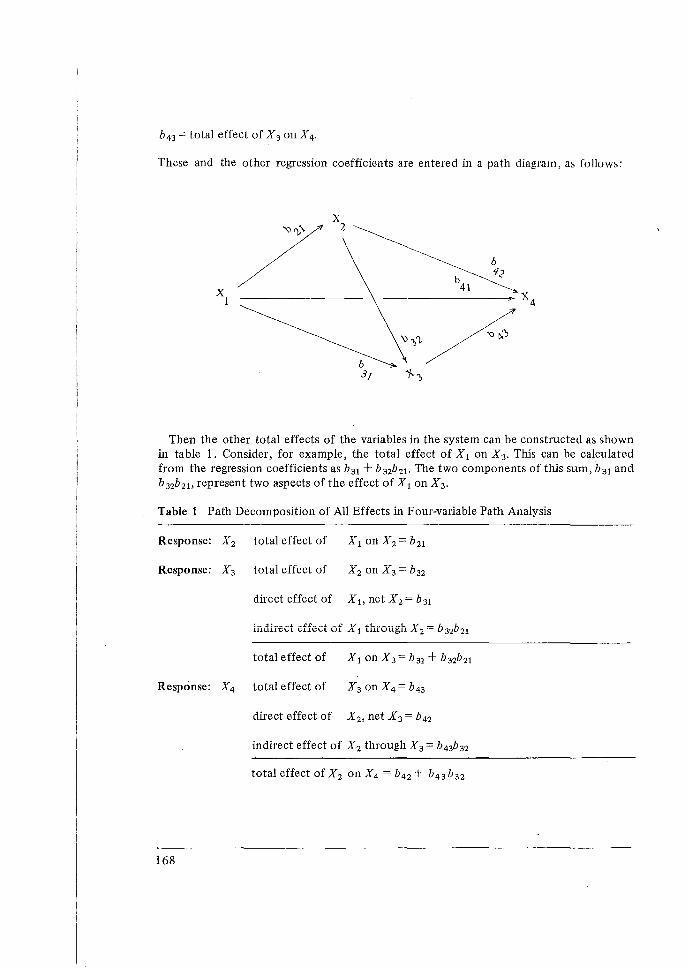
b43 =total effect of X 3 on X 4 .

These and the other regression coefficients are entered in a path diagram, as follows:

x 1

x 2

Then the other total effects of the variables in the system can be constructed as shown in table 1. Consider, for example, the total effect of X1 on X3 • This can be calculated from the regression coefficients as b31 + b32b21 • The two components of this sum, b31 and b32b2 i, represent two aspects of the effect of X 1 on X 3 •

Table 1 Path Decomposition of All Effects in Four-variable Path Analysis

Response: X 2 total effect of

Response: X3 totai effect of

direct effect of Xi, net X 2 = b31

total effect of

Response: X4 total effect of

direct effect of X 2, net X 3 = b 42

168

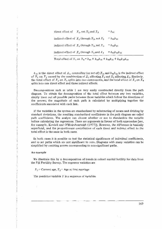
direct effect of X 1, net X 2 and X 3 = b4 1

b 31 is the direct effect of X 1, controlling (or net of) X 2 , and b32b21 is the indirect effect of X 1 on X 2 caused by the combination of X 1 affecting X2 and X 2 affecting X 3• Similarly, the total effect of X 2 on X4 splits into two components, and the· total effect of X1 on X4

splits into one direct effect and three indirect effects.

Decompositions such as table 1 are very easily constructed directly from the path diagram. To obtain the decomposition of the total effect between any two variables, simply trace out all possible paths between those variables which follow the directions of the arrows; the magnitude of each path is calculated by multiplying together the coefficients associated with each link.

If the variables in the system are standardized by substracting of means and dividing by standard deviations, the resulting stand-ardized coefficients in the path diagram are called path coefficients. The analyst can choose whether or not to standardize the variable before calculating the regressions. There are arguments in favour of both approaches [see, for example, Kendall and O'Muircheartaigh (1977)]. However, the difference is basically superficial, and the proportionate contribution of each direct and indirect effect to the total effect is the same in both cases.

In both cases it is possible to test the statistical significance of individual coefficients, and to set paths which are not significant to zero. Diagrams with many variables can be simplified by omitting arrows corresponding to non-significant paths.

An example

We illustrate this by a decomposition of trends in cohort marital fertility for data from the Fiji Fertility Survey. The regressor variables are

X 1 =Current age,X2 =Age at first marriage

The predictor variable Y is a sequence of variables

169

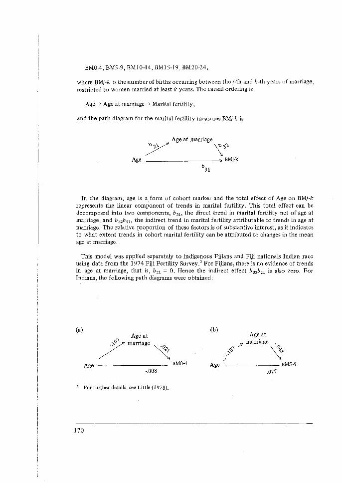
BM0-4, BMS-9, BMl0-14, BMlS-19, BM20-24,

where BMj-k is the number of births occurring between the j-th and k-th years of marriage, restricted to women married at least k years. The causal ordering is

Age-+ Age at marriage-+ Marital fertility,

and the path diagram for the marital fertility measures BMj-k is

Age at marriage 7 \~~ Age BMj-k

b31

In the diagram, age is a form of cohort marker and the total effect of Age on BMj-k represents the linear component of trends in marital fertility. This total effect can be decomposed into two components, b31, the direct trend in marital fertility net of age at marriage, and b32b21 , the indirect trend in marital fertility attributable to trends in age at marriage. The relative proportion of these factors is of substantive interest, as it indicates to what extent trends in cohort marital fertility can be attributed to changes in the mean age at marriage.

This model was applied separately to indigenous Fijians and Fiji nationals Indian race using data from the 1974 Fiji Fertility Survey.3 For Fijians, there is no evidence of trends in age at marriage, that is, b21 = 0. Hence the indirect effect b32b21 is also zero. For Indians, the following path diagrams were obtained:

(a) :'\ Age at

/marriage~

Age -.008

3 For further details, see Little (1978),

170

(b)

BM04 Age

Age at

mmfage ~

-------- BMS-9 /

.027

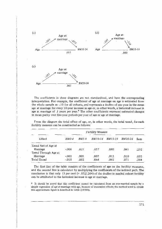
(c) (d) Age at Age at

//mmfag' , ~ 7

,mmfago .,.,6' \

Age BMl0-14 Age BM15-19 .057 .080

(e) Age at

\-r::iV marriage

7 Age

~o.Y ~

BM20-24 .061

The coefficients in these diagrams are not standardized, and have the corresponding interpretation. For example, the coefficient of age at marriage on age is estimated from the whole sample as -.10 for all cohorts, and represents a decline of one year in the mean age at marriage for every 10-year increase in age or, in other words, a historical increase in age at marriage of .1 years per year.4 The other coefficients represent estimated changes in mean parity over five-year periods per year of age or age at marriage.

From the diagram the total effect of age, or, in other words, the total trend, for each fertility measure can be constructed as follows:

Fertility Measure

Effect BM0-4 BM5-9 BMI0-14 BM15-19 BM20-24 Sum

Trend Net of Age at Marriage -.008 .027 .057 .080 .061 .232

Trend Through Age at Marriage -.002 .005 .007 .012 .010 .032

Total Trend -.010 .032 .064 .092 .071 .264

The first line of the table consists of the coefficients of age on the fertility measures, and the second line is calculated by multiplying the coefficients of the indirect path. The conclusion is that only 13 per cent(= .032/.264) of the decline in marital cohort fertility can be attributed to the historical increase in age at marriage.

4 It should be noted that this coefficient cannot be calculated from an ever-married sample by a simple regression of age at marriage with age, because of truncation effects; the method used to obtain this approximate figure is described in Little (1978b).

171

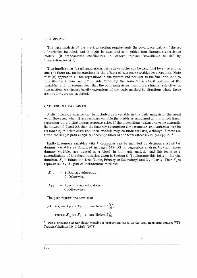
ASSUMPTIONS

The path analysis of the previous section requires only the covadance matrix of the set of variables included, and it might be described as a 'guided tour through a covariance matrix' (if standardized coefficients are chosen, replace 'covariance matrix' by 'correlation matdx').

This implies that (a) all associations between variables can be described by correlations, and (b) there are no interactions in the effects of regressor variables on a response. Note that (b) applies to all the regressions in the system and not just to the final one. Add to this the extraneous assumption introduced by the non-circular causal ordering of the variables, and it becomes clear that the path analysis assumptions are highly restrictive. In this section we discuss briefly extensions of the basic method to situations where these assumptions are not satisfied.

CATEGORICAL VARIABLES

A dichotomous variable can be included as a variable in the path analysis in the usual way. However, when it is a response variable the problems associated with multiple linear regression on a dichotomous response arise. If the proportions taking one value generally lie between 0.2 and 0.8 then the linearity assumption for parameters and variables may be reasonable; in other cases non-linear models may be more realistic, although if these are fitted the simple path analytical decomposition of the total effect no longer applies.5

Multichotomous variables with k categories can be included by defining a set of k-1 durruny variables as described in pageSI 48-15 3 on regression analysis/Mukerji. These dummy variables are treated as a block in the path analysis, and this leads to a generalization of the decomposition given in Section C. To illustrate this, let X 1 =Marital duration, X 2 = Education level (None, Primary or Secondary) and X 3 =Parity. Then X 2 is represented by the pair of dichotomous variables

X21 1, Primary education; 0, Otherwise

X 22 1, Secondary education; 0, Otherwise.

The path regressions consist of

(a) regress X 21 on X1 coefficient b ~Q;

regress X 22 on X 1 coefficient b~/;

s For a discussion of non-linear models for proportions based on the logit transformation, see WFS Technical Bulletin No. 5, Little (1978).

172

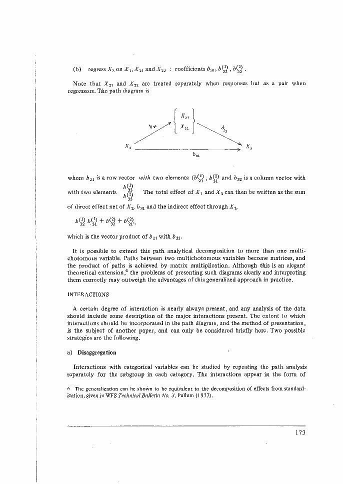
(b) regress X 3 on X 1, X 21 and X 22 : coefficients b 31 , b~1J , b~2J .

Note that X 21 and X 22 are treated separately when responses but as a pair when regressors. The path diagram is

where b 21 is a row vector with two elements (b~1/ , b~? and b32 is a column vector with

bCiJ with two elements b(2) The total effect of X 1 and X 3 can then be written as the sum

33

of direct effect net of X 2' b 31 and the indirect effect through X 2'

which is the vector product of b 21 with b 32•

It is possible to extend this path analytical decomposition to more than one multi­chotomous variable. Paths between two multichotomous variables become matrices, and the product of paths is achieved by matrix multiplication. Although this is an elegant theoretical extension,6 the problems of presenting such diagrams clearly and interpreting them correctly may outweigh the advantages of this generalized approach in practice.

INTERACTIONS

A certain degree of interaction is nearly always present, and any analysis of the data should include some description ot the major interactions present. The extent to which interactions should be incorporated in the path diagram, and the method of presentation, is the subject of another paper, and can only be consid1:1red briefly here. Two possible strategies are the following.

a) Disaggregation

Interactions with categorical variables can be studied by repeating the path analysis separately for the subgroup in each category. The interactions appear in the form of

6 The generalization can be shown to be equivalent to the decomposition of effects from standard­ization, given in WFS Technical Bulletin No. 3, Pullum (1977).

173

different path coefficients for the different groups. For example, the path analysis of trends in cohort marital fertility given in pages 127-130 was carried out separately for Fijians and Indians, in effect a disaggregation with respect to the variable race. Disaggregation is particularly natural in this case as these races are known to have many distinguished characteristics. It was noted earlier that Indians experienced a historical increase in mean age at marriage, whereas the mean age at marriage of Fijians has remained relatively stable. This would be evident from the different path coefficients of important inter­action effects, that between age and race on age at marriage, which would not be evident from a path analysis on the complete data.

Interactions with interval-level variables can also be investigated by forming categories by grouping and then repeating the path analysis for each group separately. A common instance of this approach is the practice of repeating certain analyses separately for each birth or marriage cohort.

Disaggregation is conceptually simple and theoretically attractive. The main limitations concern the degree of disaggregation that is practically feasible for the given sample size, and the fact that formal statistical tests of the interactions are not immediately available.

b) Inclusion of interaction terms in the regressions

A more selective way of including specific interactions which are thought to be present is to include them in the regressions, using the methods indicated in Section A. The statistical significance of included interactions can be assessed. The interactions with categorical variables can then be presented by disaggregation so that path coefficients corresponding to interactions are different between groups, and other coefficients are equal between groups. Interactions with intervalscaled variables pose a more difficult presentational problem, which can only be approached with a certain amount of trial and error.

NON-RECURSIVE MODELS

Path models with a strict causal ordering and no circular causation are called recursive models. We have already given in section B examples where the interpretation of the data is highly problematical because of circular causation between the observed variables. In this section we give an example of a situation where circularity is produced by an un­observed variable.

Suppose that X 1 = Age, X 2 = Education, X 3 = Knowledge of family planning outlet, X 4 =Current use of efficient contraception.7 One possible causal ordering is

Age-+ Education -+ Knowledge of outlet -+ Current use.

7 This example arises from a study of family planning availability reported in Rodriguez (1978).

174

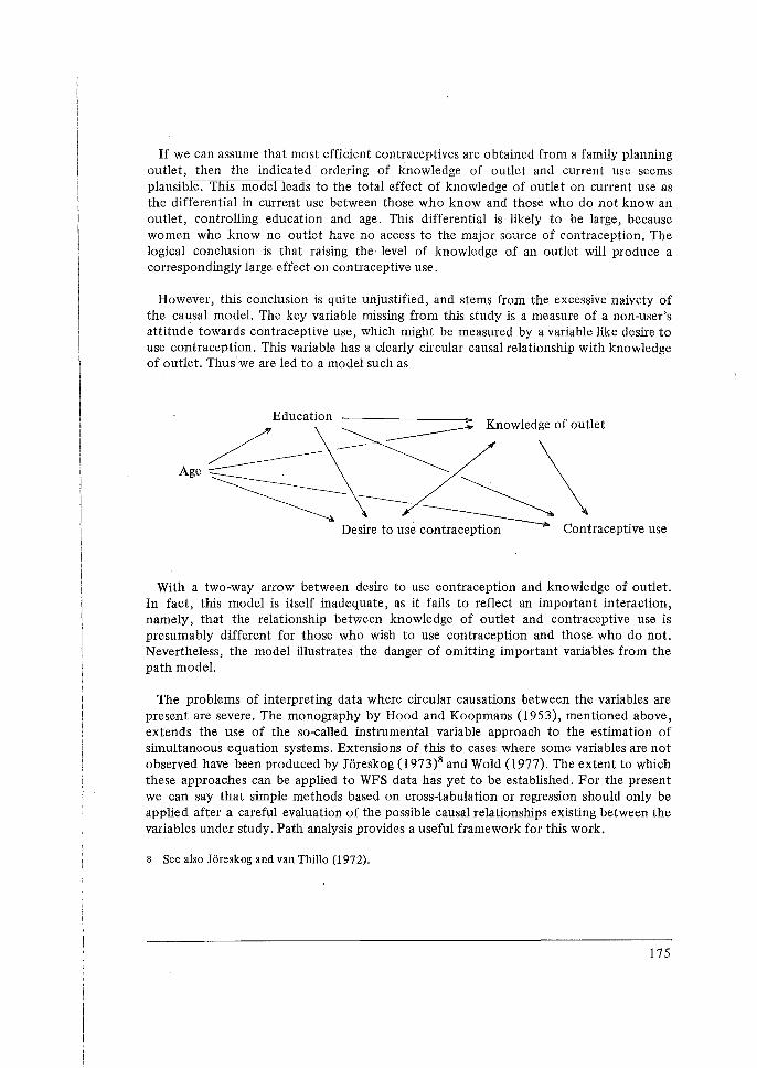
If we can assume that most efficient contraceptives are obtained from a family planning outlet, then the indicated ordering of knowledge of outlet and current use seems plaus1b1e. This model leads to the total effect of knowledge of outlet on current use as the differential in current use between those who know and those who do not know an outlet, controlling education and age. This differential is likely to be large, because women who know no outlet have no access to the major source of contraception. The logical conclusion is that raising the level of knowledge of an outlet will produce a correspondingly large effect on contraceptive use.

However, this conclusion is quite unjustified, and stems from the excessive naivety of the causal model. The key variable missing from this study is a measure of a non-user's attitude towards contraceptive use, which might be measured by a variable like desire to use contraception. This variable has a clearly circular causal relationship with knowledge of outlet. Thus we are led to a model such as

Education ~ ~ Knowlodgo of outfot

Age~c~~\ D . ·~ct t· esrre to use contraception on racep 1ve use

With a two-way arrow between desire to use contraception and knowledge of outlet. In fact, this model is itself inadequate, as it fails to reflect an important interaction, namely, that the relationship between knowledge of outlet and contraceptive use is presumably different for those who wish to use contraception and those who do not. Nevertheless, the model illustrates the danger of omitting important variables from the path model.

The problems of interpreting data where circular causations between the variables are present are severe. The monography by Hood and Koopmans (1953), mentioned above, extends the use of the so-called instrumental variable approach to the estimation of simultaneous equation systems. Extensions of this to cases where some variables are not observed have been produced by JOreskog (1973)8 and Wold (1977). The extent to which these approaches can be applied to WFS data has yet to be established. For the present we can say that simple methods based on cross-tabulation or regression should only be applied after a careful evaluation of the possible causal relationships existing between the variables under study. Path analysis provides a useful framework for this work.

8 See also JOreskog and van Thillo (1972).

175

BIBLIOGRAPHY

Gordon, R.A., 'Issues in Multiple Regression'. American Journal of Sociology, VoL 13, No. 5 (pp. 592-601). 1968.

Hood, W.C. and T.C. Koopmans (eds.), Studies in Econometric Method. Cowles Commission Monograph No. 14, Wiley Press. 1953.

JOreskog, K.G., 'A General Method for Estimating a Linear Structural Equation System, in Structural Systems in the Social Sciences, A.S. Goldberger and 0.D. Duncan (eds.) New York Seminar Press. 1973.

Ji:ireskog, K.G. and M. Van Thillo, 'LISREL: A General Computer Program for Estimating a Linear Structural Equation System Involving Multiple Indicators of Un­measured Variables, Research Bulletin 72-56. Educational Testing Services, Princeton, New Jersey. 1972.

Kendall, M.G. and C.A. O'Muircheartaigh, 'Path Analysis and Model Building', WFS Technical Bulletin Series, No. 2. International Statistical Institute, Voorburg, Nether­lands. 1977.

Little, R . .T.A., 'Generalized Linear Models for Cross-Classified Data'. WFS Technical Bulletin Series, No. 5. International Statistical Institute, Voorburg, Netherlands. 197 8.

Little, R.J.A. Regression Analysis of Trends and Differentials in Fertility Using Maternity History Data. WFS/TECH 892. 1978.

Pullum, T.W., 'Standardization'. WFS Technical Bulletin Series, No. 3. International Statistical Institute, Voorburg, Netherlands. 1977.

Rodriguez, G., 'Family Planning Availability and Contraceptive Practice', International Family Planning Perspectives and Digest. December 197 8.

Wold, H., 'On the Transition from Pattern Recognition to Model Building' in Mathemat­ical Economics and Game Theory: Essays in Honor of Oscar Morgenstern. R. Henn and 0. Moeschlin (eds.). Berlin, Springer. 1977.

176

WORLD FERTILITY SURVEY

OCCASIONAL PAPERS

1. Fertility and Related Surveys

2. The World Fertility Survey: Problems and Possibilities

World Fertility Survey Inventory: Major Fertility and Related Surveys 1960-73

3. Asia

4. Africa

5. Latin America

6. Europe, North America and Australia

7. The Study of Fertility and Fertility Change in Tropical Africa

8. Community-Level Data in Fertility Surveys

William G. Duncan

J. C. Caldwell

l Swnuel Baum '' al

John C. Caldwell

Ronald Freedman 9. Examples of Community-Level Questionnaires Ronald Freedman

10. A Selected Bibliography of Works on Fertility Gyorgy T. Acsadi 11. Economic Data for Fertility Analysi Deborah S. Freedman (with Eva Mueller)

12. Economic Modules for use in Fertility Surveys DeborahS.Freedman and Eva Mueller in Less Developed Countries

13. Ideal Family Size Helen Ware

14. Modernism David Goldberg

15. The Fiji Fertility Survey: M.A. Sahib et al A Critical Commentary

16. The Fiji Fertility Survey: M.A. Sahib et al A Critical Commentary-Appendices

17. Sampling Errors for Fertility Surveys L. Kish et al

18. The Dominican Republic Fertility Survey: N. Ramirez et al An Assessment

19. WFS Modules: Abortion · Factors other than WPS Central Staff Contraception Affecting Fertility · Family Planning . General Mortality

N.V. DRUKKERU TRIO •THE HAOUE •THE NETHERLANDS