novel cascade spline architectures for the identification of nonlinear systems

IEEE TRANSACTIONS ON CIRCUITS AND SYSTEMS—I: REGULAR PAPERS, VOL. 62, NO. 7, JULY 2015 1825

Novel Cascade Spline Architectures for theIdentification of Nonlinear Systems

Michele Scarpiniti, Member, IEEE, Danilo Comminiello, Member, IEEE, Raffaele Parisi, Senior Member, IEEE, andAurelio Uncini, Member, IEEE

Abstract—In this paper two novel nonlinear cascade adaptive ar-chitectures, here called sandwich models, suitable for the identifi-cation of general nonlinear systems are presented. The proposedarchitectures rely on the combination of structural blocks, eachone implementing a linear filter or a memoryless nonlinear func-tion. All the nonlinear functions involved in the adaptation processare based on spline functions and can be easily modified duringlearning using gradient-based techniques. In particular, a simpleform of the on-line adaptation algorithms for the two architecturesis derived. In addition, we analytically obtain a bound for the se-lection of the learning rates involved in the learning algorithms, inorder to guarantee a convergence towards a minimum of the costfunction. Finally, some experimental results demonstrate the effec-tiveness of the proposed method.Index Terms—Hammerstein-Wienermodels, nonlinear adaptive

filters, nonlinear cascade adaptive filters, nonlinear system identi-fication, sandwich models, spline adaptive filters.

I. INTRODUCTION

T HE THEORY OF linear adaptive filtering (LAF) is wellestablished. The use of LAF methods for the solution of

real problems is extensive and represents a central paradigm formany strategic real-world applications. The basic discrete-timefilter is a simple linear combiner, whose length is determined byfollowing some proper criterion. Its weights are then adapted bychoosing the most convenient optimization strategy [1].In contrast, in many practical situations, the nature of the

process of interest (POI) is affected by any nonlinearity andthus requires the use of nonlinear adaptive filter (NAF) models.In the ideal case, if the nature of the nonlinearities is known apriori, it is possible to determine the NAF structure, in analogywith the mathematical model of nonlinearities. For example, ifthe underlying laws of the POI are characterized by a nonlineardifferential equation, the architecture that implements the NAFcan be determined from the discrete-time representation of thenonlinear differential equation itself. In this case the NAF is re-ferred to as white-box (or structural model) and the process ofadaptation consists in the estimation of the free model parame-ters (e.g., the coefficients of the nonlinear difference equation).

Manuscript received February 06, 2015; revised April 02, 2015; acceptedApril 09, 2015. Date of publication June 16, 2015; date of current version June24, 2015. This work has been partially supported by the Sapienza UniversityProject: Ambient Cloud (AmC), under grant number C26A13TB5Z. This paperwas recommended by Associate Editor J. M. Olm.The authors are with the Department of Information Engineering, Electronics

and Telecommunications, “Sapienza” University of Rome, 00184 Rome, Italy(e-mail: [email protected]; [email protected];[email protected]; [email protected]).Color versions of one or more of the figures in this paper are available online

at http://ieeexplore.ieee.org.Digital Object Identifier 10.1109/TCSI.2015.2423791

On the contrary, if any a priori knowledge about the nature ofnonlinearity is not available, it is preferred to use a black-box ap-proach (functional model). In these cases, a unique frameworkto the solution does not exist and the existence of the solutioncould not be guaranteed.One of the most well-known functional models is based on

the Volterra series [2]. Unfortunately, due to the large numberof free parameters required, the Volterra adaptive filter (VAF)is generally employed only in situations of mild nonlinearity[2], [3]. Neural networks (NNs) [4], [5] represent another flex-ible tool to realize black-box NAFs, but they generally requirea high computational cost and are not always feasible in on-lineapplications.Of particular interest is the estimation of specialized classes

of nonlinear systems [6]. As a matter of fact, these architec-tures can be successfully used in several applications in all fieldsof engineering [7], from circuit and system theory to modelingnonlinear characteristics of electronic devices and resistive net-works [8]–[10], to signal processing [11], [12], biomedical dataanalysis [13], digital communications [14], [15], even to hy-draulics [16] and chemistry [17].In nonlinear filtering one of the most used structures is the

so-called block-oriented representation, in which linear time in-variant (LTI) models are connected with memoryless nonlinearfunctions. The basic classes of block-oriented nonlinear sys-tems are represented by the Wiener and Hammerstein models[18]–[20] and all those architectures originated by the connec-tion of these two classes according to different topologies (i.e.,parallel, cascade, feedback, etc. [21]). More specifically, theWiener model consists of a cascade of an LTI filter followedby a static nonlinear function and sometimes it is known aslinear-nonlinear (LN) model [11], [22]–[24]. Conversely, theHammerstein model consists of a cascade connection of a staticnonlinear function followed by an LTI filter [25]–[27] and issometimes indicated as nonlinear-linear (NL) model.In a general nonlinear problem, with no a priori information

available, the best adaptive model (Hammerstein or Wiener)is the most similar to the one to be identified. In this sense ablock-oriented architecture may not be the best solution for theidentification of a general nonlinear system. In order to over-come this nonfunctional behavior, architectures combining bothbasic nonlinear systems were adopted [20].Unfortunately in many practical cases, due to the generality

of the model to be identified, the Wiener and Hammerstein ar-chitectures might not be the best solutions. For this reason cas-cade models, such as the linear-nonlinear-linear (LNL) or thenonlinear-linear-nonlinear (NLN) models, were also introduced[18], [28], [29]. Cascade models, here called sandwich models,constitute a relatively simple but important class of nonlinear

1549-8328 © 2015 IEEE. Personal use is permitted, but republication/redistribution requires IEEE permission.See http://www.ieee.org/publications_standards/publications/rights/index.html for more information.

1826 IEEE TRANSACTIONS ON CIRCUITS AND SYSTEMS—I: REGULAR PAPERS, VOL. 62, NO. 7, JULY 2015

models that can approximate a wide class of nonlinear systems[30]. Several choices for the nonlinearity are possible, namelysome invertible squashing functions, piece-wise linear functions[8], [31], [32], polynomial nonlinearities [33], splines [34], andso on.Recently a novel approach for the identification of Wiener

and Hammerstein models based on Spline Adaptive Filters(SAFs) has been proposed [35]–[37]. Among the advantagesof these solutions, in order to yield great representative po-tential, high performance, low computational cost and easyimplementability in dedicated hardware, all the nonlinearitiesinvolved in such systems are flexible and adapted by meansof a fixed length look-up table (LUT). Moreover, in order tohave a continuous and derivable smooth function, the LUTs areinterpolated by a low-order uniform spline, like done in [35]for the Wiener SAF (WSAF) and in [37] for the HammersteinSAF (HSAF).Following this approach and by properly extending the work

on SAFs, in this paper we propose two novel architectures forthe NLN and LNL models, named here as Sandwich 1 (S1)and Sandwich 2 (S2) respectively. These architectures are op-timized by following a gradient-based approach and comparedto alternative and more conventional solutions in a number ofapplications.The rest of the paper is organized as follows. Section II in-

troduces the Wiener and Hammerstein SAF, Sections III andIV derive the algorithms for the NLN and LNL models respec-tively. Then Section V shows the convergence condition of theproposed architecture, Section VI describes the computationalcost while Section VII shows some experimental results. FinallySection VIII concludes the work.

A. Notation

In this paper matrices are represented by boldface cap-ital letters, i.e., . All vectors are columnvectors, denoted by boldface lowercase letters, like

, where denotesthe -th individual entry of . In recursive algorithm definition,a discrete-time subscript index is added. For example, theweight vector, calculated according to some law, is written as

. In the case of signal regression, vectors areindicated as .Moreover, regarding the interpolated nonlinearity, the LUTcontrol points are denoted as ,where is the -th control point, while the -th span is denotedby .The Euclidean norm and the transpose of a vector are denoted

by and , respectively.

II. BACKGROUND ON SAF

For a complete description of spline adaptive filtering andspline interpolation, we refer to our recent papers [35] and [37].In the following we briefly recall the main concepts of thisapproach.In order to compute the nonlinear output that

is a spline interpolation of some adaptive control points con-tained in a LUT, we have to determine the explicit dependencebetween the input signal and . This can be easily done

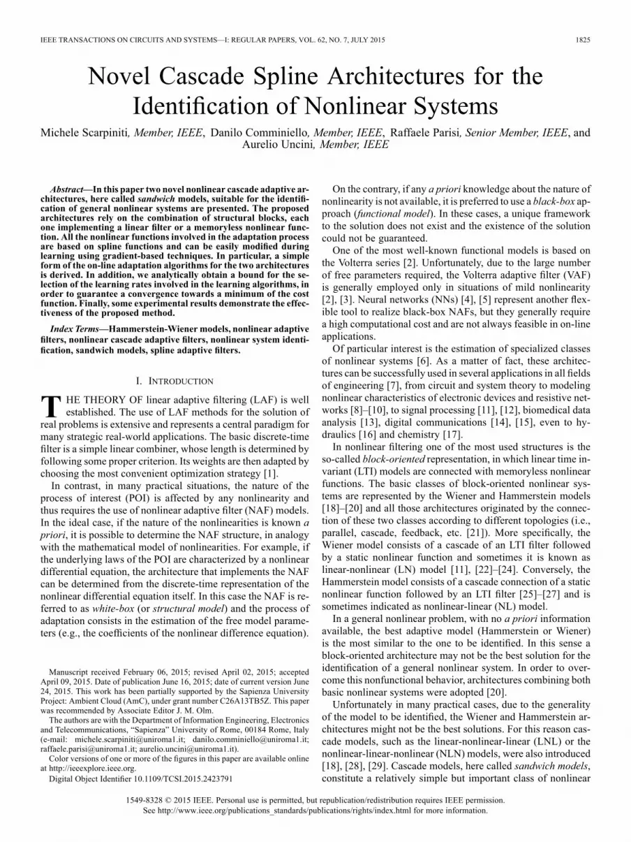
Fig. 1. Block diagram of: (a) a Wiener system; (b) a Hammerstein system.

by considering that is a function of two local parametersand that depend on .In the simple case of a uniformly spaced spline and a third-

order local polynomial interpolator (adopted in thiswork), each spline segment, denoted as span, is controlled byfour control points, also known as knots, addressed bythe span index that points at the first element of the related fourpoints contained in the LUT. The computation procedure for thedetermination of the span index and the local parameterscan be expressed by the following equations [38]:

(1)

where is the uniform space between knots, is the flooroperator and is the fixed LUT length i.e., the total number ofcontrol points. The second term in the right side of the secondequation is an offset value needed to force to be always non-negative. Note that the index depends on the time index ,i.e., ; for simplicity of notation in the following we will writesimply .Referring to [35] and to [37], the output of the nonlinearity

can be evaluated as

(2)

where the vector is defined as, is a pre-computed matrix,

called spline basis matrix, and the vector contains thecontrol points at the instant . More specifically, is definedby , where is the-th entry in the LUT.It could be very important to know the derivative of (2) with

respect to its input. It is easily evaluated as

(3)

where .The on-line learning algorithm can be derived by considering

the cost function1 (CF) . In order toderive the LMS algorithm, this CF is usually approximated byconsidering only the instantaneous error

(4)

The expression of the error signal in (4) depends on theparticular architecture used.

1In this work we consider only real-valued variables.

SCARPINITI et al.: NOVEL CASCADE SPLINE ARCHITECTURES FOR THE IDENTIFICATION OF NONLINEAR SYSTEMS 1827

Fig. 2. Block diagram of a Sandwich 1 system.

A. Wiener SAFWith reference to Fig. 1(a), let us define the output error

as

(5)

where is the reference signal, i.e., the output signal of thesystem to be estimated including any possible noise. The on-linelearning algorithm can be derived by the minimization of (4).We proceed by applying the stochastic gradient adaptation [35],obtaining the LMS iterative algorithm

(6)

for the weights of the linear filter and

(7)

for the spline control points. The parameters and , repre-sent the learning rates for the weights and for the control pointsrespectively and, for simplicity, incorporate the other constantvalues.

B. Hammerstein SAFWith reference to Fig. 1(b), we can define the output erroras

(8)

where and each sampleis evaluated by using an interpolation

scheme similar to (2).As in the Wiener case, the learning algorithm is derived by

minimizing the CF (4). We proceed by applying the stochasticgradient adaptation as done in [37], obtaining the LMS iterativealgorithm

(9)

for the weights of the linear filter and

(10)

for the spline control points. In (10),is a matrix which collects past

vectors , where each vector assumes the value ofif evaluated in the same span of the current sample inputor in an overlapped span, otherwise it is a zero vector.As in the Wiener case, the learning rates and

incorporate the other constant values.In the following paragraphs we introduce the novel S1 and S2

architecture, deriving the learning algorithms and convergencebounds. It must be underlined that the systems to be identifiedare assumed to derive from the same class of the system used forthe identification. These systems are described by the nonlinear-linear-nonlinear (NLN) and the linear-nonlinear-linear (LNL)models, respectively. The reference signal is considered asthe sum of the model output signal and a Gaussian noise withzero mean and variance .

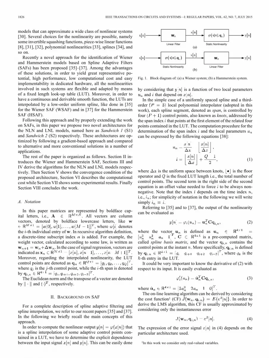
III. SANDWICH 1 SAFThe S1 model consists in the cascade of a memoryless non-

linear function, a linear filter and a second memoryless non-linear function and can be considered as the cascade of a Ham-merstein system and aWiener system. The basic model is shownin Fig. 2. From the symbols defined in Fig. 2, we have

(11)

(12)

(13)

where and are the spline control points for the first andsecond nonlinearity respectively.Let us denote with the error signal of the

S1 system. We then have to minimize the following CF

(14)

This optimization process can be performed by following an ap-proach that is similar to the popular backpropagation paradigmemployed in feedforward neural networks [4].Namely, the learning rule for the output nonlinearity can be

found by computing the gradient of the error w.r.t. the splinecontrol points

(15)

For the learning rule of the linear filter it is possible to obtain

(16)

For the learning rule of the first spline control points, we get

(17)


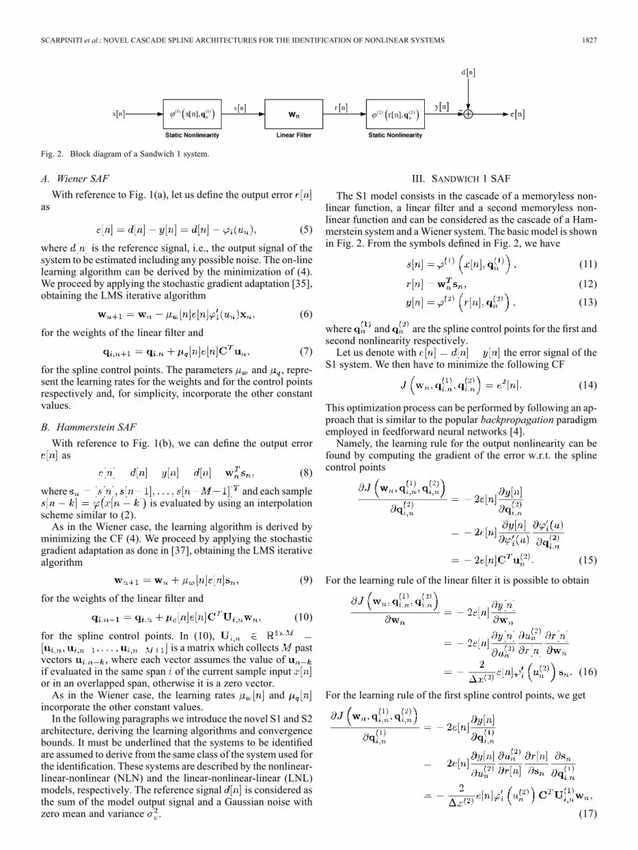
Fig. 3. Implementation of the proposed S1 learning algorithm.

where is amatrix which collects past vectors , each one as-suming the value of if it was evaluated in the same spanof the current sample input or in an overlapped span,

otherwise it is a zero vector. The matrix, not so easy tobe calculated, is essential to correctly evaluate the derivative

. We have implicitly assumed that ,for in order to avoid the evaluation ofnon-causal derivatives. This assumption can be practicallyimplemented by using a very small learning rate , sothat the first nonlinearity can be considered time-invariant for

samples. This is similar to the temporal back-propagationalgorithm for neural networks [39], [40].Finally, the three learning rules can be written as

(18)

(19)and

(20)

The parameters , and represent thelearning rates for the weights and for the control points respec-tively and, for simplicity, incorporate the other constant values.A summary of the proposed LMS algorithm for the nonlinear

S1 architecture, in the case of using constant learning rates, canbe found in Algorithm 1. Fig. 3 shows the implementation ofthe proposed learning algorithm.

Algorithm 1 Summary of the Sandwich 1 SAF-LMSalgorithm

Initialize: , ,

1: for do

2:

3:

4:

5:

6:

7:

8:

9:

10:

11:

12:

13:

14: end for

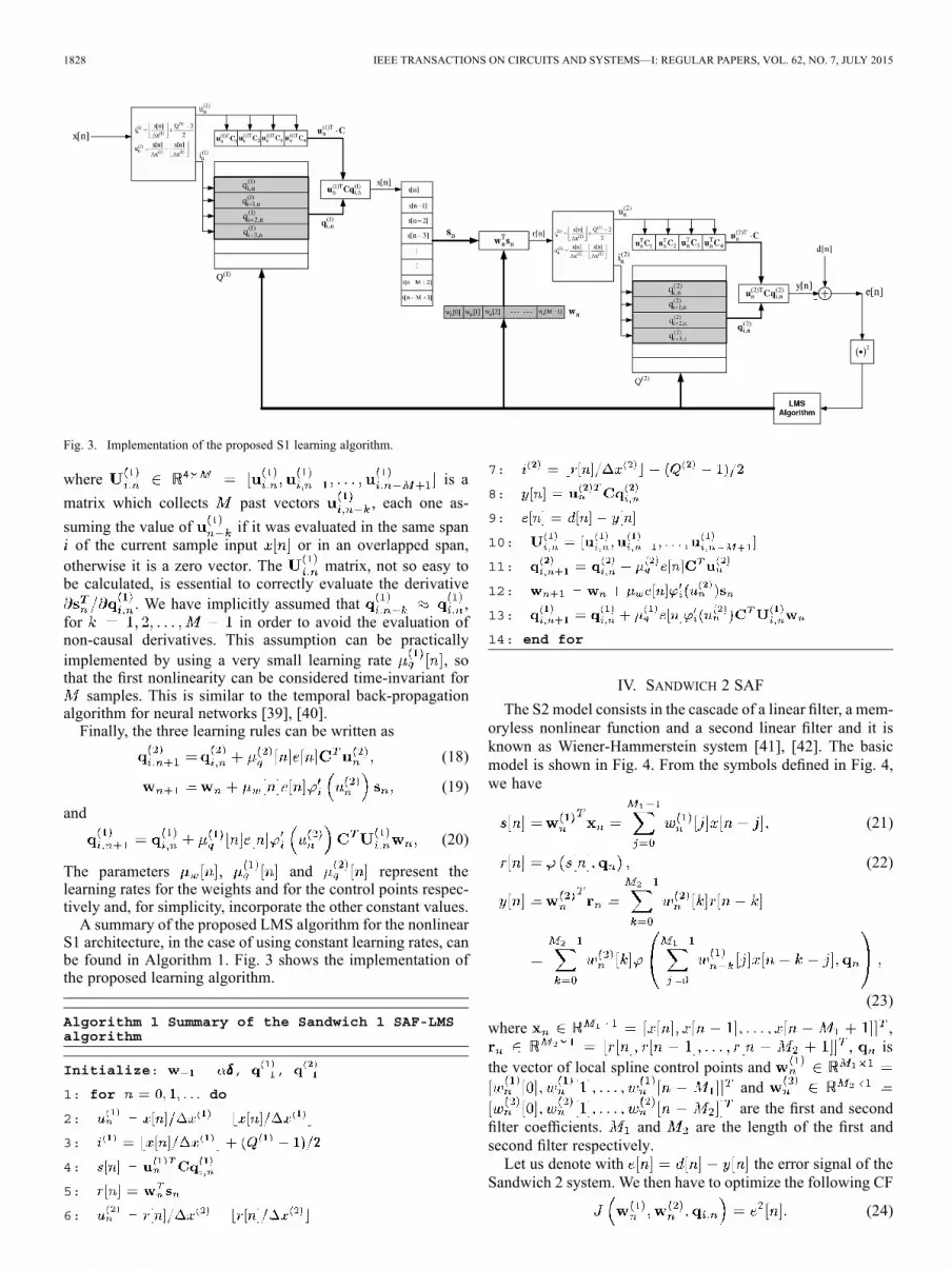
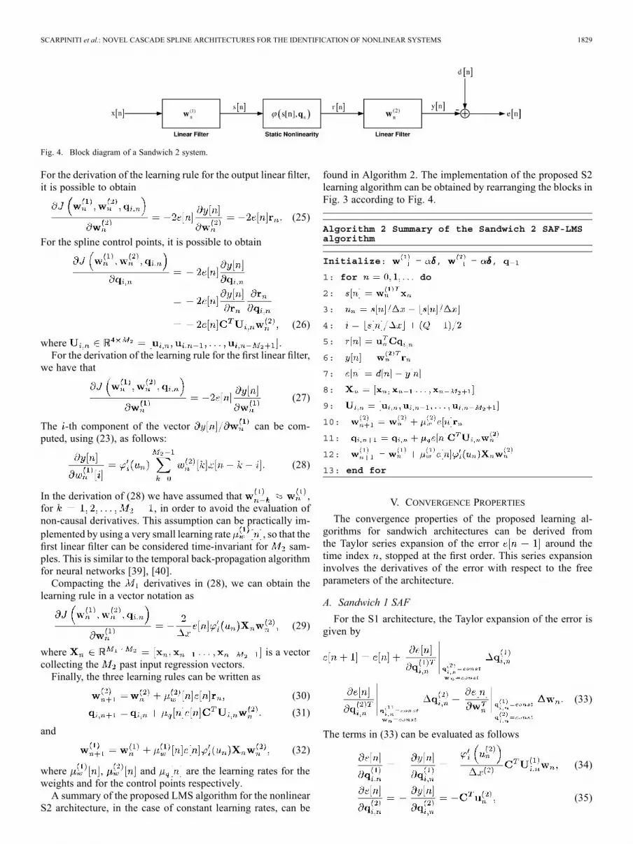
IV. SANDWICH 2 SAFThe S2 model consists in the cascade of a linear filter, a mem-

oryless nonlinear function and a second linear filter and it isknown as Wiener-Hammerstein system [41], [42]. The basicmodel is shown in Fig. 4. From the symbols defined in Fig. 4,we have

(21)

(22)

(23)

where ,, is

the vector of local spline control points andandare the first and second

filter coefficients. and are the length of the first andsecond filter respectively.Let us denote with the error signal of the

Sandwich 2 system. We then have to optimize the following CF

(24)


Fig. 4. Block diagram of a Sandwich 2 system.

For the derivation of the learning rule for the output linear filter,it is possible to obtain

(25)

For the spline control points, it is possible to obtain

(26)

where .For the derivation of the learning rule for the first linear filter,

we have that

(27)

The -th component of the vector can be com-puted, using (23), as follows:

(28)

In the derivation of (28) we have assumed that ,for , in order to avoid the evaluation ofnon-causal derivatives. This assumption can be practically im-plemented by using a very small learning rate , so that thefirst linear filter can be considered time-invariant for sam-ples. This is similar to the temporal back-propagation algorithmfor neural networks [39], [40].Compacting the derivatives in (28), we can obtain the

learning rule in a vector notation as

(29)

where is a vectorcollecting the past input regression vectors.Finally, the three learning rules can be written as

(30)(31)

and

(32)

where , and are the learning rates for theweights and for the control points respectively.A summary of the proposed LMS algorithm for the nonlinear

S2 architecture, in the case of constant learning rates, can be

found in Algorithm 2. The implementation of the proposed S2learning algorithm can be obtained by rearranging the blocks inFig. 3 according to Fig. 4.

Algorithm 2 Summary of the Sandwich 2 SAF-LMSalgorithm

Initialize: , ,

1: for do

2:

3:

4:

5:

6:

7:

8:

9:

10:

11:

12:

13: end for

V. CONVERGENCE PROPERTIESThe convergence properties of the proposed learning al-

gorithms for sandwich architectures can be derived fromthe Taylor series expansion of the error around thetime index , stopped at the first order. This series expansioninvolves the derivatives of the error with respect to the freeparameters of the architecture.

A. Sandwich 1 SAFFor the S1 architecture, the Taylor expansion of the error is

given by

(33)

The terms in (33) can be evaluated as follows

(34)

(35)


(36)

(37)

(38)

and

(39)

Substituting (34)–(39) into (33), we have

(40)

In order to ensure the convergence of the algorithm, we desirethat . This aim is reached if the followingrelation holds

(41)

that implies the following bound on the choice of the learningrates:

(42)

If the three learning rates , and are chosenaccording to (42), then the algorithms is guaranteed to convergeto its optimal solution. Note that in (42) all quantities are pos-itive, thus no positivity constrains are needed. In addition, theconvergence properties depend on the slope, but not on the signof the derivative. The potential problem of diverging ofis avoided by its intrinsic definition (3).

B. Sandwich 2 SAFFor the S2 architecture, the Taylor expansion of the error is

given by

(43)

The terms in (43) can be evaluated as follows

(44)

(45)

(46)

(47)(48)

and

(49)

Substituting (44)–(49) into (43), we have

(50)

In order to ensure the convergence of the algorithm, we desirethat . This aim is reached if the followingrelation holds

(51)

that implies the following bound on the choice of the learningrates:

(52)

If the three learning rates , and are chosenaccording to (52), then the algorithm is guaranteed to convergeto its optimal solution. Note that also in (52) all quantities arepositive, thus no positivity constraints are needed and the con-vergence properties depend on the slope, but not on the sign ofthe derivative.Note that the bounds in (42) and (52) are useful to check

the convergence of the proposed algorithms. In fact, if at anytime (42) and (52) are not verified, it is possible to scale allthe learning rates, in order to satisfy these bounds and hence toguarantee the convergence of the algorithms.

VI. COMPUTATIONAL ANALYSIS

From the computational point of view each proposed archi-tecture requires the evaluation of three processing blocks. Foreach block it has to be evaluated the computational cost of theforward phase (i.e., the evaluation of the system output) and ofthe backward phase (i.e., the adaptation of the adaptive system).It is well known from literature that the computational cost ofthe LMS algorithm is multiplications plus additionsfor each input sample [1]. In addition the cost of the spline eval-uation must be considered. The whole computational costs forthe S1 and S2 architectures are reported in Table I. In particular,this table shows that the computational cost of the S1 architec-ture is linear with the filter length , while the cost of the S2architecture is quadratic, since it depends on the product .Moreover, every spline evaluation requires an additional cost ofone division and one floor operation.It is straightforward to note that the computational cost can be

reduced by using some smart trick, like choosing the samplingstep or the learning rates as a power of two. In fact,


TABLE IEVALUATION OF THE COMPUTATIONAL COST FOR S1 AND S2 ARCHITECTURES FOR EACH INPUT SAMPLE

these constraints transform the multiplications into shift opera-tions. In addition, the spline polynomial interpolation could beimplemented by using the Horner's rule [43], in order to furtherreduce the complexity of the algorithm.

VII. EXPERIMENTAL RESULTSIn order to validate the proposed nonlinear adaptive filtering

solutions, several tests were performed for the general problemof system identification.

A. First Experiment

The first experiment consists in the identification of anunknown Sandwich 1 system composed by a linear component

and twononlinear memoryless target functions. These functions areimplemented by two 23-point length LUTs and ,interpolated by a uniform third degree spline with an intervalsampling and defined as

and

The input signal consists of 50,000 samples of the signalgenerated by the following relationship

(53)

where is a zero mean white Gaussian noise with unitaryvariance and is a parameter that determines thelevel of correlation between adjacent samples. Experiments areconducted with set to 0.1 and 0.95. In addition it is consideredan additive white noise such that the signal to noise ratio(SNR) is 30 dB.The learning rates are set to . The

linear filter is initialized as , withand using . The filter length is set to

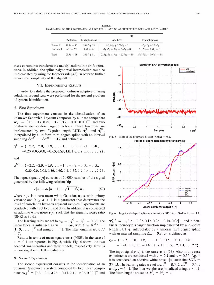
.Results in terms of mean square error (MSE), in the case of

are reported in Fig. 5, while Fig. 6 shows the twoadapted nonlinearities and their models, respectively. Resultsare averaged over 100 simulations.

B. Second Experiment

The second experiment consists in the identification of anunknown Sandwich 2 system composed by two linear compo-nents and

Fig. 5. MSE of the proposed S1 SAF with .

Fig. 6. Target and adapted spline nonlinearities (SPL) in S1 SAFwith .

, and a non-linear memoryless target function implemented by a 23-pointlength LUT interpolated by a uniform third degree splinewith an interval sampling . is defined as

The input signal is the same as in (53). Also in this caseexperiments are conducted with and . Againit is considered an additive white noise such that

. The learning rates are set to ,and . The filter weights are initialized using .The filter lengths are set to .


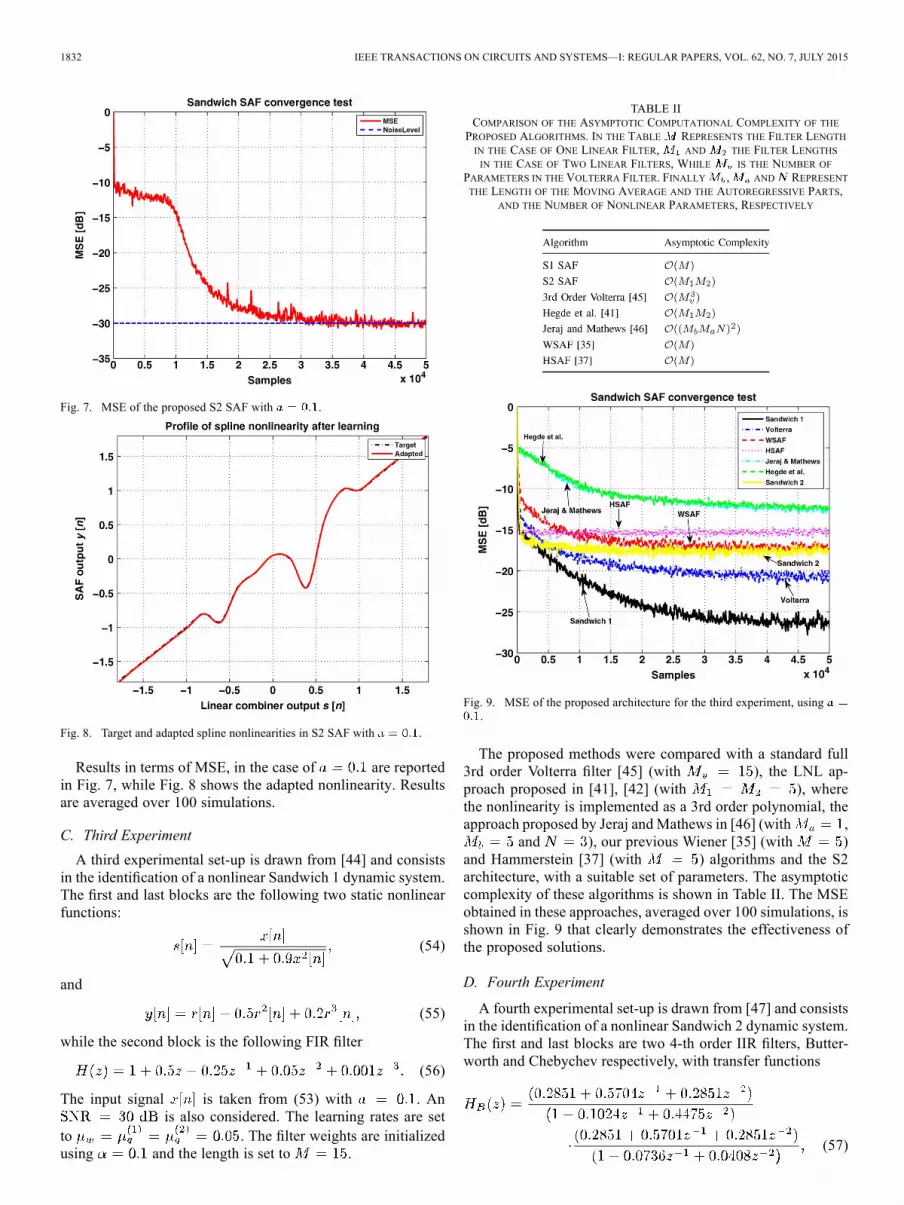
Fig. 7. MSE of the proposed S2 SAF with .

Fig. 8. Target and adapted spline nonlinearities in S2 SAF with .

Results in terms of MSE, in the case of are reportedin Fig. 7, while Fig. 8 shows the adapted nonlinearity. Resultsare averaged over 100 simulations.

C. Third ExperimentA third experimental set-up is drawn from [44] and consists

in the identification of a nonlinear Sandwich 1 dynamic system.The first and last blocks are the following two static nonlinearfunctions:

(54)

and

(55)

while the second block is the following FIR filter

(56)

The input signal is taken from (53) with . Anis also considered. The learning rates are set

to . The filter weights are initializedusing and the length is set to .

TABLE IICOMPARISON OF THE ASYMPTOTIC COMPUTATIONAL COMPLEXITY OF THE

PROPOSED ALGORITHMS. IN THE TABLE REPRESENTS THE FILTER LENGTHIN THE CASE OF ONE LINEAR FILTER, AND THE FILTER LENGTHSIN THE CASE OF TWO LINEAR FILTERS, WHILE IS THE NUMBER OF

PARAMETERS IN THE VOLTERRA FILTER. FINALLY , AND REPRESENTTHE LENGTH OF THE MOVING AVERAGE AND THE AUTOREGRESSIVE PARTS,

AND THE NUMBER OF NONLINEAR PARAMETERS, RESPECTIVELY

Fig. 9. MSE of the proposed architecture for the third experiment, using.

The proposed methods were compared with a standard full3rd order Volterra filter [45] (with ), the LNL ap-proach proposed in [41], [42] (with ), wherethe nonlinearity is implemented as a 3rd order polynomial, theapproach proposed by Jeraj andMathews in [46] (with ,

and ), our previous Wiener [35] (with )and Hammerstein [37] (with ) algorithms and the S2architecture, with a suitable set of parameters. The asymptoticcomplexity of these algorithms is shown in Table II. The MSEobtained in these approaches, averaged over 100 simulations, isshown in Fig. 9 that clearly demonstrates the effectiveness ofthe proposed solutions.

D. Fourth Experiment

A fourth experimental set-up is drawn from [47] and consistsin the identification of a nonlinear Sandwich 2 dynamic system.The first and last blocks are two 4-th order IIR filters, Butter-worth and Chebychev respectively, with transfer functions

(57)


TABLE IIIMSE IN DB OF THE PROPOSED S1 AND S2 ARCHITECTURES, COMPARED WITH OTHER REFERENCED APPROACHES, USING REAL DATA

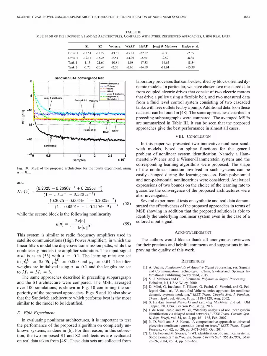
Fig. 10. MSE of the proposed architecture for the fourth experiment, using.

and

(58)

while the second block is the following nonlinearity

(59)

This system is similar to radio frequency amplifiers used insatellite communications (High Power Amplifier), in which thelinear filters model the dispersive transmission paths, while thenonlinearity models the amplifier saturation. The input signal

is as in (53) with . The learning rates are setto , and . The filterweights are initialized using and the lengths are setto .The same approaches described in preceding subparagraph

and the S1 architecture were compared. The MSE, averagedover 100 simulations, is shown in Fig. 10 confirming the su-periority of the proposed approaches. Figs. 9 and 10 also showthat the Sandwich architecture which performs best is the mostsimilar to the model to be identified.

E. Fifth ExperimentIn evaluating nonlinear architectures, it is important to test

the performance of the proposed algorithm on completely un-known systems, as done in [6]. For this reason, in this subsec-tion, the two proposed S1 and S2 architectures are evaluatedon real data taken from [48]. These data sets are collected from

laboratory processes that can be described by block-oriented dy-namic models. In particular, we have chosen two measured datafrom coupled electric drives that consist of two electric motorsthat drive a pulley using a flexible belt, and two measured datafrom a fluid level control system consisting of two cascadedtanks with free outlets fed by a pump. Additional details on thesedata sets can be found in [48]. The same approaches described inpreceding subparagraphs were compared. The averaged MSEsare summarized in Table III. It can be seen that the proposedapproaches give the best performance in almost all cases.

VIII. CONCLUSIONIn this paper we presented two innovative nonlinear sand-

wich models, based on spline functions for the generalproblem of nonlinear system identification. Namely a Ham-merstein-Wiener and a Wiener-Hammerstein system and thecorresponding learning algorithms were proposed. The shapeof the nonlinear function involved in such systems can beeasily changed during the learning process. Both polynomialand non-polynomial nonlinearities were considered. Analyticalexpressions of two bounds on the choice of the learning rate toguarantee the convergence of the proposed architectures werealso investigated.Several experimental tests on synthetic and real data demon-

strated the effectiveness of the proposed approaches in terms ofMSE showing in addition that the proposed solution is able toidentify the underlying nonlinear system even in the case of acolored input signal.

ACKNOWLEDGMENT

The authors would like to thank all anonymous reviewersfor their precious and helpful comments and suggestions in im-proving the quality of this work.

REFERENCES[1] A. Uncini, Fundamentals of Adaptive Signal Processing, ser. Signals

and Communication Technology. Cham, Switzerland: Springer In-ternational Publishing Switzerland, 2015.

[2] V. J. Mathews and G. L. Sicuranza, Polynomial Signal Processing.Hoboken, NJ, USA: Wiley, 2000.

[3] D. Mirri, G. Iuculano, F. Filicori, G. Pasini, G. Vannini, and G. Pel-legrini Gualtieri, “A modified Volterra series approach for nonlineardynamic systems modeling,” IEEE Trans. Circuits Syst. I, Fundam.Theory Appl., vol. 49, no. 8, pp. 1118–1128, Aug. 2002.

[4] S. Haykin, Neural Networks and Learning Machines, 2nd ed. OldTappan, NJ, USA: Pearson Publishing, 2009.

[5] J. de Jesus Rubio and W. Yu, “Stability analysis of nonlinear systemidentification via delayed neural networks,” IEEE Trans. Circuits Syst.II, Exp. Briefs, vol. 54, no. 2, pp. 161–165, Feb. 2007.

[6] N. D. Vanli and S. S. Kozat, “A comprehensive approach to universalpiecewise nonlinear regression based on trees,” IEEE Trans. SignalProcess., vol. 62, no. 20, pp. 5471–5486, Oct. 2014.

[7] O. De Feo and M. Storace, “PWL identification of dynamical systems:Some examples,” in Proc. Int. Symp. Circuits Syst. (ISCAS2004), May23–26, 2004, vol. 4, pp. 665–668.


[8] C. Wen and X. Ma, “A basis-function canonical piecewise-linear ap-proximation,” IEEE Trans. Circuits Syst. I, Reg. Papers, vol. 55, no. 5,pp. 1328–1334, Jun. 2008.

[9] B. N. Bond, Z. Mahmood, Y. Li, R. Sredojević, A. Megretski, V. Sto-janović, Y. Avniel, and L. Daniel, “Compact modeling of nonlinearanalog circuits using system identification via semidefinite program-ming and incremental stability certification,” IEEE Trans. Comput.-Aided Design Integr. Circuits Syst., vol. 29, no. 8, pp. 1149–1162, Aug.2010.

[10] S. Orcioni, “Approximation and analog implementation of nonlinearsystems represented by Volterra series,” in Proc. 6th IEEE Int. Conf.Electron., Circuits, Syst., 1999, pp. 1109–1113.

[11] G. Mzyk, “A censored sample mean approach to nonparametric iden-tification of nonlinearities in Wiener systems,” IEEE Trans. CircuitsSyst. II, Exp. Briefs, vol. 54, no. 10, pp. 897–901, Oct. 2007.

[12] M. Scarpiniti, D. Comminiello, R. Parisi, and A. Uncini, “Compar-ison of Hammerstein and Wiener systems for nonlinear acoustic echocancelers in reverberant environments,” in Proc. 17th Int. Conf. Digit.Signal Process. (DSP2011), Corfu, Greece, Jul. 6–8, 2011, pp. 1–6.

[13] K. J. Hunt, M. Munih, N. N. Donaldson, and F. M. D. Barr, “Investi-gation of the Hammerstein hypothesis in the modeling of electricallystimulated muscle,” IEEE Trans. Biomed. Eng., vol. 45, no. 8, pp.99–1009, Aug. 1998.

[14] Z. Zhu and H. Leung, “Adaptive identification of nonlinear systemswith application to chaotic communications,” IEEE Trans. CircuitsSyst. I, Fundam. Theory Appl., vol. 47, no. 7, pp. 1072–1080, Jul.2000.

[15] L. Peng and H. Ma, “Design and implementation of software-definedradio receiver based on blind nonlinear system identification and com-pensation,” IEEE Trans. Circuits Syst. I, Reg. Papers, vol. 58, no. 11,pp. 2776–2789, Nov. 2011.

[16] B. Kwak, A. E. Yagle, and J. A. Levitt, “Nonlinear system identifi-cation of hydraulic actuator friction dynamics using a Hammersteinmodel,” in Proc. IEEE ASSP98, Seattle, WA, USA, May 1998, vol. 4,pp. 1933–1936.

[17] J.-C. Jeng, L. M.-W. , and H.-P. Huang, “Identification of block-ori-ented nonlinear processes using designed relay feedback tests,” Ind.Eng. Chem. Res., vol. 44, no. 7, pp. 2145–2155, 2005.

[18] L. Ljung, System Identification—Theory for the User, 2nd ed. UpperSaddle River, NJ, USA: Prentice Hall, 1999.

[19] A. E. Nordsjo and L. H. Zetterberg, “Identification of certaintime-varying Wiener and Hammerstein systems,” IEEE Trans. SignalProcess., vol. 49, no. 3, pp. 577–592, Mar. 2001.

[20] S. Boyd and L. O. Chua, “Uniqueness of a basic nonlinear structure,”IEEE Trans. Circuits Syst., vol. CAS-30, no. 9, pp. 648–651, Sep. 1983.

[21] R. Haber and H. Unbehauen, “Structure identification of nonlinear dy-namic systems—A survey on input/output approaches,” Automatica,vol. 26, no. 4, pp. 651–677, 1990.

[22] E. W. Bai, “Frequency domain identification of Wiener models,” Au-tomatica, vol. 39, pp. 1521–1530, Sep. 2003.

[23] M. Korenberg and I. Hunter, “Twomethods for identifyingWiener cas-cades having noninvertible static nonlinearities,” Ann. Biomed. Eng.,vol. 27, no. 6, pp. 793–804, 1999.

[24] D. Westwick and M. Verhaegen, “Identifying MIMO Wiener systemsusing subspace model identificationmethods,” Signal Process., vol. 52,no. 2, pp. 235–258, Jul. 1996.

[25] E. W. Bai, “Frequency domain identification of Hammerstein models,”IEEE Trans. Autom. Control, vol. 48, pp. 530–542, 2003.

[26] I. J. Umoh and T. Ogunfunmi, “An affine projection-based algorithmfor identification of nonlinear hammerstein systems,” Signal Process.,vol. 90, no. 6, pp. 2020–2030, Jun. 2010.

[27] J. Vörös, “Identification of Hammerstein systems with time-varyingpiecewise-linear characteristics,” IEEE Trans. Circuits Syst. II, Exp.Briefs, vol. 52, no. 12, pp. 865–869, Dec. 2005.

[28] L. Ljung, “Identification of nonlinear systems,” in Proc. 9th Int. Conf.Control, Autom., Robot., Vis. (ICARCV 2006), Singapore, 2006.

[29] H.-E. Liao and W. A. Sethares, “Cross-term analysis of LNL models,”IEEE Trans. Circuits Syst. I, Fundam. Theory Appl., vol. 43, no. 4, pp.333–335, Apr. 1996.

[30] S. Billings and S. Y. Fakhouri, “Identification of a class of nonlinearsystems using correlation analysis,” Proc. IEEE, vol. 125, no. 7, pp.691–697, Jul. 1978.

[31] O. De Feo andM. Storace, “Piecewise-linear identification of nonlineardynamical systems in view of their circuit implementations,” IEEETrans. Circuits Syst. I, Reg. Papers, vol. 54, no. 7, pp. 1542–1554, Jul.2007.

[32] C. Wen and H. Ma, “A canonical piecewise-linear representationtheorem: Geometrical structures determine representation capability,”IEEE Trans. Circuits Syst. II, Exp. Briefs, vol. 58, no. 12, pp. 936–940,Dec. 2011.

[33] A. Stenger and W. Kellerman, “Adaptation of a memoryless pre-processor for nonlinear acoustic echo cancelling,” Signal Process.,vol. 80, no. 9, pp. 1747–1760, Sep. 2000.

[34] C. de Boor, A Practical Guide to Splines. New York: Springer-Verlag, 2001, rev. ed..

[35] M. Scarpiniti, D. Comminiello, R. Parisi, and A. Uncini, “Nonlinearspline adaptive filtering,” Signal Process., vol. 93, no. 4, pp. 772–783,Apr. 2013.

[36] M. Scarpiniti, D. Comminiello, R. Parisi, and A. Uncini, “Nonlinearsystem identification using IIR spline adaptive filters,” Signal Process.,vol. 108, pp. 30–35, Mar. 2015.

[37] M. Scarpiniti, D. Comminiello, R. Parisi, and A. Uncini, “Hammer-stein uniform cubic spline adaptive filters: Learning and convergenceproperties,” Signal Process., vol. 100, pp. 112–123, Jul. 2014.

[38] S. Guarnieri, F. Piazza, and A. Uncini, “Multilayer feedforward net-works with adaptive spline activation function,” IEEE Trans. NeuralNetw., vol. 10, no. 3, pp. 672–683, May 1999.

[39] E. A. Wan, “Temporal backpropagation for FIR neural networks,” inProc. Int. Joint Conf. Neural Netw. (IJCNN), San Diego, CA, USA,Jun. 17–21, 1990, vol. 1, pp. 575–580.

[40] P. Campolucci, A. Uncini, F. Piazza, and B. D. Rao, “On-line learningalgorithms for locally recurrent neural networks,” IEEE Trans. NeuralNetw., vol. 10, no. 2, pp. 253–271, Mar. 1999.

[41] V. Hegde, C. Radhakrishnan, D. J. Krusienski, andW. K. Jenkins, “Ar-chitectures and algorithms for nonlinear adaptive filters,” in Conf. Rec.36th Asilomar Conf. Signals, Syst., Comput., Pacific Grove, CA, USA,Nov. 3–6, 2002, vol. 2, pp. 1015–1018.

[42] V. Hegde, C. Radhakrishnan, D. J. Krusienski, andW. K. Jenkins, “Se-ries-cascade nonlinear adaptive filters,” in Proc. 45th Midwest Symp.Circuits Syst. (MWSCAS2002), Tulsa, OK, USA, Aug. 4–7, 2002, vol.3, pp. 219–222.

[43] T. H. Cormen, C. E. Leiserson, R. L. Rivest, and C. Stein, Introductionto Algorithms, 3rd ed. Cambridge, MA, USA: MIT Press, 2009.

[44] Y. Zhu, “Estimation of an N-L-N Hammerstein-Wiener model,” Auto-matica, vol. 38, no. 9, pp. 1607–1614, Sep. 2002.

[45] M. Schetzen, “Nonlinear system modeling based on the Wienertheory,” Proc. IEEE, vol. 69, no. 12, pp. 1557–1573, Dec. 1981.

[46] J. Jeraj and V. J. Mathews, “A stable adaptive Hammerstein filter em-ploying partial orthogonalization of the input signals,” IEEE Trans.Signal Process., vol. 54, no. 4, pp. 1412–1420, Apr. 2006.

[47] T.M. Panicker, V. J.Mathews, andG. L. Sicuranza, “Adaptive parallel-cascade truncated Volterra filters,” IEEE Trans. Signal Process., vol.46, no. 10, pp. 2664–2673, Oct. 1998.

[48] T. Wigren and J. Schoukens, “Three free data sets for development andbenchmarking in nonlinear system identification,” in Proc. 2013 Eur.Control Conf. (ECC2013), Zürich, Switzerland, Jul. 17–19, 2013, pp.2933–2938.

Michele Scarpinitiwas born in Leonberg, Germany,in 1978. He received the Laurea degree in elec-trical engineering with honors from the Universityof Rome “La Sapienza,” Italy, in 2005 and thePh.D. degree in information and communicationengineering in 2009. From March 2008 he is anAssistant Professor of Circuit Theory with theDepartment of Information Engineering, Electronicsand Telecommunications, University of Rome “LaSapienza,” Italy. His present research interestsinclude nonlinear adaptive filters, audio processing

and neural networks for signal processing, ICA, and blind signal processing.He is a member of IEEE, a member of the “Audio Engineering Society” (AES)and a member of the “Società Italiana Reti Neuroniche” (SIREN).

Danilo Comminiello (M’12) received the Telecom-munication Engineer degree in 2008 and the Ph.D.degree in Information and Communication Engi-neering in 2012, both from University of Rome “LaSapienza,” Italy.He is currently a Research Fellow at Depart-

ment of Information Engineering, Electronics andTelecommunications (DIET), University of Rome“La Sapienza,” Italy. From November 2008 toOctober 2011, during his Ph.D., he collaboratedwith Fondazione Ugo Bordoni, Rome, on projects

focused on speech quality evaluation and enhancement. From October 2010to January 2011 he was a Visiting Researcher at the department of Teoría de


la Señal y Comunicaciones (TSC), Universidad Carlos III de Madrid, Spain.His current research interests include signal processing and machine learningtheory, particularly focused on audio and speech intelligent systems. He isa member of the “Audio Engineering Society” (AES) and a member of the“Società Italiana Reti Neuroniche” (SIREN).

Raffaele Parisi received the Laurea degree in elec-trical engineering with honors and the Ph.D. degreein information and communication engineering fromthe University of Rome “La Sapienza,” Rome, Italy,in 1991 and 1995, respectively.In 1994 and 1999, he was a Visiting Student and a

Visiting Researcher with the Department of Electricaland Computer Engineering, University of Californiaat San Diego, La Jolla, CA, USA. Since 1996, hehas been with the University of Rome “La Sapienza,”where he is currently an Associate Professor with the

Department of Information Engineering, Electronics and Telecommunications.His research interests are in the areas of neural networks, digital signal pro-cessing, optimization theory, and array processing. He is a senior member ofIEEE and a member of the “Società Italiana Reti Neuroniche” (SIREN).

Aurelio Uncini (M’88) received the Laurea degreein electronic engineering from the University ofAncona, Italy, on 1983 and the Ph.D. degree inelectrical engineering in 1994 from University ofBologna, Italy. At present time he is Full Professorwith the Department of Information Engineering,Electronics and Telecommunications, where he isteaching Circuits Theory, Adaptive Algorithm forSignal Processing and Digital Audio Processingand where he is the founder and director of the“Intelligent Signal Processing and Circuits” (ISPAC)

group. His present research interests include also adaptive filters, adaptiveaudio and array processing, machine learning for signal processing, blindsignal processing and multi-sensors data fusion.He is a member of the Associazione Elettrotecnica ed Elettronica Italiana

(AEI), of the International Neural Networks Society (INNS), and of the SocietàItaliana Reti Neuroniche (SIREN).

novel cascade spline architectures for the identification of nonlinear systems

Documents