north atlantic oscillation imprints in the central iberian
TRANSCRIPT

North Atlantic Oscillation imprints in the Central Iberian Peninsula for the last two millennia: from ordination
analyses to the Bayesian approach
Guiomar Sánchez López
ADVERTIMENT. La consulta d’aquesta tesi queda condicionada a l’acceptació de les següents condicions d'ús: La difusió d’aquesta tesi per mitjà del servei TDX (www.tdx.cat) i a través del Dipòsit Digital de la UB (diposit.ub.edu) ha estat autoritzada pels titulars dels drets de propietat intel·lectual únicament per a usos privats emmarcats en activitats d’investigació i docència. No s’autoritza la seva reproducció amb finalitats de lucre ni la seva difusió i posada a disposició des d’un lloc aliè al servei TDX ni al Dipòsit Digital de la UB. No s’autoritza la presentació del seu contingut en una finestra o marc aliè a TDX o al Dipòsit Digital de la UB (framing). Aquesta reserva de drets afecta tant al resum de presentació de la tesi com als seus continguts. En la utilització o cita de parts de la tesi és obligat indicar el nom de la persona autora. ADVERTENCIA. La consulta de esta tesis queda condicionada a la aceptación de las siguientes condiciones de uso: La difusión de esta tesis por medio del servicio TDR (www.tdx.cat) y a través del Repositorio Digital de la UB (diposit.ub.edu) ha sido autorizada por los titulares de los derechos de propiedad intelectual únicamente para usos privados enmarcados en actividades de investigación y docencia. No se autoriza su reproducción con finalidades de lucro ni su difusión y puesta a disposición desde un sitio ajeno al servicio TDR o al Repositorio Digital de la UB. No se autoriza la presentación de su contenido en una ventana o marco ajeno a TDR o al Repositorio Digital de la UB (framing). Esta reserva de derechos afecta tanto al resumen de presentación de la tesis como a sus contenidos. En la utilización o cita de partes de la tesis es obligado indicar el nombre de la persona autora. WARNING. On having consulted this thesis you’re accepting the following use conditions: Spreading this thesis by the TDX (www.tdx.cat) service and by the UB Digital Repository (diposit.ub.edu) has been authorized by the titular of the intellectual property rights only for private uses placed in investigation and teaching activities. Reproduction with lucrative aims is not authorized nor its spreading and availability from a site foreign to the TDX service or to the UB Digital Repository. Introducing its content in a window or frame foreign to the TDX service or to the UB Digital Repository is not authorized (framing). Those rights affect to the presentation summary of the thesis as well as to its contents. In the using or citation of parts of the thesis it’s obliged to indicate the name of the author.

NORTH ATLANTIC OSCILLATION IMPRINTS IN THE CENTRAL IBERIANPENINSULA FOR THE LAST TWO MILLENNIA: FROM ORDINATION
ANALYSES TO THE BAYESIAN APPROACH
Memoria presentada por Guiomar Sánchez López para optar al grado de
doctora dentro del Programa de Doctorado de Ciències de la Terra de la Universitat de
Barcelona. Esta memoria ha sido realizada bajo la dirección del Dr. Santiago Giralt
Romeu (ICTJA-CSIC) y el Dr. Armand Hernández Hernández (IDL-Universidade de
Lisboa), y bajo la tutela del Dr. Lluís Cabrera Pérez (Universitat de Barcelona).
Guiomar Sánchez López
En Barcelona, Julio del 2016
Dr. Santiago Giralt Romeu Dr. Armand Hernández Hernández
Dr. Lluís Cabrera Pérez


“Daría todo lo que sé,
por la mitad de lo que ignoro”
René Descartes

A mi madre
A Chema

CONTENTS
Agradecimientos/Acknowledgements x
Abstract xiii
Resumen xv
Glossary xxv
CHAPTER 1: INTRODUCTION1
CLIMATE 1
1.1 Global circulation model (GCM) of climate 2
1.1.1 The Intertropical Convergence Zone (ITCZ) 7
1.1.2 Climate modes 8
1.2 Climate variability in the North Atlantic region 8
1.2.1 The North Atlantic Oscillation (NAO) 10
1.2.2 Other climate modes in the North Atlantic: the East Atlantic (EA), Scandinavian (SCAND) and Atlantic Multidecadal Oscillation (AMO)
15
1.3 The climate variability in the Iberian Peninsula 20
1.3.1 Regional climate 20
1.3.2 Influence of the main climate modes on the present-day climate of the Iberian Peninsula
20
1.3.3 African dust episodes in the Iberian Peninsula 22
1.4 Climate reconstructions 25
1.4.1 Quantitative reconstructions 28
1.4.2 The Bayesian method 31
1.4.3 NAO reconstructions 33
1.4.4 Reconstructions in the Iberian Peninsula 35
LAKES 37
1.5 Alpine lakes 38
v

1.6 Lacustrine sediments 42
AIMS 44
THESIS STRUCTURE 44
CHAPTER 2: STUDY SITES 46
2.1 The Iberian Central Range 46
2.1.1 Peñalara Lake 47
2.1.2 Cimera Lake 50
CHAPTER 3: DATA, MATERIALS AND METHODOLOGY 53
3.1 Instrumental data 53
3.1.1 Climate index 53
3.1.2 Climatic data 53
3.1.3 Limnological data 55
- Lake water column temperatures 55
- Ice phenology 57
3.2 Lake coring campaigns 60
3.3 Core selection, image acquisition and sediment characterization 61
3.4 Radiometric dating 63
3.4.1 210Pb and 137Cs dating 63
3.4.2 AMS 14C radiocarbon dating 67
3.4.3 Chronological models 67
3.5 Geochemical analyses 68
3.5.1 X-Ray Fluorescence (XRF) core scanning 68
3.5.2 Bulk X-Ray Diffraction (XRD) 68
3.5.3 Clay X-Ray Diffraction (XRD) 69
3.5.4 Bulk elemental (TC, TN) and stable isotope (δ13C, δ15N) organicchemistry
70
3.5.5 Elemental chemical analyses ([NO3-], [SO4
-2], [TP]) 72
3.6 Statistical treatment of data 73
vi

3.6.1 Pearson product-moment correlation coefficients 73
3.6.2 Redundancy Data Analyses (RDAs) 73
3.6.3 Principal Component Analyses (PCAs) 75
3.6.4 The Bayesian model: random walk-modularised model 75
CHAPTER 4: RESULTS 81
4.1 Relationships between climate index, climatic and limnological data 81
4.1.1 Peñalara Lake 81
4.1.2 Cimera Lake 81
4.2 Facies description 86
4.2.1 Peñalara Lake 86
4.2.2 Cimera Lake 86
4.3 Chronological models 89
4.3.1 Peñalara Lake 89
4.3.2 Cimera Lake 91
4.4 Geochemical and mineralogical characterization of the lake sediments
93
4.4.1 Peñalara Lake 93
4.4.2 Cimera Lake 93
4.5 Geochemical and mineralogical characterization of an aeolian dust sample
96
4.6 Redundancy Data Analyses (RDAs) 96
4.6.1 Peñalara Lake 96
4.6.2 Cimera Lake 97
4.7 Principal Component Analyses (PCAs) 97
4.7.1 Peñalara Lake 97
4.7.2 Cimera Lake 99
4.8 Bayesian model: random walk-modularised 100
DISCUSSION
CHAPTER 5: THE PRESENT-DAY NAO EFFECTS ON 106
vii

THE ICE PHENOLOGY OF IBERIAN ALPINE LAKES
5.1 Conceptual lake model 106
5.2 Differences in winter NAO effects 111
5.2.1 Morphometric factors 111
5.2.2 The altitude effect 112
5.2.3 The latitude effect 112
CHAPTER 6: THE EA PATTERN AND NAO INTERPLAY OVER THE IBERIAN PENINSULA FOR THE LAST TWO MILLENNIA
114
6.1 Sedimentology and interpretation of statistical analyses (RDAs and PCAs)
114
6.2 Climatic and environmental changes in the Iberian Central Range and the Iberian Peninsula over the last two millennia
119
6.2.1 The Roman Period (RP; ca. 250 BC – 500 AD) 120
6.2.2 The Early Middle Ages (EMA; 500 – 900 AD) 122
6.2.3 The Medieval Climate Anomaly (MCA; 900 – 1300 AD) 123
6.2.4 The Little Ice Age (LIA; 1300 – 1850 AD) 124
6.2.5 The Industrial Era (1850 – 2012 AD) 125
6.3 Climate-forcing mechanisms driving climate variability in the Iberian Peninsula over the last two millennia
125
CHAPTER 7: THE NAO IMPRINTS ON THE IBERIAN CENTRAL RANGE FOR THE LAST TWO MILLENNIA RECONSTRUCTED USING A BAYESIAN APPROACH
130
7.1 The NAO impact on the Iberian Central Range 130
7.2 Global aspects of the NAO impact on the Iberian Central Range 131
CHAPTER 8: CONCLUSIONS AND FUTURE WORKS 135
8.1 Concluding remarks 135
8.1.1 Methodological conclusions 135
8.1.2 Limnological conclusions 135
8.1.3 Climatic conclusions 136
8.2 Perspectives and future works 136
viii

REFERENCES 138
APPENDICES 178
Theoretical R session (Appendix A) 178
Chemical and mineralogical data (Appendix B) 183
ix

Agradecimientos/Acknowledgements
Después de un largo camino por fin ha llegado el momento más dulce, el deagradecer a todas las aquellas personas que me han ayudado a llegar hasta aquí y sin lascuales no habría sido posible esta tesis. Espero no dejarme alguna en el tintero porquehan sido tantas...
Santi y Armand, gracias por guiarme y alumbrarme durante el recorrido que hasupuesto esta tesis. Os agradezco enormemente vuestra ayuda, apoyo, infinita paciencia,sí infinita creedme, gran conocimiento, pasión por la ciencia, rigor científico, esfuerzo yenseñanzas, y por supuesto, vuestra calidad humana y vuestro cariño... porque sin todoeso no hubiese sido posible llegar hasta aquí. Algunas veces el camino no ha sido fácil,pero sabía que siempre ibais a estar ahí para apoyarme en mis tropiezos y para continuarguiándome, simplemente ¡¡gracias!!
Chusa y Olga, por ser unas excelentes compañeras durante esta travesía. Habéishecho que este largo viaje haya sido más ameno, divertido y mucho más llevadero.Olga, no te puedes imaginar la de veces que me he acordado de tus consejos y de tusfrases cargadas de experiencia, han sido de gran ayuda. Chusa, gracias por tu vitalidad yalegría que han llenado el despacho de energía positiva durante toda la tesis y por estarsiempre dispuesta a echar una mano y colaborar.
Alberto, Juan José y Roberto, por formar parte de lo que considero mi familiacientífica y por tratarme siempre con tanto cariño, ayudarme en todo lo que henecesitado y transmitirme vuestro enorme conocimiento.
Kiko y Manolo, gracias a vuestra dedicación, esfuerzo y pasión por los lagos, queha permitido llevar a cabo las campañas de campo de esta tesis y obtener valiosos datospara el desarrollo de la misma. Habéis realizado y realizáis un gran trabajo que, sinninguna duda, va mucho más allá de vuestras obligaciones profesionales. Igualmente osagradezco el conocimiento que me habéis transmitido sobre ambientes lacustres duranteestos años y que ha sido fundamental para alcanzar la meta final.
Al hilo de las campañas de campo, agradecer al personal del centro de visitantesPeñalara, por su ayuda y atención durante la campaña de campo en la Laguna dePeñalara, aportaron su grano de arena para poder obtener los sedimentos que formanparte de esta tesis.
Vitor y Pedro, gracias por hacer tan llevadera la campaña de Azores y porfacilitarnos las cosas y por supuesto por trabajar tan duro en ella, y aunque no formeparte directamente de esta tesis fue mi primera campaña de campo y siempre larecordaré con mucho cariño, ¡disfruté muchísimo en ella y en mi memoria quedaránpara siempre grandes momentos vividos!
Sergi, porque sin tus “temidas” correcciones no hubiese salido adelante un grantrabajo, y aunque me han dado más de un dolor de cabeza e incluso me han hecho sudarun poco tinta a veces, han sido inmensamente beneficiosas y enriquecedoras, ¡¡graciasSergi!!
Javier Sigró y Ricardo Trigo gracias por enseñarme tanto sobre clima, aunque mequede tantísimo por aprender aún, por ayudarme durante la tesis y por transmitirme
x

grandes ideas.
Marta Rejas, gracias por preguntarme e interesarte por mí cuando nosencontramos por el instituto, los empujoncitos de ánimo siempre son de gran ayuda enesta andadura que es la tesis. Sole, Jordi y Josep, gracias por resolverme cualquier dudade difracción y facilitarme siempre con una sonrisa cualquier cosa que os he pedido ohe necesitado. Joan Manel Bruach, gracias por enseñarme y ser tan atento durante losdías que estuvimos preparando algunas muestras para las dataciones de plomo y porpasarme las fotos de los aparatos que he necesitado. Laia Comas, muchas gracias porresolverme dudas y facilitarme con tanta rapidez las figuras necesarias.
Me gustaría dar las gracias a María José Ortiz y al grupo de Física del Clima dela Universidad de Alcalá por darme la oportunidad de comenzar mi formación científicaen ese campo.
También me gustaría agradecer el apoyo económico recibido y sin el cual nohubiese sido posible la realización de esta tesis doctoral. Por eso cito a los proyectosPaleoNAO (CGL2010-15767; subprograma BTE) y RapidNAO (CGL2013-40608-R)así como a la beca de doctorado JAE PreDOC (JAEPRE2011-01171, BOE 20/06/2011)que me han permitido el desarrollo de todas las actividades científicas y estancias en elextranjero.
I would like to thank for my first short stay abroad to all the hospitable peoplefrom Québec and from the research centre Eau Terre Environnement of the InstitutNational de la Recherche Scientifique, especially to Pierre and François. I also feelgrateful to Patricia, María and Kamil from the University of Lisbon for helping andinspiring me about Bayesian reconstructions. I would like to thank to Andrew andNiamh for helping to conduct the last part of this thesis, and to John, Thinh, Sarah andNancy for allowing me to have nice meals with them during the three months that I wasin Dublin. Derek and Jane, thank you for allowing me to stay in your lovely andcomfortable home during these three months and for playing lovely music during thisperiod.
A Helena, Mari, Chusa, Encarni, Laura, Clara y Pili. No tiene precio vuestracompañía y apoyo durante todo este tiempo. Sin duda, vuestra amistad y cariño es unade las mejores cosas de esta etapa. Los buenos momentos y las risas (y alguna que otralagrimita) que hemos compartido son de las mejores cosas que me ha dado la tesis. Larisoterapia ha sido de gran ayuda para el estrés y en los momentos difíciles. Todo ellome ha ayudado a seguir hacia delante y me ha hecho tan agradable y divertida laexistencia durante este periodo. ¡¡No puedo evitar esbozar una enorme sonrisa cuandome acuerdo de todas vosotras!! :) y estoy segura de que nos quedan muchas másalegrías y risas por compartir!!¡¡Muuuchas gracias chicas!! Y a las que todavía seguísremando para alcanzar la orilla deciros que no os rindáis nunca, que un día, casi sindaros cuenta, estaréis pisando tierra firme.
Mamá, una tesis es mucho más que el fruto de unos pocos años, y sin tu enormesacrificio y lucha para sacar a tus hijas adelante no habría sido posible que yo llegarahasta aquí. Muchas veces me pregunto si yo hubiese sido capaz de hacer todo lo que túhas hecho, de haber salido adelante y de no haberme rendido jamás. Sin dudarlo hassido y eres un ejemplo de lucha, de tesón y de positivismo y en esta etapa de mi vida he
xi

sido más consciente que nunca de ello. Has sido y serás mi gran ejemplo a seguirsiempre. Todos mis logros te los debo a ti, y a la gran madre que eres, y aunque acualquier persona su madre le parecerá la mejor, yo estoy convencida que la mía tienealgo especial, te quiero mamá.
Abuela, aunque no estés aquí para poder sentirte orgullosa de mí, siempre hassido y serás otro gran ejemplo de lucha en esta vida. Mientras formaste parte de ella nosayudaste en todo lo que pudiste y nos diste tu cariño, amor y cuidados. Siempre estaráspresente en mis recuerdos. Te echo tanto de menos y añoro tanto tus comidas.
Natalia, por ser la mejor hermana del mundo mundial, por tu cariño y porpreocuparte por mí y apoyarme en todo lo que puedes ahora y siempre, te quierohermana.
Iván y Eva, por hacerme partícipe de vuestra vida y de la de Simón y Marco.Gracias por cultivar el cariño que recibo de ellos, que no es fácil con la distancia quenos separa, y aunque no puedo disfrutar de vosotros todo lo que me gustaría, siempreque tengo la ocasión hacéis que sea entrañable y divertido, os quiero familia.
Merce y Jose, por tratarme con tanto cariño y amor durante todos estos años, ypor preocuparos y ayudarnos en todo lo que podéis en la otra gran aventura, la deemanciparse. Os quiero familia.
Chema, sin tu amor, tu cariño, tu apoyo, tu paciencia, tus consejos y tu fuerza nohabría podido llegar hasta aquí. Por creer en mí, muchas veces incluso más que yomisma. Porque en muchas ocasiones me has dado el aliento necesario para tirar paradelante cuando estaba agotada y creía que no podía más. Por aguantarme, sé que a vecesno ha sido nada fácil. Por haber sacrificado muchas cosas para que yo consiguiesealcanzar esta meta. Por recibirme al llegar a casa con una enorme sonrisa y un mimodespués de un día duro. Por ser el mejor compañero durante todos estos años y los quevendrán. Y por todo lo que me aportas y que no soy capaz de expresar con palabras,pero que tú y yo sabemos. Sencillamente, te quiero Chema.
Y como ya he dicho al principio, gracias a todas aquellas personas que me dejoen el tintero y que no por ello son menos importantes, todas han contribuido a quefinalizase esta tesis.
xii

Abstract
The climate variability of the Iberian Peninsula (IP) can be explained in terms ofrelatively few large-scale atmospheric modes of climate variability, such as the NorthAtlantic Oscillation (NAO), the East Atlantic (EA) and the Scandinavian (SCAND)patterns. Many studies on the present-day IP climatology clearly show that the NAO isthe most prominent mode, especially in winter. However, the most recent investigationshave highlighted that, in spite of this importance, other climate modes seem to play akey role in both modulating the NAO-climate relationship and controlling certainmeteorological parameters, such as the precipitation and/or temperature during a givenseason of the year. These complex present-day climate dynamics have begun to be wellcharacterized from the meteorological perspective, but little is known about the pastevolution of these climate interactions. Furthermore, there is a reasonable understandingof the past NAO evolution in the northern and the southern latitudes of the IP, butalmost no information is available on the evolution of this climate mode in the CentralIP. This knowledge is crucial to accurately characterizing the past climate evolution ofthe entire IP.
Within this framework, the main aim of this PhD thesis is to characterize theimpacts of the NAO on the Central IP over the last 2,000 years. For that, three stepshave been followed: 1) the establishment of a conceptual model to depict the NAOinfluence on the ice phenology of the Peñalara and Cimera alpine lakes (Iberian CentralRange, ICR); 2) to characterize the main climate changes in the ICR using Peñalara andCimera sediments and the spatio-temporal evolution of the NAO, as well as itsrelationships with other climate modes, over the last two millennia; and 3) to perform aquantitative regional NAO reconstruction using the geochemical composition of theCimera Lake sediments and a random walk-modularised Bayesian model.
The conceptual lake model formulated to understand the present-day influence ofthe NAO on the limnological evolution of Peñalara (2016 m asl) and Cimera (2140 masl) lakes was established using Pearson's correlation coefficients between seasonaltime-scale series of the NAO index, climatic data (i.e., air temperature and precipitationdata) and ice phenology records from both lakes. The results suggest that the effects ofthe NAO are only reflected in the thawing process via the air temperature and theinsulating effect of snow accumulation on the ice cover. An altitude component isevident in our survey because the effects of the NAO on Peñalara Lake are restricted towinter, whereas for higher Iberian alpine lakes (i.e., Redon Lake, Pyrenees), the effectsextend into spring. A latitudinal component is also clear: in northern Europe, the NAOsignal is primarily reflected in lake ice phenology via the air temperature, whereas ourresults confirm that in southern Europe, the strong dependence of both precipitation andtemperature on the NAO determines the importance of these climatic variables for lakeice cover.
The past NAO impacts on the Central IP were determined by the multi-proxycharacterization of the sediments of Peñalara and Cimera lakes using ordinationstatistical analyses. This approach was used to reconstruct the intense runoff events, thelake productivity and the soil erosion in the Cimera Lake catchment and to interpretthese factors in terms of temperature and precipitation variability in the ICR for the last
xiii

two millennia. The spatio-temporal integration of this reconstruction with other Iberianreconstructions was employed to identify the main climate drivers over this region.During the Roman Period (RP; 200 BC – 500 AD) and the Early Middle Ages (EMA;500 – 900 AD), N–S and E–W humidity gradients, respectively, were dominant in theIP, whereas during the Medieval Climate Anomaly (MCA; 900 – 1300 AD) and LittleIce Age (LIA; 1300 – 1850 AD), these gradients were not evident. These differencescould be ascribed to the interactions between the NAO and EA climate modes. Duringthe RP, the generally warm conditions and the E–W humidity gradient in the IP indicatea dominant interaction between a negative NAO phase and a positive EA phase (NAO -–EA+), whereas the opposite conditions during the EMA indicate a NAO+–EA-
interaction. The dominantly warm and arid conditions during the MCA and the oppositeconditions during the LIA in the IP indicate the interaction of the NAO+–EA+ andNAO-–EA-, respectively. Furthermore, the higher solar irradiance and fewer tropicalvolcanic eruptions during the RP and MCA may support the predominance of the EA+
phase, whereas the opposite conditions during the EMA and LIA may support thepredominance of the EA- phase, which would favour the occurrence of frequent andpersistent blocking events in the Atlantic region. In addition, evidence of African dustinputs in these lakes could denote a coupled displacement between the IntertropicalConvergence Zone and the NAO during the study period.
Finally, a Bayesian random walk-modularised model was formulated toquantitatively reconstruct the evolution of the NAO impacts in the ICR (NAO ICR) forthe last two millennia using the raw chemical element profiles obtained from theCimera Lake sediments using an X-Ray-Fluorescence Avaatech® core scanner. Theobtained quantitative values of the NAOICR were in accordance with previouslyreconstructed precipitation and temperature conditions. In addition, the comparison ofthe NAOICR with other NAO approaches show that the local impact of the NAO can alsodisplay global aspects of this climate mode and that this impact reconstruction couldtherefore be considered an approximately regional index for the entire IP.
xiv

Resumen
Introducción (capítulo 1)
El clima incluye el análisis del comportamiento de diferentes componentes comola atmósfera, la hidrosfera, la criosfera, la pedosfera y la biosfera, así como de susprocesos, sus interacciones y el intercambio de flujos de energía y materia entre ellos.Por tanto, la circulación climática global comprende las interacciones entre lascirculaciones atmosférica y oceánica y es la responsable de la distribución de energíadesde el ecuador hasta los polos. Como consecuencia de estas interacciones, variablesclimáticas globales y regionales como la temperatura, la precipitación o la presiónatmosférica fluctúan de manera regular y forman patrones climáticos. Muchas de estasfluctuaciones son conocidas como modos u oscilaciones climáticas, que poseencaracterísticas identificables y efectos regionales específicos. El estado de estos modosclimáticos se monitoriza mediante valores escalares llamados índices climáticos.
En el sector del Atlántico Norte operan diferentes modos climáticos pero, laOscilación del Atlántico Norte (siglas en inglés, NAO), ha sido reconocida desde hacecasi un siglo como el principal modo atmosférico de variabilidad climática a gran escalaen esta región, sobre todo durante el invierno. La NAO tiene dos centros de acción: elsistema de altas presiones centrado en Azores y el de bajas presiones situado enIslandia. Durante la fase positiva (negativa) de la NAO ambos centros de acción sonreforzados (debilitados), asociándose dicha fase con vientos fuertes (débiles) del oesteque provocan condiciones cálidas y húmedas (frías y secas) en el norte de Europa y lascontrarias en el sur.
El patrón del Atlántico Este (siglas en inglés, EA), así como el Escandinavo(siglas en inglés, SCAND), son otros dos modos atmosféricos a gran escala que tambiéncontribuyen a la variabilidad climática de la región del Atlántico Norte. Uno de susimpactos más destacados es su influencia en la posición geográfica e intensidad de losdos centros de acción del dipolo de la NAO y, por tanto, de la relación NAO-clima en elsector europeo del Atlántico Norte.
La Oscilación Multidecadal Atlántica (siglas en inglés, AMO) es otro patrón queactúa en la región Atlántica. La AMO ha sido identificada como un patrón deoscilaciones de baja frecuencia (ciclos de 65-80 años) de las temperaturas de lasuperficie del mar del Atlántico y regula variables climáticas sobre diferentes regionesdel hemisferio Norte.
Mucha de la variabilidad climática en la Península Ibérica (siglas en inglés IP)puede ser explicada por un reducido número de modos atmosféricos a gran escala queoperan en el sector noratlántico, aunque la NAO es el principal modo regulador de laclimatología de esta región. Los efectos de la NAO de invierno en el clima de la IP sonmás evidentes en los registros de precipitación que en los de temperatura. Por su parte,el EA y el SCAND también influyen en el clima de esta región. El EA gobierna lastemperaturas de invierno y de verano, mientras que los efectos del SCAND en el climaibérico son más variables y muestran patrones espacio-temporales menos claros, aunquemayoritariamente este modo climático muestra relaciones significativas con la
xv

precipitación durante el invierno y con la temperatura durante el verano.
Los ecosistemas lacustres de alta montaña son uno de los indicadores mássensibles de la variabilidad climática regulada por estos patrones climáticos. Enparticular, los efectos de la NAO de invierno se suelen ver reflejados en la fenología delhielo de los lagos a través de la temperatura del aire, especialmente en la fecha delinicio del deshielo. Sin embargo, estos efectos no han sido muy estudiados en áreasmeridionales del Atlántico Norte debido a que las series de datos existentes sobre lafenología del hielo de los lagos de esta región suelen ser escasas y cortas. Además, losefectos de la señal de la NAO a través de otras variables climáticas como la nieveacumulada sobre la cubierta de hielo tampoco han sido bien determinados hasta ahora.
Por otra parte, las evidencias de estos cambios climáticos durante largos periodosde tiempo son comúnmente conservadas en archivos naturales como, por ejemplo, elhielo, los sedimentos marinos, los espeleotemas, los anillos de los árboles y/o corales,aunque uno de los archivos más extensamente utilizados en ecosistemas continentalesson los sedimentos lacustres. En la IP los estudios más frecuentes sobre registroslacustres son de áreas de altitud media o baja, lo cual conlleva muchas veces a que estasreconstrucciones tengan que enfrentarse con el reto adicional de distinguir entre lasseñales ambientales o climáticas y las antrópicas.
Antes de los años 70 muchas reconstrucciones ambientales o climáticas serestringían a interpretaciones cualitativas como “frío”, “temperado”, “húmedo”, “seco”,etc. Sin embargo, los problemas derivados del calentamiento global y de los impactosantrópicos provocaron una respuesta rápida de las paleodisciplinas para enfrentarse aestos problemas, transformando su enfoque descriptivo y académico en uno cuantitativoy aplicado. Los parámetros biológicos y los llamados métodos clásicos han sido los másusados para llevar a cabo estas reconstrucciones cuantitativas aunque, en las últimasdécadas, la estadística bayesiana ha ganado en popularidad. Esta estadística forma partede las llamadas “estadísticas de aprendizaje”, cuya metodología está basa en “aprender”de los datos, presentando así una mayor ventaja en su coherencia y manejo de lasincertidumbres comparada con la estadística clásica. No obstante, la mayoría de lasaproximaciones bayesianas también utilizan parámetros biológicos, mientras que el usode parámetros alternativos, los cuales implican menores costes de tiempo, muestreo yanálisis como, como por ejemplo datos geoquímicos de sedimentos lacustres, no hansido aún bien explorado en este tipo de estadística.
Objetivos
El objetivo de esta Tesis Doctoral es caracterizar los impactos de la NAO en lazona central de la IP para los últimos 2000 años. Para ello se han seguido tres pasos: 1)establecer un modelo conceptual que represente la influencia actual de la NAO en lafenología del hielo de las lagunas alpinas de Peñalara y Cimera, localizadas en SistemaCentral Ibérico (en adelante ICR, siglas en inglés); 2) caracterizar los principalescambios climáticos en el ICR utilizando los sedimentos lacustres de las lagunasanteriormente mencionadas así como la evolución espacio-temporal de la NAO y surelación con otros modos climáticos para los últimos dos mil años; y 3) obtener unareconstrucción cuantitativa regional de la NAO usando la composición geoquímica de
xvi
los sedimentos de la laguna de Cimera y un modelo bayesiano de camino aleatorio-modularizado.
Lugares de estudio: Laguna de Peñalara y Laguna Cimera (capítulo 2)
La laguna de Peñalara (40°50'N – 3°57'O) es una pequeña (0,6 ha, 115 m delargo, y 71,5 m de ancho) y somera (4,8 m de profundidad máxima) laguna alpina (2016m snm) localizada en el flanco sureste del macizo de Peñalara en la Sierra deGuadarrama en el ICR. Esta laguna se asienta en una depresión de un circo glacial y elárea de su cuenca (149 ha) está compuesta de rocas metamórficas (gneiss) y pequeñaszonas de arbustos, pastos y turberas. La laguna está cubierta de hielo desde noviembre-diciembre hasta marzo-abril, es monomíctica con estratificación térmica de sus aguasbajo la cubierta de hielo durante el periodo invernal aunque el resto del año la columnade agua suele permanecer homogénea.
La laguna Cimera (40°15'N – 5°18'O) es la más alta (2140 m snm) de una seriede cinco lagunas alpinas localizadas en un circo glacial del Macizo Central de la Sierrade Gredos en el ICR. Cimera es una laguna somera (9,4 m de profundidad máxima) conuna superficie pequeña (5 ha, 384 m de largo y 177 m de ancho) y una cuenca pequeña(75,6 ha) principalmente compuesta de roca plutónica (granitos) y con suelosescasamente desarrollados y pequeñas praderas. Cimera es una laguna polimícticadiscontinua que normalmente se hiela entre noviembre-diciembre y está totalmente librede hielo en mayo-junio.
El clima del ICR es de tipo alpino inmerso en un clima mediterráneocontinentalizado. La llegada frecuente de depresiones atlánticas desde el suroeste sueleocurrir en otoño, en invierno y en primavera; sin embargo en verano el anticiclón de lasAzores es persistente evitando el transporte de humedad desde el oeste. Comoconsecuencia de estas situaciones, el clima del ICR se caracteriza por abundantesprecipitaciones en estado sólido y bajas temperaturas durante el invierno y porcondiciones secas y cálidas durante el verano. Las temperaturas máximas y mínimasestimadas para el periodo 1951–1999 AD varían entre 0 y 2ºC y entre 20 y 22ºC,respectivamente. La precipitación líquida total anual estimada para el periodo 1951–1999 AD es aproximadamente de 1400 mm.
Datos, materiales y metodología (capítulo 3)
Para determinar los efectos actuales de la NAO en la fenología del hielo de laslagunas de Peñalara y Cimera se han empleado tres conjuntos de datos: un índiceclimático, datos limnológicos y climáticos.
El índice climático utilizado está basado en datos mensuales del índice de laNAO durante el periodo 1825–2013 AD. Estos datos se obtuvieron del ClimaticResearch Unit (CRU) de la Universidad East Anglia (UK). Para la región de Peñalara seutilizaron datos mensuales de precipitación total, temperatura media del aire y días denieve para el periodo 1950–2011 AD, siendo obtenidos todos estos datos de la estaciónmeteorológica del puerto de Navacerrada (40°46'N – 4°19'O; 1860 m snm). Para laregión de Cimera, se emplearon datos de anomalías regionales mensuales de
xvii
precipitación y de temperaturas máximas y mínimas del aire de 16 estacionesmeteorológicas localizadas en sus alrededores para el periodo 1950–2011 AD. Los datosde espesor de nieve para el periodo 2010–2013 AD se obtuvieron del nivómetro PuertoPeones (40°15'N – 5°26'O; 2165 m snm), localizado aproximadamente a 10 km al oestede la laguna. En la laguna de Peñalara, la temperatura de su agua fue medida a 0.5, 1, 2,3 y 4 m de profundidad a intervalos de diez minutos, dos y cuatro horas durante elperiodo 1950–2011 AD mediante diferentes cadenas de termistores HOBO Water TempPro V1 & V2. En la laguna de Cimera, la temperatura de su agua se midió cada hora a0.5, 3, 6 y 9 m de profundidad para el perido 2006–2013 AD mediante el mismomodelo de cadenas de termistores. Los datos diarios medios de estas temperaturas secalcularon a partir de estas medidas. Los datos de fenología del hielo incluyen lasfechas de formación y desaparición de la cubierta de hielo así como de su duración.Para la laguna de Peñalara estos datos se obtuvieron a partir de observaciones diarias dela laguna y comprenden el periodo 1993–2013 AD, mientras que para Cimera fuerondeducidos de las medidas de temperatura de su agua, siendo este método validadomediante la comparación de medidas de la temperatura del agua de Peñalara y sus datosde fenología del hielo. Este último conjunto de datos de Cimera abarca el periodo 2006–2013 AD.
Se emplearon análisis de correlaciones de Pearson a 1%, 5% y 10% niveles designificación para obtener los coeficientes de correlación y sus respectivos p-valoresentre series mensuales y entre series estacionales de invierno (enero–marzo) yprimavera (marzo–mayo) de los diferentes conjuntos de datos instrumentales.
De todos los sondeos de sedimento obtenidos en ambas lagunas, un sondeo decada laguna fue seleccionado y empleado para reconstruir las condiciones climáticas delos últimos dos milenios en el ICR. Ambos sondeos fueron abiertos longitudinalmente yfotografiados en color mediante una cámara situada en el escáner de fluorescencia derayos-X para sondeos de la Universidad de Barcelona (España). Estas imágenes juntocon 30 frotis en Peñalara y 41 en Cimera, preparados cada 5 cm y en las capassedimentarias más relevantes, sirvieron para identificar y cuantificar cualitativamentelos principales componentes de los sedimentos y sus evoluciones temporales.
Los perfiles de concentración de 210Pb y las dataciones radiocarbónicas seobtuvieron en ambos sondeos. El modelo de edad del testigo de Peñalara se construyómediante interpolación lineal, mientras que para el sondeo de Cimera se utilizó elpaquete 'clam' del programa estadístico R.
Ambos sondeos fueron muestreados para determinar el carbono orgánico total(siglas en inglés TOC), el nitrógeno total (siglas en inglés TN) y sus respectivosisótopos estables (δ13C, δ15N). Estos análisis se realizaron mediante un espectrómetro demasas Finnigan DELTAplus® TC/EA-CF-IRMS situado en los Centros Científicos yTecnológicos de la Universidad de Barcelona (CCiT-UB, Barcelona, España). Lacomposición química de los sedimentos de ambos sondeos fue obtenida mediante elescáner Avaatech® de fluorescencia de rayos X (de aquí en adelante XRF, siglas eninglés). Se midieron un total de treinta elementos aunque sólo diez ligeros (Al, Si, K,Ca, Ti, V, Cr, Mn, Fe and Zn) y tres pesados (Rb, Sr and Zr) tuvieron suficienteintensidad (cuentas por segundo) como para ser considerados estadísticamenteconsistentes. Las mismas muestras empleadas para medir el contenido de materia
xviii

orgánica fueron utilizadas para determinar su composición mineralógica mediantedifracción de rayos X (siglas en inglés XRD). Este análisis fue realizado mediante eldifractómetro de rayos X automático SIEMENS®-D500 situado en el instituto deCiencias de la Tierra Jaume Almera (ICTJA-CSIC; Barcelona, España). Una selecciónde estas muestras también fue utilizada para identificar su composición arcillosamediante XRD. La composición arcillosa y las concentraciones de nitratos (NO3-),fósforo total y sulfatos (SO4
-2) también fueron determinados en una muestra de polvorecogida en la cuenca de Cimera en junio del 2014. Los nitratos y sulfatos fuerondeterminados mediante cromatografía iónica y el fósforo mediante espectrometría demasas por inducción de plasma (siglas en inglés ICP-MS) en los CCiT-UB.
Con el fin de establecer el origen de los parámetros geoquímicos y susrelaciones con las fases minerales asociadas, se aplicaron los análisis estadísticos deredundancias (siglas en inglés RDAs) en el conjunto de datos geoquímicos (XRF, TOC,TN, δ13C y δ15N), como variable respuesta, y en los datos mineralógicos obtenidosmediante los análisis de XRD, como variable explicativa, de cada sondeo. El análisis decomponentes principales (siglas en inglés PCAs) se aplicó a los datos geoquímicosnormalizados para determinar los principales procesos ambientales que controlan laentrada, distribución y depósito de los sedimentos en ambos lagos.
El modelo bayesiano de camino aleatorio-modularizado se formuló parareconstruir la evolución de los impactos de la NAO en el ICR (de aquí en adelanteNAOICR) durante los últimos dos milenios a partir de los datos de composición químicade los sedimentos de la laguna de Cimera obtenidos mediante XRF. Este modelo es decamino-aleatorio porque la reconstrucción de la NAOICR depende del tiempo actual y esmodularizado porque se divide en tres pasos diferentes; aunque también incluye uncuarto paso que corresponde a la validación del modelo. Estos cuatro pasos consistenbrevemente en:
I) Calibración inicial en que el que se realiza una estimación del nexo causalentre el clima (NAO) y el parámetro utilizado (datos de XRF) durante el periodo desolapamiento instrumental seleccionado que, en este caso, ha sido de 1930–2012 AD.
II) Obtención de las distribuciones de probabilidad a posteriori de la NAOutilizando sólo la información de cada capa del sondeo. Estas distribuciones sonconocidas como las distribuciones marginales de la NAO.
III) Ajuste del modelo donde se crean las distribuciones posteriores de la NAO ICR
utilizando las distribuciones marginales obtenidas en el paso anterior.
IV) Validación del modelo mediante validación cruzada.
Resultados (capítulo 4)
Los principales resultados obtenidos están integrados en los siguientes capítulos(capítulos 5, 6 y 7) que constituyen la discusión de la tesis con el fin de facilitar lacompresión de las ideas discutidas en cada uno.
xix

Los efectos actuales de la NAO en la fenología del hielo de lagos alpinos ibéricos(capítulo 5)
El modelo conceptual del lago obtenido a partir los coeficientes de correlación dePearson entre las series estacionales (invierno y primavera) del índice de la NAO, datosclimáticos (precipitación, temperatura del aire y nieve) y las variables limnológicas(registros de fenología del hielo) de la laguna de Peñalara permitió determinar losefectos de la NAO en la cubierta de hielo de los lagos alpinos del ICR.
Los resultados sugieren que los datos climáticos correspondientes al área dePeñalara están altamente influenciados por la NAO de invierno. En inviernos conprevalencia de fases negativas de la NAO existe un efecto bien definido en latemperatura del aire (más fría) y en la precipitación (más abundante), lo que conlleva auna mayor abundancia de días de nieve en la zona. Estas condiciones climáticascontrolan los procesos de fenología del hielo (congelación y derretimiento) a diferentesescalas temporales dado que el proceso de formación de hielo ocurre más rápido que eldeshielo debido a las diferentes propiedades físicas del agua y del hielo. La fecha deformación de la cubierta de hielo no presenta relación estadísticamente significativa nicon las variables climáticas en invierno ni en primavera; esta variable sólo presentarelación con la temperatura media mensual del aire en noviembre. El proceso deformación de la cubierta de hielo está principalmente controlado por las propiedadesparticulares de cada lago, las cuales determinan la pérdida de calor antes de laformación del hielo y por tanto, este proceso no suele verse reflejado a escalaestacional. Por el contrario, los resultados muestran que la duración de la cubierta dehielo y la fecha de deshielo están correlacionadas negativamente con la temperatura delaire en invierno y positivamente con los días de nieve en invierno. El proceso dedeshielo de la cubierta es más lento que el de formación y depende primordialmente dela radiación solar y de las condiciones climáticas estacionales. Éste comienza cuando latemperatura empieza a elevarse a finales del invierno o principios de la primavera. Sinembargo, la nieve que se ha ido acumulando durante el invierno sobre la cubierta dehielo reduce el calor absorbido por la misma debido a su baja conductividad térmica.Por tanto, la temperatura del aire en invierno acoplada con el efecto aislante de lacubierta de nieve controlan la duración de la cubierta de hielo y la subsiguiente fechade deshielo.
Además, otros factores no climáticos, como la morfometría del lago, la altitud ola latitud pueden controlar parcialmente la fenología del hielo y, por tanto, los efectos dela NAO sobre esta variable.
Interacción entre el patrón del Atlántico Este (EA) y la NAO en la Península Ibéricadurante los dos últimos milenios (capítulo 6)
Los modelos de edad, la caracterización multiparamétrica de los sedimentos delas lagunas de Peñalara y Cimera, y las interpretaciones de los análisis de PCA y RDAhan indicado que la deposición sedimentaria de ambas lagunas está principalmentegobernada por cambios en la intensidad de la escorrentía superficial y la productividadde las lagunas, así como, en el caso de Cimera, por la erosión del suelo en la cuenca.
xx

Estos procesos fueron principalmente controlados por los eventos lluvia-sobre-nieve ypor la duración de la cubierta de hielo, respectivamente. A su vez, dichos procesos sedesencadenaron por variaciones de precipitación y temperatura durante los últimos dosmil años.
Estos resultados han permitido caracterizar las condiciones climáticas yambientales en el ICR para los últimos dos milenios: el comienzo del Periodo romano(de aquí en adelante RP; 200 aC – 500 AD) se caracterizó por una alternancia entreperiodos fríos y cálidos indicado por oscilaciones en la intensidad de la escorrentíasuperficial y la erosión del suelo, aunque condiciones cálidas dominaron durante el finalde este periodo y el comienzo de la Alta edad media (de aquí en adelante EMA; 500 –900 AD). Un descenso notable en eventos de intensa escorrentía y la reducciónprogresiva de la erosión del suelo al final de la EMA indican un cambio haciacondiciones de temperatura más frías. En términos de precipitación, tanto el RP como laEMA presentan una transición de condiciones áridas hacia más húmedas quecondujeron a la disminución de la productividad de los lagos por una mayor duración desus cubiertas de hielo. La Anomalía Cálida Medieval (de aquí en adelante MCA; 900 –1300 AD) se caracterizó por condiciones cálidas y secas con frecuentes episodios deintensa escorrentía superficial y un incremento de la productividad de los lagos y de laerosión del suelo en Cimera, mientras que la Pequeña edad del hielo (de aquí enadelante LIA; 1300 – 1850 AD) presentó condiciones climáticas opuestas. Finalmente,el periodo industrial (1850 – 2012 AD) muestra un aumento de la productividad de loslagos probablemente relacionado con el calentamiento global.
La integración espacio temporal de la reconstrucción en el ICR con otrasreconstrucciones llevadas a cabo en diferentes partes de la IP ha permitido identificarlos principales mecanismos climáticos que actuaron en esta región durante estos dosúltimos milenios. El RP y la EMA se caracterizaron por el predominio de gradientes dehumedad N–S y E–W mientras que en la LIA y la MCA dichos gradientes no fueronevidentes. Estas diferencias climáticas pueden deberse a interacciones entre el EA y laNAO. De este modo, durante el RP, las condiciones cálidas generalizadas y el gradientede humedad E–W indican un predominio en la interacción entre la fase negativa de laNAO y la positiva del EA (NAO-–EA+), mientras que las condiciones opuestas durantela EMA señalan una interacción NAO+–EA-. Las condiciones cálidas predominantesdurante la MCA y las frías durante la LIA muestran las interacciones NAO+–EA+ yNAO-–EA- respectivamente.
Así mismo, las variaciones en la llegada de polvo Africano a la IP durante losúltimos dos mil años podría ser el resultado del movimiento acoplado entre la Zona deConvergencia Intertropical (siglas en inglés ITCZ) y la NAO. De este modo, unpredominio de NAO+ provocarían una reducción de las precipitaciones en el sur deEuropa y en el norte de África y una posición más septentrional de la ITCZ favoreceríalas emisiones de polvo desde el norte de África (oeste y norte de la región desértica delSahara) facilitando intensas emisiones de polvo y su transporte hacia la IP. Por elcontrario, una fase NAO- acoplada a una posición más meridional de la ITCZ derivaríaen el escenario opuesto. Por consiguiente, la evidencia de la llegada de polvo Africano ala laguna de Cimera durante periodos secos como la EMA y la MCA quizás sugiera unpredominio de NAO+ acoplado con una posición más septentrional del ITCZ. A su vez,
xxi

estas condiciones podrían derivar en un predominio de veranos más secos en la IPdurante ambos periodos. Sin embargo, las menores evidencias de estas llegadas a lalaguna de Cimera durante periodos más húmedos como el RP o la LIA apuntarían alescenario opuesto, apoyando la hipótesis de un predominio de la fase NAO - acopladacon una posición más meridional del ITCZ durante ambos periodos. Esta situacióntambién podría evidenciar, por tanto, el aumento de la frecuencia de veranos máshúmedos en la IP durante el RP y la LIA.
Huellas de la NAO en el Sistema Central Ibérico para los dos últimos mileniosreconstruidas utilizando una aproximación bayesiana (capítulo 7)
La NAO reconstruida mediante el modelo bayesiano de camino aleatorio-modularizado muestra el impacto de la NAO en el ICR (NAO ICR) para los dos últimosmilenios. La comparación de esta NAO con el índice multidecadal de la NAO obtenidodel CRU para el periodo 1930–1825 AD evidencia que ambas curvas muestranvariaciones multidecadales similares. Además, la NAOICR debería estar en concordanciacon las condiciones climáticas del ICR derivadas de la aproximación multiparamétrica.Por ello, se comparó este impacto de la NAO en el ICR con las condiciones térmicas(frío/cálido) y de humedad (árido/húmedo) de esta región deducidas de los análisis dePCAs y RDAs. La NAOICR durante el RP muestra variaciones multidecadales entrefases de impactos positivos y negativos aunque presenta un predominio de valoresnegativos, los cuales estarían en concordancia con un escenario dominado porcondiciones húmedas. Las condiciones térmicas durante este periodo presentan cambiosentre periodos cálidos y fríos. El comienzo de la EMA se caracteriza por un impactopositivo de la NAO coincidiendo con condiciones cálidas en el ICR, aunque el impactocontrario prevalece durante el resto del periodo simultáneamente con un cambio decondiciones secas a más húmedas. Un impacto positivo de la NAO prevalece durante laMCA junto con el predominio de condiciones cálidas y áridas mientras que, por elcontrario, una tendencia hacia una fase negativa del impacto de este modo climáticocaracterizaría la LIA así como un escenario generalizado de condiciones húmedas. Esteimpacto predomina hasta el comienzo de la era industrial coincidiendo con un marcadoperiodo húmedo. Por lo tanto, las condiciones de humedad y de temperatura obtenidas apartir de los registros lacustres de Peñalara y Cimera parecen ser consistentes con lasposibles condiciones climáticas asociadas a la NAOICR.
Finalmente, la comparación de la NAOICR con otras tres reconstrucciones de esteíndice (dos más simples realizadas por Trouet et al. (2009) y Olsen et al. (2012) y otramucho más robusta llevada a cabo por Ortega et al. (2015)) muestra que una sencillaaproximación de la NAO podría reflejar aspectos regionales o globales de este índiceclimático y por lo tanto, la NAOICR podría llegar a considerarse un índice regional deeste modo climático para la IP. Sin embargo, hay dos inconvenientes que deben tenerseen cuenta cuando se lleve a cabo una reconstrucción simplista de la NAO: 1) Laprecisión de la baja resolución temporal de la reconstrucción, que principalmentedepende de la resolución del parámetro empleado; y 2) el papel de otros modos devariabilidad climática en la evolución del clima así como sus interacciones con la NAOdurante los últimos milenios. Este papel no ha sido todavía bien abordado a pesar de la
xxii

gran relevancia que ha mostrado en los datos meteorológicos instrumentales.
Conclusiones (capítulo 8)
El estudio de la los impactos de la NAO y su integración con otrasreconstrucciones en la IP han dado lugar a las siguientes conclusiones metodológicas,limnológicas y climáticas:
Conclusiones metodológicas:
- El impacto climático de la NAO en los lagos alpinos de la IP ha sidocaracterizado mediante un modelo conceptual, el cual ha contribuido a entender latransmisión de la señal de la NAO a los sedimentos de los lagos alpinos.
- Los datos geoquímicos procedentes del análisis por XRF mediante escáner y elmodelo bayesiano de camino aleatorio-modularizado pueden considerarse unaherramienta precisa para llevar a cabo una reconstrucción climática con bajos costes entérminos de tiempo, muestreo y análisis.
- Una reconstrucción local de los impactos de la NAO puede mostrar aspectosglobales de este modo climático y puede ser utilizada como un índice aproximado parala IP. A su vez, este índice regional puede integrarse en una reconstrucción más robustade dicho índice.
- La interacción entre la NAO y los otros modos climáticos puede ser un factorclave en la relación causal entre el parámetro y los datos climáticos y debe de ser tenidaen cuenta cuando se reconstruye el primer modo climático.
Conclusiones limnológicas:
- El proceso de deshielo de la cubierta de los lagos alpinos ibéricos estáfuertemente afectado por la NAO, mientras que el de formación de la misma dependede condiciones sinópticas a corto plazo y de factores no climáticos como la morfometríadel lago.
- La fecha de deshielo y la duración de la cubierta de los lagos alpinos de la IPrefleja los efectos de la NAO a través de la temperatura del aire y de la nieve acumuladasobre dicha cubierta.
- La sedimentación en las lagunas de Peñalara y Cimera está dominada por laescorrentía, la productividad del lago así como, en el caso de Cimera, por la erosión delsuelo. Estos procesos están principalmente controlados por los eventos lluvia-sobre-nieve y por la duración de la cubierta de hielo, respectivamente.
Conclusiones climáticas:
- A menor altitud, la señal de la NAO se manifiesta vía el efecto acoplado de latemperatura del aire y la precipitación (nieve acumulada en la cubierta) durante elinvierno. A mayor altitud, los efectos de la NAO sobre la cubierta de hielo se transmitenmediante estas variables desacopladas, a través de la temperatura de primavera y lanieve acumulada durante el invierno.
- En el norte de Europa, los efectos de la NAO en la cubierta de los lagos alpinosestán principalmente relacionados con la temperatura del aire, mientras que en el sur esa través de esta variable climática y la precipitación en forma de nieve.
xxiii

- Las condiciones cálidas y los gradientes de humedad registrados en la IPdurante el RP sugieren un predominio de las fases NAO-–EA+, mientras que lascondiciones opuestas durante la EMA sugieren una preponderancia de las fases NAO+–EA- en esta región. Por el contrario, la homogeneidad espacial de condiciones cálidas yáridas durante la MCA y las contrarias durante la LIA indican interacciones de NAO+–EA+ y NAO-–EA-, respectivamente.
- La evidencia de la llegada de polvo africano a la laguna de Cimera duranteperiodos áridos como la EMA y la MCA, sugieren un predominio de la fase NAO+
acoplada con una posición más septentrional del ITCZ, así como un particularpredominio de veranos más áridos durante ambos periodos. Por el contrario, la menorevidencia de esta llegada durante el RP y la LIA sugieren el escenario climáticocontrario.
- Se ha reconstruido la evolución y el impacto de la NAO en el centro de la IPpara los últimos dos mil años, los cuales presentan concordancia con otrasreconstrucciones de la NAO con diferentes grados de robustez metodológica yresoluciones temporales.
xxiv

Glossary
Acronyms and abbreviations
AABW Antarctic Bottom Water
AD Anno Dómini
AMO Atlantic Multidecadal Oscillation
AMOC Atlantic Meridional Overturning Circulation
AMS Accelerator Mass Spectrometry
ANN Artificial Neural Networks
AO Arctic Oscillation
BP Before present
CCD Charged Coupled Device
CCiT-UB Centres Científics i Tecnològics of the Universitat de Barcelona
CF:CS Constant Flux: Constant Sedimentation model
Chl-a chlorophyll a
CRU Climatic Research Unit of the University of East Anglia (United Kingdom)
CSIC Consejo Superior de Investigaciones Científicas
E East
EA East Atlantic
EA- negative phase of East Atlantic
EA+ positive phase of East Atlantic
EAi East Atlantic index
EMA Early Middle Ages
ENSO El Niño–Southern Oscillation
EOF Empirical Orthogonal Function
EU1 Eurasian Type 1
GCM Global Circulation Model
GLR-ML Gaussian logit regression and maximum-likelihood calibration
ICP-MS Inductively Coupled Plasma Mass Spectrometry
ICR Iberian Central Range
xxv

ICTJA Instituto de Ciencias de la Tierra Jaume Almera
IGME Instituto Geológico y Minero de España
IP Iberian Peninsula
ITCZ Intertropical Convergence Zone
JFM January to March
LaRAM ICTA-UAB
Laboratori de Radioactivitat Ambiental of the Institut de Ciència i Tecnologia Ambientals at the Universitat Autònoma de Barcelona
LIA Little Ice Age
LOI Loss On Ignition
MAM March to May
MAT Modern Analogue Technique
MCA Medieval Climate Anomaly
MDP Marginal Data Posterior
MJO Madden-Julian Oscillation
N North
NADW North Atlantic Deep Water
NAM Northern Annular Mode
NAO North Atlantic Oscillation
NAO- negative phase of North Atlantic Oscillation
NAO+ positive phase of North Atlantic Oscillation
NAOi North Atlantic Oscillation index
NAOICR ancient NAO impact in the ICR
NAOOls NAO approach by Olsen et al. (2012)
NAOOrt NAO approach by Ortega et al. (2015)
NAOTro NAO approach by Trouet et al. (2009)
NAOVinther NAO approach by Vinther et al. (2003a)
NOAA National Oceanic and Atmospheric Administration of the U.S.
P or Precip precipitation
PC Principal Component
PC1cim first eigenvector of Cimera Lake record
PC1pe first eigenvector of Peñalara Lake record
xxvi

PC2cim second eigenvector of Cimera Lake record
PC2pe second eigenvector of Peñalara Lake record
PC3cim third eigenvector of Cimera Lake record
PCA Principal Component Analysis
PCR Principal components regression
PDO Pacific Decadal Oscillation
PhD Doctor of Philosophy
RDA Redundancy Data Analysis
RMSE Root Mean Squared Error
RMSEP Root Mean Squared Error of Prediction
RP Roman Period
RSD Relative Standard Deviation
S South
SCAND Scandinavian
SCAND- negative phase of Scandinavian
SCAND+ positive phase of Scandinavian
SCANDi Scandinavian index
SLP Sea Level Pressure
SR Sedimentation Rate
SST Sea Surface Temperature
T or Temp temperature
TC Total Carbon
TN Total Nitrogen
TOC Total Organic Carbon
TP Total Phosphorous
UK United Kingdom
US United States
W West
WA Weighted-Averaging regression
WA-PLS Weighted-Averaging Partial Least Squares regression
XRD X-Ray Diffraction
xxvii

XRF X-Ray Fluorescence
Alb Albite
Clc Clinochlore
Kln Kaolinite
Mc Microcline
Ms Muscovite
Pkg Palygorskite
Qtz Quartz
Sap Saponite
asl about sea level
ca circa
cal calibrated
kyr thousand years
n number of samples
r Pearson's correlation coefficient
s second
sp species
spp plural species
subsp subspecies
yr year
Elements, isotopes and chemical formulas
Al Aluminium
Ca Calcium
Cr Chromium
Cu Copper
Fe Iron
K Potassium
xxviii

Mn Manganese
Rb Rubidium
Si Silicon
Sn Tin
Sr Strontium
Ti Titanium
V Vanadium
Zn Zinc
Zr Zirconium
137Cs isotope caesium-137210Pb isotope lead-210210Pbex excess of isotope
lead-210226Ra isotope radium-226
CO2 Carbon dioxide
HCl Hydrochloric acid
HF Hydrofluoric acid
NO3- Nitrate
SO4-2 Sulphate
Symbols
δ13C Stable carbon isotopes; the ratio of 13C to 12C in a sample relative to a standard
δ15N Stable nitrogen isotopes; the ratio of 15N to 14N in a sample relative to astandard
δ18O Stable oxygen isotopes; the ratio of 18O to 16O in a sample relative to a standard
σ standard deviation
Ø empty set
f() response function
xxix

Xm matrix of modern data predictors
Ym matrix of modern data responses
p() probability distribution
Units
ppm parts per million
‰ per mil; one part per thousand
% percentage
wt% weight percentageo degree oC degree Celsius
K degree Kelvin
cps counts per second
s second
μm micrometre
mm millimetre
cm centimetre
m metre
km kilometre
ha hectare
μg microgram
mg milligram
g gram
μg Chl-a l-1 microgram of chlorophyll-a per litre
μg P-PO4 l-1 microgram of phosphates per litre
Tg yr-1 teragram per year
ml millilitre
cc cubic centimetre
mm yr-1 millimetre per year
mb milibar
xxx
μS/cm microsiemens per centimetre
mA miliampere
kV kilovolt
Bq/kg becquerel per kilogram
Notation used in the in the mathematical derivations of the random-walk modularised Bayesian model (section 3.6.4)
m, f superscripts denote modern and fossil elements, respectively
i,j subscripts correspond to the number of the core layers (i.e., depths) and chemical elements from XRF proxy, respectively
t age of all depths in the sediment core
tmi modern ages of the overlapping period in AD years
tfi fossil ages not included in the overlapping period in AD and BC
years
XRFij represents the chemical element j measured at the depth i of CIM12-04A core expressed as count per second
XRFmij XRFij modern data in the overlapping period
XRFfij XRFij modern data in the overlapping period
NAOmi modern annual index data for each tmi of the overlapping period
NAOgrid grid of NAO values of length k
MDP Marginal Data Posterior
θ set of parameters (β0, β1, β2, μ, σ) governing the relationship between NAO and XRF in the overlapping period.
μ mean
σ standard deviation
NAOf is the fossil impact of NAO estimated by the model
εmax, εmin maximum and minimum uncertainties, respectively
prec precision
Ga() Gamma distribution
N() Normal distribution
xxxi

Chapter 1
1. INTRODUCTION
CLIMATE
Climate in a narrow sense is usually defined as the statistical description ofweather in terms of the mean and variability of relevant surface variables, such as thetemperature, precipitation, wind, pressure, cloudiness, and humidity, among others, overa period of time (Le Treut et al., 2007). The classical period for averaging thesevariables is 30 years, as defined by the World Meteorological Organization, althoughother periods can be used depending on the purpose. For instance, when climatologistsanalyse the distant past, such as the Last Glacial Maximum between 21,000 and 18,000years ago, depending on whether marine or continental records are employed, they areoften interested in variables characteristic of longer time intervals (Goosse et al., 2010).Climate differs from weather in that the latter only describes the short-term conditionsof the meteorological variables in a given region (Gutro, 2005).
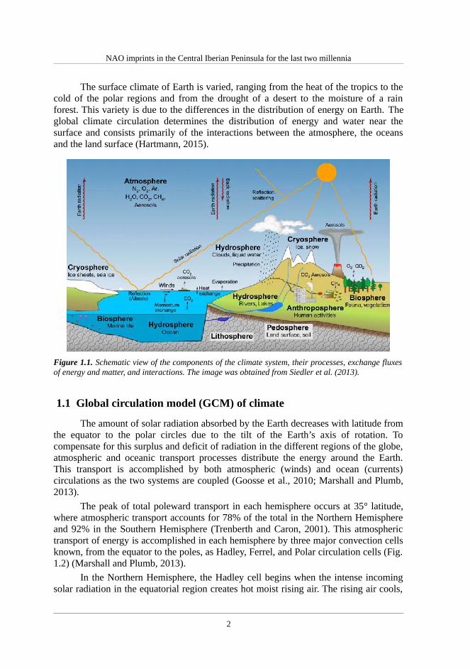
Climate in a wider sense is the state, including a statistical description, of theclimate system (Le Treut et al., 2007). Consequently, this definition includes theanalysis of the behaviour of the five major components of the climate system: theatmosphere (the gaseous envelope surrounding the Earth), the hydrosphere (liquidwater, i.e., oceans, lakes, underground water, etc.), the cryosphere (solid water, i.e., seaice, glaciers, ice sheets, etc.), the pedosphere (land surface and soil) and the biosphere(all living organisms), as well as their processes, the interactions and the exchangefluxes of energy and matter between them (Goosse et al., 2010; Siedler, et al., 2013)(Fig. 1.1). In addition, the climate system evolves over time under the influence of itsown internal dynamics and external forcings, such as volcanic eruptions, solarvariations and anthropogenic impacts (Le Treut et al., 2007). Therefore, the lithosphere,which comprises the solid Earth, which supplies minerals through processes such asvolcanism and weathering, and the anthroposphere (i.e., human activities) are twoadditional components that also form part of the climate system (Siedler, et al., 2013)(Fig. 1.1).
The importance of climate is so basic that sometimes it is overlooked. If theclimate were not more or less as it is, life and civilization on this planet would not havedeveloped in the same ways (Huntington, 1922; Fagan, 2009). Climate affects humanlives in many ways; for example, climate influences the type of clothing and housingthat people have developed. In the modern world, with the great technological advancesof the last century, one might think that climate no longer constitutes a force capable ofchanging the course of human history. However, this is an apparent illusion since we areas sensitive now as we have ever been to climate fluctuations and climate changes(Hartmann, 2015). Hence, the understanding of the past and present climate and theprediction of future climate scenarios are necessary for human development and thepreservation of natural environments.
1
NAO imprints in the Central Iberian Peninsula for the last two millennia
The surface climate of Earth is varied, ranging from the heat of the tropics to thecold of the polar regions and from the drought of a desert to the moisture of a rainforest. This variety is due to the differences in the distribution of energy on Earth. Theglobal climate circulation determines the distribution of energy and water near thesurface and consists primarily of the interactions between the atmosphere, the oceansand the land surface (Hartmann, 2015).
Figure 1.1. Schematic view of the components of the climate system, their processes, exchange fluxesof energy and matter, and interactions. The image was obtained from Siedler et al. (2013).
1.1 Global circulation model (GCM) of climate
The amount of solar radiation absorbed by the Earth decreases with latitude fromthe equator to the polar circles due to the tilt of the Earth’s axis of rotation. Tocompensate for this surplus and deficit of radiation in the different regions of the globe,atmospheric and oceanic transport processes distribute the energy around the Earth.This transport is accomplished by both atmospheric (winds) and ocean (currents)circulations as the two systems are coupled (Goosse et al., 2010; Marshall and Plumb,2013).
The peak of total poleward transport in each hemisphere occurs at 35° latitude,where atmospheric transport accounts for 78% of the total in the Northern Hemisphereand 92% in the Southern Hemisphere (Trenberth and Caron, 2001). This atmospherictransport of energy is accomplished in each hemisphere by three major convection cellsknown, from the equator to the poles, as Hadley, Ferrel, and Polar circulation cells (Fig.1.2) (Marshall and Plumb, 2013).
In the Northern Hemisphere, the Hadley cell begins when the intense incomingsolar radiation in the equatorial region creates hot moist rising air. The rising air cools,
2

Introduction
moisture condenses and intense precipitation results, releasing latent heat. Once the airhas risen, it flows northwards at high levels, cools, and eventually sinks atapproximately 30°N (Trenberth and Stepaniak, 2003) (Fig. 1.2). The descending air isvery dry, having lost most of its moisture in the tropics, and when it is warmed, itscapacity to take up moisture is further increased. The resulting hot dry air causes intenseevaporation at the Earth’s surface, and this gives rise to the subtropical belt of desertscentred between 15° and 30°N (Wallace and Hobbs, 2006; Berner and Berner, 2012)(Fig. 1.2). After reaching the Earth's surface, the air flows southwards, picking upmoisture as it flows over the oceans and being deflected to the right by the Coriolisforce due to the rotation of the Earth. This surface flow is known as the northeast tradewinds (Wallace and Hobbs, 2006; Berner and Berner, 2012) (Fig. 1.2). Upon reachingthe equator, the dry northeast trades converge with the humid southeast trades from theSouthern Hemisphere and form a band of increased convection, cloudiness, and heavyprecipitation called the Intertropical Convergence Zone (ITCZ). Finally, the air rises atthe equator to complete the low-latitude cycle forming the convection cell (Fig. 1.2)(Trenberth and Stepaniak, 2003).
Figure 1.2. Schematic representation of the global atmospheric circulation on the Earth (© 2001Brooks/Cole-Thomson Learning). The figure shows the three convection cells (Hadley, Ferrel andPolar cells) and air circulation patterns.
At approximately 30°N, additional air descends and then flows north along thesurface rather than south. This is the beginning of the Ferrel cell (Trenberth andStepaniak, 2003) (Fig. 1.2). The northward-flowing air is deflected to the right, formingthe prevailing westerlies, which flow from southwest to northeast in the NorthernHemisphere. The westerlies continue until they encounter a cold mass of air movingsouth from the North Pole at approximately 50°N. This zone where the air masses meetis known as the polar front, and it is a region of unstable air, storm activity, and
3

NAO imprints in the Central Iberian Peninsula for the last two millennia
abundant precipitation (Fig. 1.2). The polar jet stream (a very fast air stream) occurs atthis boundary (Wallace and Hobbs, 2006; Berner and Berner, 2012). The warmer airfrom the south rises over the polar air and then turns south at high altitude to completethe Ferrel cell (Fig. 1.2). Meanwhile, the southward-flowing polar air (polar easterlies)is warmed by condensation at the polar front and by contact with the southern air. As aresult, it too rises and then flows northward at high altitude to the pole, where it sinks,thus completing the polar cell (Wallace and Hobbs, 2006; Berner and Berner, 2012)(Fig. 1.2).
Global oceanic circulation also plays an essential role in distributing the heataround the Earth (Marshall and Plumb, 2013; Siedler, et al., 2013). The surface oceancirculation is mainly driven by the prevailing winds. At mid-latitudes, the atmosphericwesterlies induce eastward currents in the ocean while the trade winds are responsiblefor westward currents in the tropics (Talley et al., 2011) (Fig. 1.3). Because of thepresence of continental barriers, those currents form loops called subtropical gyres (i.e.,the Pacific, Atlantic, and Indian Ocean gyres; Fig. 1.3). The surface currents in thesegyres are intensified along the western boundaries of the oceans (the east coasts ofcontinents), thereby inducing well-known strong currents, such as the Gulf Stream offthe east coast of the USA and the Kuroshio of Japan (Marshall and Plumb, 2013;Siedler, et al., 2013) (Fig. 1.3). At higher latitudes in the Northern Hemisphere, theeasterlies aid in the formation of weaker subpolar gyres. In the Southern Ocean, becauseof the absence of continental barriers, a current that connects all the ocean basins can bemaintained: the Antarctic Circumpolar Current (Marshall and Plumb, 2013; Siedler, etal., 2013) (Fig. 1.3). All these currents run basically parallel to the surface winds. Incontrast, the equatorial counter-currents, which are present at or just below the surfacein all the ocean basins, run in the direction opposite to the trade winds (Talley et al.,2011; Talley, 2013; Siedler, et al., 2013) (Fig. 1.3).
The deep ocean circulation is driven by density variations arising fromdifferences in temperature and salinity, giving rise to the term thermohaline circulation(Berner and Berner, 2012) (Fig. 1.4). At high latitudes, because of its low temperatureand relatively high salinity, surface water can be dense enough to sink to great depths.This process, often referred to as deep oceanic convection, is only possible in a fewplaces worldwide, and it occurs mainly in the North Atlantic and in the Southern Ocean(Siedler, et al., 2013; Marshall and Plumb, 2013) (Fig. 1.4). In the North Atlantic, theLabrador and Greenland-Norwegian Seas are the main sources of the North AtlanticDeep Water (NADW), which flows southward along the western boundary of theAtlantic towards the Southern Ocean (Fig. 1.4). There, it is transported to the otheroceanic basins after some mixing with ambient water masses. This deep water thenslowly upwells towards the surface in the other oceanic basins, forming upward fluxesin the North Indian and North Pacific Oceans (Talley et al., 2011; Talley, 2013) (Fig.1.4). Although sinking occurs within very small regions, upwelling is broadlydistributed throughout the ocean. The return flow to the sinking regions is achievedthrough surface and intermediate-depth circulation (Talley et al., 2011; Talley, 2013)(Fig. 1.4). In the Southern Ocean, Antarctic Bottom Water (AABW) is mainly producedin the Weddell and Ross Seas. This water mass is colder and denser than NADW andthus flows below it (Talley et al., 2011; Talley, 2013) (Fig. 1.4).
4

Introduction
5
Fig
ure
1.3
. Ill
ustr
atio
n of
the
glob
al s
urfa
ce o
cean
ic c
urre
nts
and
ocea
nic
gyre
s (T
alle
y et
al.,
201
1).

NAO imprints in the Central Iberian Peninsula for the last two millennia
Figure 1.4. A) A three-dimensional schematic representation of the global oceanic circulation from aSouthern Ocean perspective. The figure shows the connection between the three major ocean basinsand the various water masses involved in this flow. B) A global map with a two-dimensional schematicrepresentation of the deep oceanic circulation shown in A. Both figures have a common legend andwere obtained from Talley (2013).
6

Introduction
1.1.1 The Intertropical Convergence Zone (ITCZ)
The ITCZ is one of the most noticeable aspects of the global circulation. Asstated before, the ITCZ is the zone of low pressure that encircles the Earth near theequator, from approximately 5° north to 5° south, where the trade winds converge andwhere the tropical rain forests are found (Figs. 1.2 and 1.5). The ITCZ moves north andsouth following the sun during the year and presents a seasonal pattern, moving northstarting in February, reaching its most northern position in June/August atapproximately 20°N (Hastenrath, 1991) and retreating southwards until December (Fig.1.5B). This seasonal pattern in the atmospheric general circulation is responsible for therainy season (monsoon) in many equatorial regions of South America, Africa andIndonesia. An important impact of these seasonal changes in the positions of the ITCZand associated rainfall distributions is that they partially explain the annual cycle ofAfrican dust emissions (Engelstaedter et al., 2006).
On longer time scales, palaeorecords indicate that the migration of the ITCZexhibits a seasonal-like pattern following differently warming between hemispheres(Haug et al., 2001; Wanner et al., 2008). For example, clear evidence for these ITCZmigrations come from the Cariaco basin records (Haug et al., 2001; Schneider et al.,2014). The ITCZ appeared to shift to a more southerly position as the NorthernHemisphere cooled from the Holocene thermal maximum at approximately 8 kyr BP tothe beginning of the Little Ice Age at ca. 1450 (Haug et al., 2001). Simultaneously, theAfro-Asian summer monsoon rainfall systems were less active, and the correspondingcontinental areas were exposed to increasing aridity (Wanner and Brönnimann, 2012;Schneider et al., 2014). These ITCZ variations in the Holocene mostly arose becausesummer insolation in the Northern Hemisphere weakened with the precession of theEarth’s perihelion from the Northern Hemisphere to the Southern Hemisphere summer(Schneider et al., 2014).
Figure 1.5. A) View of the Americas from space as captured by NOAA's GOES-East satellite on 22 nd
April, 2014, at 11:45 UTC/7:45 a.m. EDT (http://www.nasa.gov). Near the equator, GOES imageryshows a line (region between dashed red lines) of pop-up thunderstorms associated with theIntertropical Convergence Zone (ITCZ). B) Mean seasonal position of the ICTZ in July (borealsummer; red line) and February (austral summer; blue line) (http://www.weatherwise.org).
7

NAO imprints in the Central Iberian Peninsula for the last two millennia
1.1.2 Climate modes
The Earth’s atmosphere, oceans, cryosphere, and continental hydrology exchangemass and energy on all time scales. Consequently, global- or regional-scale climatevariables, such as the temperature, rainfall, surface pressure, or wind speed, fluctuatemore or less regularly and form climate patterns (e.g., Ropelewski and Halpert, 1987;Hurrell and van Loon, 1997; Viron et al., 2013). Many of these fluctuations are knownas modes or oscillations with identifiable characteristics and specific regional effects,and their states are monitored by using scalar values of the so-called climate indices(e.g., Ropelewski and Jones, 1987; Hurrell, 1995; Thompson and Wallace, 2000;Enfield et al., 2001; Deser et al., 2010; Christensen et al., 2013). Some of the best-known oscillations extend over large areas of the globe, such as the El Niño–SouthernOscillation (ENSO), the North Atlantic Oscillation (NAO), the Pacific DecadalOscillation (PDO), and the Madden-Julian Oscillation (MJO) (e.g., Philander 1983;Hurrell, 1995; Zhang et al., 1997; Zang, 2005). Furthermore, many teleconnectionsbetween these indices are also known to exist (e.g., Wallace and Gutzler, 1981;Alexander et al., 2002; Liu and Alexander, 2007), whereas certain oscillations are morelocalized and are thus associated with the climate of smaller regions.
Barnston and Livezey (1987) identified 12 different climate modes in theNorthern Hemisphere. Currently, more than 25 different climate modes have beenidentified for recent decades at the global scale (Viron et al., 2013; Table. 1.1).
1.2 Climate variability in the North Atlantic region
The complexity of the climate variability in the North Atlantic region and itsnumerous impacts have attracted the attention of a wide variety of scientificcommunities, most of them focussed on disentangling the processes that control thesevariations (e.g., Marshall et al., 2001; Vicente-Serrano and Trigo, 2011). The climatevariability in this region is highly influenced by a number of different climate modesthat operate in the North Atlantic sector, such as the Atlantic Multidecadal Oscillation(AMO), the Arctic Oscillation (AO) and the NAO (e.g., Sutton and Hodson, 2005;Hurrell et al., 2006; Hurrell, 2015). These modes induce significant changes in surfaceair temperature, precipitation, ocean surface temperature and heat content, oceancurrents, ocean current-related heat transport from the equator to the North Pole, andsea ice cover in the Arctic and sub-Arctic regions (Hurrell et al., 2006; Hurrell, 2015).Such climatic fluctuations affect agricultural harvests, water management, energysupply and demand, primary activities over land and sea, etc., thereby affecting thehuman welfare of millions of people and the equilibrium of numerous environmentalcycles in the North Atlantic region (e.g., Hurrell et al., 2003; Vicente-Serrano and Trigo,2011).
Over the middle and high latitudes of the Northern Hemisphere, the NAO is themost prominent and recurrent pattern of atmospheric variability and explains a largeproportion of the climate variability of the North Atlantic Ocean, North America, theArctic, Eurasia and the Mediterranean areas (Hurrell and van Loon, 1997; Jones et al.,2003; Hurrell et al., 2003).
8

Introduction
Abbreviation Index Name
AAO Antarctic Oscillation
AMMSST Atlantic Meridional Mode
AMO Atlantic Multidecadal Oscillation
AO Arctic Oscillation
ATLTRI Atlantic Tripole SST EOF
BRAZILRAIN Northeast Brazil Rainfall Anomaly
CAR Caribbean SST
EA East Atlantic
EOFPAC Tropical Pacific SST EOF
EPO East/North Pacific Oscillation
GMSST Global Mean Land/Ocean Temperature
INDIAMON Central Indian Precipitation
MJO Madden-Julian Oscillation
NAO North Atlantic Oscillation
NOI Northern Oscillation
NP North Pacific Pattern
PACWARM Pacific Warmpool
PDO Pacific Decadal Oscillation
PNA Pacific North American
SAHELRAIN Sahel Standardized Rainfall
SCAND Scandinavian
SOI Southern Oscillation
SWMONSOON SW Monsoon Region Rainfall
TNA Tropical Northern Atlantic
TSA Tropical Southern Atlantic
WHWP Western Hemisphere Warm pool
WP Western Pacific Index
Table 1.1. List of the most relevant worldwide indices of large-scale modes of climate variability(Viron et al., 2013).
9

NAO imprints in the Central Iberian Peninsula for the last two millennia
1.2.1 The North Atlantic Oscillation (NAO)
The NAO has been recognized for almost a century as the leading large-scalemode of climate variability in the North Atlantic region, especially during winter(Hurrell et al., 2003). The NAO is related to the redistribution of atmospheric massbetween the Arctic and the subtropical Atlantic and is manifested as a meridional dipoleanomaly in sea-level pressure (SLP), with the two centres of action locatedapproximately over Iceland and the Azores (Hurrell, 1995; Hurrell et al., 2003) (Fig.1.6A).
Figure 1.6. Spatial display of the first three eigenvectors of the gridded winter (December–February)monthly sea-level pressure anomalies (in mb) for the North Atlantic domain (1872–2009 AD)calculated using the 20CRv2 global dataset (Compo et al., 2011): A) North Atlantic Oscillation(NAO), B) East Atlantic pattern (EA) and C) Scandinavian pattern (SCAND). The empiricalorthogonal function was performed using the cross-correlation matrix. Values adjacent to each mapare the percentage of the total variance explained by each eigenvector. All the figures were obtainedfrom Comas-Bru and McDermott (2014).
The first descriptions of phenomena associated with the NAO were given byScandinavian seafarers, who realized that winter temperatures in Greenland andScandinavia varied in opposite phase (Wanner et al., 2001; Stephenson et al., 2003;Luterbacher et al., 2008; Hense and Glowienka-Hense, 2010). The colonization ofGreenland began in 985 AD, and until 1300 AD, ships frequently sailed betweenScandinavia and Greenland, enabling a detailed understanding of the weather, climate,and remote links (Haine, 2008). The first published work dates back to the mid-18thcentury and focused on the description of thermal and hydrological conditions inGreenland versus Scandinavia (Egede, 1745; Crantz, 1765). In 1811 AD, Gronau
10

Introduction
described the links between the weather conditions in Greenland and Germany (Gronau,1811). Later studies confirmed these relationships by analysing early temperature timeseries (Dove, 1839). However, the concept of the NAO with two pressure centresappeared with the availability of pressure data over Europe and North Atlantic and withthe development of correlation analysis in the late 19th and early 20th centuries(Teisserenc, 1883; Defant, 1924; Walker, 1924).
The NAO has two phases, and the swings from one phase to another producelarge changes in the mean wind speed and direction over the Atlantic, in the heat andmoisture transport between the Atlantic and the neighbouring continents, especiallyEurope, and in the intensity, paths and number of storms (Hurrell and van Loon 1997;Hurrell et al., 2003). The positive NAO phase (NAO+) is characterized by an intensifiedAzores high and deeper Iceland low, which leads to a stronger meridional pressuregradient over the North Atlantic, a more zonal flow regime and stronger westerlies, inparticular in the central and eastern North Atlantic, as well as a more northerly track ofstronger storms crossing the Atlantic (Fig. 1.7A). Consequently, NAO+ is associatedwith warmer and wetter conditions over Northern and Central Europe as a result of thesuccession of low-pressure centres embedded in the northwesterly flow and with dryconditions over southern Europe (Fig. 1.7A). The effects on the ocean of the NAO+
involve a tripole pattern in the sea surface temperatures (SSTs), with negative SSTanomalies from the Greenland and Irminger Seas to Newfoundland, positive SSTanomalies in the central North Atlantic and negative SST anomalies further south alongthe western coast of Africa (Pinto and Raible, 2012) (Fig. 1.7A). During a negativeNAO (NAO-) phase, the Azores high is weaker and the Iceland low is shallower. Thisatmospheric circulation pattern leads to a reduced meridional pressure gradient andproduces weaker westerlies over the North Atlantic and Western Europe and a moresoutherly track of storms crossing the Atlantic (Fig. 1.7B). Over Southern Europe, theNAO- leads to unsteady weather conditions that are typically wetter than normal, whileover Northern Europe, dryer and colder conditions are found, usually associated with ablocking (stationary high) situation extending from Urals/Eastern Europe toWestern/Central Europe. Such a blocking high may remain in place for several weeks,leading to stable weather conditions over Central Europe (Pinto and Raible, 2012) (Fig.1.7B). The SST anomalies during NAO- are opposite in sign to those during NAO+ (Fig.1.7).
The NAO has also been related to the frequency of atmospheric blockingepisodes in the North Atlantic region. An atmospheric blocking is a large-scale mid-latitude phenomenon often associated with a split in the zonal jet as well as withpersistent quasi-stationary synoptic-scale high-pressure systems (e.g., Diao et al., 2006).This phenomenon causes large-scale circulation anomalies and exerts a strong impactupon the weather patterns (Sillmann and Croci-Maspoli, 2009; Sillmann et al., 2011;Pfahl and Wernli, 2012). Thus, the NAO+ leads to a ‘cold ocean/warm land’ pattern(Fig. 1.7A), which is unfavourable for the development and persistence of blockingevents, whereas the NAO- phase leads to a ‘warm ocean/cold land’ pattern (Fig. 1.7B),which promotes the formation and persistence of blocking events (Shabbar et al., 2001;Barriopedro et al., 2006). Furthermore, these blocking events have also been related tovariations in the zonal position of the NAO; thus, the frequency of Euro-Atlantic
11

NAO imprints in the Central Iberian Peninsula for the last two millennia
blocking events is distributed along the northwest-southeast (southwest-northeast)direction for NAO+ (NAO-). One blocking action centre over south Europe is observedduring NAO+ while two blocking action centres in Greenland and European continentare observed during NAO- (Yao and Luo, 2014) (Fig. 1.7). Over longer periods, theseblocking events have also been associated with solar irradiance variations. Thedevelopment of frequent and persistent atmospheric blocking events in the easternNorth Atlantic is promoted when low solar irradiance conditions predominate (e.g.,Moffa-Sánchez et al., 2014).
Figure 1.7. A schematic overview of the two phases of the NAO: A) the positive phase (NAO+) and B)the negative phase (NAO-). Shading indicates SSTs (bordered by dashed contours) and sea-ice extent.Arrows show the flow systems in the ocean (light red and blue), atmosphere (green and yellow arrowsrepresent the westerly and trade winds, respectively) and rivers. Solid blue and red contours indicateSLPs (H=high, L=Low), and white rectangles describe either characteristic climate conditions orimportant processes. Modified from Wanner et al. (2001).
The measure for the temporal state of the NAO, i.e., the variability in the strengthof the SLP gradient, is traditionally expressed as the North Atlantic Oscillation index(NAOi). The first index of the NAO was constructed by Walker and Bliss (1932) usinga linear combination of surface pressure and temperature measurements from weatherstations on both sides of the Atlantic basin. However, and since there is no unique wayto define the spatial structure of the NAO, there is no universally accepted index toassess the temporal evolution of this mode (Hurrell et al., 2003). Most modern indicesof NAO are derived either from 1) the simple difference in SLP anomalies betweenvarious northern and southern locations or 2) the Principal Component (PC) time seriesof the leading Empirical Orthogonal Function (EOF) of regional gridded SLP data. Thefirst indices were usually based on instrumental records from individual stations near
12

Introduction
the NAO centres of action, such as the indices that Hurrell et al. (1995) and Jones et al.(1997) obtained from SLP data from Stykkisholmur (Iceland) and Lisbon (Portugal) andfrom Stykkisholmur (Iceland) and Gibraltar (UK), respectively. Furthermore, theindices are also sometimes obtained from gridded SLP analyses (e.g., Portis et al., 2001;Luterbacher et al., 2002). The major advantage of most of these indices is theirextension back to the mid-19th century or earlier (Jones et al., 2003). Nevertheless, thedisadvantage of these station-based indices is that, on one hand, they can onlyadequately capture NAO variability for parts of the year because they are fixed in spaceand the NAO centres of action vary spatially through the annual cycle, and, on the otherhand, they contain noisy signals from small-scale meteorological phenomena not relatedto the NAO that affect individual station pressures. The second indices (Wang et al.,2012; Moore et al., 2013; Comas-Bru and McDermott, 2014), based on the PC timeseries, are more optimal representations of the full NAO spatial pattern as they arebased on gridded SLP data; however, they can only be computed for the 20th centurydue to the lack of reliable gridded instrumental data further back in time (Hurrell et al.,2003).
These definitions led to slightly different NAO indices and also to differentcharacteristic spatial patterns. However, the different NAO indices are stronglycorrelated (r = 0.71–0.97; Leckebusch et al., 2008) with each other on interannual andlonger time scales, although the choice of the southern station makes some difference.In contrast, the specific location of the northern node (among stations in Iceland) is notcritical since the temporal variability over this region is much greater than the spatialvariability (Jones et al., 2003).
The NAO, as stated previously, is typically a winter mode, although it also varieson shorter time scales, such as the daily scale (Pinto et al., 2009; Blessing et al., 2005),and its index is usually determined for each month of the year (e.g., Barnston andLivezey, 1987; Jones et al., 1997; Comas-Bru and McDermott, 2014). Nonetheless, theeffects of the NAO are not restricted to winter, and several recent studies havecharacterized the dynamics of the summer NAO (e.g., Folland et al. 2009) and itscorresponding impact on European climate (e.g., Chronis et al. 2011; Bladé et al. 2012).The variability in the NAO has also been investigated and reconstructed (see section1.4.3 for further details) for longer time scales, such as decadal and centennial timescales, mostly to assess its potential long-term predictability. It seems that the NAOdoes not vary on any preferred time scale (Hurrell et al., 2003). Nevertheless, there areperiods in which NAO patterns persist over consecutive years or decades. For instance,Hurrell (1995) provided evidence that the NAO has shifted phase over the last 130years (Figure 1.8): the NAO shifted from a predominantly more negative phase before1910 AD to a more positive phase in the 1920s, followed by a negative trend enduringuntil the late 1960s. Afterwards, a strong positive trend developed and persisted untilthe mid-1990s. In the past 15 years (1995–2010), a negative trend in the NAO indiceshas been observed (Cattiaux et al., 2010; Jung et al., 2011). Conversely, the winterindex has shown a clear positive trend during the last four years (Figure 1.8).
13

NAO imprints in the Central Iberian Peninsula for the last two millennia
Figure 1.8. Winter (December to March) station-based NAO index (Hurrell, 1995) for the period1846–2015 AD (updated data from https://climatedataguide.ucar.edu/climate-data/hurrell-north-atlantic-oscillation-nao-index). The red and blue bars represent unfiltered data from year to year; theblack line represents the smoothed data obtained after applying the Loess function and a span degreeof 0.15 to illustrate the low-frequency behaviour.
The low-frequency NAO variability (decadal and longer) and its importance forthe winter atmospheric circulation over the North Atlantic and Europe have motivatedthe assessment of the possible underlying physical mechanisms behind them (e.g.,Wanner et al., 2001; Marshall et al., 2001; Hurrell et al., 2003). In fact, the origin of thelow-frequency variability has led to debate in the scientific community during the lastdecades. Several authors suggested that external parameters, such as volcanoes(Marshall et al., 2001; Fischer et al., 2007), solar activity (Spangehl et al., 2010;Schindell, 2001) or stratospheric–tropospheric coupling (Perlwitz et al., 2000; Scaife etal., 2005), are the major drivers of the low-frequency variability, while other authorssuggested that internal variability in the atmosphere, i.e., wave–wave interaction, is theleading factor (James and James, 1989; Franzke et al., 2000; Feldstein, 2000; Woollingset al., 2008). In addition, other factors such as the coupling between the ocean and theatmosphere (Bjerknes, 1964; Lau, 1997; Wanner et al., 2001), feedback processesassociated with the oceanic Atlantic Meridional Overturning Circulation (AMOC), thebranch of the thermohaline circulation in the Atlantic Ocean (Timmermann et al., 1998)(Figs. 1.4 and 1.7) and links to tropical SSTs, either over the Indian Ocean (Hoerling etal., 2001) or the Pacific Ocean (Trenberth et al., 1998; Müller, 2008), may also be ofgreat importance for the decadal and longer time scales of NAO variability.
Another main aspect of NAO is its importance and evolution in future climatescenarios. The relevance of NAO in future climate changes mostly depends on theregion, although there is high confidence that the NAO index will increase in responseto anthropogenic forcing (Visbeck et al., 2001; Christensen et al., 2013). For example,by mid-21st century, the anthropogenic warming signal in North America will verylikely be large compared to natural variability, such as that stemming from the NAO(Christensen et al., 2013). In Europe, the model simulations show that NAO changescontribute to the uncertainty of predictions in the near-term projections, whereas NAOtrends do not account for a large fraction of the long-term future changes in meantemperature or precipitation (Stephenson et al., 2006; Kjellström et al., 2013). In theArctic region, the NAO is assigned high relevance in temperature and precipitation
14

Introduction
variability (Christensen et al., 2013).
Therefore, the marked importance of NAO in many different climatic aspectsthat affect large areas of the Northern Hemisphere and their ascribed impacts have ledto many of the studies referred to in this section. However, a number of interestingquestions and aspects about this phenomenon remain unanswered or unexplored,including the climatic processes that govern NAO variability, how the phenomenon hasvaried in the past or will vary in the future, and whether it is at all predictable (Hurrellet al., 2003).
1.2.2 Other climate modes in the North Atlantic: the East Atlantic(EA), Scandinavian (SCAND) and Atlantic Multidecadal Oscillation(AMO)
The NAO exerts a major influence on the climate of the North Atlantic region;however, there are other large-scale modes that may also contribute significantly to theclimate variability of the North Atlantic sector (Fig. 1.6).
The East Atlantic (EA) mode is the second mode of climate variability in thisregion (Fig. 1.6B). The EA was first described by Wallace and Gutzler (1981) asanomalously high 500 mb height anomalies over the subtropical North Atlantic andEastern Europe when it is in positive mode. This atmospheric pattern is structurallysimilar to the NAO and consists of a north-south dipole of anomalous SLP centresspanning the North Atlantic from east to west (Barnston and Livezey, 1987) (Fig. 1.6B).As a climate mode, its temporal variability is measured using an index, the EA index(EAi) (Fig. 1.9). Moore and Renfrew (2012) derived the EAi in 1870 AD based on SLPdata from Valentia Island (Ireland), although this index has also been defined in theliterature as the second leading EOF of regional gridded SLP (Moore et al., 2013). TheEA is also more prominent during winter (Barnston and Livezey, 1987) and may have arole in positioning the primary North Atlantic storm track (Seierstad et al., 2007;Woollings et al., 2010). Its two phases are currently associated with variations intemperatures and precipitation in Scandinavia, Europe and North America (e.g.,Rodríguez-Puebla et al., 1998; Krichak and Alpert, 2005; Comas-Bru and McDermott,2014). This mode has also exhibited very strong multidecadal variability during recentdecades.
The Scandinavian pattern (SCAND) is the third leading mode of winter SLPvariability in the North Atlantic region. The SCAND was originally identified byBarnston and Livezey (1987) through an orthogonally rotated principal componentanalysis applied to monthly-mean 700 mb height anomalies over the extratropicalNorthern Hemisphere, and they referred to this climate mode as Eurasian Type 1 (EU1).The SCAND has a primary centre of action around the Scandinavian Peninsula, withtwo other centres of action with the opposite sign, one over Western Europe and theother over eastern Russia–western Mongolia (Fig. 1.6C). The SCAND index (SCANDi)defined by Barnston and Livezey (1987) has been updated by the Climate PredictionCenter of the United States National Oceanic and Atmospheric Administration (NOAA)(Fig. 1.9). Its positive phase is characterized by prominent anticyclonic anomalies near
15

NAO imprints in the Central Iberian Peninsula for the last two millennia
the Scandinavian Peninsula that give rise in winter to below-normal temperatures acrosscentral Russia and western Europe, above-normal precipitation across southern Europe,and dry conditions over the Scandinavian region. Additionally, this mode also appearsto influence the East Asian climate (Bueh and Nakamura, 2007).
Figure 1.9. Time series of the winter mean (December to February) indices of the NAO (black curve),EA (red curve), and SCAND (blue curve) for the period 1871–2008 AD. The indices are derived fromthe principal components of the EOF decomposition of the monthly mean winter (December toFebruary) SLP field from the 20CR reanalysis dataset. A low-pass filter with a cut-off of 21 years wasused. Modified from Moore et al. (2013).
Hence, in addition to the NAO, these two last climate modes also modulate theclimate variability over the Atlantic region and influence the geographical position andstrength of the two centres of action of the NAO dipole, modifying the NAO-climaterelationship in the European North Atlantic sector (Comas-Bru et al., 2014). The EAand SCAND were described almost three decades ago, but studies focusing on thissubject have emerged in the last few years. Moore et al. (2011) proposed for the firsttime that the phase of the EA plays a role in modulating the location and strength of theNAO dipole. This work was expanded and completed by Moore and Renfrew (2012).Subsequently, Moore et al. (2013) investigated the effects of both the EA and SCANDmodes on the variability of the NAO centres of action by selecting winters characterizedby different combinations of the NAO–EA and NAO–SCAND phases. These authorsdescribed the movement of the NAO structure along a northeast-southwest axisdepending on the state of the EA and a clockwise/anticlockwise movement associatedwith the state of the SCAND. More recently, Comas-Bru and McDermott (2014),following the approach of Moore et al. (2013), also found important modulatinginfluences of the EA and the SCAND on the geographical positions of the NAO dipole.When the NAO and the EA are of the same sign, the NAO centres of action migratenortheastwards, whereas during phases of opposite sign, they move towards thesouthwest. When the NAO and the SCAND show the same sign, the centres of action ofthe first climate mode move anticlockwise, while when their phases are of oppositesign, they follow a clockwise rotation (Fig. 1.10). However, the most relevantcontribution of these authors is that they have demonstrated for the first time that muchof the multidecadal climate variability during the twentieth century in the North
16

Introduction
Atlantic–European sector can be linked to specific combinations of NAOi–EAi andNAOi–SCANDi signs (Comas-Bru and McDermott, 2014) (Fig. 1.11). Anotherimportant contribution of this study is that these excursions of the NAO dipolemodulated by EA and SCAND can result in spatial and temporal non-stationarity of theNAO-climate relationship. This situation could have important implications forreconstructions of the NAOi in the past using climate-sensitive proxies (e.g., tree rings,speleothems, lake sediments, and corals) as some regions may exhibit temporal non-stationarities in the proxy-NAOi relationship, which is a key factor of a reconstruction(Comas-Bru and McDermott, 2014; Comas-Bru et al., 2016).
Figure 1.10. Teleconnectivity matrix of the winter (December to February) monthly sea-level pressurefield in the North Atlantic region (10–80°N, 100°W–40°E) for the period 1872–2009 AD for differentlinear combinations of NAO–EA (left) and NAO–SCAND (right). In A) and B), both patterns exhibitthe same sign, i.e., (NAO–EA)S and (NAO–SCAND)S, whereas in C) and D), they exhibit oppositesigns, i.e., (NAO–EA)O and (NAO–SCAND)O. Light, medium and dark grey shadings represent areaswith correlations of 0.5, 0.6 and 0.7, respectively. Black crosses indicate the location of the grid cellswith the highest correlation. This figure was obtained from Comas-Bru and McDermott (2014).
17

NAO imprints in the Central Iberian Peninsula for the last two millennia
Figure 1.11. Correlation distribution maps that show the spatial coherence of the NAO–climaterelationship with the CRU-TS3.1 dataset and our EOF-based indices for different combinations ofsigns: A) and E) (NAO–EA)S, n = 57; C) and G) (NAO–EA)O, n = 51; B) and F) (NAO–SCAND)S, n =56; D) and H) (NAO–SCAND)O, n = 52. This figure was obtained from Comas-Bru and McDermott(2014).
In contrast, the Atlantic Multidecadal Oscillation (AMO) has been identified as acoherent pattern of low-frequency oscillations (65–80 yr cycle) of North Atlantic SSTs.Early studies only identified the multidecadal SST variations (e.g., Kushnir, 1994;Schlesinger and Ramankutty, 1994). Nevertheless, since the work of Kerr (2000), thepattern has been commonly referred to as the AMO. Although this is still a point ofcontroversy (Clement et al., 2015), the AMO is generally suggested to be induced byAtlantic thermohaline circulation variations and associated ocean heat transportfluctuations (e.g., Folland et al., 1986; Gray et al., 1997; Delworth and Mann, 2000;Knight et al., 2005; McCarthy et al., 2015).
Indices of the AMO have traditionally been based on average annual SSTanomalies in the North Atlantic region (Kaplan, 1998), whereas the modern AMO indexis obtained after removing any linear trend in order to account for the influence of therecent global warming. Therefore, this revised index is defined by subtracting the globalmean SST anomalies from the North Atlantic SST anomalies (Fig. 1.12) (Trenberth andShea, 2006; Parker et al., 2007). However, because the instrumental SST records onlyspan ca. 150 years, it remains a matter of debate whether the observed SST variabilitymerely reflects a transient feature on a ‘red noise’ background or a truly oscillatoryphenomenon (Delworth and Mann, 2000; Knudsen et al., 2011).
Several studies have linked climate changes to AMO variability, but the couplingbetween the AMO and the precipitation anomalies is spatially complex. The AMOdrives climate and precipitation patterns over North America (Enfield et al., 2001;Sutton and Hodson, 2005; Hu and Feng, 2008), droughts in the Sahel region of Africa
18

Introduction
(Folland, 1986), variability in Northeast Brazilian rainfall (Folland, 2001), and tropicalhurricane frequency and intensity (Goldenberg, 2001). The positive AMO phase isassociated with a pattern of horseshoe-shaped SST anomalies in the North Atlantic withpronounced warming in the tropical and parts of the eastern subtropical North Atlantic,an anomalously cool area off the US East Coast, and warm anomalies surrounding thesouthern tip of Greenland. The negative AMO phase is associated with the oppositeconditions (Fig. 1.12) (Bjerknes, 1964; Kushnir, 1994). Cool AMO phases occurred inthe 1900s – 1920s and 1960s – 1980s, while a warm phase occurred in the 1930s –1950s and since the beginning of the mid-1990s (Fig. 1.12)
Figure 1.12. A) Composite maps of the SST field showing the spatial pattern of the AMO index for theperiod 1940–2011 AD. The thick grey contour line denotes 0 °C, whereas thin (dashed) lines denotepositive (negative) SST at intervals of 5 °C (Yamamoto and Palter, 2016). B) AMO index computed asthe linearly detrended North Atlantic SST anomalies for the period 1856–2013 AD. The data wereobtained from http://www.esrl.noaa.gov/psd/data/timeseries/AMO/.
19

NAO imprints in the Central Iberian Peninsula for the last two millennia
1.3 The climate variability in the Iberian Peninsula
1.3.1 Regional climate
The precipitation and temperature regimes in the Iberian Peninsula (IP) arecharacterized by spatial and temporal variability. Both regimes exhibit a strong seasonaland interannual variability, and east–west and north–south gradients due to thedistribution of orography and the Atlantic origin of many synoptic disturbances(Serrano et al., 1999). Annual precipitation values over the IP range from ca. 300 mmyr-1 in the southeastern coastal semidesert regions (Romero et al., 1998; Rodriguez-Puebla et al., 1998) to more than ca. 1200 mm yr-1 in the northwestern provinces(Rodriguez-Puebla et al., 1998; Esteban-Parra et al., 2003), whereas the annual meantemperatures range from ca. 17 °C in southern Iberia to ca. 11 °C in northern Iberia(Brunet et al., 2001, 2007; Rodríguez-Puebla et al., 2001; Esteban-Parra et al., 2003)(Fig. 1.13). The spatial and seasonal variability of the climatic variables can be partlyexplained by the global circulation (e.g., seasonal movements of the Azores high-pressure system) and the regional geography (e.g., latitude, orography, and oceanic andcontinental influences) (Trigo and Paulotikof, 2001). However, the interannualvariability, i.e., the large range of values for precipitation and temperature observedfrom year to year, is mainly controlled by the main large-scale atmospheric circulationmodes and related blocking conditions that affect the IP (von Storch et al., 1993;Rodríguez-Puebla et al., 1998, Trigo et al. 2004; Sousa et al. 2015).
Figure 1.13. Maps of mean annual A) temperature (°C) and B) precipitation (mm) for the IberianPeninsula obtained from Ninyerola et al. (2005).
1.3.2 Influence of the main climate modes on the present-day climate ofthe Iberian Peninsula
Most of the climatic variability over the IP can be explained in terms of relativelyfew large-scale atmospheric modes that mainly operate in the North Atlantic-Europeansector and, to a lesser extent, in the Mediterranean region (El Kenawy et al., 2012). TheNAO is the most prominent mode, especially in winter (Jerez and Trigo, 2013). Theeffects of the winter NAO on the IP climate are more evident in the precipitationrecords than in the air temperature measurements (Castro-Díez et al. 2002; Trigo et al.,
20

Introduction
2002; Comas-Bru and McDermott, 2014). These effects are also observed in themountainous regions of Spain, such as the Central Range and the Pyrenees. In theseregions, the winter NAO primarily causes deviations between wet and dry climaticconditions rather than between cold and warm conditions (López-Moreno et al. 2011;Durán et al. 2014). Other modes may have received less attention, although theirimpacts have also been reported. In particular, the EA and the SCAND modes havedemonstrated their influence on the Iberian climate (Paredes et al., 2006; Trigo et al.,2008; Martín et al., 2010; Ramos et al., 2010; Hernández et al 2015). The EA governswinter and summer temperatures, whereas SCAND impacts on Iberian climate are morevariable and display a less clear pattern, although it shows the most significantrelationships with precipitation during winter and with temperatures during summer(Comas-Bru and McDermott, 2014; Hernández et al., 2015) (Fig. 1.14).
Figure 1.14. Composites showing the impact of the NAO (1st column), EA (2nd column) and SCANDmodes (3rd column) on the mean precipitation (1st row) and temperature (2nd row) for A) winter(November to February average, NDJF) and B) summer (April to August average, AMJJA). Units areas follows: mm month−1 for precipitation and K for temperature. The time period was 1959–2007 AD.Data source: MM5 simulation. The image was modified from Hernández et al. (2015).
21

NAO imprints in the Central Iberian Peninsula for the last two millennia
1.3.3 African dust episodes in the Iberian Peninsula
North Africa is widely regarded as the Earth's largest source of dust (e.g.,Prospero et al., 2002; Washington et al., 2003; Ginoux et al., 2004, 2012). The amountof dust emitted annually from this region is estimated to be approximately 1400 Tg yr-1,which represents 65% of the global dust emissions (Ginoux et al., 2004). This airborneplume of dust from arid and semi-arid regions, such as the Sahara and the Sahel, istransported yearly over the Atlantic Ocean, the Caribbean, Mediterranean sea andEurope (Prospero et al.,1981; Coudé -Gaussen, 1982).
Annual westward Atlantic transport occurs under the influence of trade windsand presents a marked seasonality modulated by the migration of the ITCZ (Prospero etal.,1981; Pye, 1987; Torres-Padrón et al., 2002; Engelstaedter et al., 2006;). In theboreal winter, sources located in the southern Sahara and the Sahel (< 20º N) areespecially active and are linked to dry northeasterly trade winds that prompt dust exportacross the North African tropical coast (< 15º N) (Engelstaedter and Washington, 2007;Menut et al., 2009; Marticorena et al., 2010; Fig. 1.15). During the boreal summer thenortheasterly trade winds and the ITCZ shift northward, enhancing emissions fromSaharan sources and increasing dust export at subtropical latitudes (20–30º N).Concurrently the northward shift in the monsoon rain band to the southern Sahel tendsto decrease Sahelian dust emissions (Engelstaedter and Washington, 2007; Knippertzand Todd, 2010; Ashpole and Washington, 2013) (Fig. 1.15).
Figure 1.15. Monthly mean data from the Total Ozone Mapping Spectrometer absorbing AerosolIndex (TOMS AI) (x10) for the period 1980–1992 AD (Engelstaedter et al., 2006). These satellite datashow the marked seasonality in dust emissions from the North African region.
22

Introduction
The annual northwards dust transport leads to the occurrence of dust episodesover the Mediterranean and the IP (Fig. 1.16). This transport towards higher latitudes isrelated to cyclonic activity inside and around the Mediterranean basin (Alpert and Ziv,1989; Bergametti et al., 1989) and is driven by more complex wind fields than in thecase of the Atlantic transport. The wind trajectories depend on the relative position ofboth high- and low-pressure systems over the Atlantic Ocean and the Mediterranean Seaand on the westerly wind regime over Europe (Coudé-Gaussen et al., 1982; Bergamettiet al., 1989; Moulin et al., 1997; Rodríguez et al., 2001). Such meridional transportoccurs when the westerly regime is weak, disrupted or displaced northward, and thistype of transport is more frequent during the summer (Coudé-Gaussen et al., 1982;Guerzoni et al., 1997; Rodríguez et al., 2001; Torres-Padrón et al., 2002; Ginoux et al.,2004). Three main atmospheric configurations (Fig. 1.17) favour the transport of dustfrom North Africa towards the Mediterranean and the IP (Coudé-Gaussen, 1982;Coudé-Gaussen et al., 1987; Bergametti et al., 1989; Rodríguez et al., 2001): 1) a SW–NE transport towards the northern part of the Mediterranean occurs mostly in winterwhen a large depression system develops between the Canary Islands and the IP (Fig.1.17A); 2) between seasons, a SE–NW transport is initiated by the simultaneousoccurrence of a strong central European anticyclone and a depression off Portugal (Fig.1.17B); and 3) summer dust transport mainly results from the westwards shift in theNorth African anticyclone associated with the remoteness of the Azores high (Fig.1.17C), which provides a SW–NE depression trench along the African coast towards theIP and the western part of the Mediterranean (Coudé-Gaussen, 1982; Rodríguez et al.,2001; Bout-Roumazeilles et al., 2007).
Figure 1.16. A) Natural-colour image of dust sweeping over the Iberian Peninsula acquired by theModerate Resolution Imaging Spectroradiometer (MODIS) on NASA’s Aqua satellite at 2 p.m. localtime (14:00 UTC) on 21st February, 2016 (http://earthobservatory.nasa.gov/IOTD/view.php?id=87566&src=eoa-iotd). B) African dust plume detected by the Ozone Monitoring Profile Suite(OMPS) on the Suomi NPP satellite. The image also shows the OMPS Aerosol Index over VIIRS RGB(http://ozoneaq.gsfc.nasa.gov/omps/blog/2016/02/saharan-dust-over-spain).
23

NAO imprints in the Central Iberian Peninsula for the last two millennia
In addition, interannual and multiannual variations in North Africa dustemissions have been extensively related to variability in atmospheric modes, such as theNAO and the ENSO (e.g., Prospero and Nees, 1986; Moulin et al., 1997; Chiapello andMoulin, 2002; Rodríguez et al., 2015). As stated previously, the meridional transport ofAfrican dust implies weak, disrupted and/or displaced northward westerlies. Suchsynoptic situations are very similar to the positive phase of the NAO (Hurrell, 1995).During NAO+ years, precipitation is most likely to be lower over the Mediterranean andlarge areas of North Africa, favouring the intensity of both dust uptake and meridionaltransport, whereas during NAO- years, the opposite conditions prevail (Moulin et al.,1997).
24
Figure 1.17. Three main atmospheric configurations favouring the meridional transport of Saharan dust towards Europe A) strong low pressure (L) over the Iberian peninsula during winter, B) strong high pressure (H) over central Mediterranean combined with a low pressure off Portugal during fall, and C) strong low pressure over North Africa and tropical Atlantic and low pressure over North Atlantic during summer. Modified from Coudé-Gaussen (1982) and Rodríguez et al. (2001) by Bout-Roumazeilles et al. (2007).

Introduction
1.4 Climate reconstructions
The climate on Earth varies on all time scales, from years to millions of years.Different mechanisms and factors, some external to the climate system (e.g., solaractivity, Earth orbital parameters, volcanism) and others internal to the system (e.g.,Earth system feedbacks), are responsible for this climate variability (Jones and Mann,2004; Mann, 2007).
Any improvements in our ability to predict future climate changes are most likelyto result from a better understanding of the workings of the climate system as a whole(Bradley, 2015). Such improvements in understanding can, in turn, be achieved througha better ability to document and explain, from a fundamental dynamical point of view,observed past variations (Bradley and Eddy, 1991; Alverson et al., 1999, 2003; Bradley,2008). Instrumental meteorological records only span a tiny fraction (< 10-7) of theEarth’s climatic history (Bradley, 2015), and they can only assess large-scale(hemispheric and global) climate changes over roughly the past 100 – 150 years, whilemore regionally limited data (e.g., in Europe) are available as far back as the early 18thcentury (Jones and Mann, 2004). Consequently, these records cannot provide a totallyadequate perspective on climatic variations and the evolution of the present-day climate(Bradley, 2015). Thus, improved knowledge of past large-scale climate changes areessential to place recent, potentially anomalous, climate changes in a longer-termcontext, such as multicentury time scales (Jones and Mann, 2004).
Evidence of past climatic conditions is commonly preserved in natural archives,such as ice, marine and lacustrine sediments, cave deposits (speleothems), tree rings andcorals, among others. Therefore, the records retrieved from these natural archivesprovide materials that contain climatic signals and are thus indirect indicators, or prox-ies, of past climatic conditions (Juggins and Birks, 2012; Bradley, 2015) (Table 1.2). Icecores provide a unique record for reconstructing precipitation, temperature, atmosphericcomposition, atmospheric circulation, wind speed, the occurrence of explosive volcaniceruptions, and even past variations in solar activity, principally via the study of stableisotopes (e.g., Dansgaard et al., 1993; Grootes and Stuiver, 1997; Jouzel et al., 2007).The remains of calcareous and siliceous organisms (e.g., diatoms and foraminifera) pre-served in marine sediment records are an excellent tool with which to determine tem-perature and sea level variations and past atmospheric compositions (i.e., past CO2 con-centration levels) via oxygen isotopic compositions (e.g., Mix, 1987; Ravelo and Hil-laire-Marcel, 2007), quantitative interpretations of species assemblages, spatial vari-ations through time (e.g., Imbrie and Kipp, 1971; Molfino et al., 1982; Guiot and deVernal, 2007), and Mg/Ca ratios (e.g., Rosenthal, 2007). Lacustrine records are one ofthe most widely used archives to conduct different palaeoclimate inferences due to thelarge number of proxies available, including lithostratigraphic proxies, such as varvethickness (e.g., Ojala and Alenius, 2005; Besonen et al., 2008; Ortega et al., 2015); geo-chemical proxies, such as chemical elements obtained by scanning X-ray fluorescenceanalysis (e.g., Bakke et al. 2010); organic geochemical biomarkers, such as lipids,which act as palaeothermometers (e.g., Tierney et al., 2008, 2010; Powers et al., 2010,2011); physical proxies, such as sediment magnetic properties, optical properties, andstable isotope ratios (Yancheva et al., 2007); and extensively used biological proxies,
25

NAO imprints in the Central Iberian Peninsula for the last two millennia
such as pollen, diatoms, chironomids, cladocerans, and chrysophytes (Birks, 2003), al-though these latter proxies commonly involve high costs in terms of time, sample col-lection and analyses (Juggins and Birks, 2012). The high temporal resolution of spe-leothems (i.e., yearly) provide records of rapid environmental changes in the form ofstable isotopes of oxygen and carbon and are usually employed for reconstructing thetemperature or precipitation history of a given site (e.g., Martín-Chivelet et al., 2011;Medina-Elizalde et al., 2010). Variations in tree-ring widths from one year to the nextare also a high temporal resolution source of climatic information; thus, temperatures,droughts and even climate modes have been reconstructed using them (Cook et al.,2002, 2007; Büntgen et al., 2008; McGregor et al. 2010). Coral growth rates, isotopes,and trace elements in the coral structure provide information about temperature, rainfall,river runoff, ocean circulation, and modes of ocean-atmospheric circulation, such asENSO or the Indian Ocean Dipole (e.g., Swart et al., 1996; Felis et al., 2000; Asami etal., 2005; Goodkin et al., 2012). Although many of these works are limited to the lastfew centuries or to short windows of time to reduce analytical costs, corals dating backto the last interglacial, or even earlier, are often found on raised marine terracesthroughout the tropics, making it possible to reconstruct SSTs for much longer periods(e.g., Gagan et al., 1998).
Before the 1970s, many of the reconstructions were typically restricted toqualitative interpretations, and they were presented as 'acid', 'mildly basic', 'cool','temperate', 'moist', or 'dry' (Battarbee et al., 1986; Smol et al., 2012). Earlypalaeolimnological studies usually only considered academic questions, such as lakeontogeny, changes in lake productivity, processes and rates of lake infilling, the balancebetween internal (autochthonous) and external (allochthonous) organic sources, and thetime and impact of catchment disturbances on lake development (e.g., Deevey 1955;Livingstone, 1957; Wright 1966; Pennington et al. 1972; Likens and Davis 1975;Oldfield, 1977; Likens 1985). However, the increasing realization of the majorenvironmental problems facing society, such as the eutrophication of inland waterbodies, atmospheric contamination by heavy metals and persistent organic pollutants inthe late 1970s and early 1980s and global warming in the early 1990s, provokeddisciplines such as palaeoecology, palaeoclimatology, and palaeoceanography toquickly respond to the challenges posed by these environmental problems andtransformed their fields from primarily descriptive and academic disciplines intoquantitative and strongly applied disciplines (Birks, 2012).
26
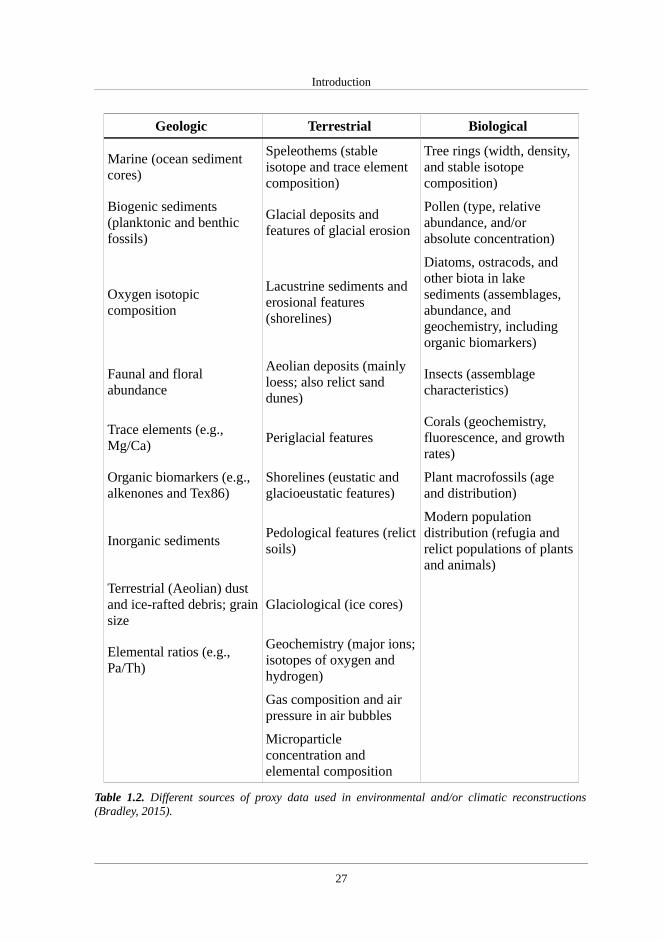
Introduction
Geologic Terrestrial Biological
Marine (ocean sediment cores)
Speleothems (stable isotope and trace element composition)
Tree rings (width, density, and stable isotope composition)
Biogenic sediments (planktonic and benthic fossils)
Glacial deposits and features of glacial erosion
Pollen (type, relative abundance, and/or absolute concentration)
Oxygen isotopic composition
Lacustrine sediments and erosional features (shorelines)
Diatoms, ostracods, and other biota in lake sediments (assemblages, abundance, and geochemistry, including organic biomarkers)
Faunal and floral abundance
Aeolian deposits (mainly loess; also relict sand dunes)
Insects (assemblage characteristics)
Trace elements (e.g., Mg/Ca)
Periglacial features Corals (geochemistry, fluorescence, and growth rates)
Organic biomarkers (e.g., alkenones and Tex86)
Shorelines (eustatic and glacioeustatic features)
Plant macrofossils (age and distribution)
Inorganic sediments Pedological features (relictsoils)
Modern population distribution (refugia and relict populations of plantsand animals)
Terrestrial (Aeolian) dust and ice-rafted debris; grainsize
Glaciological (ice cores)
Elemental ratios (e.g., Pa/Th)
Geochemistry (major ions;isotopes of oxygen and hydrogen)
Gas composition and air pressure in air bubbles
Microparticle concentration and elemental composition
Table 1.2. Different sources of proxy data used in environmental and/or climatic reconstructions(Bradley, 2015).
27

NAO imprints in the Central Iberian Peninsula for the last two millennia
1.4.1 Quantitative reconstructions
The appearance of the concept of calibration, namely 'transfer functions', in theearly 1970s revolutionised Quaternary palaeoecology. Imbrie and Kipp (1971) presen-ted, for the first time, a procedure for the quantitative reconstruction of past environ-mental variables (i.e., SSTs) based on biostratigraphical fossil assemblages (i.e., plank-tonic foraminifer assemblages) involving so-called transfer functions. A transfer func-tion is a mathematical equation for reconstructing past environmental conditions fromthe abundance of multiple species. Hence, this term refers not to a single numericalmethod but to a range of regression-based techniques. The equation is empirically de-rived from a training or calibration dataset of modern samples and associated environ-mental measurements. A mathematical representation of the transfer function conceptcan be written as follows:
Ym
=f ( Xm)+error (Eq. 1.1)
where Ym is a matrix of modern data responses (i.e., taxon abundances), Xm is a matrix ofcontemporary physico-chemical environmental 'predictors', and f() is a set of ecologicalresponse functions (i.e., transfer functions).
Since the pioneering work of Imbrie and Kipp (1971), the general approach ofquantitative palaeoenvironmental reconstruction has been adopted in many palaeodis-ciplines and multiple methods have been proposed that attempt to account for, either ex-plicitly or implicitly, the particular numerical properties of different palaeorecords. Inany case, a quantitative reconstruction usually involves three separate steps (Jugginsand Birks, 2012): 1) the development of the modern training set, 2) the development ofthe numerical model to solve the mathematical equation that relates the palaeorecorddata and the environment in the present, and 3) the application of the model to the fossilstratigraphic record and the evaluation of the resulting reconstruction. Each of thesesteps involves a number of decisions concerning training-set selection; data transforma-tion and screening; choice of numerical method; model selection, testing, and evalu-ation; and assessment of the final reconstruction (Figure 1.18).
Different methods exist to conduct quantitative reconstructions, although most ofthem are applied to biostratigraphical proxies with different ecological or statisticalbases (Figure 1.19). There is a major conceptual distinction between inverse and clas-sical methodological approaches and between methods that assume a linear response ofthe proxy to a given environmental gradient and methods that assume a non-linear rela-tionship (ter Braak, 1995; Birks, 1995, 2003; Guiot and de Vernal, 2007; Birks et al.,2010). The classical approaches estimate the response function f() of Eq. 1.1 using a re-gression of Ym on Xm (Birks, 2012). The regression can be linear, non-linear, or mul-tivariate. An example of the classical method approach is the Gaussian logit regressionand maximum-likelihood calibration (GLR-ML) (Figure 1.19). In contrast, inverse ap-proaches estimate the inverse of f() directly from the training set using an inverse re-gression of Xm on Ym (Birks, 2012). The Weighted-Averaging regression (WA),Weighted-Averaging Partial Least Squares Regression (WA-PLS), Modern AnalogueTechnique (MAT), Principal Components Regression (PCR) or Artificial Neural Net-works (ANN) are examples of inverse methods (Figure 1.19) (Juggins and Birks, 2012).
28

Introduction
29
Fig
ure
1.1
8. S
chem
atic
dia
gram
sho
win
g th
e st
eps
invo
lved
in
a qu
anti
tati
ve r
econ
stru
ctio
n fr
om b
iost
rati
grap
hica
l pa
laeo
lim
nolo
gica
l da
ta u
sing
a m
oder
n tr
aini
ng o
r ca
libr
atio
n da
tase
t.

NAO imprints in the Central Iberian Peninsula for the last two millennia
Figure 1.19. Conceptual diagram illustrating the different approaches to multivariate calibration us-ing a biological proxy. Sp represents biological taxa in the modern training set and Env is the environ-mental variable of interest in the modern data. C represents components. The figure was obtained fromJuggins and Birks (2012).
A basic requirement for a reconstruction model is that it should be statisticallysignificant, accurate, precise, and reliable, and it should make sense from the ecologicaland palaeoecological points of view (Birks et al., 2010; Juggins and Birks, 2012). If amodel is statistically significant, the obtained results are not likely to occur randomlyand are likely attributable to a specific cause, such as climate. Statistical significancecan be strong or weak and does not always indicate practical significance (Harris,1998). Model accuracy and precision are measured by the prediction error, which isusually calculated as the root mean squared error (RMSE). Some form of cross-valida-tion provides a more realistic estimate of the prediction error when the model is appliedto new data (Juggins and Birks, 2012). Ideally, this would involve testing the model us-ing an independent test dataset, a so-called external cross-validation (Birks, 2012).However, we rarely have the luxury of an additional test dataset – these samples areusually employed more profitably in the training set (Lotter et al., 1999). Instead, an in -ternal cross-validation of the training set simulating the likely errors is used when the
30

Introduction
model is applied to new data. There are three main types of internal cross-validationavailable: k-fold leave-out, leave-one-out, and bootstrapping (Juggins and Birks, 2012).In the k-fold leave-out method, the order of the samples is randomized and a fixed pro-portion (e.g., 20%) is left out of the training set (giving, in this case, a five-fold leave-out). The calibration function based on the remaining samples is then applied to the left-out samples, which act as the test set, and the squared errors accumulate to form theRMSE of the prediction (RMSEP). Note that the RMSEP is distinguished from the so-called apparent RMSE calculated solely from the training set. The leave-one-out meth-od is a special case of k-fold leave-out in which each sample is left out to form a singlesample test set (Manly, 1997). Larger training sets usually include some inherent replic-ation; thus, as the training-set size increases, leave-one-out RMSEP becomes a less reli-able estimate of true prediction errors (Næs et al., 2002). The k-fold leave-out methodprovides a more rigorous test but can be overly pessimistic because the training sets ineach step are of a correspondingly smaller size (Webb, 2002). This problem is addressedin bootstrap cross-validation by selecting samples from the original training set (of sizen) with replacement to give a new bootstrap training set also of size n (Stine, 1990;Mooney and Duval 1993; Manly 1997). Since samples are selected with replacement,some will be included more than once and, on average, approximately one third will re -main unselected. These become the bootstrap test dataset. This procedure is repeated alarge number of times (typically 1000) and the squared errors for the test samples accu-mulate across all bootstrap cycles to form the bootstrap RMSEP (Birks et al. 1990;Simpson and Birks, 2012).
In any case, there is no single ‘best’ or ‘optimal’ method that can be recommen-ded: differences in training-set size, taxonomic diversity in biological proxies, and formand complexity of the proxy–environment relationship make some numerical tech-niques more useful than others for particular datasets. Model selection thus becomes acrucial step in any quantitative reconstruction (Xu et al., 2010). For instance, Jugginsand Birks (2012) using diatom data and most of the methods show in Figure 1.19 illus-trate the issues of model selection and reconstruction evaluation by reconstructing therecent acidification history of The Round Loch of Glenhead, a small soft-water lake inGalloway located in southwestern Scotland.
1.4.2 The Bayesian method
Bayesian statistics is based on Bayes' theorem. This theorem was discovered bythe Reverend Thomas Bayes but was published posthumously two years after his death,in 1763 AD. Laplace and other statisticians used this method in the 19th century, but ithad largely fallen from favour by the early 20th century. However, by the middle of the20th century, interest in Bayesian methods was renewed by different statisticians, suchas De Finetti, Jeffreys, Savage, and Lindley. They developed a complete method of stat-istical inference based on Bayes' theorem (Bolstad, 2007). Bayesian statistics belongs tothe so-called ‘statistical learning’ methods because it learns from the data (Hastie et al.,2011), and it is considered to be an inverse method.
31

NAO imprints in the Central Iberian Peninsula for the last two millennia
The mathematical equation of the theorem for multiple events is defined as fol-lows:
P (Bi|A )=P ( A|Bi )⋅P ( Bi )
∑j= 1
n
P ( A|B j )⋅P (B j )
(Eq. 1.2)
where B1,...,Bn are n unobservable events with disjoint pair of events, Bi∩Bj=Ø fori=1,...,n, j=1,...,n and i≠j. The equation comes from the definition of conditional prob-ability (Bolstad, 2007). The marginal probability of event A is found by the law of totalprobability, and each of the joint probabilities is found from the multiplication rule (i.e.,denominator of the Eq. 1.2). P(Bi) is the prior probability of event Bi, P(A|Bi) corres-ponds to the likelihood, and P(Bi|A) is the posterior probability of event Bi.
Furthermore, the equation 1.2 can be simplified and is usually expressed in itsproportional form as follows:
posterior prior · likelihood∝
The reconstruction methods previously cited in section 1.4.1 (Figure 1.19) havedifferent statistical and ecological motivations but they have one thing in common: theyare all so-called frequentist methods and make the assumption that the model paramet-ers (e.g., WA optima and WA-PLS coefficients) are fixed and can be estimated from ob-servations (the measured data) distributed randomly about the fitted values (Holden etal., 2008). Conversely, the Bayesian approach in past reconstructions does not rely onan explicit relationship model between proxy and environmental variables but assumesthat the model is unknown and must be estimated from the measured data, which arefixed. Specifically, the Bayesian approach uses measured information to modify someprior belief about the environmental values (Robertson et al., 1999). This additional in-formation is derived from a training set and expressed as a conditional probability dens-ity function, namely 'likelihood', which is combined with the prior probability densityfunction to give a posterior density function using the Bayes’ theorem (Eq. 1.2). Anoth-er advantage of the Bayesian approach is that observations under all conditions are notrequired, making it possible to reconstruct past situations without analogous proxies inthe modern environment (Guiot and de Vernal, 2007).
Bayesian approaches have been applied to several aspects of palaeolimnology,such as the construction of age-depth models (e.g., Buck et al., 1999; Bronk Ramsey,2007; Blaauw and Christen, 2005; Blaauw et al., 2007; Haslett and Parnell, 2008), al-though environmental reconstructions, particularly climate reconstructions, are the mostpopular. For instance, Toivonen et al. (2001) described a Bayesian model with a condi-tional probability density function based on a unimodal model. Vasko et al. (2000) andKorhola et al. (2002) extended this to include a more realistic multinomial Gaussian re-sponse model and applied it to chironomid-based temperature reconstructions. Haslett etal. (2006) further developed these ideas for more generalized modelling of pollen-cli-mate response surfaces, and Holden et al. (2008) described a computationally efficientapproach based on probability weighting of species response curves. Li et al. (2010) de-veloped a Bayesian hierarchical model to reconstruct past temperatures that integrates
32

Introduction
information from different sources, such as climate proxies with different temporal res-olutions. More recently, Parnell et al. (2015) outlined a model (i.e., Bclim) and al-gorithm to describe the palaeoclimate and its volatility from pollen proxy data. Cahill etal. (2016) developed a Bayesian transfer function to reconstruct relative sea level usingforaminifera data. As in the frequentist reconstruction methods, to the best of our know-ledge, all of these Bayesian approaches used biological proxies to create the reconstruc-tions.
Although the prediction errors for Bayesian methods are similar to those of con-ventional approaches, they have a major advantage in their coherent and explicit hand-ling of uncertainty (Birks et al. 2010; Li et al. 2010). However, the lack of availablesoftware and the huge computational burden of most existing models (days to weeks fora single reconstruction) currently prevent more widespread use.
1.4.3 NAO reconstructions
The importance of the NAO on the climate variability of the North Atlanticregion has promoted different initiatives in recent decades to reconstruct the NAOi atdifferent time scales and temporal resolutions (e.g., Appenzeller et al., 1998; Glueckand Stockton, 2001; Luterbacher et al., 2002; Vinther et al., 2003a, b; Jones and Mann,2004; Goodkin et al., 2008; Trouet et al., 2009; Küettel et al. 2010; Olsen et al., 2012;Ortega et al., 2015) (Fig. 1.20).
Different proxies can register different aspects of the temporal evolution of theNAO; thus, the NAOi reconstructions are either based on single proxy archives (e.g.,ice cores) (Appenzeller et al., 1998), on only pressure-sensitive proxy data distributedacross Europe (Casty et al., 2007; Küettel et al., 2010) or on multi-proxy data fromdifferent records (e.g., tree rings, speleothems, lake sediments, or documents) that aresensitive to temperature and/or precipitation variations (Luterbacher et al., 2002; Trouetet al., 2009; Ortega et al., 2015). In particular, a common lacustrine sedimentary proxyusually employed in these reconstructions is the varve thickness in varved sediments(e.g., Ortega et al., 2015), although non-varved lacustrine records (e.g., Olsen et al.,2012) and a wide range of other lacustrine proxies have been extensively used toconduct different climate reconstructions (Battarbee, 2000; Smol and Cumming, 2000;Fritz, 2008; Pla-Rabes, 2011). Therefore, non-varved lacustrine sediments and theirassociated proxies can also constitute a proper alternative when creating an NAOireconstruction.
As a reconstruction, the NAOi is obtained by estimating an statisticalrelationship between the employed proxy and climate data or the NAOi during anoverlapping instrumental period. Regression techniques are also one of the mostextensively types of techniques used to conduct these reconstructions (e.g., Cook et al.,2002; Ortega et al., 2015), although a recent study employed a transfer function andMonte-Carlo-Markov-chain techniques to obtain a NAOi for the past ca. 5000 years(Olsen et al., 2012). NAO reconstructions generally show a good agreement with theinstrumental NAOi until ca. 1850 (Fig. 1.20). Farther back in time, considerablediscrepancies appear between the reconstructions (Pinto and Raible, 2012). Multiple
33

NAO imprints in the Central Iberian Peninsula for the last two millennia
factors may be responsible for these disagreements, such as the use of differentcalibration periods, differences in the response of the proxies to the climate modesand/or the stationarity of the relationship assumed between the proxies and the NAO(Pinto and Raible, 2012; Comas-Bru et al., 2016). Furthermore, chronologicaluncertainties associated with the dating methods might also contribute to these temporaldiscrepancies. Therefore, the selection of a statistical method that presents a majoradvantage in its coherence and explicit handling of uncertainties, such as the Bayesianapproach (Juggins and Birks, 2011), could contribute to improving this disagreement.Although Bayesian inference has been extensively used during the last decade forclimate and environmental reconstructions using biological proxies (see previoussection for further details), neither Bayesian inference nor non-biological proxies haveyet been used to conduct a reconstruction of the NAO.
Figure 1.20. A) Low-frequency variability in different NAO reconstructions (Jones et al., 1997;Appenzeller et al., 1998; Glueck and Stockton, 2001; Cook et al., 2002; Luterbacher et al., 2002;Vinther et al., 2003a; Jones, 2004; Goodkin et al., 2008; Trouet et al., 2009; Küttel et al., 2010) forthe past millennium and in observations from 1864 to 2009 AD (Hurrell, 1995). The figure wasobtained from Pinto and Raible (2012). B) NAO Ensemble reconstruction for 'model-constrained' fromOrtega et al. (2015). The intermediate and light purple envelopes represent the total ensemble spreadand the regression uncertainties across the ensemble, respectively, whereas the dark purple line showsthe ensemble mean. The black and red lines denote NAOVinther (Vinther et al., 2003b) and NAOTrouet
(Trouet et al., 2009), respectively. The horizontal magenta (or cyan) bars enclose centuries (marked bytick marks) with positive (or negative) mean NAO values that are significantly different (p-value <0.05) than zero.
34

Introduction
Another possible solution to reconcile the NAO reconstruction disagreementscould be the use of an appropriate concept of the NAO when a reconstruction isattempted. The NAO in a strict sense must be reconstructed using large high temporalresolution multi-proxy datasets from different geographical places, which will provide amuch better constrained NAO signal and, consequently, a more accurate NAOireconstruction (e.g., Ortega et al., 2015). In contrast, a simpler approach, such as the useof one or several proxies from a given region or group of regions will provide theregional NAO effects instead of a more realistic NAO reconstruction (e.g., Trouet et al.,2009; Olsen et al. 2012). Consequently, these different possible concepts of NAOshould be taken into account in the NAOi comparisons and in the use of these differentreconstructions.
1.4.4 Reconstructions in the Iberian Peninsula
Numerous environmental reconstructions in the IP have been conducted usingnatural archives, such tree rings (e.g., Büntgen et al., 2008), historical documents (e.g.,Benito et al, 2003b), peat bogs (e.g., Martínez-Cortizas et al., 1999), marine sediments(e.g., Nieto-Moreno et al., 2011) and speleothems (e.g., Martín-Chivelet et al., 2011)(Fig. 1.21), and at different temporal scales, from a centennial-resolution climate recon-struction covering the last 50,000 years carried out by Cacho et al. (1999) to annual-res-olution climate reconstruction for the last 200 years developed by Campelo et al.(2009).
In spite of the large diversity of natural archives employed in these Iberian recon-structions, lacustrine sedimentary records are one of the most widely used to determinethe environmental and climatic history of this region (Fig. 1.21). The most frequentlystudied lacustrine records are from low- and mid-elevation areas, such as the sediment-ary records from Sanabria Lake (1000 m asl; Jambrina-Enríquez et al., 2014) and EnolLake (1075 m asl; Moreno et al., 2011) in the northern IP; Arreo Lake (655 m asl; Co-rella et al., 2013), Estanya (670 m asl; Riera et al., 2004; Morellón et al. 2009, 2011)and Montcortès Lake (1027 m asl; Corella et al. 2011) in the Pre-Pyrenees; the Tablasde Daimiel wetland (616 m asl; Gil García et al., 2007) and Taravilla Lake (1100 m asl;Moreno et al., 2008) in the Central IP; and Zoñar Lake (300 m asl; Valero-Garcés et al.,2006; Martín-Puertas et al. 2008, 2010;) in the southern IP (Fig. 1.21).
Moreover, climate reconstructions from the main Iberian mountain ranges haveincreased over the last decade, including reconstructions of the Pyrenees from RedonLake (2240 m asl; Pla and Catalan, 2005; Pla-Rabes and Catalan, 2011), Marboré Lake(2500 m asl; Salabarnada, 2011) and Basa de la Mora Lake (1914 m asl; Morellón et al.,2012; Moreno et al., 2012; Pérez-Sanz et al., 2013) and the ranges of southern Spain(Sierra Nevada) from Laguna de Rio Seco (3020 m asl; Jiménez-Espejo et al., 2014)(Fig. 1.21). In addition, several environmental reconstructions in the Iberian CentralRange (ICR) are based on palynological records from different peatlands (> 1700 m asl;López-Sáez et al., 2014) (Fig. 1.21). However, to the best of our knowledge, only twoclimate reconstructions have been conducted based on an alpine lake located in this
35

NAO imprints in the Central Iberian Peninsula for the last two millennia
mountainous region (Cimera Lake, 2140 m asl) (Fig. 1.21), and they cover only the lastseveral centuries (Granados and Toro, 2000; Agustí-Panareda and Thompson, 2002).
The last two millennia are the most reconstructed time interval, and climate re-constructions usually distinguish five main climatic periods: the Roman Period (RP;650 BC – 500 AD), the Early Middle Ages (EMA; 500 – 900 AD), the Medieval Cli-mate Anomaly (MCA; 900 - 1300 AD), the Little Ice Age (LIA; 1300 - 1850 AD); andthe so-called Industrial Era (1850 – present). The studied records provide detailed in-formation on the climatic evolution for specific time windows (e.g., MCA and LIA,Morellón et al., 2012; Moreno et al., 2012), whereas other periods (e.g., EMA and RP,Luterbacher et al., 2016) remain less studied. Furthermore, when comparing the envir-onmental and climate information between the lowlands and highlands, it is clear thatthe spatial coverage of the latter must be improved.
The influence of the NAO on the IP has also been determined for these historicalperiods (e.g., Nieto-Moreno et al., 2011; Morellón et al., 2012; Moreno et al. 2012).These climate reconstructions commonly ascribe the warm and arid climate conditionsof the MCA to the dominance of the positive phases of the NAO and the humid andcold conditions of the LIA to the dominance of the negative phases of the NAO (Trouetet al., 2009; Ortega et al., 2015). Nevertheless, the role of the other climate modes in theclimatic evolution, as well as their interactions with the NAO, over the last millenniahas not been well addressed yet.
Figure 1.21. Topographical map of the Iberian Peninsula showing the locations of different recordsused to conduct environmental reconstructions in the IP. The reader is refereed to the figure caption ofFig. 6.4 for references. The record used in this study are underlined.
36

Introduction
LAKES
The usual definition of lake is 'an enclosed body of standing water surrounded byland'. Nevertheless, given the great variety of bodies of standing waters, it is notsurprising that all lake definitions must be a bit arbitrary (Cohen, 2003; O'Sullivan andReynolds, 2008).
Lakes comprises a small fraction of the Earth's land surface, approximately 1%,and contain a tiny volume of the Earth's water, less than 0.02% of the hydrosphere'swater (Talbot and Allen, 1996; Wetzel, 2001). They can be classified according todifferent features, such as basin origin (Wetzel, 2001), chemistry (Eugster and Hardie,1978), mixing period (Lewis, 1983), temperature (Hutchinson and Löffler, 1956),trophic state (Hutchinson, 1969) or the formation of an ice-cover during the winterseason, which is the traditional characteristic used to classify a lake as a high mountainor alpine lake (Toro and Granados, 2000).
Physical, chemical and biological lacustrine processes are of interest becausethey reflect the responses of these water bodies to external forcings, such as climate. Inaddition, these processes also act as intermediary filters between these external forcingand the palaeolimnological record (Cohen, 2003). For instance, lake-level oscillationsare mainly attributed to the difference between water outputs and inputs, which arecommonly controlled by climate (Imboden and Wüest, 1995). Lake-level variations canbe recorded directly by ancient shoreline elevations or indirectly by salinity indicatorsand can be used to conduct climate reconstructions (e.g., Corella et al., 2013). Thedifferent chemical cycles associated with lakes are also a great focus of attention. Forexample, CO2, which plays a key role in photosynthesis and in other processes in thelacustrine carbon cycle, is one of the most important drivers of climate change (Cole etal., 1994, 2007). Thus, variations in CO2 concentrations will be reflected in lakes, andthese effects can be used to study anthropic emissions and their ascribed impacts(Adrian et al., 2009). The biotas of lakes are the most complex components of thesenatural systems and involve numerous species (e.g., algae, vascular plants, sponges,annelids, crustaceans, insects and molluscs) and various interactions both between thespecies and with the external environment (Margalef, 1983). The responses of thesefreshwater organisms to abiotic factors, such as lake water temperature (Granados andToro, 2000), dissolved oxygen (Dinsmore et al., 1999), pH (Battarbee, 1986), salinity(Bos et al., 1999), and nutrient availability (Leland and Berkas, 1998), have also beenextensively used to reconstruct past environmental and climatic conditions and currentglobal change effects.
The highest concentration of lakes is in the boreal and Arctic latitudes (45°–75°N), whereas the abundance of lakes is lower in southern latitudes, where the contin-ental area is also lower (Fig. 1.22A) (Verpoorter et al., 2014). Other distinctive featuresof these water bodies are that their size distribution decreases dramatically with eleva-tion and that only approximately 10% of lakes are located at elevations higher than2000 m asl (Fig. 1.22B) (Verpoorter et al., 2014). Alpine lakes, or so-called mountainlakes, form part of this marginal freshwater bodies group. Nevertheless, although thismeagre figurensuggests alpine lakes play an apparently negligible role in the Earth sys-tem,nthey are particularly suitable ecosystems for studies on certain environmental and
37

NAO imprints in the Central Iberian Peninsula for the last two millennia
ecological topics (Adrian et al., 2009; Catalan et al., 2013). For this reason, the scientif-ic community has paid far more attention to them than their quantitative relevancewould suggest.
Figure 1.22. A) The latitudinal distribution of lake abundance (grey line) and B) the elevation distri -bution of lakes by cumulative percentage abundance (dashed grey line). Both data were compiled froma high-resolution satellite imagery database (Global Water Bodies database (GLOWABO)). Both im-ages were modified from Verpoorter et al. (2014).
1.5 Alpine lakes
Alpine lakes are among the most similar ecosystems throughout the worldbecause, as stated previously, they all experience ice cover (Catalan et al, 2006). Theselakes are located in most of the large and high ranges around the world (e.g., the Alps,the Pyrenees, Himalayas, Rocky Mountains, Andes, Kilimanjaro), where the lowpermeability of crystalline bedrock favours their presence (Fig. 1.23). Most alpine lakesoriginated during the last glaciation due to the interaction of ice and hard bedrock; thus,they are generally young ecosystems (Catalan et al, 2006). Their particular locationleads to distinct environmental conditions that define their limnological and biologicalfeatures. Low rock weathering and limited soil development lead to highly dilutedwaters in terms of major salt components and nutrients (e.g., Toro et al., 2006).Consequently, lacustrine organisms face challenges, such as oligotrophy, in theseextreme habitats. The formation and development of ice and snow covers for severalmonths is the distinctive dynamical feature of these lake ecosystems (Fig. 1.23). Thisice cover plays a key role in lake productivity through its influence on the growingseason length and summer stratification as well as in the lake overturning strength andtiming, which controls the internal lake nutrient cycle (Catalan et al., 2002; Pla-Rabesand Catalan, 2011).
Another common feature of alpine lakes is that they are usually small waterbodies in which matter loading from the catchment is fundamental in determining thecharacteristics and biogeochemical cycles of the lake (Fig. 1.23). Alpine lakecatchments are relatively small compared to lowland lakes and are usually poorlyvegetated as a result of their positions close to or above the treeline. Consequently,atmospheric loading also tends to be significant in determining the compositional
38

Introduction
characteristics of runoff and thus the lake water (Catalan et al., 2006; Adrian et al.,2009; Mladenov et al. 2011). Therefore, atmospheric inputs have a significant influenceon the biogeochemistry of alpine lakes and can affect their water chemistry (Reche at al.2009), which in turn affects their primary productivity (Psenner, 1999) and carbon pool(Psenner,1999; Mladenov et al. 2011). One of these most important atmospheric loadingfactors in European alpine lakes is African dust events (e.g., Hervás et al., 2009;Mladenov et al., 2011). European alpine lakes are exposed to these aeolian inputs undercertain climatic conditions (Bergametti et al., 1989; Moulin et al. 1997, Ginoux et al.,2004). The African dust includes variable amounts of quartz and clays, such as illite,kaolinite, and smectite, among others components; thus, their arrival leads to the inputof limiting nutrients (e.g., phosphorus, nitrogen and iron) to these oligotrophicecosystems. Different chemical, mineralogical and biological analyses conducted onsamples collected from direct atmospheric deposition in lake catchments or at differentlake water depths have been employed to assess the arrival and the effects of theseAfrican airborne inputs (e.g., Reche et al., 2009; Morales-Baquero et al., 2006). Inparticular, a fibrous clay called palygorskite has been used to trace the origin of theAfrican dust (Coudé-Gaussen et al., 1982; Molinaroli, 1996). For instance, the westernSahara and southern Morocco are dust sources that are particularly rich in palygorskite(Molinaroli, 1996). In these areas, the formation of palygorskite is favoured byevaporation and chemical concentration (Singer and Galan, 1984) on poorly drainedcarbonated rocks in the anti-Atlas (El Mouden et al.,2005). These dust sources havebeen essentially confirmed by back trajectory analysis for dust deposited overnortheastern Spain (Middleton and Goudie, 2011). In addition, the chemical and mineralsignatures of dust events might be identifiable in the lake sediments (Nieto-Moreno etal. 2013; Jiménez-Espejo et al., 2014), which can also contribute to reconstructions ofpast climate conditions. In the IP, many different studies support the arrival andbiogeochemical effects of African dust in mountain lake ecosystems, particularly insouthern Iberian regions (Morales-Baquero et al., 2006; Pulido-Villena et al., 2006,2008; Mladenov et al.,2011).
In general, mountain lake ecosystems are also sensitive indicators of climaticvariability (Thompson et al., 2009). Lakes located in the IP are particularly sensitive tothe NAO climate mode due to their geographical position. These freshwater ecosystemsrespond substantially to changes in air temperature, wind speed or precipitation, amongother climatic variables, which are controlled by large-scale climatic fluctuations(Sharma and Magnuson, 2014). These responses are then recorded in lake parameters.Physical lake water parameters, such as water temperature and ice phenology, appear tomore rapidly reflect the effects of these climate patterns and exhibit higher sensitivitiesthan other lacustrine parameters, such as chemical or biological ones (Straile et al.,2003; George et al. 2004; Salmaso, 2012). Individual physical lake properties influencefreezing processes much more strongly than thawing processes. For instance, the timingof ice-off makes a better direct indicator of climatic changes and thus of NAO effectsthan the timing of ice-on (Šporka et al. 2006; Adrian et al., 2009). Consequently, thewinter NAO effects are typically reflected in the ice phenology via the air temperature,particularly in the ice-off date. In Northern Europe, many studies have found this strongrelationship (Yoo and D'Odorico, 2002; Brown and Duguay, 2010). However, relatively
39

NAO imprints in the Central Iberian Peninsula for the last two millennia
scarce data on ice phenology are available for meridional areas of the NorthernHemisphere (Brown and Duguay, 2010) and for the effects of the NAO signal via otherclimatic variables, such as snow accumulation (Ghanbari et al., 2009; Ruibo et al.,2012), which can play a key role in the thawing process through its insulating effect(Jensen et al., 2007; Ruibo et al., 2012). In addition, other factors, such as altitude,latitude or lake morphometry, can influence ice phenology and the resulting NAO-icerelationships (Williams and Stefan, 2006; Livingstone and Adrian, 2009). Therefore, icephenology has become one of the most valuable indicators of the effects of large-scaleoscillations on winter lacustrine dynamics throughout the Northern Hemisphere,particularly with respect to the effects of the NAO, which is the main mode of climatevariability in the North Atlantic region on the multiannual time scale (Barrie et al.,2006; Ghanbari et al. 2009; Bai et al. 2012). Nevertheless, most of the studies havefocussed on determining the influence of the NAO on alpine lakes, whereas to the bestof our knowledge, the sensitivity of these water bodies to variations of other climatemodes, such as the EA and the SCAND, has not yet been explored either in recentperiods or in the past. Some studies have assessed the sensitivity of low-altitude lakes tothese modes of climate variability during the instrumental period (Salmaso, 2012;Hernández et al., 2015). However, their impact on alpine lakes remains unknown.
Finally, altitude in alpine lakes also establishes remoteness, which is very relev-ant for organism colonization and especially for anthropic influence (Catalan et al.,2006). Lakes are ecosystems that have been influenced by humans since remote times(e.g., Corella et al., 2013; Moreno et al. 2009; Park et al., 2010; García-Alix et al.,2013). Thus, reconstructions based on lacustrine sequences from low-altitude lakes usu-ally face the additional challenge of distinguishing between environmental or climaticsignals and anthropogenic ones (e.g., Valero-Garcés et al., 2006; Morellón et al., 2011;Barreiro-Lostres et al., 2015). However, alpine lakes have been extensively recognizedas sensors of global change and key freshwater reference sites for global-scale pro-cesses due to their location outside of direct human influence (Williamson et al., 2009;Mladenov, 2011; Catalan et al., 2013). Consequently, their sediments constitute an ex-cellent archive for conducting environmental reconstructions because they often containmore pristine climatic signals compared with the low-mountain records.
40

Introduction
Figure 1.23. Images of alpine lakes. A) Redon Lake (2240 m asl) located in the Pyrenees, B) CimeraLake (2140 m asl) located in the Iberian Central Range, C) Peñalara Lake (2016 m asl) located in theIberian Central Range, D) Hagelseewli Lake (2339 m asl) located in the Central Swiss Alps and E)Chasm Lake (3604 m asl) located in the Rocky Mountains.
41

NAO imprints in the Central Iberian Peninsula for the last two millennia
1.6 Lacustrine sediments
Lakes accumulate sediments from their surrounding environment, and thesenatural archives provide a continuous and excellent record of environmental changes,resulting in accurate repositories and sources of information about the lake history(Cohen, 2003, Smol, 2008; Nichols, 2009). Sediment accumulation rates in lakes areoften high, so lake sediments offer the potential for high-resolution records of recentand past environmental conditions, such as climate variations, providing they can beadequately dated (Birks, 2015). However, no two lakes are identical; thus, theenvironmental conditions in the lake catchment and the water properties of each lakemust be carefully evaluated to make a meaningful interpretation of the sediments(Birks, 2015).
Lake sediments are made up of two basic components: allochthonous material,originating from both outside and within the lake catchment, and autochthonousmaterial, produced within the lake itself (O'Sullivan and Reynolds, 2008; Herschy,2012) (Fig. 1.24). Allochthonous material is transported to lakes by rivers and streams,overland flow, aeolian activity, and, in some cases, by subsurface drainage. Thismaterial is made up of varying amounts of fluvial or aeolian clastic sediment, dissolvedsalts, terrestrial macrofossils, phytoliths, pollen, charcoal from fires, among othercomponents (O'Sullivan and Reynolds, 2008; Herschy, 2012) (Fig. 1.24).Autochthonous material is either biogenic in origin or may result from inorganicprecipitation within the water column (often as a consequence of seasonally varyingbiological productivity, which can significantly alter the water chemistry) (O'Sullivanand Reynolds, 2008; Herschy, 2012) (Fig. 1.24). Both allochthonous and autochthonousmaterial can be useful for conducting palaeoecological and palaeoclimaticreconstructions (Nichols, 2009; Birks, 2015).
A great deal of basic information about changes in environmental and climaticconditions can be derived from relatively simple measurements of the sedimentary,organic, inorganic and biological compositions of lake sediments (Birks, 2015).
For example, the advance and retreat of glaciers is tracked quite well by changesin loss on ignition (LOI) because the proportion of clastic sediment increases (and/ororganic matter production decreases) during times of glacier growth (Nesje et al., 2000).Similarly, magnetic susceptibility also documents changes in the proportion of clasticmaterial in a sediment core, and this also may reflect glacier activity in certainsituations (Polissar et al., 2005). Various non-destructive methods are available forsediment analysis, of particular importance is the acquisition of elemental data at veryhigh resolution by scanning X-ray fluorescence (XRF) analysis (Shanahan et al., 2008;Rothwell and Croudace, 2014; Bakke et al. 2010). In many cases, the down-core recordof a specific element or elemental ratio can provide valuable insights into pastconditions.
Pollen is one of the most widely studied components of lake sediments. Itprovides a wealth of palaeoenvironmental and palaeoclimatic information (e.g., Rull etal., 2010; Parnell et al., 2015;) and is a staple proxy used in verifying general circulationmodel simulations (Prentice et al., 1996; Bartlein et al., 1998; Bennett and Willis,2001). Plant macrofossils (e.g., leaves, seeds, and fruits) are environmental indicators
42
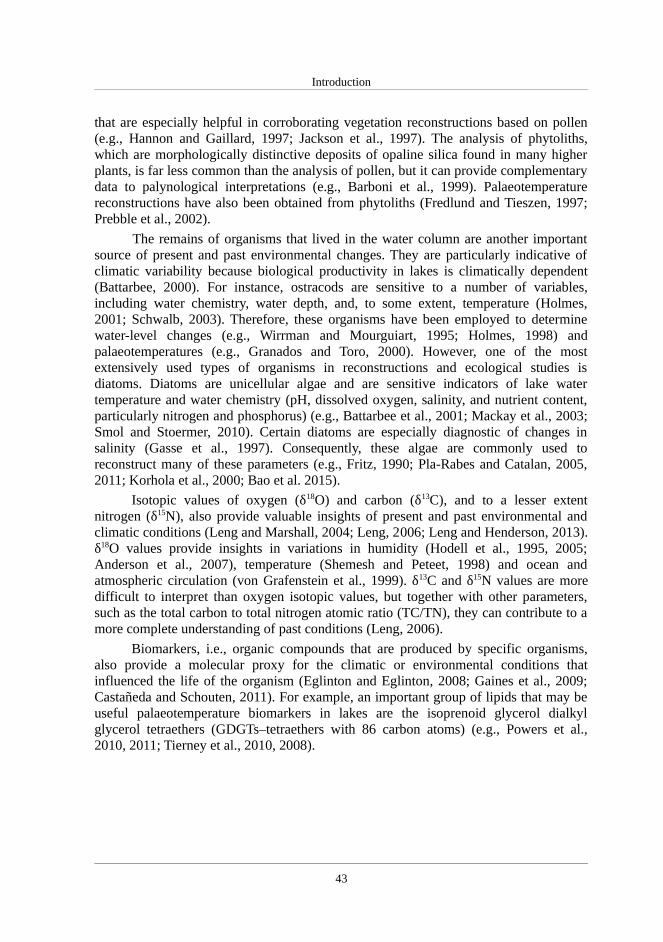
Introduction
that are especially helpful in corroborating vegetation reconstructions based on pollen(e.g., Hannon and Gaillard, 1997; Jackson et al., 1997). The analysis of phytoliths,which are morphologically distinctive deposits of opaline silica found in many higherplants, is far less common than the analysis of pollen, but it can provide complementarydata to palynological interpretations (e.g., Barboni et al., 1999). Palaeotemperaturereconstructions have also been obtained from phytoliths (Fredlund and Tieszen, 1997;Prebble et al., 2002).
The remains of organisms that lived in the water column are another importantsource of present and past environmental changes. They are particularly indicative ofclimatic variability because biological productivity in lakes is climatically dependent(Battarbee, 2000). For instance, ostracods are sensitive to a number of variables,including water chemistry, water depth, and, to some extent, temperature (Holmes,2001; Schwalb, 2003). Therefore, these organisms have been employed to determinewater-level changes (e.g., Wirrman and Mourguiart, 1995; Holmes, 1998) andpalaeotemperatures (e.g., Granados and Toro, 2000). However, one of the mostextensively used types of organisms in reconstructions and ecological studies isdiatoms. Diatoms are unicellular algae and are sensitive indicators of lake watertemperature and water chemistry (pH, dissolved oxygen, salinity, and nutrient content,particularly nitrogen and phosphorus) (e.g., Battarbee et al., 2001; Mackay et al., 2003;Smol and Stoermer, 2010). Certain diatoms are especially diagnostic of changes insalinity (Gasse et al., 1997). Consequently, these algae are commonly used toreconstruct many of these parameters (e.g., Fritz, 1990; Pla-Rabes and Catalan, 2005,2011; Korhola et al., 2000; Bao et al. 2015).
Isotopic values of oxygen (δ18O) and carbon (δ13C), and to a lesser extentnitrogen (δ15N), also provide valuable insights of present and past environmental andclimatic conditions (Leng and Marshall, 2004; Leng, 2006; Leng and Henderson, 2013).δ18O values provide insights in variations in humidity (Hodell et al., 1995, 2005;Anderson et al., 2007), temperature (Shemesh and Peteet, 1998) and ocean andatmospheric circulation (von Grafenstein et al., 1999). δ13C and δ15N values are moredifficult to interpret than oxygen isotopic values, but together with other parameters,such as the total carbon to total nitrogen atomic ratio (TC/TN), they can contribute to amore complete understanding of past conditions (Leng, 2006).
Biomarkers, i.e., organic compounds that are produced by specific organisms,also provide a molecular proxy for the climatic or environmental conditions thatinfluenced the life of the organism (Eglinton and Eglinton, 2008; Gaines et al., 2009;Castañeda and Schouten, 2011). For example, an important group of lipids that may beuseful palaeotemperature biomarkers in lakes are the isoprenoid glycerol dialkylglycerol tetraethers (GDGTs–tetraethers with 86 carbon atoms) (e.g., Powers et al.,2010, 2011; Tierney et al., 2010, 2008).
43
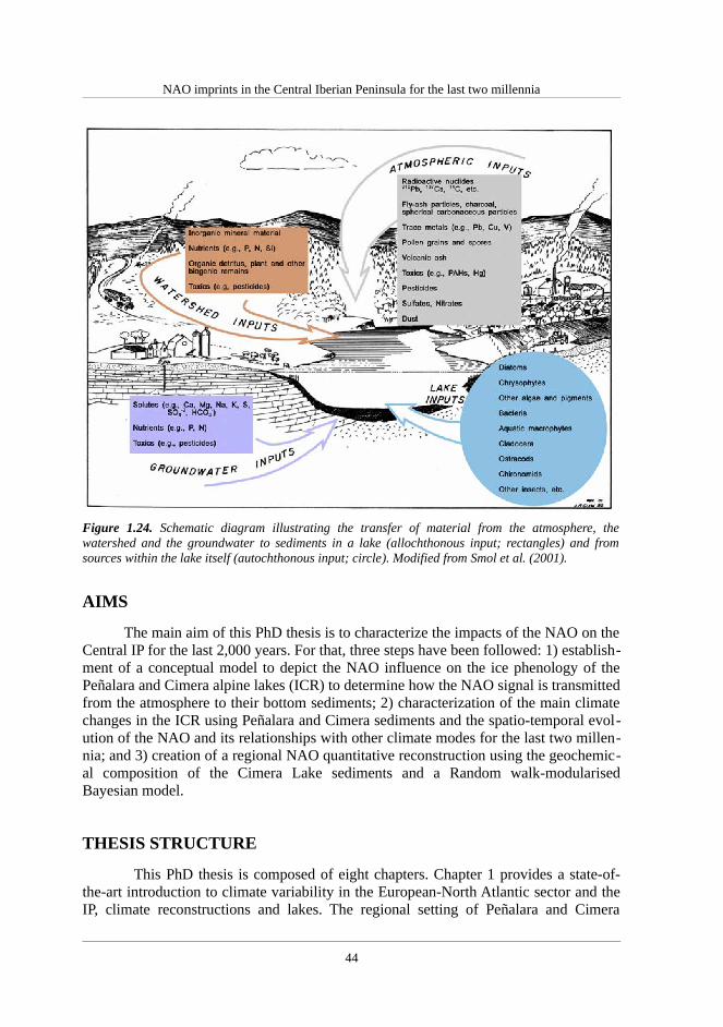
NAO imprints in the Central Iberian Peninsula for the last two millennia
Figure 1.24. Schematic diagram illustrating the transfer of material from the atmosphere, thewatershed and the groundwater to sediments in a lake (allochthonous input; rectangles) and fromsources within the lake itself (autochthonous input; circle). Modified from Smol et al. (2001).
AIMS
The main aim of this PhD thesis is to characterize the impacts of the NAO on theCentral IP for the last 2,000 years. For that, three steps have been followed: 1) establish-ment of a conceptual model to depict the NAO influence on the ice phenology of thePeñalara and Cimera alpine lakes (ICR) to determine how the NAO signal is transmittedfrom the atmosphere to their bottom sediments; 2) characterization of the main climatechanges in the ICR using Peñalara and Cimera sediments and the spatio-temporal evol-ution of the NAO and its relationships with other climate modes for the last two millen-nia; and 3) creation of a regional NAO quantitative reconstruction using the geochemic-al composition of the Cimera Lake sediments and a Random walk-modularisedBayesian model.
THESIS STRUCTURE
This PhD thesis is composed of eight chapters. Chapter 1 provides a state-of-the-art introduction to climate variability in the European-North Atlantic sector and theIP, climate reconstructions and lakes. The regional setting of Peñalara and Cimera
44

Introduction
Lakes, including geographical, geological, vegetation, climatic and limnological fea-tures, are presented in Chapter 2. All the methodological procedures employed, includ-ing instrumental data, sediment analyses and statistical treatments, are described inChapter 3. Chapter 4 includes the results of the chemical and statistical analyses per-formed and the age-depth models of both lake sequences. Discussion is provided inChapters 5, 6 and 7. Chapter 5 establishes the present-day influence of the NAO on theice phenology of Iberian alpine lakes by the construction of a conceptual lake model. InChapter 6, the age-depth models, geochemical compositions and the results from Re-dundancy Data Analysis and Principal Component Analysis (RDA and PCA) ofPeñalara and Cimera lake sediment sequences have allowed us to determine the mainenvironmental processes that controlled the terrigenous inputs and organic productivityin each lake for the last two millennia and to qualitatively reconstruct the climatic con-ditions in the ICR for this period. Moreover, the integration of both reconstructions withother relevant Iberian reconstructions have finally permitted us to determine the inter-play of climate modes and forcing mechanisms acting in the IP for the last two millen-nia. Chapter 7 presents the reconstruction of the quantitative impact of the NAO in theICR for the last two millennia obtained using a random walk-modularised Bayesianmodel and geochemical elements in the Cimera Lake record measured via X-Ray Fluor-escence analysis. This chapter also contains a discussion of the model validation and acomparison of the reconstructed NAO impact with other NAO approaches. Finally,Chapter 8 provides the concluding remarks of the thesis grouped according to theirmethodological, limnological or climatic implications, and future works are proposed.The raw data obtained during the experimental processes are contained in the appen-dices.
45
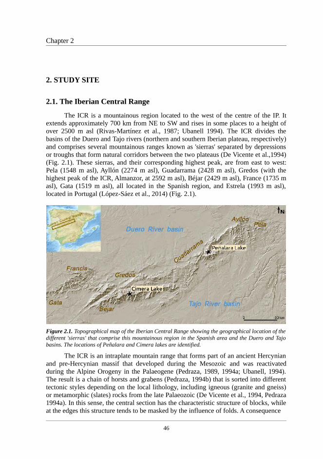
Chapter 2
2. STUDY SITE
2.1. The Iberian Central Range
The ICR is a mountainous region located to the west of the centre of the IP. Itextends approximately 700 km from NE to SW and rises in some places to a height ofover 2500 m asl (Rivas-Martínez et al., 1987; Ubanell 1994). The ICR divides thebasins of the Duero and Tajo rivers (northern and southern Iberian plateau, respectively)and comprises several mountainous ranges known as 'sierras' separated by depressionsor troughs that form natural corridors between the two plateaus (De Vicente et al.,1994)(Fig. 2.1). These sierras, and their corresponding highest peak, are from east to west:Pela (1548 m asl), Ayllón (2274 m asl), Guadarrama (2428 m asl), Gredos (with thehighest peak of the ICR, Almanzor, at 2592 m asl), Béjar (2429 m asl), France (1735 masl), Gata (1519 m asl), all located in the Spanish region, and Estrela (1993 m asl),located in Portugal (López-Sáez et al., 2014) (Fig. 2.1).
Figure 2.1. Topographical map of the Iberian Central Range showing the geographical location of thedifferent 'sierras' that comprise this mountainous region in the Spanish area and the Duero and Tajobasins. The locations of Peñalara and Cimera lakes are identified.
The ICR is an intraplate mountain range that forms part of an ancient Hercynianand pre-Hercynian massif that developed during the Mesozoic and was reactivatedduring the Alpine Orogeny in the Palaeogene (Pedraza, 1989, 1994a; Ubanell, 1994).The result is a chain of horsts and grabens (Pedraza, 1994b) that is sorted into differenttectonic styles depending on the local lithology, including igneous (granite and gneiss)or metamorphic (slates) rocks from the late Palaeozoic (De Vicente et al., 1994, Pedraza1994a). In this sense, the central section has the characteristic structure of blocks, whileat the edges this structure tends to be masked by the influence of folds. A consequence
46

NAO imprints in the Central Iberian Peninsula for the last two millennia
of these block dynamics is the asymmetry between the northern and southern slopes ofthe ICR, particularly in the western sector, because of the high altitude of the northernplateau with respect to the deeply set valleys in the Tajo River basin.
Glacial morphologies in the ICR developed only above 1900 m asl throughoutthe Quaternary (Pedraza and Carrasco, 2006; Palacios et al., 2011, 2012). Consequently,well-developed glaciated morphologies, such as mountain glaciers, small ice caps, icefields, valley slope, or cirque glaciers, are found on the summits of different sectors ofthe ICR (Pedraza and Carrasco, 2006). Some of these glacial geomorphologies favouredthe formation of lakes, whose basins can be classified accord to this genesis (e.g.,cirque, moraine, and bottom valley) (Wetzel, 2001). Lakes are only found in Sierra deGuadarrama (Spain), Sierra de Gredos (Spain) and Serra da Estrela (Portugal), wherethe glacial activity was more intense (Pedraza and Carrasco, 2006).
The vegetation in low and middle altitudes of the ICR is dominated by oakforests of Quercus ilex subsp. ballota, Quercus suber and Quercus pyrenaica (Devesa,1995; Pulido et al., 2007). The timberline, located between 1900 and 2100 m asl, isrepresented by pine forests of Pinus sylvestris and Pinus nigra, which are especiallyprominent in Sierra de Gredos and Sierra de Guadarrama (Martínez, 1999). Higherareas are occupied by shrublands, where brooms, such as Cytisus oromediterraneus,Echinospartum ibericum, and Echinospartum barnadesii, or heathlands of Ericaaustralis in more humid areas, are the prevailing vegetation (Rivas-Martínez, et al.,1987; Sánchez-Mata, 1989; Fernández-González, 1991). Psychroxerophilous grasslandsare the dominant vegetation in the highest areas (Toro et al., 2006; López-Sáez et al.2014).
The climate of the ICR is an alpine type immersed in a Mediterranean climatewith a strong continental influence (Durán et al., 2013). The arrival of Atlanticdepressions from the SW frequently occurs in fall, winter and spring; however, insummer, the Azores anticyclone is persistent and does not favour moisture transportfrom the west. Consequently, the ICR climate is characterized by a significant amountof solid precipitation and low temperatures in winter and warm and dry conditions insummer (Sánchez-López et al., 2015). The minimum and maximum temperaturesestimated for the period 1951–1999 AD oscillate between 0 and 2 °C and between 20and 22 °C, respectively. The total mean annual rainfall estimated for the period 1951–1999 AD is ca. 1400 mm and occurs in the humid ombrotype region (Ninyerola et al.,2005).
2.2. Peñalara Lake
Peñalara Lake (40°50'N – 3°57'W) is a tiny (0.6 ha, 115 m long, and 71.5 mwide) and shallow (4.8 m maximum depth) alpine lake (2016 m asl) located on thesoutheastern slope of the Peñalara Massif in the Sierra de Guadarrama (Fig. 2.1). It islocated in an over-excavated depression of a glacial cirque, and its catchment (140 ha)is composed of metamorphic rocks (gneiss) partially covered by Late Pleistoceneglacial moraine deposits (Palacios et al., 2003) (Fig. 2.2). The watershed exhibits smallzones of shrubs (Cytisus sp., Juniperus sp.), psychroxerophytic grassland (Festuca sp.),
47

Study site
meadows (Nardus sp.) and peat bogs (Sphagnum spp.), but the acidic nature of thecatchment bedrock does not allow the development of thick soils (Toro et al., 2006).
The deepest sector of the lake is located in the northern portion of the lake, and itis dominated by fine sediments. In contrast, the southern sector is shallower (< 2 mdeep) and accumulates cobble to boulder deposits transported by rock avalanches froma scree field developed at the base of a steep relief (Fig. 2.2). Peñalara has varioustemporary water inflows and a single outlet located on its southern shore (Fig. 2.2).
Figure 2.2. A) Topographic and B) bathymetric maps of Peñalara Lake according to Toro andGranados (2002). C) Panoramic view of Peñalara Lake from its northern side in May 2013 AD.
Peñalara Lake has been monitored since 1992 AD, and there are accuratephysico-chemical and biological datasets that have allowed for the characterization ofthe lacustrine dynamics. The lake is usually ice-covered from November-December toMarch-April, with a mean ice-cover duration of approximately 115 Julian days,although the ice cover can extend until May in severe winters (Fig. 2.3). In addition, thelake can exhibit two clearly differentiated ice covers in years with irregular winters thatpresent unusual warm periods of 2 or 3 weeks, such as 1999 and 2012 AD (Granados etal., 2006; Sánchez-López et al., 2015). The lake is monomictic, with thermal
48

NAO imprints in the Central Iberian Peninsula for the last two millennia
stratification of its waters occurring during the winter period under the ice cover. Therest of the year, the water column remains largely homogeneous (Fig. 2.3). Thedissolved oxygen of the water column has an annual periodic fluctuation (4–12 mg/l)with winter depletion below the ice cover. The lake water is very diluted, with a lowconductivity (10 μS/cm at 25ºC), an extremely low alkalinity (with mean values range40–60 μeq /l) and slightly acidic pH (a pH value of 6.2) (Toro and Granados, 2002;Granados et al., 2006).
During the early 1990s, the lake presented a marked tendency towardseutrophication, but the Spanish authorities began to carry out control policies to reducetourist impacts and the lake rapidly returned to its original trophic status (Toro andGranados, 2002). Currently, Peñalara Lake can be considered an oligotrophic lakeaccording to its low values of total phosphorus (mean values of 7 μg P-PO4 l-1),chlorophyll (maximum and mean values of 8 μg Chl-a l-1, 1.8 μg Chl-a l-1, respectively)and Secchi disk depth (maximum depth of 4.8 m) (Toro and Granados, 2002; Toro et al.,2006).
Figure 2.3. A) Monthly lake water temperatures at different depths, from lake surface (0.5 m) to lakebottom (4 m), and ice-cover duration in Julian days (white rectangles) for Peñalara Lake for theperiod 1998–2013 AD. The grey bands correspond to periods without lake water temperature data. B-G) Views of Peñalara Lake showing the different phases of the ice phenology from the formation of theice cover to the totally ice-free phase. Photos by I. Granados and M. Toro.
The weather station at Puerto de Navacerrada (40°46'N – 4°19'W; 1860 m asl), 8km southwest of Peñalara Lake, provides the only available meteorological data for thelake area for the period between 1950 and 2011 AD. The mean annual air temperaturein this area is approximately 6 °C, and the temperature is typically below 0 °C fromDecember to February. The mean maximum and minimum air temperatures are 20 °C
49

Study site
and -5 °C, respectively. The mean annual precipitation is 1339 mm, ranging from ca.805 mm and ca. 2380 mm per year, with the wettest period occurring from earlyOctober to late May. Snowfall primarily occurs from November to April (Fig. 2.4).
Figure 2.4. Climograph of the Peñalara Lake area including average monthly precipitation (bluebars), temperature (red lines) and snow days (black asterisks) for the period 1950–2011 AD. Climaticdata are from the Navacerrada weather station.
2.3. Cimera Lake
Cimera Lake (40°15'N – 5°18'W) is the highest (2140 m asl) of a series of 5alpine lakes located in a glacial cirque in the Massif Central of Sierra de Gredos (Figs.2.1 and 2.5; Palacios et al., 2011). Cimera is a shallow lake (9.4 m maximum depth)with a small surface area (5 ha, 384 m long, 177 m wide), and its catchment (75.6 ha) isprimarily composed of exposed plutonic rocks (granites) and exhibits scarce developedsoils and small grasslands and psychroxerophytic meadows (Nardus sp.) (Granados andToro, 2000) (Fig. 2.5). The southern sector has a mean water depth of 5.5 m, and itssediment is dominated by coarse gravel scree deposits. There are two temporary streaminlets in the southern littoral zone of the lake and one outlet on the northern side thatbecomes dry in late summer (Fig. 2.5). Flood currents from these streams are the originof the major volume of fine sediment inputs accumulated in the offshore zone of thenorthern part of the lake (Fig. 2.5).
Although Cimera has not been monitored for a long period because of itremoteness, different limnological studies conducted in the lake have determined itsmain physico-chemical features and characterized its lacustrine dynamics. Cimera is adiscontinuous, cold, polymictic lake (Toro et al., 2006) that usually starts to freezebetween November and December, and it becomes completely ice-free in May-June(Sánchez-López et al., 2015) (Fig. 2.6). The ice cover has a mean duration of 190 days,and the duration depends on the severity of the winter, with a difference of ca. 2 monthsbetween mild and severe winters (Granados and Toro, 2000; Sánchez-López et al.,2015) (Fig. 2.6). Cimera can also be classified as an oligotrophic lake because of thetotal mean phosphorus values (7 μg P-PO4 l-1), maximum and mean annual chlorophyllvalues (11.5 μg Chl-a l-1 and 2.1 μg Chl-a l-1, respectively) and mean Secchi disk depth
50
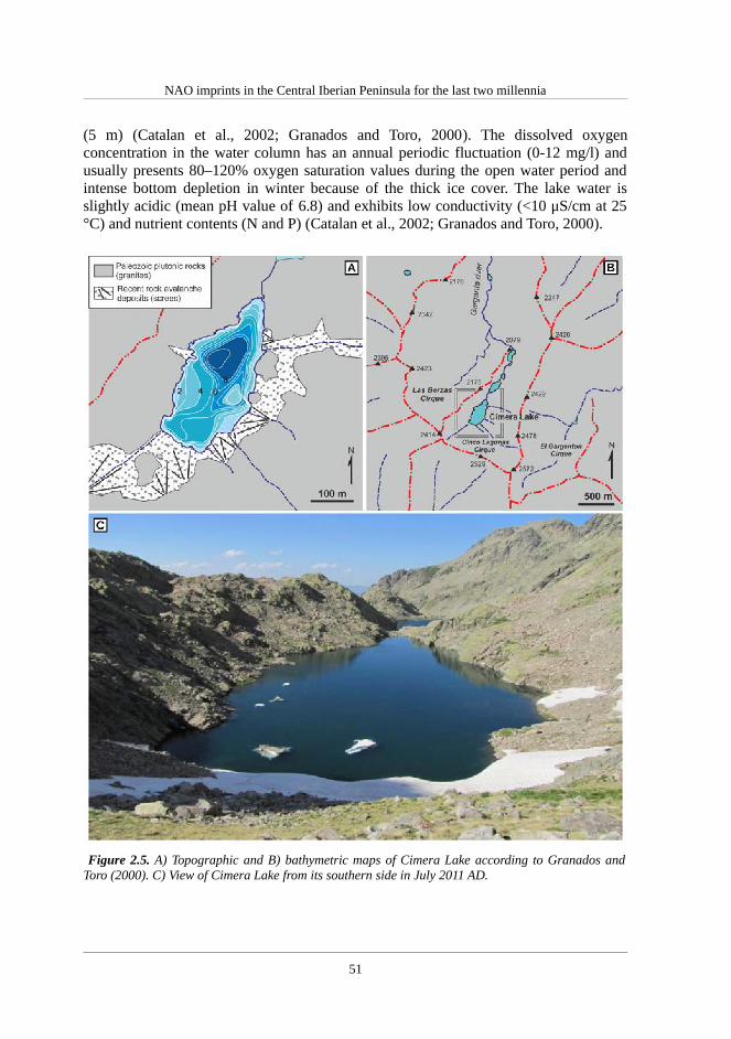
NAO imprints in the Central Iberian Peninsula for the last two millennia
(5 m) (Catalan et al., 2002; Granados and Toro, 2000). The dissolved oxygenconcentration in the water column has an annual periodic fluctuation (0-12 mg/l) andusually presents 80–120% oxygen saturation values during the open water period andintense bottom depletion in winter because of the thick ice cover. The lake water isslightly acidic (mean pH value of 6.8) and exhibits low conductivity (<10 μS/cm at 25°C) and nutrient contents (N and P) (Catalan et al., 2002; Granados and Toro, 2000).
Figure 2.5. A) Topographic and B) bathymetric maps of Cimera Lake according to Granados andToro (2000). C) View of Cimera Lake from its southern side in July 2011 AD.
51

Study site
Figure 2.6. A) Monthly lake water temperatures at different depths, from lake surface (0.5 m) to lakebottom (9 m), and ice-cover duration in Julian days (white rectangles) for Cimera Lake for the period2006–2013 AD. The grey band corresponds to a period without lake water temperature data. B-F)Chronological views of Cimera Lake showing the different phases of the ice phenology from theformation of the ice cover to totally ice-free conditions during the period of 2010/2011 AD. G-I) Viewsfrom the northern side of Cimera Lake catchment of different phases of the ice cover from theformation phase to the totally ice-free phase. Photos by I. Granados and M. Toro.
There are no weather stations near Cimera Lake because of its remoteness.Nevertheless, the total annual precipitation and average air temperature have beenpreviously estimated to be slightly higher and lower, respectively, than those in thePeñalara Lake area (Toro et al., 2006). The snow season in this region is longer thanPeñalara Lake area due to the higher altitude.
52
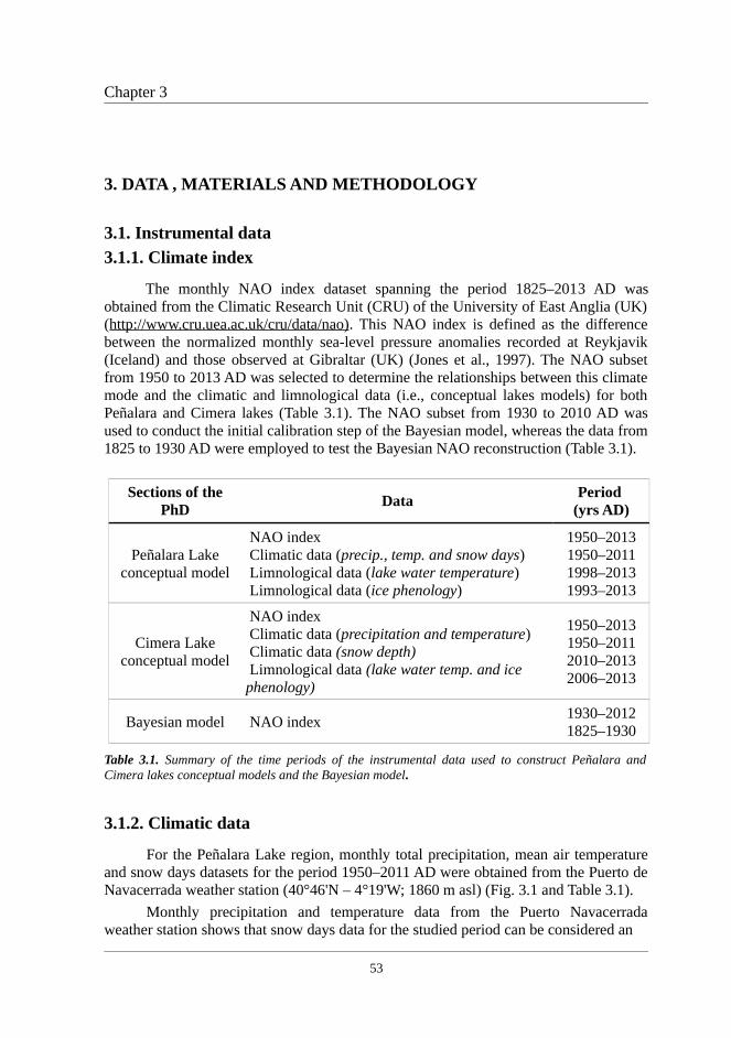
Chapter 3
3. DATA , MATERIALS AND METHODOLOGY
3.1. Instrumental data
3.1.1. Climate index
The monthly NAO index dataset spanning the period 1825–2013 AD wasobtained from the Climatic Research Unit (CRU) of the University of East Anglia (UK)(http://www.cru.uea.ac.uk/cru/data/nao). This NAO index is defined as the differencebetween the normalized monthly sea-level pressure anomalies recorded at Reykjavik(Iceland) and those observed at Gibraltar (UK) (Jones et al., 1997). The NAO subsetfrom 1950 to 2013 AD was selected to determine the relationships between this climatemode and the climatic and limnological data (i.e., conceptual lakes models) for bothPeñalara and Cimera lakes (Table 3.1). The NAO subset from 1930 to 2010 AD wasused to conduct the initial calibration step of the Bayesian model, whereas the data from1825 to 1930 AD were employed to test the Bayesian NAO reconstruction (Table 3.1).
Sections of thePhD
DataPeriod
(yrs AD)
Peñalara Lakeconceptual model
NAO index Climatic data (precip., temp. and snow days) Limnological data (lake water temperature) Limnological data (ice phenology)
1950–20131950–20111998–20131993–2013
Cimera Lakeconceptual model
NAO index Climatic data (precipitation and temperature) Climatic data (snow depth) Limnological data (lake water temp. and ice phenology)
1950–20131950–20112010–20132006–2013
Bayesian model NAO index1930–20121825–1930
Table 3.1. Summary of the time periods of the instrumental data used to construct Peñalara andCimera lakes conceptual models and the Bayesian model.
3.1.2. Climatic data
For the Peñalara Lake region, monthly total precipitation, mean air temperatureand snow days datasets for the period 1950–2011 AD were obtained from the Puerto deNavacerrada weather station (40°46'N – 4°19'W; 1860 m asl) (Fig. 3.1 and Table 3.1).
Monthly precipitation and temperature data from the Puerto Navacerradaweather station shows that snow days data for the studied period can be considered an
53

NAO imprints in the Central Iberian Peninsula for the last two millennia
equivalent measure of snow depth. The percentage of precipitation days and the amountof precipitation (mm) when the maximum temperature is below 4 °C is approximately80% in December, January and February (Fig. 3.2). Therefore, there is a directrelationship between the number of precipitation days and the total amount ofprecipitation and the majority of the precipitation that falls during these winter monthsis in the form of snow (Fig. 3.2).
No high-altitude meteorological stations exist close to Cimera Lake. Thus,regional climate series were used for this area. Regional monthly anomalies ofprecipitation and maximum and minimum air temperatures from 16 meteorologicalstations located in the surrounding area and covering the period 1950–2011 AD wereselected (Fig. 3.1 and Table 3.1). The snow depth dataset for the period 2010–2013 ADwas obtained from the Puerto Peones snow gauge dataset (40°15'N – 5°26'W; 2165 masl) (Table 3.1), which is located approximately 10 km west of the lake (Fig. 3.1).
All the climatic data time series were quality controlled and homogenizedfollowing the recommended protocols of Aguilar et al. (2003) and Brunet et al. (2008).
Figure 3.1. Map of the topography of the Iberian Central Range showing the locations of the weatherstations (black circles), the snow gauge (black square) and Peñalara and Cimera lakes (black stars).
54

Data, Materials and Methodology
Figure 3.2. Percentages of monthly precipitation data from the Puerto Navacerrada meteorologicalstation for the period 1946–2010 AD expressed in total days (blue bars) and amount of precipitationin mm (light blue bars) with maximum temperatures below 4 °C.
3.1.3. Limnological data- Lake water column temperatures
Measures of lake water column temperatures at different depths, different timeintervals and for different time periods were obtained using thermistor chains located inPeñalara and Cimera lakes (Table 3.1, Figs. 2.3A and 2.6A)
In Peñalara Lake, lake water temperatures were measured at 0.5, 1, 2, 3 and 4 mof water depth at intervals of ten minutes, two hours and four hours for the period1998–2013 AD. Different thermistors were used: one Tinytalk II thermistor was used at0.5 m deep between 1998 and 2005 AD, and HOBO Water Temp Pro V1 & V2thermistor chains were used at 0.5, 1, 2, 3 and 4 m deep from 2005 to 2013 AD (Fig.3.3). Linear regression models were employed to inter-calibrate the different devicesand to obtain a mean daily homogeneous dataset covering the complete period (Fig.3.4).
In Cimera Lake, lake water temperatures were measured hourly with HOBOWater Temp Pro V1 & V2 thermistors (Fig. 3.3) at water depths of 0.5, 3, 6, and 9 m forthe period 2006–2013 AD. Daily temperature data were obtained from thesemeasurements by calculating the mean daily values.
Figure 3.3. Photos of A) HOBO Water Temp ProV2 and B) Tinytalk II thermistors.
55

NAO imprints in the Central Iberian Peninsula for the last two millennia
56
Fig
ure
3.4
. Mea
n da
ily
data
sets
of l
ake
wat
er te
mpe
ratu
re m
easu
red
at 0
.5, 1
, 2, 3
and
4 m
of w
ater
dep
th (
blac
k li
nes)
and
thei
r co
rres
pond
ing
hom
ogen
eous
dat
aset
s (r
ed li
nes)
from
Peñ
alar
a L
ake
for
the
peri
od 1
998–
2013
AD
.

Data, Materials and Methodology
- Ice phenology
The ice phenology data include freeze-up and break-up dates and ice-coverduration. The freeze-up date is defined as the first day the lake is completely ice-covered as determined by a visual inspection. The break-up date is defined as the firstday the ice cover begins to break. The ice-cover duration is expressed as the number ofdays that the lake is completely ice-covered (Ruibo et al., 2012). These definitionsrequire nearly daily observations of each lake to collect the ice phenology data.
In Peñalara Lake, the ice data were obtained from daily visual observations ofthe lake and span the period 1993–2013 AD (Table 3.2). The ice cover on Peñalara doesnot continuously cover the lake surface during irregular winters with warm periods ofabove-mean air temperatures that persist for 2 or 3 weeks. In these years, the lakeexhibits two clearly differentiated ice-covered periods, with the second ice-coveredperiod usually occurring either at the beginning or the end of the winter (Table 3.2).Nevertheless, the ice-free period between these two ice-covered periods is typically lessthan 13% of the total ice-cover duration, with the exception of 1998 AD, in which theice-free period accounted for 34.4% of the total ice-covered period (Table 3.2).Therefore, the ice-cover duration in Peñalara Lake is represented by the sum of the twoice-covered periods and excluding the in-between ice-free days. The ice datacorresponding to the year 1998 AD were considered outliers and were not included inthe subsequent statistical analyses.
There are no daily available observations for Cimera Lake because of its remotelocation. Hence, ice phenology dates for this lake were deduced from lake watertemperatures measured by the thermistor chains (Table 3.3). The freeze-up date wasdefined as the date when the lake water temperature changed from an autumnoverturning pattern to winter stratification, and the break-up date was defined as thedate when the lake water temperature changed from winter stratification to a springoverturning pattern (Fig. 2.5A). This method of deriving the ice phenology metric inCimera Lake was verified using Peñalara Lake data. The differences between thefreeze-up and break-up dates based on daily visual observations and those based onwater temperatures measured using the thermistors at different water depths in PeñalaraLake were calculated (Table 3.4). These differences show that dates based on themeasured water temperature data were typically earlier than those obtained based ondaily visual observations. However, the differences in the freeze-up and break-up datesbetween the daily observations and the water temperatures measured using thermistorswere less than five days. Therefore, these differences were considered negligible and icedata deduced from measured water temperature can be considered similar to ice datafrom visual observation of the lake. The ice phenology data deduced from watertemperature span the period 2006–2013 AD.
All ice date data from both lakes were expressed in Julian days, and theobservation year for both dates is given as the year of break-up. The ice-cover durationis expressed in number of days (Tables 3.2 and 3.3).
57

NAO imprints in the Central Iberian Peninsula for the last two millennia
Data yearconsidered
Freeze-up date
Julian day
Break-up date
Julianday
Ice-cover duration in
days
Number of
covers
Totaldays
% Ice-free days between covers
1993 08/12/92 343 01/04/93 90 114 1 114 –
1994 27/12/93 361 – – – – – –
1995 – – – – – – – –
1996 05/12/95 339 25/04/96 115 142 1 142 –
1997 24/12/96 359 13/03/97 71 79 1 79 –
199801/01/9810/04/98
1100
08/03/9810/05/98
66129
6630
2 96 34.4
199930/11/9816/12/98
334350
12/12/9813/04/99
345102
12118
2 130 3.1
2000 16/11/99 320 29/02/00 59 105 1 105 –
2001 19/12/00 354 – – – 1 - –
2002 16/11/01 320 25/03/02 83 129 1 129 –
200323/11/0205/01/03
3275
25/12/0222/04/03
358111
32107
2 139 7.9
200403/12/0306/05/04
337127
27/04/0419/05/04
117139
14613
2 159 5.7
2005 04/12/04 339 10/04/05 99 127 1 127 –
2006 14/11/05 318 17/04/06 106 154 1 154 –
200710/12/0623/01/07
34423
19/01/0722/04/07
18111
4089
2 129 3.1
200814/12/0723/03/08
34883
15/03/0808/04/08
7498
9216
2 108 7.4
2009 25/11/08 330 25/04/09 114 151 1 151 –
2010 19/12/09 353 26/04/10 115 128 1 128 –
2011 23/11/10 327 14/04/11 103 142 1 142 –
201218/12/1114/04/12
352105
29/03/1210/05/12
88130
10226
2 128 12.5
2013 13/01/13 13 23/05/13 142 130 1 130 -
Table 3.2. Ice phenology records for Peñalara Lake obtained by visual observations of the lake. Thedata in grey italics correspond to the anomalous year 1998 AD and were not included in the analyses.
58

Data, Materials and Methodology
Data yearconsidered
Freeze-up date
Julian dayBreak-up
dateJulian day
Ice-cover duration in days
2007 28/11/2006 331 07/05/2007 126 160
2008 20/11/2007 323 20/06/2008 171 213
2009 05/11/2008 309 – – –
2010 03/12/2009 336 22/06/2010 172 201
2011 15/11/2010 318 26/05/2011 145 192
2012 14/11/2011 317 24/05/2012 144 192
2013 26/11/2012 330 16/06/2013 166 202
Table 3.3. Ice phenology records for Cimera Lake deduced from lake water column temperaturesmeasured by thermistor chains at different water depths.
Daily visual observationFrom lake water
temperaturesDifferences between
dates (days)
Freeze-update
Break-update
Freeze-update
Break-update
Freeze-update
Break-update
14/11/2005 17/04/2006 – 19/04/2006 – 2
10/12/2006 19/01/2007 – – – –
23/01/2007 22/04/2007 23/01/2007 20/04/2007 0 -2
14/12/2007 15/03/2008 10/12/2007 15/03/2008 -4 0
23/03/2008 08/04/2008 23/03/2008 07/04/2008 0 -1
25/11/2008 25/04/2009 – 22/04/2009 – -3
19/12/2009 26/04/2010 – 25/04/2010 – -1
23/11/2010 14/04/2011 – – – –
18/12/2011 29/03/2012 18/12/2011 25/03/2012 0 -4
14/04/2012 10/05/2012 14/04/2012 08/05/2012 0 -2
13/01/2013 23/05/2013 13/01/2013 23/05/2013 0 0
Table 3.4. Ice phenology dates from Peñalara Lake obtained by visual observations of the lake anddeduced from lake water column temperatures measured by thermistor chains at different waterdepths.
59

NAO imprints in the Central Iberian Peninsula for the last two millennia
3.2. Lake coring campaigns
In February 2012, seven sediment cores (6.6 and 9 cm inner diameters and up to152 cm long) using the UWITEC© piston recovering system and three sediment cores(6.6 cm inner diameter and up to 45.5 cm long) using the UWITEC© gravity systemwere retrieved from Peñalara Lake (Fig. 3.5). In March 2012, ten cores (6.6 cm innerdiameter and up to 124.8 cm long) were recovered from Cimera Lake using theUWITEC© gravity system (Fig. 3.5). The sediment cores were sealed, transported to theInstituto de Ciencias de la Tierra Jaume Almera-Consejo Superior de InvestigacionesCientíficas (ICTJA-CSIC; Barcelona, Spain) laboratory and stored in a cold room at + 4°C until sampling.
Figure 3.5. UWITEC© A) piston and B) gravity recovering systems. C) Cutting a sediment corerecovered from Cimera Lake in March 2012 before to be sealed the core with foam. D) Sediment coresrecovered from Peñalara Lake in February 2012.
60

Data, Materials and Methodology
3.3. Core selection, image acquisition and sediment characterization
All the sediment cores were split longitudinally into two halves, and after avisual lithological description, the cores PE12-01-01 (126.5 cm long) from PeñalaraLake and CIM12-04A (124.8 cm long) from Cimera Lake were selected as the mostrepresentative of the main offshore facies of both lakes (Fig. 3.6).
After the selection of the cores, the best preserved half of each core was imagedwith a Charged Coupled Device (CCD) colour line-scan camera mounted in anX-RayFluorescence (XRF) Avaatech core scanner located at the University of Barcelona(Spain) to obtain a visual record of both cores (Fig. 3.7).
Figure 3.6. A) Aerial photo from the Instituto Geológico y Minero de España (IGME) and B)bathymetric map of Peñalara Lake. C) Aerial photo from the IGME and D) bathymetric map ofCimera Lake. Red points indicate the location of the cores used in this study, i.e., PE12-01-01 andCIM12-04A from Peñalara and Cimera lakes, respectively.
61

NAO imprints in the Central Iberian Peninsula for the last two millennia
Figure 3.7. Core images acquired with a colour line-scan camera of A) the PE-12-01-01 core fromPeñalara Lake and B) the CIM12-04A core from Cimera Lake. Top of both cores on the left.
Smear slides were conducted every 5 cm and in the most relevant sedimentarylayers in both cores in order to identify and describe the main components of thesediments and their temporal evolution. Thus, 30 smear slides were collected fromPE12-01-01, and 41 smear slides were collected from CIM12-04A (Fig. 3.8). In thesmear slide procedure, a tiny sediment sample was taken using a toothpick and placedon a clear glass microscope slide, and the sample was then dispersed using a drop ofdistilled water. The sediment water/mixture was smeared out using the toothpick. Theslide was allowed to dry over 24 hours to evaporate the water. A few drops of UVLoctite® 358 adhesive was then placed on the sample, and a glass cover slip wasapplied. Then, the smear slide was placed under UV light during 30 seconds to hardenthe adhesive (Rothwell, 1998) (Fig. 3.8). Microscopic observations under a high-endpolarization microscope (Leica® DM4500 P with x630 magnification) located in theICTJA-CSIC were then conducted (Fig. 3.8).
The uppermost 56.5 cm of the core PE12-01-01 is composed of dark brownorganic-rich lacustrine sediments, whereas the lowermost 70 cm is composed of lightgrey and light brown sandy disturbed sediments, which probably accumulated underglacial-lacustrine conditions (Fig. 3.7). Hence, only the organic-rich lacustrinesediments from PE12-01-01 were considered when conducting the analyses.
Figure 3.8. A) Smear slide preparation from lacustrine sediments using a toothpick (photo by S.Giralt). B) Image of smear slides from the PE12-01-01 and CIM12-04A cores (photo by S. Giralt). C)High-end polarization microscope Leica® DM4500 P located in ITCJA-CSIC (Barcelona, Spain) usedin the observation of the smear slides (photo by E. Montoya).
62

Data, Materials and Methodology
3.4. Radiometric dating
3.4.1. 210Pb and 137Cs dating
The concentration profiles of 210Pb along the lacustrine section of PE12-01-01and in the uppermost 20 cm of the core CIM12-04A were determined by quantifying itsdecay product 210Po by alpha spectroscopy following Sánchez-Cabeza et al. (1998)(Tables 3.5 and 3.6). The procedure consisted of adding a given amount of 209Po as theinternal tracer and then totally dissolving 200–300-mg sediment aliquots of each samplein an acid medium using an analytical microwave oven. Polonium isotopes were platedonto pure silver discs in HCl (1 N) at 70 °C while being stirred for 8 h. Poloniumemissions were subsequently counted with alpha spectrometers equipped with low-background silicon surface barrier detectors for 4 × 10⁵ s in the Laboratori deRadioactivitat Ambiental of the Institut de Ciència i Tecnologia Ambientals at theUniversitat Autònoma de Barcelona (LaRAM ICTA-UAB, Barcelona, Spain) (Fig. 3.9).
Six samples from between 25 and 29 cm in the core PE12-01-01 were analysedfor 226Ra (via 214Pb through its 351 keV gamma emission line) by gamma spectrometryusing a high-purity intrinsic germanium detector located in the LaRAM ICTA-UAB(Fig. 3.9). The excess 210Pb (210Pbex) concentrations were calculated by subtracting 226Ra(assumed to equal to the supported 210Pb activity) from the total 210Pb concentrations(Table 3.5). The supported 210Pb concentration of the core CIM1204A was estimated byaveraging the concentration of 210Pb below 9 cm, where it remained constant becausethere was not enough material available to conduct measurements by gammaspectrometry (Table 3.6). The 210Pbex-derived sediment accumulation rates of both coreswere calculated by applying the constant flux: constant sedimentation model (CF:CS)(Krishnaswamy et al., 1971). The 137Cs concentrations of six samples between 25 and29 cm in the PE12-01-01 core were determined from the gamma measurements andused to constrain and verify the 210Pb age model (Masqué et al., 2003).
Figure 3.9. A) ORTEC® and B) Canberra® alpha spectrometers used for the 210Pb analyses. C)HPGe gamma spectrometer and its D) coaxial Ge detector used for the 226Ra and 137Cs analyses. Allthe equipment is located in the LaRAM ICTA-UAB (Barcelona, Spain). Photos by J.J. Bruach.
63

NAO imprints in the Central Iberian Peninsula for the last two millennia
PE12-01-01core depth (cm)
Accumulated mass (g·cm-2)
210Pb total (Bq·kg-1)
210Pb excess (Bq·kg-1)
137Cs (Bq·kg-1)
226Ra (Bq·kg-1)
0 0.22 190 ± 10 112 ± 12 – –
3.5 1.08 216 ± 11 137 ± 13 – –
8 2.47 234 ± 11 155 ± 13 – –
12 3.49 253 ± 11 175 ± 13 – –
16 4.61 243± 9 164 ± 11 – –
20 5.71 246 ± 10 167 ± 12 – –
24 7.07 252 ± 11 174 ± 12 – –
24.5 7.27 244 ± 17 166± 18 – –
25 7.44 300 ± 15 151 ± 16 70 ± 5 82 ± 3
25.5 7.64 229 ± 9 151 ± 11 65 ± 2 87 ± 3
26 7.82 212 ± 14 134 ± 15 65 ± 5 83 ± 9
26.5 8.00 197 ± 15 118 ± 16 – –
27 8.26 180± 7 102 ± 9 – –
27.5 8.47 173 ± 11 95 ± 12 – –
28 8.69 149 ± 7 71 ± 9 62 ± 3 75 ± 5
28.5 8.98 142 ± 5 63 ± 8 38 ± 1 72 ± 2
29 9.18 – – 42 ± 1 72 ± 3
29.5 9.33 147 ± 8 68 ± 10 – –
30 9.55 138 ± 7 60 ± 9 – –
31.6 10.16 122 ± 5 44± 8 – –
33 10.75 102 ± 4 24 ± 8 – –
34.6 11.42 108 ± 5 30 ± 8 – –
36 – 150 ± 6 71 ± 9 – –
37.5 – 144 ± 7 65 ± 9 – –
39 – – – – –
40.5 – 143 ± 7 65 ± 9 – –
42 – – – – –
43.5 – 154 ± 6 75 ± 9 – –
45 – 147 ± 6 68 ± 9 – –
64

Data, Materials and Methodology
PE12-01-01core depth (cm)
Accumulated mass (g·cm-2)
210Pb total (Bq·kg-1)
210Pb excess (Bq·kg-1)
137Cs (Bq·kg-1)
226Ra (Bq·kg-1)
46.5 – – – – –
48 – 141 ± 6 62 ± 9 – –
49.5 – – – – –
51 – 154 ± 9 76 ± 11 – –
52.5 – 146 ± 6 67 ± 8 – –
54 – – – – –
56.5 – 98.0 ± 5.2 19.4 ± 8.1 – –
Table 3.5. Total and excess 210Pb, 137Cs and 226Ra concentrations in the core PE12-01-01.
CIM12-04Acore depth (cm)
Accumulated mass (g·cm-2)
210Pb total (Bq·kg-1)
210Pb excess (Bq·kg-1)
0.1 0.04 1211 ± 39 993 ± 41
0.3 0.07 1249 ± 48 1032 ± 50
0.5 0.09 1176 ± 45 959 ± 47
0.7 0.12 1041± 57 823 ± 58
0.9 0.13 1262 ± 48 1044 ± 49
1.1 0.17 1123 ± 49 905 ± 50
1.3 0.19 1215 ± 67 997 ± 68
1.5 0.22 1170 ± 67 952 ± 68
1.7 0.26 1109 ± 58 891 ± 60
1.9 0.31 1027 ± 52 808 ± 54
2.1 0.39 1154 ± 52 936 ± 53
2.3 0.44 1014 ± 55 795 ± 56
2.5 0.48 1063 ± 50 845 ± 51
2.7 0.55 949 ± 53 730 ± 54
2.9 0.62 1036 ± 57 818 ± 58
3.1 0.69 1055 ± 37 837 ± 38
3.3 0.76 946 ± 56 727 ± 57
3.5 0.79 929 ± 54 710 ± 55
65

NAO imprints in the Central Iberian Peninsula for the last two millennia
CIM12-04Acore depth (cm)
Accumulated mass (g·cm-2)
210Pb total (Bq·kg-1)
210Pb excess (Bq·kg-1)
3.7 0.83 919 ± 42 700 ± 43
3.9 0.93 874 ± 45 656 ± 47
4.1 1.01 683 ± 33 465 ± 35
4.3 1.07 751 ± 42 533 ± 44
4.5 1.13 701 ± 38 483 ± 39
4.7 1.17 659 ± 34 441 ± 36
4.9 1.23 616 ± 34 398 ± 36
5.1 1.32 549 ± 19 330 ± 22
5.3 1.39 539 ± 34 321 ± 36
5.5 1.46 439 ± 20 221 ± 22
5.7 1.51 527 ± 32 308 ± 33
5.9 1.60 587 ± 29 368 ± 31
6.1 1.68 499 ± 23 281 ± 25
6.3 1.74 434 ± 24 216 ± 26
6.5 1.80 411 ± 16 193 ± 19
6.7 1.90 424 ± 25 206 ± 27
6.9 1.95 404 ± 24.4 185 ± 27
7.1 2.06 439 ± 15 220 ± 18
7.3 2.11 454 ± 26.7 236 ± 29
7.5 2.18 459 ± 25.9 241 ± 28
7.7 2.25 437 ± 15.3 218 ± 19
7.9 2.35 453 ± 26.4 235 ± 27
8.1 2.43 447 ± 15.1 229 ± 18
8.3 2.49 453 ± 25 235 ± 27
8.5 2.56 – –
8.7 2.68 446 ± 16 228 ± 19
8.9 2.79 404 ± 19 186 ± 21
9.1 2.94 351 ± 16 133 ± 20
Table 3.6. Total and excess 210Pb concentrations in the core CIM12-04A.
66

Data, Materials and Methodology
3.4.2. AMS 14C radiocarbon dating
14C radiocarbon dating was performed on terrestrial plant macroremains andpollen concentrates. The pollen concentrates were obtained following the protocol ofRull et al. (2010):
• Transfer 2 cc of sediment sample into 50 ml test glass tubes• Add 15 ml of potassium hydroxide solution (10%), stir and heat in a water
bath for 20 minutes• Add distilled water up to 50 ml, stir, centrifuge and decant• Rinse a minimum of two times with water until the pH of distilled water is
attained• Sieve through a 200 μm mesh• Add 15 ml of hydrochloric acid (37%), stir and heat in a water bath for 10
minutes• Add distilled water up to 50 ml, stir, centrifuge and decant• Rinse a minimum of two times with water until the pH of distilled water is
attained• Transfer the sample to a Teflon test tube, centrifuge and decant• Add 15 ml of hydrofluoric acid (70%), stir and heat in a water bath for 20
minutes, centrifuge and decant• Add 15 ml of HF, stir and leave overnight (~12 hours)• Add distilled water up to 50 ml, stir, centrifuge and decant• Rinse a minimum of two times with water until the pH of distilled water is
attained• Transfer the suspension to a small glass vial with a screw cap
A total of 6 and 7 AMS 14C samples were obtained for PE12-01-01 and CIM12-04A cores, respectively. Samples for radiocarbon dating were analysed at either the BetaAnalytic Laboratory (USA) or the Poznan Radiocarbon Laboratory (Poland).Radiocarbon ages were calibrated to calendar years (BP and AD/BC) using the onlineCALIB 7.1 software (Stuiver and Reimer, 1993) and INTCAL13 curve (Reimer et al.,2013) by selecting the median of the 95.4% distribution (2σ probability interval).
3.4.3. Chronological models
The age-depth model for PE12-01-01 core was constructed by linearinterpolation between selected 14C dates together with 210Pb and 137Cs profiles, and theage-depth model for the CIM12-04A core was established using 210Pb profiles and theR-code package 'clam' and a smooth spline (type 4) with a 0.3 smoothing value and1000 iterations applied to the selected 14C dates (Blaauw, 2010).
67

NAO imprints in the Central Iberian Peninsula for the last two millennia
3.5. Geochemical analyses
3.5.1. X-Ray Fluorescence (XRF) core scanning
An XRF Avaatech® core scanner (Fig. 3.10A) was employed to determine thechemical composition of the sediments from both cores. The core scanner is installed ina seagoing container, and the measurement system moves along one half of the core(Fig. 3.10B). A prism is lowered onto the sediment surface at each measurementposition, and radiation generated in the X-ray tube enters at an angle of 45º. Theincoming X-ray radiation provokes an electron of a given chemical element to beejected from an inner shell of the atom, and the resulting vacancy is subsequently filledby an electron falling back from an outer shell. The energy difference between the twoshells is emitted as electromagnetic radiation. The wavelength of the emitted radiationis characteristic for each element, and the amplitudes of peaks in the XRF spectrum areproportional to the concentrations of the corresponding elements in the analysedsample. The detector of the outgoing radiation is likewise installed at an angle of 45º(Fig. 3.10C). The entire measurement system is flushed with helium to prevent partialor complete absorption of emitted soft radiation from the sample by air. A net countingtime of 30 seconds is commonly applied, although major element analysis can beachieved with shorter counting times (Richter et al., 2006). The XRF settings for thePE12-01-01 and CIM12-04A core analyses were as follows: 2 mm spatial resolution; 2mA; 15 s count time and 10 kV for lighter elements; and 55 s count time and 30 kV forheavier elements. Thirty chemical elements were measured, although only ten light (Al,Si, K, Ca, Ti, V, Cr, Mn, Fe and Zn) and three heavy (Rb, Sr and Zr) elements hadsufficient counts to be considered statistically consistent.
Figure 3.10. A) Image of the XRF Avaatech core scanner at the University of Barcelona (Spain). B)XRF Avaatech core scanner measurement system moving along a core half. C) The prism of the XRFAvaatech core scanner measurement system (photos by J. Frigola)
3.5.2. Bulk X-Ray Diffraction (XRD)
Different sampling resolutions were selected in the upper and lower parts of bothcores for determining bulk mineralogical composition by XRD. These samplingresolutions were based on previous chronological models conducted on Peñalara (Toroand Granados, 2002) and Cimera sediments (Granados and Toro, 2000). The PE12-01-01 core was sampled every 2 mm between 0 and 37 cm depth (186 samples), and every5 mm between 37 and 56.5 cm depth (39 samples). The CIM12-04A core was sampledevery 2 mm between depths of 0 and 36 cm (181 samples) and every 5 mm between
68

Data, Materials and Methodology
depths of 36 and 124.8 cm (178 samples). All of the samples were dried at 60 °C for 48h and manually ground using an agate mortar. The XRD analysis was conducted using aSIEMENS®-D500 automatic X-Ray diffractometer (Cu K-alpha, 40 kV, 30 mA, with agraphite monochromator) at the ICTJA-CSIC (Barcelona, Spain) (Fig. 3.11A). Powdersamples were added to measurement plates with a diameter of 25 mm and a height of 1mm and manually compacted prior to loading into the diffractometer (Fig. 3.11B). TheXRD patterns revealed that the samples were primarily composed of a crystallinefraction (highlighted by different peaks) and a negligible amorphous one. Theidentification and quantification of the relative abundances of the differentmineralogical species were conducted following the standard procedure (Chung, 1974a,1974b).
Figure 3.11. A) Image of the SIEMENS®-D500 automatic X-ray diffractometer at the ICTJA-CSIC(Barcelona, Spain) used to determine the mineralogical composition via bulk XRD. B) Image of twocompacted samples prepared on measurement plates for XRD analysis.
3.5.3. Clay X-Ray Diffraction (XRD)
Among the samples used for bulk XRD analysis, 35 samples from PE12-01-0and 63 samples from CIM12-04A were selected for identification of clay mineralscomposition via XRD. The XRD analysis was conducted using the X-Raydiffractometer located at the ICTJA-CSIC (Barcelona, Spain) (Fig. 3.11A). The clayfraction separation was performed according to Moore and Reynolds (1997). A claysuspension of each sample was pipetted onto a glass slide and air dried for 24 h toobtain oriented aggregates. Then, glycolation and heat treatment (350 °C) were appliedto the dried samples. XRD analysis of the treated samples (dried, glycolated and heated)was finally employed to identify the clays. The identification and quantification of therelative abundance of the different clay minerals were conducted following the samestandard procedure as for mineral species (Chung, 1974 a, b). The clay composition of asample of a dust collected after a dust deposition episode in June 2014 in the CimeraLake catchment was also determined (Fig. 3.12).
69

NAO imprints in the Central Iberian Peninsula for the last two millennia
Figure 3.12. Photosof a dust depositionepisode in CimeraLake catchment takenin June 2014. A dustsample of this episodewas collected for XRDanalysis.
3.5.4. Bulk elemental (TC, TN) and stable isotope (δ13C, δ15N) organicchemistry
The same samples employed to measure the bulk mineralogical composition viaXRD were also used to determine the TC, TN and stable isotope values (δ13C, δ15N) inboth cores. For these organic chemistry analyses, 2.5 mg of each ground sample wasweighed in a CPA225D electronic microbalance (0.01 mg readability, 100 g weightingcapacity) at the ICTJA-CSIC and packed in a tin (Sn) capsule (4 mm of diameter and 6mm long) (Fig. 3.13). Vanadium pentoxide (VO5) was added to all the samples prior toencapsulation to catalyse oxidation.
The TC, TN (RSD, 5% of the measurements) and stable isotope (δ13C, δ15N,0.2‰ analytical precision) analyses were conducted using a Finnigan DELTAplus®TC/EA-CF-IRMS spectrometer at the Centres Científics i Tecnològics of the Universitatde Barcelona (CCiT-UB, Barcelona, Spain) (Fig. 3.14). The CF-IRMS transforms thesample into a gas that is then introduced into the spectrometer automatically. Theprocedure consists of sample combustion, gas treatment (CO2, N2, CO) and gasseparation in a chromatographic column in order to separately analyse the gases using amass spectrometer. Combustion takes places in an oven with an oxygen atmosphere intowhich the small tin capsule is introduced. The reference substances used to calibrate thestable isotope measurements are shown in Table 3.7.
The carbonate content of the samples was below the detection limit (< 1%) of theXRD analysis; thus, the TC was considered equivalent to the total organic carbon(TOC).
70

Data, Materials and Methodology
Figure 3.13. A) CPA225D electronic microbalance located in the ICTJA-CSIC (Barcelona, Spain)used to weigh ground samples for TC, TN, δ13C and δ15N analyses (photo by E. Montoya). B) Tincapsules used to package the samples (http://www.ludiswiss.com). C) Microtiter plate used to containthe samples after packing (photo by S. Giralt).
Figure 3.14. Image of the Finnigan DELTAplus® TC/EA-CF-IRMS spectrometer at the CCiT-UB(Barcelona, Spain) (photo by J.J. Pueyo).
71

NAO imprints in the Central Iberian Peninsula for the last two millennia
Stableisotope
Reference Isotopic signature(‰)
Standarddeviation
δ13C Antropina -28.8 –
IAEA CH7 -32.2 0.050
IAEA CH6 -10.4 0.033
USGS 40 -26.3 0.042
UCGEMA-F -26.3 –
UCGEMA-S -24.9 –
δ15N IAEA N2 4.7 0.2
IAEA N1 20.5 0.2
IAEA NO3 4.7 –
USGS 40 -4.3 –
UCGEMA-F 4.9 –
Table 3.7. References used for the stable isotope analyses, their corresponding isotopic signaturevalues and standard deviations.
3.5.5. Elemental chemical analyses ([NO3-], [SO4
-2], [TP])
Nitrate (NO3-), total phosphorus (TP) and sulphate (SO4
-2) concentrations werealso measured in the dust sample collected from the Cimera Lake catchment in June2014 (Fig. 3.12). An aliquot of this sample was treated with a hot 5% HCl solution toextract soluble nitrogen, phosphor and sulphate compounds. Nitrate and sulphate weremeasured in the solution by ion chromatography, and phosphorus was measured byinductively coupled plasma mass spectrometry (ICP-MS) at the CCiT-UB (Fig. 3.15).
Figure 3.15. A) Plasma source of the inductively coupled plasma mass spectrometer (ICP-MS) and B)ion chromatography line, both at the CCiT-UB (Barcelona, Spain). C) A detail of its column andinjection pump.
72

Data, Materials and Methodology
3.6. Statistical treatment of data
3.6.1. Pearson product-moment correlation coefficients
The freeze-up process begins in early winter (November-December) in bothlakes, whereas the break-up process ranges from late winter to early spring (March-April) for Peñalara Lake to late spring (May-June) for Cimera Lake (Tables 3.2 and3.3). Due to these differences, two seasons were defined to obtain comparablerelationships between the NAO index, climatic and ice phenology instrumental datasetsin each lake. The winter season, which spans from January to March (hereafter JFM),and the spring season, which spans from March to May (hereafter MAM). Pearson’scorrelation analyses at 1%, 5%, and 10% significance levels were used to obtaincorrelation coefficients and their respective p-values between the different instrumentaldatasets for JFM and MAM in each lake (Table 3.1). In addition, because the freezingprocess is quicker than the melting process, monthly data from September to Decemberwere also used in the analysis of the freezing process in both lakes. In the following textand unless otherwise stated, significance (p-value) always refers to p < 0.01.
Pearson's correlation analyses at 1% and 5% significance levels wereconducted for the thirteen chemical elements obtained by XRF analysis in both cores toeliminate redundant information and simplify the results. From the elements with highlysignificant correlations (r > 0.8, p-value < 0.01; Table 3.8), the most representativeelements with the largest number of XRF counts (i.e., Ti, Si, V, Cr, Mn, Zn, Rb and Zr)were selected to conduct the following statistical analyses for the PE12-01-01 andCIM12-04A cores.
3.6.2. Redundancy Data Analyses (RDA)
It was necessary to resample the XRF data using linear interpolation to obtain thesame spatial resolution among all the proxies used in the RDAs. The XRF data wereresampled with a regular spacing of 5 mm between 37 and 56.5 cm depth for PE12-01-01 core and between 36 and 124.8 cm depth for CIM12-04A core using the function'approxTime' from the package 'simecol' (Petzoldt and Rinke, 2007) in the R software(R Core Team, 2015).
RDAs were conducted between the geochemical datasets (i.e., XRF, TOC, TN,δ13C and δ15N data) as the response variable and the mineralogical datasets obtainedfrom XRD analyses as the explanatory variable in each core. The mineralogicalcomposition of the sediment was used as a constraining matrix because eachmineralogical species represents a 'compendium' of geochemical elements (Giralt et al.,2008). The RDA was used to establish the origin of the geochemical parameters andtheir relationships with the associated mineral phases. This statistical treatment of thedata was performed using the package 'vegan' (Oksanen et al., 2013) in the R software(R Core Team, 2015).
73

NAO imprints in the Central Iberian Peninsula for the last two millennia
A)Al Si K Ca Ti V Cr Mn Fe Zn Rb Sr Zr
Al 1
Si 0.99 1
K 0.97 0.97 1
Ca 0.96 0.96 0.98 1
Ti 0.96 0.96 0.98 0.97 1
V 0.48 0.48 0.48 0.47 0.5 1
Cr 0.59 0.59 0.6 0.6 0.58 0.33 1
Mn 0.90 0.89 0.94 0.93 0.93 0.48 0.58 1
Fe 0.93 0.92 0.97 0.95 0.98 0.48 0.57 0.94 1
Zn 0.23 0.25 0.15 0.14 0.26 0.23 0.03 0.16 0.24 1
Rb 0.89 0.88 0.95 0.93 0.93 0.46 0.56 0.91 0.95 0.12 1
Sr 0.64 0.62 0.75 0.75 0.7 0.32 0.45 0.72 0.73 -0.29 0.82 1
Zr 0.44 0.47 0.49 0.55 0.51 0.3 0.28 0.5 0.5 0.15 0.49 0.43 1
B)Al Si K Ca Ti V Cr Mn Fe Zn Rb Sr Zr
Al 1
Si 0.99 1
K 0.84 0.88 1
Ca 0.41 0.47 0.69 1
Ti 0.69 0.74 0.94 0.79 1
V 0.31 0.34 0.5 0.54 0.59 1
Cr 0.6 0.62 0.62 0.46 0.62 0.37 1
Mn 0.34 0.34 0.31 0.34 0.32 0.14 0.31 1
Fe 0.52 0.59 0.84 0.69 0.92 0.58 0.54 0.19 1
Zn 0.23 0.26 0.4 0.63 0.55 0.38 0.37 0.4 0.53 1
Rb 0.2 0.22 0.42 0.37 0.4 0.21 0.1 -0.02 0.29 0.01 1
Sr 0.06 0.08 0.26 0.44 0.29 0.24 0.08 0 0.17 0.06 0.81 1
Zr 0.13 0.17 0.41 0.53 0.56 0.38 0.27 0.18 0.58 0.57 0.24 0.18 1
Table 3.8. Pearson's correlation coefficients among the elements obtained by XRF analysis from A)PE12-01-01 and B) CIM12-04A cores, respectively. All of the correlations are significant at the 0.01level except for the numbers in italics and grey, which indicate no significant correlations; n>250.
74
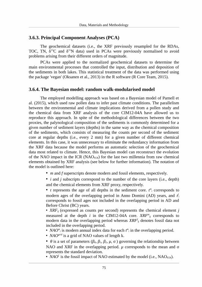
Data, Materials and Methodology
3.6.3. Principal Component Analyses (PCA)
The geochemical datasets (i.e., the XRF previously resampled for the RDAs,TOC, TN, δ13C and δ15N data) used in PCAs were previously normalised to avoidproblems arising from their different orders of magnitude.
PCAs were applied to the normalized geochemical datasets to determine themain environmental processes that controlled the input, distribution and deposition ofthe sediments in both lakes. This statistical treatment of the data was performed usingthe package 'vegan' (Oksanen et al., 2013) in the R software (R Core Team, 2015).
3.6.4. The Bayesian model: random walk-modularised model
The employed modelling approach was based on a Bayesian model of Parnell etal. (2015), which used raw pollen data to infer past climate conditions. The parallelismbetween the environmental and climate implications derived from a pollen study andthe chemical data from XRF analysis of the core CIM12-04A have allowed us toreproduce this approach. In spite of the methodological differences between the twoproxies, the palynological composition of the sediments is commonly determined for agiven number of sediment layers (depths) in the same way as the chemical compositionof the sediments, which consists of measuring the counts per second of the sedimentcore at regular depths (i.e., every 2 mm) for a given number of different chemicalelements. In this case, it was unnecessary to eliminate the redundancy information fromthe XRF data because the model performs an automatic selection of the geochemicaldata most related to climate. Hence, this Bayesian model can reconstruct the evolutionof the NAO impact in the ICR (NAOICR) for the last two millennia from raw chemicalelements obtained by XRF analysis (see below for further information). The notation ofthe model is outlined here:
• m and f superscripts denote modern and fossil elements, respectively.
• i and j subscripts correspond to the number of the core layers (i.e., depth)and the chemical elements from XRF proxy, respectively.• t represents the age of all depths in the sediment core. tm
i corresponds tomodern ages of the overlapping period in Anno Domini (AD) years, and tf
i
corresponds to fossil ages not included in the overlapping period in AD andBefore Christ (BC) years.• XRFij (expressed as counts per second) represents the chemical element jmeasured at the depth i in the CIM12-04A core. XRFm
ij corresponds tomodern data in the overlapping period whereas XRFf
ij denotes fossil data notincluded in the overlapping period.• NAOm
i is modern annual index data for each tmi in the overlapping period.
• NAOgrid is a grid of NAO values of length k.• θ is a set of parameters (β0, β1, β2, μ, σ ) governing the relationship betweenNAO and XRF in the overlapping period. μ corresponds to the mean and σrepresents the standard deviation.• NAOf is the fossil impact of NAO estimated by the model (i.e., NAOICR).
75
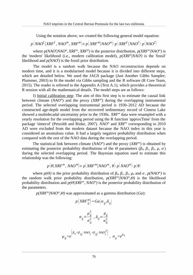
NAO imprints in the Central Iberian Peninsula for the last two millennia
Using the notation above, we created the following general model equation:
p ( NAOf |XRF f , NAOm , XRFm )∝p ( XRFm|NAOm )⋅p (XRFf |NAOf )⋅p (NAO f )
where p(NAOf|NAOm, XRFm, XRFf)) is the posterior distribution, p(XRFm|NAOm) isthe 'modern' likelihood (i.e., modern calibration model), p(XRFf|NAOf) is the 'fossil'likelihood and p(NAOf) is the fossil prior distribution.
The model is a random walk because the NAO reconstruction depends onmodern time, and it is a modularised model because it is divided into different steps,which are detailed below. We used the JAGS package (Just Another Gibbs Sampler;Plummer, 2003) to fit the model via Gibbs sampling and the R software (R Core Team,2015). The reader is referred to the Appendix A (Text A.1), which provides a theoreticalR session with all the mathematical details. The model steps are as follows:
I) Initial calibration step: The aim of this first step is to estimate the causal linkbetween climate (NAOm) and the proxy (XRFm) during the overlapping instrumentalperiod. The selected overlapping instrumental period is 1930–2012 AD because theconstructed age-depth model from the recovered sedimentary record of Cimera Lakeshowed a multidecadal uncertainty prior to the 1930s. XRFm data were resampled with ayearly resolution for the overlapping period using the R function 'approxTime' from thepackage 'simecol' (Petzoldt and Rinke, 2007). NAOm and XRFm corresponding to 2010AD were excluded from the modern dataset because the NAO index in this year isconsidered an anomalous value. It had a largely negative probability distribution whencompared with the rest of the NAO data during the overlapping period.
The statistical link between climate (NAOm) and the proxy (XRFm) is obtained byestimating the posterior probability distributions of the Ө parameters (β0, β1, β2, μ, σ )during the selected overlapping period. The Bayesian equation used to estimate thisrelationship was the following:
p (θ|XRFm , NAOm)∝ p (XRFm|NAOm , θ )⋅p ( NAOm )⋅p (θ )
where p( )Ө is the prior probability distribution of β0, β1, β2, μ0 and σ , p(NAOm) isthe random walk prior probability distribution, p(XRFm|NAOm, )Ө is the likelihoodprobability distribution and p( |XRFӨ m, NAOm) is the posterior probability distribution ofthe parameters.
p(XRFm|NAOm, )Ө was approximated as a gamma distribution (Ga):
p (XRFijm) Ga∼ (α ij
,δij )
αij=
μ ij2
σij2
, δij=μ
ij
σ ij2
μ ij=e(β0j+β
1j⋅NAO
i+β
2j⋅NAO
i2)
, σij
=eμ0j
76

Data, Materials and Methodology
μij and σij correspond to mean and standard deviations of the gamma distribution,respectively.
We approximated the prior probability distributions of β0j, β1j, β2j, μ0j, as normaldistributions and approximated the prior probability distribution of σ as a uniformdistribution, defining their means and their precisions as follows:
p ( β0 j ) N∼ (0, 100 ) , p ( β1 j ) N∼ (0, 100 ) , p ( β2 j ) N∼ (0, 100 ) ,
p (μ j ) N∼ (0, 100 ) , p (σ ) U∼ ( 0,100)
p(NAOm) was approximated as a time-dependent normal distribution through theprecision (prec):
p (NAOim ) N∼ (NAO
i−1m , prec
i)
preci=
1
( tim−t i−1
m )⋅σ2
Finally, we ran the model to obtain the posterior probability distributions of theӨ parameters, p( |XRFӨ m, NAOm). The settings of the JAGS package were 4 chains,3000 iterations and 2000 burn-ins.
II) Creating Marginal Data Posteriors (MDPs) step: The objective of this secondstep is to obtain the posterior distributions of the NAO given only the information inthat layer of the core. These are known as Marginal Data Posteriors (MDPs) of NAO.
The MDPs of NAO for each layer were obtained using an NAOgrid of k=50 valuesbetween -3 and 3, the posterior probability distribution of the Ө parameters from thecalibration step and the XRFf data. The k MDPs of each layer were the sum of thegamma distributions of each j chemical element:
p ( MDPik ) Ga∼ (α j
,δj )
αj=
μ j2
σj2
, δ j=μ
j
σ j2
μ j =e(β0j+β
1j⋅NAO
kgrid
+β2j⋅NAO
kgrid 2
), σ
j=e
μ0j
Finally, we calculated the precision (precisMDP) and the mean (µMDP) of the kMDPs obtained for each layer (MDPik) and their maximum and minimum uncertainties(εmax, εmin):
μMDPi =MDPifinal⋅NAOgrid , MDPi
final=MDP
i
∑K
MDPk
77

NAO imprints in the Central Iberian Peninsula for the last two millennia
σ MDPi=√MDPifinal⋅NAOgrid2
−μi2 , precis
MDPi=
1
σ MDPi
2
εmaxi
=μMDP i
+ 2⋅sdMDPi
, εmini
=μMDPi
− 2⋅σMDP i
III) Model fitting step: We create the posterior distribution of NAOf using theMDPs. In other words, we obtained the NAOICR for the last two millennia. The posteriordistribution of NAOf is created using the mean (µMDP) and precision (precMDP) of theMDPs from step II. The Bayesian equation of this step is as follows:
p ( NAOf |MDPs)∝ p ( MDPs|NAOf )⋅p ( NAO f )
where p(NAOf) is the random walk prior probability distribution, p(MDPs|NAOf)is the likelihood probability distribution and p(NAOf|MDPs) is the posterior probability distribution of the NAOf.
p(NAOf) was approximated as a time-dependent normal distribution through the precision (precisf). The first NAOf should have a vague prior distribution:
p (NAOif ) N∼ ( NAO
i−1f , precis
f i) i=2,3,4 . . .n layers
p (NAOif ) N∼ (0,100 ) i=1
precf i=
1
(t if −t i−1
f )⋅σ 2
The p(MDPs|NAOf) likelihood is approximated as a normal distribution:
μMDP i
N∼ ( NAOif ,precis
MDPi)
In the data model, we also include the first NAOm as it depends on the last NAOf
value. This is approximated as a normal distribution. The sd has a log-normaldistribution with the parameters a and b:
NAO1m N∼ (NAO
if ,precis
mf ) i=n layers
precismf
=1
(tm1−t
f i)⋅σ2i=n layers
σ∼exp ( a,b)
78

Data, Materials and Methodology
Once we defined all the data for the model, we ran the model to obtain theposterior probability distribution of NAOf, p(NAOf|MDPs). The settings of the JAGSpackage (Plummer, 2003) were 3 chains, 3000 iterations and 2000 burn-ins. Finally, theimpact of the NAO in the ICR (NAOICR) for the last two millennia were calculated asthe median of NAOf obtained from the model and its uncertainties as the 5th and 95th
quantiles.
IV) Model validation step: As in any reconstruction, the last step of the model isinvolves statistical validation. A 5-fold cross-validation of the modern data wasconducted to evaluate the model performance. The predicted geochemical data wereobtained as the median of the predicted values and the uncertainty bounds containingthe true (i.e., measured) data for 80% of the samples. The correlation between the trueand predicted data was also calculated.
In addition, the NAOICR obtained was visually compared with the multidecadalNAO index from CRU for the period 1930–1825 AD, which was not included in thecalibration of the model. This multidecadal NAO index was calculated using a loessfunction and smoothing span degree of 0.10. The non-stationary variability of theuncertainties associated with the chronological model of Cimera Lake hampered themathematical comparison between the instrumental and the reconstructed data.
Finally, to determine whether some global aspects could be depicted in thereconstructed NAO impacts for the ICR, the NAOICR was visually compared withthree different NAO approaches: i) the approach from Trouet et al. (2009), which is asimplistic approach based on two records (from Scotland and Morocco) (Fig. 3.16); ii)the variability in NAO obtained by Olsen et al. (2012), which is also a simplisticapproach based on a palaeo-redox proxy (Mn/Fe ratio) in a sediment record from asmall lake near Kangerlussuaq (Greenland) (Fig. 3.16); and iii) the much more robustreconstruction by Ortega et al. (2015), which employed multi-proxy data from differentlocations in the Northern Hemisphere (i.e., 48 proxies) (Fig. 3.16).
79

NAO imprints in the Central Iberian Peninsula for the last two millennia
Figure 3.16. Location of the initial 48 proxy records (ice cores, lake sediments, speleothems and treerings) used for the reconstruction of the NAO by Ortega et al. (2015). The two proxies used in theNAO approach of Trouet et al. (2009) are highlighted with yellow boxes. Records from Lake SS1220(Kangerlussuaq, 67°03’N - 51°13’W) used in the NAO approach by Olsen et al. (2012) and theCimera Lake record are shown with black diamonds. The figure was modified from Ortega et al.(2015).
80

Chapter 4
4. RESULTS
4.1. Relationships between climate index, climatic and limnological data
The results of Pearson’s correlation analyses between the studied series for JFMand MAM and between monthly data from September to December are shown in Tables4.1 and 4.2 for Peñalara Lake and in Tables 4.3 and 4.4 for Cimera Lake, respectively.
4.1.1. Peñalara Lake
During JFM, the NAO is positively correlated with air temperature (r= 0.69) andnegatively with precipitation (r= -0.67) and snow days (r= -0.64). Air temperaturedisplays negative correlations with precipitation (r= -0.59), snow days (r= -0.75), ice-cover duration (r= -0.59, p-value < 0.05) and ice-off (r= -0.65), whereas precipitation ispositively correlated with snow days (r= 0.69), ice-cover duration (r= 0.52, p-value <0.05) and ice-off (r= 0.53, p-value < 0.05). Snow days show positive correlations withice-cover duration and ice-off (r= 0.66 and r= 0.70, respectively) (Table 4.1). DuringMAM, the NAO is positively correlated with air temperature (r= 0.36) and negativelywith precipitation and snow days (r= -0.50 and r= -0.31, respectively; p-value < 0.05).Air temperature displays negative correlations with precipitation (r= -0.43) and snowdays (r= -0.85), whereas precipitation is positively correlated with snow days (r= 0.51)(Table 4.1). Finally, the correlations between ice records are the same in both seasons(winter and spring) because data are annual and do not depend on seasonality. Only ice-off and ice-cover duration are positively correlated each other (r= 0.67) (Table 4.1).Finally, with respect to monthly data and the freezing process, the freeze-up date is onlypositively correlated with November temperature (r= 0.54, p-value < 0.05) (Table 4.2).
4.1.2. Cimera Lake
During JFM, the NAO is positively correlated with maximum temperature (r=0.70) and negatively with precipitation (r= -0.71). Maximum air temperature shows apositive correlation with the minimum air temperature (r=0.51) and a negativecorrelation with precipitation (r= -0.62). The remaining variables do not displaysignificant correlations in this season (Table 4.3). In MAM, the NAO displays a positivecorrelation with maximum air temperatures (r= 0.42) and negative correlations withprecipitation (r= -0.51). Maximum air temperature is also positively correlated with theminimum air temperature (r= 0.79) and negatively correlated with precipitation (r=-0.59) (Table 4.3). Finally, the correlations between ice records are also the same in bothwinter and spring because they have an annual character. Only ice-off and ice-coverduration are positively correlated (r= 0.91) (Table 4.3). With respect to monthly dataand the freezing process, the freeze-up date is not significantly correlated with any data(Table 4.4).
81

NAO imprints in the Central Iberian Peninsula for the last two millennia
WINTER
(JFM)NAO Temp Precip
Snowdays
Freeze-up Ice-cover Break-up
NAO 1
Temp 0.69*** 1
Precip -0.67*** -0.59*** 1
Snow days -0.64*** -0.75*** 0.69*** 1
Freeze-up -0.09 0.05 0.00 -0.01 1
Ice-cover -0.53** -0.59** 0.52** 0.66*** -0.37 1
Break-up -0.52** -0.65*** 0.53** 0.70*** 0.41 0.67*** 1
SPRING(MAM)
NAO Temp PrecipSnowdays
Freeze-up Ice-cover Break-up
NAO 1
Temp 0.36*** 1
Precip -0.50*** -0.43*** 1
Snow days -0.31** -0.85*** 0.51*** 1
Freeze-up – – – – 1
Ice-cover 0.35 -0.14 -0.04 0.22 -0.37 1
Break-up 0.04 -0.30 -0.14 0.16 0.41 0.67*** 1
Table 4.1. Pearson's correlation coefficients in winter (JFM) (top) and spring (MAM) (bottom)between limnological data, climatic data and the NAO index for Peñalara Lake. * denotes that thecorrelation is significant at the 0.1 level, ** at the 0.05 level and *** at the 0.01 level. The numbers initalics are annual correlations.
82

Results
September NAO Temp Precip Snow days Freeze-up
NAO 1
Temp 0.61 1
Precip -0.47** -0.31 1
Snow days -0.27*** -0.53 -0.23 1
Freeze-up 0.18 -0.05 -0.36 – 1
October NAO Temp Precip Snow days Freeze-up
NAO 1
Temp 0.50** 1
Precip -0.60*** -0.49** 1
Snow days -0.42* -0.81*** 0.45** 1
Freeze-up -0.08 -0.10 -0.15 0.31 1
November NAO Temp Precip Snow days Freeze-up
NAO 1
Temp 0.51** 1
Precip -0.10 0.08 1
Snow days -0.47** -0.71*** 0.40* 1
Freeze-up 0.30 0.54** 0.34 0.01 1
December NAO Temp Precip Snow days Freeze-up
NAO 1
Temp 0.48** 1
Precip -0.70*** -0.34 1
Snow days -0.54** -0.66*** 0.64*** 1
Freeze-up 0.06 0.19 0.15 0.21 1
Table 4.2. Pearson's correlation coefficients between monthly (September, October, November andDecember) freeze-up date, climatic data and the NAO index for Peñalara Lake. * denotes that thecorrelation is significant at the 0.1 level, ** at the 0.05 level and *** at the 0.01 level. The numbers initalics are annual correlations. Bold numbers highlight significant correlations of freeze-up.
83

NAO imprints in the Central Iberian Peninsula for the last two millennia
WINTER(JFM)
NAOTempMax
TempMin
PrecipSnowdepth
Freeze-up Ice-coverBreak-
up
NAO 1
Temp Maximum
0.70*** 1
Temp Minimum
0.12 0.51*** 1
Precip -0.71*** -0.62*** 0.20 1
Snow depth
-0.47 – – – 1
Freeze-up -0.41 -0.58 0.46 -0.22 0.22 1
Ice-cover -0.34 0.07 0.05 -1.00 -0.02 -0.13 1
Break-up -0.61 -0.15 -0.04 -1.00 0.16 0.28 0.91*** 1
SPRING(MAM)
NAOTempMax
TempMin
PrecipSnowdepth
Freeze-up Ice-coverBreak-
up
NAO 1
Temp Maximum
0.42*** 1
Temp Minimum
0.21 0.79*** 1
Precip -0.51*** -0.59*** -0.18 1
Snow depth
-0.28 -1.00 -1.00 - 1
Freeze-up – – – – – 1
Ice-cover -0.79* -0.05 0.06 0.25 0.77 -0.13 1
Break-up -0.87** -0.35 -0.17 0.01 0.84 0.28 0.91*** 1
Table 4.3. Pearson's correlation coefficients in winter (JFM) (top) and spring (MAM) (bottom)between limnological data, climatic data and the NAO index for Cimera Lake. * denotes that thecorrelation is significant at the 0.1 level, ** at the 0.05 level and *** at the 0.01 level. The greynumbers indicate correlations where n < 5. The numbers in italics are annual correlations.
84

Results
September NAOTemp Max
Temp Min
PrecipSnow depth
Freeze-up
NAO 1
Temp Maximum -0.12 1
Temp Minimum 0.46 0.53 1
Precip -0.49 -0.53 1
Snow depth -0.31 1.00 1.00 – 1
Freeze-up -0.51 -0.23 -0.52 0.78 -0.77 1
October NAOTempMax
TempMin
PrecipSnowdepth
Freeze-up
NAO 1
Temp Maximum -0.01 1
Temp Minimum 0.67 0.53 1
Precip 0.40 -0.70 1
Snow depth -0.43 -1.00 -1.00 – 1
Freeze-up 0.17 -0.78 -0.03 0.19 -0.17 1
November NAOTemp Max
Temp Min
PrecipSnow depth
Freeze-up
NAO 1
Temp Maximum 0.61 1
Temp Minimum 0.16 0.45 1
Precip 1.00 0.65 1
Snow depth 0.57 1.00 1.00 – 1
Freeze-up -0.23 -0.86 -0.79 0.52 -0.30 1
December NAOTemp Max
Temp Min
PrecipSnow depth
Freeze-up
NAO 1
Temp Maximum 0.80 1
Temp Minimum 0.74 0.56 1
Precip -0.99 -0.58 0.06 1
Snow depth 0.51 1.00 1.00 – 1
Freeze-up -0.10 -0.03 0.03 -0.43 0.08 1
Table 4.4. Pearson's correlation coefficients between monthly (September, October, November andDecember) freeze-up date, climatic data and the NAO index for Cimera Lake. * denotes that thecorrelation is significant at the 0.1 level, ** at the 0.05 level and *** at the 0.01 level. The greynumbers indicate correlations where n < 5. The numbers in italics are annual correlations.
85

NAO imprints in the Central Iberian Peninsula for the last two millennia
4.2. Facies description
4.2.1. Peñalara Lake
Two sedimentary facies were identified in the uppermost 56.5 cm of the PE12-01-01 core (Fig. 4.1). Facies M1 is composed of brown silty mud with abundantamorphous aggregates of organic matter and few preserved terrestrial plant remains(i.e., phytoclasts) (Fig. 4.1). In the M1 facies, the diatom content is high and dominatedby Aulacoseira sp. colony chains, whereas the mineral content is low and featuresrounded grains (Fig. 4.1). Facies M2 is composed of brown silty mud with dispersedfine sand. This facies presents a higher mineral content and less organic matter anddiatoms than facies M1. Organic matter is present in this second facies as scatteredamorphous aggregates with a very low composition of phytoclasts (Fig. 4.1). Mineralspresent more angular shapes than in facies M1. These two facies represent a singlelithostratigraphic unit.
The facies description, together with previous visual observations, allowed us tocreate a synthetic stratigraphic column of the core PE12-01-01. The brown silty mud(facies M1) is the dominant facies and presents interbedded layers of differentthicknesses of brown silty mud with dispersed fine to very fine sand (facies M2) (Fig.4.1).
4.2.2. Cimera Lake
Three sedimentary facies were identified in the core CIM12-04A (Fig. 4.2).Facies M1 is composed of massive brown silty mud with dispersed grains of fine sand.Organic matter is present as predominant amorphous aggregates and a low content ofaltered terrestrial plant remains (i.e., phytoclasts) (Fig. 4.2). Facies M2 is characterizedby poorly defined layers of brown silty mud and fine to medium sand. The sand grainshape appears to be more angular than in facies M1, and there are amorphousaggregates of organic material, although in a lower proportion than in facies M1 (Fig.4.2). Facies S is composed of white to ochre coarse sand with granules forming well-defined tabular layers, some of which include pebble clasts. Most of the grains show amore angular shape than those in facies M2, and the terrigenous fraction in facies S issignificantly higher than the organic matter content (Fig. 4.2).
The facies description, together with previous visual observations, allowed us tocreate a synthetic stratigraphic column of the core CIM12-04A. The brown silty mud(facies M1) is the dominant facies with interbedded layers of poorly defined brown siltymud with fine to medium sand (facies M2) and layers of coarse sand (facies S). Thelatter facies are more common in the lower part of the sequence (Fig. 4.2).
86

Results
Figure 4.1. A) Synthetic lithological columns with the defined facies and image of the PE12-01-01core taken with the colour line-scan camera. B, C) Detailed core image of facies M1 and M2,respectively. D, E) Images of facies M1 and M2 acquired from smear slides with a camera installed inthe high-end polarization microscope Leica® DM4500 P, respectively.
87

NAO imprints in the Central Iberian Peninsula for the last two millennia
Figure 4.2. A) Synthetic lithological columns with the defined facies and image of CIM12-04A coretaken with the colour line-scan camera. B-D) Detailed core image of facies M1, M2 and S,respectively. E-G) Images of facies M1, M2 and S acquired from smear slides with a camera installedin the high-end polarization microscope Leica® DM4500 P, respectively.
88

Results
4.3. Chronological models
4.3.1. Peñalara Lake
The 210Pb concentration profile of the core PE12-01-01 displays a complexpattern (Fig. 4.3). The 210Pb concentration increases from the surface (190 Bq/kg) to 12cm (250 Bq/kg) and remains constant down to 25 cm of core depth. Then, the 210Pbconcentration gradually decreases to values of approximately 100 Bq/kg at 35 cm ofcore depth. From this depth to 52 cm, the 210Pb concentration is approximately 150Bq/kg (Fig. 4.3). 137Cs is detected in all the analysed samples between 25 and 29 cm ofcore depth, showing a clear decreasing-downwards trend. These results indicate that thismaterial accumulated after the 1950s AD (Fig. 4.3). The interpretation of these data isthat the uppermost 25 cm correspond to the deposition and reworking of sediment sincethe 1990s when the area was declared a Natural Park and the resulting removal ofgarbage previously deposited into the lake. (Toro and Granados, 2002) (Fig. 4.3). Theexcess 210Pb concentration profile between 25 and 35 cm of core depth and the 137Csdata were used to obtain an average sedimentation rate (SR) of 1.6 ± 0.1 mm/yr for thiszone by applying the CF:CS model. The age of this zone thus ranges between the early1920s and the late 1980s AD.
Four of the six 14C dates from PE12-01-01 were not included in the constructionof the linear age-depth model (Table 4.5 and Fig. 4.4). On one hand, the ages at 10 and28 cm are inconsistent with the presence of 210Pbex because they are older than the 210Pb-derived ages. This may be explained by sediment reworking. On the other hand, the 14Cdates at 41.5 and 48 cm overlap but the lithology of the core does not suggest thepresence of an instantaneous event, such as a fine-grained mass wasting deposit (Fig.4.1). Hence, the 14C date at 48 cm was rejected because it was younger than the date at41.5 cm, likely as a result of reworking of younger sediment. The fourth date rejectedwas found at 55.5 cm of core depth, and it is much younger than the previousradiocarbon date (Table 4.5).
Therefore, the obtained SRs from the linear age-depth model were 0.07 mm/yrand 0.11 mm/yr for the 25 – 41.5 cm and 41.5 – 55 cm intervals, respectively (Fig. 4.4).Hence, the resultant age-depth for Peñalara Lake record indicates that the 25 – 55 cmsediment sequence spans from 263 ± 95.5 BC to 1986 ± 1 AD (Fig. 4.4).
Depth(cm)
Lab Code Material 14C years BPCal. years BP
(2σ)Cal. years AD/BC
(2σ)
10 Beta - 333757 Pollen c. 730 ± 30 681± 28 1269 ± 28 AD
28 Beta - 333758 Pollen c. 1190 ± 30 1118 ± 65 832 ± 65 AD
41.5 Poz-61899 Pollen c. 1060 ± 30 966.5 ± 39.5 983.5 ± 39.5 AD
48 Poz-61900 Pollen c. 1085 ± 30 974 ± 40 976 ± 40 AD
55 Beta - 333759 Pollen c. 2180 ± 30 2213.5 ± 95.5 263.5 ± 95.5 BC
55.5 Beta - 333760 Wood 120 ± 30 80 ± 69 1870 ± 69 AD
Table 4.5. Radiocarbon dates and calibrated ages for the PE12-01-01 core. Results are reported with2σ uncertainty. Samples in italics were discarded. 'Pollen c.' denotes pollen concentrate.
89

NAO imprints in the Central Iberian Peninsula for the last two millennia
Figure 4.3. Activity depth profiles of total 210Pb (solid black squares), excess 210Pb (open blacksquares), 226Ra (orange diamond) and 137Cs (blue circles) for core PE12-01-01, with error barsrepresenting 1σ uncertainties.
Figure 4.4. Age-depth linear model of the core PE12-01-01 based on the AMS 14C dates and 210Pbactivity depth profile. The error bars of the red points represent the ± 2σ calibrated age range for theAMS 14C dates. The black continuous line represents the age-depth function framed by a grey area thatcorresponds to the error model. The blue dashed line represents the zone of 210Pb dates.
90

Results
4.3.2. Cimera Lake
The concentration profile of the excess 210Pb can be divided into three intervalsaccording to its slopes: 0 – 4 cm, 4 – 6.5 cm and 6.5 – 9 cm. The supported 210Pbhorizon is attained at 9.2 cm. Relatively lower concentrations of 210Pbex were measuredin the sandy layers and excluded from the estimation of the sedimentation rates for eachzone (Fig. 4.5). The sedimentation rates obtained by applying the CF:CS model were4.1 ± 0.8 mm/yr for 0 – 4 cm and 0.65 ± 0.02 mm/yr for 4 – 6.5 cm. Hence, these twozones cover the period from 2012 to 1954 ± 2 AD. The concentration of 210Pbex wasconstant in the 6.5 – 9 cm interval; thus, a chronology could not be derived.
The seven AMS 14C dates determined between 10 and 124.5 cm exhibitstratigraphic coherence, except for the sample located at 10 cm because the age of thissample was too old for its stratigraphic location (Table 4.6), likely due to reworking ofolder sediment. Therefore, this sample was not used in the construction of the age-depthmodel (Fig. 4.5).
The resulting age-depth model constructed using the 210Pb profiles and a smoothspline (Blaauw, 2010) shows that the uppermost 124.5 cm of sedimentary infill spansfrom 172 ± 65 BC (2122 ± 65 cal yr BP) to 2012 AD (Fig. 4.5). The four distinct SRintervals that can be differentiated in the age-depth model correspond to a) 4.1 mm/yrfor 0 – 4 cm and b) 0.65 mm/yr for 4 – 6.5 cm from the CF:CS mode; and c) 0.2 mm/yrfor 6.5 – 29.5 cm and d) 0.9 mm/yr for 29.5 – 124.5 from the linear interpolationbetween selected radiocarbon dates.
Depth(cm)
Lab Code Material 14C years BPCal. years BP
(2σ)Cal. years AD/BC
(2σ)
10 Beta - 333752 Pollen c. 1420 ± 30 1329 ± 39 621 ± 39 AD
29.5 Poz-61896 Pollen c. 1140 ± 30 1032 ± 63 918 ± 63 AD
49 Beta - 333753 Pollen c. 1170± 30 1113 ± 66 837 ± 66 AD
67.5 Poz-61897 Pollen c. 1425 ± 30 1332 ± 40 618 ± 40 AD
86 Beta - 333754 Pollen c. 1940 ± 30 1885 ± 64.5 64.5 ± 64.5 AD
105.5 Poz-61898 Pollen c. 1875 ± 30 1803.5 ± 76.5 146.5 ± 76.5 AD
124.5 Beta - 333755 Pollen c. 2160 ± 30 2122.5 ± 65.5 172.5 ± 65.5 BC
Table 4.6. Radiocarbon dates and calibrated ages for CIM12-04A core from Cimera Lake. Results arereported with 2σ uncertainty. Samples in italics were discarded. 'Pollen c.' denotes pollen concentrate.
91

NAO imprints in the Central Iberian Peninsula for the last two millennia
Figure 4.5. Activity depth profiles of total 210Pb (solid black and red squares) and excess 210Pb (openblack squares) for the core CIM12-04A, with error bars representing 1σ uncertainties.
Figure 4.6. Age-depth model of the core CIM12-04A based on the AMS 14C dates and 210Pb activitydepth profile and constructed using the R-code package 'clam'. The error bars of the red pointsrepresent the ± 2σ calibrated age range for the AMS 14C dates. The black continuous line representsthe age-depth function framed by a grey area that corresponds to the error model. The blue dashedline represents the zone of 210Pb dates.
92

Results
4.4. Geochemical and mineralogical characterization of the lakesediments
4.4.1. Peñalara Lake
The average TOC content is approximately 4 wt%, with a range from 2 to 5.5 wt%, and the TN content is approximatly 0.4 on average, with a range from 0 and 0.55 wt%. Both proxies covary positively and display lower values in facies M2 (Fig. 4.7). Thecarbon-nitrogen atomic ratio (TOC/TN) remains constant with values of approximately14, from the bottom to 25 cm of the core depth sequence (Fig. 4.7). The isotopiccomposition of the organic matter ranges between -26‰ and -25‰ and from 3 to 4.5‰for δ13C and δ15N, respectively. The most prominent change in δ13C values occurs at27.5 cm, where the values abruptly drop to around -26‰ and remain unchanged until25 cm of core depth (Fig. 4.7). The δ15N values are almost invariable along the core(Fig. 4.7). The chemical elements that display the most remarkable oscillations are Al,Si, K, Ca, Ti and Fe, which peak in the silty intervals (i.e., facies M2; Fig. 4.7). Thechemical elements V, Cr, Mn and Zn show noisy signals. The profiles of Rb, Sr and Zrdecrease upwards (Fig. 4.7). The mineralogical composition of the PE12-01-01sediment record shows that the percentages of muscovite slightly decrease upwards,whereas the proportions of quartz increase. The rest of the mineral proportions remainroughly constant (Fig. 4.7). The clay mineral analyses confirm the presence ofpalygorskite in the Peñalara Lake record (Fig. 4.7).
4.4.2. Cimera Lake
The TOC and TN contents of the CIM12-04A sequence display average values ofapproximately 3.5 and 0.35 wt%, respectively. From the bottom to a depth of 6 cm, bothparameters positively covary around their respective mean values (Fig. 4.8). Above thisinterval, the TOC and TN percentages largely increase until the top of the core. Fromthe core bottom to a depth of 14.5 cm, the TOC/TN ratio remains constant at around 12.Subsequently, the TOC/TN ratio increases to 14 in the 14.5 – 6.5 cm depth interval (Fig.4.8). Above 6.5 cm, the ratio decreases to 11, and a final sudden increase occurs at thetop of the core (Fig. 4.8). The δ13C isotopic composition ranges between -25.5 and-24‰ and the δ15N isotopic composition between 0 and 3‰ (Fig. 4.8). The δ13C valuesdisplay an enrichment trend above 35 cm and a sudden depletion at the top of the core,whereas the δ15N values show a noticeable depletion trend from 14.5 cm to the top ofthe core (Fig. 4.8). Al, Si, K, Ca, Ti and Fe display the largest oscillations, whereas V,Cr and Mn are the noisiest. The Mn profile decreases upwards, whereas Zr displays theopposite pattern (Fig. 4.8). All of the inorganic elements show fewer counts in theuppermost centimetres (Fig. 4.8). The mineral species exhibit roughly constantpercentages from the core bottom up to 35 cm of core depth. Above this interval,kaolinite and clinochlore increase, whereas quartz and microcline display the oppositetrend (Fig. 4.8). Between 35 and 10 cm, muscovite diminishes from 29% to 24 wt%.,and albite remains constant. The uppermost 10 cm is characterized by an increase inmuscovite and major oscillations of albite (Fig. 4.8). Finally, the clay mineral analysesconfirm a significant amount of palygorskite in the Cimera Lake sediments (Fig. 4.8).
93

NAO imprints in the Central Iberian Peninsula for the last two millennia
94
Fig
ure
4.7
. St
rati
grap
hic
colu
mn
of t
he P
E12
-01-
01 c
ore,
wit
h fa
cies
, el
emen
tal
(TO
C,
TN
, TO
C/T
N r
atio
; li
ght-
blue
lin
es)
and
isot
opic
co
mpo
siti
ons
(δ13
C a
nd δ
15N
; da
rk-b
lue
line
s),
XR
F p
rofi
les
(exp
ress
ed i
n co
unts
per
sec
ond;
ora
nge
line
s),
min
eral
ogy
(exp
ress
ed a
s pe
rcen
tage
s of
tot
al d
ry w
eigh
t, M
s=m
usco
vite
, K
ln=
kaol
init
e, C
lc=
clin
ochl
ore,
Qtz
=qu
artz
, M
c=m
icro
clin
e, A
lb=
albi
te;
ligh
t-gr
een
line
s co
rres
pond
to
orig
inal
dat
a an
d da
rk-g
reen
lin
es c
orre
spon
d to
sm
ooth
ed d
ata
calc
ulat
ed w
ith
the
loes
s fu
ncti
on a
nd a
spa
n de
gree
of
0.1
0),
clay
fra
ctio
n (P
kg=
paly
gors
kite
, ye
llow
bar
s),
and
the
firs
t an
d se
cond
eig
enve
ctor
sco
res
(PC
1 pe a
nd P
C2 pe
; bl
ack
line
s) w
ith
dept
h. T
he g
rey
line
s an
d gr
ey b
ars
corr
espo
nd to
are
as o
f rew
orke
d se
dim
ents
in th
e co
re (
i.e.,
uppe
rmos
t 25
cm).

Results
95
Fig
ure
4.8
. St
rati
grap
hic
colu
mn
of t
he C
IM12
-04A
cor
e, w
ith
faci
es,
elem
enta
l (T
OC
, T
N,
TOC
/TN
rat
io;
ligh
t-bl
ue l
ines
) an
d is
otop
ic
com
posi
tion
s (δ
13C
and
δ15
N;
dark
-blu
e li
nes)
, X
RF
pro
file
s (e
xpre
ssed
in
coun
ts p
er s
econ
d; o
rang
e li
nes)
, m
iner
alog
y (e
xpre
ssed
as
perc
enta
ges
of t
otal
dry
wei
ght,
Ms=
mus
covi
te,
Kln
=ka
olin
ite,
Clc
=cl
inoc
hlor
e, Q
tz=
quar
tz,
Mc=
mic
rocl
ine,
Alb
=al
bite
; li
ght-
gree
n li
nes
corr
espo
nd to
ori
gina
l dat
a an
d da
rk-g
reen
line
s co
rres
pond
to s
moo
thed
dat
a ca
lcul
ated
wit
h th
e lo
ess
func
tion
and
a s
pan
degr
ee o
f 0.1
0), c
lay
frac
tion
(P
kg=
paly
gors
kite
, yel
low
bar
s), a
nd th
e fi
rst,
seco
nd a
nd th
ird
eige
nvec
tor
scor
es (
PC
1 cim, P
C2 ci
m a
nd P
C3 ci
m;
blac
k li
nes)
wit
h de
pth.

NAO imprints in the Central Iberian Peninsula for the last two millennia
4.5. Geochemical and mineralogical characterization of an aeolian dustsample
The clay minerals analyses also confirm the presence of palygorskite in the dustsample from Cimera Lake collected in June 2014 (Fig. 4.9). The concentrations ofnitrate, sulphate and total phosphorus ([NO3
-], [SO4-2], and [TP]) in this dust sample
were 190 ppm, 530 ppm and 0.5 ppm, respectively.
Figure 4.9. Diffractogram obtained by XRD of the clay composition of the dust event sample collectedin Cimera Lake in June 2014. Palygorskite is present in the sample.
4.6. Redundancy Data Analyses (RDAs)
4.6.1. Peñalara Lake
The results from the reworked sediments in the uppermost 25 cm of the PE12-01-01 core have been neglected, and they have not been taken into account in neither ofthe following statistical analyses (Fig. 4.7).
The RDA biplot of PE12-01-01 displays three main groups (Fig. 4.10A): group Aencompasses the δ13C values and is associated with quartz, albite and microcline; groupB only includes muscovite related with Mn, Si, and the TOC and TN profiles; and groupC is associated with kaolinite and clinochlore. The remaining chemical elements (i.e.,Ti, Cr, V, Zr, and Rb) and the δ15N values are located between groups A and B, whereasZn is located between groups B and C.
96

Results
4.6.2. Cimera Lake
The RDA biplot from the core CIM12-04A has allowed us to define three maingroups (Fig. 4.10B): group A includes Ti, Rb and δ15N values and is associated withquartz, albite and microcline; group B is associated with muscovite and the TOC andTN proportions; and group C includes Zn and δ13C values and is associated withkaolinite and clinochlore. Zr is located between groups A and B, although most of thegeochemical elements (i.e., Si, V, Cr and Mn) are generally located in the centre of thebiplot.
Figure 4.10. RDA biplots for the cores A) PE12-01-01 and B) CIM12-04A. Light red, grey and yellowareas indicate groups A, B and C, respectively.
4.7. Principal Component Analyses (PCAs)
4.7.1. Peñalara Lake
The PCA of the geochemical dataset from the PE12-01-01 core shows that thetwo first eigenvectors account for 57% of the total variance (Table 4.7). The firsteigenvector (PC1pe) represents 36% of the total variance, and it is primarily controlledby all the geochemical elements at the positive end (Fig. 4.11A and Table 4.7). Thesecond eigenvector (PC2pe) accounts for 21% of the total variance. This is tied by TOC,TN and, to minor extent, by δ15N and Zn at its positive end and by δ13C with a minorcontribution of Rb at the negative end (Fig. 4.11A and Table 4.7). The othereigenvectors defined by the PCA analysis were not considered because they explain<11% of the total variance, and according to the broken-stick model, only the first twoaxes from the PCA can be considered significant (Table 4.7 and Fig. 4.11B).
97

NAO imprints in the Central Iberian Peninsula for the last two millennia
Component Initial eigenvalues Component
Total % of variance % Cumulative 1 2
1 2.08 36.01 36.01 TOC 0.22 0.53
2 1.60 21.46 57.46 TN 0.24 0.51
3 1.15 10.94 68.40 δ13C – -0.45
4 0.91 6.91 75.32 δ15N 0.19 0.30
5 0.89 6.55 81.87 Si 0.37 -0.13
6 0.85 5.97 87.83 Ti 0.42 -0.19
7 0.68 3.87 91.70 V 0.24 -0.19
8 0.66 3.65 95.35 Cr 0.22 –
9 0.54 2.45 97.80 Mn 0.33 -0.11
10 0.42 1.50 99.30 Zn 0.37 0.11
11 0.27 0.60 99.91 Rb 0.37 -0.21
12 0.11 0.09 100 Zr 0.24 -0.11
Table 4.7. Principal component analysis (PCA) results for the PE12-01-01 core. Eigenvalues for thetwelve obtained components, the percentage of the variance explained and the cumulative percentagefor every axis are shown (left). Factor loads for every variable in the main axes from the PCA are alsoshown (right). The hyphens correspond to loadings of <0.
Figure 4.11. A) PCA biplots showing the first and second eigenvectors for the PE12-01-01 sequence.B) Scree plot displaying the proportion of the total variance explained by each of the components fromPCA of PE12-01-01 sequence.
98

Results
4.7.2. Cimera Lake
The PCA of the geochemical dataset from CIM12-04A sequence shows that thefirst three eigenvectors account for 67% of the total variance (Table 4.8). The firsteigenvector (PC1cim) explains 34% of the total variance and is primarily controlled by Tiand, to a lesser extent, by the remaining geochemical elements at the negative end andby TOC and TN percentages at the positive end (Fig. 4.12 and Table 4.8). The secondeigenvector (PC2cim) represents 18.5% of the total variance and is mainly controlled byTOC, TN, Si, Mn and Cr at the negative end, and by Rb and δ13C at the positive end(Fig. 4.12 and Table 4.8). The third eigenvector (PC3cim) accounts for 14% of the totalvariance and is mostly controlled by δ13C values at the positive end and by δ15N valuesat the negative end (Fig. 4.12 and Table 4.8). The other eigenvectors defined by thePCA analysis were not considered because they explain considerably lower percentagesof the total variance, and according to the broken-stick model, only the first three axesfrom the PCA can be considered significant (Table 4.8 and Fig. 4.12C).
Component Initial eigenvalues Component
Total % of variance % Cumulative 1 2
1 2.01 33.81 33.81 TOC 0.29 -0.49
2 1.49 18.51 52.32 TN 0.30 -0.50
3 1.31 14.31 66.63 δ13C -0.14 0.24
4 0.98 7.97 74.6 δ15N – –
5 0.93 7.24 81.84 Si -0.29 -0.39
6 0.75 4.72 86.56 Ti -0.44 -0.19
7 0.67 3.7 90.26 V -0.32 -0.11
8 0.63 3.27 93.53 Cr -0.30 -0.31
9 0.61 3.07 96.6 Mn -0.19 -0.28
10 0.53 2.32 98.92 Zn -0.33 –
11 0.32 0.86 99.78 Rb -0.29 0.26
12 0.17 0.23 100 Zr -0.34 –
Table 4.8. Principal component analysis (PCA) results for the CIM12-04A core. Eigenvalues for thetwelve obtained components, the percentage of the variance explained and the cumulative percentagefor every axis are shown (left). Factor loads for every variable in the main axes from the PCA are alsoshown (right). The hyphens correspond to loadings of <0.
99

NAO imprints in the Central Iberian Peninsula for the last two millennia
Figure 4.12. A, B, C) PCA biplots showing the first, second and third eigenvectors for the CIM12-04Asequence, respectively. D) Scree plot displaying the proportion of the total variance explained by eachof the components from PCA of CIM12-04A sequence.
4.8. Bayesian model: random walk-modularised
The trace plots of the Ө parameters (β0, β1, β2, μ, σ ) for the thirteen chemicalelements display chains beginning at different initial values, and they indicate goodmixing and convergence. Furthermore, all the parameters exhibit a normal posteriordistribution (Fig. 4.13).
The Fig. 4.14 exhibits the mean of the MDPs (µMDP) obtained in the second stepof the Bayesian model with their uncertainties (εmax, εmin) and the ancient NAO (i.e.,median of NAOf) obtained from all the geochemical elements of CIM12-04A sequencein the third step of the model. This NAO fossil ranges between -2 and 2 values andrepresent a quantitative impact of the NAO in the ICR over the last two millennia, i.e.,the NAOICR. From 200 BC to ca. 400 AD, the NAOICR presents a predominance ofnegative values, and for the period ca. 400 – 650 AD, it shows the opposite conditions(Fig. 4.14B). After that, negative values prevail until ca. 900 AD. Then, between ca. 900AD and 1450 AD, the ancient NAO remains constant and shows positive values.
100

Results
Finally, NAOICR displays a trend towards negative values for the period ca. 1450 – 1900AD, with a predominant negative scenario during the last 50 years of this period (Fig.4.14B).
Figure 4.13. A-G) Trace plots of the four chains of the parameters (βӨ 0, β1, β2, μ, σ ) (red, green, blueand black lines) (left) and density distributions of these parameters, both obtained from the initialӨcalibration step (right) for each geochemical element. Note that a unique figure of t he σ parameter iscommon for all the geochemical elements.
101

NAO imprints in the Central Iberian Peninsula for the last two millennia
Figure 4.13. A-G) Trace plots of the four chains of the parameters (βӨ 0, β1, β2, μ, σ ) (red, green, blueand black lines) (left) and density distributions of these parameters, both obtained from the initialӨcalibration step (right) for each geochemical element. Note that a unique figure of t he σ parameter iscommon for all the geochemical elements.
102

Results
Figure 4.13. A-G) Trace plots of the four chains of the parameters (βӨ 0, β1, β2, μ, σ ) (red, green, blueand black lines) (left) and density distributions of these parameters, both obtained from the initialӨcalibration step (right) for each geochemical element. Note that a unique figure of t he σ parameter iscommon for all the geochemical elements.
103

NAO imprints in the Central Iberian Peninsula for the last two millennia
Figure 4.13. A-G) Trace plots of the four chains of the parameters (βӨ 0, β1, β2, μ, σ ) (red, green, blueand black lines) (left) and density distributions of these parameters, both obtained from the initialӨcalibration step (right) for each geochemical element. Note that a unique figure of t he σ parameter iscommon for all the geochemical elements.
Figure 4.14. A) Black points correspond to the annual NAO index data for the overlapping period 1930–2012 AD(i.e., NAOm). Red points show the Marginal Data Posteriors (MDPs) of NAO obtained in the second step of theBayesian model. The red horizontal bars show the uncertainty bounds (twice the standard deviation of each MDP).B) Values of the ancient NAO impact (NAOICR) obtained using the Bayesian model (black line) and the uncertaintymodel (grey band) for the last two millennia. The first values without the uncertainty band correspond to the NAOindex data for the overlapping period (NAOm).
104

Results
The 5-fold cross-validation shows that the predicted values of the moderngeochemical elements (XRFm) obtained using the Bayesian model and the true values(i.e., the measured XRF values) do not follow a linear regression trend for any of theelements. Consequently, the correlations between the two datasets are low for all thegeochemical elements (Fig. 4.15).
Figure 4.15. Cross-validation of the modern training set used in the Bayesian model. The figures showthe true (i.e., measured) vs. predicted value of each chemical element, with vertical lines representingthe uncertainty of the prediction (80% of the true samples). The red lines represent a linear regressionline with intercept=0 and slope=1 values. The number located in the upper left corner of the plotsindicates the correlation between the true and predicted values.
105

Chapter 5
5. THE PRESENT-DAY NAO EFFECTS ON THE ICE PHENOLOGY OF IBERIAN ALPINE LAKES
5.1. Conceptual lake model
The effects of the NAO on the relationships between climate variables and icephenology in Iberian alpine lakes have been established using a conceptual lake model.Peñalara Lake has the longest and most complete dataset (Table 3.1) for development ofa conceptual model.
The Pearson correlation analyses suggest that the climatic data from the PeñalaraLake area are highly influenced by the winter NAO (Table 4.1). In winters with aprevalent negative phase of the NAO, a well-defined effect on air temperature (colder)and on precipitation (rainier) is found; hence, there are more snow days (Table 4.1).These climatic conditions control ice processes (i.e., freezing and thawing) at differenttime scales because freezing occurs faster than melting due to the different physicalproperties of water and ice.
Neither the winter (JFM) nor the spring (MAM) climatic variables exhibitsignificant relationships with the freeze-up dates; only the monthly mean airtemperature in November is related to the freeze-up dates (Table 4.2). The freezingprocess is primarily driven by lake properties (e.g., surface area and mean depth) thatdetermine the heat lost from lakes before freezing (Korhonen, 2006). Moreover, thefreezing process is highly dependent on specific daily synoptic conditions (e.g., ananticyclone centred over the IP). Once the lake has lost its heat content during autumn,ice cover forms quickly after the surface water temperature falls below the freezingpoint, which typically occurs after a cold night with no wind (Bengtsson, 2012) (Fig.5.1). Therefore, the freezing process is often not reflected in seasonal-scale data (i.e.,autumn or early winter).
In contrast, the results show that the ice-cover duration and break-up date arenegatively correlated with the winter air temperature and positively correlated withwinter snow days (Table 4.1). The thawing process is slower than the freezing processand is primarily dependent on solar radiation and seasonal climatic conditions (Paleckiand Barry, 1986). The melting process begins when the air temperature initially rises inlate winter or early spring (Fig. 5.2). However, the snow that previously accumulatedover the ice cover reduces the heat absorbed due to its lower thermal conductivity withrespect to ice (Adams, 1981). Thus, the winter air temperatures coupled with theinsulating effect of snow largely control the duration of ice cover and the subsequentbreak-up date (Figs. 5.2 and 5.3A).
At the regional scale, the effects of the NAO on the selected climatic variablesare weaker in spring than in winter (Table 4.1 and Figs. 5.4 and 5.5). Moreover, forPeñalara Lake, the thawing process is typically controlled by late winter or early springclimatic conditions; the lake is often ice free during spring (Toro et al., 2006).
106

NAO imprints in the Central Iberian Peninsula for the last two millennia
Therefore, the NAO effects are only transmitted to the thawing process in winter (Table4.1 and Fig. 5.3A).
Nevertheless, some non-climatic factors (e.g., lake morphometry, altitude, andlatitude) can partially control the lake ice phenology and the effects of the NAO.Therefore, the conceptual lake model developed for Peñalara Lake was adjusted forCimera Lake to account for some of these non-climatic factors (Fig. 5.3B). In addition,the conceptual lake model for Redon Lake (Fig. 5.3C), an alpine lake (2240 m asl, 24ha, 655 m long, 565 m wide and 73 m maximum depth) located in the Central SpanishPyrenees that is typically ice-covered from early December to May-June (Pla-Rabes andCatalan, 2011), is also discussed to account for these non-climatic factors (Sánchez-López et al., 2015).
Figure 5.1. Two different stages of lake ice formation. A) During autumn, the lake surfaceprogressively loses its heat to the cooler air. This cooled surface water sinks and is replaced bywarmer and less dense water from the bottom of the lake (water temperature > 4 °C). The mixingcontinues until all the lake water has reached a maximum-density temperature of approximately 4 °C.B) The end of the mixing process means that the cooled water does not sink and that it remains at thesurface, allowing it to cool further. Once this water reaches the freezing point (below 0 °C), solid iceforms on the surface of the lake. Snowfall during winter accumulates on the ice cover, acting as ablanket due to its insulating effect.
Figure 5.2. Lake ice thawing process. Astemperatures increase, the accumulated snow onthe ice cover begins to melt. Once the snow meltsoff the top of the ice cover, the ice is exposed to thesun and it decays through two methods: 1) meltingcaused by solar radiation and pools of meltwateron the surface of the ice and 2) heat conductionfrom the surrounding land and warmer waterflowing under the ice from streams or runoff.
107

Discussion
108
Fig
ure
5.3
. C
once
ptua
l m
odel
s fo
r A
) P
eñal
ara
Lak
e, B
) C
imer
a L
ake
and
C)
Red
on L
ake
(Sán
chez
-Lóp
ez e
t al
., 20
15)
in w
inte
r (J
FM
) (t
op)
and
spri
ng (
MA
M)
(bot
tom
). T
he g
reen
lin
es r
epre
sent
pos
itiv
e co
rrel
atio
ns, a
nd t
he r
ed l
ines
rep
rese
nt n
egat
ive
corr
elat
ions
. Das
hed
line
s re
pres
ent
non-
sign
ific
ant c
orre
lati
ons.
The
arr
owhe
ad in
dica
tes
the
dire
ctio
n of
the
effe
ct.

NAO imprints in the Central Iberian Peninsula for the last two millennia
109
Fig
ure
5.4
. B
ar g
raph
s of
the
win
ter
(JF
M)
NA
O i
ndex
(i.e
., po
siti
ve p
hase
in
red
bars
and
neg
ativ
e ph
ase
in b
lue
bars
). T
he l
ines
co
rres
pond
to
win
ter
(JF
M)
anom
alie
s in
the
max
imum
(bl
ack
line
, top
) an
d m
inim
um (
thin
lin
e, t
op)
tem
pera
ture
s an
d pr
ecip
itat
ion
(bla
ck d
ashe
d li
ne, b
otto
m)
from
A)
the
Nav
acer
rada
wea
ther
sta
tion
and
B)
regi
onal
dat
a fr
om th
e C
imer
a L
ake
area
.

Discussion
110
Fig
ure
5.5
. B
ar g
raph
s of
the
spr
ing
(MA
M)
NA
O i
ndex
(i.e
., po
siti
ve p
hase
in
red
bars
and
neg
ativ
e ph
ase
in b
lue
bars
). T
he l
ines
co
rres
pond
to s
prin
g (M
AM
) an
omal
ies
in th
e m
axim
um (
blac
k li
ne, t
op)
and
min
imum
(th
in li
ne, t
op)
tem
pera
ture
s an
d pr
ecip
itat
ion
(bla
ck d
ashe
d li
ne, b
otto
m)
from
A)
the
Nav
acer
rada
wea
ther
sta
tion
and
B)
regi
onal
dat
a fr
om th
e C
imer
a L
ake
area
.

NAO imprints in the Central Iberian Peninsula for the last two millennia
5.2. Differences in winter NAO effects
5.2.1. Morphometric factors
Redon Lake is larger and deeper than Peñalara and Cimera lakes; thus,dissimilarities exist between the ice phenologies of these lakes (Fig. 5.6). Lakemorphometry is an important factor that controls ice cover because it affects thestrength of wind action, water circulation, water temperature, and heat storage in thelake (Jeffries and Morris, 2007). Although lake morphometry is an important factor forthe freezing process, it has been determined to be less important for predicting thebreak-up date compared with air temperature, latitude and elevation (Williams andStefan, 2006). For Cimera Lake, there is an escarpment on the southern side of thecatchment that exerts a shading effect conducive to extended ice cover and later break-up dates (Fig. 2.5). Nevertheless, our results show that the NAO effects on icephenology are more prominent than the shading effect. Thus, neither morphometricdissimilarities between lakes nor the shading effect over Cimera require the introductionof any adjustment to the conceptual models (Fig. 5.3).
Figure 5.6. Boxplots of ice phenology for Peñalara Lake (yellow), Cimera Lake (orange) and RedonLake (blue). The black circles correspond to outliers. Freeze-up and break-up are in Julian dayswhereas ice-cover duration is in number of days. The data periods are 1993–2013, 2006–2013 and1997–2013 for Peñalara, Cimera and Redon lakes, respectively.
5.2.2. The altitude effect
The conceptual model developed for Peñalara Lake (2016 m asl) (Fig. 5.3A)exhibits some variability for Cimera Lake (2140 m asl) and Redon Lake (2240 m asl)(Figs. 5.3B and 5.3C) because the lake altitude strongly affects the break-up date(Šporka et al., 2006; Brown and Duguay, 2010).
In winter, the results demonstrate that the NAO has smaller effects onprecipitation and on air temperature for Redon Lake (r= -0.41 and r= 0.43, respectively)
111

Discussion
(Sánchez-López et al., 2015) than for Peñalara Lake (r= -0.67 and r= 0.69, respectively;Table 4.1). The Redon Lake snow data are not sufficient to obtain significantcorrelations; however, these data suggest a higher dependency of snow accumulation onprecipitation than on air temperature (Sánchez-López et al., 2015). In contrast, snowdays in the Peñalara Lake area depend on air temperature (r= -0.75) and precipitation(r= 0.69). Moreover, the significant relationships between winter climatic variables (i.e.,air temperature and snow days) and ice records (i.e., break-up and ice-cover duration)found for Peñalara Lake only occur in spring in the Redon Lake area (Fig. 5.3).Therefore, the ice-cover duration and break-up date are negatively correlated with thespring air temperature and positively correlated with the spring snow depth in theRedon Lake area (Fig. 5.3). However, the spring snow depth exhibits a small and non-significant correlation with precipitation in this season; thus, the spring snow depthprimarily corresponds to winter and early spring accumulations (Fig. 5.3) (López-Moreno, 2005; Sánchez-López et al., 2015). These results demonstrate the increasingimportance of air temperature relative to snowfall as the altitude decreases. At high-elevation sites, air temperatures are typically below 0 °C for longer periods; thus, thesnow accumulation primarily depends on precipitation rather than the air temperature.However, the air temperature increases as the elevation decreases; thus, snowfall iscontrolled by precipitation and air temperature (López-Moreno et al. 2011a). Inaddition, the winter snow cover lasts longer at higher-altitude sites, which extends theinsulating effect of the snow cover, which influences the melting process. Therefore, thewinter NAO effects on the melting process are uncoupled with both the snowaccumulation (i.e., winter snow depth) and the air temperature (i.e., spring airtemperature) in the highest studied lake (i.e., Redon Lake) until spring, whereas theeffects are coupled at lower sites (i.e., Peñalara Lake) and only occur in winter (Fig.5.3).
For Cimera Lake, the NAO appears to control regional air temperatures andprecipitation in winter (r= 0.70 and r= -0.71, respectively) and spring (r= 0.42 and r=-0.51, respectively) (Table 4.3 and Figs. 5.4 and 5.5). Therefore, it is expected that theNAO effects on ice phenology in the Cimera Lake region should reflect a combinationof the effects found in the Peñalara Lake and Redon Lake regions. Unfortunately, thescarcity of available data only permits a partial establishment of these relationships forthis lake (Tables 4.3 and 4.4, and Fig. 5.3B).
5.2.3. The latitude effect
Latitude is also an important factor that primarily affects the break-up date(Brown and Duguay, 2010), modulating the NAO effects on the ice melting process.
Despite the differences between the effects of the NAO on climatic variables inthe Peñalara Lake and Redon Lake areas (Fig. 5.3) that are primarily due to altitudeeffects, the results show that the effects of the NAO on precipitation and snowaccumulation increase as the latitude decreases (Fig. 5.3). Therefore, the effects of theNAO on the selected climatic variables become more complex as the latitude decreases.At high latitudes, the NAO largely controls the air temperature. However, at lowlatitudes, the NAO effects on precipitation increase (Trigo et al., 2002). For example,
112

NAO imprints in the Central Iberian Peninsula for the last two millennia
López-Moreno et al. (2011b) showed that the NAO primarily controls the differencesbetween cold and warm conditions over the Alps; nevertheless, the NAO producessignificant differences between wet and dry conditions in the ICR and the Pyrenees.Consequently, the NAO effects on snowpack evolution and ice phenology will bedifferent in each region. Moreover, the air temperature primarily governs snowaccumulation in the Swiss Alps, whereas precipitation exhibits a variable effect on snowaccumulation in this region. However, the snowpack is controlled by precipitation ratherthan by air temperature in the Pyrenees (López-Moreno et al., 2011a).
Latitude controls ice phenology via solar radiation due to the strong dependenceof ice dynamics on the radiative balance at the surface of a lake (Leppäranta, 2010).High-latitude locations have air temperatures that are often below 0 °C for a substantialperiod of time in winter; this trend is also reflected in lake ice behaviour. Previousstudies that focussed on predicting break-up dates introduced latitude as an importantfactor in determining this ice parameter (e.g., Weyhenmeyer et al., 2011; Livingstoneand Adrian, 2009). These studies are usually based on the break-up dates of lakeslocated in higher-latitude sites where the air temperature is the primary factor thatdetermines ice phenology, as opposed to other factors such as precipitation or snowaccumulation (Thompson et al., 2009).
At higher latitudes, such as Lake Baikal (Livingstone, 1999), the Baltic region(Yoo and D’Odorico, 2002) and the English Lake District (George, 2007), the NAOsignal primarily affects ice phenology via the air temperature, whereas at lower latitudes(e.g., the IP), the NAO effects on ice cover are transmitted via both the air temperatureand precipitation. The latter factor plays an important role in the amount of snow thataccumulates on the ice cover, which is important due to the insulating effect of snow(Tables 4.1, 4.3 and Fig. 5.3).
113

Chapter 6
6. THE EA PATTERN AND NAO INTERPLAY OVER THE IBERIANPENINSULA FOR THE LAST TWO MILLENNIA
6.1. Sedimentology and interpretation of statistical analyses (RDAs andPCAs)
The RDAs of the Peñalara and Cimera lake records show that some geochemicalelements can be used as indicators of physico-chemical processes that control thesedimentary deposition in the lakes (Fig. 6.1). The similarities between both RDAsindicate that these processes are analogous in both lakes and that the differencesbetween the indicators might be primarily ascribed to differences in parent rocks (gneissin Peñalara Lake and granites in Cimera Lake) and, to a lesser extent, to lakemorphometry. In the PE12-01-01 record, chemical elements such as Si, Mn, Zr, and Ti,as well as the organic content, are related to fine material (i.e., muscovite), whereasthese elements do not have any association with coarse material from the gneiss (i.e.,quartz, albite and microcline). In the CIM12-04A record, Ti, Zr and Rb are associatedwith coarse material from the granites (i.e., quartz, albite and microcline), whereas theorganic content is associated with fine material (i.e., muscovite). These relationshipssuggest that the first RDA eigenvector in both records can be interpreted in terms of thehydrological sorting of siliciclastic inputs (Fig. 6.1).
The PC1pe is related to most of the chemical elements and partially to the TOCand TN contents (Fig. 6.1 and Table 4.7). The PC1cim is associated with most of thechemical elements and with Ti in particular, and it is derived from detrital minerals thatare not affected by diagenetic processes. Furthermore, the lack of association betweenthese detrital elements and the organic matter suggests that both PC1s (PC1 pe andPC1cim) reflect changes in the input of siliciclastic material from the catchment (Fig. 6.1and Table 4.7). Negative (positive) values of the two first eigenvectors indicate higher(lower) siliciclastic inputs with a major (minor) presence of coarse material (Fig. 6.1).Thus, higher siliciclastic inputs imply lower hydrological sorting because of fine andcoarse detrital material entering the lakes, and vice versa. These coarser siliciclasticinputs lead to the dilution of the in-lake organic matter production, thereby reducing itspercentages in the deposited lake sediments, whereas fine siliciclastic material inputs(i.e., muscovite) result in the opposite conditions. In alpine lakes, one of the maintransport processes governing siliciclastic inputs is runoff derived from snowmelt andrainfall. The intensity of the runoff is controlled by the occurrence of a well-definedmelt season in terms of temperature and rainfall variations (Pelto, 2008). Hence, duringperiods characterized by warmer springs caused by an earlier increase in temperature,the snowmelt coincides with the arrival of spring rainfall, thereby leading to rain-on-snow events, which are responsible for intense runoff episodes (Asikainen et al., 2006;Nesje et al., 2001; Parris et al., 2010; Fig. 6.2). These higher-energy runoff currentsreduce the hydrological sorting and increase the proportion of coarse-grained material
114

NAO imprints in the Central Iberian Peninsula for the last two millennia
from less weathered parent rock (i.e., quartz, albite and microcline) in the sediments.
Figure 6.1. RDA and PCA biplots for the A) PE12-01-01 and B) CIM12-04A records. Light red, greyand yellow areas indicate groups A, B and C, respectively.
115
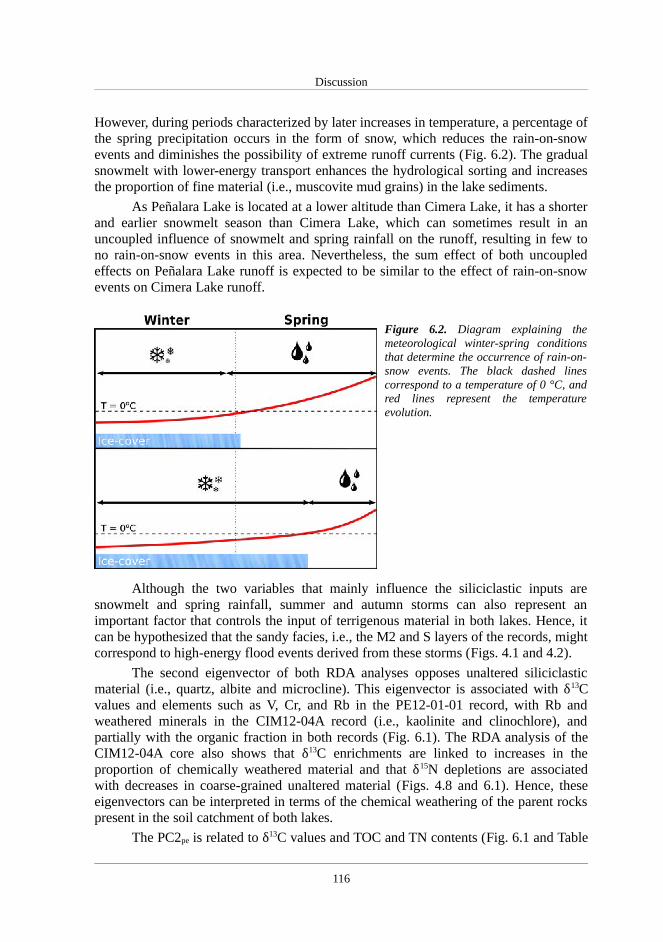
Discussion
However, during periods characterized by later increases in temperature, a percentage ofthe spring precipitation occurs in the form of snow, which reduces the rain-on-snowevents and diminishes the possibility of extreme runoff currents (Fig. 6.2). The gradualsnowmelt with lower-energy transport enhances the hydrological sorting and increasesthe proportion of fine material (i.e., muscovite mud grains) in the lake sediments.
As Peñalara Lake is located at a lower altitude than Cimera Lake, it has a shorterand earlier snowmelt season than Cimera Lake, which can sometimes result in anuncoupled influence of snowmelt and spring rainfall on the runoff, resulting in few tono rain-on-snow events in this area. Nevertheless, the sum effect of both uncoupledeffects on Peñalara Lake runoff is expected to be similar to the effect of rain-on-snowevents on Cimera Lake runoff.
Figure 6.2. Diagram explaining themeteorological winter-spring conditionsthat determine the occurrence of rain-on-snow events. The black dashed linescorrespond to a temperature of 0 °C, andred lines represent the temperatureevolution.
Although the two variables that mainly influence the siliciclastic inputs aresnowmelt and spring rainfall, summer and autumn storms can also represent animportant factor that controls the input of terrigenous material in both lakes. Hence, itcan be hypothesized that the sandy facies, i.e., the M2 and S layers of the records, mightcorrespond to high-energy flood events derived from these storms (Figs. 4.1 and 4.2).
The second eigenvector of both RDA analyses opposes unaltered siliciclasticmaterial (i.e., quartz, albite and microcline). This eigenvector is associated with δ13Cvalues and elements such as V, Cr, and Rb in the PE12-01-01 record, with Rb andweathered minerals in the CIM12-04A record (i.e., kaolinite and clinochlore), andpartially with the organic fraction in both records (Fig. 6.1). The RDA analysis of theCIM12-04A core also shows that δ13C enrichments are linked to increases in theproportion of chemically weathered material and that δ15N depletions are associatedwith decreases in coarse-grained unaltered material (Figs. 4.8 and 6.1). Hence, theseeigenvectors can be interpreted in terms of the chemical weathering of the parent rockspresent in the soil catchment of both lakes.
The PC2pe is related to δ13C values and TOC and TN contents (Fig. 6.1 and Table
116

NAO imprints in the Central Iberian Peninsula for the last two millennia
4.7A). The PC2cim is mostly related to the TOC, TN and Rb values (Fig. 6.1 and Table4.7B). The TOC concentration is a bulk value that represents the fraction of organicmatter that escaped remineralization during sedimentation, and it is commonlyconsidered a good indicator of the organic productivity of a lake (Meyers and Teranes,2001). The burial of organic matter is frequently followed by the rapid loss of N(Cohen, 2003), and the positive covariance of the two proxies in both lakes indicatesnegligible organic matter degradation. In addition, the TOC/TN ratio, featuring a valueof approximately 13 in both records (Figs. 4.7 and 4.8), suggests that the accumulatedorganic matter has a mainly algal origin (Meyers and Lallier-Vergès, 1999). Therefore,both PC2pe and PC2cim are associated with variations in the lake organic productivity. InPC2pe, positive (negative) values of the second eigenvector represent a decrease(increase) in lake productivity associated with both the internal recycling of nutrientsand, to a lesser extent, the input of weathered material from the catchment (Fig. 6.1). InPC2cim, the variations in lake productivity show the opposite pattern (Fig. 6.1). Theweathered material is produced by a series of chemical reactions that occur in the soil(Catalan et al., 2014) and that generate a pool of micronutrients that, when released bysoil erosion, might enhance the in-lake productivity. In alpine lakes, the ice-coverduration modulates lake productivity through its influence on the growing seasonlength, summer stratification, and lake overturning strength and timing, whichdetermine the internal lake nutrient cycle (Catalan and Fee, 1994; Catalan et al., 2002;Pla-Rabes and Catalan, 2011). The ice cover of Iberian alpine lakes depends on both thewinter-spring temperature and accumulated precipitation in the form of snow on the icecover. Cold (warm) and wet (dry) conditions will lead to longer (shorter) ice-coverdurations, which is partly a result of the enhanced (reduced) insulating effect of thesnow deposited on the ice cover (Sánchez-López et al., 2015). Therefore, during periodscharacterized by colder spring temperatures and a prolonged snow season, the ice coverwill last longer (Fig. 6.2), which will lead to a shorter growing season and thus lowerlake productivity. However, the opposite situation occurs during periods characterizedby shorter ice-cover durations as a result of warmer spring temperatures and a shortersnow season (Fig. 6.2).
Additionally, the presence of other factors, such as the nutrient inputs fromoutside the catchment, can also influence the productivity of alpine lakes. A number ofstudies have shown that the arrival of African dust is an important source of limitingnutrients, such as phosphor and nitrogen, for these oligotrophic environments (Toro etal., 2006; Reche et al., 2009; Camarero and Catalan, 2012). Thus, dust events canenhance lake productivity. African dust events are clearly recorded in the Cimera lakesequence, as evidenced by the accumulation of palygorskite (Fig. 4.8). This clay isformed in very arid conditions, such deserts, or in alkaline environments (Singer andNorrish, 1974). Therefore, it was most likely deposited in Cimera Lake during Sahara-Sahel dust events that affect the IP (Rodríguez et al., 2015). These external inputs ofnutrients are also supported by the results obtained from the sample collected in theCimera catchment after a dust episode, which revealed concentrations of nitrate,sulphate and total phosphorous several orders of magnitude higher than those of thewater in the lake (Table 6.1; Toro et al., 2006). Nevertheless, the relationship betweenthese external nutrient inputs (reflected by the palygorskite percentages) and lake
117

Discussion
productivity (reflected by the TOC and TN contents through the negative scores ofPC2cim) appears to be opposite to the expected relationship (i.e., rPC2= 0.38, p-value <0.01). More palygorskite is related to lower lake productivity, and vice versa. Therespiration of the organic matter accumulated in the lake bottom provokes a release ofCO2, which, in turn, produces a decrease in the pH of the water layers closer to thesediments (Catalan and Camarero, 1993). The stability of palygorskite depends on bothpH and concentrations of Mg and Si, being more stable under alkaline pH conditions(Velde, 1995). Therefore, lake productivity decreases during long-lasting ice-cover, andpalygorskite is preserved due to the higher alkalinity in the first millimetres of lakesediment (Velde, 1995). On the contrary, when lake productivity increases due to eitherextra nutrient inputs or shorter ice-cover durations, bacterial activity in the sedimentalso increases (Reche et al., 2009), provoking an increase in CO2 concentration and adecrease in the pH. Under these conditions, the palygorskite deposited in the sedimentis less stable. As a result, enhanced Cimera Lake productivity reflects intense aridepisodes associated with short-lasting ice cover and enhanced African dust inputs. InPeñalara Lake, the mineralogical data showed that the influence of African dust inputson lake productivity is less clear (Fig. 4.7). No apparent relationship was found in thecorrelation coefficients between lake productivity (reflected in the positive scores of thesecond eigenvector) and palygorskite (rPC2= 0.05, p-value > 0.1), although positive butnon-significant correlations were found between this clay and the TOC and TNpercentages.
Samples/Analyses [NO3-] [SO4
-2] TP
Dust sample (ppm) 190 530 0.5
Lake water (ppb) 36 0.3 9
Table 6.1. Concentration of nitrate (NO3-), sulphate (SO4
-2) and total phosphorous (TP) in the dustsample collected in the Cimera Lake catchment (in ppm) and in a water sample from Cimera Lake (inppb; Toro et al., 2006).
The third eigenvector is only significant in Cimera Lake (PC3cim), and theinterpretation of PC3cim is related to variations in the isotopic composition (i.e., δ13C andδ15N values) of the organic matter (Fig. 6.1). Because the RDA eigenvector has beenpreviously interpreted in terms of the inputs of weathered material produced in soils, thePC3cim could be a rough indicator of soil erosion. Neither of the isotopic signaturesshows a trend from the bottom to a depth of 35 cm in the studied core. Above thisinterval, δ13C enrichment and δ15N depletion occur, with the latter change moreprominent in the uppermost 7.5 cm of the sequence (Fig. 4.8). These variations coincidewith remarkable increases in the contents of clay minerals (Fig. 4.8). The TOC/TN ratioincreases between 22.5 cm and 7.5 cm of core depth, and together with the δ13Cfluctuations located between 35 and 7.5 cm, it may be related to inputs of organicmatter from the erosion of the catchment soil (Meyers and Lallier-Vergès, 1999; Meyersand Teranes, 2001). Soil organic matter is usually enriched with respect to δ 13C valuesbecause of remineralization and depleted with respect to δ15N values because of its
118

NAO imprints in the Central Iberian Peninsula for the last two millennia
atmospheric origin (Meyers and Teranes, 2001). Therefore, the supply of this organicmatter to the lake might explain the variations in the isotope records. The positivecovariance between the PC3cim and the increased clay mineral proportions also supportthe soil erosion hypothesis (Fig. 4.8).
However, in the uppermost 7.5 cm, the TOC and TN percentages increasesignificantly and the δ15N depletion is more prominent (Fig. 4.8), and these changescould be related to global climate change (Catalan et al., 2013). The lake productivitycould have been enhanced because of temperature increases and large inputs ofatmospheric nitrogen (δ15N depleted) resulting from the increase in the global pool ofreactive nitrogen (Bergstrom and Jansson, 2006). Fossil fuel combustion and the Haber-Bosch process have altered the global nitrogen cycle (Galloway and Cowling, 2002). Alarge number of sediment records from remote lakes in the Northern Hemisphere alsoshow this δ15N depletion during the Industrial Era (Hastings et al., 2009; Holtgrieve etal., 2011). The enhancement of chemical weathering over a short time scale because ofthe present global warming trend (Catalan et al., 2014) might also intensify thebiogeochemical reactions within the lake, thereby contributing to the observed increasesin TOC and TN and decreases in the TOC/TN ratio during the Industrial Era. Hence, thePC3cim in this last interval could provide an indicator of the effects of global warmingand/or human pollution, which could have similar effects on the δ15N values because ofthe organic matter inputs derived from soil erosion.
In summary, from the bottom to a depth of 7.5 cm in the Cimera sequence,positive values of the PC3cim reflect an enhancement of soil erosion episodes, whereas inthe uppermost 7.5 cm, this eigenvector might also reflect the influence of globalwarming and/or human pollution on lake productivity.
6.2. Climatic and environmental changes in the Iberian Central Rangeand the Iberian Peninsula over the last two millennia
The multivariate RDA and PCA analyses of geochemical and mineralogicaldatasets from Peñalara and Cimera records have allowed us to determine climatic andenvironmental changes in the ICR. This reconstruction has been primarily focussed onthe Cimera Lake sequence because it presents a much better constrained chronologythan the Peñalara sequence, although the latter sequence supports the climatic andenvironmental conditions described for the ICR (Fig. 6.3). This reconstruction includesfive main climate chronozones: The Roman Period (RP; ca. 250 BC – 500 AD), theEarly Middle Ages (500 – 900 AD), The Medieval Climate Anomaly (MCA; 900 –1300 AD), The Little Ice Age (1300 – 1850 AD) and the Industrial Era (1850 – 2012AD).
Comparisons with the main IP sedimentary records have been used to establishthe contextual climatic and environmental conditions over the last two millennia in theIP in these climatic chronozones (Fig. 6.4).
119

Discussion
Figure 6.3. Variations in the PC1pe and PC2pe scores relative to age in the Peñalara Lake sequenceand in the PC1cim, PC2cim and PC3cim scores relative to age in the Cimera Lake sequence. Main climateperiods are indicated with grey dashed lines. Original data are plotted in grey lines, and smootheddata calculated with the loess function and a span degree of 0.10 are represented by thicker blacklines. Vertical bars correspond to thermal and hydrological conditions suggested by the processesassigned to PC1cim and PC2cim. Note that the PC2pe values have been inverted to be in agreement withthe ice-cover duration of PC2cim.
6.2.1. The Roman Period (RP; ca. 250 BC – 500 AD)
In terms of thermal conditions, the sedimentary records from the NW of the IPindicate predominantly warm conditions during this period (Martínez-Cortizas et al.,1999; Desprat et al., 2003; Álvarez et al., 2005; Martín-Chivelet et al., 2011;). In thePyrenees, Redon Lake displayed low winter-spring temperatures (~200 BC – 400 AD)and a warming trend at the end (Pla and Catalan, 2005, 2011), whereas the summer-autumn temperatures showed a transition from cold to warm conditions (Catalan et al.,2009). In the centre of the IP, Almenara de Adaja (López-Merino et al., 2009) and Tab-las de Daimiel (Gil-García et al., 2007) registered a centennial-scale alternation of coldand warm periods, whereas the Peñalara and Cimera lakes sequences exhibited decadalshort-lived periods of rain-on-snow events, which suggest cold and warm oscillations(Figs. 6.3 and 6.4). These differences in the frequency of climatic oscillations can bepartially ascribed to the lower temporal resolution of the first Iberian records. Finally,the Tajo Prodelta recorded a warm period (Abrantes et al. 2005; Rodrigues et al., 2009).To the best of our knowledge, records from the southern IP have not been employed intemperature reconstructions.
120
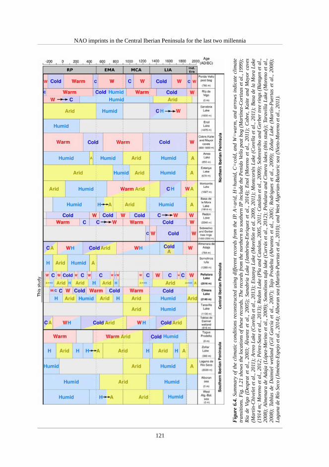
NAO imprints in the Central Iberian Peninsula for the last two millennia
121
Fig
ure
6.4.
Sum
mar
y of
the
cli
mat
ic c
ondi
tions
rec
onst
ruct
ed u
sing
diff
eren
t re
cord
s fr
om t
he I
P. A
=ar
id, H
=hu
mid
, C=
cold
, an
d W
=w
arm
, an
d ar
row
s in
dica
te c
lim
ate
tran
sitio
ns. F
ig. 1
.21
show
s th
e lo
cati
ons
of th
ese
reco
rds.
The
rec
ords
from
the
nort
hern
to s
outh
ern
IP in
clud
e th
e P
enid
o Ve
llo
peat
bog
(M
artí
nez-
Cor
tizas
et a
l., 1
999)
; R
ía d
e Vi
go (
Des
prat
et
al.,
2003
; Á
lvar
ez e
t al
., 20
05);
San
abri
a L
ake
(Jam
brin
a-E
nriq
uez
et a
l., 2
014)
; E
nol
(Mor
eno
et a
l., 2
011)
; C
obre
, K
aite
and
May
or c
aves
(M
artí
n-C
hive
let e
t al.,
201
1);
Arr
eo L
ake
(Cor
ella
et a
l., 2
013)
; E
stan
ya L
ake
(Mor
elló
n et
al.
2009
, 201
1);
Mon
tcor
tès
Lak
e (C
orel
la e
t al.,
201
1);
Bas
a de
la M
ora
Lak
e (1
914
m;
Mor
eno
et a
l., 2
012;
Pér
ez-S
anz
et a
l., 2
013)
; R
edon
Lak
e (P
la a
nd C
atal
an, 2
005,
201
1; C
atal
an e
t al.,
200
9);
Sobr
estr
ibo
and
Ger
ber
tree
rin
gs (
Bün
tgen
et a
l.,
2008
); A
lmen
ara
de A
daja
(Ló
pez-
Mer
ino
et a
l., 2
009)
; So
mol
inos
tuf
a la
ke (
Cur
rás
et a
l., 2
012)
; P
eñal
ara
and
Cim
era
lake
s (t
his
stud
y);
Tara
villa
Lak
e (M
oren
o et
al.,
20
08);
Tab
las
de D
aim
iel
wet
land
(G
il G
arcí
a et
al.,
200
7);
Tajo
Pro
delta
(A
bran
tes
et a
l., 2
005;
Rod
rigu
es e
t al
., 20
09);
Zoñ
ar L
ake
(Mar
tín-P
uert
as e
t al
., 20
08);
La
guna
de
Río
Sec
o (J
imén
ez-E
spej
o et
al.,
201
4);
Alb
oran
sea
(M
artín
-Pue
rtas
et a
l., 2
010)
; an
d W
est A
lger
ian-
Bal
eari
c se
a (N
ieto
-Mor
eno
et a
l., 2
011)
.

Discussion
In terms of humidity, the northwestern IP presented an arid phase that was ob-served in the marine and lacustrine records (Bernárdez et al., 2008; Jambrina-Enríquezet al., 2014), although towards the east, Enol Lake showed the opposite conditions(Moreno et al., 2011). In the Pyrenees, Estanya Lake displayed a dry climate scenario(Morellón et al., 2009), whereas the remaining records (Arreo, Montcortès and Basa dela Mora Lakes) displayed large increases in water availability (Corella et al., 2011,2013; Pérez-Sanz et al., 2013). In the Central IP, all of the records showed an alternationbetween arid and humid phases (Gil-García et al., 2007; López-Merino et al., 2009;Currás et al., 2012). Peñalara and Cimera lakes showed multidecadal alternations oflong and short ice-cover durations derived from variations in lake productivity (Figs.6.3 and 6.4) resulting from fluctuations between periods of longer winter snow seasonsduring colder and/or wetter conditions and the opposite conditions. These multidecadalalternations led to periodic oscillations in soil erosion in Cimera Lake (Fig. 6.3). In ad-dition, the presence of facies S and M2 in the ICR sequences might be associated withfrequent autumn/summer storms in this region (Figs. 4.7 and 4.8). In the southern IPand western Mediterranean region, marine records (Alboran Sea and west Algerian-Balearic Basin) and terrestrial records (Zoñar Lake) displayed prevalent wet conditions(Martín-Puertas et al., 2008, 2010; Nieto-Moreno et al., 2011). This humid interval wasnot favourable to African aeolian inputs in the IP (Martín-Puertas et al., 2010; Nieto-Moreno et al., 2011; Jiménez-Espejo et al., 2014); thus, the Cimera Lake productivitywas not enhanced (Fig. 6.3).
Therefore, during the RP, the northern IP was characterized by a E–W longitud-inal gradient in terms of humidity (Fig. 6.4), with humid conditions prevailing at higheraltitudes towards the eastern areas and dry conditions prevailing at lower altitudes to-wards the western areas. A broad N–S humidity gradient also occurred, with humid con-ditions generally occurring in the southern part of the IP and dominant arid conditionsoccurring in the northern part (Fig. 6.4). These E–W and N–S humidity gradients high-light the complex interplay between geography, topography and climate.
6.2.2. The Early Middle Ages (EMA; 500 – 900 AD)
General humid and cold conditions were registered by the marine and lacustrinerecords in the NW IP (Desprat et al., 2003; Álvarez et al., 2005; Jambrina-Enríquez etal., 2014) during the EMA. However, spatial heterogeneity was also observed as indic-ated by the predominantly warm temperatures of the Penido Vello peat bog (Martínez-Cortizas et al., 1999) and speleothem records from the Cobre, Mayior and Kaite caves(Martín-Chivelet et al., 2011) (Fig. 6.4). In the Pyrenees, the records showed a strongdisparity in humidity, with Arreo Lake displaying wet conditions caused by less salineconditions and high lake levels (Moreno et al., 2011; Corella et al., 2013) and EstanyaLake presenting a dominant dry scenario between 500 and 750 AD (Morellón et al.,2009). Montcortès and Basa de la Mora lakes displayed a shift from humid to arid con-ditions (Corella et al., 2011; Pérez-Sanz et al., 2013). In terms of the thermal conditionsin the Pyrenees, the summer-autumn temperatures in Redon Lake exhibited a transitionfrom cold to warm temperatures (Catalan et al., 2009), whereas the winter-spring tem-peratures remained cold (Pla and Catalan, 2005, 2011). In the central IP, the Almenara
122

NAO imprints in the Central Iberian Peninsula for the last two millennia
de Adaja (López-Merino et al., 2009) and Tablas de Daimiel (Gil-García et al., 2007) re-cords registered a cold and arid EMA, although the first record indicated the oppositeconditions at the end of this period. Peñalara Lake sequence recorded less intense run-off events and shorter ice-cover durations, possibly as a consequence of predominantcold and dry conditions. Between 500 and 630 AD, Cimera Lake was characterized bymore rain-on-snow events and shorter ice-cover durations, as reflected in enhanced lakeproductivity, which suggested warm temperatures and arid conditions and shorter snowseasons. In contrast, from 630 to 900 AD, the Cimera Lake record presented the oppos-ite conditions (Figs. 6.3 and 6.4). These long-term climate conditions may also indicatea progressive inhibition of soil erosion surrounding Cimera Lake. The lack of facies M2in the Peñalara sequence and the low frequency of facies S in the Cimera sequence(Figs. 4.7 and 4.8) are consistent with the low number of floods observed in the TajoRiver basin during this climate period (Benito et al., 2003a, 2003b). In the southern IPand western Mediterranean region, the marine and terrestrial records displayed a trendtowards drier conditions (Martín-Puertas et al., 2008, 2010; Nieto-Moreno et al., 2011).
Therefore, the E–W humidity gradient only occurred in the northern IP, and pro-gressively more arid conditions occurred westwards. Nevertheless, the N–S humiditygradient affected the entire IP and produced generally humid conditions in the northernarea, a transition from arid to humid conditions in the ICR, and a dry scenario in thesouthern area (Fig. 6.4). The progressive increase in humidity in the ICR suggests asouthwards displacement of this humidity gradient over time.
6.2.3. The Medieval Climate Anomaly (MCA; 900 – 1300 AD)
Moreno et al. (2012) conducted a comprehensive characterization of the MCAclimate evolution for the IP and showed that the selected continental records from theMediterranean IP generally registered drier conditions, as indicated by lower waterlevels and higher chemical concentrations. Marine cores also indicated a decrease in thefluvial supply and an increase in African dust particles. Records from the NW IP indic-ated an increase in humidity during the MCA, which reflects the opposite behaviour tothat of the Mediterranean IP. Thus, Morellón et al. (2012) focussed on the available cli-matic evidence from the Pyrenees and concluded that warmer and more arid conditionsprevailed during the MCA in this region, as evidenced by lower lake levels, decreasedrunoff and a significant development of xerophytes and Mediterranean vegetation. Theonly climate reconstruction that presented an opposite behaviour was that of RedonLake, and the opposite behaviour might have been related to the combination of mul-tiple local factors, such as the geographical location and orientation (Morellón et al.,2012).
Climate records that were not included in the previous reviews suggest that hightemperatures occurred in the northern IP (Martín-Chivelet et al., 2011) and arid condi-tions occurred in the south IP (Martín-Puertas et al., 2010) (Fig. 6.4). In the ICR, thePeñalara Lake record only contains the last 150 years of the MCA, during which it re -gistered a transition from a warm-arid to a cold-humid scenario. The Cimera Lake re-cord displayed a predominant warm and arid scenario, as indicated by the prevalentrain-on-snow events, an increasing trend in lake productivity caused by short ice-cover
123

Discussion
durations related to the shorter snow season, and an increase in African aeolian inputs(Fig. 6.3). Furthermore, the development and weathering of soils in the Cimera Lakecatchment caused by these optimal climatic conditions resulted in soil erosion, which isindicated by a marked increase in erosion (Fig. 6.3). The scarce presence of facies M2(Fig. 4.8) might be associated with a low frequency of autumn/summer storms in theICR. Benito et al. (2003a) found that large flood events decreased in the Tajo Riverbasin during the period 1205 –1450 AD, which might partially support our hypothesis.
The integration of the previous works with these new climate records (Fig. 6.4)indicates that although wet conditions were recorded in the marine records from thenorthwest end of the IP, arid and dry conditions were mostly predominant throughoutthe entire IP (Moreno et al., 2012). Thus, compared with the conditions during the RPand EMA, evident N–S or E–W humidity gradients did not occur during the MCA.
6.2.4. The Little Ice Age (LIA; 1300 – 1850 AD)
Morellón et al. (2012) also included a detailed reconstruction of the main climatechanges during the LIA in the Pyrenees. To the best of our knowledge, additional com-prehensive LIA evolutions for the entire IP are not available.
Northern Iberian records consistently show that the onset of the LIA resulted incold and humid climate conditions that progressively became warmer. Only the Ría deVigo record displays arid conditions (Desprat et al., 2003; Álvarez et al., 2005). In thePyrenees, Morellón et al. (2012) demonstrated that cold and humid conditions withhigher lake levels and increased runoff prevailed during this period. All of the records inthe mid-latitudes of the IP recorded cold conditions, although they displayed differencesin terms of humidity, with Taravilla Lake (Moreno et al., 2008) and Tajo Prodelta(Abrantes et al., 2005; Rodrigues et al., 2009) showing predominantly wet conditionsand Almenara de Adaja (López-Merino et al., 2009) and Tablas de Daimiel (Gil-Garcíaet al., 2007) displaying predominantly arid conditions (Fig. 6.4). The Cimera Lake re-cord was characterized by a decreasing trend of intense runoff events and prevalent lowlake productivity with decadal oscillations, which indicated predominantly long ice-cover durations caused by prolonged snow seasons (Fig. 6.3). These conditions on theICR were likely provoked by a colder period with dry-wet-dry decadal oscillationswithin the framework of a generally humid scenario (Fig. 6.4). This climatic scenariowas broadly reflected in the Cimera Lake soil erosion, which was generally constantand likely caused by cold conditions hampering the development and disintegration ofsoils (Fig. 6.3). The high frequency of facies M2 in the Cimera sequence (Fig. 4.8)might also indicate the major presence of autumn/summer storms in the ICR, which wasalso observed for the Tajo River (Benito et al., 2003a, 2003b). The Peñalara sequencealso showed a minor presence of run-off events, thereby indicating a predominantlycold scenario, although the prevalence of dry conditions and the lack of the facies M2recorded in this sequence suggest a dry scenario (Figs. 6.3, 6.4 and 4.7). The differencesbetween ICR lakes can be partially attributed to differences in altitude. Finally, in thesouthern IP and western Mediterranean, humid conditions with a decadal oscillatingpattern were observed (Martín-Puertas et al., 2010; Nieto-Moreno et al., 2011). Thegenerally low levels of lake productivity present in the central and southern Iberian re-
124
NAO imprints in the Central Iberian Peninsula for the last two millennia
cords (Martín-Puertas et al., 2008; Jiménez-Espejo et al., 2014) may be explained by thedominantly humid conditions that prevailed during the LIA and likely inhibited the de-position of nutrient inputs from North African dust.
Therefore, despite minor discrepancies, prevalent wet and cold climatic condi-tions were recorded throughout the entire IP during the LIA (Fig. 6.4).
6.2.5. The Industrial Era (1850 – 2012 AD)
The records included in this study show that, over the last 150 years, the IP hasbeen characterized by predominantly warm and arid conditions (Fig. 6.4), which aremost likely associated with the current global warming trend. Nevertheless, the intensityof human activities during the Industrial Era and their impact on natural ecosystemshave increased the difficulty of discerning and evaluating climate signals (Fig. 6.4).
The Peñalara Lake sequence exhibited long ice-cover durations during the firstpart of this period, although presented a conspicuous decrease during the second partand a marked increase of intense run-off events during the whole period (Fig. 6.3).These conditions are in concordance with the global warming scenario. The CimeraLake sequence showed an increasing trend of lake productivity that was partiallytriggered by progressively shorter ice-cover durations, which were likely caused by lessprolonged snow seasons and suggest prevalent arid conditions in the ICR (Fig. 6.3).However, between 1850 and 1950 AD, the Cimera sequence presented a shift from alow to a high frequency of intense runoff episodes, whereas over the last 50 years, thesequence displayed a marked decrease in these episodes (Fig. 6.3). These environmentalconditions suggest an earlier warming and a rapid shift to cold conditions over the lastdecades. These colder conditions for the last 50 years clearly contradict the currentglobal warming scenario. Granados and Toro (2000) indicated that the Cimera Lakesummer water has warmed by more than 1.5 °C since the 1980s, which is consistentwith the rise in temperatures caused by global warming. The PC3cim might also reflectthe influence of global warming in Cimera Lake. An explanation for this apparent con-tradiction may be found in the rapid increase in organic matter (i.e., TOC and TN) in thesediments. This increase in the proportion of organic matter has most likely diluted theinorganic fraction of the sediments, thereby lowering the signal of almost all the ele-ments measured with XRF (Fig. 4.8).
6.3. Climate-forcing mechanisms driving climate variability in theIberian Peninsula over the last two millennia
The climate evolution of the IP over the last 2,000 years indicates that two spati-otemporal climate patterns have occurred. During the RP and EMA periods, E–W andN–S humidity gradients co-occurred, whereas during the MCA and LIA, these climategradients were not observed (Fig. 6.4).
The NAO has been shown to be the climate mode responsible for the largestshare of the climate variability in the North Atlantic and European regions in recentdecades (Hurrell et al., 2003). Thus, the majority of Iberian climate reconstructions over
125

Discussion
the last 1000 years have attributed most of the observed climate variability to variationsin the NAO (e.g., Nieto-Moreno et al., 2011; Morellón et al., 2012; Moreno et al.,2012). These climate reconstructions commonly ascribe the warm and arid climate con-ditions of the MCA to the dominant positive phases of the NAO and the humid and coldconditions of the LIA to the predominance of negative phases of the NAO (Trouet et al.,2009; Ortega et al., 2015).
Nevertheless, as initially stated, recent works suggest that other North Atlanticclimate modes, such as the EA and SCAND climate patterns, significantly influencemost climate variables in Europe (Jerez and Trigo, 2013; Comas-Bru and McDermott,2014). Furthermore, the influence of the combined influence of the NAO and EA overEurope has been extended to vegetation dynamics and carbon uptake (Bastos et al.,2016) and to precipitation dynamics and the δ18O–NAO relationship (Comas-Bru et al.,2016).
The EA and SCAND modulate variations in the strength and location of the NAOdipoles at the multidecadal scale (Comas-Bru and McDermott, 2014). The combined in-fluence of the NAO–EA and NAO–SCAND leads to shifts in the winter temperatureand precipitation anomaly patterns in Western Europe (Comas-Bru and McDermott,2014). When the NAO and EA modes have the same sign, the precipitation and temper-ature patterns present a homogeneous spatial distribution, whereas when these modeshave the opposite sign, the precipitation and temperature patterns present heterogeneousspatial distributions (Bastos et al., 2016; Comas-Bru and McDermott, 2014) (Fig. 1.11).In the IP, Hernández et al. (2015) showed that the NAO mainly governs winter precipit-ation and that the EA governs winter and summer temperatures (Fig. 1.14). These au-thors also showed that the Iberian lake dynamics are sensitive to the seasonal effects ofinterannual variations in these three patterns.
The role of these other climate modes and their interactions could explain thespatiotemporal climate variability observed in the IP over the last millennia. The humid-ity gradients recognized during the RP and EMA periods in the IP might have beencaused by a predominant coincidence of the NAO and EA in opposite phases (NAO+–EA- or NAO-–EA+). The thermal conditions and the humidity gradients present duringthe RP suggest that the prevalent climate was dominated by the phase combinationNAO-–EA+ (Fig. 6.4), which Hernández et al. (2015) indicated led to wet and warmwinters and warm summers (Fig. 1.14). Conversely, the EMA presented an arid gradientwith generally cold conditions, which suggests that the NAO+–EA- combination domin-ated the main climate variability and led to dry and cold winters and cold summers (Fig.6.4).
However, the spatially homogeneous climate conditions that dominated the MCAand LIA also might have been caused by a predominance of both climate modes actingin the same phase. Thus, the MCA would be marked by a predominance of the positivephases of the NAO and EA (NAO+–EA+), leading to dry and warm winters and warmsummers, whereas the LIA would be dominated by the opposite phases (NAO-–EA-),leading to cold and wet winters and cold summers (Fig. 6.4).
The relationship between climate (e.g., NAO) and external climatic forcings,such as volcanic and solar forcings (e.g., in the frequency domain), is a controversial is-
126

NAO imprints in the Central Iberian Peninsula for the last two millennia
sue because of their complex relationships (Mann, 2007; Sigl et al., 2015; Stoffel et al.,2015). Despite the complex relationships, the predominant NAO and EA phases duringthe RP, EMA, MCA and LIA appear to be associated with a large-scale dynamic re-sponse of the climate system to explosive volcanic and solar forcings. During the RPand MCA, the solar irradiance was relatively high, and there were few tropical explos-ive volcanic eruptions, whereas during the EMA and LIA, the solar irradiance was char-acterized by several periods of solar minima, and there were more frequent tropical vol-canic eruptions (Table 6.2; Steinhilber et al., 2009; Sigl et al., 2015). These forcingsmight have modulated the NAO and EA phases over the last two millennia (Table 6.2).Most of the climate reconstructions for the last millennium have assumed a linear rela-tionship between the solar activity and the NAO because other climate modes have notbeen considered (Morellón et al., 2012). However, our results suggest that, at the multi-decadal scale, the solar activity fluctuations are reflected in the EA.
Climate period RP EMA MCA LIA
Tropical volcanic eruptions - + - +
Solar irradiance forcing high low high low
Blocking events frequency low high low high
Ocean and continent conditions during blockingevents
---Cold ocean
Warmcontinent
---Warm ocean
Cold continent
EA phase + - + -
NAO phase - + + -
ITCZ position southern northern northern southern
General climate conditionsover Iberian Peninsula
Wet and warm winters and
summers
Dry andcold win-ters andsummers
Dry andwarm win-
ters andsummers
Wet and coldwinters and
summers
Table 6.2. Frequency of tropical volcanic eruptions from Sigl et al. (2015), intensity of solar irradi-ance forcing obtained from Steinhilber et al. (2009), presence of blocking events, and the ocean andcontinent conditions ascribed to these forcings, the NAO and EA phases and general climate condi-tions over the IP during the RP, EMA, MCA and LIA climate periods.
Another consequence of the relationship between solar activity and climatemodes is the development of atmospheric blocking events, which consist of a quasi-sta-tionary high-pressure system in the eastern North Atlantic region that modifies the flowof the westerly winds (Trigo et al., 2004; Barriopedro et al., 2008). Low solar irradiancepromotes the development of frequent and persistent atmospheric blocking events(Moffa-Sánchez et al., 2014). The duration of these blocking events is usually suffi-ciently long (i.e., between 1 and 3 weeks) to induce significant climate anomalies over awide area of Europe (Trigo et al., 2004), although the occurrence of these anomalies isdependent on the location (Sousa et al., 2015). Recently, the location and persistence of
127

Discussion
these blocking events over the eastern North Atlantic has also been associated with thephase of the EA pattern (Moffa-Sánchez et al., 2014). The position, frequency and per-sistence of these blocking events on the central North Atlantic Ocean are mainly condi-tioned by the phase of the NAO (Shabbar et al., 2001). The NAO+ phase leads to a ‘coldocean/warm land’ pattern, which is unfavourable for the development and persistence ofblocking events, whereas the NAO- phase leads to a ‘warm ocean/cold land’ pattern,which promotes the formation and persistence of blocking events (Shabbar et al., 2001).
During the EMA and LIA, low solar irradiance promoted the development of fre-quent and persistent atmospheric blocking events (Moffa-Sánchez et al., 2014). Thedominance of EA- climate phase conditions during these two climate periods suggeststhat blocking events developed on the North Atlantic Ocean (Table 6.2). However, theNAO phase of these climate periods determined the main humidity and thermal domin-ance conditions. The NAO+ phase dominated the EMA and led to a 'cold ocean/warmland' pattern (Shabbar et al., 2001), which inhibited ocean water evaporation. This pat-tern, together with the low-frequency and less persistent blocking events, generally ledto arid and relatively cold conditions in the IP (Table 6.2). Conversely, the LIA wasgoverned by a NAO- phase, which led to a 'warm ocean/cold land' pattern (Shabbar etal., 2001) that enhanced ocean water evaporation. This second pattern, together with thehigh-frequency and persistent blocking events, promoted a generally humid and coldscenario during this period (Table 6.2).
The delivery of African dust to Cimera Lake is related to climate conditions andis therefore representative of underlying forcing mechanisms over the last two millen-nia. On one hand, the meridional transport of African dust is related to cyclone activityinside and around the Mediterranean basin (Alpert and Ziv, 1989; Bergametti et al.,1989), and transport occurs when the westerly regime is weak, disrupted or displacednorthwards (e.g., Rodríguez et al., 2001; Torres-Padrón et al., 2002; Ginoux et al.,2004). On the other hand, an arid source region and sufficient storminess and air turbu-lence to entrain dust and inject it into the atmosphere are necessary conditions for theavailability of dust. These processes are mostly controlled by the latitudinal migrationof the ITCZ and its associated wind cycle and rainfall belt (e.g., Engelstaedter et al.,2006; Bout-Roumazeilles et al., 2007). Hence, variability in the African dust inputs inthe IP over the last two millennia could be the result of coupled movements between theNAO and the ITCZ. A predominance of NAO+ provokes lower precipitation over south-ern Europe and Northern Africa, and the related northern position of the ICTZ enhancesdust emissions from Northern Africa (western and northern Saharan). Both of thesefactors favour a higher intensity of dust uptake and transport towards the IP, particularlyduring summer. Conversely, a NAO- phase coupled with a more southern position of theITCZ results in wet summer conditions in Northern Africa, reducing dust emission fromthe hyper-arid region of the Sahara desert. Consequently, the evidence of African dustinputs in Cimera Lake during dry periods, such as the EMA and MCA, may suggest apredominant NAO+ coupled with a more northern position of the ITCZ during this peri-od. Furthermore, from this scenario, a particular predominance of dry summers in the IPduring both periods could be derived (Table 6.2). In contrast, less evidence of these in-puts during wetter periods, such as the RP and the LIA, hint at the opposite scenario andsupport the hypothesis of a predominance of NAO- phases coupled with a more southern
128

NAO imprints in the Central Iberian Peninsula for the last two millennia
position of the ITCZ during these periods. This situation would also indicate the exist-ence of more frequent wet summers in the IP (Table 6.2). Different palaeorecords haveextensively indicated ITCZ migrations at millennial time scale during the Holocene(e.g., Haug et al., 2001; Schneider et al., 2014), as well as possible coupling with theNAO during these migrations (Wanner and Brönnimann, 2012; Wirth et al., 2013).However, to our knowledge, these shifts in the ITCZ have not been documented yet forshorter time scales, such multidecadal or centennial time scales.
129

Chapter 7
7. THE NAO IMPRINTS ON THE IBERIAN CENTRAL RANGE FORTHE LAST TWO MILLENNIA RECONSTRUCTED USING ABAYESIAN APPROACH
7.1. The NAO impact on the Iberian Central Range
The ancient NAO (NAOICR) obtained from the random walk-modularisedBayesian model is a record of the NAO impact in the ICR for the last two millennia. Toevaluate the reliability of these reconstructed values and of the model, a 5-fold cross-validation of the modern data was conducted. However, the obtained results did notallow us to statistically validate the Bayesian model (Juggins and Birks, 2012).Consequently, to determine the degree to which the model can be validated, theobtained ancient NAOICR was compared with multidecadal NAOi data from CRU forthe period 1930–1825 AD. This NAOi was not included in the calibration of the model(Fig. 7.1). The visual inspection of this comparison showed that both lines displayedsimilar multidecadal variations, although the mean value of the NAOICR impacts wasdominated by negative values, whereas the instrumental NAO index presentedoscillations between positive and negative values (Fig. 7.1). However, taking intoaccount the uncertainty values of the reconstructed NAO impacts, the NAOICR displayedsimilar values to the instrumental NAO (Fig. 7.1). Hence, although the model cannot bevalidated by cross-validation, the NAOICR impacts reproduce similar inter-decadaloscillations and values as those present in the instrumental NAO record.
Figure 7.1. The light grey line corresponds to the annual NAOi calculated from the monthly NAOifrom CRU for the period 1825–1930 AD and the dark grey line correspond to a smoothed version ofthese data calculated with the loess function and a span degree of 0.10. The red line correspond to themedian value of the NAO impact in the Iberian Central Range (NAO ICR) obtained in this study for theperiod 1825–1930 AD, and the red light band shows the uncertainty of the model obtained based onthe 5th and 95th quantiles.
As previously mentioned on page 30, another important aspect necessary for amodel to be valid is that it must make ecological sense. The NAOICR must be in accord-ance with the reconstructed temperature and precipitation conditions determined in theICR for the last two millennia from the multi-proxy approach applied to sediments of
130

NAO imprints in the Central Iberian Peninsula for the last two millennia
the CIM12-04A (Fig. 7.2). Another important aspect of this comparison is that both re-constructions were obtained by independent statistical methods: PCA was used to re-construct the climate conditions in the ICR from the Cimera Lake sediments, whereasNAOICR was obtained by Bayesian statistics using the random walk-modularised model(see section 3.6 for further details). The NAOICR during the RP showed multidecadal al-ternations between both phases, although it presented a predominance of negative val-ues (Fig. 7.2), which is in accordance with the humid scenario suggested by the recon-structed precipitation. The dominant temperature conditions during this period shiftedbetween colder and warmer periods (Fig. 7.2). The EMA onset was characterized by apositive NAOICR coinciding with warm conditions in the ICR, although the oppositephase prevailed during the rest of the period, coinciding with a change from dominantlyarid conditions to humid conditions (Fig. 7.2). A positive impact of the NAOICR pre-vailed in the region during the MCA together with a predominantly warm and arid scen-ario (Fig. 7.2). In contrast, the LIA was characterized by a trend towards a prevalentnegative phase and a colder period with dry-wet-dry decadal oscillations in the contextof a generally humid scenario (Fig. 7.2). Finally, this negative phase predominated untilthe onset of the Industrial Era, coinciding with a short markedly humid period (Fig.7.2). Hence, temperature and humidity conditions obtained from the Cimera Lake se-quence appear to be consistent with the possible climate conditions ascribed to NAOICR
(Fig. 7.2).
7.2. Global aspects of the NAO impact on the Iberian Central Range
Finally, to determine whether some global aspects are depicted in the NAO ICR
and may therefore be roughly considered regional indices for the entire IP, the NAOICR
reconstruction has been compared with the three different NAO approaches: i) the NAOindex from Trouet et al. (2009) (NAOTro), which can be considered a simplistic ap-proach based on two records from Scotland and Morocco (Figs. 3.16 and 7.3); ii) themultidecadal NAO index obtained by Olsen et al. (2012) (NAOOls), which can also beconsidered a simplistic approach based on a palaeo-redox proxy (Mn/Fe ratio) in a sedi-ment record from a small lake near Kangerlussuaq (Greenland, Figs. 3.16 and 7.3); andiii) the much more robust NAO reconstruction from Ortega et al. (2015) (NAOOrt),which employed multi-proxy data from different locations in the Northern Hemisphere(Figs. 3.16 and 7.3). None of the three NAO indices completely cover the last two mil-lennia. Therefore, the comparisons have been carried out for the respective overlappingperiods.
The NAOOls presented a predominant positive phase of NAO for the last two mil-lennia, which contrasts with the other two NAO indices (Fig. 7.3). During the RP andEMA, only the NAOOls and the NAOICR are available. A more positive phase predomin-ated in the NAOOls during the RP and a more negative one prevailed in the EMA, whilethe NAOICR presented both approximately opposite values and different variability dur-ing these two climate periods (Fig. 7.3). All four indices almost cover the MCA period,and NAOOls, NAOTro, and NAOICR showed prevalent positive phases, whereas the NA-OOrt index, despite presenting increasingly positive values, did not display a marked per-sistent positive phase during the Medieval period (Fig. 7.3). The similarity between
131

Discussion
Figure 7.2. A) Scores of the first (PC1cim) and B) second (PC2cim) eigenvectors obtained from the mul-tiproxy analysis of Cimera Lake sediments; these eigenvectors reflect thermal and humid conditions,respectively. C) and D) bars with cold and warm conditions, and arid and humid conditions deducedfrom A) and B), respectively. E) Values of the NAO impact in the ICR obtained in this study (blackline) and the associated uncertainty (grey band).
NAOTro and NAOOls can be partly ascribed to the fact that the latter index was based onthe first one in the construction of the reconstruction, whereas the major agreementbetween NAOICR and NAOTro can be ascribed to the geographical location of the proxyused as the southern node in the NAOTro calculations. The relative geographical proxim-ity between Cimera Lake and Morocco most likely indicates that both sites mostly ex-perienced similar climate conditions and that both records therefore registered similarNAO impacts. Additionally, the differences between the different instrumental indicesof NAO support this hypothesis. Jones et al. (2003) showed that, although differentNAO indices were highly correlated on interannual and longer time scales, the choice ofthe southern station in the calculation of the indices produced some significant differ-
132

NAO imprints in the Central Iberian Peninsula for the last two millennia
ences. In contrast, the specific location of the northern node was not critical because thetemporal variability over this region was much larger than the spatial variability.
Fewer discrepancies were found during the LIA, where all NAO reconstructionsshowed values predominantly lower than those during the MCA (Fig. 7.3). The coldtemperatures registered during the LIA in most of the North Hemisphere (Mann, 2007)have been extensively related to the high frequency of solar minimum events (Steinhil-ber et al., 2009), which could have produced a predominance of negative NAO phases.Furthermore, the predominance of these periods of solar minima may also have contrib-uted to the prevalence of negative EA phases, producing a dominance of cold summersin the IP (Table 6.2). However, taking into account the age-depth model errors, only onesolar minimum event may is reflected in all the NAO reconstructions (Fig. 7.3). Thisevent corresponds to the Spörer Minimum (1450 – 1550 AD), one of the longest (90years) and lowest periods of total solar irradiance in the last two millennia (Steinhilberet al., 2009).
Finally, during the onset of the Industrial Era, the NAOICR and NAOOrt showednegative values, whereas the NAOTro presented the opposite phase values preceded by anegative phase period.
Figure 7.3. A) The black line denotes the NAO impact values in the ICR for this study (NAO ICR); thelight grey band shows the uncertainty of the model obtained from by 5 th and 95th quantiles. In B), C)and D) the grey lines denote NAO approaches from Ortega et al. (2015) (NAOOrt), Olsen et al. (2012)(NAOOls) and Trouet et al. (2009) (NAOTro), respectively. The coloured lines (NAOOrt orange line, NA-OOls green line and NAOTro blue line) correspond to smoothed data calculated using the loess functionand a span degree of 0.10. The grey band denotes the period Spörer Minimum (1450 – 1550 AD),which has been slightly spanning for taking into account the age model uncertainty of the NAOICR.
133

Discussion
Hence, the differences between these reconstructions showed that a simplisticNAO approach can sometimes reflect local or regional aspects of this climate mode.Thus, the NAOICR reconstruction can be considered a regional NAO index, althoughsuch a simplistic approach should not be considered a global index.
The main strength of the approach followed here is that it provides many oppor-tunities to obtain robust and accurate high-resolution NAO reconstructions using non-biological proxies, such as the chemical composition of the sediments. Performing anumber of these NAO reconstructions in a relatively small geographical area and integ-rating them into a unique index might permit researchers to obtain robust and high-res-olution reconstructions of the regional NAO impacts, and that might improve the cur-rent knowledge of the spatio-temporal evolution of this climate mode. Furthermore, re-constructing the impacts of other climate modes, such as the EA, might accurately char-acterize their spatio-temporal interactions and determine)whether their relationships arenon-stationary.
However, there are two drawbacks resulting from a simplistic NAO approachthat should be taken into account: 1) the accuracy of the low-resolution reconstruction,which primarily depends on the resolution of the employed proxy, such as the two re-cords (from Scotland and Morocco) used by Trouet et al. (2009), which featured a mul-tidecadal resolution that partly undermined this aspect (e.g., Lehner et al., 2012), and 2)the role of other climate modes in the climate evolution and their interactions with theNAO over the last millennia have not been well addressed, despite the many lines ofevidence showing their relevance in both current (Jerez and Trigo, 2013; Comas-Bruand McDermott, 2014) and past climate reconstructions (Hernández et al. 2015; Comas-Bru et al., 2016). To a large extent, the first limitation has been thoroughly addressed byOrtega et al. (2015), who developed an improved NAO reconstruction index that fea-tures an annual resolution and is based on multiple records (Figs. 3.16 and 7.3). Thesecond weakness might be improved by the identification of regions where proxies canbe used to robustly reconstruct changes in NAO or climate conditions without the con-comitant influence of the EA (Comas-Bru et al., 2016).
134

Chapter 8
8. CONCLUSIONS AND FUTURE WORKS
8.1. Concluding remarks
The study of NAO impacts in the Central IP and the integration with otherreconstructions yield the following methodological, limnological and climaticconclusions.
8.1.1. Methodological conclusions
- The climatic impacts of the NAO on Iberian alpine lakes has been characterizedby means of a conceptual lake model, which has contributed to better undesrstanding ofthe transmission of the NAO signal to Iberian alpine lake sediments.
- The method involving geochemical data obtained from the XRF core scannerand a random walk-modularised Bayesian model has proven to be an accurate tool forconducting a high-resolution climate reconstruction with low costs in terms of time,sample collection and analyses.
- A local reconstruction of the impacts of the NAO can also show global aspectsof this climate mode and thus, this reconstuction can be considered a first step to obatinan accurate regional NAO index for the entire IP. Additionally, this regional index canbe integrated into more robust global NAO reconstructions that employ gridded proxydata from many different regions.
- The interplay between the NAO and other climate modes can be a key factorfor the causal relationship between the proxy and climatic data and it should be takeninto account in any NAO reconstruction.
8.1.2. Limnological conclusions
- The melting process of Iberian alpine lakes is strongly affected by the NAO,whereas the freezing process is dependent on short-term synoptic conditions (e.g., ananticyclone centred over the IP) and non-climatic factors that determine the heat lossrate, such as lake morphometry.
- The break-up date and ice-cover duration of Iberian alpine lakes reflect theNAO effects via the winter air temperature and snow accumulation. This resulthighlights the important role of the insulating effect of snow during the thawing periodin mid-latitude areas, such as the IP, and in the transmission of the NAO signal toIberian alpine lake sediments.
- The sedimentation in Peñalara and Cimera lakes is dominated by runoff lakeproductivity, as well as by soil erosion in the Cimera Lake. These environmentalprocesses are primarily controlled by rain-on-snow events and the ice-cover duration.
135

NAO imprints in the Central Iberian Peninsula for the last two millennia
8.1.3. Climatic conclusions
- At lower altitudes, the NAO signal is manifested via the coupled behaviour ofthe air temperature and precipitation during winter in Iberian alpine lakes. In contrast, athigher altitudes, the NAO affects the ice phenology by means of precipitation in winter(snow deposited over the lake ice cover) and air temperature in spring; thus, theseclimatic variables exhibit uncoupled behaviour at higher altitudes.
- The NAO effects on ice cover are largely related to air temperature at higherlatitudes and to precipitation (snow accumulation) at lower latitudes because the latitudeaffects ice dynamics via solar radiation. Consequently, in northern Europe, the NAOsignal primarily affects lake ice phenology via air temperature, whereas in southernEurope, the NAO affects the ice cover through both precipitation and air temperaturechanges.
- The generally warm conditions and humidity gradients recorded in the IPduring the RP suggest a predominance of the NAO-–EA+ phases, whereas the oppositeclimatic conditions during the EMA suggest the NAO+–EA- phases predominated in thisregion. In contrast, the spatially homogeneous warm and arid conditions during theMCA and the opposite conditions during the LIA in the IP indicate NAO+–EA+ andNAO-–EA- interactions, respectively.
- The high solar irradiance and fewer tropical volcanic eruptions during the RPand MCA may support the hypothesis of a predominant EA+ phase during these periods.The opposite scenario during the EMA and LIA (i.e., low solar irradiance and moretropical volcanic eruptions) may indicate a predominance of the EA- phase, whichwould promote the formation of frequent and persistent atmospheric blocking events inthe Atlantic region during these periods.
- The evidence of African dust inputs in Cimera Lake during dry periods such asthe EMA and MCA may also suggest a predominant NAO+ phase coupled with a morenorthern position of the ITCZ during these periods. Furthermore, this scenario suggestsa particular predominance of dry summers in the IP during both periods. In contrast,less evidence of these inputs during wetter periods, such as the RP and the LIA, suggestthe opposite scenario.
- The evolution and impact of the NAO in the Central IP have been reconstructedfor the last 2,000 years. These impacts show a multidecadal time-scale resolution withpredominantly negative values during the RP and the second half of the EMA, positivevalues during the first part of the EMA and the MCA, and a decreasing trend towardsthe opposite conditions during the LIA. Furthermore, this NAO approach is inaccordance with other NAO reconstructions with different degrees of methodologicalrobustness and lower time resolutions.
8.2. Perspectives and future works
This PhD thesis provides valuable insights into the use of Iberian alpine lakes assensors of the influences of climate modes, such as the NAO, and into the use ofBayesian statistics to precisely determine these climate mode influences in the past.
136

Discussion
However, further work can be proposed to complete and improve the interpretations,which is reflected in the following points:
- To explore the combined influence of various climate modes (i.e., NAO, EAand SCAND) on ice phenology.
- To obtain a more accurate origin of the African dust inputs and compare theresults with other records, such as those from the Cariaco basin, to better constrain theITCZ migrations over the last two millennia.
- To examine the role of SCAND and/or AMO and their interactions with theNAO in the present and past climate variability of the IP.
- To improve the validation of the implemented Bayesian model, such as bymeans of a bootstrap cross-validation.
- To integrate more geochemical data from other Iberian lakes in order to con-struct a longer and more precise spatio-temporal NAO index for the entire IP.
- To integrate the NAO–EA and/or NAO–SCAND intercations in the quantitat-ive reconstructions of NAO impact in the ICR. This may consist in creating a 'new' cli-mate index which contain these interactions, such as a linear combinations of these in-deces, and to use it during the intial calibration step of the Bayesian model.
137

REFERENCES
Abrantes, F., Lebreiro, S., Rodrigues, T., Gil, I., Bartels-Jónsdóttir, H., Oliveira, P., Kissel, C., Grimalt, J.O., 2005. Shallow-marine sediment cores record climate variability and earthquake activity off Lisbon (Portugal) for the last 2000 years. Quaternary Science Reviews 24, 2477–2494.
Adams, W.P., 1981. Snow and ice on lakes. In Handbook of Snow: Principles, Processes, Management and Use. Gray, D.M., Male, D.H. (eds). Pergamon Press, Canada, pp. 437–474.
Adrian, R., O’Reilly, C.M., Zagarese, H., Baines, S.B., Hessen, D.O., Keller, W.. Livingstone, D.M., Sommaruga, R., Straile, D., Van Donk, E., Weyhenmeyer, G.A., Winderl ,M., 2009. Lakes as sentinels of climate change. Limnology and Oceanography 54(6), 2283.
Aguilar, E., Auer, I., Brunet, M., Peterson, T.C., Wieringa, J., 2003. Guidelines on climate metadata and homogenization. World Meteorological Organization, Geneva. WCDMP-No.53, WMO-TD No.1186.
Agustí-Panareda, A., Thompson, R., 2002. Reconstructing air temperature at eleven remote alpine and arctic lakes in Europe from 1781 to 1997 AD. Journal of Paleolimnology 28, 7–23.
Alexander, M.A., Bladé, I., Newman, M., Lanzante, J.R., Lau, N.C., Scott, J.D., 2002. The atmospheric bridge: The influence of ENSO teleconnections on air-sea interaction over the global oceans. Journal of Climate 15(16), 2205–2231.
Alpert, P., Ziv, B., 1989. The Sharav cyclone: observations and some theoretical considerations. Journal of Geophysical Research: Atmospheres 94(D15), 18495–18514.
Álvarez, M.C., Flores, J.A., Sierro, F.J., Diz P., Francés, G., Pelejero, C., Grimalt, J.O., 2005. Millennial surface water dynamics in the Ría de Vigo during the last 3000 years as revealed by coccoliths and molecular biomarkers. Palaeogeography, Palaeoclimatology, Palaeoecology 218(1), 1–13.
Alverson, K., Oldfield, F., Bradley, R.S., 1999. Past Global Changes and Their Significance for the Future. Elsevier, Amsterdam, 479 pp.
Alverson, K.D., Bradley, R.S., Pedersen, T.F., 2003. Paleoclimate, global change and
138

NAO imprints in the Central Iberian Peninsula for the last two millennia
the future. Springer Verlag, Berlin, 220 pp.
Anderson, L., Abbott, M.B., Finney, B.P., Burns, S.J., 2007. Late Holocene moisture balance variability in the southwest Yukon Territory, Canada. Quaternary Science Reviews 26, 130–141.
Appenzeller, C., Stocker, T.F., Anklin, M., 1998. North Atlantic oscillation dynamics recorded in Greenland ice cores. Science 282, 446–449.
Asami, R., Yamada, T., Iryu, Y., Quinn, T.M., Meyer, C.P., Paulay, G., 2005. Interannualand decadal variability of the western Pacific sea surface condition for the years 1787–2000: reconstruction based on stable isotope record from a Guam coral. Journal of Geophysical Research 110, C05018.
Ashpole, I., Washington, R., 2013. Intraseasonal variability and atmospheric controls ondaily dust occurrence frequency over the central and western Sahara during the boreal summer. Journal of Geophysical Research: Atmospheres 118, 12915–12926.
Asikainen, C.A., Francus, P., Brigham-Grette, J., 2007. Sedimentology, clay mineralogyand grain-size as indicators of 65 Ka of climate change from El'gygytgyn Crater Lake, Northeastern Siberia. Journal of Paleolimnology 37, 105–122.
Bai, X., Wang, J., Sellinger, C., Clites, A., Assel, R., 2012. Interannual variability of ice cover and its relationship to NAO and ENSO. Journal of Geophysical Research: Oceans 117, CO3002.
Bakke, J., Lie, Ø., Heegaard, E., Dokken, T., Haug, G.H., Birks, H.J.B., Dulski, P., Nilsen, T., 2010. Rapid oceanic and atmospheric changes during the Younger Dryas cold period. Nature Geoscience 2, 202–205.
Bao, R., Hernández, A., Sáez, A., Giralt, S., Prego, R., Pueyo, J.J., Moreno, A., Valero-Garcés, B.L., 2015. Climatic and lacustrine morphometric controls of diatom paleoproductivity in a tropical Andean lake. Quaternary Science Reviews 129, 96–10.
Barboni, R., Bonnefille, R., Alexandre, A., Meunier, J.D., 1999. Phytoliths as paleoenvironmental indicators, West Side Middle Awash Valley, Ethiopia. Palaeogeography, Palaeoclimatology, Palaeoecology 152, 87–100.
Barnston, A.G., Livezey, R. E., 1987. Classification, seasonality and persistence of low-frequency atmospheric circulation patterns. Monthly weather review 115(6), 1083–1126.
Barreiro-Lostres, F., Brown, E., Moreno, A., Morellón, M., Abbott, M., Hillman, A., Giralt, S., Valero-Garcés, B., 2015. Sediment delivery and lake dynamics in a
139

References
Mediterranean mountain watershed: Human-climate interactions during the last millennium (El Tobar Lake record, Iberian Range, Spain). Science of the Total Environment 533, 506–519.
Barriopedro, D., García-Herrera, R., Lupo, A.R., Hernández, E., 2006. A climatology ofNorthern Hemisphere blocking. Journal of Climate 19(6), 1042–1063.
Barriopedro, D., García-Herrera, R., Huth, R., 2008. Solar modulation of Northern Hemisphere winter blocking. Journal of Geophysical Research: Atmospheres 113, D14118.
Bartlein, P.J., Anderson, K.H., Anderson, P.M., Edwards, M.E., Mock, C.J., Thompson, R.S., Webb, R.S., Webb III, T., Whitlock, C., 1998. Paleoclimate simulations for North America over the past 21,000 years: features of the simulated climate and comparisons with paleoenvironmental data. Quaternary Science Reviews 17, 549–585.
Bastos, A., Janssens, I.A., Gouveia, C.M., Trigo, R.M., Ciais, P., Chevallier, F., Peñuelas, J., Rödenbeck, C., Piao, S., Friedlingstein, P., Running, S.W., 2016. European land CO2 sink influenced by NAO and East-Atlantic Pattern coupling. Nature Communications 7, 10315.
Battarbee, R.W., Smol, J.P., Meriläinen, J., 1986. Diatoms as indicators of pH: a historical review. In Diatoms and lake acidity. Smol, J.P., Battarbee, R.W., Davis, R.B., Meriläinen, J. (eds). Junk Publications, Dordrecht, pp. 5–14.
Battarbee, R.W., 2000. Palaeolimnological approaches to climate change, with special regard to the biological record. Quaternary Science Reviews 19, 107–124.
Battarbee, R.W., Jones, V.J., Flower, R.J., Cameron, N.G., Bennion, H., Carvalho, L., Juggins, S., 2001. Diatoms. In Tracking Environmental Change Using Lake sediments, vol. 3. Smol, J.P., Birks, H.J.B., Last, W.M. (eds.). Kluwer Academic, Dordrecht, pp. 155–202.
Bengtsson, L., 2012. Ice covered lakes. In Encyclopedia of lakes and reservoirs. Bengtsson, L., Herschy, R.W., Fairbridge, R.W. (eds). Springer, New York, pp. 357–360.
Benito, G., Sopeña, A., Sánchez-Moya, Y., Machado, M.J., Pérez-González, A., 2003a. Palaeoflood record of the Tagus River (Central Spain) during the Late Pleistocene and Holocene. Quaternary Science Reviews 22, 1737–1756.
Benito, G., Diéz-Herrero, A., Fernández de Villalta, M., 2003b. Magnitude and frequency of flooding in the Tagus basin (Central Spain) over the last millennium. Climatic Change 58(1–2), 171–192.
140

NAO imprints in the Central Iberian Peninsula for the last two millennia
Bergametti, G., Gomes, L., Remoudaki, E., Desbois, M., Martin, D., Buat-Ménard, P., 1989. Present transport and deposition of dust to the north-western Mediterranean. InPaleoclimatology and Paleometeorology: Modern and past patterns of global atmospheric transport. Leinen, M., Sarnthein, M. (eds). Kluwer Academic, Boston, Mass, pp. 227–252.
Bergstrom, A.K., Jansson, M., 2006. Atmospheric nitrogen deposition has caused nitrogen enrichment and eutrophication of lakes in the northern hemisphere. Global Change Biology 12, 635–643.
Bernárdez, P., González-Álvarez, R., Francés, G., Prego, R., Bárcena, M.A., Romero, O.E., 2008. Late Holocene history of the rainfall in the NW Iberian peninsula – evidence from a marine record. Journal of Marine Systems 72, 366–382.
Berner, E.K., Berner, R.A., 2012. Introduction to the Global Environment: The Water and Energy Cycles and Atmospheric and Oceanic Circulation. In Global environment: water, air, and geochemical cycles. Princeton University Press, pp. 1–23.
Besonen, M.R., Bradley, R.S., Mudelsee, M., Abbott, M., Francus, P., 2008. A 1,000 year record of hurricane activity from Boston, Massachusetts. Geophysical Research Letters 35, L14705.
Birks, H.J.B, Line, J.M., Juggins, S., Stevenson, A.C., ter Braak, C.J.F., 1990. Diatoms and pH reconstruction. Philosophical Transactions of the Royal Society B 327, 263–278.
Birks, H.J.B, 1995. Quantitative palaeoenvironmental reconstructions. In Statistical modelling of Quaternary science data. Technical guide 5. Maddy, D., Brew, J. (eds). Quaternary Research Association, Cambridge, pp. 161–254.
Birks, H.J.B., 2003. Quantitative palaeoenvironmental reconstructions from Holocene biological data. In Global change in the Holocene. Mackay, A., Battarbee, R.W., Birks, H.J.B., Oldfield, F. (eds). Arnold, London, pp. 107–123.
Birks, H.J.B., Heiri, O., Seppä, H., Bjune, A.E., 2010. Strengths and weaknesses of quantitative climate reconstructions based on late-Quaternary biological proxies. TheOpen Ecology Journal 3, 68–110.
Birks, H.J.B., 2012. Overview of numerical methods in palaeolimnology. In Tracking environmental change using lake sediments. Birks, H.J.B., Lotter, A.F., Juggins, S., Smol, J.P. (eds). Springer Netherlands, pp. 19–92.
Bjerknes J., 1964. Atlantic air–sea interaction. Advances in Geophysics 10, 1–82.
141

References
Blaauw, M., Christen, J.A., 2005. Radiocarbon peat chronologies and environmental change. Journal of the Royal Statistical Society: Series C (Applied Statistics) 54, 805–816.
Blaauw, M., Bakker, R., Christen, J.A., Hall, V.A., van der Plicht, J., 2007. A Bayesian framework for age-modelling of radiocarbon-dated peat deposits: case studies from the Netherlands. Radiocarbon 49, 357–367.
Blaauw, M., 2010. Methods and code for ‘classical’ age-modelling of radiocarbon sequences. Quaternary Geochronology 5, 512–518.
Bladé, I., Liebmann, B., Fortuny, D., van Oldenborgh, G.J., 2012. Observed and simulated impacts of the summer NAO in Europe: implications for projected drying in the Mediterranean region. Climate dynamics 39(3-4), 709–727.
Blessing, S., Fraedrich, K., Junge, M., Kunz, T., Linkheit, F., 2005. Daily North-Atlantic Oscillation (NAO) index: statistics and its stratospheric polar vortex dependence. Meteorologische Zeitschrift 14(6), 763–769.
Bolstad, W.M., 2007. Introduction to Bayesian Statistics. John Wiley and Sons (eds). Hoboken, New Jersey.
Bos, D.G., Cumming, B.F., Smol, J.P., 1999. Cladocera and Anostraca from the interior plateau of British Columbia, Canada, as paleolimnological indicators of salinity and lake level. Hydrobiologia 392, 129–141.
Bout-Roumazeilles, V., Nebout, N.C., Peyron, O., Cortijo, E., Landais, A., Masson-Delmotte, V., 2007. Connection between South Mediterranean climate and North African atmospheric circulation during the last 50,000 yr BP North Atlantic cold events. Quaternary Science Reviews 26(25), 3197–3215.
Bradley, R.S., Eddy, J.A., 1991. Records of past global changes. In Global Changes of the Past. Bradley, R.S. (ed). University Corporation for Atmospheric Research, Boulder, pp. 5–9.
Bradley, R.S., 2008. Holocene perspectives on future climate change. In Natural Climate Variability and Global Warming: A Holocene Perspective. Battarbee, R.W., Binney, H.A. (eds). Wiley-Blackwell, Chichester, pp. 254–268.
Bradley, R.S., 2015. Paleoclimatology: reconstructing climates of the Quaternary. Academic Press, Amsterdam.
Bronk Ramsey, C., 2007. Deposition models for chronological records. Quaternary Science Reviews 27, 42–60.
142

NAO imprints in the Central Iberian Peninsula for the last two millennia
Brown, L.C., Duguay, C.R., 2010. The response and role of ice cover in lake-climate interactions. Progress in Physical Geography 34, 671–704.
Brunet, M., Aguilar, E., Saladíe, O., Sigró, J., López, D., 2001. The Spanish temperatureseries. Time variations and trends over the last 150 years. In Geophysical Research Abstracts Vol. 3, No. GRA3, pp. 5333–5376.
Brunet, M., Jones, P.D., Sigró, J., Saladié, O., Aguilar, E., Moberg, A., Della-Marta, P.M., Lister, D., Walther, A., López, D., 2007. Temporal and spatial temperature variability and change over Spain during 1850–2005. Journal of Geophysical Research: Atmospheres 112(D12).
Brunet, M., Saladié O., Jones P., Sigró, J., Aguilar, E., Moberg, A., Lister, D., Walther, A., Almarza, C., 2008. A case-study/guidance on the development of long-term daily adjusted temperature datasets. World Meteorological Organization, Geneva. WCDMP-66/ WMO-TD-1425.
Buck, C.E., Christen, J.A., James, G.N., 1999. BCal: an on-line Bayesian radiocarbon calibration tool. Internet Archaeology 7. http://intarch.ac.uk/journal/issue7/buck toc.html.
Bueh, C., Nakamura, H., 2007. Scandinavian pattern and its climatic impact. Quarterly Journal of the Royal Meteorological Society 133(629), 2117–2131.
Büntgen, U., Frank, D., Grudd, H., Esper, J., 2008. Long-term summer temperature variations in the Pyrenees. Climate Dynamics 31(6), 615–631.
Cacho, I., Grimalt, J.O., Pelejero, C., Canals, M., Sierro, F.J., Flores, J.A., Shackleton, N., 1999. Dansgaard-Oeschger and Heinrich event imprints in the Alboran Sea paleotemperatures. Paleoceanography 14, 698–705.
Cahill, N., Kemp, A.C., Horton, B.P., Parnell, A.C., 2016. A Bayesian hierarchical model for reconstructing relative sea level: from raw data to rates of change. Climate of the Past 12, 525–542.
Camarero, L., Catalan, J., 2012. Atmospheric phosphorus deposition may cause lakes torevert from phosphorus limitation back to nitrogen limitation. Nature Communications 3, 1118.
Campelo, F., Nabais, C., García-González, I., Cherubini, P., Gutiérrez, E. Freitas, H., 2009. Dendrochronology of Quercus ilex L. and its potential use for climate reconstruction in the Mediterranean region. Canadian Journal of Forest Research 39, 2486–2493.
Castañeda, I., Schouten, S., 2011. A review of molecular organic proxies for examining
143

References
modern and ancient lacustrine environments. Quaternary Science Reviews 30, 2851–2891.
Castro-Díez, Y., Pozo-Vázquez, D., Rodrigo, F.S., Esteban-Parra, M.J., 2002. NAO and winter temperature variability in southern Europe. Geophysical Research Letters 29(8), 1160.
Casty, C., Raible, C.C., Stocker, T.F., Wanner, H., Luterbacher, J., 2007. A European pattern climatology 1766–2000. Climate Dynamics 29, 791–805.
Catalan, J., Camarero, L., 1993. Seasonal changes in alkalinity and pH in two Pyrenean lakes of very different water residence time. Internationale Vereinigung fur Theoretische und Angewandte Limnologie Verhandlungen 25(2), 749–753.
Catalan, J., Fee, E.J., 1994. Interanual variability in limnic ecosystems: origin, patterns and predictability. In Limnology Now: A Paradigm of Planetary Problems. Margalef, R., (ed). Elsevier Science, New York, pp. 81–97.
Catalan, J., Ventura, M., Brancelj, A., Granados, I., Thies, H., Nickus, U., Korhola, A., Lotter, A.F., Barbieri, A., Stuchlík., E., Lien., L., Bitušík., P., Buchaca, T., Camarero, L., Goudsmit, G.H., Kopáćek, J., Lemcke, G., Livingstone, D.M., Müller, B., Rautio, M., Sisko, M., Sorvari, S., Sporka, F., Strunecky, O., Toro, M., 2002. Seasonal ecosystem variability in remote mountain lakes: implications for detecting climatic signals in sediment records. Journal of Paleolimnology 28, 25–46.
Catalan, J., Camarero, L., Felip, M., Pla, S., Ventura, M., Buchaca, T., Bartumeus, F., deMendoza, G., Miró, A., Casamayor, E.O., Medina-Sánchez, J.M., Bacardit, M., Altuna, M., Bartrons, M., Díaz de Quijano, D., 2006. High mountain lakes: extreme habitats and witnesses of environmental changes. Limnetica 25(1-2), 551–584.
Catalan, J., Pla, S., García, J., Camarero, L., 2009. Climate and CO2 saturation in an alpine lake throughout the Holocene. Limnology and Oceanography 54, 2542–2552.
Catalan, J., Pla-Rabés, S., Wolfe, A., Smol, J.P., Rühland, K.M., Anderson, N.J., Kopáček, J., Stuchlík, E., Schmidt, R., Koinig, K., Camarero, L., Flower, R., Heiri, O., Kamenik C., Korhola, A., 2013. Global change revealed by palaeolimnological records from remote lakes: a review. Journal of Paleolimnology 49, 513–535.
Catalan, J., Pla-Rabés, S., García, J., Camarero, L., 2014. Air temperature-driven CO2 consumption by rock weathering at short timescales: Evidence from a Holocene lake sediment record. Geochimica et Cosmochimica Acta 136, 67–79.
Cattiaux, J., Vautard, R., Cassou, C., Yiou, P., Masson-Delmotte, V., Codron, F., 2010. Winter 2010 in Europe: a cold extreme in a warming climate. Geophysical Research Letters 37, L20704.
144

NAO imprints in the Central Iberian Peninsula for the last two millennia
Chiapello, I., Moulin, C., 2002. TOMS and METEOSAT satellite records of the variability of Saharan dust transport over the Atlantic during the last two decades (1979–1997). Geophysical Research Letters 29(8), 1176.
Christensen, J.H., Krishna, K., Kumar, Aldrian, E., An, S.I., Cavalcanti, I.F.A., de Castro, M., Dong, W., Goswami, P., Hall, A., Kanyanga, J.K, Kitoh, A., Kossin, J., Lau, N.C., Renwick, J., Stephenson, D.B., Xie, S.P., Zhou, T., 2013. Climate Phenomena and their Relevance for Future Regional Climate Change. In Climate Change 2013: The Physical Science Basis. Contribution of Working Group I to the Fifth Assessment Report of the Intergovernmental Panel on Climate Change. Stocker,T.F., Qin, D., Plattner, G.K., Tignor, M., Allen, S.K, Boschung, J., Nauels, A., Xia,Y.,Bex, V., Midgley, P.M. (eds). Cambridge University Press, Cambridge, United Kingdom and New York, NY, USA.
Chronis, T., Raitsos, D.E., Kassis, D., Sarantopoulos, A., 2011. The summer North Atlantic Oscillation influence on the eastern Mediterranean. Journal of Climate 24(21), 5584–5596.
Chung, F.H., 1974a. Quantitative interpretation of X-ray diffraction patterns of mixtures. I. Matrix-flushing method for quantitative multicomponent analysis. Journal of Applied Crystallography 7, 519–525.
Chung, F.H., 1974b. Quantitative interpretation of X-ray diffraction patterns of mixtures. II. Adiabatic principle of X-ray diffraction analysis of mixtures. Journal of Applied Crystallography 7, 526–531.
Clement, A., Bellomo, K., Murphy, L.N., Cane, M.A., Mauritsen, T., Rädel, G., Stevens,B., 2015. The Atlantic Multidecadal Oscillation without a role for ocean circulation. Science 350(6258), 320–324.
Cohen, A.S., 2003. In Paleolimnology: The History and Evolution of Lake Systems. Oxford University Press, p. 528.
Cole, J.J., Caraco, N.F., Kling, G.W., Kratz, T.K., 1994. Carbon-dioxide supersaturationin the surface waters of lakes. Science 265, 1568–1570.
Cole, J.J., Prairie, Y.T., Caraco, N.F., McDowell, W.H., Tranvik, L.J., Striegl, R.G., Duarte, C.M., Kortelainen, P., Downing, J.A., Middelburg, J.J., Melack, J., 2007. Plumbing the global carbon cycle: Integrating inland waters into the terrestrial carbon budget. Ecosystems 10, 171–184.
Comas-Bru, L., McDermott, F., 2014. Impacts of the EA and SCA patterns on the European twentieth century NAO-winter climate relationship. Quarterly Journal of the Royal Meteorological Society 140, 354–363.
145

References
Comas-Bru, L., McDermott, F., Werner. M., 2016. The effect of the East Atlantic patternon the precipitation δ18O‐NAO relationship in Europe. Climate Dynamics 1, 1–11.
Compo, G.P., Whitaker, J.S., Sardeshmukh, P.D., Matsui, N., Allan, R.J., Yin, X., Gleason, B.E., Vose, R.S., Rutledge, G., Bessemoulin, P., Brönnimann, S., Brunet, M., Crouthamel, R.I., Grant, A.N., Groisman, P.Y., Jones, P.D., Kruk, M.C., Kruger, A.C., Marshall, G.J., Maugeri, M., Mok, H.Y., Nordli, Ø., Ross, T.F., Trigo, R.M., Wang, X.L., Woodruff, S.D., Worley, S.J., 2011. The Twentieth Century Reanalysis Project. Quarterly Journal of the Royal Meteorological Society 137(654), 1–28.
Cook, E.R., D’Arrigo, R.D., Mann, M.E., 2002. A well verified, multiproxy reconstruction of the winter North Atlantic Oscillation index since A.D. 1400. Journal of Climate 15, 1754–1764.
Cook, E.R., Seager, R., Cane, M.A., Stahle, D.W., 2007. North American drought: reconstructions, causes, and consequences. Earth-Science Reviews 81(1), 93–134.
Corella, J.P., Valero-Garcés, B., Moreno, A., Morellón, M., Rull, V., Giralt, S., Rico, M.T., and Pérez-Sanz, A., 2011. Climate and human impact on a meromictic lake during the last 6000 years (Montcortés Lake, Central Pyrenees, Spain). Journal of Paleolimnology 46, 351–367.
Corella, J.P., Stefanova, V., El Anjoumi, A., Rico, E., Giralt, S., Moreno, A., Plata-Montero, A., Valero-Garcés, B.L., 2013. A 2500-year multi-proxy reconstruction of climate change and human activities in northern Spain: the Lake Arreo record. Palaeogeography, Palaeoclimatology, Palaeoecology 386, 555–568.
Coudé-Gaussen, G., 1981. Etude détaillée d’un échantillon de poussières éoliennes prélevé au Tanezrouft, le 10 décembre 1980 Recherches géographiques à Strasbourg 16/17 121–30.
Coudé-Gaussen, G., Hillaire-Marcel, C., Rognon, P., 1982. Origine et évolution pédologique des fractions carbonatées dans les loess des Matmata (Sud-Tunisien) d’après leurs teneurs en 13C et 18O. Comptes Rendus de l’Académie des Sciences deParis 295, 939–942.
Coudé-Gaussen, G., Rognon, P., Bergametti, G., Gomes, L., Strauss, B., Le Coustumer, M.N., 1987. Saharan dust on Fuerteventura island (Canaries): chemical and mineralogical characteristics, air mass trajectories, and probable sources. Journal of Geophysical Research 92, 9753–9771.
Crantz, D., 1765. The History of Greenland; Including an Account of the Mission Carried on by the United Brethren in that Country. London: Longman, Hurst, Rees, Orme and Brown; xi, 359 pp; 2 volumes, vi, 323.
146

NAO imprints in the Central Iberian Peninsula for the last two millennia
Currás, A., Zamora, L., Reed, J.M., García-Soto, E., Ferrero, S., Armengol, X., Mezquita-Joanes, F., Marqués, M.A., Riera, S., Julià, R., 2012. Climate change and human impact in central Spain during Roman times: high-resolution multi-proxy analysis of a Tufa lake record (Somolinos, 1280 m asl). Catena 89, 31–53.Dansgaard, W., Johnsen, S.J., Clausen, H.B., Dahl-Jensen, D., Gundestrup, N.S., Hammer, C.U., Hvidberg, C.S., Steffensen, J.P., Sveinbjornsdottir, A.E., Jouzel, J., Bond, G., 1993. Evidence for general instability of past climate from a 250-kyr ice-core record. Nature 364, 218–220.
Deevey, E.S., 1955. The obliteration of the hypolimnion. Memorie Dell’istituto Italiano Di Idrobiologia 8(suppl), 9–38.
Defant, A., 1924. Die Schwankungen der atmosphärischen Zirkulation über dem Nordatlantischen Ozean im 25-jährigen Zeitraum 1881–1905. Geogr Ann 6, 13–41.
Delworth, T.L., Mann, M.E., 2000. Observed and simulated multidecadal variability in the Northern Hemisphere. Climate Dynamics 16, 661–676.
De Pedraza, J., López, J., 1980. Gredos. Geología y glaciarismo. Trazo-Editorial. Zaragoza. 31 pp.
Deser, C., Alexander, M.A., Xie, S.P., Phillips, A.S., 2010. Sea surface temperature variability: Patterns and mechanisms. Annual Review of Marine Science 2, 115–143.
Desprat, S., Sanchez Goñi, M.F., Loutre, M.F., 2003. Revealing climatic variability of the last three millennia in northwestern Iberia using pollen influx data. Earth and Planetary Science Letters 213(1), 63–78.
De Vicente, G., González, J.M., Calvo, J.P., Muñoz, A., Giner, J., Rodríguez, M., 1994. Evolución y estructuras alpinas en la zona del centro peninsular. Cadernos do Laboratorio Xeolóxico de Laxe 19, 175–190.
Devesa, J.A., 1995. Vegetación y Flora de Extremadura. Universitas Editorial, Badajoz.
Diao, Y., Li, J., Luo, D., 2006. A new blocking index and its application: blocking action in the Northern Hemisphere, Journal of Climate 19, 4819–4839.
Dinsmore, W.P., Scrimgeour, G.J., Prepas, E.E., 1999. Empirical relationships between profundal macroinvertebrate biomass and environmental variables in boreal lakes of Alberta, Canada. Freshwater Biology 41, 91–100.
Dove, H.W., 1839. Überdie geographische Verbreitung gleichartiger Witterungserscheinungen. Erste Abhandlung: Überdie nicht periodischen Änderungender Temperaturvertheilung auf der Oberfläche der Erde. Abh. Königl. Akad. Wiss. Berlin, 1839, 287–415.
147

References
Durán, L., Sánchez, E., Yagüe, C., 2013. Climatology of precipitation over the Iberian Central System mountain range. International Journal of Climatology 33, 2260–2273.
Durán, L., Rodríguez-Fonseca, B., Yagüe, C., Sánchez, E., 2014. Water vapour flux patterns and precipitation at Sierra de Guadarrama mountain range (Spain). International Journal of Climatology 35(7), 1593–1610.
Egede, H., 1745. History of Greenland - A Description of Greenland: Shewing the Natural History, Situation, Boundaries, and Face of the Country; the Nature of the Soil; the Rise and Progress of the Old Norwegian Colonies; the Ancient and Modern Inhabitants; their Genius and Way of Life, and Produce of the Soil; their Plants, Beasts, Fishes, &c.’ (translated from the Danish). Picadilly, London: Pickering Book-seller; 220.
Eglinton, T.I., Eglinton, G., 2008. Molecular proxies for paleoclimatology. Earth and Planetary Science Letters 275, 1–16.
El Kenawy, A., López-Moreno, J.I., Vicente-Serrano, S.M., 2012. Trend and variability of surface air temperature in northeastern Spain (1920–2006): linkage to atmosphericcirculation. Atmospheric Research 106, 159–180.
El Mouden, A., Bouchaou, L., Snoussi, M., 2005. Constraints on alluvial clay mineral assemblages in semiarid regions. The Souss Wadi Basin (Morocco, Northwestern Africa). Geologica Acta 3(1), 3–13.
Enfield, D.B., Mestas-Nuñez, A.M., Trimble, P.J., 2001. The Atlantic multidecadal oscillation and its relationship to rainfall and river flows in the continental US. Geophysical Research Letters 28, 2077–2080.
Engelstaedter, S., Tegen, I., Washington, R., 2006. North African dust emissions and transport. Earth-Science Reviews 79(1), 73–100.
Engelstaedter, S., Washington, R., 2007. Atmospheric controls on the annual cycle of North African dust. Journal of Geophysical Research: Atmospheres 112, D17111.
Esteban-Parra, M.J., Pozo-Vazquez, D., Rodrigo, F.S., Castro-Diez, Y., 2003. Temperature and precipitation variability and trends in Northern Spain in the context of the Iberian Peninsula climate. In Mediterranean Climate: Variability and Trends. Bolle, H.J. (ed), Springer, New York, pp. 259 – 276.
Eugster, H.P., Hardiem, L.A., 1978. Saline lakes. In Lakes: Chemistry, Geology, Physics. Lerman, A. (ed). Springer-Verlag, New York, pp. 237–293.
Fagan, B., 2009. The long summer: how climate changed civilization. Basic books, New York.
148

NAO imprints in the Central Iberian Peninsula for the last two millennia
Feldstein, S.B., 2000. The timescale, power spectra, and climate noise properties of teleconnection patterns. Journal of Climate 13, 4430–4440.Felis, T., Pätzold, J., Loya, Y., Fine, M., Nawar, A.H., Wefer, G., 2000. A coral oxygen isotope record from the northern Red Sea documenting NAO, ENSO, and North Pacific teleconnections on Middle East climate variability since the year 1750. Paleoceanography 15, 679–694.
Fernández-González, F., 1991. La vegetación del valle del Paular (Sierra de Guadarrama, Madrid), I. Lazaroa 12, 153–272.
Fischer, E.M., Luterbacher, J., Zorita, E., Tett, S.F.B., Casty, C., Wanner, H., 2007. European climate response to tropical volcanic eruptions over the last half millennium. Geophysical Research Letters 34, L05707.
Folland, C.K., Palmer, T.N., Parker, D.E., 1986. Sahel rainfall and worldwide sea temperatures, 1901 – 85. Nature 320(6063), 602 – 606.
Folland, C.K., Colman, A.W., Rowell, D.P., Davey, M.K., 2001. Predictability of northeast Brazil rainfall and real-time forecast skill, 1987–1998. Journal of Climate 14(9), 1937–1958.
Folland, C.K., Knight, J., Linderholm, H.W., Fereday, D., Ineson, S., Hurrell, J.W., 2009. The summer North Atlantic Oscillation: past, present, and future. Journal of Climate 22(5), 1082–1103.
Franzke, C., Fraedrich, K., Lunkheit, F., 2000. Low frequency variability in a simplifiedatmospheric global circulation model: storm track induced ‘spatial resonance. Quarterly Journal of the Royal Meteorological Society 126, 2691–2708.
Fredlund, G.G., Tieszen, L.L., 1997. Calibrating grass phytolith assemblages in climaticterms: application to late Pleistocene assemblages from Kansas and Nebraska. Palaeogeography Palaeoclimatology, Palaeoecology 136, 199–211.
Fritz, S.C., 1990. Twentieth century salinity and water-level fluctuations in Devils Lake,North Dakota: test of a diatom-based transfer function. Limnology and Oceanography 35, 1771–1781.
Fritz, S.C., 2008. Deciphering climatic history from lake sediments. Journal of Paleolimnology 39, 5–16.
Gaines, S.M., Eglinton, G., Rullkötter, J., 2009. Echoes of Life: What Fossil Molecules Reveal About Earth History.Oxford University Press, Oxford, 357 pp.
Galloway, J.N., Cowling, E.B., 2002. Reactive nitrogen and the world: 200 years of change. Ambio 31, 64–71.
149

References
García-Alix, A., Jimenez-Espejo, F.J., Lozano, J.A., Jiménez-Moreno, G., Martinez-Ruiz, F., García Sanjuán, L., Aranda Jiménez, G., García Alfonso, E., Ruiz-Puertas, G., Scott Anderson, R., 2013. Anthropogenic impact and lead pollution throughout the Holocene in Southern Iberia. Science of the Total Environment 449, 451–460.
Gasse, F., Barker, P., Gell, P.A., Fritz, S.C., Chalié, F., 1997. Diatom-inferred salinity in palaeolakes: an indirect tracer of climate change. Quaternary Science Review 16, 547–563.
George, D.G., Maberly, S.C., Hewitt, D.P., 2004. The influence of the North Atlantic Oscillation on the physical, chemical and biological characteristics of four lakes in the English Lake District. Freshwater Biology 49, 760–774.
George, D.G., 2007. The impact of the North Atlantic Oscillation on the development ofice on Lake Windermere. Climatic Change (3–4) 81, 455–468.
Ghanbari, R.M., Bravo, H.R., Magnuson, J.J., Hyzer, W.G., Benson, B.J., 2009. Coherence between lake ice cover, local climate and teleconnections (Lake Mendota,Wisconsin). Journal of Hydrology 374, 282–293.
Gil-García, M., Ruiz Zapata, M., Santisteban, J., Mediavilla, R., López-Pamo, E., Dabrio, C., 2007. Late holocene environments in Las Tablas de Daimiel (south central Iberian peninsula, Spain). Vegetation History and Archaeobotany 16, 241–250.
Ginoux, P., Prospero, J.M., Torres, O., and Chin, M., 2004. Long-term simulation of global dust distribution with the GOCART model: Correlation with North Atlantic Oscillation. Environmental Modelling and Software 19, 113–128.
Ginoux, P., Prospero, J.M., Gill, T.E., Hsu, N.C., Zhao, M., 2012. Global-scale attribution of anthropogenic and natural dust sources and their emission rates based on MODIS Deep Blue aerosol products, Reviews of Geophysics 50, RG3005.
Giralt, S., Moreno, A., Bao, R., Sáez, A., Prego, R., Valero-Garcés, B.L., Pueyo, J.J., González-Sampériz, P., Taberner, C., 2008. A statistical approach to disentangle environmental forcings in a lacustrine record: the Lago Chungara case (Chilean Altiplano). Journal of Paleolimnology 40, 195–215.
Glueck, M.F., Stockton, C.W., 2001. Reconstruction of the North Atlantic oscillation. International Journal of Climatology 21, 1453–1465.
Goldenberg, S.B., Landsea, C.W., Mestas-Nuñez, A.M., Gray, W.M., 2001. The recent increase in Atlantic hurricane activity: causes and implications. Science 293, 474–479.
150

NAO imprints in the Central Iberian Peninsula for the last two millennia
Goodkin, N.F., Hughen, K.A., Doney, S.C., Curry, W.B., 2008. Increased multidecadal variability of the North Atlantic Oscillation since 1781. Nature Geoscience 1, 1844–848.
Goodkin, N.F., Druffel, E.R.M., Hughen, K.A., Doney, S.C., 2012. Two centuries of limited variability in subtropical North Atlantic thermocline variability. Nature Communications 3, 803.
Goosse, H., Barriat, P.Y., Lefebvre, W., Loutre, M.F., Zunz, V., 2010. Introduction to climate dynamics and climate modeling. Université catholique de Louvain. Online textbook available at http://www.climate.be/textbook.
Granados, I., Toro, M., 2000. Recent Warming in a High Mountain Lake (Laguna Cimera, Central Spain) inferred by means of fossil chironomids. Journal of Limnology 59 (1), 109–119.
Granados, I., Toro, M., Rubio-Romero, A., 2006. Laguna Grande de Peñalara 10 años de seguimiento limnológico. Dirección General del Medio Natural, Consejería de Medio Ambiente y Ordenación del Territorio, Comunidad de Madrid. 198 pp.
Gray, W.M., 1997. Role of the ocean conveyor belt as a cause of global multidecadal climate, paper presented at Meeting on Atlantic Climate Variability, Lamont-Doherty Earth Obs., Earth Inst. at Columbia Univ., Palisades, New York.
Gronau, K.L., 1811. Das Klima der Polarländer. In Repertorium des Neuesten und Wissenwurdigsten aus der gesamten Naturkunde. Flörke, H.F. (eds). Berlin.
Grootes, P.M., Stuiver, M., 1997. Oxygen 18/16 variability in Greenland snow and ice with 10− 3‐to 105‐year time resolution. Journal of Geophysical Research: Oceans 102(C12), 26455–26470.
Gu, R., Stefan, H.G., 1990. Year-round temperature simulation of cold climate lakes.Cold Regions Science and Technology 18, 147–160.
Guerzoni, S., Molinaroli, E., Chester, R., 1997. Saharan dust inputs to the western Mediterranean sea: depositional patterns, geochemistry and sedimentological implications. Deep-Sea Research II 44 (3–4), 631–654.
Guiot, J., de Vernal, A., 2007. Transfer functions: methods for quantitative paleoceanography based on microfossils. Developments in marine geology 1, pp. 523–563.
Gutro, R., 2005. What’s the difference between weather and climate?. NASA. RetrievedJune 8, 2016, from http://www.nasa.gov/mission_pages/noaa-n/climate/climate_weather.html
151

References
Haine, T., 2008. What did the Viking discoverers of America know of the North AtlanticEnvironment?. Weather 63, 60–65.
Hannon, G.E., Gaillard, M.J., 1997. The plant-macrofossil record of past lake-level changes. Journal Paleolimnology 18, 15–28.
Harris, M.B., 1998. Basic statistics for behavioral science research.
Hartmann, Dennis L., 2015. Global physical climatology. Vol. 103. Newnes.
Haslett, J., Whiley, M., Bhattacharya, S., Salter-Townsend, M., Wilson, S., Allen, J., Huntley, B., Mitchell, F., 2006. Bayesian palaeoclimate reconstruction. Journal of theRoyal Statistical Society: Series A (Statistics in Society) 169, 395–438.
Haslett, J., Parnell, A., 2008. A simple monotone process with application to radiocarbon-dated depth chronologies. Journal of the Royal Statistical Society: SeriesC (Applied Statistics) 57, 399–418.
Hastenrath, S., 1991. Climate Dynamics of the Tropics. Atmospheric sciences library, 8.
Hastie, T., Tibshirani, R., Friedman, J., 2001. The elements of statistical learning. Springer, New York.
Hastings, M.G., Jarvis, J.C., Steig, E.J., 2009. Anthropogenic impacts on nitrogen isotopes of ice-core nitrate. Science 324, 1288.
Haug, G.H., Hughen, K.A., Sigman, D.M., Peterson, L.C., Röhl, U., 2001. Southward migration of the intertropical convergence zone through the Holocene. Science 293, 1304–1308.
Hense, A., Glowienka-Hense, R., 2010. Comments on: on the weather history of North Greenland, west coast by Julius Hann. Meteorologische Zeitschrift 19(2), 207–211.
Hernández, A., Trigo, R.M., Pla‐Rabes, S., Valero‐Garcés B.L., Jerez, S., Rico‐Herrero, M., Vega, J.C., Jambrina‐Enríquez, M., Giralt, S., 2015. Sensitivity of two Iberian lakes to North Atlantic atmospheric circulation modes, Climate Dynamics 45, 3403–3417.
Herschy, R.W., 2012. Lakes sediments. In Encyclopedia of lakes and reservoirs. Bengtsson, L., Herschy, R.W., Fairbridge, R.W. (eds). Springer, New York, pp. 458–463.
Hervàs, A., Camarero, L., Reche, I., Casamayor, E.O., 2009. Viability and potential for immigration of airborne bacteria from Africa that reach high mountain lakes in Europe. Environmental Microbiology 11(6), 1612–1623.
152

NAO imprints in the Central Iberian Peninsula for the last two millennia
Hodell, D.A., Curtis, J.H., Brenner, M., 1995. Possible role of climate in the collapse of Classic Maya civilization. Nature. 375, 391–394.
Hodell, D.A., Brenner, M., Curtis, J.H., 2005. Terminal Classic drought in the northern Maya lowlands inferred from multiple sediment cores in Lake Chichancanab (Mexico). Quaternary Science Reviews 24, 1413–1427.
Hoerling, M.P., Hurrell, J.W., Xu, T., 2001. Tropical origins for recent North Atlantic climate change. Science 292, 90–92.
Holden, P., Mackay, A., Simpson, G.L., 2008. A Bayesian palaeoenvironmental transfer function model for acidified lakes. Journal Paleolimnology 39, 551–566.
Holmes, J.A., 1998. A late Quaternary ostracod record from Wallywash Great Pond, a Jamaican marl lake. Journal Paleolimnology 19, 115–128.
Holmes, J.A., 2001. Ostracoda. In Tracking Environmental Change Using Lake sediments, vol. 4. Smol, J.P., Birks, H.J.B., Last, W.M. (eds.). Kluwer Academic, Dordrecht, pp. 125–151.
Holtgrieve, G.W., Schindler, D.E., Hobbs, W.O., Leavitt, P.R., Ward, E.J., Bunting, L., Chen,G., Finney, B.P., Gregory-Eaves, I., Holmgren, S., Lisac, M.J., Lisi, P.J., Nydick, K., Rogers, L.A., Saros, J.E., Selbie, D.T., Shapley, M.D., Walsh, P.B., Wolfe, A.P., 2011. A coherent signature of anthropogenic nitrogen deposition to remote watersheds of the northern hemisphere. Science 334, 1545–1548.
Hu, Q., Feng, F., 2008. Variation of the North American summer monsoon regimes and the Atlantic multidecadal oscillation. Journal of Climate 21, 2371–2383.
Huntington, E., 1922. Civilization and climate. Yale University Press.
Hurrell, J.W., 1995. Decadal trends in the North Atlantic Oscillation: regional temperatures and precipitation. Science 269(5224), 676–679.
Hurrell, J.W., van Loon, H., 1997. Decadal variations in climate associated with the North Atlantic Oscillation, Climatic Change 36, 301–326.
Hurrell, J.W., Kushir, Y., Ottersen, G., Visbeck, M., 2003. An overview of the North Atlantic Oscillation. In The North Atlantic Oscillation, Climatic Significance and Environmental Impact. Hurrell, J.W., Kushir, Y., Ottersen, G., Visbeck, M. (eds). Geophysical Monograph 134. American Geophysical Union, Washington, pp. 1–35.
Hurrell, J.W., Visbeck, M., Busalacchi, A., Clarke, R.A., Delworth, T.L., Dickson, R.R.,Johns, W.E., Koltermann, K.P., Kushnir, Y., Marshall, D., Mauritzen, C., Mccartney, M.S., Piola, A., Reason, C., Reverdin, G., Schott, F., Sutton, R., Wainer, I., Wright,
153

References
D., 2006. Atlantic climate variability and predictability: A CLIVAR perspective. Journal of Climate 19(20), 5100–5121.
Hurrell, J.W., 2015. Climate Variability: North Atlantic and Arctic Oscillation. In Encyclopedia of Atmospheric Sciences, second volume, pp. 47–60.
Hutchinson, G.E., Loffler, J., 1956. The thermal classification of lakes. Proceedings of the National Academy of Sciences 42, 84–86.
Hutchinson, G.E., 1969. Eutrophication, past and present. In Eutrophication: Causes, Consequences, Correctives. National Academy of Sciences, Washington DC, pp. 17–26.
Imboden, D.M., Wüest, A., 1995. Mixing mechanisms in lakes. In Physics and chemistry of lakes. Lerman, A., Imboden, D., Gat, J. (eds). Springer-Verlag, Berlin, pp. 83–138.
Imbrie, J., Kipp, N.G., 1971. A new micropaleontological method for quantitative paleoclimatology: application to a Late Pleistocene Caribbean core. In The Late Cenozoic glacial ages. Turekian, K.K. (ed). Yale University Press, New Haven, pp. 77–181.
Jackson, S.T., Overpeck, J.T., Webb III, T., Keattch, S.E., Anderson, K.H., 1997. Mapped plant-macrofossils and pollen records of late Quaternary vegetation in eastern North America. Quaternary Science Reviews 16, 1–70.
Jambrina-Enríquez, M., Rico, M., Moreno, A., Leira, M., Bernández, P., Prego, R., Recio, C., Valero-Garcés, B.L., 2014. Timing of deglaciation and postglacial environmental dynamics in NW Iberia: the Sanabria Lake record. Quaternary ScienceReviews 94, 136–158.
James, I.N., James, P.M., 1989. Ultra-low frequency variability in a simple atmospheric circulation model. Nature 342, 53–55.
Jeffries, M.O., Morris, K., 2007. Some aspects of ice phenology on ponds in central Alaska, USA. Annals of Glaciology 46, 397–403.
Jensen, O.P., Benson, B.J., Magnuson, J.J., Card, V.M., Futter, M.N., Soranno, P.A., Stewart, K.M., 2007. Spatial analysis of ice phenology trends across the Laurentian Great Lakes region during a recent warming period. Limnology and Oceanography 52(5), 2013–2026.
Jerez, S., Trigo, R.M., 2013. Time-scale and extent at which large-scale circulation modes determine the wind and solar potential in the Iberian Peninsula. Environmental Research Letters 8(4), 044035.
154
NAO imprints in the Central Iberian Peninsula for the last two millennia
Jiménez-Espejo, F.J., García-Alix, A., Jiménez-Moreno, G., Rodrigo-Gámiz, M., Anderson, R.S., Rodríguez-Tovar, F.J., Martínez-Ruiz, F., Giralt, S., Delgado Huertas, A., Pardo-Igúzquiza, E., 2014. Saharan aeolian input and effective humidity variations over western Europe during the Holocene from a high altitude record. Chemical Geology 374–375, 1–12.
Jones, P.D., Jonsson, T., Wheeler, D., 1997. Extension to the North Atlantic Oscillation using early instrumental pressure observations from Gibraltar and south-west Iceland. International Journal of Climatology 17, 1433–1450.
Jones, P.D., Osborn, T.J., Briffa, K.R., 2001. The evolution of climate over the Last Millennium. Science 292, 662–667.
Jones, P.D., Osborn, T.J., Briffa, K.R., 2003. Pressure‐Based Measures of the North Atlantic Oscillation (NAO): A Comparison and an Assessment of Changes in the Strength of the NAO and in its Influence on Surface Climate Parameters. In The North Atlantic Oscillation, Climatic Significance and Environmental Impact. Hurrell, J.W., Kushir, Y., Ottersen, G., Visbeck, M. (eds). Geophysical Monograph 134. American Geophysical Union, Washington, pp. 51–62.
Jones, P.D., Mann, M.E., 2004. Climate over the past millennia. Reviews of Geophysics. 42, RG2002.
Jones, P.D., Briffa, K.R., Osborn, T.J., Lough, J.M., Van Ommen, T.D., Vinther, B.M., Luterbacher, J., Wahl, E.R., Zwiers, F.W., Mann, M.E., Schmidt, G.A., Ammann, C.M., Buckley, B.M., Cobb, K.M., Esper, J., Goosse, H., Graham, N., Jansen, E., Kiefer, T., Kull, C., Küttel, M., Mosley-Thompson, E., Overpeck, J.T., Riedwyl, N., Schulz, M., Tudhope, A.W., Villalba, R., Wanner, H., Wolff, E., Xoplaki, E., 2009. High-resolution palaeoclimatology of the last millennium: A review of current status and future prospects. The Holocene 19, 3–49.
Jouzel, J., Masson-Delmotte, V., Cattani, O., Dreyfus, G., Falourd, S., Hoffmann, G., Nouet, J., Barnola, J.M., Chappellaz, J., Fischer, H., Gallet, J.C., Johnsen, S., Leuenberger, M., Loulergue, L., Luethi, D., Oerter, H., Parrenin, F., Raisbeck, G., Raynaud, D., Schwander, J., Spahni, R., Souchez, R., Selmo, E., Schilt, A., Steffensen, J.P., Stenni, B., Stauffer, B., Stocker, T., Tison, J.-L., Werner, M., Wolff, E.W., 2007. Orbital and millennial Antarctic climate variability over the last 800,000 years. Science 317(5839), 793–796.
Juggins, S., Birks, H.J.B., 2012. Quantitative environmental reconstructions from biological data. In Tracking environmental change using lake sediments. Birks, H.J.B., Lotter, A.F., Juggins, S., Smol, J.P. (eds). Springer Netherlands, pp. 431–494.
Jung, T., Vitart, F., Ferranti, L., Morcrette, J.J., 2011. Origin and predictability of the extreme negative NAO winter of 2009/10. Geophysical Research Letters 38, L07701.
155

References
Kaplan, A., Cane, M.A., Kushnir, Y., Clement, A.C., 1998. Analyses of global sea surface temperatures 1856–1991. Journal of Geophysical Research: Oceans 103, 18575–18589.
Kerr, R.A., 2000. A North Atlantic climate pacemaker for the centuries. Science 288, 1984–1985.
Kjellström, E., Thejll, P., Rummukainen, M., Christensen, J.H., Boberg, F., Christensen,O.B., Maule, C.F, 2013. Emerging regional climate change signals for Europe under varying large-scale circulation conditions. Climate Research 56, 103–119.
Knight, J.R., Allan, R.J., Folland, C.K., Vellinga, M., Mann, M.E., 2005. A signature of persistent natural thermohaline circulation cycles in observed climate, Geophysical Research Letters 32, L20708.
Knight, J.R., Folland, C.K., Scaife, A.A., 2006. Climate impacts of the Atlantic multidecadal oscillation. Geophysical Research Letters 33, L17706.
Knippertz, P., Todd, M.C., 2012. Mineral dust aerosols over the Sahara: Meteorological controls on emission and transport and implications for modeling. Reviews of Geophysics 50, RG1007.
Knudsen, M.F., Seidenkrantz, M.S., Jacobsen, B.H., Kuijpers, A., 2011. Tracking the Atlantic Multidecadal Oscillation through the last 8,000 years. Nature Communications 2, 178.
Korhola, A., Vasko, K., Toivonen, H.T.T., Olander, H., 2002. Holocene temperature changes in northern Fennoscandia reconstructed from chironomids using Bayesian modelling. Quaternary Science Reviews 21, 1841–1860.
Korhonen, J., 2006. Long-term changes in lake ice cover in Finland. Hydrology Research 37(4–5), 347–363.
Krichak, S.O., Alpert, P., 2005. Decadal trends in the east Atlantic–west Russia pattern and Mediterranean precipitation. International Journal of Climatology 25(2), 183–192.
Krishnaswamy, S., Lal, D., Martin, J.M., Meybeck, M., 1971. Geochronology of lake sediments. Earth and Planetary Science Letters 11(1–5), 407–414.
Küettel, M., Xoplaki, E., Gallego, D., Luterbacher, J., Garcia-Herrera, R., Allan, R., Barriendos, M., Jones, P.D., Wheeler, D., Wanner, H., 2010. The importance of ship log data: reconstructing North Atlantic, European and Mediterranean sea level pressure fields back to 1750. Climate Dynamics 34, 115–1128.
156

NAO imprints in the Central Iberian Peninsula for the last two millennia
Kushnir, Y., 1994. Interdecadal variations in North Atlantic sea surface temperature and associated atmospheric conditions. Journal of Climate 7, 141 – 157.
Lau, N.C., 1997. Interactions between global SST anomalies and the midlatitude atmospheric circulation. Bulletin of the American Meteorological Society 78, 21–33.Leckebusch, G.C., Kapala, A., Mächel, H., Pinto, J.G., Reyers, M., 2008. Indices of the North Atlantic and Artic Oscilations/Indices der Nordatlantischen und Arktischen Oszillation. Promet (Meteorologische Fortbildung), special issue on the North Atlantic Oscillation (NAO) 3-4, 95–100.
Lehner, F., Raible, C.C., Stocker, T.F., 2012. Testing the robustness of a precipitation proxy-based North Atlantic Oscillation reconstruction. Quaternary Science Reviews 45, 85–94.
Leland, H.V., Berkas, W.R., 1998. Temporal variation in plankton assemblages and physicochemistry of Devils Lake, North Dakota. Hydrobiologia 377, 57–71.
Leng, M.J., Marshall, J.D., 2004. Palaeoclimate interpretation of stable isotope data from lake sediment archives. Quaternary Science Reviews 23(7), 811–831.
Leng, M.J., 2006. Isotopes in palaeoenvironmental research (Vol. 10). New York, Springer.
Leng, M.J., Henderson, A.C.G., 2013. Recent advances in isotopes as palaeolimnological proxies. Journal Palaeolimnology 49, 481–496.
Leppäranta, M., 2010. Modelling the formation and decay of lake ice. InThe Impact of Climate Change on European lakes. George, G. (ed). Springer, Berlin, pp. 63–83.
Le Treut, H., Somerville, R., Cubasch, U., Ding, Y., Mauritzen, C., Mokssit, A., Peterson, T., Prather, M., 2007. Historical overview of climate change. In Climate Change 2007: The Physical Science Basis. Contribution of Working Group I to the Fourth Assessment Report of The Intergovernmental Panel on Climate Change. Solomon, S., Qin, D., Manning, M., Chen, Z., Marquis, M., Averyt, K.B., Tignor, M.,Miller, H.L. (eds). Cambridge University Press, Cambridge, United Kingdom, and New York, NY, USA.
Lewis, W.M. Jr., 1983. A revised classification of lakes based on mixing. Canadian Journal of Fisheries and Aquatic Sciences 40, 1779–1787.
Li, B., Nychka, D.W., Amman, C.M., 2010. The value of multiproxy reconstruction of past climate. Journal of the American Statistical Association 105, 883–895.
Likens, G.E., Davis, M.B., 1975. Post-glacial history of Mirror Lake and its watershed in New Hampshire, USA: an initial report. Verhandlungen Internationale Vereinigung
157

References
Limnologie 19, 982–993.
Likens, G.E., 1985. An ecosystem approach to aquatic ecology. Mirror lake and its environment. Springer, New York.
Liu, Z., Alexander, M., 2007. Atmospheric bridge, oceanic tunnel, and global climatic teleconnections. Reviews of Geophysics 45(2).
Livingstone, D.A., 1957. On the sigmoid growth phase in the history of Linsley Pond. American Journal of Science 255, 364–373.
Livingstone, D.M., 1999. Ice break-up on southern Lake Baikal and its relationship to local and regional air temperatures in Siberia and to the North Atlantic Oscillation. Limnology and Oceanography 44(6), 1486–1497.
Livingstone, D.M., Adrian, R., 2009. Modeling the duration of intermittent ice cover on a lake for climate changes studies. Limnology and Oceanography 54(5), 1709–1722.
López-Merino, L., López-Sáez, J.A., Sánchez, F.A., Pérez-Díaz, S., Shaad, D.A., Guerra Doce, E., 2009. Estudio polínico de una laguna endorreica en Almenara de Adaja (Valladolid, Meseta Norte): cambios ambientales y actividad humana durante los últimos 2800 años. Revista Española de Micropaleontología 41 (3), 333–348.
López-Moreno, J.I., 2005. Recent variations of snowpack depth in the Central Spanish Pyrenees. Arctic, Antarctic, and Alpine Research 37 (2), 253–260.
López-Moreno, J.I., Vicente-Serrano, S.M., Morán-Tejeda, E., Lorenzo-Lacruz, J., Zabalza, J., El Kenawy, A., Beniston, M., 2011a. Influence of Winter North Atlantic Oscillation Index (NAO) on Climate and Snow Accumulation in the Mediterranean Mountains. In Hydrological, Socioeconomic and Ecological Impacts of the North Atlantic Oscillation in the Mediterranean Region.Vicente-Serrano, S.M., Trigo, R.M. (eds). Advances in Global Change Research 46. Springer, New York, pp. 73–89.
López-Moreno, J.I., Vicente-Serrano, S.M., Morán-Tejeda, E., Lorenzo-Lacruz, J., Kenawy, A., Beniston, M., 2011b. Effects of the North Atlantic Oscillation (NAO) on combined temperature and precipitation winter modes in the Mediterranean mountains: Observed relationships and projections for the 21st century. Global and Planetary Change 77(1), 62–76.
López-Sáez, J.A., Abel-Schaad, D., Pérez-Díaz, S., Blanco-González, A., Alba-Sánchez,F., Dorado, M., Ruiz-Zapata, M.B., Gil-García, M.J., Gómez-González, C., Franco-Múgica, F., 2014. Vegetation history, climate and human impact in the Spanish Central System over the last 9,000 years. Quaternary International 353, 98–122.
Lotter, A.F., Walker, I.R., Brooks, S.J., Hofmann, W., 1999. An intercontinental
158

NAO imprints in the Central Iberian Peninsula for the last two millennia
comparison of chironomid palaeotemperature inference models: Europe vs North America. Quaternary Science Reviews 18, 717–735.
Luterbacher, J., Xoplaki, E., Dietrich, D., Jones, P.D., Davies, T.D., Portis, D., Gonzalez-Rouco, J.F., von Storch, H., Gyalistras, D., Casty, C., Wanner, H., 2002. Extending North Atlantic Oscillation Reconstructions Back to 1500. Atmospheric Science Letters 2, 114–124.
Luterbacher, J., Brönnimann, S., Wanner, H., 2008. The history of scientific Research on the North Atlantic Oscillation/Historische Entwicklung der Nordatlantischen Oszillations-Erforschung. Promet (Meteorologische Fortbildung), special issue on the North Atlantic Oscillation (NAO) 3-4, 79–88.
Luterbacher, J., Werner, J.P., Smerdon, J.E., Fernández-Donado, L., González-Rouco, F.J., Barriopedro, D., Ljungqvist, F.C., Büntgen, U., Zorita, E., Wagner, S., Esper, J., McCarroll, D., Toreti, A., Frank, D., Jungclaus, J.H., Barriendos, M., Bertolin, C., Bothe, O., Brázdil, R., Camuffo, D., 2016. European summer temperatures since Roman times. Environmental Research Letters 11, 024001.
Mackay, A., Jones, V.J., Battarbee, R.W., 2003. Approaches to Holocene climate reconstruction using diatoms. In Global Change in the Holocene. Mackay, A., Battarbee, R., Birks, H.J.B., Oldfield, F. (eds). Arnold, London, pp. 294–309.
Manly, B.F.J., 1997. Randomization, bootstrap and Monte Carlo methods in biology, 2nd edn. Chapman & Hall, London.
Mann, M.E., 2007. Climate over the past two millennia. Annual Review of Earth and Planetary Sciences 35(1), 111.
Margalef, R., 1983. Limnología. Ediciones Omega: Barcelona.
Marshall, J., Kushnir, Y., Battisti, D., Chang, P., Czaja, A., Dickson, R., Hurrell, J., McCartney, M., Saravanan, R., Visbeck, M., 2001. North Atlantic climate variability:phenomena, impacts and mechanisms. International Journal of Climatology 21(15), 1863–1898.
Marshall, J., Plumb, R.A., 2013. Atmosphere, ocean and climate dynamics: an introductory text (Vol. 21). Academic Press.
Marticorena, B., Chatenet, B., Rajot, J.L., Traoré, S., Coulibaly, M., Diallo, A., Koné, I.,Maman, A., NDiaye, T., Zakou, A., 2010. Temporal variability of mineral dust concentrations over West Africa: analyses of a pluriannual monitoring from the AMMA Sahelian Dust Transect. Atmospheric Chemistry and Physics 10, 8899–8915.
Martín, M.L., Valero, F., Morata, A., Luna, M.Y., Pascual, A., Santos-Muñoz, D., 2010.
159

References
Springtime coupled modes of regional wind in the Iberian Peninsula and large-scale variability patterns. International Journal of Climatology 31, 880–95.
Martín-Chivelet, J., Muñoz-García, M.B., Lawrence Edwards, R., Turrero, M.M., Ortega, A.I., 2011. Land surface temperature changes in Northern Iberia since 4000 yr BP, based on δ13C of speleothems. Global and Planetary Change 77, 1–12.
Martín-Puertas, C., Valero-Garcés, B.L., Mata, M.P., González-Sampériz, P., Bao, R., Moreno, A., Stefanova, V., 2008. Arid and humid phases in southern Spain during thelast 4000 years: the Zoñar Lake record, Córdoba. The Holocene 18, 907–921.
Martín-Puertas, C., Jiménez-Espejo, F., Martínez-Ruiz, F., Nieto-Moreno, V., Rodrigo, M., Mata, M.P., Valero-Garcés, B.L., 2010. Late Holocene climate variability in the southwestern Mediterranean region: an integrated marine and terrestrial geochemical approach. Climate of the Past 6, 807–816.
Martínez, F., 1999. Los bosques de P. Sylvestris del Sistema Central español. Distribución, Historia, Composición Florística y tipología. PhD Thesis, Universidad Complutense de Madrid. 701 pp.
Martínez-Cortizas, A., Pontevedra-Pombal, X., García-Rodeja, E., Nóvoa Muñoz, J.C., Shotyk, W., 1999. Mercury in a Spanish Peat Bog: archive of climate change and atmospheric metal deposition. Science 284, 939–942.
Masqué, P., Fabres, J., Canals, M., Sánchez-Cabeza, J.A., Sánchez-Vidal, A., Cacho, I., Calafat, A.M., Bruach, J.M., 2003. Accumulation rates of major constituents of hemipelagic sediments in the deep Alboran Sea: A centennial perspective of sedimentary dynamics. Marine Geology 193, 207–233.
McCarthy, G.D., Haigh, I.D., Hirschi, J.J.M., Grist, J.P., Smeed, D.A., 2015. Ocean impact on decadal Atlantic climate variability revealed by sea-level observations. Nature 521, 508–510.
McGregor, S., Timmermann, A., Timm, O., 2010. A unified proxy for ENSO and PDO variability since 1650. Climate of the Past 6, 1–17.
Medina-Elizalde, M., Burns, S.J., Lea, D.W., Asmerom, Y., Von Gunten, L., Polyak, V., Vuille, M., Karmalkar, A., 2010. High resolution stalagmite record from the Yucatán peninsula spanning the Maya terminal classic period. Earth and Planetary Science Letters 298, 255–262.
Menut, L., Chiapello, I., Moulin, C., 2009. Predictability of mineral dust concentrations:The African Monsoon Multidisciplinary Analysis first short observation period forecasted with CHIMEREDUST. Journal of Geophysical Research: Atmospheres 114, D07202.
160

NAO imprints in the Central Iberian Peninsula for the last two millennia
Meyers, P.A., Lallier-Vergès, E., 1999. Lacustrine sedimentary organic matter records of Late Quaternary paleoclimates. Journal of Paleolimnology 21, 345–372.
Meyers, P.A., Teranes, J.L., 2001. Sediment organic matter. In Tracking Environmental Changes Using Lake Sediment, Vol. 2: Physical and Geochemical Methods. Last, W.M., Smol, J.P. (eds). Dordrecht, Kluwer Academic, pp. 239–270.
Middleton, N.J., Goudie, A.S., 2001. Saharan dust: sources and trajectories. Transactions of the Institute of British Geographers 26(2), 165–181.
Mix, A.C., 1987. The oxygen-isotope record of glaciation. In North America and Adjacent Oceans During the Last Deglaciation. The Geology of North America, vol. K-3. Ruddiman, W.F., Wright Jr., H.E. (eds). Geological Society of America, Boulder, pp. 111–135.
Mladenov, N., Sommaruga, R., Morales-Baquero, R., Laurion, I., Camarero, L., Dieguez, M.C., Camacho, A., Delgado, A., Torres, O., Chen, Z., Felip, M., Reche, I., 2011. Dust inputs and bacteria influence dissolved organic matter in clear alpine lakes. Nature Communications 2, 405.
Moffa-Sánchez, P., Born, A., Hall, I.R., Thornalley, D.J., Barker, S., 2014. Solar forcingof North Atlantic surface temperature and salinity over the past millennium. Nature Geoscience 7(4), 275–278.
Molfino, B., Kipp, N.G., Morley, J.J., 1982. Comparison of foraminiferal, coccolithophorid and Radiolarian paleotemperature equations: assemblage coherencyand estimate concordancy. Quaternary Research 17, 279–313.
Molinaroli, E., 1996. Mineralogical characterization of Saharan dust with a view to its final destination in Mediterranean sediments. In The impact of desert dust across the Mediterranean. Guerzoni, S., Chester, R. (eds). Springer Netherlands, pp.153–162.
Mooney, C.Z., Duval, R.D., 1993. Bootstrapping: a non-parametric approach to statistical inference. Sage, Newbury Park.
Moore, D.M., Reynolds, R.C., Jr., 1997. X-ray Diffraction and the Identification and Analysis of Clay Minerals. Oxford University Press, Oxford, 378 pp.
Moore, G.W.K., Pickart, R,S., Renfrew, I.A., 2011. Complexities in the climate of the subpolar North Atlantic: a case study from the winter of 2007. Quarterly Journal of the Royal Meteorological Society 137, 757–767.
Moore, G.W.K., Renfrew, I.A., 2012. Cold European winters: interplay between the NAO and the East Atlantic mode. Atmospheric Science Letters 13, 1–8.
161

References
Moore, G.W.K., Renfrew, I.A., Pickart, R., 2013. Multi-decadal mobility of the North Atlantic Oscillation. Journal of Climate 26(8), 2453–2466.
Morales-Baquero, R., Pulido-Villena, E., Reche, I., 2006. Atmospheric inputs of phosphorus and nitrogen to the southwest Mediterranean region: Biogeochemical responses of high mountain lakes. Limnology and Oceanography 51(2), 830–837.
Morellón, M., Valero-Garcés, B., Vegas-Vilarrúbia, T., González-Sampériz, P., Romero, Ó., Delgado-Huertas, A., Mata, P., Moreno, A., Rico, M., Corella, J.P., 2009. Lateglacial and Holocene palaeohydrology in the western Mediterranean region: the Lake Estanya record (NE Spain). Quaternary Science Reviews 28, 2582–2599.
Morellón, M., Valero-Garcés, B., González-Sampériz, P., Vegas-Vilarrúbia, T., Rubio, E., Rieradevall, M., Delgado-Huertas, A., Mata, P., Romero, Ó., Engstrom, D.R., López-Vicente, M., Navas, A., Soto, J., 2011. Climate and human signatures during the medieval warm period and the little ice age in the Spanish pre-Pyrenees: the LakeEstanya record. Journal of Paleolimnology 46(3), 423–452.
Morellón, M., Pérez-Sanz, A., Corella, J.P., Büntgen, U., Catalán, J., González-Sampériz, P., González-Trueba, J.J., López-Sáez, J.A., Moreno, A., Pla-Rabes, S., Saz-Sánchez, M.A., Scussolini, P., Serrano, E., Steinhilbe, F., Stefanova, V., Vegas-Vilarrúbia, T., Valero-Garcés, B., 2012. A multi-proxy perspective on millennium-long climate variability in he Southern Pyrenees. Climate of the Past 8, 683–700.
Moreno, A., Valero-Garcés, B.L., González-Sampériz, P., Rico, M., 2008. Flood response to rainfall variability during the last 2000 years inferred from the Taravilla Lake record (Central Iberian Range, Spain). Journal of Paleolimnology 40, 943–961.
Moreno, A., Santoro, C.M., Latorre, C., 2009. Climate change and human occupation inthe northernmost Chilean Altiplano over the last ca. 11 500 cal. a BP. Journal of Quaternary Science, 24(4), 373–382.
Moreno, A., López-Merino, L., Leira, M., Marco Barba, J., González-Sampériz, P., Valero-Garcés, B.L., López-Sáez, J.A., Santos, L., Mata, P., Ito, E., 2011. Revealing the last 13,500 years of environmental history from the multiproxy record of a mountain lake (Lago Enol, N Iberian Peninsula). Journal of Paleolimnology 46(3), 327–349.
Moreno, A., Pérez, A., Frigola, J., Nieto-Moreno, V., Rodrigo-Gámiz, M., González-Sampériz, P., Morellón, M., Martín-Puertas, C., Corella, J. P., Belmonte, A.,Sancho, C., Cacho, I., Herrera, G., Canals, M., Jiménez-Espejo, F., Martínez-Ruiz, F., Vegas, T., Valero-Garcés, B.L., 2012. The Medieval Climate Anomaly in the Iberian Peninsula reconstructed from marine and lake records, Quaternary Science Reviews 43, 16–32.
162

NAO imprints in the Central Iberian Peninsula for the last two millennia
Moulin, C., Lambert, C.E., Dulac, F., Dayan, U., 1997. Control of atmospheric export of dust from north Africa by the north Atlantic Oscillation. Nature 387, 691–694.
Müller, W.A., Frankignoul, C., Chouaib, N., 2008. Observed decadal tropical Pacific–North Atlantic teleconnections. Geophysical Research Letters 35, L24810.
Næs, T., Isaksson, T., Fearn, T., Davies, T., 2002. A user-friendly guide to multivariate calibration and classification. NIR Publications, Chichester.
Nesje, A., Dahl, S.O., Andersson, C., Matthews, J.A., 2000. The lacustrine sedimentary sequence in Sygneskardvatnet, western Norway: a continuous, high-resolution recordof the Jostedalsbreen ice cap during the Holocene. Quaternary Science Reviews 19, 1047–1065.
Nesje, A., Dahl, S.O., Matthews, J.A., Berrisford, M.S., 2001. A ~ 4500-yr record of river floods obtained from a sediment core in Lake Atnsjoen, eastern Norway. Journal of Paleolimnology 25, 329–342.
Nichols, G., 2009. Sedimentology and stratigraphy. John Wiley and Sons.
Nieto-Moreno, V., Martínez-Ruiz, F., Giralt, S., Jiménez -Espejo, F., Gallego-Torres, D.,Rodrigo-Gámiz, M., García -Orellana, J., Ortega-Huertas, M., de Lange, G.J., 2011. Tracking climate variability in the Western Mediterranean during the Late Holocene: a multiproxy approach. Climate of the Past 7, 1395–1414.
Nieto-Moreno, V., Martinez-Ruiz, F., Giralt, S., Gallego-Torres, D., García-Orellana, J., Masqué, P., Ortega-Huertas, M., 2013. Climate imprints during the 'Medieval Climate Anomaly' and the 'Little Ice Age' in marine records from the Alboran Sea basin. Holocene 23(9), 1227–1237.
Ninyerola, M., Pons, X., Roure, J.M., 2005. Atlas Climático Digital de la Península Ibérica. Metodología y aplicaciones en bioclimatología y geobotánica. Universidad Autónoma de Barcelona, Bellaterra.
Ojala, A.E.K., Alenius, T., 2005. 10,000 years of interannual sedimentation recorded in the Lake Nautajarvi (Finland) clastic-organic varves. Palaeogeography, Palaeoclimatology, Palaeoecology 219, 285–302.
Oksanen, J., Blanchet, F.G., Kindt, R., Legendre, P., Minchin, P.R., O'Hara, R.B., Simpson, G.L., Solymos, P., Henry, M., Stevens, H., Wagner, H., 2013. Vegan: community ecology package. R package version 2.0-10. http://CRAN.Rproject.org/package=vegan.
Oldfield, F., 1977. Lakes and their drainage basins as units of sediment-based ecologicalstudy. Progress in Physical Geography 1, 460–504.
163

References
Olsen J., Anderson N.J., Knudsen, M.F., 2012. Variability of the North Atlantic Oscillation over the past 5,200 years. Nature Geosciences 5, 808–812.
Ortega, P., Lehner, F., Swingedouw, D., Masson-Delmotte, V., Raible, C.C., Casado, M.,Yiou, P., 2015. A model-tested North Atlantic Oscillation reconstruction for the past millennium. Nature, 523(7558), 71–74.
O'Sullivan, P., Reynolds, C.S., 2008. The lakes handbook: limnology and limnetic ecology (Vol. 1). John Wiley & Sons.
Palacios, D., de Andrés, N., Luengo, E., 2003. Distribution and effectiveness of nivationin Mediterranean mountains: Peñalara (Spain). Geomorphology 54, 157–178.
Palacios, D., Marcos, J., Vázquez-Selem, L., 2011. Last Glacial Maximum anddeglaciation of Sierra de Gredos, central Iberian Peninsula. Quaternary International233, 16–26.
Palacios, D., Andrés,N., Marcos, J., Vázquez-Selem, L., 2012. Maximum glacial advance and deglaciation of the Pinar Valley (Sierra de Gredos, Central Spain) and its significance in the Mediterranean context. Geormorphology 177–178, 51–61.
Palecki, M.A., Barry, R.G., 1986. Freeze-up and break-up of lakes as an index of temperature changes during the transition seasons: a case study for Finland. Journal of Climate and Applied Meteorology 25 (7), 893–902.
Paredes, D., Trigo, R.M., Garcia-Herrera, R., Trigo, I.F., 2006. Understanding precipitation changes in Iberia in early spring:weather typing and storm-tracking approaches. Journal of Hydrometeorology 7, 101–13.
Park, J., Byrne, R., Böhnel, H., Garza, R.M., Conserva, M., 2010. Holocene climate change and human impact, central Mexico: a record based on maar lake pollen and sediment chemistry. Quaternary Science Reviews 29, 618–632.
Parker, D. Folland, C., Scaife, A., Knight, J., Colman, A., Baines, P., Dong, B., 2007. Decadal to multidecadal variability and the climate change background. Journal of Geophysical Research: Atmospheres 112, D18115.
Parnell, A.C., Sweeney, J., Doan, T.K., Salter‐Townshend, M., Allen, J.R., Huntley, B., Haslett, J., 2015. Bayesian inference for palaeoclimate with time uncertainty and stochastic volatility. Journal of the Royal Statistical Society: Series C (Applied Statistics) 64(1), 115–138.
Parris, A.S., Bierman, P.R., Noren, A.J., Prins, M.A., Lini, A., 2010. Holocene paleostorms identified by particle size signatures in lake sediments from northeasternUnited State. Journal of Paleolimnology 43, 29–49.
164

NAO imprints in the Central Iberian Peninsula for the last two millennia
Pedraza, J., 1989. La morfogénesis del Sistema Central y su relación con la morfología granítica. Cadernos do Laboratorio Xeolóxico de Laxe 13, 31–46.
Pedraza, J., 1994a. Los modelos genético-evolutivos del Sistema Central Español: Implicaciones morfotectónicas. Cadernos do Laboratorio Xeolóxico de Laxe 13, 91–118.
Pedraza, J., 1994b. Geomorfología del Sistema Central. In Geomorfología de España. Gutiérrez-Elorza, M. (ed). Editorial Rueda, Madrid, pp. 63–100.
Pedraza, J., Carrasco, R.M., 2006. El glaciarismo Pleistoceno del Sistema Central. Revista de la Asociación Española para la Enseñanza de las Ciencias de la Tierra 13, 278–288.
Pelto, M.S., 2008. Impact of Climate Change on North Cascade Alpine Glaciers, and Alpine Runoff. Northwest Science 82, 65–75.
Pennington, W., Haworth, E.Y., Bonny, A.P., Lishman, J.P., 1972. Lake sediments in northern Scotland. Philosophical Transactions of the Royal Society B 264, 191–294.
Pérez-Sanz, A., González-Sampériz, P., Moreno, A., Valero-Garcés, B., Gil-Romera, G.,Rieradevall, M., Tarrats, P., Lasheras-Álvarez, L., Morellón, M., Belmonte, A., Sancho, C., Sevilla-Callejo, M., Navas, A., 2013. Holocene climate variability, vegetation dynamics and fire regime in the central Pyrenees: the Basa de la Mora sequence (NE Spain). Quaternary Science Reviews 73, 149–169.
Perlwitz, J., Graf, H.F., Voss, R., 2000. The leading variability mode of the coupled troposphere–stratosphere winter circulation in different climate regimes. Journal of Geophysical Research 105, 6915–6926.
Petzoldt, T., Rinke, K., 2007. Simecol: an object-oriented framework for ecological modeling in R. Journal of Statistical and Software 22(9), 1–31. http://www.jstatsoft.org/v22/i09/.
Pfahl, S., Wernli, H., 2012. Quantifying the relevance of atmospheric blocking for co‐located temperature extremes in the Northern Hemisphere on (sub‐) daily time scales.Geophysical Research Letters 39(12).
Philander, S.G.H., 1983. El Niño southern oscillation phenomena. Nature 302, 295-301.Pinto, J.G., Zacharias, S., Fink, A.H., Leckebusch, G.C., Ulbrich, U., 2009. Factors contributing to the development of extreme North Atlantic cyclones and their relationship with the NAO. Climate Dynamics 32, 711–737.
Pinto, J.G., Raible, C.C., 2012. Past and recent changes in the North Atlantic Oscillation. Wiley Interdisciplinary Reviews: Climate Change 3, 79–90.
165

References
Pla, S., Catalan, J., 2005. Chrysophyte cysts from lake sediments reveal the submillennial winter/spring climate variability in the northwestern Mediterranean region throughout the Holocene. Climate Dynamics 24, 263–278.
Pla-Rabes, S., Catalan, J., 2011. Deciphering chrysophyte responses to climate seasonality. Journal of Paleolimnology 46, 139–150.
Plummer, M., 2003. JAGS: a program for analysis of Bayesian graphical models using Gibbs sampling. In Proceedings of the 3rd International Workshop on Distributed Statistical Computing.
Polissar, P., Abbott, M.B., Wolfe, A.P., Bezada, M., Rull, V., Bradley, R.S., 2005. Solar modulation of Little Ice Age climate in the Tropical Andes. Proceedings of the National Academy of Sciences US.A 103(24), 8937–8942.
Portis, D.H., Walsh, J.E., Hamly, M.E., Lamb, P.J., 2001. Seasonality of the North Atlantic Oscillation. Journal of Climate 14(9), 2069–2078.
Powers, L.A., Werne, J.P., Sinninghe Damsté, J.S., Hopmans, E.C., Schouten, S., 2010. Applicability and calibration of the TEX86 paleothermometer in lakes. Organic Geochemistry 41, 404–413.
Powers, L.A., Johnson, T.C., Werne, J.P., Castañeda, I.S., Hopmans, E.C., Damsté, J.S.S., Schouten, S., 2011. Organic geochemical records of environmental variabilityin Lake Malawi during the last 700 years, Part I: The TEX 86 temperature record. Palaeogeography, Palaeoclimatology, Palaeoecology 303(1), 133–39.
Prebble, M., Schulmeister, J., 2002. An analysis of phytolith assemblages for the quantitative reconstruction of late Quaternary environments of the Lower Taieri Plain, Otago, South Island, New Zealand. II. Paleoenvironmental reconstruction. Journal of Paleolimnology 27, 415–427.
Prentice, I.C., Guiot, J., Huntley, B., Jolly, D., Cheddadi, R., 1996. Reconstructing biomes from palaeoecological data: a general method and its application to Europeanpollen data at 0 and 6 ka. Climate Dynamics 12, 185–194.
Prospero, J.M., Carlson, T., 1980. Saharan air outbreaks over the Tropical North Atlantic. Pure and Applied Geophysics 119, 677–691.
Prospero, J.M., 1981. Arid regions as sources of minerals aerosols in the marine atmosphere. Geological Society of America, Special paper 186, 71–86.
Prospero, J.M., Nees, R.T., 1986. Impact of the North African Drought and El-Niño on mineral dust in the Barbados trade winds. Nature 320(6064), 735–738.
166

NAO imprints in the Central Iberian Peninsula for the last two millennia
Prospero, J.M., Ginoux, P., Torres, O., Nicholson, S.E., Gill, T.E., 2002. Environmental characterization of global sources of atmospheric soil dust identified with the Nimbus 7 Total Ozone Mapping Spectrometer (TOMS) absorbing aerosol product. Reviews of geophysics 40, 1–31.
Psenner, R., 1999. Living in a dusty world: airborne dust as a key factor for alpine lakes. Water, Air and Soil Pollution 112, 217–227.
Pulido, F., Sanz, R., Abel-Schaad, D., Ezquerra, F.J., Gil, A., González, G., Hernández, A., Moreno, G., Pérez, J.J., Vázquez, F., 2007. Los bosques de Extremadura. Evolución, ecología y conservación. Junta de Extremadura, Mérida, p. 343.
Pulido‐Villena, E., Reche, I., Morales‐Baquero, R., 2006. Significance of atmospheric inputs of calcium over the southwestern Mediterranean region: High mountain lakes as tools for detection. Global Biogeochemical Cycles 20(2).
Pulido‐Villena, E., Wagener, T., Guieu, C., 2008. Bacterial response to dust pulses in thewestern Mediterranean: Implications for carbon cycling in the oligotrophic ocean. Global Biogeochemical Cycles 22(1).
Pye, K., 1987. Aeolian Dust and Dust Deposits. Academic Press, San Diego, USA.
R Core Team, 2015. R: A Language and Environment for Statistical Computing. R Foundation for Statistical Computing, Vienna, Austria. http://www.R-project.org.
Ramos, A.M., Lorenzo, M.N., Gimeno, L., 2010. Compatibility between modes of low-frequency variability and circulation types: a case study of the northwest Iberian Peninsula. Journal of Geophysical Research: Atmospheres 115, D02113.
Ravelo, A.C., Hillaire-Marcel, C., 2007. The use of oxygen and carbon isotopes of foraminifera in paleoceanography. In Proxies in Late Cenozoic Paleoceanography. Hillaire-Marcel, C., de Vernal, A. (eds). Elsevier, Amsterdam, pp. 735–764.
Reche, I., Ortega-Retuerta, E., Romera, O., Pulido-Villena, E., Morales-Baquero, R., Casamayor, E.O., 2009. Effect of Saharan dust inputs on bacterial activity and community composition in Mediterranean lakes and reservoirs. Limnology and Oceanography 54, 869–879.
Reimer, P.J., Bard, E., Bayliss, A., Beck, J.W., Blackwell, P.G., Ramsey, C.B., Buck, C.E., Cheng, H., Edwards, R.L., Friedrich, M., Grootes, P.M., 2013. INTCAL13 and MARINE13 radiocarbon age calibration curves 0–50,000 years cal BP. Radiocarbon 55, 1869–1887.
Richter, T.O., Van der Gaast, S., Koster, B., Vaars, A., Gieles, R., de Stigter, H.C., De Haas, H.,van Weering, T.C., 2006. The Avaatech XRF Core Scanner: technical
167

References
description and applications to NE Atlantic sediments. Geological Society, London, Special Publications 267(1), 39–50.
Riera, S., Wansard, R., Julià, R., 2004. 2000-year environmental history of a karstic lakein the Mediterranean Pre-Pyrenees: the Estanya Lakes (Spain). Catena 55, 293–324.
Rivas-Martínez, S., Belmonte, D., Cantó, P., Fernández-González, F., Fuente, V., Moreno, J.M., Sánchez-Mata, D., Sancho, L.G., 1987. Piornales, enebrales y pinares oromediterráneos (Pino-Cytision oromediterranei) en el Sistema Central. Lazaroa 7, 93–124.
Robertson, I., Lucy, D., Baxter, L., Pollard, A.M., Aykroyd, R.G., Barker, A.C., Carter, A.H.C., Switsur, V.R., Waterhouse, J.S., 1999. A kernel-based Bayesian approach to climatic reconstruction. Holocene 9, 495–500.
Rodrigues, T., Grimalt, J.O., Abrantes, F.G., Flores, J.A., Lebreiro, S.M., 2009. Holocene interdependences of changes in sea surface temperature, productivity, and fluvial inputs in the Iberian continental shelf (Tagus mud patch). Geochemistry, Geophysics, Geosystems 10(7).
Rodríguez, S., Querol, X., Alastuey, A., Kallos, G., Kakaliagou, O., 2001. Saharan dust contributions to PM10 and TSP levels in Southern and Eastern Spain. Atmospheric Environment 35, 2433–2447.
Rodríguez, S., Cuevas, E., Prospero, J.M., Alastuey, A., Querol, X., López-Solano, J., García, M.I., Alonso-Pérez, S., 2015. Modulation of Saharan dust export by the North African dipole. Atmospheric Chemistry and Physics 15(13), 7471–7486.
Rodríguez-Puebla, C., Encinas, A.H., Nieto, S., Garmendia, J., 1998. Spatial and temporal patterns of annual precipitation variability over the Iberian Peninsula. International Journal of Climatology 18, 299–316.
Rodríguez-Puebla, C., García-Casado, L.A., Frías, M.D., 2001. Trend and Interannual Variations in Air Temperature over Iberian Peninsula, In 13th Symposium on Global Change and Climate Variations, 13–17 January 2002, Orlando, Florida. American Meteorological Society, Boston, USA. 106–108.
Romero, R., Guijarro, J.A., Ramis, C., Alonso, S., 1998. A 30-year (1864–1993) daily rainfall data base for the Spanish Mediterranean region: First exploratory study. International Journal of Climatology 18, 541–560.
Ropelewski, C.F., Halpert, M.S., 1987. North American precipitation and temperature patterns associated with the El Niño/Southern Oscillation (ENSO). Monthly Weather Review 114(12), 2352–2362.
168

NAO imprints in the Central Iberian Peninsula for the last two millennia
Ropelewski, C.F., Jones, P.D. 1987. An extension of the Tahiti–Darwin Southern Oscillation Index. Monthly Weather Review 115, 2161–2165.
Rosenthal, Y., 2007. Elemental proxies for reconstructing Cenozoic seawater paleotemperatures from calcareous fossils. In Proxies in Late Cenozoic Paleoceanography. Hillaire-Marcel, C., de Vernal, A. (eds). Elsevier, Amsterdam, pp. 765–797.
Rothwell, R.G., 1998. The smear slide method. In Minerals and Mineraloids in Marine Sediments. Springer, Netherlands, pp. 21–24.
Rothwell, R.G., Croudace, I., 2014. Micro-XRF Studies of Sediment Cores: A Non-destructive Tool for the Environmental Sciences. Springer, Berlin.
Ruibo, L., Leppäranta, M., Cheng, B., Heil, P., Li, Z., 2012. Changes in ice-season characteristics of a European Arctic lake from 1964 to 2008. Climatic Change 115, 725–739.
Rull, V., Stansell, N.D., Montoya, E., Bezada, M., Abbott, M.B., 2010. Palynological signal of the Younger Dryas in the tropical Venezuelan Andes. Quaternary Science Reviews 29, 3045–3056.
Salabarnada, A., 2011. Recent Depositional evolution of a high altitude alpine lake: Marboré Lake (Ordesa - Monte Perdido National Park, Spanish Pyrenees). MSc Thesis, UIMP University, 42 pp.
Salmaso, N., 2012. Influence of atmospheric modes of variability on a deep lake south of the Alps. Climate Research 51(2), 125.
Sánchez-Cabeza, J.A., Masqué, P., Ani-Ragolta, I., 1998. 210Pb and 210Po analysis in sediments and soils by microwave acid digestion. Journal of Radioanalytical and Nuclear Chemistry 227 (1–2), 19–22.
Sánchez-López G., Hernández A., Pla-Rabes,S., Toro M., Granados I., Sigró J., Trigo R.M., Rubio-Inglés M.J., Camarero L., Valero-Garcés B., Giralt. S., 2015. The effects of the NAO on the ice phenology of Spanish alpine lakes. Climatic Change 130, 101-113.
Sánchez-Mata, D., 1989. Flora y vegetación del Macizo Oriental de la Sierra de Gredos (Ávila). Institución Gran Duque de Alba, Ávila.
Scaife, A.A., Knight, J.R., Vallis, G., Folland, C.K., 2005. A stratospheric influence on the winter NAO and north Atlantic surface climate. Geophysical Research Letters 32,L18715.
169

References
Schlesinger, M.E., Ramankutty, N., 1994. An oscillation in the global climate system of period 65–70 years. Nature 367, 723–726.
Schneider, T., Bischoff, T., Haug, G.H., 2014. Migrations and dynamics of the intertropical convergence zone. Nature 513(7516), 45–53.
Schwalb, A., 2003. Lacustrine ostracodes as stable isotope recorders of late-glacial and Holocene environmental dynamics and climate. Journal Paleolimnology 29, 265–351.
Seierstad, I.A., Stephenson, D.B., Kvamsto, N.G., 2007. How useful are teleconnection patterns for explaining variability in extratropical storminess? Tellus A 59, 170–181.
Serrano, A., García A.J., Mateos, V.L., Cancillo, M.L., Garrido, J., 1999. Monthly modes of variation of precipitation over the Iberian Peninsula. Journal of Climate 12,2894–2919.
Shabbar, A., Huang, J.P., Higuchi, K., 2001. The relationship between the wintertime North Atlantic Oscillation and blocking episodes in the North Atlantic. International Journal of Climatology 21, 355–369.
Sharma, S., Magnuson, J.M., 2014. Oscillatory dynamics do not mask linear trend in thetiming of ice breakup for Northern Hemisphere lakes from 1855 to 2004. Climatic Change 124, 835–847.
Shemesh, A., Peteet, D., 1998. Oxygen isotopes in fresh water biogenic opal—northeastern U.S. Allerød-Younger Dryas temperature shift. Geophysical Research Letters 25, 1935–1938.
Shindell, D.T., Schmidt, G.A., Mann, M.E., Rind, D., Waple, A., 2001. Solar forcing of regional climate change during the Maunder Minimum. Science 294, 2149–2152.
Siedler, G., Griffies, S.M., Gould, J., Church, J.A., 2013. Ocean circulation and climate:a 21st century perspective (Vol. 103). Academic Press.
Sigl, M., Winstrup, M., McConnell, J.R., Welten, K.C., Plunkett, G., Ludlow, F., Büntgen, U., Caffee, M., Chellman, N., Dahl-Jensen, D., Fischer, H., Kipfstuhl, S., Kostick, C., Maselli, O.J., Mekhaldi, F., Mulvaney, R., Muscheler, R., Pasteris, D.R.,Pilcher, J.R. , Salzer, M., Schüpbach, S., Steffensen, J.P., Vinther, B.M., Woodruff, T.E., 2015. Timing and climate forcing of volcanic eruptions for the past 2,500 years.Nature 523, 543–549.
Sillmann, J., Croci-Maspoli, M., 2009. Present and future atmospheric blocking and its impact on European mean and extreme climate. Geophysical Research Letters 36, L10702.
170

NAO imprints in the Central Iberian Peninsula for the last two millennia
Sillmann, J., Croci-Maspoli, M., Kallache, M., Katz, R.W., 2011. Extreme cold winter temperatures in Europe under the influence of North Atlantic atmospheric blocking. Journal of Climate 24(22), 5899–5913.
Simpson, G.L., Birks, H.J.B., 2012. Statistical Learning in Palaeolimnology. In Tracking environmental change using lake sediments. Birks, H.J.B., Lotter, A.F., Juggins, S., Smol, J.P. (eds). Springer Netherlands, pp. 249–339.
Singer, A., Norrish, K., 1974. Pedogenic palygorskite occurrences in Australia. American Mineralogist 59, 508–517.
Singer, A., Galan, E., 1984. Palygorskite–Sepiolite. Occurences, Genesis and Uses. Developments in Sedimentology. Elsevier, Amsterdam.
Smol, J.P., Cumming, B.F., 2000. Tracking long-term changes in climate using algal indicators in lake sediments. Journal of Phycology 36, 986–1011.
Smol, J.P., Birks, H.J.B., Last, W.M., 2001. Using biology to study long-term environmental change. In Tracking Environmental Change Using Lake Sediments: Terrestrial, Algal, and Siliceous Indicators. Smol, J.P., Birks, H.J.B., Last, W.M. (eds). Kluwer Academic, Dordrecht, The Netherlands, Vol. 3, pp.1–4.
Smol, J.P., 2008. Pollution of Lakes and Rivers: a paleoenvironmental perspective. Blackwell, Oxford, 383 pp.
Smol, J.P., Stoermer, E.F., 2010. The Diatoms: Applications for the Environmental and Earth Sciences. Cambridge University Press, Cambridge, 667 pp.
Smol, J.P., Birks, H.J.B., Lotter, A.F., Juggins, S., 2012. The march towards the quantitative analysis of palaeolimnological data. In Tracking environmental change using lake sediments. Birks, H.J.B., Lotter, A.F., Juggins, S., Smol, J.P. (eds). Springer Netherlands, pp. 3–17.
Sousa, P.M., Barriopedro, D., Trigo, R.M., Ramos, A.M., Nieto, R., Gimeno, L., Turkman K.F., Liberato, M.L.R., 2015. Impact of Euro-Atlantic blocking patterns in Iberia precipitation using a novel high resolution dataset. Climate Dynamics 1–19.
Spangehl, T., Cubasch, U., Raible, C.C., Schimanke, S., Körper, J., Hofer, D., 2010. Transient climate simulations from the Maunder Minimum to present day: role of thestratosphere. Journal of Geophysical Research 115, D00I10.
Šporka, F., Livingstone, D.M., Stuchlík, E., Turek, J., Galas, J., 2006. Water temperatures and ice cover in lakes of the Tatra Mountains. Biologia 61(18), 77–90.
Steinhilber, F., Beer, J., Fröhlich, C., 2009. Total solar irradiance during the Holocene.
171

References
Geophysical Research Letters 36(19), L19704.
Stephenson, D.B., Wanner, H., Brönnimann, S., Luterbacher, J., 2003. The North Atlantic oscillation. Climatic significance and environmental impact. Geophysical Monograph Series 134, 37–50.
Stephenson, D.B., Pavan, V., Collins, M., Junge, M.M., Quadrelli, R., 2006. North Atlantic Oscillation response to transient greenhouse gas forcing and the impact on European winter climate: a CMIP2 multi-model assessment. Climate Dynamics 27(4), 401–420.
Stine, R., 1990. An introduction to bootstrap methods: examples and ideas. In Modern methods of data analysis. Fox, J., Long, J.S. (eds). Sage, Newbury Park, pp. 325–373.
Stoffel, M., Khodri, M., Corona, C., Guillet, S., Poulain, V., Bekki, S., Guiot, J., Luckman, B.H., Oppenheimer, C., Lebas, N. Beniston, M., Masson-Delmotte, V. 2015. Estimates of volcanic-induced cooling in the Northern Hemisphere over the past 1,500 years. Nature Geoscience 8, 784–788.
Straile, D., Livingstone, D.M., Weyhenmeyer, G.A., George, D.G., 2003. The response of freshwater ecosystems to climate variability associated with the North Atlantic Oscillation. In The North Atlantic Oscillation, Climatic Significance and Environmental Impact. Hurrell, J.W., Kushir, Y., Ottersen, G., Visbeck, M. (eds). Geophysical Monograph 134. American Geophysical Union, Washington, pp. 263–279.
Stuiver, M., Reimer, P.J., 1993. Extended C-14 data base and revised Calib 3.0 C-14 age calibration program. Radiocarbon 35, 215–230.
Sutton, R.T., Hodson, D.L.R., 2005. Atlantic ocean forcing of North American and European summer climate. Science 309, 115–118.
Swart, P.K., Dodge, R.E., Hudson, H.J., 1996. A 240-year stable oxygen and carbon isotopic record in a coral from South Florida: implications for the prediction of precipitation in southern Florida. Palaios 11, 362–375.
Talbot, M.R., Allen, P.A., 1996. Lakes. In Sedimentary Environments. Reading, H.G. (ed). Blackwell, Oxford, pp. 83–124.
Talley L.D., Pickard G.L., Emery W.J., Swift J.H., 2011. Descriptive Physical Oceanography: An Introduction (Sixth Edition). Elsevier, Boston, 560 pp.
Talley, L.D., 2013. Closure of the global overturning circulation through the Indian, Pacific, and Southern Oceans: Schematics and transports. Oceanography 26, 80– 97.
172

NAO imprints in the Central Iberian Peninsula for the last two millennia
Teisserenc de Bort., 1883. Etude sur l’hiver de 1879–80 et recherches sur l’influence dela position des grands centres d’action de l’atmosphère dans les hivers anormaux. Ann de la Soc Météor de France 31, 70–79.
ter Braak, C.J.F., 1995. Non-linear methods for multivariate statistical calibration and their use in palaeoecology: a comparison of inverse (k-nearest neighbours, partial least squares and weighted averaging partial least squares) and classical approaches. Chemometrics and Intelligent Laboratory Systems 28, 165–180.
Thompson, D.W.J., Wallace, J.M., 2000. Annular modes in the extratropical circulation. Part I: Month-to-month variability. Journal of Climate 13, 1000–1016.
Thompson, R., Ventura, M., Camarero, L., 2009. On the climate and weather of mountain and sub-arctic lakes in Europe and their susceptibility to future climate change. Freshwater Biology 54, 2433–2451.
Tierney, J.E., Russell, J.M., Huang, Y., Damsté, J.S.S., Hopmans, E.C., Cohen, A.S., 2008. Northern hemisphere controls on tropical southeast African climate during the past 60,000 years. Science 322(5899), 252–255.
Tierney, J.E., Mayes, M.T., Meyer, N., Johnson, C., Swarzenski, P.W., Cohen, A.S., Russell, J.M., 2010. Late-twentieth-century warming in Lake Tanganyika unprecedented since AD 500. Nature Geoscience 3(6), 422–425.
Timmermann, A., Latif, M., Voss, R., Grötzner, A., 1998. North Atlantic interdecadal variability: a coupled air–sea mode. Journal of Climate 11, 1906–1931.
Toivonen, H., Manilla, H., Korhola, A., Olander, H., 2001. Applying Bayesian statistics to organism-based environmental reconstruction. Ecological Applications 11(2), 618–630.
Toro M., Granados, I., 2000. Las lagunas de la Sierra de Gredos. Monografías de la Redde Espacios Naturales de Castilla y León. Ed. Junta de Castilla y León, Valladolid, p.42.
Toro, M., Granados, I., 2002. Restoration of a small high mountain lake after recent tourist impact: the importance of limnological monitoring and palaeolimnology. Water, Air, and Soil Pollution: Focus 2, 295–310.
Toro, M., Granados, I., Robles, S., Montes, C., 2006. High mountain lakes of Central Range (Iberian Peninsula): Regional limnology and environmental changes. Limnetica 25(1-2), 217–252.
Torres-Padrón, M.E., Gelado-Caballero, M.D., Collado-Sánchez, C., Siruela-Matos, V.F., Cardona-Castellano, P.J., Hernández-Brito, J.J., 2002. Variability of dust inputs
173

References
to the CANIGO zone. Deep-Sea Research II 49, 3455–3464.
Trenberth, K.E., Branstator, G.W., Karoly, D., Kumar, A., Lau, N.C., Ropelewski, C., 1998. Progress during TOGA in understanding and modeling global teleconnections associated with tropical sea surface temperatures. Journal of Geophysical Research 103, 14291–14324.
Trenberth, K.E., Caron, J.M., 2001. Estimates of meridional atmosphere and ocean heat transports. Journal of Climate 14(16), 3433–3443.
Trenberth, K.E., Stepaniak, D.P., 2003. Seamless poleward atmospheric energy transports and implications for the Hadley circulation. Journal of Climate 16(22), 3706–3722.
Trenberth, K.E., Shea, D.J., 2006. Atlantic hurricanes and natural variability in 2005. Geophysical Research Letters 33, L12704.
Trigo, R.M., Palutikof, J.P., 2001. Precipitation scenarios over Iberia: a comparison between direct GCM output and different downscaling techniques. Journal of Climate 14(23), 4422–4446.
Trigo, R.M., Osborn, T.J., Corte-Real, J., 2002. The North Atlantic oscillation influence on Europe: climate impacts and associated physical mechanisms. Climate Research 20(1), 9–17.
Trigo, R.M., Trigo, I.F., DaCamara, C.C., Osborn, T.J., 2004. Climate impact of the European winter blocking episodes from the NCEP/NCAR Reanalyses. Climate Dynamics 23(1), 17–28.
Trigo, R.M., Valente, M.A., Trigo, I.F., Miranda, P.M.A, Ramos, A.M., Paredes, D., García-Herrera, R., 2008. The impact of north atlantic wind and cyclone trends on European precipitation and significant wave height in the Atlantic. Annals of the New York Academy of Sciences 1146, 212–34.
Trouet, V., Esper, J., Graham, N. E., Baker, A., Scourse, J. D., and Frank, D.C., 2009. Persistent positive North Atlantic Oscillation mode dominated the Medieval Climate Anomaly. Science 324, 78–80.
Ubanell, A.G., 1994. Los modelos tectónicos del Sistema Central Español. Cadernos do Laboratorio Xeolóxico de Laxe 19, 249–260.
Valero-Garcés, B., González-Sampériz, P., Navas, A., Machín, J., Mata, P., Delgado-Huertas, A., Bao, R., Moreno, A., Carrión, J.S., Schwalb, A., González-Barrios, A., 2006. Human impact since medieval times and recent ecological restoration in a Mediterranean lake: the Laguna Zoñar, southern Spain. Journal of Paleolimnology
174
NAO imprints in the Central Iberian Peninsula for the last two millennia
35, 441–465.
Vasko, K., Toivonen, H., Korhola, A., 2000. A Bayesian multinomial Gaussian responsemodel for organism-based environmental reconstruction. Journal of Paleolimnology 24, 243–250.
Velde, B., 1995. Origin and mineralogy of clays: Clays and the Environment. Velde, B. (ed). Springer, Berlin, pp. 334.
Verpoorter, C., Kutser, T., Seekell, D.A., Tranvik, L.J., 2014. A global inventory of lakes based on high‐resolution satellite imagery. Geophysical Research Letters 41(18), 6396–6402.
Vicente-Serrano, S.M., Trigo, R.M., 2011. Hydrological, socioeconomic and ecological impacts of the North Atlantic Oscillation in the Mediterranean region. Advances in global change research, vol. 46. Springer, New York.
Vinther, B.M., Johnsen, S.J., Andersen, K.K., Clausen, H.B., Hansen, H.W., 2003a. NAO signal recorded in the stable isotopes of Greenland ice cores. Geophysical Research Letters 30, 1387.
Vinther, B.M., Andersen, K.K., Hansen, A.W., Schmith, T., Jones, P.D., 2003b. Improving the Gibraltar/Reyjavik NAO Index. Geophysical Research Letters 30, 2222.
Viron, O., Dickey, J.O., Ghil, M., 2013. Global modes of climate variability. Geophysical Research Letters 40(9), 1832–1837.
Visbeck, M.H., Hurrell, J.W., Polvani, L., Cullen, H.M., 2001. The North Atlantic Oscillation: past, present, and future. Proceedings of the National Academy of Sciences 98(23), 12876–12877.
von Grafenstein, U., Erlenkeuser, H., Brauer, A., Jouzel, J., Johnsen, S.J., 1999. A mid-European decadal isotope-climate record from 15,500 to 5,000 years B.P. Science 284, 1654–1657.
von Storch, H., 1999. On the use of ‘‘inflation’’ in statistical downscaling. Journal ofClimate 12, 3505–3506.
Walker, G.T., 1924. Correlation in seasonal variation of weather. IX Memoirs of the India Meteorological Department 25, 275–332.
Walker, G.T., Bliss, E.W., 1932. World Weather V. Memoirs of Royal Meteorological Society 4, 53–84.
175
References
Wallace, J.M., Gutzler, D.S., 1981. Teleconnections in the geopotential height field during the Northern Hemisphere winter. Monthly Weather Review 109, 784–812.
Wallace, J.M., Hobbs, P.V., 2006. Atmospheric science: an introductory survey (2nd edition). International Geophysics Series 92, Associated press, pp. 484.
Wang, Y.H., Magnusdottir, G., Stern, H., Tian, X., Yu, Y., 2012. Decadal variability of the NAO: Introducing an augmented NAO index. Geophysical Research Letters 39, L21702.
Wanner, H., Brönnimann, S., Casty, C., Gyalistras, D., Luterbacher, J., Schmutz, C., Stephenson, D.B., Xoplaki, E., 2001. North Atlantic oscillation. Concepts and studies. Surveys in Geophysics 22(4), 321–382.
Wanner, H., Beer, J., Bütikofer, J., Crowley, T.J., Cubasch, U., Flückiger, J., Goosse, H.,Grosjean, M., Joos, F., Kaplan, J.O., Küttel, M., Müller, S.A., Prentice, I.C., Solomina, O., Stocker, T.F., Tarasov, P., Wagner, M., Widmann, M., 2008. Mid-to Late Holocene climate change: an overview. Quaternary Science Reviews 27(19), 1791–1828.
Wanner, H., Brönnimann, S., 2012. Is there a global Holocene climate mode. PAGES news 20(1), 44–5.
Washington, R., Todd, M.C., Middleton, N.J., Goudie, A.S., 2003. Dust-storm source areas determined by the total ozone monitoring spectrometer and surface observations. Annals of the Association of American Geographers 93 (2), 297–313.
Webb, A., 2002. Statistical pattern recognition, 2nd ed. Arnold, London.
Wetzel, R.G., 2001. Limnology. Lake and rivers ecosystems. 3rd ed. Academic Press, San Diego, USA.
Williams, S.G., Stefan, H.G. 2006. Modeling of lake ice characteristics in North America using climate, geography, and lake bathymetry. Journal of Cold Regions Engineering 20(4), 140–167.
Williamson, C.E., Saros, J.E., Vincent, W.F., Smold, J.P., 2009. Lakes and reservoirs as sentinels, integrators, and regulators of climate change. Limnology and Oceanography 54, 2273–2282.
Wirth, S.B., Glur, L., Gilli, A., Anselmetti, F.S., 2013. Holocene flood frequency acrossthe Central Alps–solar forcing and evidence for variations in North Atlantic atmosphericcirculation. Quaternary Science Reviews 80, 112–128.
Wirrman, D., Mourguiart, P., 1995. Late Quaternary spatio-temporal limnological
176

NAO imprints in the Central Iberian Peninsula for the last two millennia
variations in the Altiplano of Bolivia and Peru. Quaternary Research 43, 344–354.
Woollings, T.J., Hoskins, B.J., Blackburn, M., Berrisford, P., 2008. A New Rossby Wave-breaking Interpretation of the North Atlantic oscillation. Journal of the Atmospheric Sciences 65, 609–626.
Woollings, T., Hannachi, A., Hoskins, B., 2010. Variability of the North Atlantic eddy-driven jet stream. Quarterly Journal of the Royal Meteorological Society 136, 856–868.
Wright, H.E., 1966. Stratigraphy of lake sediments and the precision of the paleoclimatic record. In World climate from 8000 to 0 BC. Sawyer, J.S. (ed). Royal Meteorological Society, London, pp. 157–173.
Xu, Q., Li, Y., Bunting, M.J., Tian, F., Liu, J., 2010. The effects of training set selection on the relationship between pollen assemblages and climate parameters: implications for reconstructing past climate. Palaeogeography, Palaeoclimatology and Palaeoecology 1289, 123–133.
Yamamoto, A., Palter, J.B., 2016. The absence of an Atlantic imprint on the multidecadal variability of wintertime European temperature. Nature communications, 7.
Yancheva, G., Nowaczyk, N.R., Mingram, J., Dulski, P., Schettler, G., Negendank, J.F.W., Liu, J., Sigman, D.M., Peterson, L.C., Haug, G.H., 2007. Influence of the intertropical convergence zone on the East Asian monsoon. Nature 445, 74–77.
Yao, Y., Luo, D., 2014. Relationship between zonal position of the North Atlantic Oscillation and Euro-Atlantic blocking events and its possible effect on the weather over Europe. Science China Earth Sciences 57(11), 2628–2636.
Yoo, J., D’Odorico, P., 2002. Trends and fluctuations in the dates of ice break-up of lakes and rivers in Northern Europe: the effect of the North Atlantic Oscillation. Journal of Hydrology 268(1), 100–112.
Zhang, Y.,J., Wallace, M., Battisti, D.S., 1997. ENSO-like interdecadal variability: 1900–93. Journal of Climate 10, 1004–1020.
Zhang, C., 2005. Madden‐julian oscillation. Reviews of Geophysics 43(2).
177

Appendix A
Theoretical R session
Text A1. Theoretical R session with all the mathematical details of the Random walk-modularised Bayesian model.
###RANDOM WALK-MODULARIZED BAYESIAN MODEL SCRIPT FOR R IN LINUX VERSION###
## To install JAGS package (Just Another Gibbs Sampler; Plummer, 2003) is #previously required.
########Required Packages and Libraries########
install.packages('rjags')library(rjags)install.packages('R2jags')library(R2jags)install.packages('coda')library(coda)install.packages('runjags')library(runjags)install.packages('MASS')install.packages('fitdistrplus')library(fitdistrplus)
##Set working directorysetwd("~/Directory")
## Load your data model:
#NAO_m a numerical integer vector of length m that corresponds to modern #annual NAO index data of the overlapping period
#xrf_m a numerical integer matrix of m rows and n columns (i.e., number of #geochemical elements) that corresponds to modern data in the overlapping #period
#time_m a numerical vector of length n that corresponds to modern ages of the#overlapping period in Anno Domini (AD) years. This data must be sorted in #descending age, i.e., from older to punger ages.
#xrf_f a numerical integer matrix of l rows and n columns (i.e., number of #geochemical elements) that denotes fossil data the rest of geochemical data #data not included in the overlapping period
#time_f a numerical vector of length l that corresponds to fossil ages not #included in the overlapping period in AD and Before Christ (BC) years. BC #years must be negative values. Data sorted as t_m
load('DATA.Rdata')
178

NAO imprints in the Central Iberian Peninsula for the last two millennia
##pow function used in a couple of placespow = function(x,n) return(x^n)
##########################################################################################################################################################Step1##INITIAL CALIBRATION STEP. Run the first model on only the modern data##############################################################
data=list(N.rows_m = nrow(xrf_m),N.cols_m=ncol(xrf_m),xrf_m=xrf_m,NAO_m=NAO_m,time_m=time_m)
NAOmodel="model{
## MODERN DATA. likelihoodfor(j in 1:N.cols_m) {for(i in 1:N.rows_m) {xrf_m[i,j] ~ dgamma(alpha[i,j],delta[i,j])
alpha[i,j] <- pow(gamma_mean[i,j],2)/pow(gamma_sd[i,j],2)delta[i,j] <- gamma_mean[i,j]/pow(gamma_sd[i,j],2)
gamma_mean[i,j] <- exp(beta0[j] + beta1[j]*NAO_m[i]+beta2[j]*pow(NAO_m[i],2))gamma_sd[i,j] <- exp(mu0[j])
}#End i loop, rows}#End j loop, columns
## Priors. One for each column (geochemical data)for (j in 1:N.cols_m) {
beta0[j] ~ dnorm(0,0.01)beta1[j] ~ dnorm(0,0.01)beta2[j] ~ dnorm(0,0.01)mu0[j] ~ dnorm(0,0.01)
}#End loop priors
## Randow walk prior distribution for NAO modernfor(i in 2:N.rows_m) { NAO_m[i]~ dnorm(NAO_m[i-1],prec_m[i]) prec_m[i] <- 1/((time_m[i]-time_m[i-1])*pow(sd_rw,2))}
#Prior distribution for rw parametersd_rw ~ dunif(0,100)
}##End model"pars=c("beta0","beta1","beta2","mu0","sd_rw")
myinitial<-function(){list("beta0"=rnorm(1,0,3),"beta1"=rnorm(1,0,1),"beta2"=rnorm(1,0,1),"mu0"=rnorm(1,0,1))}
179

Theoretical R session
## RUN THE MODEL run.mcmc <- jags(data=data, parameters.to.save=pars, model.file=textConnection(NAOmodel),n.chains=4, n.iter=3000, n.burnin=2000,n.thin=4,DIC=FALSE)
results.jags<-as.mcmc(run.mcmc)plot(results.jags)
# Fit a log normal distribution to the sd_rw parameter# Plan is to use this as a prior in the later fossil model
## Fit a log-normal distribution to the 50 random data setresults = run.mcmc$BUGSoutput$sims.listlnorm_pars = fitdist(as.vector(results$sd_rw),'lnorm')plot(lnorm_pars)
##########################################################################################################################################################Step2##CREATING Marginal Data Posteriors(MDPs). Create MDPs of NAO_f from NAO_grid########################################################################################################################################################
# Now run importance sampling on a grid of NAO_f values to get MDPs of NAO_f,#one for each layer
# Store these as just the mean and prec for use in the next jags modelNAO_grid = seq(-3,3,length=50)beta0 = apply(results$beta0,2,'median')beta1 = apply(results$beta1,2,'median')beta2 = apply(results$beta2,2,'median')mu0 = apply(results$mu0,2,'median')N.rows_f = nrow(xrf_f)MDP_raw = MDP = matrix(0,nrow=N.rows_f,ncol=length(NAO_grid))
# Create MDPsfor(i in 1:N.rows_f) { print(i) for(k in 1:length(NAO_grid)) { for(j in 1:nrow(results$beta0)) { beta0 = results$beta0[j,] beta1 = results$beta1[j,] beta2 = results$beta2[j,] mu0 = results$mu0[j,] gamma_mean = exp(beta0 + beta1*NAO_grid[k]+beta2*pow(NAO_grid[k],2)) gamma_sd = exp(mu0) alpha = pow(gamma_mean,2)/pow(gamma_sd,2) delta = gamma_mean/pow(gamma_sd,2) MDP_raw[i,k] = MDP_raw[i,k] + sum(dgamma(xrf_f[i,],alpha,rate=delta,log=TRUE))
} MDP[i,k] = exp(MDP_raw[i,k]/nrow(results$beta0)) }}
MDP_final = sweep(MDP,1,apply(MDP,1,'sum'),'/')
180

NAO imprints in the Central Iberian Peninsula for the last two millennia
MDP_mean = round(MDP_final,5)%*%NAO_grid # Rounding required otherwise numerical errorsMDP_sd = sqrt(round(MDP_final,5)%*%(NAO_grid^2)-MDP_mean^2)MDP_prec = 1/(MDP_sd^2)MDP_high = MDP_mean+2*MDP_sdMDP_low = MDP_mean-2*MDP_sd
# If any of the MDP_prec values are infinite make them something finiteMDP_prec[is.infinite(MDP_prec)] = 1e10
# Plot MDPsplot(time_f,MDP_mean,xlim=range(c(time_f,time_m)),ylim=range(c(MDP_low,MDP_high,NAO_m)),col='red',pch=19,cex=0.5)points(time_m,NAO_m,pch=19,cex=0.5)for(i in 1:N.rows_f) { lines(c(time_f[i],time_f[i]),c(MDP_low[i],MDP_high[i]),col='red')}
##########################################################################################################################################################Step3##MODEL FITTING. Now run a final jags model using the MDP means and precisionto obatin the ancient NAO (NAO_f)########################################################################################################################################################
fossil_model="
model {# Likelihood for MDPfor(i in 1:N.rows_f) {MDP_mean[i] ~ dnorm(NAO_f[i],MDP_prec[i])}
# Random walk prior for NAO_ffor(i in 2:N.rows_f) { NAO_f[i]~ dnorm(NAO_f[i-1],prec_f[i])prec_f[i] <- 1/((time_f[i]-time_f[i-1])*pow(sd_rw,2))}
# First fossil NAO should have vague priorNAO_f[1] ~ dnorm(0,0.01)
# Also include first NAO_m value as this depends on last NAO_f valueNAO_m_1 ~ dnorm(NAO_f[N.rows_f],prec_m_f) prec_m_f <- 1/((time_m_1-time_f[N.rows_f])*pow(sd_rw,2))
# Use a log normal prior on sd_rw, taken from the posterior from the modern data runsd_rw ~ dlnorm(a_rw,b_rw) # a_rw and b_rw should be specified in the data}"
181

Theoretical R session
data=list(N.rows_f=nrow(xrf_f),MDP_mean=MDP_mean[,1],MDP_prec=MDP_prec[,1],time_f=time_f,NAO_m_1=NAO_m[1],time_m_1=time_m[1],a_rw=lnorm_pars$estimate[1],b_rw=1/pow(lnorm_pars$estimate[2],2))
pars=c("NAO_f","sd_rw")myinitial<-function(){list('NAO_f'=rep(0,N.rows_f),'sd_rw'=mean(results$sd_rw))}
## RUN THE MODELfossil_model_run = jags(data=data, parameters.to.save=pars, inits=myinitial, model.file=textConnection(fossil_model),n.chains=3, n.iter=3000, n.burnin=2000,n.thin=1,DIC=FALSE)
# Plot NAO reconstructionpar(mfrow=c(1,1))mcmc.jags<-fossil_model_run$BUGSoutput$sims.listNAO_fmed<-apply(mcmc.jags$NAO_f,2,median)NAO_flow<-apply(mcmc.jags$NAO_f,2,quantile,0.05)NAO_fhigh<-apply(mcmc.jags$NAO_f,2,quantile,0.95)time_all = c(data$time_f,time_m)NAO_all_med = c(NAO_fmed,NAO_m)NAO_all_low = c(NAO_flow,NAO_m)NAO_all_high = c(NAO_fhigh,NAO_m)
plot(time_all,NAO_all_med,type="l",xaxt='n',ylim=c(-3,2))axis(1,at=seq(-200,2000,by=50))lines(time_all,NAO_all_low,col='red',lwd=1.5)lines(time_all,NAO_all_high,col='red',lwd=1.5)abline(h=0,col='red')
# Save your reconstructed NAOwrite.table(NAO_fossil,file='NAO_fossil.csv',sep=',',col.names = TRUE,row.names=FALSE)
####### REFERENCES ######
#Plummer, M. 2003. JAGS: a program for analysis of Bayesian graphical models #using Gibbs sampling. In Proceedings of the 3rd International Workshop on #Distributed Statistical Computing.
182

Appendix B
Chemical and mineralogical data
Table B.1. Geochemical proxies analysed from PE12-01-01 core: TC, TN, (in percentages), δ 13C andδ15N (in ‰).
Depth (cm) TC (%) δ13C (‰) TN (%) δ15N (‰)
0.2 4.93 -25.946 0.424 3.34
0.4 3.94 -25.984 0.338 3.73
0.6 4.14 -25.898 0.376 2.80
0.8 4.52 -26.118 0.388 3.42
1 5.02 -26.030 0.460 3.62
1.2 4.17 -26.019 0.381 2.91
1.4 4.27 -25.833 0.382 3.62
1.6 4.39 -26.070 0.379 2.98
1.8 4.51 -25.996 0.410 3.68
2 4.48 -25.899 0.395 3.00
2.2 5.05 -25.810 0.473 3.39
2.4 0.04 -25.860 0.004 3.61
2.6 4.69 -26.002 0.417 3.55
2.8 4.04 -25.734 0.376 3.58
3 4.75 -25.940 0.425 3.35
3.2 3.90 -25.928 0.348 2.96
3.4 3.76 -25.889 0.337 3.46
3.6 4.50 -25.918 0.414 3.57
3.8 3.88 -25.885 0.352 3.14
4 3.41 -26.023 0.300 2.75
4.2 3.63 -25.925 0.323 3.32
4.4 5.07 -25.881 0.436 3.76
4.6 4.88 -25.847 0.444 3.68
183

NAO imprints in the Central Iberian Peninsula for the last two millennia
Depth (cm) TC (%) δ13C (‰) TN (%) δ15N (‰)
4.8 4.71 -26.047 0.393 3.35
5 5.08 -26.017 0.446 3.42
5.2 3.19 -25.253 0.309 3.31
5.4 4.24 -25.813 0.414 3.78
5.6 3.49 -25.879 0.345 3.29
5.8 4.42 -25.726 0.445 3.21
6 4.72 -25.919 0.440 3.83
6.2 3.46 -25.737 0.321 3.40
6.4 4.92 -26.072 0.445 3.36
6.6 4.54 -25.982 0.413 3.65
6.8 1.83 -25.783 0.203 1.83
7 5.14 -25.893 0.475 3.44
7.2 4.12 -25.910 0.391 3.37
7.4 5.11 -26.116 0.472 4.01
7.6 5.01 -25.941 0.470 3.22
7.8 4.83 -25.910 0.450 3.32
8 3.78 -25.720 0.378 3.49
8.2 3.85 -25.790 0.355 3.19
8.4 3.56 -25.923 0.333 3.54
8.6 4.77 -25.866 0.443 3.84
8.8 4.18 -25.881 0.385 3.25
9 5.30 -25.908 0.489 4.04
9.2 5.23 -25.965 0.475 3.95
9.4 4.37 -25.966 0.374 3.70
9.6 5.24 -26.006 0.469 3.78
9.8 4.87 -25.941 0.463 3.92
10 4.99 -25.878 0.475 3.40
10.2 4.66 -25.948 0.449 3.76
10.4 5.41 -25.957 0.492 3.68
10.6 4.87 -25.880 0.452 3.76
184
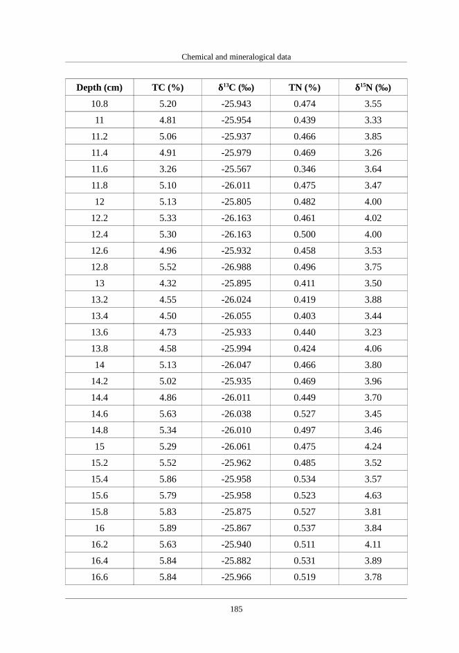
Chemical and mineralogical data
Depth (cm) TC (%) δ13C (‰) TN (%) δ15N (‰)
10.8 5.20 -25.943 0.474 3.55
11 4.81 -25.954 0.439 3.33
11.2 5.06 -25.937 0.466 3.85
11.4 4.91 -25.979 0.469 3.26
11.6 3.26 -25.567 0.346 3.64
11.8 5.10 -26.011 0.475 3.47
12 5.13 -25.805 0.482 4.00
12.2 5.33 -26.163 0.461 4.02
12.4 5.30 -26.163 0.500 4.00
12.6 4.96 -25.932 0.458 3.53
12.8 5.52 -26.988 0.496 3.75
13 4.32 -25.895 0.411 3.50
13.2 4.55 -26.024 0.419 3.88
13.4 4.50 -26.055 0.403 3.44
13.6 4.73 -25.933 0.440 3.23
13.8 4.58 -25.994 0.424 4.06
14 5.13 -26.047 0.466 3.80
14.2 5.02 -25.935 0.469 3.96
14.4 4.86 -26.011 0.449 3.70
14.6 5.63 -26.038 0.527 3.45
14.8 5.34 -26.010 0.497 3.46
15 5.29 -26.061 0.475 4.24
15.2 5.52 -25.962 0.485 3.52
15.4 5.86 -25.958 0.534 3.57
15.6 5.79 -25.958 0.523 4.63
15.8 5.83 -25.875 0.527 3.81
16 5.89 -25.867 0.537 3.84
16.2 5.63 -25.940 0.511 4.11
16.4 5.84 -25.882 0.531 3.89
16.6 5.84 -25.966 0.519 3.78
185

NAO imprints in the Central Iberian Peninsula for the last two millennia
Depth (cm) TC (%) δ13C (‰) TN (%) δ15N (‰)
16.8 5.96 -25.821 0.531 4.06
17 5.35 -25.949 0.481 4.46
17.2 6.16 -25.954 0.559 3.84
17.4 5.45 -25.912 0.511 4.11
17.6 5.86 -25.911 0.531 3.52
17.8 5.72 -25.881 0.514 3.77
18 6.22 -27.667 0.524 4.59
18.2 5.72 -25.875 0.513 3.72
18.4 5.68 -25.918 0.514 3.88
18.6 5.04 -25.941 0.456 3.62
18.8 5.69 -25.858 0.528 3.78
19 5.59 -25.968 0.509 4.06
19.2 5.91 -25.955 0.547 3.92
19.4 6.10 -25.847 0.546 3.99
19.6 5.85 -25.891 0.529 3.44
19.8 5.86 -25.884 0.543 3.93
20 6.21 -25.902 0.530 3.56
20.2 5.17 -25.980 0.447 3.74
20.4 5.24 -25.956 0.478 4.05
20.6 5.03 -26.026 0.461 3.74
20.8 4.82 -25.838 0.437 4.54
21 4.74 -25.996 0.449 3.93
21.2 5.24 -25.950 0.473 4.02
21.4 5.03 -25.872 0.473 3.61
21.6 6.20 -25.938 0.563 3.82
21.8 5.21 -25.787 0.476 4.16
22 5.29 -26.092 0.469 4.00
22.2 4.87 -26.112 0.446 3.53
22.4 5.26 -25.831 0.491 4.07
22.6 1.96 -25.876 0.214 2.61
186

Chemical and mineralogical data
Depth (cm) TC (%) δ13C (‰) TN (%) δ15N (‰)
22.8 4.07 -25.974 0.366 3.27
23 2.31 -25.691 0.227 3.62
23.2 3.57 -25.887 0.328 3.60
23.4 3.79 -25.973 0.354 3.83
23.6 5.35 -25.886 0.489 4.27
23.8 5.55 -26.030 0.510 4.12
24 5.21 -26.020 0.467 3.91
24.2 5.60 -25.945 0.499 3.83
24.4 5.50 -25.984 0.491 4.03
24.6 5.29 -26.011 0.478 4.30
24.8 5.44 -25.840 0.495 4.00
25 5.19 -25.917 0.479 3.84
25.2 5.09 -25.908 0.454 3.72
25.4 5.10 -25.846 0.443 4.28
25.6 5.53 -25.814 0.488 4.33
25.8 5.59 -25.945 0.495 3.96
26 5.29 -25.855 0.447 4.05
26.2 5.00 -25.941 0.435 3.70
26.4 5.00 -25.988 0.407 3.80
26.6 5.02 -25.928 0.444 3.41
26.8 4.56 -25.803 0.383 3.78
27 4.98 -25.816 0.412 3.89
27.2 4.44 -25.865 0.380 3.34
27.4 4.86 -26.006 0.415 4.06
27.6 3.86 -25.836 0.319 3.26
27.8 2.62 -25.529 0.229 4.16
28 3.53 -25.633 0.293 3.76
28.2 2.94 -25.619 0.238 3.83
28.4 2.64 -25.711 0.218 3.04
28.6 2.64 -25.389 0.216 3.49
187

NAO imprints in the Central Iberian Peninsula for the last two millennia
Depth (cm) TC (%) δ13C (‰) TN (%) δ15N (‰)
28.8 2.11 -25.490 0.177 3.13
29 2.97 -25.601 0.249 3.52
29.2 4.18 -25.854 0.356 3.87
29.4 3.54 -25.742 0.302 4.02
29.6 4.31 -25.804 0.374 3.83
29.8 3.92 -25.805 0.343 3.27
30 4.27 -25.559 0.362 3.87
30.2 3.42 -25.711 0.286 3.71
30.4 5.08 -26.752 0.352 3.79
30.6 4.20 -25.665 0.356 3.93
30.8 4.31 -25.764 0.362 4.18
31 3.87 -25.694 0.330 3.24
31.2 4.20 -25.647 0.355 3.78
31.4 4.08 -25.600 0.344 3.83
31.6 3.60 -25.634 0.305 3.42
31.8 3.65 -25.589 0.307 3.44
32 3.75 -25.618 0.328 3.93
32.2 3.60 -25.764 0.310 3.47
32.4 3.53 -25.736 0.293 3.91
32.6 3.26 -25.740 0.286 3.93
32.8 4.04 -25.297 0.268 3.23
33 2.98 -25.750 0.259 3.89
33.2 3.03 -25.416 0.272 3.85
33.4 3.39 -25.637 0.296 3.68
33.6 3.46 -25.625 0.275 3.97
33.8 3.62 -25.616 0.308 3.70
34 3.59 -25.650 0.299 3.40
34.2 3.54 -25.602 0.296 3.40
34.4 2.78 -25.566 0.236 3.03
34.6 3.49 -25.675 0.288 4.16
188

Chemical and mineralogical data
Depth (cm) TC (%) δ13C (‰) TN (%) δ15N (‰)
34.8 3.61 -25.680 0.301 3.49
35 4.37 -25.773 0.391 4.03
35.2 3.76 -25.560 0.335 3.68
35.4 4.10 -25.855 0.355 3.95
35.6 4.49 -25.690 0.400 4.04
35.8 4.20 -25.642 0.377 4.43
36 5.31 -25.846 0.459 4.26
36.2 5.47 -25.768 0.484 4.21
36.4 5.10 -25.737 0.450 4.19
36.6 5.13 -25.692 0.451 4.14
36.8 5.27 -25.623 0.453 4.35
37 5.18 -25.710 0.449 4.13
37.5 4.95 -25.665 0.437 3.69
38 4.93 -25.800 0.433 3.91
38.5 4.97 -25.762 0.436 3.97
39 4.69 -25.793 0.400 3.58
39.5 5.11 -25.672 0.444 3.89
40 5.04 -25.572 0.458 4.33
40.5 4.93 -25.632 0.437 4.00
41 5.18 -25.691 0.451 4.74
41.5 5.10 -25.785 0.434 3.88
42 4.85 -25.749 0.425 3.67
42.5 4.79 -25.765 0.421 4.11
43 4.95 -25.701 0.442 3.77
43.5 4.54 -25.611 0.388 3.79
44 4.59 -25.7 0.410 3.60
44.5 4.83 -25.733 0.428 3.62
45 4.99 -25.614 0.442 3.88
45.5 4.87 -25.648 0.454 4.42
46 5.05 -25.663 0.442 3.93
189

NAO imprints in the Central Iberian Peninsula for the last two millennia
Depth (cm) TC (%) δ13C (‰) TN (%) δ15N (‰)
46.5 4.23 -25.619 0.376 3.49
47 4.44 -25.630 0.401 3.59
47.5 4.94 -25.798 0.433 3.16
48 4.25 -25.669 0.386 3.96
48.5 5.62 -25.701 0.503 4.20
49 5.20 -25.574 0.457 4.04
49.5 4.95 -25.713 0.439 3.99
50 5.08 -25.736 0.441 3.74
50.5 5.39 -25.756 0.456 4.01
51 4.74 -25.634 0.426 3.57
51.5 4.90 -25.682 0.449 3.71
52 5.20 -25.742 0.453 3.81
52.5 4.81 -25.691 0.429 3.66
53 4.82 -25.694 0.409 3.68
53.5 4.56 -25.664 0.403 4.29
54 4.58 -25.630 0.411 4.56
54.5 4.87 -25.700 0.430 3.63
55 4.81 -25.787 0.408 3.89
55.5 4.18 -25.692 0.384 3.20
56 3.82 -25.494 0.326 3.72
56.5 3.09 -25.482 0.277 3.24
Table B.2. Geochemical proxies analysed CIM12-04A core: TC, TN, (in percentages), δ 13C and δ 15N(in ‰).
Depth (cm) TC (%) δ13C (‰) TN (%) δ15N (‰)
0 5.67 -24.74 0.63 0.41
0.2 6.22 -25.35 0.57 0.51
0.4 7.72 -26.18 0.53 0.66
190

Chemical and mineralogical data
Depth (cm) TC (%) δ13C (‰) TN (%) δ15N (‰)
0.6 5.51 -24.41 0.59 0.44
0.8 5.36 -24.38 0.57 -0.20
1 5.26 -24.22 0.55 0.24
1.2 5.00 -24.41 0.52 0.02
1.4 4.94 -24.25 0.50 0.82
1.6 4.86 -24.43 0.51 0.34
1.8 4.62 -24.27 0.48 0.41
2 4.10 -24.10 0.40 1.30
2.2 4.43 -23.98 0.48 0.93
2.4 4.69 -24.07 0.50 0.74
2.6 4.62 -24.42 0.49 0.44
2.8 4.13 -24.29 0.44 0.27
3 5.32 -24.49 0.52 0.52
3.2 3.55 -24.38 0.35 0.76
3.4 3.63 -24.25 0.36 1.34
3.6 3.97 -24.22 0.41 0.90
3.8 4.03 -24.31 0.41 1.25
4 3.80 -24.24 0.38 1.30
4.2 3.82 -24.31 0.40 1.83
4.4 3.80 -24.33 0.38 1.46
4.6 3.24 -24.26 0.31 1.42
4.8 3.24 -24.17 0.32 0.91
5 3.16 -24.03 0.31 1.59
5.2 2.96 -24.29 0.29 1.14
5.4 2.96 -24.27 0.28 2.27
5.6 3.14 -24.03 0.30 2.30
5.8 3.46 -24.22 0.34 2.05
6 3.57 -24.29 0.34 2.18
6.2 3.64 -24.29 0.35 1.67
6.4 3.40 -24.27 0.34 1.58
191
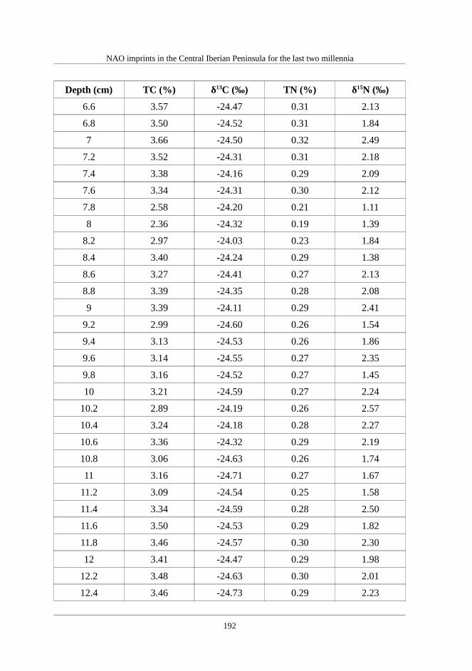
NAO imprints in the Central Iberian Peninsula for the last two millennia
Depth (cm) TC (%) δ13C (‰) TN (%) δ15N (‰)
6.6 3.57 -24.47 0.31 2.13
6.8 3.50 -24.52 0.31 1.84
7 3.66 -24.50 0.32 2.49
7.2 3.52 -24.31 0.31 2.18
7.4 3.38 -24.16 0.29 2.09
7.6 3.34 -24.31 0.30 2.12
7.8 2.58 -24.20 0.21 1.11
8 2.36 -24.32 0.19 1.39
8.2 2.97 -24.03 0.23 1.84
8.4 3.40 -24.24 0.29 1.38
8.6 3.27 -24.41 0.27 2.13
8.8 3.39 -24.35 0.28 2.08
9 3.39 -24.11 0.29 2.41
9.2 2.99 -24.60 0.26 1.54
9.4 3.13 -24.53 0.26 1.86
9.6 3.14 -24.55 0.27 2.35
9.8 3.16 -24.52 0.27 1.45
10 3.21 -24.59 0.27 2.24
10.2 2.89 -24.19 0.26 2.57
10.4 3.24 -24.18 0.28 2.27
10.6 3.36 -24.32 0.29 2.19
10.8 3.06 -24.63 0.26 1.74
11 3.16 -24.71 0.27 1.67
11.2 3.09 -24.54 0.25 1.58
11.4 3.34 -24.59 0.28 2.50
11.6 3.50 -24.53 0.29 1.82
11.8 3.46 -24.57 0.30 2.30
12 3.41 -24.47 0.29 1.98
12.2 3.48 -24.63 0.30 2.01
12.4 3.46 -24.73 0.29 2.23
192

Chemical and mineralogical data
Depth (cm) TC (%) δ13C (‰) TN (%) δ15N (‰)
12.6 3.42 -24.39 0.29 1.96
12.8 3.34 -24.40 0.28 1.93
13 3.25 -24.56 0.31 3.02
13.2 3.26 -24.42 0.31 2.23
13.4 3.23 -24.47 0.31 2.40
13.6 2.93 -24.43 0.28 2.18
13.8 2.44 -24.39 0.24 2.26
14 2.25 -24.37 0.24 1.86
14.2 2.55 -24.74 0.27 1.77
14.4 2.47 -24.61 0.24 1.83
14.6 2.60 -24.61 0.26 3.04
14.8 2.55 -24.60 0.26 2.30
15 2.59 -24.60 0.26 2.11
15.2 2.72 -24.51 0.26 2.64
15.4 2.73 -24.64 0.27 2.20
15.6 2.83 -24.52 0.27 2.55
15.8 2.94 -24.53 0.29 3.10
16 2.90 -24.43 0.28 2.84
16.2 2.89 -24.45 0.28 2.99
16.4 3.00 -24.30 0.29 2.71
16.6 3.15 -24.38 0.31 2.05
16.8 2.71 -24.40 0.27 2.26
17 2.81 -24.42 0.28 2.18
17.2 2.88 -24.36 0.29 3.19
17.4 2.77 -24.42 0.28 2.24
17.6 2.60 -24.59 0.26 2.29
17.8 2.63 -24.40 0.27 2.86
18 2.61 -24.42 0.26 2.46
18.2 2.55 -24.51 0.26 1.96
18.4 2.37 -24.49 0.24 2.05
193

NAO imprints in the Central Iberian Peninsula for the last two millennia
Depth (cm) TC (%) δ13C (‰) TN (%) δ15N (‰)
18.6 2.81 -24.54 0.28 2.37
18.8 2.78 -24.51 0.29 2.48
19 2.54 -24.56 0.27 1.26
19.2 2.59 -24.63 0.26 2.85
19.4 2.56 -24.67 0.27 2.46
19.6 2.70 -24.68 0.29 2.58
19.8 2.61 -24.50 0.28 2.33
20 2.56 -24.54 0.27 2.67
20.2 2.19 -24.56 0.23 2.13
20.4 1.85 -24.72 0.20 1.12
20.6 1.65 -24.62 0.18 2.29
20.8 1.85 -24.55 0.20 2.37
21 2.45 -24.60 0.26 2.35
21.2 2.30 -24.67 0.24 1.41
21.4 2.06 -24.58 0.22 1.83
21.6 2.43 -24.64 0.26 1.99
21.8 2.52 -24.65 0.26 2.13
22 2.92 -24.77 0.30 2.37
22.2 2.96 -24.77 0.30 2.57
22.4 3.05 -24.72 0.31 2.33
22.6 3.22 -24.67 0.29 3.18
22.8 3.22 -24.65 0.36 1.72
23 3.07 -24.77 0.32 2.37
23.2 3.26 -24.83 0.33 2.28
23.4 3.26 -24.86 0.33 2.19
23.6 3.25 -24.95 0.34 1.58
23.8 3.33 -24.81 0.33 2.69
24 3.47 -24.76 0.34 2.49
24.2 3.40 -24.94 0.33 2.79
24.4 3.30 -24.84 0.33 2.60
194

Chemical and mineralogical data
Depth (cm) TC (%) δ13C (‰) TN (%) δ15N (‰)
24.6 3.34 -24.81 0.32 2.87
24.8 3.32 -24.81 0.32 2.61
25 3.30 -24.88 0.32 2.37
25.2 3.48 -24.90 0.35 2.85
25.4 3.12 -24.92 0.31 2.55
25.6 3.37 -25.01 0.34 2.44
25.8 3.20 -24.83 0.32 2.70
26 3.39 -24.83 0.34 2.35
26.2 3.49 -24.76 0.35 2.34
26.4 3.42 -24.71 0.34 2.55
26.6 3.50 -24.79 0.34 2.69
26.8 3.62 -24.82 0.36 2.89
27 3.39 -24.77 0.33 2.92
27.2 3.53 -25.03 0.33 2.94
27.4 3.39 -24.93 0.34 3.00
27.6 3.49 -24.90 0.34 2.85
27.8 3.27 -24.90 0.32 2.70
28 3.19 -24.89 0.32 2.79
28.2 3.27 -24.83 0.32 2.80
28.4 3.30 -24.70 0.33 2.96
28.6 3.32 -24.90 0.33 2.84
28.8 3.46 -24.79 0.34 2.80
29 3.30 -25.08 0.33 3.37
29.2 3.00 -24.90 0.31 2.52
29.4 3.14 -24.89 0.31 2.59
29.6 3.24 -24.84 0.32 2.56
29.8 4.06 -25.15 0.36 3.02
30 3.40 -24.89 0.34 2.90
30.2 3.92 -25.15 0.37 2.52
30.4 3.41 -24.84 0.34 2.50
195

NAO imprints in the Central Iberian Peninsula for the last two millennia
Depth (cm) TC (%) δ13C (‰) TN (%) δ15N (‰)
30.6 3.53 -25.00 0.34 2.77
30.8 3.51 -25.02 0.34 2.84
31 3.21 -24.86 0.32 2.44
31.2 3.29 -24.94 0.33 2.55
31.4 3.26 -24.98 0.33 2.10
31.6 3.57 -24.80 0.36 2.32
31.8 3.05 -24.74 0.31 2.38
32 3.09 -24.81 0.30 2.98
32.2 3.22 -24.88 0.32 3.05
32.4 3.48 -25.17 0.32 2.38
32.6 3.27 -24.85 0.33 3.01
32.8 3.27 -24.87 0.32 2.41
33 3.30 -24.93 0.33 3.07
33.2 3.16 -24.88 0.31 2.86
33.4 3.73 -25.11 0.35 2.56
33.6 3.51 -25.13 0.34 3.04
33.8 3.48 -25.25 0.32 2.95
34 3.64 -25.03 0.33 2.97
34.2 3.51 -25.00 0.33 2.96
34.4 3.32 -25.01 0.30 3.17
34.6 3.23 -25.12 0.32 2.62
34.8 3.80 -25.11 0.37 2.96
35 3.59 -25.32 0.33 3.61
35.2 3.97 -25.21 0.37 3.31
35.4 3.34 -25.36 0.32 3.69
35.6 3.22 -25.35 0.31 3.46
35.8 2.82 -25.46 0.27 2.51
36 2.79 -25.46 0.27 3.23
36.5 3.28 -25.35 0.31 2.74
37 3.63 -25.42 0.36 3.31
196

Chemical and mineralogical data
Depth (cm) TC (%) δ13C (‰) TN (%) δ15N (‰)
37.5 3.90 -25.34 0.38 2.90
38 4.39 -25.44 0.40 2.93
38.5 4.42 -25.36 0.42 3.22
39 4.13 -25.25 0.39 3.00
39.5 3.71 -25.26 0.36 3.12
40 3.72 -25.17 0.36 2.66
40.5 3.93 -25.26 0.37 2.30
41 3.88 -25.19 0.38 2.44
41.5 3.60 -25.28 0.35 2.52
42 4.19 -25.37 0.40 2.46
42.5 3.75 -25.41 0.37 3.15
43 3.18 -25.37 0.32 2.77
43.5 3.00 -25.26 0.30 2.81
44 3.52 -25.34 0.34 3.21
44.5 3.53 -25.17 0.34 3.02
45 2.76 -25.14 0.28 2.82
45.5 1.85 -25.03 0.18 2.59
46 3.80 -25.26 0.37 2.71
46.5 4.06 -25.33 0.39 2.99
47 4.09 -25.23 0.38 2.42
47.5 3.71 -25.10 0.36 2.97
48 2.88 -25.04 0.29 2.32
48.5 3.70 -25.05 0.37 2.16
49 3.89 -25.06 0.40 2.51
49.5 3.67 -24.94 0.36 2.62
50 3.61 -24.96 0.37 2.52
50.5 3.80 -24.95 0.38 2.11
51 3.58 -25.12 0.35 1.91
51.5 3.54 -24.99 0.36 2.44
52 2.94 -24.81 0.29 2.19
197

NAO imprints in the Central Iberian Peninsula for the last two millennia
Depth (cm) TC (%) δ13C (‰) TN (%) δ15N (‰)
52.5 3.30 -25.02 0.31 1.80
53 3.70 -24.83 0.37 2.28
53.5 3.56 -24.85 0.36 2.50
54 4.01 -24.78 0.42 2.23
54.5 3.73 -24.69 0.38 2.66
55 3.98 -24.92 0.40 2.56
55.5 3.90 -24.74 0.39 2.83
56 4.23 -25.03 0.42 3.00
56.5 4.20 -25.44 0.40 2.44
57 4.04 -25.11 0.41 2.11
57.5 4.92 -25.70 0.48 2.82
58 4.69 -25.58 0.45 2.80
58.5 4.78 -25.53 0.46 2.84
59 4.46 -25.16 0.43 2.96
59.5 4.17 -25.17 0.40 2.70
60 3.67 -25.01 0.37 2.87
60.5 3.14 -25.07 0.31 2.08
61 3.42 -25.12 0.35 2.14
61.5 3.83 -25.14 0.39 2.44
62 3.88 -25.06 0.38 2.16
62.5 3.10 -25.12 0.30 2.27
63 4.04 -25.06 0.38 2.61
63.5 4.44 -24.97 0.41 2.57
64 4.24 -25.04 0.41 2.91
64.5 4.13 -24.96 0.40 2.81
65 4.15 -25.02 0.39 2.95
65.5 3.23 -24.96 0.31 2.82
66 3.68 -24.79 0.34 2.49
66.5 3.92 -24.94 0.42 2.94
67 3.96 -25.03 0.38 2.46
198

Chemical and mineralogical data
Depth (cm) TC (%) δ13C (‰) TN (%) δ15N (‰)
67.5 4.25 -25.02 0.40 2.44
68 4.38 -25.10 0.42 2.33
68.5 3.73 -24.97 0.35 2.62
69 4.47 -24.97 0.42 2.40
69.5 4.57 -25.08 0.43 2.16
70 4.23 -25.02 0.39 1.97
70.5 3.75 -24.78 0.37 2.41
71 3.65 -24.86 0.34 2.19
71.5 3.38 -24.62 0.33 2.26
72 3.41 -24.63 0.34 1.93
72.5 2.69 -24.57 0.27 2.08
73 1.17 -24.99 0.13 1.44
73.5 1.67 -24.93 0.18 1.73
74 3.85 -25.02 0.38 1.90
74.5 3.23 -25.03 0.31 2.56
75 3.06 -25.04 0.31 2.19
75.5 3.37 -24.86 0.33 2.29
76 3.01 -24.77 0.29 2.50
76.5 3.09 -24.69 0.31 2.47
77 3.07 -24.82 0.29 2.10
77.5 1.93 -25.04 0.20 2.18
78 2.31 -24.80 0.22 2.19
78.5 3.32 -24.87 0.32 2.74
79 3.18 -24.72 0.35 2.11
79.5 2.67 -24.68 0.28 1.97
80 2.77 -24.79 0.28 2.60
80.5 3.76 -24.85 0.38 3.01
81 3.61 -24.74 0.36 2.09
81.5 3.65 -24.85 0.36 2.40
82 3.85 -24.71 0.37 2.60
199

NAO imprints in the Central Iberian Peninsula for the last two millennia
Depth (cm) TC (%) δ13C (‰) TN (%) δ15N (‰)
82.5 3.83 -24.64 0.37 2.64
83 4.07 -24.75 0.40 2.31
83.5 4.01 -24.65 0.43 1.99
84 4.20 -24.67 0.42 2.07
84.5 4.23 -24.65 0.43 1.82
85 4.31 -24.51 0.44 2.42
85.5 3.28 -24.69 0.33 2.27
86 2.62 -24.75 0.27 1.71
86.5 3.08 -25.13 0.32 2.51
87 3.58 -25.13 0.35 2.53
87.5 3.67 -25.01 0.36 2.42
88 3.82 -25.18 0.36 2.60
88.5 3.83 -25.06 0.37 3.00
89 3.95 -25.04 0.39 2.88
89.5 3.87 -24.91 0.37 2.58
90 3.42 -24.79 0.35 2.55
90.5 4.22 -24.87 0.42 2.48
91 4.55 -24.96 0.45 2.55
91.5 4.43 -24.81 0.43 2.53
92 4.31 -24.85 0.41 2.88
92.5 3.72 -24.78 0.37 2.51
93 3.09 -24.84 0.30 2.40
93.5 3.73 -24.99 0.37 2.49
94 3.84 -24.87 0.38 2.56
94.5 4.13 -24.75 0.41 3.00
95 2.81 -24.76 0.28 2.91
95.5 3.46 -25.02 0.35 2.40
96 3.62 -24.90 0.35 2.73
96.5 3.33 -24.96 0.32 2.81
97 3.34 -25.02 0.31 2.67
200

Chemical and mineralogical data
Depth (cm) TC (%) δ13C (‰) TN (%) δ15N (‰)
97.5 3.53 -24.79 0.33 2.62
98 3.10 -24.96 0.30 3.01
98.5 3.39 -25.07 0.34 2.99
99 4.22 -25.34 0.40 3.10
99.5 4.49 -25.24 0.43 3.27
100 4.45 -25.14 0.43 3.03
100.5 4.04 -25.14 0.39 2.94
101 – – – –
101.5 – – – –
102 – – – –
102.5 – – – –
103 – – – –
103.5 – – – –
104 – – – –
104.5 – – – –
105 – – – –
105.5 4.44 -25.66 0.40 2.88
106 5.05 -25.78 0.45 3.16
106.5 4.73 -25.63 0.44 2.97
107 4.88 -25.58 0.46 2.87
107.5 4.65 -25.26 0.43 2.60
108 4.16 -25.19 0.40 2.40
108.5 4.56 -25.31 0.42 2.67
109 4.73 -25.32 0.44 2.60
109.5 3.82 -25.08 0.37 2.48
110 4.15 -25.34 0.39 2.79
110.5 5.25 -25.36 0.49 2.54
111 4.95 -25.17 0.47 2.90
111.5 3.33 -25.14 0.33 1.87
201

NAO imprints in the Central Iberian Peninsula for the last two millennia
Depth (cm) TC (%) δ13C (‰) TN (%) δ15N (‰)
112 3.04 -25.01 0.28 2.91
112.5 6.59 -25.29 0.97 -8.77
113 4.32 -24.95 0.42 2.44
113.5 4.20 -25.06 0.40 2.65
114 4.32 -25.18 0.41 2.55
114.5 3.70 -25.12 0.36 2.29
115 3.22 -25.24 0.31 2.70
115.5 4.20 -25.29 0.41 2.41
116 4.05 -25.21 0.39 2.34
116.5 3.90 -25.21 0.37 2.58
117 3.84 -25.12 0.37 2.65
117.5 1.79 -25.35 0.18 2.07
118 3.41 -25.27 0.32 2.04
118.5 2.90 -25.22 0.27 1.82
119 3.17 -25.34 0.31 2.42
119.5 3.79 -25.31 0.36 2.54
120 3.91 -25.24 0.37 2.76
120.5 3.78 -25.09 0.36 2.52
121 3.68 -25.02 0.35 2.67
121.5 4.00 -25.32 0.36 2.90
122 4.23 -25.16 0.38 2.37
122.5 3.78 -24.92 0.36 2.72
123 4.06 -24.92 0.38 2.52
123.5 3.71 -24.85 0.38 2.06
124 4.23 -24.82 0.41 2.65
124.5 4.85 -24.93 0.47 2.46
125 3.06 -25.23 0.30 2.04
202

Chemical and mineralogical data
Table B.3. Chemical elements XRF core-scanner measurements from PE12-01-01 core (in cps).
Depth(mm)
Al Si K Ca Ti V Cr Mn Fe Zn Rb Sr Zr
25 977 33309 20773 9023 10844 1632 1350 2120 132416 939 4764 2740 7374
26 1037 33250 21083 9367 10516 1385 1030 2567 132692 977 4752 3012 7756
28 759 31456 22747 9767 13511 1414 1454 2358 156390 979 5172 3212 9899
30 751 31829 27055 10769 15257 1669 1081 1953 163673 997 5198 3166 11496
32 1371 39020 30380 11585 16810 1504 1003 2367 174093 1124 5681 3523 8019
34 1690 43868 35197 12957 18090 1708 1275 2274 178984 1092 5703 3555 9445
36 1919 47674 40699 13559 20882 1748 1591 2485 201596 1146 5727 3592 9078
38 1749 46190 36428 12730 18300 1905 1254 2023 185695 1105 5737 3295 8080
40 1462 44221 35574 12085 17902 1966 1348 2353 181137 1068 5714 3479 8674
42 1493 43837 33887 12237 17849 1813 2045 2621 176769 1165 5364 3695 9902
44 1550 46204 35698 13038 17666 1517 1312 1876 178231 1011 5648 3824 9344
46 1630 43803 36544 12964 19183 1977 963 2097 181274 1098 5868 3729 10830
48 1395 41297 33681 13623 18084 1801 1792 2746 177558 1102 5662 3541 9065
50 1323 40796 33934 12157 16942 1966 1390 2019 173454 1178 5455 3161 9908
52 1266 37951 28874 11170 15460 1907 1291 2224 167462 1068 5157 3356 9022
54 1648 41372 28477 10837 14405 2096 1520 1933 151886 1001 5024 3002 8930
56 1348 38206 23974 9611 12044 1378 1577 1623 137718 1023 5028 3077 7067
58 1389 39797 29886 11250 15579 1482 1499 2241 167009 1030 5060 3288 9093
60 1889 46458 37684 13016 19514 1555 1367 2267 193402 1105 5529 3219 9520
62 1459 42131 35864 12097 17581 1758 1116 2025 182401 1030 5161 2942 9168
64 1711 44464 32902 11865 16862 1690 1733 2283 171862 1002 4922 3060 8504
66 1805 47026 37644 13490 17542 1586 1251 2366 175962 1109 5195 3092 7945
68 1663 44511 38029 13384 18288 1993 1118 2695 182561 1208 5189 3026 10465
70 1819 46463 36875 13452 18893 1677 1525 2055 188344 1174 5455 3169 9194
72 1583 42743 30839 12311 17076 1903 1065 2053 173450 1092 5204 3135 9946
74 877 34301 22809 9579 12605 1054 395 1811 153404 1078 5221 3121 8800
76 1366 40764 30394 11213 15316 1841 1606 2343 166103 1035 5158 3047 9211
78 1311 41427 32221 12137 16086 1852 1675 1850 171145 1069 5102 3214 10085
80 1457 42246 33892 12307 16771 2139 1660 1926 178958 1139 5455 3226 11395
82 1550 42421 33107 12184 17210 1721 1574 2159 180224 1098 5317 3242 9198
84 1251 40152 31896 11550 16566 1774 1213 1946 176261 1113 5387 3005 10208
86 1786 44962 35976 13183 18540 1573 1784 2450 192087 1085 5463 3131 10566
88 1772 42856 33936 12924 18559 1800 1303 2285 192081 1088 5516 3336 10958
90 1712 44088 34010 12213 17799 1469 1237 2035 185143 1104 5256 2943 9624
203
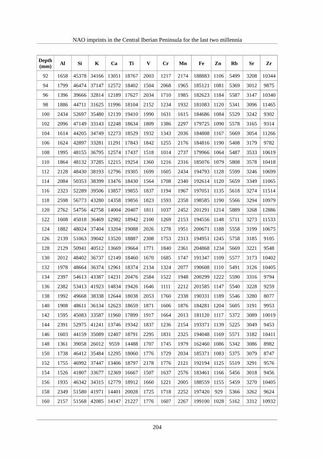
NAO imprints in the Central Iberian Peninsula for the last two millennia
Depth(mm)
Al Si K Ca Ti V Cr Mn Fe Zn Rb Sr Zr
92 1658 45378 34166 13051 18767 2003 1217 2174 188883 1106 5499 3208 10344
94 1799 46474 37147 12572 18402 1504 2068 1965 185121 1081 5369 3012 9875
96 1396 39666 32814 12189 17627 2034 1710 1985 182623 1184 5587 3147 10340
98 1886 44711 31625 11996 18104 2152 1234 1932 181083 1120 5341 3096 11465
100 2434 52697 35480 12139 19410 1990 1631 1615 184686 1084 5529 3242 9302
102 2096 47149 33143 12248 18634 1809 1386 2297 179725 1090 5578 3165 9314
104 1614 44205 34749 12273 18529 1932 1343 2036 184808 1167 5669 3054 11266
106 1624 42897 33281 11291 17843 1842 1255 2176 184816 1190 5408 3179 9782
108 1995 48155 36795 12574 17437 1518 1014 2737 179966 1064 5487 3533 10619
110 1864 48132 37285 12215 19254 1360 1216 2316 185076 1079 5808 3578 10418
112 2128 48430 38193 12796 19305 1699 1605 2434 194793 1128 5599 3246 10699
114 2084 50353 38399 13476 18430 1564 1708 2340 192614 1120 5659 3349 11065
116 2323 52289 39506 13857 19855 1837 1194 1967 197051 1135 5618 3274 11514
118 2598 56773 43280 14358 19856 1823 1593 2358 198585 1190 5566 3294 10979
120 2762 54756 42758 14004 20407 1811 1037 2452 201291 1214 5889 3268 12886
122 1608 45018 36469 12982 18942 2100 1269 2153 194556 1148 5711 3273 11533
124 1882 48024 37404 13204 19088 2026 1278 1951 200671 1188 5558 3199 10675
126 2139 51063 39042 13520 18887 2308 1753 2313 194951 1245 5758 3185 9105
128 2129 50941 40512 13669 19664 1771 1840 2361 204868 1234 5669 3221 9548
130 2012 48402 36737 12149 18460 1670 1685 1747 191347 1109 5577 3173 10402
132 1978 48664 36374 12961 18374 2134 1324 2077 190608 1110 5491 3126 10405
134 2397 54613 43387 14231 20476 2584 1522 1948 200299 1222 5590 3316 9794
136 2382 53413 41923 14834 19426 1646 1111 2212 201585 1147 5540 3228 9259
138 1992 49668 38338 12644 18038 2053 1760 2338 190331 1189 5546 3280 8077
140 1908 48611 36134 12623 18659 1871 1606 1876 184281 1204 5605 3191 9953
142 1595 45083 33587 11960 17899 1917 1664 2013 181120 1117 5372 3089 10019
144 2391 52975 41241 13746 19342 1837 1236 2154 193371 1139 5225 3049 9453
146 1603 44159 35089 12407 18791 2295 1831 2325 194048 1169 5571 3182 10411
148 1361 39058 26012 9559 14488 1707 1745 1979 162460 1086 5342 3086 8982
150 1738 46412 35484 12295 18060 1776 1729 2034 185371 1083 5375 3079 8747
152 1755 46992 37447 13406 18797 2178 1776 2121 192194 1125 5519 3291 9576
154 1526 41807 33677 12369 16667 1507 1637 2576 183461 1166 5456 3018 9456
156 1935 46342 34315 12779 18912 1660 1221 2005 188559 1155 5459 3270 10405
158 2349 51580 41971 14401 20028 1725 1718 2252 197420 929 5366 3262 9624
160 2157 51568 42085 14147 21227 1776 1607 2267 199100 1028 5162 3312 10932
204

Chemical and mineralogical data
Depth(mm)
Al Si K Ca Ti V Cr Mn Fe Zn Rb Sr Zr
162 2094 49944 38516 14203 20132 1655 1439 2263 195025 1064 5456 3261 11749
164 2026 48896 40476 14118 19546 1938 1922 2514 195280 1057 5306 3151 9537
166 1752 44707 36906 12962 17925 1803 990 1710 186232 1015 5443 3091 9678
168 1735 44985 36505 12646 18213 2059 1387 2144 190702 1094 5289 3099 9464
170 1522 43745 35988 13846 19571 1647 834 2060 194636 1079 5349 3223 9454
172 1596 42022 35998 12801 19321 1733 1655 2492 195014 1111 5635 3360 11034
174 1405 39536 32761 12298 17340 1949 1597 2370 183989 1082 5611 3091 10830
176 1414 40892 33751 12056 16914 1513 1488 2094 171193 1070 5526 3380 9694
178 1513 41369 34815 12189 16308 1533 1476 2210 171732 993 5045 2857 10611
180 1247 39166 30422 11568 16403 1637 1387 2006 176738 1126 5448 3162 12021
182 1152 36112 29161 10679 16466 2212 1507 1771 175745 1092 5525 3171 10968
184 1248 40125 31742 12185 17579 1948 1198 2748 176840 1113 5319 3363 10017
186 1467 40672 33222 11952 17359 1457 839 2219 185205 1156 5626 3514 11022
188 1275 39652 31165 12462 18468 1803 1583 2070 186008 1246 5563 3316 9990
190 1536 41935 34475 12513 17794 1955 1431 1726 186957 1288 5292 3024 12264
192 1267 39232 31676 12245 16869 2320 1152 2151 177892 1150 5519 3396 10893
194 1311 40839 34758 12153 18617 1572 1484 2035 193699 1049 5544 3161 9297
196 1394 41870 32717 12548 17494 1728 1204 1895 183478 1170 5511 3266 9546
198 1333 41147 33278 13063 17728 1960 1273 2413 183578 1137 5426 3289 8774
200 1167 37452 31610 12161 17087 1745 1324 1923 184214 1126 5468 3406 9338
202 1117 35545 28321 10836 15880 1546 1447 1773 169045 1154 5376 3103 10288
204 1290 38357 27964 11236 15178 1572 1686 1788 165587 1128 5582 3421 10019
206 1428 40354 30354 11248 16157 1672 1803 2529 173101 1086 5661 3244 10155
208 1290 40466 31139 11551 15692 1397 1714 2174 168576 1075 5151 3191 9920
210 1179 38264 30639 11257 16238 1538 1272 1967 171755 1035 5590 3398 9831
212 1491 40613 32567 11590 17642 1912 1355 1918 183935 1151 5290 3144 13550
214 1329 39311 33941 13272 17128 2141 1670 2140 191780 1123 5611 3579 11936
216 1663 45246 41852 14605 20061 1679 1503 2115 202482 1012 6720 4692 11371
218 1707 45189 35808 13793 17738 1404 1147 2453 185686 1163 5878 3419 12348
220 2530 51831 41639 15895 19945 1733 1363 2209 195583 1092 5662 3668 11229
222 2029 50420 43427 14825 22112 1982 1543 2589 197661 1173 5747 3695 11076
224 1481 42195 36795 14260 18767 1878 1321 2156 182366 1123 5662 3283 11814
226 1043 37734 30869 11945 16807 1577 1484 2375 173706 1189 5528 3368 11739
228 729 30695 22721 10733 14661 1649 1314 2003 155747 1226 5409 3280 9830
230 458 27733 18479 8198 12528 1921 1144 1917 149850 1122 5282 3123 9197
205

NAO imprints in the Central Iberian Peninsula for the last two millennia
Depth(mm)
Al Si K Ca Ti V Cr Mn Fe Zn Rb Sr Zr
232 1255 40655 27255 11014 13762 1383 894 1720 156716 1176 5356 3197 9805
234 1752 43407 33003 11829 15884 1860 1633 2121 168322 1025 5292 3146 9353
236 1526 40506 29072 10582 14824 2128 1100 1819 158999 1101 5296 3189 8671
238 1190 36392 28401 11284 16107 1910 921 1936 173110 1027 5137 3342 9349
240 1567 41800 34455 13321 17597 1757 917 2432 184526 1187 5569 3443 9023
242 1929 44707 36359 13202 17991 2128 1627 1982 183661 1103 5611 3410 10654
244 1555 44816 36454 12782 18213 2238 1524 2359 187499 1140 5393 3453 13181
246 1859 45301 35860 13031 18865 1842 1111 2211 187440 1096 5728 3105 10793
248 1889 47197 38719 13410 18849 1640 1190 2086 187466 1110 5496 3383 11485
250 1896 48348 38818 13513 19136 1636 1525 2354 191160 1232 5562 3466 10090
252 1958 48631 38850 15700 19171 1394 1558 2151 189910 1126 5634 3366 10757
254 1959 46448 36469 13966 19663 1365 1234 2171 184697 1073 5735 3611 10957
256 1523 41060 33830 12875 17917 1473 1091 1985 177705 1078 5705 3651 9522
258 617 28861 18955 8731 12315 1649 1078 1924 145957 1146 5274 3371 9666
260 693 29602 19011 8212 11543 1627 832 1395 132772 1087 5507 3625 8880
262 978 31616 18414 7882 11168 1659 1024 1830 128639 1065 5129 3199 9709
264 897 31792 16862 7574 9645 1460 572 1735 116375 853 5238 3559 10519
266 915 32858 21284 9283 10524 1297 1029 1928 128632 934 5225 3684 9306
268 1056 34696 21242 9907 11370 1353 961 1321 128345 897 4915 3547 9436
270 1786 43296 33805 12958 16993 1521 2042 1553 169487 936 4992 3469 9703
272 1561 41544 35022 12495 19267 2204 1801 2335 185618 957 6031 4101 9741
274 1594 42598 37149 14550 18627 1737 1537 2234 169962 880 5938 4817 9072
276 1800 46236 40976 15343 18707 2047 1489 2545 185754 959 6323 5345 12067
278 1206 39201 37196 13837 18988 1522 1255 1434 190306 1148 6763 5333 11648
280 1204 36417 34977 13125 18839 2122 1505 2228 184694 1188 6584 5132 8938
282 878 33547 29655 11950 15914 1840 1947 1995 164992 1017 6324 5637 10593
284 1339 39006 30742 11924 16047 1857 1877 2400 155955 929 6079 5674 12056
286 1535 41531 33731 12833 17937 1677 1020 2309 171673 919 5638 4991 9741
288 1565 40477 35536 15676 17927 2011 1144 2150 172522 1020 6752 4707 9139
290 1944 46060 40507 16125 19079 1803 1143 1926 190387 1140 5998 4605 9327
292 1526 39616 31587 12239 15732 1739 1002 1444 163472 1128 6432 4665 10549
294 1797 44402 36343 13764 20098 1985 1577 2198 175952 1028 6064 4985 10291
296 2476 52395 44868 14804 21419 1491 1710 2437 194338 1074 6121 4081 11167
298 2312 52625 45819 15700 21099 1742 1025 2019 193799 1090 6129 4293 11105
300 2305 50128 42100 15133 20389 1638 1763 2012 194441 1195 6187 4013 10001
206

Chemical and mineralogical data
Depth(mm)
Al Si K Ca Ti V Cr Mn Fe Zn Rb Sr Zr
302 2276 50589 45833 15380 22243 1720 1252 2918 209895 1057 6601 3936 10534
304 1997 47549 43984 14428 18908 1608 1443 2975 186644 1089 6160 4543 11284
306 1445 40522 38819 13963 17358 1676 1166 2261 168334 946 6361 4419 10453
308 1819 44579 40396 14215 20380 1844 1481 2446 190788 1018 6694 4472 9629
310 1798 46337 42665 14774 19370 2036 1655 2230 184296 955 6420 5053 10708
312 1620 44824 40780 15876 19634 1877 1220 1896 186473 1044 6341 4564 13899
314 1768 43202 38983 15768 18517 1908 1184 2454 175584 1008 6289 4603 11799
316 1597 41672 35838 13640 18949 1384 1060 2273 184388 952 6200 4101 10217
318 1333 37006 27865 11676 16006 1595 1390 2040 162019 1017 5950 3964 10864
320 1266 37168 26057 10443 12807 1481 1050 1742 129279 1043 6193 4256 10746
322 1606 37989 24669 9907 11651 1168 1691 1265 121343 877 5559 4018 12610
324 1404 37484 28512 10834 13378 1461 1305 1363 135810 890 5483 4052 13004
326 1062 32695 23192 11066 13094 1413 1006 1504 138801 817 5144 4048 11881
328 884 31510 23328 9426 12315 1429 208 1794 134747 902 5390 4428 10047
330 1979 46697 38987 14048 17864 2492 1511 1853 166498 852 6021 4687 9724
332 1606 43132 38853 13296 20195 1433 1554 1894 188093 852 6180 4643 11255
334 1727 43893 37341 14007 18533 1761 1197 2000 181817 1063 6251 4661 12870
336 2238 51996 41925 14056 21351 2374 1660 2345 189154 1045 6425 4837 13551
338 1662 42526 40966 13398 18680 2155 1271 1289 175082 983 6182 4436 13771
340 1565 41342 37181 13160 18204 1453 1276 2101 178833 1035 6606 4839 11147
342 1908 46528 41301 14863 18997 1945 1880 2108 172951 911 6509 4717 10420
344 1960 48621 41696 13885 18805 1579 1700 2157 181012 943 6130 4517 11619
346 1893 46512 40764 13333 19498 1626 1025 1949 188999 969 6292 4217 11913
348 1877 42829 36325 12357 17148 1740 1331 1624 169135 912 6055 3723 10639
350 1866 46656 38638 13100 19805 2328 1275 2518 184028 1009 6272 3714 8445
352 1976 47048 39429 14332 19139 1711 1088 2231 188791 1097 5953 3512 9361
354 1573 42670 38391 13508 19548 2043 1508 2428 193965 1111 6015 3517 11174
356 1581 41128 37061 14751 18569 2261 1155 2304 187902 1169 6247 3621 11750
358 3001 56999 40979 14646 19869 1732 1789 2617 191735 1014 6027 3574 11827
360 1898 45758 38977 14426 19848 2023 1637 2337 196397 1054 6022 3417 11056
362 1649 43015 38215 14155 19467 1616 1895 1682 191735 1206 6289 3681 10642
364 2005 47801 41985 14657 20411 1458 1364 1889 191644 1190 6104 3709 10641
366 1919 45945 37024 13718 19801 2100 1811 2680 194477 1160 6395 3523 11015
368 1995 48548 40911 15008 21349 1902 1681 1752 199087 1172 6331 3861 10193
370 1728 44646 38570 13076 20049 2031 1000 2519 195761 1093 6498 3715 10715
207

NAO imprints in the Central Iberian Peninsula for the last two millennia
Depth(mm)
Al Si K Ca Ti V Cr Mn Fe Zn Rb Sr Zr
372 2125 50297 42628 15510 20731 1651 1523 2017 201886 1154 6277 3765 12063
374 2525 52628 44007 15550 20644 1676 1420 2311 201595 1025 6314 3761 12311
376 2722 56007 48534 16502 21583 1423 1711 2270 207470 1182 6372 3855 11689
378 1968 48286 42446 15360 20077 2008 2430 2142 198142 1075 6353 3752 13378
380 2027 45952 37020 13718 19348 2201 1232 2209 188196 1090 6431 3904 14540
382 1828 43340 35020 13379 19609 2252 1277 1799 189658 1155 6251 3620 10466
384 1304 35678 28728 10676 16297 1995 1052 1961 174718 1088 6304 3476 11201
386 1640 42773 35833 13610 18838 1642 1315 2019 181501 1143 6240 3838 13063
388 1801 44994 37354 13472 18426 1149 1540 2279 187175 1039 6412 3595 11420
390 2149 48506 41158 13877 19754 1893 1500 2540 192285 1082 6240 3792 11920
392 2068 49570 42450 14815 21263 1748 2109 1960 204425 979 6387 3968 12943
394 2254 49292 44146 15056 20934 1888 1265 2019 198016 1128 6561 3861 12453
396 2310 49828 41923 14424 19857 1807 2128 2436 197379 1108 6468 3873 12484
398 2190 49084 41884 15727 20052 2327 1566 1914 194534 1172 6524 3752 12506
400 1699 42463 36079 13533 17516 2057 1227 2036 183266 1052 6263 3836 12622
402 1699 44923 36813 13731 19425 1326 1625 2214 189213 1040 6446 3651 12626
404 2087 47354 37940 13440 18458 1704 1185 2429 189944 1218 6293 3832 11465
406 2188 48951 40050 14032 20045 1459 1284 1540 186651 1079 6413 3778 12031
408 1514 40924 31663 12134 16178 1883 1224 1992 157233 1023 6206 3625 11727
410 1196 34891 21791 8660 10181 1483 1142 1837 120495 1042 5788 3449 11533
412 955 33714 18692 8604 9717 1586 1249 1432 112795 875 5015 3200 10947
414 552 29474 13148 7478 6949 1473 393 1303 87422 804 4633 2764 9494
416 621 29729 13739 6817 6887 1584 950 1536 85924 804 4294 2635 7366
418 622 28680 13153 6641 6201 1178 998 1244 90532 818 4400 2712 7878
420 620 29105 14630 6851 6944 1589 1038 753 89647 827 4563 2788 8437
422 730 28352 14733 7369 8225 1650 1332 1289 100557 823 4580 2865 9896
424 1185 34178 18645 7938 8567 1904 818 896 99083 825 4703 2962 7913
426 1078 33017 20309 8536 10904 1601 1136 1478 109612 873 5128 2870 8533
428 1514 39518 28230 11061 16120 1941 966 1762 158911 938 5611 3380 10035
430 2613 53181 42787 15038 20469 1693 2163 2407 194098 1099 6354 3789 11994
432 2852 57323 47990 17046 21713 1286 949 2708 207313 1071 6641 4096 11303
434 2767 58054 48046 16905 23104 1921 1464 2605 208755 1091 6771 4063 13261
436 2665 55898 47271 16238 22168 2061 1419 2376 201258 1182 6761 4422 12886
438 2212 50947 41258 16196 20211 1993 1529 2302 192638 1060 6827 4299 13311
440 2044 49800 40427 14358 19137 1666 1389 2710 181658 1039 6415 3874 10216
208

Chemical and mineralogical data
Depth(mm)
Al Si K Ca Ti V Cr Mn Fe Zn Rb Sr Zr
442 2175 52766 41615 15904 20213 1530 1509 2446 187848 1046 6099 3707 12683
444 2934 59209 46889 16353 21932 1881 1364 1996 207943 1093 6600 3850 12771
446 2878 60175 48396 16689 21606 1882 1306 2118 206835 1125 6652 3886 12445
448 2929 58441 47455 17020 21622 2188 1758 2223 197065 1072 6428 3882 11557
450 2667 54731 44649 15190 20586 1982 1382 3077 200221 1014 6592 3942 11136
452 3073 61053 49353 16264 21534 2010 1960 2578 201514 1045 6546 3851 11489
454 2861 57063 46196 16337 20768 1928 1783 2159 197667 1124 6490 3912 12804
456 2841 56819 45831 16495 21119 1681 1447 2123 203417 1085 6484 3764 12057
458 3109 59462 48571 17751 22028 2308 1311 2372 202142 1144 6399 3812 12358
460 2569 56619 48045 16593 21900 1824 1672 2513 204417 1170 6536 3749 12085
462 2868 57193 45759 16692 21603 1946 1413 2059 196453 1143 6531 3725 11373
464 3019 62381 50812 17435 22344 2121 1594 2656 207321 1155 6359 3825 12747
466 3029 60980 47434 17331 22399 1727 1363 2963 205421 1111 6443 3831 11654
468 3301 61619 49551 17901 22128 1888 2125 2388 203649 1187 6281 3716 10957
470 2919 57537 46397 17425 22484 1906 1905 2145 203592 1123 6320 3738 12379
472 3356 63158 51083 17426 22523 1372 1714 2005 208157 1191 6547 3642 10861
474 2538 55199 46977 16481 22243 1601 1311 2584 206947 1160 6342 3911 12787
476 3080 59101 49201 17640 22718 1704 1520 2588 211459 1180 6543 3725 12129
478 3375 64589 51831 18159 23373 1881 1813 3012 212114 1221 6615 3714 10128
480 2744 56793 47140 16866 22261 1533 1826 2152 206083 1104 6623 3672 11758
482 2443 52886 44466 15100 21685 2132 1720 1983 202429 1166 6407 3713 10757
484 3089 57214 47725 16023 22835 1946 1663 2522 205135 1203 6485 3750 10482
486 2913 57752 47075 15867 23120 2231 2097 2200 203993 1183 6512 4021 10539
488 2531 53809 46346 16383 22000 1648 2031 2765 204541 1161 6588 3850 12782
490 2442 52231 42602 15839 22181 2221 1841 2452 200963 1218 6457 3957 11543
492 2484 51847 42277 15414 21262 2094 1620 2978 204373 1132 6516 3786 11863
494 2386 49704 38338 14604 18987 1623 1404 2723 196059 1189 6446 3850 11173
496 1942 45837 36985 14536 19572 1941 1481 2222 190917 1158 6273 3924 11834
498 1186 36665 29272 12024 17724 2033 1150 1882 182840 1067 6455 3820 11122
500 1926 45749 35486 13930 18450 1780 1552 1852 183311 1107 6255 3814 11483
502 2033 46365 34449 12797 18086 1861 1511 2110 177382 1106 6465 3888 11349
504 1791 44396 35933 13976 18355 1901 1247 2704 188575 1071 6355 3760 11831
506 1983 47129 38265 14295 19462 1996 1685 2514 190754 1185 6399 3890 10763
508 1977 47299 39280 14490 19994 1929 1600 2294 195771 1145 6576 3903 12516
510 2177 51948 44497 16367 21756 1796 1673 2639 202060 1187 6756 4026 11890
209

NAO imprints in the Central Iberian Peninsula for the last two millennia
Depth(mm)
Al Si K Ca Ti V Cr Mn Fe Zn Rb Sr Zr
512 2826 57337 49078 17072 21968 1902 1659 2494 208860 1212 6481 4230 12601
514 2544 54518 47650 16356 21694 1925 1557 2825 209779 1180 6665 4083 10273
516 2137 48028 42354 15636 22087 1842 1897 2317 208213 1270 6642 3922 12100
518 2010 48080 41590 15663 20526 2329 1072 2369 205983 1222 6735 4059 10759
520 2459 51423 45259 16798 21838 2027 1532 2575 208903 1227 6627 4080 12342
522 1532 40906 35950 13980 19607 1738 1336 2514 193893 1051 6743 4127 13023
524 1110 37150 31481 13135 18094 1555 1353 1841 190076 1114 6714 3958 10855
526 1406 39362 31974 13524 18441 2038 1756 2376 191243 1160 6720 4111 10996
528 2199 51626 44810 16478 21146 1755 1683 2860 205338 1139 6658 3988 10347
530 1810 45034 40890 15558 19576 1492 1282 1931 195610 1199 6761 4121 10150
532 2186 48486 43949 16679 21379 1762 1316 2135 205459 1202 6916 4188 10373
534 2356 55417 53084 18271 23187 1859 1720 2501 215353 1221 6801 4060 10818
536 2948 55944 54970 18839 23460 1649 1817 2302 217794 1240 6732 4253 10372
538 2640 55808 49716 18229 22530 1585 1480 2816 211138 1161 6447 3639 11395
540 2804 54521 49238 17828 21836 1580 1633 2854 205156 1020 6259 4235 9210
542 1896 43870 42857 16056 19837 1766 1521 2007 179095 910 6432 4552 6901
544 2218 48532 47795 17660 18993 1250 2424 2061 182719 949 6030 4722 7255
546 1926 43371 42526 17564 20035 1406 1547 2456 177942 844 5766 4695 8423
548 1908 45302 42589 15926 17443 1531 1365 2815 164590 758 5453 3975 8756
550 1718 44201 40874 15584 17638 1096 1318 2078 160801 721 5190 3655 7407
552 1720 41766 31923 12828 13212 1417 1814 2116 128299 793 4552 3466 7363
554 2211 46058 27186 10234 10855 1449 1489 1340 103822 645 3933 3040 6575
556 1779 40808 29295 10694 11540 1023 2324 933 103735 622 4224 3062 5579
558 1591 39217 28811 12541 13142 1228 1660 1210 118472 590 4534 3911 5288
560 1582 41267 30769 12126 13722 1641 1287 1684 130410 718 4389 3172 5650
562 2209 46827 37035 14025 15107 1876 1505 1743 142399 624 3969 3570 5329
564 2432 49910 41592 15569 17285 1767 1730 2012 166976 706 4381 4172 6287
566 2256 47153 38558 14125 17777 2044 1602 2332 172371 695 4431 3971 6236
Table B.4. Chemical elements XRF core-scanner measurements from CIM12-04A core (in cps)
Depth(mm)
Al Si K Ca Ti V Cr Mn Fe Zn Rb Sr Zr
0 955 30561 17416 8324 7974 1624 607 1210 130191 916 6079 2815 9011
1 965 31240 19631 8314 9120 1266 1063 1616 144219 951 6425 2705 9255
210

Chemical and mineralogical data
Depth(mm)
Al Si K Ca Ti V Cr Mn Fe Zn Rb Sr Zr
3 788 30304 20528 9240 9833 1170 722 1940 148490 1063 6617 2800 9942
5 767 31268 18933 7674 8682 1311 1273 1323 136680 988 6577 2834 9429
7 1340 38152 27017 9829 10660 1612 1585 1686 145515 1055 6414 2827 9473
9 1692 39477 29283 10148 11520 1494 1263 1515 148465 1030 6576 2760 8956
11 1469 37523 27885 9328 11576 1633 1070 1218 145763 967 6543 2828 10698
13 1580 41139 31785 10464 12420 1196 1271 1638 159511 1094 6824 2821 8811
15 1879 42172 29406 10167 11734 1275 1252 1033 151077 974 6738 2995 9526
17 1396 37633 26162 9576 9586 1184 902 1738 127035 895 5781 2452 8292
19 949 29417 14365 6201 5997 1198 965 1550 100936 846 5534 2355 7244
21 914 30600 15181 7350 5867 1415 976 1245 87066 838 5796 2315 7253
23 1044 32154 16368 7004 5456 1041 972 1817 84896 868 5587 2481 7501
25 1553 37040 23920 8976 8978 1336 1117 1505 114546 1095 6122 2652 8284
27 1622 38536 27525 10401 10780 770 1243 1949 139096 1129 7040 3067 10493
29 1985 41733 31927 11403 12017 1290 1712 1438 149572 1203 7260 3172 10938
31 2425 44941 36143 13467 13446 1404 1355 1831 156319 1333 7359 3158 10749
33 1897 38577 25250 11082 9334 1153 1608 1631 125325 1166 6764 2982 10280
35 1347 33977 16907 7938 5898 1023 592 1338 95235 1008 6219 2677 7981
37 1516 35143 16324 7060 4872 1052 916 1364 70018 988 6186 2728 8963
39 2194 42030 30971 12069 10200 1144 1774 1597 127110 1091 7098 3215 11073
41 2561 47718 44630 15501 15636 1071 1913 2701 173909 1268 7977 3506 12256
43 2014 43691 42780 14818 16048 1717 1176 1646 180770 1333 8126 3518 12284
45 2374 44441 43001 14240 15310 1767 1606 1666 180939 1394 8198 3424 11234
47 2296 45472 41927 15911 16196 1415 1803 2350 178739 1273 8271 3234 10573
49 1898 40764 36589 12751 14611 1698 1252 1017 168932 1173 8243 3354 10124
51 1725 38264 38002 13739 14410 1501 1328 1885 169588 1082 8705 3551 10407
53 1436 37123 32340 11499 12829 1617 1393 1862 156888 1119 8772 3583 10430
55 1677 36898 34788 13717 14479 1628 1738 1993 162701 1205 9318 3885 10017
57 1474 37366 33862 13356 13622 1503 991 2497 162031 1198 8720 3696 9602
59 1458 36151 34956 13087 13711 1374 1253 1839 167709 1236 8053 3492 11422
61 1609 39209 38707 13726 15094 1642 1726 1958 173539 1289 8210 3340 11318
63 2003 41450 40229 15256 16281 1792 1834 1540 181020 1200 8237 3431 11545
65 2139 45421 44182 15206 16660 1723 1300 1914 188155 1266 8420 3421 10594
67 2516 47710 48060 16037 16947 1530 1619 2052 193847 1150 8516 3518 12311
69 2099 44674 43928 16795 17609 1841 1100 2076 191800 1211 8471 3458 11438
71 1514 37435 38320 15000 15830 1626 833 1756 182546 1234 8324 3479 11030
211

NAO imprints in the Central Iberian Peninsula for the last two millennia
Depth(mm)
Al Si K Ca Ti V Cr Mn Fe Zn Rb Sr Zr
73 1145 33982 34777 13879 15105 1201 661 1660 179131 1206 8415 3527 10821
75 1100 32241 28514 12081 13143 1512 1425 2206 169465 1222 8305 3609 9900
77 782 30896 25151 11443 11350 1417 1355 1503 149439 1159 8588 3600 10828
79 522 27653 20234 9815 10246 1211 907 2022 146049 1122 9412 3555 10513
81 689 30301 28142 13324 11239 789 889 1010 140199 1283 11924 4231 10660
83 890 30152 25214 13059 11577 1590 1116 1416 140924 1203 12078 4285 9787
85 850 29439 24415 10388 10424 1479 1029 828 136168 1138 9974 3891 8935
87 858 30302 28143 12723 13064 1889 1020 1813 154518 1162 9229 4144 9285
89 725 30723 26419 11196 11171 1850 1133 1327 147875 1184 8690 3923 10042
91 811 31437 27862 14390 13235 1414 1080 1162 157693 1231 8095 3291 10801
93 887 31929 32025 15900 13836 1793 1528 1799 169578 1197 8513 3283 11874
95 976 31409 31769 16078 13882 1737 1247 1752 171562 1333 8934 3466 11026
97 981 31599 32696 15564 13792 1627 1202 1891 164757 1172 8829 3422 10705
99 821 31363 31269 15393 13592 1385 1275 1960 170787 1194 8812 3602 10483
101 944 31816 32724 16402 13986 1769 1361 1839 170881 1102 8398 3718 10269
103 1016 31184 33271 16547 13682 1724 843 1958 168788 1226 8507 3703 10941
105 837 30642 33418 17459 13918 1639 1185 1375 172253 1200 8834 3607 11765
107 916 30243 32035 16925 14678 1654 1723 2058 179017 1279 8318 3445 12231
109 635 29657 32717 16256 13974 1370 1848 1525 175890 1232 8373 3365 11564
111 786 30647 32755 15588 14506 1747 1255 2182 176689 1355 8517 3458 11726
113 991 31871 34511 15512 14707 1646 1055 1781 178687 1261 8289 3400 12240
115 631 29006 29441 15018 14411 1426 1481 1833 175488 1263 8296 3395 11788
117 525 28691 30075 14824 13682 1951 1254 1466 167776 1212 8303 3400 12283
119 930 29860 28324 13514 13699 1726 1361 1667 171495 1209 8417 3377 12122
121 910 32318 30667 13977 13899 1517 1204 2008 170112 1299 8322 3553 12936
123 661 28692 26493 12868 12861 1400 1157 1912 162903 1184 8249 3207 10476
125 843 29464 25290 12682 12080 1647 1319 1621 154662 1243 8375 3639 12293
127 792 28114 22769 12296 11380 1259 1485 1255 145991 1153 9209 3698 10820
129 829 30548 23944 12877 10967 1431 1090 1483 150675 1128 9862 3971 10040
131 919 30855 26842 14476 11561 1197 1235 1577 146318 1102 9449 4117 10214
133 794 29371 26787 15221 12045 1604 914 1925 158678 1097 9667 4249 10103
135 697 28747 30362 15020 14967 1344 1309 1812 168946 1115 9846 4071 10558
137 850 29025 30572 16140 13687 1557 1082 1577 171938 1112 9881 3926 12043
139 777 31172 32916 16167 14738 1267 1445 1747 180422 1242 9710 3721 11790
141 861 30962 29894 14539 13178 1660 737 1571 167841 1229 9093 3846 11502
212

Chemical and mineralogical data
Depth(mm)
Al Si K Ca Ti V Cr Mn Fe Zn Rb Sr Zr
143 886 29582 26311 14897 12107 1293 849 1649 164607 1189 9286 3705 11070
145 1007 31721 32687 16284 13746 1360 710 1801 178472 1215 9234 3748 13091
147 846 31250 31306 16174 13614 1537 583 1842 178868 1227 9205 3860 11895
149 1011 33406 36790 18343 15605 1725 1507 1662 187420 1301 9078 3774 11313
151 1047 32625 39274 19494 16163 1862 1352 2115 193288 1228 9017 3784 11729
153 1118 34832 44603 18636 17157 2002 1219 1850 196557 1299 8830 3551 12038
155 978 33629 43350 19619 17431 2028 1172 1811 193186 1296 8947 3610 12992
157 1182 33915 41048 20523 17187 1766 1582 2283 191180 1230 9152 3708 10883
159 962 33236 42708 19995 17385 1607 1149 1732 191340 1291 9514 3917 12651
161 979 32866 42378 19174 17766 1997 1717 1763 205376 1292 8889 3584 12306
163 778 31866 39338 17843 16379 1455 846 1695 196778 1246 8992 3493 13562
165 918 31145 36137 16543 15722 1844 1245 1788 187104 1264 8909 3636 11801
167 838 30288 34179 16651 15581 1584 1248 1670 189463 1207 9147 3581 12290
169 1171 33658 38704 17694 15463 1506 721 1628 186447 1219 9233 3555 11199
171 1288 34238 36691 16583 15462 1523 1127 1821 183311 1171 9344 3734 11856
173 1180 34803 39430 14901 14983 1358 709 1605 177318 1195 9487 3723 11849
175 1336 36438 40836 17453 15593 1527 996 1643 185050 1110 9387 3758 11544
177 1390 38675 45815 17368 16476 1749 1749 1918 185050 1173 9935 3990 10915
179 1533 39641 46406 16978 16682 1559 1628 1655 188741 1127 9689 4063 12103
181 1718 40235 47227 15965 17446 2029 1338 1783 195505 1136 9324 3562 11026
183 1423 39317 46432 16622 17232 1732 991 1417 191475 1145 9249 3658 10856
185 1678 41496 47238 15725 17173 1638 1455 1599 190391 1071 9045 3519 11450
187 1979 44949 49840 15968 17535 2174 1376 1105 192778 1144 9344 3565 12070
189 1815 43156 46896 13948 16592 1629 1830 1787 191131 1159 9318 3577 10936
191 1618 40964 45708 14081 17553 1987 1474 1682 191136 1130 9409 3615 11292
193 1914 42909 47495 15633 17026 1857 1050 1648 190476 1144 9263 3712 11714
195 1115 33243 30160 10912 12347 1496 1097 1268 155026 1047 9301 3765 11917
197 1175 33648 21364 9877 8753 1477 1085 1709 118322 1178 9461 3486 9295
199 867 29854 23909 9072 10398 1036 1214 1736 118857 913 10556 3912 11610
201 1640 38625 37342 13799 12745 1381 1802 1976 148338 876 10140 4144 10046
203 1943 44215 44150 14949 15914 1797 1614 1655 184703 1009 9039 3777 9444
205 2914 52114 54961 19435 19561 1901 1397 2034 207593 1182 8889 3686 10623
207 3670 57972 56219 18156 18146 1464 1490 1435 202963 1157 9146 3610 11590
209 3950 64059 64004 20219 19571 1809 2425 2374 198266 1158 9313 3871 11792
211 3477 59631 59605 21092 20830 1578 1403 1713 199845 1130 9369 4123 11725
213

NAO imprints in the Central Iberian Peninsula for the last two millennia
Depth(mm)
Al Si K Ca Ti V Cr Mn Fe Zn Rb Sr Zr
213 3060 54448 53076 18730 19292 2047 2092 2192 209899 1160 9953 4317 9968
215 2710 50362 50429 18598 17619 1417 1358 2421 181962 1079 9410 3692 11466
217 1801 42445 40471 14402 17179 1415 1622 1500 158665 845 9238 3532 12597
219 1501 37742 30650 10619 10153 1258 1699 1429 123562 1053 8360 3333 10658
221 824 29020 15938 6650 6062 782 1417 1327 85268 988 7771 3207 10242
223 901 29417 12604 5086 4125 1266 767 1161 59756 850 6850 2986 9087
225 651 26191 6594 4771 3358 1066 582 1708 50487 820 6920 2554 11137
227 402 24057 5624 5600 4760 1439 1191 1519 79406 879 7410 2993 10832
229 1105 33752 31184 11088 12191 1023 945 1371 148381 927 7873 3154 10173
231 2447 49359 49598 15757 17384 1232 1226 1924 191091 1133 8841 3340 10487
233 2788 52400 53359 14563 17536 1512 1690 1251 198724 1173 9177 3645 12411
235 2989 52623 52542 16501 17816 1595 1901 1853 193333 1255 9292 3659 11366
237 2965 53411 50582 13921 18343 1963 2061 1944 194881 1183 9184 3604 11879
239 3207 55561 53749 14740 19461 1863 2058 1622 196270 1100 9341 3669 10695
241 2886 52328 50548 14158 18390 1485 1960 1854 199817 1138 9085 3725 13063
243 2641 48092 45886 14225 16451 1844 1680 1632 195986 1190 9235 3578 11178
245 2757 49744 49661 13154 17449 2122 1576 1491 195311 1123 8975 3565 12144
247 2631 50928 49522 13785 17975 1428 1680 1727 196742 1074 9159 3498 12236
249 2591 47924 44349 12790 17590 1924 1792 1586 188259 1285 9293 3345 12367
251 2551 47179 43688 12138 16358 1599 1421 1484 188522 1185 9058 3574 11366
253 2745 49369 49528 12614 17674 1687 1834 1702 197332 1135 9048 3669 11804
255 2291 44944 45642 12404 16608 1852 1797 1744 197017 1162 8830 3571 11012
257 2465 48090 44509 12204 15588 1733 1634 1685 190230 1182 9510 3585 10929
259 2190 44766 43905 14034 16214 1615 1555 1479 192284 1197 9397 3379 11228
261 2392 43896 43536 12491 15432 1724 1461 1482 189070 1152 9024 3790 11144
263 1995 43663 46498 13364 17267 1737 1042 2208 191658 1234 8956 3557 12497
265 2499 46854 48157 13756 18027 1811 1428 1565 196756 1207 9138 3498 14263
267 2281 46669 47720 13014 18484 1964 1489 2035 196092 1107 9271 3489 12231
269 2112 43514 43408 13785 17582 1531 1065 1532 193253 1160 9021 3491 11513
271 2596 46197 46647 13014 16910 1800 1564 1260 190164 1273 9030 3488 11486
273 2276 46678 49582 14510 17892 1842 1834 1835 197653 1237 9483 3609 10772
275 2064 44237 46643 13344 17607 1432 1591 1853 189110 1167 8821 3431 12378
277 2123 43444 44277 12864 15948 1501 1410 1754 185704 1199 9068 3397 12585
279 1555 38798 41205 12005 14288 1192 379 1269 178036 1127 9408 3595 11757
281 1579 39705 41854 14844 15517 1372 1283 1813 180893 1126 9066 3449 11335
214

Chemical and mineralogical data
Depth(mm)
Al Si K Ca Ti V Cr Mn Fe Zn Rb Sr Zr
283 1824 40643 45383 13608 16614 1295 1404 1594 184111 1183 9092 3335 10843
285 1311 37092 43857 13402 16345 1115 1034 1499 179780 1113 9315 3592 12252
287 1593 40894 45753 13748 16279 1702 1802 1959 181573 1069 9225 3478 11302
289 2049 45434 47757 14989 17237 1461 1467 2035 190580 1132 9167 3527 10986
291 2246 46974 50059 13715 15465 1457 1883 1574 185345 1155 9297 3515 11089
293 2740 50199 52233 14335 16723 1840 1238 1535 192337 1068 9407 3472 10922
295 1782 40424 41721 14414 15272 1871 1230 1715 179409 1160 9405 3440 12725
297 1759 41070 47002 13030 15450 1599 1772 1639 183356 1127 9567 3342 11104
299 2324 44091 48720 13286 15823 1739 1245 1811 186629 1129 9521 3552 11180
301 1639 40904 44598 13080 15791 1522 1238 2351 181266 1206 9494 3500 12711
303 1240 37553 40350 11920 15274 1668 1472 1311 180909 1127 9292 3580 13159
305 1970 42537 46841 14487 16784 1732 1403 1778 192602 1194 9143 3478 12769
307 2041 44288 47679 14599 16696 1523 1846 2264 194523 1305 8794 3608 11811
309 2408 47280 50713 15199 18318 1457 1954 2194 196298 1236 9362 3662 11833
311 2673 49766 53957 15773 17784 2023 1669 1721 191204 1067 9642 3683 13696
313 2703 50772 51892 15602 17276 1556 1755 1815 192607 1034 9119 3370 11912
315 2000 43374 47282 12979 16532 1605 1340 1981 196090 1131 8746 3458 10614
317 2069 44461 47451 14767 18157 1518 2170 1913 189966 1202 8749 3504 11063
319 2297 45994 45297 14307 16442 1650 891 1735 189805 1140 9263 3512 11130
321 2132 43964 50216 13917 16745 1133 1061 1567 196590 1142 9629 3607 11014
323 2170 45413 47316 14155 19254 1601 1186 1440 194067 1245 9266 3369 12151
325 1757 41245 46970 12627 16257 1602 1195 1451 181965 1282 9444 3619 10030
327 2222 46477 52805 13797 17496 1645 1156 1576 182956 1021 9489 3599 10191
329 2628 48101 50963 13723 18830 1899 1941 1704 196073 1141 9827 3345 11306
331 2993 53048 54819 15156 17008 1445 1675 1927 192113 1200 9264 3451 11606
333 2437 48742 50998 14598 16292 1504 1531 1546 182914 1122 9365 3693 10257
335 2061 41981 40551 12719 13941 1428 989 1251 155772 1130 9162 3384 11192
337 2441 45413 43787 11842 15033 1700 1319 1129 165303 1040 9357 3481 12030
339 2680 49161 49172 11917 17032 1623 1856 1498 192742 1205 9804 3680 11154
341 2416 46520 48587 12046 17314 1869 1466 1499 190474 1007 10251 3532 10991
343 2271 44783 47416 12111 15913 1363 1147 1783 175824 1098 10647 3799 10407
345 2066 44013 48949 12237 17127 1574 1135 1682 186246 993 10198 3539 11318
347 2310 44831 49347 12593 18009 1666 1526 1656 191814 1160 9764 3684 12835
349 2291 45088 48146 12575 17054 1201 1269 1577 184005 1113 9913 3705 12018
351 2200 45773 50945 12289 17730 1524 1223 1508 190148 1096 10564 3494 12086
215
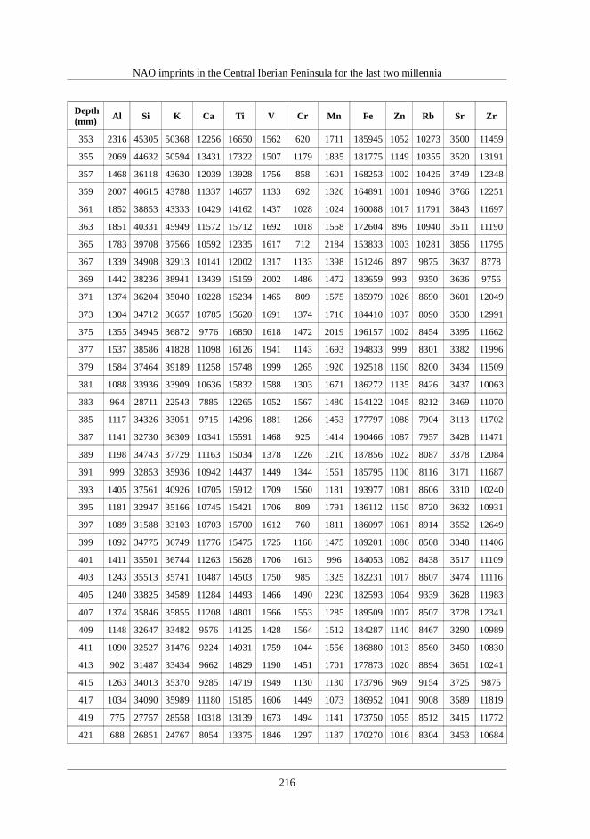
NAO imprints in the Central Iberian Peninsula for the last two millennia
Depth(mm)
Al Si K Ca Ti V Cr Mn Fe Zn Rb Sr Zr
353 2316 45305 50368 12256 16650 1562 620 1711 185945 1052 10273 3500 11459
355 2069 44632 50594 13431 17322 1507 1179 1835 181775 1149 10355 3520 13191
357 1468 36118 43630 12039 13928 1756 858 1601 168253 1002 10425 3749 12348
359 2007 40615 43788 11337 14657 1133 692 1326 164891 1001 10946 3766 12251
361 1852 38853 43333 10429 14162 1437 1028 1024 160088 1017 11791 3843 11697
363 1851 40331 45949 11572 15712 1692 1018 1558 172604 896 10940 3511 11190
365 1783 39708 37566 10592 12335 1617 712 2184 153833 1003 10281 3856 11795
367 1339 34908 32913 10141 12002 1317 1133 1398 151246 897 9875 3637 8778
369 1442 38236 38941 13439 15159 2002 1486 1472 183659 993 9350 3636 9756
371 1374 36204 35040 10228 15234 1465 809 1575 185979 1026 8690 3601 12049
373 1304 34712 36657 10785 15620 1691 1374 1716 184410 1037 8090 3530 12991
375 1355 34945 36872 9776 16850 1618 1472 2019 196157 1002 8454 3395 11662
377 1537 38586 41828 11098 16126 1941 1143 1693 194833 999 8301 3382 11996
379 1584 37464 39189 11258 15748 1999 1265 1920 192518 1160 8200 3434 11509
381 1088 33936 33909 10636 15832 1588 1303 1671 186272 1135 8426 3437 10063
383 964 28711 22543 7885 12265 1052 1567 1480 154122 1045 8212 3469 11070
385 1117 34326 33051 9715 14296 1881 1266 1453 177797 1088 7904 3113 11702
387 1141 32730 36309 10341 15591 1468 925 1414 190466 1087 7957 3428 11471
389 1198 34743 37729 11163 15034 1378 1226 1210 187856 1022 8087 3378 12084
391 999 32853 35936 10942 14437 1449 1344 1561 185795 1100 8116 3171 11687
393 1405 37561 40926 10705 15912 1709 1560 1181 193977 1081 8606 3310 10240
395 1181 32947 35166 10745 15421 1706 809 1791 186112 1150 8720 3632 10931
397 1089 31588 33103 10703 15700 1612 760 1811 186097 1061 8914 3552 12649
399 1092 34775 36749 11776 15475 1725 1168 1475 189201 1086 8508 3348 11406
401 1411 35501 36744 11263 15628 1706 1613 996 184053 1082 8438 3517 11109
403 1243 35513 35741 10487 14503 1750 985 1325 182231 1017 8607 3474 11116
405 1240 33825 34589 11284 14493 1466 1490 2230 182593 1064 9339 3628 11983
407 1374 35846 35855 11208 14801 1566 1553 1285 189509 1007 8507 3728 12341
409 1148 32647 33482 9576 14125 1428 1564 1512 184287 1140 8467 3290 10989
411 1090 32527 31476 9224 14931 1759 1044 1556 186880 1013 8560 3450 10830
413 902 31487 33434 9662 14829 1190 1451 1701 177873 1020 8894 3651 10241
415 1263 34013 35370 9285 14719 1949 1130 1130 173796 969 9154 3725 9875
417 1034 34090 35989 11180 15185 1606 1449 1073 186952 1041 9008 3589 11819
419 775 27757 28558 10318 13139 1673 1494 1141 173750 1055 8512 3415 11772
421 688 26851 24767 8054 13375 1846 1297 1187 170270 1016 8304 3453 10684
216

Chemical and mineralogical data
Depth(mm)
Al Si K Ca Ti V Cr Mn Fe Zn Rb Sr Zr
423 630 26044 20319 7905 11014 1442 1456 1342 160489 1028 8777 3545 10860
425 459 25307 20866 7213 11189 1287 1393 1391 158524 1012 9320 3783 11630
427 662 25629 23439 8398 12696 1417 1218 1424 172125 1092 9080 3662 11878
429 370 24201 18114 7676 10599 1216 1043 1015 158805 1069 8780 3548 11530
431 484 25537 18730 7864 10292 1369 1069 1166 147138 1002 8395 3587 11121
433 306 22324 4972 4956 4809 1374 290 1458 105243 954 7736 3176 10657
435 359 23279 5221 4473 5101 998 456 1577 101517 880 7671 3051 10670
437 425 24462 14757 6471 10000 1309 895 1641 145757 980 7812 3271 10694
439 493 25643 17640 8161 9945 1809 1147 1551 152088 1191 8326 3589 10562
441 429 26948 19651 6733 10225 1058 925 1416 145814 1008 9156 3815 9784
443 471 26205 15904 6114 6687 1350 791 1111 122415 875 10055 5302 7751
445 675 26771 17075 7741 8037 1284 346 1426 116717 916 10285 4554 10677
447 991 28866 15984 6422 7453 1023 863 1436 122908 788 8718 3330 10646
449 565 25502 17335 6652 9594 869 697 1703 136125 889 9065 3547 11022
451 626 26668 20829 7818 11127 1291 800 1596 148025 941 8665 3476 10954
453 745 26049 18367 7418 10483 1548 1013 1560 148781 986 8285 3193 10263
455 607 27504 24748 8451 11439 834 941 1457 161014 1029 8132 3348 10444
457 1290 34343 26862 8513 11195 1145 864 1153 157381 1042 7604 3456 10193
459 976 30149 12268 5613 4659 1070 657 964 81888 872 7338 2917 9821
461 796 27238 3222 4300 2087 1155 526 1666 51152 803 7050 3022 10392
463 938 28277 3021 3952 1878 1083 552 1298 44009 645 6962 2654 9370
465 668 26652 5845 4779 3058 1203 392 1218 67741 632 6922 2807 7953
467 805 26629 9904 5544 3452 1345 755 1491 76182 719 7093 2474 6641
469 633 25330 8196 5136 3640 1094 1387 1288 63422 618 7423 3111 5450
471 627 26644 13696 5972 6345 1100 229 1294 109775 646 8746 4166 8844
473 645 26640 14106 5448 5573 1528 304 1666 102639 777 8422 3691 9532
475 830 26522 18120 6345 8173 1302 623 1345 128047 699 8968 3207 10347
477 796 26767 12723 6066 7142 975 1148 1298 114325 877 8319 2942 9319
479 681 26220 14037 6284 7796 1354 1059 1901 137618 977 7638 2931 9888
481 813 25763 8950 5795 5906 831 179 1072 119936 930 7034 2905 9393
483 833 27847 14649 6728 7292 1129 884 1132 138202 956 7353 2841 9271
485 707 27690 18627 7498 8739 1098 403 1446 149906 947 7969 3062 10078
487 1153 34005 29970 10207 11923 1541 1287 1549 172353 1001 7791 3281 9595
489 1343 33577 32890 11096 13379 1593 794 1836 183699 1076 7565 3186 9472
491 1319 31299 23772 8364 10459 983 1076 1636 167663 1140 7794 3310 9998
217

NAO imprints in the Central Iberian Peninsula for the last two millennia
Depth(mm)
Al Si K Ca Ti V Cr Mn Fe Zn Rb Sr Zr
493 1518 35359 32323 10795 12744 1335 857 1580 181169 1158 7536 3053 10563
495 1109 30370 22672 8097 11826 1245 1399 1786 165647 1051 7483 3148 9608
497 1449 35953 27715 8804 11097 1488 1205 1538 167932 1046 7508 3192 9646
499 1016 29550 24468 9595 11101 1366 925 1689 167129 1136 7943 3424 10727
501 1047 32148 30668 10814 12041 1351 1348 1634 178233 1098 7878 3184 10702
503 1252 33795 34649 10430 13185 917 1055 1516 179598 1191 8290 3323 10820
505 994 30098 27739 8101 10794 1329 947 1665 166778 1055 8425 3444 11352
507 1095 31388 29690 9925 12625 1469 1291 1332 177123 1140 8083 3383 10613
509 1614 38958 42852 11911 14287 1412 1486 1843 195013 1182 8800 3558 10881
511 1990 41595 41648 12338 14867 1704 1597 1937 172823 1082 9190 3506 11278
513 2337 47482 48111 13053 16341 1527 1809 1877 189487 1044 9277 3359 8494
515 2333 47227 51744 14031 16422 1350 1453 1923 193255 1163 8855 3962 9236
517 1226 34572 31129 10579 12895 1380 1121 1643 173680 1222 8338 3443 9555
519 1866 42911 42601 12237 15587 1583 1417 1689 188421 1132 8082 3292 9853
521 2358 47416 46089 12655 16964 1816 1804 1615 199253 1180 8175 3411 11846
523 1938 46194 44048 11960 16089 1443 1610 1570 187191 1154 8430 3163 10087
525 2527 52405 46771 12629 16670 1503 1351 2123 191634 1176 8369 3306 11622
527 2192 46833 46707 12231 15988 1813 1784 1693 196664 1171 8311 3424 10039
529 2164 48287 44109 11777 16110 1607 1383 1595 192451 1090 7922 3311 10435
531 2549 51285 50168 13805 16936 1396 1906 1599 197636 1195 8133 3195 9390
533 2122 47206 46913 13454 18044 2059 1447 2035 193991 1061 8272 3499 10429
535 1653 40491 45436 13061 16075 1524 1322 1803 190127 1048 8581 3396 11005
537 923 30623 30157 10829 13040 1330 1155 1389 175577 1051 8700 3445 9715
539 758 31846 39169 11169 14383 1407 858 1615 174531 967 8770 3338 9451
541 596 25406 15972 6731 7973 1309 521 1302 145594 1006 7931 3170 10334
543 369 24790 13481 6774 8654 1212 227 1777 145520 851 7696 3190 9871
545 720 26452 20603 7540 10779 1440 1154 1831 156247 1020 7540 2991 10142
547 667 27299 19444 8207 10269 1252 888 1248 151722 833 7274 2868 9971
549 822 28173 18236 7681 8357 1623 1319 2184 140312 893 7315 2793 9150
551 571 25054 10279 5675 7160 1311 599 1245 125971 897 7139 2898 9119
553 699 27120 14157 6890 7694 1206 1213 1582 129135 953 7440 2960 9887
555 675 25180 13022 5916 7197 1073 1126 1142 124930 1018 7305 3152 10373
557 336 22547 9789 6295 8803 1265 702 1605 131089 862 7210 3119 10557
559 282 23456 11034 6272 7858 1485 1059 1511 130223 906 7288 3092 9798
561 389 23876 12703 6692 7815 1255 1055 1308 136009 864 7079 2891 9245
218

Chemical and mineralogical data
Depth(mm)
Al Si K Ca Ti V Cr Mn Fe Zn Rb Sr Zr
563 446 23902 13662 6599 8744 1046 1179 1395 143384 975 7119 2809 9710
565 369 25091 15312 6803 7852 1090 1202 1419 128001 906 7539 3034 9302
567 747 29579 27614 8703 11725 1524 1066 970 150877 968 7635 3043 9377
569 817 30298 29495 9867 12357 1570 1094 1203 159499 968 7619 3123 8661
571 749 29753 25165 8684 10657 1240 1541 1408 150926 948 7380 2947 8540
573 851 29126 20672 7411 8878 1051 885 1538 135127 859 7082 2750 8424
575 890 29417 19200 7423 7836 1127 1008 1249 123066 823 6633 2634 9910
577 744 27194 18316 6823 7912 1184 211 1085 122575 871 6741 2713 9459
579 713 27102 20645 8843 9852 1064 720 2156 146024 1031 7059 2925 9024
581 982 30584 28418 9848 11047 1879 1152 1140 151428 971 7238 3071 10604
583 888 29745 24751 9242 10020 1127 870 1080 150527 917 7316 2895 9023
585 847 30404 19745 7914 8341 1417 716 1394 127123 987 7786 3197 9420
587 465 23714 4498 4617 2382 887 422 1260 65973 876 7190 3033 9118
589 701 27171 14088 7075 5701 892 435 1347 113551 858 6997 2624 8308
591 1276 32046 23760 8009 9777 1264 1285 1212 142723 1043 7667 3122 10443
593 1129 28800 14725 6177 6814 1173 462 1549 115762 1084 8067 3224 9112
595 630 26411 14542 6234 5585 1062 490 1239 100204 912 9189 3768 8645
597 1152 30920 23367 7516 11108 1806 740 1944 135525 1006 8992 3462 10521
599 1306 36256 32034 10128 11803 1414 1320 1213 161683 1174 8229 3257 9639
601 1208 34305 33847 10068 11975 1765 1334 1975 166100 1057 8211 3263 9108
603 1453 36422 33276 9947 12755 1905 1187 1917 173215 1138 8364 3138 10127
605 1340 36448 39605 11106 13523 1562 1466 1996 174615 1087 8596 3333 9954
607 1151 34015 31928 9749 13559 1449 1784 1656 174622 1146 8840 3365 10175
609 1658 38181 34805 9820 12992 1331 1298 1388 171795 1092 8007 3310 11534
611 1278 35850 31275 9026 12262 1407 1394 1522 173032 1122 8365 3129 9687
613 1465 35998 31786 9735 11702 1266 1122 1682 156646 1031 8454 3263 10369
615 2108 42715 37202 11123 13330 1386 976 1882 167493 1048 8649 3325 9502
617 2451 48562 43624 11963 15372 1661 997 1740 175285 1037 8094 3285 10500
619 2592 50758 46470 12837 15438 1544 1865 1615 182998 1029 8433 3229 9532
621 2579 50899 44741 11952 15799 1549 1370 1574 193091 1117 8159 3380 9080
623 1751 40962 38715 11774 15466 1598 1597 1762 189660 1171 8122 3550 10140
625 2350 48150 46376 11635 17187 1226 1528 1786 204599 1193 7974 3372 11308
627 2038 46715 46159 12966 15927 1888 1627 1764 200943 1138 8145 3202 10221
629 2109 43538 40749 12006 15206 1615 1601 849 194705 1172 8361 3031 9543
631 1672 39062 35706 10352 13907 1490 1298 1294 185395 1127 8507 3263 10272
219

NAO imprints in the Central Iberian Peninsula for the last two millennia
Depth(mm)
Al Si K Ca Ti V Cr Mn Fe Zn Rb Sr Zr
633 1853 42550 41585 10451 15092 1522 1489 2051 190638 1073 8179 3458 9667
635 2244 45721 43830 11214 15716 1584 1105 1816 197012 1068 7915 3313 9840
637 1479 35650 32214 9937 12117 1358 1287 1556 176143 1184 8312 3339 9770
639 2211 45811 44616 11518 15246 1145 2004 1765 191348 1180 8244 3179 9341
641 2254 46197 45138 12937 15557 1335 985 1827 198426 1194 8723 3453 10813
643 1639 38559 35799 11202 13445 1395 1514 1855 177560 1089 8733 3331 10368
645 2122 45862 44396 12122 14795 1807 1541 1891 190237 1204 9126 3385 11020
647 1350 35673 35046 9729 13257 1481 1099 1664 171650 1155 9148 3617 9712
649 2235 44562 46403 12280 15685 1890 1522 1180 180763 1013 9569 3670 12784
651 2936 53026 51579 13196 16227 1719 1410 1792 196485 1103 8534 3314 11508
653 2205 44372 45658 11947 15517 1791 1720 1668 196768 1206 8395 3253 10398
655 1903 40842 38000 11515 11933 1360 834 1351 174719 1064 8717 3320 9539
657 2406 47484 43961 11126 15573 1104 1286 1664 188305 1127 9221 3639 9693
659 2293 47071 44620 11831 15257 1001 1328 1507 181596 1046 9216 3929 11556
661 2057 42954 40360 11019 13875 1433 807 1329 180086 1142 8531 3300 10052
663 2991 54852 53244 13433 16799 1175 1443 1352 199400 1104 8555 3186 9704
665 3116 54499 52245 12709 17289 1377 1493 1705 206520 1150 8178 3131 10407
667 2697 51637 49713 12533 17601 1874 1217 1877 196012 1146 8329 3087 10581
669 3060 52825 52958 13216 16597 1625 1475 1838 200442 1152 8305 3254 11154
671 2846 52002 50656 12952 16746 1442 1665 1951 200282 1122 8336 3250 10863
673 2659 49393 46556 12549 14842 1632 1416 1855 191648 1150 8600 3052 11458
675 2732 51271 51555 13874 16887 1791 1486 2027 197797 1038 9280 3441 12109
677 3335 56048 56212 13893 19666 1299 1340 1945 204449 1136 9360 3646 11962
679 2821 52061 49428 13574 15870 1892 2177 1667 191952 1089 9378 3562 11164
681 2809 52346 50955 13413 15949 1143 1316 1507 177488 1122 9154 3434 10074
683 3281 57689 55239 13514 17039 1532 2044 1634 185958 1132 8384 3206 9797
685 3196 57255 51337 13000 15334 1957 1271 2122 187003 1090 8335 3140 9526
687 2820 55135 50769 13227 15801 1827 1502 1858 195393 1088 8400 3227 10572
689 3105 55690 52053 13009 16469 1414 1453 1879 200840 1160 8376 3166 10332
691 3143 56785 52644 13942 16239 1571 1683 1780 199221 1148 8474 3218 10095
693 3199 56111 53096 12653 16310 1798 1779 1715 198211 1133 8683 3183 10484
695 3067 53634 50736 12644 17188 1692 1599 1612 198841 1218 8264 3166 9866
697 3217 55198 52556 12899 16514 1492 1382 2417 200721 1168 8553 3255 10386
699 2395 48187 52197 12582 17056 1831 1615 1809 198557 1089 8712 3390 10722
701 3191 56438 54509 13891 17367 1924 1586 1760 202300 1106 8847 3492 11824
220

Chemical and mineralogical data
Depth(mm)
Al Si K Ca Ti V Cr Mn Fe Zn Rb Sr Zr
703 2965 56229 55568 13658 17392 1556 1255 1579 204540 1203 8804 3529 11963
705 2644 49234 50645 13781 15323 1492 1217 1547 197318 1092 8861 3407 11445
707 2497 48264 51594 13233 18689 1475 1538 1735 201174 1011 8939 3409 12009
709 1978 44001 48369 12722 15647 1694 1311 2061 195046 1031 9113 3497 11937
711 1727 41712 48317 13224 16341 1897 891 1753 192562 1092 8934 3256 11835
713 1915 44143 49674 13723 16252 1654 1748 1876 195499 1125 8842 3414 10163
715 1416 37618 40443 11946 13452 1171 1102 1523 185179 1101 8937 3260 11362
717 1095 32492 33018 10782 12298 1312 1728 1357 170559 1073 8979 3827 11575
719 1213 31298 29703 10133 11181 1252 1407 2173 149127 1006 10217 3921 8795
721 891 28356 18366 6596 5847 987 688 798 96686 861 10993 4335 8150
723 776 29787 22641 7876 7494 1034 1641 1422 112040 775 10590 4228 8708
725 1570 40449 45425 11663 14380 1083 1875 2215 174845 830 10247 3814 9173
727 2097 46375 49233 11668 13541 1279 1407 1726 169336 1015 12222 3859 9519
729 2233 49099 51582 12737 15853 1328 1530 1714 184084 1004 11317 3359 11905
731 2042 43984 45457 11230 14435 1426 916 1829 184323 1060 8919 3242 10448
733 1675 39830 42354 12001 14390 1446 925 1303 177456 1043 8730 3126 10855
735 1223 35662 38064 10850 12987 1808 797 1910 179520 1125 8685 3235 10320
737 1454 37962 42835 11106 14092 1863 1450 1982 176198 1005 8511 3589 11415
739 1864 42321 44952 12291 15295 1211 1173 1180 194605 1065 8378 3273 12278
741 2045 44208 47961 12460 16181 1338 1515 1308 195571 1104 8530 3265 11509
743 2091 46105 52142 13926 16887 1622 1903 1505 207406 1176 8752 3200 11773
745 1717 42358 49904 13973 16115 1241 1470 1869 203369 1094 9170 3493 12142
747 2052 41925 47899 12544 16811 1396 1435 1668 206341 1286 9319 3484 10690
749 1610 38398 46273 12460 15944 1603 1368 1860 198071 1089 8981 3231 10544
751 1337 38184 46570 12915 15853 1476 1070 1537 200440 1149 9083 3210 11625
753 1598 37734 42820 11520 15308 1347 1020 1140 190952 1109 9388 3483 11213
755 1616 39068 47151 13447 15699 1647 966 1462 192381 1200 10259 3716 11526
757 1033 33819 39624 12064 15016 1269 1045 1053 177771 1047 10780 3647 10746
759 2317 41862 37126 11317 14264 1616 1851 2076 175565 1008 9980 3722 10649
761 1241 34253 35393 9501 13276 1492 1438 1600 185366 1103 10057 3842 11338
763 1567 36426 41139 10813 14539 1411 1084 1539 174138 1087 10539 3802 9887
765 1108 31727 34867 10376 14215 2029 1089 1708 181297 1026 10167 3821 9304
767 1244 33777 33853 10743 12796 1319 1293 1775 175492 1105 10496 3724 9913
769 939 32074 36152 9989 13545 2137 1418 1470 175647 1113 9851 3564 10372
771 1194 30422 20240 7831 10482 1281 346 1492 156453 1088 8462 3087 9786
221

NAO imprints in the Central Iberian Peninsula for the last two millennia
Depth(mm)
Al Si K Ca Ti V Cr Mn Fe Zn Rb Sr Zr
773 1323 34175 31245 9664 10612 1230 1458 1850 160440 1099 8006 3229 10281
775 1907 42563 45465 12211 15891 1279 1063 1064 190472 1114 8405 3065 8469
777 2553 49398 49738 14380 16352 1552 1482 1767 191175 1126 8775 3430 9699
779 2325 48074 46902 12667 15645 1338 1341 1814 175453 1037 10049 4157 9722
781 1658 40475 41930 11200 12122 1621 1102 2096 145586 798 11193 3759 10712
783 1498 37096 34650 10415 10867 1565 707 1283 147460 893 9634 3554 8650
785 1645 38403 38289 9768 13523 1247 1731 1616 161345 937 13092 3770 8968
787 1455 38034 38209 10323 13474 1513 1381 1751 167531 991 11471 3299 10352
789 1403 37753 38577 11252 13082 1253 1528 1532 173119 998 9637 3625 9606
791 1518 37900 36567 13695 12826 1668 1101 1897 171262 915 9270 3234 9263
793 845 30576 29720 9759 12358 1282 1062 1136 172688 1043 8859 3444 10059
795 1161 35147 36753 10961 14418 1026 761 1475 188393 1108 8867 3140 10421
797 1006 34140 39332 11450 13263 1795 1056 1524 175488 1033 9182 3430 12418
799 1127 31612 32556 9927 12867 1449 772 1070 171957 1060 8935 3330 10963
801 983 32148 33004 10143 13263 1345 1013 1887 177354 1098 8901 3507 10639
803 1094 31226 32163 9542 14281 1890 1181 1454 189102 1214 8956 3460 10478
805 1109 32747 35104 9979 12817 1707 1203 1618 182928 1022 9005 3326 10137
807 1433 35418 32146 9106 12025 1599 1215 1528 163564 1004 8339 3130 9193
809 1161 30242 14051 6437 6603 1577 730 1473 117014 1041 8003 3207 9876
811 1092 31236 23782 8100 9532 1408 1227 2008 146364 948 7738 2859 10245
813 769 26656 17769 6785 8521 1399 1037 1492 141819 1016 8412 3082 9276
815 584 24412 4787 4285 4147 1313 1262 1548 100696 972 7625 2939 9973
817 590 24040 3995 4099 3704 963 423 1908 94560 948 7456 2992 8550
819 1251 31178 17748 6795 7417 1547 956 1603 125896 954 7319 2826 9223
821 1270 31116 21067 7763 8564 1390 807 1315 142911 1006 7495 2967 9120
823 1049 30054 19262 7100 7745 1263 1267 1807 135032 943 7659 2830 9444
825 1263 32455 20089 7517 7971 1363 716 1518 131490 969 7570 3033 9413
827 1063 32917 21333 7376 8336 1383 827 1590 136522 996 7518 2873 8268
829 1357 35584 28615 9355 10631 969 1169 1434 152374 966 7749 3145 9576
831 1317 33320 27346 8745 10949 1010 982 1443 153275 1037 7459 2933 9433
833 705 29149 22017 7600 9552 1036 1148 1447 147551 1014 7623 2906 8603
835 454 25406 16133 6608 8358 1240 1386 1599 141387 1065 8269 2807 9055
837 1136 33065 28347 9128 11339 1516 1005 1204 157411 1046 7626 2737 8991
839 1555 38371 33740 9576 12230 1241 1527 1833 162188 1045 7368 2900 9563
841 1403 37264 32219 9458 11503 1560 781 1724 155885 972 7313 2831 8489
222

Chemical and mineralogical data
Depth(mm)
Al Si K Ca Ti V Cr Mn Fe Zn Rb Sr Zr
843 1447 36420 31346 9730 11359 1160 772 1346 156729 1037 7766 2903 9292
845 1329 34850 29523 9613 10941 1446 1614 1631 148801 913 7959 3067 8614
847 1387 35254 34283 9906 11654 1938 1135 1105 145456 932 10874 4479 8465
849 1319 35106 34204 10128 12361 1248 1089 992 144040 835 10323 4265 9123
851 1046 33816 31544 9154 12320 1125 756 1062 150221 992 9130 3241 11255
853 1372 36971 35188 11038 13922 1147 1477 1407 148056 972 9932 3763 10368
855 1606 38535 40226 11720 14815 931 1379 1210 170357 902 10090 3513 8749
857 1183 33470 37149 10686 12974 1641 715 1713 171900 1027 8778 3350 9759
859 1211 34684 36731 10644 13783 1573 1503 1675 179674 1131 7984 3146 10374
861 1184 34768 38169 10173 13716 1342 1077 1226 183796 1143 8605 3334 9903
863 1195 34909 39170 10927 14011 1218 1529 1869 181756 1158 8737 3217 10380
865 1347 37200 41557 11612 14440 1472 1118 1337 185893 1090 8661 3379 10848
867 1530 39380 42470 11650 15324 1651 1180 1661 188573 1158 8184 3303 12628
869 1432 37304 37137 10673 14400 1261 1612 1611 185252 1124 8700 3218 11287
871 1533 37751 34093 10240 13093 1583 1375 1229 176048 1107 8415 3352 11477
873 785 29210 24486 8311 10698 1593 1292 2116 162907 1071 8440 2979 10481
875 1069 32373 37271 10318 13681 1048 1910 1598 184711 1080 8562 3127 11521
877 1250 33048 39294 11017 15201 1349 1612 1587 185140 1090 8798 3179 11102
879 1655 39222 45556 11895 14991 1559 1073 1657 189341 1213 8481 3136 10057
881 1220 33578 40248 10752 14109 1492 1555 1543 187679 1092 8261 3462 10855
883 1631 40008 43931 12177 15450 1521 937 973 193620 1144 8378 3402 11232
885 1894 40223 39680 11096 13935 1341 1052 1530 183216 1061 8547 3231 10209
887 1612 39046 43371 11413 15083 1392 1415 1731 186600 1099 8465 3100 10048
889 2433 47342 48905 11731 15992 1200 1400 1758 193940 1094 8620 3267 9928
891 2424 46491 49634 12935 16601 1687 1037 1573 176715 972 9294 3553 10969
893 2352 46666 48829 14162 15987 1604 1434 1938 182847 1055 8533 3246 9952
895 2265 47400 46112 13450 15053 1453 1133 1969 178577 1023 8415 3297 9519
897 2416 46366 45924 11359 14667 1416 1114 2027 182637 996 8459 3243 10140
899 2399 44472 43164 11493 14906 1506 1469 1144 184660 1096 8227 3339 10330
901 2578 47595 43616 11620 15060 1596 1492 1517 191328 1092 7902 3150 10867
903 3285 54944 51413 13117 17066 1589 1859 2342 195581 1132 7806 2936 9945
905 3069 52583 47841 12221 15948 1216 1489 1738 189206 1054 8024 3034 9585
907 2873 53313 47830 13341 16162 1519 1802 1479 187579 1076 7991 3136 9910
909 2942 54806 47875 12815 16307 1246 1523 1801 191535 1035 7825 3097 10521
911 2985 54104 49937 14169 17339 1896 2159 2227 193978 1026 8352 3255 10669
223

NAO imprints in the Central Iberian Peninsula for the last two millennia
Depth(mm)
Al Si K Ca Ti V Cr Mn Fe Zn Rb Sr Zr
913 2894 53901 48251 12374 16438 1311 1546 1792 191361 1060 8054 2940 10347
915 3150 55166 48563 12543 16780 1828 1675 2020 195433 1048 8071 3131 9453
917 2962 53744 49317 13121 15591 1554 1450 1730 186978 1031 8467 3315 9542
919 3094 53581 49581 13767 15277 1280 1191 1802 181391 1036 8328 3227 9415
921 2540 47931 46541 11992 15344 1626 1482 1571 177398 1064 8728 3384 8917
923 2350 45765 45009 11983 16138 1288 987 2287 181214 1090 9565 3752 9844
925 2191 45302 46897 12658 17046 1282 1922 2274 187424 1069 8256 3247 11008
927 2746 51272 53394 14162 18243 1273 1710 2245 195507 1170 9183 3465 10239
929 3276 55800 56729 15212 16291 1454 1865 1693 184269 1057 9485 3680 11922
931 3241 54016 51894 14003 16671 1825 1301 1613 186885 1100 8748 3668 9940
933 2662 50874 49593 13804 16309 1072 927 1662 196045 1185 8308 3360 11203
935 2713 49212 49778 12983 16415 1461 1471 2091 193431 1159 8352 3166 10988
937 2646 50586 50720 15054 16970 1448 1338 2149 194409 1110 8783 3384 11185
939 2485 48750 50215 13445 15745 1555 1997 2318 184293 1102 9305 3535 10424
941 3354 54587 52903 15655 17613 1741 1814 2214 195758 1165 9243 3670 10791
943 2755 52152 51933 13645 15774 1434 1535 2016 184861 940 11255 3943 8945
945 2566 50237 46737 13155 16283 1900 956 1818 182704 966 10378 3828 8240
947 2469 47836 47036 13513 15705 1442 1492 2124 183040 1100 8757 3465 11265
949 2118 45198 45080 11398 16205 1419 816 1578 171550 1006 9902 3394 10841
951 3155 55715 54113 13778 16260 962 2029 1513 185549 996 11409 3746 9114
953 3045 55289 54999 14691 16119 1460 1730 1862 187583 1088 9787 3534 10891
955 2076 43136 43304 12388 14757 1581 1649 1780 178816 1233 8613 3354 11355
957 1602 39948 40258 11952 14640 1655 1296 1697 178624 1262 8844 3408 10296
959 1612 37973 37542 11164 14711 1632 1717 1290 169546 1127 9573 4231 9136
961 1399 34858 29526 9586 12161 1381 1194 1241 152126 1055 9362 3631 9318
963 963 28983 23005 8568 11116 1735 1128 2059 152225 1136 9369 3326 10753
965 944 29589 22422 8801 10794 1400 702 2175 160613 1191 9152 3481 11767
967 1324 33849 28981 10112 12353 1317 1657 1530 165661 1202 9303 3728 12386
969 1575 37424 32933 10642 13303 1684 822 2314 168866 1235 9619 3669 10804
971 2229 43915 43108 13137 15633 1784 1218 2364 185557 1116 9575 3660 12447
973 3306 57970 58628 14844 19016 1700 1891 2127 195625 1245 9637 3816 12499
975 3155 56611 60172 15721 19458 1720 2007 1966 201517 1218 9659 3723 11591
977 3071 54489 59281 14611 17665 1404 1915 1204 187513 1113 10615 3731 9739
979 2721 50897 55742 14617 17466 1793 1333 2068 181406 970 10680 3644 10106
981 2940 51733 53800 15968 17521 2087 1644 2222 182896 1086 9313 3432 10215
224

Chemical and mineralogical data
Depth(mm)
Al Si K Ca Ti V Cr Mn Fe Zn Rb Sr Zr
983 3102 54219 53498 13840 17958 1307 1503 2571 180468 1166 9269 3455 11167
985 4268 65152 59635 15565 18719 1536 1850 2427 182818 1376 8829 3390 10445
987 4421 67092 59036 17167 18295 1284 1571 2047 186066 1174 9158 3262 10609
989 4626 68368 59886 15786 17931 1613 1845 2029 184042 1225 9239 3261 10712
991 4748 69046 60380 16109 19117 1403 1596 2008 183896 1224 8622 3344 10004
993 4257 66572 58308 15944 16906 1264 1927 2035 177819 1227 8817 3340 10820
995 4512 68097 58272 15796 18237 1786 1586 2530 183619 1261 8699 3228 10587
997 5007 70998 64314 17276 19149 1626 2046 2212 183225 1275 8781 3492 11818
999 4389 64603 60511 17083 18333 1398 1800 2693 183395 1242 9467 3508 10853
1001 3286 56747 57629 14868 19562 1388 1397 2423 188387 1229 9663 3694 10988
1003 2903 51389 49744 14446 16860 1540 1223 1712 182403 1165 8729 3270 10866
1005 2957 53003 48441 13479 17863 1749 1154 2059 194008 1220 8907 3333 9874
1007 2049 43709 41896 11435 15132 1432 1510 1666 187131 1102 8784 3386 9289
1009 2295 45351 41573 11073 12876 1692 1228 1805 171224 959 9811 3822 8772
1011 1495 38520 31082 8426 7360 1082 1159 932 115347 698 11193 4206 5758
1013 1486 35214 25010 7369 7755 1060 1312 771 105960 642 11234 3335 7982
1015 1671 39415 38433 12252 12507 1597 1002 999 151895 912 9888 4012 8460
1017 1743 38856 30128 10047 11801 1193 528 1773 135283 807 11384 4298 8887
1019 1863 41522 37724 11710 11221 1802 794 1522 126415 719 11860 5979 8385
1021 1737 39733 38976 11127 12258 1174 992 1381 131854 681 11696 4780 6690
1023 1289 34438 28715 10028 9394 1440 958 1532 116360 663 11002 4463 6378
1025 2641 47419 42532 14121 11430 1398 1303 1135 139948 1008 10301 4088 7991
1027 2500 47631 44693 12429 15811 1680 812 2605 157476 1117 10199 3726 9150
1029 1507 34337 26405 7855 10632 1053 753 2371 120679 869 10533 4562 7770
1031 1963 41661 38715 13089 14206 1403 1514 1936 142527 896 9099 3452 8680
1033 1858 41714 37406 11628 13291 1180 874 1737 152478 1150 8906 3201 10180
1035 1756 39056 37206 9395 12993 1694 1168 1827 167453 1041 8540 3131 9152
1037 1540 37223 41263 10518 9625 1514 840 1207 132443 746 10840 4080 7934
1039 1784 37402 26506 17069 7316 1113 299 1315 101974 665 11347 4120 6887
1041 1628 39210 30020 11410 18877 1683 1555 1315 142289 768 9499 3771 8438
1043 1511 37830 38620 11731 14058 1383 1662 1823 173972 996 9218 4860 9660
1045 1479 36222 32695 11095 14518 1541 901 1587 164374 1071 8983 3542 11339
1047 2838 49815 48608 14947 16773 2191 1709 1803 171071 1114 9317 3991 10155
1049 3637 58406 52979 14791 16636 1430 1617 1612 173487 1260 8664 3226 11703
1051 2709 51335 47371 13368 16907 1452 1998 1931 185655 1312 8384 3181 10286
225

NAO imprints in the Central Iberian Peninsula for the last two millennia
Depth(mm)
Al Si K Ca Ti V Cr Mn Fe Zn Rb Sr Zr
1053 2706 48956 47045 13212 16093 1502 1319 2336 184411 1261 8386 3293 11183
1055 2998 53869 47426 13049 16215 1310 1571 2362 188453 1171 8328 3198 10670
1057 2091 42101 38934 10885 14179 1455 1371 2122 169077 1132 8381 3336 8517
1059 2220 45240 44840 12457 16236 543 687 2349 163160 1214 8432 3188 10349
1061 1817 41582 35844 11176 13205 1439 605 2326 151220 1155 7706 3130 10155
1063 1509 38460 36158 12211 12942 1086 818 1916 144118 1236 7937 3180 10057
1065 1059 30962 26945 9925 11191 1389 1135 2443 137429 1335 7847 3011 9973
1067 738 28764 22447 9238 10426 1132 856 1714 128245 1210 8151 3156 10544
1069 885 27921 20567 8477 9939 997 1048 2200 123369 1168 8225 3375 9050
1071 1120 29413 14314 6882 7234 1345 1075 1731 112643 1140 7790 3073 10243
1073 1019 27794 15743 7647 7409 1073 746 1835 114894 1193 8036 3102 9034
1075 1437 35437 32362 12057 13547 1420 541 2195 138725 1139 8087 3053 10381
1077 1155 31560 21086 9276 10294 1368 771 2015 127592 1167 7635 2999 10434
1079 808 26967 18572 8624 8286 1037 764 2299 121610 1104 7192 2849 10423
1081 849 28584 17691 8433 8866 984 1109 1821 119594 1157 7541 3181 10416
1083 966 29287 17493 8116 8224 1213 791 1909 121416 1086 7341 2909 10746
1085 1089 30150 20805 9009 9327 1653 875 1932 125406 1142 7560 2919 9093
1087 1136 32608 28624 10162 11290 1490 1437 2129 132024 1091 7878 3248 8376
1089 958 29369 22646 9408 9964 1380 793 1413 123151 1019 7964 3136 9063
1091 1146 32408 26174 9698 9131 1123 858 1943 121440 985 7972 3242 9731
1093 1525 36279 27620 10364 11091 1114 1074 2197 128845 1097 7346 3040 9835
1095 1355 35048 24538 9737 10106 1445 1115 2248 125142 1118 7334 3106 8769
1097 1000 31953 24145 11190 10869 1434 869 2503 132354 1052 7312 2956 9119
1099 1045 29923 21302 9478 9533 1107 694 1913 130184 1129 7218 3012 9923
1101 864 29688 19155 8564 9440 777 912 2138 126054 1187 7391 3011 10009
1103 1523 36586 25558 9448 10242 1517 1126 2212 134284 1107 7213 3013 9522
1105 1974 39835 33053 11242 11828 1570 1159 2464 133846 1178 8092 3368 9771
1107 1324 33102 23290 9199 10499 1315 577 1732 128540 1180 7872 3330 9226
1109 1353 34600 25524 9783 10573 1651 1170 1672 134066 1217 7732 3291 11197
1111 1609 37781 30460 10530 11745 1517 1220 2220 139539 1167 8158 3296 10903
1113 1656 36400 31147 11619 11379 1791 784 2091 136696 1149 8499 3173 10192
1115 2025 41508 39110 12441 13550 1428 1155 2271 140455 1028 10028 3792 10562
1117 2103 44728 42289 12902 14276 1238 1242 1333 139918 1043 10758 4044 8811
1119 1858 43351 38550 12482 13707 1329 920 1850 150893 1167 8971 3447 9375
1121 2152 44443 40138 12690 14947 1442 1347 2229 150885 1275 8519 3427 9800
226

Chemical and mineralogical data
Depth(mm)
Al Si K Ca Ti V Cr Mn Fe Zn Rb Sr Zr
1123 2148 45317 40104 13127 14238 1693 1010 1953 154832 1346 7876 3319 8681
1125 2420 45461 40286 12587 14930 1513 1478 2147 156923 1201 7804 3118 8922
1127 1016 33287 27203 10111 10417 1379 820 1715 128227 1252 7486 2955 9280
1129 1039 30831 21269 8970 8894 1085 1042 1660 118146 1031 8295 3294 9685
1131 1384 33750 19883 8176 8234 1046 789 1819 117673 1147 7741 3429 11977
1133 1621 34764 20680 8397 8710 1540 976 1540 113982 1081 7927 3248 8693
1135 1392 34577 26092 9411 10083 954 1121 2033 122247 1121 7924 3119 9680
1137 1096 33433 25034 10290 10585 1473 1419 2587 133011 1104 7876 3203 9998
1139 1302 33477 24686 10102 10337 940 1357 2364 130381 1063 8355 3329 9713
1141 1310 34079 27674 9779 10653 1176 1504 1801 130189 1030 8470 3448 9440
1143 1222 33410 26385 10072 10420 1763 876 1776 129017 1095 8956 3839 9614
1145 1054 32347 25392 10317 9427 1162 1228 1858 118443 1050 8775 3743 9021
1147 1386 34557 28119 10693 9846 1298 1233 1888 119359 1156 8332 3387 9662
1149 1304 34023 26599 9995 10290 1438 915 1858 129132 1107 8044 3262 9698
1151 1761 39230 28558 10431 11392 1490 1667 2306 139829 1150 8223 3401 10362
1153 1660 36732 26106 9750 10084 1440 1184 1974 131048 1258 8642 3181 10701
1155 1876 41321 36600 11961 12599 1221 1282 2152 147083 1197 9295 3676 11108
1157 2117 44631 44723 13161 14685 1407 1285 2537 160810 1104 9432 3663 11451
1159 2216 44361 43798 14382 15439 1525 1499 2323 161286 1087 9410 3756 12035
1161 2725 48655 46650 13449 15960 1809 1285 2200 178440 1185 9347 3582 11584
1163 2634 48867 44229 13810 17075 1293 1067 2053 166354 1122 9520 3901 11701
1165 2275 47639 46572 14012 16919 1283 1058 2027 161915 1231 9914 3701 10360
1167 2754 50953 47591 14653 15956 1600 1524 2075 161324 1267 10187 3886 9786
1169 1399 31361 20722 7593 8145 1361 681 1419 104578 753 10879 3999 9571
1171 1367 36349 34330 12268 11185 940 1177 1021 133184 901 10046 3731 11957
1173 1849 40193 34621 13234 11781 1834 854 1829 143531 1026 8891 3529 10530
1175 1847 39302 31061 9739 11433 1269 1082 1794 143934 1077 8611 3477 10088
1177 1854 39536 32965 10922 11454 1380 858 1885 141342 1041 8984 3622 11664
1179 1877 39941 32716 10706 11372 1087 1056 2126 142717 1021 9053 3629 11651
1181 1801 38903 35653 10163 13277 1512 1324 1800 151169 1038 10650 4049 10132
1183 1561 35702 33279 10732 12814 1163 1074 1812 146220 953 9737 3546 10868
1185 1648 36191 31392 10648 11452 1550 1094 1771 143600 1065 8908 3478 11347
1187 1619 39045 36437 11688 12794 1491 1687 1796 153159 1104 8548 3308 10690
1189 1717 38582 35162 11374 12334 1277 880 1649 148556 1138 8710 3385 10780
1191 1624 37196 31640 11686 12300 1544 1101 2479 140615 1095 8903 3215 9980
227

NAO imprints in the Central Iberian Peninsula for the last two millennia
Depth(mm)
Al Si K Ca Ti V Cr Mn Fe Zn Rb Sr Zr
1193 1427 34734 30719 9600 11507 1107 1164 2129 134722 1258 7963 3469 10025
1195 1238 35110 33368 10930 12434 1671 1757 2153 138692 1184 7963 3439 10574
1197 1561 37247 31597 9994 12446 1281 1360 2001 161071 1183 7916 3111 9664
1199 1909 40402 34206 9924 12503 1421 1777 1802 167212 1079 7791 2978 9917
1201 1829 40809 33561 9706 11998 1040 1336 1879 137274 1107 9297 3638 10754
1203 3231 58449 55657 13950 16959 1394 1801 1854 159542 1093 10196 3639 9391
1205 4127 67647 57541 14453 18036 1439 2036 2086 165214 1246 9030 3549 10424
1207 4023 66502 56697 14586 17647 1714 2035 2104 164341 1238 9002 3567 11261
1209 4342 65369 55195 14441 17269 1784 1624 2141 166586 1132 8951 3670 11490
1211 3840 60241 53406 14318 17033 1622 1951 2029 170637 1297 8756 3438 11770
1213 3673 59298 51788 13711 16924 1505 1533 1700 173034 1198 8783 3463 10594
1215 1910 44524 40967 11745 13991 1697 1190 1584 159284 1058 9035 4056 9622
1217 2006 42459 40169 10818 13854 1432 1120 1590 158807 980 9234 3686 10782
1219 1496 38819 35560 11372 14100 1320 1783 1893 162201 1166 8775 3414 10445
1221 1894 41953 41616 11774 15499 1607 1274 1879 167751 1122 8527 3298 12174
1223 1640 37476 32267 10667 12884 1001 1119 1908 153944 1044 8666 3427 11185
1225 1729 37026 28059 9014 11880 1246 1185 1784 143565 1083 8751 3487 10021
1227 2633 45677 35360 9845 12273 1476 1612 1522 141473 974 8818 3600 8928
1229 1735 37877 28160 8468 10088 1440 1481 1117 126167 940 8110 3886 7800
1231 1300 32145 21046 7508 8721 1330 953 1742 110106 887 7051 3258 8195
1233 2733 49841 36701 10286 12181 1584 1103 1569 134095 987 7098 2734 8594
1235 2263 44693 35243 9885 12710 1130 1398 2173 146416 1011 7293 2751 8397
1237 1575 39353 26904 8931 10396 1283 1472 1583 141896 914 7198 2534 7842
1239 1864 41939 33616 8768 11264 1230 1575 1562 164452 789 8112 2538 6444
Table B.5. XRD intensity measurements of bulk mineralogical composition from PE12-01-01 core (incps).
Depth (cm) Muscovite Kaolinite Clinochlore Quartz Microcline Albite
0.2 62.49 20.41 20.41 147.8 18.25 41.75
0.4 58.83 19.54 19.54 131.6 9.44 43.61
0.6 31.61 22.22 22.22 100.2 12.66 29.48
228

Chemical and mineralogical data
Depth (cm) Muscovite Kaolinite Clinochlore Quartz Microcline Albite
0.8 50.81 21.33 21.33 72.58 9.64 18.47
1.0 36.32 10.14 10.14 75.66 11.83 23.09
1.2 38.51 19.25 19.25 87.61 9.28 32.6
1.4 41.23 19.57 19.57 82.19 40.9 28.53
1.6 57.63 14.84 14.84 134.5 23.85 40.47
1.8 46.78 14.58 14.58 103.3 17.63 21.38
2.0 37.54 14.45 14.45 60.82 29.9 18.28
2.2 33.67 14.71 14.71 62.1 3.72 22.31
2.4 52.65 21.61 21.61 125.3 11.12 42.43
2.6 29.22 15.21 15.21 58.99 8.54 22.63
2.8 53.76 22.81 22.81 134.1 15.73 56.23
3.0 58.68 18.75 18.75 124.7 20.83 34.56
3.2 79 24.87 24.87 139.2 8.7 51.42
3.4 38.56 25.28 25.28 64.51 7.96 23.59
3.6 39.25 17.74 17.74 85.37 7.18 23.3
3.8 36.1 16.39 16.39 115.9 8.67 30.26
4.0 16.72 7.48 7.48 31.27 7.11 6.3
4.2 51.15 15.2 15.2 144 11.91 46.37
4.4 35.54 8.28 8.28 69.58 4.69 28.47
4.6 32.09 12.31 12.31 57.7 8.66 22.61
4.8 54.13 22.58 22.58 79.32 13.24 34.9
5.0 30.02 17.33 17.33 57.11 7.92 22.32
5.2 31.28 30.23 30.23 99.28 14.75 39.24
5.4 45.21 14.3 14.3 102.6 5.5 28.17
5.6 54.41 17.85 17.85 96.23 10.48 41.13
5.8 35.54 13.23 13.23 80.69 10.52 31.96
6.0 31.97 12.43 12.43 57.68 11.15 27.39
6.2 49.12 17.49 17.49 96 11.1 27.13
6.4 25.87 8.8 8.8 63.54 2.1 4.29
6.6 38.72 20.23 20.23 77.13 11.26 17.63
229

NAO imprints in the Central Iberian Peninsula for the last two millennia
Depth (cm) Muscovite Kaolinite Clinochlore Quartz Microcline Albite
6.8 51.71 15.18 15.18 138.4 13.15 34.76
7.0 27.41 19.97 19.97 65.93 4.17 21.35
7.2 41.6 18.39 18.39 125 14.02 43.72
7.4 52.47 9.48 9.48 64.2 12.11 20.48
7.6 43.58 12.86 12.86 136.3 12.45 41.59
7.8 35.14 14.97 14.97 68.1 9.62 22.49
8.0 40.09 20.43 20.43 132.3 17.42 48.33
8.2 20.84 6.64 6.64 81.72 16.08 32.7
8.4 54.33 18.11 18.11 101.7 10.46 27.76
8.6 38.38 15.91 15.91 134.9 8.1 49.03
8.8 19 5.66 5.66 87.82 13.06 35.78
9.0 20.09 12 12 75.73 7.65 20.07
9.2 20.82 11.76 11.76 45.66 7.09 19.68
9.4 30.44 14.44 14.44 52.03 2.81 3.7
9.6 31.2 11.29 11.29 141.1 28.8 24.8
9.8 20.92 9.39 9.39 57.21 6.3 14.58
10.0 23.05 23.05 23.05 108.9 19.69 30.48
10.2 37.34 20.34 20.34 97.67 13.57 31.36
10.4 27.01 14.79 14.79 61.98 12.68 10.25
10.6 28.38 12.41 12.41 104.9 10.48 36.48
10.8 24.82 26.41 26.41 126.5 11.78 62.89
11.0 21.89 11.45 11.45 75.32 11.77 28.59
11.2 32.33 7.36 7.36 76.79 8.3 22.37
11.4 25.17 12.6 12.6 66.35 9.45 22.53
11.6 32.22 14.83 14.83 66.73 4.83 16.83
11.8 13.52 8.83 8.83 96.94 10.88 24.39
12.0 35.78 12.51 12.51 61.84 6.75 22.48
12.3 20.27 14.37 14.37 47.11 4.54 12.86
12.6 35.29 10.15 10.15 82.32 6.71 66.94
12.8 37.28 19.84 19.84 131.1 8.54 25.77
230

Chemical and mineralogical data
Depth (cm) Muscovite Kaolinite Clinochlore Quartz Microcline Albite
13.0 41.88 22.84 22.84 182.9 21.14 36.76
13.2 29.09 13.13 13.13 86.54 13.48 33.55
13.4 36.58 14.69 14.69 138.8 11.45 48.54
13.6 23.81 12.58 12.58 67.46 6.5 32.95
13.8 37.51 17.53 17.53 114.9 8.36 32.14
14.0 32.23 12.62 12.62 121 12.33 26.47
14.2 20.68 12.24 12.24 63.03 8.62 27.71
14.4 21.21 4.92 4.92 73.51 4.9 17.25
14.6 47.04 15.54 15.54 118.9 8.54 49.9
14.8 41.29 10.04 10.04 66.69 11.52 22.66
15.0 22.74 9.65 9.65 91.95 4.88 28.78
15.2 44.28 22.6 22.6 107.6 12.68 46.07
15.4 30.43 6.99 6.99 44.75 4.1 8.46
15.6 22.86 12.2 12.2 81.43 9.47 23.53
15.8 24.9 5.86 5.86 91.26 12.79 33.17
16.0 39.78 16.95 16.95 92.98 12.92 44.41
16.2 40.79 15.41 15.41 86.53 5.12 30.59
16.4 44.31 12.63 12.63 94.18 9.51 29.81
16.6 20.51 8.56 8.56 98.78 14.57 33.49
16.8 19.93 9.58 9.58 85.81 10.25 38.7
16.8 23.27 10.82 10.82 101.5 15.29 25.32
17.0 33.85 12.79 12.79 68.86 14.53 23.38
17.2 24.52 9.51 9.51 63.05 12.03 22.88
17.4 53.79 10.28 10.28 137.1 12.63 33.72
17.6 27.42 16.53 16.53 51.31 13.52 20.1
17.8 35.8 12.68 12.68 58.72 11.21 51.17
18.0 22.27 13.97 13.97 72.47 11.17 17.48
18.2 24.97 11.81 11.81 41.27 6.23 37.02
18.4 25.27 9.79 9.79 71.1 13.37 19.43
18.6 29.48 13.02 13.02 113 0.01 39.25
231

NAO imprints in the Central Iberian Peninsula for the last two millennia
Depth (cm) Muscovite Kaolinite Clinochlore Quartz Microcline Albite
18.8 44.93 12.99 12.99 102.7 3.65 21.88
19.0 17.19 9.94 9.94 94.26 15.4 28.52
19.2 20.7 13.42 13.42 67.69 9.18 24.37
19.4 17.7 5.43 5.43 103.3 10.93 12.38
19.6 35.14 10.23 10.23 81.89 21.89 22.92
19.8 30.53 12.45 12.45 58.17 8.61 22.46
20.0 40.62 21.84 21.84 132.3 17.85 50.07
20.2 27.47 16.96 16.96 64.9 8.37 20.94
20.4 28.71 9.71 9.71 81.96 12.63 22.37
20.6 26.51 11.51 11.51 91.72 13.84 19.06
20.8 53.19 12.24 12.24 119.4 9.84 17.58
21.0 40.35 17.3 17.3 104.4 16.56 36.35
21.2 28.27 10.16 10.16 68.9 11.68 16.4
21.4 42.29 12.96 12.96 136.8 15.31 47.88
21.6 34.89 11.61 11.61 82.84 14.38 32.99
21.8 35.76 14.67 14.67 62.32 3.53 38.42
22.0 44.29 14.58 14.58 154 14 49.79
22.2 39 8.2 8.2 80.01 11.24 26.67
22.4 48.75 11.99 11.99 112.6 9.14 27.48
22.6 50.3 16.75 16.75 194.3 9.11 150.3
22.8 50.94 13.85 13.85 191.6 20.3 49.78
23.0 51.09 10.28 10.28 155 14.93 39.03
23.2 23.17 9.83 9.83 108.1 16.52 21.45
23.4 30.62 12.95 12.95 125.9 16.98 52
23.6 38.04 16.26 16.26 168.2 14.73 43.72
23.8 39.94 23.44 23.44 172 18.03 58.39
24.0 11.69 12.01 12.01 80.9 16.22 18.24
24.2 36.28 10.02 10.02 129.6 78.68 35.53
24.4 44.56 17.29 17.29 116.7 12.95 36.58
24.6 25.57 14.77 14.77 74.49 10.48 25.7
232

Chemical and mineralogical data
Depth (cm) Muscovite Kaolinite Clinochlore Quartz Microcline Albite
24.8 40.88 17.84 17.84 126.4 4.92 46.06
25.0 44.31 14.93 14.93 73.83 8.93 21.1
25.2 43.78 17.95 17.95 95.54 16.04 26.42
25.4 33.83 9.32 9.32 96.12 15.49 27.79
25.6 40.47 13.13 13.13 103.8 15.6 35.09
25.8 33.99 19.96 19.96 107.9 4.06 25.68
26.0 46.94 21.42 21.42 123.1 12.61 28.63
26.2 40.22 25.49 25.49 150.4 13.29 77.79
26.4 31.54 12.3 12.3 116.7 12.84 27.2
26.6 43.84 15.1 15.1 131.2 12.16 36.13
26.8 33.63 23.59 23.59 130.2 12.55 25.13
27.0 40.17 17.7 17.7 141.6 17.24 40.36
27.2 27.41 15.6 15.6 134.1 17.02 41.82
27.4 28.8 16.08 16.08 107.8 15.32 31.48
27.6 37.22 14.29 14.29 150.7 12.68 64.84
27.8 46.17 26.51 26.51 302.4 35.92 64.76
28.0 49.62 24.69 24.69 215.6 29 57.9
28.2 44.23 12 12 153.1 13.38 57.87
28.4 54.57 24.67 24.67 238.7 29.74 105.3
28.6 50.7 22.76 22.76 223.4 35.3 67.38
28.8 44.44 24.4 24.4 226.7 33.79 53.49
29.0 32.09 9.65 9.65 186.2 24.6 49.63
29.2 36.89 16.96 16.96 163.4 17.76 41.77
29.4 29.26 19.62 19.62 196.6 19.48 59.28
29.6 33.1 21.54 21.54 177.7 11.98 39.22
29.8 48.99 23.74 23.74 122.1 16.86 39.58
30.0 42.83 13.81 13.81 178.5 29.77 50.18
30.2 36.7 16.4 16.4 74.7 14.95 55.52
30.4 – – – – – –
30.6 53.64 16.44 16.44 166.8 23.93 70.68
233

NAO imprints in the Central Iberian Peninsula for the last two millennia
Depth (cm) Muscovite Kaolinite Clinochlore Quartz Microcline Albite
30.8 38.13 24.26 24.26 158.4 14.9 48.11
31.0 50.71 23.14 23.14 162.2 23.66 42.57
31.2 74.42 22.53 22.53 206.8 27 49.01
31.4 69.88 27.86 27.86 208.8 37.46 51.28
31.6 60.1 20.18 20.18 217.6 34.02 63.38
31.8 67.41 27.81 27.81 204.9 22.08 61.88
32.0 47 28.64 28.64 196 23.96 36.88
32.2 43.05 12.68 12.68 155.4 15.72 37.42
32.4 43.48 12.52 12.52 96.43 16.67 29.38
32.6 57.55 13.99 13.99 193 23.13 57.19
32.8 35.02 12.91 12.91 151 9.6 40.67
33.0 53.8 19.65 19.65 223 26.73 83.5
33.2 35.39 16.76 16.76 229.9 134.9 96.67
33.4 85.52 20.34 20.34 251.1 38.14 68.85
33.6 39.83 12.95 12.95 164.2 17.32 36.25
33.8 60.81 15.7 15.7 225.6 37.55 74.83
34.0 41.31 25.14 25.14 214.5 30.91 103.7
34.2 69.9 21.33 21.33 301.5 24.38 114.7
34.4 52.75 27.83 27.83 204.4 23.71 46.63
34.6 48.12 20.81 20.81 145.1 18.23 37.99
34.8 32.58 30.31 30.31 202.6 18.49 40.9
35.0 43.53 22.01 22.01 160.3 24.77 40.44
35.2 62.96 23.84 23.84 179.4 16.08 58
35.4 47.66 5.3 5.3 128 17.39 34.04
35.6 34.79 15.78 15.78 148.5 23.86 70.42
35.8 40.65 13.08 13.08 163.4 15.15 37.88
36.0 33.88 9.33 9.33 85.22 3.37 15.98
36.2 23.18 8.91 8.91 129.1 12.68 39.29
36.4 49.66 23.92 23.92 153.1 16.19 30.66
36.6 26.73 7.63 7.63 106.1 13.96 29.97
234

Chemical and mineralogical data
Depth (cm) Muscovite Kaolinite Clinochlore Quartz Microcline Albite
36.8 27.54 12.2 12.2 99.13 18.87 48.47
37.0 60.05 19.91 19.91 188.8 22.98 44.05
37.5 77.19 28.07 28.07 202.9 31.45 47.74
38.0 99.44 23.32 23.32 213.2 32.62 62.08
38.5 63.54 19.2 19.2 159.7 29.58 40.98
39.0 98.45 6.25 6.25 211.2 26.81 65.03
39.5 64.29 24.51 24.51 174.5 22.14 50.62
40.0 41.49 17.34 17.34 152.1 21.33 50.97
40.5 58.35 25.24 25.24 161 27.3 46.55
41.0 56.64 18.4 18.4 180 27.65 89
41.5 42.89 19.86 19.86 145.6 13.27 42.79
42.0 75.42 31.16 31.16 181.6 22.24 59.57
42.5 60.4 18.78 18.78 178 17.92 53.46
43.0 82.82 24.15 24.15 191.6 34.91 56.11
43.5 78.49 25.27 25.27 181 16.23 52.57
44.0 78.76 29.17 29.17 219.3 35.43 69.28
44.5 90.16 28.01 28.01 217.3 33.21 63.88
45.0 82.94 18.8 18.8 165 26.94 53.71
45.5 76.44 22.31 22.31 206.1 47.22 68.78
46.0 59.97 27.45 27.45 172.7 32.9 41.59
46.5 64.18 19.55 19.55 218.4 32.43 64.98
47.0 47.86 23.28 23.28 173.6 16.7 16.53
47.5 32.92 27.66 27.66 122 21.13 52.42
48.0 70.75 19.83 19.83 189.6 27.2 71.35
48.5 41.23 19.27 19.27 92.32 3.89 19.25
49.0 49.99 10.33 10.33 145.8 35.64 55.61
49.5 69.01 23.04 23.04 157.5 20.82 33.38
50.0 74.98 19.84 19.84 171.1 20.33 70.45
50.5 60.38 21.91 21.91 193.1 19.19 57.15
51.0 77.28 26.79 26.79 213.8 28.7 58.72
235
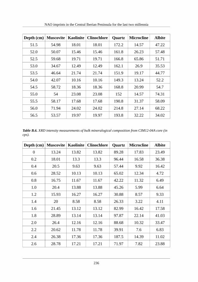
NAO imprints in the Central Iberian Peninsula for the last two millennia
Depth (cm) Muscovite Kaolinite Clinochlore Quartz Microcline Albite
51.5 54.98 18.01 18.01 172.2 14.57 47.22
52.0 50.07 15.46 15.46 161.8 26.23 57.48
52.5 59.68 19.71 19.71 166.8 65.86 51.71
53.0 34.67 12.49 12.49 162.1 26.9 35.53
53.5 46.64 21.74 21.74 151.9 19.17 44.77
54.0 42.07 10.16 10.16 149.3 13.24 52.2
54.5 58.72 18.36 18.36 168.8 20.99 54.7
55.0 54 23.08 23.08 152 14.57 74.31
55.5 58.17 17.68 17.68 190.8 31.37 58.09
56.0 71.94 24.02 24.02 214.8 27.14 68.22
56.5 53.57 19.97 19.97 193.8 32.22 34.02
Table B.6. XRD intensity measurements of bulk mineralogical composition from CIM12-04A core (incps).
Depth (cm) Muscovite Kaolinite Clinochlore Quartz Microcline Albite
0 13.24 13.82 13.82 89.28 17.83 23.49
0.2 18.01 13.3 13.3 96.44 16.58 36.38
0.4 20.5 9.63 9.63 57.44 9.92 16.42
0.6 28.52 10.13 10.13 65.02 12.34 4.72
0.8 16.75 11.67 11.67 42.22 11.32 6.49
1.0 20.4 13.88 13.88 45.26 5.99 6.64
1.2 15.93 16.27 16.27 30.88 8.57 9.33
1.4 20 8.58 8.58 26.33 3.22 4.11
1.6 21.45 13.12 13.12 82.99 16.42 17.58
1.8 28.89 13.14 13.14 97.87 22.14 41.03
2.0 26.4 12.16 12.16 88.68 10.32 33.47
2.2 20.62 11.78 11.78 39.91 7.6 6.83
2.4 26.38 17.36 17.36 187.5 14.39 11.02
2.6 28.78 17.21 17.21 71.97 7.82 23.88
236

Chemical and mineralogical data
Depth (cm) Muscovite Kaolinite Clinochlore Quartz Microcline Albite
2.8 31.71 13.32 13.32 78.88 35.02 128.9
3.0 26.26 23.1 23.1 81.75 11.82 23.61
3.2 22.81 19.02 19.02 109.5 21.75 28.88
3.4 27.5 14.49 14.49 77.18 12.46 20.18
3.6 21.73 18.77 18.77 93.73 48.86 89.08
3.8 13.37 14.76 14.76 47.12 5.75 19.88
4.0 21.1 12.29 12.29 77.43 10.23 22.54
4.2 26.64 21.24 21.24 95.46 17.89 23.11
4.4 31.08 13.38 13.38 114.4 10.42 15.82
4.6 16.45 9.65 9.65 81.78 14.79 14.63
4.8 25.79 14.91 14.91 65.8 18.34 15.84
5.0 21.46 12.28 12.28 71.74 11.71 23.62
5.2 18.69 15.63 15.63 118.3 23.31 37.81
5.4 21.52 18.45 18.45 60.84 11.82 15.38
5.6 24.06 21.5 21.5 59.16 48.54 16.47
5.8 12.06 19.11 19.11 36.52 14.71 3.43
6.0 17.09 14.8 14.8 62.38 9.54 13.65
6.2 26.39 16.49 16.49 95.45 14.29 15.02
6.4 28.04 14.9 14.9 105.3 13.48 30.54
6.6 17.17 14.09 14.09 36.35 10.92 6.68
6.8 8.19 14.07 14.07 60.85 13.73 22.54
7.0 22.45 15.5 15.5 119.9 11.52 12.88
7.2 31.67 15.96 15.96 115.7 24.8 25.88
7.4 23.78 18.48 18.48 103 17.85 33.06
7.6 16.31 11.98 11.98 63.21 6.3 10.34
7.8 12.38 16.86 16.86 72.38 10.41 19.88
8.0 20.92 19.07 19.07 105.8 20.35 43.97
8.2 20.19 11.76 11.76 82.78 10.96 14.83
8.4 12.23 12.03 12.03 70.16 11.56 28.48
8.6 13.78 20.72 20.72 65.33 6.9 22.36
237

NAO imprints in the Central Iberian Peninsula for the last two millennia
Depth (cm) Muscovite Kaolinite Clinochlore Quartz Microcline Albite
8.8 23.48 14.75 14.75 104.5 15.04 21.07
9.0 27.96 18.5 18.5 157.4 16.19 21.62
9.2 24.98 15.79 15.79 97.21 23.75 35.03
9.4 7.48 11.53 11.53 61.95 12.88 30.43
9.6 17.5 13.41 13.41 77.95 19.35 24.7
9.8 26.48 13.85 13.85 52.29 9.95 17.87
10.0 11.49 16.49 16.49 70.05 10.81 16.13
10.2 21.58 14.89 14.89 113.4 29.6 40.1
10.4 21.96 12.59 12.59 94.11 17.79 35.27
10.6 35.9 17.92 17.92 111.9 35.03 24.89
10.8 29.07 14.54 14.54 156.7 15.99 35.73
11.0 35.31 29.03 29.03 136.1 25.52 39.8
11.2 32.67 21.91 21.91 99.69 18.35 39.63
11.4 39.48 20.82 20.82 110.4 20.08 33.53
11.6 17.44 15.82 15.82 127 14.27 37.2
11.8 31.47 16.37 16.37 177 14.64 35.91
12.0 27.96 23.74 23.74 144.6 46.47 62.76
12.2 13.27 19.99 19.99 95.03 15.13 25.25
12.4 34.03 18.39 18.39 98.49 17.61 24.27
12.6 25.86 21.81 21.81 93.9 12.57 39.39
12.8 28.54 20.84 20.84 130.4 15.73 24.81
13.0 26.52 20.47 20.47 66.44 10.61 26.04
13.2 16.48 15.49 15.49 121.2 16.64 30.34
13.4 27.43 16.33 16.33 109.6 27.05 44.97
13.6 18.39 20.79 20.79 116.4 33.39 25.38
13.8 41.39 20.39 20.39 137.8 25.63 149.3
14.0 22.88 19.68 19.68 157.2 30.72 29.94
14.2 31.31 18.74 18.74 123.3 26.12 40.47
14.4 44 23.32 23.32 143.2 66.15 35.87
14.6 24 16.08 16.08 48.34 5.15 12.13
238

Chemical and mineralogical data
Depth (cm) Muscovite Kaolinite Clinochlore Quartz Microcline Albite
14.8 26.11 21.89 21.89 113.6 32.72 63.67
15.0 36.72 25.2 25.2 148 25.64 52.82
15.2 31.91 28.33 28.33 121.8 53.1 29.51
15.4 21.06 18.52 18.52 119.7 21.46 42.98
15.6 27.88 23.72 23.72 94.14 25.61 28.84
15.8 30.26 25.07 25.07 191.9 27.08 59.14
16.0 38.42 23.02 23.02 141.6 24.88 55.51
16.2 36.07 21.11 21.11 146.7 24.57 60.86
16.4 28.74 26.58 26.58 108.3 15.61 40.83
16.6 32.23 20.61 20.61 119.7 41.37 35.76
16.8 25.92 27.04 27.04 122.4 15.05 37.22
17.0 34.42 22.87 22.87 169.4 29.59 39.18
17.2 29.88 22.59 22.59 119.2 14.38 43.08
17.4 32.54 18.27 18.27 119.1 18.58 69.23
17.6 26.29 21.06 21.06 122 14.6 31.07
17.8 29.57 24.11 24.11 110.9 17.45 130
18.0 64.94 21.74 21.74 191.6 51.35 66.79
18.2 32.78 20.55 20.55 133.4 23.77 42.66
18.4 35.48 25.46 25.46 163.6 24.77 103.5
18.6 42.57 22.88 22.88 160.7 107.8 178.4
18.8 59.62 25.15 25.15 193.2 36.43 48.47
19.0 35.76 28.64 28.64 195.3 70.38 58.44
19.2 28.22 19.04 19.04 141.6 21.58 29.82
19.4 32.75 21.46 21.46 151.4 60.49 92.41
19.6 44.22 24.84 24.84 228.5 21.48 45.06
19.8 55.17 22.22 22.22 193.8 45.52 54.27
20.0 46.03 26.34 26.34 166.7 31.75 64.81
20.2 48.21 26.46 26.46 210.6 60.47 51.96
20.4 34.16 24.45 24.45 150.6 43.15 67.68
20.6 86.29 24.92 24.92 286.8 137 83.76
239

NAO imprints in the Central Iberian Peninsula for the last two millennia
Depth (cm) Muscovite Kaolinite Clinochlore Quartz Microcline Albite
20.8 43.78 20.18 20.18 213.7 100.1 43.48
21.0 38.24 21.23 21.23 139.1 16.5 46.02
21.2 25.71 18.9 18.9 144.5 31.7 56.51
21.4 34.88 24.37 24.37 197 25.65 108.6
21.6 28.97 18.46 18.46 118.1 27.38 33.37
21.8 33.97 25.58 25.58 165.2 34.55 82.28
22.0 34.35 20.46 20.46 124.7 18.48 44.22
22.2 29.3 21.11 21.11 158.2 16.74 31.33
22.4 45.33 31.11 31.11 162.1 21.95 44.83
22.6 29.59 21.25 21.25 110 33.44 38.17
22.8 36.91 28.51 28.51 131.2 28.33 59.68
23.0 30.69 19.84 19.84 99.73 17.54 31.58
23.2 28.5 27.29 27.29 116.5 23.2 40.58
23.4 30.77 26.27 26.27 198.1 25.3 37.64
23.6 37.15 21.99 21.99 100.1 18.98 39.5
23.8 52.81 28.59 28.59 166.4 20.77 51.72
24.0 30.14 23.05 23.05 86 10.02 23.77
24.2 31.06 25.02 25.02 115 14.84 41.58
24.4 31.38 19.87 19.87 124 26.05 23.99
24.6 35.43 20.69 20.69 139.2 17.99 48.93
24.8 41.09 19.14 19.14 172.3 27.48 41.8
25.0 22.81 18.57 18.57 94.74 19.98 19.98
25.2 22.75 17.59 17.59 86.09 9.62 31.43
25.4 24.43 19.69 19.69 101.3 17.43 35.93
25.6 30.73 25.61 25.61 139.3 17.99 48.93
25.8 36.22 19.58 19.58 112.6 22.06 40.58
26.0 24.42 13.49 13.49 92.46 17.23 24.4
26.2 23.63 20.07 20.07 100.6 23.68 29.3
26.4 32.19 19.12 19.12 134.5 27.99 41.85
26.6 19.91 17.27 17.27 118.2 15.89 62.22
240

Chemical and mineralogical data
Depth (cm) Muscovite Kaolinite Clinochlore Quartz Microcline Albite
26.8 29.44 17.61 17.61 105.3 19.19 34.62
27.0 22.71 18.65 18.65 100 28.91 38.94
27.2 25.52 19.57 19.57 83.48 11.07 31.72
27.4 36.67 14.42 14.42 110.1 19.27 35.89
27.6 21.14 17.12 17.12 89.27 65.59 33.96
27.8 29.12 20.83 20.83 124.4 12.35 71.52
28.0 29.11 25.74 25.74 126.1 16.62 29.98
28.2 17.92 26.54 26.54 114.4 20.17 34.7
28.4 23.42 22.61 22.61 138.3 30.84 42.33
28.6 28.83 30.15 30.15 119.2 24.02 47.55
28.8 33.18 21.57 21.57 96.71 15.94 20.92
29.0 33.98 18.42 18.42 166.3 28.03 31.51
29.2 23.77 21.39 21.39 92.43 20.68 31.44
29.4 81.25 25.74 25.74 179.9 51.58 73.71
29.6 26.31 19.47 19.47 112.8 17.01 32.2
29.8 35.67 26.59 26.59 135.8 32.75 36.92
30.0 37.15 28.98 28.98 134.4 23.97 39.2
30.2 18.48 16.34 16.34 75 18.29 25.72
30.4 31.22 19.12 19.12 116.5 21.12 33.48
30.6 32.61 19.85 19.85 108.7 31.63 39.48
30.8 10.94 18.57 18.57 108.1 11.53 25.93
31.0 35.03 23.07 23.07 119.7 26.19 36.33
31.2 34.66 21.49 21.49 133.4 16.64 38.21
31.4 39.57 19.13 19.13 131.3 29.48 36.7
31.6 37.35 18.97 18.97 124.6 52.44 52.7
31.8 34.41 21.35 21.35 117.2 15.55 34.06
32.0 32.72 20.27 20.27 110.8 41.88 27.47
32.2 28.23 16.69 16.69 120.9 18.46 35.81
32.4 25.17 15.52 15.52 112.2 24.29 36.44
32.6 27.72 16.71 16.71 113.2 17.1 32.06
241

NAO imprints in the Central Iberian Peninsula for the last two millennia
Depth (cm) Muscovite Kaolinite Clinochlore Quartz Microcline Albite
32.8 28.36 18.8 18.8 130.1 23.22 28.7
33.0 32.03 20.13 20.13 113.4 22.53 41.14
33.2 31.17 16.15 16.15 96.54 16.48 68.32
33.4 34.51 22.69 22.69 121.4 45.09 34.97
33.6 26.52 26.35 26.35 103.3 22.74 25.73
33.8 22.38 23.44 23.44 135.1 17.98 31.79
34.0 29.84 23.76 23.76 97.43 28.36 27.23
34.2 38.44 24.7 24.7 146.9 21.38 50.38
34.4 38.74 16.79 16.79 154.8 24.98 49.63
34.6 35.47 17.89 17.89 172.7 36.12 31.92
34.8 46.21 19.94 19.94 184.3 52.17 140.1
35.0 28.84 10.29 10.29 131.4 54.36 42.57
35.2 23.12 19.04 19.04 117.9 17.39 27.31
35.4 32.06 24.75 24.75 131.3 87.95 39.07
35.6 39.14 17.4 17.4 151.4 32.76 51.03
35.8 32.51 22.5 22.5 129.6 52.52 42.33
36.0 65.08 16.91 16.91 255.1 101.5 92.06
36.5 32.72 16.36 16.36 160.9 26.83 48.92
37.0 38.58 19.27 19.27 155.1 33.43 49.63
37.5 41.63 18.93 18.93 160.6 77.61 49.92
38.0 34.43 17.05 17.05 125.3 24.96 33.3
38.5 30.14 16.59 16.59 120.3 18.45 32.59
39.0 35.41 18.23 18.23 131.9 26.58 35.22
39.5 51.66 19.64 19.64 138.1 27.38 30.7
40.0 33.67 19.01 19.01 156.9 94.31 32.88
40.5 31.57 19.43 19.43 130.5 20.56 43.67
41.0 35.08 17.13 17.13 131.1 35.92 30.13
41.5 36.49 16.36 16.36 146.4 43.94 39.75
42.0 35.68 18.91 18.91 129.1 21.12 31.19
42.5 35.38 16.88 16.88 140.3 32.25 31.09
242

Chemical and mineralogical data
Depth (cm) Muscovite Kaolinite Clinochlore Quartz Microcline Albite
43.0 32.95 19.93 19.93 138.9 26.88 34.99
43.5 38.45 19.76 19.76 190.1 62.24 47.33
44.0 29.99 17.86 17.86 140.7 26.25 80.41
44.5 34.67 21.76 21.76 153.3 40.73 73.94
45.0 43.52 17.49 17.49 178.5 46.53 70.06
45.5 66.18 24.92 24.92 299 81.93 64.03
46.0 33.8 16.7 16.7 136.9 23.46 51.1
46.5 38.48 19.07 19.07 138.7 36.81 31.99
47.0 35.27 15.17 15.17 153.3 19.01 30.53
47.5 41.78 19.51 19.51 169.1 53.42 38.67
48.0 41.22 16.47 16.47 182.2 60.12 34.83
48.5 32.56 18.62 18.62 151.1 22.91 34.72
49.0 36 18.39 18.39 163.8 28.75 44.74
49.5 39.11 19.63 19.63 153.9 43.17 43
50.0 38.42 20.27 20.27 164.3 36.88 39.89
50.5 34.13 18.2 18.2 140.5 29.92 39.17
51.0 37.67 19.7 19.7 133.4 31.88 44.97
51.5 50.17 24.42 24.42 142.1 28.63 44.97
52.0 55.58 25.07 25.07 210.9 65.41 46.33
52.5 35.15 18.94 18.94 135.7 32.62 44.16
53.0 33.47 19.19 19.19 142.4 30.06 30.59
53.5 36.64 17.14 17.14 148.1 26.87 45.51
54.0 39.83 25.16 25.16 117.6 24.77 31.05
54.5 48.6 19.92 19.92 142.2 21.23 54.91
55.0 35.35 21.62 21.62 123.8 18.23 42.31
55.5 43.17 21.39 21.39 128 95.32 52.12
56.0 37.35 25.34 25.34 132.8 24.52 28.17
56.5 27.67 20.86 20.86 119.6 20.21 32.63
57.0 52.58 24.15 24.15 155.8 37.28 44.2
57.5 36.97 21.67 21.67 154.2 44.63 37.46
243
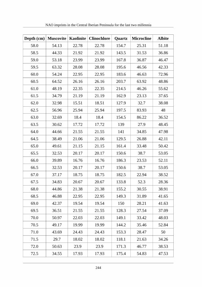
NAO imprints in the Central Iberian Peninsula for the last two millennia
Depth (cm) Muscovite Kaolinite Clinochlore Quartz Microcline Albite
58.0 54.13 22.78 22.78 154.7 25.31 51.18
58.5 44.33 21.92 21.92 143.5 31.53 36.86
59.0 53.18 23.99 23.99 167.8 36.87 46.47
59.5 63.32 28.08 28.08 195.6 46.56 42.33
60.0 54.24 22.95 22.95 183.6 46.63 72.96
60.5 64.52 26.16 26.16 203.7 63.92 48.86
61.0 48.19 22.35 22.35 214.5 46.26 55.62
61.5 34.79 21.19 21.19 162.9 23.13 37.65
62.0 32.98 15.51 18.51 127.9 32.7 38.08
62.5 56.96 25.94 25.94 197.5 83.93 48
63.0 32.69 18.4 18.4 154.5 86.22 36.52
63.5 30.62 17.72 17.72 139 27.9 48.45
64.0 44.66 21.55 21.55 141 34.85 47.98
64.5 38.49 21.06 21.06 129.5 26.88 42.11
65.0 49.61 21.15 21.15 161.4 33.48 50.42
65.5 32.53 20.17 20.17 150.6 38.7 53.05
66.0 39.89 16.76 16.76 186.3 23.53 52.11
66.5 32.53 20.17 20.17 150.6 38.7 53.05
67.0 37.17 18.75 18.75 182.5 22.94 38.52
67.5 34.83 20.67 20.67 133.8 52.3 28.36
68.0 44.86 21.38 21.38 155.2 30.55 38.91
68.5 46.88 22.95 22.95 149.3 31.89 41.65
69.0 42.37 19.54 19.54 150 28.21 41.63
69.5 36.51 21.55 21.55 128.3 27.54 37.09
70.0 50.97 22.03 22.03 149.1 33.42 48.03
70.5 49.17 19.99 19.99 144.2 35.46 52.84
71.0 43.69 24.43 24.43 153.3 28.47 50
71.5 29.7 18.02 18.02 118.1 21.63 34.26
72.0 50.63 23.9 23.9 171.3 46.77 38.53
72.5 34.55 17.93 17.93 175.4 54.83 47.53
244

Chemical and mineralogical data
Depth (cm) Muscovite Kaolinite Clinochlore Quartz Microcline Albite
73.0 77.07 26.34 26.34 319.5 172.7 75.07
73.5 42.68 19.69 19.69 213.9 71.84 59.3
74.0 25.46 15.98 15.98 114.7 18.33 28.44
74.5 36.79 17.02 17.02 142.4 30.67 41.08
75.0 47.06 19.98 19.98 140.2 74.2 55.52
75.5 38.47 19.39 19.39 121 26.33 40.97
76.0 38.8 25.04 25.04 161.3 47.72 57.87
76.5 66.63 24.34 24.34 184.3 45.76 56.68
77.0 54.17 24.041 24.04 204.5 60.75 70.46
77.5 43.4 19.35 19.35 222.5 76.49 64.74
78.0 34.6 18.6 18.6 185.1 50.08 82.03
78.5 44.25 20.24 20.24 182.9 44.13 47.26
79.0 35.42 17.82 17.82 172.3 45.83 52.72
79.5 40.13 21.81 21.81 190.2 63.46 59.23
80.0 29.12 16.92 16.92 136.1 37.3 37.87
80.5 35.84 19.54 19.54 125.2 27.57 40.72
81.0 58.44 22.96 22.96 166.1 47.21 56.73
81.5 37.08 25.19 25.19 127.7 36.54 37.97
82.0 47.53 21.57 21.57 137 39.91 53.78
82.5 41.67 21.04 21.04 117.3 23.93 54.14
83.0 30.27 19.5 19.5 139.8 18.15 64.22
83.5 34.3 18.99 18.99 125.2 20.67 33.56
84.0 44.24 20.27 20.27 123.6 33.13 36.52
84.5 34.3 18.99 18.99 125.2 20.67 33.56
85.0 30.66 17.72 17.72 124.5 16.21 34.81
85.5 52.13 21.29 21.29 140.2 22.42 52.33
86.0 53.55 21.4 21.4 210.6 81.91 45.91
86.5 52.28 27.73 27.73 153.6 38.27 53.18
87.0 33.42 19.26 19.26 127.1 22.02 52.13
87.5 41.81 20.75 20.75 133.2 28.67 38.58
245
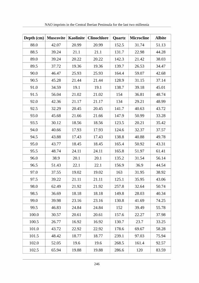
NAO imprints in the Central Iberian Peninsula for the last two millennia
Depth (cm) Muscovite Kaolinite Clinochlore Quartz Microcline Albite
88.0 42.07 20.99 20.99 152.5 31.74 51.13
88.5 39.24 21.1 21.1 131.7 22.98 44.28
89.0 39.24 20.22 20.22 142.3 21.42 38.03
89.5 37.72 19.36 19.36 139.7 26.53 34.47
90.0 46.47 25.93 25.93 164.4 59.07 42.68
90.5 45.28 21.44 21.44 128.9 31.15 37.14
91.0 34.59 19.1 19.1 138.7 39.18 45.01
91.5 56.04 21.02 21.02 154 36.81 48.74
92.0 42.36 21.17 21.17 134 29.21 48.99
92.5 32.29 20.45 20.45 141.7 40.63 43.72
93.0 45.68 21.66 21.66 147.9 50.99 33.28
93.5 30.12 18.56 18.56 123.5 20.21 35.42
94.0 40.66 17.93 17.93 124.6 32.37 37.57
94.5 43.88 17.43 17.43 138.8 40.88 49.78
95.0 43.77 18.45 18.45 165.4 50.92 43.31
95.5 48.74 24.11 24.11 165.8 51.97 61.41
96.0 38.9 20.1 20.1 135.2 31.54 56.14
96.5 51.43 22.1 22.1 156.9 36.9 44.54
97.0 37.55 19.02 19.02 163 31.95 38.92
97.5 39.22 21.11 21.11 125.1 35.95 43.06
98.0 62.49 21.92 21.92 257.8 32.64 50.74
98.5 36.69 18.18 18.18 149.8 28.03 40.34
99.0 39.98 23.16 23.16 130.8 41.69 74.25
99.5 46.83 24.84 24.84 152 39.49 55.78
100.0 30.57 20.61 20.61 157.6 22.27 37.98
100.5 26.77 16.92 16.92 130.7 23.7 33.25
101.0 43.72 22.92 22.92 178.6 69.67 58.28
101.5 48.42 18.77 18.77 239.1 97.03 75.94
102.0 52.05 19.6 19.6 268.5 161.4 92.57
102.5 65.94 19.88 19.88 286.6 120 83.59
246
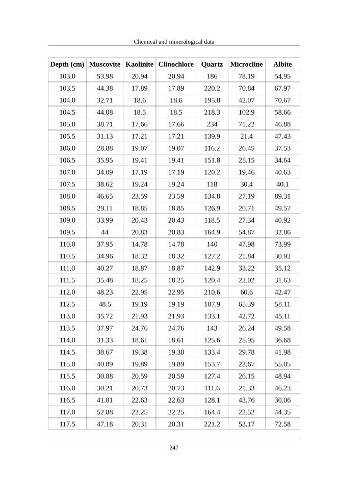
Chemical and mineralogical data
Depth (cm) Muscovite Kaolinite Clinochlore Quartz Microcline Albite
103.0 53.98 20.94 20.94 186 78.19 54.95
103.5 44.38 17.89 17.89 220.2 70.84 67.97
104.0 32.71 18.6 18.6 195.8 42.07 70.67
104.5 44.08 18.5 18.5 218.3 102.9 58.66
105.0 38.71 17.66 17.66 234 71.22 46.88
105.5 31.13 17.21 17.21 139.9 21.4 47.43
106.0 28.88 19.07 19.07 116.2 26.45 37.53
106.5 35.95 19.41 19.41 151.8 25.15 34.64
107.0 34.09 17.19 17.19 120.2 19.46 40.63
107.5 38.62 19.24 19.24 118 30.4 40.1
108.0 46.65 23.59 23.59 134.8 27.19 89.31
108.5 29.11 18.85 18.85 126.9 20.71 49.57
109.0 33.99 20.43 20.43 118.5 27.34 40.92
109.5 44 20.83 20.83 164.9 54.87 32.86
110.0 37.95 14.78 14.78 140 47.98 73.99
110.5 34.96 18.32 18.32 127.2 21.84 30.92
111.0 40.27 18.87 18.87 142.9 33.22 35.12
111.5 35.48 18.25 18.25 120.4 22.02 31.63
112.0 48.23 22.95 22.95 210.6 60.6 42.47
112.5 48.5 19.19 19.19 187.9 65.39 58.11
113.0 35.72 21.93 21.93 133.1 42.72 45.11
113.5 37.97 24.76 24.76 143 26.24 49.58
114.0 31.33 18.61 18.61 125.6 25.95 36.68
114.5 38.67 19.38 19.38 133.4 29.78 41.98
115.0 40.89 19.89 19.89 153.7 23.67 55.05
115.5 30.88 20.59 20.59 127.4 26.15 48.94
116.0 30.21 20.73 20.73 111.6 21.33 46.23
116.5 41.81 22.63 22.63 128.1 43.76 30.06
117.0 52.88 22.25 22.25 164.4 22.52 44.35
117.5 47.18 20.31 20.31 221.2 53.17 72.58
247

NAO imprints in the Central Iberian Peninsula for the last two millennia
Depth (cm) Muscovite Kaolinite Clinochlore Quartz Microcline Albite
118.0 37.34 18.96 18.96 143.7 34.68 51.66
118.5 57.69 24.53 24.53 183.2 101.2 158
119.0 62.83 27.48 27.48 181.3 35.22 37.65
119.5 46.17 21.52 21.52 133.7 28.15 33.42
120.0 42.33 20.36 20.36 147.1 20.57 41.05
120.5 66.15 26.79 26.79 165.5 38.72 50.53
121.0 31.88 18.79 18.79 135.8 28.55 66.11
121.5 55.13 24.76 24.76 168.8 66.23 49.24
122.0 40.67 22.28 22.28 127.3 26.21 37.58
122.5 39.66 18.63 18.63 158.4 29.82 36.35
123.0 56.03 23.49 23.49 167.2 24.52 34.81
123.5 41.79 16.79 16.79 173.9 48.74 40.03
124.0 26.77 16.11 16.11 136.1 34.61 41.66
124.5 34.25 18.86 18.86 132 42.53 40.01
125.0 50.9 23.37 23.37 194.1 75.13 50.21
Table B.7. XRD intensity measurements of bulk clay minerals composition from PE12-01-01 core (incps); Sap=saponite, Clc=clinochlore, Pkg=palygorskite, Ms=muscovite, Kln=kaolinite.
Depth(mm)
SampleSap
glycolatedClc
driedPkg
heatedMs
driedKln
driedPkg
dried
2 AO-1 3.13 7.17 33.57 22.06 9.6 3.08
10 AO-2 – 6.86 29.42 19.4 9.09 3.76
18 AO-3 2.12 8.05 29.1 23.41 8.71 2.88
34 AO-4 – 6.51 25.12 18.37 8.3 1.21
48 AO-5 – 7.13 21.43 12.89 6.97 1.7
68 AO-6 – 8.68 29.16 22.21 9.35 2.54
80 AO-7 1.36 11.03 22.88 15.82 8.64 2.66
98 AO-8 – 9.15 20.92 14.01 6.92 2.89
114 AO-9 0.69 6.59 16.43 10.77 6.49 2.78
130 AO-10 – 5.83 12.65 6.89 7.29 2.81
248

Chemical and mineralogical data
146 AO-11 1.53 5.61 14.76 8.38 12.62 3.05
162 AO-12 1.95 5.62 11.87 7.9 6.67 1.83
178 AO-13 – 7.34 15.69 10.71 6.63 2.46
192 AO-14 2.02 4.39 14.3 9.6 6.92 2.98
210 AO-15 – 6.8 14.56 9.04 7.14 3.67
226 AO-16 – 5.97 18.8 13 7.4 3.01
242 AO-17 – 7.76 13.94 7.27 6.04 2.63
258 AO-18 – 5.86 11.22 7.75 5.62 3.11
276 AO-19 – 7.09 11.82 6.94 6.6 3.71
290 AO-20 2.93 5.19 12.68 8.28 6.43 3.31
298 AO-21 – 9.51 12.02 8.36 5.37 3.14
330 AO-22 2.85 7.36 10.68 7.74 5.98 2.91
346 AO-23 – 6.76 12.84 9.07 6.56 3.41
370 AO-24 – 4.95 13.09 7.84 6.59 2.59
380 AO-25 – 4.14 8.53 5.95 5.98 4.12
395 AO-26 2.99 7.08 15.9 8.43 6.46 2.35
415 AO-27 – 4.15 11.89 7 6.44 2.09
435 AO-28 – 7.53 18.62 9.33 7.29 3.8
455 AO-29 – 8.71 18.1 11.23 7.84 3.6
475 AO-30 – 9.31 14.63 10.26 8.33 3.15
495 AO-31 – 8.07 15.94 9.33 6.9 3.59
515 AO-32 – 7.83 15.85 9.6 6.67 3.07
535 AO-33 2.73 7.48 16.12 10.21 7.99 2.98
555 AO-34 – 9.74 16.67 10.33 6.93 3.39
560 AO-35 5.15 15.18 28.16 17.87 10.29 3.21
Table B.8. XRD intensity measurements of bulk clay minerals composition from CIM12-04A core (incps); Sap=saponite, Clc=clinochlore, Pkg=palygorskite, Ms=muscovite, Kln=kaolinite.
Depth(mm)
SampleSap
glycolatedClc
driedPkg
heatedMs
driedKln
driedPkg
dried
2 AO-36 – 9.73 8.37 7.96 8.95 3.32
249

NAO imprints in the Central Iberian Peninsula for the last two millennia
16 AO-37 2.4 7.66 8.64 6.87 8.14 3.58
30 AO-38 1.73 8.54 11.16 8.53 9.02 3.23
42 AO-39 1.75 10.17 14.69 9.9 10.26 3.81
54 AO-40 2.25 11.81 14.51 10.45 10.49 3.04
72 AO-41 – 6.85 12.88 9.67 9.3 3.12
86 AO-42 – 7.95 12.42 9.53 8.89 2.55
96 AO-43 1.63 9.56 13.09 8.06 9.29 3.64
110 AO-44 – 10.47 14.18 10 9.41 3.25
128 AO-45 – 13.31 15.81 9.84 10.25 3.76
138 AO-46 3.17 10.29 14.97 9.8 9.06 2.97
152 AO-47 – 10.66 13.07 7.38 9.65 4.08
168 AO-48 1.88 10.22 19.55 11.72 12.84 4.21
180 AO-49 1.99 14.94 20.5 12.45 15.42 6.99
198 AO-50 – 9.28 18.36 11.12 12.39 4.52
214 AO-51 2.9 11.34 14.73 12.71 11.87 3.99
224 AO-52 – 8.7 17.15 10.94 9.5 2.92
238 AO-53 2.79 9.82 14.54 11.17 10.35 3.24
254 AO-54 – 9.79 13.38 10.24 9.37 2.31
264 AO-55 – 10.97 12.9 9.11 9.71 3.14
278 AO-56 – 8.63 12.4 9.08 10.01 4.3
294 AO-57 – 8.96 15.44 10.2 9.67 3.51
310 AO-58 – 7.12 11.81 8.65 9.23 4.51
324 AO-59 1.67 5.91 10.46 7.92 8.44 3.92
334 AO-60 2.63 8.06 11.37 7.44 9.87 3.81
352 AO-61 – 8.4 11.98 8.04 9.57 4.2
365 AO-62 – 11.79 14.43 10 10.76 4.93
390 AO-63 1.76 9.69 14.46 9.5 11.48 4.67
415 AO-64 – 9.23 16.94 9.38 4.31 4.31
440 AO-65 – 5.14 14.52 8.61 10.66 4.29
465 AO-66 – 9.66 14.73 9.29 11.82 4.31
490 AO-67 1.6 7.1 14.7 9.56 10.94 4.28
250
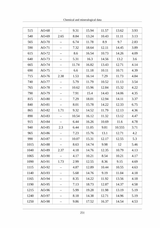
Chemical and mineralogical data
515 AO-68 – 9.31 15.94 11.57 13.62 3.93
540 AO-69 2.65 8.84 13.24 10.43 11.11 3.13
565 AO-70 – 6.74 11.78 8.9 9.7 2.83
590 AO-71 – 7.32 18.64 12.11 14.45 3.89
615 AO-72 – 8.6 16.54 10.73 14.26 4.09
640 AO-73 – 5.31 16.3 14.56 13.2 3.6
665 AO-74 – 11.74 16.82 13.43 12.71 4.14
690 AO-75 – 6.6 11.18 10.11 10.71 4.39
715 AO-76 2.38 1.53 16.14 7.29 11.73 4.84
740 AO-77 – 5.79 11.79 10.52 11.13 3.54
765 AO-78 – 10.62 15.96 12.84 15.32 4.22
790 AO-79 – 7.91 15.4 14.43 14.06 4.35
815 AO-80 – 7.29 18.01 12.94 14.11 3.37
840 AO-81 – 8.01 15.78 14.22 12.33 6.75
865 AO-82 1.71 9.32 14.52 11.79 12.13 4.36
890 AO-83 – 10.54 16.12 11.32 13.12 4.47
915 AO-84 – 6.44 16.26 10.69 11.6 4.78
940 AO-85 2.3 6.44 11.05 9.81 10.555 3.71
965 AO-86 – 7.23 15.76 13.1 12.71 4.2
990 AO-87 – 10.07 15.31 12.17 12.55 5.3
1015 AO-88 – 8.63 14.74 9.98 12 5.46
1040 AO-89 2.37 4.18 14.76 12.35 10.79 4.13
1065 AO-90 – 4.17 10.21 8.54 10.21 4.17
1090 AO-91 1.73 2.99 12.55 8.36 9.15 4.69
1115 AO-92 – 4.87 12.89 10.44 10.55 4.63
1140 AO-93 – 5.68 14.76 9.19 11.04 4.18
1165 AO-94 – 8.35 14.22 11.92 13.56 4.18
1190 AO-95 – 7.13 18.73 12.87 14.37 4.58
1215 AO-96 – 5.99 19.28 11.98 13.19 5.19
1240 AO-97 – 8.18 14.38 12.71 14.96 5.19
1250 AO-98 – 9.86 17.52 16.37 14.54 4.53
251