nonparametric comparison of roc curves: testing equivalence
TRANSCRIPT

Institute of Mathematical Statistics
COLLECTIONS
Volume 7
Nonparametrics and Robustness inModern Statistical Inference andTime Series Analysis:A Festschrift in honor of ProfessorJana Jureckova
J. Antoch, M. Huskova and P.K. Sen, Editors
Institute of Mathematical StatisticsBeachwood, Ohio, USA

Institute of Mathematical StatisticsCollections
The production of the Institute of Mathematical StatisticsCollections is managed by the
IMS Office: Marten Wegkamp, Executive Secretary andElyse Gustafson, Executive Director.
Library of Congress Control Number: 2010937067
International Standard Book Number 978-0-940600-80-5
International Standard Serial Number 1939-4039
Copyright c© 2010 Institute of Mathematical Statistics
All rights reserved
Printed in Lithuania

Contents
Preface
Jaromır Antoch, Marie Huskova and PranabK. Sen . . . . . . . . . . . . . . . . . . . . . . . . . v
Contributors of this volume
. . . . . . . . . . . . . . . . . . . . . . . . . . . . . . . . . . . . . . . . . . . . . . . . . . . . . . . . . . . . . . . . . . . . . . . . . . . vii
Life and Work of Jana Jureckova: An Appreciation
Jaromır Antoch, Marie Huskova and PranabK. Sen . . . . . . . . . . . . . . . . . . . . . . . . . 1
Nonparametric comparison of ROC curves: Testing equivalence
Jaromır Antoch, Lubos Prchal and Pascal Sarda . . . . . . . . . . . . . . . . . . . . . . . . . . . . 12
The unbearable transparency of Stein estimation
Rudolf Beran . . . . . . . . . . . . . . . . . . . . . . . . . . . . . . . . . . . . . . . . . . . . . . . . . . . . . . . . . . . . . . .25
On the estimation of cross-information quantities in rank-basedinference
Delphine Cassart, Marc Hallin and Davy Paindaveine . . . . . . . . . . . . . . . . . . . . . . 35
Estimation of irregular probability densities
Lieven Desmet, Irene Gijbels and Alexandre Lambert . . . . . . . . . . . . . . . . . . . . . . . 46
Measuring directional dependency
Yadolah Dodge and Iraj Yadegari . . . . . . . . . . . . . . . . . . . . . . . . . . . . . . . . . . . . . . . . . . . 62
On a paradoxical property of the Kolmogorov-Smirnov two-sampletest
Alexander Y. Gordon and Lev B. Klebanov . . . . . . . . . . . . . . . . . . . . . . . . . . . . . . . . . 70
MCD-RoSIS – A robust procedure for variable selection
Charlotte Guddat, Ursula Gather and Sonja Kuhnt . . . . . . . . . . . . . . . . . . . . . . . . . 75
A note on reference limits
Jing-Ye Huang, Lin-An Chen and Alan H. Welsh . . . . . . . . . . . . . . . . . . . . . . . . . . .84
Simple sequential procedures for change in distribution
Marie Huskova and Ondrej Chochola . . . . . . . . . . . . . . . . . . . . . . . . . . . . . . . . . . . . . . . 95
A class of multivariate distributions related to distributionswith a Gaussian component
Abram M. Kagan and Lev B. Klebanov . . . . . . . . . . . . . . . . . . . . . . . . . . . . . . . . . . . . 105
iii

Locating landmarks using templates
Jan Kalina . . . . . . . . . . . . . . . . . . . . . . . . . . . . . . . . . . . . . . . . . . . . . . . . . . . . . . . . . . . . . . . .113
On the asymptotic distribution of the analytic center estimator
Keith Knight . . . . . . . . . . . . . . . . . . . . . . . . . . . . . . . . . . . . . . . . . . . . . . . . . . . . . . . . . . . . . . 123
Rank tests for heterogeneous treatment effects with covariates
Roger Koenker . . . . . . . . . . . . . . . . . . . . . . . . . . . . . . . . . . . . . . . . . . . . . . . . . . . . . . . . . . . . 134
A class of minimum distance estimators in AR(p) modelswith infinite error variance
Hira L. Koul and Xiaoyu Li . . . . . . . . . . . . . . . . . . . . . . . . . . . . . . . . . . . . . . . . . . . . . . .143
Integral functionals of the density
David M. Mason, Elizbar Nadaraya and Grigol Sokhadze . . . . . . . . . . . . . . . . . . 153
Qualitative robustness and weak continuity: the extreme unction?
Ivan Mizera . . . . . . . . . . . . . . . . . . . . . . . . . . . . . . . . . . . . . . . . . . . . . . . . . . . . . . . . . . . . . . . 169
Asymptotic theory of the spatial median
Jyrki Mottonen, Klaus Nordhausen and Hannu Oja. . . . . . . . . . . . . . . . . . . . . . . .182
Second-order asymptotic representation of M-estimatorsin a linear model
Marek Omelka . . . . . . . . . . . . . . . . . . . . . . . . . . . . . . . . . . . . . . . . . . . . . . . . . . . . . . . . . . . . 194
Extremes of two-step regression quantiles
Jan Picek and Jan Dienstbier . . . . . . . . . . . . . . . . . . . . . . . . . . . . . . . . . . . . . . . . . . . . . 204
Is ignorance bliss: Fixed vs. random censoring
Stephen Portnoy . . . . . . . . . . . . . . . . . . . . . . . . . . . . . . . . . . . . . . . . . . . . . . . . . . . . . . . . . . 215
The Theil–Sen estimator in a measurement error perspective
Pranab K. Sen and A.K.Md. Ehsanes Saleh . . . . . . . . . . . . . . . . . . . . . . . . . . . . . . 224
The Lasso with within group structure
Sara van de Geer . . . . . . . . . . . . . . . . . . . . . . . . . . . . . . . . . . . . . . . . . . . . . . . . . . . . . . . . . 235
Nonparametric estimation of residual quantiles in a conditionalKoziol–Green model with dependent censoring
Noel Veraverbeke . . . . . . . . . . . . . . . . . . . . . . . . . . . . . . . . . . . . . . . . . . . . . . . . . . . . . . . . . . 245
Robust error-term-scale estimate
Jan Amos Vısek . . . . . . . . . . . . . . . . . . . . . . . . . . . . . . . . . . . . . . . . . . . . . . . . . . . . . . . . . . 254
iv

Preface
In the broader domain of Statistics and Probability theory, Jana Jureckova is adistinguished researcher, especially in Europe and among the women researchers.Her fundamental research contributions stemmed from the inspiring ideas of heradvisor Jaroslav Hajek and covered the evolving areas of nonparametrics, generalasymptotic theory, robust statistics, as well as, applications in sampling theory,econometrics and environmetrics.
She has a longstanding and exemplary leadership to the academics; the Czech(oslovakian) school of statistics has indeed benefited from her professional acumen.
Jana has an illuminating career in the Department of Probability and Mathe-matical Statistics at the Faculty of Mathematics and Physics, Charles Universityin Prague, for over forty years.
It was thought that at the juncture of her career, Jana should be honored andrecognized for her standing in her professional field.
The idea of floating this Festschrift was essentially due to the three editors of thisvolume and, in addition, the spontaneous response from her colleagues far beyondthe boundaries of her native country has been truly inspiring. Jana has a long listof collaborators and former advisees too. Because of time and space constraints,not all of them were invited to contribute to this Festschrift, and a chosen handfulof contributors with professional standing have spanned the broad area of Jana’sresearch interest.
Besides an article of appreciation of Jana’s life and work by the three editors,there are twenty-four articles with a list of co-authors over 40. All these articles havegone through the usual peer-reviewing in strict adherence to the high standards ofthe IMS Lecture Notes and Collection Series. To all the reviewers we have deepgratitude for their most timely job. To the contributors we are truly grateful fortheir willingness to contribute in a relatively short time and to many of them forrefereeing some other submitted articles. We could not have reached this stage ofthe Festschrift without their support and interest.
Last but not the least, our profound thanks are due to the Department of Prob-ability and Mathematical Statistics, at the Faculty of Mathematics and Physics atCharles University in Prague for their enthusiastic support in all respects.
We would like to thank Blanka Anfilova for all administrative assistance andIva Maresova for meticulous job with the electronic preparation of the manuscriptduring the reviewing stage as well as the final phase.
We are indeed very grateful to the IMS Editorial Office for their constant as-sistance from the initiation of this project to its very completion. Initial contactwith Professor Anirban Dasgupta (editor of the IMS Collection Series at that time)facilitated the negotiation. In particular, IMS Executive Director Elyse Gustafsondeserves our most sincere appreciation for their untiring efforts to have this volumereleased on time and the same applies to Production Manager Ms Geri Mattson forcarrying out publications related tasks expeditiously and efficiently.
We conclude this note with a toast to Jana Jureckova for her consent to thisproject and occasional help too.
v

Jaromır AntochCharles University, Czech Republic
Marie HuskovaCharles University, Czech Republic
Pranab K. SenUniversity of North Carolina, U. S.A.
vi

Contributors to this volume
Antoch, J., Charles University in Prague
Beran, R., University of California
Cassart, D., Universite Libre de Bruxelles
Chen, L-A., National Chiao Tung University, TaiwanChochola, O., Charles University
Desmet, L., Katholieke Universiteit LeuvenDienstbier, J., Charles University in PragueDodge, Y., Universite de Neuchatel
Gather, U., Technische University DortmundGijbels, I., Katholieke Universiteit LeuvenGordon, A.Y., University of North Carolina, CharlotteGuddat, Ch., Technische University Dortmund
Hallin, M., Universite Libre de BruxellesHuang, J.-Y., National Institute of Technology, TaiwanHuskova, M., Charles University in Prague
Kagan, A.M., University of MarylandKalina, J., Charles University in PragueKlebanov, L. B., Charles University in PragueKnight, K., University of TorontoKoenker, R., University of IllinoisKoul, H. L., Michigan State UniversityKuhnt, S., Technische University Dortmund
Lambert, A., Universite catholique de Louvain
Mason, D.M., Delaware UniversityMizera, I., University of AlbertaMottonen, J., University of Helsinki
Nadaraya, E., Tbilisi State UniversityNordhausen, K., University of Tampere
Oja, H., University of TampereOmelka, M., Charles University in Prague
Paindaveine, D., Universite Libre de BruxellesPicek, J., Technical University of LiberecPortnoy, S., University of IllinoisPrchal, L., Charles University in Prague
vii

Saleh, E., Carleton University, OttavaSarda, P., Universite ToulouseSen, P.K., University of North Carolina, Chapel HillSokhadze, G., Tbilisi State University
ven de Geer, S., EHT ZurichVeraverbeke, N., Hasselt UniversityVısek, J. A., Charles University in Prague
Welsh, A.H., Australian National University, Canberra
Xiaoyu, L., Michigan State University
Yadegari, I., Tarbiat Modares University of Tehran
viii

ix


IMS CollectionsNonparametrics and Robustness in Modern Statistical Inference and Time SeriesAnalysis: A Festschrift in honor of Professor Jana JureckovaVol. 7 (2010) 1–11c© Institute of Mathematical Statistics, 2010DOI: 10.1214/10-IMSCOLL701
Life and Work of Jana Jureckova:
An Appreciation
Jaromır Antoch1 and Marie Huskova1 and Pranab K. Sen2
Charles University at Prague, and University of North Carolina at Chapel Hill
Abstract: Professor Jana Jureckova has extensively contributed to many ar-eas in statistics and probability theory. Her contributions are highlighted herewith reverent appreciation and admiration from all her colleagues, advisees aswell as research collaborators.
Professor Jana Jureckova has extensively contributed to many areas in statisticsand probability theory. This article is an appreciation of her work that draws onfeedback from her colleagues, collaborators and advisees.
Jana (Pristoupilova) Jureckova was born on September 20, 1940, in Prague,Czechoslovakia. She spent a larger part of her childhood in Roudnice nad Labem(central Bohemia). She had her school and college education in Prague. She gradu-ated (MSc.) from the Charles University at Prague in 1962, and earned her Ph.D.(CSc.) degree in Statistics in 1967 from the Czechoslovak Academy of Sciences. Herdissertation advisor was Professor Jaroslav Hajek and the principal theme of herthesis was R-estimation based on the uniform asymptotic linearity of linear rankstatistics in the parameter of interest. This work not only provided a rigorous jus-tification of asymptotics for rank estimators in linear models but also opened up anovel and elegant approach to the study of asymptotic properties of nonparametrictests and estimates. In later years Jana has tremendously expanded the domain ofthis basic theme far beyond linear rank statistics.
Professor Hajek was inspirational for career development of not only a numberof his advisees but also of many other colleagues in Prague and abroad. All thethree editors of this collection have benefited a lot from Professor Hajek’s visionand his professional acumen. Jana was no less fortunate than others to join theDepartment of Probability and Mathematical Statistics at Faculty of Mathematicsand Physics, Charles University in Prague, in 1964, even before her dissertationwork was completed. It would be interesting to note that Professor Hajek formeda very active and bright group of researchers, including some outstanding womenmembers in the Department of Probability and Mathematical Statistics, the CharlesUniversity in Prague, at a time when mathematical sciences used to have a farsmaller representation of women researchers and teachers. With a deep sense of
1Department of Probability and Mathematical Statistics, Charles University, Prague,Sokolovska 83, CZ–186 75 Prague 8, Czech Republic.e-mails: {antoch,huskova}@karlin.mff.cuni.cz
2Departments of Biostatistics and Statistics Operations Research, University of North Car-olina, Chapel Hill, NC 27599-7420, USA. e-mail: [email protected]
AMS 2000 subject classifications: asymptotics, Jaroslav Hajek, nonparametrics, rank estima-tor, regression rank scores; robustness, tail-behavior, uniform asymptotic linearity.
Keywords and phrases: 60, 62.
1

2 Jaromır Antoch, Marie Huskova and Pranab K. Sen
devotion and professional acumen Jana has been associated with her alma materfor more than forty-three years. In 1982 Jana passed her habilitation, in 1984 shedefended her DrSc. scientific degree and, finally, in 1992 she was appointed by thepresident of Czechoslovakia to the rank of a full professors. At the present she holds apivotal position at the Jaroslav Hajek Center of Theoretical and Applied Statistics,established under the auspices of the Ministry of Education, Czech Republic.
Jana has published extensively (more than 120 scientific articles), mostly, inthe leading journals of statistics and probability theory and coauthored a numberof monographs too. We enclose herewith Jana’s list of publications. Her researchinterests cover a wide area of statistical inference, including (but not limited to):
a) statistical procedures based on ranks;b) robust statistical procedures based on so called M-statistics and L-statistics;c) statistical procedures based on extreme sample observations;d) tail behavior and its application in statistics;e) asymptotic methods of mathematical statistics;f) finite sample behavior of estimates and tests.
During 1967 – 1976 her research attention mostly focused on nonparametrics, andthe impact of Professor Hajek’s outstanding research was well reflected in Jana’swork. She realized a harder way to excel in research at the demise of Jaroslav Hajekin 1974, and undertook a much broader research field. She exploited in the late1970’s the relationship of R-, M- and L-estimators using the same uniform asymp-totic linearity she developed in her dissertation. In collaboration with P.K. Sen,in 1981, she exploited the moment convergence of R-, L-, and M-estimators in abroader sequential context. Berry-Essen bounds for the normal approximation ofthe distribution of rank statistics were also studied in detail. Gradually, she becomemore interested in robust inference, and has contributed extensively in this field. Herresearch, some in collaboration with others, culminated in the 1996 Jureckova – Senbook. Regression rank scores and their use in statistical inference has been a favoritetopic of research of Jana. Her work with Gutenbrunner, Portnoy and Koenker isspecially noticeable. Moving beyond the independence assumption was a naturalfollow-up, and in that respect, in later years, her work with Hallin, Koul and oth-ers are noteworthy. Shrinkage estimation in a robust setup has also Jana’s imprintfrom time to time. Quantile regression is another topic of Jana’s research interest.Extreme value distributions and tail behavior of robust statistics have been exten-sively studied by Jana. In addition, she has always fathomed into adaptive robustinference and their computational aspects, later work with Jan Picek bearing thistestimony.
Jana has co-edited a number of monographs, the most noteworthy was the firstone in 1978: Contributions to Statistics: Essays in memory of Jaroslav Hajek. Shehas co-authored a number of monographs, some in an advanced level and some atintermediate levels with some emphasis on data analysis. All they are cited in theenclosed list of publications.
Jana has an impressive list of places where she has visited from time to time: Uni-versity of North Carolina, Chapel Hill; University of Illinois at Urbana-Champaign;Universite Libre de Bruxelles; Universite P. Sabatier, Toulouse; Universite de Neu-chatel; Carleton University in Ottawa, Limburgs University Center at Diepenbeek;Humboldt University in Berlin, University at Bordeaux, and University of Rome.
Jana can communicate well in Russian, French, German and English languages,in addition to her mother tongue. No wonder, she had collaborators from all thefive continents and in diverse setups. Jana has a most impressive list of extensive

Jana Jureckova: Life and Works 3
international research collaboration, including Pranab K. Sen (University of NorthCarolina), Roger Koenker and Stephen Portnoy (University of Illinois), EhsanesSaleh (Carleton University, Ottawa), Marc Hallin (Universite Libre de Bruxelles),Xavier Milhaud (University P. Sabatier, Toulouse), Hira Koul (Michigan State Uni-versity), Yadolah Dodge (Universite de Neuchatel), Paul Janssen and Noel Veraver-beke (Hasselt University), Lev B. Klebanov (St. Petersburg, Charles University)and Keith Knight (University of Toronto) among others, as well as a number ofher own advisees all over the world. She has long fruitful discussions with AbramM. Kagan (St. Petersburg, University of Maryland), Allan Welsh (The AustralianNational University), Witting (University of Freiburg) and Ivan Mizera (Universityof Alberta) among others. Note that Jana has supervised the doctoral dissertationof more than 15 advisees; the list is appended here. Many of them have proclaimedsignificant professional recognition.
Jana had important international collaborative research grants, co-sponsored bythe Czech National Grant Agency, National Science Foundation in USA or NSERCin Canada.
Jana is an elected member of the International Statistical Institute, Fellow of theInstitute of Mathematical Statistics, member of the Bernoulli Society (where sheserved in the council as well as its European regional committee). Since 2003 she isthe elected fellow of the Learned Society of Czech Republic, the most prestigiousCzech scientific society. During 2000, she was visiting Belgian Universities for sixmonths under a Francqui Foundation distinguished faculty position.
She has served on the editorial board of a number of leading statistics journals,including Annals of Statistics (1992 – 1997), Journal of the American Statistical As-sociation (2006 – 2008), Sankhya (2006 – 2011), Sequential Analysis (1982 – 2002),and Statistics (1980 – 1993). She has also served on the Review Panel of (US) NSFGrants and many other Research sponsoring agencies in Czech Republic and else-where. Jana has organized or co-organized a number of important internationalmeetings. Let us mention a series of successful workshops on Perspectives in Mod-ern Statistical Inference (1998, 2002, 2005), series of conferences on L1-statisticalprocedures (1987, 1992, 1997, 2002) and ICORS 2010 among others. With JaromırAntoch and Tomas Havranek Jana started very successful series of biennial con-ferences ROBUST at 1980 which impacted Czech Statistical Community in a pro-found way.
Even now Jana is as active, as energetic and as persuasive in basic research andprofessional development as in the time when she started her scientific career. Wewish her a very long and even more prosperous life in future.

4 Jaromır Antoch, Marie Huskova and Pranab K. Sen
PH.D. GUIDANCE (co-adviser)
Served as the adviser and supervised the doctoral dissertations of the followingpersons at Charles University in Prague. (Cornelius Gutenbrunner at Freiburg Uni-versity and Hana Kotouckova at Masaryk University, Brno).
Jaromır Antoch Behavior of the Location Estimators from thePoint of View of Large Deviations (adviserV. Dupac)
1982
Cornelius Gutenbrunner Zur Asymptotik von Regression Quantil Pro-zessen und daraus abgeleiten Statistiken
1985
Jan Hanousek Robust Bayesian Type Estimators 1990
Marek Maly The Asymptotics for Studentized k-step M -Es-timators of Location
1991
Bohumır Prochazka Trimmed Estimates in the Nonlinear RegressionModel
1992
Ivan Mizera Weak Continuity and Identifiability of M-Func-tionals
1993
Jan Picek Testing Linear Hypotheses Based on RegressionRank Scores
1996
Ivo Muller Robust Methods in the Linear CalibrationModel
1996
Jan Svatos M-estimators in Linear Model for Irregular Den-sities
2000
Alena Fialova Estimating and Testing Pareto Tail Index 2001
Marek Omelka Second Order Properties of some M- and R-estimators
2006
Martin Schindler Inference Based on Regression Rank Scores 2008
Hana Kotouckova History of Robust Mathematical-StatisticalMethods
2009
MONOGRAPHS AND TEXTBOOKS
Robuste statistische Methoden in linearen Modellen. In: K.M. S. Humak: Statistis-che Methoden der Modellbildung II, 195–255 (Chapter 2). Akademie-Verlag, Berlin,1983. English translation: Nonlinear Regression, Functional Relations and RobustMethods. (Bunke, H. and Bunke, O., eds.), 104–158 (Chapter 2). J. Wiley, NewYork, 1989.
Robust Statistical Inference: Asymptotics and Interrelations (co-author P.K. Sen),J. Wiley, New York, 1996.
Adaptive Regression (co-author Y. Dodge). Springer-Verlag, New York, 2000.
Robust Statistical Methods (textbook, in Czech). Karolinum, Publishing House ofCharles University in Prague, 2001.
Robust Statistical Methods with R (co-author J. Picek). Chapman & Hall/CRC,2005.

Jana Jureckova: Life and Works 5
Publications of Jana Jureckova
Jureckova, J. (1969). Asymptotic linearity of a rank statistic in regression param-eter. Ann. Math. Statist. 40, 1889–1900.
Jureckova, J. (1971). Nonparametric estimate of regression coefficients. Ann.Math. Statist. 42, 1328–1338.
Jureckova, J. (1971). Asymptotic independence of rank test statistic for testingsymmetry on regression. Sankhya A 33, 1–18.
Jureckova, J. (1972). An asymptotic theorem of nonparametrics. Coll. Math. Soc.J. Bolyai (Proc. 9th European Meeting of Statisticians), pp. 373–380.
Jureckova, J. (1973). Almost sure uniform asymptotic linearity of rank statistics inregression parameter. Trans. 6th Prague Conf. on Inform. Theory, RandomProcesses and Statist. Decis. Functions, pp. 305–313.
Jureckova, J. (1973). Central limit theorem for Wilcoxon rank statistics process.Ann. Statist. 1, 1046–1060.
Jureckova, J. (1973). Asymptotic behaviour of rank and signed rank statisticsfrom the point of view of applications. Proc. 1st Prague Symp. on Asympt.Statist., Vol. 1, pp. 139–155.
Jureckova, J. (1975). Nonparametric estimation and testing linear hypotheses inthe linear regression model. Math. Operationsforsch. Statist. 6, 269–283.
Jureckova, J. (1975). Asymptotic comparison of maximum likelihood and a rankestimate in simple linear regression model. Comment. Math. Univ. Carolinae16, 87–97.
Jureckova, J. and Puri, M. L. (1975). Order of normal approximation of rankstatistics distribution. Ann. Probab. 3, 526–533.
Jureckova, J. (1977). Asymptotic relations of least-squares estimate and of tworobust estimates of regression parameter vector. Trans. 7th Prague Conf. onInform. Theory, Random Processes and Statist. Decis. Functions A, pp. 231–237.
Jureckova, J. (1977). Locally optimal estimates of location. Comment. Math.Univ. Carolinae 18, 599–610.
Jureckova, J. (1977). Asymptotic relations of M-estimates and R-estimates in lin-ear regression model. Ann. Statist. 5, 464–472.
Jureckova, J. (1978). Bounded-length sequential confidence intervals for regres-sion and location parameters. Proc. 2nd Prague Symp. on Asympt. Statist.,pp. 239–250.
Jureckova, J. (1979). Finite-sample comparison of L-estimators of location. Com-ment. Math. Univ. Carolinae 20, 507–518.
Jureckova, J. 1979). Contributions to Statistics. Jaroslav Hajek Memorial Volume.(Jureckova, J., ed.) Academia, Prague and Reidel, Dordrecht.
Jureckova, J. (1979). Nuisance medians in rank testing scale. Contributions toStatistics – J. Hajek Memorial Volume (Jureckova, J. ed.), pp. 109–117.
Jureckova, J. (1980). Asymptotic representation of M-estimators of location. Math.Operationsforsch. Statist., Ser. Statistics 11, 61–73.
Jureckova, J. (1980), Rate of consistency of one-sample tests of location. J. Statist.Planning Infer. 4, 249–257.
Jureckova, J. (1980). Robust statistical inference in linear regression model. Proc.3rd Intern. Summer School on Probab. and Statistics, Varna 1978, pp. 141–166.
Jureckova, J. (1980). Robust estimation in linear regression model. Banach CentrePublications 6, 168–174.

6 Jaromır Antoch, Marie Huskova and Pranab K. Sen
Jureckova, J. and Sen, P.K. (1981). Sequential procedures based on M-estimatorswith discontinuous score functions. J. Statist. Planning Infer. 5, 253–266.
Jureckova, J. and Sen, P.K. (1981). Invariance principles for some stochastic pro-cesses related to M-estimators and their role in sequential statistical inference.Sankhya A 43, 190–210.
Jureckova, J. (1981). Tail behavior of location estimators. Ann. Statist. 9, 578–585.
Huskova, M. and Jureckova, J. (1981). Second order asymptotic relations of M-estimators and R-estimators in two-sample location model. J. Statist. Plan-ning Infer. 5, 309–328.
Jureckova, J. (1981). Tail behaviour of location estimators in non-regular cases.Comment. Math. Univ. Carolinae 22, 365–375.
Jureckova, J. and Sen, P.K. (1982). Simultaneous M-estimator of the commonlocation and scale-ratio in the two-sample problem. Math. Operationsforsch.Statist., Ser. Statistics 13, 163–169.
Jureckova, J. and Sen, P.K. (1982). M-estimators and L-estimators of location:Uniform integrability and asymptotically risk-efficient sequential version. Comm.Statist. C 1, 27–56.
Jureckova, J. (1982). Tests of location and criterion of tails. Coll. Math. Soc. J.Bolyai 32, 469–478.
Jureckova, J. (1983). Robust estimators of location and regression parameters andtheir second order asymptotic relations. Trans. 9th Prague Conf. on Inform.Theory, Random Processes and Statistics & Decisons Functions, pp. 19–32.Academia, Prague.
Jureckova, J. (1983). Asymptotic behavior of M-estimators of location in non-regular cases. Statistics & Decisions 1, 323–340.
Jureckova, J. (1983). Winsorized least-squares estimator and its M-estimator coun-terpart. Contributions to Statistics: Essays in Honour of Norman L. Johnson(Sen, P.K., ed.), pp. 237–245. North Holland.
Jureckova, J. (1983). Trimmed polynomial regression. Comment. Math. Univ.Carolinae 24, 597–607.
Jureckova, J. (1983). Robust estimators and their relations. Acta Univ. Carolinae– Math. et Phys. 24, 49–59.
Jureckova, J. (1984). Regression quantiles and trimmed least squares estimatorunder a general design. Kybernetika 20, 345–357.
Jureckova, J. (1984). Rates of consistency of classical one-sided tests. Robustnessof Statistical Methods and Nonparametric Statist. (Rasch, D. and Tiku, M. L.,eds.), pp. 60–62. Deutscher Verlag der Wissenschaften, Berlin.
Jureckova, J. and Vısek, J. A. (1984). Sensitivity of Chow–Robbins procedure tothe contamination. Sequential Analysis 3, 175–190.
Jureckova, J. and Sen, P.K. (1984). On adaptive scale-equivariant M-estimatorsin linear models. Statistics & Decisions 2, Suppl. Issue No. 1, 31–46.
Behnen, K., Huskova, M., Jureckova, J. and Neuhaus, G. (1984). Two-samplelinear rank tests and their Bahadur efficiencies. Proc. 3rd Prague Symp. onAsympt. Statist. 1, pp. 103-117.
Jureckova, J. (1984). M-, L- and R-estimators. Handbook of Statistics Vol. 4(Krishnaiah, P.R. and Sen, P.K., eds.), pp. 464–485 (Chapter 21). ElsevierSci. Publishers.
Jureckova, J. (1985). Representation of M-estimators with the second order asymp-totic distribution. Statistics & Decisions 3, 263–276.

Jana Jureckova: Life and Works 7
Janssen, P., Jureckova, J. and Veraverbeke, N. (1985). Rate of convergence ofone- and two-step M-estimators with applications to maximum likelihood andPitman estimators. Ann. Statist. 13, 1222–1229.
Jureckova, J. (1985). Robust estimators of location and their second-order asymp-totic relations. Celebration of Statistics. The ISI Centenary Volume (Atkin-son, A.C. and Fienberg, S. E., eds.), pp. 377–392. Springer-Verlag, New York.
Antoch, J. and Jureckova, J. (1985). Trimmed least squares estimator resistant toleverage points. Comp. Statist. Quarterly 4, 329–339.
Jureckova, J. (1985). Sequential confidence intervals based on robust estimators.Sequential Methods in Statistics. Banach Centre Publications 16, 309–319.
Jureckova, J. (1985). Tail-behavior of L-estimators and M-estimators. Proc. 4thPannonian Symp. 1, pp. 205–217.
Huskova, M. and Jureckova, J. (1985). Asymptotic representation of R-estimatorsof location. Proc. 4th Pannonian Symp. 1, 145–165.
Jureckova, J. (1985). Linear statistical inference based on L-estimators. LinearStatistical Inference (Calinski, T. and Klonecki, W., eds.), pp. 88–98. LectureNotes in Statistics 15, Springer-Verlag.
Jureckova, J. (1986). Asymptotic representation of L-estimators and their relationsto M-estimators. Sequential Analysis 5, 317–338.
Jureckova, J. and Kallenberg, W.C.M. (1987). On local inaccuracy rates andasymptotic variances. Statistics & Decisions 5, 139–158.
Jureckova, J. and Sen, P.K. (1987). A second order asymptotic distributional rep-resentation of M-estimators with discontinuous score functions. Ann. Probab.5, 814–823.
Jureckova, J. and Portnoy, S. (1987). Asymptotics for one-step M-estimators inregression with application to combining efficiency and high breakdown point.Comm. Statist. A 16, 2187–2199.
Jureckova, J. and Sen, P.K. (1987). An extension of Billingsley’s uniform bound-edness theorem to higher dimensional M-processes. Kybernetika 23, 382–387.
Jureckova, J., Kallenberg, W.C.M. and Veraverbeke, N. (1988). Moderate andCramer-type deviations theorems for M-estimators. Statist. Probab. Letters6, 191–199.
Dodge, Y. and Jureckova, J. (1988). Adaptive combination of least squares andleast absolute deviations estimators. Statist. Analysis Based on L1-Norm(Dodge, Y., ed.), pp. 275–284. North Holland.
Dodge, Y. and Jureckova, J. (1988). Adaptive combination of M-estimator and L1-estimator in the linear model. Optimal Design and Analysis of Experiments(Dodge, Y., Fedorov, V.V. and Wynn, H. P., eds.), pp. 167–176. ElsevierSci. Publ., Amsterdam.
Jureckova, J. (1989). Consistency of M-estimators in linear model generated bynon-monotone and discontinuous ψ-functions. Probab. and Math. Statist. 10,1–10.
Jureckova, J. and Sen, P.K. (1989). Uniform second order asymptotic linearity ofM-estimators in linear models. Statistics & Decisions 7, 263–276.
Jureckova, J. Saleh, A.K.M.E. and Sen, P.K. (1989). Regression quantiles andimproved L-estimation in linear models. Probability, Statistics and Designof Experiments (Bahadur, R.R., ed.), pp. 405–418. Wiley Eastern Ltd., NewDelhi.
Jureckova, J. (1989). Consistency of M-estimators of vector parameters. Proc.4th Prague Conf. on Asympt. Statist. (Mandl, P. and Huskova, M., eds.),pp. 305–312. Charles University Press, Prague.

8 Jaromır Antoch, Marie Huskova and Pranab K. Sen
Jureckova, J. and Saleh, A.K.M.E. (1990). Robustified version of Stein’s multi-variate location estimation. Statist. and Probab. Letters 9, 375–380.
Jureckova, J. and Sen, P.K. (1990). Effect of the initial estimator on the asymp-totic behavior of one-step M-estimator. Ann. Inst. Statist. Math. 42, 345–357.
Jureckova, J. and Welsh, A.H. (1990). Asymptotic relations between L- and M-estimators in the linear model. Ann. Inst. Statist. Math. 42, 671–698.
He, X., Jureckova, J., Koenker, R. and Portnoy, S. (1990). Tail behavior of regres-sion estimators and their breakdown points. Econometrica 58, 1195–1214.
Jureckova, J. (1991). Confidence sets and intervals. Handbook of Sequential Analy-sis (Ghosh, B.K. and Sen, P.K., eds.), pp. 269–281 (Chapter 11). M. Dekker,New York.
Dodge, Y., Jureckova, J. and Antoch, J. (1991). Adaptive combination of leastsquares and least absolute deviations estimators: Computational aspects.Comp. Statist. & Data Analysis 12, 87–100.
Dodge, Y. and Jureckova, J. (1991). Flexible L-estimation in the linear model.Comp. Statist. & Data Analysis 12, 211–220.
Jureckova, J. (1991). Comments to the paper “Nonparametrics: retrospectives andperspectives” by P.K. Sen. Nonpar. Statist. 1, 49–50.
Jureckova, J. (1992). Estimation in a linear model based on regression rank scores.Nonpar. Statist. 1, 197–203.
Gutenbrunner, C. and Jureckova, J. (1992). Regression rank scores and regressionquantiles. Ann. Statist. 20, 305–330.
Jureckova, J. (1992). Uniform asymptotic linearity of regression rank scores pro-cess. Nonparametric Statistics and Related Topics (Saleh, A.K.M.E., ed.),pp. 217–228. Elsevier Sciences Publishers.
Jureckova, J. (1992). Tests of Kolmogorov–Smirnov type based on regression rankscores. Trans. 11th Prague Conf. on Inform. Theory, Random Proc.andStatist. Decis. Functions, Vol. B (Vısek, J. A., ed.), pp. 41–49. Academia,Prague & Kluwer Acad. Publ.
Dodge, Y. and Jureckova, J. (1992). A class of estimators based on adaptive convexcombinations of two estimation procedures. L1-Statist. Analysis and RelatedMethods (Dodge, Y., ed.), pp. 31–45. North Holland.
Gutenbrunner, C., Jureckova, J., Koenker, R., and Portnoy, S. (1993). Tests oflinear hypotheses based on regression rank scores. Nonpar. Statist. 2, 307–331.
Jureckova, J. and Sen, P.K. (1993). Asymptotic equivalence of regression rankscores estimators and R-estimators in linear models. Statistics and Probabil-ity: A Raghu Raj Bahadur Festschrift (Ghosh, J,K., Mitra, S.K., Parthasarathy,K.R., and Prakasa Rao B. L. S., eds.), pp. 279–292. Wiley Eastern LimitedPublishers.
Jureckova, J. and Sen, P.K. (1993). Regression rank scores scale statistics and stu-dentization in linear models. Asymptotic Statistics [Proc. 5th Prague Symp.](Mandl, P. and Huskova, M., eds.) pp. 111–121. Physica-Verlag, Heidelberg.
Jureckova, J. and Milhaud, X. (1993). Shrinkage of maximum likelihood estima-tor of multivariate location. Asymptotic Statistics [Proc. 5th Prague Symp.](Mandl, P. and Huskova, M., eds.), pp. 303–318. Physica-Verlag, Heidelberg.
Jureckova, J. and Prochazka, B. (1994). Regression quantiles and trimmed leastsquares estimator in nonlinear regression model. Nonpar. Statist. 3, 201–222.
Jureckova, J., Koenker, R., and Welsh, A.H. (1994). Adaptive choice of trimmingproportions. Ann. Inst. Statist. Math. 40, 737–755.

Jana Jureckova: Life and Works 9
Jureckova, J. (1995). Regression rank scores: Asymptotic linearity andRR-estimators.Proceedings of MODA 4 (Kitsos, C. P. and Muller, W.G., eds.), pp. 193–203.Physica-Verlag, Heidelberg.
Dodge, Y. Jureckova, J. (1995). Estimation of quantile density function based onregression quantiles. Statist. Probab. Letters 23, 73–78.
Jureckova, J. (1995). Affine and scale-equivariant M-estimators in linear model.Probability and Math. Statist. 15, 397–407.
Jureckova, J. and Maly, M. (1995). The asymptotics for studentized k-step M-estimators of location. Sequential Analysis 14 (3), 225–245.
Jureckova, J. (1995). Trimmed mean and Huber’s estimator: Their difference as agoodness-of-fit criterion. J. of Statistical Science 29, 31–35.
Jureckova, J., ed. (1997). Environmental Statistics and Earth Science. Environ-metrics 7 (5), (special issue).
Dodge, Y. and Jureckova, J. (1997). Adaptive choice of trimming proportion intrimmed least squares estimation. Statist. and Probab. Letters 33, 167–170.
Hallin, M., Jureckova, J., Kalvova, J., Picek, J., and Zahaf, T. (1997). Non-parametric tests in AR models with applications to climatic data. Envi-ronmetrics 8, 651–660.
Jureckova, J. and Klebanov, L. B. (1997). Inadmissibility of robust estimators withrespect to L1 norm. L1-Statistical Procedures and Related Topics (Dodge, Y.,ed.). IMS Lecture Notes – Monographs Series 31, 71–78.
Jureckova, J. and Sen, P.K. (1997). Asymptotic representations and interrela-tions of robust estimators and their applications. Handbook of Statistics 15(Maddala, G. S. and Rao, C.R., eds.), pp. 467–512. North Holland.
Jureckova, J. (1998). Characterization and admissibility in invariant models. PragueStochastics’98 (Huskova, M., Lachout, P., and Vısek, J. A., eds.), pp. 275–278.JCMF Praha.
Hallin, M., Jureckova, J., and Milhaud, X. (1998). Characterization of error dis-tributions in time series regression models. Statist. and Probab. Letters 38,335–345.
Huskova, M. and Jureckova, J. (1998). Jaroslav Hajek and its impact on the theoryof rank tests. Collected Works of Jaroslav Hajek with Commentary (Huskova,M., Beran, R. and Dupac, V., eds.), pp. 15–20. J. Wiley.
Jureckova, J. and Klebanov, L. B. (1998). Trimmed, Bayesian and admissible es-timators. Statist. and Probab. Letters 42, 47–51.
Jureckova, J. and Sen, P.K. (1998). Partially adaptive rank and regression rankscores tests in linear models. Applied Statistical Science IV (Ahmad, E.,Ahsanullah, M., Sinha, B.K., eds.), pp. 1–12.
Picek, J. and Jureckova, J. (1998). Application of rank tests for detection of de-pendence in time series (in Czech). ROBUST’98 (Antoch, J. and Dohnal,G., eds.), pp. 149–160. JCMF Praha.
Jureckova, J. (1999). Equivariant estimators and their asymptotic representations.Tatra Mountains Mathematical Publications 17, 1–9.
Jureckova, J. (1999). Regression rank scores tests against heavy-tailed alternatives.Bernoulli 5, 659–676.
Hallin, M., Jureckova, J., Picek, J., and Zahaf, T. (1999). Nonparametric tests ofindependence of two autoregressive time series based on autoregression rankscores. J. Statist. Planning Infer. 75, 319–330.
Hallin, M. and Jureckova, J. (1999). Optimal tests for autoregressive models basedon autoregression rank scores. Ann. Statist. 27, 1385–1414.

10 Jaromır Antoch, Marie Huskova and Pranab K. Sen
Jureckova, J. and Milhaud, X. (1999). Characterization of distributions in invari-ant models. J. Statist. Planning Infer. 75, 353–361.
Portnoy, S. and Jureckova, J. (1999). On extreme regression quantiles. Extremes2 (3), 227–243.
Jureckova, J. (2000). Tests of tails based on extreme regression quantiles. Statist.& Probab. Letters 49, 53–61.
Kalvova, J., Jureckova, J., Picek, J., and Nemesova, I. (2000). On the order ofautoregressive (AR) model in temperature series. Meteorologicky casopis 3,19–23.
Jureckova, J. and Sen, P.K. (2000). Goodness-of-fit tests and second order asymp-totic relations. J. Statist. Planning Infer. 91, 377–397.
Jureckova, J., Koenker, R., and Portnoy, S. (2001). Tail behavior of the leastsquares estimator. Statist. & Probab. Letters 55, 377–384.
Jureckova, J. and Picek, J. (2001). A class of tests on the tail index. Extremes4 (2), 165–183.
Picek, J. and Jureckova, J. (2001). A class of tests on the tail index using themodified extreme regression quantiles. ROBUST’2000 , pp. 217–226 (Antoch,J. and Dohnal, G., eds.). Union of Czech Mathematicians and Physicists,Prague.
Jureckova, J. and Sen, P.K. (2001). Asymptotically minimum risk equivariant es-timators. Data Analysis from Statistical Foundations – Festschrift in honourof the 75th birthday of D.A.S. Fraser (Saleh, A.K.M.E., ed.), 329–343. NovaScience Publ., Inc., Huntington, New York.
Jureckova, J., Koenker, R., and Portnoy, S. (2001). Estimation of Pareto indexbased on extreme regression quantiles. Prepress #22, Charles University,Department of Probability and Math. Statistics.
Jureckova, J., Picek, J., and Sen, P.K. (2002). A goodness-of-fit test with nuisanceparameters: Numerical performance. J. Statist. Planning Infer. 102 (2), 337–347.
Jureckova, J. (2002). L1 derivatives, score functions and tests. Statistical DataAnalysis Based on the L1 Norm and Related Methods (Dodge, Y., ed.), pp. 183–189. Birkhauser, Basel.
Dodge, Y. and Jureckova, J. (2002). Adaptive combinations of tests. Goodness-of-Fit Tests and Model Validity (Huber-Carol, C., Balakrishnan, N., Nikulin,M. S. and Mesbach, M., eds.), pp. 411–422. Birkhauser, Boston.
Jureckova, J. (2003). Statistical tests on tail index of a probability distributionwith a discussion. Metron LXI (2), 151–190.
Jureckova, J. (2003). “Statistical tests for comparison of two data-sets” with adiscussion (in Czech). Statistika 3, 1–23.
Jureckova, J. and Milhaud, X. (2003). Derivative in the mean of a density andstatistical applications. Mathematical Statistics and Applications. Festschriftfor Constance van Eeden (Moore, M., Leger, C., and Froda, S., eds.) IMSLecture Notes 42, pp. 217–232.
Jureckova, J., Picek, J. and Sen, P.K. (2003). Goodness-of-fit tests with nuisanceregression and scale. Metrika 58, 235–258.
Sen, P.K., Jureckova, J., and Picek, J. (2003). Goodness-of-fit test of Shapiro–Wilk type with nuisance regression and scale. Austrian J. of Statist. 32 (1&2), 163–177.
Jureckova, J. and Picek, J. (2004). Estimates of the tail index based on nonpara-metric tests. Statistics for Industry and Technology (Hubert, M., Pison, G.,Struyf, A., and Van Aelst, V., eds.), pp. 141–152. Birkhauser, Basel.

Jana Jureckova: Life and Works 11
Fialova, A., Jureckova, J., and and Picek, J. (2004). Estimating Pareto tail indexbased on sample means. Revstat 2 (1), 75–100.
Jureckova, J. and Picek, J.: Two-step regression quantiles. Sankhya 67 (2), 227–252.
Jureckova, J. and Sen, P.K. (2006). Robust multivariate location estimation, ad-missibility and shrinkage phenomenon. Statistics & Decisions 24, 273–290.
Jureckova, J. and Saleh, A.K.M.E. (2006). Rank tests and regression rank scorestests in measurement error models. KPMS Preprint 54, Charles University inPrague.
Hallin, M. Jureckova, J., and Koul, H. L. (2007). Serial autoregression rank scorestatistics. In: Advances in Statistical Modelling and Inference (invited paper).Essays in Honor of Kjell A. Doksum (Vijay Nair, ed.), pp. 335–362. WorldScientific, Singapore.
Jureckova, J. and Picek, J. (2007). Shapiro–Wilk type test of normality undernuisance regression and scale. Comp. Statist. & Data Analysis 51 (10), 5184–5191.
Jureckova, J. (2007). Remark on extreme regression quantile I. Sankhya 69, 87–100.
Jureckova, J. (2007). Remark on extreme regression quantile II. Bull. of the Intern.Statist. Institute, Proceedings of the 56th Session, Section CPM026.
Jureckova, J. (2008). Regression rank scores in nonlinear models. In: Beyond Para-metrics in Interdisciplinary Research: Festschrift in honor of Professor PranabK. Sen’ (Balakrishnan, N., Pena, E.A., and Silvapulle, M. J., eds.). Instituteof Mathematical Statistics Collections 1, 173-183.
Pavlopoulos, H., Picek, J., and Jureckova, J. (2008): Heavy tailed durations ofregional rainfall. Applications of Mathematics 53, 249–265.
Jureckova, J., Kalina, J., Picek, J., and Saleh, A.K.M.E. (2009). Rank tests oflinear hypothesis with measurement errors both in regressors and responses.KPMS Preprint 66, Charles University in Prague.
Jureckova, J., Koul, H. L., and Picek, J. (2009). Testing the tail index in au-toregressive models. Annals of the Institute of Statistical Mathematics 61,579–598.
Jureckova, J. and Picek, J. (2009). Minimum risk equivariant estimators in linearregression model. Statistics & Decisions 27, 1001–1019.
Jureckova, J. and Omelka, M. (2010). Estimator of the Pareto index based onnonparametric test. Communications in Statistics – Theory and Methods 39,1536–1551.
Jureckova, J., Picek, J., and Saleh, A.K.M.E. (2010). Rank tests and regressionrank scores tests in measurement error models. Computational Statistics andData Analysis, in print.
Jureckova, J. (2010). Nonparametric regression based on ranks. In: Lexicon ofStatistical Science (Lovric, M., ed.) Springer, to appear.
Jureckova, J. (2010). Adaptive linear regression. In: Lexicon of Statistical Science(Lovric, M., ed.) Springer, to appear.

IMS CollectionsNonparametrics and Robustness in Modern Statistical Inference and Time SeriesAnalysis: A Festschrift in honor of Professor Jana JureckovaVol. 7 (2010) 12–24c© Institute of Mathematical Statistics, 2010DOI: 10.1214/10-IMSCOLL702
Nonparametric comparison of ROC
curves: Testing equivalence∗
Jaromır Antoch1 , Lubos Prchal1,2 and Pascal Sarda2
Charles University of Prague and Universite Paul Sabatier Toulouse
Abstract: The problem of testing equivalence of two ROC curves is ad-dressed. A transformation of corresponding ROC curves, which motivates atest statistic based on a distance of two empirical quantile processes, is sug-gested, its asymptotic distribution found and a simulation scheme proposedthat enables us to find critical values.
1. Introduction
Receiver operating characteristic (ROC) curves are a popular and widely used toolsthat can help to summarize the overall performance of diagnostic methods and/orclassifiers assigning individuals g ∈ G = G0 ∪G1,G0 ∩G1 = ∅, into one of the groupsG0 or G1. Typically, the G1 individuals hold a feature of interest and are referred toas positives, while the G0 individuals are without the feature and are referred to asnegatives.
Assume that a suitable diagnostic measure Y is available. By convention, thelarger values of Y are supposed to be more indicative for an individual to belongto G1, so that if Y ≥ t, t ∈ R is a fixed threshold, then an individual is assigned to G1.On the contrary, if Y < t then it is assigned to G0. Let us introduce probabilitiesF0(t) = P(Y ≤ t | G0) and F1(t) = P(Y ≤ t | G1). It is evident that F0(t) and F1(t)as functions of t are distribution functions of the diagnostic variable Y for the G0and G1 groups, so that we can denote the corresponding random variables by Y0
and Y1. With this notation in mind, one possible way is to define ROC functionsas mapping �(·;F0, F1), where
�( · ;F0, F1) : R→ [0, 1]× [0, 1]
t →[1− F0(t), 1− F1(t)
].
(1)
In other words, it is a curve in a unit square [0, 1] × [0, 1] square consisting of1−F1(t) on the vertical axis plotted against 1−F0(t) on the horizontal axis for allt ∈ R. We refer the readers to the monographs Zhou et al. [32] and Pepe [23] forthe properties and applications of ROC curves.
In practice, ROC curves are often used to compare several diagnostic methods(classifiers). It is usually accepted that the method with a corresponding ROC curve
∗Work was supported by grant GACR 201/09/0755 and research project MSM 0021620839.1Charles University in Prague, Department of Probability and Mathematical Statistics,
Sokolovska 83, CZ – 186 75 Praha 8, Czech Republic. e-mails: [email protected],
[email protected] Paul Sabatier, Institut de Mathematiques de Toulouse, UMR 5219, 118 route de
Narbonne, F – 310 62 Toulouse cedex, France. e-mail: [email protected] 2000 subject classifications: Primary 62G05; secondary 62H30, 62P99.Keywords and phrases: ROC curves, binary classification, kernel ROC curves.
12

Nonparametric comparison of ROC curves: Testing equivalence 13
closest to the point (0, 1) is the best one for the particular problem. However, thisoversimplified rule is not easily applicable in practice because ROC curves in manyapplications are mostly non convex and the effect on the analysis can be non-trivial.Some examples are presented in this paper. Figure 1 displays three plots, each witha pair of ROC curves corresponding to different association measures suitable forthe collocation extraction. It illustrates three typical situations that we come across.
0 0.2 0.4 0.6 0.8 1
0
0.2
0.4
0.6
0.8
1
fpr
tpr
0 0.2 0.4 0.6 0.8 1
0
0.2
0.4
0.6
0.8
1
fpr
tpr
0 0.2 0.4 0.6 0.8 1
0
0.2
0.4
0.6
0.8
1
fpr
tpr
Fig. 1. Examples of ROC curves for several linguistic measuresdescribed in Pecina and Schlesinger [22].
First, everyone would agree that the solid curve in Figure 1a outperforms thedashed one. Figure 1b seems to be the opposite case, because both associationmeasures provide, at least optically, equivalent ROC curves. Finally, the situationin Figure 1c is not at all clear. On one hand the solid line is much closer to thepoint (0, 1). On the other hand, the curves are crossing and it is not at all clearwhich of them we should prefer. In all three cases, nevertheless, a natural questionarises: Are these ROC curves significantly different?
Several methods exist for testing the equivalence of two ROC curves. The pioneerwork, proposed for normally distributed variables, was Greenhouse and Mantel [11],later extended by Weiand et al. [30] and Beam and Wieand [2]. The most widelyused current approach is based on the AUC (area under the curve), proposed byBamber [1] and developed further by, e. g., Hanley and McNeil [13] and Delong etal. [6]. A totally different approach to testing is based on a permutation principlesuggested by Venkatraman and Begg [29]. Additional parametric methods, mainlyconnected to the binormal ROC curves and their transformations, have been alsodeveloped. We refer to Zhou et al. [32] for the review of the parametric ROC curvemodeling.
In practice it is usual that we do not have any a priori information about theform of the underlying distribution of Y . In such a case a parametric approach isnot appropriate. Since we often deal with curves possibly crossing each other asin Figure 1c, the AUC test does not work, since the crossing curves may have thesame AUC but represent diagnostic methods with completely different properties.However, in case of large sample sizes, large numbers of considered ROC curves dis-qualify the use of the permutation principle or other resampling techniques becausethey are unsupportable from a computational point of view.
All of these considerations motivated us to suggest a new test of equivalence oftwo ROC curves. The basic idea is to transform the testing problem and considerthe methods separately in groups G0 and G1 rather than to compare the ROC curvesthemselves. We believe that this alternative approach covers a large field of ROCsettings and might open new perspectives of a ROC curve analysis as a whole.It leads to a test statistic based on the difference between the quantile processesassociated with diagnostic variables of each group, and enables us to determine theasymptotic distribution under the null hypothesis of ROC curves equivalence. These

14 J. Antoch et al.
points are discussed in Section 2, where a more precise setting for ROC curves andtheir estimators are presented as well.
Regarding estimation of F0(t) and F1(t), we use the empirical cumulative distri-bution function (CDF). The main competitor of the empirical CDF is the smoothkernel CDF estimator that possesses some theoretical and “visual” advantages forCDF and ROC curve estimation. For details see, e. g., Falk [9] or Zhou et al. [33].However, in the case of large sample size of data the possible advantage of the ker-nel ROC curve appears to be completely negligible. On the other hand, estimatingROC curves and testing their equivalence are totally different tasks. In our expe-rience, the kernel estimator does not substantially improve the testing procedure,whereas the empirical CDF estimator is easier to apply. Nevertheless, in other prac-tical situations the kernel approach can be useful, at least as an alternative to theempirical CDF. It is shown that all theoretical results remain true when testing isbased on either the empirical or the kernel estimators.
The rest of the paper is organized as follows. Section 2 contains the hypothesisformulation, description of the test procedure, discussion about finding critical val-ues and the use of the kernel estimators instead of the empirical ones. The proofsof the theoretical results formulated in Section 2 are given in Appendix.
2. Test of equivalence of two ROC curves
2.1. Hypothesis formulation
Let Y be a diagnostic variable with distribution functions F0(t) and F1(t), and letY0 and Y1 denote corresponding random variables as introduced in Section 1 aboveformula (1). Denote, according to (1), the ROC curve associated to Y by
(2) ROCY ={r ∈ [0, 1]2 : ∃ t ∈ R �(t;F0, F1) = r
}.
Moreover, assume that:
(C1) Y0 and Y1 have continuous distributions with densities f0(t) and f1(t) suchthat f0(t) > 0 and f1(t) > 0 on the same interval IY ⊆ R, and that thedensities are equal to zero outside IY .
(C2) Y0 and Y1 are independent.
Remarks.
(i) Model assumption (C1) on supports assures one-to-one mapping between thethresholds and ROC points in the unit square [0, 1]× [0, 1] square. This tech-nically simplifies the notation used later, but it can be relaxed if one properlytakes into account the relationship between t and the ROC curve
(ii) Assumption (C2) means that diagnostic variable Y0 keeps only the informationassuring that negatives belong to G0, while diagnostic variable Y1 keeps onlythe information assuring that positives belong to G1.
Let us introduce another diagnostic variable Z with the distribution functionsG0(t) and G1(t), denoting the corresponding ROC curve by
(3) ROCZ ={r ∈ [0, 1]2 : ∃ t ∈ R �(t;G0, G1) = r
},
and assume that Z0 and Z1 also satisfy conditions (C1) and (C2) with densitiesg0(t) and g1(t) on some IZ . Our main goal is to compare these two ROC curves;more precisely, we aim to test equivalence of ROCY and ROCZ .

Nonparametric comparison of ROC curves: Testing equivalence 15
Taking into account the definition of ROC curves, the equivalence of ROCY andROCZ means that for any particular point rY ∈ ROCY there exists an “identical”point rZ ∈ ROCZ , i. e. rY = rZ . Equivalently, for any threshold tY ∈ IY theequivalence of the curves assures that we can find a threshold tZ ∈ IZ such that�(tY ;F0, F1) = �(tZ ;G0, G1). This allows us to express the ROC equivalence interms of distribution functions, i. e.
ROCY ≡ ROCZ ⇐⇒(4)
∀ tY ∈ IY ∃ tZ ∈ IZ : F0(tY ) = G0(tZ) & F1(tY ) = G1(tZ).
Due to (C1), all considered distribution functions are strictly increasing on IY ,IZ respectively, so that there exist increasing transformation functions τ0, τ1 : IY →IZ relating separately distribution functions in group G0 and G1. Define functionsτ0(t) and τ1(t) such that F0(t) = G0
(τ0(t)
)and F1(t) = G1
(τ1(t)
), i. e.,
(5) τ0(t) = G−10
(F0(t)
)and τ1(t) = G−1
1
(F1(t)
)∀ t ∈ IY .
ROC curves consist of the values of distribution functions evaluated simultaneouslyat the same thresholds. Therefore, they are equivalent if and only if the groups G0and G1 are related by the same threshold transformations τ0(t) ≡ τ1(t). Hence, wemay formulate the null hypothesis of the two ROC curves equivalence as
(H) τ0(t) = τ1(t) ∀ t ∈ IY ,
which we aim to test against the alternative
(A) ∃ JY ⊆ IY ,JY �= ∅, such that τ0(t) �= τ1(t) ∀ t ∈ JY .
Before deriving a test statistic, let us have a look at the transformations used.First, notice that the original problem of comparing two ROC curves is transformedinto the problem of comparing behavior of the involved diagnostic methods on G0and G1. Indeed, in order to have identical ROC curves it is not necessary thatconsidered diagnostic methods behave exactly in the same manner, but that theirbehavior globally agrees both on the “positive” and the “negative” parts of thepopulation. Globally it means that both methods correctly recognize the same pro-portion of G0 and G1 individuals, even though not necessarily the same individuals.Moreover, note that the transformations are not only technical tools but provide aninteresting diagnostic approach as well. They have been studied extensively, e. g.,by Doksum [7] and Doksum and Sievers [8], who proposed confidence regions andstatistical inference about their shape.
To get insight into this concept, the upper row of plots in Figure 2 displayempirical estimators
(6) τ0(t) = G−10
(F0(t)
)and τ1(t) = G−1
1
(F1(t)
), ∀ t ∈ IY ,
of the transformation functions used for the three ROC pairs presented in Figu-re 1. The empirical CDF’s Fk(t) and Gk(t), k = 0, 1, are based on the samplesY01, . . . , Y0nY
0, Y11, . . . , Y1nY
1, Z01, . . . , Z0nZ
0, and Z11, . . . , Z1nZ
1, with a total sample
size n = n0 + n1 = nY0 + nZ
0 + nY1 + nZ
1 . The quantile functions used are defined as
G−1k (u) = inf
{t : Gk(t) > u
}, k = 0, 1.
We clearly see almost identical transformations in the central plot as expectedin the case of equivalent ROC curves, while τ0(t) and τ1(t) have rather different

16 J. Antoch et al.
forms in the other two cases. Another point of view is presented in lower plots ofFigure 2. The transformation functions are plotted one against the other. Under thenull hypothesis the obtained cloud of points should lie along the straight line withthe unit-slope. In the central plot we see that a majority of points, with respectto supports of transformations, touches the line indicating ROC equivalence, whilethe points on the other plots are considerably far away from the expected nullhypothesis line.
−1 0 1 2 3
0
5
10
15
20
t
tau
k
−1 0 1 2 3
−3
−2
−1
0
1
t
tau
k
−2 −1 0 1−1.5
−1
−0.5
0
0.5
1
t
tau
k
0 5 10 15 20
0
5
10
15
20
tau0
tau
1
−3 −2 −1 0 1−3
−2.5
−2
−1.5
−1
−0.5
0
0.5
1
tau0
tau
1
−2 0 2 4 6 8 10−2
0
2
4
6
8
10
tau0
tau
1
Fig. 2. Transformation functions corresponding to the ROC curves plottedin Figure 1. The upper plots presents the form of τ0(t) (solid lines) andτ1(t) (dashed lines) depending on the threshold t, while the lower plots showtransformation τ0(t) plotted against τ1(t).
2.2. Test statistic
As illustrated by the graphs in Figure 2, transformation functions τ0(t) and τ1(t)indicate (non)equivalence of two ROC curves. Therefore, we suggest basing a de-cision on the distance between them. Precisely, we suggest a test statistic of theform
(7) Tn = n
∫I∗Y
(τ0(t)− τ1(t)
)2dt,
where the integral is on a closed interval I∗Y ⊆ IY such that the densities g0(s) andg1(s) are positive and finite for all s in the images of τ0(t) and τ1(t), t ∈ I∗Y , i. e.
(C3) 0 < g0(τ0(t)
)<∞ and 0 < g1
(τ1(t)
)<∞ ∀ t ∈ I∗Y .
There is a lack of symmetry as concerns cdf’s F (x) and G(x) in the definitionof Tn inherited from the genesis of ROC curves. Our numerical calculations bothwith real and simulated data show, however, that its influence on the p values isquite negligible, especially when the size of the data is large.
As expected, test statistic Tn should be small under the null hypothesis and in-crease with growing difference between τ0(t) and τ1(t) under the alternative. Hence,

Nonparametric comparison of ROC curves: Testing equivalence 17
if an appropriate critical value c(α) is available, the decision rule rejects the null hy-pothesis whenever Tn > c(α). Theorem 2.1 stated below establishes the asymptoticdistribution of Tn under the null hypothesis (H).
Theorem 2.1. Assume the setting described in Subsection 2.1 and the test statisticTn defined by (7). Let conditions (C1) – (C3) hold and Y0, Y1, Z0 and Z1 be mutuallyindependent. Let n0 and n1 tend to infinity such that nY
0 /n0 → κ0, nY1 /n1 → κ1,
κ0, κ1 ∈ (0, 1), and n tends to infinity such that n/n0 → κ0 and n/n1 → κ1,where 1/κ0, 1/κ1 ∈ (0, 1). Then, under the null hypothesis (H), the test statistic Tn
converges for n→∞ in distribution to the infinite weighted sum of independent χ21
variables η21 , η22 , . . ., i. e.
(8) TnD−→ TB =
∞∑j=1
λjη2j ,
where {λj} represent the eigenvalues of the covariance operator of the zero-meanGaussian process B(t) with the covariance structure
(9) cov(B(s), B(t)
)= c0
F0(s)(1− F0(t)
)g0(τ0(s)
)g0(τ0(t)
) + c1F1(s)
(1− F1(t)
)g1(τ1(s)
)g1(τ1(t)
) ,s ≤ t ∈ I∗Y , c0 = κ0/
(κ0(1− κ0)
), c1 = κ1/
(κ1(1− κ1)
).
Proof. Postponed to Appendix A.
Asymptotic distribution of Tn is stated in Theorem 2.1 for independent realiza-tions of independent diagnostic variables Y and Z. However, this condition is notalways realistic in practice.
We think that the above test procedure behaves well for weakly dependent vari-ables. However, when strong dependence is suspected, we suggest to use followingtwo-step approach. The first step consists of determining separately critical val-ues based on the limit processes of Fk(t) and G−1
k (t), k = 0, 1 (see appendix A).A critical value for Tn can then be obtained by using a Bonferroni inequality asderived in Horvath et al. [14]. Of course, the accuracy of this procedure, and moregenerally the problem of dependence between diagnostic variables, should warranta deep study of its own.
Taking into account the genesis of the test statistics, which is data dependent,its power against any alternative is of natural interest. Thus, the following theoremassures the consistency of the suggested test statistic.
Theorem 2.2. Assume the setting and assumptions of Theorem 2.1 and the teststatistic Tn defined by (7). Then this test is consistent against any alternative forwhich the conditions of Theorem 2.1 are satisfied.
Proof. Postponed to Appendix A.
2.3. Critical values
We have seen that the distribution of the test statistic can be approximated bythe distribution of an infinite weighted sum of χ2
1 variables TB =∑∞
j=1 λjη2j . As
a practical matter, several problems have to be solved. First, we need to estimateunknown eigenvalues {λj}. Second, even if the eigenvalues were known, we would

18 J. Antoch et al.
need to set an appropriate cut-off point and consider only a finite approximationof (8). Finally, even the finite approximation of TB may still be quite complex andgreat attention has to be paid to obtain reliable critical values.
We start with estimating the eigenvalues of the covariance operator, say Γ, ofthe limit process B(t). The covariance operator is a kernel operator whose kernelis formed by the covariance structure (9) of the underlying process, i. e.,
(10) Γξ(t) =
∫I∗Y
cov(B(s), B(t)
)ξ(s) ds, ξ ∈ L2(I∗Y ).
Therefore, estimators of the eigenvalues of Γ can be based on the estimatedcov
(B(s), B(t)
). For that purpose, we suggest using a plug-in estimator
cov(B(s), B(t)
)= c0
F0(s)(1− F0(t)
)g0(τ0(s)
)g0(τ0(t)
) + c1F1(s)
(1− F1(t)
)g1(τ1(s)
)g1(τ1(t)
) ,where s, t ∈ {t1, . . . , tp} ⊂ I∗Y and Fk(t), k = 0, 1, are the empirical CDFs, τk(t) aregiven by (6), and gk(t) stands for the kernel estimators of the densities gk(t). For de-tails see, e. g., Silverman [26]. The covariance operator Γ then can be approximatedby its discrete estimated version
(11) Γn,p =(ωi cov
(B(ti), B(tj)
))p
i,j=1,
where ωi stands for the weights used for the numerical quadrature replacing theoret-ical integration in (10) by discrete summation over {t1, . . . , tp}. Another possibilityis to use ωi = ti − ti−1. Spectral decomposition of the matrix Γn,p then provides
consistent estimators{λj
}of the asymptotic eigenvalues
{λj
}.
Values of ci’s are in practice established by the data, as seen in Theorem 2.1.The real problem can arise when the proportion of G0 elements – and therefore alsoof G1 elements – is extreme, i. e., very close to zero or n. Regarding the value of p,it follows from our calculations that it is preferable to keep the grid of values ti asdense as possible, of course, to be able to estimate Γξ(t). We used p = 103 for ourcalculations.
Theorem 2.3. Assume that kernel density estimators gk(t) are based on con-tinuous, bounded, compactly supported kernels and on bandwidths {hk} such that,hk → 0 and hkn
Zk / log(n
Zk )→∞ for nZ
k →∞, k = 0, 1. Then, under the conditionsof Theorem 2.1, it holds∣∣∣λj − λj
∣∣∣ P−→ 0 as n→∞, j = 1, 2, . . .
Proof. Postponed to Appendix A.
Suppose that the described estimation procedure results in J positive eigenval-ues that allow approximation of the infinite representation of TB by its first Jcomponents, i. e.,
(12) TB ≈J∑
j=1
λjη2j ≡ SJ ,
where η21 , . . . , η2J stand for independent χ2 variables with one degree of freedom. In
our calculations we set J in such a way that we have used all eigenvalues largerthan 10−10.

Nonparametric comparison of ROC curves: Testing equivalence 19
As distribution of SJ is not explicitly known, we can perform Monte Carlo simu-lation to obtain the desired critical value. The simulation scheme is straightforward:
1. FOR k = 1 : K2. Simulate J independent χ2
1 variables η21 , . . . , η2J
3. Calculate the value of SJ and store it to SJk
4. ENDFOR
Once the sample SJ1 , . . . , S
JK is available, we form standard empirical distribution
and quantile functions and use estimated quantiles instead of the unknown exactones. If extreme quantiles are required, more sophisticated rare event methods basedon properly tuned importance sampling or saddle point approximation should beused to obtain reliable results.
Concerning computational costs, performing sufficiently many (K ≈ 106) simu-lations for J ≈ 1000 components is feasible on a standard “home” computer in acouple of seconds. We point out that taking squares of standard normal variablesis considerably faster, mainly for a large J value, than a direct simulation of χ2
variables, especially if a matrix language such as Matlab, e. g., is available. Noticethat far fewer simulations are required to get critical values for the test statistic (8)at standards α-levels. Typically K = 104 is enough. However, in our context oneneeds reasonably exact p-values for small values of p, making it necessary to run alarge number of simulations in order to obtain a reliable estimator of the tail of thedistribution.
Kac and Siegert [16] have shown that the characteristic function of TB takes theform
ψTB (ς) = E exp{iςTB} =∞∏j=1
(1− iςλj)−1/2, ς ∈ R,
so that the inverse formula by Gil-Pelaez [10] provides the distribution function ofTB , i. e.,
P(TB ≤ s) = HTB (s) =1
2− 1
π
∫ ∞
0
�(e−iςsψTB (ς)
ς
)dς, s ≥ 0,(13)
where �(z) stands for the complex part of a complex number z ∈ C.
If TB is approximated by SJ , Imhof [15] suggested to represent its distributionfunction by
(14) P(SJ < s) =1
2− 1
π
∫ ∞
0
sin θ(s, u)
uρ(u)du,
where 2θ(s, u) =∑J
j=1 arctan(λju
)− su, ρ(u) =
∏Jj=1
(1 + λ2u2)1/4. In practice,
the integration in (14) has to be carried over a finite range 0 ≤ u ≤ U . Imhof[15] claims that the truncation error is satisfactorily small and provides its upper
bound(JUJ
)−1 ∏Jj=1 λ
−1/2j . However, our numerical experiments show that the
integration of (14) must be performed extremely carefully with either a very finestep of the order 10−6 or rather tricky weighting. We point out that a naive use ofnumerical quadrature often leads to the values of distribution function greater thanone, which is, of course, an unacceptable property. As one does not obtain an ade-quate precision gain with respect to the computational costs of Imhof’s procedure,simulations turn out to be the most favorable in practice.

20 J. Antoch et al.
2.4. Kernel estimator
The methodology described above is based on the use of the empirical estimators ofdistribution and quantile functions Fk(t), G
−1k (p), k = 0, 1. Evidently, to estimate
cdf’s Fk(t), k = 0, 1, one might use the kernel estimators instead, i. e.,
Fk(t) =1
nYk
nYk∑
i=1
H
(t− Yki
hk
), t ∈ R, k = 0, 1,(15)
where H(·) is an appropriate cumulative kernel function and the bandwidth pa-rameters h0 and h1 control the smoothness of estimators. Analogously, kernelestimators G−1
k (p) might be used to estimate quantile functions G−1k (p), where
G−1k (p) = inf
{t : Gk(t) > p
}, p ∈ (0, 1), k = 0, 1.
Combining these two kernel estimators and following ideas of Section 2.1 wenaturally come to the kernel analogue of the empirical transformation functions (6),i. e., to
(16) τk(t) = G−1k
(Fk(t)
), t ∈ IY , k = 0, 1.
Consequently, in the definition (7) one can replace the empirical transformationsτk(t) with the kernel ones τk(t) and obtain the kernel analogue of the test statis-tic Tn. As one might expect, both Theorem 2.1 and Theorem 2.3 hold for the kerneltype test statistic as well (see Appendix A for a formal proof). Hence, in the prac-tice of performing the test procedure, one may follow the same “lines” both for theempirical and the kernel estimators.
It is well known that the kernel estimators offer some advantages compared totheir empirical analogues. The most important is probably the fact that kernelsmoothing typically brings a better “visual” effect as it provides a continuous curvein the ROC square instead of discrete points of an empirical ROC curve. On theother hand, if smoothing parameters are not properly chosen, the kernel type teststatistic may lead to irrelevant and unreliable results.
The kernel CDF estimator has been proposed and studied for the first time byNadaraya [20]. Concerning the kernel ROC curves, one finds the proposals in, e. g.,Zhou et al. [33] or Lloyd [19]. The last paper has been followed-up by an interestingpaper of Hall et al. [12]. Later, Prchal [24] suggested an automatic procedure that,by means of data transformation, improves accuracy of kernel ROC curves.
Appendix A: Proofs
Theorem 2.1 is stated for the test statistic Tn defined by (7), which is based onthe empirical estimators of the distribution and quantile functions. However, weprovide its proof for a more general class of estimators satisfying conditions (P1)and (P2) listed below.
Let Y1, . . . , Ym and Z1, . . . , Zn be i.i.d. samples with respective continuous distri-bution functions F (t) and G(t) such that the supports of their densities are real in-tervals IY and IZ . Let I∗Y ⊆ IY be a closed interval such that 0 < g
(G−1
(F (t)
))<
∞, ∀ t ∈ I∗Y . Let F (t) and G(t) be the estimators of F (t) and G(t), and G−1(u) =
inf {t : G(t) > u} be an estimator of the quantile function G−1(u), such that
(P1) supt∈I∗
Y
∣∣∣F (t)− F (t)∣∣∣ a.s.−→ 0,

Nonparametric comparison of ROC curves: Testing equivalence 21
(P2)√m(F (t)−F (t)
) D−→W1
(F (t)
)&√n(G(t)−G(t)
) D−→W2
(G(t)
), ∀ t ∈ I∗Y ,
where W1 and W2 stand for independent Brownian bridges.The first step of proving Theorem 2.1 concerns a weak convergence result of an
estimated quantile process.
Lemma A.1. Let m and n tend to infinity such that m/(n + m) → κ ∈ (0, 1).Then, under the conditions (P1) and (P2),
√m+ n
(G−1
(F (t)
)−G−1
(F (t)
))(17)
D−→ 1√κ(1− κ)
1
g(G−1
(F (t)
))W (F (t)
), t ∈ I∗Y ,
where{W (s), s ∈ [0, 1]
}denotes a Brownian bridge defined on [0, 1].
Proof. First, notice that√m+ n
(G−1
(F (t)
)−G−1
(F (t)
))can be decomposed as
√m+ n
(G−1
(F (t)
)−G−1
(F (t)
))(18)
+G−1
(F (t)
)−G−1
(F (t)
)F (t)− F (t)
√m+ n
(F (t)− F (t)
), t ∈ I∗Y .
The second term, using (P1), (P2) and the same arguments as in the proof ofTheorem 4.1 by Doksum [7], converges in distribution to
1√κ
1
g(G−1
(F (t)
))W1
(F (t)
), ∀ t ∈ I∗Y .
Further, from (P2) and (3.4) in Ralescu and Puri [25] we can deduce that
(19) supu=F (t), t∈I∗
Y
∣∣∣√m+ n(G−1(u)−G−1(u)
)− U(u)
∣∣∣ P−→ 0,
where U(u) ≡(√
1− κg(G−1(u)
))−1
V (u) and V stands for a Brownian bridge
independent of W1. Note that when G(.) is the empirical function, (19) can bededuced from results stated by Kiefer (1970, 1972), see Theorems 4.3.2 and 5.2.1in Csorg¨ and Revesz [5]. Together with (P1) and continuity arguments we obtain
supt∈I∗
Y
∣∣∣√m+ n(G−1
(F (t)
)−G−1
(F (t)
))− U
(F (t)
)+ U
(F (t)
)− U
(F (t)
)∣∣∣≤ sup
0≤u≤1
∣∣∣√m+ n(G−1(u)−G−1(u)
)− U(u)
∣∣∣+ supt∈I∗
Y
∣∣∣U(F (t)
)− U
(F (t)
)∣∣∣,that converges to 0 in probability.
Proof of Theorem 2.1
Proof. If F (t) stands for the empirical CDF estimator, the property (P1) is satisfieddue to the well-known Glivenko–Cantelli theorem, whereas the proof of (P2) canbe found, e. g., in Billingsley [4]. Hence, Lemma A.1 holds for this case and withcontinuity of L2 norm with respect to the Skorochod topology it assures
(20) TnD−→
∫I∗Y
B2(t) dt,

22 J. Antoch et al.
where{B(t), t ∈ I∗Y
}is a zero-mean Gaussian process with the covariance struc-
ture given by (9). As E B2(t) < ∞ ∀ t ∈ I∗Y , B(t) admits the Karhunen-Loevedecomposition
B(t) =∞∑j=1
√λjηjvj(t),
where ηj are real random variables following the standard normal distribution and{vj} is the orthonormal system of the eigenfunctions corresponding to the eigen-values {λj} of the covariance operator Γ of
{B(t), t ∈ I∗Y
}. It follows from Kac and
Siegert [16] that
(21)
∫I∗Y
B2(t) dt =
∫I∗Y
⎛⎝ ∞∑j=1
√λjηjvj(t)
⎞⎠2
dt =∞∑j=1
λjη2j ,
which assures the statement of Theorem 2.1.
Proof of Theorem 2.2
Proof. We have shown above that, under the assumptions of Theorem 2.1, Lemma A.1holds. Thus
(22) n
∫I∗Y
(τ0(t)− τ0(t)− τ1(t) + τ1(t)
)2dt
D−→∫I∗Y
B2(t) dt,
where{B(t), t ∈ I∗Y
}is a zero-mean Gaussian process with the covariance structure
given by (9). Under an alternative hypothesis and a given critical value tα, theprobability of rejecting the null hypothesis is P
(Tn > tα
). Using (22) we have
limn→∞P
(Tn > tα
)−→ 1,
what proves consistency of the test.
Remark. As pointed out in Section 2.4, Theorem 2.1 remains valid when thekernel CDF estimators are used. Indeed, property (P1) is due to Nadaraya [20],while Nixdorf [21] has shown (P2).
Proof of Theorem 2.3
Proof. According to the Glivenko–Cantelli theorem one has for k = 0, 1
sups,t∈I∗
Y
∣∣∣Fk(s)(1− Fk(t)
)− Fk(s)
(1− Fk(t)
)∣∣∣(23)
= sups,t∈I∗
Y
∣∣∣(1− Fk(t))(Fk(s)− Fk(s)
)+ Fk(s)
(Fk(t)− Fk(t)
)∣∣∣ a.s.−→ 0.
Further, Bertrand-Retali [3] has shown that
(24) supt∈I∗
Y
∣∣∣gk(t)− gk(t)∣∣∣ a.s.−→ 0.
For validity of
(25) supε<u<1−ε
∣∣∣G−1k (u)−G−1
k (u)∣∣∣ a.s.−→ 0

Nonparametric comparison of ROC curves: Testing equivalence 23
see Van der Vaart and Wellner [28] and the references therein. Combining (23), (24)and (25) leads to
(26) sups,t∈I∗
Y
∣∣∣cov(B(s), B(t))− cov
(B(s), B(t)
)∣∣∣ a.s.−→ 0.
The statement of Theorem 2.3 now follows from (26) and result (15) in Yao et al.[31].
References
[1] Bamber, D. (1975). The area above the ordinal dominance graph and thearea below the receiver operating characteristic graph. J. Math. Psych. 12387 – 415.
[2] Beam, C.A. and Wieand, H. S. (1991). A statistical method for the com-parison of a discrete diagnostic test with several continuous diagnostic tests.Biometrics 47 907 – 919.
[3] Bertrand-Retali, M. (1978). Convergence uniforme d’un estimateur de ladensite par la methode du noyau. Rev. Roumaine Math. Pures Appl. 23 361 –385. (In French)
[4] Billingsley, P. (1968). Convergence of Probability Measures. J. Wiley, NewYork.
[5] Csorgo, M. and Revesz, P. (1981). Strong Approximations in Probabilityand Statistics. Academic Press, New York.
[6] Delong, E.R., Delong, D.M., and Clarke-Pearson, D. L. (1988).Comparing the areas under two or more correlated receiver operating char-acteristic curves: A nonparametric approach. Biometrika 44 837 – 846.
[7] Doksum, K.A. (1974). Empirical probability plots and statistical inferencefor nonlinear models in the two-sample case. Ann. Statist. 2 267 – 277.
[8] Doksum, K.A. and Sievers, G. L. (1976). Plotting with confidence: Graph-ical comparisons of two populations. Biometrika 63 421 – 434.
[9] Falk, M. (1983). Relative efficiency and deficiency of kernel type estimator ofsmooth distribution functions. Statist. Neerlandica 37 73 – 83.
[10] Gil-Pelaez, J. (1951). Note on the inversion theorem. Biometrika 38 481 –482.
[11] Greenhouse, S.W. and Mantel, N. (1950). The evaluation of diagnostictests. Biometrics 6 399 – 412.
[12] Hall, P., Hyndman, R. J., and Fan, Y. (2004). Nonparametric confidenceintervals for receiver operating characteristic curves, Biometrika 91 743 – 750.
[13] Hanley, J.A. and McNeil, B. J. (1983). A method of comparing the areaunder two ROC curves derived from the same cases. Radiology 148 839 – 843.
[14] Horvath, L., Horvath, Z., and Zhou, W. (2008). Confidence bands forROC curves. J. Stat. Plann. Inference 138 (6) 1894 – 1904.
[15] Imhof, J. P. (1961). Computing the distribution of quadratic forms in normalvariables. Biometrika 48 419 – 426.
[16] Kac, M. and Siegert, J. F. (1947). An explicit representation of a stationarygaussian process. Ann. Math. Stat. 18 438 – 442.
[17] Kiefer, J. (1970). Deviations between the sample quantile process and thesample distribution functions. In: Nonparametric Techniques in Statistical In-ference (M. L. Puri, Ed.) 299 – 319, Cambridge University Press, London.
[18] Kiefer, J. (1972). Skorohod embedding of multivariate rvs and the sampledf. Z. Wahrscheinlichkeitstheorie verw. Gebiete 24 1 – 35.

24 J. Antoch et al.
[19] Lloyd, C. J. (1998). Using smoothed receiver operating characteristic curvesto summarize and compare diagnostic systems. J. Amer. Statist. Assoc. 931356 – 1364.
[20] Nadaraya, E.A. (1964). Some new estimates for distribution functions. The-ory Probab. Appl. 15 497 – 500.
[21] Nixdorf, R. (1985). Central limit theorem in C[0, 1] for a class of estimatorsof a distribution function. Statist. Neerlandica 39 251 – 260.
[22] Pecina, P. and Schlesinger, P. (2006). Combining association measuresfor collocation extraction. In: Proceedings of the 21th International Conferenceon Computational Linguistics and 44th Annual Meeting of the Association forComputational Linguistics (COLING/ACL 2006), Poster Sessions, Sydney.
[23] Pepe, M. S. (2003). The Statistical Evaluation of Medical Tests for Classifi-cation and Prediction. Oxford University Press, Oxford.
[24] Prchal, L. (2007). Kernel ROC curve estimator for skewed diagnostic vari-ables. Preprint, UPS Toulouse.
[25] Ralescu, S. S. and Puri, M. L. (1996). Weak convergence of sequence of firstpassage processes and applications. Stochastic Process. Appl. 62 327 – 345.
[26] Silverman, B.W. (1986). Density Estimation for Statistics and Data Anal-ysis. Chapman & Hall, New York.
[27] Strawderman, R. L. (2004). Computing tail probabilities by numericalFourier inversion: The absolutely continuous case, Statistica Sinica 14 175 –201.
[28] Van der Vaart, A.W. and Wellner, J. A. (1996). Weak Convergence andEmpirical Processes with Applications to Statistics. Springer, New York.
[29] Venkatraman, E. S. and Begg, C.B. (1996). A distribution-free procedurefor comparing receiver operating characteristic curves from a paired experi-ment. Biometrika 83 835 – 848.
[30] Wieand, S., Gail, M.H., James, B.R., and James, K. L. (1989). A familyof nonparametric statistics for comparing diagnostic markers with paired andunpaired data. Biometrika 76 585 – 592.
[31] Yao, F., Muller, H.-G., and Wang, J.-L. (2005). Functional data analysisfor sparse longitudinal data. J. Amer. Statist. Assoc. 100 577 – 590.
[32] Zhou, X.H., McClish, D.K., and Obuchowski, N.A. (2002). StatisticalMethods in Diagnostic Medicine. J. Wiley, New York.
[33] Zou, K.H., Hall, W. J., and Shapiro, D. E. (1997). Smooth non-parametric receiver operating characteristic (ROC) curves for continuous di-agnostic tests. Stat. Med. 16 2143 – 2156.

IMS CollectionsNonparametrics and Robustness in Modern Statistical Inference and Time SeriesAnalysis: A Festschrift in honor of Professor Jana JureckovaVol. 7 (2010) 25–34c© Institute of Mathematical Statistics, 2010DOI: 10.1214/10-IMSCOLL703
The unbearable transparency of Stein
estimation
Rudolf Beran
University of California, Davis
Abstract: Charles Stein [10] discovered that, under quadratic loss, the usualunbiased estimator for the mean vector of a multivariate normal distributionis inadmissible if the dimension n of the mean vector exceeds two. On theway, he constructed shrinkage estimators that dominate the usual estimatorasymptotically in n. It has since been claimed that Stein’s results and the sub-sequent James–Stein estimator are counter-intuitive, even paradoxical, and notvery useful. In response to such doubts, various authors have presented alter-native derivations of Stein shrinkage estimators. Surely Stein himself did notfind his results paradoxical. This paper argues that assertions of “paradoxical”or “counter-intuitive” or “not practical” have overlooked essential argumentsand remarks in Stein’s beautifully written paper [10]. Among these overlookedaspects are the asymptotic geometry of quadratic loss in high dimensions thatmakes Stein estimation transparent; the asymptotic optimality results that canbe associate with Stein estimation; the explicit mention of practical multipleshrinkage estimators; and the foreshadowing of Stein confidence balls. Theseideas are fundamental for studies of modern regularization estimators that relyon multiple shrinkage, whether implicitly or overtly.
1. Introduction
In a profoundly prophetic paper that opened a new statistical world to exploration,Charles Stein [10] discovered, among other things, that the usual unbiased estimatorfor the mean of an n-dimensional multivariate normal distribution is inadmissibleunder quadratic loss if n ≥ 3. It has since been claimed that Stein’s results arecounter-intuitive, even paradoxical. In response, Efron and Morris [6] presented analternative empirical Bayes approach to Stein estimation. Stigler [13] gave anotherderivation based on a “Galtonian perspective”. Fundamental results such as Stein’sclearly merit rederivations that increase our understanding. But surely Stein himselfdid not find his results paradoxical. Is it not more likely that such claims merelyoverlook arguments and remarks in his pioneering paper [10]? This article brieflyexamines some of those arguments in the context of the paper’s era and of laterdevelopments.
Sections 1 and 3 in Stein [10] presented the first of the paper’s brilliant insights.Observed is the random n-vector X, whose distribution about the unknown meanvector ξ is n-dimensional normal with identity covariance matrix. A fuller notationwould write Xn and ξn to express the dependence on n. We follow Stein [10] in
not so doing. The quality of an estimator ξ = ξ(X) of ξ is measured through its
1Department of Statistics, University of California at Davis, One Shields Avenue, Davis, CA95616, USA, e-mail: [email protected]
AMS 2000 subject classifications: Primary 62F12, 62J07; secondary 62-02.Keywords and phrases: dimensional asymptotics, orthogonal equivariance.
25

26 R. Beran
normalized quadratic loss n−1|ξ−ξ|2 and through the corresponding risk Rn(ξ, ξ) =
n−1E|ξ − ξ|2, where | · | is Euclidean norm and E is expectation under the model.The risk of the usual unbiased estimator X is thus 1.
Suppose that limn→∞ |ξ|2/n = a < ∞. By the weak law of large numbers, thefollowing relations are very nearly true with high probability when the dimensionn is large:
(1.1) |n−1/2ξ|2 ≈ a, |n−1/2X − n−1/2ξ|2 ≈ 1, |n−1/2X|2 ≈ 1 + a.
Asymptotically in n, we have a right-angled triangle in which, approximately,n−1/2X is the hypotenuse, n−1/2ξ is the base, and n−1/2X − n−1/2ξ is the vectorthat joins base to hypotenuse. The angle θ between n−1/2ξ and n−1/2X is thusdetermined approximately by cos(θ) ≈ a1/2/(1 + a)1/2.
In seeking estimators of ξ that are admissible or minimax, it suffices to considerestimators equivariant under the orthogonal group on Rn.
This follows from the Hunt–Stein theorem and compactness of the orthogonalgroup. By Section 3 of Stein [10], every orthogonally equivariant estimator ξ(X)has the form
(1.2) ξ(X) = h(|X|)Xfor some real-valued function h; it therefore lies along the vector X.
Under the asymptotic geometry of the previous paragraph, the orthogonal pro-jection of n−1/2ξ onto n−1/2X defines an orthogonally equivariant oracle estimatorn−1/2ξO whose loss |n−1/2ξO −n−1/2ξ|2 is asymptotically minimal. For large n, ξOsatisfies
(1.3) n−1/2ξO = |n−1/2ξ| cos(θ)X/|X| ≈ [a/(1 + a)]n−1/2X.
Consider the asymptotic Stein estimator
(1.4) ξAS = [(|n−1/2X|2 − 1)/|n−1/2X|2]X = [1− n/|X|2]X.
By (1.1) and (1.3), ξAS asymptotically approximates ξO for every positive finitea. Consequently, under the asymptotics of the preceding two paragraphs and forevery positive finite a, the estimator ξAS minimizes limiting loss, and hence risk,among all orthogonally equivariant estimators. By the geometry of the situationthe minimized loss or risk is, with probability tending to one,
(1.5) n−1|ξAS − ξ|2 ≈ n−1|ξO − ξ|2 = |n−1/2ξ|2 sin2(θ) ≈ a/(1 + a).
This agrees with the evaluation that follows equation (8) of Stein [10].
In the Introduction to Stein [10], on p. 198, a geometrical rationale for ξAS wasstated succinctly (notation adjusted): “It certainly seems more reasonable [in es-timating ξ] to cut X down at least by a factor of [(|X|2 − n)/|X|2]−1/2 to bringthe estimate within the sphere. Actually, because of the curvature of the spherecombined with the uncertainty of our knowledge of ξ, the best factor, to withinthe approximation considered here, turns out to be (|X|2−n)/|X|2.” The phrasingindicates full awareness of the intuitive asymptotic geometry described above. Itseems likely that few contemporaries shared this awareness.
Stein’s penetrating asymptotic insights led to extensive later investigations forfinite n. For instance, the James–Stein [8] estimator
(1.6) ξS = [1− (n− 2)/|X|2]X
is a refinement of ξAS that is orthogonally equivariant, improves on the risk forn ≥ 2, and also minimizes limiting loss as n→∞.

Stein estimation 27
2. Optimality in the fixed length submodel
The preceding section showed heuristically that the James–Stein and asymptoticStein estimators possess asymptotic optimality properties. These can be refinedand proved by studying orthogonally equivariant estimators of ξ in detail, a projectbegun fruitfully in Section 3 of Stein [10] and continued here.
The orthogonal group is not transitive over the the full parameter space of theN(ξ, I) model but is transitive in the fixed length submodel where |ξ| = ρ0, a fixedknown value, and only the direction vector μ = ξ/|ξ| is unknown. In this submodel,the conditional risk, given |X|, of any orthogonally equivariant estimator (1.2) is
(2.1) n−1[h2(|X|)|X|2 − 2h(|X|)E(ξ′X||X|) + ρ20].
Let μ = X/|X| denote the direction vector of X. The conditional distribution ofμ given |X| is Langevin on the unit sphere in Rn, with mean direction μ = ξ/|ξ|and dispersion parameter κ = ρ0|X| (cf. Watson [14] for n ≥ 2). Let An(z) =In/2(z)/In/2−1(z) for z ≥ 0, where Iν(·) is the modified Bessel function of the firstkind and order ν. The choice of h that minimizes (2.1) is
(2.2) h0(|X|) = |X|−2E(ξ′X||X|) = ρ0|X|−1E(μ′μ||X|) = ρ0|X|−1An(ρ0|X|).
The minimum risk orthogonally equivariant estimator of ξ is therefore
(2.3) ξE(ρ0) = ρ0An(ρ0|X|)μ, n ≥ 1.
See Beran [2] for further details and references.The foregoing considerations, compactness of the orthogonal group, and the
Hunt–Stein theorem prove the following result:
• In the fixed length submodel where |ξ| = ρ0, the minimum risk orthogonally
equivariant estimator of ξ is ξE(ρ0), defined in (2.3). This estimator is mini-max and admissible among all estimators of ξ.
Another orthogonally equivariant estimator of ξ is
(2.4) ξAE(ρ0) = (ρ20/|X|)μ.
This estimator will be seen to approximate ξE(ρ0) for large n and to have asymp-totically the same risk. Exact calculations using (2.1) ultimately yield the followingresult:
• In the fixed length submodel where |ξ| = ρ0,
(2.5) Rn(ξE(ρ0), ξ) = n−1E[ρ20 − ρ20A2n(ρ0|X|)]
(2.6) Rn(ξAE(ρ0), ξ) = n−1E[ρ20 − 2ρ30|X|−1An(ρ0|X|) + ρ4|X|−2].
These exact risk expressions in the fixed length submodel have simple approx-imations as n → ∞. This is to be expected from the informal asymptotics in theIntroduction. For t ≥ 0, define the function
(2.7) r(t) = t/(1 + t).
Note that limn→∞ zn = z ≥ 0 implies limn→∞ znAn(nzn) = (z2 +1/4)1/2− 1/2.This limit together with (2.5) and (2.6) yield:

28 R. Beran
• In the fixed length submodel where |ξ| = ρ0 and for every finite c > 0,
(2.8) limn→∞ sup
ρ20≤nc
|Rn(ξE(ρ0), ξ)− r(ρ20/n)| = 0
(2.9) limn→∞ sup
ρ20≤nc
|Rn(ξAE(ρ0), ξ)− r(ρ20/n)| = 0.
The estimators ξE(ρ0) and ξAE(ρ0) are asymptotically equivalent in the sensethat
(2.10) limn→∞ sup
ρ20≤nc
E|ξE(ρ0)− ξAE(ρ0)|2 = 0.
Beran [2] gave the proof details.
3. Asymptotic minimaxity: From Stein to Pinsker
The foregoing results for the fixed length submodel have powerful implications forestimation of ξ in the full N(ξ, I) model. The first of these is an asymptotic lowerbound on maximum risk over balls in the parameter space:
• In the full N(ξ, I) model, for every finite c > 0,
(3.1) lim infn→∞ inf
ξsup|ξ|2≤nc
Rn(ξ, ξ) ≥ r(c),
the infimum being taken over all estimators ξ.
This result follows easily from preceding considerations. Indeed, as Stein [10]pointed out, the estimation problem is invariant under the orthogonal group, whichis compact. By the Hunt–Stein theorem,
(3.2) infξ
sup|ξ|2≤nc
Rn(ξ, ξ) = infξI
sup|ξ|2≤nc
Rn(ξ, ξ),
the infimum on the right side being taken only over orthogonally equivariant es-timators ξI . Using the first bulleted result in the previous subsection on the fixedlength model, with ρ0 = n1/2c1/2,
(3.3) infξI
sup|ξ|2≤nc
Rn(ξ, ξ) ≥ infξI
sup|ξ|2=nc
Rn(ξ, ξ) = sup|ξ|2=nc
Rn[ξE(n1/2c1/2), ξ].
Because of (2.8), the right side of (3.3) converges to r(c), thereby establishing(3.1).
This result is actually an instance of Pinkser’s [9] theorem on estimation of ξ. SeeBeran and Dumbgen [5] for a relevant statement of the latter. The argument abovepursues ideas broached in Section 3 of Stein [10] rather than ideas in Pinsker’s later,more general study of the problem through Bayes estimators.
To construct estimators that achieve the lower bound (3.1) for every c > 0, itsuffices to construct a good estimator ρ of |ξ| from X and then form the adaptiveestimators
(3.4) ξE(ρ) = ρAn(ρ|X|)μ, ξAE(ρ) = (ρ2/|X|)μ.
The following local asymptotic minimax result governs estimation of |ξ|2:

Stein estimation 29
• In the full N(ξ, I) model, for every finite b > 0,
(3.5) limc→∞ lim inf
n→∞ infρ
sup||ξ|2/n−b|≤n−1/2c
n−1E(ρ2 − |ξ|2)2 ≥ 2 + 4b,
the infimum being taken over all estimators ρ. If ρ2 = |X|2−n+ d or [|X|2−n+ d]+, where d is a constant, then
(3.6) limn→∞ sup
||ξ|2/n−b|≤n−1/2c
n−1E(ρ2 − |ξ|2)2 = 2 + 4b
for every finite c > 0.
For a proof, see Beran [2]. A related treatment for estimators of |ξ| was given byHasminski and Nussbaum [7].
If ρ2 is [|X|2 − n + 2]+, then ξAE(ρ) coincides with the positive-part James–
Stein estimator and ξE(ρ) is defined. The James–Stein estimator ξS is ξAE(ρ) whenρ2 = |X|2−n+2. This definition works formally even when |X|2−n+2 is negative.For such ρ, the asymptotic risks of the adaptive estimators in (3.4) are readily found:
• In the full N(ξ, I) model with ρ2 = |X|2 − n + d or [|X|2 − n + d]+, thefollowing holds for every finite c > 0:
(3.7) limn→∞ sup
|ξ|2≤nc
|Rn(ξAE(ρ), ξ)− r(|ξ|2/n)| = 0.
Consequently,
(3.8) limn→∞ sup
|ξ|2≤nc
Rn(ξAE(ρ), ξ) = r(c),
for every finite c > 0. Hence, ξAE(ρ) achieves the asymptotic minimax bound
(3.1). The same conclusions hold for ξE(ρ) when ρ2 = [|X|2 − n+ d]+.
This result entails, in particular, that the James–Stein estimator ξS and thepositive-part James–Stein estimator are both asymptotically minimax for ξ on ballsabout the origin. Such is not the case for the classical estimator X because
(3.9) limn→∞ sup
|ξ|2≤nc
Rn(X, ξ) = 1 > r(c)
for every c > 0.
4. Stein confidence sets
Remark (viii) on p. 205 of Stein [10] briefly stated:“Nevertheless it seems clear thatwe shall obtain confidence sets which are appreciably smaller geometrically thanthe usual disks centered at the sample mean vector.” A method for constructingsuch confidence balls was described in the penultimate paragraph of Stein [12], inconnection with a general conjecture. We describe how, asymptotically in n, Stein’smethod yields geometrically smaller confidence sets for ξ that are centered at theJames–Stein estimator ξS .
Consider confidence balls for ξ centered at estimators ξ = ξ(X),
(4.1) C(ξ, d) = {x : |ξ − x| ≤ d}.

30 R. Beran
The radius d = d(X) is such that the coverage probability P(C(ξ, d) � ξ) under
the model is exactly or asymptotically α. The geometrical size of C(ξ, d), viewedas a set-valued estimator of ξ, is measured by the geometrical risk
(4.2) Gn(C(ξ, d), ξ) = n−1/2E supx∈C(ξ,d)
|x− ξ| = n−1/2E|ξ − ξ|+ n−1/2E(d).
This geometrical risk extends to confidence sets the quadratic risk criterion thatsupports Stein point estimation.
The classical confidence ball for ξ is
(4.3) CC = C(X,χ−1n (α)),
where the square of χ−1n (α) is the α-th quantile of the chi-squared distribution with
n degrees of freedom. CC is a ball centered at X whose squared radius for large nis approximately n+(2n)1/2Φ−1(α). Here Φ−1 denotes the quantile function of thestandard normal distribution. From this and (4.2):
• For every α ∈ (0, 1) and every c > 0,
(4.4) P(CC � ξ) = α for every ξ.
(4.5) limn→∞ sup
|ξ|2≤nc
|Gn(CC , ξ)− 2| = 0.
Stein confidence balls for ξ have the form (4.1), with the James–Stein estimator
ξS as center. To construct suitable critical values d in this case, consider the root
(4.6) Dn(X, ξ) = n−1/2{|ξS − ξ|2 − [n− (n− 2)2/|X|2]},
which compares the loss of the James–Stein estimator with an unbiased estimatorof its risk. By orthogonal invariance, the distribution of Dn(X, ξ) depends on ξ onlythrough |ξ|2 and can thus be written asHn(|ξ|2). Let⇒ designate weak convergenceof distributions. The triangular array central limit theorem implies:
• Suppose that limn→∞ |ξ|2/n = a <∞. Then
(4.7) Hn(|ξ|2)⇒ N(0, σ2(a)),
where
(4.8) σ2(t) = 2− 4t/(1 + t)2 ≥ 1.
It follows from (3.6) that ρ2 = [|X|2−n+2]+ is a good estimator of |ξ|2 such thatlimn→∞ sup|ξ|2≤nc P[|ρ2/n − |ξ|2/n| > ε] = 0 for every c > 0 and ε > 0. This and
(4.7) motivate approximatingHn(|ξ|2) byN(0, σ2(ρ2/n)). The latter approximationand the definition (4.6) of Dn(X, ξ) suggest the asymptotic Stein confidence ball
(4.9) CSA = C(ξS , dA(α)),
where
(4.10) dA(α) = [n− (n− 2)2/|X|2 + n1/2σ2(ρ2/n)Φ−1(α)]1/2+ .
Asymptotic analysis establishes

Stein estimation 31
• For every α ∈ (0, 1) and every c > 0,
(4.11) limn→∞ sup
|ξ|2≤nc
|P(CSA � ξ)− α| = 0
and
(4.12) limn→∞ sup
|ξ|2≤nc
|Gn(CSA, ξ)− rS(|ξ|2/n)| = 0,
where
(4.13) rSA(t) = 2[t/(1 + t)]1/2 < 2.
Like the classical confidence ball centered at X, the Stein confidence ball CSA
entered at ξS has correct asymptotic coverage probability α, uniformly over largecompact balls about the shrinkage point ξ = 0. Comparing (4.12) with (4.5), thegeometrical risk of CSA is asymptotically smaller than that of CC , particularlywhen ξ is near 0.
To obtain valid bootstrap critical values for Stein confidence sets requires carebecause the naive bootstrap fails. Define the constrained length estimator of ξ by
(4.14) ξCL = [1− (n− 2)/|X|2]1/2+ X.
The triangular array central limit theorem implies:
• Suppose that limn→∞ |ξ|2/n = a <∞. Then, for σ2 defined in (4.8)
(4.15) Hn(|ξCL|2)⇒ N(0, σ2(a)),
while
(4.16) Hn(|X|2)⇒ N(0, σ2(1 + a)), Hn(|ξS |2)⇒ N(0, σ2(a2/(1 + a))),
the weak convergences all being in probability.
See Beran [1] for proof details.
In view of (4.7), the bootstrap distribution estimator HB = Hn(|ξCL|2) convergesweakly in probability to Hn(|ξ|2), as desired, while the naive bootstrap distribution
estimators Hn(|X|2) and Hn(|ξS |)2 do not. Let dB(α) be the α-th quantile of HB .Conclusions (4.11) and (4.12) continue to hold for the bootstrap Stein confidence
ball CSB = C(ξS , dB(α)). Further analysis reveals that both the asymptotic andbootstrap forms of the Stein confidence ball have coverage errors of order O(n−1/2)and that coverage accuracy of order O(n−1 is achieved by a prepivoted bootstrapconstruction of the confidence ball radius. See Beran [1] for details.
5. Multiple Stein shrinkage
The James–Stein estimator is often viewed as a curiosity of little practical use. Thesemifinal paragraph on p. 198 of Stein [10] addressed this point and showed how toresolve it: “A simple way to obtain an estimator which is better for most practicalpurposes is to represent the parameter space . . . as an orthogonal direct sum oftwo or more subspaces, also of large dimension and apply spherically symmetric

32 R. Beran
estimators separately in each.” The geometric asymptotic reasoning in Stein’s paperextends readily to multiple shrinkage.
Let O = [O1|O2| . . . |Os] be a specified n×n orthogonal matrix partitioned into ssubmatrices {Ok : 1 ≤ k ≤ s} such that Ok is n×nk, each nk ≥ 1, and
∑sk=1 nk = n.
Define Pk = OkO′k. The {Pk : 1 ≤ k ≤ s} are orthogonal projections into Rn, are
mutually orthogonal, and sum to In. The mean vector ξ and the data vector X canthen be expressed as sums, ξ =
∑sk=1 Pkξ and X =
∑sk=1 PkX, the summands in
each case being mutually orthogonal.Consider the candidate multiple shrinkage estimators
(5.1) ξ(a) =s∑
k=1
akPkX, a ∈ [0, 1]s,
where a = (a1, a2, . . . , as). These form the closure of the class of candidate penalizedleast squares estimators
(5.2) argminξ∈Rn
[|X − ξ|2 +s∑
k=1
λk|Pkξ|2], λk ≥ 0, 1 ≤ k ≤ s.
Let τk = n−1 tr(Pk) = nk/n and let wk = n−1|Pkξ|2. Then, the normalized
quadratic risk n−1E|ξ(a)− ξ|2 is
(5.3) R(ξ(a), ξ) =s∑
k=1
r(ak, τk, wk),
where r(ak, τk, wk) = (ak − ak)2(τk + wk) + τkak, with ak = wk(τk + wk)
−1. Leta = (a1, a2, . . . , as). The oracle multiple shrinkage estimator that minimizes risk is
clearly ξMS = ξ(a) and the oracle risk is
(5.4) R(ξMS) =s∑
k=1
τkwk(τk + wk)−1.
Unfortunately, ξMS depends on the unknown {wk}.Let wk = w+, where wk = p−1|PkX|2−τk , and w+ is the positive part of w. Note
that wk is non-negative like wk and satisfies the inequality |wk − wk| ≤ |wk − wk|.Replacing wk with wk in the oracle estimator just described yields the multiple
shrinkage estimator
(5.5) ξMS =s∑
k=1
wk(τk + wk)−1PkX.
Plugging {wk} into (5.4) also yields an estimator for the risk of ξMS ,
(5.6) R(ξMS) =
s∑k=1
τkwk(τk + wk)−1.
Asymptotically in n, the following holds:
• For every finite c > 0 and fixed integer s,
(5.7) limn→∞ sup
n−1|ξ|2≤c
|R(ξMS , ξ)−R(ξMS , ξ)| = 0.

Stein estimation 33
Moreover, for V equal to either the loss n−1|ξMS − ξ|2 or the risk R(ξMS , ξ),
(5.8) limn→∞ sup
n−1|ξ|2≤c
E|R(ξMS)− V | = 0.
Thus, the risk of the multiple shrinkage estimator ξMS converges to the best riskachievable over the candidate class; and its plug-in risk estimator converges to itsactual risk or loss. Stein [11] improved on ξMS through an exact risk analysis forfinite n and described an application to estimation of means in ANOVA models.The foregoing development is extended in Beran [4] to multiple affine shrinkage ofa data matrix X, with first application to MANOVA models.
A much larger class of candidate estimators is generated by including, for eachvalue of n, every possible selection of the column dimensions n1, n2, . . . , ns. Rede-fine ξMS and ξMS to minimize, respectively, estimated risk and risk over this largerclass of candidate estimators. Convergences (5.7) and (5.8) continue to hold, by ap-plying the analysis in Beran and Dumbgen ([5], p. 1832) of bounded total variationshrinkage.
6. Adaptive symmetric linear estimators
Larger than the class of candidate multiple shrinkage estimators is the class ofcandidate symmetric linear estimators
(6.1) ξ(A(t)) = A(t)X, t ∈ T ,
where {A(t) : t ∈ T } is a family of n× n positive semidefinite matrices indexed byt. This class of estimators includes penalized least squares estimators with multiplequadratic penalties, running weighted means, nested submodel fits in regression,and more.
Let {λk(t) : 1 ≤ k ≤ s} denote the distinct eigenvalues of A(t) and let {Pk(t) : 1 ≤k ≤ s} denote the associated eigenprojections. Here s ≤ n may depend on n. Then
(6.2) ξ(A(t)) =s∑
k=1
λk(t)Pk(t)X, t ∈ T
represents ξ(A(t)) as a candidate multiple shrinkage estimator.If the index set T is not too large, in the covering number sense of modern
empirical process theory, it may be possible to find t = t(X) ∈ T such that the
risk of the adaptive estimator ξ(A(t)) converges to the smallest risk achievableover the candidate class (6.2) as n tends to infinity. See Beran and Dumbgen [5]and Beran [3] for instances of such asymptotics. Such results link the profoundinsights and results in Stein [10] with modern theory for regularized estimators ofhigh-dimensional parameters—estimators that have proved their value in practice.
7. Envoi
Gauss offered two brief justifications for the method of least squares. The first waswhat we now call the maximum likelihood argument. The second, mentioned yearslater in a letter to Bessel, was the concept of risk and the start of what we now callthe Gauss–Markov theorem.

34 R. Beran
Stein’s prophetic work [10] revealed that neither maximum likelihood estima-tors nor unbiased estimators necessarily have low risk when the dimension of theparameter space is not small. Despite the wonderfully transparent asymptotic ge-ometry in his paper—geometry that extends readily to useful multiple shrinkageestimators and to the construction of confidence balls around these—many foundhis insights unbearable and labelled his findings paradoxical. Few contemporariesappear to have read his paper [10] carefully. Modern regularization estimators thatreduce risk through beneficial multiple shrinkage have made manifest the funda-mental nature of Stein’s achievement.
References
[1] Beran, R. (1995). Stein confidence sets and the bootstrap. Statistica Sinica 5109–127.
[2] Beran, R. (1996). Stein estimation in high dimensions: a retrospective. InMadan Puri Festschrift (E. Brunner and M. Denker, eds.) 91–110. VSP, Zeist.
[3] Beran, R. (2007). Adaptation over parametric families of symmetric linear es-timators. Journal of Statistical Planning and Inference (Special Issue on Non-parametric Statistics and Related Topics) 137 684–696.
[4] Beran, R. (2008). Estimating a mean matrix: boosting efficiency by multipleaffine shrinkage. Annals of the Institute of Statistical Mathematics 60 843–864.
[5] Beran, R. and Dumbgen, L. (1998). Modulation of estimators and confidencesets. Annals of Statistics 26 1826–1856.
[6] Efron, B. and Morris, C. (1973). Stein’s estimation rule and its competitors— an empirical Bayes approach. Journal of the American Statistical Association68 117–130.
[7] Hasminski, R. Z. and Nussbaum, M. (1984). An asymptotic minimax boundin a regression problem with an increasing number of nuisance parameters. InProceedings of the Third Prague Symposium on Asymptotic Statistics (P. Mandland M. Huskova, eds.) 275–283. Elsevier, New York.
[8] James, W. and Stein, C. (1961). Estimation with quadratic loss. In Proceed-ings of the Fourth Berkeley Symposium on Mathematical Statistics and Proba-bility (J. Neyman, ed.) 1 361–380. University of California Press.
[9] Pinsker, M. S. (1980). Optimal filtration of square-integrable signals in Gaus-sian white noise. Problems of Information Transmission 16 120–133.
[10] Stein, C. (1956). Inadmissibility of the usual estimator for the mean of amultivariate normal distribution. In Proceedings of the Third Berkeley Sympo-sium on Mathematical Statistics and Probability (J. Neyman, ed.) 1 197–206.University of California Press.
[11] Stein, C. (1966). An approach to the recovery of inter-block informationin balanced incomplete block designs. In Festschrift for Jerzy Neyman (F. N.David, ed.) 351–364. Wiley, New York.
[12] Stein, C. (1981) Estimation of the mean of a multivariate normal distribution.Annals of Statistics. 9 1135–1151.
[13] Stigler, S. M. (1990). A Galtonian perspective on shrinkage estimators.Statistical Science 5 147–155.
[14] Watson, G. S. (1983). Statistics on Spheres. Wiley-Interscience, New York.
IMS CollectionsNonparametrics and Robustness in Modern Statistical Inference and Time SeriesAnalysis: A Festschrift in honor of Professor Jana JureckovaVol. 7 (2010) 35–45c© Institute of Mathematical Statistics, 2010DOI: 10.1214/10-IMSCOLL704
On the estimation of cross-information
quantities in rank-based inference
Delphine Cassart1 , Marc Hallin1,∗ and Davy Paindaveine1,†
Universite Libre de Bruxelles
Abstract: Rank-based inference and, in particular, R-estimation, is a redthread running through Jana Jureckova’s entire scientific career, starting withher dissertation in 1967, where she laid the foundations of an extension tolinear regression of the R-estimation methods that had recently been pro-posed by Hodges and Lehmann [13]. Cross-information quantities in that con-text play an essential role. In location/regression problems, these quantities
take the form∫ 10 ϕ(u)ϕg(u) du where ϕ is a score function and ϕg(u) :=
g′(G−1(u))/g(G−1(u)) is the log-derivative of the unknown actual underly-ing density g computed at the quantile G−1(u); in other models, they involvemore general scores. Such quantities appear in the local powers of rank testsand the asymptotic variance of R-estimators. Estimating them consistently isa delicate problem that has been extensively considered in the literature. Weprovide here a new, flexible, and very general method for that problem, whichfurthermore applies well beyond the traditional case of regression models.
1. Introduction
1.1. Asymptotic linearity and the foundations of R-estimation
The 1969 volume of the Annals of Mathematical Statistics is rightly famous for twopathbreaking papers (Jureckova [15]; Koul [17]) that opened the door toR-estimation procedures in linear regression models. Both papers were their au-thor’s first publication. Both were addressing, with different mathematical tools,in slightly different contexts, and under different assumptions, the same essentialproblem: the uniform asymptotic linearity of residual rank-based statistics in aregression parameter.
The idea of using rank-based test statistics in order to construct point estimatorsand confidence regions had been proposed, in 1963, by Hodges and Lehmann [13],
∗Academie Royale de Belgique and CentER, Tilburg University. Research supported by theSonderforschungsbereich “Statistical modelling of nonlinear dynamic processes” (SFB 823) of theGerman Research Foundation (Deutsche Forschungsgemeinschaft) and a Discovery Grant of theAustralian Research Council. The financial support and hospitality of ORFE and the BendheimCenter at Princeton University, where part of this work was completed, is gratefully acknowledged.Marc Hallin is also a member of ECORE, the association between CORE and ECARES.
†Research supported by a Mandat d’Impulsion Scientifique of the Fonds National de laRecherche Scientifique, Communaute francaise de Belgique. Davy Paindaveine is also a memberof ECORE, the association between CORE and ECARES.
1ECARES, Universite Libre de Bruxelles, Avenue F.D. Roosevelt, 50, CP114, B-1050 Brussels,Belgium; e-mail: [email protected]; [email protected]; [email protected]; url:http://homepages.ulb.ac.be/~dpaindav
AMS 2000 subject classifications: Primary 62G99; secondary 62G05, 62G10.Keywords and phrases: sample, Rank tests, R-estimation, cross-information, local power,
asymptotic variance.
35

36 D. Cassart, M. Hallin, and D. Paindaveine
in the context of one- and two-sample location models. The potential applicationsof that idea in a much broader context were clear, and immediately triggered asurge of activity with the objective of extending the new technique to more generalmodels. The analysis of variance case very soon was developed by Lehmann himself(Lehmann [23]; see also Sen [29]), very much along the same lines as in his originalpaper with Hodges. But the simple and multiple regression cases were considerablymore difficult, the main obstacle to the desired result being a uniform asymptoticlinearity property of the rank statistics to be used in the (regression) parameters.That result was more challenging than expected; it is missing, for instance, inAdichie [1]. It was successfully established, simultaneously and independently, in1967, in two doctoral dissertations, one by Jana Jureckova (in Czech, defended inPrague; advisor Jaroslav Hajek), the other one by Hira Koul (defended in Berke-ley; advisor Peter Bickel). Although essentially addressing the same issue, the twocontributions (Jureckova [15]; Koul [17]) have little overlap: ranks and Hajek pro-jection methods on one hand, signed-ranks and Billingsley-style weak convergencetechniques on the other. Both got published in the same 1969 issue of the Annalsof Mathematical Statistics.
Those uniform asymptotic linearity results paved the way for a complete theoryof rank-based estimation in linear models and their extensions to parametric re-gression and time series, both linear and nonlinear —see the monographs by Puriand Sen [26], Jureckova and Sen [16], or Koul [18, 19] for systematic expositions.
This modest contribution to the subject is a tribute to Jana Jureckova’s pio-neering work in the domain.
1.2. Cross-information quantities
Denoting by Q˜ (ϑϑϑ0) some rank-based test statistic for a two-sided null hypothe-
sis of the form ϑϑϑ = ϑϑϑ0, an R-estimator ϑϑϑ˜ of ϑϑϑ is usually defined as a minimizer
of Q˜ (ϑϑϑ), that is, ϑϑϑ˜ := argminϑϑϑ Q˜ (ϑϑϑ). Under appropriate regularity conditions,
and irrespective of the model under study, the asymptotic performances of the R-estimator ϑϑϑ˜ and the related rank test typically are the same. More specifically, the
local powers of rank tests are monotone functions of quantities of the form
(1.1)
(∫ 1
0
ϕ(u)ϕg(u) du
)2
,
whereas the related R-estimators are asymptotically normal, with asymptotic vari-ances proportional to the inverse of the same quantity. Here ϕ is the score functiondefining the rank-based statistic Q˜ (ϑϑϑ) from which the R-estimator is constructed,while, in the context of location and regression, ϕg(u) := g′(G−1(u))/g(G−1(u))is the log-derivative of the unknown actual underlying density g (with distributionfunction G) of the error terms underlying the model, computed at G−1(u). All usualscore functions ϕ themselves being of the form ϕf for some reference density f , theintegral in (1.1) generally is of the form
J (f ; g) :=
∫ 1
0
ϕf (u)ϕg(u) du =
∫ ∞
−∞
f ′(F−1(G(z)))
f(F−1(G(z)))
g′(z)g(z)
g(z) dz.
Under that form, and since
If := J (f ; f) =
∫ ∞
−∞
(f ′(z)f(z)
)2
f(z) dz and Ig := J (g; g) =
∫ ∞
−∞
(g′(z)g(z)
)2
g(z) dz

On the estimation of cross-information quantities in rank-based inference 37
are Fisher information quantities (for location), J (f ; g) clearly can be interpretedas a cross-information quantity, which explains the terminology and the notation weare using throughout, although ϕf and ϕg in the sequel need not be log-derivativesof probability densities.
That relation between rank tests and R-estimators extends to the multiparametercase, with information and cross-information quantities entering the definition ofinformation and cross-information matrices. It also extends to more general models,much beyond the case of linear regression, where information and cross-informationquantities still take the form (1.1), but involve scores ϕf and ϕg that are not locationscores anymore; the notation J (g) will be used in a generic way for an integral ofthe form (1.1) where ϕ is the score of the rank statistic under study, and ϕg thelog-derivative of the unknown actual density g with respect to the appropriateparameter of interest.
1.3. One-step R-estimation
An alternative to the classical Hodges–Lehmann argmin definition of an R-estimatorwas considered recently, for the estimation of the shape matrix of elliptical obser-vations, by Hallin, Oja, and Paindaveine (2006). That method, which is directlyconnected to Le Cam’s one-step approach to estimation problems, actually extendsto a very broad range of uniformly locally asymptotically normal (ULAN) mod-els, and is based on the local linearization of a rank-based version of the centralsequence of the family.
Such a linearization, in a sense, revives, in the context of Le Cam’s asymptotictheory of statistical experiments, an old idea that goes back to van Eeden andKraft [31] and Antille [2]. The same idea also has been exploited by McKean andHettmansperger [24], still in the traditional linear model setting, and in the slightlydifferent approach initiated by Jaeckel [14] (which involves the argmin of a functionthat is not purely rank-based).
One-step estimators avoid some of the computational problems related withargmins of discrete-valued and possibly non-convex objective functions of (in themultiparameter case) several variables. Under their original form (as proposed byvan Eeden and Kraft), however, they fail to achieve the same optimality bounds(parametric or nonparametric) as their argmin counterparts. McKean and Hettman-sperger [24], in the context of linear models with symmetric noise, and Hallin, Oja,and Paindaveine [12], in the context of shape matrix estimation, solve that problemby introducing an estimated cross-information factor in the linearization step. Al-though different from (1.1) (since the scores ϕf and ϕg are those related to shapeparameters), the cross-information quantity for shape plays exactly the same rolein the asymptotic covariance matrix of R-estimators of shape as (1.1) does in theasymptotic variance of R-estimators of location or in the asymptotic covariancematrix of R-estimators of regression coefficients.
Whether entering as an essential ingredient in some one-step form of estimationor not, cross-information quantities explicitly appear in the asymptotic variancesof R-estimators, and thus need to be estimated.
Now, the trouble with cross-information quantities is that, being expectations,under the unspecified actual density g, of a function which itself depends on thatunknown g, they are not easily estimated. That difficulty may well be one of themain reasons why R-estimation, despite all its attractive theoretical features, neverreally made its way to everyday practice.

38 D. Cassart, M. Hallin, and D. Paindaveine
1.4. Estimation of cross-information quantities
A vast literature has been devoted to the problem of estimating (1.1) in the contextof linear models with i.i.d. errors (except for Hallin, Oja, and Paindaveine 2006,more general cross-information quantities, to the best of our knowledge, have notbeen considered so far). Four approaches, mainly, have been investigated.
(a) McKean and Hettmansperger [24] estimate J (f ; g) as the ratio of a (1 − α)confidence interval to the corresponding standard normal interquantile range; thatidea can be traced back to Lehmann [23] and Sen [29], and requires the arbitrarychoice of a confidence level (1− α), which has no consequence in the limit, but forfinite n may have quite an impact (Aubuchon and Hettmansperger [3] in the samecontext propose using the interquartile ranges or median absolute deviations fromthe median). A similar idea, along with powerful higher-order methods leading tomost interesting distributional results, is exploited by Omelka [25], but requires thesame choice of a confidence level (1− α).
(b) Some other authors (Antille [2]; Jureckova and Sen [16], p. 321) rely on theasymptotic linearity property of rank statistics, by evaluating the consequence of aO(n−1/2) perturbation of ϑϑϑ0 on the test statistic for H0: ϑϑϑ = ϑϑϑ0. This again involvesan arbitrary choice—that of the amplitude cn−1/2, c ∈ R0 (in the multiparametercase, cn−1/2, c ∈ Rk \ {0}) of the perturbation. Again, different values of c or clead, for finite n, to completely different estimators; asymptotically, this has noimpact, but finite-n results can be quite dramatically affected.
(c) More sophisticated methods involving window or kernel estimates of g—henceperforming poorly under small and moderate sample sizes—have been considered,for Wilcoxon scores, by Schuster [27] and Schweder [28] (see also Cheng and Ser-fling [7]; Koul, Sievers and McKean [20]; Bickel and Ritov [5]; Fan [8] and, in amore general setting, Section 4.5 of Koul [19]). Instead of a confidence level (1−α)or a deviation c, a kernel and a bandwidth are to be selected. Density estimationmethods, moreover, are kind of antinomic to the spirit of rank-based methods: ifestimated densities are to be used, indeed, using them all the way by consideringsemiparametric tests based on estimated scores (in the spirit of Bickel et al. [4])seems more coherent than considering ranks.)
(d) Finally, jacknifing and the bootstrap also have been utilized in this context: seeGeorge and Osborne [9] and George et al. [10] for an investigation of that approachand some empirical findings.
The approach proposed in Hallin, Oja, and Paindaveine [12] is of a different na-ture. It is based on the asymptotic linearity of a rank-based central sequence, hencerequires uniform local asymptotic normality in the Le Cam sense, and consists insolving a local linearized likelihood equation. It does not involve any arbitrarychoices, and, irrespective of the dimension of the parameter of interest, its imple-mentation involves one-dimensional optimization only. However, it only can handleinformation quantities entering as a scalar factor in the information matrix of agiven model, or, in the case of a block-diagonal information matrix, in some diag-onal block thereof. This places a restriction on the quantities to be estimated, andrules out some cases, such as the information quantity for skewness derived in Cas-sart et al. [6]. In this contribution, we propose a generalization of the Hallin, Oja,and Paindaveine method that does not require uniform local asymptotic normality,

On the estimation of cross-information quantities in rank-based inference 39
and can accommodate much more general situations, including that of Cassart etal. [6].
2. Consistent estimation of cross-information quantities
Let P(n) := {P(n)ϑϑϑ;g| ϑϑϑ ∈ ΘΘΘ, g ∈ F} be a family (actually, a sequence of them, in-
dexed by n ∈ N) of probability measures over some observation space (usually, Rn,equipped with its Borel σ-field), indexed by a k-dimensional parameter ϑϑϑ ∈ Rk
and a univariate probability density g; ϑϑϑ ranges over some open subset ΘΘΘ of Rk,and g over some broad class of densities F . Associated with that observation,
assume that there exists an n-tuple (Z(n)1 (ϑϑϑ), . . . , Z
(n)n (ϑϑϑ)) of residuals such that
Z(n)1 (ϑϑϑ0), . . . , Z
(n)n (ϑϑϑ0) under P
(n)ϑϑϑ;g are independent and identically distributed with
density g iff ϑϑϑ = ϑϑϑ0.
Denoting by R(n)i (ϑϑϑ) the rank of Z
(n)i (ϑϑϑ) among Z
(n)1 (ϑϑϑ), . . . , Z
(n)n (ϑϑϑ), the vector
R(n)(ϑϑϑ) := (R(n)1 (ϑϑϑ), . . . , R
(n)n (ϑϑϑ)) under P
(n)ϑϑϑ;g is uniformly distributed over the n!
permutations of {1, . . . , n}, irrespective of g—a distribution-freeness property which
serves as the starting point of rank tests and R-estimation of ϑϑϑ in the family P(n).Our goal is to estimate consistently a cross-information quantity J (g) > 0 that
enters the picture through the following assumption.
Assumption (A) There exists a sequence S˜(n)(ϑϑϑ) of k-dimensional R(n)(ϑϑϑ)-
measurable statistics such that, under P(n)ϑϑϑ;g,
(i) S˜(n)(ϑϑϑ), n ∈ N is uniformly tight and asymptotically bounded away from the
origin; more precisely, for all ε > 0, there exist δε > 0, Mε and Nε such that,for all n ≥ Nε,
P(n)ϑϑϑ;g
[δε ≤ ‖S˜(n)(ϑϑϑ)‖ ≤Mε
]≥ 1− ε
(uniformity here is with respect to n, not ϑϑϑ);(ii) there exists a continuous mapping ϑϑϑ → ΥΥΥ−1(ϑϑϑ), where ΥΥΥ−1(ϑϑϑ) is a full-rank
k × k matrix such that
(2.1) S˜(n)(ϑϑϑ+ n−1/2t(n)) = S˜(n)(ϑϑϑ)− J (g)ΥΥΥ−1(ϑϑϑ)t(n) + oP(1) as n→∞
for any bounded sequence t(n) ∈ Rk.
We will also need
Assumption (B) A root-n consistent estimator ϑϑϑ(n)of ϑϑϑ is available, such that,
under P(n)ϑϑϑ;g, S˜(n)(ϑϑϑ
(n)) is asymptotically bounded away from zero: for all ε > 0,
there exist δε and Nε such that
P(n)ϑϑϑ;g
[‖S˜(n)(ϑϑϑ
(n))‖ ≥ δε
]≥ 1− ε
for all n ≥ Nε.
Note that part (i) of Assumption (A) is rather mild, as it is satisfied as soon as
S˜(n)(ϑϑϑ) under P(n)ϑϑϑ;g is converging in distribution to a random vector that has no
atom at the origin. As for part (ii), it does not require the asymptotic linearity (2.1)
to be uniform. Similarly, Assumption (B) requires that S˜(n)(ϑϑϑ(n)
) asymptotically

40 D. Cassart, M. Hallin, and D. Paindaveine
has no atom at 0. The statistic S˜(n) indeed is to provide, via its local behavior (2.1),
an estimator for J (g)—not a test statistic, nor (through some estimating equation)an estimator for ϑϑϑ: Assumption (B) thus explicitly rules out an estimator that would
be obtained as ϑϑϑ(n)
= argminϑϑϑ‖S˜(n)(ϑϑϑ)‖.In order to control for the uniformity of local behaviors, a discretized version
ϑϑϑ(n)
# of ϑϑϑ(n)will be considered in theoretical asymptotic statements. Such a version
can be obtained, for instance, by letting(ϑϑϑ(n)
#
)i:= (cn1/2)−1sign
((ϑϑϑ
(n))i
)�cn1/2|(ϑϑϑ
(n))i|�, i = 1, . . . , k
for some arbitrary discretization constant c > 0. This discretization trick, which isdue to Le Cam, is quite standard in the context of one-step estimation. While retain-ing root-n consistency, discretized estimators indeed enjoy the important propertyof asymptotic local discreteness, that is, as n → ∞, they only take a boundednumber of distinct values in ϑϑϑ-centered balls with O(n−1/2) radius. In fixed-n prac-tice, however, such discretizations are irrelevant (one cannot work with an infi-nite number of decimal values, and c can be chosen arbitrarily large). The reasonwhy discretization is required in asymptotic statements is that (see, for instance,
Lemma 4.4 of Kreiss [21]), (2.1) then also holds with n1/2(ϑϑϑ(n)
# −ϑϑϑ) substituted for
t(n), yielding
(2.2) S˜(n)(ϑϑϑ(n)
# ) = S˜(n)(ϑϑϑ)− n1/2J (g)ΥΥΥ−1(ϑϑϑ)(ϑϑϑ(n)
# − ϑϑϑ) + oP(1)
as n→∞ under P(n)ϑϑϑ;g. This stochastic form of (2.1) in a sense takes care of unifor-
mity problems.We now describe the construction of our estimator of J (g). For any λ ∈ R+,
define
(2.3) ϑϑϑ˜ (n)λ := ϑϑϑ
(n)
# + n−1/2λΥΥΥ(ϑϑϑ(n)
# )S˜(n)(ϑϑϑ(n)
# ).
When λ ranges over the positive real line, ϑϑϑ˜ (n)λ for fixed n thus moves, monotonically
with respect to λ, along a half-line with origin ϑϑϑ(n)
# . Note that any ϑϑϑ˜ (n)λ , once
discretized into ϑϑϑ˜ (n)λ#, provides a new root-n consistent and asymptotically locally
discrete estimator of ϑϑϑ to which (2.2) applies. It follows that
(2.4) S˜(n)(ϑϑϑ˜ (n)λ#)− S˜(n)(ϑϑϑ
(n)
# ) = −λJ (g)S˜(n)(ϑϑϑ#) + oP(1),
still as n→∞ under P(n)ϑϑϑ;g. Moreover, ϑϑϑ˜ (n)
λ# also can serve as the starting point for
an iteration of the type (2.3), yielding, for any μ ∈ R+, a further root-n consistentestimator of the form
(2.5) ϑϑϑ˜ (n)λ# + n−1/2μΥΥΥ(ϑϑϑ˜ (n)
λ#)S˜(n)(ϑϑϑ˜ (n)λ#).
From (2.4) we thus obtain, for all λ > 0,
S˜(n)′(ϑϑϑ˜ (n)λ#)ΥΥΥ
′(ϑϑϑ˜ (n)λ#)ΥΥΥ(ϑϑϑ
(n)
# )S˜(n)(ϑϑϑ(n)
# )(2.6)
= (1− λJ (g))S˜(n)′(ϑϑϑ(n)
# )ΥΥΥ′(ϑϑϑ˜ (n)λ#)ΥΥΥ(ϑϑϑ
(n)
# )S˜(n)(ϑϑϑ(n)
# ) + oP(1)
= (1− λJ (g))S˜(n)′(ϑϑϑ(n)
# )ΥΥΥ′(ϑϑϑ)ΥΥΥ(ϑϑϑ)S˜(n)(ϑϑϑ(n)
# ) + oP(1).(2.7)

On the estimation of cross-information quantities in rank-based inference 41
The intuition behind our method lies in the fact that (2.6), which is the scalarproduct of the increments in (2.3) and (2.5), is, up to oP(1)’s, a decreasing linearfunction (2.7) of λ: since ΥΥΥ has full-rank, the quadratic form in (2.7) indeed ispositive definite. That function takes positive values for λ close to zero, and changessign at λ = J−1(g).
Let therefore (c is an arbitrary discretization constant that plays no role inpractical implementations)
λ(n)− := min
�
{λ� :=
�
c
such that S˜(n)′(ϑϑϑ˜ (n)λ�+1#
)ΥΥΥ′(ϑϑϑ˜ (n)λ�+1#
)ΥΥΥ(ϑϑϑ(n)
# )S˜(n)(ϑϑϑ(n)
# ) < 0}
(2.8)
and λ(n)+ := λ
(n)− + 1
c . Defining J (n)(g) := (λ(n))−1, where λ(n) is based on a linear
interpolation between λ(n)− and λ
(n)+ , namely
λ(n) := λ(n)−
+
(λ(n)+ − λ
(n)− )S˜(n)′(ϑϑϑ˜ (n)
λ(n)− #
)ΥΥΥ′(ϑϑϑ˜ (n)
λ(n)− #
)ΥΥΥ(ϑϑϑ(n)
# )S˜(n)(ϑϑϑ(n)
# )
[S˜(n)′(ϑϑϑ˜ (n)
λ(n)− #
)ΥΥΥ′(ϑϑϑ˜ (n)
λ(n)− #
)− S˜(n)′(ϑϑϑ˜ (n)
λ(n)+ #
)ΥΥΥ′(ϑϑϑ˜ (n)
λ(n)+ #
)]ΥΥΥ(ϑϑϑ(n)
# )S˜(n)(ϑϑϑ(n)
# )
= λ(n)−
+1
c
S˜(n)′(ϑϑϑ˜ (n)
λ(n)− #
)ΥΥΥ′(ϑϑϑ˜ (n)
λ(n)− #
)ΥΥΥ(ϑϑϑ(n)
# )S˜(n)(ϑϑϑ(n)
# )
[S˜(n)′(ϑϑϑ˜ (n)
λ(n)− #
)ΥΥΥ′(ϑϑϑ˜ (n)
λ(n)− #
)− S˜(n)′(ϑϑϑ˜ (n)
λ(n)+ #
)ΥΥΥ′(ϑϑϑ˜ (n)
λ(n)+ #
)]ΥΥΥ(ϑϑϑ(n)
# )S˜(n)(ϑϑϑ(n)
# ),
we have the following result (see the Appendix for the proof).
Proposition 2.1. Let Assumptions (A) and (B) hold. Then J (n)(g) = J (g)+oP(1)
as n→∞, under P(n)ϑϑϑ;g.
As already mentioned, discretizing the estimators is a mathematical device whichis needed in the proof of asymptotic results but makes little sense in a fixed-npractical situation, as a very large discretization constant can be chosen. In practice,still assuming that Assumptions (A) and (B) hold, we recommend directly compu-ting (J (n)(g))−1 as
(J (n)(g))−1 := λ(n) := inf{λ such that S˜(n)′(ϑϑϑ˜ (n)
λ )ΥΥΥ′(ϑϑϑ˜ (n)λ )ΥΥΥ(ϑϑϑ
(n))S˜(n)(ϑϑϑ
(n))< 0
}.
Indeed, for large values of the discretization constant c, ϑϑϑ(n)
# and ϑϑϑ(n)
are arbitrarily
close, as well as λ(n)− and λ
(n)+ defined in (2.8).
3. Conclusion
Proposition 2.1 establishes the consistency of the proposed estimator of cross-information quantities. Consistency indeed is the only property required from es-timators of cross-information quantities—be it in the construction of a one-stepR-estimator ϑϑϑ˜ of ϑϑϑ or in the estimation of its asymptotic variance (with the pur-

42 D. Cassart, M. Hallin, and D. Paindaveine
pose, for instance, of computing asymptotically valid confidence regions for ϑϑϑ). Wedo not provide (and, to the best of our knowledge, nobody, in that context, ever has)any indication about the consistency rates and asymptotic distribution of J (n)(g)as an estimator of J (g)—even less about its optimality. While they have no im-pact on the asymptotic behavior of ϑϑϑ˜ , the choices of (i) the sequence of rank-basedstatistics S˜(n)(ϑϑϑ), (ii) the initial estimator ϑϑϑ
(n), and (iii) the discretization con-
stant c are likely to affect its finite-sample performances. However, the magnitudeof such effects can be expected to be negligible when compared to the estimationerror ( ϑϑϑ˜ − ϑϑϑ) itself.
Appendix A: Proof of Proposition 2.1
To start with, let us show that λ(n)− , defined in (2.8), hence also λ
(n)+ , is OP(1)
under P(n)ϑϑϑ;g. Assume therefore it is not: then, there exist ε > 0 and a sequence
ni ↑ ∞ such that, for all L ∈ R and i, P(ni)ϑϑϑ;g [λ
(ni)− > L] > ε. This implies, for
arbitrarily large L, that
P(ni)ϑϑϑ;g
[S˜(ni)′(ϑϑϑ˜ (ni)
L# )ΥΥΥ′(ϑϑϑ˜ (ni)L# )ΥΥΥ(ϑϑϑ
(ni)
# )S˜(ni)(ϑϑϑ(ni)
# ) > 0]> ε,
hence, in view of (2.7),
P(ni)ϑϑϑ;g
[(1− LJ (g))S˜(ni)′(ϑϑϑ
(ni)
# )ΥΥΥ′(ϑϑϑ)ΥΥΥ(ϑϑϑ)S˜(ni)(ϑϑϑ(ni)
# ) + ζ(ni) > 0]> ε
for all i, where ζ(n), n ∈ N is some oP(1) sequence. For L > (J (g))−1, this entails,for all i,
P(ni)ϑϑϑ;g
[0 < S˜(ni)′(ϑϑϑ
(ni)
# )ΥΥΥ′(ϑϑϑ)ΥΥΥ(ϑϑϑ)S˜(ni)(ϑϑϑ(ni)
# ) < |ζ(ni)|/(LJ (g)− 1)]> ε,
which contradicts Assumption (B) that S˜(n)(ϑϑϑ(n)
) is bounded away from zero. It
follows that λ(n)− is OP(1) under P
(n)ϑϑϑ;g; actually, we have shown the stronger result
that, for any L > (J (g))−1, limn→∞ P(n)ϑϑϑ;g[λ
(n)− > L] = 0.
In view of Assumption (B), for all η > 0, there exist δη > 0 and an integer Nη
such that
P(n)ϑϑϑ;g
[S˜(n)′(ϑϑϑ
(n)
# )ΥΥΥ′(ϑϑϑ˜ (n)# )ΥΥΥ(ϑϑϑ
(n)
# )S˜(n)(ϑϑϑ(n)
# ) ≥ δη
]≥ 1− η/2
for all n ≥ Nη. In view of (2.4), the fact that λ(n)− and λ
(n)+ are OP(1), and Assump-
tion (A), for all η > 0 and ε > 0, there exists an integer Nε,δ ≥ Nη such that, for
all n ≥ Nε,δ (with λ(n)± standing for either λ
(n)− or λ
(n)+ ),
P(n)ϑϑϑ;g
[(1 − J (g)λ
(n)± )S˜(n)′(ϑϑϑ
(n)
# )ΥΥΥ′(ϑϑϑ˜ (n)# )ΥΥΥ(ϑϑϑ
(n)
# )S˜(n)(ϑϑϑ(n)
# )
∈[S˜(n)′(ϑϑϑ˜ (n)
λ±#)ΥΥΥ′(ϑϑϑ˜ (n)
λ±#)ΥΥΥ(ϑϑϑ(n)
# )S˜(n)(ϑϑϑ(n)
# )± ε]]≥ 1− η/2.

On the estimation of cross-information quantities in rank-based inference 43
It follows that for all η > 0, ε > 0 and n ≥ Nε,δ, letting δ = δη,
P(n)ϑϑϑ;g
[A
(n)ε,δ
]:= P
(n)ϑϑϑ;g
[(1 − J (g)λ
(n)± )S˜(n)′(ϑϑϑ
(n)
# )ΥΥΥ′(ϑϑϑ˜ (n)# )ΥΥΥ(ϑϑϑ
(n)
# )S˜(n)(ϑϑϑ(n)
# )
∈[S˜(n)′(ϑϑϑ˜ (n)
λ±#)ΥΥΥ′(ϑϑϑ˜ (n)
λ±#)ΥΥΥ(ϑϑϑ(n)
# )S˜(n)(ϑϑϑ(n)
# )± ε]
and S˜(n)′(ϑϑϑ(n)
# )ΥΥΥ′(ϑϑϑ˜ (n)# )ΥΥΥ(ϑϑϑ
(n)
# )S˜(n)(ϑϑϑ(n)
# ) ≥ δ
]≥ 1− η.
Next, denote by D(n), D(n) and D(n)± the graphs of the mappings
λ → S˜(n)′(ϑϑϑ˜ (n)λ−#)ΥΥΥ
′(ϑϑϑ˜ (n)λ−#)ΥΥΥ(ϑϑϑ
(n)
# )S˜(n)(ϑϑϑ(n)
# )
−c(λ− λ−)[S˜(n)′(ϑϑϑ˜ (n)λ−#)ΥΥΥ
′(ϑϑϑ˜ (n)λ−#)− S˜(n)′(ϑϑϑ˜ (n)
λ+#)ΥΥΥ′(ϑϑϑ˜ (n)
λ+#)]
×ΥΥΥ(ϑϑϑ(n)
# )S˜(n)(ϑϑϑ(n)
# ),
λ → (1− J (g)λ)S˜(n)′(ϑϑϑ(n)
# )ΥΥΥ′(ϑϑϑ(n)# )ΥΥΥ(ϑϑϑ
(n)
# )S˜(n)(ϑϑϑ(n)
# ),
and
λ → (1− J (g)λ)S˜(n)′(ϑϑϑ(n)
# )ΥΥΥ′(ϑϑϑ(n)# )ΥΥΥ(ϑϑϑ
(n)
# )S˜(n)(ϑϑϑ(n)
# )± ε,
respectively. These graphs take the form of four random straight lines, intersectingthe horizontal axis at λ(n) (our estimator of (J (n)(g))−1), λ0 := (J (g))−1, λ+
0 and
λ−0 , respectively. Since D(n)± and D(n) are parallel, with a negative slope, we have
that
λ−0 ≤ λ0 ≤ λ+0 .
Under A(n)ε,δ , that common slope has absolute value at least J (g)δ, which implies
that
λ+0 − λ−0 ≤ 2ε/J (g)δ.
Still under A(n)ε,δ , for λ values between λ
(n)− and λ
(n)+ , D(n) is lying between D
(n)−
and D(n)+ , which entails
λ−0 ≤ λ(n) ≤ λ+0 .
Summing up, for all η > 0 and ε > 0, there exist δ = δη > 0, and N = NεJ (g)δ/2,δ
such that, for any n ≥ N , with P(n)ϑϑϑ;g probability larger than 1− η,
|λ(n) − λ0| ≤ λ+0 − λ−0 ≤ ε. �
Acknowledgement. We gratefully acknowledge the insightful comments by twoanonymous referees.

44 D. Cassart, M. Hallin, and D. Paindaveine
References
[1] Adichie, J. N. (1967). Estimates of regression parameters based on rank tests.Annals of Mathematical Statistics 38 894–904.
[2] Antille, A. (1974). A linearized version of the Hodges–Lehmann estimator.Annals of Statistics 2 1308–1313.
[3] Aubuchon, J. C. and Hettmansperger, T.P. (1984). A note on the esti-mation of the integral of f2(x). Journal of Statistical Planning and Inference 9321–331.
[4] Bickel, P. J., Klaassen, C.A. J., Ritov, Y., and Wellner, J. A. (1993).Efficient and Adaptive Statistical Inference for Semiparametric Models, JohnsHopkins University Press, Baltimore.
[5] Bickel, P. J. and Ritov, Y. (1988). Estimating integrated squared densityderivatives. Sankhya A 50 381–393.
[6] Cassart, D., Hallin, M., and Paindaveine, D. (2010). A class of optimalsigned-rank tests for symmetry. Submitted.
[7] Cheng, K. F. and Serfling, R. J. (1981). On estimation of a class ofefficiency-related parameters. Scandinavian Actuarial Journal 8 83–92.
[8] Fan, J. (1991). On the estimation of quadratic functionals. Annals of Statistics19 1273–1294.
[9] George, K. J. and Osborne, M. (1990). The efficient computation of linearrank statistics. Journal of Statistical Computation and Simulation 35 227–237.
[10] George, K. J., McKean, J.W., Schucany, W.R., and Sheather, S. J.(1995). A comparison of confidence intervals from R-estimators in regression.Journal of Statistical Computation and Simulation 53 13–22.
[11] Hajek, J. and Sidak, Z. (1967). Theory of Rank Tests. Academic Press,New York.
[12] Hallin, M., Oja, H., and Paindaveine, D. (2006). Semiparametrically effi-cient rank-based inference for shape: II Optimal R-estimation of shape. Annalsof Statistics 34 2757–2789.
[13] Hodges, J. L., Jr. and Lehmann, E. L. (1963). Estimates of location basedon rank tests. Annals of Mathematical Statistics 34 598–611.
[14] Jaeckel, L.A. (1972). Estimating regression coefficients by minimizing thedispersion of the residuals. Annals of Mathematical Statistics 43 1449–1458.
[15] Jureckova, J. (1969). Asymptotic linearity of a rank statistic in regressionparameter. Annals of Mathematical Statistics 40 1889–1900.
[16] Jureckova, J. and Sen, P.K. (1996). Robust Statistical Procedures: Asymp-totics and Interrelations. New York: Wiley.
[17] Koul, H. L. (1969). Asymptotic behavior of Wilcoxon type confidence regionsin multiple linear regression. Annals of Mathematical Statistics 40 1950–1979.
[18] Koul, H. L. (1992). Weighted Empiricals and Linear Models, IMS lectureNotes-Monograph 21, Institute of Mathematical Statitics.
[19] Koul, H. L. (2002). Weighted Empirical Processes in Dynamic NonlinearModels, 2nd edition. New York: Springer Verlag.
[20] Koul, H. L., Sievers, G. L., and McKean, J.W. (1987). An estimator ofthe scale parameter for the rank analysis of linear models under general scorefunctions. Scandinavian Journal of Statistics 14 131–141.
[21] Kreiss, J.-P. (1987). On adaptive estimation in stationary ARMA processes.Annals of Statistics 15 112–133.
[22] Le Cam, L.M. (1986). Asymptotic Methods in Statistical Decision Theory.New-York: Springer-Verlag.

On the estimation of cross-information quantities in rank-based inference 45
[23] Lehmann, E. L. (1963). Nonparametric confidence intervals for a shift param-eter. The Annals of Mathematical Statistics 34 1507–1512.
[24] McKean, J.W. and Hettmansperger, T. P. (1978). A robust analysis ofthe general linear model based on one-step R-estimates. Biometrika 65 571–579.
[25] Omelka, M. (2008). Comparison of two types of confidence intervals based onWilcoxon-type R-estimators. Statistics and Probability Letters 78 3366–3372.
[26] Puri, M. L. and Sen, P.K. (1985). Nonparametric Methods in General LinearModels. New York: J. Wiley.
[27] Schuster, E. (1974). On the rate of convergence of an estimate of a functionalof a probability density. Scandinavian Actuarial Journal 1 103–107.
[28] Schweder, T. (1975). Window estimation of the asymptotic variance of rankestimators of location. Scandinavian Journal of Statistics 2 113–126.
[29] Sen, P.K. (1966). On a distribution-free method of estimating asymptotic ef-ficiency of a class of nonparametric tests. The Annals of Mathematical Statistics37 1759–1770.
[30] van Eeden, C. (1972). An analogue, for signed-rank statistics, of Jureckova’sasymptotic linearity theorem for rank statistics. The Annals of MathematicalStatistics 43 791–802.
[31] van Eeden, C. and Kraft, C.H. (1972). Linearized rank estimates andsigned-rank estimates for the general linear hypothesis. The Annals of Mathe-matical Statistics 43 42–57.

IMS CollectionsNonparametrics and Robustness in Modern Statistical Inference and Time SeriesAnalysis: A Festschrift in honor of Professor Jana JureckovaVol. 7 (2010) 46–61c© Institute of Mathematical Statistics, 2010DOI: 10.1214/10-IMSCOLL705
Estimation of irregular probability
densities∗
Lieven Desmet1,† , Irene Gijbels2,† and Alexandre Lambert3
Katholieke Universiteit Leuven and Universite catholique de Louvain
Abstract: This paper deals with nonparametric estimation of an unknowndensity function which possibly is discontinuous or non-differentiable in anunknown finite number of points. Estimation of such irregular densities isaccomplished by viewing the problem as a regression problem and applyingrecent techniques for estimation of irregular regression curves. Moreover, themethod can deal with estimation of densities that have an irregularity at theendpoint(s) of their support. A simulation study compares the performance ofthe proposed method with those of other methods available in the literature.A further illustration on real data is provided.
1. Introduction
Consider a random variable X with unknown density function fX . Based on ani.i.d. sample X1, X2, · · · , Xn from X a well-known nonparametric estimator for fXis the kernel density estimator
(1) fn(x) =1
n
n∑i=1
1
hK
(x−Xi
h
),
with K a kernel function and h > 0 a bandwidth parameter. When fX(·) is con-tinuous at x, then fn(x) is a consistent estimator of fX(x). By contrast, in pointsof discontinuity the estimate will typically smooth out the discontinuous behaviourand will not be consistent (see e. g. [20] and [27]). A particular example here isthe case of a density with support [0,+∞[ (for example an exponential density)which is discontinuous at the endpoint 0 of its support. See for example [11]. Sev-eral approaches for obtaining consistent estimates of densities at such discontinu-ous endpoints or boundary points have been proposed in the literature: a reflectionmethod of [25], transformation methods as in [21] and kernel methods with specially
∗This research was supported by the IAP research network P6/03, Federal Science Policy,Belgium.
†The first and second author gratefully acknowledge financial support from the GOA/07/04-project of the Research Fund KULeuven.
1This work was part of the doctoral research of the first author carried out at the KatholiekeUniversiteit Leuven; e-mail: [email protected]
2Katholieke Universiteit Leuven, Department of Mathematics and Leuven Statistics ResearchCenter (LStat), Box 2400, Celestijnenlaan 200B, B-3001 Leuven (Heverlee), Belgium; e-mail:[email protected]
3This work was initiated during the doctoral research of the third author carried out while atthe Institut de Statistique, Universite catholique de Louvain; e-mail: [email protected]
AMS 2000 subject classifications: Primary 62G07; secondary 62G08.Keywords and phrases: density estimation, irregularities, local linear fitting, variance stabiliza-
tion.
46

Estimating irregular densities 47
adapted kernels for the boundary points, as in [17]. There is also a vast literatureon detection of locations of discontinuity points in density or regression functions(see e. g. [6], [28], [12], among others, and references therein).
An important issue in kernel density estimation is the choice of the bandwidth.Global and local bandwidth selection procedures have been studied. See [27] andreferences therein. Papers on local bandwidth selection in kernel density estima-tion include [23], [24] and [18], among others. See [5] for a comparative study onbandwidth selectors.
In this paper we consider the more general problem of estimating fX when thisfunction possibly exhibits discontinuities, at the function itself or in its derivative, atcertain (unknown) locations at the interior or at the boundary of its support. If thedensity is continuous but not differentiable at a point x, then the estimate (1) willbe consistent but the rate of convergence is slower than at points of continuity. Todeal with estimation of densities that possibly show irregularities of the jump type(i. e. discontinuity in the function itself) or of the peak type (i. e. discontinuity inthe derivative) we first view the density estimation problem as a regression problemand then apply the technique developed by [10] for regression functions with jumpand/or peak irregularities to the resulting regression problem. Of importance isto link the density estimation problem with the regression problem to see howproperties of the regression estimation context lead to properties of the resultingdensity estimator. Viewing density estimation as a regression problem is not new,and has been used in for example [7] and [19] for respectively estimation of densitiesat boundaries and densities at points of discontinuity. The contribution of this paperconsists of dealing with estimation of irregular densities showing jump or peakirregularities at unknown locations. The proposed method also leads to consistentestimation at (discontinuous) boundary points. The method relies on local linearfits. The merits of techniques based on local linear fitting for estimating regressioncurves and surfaces with irregularities have been largely proven in [13], [14], [11],[9] and [8].
The paper is organized as follows. In Section 2 we recall how binning of the dataleads to a regression problem, and we briefly discuss important properties of thisregression problem. Section 3 provides insights in how irregularities in the densityfX have an impact on the regression problem. The proposed estimation procedure isdiscussed in Section 4. The finite sample performance of the method is investigatedvia a simulation study in Section 5, which includes also comparisons with existingmethods, and a real data example.
2. Density estimation formulated in a regression context
2.1. Data binning
Define an interval [a, b] such that essentially no data point Xi fall outside it. Par-tition the interval [a, b] into N subintervals {Ik; k = 1, · · · , N} of equal length(b− a)/N . More precisely, let Ik = [a+(k− 1) b−a
N , a+ k b−aN [, for k = 1, · · · , N − 1,
and let the last bin be IN = [a + N−1N (b − a), b]. Denote by Ck the number of
observations in the bin Ik, k = 1, · · · , N . The bin counts (C1, . . . , CN ) behave likea multinomial distribution with n trials and probabilities (β1/N, . . . , βN/N) where
βk := N∫ a+(b−a) k
N
a+(b−a) k−1N
fX(x) dx, k = 1, · · · , N . Denote by xk = a + b−aN (k − 1
2 ) the
center of the bin Ik, k = 1, · · · , N .

48 L. Desmet, I. Gijbels, and A. Lambert
Then, asymptotically, forN = N(n) tending to infinity with n, we have that βk ≈(b − a)fX(xk). Since the counts Ck ∼ Binomial(n, βk/N), it holds that E(Ck) =nβk/N = mβk, withm = n/N , and Var(Ck) = nβk/N(1−βk/N) = mβk(1−βk/N),and hence asymptotically, as N tends to infinity, E{Ck/((b − a)m)} ≈ fX(xk)and Var{Ck/((b − a)m)} ≈ fX(xk)/((b − a)m). Estimating fX(x) can thus beviewed as a heteroscedastic nonparametric regression problem where the regressioncurve (the mean regression function) is fX(x) and the conditional variance functionσ2(x) ≈ fX(x)/m with data set {(xk, Ck/((b− a)m), k = 1, · · ·N} as the sample.
We will assume that m → ∞ as n → ∞, meaning that the number of data perbin also increases as the total number of data increases.
For future developments it is convenient to treat the bin counts as Poisson vari-ables. Indeed, the variables Ck ∼ Binomial(n, βk/N) behave asymptotically likePoisson variables with parameter mβk (recall, as n→∞, we have that N →∞).
A widely used approach to diminish heteroscedasticity is to apply a variance-stabilizing transformation to the bin counts, which in some sense normalizes theirvariance to a constant value.
Strictly speaking, the local linear fitting procedure does not require the condi-tional variance to be constant but its consistency properties are established undercontinuity. This is not guaranteed when starting from densities with jumps as thesewill show up in the conditional variance. Due to the variance stabilizing transfor-mation we need however not to worry about this. See Section 3.
2.2. Variance stabilizing transformations
It was suggested already by [2] that the square root of a Poisson variable (say X ∼Poisson(λ) with λ > 0) has a distribution that is closer to the normal distributionthan the original variable. The variance is approximately 1/4 when λ is large. Thisidea was further explored in [1], in particular by considering transformations of thetype
√X + c with c ≥ 0.
The behaviour of the expectation and the variance of the transformed√X + c
Poisson random variable X, for λ→∞, can be obtained via Taylor expansion. Thefollowing result can be found in for example [4].
Lemma 1 Assume X ∼ Poisson(λ) and c ≥ 0 is a constant. Then it holds:
E(√X + c) = λ
12 +
4c− 1
8λ−
12 − 16c2 − 24c+ 7
128λ−
32 +O(λ−
52 )
V ar(√X + c) =
1
4+
3− 8c
32λ−1 +
32c2 − 52c+ 17
128λ−2 +O(λ−3) .
In [1] it was proposed to take c = 3/8 in order to get a constant variance andnearly constant bias but [4] argue that the choice c = 1/4 is better for minimizingthe first order bias E(
√X + c)−
√λ while still stabilizing the variance equally well
(for λ large enough). In this paper we opt for the choice c = 1/4.
2.3. Asymptotic properties of the transformed bin counts
In [4] the behaviour of the transformed bin counts as stochastic variables was studiedin detail. That paper establishes an explicit decomposition of the transformed bincounts in a deterministic term directly related to the (square root of the) density inthe corresponding grid points, a deterministic o(1) term and a stochastically small

Estimating irregular densities 49
random variable. This result extends Lemma 1 and applies it to the binning casewhere the bin counts Ck are assumed Poisson variables with parameter mβk.
Proposition 1 With notations as before, Yk =√Ck + 1
4 , we have
(2) Yk =√
mβk + εk +1
2Zk + ξk, k = 1, 2, . . . , N ,
where the Zk are i.i.d. N(0, 1) variables, the εk are constants that are O((mβk)− 3
2 ),
the quantity∑N
k=1 ε2k is O(1) and the ξk are independent and stochastically small
variables. More, precisely we have: E|ξk|� ≤ c�(mβk)− �
2 and P (|ξk| > α) ≤ (α2mβk)− �
2
where � > 0, α > 0 and c� > 0 is a constant (depending on � only).
The authors in [4] rely on this regression model to estimate fX(·) using waveletblock thresholding techniques. The simulation study in Section 5 includes a com-parison with this method.
The above result is of course an asymptotic result requiring that mβk → ∞.Note that then the εk are o(1) quantities and the ξk are oP (1). It is thus importantthat βk > 0 while m → ∞. In other words, the result is not applicable for βk = 0as the parameter of a Poisson variable cannot be 0. Consequently, the finite samplebehaviour of any estimate using this model could be bad in regions where the truedensity is zero or close to zero. Therefore, we need to assume, on the domain underconsideration, that inf fX(x) > 0.
3. Variance stabilization and irregularities
We now turn to the situation that the unknown density fX is continuous andtwice differentiable except at a finite (unknown) number of points in which thedensity function itself or its derivative is discontinuous. A point s is called a jumpirregularity when fX(s+) = fX(s−) + d with fX(s−) > 0, fX(s+) > 0, and d �= 0.A point s is called a peak irregularity when f ′X(s+) = f ′X(s−) + d∗, with d∗ �= 0and fX(s+) = fX(s−) > 0, where f ′X denotes the first derivative of fX . We assumethat the second order derivatives of fX at all regular points (i. e. points at which fXis continuous and twice differentiable) are uniformly bounded. We now investigatewhat is the impact of such irregularities on the regression problem related to thetransformed counts.
The following result shows how the asymptotic variance changes with the gridpoint xk. It is an immediate consequence of Lemma 1.
Corollary 1 Let Ck be the bin counts and suppose that xk and xk+1 are in theinterior of the support of fX . Then the asymptotic difference in variance over theseneighbouring grid points behaves like:
ΔVark := Var(
√Ck +
1
4)− Var(
√Ck+1 +
1
4) =
1
m
3− 8c
32(1
βk− 1
βk+1) + o(1/m) .
Proof. Apply Lemma 1 to the variables Ck that are distributed as Poisson variableswith parameter mβk. Then we have Var(
√Ck + c) = 1
4 + 3−8c32
1mβk
+ o(1/m). Theresult follows by rewriting this equation in the neighbouring point with index k+1and taking the difference. �
From the result in Corollary 1 we get insight into the effect of the variancestabilisation on the behaviour of the conditional variance function in the regression

50 L. Desmet, I. Gijbels, and A. Lambert
problem, and more particularly on how this variance changes with the x-coordinate.We first study ΔVark, with xk and xk+1 interior points of the support of fX , fordifferent situations, namely that the interval ]xk, xk+1[: (S1) does not contain anyirregularity point; (S2) contains a jump irregularity point s; and (S3) contains apeak irregularity point s. The findings can be summarized as follows:
(S1). We have that |fX(xk)− fX(xk+1)| = O(1/N) and since asymptoticallyβk → (b − a)fX(xk) we have that ( 1
βk− 1
βk+1) → 0 as well as 1/m → 0.
Therefore ΔVark vanishes asymptotically, or in other words the variance insmooth regions of the density fX tends to behave like a constant.(S2). In this situation we have fX(xk) = fX(s−) +O(1/N) and fX(xk+1) =fX(s−)+d+O(1/N) and a first order approximation of the ( 1
βk− 1
βk+1) term
is given by d[(b − a) fX(s−)(fX(s−) + d)]−1. However, since 1/m → 0, thequantity ΔVark will converge to zero although slower than in situation (S1)(and (S3)).(S3). In this case, an analysis similar to the one in (S1) applies, and thedifference in variance ΔVark vanishes asymptotically.
The case when the unknown density shows a jump discontinuity at an endpointof its support is discussed in Section 4.2.
4. Proposed estimation procedure
4.1. Jumps and peaks preserving fit
In [10] a nonparametric method for estimating regression curves with jump and/orpeak irregularities using local linear fitting was proposed. The aim is to apply thismethod to the regression model obtained from the binned and transformed data.
The requirement of homoscedastic errors in [10] can be relaxed since it is sufficientto have a continuous (locally constant) conditional variance for the method to work.From the result in (2) and the discussion in Section 3 we know that the regression
model for (xk, Yk) has a less heteroscedastic conditional variance, and the effect ofirregularities in the interior of the support vanishes asymptotically.
We need to assume that m = n/N → ∞; thus the number of observations perbin grows as the number of observations grows.
From the transformed bin counts Yk =√Ck + 1
4 we can effectively estimate
the function g(·) that relates to the original density fX(·) as follows: g(x) ≈√m(b− a)fX(x) + 1
4 . Once an estimate for g(·) is obtained we recover an estimate
for fX(·) by applying an inverse transformation.In summary, the estimation procedure reads as follows:
• Step 1. Binning step: set up the grid of N equal-length intervals and calculatethe bin counts Ck, k = 1, . . . , N .
• Step 2. Root transform: put Yk =√Ck + 1
4 and treat (xk, Yk), k = 1, . . . , N
as the new equispaced sample for a nonparametric regression problem.• Step 3. Apply the jump and peak preserving local linear fit of [10] to obtainan estimate g(·) of g(·).
• Step 4. Perform an inverse transformation and renormalization
(3) fX(.) = S (g2(.)− 1
4)+ ,

Estimating irregular densities 51
where z+ = max(z, 0) and S is a normalization constant.
The jump and peak preserving local linear fitting method of [10] consists offitting three local linear models, using observations in a centered, a right and aleft neighbourhood of the point. In the presence of a jump or peak irregularity,one of the three fits will outperform the other two, and this fit is selected in a datadriven way using an appropriate diagnostic quantity. We now provide details of thisestimation algorithm in Step 3. Let Kc be a bounded symmetric kernel densityfunction supported on the interval [−1/2, 1/2], and let h > 0 be the bandwidthparameter. The (conventional) local linear estimate for g(x) is obtained by weightedleast-squares minimization:
(4) (ac,0(x), ac,1(x)) = arg mina0,a1
N∑k=1
[Yk − a0 − a1(xk − x)
]2Kc
(xk − x
h
).
Starting from this conventional kernel Kc one then considers one-sided versionsK�(x) = Kc(x) I{x ∈ [−1/2, 0 [ } and Kr(x) = Kc(x) I{x ∈ [0, 1/2] } which viaa weighted least-squares minimization as in (4) but with K = K�, respectivelyK = Kr, leads to the left local linear estimate, respectively the right local linearestimate, denoted by (aj,0(x), aj,1(x)) with j = �, r respectively.
Consider the Residual Sum of Squares (RSS) of the three fits, defined as:
(5) RSSj(x) =
N∑k=1
[Yk − aj,0(x)− aj,1(x)(xk − x)
]2Kj
(xk − x
h
), j = c, �, r .
Then an important diagnostic quantity is
(6) diff(x) = max
(RSSc(x)
wc(x)− RSS�(x)
w�(x),RSSc(x)
wc(x)− RSSr(x)
wr(x)
),
where wj(x) =N∑
k=1
Kj
(xk − x
h
), for j = c, �, r. The peak and jump preserving
local linear regression estimator is then given by
(7) g(x) =
⎧⎪⎪⎪⎨⎪⎪⎪⎩ac, 0(x) if diff(x) < u
ar, 0(x) if diff(x) ≥ u and RSSr(x)wr(x)
< RSS�(x)w�(x)
a�, 0(x) if diff(x) ≥ u and RSSr(x)wr(x)
> RSS�(x)w�(x)
(a�, 0(x) + ar, 0(x))/2 if diff(x) ≥ u and RSSr(x)wr(x)
= RSS�(x)w�(x)
,
where u > 0 is a suitably chosen threshold value.
Together with good choices of the parameters h and u involved, this leads to thefollowing practical estimation algorithm:
Consider a grid of bandwidths hgrid := (h1, . . . , hM ).Iterate over these bandwidths and put h := hq, q = 1, . . . ,M .For this bandwidth:
� Calculate estimates aj,0(x) and aj,1(x) for j = �, r, c.
� Obtain d := supx |ar,0(x)− a�,0(x)| and d∗ := supx |ar,1(x)− a�,1(x)|.

52 L. Desmet, I. Gijbels, and A. Lambert
� Put umax := 12
(d2
Cc0(0)v0,c
+ d∗2 Cc
2(0)v0,c
h2), with v0,c =
∫ 1/2
−1/2Kc(t) dt and
with Cc0(0) and Cc
2(0) constants that only depend on K (see [10] fordetails).
� Put ugrid := (0.001umax, 0.01umax, 0.1umax, umax).Now iterate over the threshold values and put u := up, p = 1, . . . , 4.
∗ For the combination of h and u values at hand, calculate g−k(xk) asin (7), but leaving out the k-th observation itself.
∗ Calculate∑n
k=1[Yk − g−k(xk)]2.
� Retain the value of u that yields the minimum for the sum in the formerstep and associate with hq by putting it uq.
Repeat the above procedure for each bandwidth and look for the bandwidthhq (and associated threshold uq) that yields the lowest value for the sum.Calculate the final estimate with (7) from the couple (h, u) obtained as above.
For a detailed study of this jump and peak preserving estimator, in a generalregression context, see [10]. From this and previous studies we need to imposeconditions on how the bandwidth decreases as N → ∞. More precisely, we needto impose that h ∼ (logN)2/5N−1/5, which can be translated to a condition on ndepending on the relation between N and n.
From the discussion in Section 3 it is already clear that the above estimationprocedure can deal with estimation of irregular densities at the interior of theirsupport. We now show that the method can also handle a non-smooth behaviourof the density at an unknown boundary.
4.2. Densities with discontinuity at the boundary
As mentioned before a boundary point can be seen as a potential jump in theregression function to be estimated with the jump and peak preserving local linearfit of Section 4.1. In practice, we take a large enough binning interval (extendingto the left of the smallest and to the right of the largest observation) and considerthe unknown density as a function defined on this whole interval (coinciding withthe density on its support and with value zero outside of the support).
Let s be a boundary point of the support of fX , and suppose that fX(·) isdiscontinuous in s, i. e. fX(s−) = 0, and fX(s+) = dB > 0, and we have uniformlybounded derivatives up to the second order outside of s. Then to the left of sthe bin counts have variance zero (since they remain zero themselves) and to theright of s we see the variance converging to 1/4. Therefore, asymptotically, thejump discontinuity in the variance cannot be resolved by a variance stabilizingtransformation.
The proposed method however can deal with this situation in an automatic way.The jump and peak preserving estimator from Section 4.1 will select the suitableone-sided local linear fit in the neighbourhood of the boundary, and hence willestimate the jump correctly. The argumentation for this is in two steps: first weanalyse this problem in the regression context in Lemma 2 and then we apply thisto the density estimation setting.
Lemma 2 Consider a regression model Yi = m(xi)+ εi where m(·) is an unknownfunction such that m(x) = 0 for x < s and m(s+) = d > 0 (and m has continuoussecond order derivatives outside of s), the errors have constant variance σ2 for

Estimating irregular densities 53
xi > s (and are 0 for xi < s), with Eε4 < ∞. Assume the kernel K is uniformLipschitz continuous and h → 0, nh
log n → ∞ as n → ∞. Then asymptotically, wehave the following behaviour of the residual sum of squares quantities, in pointsx = s+ τh near the jump point s.
−1/2 < τ ≤ 0 0 < τ < 1/2
RSSc(x)wc(x)
d2Cc
0(τ)
v0,c+
vτ,+0,c
v0,cσ2 + o(1) a.s. d2
Cc0(τ)
v0,c+
vτ,+0,c
v0,cσ2 + o(1) a.s.
RSSr(x)wr(x)
d2Cr
0 (τ)
v0,r+
vτ,+0,r
v0,rσ2 + o(1) a.s. σ2 + o(1) a.s.
RSS�(x)w�(x)
o(1) a.s. d2C�
0(τ)
v0,�+
vτ,+0,�
v0,�σ2 + o(1) a.s.
where asymptotic remainder terms are uniform in x and with vτ,+0,j :=∫11/2−τ Kj(t) dt
for j = �, r, c.
The proof of Lemma 2 is omitted here, and can be found in [8].We cannot immediately apply this result to our density estimation setting where
responses Yk are obtained from transformed bin counts. However, asymptoticallywe do have conditions as in the lemma: for xk < s we have Ck = 0, Yk = 0.5 andVarYk = 0, whereas for xk > s, asymptotically Yk =
√mβk +
12Zk + oP (1), with Zk
standard normal variables as in (2).
The jump d and the quantity σ2 in the lemma then correspond to (√
m(b− a)dB−0.5), respectively 1/4 in our setting. Asymptotically, as m → ∞, the contributionof the jump increases unboundedly. Therefore, considering (7) and the definition of
diff(x) in (6), we have for −1/2 < τ ≤ 0, diff(x) = RSSc(x)wc(x)
−RSS�(x)w�(x)
which increases
asymptotically above threshold values and clearly RSSr(x)wr(x)
> RSS�(x)w�(x)
so the left es-
timate will be selected. Now for 0 < τ < 1/2 we will see diff(x) = RSSc(x)wc(x)
− RSSr(x)wr(x)
increase above threshold and since RSS�(x)w�(x)
> RSSr(x)wr(x)
, the right estimate will be
selected.
5. Numerical analysis
5.1. Simulation study
The proposed estimation method is applied to five test densities with jump and/orpeak irregularities in the interior or with discontinuous boundary.
Model (a) is a discontinuous density defined from two different exponential den-sities.
fX(x) = 0.5 exp(x) I{x < 0}+ 5 exp(−10x) I{x ≥ 0} .Model (b) is a discontinuous density which is a mixture of two different normaldensities and was considered in [15]:
fX(x) = 0.5fN(0,( 103 )2) I{x < 0}+ 0.5fN(0,( 32
3 )2) I{x ≥ 0} .
Model (c) is the claw density defined in [22] (their model #10). It can be seen as aconvex combination of normal densities:
fX(x) =1
2fN(0,1)(x) +
1
10
(fN(−1,( 1
10 )2)(x) + fN(− 1
2 ,(110 )
2)(x) + fN(0,( 110 )
2)(x)
+fN( 12 ,(
110 )
2)(x) + fN(1,( 110 )
2)(x))
.

54 L. Desmet, I. Gijbels, and A. Lambert
Strictly speaking this is a smooth model but it is challenging.Model (d) is the standard exponential density (so with a discontinuity at the bound-ary).Model (e) is a density with discontinuity in the first derivative.
fX(x) = 5 exp(−|10x|) .
All these models have unbounded support (on at least one side), and are shown inFigure 1.
−5 −3 −1 1
01
23
45
a
−20 10 40
0.00
0.04
0.08
0.12
b
−3 −1 1 3
0.0
0.2
0.4
0.6
c
0 2 4 6
0.0
0.4
0.8
d
−3 −1 1 3
02
46
810
e
Fig. 1. The five test models.
An illustration of the effect of the variance stabilization is provided in Figure 2.Hundred samples of size n = 16384 are generated from each model. Each sample isbinned into N = 256 bins. In each gridpoint we thus have a sample of bin countsand transformed bin counts of size 100 (from the 100 repetitions), from which thesample standard deviations are then calculated.
−5 −3 −1 1
01
23
45
6
Model (a)
−20 0 20 40
0.0
0.1
0.2
0.3
0.4
Model (b)
−3 −1 1 3
0.0
0.5
1.0
1.5
2.0
2.5
Model (c)
−1 0 1 2 3
0.0
0.5
1.0
1.5
2.0
2.5
Model (d)
−3 −1 1 3
01
23
45
6
Model (e)
Fig. 2. Variance stabilization in each model. Black circles indicate standard deviationsbased on bin counts Ck, grey crosses show standard deviations based on transformed bin
counts√
Ck + 14for a large value m = 64.
As can be seen from Figure 2 the original bin counts are strongly heteroscedasticand the standard deviations follow the shape of the density itself, as explained inSection 2.1. This greatly improves when taking a transformation: peaks get largely

Estimating irregular densities 55
suppressed and discontinuities also diminish. However, in those regions where thedensity was already small (near zero) we still have small values after transformationand hence standard deviation is still far from the theoretical value. In addition, adiscontinuity at the boundary still gives rise to a discontinuity of magnitude 0.5in the standard deviation of the transformed values (see Model (d)). However thisdoes not cause any problem, as explained in Section 4.2.
In this simulation study we include a comparison with a variety of other methods,such as standard kernel density estimation methods (see the estimator in (1)) withdifferent bandwidth selection strategies as well as methods developed for densitieswith irregularities such as wavelet thresholding and a histogram method combinedwith a suitable selection of the number of bins. An overview of the consideredestimators and their short notation is given in Table 1.
Table 1Overview of estimators
Name Method Input data Main smoothing parameter
f1 proposed esti-mator
binned transformed global bandwidth (cross-validation)
kernel raw data global bandwidth:
f2 Sheather-Jones solve-the-equation (ste)
f3 Sheather-Jones direct plug-in (dpi)
f4 conventionallocal linear
binned transformed local bandwidth
f5 wavelet raw data thresholding
f6 wavelet binned transformed blocked thresholdinghistogram raw data number of bins:
f7 penalized max likelihood (Hellinger distance)
f8 penalized max likelihood (L2 distance)
Details about the methods are provided below.
• The proposed estimator is denoted by f1 = fX , defined in (3), and is obtainedvia the fully automatic procedure described in Section 4.1. We use an equis-paced grid of bandwidth values hgrid = {0.02 + (q − 1)0.01; q = 1, · · · , 13}.
• Methods f2 and f3 are kernel density estimators based on the Sheather-Jonesbandwidth selectors, respectively with direct plug-in and solve-the-equationstrategies, as implemented in R: stats package. See [26].
• Method f4 is the estimate obtained from local kernel regression with a variablebandwidth as in [16] (package R: lokern).
• Estimator f5 is a recent wavelet thresholding method of [15]. As recommendedin that paper we use the Haar wavelet basis for which the theory was developedas well as the guidelines on the finest resolution level. An important procedureparameter is then still the p-value for the testing procedure, for which noguidelines are given. The results reported here are for p = 0.05 (which gavethe best performance in the majority of cases).
• In f6, binned and transformed data are used as a model for√f (up to a
scaling factor). The block thresholding wavelet method yields√f and the
final estimate is obtained by squaring and renormalization (see [4]). The pa-rameter λ∗ in the James-Stein shrinkage formula regulates thresholding. Thestandard value of 4.50524 recommended in the paper gives only small amountof smoothing (visually the estimates were quite wiggly), therefore simulations

56 L. Desmet, I. Gijbels, and A. Lambert
were also done for 10 and 100 times this value. The reported results are forλ∗ = 10× 4.50524.
• Methods f7 and f8 are histogram methods developed by [3] where the num-ber of bins is selected by maximization of a maximum likelihood criterium(respectively based on Hellinger or L2 distance) over a grid of values namelyfrom 10 to 100 (steps of 2) or from 100 to 800 (steps of 10).
In the simulation study hundred replications were performed and in one replica-tion a sample of size n was generated from the given distribution. For the methodsthat are based on regression, data were binned over a number N of bins: for samplessizes n 2048, 1024 and 512, the number of bins N are respectively 512, 256 and 128.
We now summarize the simulation results. For saving space we only presentplots for Model (a) and sample size n = 1024. These pictures provide informationon the performance of each method, including its variability. For each method wepresent pointwise 10% and 90% quantiles and median values calculated from the100 estimation values. For increasing the visibility at the peak irregularity at thepoint zero, we add short horizontal segments at that location.
−5 −4 −3 −2 −1 0 1
01
23
45
6
f1
−5 −4 −3 −2 −1 0 1
01
23
45
6
f2
−5 −4 −3 −2 −1 0 1
01
23
45
6
f3
Fig. 3. 10% and 90% percentiles (dotted lines), median (black solid line) and true model
(thick grey line). Left panel: f1, middle panel: f2 and right panel: f3.
Figure 3 presents the results for the proposed jump and peak preserving locallinear method (f1) and for the global bandwidth kernel methods (f2 and f3). From
this figure it can be seen that f1 shows reasonably low bias and low variance (except
near the irregularity where the gap between quantiles is larger). The estimates f2, f3have higher variance in the smooth regions and both underestimate the irregularity(unlike for f1, the true model value falls outside the 10% to 90% quantile interval).In general we noticed that the cross-validation procedure selects significantly largerbandwidths than the Sheather-Jones bandwidth selectors. However, bias is stillreduced thanks to one-sided estimation in the jump and peak preserving procedure.Outside of the irregularities, variance is kept low thanks to the larger bandwidth.
Using a local bandwidth parameter (estimate f4) introduces some artifacts ascan be seen from Figure 4. This happens in all models except in Model (c). Theartifacts are related to jumps in the local bandwidth selection taking place in thetransition from flat regions (large selected bandwidth) to regions with higher densityvalues (more reasonable smaller bandwidth values are selected). Local bandwidthselection around irregularities behaves as one would expect as can be seen in theright panel of Figure 4. Across all models, the variance of f4 is comparable to thatof f1 or slightly larger. In Model (a) the variance is larger for f4 than for f1. The

Estimating irregular densities 57
−5 −4 −3 −2 −1 0 1
01
23
45
f4
−3 −2 −1 0
0.02
0.06
0.10
0.14
local bandwidth
Fig. 4. Left panel: 10% and 90% quantiles (dotted lines), median (black solid line) and
true model (thick grey line) for f4. Right panel: selected local bandwidth 10%, 50% and90% quantiles.
bias for f4 is comparable with that of f2 and f3.
For results on Model (a) for the wavelet threshold method (estimate f5 of [15]),see Figure 5 (left panel). In terms of bias this wavelet method does a rather poorjob, in particular in Models (a), (c), (d) and (e), where the true model values atirregular points fall outside of the band delimited by 10% and 90% quantiles (notall plots are shown here). The variability is also quite large in certain models.
−5 −4 −3 −2 −1 0 1
01
23
45
f5
−5 −4 −3 −2 −1 0 1
01
23
45
f6
Fig. 5. Left panel: 10% and 90% quantiles (dotted lines), median (black solid line) and
true model (thick grey line) for f5. Right panel: same for f6.
The blocked wavelet thresholding estimate f6 is based on squaring the estimate

58 L. Desmet, I. Gijbels, and A. Lambert
obtained from the binned transformed data. This approach introduces a systematicbias in the baseline (bin counts of zero are transformed to a value of 0.5, squaringand rescaling still yields a non-zero value). Especially in Models (b), (c) and (d)this effect was visible (due to the scale of these models). In general the performance
of this blocked wavelet estimate f6 was rather poor. A possible explanation is againthe bias in the baseline, which in turn causes bias in other regions when doing thenormalization step.
The histogram methods of [3] (estimates f7 and f8) perform quite well. See
Figure 6 for results for Model (a), showing a better performance for f8 than for f7at the discontinuity location. In general the variant f8 based on an L2 measure,selected a larger number of bins (resulting into better bias properties but a largervariance). Except for Model (e) the bias is indeed quite good. For these models, themethod based on L2 outperforms the recommended one, both in terms of bias andMISE (see also Table 2).
−5 −4 −3 −2 −1 0 1
01
23
45
f7
−5 −4 −3 −2 −1 0 1
01
23
45
f8
Fig. 6. Left panel: 10% and 90% quantiles (dotted lines), median (black solid line) and
true model (thick grey line) for f7. Right panel: same for f8.
Table 2MISE values for n=2048 and n=512.
Model (a). Model (b). Model (c). Model (d). Model (e).n 2048 512 2048 512 2048 512 2048 512 2048 512f1 0.01929 0.0973 0.001084 0.002156 0.006986 0.01169 0.00593 0.01375 2.122 2.407f2 0.05620 0.08888 (0.02926) (0.1216) 0.01032 0.05013 0.01254 0.02253 2.474 2.516f3 0.05609 0.1273 0.001887 0.002853 0.008586 0.01456 0.01153 0.01961 2.472 2.501f4 0.04827 0.08178 0.001222 0.002719 0.006762 0.02012 0.02916 0.01974 2.558 2.4851f5 0.04907 0.1257 0.0009915 0.002741 0.016394 0.04696 0.009218 0.06274 2.598 2.827f6 0.07452 0.1041 0.002454 0.003847 0.01740 0.01826 0.02551 0.03288 3.407 3.503
f7 0.06238 0.1448 0.001023 0.003562 0.01195 0.03666 0.007062 0.01451 2.812 3.124f8 0.02697 0.09854 0.0007281 0.002595 0.01055 0.02696 0.005029 0.01128 2.521 2.412
In Table 2 we provide the MISE (Mean Integrated Squared Error) values for all
models for sample sizes n = 2048 and n = 512. From this table it is seen that f1

Estimating irregular densities 59
has the best performance in many models (for example in the challenging Model(e)) or it has very competitive performance. If it is outperformed, then this is by
f8. The latter estimate has good to very good performance in Models (a), (b) and
(d). The proposed estimate f1 is doing quite well overall, far better than f3, f5 and
f6.
As for specific methods: among the Sheather-Jones global bandwidth methods,f3 (direct plug-in, with larger selected bandwidths) shows better MISE (some val-
ues for f2 were unreliable due to convergence problems and therefore put betweenparentheses). It is not surprising that f3 is doing well in smooth models such asmodel (c), however from pictures its inconsistency at jumps and unsatisfactorybehaviour at peaks is clearly visible (see Figure 3 for Model (a)). For the local
bandwidth type kernel estimate f4, note the low value for Model (c) and the highvalue for Model (d) (n = 2048), probably due to the artifacts mentioned before.
Finally, in the histogram methods f8 outperforms f7 also in terms of MISE (theformer method selects generally a larger number of bins).
The effect of sample size is also clearly visible: MISE values are generally largerfor the smaller sample size, in line with a general decline in variance and biasperformance noticed for smaller sample size.
5.2. Data example: call center data
The data example concerns data gathered between January 1st and December 31stof 1999 in the call-center of “Anonymous Bank” in Israel. We gratefully acknowledgeProf. Avisham Mandelbaum and Dr. Ilan Guedj from Technion University at Haifafor making the data freely accessible.
The dataset, organized per month, contains some 20000–40000 records on phonecalls made to the call center. Among many other features recorded we focus on thetime the call entered the system. We use data for the month of May, concerning39553 phonecalls.
0 5 10 15 20
0.00
0.04
0.08
time 24 hours
dens
ity
Fig. 7. Black solid line: proposed estimate f1, black dotted line: kernel estimate f3.

60 L. Desmet, I. Gijbels, and A. Lambert
In Figure 7 data are plotted together with two density estimates: the proposedestimator f1 and the kernel density estimate f3 based on Sheather-Jones direct plug-in bandwidth (of value 0.264; the solve-the-equation bandwidth yields a bandwidth
of 0.297 and f2 is very similar to f3). The bandwidth selected in the cross-validationprocedure was 0.72. This results in a smooth curve except for some peak features.In contrast, the estimate f3 based on a smaller bandwidth produces a rather wigglycurve (probably too wiggly to reflect the true underlying density). The estimate f1shows a smoothly ascending curve (starting shortly after 7am, time at which the callcenter begins to be staffed), leading to a peak between 10 and 11 when people seemto be most keen on thinking about banking. After the peak, the density decreasesto a plateau in the early afternoon and then descends further to reach a minimumaround 8pm. After this, the density increases again peaking around 10pm, whichmay be related to phone rates in Israel which change at that time. The call centerstops being staffed at midnight.
References
[1] Anscombe, F. J. (1948). The transformation of Poisson, Binomial andNegative-Binomial data. Biometrika 35 246–254.
[2] Bartlett, M. S. (1936). The square root transformation in the analysis ofvariance. Journal of the Royal Statistical Society, Supplement 3 68.
[3] Birge, L. and Rozenholc, Y. (2006). How many bins should be put in aregular histogram. ESAIM Probability and Statistics 10 24–45.
[4] Brown L., Cai T., Zhang R., Zhao L., and Zhou H. (2010). The Root-Unroot algorithm for density estimation as implemented via wavelet blockthresholding. Probability Theory and Related Fields 146 401–433.
[5] Cao, R., Cuevas, A., and Gonzalez Manteiga, W. (1994). A compara-tive study of several smoothing methods in density estimation. ComputationalStatistics & Data Analysis 17 153–176.
[6] Couallier, V. (1999). Estimation non parametrique d’une discontinuite dansune densite. C.R. Acad. Sci. Paris 329 633–636.
[7] Cheng, M.-Y., Fan, J., and Marron, J. S. (1997). On automatic boundarycorrections. The Annals of Statistics 25 1691–1708.
[8] Desmet, L. (2009). Local linear estimation of irregular curves with applica-tions. Doctoral Dissertation, Statistics Section, Department of Mathematics,Katholieke Universiteit Leuven, Belgium.
[9] Desmet, L. and Gijbels, I. (2009). Local linear fitting and improved estima-tion near peaks. The Canadian Journal of Statistics 37 453–475.
[10] Desmet, L. and Gijbels, I. (2009). Curve fitting under jump and peakirregularities using local linear regression. Communications in Statistics–Theoryand Methods, to appear.
[11] Gijbels, I. (2008). Smoothing and preservation of irregularities using locallinear fitting. Applications of Mathematics 53 177–194.
[12] Gijbels, I. and Goderniaux, A.-C. (2004). Bandwidth selection for changepoint estimation in nonparametric regression. Technometrics 46 76–86.
[13] Gijbels, I., Lambert, A., and Qiu, P. (2006). Edge-preserving image de-noising and estimation of discontinuous surfaces. IEEE Transactions on PatternAnalysis and Machine Intelligence 28 1075–1087.
[14] Gijbels, I., Lambert, A., and Qiu, P. (2007). Jump-preserving regressionand smoothing using local linear fitting: a compromise. The Annals of the In-

Estimating irregular densities 61
stitute of Statistical Mathematics 59 235–272.[15] Herrick, D.R.M., Nason, G. P., and Silverman, B.W. (2001). Some
new methods for wavelet density estimation. Sankhya Series A 63 394–411.[16] Herrmann, E. (1997). Local bandwidth choice in kernel regression estimation.
Journal of Computational and Graphical Statistics 6 35–54.[17] Jones, M.C. and Foster, P. J. (1993). Generalized jackknifing and higher
order kernels. Journal of Nonparametric Statistics 3 81–94.[18] Park, B.U., Jeong, S.-O., Jones, M.C., and Kang, K.H. (2003).
Adaptive variable location kernel density estimators with good-performance atboundaries. Journal of Nonparametric Statistics 15 61–75.
[19] Lambert, A. (2005). Nonparametric estimations of discontinuous curves andsurfaces. Doctoral dissertation, Institut de Statistique, Universite catholique deLouvain, Louvain-La-Neuve, Belgium.
[20] Leibscher, E. (1990). Kernel estimators for probability densities with dis-continuities. Statistics 21 185–196.
[21] Marron, J. S. and Ruppert, D. (1994). Transformations to reduce bound-ary bias in kernel density estimation. Journal of the Royal Statistical Society,Series B 56 653–671.
[22] Marron, J. S. and Wand, M.P. (1992). Exact mean integrated squarederror. The Annals of Statistics 20 712–736.
[23] Mielniczuk, J., Sarda, P. and Vieu, P. (1989). Local data-driven band-width choice for density estimation. Journal of Statistical Planning and Infer-ence, 23, 53–69.
[24] Schucany, W.R. (1989). Locally optimal window widths for kernel densityestimation with large samples. Statistics & Probability Letters 7 401-405.
[25] Schuster, E. F. (1985). Incorporating support constraints into nonparamet-ric estimators of densities. Communications in Statistics–Theory and Methods14 1123–1136.
[26] Sheather, S. J. and Jones, M.C. (1991). A reliable data-based bandwidthselection method for kernel density estimation. Journal of the Royal StatisticalSociety, Series B 53 683–690.
[27] Wand, M.P. and Jones, M.C. (1995). Kernel Smoothing. Chapman andHall, London.
[28] Wu, J. S. and Chu, C.K. (1993). Kernel type estimators of jump points andvalues of regression function. The Annals of Statistics 21 1545–1566.

IMS CollectionsNonparametrics and Robustness in Modern Statistical Inference and Time SeriesAnalysis: A Festschrift in honor of Professor Jana JureckovaVol. 7 (2010) 62–69c© Institute of Mathematical Statistics, 2010DOI: 10.1214/10-IMSCOLL706
Measuring directional dependency
Yadolah Dodge1 and Iraj Yadegari2
Abstract: In this article we propose new methods for finding the directionof dependency between two random variables which are related by a linearfunction.
1. Introduction
The concepts of regression and correlation has been discovered by Francis Galtonand Karl Pearson at the turn of the 20th century. The Galton–Pearson correlationcoefficient is probably the most frequently used statistical tool in applied sciences,and up to now different interpretations for it has been provided. Rodgers and Nice-wander [8] provided thirteen interpretations for it. Rovine and von Eye [9], andFalk and Well [5] show a collection of algebraic and geometric interpretation of thecorrelation coefficient. An elegant property of the correlation coefficient similar tothat of given random variable which is defined by its mean and variance can befound in Nelsen [7] who shows shows that the correlation coefficient is equal to theratio of a difference and a sum of two moments of inertia about certain line in theplane. Dodge and Rousson [1] provided four new asymmetric interpretations in caseof symmetrical error in the linear relationship of two variables including the cube ofthe correlation coefficient. Using the relationship found in their paper, and assum-ing the existence of linear relation between two random variables, they determinedthe direction of dependence in linear regression model. That is, they provided amodel on the basis of which one can make a distinction between dependent and in-dependent variables in a linear regression. The directional dependence between twovariables, when they follow the Laplace distributions, were provided by Dodge andWhittaker [3] using graphical model approach. Muddapur [6] arrives at the samerelationship and found yet another formula between the correlation coefficient andthe ratio of two coefficients of kurtosis. However, the author does not indicate howit could be used in determining the direction of dependence between two variablesin simple linear regression.
Dodge and Yadegari [4] presented five new asymmetric faces of the correlationcoefficient. One of these formulas is the fourth power of the correlation coefficientsand ratio of coefficients of excess kurtosis of response and explanatory variable. Also,they showed that, in the regression through the origin, the coefficient of correlationis equal to the ratio of coefficients of variation of explanatory variable to responsevariable. Thus, the coefficient of variation of response variable is larger that thecoefficient of variation of explanatory variable.
1Instiute Of Statistics, University of Neuchatel, Switzerland, e-mail: [email protected] Azad University, Kermanshah, Iran, e-mail: [email protected] 2000 subject classifications: Primary 62J05; secondary 62M10.Keywords and phrases: asymptotic interpretation of the correlation coefficient, causality, cor-
relation coefficient, Kurtosis coefficient, linear regression, response variable coefficient of variation,skewness coefficient.
62

Measuring directional dependence 63
In Section 2 we review some asymmetric formulas for the correlation coefficient,and in Section 3 the concept of the directional dependency between two variablesis presented and procedures for determining the direction of dependency betweenresponse and explanatory variables in linear regression are discussed. In Section 4we provide asymmetric measures of directional dependency in linear regression.
2. Some asymmetric faces of the correlation coefficient
Rodgers and Nicewander [8], Rovine and von Eye [9], Falk and Well [5] and Nelsen[7] provided different faces of the correlation coefficient which was discussed byDodge and Rousson [1, 2] and Dodge and Yadegar in [4]. Also, we present a newface of correlation coefficient. Later we use some of these formulas for determiningthe direction of dependency between two variables.
Let us consider two random variables X and Y that are related by
Y = α+ βX + ε,(2.1)
where the skewness and the excess kurtosis coefficients of the random variables Xand Y are not zero, α is the intercept, β is the slope parameter and ε is an errorvariable that is independent of X and has normal distribution with zero mean andfixed variance. The correlation coefficient between two random variables X and Yis defined as follows
ρ =Cov(X,Y )
σXσY,(2.2)
where Cov(X,Y ) is covariance between X and Y , σ2X and σ2
Y are variances of Xand Y , respectively. Under the linear model (2.1) we have
ρ = βσX
σY.(2.3)
Since X is independent of ε, starting with (2.1) we can write
σ2Y = β2σ2
X + σ2ε
and using (2.3) we have
1− ρ2 =
(σε
σY
)2
.(2.4)
Afterwards we easily obtain(Y − μY
σY
)= ρ
(X − μX
σX
)+ (1− ρ2)
12
(ε− με
σε
).(2.5)
2.1. Cube of the correlation coefficient
The classical notion of skewness is given in the univariate case by the standardizedthird central moment. The coefficient of skewness of X is
γX = E(X − μX
σX
)3
.(2.6)
Dodge and Rousson [1] have proved that under the assumption of symmetry ofthe error variable and under model (2.1), the cube of the correlation coefficient is

64 Y. Dodge and I. Yadegari
equal to the ratio of the skewness of the response variable and the skewness of theexplanatory variable. We can derive it in the same way. From third power of bothsides of (2.5) and under expectation we have
γY = ρ3γX + (1− ρ2)32 γε,
where γε is the skewness coefficient of the error variable. If the error variable issymmetric, γε = 0, then
ρ3 =γYγX
(2.7)
as long as γX �= 0.
2.2. The 4th power of the correlation coefficient
The coefficient of excess kurtosis of random variable X is defined by
κX = E(X − μX
σX
)4
− 3.(2.8)
Dodge and Yadegari [4] showed that under the assumption of symmetry of theerror variable and under model (2.1), the 4th power of the correlation coefficientis equal to the ratio of the kurtosis of the response variables and the kurtosis ofthe explanatory variable. From the 4th power of both sides of (2.5) and underexpectation, and after simplification and using (2.4) we have
κY = ρ4κX + (1− ρ2)2κε.
If κε = 0, we have (as long as κX �= 0)
ρ4 =κY
κX.(2.9)
This formula has a natural interpretation: add a symmetric error to an explanatoryvariable and you get a response variable with less kurtosis. Also, the fourth powerof the correlation may be described as the percentage of kurtosis which is preservedby a linear model.
2.3. The 5th power of the correlation coefficient
If we assume that X and Y are asymmetric, from the fifth power of both sides of(2.5) and under expectation we can obtain
E
(Y − μY
σY
)5
= ρ5E
(X − μX
σX
)5
+ C53
(ρ3γX(1− ρ2) + ρ2(1− ρ2)
32 γε
)+(1− ρ2)
52E
(ε− με
σε
)5
,(2.10)
where Cmn = m!
n!(m−n)! . If we assume that E(
ε−με
σε
)3
= E(
ε−με
σε
)5
= 0, then from
(2.7) and (2.10) we have(E
(Y − μY
σY
)5
− C53γY
)= ρ5
(E
(X − μX
σX
)5
− C53γX
).(2.11)

Measuring directional dependence 65
Hence, we obtain a new expression for the correlation coefficient:
ρ5 =E
(Y−μY
σY
)5
− C53γY
E(
X−μX
σX
)5
− C53γX
.(2.12)
This formula represents another asymmetric face of the correlation coefficient.
2.4. The ratio of excess kurtosis to skewness
By dividing equation (2.9) to equation (2.7) we obtain
ρ =κY /γYκX/γX
.(2.13)
The equation (2.12) signifies that we can express the correlation coefficient as a ratioof a function of Y to the same function of X. This ratio is an asymmetric functionof the excess kurtosis and the skewness coefficients of dependent and independentrandom variables.
2.5. Asymmetric function of Joint Distribution
Another asymptotic formula for ρ under model (2.1) may be obtained by introduc-ing higher order correlations
ρij(X,Y ) = E
[(X − μX
σX
)i (Y − μY
σY
)j].
We can obtain a beautiful formula for ρ as
ρ =ρ12(X,Y )
ρ21(X,Y ).(2.14)
Result (2.14) shows a different asymmetric face of correlation which comes fromjoint distribution of X and Y (Dodge and Rousson [1, 2]).
2.6. The ratio of two coefficients of variation
The coefficient of variation of random variable X, denoted by CVX , is defined as
CVX =σX
μX.(2.15)
The correlation coefficient can also be expressed as the ratio of two coefficientsof variation of random variables related by a linear regression forced from origin(Dodge and Yadegari [4]). Let us consider two random variables X and Y that arerelated by regression model
Y = βX + ε,(2.16)
where ε is an error variable with zero mean and fixed variance that is independentof X and β ∈ R is a constant. In the model (2.16) we have μY = βμX , then
ρ =CVX
CVY.(2.17)
From equation (2.17) we conclude that the coefficient of variation of the responsevariable will always be greater than the coefficient of variation of the explanatoryvariable.

66 Y. Dodge and I. Yadegari
3. Determining direction of dependence
Consider the situation that a linear relationship exists between two random vari-ables X and Y in the following form
Y = α+ βX + ε.(3.1)
In (3.1) the random variable Y is a linear function of the random variable X, and Xis assume to be independent of the error variable ε. In this situation we say that theresponse variable Y depends on the variable X, and the direction of dependency isfrom X to Y . Equation (3.1) can also be thought as a causal relationship betweenexplanatory variable (cause) and response variable (effect). If X causes Y , then weselect the model (3.1). On the other hand, if Y causes X, then we select the model
X = α′ + β′Y + ε′.(3.2)
In (3.2) the error variable ε′ is independent of the explanatory variable Y . In bothmodels (3.1) and (3.2) we assume that the error variable has a normal distributionwith zero mean and fixed variance.
If we wish to investigate the direction of dependency, we may hesitate betweenmodel (3.1) and model (3.2). To answer such a question, Dodge and Rousson [1]and Dodge and Yadegari [4] proposed some methods for determining the directionof dependency in the linear regression based on the assumption that the skewnessor kurtosis coefficient of the error variable is zero.
In what follows, we change the problem of determining the direction of depen-dence to the problem of comparing two dependent variances or two dependentcoefficients of skewness, kurtosis and variation.
3.1. Using joint distribution
Dodge and Rousson [2] has showed an asymmetric face of correlation coefficient,that no assumption is needed about the error variable (except its independencewith the explanatory variable).
ρXY =ρ12(X,Y )
ρ21(X,Y ).(3.3)
This formula can be obtained from joint distribution. They used formula (3.3) todetermine the direction of dependence between X and Y . Since |ρXY | ≤ 1,
ρ212(X,Y ) ≤ ρ221(X,Y ).(3.4)
Thus, Y is a response variable. A similar argument can be provided for the linearregression dependence of X on Y . Then, ρ212(X,Y ) ≤ ρ221(X,Y ) implies Y is theresponse variable and ρ212(X,Y ) ≥ ρ221(X,Y ) implies X is the response variable.
3.2. Comparing skewness coefficients
Dodge and Rousson [2] showed that under assumption of symmetry of the errorvariable and under model (3.1), the cube of the correlation coefficients is equal to theratio of the skewness of the response variable and the skewness of the explanatoryvariable:
ρ3XY =γYγX
,(3.5)

Measuring directional dependence 67
(as long as γX �= 0). They used formula (3.5) to determine the direction of depen-dence between X and Y . Since |ρXY | ≤ 1,
γ2Y ≤ γ2
X .(3.6)
Thus, the direction of dependence is from X to Y (Y is a response variable). Asimilar argument can be provided for the linear regression dependence of X on Y .Then, γ2
X ≥ γ2Y implies Y is the response variable and γ2
X ≤ γ2Y implies X is the
response variable.
3.3. Comparing kurtosis coefficients
Dodge and Yadegari [4] gave another method that works in symmetric and asym-metric situations. Under model (2.1), the fourth power of the correlation coefficientis equal to the ratio of kurtosis of the response variable to the kurtosis of theexplanatory variable, (as long as κX �= 0)
ρ4 =κY
κX,(3.7)
where κX and κY are kurtosis coefficients of X and Y respectively (as long asκX �= 0). Since ρ4 ≤ 1
κY ≤ κX .(3.8)
This shows that the kurtosis of the response variable is always smaller than thekurtosis of the explanatory variable. Then, for a given ρXY , κX ≥ κY implies Y isthe response variable and κX ≤ κY implies X is the response variable.
We can similarly use inequalities (2.13) and the 5th power of the correlationcoefficient (2.12) to assessing direction of dependence in a linear regression.
3.4. Comparing coefficients of variation
Now consider the situation that a linear relationship exists between two randomvariables X and Y in the following form
Y = βX + ε.(3.9)
If X causes Y , then we select the model (3.9). In the other hand, if Y causes X,then we select the model
X = β′Y + ε′.(3.10)
In (3.10) the error variable ε′ is independent of the explanatory variable Y . In bothmodels (3.9) and (3.10) we assume that the error variable has a zero mean and fixedvariance. Under assumptions of the model (3.9) and from (3.10), we can concludethat
ρ =CVX
CVY.(3.11)
Thus, the coefficient of variation of response variable is larger than the coefficientof variation of explanatory variable.

68 Y. Dodge and I. Yadegari
3.4.1. Special case (comparing variables)
Let us consider two random variables X and Y , where a linear relationship existsbetween them in the following form
Y = X + ε(3.12)
or
X = Y + ε′.(3.13)
Under model (3.12) we have ρ2 =σ2X
σ2Y
(obtained from (2.3) when β = 1) and then
σ2Y > σ2
X , and under model (3.13) we can obtain that σ2Y < σ2
X . Then, the varianceof the explanatory variable is always smaller than the variance of the responsevariable. Then, σ2
Y > σ2X implies Y is the response variable and σ2
Y < σ2X implies
X is the response variable.
4. Measures of the directional dependency
We say that the direction of dependency is from X to Y , denoted by X → Y , if alinear relationship exists between random variables X and Y in the following form
Y = α+ βX + ε,(4.1)
where α is the intercept and β is the slope parameter and ε is an error variablethat is independent of X and has a normal distribution with zero mean and a fixedvariance. For measuring amount of asymmetric dependency between X and Y wecannot use the Galton–Pearson correlation coefficient, because the Galton–Pearsoncorrelation is a symmetric measure of dependency between two random variables.In situations where we have asymmetric measures of dependency, we can presentnew procedures for determining the direction of dependency. Using the skewnessand kurtosis coefficients, in this section, we propose two new asymmetric measuresof dependency to distinguish the response from explanatory variable.
Let us consider two random variables X and Y that are related by a linearrelationship (4.1). We define another directional correlation coefficient as
S(X → Y ) =γ2X
γ2X + γ2
Y
.(4.2)
Here are some properties of this measure:
1. 0 < S(X → Y ) < 1
2. S(Y → X) = 1− S(X → Y )
3. If γ2Y ≤ γ2
X , then S(Y → X) ≤ S(X → Y )
4. If γ2X = γ2
Y , then S(X → Y ) = S(Y → Y ) = 12
5. If γ2Y < γ2
X , then 12 < S(X → Y ) < 1
6. If γ2Y > γ2
X , then 0 < S(X → Y ) < 12 .
Thus, S(X → Y ) > S(Y → X) implies Y is the response variable and S(X →Y ) < S(Y → X) implies X is the response variable.

Measuring directional dependence 69
We can use the kurtosis coefficients to introduce another asymmetric measures ofdependency between two random variables, which measures the directional depen-dency. Under the model (4.1), we define a measure of the directional dependencein this model as
K(X → Y ) =κ2X
κ2X + κ2
Y
.(4.3)
Here are some properties of the kurtosis-based directional correlation:
1. 0 < K(X → Y ) < 1
2. K(Y → X) = 1−K(X → Y )
3. If κX = κY , then K(X → Y ) = K(Y → X) = 12
4. If κ2Y < κ2
X , then 12 < K(X → Y ) ≤ 1
5. If κ2Y ≤ κ2
X , then K(Y → X) ≤ K(X → Y )
6. If κ2Y > κ2
X , then 0 ≤ K(X → Y ) < 12 .
Thus, K(X → Y ) > K(Y → X) implies Y is the response variable and K(X →Y ) < K(Y → X) implies X is the response variable.
References
[1] Dodge, Y. and Rousson, V. (2000). Direction dependence in a regressionline. Commun. Stat. Theory Methods 29 9–10 1957–1972.
[2] Dodge, Y. and Rousson, V. (2001). On asymmetric property of the correla-tion coefficient in the regression line. Am. Stat. 55 1 51–54.
[3] Dodge, Y. and Wittaker, J. (2000). The information for the direction ofdependence in L1 regression. Commun. Stat. Theory Methods 29 9–10 1945–1955.
[4] Dodge, Y. and Yadegari, I. (2009). On direction of dependence. Metrika 72139–150.
[5] Falk, R. and Well, A.D. (1997). Faces of the correlation coefficient. J.Statistics Education [Online] 5 3.
[6] Muddapur, M. (2003). Dependence in a regression line. Commun. Stat. TheoryMethods 32 10 2053–2057.
[7] Nelsen, R.B. (1998). Regression lines, and moments of inertia. Amer. Statis-tician 52 4 343–345.
[8] Rodgers, J. L. and Nicewander, W.A. (1988). Thirteen ways to look atthe correlation coefficient. Am. Stat. 42 59–66.
[9] Rovine, M. J. and Eye, A. (1997). A 14th way to look at a correlation coef-ficient: Correlation as the proportion of matches. Am. Stat. 51 42–46.

IMS CollectionsNonparametrics and Robustness in Modern Statistical Inference and Time SeriesAnalysis: A Festschrift in honor of Professor Jana JureckovaVol. 7 (2010) 70–74c© Institute of Mathematical Statistics, 2010DOI: 10.1214/10-IMSCOLL707
On a paradoxical property of the
Kolmogorov–Smirnov two-sample test
Alexander Y. Gordon1 and Lev B. Klebanov2
University of North Carolina at Charlotte and Charles University at Prague
Abstract: The two-sample Kolmogorov–Smirnov test can lose power as thesize of one sample grows while the size of the other sample remains constant. Inthis case, a paradoxical situation takes place: the use of additional observationsweakens the ability of the test to reject the null hypothesis when it is false.
1. Biasedness of the Kolmogorov goodness-of-fit test
We start with partially known results on biasedness of the Kolmogorov goodness-of-fit test (see [1]).
Let us recall some definitions. Suppose that X1, . . . , Xn are independent andidentically distributed (i.i.d.) random variables (observations) with (unknown) dis-tribution function (d.f.) F . Based on the observations, one needs to test the hy-pothesis
H0 : F = F0,
where F0 is a fixed d.f.
Definition 1.1. For a specific alternative hypothesis, a test is said to be unbiasedif the probability of rejecting the null hypothesis(a) is greater than or equal to the significance level when the alternative is true,and(b) is less than or equal to the significance level when the null hypothesis is true(i. e. the test is of the α level).A test is said to be biased for an alternative hypothesis, if (a) is not true while (b)remains true (i. e. for this alternative test remains to be of level α).
Below we will consider a test with the following properties:
1. For a distance d in the space of d.f.’s we reject the null hypothesis H0 if
d(Gn, F0) > δα,
where Gn is a sample d.f. of X1, . . . , Xn and δα satisfies the inequality
(1.1) IP{d(Gn, F0) > δα} ≤ α.
1Department of Mathematics and Statistics, University of North Carolina at Charlotte, 9201University City Blvd, Charlotte, NC 28223, USA, e-mail: [email protected]
2Department of Probability and Statistics Charles University, Sokolovska 83, Prague, 18675,Czech Republic, e-mail: [email protected]
AMS 2000 subject classifications: Primary 62G10Keywords and phrases: Kolmogorov goodness-of-fit test, Kolmogorov–Smirnov two-sample
test, unbiasedness
70

On a paradoxical property 71
2. The test is distribution free, i. e., the probability
IPF {d(Gn, F ) > δα}
does not depend on the continuous d.f. F .
We call such tests distance-based.Denote by B(F, δ) an closed ball of radius δ > 0 centered at F in the metric
space of all d.f.’s with the distance d.Let F0 be a continuous d.f. and let δα be defined to satisfy (1.1).
Theorem 1.1. Suppose that for some α > 0 there exists a continuous d.f. Fa suchthat
(1.2) B(Fa, δα) ⊂ B(F0, δα),
and
(1.3) IPFa{Gn ∈ B(F0, δα) \B(Fa, δα)} > 0.
Then the distance-based test is biased for the alternative Fa.
Proof. Let X1, . . . , Xn be a sample from Fa and Gn be the corresponding sampled.f. Then
IPFa{Gn ∈ B(Fa, δα)} ≥ 1− α.
In view of (1.2) and (1.3) we have
IPFa{Gn ∈ B(F0, δα)} > 1− α,
that is
IPFa{d(Gn, F0) > δα} < α.
Note that Theorem 1.1 is not a consequence of the result [2], because the al-ternative distribution in [2] is an n-dimensional distribution, and therefore, theobservations X1, . . . , Xn are not i.i.d. random variables.
Consider now the Kolmogorov goodness-of-fit test. Clearly, it is a distance-basedtest for the uniform distance
(1.4) d(F,G) = supx|F (x)−G(x)|.
Let us show that there are F0 and Fa such that (1.2) holds. Without loss of gener-ality we may choose
F0(x) =
⎧⎪⎨⎪⎩0, x < 0,
x, 0 ≤ x < 1,
1, x ≥ 1.
For a fixed n, we define δα so that (1.1) is true.The ball B(F0, δα) with δα = 0.2 is shown in Figure 1. Its center – the function
F0 – is shown in black, while the lower and upper “boundaries” of the ball areshown in gray.

72 A. Y. Gordon, L. B. Klebanov
�1.0 �0.5 0.5 1.0 1.5 2.0
0.2
0.4
0.6
0.8
1.0
Fig 1. The ball B(F0, δα).
�1.0 �0.5 0.5 1.0 1.5 2.0
0.2
0.4
0.6
0.8
1.0
Fig 2. The ball B(Fa, δα).
Consider now the following d.f.:
Fa(x) =
⎧⎪⎪⎪⎪⎪⎪⎨⎪⎪⎪⎪⎪⎪⎩
0, x < δα/2,
2x− δα, δα/2 ≤ x < δα,
x, δα ≤ x < 1− δα,
2x− (1− δα), 1− δα ≤ x < 1− δα/2,
1, x ≥ 1− δα/2.
Comparing Figures 1 and 2, we see that B(Fa, δα) ⊂ B(F0, δα), and thereforeKolmogorov test is biased for alternative Fa.
2. Biasedness of the Kolmogorov–Smirnov two-sample test forsubstantially different sizes of the samples and the paradox
Let us turn to two-sample problem. Suppose that we have two samples X1, . . . , Xm
and Y1, . . . , Yn, where all observations are independent. We also suppose that all

On a paradoxical property 73
Xi’s have the same d.f. F and all Yj ’s – the same d.f. G. We suppose that both Fand G are continuous functions. The null hypothesis is now H0 : F = G. It is clearthat, without loss of generality, we may assume
(2.5) G(x) =
⎧⎪⎨⎪⎩0, x < 0,
x, 0 ≤ x < 1,
1, x ≥ 1.
In addition, we suppose that
(2.6) suppF ⊂ [0, 1] and F is absolutely continuous.
From the results of Section 1 we see that, for an arbitrary fixed n and suffi-ciently large nm, the two-sample Kolmogorov–Smirnov test is biased (for alterna-tive F = Fa �= G given in Section 1), because for m → ∞ we obtain in the limitthe Kolmogorov goodness-of-fit test.
In Section 3 we show that in the case where m = n the Kolmogorov–Smirnovtest is unbiased, at least for small values of α for any alternative (2.6). However,for the same values of α and fixed n, the test will no longer be unbiased if m islarge enough. In other words, the power of the test for some alternatives will besmaller for a large m � n than for m = n. This means, paradoxically, that usingthe Kolmogorov–Smirnov test one cannot benefit from the additional informationcontained in a much larger sample: vice versa, instead of gaining power, the test losesit. The situation here is in some sense similar to that in statistical estimation theoryin the situation where non-convex loss functions are used (see, for example, [3]).
3. On the unbiasedness of two-sample Kolmogorov–Smirnov test forsamples of the same size
Here we will show that in the case where m = n the Kolmogorov–Smirnov test isunbiased, at least for small values of α, for any alternative satisfying (2.6).
Theorem 3.1. For m = n there exists α ∈ (0, 1) such that the Kolmogorov–Smirnov test is unbiased for any alternative (2.6).
Proof. Recall that the Kolmogorov-Smirnov statistic is of the form
Dn = supx|Fn(x)−Gn(x)|,
where Fn and Gn are sample d.f.’s based on the samples Xj and Yj (j = 1, . . . , n),respectively. Clearly, under the hypothesis H0 the distribution of the Kolmogorov–Smirnov statistic is discrete and therefore for some α ∈ (0, 1) the event Dn > δα isequivalent to the event Dn = 1. The latter event takes place if and only if
(3.7) max(X1, . . . , Xn) < min(Y1, . . . , Yn) or max(Y1, . . . , Yn) < min(X1, . . . , Xn)
The probability of the event (3.7) equals
(3.8)
∫ 1
0
(Fn(x)(1− x)n−1 + (1− F (x))nxn−1
)dx.
In (3.8) we suppose that Y1 has d.f. (2.5) and X1 has d.f. F (x).

74 A. Y. Gordon, L. B. Klebanov
It is easy to see that the function yn(1 − x)n−1 + (1 − y)nxn−1, for any x (0 <x < 1) has a minimum in y (0 < y < 1) at the point y = x. Therefore, the integral(3.8) attains its minimum in F for F (x) ≡ x. This minimum equals∫ 1
0
zn−1(1− z)n−1 dz = nΓ2(n)
Γ(2n),
what can be easily seen from combinatorial considerations, too. The integral rep-resents the probability of rejecting the alternative, and it is minimal when F = G,i. e., when the null hypothesis is true.
Note that in the case m = n = 2 Theorem 3.1 establishes the unbiasedness of theKolmogorov–Smirnov test for any alternative satisfying(2.6), because other valuesof δα lead to a trivial result. We believe that in the case m = n the test is unbiasedfor any α and any continuous alternative.
4. Concluding remarks
It has been shown that for the two-sample Kolmogorov–Smirnov test a paradoxicalsituation takes place: one cannot use additional information contained in a verylarge sample if the second sample is relatively small.
This paradoxical situation takes place not only for the Kolmogorov–Smirnov test.A similar paradox takes place, e. g., for the Cramer–Von Mises two-sample test (see[4], where the biasedness of the Cramer–Von Mises goodness-of-fit test is proved).We believe that a new approach is needed for handling the case of substantiallydifferent sample sizes.
Acknowledgement
The second named author was supported by the Grant MSM 002160839 of theMinistry of Higher Education of Czech Republic.
References
[1] Massey, F.J., Jr (1950). A Note on the Power of a Non-Parametric Test.Annals of Math. Statist. 21 440–443.
[2] Thompson, Roy O.R.Y (1979). Bias and Monotonicity of Goodness-of-FitTests. Journal of Amer. Statist. Association 74 875–876.
[3] Klebanov, L., Rachev, S., Fabozzi, F. (2009). Robust and Non-Robustmodels in Statistics, Nova, New York.
[4] Thompson, Roy O.R.Y (1966) Bias of the One-Sample Cramer-Von MisesTest. Journal of Amer. Statist. Association 61 246-247.

IMS CollectionsNonparametrics and Robustness in Modern Statistical Inference and Time SeriesAnalysis: A Festschrift in honor of Professor Jana JureckovaVol. 7 (2010) 75–83c© Institute of Mathematical Statistics, 2010DOI: 10.1214/10-IMSCOLL708
MCD-RoSIS – A robust procedure for
variable selection∗
Charlotte Guddat1 and Ursula Gather1 and Sonja Kuhnt1
TU Dortmund University
Abstract: Consider the task of estimating a regression function for describingthe relationship between a response and a vector of p predictors. Often onlya small subset of all given candidate predictors actually effects the response,while the rest might inhibit the analysis. Procedures for variable selection aimto identify the true predictors. A method for variable selection when the di-mension p of the regressor space is much larger than the sample size n is SureIndependence Screening (SIS). The number of predictors is to be reduced toa value less than the number of observations before conducting the regres-sion analysis. As SIS is based on nonrobust estimators, outliers in the datamight lead to the elimination of true predictors. Hence, a robustified versionof SIS called RoSIS was proposed which is based on robust estimators. Here,we give a modification of RoSIS by using the MCD estimator in the new al-gorithm. The new procedure MCD-RoSIS leads to better results, especiallyunder collinearity. In a simulation study we compare the performance of SIS,RoSIS and MCD-RoSIS w.r.t. their robustness against different types of datacontamination as well as different degrees of collinearity.
1. Introduction
In the analysis of high dimensional data the curse of dimensionality Bellmann [1]is a phenomenon which hinders an accurate modeling of the relation between a re-sponse variable Y ∈ R and a p-dimensional vector of predictors X = (X1, . . . , Xp)
T
∈ Rp. There are essentially two ways to handle the problem: we either use a re-gression method that is able to cope with high dimensional data, or we apply adimension reduction technique that projects the p-dimensional predictor onto asubspace of lower dimension K � p followed by a usual regression procedure.
For the later approach, Li [10] proposed the model
(1.1) Y = f(b1X, . . . , bKX, ε),
where f : RK → R is an unknown link function to be estimated from observations(xT
i , yi)T , i = 1, . . . , n, and ε is an error term that is independent from X. The
vectors bi, i = 1, . . . ,K, are called effective dimension reduction (edr) directionswhich span a K-dimensional subspace SY |X assumed to be the central subspace in
∗This work was partially supported by the German Science Foundation (DFG, SFB 475, “Re-duction of complexity in multivariate data structures”, and SFB 823, “Statistical modelling ofnonlinear dynamic processes”).
1Faculty of Statistics, TU Dortmund University, 44221 Dortmund, Germany,e-mails: guddat,gather,[email protected]
AMS 2000 subject classifications: Primary 62G35, 62J99.Keywords and phrases: Variable selections, dimension reduction, regression, outliers, robust
estimation.
75

76 Ch. Guddat et al.
the sense of Cook [2, 3]. Under model (1.1) the projection of X onto SY |X capturesall relevant information that is given by the original data. In this paper we furtherrestrict the link function by assuming a linear model Y = bTX + ε with b ∈ Rp.
Commonly, variable selection is conducted simultaneously to the regression anal-ysis — it is part of the model selection Li et al. and Cox and Snell [11, 4]. Here, wefocus on variable selection as a prestep to the regression and assume model (1.1).A special case of dimension reduction arises if all edr directions are projectionsonto one component of X each. Hence, out of the p predictors at hand only KV S
canonical unit vectors bi ∈ Rp, i = 1, . . . ,KV S , KV S � p, are classified as beingrelevant and are solely used in the following regression analysis.
These days, we face a more difficult situation than the one described above moreand more often: The sample size n can be much smaller than the dimension p ofthe regressor space. The accomplishment of this challenge is an important part ofcurrent research. Fan and Lv [6] provide a procedure for variable selection espe-cially for this situation. They can even show that their method Sure IndependenceScreening (SIS) possesses the sure screening property. That is, after the selectionof n − 1 or n/ log(n) variables by SIS, all true predictors are in the chosen subsetwith a very high probability when some conditions are fulfilled.
However, SIS is based on nonrobust estimators such that outliers in the datamight influence the selection of predictors negatively, i. e. variables with an effecton Y are not extracted or noise variables are selected as being relevant. Hence,Gather and Guddat (2008) provide a robust version of SIS called RoSIS — RobustSure Independence Screening. Here, we suggest a further modification which resultsin the new procedure MCD-RoSIS being in many situations even more robust thanRoSIS and also working better under collinearity. We show this by a simulationstudy where we replace observations by outliers in the response as well as in thepredictors and vary the sample size and the dimension of the regressor space. Also,we investigate different degrees of collinearity.
2. SIS and RoSIS
Sure Independence Screening (SIS; Fan and Lv [6]) is a procedure for variable se-lection that is constructed for situations with p � n. Assuming the linear model,the method is based on the determination of the pairwise covariances of each stan-dardized predictor Zj , j = 1, . . . , p, with the response. Aim is to reduce the numberof predictors to a value KSIS which is smaller than the sample size n. Therefore,those variables whose pairwise covariance with Y belong to the absolutely largest,are selected for the following regression analysis.
The empirical version of Zj = (Xj − μj)/σj results from the substitution of theexpectation μj and the variance σ2
j of Xj by the corresponding arithmetic mean
Xj and the empirical variance s2j , j = 1, . . . , p, respectively. For the estimation ofthe covariance Cov(Zj , Y ), j = 1, . . . , p, the empirical covariance is used. All theseestimators are sensitive against outliers as we know. Hence, it is possible that out-liers lead to an underestimation of the relation between a true predictor and Y orto an overestimation of the relation between a noise variable and Y , respectively.In the case of a strong deviation between true and estimated covariance, the elimi-nation of a true predictor results. To avoid this, Gather and Guddat [7] introducea robust version of SIS which is based on a robust standardization of the predic-tors and a robust estimation of the covariances using the Gnanadesikan–Kettenringestimator Gnanadesi and Kankettenring [8] employing the robust tau-estimate for

MCD-RoSIS – A robust procedure for variable selection 77
estimating the univariate scale Maronna and Zamar [12]. First comparisons of thisnew method Robust Sure Independence Screening (RoSIS) with SIS have shownpromising results Gather and Guddat [7].
However, as previous results indicate that the Gnanadesikan-Kettenring esti-mator is not the best choice under collinearity for example, we suggest a versionof RoSIS which employs the Minimum Covariance Determinant (MCD) estimatorRousseeuw [14] coping with this situation much better. We call this version MCD-RoSIS and refer to RoSIS in the following as GK-RoSIS for a better distinction.After a robust standardization and the estimation of the pairwise covariances bythe MCD estimator the resulting values are ordered by their absolute size. Thosepredictors belonging to the KSIS largest results are selected for the following anal-ysis. The number KSIS is to be chosen smaller than the sample size, e. g. Fan andLv [6] suggest KSIS = n− 1 or KSIS = n/log(n).
Definition 2.1. Let {(XT1 , Y1)
T . . . , (XTn , Y
Tn )T } be a sample of size n in Rp+1,
where p >> n, and KSIS ∈ {1, . . . , n} given. MCD-RoSIS selects the variables asfollows:
(i) Robust standardization of the observations of the predictors by Median andMAD.
(ii) Robust estimation of the pairwise covariances Cov(Zj , Y ) byωrob,j = CMCD({z1,j , . . . , zn,j}, {y1, . . . , yn}), j = 1, . . . , p,by means of the MCD estimator.
(iii) Ordering of the estimated values by their absolute size:|ωrob,j1 |(1) ≤ |ωrob,j2 |(2) ≤ . . . ≤ |ωrob,jp |(p).
(iv) Selection of KSIS variables:
U ={Zj : |ωrob,jKS
|(KS) ≤ |ωrob,j |, 1 ≤ j ≤ p}.
In the following section we examine to which extent SIS, GK-RoSIS and MCD-RoSIS are robust against large aberrant data points by means of a simulation studyand compare the performance of both methods in different situations regardingthe dimension p, the sample size n, the types of outliers as well as the degree ofcollinearity.
3. Comparison of SIS and MCD-RoSIS
In order to examine the effect of outliers on the correct selection of predictors, wesimulate different outlier scenarios. We look at the effect of outliers in predictorvariables and in the response variable while we vary the dimension p, the sample sizen as well as the degree of collinearity. The following subsection contains a detaileddescription of the data generating processes. All simulations are carried out usingthe free software R (2008).
We look at three different models. The setup is the same as Fan and Lv [6]chose for checking the performance of SIS. The n observations of the p predictorsX1, . . . , Xp are generated from a multivariate normal distribution N (0,Σ) withcovariance matrix Σ = (σij) ∈ Rp×p having the entries σii = 1, i = 1, . . . , p,and σij = ρ, i �= j. The observations of ε are drawn from an independent standardnormal distribution. The response is assigned according to the model Y = f(X)+εwhere f(X) is the link function chosen as presented in Model 1 through Model 3.

78 Ch. Guddat et al.
Model 1: Y = 5X1 + 5X2 + 5X3 + ε,Model 2: Y = 5X1 + 5X2 + 5X3 − 15ρ1/2X4 + ε,
where Cov(X4, Xj) = ρ1/2 , j = 1, 2, 3, 5, . . . , p
Model 3: Y = 5X1 + 5X2 + 5X3 − 15ρ1/2X4 +X5 + εwhere Cov(X4, Xj) = ρ1/2 , j = 1, 2, 3, 5, . . . , p,and Cov(X5, Xj) = 0 , j = 1, 2, 3, 4, 6 . . . , p.
The models are taken over from Fan and Lv [6] simulations. The link functionin Model 1 is linear in three predictors and a noise term. The second link functionincludes a fourth predictor which has correlation ρ1/2 with all the other p − 1candidate predictors, but is uncorrelated with the response. Hence, SIS can pickall true predictors only by chance. In the third model a fifth variable is added thatis uncorrelated with the other p − 1 predictors and that has the same correlationwith Y as the noise has. Depending on ρ, X5 has weaker marginal correlation withY than X6, . . . , Xp and hence has a lower priority of being selected by SIS.
We consider a dimension of p = 100 and 1000; the sample size is set to be n = 50and 70; collinearity is varied by ρ = 0, 0.1, 0.5, 0.9. The number of repetitions is200. We apply SIS, GK-RoSIS and MCD-RoSIS to each generated data set for theselection of n− 1 variables.
For contaminating the data we replace 10% of the simulated observations byvalues, which are on the boundary of specific tail regions according to the notion ofα-outliers Davies and Gather ([5]). For a contamination of the response we replaceyi by f(x) + z1−α/2 with z1−α/2 the (1 − α/2)-quantile of the error distribution
and α = 1 − 0.9991n depending on the sample size n, keeping xi as it is. Concern-
ing contamination of X we distinguish between two different directions. We placeoutliers in X1- or in X1+X2+X3-direction by choosing a contamination such thatxTΣ−1x = χ2
0.9991n ,p
, with χ2
0.9991n ,p
the quantiles of the χ2-distribution with p de-
grees of freedom. For the X1-direction we keep the values xi,2, ...,xi,p and use thelargest solution of the equation with respect to the first entry of x as replacementfor xi,1. For the X1 +X2 +X3-direction we insert xi,4, ...,xi,p, set the first threeentries of x equal and take the largest solution as replacement for xi,1,xi,2,xi,3.
As the goal of a method for variable selection is to detect the predictors whichhave an influence on the response a natural measure of performance is the numberof correctly selected as well as the number of falsely selected predictors. As we fixthe number of variables to be selected as KSIS = n − 1 it is sufficient to look atthe number of correctly selected variables.
In the following we shortly summarize the resulting performance of SIS, GK-RoSIS and MCD-RoSIS. Generally, we found that the new method MCD-RoSISidentifies all true predictors in almost 100% of the cases for all settings when thedata are contaminated in one of the X-directions while the classical procedure SISfails here very often. Especially, under high collinearity or when the dimension pis large the performance of SIS is very bad. In these situations partly none of thepredictors can be identified by SIS in many cases. GK-RoSIS works mostly betterthan SIS, but not as good as MCD-RoSIS.

MCD-RoSIS – A robust procedure for variable selection 79
0 1 2 30
50
100
%
uncontaminated
SISGK−RoSISMCD−RoSIS
0 1 2 3
Y−direction
0 1 2 30
50
100
%
X1−direction
0 1 2 3
(X1 + X2 + X3)−direction
Number of correctly selected variables
Fig 1. SIS, GK-RoSIS and MCD-RoSIS in Model 1 with p = 100, n = 70, ρ = 0.5
Comparing both procedures when the data are uncontaminated or contaminatedin Y -direction we have to distinguish between the models. While for Model 1 MCD-RoSIS is only almost as good as SIS, it is generally speaking the better choice forModel 2 and 3. GK-RoSIS is rather on the same level as SIS but suffers stronglyfrom high collinearity.
Figure 1 shows the performance of SIS GK- and MCD-RoSIS for Model 1 withparameters p = 100, n = 70 and ρ = 0.5. As described before, all three proceduresperform similarly good for uncontaminated data and when outliers are given in theresponse. For the situations with outliers in X the superiority of MCD-RoSIS isobvious.
Concerning Model 2 Figure 2 shows the case of parameters p = 100, n = 70 andρ = 0.9. In all data situation SIS and GK-RoSIS correctly select all predictors inaround 50− 60% of the cases, whereas MCD-RoSIS has a rate of more than 95%.
In Figure 3 we find the results for Model 3 with parameters p = 1000, n = 50and ρ = 0.1. This model includes a predictor that has only a very small correlationwith the response. That is why SIS is not able to identify this variable X5 evenwhen the data are generated from the assumed model. Clearly, MCD-RoSIS findsmore true predictors.
To complement the treated parameter situations, Table compares all methods,data situations and models for parameters p = 1000, n = 50 and ρ = 0. For allother simulations results see Guddat et al. [9].
We have seen that the MCD-RoSIS and GK-RoSIS are the better proceduresfor variable selection when outliers in X are present while MCD-RoSIS is at leasta little weaker in the uncontaminated situations. It has also turned out that GK-

80 Ch. Guddat et al.
0 1 2 3 40
50
100
%
uncontaminated
SISGK−RoSISMCD−RoSIS
0 1 2 3 4
Y−direction
0 1 2 3 40
50
100
%
X1−direction
0 1 2 3 4
(X1 ++ X2 ++ X3)−direction
Number of correctly selected variables
Fig 2. SIS, GK-RoSIS and MCD-RoSIS in Model 2 with p = 100, n = 70, ρ = 0.9
RoSIS suffers from collinearity as it shows inferior results in the respective situationsof contamination. The reason presumably lies in the fact that the Gnandesikan–Kettenring estimator is based on univariate scale estimators. We have also observedthat MCD-RoSIS is more suitable even for uncontaminated data when true predic-tors have only a small or no correlation with the response.
At first sight it is a little bit unexpected that the robustified procedures do notperform generally better when there is a contamination in Y -direction. The reasonis that the size of α-outliers is dependent on the dimension. As the response is onedimensional, the magnitude of outlying observations in this direction is compara-tively small. Hence, the application of robust estimators in the algorithm for variableselection is not beneficial yet. But the superiority of MCD-RoSIS increases alongwith the magnitude of the outliers. Altogether, we can conclude that MCD-RoSISis a very good alternative for the variable selection in high dimensional settings.
4. Summary
We provide a robustified version of Sure Independence Screening (SIS) introducedby Fan and Lv [6] which is a procedure for variable selection when the number ofpredictors is much larger than the sample size. Aim is the reduction of the dimensionto a value which is smaller than the sample size such that usual regression methodsare applicable. We modify the algorithm by using robust estimators. To be precise,we employ Median and MAD for standardization as well as the MCD covarianceestimator for the identification of the important variables. This leads to the newprocedure MCD Robust Sure Independence Screening (MCD-RoSIS).

MCD-RoSIS – A robust procedure for variable selection 81
0 1 2 3 4 50
50
100
%
uncontaminated
SISGK−RoSISMCD−RoSIS
0 1 2 3 4 5
Y−direction
0 1 2 3 4 50
50
100
%
X1−direction
0 1 2 3 4 5
(X1 + X2 + X3)−direction
Number of correctly selected variables
Fig 3. SIS, GK-RoSIS and MCD-RoSIS in Model 3 with p = 1000, n = 50, ρ = 0.1
In a simulation study we compare the performance of the classical procedureSIS and of the robustified versions GK- and MCD-RoSIS in different scenarios. Weobserve that MCD-RoSIS is the better choice for variable selection under strong con-tamination of the data. But we can also detect that MCD-RoSIS is at least almostas good as the classical procedure in the uncontaminated situations. GK-RoSIS isin many contaminated situations better than SIS, but it is also very sensible againstcollinearity. In case of predictors that have only small correlation with the responseMCD-RoSIS always finds more often all true predictors even when the data areuncontaminated. Under comparatively small deviations the robustified procedureis not always the better choice. In these situations the behavior corresponds to thatin the uncontaminated case. Obviously, as in other data situations the outliers mustbe of some size such that the use of robust estimators is profitable.

82 Ch. Guddat et al.
Table. Simulation results for p = 1000, n = 50, ρ = 0
No. of correctly sel. predictorsModel 1
method0 1 2 3
uncontaminated SIS 0.000 0.000 0.010 0.990GK-RoSIS 0.020 0.130 0.225 0.625MCD-RoSIS 0.025 0.020 0.005 0.950
Y -direction SIS 0.000 0.000 0.015 0.985GK-RoSIS 0.010 0.115 0.280 0.595MCD-RoSIS 0.030 0.030 0.005 0.935
X1-direction SIS 0.000 0.005 0.865 0.130GK-RoSIS 0.035 0.130 0.365 0.470MCD-RoSIS 0.000 0.000 0.000 1.000
(X1 +X2 +X3)- SIS 0.590 0.120 0.080 0.210direction GK-RoSIS 0.245 0.175 0.115 0.465
MCD-RoSIS 0.000 0.000 0.000 1.000
No. of correctly sel. predictorsModel 2
method0 1 2 3 4
uncontaminated SIS 0.000 0.000 0.010 0.940 0.050GK-RoSIS 0.015 0.130 0.230 0.605 0.020MCD-RoSIS 0.010 0.035 0.000 0.005 0.950
Y -direction SIS 0.000 0.000 0.015 0.940 0.045GK-RoSIS 0.005 0.120 0.265 0.565 0.045MCD-RoSIS 0.020 0.030 0.010 0.010 0.930
X1-direction SIS 0.000 0.005 0.820 0.170 0.005GK-RoSIS 0.035 0.120 0.375 0.450 0.020MCD-RoSIS 0.000 0.000 0.000 0.000 1.000
(X1 +X2 +X3)- SIS 0.560 0.145 0.085 0.195 0.015direction GK-RoSIS 0.245 0.175 0.115 0.435 0.030
MCD-RoSIS 0.000 0.000 0.000 0.000 1.000
No. of correctly sel. predictorsModel 3
method0 1 2 3 4 5
uncontaminated SIS 0.000 0.000 0.015 0.830 0.150 0.005GK-RoSIS 0.015 0.100 0.260 0.545 0.080 0.000MCD-RoSIS 0.020 0.010 0.005 0.000 0.010 0.955
Y -direction SIS 0.000 0.000 0.025 0.825 0.145 0.005GK-RoSIS 0.005 0.115 0.295 0.500 0.085 0.000MCD-RoSIS 0.005 0.010 0.005 0.005 0.020 0.955
X1-direction SIS 0.000 0.010 0.735 0.215 0.040 0.000GK-RoSIS 0.050 0.075 0.430 0.385 0.060 0.000MCD-RoSIS 0.000 0.000 0.000 0.000 0.000 1.000
(X1 +X2 +X3)- SIS 0.495 0.200 0.080 0.175 0.050 0.000direction GK-RoSIS 0.205 0.190 0.160 0.380 0.065 0.000
MCD-RoSIS 0.000 0.000 0.000 0.000 0.000 1.000
References
[1] Bellman, R. E. (1961). Adaptive Control Processes. Princeton UniversityPress.
[2] Cook, R.D. (1994).On the Interpretation of Regression Plots. J. Amer. Statist.Assoc., 89 177–189.
[3] Cook, R.D. (1998). Regression Graphics: Ideas for Studying RegressionsThrough Graphics. Wiley, New York.
[4] Cox, D.R., Snell, E. J. (1974). The Choice of Variables in ObservationalStudies. Appl. Statist. 23 51–59.
[5] Davies, P. L. and Gather, U. (1993). The Identification of Multiple Outliers(with discussion and rejoinder). J. Amer. Statist. Assoc. 88 782–792.
[6] Fan, J. Q. and Lv, J. (2008). Sure Independence Screening for UltrahighDimensional Feature Space (with discussion and rejoinder). J. Roy. Stat. Soc.B 70 849–911.

MCD-RoSIS – A robust procedure for variable selection 83
[7] Gather, U. and Guddat, C. (2008). Comment on “Sure IndependenceScreening for Ultrahigh Dimensional Feature Space” by Fan, J.Q. and Lv, J. J.Roy. Stat. Soc. B 70 893–895.
[8] Gnanadesikan, R., Kettenring, J. (1972). Robust Estimates, Residuals,and Outlier Detection With Multiresponse Data. Biometrics 28 81–124.
[9] Guddat, C., Gather, U., and Kuhnt, S. (2010). MCD-RoSIS - A RobustProcedure for Variable Selection. Discussion Paper, SFB 823, TU Dortmund,Germany.
[10] Li, K.-C. (1991). Sliced Inverse Regression for Dimension Reduction (withdiscussion). J. Amer. Statist. Assoc. 86 316–342.
[11] Li, L., Cook, R.D. and Nachtsheim, C. J. (2005). Model-free VariableSelection. J. Roy. Stat. Soc. B 67 285–299.
[12] Maronna, R.A., Zamar, R.H. (2002). Robust Estimates of Location andDispersion for High-dimensional Datasets. J. Amer. Statist. Assoc. 44 307–317.
[13] R Development Core Team (2008). R: A Language and Environmentfor Statistical Computing, R Foundation for Statistical Computing. Vienna,Austria, ISBN 3-900051-07-0, URL http://www.R-project.org.
[14] Rousseeuw, P. J. (1984). Least Median of Squares Regression. J. Amer.Statist. Assoc. 84 871–880.

IMS CollectionsNonparametrics and Robustness in Modern Statistical Inference and Time SeriesAnalysis: A Festschrift in honor of Professor Jana JureckovaVol. 7 (2010) 84–94c© Institute of Mathematical Statistics, 2010DOI: 10.1214/10-IMSCOLL709
A note on reference limits
Jing-Ye Huang 1,∗ Lin-An Chen 2,† and A.H. Welsh 3,§,‡
National Taichung Institute of Technology∗, National Chiao Tung University† and TheAustralian National University‡
Abstract: We introduce a conceptual framework within which the problemof setting reference intervals is one of estimating population parameters. Theframework enables us to broaden the possibilities for inference by showing howto create confidence intervals for population intervals. We propose a new kindof interval (the γ-mode interval) as the population parameter of interest andshow how to estimate and make optimal inference about this interval. Finally,we clarify the relationship between our reference intervals and other types ofintervals.
1. Introduction
Reference limits are fundamentally important in clinical chemistry, toxicology, envi-ronmental health, metrology (the study of measurement), quality control, engineer-ing and industry (Holst & Christensen [9]) and there are published standards fortheir statistical methodology; see for example the International Standards Organ-isation (ISO 3534-1, 1993; 3534-2, 1993), the International Federation of ClinicalChemists (IFCC) (Solberg, [19, 20], Peticlerc & Solberg [16], Dybkær & Solberg [4],National Committee for Clinical Laboratory Standards (NCCLS C28-A2 [12]) andthe International Union of Pure and Applied Chemistry (IUPAC) (Poulsen, Holst& Christensen [17]). The purpose of this paper is to discuss reference limits from amore statistical perspective.
Suppose that we have a sample X1, . . . , Xn of size n ≥ 1 of independent ob-servations from the distribution F (·; θ) with unknown parameter θ. The referencelimit problem is to use the sample to construct an interval for an unobserved statis-tic w = w(Z1, . . . , Zm), m ≥ 1, which has distribution function Fw(·; θ) whenZ1, . . . , Zm have the same distribution F (·; θ) as X1, . . . , Xn. The statistic w is of-ten the sample mean Z = m−1
∑mi=1 Zi or, when m = 1, a single observation, but
the general formulation is useful.
The IFCC standard (γ-content) reference interval for w is an estimate of theinter-fractile interval Cif
w,γ(θ) = [F−1w {(1− γ)/2; θ}, F−1
w {(1 + γ)/2; θ}], often withγ = 0.95. This target interval ensures the intuitive requirement that a reference
1Department of Statistics, National Taichung Institute of Technology, 129 Sanmin Rd., Sec. 3,Taichung, Taiwan, e-mail: [email protected]
2Institute of Statistics, National Chiao Tung University, 1001 Ta Hsueh Rd. Hsinchu, Taiwan,e-mail: [email protected]
3Centre for Mathematics and its Applications, The Australian National University, CanberraACT 0200, Australia, e-mail: [email protected]
§Research supported by Australian Research Council DP0559135.AMS 2000 subject classifications: Primary 62F25; secondary 62G15.Keywords and phrases: confidence interval, coverage interval, inter-fractile interval, mode in-
terval, reference interval, reference limits, tolerance interval.
84

Reference limits 85
interval represent a specified proportion of the central values obtained in the refer-ence population is satisfied. The standard requires either applying a known (possi-bly identity) transformation to the data, estimating the normal version of Cif
w,γ(θ)and then retransforming to obtain the interval, or a nonparametric approach whichestimates Cif
w,γ(θ) directly. The IFCC recommends that the reference interval bereported with 1−α (usually 1−α = 0.95) confidence intervals for the endpoints ofCif
w,γ(θ).It is useful to see how the IFCC standard works in a simple example. Suppose
that w is a single observation from an exponential distribution with mean θ andthe estimation sample is from the same distribution. For the parametric approach,there is no transformation (not depending on θ) that produces exact normality butwe can apply transformations which stabilise the variance (g(x) = log(x)) or sym-metrise the distribution (g(x) = x1/3). In either case, let Ag = n−1
∑ni=1 g(Xi) and
Sg = (n− 1)−1∑n
i=1{g(Xi)−Ag}2 be the sample mean and variance of the trans-formed data. Then the IFCC 95% reference interval is [g−1(Ag−1.96Sg), g
−1(Ag +1.96Sg)]. Since E{g(X)} ≈ g(θ) and var{g(X)} ≈ θ2g′(θ)2, the reference inter-val is estimating [0.1408θ, 7.099θ] when we use the logarithmic transformation and[0.0416θ, 4.5194θ] when we use the cube root transformation. The actual coverageof these intervals is 0.868 (length = 6.9582θ) and 0.948 (length 4.478θ) respectively.The nonparametric approach produces an estimate of the 95% inter-fractile inter-val [0.0253θ, 3.6889θ] (length = 3.664θ). None of these intervals includes the regionaround zero, the region of highest probability for the exponential distribution.
The exponential example shows that we need a conceptual framework to evaluatereference intervals and unambiguous, interpretable methods for constructing refer-ence intervals with desirable properties. Our approach developed in Section 2 is totreat underlying population intervals (such as Cif
w,γ(θ) or [μw − kσw, μw + kσw]) asparameters and then consider estimating and making inference about them. In thisframework, reference intervals are ‘point estimates’ of underlying intervals so wecan use well-established ideas to evaluate and interpret them. The only new issue isthat the unknown parameter is an interval rather than a familiar vector. The treat-ment of an interval as an unknown parameter is arguably implicit in the statisticalliterature (for example in Carroll & Ruppert [1]) but it is useful to make it explicitin the present context because it enables us to separate discussion of the choice ofparameter from discussion of alternative estimators and methods of inference. Aswe discuss in Section 3, it also allows us to relate reference intervals to well-knownintervals for future observations such as prediction and tolerance intervals.
In this paper, we also propose that reference intervals be based on a new γ-content interval Cw,γ(θ) defined in Section 2 which we call the γ-mode interval,rather than the inter-fractile interval Cif
w,γ(θ). The γ-mode interval is the same asthe inter-fractile interval when w has a unimodal, symmetric distribution; it is amore appropriate and useful interval when w has an asymmetric distribution whichcannot be transformed directly to normality. For a single observation from an expo-nential distribution, the 95%-mode interval is [0, λ−12.9957] which is shorter thanthe other intervals we examined and includes the mode of the distribution. Theγ-mode interval contains the highest density points in the sample space so has thehighest-density property used as a starting point by Eaton et al. [5] for their dis-cussion of multivariate reference intervals for the multivariate normal distribution.Even for the multivariate normal distribution, multivariate reference intervals aredifficult to obtain; for recent results, see for example Trost [21] and Eaton et al. [5].
We define the intervals and present some results on optimal confidence intervalsin Section 2. We discuss in detail the relationship between reference and confidence

86 Jing-Ye Huang et al.
intervals for γ-mode intervals and prediction and tolerance intervals in Section 3.We illustrate the methodology and explore the relationships between the differentkinds of intervals further in the Gaussian and Gamma cases in Sections 4 and 5 re-spectively. We restrict ourselves to these simple cases so that we can obtain explicitresults and make comparisons with other methods in the literature: the results canbe extended to other statistics w and other models such as regression and general-ized linear models in which one or more model parameters are functions of knowncovariates.
Although our present focus is on parametric methods, we have developed a non-parametric approach (using order statistics) when w is a single observation (soFw = F ). However, the approach is difficult to apply with complex, structureddata, when w is a more general statistic, is less efficient than the parametric meth-ods, and the confidence intervals perform poorly in small samples (because tailquantiles are difficult to estimate). Parametric methods overcome these difficultiesat the cost of requiring more careful model examination (including diagnostics)and consideration of robustness. At least when the model holds, parametric andnonparametric methods should estimate the same interval. This is the case withour methodology but not with the IFCC method where parametric estimation canlead to estimating a different interval from the one we have specified (which we caninterpret as bias) and does not necessarily yield efficient estimators (in the sensethat their variance is larger than necessary).
2. Definitions and results
A random interval C = [a, b] is an unbiased estimator of a nonrandom intervalC(θ) = [a(θ), b(θ)] if Eθ[Length{(C ∩ C(θ)c) ∪ (Cc ∩ C(θ))] = 0 and a consistentestimator of C(θ) if Prθ[Length{(C ∩ C(θ)c) ∪ (Cc ∩ C(θ))} > ε] → 0 for allε > 0. That is, the length of the region in which the intervals do not overlap hasexpectation zero or tends to zero in probability. We can show that an interval isunbiased or consistent if �a+(1−�)b is unbiased or consistent for �a(θ)+(1−�)b(θ),0 ≤ � ≤ 1. Thus the discussion of separate maximum likelihood and uniformlyminimum variance unbiased estimation of the endpoints of the normal inter-fractileinterval in Trost [21] immediately applies to estimation of that interval as a singleparameter.
A 100(1− α)% confidence interval for C(θ) is a realisation of a random interval
Cα = [aα, bα] which satisfies
Pθ(aα ≤ a(θ) < b(θ) ≤ bα) = Pθ{Cα ⊇ C(θ)} = 1− α for all θ.
To develop an optimality theory based on the concept of uniformly most accurate(UMA) confidence intervals, we define a 100(1 − α)% confidence interval Cα forC(θ) to be type I UMA if
Pθ{Cα ⊇ C(θ′)} ≤ Pθ{C∗α ⊇ C(θ′)}, for all θ′ < θ,
type II UMA if
Pθ{Cα ⊇ C(θ′)} ≤ Pθ{C∗α ⊇ C(θ′)}, for all θ′ > θ,
for any other 100(1−α)% confidence interval C∗α for C(θ). A 100(1−α)% confidenceinterval Cα for C(θ) is unbiased if
Pθ{Cα ⊇ C(θ′)} ≤ 1− α, for all θ �= θ′,

Reference limits 87
and UMA unbiased if it is unbiased and
Pθ{Cα ⊇ C(θ′)} ≤ Pθ{C∗α ⊇ C(θ′)}, for all θ �= θ′,
for any other 100(1− α)% unbiased confidence interval C∗α for C(θ).The following theorem shows how to construct optimal confidence intervals for
a wide class of fixed intervals, including many of the intervals of interest to us.
Theorem 2.1. Consider the interval C(θ) = [a(θ), b(θ)], where θ is a scalar un-
known parameter and a and b are increasing functions of θ. Let T = [θ1, θ2] be an
interval with θ1 < θ2 and define CT = [a(θ1), b(θ2)].
i) If T is a 100(1 − α)% confidence interval for θ, then CT is a 100(1 − α)%confidence interval for C(θ).
ii) If T is a 100(1−α)% unbiased confidence interval for θ, then CT is a 100(1−α)% unbiased confidence interval for C(θ).
iii) If T is a 100(1 − α)% UMA unbiased confidence interval for θ, then CT is a100(1− α)% UMA unbiased confidence interval for C(θ).
Proof. As a and b are monotone increasing, we have that for any θ′
{CT ⊇ C(θ′)} = {a(θ1) ≤ a(θ′) < b(θ′) ≤ b(θ2)} ⇔ {θ1 ≤ θ′ ≤ θ2}so
Pθ{CT ⊇ C(θ′)} = Pθ(θ1 ≤ θ′ ≤ θ2).
The results i) and ii) follow from the definitions of confidence intervals and unbiasedconfidence intervals. For iii), suppose that C∗α is a 100(1− α)% confidence intervalfor C(θ) and consider the set T ∗ = {θ : C(θ) ⊂ C∗α}. Then, for any θ′,
Pθ(θ′ ∈ T ∗) = Pθ{C(θ′) ⊂ C∗α}
so setting θ′ = θ, we see that T ∗ is a 100(1− α)% confidence set for θ and settingθ′ �= θ, we see that T ∗ is an unbiased 100(1−α)% confidence set for θ whenever C∗αis a unbiased 100(1 − α)% confidence interval for C(θ). Since T is a 100(1 − α)%UMA unbiased confidence set for θ
Pθ{CT ⊇ C(θ′)} = Pθ(θ1 ≤ θ′ ≤ θ2) ≤ Pθ(θ′ ∈ T ∗) = Pθ{C∗α ⊇ C(θ′)}
and the result obtains.
The theorem can be applied with a and b decreasing if we reparametrize the modeland write a and b as increasing functions of the transformed parameter.
A slightly different approach is required for the case that one endpoint of theinterval C(θ) is known.
Theorem 2.2. Consider the interval C(θ) = [a, b(θ)], where a is known and b is amonotone increasing function of a scalar unknown parameter θ, or C(θ) = [a(θ), b],where a is a monotone increasing function of a scalar unknown parameter θ and bis known. Let T = (−∞, θ2] be an upper interval or T = [θ1, ∞) be a lower interval
according to whether a is known or b is known, and define CT = [a, b(θ2)], if a is
known, or CT = [a(θ1), b], if b is known.
i) If T is a 100(1 − α)% upper/lower confidence interval for θ, then CT is a100(1− α)% confidence interval for C(θ) with a/b known.
ii) If T is a 100(1 − α)% UMA upper/lower confidence interval for θ, then CT
is a 100(1 − α)% type I/type II UMA confidence interval for C(θ) with a/bknown.

88 Jing-Ye Huang et al.
Proof. The proof is similar to that of Theorem 1 using the relations {a ≤ b(θ) ≤b(θ2)} ⇔ {θ ≤ θ2} when a is known and {a(θ1) ≤ a(θ) ≤ b} ⇔ {θ1 ≤ θ} when b isknown.
A much simpler but more restricted theory for optimal confidence intervals baseddirectly on the length or the length on the log scale can be constructed in particularcases.
Theorem 2.3. Suppose that the interval C(θ) = [a(θ), b(θ)] is a location intervalso that a(θ) = θ + k1 and b(θ) = θ + k2 or a scale interval so that a(θ) = k1θ andb(θ) = k2θ with k1, k2 �= 0. Then in the location/scale case, if T is the shortest/log-shortest 100(1−α)% confidence interval for θ, it follows that CT is the shortest/log-shortest 100(1− α)% confidence interval for C(θ).
Proof. For the location family, the length of C is
length(CT ) = b(θ2)− a(θ1) = length(T ) + k2 − k1
and for the scale family
lengthlog(CT ) = log b(θ2)− log a(θ1) = lengthlog(T ) + log k2 − log k1
and the result follows from the fact that k2 − k1 and log k2 − log k1 are fixed.
The intuitive meaning of the above results is that good confidence intervals forC(θ) are obtained from good confidence intervals for θ. Not surprisingly, the casein which θ is a vector parameter is much more difficult to handle; exact intervalscan only be constructed in particular cases (for an example, see Section 4) but wecan construct asymptotic intervals.
The above results apply to any kind of interval; we now turn our attention toa particular type of interval. A γ-content interval for w is a nonrandom intervalCw,γ(θ) = [aw,γ(θ), bw,γ(θ)] which satisfies Prθ{w ∈ Cw,γ(θ)} = Fw{bw,γ(θ); θ} −Fw{aw,γ(θ); θ} = γ. Note that Cw,γ(θ) is non-random so tolerance intervals are notγ-content intervals in this sense; see Section 3 for further discussion.
A reference interval for w is an estimate of a γ-content interval for w. A con-fidence interval for an interval captures the uncertainty in estimating the intervaland provides an estimate with the same content as the interval with confidence1−α. i. e. a 1−α confidence interval for a γ-content interval is a γ-content intervalwith confidence 1− α.
Consider the class of γ-content intervals Cw,γ,δ(θ) = [F−1w (δ; θ), F−1
w (γ + δ; θ)],0 < δ < 1 − γ, where δ is a location constant to be chosen by the user. Theseintervals include the inter-fractile intervals when δ = (1−γ)/2 but are more flexible.A γ-mode interval is the shortest interval in the class Cw,γ,δ(θ), namely Cw,γ(θ) =Cw,γ,δ∗(θ), where δ∗ = δ∗(γ, θ) = argδmin0<δ<1−γF
−1w (γ + δ; θ) − F−1
w (δ, θ). A γ-mode interval always contains the highest density points in the sample space and,if it is unique, the mode of Fw (c.f. Eaton et al. [5]. We propose that referenceintervals be based on γ-mode intervals instead of inter-fractile intervals.
3. Relationships with other intervals
Reference intervals and confidence intervals for population intervals are related toprediction, expectation tolerance and tolerance intervals. These are realisations ofrandom intervals (L,U) which satisfy

Reference limits 89
Pθ(L ≤ w ≤ U) = γ (prediction interval),EPθ (Fw(U ; θ)− Fw(L; θ)) = γ (expectation tolerance interval) orPθ (Fw(U ; θ)− Fw(L; θ) ≥ γ) = 1− α (γ-level tolerance interval)
respectively. Prediction intervals are expectation tolerance intervals because
Eθ (Fw(U ; θ)− Fw(L; θ)) = Eθ (Pθ(L ≤ w ≤ U |L,U)) = Pθ(L ≤ w ≤ U) = γ
although the converse is not true. Prediction intervals are interpreted in this way inthe IUPAC recommendations where they are called coverage intervals (Poulsen etal. 1997). Tolerance intervals (see for example Wilks [25], Wald [23], Paulson [15],Guttman [8], Patel [14] and Krishnamoorthy and Mathew [11]) are conceptuallymore complicated. These definitions do not involve a non-stochastic populationinterval so they are not γ-content intervals in the sense used in this paper. We havethe following result.
Theorem 3.1. Suppose that [aw,γ(θ), bw,γ(θ)] is a γ-content interval for w. If Fw
is continuous at aw,γ(θ) and bw,γ(θ), then a reference interval which is consistentfor [aw,γ(θ), bw,γ(θ)] is an asymptotic γ-level prediction and expectation toleranceinterval for w. A 100(1− α)% confidence interval for [aw,γ(θ), bw,γ(θ)] is a 100(1−α)% γ-level tolerance interval for w.
Proof. Suppose that [a, b] is a consistent estimator of [aw,γ(θ), bw,γ(θ)]. Then
Pθ
(a ≤ w ≤ b
)= Eθ{Pθ
(a ≤ w ≤ b|a, b
)} = Eθ
(Fw(b; θ)− Fw(a; θ)
)→ γ,
as n→∞ and the first part obtains. Next, suppose that [aα, bα] is a 100(1− α)%confidence interval for [aw,γ(θ), bw,γ(θ)]. Then
Pθ
(Fw(bα; θ)− Fw(aα; θ) ≥ γ
)= Pθ
(Fw(bα; θ)− Fw(aα; θ) ≥ Fw(bw,γ(θ); θ)− Fw(aw,γ(θ); θ)
)≥ Pθ
(Fw(aα; θ) ≤ Fw(aw,γ(θ); θ) < Fw(bw,γ(θ); θ) ≤ Fw(bα; θ)
)≥ 1− α
so [aα, bα] is a 100(1− α)% γ-level tolerance interval for w.
Reference intervals are good prediction intervals (appropriate for making one ora few predictions) because, as pointed out by Carroll & Ruppert [1], adjustmentsfor estimation uncertainty in prediction intervals are typically of order 1/n. Theconfidence intervals adjust for estimation uncertainty at order 1/n1/2 so it is inter-esting that these relate to tolerance intervals. Tolerance intervals cannot generallybe interpreted as confidence intervals for a population γ-content interval C (Willink[24], Chen and Hung [2]) because there are shorter tolerance intervals which do nothave the coverage property of the confidence intervals.
Poulsen et al. [17] recommended that their coverage (prediction or expectationtolerance) intervals be reported with the coverage uncertainty, the value of β making
Pθ (γ − β ≤ Fw(U ; θ)− Fw(L; θ) ≤ γ + β) = 1− α.
The coverage uncertainty is the adjustment required to make the coverage intervala (γ − β)-level 100(1 − α)% tolerance interval. It seems more useful to constructdirectly intervals which achieve a chosen level. For coverage intervals, this leads

90 Jing-Ye Huang et al.
to reporting tolerance intervals analogously to the way we recommend reportingconfidence intervals; for reference levels, it leads to reporting confidence intervalsfor population intervals.
More insight can be achieved by comparing reference intervals and 100(1− α)%confidence intervals for γ-mode intervals to prediction and tolerance intervals insome simple cases. These calculations are presented in the following Sections. Someother examples of reference intervals but without confidence intervals are given byChen et al. [3].
4. The Gaussian distribution
In this section, we derive the γ-mode, reference and confidence intervals for theGaussian model.
4.1. The γ-mode interval
The mean Z of m independent N(μ, σ2) random variables has a N(μ,m−1σ2) dis-tribution so the quantile function is F−1
Z(u) = μ+m−1/2σΦ−1(u), where Φ is the
standard Gaussian cumulative distribution function. The location constant δ∗ in theγ-mode interval satisfies the estimating equation φ
(Φ−1(γ + δ∗)
)= φ
(Φ−1(δ∗)
),
where φ is the standard Gaussian density function. Since φ is symmetric, δ∗ satis-fies Φ−1(γ + δ∗) = −Φ−1(δ∗) = Φ−1(1− δ∗), so δ∗ = (1− γ)/2. It follows that theγ-mode interval for the mean of m ≥ 1 observations is
(1) CZ,γ(μ, σ) =[μ− Φ−1 {(1 + γ)/2}σ/m1/2, μ+Φ−1 {(1 + γ)/2}σ/m1/2
]which is centered at the mode μ.
4.2. The reference interval
We construct the reference interval by estimating (1). Suppose that X1, . . . , Xn
are independent N(μ, σ2) random variables. Then in (1) we can replace μ by thesample mean X and σ by the scaled sample standard deviation cnS, where cn isa non-stochastic function of n. The maximum likelihood estimator of CZ,γ(μ, σ)
has cn = {(n− 1)/n}1/2; the uniformly minimum variance unbiased estimator hascn = {(n− 1)/2}1/2Γ{(n− 1)/2}/Γ(n/2) etc.
4.3. The confidence interval with known variance
When the underlying variance σ2 known, it follows from Theorems 2.1 and 2.3 thata 100(1− α)% UMA unbiased and shortest confidence interval for (1) with m = 1is
(2) [X − k∗n(γ, 1− α)σ, X + k∗n(γ, 1− α)σ],
where k∗n(γ, 1− α) = Φ−1 {(1 + γ)/2}+ n−1/2Φ−1(1− α/2).The interval (2) is also the mean-based γ-level 100(1− α)% two-sided tolerance
interval constructed by Owen [13] to control both tails. On the other hand, a widelyused mean-based γ-level 100(1− α)% two-sided tolerance interval (see for example

Reference limits 91
Proschan, 1953 p 560) is of the same form as (2) but with k∗n = k∗n(γ, 1 − α)satisfying
γ = Φ(n−1/2Φ−1 (1− α/2) + k∗n
)− Φ
(n−1/2Φ−1 (1− α/2)− k∗n
).
Comparison of the values of k∗n(γ, 1 − α) in this interval and (2) shows that theconfidence interval is wider than this tolerance interval (so the tolerance intervalundercovers the γ-mode interval). When γ = 1−α, we can write k∗n(γ, 1−α) in (2)as k∗n = Φ−1 (1− α/2) (1 + n−1/2). This interval resembles but is wider than the100(1−α)% prediction interval in which 1+n−1/2 is replaced by (1+n−1)1/2. Theseintervals are both wider than the naive prediction interval (α = 1) which effectivelyreplaces 1+n−1/2 by 1. These calculations confirm the general relationships betweenthe different intervals.
4.4. The confidence interval with unknown variance
Suppose now that the underlying distribution has both parameters unknown. LetTν(·; η) be the distribution function of the noncentral t-distribution with ν degreesof freedom and noncentrality parameter η. Then we can show that a 100(1− α)%confidence interval for (1) with m = 1 is
(3)[X − kn(γ, 1− α)S, X + kn(γ, 1− α)S
],
where kn(γ, 1− α) = n−1/2T−1n−1
[1− α/2;n1/2Φ−1 {(1 + γ)/2}
].
The confidence interval (3) is the mean and variance based γ-level 100(1− α)%two-sided tolerance interval controlling both tails. Alternative mean and variancebased γ-level 100(1−α)% tolerance intervals have been given by Wald & Wolfowitz[23] and Howe [10]. The 100γ% prediction interval is of the same form as (3) withkn(γ) = T−1
n−1((1 + γ)/2)(1 + n−1)1/2 and the relationships between these intervalsare the same as when σ is known.
5. The Gamma distribution
In this section, we derive the γ-mode, reference and confidence intervals for theGamma model.
5.1. The γ-mode interval
The Gamma distribution γ(κ, θ) with density f(x, θ, κ) = xκ−1 exp(−x/θ)/θκΓ(κ),x > 0, θ, κ > 0 is also the θχ2
2κ/2 distribution. The mean Z of m ≥ 1 independentobservations from this distribution has a θχ2
2mκ/2m distribution so the γ-modeinterval for the mean of m > 1/κ observations is
(4) CZ,γ(θ) =[θG−1
2mκ {δ∗(κ)} /2m, θG−12mκ {γ + δ∗(κ)} /2m
],
where δ∗(κ) = argδinf0<δ<1−γG−12mκ(γ + δ) − G−1
2mκ(δ) and Gν is the cumulativedistribution function of the chi-squared distribution with ν degrees of freedom. Themode is θ(mκ − 1)/m when m > 1/κ and zero when m ≤ 1/κ. Provided κ > 1,when m = 1, (4) is also the γ-mode interval for a single observation. However, whenκ = 1 (i. e. the exponential distribution), (4) with κ = 1 gives the γ-mode interval

92 Jing-Ye Huang et al.
for the sample mean of m ≥ 2 observations but the γ-mode interval for a singleobservation is
(5) CZ,γ(θ) = [0, −θ log(1− γ)].
The mode 0 is always in this interval.
5.2. The reference interval
Suppose that X1, . . . , Xn are independent γ(κ, θ) random variables. The maximumlikelihood estimator κ of κ satisfies ψ(κ)−log(κ) = n−1
∑ni log(Xi/X) with ψ(·) the
digamma function and, the method of moments estimator, κ = nX2/∑n
i (Xi−X)2.In either case, we estimate θ by X/κ. If κ is known, both estimators are obtainedby replacing κ by κ in (4). The maximum likelihood estimator of (5) is CZ,γ(θ) =[0, −X log(1− γ)].
5.3. Confidence intervals
Suppose initially that the shape parameter κ > 1 is known so the γ-mode intervalis (4). Choose g and h to satisfy 1 − α = Pr(g < χ2
2nκ < h). Then, from Theorem2.1, a 100(1− α)% confidence interval for (4) with m = 1 is
(6)[nXG−1
2κ (δ∗)/h, nXG−1
2κ (γ + δ∗)/g].
From Theorem 2.1, for the UMA unbiased confidence interval, g and h also satisfyG
′2nκ(g) = G
′2nκ(h); from Theorem 2.3, for the log-shortest confidence interval
based on the pivot 2nX/θ, g and h also satisfy gG′2nκ(g) = hG
′2nκ(h).
A two-sided γ-level 100(1 − α)% tolerance interval for the gamma distributionwith known shape parameter was given by Guenther [7]. The interval is (Xc1, Xc2),where, for large 2nκ, c1 and c2 satisfy the two equations
G2κ(hc2/n)−G2κ(hc1/n) = G2κ(gc2/n)−G2κ(gc1/n) = γ,
where g and h satisfy 1− α = Pr(g < χ22nκ < h). The tolerance interval is close to
but not the same as the confidence interval for the γ-mode interval.If κ = 1, the γ-mode interval for a single observation is (5) and from Theorem
2.2, a 100(1− α)% type II UMA confidence interval for (5) is
(7) [0,−2nX log(1− γ)/G−12n (α)].
The confidence interval (7) is constructed as a two-sided interval but is numericallythe same as the one-sided γ-level 100(1 − α)% tolerance interval. The two-sidedγ-level 100(1 − α)% tolerance interval obtained by Goodman & Madansky [6] bycontrolling both tails like Owen [13], is the same as the 100(1 − α)% confidenceinterval for the inter-fractile interval, namely
(8)[−2nX log {(1 + γ)/2} /G−1
2n (1− α/2), −2nX log {(1− γ)/2} /G−12n (α/2)
].
We argue that the confidence interval for the mode interval is the more meaningfulinterval and question the value of the standard two-sided tolerance interval (8)which omits the highest density region. Prediction intervals can be constructed

Reference limits 93
from the normalized spacings between order statistics but these do not relate in asimple way to the estimated γ mode interval.
When the shape parameter κ is also unknown, exact intervals are not available.However, it is straightforward to use large sample approximations based on Taylorseries expansions of the endpoints of the reference interval to construct approximateconfidence intervals for (4).
References
[1] Carroll, R. J. and Ruppert, D. (1991). Prediction and tolerance intervalswith transformation and/or weighting. Technometrics 33 197–210.
[2] Chen, L.-A. and Hung, N.-H. (2006). Extending the discussion on coverageintervals and statistical coverage intervals. Metrologia 43 L43–L44.
[3] Chen, L.-A., Huang, J.-Y., and Chen, H.-C. (2007). Parametric coverageinterval. Metrologia 44 L7–L9.
[4] Dybkær, R. and Solberg, H. E. (1987). International Federation of ClinicalChemistry (IFCC). Approved recommendation (1987) on the theory of referencevalues. Part 6. Presentation of observed values related to reference values. Clin-ica Chimica Acta 170 33–42; J. Clinical Chemistry and Clinical Biochemistry25 657–662.
[5] Eaton, M. L, Muirhead, R. J., and Pickering, E.H. (2006). Assessing avector of clinical observations. J. Statist. Plan. Inf. 136 3383–3414.
[6] Goodman, L.A. and Madansky, A. (1962). Parameter-free and nonpara-metric tolerance limits: the exponential case. Technometrics 4 75–96.
[7] Guenther, W.C. (1972). Tolerance intervals for univariate distributions.Naval Research Logistics Quarterly 19 310–333.
[8] Guttman, I. (1970). Statistical tolerance regions: Classical and Bayesian. Grif-fin, London.
[9] Holst, E. and Christensen, J.M. (1992). Intervals for the description ofthe biological level of a trace element in a reference population. The Statistician41 233–242.
[10] Howe, W.G. (1969). Two-sided tolerance limits for normal populations -some improvements. J. Amer. Statist. Assoc. 64 610–620.
[11] Krishnamoorthy, K. and Mathew, T. (2009). Statistical Tolerance Re-gions: Theory, Application and Computation. Wiley, New York.
[12] NCCLS C28-A2 (1995). How to define and determine reference intervals inthe clinical laboratory: Approved Guideline. Second edition. Villanova, PA, Na-tional Committee for Clinical Laboratory Standards.
[13] Owen, D.B. (1964). Control of percentage in both tails of the normal distri-bution. Technometrics 6 377–387.
[14] Patel, J.K. (1986). Tolerance limits – A review. Communications in Statistics– Theory and Methods 15 2719–2762.
[15] Paulson, E. (1943). A note on tolerance limits. Ann. Math. Statist. 14 90–93.[16] Petitclerc, C. and Solberg, H. E. (1987). International Federation of
Clinical Chemistry (IFCC). Approved recommendation (1987) on the theoryof reference values. Part 2. Selection of individuals for the production of refer-ence values. Clinica Chimica Acta 170 1–12; J. Clinical Chemistry and ClinicalBiochemistry 25 639–644.
[17] Poulsen, O.M., Holst, E., and Christensen, J.M. (1997). Calculationand application of coverage intervals for biological reference values (technicalreport). Pure and Applied Chemistry 69 1601–1611.

94 Jing-Ye Huang et al.
[18] Proschan, F. (1953). Confidence and tolerance intervals for the normal dis-tribution. J. Amer. Statist. Assoc. 48 550–564.
[19] Solberg, H. E. (1987). International Federation of Clinical Chemistry(IFCC). Approved recommendation (1986) on the theory of reference values.Part 1. The concept of reference values. Annales de Biologie Clinique 45 237–241; Clinica Chimica Acta 165 111–118; J. Clinical Chemistry and ClinicalBiochemistry 25 337–42.
[20] Solberg, H. E. 1987. International Federation of Clinical Chemistry (IFCC).Approved recommendation (1987) on the theory of reference values. Part 5.Statistical treatment of collected reference values. Determination of referencelimits. Clinica Chimica Acta 170 13–32; J. Clinical Chemistry and ClinicalBiochemistry 25 645–656.
[21] Trost, D.C. (2006). Multivariate probability-based detection of drug-induced hepatic signals. Toxicol. Review 25 37–54.
[22] Wald, A. (1943). An extension of Wilks’ method for setting tolerance limits.Ann. Math. Statist. 14 45–55.
[23] Wald, A. and Wolfowitz, J. (1946). Tolerance limits for a normal distri-bution. Ann. Math. Statist. 17 208–218.
[24] Willink, R. (2004). Coverage intervals and statistical coverage intervals.Metrologia 41 L5–L6.
[25] Wilks, S. S. (1941). Determination of sample sizes for setting tolerance limits.Ann. Math. Statist. 12 91–96.

IMS CollectionsNonparametrics and Robustness in Modern Statistical Inference and Time SeriesAnalysis: A Festschrift in honor of Professor Jana JureckovaVol. 7 (2010) 95–104c© Institute of Mathematical Statistics, 2010DOI: 10.1214/10-IMSCOLL710
Simple sequential procedures for change
in distribution
Marie Huskova∗,1 and Ondrej Chochola1
Charles University of Prague, Department of Statistics
Abstract: A simple sequential procedure is proposed for detection of a changein distribution when a training sample with no change is available. Its proper-ties under both null and alternative hypothesis are studied and possible mod-ifications are discussed. Theoretical results are accompanied by a simulationstudy.
1. Introduction
We assume that the observations X1, . . . , Xn, . . . are arriving sequentially, Xi has acontinuous distribution function Fi, i = 1, 2, . . . and the first m observations havethe same distribution function F0, i. e.,
F1 = . . . = Fm = F0,
where F0 is unknown.X1, . . . , Xm are usually called training data. We are interestedin testing the null hypothesis
H0 : Fi = F0, ∀ i ≥ m,
against the alternative hypothesis
HA : there exists k∗ ≥ 0 such that Fi = F0, 1 ≤ i ≤ m+ k∗,
Fi = F 0, m+ k∗ < i <∞, F0 �= F 0.
In case of independent observations there are no particular assumptions on thedistribution functions Fi except their continuity. In case of dependent observationscertain dependency among observations is assumed. Such a problem was consid-ered by [2, 11] and [12]. Mostly such testing problems concern a change in finitedimensional parameter, see, [3, 8, 1] among others. They developed and studiedsequential tests for a change in parameters in regression models.
Our test procedure is described by the stopping rule:
(1) τm,N = inf{1 ≤ k ≤ N : |Q(m, k)| ≥ c qγ(k/m)}∗Acknowledgement. The work of the first author has been supported by grants GACR
201/09/J006, MSM 0021620839 and LC06024. The work of the second author has been supportedby grants SVS 261315/2010 and GAUK 162310.
1Address: MFF UK Sokolovska 83, CZ – 186 75 Praha 8, Czech Republice-mail: [email protected], e-mail: [email protected]
AMS 2000 subject classifications: 62G20, 62E20, 62L10.Keywords and phrases: change in distribution, sequential monitoring.
95

96 M. Huskova and O. Chochola
with inf ∅ := ∞ and either N = ∞ or N = N(m) with limm→∞N(m)/m = ∞.Q(m, k) is a detector depending on X1, . . . , Xm+k, k = 1, 2, . . ., qγ(t), t ∈ (0,∞)is a boundary function with γ ∈ [0, 1/2) (a tuning parameter) and c is a suitablychosen positive constant.
We require under H0 for α ∈ (0, 1) (fixed) and, under HA ,
(2) limm→∞PH0
(τm,N <∞
)= α,
and, under HA ,
(3) limm→∞PHA
(τm,N <∞
)= 1.
The request (2) means that the test has asymptotically level α and (3) correspondsto consistency of the test. We usually choose the detectors Q(m, k)’s and the bound-ary function qγ(·), then constant c has to fulfill under H0
limm→∞P
(max
1≤k≤N
|Q(m, k)|qγ(k/m)
≥ c
)= α.
In the present paper we choose
(4) Q(m, k) =1
σm√m
m+k∑i=m+1
(Fm(Xi)− 1/2), k = 1, 2, . . . ,
where Fm is an empirical distribution function based on X1, . . . , Xm and σm is asuitable standardization based on X1, . . . , Xm. We put
(5) qγ(t) = (1 + t)(t/(1 + t))γ , t ∈ (0,∞), 0 ≤ γ < 1/2.
Two sets of assumptions on the joint distribution of Xi’s are considered. One setassumes that {Xi}i are independent random variables and Xi has continuous dis-tribution function Fi, i = 1, 2, . . . ., i. e., under H0 they are independent identicallydistributed (i.i.d.) with common unknown continuous distribution function F0. Theother set of conditions admits dependent observations.
Notice that the detector Q(m, k) can be expressed through empirical distribu-tion function based on X1, . . . , Xm and observations Xm+1, . . . , Xm+k. Differenttest procedures for our problem based on empirical distribution functions were pro-posed by [11] and [2]. In these papers there are rather strict restrictions on N andindependent observations are assumed. The paper [12] focuses the sequential detec-tion of a change in the error distribution in time series. The studied procedure isbased on empirical distribution functions of residuals. One can develop rank basedprocedures along the above lines but we do not pursue it here. Certain class ofrank based are considered in [12] while U -statistics based sequential procedures arestudied in [5] and [6].
The rest of the paper is organized as follows. Section 2 contain theoretical resultstogether with discussions. Section 3 presents results of a simulation study. Theproofs are in Section 4.
2. Main Results
Here we formulate assertions on limit behavior of our test procedure under bothnull hypothesis as well under some alternatives and discuss various consequences.Under the null hypothesis we consider two sets of assumptions:

Sequential procedure for change in distribution 97
(H1) {Xi}i are independent identically distributed (i.i.d.) random variables, Xi
has continuous distribution function F0.(H2) {Xi}i is a strictly stationary α- mixing sequence with {α(i)}i such that for
all δ > 0
(6) P (|X1 −X1+i| ≤ δ) ≤ D1δ, i = 1, 2, . . . ,
(7) α(i) ≤ D2i−(1+η)3, i = 1, 2, . . .
for some positive constants η,D1, D2. Xi has continuous distribution functionF0. Here the coefficient α(i)’s are defined as
α(i) = supA,B
|P (A ∩B)− P (A)P (B)|
where sup is taken over A ∈ σ(Xj , j ≤ n) and A ∈ σ(Xj , j ≥ n+ i).
Next the assertion on limit behavior of the functional of Q(m, k) under H0 is stated.
Theorem 1(I) Let the sequence {Xi}i fulfill the assumption (H1) and put σ2
m = 1/12. Then
(8) limm→∞P
(sup
1≤k<N
|Q(m, k)|qγ(k/m)
≤ x
)= P
(sup
0≤t≤1
|W (t)|tγ
≤ x
)for all x, where qγ(·) is defined in (5) and {W (t); 0 ≤ t ≤ 1} is a Wiener process.
(II) Let the sequence {Xi}i fulfill the assumption (H2) and let, as m→∞,
(9) N(m)/m→∞, (logN(m))2/m→ 0.
Moreover, let estimator σm be such that, as m→∞, σ2m − σ2 = oP (1), where
σ2 =1
12+ 2
∞∑j=1
cov{F0(X1), F0(Xj+1)}.
Then (8) holds true.
Concerning alternatives we consider either of the following setups:
(A1) {Xi}i are independent random variables,Xi has continuous distribution func-tion F0 for i = 1, . . . ,m + k∗ and F 0 for i = m + k∗ + 1, . . ., such that∫F0(x) dF
0(x) �= 1/2.
(A2) For some integer k∗ ≤ Nη, η ∈ [0, 1) {Xi}m+k∗i=1 is a strictly stationary α-
mixing sequence with {α0(i)}i with continuous distribution function F0 andsatisfying (6) and (7). Given X1, . . . , Xm+k∗ the sequence {Xi}∞m+k∗ is astrictly stationary α- mixing sequence with {α0(i)}i with continuous distri-bution function F 0 and such that for all δ > 0
(10) P (|Xm+k∗+1 −Xm+k∗+1+i| ≤ δ) ≤ D3δ, i = 1, 2, . . . ,
(11) α0(i) ≤ D4i−(1+κ)3, i = 1, 2, . . .
for some positive constants κ,D3, D4. Also∫F0(x) dF
0(x) �= 1/2 is assumed.

98 M. Huskova and O. Chochola
Alternative hypotheses cover a change in parameters like location but also a changein the shape of distribution. Additionally, alternative (A.2) is sensitive w.r.t. achange in dependence among observations.
Theorem 2 Let {Xi}i fulfill either (A1) or (A2), let k∗ < Nη for some 0 ≥ η < 1,
let (5) be satisfied. Then, as m→∞,
sup1≤k<N
|Q(k,m)|qγ(k/m)
P→∞.
Proofs of both theorems are postponed to Section 4.
Theorem 1 provides approximation for critical value c so that the test procedurefulfills (2) under the null hypothesis (H1) or (H2), i. e., c is the solution of theequation
(12) P
(sup
0≤t≤1
|W (t)|tγ
≤ c
)= 1− α.
Notice that under (H1) the test procedure is distribution free and hence approxi-mation for c can be obtained by simulation for arbitrary continuous F0.
Both theorems certainly hold under more general assumptions but their proofsbecome much more technical and quite long.
The basic idea of the proof under the null hypothesis is to show that the limitdistribution of the process {Vm(t), t > 0}, where
Vm(t) =1√m
m+�mt∑i=m+1
(Fm(Xi)− 1/2)
is the same as of {Zm(t), t > 0} with
Zm(t) =1√m
(m+�mt∑i=m+1
(F0(Xi)− 1/2)− k
m
m∑j=1
(F0(Xj)− 1/2)).
Moreover, as m→∞ the process{
1√m
(∑m+�mti=m+1 (F0(Xi)−1/2), t > 0
}converges
to a Gaussian process in a certain sense and 1√m
∑mj=1(F0(Xj)− 1/2) converges in
distribution to N(0, σ2), where
σ2 =1
12+ 2
∞∑j=1
cov{F0(X1), F0(Xj+1)}.
In case of independent observations σ2 = 1/12 while for dependent ones the secondterm in σ2 is generally nonzero and also unknown. As an estimator of σ2 we usethe estimator
σ2m = R(0) + 2
Λm∑k=1
w(k/Λm)Rm(k),(13)
Rm(k) =1
n
n−k∑i=1
(Fm(Xi)− 1/2)(Fm(Xi+k)− 1/2),(14)

Sequential procedure for change in distribution 99
where w(·) is a weight function. Usual choices are either
w1(t) = 1I{0 ≤ t ≤ 1/2}+ 2(1− t){1/2 < t ≤ 1}
or
w2(t) = 1− tI{0 ≤ t ≤ 1}.
The weight w1(·) is called the flat top kernel, while w2(·) is the Bartlett kernel.
Theorem 3 Let the sequence {Xi}i fulfill the assumption (H1) and let
Λm →∞, Λm(logm)−β → 0
for some β > 2. Then, as m→∞,
σ2m − σ2 = oP (1).
Proof. It is omitted since it very similar to the proof of Theorem 1 (II).
3. Simulations
In this section we report the results of a small simulation study that is performed inorder to check the finite sample performance of the monitoring procedure consideredin the previous section. The simulations were performed using the R software.
All results are obtained for the level α = 5% where the critical values c were setusing the limit distribution as indicated in (12). Unfortunately the explicit formfor the distribution of sup0≤t≤1 |W (t)|/tγ is known only for γ = 0 otherwise thesimulated critical values are used. They are reported in [8] for example. We choosethree different length of the training data m = 50, 100 and 500 to asses the ap-proximation based on asymptotics. The estimate σ2
m is set to 1/12 for independentobservations and it is calculated according to (13) with flat top kernel for dependentones. We also comment on a common situation when we do not have the apriori in-formation about the independence and the estimate of σ2
m is calculated also for theindependent observations. The symbol tk stands for t-distribution with k degreesof freedom.
The empirical sizes of the procedure under the null hypothesis are based on 10 000replications and monitoring period of length 10 000. They are reported in Table 1for both independent and dependent observations, where dependent ones form anAR(1) sequence with a coefficient ρ. Since the procedure make use of the empiricaldistribution function it is convenient also for distributions with heavier tails. Twosuch examples are shown in the table, as well as a skewed distribution (demeanedLog-normal one). We use different values of a tuning constant γ and since we willlater examine an early change, we are mostly interested in γ close to 1/2.
We can see that for independent observations the level is kept and the prolonga-tion of the training period has no significant effect. This is not the case when we donot make use of the independence information (figures are not reported here). Thereason is that we need more data to estimate σ2 precisely enough and thereforethe prolongation will bring the empirical size closer to the required level. Similarreasoning holds for dependent observations as well. For γ in question (0.49), theresults are satisfactory. Typically, the results for more regular distributions (e. g.normal one) are better than those reported here.

100 M. Huskova and O. Chochola
Table 1Empirical sizes for 5% level for different distribution of errors
being either independent (ρ = 0) or forming AR(1) sequence with coefficient ρ.
t1 t4 LN(0,1)-e−1/2
ρ m \ γ 0 0.25 0.45 0.49 0 0.25 0.45 0.49 0 0.25 0.45 0.4950 4.7 4.5 2.9 1.7 4.4 4.3 2.8 1.7 4.3 4.1 3.0 1.7
0 100 4.6 4.7 3.4 2.2 4.7 4.3 3.2 2.0 4.7 4.3 3.1 2.0500 4.5 4.5 4.2 3.0 4.2 4.4 3.8 2.8 4.4 4.5 4.0 3.050 9.4 9.0 6.7 4.6 8.6 8.7 6.6 4.6 9.0 8.8 6.7 4.6
0.2 100 7.5 7.6 5.7 3.8 6.6 6.4 5.3 3.8 7.5 7.5 5.8 3.9500 5.7 5.8 5.3 4.1 5.0 5.3 4.7 3.5 5.2 5.6 5.1 3.850 12.1 12.2 8.7 5.6 10.3 10.4 7.6 5.2 11.0 10.9 7.9 5.4
0.4 100 10.9 11.0 8.3 5.9 9.0 9.3 6.9 4.8 8.9 8.8 6.4 4.2500 8.8 9.6 8.8 6.6 6.7 7.2 6.4 4.9 7.2 7.4 6.8 5.0
Now we focus on alternatives. We take k∗ = 0, i. e. the change occurs right afterthe end of training period. Therefore we use γ = 0.49, which is the most convenientchoice for an early change. The maximal length of the monitoring period is 500 andthe number of replications is 2500.
Table 2 summarizes results for stopping times for independent observation whenchange is in the location with zero location before the change and μ0 afterwards.For comparison there are k∗ = 0 and also k∗ = 9. The latter case leads to a smallincrease in the delay of detection, otherwise the results are analogous, so we willreport only results for k∗ = 0 onwards. The detection delays are quite small even fora smaller change. The prolongation of the training period leads mainly to reducingextremes of the delay. However when we do not have the apriori information aboutthe independence i. e. the estimate of σ2 need to be calculated, the delays aremonotonically decreasing in m. The results are generally a bit worse even for thelargest m (figures are not reported here). In some simulations where the max valueequals to 500 the change was not detected, however this is quite rare in this setting.
The results for dependent observations are shown in Table 3. In the the upperpart there are stopping times for a unit change in mean, when errors form AR(1)sequence. For dependent observations the positive impact of increased m is clearlyvisible. With an increasing dependence amongst the data, the performance of theprocedure is worsening. However the results for m = 500 are satisfactory even withρ = 0.4. The lower part of the table presents the results for change in distribution ofinnovations from t4 to demeaned Log-normal one. The procedure detects the changefor larger m, however the performance is not satisfactory. This pair of distributionswas chosen because it fulfills the requirement on F0 and F 0 as described in (A1).That requirement excludes the possibility of change from a symmetric distributionto another symmetric one. Simulations confirmed that the procedure is insensitiveto this type of change.
Table 4 shows the results for a change in variance of independent observations.Due to the requirement of (A1) we choose two skewed distributions, Log-normal andχ22 ones, which were again demeaned. We consider doubling either the variance or
the standard deviation. The results are generally better for Log-normal distributionbecause it is more skewed. One can see an improvement in delay with an increasingm. A longer training period is crucial mainly for a smaller change.

Sequential procedure for change in distribution 101
Table 2Summary of the stopping times for independent observations
with different distributions when change in location of μ0 occurs,σ2m = 1/12 and k∗ = 0 (if not stated otherwise).
t4 t1 LN(0,1)-e−1/2 t4, k∗=9μ0 \m 50 100 500 50 100 500 50 100 500 50 100 500
Min. 5 5 5 4 4 4 5 4 5 24 18 241st Qu. 8 9 10 9 12 12 11 14 13 30 24 31
1 Median 11 13 13 16 20 19 13 18 15 34 27 34Mean 12 15 14 21 24 23 14 18 16 35 28 353rd Qu. 15 18 17 28 31 29 16 22 18 39 32 39Max. 52 54 46 126 124 100 33 42 30 81 64 67Min. 5 5 6 4 4 4 5 4 7 25 18 271st Qu. 14 19 18 18 25 22 35 52 32 44 36 45
0.5 Median 22 31 26 38 48 38 59 85 44 55 47 53Mean 27 36 29 60 69 46 73 99 45 60 52 553rd Qu. 34 47 37 77 91 64 96 131 57 71 62 64Max. 153 197 110 500 500 250 464 500 128 205 214 124
Table 3Summary of the stopping time for errors forming AR(1) process.
Upper part – change in mean of +1 occurs,lower part-change in distribution of innovations, k∗ = 0 for both.
ρ = 0 ρ = 0.2 ρ = 0.4distribution \m 50 100 500 50 100 500 50 100 500
Min. 5 5 5 2 4 11 3 6 101st Qu. 8 9 10 37 34 32 56 47 42
t4 Median 11 13 13 63 50 42 141 78 60Mean 12 15 14 120 61 45 234 125 663rd Qu. 15 18 17 123 71 56 500 140 83Max. 52 54 46 500 500 168 500 500 365Min. 1 2 4 3 5 8 4 8 91st Qu. 9 10 10 19 19 19 38 33 32
LN(0,1)-e−1/2 Median 14 13 13 34 27 24 113 58 45Mean 23 15 13 90 38 26 230 116 513rd Qu. 23 18 16 76 41 31 500 122 62Max. 500 75 30 500 500 67 500 500 324
Min. 1 2 6 2 5 7 4 6 7t4 1st Qu. 59 49 43 201 106 70 500 311 109↓ Median 500 159 83 500 500 145 500 500 262
LN(0,1)-e−1/2 Mean 328 247 106 383 339 193 423 395 2833rd Qu. 500 500 141 500 500 276 500 500 500Max. 500 500 500 500 500 500 500 500 500
4. Proofs
We focus on the proofs for independent observations and give modifications neededfor dependent ones. The line of both proofs is the same, however for dependentobservations it is more technical.
Proof of Theorem 1.
(I) The detector Q(m, k) can be decomposed into two summands:
σm
√mQ(m, k) = J1(m, k) + J2(m, k),

102 M. Huskova and O. Chochola
Table 4Summary of the stopping time for independent observations
with different distributions when a change in a standard deviation(multiplied by κ0) occurs, σ2
m = 1/12 and k∗ = 0.
LN(0,1)-e−1/2 χ22 − 2
\κ0 2√2 2
√2
\m 50 100 500 50 100 500 50 100 500 50 100 500Min. 1 1 3 1 2 3 1 1 3 1 2 31st Qu. 14 14 14 56 35 33 25 25 24 500 119 60Median 50 39 31 500 158 75 500 93 59 500 500 173Mean 151 72 44 333 239 113 282 193 91 397 360 2233rd Qu. 221 89 61 500 500 153 500 440 125 500 500 396Max. 500 500 365 500 500 500 500 500 500 500 500 500
where
J1(m, k) =1
m
m+k∑i=m+1
m∑j=1
h(Xj , Xi),
J2(m, k) =m+k∑
i=m+1
(F0(Xi)− 1/2)− k/mm∑i=1
(F0(Xi)− 1/2)
with
h(Xj , Xi) = I{Xj ≤ Xi}−E(I{Xj ≤ Xi}|Xi)−E(I{Xj ≤ Xi}|Xj)+EI{Xj ≤ Xi}.
Since given X1, . . . , Xm term J1(m, k) can be expressed as the sum of independentrandom variables with zero mean and since for i �= j
E(h(Xj , Xi)|Xi) = E(h(Xj , Xi)|Xj) = Eh(Xj , Xi) = 0
we get by the Hajek -Renyi inequality for any q > 0:
E(P ( max
1≤k≤N
|J1(m, k)|√m(1 + k/m)(k/(m+ k))γ
≥ q|X1, . . . , Xm))
≤ q−2N∑
k=1
E(∑m
j=1 h(Xj , Xi))2
m3(1 + k/m)2(k/(m+ k))2γ
≤ q−2D( m∑
k=1
m−2+2γk−2γ +
N∑k=m+1
k−2)= q−2O(m−1)
for some D > 0. The last relation holds true for any N integer and therefore
the limit behavior of max1≤k≤N|Q(m,k)|qγ(k/m) is the same as max1≤k≤N
|J2(m,k)|√mqγ(k/m)
. The
proof can be finished along the line of Theorem 2.1 in [8].
(II) The proof follows the same line as above but due to dependence modificationsare needed. Notice that α-mixing of {Xi}i implies α-mixing of {φ(Xi)}i for anymeasurable function φ with the same mixing coefficient as the original sequence.Then by Lemma 3.3 in [4] we get that there is a positive constant D such that forh(·, ·) defined above
|E(h(Xi1 , Xi2)h(Xi3 , Xi4)| ≤ D(α(i))2/3−ξ

Sequential procedure for change in distribution 103
for any ξ > 0, where i = min(i(2) − i(1), i(4) − i(3)) with i(1) ≤ i(2) ≤ i(3) ≤ i(4).Then after some standard calculations we get that
EJ1(m, k)2 ≤ Dmk
for some D > 0 and hence by Theorem B.4 in [9] we get that also under presentassumptions
P ( max1≤k≤N
|J1(m, k)|(1 + k/m)(k/(m+ k))γ
≥ q) ≤ q−2O(m−1(logN)2).
The proof is then again finished along the line of Theorem 2.1 in [8] but instead ofKomlos-Major-Tusnady results we use Theorem 4 in [10].
Proof of Theorem 2 Going through the proof of Theorem 1(I) we find that if inJ2(m, k) we replace 1/2 by EF (Xi) and denote this by JA
2 (m, k) then even underour alternative
max1≤k≤N
|JA2 (m, k)|√mqγ(k/m)
= OP (1), max1≤k≤N
|J1(m, k)|√mqγ(k/m)
= oP (1).
Moreover,
max1≤k≤N
|max(0, k − k∗)|√mqγ(k/m)
→∞.
To prove part (II) we proceed similarly.
References
[1] Aue, A., Horvath, L., Huskova, M., and Kokoszka, P. (2006). Change-point monitoring in linear models. Econometrics Journal 9 373–403.
[2] Bandyopadhyay, U. and Mukherjee, A. (2007). Nonparametric partial se-quential test for location shift at an unknown time point. Sequential Analysis26 99-113.
[3] Chu, C.-S., Stinchcombe, M., and White, H. (1996). Monitoring structuralchange. Econometrica 64 1045–1065.
[4] Dehling, H. and Wendler, M. (2010). Central limit theorem and the boot-strap for U -statistics of strongly mixing data. Journal of Multivariate Analysis101 126–137.
[5] Gombay, E. (1995). Nonparametric truncated sequential change-point detec-tion. Statistics & Decisions 13 71–82.
[6] Gombay, E. (2004). U-statistics in sequential tests and change detection. Se-quential Analysis 23 254–274.
[7] Gombay, E. (2008). Weighted logrank statistics in sequential tests. SequentialAnalysis 27 97–104.
[8] Horvath, L., Huskova, M., Kokoszka, P., and Steinebach, J. (2004).Monitoring changes in linear models. Journal of Statistical Planning and Infer-ence 126 225–251.
[9] Kirch C. (2006). Resampling Methods for the change analysis of depen-dent data. PhD. Thesis, University of Cologne, Cologne. http://kups.ub.uni-koeln.de/volltexte/2006/1795/.
[10] Kuelbs, J. and Philipp, W. (1980). Almost sure invariance principles forpartial sums of mixing B-valued random variables. Ann. Probab. 8 6 1003–1036.

104 M. Huskova and O. Chochola
[11] Lee S., Lee Y. and Na O. (2009). Monitoring distributional changes inautoregressive models. Commun. Statist. Theor. Meth. 38 2969-2982.
[12] Lee S., Lee Y. and Na O. (2009). Monitoring parameter change in timeseries. Journal of Multivariate Analysis 100 715–725.
[13] Mukherjee, A. (2009). Some rank-based two-phase procedures in sequentialmonitoring of exchange rate. Sequential Analysis 28 137-162.

IMS CollectionsNonparametrics and Robustness in Modern Statistical Inference and Time SeriesAnalysis: A Festschrift in honor of Professor Jana JureckovaVol. 7 (2010) 105–112c© Institute of Mathematical Statistics, 2010DOI: 10.1214/10-IMSCOLL711
A class of multivariate distributions
related to distributions with a Gaussian
component
Abram M. Kagan1 and Lev B. Klebanov2
Abstract: A class of random vectors (X, Y), X ∈ Rj , Y ∈ Rk with charac-teristic functions of the form
h(s, t) = f(s)g(t) exp{s′Ct}where C is a (j × k)-matrix and prime stands for transposition is introducedand studied. The class contains all Gaussian vectors and possesses some of theirproperties. A relation of the class to random vectors with Gaussian componentsis of a particular interest. The problem of describing all pairs of characteristicfunctions f(s), g(t) such that h(s, t) is a characteristic function is open.
1. Introduction
In the paper we study properties of random vectors (X, Y) taking values in Rm,m = j + k with characteristic functions h(s, t) = E exp i{s′X+ t′Y} of the form
(1) h(s, t) = f(s)g(t) exp{s′Ct}.
Here s ∈ Rj , t ∈ Rk, C is a (j × k)-matrix, prime stands for transposition, andf(s), g(t) are the (marginal) characteristic functions of X and Y.The class of m-variate distributions with characteristic functions (1) includes allGaussian distributions and, trivially, all distributions of independent X and Y (forthe latter C = 0). The dependence between X and Y is, in a sense, concentratedin the matrix C and it seems natural to call this form of dependence Gaussian-like.Note that if E(|X|2) < ∞, E(|Y2) < ∞, −C is the covariance matrix of X andY, −C = cov(X, Y). We call the distributions with characteristic functions (1)GL-distributions.
When f(s), g(t) are characteristic functions, (1) is, in general, not a characteristicfunction. For example, in case of j = k = 1 if f(s) = sin s/s is the characteristicfunction of a uniform distribution on (−1, 1), then for any characteristic functiong(t) (1) is not a characteristic function unless C = 0 (if C �= 0, h(s, t) is unbounded).
In the next section it is shown that if f(s), g(t) have Gaussian components,(1) is a characteristic function for all C with sufficiently small elements. We knowof no other examples of f(s), g(t) when h(s, t) is a characteristic function. Note
1Department of Mathematics, University of Maryland, College Park, MD 20742, USA. e-mail:[email protected]
2Department of Probability and Statistics, MFM, Charles University, Sokolovska 83, 18675,Prague, Czech Republic. e-mail: [email protected]
AMS 2000 subject classifications: Primary 60E05, 60E10Keywords and phrases: Gaussian-like dependence, uncorrelatedness and independence, Frechet
classes.
105

106 A.M. Kagan, L. B. Klebanov
in passing that the absence of Gaussian components plays an important role inproblem of the arithmetic of characteristic functions (see, e. g., [3]).
The vectors (X, Y) with characteristic functions (1) have some nice properties.
2. Properties of the GL-distributions
Proposition 1. If (X1, Y1), (X2, Y2) are independent random vectors havingGL-distributions and a, b constants, (X, Y) = a(X1, Y1) + b(X2, Y2) also has aGL-distribution.
Proposition 2. If (X, Y) has a GL-distribution and X1 (resp. Y1) is a subvectorof X (resp. Y), then (X1, Y1) also has a GL-distribution.
Proof. Assuming X1 (resp. Y1) consisting of the first j1 (resp. k1) components ofX (resp. Y) and denoting C1 the submatrix of the first j1 rows and k1 columnsof the matrix C from the characteristic function (1) of (X, Y), s1 (resp. t1) thevector of the first j1 (resp. k1) components of s (resp. t), the characteristic functionof X1, Y1) is
h1(s1 t1) = f1(s1)g1(t1) exp{s′1C1t1}
with f1(s1) = f(s1,0), g1(t1) = g(t1,0).
Proposition 3. Let (X, Y) have a GL-distribution and E(|X|2) <∞,E(|Y|2) < ∞. If linear forms L1 = a′X, L2 = b′Y where a ∈ Rj , b ∈ Rk areconstant vectors, are uncorrelated, they are independent.
Proof. In the characteristic function (1), −C = cov(X, Y) whence cov(L1, L2) =−a′Cb. Thus, uncorrelatedness of L1 and L2 means a′Cb = 0. But then for u, v ∈ R
E exp{i(uL1 + vL2)} = f(ua)g(vb) exp{uva′Cb} = f(ua)g(vb).
Proposition 3 is related to Vershik’s (see, [5]) characterization of of Gaussianvectors. Let Z be an m-variate random vector with covariance matrix V of rank≥ 2. If any two uncorrelated linear forms a′Z, b′Z are independent, Z is a Gaussianvector [5]. The reverse is a well known property of Gaussian vectors.
The property stated in Proposition 3 is not characteristic of the random vectors withGL-distributions. However, if to assume additionally that (X, Y) are the vectorsof the first and second components, respectively, of independent (not necessarilyidentically distributed) bivariate random vectors (X1, Y1), . . . , (Xn, Yn), the GL-distributions are characterized by “uncorrelatedness of a′X and b′Y implies theirindependence” property. The following result holds.
Theorem 2.1. If E(X2j + Y 2
j ) <∞, j = 1, . . . , n and any two uncorrelated linearforms
L1 = a1X1 + . . .+ anXn, L2 = b1Y1 + . . .+ bnYn
are independent, then (i) cov(Xj , Yj) = 0 implies independence of Xj and Yj (atrivial part), (ii) if, additionally, #{i : cov(Xi, Yi) �= 0} ≥ 3, the characteristicfunction hj(s, t) of any uncorrelated (Xj , Yj) in a vicinity of s = t = 0 has theform of
(2) hj(s, t) = fj(s)gj(t) exp{Cjst}

A class of multivariate distributions 107
for some constant Cj, (iii) if neither of those hj(s, t) vanishes, (2) holds for alls, t ∈ R.
Proof. See [1]
Theorem 2.1 and the next result also proved in [1] show that some characteristicproperties of the Gaussian distributions, after being modified for the setup of par-titioned random vectors, become characteristic properties of the GL-distributions.
Theorem 2.2. If (X1, Y1), . . . , (Xn, Yn) is a sample of size n ≥ 3 from a bivariatepopulation and the sample mean X of the first components is independent of thevector of the residuals (Y1 − Y , . . . , Yn − Y ) of the second components and (notor) Y is independent of (X1 − X, . . . , Xn − X), then the population characteristicfunction h(s, t) in a vicinity of s = t = 0 has the form
(3) h(s, t) = f(s)g(t) exp{Cst}
for some C. If h(s, t) does not vanish, (3) holds for all s, t ∈ R.
The next two properties demonstrate the role of Gaussian components in GL-distributions.Recall that a random vector ξ with values in Rs has a Gaussian component if
(4) ξ = η + ζ
where η and ζ are independent random vectors and ζ has an s-variate Gaussiandistribution. In terms of characteristic functions, if f(u), u ∈ Rs is the characteristicfunction of ξ, (4) is equivalent to
(5) f(u) = f1(u) exp{−u′V u/2}
where V is a Hermitian (s × s)-matrix and f1(u) is a characteristic function. Inview of (5), they say also that f(u) has a Gaussian component.
Theorem 2.3. If f(s), s ∈ Rj , g(t), t ∈ Rk are characteristic functions havingGaussian components and C = [crq] is a (j × k)-matrix, then for sufficiently small|crq|, r = 1, . . . , j; q = 1, . . . , k the function
h(s, t) = f(s)g(t) exp{s′Ct}.
is the characteristic function of a random vector (X, Y) with values in Rm, m =j + k. Plainly,
h(s, 0) = f(s), h(0, t) = g(t)
are the (marginal) characteristic functions of X and Y.
Note that if F(F, G) is the Frechet class of m-variate distribution functionsH(x, y) with H(x, ∞) = F (x), H(∞, y) = G(y), Theorem 2.3 means that ifX ∼ F (x) and Y ∼ G(y) have Gaussian components, the class F(F, G) containsH(x, y) with the characteristic function
h(s, t) =
∫Rm
exp{i(s′x+ t′y)}dH(x, y)
of the form (3) for all C with sufficiently small elements.

108 A.M. Kagan, L. B. Klebanov
Proof. By assumption,
f(s) = f1(s) exp{−s′V1s/2}, g(t) = g1(t) exp{−t′V2t/2}
where V1, V2 are (j×j) and (k×k) Hermitian matrices respectively, and f1(s), g1(t)are characteristic functions. Let now ζ ′ = (ζ1, ζ2)
′ be an m-dimensional Gaussianvector with mean vector zero and covariance matrix
V =
[V1 CC ′ V2
]where Vi is the covariance matrix of ζi, i = 1, 2 and C = [crq] = cov(ζ1, ζ2) is a(j × k)-matrix.
The matrix
V =
[V1 00 V2
]is positive definite. Hence, for all sufficiently small |crq| (their smallness is deter-mined by V1, V2) the matrix
V =
[V1 CC ′ V2
]+
[0 CC ′ 0
](6)
is also positive definite so that (6) is Hermitian and may be chosen as a covariancematrix. Indeed, the property of a matrix to be positive definite is determined bypositivity of a (finite) number of submatrices and plainly is preserved under smalladditive perturbations as in (6).
Now one sees that the function (3) rewritten as
h(s, t) = f1(s)g1(t) exp
{−1
2(s′V1s− 2s′Ct+ t′V2t)
}is a product of three characteristic functions, f1(s), g1(t) and
ϕ(s, t) = exp
{−1
2(s′V1s− 2s′Ct+ t′V2t)
},
the latter being the characteristic function of an m-variate Gaussian distributionN(0, V ), and thus is a characteristic function itself.
Remark. In case of j = k = 1, the smallness of |C| required in Theorem 2.3 canbe quantified. Namely, if the variances of the Gaussian components ζ1 and ζ2 areσ21 and σ2
2 , suffice to assume |C| < σ1σ2. In this case, C = ρσ1σ2 for some ρ, |ρ| < 1and
h(s, t) = f1(s)g1(t) exp
{−1
2(σ2
1s2 − 2ρσ1σ2st+ σ2
2t2)
}with the third factor on the right being the characteristic function of a bivariateGaussian distribution.
Theorem 2.4. If (X, Y) has a GL-distribution with C �= 0 and X is a Gaussianvector, then any linear form b′Y either is independent of X or has a Gaussiancomponent.

A class of multivariate distributions 109
Proof. Fix b ∈ Rk. If for any a ∈ Rj , a′Cb = 0, then for any u ∈ R
E exp{iu(a′X+ b′Y)} = h(ua) = f(ua)g(ub) exp{u2a′Cb} = f(ua)g(ub).
Thus, in this case b′Y is independent of any a′X implying independence of b′Yand X. Indeed, for any u ∈ R, u �= 0 and v ∈ Rj ,
E exp{i(v′X+ ub′Y)} = E exp{iu(a′X+ b′Y)} = f(ua)g(ub) = f(v)g(ub).
Suppose now that there exists an a ∈ Rj such that a′Cb �= 0. Then, denoting Vthe covariance matrix of X,
E exp{iu(a′X+ b′Y)} = g(ub) exp{−u2
2(a′V a− 2a′Cb)}.
One can always choose |b| large enough (replacing, if necessary, b with λb) so that
a′V a− 2a′Cb = −σ2 < 0.
Nowg(ub) = h(ua, ub) exp{−σ2u2/2}
and since h(ua, ub) is a characteristic function, the random variable b′Y with thecharacteristic function g(ub) has a Gaussian component.
As a direct corollary of Theorem 2.4 note that in case j = k = 1, if (X, Y ) hasa GL-distribution and X is Gaussian, either Y is independent of X (in which caseits distribution may be arbitrary) or it has a Gaussian component.
Cramer classical theorem (see, e. g., Linnik and Ostrovskii (1977)) claims that thecomponents of a Gaussian random vector are necessarily Gaussian (the componentsof a Poisson random variable are necessarily Poisson and the components of thesums of independent Poisson and Gaussian random variables are necessarily ofthe same form so that the above is not a characteristic property of the Gaussiandistribution). A corollary of Theorems 2.3 and 2.4 shows that the class of GL-distributions is not closed with respect to deconvolution.
Corollary 1. There exist independent bivariate vectors (X1, Y1), (X2, Y2) whosedistributions are not GL while their sum (X1+Y1, X2+Y2) has a GL-distribution.
Proof. There are examples of independent random variables Y1, Y2 without Gaus-sian components whose sum Y1 + Y2 has a Gaussian component. In [4] was shownthat independent identically distributed random variables Y1, Y2 with the charac-teristic function f(t) = (1− t2)e−t2/2 have no Gaussian component while their sum
Y1 + Y2 whose characteristic function is (1 − t2)2e−t2 has a Gaussian component
with the characteristic function e−t2/4.Il’inskii [2] showed that any non-trivial (i. e., with ab �= 0) linear combination
aY1+bY2 of the above Y1, Y2 has a Gaussian component. It leads to that any vector(aX1 + bY1, aX2 + bY2) with ab �= 0, Y1, Y2 from Il’inski’si example and GaussianX1, X2 has a GL-distribution.
Let now (X1, Y1), (X2, Y2) be independent random vectors with Gaussian firstcomponents and such thatXi and Yi, i = 1, 2 are not independent (their dependencemay be arbitrary). Due to Theorem 2.4, in case of j = k = 1 the distributions ofthe vectors (Xi, Yi), i = 1, 2 are not GL. At the same time, both components oftheir sum (X, Y ) = (X1 +X2, Y1 + Y2) have Gaussian components so that due toTheorem 2.3 the vector (X, Y ) has a GL-distribution.

110 A.M. Kagan, L. B. Klebanov
Combining Theorems 2.1 and 2.4 leads to a characterization of distributions witha Gaussian component by a property of linear forms.
Corollary 2. Let (X1, Y1), . . . , (Xn, Yn), n ≥ 3 be independent random vectorswith Gaussian first components. Assume that for i = 1, . . . , n
E|Yi|2 <∞, cov(Xi, Yi) �= 0
and the characteristic functions hi(s, t) of (Xi, Yi) do not vanish. Then uncorre-latedness of pairs L1 = a1X1 + . . . + anXn, L2 = b1Y1 + . . . + bnYn in the firstand second components is equivalent to their independence if and only if Y1, . . . , Yn
have Gaussian components.
Proof. From Theorem 2.1 (assuming E(Xi) = 0),
hi(s, t) = e−σ2i s
2/2gi(t) exp{Cist}
where σ2i = E(X2
i ), gi(t) is the characteristic function of Yi and Ci = −cov(Xi, Yi) �=0. Then by Theorem 2.4 Yi has a Gaussian component. For the sufficiency part seeProposition 3.
To the best of the authors’ knowledge, it is the first example of characterizationof distributions with Gaussian components.
For simplicity, let us consider the case of two-dimensional vector (X,Y ) with aGL-distribution.
Hypothesis Vector (X,Y ) has GL-distribution if and only if both X and Y haveGaussian components.
To support this Hypothesis note that it is true for infinitely divisible characteristicfunction h(s, t).
This fact is rather simple, and its proof follows from Levy Chinchine represen-tation for infinitely divisible characteristic functions.
Let us give another example of characterization of distributions with a Gaussiancomponent, supporting the Hypothesis. To this aim consider a set ξ1, . . . , ξn ofindependent random variables, and two sets a1, . . . , an, b1, . . . , bn of real constants.Denote
(7) J = {j : ajbj �= 0}, J1 = {1, . . . , n} \ J.
Theorem 2.5. Let
X =n∑
j=1
ajξj , Y =n∑
j=1
bjξj .
Denote by h(s, t) the characteristic function of the pair (X,Y ) and suppose that theset J �= ∅. The pair (X,Y ) has a GL-distribution if and only if all ξj with j ∈ Jhave Gaussian distribution. In this case
(8) h(s, t) = f(s)g(t) exp{cst},
where both f and g have Gaussian components or are Gaussian.
Proof. Let us calculate h(s, t). We have
(9) h(s, t) = E exp{isX + itY } = E exp
⎧⎨⎩n∑
j=1
i(saj + tbj)ξj
⎫⎬⎭ =
n∏j=1
hj(saj + tbj),

A class of multivariate distributions 111
where hj is the characteristics function of ξj (j = 1, . . . , n). From (8) and (9) itfollows that
(10)n∏
j=1
hj(saj + tbj) = f(s)g(t) exp{cst}.
The equation (10) is very similar to that appearing in known Skitovich–DarmoisTheorem. The same method shows us that the functions hj with j ∈ J are charac-teristic functions of Gaussian distributions. Therefore, the functions f(s) and g(t)are represented as the products of Gaussian characteristic functions (hj with j ∈ J)and some other functions (hj with j ∈ J1).
Reverse statement is trivial.
GL-distributions may be of some interest for the theory of statistical models.Let F (x) and G(y) be a j- and k-variate distribution functions with
∫|x|2dF (x) <
∞,∫|y|2 dG(y) < ∞. Does there exist an m-variate, m = j + k, distribution
function H(x, y) with marginals F and G such that if (X, Y) ∼ H, the covariancematrix cov(X, Y) is a given (j × k)-matrix C? In other words, is it possible toassume as a statistical model the triple (F, G; C)?
Since for any variables ξ, η with σ2ξ = var(ξ) <∞, σ2
η = var(η) <∞,
(11) |cov(ξ, η)| ≤ σξση,
the elements of C must satisfy conditions a la (11). Even in case of j = k = 1, (11)is not always (i. e., not for all F, G) sufficient.
Proposition 4. If X ∼ F, Y ∼ G have Gaussian components with covariance ma-trices V1, V2, there exist models (F, G; C) for all C with sufficiently small elements,their smallness is determined by V1 and V2.
Proof. As shown in Theorem 2.3, the function
h(s, t) = f(s)g(t) exp{±s′Ct}
where f(s), g(t) are the characteristic functions of X and Y, is for all C withsufficiently small elements the characteristic function of a distribution H(x, y)with marginals F and G. Simple calculation shows that cov(X, Y) = ∓C.
Certainly, the presence of Gaussian components in X and Y is an artificialcondition for the existence of a model (F, G; C). And besides, the statisticianwould prefer to work with the distribution function or the density and not with thecharacteristic function.
H. Furstenberg, Y. Katznelson and B.Weiss (private communication) showedthat if j- and k-dimensional random vectors X ∼ F, Y ∼ G with finite secondmoments are such that for any unit vectors a ∈ Rj , b ∈ Rk
E(|a′X|) > A, E(|b′Y|) > A,
then for all sufficiently small (depending on A) absolute values of the elements ofan (j × k)-matrix C there exists an m = (j + k)-variate distribution H(x, y) withmarginals F (x) and G(y) and cov(X,Y) = C. Their proof is based on the convexityof the Frechet class F(F, G) that allows constructing the required H as a convexcombination of Hrq ∈ F(F, G) where for a given pair(r, q),∫ m
R
xryq dHrq(x ,y) = ±ε

112 A.M. Kagan, L. B. Klebanov
for some ε > 0 while for all other pairs (r′, q′) �= (r, q),∫ m
R
xr′yq′ dHrq(x ,y) = 0.
The resulting H, though given in an explicit form, is not handy for using in appli-cations and would be interesting to construct (in case of absolutely continuous Fand G) an absolutely continuous H with the required property.
Acknowledgement
The first author worked on the paper when he was visiting Department of Statistics,the Hebrew University in Jerusalem as a Forchheimer professor. The work of thesecond author was supported by the Grant MSM 002160839 from the Ministry ofEducation of Czech Republic and by Grant IAA 101120801 from the Academy ofSciences of Czech Republic.
References
[1] Bar-Lev, S. K., Kagan, A. M. (2009). Bivariate distributions with Gaussian-type dependence structure. Comm. in Statistics - Theory and Methods, 38,2669-2676.
[2] Il’inskii, A.I. (2010) On a question by Kagan. J. Math. Physics, Analysis andGeometry, accepted for publication.
[3] Linnik, Yu. V. (1960). Decomposition of Probability Distributions. Amer.Math. Soc.
[4] Linnik, Yu. V., Ostrovskii, I. V. (1977). Decomposition of Random Vari-ables and Vectors. Amer. Math. Soc.
[5] Vershik, A. M. (1964). Some characteristic properties of Gaussian stochasticprocesses. Theor. Probab. Applic., 9, 390-394.

IMS CollectionsNonparametrics and Robustness in Modern Statistical Inference and Time SeriesAnalysis: A Festschrift in honor of Professor Jana JureckovaVol. 7 (2010) 113–122c© Institute of Mathematical Statistics, 2010DOI: 10.1214/10-IMSCOLL712
Locating landmarks using templates∗
Jan Kalina
Charles University in Prague and Academy of Sciences of the Czech Republic
Abstract: This paper examines different approaches to classification and dis-crimination applied to two-dimensional (2D) grey-scale images of faces. Thedatabase containing 212 standardized images is divided to a training set anda validation set. The aim is the automatic localization of the mouth. We fo-cus on template matching and compare the results with standard classificationmethods. We discuss the choice of a suitable template and inspect its robust-ness aspects.
While methods of image analysis are well-established, there exists a popu-lar belief that statistical methods cannot handle this task. We ascertain thatsimple methods are successful even without a prior reduction of dimension andfeature extraction. Template matching and linear discriminant analysis turnout to give very reliable results.
1. Introduction
The aim of this paper is to locate landmarks in two-dimensional (2D) grey-scaleimages of faces, to examine some aspects of template matching including the con-struction of templates and robustness aspects, and to compare different methodsfor locating landmarks. In contrary to standard approaches, we want to examinemethods applied to raw data, without a prior reduction of dimension and featureextraction. There exists a popular belief that statistical methods cannot handle thistask. We refer to [13] giving a survey of 181 recent articles on face detection and facerecognition, which is still not an exhaustive survey but rather a study of selectedremarkable specific approaches. Existing methods of image analysis are complicatedcombinations of ad hoc methods of mathematics, statistics and informatics as wellas heuristic ideas which are tailor-made to suit the particular data and the par-ticular task. These black boxes are far too complex to implement for users of themethods in all areas of applications. We point out that these reliable methods arebased on extremely simple features, albeit organized in a cascade (see [10]), andfurthermore simple templates are used also in complicated situations, for examplein the spaces with the reduced dimension (see [9]). Our aim is also to comparetemplate matching with methods of multivariate statistics; these turn out to yieldsuccessful results for standardized images. Reduction of dimension becomes unnec-essary when very fast computers are available to analyze raw data and templatematching has a clear interpretation and can be implemented routinely.
Charles University in Prague, KPMS MFF, Sokolovska 83, 186 75 Praha 8 and Institute ofComputer Science, Academy of Sciences of the Czech Republic, Pod Vodarenskou vezı 2, 182 07Praha 8, Czech Republic. e-mail: [email protected]: http://www.euromise.org/homepage/people/kalina.html
∗This work is supported by Jaroslav Hajek Center for Theoretical and Applied Statistics,project LC 06024 of the Ministry of Education, Youth and Sports of the Czech Republic.
AMS 2000 subject classifications: Primary 62H30; secondary 62H35.Keywords and phrases: classification and discrimination, high-dimensional data.
113

114 J. Kalina
Possible applications of detecting objects in images include also face detectionfor forensic anthropology, secret service or military applications, but also other ap-plications on images with other objects than faces (weather prediction from satelliteimages, automatic robot vision) or even detection of events in financial time series(fraud detection).
We work with the database of images from the Institute of Human Genetics,University Clinic in Essen, Germany, which was acquired as a part of grants BO1955/2-1 and WU 314/2-1 of the German Research Council (DFG). It contains 212grey-scale images of faces of size 192 × 256 pixels. We divide them to a trainingdatabase of 124 images and a validation database with 88 images. A grey value inthe interval [0,1] corresponds to each pixel, where low values are black and largevalues white. The images were taken under standardized conditions always with theperson sitting straight in front of the camera looking in it. While the size of thehead can differ only slightly, the heads are often rotated by a small angle and theeyes are not in a perfectly horizontal position in such images. For example there areno images with closed eyes, hair over the face covering the eyes or other nuisanceeffects. The database does not include images with a three-dimensional rotation(a different pose).
The Institute of Human Genetics is working on interesting problems in the ge-netic research using images of faces. The ambitions of the research are to classifyautomatically genetic syndromes from a picture of a face; to examine the connec-tion between the genetic code and the size and shape of facial features; and alsoto visualize a face based only on its biometric measures. Some of the results aredescribed in the papers by [12], [9] and [1].
All such procedures require as the first step the localization of landmarks, al-though this is not their primary aim. The landmarks are defined as points ofcorrespondence (exactly defined biologically or geometrically) on each object thatmatches between and within populations (see [2] or [3]). Examples of landmarksinclude the soft tissue points located on inner and outer commisure of each eyefissure, the points located at each labial commisure, the midpoints of the vermilionline of the upper and lower lip (see [4]).
The team of genetics researchers uses two approaches to locate 40 landmarksin each face as follows [1]. One possibility is the manual identification, carefullyperformed by an anthropologist trained in this field. Another approach used atthe institute is a semi-automatic procedure based on [12]. This starts with a two-dimensional wavelet transformation of the images and uses templates in the space ofthe wavelet coefficients. However it turns out to be very sensitive to slight rotationsof the face. This is the motivation for our study of template matching and itsrobustness.
Chapter 2 is devoted to template matching applied to locating the mouth inimages of the training database. We study robustness to local modifications ordifferent lighting conditions. Chapter 3 compares different methods of classificationanalysis for the same task.
2. Locating the mouth using template matching
We describe our construction of templates and apply them with the aim to localizethe mouth in the training database with 124 images of faces. Template matchingis a tailor made method for object detection in grey-scale images using an idealobject with the ideal shape in the typical form, particularly applicable to locating

Locating landmarks using templates 115
Fig 1. An image from the database. Every image is a matrix of 192× 256 pixels.
faces or their landmarks in a single image. [13] gives a list of references on templatematching.
The template is placed on every possible position in the image and the simi-larity is measured between the template and each part of the image, namely thegrey value of each pixel of the template is compared with the grey value of thecorresponding pixel of the image. The standard solution is to compute the Pearsonproduct-moment correlation coefficient r to compare all grey values of the imageignoring the coordinates of the pixels. In the following text we consider the Pear-son product-moment correlation coefficient r (shortly called correlation coefficient)and the weighted Pearson product-moment correlation coefficient (shortly calledweighted correlation coefficient).
2.1. Construction of templates
In the references [13] or [10] we have found no instructions on a sophisticated con-struction of templates. We construct the set of mouth templates in the followingway. Starting with a particular mouth with a typical appearance, we compute thePearson product-moment correlation coefficient between this mouth of size 27× 41pixels and every possible rectangular area of the size 27 × 41 pixels of every im-age of the training set. In 16 images the maximal correlation coefficient betweenthe template and the image exceeds 0.85 and this largest correlation coefficientis obtained each time in the mouth. The symmetrized average of the grey valuesof the 16 mouths is used as the first template. The process of averaging removesindividual characteristics and retains typical properties of objects.
The procedure was then repeated with such initial mouth, which did not have thecorrelation coefficient with any of the previous mouth templates above 0.80. Someof the initial templates are rectangles including just the mouth itself and the nearestneighbourhood, others go as far downwards as to the chin. Nonstandard mouthsare also included as initial templates, for example not horizontal, open with visibleteeth, smiling or luminous lips after using lipstick. Therefore we subjectively selectdifferent sizes of the templates.
Altogether a set of 13 mouth templates of different sizes was constructed. Allthe 13 templates together lead to correct locating the mouth in every of 124 exam-ined images, when the correlation coefficient is used as the measure of associationbetween the template and the image.
Based on these templates we created a new set of templates. We selected oneparticular template and averaged such mouths, which have the correlation coeffi-cient with it over 0.80. The symmetrized mean becomes one of the new templates.Then we selected another of the previous templates, symmetrized it and performed

116 J. Kalina
Fig 2. Left: one of the templates for the mouth. Right: a mouth with a plaster.
the same procedure. The selection of templates from the set of 13 templates wassubjective and we have tried to select templates, which would be very differentfrom those selected in previous steps. When the number of these new templatesreached 7, it was possible to locate all the mouths in the whole database. Thereforeour final set includes 7 mouth templates with different sizes, namely two templateswith a beard and five without it.
One of the templates is shown in Figure 2 (left). This template has the size21× 51 pixels. It locates the mouth in 99 % images of the training database, whenusing the correlation coefficient r as the measure of similarity between the templateand the image. It is also the best template in the following sense. In a particularimage the separation between the mouth and all non-mouths can be measured inthe form
(2.1)max{r(template, mouth); all positions of the mouth}
max{r(template, non-mouth); all non-mouths} .
The worst separation (2.1) over all the 124 images is a measure of the qualityof a template. The best such result is obtained for the non-bearded template inFigure 2 (left).
2.2. Results of the template matching
The references on image analysis (for example [6] or [7]) describe the Pearsonproduct-moment correlation coefficient as the standard and only recommendablemeasure of similarity between the template and the image. The importance of thelips or the central area of the template can be underlined properly if the weightedPearson product-moment correlation coefficient
(2.2) rw(x,y) =
∑ni=1 wi(xi − xW )(yi − yW )√∑n
i=1[wi(xi − xW )2]∑n
j=1[wj(yj − yW )2].
is used with radial weights wR. Let both the template and the weights be matricesof size n1 × n2 pixels. The idea is to define the radial weight wR
ij of a pixel withcoordinates [i, j] inversely proportional to its distance from the midpoint [i0, j0].Formally let us firstly define
(2.3) w∗ij =1√
(i− i0)2 + (j − j0)2.
If n1 and n2 are odd numbers, then w∗i0j0 is not defined and we define additionally
w∗i0j0 = 1. The radial weights wR are defined as
(2.4) wRij =
w∗ij∑n1
k=1
∑n2
l=1 w∗k�
, i = 1, . . . , n1, j = 1, . . . , n2.

Locating landmarks using templates 117
Table 1Percentages of images with the correctly located mouth using different templates. Comparisonof the Pearson product-moment correlation coefficient, weighted Pearson product-momentcorrelation coefficient with radial weights and Spearman’s rank correlation coefficient. The
templates have different sizes.
Template with description r rw rS Size of the templateAll 7 templates 1.00 1.00 0.941. Non-bearded 0.99 0.99 0.83 21× 512. Non-bearded 0.93 0.94 0.80 27× 413. Non-bearded 0.94 0.91 0.82 21× 414. Non-bearded 0.92 0.69 0.83 21× 415. Non-bearded 0.95 0.96 0.60 26× 416. Bearded 0.91 1.00 0.50 26× 567. Bearded 0.62 0.78 0.43 29× 56
Weighted correlation coefficient with equal weights corresponds to classical Pearsoncorrelation coefficient without weighting.
Now we examine the performance of particular mouth templates in locatingthe mouth over the training set of 124 images of the database using the classicalcorrelation coefficient r, weighted correlation coefficient rw with radial weights andSpearman’s rank correlation rS as the similarity measures between the templateand the image. The results are summarized in Table 1 as percentages of correctlylocalized mouths over the database with 124 images. The top of the table givesresults with 7 templates from Section 2.1. Further, the table contains results oflocating the mouth with just one template at the time.
The template in Figure 2 (left) with radial weights yields the best results overnon-bearded templates in terms of the separation (2.1), where the correlation coeffi-cient r is replaced by weighted correlation rw with radial weights. The improvementin locating the mouth with radial weights compared to equal weights is remarkablein images with a different size or rotation of the face. Other attempts to define tem-plates or other combinations of several templates were less successful. Spearman’srank correlation coefficient rS has a low performance in locating the mouth.
The validation set contains 88 images taken under the same conditions as thetraining set. The set of 7 templates locate the mouth correctly in 100 % of imagesof the validation set with both equal and radial weights. The non-bearded templatehas the performance 100 % also for both equal and radial weights for the weightedcorrelation coefficient.
Robust modifications of the correlation coefficient in the context of image anal-ysis of templates were inspected by [8]; the best performance was obtained witha weighted Pearson product-moment correlation coefficient with weights determinedby the least weighted squares regression [11]. The next section 2.3 studies robust-ness aspects of template matching. Although the literature is void of discussionsabout robustness aspects in the image analysis context, we will see in Section 3 thatalso some non-robust classification methods perform very successfully in compari-son with template matching with the weighted Pearson product-moment correlationcoefficient r.
2.3. Robustness of the results
An important aspect of the methods for locating objects in images is their ro-bustness with respect to violations of the standardized conditions. This study goesbeyond the study of sensitivity to asymmetry of the image by [8].

118 J. Kalina
To examine the local sensitivity of the classical and weighted correlation coeffi-cient, we study the effect of a small plaster similarly with Figure 2 (right). Greyvalues in a rectangle of size 3×5 pixels are set to 1. Every mouth in the database ismodified in this way placing the plaster always on the same position to the bottomright corner of the mouth, below the midpoint of the mouth by 7 to 9 rows and onthe right from the midpoint by 16 to 20 columns.
We use the set of 7 templates and different weights to search for the mouth insuch modified images. Equal weights localize the mouth correctly in 88 % out of the124 images. Radial weights wR are robust to such plaster and locates the mouthcorrectly in 100 % of images.
Now we study theoretical aspects of the robustness of the template matching.
We need the notation tw and xw for the weighted means of the template t andan image (mouth or non-mouth) x respectively, for example xw =
∑ni=1 wixi. The
weighted variance S2w(x;w) of x with weights w is defined by
(2.5) S2w(x) =
n∑i=1
wi(xi − xw)2
and an analogous notation S2w(t) is used for the weighted variance of grey values
of the template t with weights w. The weighted covariance Sw(x, t) between xand t equals
(2.6) Sw(x, t) =
n∑i=1
wi(xi − xw)(ti − tw).
The following practical theorem studies the robustness of rw(x, t) with respectto an asymmetric modification of the image, for example a part of the image canhave a different illumination, in the matrix notation x∗ = (x∗ij)i,j with x∗ij = xij
for j < j0 and x∗ij = xij + ε for j ≥ j0 for some j0 for every i.
We study how adding a constant ε to a part of the image effects the weightedcorrelation coefficient of such image with the original template and original weights.Here the notation x+ε with x = (x1, . . . , xn)
T stands for (x1+ε, x2+ε, . . . , xn+ε)T .We also use the following notation. The image x is divided to two parts and
∑I
or∑
II denote the sum over the pixels of the first or second part, respectively.Dividing the image x to three parts, the sums over particular parts are denoted by∑
I ,∑
II and∑
III .
Theorem 2.1. Let t denote the template, x the image and w the weights. Weassume these matrices to have the same size. Then the following formulas are true.
1. For x = (x1,x2)T and x∗ = (x1,x2 + ε)T , rw(x
∗, t) =
(2.7) =Sw(x, t) + ε
∑II witi − εv2tw
Sw(t)√
S2w(x) + v2(1− v2)ε2 + 2ε(2v2 − 1)(
∑II wixi − v2xw)
,
where v2 =∑
II wi.2. For x = (x1,x2)
T and x∗ = (x1 + ε,x2 − ε)T , rw(x∗, t) =
(2.8) =Sw(x, t) + ε(
∑I witi −
∑II witi)− εvtw
Sw(t)√
S2w(x) + ε2(1− v)2 − 2εvxw + 2ε(
∑I wixi −
∑II wixi)
,
where v =∑
I wi −∑
II wi.

Locating landmarks using templates 119
3. For x = (x1,x2,x3)T and x∗ = (x1,x2 + ε,x3 − ε)T , rw(x
∗, t) =
(2.9) =Sw(x, t) + εtw(w3 − w2) + ε(
∑II witi −
∑III witi)
Sw(t)√
S2w(x) + t+ ε2 [w2 + w3 − (w2 + w3)2]
,
where w2 =∑
II wi and w3 =∑
III wi and
(2.10) t = ε
[∑II
wixi −∑III
wixi + xw(w3 − w2)
].
4. Let ε denote a matrix of the same size as x containing constants (εij)ij. Then
(2.11) rw(x+ ε, t) =Sw(x, t) + Sw(t, ε)
Sw(t)√
S2w(x) + S2
w(ε) + 2Sw(x, ε).
For the special case with the symmetric mouth, symmetric template and sym-metric weights we can formulate the following corollary of Theorem 2.1, where wecan express r∗w(x, t) as a function of rw(x, t). In this special case the weighted corre-lation coefficient r∗w(x, t) always decreases compared to rw(x, t), and the theoremexpresses the level of the decrease and thus proves the template matching to bereasonably robust to small modifications of the template.
Theorem 2.2. Let us consider a particular template t, image x and weights w.We assume that all these matrices have the same size and are symmetric along thevertical axis. Then the following formulas are true.
1. Let t, x and w have an even number of columns. Let us perform the followingmodification x∗ of the mouth x. Grey values on one side of the axis are equalto those of x and the remaining are increased by ε compared to those from x.Then the weighted correlation coefficient between the template and the modifiedmouth x∗ can be expressed by
(2.12) rw(x∗, t) = rw(x, t)
Sw(x)√S2w(x) +
ε2
4
.
2. Let t, x and w have an even number of columns. Let us perform the fol-lowing modification x∗ of the mouth x. Grey values on one side of the axisare increased by ε and the remaining are decreased by ε compared to thosefrom x. Then the weighted correlation coefficient between the template andthe modified mouth x∗ can be expressed by
(2.13) rw(x∗, t) = rw(x, t)
Sw(x)√S2w(x) + ε2
.
3. Let us perform the following modification x∗ of the mouth x. For a specificnumber k in {0, 1, . . . , j/2}, grey values in columns 1, . . . , k are increasedby ε and in columns k − j + 1, . . . , k are decreased by ε compared to thosefrom x. The remaining grey values are equal to those in x. Then the weightedcorrelation coefficient between the template and the modified mouth x∗ can beexpressed by
(2.14) rw(x∗, t) = rw(x, t)
Sw(x)√S2w(x) + 2vε2
,
where v =∑n
i=1
∑kj=1 wij.

120 J. Kalina
Table 2Percentages of correctly classified images using different classification methods implemented inR software. The classification rule is learned over the training data set with 124 images andfurther applied to the validation set with 88 images. The template matching uses 7 templates
with radial weights.
Results over theClassification method training set validation set R libraryLinear discriminant analysis 1.00 1.00 neural
Support vector machines 0.90 0.85 e1071
Hierarchical clustering 0.53 - cluster
Classification tree 0.97 0.90 tree
Neural network – multilayer 1.00 1.00 neural
Neural network – Kohonen 0.98 0.96 kohonen
Template matching 1.00 1.00 -
3. Locating the mouth using classification methods
This section compares classification methods applied to locating the mouth in theoriginal images. This has not been inspected in this context without the usual priorsteps of dimension reduction and feature extraction because of a high computationalcomplexity.
Locating the mouth in the whole images without a preliminary reduction ofdimension is a task with an enormous computational complexity. Therefore weconsider the mouth and only one non-mouth from every image of the training setwith 124 images, always with the size 21× 51 pixels; this is the size of the templatein Figure 2 (left). We select such non-mouth which has the largest correlationcoefficient with the template in Figure 2 (left). A shifted mouth was not consideredto be a non-mouth, so the non-mouths are required be at least five pixels distant(in the Euclidean sense) from the mouth. All mouths and non-mouths are selectedin such position that the correlation coefficient with the template in Figure 2 (left)is larger than the correlation coefficient between the template and the same image(mouth or non-mouth) shifted aside; this ensures the images to have centered in thesame way, treating the fact that the midpoint of the template does not correspondto the midpoint of the lips.
Such training database for the next work contains 248 images (a group of 124mouths and a group of 124 non-mouths) with the aim to classify these images togroups. We apply linear discriminant analysis, support vector machines, hierarchicalclustering, classification trees and neural networks to this task. These methodswere selected as standard for classification analysis (see [5]). We point out that thedimension of the data much larger than the number of data.
Now we discuss the results of particular methods summarized in Table 2, whichdescribes the results of the classification over the training set with 248 images.The resulting classification rule was further used on the validation set to exam-ine the reliability of the classification rules, which had been learned over the de-scribed training set. The validation set was created from the original validationdatabase of 88 images in the same way again as a set containing the mouth andonly one non-mouth from each image in the same way as before, so it contains 176images (88 mouths and 88 non-mouths). We use additional libraries of the R soft-ware (http://cran.r-project.org) for the computation of standard classificationmethods; the libraries are listed in Table 2.
The linear discriminant analysis yielding 100 % correct results consists in com-puting the classification score and classifying based on the inner product of theimage with the score. The classification yields correct results without error. In-

Locating landmarks using templates 121
fluential values of the score appear in the top corners. This corresponds to theintuition, because the top corners have the lowest variability in the images of bothmouths and non-mouths.
Results of the support vector machines classifier with a radial basis kernel werenot convincing, although the classification is based on 136 support vectors, whichindicates the complexity of this classification problem. Such classification rule isbased on 136 closest images to the nonlinear boundary between the group of mouthsand the group of non-mouths.
The hierarchical clustering with the average linkage method with the Euclideandistance measure giving two clusters as the output yields poor output. One clustercontained 58 non-mouths and the other contained 190 remaining images, namely 66non-mouths and all 124 mouths. The method is not able to classify correctly suchworst non-mouths which visually resemble a mouth. While there is a much largervariability among the non-mouths than among mouths, the method perceives themouths to be a large and rather heterogeneous group. Non-mouths very differentfrom mouths are classified as non-mouths, while problematic non-mouths are clas-sified as mouths. Hierarchical clustering is an agglomerative (bottom-up) methodstarting with individual objects as individual clusters and merges recursively a se-lected pair of clusters into a single cluster; therefore it does not allow to classifya new observation from the validation set.
The classification tree is based only on 6 pixels, which can be found outside lips.It relies too strongly on specific properties of the training set and can hardly beaccepted as a practical classification rule.
For neural networks we use two different approaches. The multilayer perceptronnetworks with 4 neurons as an example of supervised methods yields 100 % correctresults in classifying the images as mouths or non-mouths. Kohonen self-organizingmaps are an example of unsupervised methods based on mapping the multivariatedata down onto a two-dimensional grid, while its size is a selectable parameter. Wewere not able to find any value of this size, for which 100 % correct results wouldbe obtained.
The validation set also contains one atypical face. This is an older lady withan unusually big mouth, which is at the same time affected by small rotation,nonsymmetry and a light grimace. Nevertheless the classifiers either localize themouth correctly in this image, or they fail also in several other faces (Table 2).
4. Conclusions
The aim of this work was to study different methods for the automatic localization ofthe mouth in two-dimensional grey-scale images of faces. Standard approaches startwith an initial transformation of the image, for example Procrustes superimpositionor even principal components analysis used in the right circumstances. These reducethe dimension of the image, so that the ultimate analysis is done on shape and shapealone. However the templates applied to raw data have not been examined fromthe statistical point of view.
Chapter 2 of this papers describes our approach to the construction of templates.A set of 7 mouth templates is able to localize the mouth in all 124 images of thetraining database; here the weighted Pearson product-moment correlation coeffi-cient was used with radial weights. It is presented theoretically how this weightedcorrelation coefficient varies for distorted images.
Chapter 3 presents an experiment comparing different classification methods.Classification trees are rather controversial for these data; they are based on a very

122 J. Kalina
small number of pixels. This instability could be solved by using large patches(e.g. patch mean) or some other features (e.g. Haar-like features) rather than pixelintensities. Neural networks represent a black box, for which we are not able toanalyze the result in a transparent and explanatory way. Results of support vec-tor machines (SVM) and hierarchical clustering were not satisfactory. The SVMdepend on several parameters to be tuned to perform optimally; an inexperiencedpractitioner using default parameter settings would however not obtain successfulresults. Therefore we praise template matching, linear discriminant analysis andmultilayer neural networks, which yielded correct results in 100 % of images ofboth the training and validation databases.
Non-robust methods turn out to be able to attain the best results, which isthe case of the template matching and linear discriminant analysis. At the sametime template matching and linear discriminant analysis allow for a nice and clearinterpretation.
The author is thankful to two anonymous referees for valuable comments andtips for improving the paper.
References
[1] Bohringer, S., Vollmar, T., Tasse, C., Wurtz, R. P., Gillessen-Kaesbach, G., Horsthemke, B., and Wieczorek, D. (2006). Syndromeidentification based on 2D analysis software. Eur. J. Human Genet. 14 1082–1089.
[2] Bookstein, F. L. (1991). Morphometric tools for landmark data. Geometryand biology. Cambridge University Press, Cambridge.
[3] Dryden, I. L. and Mardia, K.V. (1999). Statistical shape analysis. JohnWiley, New York.
[4] Farkas, L. (1994). Anthropometry of the head and face. Raven Press, NewYork.
[5] Hardle, W. and Simar, L. (2003). Applied multivariate statistical analysis.Springer, Berlin.
[6] Jain, A.K. (1989): Fundamentals of digital image processing. Prentice-Hall,Englewood Cliffs.
[7] James, M. (1987): Pattern recognition. BSP Professional books, Oxford.[8] Kalina, J. (2007). Locating the mouth using weighted templates. Journal of
Applied Mathematics, Statistics and Informatics 3 111–125.[9] Loos, H. S., Wieczorek, D., Wurtz, R. P., Malsburg von der, C., and
Horsthemke, B. (2003). Computer-based recognition of dysmorphic faces.Eur. J. Human Genet. 11 555–560.
[10] Viola P. and Jones M.J. (2004). Robust real-time face detection. Int. Jour-nal of Comp. Vision 57 137–154.
[11] Vısek, J. A. (2001). Regression with high breakdown point. In J. Antoch,G. Dohnal (Eds.): ROBUST 2000, Proceedings of the 11-th summer schoolJCMF, Nectiny, September 11-15, 2000, JCMF and Czech Statistical Society,Prague, 324–356.
[12] Wiskott, L., Fellous, J.M., Kruger, N., and Malsburg von der, C.(1997). Face recognition by elastic bunch graph matching. IEEE Trans. PatternAnal. Machine Intel. 19 775–779.
[13] Yang, M.-H., Kriegman, D. J., and Ahuja, N. (2002) Detecting faces inimages: A survey. IEEE Trans. Pattern Anal. and Machine Intel. 24 34–58.

IMS CollectionsNonparametrics and Robustness in Modern Statistical Inference and Time SeriesAnalysis: A Festschrift in honor of Professor Jana JureckovaVol. 7 (2010) 123–133c© Institute of Mathematical Statistics, 2010DOI: 10.1214/10-IMSCOLL713
On the asymptotic distribution of the
analytic center estimator
Keith Knight∗
University of Toronto
Abstract: The analytic center estimator is defined as the analytic center ofthe so-called membership set. In this paper, we consider the asymptotics ofthis estimator under fairly general assumptions on the noise distribution.
1. Introduction
Consider the linear regression model
(1.1) Yi = xTi β + εi (i = 1, · · · , n)
where xi is a vector of covariates (of length p) whose first component is always 1, βis a vector of unknown parameters and ε1, · · · , εn are i.i.d. random variables with|εi| ≤ γ0 where it is assumed that γ0 is known. We will not necessarily require thatthe bound γ0 be tight although there are advantages in estimation if it is knownthat the noise is “boundary visiting” in the sense that P (|εi| ≤ γ0 − ε) < 1 for allε > 0.
Given the bound γ0 on the absolute errors, we can define the so-called member-ship set (Schweppe [19]; Bai et al., [4])
(1.2) Sn ={φ : −γ0 ≤ Yi − xT
i φ ≤ γ0 for all i = 1, · · · , n},
which contains all parameter values consistent with the assumption that |εi| ≤ γ0.There is a considerable literature on estimation based on the membership set indifferent settings; see, for example, Milanese and Belforte [16], Makila [15], Tse etal. [21], and Akcay et al. [3].
The membership set Sn in (1.2) is a bounded convex polyhedron and we can
use some measure of its center to estimate β. The analytic center estimator βn isdefined to be the maximizer of the concave objective function
gn(φ) =
n∑i=1
ln(γ20 − (Yi − xT
i φ)2)
=n∑
i=1
{ln(γ0 − Yi + xT
i φ) + ln(γ0 + Yi − xTi φ)
}.(1.3)
∗This research was supported by a grant from the Natural Sciences and Engineering ResearchCouncil of Canada
1Department of Statistics, University of Toronto, 100 St. George St., Toronto, ON M5S 3G3Canada e-mail: [email protected]
AMS 2000 subject classifications: Primary 62J05; secondary 62G20.Keywords and phrases: analytic center estimator, set membership estimation, Poisson pro-
cesses.
123

124 K. Knight
βn is the analytic center (Sonnevend, [20]) of the membership set Sn. The ideais that the logarithmic function essentially acts as a barrier function that forcesthe estimator away from the boundary of Sn and thus makes the constraint thatthe estimator must lie in Sn redundant. In certain applications, the analytic centerestimator is computationally convenient since it can be computed efficiently in “on-line” applications, more so other estimators based on the membership set such as theChebyshev center or the maximum volume inscribed ellipsoid estimators. Bai et al.(2000) derive some convergence results for the analytic center estimator but do notgive its limiting distribution. In addition, Bai et al. [4], Akcay [2], and Kitamura etal. [11] discuss properties of the membership set, showing under different conditionsthat the membership set shrinks to a single point as the sample size increases.
The maximizer of gn in (1.3) lies in the interior of Sn and hence βn satisfies
(1.4)
n∑i=1
Yi − xTi βn
γ20 − (Yi − xT
i βn)2xi = 0.
The “classical” approach to asymptotic theory is to approximate (1.4) by a linear
function of√n(βn − β) and derive the limiting distribution of
√n(βn − β) via
this approximation. However, expanding (1.4) in a Taylor series around β, it iseasy to see that if the distribution of {εi} has a sufficiently large concentration ofprobability in a neighbourhood of ±γ0 then asymptotic normality will not hold.Intuitively, we should have a faster convergence rate in such cases but a differentapproach is needed to prove this.
In this paper, we will consider the asymptotic distributions of both the mem-bership set and the analytic center estimator under the assumption that the noisedistribution is regularly varying at the boundaries ±γ0 of the error distribution. Insection 2, we provide some of the necessary technical foundation for section 3 wherewe derive the asymptotics of the membership set and the analytic center estimator.
2. Technical preliminaries
Define F to be the distribution function of {εi}; we then define non-decreasingfunctions G1 and G2 on [0, 2γ0] by
G1(t) = 1− F (γ0 − t)(2.1)
G2(t) = F (−γ0 + t).(2.2)
We will assume that both G1 and G2 are regularly varying at 0 with the sameparameter of regular variation α and that G1 and G2 are “balanced” in a neigh-bourhood of 0. More precisely, for each x > 0,
limt↓0
Gk(tx)
Gk(t)= xα for k = 1, 2
and
limt↓0
G1(t)
G1(t) +G2(t)= κ
where 0 < κ < 1. Thus for some sequence of constants {an} with an → ∞ andsome α > 0, we have
limn→∞nG1(t/an) = κtα(2.3)
limn→∞nG2(t/an) = (1− κ)tα(2.4)

Analytic center estimator 125
where 0 < κ < 1. The parameter α describes the concentration of probability massclose to the endpoints ±γ0; this concentration increases as α becomes smaller.
The type of convergence as well as the rate of convergence are determined by α.If α > 2, we can approximate the left hand side of (1.4) by a linear function andobtain asymptotic normality using the classical argument. On the other hand, whenα < 2, the limiting distribution is determined by the the errors lying close to theendpoints ±γ0; in particular, given the conditions (2.1) – (2.4) on the distributionF of {εi}, it is straightforward to derive a point process convergence result for thenumber of {εi} lying within O(a−1
n ) of ±γ0.We will make the following assumptions about the errors {εi} and the design
{xi}:(A1) {εi} are i.i.d. random variables on [−γ0, γ0] with distribution function F where
G1 and G2 defined in (2.1) and (2.2) satisfy (2.3) and (2.4) for some sequence{an}, α > 0, and 0 < κ < 1.
(A2) There exists a probability measure μ on Rp such that for each set B withμ(∂B) = 0,
limn→∞
1
n
n∑i=1
I(xi ∈ B) = μ(B).
Moreover, the mass of μ is not concentrated on a lower dimensional subspaceof Rp.
Under conditions (A1) and (A2), it is easy to verify that the point process
Mn(A×B) =n∑
i=1
I {an(γ0 − εi) ∈ A,−xi ∈ B}(2.5)
+n∑
i=1
I {an(γ0 + εi) ∈ A,xi ∈ B}
converges in distribution with respect to the vague topology on measures (Kallen-berg, [10]) to a Poisson process M whose mean measure is given by
(2.6) E[M(A×B)] =
{α
∫A
tα−1 dt
}μ(B)
where
(2.7) μ(B) = κμ(−B) + (1− κ)μ(B).
We can represent the points of the limiting Poisson process M in terms of twoindependent sequences of i.i.d. random variables {Ei} and {Xi} where {Ei} areexponential with mean 1 and {Xi} have the measure μ defined in (2.7). For a givenvalue of α, we then define
(2.8) Γi = E1 + · · ·+ Ei for i ≥ 1.
The points of the Poisson process M in (2.5) (with mean measure given in (2.6))
are then represented by {(Γ1/αi ,Xi) : i ≥ 1}.
In the case where the support of {xi} (and of the limiting measure μ) is un-bounded, we need to make some additional assumptions; note that (A3) and (A4)below hold trivially (given (A1) and (A2)) if {xi} are bounded.

126 K. Knight
(A3) G1 and G2 defined in (2.1) and (2.2) satisfy
n {G1(t/an) +G2(t/an)} = tα{1 + rn(t)}
where for any u,max1≤i≤n
|rn(xTi u)| → 0.
(A4) For the measure μ defined in (A2),
1
n
n∑i=1
‖xi‖α →∫‖x‖α μ(dx) <∞.
Moreover,1
nmax1≤i≤n
‖xi‖α → 0.
As stated above, βn maximizes a concave objective function or, equivalently,minimizes a convex objective function. The key tool that will be used in deriving thelimiting distribution of βn is the notion of epi-convergence in distribution (Geyer,[9]; Pflug, [18]; Knight, [12]; Chernozhukov, [7]; Chernozhukov and Hong, [8]) andpoint process convergence for extreme values (Kallenberg, [10]; Leadbetter et al,[13]).
3. Asymptotics
It is instructive to first consider the asymptotic behaviour of the membership setas a random set. Define a centered and rescaled version of Sn defined in (1.2):
S ′n = an(Sn − β)
=
n⋂i=1
{u : an(εi − γ0) ≤ uTxi ≤ an(εi + γ0)
}.(3.1)
Note that S ′n is closely related to the point process Mn defined in (2.5).The following result describes the asymptotic behaviour of {S ′n} as a sequence of
random closed sets using the topology induced by Painleve–Kuratowski convergence(Molchanov, 2005). Since we have a finite dimensional space, it follows that thePainleve–Kuratowski topology coincides with the Fell (hit or miss) topology (Beer,
[6]); thus S ′nd−→ S ′ if
P (S ′n ∩K �= ∅)→ P (S ′ ∩K �= ∅)
for all compact sets K such that
P (S ′ ∩K �= ∅) = P (S ′ ∩ intK �= ∅) .
It turns out that the convexity of the random sets {S ′n} provides a very simplesufficient condition for checking convergence in distribution.
Lemma 3.1. Assume the model (1.1) and conditions (A1) – (A4). If S ′n is definedas in (3.1) then
(3.2) S ′nd−→ S ′ =
∞⋂i=1
{u : uTXi ≤ Γ
1/αi
}where {Γi}, {Xi} are independent sequences with Γi defined in (2.8) and {Xi}i.i.d. with distribution μ defined in (2.7).

Analytic center estimator 127
Proof. First, note that S ′ has an open interior with probability 1. To see this, define
S ′′ =
∞⋂i=1
{u : ‖u‖‖Xi‖ ≤ Γ
1/αi
}=
{u : ‖u‖ ≤ min
i
Γ1/αi
‖Xi‖
}
and note that S ′′ ⊂ S ′. Using the properties of the Poisson process M whose meanmeasure is defined in (2.6), we have
P
(mini
Γ1/αi
‖Xi‖> r
)= exp
(−rα
∫‖x‖α μ(dx)
)for r ≥ 0. Thus S ′′ contains an open set with probability 1 and therefore so mustS ′. The fact that S ′ contains an open set makes proof of convergence in distributionvery simple; we simply need to show that
P (u1 ∈ S ′n, · · · ,uk ∈ S ′n)→ P (u1 ∈ S ′, · · · ,uk ∈ S ′)
for any u1, · · · ,uk. Defining x+ = xI(x > 0) and x− = −xI(x < 0), we then have
P (u1 ∈ S ′n, · · · ,uk ∈ S ′n)
=
n∏i=1
{1−G2
(a−1n max
1≤j≤k(uT
j xi)+
)−G1
(a−1n min
1≤j≤k(uT
j xi)−
)}
→ exp
[−
∫ {(1− κ)
(max1≤j≤k
uTj x
)α
+
+ κ
(min
1≤j≤kuTj x
)α
−
}μ(dx)
]
= exp
{−
∫ (max1≤j≤k
uTj x
)α
+
μ(dx)
}= P (u1 ∈ S ′, · · · ,uk ∈ S ′) ,
which completes the proof.
Note that S ′ is bounded with probability 1; this follows since for any u �= 0,P (XT
i u > 0) ≥ min(κ, 1 − κ) > 0, hence P (XTi u > 0 infinitely often) = 1. Thus
with probability 1, for each u ∈ S ′ there exists j such that such that 0 < XTj u ≤ Γj
and so for t sufficiently large tu �∈ S ′.Lemma 3.1 says that points in the membership set lie within Op(a
−1n ) of β and
therefore the analytic center estimator βn (or indeed any estimator based on the
membership set) must satisfy βn − β = Op(a−1n ). Since an = n1/αL(n) it follows
that we have a faster than Op(n−1/2) convergence rate when α < 2. On the other
hand, if α > 2 then n1/2/an →∞; fortunately, in these cases, it is typically possibleto achieve Op(n
−1/2) convergence.
Theorem 3.1. Assume the model (1.1) and conditions (A1) – (A4) for some α ≥ 2and assume that
E[(γ0 − εi)−1] = E[(γ0 + εi)
−1].
Suppose that βn maximizes (1.3).

128 K. Knight
(i) If α > 2 then√n(βn − β)
d−→ N (0, σ2C−1) where
σ2 = Var[εi/(γ20 − ε2i )]
/{E[(γ2
0 + ε2i )/(γ20 − ε2i )
2]}2
and C =
∫xxT μ(dx).
(ii) If α = 2 then
b(1)n
b(2)n
(βn − β)d−→ N (0, C−1)
where {b(1)n } satisfies
1
b(1)n
n∑i=1
γ20 + ε2i
(γ20 − ε2i )
2
p−→ 1
and {b(2)n } satisfies
1
b(2)n
n∑i=1
εiγ20 − ε2i
xid−→ N (0, C−1).
The proof of Theorem 3.1 is standard and will not be given here. Note thatconditions (A2) – (A4) are much stronger than necessary for Theorem 3.1 to hold.For example, we need only assume that
1
n
n∑i=1
xixTi → C
and1
nmax1≤i≤n
‖xi‖2 → 0
for asymptotic normality to hold. More generally, Theorem 3.1 also holds in thecase where the bounds ±γ0 are overly conservative in the sense that for some ε > 0,
P (−γ0 + ε ≤ εi ≤ γ0 − ε) = 1.
In this case, if the model (1.1) contains an intercept (that is, one element of xi isalways 1) then we can rewrite the model (1.1) as
Yi = θ + xTi β + (εi − θ)
= xTi β
′ + ε′i (i = 1, · · · , n)
where ε′i = εi−θ. Then there exists θ such that {ε′i} satisfies the moment conditionsin Theorem 3.1 and so the proof of Theorem 3.1 will go through as before.
When α < 2, the limiting behaviour of βn is highly dependent on the limitingPoisson process M (with mean measure given in by (2.6)). In particular, the se-quences of random variables {(γ0 − εi)
−1} and {(γ0 + εi)−1} lie in the domain of
a stable law with index α and so it is not surprising to have non-Gaussian limitingdistributions.
Theorem 3.2. Assume the model (1.1) and conditions (A1) – (A4) for some 0 <
α < 2 and assume that βn maximizes (1.3). Define {Γi} and {Xi} as in Lemma3.1 and S ′ as in (3.2).

Analytic center estimator 129
(a) If α < 1 then an(βn − β)d−→ U where U maximizes
∞∑i=1
ln
(1− XT
i u
Γ1/αi
)
over u ∈ S ′.(b) If α = 1 and
na−1n E
[εi
γ20 − ε2i
I
(∣∣∣∣ εiγ20 − ε2i
∣∣∣∣ ≤ an
)]→ 0
then an(βn − β)d−→ U where U maximizes
∞∑i=1
�
(XT
i u
Γ1/αi
)−
∞∑i=1
{XT
i u
Γ1/αi
− E
(XT
i u
Γ1/αi
I(Γ1/αi ≥ 1)
)}
over u ∈ S ′ where �(x) = ln(1− x) + x.(c) If 1 < α < 2 and
E[(γ0 − εi)−1] = E[(γ0 + εi)
−1]
then an(βn − β)d−→ U where U maximizes
∞∑i=1
�
(XT
i u
Γ1/αi
)−
∞∑i=1
{XT
i u
Γ1/αi
− E
(XT
i u
Γ1/αi
)}
over u ∈ S ′ where �(x) = ln(1− x) + x.
Proof. an(βn − β) maximizes the concave function
Zn(u) =n∑
i=1
{ln
(1 +
xTi u
an(γ0 − εi)
)+ ln
(1− xT
i u
an(γ0 + εi)
)}subject to u ∈ S ′n defined in (3.1). Since the limiting objective function is finite onan open set (since S ′ contains an open set with probability 1), it suffices to showfinite dimensional weak convergence of Zn. Note that we can write (for u ∈ S ′n),
Zn(u) =
∫ln
(1− xTu
w
)Mn(dw × dx)
where Mn is defined in (2.5). For α < 1, we approximate ln(1 + xTu/w) by asequence of bounded functions {gm(w,x;u)}. Following Lepage et al. [14], we have∫
gm(w,x;u)d−→
∞∑i=1
gm(Γ1/αi ,Xi;u) as n→∞
→∞∑i=1
ln(1−XTi u/Γ
1/αi ) with probability 1 as m→∞
and
limm→∞ lim sup
n→∞P
[∣∣∣∣∫ {ln(1 + xTu/w)− gm(w,x;u)
}Mn(dw × dx)
∣∣∣∣ > ε
]= 0.

130 K. Knight
For 1 ≤ α < 2, a similar argument works by writing ln(1 + xTu/w) = xTu/w +�(xTu/w) and applying the argument used for α < 1 to∫
�(xTu/w)Mn(dw × dx) =
n∑i=1
{�
(− xT
i u
an(γ0 − εi)
)+ �
(xTi u
an(γ0 + εi)
)}.
The result now follows by noting that, in each case, the limiting objective functionZ has a unique maximizer on the set S ′; to see this, note that Z is strictly concaveon S ′ and that as u→ ∂S ′, Z(u)→ −∞.
In Theorem 3.2, note that no moment condition is needed when α < 1. In thiscase, the limit of an(βn − β), U , can be interpreted as the analytic center of therandom set S ′, and thus
P (U ∈ intS ′) = 1.
In contrast, we require a moment condition for 1 ≤ α < 2 (such as
(3.3) E[(γ0 − εi)−1] = E[(γ0 + εi)
−1]
for α > 1) in order to have P (U ∈ intS ′) = 1. What happens if the momentcondition, for example (3.3), fails? Theorem 3.3 below states that the limiting dis-
tribution of an(βn − β) is concentrated the vertices of the limiting membershipset S ′.Theorem 3.3. Assume the model (1.1) and conditions (A1) – (A4) for some α ≥ 1
and assume that βn maximizes (1.3). Define S ′ as in (3.2) with {Γi} and {Xi} asin Lemma 3.1. If for some (non-negative) sequence {bn} (bn = n for α > 1)
b−1n
n∑i=1
{(γ0 − εi)
−1 − (γ0 + εi)−1
} p−→ ω �= 0
then an(βn − β)d−→ U where U maximizes
ω
∫uTxμ(dx) subject to u ∈ S ′.
Proof. an(βn − β) maximizes
Zn(u) =anbn
n∑i=1
{ln
(1 +
xTi u
an(γ0 − εi)
)+ ln
(1− xT
i u
an(γ0 + εi)
)}for u ∈ S ′n. Defining �(x) = ln(1− x) + x as before, we have (for u ∈ S ′n),
Zn(u) =1
bn
n∑i=1
xTi u
{(γ0 − εi)
−1 − (γ0 + εi)−1
}+anbn
n∑i=1
{�
(− xT
i u
an(γ0 − εi)
)+ �
(xTi u
an(γ0 + εi)
)}
=1
bn
n∑i=1
xTi u
{(γ0 − εi)
−1 − (γ0 + εi)−1
}+ op(1)
p−→ ω
∫uTxμ(dx)

Analytic center estimator 131
noting that an = o(bn) and applying the results of Adler and Rosalsky [1]. SinceS ′ is bounded, the linear function ω
∫uTxμ(dx) has a finite maximum on S ′.
Uniqueness follows from the assumption that the measure μ puts zero mass onlower dimensional subsets.
For α > 1, ω = E[(γ0 − εi)−1 − (γ0 + εi)
−1] while for α = 1, ω is typically firstmoment of an appropriately truncated version of (γ0−εi)
−1−(γ0+εi)−1 where the
truncation depends on the slowly varying component of the distribution functionF near ±γ0. Note that the limiting distribution of an(βn − β) depends on ω onlyvia its sign. Like κ, ω is a measure of the relative weight of the distribution F nearits endpoints ±γ0. However, they are not necessarily related in the sense that fora given value of κ, ω can be positive or negative; for example, κ > 1/2 does notimply that ω > 0. The following implication of Theorem 3.3 is interesting: Eventhough βn lies in the interior of Sn (and thus an(βn−β) lies in the interior of S ′n),the limiting distribution is concentrated on the boundary of S ′.
It is also interesting to compare the limiting distribution of the analytic cen-ter estimator to those of other estimator, for example, the least squares estimatorconstrained to the membership set and the Chebyshev center estimator. The con-strained least squares estimator βn minimizes
n∑i=1
(Yi − xTi φ)
2
subject to φ ∈ Sn. The asymptotics of βn depend on whether or not E(εi) =
0. If E(εi) �= 0 then an(βn − β) converges in distribution to the maximizer ofE(εi)
∫xTuμ(dx) subject to u ∈ S ′ similar to the result of Theorem 3.3 with ω
defined differently; note that this result holds for any α > 0. Moreover, for α ≥ 1,the analytic center estimator βn and the constrained least squares estimator βn
have the same limiting distribution if both ω and E(εi) are non-zero and have thesame sign. On the other hand, when E(εi) = 0, the type of limiting distribution
depends on α, specifically whether or not α < 2. If α ≥ 2 then βn has the samelimiting distribution as the unconstrained least squares estimator; for example, forα > 2, we have √
n(βn − β)d−→ N (0,Var(εi)C
−1)
where C is defined as in Theorem 3.1. For α < 2, an(βn − β) converges in distri-bution to the maximizer of W Tu subject to u ∈ S ′ where W ∼ N (0, C) and Wis independent of the Poisson process defining S ′.
Similarly, we can derive the asymptotics for the Chebyshev center estimator,defined as the center of largest radius ball (in the Lr norm) contained within Sn;βn maximizes δ subject to the constraints
xTi φ+ ‖xi‖qδ ≤ Yi + γ0 for i = 1, · · · , n
−xTi φ+ ‖xi‖qδ ≤ γ0 − Yi for i = 1, · · · , n
where q is such that r−1+q−1 = 1. If (βn,Δn) is the solution of this linear program
then (an(βn − β), anΔn)d−→ (U ,Δ0) where the limit maximizes δ subject to
uTXi + δ‖Xi‖q ≤ Γ1/αi for i ≥ 1.
Note that P (U ∈ intS ′) = 1 without any moment conditions. The downside of theChebyshev center estimator is that it is somewhat computationally more complexthan the analytic center estimator.

132 K. Knight
Acknowledgements
The author would like to thank the referees for their very useful comments on thispaper.
References
[1] Adler, A. and Rosalsky, A. (1991). On the weak law of large numbersfor normed weighted sums of I.I.D. random variables. International Journal ofMathematics and Mathematical Sciences. 14 191–202.
[2] Akcay, H. (2004). The size of the membership-set in a probabilistic frame-work. Automatica 40 253–260.
[3] Akcay, H., Hjalmarsson, H. and Ljung, L. (1996). On the choice ofnorm in system identification. IEEE Transactions on Automatic Control. 411367–1372.
[4] Bai, E.W., Cho, H. and Tempo, R. (1998). Convergence properties of themembership set. Automatica 34 1245–1249.
[5] Bai, E.W., Fu, M., Tempo, R., and Ye, Y. (2000). Convergence resultsof the analytic center estimator. IEEE Transactions on Automatic Control 45569–572.
[6] Beer, G. (1993). Topologies on Closed and Closed Convex Sets. Kluwer, Dor-drecht.
[7] Chernozhukov, V. (2005). Extremal quantile regression. Annals of Statistics33 806–839.
[8] Chernozhukov, V. and Hong, H. (2004). Likelihood estimation and infer-ence in a class of non-regular econometric models. Econometrica 77 1445–1480.
[9] Geyer, C. J. (1994). On the asymptotics of constrained M-estimation. Annalsof Statistics 22 1993–2010.
[10] Kallenberg, O. (1983). Random Measures. (third edition) Akademie-Verlag.[11] Kitamura, W., Fujisaki, Y., and Bai, E.W. (2005). The size of the mem-
bership set in the presence of disturbance and parameter uncertainty. Proceed-ings of the 44th IEEE Conference on Decision and Control 5698–5703.
[12] Knight, K. (2001). Limiting distributions of linear programming estimators.Extremes 4 87–104.
[13] Leadbetter, M.R., Lindgren, G. and Rootzen, H. (1983). Extremesand Related Properties of Random Sequences and Processes. Springer, NewYork.
[14] Lepage, R., Woodroofe, M., and Zinn, J. (1981). Convergence to a stabledistribution via order statistics. Annals of Probability 9 624–632.
[15] Makila, P.M. (1991). Robust identification and Galois sequences. Interna-tional Journal of Control 54 1189–1200.
[16] Milanese, M. and Belforte, G. (1982). Estimation theory and uncertaintyintervals evaluation in the presence of unknown but bounded errors – linearfamilies of models and estimators. IEEE Transactions on Automatic Control27 408–414.
[17] Molchanov, I. (2005). Theory of Random Sets. Springer, London.[18] Pflug, G.Ch. (1995). Asymptotic stochastic programs. Mathematics of Op-
erations Research 20 769–789.[19] Schweppe, F.C. (1968). Recursive state estimation: unknown but bounded
errors and system inputs. IEEE Transactions on Automatic Control 13 22–28.

Analytic center estimator 133
[20] Sonnevend, G. (1985). An analytic center for polyhedrons and new classes ofglobal algorithms for linear (smooth convex) programming. In Lecture Notesin Control and Information Sciences 84 866–876.
[21] Tse, D.N.C., Daleh, M.A. and Tsitsiklis, J. N. (1993). Optimal asymp-totic identification under bounded disturbances. IEEE Transactions on Auto-matic Control 38 1176–1190.

IMS CollectionsNonparametrics and Robustness in Modern Statistical Inference and Time SeriesAnalysis: A Festschrift in honor of Professor Jana JureckovaVol. 7 (2010) 134–142c© Institute of Mathematical Statistics, 2010DOI: 10.1214/10-IMSCOLL714
Rank tests for heterogeneous treatment
effects with covariates
Roger Koenker∗
Abstract: Employing the regression rankscore approach of Gutenbrunnerand Jureckova [2] we consider rank tests designed to detect heterogeneoustreatment effects concentrated in the upper tail of the conditional responsedistribution given other covariates.
1. Introduction
Heterogeneous treatment response has long been recognized as an essential featureof randomized controlled experiments. The Neymann [11] framework of “potentialoutcomes” foreshadows modern developments by Rubin [13] and others acknowl-edging the right of each experimental subject to have a distinct response to treat-ment. Statistical inference based on ranks has played an important role in thesedevelopments. Lehmann [9] describes several heterogeneous treatment effect modelsand derives locally optimal rank tests for them. Rosenbaum [12] has reemphasizedthe relevance of heterogeneity of treatment effects in biomedical applications andstressed the rank based approach to inference. He et al. [5] have recently proposedtests based on “expected shortfall” designed to detect response in the upper orlower tail of the response distribution after adjusting for covariate effects.
Rank tests for the treatment-control model have focused almost exclusively onthe two sample problem without considering possibly confounding covariate effects.In this paper we will describe some new rank tests designed for several hetero-geneous treatment effect models. The tests employ the regression rankscores in-troduced by Gutenbrunner and Jureckova [2] and therefore are able to cope withadditional covariate effects.
2. Quantile Treatment Effects
For the two sample setting Lehmann [10] introduced a general model of treatmentresponse in the following way:
Suppose the treatment adds the amount Δ(x) when the response of theuntreated subject would be x. Then the distribution G of the treatmentresponses is that of the random variableX+Δ(X) whereX is distributedaccording to F .
Department of Economics, 410 David Kinley Hall, 1407 W. Gregory, MC-707, Urbana, IL61801, USA. e-mail: [email protected]
∗Partially supported by NSF Grant SES 08-50060. The author would like to thank XumingHe and Ya-Hui Hsu for valuable conversations on the subject of this paper.
AMS 2000 subject classifications: Primary 62G10; secondary 62J05.Keywords and phrases: regression rankscores, rank test, quantile treatment effect
134

Heterogeneous treatment effects 135
Thus, F (x) = G(x+Δ(x)) so Δ(x) is the horizontal distance between the controldistribution, F , and the treatment distribution, G,
Δ(x) = G−1(F (x))− x.
Plotting Δ(x) versus x yields what is sometimes called the “shift plot.” For presentpurposes we find it more convenient to evaluate Δ(x) at x = F−1(τ) and define thequantile treatment effect as
δ(τ) = G−1(τ)− F−1(τ)
The average treatment effect can be obtained by simply integrating:
δ =
∫ 1
0
δ(τ) dτ =
∫(G−1(τ)− F−1(τ)) dτ ≡ μ(G)− μ(F ),
for some τ0 and τ1 in (0, 1). But mean treatment may obscure many importantfeatures of δ(τ). Only in the pure location shift case do we not lose something bythe aggregation. We now consider three simple models of the quantile treatmenteffect.
Partial Location Shift: Rather than assuming that the treatment induces aconstant effect δ(τ) = δ0 over the entire distribution we may instead consider apartial form of the location shift restricted to an interval
δ(τ) = δ0I(τ0 < τ < τ1).
Thus, the shift may occur only in the upper tail, or near the median, or of course,over all of (0, 1).
Partial Scale Shift: Similarly, we may consider treatment effects that corre-spond to scale shifts of the control distribution over a restricted range,
δ(τ) = δ0I(τ0 < τ < τ1)F−1(τ).
Imagine stretching the right tail of the control distribution beyond some specifiedτ0 quantile, while leaving the distribution below F−1(τ0) unperturbed.
Lehmann Alternatives: The family of Lehmann (1953) alternatives may beexpressed as
G(x) = F (x)γ or 1−G(x) = (1− F (x))1/γ ,
and has been widely considered in the literature in part perhaps because it is closelyassociated with the Cox proportional hazard model. In the two sample version ofthe Cox model, when 1/γ = k, an integer, the treatment distribution is that of arandom variable taking the minimum of k trials from the control distribution. Thequantile treatment effect for the Cox form of the Lehmann alternative is easily seento be,
(1) δ(τ) = F−1(1− (1− τ)γ)− F−1(τ).
Rosenbaum [12] and Conover and Salsburg [1] argue that the Lehmann familyoffers an attractive model for two sample treatment-control experiments in which

136 R. Koenker
a substantial fraction of subjects fail to respond to treatment, but the remainderexhibit a significant response.
Each of the foregoing semi-parametric alternatives are intended to capture tosome degree the idea that the treatment strongly influences the response, but insome restrictive way that makes conventional tests for a full location shift unsat-isfactory. As in the motivating example of He et al. [5] involving treatments forrheumatoid arthritis there is a need for a more targeted approach capable of de-tecting a more localized effect.
3. Rank Tests for QTEs
We very briefly review some general theory of rank tests in the regression settingbased on the regression rankscores introduced by Gutenbrunner and Jureckova [2].For further details see, Gutenbrunner et al. [3] or Koenker [7]. Consider the linearquantile regression model
(2) QY |X,Z(τ |x, z) = x�β(τ) + zδ(τ).
We have a binary treatment variable, z, and p other covariates, denoted by thevector x. We would like to test the hypothesis H0 : δ(τ) ≡ 0 versus local alternativesHn : δn(τ) = δ0(τ)/
√n in the presence of other covariate effects represented by the
linear predictor x�β(τ) terms. Of course, in the two sample setting the latter termis simply an intercept. We will write X to denote the matrix with typical row xi ofthe observed covariates.
Under the null hypothesis the regression rankscores are defined as,
a(τ) = argmax {a�y|X�a = (1− τ)X�1, a ∈ [0, 1]n}
This n-vector constitutes the dual solution to the quantile regression problem
β(τ) = argmin∑
ρτ (yi − x�i β).
The function ai(τ) = 1 when yi > x�i β(τ) and ai(τ) = 0 when yi < x�i β(τ) andintegrating,
bi =
∫ 1
0
ai(τ) dτ i = 1, . . . , n,
yields “ranks” of the observations. In the two sample setting these ai(τ)’s are exactlythe rankscores of Hajek (1965). Generalizing, we may consider integrating withanother score function to obtain,
bϕi =
∫ 1
0
ai(τ) dϕ(τ).
As described in Hajek and Sidak [4] the choice of ϕ is dictated by the form of thealternative Hn. When δ0(τ) is of the pure location shift form δ0(τ) = δ0, thereare three classical options for ϕ: normal (van der Waerden) scores ϕ(τ) = Φ−1(τ),Wilcoxon scores ϕ(τ) = τ , and sign scores ϕ(τ) = |τ− 1
2 |. These choices are optimalunder iid error models
(3) yi = x�i β + ui

Heterogeneous treatment effects 137
when the ui’s are Gaussian, logistic and double exponential, respectively. In thisform the model is a special case of (2) in which the coordinates of β(τ) are allindependent of τ except for the “intercept” component that takes the form β0(τ) =F−1u (τ), the quantile function of the iid errors. For simplicity of exposition, we will
maintain this iid error model in the next subsection, with the understanding thateventually it may be relaxed.
4. Noncentralities and Scores
Choice of the score function, ϕ can be motivated by examining the noncentralityparameter of the corresponding rank tests under local alternatives. Our test statisticis
Tϕn = s�nQ
−1n sn/A
2(ϕ)
where sn = (z− z)�bϕn, Qn = (z− z)�(z− z), z = PXz, the projection of z onto thespace spanned by the x covariates, and A2(ϕ) =
∫(ϕ(t)−ϕ)2 dt, with ϕ =
∫ϕ(t) dt.
Theorem 1. (Gutenbrunner, Jureckova, Koenker and Portnoy) Under the localalternative, Hn : δn(u) = δ0(u)/
√n to the null model (3), Tn is asymptotically
χ21(η) with noncentrality parameter
η = [QnA2(ϕ)]−
12
∫ 1
0
f(F−1(u))δ0(u) dϕ(u).
A general strategy for selecting score functions, ϕ, is to optimize this noncentral-ity parameter given choices of δ0(u) and f . In the case of location shift, δ0(u) = δ0,
η = δ0
∫ 1
0
f(F−1(u)) dϕ(u)
= −δ0∫ 1
0
f ′
f(F−1(u))ϕ(u) du,
and optimal performance of the test is achieved by choosing ϕ(u) = f ′/f(F−1(u)),thereby achieving the same asymptotic efficiency as the likelihood ratio test. In thecase of partial location shifts we may consider trimmed score functions of the form,
ϕ(u) =f ′
f(F−1(u))I(τ0 < u < τ1).
In particular we will consider the trimmed Wilcoxon scores ϕ(u) = uI(τ0 < u < τ1)in the next section. Hettmansperger [6] has previously considered symmetricallytrimmed Wilcoxon tests motivated by robustness considerations. It is important toemphasize that the optimal score functions depend on both on the density f andthe form of the treatment response δ0(u), however following conventional practicein rank statistics we will focus on the latter dependence and attempt to select teststhat are robust to the former.
For scale shift alternatives we have local alternatives of the form
δn(u) = δ0F−1(u)/
√n
and noncentrality parameter
η = [QnA2(ϕ)]−
12 δ0
∫f(F−1(u))F−1(u) dϕ(u)

138 R. Koenker
and again integrating by parts we have optimal score functions of the form,
ϕ(u) = −(1 + F−1(u) · f′
f(F−1(u)))
which for the Gaussian distribution yields ϕ(u) = (Φ−1(u))2 − 1. Again, we mayconsider partial scale shifts and obtain restricted forms.
Finally, for alternatives of the Lehmann type (1) we will consider localized ver-sions with γn = 1 + γ0/
√n, so expanding,
δn(u) = γ0(f(F−1(u)))−1[−(1− u) log(1− u)]/
√n+ o(1/
√n),
uniformly for u ∈ [ε, 1 − ε] for some ε > 0. Again integrating by parts in thenoncentrality expression we have,
η = −[QnA2(ϕ)]−
12 γ0
∫[(1− u) log(1− u)] dϕ(u)
= −[QnA2(ϕ)]−
12 γ0
∫[log(1− u) + 1]ϕ(u) du,
so the optimal score function is ϕ(u) = log(1 − u) + 1. (An alternative derivationof this result can be found in Conover and Salsburg [1]). An apparent advantageof this class of alternatives is that the score function is independent of the errordistribution F .
5. Simulation Evidence
Throughout this section we will consider models that under the null hypothesistake the form,
yi = β0 + xiβ1 + vi
with vi iid from some distribution, F , with Lebesgue density, f . The covariate, xwill be standard normal. Three families of alternatives will be considered, one fromeach of the three general classes already discussed:
Location Shift δn(u) = γnI(τ0 < u < τ1)Scale Shift δn(u) = γnF
−1(u)I(τ0 < u < τ1)Lehmann Shift δn(u) = F−1(1− (1− u)γn)− F−1(u)
where in the location and scale shift cases, γn = γ0/√n while in the Lehmann
case γn = 1 + γ0/√n. Having specified quantile functions for the alternatives, it
is straightforward to generate data according to these specifications. Under thealternatives we have,
yi = β0 + xiβ1 + ziδn(Ui) + F−1(Ui),
where the Ui are iid U [0, 1] random variables. The treatment indicator, zi is gener-ated as Bernoulli with probability 1/2 throughout the simulations.
A convenient property of the regression rankscores is that they are invariant tothe parameter, β, so we can take β = 0 for purposes of generating the data for thesimulations. Of course, test statistics are based on inclusion of the covariate, xi inestimation of the rankscores under the null model. Dependence between xi and thetreatment indicator is potentially a serious problem. Asymptotically, this is seen inthe appearance of Qn in the noncentrality parameter. But to keep things simple, wewill maintain independence of x and z mimicking full randomization of treatment.

Heterogeneous treatment effects 139
We consider the following collection of tests for “treatment effect:”
T Student t-testN Normal (van der Waerden) rank testS Sign (median) rank testW[τ0, τ1] Trimmed Wilcoxon rank testH[τ0, τ1] Trimmed normal scale rank testL Lehmann Alternative rank test
All the rank tests are computed as described in Section 3, following Gutenbrunneret al. [3]. The piecewise linearity of the ai(u) functions can be exploited, so
bϕi =
∫ 1
0
ai(u) dϕ(u) =J∑
j=1
ai(τj)− ai(τj−1)
τj − τj−1
∫ τj
τj−1
ϕ(u) du.
The last integral can be computed in closed form for all of our examples. See thefunction ranks in [8] for further details.
γ0 = 0 γ0 = 0.5 γ0 = 1n=50 n=100 n=500 n=50 n=100 n=500 n=50 n=100 n=500
LocationT 0.0518 0.0560 0.0523 0.1234 0.1448 0.1566 0.3212 0.3402 0.4468N 0.0540 0.0561 0.0516 0.1133 0.1359 0.1531 0.2030 0.2577 0.4090W[0,1] 0.0559 0.0576 0.0524 0.1045 0.1188 0.1262 0.1693 0.1982 0.3070S 0.0678 0.0649 0.0542 0.0752 0.0510 0.0536 0.0519 0.0460 0.0534W[.6,.95] 0.0547 0.0514 0.0527 0.2906 0.3667 0.4504 0.5341 0.7156 0.9175H[0,1] 0.0363 0.0432 0.0467 0.1473 0.2179 0.2538 0.3882 0.4926 0.7166H[.5,1] 0.0300 0.0434 0.0514 0.2211 0.3376 0.3844 0.6654 0.7827 0.9055L 0.0460 0.0529 0.0531 0.1846 0.2612 0.2970 0.4481 0.5744 0.7831
ScaleT 0.0496 0.0569 0.0514 0.1033 0.1382 0.1593 0.2671 0.2984 0.4277N 0.0506 0.0573 0.0507 0.0903 0.1123 0.1451 0.1557 0.1867 0.3368W[0,1] 0.0531 0.0565 0.0500 0.0798 0.0894 0.0974 0.1290 0.1395 0.2066S 0.0698 0.0580 0.0520 0.0709 0.0473 0.0553 0.0569 0.0507 0.0562W[.6,.95] 0.0536 0.0554 0.0491 0.1665 0.2077 0.2635 0.3610 0.4593 0.6506H[0,1] 0.0346 0.0412 0.0453 0.1118 0.2026 0.3093 0.2561 0.3817 0.7460H[.5,1] 0.0318 0.0440 0.0475 0.1385 0.3205 0.4873 0.4336 0.6418 0.9326L 0.0460 0.0539 0.0493 0.1307 0.2175 0.3282 0.2999 0.4208 0.7556
LehmannT 0.0545 0.0534 0.0488 0.3866 0.4347 0.5420 0.7795 0.8618 0.9612N 0.0559 0.0547 0.0493 0.3719 0.4215 0.5379 0.7388 0.8403 0.9585W[0,1] 0.0568 0.0544 0.0507 0.3700 0.4093 0.5093 0.7273 0.8291 0.9457S 0.0717 0.0594 0.0570 0.3145 0.2830 0.3698 0.5395 0.6520 0.8246W[.6,.95] 0.0555 0.0514 0.0508 0.3802 0.4402 0.5512 0.7885 0.8601 0.9662H[0,1] 0.0366 0.0364 0.0483 0.0459 0.0841 0.1397 0.0812 0.1022 0.3149H[.5,1] 0.0336 0.0433 0.0468 0.2709 0.4081 0.5494 0.7111 0.8240 0.9616L 0.0500 0.0529 0.0474 0.3892 0.4808 0.6111 0.8034 0.8920 0.9823
Table 1Rejection Frequencies for Several Rank Tests: Nominal level of significance for all tests is 0.05,table entries are each based on 10,000 replications, all models have standard normal iid errors
under the null and local alternatives with the indicated γ0 parameters.
In Table 1 we report results of a simulation with Gaussian F . Entries in thetable represent empirical rejection frequencies for 10,000 replications. There arethree sample sizes, three settings of the local alternative parameter, γ0, and threedistinct forms for the alternative hypothesis. Eight tests are evaluated: two versionsof the Wilcoxon test one trimmed, one untrimmed; and two of the normal scale test

140 R. Koenker
one trimmed, one untrimmed. The first three columns of the table evaluate size ofthe test. These entries generally lie with experimental sampling accuracy for thenominal 0.05 level of the tests. Power of the tests for γ0 = 0.5 and γ0 = 1 arereported in the next six columns.
γ0 = 0 γ0 = 0.5 γ0 = 1n=50 n=100 n=500 n=50 n=100 n=500 n=50 n=100 n=500
LocationT 0.0447 0.0491 0.0455 0.0718 0.0883 0.0962 0.1521 0.1880 0.2047N 0.0498 0.0532 0.0477 0.0756 0.0889 0.1054 0.1160 0.1627 0.2187W[0,1] 0.0534 0.0538 0.0493 0.0791 0.0860 0.1013 0.1132 0.1438 0.1991S 0.0645 0.0448 0.0537 0.0647 0.0586 0.0493 0.0544 0.0507 0.0520W[.6,.95] 0.0502 0.0523 0.0507 0.1746 0.2314 0.3133 0.3774 0.5304 0.7467H[0,1] 0.0354 0.0421 0.0496 0.0757 0.1038 0.1246 0.1693 0.2411 0.3226H[.5,1] 0.0304 0.0419 0.0519 0.0930 0.1520 0.1720 0.2677 0.3839 0.4714L 0.0445 0.0486 0.0488 0.0964 0.1314 0.1575 0.2055 0.3043 0.3987
ScaleT 0.0494 0.0475 0.0498 0.0753 0.1075 0.1163 0.1430 0.2264 0.2937N 0.0566 0.0518 0.0505 0.0750 0.0902 0.0976 0.1068 0.1529 0.2157W[0,1] 0.0598 0.0538 0.0521 0.0707 0.0805 0.0802 0.0975 0.1237 0.1527S 0.0713 0.0491 0.0531 0.0656 0.0642 0.0496 0.0582 0.0528 0.0545W[.6,.95] 0.0542 0.0532 0.0507 0.1289 0.1688 0.1952 0.2568 0.3697 0.5176H[0,1] 0.0339 0.0426 0.0497 0.0741 0.1246 0.1709 0.1315 0.2521 0.4378H[.5,1] 0.0293 0.0415 0.0508 0.0776 0.1902 0.2493 0.1831 0.4136 0.6404L 0.0469 0.0510 0.0512 0.0919 0.1448 0.1815 0.1647 0.3004 0.4724
LehmannT 0.0436 0.0459 0.0465 0.2645 0.4320 0.5146 0.4851 0.7550 0.9345N 0.0497 0.0488 0.0474 0.3319 0.4286 0.5270 0.6928 0.8440 0.9551W[0,1] 0.0536 0.0495 0.0490 0.3361 0.4129 0.4979 0.6994 0.8360 0.9426S 0.0703 0.0468 0.0560 0.2698 0.3174 0.3462 0.5261 0.6585 0.8242W[.6,.95] 0.0525 0.0513 0.0504 0.3447 0.4540 0.5401 0.7158 0.8699 0.9578H[0,1] 0.0366 0.0435 0.0490 0.0393 0.0894 0.1377 0.0320 0.0927 0.2932H[.5,1] 0.0336 0.0412 0.0473 0.2144 0.4222 0.5439 0.4772 0.8293 0.9614L 0.0468 0.0488 0.0509 0.3417 0.4884 0.6057 0.7082 0.8982 0.9799
Table 2Rejection Frequencies for Several Rank Tests: Nominal level of significance for all tests is 0.05,table entries are each based on 10,000 replications, all models have iid Student t3 errors under
the null and local alternatives with the indicated γ0 parameters.
The restricted location shift alternative is specified as δn(u) = γnI(0.6 < u < 1)so there is no signal at the median and the poor performance of the sign testreflects this handicap. The other classical tests of global location shift also performrather badly, even worse than the global normal scale test. The best performanceis achieved by the trimmed Wilcoxon test, but the trimmed normal scale tests isalso quite a strong contender.
The restricted scale shift alternative is specified as δn(u) = γnΦ−1(u)I(0.5 <
u < 1) so again there is no signal at the median and the sign test is a disaster. TheStudent t test, the Wilcoxon, and the normal scores tests perform even worse thantheir lack-luster showing for the location shift alternative. Here, not surprisinglygiven that it was designed for this situation, the trimmed normal scale test is theclear winner.
The Lehmann alternative affords an opportunity for all the tests to demonstratesome strength; these alternatives combine features of global location and scale shiftwith a more pronounced effect in the right tail so all the tests have something tooffer. Again, not surprisingly, the Lehmann test designed for this situation is theclear winner, but the classical location shift tests are not far behind. Only the global

Heterogeneous treatment effects 141
normal scale test is poor in this case.The banal conclusion that may be drawn from Table 1 seems to be that it pays to
know what the alternative is before choosing a test. But if we delve slightly deeperwe may be led to the conclusion that the Lehmann alternatives are quite adequatelycountered by traditional rank tests, while the asymmetric forms of the Wilcoxon andnormal scale tests are better for stronger forms of asymmetric response captured inthe partial location and scale shift alternatives. Before jumping to such conclusions,however, it would be prudent to consider whether the normality assumption thatunderlies all of the simulation results of Table 1 is critical.
Table 2 reports simulation results for an almost identical experimental setupexcept that Gaussian error is replaced everywhere by Student t3 error. Most of thefeatures of the two tables are very similar. Especially in the partial location shiftsetting one sees even worse performance of the classical global rank tests and the ttest. Performance of the Lehmann test deteriorates somewhat for both the locationand scale alternatives under Student errors, but remains strong for the Lehmannalternative.
6. Conclusions
Rank tests continue to play an important role in many domains of statistical appli-cation like survival analysis, but their potential value in the context of linear modelsremains under-appreciated. The regression rankscore methods of Gutenbrunner andJureckova [2] have opened a wide vista of new opportunities for rank based infer-ence in the regression setting. More targeted inference is particularly important inthe context of heterogeneous treatment models. We have taken a few steps in thisdirection, but there are interesting new paths ahead.
References
[1] Conover, W. and Salsburg, D. (1988). Locally most powerful tests fordetecting treatment effects when only a subset of patients can be expected to‘respond’ to treatment. Biometrics 44 189–196.
[2] Gutenbrunner, C. and Jureckova, J. (1992). Regression quantile and re-gression rank score process in the linear model and derived statistics. Ann.Statist. 20 305–330.
[3] Gutenbrunner, C., Jureckova, J., Koenker, R., and Portnoy, S.(1993). Tests of linear hypotheses based on regression rank scores. J. Non-parametric Statistics 2 307–331.
[4] Hajek, J. and Sidak, Z. (1967). Theory of Rank Tests. Academia, Prague.[5] He, X., Hsu, Y.-H., and Hu, M. (2009). Detection of treatment effects by
covariate adjusted expected shortfall. Preprint.[6] Hettmansperger, T. (1968). On the trimmed Mann–Whitney statistics. An-
nals of Math. Stat. 39 1610–1614.[7] Koenker, R. (2005). Quantile Regression. Cambridge Univ. Press, Cam-
bridge.[8] Koenker, R. (2009). quantreg. R package version 4.45, available from
http://CRAN.R-project.org/package=quantreg.[9] Lehmann, E. (1953). The power of rank tests. Ann. Math. Stat. 24 23–43.
[10] Lehmann, E. (1974). Nonparametrics: Statistical Methods Based on Ranks.Holden-Day.

142 R. Koenker
[11] Neyman, J. (1923). On the application of probability theory to agriculturalexperiments. Essay on Principles. Section 9. Statistical Science 5 465–472. (Intranslation from the original Polish.)
[12] Rosenbaum, P.R. (2007). Confidence intervals for uncommon but dramaticresponses to treatment. Biometrics 63 1164–1171.
[13] Rubin, D.B. (1978). Bayesian inference for causal effects: The role of ran-domization. The Annals of Statistics 6 34–58.

IMS CollectionsNonparametrics and Robustness in Modern Statistical Inference and Time SeriesAnalysis: A Festschrift in honor of Professor Jana JureckovaVol. 7 (2010) 143–152c© Institute of Mathematical Statistics, 2010DOI: 10.1214/10-IMSCOLL715
A class of minimum distance estimators in
AR(p) models with infinite error variance∗
Hira L. Koul1 and Xiaoyu Li
Michigan State University
Abstract: In this note we establish asymptotic normality of a class of mini-mum distance estimators of autoregressive parameters when error variance isinfinite, thereby extending the domain of their applications to a larger classof error distributions that includes a class of stable symmetric distributionshaving Pareto-like tails. These estimators are based on certain symmetrizedrandomly weighted residual empirical processes. In particular they includeanalogs of robustly weighted least absolute deviation and Hodges–Lehmanntype estimators.
1. Introduction
When modeling extremal events one often comes across autoregressive time serieswith infinite variance innovations, cf. Embrecht, Kuppelberg and Mikosch [10]. As-sessing distributional properties of classical inference procedures in these time seriesmodels is thus important. Weak and strong consistency with some convergence rateof the least square (LS) estimator of the autoregressive parameter vector in suchmodels are discussed in Kanter and Steiger [13], Hannan and Kanter [12], andKnight [14]) while Davis and Resnick [4, 5] discuss its limiting distribution. Strongconsistency and convergence rate of the least absolute deviation (LAD) estimatorare considered separately by Gross and Steiger [11], and An and Chen [1]. Davis,Knight and Liu [6] and Davis and Knight [5] discuss consistency and asymptoticdistributions of the LAD and M-estimators in autoregressive models of a knownorder p when error distribution is in the domain of attraction of a stable distri-bution of index α ∈ (0, 2). Knight [15] proves asymptotic normality of a class ofM -estimators in a dynamic linear regression model where the errors have infinitevariance but the exogenous regressors satisfy the standard assumptions. Ling [18]discusses asymptotic normality of a class of weighted LAD estimators.
Minimum distance (m.d.) estimation method consists of obtaining an estimatorof a parameter by minimizing some dispersion or pseudo distance between the dataand the underlying model. For a stationary autoregressive time series of a knownorder p with i.i.d. symmetric innovations a class of m.d. estimators was proposedin Koul [16]. This class of estimators is obtained by minimizing a class of certainintegrated squared differences between randomly weighted empirical processes ofresiduals and negative residuals. More precisely, let p be a known positive integer
∗Research in part supported by the USA NSF DMS Grant 0704130.1Michigan State University, East Lansing, USA. e-mail: [email protected] 2000 subject classifications: Primary 62G05; secondary 62M10, 62G20.Keywords and phrases: asymptotic normality, Pareto-like tails distributions.
143

144 H.L. Koul and Xiaoyu Li
and consider the linear autoregressive process {Xi} obeying the model
Xi = ρ1Xi−1 + ρ2Xi−2 + · · ·+ ρpXi−p + εi, i = 0,±1,±2, · · · ,(1.1)
for some ρ := (ρ1, · · · , ρp)′ ∈ Rp, where the innovations {εi} are i.i.d. r.v.’s froma continuous distribution function (d.f.) F , symmetric around zero, not necessarilyknown otherwise. We shall also assume {Xi} is a strictly stationary solution of theequations (1.1). Some sufficient conditions for this to exist in the case of some heavytail error distributions are given in the next section. Here, and in the sequel, bystationary we mean strictly stationary.
Let Yi−1 := (Xi−1, · · · , Xi−p)′. Because of the assumed symmetry of the inno-
vation d.f. F , Xi − ρ′Yi−1 and −Xi + ρ′Yi−1 have the same distribution for eachi = 1, · · · , n. Using this fact, the following class of m.d. estimators was proposed inKoul [16].
K+h (t) :=
∫ ∥∥∥n−1/2n∑
i=1
h(Yi−1){I(Xi ≤ x+ t′Yi−1)
−I(−Xi < x− t′Yi−1)}∥∥∥2
dG(x),
ρ+h := argmin{K+h (t); t ∈ Rp}.
Here h is a measurable function from Rp to Rp with its components hk, k = 1, · · · , p,G is a nondecreasing right continuous function on R having left limits, possiblyinducing a σ-finite measure on R, and ‖ · ‖ stands for the usual Euclidean norm.
A large subclass of the estimators ρ+h , as h and G vary, is known to be robustagainst additive innovation outliers, cf. Dhar [8]. The class of estimators ρ+h , whenh(x) = x and as G varies, have desirable asymptotic relative efficiency properties.Moreover, for h(x) = x, ρ+h becomes the LAD estimator when G is degenerate atzero while for G(x) ≡ x, it is an analog of the Hodges–Lehmann estimator.
Asymptotic normality of these estimators under a broad set of conditions on h,G and F was established in Koul (16, 17, chapter 7). These conditions includedthe condition of finite error variance. Main reason for having this assumption wasto ensure stationarity of the underlying process {Xi} satisfying (1.1). Given theimportance of heavy tail error distributions and robustness properties of these m.d.estimators, it is desirable to extend the domain of their applications to autoregres-sive time series with heavy tail errors. We now establish asymptotic normality ofthese estimators here under similar general conditions in which not only the errorvariance is not finite but also even the first moment may not be finite.
In the next section, we first state general conditions for asymptotic normality ofthese estimators. Then we give a set of sufficient and easy to verify conditions thatimply these general conditions. Among the new results is the asymptotic normalityof a class of analogs of robust Hodges–Lehmann type estimators of the autoregres-sive parameters when error distribution has infinite variance. We also give examplesof several functions h and G that satisfy the assumed conditions. In the last sectionanother class of m.d. estimators based on residual ranks is discussed briefly to beused when errors may not have a symmetric distribution.
2. Main result
To describe our main result we now state the needed assumptions, most of whichare the same as in Koul [17].
Either e′h(y)y′e ≥ 0, Or e′h(y)y′e ≤ 0, ∀ y, e ∈ Rp, ‖e‖ = 1.(2.1)

A class of minimum distance estimators in AR(p) models 145
(a) 0 < E(|hk(Y0)| ‖Y0‖) <∞, ∀ 1 ≤ k ≤ p. (b) E‖h(Y0)‖2 <∞.(2.2)
In the following assumptions b is any positive finite real number.∫E‖h(Y0)‖2|F (x+ n−1/2(v′Y0 + a‖Y0‖))− F (x)| dG(x) = o(1),(2.3)
∀ ‖v‖ ≤ b, a ∈ R.
There exists a constant k ∈ (0,∞), such that for all δ > 0, ‖v‖ ≤ b and 1 ≤ k ≤ p,
lim infn
P(∫ [
n−1/2n∑
i=1
n∑k=1
h±k (Yi−1){F (x+ n−1/2v′Yi−1 + δni)(2.4)
−F (x+ n−1/2v′Yi−1 − δni)}]2
dG(x) ≤ kδ2)= 1,
where δni := n−1/2δ‖Yi−1‖, h+k := max(0, hk), h
−k := hk − h+
k .∫ ∥∥∥n−1/2n∑
i=1
h(Yi−1){F (x+ n−1/2v′Yi−1)− F (x)(2.5)
−n−1/2v′Yi−1f(x)}∥∥∥2
dG(x) = op(1), ∀ ‖v‖ ≤ b.
The d.f. F has Lebesgue density f satisfying the following.
(a) 0 <
∫f2 dG <∞, (b) 0 <
∫f dG <∞, (c)
∫ ∞
0
(1− F ) dG <∞.(2.6)
Assumption of stationarity replaces the assumption of finite error variance (7.4.7)(b)of Koul [17]. We are now ready to state our main result.
Theorem 2.1 Assume the autoregressive process given at (1.1) exists and is strictlystationary. In addition, assume the functions h, G, F satisfy assumptions (2.1) –(2.6) and that G and F are symmetric around zero. Then,
n1/2(ρ+h − ρ) = −{Bn
∫f2 dG
}−1
S+n + op(1),
where Bn := n−1∑n
i=1 h(Yi−1)Y′i−1, and
S+n :=
∫n−1/2
n∑i=1
h(Yi−1){I(εi ≤ x)− I(−εi < x)
}f(x) dG(x)
= n−1/2n∑
i=1
h(Yi−1)[ψ(−εi)− ψ(εi)], ψ(x) :=
∫ x
−∞f dG.
Consequently,
n1/2(ρ+h − ρ)→d N(0,
Var(ψ(ε))
(∫f2 dG)2
B−1HB−1),
where B := Eh(Y0)Y′0 and H := Eh(Y0)h(Y0)
′.

146 H.L. Koul and Xiaoyu Li
The existence of ρ+h under the finite variance assumption has been discussedin Dhar [9]. Upon a close inspection one sees that this proof does not requirethe finiteness of any error moment but only the stationarity of the process andassumptions (2.1), (2.2)(b) and (2.6)(c). Also note that (2.1), (2.2)(a) and theErgodic Theorem implies the existence of B−1, and B−1
n for all n.In view of the stationarity of the process {Xi}, the details of the proof of Theorem
2.1 are very similar to that of Theorem 7.4.5 in Koul [17] and are left out for aninterested reader.
3. Some stronger assumptions and Examples
In this section we shall now discuss some easy to verify sufficient conditions for(2.3) to (2.5). In particular, we shall show that the above theorem is applicable torobust LAD and analogs of robust Hodges–Lehmann type estimators.
First, consider (2.4) and (2.5). As shown in Koul [17], under the finite errorvariance assumption, (2.2)(a), (2.4) and (2.5) are implied by (2.2)(b), (2.6)(a) andthe assumption ∫
|f(x+ s)− f(x)|2 dG(x)→ 0, s→ 0.(3.1)
We shall now show that (2.4) and (2.5) continue to hold under (2.2)(a), (2.6)(a) and(3.1) when {Xi} is stationary, without requiring the error variance to be finite. First,consider (2.4). Recall δni := n−1/2δ‖Yi−1‖. Then, the r.v.’s inside the probabilitystatement of (2.4) equals to∫ [
n−1/2n∑
i=1
h±k (Yi−1)
∫ δni
−δni
f(x+ n−1/2v′Yi−1 + s) ds]2
dG(x)
=
n∑i=1
n∑j=1
∫n−1h±k (Yi−1)h
±k (Yj−1)
·∫ δni
−δni
∫ δnj
−δnj
f(x+ n−1/2v′Yi−1 + s)f(x+ n−1/2v′Yj−1 + t) dsdt dG(x)
= δ2n−2n∑
i=1
n∑j=1
‖Yi−1‖‖Yj−1‖h±k (Yi−1)h±k (Yj−1)
1
δniδnj
∫ δni
−δni
∫ δnj
−δnj
∫f(x+ n−1/2v′Yi−1 + s)
·f(x+ n−1/2v′Yj−1 + t) dG(x) dsdt
≤ δ2(n−1
n∑i=1
‖Yi−1‖ |hk(Yi−1)|)2
max1≤i,j≤n
1
δniδnj
∫ δni
−δni
∫ δnj
−δnj
∫f(x+ n−1/2v′Yi−1 + s)
·f(x+ n−1/2v′Yj−1 + t) dG(x) dsdt
≤ 4δ2(n−1
n∑i=1
‖Yi−1‖ |hk(Yi−1)|)2
×[max1≤i≤n
1
2δni
∫ δni
−δni
(∫f2(x+ n−1/2v′Yi−1 + s) dG(x)
)1/2]2ds

A class of minimum distance estimators in AR(p) models 147
→p 4δ2[E(‖Y0‖|hk(Y0)|
)]2(∫f2 dG
).
The above last claim is implied by the Ergodic Theorem which uses (2.2)(a), andthe fact that under (2.6)(a) and (3.1), the second factor in the last but one boundabove tends, in probability, to a finite and positive limit
∫f2 dG.
The argument for verifying (2.5) is similar. Let bni := n−1/2b||Yi−1‖. Then,∫ ∥∥∥n−1/2n∑
i=1
h(Yi−1){F (x+n−1/2v′Yi−1)−F (x)−n−1/2v′Yi−1f(x)
}∥∥∥2
dG(x)
=
p∑k=1
∫ [n−1/2
n∑i=1
hk(Yi−1)
∫ n−1/2v′Yi−1
0
{f(x+ s)− f(x)} ds]2
dG(x)
≤ b2n−2
p∑k=1
n∑i=1
n∑j=1
‖Yi−1‖‖Yj−1‖|hk(Yi−1)||hk(Yj−1)|
× max1≤i,j≤n
1
bnibnj
∫ bni
−bni
∫ bnj
−bnj
{∫|f(x+s)−f(x)||f(x+t)−f(x)| dG(x)
}dsdt
≤ 4b2p∑
k=1
(n−1
n∑i=1
‖Yi−1‖|hk(Yi−1)|)2
×[max1≤i≤n
1
2bni
∫ bni
−bni
(∫|f(x+ s)− f(x)|2 dG(x)
)1/2
ds]2
→p 0.
The last but one inequality follows from the Cauchy–Schwarz inequality,∫|f(x+ s)− f(x)||f(x+ t)− f(x)| dG(x)
≤{∫
|f(x+ s)− f(x)|2 dG(x)}1/2{∫
|f(x+ t)− f(x)|2 dG(x)}1/2
,
while the last claim follows from (2.2)(a), Ergodic Theorem, and (3.1).
Now we turn to the verification of (2.3). First, consider the case when G is afinite measure. In this case, by the Dominated Convergence Theorem, (2.2)(b) andthe continuity of F readily imply (2.3).
Of special interest among finite measures G is the measure degenerate at zero.Now assume that the distribution of Y0 is continuous. Then, because F is contin-uous, the joint distribution of Yi−1, Xi, 1 ≤ i ≤ n, is continuous for all n, andhence,
K+h (t) :=
∥∥∥ n∑i=1
h(Yi−1)sign(Xi − t′Yi−1)∥∥∥2
, ∀ t ∈ Rp, w.p. 1,
and the corresponding m.d. estimator, denoted by ρ+h,LAD, becomes an analog ofthe LAD estimator. Note also that now (3.1) is equivalent to the continuity of f atzero, ψ(x) of Theorem 2.1 equals f(0)I(x > 0) and Var(ψ(ε)) = f2(0)/4, where ε isthe innovation variable having d.f. F . We summarize asymptotic normality resultfor ρ+h,LAD in the following

148 H.L. Koul and Xiaoyu Li
Corollary 3.1 Assume the stationary AR(p) model (1.1) and assumptions (2.1),(2.2) hold. In addition, assume that the symmetric error density f is continuous at0 and f(0) > 0. Then,
n1/2(ρ+h,LAD−ρ)→d N(0,B−1HB−1
4f2(0)
), B := Eh(Y0)Y
′0 , H := Eh(Y0)h(Y0)
′.
Note that this result does not require finiteness of any error moment.Examples of h that satisfy (2.1) and (2.2) include the weight function
h(y) = h1(y) := yI(‖y‖ ≤ c) + c(y/‖y‖2)I(‖y‖ > c), c > 0,(3.2)
h(y) = h2(y) := y/(1 + ‖y‖2).(3.3)
Note that both are bounded functions and trivially satisfy (2.1). Moreover, conti-nuity of Y0 implies that h1 satisfies (2.2), because for all 1 ≤ k ≤ p,
0 < cE( |Y0k|‖Y0‖
I(‖Y0‖ > c))
≤ E(|h1k(Y0)| ‖Y0‖
)≤ E
(‖Y0‖2I(‖Y0‖ ≤ c) + cI(‖Y0‖ > c)
)≤ c2 + c.
Similarly, h2 also satisfies (2.2), because for all 1 ≤ k ≤ p,
0 < E( |Y0k|‖Y0‖1 + ‖Y0‖2
)= E|h2k(Y0)| ‖Y0‖ ≤ E
(‖Y0‖2/(1 + ‖Y0‖2
)< 1.
Ling [18] considers weighted LAD estimators obtained by minimizing∑ni=1 g(Yi−1)|Xi − t′Yi−1| w.r.t. t, where g is a positive measurable function on Rp
satisfyingE{g(Y0) + g2(Y0)}(‖Y0‖2 + ‖Y0‖3) <∞.(3.4)
This estimator corresponds to ρ+h,LAD with h(y) = g(y)y. Ling establishes asymp-totic normality of this estimator under some assumptions that include f beingdifferentiable everywhere.
Now note that with h(y) = g(y)y, (2.1) is a priori satisfied, and (2.2) becomes0 < E
(g(Y0)|Y0k|‖Y0‖
)<∞, 1 ≤ k ≤ p and E
(g2(Y0)‖Y0‖2
)<∞. Positivity condi-
tion is again implied by the continuity of the distribution of Y0 and g being positive.The finiteness of these two expectation is implied by E
[(g(Y0)+g2(Y0)
)‖Y0‖2
]<∞,
clearly a much weaker condition than (3.4). And the above corollary does not re-quire differentiability of f . Thus for a large class of weighted LAD estimators, theabove corollary provides a some what stronger result.
Bounded h and σ-finite G: Now we continue our discussion of assumption(2.3) for a general G that may not induce a finite measure. Note that because thesecond error moment is not necessarily finite, the identity function h(x) ≡ x doesnot satisfy (2.2). Moreover, if h is unbounded then the corresponding ρ+h is knownto be non-robust against innovation outliers, cf. Dhar [8]. This property is similarto that of M-estimators, cf. Denby and Martin [7]. We shall thus verify (2.3) onlyfor a bounded h and a large class of G’s. Accordingly, suppose for some C <∞,
supy∈Rp
‖h(y)‖ ≤ C.(3.5)
Additionally, suppose F is absolutely continuous with density f satisfying∫ ∫f(x+ s)P (‖Y0‖ > n1/2β|s|) dG(x) ds→ 0, ∀ 0 < β <∞.(3.6)

A class of minimum distance estimators in AR(p) models 149
Now we shall show that (3.5) and (3.6) implies (2.3). Then, by the Fubini The-orem, ∫
E‖h(Y0)‖2|F (x+ n−1/2(v′Y0 + a‖Y0‖))− F (x)| dG(x)
≤ C2E
∫ n−1/2(b+|a|)‖Y0‖
−n−1/2(b+|a|)‖Y0‖
∫f(x+ s) dG(x) ds
= C2
∫ ∫f(x+ s)P (‖Y0‖ > n1/2c−1|s|) dG(x) ds
→ 0, by (3.6).
To summarize, we have shown (2.2)(a), (2.6)(a) and (3.1) imply (2.4) and (2.5)for general h and G, while (3.6) implies (2.3) for bounded h and a σ-finite G.
Verification of (3.6) is relatively easy if the following two assumptions hold.
G is absolutely continuous with dG(x) = γ(x) dx, where γ is bounded, i. e.,(3.7)
‖γ‖∞ := supx∈R |γ(x)| <∞,
E‖Y0‖ <∞.(3.8)
For, then, by Fubini’s Theorem, the left hand side of (3.6) is bounded above by
‖γ‖∞∫ {∫
f(x+ s) dx}P(‖Y0‖ ≥ n1/2c−1|s|
)ds = 2n−1/2c‖γ‖∞E‖Y0‖ → 0.
Among the G satisfying (3.7) is the Lebesgue measure dG(x) ≡ dx, whereγ(x) ≡ 1. For this G, (2.6) and (3.1) are implied by (2.6)(a) and E|ε| < ∞,and the ψ(x) of Theorem 2.1 equals to F (x), where F is the d.f. of ε, so thatVar(ψ(ε) = Var(F (ε)) = 1/12. Moreover,
K+h (t) = n−1
p∑k=1
n∑i=1
n∑j=1
hk(Xi−1)hk(Xj−1)[∣∣Xi +Xj − (Yi−1 + Yj−1)
′t∣∣
−∣∣Xi −Xj − (Yi−1 − Yj−1)
′t∣∣],
and the corresponding ρ+h , denoted by ρ+h,HL, is a robust analog of the Hodges–Lehmann type estimator, when h is bounded. Note that for bounded h, (2.2) isimplied by (3.8). Because of the importance of this class of estimators we summarizetheir asymptotic normality result in the following corollary.
Corollary 3.2 Assume the stationary AR(p) model (1.1) holds. In addition, sup-pose h is bounded and satisfies (2.1), and the error d.f. F is symmetric around zeroand satisfies
∫f2(x) dx <∞, and E|ε| <∞. Then, (3.8) holds, and
n1/2(ρ+h,HL − ρ)→d N(0,
B−1HB−1
12(∫f2(x) dx)2
),
where B := Eh(Y0)Y′0 and H := Eh(Y0)h(Y0)
′.
Perhaps it is worth emphasizing that none of the above mentioned literature dealingwith the various estimators in AR(p) models with infinite error variance include thisclass of estimators.

150 H.L. Koul and Xiaoyu Li
It is thus apparent from the above discussion that asymptotic normality holdsfor some members of the above class of m.d. estimators without requiring finitenessof any moments, and for some other members requiring only the first error momentto be finite. If one still does not wish to assume (3.8), then it may be possible toverify (3.6) for some heavy tail error densities. We do not do this but now will givean example of a large class of strictly stationary processes satisfying (1.1) and forwhich this condition holds but which has infinite variance.
Recall that a d.f. F of the error variable ε is said to have a Pareto-like tails ofindex α if for some α > 0, 0 ≤ a ≤ 1, 0 < C <∞,
xα(1− F (x))→ aC, xαF (−x)→ (1− a)C, x→∞.(3.9)
From Brockwell and Davis [2], p. 537, Proposition 13.3.2, it follows that if 1−ρ1x−ρ2x
2 − · · · − ρpxp �= 0, |x| ≤ 1, and if F satisfies (3.9), then {Xi} satisfying (1.1)
exists and is strictly stationary and invertible.Now, (3.9) readily implies xαP (|ε| > x)→ C, as x→∞, and hence E|ε|δ <∞,
for δ < α, E|ε|δ = ∞, for δ ≥ α. Suppose 1 < α < 2. Then E|ε| < ∞, andVar(ε) =∞. Thus we have a large class of strictly stationary AR(p) processes withfinite first moment and infinite variance. In particular these processes satisfy (3.8).We summarize the above discussion in the following corollary.
Corollary 3.3 Assume the autoregressive model (1.1) holds with the error d.f. Fhaving Pareto-like tail of index 1 < α < 2. In addition, suppose (2.1) holds, G hasa bounded Lebesgue density, h is bounded, F has square integrable Lebesgue density,and both F and G are symmetric around zero. Then, the conclusion of Theorem2.1 holds for the class of m.d. estimators ρ+h .
This still leaves open the problem of obtaining asymptotic distribution of a suit-ably standardized ρ+h when a stationary solution to (1.1) exists with the error d.f.having Pareto-like tail of index α ≤ 1.
4. M.D. estimators when F is not symmetric
Here we shall describe an asymptotic normality result of a class of minimum distanceestimators when F may not be symmetric and when in (1.1) error variance may beinfinity. Let Ri(t) denote the rank of Xi − t′Yi−1 among Xj − t′Yj−1, j = 1, · · · , n,hn := n−1
∑ni=1 h(Yi−1), and define the randomly weighted empirical process of
residual ranks
Zh(t, u) := n−1/2n∑
i=1
(h(Yi−1)− hn)[I(Ri(t) ≤ nu)− u], u ∈ [0, 1],
Kh(t) :=
∫ 1
0
‖Zh(t, u)‖2 dL(u), ρh := argmin{Kh(t); t ∈ Rp},
where L is a d.f. on [0, 1]. See Koul [17] for a motivation on using the dispersionKh. It is an analog of the classical Cramer – von Mises statistic useful in regres-sion and autoregressive models. The following proposition describes the asymptoticnormality of ρh.
Proposition 4.1 Assume the process satisfying (1.1) is strictly stationary withthe error d.f. F having uniformly continuous Lebesgue density f and finite first

A class of minimum distance estimators in AR(p) models 151
moment. In addition, assume L is a d.f. on [0, 1], (3.5) holds, and the followinghold with Yn−1 := n−1
∑ni=1 Yi−1.
Either e′(h(Yi−1)− hn)(Yi−1 − Yn−1)′e ≥ 0,(4.1)
Or e′(h(Yi−1)− hn)(Yi−1 − Yn−1)′e ≤ 0, ∀ i = 1, · · · , n, e ∈ Rp, ‖e‖ = 1.
Let F−1(u) := inf{x;F (x) ≥ u}, q(u) := f(F−1(u)), 0 ≤ u ≤ 1. Then,
rn1/2(ρh − ρ) = −{Cn
∫ 1
0
q2 dL
}−1
Sn + op(1),
where Cn := n−1∑n
i=1(h(Yi−1)− hn)(Yi−1 − Yn−1)′, and
Sn :=
∫ 1
0
n−1/2n∑
i=1
(h(Yi−1)− hn){I(F (εi) ≤ u)− u
}q(u) dL(u)
= −n−1/2n∑
i=1
(h(Yi−1)− hn)[ϕ(εi)−∫ 1
0
ϕ(u) du], ϕ(u) :=
∫ u
0
q dL.
Consequently, n1/2(ρh−ρ)→d N(0, τ2C−1GC−1
), where τ2 := Var(ϕ(ε))/(
∫ 1
0q2 dL)2
and
C := E{(
h(Y0)− Eh(Y0))Y ′0
}, G := E
(h(Y0)− Eh(Y0)
)(h(Y0)− Eh(Y0)
)′.
The proof of this claim is similar to that of the asymptotic normality of an analogousestimator θmd discussed in chapter 8 of the monograph by Koul [17] in the case offinite variance, hence not given here. Note that again for bounded h, ρh are robustagainst innovation outliers.
A useful member of this class is obtained when L(u) ≡ u. In this case
Kh(t) = −2n−2
p∑k=1
n∑i=1
n∑j=1
(hk(Yi−1)− hnk)(hk(Yj−1)− hnk)∣∣Ri(t)−Rj(t)
∣∣,hnk := n−1
n∑i=1
hk(Yi−1), 1 ≤ k ≤ p.
In the case of finite variance and when h(x) ≡ x, the asymptotic variance of thecorresponding estimator is smaller than that of the LAD (Hodges–Lehmann) es-timator at logistic (double exponential) errors. It is thus interesting to note thatthe above asymptotic normality of the robust analogs of this estimator holds evenwhen error variance may be infinite. Note that when L(u) ≡ u, the correspondingτ2 = 1/[12(
∫f3(x) dx)2].
Acknowledgement. Authors would like to thank the two anonymous refereesfor some constructive comments.
References
[1] An, H. Z. and Chen, Z.G. (1982). On convergence of LAD estimates inautoregression with infinite variance. J. Multiv. Anal. 12 335–345.

152 H.L. Koul and Xiaoyu Li
[2] Brockwell, P. J. and Davis, R.A. (1991). Time Series: Theory and Meth-ods. Second edition. New York, Springer.
[3] Davis, R.A. and Knight, K. (1987). M-estimation for autoregressions withinfinite variance. Stoc. Proc. & Appl. 40 145–180 North-Holland.
[4] Davis, R.A. and Resnick, S. I. (1985). Limit theory for moving averageof random variables with regularly varying tail probabilities. Ann. Probab. 13179–195.
[5] Davis, R.A. and Resnick, S. I. (1986). Limit theory for the sample covari-ance and correlation functions of moving averages. Ann. Statist. 14 533-558.
[6] Davis, R.A., Knight, K. and Liu, J. (1992). M -estimation for autoregres-sions with infinite variance. Stoc. Proc. Appl. 40 1 145–180.
[7] Denby, L. and Martin, D. (1979). Robust estimation of the first orderautoregressive parameter. J. Amer. Statist. Assoc. 74 140–146.
[8] Dhar, S.K. (1991). Minimum distance estimation in an additive effects out-liers model. Ann. Statist. 19 205–228.
[9] Dhar, S.K. (1993). Computation of certain minimum distance estimators inAR[k] model. J. Amer. Statist. Assoc. 88 278–283.
[10] Embrecht, P., Kluppelberg, C., and Mikosch, T. (2001). Modellingextremal events for insurance and finance. Springer-Verlag, Berlin –Heidelberg.
[11] Gross, S. and Steiger, W. L. (1979). Least absolute deviation estimates inautoregression with infinite variance. J. Appl. Probab. 16 104–116.
[12] Hannan, E. J. and Kanter, M. (1977). Autoregressive processes with infi-nite variance. Adv. Appl. Probab. 6 768–783.
[13] Kanter, M. and Steiger, W. L. (1974). Regression and autoregression withinfinite variance. Advances in Appl. Probability 6 768–783.
[14] Knight, K. (1987). Rate of convergence of centred estimates of autoregressiveparameters for infinite variance autoregression. J. Time Ser. Anal. 8 51–60.
[15] Knight, K. (1993). Estimation in dynamic linear regression models with in-finite variance errors. Econometric Theory 9 570–588.
[16] Koul, H. L. (1986). Minimum distance estimation and goodness-of-fit tests infirst-order autoregression. Ann. Statist. 14 1194–1213.
[17] Koul, H. L. (2002). Weighted Empirical Processes in Dynamic NonlinearModels. Second edition. New York, Springer.
[18] Ling, S.Q. (2005). Self-weighted least absolute deviation estimation for infi-nite variance autoregressive models. J.R. Statist. Soc. B 67 381-393.

IMS CollectionsNonparametrics and Robustness in Modern Statistical Inference and Time SeriesAnalysis: A Festschrift in honor of Professor Jana JureckovaVol. 7 (2010) 153–168c© Institute of Mathematical Statistics, 2010DOI: 10.1214/10-IMSCOLL716
Integral functionals of the density
David M. Mason*,1 Elizbar Nadaraya2 and Grigol Sokhadze3
University of Delaware and Tbilisi State University
Abstract: We show how a simple argument based on an inequality of McDi-armid yields strong consistency and central limit results for plug-in estimatorsof integral functionals of the density.
1. Introduction
Let X be a random variable with cumulative distribution function F having densityf. Let us consider a general class of integral functionals of the form
(1.1) T (f) =
∫IR
Φ(f (0)(x), f (1)(x), . . . , f (k)(x)
)dx,
with k ≥ 0, where f (0) = f and f (j) denotes the jth derivative of f , for j = 1, . . . , k,if k ≥ 1, and Φ is a smooth function defined on IRk+1. Under suitable regularconditions, which will be specified below, T (f) is finite. Some special cases of (1.1)are
(1.2) (i)
∫IR
φ (f(x)) f (x) dx, (ii)
∫IR
Φ(f(x)) dx and (iii)
∫IR
(f (k)(x)
)2
dx.
The estimation of integral functionals of the density and its derivatives has beenstudied by a large number statisticians over many decades. Such integral functionalsfrequently arise in nonparametric procedures such as bandwidth selection in densityestimation and in location and regression estimation using rank statistics. For goodsources of references to current and past research literature in this area along withstatistical applications consult Nadaraya [9], Levit [7], and Gine and Mason [5].
We shall be studying plug-in estimators of T (f). These estimators are obtainedby replacing f (j), for j = 0, . . . , k, by kernel estimators based on a random sampleof X1, , . . . , Xn, n ≥ 1, i.i.d. X, defined as follows. Let K (·) be a kernel defined onIR with properties soon to be stated. For h > 0 and each x ∈ IR define the functionon IR
Kh(x− ·) = h−1K ((x− ·) /h) .1Statistics Program, University of Delaware, 206 Townsend Hall, Newark, DE 19716, USA,
E-mail: [email protected] Department of Mathematical Statistics, Tbilisi State University 2, Universitet str., Tbilisi, 0143,Republic of Georgia, E-mail: [email protected] Department of Probability Theory and Mathematical Statistics, Tbilisi State University 2, Uni-versitet str., Tbilisi, 0143, Republic of Georgia, E-mail: [email protected]
∗Research partially an NSF Grant.AMS 2000 subject classifications: Primary 62E05, 62E20; secondary 62F07.Keywords and phrases: Integral functionals, kernel density estimators, inequalities, consistency
and central limit theorem.
153

154 D.M. Mason, E. Nadaraya and G. Sokhadze
The kernel estimator of f based on X1, , . . . , Xn, n ≥ 1, and a sequence of positiveconstants h = hn converging to zero, is
fhn(x) =
1
n
n∑i=1
Khn(x−Xi), for x ∈ IR,
and the kernel estimator of f (j), for j = 1, . . . , k, is
f(j)hn
(x) =1
n
n∑i=1
K(j)hn
(x−Xi), for x ∈ IR,
where K(j)hn
is the jth derivative of Khn . Note that K(j)hn
= h−j−1n K(j), where K(j) is
the jth derivative of K. We shall often write f(0)h (x) = fh(x) and K
(0)h (x) = Kh(x).
Also we denote the expectation of these estimators as
(1.3) f(j)h (x) = Ef
(j)h (x), for j = 0, . . . , k.
Our plug-in estimator of T (f) is
(1.4) T (fh) =
∫IR
Φ(fh(x), f
(1)h (x), . . . , f
(k)h (x)
)dx.
The goal of this paper is to show how a simple argument based on an inequalityof McDiarmid yields a useful representation for T (fh). This means that it can bewritten as a sum of i.i.d. random variables plus a remainder term that convergesto zero at a good stochastic rate. This will permit us to establish a nice strongconsistency result and central limit theorem for T (fh). In the process we shallgeneralize and extend the results and methods of Mason [8] to multivariate integralfunctionals and estimators of the form (1.1) and (1.4). The [8] paper dealt solelywith the special case in example (i).
In a paper closely related to this one, [5] investigated the Levit [7] estimator ofintegral functionals of the density:
(1.5) Θ(F ) =
∫IR
ϕ(x, F (x), f(x), . . . , f (k)(x)) dF (x) ,
which is formed by replacing in (1.5) the cumulative distribution function F by theempirical distribution function Fn and the f (j) by modified kernel estimators. Theyused very powerful U–statistics inequalities to obtain uniform in bandwidth typeconsistency and central limit results for the Levit estimator. These are results thathold uniformly in an ≤ h ≤ bn, where an and bn are suitable sequences of positiveconstants converging to zero.
With a lot more effort, we could derive analog results here for T(fh
)using
the methods in [5], as well as the modern empirical process tools developed inEinmahl and Mason [4] and Dony, Einmahl and Mason [2] in their work on uniformin bandwidth consistency of kernel type estimators. However, such an endeavour iswell beyond the scope of the present paper. We should point out that one cannot
extend our approach to handle the addition of x, F and Fn into T (f) and T(fh
)without imposing moment conditions on F and Φ. The reason is that one has tointegrate with respect to dx instead of dF (x).
Our representation theorem is stated and proved in Section 2. In Section 3 we
use it to derive a strong consistency result and central limit theorem for T(fh
).
We conclude by applying our central limit theorem to the three examples in (1.2).

Integral functionals 155
2. A representation theorem
Before we state our representation theorem, we shall gather together our basicassumptions along with some of their implications that will be used throughoutthis paper.
Assumptions on the density f .
(F.i) The density function f is continuously differentiable up to order k ≥ 1, ifk ≥ 1.
(F.ii) For some constant M > 0, supx∈IR∣∣f (j) (x)
∣∣ ≤M for j = 0, . . . , k.
(F.iii) For each j = 0, . . . , k, f (j) ∈ L1 (IR).
Assumptions on the kernel K.
(K.i)∫IR|K| (x) dx = κ <∞.
(K.ii)∫IRK(x) dx = 1.
(K.iii) The kernel K is k + 1-times continuously differentiable.
(K.iv) For some D > 0, supx∈IR |K(j)(x)| ≤ D <∞, j = 0, . . . , k + 1.
(K.v) For each j = 0, . . . , k, lim|x|→∞K(j) (x) = 0 and K(j) ∈ L1 (IR).
We shall repeatedly use the fact following by integration by parts that under ourassumptions on f and K, that for j = 0, . . . , k,(2.1)
f(j)h (x) = h−j−1
∫IR
K(j)
(x− y
h
)f (y) dy = h−1
∫IR
K
(x− y
h
)f (j) (y) dy.
For j = 0, 1, . . . , k, set
g(j)n,h(x) = hj f
(j)h (x) =
1
nh
n∑i=1
K(j)((x−Xi) /h).
Our assumptions on f and K permit us to apply Theorem 2 of [2] to get for someh0 > 0, every c > 0 and each j = 0, 1, . . . , k, with probability 1,
(2.2) lim supn→∞
supc log n
n ≤h≤h0
supx∈R
√nh
∣∣∣g(j)n,h (x)− Eg(j)n,h (x)
∣∣∣√| log h| ∨ log logn
=: Gj(c) <∞.
This implies that as long as hn converges to zero at a rate such that hn ≥ (c logn) /nfor some c > 0, for each j = 0, 1, . . . , k, with probability 1,
(2.3) supx∈R
∣∣∣f (j)hn
(x)− f(j)hn
(x)∣∣∣ = O
(√| log hn| ∨ log log n√nh
1/2+jn
).
To see this, notice that
h−jEg(j)n,h (x) = f
(j)h (x) =
∫IR
h−j−1K (j)
(x− y
h
)f(y) dy,

156 D.M. Mason, E. Nadaraya and G. Sokhadze
where f(j)h (x) is as in (1.3). Now by applying the formula (2.1) we get
f(j)h (x) = h−1
∫IR
K
(x− y
h
)f (j) (y) dy,
which, in turn, by the change of variables v = x−yh or y = x− hv
(2.4) =
∫IR
K (v) f (j)(x− hv) dv.
From (2.4) we get via (K.i) and (F.ii) that
(2.5) supx∈IR
∣∣∣f (j)h (x)
∣∣∣ ≤ κM , 0 ≤ j ≤ k.
Therefore as long as
(2.6)√| log hn| ∨ log logn/(
√nh1/2+k
n )→ 0, as n→∞,
we can infer from (2.3) that with probability 1 for all large enough n
(2.7){(
fh(x), f(1)h (x), . . . , f
(k)h (x)
): x ∈ IR
}⊂ C,
where C is any open convex set such that
(2.8) [−κM, κM ]k+1 ⊂ C.
Assumptions on Φ
(Φ.i) Φ(0, . . . , 0) = 0.
(Φ.ii) The function Φ possesses all derivatives up to second order on an open convex
set C containing [−κM, κM ]k+1
.
(Φ.iii) The second order derivatives of Φ are uniformly bounded on C by a constantBΦ > 0.
For j = 0, . . . , k, let
(2.9) Φj (y0, y1, . . . , yk) =∂Φ(y0, y1, . . . , yk)
∂yj;
and for 0 ≤ i, j ≤ k set
Φi,j (y0, y1, . . . , yk) =∂2Φ(y0, y1, . . . , yk)
∂yi∂yj.
Our assumptions on Φ say that for all 0 ≤ i, j ≤ k,
(2.10) sup {|Φi,j | (y0, y1, . . . , yk) : (y0, y1, . . . , yk) ∈ C} ≤ BΦ.
We shall first verify that T (f), T (fh) and T(fh
)are finite.

Integral functionals 157
Notice that by Taylor’s theorem for each (y0, y1, . . . , yk) ∈ C for some yk ∈ C
|Φ| (y0, y1, . . . , yk) =
∣∣∣∣∣∣k∑
j=0
Φj (0, 0, . . . , 0) yj +1
2
k∑i,j=0
∫IR
Φi,j (yk) yiyj
∣∣∣∣∣∣ ,which for some constant AΦ is
≤ AΦ
⎛⎝ k∑j=0
|yj |+k∑
j=0
|yj |2⎞⎠ .
This implies using (2.10) that for any k+1 bounded measurable functions ϕ0,. . . , ϕk
in L1 (IR) taking values in C,
(2.11)
∫IR
|Φ| (ϕ0 (x) , ϕ1 (x) , . . . , ϕk (x)) dx <∞.
From the assumptions on f and K we can easily infer that the functions f (j) and
f(j)h , j = 0, . . . , k are bounded and in L1 (IR) . This when combined with (2.5) and(2.11) implies that both T (f) and T (fhn) are finite. Similarly, the assumptions on
K imply that each f(j)h is bounded and in L1 (IR) , which in combination with (2.7)
and (2.11) gives, with probability 1, that the estimator T (fhn) is finite for all nsufficiently large.
Next we shall represent the difference T (fhn)−T (fhn) as a sum of i.i.d. randomvariables Sn(hn) plus a remainder term Rn. By Taylor’s formula we can write
(2.12) T (fhn)− T (fhn) = Sn(hn) +Rn,
where for any h > 0, Sn(h) is the sum of i.i.d. random variables
(2.13) Sn(h) =
k∑j=0
∫IR
Φj(fh(x), f(1)h (x), . . . , f
(k)h (x))
(f
(j)h (x)− f
(j)h (x)
)dx;
and Rn is the remainder term
(2.14) Rn =1
2
k∑i,j=0
∫IR
Φi,j (yk (x))(f
(i)hn
(x)− f(i)hn
(x))(
f(j)hn
(x)− f(j)hn
(x))dx,
with yk (x) on the line joining
(fh(x), f(1)h (x), . . . , f
(k)h (x)) and (fh(x), f
(1)h (x), . . . , f
(k)h (x)).
Here is our representation theorem. It determines the size of the stochastic remain-der term Rn in the representation (2.12). Our consistency result and central limit
theorem for T(fh
)will follow from it.
Theorem 2.1. Assume the above conditions on the density f , the kernel K and thefunction Φ. Then for any positive sequence h = hn ≤ 1 converging to zero at the rate(2.6) the remainder term in the representation (2.12) satisfies, with probability 1,
(2.15) Rn = O(logn/(nh2k+1
n )).
Moreover,
(2.16) Rn = Op
(1/(nh2k+1
n )).

158 D.M. Mason, E. Nadaraya and G. Sokhadze
Remark 2.2. We call (2.15) a strong representation and (2.16) a weak represen-tation.
Proof of Theorem 2.1. Applying standard inequalities, we get from (2.10), (2.5)and (2.7) that for some CΦ > 0, with probability 1 for all large n,
(2.17) |Rn| ≤ CΦ
∫IR
k∑j=0
(f
(j)hn
(x)− f(j)hn
(x))2
dx.
Let Wk be the Sobolev space of functions g having continuous derivatives of orderup to k ≥ 1, each in L2 (IR) , with the Sobolev norm
‖g‖k =
√√√√ k∑j=0
∫IR
|g(j)(x)|2 dx.
The space Wk has the inner product
〈g1, g2〉k =
k∑j=0
∫IR
g(j)1 (x)g
(j)2 (x) dx.
Set rn(k) = ‖fhn − fhn‖2k. We see that with this notation, |Rn| ≤ CΦrn(k). Nextset
Yi = Yi(x) =1
n{Khn(x−Xi)− fhn(x)} ,
where fhn(x) = Efhn(x). Then
n∑i=1
Yi(x) =1
n
n∑i=1
{Khn(x−Xi)− fhn(x)} = fhn(x)− fhn(x).
Therefore
(2.18) rn(k) =
∥∥∥∥∥n∑
i=1
Yi
∥∥∥∥∥2
k
.
Let us now estimate the ‖ · ‖k norm of the function gi = gi(x) =1n Khn(x−Xi) for
each i = 1, . . . , n. We have
‖gi‖k =
⎛⎝ k∑j=0
1
n2
∫IR
(K
(j)hn
(x−Xi))2
dx
⎞⎠1/2
=
⎛⎝ 1
n2
k∑j=0
∫IR
(1
hj+1n
K(j)
(x−Xi
hn
))2
dx
⎞⎠1/2
=1
n
⎛⎝ k∑j=0
1
h2j+1n
∫IR
(K(j)
(x−Xi
hn
))2
dx−Xi
hn
⎞⎠1/2
≤
⎛⎝ k∑j=0
∫IR
(K(j) (u)
)2
du
⎞⎠1/2 /(n
√h2k+1n
).

Integral functionals 159
Therefore
(2.19) ‖gi‖k ≤ ‖K‖k/(
n
√h2k+1n
)=: Dn/2.
Note that (K.iv) and (K.v) imply that ‖K‖2k is finite. Observe that (2.19) yieldsthe bound,
(2.20) ‖Yi‖k ≤ ‖gi‖k + E‖gi‖k ≤ Dn.
We shall control the size of rn(k) using McDiarmid’s inequality, which for conve-nience we state here.
McDiarmid’s inequality (See Devroye [1]) Let Y1, . . . , Yn be independent randomvariables taking values in a set A and assume that the function H : An → IR,satisfies for each i = 1, . . . , n and some ci,
supy1,...,yn,y,∈A
|H(y1, . . . , yi−1, yi, yi+1, . . . , yn)−H(y1, . . . , yi−1, y, yi+1, . . . , yn)| ≤ ci.
then for every t > 0,
P {|H(Y1, . . . , Yn)− EH(Y1, . . . , Yn)| ≥ t} ≤ 2 exp
(−2t2
/ n∑i=1
c2i
).
Applying McDiarmid’s inequality, in our situation, with
H(Y1, . . . , Yn) =
∥∥∥∥∥n∑
i=1
Yi
∥∥∥∥∥k
and ci = 2Dn, for i = 1, . . . , n, which comes from (2.20), we obtain for every t > 0,
(2.21) P
{∣∣∣∣∣∥∥∥∥∥
n∑i=1
Yi
∥∥∥∥∥k
− E
∥∥∥∥∥n∑
i=1
Yi
∥∥∥∥∥k
∣∣∣∣∣ ≥ t
}≤ 2 exp
(− t2nh2k+1
n
2‖K‖2k
).
Setting t = 2√logn/
√nh2k+1
n into the probability bound in (2.21), we get via theBorel–Cantelli lemma that with probability 1,
(2.22)
∥∥∥∥∥n∑
i=1
Yi
∥∥∥∥∥k
= E
∥∥∥∥∥n∑
i=1
Yi
∥∥∥∥∥k
+O
( √logn√nh2k+1
n
).
Furthermore, by Jensen’s inequality,(E
∥∥∥∥∥n∑
i=1
Yi
∥∥∥∥∥k
)2
≤ E
∥∥∥∥∥n∑
i=1
Yi
∥∥∥∥∥2
k
=
n∑i=1
k∑j=0
E
∫IR
(Y
(j)i (x)
)2
dx,
that is, (E
∥∥∥∥∥n∑
i=1
Yi
∥∥∥∥∥k
)2
≤ 1
n2
n∑i=1
k∑j=0
∫IR
E{K
(j)h (x−Xi)− f
(j)h (x)
}2
dx

160 D.M. Mason, E. Nadaraya and G. Sokhadze
≤ 1
n2
n∑i=1
k∑j=0
∫IR
E
(1
hj+1n
K(j)
(x−Xi
hn
))2
dx
≤ 1
n2h2k+2n
n∑i=1
k∑j=0
∫IR
E
(K(j)
(x−Xi
hn
))2
dx
=1
n2h2k+2n
n∑i=1
k∑j=0
∫IR2
(K(j)
)2(x− y
hn
)f(y) dydx,
which by using Fubini’s theorem is seen to
(2.23) = ‖K‖2k/(nh2k+1
n
).
From (2.18), (2.22) and (2.23) we conclude for any positive sequence h = hn con-verging to zero at the rate (2.6) that Rn = O
(logn/
(nh2k+1
n
)), a.s.
The proof of (2.18) follows similar lines. Therefore we have proved our mainresult. �
3. Applications of the representation theorem
3.1. Consistency
As our first application of Theorem 2.1 we shall establish a strong consistency result
for T(fh
).
Theorem 3.1. Assume the conditions of Theorem 2.1. If a positive sequence h =hn ≤ 1 is chosen so that
(3.1) log n/(nh2k+1
n
)→ 0,
then with probability 1, we have, as n→∞,
(3.2) T (fhn)→ T (f) .
Proof of Theorem 3.1. First, by Theorem 2.1 and (3.1),
(3.3) T (fhn)− T (fhn) = Sn(hn) +Rn with Rn = o(1), a.s.
Let X1, . . . , Xn be i.i.d. with density f. Recall the definition of Φj in (2.9) and setfor i = 1, . . . , n,
(3.4) Zi (hn) :=
k∑j=0
∫IR
Φj(fhn(x), f(1)hn
(x), . . . , f(k)hn
(x))K(j)hn
(x−Xi) dx.
and for future reference write for any h > 0 and X with density f ,
(3.5) Z (h) :=
k∑j=0
∫IR
Φj(fh(x), f(1)h (x), . . . , f
(k)h (x))K
(j)h (x−X) dx.

Integral functionals 161
In this notation we can write
(3.6) Sn(hn) = n−1n∑
i=1
{Zi (hn)− EZi (hn)} .
Keeping in mind that (2.5) implies
(3.7){(
fh(x), f(1)h (x), . . . , f
(k)h (x)
): x ∈ IR
}⊂ [−κM, κM ]
k+1
and that we can infer from the assumptions on Φ that for some DΦ > 0,
sup{|Φj | (y0, y1, . . . , yk) : (y0, y1, . . . , yk) ∈ [−κM, κM ]
k+1}≤ DΦ
we get that for 1 ≤ i ≤ n,
|Zi (hn)| ≤k∑
j=0
∫IR
|Φj | (fhn(x), f(1)hn
(x), . . . , f(k)hn
(x))∣∣∣K(j)
hn
∣∣∣ (x−Xi) dx
≤ DΦ
k∑j=0
∫IR
∣∣∣K(j)hn
∣∣∣ (x−Xi) dx = DΦ
k∑j=0
h−j−1n
∫IR
∣∣∣K(j)∣∣∣ (x−Xi
hn
)dx
= DΦ
k∑j=0
h−jn
∫IR
∣∣∣K(j)∣∣∣ (u) du ≤ Lh−k
n
for some L > 0. Therefore we can apply Hoeffding’s inequality [6] to get,
P
{|Sn(hn)| >
2√lognL√nhk
n
}≤ 2 exp (−2 log n) ,
from which we readily conclude using the Borel–Cantelli lemma that, with proba-bility 1,
(3.8) Sn(hn) = O
(√logn/ (nh2k
n )
).
Thus whenever√
log nnh2k
n= o(1), then, with probability 1,
(3.9) Sn(hn) = o (1) .
Next we shall show that T (fh)→ T (f). Recall by (2.4), for each j = 0, . . . , k,
f(j)hn
(x) =
∫IR
K (v) f (j)(x− hnv) dv,
which by (F.ii), (K.i) and the dominated convergence theorem implies that for eachj = 0, . . . , k,
f(j)hn
(x)→ f (j)(x) for a.e. x ∈ IR.
Thus for a.e. x ∈ IR, as →∞,
(3.10) Φ(fhn(x), f(1)hn
(x), . . . , f(k)hn
(x))→ Φ(f(x), f (1)(x), . . . , f (k)(x)).

162 D.M. Mason, E. Nadaraya and G. Sokhadze
Write for each j = 0, . . . , k,
g(j)hn
(x) =
∫IR
|K| (v)∣∣∣f (j)
∣∣∣ (x− hv) dv and g(j) = κ∣∣∣f (j)
∣∣∣ ,where κ is as in (K.i). Clearly for each j = 0, . . . , k,
∣∣∣f (j)hn
∣∣∣ ≤ g(j)hn
, and
(3.11) g(j)hn
(x)→ g(j)(x) for a.e. x ∈ IR.
Notice that for each n ≥ 1 and j = 0, . . . , k,
(3.12)
∫IR
g(j)hn
(x) dx =
∫IR
∣∣∣g(j)∣∣∣ (x) dx.Also since Φ (0, . . . , 0) = 0 and Φ is assumed to be differential with continuousderivatives Φj on C, where C satisfies (2.8), we get by (3.7) and the mean valuetheorem that for some MΦ > 0,
(3.13) |Φ| (fhn(x), f
(1)hn
(x), . . . , f(k)hn
(x)) ≤MΦ
k∑j=0
g(j)hn
(x), for all x ∈ IR.
From (3.10), (3.11), (3.12) and (3.13), we readily that as n→∞,
T (fh) =
∫IR
Φ(fhn(x), f(1)hn
(x), . . . , f(k)hn
(x)) dx→ T (f) ,
using a standard convergence result that is stated, for instance, as problem 12 on p.102 of Dudley [3]. It says that if fn and gn are integrable functions for a measure μwith |fn| ≤ gn, such that as n → ∞, fn (x) → f (x) and gn (x) → g (x) for almostall x. Then
∫gn dμ→
∫g dμ <∞, implies that
∫fn dμ→
∫f dμ.
Therefore whenever T(fh
)− T (fh) = o (1) a.s., we have
(3.14) T(fh
)− T (f)→ 0 a.s.
Now (3.1), i. e., log n
nh2k+1n
→ 0, implies lognnh2k
n→ 0. Thus both (3.3) and (3.9) hold,
which imply (3.14). �
Remark 3.2. In the case k = 0, Theorem 3.1 generalizes the first part of Theorem2 in [8] from k = 0 to k ≥ 0 and to a larger class of functions Φ. Moreover, theproof of Theorem 3.1 completes that of the first part of Theorem 2 of [8]. A finaleasy step showing that T (fh)→ T (f) is missing there.
3.2. Central limit theorem
In this section we shall use Theorem 2.1 to establish a central limit theorem forT(fh
). Before stating and proving our result, we must first introduce some addi-
tional assumptions and then derive a limiting variance needed in its formulation.
Assumptions on the density f .

Integral functionals 163
(F.iv) Assume that for some 0 < M <∞, |f(x)| ≤M for x ∈ IR, and if k ≥ 1 thenf is 2k-times continuously differentiable and its derivatives f (j) satisfy for x ∈ IR,|f (j)(x)| ≤M <∞, j = 1, . . . , 2k.
Assumptions on the kernel K.
We assume conditions (K.i)-(K.v) on the kernel.
Assumptions on Φ.
Φ : Rk+1 → R, k ≥ 0, such that Φ (0, . . . , 0) = 0 and all of its partial derivatives iny0, . . . , yk,
∂m0
∂ym00
. . .∂mk
∂ym0
k
Φ(y0, . . . , yk),
where
m0 +m1 + · · ·+mk = j, 0 ≤ j ≤ k + 1,
are continuous on an open convex set C containing [−κM, κM ]k+1
and they areuniformly bounded on C by a constant BΦ > 0.
Preliminaries to calculating a variance
Let p and q be m times continuously differentiable functions such that for each0 ≤ j ≤ m
(3.15) limv→∞ p(j) (±v) q(m−j) (±v) = 0.
We shall be use the formula following from integration by parts and (3.15):
(3.16)
∫R
p(m) (v) q (v) dv = (−1)m∫R
p (v) q(m) (v) dv.
Set
f(j)h (y + hu) =
∫IR
h−j−1K (j)
(y − t
h+ u
)f(t) dt,
which by the change of variable v = y−th + u or t = y + h (u− v)
=
∫IR
h−jK (j) (v) f(y + h (u− v)) dv.
Applying, in turn, the formula (3.16) we get
(3.17) f(j)h (y + hu) =
∫IR
K (v) f (j)(y + h (u− v)) dv.
Notice from (3.17), (F.iv) and (K.i), we get from the bounded convergence theoremthat for every 0 ≤ j ≤ 2k and a.e. y ∈ IR
(3.18) f(j)h (y + hu)→ f (j)(y).
Let Ψ be a function from IRk+1 → IR satisfying the assumptions on Φ and set

164 D.M. Mason, E. Nadaraya and G. Sokhadze
(3.19) Ψ (y) = Ψ(f(y), f (1)(y), . . . , f (k)(y)
)and
(3.20) Ψ (y, h) = Ψ(fh(y), f
(1)h (y), . . . , f
(k)h (y)
).
Notice that we have
(3.21) Ψ (y + hu, h) = Ψ(fh(y + hu), f
(1)h (y + hu), . . . , f
(k)h (y + hu)
).
Clearly by (3.18), Ψ (y + hu, h)→ Ψ(y). Let for j = 0, . . . , k,
Ψj (y0, y1, . . . , yk) =∂Ψ(y0, y1, . . . , yk)
∂yj.
Further set for j = 0, . . . , k,
Ψj (y) = Ψj
(f(y), f (1)(y), . . . , f (k)(y)
)and
Ψj (y, h) = Ψj
(fh(y), f
(1)h (y), . . . , f
(k)h (y)
).
Note that we have
Ψj (y + hu, h) = Ψj
(fh(y + hu), f
(1)h (y + hu), . . . , f
(k)h (y + hu)
).
We see that
dΨ(y + hu, h)
du= h
⎛⎝ k∑j=0
Ψj (y + hu, h) f(j+1)h (y + hu)
⎞⎠ .
Write
Ψ(1) (y0, y1, . . . , yk+1) =
k∑j=0
Ψj (y0, y1, . . . , yk) yj+1,
and observe that
Ψ(1) (y) :=d
dyΨ(y) = Ψ(1)
(f (y) , . . . , f (k+1) (y)
).
We see thatdΨ(y + hu, h)
du= hΨ(1) (y + hu, h) ,
whereΨ(1) (y + h, h) = Ψ(1)
(fh (y + hu) , . . . , f
(k+1)h (y + hu)
).
We shall writeΨ(1) (y, h) = Ψ(1)
(fh (y) , . . . , f
(k+1)h (y)
).
Now for m ≥ 1 set
Ψ(m−1)j (y0, y1, . . . , yk+m−1) =
d
dyjΨ(m−1) (y0, y1, . . . , yk+m−1) , 0 ≤ j ≤ k +m− 1.

Integral functionals 165
Here Ψ(0) = Ψ and Ψ(0)j = Ψj . Also let
Ψ(m) (y0, y1, . . . , yk+m) =k+m−1∑
j=0
Ψ(m−1)j (y0, y1, . . . , yk+m−1) yj+1,
and note that
Ψ(m) (y) :=dm
dymΨ(y) = Ψ(m)
(f (y) , . . . , f (k+m) (y)
).
Set
Ψ(m) (y + h, h) = Ψ(m)(fh (y + hu) , . . . , f
(k+m)h (y + hu)
)and
Ψ(m) (y, h) = Ψ(m)(fh (y) , . . . , f
(k+m)h (y)
).
We readily get that
(3.22)dmΨ(y + hu, h)
dum= hmΨ(m) (y + hu, h)
and, as h↘ 0,
(3.23) h−m dmΨ(y + hu, h)
dum= Ψ(m) (y + hu, h)→ Ψ(m) (y) =
dm
dymΨ(y) .
Computation of limit variance
We are now prepared to compute our limiting variance. Let Φj (x) and Φj (x, h) bedefined exactly as Ψj (x) and Ψj (x, h). Recall the definition of Sn(h) in (2.13) andthat of Z (h) in (3.5). We can write
Sn(h) =
k∑j=0
∫IR
Φj (x, h)(f
(j)h (x)− f
(j)h (x)
)dx.
and
Z (h) =
k∑j=0
∫IR
Φj (x, h)h−j−1K (j)
(x−X
h
)dx.
Thus we see that if Z1 (h), . . . , Zn (h) are i.i.d. Z (h), then
Sn(h) =d n−1n∑
i=1
(Zi (h)− EZi (h)) .
Now
EZ (h) =
k∑j=0
∫IR
[∫IR
Φj (x, h)h−j−1K (j)
(x− y
h
)dx
]f (y) dy
(3.24) =
k∑j=0
∫IR
[∫IR
Φj (y + hu, h)h−jK (j) (u) du
]f (y) dy.

166 D.M. Mason, E. Nadaraya and G. Sokhadze
Note that we get from (3.16) and (3.22), the identity
(3.25)
∫IR
Φj (y + hu, h)h−jK (j) (u) du = (−1)j∫IR
Φ(j)j (y + hu, h)K (u) du,
and from (3.23) we conclude that for a.e. y ∈ IR and all u, as h↘ 0,
(3.26) Φ(j)j (y + hu, h)→ dj
dyjΦj
(f(y), f
(1)h (y), . . . , f
(k)h (y)
)=: Φ
(j)j (y) .
Set
(3.27) μk (y) =k∑
j=0
(−1)j Φ(j)j (y) .
Note that our assumptions imply that for someB > 0 and all h > 0 and j = 0, . . . , k,
max0≤j≤k
supu,y
∣∣∣Φ(j)j (y + hu, h)
∣∣∣ ≤ B and thus∣∣∣Φ(j)
j (y + hu, h)K(u)∣∣∣ ≤ B |K| (u) .
Therefore by (3.26) and the dominated convergence theorem as h↘ 0
H(j)h (y) :=
∫IR
Φ(j)j (y + hu, h)K (u) du→ Φ
(j)j (y) .
Now∣∣∣H(j)
h (y)∣∣∣ ≤ B
∫IR|K| (u) du = Bκ. Hence by the bounded convergence theo-
rem ∫IR
H(j)h (y) f (y) dy →
∫IR
Φ(j)j (y) f (y) dy.
This of course implies that as h→ 0,
EZ (h)→∫IR
⎧⎨⎩k∑
j=0
(−1)j Φ(j)j (y)
⎫⎬⎭ f(y) dy =
∫IR
μk (y) f(y) dy = Eμk (X) .
Next write for 0 ≤ j,m ≤ k,
γj,m (y) =
∫IR2
Φj (x, h) Φm (z, h)h−2−j−mK (j)
(x− y
h
)K (m)
(z − y
h
)dxdz
=
∫IR2
Φm (y + hu, h) Φj (y + hv, h)h−j−mK (j) (u)K (m) (v) dvdu.
Similarly we see that
Eγj,m (X)→ (−1)m+j∫IR
Φ(m)m (y) Φ
(j)j (y) f (y) dy.
Therefore since
EZ2 (h) =
k∑j=0
k∑m=0
∫IR
γj,m (y) f (y) dy,
we conclude that as h→ 0,
EZ2 (h)→k∑
j=0
k∑m=0
∫IR
Φ(m)m (y) Φ
(j)j (y) (−1)m+j
f (y) dy = Eμ2k (X) .

Integral functionals 167
Clearly the same proof shows that as h→ 0, EZ4 (h)→ Eμ4k (X) .
Also it is readily verified that Eμk (X), Eμ2k (X) and Eμ4
k (X) are finite underthe conditions on Φ and f . In summary, we get
Lemma Under the above assumptions for any sequence of positive numbers hn → 0,as n→∞,
(3.28) nV ar (Sn(hn)) = V ar (Z(hn))→ V ar (μk (f (X))) =: σ2 (f) <∞
and
(3.29) EZ4 (hn)→ Eμ4k (X) <∞.
Part (2.16) of Theorem 2.1 and the above lemma, combined with Lyapunov’scentral limit theorem, yield the next result.
Theorem 3.3. Under the above assumptions imposed in this subsection on thedensity f , the kernel K and function Φ, if a positive sequence h = hn ≤ 1 is chosenso that 1/
(√nh2k+1
n
)→ 0 then
(3.30)√n{T (fh)− T (fh)
}→d N
(0, σ2 (f)
).
In the next subsection, we shall discuss smoothness conditions that permit thereplacement of T (fh) by T (f) in (3.30).
3.3. Three examples of the application of Theorem 3.3
In this subsection we apply Theorem 3.3 to the three examples (i), (ii) and (iii)in (1.2). In the first two k = 0, so in addition to the smoothness conditions inour central limit theorem, we require
√nhn → ∞. In example (i), μ0(f (x)) =
Φ1 (f (x)) , where Φ1 (x) = ddx (φ (x)x) , giving σ2 (f) = V ar (Φ1 (f (X))) . This
matches with the second part of Theorem 2 of [8]. In example (ii), one gets thatμ0(f (x)) = Φ′ (f (x)) and σ2 (f) = V ar (Φ′ (f (X))) . This agrees with Theorem3 of [5]. Note that example (i) is a special case of (ii). To apply Theorem 3.3 toexample (iii) we must choose hn such that
√nhk+1
n →∞. In this case μk(f (x)) =2f (2k) (x), and σ2 (f) = V ar
((2f (2k) (X)
)), which is in agreement with Theorem
4 of [5].
Let us now briefly discuss conditions under which we can replace T (fh) by T (f)in (3.30). Towards this end, we cite here Proposition 1 of [5], which, in turn, wasmotivated by Proposition 1 of [7].
Proposition 3.4. Assume that K is integrable, has compact support, and for someinteger s ≥ 1,
(3.31)
∫IR
K(u) du = 1,
∫IR
ukK(u) du = 0 for k = 1, . . . , s,
and let H be a non-negative measurable function. Then there is a constant CK > 0such that, for every s times continuously differentiable function g satisfying forsome h0 > 0, Lg > 0, 0 < α ≤ 1,
(3.32) sup|h|≤h0
|h|−α∣∣∣g(s) (x+ h)− g(s) (x)
∣∣∣ =: LgH(x), for every x ∈ IR,

168 D.M. Mason, E. Nadaraya and G. Sokhadze
one has, for all 0 < h ≤ h0 and every x ∈ IR,
(3.33)
∣∣∣∣ 1h∫IR
g (u)K
(x− u
h
)du− g (x)
∣∣∣∣ ≤ hs+αCKLgH(x).
Therefore if our kernel K also has compact support and satisfies (3.31) withs = 1 and our density f fulfills condition (3.32) with α = 1 and H ∈ L1 (IR), thenfor all h > 0 small enough, for every Φ, which is Lipschitz on [−κM, κM ], thereexists a constant B > 0 such that∣∣∣∣∫
IR
Φ(fh (x)) dx−∫IR
Φ(f (x)) dx
∣∣∣∣ ≤ h2B
∫IR
H(x) dx.
Thus if we have both√nhn →∞ and
√nh2
n → 0, we can conclude in examples (i)and (ii) that
(3.34)√n(T(fhn
)− T (f)
)→d N
(0, σ2 (f)
).
We can also apply this proposition to example (iii) for any k ≥ 1. Here, in orderto be able to replace T (fh) by T (f), we require that both
√nh2k+1
n → ∞ and√nhs+α
n → 0, where s and α satisfy (3.32) and (3.33).
Acknowledgements The authors thank the two referees for a careful reading ofthe manuscript.
References
[1] Devroye, L. (1991). Exponential inequalities in nonparametric estimation.Nonparametric functional estimation and related topics (Spetses, 1990), 31–44,NATO Adv. Sci. Inst. Ser. C Math. Phys. Sci., 335, Kluwer Acad. Publ., Dor-drecht.
[2] Dony, J., Einmahl, U. and Mason, D.M. (2006). Uniform in bandwidthconsistency of local polynomial regression function estimators. Austrian J.Statistics 35 105–120.
[3] Dudley, R.M. (1989). Real Analysis and Probability, Chapman & Hall Math-ematics Series, New York.
[4] Einmahl, U. and Mason, D.M. (2005). Uniform in bandwidth consistencyof kernel-type function estimators. Ann. Statist. 33 1380–1403.
[5] Gine, E. and Mason, D.M.(2008) Uniform in bandwidth estimation of inte-gral functionals of the density function. Scand. J. Statist. 35 739–761.
[6] Hoeffding, W. (1963). Probability inequalities for sums of bounded randomvariables, J. Amer. Statist. Assoc. 58 13–30.
[7] Levit, B. Ya (1978). Asymptotically efficient estimation of nonlinear function-als. (Russian) Problems Inform. Transmission 14 65–72.
[8] Mason, D.M. (2003). Representations for integral functionals of kernel densityestimators. Austrian J. Statistics 32 131–142.
[9] Nadaraya, E.A. (1989). Nonparametric estimation of probability densitiesand regression curves. (Translated from the Russian) Mathematics and its Ap-plications (Soviet Series), 20. Kluwer Academic Publishers Group, Dordrecht,1989; Russian original: Tbilis. Gos. Univ., Tbilisi , 1983.

IMS CollectionsNonparametrics and Robustness in Modern Statistical Inference and Time SeriesAnalysis: A Festschrift in honor of Professor Jana JureckovaVol. 7 (2010) 169–181c© Institute of Mathematical Statistics, 2010DOI: 10.1214/10-IMSCOLL717
Qualitative robustness and weak
continuity: the extreme unction?
Ivan Mizera1,∗
University of Alberta
Abstract: We formulate versions of Hampel’s theorem and its converse, es-tablishing the connection between qualitative robustness and weak continuityin full generality and under minimal assumptions.
1. Qualitative robustness
The definition of qualitative robustness was given by Hampel [11]. Suppose that tnis a sequence of statistics (estimators or test statistics), that, for each sample size n,describe a procedure. Let P be a probability measure that identifies the stochasticmodel we believe that underlies the data, and let LP (tn) be the distribution of tnunder this stochastic model; Hampel [11] implicitly views the data as independent,identically distributed random elements of some sampling space X (assumed to becomplete separable metric space), with P then the common distribution of theserandom elements, a member of P(X ), the space of all probability measures on X(defined on the Borel σ-field generated by the topology of X ). Let π denote theProkhorov metric on P(X ), as defined in Huber [15]; see also Section 3 below.
Definition 1. Let P be a probability measure from P(X ). A procedure tn is calledqualitatively robust at P if for any ε > 0 there is δ > 0 such that
(1) π(P,Q) ≤ δ implies π(LP (tn),LQ(tn)) < ε
for all sufficiently large n.
The fact that (qualitative) “robustness is related to some form of continuity”,as we can read, for instance, on page 72–73 of Maronna et al. [18], became a partof universal statistical knowledge. It was demonstrated already by Hampel [11] forprocedures representable by functionals on the space P(X ), the procedures that canbe summarized in terms of a functional, T , defined on a subset of P(X ) rich enoughto guarantee that for any relevant collection of xi’s,
(2) tn(x1, . . . , xn) = T (Δx1,...,xn),
where Δx1,...,xn stands for the empirical probability supported by the points x1,x2, . . . , xn (the probability allocating mass 1/n to every of the xi’s). For proce-dures representable by functionals, qualitative robustness is essentially equivalent to
∗Research supported by the Natural Sciences and Engineering Research Council of Canada.1Department of Mathematical and Statistical Sciences, University of Alberta, Edmonton, Al-
berta, T6G 2G1, Canada. e-mail: [email protected] 2000 subject classifications: Primary 62F35, 62B99; secondary 60K35, 60B10.Keywords and phrases: qualitative robustness, weak continuity, consistency.
169

170 I. Mizera
weak continuity, the continuity with respect to the weak convergence of probabilitymeasures—as defined, for instance, by Billingsley [1].
Possible subtleties arising in this context can be illustrated on a very simple (andalready discussed elsewhere) example: median. We define the estimator as the valueof t where the graph of the function
(3) ψ(t) =1
n
n∑i=1
sign(Xi − t)
crosses zero level. This happens when ψ(t) = 0; but there may be no such t, asψ is not continuous. Nonetheless, given that ψ is nondecreasing, we can completeits graph by vertical segments connecting the jumps, and then take t giving thelocation where such augmented graph intersects the horizontal coordinate axis.
Such a provision takes care of jumps, but still leaves possible ambiguity: some-times there may be not one, but several t such that ψ(t) = 0. (Note that if ψhappens to cross zero level at a jump, then the corresponding location is unique.)To finalize the definition of median, we have to adopt some “ambiguity resolutionstance”. Roughly, there are three possibilities.
(i) Ignore: that is, consider median defined not for all n-tuples of data, but onlyfor those for which it is defined uniquely. In statistical science, such a strategy isoften vindicated by the fact that data configurations yielding ambiguous resultshappen to be rather a mathematical than practical phenomenon, especially if theunderlying stochastic model implies their occurrence with probability zero. Whilethis point of view is pertinent, for instance, for the Huber estimator—which intheory can yield non-unique result, but in practice seldom will—for the median,however, the ambiguity is bound to occur for most of data configurations witheven n.
(ii) View the definition as set-valued: instead of uniquely defined median, considera median set—in this case always a closed interval, due to the monotonicity of ψ.This strategy is likely to be successful if it can be pursued without invoking toomuch of non-standard mathematics—simply as an attitude that instead of ignoringambiguous data configurations, one can rather admit an occasional possibility ofmultiple solutions and still maintain some theoretical control over these, as pointedout by Portnoy and Mizera [23] in the discussion of Ellis [8].
(iii) Consider a suitable selection: that is, define the median as a point selected insome specific way from the median set. The often used alternative is the midpointof the median interval—but minimum or maximum could be considered too. Theselection strategy may be naturally suggested by the implementation of the method,when a specific algorithm returns some particular, and thus unique, solution.
A functional representation of the median can be obtained via the straightfor-ward extension of (3): we define the median functional, T (P ), to be the location twhere the graph of
(4) ψP (t) =
∫sign(x− t)P (dx)
crosses the zero level (using the same provision as above to define what this pre-cisely means). Any “ambiguity resolution stance” mentioned above can be directlygeneralized to this situation.

Qualitative robustness and weak continuity 171
A standard argument shows that if Pn → P weakly, then ψPn(t) → ψP (t) forevery continuity point t of ψ; further analytical argument based on monotonicityyields that every limit point of a sequence tn of points giving locations where ψPn
crosses zero level is a location where ψP crosses zero level. In the terminologyintroduced below, T is weakly semicontinuous at every P , and weakly continuousat every P for which it is uniquely defined. Therefore, by Theorem 6.2 of Huber[15], or by our Theorem 1, median is qualitatively robust at every P for which T isuniquely defined.
The justification of this step—from continuity to qualitative robustness—is thetheme of this note, and we will return to it in the next section. Let us illustratenow why uniqueness is necessary, on a simple example (capturing nevertheless theessence of behavior for any P yielding a non-degenerate median interval): let P beconcentrated with equal mass 1/2 in two points, −1, and +1. Fix ε = 1/4, say. LetQ−α and Q+
α be concentrated on {−1,+1} with corresponding probabilities 1/2+α,1/2−α and 1/2−α, 1/2+α, respectively; given δ > 0, we can always choose α > 0so that both π(P,Q−α ) < δ and π(P,Q+
α ) < δ. A standard probabilistic argumentyields that we can find N such that for any n > N , the probability of median being+1 is bounded from above by 1/4, if we sample from Q−α ; and the same bound takesplace for the probability of median being −1, if we sample from Q+
α . Consequently,π(LQ1(tn),LQ2(tn)) > 1/4 for n > N . Given that we arrived to this for fixed ε andarbitrary δ, we conclude that median cannot be qualitatively robust at P .
Note that to reach this conclusion, we essentially do not need to know how theestimator is defined in ambiguous situations: albeit data configurations with equalnumber of −1’s and +1’s are possible, they occur only with small probability, whichfurther decreases to 0 for n → ∞. The fact that qualitative robustness requiresuniqueness of T at P does not depend, and would not change with an adopted“ambiguity resolution stance”. The probabilistic behavior of a sample of size nfrom P is not relevant either: except for the data configuration with equal numberof −1’s and +1’s, which occurs with small probability ηn (tending to 0 with growingn), there are only two possible cases, by symmetry each occurring with probability1− ηn/2: either −1’s or +1 are in majority, and the median is then unambiguouslyequal to −1 or +1.
The situation is somewhat different in the functional setting, where the weakcontinuity of T depends on the adopted “ambiguity resolution stance”. If we takein the example above T (P ) to be 0, the midpoint of the median set [−1, 1], thenwe loose continuity: for α→ 0 we have T (Q−α ) = −1 for all α > 0, which suddenlyjumps to 0 for P (which corresponds to α = 0). If we adopt the set-valued definitionof T , then we have a set-valued weak semicontinuity at P : for any sequence Qn con-verging weakly to P , the sets T (Qn) are eventually contained in an ε-neighborhoodof the set T (P ). It might be tempting to consider this as a, possibly extended,definition of robustness, as indicated in Section 1.4 of Huber [15]:
“We could take this . . . as our definition and call a . . . statistical functional T robust ifit is weakly continuous. However, following Hampel [11], we prefer to adopt a slightlymore general definition.”
Indeed, Definition 1 has an advantage that it is directly based on the proceduresrather than on their functional representations, whose existence and form may notbe always that clear and intuitive as in our median example, and whose scopeis limited to permutation-invariant, exchangeable situations—while Definition 1exhibits a clear potential for extensions to situations structured beyond such aframework; and also, as we have seen, essentially does not depend on the adopted

172 I. Mizera
“ambiguity resolution stance”.Thus, adopting the Hampel [11]’s Definition 1 of the qualitative robustness, we
would like to revisit now how it relates to the weak continuity of T at P , in situationswhen T is uniquely defined at P , but possibly may not be so elsewhere.
2. Weak continuity
Definition 2. A functional T is called weakly continuous at P , if for any ε > 0there is δ > 0 such that
(5) π(P,Q) ≤ δ implies d(θ, τ) < ε
for any value θ and τ of T at P and Q, respectively.
The appearance of the word “any” above means that the definition is formulatedfor set-valued T , without explicitly mentioning this fact; the value of T is consideredto be a subset of X . Of course, univalued T (with values that are singletons, setsconsisting of precisely one element) are a special case.
For a set-valued functional T , we can also define weak semicontinuity of T at Pby the requirement that for any ε > 0 there is δ > 0 such that π(P,Q) < δ impliesthat T (Q) ⊆ T (P )ε, the set T (P )ε containing all points within ε distance fromthe set T (P ). This seems to be equivalent to Definition 2, but is not: T is weaklycontinuous at P , if and only if it is weakly semicontinuous and univalued at P .
As mentioned above, Hampel [11] pointed out that weak continuity at P impliesqualitative robustness at P . However, his Theorem 1 and its Corollary required alsoan additional assumption of global pointwise continuity of all tn: every tn had to becontinuous as a function of the vector (x1, x2, . . . , xn), for all such vectors. AlthoughHampel [11] gives also a version (Theorem 1a) which weakens this assumption andallows exceptions from the pointwise continuity if those occur under zero probabilityP , verifying his condition can be in general burdensome.
For instance, the condition of pointwise global continuity holds true, and is notdifficult to verify for every data vector, if we define the median as the midpoint ofthe median interval. However, when exploring, in Mizera and Volauf [20], the sametopic for a multivariate generalization of the median called the Tukey median, werealized that this route would lead to serious complications. First, specifying theappropriate selection from a convex set in Rk is not that straightforward for k > 1;second, we realized that the Tukey median may not be always continuous—so, third,we would have to show that such configurations occur with probability zero underP yielding the weak continuity of the Tukey median.
Such complications are not necessary: Huber [15], while giving the result thename of Hampel, also noted that weak continuity of T at P is all what is needed.A somewhat related global version was given already by Hampel [11]: weak con-tinuity at an empirical probability Δx1,...,xn implies the pointwise continuity of tnat (x1, . . . , xn); therefore, if weak continuity is postulated at all P , the pointwisecontinuity then follows. The Hampel [11]’s proof suggests that some version of localpointwise continuity, or even local boundedness would suffice; but it is not obvioushow such a condition would have to be formalized.
So, we could use Theorem 6.2, Section 2.6 of Huber [15] to conclude that theTukey median is qualitatively robust whenever it is weakly continuous—if not forthe following. Huber [15]’s formulation and proof uses for the first π in (1) the Levymetric, instead of the Prokhorov one. This means that Theorem 6.2 is formally

Qualitative robustness and weak continuity 173
valid only for X = R; that is good enough for our median example, but does notapply to the Tukey median, when X = Rk. Actually, Huber [15] allows tn to assumevalues in Rk; but P is clearly restricted to P(R).
We did not consider this minor detail to be of major importance; it is clear thatHuber [15] envisioned the broad validity of his Theorem 6.2—only for educationalor practical reasons he preferred the simple argument based on the uniformity inthe Glivenko–Cantelli theorem (with a direct consequence for the Levy metric)to possibly more technical treatment required for the general case (which can benowadays carried in the language of the modern theory of empirical processes,which Huber [15] pioneered in his works). Thus, writing Mizera and Volauf [20],we believed that we could limit our focus to continuity questions, their statisticalconsequences for robustness being well known.
However, the reviewers of Mizera and Volauf [20] did not initially share thisview—until we introduced in the revised version a theorem, which up to sometechnical details is identical with Theorem 1 below. Its proof, however, was consid-erably out of scope of Mizera and Volauf [20]; in lieu of it we rather promised that“the proof of the theorem will appear elsewhere in the literature”—hoping thatsomebody (a referee or anybody else) would argue that this is not really necessary,because the theorem appears to be an obvious consequence of Huber [15], Hampel[11], or some other reference.
However, it seems that our hope has not materialized, and it is time to fulfill ourpromise now. Before formulating the theorem and showing how the original proofof Huber [15] can be altered to cover rigorously also the multidimensional case, weneed to discuss one formal subtlety. Thinking of our functionals and procedures asof set-valued mappings, we are not completely sure whether we may still speak in amathematically consistent manner about their distribution. There are ways to for-malize the notion of law for set-valued random functions—however, we would preferto stay away from this level of abstraction. In practice, a lot of procedures consist offunctions yielding unique values with probability one—we will call such set-valuedfunctions lawful, as we can speak about their distributions without ambiguities.For instance, the �1 regression estimator is lawful as long as the distribution ofcovariates is continuous. However, the case of median—as well as that of the Tukeymedian—is different; the median is not lawful for even n, unless we consider its law-ful version: a univalued selection from the estimator, that is a univalued functionpicking always one value from the set of all possible ones. This resembles the selec-tion strategy for the “ambiguity resolution stance”, with one important distinction:now the selection does not have to be deterministic, but may be also randomized: alawful version of the sample median may be a point selected at random accordingto the uniform distribution on the median interval. We stress that lawful versionsare introduced exclusively for “law enforcement”, to ensure that the symbol L(tn)in the definition of qualitative robustness is well-defined; as far as other aspects areconcerned, we will consider functionals in their original deterministic expression.
Theorem 1. Suppose that a procedure tn is represented by a functional T . If T isweakly continuous at P , then any lawful version of tn is qualitatively robust at P .
The proof—which is that of Huber [15], only the argument using the Levy metricis replaced by a more general one—is given in Section 3. The rest of this sectionpresents the converse to Theorem 1, to make this note self-contained; we essentiallyfollow Hampel [11], the proofs are given in Section 3.
The appropriate formulation of the converse requires some insights into the na-ture how the procedure is represented by a functional. We remark that the general

174 I. Mizera
question of representability by functionals may involve some delicate aspects; Ham-pel [11] and Huber [15] addressed the question to some extent; see also Mizera [19].For example, such representation exist only when the tn’s exhibit some mutualconsistency—if an empirical probability for a given n arises as an empirical proba-bility for some other n, the corresponding tn should yield the same result. Again,we do not want to go into more depth than needed here.
Developing all the theory in the set-valued context, we have to include an ap-propriate definition of convergence in probability: for the purposes of Definition 3,we say that a sequence of random sets En converge to E in probability, if for anyselected subsequence xn ∈ En, the distance of xn to E converges to 0 in probability.In the set-valued terminology, this may be called rather “upper convergence”, butfor the present purpose, the name and definition are good enough; the interestingcases will be those when E = {x} is a singleton, and then the term “convergence”is justified, and means that xn converges to x in probability for any sequence tnselected from the En’s.
Definition 3. A representation of a procedure tn by a functional T is called consis-tent at P , if tn converges in probability to T (P ) whenever the data are independentand identically distributed according to the law P .
Proposition 1. If a procedure tn is represented by a functional T weakly continuousat P , then this representation is consistent at P .
Definition 4. A representation of a procedure tn by a functional T is called regular,if (i) it is consistent for every P in the domain of T ; and (ii) for every P and everyτ ∈ T (P ), there is a sequence Pν of empirical probabilities weakly converging to P ,the functional T is univalued at every Pν , and T (Pν) converges to τ .
The following result serves as a “prototype” of the converse part of Hampel’stheorem. It can be used for disproving qualitative robustness in nonregular cases—in particular, when T is not univalued at P .
Proposition 2. Suppose that a procedure tn is represented by a functional T . Ifthere are Q−ν , Q
+ν such that (i) both Q−ν and Q+
ν weakly converge (in n) to P ; (ii)T (Q−ν ) converges to θ and T (Q+
ν ) to τ , where θ �= τ ; (iii) T is univalued at every Q−νand Q+
ν ; (iv) the representation of tn by T is at every Q−ν and Q+ν consistent—then
no lawful version of tn is qualitatively robust at P .
The converse to Theorem 1 is formulated for regular representations.
Theorem 2. Suppose that the representation of a procedure tn by a functional Tis regular. If some lawful version of tn is qualitatively robust at P , then T is weaklycontinuous (in particular, uniquely defined) at P .
3. Proofs
We assume that S is a Polish space, a complete and separable metric space with ametric d. For E ⊂ S, Eε denotes the ε-fattening of E, the set of all x ∈ S withinε distance from E. The Prokhorov metric, π(P,Q), is defined as the infimum of allε > 0 such that P (E) ≤ Q(Eε) + ε for all measurable E. It is uniformly equivalentto the bounded Lipschitz metric β,
(6)2
3π2(P,Q) ≤ β(P,Q) ≤ 2π(P,Q).
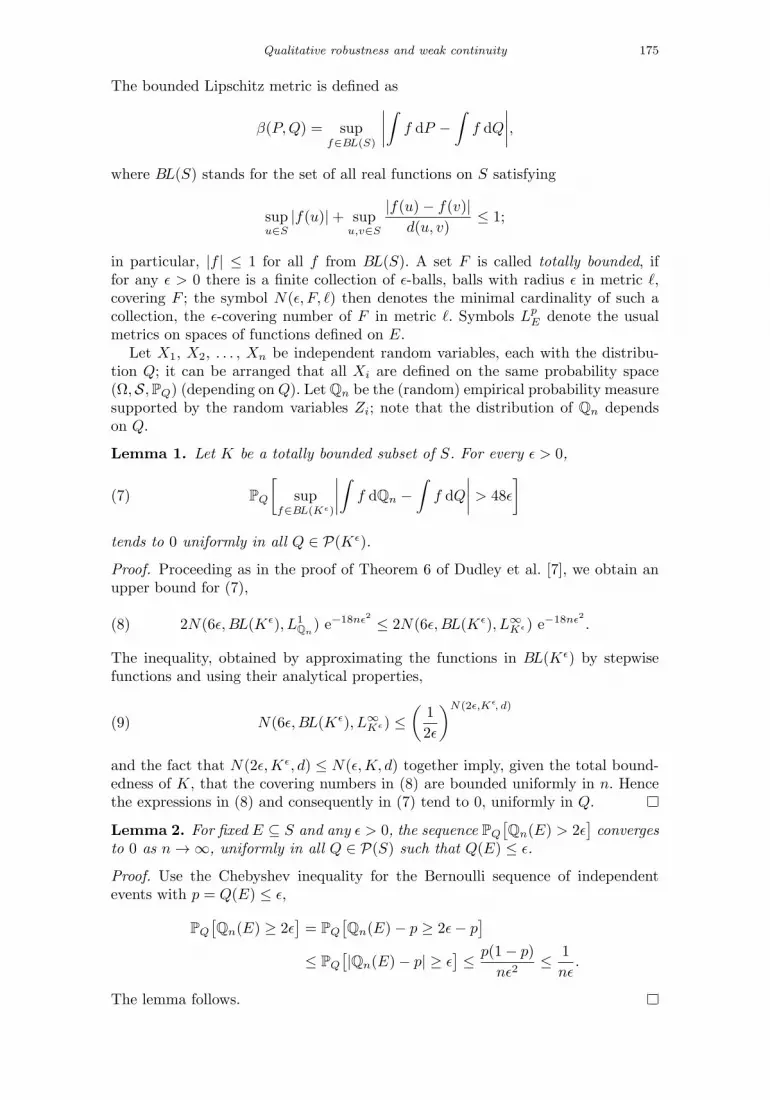
Qualitative robustness and weak continuity 175
The bounded Lipschitz metric is defined as
β(P,Q) = supf∈BL(S)
∣∣∣∣∫ f dP −∫
f dQ
∣∣∣∣,where BL(S) stands for the set of all real functions on S satisfying
supu∈S
|f(u)|+ supu,v∈S
|f(u)− f(v)|d(u, v)
≤ 1;
in particular, |f | ≤ 1 for all f from BL(S). A set F is called totally bounded, iffor any ε > 0 there is a finite collection of ε-balls, balls with radius ε in metric �,covering F ; the symbol N(ε, F, �) then denotes the minimal cardinality of such acollection, the ε-covering number of F in metric �. Symbols Lp
E denote the usualmetrics on spaces of functions defined on E.
Let X1, X2, . . . , Xn be independent random variables, each with the distribu-tion Q; it can be arranged that all Xi are defined on the same probability space(Ω,S,PQ) (depending on Q). Let Qn be the (random) empirical probability measuresupported by the random variables Zi; note that the distribution of Qn dependson Q.
Lemma 1. Let K be a totally bounded subset of S. For every ε > 0,
(7) PQ
[sup
f∈BL(Kε)
∣∣∣∣∫ f dQn −∫
f dQ
∣∣∣∣ > 48ε
]tends to 0 uniformly in all Q ∈ P(Kε).
Proof. Proceeding as in the proof of Theorem 6 of Dudley et al. [7], we obtain anupper bound for (7),
(8) 2N(6ε, BL(Kε), L1Qn
) e−18nε2 ≤ 2N(6ε, BL(Kε), L∞Kε) e−18nε2 .
The inequality, obtained by approximating the functions in BL(Kε) by stepwisefunctions and using their analytical properties,
(9) N(6ε, BL(Kε), L∞Kε) ≤(
1
2ε
)N(2ε,Kε, d)
and the fact that N(2ε,Kε, d) ≤ N(ε,K, d) together imply, given the total bound-edness of K, that the covering numbers in (8) are bounded uniformly in n. Hencethe expressions in (8) and consequently in (7) tend to 0, uniformly in Q.
Lemma 2. For fixed E ⊆ S and any ε > 0, the sequence PQ
[Qn(E) > 2ε
]converges
to 0 as n→∞, uniformly in all Q ∈ P(S) such that Q(E) ≤ ε.
Proof. Use the Chebyshev inequality for the Bernoulli sequence of independentevents with p = Q(E) ≤ ε,
PQ
[Qn(E) ≥ 2ε
]= PQ
[Qn(E)− p ≥ 2ε− p
]≤ PQ
[|Qn(E)− p| ≥ ε
]≤ p(1− p)
nε2≤ 1
nε.
The lemma follows.

176 I. Mizera
Lemma 3. Let P ∈ P(S). For any ε > 0, there exists a totally bounded subset Kof S such that
(10) PQ
[sup
f∈BL(S)
∣∣∣∣∫Kε
f dQn −∫Kε
f dQ
∣∣∣∣ > 96ε
]→ 0,
uniformly in all Q ∈ P(S) such that π(P,Q) ≤ ε/2.
Proof. Given ε > 0, choose a compact subset K of S such that P (K) ≥ 1 − ε/2;here we use the fact that a probability measure on a Polish space is tight, in theterminology of Theorem 1.4 of Billingsley [1]. Fix η > 0 and choose n0 such that(7) in Lemma 1 is bounded by η/3 for all n ≥ n0. Choose n1 such that
(11)n1(1− ε)
2≥ n0,
4ε
n1(1− ε)≤ η
3, and
1
2304n1ε2≤ η
3;
note that the first inequality also implies n1 ≥ n0. Let Q be an element from P(S)such that π(P,Q) ≤ ε/2; then
1− ε
2≤ P (K) ≤ Q(Kε/2) +
ε
2≤ Q(Kε) +
ε
2
and consequently 1 − ε ≤ Q(Kε). Let NQ be the (random) number of Xi ∈ Kε;let QKε denote the conditional probability on Kε defined by QKε(E) = Q(E ∩Kε)/Q(Kε). Using again the Chebyshev argument as in Lemma 2, for the Bernoulliseries of events with p = Q(Kε) ≥ 1− ε, we obtain, using the first two inequalitiesin (11), that for any n ≥ n1,
PQ
[NQ ≤ n0
]≤ PQ
[NQ ≤ 1
2n1(1− ε)]≤ PQ
[NQ ≤ 1
2n(1− ε)]
≤ PQ
[∣∣∣∣NQ
n− p
∣∣∣∣ ≥ p
2
]≤ 4(1− p)
np≤ 4ε
n1(1− ε)≤ η
3,
(12)
uniformly in Q. The Chebyshev inequality yields once again, now together with thethird inequality in (11), that for n ≥ n1,
(13) PQ
[∣∣∣∣NQ
n− p
∣∣∣∣ > 48ε
]≤ p(1− p)
482 nε2≤ p ε
2034n1ε2≤ 1
2034n1ε≤ η
3,
again uniformly in Q. Dividing the expression within (10) by p = Q(Kε), we obtainthat for n ≥ n1,
PQ
[sup
f∈BL(S)
∣∣∣∣ 1
np
∑Xi∈Kε
f(Xi)−1
p
∫Kε
f dQ
∣∣∣∣ ≥ 96ε
p
]≤ PQ
[sup
f∈BL(S)
∣∣∣∣ 1
np
∑Xi∈Kε
f(Xi)−1
NQ
∑Xi∈Kε
f(Xi)
∣∣∣∣ ≥ 96ε
2p
]+ PQ
[sup
f∈BL(S)
∣∣∣∣ 1
NQ
∑Xi∈Kε
f(Xi)−1
Q(Kε)
∫f dQ
∣∣∣∣ ≥ 96ε
2p
]= PQ
[∣∣∣∣NQ
n− p
∣∣∣∣ supf∈BL(S)
∣∣∣∣ 1
NQ
∑Xi∈Kε
f(Xi)
∣∣∣∣ ≥ 48ε
]+ PQ
[sup
f∈BL(Kε)
∣∣∣∣ 1
NQ
∑Xi∈Kε
f(Xi)−∫
f dQKε
∣∣∣∣ ≥ 48ε
p
]≤ PQ
[∣∣∣∣NQ
n− p
∣∣∣∣ > 48ε
]+ PQ
[sup
f∈BL(Kε)
∣∣∣∣ 1
NQ
∑Xi∈Kε
f(Xi)−∫
f dQKε
∣∣∣∣ > 48ε
].

Qualitative robustness and weak continuity 177
By (13), the left-hand expression is dominated by η/3; the right-hand one can bewritten as
∞∑m=1
PQ
[sup
f∈BL(Kε)
∣∣∣∣ 1
NQ
∑Xi∈Kε
f(Xi)−∫
f dQKε
∣∣∣∣ > 48ε
∣∣∣∣ NQ = m
]PQ[NQ = m]
which can be split to two sums: the first is dominated by∑m≤n
PQ[NQ = m] = PQ
[NQ ≤ n0
]≤ 1
3η,
by (12); the second is
∑m>n
PQ
[sup
f∈BL(Kε)
∣∣∣∣ 1
NQ
∑Xi∈Kε
f(Xi)−∫
f dQKε
∣∣∣∣ > 48ε
∣∣∣∣ NQ = m
]PQ[NQ = m]
=∞∑
m>n
PQKε
[sup
f∈BL(Kε)
∣∣∣∣ 1mm∑i=1
f(Zi)−∫
f dQKε
∣∣∣∣ > 48ε
]PQ[NQ = m]
≤ 13η
∞∑m>n
PQ[NQ = m] ≤ 13η,
where Z1, Z2, . . . , Zm are independent random variables (different for each m), eachwith distribution QKε , so that Lemma 1 applies. As η was arbitrary, the lemmafollows.
Lemma 4. For any α, η > 0, there exists δ > 0 and ν such that
(14) PQ
[π(Qn, P ) > α
]< η
whenever n ≥ ν and π(P,Q) < δ.
Proof. Given P and α, choose ε < α2/12 such that 96ε ≤ α2/3. As in the proof ofLemma 3, we take a compact K such that Q(Kε) ≥ 1− ε whenever π(Q,P ) < δ =ε/2. By (6), we obtain
PQ
[π(Qn, P ) > α
]≤ PQ
[β(Qn, P ) > 2
3α2]
≤ PQ
[sup
f∈BL(S)
∫S\Kε
|f | dQn + supf∈BL(S)
∫S\Kε
|f | dQ > 13α
2
]+ PQ
[sup
f∈BL(S)
∣∣∣∣∫Kε
f dQn −∫Kε
f dQ
∣∣∣∣> 13α
2
]≤ PQ
[Qn(S \Kε) > 1
4α2]+ PQ
[sup
f∈BL(S)
∣∣∣∣∫Kε
f dQn −∫Kε
f dQ
∣∣∣∣> 96ε(1− ε)
]By Lemma 3, there exists n1 such that the second term is bounded by η/2 forn ≥ n1. Since Q(S \Kε) ≤ ε < α2/12, Lemma 2 yields n2 such that for n ≥ n2,
PQ
[Qn(S \Kε) > 1
4α2]≤ PQ
[Qn(S \Kε) > 1
6α2]≤ 1
2η.
Setting ν = max{n1, n2} concludes the proof.

178 I. Mizera
Proof of Theorem 1. Let � be the metric on the range of T . Given ε > 0, weakcontinuity of T at P yields α such that �(τ, T (P )) < ε/3 whenever τ ∈ T (Q) andπ(P,Q) < α. Setting η to ε/3 and taking ν and δ yielded by Lemma 4, we obtainthat if n ≥ ν and π(P,Q) ≤ δ, then
PQ
[�(τ, T (P )) > 1
3ε]< 1
3ε
whenever τ ∈ T (Qn). The Strassen theorem — see Huber [15], Chapter 2, Theorem3.7, or also the original paper Strassen [26]—then gives
(15) π(LQ(tn), δT (P )) ≤ 13ε;
here δT (P ) stands, in the spirit of the notation introduced above, for the point(Dirac) measure concentrated in T (P ). Using (15) once again for Q = P and thencombining both inequalities, we obtain the desired result: if π(P,Q) ≤ δ, thenπ(LQ(tn),LP (tn)) < ε for n ≥ ν, uniformly in Q.
Proof of Proposition 1. The proposition follows from the Varadarajan theorem,stating that when the data are independently sampled from P , the correspond-ing empirical probability measures converge weakly to P with probability one. Theconsistency then follows from the weak continuity of T at P .
Proof of Proposition 2. Let � be the metric on the range of T , and suppose that�(θ, τ) = ε > 0. Suppose that some lawful version of tn is qualitatively robust at P .Given ε/4, we may pick Q−, Q+, out of Q−ν and Q+
ν satisfying assumptions (ii), (iii),and (iv), such that T is univalued, and the representation of tn by T is consistentat both Q− and Q+; by qualitative robustness, we can pick them so that for somen1
π(LQ−(tn),LP (tn)) ≤ 14ε,(16)
π(LQ+(tn),LP (tn)) ≤ 14ε,(17)
for all n ≥ n1. The consistency at Q− and Q+ yields n2 such that for all n ≥ n2,
PQ−[�(T (Q−n ), T (Q
−)) ≥ 14ε]< 1
4ε,(18)
PQ−[�(T (Q−n ), T (Q
−)) ≥ 14ε]< 1
4ε.(19)
Take n ≥ max{n1, n2}. Applying the Strassen theorem to (18) and (19) (given thatT is univalued at Q− and Q+), we obtain that
π(LQ−(tn), δT (Q−)) <14ε,(20)
π(LQ+(tn), δT (Q+)) <14ε.(21)
Combining (20), (21) with (16) and (17) yields that d(θ, τ) = π(δT (Q−), δT (Q+)) < ε,a contradiction.
Proof of Theorem 2. Suppose that θ, τ ∈ T (P ), θ �= τ . By the regularity of T , thereare Q−ν and Q+
ν that satisfy the assumptions of Proposition 2. Hence θ = τ . Thesame argument yields that θ must be equal to the limit (possibly in a one-pointcompactification of the range of T ) of any other sequence T (Pν) such that Pν → P .Hence, T has a unique limit at P , equal to T (P ).

Qualitative robustness and weak continuity 179
4. Final remarks
After the introduction by Hampel [11], which reappeared in the more settled formin Hampel, Ronchetti, Rousseeuw and Stahel (1986), and the influential treatmentby Huber [15], all in the context of estimation and independent sampling, quali-tative robustness was extended to hypothesis testing framework by Lambert [16]and Rieder [24]; dependent data models of time series flavor were considered byPapantoni-Kazakos [21], Boente et al. [2]; some further theoretical aspects wereaddressed by Cuevas [3]. It seems that despite these developments, its use for eval-uating robustness was not too intense: a few relevant references are Rieder [25],Good and Smith [9], Cuevas and Sanz [4], Machado [17], and He and Wang [13].The fade-out citation pattern is indicated by the only 21st century exception re-trieved from scholar.google.com, Daouia and Ruiz-Gazen [5].
As the name indicates, and the definition clearly shows, qualitative robustnessdoes not provide any “quantitative” appraisal: the procedure is judged either notrobust or robust—and in the latter case we do not know “how much”. The rushfor “more” and “most” robust methods might have been the reason that otherrobustness criteria gained more following. Nevertheless, given the multitude of “de-sirable features” considered in the screening of aspiring data-analytic techniques,qualitative robustness may be just enough to draw a dividing line in the territoryof robustness—especially in complex situations where classical criteria modeled instandard circumstances may loose steam.
In the universe of mathematical sciences, qualitative robustness is similar tothe notion of stability used in the theory of differential equations: a small changein initial conditions still renders the new solution staying in a tube enclosing theoriginal one. Interestingly, the translation of “qualitatively robust at P” to “solutionexists, is unique, and depends continuously on the data”, discussed in this note,corresponds exactly to what in applied mathematics is called well-posed problem inthe sense of Hadamard [10]. Indeed, continuous dependence on the data is essentialfor any procedure, in particular for its numerical implementation—which is alwaysbased on approximation; it ensures the stability of an algorithm. A referee pointedout that among the references given above, we might have missed some that, likeHildebrand and Muller [14], refer more generally to “robustness” or “continuity”without mentioning explicitly qualitative robustness. In the similar spirit, we maysee witness a resurrection of the term (likely under a different name) in learningtheory — see Poggio, Rifkin, Mukherjee, and Niyogi (2004).
Of course, numerical stability requires only pointwise continuity; qualitative ro-bustness goes a step further, requiring continuity with respect to the distributionunderlying the data. Some may argue that it goes too far, indicating that continuityviolated by statistical procedures otherwise in common use may be too stringent arequirement. In the context of well-posedness in the sense of Hadamard [10], theusual mode of requiring continuity is “in some reasonable topology”. All this in-dicates that the most important aspect of qualitative robustness, and robustnesstheory in general, lies at its very start—as pointed out by Davies [6], and put downalready by Huber [15],
“It is by no means clear whether different metrics give rise to equivalent robustnessnotions; to be specific we work with Levy metric for F and the Prokhorov metric forL(Tn).”
We remark that such a choice might came out as natural under the influence ofBillingsley [1] in the times of Hampel [11]; the question is whether it still remains

180 I. Mizera
such. Of course, the relationship between qualitative robustness and continuitydiscussed in this note indicates that it is only the induced topology, not a particularmetric, that matters for qualitative robustness.
References
[1] Billingsley, P. (1968). Convergence of Probability Measures. Wiley, NewYork.
[2] Boente, G., Fraiman, R. and Yohai, V. J. (1987). Qualitative robustnessfor stochastic processes. Ann. Statist. 15 1293–1312.
[3] Cuevas, A. (1988). Quantitative robustness in abstract inference. J. Statist.Planning Inference 18 277–289.
[4] Cuevas, A. and Sanz, P. (1989). A class of qualitatively robust estimates.Statistics 20 509–520.
[5] Daouia, A. and Ruiz–Gazen, A. (2006). Robust nonparametric frontierestimators: Qualitative robustness and influence function. Statistica Sinica 161233–1253.
[6] Davies, P. L. (1993). Aspects of robust linear regression. Ann. Statist. 211843–1899.
[7] Dudley, R.M. Gine, E. and Zinn, J. (1991). Uniform and universalGlivenko-Cantelli classes. J. Theoret. Probab. 4 485–510.
[8] Ellis, S. P. (1998). Instability of least squares, least absolute deviation andleast median of squares linear regression. Statist. Sci. 13 337–350.
[9] Good, I. J. and Smith, E. P. (1986). An additive algorithm analogous tothe singular decomposition or a comparison of polarization and multiplicativemodels: An example of qualitative robustness. Commun. Statist. B 15 545–569.
[10] Hadamard, J. (1902). Sur les problemes aux derivees et leur significationphysique. Princeton University Bulletin 49–52.
[11] Hampel, F.R. (1971). A general qualitative definition of robustness. Ann.Math. Statist. 42 1887–1896.
[12] Hampel, F.R., Ronchetti, E.M., Rousseeuw, P. J. and Stahel, W.A.(1986). Robust Statistics: The Approach Based on Influence Functions. Wiley,New York.
[13] He, X. and Wang, G. (1997). Qualitative robustness of S∗-estimators ofmultivariate location and dispersion. Statistica Neerlandica 51 257–268.
[14] Hildebrand, M. and Muller, C.H. (2007). Outlier robust corner-preserving methods for reconstructing noisy images. Ann. Statist. 35 132–165.
[15] Huber, P. J. (1981). Robust Statistics. Wiley, New York.[16] Lambert, D. (1982). Qualitative robustness of tests. J. Amer. Statist. Assoc.
77 352–357.[17] Machado, J.A. F. (1993). Robust model selection and M-estimation. Econo-
metric Theory 9 478–493.[18] Maronna, R.A., Martin, R.D., and Yohai, V. J. (2006). Robust Statis-
tics: Theory and Methods. Wiley, New York.[19] Mizera, I. (1995). A remark on existence of statistical functionals. Kyber-
netika 31 315–319.[20] Mizera, I. and Volauf, M. (2002). Continuity of halfspace depth contours
and maximum depth estimators: Diagnostics of depth-related methods. Jour-nal of Multivariate Analysis 83 365–368.
[21] Papantoni-Kazakos, P. (1984). Some aspects of qualitative robustness intime series. In Robust and Nonlinear Time Series Analysis,(J. Franke, W.

Qualitative robustness and weak continuity 181
Hardle and D. Martin, eds.) Lecture Notes in Statistics 26 218–230. Springer-Verlag, New York.
[22] Poggio, T., Rifkin, R., Mukherjee, S., and Niyogi, P. (2004). Generalconditions for predictivity in learning theory. Nature 428 419–422.
[23] Portnoy, S. and Mizera, I. (1998). Comment of “Instability of leastsquares, least absolute deviation and least median of squares linear regres-sion”. Statistical Science 13 344–347.
[24] Rieder, H. (1982). Qualitative robustness of rank tests. Ann. Statist. 10 205–211.
[25] Rider, H. (1983). Continuity properties of rank procedures. Statist. Decisions1 341–369.
[26] Strassen, V. (1976). The existence of probability measures with givenmarginals. Ann. Math. Statist. 36423–439.

IMS CollectionsNonparametrics and Robustness in Modern Statistical Inference and Time SeriesAnalysis: A Festschrift in honor of Professor Jana JureckovaVol. 7 (2010) 182–193c© Institute of Mathematical Statistics, 2010DOI: 10.1214/10-IMSCOLL718
Asymptotic theory of the spatial median
Jyrki Mottonen1,∗ , Klaus Nordhausen2,3 and Hannu Oja2
University of Helsinki, University of Tampere and Tampere University Hospital
Abstract: In this paper we review, prove and collect the results on the lim-iting behavior of the regular spatial median and its affine equivariant mod-ification, the transformation retransformation spatial median. Estimation ofthe limiting covariance matrix of the spatial median is discussed as well. Somealgorithms for the computation of the regular spatial median and its differentmodifications are described. The theory is illustrated with two examples.
1. Introduction
For a set of p-variate data points y1, . . . ,yn, there are several versions of multivari-ate median and related multivariate sign test proposed and studied in the literature.For some reviews, see Small [23], Chaudhuri and Sengupta [6] and Niinimaa andOja [17]. The so called spatial median which minimizes the sum
∑ni=1 |yi−μ| with
a Euclidean norm | · | has a very long history, Gini and Galvani [8] and Haldane [10]for example have independently considered the spatial median as a generalizationof the univariate median. Gover [9] used the term mediancenter. Brown [3] has de-veloped many of the properties of the spatial median. This minimization problem isalso sometimes known as the Fermat-Weber location problem, see Vardi and Zhang[25]. Taking the gradient of the objective function, one sees that if μ solves theequation
∑ni=1{U(yi − μ)} = 0 with spatial sign U(y) = |y|−1y, then μ is the
observed spatial median. The spatial sign test for H0 : μ = 0 based on the sum ofspatial signs,
∑ni=1 U(yi) was considered by Mottonen and Oja [14], for example.
The spatial median is unique, if the dimension of the data cloud is greater thanone, see Milasevic and Ducharme [13]. The so called Weiszfeld algorithm for thecomputation of the spatial median has a simple iteration step, namely μ ← μ+{
∑ni=1 |yi −μ|−1}−1
∑ni=1{U(yi − μ)}. The algorithm may fail sometimes, how-
ever, but a slightly modified algorithm which converges quickly and monotonicallyis described by Vardi and Zhang [25].
One drawback of the spatial median (the spatial sign test) is the lack of equiv-ariance (invariance) under affine transformations of the data. The performance ofthe spatial median as well as the spatial sign test then may be poor compared toaffine equivariant and invariant procedures if there is a significant deviance from
∗Corresponding author1Department of Social Research, University of Helsinki P.O.Box 68, 00014 University of
Helsinki, Finland, e-mail: [email protected] School of Public Health, University of Tampere, 33014 University of Tampere, Fin-
land, e-mail: [email protected]; [email protected] of Internal Medicine, Tampere University Hospital, P.O.Box 2000, 33521 Tam-
pere, FinlandAMS 2000 subject classifications: Primary 62H12; secondary 62G05, 62G20.Keywords and phrases: asymptotic normality, Hettmansperger–Randles estimate, multivariate
location, spatial sign, spatial sign test, transformation retransformation.
182

Asymptotic theory of the spatial median 183
a spherical symmetry. Chakraborty et al. [4] proposed and investigated an affineequivariant modification of the spatial median constructed using an adaptive trans-formation and retransformation (TR) procedure. An affine invariant modificationof the spatial sign test was also proposed. Randles [19] used Tyler’s transforma-tion [24] to construct an affine invariant modification of the spatial sign test. LaterHettmansperger and Randles [11] proposed an equivariant modification of the spa-tial median, again based on Tyler’s transformation; this estimate is known as theHettmansperger–Randles (HR) estimate.
In this paper we review and collect the results on the limiting behavior of theregular spatial median and its affine equivariant modification, the transformationretransformation spatial median. In Section 2 some auxiliary results and tools forasymptotic studies are given. Asymptotic theory for the regular spatial median isreviewed in Section 3. Estimation of the limiting covariance matrix of the spatialmedian is discussed in Section 4. Section 5 considers the transformation retransfor-mation spatial median. The paper ends with some discussion on the algorithms forthe computation of the spatial median in Section 6 and two examples in Section7. Many of the results can be collected from Arcones [1], Bai et al. [2], Brown [3],Chakraborty et al. [4], Chaudhuri [5], Mottonen et al. [14] and Rao [20]. See alsoNevalainen et al. [16] for the spatial median in the case of cluster correlated data.For the proofs in this paper it is crucial that the dimension p > 1. For the propertiesof the univariate median, see Section 2.3 in Serfling [22], for example.
2. Auxiliary results
Let y �= 0 and μ be any p-vectors, p > 1. Write also r = |y| and u = |y|−1y.Then accuracies of different (constant, linear and quadratic) approximations of
function μ→ |y − μ| around the origin are given by
(A1) ||y − μ| − |y|| ≤ |μ|,(A2) ||y − μ| − |y|+ u′μ| ≤ 2r−1|μ|2 and(A3)
∣∣|y − μ| − |y|+ u′μ− μ′(2r)−1[Ip − uu′]μ∣∣ ≤ C1r
−1−δ|μ|2+δ for all 0<δ<1,
where C1 does not depend on y or μ.
Similarly, the accuracies of constant and linear approximations of unit vector|y − μ|−1(y − μ) around the origin are given by
(B1)∣∣∣ y−μ|y−μ| −
y|y|
∣∣∣ ≤ 2r−1|μ| and
(B2)∣∣∣ y−μ|y−μ| −
y|y| −
1r [Ip − uu′]μ
∣∣∣ ≤ C2r−1−δ|μ|1+δ for all 0 < δ < 1,
where C2 does not depend on y or μ.
For these and similar results, see Arcones [1] and Bai et al. [2].
Lemma 1. Assume that the density function f(y) of the p-variate continuousrandom vector y is bounded. If p > 1 then E{|y|−α} exists for all 0 ≤ α < 2.
The following key result for convex processes is Lemma 4.2 in Davis et al. [7]and Theorem 1 in Arcones [1].
Theorem 1. Let Gn(μ), μ ∈ Rp, be a sequence of convex stochastic processes, andlet G(μ) be a convex (limit) process in the sense that the finite dimensional distri-butions of Gn(μ) converge to those of G(μ). Let μ, μ1, μ2, . . . be random variables

184 J. Mottonen, K. Nordhausen and H. Oja
such that
G(μ) = infμ
G(μ) and Gn(μn) = infμ
Gn(μ), n = 1, 2, . . .
Then μn →d μ.
3. Spatial median
Let y be a p-variate random vector with cdf F , p > 1. The spatial median of Fminimizes the objective function
D(μ) = E{|y − μ| − |y|}.
Note that no moment assumptions are needed in the definition as ||y−μ|−|y|| ≤ |μ|but for the asymptotic theory we assume that
(C1) The p-variate density function f of y is continuous and bounded.(C2) The spatial median of the distribution of y is zero and unique.
We next define vector and matrix valued functions
U(y) =y
|y| , A(y) =1
|y|
[Ip −
yy′
|y|2
], and B(y) =
yy′
|y|2
for y �= 0 and, by convention, U(0) = 0 and A(0) = B(0) = 0. We write alsoA = E {A(y)} and B = E {B(y)} .
The expectation definingB clearly exists and is bounded (|B(y)|2 = tr(B(y)′B(y))= 1). Our assumption implies that E(|y|−1) < ∞ and therefore also A exists andis bounded. Auxiliary result (A3) in Section 2 then implies
Lemma 2. Under assumptions (C1) and (C2), D(μ) = 12μ′Aμ+ o(|μ|2).
See also Lemma 19 in Arcones [1].Let Y = (y1, . . . ,yn)
′ be a random sample from a p-variate distribution F . Write
Dn(μ) = ave{|yi − μ| − |yi|}.
The function Dn(μ) as well as D(μ) are convex and bounded. Boundedness followsfrom (A1). The sample spatial median μ is defined as
μ = μ(Y) = argmin Dn(μ).
The estimate μ is unique if the observations do not fall on a line. Under assumption(C1) μ is unique with probability one. As D(μ) is the limiting process of Dn(μ),Theorem 1 implies that μ→P 0.
The statistic Tn = T(Y) = ave {U(yi)} is the spatial sign test statistic fortesting the null hypothesis that the spatial median is zero. As μ is assumed to bea zero vector, the multivariate central limit theorem implies that
Lemma 3.√nTn →d Np(0,B).
The approximation (A3) in Section 1 implies that∣∣∣∣∣n∑
i=1
{|yi − n−1/2μ| − |yi|} −1√n
n∑i=1
y′i|yi|
μ− μ′1
n
n∑i=1
[1
2|yi|
[Ip −
yiy′i
|yi|2
]]μ
∣∣∣∣∣

Asymptotic theory of the spatial median 185
≤ C1
n(2+δ)/2
n∑i=1
|μ|2+δ
r1+δi
→P 0, for all μ,
and we get
Lemma 4. Under assumptions (C1) and (C2),
nDn(n−1/2μ)−
(√nTn −
1
2Aμ
)′μ →P 0.
Now apply Theorem 1 with Gn(μ) = nDn(n−1/2μ) and G(μ) =
(z− 1
2Aμ)′μ
where z ∼ Np(0,B). We then obtain (A is positive definite)
Theorem 2. Under assumptions (C1) and (C2),√nμ →d Np(0,A
−1BA−1).
It is well known that, if E(yi) = 0 and the second moments exist, also√ny→d
Np(0,Σ) where Σ is the covariance matrix of yi. The asymptotic relative effi-ciency of the spatial median with respect to the sample mean is then given bydet (Σ)/det
(A−1BA−1
). The spatial median has good efficiency properties even
in the multivariate normal model. Mottonen et al [15] for example calculated theasymptotic relative efficiencies e(p, ν) of the multivariate spatial median with re-spect to the mean vector in the p-variate tν,p distribution case (t∞,p is the p-variatenormal distribution). In the 3-variate and 10-variate cases, for example, the asymp-totic relative efficiencies are
e(3, 3) = 2.162, e(3, 10) = 1.009, e(3,∞) = 0.849,e(10, 3) = 2.422, e(10, 10) = 1.131, e(10,∞) = 0.951.
4. Estimation of the covariance matrix of the spatial median
For a practical use of the normal approximation of the distribution of μ one natu-rally needs an estimate for the asymptotic covariance matrix A−1BA−1. We esti-mate A and B separately. Recall that we assume that the true value μ = 0. Write,as before,
A(y) =1
|y|
(Ip −
yy′
|y|2
)and B(y) =
yy′
|y|2 .
Then write A = A(Y) = ave {A(yi − μ)} and B = B(Y) = ave {B(yi − μ)} .We will show that, under our assumptions, A and B converge in probability to thepopulation values A = E {A(yi)} and B = E {B(yi)} , respectively:
Theorem 3. Under assumptions (C1) and (C2), A→P A and B→P B.
Proof We thus assume that the true spatial median μ = 0. By Theorem 2,√nμ = Op(1). Write A = ave {A(yi)} and B = ave {B(yi)} . Then by the law of
large numbers A→P A and B→P B. Our auxiliary result (B1) implies that∣∣∣∣ (y − μ)(y − μ)′
|y − μ|2 − yy′
|y|2
∣∣∣∣ ≤ 4|μ||y| , ∀ y �= 0,μ,
and therefore by Slutsky’s theorem |B− B| ≤ 1n
∑ni=1{4|μ|/|yi|} →P 0. As B→P
B, also B→P B.We now prove that A→P A. We play with three positive constants, “large” δ1,
“small” δ2 and “small” δ3. For a moment, we assume that |μ| < δ1/√n. (This is true

186 J. Mottonen, K. Nordhausen and H. Oja
with a probability that can be made close to one with large δ1.) Next we write I1i =
I{|yi − μ| < δ2√
n
}, I2i = I
{δ2√n≤ |yi − μ| < δ3
}and I3i = I { |yi − μ| ≥ δ3} .
Then
A− A =1
n
n∑i=1
(A(yi)−A(yi − μ))
=1
n
n∑i=1
(I1i · [A(yi)−A(yi − μ)]) +1
n
n∑i=1
(I2i · [A(yi)−A(yi − μ)])
+1
n
n∑i=1
(I3i · [A(yi)−A(yi − μ)]) .
The first average is zero with probability
P (I11 = . . . = I1n = 0) ≥(1− δp2cpM
np/2
)n
≥(1− δ22cpM
n
)n
→ e−cpMδ22 ,
where M = supy f(y) < ∞ and cp is the volume of the p-variate unit ball. (Thefirst average is thus zero with a probability that can be made close to one withsmall choices of δ2 > 0.) For the second average, one gets
1
n
n∑i=1
|I2i · [A(yi)−A(yi − μ)]| ≤ 1
n
n∑i=1
6I2i|μ||yi − μ||yi|
≤ 1
n
n∑i=1
6I2iδ1δ2|yi|
which converges to a constant which can be made as close to zero as one wisheswith small δ3 > 0. Finally, also the third average
1
n
n∑i=1
|I3i · [A(yi)−A(yi − μ)]| ≤ 1
n
n∑i=1
6I3i|μ||yi − μ||yi|
≤ 1
n√n
n∑i=1
6I3iδ1δ3|yi|
converges to zero in probability for all choices of δ1 and δ3, and the proof follows.�
Theorems 2 and 3 thus suggest that the distribution of μ can be approximated
by Np
(μ, 1
nA−1BA−1
). Approximate 95 % confidence ellipsoids for μ are given
by{μ : n(μ− μ)′AB−1A(μ− μ) ≤ χ2
p,.95
}, where χ2
p,.95 is the 95 % quantile of
a chi square distribution with p degrees of freedom. Also, by Slutsky’s theorem,under the null hypothesis H0 : μ = 0 the squared version of the test statisticQ2 = nT′nB
−1Tn →d χ2p.
5. Transformation retransformation spatial median
Shifting the data cloud, naturally shifts the spatial median by the same constant,that is, μ(1na
′ + Y) = a + μ(Y), It is also easy to see that rotating the datacloud also rotates the spatial median correspondingly, that is, μ(YO′) = Oμ(Y),for all orthogonal p× p matrices O. Unfortunately, the estimate is not equivariantunder heterogeneous rescaling of the components, and therefore not fully affineequivariant.

Asymptotic theory of the spatial median 187
A fully affine equivariant version of the spatial median can be found using theso called transformation retransformation estimation technique. First, a positivedefinite p× p scatter matrix S = S(Y) is a matrix valued sample statistic which isaffine equivariant in the sense
S(1na′ +YB′) = BS(Y)B′
for all p-vectors a and all nonsingular p × p matrices B. Let S−1/2 be any matrixwhich satisfies S−1/2S(S−1/2)′ = Ip. The procedure is then as follows.
1. Take any scatter matrix S = S(Y).2. Transform the data matrix: Y(S−1/2)′.3. Find the spatial median for the standardized data matrix μ(Y(S−1/2)′).4. Retransform the estimate: μ(Y) = S1/2μ(Y(S−1/2)′).
This median μ(Y) utilizing “data driven” transformation S−1/2 is known as thetransformation retransformation (TR) spatial median. (See Chakraborty et al. [4]for other type of data driven transformations.) Then the affine equivariance follows:
Theorem 4. Let S = S(Y) be any scatter matrix. Then the transformation retrans-formation spatial median μ(Y) = S1/2μ(Y(S−1/2)′) is affine equivariant, that is,μ(1na
′ +YB′) = a+Bμ(Y).
The proof easily follows from the facts that the regular spatial median is shiftand orthogonally equivariant and that (S(1na
′ + YB′))−1/2 = O(S(Y))−1/2 forsome orthogonal matrix O.
In the following we assume (without loss of generality) that the population valueof S is Ip, and that S = S(Y) is a root-n consistent estimate of Ip. We writeΔ =
√n(S−1/2 − I) = Op(1) and Y∗ = Y(S−1/2)′. Then we have the following
result for the test statistic.
Lemma 5. Let Y be a random sample from a symmetric distribution satisfying(C1) and (C2). (By a symmetry we mean that −yi and yi have the same distri-bution.) Assume also that scatter matrix S = S(Y) satisfies
√n(S − Ip) = Op(1).
Then√n(T(Y∗)−T(Y))→P 0.
Proof Our assumptions imply that also Δ =√n(S−1/2 − Ip) = Op(1). Thus
S−1/2 = Ip + n−1/2Δ where Δ is bounded in probability. Using auxiliary result(B2) in Section 2 we obtain
1√n
n∑i=1
U(S−1/2yi)−1√n
n∑i=1
Ui =1
n
n∑i=1
(Δ−U′iΔUi)Ui + oP (1)
where Ui = U(yi), i = 1, . . . , n. For |Δ| < M , the second term in the expan-sion converges uniformly in probability to zero due to its linearity with respect tothe elements of Δ and due to the symmetry of the distribution of Ui. (E(Ui) =E(U′iΔUiUi) = 0) . Therefore n−1/2
∑ni=1 U(S−1/2yi)−n−1/2
∑ni=1 Ui →P 0 and
the proof follows. �
We also have to show that A(Y∗) and A(Y) both converge to A, and similarlywith B(Y∗) and B(Y):
Lemma 6. Let Y be a random sample from a distribution satisfying (C1) and(C2). Assume also that scatter matrix S = S(Y) satisfies
√n(S − Ip) = Op(1).
A(Y∗)−A(Y)→P 0 and B(Y∗)−B(Y)→P 0.

188 J. Mottonen, K. Nordhausen and H. Oja
Proof Again S−1/2 = Ip + n−1/2Δ where Δ = Op(1). Suppose that Δ ≤ M .(P (Δ ≤M)→ 1 as M →∞.) Write y∗i = (Ip − n−1/2Δ)yi. Then∣∣∣∣y∗i y∗i ′|y∗i |2
− yiy′i
|yi|2
∣∣∣∣ ≤ 1√n|Δ| and
∣∣∣∣ 1
|y∗i |− 1
|yi|
∣∣∣∣ ≤ |Ip − (Ip − n−1/2Δ)−1||yi|
.
The first inequality gives |B(Y∗)−B(Y)| ≤ 1√n|Δ| → 0. The two inequalities
together imply that∣∣∣∣ 1
|yi|
(Ip −
yiy′i
|yi|2
)− 1
|y∗i |
(Ip −
y∗i y∗i′
|y∗i |2
)∣∣∣∣ ≤ 1
|yi|
(3M√n
+ o(n−1/2)
).
Then |A(Y∗)−A(Y)| ≤ 1n
∑ni=1
[1|yi|
(3M√n+ o(n−1/2)
)]→P 0. �
Using Lemmas 5 and 6 and the auxiliary results in Section 2 we then get
Theorem 5. Let Y be a random sample from a symmetric distribution satisfying(C1) and (C2). Assume also that scatter matrix S = S(Y) satisfies
√n(S− Ip) =
Op(1). Then√nμ(Y) and
√nμ(Y) have the same limiting distribution.
Proof Write again S−1/2 = Ip+n−1/2Δ, and y∗i = (Ip−n−1/2Δ)yi, i = 1, . . . , n,and Y∗ = (y∗1, . . . ,y
∗n)′. Then our auxiliary results imply that that∣∣∣∣∣
n∑i=1
{|y∗i − n−1/2μ| − |y∗i |} −1√n
n∑i=1
y∗i′
|y∗i |μ− μ′
1
n
n∑i=1
[1
2|y∗i |
[Ip −
y∗i y∗i′
|y∗i |2
]]μ
∣∣∣∣∣≤ C1
n(2+δ)/2
n∑i=1
|μ|2+δ|(Ip − n−1/2Δ)−1|1+δ
|y∗i |1+δ→P 0
Thus Lemmas 5 and 6 together with Theorem 1 imply that√nμ(Y∗) and
√nμ(Y)
have the same limiting distribution. As√nμ(Y) = S1/2
√nμ(Y∗), the result follows
from Slutsky’s theorem. �
Based on the results above, the distribution of μ can in the symmetric case be
approximated by Np
(μ, Cov(μ)
), where Cov(μ) = 1
nS1/2A−1
S BSA−1S (S1/2)′ with
AS = ave{
1|ei|2
(Ip − eie
′i
|ei|2)}
and BS = ave{
eie′i
|ei|2}
calculated from the standard-
ized residuals ei = S−1/2(yi − μ), i = 1, . . . , n.The stochastic convergence and the limiting normality of the spatial median did
not require any moment assumptions. Therefore, for the transformation, a scattermatrix with weak assumptions should be used as well. It is an appealing idea tolink also the spatial median with the Tyler’s transformation. This was proposed byHettmansperger and Randles [11]:
Definition 1. Let μ be a p-vector and S > 0 a symmetric p× p matrix, and defineei = S−1/2(yi − μ), i = 1, . . . , n. The Hettmansperger–Randles (HR) estimate oflocation and scatter are the values of μ and S which simultaneously satisfy
ave {U(ei)} = 0 and p ave {U(ei)U(ei)′} = Ip.

Asymptotic theory of the spatial median 189
Note that the HR estimate is not a TR estimate as the location vector and scattermatrix are in fact estimated simultaneously. This pair of estimates was first men-tioned in Tyler [24]. Hettmansperger and Randles [11] developed the properties ofthese estimates. They showed that the HR estimate has a bounded influence func-tion and a positive breakdown point. The distribution of the HR location estimatecan be approximated by
Np
(0,
1
npS1/2A−2
S S1/2
)where AS = ave(A(S−1/2(yi − μ))) and S is Tyler’s scatter matrix.
6. Computation of the spatial median
The spatial median can often be computed using the following two steps:
Step 1: ei ← yi − μ, i = 1, . . . , n
Step 2: μ← μ +(∑n
i=1 |ei|−1)−1 ∑n
i=1 U(ei)
provided an initial estimate for μ.The above algorithm may fail in case of ties or when an estimate falls on a data
point. Assume then that the distinct data points are y1, . . . ,ym with multiplicitiesw1, . . . , wm (w1 + . . .+wm = n). The algorithm by Vardi and Zhang [25] then usesthe steps:
Step 1: ei ← yi − μ, i = 1, . . . ,mStep 2: c← (
∑ei=0 wi)/|
∑ei �=0 wiU(ei)|
Step 3: μ← μ + max (0, 1− c)(∑
ei �=0 wi|ei|−1)−1 ∑
ei �=0 wiU(ei)
Furthermore many other approaches can be used to solve this non-smooth opti-mization problem. For example Hossjer and Croux [12] suggest a steepest descentalgorithm combined with stephalving and discuss also some other algorithms. Weprefer however the above algorithm since it seems efficient and can be easily com-bined with the HR approach with the following steps:
Step 1: ei ← S−1/2(yi − μ), i = 1, . . . , n
Step 2: μ← μ +[∑n
i=1{|ei|−1}]−1
S1/2∑n
i=1{U(ei)}Step 3: S ← (p/n) S1/2
∑ni=1{U(ei)U(ei)
′} S1/2.
There are actually two ways to implement the algorithm. The first one is justto repeat these three steps 1, 2 and 3 until convergence. The second one is first(i) to repeat steps 1 and 2 until convergence, and then (ii) repeat steps 1 and 3until convergence. Finally (i) and (ii) are repeated until convergence. The secondversion is sometimes considered faster and more stable, see Hettmansperger andRandles[11] and the references therein.
Both versions of the algorithm are easy to implement and the computation isfast even in high dimensions. Unfortunately, there is no proof for the convergenceof the algorithms so far, although in practice they always seem to work. There is noproof for the existence or uniqueness of the HR estimate either. In practice, this isnot a problem, however. One can start with any initial root-n consistent estimates,then repeat the above steps for location and scatter, and stop after k iterations.If, in the spherical case around the origin, the initial location and shape estimates,say μ and S are root-n consistent, that is,
√nμ = OP (1) and
√n(S− Ip) = OP (1)

190 J. Mottonen, K. Nordhausen and H. Oja
and tr(S) = p then the k-step estimate using the single loop version of the abovealgorithm (obtained after k iterations) satisfies
√nμk =
(1
p
)k√nμ+
[1−
(1
p
)k]
1
E(r−1i )
p
p− 1
√n ave{ui}+ oP (1)
and
√n(Sk − Ip) =
(2
p+ 2
)k√n(S− Ip)
+
[1−
(2
p+ 2
)k]p+ 2
p
√n (p · ave{uiu
′i} − Ip) + oP (1).
Asymptotically, the k-step estimate behaves as a linear combination of the initialpair of estimates and Hettmansperger–Randles estimate. The larger k, the moresimilar is the distribution to that of the HR estimate. More work is needed, however,to carefully consider the properties of this k-step HR-estimate.
7. Examples
y_1
−0.4 −0.2 0.0 0.2 0.4 −2 −1 0 1 2 3 4
−0.3
−0.1
0.1
0.3
−0.4
−0.2
0.0
0.2
0.4
y_2
−0.4
−0.2
0.0
0.2
0.4
−0.3 −0.1 0.1 0.3
−2−1
01
23
4
−0.4 −0.2 0.0 0.2 0.4
y_3
sample mean vectorspatial medianequivariant spatial median
Fig 1. The sample mean vector, the spatial median and the HR location estimate with correspond-ing bivariate 95% confidence ellipsoids for a simulated dataset from a non-spherical 3-variate t3distribution.
In this section we compare the mean vector, the regular spatial median, and theHR location estimate for simulated and real datasets. First, the simulated data with

Asymptotic theory of the spatial median 191
LaggedSalinity
0 1 2 3 4 5 22 24 26 28 30 32
46
810
1214
01
23
45
Trend
01
23
45
4 6 8 10 12 14
2224
2628
3032
0 1 2 3 4 5
Discharge
sample mean vectorspatial medianequivariant spatial median
Fig 2. Salinity data with the sample mean vector, the spatial median and the HR location estimatewith corresponding bivariate 95% confidence ellipsoids. Two outliers are marked with a darkercolour.
sample size n = 200 was generated from a 3-variate spherical t distribution with 3degrees of freedom. In the case of a spherical distribution, the regular spatial medianand the affine equivariant HR location estimate are behaving in a very similar way.To illustrate the differences between these two estimates in a non-spherical case,the third component was multiplied by 10. The three location estimates with theirbivariate 95% confidence ellipsoids are presented in Figure 1. The mean vector isless accurate due to the heavy tails of the distribution. For non-spherical data, theequivariant HR location estimate is more efficient than the spatial median as seenin the Figure. If the measurement units for the components are the same, however,as in the case of the repeated measures, and heterogeneous rescaling is not natural,then of course the spatial median may be preferable.
To illustrate the robustness properties of the three estimates we consider thethree variables “Lagged Salinity”, “Trend” and “Discharge” in the Salinity datasetdiscussed in Rousseeuw and Leroy [21]. There are two clearly visible outliers amongthe 28 observations. As seen from Figure 2, the mean vector and the correspondingconfidence ellipsoid are clearly affected by these outliers. The HR estimate seems abit more accurate than the spatial median due to the different scales of the marginalvariables. Estimation of the spatial median and HR estimate and their covariancesis implemented in the R package MNM [18].
Acknowledgements. We thank the two referees for their valuable comments onthe earlier version of the paper.

192 J. Mottonen, K. Nordhausen and H. Oja
References
[1] Arcones, M.A. (1998). Asymptotic theory for M-estimators over a convexkernel. Econometric Theory 14 387–422.
[2] Bai, Z.D., Chen, X.R., Miao, B.Q., and Rao, C.R. (1990). Asymptotictheory of least distances estimate in multivariate linear models. Statistics 21503–519.
[3] Brown, B.M. (1983). Statistical uses of the spatial median. Journal of theRoyal Statistical Society, Series B 45 25–30.
[4] Chakraborty, B, Chaudhuri, P., and Oja, H. (1998). Operating trans-formation re-transformation on spatial median and angle test. Statistica Sinica8 767–784.
[5] Chaudhuri, P. (1992). Multivariate location estimation using extension ofR-estimates through U -statistics type approach. Annals of Statistics 20 897–916.
[6] Chaudhuri, P. and Sengupta, D. (1993). Sign tests in multidimension:Inference based on the geometry of data cloud. Journal of the American Sta-tistical Society 88 1363–1370.
[7] Davis, R.A., Knight, K., and Liu, J. (1992). M-estimation for autore-gression with infinite variance. Stochastic Processes and Their Applications 40145–180.
[8] Gini, C. and Galvani, L. (1929). Di talune estensioni dei concetti di mediaai caratteri qualitative. Metron 8.
[9] Gower, J. S. (1974). The mediancentre. Applied Statistics 2 466–470.[10] Haldane, J. B. S. (1948). Note on the median of the multivariate distribu-
tions. Biometrika 35 414–415.[11] Hettmansperger, T. P. and Randles, R.H. (2002). A practical affine
equivariant multivariate median. Biometrika 89 851–860.[12] Hossjer, O. and Croux, C. (1995). Generalizing univariate signed rank
statistics for testing and estimating a multivariate location parameter. Journalof Nonparametric Statistics 4 293–308.
[13] Milasevic, P. and Ducharme, G.R. (1987). Uniqueness of the spatial me-dian. Annals of Statistics 15 1332–1333.
[14] Mottonen, J. and Oja, H. (1995). Multivariate spatial sign and rank meth-ods. Journal of Nonparametric Statistics 5 201–213.
[15] Mottonen, J., Oja, H., and Tienari, J. (1997). On the efficiency of mul-tivariate spatial sign and rank tests. Annals of Statistics 25 542–552.
[16] Nevalainen, J., Larocque, D., and Oja, H. (2007). On the multivariatespatial median for clustered data. Canadian Journal of Statistics 35 215-231.
[17] Niinimaa, A. and Oja, H. (1999). Multivariate median. In: Encyclopedia ofStatistical Sciences (Update Volume 3). Eds. by Kotz, S., Johnson, N. L. andRead, C. P., Wiley.
[18] Nordhausen, K. Mottonen, J., and Oja, H. (2009). MNM: MultivariateNonparametric Methods. An Approach Based on Spatial Signs and Ranks. Rpackage version 0.95-1.
[19] Randles, R.H. (2000). A simpler, affine equivariant multivariate, distribu-tion-free sign test. Journal of the American Statistical Association 95 1263–1268.
[20] Rao, C.R. (1988). Methodology based on the L1-norm in statistical inference.Sankhya Ser. A 50 289–313.

Asymptotic theory of the spatial median 193
[21] Rousseeuw, P. J. and Leroy, A.M. (1987). Robust Regression and OutlierDetection. John Wiley & Sons, New York.
[22] Serfling, R. J. (1980). Approximation Theorems of Mathematical Statistics.Wiley, New York.
[23] Small, C.G. (1990). A survey of multidimensional medians. InternationalStatistical Review 58 263–277.
[24] Tyler, D. E. (1987). A distribution-free M -estimator of multivariate scatter.Annals of Statistics 15 234–251.
[25] Vardi, Y. and Zhang, C.-H. (2000). The multivariate L1-median and asso-ciated data depth. The Proceedings of the National Academy of Sciences USA(PNAS) 97 1423–1426.

IMS CollectionsNonparametrics and Robustness in Modern Statistical Inference and Time SeriesAnalysis: A Festschrift in honor of Professor Jana JureckovaVol. 7 (2010) 194–203c© Institute of Mathematical Statistics, 2010DOI: 10.1214/10-IMSCOLL719
Second-order asymptotic representation
of M-estimators in a linear model
Marek Omelka1,∗
Charles University in Prague
Abstract: The asymptotic properties of fixed-scale as well as studentizedM -estimators in linear models with fixed carriers are studied. A two termvon Mises expansion (second order asymptotic representation) is derived andverified. Possible applications of this result are shortly discussed.
1. Introduction
Suppose that observations Y = (Y1, . . . , Yn)T follow a linear model
(1.1) Yi = β1 xi1 + . . .+ βp xip + ei = βTxi + ei, i = 1, . . . , n,
where β = (β1, . . . , βp)T is a vector of unknown parameters, xi = (xi1, . . . , xip)
T
(i = 1, . . . , n) are rows of a known matrix Xn, and e1, . . . , en are independent,identically distributed random variables with an unknown cumulative distributionfunction (cdf) F .
Given an absolutely continuous loss function ρ, a fixed scale (studentized) M -
estimator βn of the parameter β is defined as a solution of the minimisation
n∑i=1
ρ(Yi − tTxi
):= min,
(or
n∑i=1
ρ(
Yi−tTxi
Sn
):= min
),
where Sn is an estimator of scale.
If the function ρ is differentiable with ψ = ρ′ being continuous, then the estima-tor βn may be found as a solution of the system of equations
(1.2)
n∑i=1
xi ψ(Yi − bTxi) = 0
(or
n∑i=1
xi ψ(Yi−bTxi
Sn) = 0
).
As the defining equation (1.2) gives more flexibility to tune properties of M -
estimators by a choice of a function ψ, βn is usually defined as a carefully chosenroot of (1.2).
∗The work was supported by the grant MSM 0021620839.1Marek Omelka, Department of Probability and Mathematical Statistics, Faculty of Mathe-
matics and Physics, Charles University, Sokolovska 83, 186 75 Prague, Czech Republic. e-mail:[email protected]
AMS 2000 subject classifications: Primary 62G05; secondary 62F05.Keywords and phrases: M-estimator, empirical processes.
194

SOAR of M-estimators 195
It is well known (see e. g. Jureckova and Sen [14]) that provided some standard
regularity assumptions are met, then the M -estimator βn admits the followingrepresentation
(1.3)√n(βn − β) =
V−1n
γ1√n
n∑i=1
xi ψ(ei) +Rn, (or (3.4)) ,
with γ1 = Eψ′(e1) and Vn = 1n
∑ni=1 xix
Ti , where the remainder term Rn is of
order op(1). The equation (1.3) is sometimes called the first order asymptotic rep-
resentation of the estimator βn or asymptotic linearity of βn or a Bahadur-Kieferrepresentation. Let us recall that the interest in the behaviour of the remainderterm Rn goes back to the work of Bahadur [6] and Kiefer [15], where a similarexpansion for a sample quantile was considered. Provided that the function ψ andthe distribution of the errors F are sufficiently smooth, in Jureckova and Sen [12]it was proved that Rn = Op(
1√n). The asymptotic distribution of the random vari-
able√nRn was studied by Boos [7] for the special case of a location model and by
Jureckova and Sen [13] for an M -estimator of a general scalar parameter. The caseof a discontinuous (score) function ψ = ρ′ was treated in Jureckova and Sen [11].
Many interesting results about the distributional as well as almost sure behaviorof the reminder term Rn can be found in the work of Arcones. Among others let usmention results for U -quantiles in Arcones [1], multivariate location M -estimatorsin Arcones and Mason [5], and the two dimensional spatial medians in Arcones [3].
Important contributions to the study of the behavior of the reminder term Rn
in the context of a linear model (1.1) are the results of Jureckova and Sen [12] fromwhich the OP -rate for a general M -estimator of β can be deduced. Arcones [2]considered Lp-regression estimators (i. e. ρ(x) = |x|p, p ≥ 1) and found the almostsure behavior of Rn. Further, Arcones [4] and Knight [16] focused on the leastabsolute deviation regression estimator (i. e. ρ(x) = |x|) and derived the limitingdistribution of n1/4 Rn.
Our paper extends the results of Boos [7], and Jureckova and Sen [13] in thefollowing way. We derive a two term von Mises expansion (a second order asymptoticrepresentation ) of the M -estimator in the linear model (1.1) and we rigorously
verify that the second term of the von Mises expansion T(2)n satisfies
|T(2)n −Rn|2 = op(
1√n),
where | · |2 stands for the Euclidean norm. That yields not only the asymptoticdistribution of
√nRn, but it also enables a finer comparison of an M -estimator
with another estimator (e. g. an R-estimator) that is asymptotically equivalent.Moreover, our approach can be easily modified to verify higher order von Mises
expansions of one-step M -estimators that were derived in Welsh and Ronchetti [19]in a heuristic way.
In Section 2, we state some auxiliary results on asymptotic behaviour of M -processes, which may be of independent interest. In Section 3, we derive a twoterm von Mises expansions of an M -estimator. We finish with a short discussion ofpossible applications of our results. The proofs are to be found in Omelka [18].
2. Auxiliary results
In this section some auxiliary results concerning the asymptotic behaviour of certainprocesses associated with M -estimation in the model (1.1) are stated. It is usefulto distinguish whether an M -estimator is studentized or not.

196 M. Omelka
2.1. Fixed scale
Let {cin, i = 1, . . . , n} and {xin, i = 1, . . . , n} be triangular arrays of scalars andvectors in Rp respectively, and t = (t1, . . . , tp)
T. Our interest is in the (fixed scale)M -process
(2.1) Mn(t) =
n∑i=1
cin
[ψ(ei − tTxin√
n)− ψ(ei) +
tTxin√n
ψ′(ei)],
where t ∈ T = {s ∈ Rp : |s|2 ≤M} and M is an arbitrarily large but fixed constant.We will make the following assumptions:
X.11
n
n∑i=1
c2in = O(1), limn→∞
max1≤i≤n |cin|√n
= 0,
X.21
n
n∑i=1
|xin|22 = O(1), limn→∞
max1≤i≤n |xin|2√n
= 0,
X.3
limn→∞ max
1≤i≤n
|cin| |xin|2√n
= 0,
X.4
B2n =
1
n
n∑i=1
c2in |xin|22 = O(1), as n→∞.
While assumptionsX.1 – 3 are analogous to the assumptions used in Jureckova [9]to deal with Wilcoxon rank process, the last assumption X.4 is purely for conve-nience. If B2
n = O(1) were not satisfied, we would work with the process M ′n(t) =
Mn(t)Bn
and derive analogous results.In Section 3 we will substitute xij (j = 1, . . . , p) for cin to find the second
order asymptotic distributions of the regression M -estimator βn. For cin = |xin|2,assumptions X.1 – 4 may be summarised as
XX.1
(2.2)1
n
n∑i=1
|xin|42 = O(1), limn→∞
max1≤i≤n |xin|22√n
= 0.
For notational simplicity, in the following we will write simply ci and xi instead ofcin and xin.
The distribution function F of the errors in the model (1.1) and the function ψused to construct an M -estimator through (1.2) are assumed to satisfy the followingregularity conditions.
Fix. 1 ψ is absolutely continuous with a derivative ψ′ such that
E[ψ′(e1)]2 <∞.
Fix. 2 The (random) function p(t) = ψ′(e1+t) is continuous in the quadratic meanat the point zero, that is
limt→0
E [p(t)− p(0)]2= lim
t→0E [ψ′(e1 + t)− ψ′(e1)]
2= 0.

SOAR of M-estimators 197
Fix. 3 The second derivative of the function λ(t) = Eψ(e1 + t) is finite and con-tinuous at the point 0.
Inspecting Fix. 1 – 3 one sees that the more is assumed about the function ψ,the less is needed to be assumed about F and the other way around. In robuststatistics it is quite common to put restrictive conditions on the function ψ, as thedistribution F of the errors is generally unknown. For instance if the function ψis twice differentiable, then it is not difficult to verify that assumptions Fix. 1 – 3are met if both ψ′ and ψ′′ are bounded and ψ′′ is continuous F -almost everywhere.This includes e. g. Tukey’s biweight function
ψ(x) = x(1− x2
k2 )2 I{|x| ≤ k}.
An important class of ψ functions which do not posses a second derivative every-where are piecewise linear functions. This class includes e. g. Huber’s function
ψ(x) = max{min{x, k},−k}.
Assumptions Fix. 1 – 3 are satisfied provided that:
A.1 ψ is a continuous piecewise linear function with the derivative
ψ′(x) = αj , for rj < x ≤ rj+1, j = 0, . . . , k,
where α0, α1, . . . , αk are real numbers, α0 = αk = 0 and −∞ = r0 < r1 <. . . < rk < rk+1 =∞.
A.2 The cdf F is absolutely continuous with a derivative which is continuous atthe points r1, . . . , rk.
Note that assumption A.1 trivially implies Fix. 1 and A.2 ensures both Fix. 2and Fix.3.
Many of the following results (in particular for studentized M -estimators) sim-plify significantly if the distribution of the errors is symmetric. For the sake of laterreference let us state this assumption explicitly.
Sym The distribution of the errors is symmetric and the ψ-function is antisym-metric, that is F (x) = 1− F (−x) and ψ(x) = −ψ(−x) for all x ∈ R.
Put γ2 for the second derivative of the function λ(t) = Eψ(e1+ t) at the point 0.
That is γ2 =∑k
j=1 αj [f(rj+1) − f(rj)] in the case of a piecewise linear ψ andγ2 = Eψ′′(e1) for a sufficiently smooth and integrable ψ. Note that if Sym holdsthen γ2 = 0.
Theorem 1. Put Wc,n = 1n
∑ni=1 ci xix
Ti . If X.1 – 4 and Fix. 1 – 3 hold, then
(2.3) E supt∈T
∣∣∣Mn(t)− γ2
2 tTWc,nt∣∣∣ = o(1).
Later it will be useful to rewrite the statement of Theorem 1 (with the help ofChebychev’s inequality) as
(2.4)n∑
i=1
ci ψ(ei − tTxi√n)−
n∑i=1
ci ψ(ei) +γ1 tT√
n
n∑i=1
ci xi
= − tT√n
n∑i=1
ci xi [ψ′(ei)− γ1] +
γ2
2 tTWc,nt+ op(1)
uniformly in t ∈ T .

198 M. Omelka
2.2. Studentized M-processes
As the M -estimator is not in general scale invariant, in practice it is usually stu-dentized. To investigate properties of the studentized M -estimators, it is useful tostudy the asymptotic properties of the ‘studentized’ M -process
Mn(t, u) =n∑
i=1
ci
[ψ(e−un−1/2
(ei − tTxi√n)/S
)− ψ(ei/S)
+ tTxi
S√nψ′(ei/S) + u√
neiS ψ′(ei/S)
],
where (t, u) ∈ T = {(s, v) : |s|2 ≤ M, |v| ≤ M} (⊂ Rp+1) with M being anarbitrarily large but fixed constant.
As the studentization brings in perturbations in scale, more restrictive assump-tions on the function ψ and the distribution of the errors than in the fixed scalecase are needed.
St.1 ψ is absolutely continuous with a derivative ψ′ such that
E[ψ′
(e1S
)]2<∞.
St.2 The (random) function p(t, v) = ψ′( e1+tSev ) is continuous in the quadratic mean
at the point (0, 0), that is
lim(t,v)→(0,0)
E [p(t, v)− p(0, 0)]2= lim
(t,v)→(0,0)E[ψ′
(e1+tSev
)− ψ′
(e1S
)]2= 0.
St.3 The function λ(t, v) = Eψ( e1+tSev ) is twice differentiable and the second partial
derivatives are continuous and bounded in a neighbourhood of the point (0, 0).
If the function ψ is twice differentiable almost everywhere then it is not difficult toshow that assumptions St. 1 – 3 are met if the following functions ψ′(x), xψ′(x),ψ′′(x), xψ′′(x) and x2 ψ′′(x) are bounded and continuous F -almost everywhere.
If ψ is a piecewise linear function, then the assumptions St.1-3 are met providedA.1-2 hold with the only modification that the points r1, . . . , rk in A.2 are replacedby the points S r1, . . . , S rk.
Before we proceed, it will be useful to introduce the following notation. Let thepartial derivatives of the functions λ(t, v) = Eψ( e1+t
Sev ) and δ(t, v) = E e1S ψ′( e1+t
Sev )be indicated by subscripts. Put
(2.5) γ1 = λt(0, 0)(= 1
S Eψ′(e1S
)), γ1e = −λv(0, 0)
(= E e1
S ψ′(e1S
)),
γ2 = λtt(0, 0)(= 1
S2 Eψ′′(e1S
)), γ2e = δt(0, 0)
(= E e1
S2 ψ′′ ( e1
S
)),
γ2ee = −δv(0, 0)(= E
(e1S
)2ψ′′
(e1S
)).
The formulas in the brackets are for the case of ψ sufficiently smooth and appropri-ately integrable. We do not give formulas for the case of a piecewise linear ψ as theyare rather complicated in general case. According to the assumptions St. 1 – 3 allthese quantities are finite. Note that λtv(0, 0) = γ1+γ2e and λvv(0, 0) = γ1e+γ2ee.

SOAR of M-estimators 199
Theorem 2. If X.1-4 and St. 1 – 3 hold, then
(2.6) E sup(t,u)∈T
∣∣∣Mn(t, u)− γ2
2 tTWc,nt
− (γ2e+γ1)u tT
n
n∑i=1
ci xi − (γ2ee+γ1e)u2
2n
n∑i=1
ci
∣∣∣ = o(1),
where Wc,n was defined in Theorem 1.
Remark 1. Note that if∑n
i=1 ci = 0, the last term (corresponding to small per-turbations in scale) on the left-hand side of (2.6) vanishes. If assumption Sym (ofsymmetry) is satisfied, then γ2 = γ1e = γ2ee = 0 and even the second term on theleft-hand side of (2.6) disappears. Thus under assumption Sym Theorem 2 impliesthat
(2.7)n∑
i=1
ci ψ(e−un−1/2
(ei − tTxi√n)/S
)−
n∑i=1
ci ψ(ei/S) +γ1 tT√
n
n∑i=1
ci xi
= − tT√n
n∑i=1
ci xi
[1S ψ′(ei/S)− γ1
]− u√
n
n∑i=1
ci[eiS ψ′(ei/S)
]+ (γ2e+γ1)u tT
n
n∑i=1
ci xi + op(1),
uniformly in (t, u) ∈ T .
3. Second order asymptotic representation of M-estimators
In Section 2 technical results on approximation of linear processes associated withM -estimation in linear models were presented. One of the possible applications ofthese results is deriving a two term von Mises expansion of M -estimators definedin (1.2).
3.1. First order asymptotic representation (FOAR)
Deriving the second order asymptotic representation of a fixed scale M -estimatoris very straightforward provided one is allowed to substitute the parameter t inthe asymptotic expansion (2.4) with
√n(βn − β). To justify this substitution the
estimator βn has to be√n-root consistent, that is
√n(βn − β) = Op(1). That is
guaranteed by the following two assumptions:
Fix. 4 (St.4) The function h(t) = E ρ(e1 − t) (or h(t) = E ρ( e1−tS )) has a unique
minimum at t = 0, that is for every δ > 0: inf |t|>δ h(t) > h(0).
XX.2 V = limn→∞Vn, where Vn = 1n
∑ni=1 xi x
Ti and V is a positive definite
p× p matrix.
With the help of Fix. 4, XX.2 and Theorem 1 which implies
(3.1) supt∈T
∣∣∣∣∣ 1√n
n∑i=1
xi [ψ(ei − tTxi√n)− ψ(ei)] + γ1Vnt
∣∣∣∣∣ = op(1),

200 M. Omelka
one can use the technique of the proof of Theorem 5.5.1 of Jureckova and Sen [14]
to show that there exists a root βn of system of equations (1.2) such that
(3.2)√n(βn − β) = Op(1).
Now inserting√n(βn−β) for the parameter t in (3.1) gives the first order asymp-
totic representation (1.3).
3.1.1. FOAR for a studentized M-estimator
To be able to be as explicit as possible we will concentrate on models (1.1) thatinclude an intercept, that is xi1 = 1 for i = 1, . . . , n. Let us also assume the scaleestimator Sn to be
√n-consistent, that is there exists a finite positive constant S
such that
(3.3)√n(Sn
S − 1) = Op(1).
Similarly as for a fixed scale M -estimator one can derive the first order asymptoticrepresentation
(3.4)√n(βn − β) =
V−1n
γ1√n
n∑i=1
xi ψ(eiS
)− γ1e
γ1
√n(Sn
S − 1)u1 + op(1),
where u1 = (1, 0, . . . , 0)T ∈ Rp and γ1, γ1e are defined in (2.5) of Section 2.2.
Note that the FOAR of the slope part of βn does not depend on the asymptoticdistribution of the scale estimator Sn. This holds true also for the intercept providedthe assumption of symmetry Sym is satisfied, which implies γ1e = 0.
3.2. Second order asymptotic representation (SOAR)
3.2.1. SOAR for a fixed-scale M-estimator
For our convenience let us restate expansion (2.4) for the vector case. For l = 1, . . . , pput Wnl = 1
n
∑ni=1 xli xix
Ti and let Wn be a bilinear form from Rp × Rp to Rp
given by
Wn(t, s) = (tTWn1 s, . . . , tTWnp s)
T.
Corollary 1. Assume XX.1 and Fix. 1 – 3, then it holds uniformly in t ∈ T
(3.5)n∑
i=1
xi ψ(ei − tTxi√n)−
n∑i=1
xi ψ(ei) + γ1√nVn t
= − tT√n
n∑i=1
xi xTi [ψ
′(ei)− γ1] +γ2
2 Wn(t, t) + op(1).
The proof follows by applying Theorem 1 to each of the coordinate separately.
As the estimator βn satisfies (3.2),√n(βn−β) can be substituted for t in (3.5).
The first order asymptotic representation (1.3) and some algebraic manipulations

SOAR of M-estimators 201
yield
(3.6)√n(βn − β)− V−1
n
γ1√n
n∑i=1
xi ψ(ei)
= − 1√n
{V−1
n
γ1√n
n∑i=1
xi xTi [ψ
′(ei)− γ1]
}{V−1
n
γ1√n
n∑i=1
xi ψ(ei)
}
+γ2 V−1
n
2 γ1√nWn
(V−1
n
γ1√n
n∑i=1
xi ψ(ei),V−1
n
γ1√n
n∑i=1
xi ψ(ei)
)+ op(
1√n).
If the symmetry assumption Sym is satisfied, then the second term on the right-hand side vanishes and both factors in the first term are asymptotically normalas well as asymptotically independent. This is in agreement with the results ofJureckova and Sen [13] where the asymptotic distribution of the second term in thevon Mises expansion is shown to be a product of two normal distributions.
3.2.2. SOAR for a studentized M-estimator
If√n-consistency of Sn as expressed by (3.3) holds and assumptions St.1-4 and
XX.1-2 are satisfied, one can proceed very similarly as for the fixed scale M -estimators. Informally speaking, the second order asymptotic representation for stu-dentized M -estimators may be found by substituting
√n(βn−β) for t,
√n log(Sn
S )for u and xi for ci in (2.7). But as the resulting expression is rather long, wewill write it down only when the assumption of symmetry Sym holds. After somealgebra we get
(3.7)√n(βn − β)− V−1
n
γ1√n
n∑i=1
xi ψ(ei/S)
= − 1√n
{V−1
n
γ1√n
n∑i=1
xi xTi [ψ
′(ei/S)− γ1]
}{V−1
n
γ1√n
n∑i=1
xi ψ(ei/S)
}
− 1√n
{√n(Sn
S − 1)V−1
n
γ1√n
n∑i=1
xi
[eiS ψ′(ei/S)
]}
+ γ2e+γ1
γ1√n
√n(Sn
S − 1)
{V−1
n
γ1√n
n∑i=1
xi ψ(ei/S)
}+ op(
1√n).
Inspecting (3.7) it may be of interest to note that although the first order asymp-totic distribution of a studentized M -estimator of the slope parameters does notdepend on the asymptotic distribution of Sn, the second order distribution does,even if the assumption Sym is satisfied. Thus when excluding artificial or patho-logical examples, the studentized M -estimator cannot be asymptotically equivalentof second order with an R-estimator or a fixed scale M -estimator.
4. Conclusions
We have presented a way how to derive a second order asymptotic representationof an M -estimator in a linear model with fixed carriers. This representation may be

202 M. Omelka
used e. g. to compare the M -estimator βn with another estimator that is asymp-
totically equivalent to βn. This may be for example a one-step M -estimator (seee. g. Welsh and Ronchetti [19]) or an appropriate R-estimator (see Huskova andJureckova [8] and Jureckova [10]). For instance, it is well known that if ψ(x) is pro-portional to (F (x)− 1
2 ), then the fixed-scale M -estimator is asymptotically equiv-alent to an R-estimator based on the Wilcoxon scores. Our results can be used fora finer comparison of those estimators. The second order asymptotic results alsoproved to be useful when investigating ‘Rao Score type’ confidence interval, seeOmelka [17].
Acknowledgements
The author wish to express his thanks to Prof. Jana Jureckova for her encourage-ment, guidance and support when supervising his PhD thesis.
The author is also thankful to two anonymous referees for their remarks andcomments.
References
[1] Arcones, M.A. (1996). The Bahadur–Kiefer representation for U -quantiles.Ann. Statist. 24 1400–1422.
[2] Arcones, M.A. (1996). The Bahadur–Kiefer Representation of Lp RegressionEstimators. Econometric Theory 12 257–283.
[3] Arcones, M.A. (1998). The Bahadur–Kiefer representation of two dimen-sional spatial medians. Ann. Inst. Stat. Math 50 71–86.
[4] Arcones, M.A. (1998). Second order representations of the least absolutedeviation regression estimator. Ann. Inst. Stat. Math 50 87–117.
[5] Arcones, M.A. and Mason, D.M. (1997). A general approach to Bahadur–Kiefer representations for M -estimators. Mathematical Methods of Statistics 6267–292.
[6] Bahadur, R.R. (1966). A note on quantiles in large samples. Ann. Math.Statist. 37 577–580.
[7] Boos, D.D. (1977). Comparison of L- and M -estimators using the secondterm of the von Mises expansion. Tech. rep., North Carolina State University,Raleigh, North Carolina.
[8] Huskova, M. and Jureckova, J. (1981). Second order asymptotic relationsof M-estimators and R-estimators in two-sample location model. J. Statist.Plann. Inference 5 309–328.
[9] Jureckova, J. (1973). Central limit theorem for Wilcoxon rank statisticsprocess. Ann. Statist. 1 1046–1060.
[10] Jureckova, J. (1977). Asymptotic Relations of M-estimates and R-estimatesin linear regression model. Ann. Statist. 5 464–472.
[11] Jureckova, J. and Sen, P.K. (1989). A second-order asymptotic distri-butional representation of M -estimators with discontinuous score functions.Annals of Probability 15 814–823.
[12] Jureckova, J. and Sen, P.K. (1989). Uniform second order asymptoticlinearity of M -statistics in linear models. Statist. Dec. 7 263–276.
[13] Jureckova, J. and Sen, P.K. (1990). Effect of the initial estimator onthe asymptotic behavior of one-step M-estimator. Ann. Inst. Statist. Math. 42345–357.

SOAR of M-estimators 203
[14] Jureckova, J. and Sen, P.K. (1996). Robust Statistical Procedures: Asymp-totics and Interrelations. Wiley, New York.
[15] Kiefer, J. (1967). On Bahadur’s representation of sample quantiles. Ann.Statist. 38 1323–1342.
[16] Knight, K. (1997). Asymptotics for L1 regression estimators under generalconditions. Technical Report 9716, Dept. Statistics, Univ. Toronto.
[17] Omelka, M. (2006). An alternative method for constructing confidence inter-vals from M -estimators in linear models. In: Proceedings of Prague Stochastics2006, 568–578.
[18] Omelka, M. (2006). Second order properties of some M -estimators andR-estimators. Ph.D. thesis, Charles University in Prague, available athttp://www.karlin.mff.cuni.cz /˜omelka/Soubory/omelka thesis.pdf.
[19] Welsh, A.H. and Ronchetti, E. (2002). A journey in single steps: robustone-step M-estimation in linear regression. J. Statist. Plann. Inference 103287–310.

IMS CollectionsNonparametrics and Robustness in Modern Statistical Inference and Time SeriesAnalysis: A Festschrift in honor of Professor Jana JureckovaVol. 7 (2010) 204–214c© Institute of Mathematical Statistics, 2010DOI: 10.1214/10-IMSCOLL720
Extremes of two-step regression quantiles∗
Jan Picek1 and Jan Dienstbier1,2
Technical University of Liberec and Charles University in Prague
Abstract:The article deals with estimators of extreme value index based on two-
step regression quantiles in the linear regression model. Two-step regressionquantiles can be seen as a possible generalization of the quantile idea andas an alternative to regression quantiles. We derive the approximation of thetail quantile function of errors. Following Drees (1998) we consider a class ofsmooth functionals of the tail quantile function as a tool for the construction ofestimators in the linear regression context. Pickands, maximum likelihood andprobability weighted moments estimators are illustrated on simulated data.
1. Introduction
Let E1, . . . , En, n ∈ N be independent and identically distributed random variableswith a common distribution function function F belonging to some max-domain ofattraction of an extreme-value distribution Gγ for some parameter γ ∈ R, i.e thereexists a function a(t) with a constant sign such that for any x > 0 and some γ ∈ R
(1.1) limt→0
F−1(1− tx)− F−1(1− t)
a(t)=
x−γ − 1
γ.
The relation (1.1) is equivalent to the Fisher–Tippet result: If for some distribu-tion function Gγ(x) and sequences of real numbers a(n) > 0 and b(n), n ∈ N,limn→∞ Fn(a(n)x + b(n)) = Gγ(x) for every continuity point x of G, then Gγ isthe extreme value distribution, i. e. Gγ(x) = exp(−(1 + γx)−1/γ), γ �= 0, and thecase γ = 0 is interpreted as the limit γ → 0.
The problem of estimating the so-called extreme value index γ, which determinesthe behavior of the distribution function F in its upper tail, has received muchattention in the literature, see e. g. [3] and references cited there. More attentionhas been paid to estimators that are based on a certain number of upper orderstatistics. They are usually scale invariant but not invariant under a shift of thedata, see [1] for some examples.
However, one of the challenging ideas of the recent advances in the field of sta-tistical modeling of extreme events has been the development of models with time-dependent parameters or more generally models incorporating covariates.
∗The research was supported by the Ministry of Education of the Czech Republic under researchproject LC06024.
1Department of Applied Mathematics, Technical University of Liberec, Studentska 2, CZ-461 17Liberec, Czech Republic, e-mail: [email protected]; [email protected]
2Department of Statistics, Charles University in Prague, Sokolovska 83, CZ-186 75 Prague 8,Czech Republic,
AMS 2000 subject classifications: Primary 62G30, 62G32; secondary 62J05.Keywords and phrases: two-step regression quantile, R-estimator, extreme value index, tail
function.
204

Extremes of two-step regression quantiles 205
Therefore, in the present paper we aim at extending the general result given inDrees (1998) to linear regression. Consider the following linear model
(1.2) Y = β01n +Xβ +E,
where Y = (Y1, . . . , Yn)� is a vector of observations, X is an (n× p) known design
matrix with rows xi = (xi1, . . . , xip)′, i = 1, . . . n, 1n = (1, . . . , 1)� ∈ Rn, E =
(E1, . . . , En)� is a vector of i. i. d. errors with an unknown distribution function F ,
β0 and β = (β1, . . . , βp)� are the unknown parameters.
The outline of this paper is as follows. Section 2 describes the construction of thetwo-step regression quantiles. In Section 3 the estimation of the extremes of the two-step extreme regression quantiles is given. Following Drees (1998) we establish theapproximation for the tail quantile function of residual and we show the consistencyand the asymptotic distribution of functionals of the tail quantile function in Section4. The simulation study is contained in Section 5.
2. Two-step regression quantiles
Jureckova and Picek [9] proposed an alternative of the α-regression quantiles sug-
gested by Koenker and Basset [12] in the model (1.2) as follows: Let βnR(α) bean appropriate R-estimate of the slope parameter β and let βn0 denote [nα]-order
statistic of the residuals Yi−x�i βnR(α), then the vector βn(α) :=(βn0, βnR(α)
)�is called the two-step α-regression quantile.The initial R-estimator of the slope parameters is constructed as an inverse ofthe rank test statistic calculated in the Hodges-Lehmann manner, see [11]: DenoteRni(Y −Xb) the rank of Yi − x�i b among (Y1 − x�1 b, . . . , Yn − x�nb),b ∈ Rp, i =1, . . . , n. Note that Rni(Y−Xb) is also the rank of Yi−b0−x�i b among (Y1−b0(α)−x�1 b, . . . , Yn − b0(α) − x�nb) for any α ∈ (0, 1) because the ranks are translation
invariant. Consider the vector Sn(b) = (Sn1(b), . . . , Snp(b))�
of the linear rankstatistics, where
(2.1) Snj(b) =n∑
i=1
xijϕα
(Rni(Y −Xb)
n+ 1
), b ∈ Rp, j = 1, . . . , p.
and ϕα = α− I[x < 0], x ∈ R. Then the estimator βnR is defined as
(2.2) βnR = argminb∈Rp‖Sn(b)‖1,
where ‖S‖1 =∑p
j=1 |Sj | is the L1 norm of S, see [6]; or
(2.3) βnR = argminb∈RpDn(b),
where
(2.4) Dn(b) =n∑
i=1
(Yi − x′ib)ϕα
(Rni(Y −Xb)
n+ 1
)is the Jaeckel’s measure of rank dispersion, see [5].
βnR estimates only the slope parameters and the computation is invariant of thesize of the intercept.

206 J. Picek and J. Dienstbier
Assume the following conditions on distribution function F of errors and on Xin model (1.2):
(A1) F has a continuous density f that is positive on the support of F and has
finite Fisher’s information, i. e. 0 <∫ (
f ′(x)f(x)
)2
dF (x) <∞.
(A2) limn→∞max1≤i≤n x�i
(∑nk=1 xkx
�k
)−1xi = 0.
(A3) limn→∞ n−1∑n
i=1 x∗ix∗�i = D∗, where x∗i = (1, xi1, . . . ,xip)
�, i = 1, . . . , n,and D∗ is a positively definite (p+ 1)× (p+ 1) matrix.
Under conditions (A1) – (A3), the R-estimator (2.2) and (2.3) admits the followingasymptotic representation,
n12 (βnR − β)
= n−12 (f(F−1(α))−1D−1
n∑i=1
xi
(α− I[Ei < F−1(α)]
)+ op(n
−1/4),(2.5)
where D = limn→∞Dn, Dn = 1n
∑ni=1 xix
�i , for details see [10].
The solutions of (2.2) and (2.3) are generally not unique, nevertheless the asymp-totic representation (2.5) applies to any of such solution; e. g. we can take the centerof gravity of the set of all solutions.
Jureckova and Picek showed in [9] that the two-step regression quantiles areasymptotically equivalent to the regression quantiles suggested by Koenker andBasset in [12]. The α-regression quantile is obtained as a solution of the minimiza-tion
(2.6) βn(α) := argmin(b0,b)
{n∑
i=1
ρα(Yi − b0 − x�i b), b0(α) ∈ R,b ∈ Rp
}with the loss function given by ρα(x) = |x|(αI[x > 0] + (1 − α)I[x < 0]), x ∈R. The population counterpart of the vector βn(α) is the vector β(α) = (β0 +F−1(α), β1, . . . , βp)
�. The difference between empirical regression quantile and itstheoretical population counterpart is OP (n
−3/4) under general conditions on X andF , see e. g. Theorem 7.4.1. in [10].
3. Extremes of two-step quantiles
The authors of [9] also considered the extreme two-step quantile En:n, which theydefine as the maximum of the residuals
(3.1) En:n = max{Y1 − x�1 βnR, . . . , Yn − x�n βnR}
calculated with respect to an appropriate R-estimate βnR of β. Under suitableconditions (see [9]) En:n is a consistent estimate of En:n + β0 and
(3.2) |En:n − En:n − β0| = Op(n−δ) as n→∞, 0 < δ < 1
2
Let β+
nR be the initial R-estimate generated by the score function ϕ1− 1n(u) = I[u ≥
1− 1n ]−
1n , 0 < u < 1. In this case the Jaeckel measure of the rank dispersion (2.4)
takes the form
(3.3) max1≤i≤n
{Yi − x�i b} − Yn,

Extremes of two-step regression quantiles 207
where Yn = 1n
∑ni=1 Yi. Hence,
(3.4) β+
nR = argminb∈Rp
n∑i=1
(Yi − x�i b
)+.
Then we can define the maximal two-step regression quantile as(En:n, β
+
nR
). For
this estimate it holds that En:n + x�i β+
nR ≥ Yi, i = 1, . . . , n, while for some i0 theinequality reduces to equality.
Jureckova [8] showed in the case α → 0 or α → 1 that the two-step regres-sion quantile coincides exactly with the extreme regression quantile considered byJureckova and Portnoy in [15]. Jureckova and Portnoy also derived some propertiesof the extreme regression quantiles. The extremes of regression quantiles have beenfurther studied by Chernozhukov in [2]. He established the consistency of intermedi-ate regression quantiles and simple estimators such as Pickands. Since the two-stepα regression quantiles βn(α) are close to α-regression quantiles β(α) it should beinteresting to examine the properties of βn(α) in the extreme context. This prob-lem is closely related to the extremal properties the of high-order residuals relatedto the initial estimate βnR(α).
The methods of extreme value theory are often based not only on the maximumorder statistics but also on the other higher empirical quantiles. In fact, the es-timates of the extreme value index γ are calculated not only from extreme orderstatistics but also from the statistics of intermediate order, k → ∞, k/n → 0 asn→∞.
If we consider the regression model (1.2), then the order statistics of errorsare not directly observable but the inference can be based on the estimates of er-rors. We shall use the residuals of a suitable R-estimate discussed above. Denote{E1, . . . , En
}the set of residuals
{Y1 − x�1 (βnR − β), . . . , Yn − x�n (βnR − β)
}.
The following lemma shows that k-th ordered residual Ek:n is an appropriate esti-mate of Ek:n.
Lemma 3.1. Let βnR be an R-estimate of β, generated by a fixed nondecreasingand integrable score function ϕ : (0, 1) → R, independent of n, as in (2.1) and(2.2). Assume the conditions (A1) – (A3) and
(3.5) max1≤i≤n
‖xi‖ = O(n
12−δ
)as n→∞, 0 < δ < 1
2 ,
then
(3.6) sup1≤k≤n
∣∣∣Ek:n − Ek:n − β0
∣∣∣ = OP (n−δ), as n→∞.
Proof. Let D1, . . . , Dn denote the antiranks of E1, . . . , En, i. e. the indices satisfyingEi:n = EDi , i = 1, . . . , n. Moreover for an R-estimate βnR of the slope β and n ∈ N
un := un(βnR) := maxi=1,...,n
|x�i (βnR − β)|.
From the asymptotic representation of βnR (2.5) and (3.5) we get un = OP (n−δ)
as n→∞.

208 J. Picek and J. Dienstbier
Notice that E1:n ≤ E1:n+β0+un, because the opposite case E1:n > E1:n+β0+un
implies
ED1 = E1:n + β0 + xD1(β − βnR) ≤ E1:n + β0 + un < E1:n.
Hence, E1:n is the smallest observation among{Ei, i = 1, . . . , n
}, therefore it can-
not be greater than ED1 .Similarly, E2:n ≤ E2:n + β0 + un because E2:n > E2:n + β0 + un leads to
ED2 = E2:n + β0 + xD2(β − βnR) ≤ E2:n + β0 + un < E2:n
andED1 = E1:n + β0 + xD1(β − βnR) ≤ E2:n + β0 + un < E2:n.
If we proceed analogously, we get
(3.7) Ei,n ≤ Ei,n + β0 + un, i = 1, . . . , n.
On the other hand, it holds for the highest two-step ordered residual En:n ≥En:n + β0 − un, because En:n < En:n + β0 − un implies
EDn = En:n + β0 + xDn(β − βnR) ≥ En:n + β0 − un > En:n.
We get by the similar arguments as in (3.7)
(3.8) Ei,n ≥ Ei,n + β0 − un, i = 1, . . . , n.
Finally, un = Op(n−δ) together with (3.8) and (3.7) imply (3.6).
4. Estimators of extreme value index
Suppose for a while we have a simple location model, i. e. β = 0 in (1.2). Manyestimators of γ that are based on upper order statistics considered can be repre-sented (at least approximately) as a smooth functionals T (Qn) of the empirical tailquantile function
Qn(t) := F−1n
(1− kn
nt
)= Xn−[knt]:n, t ∈ [0, 1],
with F−1n denoting the empirical distribution function and Xi:n the ith order statis-
tic of the i.i.d. sample. Note that Qn depends on the (kn+1) largest order statistics(1 ≤ kn < n). Drees in [4] studied the asymptotic behaviour of such estimators.
Consider the general regression model (1.2) and the largest order statistics of theresiduals. Let any k ∈ N be such that Ek:n > 0. Then define the tail quantilefunction of the residuals as follows
Qn,k(t) := En−[kt]:n.
Observe that Qn,k is the consistent estimate of the empirical tail function of theerrors Qn,k(t) = En−[kt]:n in the sense of Lemma 3.1. We shall provide an approxi-
mation of Qn,k for the intermediate sequences of k(n).

Extremes of two-step regression quantiles 209
Suppose that the distribution function F in (1.2) satisfies (1.1). To obtain theapproximation of Qn,k, however, it is useful to impose stronger condition concerningthe second order approximations of the tails
(4.1) limt→0
F−1(1−tx)−F−1(1−t)a(t) − x−γ−1
γ
A(t)= K(x),
where a is the function related to (1.1), A(t) is a function of constant sign and Kis some function that is not a multiple of the (x−γ − 1)/γ.It can be shown that there is some ρ �= 0 such thatK(x) = zγ−ρ = (xρ−γ−1)/(γ−ρ),which for the cases ρ = 0 and γ = 0 is understood to be equal to the limit of zγ−ρ,as γ → 0 or ρ→ 0, respectively, see [3] for details.
The so-called second-order condition (4.1) naturally arises when discussing thebias of the estimators of γ, see [3] or [1]. Under second order condition (4.1) onecan establish following uniform approximation of the tail quantile function.
Theorem 4.1. Suppose that the distribution function F of errors in (1.2) satisfies(4.1) for some γ ∈ R and ρ ≤ 0. Suppose that the assumptions of Lemma 3.1 arefulfilled. Then we can define a sequence of Wiener processes {Wn(t)}t≥0 such thatfor suitable chosen functions A and a and each ε > 0,
supt∈(0,1]
tγ+12+ε
∣∣∣∣∣ Qn,k(t)− F−1(1− k
n
)− β0
a(k/n)−
(zγ(t)− k−
12 t−(γ+1)Wn(t)
+A
(k
n
)K(t)
)∣∣∣∣ = oP
(k−1/2 + |A(k/n)|
),(4.2)
n→∞, provided k = k(n)→∞, k/n→ 0 and√kA(k/n) = O(1)
Proof. Immediately follows from (3.6) and the approximation of the tail quantilefunction derived in Theorem 2.1 of [4].
Following [4] we consider the class of smooth statistical functionals of the estimatedempirical tail quantile function T (Qn,k) for fixed parameter values γ. We are goingto describe the properties of the functionals on space of functions that are close tothe tail quantile function (or its estimate Qn,k). Since F−1(1− t) diverges as t→ 0for γ > 0, we introduce weighted space H of real functions on the interval [0, 1]which are smooth and similar to the tail quantile function
(4.3) H :=
{h : [0, 1]→ [0,∞]
∣∣∣∣h ∈ C[0, 1], limt↓0
(log log(3/t))1/2h(t)
t1/2, t ∈ [0, 1]
}.
For each γ ∈ R and h ∈ H we define seminorm on the space of real functions onthe unit interval by ‖z‖γ,h := tγh(t)|z(t)|. In the view of Theorem 4.1
(4.4) Dγ,h :=
{z : [0, 1]→ R
∣∣∣∣limt↓0 tγh(t)z(t) = 0, (tγh(t)z(t))t∈[0,1] ∈ D[0, 1]
}equipped with the weighted supremum seminorm ‖z‖γ,h is the suitable space in
which weak convergence of Qn,k can be established. Furthermore, let Cγ,h :={z ∈ Dγ,h|z|(0,1] ∈ C(0, 1]
}be a subset of continuous functions on (0, 1] of Dγ,h.
We shall formulate the key theorem showing the consistence and asymptotical nor-mality of a broad class of functionals of Qn,k.

210 J. Picek and J. Dienstbier
Theorem 4.2. Suppose that for γ ∈ R and some h ∈ H the functional T :span(Dγ,h, 1)→ R satisfies
(i) T|Dγ,his B(Dγ,h,B(R)-measurable (where B denotes the Borel-σ-field),
(ii) T (az + b) = T (z), for all z ∈ Dγ,h, a > 0, b ∈ R,(iii) T (zγ) = T (1/γ(x−γ − 1)) = γ(iv) T|Dγ,h
is Hadamard differentiable tangentially to Cγ,h ⊂ Dγ,h, at zγ with aderivative T ′γ , i. e. for some signed measure νT,γ it holds for all 0 < εn → 0and all yn ∈ Dγ,h such that yn → y ∈ Cγ,h
(4.5) limεn→0
T (zγ − εyn)− T (zγ)
εn= T ′γ(y) =
∫ 1
0
y dνT,γ .
Then under the assumptions of Theorem 4.1 provided that√kA(k/n)→ λ
(i) T (Qn,k)→ γ
(ii) L(k1/2n (T (Qn,k)− γ))→ N (μT,γ,ρ, σT,γ), where
μT,γ,ρ :=
∫ 1
0
zγ−ρ dνT,γ
σT,γ := Var
(∫ 1
0
tγ−1W (t) dνT,γ(t)
)=
∫ 1
0
∫ 1
0
(st)γ−1 min(s, t) dνT,γ(s) dνT,γ(t)
Proof. Follows from Theorem 4.1 similarly as the proof of Theorem 3.2 in [4].
Theorem 4.2 assures that any location and scale invariant estimator of γ is con-sistent even if it is calculated from estimated residuals instead of the unobservableerrors in (1.2). Moreover, as have been shown in [4] practically all location andscale invariant estimators of γ belongs to the class satisfying the assumptions ofTheorem 4.2.
Example 4.1. (i) Pickands estimator of γ is generated by the functional
(4.6) TPick(z) =1
log 2log
(z(1/4)− z(1/2)
z(1/2)− z(1)
)I[(z(1/4)−z(1/2))(z(1/2)−z) > 0].
(ii) Generalized probability weighted moment can be regarded as
(4.7) TPWM(z) =
∫z dv1∫z dv2
I
[∫z dv2 �= 0
]for suitable finite signed Borel measures vi on [0,1], see [4].
Since the larger observation approximately follow the Generalized Pareto (GP)distribution, if we apply the maximum likelihood procedure to the observationsexceeding a given high threshold using GP distribution, we obtain an estimatorof extreme value index (i. e. the shape parameter GP distribution). The maximumlikelihood estimator is location and scale invariant, details see [3].
Note that we could also give the similar results of Theorem 4.1 and Lemma 3.1if we would replace βnR by any other suitable estimator of the slope parameter βn
fulfillingβn − β = OP (n
−1/2).

Extremes of two-step regression quantiles 211
Nevertheless, we focus on βnR because it estimates only the slope parameters in(1.2) and the computation is invariant of the size of the intercept.
But primarily we would like to stress that the nature of the two-step regressionquantiles and their relation to the regression quantiles of Koenker and Basset,which makes their properties an interesting subject to study. The studied two-stepregression α-quantile is asymptotically equivalent and numerically very close to theregression α-quantile and the maximal two-step regression quantile coincides withthe maximal regression quantile as it was already mentioned. That is importantif we have proved some results for the two-step regression quantiles only. Whilethere were described asymptotic properties of the maximal regression quantile, see[15], [8] and others, only [2] studied the properties of the extreme and intermediateregression quantiles for different sequences of αn but only in the pointwise sense.Theorem 4.1 gives immediately the uniform approximation of the tails of the two-step quantiles, which enables to base the tail modelling fully on the quantile functionof the residuals Qn,k(t).
The intrinsic connections between the regression quantiles and the two-step re-gression are important in the case that the assumptions are violated. There existvarious interesting results showing the stability of regression quantiles even underdependency and heterogenity of the conditional distribution of the errors, for someoverview see [13]. In this context, the extreme two-step regression quantiles can beobserved as an interesting pattern for working with extreme regression quantiles.
On the other hand, the previously described method are directly applicable forsome real case studies where the independence of the errors is assumed. We can refere. g. the Condroz dataset presented in [1] considering calcium level and pH levelof the soil in different regions. We could find other examples e. g. in the climatology,where the most widely-used method for dealing with the problem of dependency isdeclustering. That approach is presented in [14], where authors proposed a method-ology for estimating high quantiles of distributions of daily temperature, based onthe peaks-over-threshold analysis with a time-dependent threshold expressed interms of regression quantiles.
5. Numerical Illustration
In order to check how the estimators of extreme value index perform in the linearregression model we have conducted a simulation study. We considered the model
Yi = β0 + x�i β + Ei, i = 1, . . . , n,
where the errors Ei, i = 1, . . . , n, were simulated from the Burr, Generalized Paretoand Pareto distributions with the following parameter values: sample size n =400, β0 = 2, β = (β1, β2) = (−1, 2), α = 0.5. Concerning the regression matrixwe generated two columns (x11, . . . , xn1) and (x12, . . . , xn2) as two independentsamples from the uniform distributions R(0, 10) and R(−5, 15), respectively. TheR-estimator βR was computed by minimizing Jaeckel’s objective function (2.4).
10 000 replications of the model were simulated for each combination of the pa-rameters and then the residuals based on the R-estimator βR(0.5) were calculated.For the sake of comparison, the values of Pickands, maximum likelihood, and prob-ability weighted moments estimator were computed for k - the varying fraction ofordered residuals.
In Figures 1 – 3 we plotted the median, the 10%-, 25%-, 75%- and 90%- quantilesof sample of 10 000 estimated values of extreme index by three considered estima-tors against the intermediate sequences k in the regression model. For the sake of

212 J. Picek and J. Dienstbier
comparison, the same procedures were performed on the (normally unobservable)errors to see how much is lost by estimating the regression coefficients. Notice thatthe performance of the estimators practically depends only on the distribution oferrors and not on the structure of regression matrix.
20 40 60 80 100
−0.5
0.0
0.5
1.0
1.5
k
Val
ues
of th
e es
timat
ed e
xtre
me
inde
x
20 40 60 80 100
−0.5
0.0
0.5
1.0
1.5
k
Val
ues
of th
e es
timat
ed e
xtre
me
inde
x
Fig 1. The median, the 10%-, 25%-, 75%- and 90%- quantiles in the sample of 10 000 estimatedvalues of extreme index by Pickands (solid), maximum likelihood (dotted) and probability weightedmoments estimators (dashed) for Generalized Pareto distribution of errors with the shape param-eter γ = 0.5 (denoted by the horizontal line) in the regression model (left) and in the locationmodel with unobserved errors (right).
20 40 60 80 100
0.0
0.5
1.0
1.5
2.0
k
Val
ues
of th
e es
timat
ed e
xtre
me
inde
x
20 40 60 80 100
0.0
0.5
1.0
1.5
2.0
k
Val
ues
of th
e es
timat
ed e
xtre
me
inde
x
Fig 2. The median, the 10%-, 25%-, 75%- and 90%- quantiles in the sample of 10 000 estimatedvalues of extreme index by Pickands (solid), maximum likelihood (dotted) and probability weightedmoments estimators (dashed) for Pareto distribution of errors the with shape parameter γ = 1(denoted by the horizontal line) in the regression model (left) and in the location model withunobserved errors (right).

Extremes of two-step regression quantiles 213
20 40 60 80 100
−0.5
0.0
0.5
1.0
k
Val
ues
of th
e es
timat
ed e
xtre
me
inde
x
20 40 60 80 100
−0.5
0.0
0.5
1.0
k
Val
ues
of th
e es
timat
ed e
xtre
me
inde
x
Fig 3. The median, 10%-, 25%-, 75%- and 90%- quantiles in the sample of 10 000 estimatedvalues of extreme index by Pickands (solid), maximum likelihood (dotted) and probability weightedmoments estimators (dashed) for Burr distribution of errors with the shape parameter γ = 0.2(denoted by the horizontal line) in the regression model (left) and in the location model withunobserved errors (right).
The simulation study indicated:
(i) Results are affected by the specification of different values of k but the esti-mators give quite stable results for a suitable choice of fraction k. We see thatthe variance will be smallest for highest values of k.
(ii) The Pickands estimator, compared to the other estimators, shows a muchlarger variability. On the other hand, the maximum likelihood estimator isbiased for the Pareto distribution. It is considered on the basis of the theo-retical result that the threshold excesses have a corresponding approximatedistribution within the Generalized Pareto family (see e. g. [1]). Hence, itseems that asymptotic result does not work properly in our situation.
(iii) The R-estimator is a solution of the optimization problem (2.2) in such away it depends on initial values for the parameters to be optimized over. Itseems from our simulation experiment that the resulting value of minimizationdoes not depend (or depends very weakly) on the initial points. However, anunsuitable choice is the time expensive and it may complicate the computationconsiderably.
(iv) As we have verified on a considerably larger simulation experiment, the prop-erties of the two-step regression quantiles are very weakly affected by thechosen α and by the form of the matrix.
Acknowledgments
The authors thank three referees for their careful reading and for their comments,which helped to improve the text.

214 J. Picek and J. Dienstbier
References
[1] Beirlant, J., Goegebeur, Y., Teugels, J., and Segers, J. (2004). Statis-tics of Extremes, Theory and Applications. Wiley, Chichester.
[2] Chernozhukov, V. (2005). Extremal Quantile Regression. Ann. Math. Statist.33 (2) 806–839.
[3] de Haan, L. and Ferreira, A. (2006). Extreme Value Theory, An Introduc-tion. Springer, New York.
[4] Drees, H. . (1998) On Smooth Statistical Tail Functionals. Scandinavian Jour-nal of Statistics 25 187–210.
[5] Jaeckel, L.A. (1972). Estimating regression coefficients by minimizing thedispersion of the residuals. Ann. Math. Statist. 43 1449-1459.
[6] Jureckova, J. (1971). Nonparametric estimate of regression coefficients. Ann.Math. Statist. 42 1328–1338.
[7] Jureckova, J. (1977). Asymptotic relation of M-estimates and R-estimates inthe linear regression model. Ann. Statist. 5 464–472.
[8] Jureckova, J. (2007). Remark on extreme regression quantile. Sankhya 6987–100.
[9] Jureckova, J. and Picek, J. (2005). Two-step regression quantiles. Sankhya227–252.
[10] Jureckova, J. and Sen, P.K. (1996). Robust Statistical Procedures: Asymp-totics and Inter-Relations. J. Wiley, New York.
[11] Hodges, J. L. and Lehmann, E. L. (1963). Estimation of location based onrank tests. Ann. Math. Statist. 34 598–611.
[12] Koenker, R. and Bassett, G. (1978). Regression quantiles. Econometrica46 33–50.
[13] Koul, H. L. (2002). Weighted Empirical Processes in Dynamic NonlinearModels. (Second Edition) Springer, New York.
[14] Kysely, J., Picek, J. and Beranova, R. (2010). Estimating extremes inclimate change simulations using the peaks-over-threshold method with a non-stationary threshold. Glob. Planet. Change,doi:10.1016/j.gloplacha.2010.03.006.
[15] Portnoy, S. and Jureckova, J. (1999). On extreme regression quantiles.Extremes 2 (3) 227–243.

IMS CollectionsNonparametrics and Robustness in Modern Statistical Inference and Time SeriesAnalysis: A Festschrift in honor of Professor Jana JureckovaVol. 7 (2010) 215–223c© Institute of Mathematical Statistics, 2010DOI: 10.1214/10-IMSCOLL721
Is ignorance bliss: Fixed vs. random
censoring
Stephen Portnoy∗
Department of Statistics, University of Illinois
Abstract:While censored data is sufficiently common to have generated an enormous
field of applied statistical research, the basic model for such data is also suf-ficiently non-standard to provide ample surprises to the statistical theorist,especially one who is too quick to assume regularity conditions. Here we showthat estimators of the survival quantile function based on assuming additionalinformation about the censoring distribution behave more poorly than esti-mators (like the inverse of Kaplan–Meier) that discard this information. Thisphenomenon will be explored with special emphasis on the Powell estimator,which assumes that all censoring times are observed.
1. Introduction
In many situations where censored observations appear, it is not unreasonable un-reasonable to assume that the censoring values are known for all observations (eventhe uncensored ones). For example, one of the earliest approaches to censored re-gression quantiles was introduced by work of Powell in the mid 1980’s. Powell [10]assumed that the censoring values were constant, thus positing observations of theform Y ∗ = min(Y, c) (where Y ∗ is observed and Y is the possibly unobserved sur-vival time that is assumed to obey some linear model). More generally, we may bewilling to assume that we observe a sample of censoring times {ci} and a sample ofcensored responses Y ∗i = min(Yi, ci), a model that could apply to a single sample.In this case, one could use the empirical distributions of the {Y ∗i } and {ci} and takethe ratio of empirical survival functions to estimate the survival function of Y . Thisis asymptotically equivalent to applying the Powell method on a single sample.
Despite some optimality claims in Newey and Powell [5], it turns out that theKaplan–Meier estimate is better (asymptotically, and by simulations in finite sam-ples) even though it does not use the full sample of {ci} values. More generally, evenin multiple regression settings, the censored regression quantile estimators (Portnoy[7]) are better in simulations than Powell’s estimator, even for the constant censor-ing situation for which Powell’s estimator was developed. Remarkably, in the onesample case, replacing the empirical function of {ci} by the true survival function(assuming it is known) yields an even less efficient estimator. Thus, it appears thatdiscarding what appears to be pertinent information improves the estimators. Herewe will try to quantify and explain this conundrum.
Department of Statistics, University of Illinois, 725 S. Wright St., Champaign IL 61801, U. S.A.e-mail: [email protected]
∗Research partially supported by NSF Award DMS-0604229AMS 2000 subject classifications: Primary 62N02, 62J05; secondary 62B10Keywords and phrases: regression quantiles, conditional quantile, Powell estimator.
215

216 S. Portnoy
The basic phenomenon was first brought to my attention by Roger Koenker atcoffee some time ago. A specific example concerned asymptotics for estimators of thesurvival quantile function in a single censored sample. Though the basic asymptoticresults all appeared in the standard literature, the computations were combined asproblems on a take-home exam for advanced econometric students to emphasizethe rather surprising result that the more information an estimator incorporates,the poorer the asymptotic behavior. In fact, a recent treatment closely related tothe one sample case of Section 2 below appears in Wang and Li [11].
Specifically, consider the one-sample model: Yi are i.i.d. with cdf F (x), ci i.i.d.with cdf G(x), and we observe Y ∗i = min{Yi, ci}. The problem is to estimate Q(τ) ≡F−1(τ) (nonparametrically). There are a number of estimators that converge indistribution at rate n−1/2 to an asymptotic normal distribution with mean Q(τ)and asymptotic variance:
(1) a V ar ≡ F (ξτ )(1− F (ξτ ))
f2(ξτ )v(ξτ ) ξτ = Q(τ) = F−1(τ),
where f(x) is the density for F (x), and where v(x) depends on the estimator.The most classical estimator of the quantile function is the inverse of the Kaplan–
Meier estimator. This inversion is trivial since the Kaplan–Meier estimator is mono-tonic; and its asymptotic variance is well-known to have
(2) vKM (x) =(1− F (x))
F (x)
∫ x
0
dF (w)
(1− F (w))2(1−G(w)).
There are (at least) two alternatives that are appropriate if all the ci-values areobserved. The first is of particular interest here and was developed by Powell [10]:define the quantile function estimate, Q(τ) to minimize the following (non-convex)objective function over β:
(3)n∑
i=1
ρτ (min{Y ∗i , ci} −min{β, ci}).
This was originally introduced for fixed (constant) censoring in linear models forthe conditional median, but it was quickly recognized that the definition workedwhenever all ci-values were known. The asymptotic variance of Q(τ) is given by (1)with
(4) vPOW (x) = (1−G(x))−1.
An alternative with exactly the same asymptotic variance is the “synthetic”estimator (for example, see Leurgans [3]). Note that the c.d.f. for the observedvalue min{Yi, ci} is H(x) = 1− (1− F (x))(1−G(x)). Thus, if all {ci} are known,we can use the empiric c.d.f.’s (H for the observations, and G for the censoringtimes) to estimate F:
(5) F (x) = 1− (1− H(x))/(1− G(x)).
This function can be inverted (with perhaps some difficulty because of possible non-monotonicity) to provide an estimate of the quantile function, whose asymptoticvariance can be shown directly to coincide with that of the Powell estimator. Toprovide complete notation, define vG(x) ≡ vPOW (x).

Is ignorance bliss: Fixed vs. random censoring 217
Finally, suppose we actually know G; that is, we have additional information.Then we can replace G by G in (5) and invert. Here
vG(x) =1− (1− F (x))(1−G(x))
F (x)(1−G(x)).
For estimation of the median, ξ = Q(1/2) = F−1(1/2),
vKM =
∫ ξ
0
dF (w)
(1− F (w))2(1−G(w))
vPOW = vG = (1−G(ξ))−1
vG = (1 +G(ξ))/(1−G(ξ))
For τ = 1/2, it is immediate that:
vKM (ξτ ) ≤ vPow(ξτ ) = vG(ξτ ) ≤ vG(ξτ ).
These inequalities hold for all τ : vG(ξτ ) ≤ vG(ξτ ) since (1 − G(x)) ≤ 1 in thenumerator of vG(x). To show vKM (ξτ ) ≤ vG(ξτ ), note that (1−G(x)) ≥ (1−G(w))in the denominator of the integral in (2), and the integral can be computed directlyto provide a cancellation of the initial factors.
To provide some specific calculations where the integral in vKM can be computed,let 1 − F (x) = e−x and let G have density g(x) = c e−c(x−a) for x ≥ a. Figure 1shows efficiencies for median estimators with respect to the asymptotic varianceof the Kaplan–Meier estimator for a = 1.8 as a function of c. The unobservableestimate, med{Y }, is also plotted for comparison. Note that it is only slightly moreefficient than Kaplan–Meier.
0 2 4 6 8
0.4
0.6
0.8
1.0
eff
Pow=Ghat
true−G
med(Y)
Efficiency: F = pexp, G = pexp(1.8,c)
0 2 4 6 8
0.1
0.3
0.5
c
cen p
rob
Fig 1. One Sample Efficiencies for exponential distributions.
Several remarks can be offered.

218 S. Portnoy
• Newey and Powell [5] establish asymptotic optimality of the Powell estima-tor among all “regular” estimators. Unfortunately, their regularity conditionspreclude estimators like the Kaplan–Meier estimator that does not admit anasymptotic expansion whose second-order term is independent of the first-order term. Thus, the fact that the Powell estimator performs more poorlythan the Kaplan–Meier estimator does not contradict their result.
• By convex optimization (specifically, the Generalized Method of MomentSpaces – see Collins and Portnoy [1]), it is possible to find the range of valuesfor the efficiency of the Powell estimator for any given amount of censoring.Specifically, if p is the probability of censoring, then the efficiency of the Pow-ell estimator is greater than (1−2p), and this efficiency can be attained. Thisbound is plotted in the lower panel of Figure 1.
• When a is nearly log(2) (the median for the negative exponential distribu-tion), the probability of censoring is nearly .5, and serious computationaldifficulties can occur in samples of size 50 or bigger for Powell and the “syn-thetic” estimators. For the Powell estimator, the problem seems to be themultimodality of the objective function, an issue that will be discussed forregression quantiles later. For synthetic estimators, the ratio of survival func-tions is not monotonic, which may lead to computational problems in theinversion.
2. Regression comparisons
Since the Powell estimator was intended for the case of linear regression quantiles,the results of the previous section may not seem unduly surprising. Nonetheless,we show here that the message is remarkably similar in the regression case. Unfor-tunately, current asymptotic theory for quantile regression estimator that requireonly conditional independence of the duration and censoring variables do not admittractable formulas for asymptotic variances (see Portnoy and Lin [9], and Peng–Huang [6]). Thus we will restrict to simulation comparisons. Since the methodsof Portnoy [7] and Peng–Huang [6] appear to be quite similar, we will also focuson comparisons between the Powell method and the CRQ (“censored regressionquantiles”) method of Portnoy [7].
It is important to note that CRQ requires all estimable regression quantiles to belinear (in the parameters). The Powell estimator does not impose this requirement,positing a linear model only for the quantile of interest. Thus will we consider caseswhere the conditional quantiles are not linear, expecting that the Powell estima-tor should do better in such cases. Thus, it is surprising that even for moderatelylarge samples (n = 400), the CRQ method still outperforms the Powell estimator,often quite substantially. This appears to be due to computational difficulties as-sociated with fact that the Powell method is fitting a nonlinear response function(max{x′iβ, ci}), and so its objective function turns out to be multimodal.
Because of the computational difficulties involved in minimizing the Powell ob-jective function, we will restrict to cases with a single explanatory variable, forwhich the Powell estimator can be computed by exhaustive search. Specifically, thePowell estimator can be taken to be an “elemental” estimator; that is, one interpo-lating exactly p observations (at least when observations are in general position).This holds for the same reason as for ordinary regression quantiles: if an optimalsolution is not elemental, the linear parameters can be changed without increasingthe objective function until p observations are interpolated. Thus, for simple linear

Is ignorance bliss: Fixed vs. random censoring 219
regression, we will employ an algorithm that exhaustively examines all “n-choose-2”elemental solutions and finds the one minimizing the Powell objective function
(6)n∑
i=1
ρτ (min{Y ∗i , ci} −min{x′iβ, ci}).
While there are approximate algorithms that are much faster (especially in largerproblems), these methods depend strongly on a “starting value”, and will haverather different distributional properties (depending on the starting value). ThePowell estimator will be compared with results from the R-function crq using thedefault “grid” algorithm of Portnoy [7] as implemented in the quantreg R-package(Koenker [2]).
To be specific, we consider the following design for a simulation experiment withthree models (two of which are heteroscedastic and nonlinear), two error distribu-tions, and three choices for sample size (n = 50, 100, 200). In each case, we take1000 replications with the pairs (xi, Yi) i.i.d., and take constant censoring withc = 10. For all cases, we resample xi ∼ Unif(0, 4) in each replication. The Modelsare:
Linear: Y = 5 + 2x + εNonlinear: Y = 2.5x + max(x, 2) εHeavy Nonlin: Y = x + 4max(x, 2) ε
The error distributions are either ε ∼ N(0, 1) or ε has a location shift of anegative exponential distribution with density f(x) = exp{−(x + a)} where a ≈−.69 is chosen to provide med(ε) = 0.
0 1 2 3 4
−20
−10
010
20
30
x
y
Fig 2. Deciles for heavy nonlinear model (Normal errors).
Note that only the first model has all linear regression quantiles; and thus CRQwould be consistent only for this model. The conditional median is linear in all

220 S. Portnoy
three models; and so the Powell estimator should be consistent in all cases. A plotof the conditional quantiles for the case of “heavy” non-linearity is given in Figure 2.Figures 3 and 4 provide the results of the simulations expressed as the ratios of themedian absolute errors for the CRQ estimator over the Powell estimator. Ratios ofmean squared errors showed much less efficiency for the Powell estimator.
50 100 150 200
0.5
0.6
0.7
0.8
0.9
n
eff
iid
light nl
heavy nl
normal
neg ext
Fig 3. Efficiency for intercept: MAE(CRQ)/MAE(Powell).
The following conclusions seem quite clear from the plots:
• The one-sample story appears to hold for regression.• Heavy nonlinearity hurts Powell (computational problems) more than CRQ(bias) for n ≤ 200. For larger n, the bias may become more serious. Even ifwe believe only the median is linear, CRQ seems to be better for moderatenonlinearity and sample size.
One possible reason that CRQ seems so good concerns the fact that the CRQestimator weights each censored observation depending on the quantile crossing theobservation. Since each weight applies only to a small number of observations, theaccuracy in estimating the weights may not be very crucial. Also, most censoringoccurs near the median, where nonlinearity is smaller.
Some further complementary simulation experiments were run. One used theapproximate algorithm for the Powell estimator given in the “quantreg” R-Package(see Koenker [2]). This algorithm is based on work of Fitzenberger and attemptsto find a local minimum of the Powell objective function (with the starting valuedefaulting to the naive regression quantile estimator that ignores censoring). Thisdoes correct the worst problems with the Powell estimator in the case of heavycensoring; and in fact this version of the Powell estimator slightly outperformsCRQ for estimating the slope parameter when n = 50. In all other cases, eventhis version is less efficient than CRQ with efficiencies varying from .6 to .95 overthe range of cases in the simulation experiment above. Since this algorithm can

Is ignorance bliss: Fixed vs. random censoring 221
50 100 150 200
0.3
0.4
0.5
0.6
0.7
0.8
0.9
n
eff
iid
light nl
heavy nl
normal
neg ext
Fig 4. Efficiency for slope: MAE(CRQ)/MAE(Powell).
differ from the formal Powell estimator, it is not clear what asymptotic propertiesit has. Nonetheless, the simulations suggest that even this version is not preferableto CRQ.
Finally, a simulation experiment was run with an alternative estimator suggestedby work in Lindgren [4]. This method is based on binning the data (by x-values) intoM bins, applying Kaplan–Meier to the data in each bin, and fitting the resultingquantiles by linear least squares. Here we choose M = 8 bins equally spaced forx ∈ (0, 4). Such proposals appear regularly in the literature, but binning difficulties(the curse of dimensionality) seriously degrade such methods beyond the case ofsimple linear regression. In any event, this estimator performed only slightly betterthan the Powell estimator, and clearly suffered in comparison with CRQ.
3. Inconsistency of the Powell estimator
As noted above, if only the quantile of interest is linear, the Powell estimator can re-main consistent while CRQ is inconsistent. However, the conditions for consistencyfor these estimators differ in nontrivial ways. The author has obtained several ex-amples where the Powell estimator is inconsistent while CRQ remains consistent(Portnoy [8]). The basic idea is that the use of a nonlinear fit in the Powell es-timator permits breakdown in cases where standard regression quantile methods(RQ and CRQ) maintain breakdown robustness. In fact, CRQ can be consistenteven though some lower conditional quantiles are nonlinear: specifically, when thelower quantiles are below all censored observations. The examples do appear toviolate conditions for known consistency results, and so do not suggest any errorin the proof of consistency for the Powell estimator. They do emphasize that thenonlinear nature of the Powell objective function does impose additional regularityconditions.
Though the examples of inconsistency are somewhat pathological, they do sug-

222 S. Portnoy
gest cases where fitting a nonlinear response function (viz., the Powell estimator)leads to a (very) incorrect estimate of the true regression line. In fact, the followingfinite sample simulated example shows that Powell’s estimator may be extremelypoor even though the data do not appear unreasonable and the CRQ estimatesappear quite reasonable.
Specifically, we consider an example where x ∼ Unif(0, 4) and Y0 ∼ 5 + x +4max{x, 2}N(0, 1). Here censoring is at the constant value, c = 10, and so weobserve Y = min(Y0, 10). The specific data may be generated in R as follows:
# generate powell-crq examples
set.seed(23894291)
for(i in 1:92) {x <- 4*runif(50)
y0 <- 5 + x + 4*pmax(x,2)*rnorm(50) }y <- pmin(y0,10)
0 1 2 3
−1
0−
50
51
0
x
y
True
Powell
crq
Fig 5. Example where the Powell estimator is very poor.
The Powell estimator (with exhaustive search) gives intercept and slope esti-mates: (68.10, -20.76); while the CRQ method gives: (1.754, 1.571) The data isplotted in Figure 5, and though there is an indication of heteroscedasticity, thedata do not appear to contain outliers or other discrepancies that should lead toundue difficulties. Careful examination of the Powell objective function shows sev-eral local minima. One local minimum is indeed near the CRQ estimates, but thevalue at this local minimum is in fact somewhat larger than that at the globalminimum, and is only slightly smaller than one local minimum located rather farfrom either Powell or CRQ.
4. Conclusions
• Beware of stating the results of theorems without stating the conditions. Thehypotheses in the Newey-Powell optimality result restrict consideration to aclass that ignores the most natural alternatives.

Is ignorance bliss: Fixed vs. random censoring 223
• Is ignorance bliss? No! But seeing superfluous information can encourage oneto try to make use of the information in ways that may be detrimental!
• Be careful of using procedures whose computation may be problematic, es-pecially those defined by minimization of a multimodal objective function.Even if such procedures have provable asymptotic properties, finite samplecomputational difficulties can result in extremely poor performance.
References
[1] Collins, J. and Portnoy, S. (1981). Maximizing the variance of M-estimatorsusing the generalized method of moment spaces. Ann. Statist. 9 567–577.
[2] Koenker, R. (2008). quantreg: Quantile Regression. R package version 4.23.http://www.r-project.org.
[3] Leurgans, S. (1987). Linear models, random censoring and synthetic data.Biometrika 74 301–309.
[4] Lindgren, A. (1997). Quantile regression with censored data using generalizedL1 minimization. Comp. Statist. Data Anal. 23 509–524.
[5] Newey, W. and Powell, J. (1990). Efficient estimation of linear and type I cen-sored regression models under conditional quantile restrictions. EconometricTheory 6 295–317.
[6] Peng, L. and Huang, Y. (2008). Survival analysis with quantile regression mod-els. J. Amer. Statist. Assoc. 103 637–649.
[7] Portnoy, S. (2003). Censored regression quantiles. J. Amer. Statist. Assoc. 981001–1012.
[8] Portnoy, S. (2009). Inconsistency of the Powell estimator: examples. Preprint,Department of Statistics, University of Illinois.
[9] Portnoy, S. and Lin, G. (2010) Asymptotics for censored regression quantiles.J. Nonparametric Statistics 22 115–130.
[10] Powell, J. L. (1986). Censored regression quantiles. Journal of Econometrics32 143–155.
[11] Wang, J. and Li, Y. (2005). Estimators for the survival function when censoringtimes are known. Comm. Statist.: Theory and Methods 34 449–459.
[12] Wang, H. J. and Wang, L. (2009). Locally weighted censored quantile regres-sion. J. Amer. Statist. Assoc. 104 1117–1128.

IMS CollectionsNonparametrics and Robustness in Modern Statistical Inference and Time SeriesAnalysis: A Festschrift in honor of Professor Jana JureckovaVol. 7 (2010) 224–234c© Institute of Mathematical Statistics, 2010DOI: 10.1214/10-IMSCOLL722
The Theil–Sen estimator in a
measurement error perspective∗
Pranab K. Sen1 and A. K. Md. Ehsanes Saleh2
University of North Carolina at Chapel Hill and Carleton University, Ottawa
Abstract: In a simple measurement error regression model, the classical leastsquares estimator of the slope parameter consistently estimates a discountedslope, though sans normality, some other properties may not hold. It is shownthat for a broader class of error distributions, the Theil–Sen estimator, albeitnonlinear, is a median-unbiased, consistent and robust estimator of the samediscounted parameter. For a general class of nonlinear (including R−,M− andL− estimators), study of asymptotic properties is greatly facilitated by usingsome uniform asymptotic linearity results, which are, in turn, based on conti-guity of probability measures. This contiguity is established in a measurementerror model under broader distributional assumptions. Some asymptotic prop-erties of the Theil–Sen estimator are studied under slightly different regularityconditions in a direct way bypassing the contiguity approach.
1. Introduction
For the simple regression model Y = θ + βx + e, with nonstochastic regressors,the estimator of the slope parameter β based on the Kendall tau statistic, knownas the Theil–Sen estimator (TSE), is robust, median-unbiased and it provides adistribution-free confidence interval for β (Sen [11]). When the regressors are them-selves stochastic and, in addition, they are subject to measurement errors (ME),like the classical least squares estimator (LSE), the TSE does not estimate theslope unbiasedly or even consistently. The LSE, under some additional regularityassumptions, estimate a discounted regression parameter γ = κβ, where the dis-counting factor κ is the variance ratio of the unobserved and observed regressors.In this ME setup, there are some basic qualms:
(i) Sans the normality of the errors, when does the LSE in a ME setup estimateγ consistently and median-unbiasedly?
(ii) In the same ME setup, when does the TSE estimate γ consistently andmedian-unbiasedly?
Researchers in the past have relied heavily on normality of the errors including theME component (Fuller [1]), albeit in real applications such stringent assumptions
∗Supported by Boshamer Research Fund at the University of North Carolina at Chapel Hill,and Discovery Grant, NSERC, Canada.
1Departments of Biostatistics and Statistics & Operations Research, University of North Car-olina at Chapel Hill, NC, U. S.A. e-mail: [email protected]
2Department of Mathematics and Statistics, Carleton University, Ottawa, ON K1S5B6,Canada. e-mail: [email protected]
AMS 2000 subject classifications: Primary 62G05, 62G20; secondary 62G35Keywords and phrases: asymptotic normality, contiguity of probability measures, discounted
slope, divided differences, Kendall’s tau, least squares estimator, median unbiasedness, uniformasymptotic linearity.
224

TSE in a ME model 225
are rarely tenable. A Box-Cox type transformation on either variable may not onlydistort the form of the regression line but also complicate the error structures.Hence, it seems more reasonable to look into the usual ME model without the nor-mality of errors or even the finiteness of the error variances; the latter aspect isimportant from robustness perspectives. The present study is mainly a characteri-zation of the TSE in a ME setup where the normality of errors is dispensed withless stringent regularity assumptions. An important by-product of this characteri-zation of TSE is the scope for indepth study of various finite sample to asymptoticproperties of the TSE in a ME setup. Since the TSE is a member of a generalclass of (regression) R-estimators (which unlike the TSE may not have a closedexpression), a formulation of the contiguity of probability measures in a ME setupis incorporated here to facilitate the study of asymptotic properties of such generalnonlinear estimators. For the TSE, the contiguity based derivation of asymptoticproperties is, however, not that essential, and under slightly different regularityconditions, a direct approach is presented along with.
In passing, we may remark that in the simple regression model, the TSE providesa distribution-free confidence interval for the slope β. This procedure (Sen [11]) restson an independence clause whereby the permutation distribution of the Kendall taustatistic under the hypothesis of no regression agrees with its null distribution. Ina ME setup, this simple equivariance result may not be generally true, and hence,alternative approaches are to be developed for the confidence interval problem.
2. Preliminary notion
Consider a simple regression (without ME) model with dependent variable Yi and(nonstochastic) independent or explanatory variable ti:
Yi = θ + βti + ei, i = 1, . . . , n;(2.1)
where θ is the intercept parameter, β is the slope parameter, the ei are independentand identically distributed (i.i.d.) error variables with mean zero and finite varianceσ2e , and t1, . . . , tn are known regression constants, not all equal. In this setup, the
LSE of slope parameter β can be expressed as
βn =
∑1≤i<j≤n(Yj − Yi)(tj − ti)∑
1≤i<j≤n(tj − ti)2.(2.2)
Set S = {1 ≤ r < s ≤ n : ts �= tr} and define divided differences and relativeweights as
Zij = (Yj − Yi)/(tj − ti),
= β + (ej − ei)/(tj − ti) = β + Zoij , say,
wij = (tj − ti)2/ ∑
1≤r<s≤n
(ts − tr)2,(2.3)
for (i, j) ∈ S. Then, we have
βn =∑
{(i,j)∈S}wijZij
= β +∑
{(i,j)∈S}wijZ
oij .(2.4)

226 P.K. Sen and A.K.M.E. Saleh
Thus, whenever ei has a finite variance σ2e , even without the normality of the errors,
Eβn = β and
Var(βn) = σ2e
/ n∑i=1
(ti − tn)2.(2.5)
This representation reveals that the LSE is very sensitive to outliers and has lowefficiency for heavy-tailed distributions, along with some other undesirable prop-erties (Sen [11]). By contrast, the TSE of β is simply given by the median of theZij , (i, j) ∈ S (Sen [11]). This estimator, basically being a median of some depen-dent, non-i.i.d. but symmetrically distributed divided differences, exhibits greaterrobustness for outliers, error contamination etc. Let us consider next a ME setupand appraise the extent to which the properties of LSE and TSE are compromised.
3. The ME model
Let us consider a motivating illustration. It is of interest to regress Y , the systolicblood pressure (SBP) on W , the body mass index (BMI). Even for the same person,the SBP is known to vary over time or other extraneous factors and is also subject toME due to recording instrument. Likewise, the BMI is measured indirectly throughother physiological measurements and is thereby subject to intrinsic as well asinstrumental errors. As such consider an observable set of n independent stochasticvectors (Yi,Wi), i = 1, . . . , n where
Yi = Y oi + ηi,Wi = Xi + Ui,
Y oi = μy + βXi + ei, Xi = μx + Vi, i = 1, . . . , n,(3.1)
and the error components Ui, Vi, ei and ηi are mutually independent. Note that ηiand Ui are the measurement errors on the Y o and X variables respectively, whileei, Vi relate to intrinsic chance error for the unobservable Y o
i , Xi. Here, ηi does notaffect the regression but Ui has an affecting role in the regression. This model isknown as error in variables (EIV) models, considered by Fuller [1] and others. Thecontemplated ME model is also known as the simple structural linear relation modelwith model error, and we refer to Hsiao [5] and Kukush and Zwanzig [8] where otherpertinent references are cited.
When all the error components are assumed to be normally distributed (entailingfinite variances σ2
e , σ2η, σ
2u and σ2
v), the regression of Y on W is linear with the slopeparameter γ = κβ where the discounting factor κ, 0 ≤ κ ≤ 1, is given by
κ = σ2v/{σ2
v + σ2u}.(3.2)
Further, in this normal error model, Y − γW and W are stochastically indepen-dent. This simple resolution may not workout when the errors are not all normallydistributed: even if the the error variances are finite, Y − γW and W may be un-correlated but not necessarily independent. Even the uncorrelation may not hold ifthe error variances are not finite.
Assuming the error variances to be finite, if we blindly use the LSE of Y on Wit is given by
γnL =
∑1≤i<j≤n(Yi − Yj)(Wi −Wj)∑
1≤i<j≤n(Wi −Wj)2.(3.3)
Note that the LSE is a ratio of two U -statistics (Hoeffding [4]), and hence, underfinite variances of the errors, it converges almost surely (a.s.) to γ as n→∞. Thus,

TSE in a ME model 227
normality of the errors is not crucial for the LSE to be (strongly) consistent for γ.However, without normality of errors, strictly unbiasedness or even median unbi-asedness of the LSE may not hold. To gain further insight, we follow an estimatingequation (EE) approach. Recall that (Yi,Wi) are are i.i.d. stochastic vectors withCov(Yi,Wi) = Cov(Y o
i + ηi, Xi + Ui) = Cov(Y oi , Xi) = βσ2
v . Thus, if we let for agiven (real) b,
Sn(b) =∑
1≤i<j≤n
(Wi −Wj)(Yi − bWi − Yj + bWj)
=∑
1≤i<j≤n
(Wi −Wj)(Yi − Yj)− b∑
1≤i<j≤n
(Wi −Wj)2.(3.4)
then Sn(b) is a strictly monotone decreasing function of b ∈ R. Further note that
E(Wi −Wj)2 = 2(σ2
u + σ2v) = 2σ2
w.(3.5)
Hence, EβSn(b) = 0 only when b = βσ2v/(σ
2v + σ2
u) = γ. Thus, the graph of(b, Sn(b)), b ∈ R crosses the abscissa at b = γnL which is the LSE.
For nonnormal errors, Sn(γ) may not have a symmetric distribution around 0,and hence, the median-unbiasedness of the LSE may not hold. Also, since the LSEis the ratio of two U -statistics, it may not be unbiased for γ. However, by Theorem7.5 of Hoeffding [4] under finite 4th order moments of all the errors, the asymptoticnormality of the LSE follows readily. This result clearly depicts the high degree ofnonrobustness of LSE to outliers, error contamination and its inefficiency for heavy-tailed distributions. Moreover, for nonnormal errors, the LSE may not provide anexact confidence interval for γ.
Motivated by this less than desired performance characteristics of the LSE ina ME setup, we intend to study the performance of the TSE. In passing, we mayremark that ηi being independent of ei, Ui, Vi can easily be absorbed in the eiwithout affecting the relation with Ui, Vi, and hence, in the sequel, we omit ηiin the basic model (3.1) and work with the Yi instead of the Y o
i . Though thisadjustment does not affect the estimation of the parameters, in the expression fortheir standard errors, η will add additional variability. The convoluted density ofei and ηi takes care of that adjustment.
We follow the EE approach for the TSE too. As in Sen [11], we consider thefollowing form of the aligned Kendall tau statistic, convenient to deal with in thecontemplated ME model. For real b ∈ R, we set
Kn(b) =∑
1≤i<j≤n
sign((Yi − Yj)− b(Wi −Wj))sign(Wi −Wj).(3.6)
Since sign(ab) = sign(a)sign(b), we rewrite Kn(b) as
Kn(b) =∑
1≤i<j≤n
sign(Zij − b), b ∈ R,(3.7)
where Zij = (Yi−Yj)/(Wi−Wj). As such, Kn(b) is nonincreasing (and a step downfunction) in b.
The crux of the problem is therefore to study the nature of EβZij − b in a MEmodel and develop an estimating equation accordingly.

228 P.K. Sen and A.K.M.E. Saleh
4. Rationality of TSE in ME model
Let us define Uij = Ui − Uj , Vij = Vi − Vj , eij = ei − ej , so that we have
Yi − Yj − b(Wi −Wj) = eij + βVij − b(Uij + Vij)
= eij + (β − b)Vij − bUij ,(4.1)
for all 1 ≤ i < j ≤ n. Recall that eij , Uij , Vij are all independent and each onehas a symmetric distribution around 0. However, this symmetry is not enough toguarantee the desired pivotal result. We denote the density function of the eij , Uij
and Vij by fe(·), fu(·) and fv(·) respectively. While we allow fe(·) to be completelyarbitrary but symmetric about 0, for the other two densities, in view of their sym-metric form around 0, we make the following Assumption A, linking them to acommon member of the location-scale family of densities; the conventional normalcase is a particular one in this general family:
fu(x) = λ−1u fo(x/λu),
fv(x) = λ−1v fo(x/λv),(4.2)
where fo(·) is a symmetric density free from nuisance parameter(s) and λu, λv areunknown scale parameters.
If we assume that the density fo(·) admits of a finite variance say σ2o then
var(Uij) = λ2uσ
2o ; var(Vij) = λ2
vσ2o .(4.3)
The last two equations also imply that U∗ij = Uij/λu and V ∗ij = Vij/λv both havethe common density fo(·) and hence are identically distributed; this feature remainsin tact even if σo does not exist. Further, whenever σ2
o is finite, we note that
κ =σ2v
σ2v + σ2
u
=λ2v
λ2v + λ2
u
.(4.4)
Henceforth, we shall express γ in terms of λu and λv.In the above setup, if we let b = γ = κβ then
eij + (β − γ)Vij − γUij
= eij + β[(1− κ)Vij − κUij ],(4.5)
where eij is independent of both Uij , Vij . Further, Vij = (λv)V∗ij has the same
(symmetric) density as (λv)U∗ij = [Uij(λv/λu)]. Moreover, note that (1 − κ)/κ =
λ2u/λ
2v so that
Vij/λv − [κ/(1− κ)](U∗ij)[λu/λv]
= V ∗ij − [κ/(1− κ)]1/2U∗ij .(4.6)
Further, noting that U∗ij and V ∗ij are i.i.d. both having a common symmetric densityfo(·), we conclude that the joint density of (U∗ij , V
∗ij) is totally symmetric around
the origin 0. As such, if we let
Lij = V ∗ij −√
κ/(1− κ)U∗ij ,
Qij = U∗ij +√
κ/(1− κ)V ∗ij ,(4.7)

TSE in a ME model 229
we may express (Lij , Qij) = (U∗ij , V∗ij)P, where
√(1− κ)P is an orthogonal ma-
trix. Therefore, invoking the total symmetry of the joint density of (U∗ij , V∗ij), we
conclude that (Lij , Qij) has a totally symmetric joint density around the origin.If the independent U∗ij , V
∗ij were normally distributed, Lij , Qij would have been in-
dependent too. However, sans the normality of the U∗ij , V∗ij , the Lij , Qij would be
uncorrelated but not necessarily independent. Hence, this characterization of totalsymmetry of the joint distribution of Lij , Vij is the best we could get and thatserves our purpose too. Next, we note that
Uij + Vij =√
(1− κ)/κλvU∗ij + λvV
∗ij
= λv
√(1− κ)/κQij
= λuQij .(4.8)
and at b = κβ,
eij + β[(1− κ)λvV∗ij − κλuU
∗ij ]
= eij + βλv(1− κ)Lij(4.9)
has a symmetric distribution around 0. This is also a linear combination of eijand Lij (which are independent), and Lij is orthogonal to Qij . Thus, we concludethat for any combination (eij , Lij , Qij) = (e, l, q), we can define an orbit O of 16mass points: (e, l, q), (−e, l, q), (e,−l, q), (e, l,−q), (−e,−l, q), (−e, l,−q), (e,−l,−q),(−e,−l,−q), (e, q, l), (−e, q, l), (e,−q, l), (−e,−q, l), (e, q,−l), (−e,−q, l), (e,−q,−l),(−e,−q,−l) such that the conditional distribution of (eij .Lij , Qij) on this orbit isdiscrete uniform with a (conditional) probability mass 1/16 attached to each ofthese 16 points. Of these 16 points, 8 lead to +1 and remaining 8 to −1 for thekernel. Therefore, first taking conditional expectation over an orbit and then inte-grating over all orbits, it can be concluded that under Assumption A,
Eβ{Kn(γ)} = 0.(4.10)
Along with this result, the monotonicity of Eβ [Kn(b)] in b provide the rationalityof the estimating equation Kn(b) = 0 which yields the TSE of γ in the ME model.As such, the TSE is denoted by
γnT = median{Zij : (i, j) ∈ S}.(4.11)
We may also set γnT = γ+med{eij+βλv(1−κ)Lij : (i, j) ∈ S}, where in view of thestochastic nature of the Wi and their continuous distributions, S can be replacedby the set of all
(n2
)pairs (1 ≤ i < j ≤ n). Further, note that Kn(γ+ ε)/
(n2
)→ δ(ε)
a.s., as n → ∞, where δ(ε) is negative or positive according as ε is positive ornegative. This result follows from the a.s. convergence of U-statistics. Hence, wearrive at the main result of this section.
Theorem 4.1. Under Assumption A, the estimating equation Kn(b) = 0 leadsto the TSE γnT which is a strongly consistent estimator of γ.
5. Median-unbiasedness of TSE
Note that Kn(b) is invariant under any any change of μy, μx, and hence, withoutany loss of generality, we set μy = μx = 0. As such, for Kn(γ), we work with the

230 P.K. Sen and A.K.M.E. Saleh
variables (ei + β[(1− κ)Vi − κUi], Ui + Vi) = (Li, Qi), say i = 1, . . . , n. We denoteby
Kn(γ) = Kn((L1, Q1), . . . , (Ln, Qn)).(5.1)
Then, by arguments (on total symmetry) similar to the preceding section, we claimthat under Assumption A,
Kn((L1,−Q1), . . . , (Ln,−Qn)) = −Kn((L1, Qi), . . . , (Ln, Qn)),(5.2)
so that the distribution of Kn(γ) is symmetric about 0. This, in turn implies that
Pβ{γnT ≤ γ} = Pβ{Kn(γ) ≥ 0}= Pβ{Kn(γ) ≤ 0} = Pβ{γnT ≥ 0}.(5.3)
so that the TSE is median-unbiased for γ. In the above derivation of median-unbiasedness of TSE, we have tacitly bypassed the role of finite variances of ei, Ui, Vi,and hence, the results pertain to a general class of densities, including the Cauchy,where the variances may not necessarily exist. We may also remark that the (Yi,Wi),i ≥ 1, are i.i.d. stochastic vectors, and hence, for every (i, j) ∈ S, Zij has a symmet-ric distribution; we denote this common distribution by G(z), z ∈ R. Using thenthe moment properties of sample quantiles, as extended to U -processes, it can beshown that if G(·) admits of a finite absolute moment of order δ for some δ > 0,not necessarily an integer, then for every n ≥ 4k/δ, the TSE has a finite (absolute)moment of order k. Hence, for n ≥ 4/δ, TSE is unbiased for the discounted slopeparameter γ. For i.i.d.r.v, this moment result of sample quantile is due to Sen [10],and the rest of the proof follows by noting that the tail probability of the TSE isdominated by the tail probability of median{Z12, . . . , Z2m−1,2m} where m is thelargest integer contained in (n+ 1)/2.
6. General asymptotics of TSE
Here, in the ME setup, we discuss the asymptotic results without incorporatingcontiguity of probability measures. Note that the kernel in the definition of Kn(b)is bounded so that moments of all finite order exist. Because of the non-increasing(step-down) property of Kn(b), b ∈ R, and the boundedness of the kernel in theKendall tau statistic, the asymptotic normality and some other properties of TSEare studied by relatively simpler and direct analysis, along the lines in Section 4.
First, note that EβKn(b) is a continuous and monotone decreasing function ofb ∈ R. Further, if we set b = bn = γ + n−1/2ξ, for some fixed ξ, then for any pair(i, j),
eij + (β − bn)Vij − bnUij
= eij + βλv(1− κ)Lij −ξλv
√1− κ√nκ
Qij
= eij + βλv(1− κ)Lij − n−1/2ξλuQij ,(6.1)
where the eij , Lij , Qij are all defined in Sections 1 – 4. In the following, for simplicity,we let ξ > 0 (and a similar treatment holds for ξ < 0). As such, if we consider aspecific pair (i, j) in the summand of Kn(γ+n−1/2ξ), its expectation comes out as
−4P{Qij > 0; −β(1− κ)λvLij ≤ eij
≤ −β(1− κ)λvLij + n−1/2ξλuQij}.(6.2)
We denote the joint distribution function of (Lij , Qij) by H∗(l, q), (l, q) ∈ R2. Also,as in Section 4, we denote the density of eij by fe(·) Further, assume that

TSE in a ME model 231
Assumption B: The following functional exists:
A∗ =∫R
∫ ∞
0
qfe(β(1− κ)λvl) dH∗(l, q).(6.3)
It is easy to show that
λuA∗ = (1/2)E{fe(β((1− κ)Vij − κUij)|Uij + Vij |}.(6.4)
In the case of no measurement error, λu = 0 and Ui = 0 (a.e.), and hence, κ = 1,so that the last expression reduces to
(1/2)fe(0)E|Vij |.(6.5)
Even this expression is different from the case where the xi are nonstochastic, astreated in Section 2. Further, note that
fe(0) =
∫Rf∗2e (e) de,(6.6)
where f∗e (·) is the pdf of ei. In passing, we may remark that a sufficient conditionfor A∗ to be finite is that H∗(·) admits of a finite first order moment and fe(·) isbounded a.e. A less restrictive condition would be to assume the integrability ofQijfe(β(1− κ)λvLij). Then, by standard manipulations, along the lines of Section4, it follows that (6.2) is asymptotically
−2n−1/2A∗ξλu + o(n−1/2).(6.7)
Next, we note that for any fixed ξ,
P{√n(γnT − γ) ≤ ξ} ≤ P{
√nKn(γ + n−1/2ξ) ≤ 0},(6.8)
and a lower bound to the left hand side of (6.5) is the right hand side with ≤ beingreplaced by strict inequality (< 0). As such, for large n, we can work with either theupper or lower bound in (6.5). Since, for any b, Kn(b) is a U -statistic based on abounded kernel of degree 2, its asymptotic normality holds with appropriate meanand variance functions. Since, here b = bn = γ + ξn−1/2, the asymptotic variancecan be replaced by the corresponding expression at b = γ but the mean has to beadjusted according to (6.2). As such, (6.8) is asymptotically equivalent to
P{√n[Kn(γ + ξ/
√n)− EKn(γ + ξ/
√n)] ≤ 2ξλuA
∗}.(6.9)
Further, note that as n→∞,
nVar(Kn(γ))→ 4ν2,(6.10)
where ν2 is the variance of the first order kernel corresponding to the kernel ofKn(γ) (Hoeffding [4]).
We need to address ν2 a bit more elaborately than in the conventional regressionmodel, treated in Section 2. Note that (Yi,Wi) are i.i.d. random vectors, and hence,Y ∗i = Yi − γWi, i = 1, . . . , n are i.i.d.r.v.. Therefore Y ∗i − Y ∗j has a symmetricdistribution around 0. On the other hand, in the ME setup, as has been discussedearlier, Y ∗i −Y ∗j and Wi−Wj are not generally independent (but are uncorrelated);they are independent in the case where the errors Ui, Vi are normally distributed

232 P.K. Sen and A.K.M.E. Saleh
(irrespective of the distribution of eij). Keeping this in mind, we denote the jointdistribution function of (Y ∗i ,Wi) by H(y∗, w), for (y∗, w) ∈ R2. Then we note that
E[sign((Y ∗i − Y ∗j )(Wi −Wj))|Y ∗i ,Wi]
= 4H(Y ∗i ,Wi)− 2Hi(Y∗i )− 2H2(Wi) + 1,(6.11)
where H1(·) and H2(·) refer to the marginal distribution functions. Further, notethat by arguments presented in Section 4,
E[4H(Y ∗i ,Wi)− 2H1(Y∗i )− 2H2(Wi) + 1] = 0.(6.12)
As a result, we obtain that
ν2 = E{[4H(Y ∗i ,Wi)− 2H1(Y∗i )− 2H2(Wi) + 1]2}
=
∫ ∫R2
[4H(y, w)− 2H1(y)− 2H2(w) + 1]2 dH(y, w).(6.13)
Note that when Y ∗i ,Wi are independent, H(y, w) = H1(y)H2(w), and hence, theabove expression reduces to 1/9, so that 4ν2 = 4/9, the leading term in the varianceof√nKn(0) under the null hypothesis of independence of Y ∗i ,Wi.
Having checked the expression (6.13) for ν2 in a general ME setup, and appealingto the celebrated theorem of Hoeffding [4] on the asymptotic normality of a U -statistic when the parameter is stationary of order 0, we complete the proof ofasymptotic normality of the TSE in ME model by using (6.8) and (6.9). Hence, wehave the following.
Theorem 6.1 . Under Assumptions (A,B), for every fixed ξ ∈ R, as n→∞,
P{√n(γnT − γ) ≤ ξ} → Φ(ξ/ζ),(6.14)
where Φ(x), x ∈ R is the standard normal distribution function and
ζ2 = ν2κ/{λvA∗(1− κ)}2
= ν2/{A∗2λ2u}.(6.15)
The last result yields, as a special case, the asymptotic normality of the TSEin the nonstochastic regressor case as treated in Sen [11] and elsewhere, albeit theexpression for ν2 could be different as the regressors are not necessarily distinct.
7. Contiguity in ME models
We conclude this study with a general observation on the contiguity of probabilitymeasures in the ME model in Section 3; this result pertains to general linear rankstatistics as well as other likelihood based ones. In the hypothesis testing context,a similar result for (partially informed) stochastic regressors was established byGhosh and Sen [2]). More recently, Jureckova, Picek and Saleh [6] studied thetesting problem in a ME setup using regression rank scores. Also, Saleh, Picek andKalina [9] have studied nonparametric estimation in ME models, putting majoremphasis on numerical studies. Under the ME setup, the verification of contiguityis simpler and neater too. Further, in view of the monotonicity of Kn(b) in b ∈ R,

TSE in a ME model 233
the uniform asymptotic linearity results presented in detail in Jureckova and Sen[7] may not be needed in this specific case.
We use the same notation as in Section 3, and note that the observable r.v.s(Yi,Wi), i = 1, . . . , n are identically distributed. We denote the (bivariate) densityfunction of (Yi,Wi) by fY,W (y, w), (y, w) ∈ R2. Also, let fX(x), x ∈ R be themarginal density of Xi (unobservable). Then, we can write
fY,W (y, w) =
∫Rf(y, w|x)fX(x) dx.(7.1)
Next, we write f(y, w|x) = f(y|w, x)f(w|x). At this stage, WLOG, we take μy =0 = μx, and note that given W,X, the conditional density of Y depends only onX. This along with (3.1) lead to
fY,W (y, w) =
∫Rfe(e− βv)fU (w − v)fV (v) dv,(7.2)
where y = βv + e, x = v, w = u+ v. Therefore, we have
(∂/∂β)fe,w(e, u+ v;β)
=
∫R[(∂/∂β) log fe(e− βv)]fe(e− βv)fU (w − v)fV (v) dv,(7.3)
provided the usual regularity conditions which permit the interchange of integration(over v) and differentiation (with respect to β) hold. Further, note that the partialderivative (wrt β) inside the above integral is equal to −v(∂/∂e) log fe(e−βv), andwe write this as vψ(e− βv), where
ψ(e− βv) = −(∂/∂e)fe(e− βv)/fe(e− βv)(7.4)
is the usual Fisher score function associated with the density fe(·). Also, note that
f(v|e, w) = fe(e− βv)fU (w − v)fV (v)∫R fe(e− βv)fU (w − v)fV (v) dv
.(7.5)
As a result, (∂/∂β) log fe,w(e, w;β) can be written as
ψ∗(e, w) =∫Rvψ(e− βv)f(v|e, w) dv.(7.6)
Thus, it is easy to show that the expected value of the left hand side of (7.6) is equalto 0 (as it should be). Therefore, under the usual (Cramer) regularity conditionson the pdf fe(·), fU (·) and fV (·) along with the following:
Assumption C: ψ∗(e, w) is square integrable.It is easy to verify contiguity by invoking Le Cam’s First and Second lemma (viz.,Hajek et al. [3], ch. 7). Moreover, using the Jensen inequality along with the Cauchy–Schwarz inequality, it follows that
E[(∂/∂β) log fe,w(e, w;β)]2 = E{[E(vψ(e− βv)|e, w)]2}≤ E(V 2)E(ψ2(e− βV ))(7.7)
so that the finite fisher information of the score function associated with the pdffe(·) along with the finite second moment of W will provide a set of sufficientconditions. The technical details are therefore omitted.

234 P.K. Sen and A.K.M.E. Saleh
In passing we may remark that for the TSE based on the Kendall tau statistichaving a bounded kernel, the contiguity based proof of asymptotic normality is notneeded, and the needed regularity Assumptions A, B are relatively less restrictivethan C. However, the last expression conveys an easily verifiable condition, albeitunder the finite variance of the regressor; for fe(·) the finite Fisher informationsuffices. In Assumption B, the finiteness of the variance of V is not needed. Forgeneral linear rank statistics based R-estimator in a general ME model, the un-derlying score generating function may not be bounded, and we may not have aclosed expression for the estimator. In such a case, the contiguity based proof ofasymptotic normality should be a more plausible approach. We intend to pursuethis in a subsequent communication.
Acknowledgements. We are grateful to both the reviewers for their most usefulcomments on the original draft. Their painstaking reading has eliminated a largenumber of typos and improved the presentation as well.
References
[1] Fuller, W. (1987). Measurement Error Models. John Wiley, New York.[2] Ghosh, M. and Sen, P.K. (1971). On a class of rank order tests for re-
gression with partially informed stochastic predictors. Annals of MathematicalStatistics 42 650–661.
[3] Hajek, J., Sidak, Z., and Sen, P.K. (1999). Theory of Rank Tests. 2ndEd., Academic Press, London.
[4] Hoeffding, W. (1948). On a class of statistics with asymptotically normaldistribution. Annals of Mathematical Statistics 19 293–325.
[5] Hsiao, Cheng (1989). Consistent estimation for some nonlinear errors-in-variables models. Journal of Econometrics 41 159–185.
[6] Jureckova, J. Picek, J., and Saleh, A.K.M.E. (2009). Rank tests andregression rank score tests in measurement error models. Computational Statis-tics and Data Analysis, in press.
[7] Jureckova, J. and Sen, P.K. (1996). Robust Statistical Procedures: Asymp-totics and Interrelations. John Wiley, New York.
[8] Kukush, A. and Zwanzig, S. (2002). On consistent nonlinear estimation infunctional errors in variables models. In Total Least Squares and Errors-in-Variable Modelling (eds. Huffel, S. and Lemmerling, P.), Kluwer, Boston.
[9] Saleh, A.K.M.E., Picek, J., and Kalina, J. (2009). Nonparametric esti-mation of regression parameters in measurement error models. Metron LXVII177–200.
[10] Sen, P.K. (1959). On the moments of sample quantiles. Calcutta StatisticalAssociation Bulletin 9 1–19.
[11] Sen, P.K. (1968). Estimates of the regression coefficient based on Kendall’stau. Journal of the American Statistical Association 63 1379–1389.

IMS CollectionsNonparametrics and Robustness in Modern Statistical Inference and Time SeriesAnalysis: A Festschrift in honor of Professor Jana JureckovaVol. 7 (2010) 235–244c© Institute of Mathematical Statistics, 2010DOI: 10.1214/10-IMSCOLL723
The Lasso with within group structure
Sara van de Geer1
Seminar for Statistics, ETH Zurich
Abstract: We study the group Lasso, where the number of groups is verylarge, and the sizes of the groups is large as well. We assume there is withingroup structure, in the sense that the ordering of the variables within groups insome loose sense expresses their relevance. We propose a within group weight-ing of the variables, and show that with this structure, the group Lasso satisfiesa sparsity oracle inequality.
1. Introduction
We study a procedure for regression with group structure, in the linear model
Y = Xβ0 + ε.
Here, Y is an n-vector of observations, and X a (n ×M)-matrix of co-variables.Moreover, ε is a vector of noise, which, for simplicity, we assume to be N (0, I)-distributed. We consider the high-dimensional case, where M � n, and in fact,where there are p groups of co-variables, each of size T (i. e., M = pT ), where bothp and T can be large. We rewrite the model as
Y =
p∑j=1
Xjβ0j + ε,
where Xj = {Xj,t}Tt=1 is an (n × T )-matrix and βj = (βj,1, · · · , βj,T )T is a vector
in RT . To simplify the exposition, we consider the case where T ≤ n and where theGram matrix within groups is normalized, i. e., XT
j Xj/n = I for all j. The numberof groups p can be very large.
The group Lasso was introduced by Yuan and Lin [10]. With large T (say T = n), astandard group Lasso will generally not have good prediction properties, even whenp is small (say p = 1). Therefore, one needs to impose a certain structure withingroups. Such an approach has been considered by Meier et al. [4], Ravikumar et al.[5], and Koltchinskii and Yuan [3].
In this paper, we use a similar approach as in Meier et al. [4], but now with avery simple description of structure. This will greatly simplify the theory, i. e., we
1Seminar for Statistics, ETH Zurich, Ramistrasse 101, 8092 Zurich,e-mail: [email protected]
AMS 2000 subject classifications: Primary 62G08, 60K35; secondary 62J07.Keywords and phrases: group Lasso, oracle, sparsity.
235

236 S. van de Geer
need no high-level entropy or concentration of measure arguments. Moreover, itwill provide more insight into the required “compatibility condition” (see van deGeer [7] and van de Geer and Buhlmann [8]) or “restricted eigenvalue condition”(see Bickel et all. Bickel et al. [1], Koltchinskii [2]). We remark that the papersRavikumar et al. [5], and Koltchinskii and Yuan [3] use a fundamentally differentpenalty. The first puts certain coefficients a priori to zero, whereas the second usesa single penalization instead of the double penalization considered here.
We stress that the present paper is of theoretical nature, giving simplifications ofthe arguments in Meier et al. [4]. For practical applications and motivations, werefer to the above mentioned papers Meier et al. [4], Ravikumar et al. [5], andKoltchinskii and Yuan [3].
We assume that for all j, there is an ordering in the variables of group j: thelarger t, the less important variable Xj,t is likely to be. Given positive weights{wt}Tt=1 (which for simplicity we assume to be the same for all groups j), satisfying0 < w1 ≤ · · · ≤ wT , we express the (lack of) structure in group j with the weightedsum
‖Wβj‖22 :=T∑
t=1
w2t β
2j,t, βj ∈ Rp.
Examples of weights wt and of the interpretation of ‖Wβj‖2 are given in Section2. The structured group Lasso estimator is defined as
β := argβ∈RpT
⎧⎨⎩‖Y −Xβ‖22/n+ λ
p∑j=1
‖βj‖2 + λμ
p∑j=1
‖Wβj‖2
⎫⎬⎭ ,
where λ and μ are tuning parameters. Note that the penalty involves two termsproportional to �2-norms. Penalties proportional to squared �2-norms (as in ridgeregression) will in the high-dimensional case generally lead to inconsistent estima-tors. Note also that when T = 1, the above estimator reduces to the standard Lassoas considered by e. g. Tibshirani [6].
We show in this paper that β satisfies a sparsity oracle inequality (see Theorem6.1). This essentially means that the prediction error of the estimator is almost asgood as in the case where it is known beforehand which groups are relevant.
The paper is organized as follows. Section 2 gives a typical example for the choiceof the weights. In Section 3, we describe how we deal with the noise term. Section4 discusses approximating quadratic forms βT Σβ, where Σ = XTX/n is the Grammatrix. The reason for doing so is that we need a certain amount of identifiabilityof the parameters, expressed in terms of the compatibility condition of Section 5.The compatibility condition is an extension of the restricted eigenvalue conditionof Bickel et al. [1] (see also van de Geer and Buhlmann [8] for a comparison ofconditions). It holds for non-singular matrices Σ, and the singular matrix Σ inheritsthis if Σ and Σ are close enough. One may for example think of Σ as a “population”version of Σ. Section 5 presents the details for the present context. Our main result,a sparsity oracle inequality, can then be found in Section 6. The result is given ina non-asymptotic form. A brief discussion of its implications for a typical case isgiven in Section 7, using orders-of-magnitude to clear up the picture. All proofs aredeferred to Section 8.

Lasso with group structure 237
2. The amount of structure
LetR2(t) :=
∑s>t
1
w2s
, t = 1, . . . , T,
and let T0 ∈ {1, . . . , T} be the smallest value such that
T0 ≥ R(T0)√n.
Take T0 = T if such a value does not exist. We call T0 the hidden truncation level.The faster the wj increase, the smaller T0 will be, and the more structure we havewithin groups. The choice of T0 is in a sense inspired by a bias-variance trade off.
An extreme case. Suppose we know beforehand that all variables Xj,t with t ≥ 2are irrelevant. We then take wj = ∞ for all j ≥ 2, and we get that R(t) ≡ 0. Inthat case, T0 = 1.
A typical case. Suppose that T is large, and that for some m > 12 ,
wt = tm.
This may for example correspond to having the basis functions of the Sobolev spaceof m times differentiable functions as variables. Then ‖Wβj‖2 can be thought of
as a Sobolev norm. For t large, R(t) ( t−(2m−1)/2, and we find T0 ( n1
2m+1 , and
T0/n ( n−2m
2m+1 .
We will throughout take the tuning parameters such that λ ≥√
T0/n and λμ ≥T0/n.
3. Handling the noise
It turns out that the noisy part of the problem can be handled by appropriatelybounding, for all β, the sample correlations εTXβ/n. We note that
εTXβ/n = εTp∑
j=1
Xjβj/n =1√n
p∑j=1
V Tj βj ,
with V Tj := εTXj/
√n, j = 1, . . . , p. Write
χ2j :=
T0∑t=1
V 2j,t.
Lemma 3.1. For all β, it holds that
|εTXβ|/n ≤(
max1≤j≤p
√χ2j
T0
)√T0
n
p∑j=1
‖βj‖2 +(
max1≤j≤p
‖Vj‖∞)T0
n
p∑j=1
‖Wβj‖2.
The idea of penalization is to prevent a complex model from overfitting i. e., toreduce the estimation error. In our setup the estimation error is due to the noise

238 S. van de Geer
ε, through the term εTXβ/n. The above lemma will be invoked to show that thepenalty
λ
p∑j=1
‖βj‖2 + λμ
p∑j=1
‖Wβj‖2
will overrule the noise, provided we choose the tuning parameters λ and μ largeenough.
We now derive bounds for the χj and ‖Vj‖∞. Note that, for each j, the {Vj,t}are i.i.d. N (0, 1)-distributed, and hence that χ2
j is chi-square distributed with T0
degrees of freedom. Our bounds are based on the following expressions (see Lemma3.2). Let, for x > 0,
ν20 := ν20(x) = (2x+ 2 log(pT )),
and
ξ20 := ξ20(x) = 1 +
√4x+ 4 log p
T0+
4x+ 4 log p
T0.
Define the set
T :=
{max1≤j≤p
χ2j/T0 ≤ ξ20 , max
1≤j≤p‖Vj‖∞ ≤ ν0
}.
Lemma 3.2. It holds that
IP(T ) ≥ 1− 3 exp[−x].
By Lemma 3.1, on T ,
|εTXβ|/n ≤ ξ0
√T0
n
p∑j=1
‖βj‖2 + ν0T0
n
p∑j=1
‖Wβj‖2.
With these result in mind, we will choose λ ≥ 8ξ0√T0/n and λμ ≥ 8ν0T0/n (the
constant 8 is chosen for explicitness).
4. Comparing quadratic forms
Recall that the (sample) Gram matrix is
Σ := XTX/n.
As M = pT is larger than n, it is clear that Σ is singular. To deal with this, wewill approximate Σ by a matrix Σ, which potentially is non-singular. For example,when the rows of X are normalized versions of n i.i.d. random vectors, the matrixΣ could be the population variant of XTX/n. We let Σj be the (T × T )-submatrix
of Σ corresponding to the variables in the jth group (as Σj := XTj Xj/n = I, we
typically take Σj = I as well). We write, for general Σ,
‖β‖2Σ := βTΣβ, ‖βj‖2Σj:= βT
j Σjβj , j = 1, . . . , p.
Definepen1(β) := λ
∑j
‖βj‖2, pen2(β) := λμ∑j
‖Wβj‖2,

Lasso with group structure 239
andpen(β) := pen1(β) + pen2(β).
Let‖Σ− Σ‖∞ := max
j,k|Σj,k − Σj,k|.
Lemma 4.1. For all β
|‖β‖2Σ − ‖β‖2Σ| ≤ n‖Σ− Σ‖∞pen2(β).
5. The compatibility condition
For an index set S ⊂ {1, . . . , p}, we let
βj,S = βj l{j ∈ S}.
Define the set of restrictions
R(S) :=
{β : pen1(βSc) + pen2(β) ≤ 3pen1(βS)
}.
Definition The structured group Lasso compatibility condition holds for the setS, with constant φ(S) > 0, if for all β ∈ R(S) it holds that⎛⎝∑
j∈S‖βj‖Σj
⎞⎠2
≤ |S|‖β‖2Σ/φ2(S).
This condition is a generalization of the compatibility condition of van de Geer[7] to the case T > 1, which is in turn a slightly more general condition than therestricted eigenvalue condition of Bickel et al. [1]. A comparison can be found invan de Geer and Buhlmann [8].
Note that the above condition depends on the choice of Σ. Note also that thecompatibility holds if the matrix⎛⎜⎜⎝
Σ−1/21 · · · 0...
. . ....
0 · · · Σ−1/2p
⎞⎟⎟⎠Σ
⎛⎜⎜⎝Σ−1/21 · · · 0...
. . ....
0 · · · Σ−1/2p
⎞⎟⎟⎠is non-singular. One can then take φ2(S) as the smallest eigenvalue of this matrix.
The next lemma shows that the structured grouped Lasso compatibility conditionimplies an analogous compatibility condition with Σ replaced by Σ, provided |S| issufficiently small (depending on ‖Σ−Σ‖∞). This will be used in the sparsity oracleinequality of the next section.
Let
S(Σ) :={S :
64nλ2‖Σ− Σ‖∞|S|φ2(S)
≤ 1
2
}.
Lemma 5.1. For all S ∈ S(Σ) and all β ∈ R(S)
pen21(βS) ≤ 4λ2|S|‖β‖2Σ/φ2(S).

240 S. van de Geer
6. A sparsity oracle inequality
Theorem 6.1. Consider the structured group Lasso
β := argminβ
{‖Y −Xβ‖22/n+ pen(β),
}where
pen(β) := pen1(β) + pen2(β),
and where
pen1(β) := λ
p∑j=1
‖βj‖2, pen2(β) := λμ
p∑j=1
‖Wβj‖2,
withλ ≥ 8ξ0
√T0/n, λμ ≥ 8ν0T0/n,
with ξ0 and ν0 given in Section 3. Let also T be as in Section 3. Then IP(T ) ≥1− 3 exp[−x]. On T , we have for all S ∈ S(Σ) (with S(Σ), as given in Section 5,the small enough index sets), and all βS,
‖β − β0‖2Σ+ pen(β − βS) ≤ 4
{4λ2|S|φ2(S)
+ ‖βS − β0‖2Σ+ 2pen2(βS)
}.
The above theorem gives a bound for the prediction error
‖β − β0‖2Σ= ‖X(β − β0)‖22/n.
In addition, it bounds the �1/�2 estimation error
p∑j=1
‖βj − βS∗‖2,
where βS∗ can be taken as the “oracle” minimizing the right hand side, i. e.,
βS∗ := arg minβS : S∈S(Σ)
{4λ2|S|φ2(S)
+ ‖βS − β0‖2Σ+ 2pen2(βS)
}.
Thirdly, it bounds the estimated “smoothness”
p∑j=1
‖Wβj‖2.
7. A typical case
Let S0 := {j : ‖β0j ‖2 = 0} be the active set of β0.
— Suppose that β0 itself is sparse, in fact that S0 ∈ S(Σ).
— Let T = n, wt = tm (m > 1/2), and p ≥ n.
— Assume moreover that ‖Wβ0j ‖2 ≤ 1.

Lasso with group structure 241
We may choose λ (√log(p)T0/n, and (invoking log p/T0 = O(log(p))) λμ (
log(p)T0/n. Recall moreover that (with this particular choice of weights), T0/n (n−
2m2m+1 . Taking βS = β0 in Theorem 6.1. now yields
‖β − β0‖2Σ+ pen(β − β0) = O
(n−
2m2m+1 log(p)
|S0|φ2(S0)
).
In other words, the rate of convergence is roughly the same as in the case whereS0 is known beforehand. The price paid is a logarithmic term and a possibly verysmall constant φ(S0).
Let us now have a closer look at the requirement S0 ∈ S(Σ). Recall that thecompatibility constant depends on Σ, say φ(S) := φΣ(S). The assumption S0 ∈S(Σ) is a means to get a hold on φΣ(S). A typical case (say the case where therows of X are normalized versions of n i.i.d. sub-Gaussian random vectors, and Σis the population Gram matrix) is
‖Σ− Σ‖∞ (√
log(p)
n.
We then require that |S0|/φ2Σ(S0) is sufficiently small, say
|S0|φ2Σ(S0)
= o
(n
2m−12(2m+1)
log3/2(p)
).
8. Proofs
Proof of Lemma 3.1. We have
|εTXβ|/n ≤p∑
j=1
|V Tj βj |/
√n
≤p∑
j=1
√χ2j
T0
√T0
n‖βj‖2 +
p∑j=1
‖Vj‖∞R(T0)√
n‖Wβj‖2
≤(
max1≤j≤p
√χ2j
T0
)√T0
n
p∑j=1
‖βj‖2 +(
max1≤j≤p
‖Vj‖∞)R(T0)√
n
p∑j=1
‖Wβj‖2.
The choice of T0 guarantees that R(T0)/√n ≤ T0/n. )*
Proof of Lemma 3.2. As Vj,t is N (0, 1)-distributed, it follows from the unionbound that
IP
(max1≤j≤p
max1≤t≤T
|Vj | >√2x+ 2 log(pT )
)≤ 2pT exp
[−(x+ log(pT ))
]= 2 exp [−x] .
Furthermore, by the inequality of Wallace [9], for all a > 0,
IP
(χ2j ≥ T (1 + a)
)≤ exp
[−T0
2
(a− log(1 + a)
)].

242 S. van de Geer
We now use that
a− log(1 + a) ≥ a2
2(1 + a).
This gives
IP(χ2j ≥ T0(1 + a)) ≤ exp
[−T0
4
(a2
1 + a
)].
Insert
a =
√4x
T0+
4x
T0.
Thena2
1 + a≥ 4x
T0,
so
IP
(χ2j ≥ T0
(1 +
√4x
T0+
4x
T0
))≤ exp[−x].
Finally, apply the union bound to arrive at
IP
(max1≤j≤p
χ2j/T0 ≥ ξ20
)≤ exp[−x].
)*
Proof of Lemma 4.1.
|βT Σβ − βTΣβ| ≤ ‖Σ− Σ‖∞‖β‖21,
and‖βj‖1 ≤
√T0‖βj‖2 +R(T0)‖Wβj‖2,
Hence
‖β‖1 =
p∑j=1
‖βj‖1 ≤p∑
j=1
{√T0‖βj‖2 + T0/
√n‖Wβj‖2
},
where we use R(T0) ≤ T0/√n. Finally, invoke
√T0/n ≤ λ and T0/n ≤ λμ. )*
Proof of Lemma 5.1. Let β be some vector in R(S). Then
pen(βS) = pen1(βS) + pen2(βS) ≤ 4pen1(βS),
andpen(β) = pen1(βS) + pen1(βSc) + pen(β) ≤ 4pen1(βS).
Defineη2 := nλ2‖Σ− Σ‖∞|S|/φ2(S).
Then, since φ(S) ≤ 1, and |S| ≥ 1,
λ2‖βj‖22 = λ2‖βj‖2Σj≤ λ2‖βj‖2Σj
+ η2(λ‖βj‖2 + λμ‖Wβj‖2)2.
It follows that
pen1(βS) = λ
p∑j=1
‖βj‖2 ≤ λ∑j∈S
‖βj‖Σj + ηpen(βS)

Lasso with group structure 243
≤√|S|λ‖β‖Σ/φ(S) + 4ηpen1(βS)
≤√|S|
(λ‖β‖2
Σ+ φ(S)ηpen(β)/
√|S|
φ(S)
)+ 4ηpen1(βS)
≤ λ√|S|‖β‖Σ + 8ηpen1(βS).
The assumption
8η ≤ 1
2
givespen1(βS) ≤ 2λ
√|S|‖β‖Σ/φ(S).
)*
Proof of Theorem 6.1. Throughout, we assume we are on T .
We have for all β,
‖β − β0‖2Σ+ pen(β) ≤ 2εTX(β − β)/n+ pen(β) + ‖β − β0‖2
Σ
≤ 1
4pen(β − β) + pen(β) + ‖β − β0‖2
Σ.
It follows that for all S and for β = βS ,
‖β − β0‖2Σ+
3
4pen1(βSc) +
3
4pen2(β − βS)
≤ 5
4pen1(βS − βS) + 2pen2(βS) + ‖βS − β0‖2
Σ.
Case i)
Ifpen1(βS − βS) ≥ ‖β − β0‖2
Σ+ 2pen2(βS),
we get
(8.1) 4‖β − β0‖2Σ+ 3pen1(βSc) + 3pen2(β − βS) ≤ 9pen1(βS − βS).
So we then have β − βS ∈ R(S). We therefore can apply Lemma 5.1, to find thatwhen S ∈ S(Σ), from (8.1),
4‖β − β0‖2Σ+ 3pen(β − βS) ≤ 12pen1(βS − βS)
≤ 24λ√|S|‖β − βS‖Σ/φ(S) ≤ 3‖β − βS‖2Σ +
16λ2|S|φ2(S)
.
Hence
‖β − β0‖2Σ+ 3pen(β − βS) ≤
16λ2|S|φ2(S)
,
so also
‖β − β0‖2Σ+ pen(β − βS) ≤
16λ2|S|φ2(S)
.

244 S. van de Geer
Case ii)
Ifpen1(βS − βS) < ‖β − β0‖2
Σ+ 2pen2(βS),
we obtain
4‖β − β0‖2Σ+ 3pen1(βSc) + 3pen2(β − βS) ≤ 9‖βS − β0‖2
Σ+ 18pen2(βS),
and hence
4‖β − β0‖2Σ+ 3pen(β − βS) ≤ 12‖β − β0‖2
Σ+ 24pen2(βS).
This gives
‖β − β0‖2Σ+ pen(β − βS) ≤ 4‖β − β0‖2
Σ+ 8pen2(βS).
)*
References
[1] Bickel, J., Ritov, Y., and Tsybakov, A. (2009). Simultaneous analysisof Lasso and Dantzig selector. Annals of Statistics 37 1705–1732.
[2] Koltchinskii, V. (2009). Sparsity in penalized empirical risk minimization.Annales de l’Institut Henri Poincare, Probabilites et Statistiques 45 7–57.
[3] Koltchinskii, V. and Yuan, M. (2008). Sparse recovery in large ensemblesof kernel machines. In Conference on Learning Theory, COLT 29–238.
[4] Meier, L., van de Geer, S., and Buhlmann, P. (2009). High-dimensionaladditive modeling. Annals of Statistics 37 3779–3821.
[5] Ravikumar, P., Liu, H., Lafferty, J., and Wasserman, L. (2008).SpAM: sparse additive models. Advances in neural information processingsystems 20 1201–1208.
[6] Tibshirani, R. (1996). Regression shrinkage and selection via the Lasso. J.Roy. Statist. Soc. Ser. B 58 1 267–288.
[7] van de Geer, S. (2007). The deterministic Lasso. In JSM proceedings, (seealso http://stat.ethz.ch/research/research reports)/2007/140. Amer. Statist.Assoc.
[8] van de Geer, S. and Buhlmann, P. (2009). On the conditions used toprove oracle results for the Lasso. Electronic Journal of Statistics 1360–1392.
[9] Wallace, D. L. (1959). Bounds for normal approximations of student’s t andthe chi-square distributions. Ann. Math. Statist. 30 1121–1130.
[10] Yuan, M. and Lin, Y. (2006). Model selection and estimation in regressionwith grouped variables. Journal Royal Statistical Society Series B 68 1 49.

IMS CollectionsNonparametrics and Robustness in Modern Statistical Inference and Time SeriesAnalysis: A Festschrift in honor of Professor Jana JureckovaVol. 7 (2010) 245–253c© Institute of Mathematical Statistics, 2010DOI: 10.1214/10-IMSCOLL724
Nonparametric estimation of residual
quantiles in a conditional Koziol–Green
model with dependent censoring
Noel Veraverbeke
Hasselt University
Abstract: This paper discusses nonparametric estimation of quantiles of theresidual lifetime distribution. The underlying model is a generalized Koziol–Green model for censored data, which accomodates both dependent censoringand covariate information.
1. Introduction
Consider a fixed design regression model where for each design point (covariate)x ∈ [0, 1] there is a nonnegative response variable Yx, called lifetime or failure time.As in the case in many clinical or industrial trials, Yx is subject to random rightcensoring by a nonnegative censoring variable Cx. The observed random variablesat the design point x are
Zx = min(Yx, Cx) and δx = I(Yx ≤ Cx).
Let us denote by Fx, Gx and Hx the distribution functions of Yx, Cx and Zx
respectively. The main goal is to estimate the distribution function Fx(t) = P (Yx ≤t) (and functionals of it) from independent data (Z1, δ1), . . . , (Zn, δn) at fixed designpoints 0 ≤ x1 ≤ . . . ≤ xn ≤ 1. Here Zi = min(Yi, Ci) and δi = I(Yi ≤ Ci). Notethat at the design points xi we write Yi, Ci, Zi, δi instead of Yxi , Cxi , Zxi , δxi .
The classical assumption of independence between Yx and Cx leads to the wellknown product-limit estimator of Beran [1]), which is the extension of the estimatorof Kaplan and Meier [10] to the covariate case. However the assumption of indepen-dence between lifetime and censoring time is not always satisfied in practice and weshould rather work with a more general assumption about the association betweenYx and Cx.
As in Zheng and Klein [18], Rivest and Wells [15] and Braekers and Veraverbeke[16] we will work with an Archimedean copula model for Yx and Cx. See Nelsen[12] for information on copulas. It means that, for each x ∈ [0, 1] we assume
P (Yx > t1, Cx > t2) = ϕ−1x (ϕx(Fx(t1)) + ϕx(Gx(t2)))(1.1)
for all t1, t2, where ϕx is a known generator function depending on x in a generalway, and Fx = 1−Fx, Gx = 1−Gx. We recall that for each x, ϕx : [0, 1]→ [0,+∞]
Hasselt University, Belgium. e-mail: [email protected] 2000 subject classifications: Primary 62N01; secondary 62N02, 62G08.Keywords and phrases: Archimedean copula, asymptotic normality, dependent censoring, fixed
design, Koziol–Green model, quantiles, residual lifetime.
245

246 N. Veraverbeke
is a continuous, convex, strictly decreasing function with ϕx(1) = 0.In the random right censorship model there is an extensive literature on an im-portant submodel initiated by Koziol and Green [11]. It is a submodel obtained byimposing an extra assumption on the distribution functions Fx and Gx. In this wayit is a type of informative censoring. In the case of independence between Yx andCx, the Koziol–Green assumption is
Gx(t) = (Fx(t))βx(1.2)
for all t ≥ 0, where βx > 0 is some constant depending in a general way on x.This extra assumption leads to an estimator for the survival function that is moreefficient than the Kaplan-Meier estimator. See Cheng and Lin [4] in the case withoutcovariates and Veraverbeke and Cadarso Suarez [17] in the regression case.In order to generalize (1.2) to the dependent censoring case, we recall that forcontinuous Fx, (1.2) is equivalent to
Zx and δx are independent.(1.3)
Translating property (1.3) into the model (1.1) gives that it is equivalent to theassumption
ϕx(Gx(t)) = βxϕx(Fx(t))(1.4)
for all t ≥ 0 and for some βx > 0.
Let us consider condition (1.4) for some examples of Archimedean copula mod-els. For the independence case (ϕx(t) = − log t), (1.4) coincides with (1.2). Forthe Gumbel copula (ϕx(t) = (− log t)α, α ≥ 1), condition (1.4) becomes Gx(t) =
(Fx(t))β1/αx . For the Clayton copula (ϕx(t) = t−α − 1, α > 0), (1.4) becomes
Gx(t) = (1 + βx(Fx(t)−α − 1))−1/α. This becomes (1.2) as α→ 0.
In this paper we focus on nonparametric estimation of the median (or any otherquantile) of the conditional residual lifetime in the above model. The conditionalresidual lifetime distribution is defined as Fx(y | t) = P (Yx − t ≤ y | Yx > t), i. e.the distribution of the residual lifetime, conditional on survival upon a given time tand at a given value of the covariate x. For any distribution function F , we denoteby TF the right endpoint of the support of F . Then, for 0 < y < TFx , we have that
Fx(y | t) =Fx(t+ y)− Fx(t)
1− Fx(t).
We define, for 0 < p < 1, the p-th quantile of Fx(y | t):
Qx(t) = F−1x (p | t) = inf{y | Fx(y | t) ≥ p}
= −t+ F−1x (p+ (1− p)Fx(t))
(1.5)
where for any 0 < q < 1 we write F−1x (q) = inf{y | Fx(y) ≥ q} for the q-th quantile
of Fx.The paper is organized as follows. In Section 2 we discuss estimation of Fx andF−1x . We deal with residual quantiles in Sections 3 and 4. Some concluding remarks
are in Section 5.

Residual quantiles 247
2. Estimation of the conditional distribution function and quantilefunction
Estimation of Qx(t) on the basis of observations (Zi, δi), i = 1, . . . , n, will be doneby replacing Fx and F−1
x in (1.5) by corresponding empirical versions Fxh and F−1xh
where Fxh is the estimator studied in Braekers and Veraverbeke [2] and Gaddahand Braekers [8]. The derivation of this estimator goes as follows. From (1.1) wehave that ϕx(Hx(t)) = ϕx(Fx(t)) + ϕx(Gx(t)). Combining this with assumption(1.4) gives ϕx(Hx(t)) = (1 + βx)ϕx(Gx(t)), or with γx = 1
1+βx= P (δx = 1):
Fx(t) = ϕ−1x (γx(ϕx(Hx(t))).(2.1)
In order to estimate Fx(t) at some fixed x ∈]0, 1[, we will use the idea that obser-vations (Zi, δi) with xi close to x give the largest contribution to the estimator.Therefore we will smooth in the neighborhood of x by using Gasser-Muller typeweights defined by
wni(x;hn) =1
cn(x;hn)
xi∫xi−1
1
hnK
(x− z
hn
)dz (i = 1, . . . , n)
where cn(x;hn) =∫ xn
01hn
K(
x−zhn
)dz, x0 = 0, K is a known probability density
function and h = {hn} is a positive bandwidth sequence, tending to 0 as n → ∞.The estimator Fxh(t) of Fx(t) is now obtained by replacing γx and Hx(t) in (2.1)by the following empirical versions
γxh =n∑
i=1
wni(x;hn)δi
Hxh(t) =n∑
i=1
wni(x;hn)I(Zi ≤ t).
Hence the estimator is given by
Fxh(t) = ϕ−1x (γxhϕx(Hxh(t))).(2.2)
To formulate some results on this estimator we need to introduce some furthernotations and some regularity conditions.
First some notations: for the design points x1, . . . , xn we write Δn = min1≤i≤n(xi−xi−1) and Δn = max1≤i≤n(xi − xi−1) and for the kernel K we write ‖K‖22 =∫∞−∞K2(u) du, μK
1 =∫∞−∞ u K(u) du, μK
2 =∫∞−∞ u2K(u) du.
On the design and on the kernel, we will assume the following regularity condi-tions:
(C1) xn → 1, Δn = O(n−1), Δn −Δn = o(n−1)
(C2) K is a probability density function with finite support [−M,M ] for someM > 0, μK
1 = 0, and K is Lipschitz of order 1.
The results also require typical smoothness conditions on the elements of the model.For a fixed 0 < T < TFx
,
(C3) Fx(t) =∂∂xFx(t), Fx(t) =
∂2
∂x2Fx(t) exist and are continuous in (x, t) ∈ [0, 1]×[0, T ]
(C4) βx = ∂∂xβx, βx = ∂2
∂x2 βx exist and are continuous in x ∈ [0, 1].

248 N. Veraverbeke
The generator ϕx of the Archimedean copula has to satisfy
(C5) ϕ′x(v) = ∂∂vϕx(v), ϕ′′x(v) = ∂2
∂v2ϕx(v) are Lipschitz continuous in the x-
direction, ϕ′′′x (v) = ∂3
∂v3ϕx(v) ≤ 0 exists and is continuous in (x, v) ∈ [0, 1]×]0, 1].
Below we will use asymptotic representations for the estimator Fxh and the corre-sponding quantile estimator F−1
xh . The representation for Fxh in Lemma 1 is takenfrom Theorem 2 in Braekers and Veraverbeke [3]. The representation for F−1
xh (pn)in Lemma 2 is formulated for random pn, tending to a fixed p as n→∞ at a certainrate. The proof of Lemma 2 is not given since it parallels that of a similar result inGijbels and Veraverbeke ([9], Theorem 2.1).
Lemma 1. Assume (C1) – (C5) in [0, T ] with T < TFx , hn → 0, log nnhn
→ 0,nh5
n
log n = O(1). Then, for t < TFx ,
Fxh(t) = Fx(t) +n∑
i=1
wni(x;hn)gx(Zi, δi, t) + rn(x, t)
where
gx(Zi, δi, t) =−ϕx(Hx(t))
ϕ′x(Fx(t)){I(δi = 1)− δx}
+ γxϕ′x(Hx(t))
ϕ′x(Fx(t)){I(Zi ≤ t)−Hx(t)}
and, as n→∞,
sup0≤t≤T
|rn(x, t)| = O((nhn)−1 logn) a.s.
Lemma 2. Assume (C1) – (C5) in [0, T ] with T < TFx , hn → 0, log nnhn
= o(1),nh5
n
log n = O(1). Assume that F−1x (p) < T and that fx(F
−1x (p)) > 0, where fx = F ′x.
If {pn} is a sequence of random variables (0 < pn < 1) with pn−p = OP ((nhn)−1/2),
then as n→∞,
F−1xh (pn) = F−1
x (p) +1
fx(F−1x (p))
(pn − Fxh(F−1x (p))) + oP ((nhn)
−1/2).
3. Estimation of quantiles of the conditional residual lifetime
From (1.5) it follows that the obvious estimator for Qx(t) is given by
Qxh(t) = −t+ F−1xh (p+ (1− p)Fxh(t))(3.1)
where Fxh is the estimator in (2.2).Denote qx = p+ (1− p)Fx(t) and qxh = p+ (1− p)Fxh(t).We have the following asymptotic normality result.

Residual quantiles 249
Theorem 1. Assume (C1) – (C5) in [0, T ] with T <TFx . Assume that F−1x (qx)<T
and that fx(F−1x (qx)) > 0.
(a) If nh5n → 0 and (log n)2/(nhn)→ 0:
(nhn)1/2(Qxh(t)−Qx(t))→ N(0;σ2
x(t))
(b) If hn = Cn−1/5 for some C > 0:
(nhn)1/2(Qxh(t)−Qx(t))→ N(βx(t);σ
2x(t)).
Here
σ2x(t) =
‖K‖22f2x(F
−1x (qx))
{1− γxγx
[(1− p)
ϕx(Hx(t))
ϕ′x(Fx(t))− ϕx(Hx(F
−1x (qx))
ϕ′x(Fx(F−1x (qx))
]2
+ γ2x
[(1− p)2
ϕ′2x (Hx(t))
ϕ′2x (Fx(t))
Hx(t)(1−Hx(t))
+ϕ
′2x (Hx(F
−1x (qx))
ϕ′2x (Fx(F
−1x (qx))
Hx(F−1x (qx))(1−Hx(F
−1x (qx)))
−2(1− p)ϕ′x(Hx(t))
ϕ′x(Fx(t))
ϕ′x(Hx(F−1x (qx))
ϕ′x(Fx(F−1x (qx))
Hx(t)(1−Hx(F−1x (qx))
]}βx(t) = (1− p)bx(t) + bx(F
−1x (qx))
with
bx(t) =1
2C5/2μK
2
{−ϕx(Hx(t))
ϕ′x(Fx(t))γx +
γxϕ′x(Hx(t))
ϕ′x(Fx(t))Hx(t)
}.(3.2)
Proof. Using Lemma 2 first and then Lemma 1, we have that
Qxh(t)−Qx(t) =1
fx(F−1xh
(qx))(qxh − Fxh(F
−1x (qx))) + oP ((nhn)
−1/2)
= 1fx(F
−1x (qx))
[qxh − qx − (Fxh(F−1x (qx))− Fx(F
−1x (qx)))] + oP ((nhn)
−1/2)
= 1fx(F
−1x (qx))
n∑i=1
wni(x;hn)[(1− p)gx(Zi, δi, t)− gx(Zi, δi, F−1x (qx))]
+oP ((nhn)−1/2).
From this asymptotic representation it is now standard to derive the asymptoticnormality results. It also uses the expressions for covariance and bias functions asin Gaddah and Braekers [8].
Note. In the case of independent censoring we have that ϕx(t) = − log t and theexpression for the asymptotic variance simplifies to
‖K‖22f2x(F
−1x (qx))
{1−γx
γx(1− p)2 ln2(1− p)F 2
x (t)
+ γ2x(1− p)2F
2− 1γx
x (t)[Hx(F
−1x (qx))
(1−p)1/γx−Hx(t)
]}

250 N. Veraverbeke
If there are no covariates this leads to a (corrected) formula in Csorgo [6]. Andif there is no censoring (γx = 1), we also recognize the formula of Csorgo andCsorgo [7]:
p(1− p)F (t)
f2(p+ (1− p)F (t)).
4. Estimation of quantiles of the duration of old age
In many situations it is necessary to replace the t in Qx(t) by some estimator t. Thevariable t is then considered as an unknown parameter, usually the starting pointof “old age”. For example, t could be defined through the proportion of retiredpeople in the population under study, that is t = F−1
x (p0) for some known p0. Theunknown t could then be estimated by t = F−1
xh (p0).Let t be some general estimator for t and consider the estimator (3.1) with t replacedby t:
Qxh(t) = −t+ F−1xh (p+ (1− p)Fxh(t)).
The next theorem gives an asymptotic representation for Qxh(t)−Qx(t). It requiresa stronger form of condition (C3):
(C3’) Fx(t), Fx(t), F”x(t) =∂2
∂t2Fx(t), F′x(t) =
∂2
∂x∂tFx(t) exist and are continuousin (x, t) ∈ [0, 1]× [0, T ].
Theorem 2. Assume (C1) (C2) (C3’) (C4) (C5) in [0, T ] with T < TFx, F−1
x (qx) < T ,
fx(F−1x (qx)) > 0. Assume hn → 0, (logn)2/(nhn)→ 0,
nh5n
log n = O(1).
Also assume that t− t = OP ((nhn)−1/2). Then, as n→∞,
Qxh(t)−Qx(t) = (−1 + (1− p) fx(t)
fx(F−1x (qx))
)(t− t)
+ 1fx(F
−1x (qx))
n∑i=1
wni(x;hn){(1− p)gx(Zi, δi, t)− gx(Zi, δi, F−1x (qx))}
+oP ((nhn)−1/2).
Proof. Denote qxh = p+ (1− p)Fxh(t). Then qxh − qx = (1− p)(Fxh(t)− Fx(t)]and Qxh(t)−Qx(t) = −(t− t) + (F−1
xh (qxh)− F−1x (qx)).
Now write
Fxh(t)− Fxh(t) = {[Fxh(t)− Fxh(t)]− [Fx(t)− Fx(t)]}+{Fxh(t)− Fx(t)}+ {Fx(t)− Fx(t)}.
(4.1)
To the first term on the right hand side we can apply a modulus of continuity resultanalogous to the one in Veraverbeke [16]. The proof in the present situation goesalong the same lines and therefore it is not given here. It requires condition (C3’).To the second term in the right hand side of (4.1) we apply our Lemma 1 and tothe third term we apply a first order Taylor expansion. This gives that
qxh − qx = (1− p){fx(t)(t− t) +n∑
i=1
wni(x;hn)gx(Zi, δi, t)}+ oP ((nhn)−1/2).
This, together with Lemma 2, leads to the asymptotic representation for Qxh(t)−Qx(t).

Residual quantiles 251
Example. If t = F−1x (p0) and t = F−1
xh (p0) for some known p0, we can applyLemma 2 to t− t and from Theorem 2 we obtain that
Qxh(t)−Qx(t) =n∑
i=1
wni(x;hn)
{gx(Zi, δi, F
−1x (p0))
fx(F−1x (p0))
− gx(Zi, δi, F−1x (qx))
fx(F−1x (qx))
}+ oP ((nhn)
−1/2).
Bias and variance of the main term can be calculated and we obtain by standardarguments the following result.
Corollary. Let t = F−1x (p0), t = F−1
xh (p0), q = p + (1 − p)p0. Assume (C1) (C2)(C3’) (C4) (C5) in [0, T ] with T < TFx , hn → 0, F−1
x (q) < T , fx(F−1x (q)) > 0,
fx(F−1x (p0)) > 0.
(a) If nh5n → 0 and (log n)2/(nhn)→ 0:
(nhn)1/2(Qxh(t)−Qx(t))
d→ N(0; σ2x(t))
(b) If hn = Cn−1/5 for some C > 0:
(nhn)1/2(Qxh(t)−Qx(t))
d→ N(βx(t); σ2x(t))
Here
σ2x(t) = ‖K‖22
{1−γx
γ2x
[(1−p) ln(1−p0)
fx(F−1x (p0))
− 1−p)(1−p0) ln((1−p)(1−p0))
fx(F−1x (q))
]2+γ2
x(1− p0)2− 1
γx
[Hx(F
−1x (p0))
f2x(F
−1x (p0))
+(1−p)
2− 1γx Hx(F
−1x (q))
f2x(F
−1x (q))
− 2(1−p)Hx(F−1x (p0))
fx(F−1x (p0))fx(F
−1x (q))
]}βx(t) =
bx(F−1x (p0))
fx(F−1x (p0))
− bx(F−1x (q))
fx(F−1x (q))
, with bx(t) as in (3.2).
5. Some concluding remarks
We developed asymptotic theory for nonparametric estimation of residual quantilesof the lifetime distribution in the Koziol–Green model of right random censorship.The possible dependence between responses and censoring times is modeled by acopula. There are several remarks in order before this can be applied to real dataexamples.
(1) The model assumes that the Archimedean copula is known and also that thegenerator depends on the covariate. We remark that, due to the censoring,it is not possible to estimate the generator ϕx using only the data (Zi, δi),i = 1, . . . , n. As can be seen in Braekers and Veraverbeke [2, 3] and Gaddahand Braekers [8], a good suggestion is to choose a reasonable ϕx by lookingat the graph of a dependence measure for Yx and Cx. One could for exampletake Kendall’s tau (τ(x)), which is related to the generator via the simpleformula τ(x) = 1 + 4
∫(ϕx(t)/ϕ
′x(t)) dt.

252 N. Veraverbeke
(2) The expressions for asymptotic bias and variance are explicit but requirea lot of further estimation of unknown quantities. In order to avoid this,we suggest the following bootstrap procedure. For i = 1, . . . , n obtain Z∗ifrom Hxig(t) and independently, δ∗i from a Bernoulli distribution with pa-rameter γxig, where Hxig(t) and γxig are defined as in Section 2, but with abandwidth g = {gn} that is typically asymptotically larger than h = {hn},i. e. gn/hn → ∞ as n→∞. Next calculate γ∗xhg =
∑ni=1 wni(x;hn)δ
∗i and
H∗xhg(t) =
∑ni=1 wni(x;hn)I(Z
∗i ≤ t) and use F
∗xhg(t) = ϕ−1
x (γ∗xhgϕx(H∗xhg(t))
as a bootstrap version of F xh(t).
(3) Also the choice of the bandwidth is an important practical issue. For this, wepropose to use the above bootstrap scheme and to minimize asymptotic meansquared error expression over a large number of bootstrap samples.
(4) Alternative approaches to the copula model could be explored. For exampleone could assume conditional independence of Y and C, given that the (ran-dom) covariate X equals x. Residual quantiles could be defined and studiedstarting from Neocleous and Portnoy [13] and El Ghouch and Van Keilegom[5]. These authors developed non- and semiparametric estimators based onthe nonparametric censored regression quantiles of Portnoy [14].
Acknowledgements
This research was supported by the IAP Research Network P6/03 of the BelgianScience Policy and by the Research Grant MTM2008-03129 of the Spanish Minis-terio de Ciencia e Innovacion.
References
[1] Beran, R. (1981). Nonparametric regression with randomly censored survivaldata. Technical Report, Univ. California, Berkeley. MR
[2] Braekers, R. and Veraverbeke, N. (2005). A copula-graphic estimatorfor the conditional survival function under dependent censoring. Canad. J.Statist. 33 429–447.
[3] Braekers, R. and Veraverbeke, N. (2008). A conditional Koziol–Greenmodel under dependent censoring. Statist. Probab. Letters 78 927–937.
[4] Cheng, P. E. and Lin, G.D. (1987). Maximum likelihood estimation of asurvival function under the Koziol–Green proportional hazards model. Statist.Probab. Letters. 5 75–80.
[5] El Gouch, A. and Van Keilegom, I. (2009). Local linear quantile regres-sion with dependent censored data. Statistica Sinica 19 1621–1640.
[6] Csorgo, S. (1987). Estimating percentile residual life under random censor-ship. In: Contributions to Stochastics (W. Sandler, ed.) 19–27. Physica-Verlag,Heidelberg.
[7] Csorgo, M. and Csorgo, S. (1987). Estimation of percentile residual life.Oper. Res. 35 598–606.
[8] Gaddah, A. and Braekers, R. (2009). Weak convergence for the conditionaldistribution function in a Koziol–Green model under dependent censoring. J.Statist. Planning Inf. 139 930–943.

Residual quantiles 253
[9] Gijbels, I. and Veraverbeke, N. (1988). Weak asymptotic representationsfor quantiles of the product-limit estimator. J. Statist. Planning Inf. 18 151–160.
[10] Kaplan, E. L. and Meier, P. (1958). Nonparametric estimation from in-complete observations. J. Amer. Statist. Assoc. 53 457–481.
[11] Koziol, J. A. and Green, S. B. (1976). A Cramer-von Mises statistic forrandomly censored data. Biometrika 63 465–474.
[12] Nelsen, R.B. (2006). An Introduction to Copulas. Springer-Verlag, NewYork.
[13] Neocleous, T. and Portnoy, S. (2009). Partially linear censored quantileregression. Lifetime Data Analysis 15 357–378.
[14] Portnoy, S. (2003). Censored regression quantiles J. Amer. Statist. Assoc.98 1001–1012.
[15] Rivest, L. and Wells, M.T. (2001). A martingale approach to the copula-graphic estimator for the survival function under dependent censoring. J. Mul-tivariate Anal. 79 138–155.
[16] Veraverbeke, N. (2006). Regression quantiles under dependent censoring.Statistics 40 117–128.
[17] Veraverbeke, N. and Cadarso Suarez, C. (2000). Estimation of theconditional distribution in a conditional Koziol–Green model. Test 9 97–122.
[18] Zhang, M. and Klein, J. P. (1995). Estimates of marginal survival for de-pendent competing risks based on an assumed copula. Biometrika 82 127–138.

IMS CollectionsNonparametrics and Robustness in Modern Statistical Inference and Time SeriesAnalysis: A Festschrift in honor of Professor Jana JureckovaVol. 7 (2010) 254–267c© Institute of Mathematical Statistics, 2010DOI: 10.1214/10-IMSCOLL725
Robust error-term-scale estimate
Jan Amos Vısek1,∗
Faculty of Social Sciences, Charles University and Institute of Information Theory andAutomation
Abstract: A scale-equivariant and regression-invariant estimator of the vari-ance of error terms in the linear regression model is proposed and its consis-tency proved. The estimator is based on (down)weighting the order statisticsof the squared residuals which corresponds to the consistent and scale- andregression-equivariant estimator of the regression coefficients. A small numer-ical study demonstrating the behaviour of the estimator under the varioustypes of contamination is included.
LetN denote the set of all positive integers, R the real line and Rp the p-dimensionalEuclidean space. For a sequence of (p+1)-dimensional random vectors {(X ′
i , ei)′}∞i=1,
for any n ∈ N and some fix β0 ∈ Rp the linear regression model will be consideredin the form
Yi = X′iβ
0 + ei =
p∑j=1
Xijβ0j + ei, i = 1, 2, . . . , n or Y = Xβ0 + e.(1)
To put the introduction which follows in the proper context let us assume:
Conditions C1 The sequence{(X ′
i, ei)′}∞
i=1is sequence of independent and iden-
tically distributed (p + 1)-dimensional random variables, distributed according todistribution functions (d.f.) FX,e(x, r) = FX(x) · Fe(r) where Fe(r) = F (rσ−1).Moreover, F (r) is absolutely continuous with density f(r) bounded by U and
IEFee1 = 0, varFe (e1) = σ2. Finally, IEFX‖X1‖2 <∞.
Remark 1 The assumption that the (parent) d.f. F (r) is continuous is not onlytechnical assumption. Possibility that the error terms in regression model are dis-crete r.v.’s implies problems with treating response variable and it requires specialconsiderations, similar to those which we carry out when studying binary or limitedresponse variable, see e. g. in Judge et al. [16]. Absolute continuity is then a techni-cal assumption. Without the density, even bounded density, we have to assume thatF (r) is Lipschitz and it would bring a more complicated form of all what follows.
A general goal of regression analysis is to fit a model (1) to the data. The analy-sis usually starts with estimating the regression coefficients βj ’s, continues by theestimation of the variance σ2 of the error terms ei’s (sometimes both steps run
∗Research was supported by grant of GA CR number 402/09/0557.1Dept. Macroeconomics and Econometrics, Inst. of Economic Studies, Fac. of Social Sci-
ences, Charles University, Opletalova ulice 26, 110 01 Praha 1 and Dept. Econometrics, Insti-tute of Information Theory and Automation, Academy of Sciences of the Czech Republic. e-mail:[email protected]
AMS 2000 subject classifications: Primary 62J02; secondary 62F35Keywords and phrases: robustness, weighting the order statistics of squared residuals, consis-
tency of the scale estimator.
254

Robust error-term-scale estimate 255
simultaneously, Marazzi [22]), then it includes a validation of the assumptions, etc.The present paper is devoted to the (robust) estimation of σ2. In the classical LS-
analysis we need the estimate of σ (usually assumed as√σ2 ) for studentization of
the estimates of regression coefficients in order to establish the significance of theexplanatory variables. In the robust analysis we employ it at first for studentizingthe residuals, in the case when the properties of our estimate depends on the abso-lute magnitude of residuals, e. g. as in the case of M -estimators. So the estimationof the variance of error terms (in the case of the homoscedasticity of error terms)is one of standard (and important) steps of regression analysis. But it need not bea very simple task.
As early as in 1975 Peter Bickel [3] showed that to achieve the scale- and regression-equivariance of theM -estimates of regression coefficients the studentization of resid-uals has to be performed by a scale-equivariant and regression-invariant estimateof the scale of error terms. A proposal of such an estimator by Jana Jureckovaand Pranab Kumar Sen [18] is based on regression scores. The idea is derived fromthe regression quantiles of Roger Koenker and Gilbert Bassett [21] and the evalua-tion utilizes standard methods of the stochastic linear programming, see Jureckova,Picek [17]. As the regression quantiles are based on L1 metric (they are in fact M -estimators of the quantiles of d. f. of error terms, provided we know β0), they cancope with outliers but can be significantly influenced by the presence of leveragepoints in the data, see Maronna, Yohai [23].
We propose an alternative estimator of σ2 based on L2-metric. In fact, our proposalgeneralizes an LTS-based scale estimator studied by Croux and Rousseeuw [8]. Ofcourse, by a decision how many order statistics of the squared residuals will betaken into account one can adapt the estimator to the contamination level. Weshall return to this problem at the end of paper in Conclusions. Croux–Rousseeuwestimator was also tested on the economic data by Bramanti and Croux [6]. Later,there appeared the paper by Pison et al. [24] proposing a correction of the estimatorfor small samples.
Our estimator can be also accommodated to the level and to the character of con-tamination by selecting an appropriate estimator of regression coefficients (we shalldiscuss the topic at the end of this section). Similarly as in the classical regressionanalysis, the evaluation of the estimator proposed here represents the step whichfollows the estimation of regression coefficients. We assume that the respective es-timator of regression coefficients is scale- and regression-equivariant and consistent.Nowadays the robust statistics offer a whole range of such estimators. Let us re-call e. g. the least median of squares (LMS) (Rousseeuw [26]), the least trimmedsquares (LTS) (Hampel et al. [11]), the least weighted squares (LWS) (Vısek [40])or the instrumental weighted variables (IWV ) (Vısek [41]), to give some amongmany others (instrumental weighted variables is the robustified version of classicalinstrumental variables which became in the past (say) three decades the main esti-mating method in econometrics, being able to cope with the broken orthogonalitycondition, see Judge et al. [16], Stock, Trebbi [30] or Wooldridge [44]).
There are nowadays also quick and reliable algorithms for evaluation of the es-timates. The research for such algorithms started at very early days of robuststatistics (Rousseeuw, Leroy [29]) and it brought a lot of results, see e. g. Marazzi[22]). The research significantly intensified when Thomas Hettmansperger and Si-mon Sheather [14] discovered a high sensitivity of LMS with respect to a smallshift of data (one datum among 80 was changed less than 10% but the estimates

256 J. A. Vısek
changed surprisingly about hundreds – or for some coefficients, even thousands– percents). Fortunately, there appeared a new algorithm by Bocek, Lachout [5],based on a modification of the simplex method, which showed that the results byHettmansperger and Sheather were achieved due to a wrong algorithm they used,see Vısek [35]. The algorithm by Bocek and Lachout is (to the knowledge of presentauthor) still superior in the sense of the minimization of corresponding order statis-tic. Later also an algorithm returning a tight approximation to LTS was proposed(Vısek [34, 35]) and included into XPLORE, see Hardle et al. [12] or Cızek, Vısek[9]). Several variants of this algorithm was studied for various situations and im-proved especially for utilization for very large data sets, e. g. Agullo [1], Hawkins[13], Rousseeuw, Driessen [27, 28] and also by Hofmann et al. [15] – for deep theoret-ical study of the algorithms see Klouda [20]. Recently, the algorithm was generalizedfor evaluating LWS as well as for IWV , see Vısek [39].
Although Hettmansperger’s and Sheather’s results appeared misleading, an eval-uation of LTS by an exact algorithm (searching through all corresponding sub-samples) for their correct and damaged data (the data are nowadays referred toas Engine Knock Data, Hettmansperger, Sheather [14]) showed that the two re-spective estimates of regression coefficients are about hundreds percents different.It “has broken down” a statistical folklore that the robust methods with the highbreakdown point – although losing (a lot of) efficiency – can reliably indicate (atleast rough) idea about the underlying model. An explanation (by academic data)is given by the next three figures. First two of them indicate that a small changeof observation given by the tiny circle (the change may be even arbitrary small –if closer to the intersection of the two lines) can cause a large change of the fittedmodel, if we use unconsciously an estimator with high breakdown point. The lastfigure demonstrates that LTS and LMS can give mutually orthogonal models. Theobservations drawn by circles are taken into account by both estimators while theobservations given by ‘+’ and ‘x’ are considered only by LTS and LMS, respec-tively. In both cases the curiosities appeared due to the zero-one object function,or in other words, due to the fact that the estimators too much rely on some pointsand completely reject some others. Hence, some other pairs of estimators with highbreakdown point can presumably exhibit a similar behaviour.
−20 −10 0 10 20 30 40 50−2
0
2
4
6
8
10
12
Decreasingmodel
−20 −10 0 10 20 30 40 50−2
0
2
4
6
8
10
12
Increasingmodel
0 20 40 60 80
0
10
20
30
40
50
60
70
80
90
100
LTS
LMS
A shock caused at the first moment by Hettmansperger’s and Sheather’s results hasalso began studies of the sensitivity of robust procedures with respect to (small)changes in the data, which in fact continued the studies by Chatterjee and Hadi[7] or Zvara [45]. It appeared that the estimator with discontinuous object func-tion suffer by large sensitivity with respect of deleting even one point, see Vısek[33, 36, 37]. That is why we offer in the numerical study in the last section as therobust estimator of regression coefficient the least weighted squares (LWS) withcontinuous object function.

Robust error-term-scale estimate 257
Weighting the order statistics of squared residuals
Let us start with recalling definitions of notions we shall need later.
Definition 1 The estimator of regression coefficients, is said to be scale-equivariant(regression-equivariant) if for any c ∈ R+, b ∈ Rp, Y ∈ Rn and X – matrix of typen× p – we have
β(cY,X) = cβ(Y,X)(β(Y +Xb,X) = β(Y,X) + b
).(2)
Definition 2 The estimator σ2 of the variance σ2 of error terms is said to bescale-equivariant (regression-invariant) if for any c ∈ R+, b ∈ Rp, Y ∈ Rn and X –matrix of type n× p
σ2(cY,X) = c2σ2(Y,X)(σ2(Y +Xb,X) = σ2(Y,X)
).
Now we are going to give a proposal of estimator of variance σ2 of error terms ei’s(see (1)). Let for any β ∈ Rp ri(β) = Yi−X
′iβ denote the i-th residual and r2(h)(β)
the h-th order statistic among the squared residuals, i. e. we have
r2(1)(β) ≤ r2(2)(β) ≤ · · · ≤ r2(n)(β).
Finally, let w(u) be a weight function w : [0, 1]→ [0, 1] and put γ =∫w (F (|r|)) ·
r2f(r)dr.
Remark 2 Under Conditions C1 the d. f. Fe(r) has the density fe(r) = σ−1f(r ·σ−1) and hence
supr∈R
fe(r) ≤ σ−1 · U.(3)
Denote Ue = σ−1 · U . Further,∫w (Fe(|r|)) · r2 · fe(r)dr = σ2 ·
∫w(F (|v| · σ−1)
)·
v2f(v)dv = γ · σ2, i. e.
γ−1 ·∫
w (Fe(|r|)) · r2 · fe(r)dr = σ2.(4)
Definition 3 Let β(n) be an estimator of regression coefficients. Then put
σ2(n) = γ−1 · 1
n
n∑i=1
w
(i− 1
n
)r2(i)(β
(n)).(5)
Remark 3 The estimator σ2(n) needs to be adjusted to the parent d. f. F (r) by γ.
It is similar as e. g. mean absolute deviation, see Hampel et al. [11] and Rousseeuw,Leroy [29].
We will need some conditions on the weight function.
Conditions C2 The weight function w(u) is continuous nonincreasing, w : [0, 1]→[0, 1] with w(0) = 1. Moreover, w(u) is Lipschitz in absolute value, i. e. there is Lsuch that for any pair u1, u2 ∈ [0, 1] we have |w(u1)− w(u2)| ≤ L · |u1 − u2|.Following Hajek and Sidak [10] for any i ∈ {1, 2, . . . , n} and any β ∈ Rp let usdefine regression ranks as
π(β, i) = j ∈ {1, 2, . . . , n} ⇔ r2i (β) = r2(j)(β).(6)

258 J. A. Vısek
Let us denote the empirical distribution function (e.d.f.) of the absolute value ofresidual as
F(n)β (r) =
1
n
n∑j=1
I {|rj(β)| < r} = 1
n
n∑j=1
I{|Yj −X
′jβ| < r
}.(7)
Due to (6), r2i (β) is the π(β, i)-th smallest value among the squared residuals, i. e.|ri(β)| is the π(β, i)-th smallest value among the absolute values of the residuals.Hence e. d. f. has at |ri(β)| its π(β, i)-th jump (of magnitude 1
n ), nevertheless dueto the sharp inequality in the definition of e. d. f. (see (7)) we have
F(n)β (|ri(β)|) =
π(β, i)− 1
n.(8)
Then we have from (5)
σ2(n) = γ−1 · 1
n
n∑i=1
w
(π(β, i)− 1
n
)r2i (β)(9)
= γ−1 · 1n
n∑i=1
w(F
(n)
β(|ri(β)|)
)r2i (β).
Putting moreover
Fβ(r) = P(|Y1 −X
′1β| < r
)= P
(|e1 −X
′1
(β − β0
)| < r
),(10)
we can give key lemmas for reaching the consistency of σ2(n).
Lemma 1 Let Conditions C1 hold. Then for any ε > 0 there is Kε and nε ∈ N sothat for all n > nε
P
({ω ∈ Ω : sup
r∈R+, β∈Rp
√n∣∣∣F (n)
β (r)− Fβ(r)∣∣∣ < Kε
})> 1− ε.(11)
For the proof see Vısek [38] (the proof is based on generalization of result by Kol-mogorov and Smirnov). An alternative way how to prove (11) is to employ Skorohodembedding (see Breiman [4] or Stepan [31] for the method and e. g. Portnoy [25],Jureckova, Sen [19] or Vısek [42] for examples of employing this technique).
Lemma 2 Under Conditions C1 there isK <∞ so that for any pair β(1), β(2) ∈ Rp
we havesupr∈R
∣∣Fβ(1)(r)− Fβ(2)(r)∣∣ ≤ K ·
∥∥∥β(1) − β(2)∥∥∥ .
Proof: We have
Fβ(r) = P(∣∣∣e1 −X
′1
(β − β0
)∣∣∣ < r)=
∫I{
∣∣∣s− x′ (β − β0
)∣∣∣ < r}dFX,e(x, s)
(see (10)). Thensupr∈R
∣∣Fβ(1)(r)− F(β(2))(r)∣∣
≤ supr∈R
∫ ∣∣∣I{|s−x′ (
β(1)−β0)| < r}−I{|s−x
′ (β(2)−β0
)|<r}
∣∣∣ fe(s)ds dFX(x).
Further, recalling that supr∈R fe(r) ≤ Ue (see Remark 2), we have∫ ∣∣∣∣I {|s− x′ (
β(1) − β0)| < r
}− I
{|s− x
′ (β(2) − β0
)| < r
}∣∣∣∣ fe(s)ds

Robust error-term-scale estimate 259
≤∫ max{−r+x
′(β(1)−β0),−r+x
′(β(2)−β0)}
min{−r+x′(β(1)−β0),−r+x′(β(2)−β0)}fe(s)ds
+
∫ max{r+x′(β(1)−β0),r+x
′(β(2)−β0)}
min{r+x′(β(1)−β0),r+x′(β(2)−β0)}fe(s)ds
≤ 2 · Ue ·∣∣∣x′ (
β(1) − β(2))∣∣∣ .
Hence putting K = 2 · Ue · IE ‖X1‖, for any β(1), β(2) ∈ Rp we have
supr∈R
∣∣Fβ(1)(r)− Fβ(2)(r)∣∣ ≤ 2 · Ue
∫ ∣∣∣∣x′ (β(1) − β(2)
)∣∣∣∣ fX(x)dx
≤ 2 · Ue · IE ‖X1‖ ·∥∥∥β(1) − β(2)
∥∥∥ ≤ K ·∥∥∥β(1) − β(2)
∥∥∥ .Lemma 3 Let Conditions C1 and C2 hold. Then there is K < ∞ so that for anypair β(1), β(2) ∈ Rp and any i = 1, 2, . . . , n we have∣∣∣w (
Fβ0
(∣∣∣ri(β(1))∣∣∣))− w
(Fβ0
(∣∣∣ri(β(2))∣∣∣))∣∣∣ ≤ K ·
∥∥∥β(1) − β(2)∥∥∥ · ‖Xi‖ .
Proof: Let us recall once again that
Fβ(r) = P(∣∣∣e1 −X
′1β
∣∣∣ < r)=
∫I{
∣∣∣s− x′β∣∣∣ < r}fe(s)ds dFX(x)
and that supr∈R fe(r) ≤ Ue (see Remark 2). Then∣∣∣Fβ0
(∣∣∣ri(β(1))∣∣∣)− Fβ0
(∣∣∣ri(β(2))∣∣∣)∣∣∣
≤∫ ∣∣∣I {|s− x
′β0| <
∣∣∣ri(β(1))∣∣∣}− I
{|s− x
′β0| <
∣∣∣ri(β(2))∣∣∣}∣∣∣ fe(s)ds dFX(x).
Further∫ ∣∣∣∣I {|s− x′β0| <
∣∣∣ri(β(1))∣∣∣}− I
{|s− x
′β0| <
∣∣∣ri(β(2))∣∣∣}∣∣∣∣ fe(s)ds
≤∫ max{−|ri(β(1))|+x
′β0,−|ri(β(2))|+x
′β0}
min{−|ri(β(1))|+x′β0,−|ri(β(2))|+x′β0}fe(s)ds
+
∫ max{|ri(β(1))|+x′β0,|ri(β(2))|+x
′β0}
min{|ri(β(1))|+x′β0,|ri(β(2))|+x′β0}fe(s)ds
≤ 2 · Ue ·∣∣∣ri(β(1))− ri(β
(2))∣∣∣ ≤ 2 · Ue · ‖Xi‖ ·
∥∥∥β(1) − β(2)∥∥∥
where we have used∣∣∣|a| − |b|∣∣∣ ≤ |a− b|. Hence putting K = 2 · L · Ue, we have∣∣∣w (
Fβ0
(∣∣∣ri(β(1))∣∣∣))− w
(Fβ0
(∣∣∣ri(β(2))∣∣∣))∣∣∣ ≤ K ·
∥∥∥β(1) − β(2)∥∥∥ ‖Xi‖ .
Assertion 1 We have
n∑i=1
∣∣∣r2i (β)− e2i
∣∣∣ ≤ 2 ·∥∥∥β0 − β
∥∥∥ · n∑i=1
|ei| · ‖Xi‖+∥∥∥β0 − β
∥∥∥2 · n∑i=1
‖Xi‖2 .(12)

260 J. A. Vısek
Proof: Straightforward steps gives∣∣∣r2i (β)−e2i
∣∣∣= ∣∣∣∣[ei−X ′i
(β−β0
)]2−e2i
∣∣∣∣≤2·|ei|·‖Xi‖·∥∥∥β−β0
∥∥∥+‖Xi‖2 ·∥∥∥β−β0
∥∥∥2
.
Conditions C3 The estimator of regression coefficients β(n) is scale- and regression-equivariant and consistent.
Corollary 1 Under Conditions C1 and C3 we have
1
n
n∑i=1
∣∣∣r2i (β)− e2i
∣∣∣ = op(1) and hence also1
n
n∑i=1
r2i (β) = Op(1).(13)
Proof:Under Conditions C1 we have IE {|e1| · ‖X1‖} <∞ as well as IE{‖X1‖2
}<∞.
Hence 1n
∑ni=1 |ei| · ‖Xi‖ = Op(1) and also 1
n
∑ni=1 ‖Xi‖2 = Op(1). As
∥∥∥β − β0∥∥∥ =
op(1), applying Assertion 1, we prove the left hand side of (13). Then
1
n
n∑i=1
r2i (β) ≤1
n
n∑i=1
∣∣∣r2i (β)− e2i
∣∣∣+ 1
n
n∑i=1
e2i = Op(1).
Theorem 1 Let Conditions C1, C2 and C3 hold. Then the estimator σ2(n) is weakly
consistent, scale-equivariant and regression-invariant.
Proof: Fix ε > 0 and according to Lemma 1 find Kε > 0 and nε ∈ N so that forany n > nε we have
P
({ω ∈ Ω : sup
r∈R+, β∈Rp
√n∣∣∣F (n)
β (r)− Fβ(r)∣∣∣ < Kε
})> 1− ε.(14)
Denote the set
Bn =
{ω ∈ Ω : sup
r∈R+, β∈Rp
√n∣∣∣F (n)
β (r)− Fβ(r)∣∣∣ < Kε
}.(15)
Then for any ω ∈ Bn we have∣∣∣∣∣γ · σ2(n) −
1
n
n∑i=1
w(Fβ(|ri(β)|)
)r2i (β)
∣∣∣∣∣=
∣∣∣∣∣ 1nn∑
i=1
[w(F
(n)
β(|ri(β)|)
)− w
(Fβ(|ri(β)|)
)]r2i (β)
∣∣∣∣∣≤ 1
n
n∑i=1
∣∣∣w (F
(n)
β(|ri(β)|)
)−w
(Fβ(|ri(β)|)
)∣∣∣ r2i (β)≤ L · sup
r∈R+, β∈Rp
√n∣∣∣F (n)
β (r)−Fβ(r)∣∣∣n− 3
2
n∑i=1
∣∣∣r2i (β)∣∣∣ .Due to (13) we have n−
32
∑ni=1
∣∣∣r2i (β)∣∣∣ = op(1) and hence, due to (14),

Robust error-term-scale estimate 261
γ · σ2(n) −
1
n
n∑i=1
w(Fβ(|ri(β)|)
)· r2i (β) = op(1).(16)
Now, taking into account Condition C2, we have∣∣∣∣∣ 1nn∑
i=1
[w(Fβ(|ri(β)|)
)− w
(Fβ0(|ri(β)|)
)]· r2i (β)
∣∣∣∣∣(17)
≤ L · 1n
n∑i=1
∣∣∣Fβ(|ri(β)|)− Fβ0(|ri(β)|)∣∣∣ · r2i (β).
Now, employing Lemma 2, we have (write for a while ri instead of ri(β))
1
n
n∑i=1
∣∣∣Fβ(|ri|)− Fβ0(|ri|)∣∣∣ · r2i ≤ sup
r∈R
∣∣∣Fβ(r)− Fβ0(r)∣∣∣ 1n
n∑i=1
∣∣r2i ∣∣(18)
≤ K ·∥∥∥β − β0
∥∥∥ · 1n
n∑i=1
∣∣r2i ∣∣ .Under Condition C1, due to the consistency of β, (18) is op(1). Similarly, employingLemma 3 and once again Condition C1 and C2, we have (remember that ri(β
0) = ei)
1
n
n∑i=1
w(Fβ0(|ri(β)|)
)· r2i (β)−
1
n
n∑i=1
w(Fβ0(|ei|)
)· r2i (β) = op(1).(19)
Employing Corollary 1, due to Conditions C1, C2 and C3 we have (for ‖β−β0‖ ≤ 1)∣∣∣∣∣ 1nn∑
i=1
w(Fβ0(|ei|)
)·(r2i (β)− e2i
)∣∣∣∣∣(20)
≤ 2 ·∥∥∥β − β0
∥∥∥ 1
n
n∑i=1
[|ei| · ‖Xi‖+ ‖Xi‖2
]= op(1).
Finally, (16), (17), (19) and (20) implies that
γ · σ2(n) =
1
n
n∑i=1
w(Fβ0(|ei|)
)· e2i + op(1).(21)
Taking into account (4), the weak consistency of σ2(n) follows from (21).
The scale-equivariance and the regression-invariance of σ2(n) follows directly from
two facts. Firstly, estimator σ2(n) is based on the squared residuals of the estimator β
of regression coefficients. As the estimator β is scale- and regression-equivariant, theresiduals are scale-equivariant and regression-invariant, see (2). Since the weightsdepend on the empirical d. f., they are scale- and regression-invariant.
Conditions C4 The estimator of regression coefficients β(n) is scale- and regression-equivariant and
√n-consistent.
Corollary 2 Under Conditions C1 and C4n−
12
n∑i=1
∣∣∣r2i (β)− e2i
∣∣∣ = Op(1).(22)

262 J. A. Vısek
Proof: Similarly as in (12) we have
n−12
n∑i=1
∣∣∣r2i (β)− e2i
∣∣∣ ≤ 2·√n∥∥∥β0 − β
∥∥∥· 1n
n∑i=1
|ei|·‖Xi‖+√n∥∥∥β0 − β
∥∥∥2· 1n
n∑i=1
‖Xi‖2 .
(23)Using similar arguments as in the proof of Corollary 1, we conclude the proof.
Theorem 2 Let the Conditions C1, C2 and C4 hold. Then the estimator σ2(n) is√
n-consistent.
Proof: Similarly as above, (13) and (14) yields
√n · γ ·σ2
(n)−1√n
n∑i=1
w(Fβ(|ri(β)|)
)·r2i (β)=Op(1).(24)
Employing again Lemma 1 and Condition C1 and C2, we have∣∣∣∣∣ 1√n
n∑i=1
[w(Fβ(|ri(β)|)
)−w
(Fβ0(|ri(β)|)
)]r2i (β)
∣∣∣∣∣≤ L· sup
r∈R+, β∈Rp
√n∣∣∣F (n)
β (r)− Fβ(r)∣∣∣ 1n
n∑i=1
r2i (β) = Op(1).(25)
Similarly, utilizing Lemma 3 and once again Condition C1 and C2, we have
1√n
n∑i=1
w(Fβ0(|ri(β)|)
)·r2i (β)−
1√n
n∑i=1
w(Fβ0(|ri(β0)|)
)·r2i (β) = Op(1).(26)
Using Corollary 2, due to Conditions C1, C2 and C4 we have (for∥∥∥β0 − β
∥∥∥ ≤ 1)∣∣∣∣∣ 1√n
n∑i=1
w(Fβ0(|ei|)
)·(r2i (β)− e2i
)∣∣∣∣∣(27)
≤ 2√n∥∥∥β0 − β
∥∥∥ 1
n
n∑i=1
[|ei| · ‖Xi‖+ ‖Xi‖2
]= Op(1).
Finally, (25), (26) and (27) implies that
√n · γ ·
(σ2(n) − σ2
)=
1√n
n∑i=1
(w(Fβ0(|ei|)
)· e2i − γ · σ2
)+Op(1)
and the√n-consistency of σ2
(n) follows from the Central Limit Theorem and Re-mark 2.
In the next chapter we offer a numerical study of the proposed scale estimatorσ2. We shall use β(LWS,n,w), given as solution of extremal problem
β(LWS,n,w) = argminβ∈Rp
n∑i=1
w
(i− 1
n
)r2(i)(β),
see Vısek [35], in the role of the robust, scale- and regression-equivariant estimatorof regression coefficient. We shall need following conditions:

Robust error-term-scale estimate 263
Conditions C5 There is the only solution of
β′IE[w (Fβ(|r(β)|))X1
(e−X
′1
(β − β0
))]= 0(28)
namely β0 (the equation (28) is assumed as a vector equation in β ∈ Rp).
Conditions NC 1 The derivative f ′(r) exists and is bounded in absolute valueby Be <∞. The derivative w′(α) exists and is Lipschitz of the first order (with thecorresponding constant Jw <∞).
Theorem 3 Under Conditions C1, C2 and C5 β(LWS,n,w) is consistent, scale- andregression-equivariant. Similarly, under Conditions C1, C2, C5 andNC 1 β(LWS,n,w)
is√n-consistent.
Proof can be found in Vısek [40, 43].
Hence β(LWS,n,w) can be used as the estimator we have considered in the construc-tion of σ2.
Numerical study
The model (1) was employed with coefficients given in the first row of tables pre-sented below. The explanatory variables were generated as sample from 3-dimensionalnormal population with zero means and diagonal covariance matrix (diagonal ele-ments equal to 9).
The error terms were generated as normal with zero mean and variance equal to 2.
We have generated 100 datasets, each of them containing 100 observations. As therobust, scale- and regression-equivariant estimator we have used β(LWS,n,w), seethe end of the previous chapter. The weight function was given for processing amild contamination (see below) as
w(u) = 1 for u ∈ [0, 0.8], w(u) = 20 · (0.8− u) + 1 u ∈ [0.8, 0.85],(29)
w(u) = 0 otherwise.
For processing a heavy contamination (see again below) we have began with a weightfunction of type (29) but with the upper bound of the first interval equal to 0.4(instead of 0.8) and with much slower slope. Then we increased (step by step equalto 0.01) the upper bound of interval [0, 0.4]. The estimate of the scale of error term
β(LWS,n,w) as well as of regression coefficients were stable and they lost a stabilitywhen we overcame the value of the upper bound) 0.45. Hence we used
w(u) = 1 for u ∈ [0, 0.45], w(u) = 2.5 · (0.45− u) + 1 u ∈ [0.45, 0.85],
w(u) = 0 otherwise.
As a benchmark we offer results of the ordinary least squares β(OLS,n) and of theleast weighted squares β(LWS,n,w) for data without any contamination (the first
table). The following tables collect results of the estimation of model by β(OLS,n)
and β(LWS,n,w) under various types of contamination specified in the captions oftables (inside the frames).
The estimates were evaluated by algorithm discussed in Vısek [39] and implementedin MATLAB (the implementation is available on request). Every table contains in

264 J. A. Vısek
its first row the true values of regression model. The second and the third rowof tables contain the empirical means from hundred β(OLS,n)’s and β(LWS,n,w)’s,respectively, evaluated for the (above mentioned) 100 datasets. The type and levelof contamination is given in the first line of respective frame.
The adjusting constant γ was evaluated by numerical integration. Finally,
σ2OLS =
1
n− p
n∑i=1
r2i (β(OLS,n))
andσ2LWS = γ−1 · 1
n
n∑i=1
w
(i− 1
n
)r2(i)(β
(LWS,n,w)).
The results of estimating the variance of the error terms by these estimators aregiven on the second and on the third line of the frames, respectively.
Regression without contamination
For this case we have started with the weight function given in (29) and we haveshifted the interval [0.8,0.85] to the right – step by step (equal 0.01) – so long
while the results were stable, so that we have used finally
w(u) = 1 for u ∈ [0, 0.95] and w(u) = 20 · (0.95− u) + 1 for u ∈ [0.95, 1].
σ2OLS = 1.99(.0641) σ2
LWS = 1.99(.0647)
β0 1.5 4.3 −3.2β(OLS,n) 1.49(.0040) 4.28.0039) −3.20(.0060)β(LWS,n,w) 1.49(.0042) 4.28.0044) −3.20(.0063)
Regression with mild contamination
Contamination: For the first 5 observations we changed:(let us recall that the true values of coefficients are in the first row of tables, while
the second and the third ones contain β(OLS,n) and β(LWS,n,w), respectively;variances of estimates are in parenthesis)
Yi to 2 ∗ Yi
σ2OLS = 7.17(9.91)
σ2LWS = 2.30(.059)
1.5 4.3 −3.21.55(.016) 4.43(.017) −3.33(.022)1.49(.007) 4.30(.006) −3.20(.007)
Yi to 2 ∗ Yi
and Xi to 2 ∗Xi
σ2OLS = 72.52(1775.0)σ2LWS = 2.29(0.082)
1.5 4.3 −3.21.04(.490) 3.17(.646) −2.29(.644)1.49(.007) 4.30(.006) −3.21(.007)

Robust error-term-scale estimate 265
Regression with heavy contamination but with inappropriate weightfunction
Contamination: For the first 45 observations we changed:
Yi to 2 ∗ Yi
σ2OLS = 34.90(26.26)
σ2LWS = 31.23(20.76)
1.5 4.3 -3.2
2.16(.072) 6.18(.091) −4.61(.010)1.89(.125) 5.41(.283) −4.06(.181)
Yi to 2 ∗ Yi
and Xi to 2 ∗Xi
σ2OLS = 237.52(1144.6)σ2LWS = 214.1(1097.1)
1.5 4.3 -3.2
−.77(.206) −2.14(.248) 1.67(.211)
−1.1(.176) −3.03(.579) 2.26(.432)
Regression with heavy contamination and accommodated weightfunction
Contamination: For the first 45 observations we changed:
Yi to 2 ∗ Yi
σ2OLS = 333.99(24.66)σ2LWS = 1.89(0.057)
1.5 4.3 -3.2
2.16(.087) 6.18(.101) −4.60(.104)1.54(.112) 4.52(.682) −3.34(.394)
Yi to 2 ∗ Yi
and Xi to 2 ∗Xi
σ2OLS = 232.4(899.9)σ2LWS = 2.62(0.104)
1.5 4.3 -3.2
−.71(.188) −2.1(.244) 1.54(.242)
1.5(.109) 4.20(.736) −3.14(.41)
Conclusions of numerical study. It is clear that the outliers have a smallinfluence on the estimates while the “combined” contamination (simultaneously by
outliers and leverage points) much larger. Nevertheless, both β(LWS,n,w) as wellas σ2
LWS have copped with contamination quite well - if the weight function wasproperly accommodated to the level of contamination. In practice we do not knowthe level of contamination. Then we may keep a (rather general) rule saying that
starting with the “highest possible” robustness of σ2(n) and of β(LWS,n,w), we can
decrease their robustness so long when the estimates lose their stability, see e. g.Benacek, Vısek [2].
Acknowledgement. We would like to thank to two anonymous referees. Theircomments indicated very precisely what was to be modified to make the text clearand easier to understand.
References
[1] Agullo, J. (2001). New algorithms for computing the least trimmed squaresregression estimators. Computational Statistics and Data Analysis 36 425–439.
[2] Benacek, V. and Vısek, J. A. (2002). Determining factors of trade spe-cialization and growth of a small economy in transition. Impact of the EU

266 J. A. Vısek
opening-up on Czech exports and imports. IIASA, Austria, IR series no. IR-03-001 1–41.
[3] Bickel, P. J. (1975). One-step Huber estimates in the linear model. J. Amer.Statist. Assoc. 70 428–433.
[4] Breiman, L. (1968). Probability. Addison-Wesley Publishing Company, Lon-don.
[5] Bocek, P. and Lachout, P. (1993). Linear programming approach to LMS-estimation. Memorial volume of Comput. Statist. & Data Analysis 19 129–134.
[6] Bramanti, M.C. and Croux, C. (2007). Robust estimators for the fixedeffects panel data model. The Econometrics Journal 10 321–540.
[7] Chatterjee, S. and Hadi A. S. (1988). Sensitivity Analysis in Linear Re-gression. J. Wiley & Sons, New York.
[8] Croux, C. and Rousseeuw, P. J. (1992). A class of high-breakdown scaleestimators based on subranges. Communications in Statistics – Theory andMethods 21 1935 –1951.
[9] Cızek, P. and Vısek, J. A. (2000). The least trimmed squares. User Guideof Explore.
[10] Hajek, J. and Sidak, Z. (1967). Theory of Rank Test. Academic Press,New York.
[11] Hampel, F. R., Ronchetti, E. M., Rousseeuw, P. J., and Stahel W.A. (1986). Robust Statistics – The Approach Based on Influence Functions. J.Wiley & Sons, New York.
[12] Hardle, W., Hlavka, Z, and Klinke, S. (2000). XploRe ApplicationGuide. Springer Verlag, Heilderberg.
[13] Hawkins, D.M. (1994). The feasible solution algorithm for least trimmedsquares regression. Computational Statistics and Data Analysis 17, 185–196.
[14] Hettmansperger, T. P. and Sheather, S. J. (1992). A cautionary noteon the method of Least Median Squares. The American Statistician 46 79–83.
[15] Hofmann, M., Gatu, C., and Kontoghiorghes E. J. (2010). An exactleast trimmed squares algorithm for a range of coverage values. J. of Compu-tational and Graphical Statistics 19 191–204.
[16] Judge, G., Griffiths, W.E., Hill, R.C., Lutkepohl, H., and Lee,T.C. (1982). Introduction to the Theory and Practice of Econometrics. J.Wiley & Sons, New York.
[17] Jureckova, J. and Picek J. (2006). Robust Statistical Methods with R.Chapman & Hall, New York.
[18] Jureckova, J. and Sen, P.K. (1984). On adaptive scale-equivariant M -estimators in linear models. Statistics and Decisions 2, Suppl. Issue No. 1.
[19] Jureckova, J. and Sen, P.K. (1993). Regression rank scores scale statis-tics and studentization in linear models. Proc. Fifth Prague Symposium onAsymptotic Statistics, Physica Verlag 111–121.
[20] Klouda, K. (2007). Algorithms for computing robust regression estimates.Diploma Thesis, Faculty of Nuclear Sciences and Physical Engineering, CzechTechnical University, Prague.
[21] Koenker, R. and Bassett, G. (1978). Regression quantiles. Econometrica46 33–50.
[22] Marazzi, A. (1992). Algorithms, Routines and S Functions for Robust Statis-tics. Wadsworth & Brooks/Cole Publishing Company, Belmont.
[23] Maronna, R.A. and Yohai, V. J. (1981). The breakdown point of simul-taneous general M -estimates of regression and scale. J. of Amer. Statist. As-sociation 86 (415), 699–704.
[24] Pison, G., Van Aelst, S., and Willems, G. (2002). Small sample correc-

Robust error-term-scale estimate 267
tions for LTS and MCD. Metrika 55 111–123.[25] Portnoy, S. (1983). Tightness of the sequence of empiric c. d. f. processes
defined from regression fractiles. In Robust and Nonlinear Time-Series Analysis(J. Franke, W. Hardle, D. Martin, eds.), 231–246. Springer-Verlag, New York.
[26] Rousseeuw, P. J. (1984). Least median of square regression. J. Amer. Statist.Association 79 871–880.
[27] Rousseeuw, P. J. and Driessen, K. (2000). An algorithm for positive-breakdown regression based on concentration steps. In Data Analysis: Sci-entific Modeling and Practical Application (W. Gaul, O. Opitz, M. Schader,eds.), 335 - 346. Springer-Verlag, Berlin.
[28] Rousseeuw, P. J. and Driessen, K. (2002). Fast-LTS in Matlab, code re-vision 20/04/2006.
[29] Rousseeuw, P. J. and Leroy, A.M. (1987). Robust Regression and OutlierDetection. J. Wiley, New York.
[30] Stock, J.H. and Trebbi, F. (2003). Who invented instrumental variableregression? Journal of Economic Perspectives 17 177–194.
[31] Stepan, J. (1987). Teorie pravdepodobnosti. Academia, Praha.[32] Vısek, J. A. (1994). A cautionary note on the method of the Least Median
of Squares reconsidered. Trans. Twelfth Prague Conference on InformationTheory, Statistical Decision Functions and Random Processes, Academy ofSciences of the Czech Republic, 254–259.
[33] Vısek, J. A. (1996). Sensitivity analysis of M -estimates. Annals of the Insti-tute of Statistical Mathematics 48 469–495.
[34] Vısek, J. A. (1996). On high breakdown point estimation. ComputationalStatistics 137–146.
[35] Vısek, J. A. (2000). Regression with high breakdown point. Robust 2000 (J.Antoch & G. Dohnal, eds.) Union of the Czech Mathematicians and Physicists,324–356.
[36] Vısek, J. A. (2002). Sensitivity analysis of M -estimates of nonlinear regres-sion model: Influence of data subsets. Annals of the Institute of StatisticalMathematics 54 261–290.
[37] Vısek, J. A. (2006). The least trimmed squares. Sensitivity study. Proc.Prague Stochastics 2006 (M. Huskova & M. Janzura, eds.), matfyzpress,728–738.
[38] Vısek, J. A. (2006). Kolmogorov–Smirnov statistics in multiple regression.Proc. ROBUST 2006 (J. Antoch & G. Dohnal, eds.), Union of the Czech Math-ematicians and Physicists, 367–374.
[39] Vısek, J. A. (2006). Instrumental weighted variables – algorithm. Proc.COMPSTAT 2006 777–786.
[40] Vısek, J. A. (2009). Consistency of the least weighted squares under het-eroscedasticity. Submitted to the Kybernetika.
[41] Vısek, J. A. (2009). Consistency of the instrumental weighted variables. An-nals of the Institute of Statistical Mathematics 61 543–578.
[42] Vısek, J. A. (2010). Empirical distribution function under heteroscedasticity.To appear in Statistics.
[43] Vısek, J. A. (2010). Weak√n-consistency of the least weighted squares under
heteroscedasticity. Submitted to Acta Universitatis Carolinae – Mathematicaet Physica.
[44] Wooldridge, J.M. (2001). Econometric Analysis of Cross Section and PanelData. MIT Press, Cambridge, Massachusetts.
[45] Zvara, K. (1989). Regresnı analyza (Regression Analysis – in Czech).Academia, Praha.
