nonparametric frontier analysis with multiple constituencies.a
TRANSCRIPT
Nonparametric frontier analysis with multiple constituencies.
M.-L. Bougnol
Haworth College of Business, Western Michigan University, Kalamazoo, MI 49008.
J.H. Dulaa
School of Business Administration, University of Mississippi, University, MS 38677.
D. Retzlaff-Roberts
Mitchell College of Business, University of South Alabama, AL 36688
N.K. Womer
School of Business Administration, University of Mississippi, University, MS 38677.
April 2004
Abstract. We introduce a methodology for generalizing Data Envelopment Analysis to incorporate the role and
impact of constituencies in the classification of the model’s attributes. Constituencies determine whether entities’
attributes in a DEA study are treated as desirable or undesirable. This extension of DEA is the basis for a methodology
to answer questions that arise such as: Which constituencies find what entities efficient? Which entities are in the
efficient frontier for a specified constituency? and What benchmarking prescriptions apply to inefficient entities for
a given constituency? Constituencies allow new applications for DEA. Analyses of public projects to determine their
impact on voters, marketing studies where a product defined by multiple attributes is analyzed with respect to diverse
markets are two examples of the type of application for the new methodology. We introduce a DEA LP especially
formulated for this new framework with many desirable properties. The new methodology is motivated and validated
with a cost-benefit analysis application for a public project.
Key Words: Nonparametric Efficient Frontiers, Data Envelopment Analysis (DEA), Linear Pro-
gramming, and Convex Analysis.
Introduction.
a Corresponding Author: [email protected].
Page 1
Page 2 Bougnol et al.
Data Envelopment Analysis (DEA) is a nonparametric tool to assess efficiency of a collection of
functionally similar entities, “decision making units” (DMUs), that transform inputs into outputs.
DEA clusters the entities as efficient or inefficient depending on their relative location with respect
to an efficient frontier. It was introduced by Charnes1 et al. in 1978 and it has evolved to the
point where over a thousand articles have been published about the theory and its applications
(Seiford2). This methodology is nonparametric in the sense that it does not require an assumption
about a functional form of the efficient frontier and therefore, no parameter estimation, making it
useful in a wide variety of applications.
An important part of building a DEA model is the identification of the entities’ list of common
attributes and their classification as either inputs or outputs. In many situations, this process
involves more than just decisions as to whether to include or exclude individual attributes; it also
requires determinations as to whether an attribute will be treated as an input or output. There are
applications where particular attributes resist this determination either because it is not obvious
or because, simply, to some it is an input and to others an output.
In this paper we study a generalization of standard DEA. The generalization consists of treating
each attribute as potentially “desirable” and “undesirable” (or isotonic and anti-isotonic in the
terminology in Dyson,3 et al.). In the traditional application of DEA, attributes are determined
to be, a priori, either outputs or inputs; i.e., desirable or undesirable, and this determination does
not change in the course of the study. We will focus on the consequences of relaxing this rigid
aspect of DEA.
An attribute is desirable or undesirable depending on the judgment of a constituency. Different
constituencies provide different attribute classifications. Note that, in a model with m attributes,
there can be as many as 2m constituencies. Issues that arise under this more general model, include:
i) For each constituency, which are the entities that are DEA efficient?
ii) For each entity, which of the constituencies consider it DEA efficient?
iii) For any entities not efficient by some constituency, what modifications would make them
DEA efficient?
“Nonparametric frontiers with constituencies.” Page 3
Extending DEA to analyze the impact on multiple constituencies presents interesting challenges.
Standard LP formulations in DEA, both oriented and unoriented, need to be re-examined under
this framework. Complications emerge due to the fact that a decision about orientation for an
LP is usually tailored to the specific input/output assignment of attributes and it may not make
much sense if applied to a different classification. Unoriented forms such as the “additive” model
of Charnes,4 et al., are not appropriate for benchmarking determinations. There is a need for a
consistent unoriented benchmarking approach that works over multiple constituencies. Finally,
the analysis generates vast amounts of data. These need to be systematically processed so that
they can turned into useful information that will assist the analyst in understanding the roles of –
and interactions among – entities, attributes and constituencies. In this paper, we address these
challenges and offer tools for an effective and consistent framework for DEA that consolidates the
issues that arise when treating multiple constituencies.
The paper makes three basic contributions. The first is a framework for DEA analyses incor-
porating constituencies with discordant views about the role of particular attributes. Applications
where attributes have opposite impacts on different affected groups are now within the scope of
nonparametric frontier analysis. Our work formalizes the problem and provides a methodology
for this generalization of DEA. The second contribution of this work is a new linear programming
formulation for DEA. This LP is motivated by the new framework and has important desirable
properties; namely, i) it is unoriented; ii) it is always feasible and bounded under deleted domain;
iii) it provides necessary and sufficient conditions for efficiency classification under the variable
returns to scale assumption; iv) it is translational invariant; and v) it provides meaningful bench-
marks. Lastly, we introduce procedures for analyzing and interpreting the results generated by the
new methodology. These results provide the decision maker (and politician) with tools to make
decisions in an environment affected by the interaction of constituencies. The analysis also allows
inferences about the popularity of an entity with respect to the constituencies and the amenability
of a constituency with respect to the different entities. We motivate and validate the new method-
ology with an example. The example shows how we can apply our methodology to make a decision
about a set of complex alternatives impacting multiple constituencies, in the real sense of the word.
The problem of not having a clear classification of DEA attributes has been addressed before. A
related problem is that of “undesirable” outputs. An undesirable DEA output in the sense that less
Page 4 Bougnol et al.
is better or, analogously, a desirable input, presents a modelling and computational complication
and is discussed in Dyson,3 et al. and Scheel5. This modelling question can be treated as an issue
of DEA with multiple constituencies. An output that is the result of a transformation process;
e.g., a pollutant in, say, power generation, is a positive measure of productivity and is, in this
sense, “desirable.” The problem is that there is a significant constituency who considers pollution
undesirable; hence the two dissonant interpretations. Our analysis can be used to produce and
understand results based on one, or many, such outputs, being either desirable or undesirable or
both. As we will see, our approach is equivalent to a transformation used in Scheel5.
A more obvious and relevant use of the concept of constituencies as we are proposing here
appears in Sarrico,6 et al. Here, different student types consider universities’ attributes as either
inputs or outputs depending on their age, ability, aptitude, future job prospects, etc. For example,
an attribute measuring the university’s exclusivity is desirable for ambitious and talented students
but it is undesirable for students with less aptitude. The study in Sarrico, et al. illustrates well
the issues that arise when different constituencies weigh in about the desirability of attributes
in a DEA study and it represents an excellent example of the type of application for which our
model is designed. The concept of constituency generalizes all the modelling issues that can arise
when attributes can be considered both desirable or undesirable depending on who or how they
are viewed.
The development in this paper will be limited to the variable returns to scale (BCC) DEA model
of Banker7 et al. This is the most general of the DEA models since the efficient set is a superset
for all DEA analyses with the same data under the other returns to scale assumptions; namely,
constant, increasing, and decreasing returns to scale.
In the next section, we lay down the formal groundwork on which we will build the new frame-
work. This section contains definitions and some theory. After this, we dedicate a section to make
a case for a new DEA unoriented LP formulation that provides classification and geometric infor-
mation as well as meaningful benchmarking data. After this, we introduce the new DEA LP and
investigate its properties. We illustrate the new framework with an application involving a public
project: building Interstate-40 through the city of Memphis. We use the example to present a
methodology for analyzing and understanding the vast output of the new model. The paper closes
“Nonparametric frontiers with constituencies.” Page 5
with the conclusion that the new framework for DEA with multiple constituencies is a valuable
tool in the management scientist toolbox. All proofs have been relegated to an appendix.
The Model.
The model involves n > 1 entities (e.g., projects, processes, products, DMUs, etc.) that can be
characterized by the same m > 1 attributes. The model is defined by a data set consisting of n
points, {a1, . . . , an}, each with m components: thus, aj = (aj1, . . . , a
jm). Components correspond
to attributes of the model. The value of each component is the magnitude of the attribute with
which it is associated. We invoke the standard assumption that the data set is ‘reduced;’ i.e.,
there is no duplication of data points. The third aspect of the model are ‘constituencies.’ We say
that an attribute is ‘desirable’ for a constituency if the constituency considers greater magnitudes
preferable; and conversely, ‘undesirable’ if less is better. The indexing scheme to identify the
different constituencies presented in the following definition offers notational advantages we will
appreciate better later.
Definition 1. A constituency is an m dimensional vector δ� composed of 1s and -1s. Component i
of δ� is a ‘1’ if this constituency considers the attribute desirable; conversely, a ‘-1’ indicates that
this constituency judges this attribute as undesirable.
A study involving m attributes can have up to 2m constituencies although most may not exist
or be considered in an actual application. As long as more than one constituency is affected,
the framework is interesting and useful. In a three dimensional model the eight potential con-
stituencies are δ1 = (1, 1, 1), δ2 = (1, 1,−1), δ3 = (1,−1, 1), δ4 = (1,−1,−1), δ5 = (−1, 1, 1), δ6 =
(−1, 1,−1), δ7 = (−1,−1, 1), δ8 = (−1,−1,−1). Constituency, e.g., δ6 = (−1, 1,−1) corresponds
to the one where the first and third attributes are desirable and for which more is better (i.e., an
“output” in conventional DEA) and attribute 2 is undesirable. Although possible, it is not neces-
sary to provide a formula relating the index � with specific constituencies (e.g., a base 2 equivalent
between the components of the vector and the index �).
Page 6 Bougnol et al.
The following definition adapts the standard variable “BCC” returns to scale model for DEA
efficiency of Banker4 et al. to incorporate constituencies:
Definition 2. An entity is efficient in a DEA variable returns model with respect to a constituency,
δ�, if it is impossible to find a convex combination of the data of the remaining n− 1 entities such
that:
1. for every desirable attribute, the value of the combination is greater than or equal to that of the
entity being tested;
2. for every undesirable attribute, the value of the combination is less than or equal to that of the
entity tested; and
3. for at least one attribute, the value of the combination is a strict inequality.
From Definition 2, we can see that each constituency generates a different production possibility
set for the same DEA data set. Each production possibility set corresponds to a variable returns
envelopment polyhedral set where the efficient frontier is defined by the constituency. We will
refer to an inefficient entity for a given constituency as dominated. This occurs when there exists
a convex combination of the data that satisfies the conditions of the definition. This form of the
variable returns definition was chosen because it will simplify our theoretical development when
we introduce a new DEA LP formulation below.
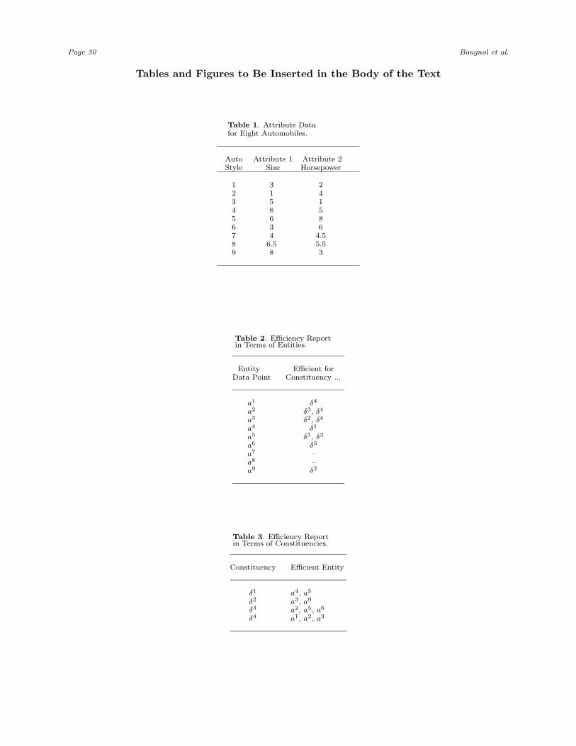
We will illustrate the ideas so far with a simple example. Imagine eight automobile models
to be marketed and sold in different markets. Table 1 presents the data corresponding to these
products. Suppose that markets are defined by their preferences for each of two attributes: size
and horsepower. This generates 22 = 4 potential markets which are the ‘constituencies’ in this
example. The constituencies are: δ1 = (1, 1), δ2 = (1,−1), δ3 = (−1, 1), and δ4 = (−1,−1). So,
for example, δ1 is the constituency (market) that values greater size and horsepower in their cars;
e.g., the North American market (perhaps from another era), and δ4 is the constituency (market)
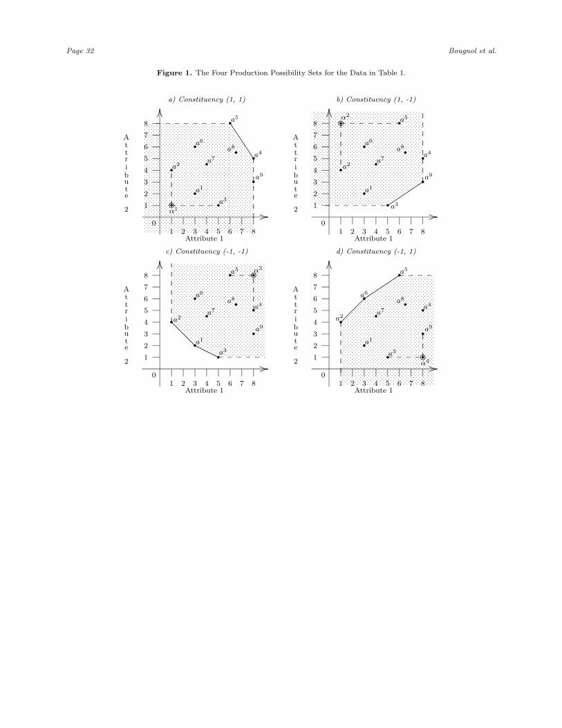
that considers both attributes undesirable; e.g., Southern Europe. Figure 1 depicts the production
possibility sets for these four constituencies.
Table 1 Here: “Attribute Data for Eight Automobiles”.
“Nonparametric frontiers with constituencies.” Page 7
Figure 1 Here: “The Four PPS for the Two-Attribute Example”.
Figures 1a, 1b, 1c, and 1d depict the four variable returns (BCC) production possibility sets for
constituencies δ1, δ2, δ3, and δ4, respectively. Consider constituency δ1, the production possibility
set for which appears in Figure 1a. In this market, bigger size and greater power are better. For
this constituency, the two points, a4 and a5 are in the efficient frontier of the production possibility
set. Each of these points is BCC efficient because no convex combination of the remaining data
points will provide a value for the two attributes that are greater than or equal to, with at least
one strictly greater, than what it is for these two points.
Table 2 summarizes the status of all the entities with respect to the different constituencies.
Table 2 Here: “Efficiency Report in Terms of Entities”.
This example of DEA with multiple constituencies in two dimensions provides insights about
the general case. The different situations that occur in this simple example reappear in higher
dimensions. This suggests that the new framework for DEA can be used to identify different
categories of points as follows:
i) Entities that are efficient for two or more constituencies as in the case of points a2, a3, and a5.
ii) Entities that are efficient for a single constituency as in the case of points a1, a4, a6, and a9.
iii) Entities that are on the boundary of the production possibility set of some constituency but are
dominated. This is the case of points a4 for constituency δ2 and a9 for constituency δ1.
iv) Entities that are always inefficient independent of the constituency. This is the case of entities
a7 and a8.
In an application of DEA with multiple constituencies, the decision maker would be interested
in the classification of entities using the categories above. Entities that are efficient for many
constituencies may be of special interest because of their broad market appeal (Category i). Entities
that appeal to a single constituency would represent to a marketer a specialty product (Category
Page 8 Bougnol et al.
ii). Entities on the boundary that are inefficient for some constituency are equivalent to weak
efficient DMUs in DEA (Category iii). From past experience with DEA, we may expect analyses
to be confounded and complicated by their presence. Entities in the fourth category may appear
to be some sort of “middle of the road” compromise (central planners of certain economies seemed
to have based policies on such conclusions). In the context of efficient frontiers these entities are
nothing more than universally inefficient alternatives and it behooves the decision maker to identify
them quickly and discard them from further consideration.
Conversely, an analysis of a DEA with multiple constituencies can focus on the constituencies
rather than the entities. Table 3 reports on the matching of each constituency and a corresponding
set of efficient entities. We can see in this example that different constituencies play different
roles. A classification scheme for constituencies can be based on the number of efficient entities
with which they can be matched; for example, a scheme based on just two categories would be as
follows:
i) Constituencies with a single, or few, efficient entities as in the case of δ1 and δ2.
ii) Constituencies with many efficient entities as in the case of δ3 and δ4.
A marketer analyzing his/her markets would identify constituencies δ1 and δ2 as more exclusive
possibly because they are more selective. Constituencies in the second category are in some sense
more amenable since they have the largest number of efficient entities.
Table 3 Here: “Efficiency Report in Terms of Constituencies”.
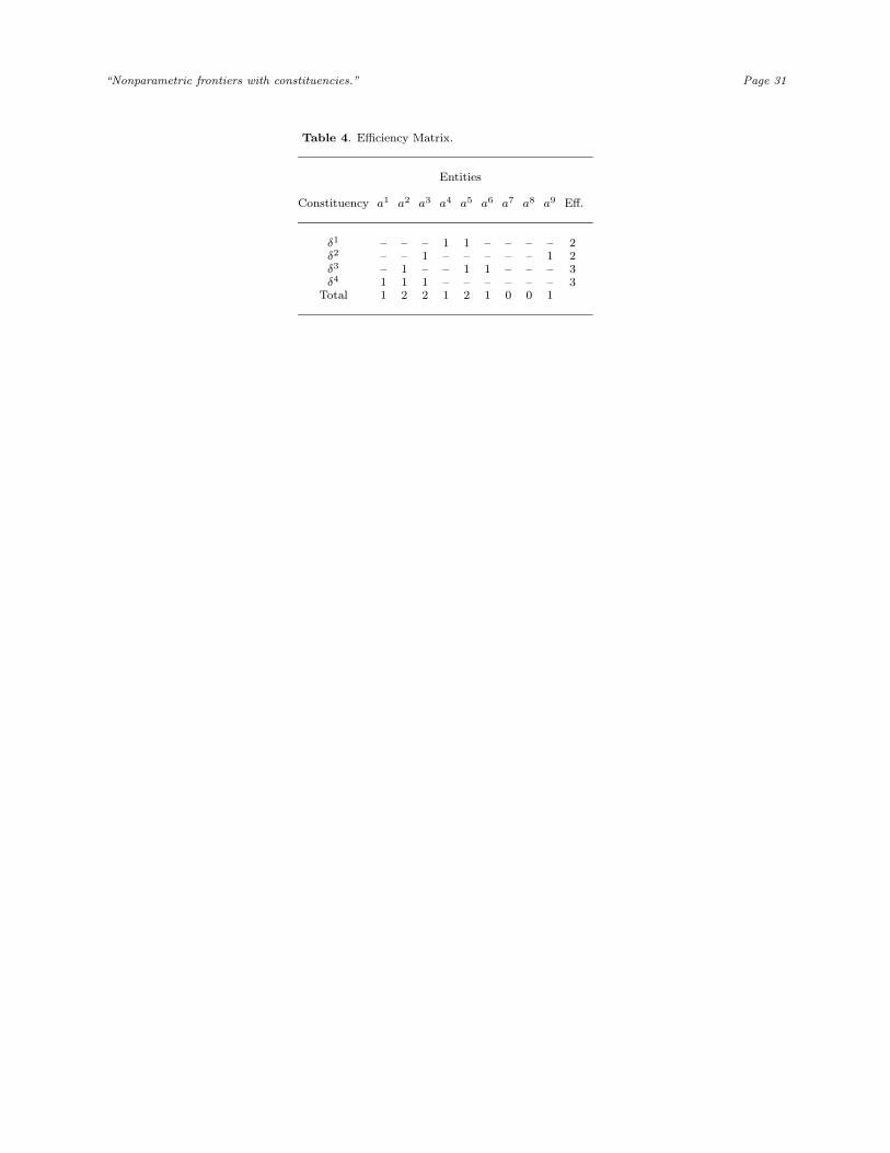
The information in Tables 2 and 3 can be summarized using a matrix as in Table 4. The
sum total of the rows in the column labeled “Eff.” gives the total number of entities that are
efficient for a given constituency and the sum total of columns in row “Total” displays the number
of constituencies finding the corresponding entity efficient. This representation permits efficient
inferencing about entities and constituencies.
Table 4 Here: “Efficiency Matrix”.
“Nonparametric frontiers with constituencies.” Page 9
The next two sections are dedicated to the theoretical device used to make the determination
about the efficiency of entities with respect to constituencies; namely the linear program formula-
tion. First we present arguments for a new DEA LP formulation. After that, we provide theoretical
results about this new LP.
A Case for a New DEA LP Formulation.
Several LP formulations have been proposed for traditional DEA. LP formulations fall into two
categories: oriented and unoriented. The choice of LP formulation used does not affect the classi-
fication of the entities.
Oriented LP forms require a judgment as to which attributes will be fixed and which will be
allowed to vary when establishing efficiency and benchmarks (for a compendium of oriented LP
DEA formulations, please refer to Seiford,8 et al.). The idea of orientation extends to the mul-
tiple constituencies model. Instead of having input and output oriented formulations, we have
“desirably” and “undesirably” oriented LP formulations. The best way to present this general-
ization is to simply consider the attribute mix and, for any constituency (except δ1 = (1, . . . , 1)
and δ2m
= (−1, . . . ,−1)), reorder, without loss of generality, the attributes such that undesirable
components are first and desirable components are last. With this, we can apply the standard
DEA oriented forms to obtain scores in either or both orientations. We can adapt the oriented
LP formulations easily to deal with the case of δ1 and δ2m
. (See, e.g., Thompson9 et al., for an
example of the case where all attributes are inputs and Adolphson10 et al. and Caporaletti11 et al.
for an example where all attributes are outputs.)
The decision as to which attribute will be fixed and which attribute will be allowed to vary, is
essentially connected to benchmarking. A benchmarking recommendation for an inefficient entity
will either be based on a reduction of inputs, or an increase of outputs, and sometimes, the very
nature of these attributes makes one or the other impractical. The decision about an oriented
form becomes arbitrary in the presence of multiple constituencies since, if there is any reason for
selecting a particular orientation for one constituency, there will be another constituency for which
this reason will be contradicted. This view is shared by Scheel5 where he states that the oriented
form is “not very appropriate” when the desirability of an attribute is not clearly defined.
Page 10 Bougnol et al.
DEA also uses unoriented LP formulations. The standard unoriented DEA LP formulation is the
additive form introduced in Charnes4 et al. This LP formulation serves the purpose of providing
necessary and sufficient conditions for the classification of entities in DEA. The additive model
in DEA can be adapted for multiple constituencies. The procedure would be the same as with
oriented forms described above. The additive model is formulated to maximize the l1-distance of
the point being tested to the efficient frontier (Charnes4 et al., Tavares12 et al.). The effect is that
inefficient entities are benchmarked by points in the efficient frontier which may be “far away” for
practical purposes. This problem with the additive model makes it unsuitable for benchmarking
purposes.
A positive characteristic of the additive model is that it is translation invariant. An affine
displacement of the data does not alter the efficient frontier and the classification of DMUs as
efficient or inefficient is invariant to translation of the data. Moreover, unlike oriented forms, the
additive model is translation invariant in its scores (Ali,13 et al.).
Finally, both the oriented forms and the unoriented additive form suffer from infeasibility under
deleted domain in the envelopment formulation (Dula14 et al., Seiford15 et al.). In fact, the LP will
always be infeasible under deleted domain when the DMU being scored is extreme efficient for the
case of the additive model. Important information such as the multipliers (weights) of a supporting
hyperplane for the production possibility set is lost when no feasible solution is available.
The arguments presented above will be used to support a new LP formulation, specifically for
DEA with constituencies. The new LP formulation we propose will have advantages of being
unoriented; providing useful and intuitive benchmarks; being translation invariant in both its
classifications results and scores; and finally, being feasible and bounded under deleted domain.
The New DEA LP Formulation.
Definition 2 establishes how entities will be classified with respect to constituencies. The classifi-
cation criterion is based on the variable returns to scale assumption. In this section, we present a
new DEA LP formulation to make this classification.
“Nonparametric frontiers with constituencies.” Page 11
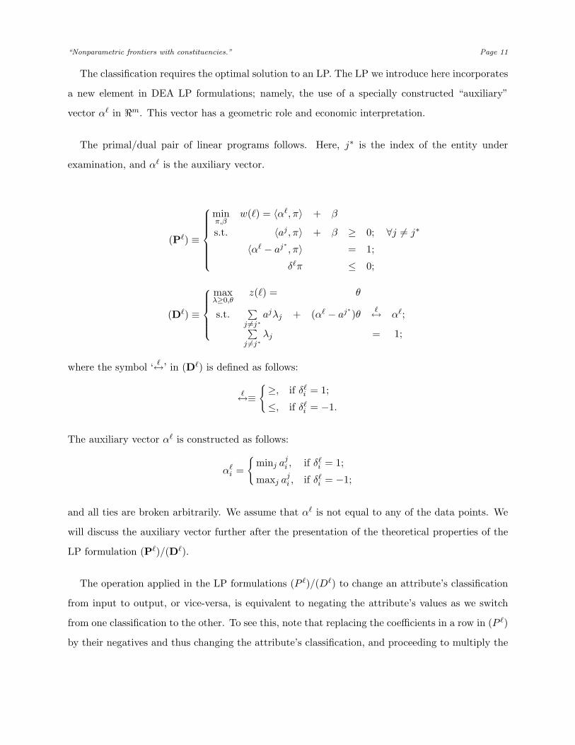
The classification requires the optimal solution to an LP. The LP we introduce here incorporates
a new element in DEA LP formulations; namely, the use of a specially constructed “auxiliary”
vector α� in �m. This vector has a geometric role and economic interpretation.
The primal/dual pair of linear programs follows. Here, j∗ is the index of the entity under
examination, and α� is the auxiliary vector.
(P�) ≡
minπ,β
w(�) = 〈α�, π〉 + β
s.t. 〈aj , π〉 + β ≥ 0; ∀j �= j∗
〈α� − aj∗, π〉 = 1;
δ�π ≤ 0;
(D�) ≡
maxλ≥0,θ
z(�) = θ
s.t.∑
j �=j∗ajλj + (α� − aj∗
)θ �↔ α�;∑j �=j∗
λj = 1;
where the symbol ‘ �↔’ in (D�) is defined as follows:
�↔≡{≥, if δ�
i = 1;
≤, if δ�i = −1.
The auxiliary vector α� is constructed as follows:
α�i =
{minj aj
i , if δ�i = 1;
maxj aji , if δ�
i = −1;
and all ties are broken arbitrarily. We assume that α� is not equal to any of the data points. We
will discuss the auxiliary vector further after the presentation of the theoretical properties of the
LP formulation (P�)/(D�).
The operation applied in the LP formulations (P �)/(D�) to change an attribute’s classification
from input to output, or vice-versa, is equivalent to negating the attribute’s values as we switch
from one classification to the other. To see this, note that replacing the coefficients in a row in (P �)
by their negatives and thus changing the attribute’s classification, and proceeding to multiply the
Page 12 Bougnol et al.
row by -1, the original coefficients are restored but the inequality will be reversed. This, therefore,
is an implementation of the technique for changing an attribute’s classification used in Scheel5.
Denote by π∗(�) = (π∗1(�), . . . , π
∗m(�)), β∗(�) and λ∗(�) = (λ∗
1(�), . . . , λ∗n(�)), θ∗(�) two optimal
solutions, the first for (P�) and the other for (D�). The corresponding optimal objective function
values are denoted by w∗(�) and z∗(�). Also, let T � be the production possibility set for constituency
δ� and we define T �/ aj∗as the production possibility set of the data when the point aj∗
is excluded
from the data set. Note that T �/ aj∗ ⊂ T �.
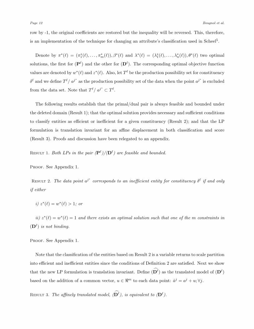
The following results establish that the primal/dual pair is always feasible and bounded under
the deleted domain (Result 1); that the optimal solution provides necessary and sufficient conditions
to classify entities as efficient or inefficient for a given constituency (Result 2); and that the LP
formulation is translation invariant for an affine displacement in both classification and score
(Result 3). Proofs and discussion have been relegated to an appendix.
Result 1. Both LPs in the pair (P�)/(D�) are feasible and bounded.
Proof. See Appendix 1.
Result 2. The data point aj∗corresponds to an inefficient entity for constituency δ� if and only
if either
i) z∗(�) = w∗(�) > 1; or
ii) z∗(�) = w∗(�) = 1 and there exists an optimal solution such that one of the m constraints in
(D�) is not binding.
Proof. See Appendix 1.
Note that the classification of the entities based on Result 2 is a variable returns to scale partition
into efficient and inefficient entities since the conditions of Definition 2 are satisfied. Next we show
that the new LP formulation is translation invariant. Define (D�) as the translated model of (D�)
based on the addition of a common vector, u ∈ �m to each data point: aj = aj + u;∀j.
Result 3. The affinely translated model, (D�), is equivalent to (D�).
“Nonparametric frontiers with constituencies.” Page 13
Proof. See Appendix 1.
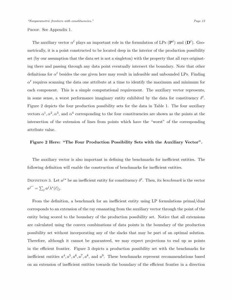
The auxiliary vector α� plays an important role in the formulation of LPs (P�) and (D�). Geo-
metrically, it is a point constructed to be located deep in the interior of the production possibility
set (by our assumption that the data set is not a singleton) with the property that all rays originat-
ing there and passing through any data point eventually intersect the boundary. Note that other
definitions for α� besides the one given here may result in infeasible and unbounded LPs. Finding
α� requires scanning the data one attribute at a time to identify the maximum and minimum for
each component. This is a simple computational requirement. The auxiliary vector represents,
in some sense, a worst performance imaginary entity exhibited by the data for constituency δ�.
Figure 2 depicts the four production possibility sets for the data in Table 1. The four auxiliary
vectors α1, α2, α3, and α4 corresponding to the four constituencies are shown as the points at the
intersection of the extension of lines from points which have the “worst” of the corresponding
attribute value.
Figure 2 Here: “The Four Production Possibility Sets with the Auxiliary Vector”.
The auxiliary vector is also important in defining the benchmarks for inefficient entities. The
following definition will enable the construction of benchmarks for inefficient entities.
Definition 3. Let aj∗ be an inefficient entity for constituency δ�. Then, its benchmark is the vector
aj∗′=
∑j ajλ∗(�)j .
From the definition, a benchmark for an inefficient entity using LP formulations primal/dual
corresponds to an extension of the ray emanating from the auxiliary vector through the point of the
entity being scored to the boundary of the production possibility set. Notice that all extensions
are calculated using the convex combinations of data points in the boundary of the production
possibility set without incorporating any of the slacks that may be part of an optimal solution.
Therefore, although it cannot be guaranteed, we may expect projections to end up as points
in the efficient frontier. Figure 3 depicts a production possibility set with the benchmarks for
inefficient entities a4, a5, a6, a7, a8, and a9. These benchmarks represent recommendations based
on an extension of inefficient entities towards the boundary of the efficient frontier in a direction
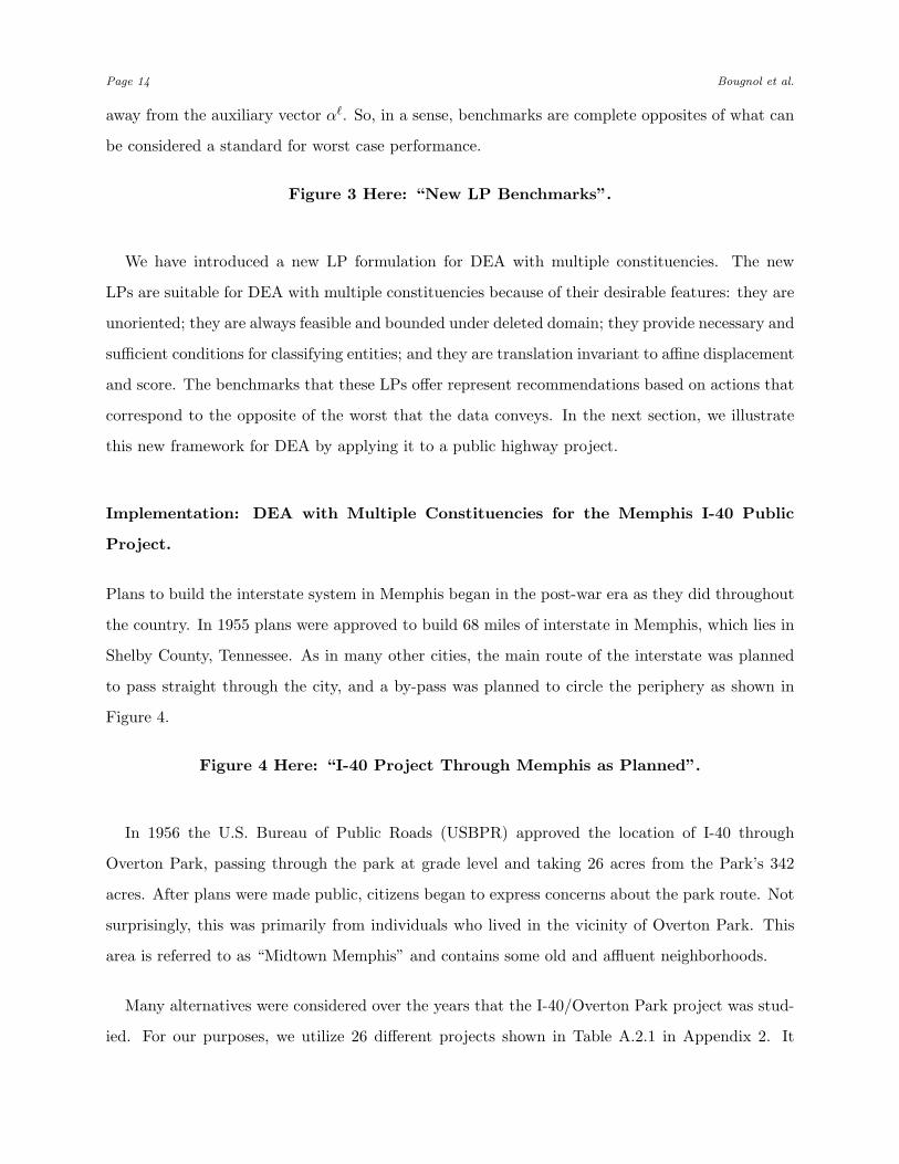
Page 14 Bougnol et al.
away from the auxiliary vector α�. So, in a sense, benchmarks are complete opposites of what can
be considered a standard for worst case performance.
Figure 3 Here: “New LP Benchmarks”.
We have introduced a new LP formulation for DEA with multiple constituencies. The new
LPs are suitable for DEA with multiple constituencies because of their desirable features: they are
unoriented; they are always feasible and bounded under deleted domain; they provide necessary and
sufficient conditions for classifying entities; and they are translation invariant to affine displacement
and score. The benchmarks that these LPs offer represent recommendations based on actions that
correspond to the opposite of the worst that the data conveys. In the next section, we illustrate
this new framework for DEA by applying it to a public highway project.
Implementation: DEA with Multiple Constituencies for the Memphis I-40 Public
Project.
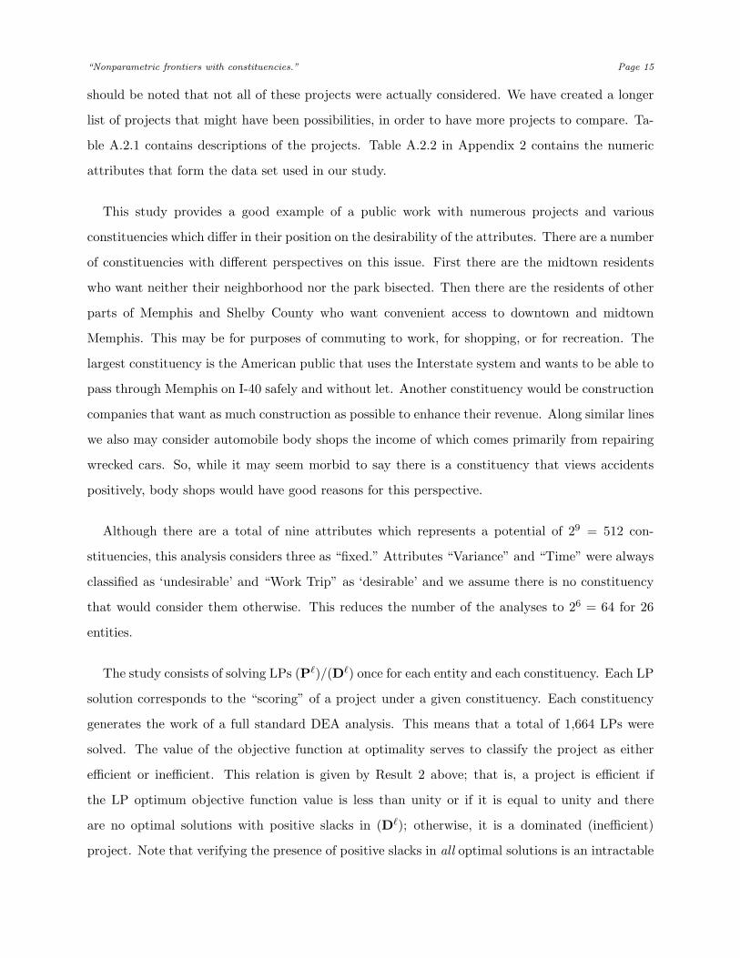
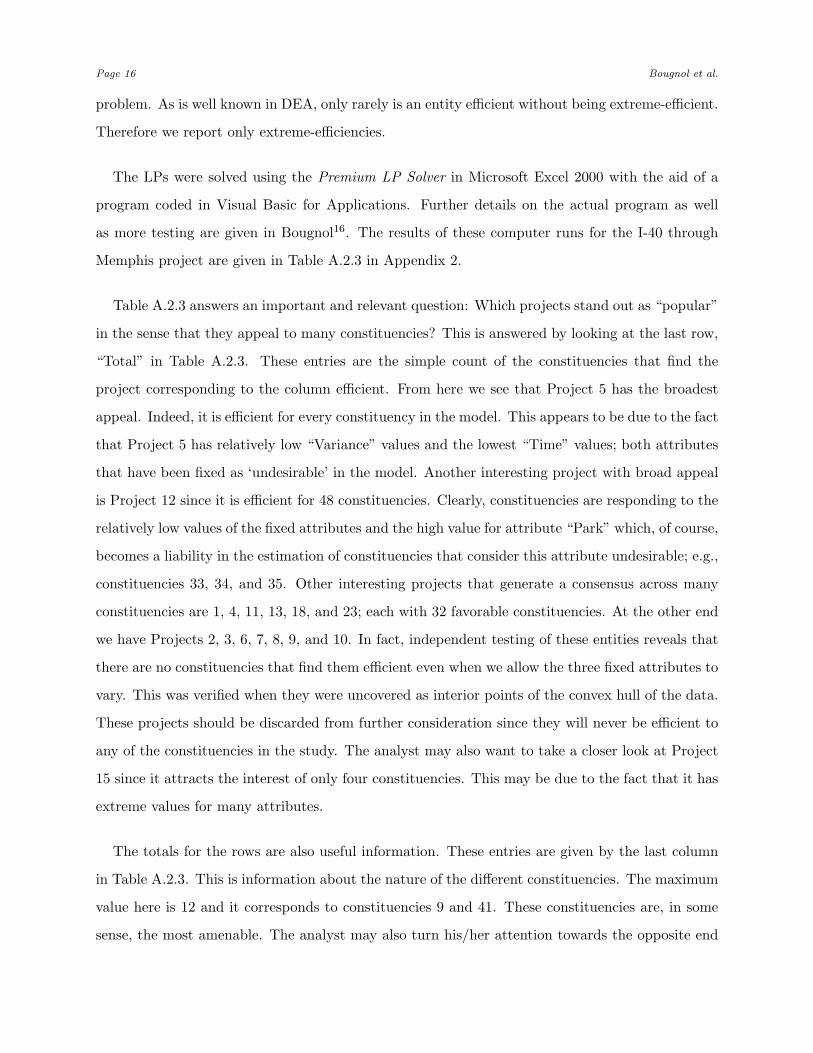
Plans to build the interstate system in Memphis began in the post-war era as they did throughout
the country. In 1955 plans were approved to build 68 miles of interstate in Memphis, which lies in
Shelby County, Tennessee. As in many other cities, the main route of the interstate was planned
to pass straight through the city, and a by-pass was planned to circle the periphery as shown in
Figure 4.
Figure 4 Here: “I-40 Project Through Memphis as Planned”.
In 1956 the U.S. Bureau of Public Roads (USBPR) approved the location of I-40 through
Overton Park, passing through the park at grade level and taking 26 acres from the Park’s 342
acres. After plans were made public, citizens began to express concerns about the park route. Not
surprisingly, this was primarily from individuals who lived in the vicinity of Overton Park. This
area is referred to as “Midtown Memphis” and contains some old and affluent neighborhoods.
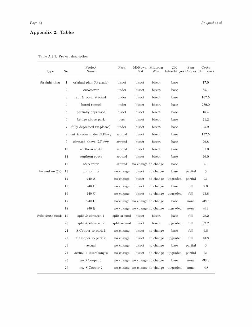
Many alternatives were considered over the years that the I-40/Overton Park project was stud-
ied. For our purposes, we utilize 26 different projects shown in Table A.2.1 in Appendix 2. It
“Nonparametric frontiers with constituencies.” Page 15
should be noted that not all of these projects were actually considered. We have created a longer
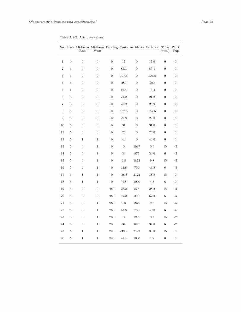
list of projects that might have been possibilities, in order to have more projects to compare. Ta-
ble A.2.1 contains descriptions of the projects. Table A.2.2 in Appendix 2 contains the numeric
attributes that form the data set used in our study.
This study provides a good example of a public work with numerous projects and various
constituencies which differ in their position on the desirability of the attributes. There are a number
of constituencies with different perspectives on this issue. First there are the midtown residents
who want neither their neighborhood nor the park bisected. Then there are the residents of other
parts of Memphis and Shelby County who want convenient access to downtown and midtown
Memphis. This may be for purposes of commuting to work, for shopping, or for recreation. The
largest constituency is the American public that uses the Interstate system and wants to be able to
pass through Memphis on I-40 safely and without let. Another constituency would be construction
companies that want as much construction as possible to enhance their revenue. Along similar lines
we also may consider automobile body shops the income of which comes primarily from repairing
wrecked cars. So, while it may seem morbid to say there is a constituency that views accidents
positively, body shops would have good reasons for this perspective.
Although there are a total of nine attributes which represents a potential of 29 = 512 con-
stituencies, this analysis considers three as “fixed.” Attributes “Variance” and “Time” were always
classified as ‘undesirable’ and “Work Trip” as ‘desirable’ and we assume there is no constituency
that would consider them otherwise. This reduces the number of the analyses to 26 = 64 for 26
entities.
The study consists of solving LPs (P�)/(D�) once for each entity and each constituency. Each LP
solution corresponds to the “scoring” of a project under a given constituency. Each constituency
generates the work of a full standard DEA analysis. This means that a total of 1,664 LPs were
solved. The value of the objective function at optimality serves to classify the project as either
efficient or inefficient. This relation is given by Result 2 above; that is, a project is efficient if
the LP optimum objective function value is less than unity or if it is equal to unity and there
are no optimal solutions with positive slacks in (D�); otherwise, it is a dominated (inefficient)
project. Note that verifying the presence of positive slacks in all optimal solutions is an intractable
Page 16 Bougnol et al.
problem. As is well known in DEA, only rarely is an entity efficient without being extreme-efficient.
Therefore we report only extreme-efficiencies.
The LPs were solved using the Premium LP Solver in Microsoft Excel 2000 with the aid of a
program coded in Visual Basic for Applications. Further details on the actual program as well
as more testing are given in Bougnol16. The results of these computer runs for the I-40 through
Memphis project are given in Table A.2.3 in Appendix 2.
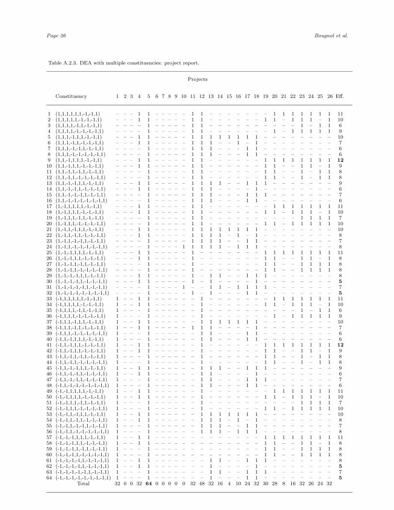
Table A.2.3 answers an important and relevant question: Which projects stand out as “popular”
in the sense that they appeal to many constituencies? This is answered by looking at the last row,
“Total” in Table A.2.3. These entries are the simple count of the constituencies that find the
project corresponding to the column efficient. From here we see that Project 5 has the broadest
appeal. Indeed, it is efficient for every constituency in the model. This appears to be due to the fact
that Project 5 has relatively low “Variance” values and the lowest “Time” values; both attributes
that have been fixed as ‘undesirable’ in the model. Another interesting project with broad appeal
is Project 12 since it is efficient for 48 constituencies. Clearly, constituencies are responding to the
relatively low values of the fixed attributes and the high value for attribute “Park” which, of course,
becomes a liability in the estimation of constituencies that consider this attribute undesirable; e.g.,
constituencies 33, 34, and 35. Other interesting projects that generate a consensus across many
constituencies are 1, 4, 11, 13, 18, and 23; each with 32 favorable constituencies. At the other end
we have Projects 2, 3, 6, 7, 8, 9, and 10. In fact, independent testing of these entities reveals that
there are no constituencies that find them efficient even when we allow the three fixed attributes to
vary. This was verified when they were uncovered as interior points of the convex hull of the data.
These projects should be discarded from further consideration since they will never be efficient to
any of the constituencies in the study. The analyst may also want to take a closer look at Project
15 since it attracts the interest of only four constituencies. This may be due to the fact that it has
extreme values for many attributes.
The totals for the rows are also useful information. These entries are given by the last column
in Table A.2.3. This is information about the nature of the different constituencies. The maximum
value here is 12 and it corresponds to constituencies 9 and 41. These constituencies are, in some
sense, the most amenable. The analyst may also turn his/her attention towards the opposite end
“Nonparametric frontiers with constituencies.” Page 17
of this “congeniality” scale; e.g., constituencies 30, 32, 62, and 64. These constituencies appear
to be the hardest to please since they approve of only five projects. The analyst should focus on
constituencies with extreme values in this column. These should trigger questions such as: What
is the cardinality of the elements of these constituencies? (small constituencies may generate less
concern than larger ones); What are the characteristics (e.g., demographics, level of influence) of
the elements in these constituencies?
Further insights into constituencies and projects can be gleaned by comparing the percentage
of efficient projects for each constituency and the percentage of projects found efficient across all
constituencies. Figures 5 and 6 present this information in a form that a decision maker can readily
use. These figures depict data processed from Table A.2.3. Figure 5 exhibits, for each project, the
proportion of the constituencies that consider it efficient ranked from high to low. A decision maker
would use this information to identify which projects are the most appealing (e.g., Project 5) and
which ones are not appealing to any constituencies (e.g., Projects 2, 3, 6, 7, 8, 9, and 10). Figure
6 can be used to learn what percentage of the projects are efficient for each of the constituencies
also ranked from high to low. This information will facilitate the identification of constituencies of
special interest: the most amenable constituencies such as Constituencies 9 and 41 are on the left
and, at the opposite end, the less congenial constituencies such as Constituencies 30, 32, 62, and
64.
Figure 5 Here: “Percentage of Constituencies Finding a Project Efficient (ranked)”.
Figure 6 Here: “Percentage of Efficient Projects for Each Constituency (ranked)”.
One remaining aspect of our analysis of this application of DEA with multiple constituencies
is benchmarking. Consider Project 2. This project is distinguished for being inefficient for all
constituencies. An interesting question is: How can this project become efficient for a given
constituency, say, the most congenial constituency: Constituency 41? When scoring Project 2
with Constituency 41, the optimal solution, although being unity, contains a slack in Attribute 1,
“Park”, making this entity inefficient. The benchmark for this project is the value of the convex
combination of the data set where the coefficients are given by the optimal solution of (D�). This
Page 18 Bougnol et al.
yields the “virtual” project (2.04, 0, 0, 0, 85.1, 0, 85.1, 0, 0). Project 2 will be efficient if its value for
the “Park” attribute is decreased by 1.96 units of damage to Overton Park.
The obvious conclusion of the application of the methodology developed for this project on the
plan to build an interstate through Memphis is that Project 5 emerges as particularly interesting.
All constituencies would consider this project efficient and, presumably, would offer no opposition.
Also interesting are the inferences about the different constituencies. A public official will be well-
served to note the amenability of Constituencies 9 and 41 and his/her dealings with them would
be very different than with Constituencies 30, 32, 62, and 64. The data for this study are less
than ideal since it involves several categorical attributes. In an ideal model, all attributes have
cardinal values but we can expect a less obvious course of action with such data. It is unlikely
that a single entity will prevail as Project 5 has in this study. In this case the decision would have
to consider not just which entity has the most number of supporting constituencies but also the
nature of the constituencies which are opposed. The analysis, nevertheless, provides important
insights about the interactions among constituencies and projects that will support decisions made
by the decision maker.
Conclusion.
This article treats a broad generalization of standard DEA. We consider what happens when the
attributes which define the entities in a DEA study are not fixed to be inputs or outputs as in
standard DEA practice. We relax this restriction allowing the classification of attributes to vary
according to different constituencies.
Multiple constituencies made it necessary to consider a new LP formulation for scoring entities.
Standard formulations turn out to be inadequate. We have introduced a new LP formulation with
important features which make it a contribution to general DEA.
The new framework for DEA and the new LP formulation were illustrated and validated by im-
plementing them on an actual application involving a public project. The result was the definition
of a methodology for generating and interpreting data with the new framework. Other analysts

“Nonparametric frontiers with constituencies.” Page 19
who wish to perform DEA studies involving constituencies now have a new tool to perform this
work.
Page 20 Bougnol et al.
Appendix 1. Proofs to Theorems
Result 1. Both LPs in the pair (P�)/(D�) are feasible and bounded.
Proof. Let us begin by establishing the feasibility of (D�). We show that the LP is feasible for
θ = 0. At this value, the system becomes:
∑j �=j∗
ajλj�↔ α�;∑
j �=j∗λj = 1 ;
λj ≥ 0; ∀j, j �= j∗.
Consider desirable attribute i. Any convex combination of all ith components aj
i;∀j, j �= j∗ must
be such that ∑j �=j∗
aj
iλj ≥ α�
i;
since, by construction, on a one-on-one basis aj
i≥ α�
i;∀j, j �= j∗. Similarly for undesirable at-
tributes. So, for θ = 0, any convex combination of the data is a feasible solution. This also
establishes the boundedness of (P�).
The feasibility of (P�) follows from the following arguments. Consider any supporting hyper-
plane: H(π, β) = 〈y, π〉+ β = 0 for the production possibility set T �\aj∗such that πi �= 0;∀i. Such
a hyperplane is always available since there is no restriction on the value of β. Therefore:
〈aj , π〉 + β ≥ 0; ∀j �= j∗
δ�π ≤ 0.
Now let us take the solution (π, β) and apply it to the constraint in (P�) involving α�: 〈α�−aj∗, π〉 =
1. By construction, (α�−aj∗) �↔ 0, π
�↔ 0; and since, by assumption α� �= aj∗, 〈α�−aj∗
, π〉 = γ > 0.
Substituting π = π/γ and recalculating a β provides the feasible solution we started off seeking.
This, of course, establishes the boundedness of (D�).
“Nonparametric frontiers with constituencies.” Page 21
Result 2. The data point aj∗corresponds to an inefficient entity for constituency δ� if and only
if either
i) z∗(�) = w∗(�) > 1; or
ii) z∗(�) = w∗(�) = 1 and there exists an optimal solution such that one of the m constraints in
(D�) is not binding.
Proof. Case i): Let z∗(�) = w∗(�) > 1. Consider (D�) and let (λ∗, θ∗) be its optimal solution.
The first m constraints of (D�) can be rewritten as follows:
∑j �=j∗
ajλ∗j
�↔ aj∗+ (aj∗ − α�
i)(θ∗ − 1).
Suppose attribute i is desirable. By construction, α�i≤ aj∗
iand since θ∗ > 1, then
aj∗
i+ (aj∗
i− α�
i)︸ ︷︷ ︸
≥0
(θ∗ − 1)︸ ︷︷ ︸>0
≥ aj∗
i.
Similarly if attribute i is undesirable we have that
aj∗
i+ (aj∗
i− α�
i)(θ∗ − 1) ≤ aj∗
i.
However, by assumption, α� �= aj∗meaning that at least one inequality is strict. Thus, when
θ∗ > 1, the data point aj∗is dominated by some convex combination of the data making it an
inefficient entity for constituency δ�.
Case ii): z∗(�) = w∗(�) = 1 and slacks occur for, at least, one optimal solution. Let a be the
‘virtual’ entity, i.e., a =∑
j �=j∗ajλ∗
j and∑
j �=j∗λ∗
j = 1. So, ai = aj∗
i for all i except at least once, where
the slack occurs, and either ai < aj∗
i or ai > aj∗
i , depending on whether the attribute is undesirable
or desirable. Therefore, a dominates aj∗by Definition 2.
To demonstrate the converse, we must show that, if either z∗(�) = w∗(�) = 1 and there are no
slacks for any optimal solution or z∗(�) = w∗(�) < 1 then aj∗is efficient.
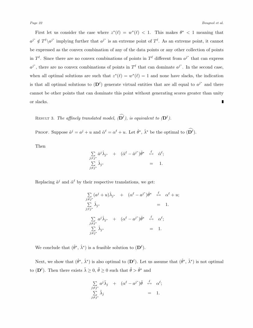
Page 22 Bougnol et al.
First let us consider the case where z∗(�) = w∗(�) < 1. This makes θ∗ < 1 meaning that
aj∗/∈ T �\aj∗
implying further that aj∗is an extreme point of T �. As an extreme point, it cannot
be expressed as the convex combination of any of the data points or any other collection of points
in T �. Since there are no convex combinations of points in T � different from aj∗that can express
aj∗, there are no convex combinations of points in T � that can dominate aj∗
. In the second case,
when all optimal solutions are such that z∗(�) = w∗(�) = 1 and none have slacks, the indication
is that all optimal solutions to (D�) generate virtual entities that are all equal to aj∗and there
cannot be other points that can dominate this point without generating scores greater than unity
or slacks.
Result 3. The affinely translated model, (D�), is equivalent to (D�).
Proof. Suppose aj = aj + u and α� = α� + u. Let θ∗, λ∗ be the optimal to (D�).
Then ∑j �=j∗
ajλj∗ + (α� − aj∗)θ∗ �↔ α�;∑
j �=j∗λj∗ = 1.
Replacing aj and α� by their respective translations, we get:
∑j �=j∗
(aj + u)λj∗ + (α� − aj∗)θ∗ �↔ α� + u;∑
j �=j∗λj∗ = 1.
∑j �=j∗
ajλj∗ + (α� − aj∗)θ∗ �↔ α�;∑
j �=j∗λj∗ = 1.
We conclude that (θ∗, λ∗) is a feasible solution to (D�).
Next, we show that (θ∗, λ∗) is also optimal to (D�). Let us assume that (θ∗, λ∗) is not optimal
to (D�). Then there exists λ ≥ 0, θ ≥ 0 such that θ > θ∗ and
∑j �=j∗
ajλj + (α� − aj∗)θ �↔ α�;∑
j �=j∗λj = 1.
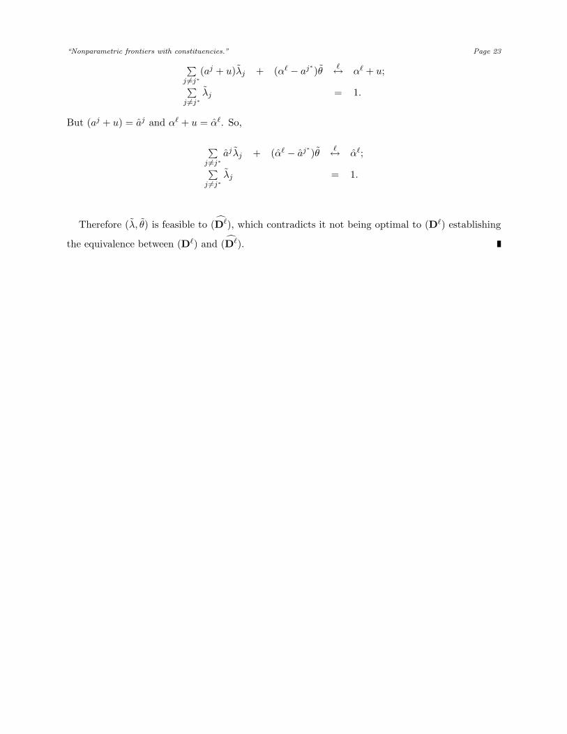
“Nonparametric frontiers with constituencies.” Page 23∑j �=j∗
(aj + u)λj + (α� − aj∗)θ �↔ α� + u;∑
j �=j∗λj = 1.
But (aj + u) = aj and α� + u = α�. So,
∑j �=j∗
ajλj + (α� − aj∗)θ �↔ α�;∑
j �=j∗λj = 1.
Therefore (λ, θ) is feasible to (D�), which contradicts it not being optimal to (D�) establishing
the equivalence between (D�) and (D�).
Page 24 Bougnol et al.
Appendix 2. Tables
Table A.2.1. Project description.
Project Park Midtown Midtown 240 Sam CostsType No. Name East West Interchanges Cooper ($millions)
Straight thru 1 original plan (@ grade) bisect bisect bisect base 17.0
2 cut&cover under bisect bisect base 85.1
3 cut & cover stacked under bisect bisect base 107.5
4 bored tunnel under bisect bisect base 280.0
5 partially depressed bisect bisect bisect base 16.4
6 bridge above park over bisect bisect base 21.2
7 fully depressed (w.plazas) under bisect bisect base 25.9
8 cut & cover under N.Pkwy around bisect bisect base 157.5
9 elevated above N.Pkwy around bisect bisect base 29.8
10 northern route around bisect bisect base 31.0
11 southern route around bisect bisect base 26.0
12 L&N route around no change no change base 40
Around on 240 13 do nothing no change bisect no change base partial 0
14 240 A no change bisect no change upgraded partial 34
15 240 B no change bisect no change base full 9.8
16 240 C no change bisect no change upgraded full 43.8
17 240 D no change no change no change base none -38.8
18 240 E no change no change no change upgraded none -4.8
Substitute funds 19 split & elevated 1 split around bisect bisect base full 28.2
20 split & elevated 2 split around bisect bisect upgraded full 62.2
21 S.Cooper to park 1 no change bisect no change base full 9.8
22 S.Cooper to park 2 no change bisect no change upgraded full 43.8
23 actual no change bisect no change base partial 0
24 actual + interchanges no change bisect no change upgraded partial 34
25 no.S.Cooper 1 no change no change no change base none -38.8
26 no. S.Cooper 2 no change no change no change upgraded none -4.8
“Nonparametric frontiers with constituencies.” Page 25
Table A.2.2. Attribute values.
No. Park Midtown Midtown Funding Costs Accidents Variance Time WorkEast West (min.) Trip
1 0 0 0 0 17 0 17.0 0 0
2 4 0 0 0 85.1 0 85.1 0 0
3 4 0 0 0 107.5 0 107.5 0 0
4 5 0 0 0 280 0 280 0 0
5 1 0 0 0 16.4 0 16.4 0 0
6 3 0 0 0 21.2 0 21.2 0 0
7 3 0 0 0 25.9 0 25.9 0 0
8 5 0 0 0 157.5 0 157.5 0 0
9 5 0 0 0 29.8 0 29.8 0 0
10 5 0 0 0 31 0 31.0 0 0
11 5 0 0 0 26 0 26.0 0 0
12 5 1 1 0 40 0 40.0 0 0
13 5 0 1 0 0 1997 0.0 15 -2
14 5 0 1 0 34 875 34.0 6 -2
15 5 0 1 0 9.8 1872 9.8 15 -5
16 5 0 1 0 43.8 750 43.8 6 -5
17 5 1 1 0 -38.8 2122 38.8 15 0
18 5 1 1 0 -4.8 1000 4.8 6 0
19 5 0 0 280 28.2 875 28.2 15 -5
20 5 0 0 280 62.2 250 62.2 6 -5
21 5 0 1 280 9.8 1872 9.8 15 -5
22 5 0 1 280 43.8 750 43.8 6 -5
23 5 0 1 280 0 1997 0.0 15 -2
24 5 0 1 280 34 875 34.0 6 -2
25 5 1 1 280 -38.8 2122 38.8 15 0
26 5 1 1 280 -4.8 1000 4.8 6 0
Page 26 Bougnol et al.
Table A.2.3. DEA with multiple constituencies: project report.
Projects
Constituency 1 2 3 4 5 6 7 8 9 10 11 12 13 14 15 16 17 18 19 20 21 22 23 24 25 26 Eff.
1 (1,1,1,1,1,1,-1,-1,1) – – – 1 1 – – – – – 1 1 – – – – – – – 1 1 1 1 1 1 1 112 (1,1,1,1,1,-1,-1,-1,1) – – – 1 1 – – – – – 1 1 – – – – – – 1 1 – 1 1 1 – 1 103 (1,1,1,1,-1,1,-1,-1,1) – – – – 1 – – – – – 1 1 – – – – – – – – – – 1 – 1 1 64 (1,1,1,1,-1,-1,-1,-1,1) – – – – 1 – – – – – 1 1 – – – – – – – 1 – 1 1 1 1 1 95 (1,1,1,-1,1,1,-1,-1,1) – – – 1 1 – – – – – 1 1 1 1 1 1 1 1 – – – – – – – – 106 (1,1,1,-1,1,-1,-1,-1,1) – – – 1 1 – – – – – 1 1 1 – – 1 – 1 – – – – – – – – 77 (1,1,1,-1,-1,1,-1,-1,1) – – – – 1 – – – – – 1 1 1 – – – 1 1 – – – – – – – – 68 (1,1,1,-1,-1,-1,-1,-1,1) – – – – 1 – – – – – 1 1 1 – – – 1 1 – – – – – – – – 69 (1,1,-1,1,1,1,-1,-1,1) – – – 1 1 – – – – – 1 1 – – – – – – 1 1 1 1 1 1 1 1 1210 (1,1,-1,1,1,-1,-1,-1,1) – – – 1 1 – – – – – 1 1 – – – – – – 1 1 – – 1 1 – 1 911 (1,1,-1,1,-1,1,-1,-1,1) – – – – 1 – – – – – 1 1 – – – – – – 1 1 – – 1 – 1 1 812 (1,1,-1,1,-1,-1,-1,-1,1) – – – – 1 – – – – – 1 1 – – – – – – 1 1 – – 1 – 1 1 813 (1,1,-1,-1,1,1,-1,-1,1) – – – 1 1 – – – – – 1 1 1 1 – – 1 1 1 – – – – – – – 914 (1,1,-1,-1,1,-1,-1,-1,1) – – – 1 1 – – – – – 1 1 1 – – – – 1 – – – – – – – – 615 (1,1,-1,-1,-1,1,-1,-1,1) – – – – 1 – – – – – 1 1 1 – – – 1 1 1 – – – – – – – 716 (1,1,-1,-1,-1,-1,-1,-1,1) – – – – 1 – – – – – 1 1 1 – – – 1 1 – – – – – – – – 617 (1,-1,1,1,1,1,-1,-1,1) – – – 1 1 – – – – – 1 1 – – – – – – – 1 1 1 1 1 1 1 1118 (1,-1,1,1,1,-1,-1,-1,1) – – – 1 1 – – – – – 1 1 – – – – – – 1 1 – 1 1 1 – 1 1019 (1,-1,1,1,-1,1,-1,-1,1) – – – – 1 – – – – – 1 1 – – – – – – – – – – 1 1 1 1 720 (1,-1,1,1,-1,-1,-1,-1,1) – – – – 1 – – – – – 1 1 – – – – – – 1 1 – 1 1 1 1 1 1021 (1,-1,1,-1,1,1,-1,-1,1) – – – 1 1 – – – – – 1 1 1 1 1 1 1 1 – – – – – – – – 1022 (1,-1,1,-1,1,-1,-1,-1,1) – – – 1 1 – – – – – 1 1 1 1 – 1 – 1 – – – – – – – – 823 (1,-1,1,-1,-1,1,-1,-1,1) – – – – 1 – – – – – 1 1 1 1 – – 1 1 – – – – – – – – 724 (1,-1,1,-1,-1,-1,-1,-1,1) – – – – 1 – – – – 1 1 1 1 1 – 1 1 1 – – – – – – – – 825 (1,-1,-1,1,1,1,-1,-1,1) – – – 1 1 – – – – – 1 – – – – – – – 1 1 1 1 1 1 1 1 1126 (1,-1,-1,1,1,-1,-1,-1,1) – – – 1 1 – – – – – 1 – – – – – – – 1 1 – – 1 1 – 1 827 (1,-1,-1,1,-1,1,-1,-1,1) – – – – 1 – – – – – 1 – – – – – – – 1 1 – – 1 1 1 1 828 (1,-1,-1,1,-1,-1,-1,-1,1) – – – – 1 – – – – – 1 – – – – – – – 1 1 – – 1 1 1 1 829 (1,-1,-1,-1,1,1,-1,-1,1) – – – 1 1 – – – – – 1 – 1 1 – – 1 1 1 – – – – – – – 830 (1,-1,-1,-1,1,-1,-1,-1,1) – – – 1 1 – – – – – 1 – 1 – – – – 1 – – – – – – – – 531 (1,-1,-1,-1,-1,1,-1,-1,1) – – – – 1 – – – – 1 – – 1 1 – 1 1 1 1 – – – – – – – 732 (1,-1,-1,-1,-1,-1,-1,-1,1) – – – – 1 – – – – – 1 – 1 – – – 1 1 – – – – – – – – 533 (-1,1,1,1,1,1,-1,-1,1) 1 – – 1 1 – – – – – – 1 – – – – – – – 1 1 1 1 1 1 1 1134 (-1,1,1,1,1,-1,-1,-1,1) 1 – – 1 1 – – – – – – 1 – – – – – – 1 1 – 1 1 1 – 1 1035 (-1,1,1,1,-1,1,-1,-1,1) 1 – – – 1 – – – – – – 1 – – – – – – – – – – 1 – 1 1 636 (-1,1,1,1,-1,-1,-1,-1,1) 1 – – – 1 – – – – – – 1 – – – – – – – 1 – 1 1 1 1 1 937 (-1,1,1,-1,1,1,-1,-1,1) 1 – – 1 1 – – – – – – 1 1 1 1 1 1 1 – – – – – – – – 1038 (-1,1,1,-1,1,-1,-1,-1,1) 1 – – 1 1 – – – – – 1 1 1 – – – – 1 – – – – – – – – 739 (-1,1,1,-1,-1,-1,-1,-1,1) 1 – – – 1 – – – – – – 1 1 – – – 1 1 – – – – – – – – 640 (-1,1,-1,1,1,1,-1,-1,1) 1 – – – 1 – – – – – – 1 1 – – – 1 1 – – – – – – – – 641 (-1,1,-1,1,1,-1,-1,-1,1) 1 – – 1 1 – – – – – – 1 – – – – – – 1 1 1 1 1 1 1 1 1242 (-1,1,-1,1,1,-1,-1,-1,1) 1 – – 1 1 – – – – – – 1 – – – – – – 1 1 – – 1 1 – 1 943 (-1,1,-1,1,-1,1,-1,-1,1) 1 – – – 1 – – – – – – 1 – – – – – – 1 1 – – 1 – 1 1 844 (-1,1,-1,1,-1,-1,-1,-1,1) 1 – – – 1 – – – – – – 1 – – – – – – 1 1 – – 1 – 1 1 845 (-1,1,-1,-1,1,1,-1,-1,1) 1 – – 1 1 – – – – – – 1 1 1 – – 1 1 1 – – – – – – – 946 (-1,1,-1,-1,1,-1,-1,-1,1) 1 – – 1 1 – – – – – – 1 1 – – – – 1 – – – – – – – – 647 (-1,1,-1,-1,1,-1,-1,-1,1) 1 – – – 1 – – – – – – 1 1 – – – 1 1 1 – – – – – – – 748 (-1,1,-1,-1,-1,-1,-1,-1,1) 1 – – – 1 – – – – – – 1 1 – – – 1 1 – – – – – – – – 649 (-1,-1,1,1,1,1,-1,-1,1) 1 – – 1 1 – – – – – – 1 – – – – – – – 1 1 1 1 1 1 1 1150 (-1,-1,1,1,1,-1,-1,-1,1) 1 – – 1 1 – – – – – – 1 – – – – – – 1 1 – 1 1 1 – 1 1051 (-1,-1,1,1,-1,1,-1,-1,1) 1 – – – 1 – – – – – – 1 – – – – – – – – – – 1 1 1 1 752 (-1,-1,1,1,-1,-1,-1,-1,1) 1 – – – 1 – – – – – – 1 – – – – – – 1 1 – 1 1 1 1 1 1053 (-1,-1,1,-1,1,1,-1,-1,1) 1 – – 1 1 – – – – – – 1 1 1 1 1 1 1 – – – – – – – – 1054 (-1,-1,1,-1,1,-1,-1,-1,1) 1 – – 1 1 – – – – – – 1 1 1 – 1 – 1 – – – – – – – – 855 (-1,-1,1,-1,-1,1,-1,-1,1) 1 – – – 1 – – – – – – 1 1 1 – – 1 1 – – – – – – – – 756 (-1,-1,1,-1,-1,-1,-1,-1,1) 1 – – – 1 – – – – – – 1 1 1 – 1 1 1 – – – – – – – – 857 (-1,-1,-1,1,1,1,-1,-1,1) 1 – – 1 1 – – – – – – – – – – – – – 1 1 1 1 1 1 1 1 1158 (-1,-1,-1,1,1,-1,-1,-1,1) 1 – – 1 1 – – – – – – – – – – – – – 1 1 – – 1 1 – 1 859 (-1,-1,-1,1,-1,1,-1,-1,1) 1 – – – 1 – – – – – – – – – – – – – 1 1 – – 1 1 1 1 860 (-1,-1,-1,1,-1,-1,-1,-1,1) 1 – – – 1 – – – – – – – – – – – – – 1 1 – – 1 1 1 1 861 (-1,-1,-1,-1,1,-1,-1,-1,1) 1 – – 1 1 – – – – – – – 1 1 – – 1 1 1 – – – – – – – 862 (-1,-1,-1,-1,1,-1,-1,-1,1) 1 – – 1 1 – – – – – – – 1 – – – – 1 – – – – – – – – 563 (-1,-1,-1,-1,-1,1,-1,-1,1) 1 – – – 1 – – – – – – – 1 1 – – 1 1 1 – – – – – – – 764 (-1,-1,-1,-1,-1,-1,-1,-1,1) 1 – – – 1 – – – – – – – 1 – – – 1 1 – – – – – – – – 5
Total 32 0 0 32 64 0 0 0 0 0 32 48 32 16 4 10 24 32 30 28 8 16 32 26 24 32

“Nonparametric frontiers with constituencies.” Page 27
Page 28 Bougnol et al.
Acknowledgment.
This work was funded by grant N00014-99-1-0719 from the Office of Naval Research.
List of References.
1. Charnes, A, WW Cooper, and E Rhodes, 1978. Measuring the efficiency of decision making
units, European Journal of Operational Research Vol. 2, No. 6, 429–444.
2. Seiford, L, 1996. Data Envelopment Analysis: The evolution of the state of the art (1978–1995),
The Journal of Productivity Analysis Vol. 7, 99–137.
3. RG Dyson, R Allen, AS Camanho, VV Podinovski, CS Sarrico, and EA Shale, 2001. Pitfalls
and protocols in DEA, European J. of Operational Research, Vol. 132, pp. 245-259.
4. Charnes, A, WW Cooper, B Golany, L Seiford, and J Stutz, 1985. Foundations of data en-
velopment analysis for Pareto-Koopmans efficient empirical production functions, Journal of
Econometrics Vol. 30, 91–107.
5. Scheel, H 2001. Undesirable outputs in efficiency valuations, European J. of Operational Re-
search, Vol. 132, pp. 400-410.
6. Sarrico, CS, SM Hogan, RG Dyson, and AD Athanassopoulos, 1997. Data envelopment analysis
and university selection, J. Operational Research Society, Vol. 48, pp. 1163–1177.
7. Banker, RD, A Charnes, and WW Cooper, 1984. Some models for estimating technological
and scale inefficiencies in data envelopment analysis, Management Science Vol. 30, No. 9,
1078–1092.
8. Seiford, L and RM Thrall, Oct-Nov 1990, Recent Developments in DEA: The Mathematical
Programming Approach to Frontier Analysis, Journal of Econometrics Vol. 46, No. 1-2, 7–38.
9. Thompson, RG, FD Jr Singleton, RM Thrall, and BA Smith, 1986. Comparative site evaluation
for locating a high-energy lab in Texas, Interfaces Vol. 16, No. 6, 35–49.
“Nonparametric frontiers with constituencies.” Page 29
10. Adolphson, DL, GC Cornia, and LC Walters. A unified framework for classifying DEA models,
Operational Research ’90: Selected Papers from the Twelfth IFORS International Conference
on Operational Research, Hugh E. Bradley (editor), Athens, Greece, 25 June 1990, 647–657,
Pergamon Press (1991), 647–657.
11. Caporaletti, LE, JH Dula and NK Womer, 1999. Performance evaluation based on multiple
attributes with nonparametric frontiers, Omega 27, 637–645.
12. Tavares, G and CH Antunes, 2001. A Tchebycheff DEA Model, Working Paper, Rutgers Uni-
versity, 640 Bartholomew Road, Piscataway, NJ 08854-8003.
13. Ali, AI and LW Seiford, 1993. Computational Accuracy and Infinitesimals in Data Envelopment
Analysis, INFOR Vol. 31, No.4 (Nov. 1993a), 290–297.
14. Dula, JH and BL Hickman, 1997. Effects of excluding the column being scored from the DEA
envelopment LP technology matrix, Journal of the Operational Research Society 48, 1001–1012.
15. Seiford, L and J Zhu, May 1999, Infeasibility of Super-Efficiency Data Envelopment Analysis
Models, INFOR Vol. 37, No. 2, 174–187.
16. Bougnol, M-L, 2001. Nonparametric Frontier Analysis with Multiple Constituencies, Ph.D.
Dissertation, The University of Mississippi, University, MS 38677.
Page 30 Bougnol et al.
Tables and Figures to Be Inserted in the Body of the Text
Table 1. Attribute Datafor Eight Automobiles.
Auto Attribute 1 Attribute 2Style Size Horsepower
1 3 22 1 43 5 14 8 55 6 86 3 67 4 4.58 6.5 5.59 8 3
Table 2. Efficiency Reportin Terms of Entities.
Entity Efficient forData Point Constituency ...
a1 δ4
a2 δ3, δ4
a3 δ2, δ4
a4 δ1
a5 δ1, δ3
a6 δ3
a7 –a8 –a9 δ2
Table 3. Efficiency Reportin Terms of Constituencies.
Constituency Efficient Entity
δ1 a4, a5
δ2 a3, a9
δ3 a2, a5, a6
δ4 a1, a2, a3
“Nonparametric frontiers with constituencies.” Page 31
Table 4. Efficiency Matrix.
Entities
Constituency a1 a2 a3 a4 a5 a6 a7 a8 a9 Eff.
δ1 – – – 1 1 – – – – 2δ2 – – 1 – – – – – 1 2δ3 – 1 – – 1 1 – – – 3δ4 1 1 1 – – – – – – 3
Total 1 2 2 1 2 1 0 0 1
Page 32 Bougnol et al.
Figure 1. The Four Production Possibility Sets for the Data in Table 1.
1 2 3 4 5 6 7 8
1
2
3
4
5
6
7
8
Attribute
2
0
Attribute 1
a) Constituency (1, 1)
..............................
.......................
.............................. .......................
•a1
•a2
•a3
•a4
•a5
•a6
•a7
•a8
•a9
...............................................................................................................................................................................................................
.
.
.
.
.
.
.
.
.
.
.
.
.
.
.
.
.
.
.
.
.
.
.
.
.
.
.
.
.
.
.
.
.
.
.
.
.
.
.
.
.
.
.
.
.
.
.
.
.
.
.
.
.
.
.
.
.
.
.
.
.
.
.
.
.
.
.
.
.
.
.
.
.
.
.
.
.
.
.
.
.
.
.
.
.
.
.
.
.
.
.
.
.
.
.
.
.
.
.
.
.
.
.
.
.
.
.
.
.
.
.
.
.
.
.
.
.
.
.
.
.
.
.
.
.
.
.
.
.
.
.
.
.
.
.
.
.
.
.
.
.
.
.
.
.
.
.
.
.
.
.
.
.
.
.
.
.
.
.
.
.
.
.
.
.
.
.
.
.
.
.
.
.
.
.
.
.
.
.
.
.
.
.
.
.
.
.
.
.
.
.
.
.
.
.
.
.
.
.
.
.
.
.
.
.
.
.
.
.
.
.
.
.
.
.
.
.
.
.
.
.
.
.
.
.
.
.
.
.
.
.
.
.
.
.
.
.
.
.
.
.
.
.
.
.
.
.
.
.
.
.
.
.
.
.
.
.
.
.
.
.
.
.
.
.
.
.
.
.
.
.
.
.
.
.
.
.
.
.
.
.
.
.
.
.
.
.
.
.
.
.
.
.
.
.
.
.
.
.
.
.
.
.
.
.
.
.
.
.
.
.
.
.
.
.
.
.
.
.
.
.
.
.
.
.
.
.
.
.
.
.
.
.
.
.
.
.
.
.
.
.
.
.
.
.
.
.
.
.
.
.
.
.
.
.
.
.
.
.
.
.
.
.
.
.
.
.
.
.
.
.
.
.
.
.
.
.
.
.
.
.
.
.
.
.
.
.
.
.
.
.
.
.
.
.
.
.
.
.
.
.
.
.
.
.
.
.
.
.
.
.
.
.
.
.
.
.
.
.
.
.
.
.
.
.
.
.
.
.
.
.
.
.
.
.
.
.
.
.
.
.
.
.
.
.
.
.
.
.
.
.
.
.
.
.
.
.
.
.
.
.
.
.
.
.
.
.
.
.
.
.
.
.
.
.
.
.
.
.
.
.
.
.
.
.
.
.
.
.
.
.
.
.
.
.
.
.
.
.
.
.
.
.
.
.
.
.
.
.
.
.
.
.
.
.
.
.
.
.
.
.
.
.
.
.
.
.
.
.
.
.
.
.
.
.
.
.
.
.
.
.
.
.
.
.
.
.
.
.
.
.
.
.
.
.
.
.
.
.
.
.
.
.
.
.
.
.
.
.
.
.
.
.
.
.
.
.
.
.
.
.
.
.
.
.
.
.
.
.
.
.
.
.
.
.
.
.
.
.
.
.
.
.
.
.
.
.
.
.
.
.
.
.
.
.
.
.
.
.
.
.
.
.
.
.
.
.
.
.
.
.
.
.
.
.
.
.
.
.
.
.
.
.
.
.
.
.
.
.
.
.
.
.
.
.
.
.
.
.
.
.
.
.
.
.
.
.
.
.
.
.
.
.
.
.
.
.
.
.
.
.
.
.
.
.
.
.
.
.
.
.
.
.
.
.
.
.
.
.
.
.
.
.
.
.
.
.
.
.
.
.
.
.
.
.
.
.
.
.
.
.
.
.
.
.
.
.
.
.
.
.
.
.
.
.
.
.
.
.
.
.
.
.
.
.
.
.
.
.
.
.
.
.
.
.
.
.
.
.
.
.
.
.
.
.
.
.
.
.
.
.
.
.
.
.
.
.
.
.
.
.
.
.
.
.
.
.
.
.
.
.
.
.
.
.
.
.
.
.
.
.
.
.
.
.
.
.
.
.
.
.
.
.
.
.
.
.
.
.
.
.
.
.
.
.
.
.
.
.
.
.
.
.
.
.
.
.
.
.
.
.
.
.
.
.
.
.
.
.
.
.
.
.
.
.
.
.
.
.
.
.
.
.
.
.
.
.
.
.
.
.
.
.
.
.
.
.
.
.
.
.
.
.
.
.
.
.
.
.
.
.
.
.
.
.
.
.
.
.
.
.
.
.
.
.
.
.
.
.
.
.
.
.
.
.
.
.
.
.
.
.
.
.
.
.
.
.
.
.
.
.
.
.
.
.
.
.
.
.
.
.
.
.
.
.
.
.
.
.
.
.
.
.
.
.
.
.
.
.
.
.
.
.
.
.
.
.
.
.
.
.
.
.
.
.
.
.
.
.
.
.
.
.
.
.
.
.
.
.
.
.
.
.
.
.
.
.
.
.
.
.
.
.
.
.
.
.
.
.
.
.
.
.
.
.
.
.
.
.
.
.
.
.
.
.
.
.
.
.
.
.
.
.
.
.
.
.
.
.
.
.
.
.
.
.
.
.
.
.
.
.
.
.
.
.
.
.
.
.
.
.
.
.
.
.
.
.
.
.
.
.
.
.
.
.
.
.
.
.
.
.
.
.
.
.
.
.
.
.
.
.
.
.
.
.
.
.
.
.
.
.
.
.
.
.
.
.
.
.
.
.
.
.
.
.
.
.
.
.
.
.
.
.
.
.
.
.
.
.
.
.
.
.
.
.
.
.
.
.
.
.
.
.
.
.
.
.
.
.
.
.
.
.
.
.
.
.
.
.
.
.
.
.
.
.
.
.
.
.
.
.
.
.
.
.
.
.
.
.
.
.
.
.
.
.
.
.
.
.
.
.
.
.
.
.
.
.
.
.
.
.
.
.
.
.
.
.
.
.
.
.
.
.
.
.
.
.
.
.
.
.
.
.
.
.
.
.
.
.
.
.
.
.
.
.
.
.
.
.
.
.
.
.
.
.
.
.
.
.
.
.
.
.
.
.
.
.
.
.
.
.
.
.
.
.
.
.
.
.
.
.
.
.
.
.
.
.
.
.
.
.
.
.
.
.
.
.
.
.
.
.
.
.
.
.
.
.
.
.
.
.
.
.
.
.
.
.
.
.
.
.
.
.
.
.
.
.
.
.
.
.
.
.
.
.
.
.
.
.
.
.
.
.
.
.
.
.
.
.
.
.
.
.
.
.
.
.
.
.
.
.
.
.
.
.
.
.
.
.
.
.
.
.
.
.
.
.
.
.
.
.
.
.
.
.
.
.
.
.
.
.
.
.
.
.
.
.
.
.
.
.
.
.
.
.
.
.
.
.
.
.
.
.
.
.
.
.
.
.
.
.
.
.
.
.
.
.
.
.
.
.
.
.
.
.
.
.
.
.
.
.
.
.
.
.
.
.
.
.
.
.
.
.
.
.
.
.
.
.
.
.
.
.
.
.
.
.
.
.
.
.
.
.
.
.
.
.
.
.
.
.
.
.
.
.
.
.
.
.
.
.
.
.
.
.
.
.
.
.
.
.
.
.
.
.
.
.
.
.
.
.
.
.
.
.
.
.
.
.
.
.
.
.
.
.
.
.
.
.
.
.
.
.
.
.
.
.
.
.
.
.
.
.
.
.
.
.
.
.
.
.
.
.
.
.
.
.
.
.
.
.
.
.
.
.
.
.
.
.
.
.
.
.
.
.
.
.
.
.
.
.
.
.
.
.
.
.
.
.
.
.
.
.
.
.
.
.
.
.
.
.
.
.
.
.
.
.
.
.
.
.
.
.
.
.
.
.
.
.
.
.
.
.
.
.
.
.
.
.
.
.
.
.
.
.
.
.
.
.
.
.
.
.
.
.
.
.
.
.
.
.
.
.
.
.
.
.
.
.
.
.
.
.
.
.
.
.
.
.
.
.
.
.
.
.
.
.
.
.
.
.
.
.
.
.
.
.
.
.
.
.
.
.
.
.
.
.
.
.
.
.
.
.
.
.
.
.
.
.
.
.
.
.
.
.
.
.
.
.
.
.
.
.
.
.
.
.
.
.
.
.
.
.
.
.
.
.
.
.
.
.
.
.
.
.
.
.
.
.
.
.
.
.
.
.
.
.
.
.
.
.
.
.
.
.
.
.
.
.
.
.
.
.
.
.
.
.
.
.
.
.
.
.
.
.
.
.
.
.
.
.
.
.
.
.
.
.
.
.
.
.
.
.
.
.
.
.
.
.
.
.
.
.
.
.
.
.
.
.
.
.
.
.
.
.
.
.
.
.
.
.
.
.
.
.
.
.
.
.
.
.
.
.
.
.
.
.
.
.
.
.
.
.
.
.
.
.
.
.
.
.
.
.
.
.
.
.
.
.
.
.
.
.
.
.
.
.
.
.
.
.
.
.
.
.
.
.
.
.
.
.
.
.
.
.
.
.
.
.
.
.
.
.
.
.
.
.
.
.
.
.
.
.
.
.
.
.
.
.
.
.
.
.
.
.
.
.
.
.
.
.
.
.
.
.
.
.
.
.
.
.
.
.
.
.
.
.
.
.
.
.
.
.
.
.
.
.
.
.
.
.
.
.
.
.
.
.
.
.
.
.
.
.
.
.
.
.
.
.
.
.
.
.
.
.
.
.
.
.
.
.
.
.
.
.
.
.
.
.
.
.
.
.
.
.
.
.
.
.
.
.
.
.
.
.
.
.
.
.
.
.
.
.
.
.
.
.
.
.
.
.
.
.
.
.
.
.
.
.
.
.
.
.
.
.
.
.
.
.
.
.
.
.
.
.
.
.
.
.
.
.
.
.
.
.
.
.
.
.
.
.
.
.
.
.
.
.
.
.
.
.
.
.
.
.
.
.
.
.
.
.
.
.
.
.
.
.
.
.
.
.
.
.
.
.
.
.
.
.
.
.
.
.
.
.
.
.
.
.
.
.
.
.
.
.
.
.
.
.
.
.
.
.
.
.
.
.
.
.
.
.
•.........................................
α1....................................................
1 2 3 4 5 6 7 8
1
2
3
4
5
6
7
8
Attribute
2
0
Attribute 1
b) Constituency (1, -1)
..............................
.......................
.............................. .......................
•a1
•a2
• a3
•a4
•a5
•a6
•a7
•a8
•a9
............................................................................................................................................................................................................................
.
.
.
.
.
.
.
.
.
.
.
.
.
.
.
.
.
.
.
.
.
.
.
.
.
.
.
.
.
.
.
.
.
.
.
.
.
.
.
.
.
.
.
.
.
.
.
.
.
.
.
.
.
.
.
.
.
.
.
.
.
.
.
.
.
.
.
.
.
.
.
.
.
.
.
.
.
.
.
.
.
.
.
.
.
.
.
.
.
.
.
.
.
.
.
.
.
.
.
.
.
.
.
.
.
.
.
.
.
.
.
.
.
.
.
.
.
.
.
.
.
.
.
.
.
.
.
.
.
.
.
.
.
.
.
.
.
.
.
.
.
.
.
.
.
.
.
.
.
.
.
.
.
.
.
.
.
.
.
.
.
.
.
.
.
.
.
.
.
.
.
.
.
.
.
.
.
.
.
.
.
.
.
.
.
.
.
.
.
.
.
.
.
.
.
.
.
.
.
.
.
.
.
.
.
.
.
.
.
.
.
.
.
.
.
.
.
.
.
.
.
.
.
.
.
.
.
.
.
.
.
.
.
.
.
.
.
.
.
.
.
.
.
.
.
.
.
.
.
.
.
.
.
.
.
.
.
.
.
.
.
.
.
.
.
.
.
.
.
.
.
.
.
.
.
.
.
.
.
.
.
.
.
.
.
.
.
.
.
.
.
.
.
.
.
.
.
.
.
.
.
.
.
.
.
.
.
.
.
.
.
.
.
.
.
.
.
.
.
.
.
.
.
.
.
.
.
.
.
.
.
.
.
.
.
.
.
.
.
.
.
.
.
.
.
.
.
.
.
.
.
.
.
.
.
.
.
.
.
.
.
.
.
.
.
.
.
.
.
.
.
.
.
.
.
.
.
.
.
.
.
.
.
.
.
.
.
.
.
.
.
.
.
.
.
.
.
.
.
.
.
.
.
.
.
.
.
.
.
.
.
.
.
.
.
.
.
.
.
.
.
.
.
.
.
.
.
.
.
.
.
.
.
.
.
.
.
.
.
.
.
.
.
.
.
.
.
.
.
.
.
.
.
.
.
.
.
.
.
.
.
.
.
.
.
.
.
.
.
.
.
.
.
.
.
.
.
.
.
.
.
.
.
.
.
.
.
.
.
.
.
.
.
.
.
.
.
.
.
.
.
.
.
.
.
.
.
.
.
.
.
.
.
.
.
.
.
.
.
.
.
.
.
.
.
.
.
.
.
.
.
.
.
.
.
.
.
.
.
.
.
.
.
.
.
.
.
.
.
.
.
.
.
.
.
.
.
.
.
.
.
.
.
.
.
.
.
.
.
.
.
.
.
.
.
.
.
.
.
.
.
.
.
.
.
.
.
.
.
.
.
.
.
.
.
.
.
.
.
.
.
.
.
.
.
.
.
.
.
.
.
.
.
.
.
.
.
.
.
.
.
.
.
.
.
.
.
.
.
.
.
.
.
.
.
.
.
.
.
.
.
.
.
.
.
.
.
.
.
.
.
.
.
.
.
.
.
.
.
.
.
.
.
.
.
.
.
.
.
.
.
.
.
.
.
.
.
.
.
.
.
.
.
.
.
.
.
.
.
.
.
.
.
.
.
.
.
.
.
.
.
.
.
.
.
.
.
.
.
.
.
.
.
.
.
.
.
.
.
.
.
.
.
.
.
.
.
.
.
.
.
.
.
.
.
.
.
.
.
.
.
.
.
.
.
.
.
.
.
.
.
.
.
.
.
.
.
.
.
.
.
.
.
.
.
.
.
.
.
.
.
.
.
.
.
.
.
.
.
.
.
.
.
.
.
.
.
.
.
.
.
.
.
.
.
.
.
.
.
.
.
.
.
.
.
.
.
.
.
.
.
.
.
.
.
.
.
.
.
.
.
.
.
.
.
.
.
.
.
.
.
.
.
.
.
.
.
.
.
.
.
.
.
.
.
.
.
.
.
.
.
.
.
.
.
.
.
.
.
.
.
.
.
.
.
.
.
.
.
.
.
.
.
.
.
.
.
.
.
.
.
.
.
.
.
.
.
.
.
.
.
.
.
.
.
.
.
.
.
.
.
.
.
.
.
.
.
.
.
.
.
.
.
.
.
.
.
.
.
.
.
.
.
.
.
.
.
.
.
.
.
.
.
.
.
.
.
.
.
.
.
.
.
.
.
.
.
.
.
.
.
.
.
.
.
.
.
.
.
.
.
.
.
.
.
.
.
.
.
.
.
.
.
.
.
.
.
.
.
.
.
.
.
.
.
.
.
.
.
.
.
.
.
.
.
.
.
.
.
.
.
.
.
.
.
.
.
.
.
.
.
.
.
.
.
.
.
.
.
.
.
.
.
.
.
.
.
.
.
.
.
.
.
.
.
.
.
.
.
.
.
.
.
.
.
.
.
.
.
.
.
.
.
.
.
.
.
.
.
.
.
.
.
.
.
.
.
.
.
.
.
.
.
.
.
.
.
.
.
.
.
.
.
.
.
.
.
.
.
.
.
.
.
.
.
.
.
.
.
.
.
.
.
.
.
.
.
.
.
.
.
.
.
.
.
.
.
.
.
.
.
.
.
.
.
.
.
.
.
.
.
.
.
.
.
.
.
.
.
.
.
.
.
.
.
.
.
.
.
.
.
.
.
.
.
.
.
.
.
.
.
.
.
.
.
.
.
.
.
.
.
.
.
.
.
.
.
.
.
.
.
.
.
.
.
.
.
.
.
.
.
.
.
.
.
.
.
.
.
.
.
.
.
.
.
.
.
.
.
.
.
.
.
.
.
.
.
.
.
.
.
.
.
.
.
.
.
.
.
.
.
.
.
.
.
.
.
.
.
.
.
.
.
.
.
.
.
.
.
.
.
.
.
.
.
.
.
.
.
.
.
.
.
.
.
.
.
.
.
.
.
.
.
.
.
.
.
.
.
.
.
.
.
.
.
.
.
.
.
.
.
.
.
.
.
.
.
.
.
.
.
.
.
.
.
.
.
.
.
.
.
.
.
.
.
.
.
.
.
.
.
.
.
.
.
.
.
.
.
.
.
.
.
.
.
.
.
.
.
.
.
.
.
.
.
.
.
.
.
.
.
.
.
.
.
.
.
.
.
.
.
.
.
.
.
.
.
.
.
.
.
.
.
.
.
.
.
.
.
.
.
.
.
.
.
.
.
.
.
.
.
.
.
.
.
.
.
.
.
.
.
.
.
.
.
.
.
.
.
.
.
.
.
.
.
.
.
.
.
.
.
.
.
.
.
.
.
.
.
.
.
.
.
.
.
.
.
.
.
.
.
.
.
.
.
.
.
.
.
.
.
.
.
.
.
.
.
.
.
.
.
.
.
.
.
.
.
.
.
.
.
.
.
.
.
.
.
.
.
.
.
.
.
.
.
.
.
.
.
.
.
.
.
.
.
.
.
.
.
.
.
.
.
.
.
.
.
.
.
.
.
.
.
.
.
.
.
.
.
.
.
.
.
.
.
.
.
.
.
.
.
.
.
.
.
.
.
.
.
.
.
.
.
.
.
.
.
.
.
.
.
.
.
.
.
.
.
.
.
.
.
.
.
.
.
.
.
.
.
.
.
.
.
.
.
.
.
.
.
.
.
.
.
.
.
.
.
.
.
.
.
.
.
.
.
.
.
.
.
.
.
.
.
.
.
.
.
.
.
.
.
.
.
.
.
.
.
.
.
.
.
.
.
.
.
.
.
.
.
.
.
.
.
.
.
.
.
.
.
.
.
.
.
.
.
.
.
.
.
.
.
.
.
.
.
.
.
.
.
.
.
.
.
.
.
.
.
.
.
.
.
.
.
.
.
.
.
.
.
.
.
.
.
.
.
.
.
.
.
.
.
.
.
.
.
.
.
.
.
.
.
.
.
.
.
.
.
.
.
.
.
.
.
.
.
.
.
.
.
.
.
.
.
.
.
.
.
.
.
.
.
.
.
.
.
.
.
.
.
.
.
.
.
.
.
.
.
.
.
.
.
.
.
.
.
.
.
.
.
.
.
.
.
.
.
.
.
.
.
.
.
.
•.........................................α2.....................................................................
1 2 3 4 5 6 7 8
1
2
3
4
5
6
7
8
Attribute
2
0
Attribute 1
c) Constituency (-1, -1)
..............................
.......................
.............................. .......................
•a1
•a2
•a3
•a4
•a5
•a6
•a7
•a8
•a9
...................................................................................................................................................................
........
.....
........
.....
........
.....
........
.....
........
.....
........
.....
........
...
.
.
.
.
.
.
.
.
.
.
.
.
.
.
.
.
.
.
.
.
.
.
.
.
.
.
.
.
.
.
.
.
.
.
.
.
.
.
.
.
.
.
.
.
.
.
.
.
.
.
.
.
.
.
.
.
.
.
.
.
.
.
.
.
.
.
.
.
.
.
.
.
.
.
.
.
.
.
.
.
.
.
.
.
.
.
.
.
.
.
.
.
.
.
.
.
.
.
.
.
.
.
.
.
.
.
.
.
.
.
.
.
.
.
.
.
.
.
.
.
.
.
.
.
.
.
.
.
.
.
.
.
.
.
.
.
.
.
.
.
.
.
.
.
.
.
.
.
.
.
.
.
.
.
.
.
.
.
.
.
.
.
.
.
.
.
.
.
.
.
.
.
.
.
.
.
.
.
.
.
.
.
.
.
.
.
.
.
.
.
.
.
.
.
.
.
.
.
.
.
.
.
.
.
.
.
.
.
.
.
.
.
.
.
.
.
.
.
.
.
.
.
.
.
.
.
.
.
.
.
.
.
.
.
.
.
.
.
.
.
.
.
.
.
.
.
.
.
.
.
.
.
.
.
.
.
.
.
.
.
.
.
.
.
.
.
.
.
.
.
.
.
.
.
.
.
.
.
.
.
.
.
.
.
.
.
.
.
.
.
.
.
.
.
.
.
.
.
.
.
.
.
.
.
.
.
.
.
.
.
.
.
.
.
.
.
.
.
.
.
.
.
.
.
.
.
.
.
.
.
.
.
.
.
.
.
.
.
.
.
.
.
.
.
.
.
.
.
.
.
.
.
.
.
.
.
.
.
.
.
.
.
.
.
.
.
.
.
.
.
.
.
.
.
.
.
.
.
.
.
.
.
.
.
.
.
.
.
.
.
.
.
.
.
.
.
.
.
.
.
.
.
.
.
.
.
.
.
.
.
.
.
.
.
.
.
.
.
.
.
.
.
.
.
.
.
.
.
.
.
.
.
.
.
.
.
.
.
.
.
.
.
.
.
.
.
.
.
.
.
.
.
.
.
.
.
.
.
.
.
.
.
.
.
.
.
.
.
.
.
.
.
.
.
.
.
.
.
.
.
.
.
.
.
.
.
.
.
.
.
.
.
.
.
.
.
.
.
.
.
.
.
.
.
.
.
.
.
.
.
.
.
.
.
.
.
.
.
.
.
.
.
.
.
.
.
.
.
.
.
.
.
.
.
.
.
.
.
.
.
.
.
.
.
.
.
.
.
.
.
.
.
.
.
.
.
.
.
.
.
.
.
.
.
.
.
.
.
.
.
.
.
.
.
.
.
.
.
.
.
.
.
.
.
.
.
.
.
.
.
.
.
.
.
.
.
.
.
.
.
.
.
.
.
.
.
.
.
.
.
.
.
.
.
.
.
.
.
.
.
.
.
.
.
.
.
.
.
.
.
.
.
.
.
.
.
.
.
.
.
.
.
.
.
.
.
.
.
.
.
.
.
.
.
.
.
.
.
.
.
.
.
.
.
.
.
.
.
.
.
.
.
.
.
.
.
.
.
.
.
.
.
.
.
.
.
.
.
.
.
.
.
.
.
.
.
.
.
.
.
.
.
.
.
.
.
.
.
.
.
.
.
.
.
.
.
.
.
.
.
.
.
.
.
.
.
.
.
.
.
.
.
.
.
.
.
.
.
.
.
.
.
.
.
.
.
.
.
.
.
.
.
.
.
.
.
.
.
.
.
.
.
.
.
.
.
.
.
.
.
.
.
.
.
.
.
.
.
.
.
.
.
.
.
.
.
.
.
.
.
.
.
.
.
.
.
.
.
.
.
.
.
.
.
.
.
.
.
.
.
.
.
.
.
.
.
.
.
.
.
.
.
.
.
.
.
.
.
.
.
.
.
.
.
.
.
.
.
.
.
.
.
.
.
.
.
.
.
.
.
.
.
.
.
.
.
.
.
.
.
.
.
.
.
.
.
.
.
.
.
.
.
.
.
.
.
.
.
.
.
.
.
.
.
.
.
.
.
.
.
.
.
.
.
.
.
.
.
.
.
.
.
.
.
.
.
.
.
.
.
.
.
.
.
.
.
.
.
.
.
.
.
.
.
.
.
.
.
.
.
.
.
.
.
.
.
.
.
.
.
.
.
.
.
.
.
.
.
.
.
.
.
.
.
.
.
.
.
.
.
.
.
.
.
.
.
.
.
.
.
.
.
.
.
.
.
.
.
.
.
.
.
.
.
.
.
.
.
.
.
.
.
.
.
.
.
.
.
.
.
.
.
.
.
.
.
.
.
.
.
.
.
.
.
.
.
.
.
.
.
.
.
.
.
.
.
.
.
.
.
.
.
.
.
.
.
.
.
.
.
.
.
.
.
.
.
.
.
.
.
.
.
.
.
.
.
.
.
.
.
.
.
.
.
.
.
.
.
.
.
.
.
.
.
.
.
.
.
.
.
.
.
.
.
.
.
.
.
.
.
.
.
.
.
.
.
.
.
.
.
.
.
.
.
.
.
.
.
.
.
.
.
.
.
.
.
.
.
.
.
.
.
.
.
.
.
.
.
.
.
.
.
.
.
.
.
.
.
.
.
.
.
.
.
.
.
.
.
.
.
.
.
.
.
.
.
.
.
.
.
.
.
.
.
.
.
.
.
.
.
.
.
.
.
.
.
.
.
.
.
.
.
.
.
.
.
.
.
.
.
.
.
.
.
.
.
.
.
.
.
.
.
.
.
.
.
.
.
.
.
.
.
.
.
.
.
.
.
.
.
.
.
.
.
.
.
.
.
.
.
.
.
.
.
.
.
.
.
.
.
.
.
.
.
.
.
.
.
.
.
.
.
.
.
.
.
.
.
.
.
.
.
.
.
.
.
.
.
.
.
.
.
.
.
.
.
.
.
.
.
.
.
.
.
.
.
.
.
.
.
.
.
.
.
.
.
.
.
.
.
.
.
.
.
.
.
.
.
.
.
.
.
.
.
.
.
.
.
.
.
.
.
.
.
.
.
.
.
.
.
.
.
.
.
.
.
.
.
.
.
.
.
.
.
.
.
.
.
.
.
.
.
.
.
.
.
.
.
.
.
.
.
.
.
.
.
.
.
.
.
.
.
.
.
.
.
.
.
.
.
.
.
.
.
.
.
.
.
.
.
.
.
.
.
.
.
.
.
.
.
.
.
.
.
.
.
.
.
.
.
.
.
.
.
.
.
.
.
.
.
.
.
.
.
.
.
.
.
.
.
.
.
.
.
.
.
.
.
.
.
.
.
.
.
.
.
.
.
.
.
.
.
.
.
.
.
.
.
•.........................................α3
........
.....
........
.....
........
.....
........
.....
1 2 3 4 5 6 7 8
1
2
3
4
5
6
7
8
Attribute
2
0
Attribute 1
d) Constituency (-1, 1)
..............................
.......................
.............................. .......................
•a1
•a2
•a3
•a4
•a5
•a6
•a7
•a8
•a9
...............................................................................................................................................................................................................
.............
.............
.............
.............
.............
.............
.
.
.
.
.
.
.
.
.
.
.
.
.
.
.
.
.
.
.
.
.
.
.
.
.
.
.
.
.
.
.
.
.
.
.
.
.
.
.
.
.
.
.
.
.
.
.
.
.
.
.
.
.
.
.
.
.
.
.
.
.
.
.
.
.
.
.
.
.
.
.
.
.
.
.
.
.
.
.
.
.
.
.
.
.
.
.
.
.
.
.
.
.
.
.
.
.
.
.
.
.
.
.
.
.
.
.
.
.
.
.
.
.
.
.
.
.
.
.
.
.
.
.
.
.
.
.
.
.
.
.
.
.
.
.
.
.
.
.
.
.
.
.
.
.
.
.
.
.
.
.
.
.
.
.
.
.
.
.
.
.
.
.
.
.
.
.
.
.
.
.
.
.
.
.
.
.
.
.
.
.
.
.
.
.
.
.
.
.
.
.
.
.
.
.
.
.
.
.
.
.
.
.
.
.
.
.
.
.
.
.
.
.
.
.
.
.
.
.
.
.
.
.
.
.
.
.
.
.
.
.
.
.
.
.
.
.
.
.
.
.
.
.
.
.
.
.
.
.
.
.
.
.
.
.
.
.
.
.
.
.
.
.
.
.
.
.
.
.
.
.
.
.
.
.
.
.
.
.
.
.
.
.
.
.
.
.
.
.
.
.
.
.
.
.
.
.
.
.
.
.
.
.
.
.
.
.
.
.
.
.
.
.
.
.
.
.
.
.
.
.
.
.
.
.
.
.
.
.
.
.
.
.
.
.
.
.
.
.
.
.
.
.
.
.
.
.
.
.
.
.
.
.
.
.
.
.
.
.
.
.
.
.
.
.
.
.
.
.
.
.
.
.
.
.
.
.
.
.
.
.
.
.
.
.
.
.
.
.
.
.
.
.
.
.
.
.
.
.
.
.
.
.
.
.
.
.
.
.
.
.
.
.
.
.
.
.
.
.
.
.
.
.
.
.
.
.
.
.
.
.
.
.
.
.
.
.
.
.
.
.
.
.
.
.
.
.
.
.
.
.
.
.
.
.
.
.
.
.
.
.
.
.
.
.
.
.
.
.
.
.
.
.
.
.
.
.
.
.
.
.
.
.
.
.
.
.
.
.
.
.
.
.
.
.
.
.
.
.
.
.
.
.
.
.
.
.
.
.
.
.
.
.
.
.
.
.
.
.
.
.
.
.
.
.
.
.
.
.
.
.
.
.
.
.
.
.
.
.
.
.
.
.
.
.
.
.
.
.
.
.
.
.
.
.
.
.
.
.
.
.
.
.
.
.
.
.
.
.
.
.
.
.
.
.
.
.
.
.
.
.
.
.
.
.
.
.
.
.
.
.
.
.
.
.
.
.
.
.
.
.
.
.
.
.
.
.
.
.
.
.
.
.
.
.
.
.
.
.
.
.
.
.
.
.
.
.
.
.
.
.
.
.
.
.
.
.
.
.
.
.
.
.
.
.
.
.
.
.
.
.
.
.
.
.
.
.
.
.
.
.
.
.
.
.
.
.
.
.
.
.
.
.
.
.
.
.
.
.
.
.
.
.
.
.
.
.
.
.
.
.
.
.
.
.
.
.
.
.
.
.
.
.
.
.
.
.
.
.
.
.
.
.
.
.
.
.
.
.
.
.
.
.
.
.
.
.
.
.
.
.
.
.
.
.
.
.
.
.
.
.
.
.
.
.
.
.
.
.
.
.
.
.
.
.
.
.
.
.
.
.
.
.
.
.
.
.
.
.
.
.
.
.
.
.
.
.
.
.
.
.
.
.
.
.
.
.
.
.
.
.
.
.
.
.
.
.
.
.
.
.
.
.
.
.
.
.
.
.
.
.
.
.
.
.
.
.
.
.
.
.
.
.
.
.
.
.
.
.
.
.
.
.
.
.
.
.
.
.
.
.
.
.
.
.
.
.
.
.
.
.
.
.
.
.
.
.
.
.
.
.
.
.
.
.
.
.
.
.
.
.
.
.
.
.
.
.
.
.
.
.
.
.
.
.
.
.
.
.
.
.
.
.
.
.
.
.
.
.
.
.
.
.
.
.
.
.
.
.
.
.
.
.
.
.
.
.
.
.
.
.
.
.
.
.
.
.
.
.
.
.
.
.
.
.
.
.
.
.
.
.
.
.
.
.
.
.
.
.
.
.
.
.
.
.
.
.
.
.
.
.
.
.
.
.
.
.
.
.
.
.
.
.
.
.
.
.
.
.
.
.
.
.
.
.
.
.
.
.
.
.
.
.
.
.
.
.
.
.
.
.
.
.
.
.
.
.
.
.
.
.
.
.
.
.
.
.
.
.
.
.
.
.
.
.
.
.
.
.
.
.
.
.
.
.
.
.
.
.
.
.
.
.
.
.
.
.
.
.
.
.
.
.
.
.
.
.
.
.
.
.
.
.
.
.
.
.
.
.
.
.
.
.
.
.
.
.
.
.
.
.
.
.
.
.
.
.
.
.
.
.
.
.
.
.
.
.
.
.
.
.
.
.
.
.
.
.
.
.
.
.
.
.
.
.
.
.
.
.
.
.
.
.
.
.
.
.
.
.
.
.
.
.
.
.
.
.
.
.
.
.
.
.
.
.
.
.
.
.
.
.
.
.
.
.
.
.
.
.
.
.
.
.
.
.
.
.
.
.
.
.
.
.
.
.
.
.
.
.
.
.
.
.
.
.
.
.
.
.
.
.
.
.
.
.
.
.
.
.
.
.
.
.
.
.
.
.
.
.
.
.
.
.
.
.
.
.
.
.
.
.
.
.
.
.
.
.
.
.
.
.
.
.
.
.
.
.
.
.
.
.
.
.
.
.
.
.
.
.
.
.
.
.
.
.
.
.
.
.
.
.
.
.
.
.
.
.
.
.
.
.
.
.
.
.
.
.
.
.
.
.
.
.
.
.
.
.
.
.
.
.
.
.
.
.
.
.
.
.
.
.
.
.
.
.
.
.
.
.
.
.
.
.
.
.
.
.
.
.
.
.
.
.
.
.
.
.
.
.
.
.
.
.
.
.
.
.
.
.
.
.
.
.
.
.
.
.
.
.
.
.
.
.
.
.
.
.
.
.
.
.
.
.
.
.
.
.
.
.
.
.
.
.
.
.
.
.
.
.
.
.
.
.
.
.
.
.
.
.
.
.
.
.
.
.
.
.
.
.
.
.
.
.
.
.
.
.
.
.
.
.
.
.
.
.
.
.
.
.
.
.
.
.
.
.
.
.
.
.
.
.
.
.
.
.
.
.
.
.
.
.
.
.
.
.
.
.
.
.
.
.
.
.
.
.
.
.
.
.
.
.
.
.
.
.
.
.
.
.
.
.
.
.
.
.
.
.
.
.
.
.
.
.
.
.
.
.
.
.
.
.
.
.
.
.
.
.
.
.
.
.
.
.
.
.
.
.
.
.
.
.
.
.
.
.
.
.
.
.
.
.
.
.
.
.
.
.
.
.
.
.
.
.
.
.
.
.
.
.
.
.
.
.
.
.
.
.
.
.
.
.
.
.
.
.
.
.
.
.
.
.
.
.
.
.
.
.
.
.
.
.
.
.
.
.
.
.
.
.
.
.
.
.
.
.
.
.
.
.
.
.
.
.
.
.
.
.
.
.
.
.
.
.
.
.
.
.
.
.
.
.
.
.
.
.
.
.
.
.
.
.
.
.
.
.
.
.
.
.
.
.
.
.
.
•.........................................
α4.......................................
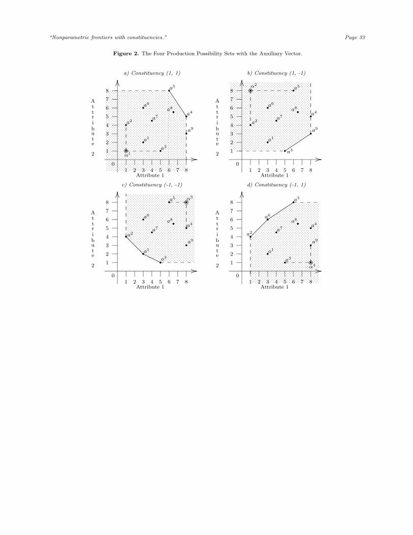
“Nonparametric frontiers with constituencies.” Page 33
Figure 2. The Four Production Possibility Sets with the Auxiliary Vector.
1 2 3 4 5 6 7 8
1
2
3
4
5
6
7
8
Attribute
2
0
Attribute 1
a) Constituency (1, 1)
..............................
.......................
.............................. .......................
•a1
•a2
•a3
•a4
•a5
•a6
•a7
•a8
•a9
...............................................................................................................................................................................................................
.
.
.
.
.
.
.
.
.
.
.
.
.
.
.
.
.
.
.
.
.
.
.
.
.
.
.
.
.
.
.
.
.
.
.
.
.
.
.
.
.
.
.
.
.
.
.
.
.
.
.
.
.
.
.
.
.
.
.
.
.
.
.
.
.
.
.
.
.
.
.
.
.
.
.
.
.
.
.
.
.
.
.
.
.
.
.
.
.
.
.
.
.
.
.
.
.
.
.
.
.
.
.
.
.
.
.
.
.
.
.
.
.
.
.
.
.
.
.
.
.
.
.
.
.
.
.
.
.
.
.
.
.
.
.
.
.
.
.
.
.
.
.
.
.
.
.
.
.
.
.
.
.
.
.
.
.
.
.
.
.
.
.
.
.
.
.
.
.
.
.
.
.
.
.
.
.
.
.
.
.
.
.
.
.
.
.
.
.
.
.
.
.
.
.
.
.
.
.
.
.
.
.
.
.
.
.
.
.
.
.
.
.
.
.
.
.
.
.
.
.
.
.
.
.
.
.
.
.
.
.
.
.
.
.
.
.
.
.
.
.
.
.
.
.
.
.
.
.
.
.
.
.
.
.
.
.
.
.
.
.
.
.
.
.
.
.
.
.
.
.
.
.
.
.
.
.
.
.
.
.
.
.
.
.
.
.
.
.
.
.
.
.
.
.
.
.
.
.
.
.
.
.
.
.
.
.
.
.
.
.
.
.
.
.
.
.
.
.
.
.
.
.
.
.
.
.
.
.
.
.
.
.
.
.
.
.
.
.
.
.
.
.
.
.
.
.
.
.
.
.
.
.
.
.
.
.
.
.
.
.
.
.
.
.
.
.
.
.
.
.
.
.
.
.
.
.
.
.
.
.
.
.
.
.
.
.
.
.
.
.
.
.
.
.
.
.
.
.
.
.
.
.
.
.
.
.
.
.
.
.
.
.
.
.
.
.
.
.
.
.
.
.
.
.
.
.
.
.
.
.
.
.
.
.
.
.
.
.
.
.
.
.
.
.
.
.
.
.
.
.
.
.
.
.
.
.
.
.
.
.
.
.
.
.
.
.
.
.
.
.
.
.
.
.
.
.
.
.
.
.
.
.
.
.
.
.
.
.
.
.
.
.
.
.
.
.
.
.
.
.
.
.
.
.
.
.
.
.
.
.
.
.
.
.
.
.
.
.
.
.
.
.
.
.
.
.
.
.
.
.
.
.
.
.
.
.
.
.
.
.
.
.
.
.
.
.
.
.
.
.
.
.
.
.
.
.
.
.
.
.
.
.
.
.
.
.
.
.
.
.
.
.
.
.
.
.
.
.
.
.
.
.
.
.
.
.
.
.
.
.
.
.
.
.
.
.
.
.
.
.
.
.
.
.
.
.
.
.
.
.
.
.
.
.
.
.
.
.
.
.
.
.
.
.
.
.
.
.
.
.
.
.
.
.
.
.
.
.
.
.
.
.
.
.
.
.
.
.
.
.
.
.
.
.
.
.
.
.
.
.
.
.
.
.
.
.
.
.
.
.
.
.
.
.
.
.
.
.
.
.
.
.
.
.
.
.
.
.
.
.
.
.
.
.
.
.
.
.
.
.
.
.
.
.
.
.
.
.
.
.
.
.
.
.
.
.
.
.
.
.
.
.
.
.
.
.
.
.
.
.
.
.
.
.
.
.
.
.
.
.
.
.
.
.
.
.
.
.
.
.
.
.
.
.
.
.
.
.
.
.
.
.
.
.
.
.
.
.
.
.
.
.
.
.
.
.
.
.
.
.
.
.
.
.
.
.
.
.
.
.
.
.
.
.
.
.
.
.
.
.
.
.
.
.
.
.
.
.
.
.
.
.
.
.
.
.
.
.
.
.
.
.
.
.
.
.
.
.
.
.
.
.
.
.
.
.
.
.
.
.
.
.
.
.
.
.
.
.
.
.
.
.
.
.
.
.
.
.
.
.
.
.
.
.
.
.
.
.
.
.
.
.
.
.
.
.
.
.
.
.
.
.
.
.
.
.
.
.
.
.
.
.
.
.
.
.
.
.
.
.
.
.
.
.
.
.
.
.
.
.
.
.
.
.
.
.
.
.
.
.
.
.
.
.
.
.
.
.
.
.
.
.
.
.
.
.
.
.
.
.
.
.
.
.
.
.
.
.
.
.
.
.
.
.
.
.
.
.
.
.
.
.
.
.
.
.
.
.
.
.
.
.
.
.
.
.
.
.
.
.
.
.
.
.
.
.
.
.
.
.
.
.
.
.
.
.
.
.
.
.
.
.
.
.
.
.
.
.
.
.
.
.
.
.
.
.
.
.
.
.
.
.
.
.
.
.
.
.
.
.
.
.
.
.
.
.
.
.
.
.
.
.
.
.
.
.
.
.
.
.
.
.
.
.
.
.
.
.
.
.
.
.
.
.
.
.
.
.
.
.
.
.
.
.
.
.
.
.
.
.
.
.
.
.
.
.
.
.
.
.
.
.
.
.
.
.
.
.
.
.
.
.
.
.
.
.
.
.
.
.
.
.
.
.
.
.
.
.
.
.
.
.
.
.
.
.
.
.
.
.
.
.
.
.
.
.
.
.
.
.
.
.
.
.
.
.
.
.
.
.
.
.
.
.
.
.
.
.
.
.
.
.
.
.
.
.
.
.
.
.
.
.
.
.
.
.
.
.
.
.
.
.
.
.
.
.
.
.
.
.
.
.
.
.
.
.
.
.
.
.
.
.
.
.
.
.
.
.
.
.
.
.
.
.
.
.
.
.
.
.
.
.
.
.
.
.
.
.
.
.
.
.
.
.
.
.
.
.
.
.
.
.
.
.
.
.
.
.
.
.
.
.
.
.
.
.
.
.
.
.
.
.
.
.
.
.
.
.
.
.
.
.
.
.
.
.
.
.
.
.
.
.
.
.
.
.
.
.
.
.
.
.
.
.
.
.
.
.
.
.
.
.
.
.
.
.
.
.
.
.
.
.
.
.
.
.
.
.
.
.
.
.
.
.
.
.
.
.
.
.
.
.
.
.
.
.
.
.
.
.
.
.
.
.
.
.
.
.
.
.
.
.
.
.
.
.
.
.
.
.
.
.
.
.
.
.
.
.
.
.
.
.
.
.
.
.
.
.
.
.
.
.
.
.
.
.
.
.
.
.
.
.
.
.
.
.
.
.
.
.
.
.
.
.
.
.
.
.
.
.
.
.
.
.
.
.
.
.
.
.
.
.
.
.
.
.
.
.
.
.
.
.
.
.
.
.
.
.
.
.
.
.
.
.
.
.
.
.
.
.
.
.
.
.
.
.
.
.
.
.
.
.
.
.
.
.
.
.
.
.
.
.
.
.
.
.
.
.
.
.
.
.
.
.
.
.
.
.
.
.
.
.
.
.
.
.
.
.
.
.
.
.
.
.
.
.
.
.
.
.
.
.
.
.
.
.
.
.
.
.
.
.
.
.
.
.
.
.
.
.
.
.
.
.
.
.
.
.
.
.
.
.
.
.
.
.
.
.
.
.
.
.
.
.
.
.
.
.
.
.
.
.
.
.
.
.
.
.
.
.
.
.
.
.
.
.
.
.
.
.
.
.
.
.
.
.
.
.
.
.
.
.
.
.
.
.
.
.
.
.
.
.
.
.
.
.
.
.
.
.
.
.
.
.
.
.
.
.
.
.
.
.
.
.
.
.
.
.
.
.
.
.
.
.
.
.
.
.
.
.
.
.
.
.
.
.
.
.
.
.
.
.
.
.
.
.
.
.
.
.
.
.
.
.
.
.
.
.
.
.
.
.
.
.
.
.
.
.
.
.
.
.
.
.
.
.
.
.
.
.
.
.
.
.
.
.
.
.
.
.
.
.
.
.
.
.
.
.
.
.
.
.
.
.
.
.
.
.
.
.
.
.
.
.
.
.
.
.
.
.
.
.
.
.
.
.
.
.
.
.
.
.
.
.
.
.
.
.
.
.
.
.
.
.
.
.
.
.
.
.
.
.
.
.
.
.
.
.
.
.
.
.
.
.
.
.
.
.
.
.
.
.
.
.
.
.
.
.
.
.
.
.
.
.
.
.
.
.
.
.
.
.
.
.
.
.
.
.
.
.
.
.
.
.
.
.
.
.
.
.
.
.
.
.
.
.
.
.
.
.
.
.
.
.
.
.
.
.
.
.
.
.
.
.
.
.
.
.
.
.
.
.
.
.
.
.
.
.
.
.
.
.
.
.
.
.
.
.
.
.
.
.
.
.
.
.
.
.
.
.
.
.
.
.
.
.
.
.
.
.
.
.
.
.
.
.
.
.
.
.
.
.
.
.
.
.
.
.
.
.
.
.
.
.
.
.
.
.
.
.
.
.
.
.
.
.
.
.
.
.
.
.
.
.
.
.
.
.
.
.
.
.
.
.
.
.
.
.
.
.
.
.
.
.
.
.
.
.
.
.
.
.
.
.
.
.
.
.
.
.
.
.
.
.
.
.
.
.
.
.
.
.
.
.
.
.
.
.
.
.
.
.
.
.
.
.
.
.
.
.
.
.
.
.
.
.
.
.
.
.
.
.
.
.
.
.
.
.
.
.
.
.
.
.
.
.
.
.
.
.
.
.
.
.
.
.
.
.
.
.
.
.
.
.
.
.
.
.
.
.
.
.
.
.
.
.
.
.
.
.
.
.
.
.
.
.
.
.
.
.
.
.
.
.
.
.
.
.
.
.
.
.
.
.
.
.
.
.
.
.
.
.
.
.
.
.
.
.
.
.
.
.
.
.
.
.
.
.
.
.
.
.
.
.
.
.
.
.
.
.
.
.
.
.
.
.
.
.
.
.
•.........................................
α1....................................................
1 2 3 4 5 6 7 8
1
2
3
4
5
6
7
8
Attribute
2
0
Attribute 1
b) Constituency (1, -1)
..............................
.......................
.............................. .......................
•a1
•a2
• a3
•a4
•a5
•a6
•a7
•a8
•a9
............................................................................................................................................................................................................................
.
.
.
.
.
.
.
.
.
.
.
.
.
.
.
.
.
.
.
.
.
.
.
.
.
.
.
.
.
.
.
.
.
.
.
.
.
.
.
.
.
.
.
.
.
.
.
.
.
.
.
.
.
.
.
.
.
.
.
.
.
.
.
.
.
.
.
.
.
.
.
.
.
.
.
.
.
.
.
.
.
.
.
.
.
.
.
.
.
.
.
.
.
.
.
.
.
.
.
.
.
.
.
.
.
.
.
.
.
.
.
.
.
.
.
.
.
.
.
.
.
.
.
.
.
.
.
.
.
.
.
.
.
.
.
.
.
.
.
.
.
.
.
.
.
.
.
.
.
.
.
.
.
.
.
.
.
.
.
.
.
.
.
.
.
.
.
.
.
.
.
.
.
.
.
.
.
.
.
.
.
.
.
.
.
.
.
.
.
.
.
.
.
.
.
.
.
.
.
.
.
.
.
.
.
.
.
.
.
.
.
.
.
.
.
.
.
.
.
.
.
.
.
.
.
.
.
.
.
.
.
.
.
.
.
.
.
.
.
.
.
.
.
.
.
.
.
.
.
.
.
.
.
.
.
.
.
.
.
.
.
.
.
.
.
.
.
.
.
.
.
.
.
.
.
.
.
.
.
.
.
.
.
.
.
.
.
.
.
.
.
.
.
.
.
.
.
.
.
.
.
.
.
.
.
.
.
.
.
.
.
.
.
.
.
.
.
.
.
.
.
.
.
.
.
.
.
.
.
.
.
.
.
.
.
.
.
.
.
.
.
.
.
.
.
.
.
.
.
.
.
.
.
.
.
.
.
.
.
.
.
.
.
.
.
.
.
.
.
.
.
.
.
.
.
.
.
.
.
.
.
.
.
.
.
.
.
.
.
.
.
.
.
.
.
.
.
.
.
.
.
.
.
.
.
.
.
.
.
.
.
.
.
.
.
.
.
.
.
.
.
.
.
.
.
.
.
.
.
.
.
.
.
.
.
.
.
.
.
.
.
.
.
.
.
.
.
.
.
.
.
.
.
.
.
.
.
.
.
.
.
.
.
.
.
.
.
.
.
.
.
.
.
.
.
.
.
.
.
.
.
.
.
.
.
.
.
.
.
.
.
.
.
.
.
.
.
.
.
.
.
.
.
.
.
.
.
.
.
.
.
.
.
.
.
.
.
.
.
.
.
.
.
.
.
.
.
.
.
.
.
.
.
.
.
.
.
.
.
.
.
.
.
.
.
.
.
.
.
.
.
.
.
.
.
.
.
.
.
.
.
.
.
.
.
.
.
.
.
.
.
.
.
.
.
.
.
.
.
.
.
.
.
.
.
.
.
.
.
.
.
.
.
.
.
.
.
.
.
.
.
.
.
.
.
.
.
.
.
.
.
.
.
.
.
.
.
.
.
.
.
.
.
.
.
.
.
.
.
.
.
.
.
.
.
.
.
.
.
.
.
.
.
.
.
.
.
.
.
.
.
.
.
.
.
.
.
.
.
.
.
.
.
.
.
.
.
.
.
.
.
.
.
.
.
.
.
.
.
.
.
.
.
.
.
.
.
.
.
.
.
.
.
.
.
.
.
.
.
.
.
.
.
.
.
.
.
.
.
.
.
.
.
.
.
.
.
.
.
.
.
.
.
.
.
.
.
.
.
.
.
.
.
.
.
.
.
.
.
.
.
.
.
.
.
.
.
.
.
.
.
.
.
.
.
.
.
.
.
.
.
.
.
.
.
.
.
.
.
.
.
.
.
.
.
.
.
.
.
.
.
.
.
.
.
.
.
.
.
.
.
.
.
.
.
.
.
.
.
.
.
.
.
.
.
.
.
.
.
.
.
.
.
.
.
.
.
.
.
.
.
.
.
.
.
.
.
.
.
.
.
.
.
.
.
.
.
.
.
.
.
.
.
.
.
.
.
.
.
.
.
.
.
.
.
.
.
.
.
.
.
.
.
.
.
.
.
.
.
.
.
.
.
.
.
.
.
.
.
.
.
.
.
.
.
.
.
.
.
.
.
.
.
.
.
.
.
.
.
.
.
.
.
.
.
.
.
.
.
.
.
.
.
.
.
.
.
.
.
.
.
.
.
.
.
.
.
.
.
.
.
.
.
.
.
.
.
.
.
.
.
.
.
.
.
.
.
.
.
.
.
.
.
.
.
.
.
.
.
.
.
.
.
.
.
.
.
.
.
.
.
.
.
.
.
.
.
.
.
.
.
.
.
.
.
.
.
.
.
.
.
.
.
.
.
.
.
.
.
.
.
.
.
.
.
.
.
.
.
.
.
.
.
.
.
.
.
.
.
.
.
.
.
.
.
.
.
.
.
.
.
.
.
.
.
.
.
.
.
.
.
.
.
.
.
.
.
.
.
.
.
.
.
.
.
.
.
.
.
.
.
.
.
.
.
.
.
.
.
.
.
.
.
.
.
.
.
.
.
.
.
.
.
.
.
.
.
.
.
.
.
.
.
.
.
.
.
.
.
.
.
.
.
.
.
.
.
.
.
.
.
.
.
.
.
.
.
.
.
.
.
.
.
.
.
.
.
.
.
.
.
.
.
.
.
.
.
.
.
.
.
.
.
.
.
.
.
.
.
.
.
.
.
.
.
.
.
.
.
.
.
.
.
.
.
.
.
.
.
.
.
.
.
.
.
.
.
.
.
.
.
.
.
.
.
.
.
.
.
.
.
.
.
.
.
.
.
.
.
.
.
.
.
.
.
.
.
.
.
.
.
.
.
.
.
.
.
.
.
.
.
.
.
.
.
.
.
.
.
.
.
.
.
.
.
.
.
.
.
.
.
.
.
.
.
.
.
.
.
.
.
.
.
.
.
.
.
.
.
.
.
.
.
.
.
.
.
.
.
.
.
.
.
.
.
.
.
.
.
.
.
.
.
.
.
.
.
.
.
.
.
.
.
.
.
.
.
.
.
.
.
.
.
.
.
.
.
.
.
.
.
.
.
.
.
.
.
.
.
.
.
.
.
.
.
.
.
.
.
.
.
.
.
.
.
.
.
.
.
.
.
.
.
.
.
.
.
.
.
.
.
.
.
.
.
.
.
.
.
.
.
.
.
.
.
.
.
.
.
.
.
.
.
.
.
.
.
.
.
.
.
.
.
.
.
.
.
.
.
.
.
.
.
.
.
.
.
.
.
.
.
.
.
.
.
.
.
.
.
.
.
.
.
.
.
.
.
.
.
.
.
.
.
.
.
.
.
.
.
.
.
.
.
.
.
.
.
.
.
.
.
.
.
.
.
.
.
.
.
.
.
.
.
.
.
.
.
.
.
.
.
.
.
.
.
.
.
.
.
.
.
.
.
.
.
.
.
.
.
.
.
.
.
.
.
.
.
.
.
.
.
.
.
.
.
.
.
.
.
.
.
.
.
.
.
.
.
.
.
.
.
.
.
.
.
.
.
.
.
.
.
.
.
.
.
.
.
.
.
.
.
.
.
.
.
.
.
.
.
.
.
.
.
.
.
.
.
.
.
.
.
.
.
.
.
.
.
.
.
.
.
.
.
.
.
.
.
.
.
.
.
.
.
.
.
.
.
.
.
.
.
.
.
.
.
.
.
.
.
.
.
.
.
.
.
.
.
.
.
.
.
.
.
.
.
.
.
.
.
.
.
.
.
.
.
.
.
.
.
.
.
.
.
.
.
.
.
.
.
.
.
.
.
.
.
.
.
.
.
.
.
.
.
.
.
.
.
.
.
.
.
.
.
.
.
.
.
.
.
.
.
.
.
.
.
.
.
.
.
.
.
.
.
.
.
.
.
.
.
.
.
.
.
.
.
.
.
.
.
.
.
.
.
.
.
.
.
.
.
.
.
.
.
.
.
.
.
.
.
.
.
.
.
.
.
.
.
.
.
.
.
.
.
.
.
.
.
.
.
.
.
.
.
.
.
.
.
.
.
.
.
.
.
.
.
.
.
.
.
.
.
.
.
.
.
.
.
.
.
.
.
.
.
.
.
.
.
.
.
.
.
.
•.........................................α2.....................................................................
1 2 3 4 5 6 7 8
1
2
3
4
5
6
7
8
Attribute
2
0
Attribute 1
c) Constituency (-1, -1)
..............................
.......................
.............................. .......................
•a1
•a2
•a3
•a4
•a5
•a6
•a7
•a8
•a9
...................................................................................................................................................................
........
.....
........
.....
........
.....
........
.....
........
.....
........
.....
........
...
.
.
.
.
.
.
.
.
.
.
.
.
.
.
.
.
.
.
.
.
.
.
.
.
.
.
.
.
.
.
.
.
.
.
.
.
.
.
.
.
.
.
.
.
.
.
.
.
.
.
.
.
.
.
.
.
.
.
.
.
.
.
.
.
.
.
.
.
.
.
.
.
.
.
.
.
.
.
.
.
.
.
.
.
.
.
.
.
.
.
.
.
.
.
.
.
.
.
.
.
.
.
.
.
.
.
.
.
.
.
.
.
.
.
.
.
.
.
.
.
.
.
.
.
.
.
.
.
.
.
.
.
.
.
.
.
.
.
.
.
.
.
.
.
.
.
.
.
.
.
.
.
.
.
.
.
.
.
.
.
.
.
.
.
.
.
.
.
.
.
.
.
.
.
.
.
.
.
.
.
.
.
.
.
.
.
.
.
.
.
.
.
.
.
.
.
.
.
.
.
.
.
.
.
.
.
.
.
.
.
.
.
.
.
.
.
.
.
.
.
.
.
.
.
.
.
.
.
.
.
.
.
.
.
.
.
.
.
.
.
.
.
.
.
.
.
.
.
.
.
.
.
.
.
.
.
.
.
.
.
.
.
.
.
.
.
.
.
.
.
.
.
.
.
.
.
.
.
.
.
.
.
.
.
.
.
.
.
.
.
.
.
.
.
.
.
.
.
.
.
.
.
.
.
.
.
.
.
.
.
.
.
.
.
.
.
.
.
.
.
.
.
.
.
.
.
.
.
.
.
.
.
.
.
.
.
.
.
.
.
.
.
.
.
.
.
.
.
.
.
.
.
.
.
.
.
.
.
.
.
.
.
.
.
.
.
.
.
.
.
.
.
.
.
.
.
.
.
.
.
.
.
.
.
.
.
.
.
.
.
.
.
.
.
.
.
.
.
.
.
.
.
.
.
.
.
.
.
.
.
.
.
.
.
.
.
.
.
.
.
.
.
.
.
.
.
.
.
.
.
.
.
.
.
.
.
.
.
.
.
.
.
.
.
.
.
.
.
.
.
.
.
.
.
.
.
.
.
.
.
.
.
.
.
.
.
.
.
.
.
.
.
.
.
.
.
.
.
.
.
.
.
.
.
.
.
.
.
.
.
.
.
.
.
.
.
.
.
.
.
.
.
.
.
.
.
.
.
.
.
.
.
.
.
.
.
.
.
.
.
.
.
.
.
.
.
.
.
.
.
.
.
.
.
.
.
.
.
.
.
.
.
.
.
.
.
.
.
.
.
.
.
.
.
.
.
.
.
.
.
.
.
.
.
.
.
.
.
.
.
.
.
.
.
.
.
.
.
.
.
.
.
.
.
.
.
.
.
.
.
.
.
.
.
.
.
.
.
.
.
.
.
.
.
.
.
.
.
.
.
.
.
.
.
.
.
.
.
.
.
.
.
.
.
.
.
.
.
.
.
.
.
.
.
.
.
.
.
.
.
.
.
.
.
.
.
.
.
.
.
.
.
.
.
.
.
.
.
.
.
.
.
.
.
.
.
.
.
.
.
.
.
.
.
.
.
.
.
.
.
.
.
.
.
.
.
.
.
.
.
.
.
.
.
.
.
.
.
.
.
.
.
.
.
.
.
.
.
.
.
.
.
.
.
.
.
.
.
.
.
.
.
.
.
.
.
.
.
.
.
.
.
.
.
.
.
.
.
.
.
.
.
.
.
.
.
.
.
.
.
.
.
.
.
.
.
.
.
.
.
.
.
.
.
.
.
.
.
.
.
.
.
.
.
.
.
.
.
.
.
.
.
.
.
.
.
.
.
.
.
.
.
.
.
.
.
.
.
.
.
.
.
.
.
.
.
.
.
.
.
.
.
.
.
.
.
.
.
.
.
.
.
.
.
.
.
.
.
.
.
.
.
.
.
.
.
.
.
.
.
.
.
.
.
.
.
.
.
.
.
.
.
.
.
.
.
.
.
.
.
.
.
.
.
.
.
.
.
.
.
.
.
.
.
.
.
.
.
.
.
.
.
.
.
.
.
.
.
.
.
.
.
.
.
.
.
.
.
.
.
.
.
.
.
.
.
.
.
.
.
.
.
.
.
.
.
.
.
.
.
.
.
.
.
.
.
.
.
.
.
.
.
.
.
.
.
.
.
.
.
.
.
.
.
.
.
.
.
.
.
.
.
.
.
.
.
.
.
.
.
.
.
.
.
.
.
.
.
.
.
.
.
.
.
.
.
.
.
.
.
.
.
.
.
.
.
.
.
.
.
.
.
.
.
.
.
.
.
.
.
.
.
.
.
.
.
.
.
.
.
.
.
.
.
.
.
.
.
.
.
.
.
.
.
.
.
.
.
.
.
.
.
.
.
.
.
.
.
.
.
.
.
.
.
.
.
.
.
.
.
.
.
.
.
.
.
.
.
.
.
.
.
.
.
.
.
.
.
.
.
.
.
.
.
.
.
.
.
.
.
.
.
.
.
.
.
.
.
.
.
.
.
.
.
.
.
.
.
.
.
.
.
.
.
.
.
.
.
.
.
.
.
.
.
.
.
.
.
.
.
.
.
.
.
.
.
.
.
.
.
.
.
.
.
.
.
.
.
.
.
.
.
.
.
.
.
.
.
.
.
.
.
.
.
.
.
.
.
.
.
.
.
.
.
.
.
.
.
.
.
.
.
.
.
.
.
.
.
.
.
.
.
.
.
.
.
.
.
.
.
.
.
.
.
.
.
.
.
.
.
.
.
.
.
.
.
.
.
.
.
.
.
.
.
.
.
.
.
.
.
.
.
.
.
.
.
.
.
.
.
.
.
.
.
.
.
.
.
.
.
.
.
.
.
.
.
.
.
.
.
.
.
.
.
.
.
.
.
.
.
.
.
.
.
.
.
.
.
.
.
.
.
.
.
.
.
.
.
.
.
.
.
.
.
.
.
.
.
.
.
.
.
.
.
.
.
.
.
.
.
.
.
.
.
.
.
.
.
.
.
.
.
.
.
.
.
.
.
.
.
.
.
.
.
.
.
.
.
.
.
.
.
.
.
.
.
.
.
.
.
.
.
.
.
.
.
.
.
.
.
.
.
.
.
.
.
.
.
.
.
.
.
.
.
.
.
.
.
.
.
.
.
.
.
.
.
.
.
.
.
.
.
.
.
.
.
.
.
.
.
.
.
.
.
.
.
.
.
.
.
.
.
.
.
.
.
.
.
.
.
.
.
.
.
.
.
.
.
.
.
.
.
.
.
.
.
.
.
.
.
.
.
.
.
.
.
.
.
.
.
.
.
.
.
.
.
.
.
.
.
.
.
.
.
.
.
.
.
•.........................................α3
........
.....
........
.....
........
.....
........
.....
1 2 3 4 5 6 7 8
1
2
3
4
5
6
7
8
Attribute
2
0
Attribute 1
d) Constituency (-1, 1)
..............................
.......................
.............................. .......................
•a1
•a2
•a3
•a4
•a5
•a6
•a7
•a8
•a9
...............................................................................................................................................................................................................
.............
.............
.............
.............
.............
.............
.
.
.
.
.
.
.
.
.
.
.
.
.
.
.
.
.
.
.
.
.
.
.
.
.
.
.
.
.
.
.
.
.
.
.
.
.
.
.
.
.
.
.
.
.
.
.
.
.
.
.
.
.
.
.
.
.
.
.
.
.
.
.
.
.
.
.
.
.
.
.
.
.
.
.
.
.
.
.
.
.
.
.
.
.
.
.
.
.
.
.
.
.
.
.
.
.
.
.
.
.
.
.
.
.
.
.
.
.
.
.
.
.
.
.
.
.
.
.
.
.
.
.
.
.
.
.
.
.
.
.
.
.
.
.
.
.
.
.
.
.
.
.
.
.
.
.
.
.
.
.
.
.
.
.
.
.
.
.
.
.
.
.
.
.
.
.
.
.
.
.
.
.
.
.
.
.
.
.
.
.
.
.
.
.
.
.
.
.
.
.
.
.
.
.
.
.
.
.
.
.
.
.
.
.
.
.
.
.
.
.
.
.
.
.
.
.
.
.
.
.
.
.
.
.
.
.
.
.
.
.
.
.
.
.
.
.
.
.
.
.
.
.
.
.
.
.
.
.
.
.
.
.
.
.
.
.
.
.
.
.
.
.
.
.
.
.
.
.
.
.
.
.
.
.
.
.
.
.
.
.
.
.
.
.
.
.
.
.
.
.
.
.
.
.
.
.
.
.
.
.
.
.
.
.
.
.
.
.
.
.
.
.
.
.
.
.
.
.
.
.
.
.
.
.
.
.
.
.
.
.
.
.
.
.
.
.
.
.
.
.
.
.
.
.
.
.
.
.
.
.
.
.
.
.
.
.
.
.
.
.
.
.
.
.
.
.
.
.
.
.
.
.
.
.
.
.
.
.
.
.
.
.
.
.
.
.
.
.
.
.
.
.
.
.
.
.
.
.
.
.
.
.
.
.
.
.
.
.
.
.
.
.
.
.
.
.
.
.
.
.
.
.
.
.
.
.
.
.
.
.
.
.
.
.
.
.
.
.
.
.
.
.
.
.
.
.
.
.
.
.
.
.
.
.
.
.
.
.
.
.
.
.
.
.
.
.
.
.
.
.
.
.
.
.
.
.
.
.
.
.
.
.
.
.
.
.
.
.
.
.
.
.
.
.
.
.
.
.
.
.
.
.
.
.
.
.
.
.
.
.
.
.
.
.
.
.
.
.
.
.
.
.
.
.
.
.
.
.
.
.
.
.
.
.
.
.
.
.
.
.
.
.
.
.
.
.
.
.
.
.
.
.
.
.
.
.
.
.
.
.
.
.
.
.
.
.
.
.
.
.
.
.
.
.
.
.
.
.
.
.
.
.
.
.
.
.
.
.
.
.
.
.
.
.
.
.
.
.
.
.
.
.
.
.
.
.
.
.
.
.
.
.
.
.
.
.
.
.
.
.
.
.
.
.
.
.
.
.
.
.
.
.
.
.
.
.
.
.
.
.
.
.
.
.
.
.
.
.
.
.
.
.
.
.
.
.
.
.
.
.
.
.
.
.
.
.
.
.
.
.
.
.
.
.
.
.
.
.
.
.
.
.
.
.
.
.
.
.
.
.
.
.
.
.
.
.
.
.
.
.
.
.
.
.
.
.
.
.
.
.
.
.
.
.
.
.
.
.
.
.
.
.
.
.
.
.
.
.
.
.
.
.
.
.
.
.
.
.
.
.
.
.
.
.
.
.
.
.
.
.
.
.
.
.
.
.
.
.
.
.
.
.
.
.
.
.
.
.
.
.
.
.
.
.
.
.
.
.
.
.
.
.
.
.
.
.
.
.
.
.
.
.
.
.
.
.
.
.
.
.
.
.
.
.
.
.
.
.
.
.
.
.
.
.
.
.
.
.
.
.
.
.
.
.
.
.
.
.
.
.
.
.
.
.
.
.
.
.
.
.
.
.
.
.
.
.
.
.
.
.
.
.
.
.
.
.
.
.
.
.
.
.
.
.
.
.
.
.
.
.
.
.
.
.
.
.
.
.
.
.
.
.
.
.
.
.
.
.
.
.
.
.
.
.
.
.
.
.
.
.
.
.
.
.
.
.
.
.
.
.
.
.
.
.
.
.
.
.
.
.
.
.
.
.
.
.
.
.
.
.
.
.
.
.
.
.
.
.
.
.
.
.
.
.
.
.
.
.
.
.
.
.
.
.
.
.
.
.
.
.
.
.
.
.
.
.
.
.
.
.
.
.
.
.
.
.
.
.
.
.
.
.
.
.
.
.
.
.
.
.
.
.
.
.
.
.
.
.
.
.
.
.
.
.
.
.
.
.
.
.
.
.
.
.
.
.
.
.
.
.
.
.
.
.
.
.
.
.
.
.
.
.
.
.
.
.
.
.
.
.
.
.
.
.
.
.
.
.
.
.
.
.
.
.
.
.
.
.
.
.
.
.
.
.
.
.
.
.
.
.
.
.
.
.
.
.
.
.
.
.
.
.
.
.
.
.
.
.
.
.
.
.
.
.
.
.
.
.
.
.
.
.
.
.
.
.
.
.
.
.
.
.
.
.
.
.
.
.
.
.
.
.
.
.
.
.
.
.
.
.
.
.
.
.
.
.
.
.
.
.
.
.
.
.
.
.
.
.
.
.
.
.
.
.
.
.
.
.
.
.
.
.
.
.
.
.
.
.
.
.
.
.
.
.
.
.
.
.
.
.
.
.
.
.
.
.
.
.
.
.
.
.
.
.
.
.
.
.
.
.
.
.
.
.
.
.
.
.
.
.
.
.
.
.
.
.
.
.
.
.
.
.
.
.
.
.
.
.
.
.
.
.
.
.
.
.
.
.
.
.
.
.
.
.
.
.
.
.
.
.
.
.
.
.
.
.
.
.
.
.
.
.
.
.
.
.
.
.
.
.
.
.
.
.
.
.
.
.
.
.
.
.
.
.
.
.
.
.
.
.
.
.
.
.
.
.
.
.
.
.
.
.
.
.
.
.
.
.
.
.
.
.
.
.
.
.
.
.
.
.
.
.
.
.
.
.
.
.
.
.
.
.
.
.
.
.
.
.
.
.
.
.
.
.
.
.
.
.
.
.
.
.
.
.
.
.
.
.
.
.
.
.
.
.
.
.
.
.
.
.
.
.
.
.
.
.
.
.
.
.
.
.
.
.
.
.
.
.
.
.
.
.
.
.
.
.
.
.
.
.
.
.
.
.
.
.
.
.
.
.
.
.
.
.
.
.
.
.
.
.
.
.
.
.
.
.
.
.
.
.
.
.
.
.
.
.
.
.
.
.
.
.
.
.
.
.
.
.
.
.
.
.
.
.
.
.
.
.
.
.
.
.
.
.
.
.
.
.
.
.
.
.
.
.
.
.
.
.
.
.
.
.
.
.
.
.
.
.
.
.
.
.
.
.
.
.
.
.
.
.
.
.
.
.
.
.
.
.
.
.
.
.
.
.
.
.
.
.
.
.
.
.
.
.
.
.
.
.
.
.
.
.
.
.
.
.
.
.
.
.
.
.
.
.
.
.
.
.
.
.
.
.
.
.
.
.
.
.
.
.
.
.
.
.
.
.
.
.
.
.
.
.
.
.
.
.
.
.
.
.
.
.
.
.
.
.
.
.
.
.
.
.
.
.
.
.
.
.
.
.
.
.
.
.
.
.
.
.
.
.
.
.
.
.
.
.
.
.
.
.
.
.
.
.
.
.
.
.
.
.
.
.
.
•.........................................
α4.......................................
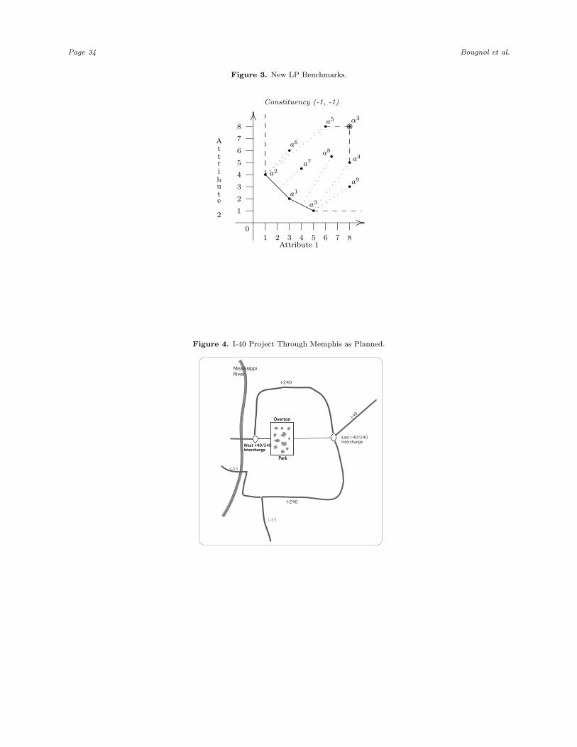
Page 34 Bougnol et al.
Figure 3. New LP Benchmarks.
1 2 3 4 5 6 7 8
1
2
3
4
5
6
7
8
Attribute
2
0
Attribute 1
Constituency (-1, -1)
..............................
.......................
.............................. .......................
•a1
• a2
•a3
• a4
•a5
•a6
•a7
•a8
•a9
...................................................................................................................................................................
........
.....
........
.....
........
.....
........
.....
........
.....
........
.....
........
...
•.........................................α3
........
.....
........
.....
........
.....
........
......
..
..
..
..
..
..
..
..
..
..
..
..
..........
..
..
..
..
..
..
.
..
..
..
..
..
..
.
..
..
..
.
Figure 4. I-40 Project Through Memphis as Planned.
Overton
Park
West I-40/240Interchange
MississippiRiver
I-240
I-240
Overton
Park
I-55
East I-40/240Interchange
West I-40/240Interchange
I-40
I-55
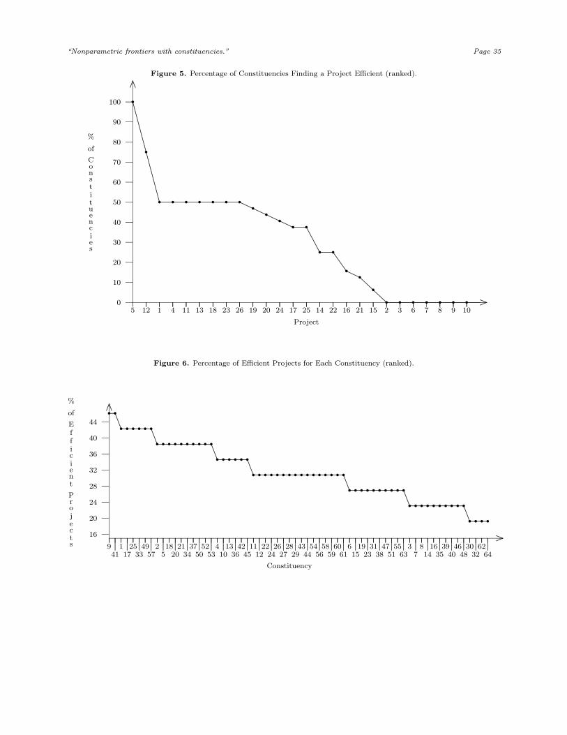
“Nonparametric frontiers with constituencies.” Page 35
Figure 5. Percentage of Constituencies Finding a Project Efficient (ranked).
0
10
20
30
40
50
60
70
80
90
100
%
of
Constituencies
.......................
....................
....................................... ....................
Project
5...........
12...........
1...........
4...........
11...........
13...........
18...........
23...........
26...........
19...........
20...........
24...........
17...........
25...........
14...........
22...........
16...........
21...........
15...........
2...........
3...........
6...........
7...
8...........
9...........
10...........
.............................................................................................................................................................................................................................................................................................................................................................................................................................................................................................................................................................................................................................................................................................................................................................................................................................................................................................................................................................................................................................................................................................................................................................................................................................................................................................................................
•
•
• • • • • • ••
••
• •
• •
••
•
• • • • • • •
Figure 6. Percentage of Efficient Projects for Each Constituency (ranked).
16
20
24
28
32
36
40
44
%
of
Efficient
Projects
..........................
....................
............................. ....................
Constituency
9...........
41.................................
1...........
17.................................
25...........
33.................................
49...........
57.................................
2...........
5.................................
18...........
20.................................
21...........
34.................................
37...........
50.................................
52...........
53.................................
4...........
10.................................
13...........
36.................................
42...........
45.................................
11...........
12.................................
22...........
24.................................
26...........
27.................................
28...........
29.................................
43...........
44.................................
54...........
56.................................
58...........
59.................................
60...........
61.................................
6...........
15.................................
19...........
23.................................
31...........
38.................................
47...........
51.................................
55...........
63.................................
3...........
7.................................
8...........
14.................................
16...........
35.................................
39...........
40.................................
46...........
48.................................
30...........
32.................................
62...........
64.................................
...................................................................................................................................................................................................................................................................................................................................................................................................................................................................................................................................................................................................................................................................................................................................................................................................................................................................................................................................................................................................................................................................................................................................................................................................................................................................................................................
• •
• • • • • •
• • • • • • • • • •
• • • • • •
• • • • • • • • • • • • • • • •
• • • • • • • • • •
• • • • • • • • • •
• • • •