comparison of roc methods for partially paired data

Comparison of ROC methods for partially-paired data

Brandon D. Gallasa and Lorenzo L. Pesceb

aFDA, Center for Devices and Radiological Health, 10903 New Hampshire Ave, Bldg. 62 Rm.3124, Silver Spring, MD, 20993-0002, USA;bUniversity of Chicago, Chicago, IL, USA

ABSTRACT

In this work we investigate ROC methods that compare the difference in AUCs (area under the ROC curve) fromtwo modalities given partially paired data. Such methods are needed to accommodate the real world situations,where every case cannot be imaged or interpreted using both modalities. We compare variance estimation ofthe bivariate binormal-model based method ROCKIT of Metz et al., as well as several different non-parametricmethods, including the bootstrap and U-statistics. This comparison explores different ROC curves, study designs(pairing structure of the data), sample sizes, case mix, and modality effect sizes.

KEY WORDS: Receiver Operating Characteristic (ROC), AUC, missing data, partially-paired data, ROCKIT,bootstrap

1. INTRODUCTION

The community of users of ROC methods is always looking for easy-to-use and validated software to analyzetheir experiments. It is well known that fully-paired designs give the most power per sample size in detectingdifferences in diagnostic performance between modalities. However, it is frequently impossible or impractical toobtain samples from the same cases for all the modalities that are being investigated. Therefore, data analystshave to resort to so-called partially-paired or missing-data schemes unless they are willing to ignore some of theirdata. In this paper we explore some of the methods to treat ROC data that is partially paired across modalitiesunder the missing at random (MAR) condition; i.e., the fact that a value is missing is unrelated to the missingvalue itself. This exploration does not include the multi-reader or location-dependent ROC experiments.

It is easy to see how, when data is partially paired across two modalities, the extent to the pairing can betreated by dividing the data into the six basic groups (Table 1). A popular method for comparing partially-pairedROC data is implemented in the software ROCKIT,1 which is a maximum likelihood solution to the bivariatebinormal-model of Metz et al.,2 separately adding the likelihoods of data in the six basic groups just mentioned.ROCKIT is popular because it is easy to use, validated and, perhaps most importantly, freely available for useon many different operating systems. The purpose of this work is to first expose readers to the nonparametricmethods in the literature:

• A bootstrap method for variance estimation3,4 that separately bootstraps within the six basic groups(Table 1).

• A U-statistic approach5,6 that introduces a design matrix. The elements of the design matrix are zeroor one, depending on whether a score was collected or not. Thus each case falls into one of the six basicgroups by this mechanism.

• The method of Zhou and Gatsonis,7 which is a generalization of the method of DeLong et al.8 that isbased on an asymptotic U-statistic result.5 Zhou and Gatsonis organize the data into the six basic groups(Table 1) and consider the covariances that interactions between these groups generate on AUC.

Further author information: (Send correspondence to B.D.G.)B.D.G.: E-mail: [email protected], Telephone: (301)796-2531

Medical Imaging 2009: Image Perception, Observer Performance, and Technology Assessment,edited by Berkman Sahiner, David J. Manning, Proc. of SPIE Vol. 7263, 72630V

© 2009 SPIE · CCC code: 1605-7422/09/$18 · doi: 10.1117/12.813688

Proc. of SPIE Vol. 7263 72630V-1

Six non-overlapping subsets of partially-paired ROC data1. normal cases read in modality m only, Nm

0 4. disease cases read in modality m only, Nm1

2. normal cases read in modality m′ only, Nm′0 5. disease cases read in modality m′ only, Nm′

1

3. normal cases read in both modalities, Nm&m′0 6. disease cases read in both modalities, Nm&m′

1

Table 1.

These methods have a lot of properties in common: 1) they are based solely on the ranks of the data, nottheir values; 2) they assume positive and negative cases affect the variance of the estimates separately, i.e., thecases are not lumped together, consistent with the fact that positive and negative cases come from two separatepopulations, constituting separate random effects; 3) they assume that data is missing at random;9 and 4) thereare other no restrictions concerning what data are missing and how much data is missing (apart from the factthat ROCKIT might not converge with very sparse data, and some nonparametric variance estimates might notbe positive).

These methods can be first divided into two groups: methods that make some assumptions about the pop-ulation from which the data is sampled (ROCKIT) and methods that make no assumptions about the data(nonparametric methods). Each method is briefly described below with little in the way of proofs due to spacelimitations.

Another purpose of this work is to characterize these nonparametric methods, and compare them to ROCKIT.We compare the different methods with a large set of Monte Carlo (MC) ROC simulation experiments based ona “contaminated” version of the binormal model.10 For each experiment, we simulate cases from two modalitiesm,m′ in the same way—i.e., the two modalities are assumed to be identical and therefore we are simulating thenull hypothesis of a comparison of AUC’s. The parameters we explore are the intrinsic separability of scoresμ, the correlation of scores ρ, the number of normal cases N0, the number of disease cases N1, the number ofcases missing in modality m′, and the amount of contamination Q. We summarize the results with the relativebias and variance of the performance and variance estimation methods. In addition to bias and variance, weanalyze what we consider to be the relevant factors in deciding what method to use: whether the software crashes(therefore providing no answer) and whether variance estimates are negative (the nonparametric methods canprovide negative estimates).

The final goal of this work is to provide easy-to-use and validated software for all the methods, as well as areference that would support and describe the software. This will give data analysts the possibility to choose amethod not based on availability or ease of use, but instead on suitability to a specific task. We will offer thesoftware on the University of Chicago website1 “Kurt Rossmann Laboratories for Radiologic Image Research.”While the work presented in this paper is a large step towards our goal, there is still some work to be done.In the conclusions, we will outline our plans to achieve this goal, as well as describe how to access some of thesoftware now.

2. METHODS

2.1. AUC

AUC is a common summary measure of the ROC curve that is equivalent to the reader’s sensitivity averagedover all specificities, as well as the probability that the score for a randomly selected disease case is larger thanthe score for a randomly selected normal case (this assumes that larger scores indicate disease). AUC is 1.0 forperfect performance and 0.5 for chance.

The empirical AUC estimates the population value based on the empirical ROC curve and has the simpleform

AUCm =N0∑

i=1

N1∑

j=1

smij

N0N1, (1)


where smij is the success outcome,

smij = s (tm1j − tm0i) =

⎧⎨

⎩

1 tm1j − tm0i > 0.5 tm1j − tm0i = 00 tm1j − tm0i < 0

, (2)

and the tm0i, tm1j are the scores from N0 normal cases and N1 disease cases from modality m. This estimate canbe thought of as the fraction of times a disease case is scored higher than a normal case.

The empirical AUC is the U-statistic estimate of Pr (tm1j > tm0i) , as well as a different normalization ofthe Mann-Whitney form of the Wilcoxon statistic. Its variance has been characterized in great detail.11–16

Additionally, the variance of the difference in AUCs generated from the same patients read in two differentmodalities has also been described.8,17 We like to express the (co)variance in terms of moments of the successoutcomes. That is

Cmm′ = E[(

Am − AUCm

)(Am′ − AUCm′

)]

=1

N0N1E [smijsm′ij ] +

N0 − 1N0N1

E [smijsm′i′j |case i �= case i′ ]

+N1 − 1N0N1

E [smijsm′ij′ |case j �= case j′ ] +[(N0 − 1) (N1 − 1)

N0N1− 1

]E

[smijsm′i′j′

∣∣∣∣case i �= case i′

case j �= case j′

]

define= c1M1mm′ + c2M2mm′ + c3M3mm′ + (c4 − 1) M4mm′ . (3)

To be clear this expression works for variances (m = m′) and covariances (m �= m′) .

We call the M ’s success moments. Please notice that we can relate these moments to the (co)variances usedby other authors as follows:

ξ10 = cov (smij , sm′i′j) = M2mm′ − M4mm′ , (4)ξ01 = cov (smij , sm′ij′) = M3mm′ − M4mm′ , (5)ξ11 = cov (smij , sm′ij) = M1mm′ − M4mm′ (6)

Cmm′ =(N0 − 1)N0N1

ξ10 +(N1 − 1)N0N1

ξ01 +1

N0N1ξ11. (7)

Also notice that, Eqs 3-7 are only appropriate for experiments where the cases are paired across the modalities.Each case must be read in both modalities.

2.2. Partial Pairing, or Missing DataWe have recently developed some notation and methodology to estimate the covariance for experiments wherethe cases are only partially-paired; some cases are read in one modality, some in the other, and some in both.6,18

Specifically, we defined a design matrix, the elements of which (dmij) are 0/1 indicators of whether a particularsuccess outcome (smij) was collected or not. Modality-specific performance is then simply

AUCm =

∑N0i=1

∑N1j=1 dmijsmij

∑N0i=1

∑N1j=1 dmij

, (8)

where the denominator equals the product of the number of normal cases read in modality m, Nm0 and the

number of disease cases read in modality m, Nm1 . If we condition on the design matrix, the impact on the

(co)variance is that the coefficients of the success moments are different:

Cmm′ |D =

∑N0i=1

∑N1j=1 dmijdm′ij

Nm0 Nm

1 Nm′0 Nm′

1

M1mm′ +

∑N0i=1

∑N1j=1 dmij

∑i′ �=i dm′i′j

Nm0 Nm

1 Nm′0 Nm′

1

M2mm′

+

∑N0i=1

∑N1j=1 dmij

∑j′ �=j dm′ij′

Nm0 Nm

1 Nm′0 Nm′

1

M3mm′ +

[∑N0i=1

∑N1j=1 dmij

∑i′ �=i

∑j′ �=j dm′i′j′

Nm0 Nm

1 Nm′0 Nm′

1

− 1

]M4mm′ (9)

= c1 |D M1mm′ + c2 |D M2mm′ + c3 |D M3mm′ +(c4 |D − 1

)M4mm′ . (10)

In what follows, we describe three nonparametric methods for estimating this (co)variance.


2.3. Bootstrap

The bootstrap makes use of the fact that the empirical distributions of normal and disease cases are, in fact, theML estimates of the true distributions of normal and disease cases. Bootstrapping, or sampling with replacement,is thus a Monte Carlo approach to estimating expected values under this assumption. In our method, one MonteCarlo bootstrap (MCBoot) separately samples with replacement from the six subsets of the data (Table 1),generating six bootstrap subsets of data. Given these, we calculate the AUCm and AUCm′ , and ΔAUC . TheMCBoot variance estimates are then the sample variances of AUCm and AUCm′ , and ΔAUC over multiplebootstraps.

For the Wilcoxon AUC and fully-paired data (dmij = 1 for all m, i, j), we can calculate the ideal bootstrapestimates of the success moments

MB1mm′ =1

∑N0i=1


N0∑

i=1

N1∑

j=1

dmijsmijdm′ijsm′ij , (11)

MB2mm′ =1

∑N0i=1

∑N1j=1

∑N0i′=1 dmijdm′i′j

N0∑

i=1

N1∑

j=1

N0∑

i′=1

dmijsmijdmi′jsm′i′j , (12)

MB3mm′ =1

∑N0i=1

∑N1j=1

∑N1j′=1 dmijdm′ij′

N0∑

i=1

N1∑

j=1

N1∑

j′=1

dmijsmijdm′ij′sm′ij′ , (13)

MB4mm′ =1

∑N0i=1

∑N1j=1

∑N0i′=1

∑N1j′=1 dmijdm′i′j′

N0∑

i=1

N1∑

j=1

N0∑

i′=1

N1∑

j′=1

dmijsmijdm′i′j′sm′i′j′ , (14)

and plug them into Eq. 9 to calculate (co)variances. This ideal bootstrap estimate of the (co)variance (I-Boot)makes use of the empirical distributions analytically, rather than with Monte Carlo sampling.19 The I-Bootestimate equals the limit of MCBoot as the number of bootstraps goes to infinity.

At the start of this work, we thought that the moments above would work for partially-paired data in thesame way that they work for fully-paired data. The simulation results showed us that this is not the case. Weare still working on the I-Boot estimator for the case of partially-paired data.

To understand the ideal bootstrap, consider M2mm′ . The expected value is an average over two normal casesand one disease case. As such, the ideal bootstrap sums over the entire discrete distribution of normal cases twiceand the entire discrete distribution of disease cases once. We can plainly see that MB2mm′ violates the M2mm′

condition that case i �= case i′. This makes the estimate biased. We investigate how biased in the simulationsbelow.

2.4. U-statistics

The “U” in U-statistics stands for unbiased. The U-statistic estimates of the success moments are very similarto those of the bootstrap:

MU1mm′ =1

∑N0i=1


N0∑

i=1

N1∑

j=1

dmijsmijdm′ijsm′ij , (15)

MU2mm′ =1

∑N0i=1

∑N1j=1

∑i′ �=i dmijdm′i′j

N0∑

i=1

N1∑

j=1

∑

i′ �=i

dmijsmijdm′i′jsm′i′j , (16)

MU3mm′ =1

∑N0i=1

∑N1j=1

∑j′ �=j dmijdm′ij′

N0∑

i=1

N1∑

j=1

∑

j′ �=j

dmijsmijdm′ij′sm′ij′ , (17)

MU4mm′ =1

∑N0i=1

∑N1j=1

∑i′ �=i

∑j′ �=j dmijdm′i′j′

N0∑

i=1

N1∑

j=1

∑

i′ �=i

∑

j′ �=j

dmijsmijdm′i′j′sm′i′j′ . (18)


Note the difference in the sums over the primed indexes. Specifically, they obey the conditions spelled out inthe expected values. For example, the U-statistic estimate for M2mm′ skips the term where case i = case i′,and normalizes the sum appropriately. As above, we plug the U-statistic estimates of the success moments intoEq. 9 to calculate (co)variances.

2.5. Zhou & Gatsonis

Zhou and Gatsonis7 were the first to have generalized the covariance expression to treat experiments where thecases are only partially-paired across the modalities. Our expression given in Eq. 9 is equivalent to theirs, whichutilizes the covariances (Eqs 4-6) rather than the success moments. They have also generalized the method ofDeLong et al.8 to estimate such a covariance, and we have derived how their estimate is related to the I-Bootand U-statistic estimates. Specifically, their estimates can be rewritten as

ξ10 =Nm&m′

1

Nm&m′1 − 1

[MB2m,m′ − AUC

∗m

AUCm′ − AUCmAUC

∗m′ + MB4mm′

], (19)

ξ01 =Nm&m′

0

Nm&m′0 − 1

[MB3m,m′ − AUC

∗m

AUCm′ − AUCmAUC

∗m′ + MB4mm′

], (20)

Cmm′ =Nm&m′

1

Nm1 Nm′

1

ξ01 +Nm&m′

0

Nm0 Nm′

0

ξ01. (21)

Note that in the expression for ξ10, AUC∗m uses all the normal cases scored by modality m, but only the disease

cases that were scored in both modalities. In the expression for ξ01, AUC∗m uses all the disease cases scored by

modality m, but only the normal cases that were scored in both modalities.

In words, the Zhou and Gatsonis estimate essentially uses the bootstrap moments to estimate the U-statisticcovariances ξ10, ξ01. Consequently, these have a positive bias plus some extra variability from the terms A∗

m. Also,there is a coefficient in front of each covariance estimate that is the consequence of trying to make these estimatesunbiased. Unfortunately, this coefficient is not appropriate for the current multiple random effect problem. Theestimate then inserts these covariances into Eq. 7 and drops the higher order contributions,

− 1N0N1

ξ10 − 1N0N1

ξ01 +1

N0N1ξ11. (22)

The consequence of dropping the higher order terms injects a positive bias to the estimate.

While it may seem to be a bad idea to inject biases into the covariance estimate, there is a benefit. Thepositive biases are forcing the estimate to be positive.

2.6. ROCKIT

The ROCKIT model is based on an ordinal categorical sampling scheme that can be shown to be applicable toquasi-continuous data with little or no loss of efficiency.2 First the data will be divided in truth runs: cases willbe rank ordered for both modalities— each sequence of cases that are either positive, negative or tied will beassigned a rank. This step allows one to treat continuous data as categorical and to reduce categorical data tothe smallest number of categories.2 This step is possible because the only information relevant to ROC analysisis the ranks of the data and not their actual values.

Then the data are divided into the six groups given in Table 1 and a likelihood is defined for each. Thesesix likelihoods are functions of the parameters that define the probability distributions of the test-scores, whichare bivariate binormal distributions for this model. The probabilities associated with each pair of categories aredefined introducing cutoffs between them (nuisance parameters):


Simulation Parametersμ = 0.75, 1.50, 2.50 N0 = 25, 50, 100ρ = 0.10, 0.50, 0.90 N1 = N0,

12N0,

14N0

Q = 0.00, 0.10, 0.50 missing in m′ = 0.0, 0.1, 0.5

Table 2. Parameter values explored.

pii′ =∫ τmi

τmi−1

∫ τm′i′

τm′i′−1

N (tm0, tm′0 |0, 0, 1, 1, ρ0 ) dtm0dtm′0, (23)

qjj′ =∫ τmj

τmj−1

∫ τmj′

τm′j′−1

N

(tm1, tm′1

∣∣∣∣am

bm,am′

bm′,

1bm

,1

bm′, ρ1

)dtm1dtm′1. (24)

In the expressions above, am, bm and am′ , bm′ are the usual parameters of the conventional binormal ROCcurve20 (one set for each modality), following the convention that the marginal distributions for the negativecases are centered at zero and have variance one. The function N () is the bivariate binormal density, and ρ0, ρ1

are the correlations of normal and disease cases. Finally the tm0, tm′0 are the scores of normal cases, tA1, tB1

are the scores from disease cases, and τmi, τm′i are the cutoffs associated with category i for modality m andcategory j for modality m′.

Since the cases are sampled independently the likelihood function is simply the product of the likelihoods.The logarithm of the likelihood is maximized using Fisher Scoring.2,21

2.7. Simulation

We designed a large set of Monte Carlo (MC) ROC simulation experiments based on a “contaminated” versionof the binormal model.10 For each experiment, we simulate cases from two modalities m,m′ in the same way; wesimulate the null hypothesis of a comparison of AUC’s. The parameters we explore are the intrinsic separabilityof scores μ, the correlation of scores ρ, and the amount of contamination Q. We explain how these parametersdetermine the underlying ROC below. Additionally, we explore the number of normal cases N0, the number ofdisease cases N1 (as a fraction of the number of normals), and the number of cases missing in modality m′. Weexplore the different parameter values in a factorial fashion (Table 2).

The model generates the following scores:

normal case i modality m : tm0i = C0i + Zm0i, (25)normal case i modality m′ : tm′0i = C0i + Zm′0i, (26)disease case j modality m : tm1j = C1j + Zm1j + (1 − qj) μ, (27)disease case j modality m′ : tm′1j = C1j + Zm′1j + (1 − qj) μ. (28)

The scores are made up of two case effects (C0i, C1j) and four independent effects (Zm0i, Zm′0i, Zm1j , Zm′1j) .These effects are independent zero-mean Gaussian random variables with the variance of the case effects σ2

C

and the variance of the independent effects σ2Z . We constrain these variances to sum to one, causing μ to equal

detectability or SNR . Another consequence of this constraint is that correlation is given by ρ = σ2C/

(σ2

C + σ2Z

)=

σ2C . In other words, the case effects correlate the scores.

The qj is a binomial random variable (mean Q) that determines whether the disease case is “contaminated”(qj = 1) or not (qj = 0) . When a case is “contaminated”, the disease features are assumed not apparent, notseen, and the score essentially comes from the distribution of normal cases. This contamination increases thecorrelation of the scores of disease cases in the model. Specifically,

corr (tA1j , tB1j) =ρ + μ2Q (1 − Q)1 + μ2Q (1 − Q)

. (29)


ROC Curves for Simulation

Sensit

ivit

y =

TPF

1-Specificity = FPF

AUC in=0.96, Q=0.0, 0.1, 0.5

AUC in=0.86, Q=0.0, 0.1, 0.5

AUC in=0.70, Q=0.0, 0.1, 0.5

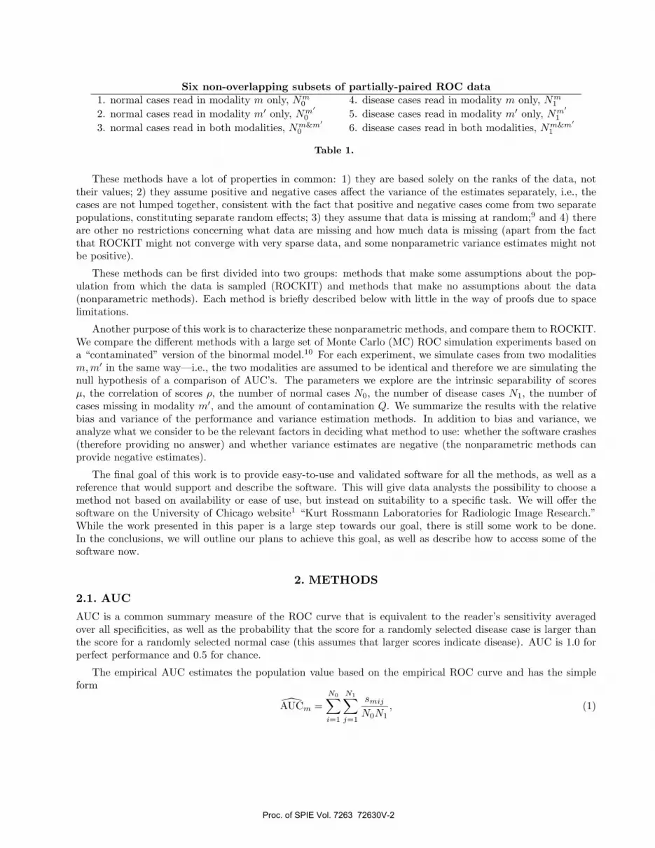
Figure 1. These are the ROC curves for the distributions used in the simulation.

AUC Q = 0.0 Q = 0.1 Q = 0.5μ = 0.75 0.702 0.681 0.601μ = 1.50 0.856 0.820 0.678μ = 2.50 0.961 0.914 0.731

Table 3. These are the ensemble AUC’s for the experiments, derived from the input SNR’s and the contaminationprobabilities.

When Q = 0, the AUC is known to be

AUCm = Pr (tm1j > tm0j) = Φ(μ/

√2)

, (30)

where Φ is the standard normal cumulative distribution function. When Q �= 0, then

AUCQm = Pr (tm1j > tm0i |tm1j ∼ H0 ) Pr (tm1j ∼ H0) + Pr (tm1j > tm0i |tm1j ∼ H1 ) Pr (tm1j ∼ H1) (31)

AUCQm = 0.5 × Q + AUCm × (1 − Q) . (32)

The contamination depresses and injects skew into the resulting ROC curve. Fig. 1 shows the impact of contam-ination on the ROC curves for the experiments we investigate. Table 3 shows the impact on AUC .

We have derived the variance of the Wilcoxon statistic for the contaminated binormal model being simulatedin this work. Therefore, we can use this analytic result to characterize the performance of the different Wilcoxonvariance estimation methods. We did not include these calculations in this paper to save space. They areavailable by request from the corresponding author.

3. RESULTS

3.1. Estimating AUC

As a U-statistic, the Wilcoxon estimate of AUC is unbiased by construction. While not shown to save space, ourresults verify this unbiasedness, validate the analytic expression for AUC, and validate the correct implementation


-0.2

-0.4

0.0

0.2

0.4Unbiased Complicated Bias

+ and -Positive Bias30% max

Relative Bias of

Variance Estimators

Diff in Modalities (A-B)

Simulation Configuration200 400 600

U-estimator Zhou & Gatsonis Bootstrap

ROCKIT




-0.5

-1

0

1

0.5

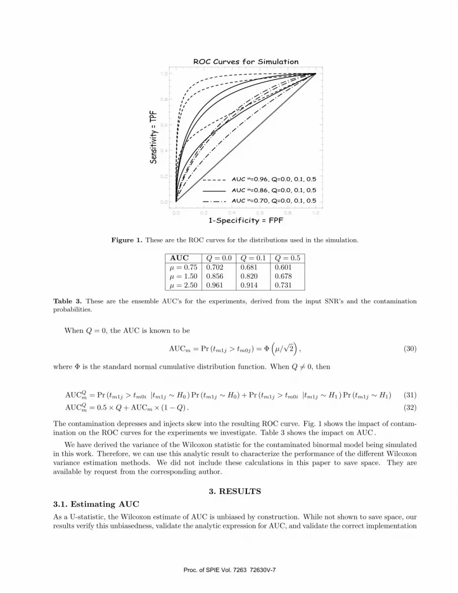
Figure 2. These plots show the bias of the variance estimators divided by the true variance.

of the simulation. We also saw that ROCKIT is biased, but the bias is small (less than .03 in AUC in all simulationconfigurations). Furthermore, this bias goes away with more samples.

In terms of variability, the Wilcoxon statistic was less variable than ROCKIT when there was more missingdata. In contrast, ROCKIT was less variable when data was more correlated and more skewed.

3.2. Estimating the variance of AUC

In the following, we present the bias and variance of the different variance estimators. For the nonparametricvariance estimators, we shall compare the variance estimates to the analytic expression of the Wilcoxon statistic(the “true” variance). For ROCKIT, we compare the variance estimates to the Monte Carlo variance of theROCKIT AUCs (MC variance is a substitute for the “true” variance).

3.2.1. Bias

In Fig.2 we plot the relative bias of the variance estimators:

relative bias = [E (variance estimate) − true variance] ÷ true variance. (33)

The plots show the relative bias estimating the variance of the difference in AUCs; the plots for the singlemodality are very similar. Please note that the x-axis is the simulation configuration, not a particular sample.In other words, each point in these plots corresponds to one combination of simulation parameters and 10,000MC trials.

The plot for the U-statistics variance estimator shows that that estimator is indeed unbiased. This result alsovalidates the analytic expressions for the Wilcoxon variance and confirms that the simulation is implemented asdescribed.


In the other plots we see that the other estimators are biased. As discussed above, the Zhou & Gatsonisestimator has a positive bias. This bias can be as much as 30%. The bootstrap is biased too, and the biasis quite complex. The bias is positive and negative depending on the simulation configuration: positive biaseshappen when the data is highly correlated and when the intrinsic separation is high. Finally, ROCKIT also hasa complex bias profile. For the most part, the bias is negative, with the bias spikes happening for the very smalldatasets. The positive biases seen in the plot occur when the intrinsic separation is high (the last third of thedata points).

3.2.2. Variance

We examine the variability of the variance estimators by comparing them to the variability of the U-statisticsvariance estimate. Specifically, in Fig. 3 we plot the ratio

variance of variance estimator ÷ variance of U-statistics variance estimator. (34)

We use the U-statistics variance estimator as the basis for comparison since it is know to be a uniformly minimumvariance unbiased estimator (UMVUE). However, as we see in the plots of Fig. 3, the biased estimators can havean advantage in terms of variability.

For the single modality, the Zhou and Gatsonis variance estimator is as efficient as the U-statistics varianceestimator. While the bootstrap variance estimator seems to be more efficient when there is missing data, andless efficient as the sample size grows.

Unlike the bias story, there is a big change between what happens estimating the variance of the singlemodality AUC and what happens for the difference in AUCs. For the difference in AUCs, the Zhou and Gatsonisvariance estimator is remarkably more efficient than the U-statistics estimator, and the bootstrap appears tomimic this favorable efficiency. At least for the Zhou and Gatsonis variance estimator, we have boiled thisincreased efficiency down to dropping the higher order term ξ11 in Eq. 7. The behavior of the bootstrap varianceestimator is not yet clear.

The behavior of the ROCKIT variance estimator is also not yet clear. One reason for this is that the varianceestimate is not an explicit equation but an iterative procedure (maximizing the likelihood). Nonetheless, theresults indicate that ROCKIT can be more efficient for estimating the variance of a single modality AUC. Forestimating the variance of the difference in AUCs, the efficiency profile is similar to that of Zhou and Gatsonisexcept when the intrinsic separability is high, where ROCKIT appears to be more variable.

Finally, if we were to examine the root mean squared error (RMSE) of the estimators, we’d find that thevariability of the variance estimators dominates the bias. Consequently, the analysis of RMSE would follow theanalysis of the variance.

3.2.3. Program Failures and Negative Variances

The bias and variance of the variance estimators overlooks two important characteristics of the methods: whetherthe software fails or whether the method returns a negative variance estimate. The bootstrap method is the onlymethod considered that does not suffer from either of these problems.

The ROCKIT software can fail if the iterative maximization method fails to converge or converges to adegenerate solution. However, the ROCKIT software cannot return negative variances.

Negative variances is a potential issue for the U-statistic and Zhou and Gatsonis variance estimators. Thesenonparametric methods did not return negative variances for the single modality. However, for the difference inmodalities, the methods can return negative variance estimates because the equation is adding and subtractingnoisy terms.

In Fig. 4 we plot the failure rate of the ROCKIT program (left plot) and the rate at which the U-statisticsestimator returns negative variances for the difference in modalities. In both cases, the rates increase with theintrinsic separation and decrease with the sample size.

The Zhou and Gatsonis method returned only eight negative variance estimates out of all 7,290,000 trials.This data is not shown. Also not shown was a 4% failure rate of ROCKIT that was observed on the FDA


As efficientas U-Statistics

0.1

1.0

10.0

Ratio of VariancesVar of Var(Estimator) ÷ Var of Var(U-estimator)

Single Modality (A)

50% data missing

Large sample sizes

Simulation Configuration200 400 600 200 400 600

Simulation Configuration

0.01

1.0

10.0

0.1

Increasing correlation, Increasing missing data

Zhou & Gatsonis Bootstrap


ROCKIT

ROCKIT

200 400 600Simulation Configuration


Difference in Modalities (A-B)




As efficientas U-Statistics

0.1

1.0

10.0


Single Modality (A)

50% data missing

Large sample sizes



0.01

1.0

10.0

0.1

Increasing correlation, Increasing missing data



ROCKIT

ROCKIT

200 400 600Simulation Configuration


Difference in Modalities (A-B)




Figure 3. These plots show the variability of the variance estimators relative to (divided by) the U-statistic varianceestimator.

machines, but not the University of Chicago machines. This failure rate was across all simulation configurationsand appears to be a memory problem. We were able to overcome these failures by running the exact same dataa second time. The failure did not occur in this second run.

4. CONCLUSION

At this stage in our project, we have analyzed the different methods across a very large set of simulations, espe-cially including very small experiments; the smallest is 12 normal and 3 disease cases read in both modality A&Band an additional 13 normal and 3 disease cases read in modality B. We first remark that the standard deviationof the variance estimates is larger than the bias. As such, statistical efficiency outweighs unbiasedness. In thislight, we found that the biased estimators (the methods of Zhou and Gatsonis, the bootstrap, and ROCKIT) ap-pear to have an advantage over the U-statistics variance estimator for the difference in modalities. Furthermorethe U-statistic variance estimator was susceptible to negative variances for the difference in modalities.

We were able to identify the source of the bias of the Zhou and Gatsonis variance estimator, as well as thesource of the variability and subsequent negative variance estimates of the U-statistic variance estimator. Withthis understanding, there is a variance estimator between them: one with less bias than that of Zhou and Gatsonisand less variability than that of the U-statistic variance estimator. We also plan on deriving the ideal bootstrapvariance estimate, the limit of an infinite number of MC bootstraps. This has been done for fully-paired data,19

but not partially-paired data. The insight of this derivation will help us understand the U-statistic estimator aswell.


ROCKIT failures

200 400 6000

20%

30%


10%

Negative estimatesU-statistic variance

estimator

200 400 6000

20%

30%


10%

Figure 4. In the plot on the left we plot the failure rate of the ROCKIT program. In the plot on the right we plot therate that the U-statistics variance estimator returns negative variances.

In addition to the future analysis mentioned above, we are in the process of rewriting ROCKIT. It willlikely be based on the proper ROC fitting procedure PROPROC, which has better numerical procedures and, inparticular, a more advanced and stable likelihood maximization algorithm.21 We expect to solve all the failuresand convergence issues found in this preliminary, as we did for PROPROC. Finally, we will explore the ideaof fitting the single modality ROC parameters first and then fitting the correlation parameter; the softwarecurrently fits all these parameters at the same time.

Finally, we intend to complete this project by writing supporting materials for the software: full descriptionsof the methods, general guidelines and minimum requirements (sample size) for the variance estimation andhypothesis testing, as well as sample data for users to see the needed data formats and experience running thesoftware.

All the software we used in this work is currently available by direct request on the University of Chicagoweb site: http://xray.bsd.uchicago.edu/krl/KRL ROC/software index.htm. It works on Mac OS X (currentlyonly 10.4), Linux, Windows and Solaris. Not all processors and operating system versions have been tested. Thelibraries are not final and further testing is necessary before they will be released freely.

The software is available as dynamically linked libraries (or loadable objects) and static ones for differentlanguages (C/++, Fortran, Java, to cite a few) and computation environments, such as R, IDL and SAS. We canprovide instruction on how to call those functions. Some models are also available as command line executables(Labroc4, Proproc2, ROCKIT). A GUI is in preparation that will have a common format for data input anddata output.

5. ACKNOWLEDGMENTS

We would like to thank Robert Nishikawa for sponsoring Brandon Gallas to work on the University of ChicagoScientific Image Recontstruction and Analysis Facility, C. Chan (cluster administrator) and the grants thatsupport this cluster and the time of Lorenzo Pesce: HHSN267200700039C (Charlies Metz PI) contract withNIH/NIAAA. We would also like to thank the FDA scientific cluster adminstrators for allowing Lorenzo Pesceto have a workspace there and assisting with installation of software.


REFERENCES1. “ROCKIT.” http://xray.bsd.uchicago.edu/krl/KRL ROC/software index.htm.2. Metz, C. E., Herman, B. A., and Roe, C. A., “Statistical comparison of two ROC curve estimates obtained

from partially-paired datasets,” Med Decis Making 18(1), 110–121 (1998).3. Efron, B., [The Jackknife, the Bootstrap and Other Resampling Plans ], Society for Industrial and Applied

Mathematics, Philadelphia, PA (1982).4. N. Gruszauskas, K. Drukker, M. Giger, C. Sennett, L. Pesce, “Performance of breast ultrasound computer-

aided diagnosis: Dependence on image selection,” Acad Radiol (accepted 2008).5. Randles, R. H. and Wolfe, D. A., [Introduction to the Theory of Nonparametric Statistics ], John Wiley and

Sons, New York (1979).6. Gallas, B. D. and Brown, D. G., “Reader studies for validation of CAD systems,” Neural Networks 21(2-3),

387–397 (2008).7. Zhou, X. H. and Gatsonis, C. A., “A simple method for comparing correlated ROC curves using incomplete

data,” Stat Med 15(15), 1687–1693 (1996).8. DeLong, E. R., Delong, D. M., and Clarke-Pearson, D. L., “Comparing the areas under two or more

correlated receiver operating characteristic curves: A nonparametric approach,” Biometrics 44, 837–845(1988).

9. Little, R. J. A. and Rubin, D. B., [Statistical Analysis with Missing Data ], Wiley, New York (1987).10. Dorfman, D. D. and Berbaum, K. S., “A contaminated binormal model for ROC data: Part II. a formal

model,” Acad Radiol 7(6), 427–437 (2000).11. Wilcoxon, F., “Individual comparisons by ranking methods,” Biometrics 1, 80–83 (1945).12. Mann, H. B. and Whitney, D. R., “On a test whether one of two random variables is stochastically larger

than the other,” Ann Math Statist 18, 50–60 (1947).13. Hoeffding, W., “A class of statistics with asymptotically normal distribution,” Ann Math Stat 19, 293–325

(1948).14. Sen, P. K., “On some convergence properties of u-statistics,” Calcutta Statistical Association Bulletin 10(37),

1–18 (1960).15. Bamber, D., “The area above the ordinal dominance graph and the area below the receiver operating

characteristic graph,” J Math Psych 12, 387–415 (1975).16. Hanley, J. A. and McNeil, B. J., “The meaning and use of the area under a receiver operating characteristic

(ROC) curve,” Radiology 143(1), 29–36 (1982).17. Hanley, J. A. and McNeil, B. J., “A method of comparing the areas under receiver operating characteristic

curves derived from the same cases,” Radiology 148(3), 839–843 (1983).18. Gallas, B. D., Pennello, G. A., and Myers, K. J., “Multi-reader multi-case variance analysis for binary data,”

J Opt Soc Am A 24(12) (2007).19. Bandos, A. I., Rockette, H. E., and Gur, D., “Exact bootstrap variances of the area under the ROC curve,”

Commun Stat A-Theor 36(13), 2443–2461 (2007).20. Pepe, M. S., [The Statistical Evaluation of Medical Tests for Classification and Prediction ], Oxford University

Press, UK (2003).21. Pesce, L. L. and Metz, C. E., “Reliable and computationally efficient maximum-likelihood estimation of

”proper” binormal ROC curves,” Acad Radiol 14, 814–829 (2007).


comparison of roc methods for partially paired data

Documents