arX

iv:h

ep-t

h/97

0307

5v1

11

Mar

199

7

UMDEPP 97-086CTP TAMU-14/97

hep-th/9703075February 1, 2008

New Couplings of Six-Dimensional Supergravity

Hitoshi NISHINO 1

Department of PhysicsUniversity of Maryland

College Park, 20742-4111, USA

and

Ergin SEZGIN 2

Department of Physics and AstronomyTexas A and M University

College Station, TX 77843-4242, USA

Abstract

We describe the couplings of six-dimensional supergravity, which contain a self-dualtensor multiplet, to n

Tanti-self-dual tensor matter multiplets, n

Vvector multiplets

and nH

hypermultiplets. The scalar fields of the tensor multiplets form a cosetSO(nT , 1)/SO(nT ), while the scalars in the hypermultiplets form quaternionic Kahlersymmetric spaces, the generic example being Sp(nH , 1)/Sp(nH )⊗Sp(1). The gaugingof the compact subgroup Sp(nH) × Sp(1) is also described. These results generalizeprevious ones in the literature on matter couplings of N = 1 supergravity in sixdimensions.

1 Research supported in part by NSF Grant PHY-93-41926 and DOE Grant DE-FG02-94ER408542 Research supported in part by NSF Grant PHY-9411543

1. Introduction

Supersymmetric field theories in six dimensions (6D) are of considerable interest forvarious reasons. Those which admit chiral supersymmetry, namely the (1, 0) and (2, 0) su-persymmetric cases, are especially interesting, because when anomaly free, they may hint atsignificant properties of various compactifications of a unifying theory in higher dimensions,such as M-theory.

While fairly general couplings of (1, 0) supergravity to matter were described sometimeago by the authors [1], recent investigations of M-theory compactifications have unsurfacedinteresting generalizations of those couplings. For example, an anomaly free model thatcontained nine anti-self-dual tensor multiplets, eight vector multiplets and twenty hypermul-tiplets was found in [2] from M-theory on (K3 × S1)/Z2. A low energy field theory for thismodel does not exist in the literature at present. In this paper, we shall close this gap andprovide the most general couplings to date of the (1, 0) supergravity in 6D.

As is well-known, when the numbers of self-dual and anti-self-dual tensor multiplets aredifferent, a manifestly Lorentz invariant lagrangian formulation no longer exists. This isbecause the non-paired self-dual or anti-self-dual components do not admit the usual kineticterm as the square of the third-rank antisymmetric tensor field strength. In the case of asingle tensor matter multiplet coupling to the (1, 0) supergravity, a lagrangian formulationdoes exist, because of the paring between the self-dual field strength of supergravity multipletand the anti-self-dual field strength of the matter tensor multiplet.

The (1, 0) supergravity will be alternatively referred to as N = 1 supergravity. Thefirst model of N = 1 supergravity coupled to a single tensor multiplet was given in [3].A more complicated system of N = 1 supergravity coupled to a single tensor multiplet,Yang-Mills vector multiplets, and hyper multiplets forming a quaternionic Kahler manifoldswas accomplished in terms of lagrangian formulation in ref. [1]. (The model was calledN = 2 supergravity in [1], according to an alternative convention for counting the numberof supersymmetries.) The gauging of the scalar manifold isometries, as well as the Sp(1)automorphism group was also given in [1].

In a work by Romans [4], the multiple tensor multiplets were coupled to supergrav-ity with no lagrangian formulation. It was found that the tensor multiplets form a cosetSO(n

T, 1)/SO(n

T) in order for the couplings to supergravity to be consistent. Afterwards

it was found by Sagnotti [5] that vector multiplets can be further introduced to this system.In this case, an interesting Yang-Mills gauge anomaly structure emerges already at the levelof classical field equations. This anomaly, and its relation to a supercurrent anomaly hasbeen discussed in [6].

Globally supersymmetric limits of the models mentioned above turn out to be rather

1

subtle. For example, the sigma model describing the hypermultiplets is based on a hyper-Kahler manifold, rather than the quaternionic Kahler manifold that arises in coupling tosupergravity. The coupling of a anti-self-dual tensor multiplet to Yang-Mills was worked outin [7] by direct construction rather than a rigid supersymmetry limit of the supergravity plustensor multiplet system. Such a limiting procedure is not known yet. Further peculiaritiesarise in the tensor multiplet plus Yang-Mills system, for the description of which, we referthe reader to [7].

In this paper, we derive all the field equations N = 1 supergravity coupled to nT

tensormultiplets, n

Hcopies of hypermultiplets and n

Vcopies of vector multiplets. The n

Tscalars

of the tensor multiplet parametrize the coset SO(nT, 1)/SO(n

T), and the 4n

Hscalars of the

hypermultiplets parametrize the coset Sp(nH, 1)/Sp(n

H) ⊗ Sp(1). The choice of the latter

coset is due to notational simplicity. Our formulae can straightforwardly be adapted to moregeneral quaternionic symmetric spaces. In this paper, we also gauge the Sp(n

H) subgroup

of the hyperscalar manifold isometry group Sp(nH, 1) and the automorphism group Sp(1).

The supersymmetry transformations provided here reduce to the full transformation rules ofthe single tensor multiplet case, and in that sense we expect our result to be exact. However,the fermionic field equations are given up to terms cubic in fermions, and bosonic fieldequations up to fermionic bilinears. In the interesting case of (anti) self-duality equations,the coefficients of the fermionic bilinears are determined as well.

An interesting feature that emerges in the coupling of Yang-Mills to multi-tensor multi-plets is that the gauge kinetic term vanishes for certain expectation value of the scalar fields[5]. Here we also find the correlated singularities in the full supersymmetry transformationof the gravitino and the gaugino. It was proposed in [8] that these singularities signal aphase transition, and in [9, 10] this was attributed to tensionless strings. The couplingsof the hypermatter constructed here do not exhibit singularities, provided that the groupSp(n

H)×Sp(1) is not gauged. The gauging of this group, however, gives rise to singularities

in a number of hypermatter couplings at the point in the moduli space where the previouslyknown gauge coupling singularities occur.

This paper is organized as follows. In the next section, we describe the geometrical aspectsof the scalar manifolds SO(n

T, 1)/SO(n

T), and Sp(n

H, 1)/Sp(n

H)⊗ Sp(1), and set up the

notation. In section 3, we give our results for all the field equations with supersymmetrytransformation rules, with their derivations based on mutual consistency. In the same section,we also present the gauging of Sp(n

H) × Sp(1). The gauging of SO(n

T) does not seem

to be possible for reasons that will be explained in section 3. In section 4, the case ofn

T= 1, namely a single tensor multiplet coupled to supergravity, which admits a lagrangian

formulation is presented. Concluding remarks are given in section 5. The Appendix isdevoted to useful notations and conventions crucial for our computations.

2

2. Preliminaries

We first fix the field contents of our total system. It consists of four kinds multiplets: themultiplet of N = 1 supergravity (eµ

m, ψµA), n

Tcopies of anti-self-dual tensor multiplets

plus one self-dual tensor multiplet denoted collectively as (BµνI , χAi, ϕα), n

Vcopies of

Yang-Mills vector multiplets (Aµ, λA), and n

Hcopies of hypermultiplets (φα, ψa). We

use the world indices µ, ν, ··· = 0, 1, ···, 5 and tangent space indices m, n, ··· = (0), (1), ···, (5).The indices A, B, ··· = 1, 2 label the fundamental representation of the automorphism groupSp(1). The scalar fields ϕα

(α = 1, ···, nT

) parametrize the coset SO(nT, 1)/SO(n

T). The

indices I, J, ··· = 0, 1, ···, nT

label the fundamental representation of SO(nT, 1), and the

indices i, j, ··· = (1) , ···, (nT

) label the fundamental representation of SO(nT). The hyper-

scalars φα(α = 1, ···, 4n

H) parametrize the coset Sp(n

H, 1)/Sp(n

H)⊗ Sp(1), and the indices

a, b, ··· = 1, ···, 2nH

label the fundamental representation of Sp(nH

).The Yang-Mills multiplet fields are in the adjoint representation of a product group

G = G1 × G2 × G3 × · · · × Gp. Some of these factors can be identified with any compactsubgroups of the isometry groups SO(n

T, 1) and Sp(n

H, 1). In this paper we will consider

the case when G1 = Sp(nH

) and G2 = Sp(1).In describing the couplings of the tensor multiplet, it is useful to introduce the coset

representatives LI and LIi, which together form an (n

T+ 1) × (n

T+ 1) matrix which

obeys the properties of an SO(nT, 1) group element [11]. Denoting the components of the

inverse matrix by LI and LiI , they obey the relations

LILI = 1 , Li

ILI = 0 , LIiLI = 0 . (1)

The SO(nT, 1) invariant constant metric

ηIJ

≡ −LILJ + LIiLJi , (2)

can be used to raise and lower the SO(nT, 1) vector indices: η

IJLJ = −LI , ηIJ

LiJ = LIi.

Another useful tensor GIJ is defined by

GIJ ≡ LILJ + LIiLJi , (3)

with the important distinction with the sign in the first term compared with (2). In contrastto the latter, GIJ is not a constant tensor, but it depends on the coordinates ϕα.

Composite SO(nT) connection Aα

ij , and coset vielbeins Vαi can be defined by

∂αLIi = −Aα

ij LI

j + Vαi LI . (4)

3

Thus we have the useful relations DαLI = ∂αLI = LIiVα i , DαLI

i = LIVαi, where Dα =

∂α + Aα which yields the commutator

⌊⌈Dα, Dβ ⌋⌉LIi =

(Vα

jVβi − Vβ

jVαi)LIj . (5)

The overall constant in the r.h.s., which is the square of the inverse radius of the hyperboloidSO(n

T, 1)/SO(n

T), is fixed to be +1 by the Hχ -terms in the closure of two supersymmetries

on BµνI . Furthermore, the curvature tensor can be read off from (5), which shows that the

manifold has a constant negative curvature.The case n

T= 1 is special in the sense that the original coset SO(n

T, 1)/SO(n

T) is

reduced to a semi-simple group manifold SO(1, 1) with the non-positive definite metric.Moreover, since there is a pair of a self-dual and an anti-self-dual tensor multiplets forming atotal field strength free of (anti)self-dual condition, we can construct an invariant lagrangian.We will discuss this particular case in section 4.

As for the coset Sp(nH, 1)/Sp(n

H) ⊗ Sp(1), many of its properties have been exhibited

in [1]. It is useful to recall that given a representative L of this coset, the Maurer-Cartanform decomposes as

L−1∂αL = AαabTab + Aα

ABTAB + VαaATaA , (6)

where Tab and TAB are generators of Sp(nH

) and Sp(1), TaA are the coset generators,Aα

ab and AαAB are the Sp(n

H) and Sp(1) composite connections, and Vα

aA are thecoset vielbeins. It is convenient to define a triplet of complex structures Jαβ

AB as 1

JαβAB =

(Vαa

AVβaB + Vαa

BVβaA

), (7)

which obey the Sp(1) algebra. The Sp(1) curvature Fαβ is related to the complexstructures as

Fαβ = 2Jαβ . (8)

For completeness, we also record the relations obeyed by the vielbeins:

gαβVaA

αVbBβ = ǫabǫAB

, VaAαV aBβ + α↔β = gαβδA

B , (9)

VaAαV bAβ + α↔β =

1

nH

gαβδab , (10)

where ǫab and ǫAB are the invariant tensors of Sp(nH

) and Sp(1), respectively.

1A correction to a misprint in [1]: The r.h.s. of eq. (2.7) should be multiplied with −2.

4

Let us next consider the local Sp(nH

) × Sp(1) gauge transformations

δφα = ξαabΛ

ab(x) + ξαABΛAB(x) , (11)

where ξαab and ξα

AB are Killing vectors in general, but for the case at hand they take thesimple form T abφα and TABφα, respectively. The covariant derivative of the hyperscalarsare defined as

Dµφα = ∂µφ

α − gAµabξα

ab − g′AµABξα

AB , (12)

where g and g′ are the gauge coupling constants for Sp(nH

) and Sp(1), respectively.The coupling of scalar field modifies the covariant derivatives of the fermionic fields in

such a way that the following replacements have to be made

gAµab → gAµ

ab + (Dµφα)Aα

ab (except in Dµλ) ,

g′AµAB → g′Aµ

AB + (Dµφα)Aα

AB . (13)

The reason for the exception made for the covariant derivative of λ is a technical one, andit is explained in [1]. One consequence of the above replacements is that the occurrence ofYang-Mills field strength dependence terms in the following commutator

⌊⌈Dµ,Dν ⌋⌉ǫA = 14Rµν

mnγmnǫA + (Dµφ

α)(Dνφβ) Fαβ

ABǫB− trzFµν C

ABǫB, (14)

where the triplet of functions CAB lie in the Sp(nH

) × Sp(1) algebra, and is given by

CAB = gAαABξαcd Tcd + g′

(Aα

ABξαCD TCD − TAB). (15)

This function arises in the field equations as well as the supersymmetry transformation rules,as we shall see in the next section. As discussed in detail in [1], this function satisfies

DµCAB = (Dµφ

α)(DαC

AB), (16)

and one can derive [1]DαC

AB = 2JαβABξβ , (17)

whereξα ≡ gAα

ABξαcd Tcd + g′AαABξαCD TCD . (18)

One of the peculiar features of the vector couplings to the tensor multiplet is the necessityof a constant matrix CIz, where the index z distinguishes the various factor groups in thetotal Yang-Mills gauge group, while I = 1, 2, ···, n

Tis for the local coordinate index for the

5

coset SO(nT, 1)/SO(n

T) [5]. The constant coefficients CIz have been related to certain

S-matrix elements in the conformal field theory an open superstring [5]. It is convenient todefine the following quantities which arise frequently in our calculations and results:

Cz ≡ CIzLI , Ciz ≡ CIzLIi , (19)

Hµνρ ≡ HµνρILI , Hµνρ

i ≡ HµνρILI

i . (20)

3. The Field Equations and Supersymmetry Transformations

Our strategy is to start with a general ansatze for the supersymmetry transformationsand field equations with unknown coefficients. We then determine all the coefficients by theclosure of supersymmetry transformations, modulo filed equations when necessary, and therequirement for the field equations to transform into each other. Although we will give thebosonic field equations up to fermionic bilinears and fermionic field equations up to cubic infermion terms, it turns out that we can still fix the full transformation rules, as well as the full(anti)self-duality equations. We shall first give the results, and then explain the derivations.Several formulae that are useful in these derivations are provided in the Appendix.

The fermionic field equations are 2

γµνρDνψρA + 1

2Hµνργνψρ

A − 12γνγµχAiVα

i∂νϕα − 2γνγµψaVα

aADνφα

+ 12Cz trz

(γρσγµλAFρσ

)+ 1

4Hµνρ

iγνρχAi − trz

(γµCABλB

)= 0 , (21)

γµDµχAi − 1

24γµνρχAiHµνρ − 1

2Ciz trz

(γµνλAFµν

)+ 1

4Hµνρiγµνψρ

A (22)

− 12γµγνψµVα

i∂νϕα − C−1

z Ciz trz

(CABλB

)= 0 , (23)

γµDµψa + 1

24γµνρψaHµνρ − γµγνψµAVα

aADνφα − 2λA ξ

α VαaA = 0 , (24)

CzγµDµλA + 14CizγµνχAiFµν + 1

24CizγµνρλAHµνρi + 1

2CizγµλAVαi∂µϕ

α

+ 14γµγνρψµAFνρ + 1

2CABγ

µψµB − 1

2C−1

z CizCABχiB − 2ψaVaA

α ξα = 0 , (25)

2A correction to a misprint in [1]: The gaugino field equation in eq. (4.3) should have the additional

term:√

2e−ϕ/√

2ψaVαaAξαI , in notation of [1].

6

where Tz are the generators of the algebra in the adjoint representation of the gauge grouplabelled by z and the summation over z is always understood. All the terms which involvethe gravitino field ψµ

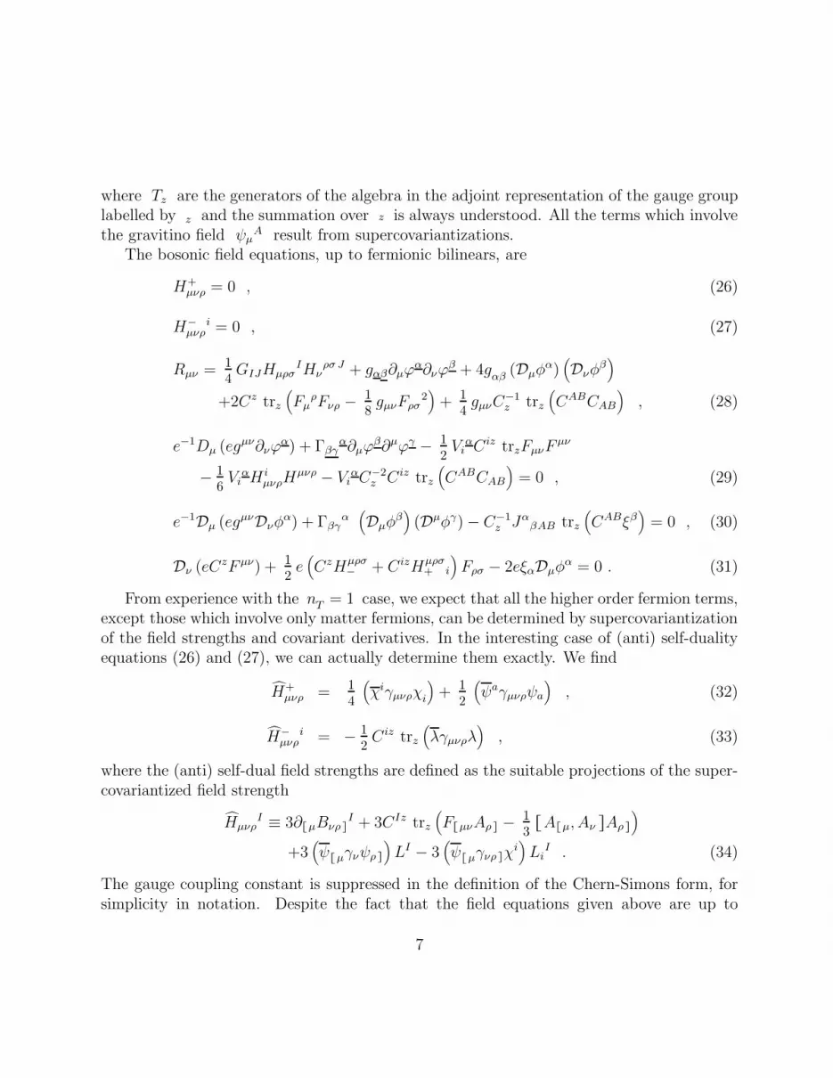
A result from supercovariantizations.The bosonic field equations, up to fermionic bilinears, are

H+µνρ = 0 , (26)

H−µνρ

i = 0 , (27)

Rµν = 14GIJHµρσ

IHνρσ J + gαβ∂µϕ

α∂νϕβ + 4g

αβ(Dµφ

α)(Dνφ

β)

+2Cz trz

(Fµ

ρFνρ − 18gµνFρσ

2)

+ 14gµνC

−1z trz

(CABCAB

), (28)

e−1Dµ (egµν∂νϕα) + Γβγ

α∂µϕβ∂µϕγ − 1

2Vi

αCiz trzFµνFµν

− 16Vi

αH iµνρH

µνρ − ViαC−2

z Ciz trz

(CABCAB

)= 0 , (29)

e−1Dµ (egµνDνφα) + Γβγ

α(Dµφ

β)

(Dµφγ) − C−1z Jα

βAB trz

(CABξβ

)= 0 , (30)

Dν (eCzF µν) + 12e

(CzHµρσ

− + CizHµρσ+ i

)Fρσ − 2eξαDµφ

α = 0 . (31)

From experience with the nT

= 1 case, we expect that all the higher order fermion terms,except those which involve only matter fermions, can be determined by supercovariantizationof the field strengths and covariant derivatives. In the interesting case of (anti) self-dualityequations (26) and (27), we can actually determine them exactly. We find

H+µνρ = 1

4

(χiγµνρχi

)+ 1

2

(ψaγµνρψa

), (32)

H−µνρ

i = − 12Ciz trz

(λγµνρλ

), (33)

where the (anti) self-dual field strengths are defined as the suitable projections of the super-covariantized field strength

HµνρI ≡ 3∂⌊⌈µBνρ ⌋⌉

I + 3CIz trz

(F⌊⌈µνAρ ⌋⌉ − 1

3⌊⌈A⌊⌈µ, Aν ⌋⌉Aρ ⌋⌉

)

+3(ψ⌊⌈µγνψρ ⌋⌉

)LI − 3

(ψ⌊⌈µγνρ ⌋⌉χ

i)Li

I . (34)

The gauge coupling constant is suppressed in the definition of the Chern-Simons form, forsimplicity in notation. Despite the fact that the field equations given above are up to

7

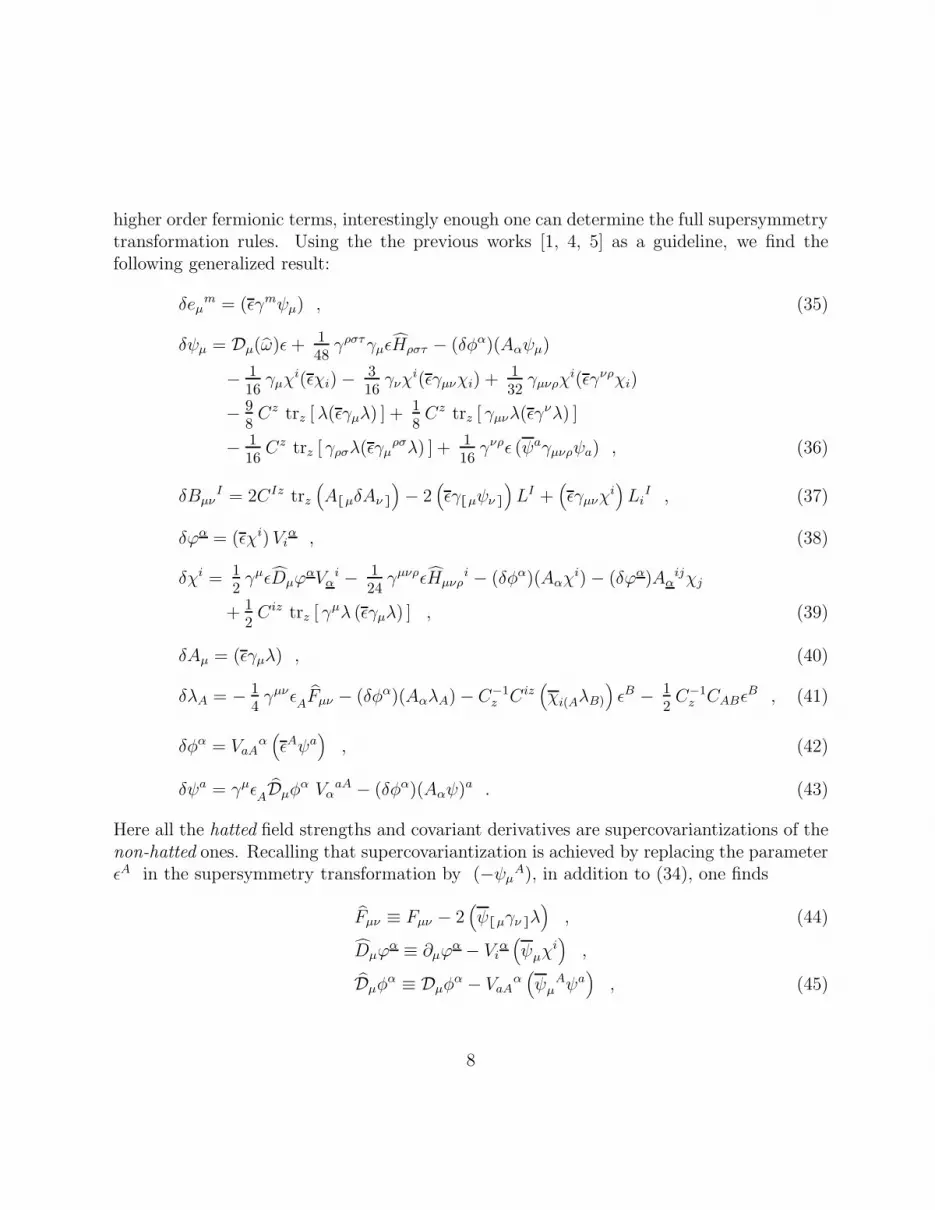
higher order fermionic terms, interestingly enough one can determine the full supersymmetrytransformation rules. Using the the previous works [1, 4, 5] as a guideline, we find thefollowing generalized result:

δeµm = (ǫγmψµ) , (35)

δψµ = Dµ(ω)ǫ+ 148γρστγµǫHρστ − (δφα)(Aαψµ)

− 116γµχ

i(ǫχi) − 316γνχ

i(ǫγµνχi) + 132γµνρχ

i(ǫγνρχi)

− 98Cz trz [λ(ǫγµλ) ] + 1

8Cz trz [ γµνλ(ǫγνλ) ]

− 116Cz trz [ γρσλ(ǫγµ

ρσλ) ] + 116γνρǫ (ψaγµνρψa) , (36)

δBµνI = 2CIz trz

(A⌊⌈µδAν ⌋⌉

)− 2

(ǫγ⌊⌈µψν ⌋⌉

)LI +

(ǫγµνχ

i)Li

I , (37)

δϕα = (ǫχi)Viα , (38)

δχi = 12γµǫDµϕ

αVαi − 1

24γµνρǫHµνρ

i − (δφα)(Aαχi) − (δϕα)Aα

ijχj

+ 12Ciz trz [ γµλ (ǫγµλ) ] , (39)

δAµ = (ǫγµλ) , (40)

δλA = − 14γµνǫ

AFµν − (δφα)(AαλA) − C−1

z Ciz(χi(AλB)

)ǫB − 1

2C−1

z CABǫB , (41)

δφα = VaAα

(ǫAψa

), (42)

δψa = γµǫADµφ

α VαaA − (δφα)(Aαψ)a . (43)

Here all the hatted field strengths and covariant derivatives are supercovariantizations of thenon-hatted ones. Recalling that supercovariantization is achieved by replacing the parameterǫA in the supersymmetry transformation by (−ψµ

A), in addition to (34), one finds

Fµν ≡ Fµν − 2(ψ⌊⌈µγν ⌋⌉λ

), (44)

Dµϕα ≡ ∂µϕ

α − Viα

(ψµχ

i)

,

Dµφα ≡ Dµφ

α − VaAα

(ψµ

Aψa)

, (45)

8

The supercovariant derivative occurring in (36) is defined by

Dµ(ω)ǫA ≡[∂µε

AB + 14ωµ

rsγrsεAB + g′Aµ

AB + (Dµφα)Aα

AB]ǫB , (46)

where the supercovariantized spin connection is given by

ωmrs = 12(Cmrs − Cmsr + Csrm) , (47)

and C is supercovariantized Ricci’s rotation coefficient:

Cµνm ≡ ∂µeνm − ∂νeµm − (ψµγmψν) . (48)

Note that the gravitational constant has always been suppressed. It can easily be rein-troduced by assigning mass dimension 1 to bosons, 3/2 to fermions and −1/2 to ǫ.Since the supersymmetry transformations determined here reduce to the full supersymme-try transformations given in [1] for the n

T= 1 case, we conjecture that they are the full

supersymmetry transformations for all nT.

The supersymmetry transformation rules presented above form a closed algebra withthe composite parameters lmn for the Lorentz transformation, ǫ3 for the supersymmetrytransformation, and ξµ for the general coordinate transformation given by

⌊⌈ δ(ǫ1), δ(ǫ2) ⌋⌉eµm = ξν∂νeµm + (∂µξν)eνm + (ǫ3γmψµ) + lm

neµn ,

ξµ ≡ (ǫ2γµǫ1) ,

ǫA3 ≡ −ξµψµ +[VbB

α(ǫB2 ψb)(Aαǫ1)

A − (1↔2)

],

lmn ≡ ξµωµmn +[

124

(ǫ2γ⌊⌈mγ

ρστγn ⌋⌉ǫ1)H−

ρστILI − 1

8ξµ

(ψaγµmnψa

)

− 14

(ǫ2γmnχ

i)

(ǫ1χi) − 18

(ǫ2γ⌊⌈m

ρχi) (ǫ1γn ⌋⌉ρχi

)

−Cz trz

(ǫ2γ⌊⌈mλ

) (ǫ1γn ⌋⌉λ

) ]− (1↔2) . (49)

We now outline the steps we have followed to derive the equations of motion and super-symmetry transformations.

(1) We first parametrize the transformation rules and the (anti) self-duality equations,as dictated by the symmetries of the theory, the existing partial results for the multi-tensormultiplet couplings [4], and the full results for the n

T= 1 case [1]. At first, we assume that

all matter fields are inert under the local Yang-Mills gauge transformations, as well as thelocal Sp(1) gauge transformations. It is convenient to perform the gauging process, afterthe ungauged results are obtained.

9

Note that factors of C−1z occur in a number of places in the equations of motion and

the transformations rules. While these factors may seem unusual, it is easy to understandtheir origin, which has to do with the fact that we have parametrized the field equationsfor the gauge fermion and the Yang-Mills field (excluding the hypermatter contributionswhich are presented here) in such a way that they agree with those of ref. [5]. For example,once the Cz factor is introduced in (25), it is clear that the closure of the supersymmetrytransformations (41) must include the C−1Ciχ

iλ -term in order to produce the CiλH -term

in the χi -field equation, upon the variation of χi. In comparing this term with the nT

=1 case [1], it is useful to note the identity (88) provided in the Appendix.

(2) Next, we require the closure of the supersymmetry transformations on the bosons.Normally, closure on the bosons does not require any field equations. However, as it has beenknown for some time [12], in the case of self-duality conditions which serve as equations ofmotion, the closure of supersymmetry algebra on the bosons does require the (anti) self-duality equations. Completing the closure calculation on the bosons, we are able to fix allthe supersymmetry transformations, including the (fermion)2 -terms, as well as the (anti)self-duality equations (32) and (33). In this context, (90) given in the Appendix is useful inestablishing the closure on eµ

m and Bµν .(3) Next, we obtain the gravitino equation by supersymmetric variation of (32), and the

χ -field equation by supersymmetry variation of (33).(4) Varying the gravitino equation under supersymmetry, we obtain the Einstein equation

(28). In doing so, (82) given in the Appendix is useful in handling the H2 -terms. Note theoccurrence of the trace gµνF

2 -term in (28), which is absent in the case of nT

= 1, due tothe use of dilaton equation of motion. Since, here we have multi dilatons, the trace term canno longer be absorbed into the the dilaton equation of motion.

(5) Varying the χ -field equation (23), we obtain the field equation (29) for the generalizeddilatons ϕα [5].

(6) Next, we obtain the hyperino field equation (24), by the requirement of the closureof two supersymmetries acting on the hyperino ψa. Varying this equation under supersym-metry, we obtain the field equation (30) for the hyperscalars φα.

(7) Finally the gaugino field equation (25) is also obtained by the closure of two super-symmetries on the gaugino λ. The variation of this equation under supersymmetry in turnyields the Yang-Mills field equation (31).

(8) Having determined the ungauged matter couplings and supersymmetry transforma-tion rules, we now turn on the gauge coupling constants g, g′, thereby gauging the groupSp(n

H) × Sp(1). To do this, we follow the following steps:

(a) We gauge covariantize the relevant derivatives in the supersymmetry transformationrules, as well as the field equations, according to the rules described in section 2.

10

(b) Next, we find that the closure calculation will require the introduction of only onenew term to the transformation rules, namely the CAB -dependent term in the gauginotransformation rule (41). This can be seen by examining the closure of supersymmetry onthe gravitino, and by varying the new gauge coupling dependent terms in Dµǫ. Furthermore,we learn that we need to add the CAB -dependent term in the gravitino field equation.

(c) Having determined the fact that the gaugino transformation rule is modified by theCAB -dependent term that is proportional to the gauge coupling constant, we then examinesystematically the effect of this new variation in all the closure calculations on the fermions.Thus we determine all the new, gauge coupling constant dependent modifications of thefermionic field equations, as given in [1].

(d) Finally, we vary the new terms in the fermionic equations of motion under the fulltransformation rules (old and new), as well as the old terms in the fermionic equationsof motion under the new, gauge coupling constant dependent gaugino transformation rule,thereby obtaining all the modifications, up to the fermionic bilinear terms in the bosonicfield equations of motion.

An important observation to be made here is that the gauging of the SO(nT, 1) or any of

its subgroups does not work, because it is not known how, and it may as well be impossible,to write down a gauge covariant field strength for antisymmetric tensor fields.

4. Invariant Lagrangian for the Case of nT

= 1

When the number of self-dual tensor multiplets differs from that of anti-self-dual tensormultiplets, the system lacks invariant lagrangian, because we can not write down the ki-netic term for purely (anti) self-dual third-rank tensor. However, we do have an invariantlagrangian for the case of n

T= 1 as in refs. [1, 4]. Since this particular case is also of

another importance with the geometry SO(1, 1) with no isotropy group, we give the detailsof the system.

First of all, the coset space is now reduced to a semi-simple group SO(1, 1), and thecoset representatives LI

i and LI can be parametrized as

(L0 L0

(1)

L1 L1(1)

)=

(cosh θ sinh θsinh θ cosh θ

),

(L0 L1

L(1)0 L(1)

1

)=

(cosh θ − sinh θ− sinh θ cosh θ

)(50)

for a rescaled field θ ≡ ϕ1/√

2. Accordingly, we have

η11 = +1 , η00 = −1 , η10 = 0 , (51)

V1(1)∂µϕ

1 = LI∂µLI(1) = ∂µθ . (52)

11

Following ref. [4], we define

aµν ≡ 12

(Bµν

0 − Bµν1)

, bµν ≡ 12

(Bµν

0 +Bµν1)

,

Bµν0 = bµν + aµν , Bµν

1 = bµν − aµν . (53)

We define the field strengths of aµν and bµν as

fµνρ ≡ 3∂⌊⌈µaνρ ⌋⌉ + 3v z trz

(F⌊⌈µνAν ⌋⌉ − 2

3A⌊⌈µAνAρ ⌋⌉

),

gµνρ ≡ 3∂⌊⌈µbνρ ⌋⌉ + 3vz trz

(F⌊⌈µνAν ⌋⌉ − 2

3A⌊⌈µAνAρ ⌋⌉

), (54)

where two constants vz and v z are defined by

vz ≡ 12

(C0z + C1z

), v z ≡ 1

2

(C0z − C1z

). (55)

Accordingly we have C(1)z = vzeθ − v ze−θ, and

Cz = vzeθ + v ze−θ . (56)

After some manipulations, we get

Hµνρ ≡ HµνρILI = e−θfµνρ + e+θgµνρ = 2e+θg−µνρ ,

Hµνρ(1) ≡ Hµνρ

ILI(1) = e+θgµνρ − e−θfµνρ = 2e+θg+

µνρ . (57)

Due to the (anti)self-dualities of BµνI , we have fµνρ = −e2θ gµνρ, f µνρ = −e2θgµνρ, where

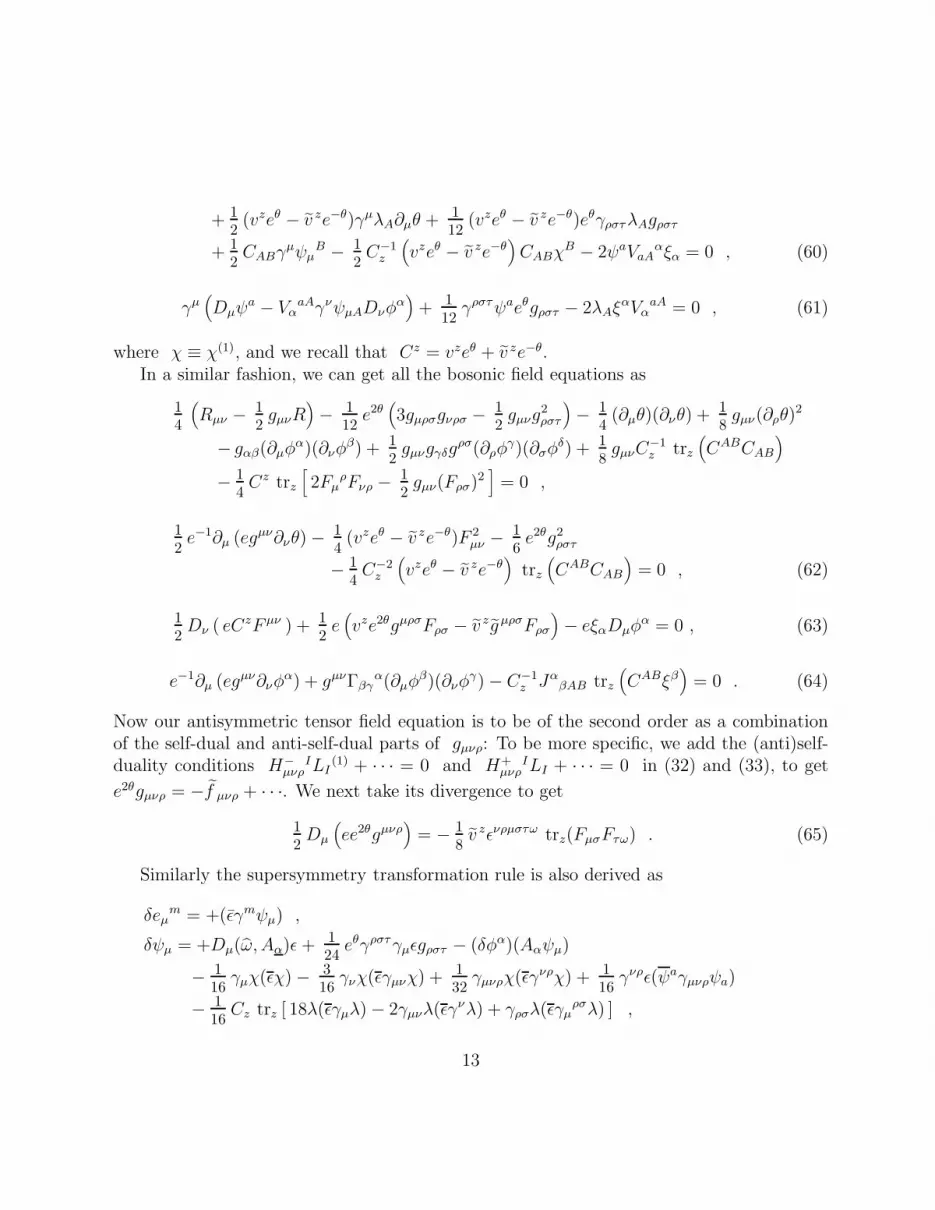
gmnr ≡ (1/6)ǫmnrstugstu and idem for f mnr.We can obtain the field equations of this system from our general case, substituting above

relations. The gravitino, dilatino, gaugino, and hyperino field equations thus obtained are

γµνρDνψρA + 1

12eθγ⌊⌈µγ

ρστγν ⌋⌉ψνAgρστ − 1

2γνγµχ

A∂νθ − 2VαaAγνγµψaDνφ

α

+ 12Czγρσγµ trz

(λAFρσ

)− 1

12eθγρστγµχ

Agρστ − trz

(CABγµλB

)= 0 , (58)

γµ(Dµχ− 1

2γνψµ∂νθ + 1

12eθγρστψµgρστ

)− C−1

z

(vzeθ − v ze−θ

)trz

(CABλB

)

− 112eθγρστχ gρστ − 1

2(vzeθ − v ze−θ) trz (γρσλFρσ) = 0 , (59)

Czγµ(DµλA + 1

4γρσψµAFρσ

)+ 1

4γρσχA(vzeθ − v ze−θ)Fρσ

12

+ 12

(vzeθ − v ze−θ)γµλA∂µθ + 112

(vzeθ − v ze−θ)eθγρστλAgρστ

+ 12CABγ

µψµB − 1

2C−1

z

(vzeθ − v ze−θ

)CABχ

B − 2ψaVaAαξα = 0 , (60)

γµ(Dµψ

a − VαaAγνψµADνφ

α)

+ 112γρστψaeθgρστ − 2λAξ

αVαaA = 0 , (61)

where χ ≡ χ(1), and we recall that Cz = vzeθ + v ze−θ.In a similar fashion, we can get all the bosonic field equations as

14

(Rµν − 1

2gµνR

)− 1

12e2θ

(3gµρσgνρσ − 1

2gµνg

2ρστ

)− 1

4(∂µθ)(∂νθ) + 1

8gµν(∂ρθ)

2

− gαβ(∂µφα)(∂νφ

β) + 12gµνgγδg

ρσ(∂ρφγ)(∂σφ

δ) + 18gµνC

−1z trz

(CABCAB

)

− 14Cz trz

[2Fµ

ρFνρ − 12gµν(Fρσ)2

]= 0 ,

12e−1∂µ (egµν∂νθ) − 1

4(vzeθ − v ze−θ)F 2

µν − 16e2θg2

ρστ

− 14C−2

z

(vzeθ − v ze−θ

)trz

(CABCAB

)= 0 , (62)

12Dν ( eCzF µν ) + 1

2e

(vze2θgµρσFρσ − v z gµρσFρσ

)− eξαDµφ

α = 0 , (63)

e−1∂µ (egµν∂νφα) + gµνΓβγ

α(∂µφβ)(∂νφ

γ) − C−1z Jα

βAB trz

(CABξβ

)= 0 . (64)

Now our antisymmetric tensor field equation is to be of the second order as a combinationof the self-dual and anti-self-dual parts of gµνρ: To be more specific, we add the (anti)self-duality conditions H−

µνρILI

(1) + · · · = 0 and H+µνρ

ILI + · · · = 0 in (32) and (33), to get

e2θgµνρ = −f µνρ + · · ·. We next take its divergence to get

12Dµ

(ee2θgµνρ

)= − 1

8v zǫνρµστω trz(FµσFτω) . (65)

Similarly the supersymmetry transformation rule is also derived as

δeµm = +(ǫγmψµ) ,

δψµ = +Dµ(ω, Aα)ǫ+ 124eθγρστγµǫgρστ − (δφα)(Aαψµ)

− 116γµχ(ǫχ) − 3

16γνχ(ǫγµνχ) + 1

32γµνρχ(ǫγνρχ) + 1

16γνρǫ(ψaγµνρψa)

− 116Cz trz [ 18λ(ǫγµλ) − 2γµνλ(ǫγνλ) + γρσλ(ǫγµ

ρσλ) ] ,

13

δbµν = +2vz trz

(A⌊⌈µδAν ⌋⌉

)− e−θ(ǫγ⌊⌈µψν ⌋⌉) + 1

2e−θ(ǫγµνχ) , δθ = +(ǫχ) ,

δχ = + 12γµǫ∂µθ − (δφα)(Aαχ) − 1

12eθγµνρǫgµνρ + 1

2

(vzeθ − v ze−θ

)trz [ γµλ(ǫγµλ) ] ,

δAµ = +(ǫγµλ) ,

δλA = − 14γµνǫAFµν − (δφα)(AαλA) − C−1

z

(vzeθ − v ze−θ

) (χ(AλB)

)ǫB − 1

2C−1

z CABǫB ,

δφα = +VaAα(ǫAψa) ,

δψa = +VαaAγµǫADµφ

α − (δφα)(Aαψ)a . (66)

Note that in the absence of gauging, the function CAB vanishes and singular behaviour inthe couplings arises in the energy-momentum tensor for the Yang-Mills field in (26) and in theYang-Mills equation (28). Furthermore, the λ2ǫ terms in the supersymmetry variation of thegravitino vanish and the χλǫ terms in the supersymmetry variation of the gaugino diverge,at the critical point where Cz = vzeθ + v ze−θ vanishes. When the gauging of Sp(n

H)×Sp(1)

is switched on, the divergent C−1z factors arise in χ, λ, Einstein, dilaton and hypermatter

field equations, and the supersymmetry variation of the gaugino picks up another singularcontribution.

When v z = 0, this result agrees with ref. [4] as far as the supergravity and Yang-Mills multiplets are concerned, and also with ref. [1] with hypermultiplets. When vz = 0,this result coincides with the system in ref. [14]. In the important cases of vz = 0 andv z = 0, this is reduced to the usual exponential factors. It is worthwhile to mention thatthe χλ -terms in the λ -transformation rules have apparently different coefficients comparedwith [1], via (88). This is attributed to the fact that our gaugino λ -field is rescaled by anexponential function of the dilaton θ.

As will be discussed in the next section, since the conservation of the Yang-Mills currentis satisfied only for η

IJCIzCJz′ = 0, the invariant lagrangian exists only for the two cases

vz = 0 or v z = 0 for our nT

= 1 system. If we formally try to integrate the field equationsfor other cases of vz v z′ 6= 0, we encounter gauge non-invariant terms in the lagrangian, thatinvalidate supersymmetry. This is because commutators of two supersymmetries will resultin a gauge transformation. Another explicit way to see this is to take the variation of theb∧F ∧F term in the lagrangian under supersymmetry. This produces gauge non-invariantterms proportional to vzv z′ which can not be cancelled. Note also that this feature for thecase vzv z′ 6= 0 at the classical level does not necessarily mean the system is inconsistent,as will be discussed in the next section.

14

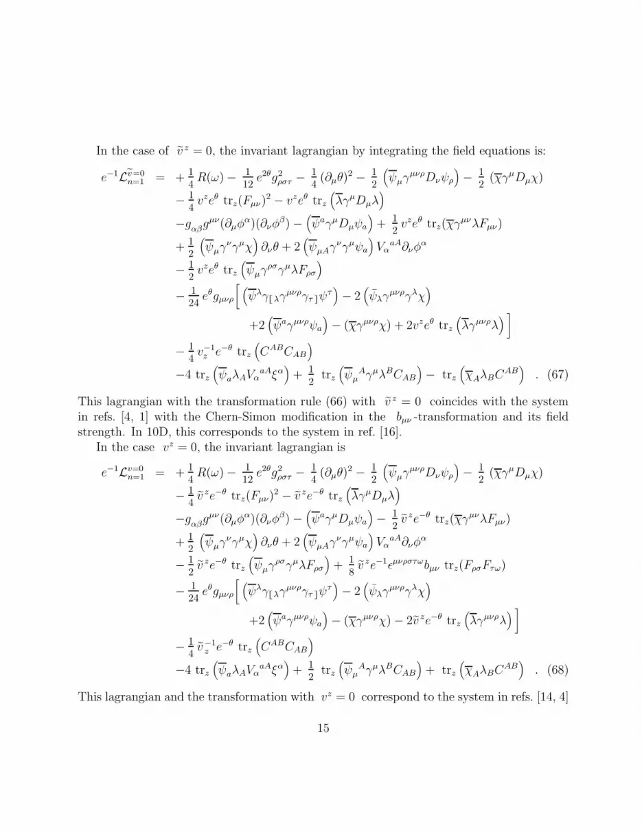
In the case of v z = 0, the invariant lagrangian by integrating the field equations is:

e−1Lv=0n=1 = + 1

4R(ω) − 1

12e2θg2

ρστ − 14

(∂µθ)2 − 1

2

(ψµγ

µνρDνψρ

)− 1

2(χγµDµχ)

− 14vzeθ trz(Fµν)

2 − vzeθ trz

(λγµDµλ

)

−gαβgµν(∂µφ

α)(∂νφβ) −

(ψaγµDµψa

)+ 1

2vzeθ trz(χγ

µνλFµν)

+ 12

(ψµγ

νγµχ)∂νθ + 2

(ψµAγ

νγµψa

)Vα

aA∂νφα

− 12vzeθ trz

(ψµγ

ρσγµλFρσ

)

− 124eθgµνρ

[ (ψλγ⌊⌈λγ

µνργτ ⌋⌉ψτ)− 2

(ψλγ

µνργλχ)

+2(ψaγµνρψa

)− (χγµνρχ) + 2vzeθ trz

(λγµνρλ

) ]

− 14v−1

z e−θ trz

(CABCAB

)

−4 trz

(ψaλAVα

aAξα)

+ 12

trz

(ψµ

AγµλBCAB

)− trz

(χAλBC

AB)

. (67)

This lagrangian with the transformation rule (66) with v z = 0 coincides with the systemin refs. [4, 1] with the Chern-Simon modification in the bµν -transformation and its fieldstrength. In 10D, this corresponds to the system in ref. [16].

In the case vz = 0, the invariant lagrangian is

e−1Lv=0n=1 = + 1

4R(ω) − 1

12e2θg2

ρστ − 14

(∂µθ)2 − 1

2

(ψµγ

µνρDνψρ

)− 1

2(χγµDµχ)

− 14v ze−θ trz(Fµν)

2 − v ze−θ trz

(λγµDµλ

)

−gαβgµν(∂µφ

α)(∂νφβ) −

(ψaγµDµψa

)− 1

2v ze−θ trz(χγ

µνλFµν)

+ 12

(ψµγ

νγµχ)∂νθ + 2

(ψµAγ

νγµψa

)Vα

aA∂νφα

− 12v ze−θ trz

(ψµγ

ρσγµλFρσ

)+ 1

8v ze−1ǫµνρστωbµν trz(FρσFτω)

− 124eθgµνρ

[ (ψλγ⌊⌈λγ

µνργτ ⌋⌉ψτ)− 2

(ψλγ

µνργλχ)

+2(ψaγµνρψa

)− (χγµνρχ) − 2v ze−θ trz

(λγµνρλ

) ]

− 14v−1

z e−θ trz

(CABCAB

)

−4 trz

(ψaλAVα

aAξα)

+ 12

trz

(ψµ

AγµλBCAB

)+ trz

(χAλBC

AB)

. (68)

This lagrangian and the transformation with vz = 0 correspond to the system in refs. [14, 4]

15

with the explicit b∧F∧F -term in the lagrangian with no modification in the bµν -transformationrule or its field strength. In 10D, this corresponds to the dual formulation [17].

5. Discussion

In this paper we have constructed the field equations of the combined system of the N =1 supergravity multiplet, n

Tcopies of anti-self-dual tensor multiplets with anti-self-dual

tensor multiplet, forming the coset space SO(nT, 1)/SO(n

T), Yang-Mills multiplets, and

hypermultiplets forming the coset Sp(nH, 1)/Sp(n

H)⊗Sp(1). Furthermore we have gauged

the group Sp(nH

) × Sp(1). These are the most general couplings of the six dimensionalsupergravity plus matter system to date. The resulting system exhibits some interestingfeatures which we now comment on.

We have already commented on the singular behaviour of the couplings at a special pointin moduli space, and the occurrence of new divergent couplings at the same point whichproportional to the gauged Sp(n

H)× Sp(1) coupling constants. Another important feature,

which was observed in [6], and which continues to hold in the more general system presentedhere, is the anomalous behaviour of the gauge couplings. Namely, writing the Yang-Millsequation (31) as

Dν (eCzF µν) = eJµ , (69)

we find thatDµ(eJ

µ) = 116ǫµνρστλη

IJCIzCJz′Fµν trz′ (FρσFτλ) . (70)

Perhaps not too surprisingly, the hypermatter contributions to this anomaly equation haveall canceled. Setting

ηIJCIzCJz′ = 0 , (71)

eliminates the anomalous divergence. This corresponds to the familiar nT

= 1 case [1] forwhich a covariant action can be written down. Interestingly, there are two possibilities thathave been treated simultaneously here. In notation of section 4, these correspond to thecases of vz = 0 or v z = 0. As discussed in section 4, the case of v z = 0 is the familiar oneconstructed by the authors a long tome ago [1], and its ten dimensional analog is well-known[15, 16]. The case of vz = 0 corresponds to the dual formulation, constructed also long ago[14], and its ten dimensional analog is the dual formulation of Chamseddine [17].

It should be emphasized that neither the elimination of the anomalous divergence (70)ensure anomaly freedom, nor does its nonvanishing mean that the theory is anomalous. Theproperty of anomaly freedom solely depends on the choice of matter multiplets, and as is

16

well-known, there are many available anomaly free sets of such multiplets, some of whichwill be discussed below.

Considering the case of nT> 1, eq. (69) represents the Bose non-symmetric covariant

gauge anomaly, as observed in [6]. Its Bose symmetric covariant version, as well as the asso-ciated local supersymmetry anomaly can be determined by considerations of Wess-Zuminoanomaly consistency conditions [6]. Although a covariant action can not be written down forn

T> 1, both the gauge as well as supersymmetry anomalies can nonetheless be associated

with the gauge and supersymmetry variation, respectively, of the Green-Schwarz type term[6]

LGS = − 18ǫµνρστλ

(η

IJBµν

ICJz)

trz (FρσFτλ) − 12ǫµνρστλη

IJCIzCJz′ωz

µνρωz′

στλ , (72)

where ωzµνρ is the Yang-Mills Chern-Simons form.

The results of [6] and our generalization which includes the hypermatter reveal therefore,a surprising situation in which an anomalous system of supermultiplets can be supersym-metrized, with the caveat that the integrability conditions for the equations of motion reflectthe anomalies. The fact that this is possible at all may be due to the manifest gauge covari-ant nature of the field equations and supersymmetry transformation rules. Attempting tosupersymmetrize a gauge non-invariant action, on the other hand, would run immediatelyinto trouble with supersymmetrization.

The anomalies of the full system discussed here are to be cancelled by the quantum one-loop effects, so that the total effective action is gauge invariant and supersymmetric, providedthat the right set of matter multiplets are included. The anomalies may cancel precisely, orGreen-Schwarz cancellation mechanism may have to be employed for the cancellation [18].The same mechanism works in the dual formulation as was shown in [19, 20, 14]. In the caseof n

T= 1, a generalized version of the Green-Schwarz mechanism was found by Sagnotti

[5] which involves the use of multi-tensor fields simultaneously. We conclude by mentioningsome of the anomaly free matter contents for the n

T= 1 and n

T> 1 cases.

For nT

= 1 without gauging, a large number of anomaly free matter contents can beobtained by compactifying the well-known anomaly free ten dimensional supergravity-Yang-Mills systems that arise in string theory [21]. All of these models have a gauge group of rank≤ 20, and they arise from a perturbative treatment of string compactification. Witten [22]has discovered a new mechanism by which a nonperturbative symmetry enhancement occurs,and a new class of anomaly-free models, not realized in perturbative string theory, emergein 6D. These can have rank greater than 20. Schwarz [23] has constructed new anomaly-freemodels in 6D, some of which may potentially arise in a similar nonperturbative scheme.

As for the gauged case with nT

= 1, an anomaly free model was found in [24], wherethe gauge group is E6 × E7 × U(1). The U(1) factor is a subgroup of the automorphism

17

group, and the hyper-fermions belong to the 912 dimensional representation of E7. Theorigin of this model still remains mysterious, and it would be very interesting to determineif it can be explained by a new kind of nonperturbative mechanism in M-theory.

In general, the necessary but not sufficient condition for the anomaly cancellation is [24]

nH− n

V+ 29n

T= 273 . (73)

As mentioned in the introduction, an example of an anomaly free model with nT

= 9 hasbeen found in [2] by considering a suitable M-theory compactification, and it has n

V=

8, nH

= 20. The matter couplings of six dimensional supergravity constructed here providesthe field theoretic description of this model.

Finally, we mention an example of an anomaly free matter content with nT> 1 found

sometime ago in [25]. It has:

nT

= 17 , nH

= 28 , nV

= 248 . (74)

The vector fields fit into the adjoint representation of E8, and we can take the hyperscalarmanifold to be E8/(E7 × Sp(1)), in which case the hyperfermions transform in 56 dimen-sional representation of E7. As far as we know, this model, which has a rather simple fieldcontent, has not found an M-theory explanation so far, and it would be interesting to see ifthere is one.

Acknowledgements

The authors are grateful to M. Duff, A. Sagnotti and E. Witten for stimulating discus-sions. H.N. would like to thank the Center for Theoretical Physics at Texas A& M Universityfor hospitality.

18

Appendix: Notations, Conventions and Lemmas

Our metric is (ηmn) = diag. (−,+,+,+,+,+), while the Clifford algebra is generatedby {γm, γn} = 2ηmn. Note that this signature differs from the one in [1]. The definitionof the Ricci tensor is the same as in [1], however, namely: Rµ

a = Rµνab eb

ν . We defineγ7 ≡ γ(0) (1) ··· (5), ǫ

012345 = +1, such that (γ7)2 = +1. More generally we have

γr1···rn =(−1)⌊⌈n/2 ⌋⌉

(6−n)!ǫr1···rns1···s6−nγs1···s6−n

γ7 . (75)

The basic gamma-matrix relations such as γmγrstγm = 0 stays the same as in ref. [1], as

well as the conventions for the Sp(1) indices, e.g.,

χAi = ǫABχ

Bi, χ

Ai= χB

iǫBA,

(ǫAB

)=

(ǫAB

)=

(0 1−1 0

), (76)

χAi = ǫABχ

BiT , χ

Ai= (χA

i)†γ0 , (77)

(χA

iγm1···mnλB

)= (−1)n+1

(λBγmn···m1χA

i

). (78)

For inner products of Sp(1) (or Sp(nH

)) symplectic spinors [13], the contractions with

ǫAB

(or ǫab) are always understood, e.g., (χiγrsλ) =

(χA

iγrsλA

)as in [1], e.g.,

(χ

iγr1···rnλ

)= (−1)n

(λγr1···rnχ

i

). (79)

Exactly as in ref. [1], for given four symplectic Majorana-Weyl spinors ψ1, · · · , ψ4, wherethe labels 1, ···, 4 denote all the possible indices they may carry, including Sp(1), Sp(n

H) or

SO(nT) indices, the Fierz arrangement formula is

(ψ1ψ2

) (ψ3ψ4

)= − 1

8(1 + c2c4)

[ (ψ1ψ4

) (ψ3ψ2

)− 1

2

(ψ1γ

rsψ4

) (ψ3γrsψ2

) ]

− 18

(1 − c2c4)[ (ψ1γ

rψ4

) (ψ3γrψ2

)− 1

12

(ψ1γ

rstψ4

) (ψ3γrstψ2

) ](80)

where γ7(ψ2, ψ4) = (c2ψ2, c4ψ4).One of the most frequently used relationships related to the (anti)self-dual tensors is

SµνρSµνρ ≡ AµνρAµνρ ≡ 0, where the third-rank tensors S and A are respectively self-dualand anti-self-dual tensors: (1/6)ǫmnr

stuSstu = +Smnr, (1/6)ǫmnrstuAstu = −Amnr. For the

tensor HµνρI we use the symbols H+

ρστI (or H−

ρστI) to distinguish their dual (or anti-

self-dual) components. The important duality properties of the gamma-matrices multiplied

19

by fermions are summarized as follows. For fermions with the positive chirality such asψµ

A, λA r or ǫA, or for fermions with negative chiralities such as χA i, ψa, we have

16ǫmnr

stu (γstuψµ) ≡ − (γmnrψµ) , 16ǫmnr

stu (γstuψa) ≡ + (γmnrψ

a) , (81)

In other words, the combination γrstψµ behaves as an anti-self-dual tensor, while γrstψa be-haves as a self-dual tensor, as far as the indices ⌊⌈ rst ⌋⌉ are concerned. It also follows thatγρστλH−

ρστI ≡ 0 or γρστχH+

ρστI ≡ 0.

In the remainder of this appendix, we shall list a number of lemmas that are useful inthe derivation of field equations and supersymmetry transformation rules.

(1) For H2 -term computation in gravitational equation the following lemma is useful:

H+⌊⌈µν

τiH+ρ ⌋⌉στi ≡ 0 . (82)

This can be verified by using the duality property of H , and simple manipulations involvingthe Schouten identity, which in the present case means that an antisymmetrization of sevenworld indices vanishes identically.

(2) For χH -terms in the derivations of χ -field equation out of anti-self-duality condition,the following lemma is useful:

(ǫγσ

⌊⌈µ|χi)H−

|νρ ⌋⌉σ ≡ − 13

(ǫχi

)H−

µνρ . (83)

This can be proven by the vanishing of (ǫγµνργστωχi)H−

στω = 0 with the γ -algebra for thel.h.s.

(3) In calculating the divergence of the Yang-Mills field equation, it is useful to note that

DµCz = ∂µC

z = (∂µϕα)Vα

iCzi , DµC

zi = (∂µϕα)Vα

iCz . (84)

(4) For the gravitino field equation out of self-duality condition, we use the lemma

(ǫγσγµνργτωχi)H

+στω

i = − 13

(ǫγστωγµνρχi)H+στω

i − 16 (ǫχi)H+µνρ

i , (85)

confirmed by γ -algebra as well as the self-duality of H+.(5) The λ2 and χ2 -terms in the supersymmetry transformation of the gravitino can be

rearranged as

δψµ|λ2 = −CIzLI

(34ǫBλµ

BA + 14γµ

νǫBλν

BA + 116γστ ǫAλµστ

), (86)

δψµ|χ2 = − 38ǫBχµ

BA + 18γµ

νǫBχν

BA , (87)

20

where λµAB = trz

(λAγµλ

B), λρστ ≡ trz

(λγρστλ

), χµ

AB ≡(χAγµχ

B), χρστ ≡ (χγρστχ).

(6) The λχ -term in δλ (41) can be rewritten by using the identity

(χi(AλB)

)ǫB = 1

4λA (ǫχi) + 1

8γρσλA (ǫγρσχi) + 1

2ǫA

(λχi

), (88)

obtained by Fierz rearrangement.(7) In order to fix the λ2 -terms in the supersymmetry transformation of the gravitino,

we arrange the ψaλ2 -terms in the commutator on ψa, which needs the lemma(ǫA2 γµνρǫ1B

)λρB

A = −4 trz

(ǫ⌊⌈ 1|γµλ

) (λγνǫ|2 ⌋⌉

)+ 1

2ξρλµνρ ,

trz

(ǫ⌊⌈ 2|γ

mnρλ

) (ǫ|1 ⌋⌉γρλ

)= − 1

2ξρλρ

mn + 2 trz

(ǫ⌊⌈ 2|γ

⌊⌈mλ) (ǫ|1 ⌋⌉γ

n ⌋⌉λ)

, (89)

where ξµ ≡ (ǫ2γµǫ1).

(8) The following non-trivial lemmas are useful for the closure checks on eµm or Bµν :

trz

(ǫ1γρσ⌊⌈µλ

) (ǫ2γν ⌋⌉

ρσλ)− (1↔2) ≡ 0 ,

(ǫ1γ

µνρσχ(i) (ǫ2γρσχ

j))− (1↔2) ≡ 0 ,

(ǫ2γρǫ1) trz

(λγµνρλ

)≡ trz [ 2 (ǫ2γµλ) (ǫ1γνλ) − (ǫ2γµνρλ) (ǫ1γ

ρλ) ] − (1↔2) . (90)

These are easily confirmed by appropriate Fierz arrangements as well as the duality propertieswe already know.

(9) It is useful to note the following relation for the closure check on λ:

(ǫ(A1 γστρǫ

B)2

)γµνστλBH

−µνρ ≡ 0 ,

(ǫ(A1 γ

µρσǫB)2

)γµ

νλBH−νρσ ≡ 0 , (91)

which can be proven by the relationship(ǫ(A1 γρστ ǫ

B)2

)⌊⌈ γρστ , γµνω ⌋⌉±λH−

µνω ≡ 0, etc.

due to the anti-self-duality of the combination(ǫA1 γρστ ǫ

B2

)as well as the anti-self-duality

of H− I .(10) In the arrangement of λχ2 -terms in the commutator on λ, the following lemma for

super-variation is useful:

δ(C−1

z Ciz)

= C−2z

(ǫχj

) (δijC2

z − CizCjz)

. (92)

21

References

[1] H. Nishino and E. Sezgin, Matter and Gauge Couplings of N=2 Supergravity in SixDimensions, Phys. Lett. 144B (1984) 187;H. Nishino and E. Sezgin, The Complete N=2, D=6 Supergravity With Matter andYang-Mills Couplings, Nucl. Phys. B144 (1986) 353.

[2] A. Sen, M-theory on (K3 × S1)/Z2, Phys. Rev. 53D (1996) 6725, hep-th/9602010.

[3] N. Marcus and J.H. Schwarz, Field Theories That Have No Manifestly Lorentz InvariantFormulation, Phys. Lett. 115B (1982) 111.

[4] L.J. Romans, Self-Duality for Interacting Fields: Covariant Field Equations for SixDimensional Chiral Supergravities, Nucl. Phys. B276 (1986) 71.

[5] A. Sagnotti, A Note on the Green-Schwarz Mechanism in Open String theories,Phys. Lett. 294B (1992) 196, hep-th/9210127.

[6] S. Ferrara, R. Minasian and A. Sagnotti, Low-Energy Analysis of M and F Theorieson Calabi-Yau Threefolds, Nucl. Phys. B474 (1996) 323, hep-th/9604097.

[7] E. Bergshoeff, E. Sezgin and E. Sokatchev, Couplings of Self-Dual Tensor Multiplet inSix Dimensions, Class. and Quant. Gr. 13 (1996) 2875, hep-th/9605087.

[8] M.J. Duff and R. Minasian and E. Witten, Evidence for Heterotic/Heterotic Duality,Nucl. Phys. B465 (1996) 413, hep-th/9601036.

[9] N. Seiberg and E. Witten, Comments on String Dynamics in Six Dimensions,Nucl. Phys. B471 (1996) 121, hep-th/9603003.

[10] M. J. Duff, H. Lu and C. N. Pope, Heterotic Phase Transitions and Singularities of theGauge Dyonic String, Phys. Lett. 378B (1996) 101, hep-th/9603037.

[11] S.J. Gates, Jr., H. Nishino and E. Sezgin, Supergravity in D=9 and Its Coupling to theNon-compact Sigma Model, Class. and Quant. Gr. 3 (1986) 21.

[12] J.H. Schwarz, Covariant Field Equations of Chiral N=2, D=10 Supergravity,Nucl. Phys. B226 (1983) 269.

[13] T. Kugo and P.K. Townsend, Supersymmetry and the Division Algebras,Nucl. Phys. B211 (1983) 357.

22

[14] H. Nishino and S.J. Gates, Jr., Dual Versions of Higher Dimensional Supergravities andAnomaly Cancellations in Lower Dimensions, Nucl. Phys. B268 (1986) 532.

[15] E. Bergshoeff, M. de Roo, B. de Wit and P. van Nieuwenhuizen, Ten Dimen-sional Einstein-Maxwell Supergravity, Its Currents, the Issue of Its Auxiliary Fields,Nucl. Phys. B195 (1982) 97.

[16] G.F. Chapline and N.S. Manton, Unification of Yang-Mills Theory and SupergravityTheory in Ten Dimensions, Phys. Lett. 120B (1983) 105.

[17] A. Chamseddine, Interacting Supergravity in Ten Dimensions: The Role of the Six-IndexGauge Field, Phys. Rev. 24D (1981) 3065.

[18] M.B. Green and J.H. Schwarz, Anomaly Cancellations in Supersymmetric D=10 GaugeTheory Requires SO(32), Phys. Lett. 149B (1984) 117.

[19] S.J. Gates, Jr. and H. Nishino, New D=10, N=1 Supergravity Coupled to Yang-MillsSupermultiplet and Anomaly Cancellations, Phys. Lett. 157B (1985) 157.

[20] A. Salam, E. Sezgin, Anomaly Freedom in Chiral Supergravities, Physica Scripta, 32

(1985) 283.

[21] M.B. Green, J.H. Schwarz and P.C. West, Anomaly Free Chiral Theories in Six Dimen-sions, Nucl. Phys. B254 (1985) 327.

[22] E. Witten, Small Instantons in String Theory, Nucl. Phys. B460 (1996) 541, hep-th/9511030.

[23] J.H. Schwarz, Anomaly-Free Supersymmetric Models in Six Dimensions, Phys. Lett.371B (1996) 223, hep-th/9512053.

[24] S. Randjbar-Daemi, A. Salam, E. Sezgin and J. Strathdee, An Anomaly-Free Model inSix Dimensions, Phys. Lett. 151B (1985) 327.

[25] E. Bergshoeff, T.W. Kephart, A. Salam and E. Sezgin, Global Anomalies in Six Dimen-sions, Mod. Phys. Lett. A1 (1986) 267.

23