UCB-PTH-98/30, LBNL-41875, NSF-ITP-98-068

hep-th/9806021

Glueball Mass Spectrum From Supergravity

Csaba Csaki1,2∗, Hirosi Ooguri1,2,3, Yaron Oz1,2,3 and John Terning1,2

1 Department of Physics, University of California at Berkeley,

Berkeley, CA 94720

2 Theoretical Physics Group, Mail Stop 50A-5101,

Lawrence Berkeley National Laboratory,

Berkeley, CA 94720

3 Institute for Theoretical Physics, University of California,

Santa Barbara, CA 93106

csaki@thwk5.lbl.gov, ooguri@thsrv.lbl.gov, yaronoz@thsrv.lbl.gov,

terning@alvin.lbl.gov

Abstract

We calculate the spectrum of glueball masses in non-supersymmetric Yang-

Mills theory in three and four dimensions, based on a conjectured duality

between supergravity and large N gauge theories. The glueball masses are

obtained by solving supergravity wave equations in a black hole geometry.

We find that the mass ratios are in good numerical agreement with the avail-

able lattice data. We also compute the leading (g2Y MN)−1 corrections to the

glueball masses, by taking into account stringy corrections to the supergravity

action and to the black hole metric. We find that the corrections to the masses

are negative and of order (g2Y MN)−3/2. Thus for a fixed ultraviolet cutoff the

masses decrease as we decrease the ’t Hooft coupling, in accordance with our

expectation about the continuum limit of the gauge theories.

∗Research Fellow, Miller Institute for Basic Research in Science.

1 Introduction

Recently Maldacena formulated a conjecture [1] stating that the large N limit of

the maximally supersymmetric conformal theories in 3, 4 and 6 dimensions are dual to

superstring/M theory on AdS4 × S7, AdS5 × S5 and AdS7 × S4 respectively, where AdSd

is a d-dimensional anti-de Sitter space. More recently Witten proposed [2] that one can

extend this duality to non-supersymmetric theories such as pure QCD. In this case the

AdS space is replaced by the Schwarzschild geometry describing a black hole in the AdS

space. When the curvature of the spacetime is small compared to the string scale and the

Planck scale, superstring/M theory is well-approximated by supergravity. It was found

that the supergravity description gives results that are in qualitative agreement with

expectations for QCD at strong coupling. This includes the area law behavior of Wilson

loops, the relation between confinement and monopole condensation, the existence of a

mass gap for glueball states, the behavior of Wilson loops for higher representations, and

the construction of heavy quark baryonic states [2–7].

In this paper, we use the supergravity description of large N gauge theories to compute

the scalar glueball mass spectrum explicitly for pure QCD3 and QCD4. The glueball

masses in QCD can be obtained by computing correlation functions of gauge invariant

local operators or the Wilson loops, and looking for particle poles. According to the

refinement of Maldacena’s conjecture given in [8, 9], correlation functions of a certain

class of local operators (chiral primary operators and their superconformal descendants)

are related at large N and large g2Y MN to tree level amplitudes of supergravity. The

correspondence between the chiral operators and the supergravity states has been worked

out in [8–14]. For example, the operator trF 2 in four dimensions corresponds to the

dilaton field of supergravity in ten dimensions. Therefore the scalar glueball∗ JPC = 0++

in QCD which couples to trF 2 is related to the dilaton propagating in the black hole

geometry. In particular, its mass is computable by solving the dilaton wave equation [2].

In [7], it was shown that the correlation function of Wilson loops is also expressed in

terms of supergraviton exchange if the distance between the loops becomes larger than

their sizes, leading again to the supergravity wave equation.

In this paper we will solve the wave equations numerically to obtain the glueball

masses. Since this description preserves all the symmetries of QCD, we can identify

the spin and the other quantum numbers of the glueballs. The mass ratios turn out to

be in excellent agreement with the available lattice data in the continuum limit. This

∗In the following we will use the notation JPC for the glueballs, where J is the glueball spin, and P ,C refer to the parity and charge conjugation quantum numbers respectively.

1

is surprising since a priori the supergravity computations are to be compared with the

strong ultraviolet coupling limit of the gauge theory g2Y MN 1.

As we will see, the supergravity computation at g2Y MN 1 gives the glueball masses

in units of the fixed ultraviolet cutoff ΛUV . For finite ‘t Hooft coupling λ = g2Y MN , the

glueball mass M would be a function of the form,

M2 = f(λ)Λ2UV . (1.1)

To take the continuum limit ΛUV → ∞, we have to simultaneously take λ → 0 so that

the right-hand side of this equation becomes of the order of the QCD mass scale ΛQCD.

This in particular requires that f(λ) decreases as we decrease the ‘t Hooft coupling λ.

We compute the leading λ−1 corrections to the supergravity computation and show

that this is indeed the case. On the superstring side, the λ−1 corrections are due to the

finite string tension. The leading order string correction to the low-energy supergravity

action was computed in [15, 16]. This modifies both the background black hole metric and

the supergravity wave equation in that background. Recently the stringy correction to

the black hole metric was obtained in [17] by solving the modified supergravity equation.

We use both this metric and the string corrected wave equation to compute the leading

λ−1 corrections to the 0++ glueball masses in QCD3. We find:

(1) The corrections to the masses are negative and of order λ−3/2:

f(λ) = c0 + c1λ−3/2 + · · · , c1 < 0, (1.2)

for the ground state and the first 5 excited levels of the 0++ glueball. Thus, for a fixed

ultraviolet cutoff, the masses decrease as we decrease the ’t Hooft coupling, in accordance

with the expectation about the continuum limit of QCD.

(2) The corrections to the ratios of the glueball masses are relatively small compared

to the correction to each glueball mass, suggesting that the corrections are somewhat

universal for all the glueball masses. This may indicate that the good agreement between

the supergravity computation and the lattice gauge theory results is not a coincidence

but is due to small λ−1 corrections to the mass ratios.

This paper is organized as follows.

In section 2, we solve the supergravity wave equations in the AdS5 black hole geometry

to obtain glueball masses in QCD3 and compare the results with lattice computations.

In section 3, we solve the supergravity wave equations in the AdS7 black hole geometry

to obtain glueball masses in QCD4 and compare the results with lattice computations.

2

In section 4, we use the string theory corrections to the low-energy supergravity action

and to the AdS5 black hole geometry to estimate corrections to the glueball masses in

QCD3.

We close the paper with a summary and discussions.

2 Glueballs in Three Dimensions

The N = 4 superconformal SU(N) gauge theory in four dimensions is realized as

a low energy effective theory of N coinciding parallel D3 branes. One can construct a

three-dimensional non-supersymmetric theory [2] by compactifying this theory on R3×S1

with anti-periodic boundary conditions on the fermions around the compactifying circle

S1. Supersymmetry is broken explicitly by the boundary conditions. As the radius R of

the circle becomes small, the fermions decouple from the system since there are no zero

frequency Matsubara modes. The scalar fields in the 4D theory will acquire masses at

one-loop, since supersymmetry is broken, and these masses become infinite as R → 0.

Therefore in the infrared we are left with only the gauge field degrees of freedom and the

theory should be effectively the same as pure QCD3.

According to Maldacena [1], the N = 4 theory in Euclidean R4 is dual to type IIB

superstring theory on AdS5 × S5 with the metric

ds2

l2s√

4πgsN= ρ−2dρ2 + ρ2

4∑i=1

dx2i + dΩ2

5 (2.1)

where ls is the string length related to the superstring tension, gs is the string coupling

constant and dΩ5 is the line element on S5. The x1,2,3,4 directions in AdS5 correspond

to R4 where the gauge theory lives. The gauge coupling constant g4 of the 4D theory is

related to the string coupling constant gs as g24 = gs. In the ’t Hooft limit (N →∞ with

g24N = gsN fixed), the string coupling constant vanishes gs → 0. Therefore we can study

the 4D theory using the first quantized string theory in the AdS space (2.1). Moreover if

gsN 1, the curvature of the AdS space is small and the string theory is approximated

by classical supergravity.

Upon compactification on S1 and imposing the supersymmetry breaking boundary

conditions, (2.1) is replaced by the Euclidean black hole geometry [2]

ds2

l2s√

4πgsN=

(ρ2 − b4

ρ2

)−1

dρ2 +

(ρ2 − b4

ρ2

)dτ 2 + ρ2

3∑i=1

dx2i + dΩ2

5 (2.2)

where τ parameterizes the compactifying circle and the x1,2,3 direction corresponding to

3

the R3 where QCD3 lives. The horizon of this geometry is located at ρ = b with

b =1

2R. (2.3)

Once again, the supergravity approximation is applicable for N →∞ and gsN 1.

According to [8, 9, 12–14], there is a one-to-one correspondence between supergravity

wave solutions on AdS5 × S5 and chiral primary fields (and their descendants) in the

N = 4 superconformal theory in four dimensions. The mass m of a p-form C on the AdS

space is related to the dimension ∆ of a (4− p) form operator in the N = 4 theory by

m2 = (∆− p)(∆ + p− 4). (2.4)

The supergravity fields on AdS5×S5 can be classified by decomposing them into spher-

ical harmonics (the Kaluza-Klein modes) on S5. They fall into irreducible representations

of the SO(6) isometry group of S5, which is also the R-symmetry group of the 4D super-

conformal theory. The spectrum of Kaluza-Klein harmonics of type IIB supergravity on

AdS5 × S5 was derived in [18, 19]. Among them, there are four Kaluza-Klein modes that

are SO(6) singlets, coming from the s-wave components on S5 of bosonic fields. They

are:

(1) The graviton gµν polarized along the R4 in (2.2). It couples to the dimension 4

stress-energy tensor Tµν of the N = 4 theory.

(2) The dilaton and the R-R scalar, which combine into a complex massless scalar field.

Its real and imaginary parts couple to the dimension 4 scalar operators O4 = tr F 2 and

O4 = tr F ∧ F of the N = 4 theory respectively.

(3) The NS-NS and R-R two-forms, which combine into a complex-valued antisymmetric

field Aµν , polarized along the R4. Its (AdS mass)2 = 16 and using (2.4) we see that it

couples to a dimension 6 two-form operator of the N = 4 theory. This operator has been

identified as O6 = dabcF aµαF

bαβF cβν [22, 23].

(4) The s-wave component of the metric gαα and the R-R 4-form Aαβγδ polarized along S5.

They combine into a massive scalar with (AdS mass)2 = 32 and couple to a dimension 8

scalar operator constructed from the gauge field strength Fµν of the N = 4 theory [24, 23].

Only these SO(6) singlet fields are related to glueballs of QCD3 since SO(6) non-singlets

are supposed to decouple in the limit R→ 0.

Let us discuss now how to identify the quantum numbers of the glueballs. The spin

and the parity of a glueball in three dimensions can be easily found from the transforma-

tion properties of the corresponding supergravity field. The charge conjugation, C, for

4

gluons is defined by AaµT

aij → −Aa

µTaji where the T a’s are the hermitian generators of the

gauge group [25]. In the string theory, charge conjugation corresponds to the worldsheet

parity transformation changing the orientation of the open string attached to D-branes.

Therefore, for example, the NS-NS two-form in supergravity is odd under the charge

conjugation. This is consistent with the fact that it couples to O6, which indeed has

C = −1.

From the point of view of QCD3, the radius R of the compactifying circle provides

the ultraviolet cutoff scale. To obtain large N QCD3 in the continuum, one has to take

g24N → 0 as R→ 0 so that g2

3N = g24N/R remains at the intrinsic energy scale of QCD3.

Here g3 is the dimensionful gauge coupling of QCD3. This is the opposite of the limit that

is required for the supergravity description to be valid. As we mentioned, the supergravity

description is applicable for g24N 1. Therefore, with the currently available techniques,

the Maldacena-Witten conjecture can only be used to study large N QCD with a fixed

ultraviolet cutoff R−1 in the strong ultraviolet coupling regime. The results we find are,

however, surprisingly close to those of the lattice computation, leading us to suspect that

(g24N)−1 corrections to the mass ratios are small. In section 4, we will estimate the leading

(g24N)−1 correction to our computation.

Consider first the 0++ glueball masses. These can be derived from the 2-point function

of the operator tr FµνFµν . In the supergravity description we have to solve the classical

equation of motion of the massless dilaton,

∂µ [√g∂νΦg

µν ] = 0 , (2.5)

on the AdS5 black hole background (2.2). In order to find the lowest mass modes we

assume following [2] that Φ is independent of τ and has the form Φ = f(ρ)eikx. Using the

metric of (2.2) one obtains the following differential equation for f :

ρ−1 d

dρ

((ρ4 − b4

)ρdf

dρ

)− k2f = 0 . (2.6)

Since the glueball mass M2 is equal to −k2, the task is to solve this equation as an

eigenvalue problem for k2. In the following we set b = 1, so the masses are computed in

units of b. If one changes variables to x = ρ2, the equation takes the form,

d2f

dx2+(

1

x+

1

x− 1+

1

x+ 1

)df

dx− k2

4x(x2 − 1)f = 0, (2.7)

namely it is an ordinary differential equation with four regular singularities at x = 0,±1

and ∞.

5

Unlike the equation with three regular singularities (known as the hypergeometric

equation), analytic solutions are not known for this type of equation. Fortunately there is

an analytical method to compute its eigenvalues k2. It is the exact WKB analysis recently

developed by mathematicians at RIMS, Kyoto University [20]. To use their approach, we

note that the differential equation (2.7) can be written as the Schrodinger-type equation(− d2

dx2+Q(x)

)g(x) = 0, (2.8)

where g(x) =√x(x2 − 1)f(x) and

Q(x) =3x4 − 6x2 − 1

4x2(x2 − 1)2+

k2

4x(x2 − 1). (2.9)

To apply the WKB analysis, one can perturb the equation as(− d2

dx2+Q(x) + (η2 − 1)R(x)

)g(x) = 0, (2.10)

by introducing a large parameter η. With a suitable choice of R(x), the secular equation,

which determines the values of k2 so that the equation admits a solution regular at both

x = 1 and ∞, becomes explicitly solvable as a asymptotic power series expansion in η−1.

Assuming the expansion is Borel summable at η = 1, the eigenvalues are approximated

by the following expression [21]

k2 = −6n(n+ 1) , (n = 1, 2, 3, ...). (2.11)

We should note that the differential equation in question is degenerate from the point of

view of the exact WKB analysis and a mathematical proof of the Borel summability in this

case has not been given. It is possible that the formula (2.11) receives small corrections.

Since the analytical expression (2.11) for k2 is still preliminary and we would like to

find masses for the other glueball states, we also solved the differential equation (2.6)

numerically. For large ρ, the black hole metric (2.2) asymptotically approaches the AdS

metric, and the behavior of the solution for a p-form for large ρ takes the form ρλ, where

λ is determined from the mass m of the supergravity field:

m2 = λ(λ+ 4− 2p) . (2.12)

Indeed both (2.6) and (2.12) give the asymptotic forms f ∼ 1, ρ−4, and only the later is

a normalizable solution [2]. Changing variables to f = ψ/ρ4 we have:(ρ2 − ρ6

)ψ′′ +

(3 ρ5 − 7ρ

)ψ′ +

(16 + k2ρ2

)ψ = 0 . (2.13)

6

For large ρ this equation can be solved by series solution with negative even powers:

ψ = Σ∞n=0a2nρ

−2n . (2.14)

Since the normalization is arbitrary we can set a0 = 1. The first few coefficients are given

by:

a2 =k2

12

a4 =1

2+

k4

384

a6 =7k2

120+

k6

23040. (2.15)

For n ≥ 5 the coefficients are given by the recursive relation:

(n2 + 4n)an = k2an−2 + n2an−4 . (2.16)

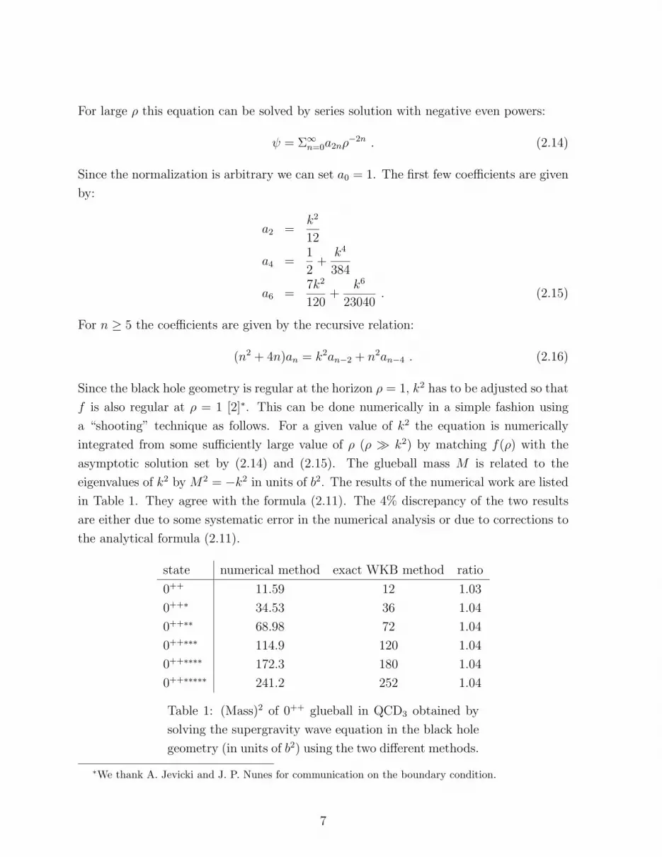
Since the black hole geometry is regular at the horizon ρ = 1, k2 has to be adjusted so that

f is also regular at ρ = 1 [2]∗. This can be done numerically in a simple fashion using

a “shooting” technique as follows. For a given value of k2 the equation is numerically

integrated from some sufficiently large value of ρ (ρ k2) by matching f(ρ) with the

asymptotic solution set by (2.14) and (2.15). The glueball mass M is related to the

eigenvalues of k2 by M2 = −k2 in units of b2. The results of the numerical work are listed

in Table 1. They agree with the formula (2.11). The 4% discrepancy of the two results

are either due to some systematic error in the numerical analysis or due to corrections to

the analytical formula (2.11).

state numerical method exact WKB method ratio

0++ 11.59 12 1.03

0++∗ 34.53 36 1.04

0++∗∗ 68.98 72 1.04

0++∗∗∗ 114.9 120 1.04

0++∗∗∗∗ 172.3 180 1.04

0++∗∗∗∗∗ 241.2 252 1.04

Table 1: (Mass)2 of 0++ glueball in QCD3 obtained by

solving the supergravity wave equation in the black hole

geometry (in units of b2) using the two different methods.

∗We thank A. Jevicki and J. P. Nunes for communication on the boundary condition.

7

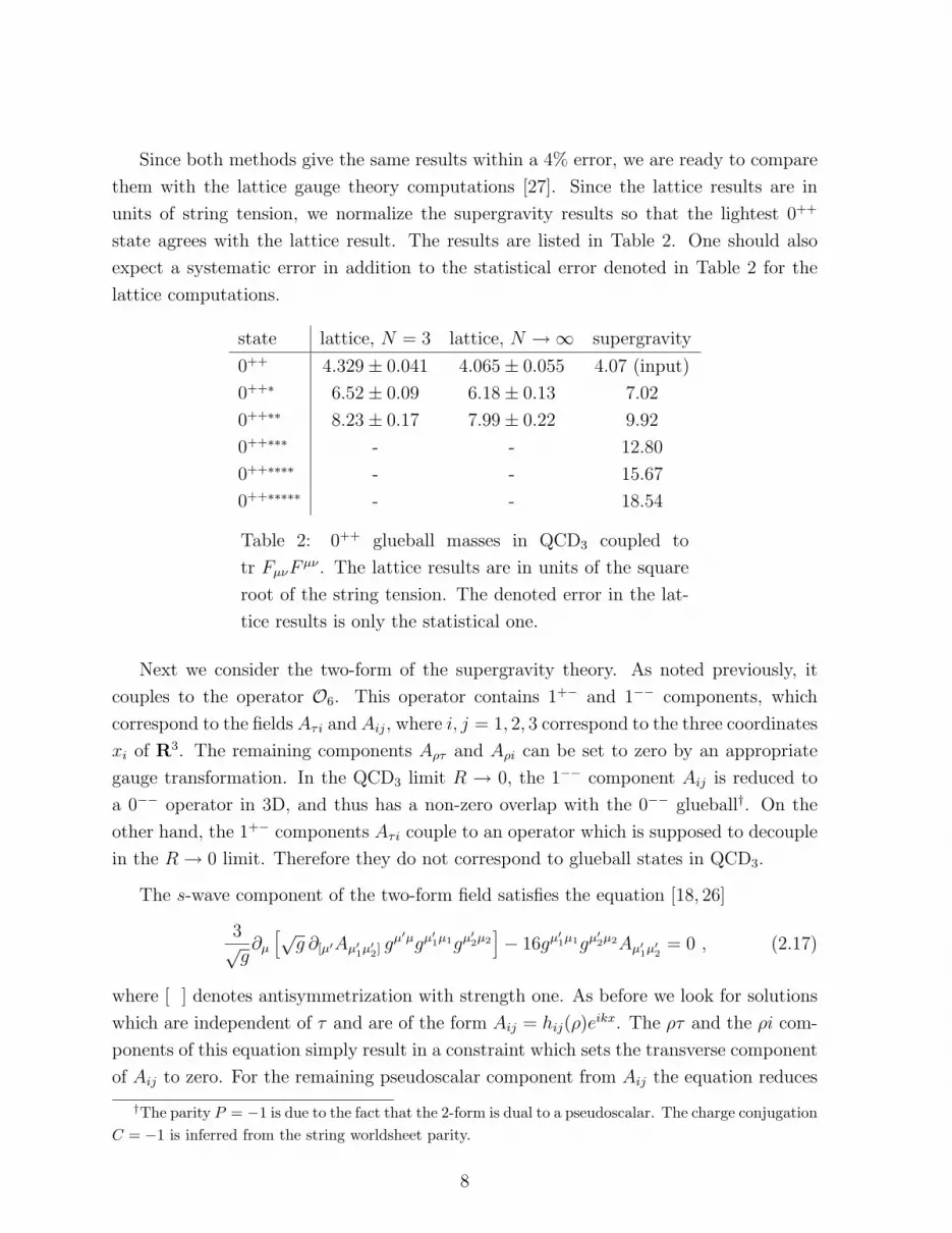
Since both methods give the same results within a 4% error, we are ready to compare

them with the lattice gauge theory computations [27]. Since the lattice results are in

units of string tension, we normalize the supergravity results so that the lightest 0++

state agrees with the lattice result. The results are listed in Table 2. One should also

expect a systematic error in addition to the statistical error denoted in Table 2 for the

lattice computations.

state lattice, N = 3 lattice, N →∞ supergravity

0++ 4.329± 0.041 4.065± 0.055 4.07 (input)

0++∗ 6.52± 0.09 6.18± 0.13 7.02

0++∗∗ 8.23± 0.17 7.99± 0.22 9.92

0++∗∗∗ - - 12.80

0++∗∗∗∗ - - 15.67

0++∗∗∗∗∗ - - 18.54

Table 2: 0++ glueball masses in QCD3 coupled to

tr FµνFµν . The lattice results are in units of the square

root of the string tension. The denoted error in the lat-

tice results is only the statistical one.

Next we consider the two-form of the supergravity theory. As noted previously, it

couples to the operator O6. This operator contains 1+− and 1−− components, which

correspond to the fields Aτi and Aij, where i, j = 1, 2, 3 correspond to the three coordinates

xi of R3. The remaining components Aρτ and Aρi can be set to zero by an appropriate

gauge transformation. In the QCD3 limit R → 0, the 1−− component Aij is reduced to

a 0−− operator in 3D, and thus has a non-zero overlap with the 0−− glueball†. On the

other hand, the 1+− components Aτi couple to an operator which is supposed to decouple

in the R→ 0 limit. Therefore they do not correspond to glueball states in QCD3.

The s-wave component of the two-form field satisfies the equation [18, 26]

3√g∂µ

[√g ∂[µ′Aµ′1µ′2] g

µ′µgµ′1µ1gµ′2µ2

]− 16gµ′1µ1gµ′2µ2Aµ′1µ′2

= 0 , (2.17)

where [ ] denotes antisymmetrization with strength one. As before we look for solutions

which are independent of τ and are of the form Aij = hij(ρ)eikx. The ρτ and the ρi com-

ponents of this equation simply result in a constraint which sets the transverse component

of Aij to zero. For the remaining pseudoscalar component from Aij the equation reduces

†The parity P = −1 is due to the fact that the 2-form is dual to a pseudoscalar. The charge conjugationC = −1 is inferred from the string worldsheet parity.

8

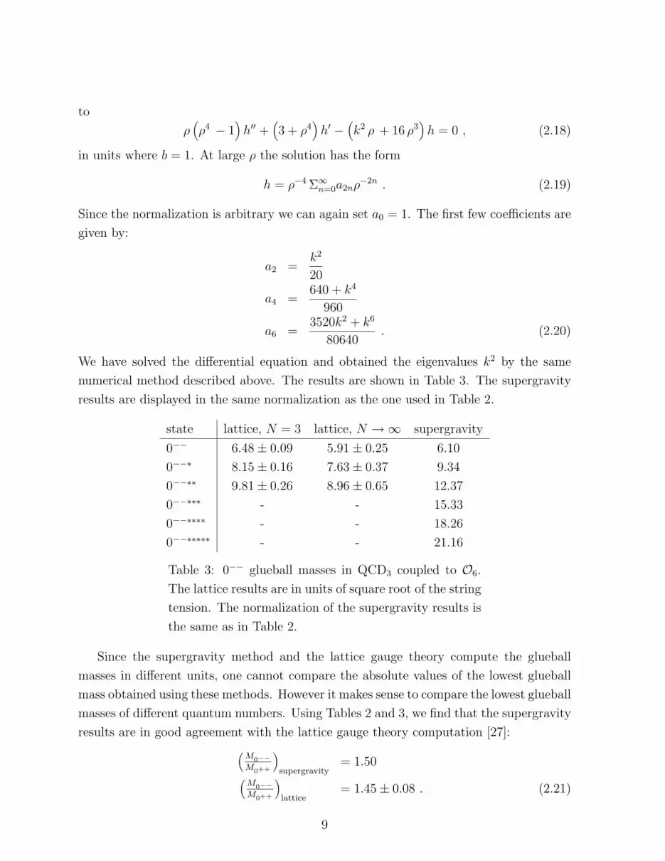
to

ρ(ρ4 − 1

)h′′ +

(3 + ρ4

)h′ −

(k2 ρ + 16 ρ3

)h = 0 , (2.18)

in units where b = 1. At large ρ the solution has the form

h = ρ−4 Σ∞n=0a2nρ

−2n . (2.19)

Since the normalization is arbitrary we can again set a0 = 1. The first few coefficients are

given by:

a2 =k2

20

a4 =640 + k4

960

a6 =3520k2 + k6

80640. (2.20)

We have solved the differential equation and obtained the eigenvalues k2 by the same

numerical method described above. The results are shown in Table 3. The supergravity

results are displayed in the same normalization as the one used in Table 2.

state lattice, N = 3 lattice, N →∞ supergravity

0−− 6.48± 0.09 5.91± 0.25 6.10

0−−∗ 8.15± 0.16 7.63± 0.37 9.34

0−−∗∗ 9.81± 0.26 8.96± 0.65 12.37

0−−∗∗∗ - - 15.33

0−−∗∗∗∗ - - 18.26

0−−∗∗∗∗∗ - - 21.16

Table 3: 0−− glueball masses in QCD3 coupled to O6.

The lattice results are in units of square root of the string

tension. The normalization of the supergravity results is

the same as in Table 2.

Since the supergravity method and the lattice gauge theory compute the glueball

masses in different units, one cannot compare the absolute values of the lowest glueball

mass obtained using these methods. However it makes sense to compare the lowest glueball

masses of different quantum numbers. Using Tables 2 and 3, we find that the supergravity

results are in good agreement with the lattice gauge theory computation [27]:(M0−−M0++

)supergravity

= 1.50(M0−−M0++

)lattice

= 1.45± 0.08 . (2.21)

9

There are still two more SO(6) singlet supergravity fields. One of them is the s-wave

component of the metric gαα and the R-R 4-form Aαβγδ polarized along S5. From (2.4) we

see that it should couple to a dimension 8 scalar operator O8. In [23, 24], this operator is

identified as a symmetrized form of[F 4 − 1

4(F 2)2

]. By using the prescription of Tseytlin

[28] to symmetrize the group indices, one finds that the operator is even under the charge

conjugation. This is also seen from the fact that gαα is clearly even both spacetime and

worldsheet parity transformations. Therefore gαα has the quantum numbers of the 0++

glueball. The classical equation of motion of gαα is that of a massive scalar with (AdS

mass)2 = 32 (in units of b2) [18] on the AdS5 black hole background (2.2). The mass

spectrum that we get is given in Table 4. In the gsN →∞ limit the operators O8 and trF 2

are not mixed since they couple to different states in the supergravity theory. However, we

expect that for finite gsN these operators will mix, thus the full 0++ spectrum is expected

to be given by the interleaving of Tables 2 and 4. For example the 0++∗∗ presumably

corresponds to the first state in Table 4.

gαα and Aαβγδ

8.85

12.06

15.00

17.98

Table 4: 0++ glueball masses in QCD3 coupled to O8, the

normalization is the same as in Table 2.

The remaining SO(6) singlet is the graviton gµν . It couples to the energy-momentum

tensor Tµν and therefore corresponds to the 2++ glueball. It would be interesting to

compute its mass and compare with the lattice result.

3 Glueballs in Four Dimensions

To construct QCD4, one starts with the superconformal theory in six dimensions

realized on N parallel coinciding M5-branes. The compactification of this theory on

a circle of radius R1 gives a five-dimensional theory whose low-energy effective theory

is the maximally supersymmetric SU(N) gauge theory with gauge coupling constant

g25 = R1. To obtain QCD4, one compactifies this theory further on another S1 of radius

R2. The gauge coupling constant g4 in 4D is given by g24 = g2

5/R2 = R1/R2. To break

supersymmetry, one imposes the anti-periodic boundary condition on the fermions around

the second S1.

10

According to Maldacena [1], the largeN limit of the six-dimensional theory isM theory

on AdS7×S4. Upon compactification on S1×S1 and imposing the anti-periodic boundary

conditions around the second S1, we find M theory to be on the black hole geometry [2].

To take the large N limit while keeping g24N finite, we have to take R1 R2. In this

limit, M theory reduces to type IIA string theory and the M5 brane wrapping on S1 of

radius R1 becomes a D4 brane. The large N limit of QCD4 then becomes string theory

on the black hole geometry given by

ds2

l2sg25N/4π

=dρ2

4ρ3/2(1− b6

ρ3

) + ρ3/2

(1− b6

ρ3

)dτ 2 + ρ3/2

4∑i=1

dx2i + ρ1/2dΩ2

4, (3.1)

with a dilaton eφ ∼ ρ3/4 [29]. The location of the horizon ρ = b2 is related to the radius

R2 of the compactifying circle as

b =1

3R2

(3.2)

As in the case of three dimensions, we will compute the spectrum of glueball masses by

solving the classical equations of motions of Kaluza-Klein modes of the supergravity the-

ory. We will consider only singlets of the SO(5) isometry group of S4, which corresponds

to the R-symmetry group of the six-dimensional theory.

Consider first the 0++ glueball. The non-extremal D4 brane solution has a non con-

stant dilaton background. As shown in [30] the dilaton is a linear combination of two

scalars. One of them is massless and couples to the relevant glueball operator. The

equation of motion for the scalar is given by (2.5) in the background of the metric (3.1).

Again assuming that the solution is independent of τ and of the form Φ = f(λ)eikx (with

λ2 = ρ), one obtains the differential equation in the units where b = 1 as

(λ7 − λ)f ′′(λ) + (10λ6 − 4)f ′(λ)− λ3k2f(λ) = 0 . (3.3)

The asymptotic solutions to this equation are f ∼ 1, λ−9, with the latter corresponding to

normalizable solutions. In order to solve the equation and find the allowed values of k2 we

introduce the function g(λ) as f(λ) = λ−9g(λ). This way g(λ) has to be asymptotically

constant for λ → ∞, and one can again look for a solution in terms of a negative power

series in λ. The differential equation for g(λ) is

(λ8 − λ2)g′′ + (14λ− 8λ7)g′ − (λ4k2 + 54)g = 0. (3.4)

The first few coefficients in the power series solution g =∑∞

n=0 a2nλ−2n are given by (for

a0 = 1)

a2 =k2

22

11

a4 =k4

1144

a6 =61776 + k6

102960. (3.5)

The regularity of f at λ = 1, after numerically solving the equation (3.4) as described in

the previous section, results in the allowed values of k2. The first six masses (normalized so

that the lightest 0++ state agrees with the lattice calculation) together with the available

lattice results [32, 33] are given in Table 5.

state lattice, N = 3 supergravity

0++ 1.61± 0.15 1.61 (input)

0++∗ 2.8 2.38

0++∗∗ - 3.11

0++∗∗∗ - 3.82

0++∗∗∗∗ - 4.52

0++∗∗∗∗∗ - 5.21

Table 5: Masses of the first few 0++ glueballs in QCD4, in

GeV, from supergravity compared to the available lattice

results. Note that the authors of ref. [33] do not quote

errors for the 0++∗ since it is not yet clear whether it is

a genuine excited state or merely a two glueball bound

state.

In order to calculate the masses of the 0−+ glueball in four dimensions we will consider

the 3-form Aαβγ of the eleven dimensional supergravity. In this case, it is more useful to

use the eleven-dimensional metric

ds2 =dλ2(

λ2

b2− b4

λ4

) +

(λ2

b2− b4

λ4

)dτ 2 + λ2

5∑i=1

dx2i + dΩ2

4, (3.6)

which reduces to (3.1) upon compactifying x5 on S1 and by going to the string frame [2]

by multiplying the metric by λ, setting λ2 = ρ, and rescaling the other coordinates. The

s-wave component of the 3-form in the harmonic expansion on S4 is a singlet of the SO(5)

isometry group [31]. Its mass squared∗ is 36 in units of b2 and using (2.4) we see that it

couples to a dimension 9 operator of the six-dimensional theory. The 3-form obeys the

following equation of motion:

4√g∂µ

[√g ∂[µ′Aµ′1µ′2µ′3] g

µ′µgµ′1µ1gµ′2µ2gµ′3µ3

]− 36gµ′1µ1gµ′2µ2gµ′3µ3Aµ′1µ′2µ′3

= 0 . (3.7)

∗The value of the mass term is fixed by matching the supergravity computation [31] to (2.4) [34].

12

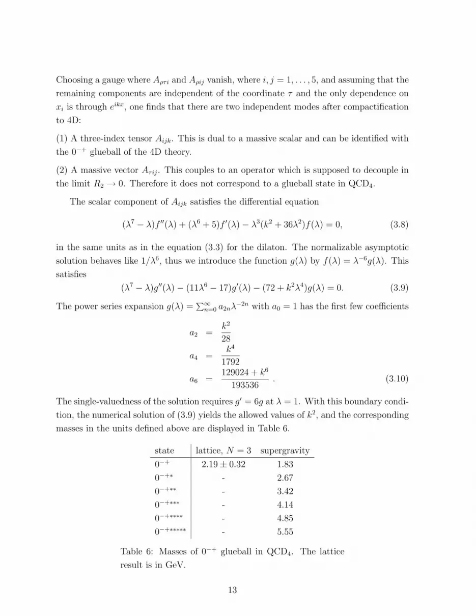
Choosing a gauge where Aρτi and Aρij vanish, where i, j = 1, . . . , 5, and assuming that the

remaining components are independent of the coordinate τ and the only dependence on

xi is through eikx, one finds that there are two independent modes after compactification

to 4D:

(1) A three-index tensor Aijk. This is dual to a massive scalar and can be identified with

the 0−+ glueball of the 4D theory.

(2) A massive vector Aτij. This couples to an operator which is supposed to decouple in

the limit R2 → 0. Therefore it does not correspond to a glueball state in QCD4.

The scalar component of Aijk satisfies the differential equation

(λ7 − λ)f ′′(λ) + (λ6 + 5)f ′(λ)− λ3(k2 + 36λ2)f(λ) = 0, (3.8)

in the same units as in the equation (3.3) for the dilaton. The normalizable asymptotic

solution behaves like 1/λ6, thus we introduce the function g(λ) by f(λ) = λ−6g(λ). This

satisfies

(λ7 − λ)g′′(λ)− (11λ6 − 17)g′(λ)− (72 + k2λ4)g(λ) = 0. (3.9)

The power series expansion g(λ) =∑∞

n=0 a2nλ−2n with a0 = 1 has the first few coefficients

a2 =k2

28

a4 =k4

1792

a6 =129024 + k6

193536. (3.10)

The single-valuedness of the solution requires g′ = 6g at λ = 1. With this boundary condi-

tion, the numerical solution of (3.9) yields the allowed values of k2, and the corresponding

masses in the units defined above are displayed in Table 6.

state lattice, N = 3 supergravity

0−+ 2.19± 0.32 1.83

0−+∗ - 2.67

0−+∗∗ - 3.42

0−+∗∗∗ - 4.14

0−+∗∗∗∗ - 4.85

0−+∗∗∗∗∗ - 5.55

Table 6: Masses of 0−+ glueball in QCD4. The lattice

result is in GeV.

13

Unlike the 3D case, there exists little lattice data on the masses of the excited glueball

states. We can however compare the ratio of masses of the lowest glueball states 0−+ and

0++

(M0−+

M0++

)supergravity

= 1.14(M0−+

M0++

)lattice

= 1.36± 0.32 , (3.11)

and the results are in agreement within the one σ error.

4 Leading String Theory Corrections

As we mentioned earlier, the supergravity computation is valid in the strong ultraviolet

coupling limit gsN 1. In order to compare with the lattice computations in the

continuum limit, we have to take gsN → 0 as we take the ultraviolet cutoff R−1 → ∞so that the scale set by the Yang-Mills coupling constant remains at the intrinsic energy

scale of QCD. The fact that the glueball masses computed in the supergravity limit are

in good agreement with the lattice results leads us to suspect that, for this particular

computation, α′ corrections are small. In this section, we test this idea.

For gsN 1, the curvature of the black hole geometry becomes larger than the

string scale. Therefore stringy corrections (to be precise, the worldsheet sigma-model

corrections) are expected to become important. The leading stringy corrections to the

low-energy supergravity action were obtained in [15, 16]. Recently Gubser, Klebanov and

Tseytlin [17] used the modified action to obtain the leading order string corrections to the

black hole metric. We use their result to calculate the leading corrections to the glueball

mass spectrum. We will perform this computation only for the 0++ glueballs in QCD3.

We expect, however, that the conclusions will be similar for the other glueball states.

According to [17], the leading (in units of the curvature) α′ = (4πgsN)−1/2 correction

to the AdS5 black hole metric (2.2) is

ds2

l2s

√4πg2

4N= (1 + δ1)

dρ2(ρ2 − b4

ρ2

) + (1 + δ2)

(ρ2 − b4

ρ2

)dτ 2 + ρ2

3∑i=1

dx2i , (4.1)

where the correction terms δ1,2 are given by the formulae

δ1 = +15γ

(5b4

ρ4+ 5

b8

ρ8− 19

b12

ρ12

)

δ2 = −15γ

(5b4

ρ4+ 5

b8

ρ8− 3

b12

ρ12

), (4.2)

14

and γ is given by γ = 18ζ(3)α′3. With these corrections of the metric, the dilaton is no

longer constant, instead it is given by

Φ0 = −45

8γ

(b4

ρ4+

b8

2ρ8+

b12

3ρ12

). (4.3)

There is also a correction to the ten-dimensional dilaton action [15, 16], given by

Idilaton = − 1

16πG10

∫d10x

√g[−1

2gµν∂µΦ∂νΦ + γe−

32ΦW

], (4.4)

where W is given in terms of the Weyl tensor, and in our background W = 180/ρ16 in

units where b = 1. To the leading order in γ, the dilaton perturbation does not mix with

the metric perturbation, so we can study the dilaton equation derived from the action

(4.4) in the fixed metric background (4.1). In subleading order in γ, the term γe−32ΦW

would generate a mixing of the dilaton and the graviton.

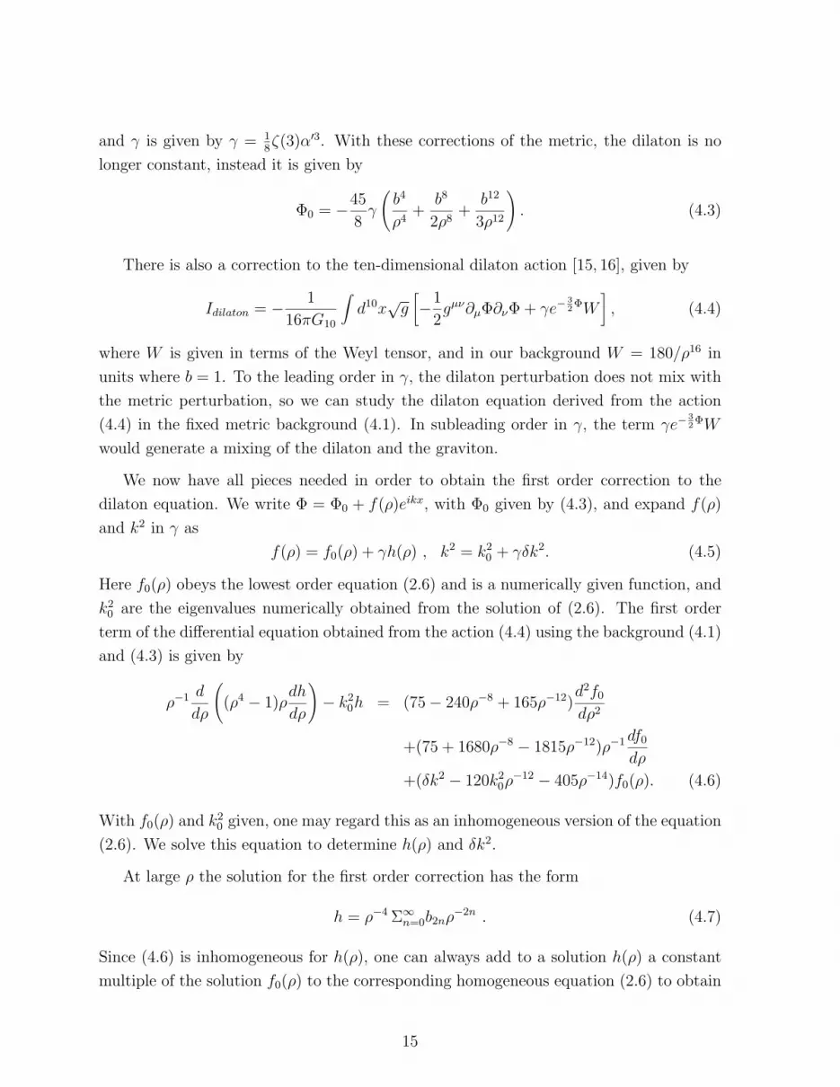
We now have all pieces needed in order to obtain the first order correction to the

dilaton equation. We write Φ = Φ0 + f(ρ)eikx, with Φ0 given by (4.3), and expand f(ρ)

and k2 in γ as

f(ρ) = f0(ρ) + γh(ρ) , k2 = k20 + γδk2. (4.5)

Here f0(ρ) obeys the lowest order equation (2.6) and is a numerically given function, and

k20 are the eigenvalues numerically obtained from the solution of (2.6). The first order

term of the differential equation obtained from the action (4.4) using the background (4.1)

and (4.3) is given by

ρ−1 d

dρ

((ρ4 − 1)ρ

dh

dρ

)− k2

0h = (75− 240ρ−8 + 165ρ−12)d2f0

dρ2

+(75 + 1680ρ−8 − 1815ρ−12)ρ−1df0

dρ

+(δk2 − 120k20ρ

−12 − 405ρ−14)f0(ρ). (4.6)

With f0(ρ) and k20 given, one may regard this as an inhomogeneous version of the equation

(2.6). We solve this equation to determine h(ρ) and δk2.

At large ρ the solution for the first order correction has the form

h = ρ−4 Σ∞n=0b2nρ

−2n . (4.7)

Since (4.6) is inhomogeneous for h(ρ), one can always add to a solution h(ρ) a constant

multiple of the solution f0(ρ) to the corresponding homogeneous equation (2.6) to obtain

15

another solution. We use this freedom to set b0 = 0. The first few coefficients are then

given by:

b2 =δk2

12

b4 =14400 + 2δk2k2

0

384

b6 =1344δk2 + 100800k2

0 + 3δk2k40

23040. (4.8)

We can now determine δk2 by the same “shooting” method described above for each

eigenvalue of k20 and its corresponding eigenfunction f0(ρ). It turns out that, for each

eigenvalue k20, there is is a unique solution with h being regular at ρ = 1. The first few

solutions are shown in Table 7.

state (−k20) (−δk2) δk2/k2

0

0++ 11.59 89.75 7.74

0++∗ 34.53 365.7 10.59

0++∗∗ 68.98 809.8 11.74

0++∗∗∗ 114.9 1397 12.16

0++∗∗∗∗ 172.3 2122 12.32

0++∗∗∗∗∗ 241.2 2991 12.40

Table 7: Leading string correction to the 0++ glueball masses in QCD3. The

first column gives the zeroth order supergravity result for the mass squared,

the second column gives the coefficient of the leading string correction and the

third column gives their ratio.

Recalling that the squared mass of each glueball states is given by

M2 = −(k2

0 +1

8δk2ζ(3)α′3 + · · ·

)b2, (4.9)

we see that the leading stringy corrections to the 0++ glueball masses are

M20++ = 11.59× (1 + 0.97ζ(3)α′3 + · · ·)b2

M20++∗ = 34.53× (1 + 1.32ζ(3)α′3 + · · ·)b2

M20++∗∗ = 68.98× (1 + 1.47ζ(3)α′3 + · · ·)b2

M20++∗∗∗ = 114.9× (1 + 1.52ζ(3)α′3 + · · ·)b2

M20++∗∗∗∗ = 172.3× (1 + 1.54ζ(3)α′3 + · · ·)b2

M20++∗∗∗∗∗ = 241.2× (1 + 1.55ζ(3)α′3 + · · ·)b2 . (4.10)

16

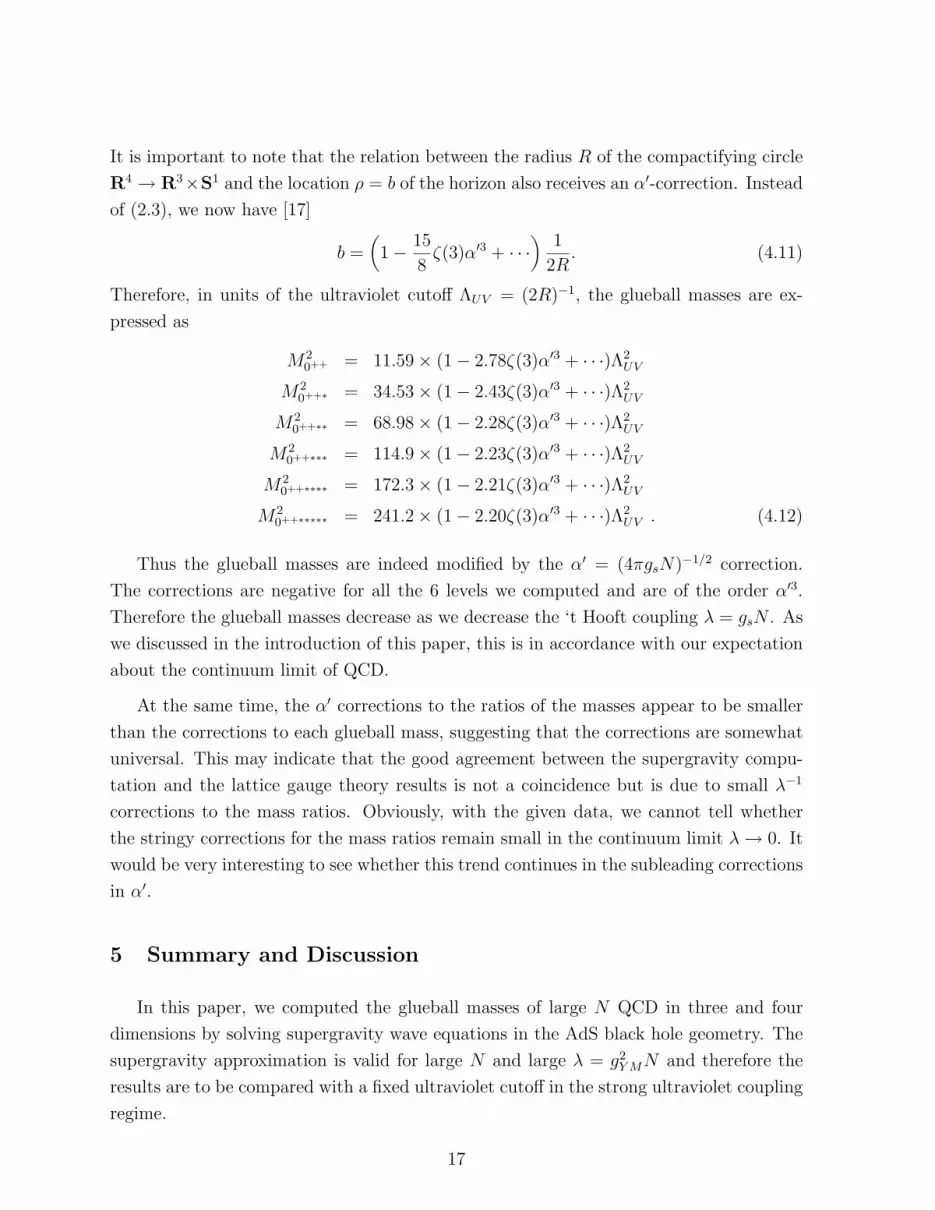
It is important to note that the relation between the radius R of the compactifying circle

R4 → R3×S1 and the location ρ = b of the horizon also receives an α′-correction. Instead

of (2.3), we now have [17]

b =(1− 15

8ζ(3)α′3 + · · ·

)1

2R. (4.11)

Therefore, in units of the ultraviolet cutoff ΛUV = (2R)−1, the glueball masses are ex-

pressed as

M20++ = 11.59× (1− 2.78ζ(3)α′3 + · · ·)Λ2

UV

M20++∗ = 34.53× (1− 2.43ζ(3)α′3 + · · ·)Λ2

UV

M20++∗∗ = 68.98× (1− 2.28ζ(3)α′3 + · · ·)Λ2

UV

M20++∗∗∗ = 114.9× (1− 2.23ζ(3)α′3 + · · ·)Λ2

UV

M20++∗∗∗∗ = 172.3× (1− 2.21ζ(3)α′3 + · · ·)Λ2

UV

M20++∗∗∗∗∗ = 241.2× (1− 2.20ζ(3)α′3 + · · ·)Λ2

UV . (4.12)

Thus the glueball masses are indeed modified by the α′ = (4πgsN)−1/2 correction.

The corrections are negative for all the 6 levels we computed and are of the order α′3.

Therefore the glueball masses decrease as we decrease the ‘t Hooft coupling λ = gsN . As

we discussed in the introduction of this paper, this is in accordance with our expectation

about the continuum limit of QCD.

At the same time, the α′ corrections to the ratios of the masses appear to be smaller

than the corrections to each glueball mass, suggesting that the corrections are somewhat

universal. This may indicate that the good agreement between the supergravity compu-

tation and the lattice gauge theory results is not a coincidence but is due to small λ−1

corrections to the mass ratios. Obviously, with the given data, we cannot tell whether

the stringy corrections for the mass ratios remain small in the continuum limit λ→ 0. It

would be very interesting to see whether this trend continues in the subleading corrections

in α′.

5 Summary and Discussion

In this paper, we computed the glueball masses of large N QCD in three and four

dimensions by solving supergravity wave equations in the AdS black hole geometry. The

supergravity approximation is valid for large N and large λ = g2Y MN and therefore the

results are to be compared with a fixed ultraviolet cutoff in the strong ultraviolet coupling

regime.

17

We computed the ratios of the masses of the excited glueball states with the mass

of the lowest state, as well as the ratio of masses of two different lowest glueball states.

These ratios are in surprisingly good agreement with the available lattice data. We also

computed the leading λ−3/2 corrections to the glueball masses taking into account stringy

corrections to the black hole geometry. We found that the corrections to the masses are in

accordance with our expectation about the continuum limit of QCD. The corrections to

the ratios of the masses appear to be smaller than the corrections to each glueball mass,

suggesting that the corrections are somewhat universal.

The above computations can be generalized to higher spin glueballs. As noted pre-

viously, the graviton couples to the energy-momentum tensor and solving its equation

of motion will give the masses of the 2++ glueball. In general the higher spin glueballs

will correspond to operators that couple to massive string excitations. The dimensions

of these operators are ∆ ∼ λ1/4 for large λ [8]. It would be interesting to see how to

extrapolate this result to the continuum λ→ 0.

Another interesting issue is the existence of SO(6) non-singlet states in supergravity.

For large λ, their masses are of the same order as the SO(6) singlet states we studied in

this paper. In the continuum limit, ΛUV →∞ and λ→ 0, those states should decouple.

Presumably λ−1 corrections make them heavy.

Maldacena’s conjecture reduces the problem of solving large N QCD in three and four

dimensions to that of controlling the α′ corrections to the two-dimensional sigma-model

with the Ramond-Ramond background. In this paper, we have extracted information

about glueballs in strongly coupled QCD using the α′-expansion of the sigma-model. It

would certainly be interesting to understand properties of such a sigma-model better.

Note Added

Recently the masses of the SO(6) non-singlet states have been computed in [35] where

it was found that they are comparable to those of the glueballs computed in this paper.

It was also shown that the leading λ−1 corrections computed using the metric (4.1) do

not make these states heavier than the glueballs. Therefore, the decoupling of the SO(6)

non-singlet states is not evident to this order.

However, more recently, it was pointed out in [36] (see also [37]) that the S5 part

of the metric also receives the O(α′3) correction. The glueball masses computed in this

paper would not be affected by such a correction since they correspond to states that

we are constant on S5. On the other hand, the masses of the SO(6) non-singlet states

18

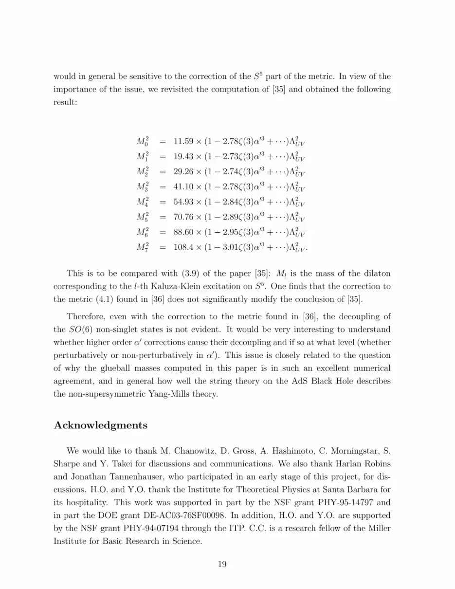
would in general be sensitive to the correction of the S5 part of the metric. In view of the

importance of the issue, we revisited the computation of [35] and obtained the following

result:

M20 = 11.59× (1− 2.78ζ(3)α′3 + · · ·)Λ2

UV

M21 = 19.43× (1− 2.73ζ(3)α′3 + · · ·)Λ2

UV

M22 = 29.26× (1− 2.74ζ(3)α′3 + · · ·)Λ2

UV

M23 = 41.10× (1− 2.78ζ(3)α′3 + · · ·)Λ2

UV

M24 = 54.93× (1− 2.84ζ(3)α′3 + · · ·)Λ2

UV

M25 = 70.76× (1− 2.89ζ(3)α′3 + · · ·)Λ2

UV

M26 = 88.60× (1− 2.95ζ(3)α′3 + · · ·)Λ2

UV

M27 = 108.4× (1− 3.01ζ(3)α′3 + · · ·)Λ2

UV .

This is to be compared with (3.9) of the paper [35]: Ml is the mass of the dilaton

corresponding to the l-th Kaluza-Klein excitation on S5. One finds that the correction to

the metric (4.1) found in [36] does not significantly modify the conclusion of [35].

Therefore, even with the correction to the metric found in [36], the decoupling of

the SO(6) non-singlet states is not evident. It would be very interesting to understand

whether higher order α′ corrections cause their decoupling and if so at what level (whether

perturbatively or non-perturbatively in α′). This issue is closely related to the question

of why the glueball masses computed in this paper is in such an excellent numerical

agreement, and in general how well the string theory on the AdS Black Hole describes

the non-supersymmetric Yang-Mills theory.

Acknowledgments

We would like to thank M. Chanowitz, D. Gross, A. Hashimoto, C. Morningstar, S.

Sharpe and Y. Takei for discussions and communications. We also thank Harlan Robins

and Jonathan Tannenhauser, who participated in an early stage of this project, for dis-

cussions. H.O. and Y.O. thank the Institute for Theoretical Physics at Santa Barbara for

its hospitality. This work was supported in part by the NSF grant PHY-95-14797 and

in part the DOE grant DE-AC03-76SF00098. In addition, H.O. and Y.O. are supported

by the NSF grant PHY-94-07194 through the ITP. C.C. is a research fellow of the Miller

Institute for Basic Research in Science.

19

References

[1] J. M. Maldacena, “The Large N Limit of Superconformal Field Theories and Supergravity,”hep-th/9711200.

[2] E. Witten, “Anti-de Sitter Space, Thermal Phase Transition, And Confinement in GaugeTheories,” hep-th/9803131.

[3] A. Brandhuber, N. Itzhaki, J. Sonnenschein, S. Yankielowicz, “Wilson Loops in the LargeN Limit at Finite Temperature,” hep-th/9803137.

[4] S.-J. Rey, S. Theisen and J. Yee, “Wilson-Polyakov Loop at Finite Temperature in LargeN Gauge Theory and Anti-de Sitter Supergravity,” hep-th/9803135.

[5] M. Li, “’t Hooft Vortices on D-branes,” hep-th/9803252; “’t Hooft vortices and phases oflarge N gauge theory,” hep-th/9804175.

[6] E. Witten, “Baryons and Branes in Anti-de Sitter Space,” hep-th/9805112.

[7] D. J. Gross and H. Ooguri, “ Aspects of Large N Gauge Theory Dynamics as Seen byString Theory,” hep-th/9805129.

[8] S.S. Gubser, I.R. Klebanov, A.M. Polyakov, “Gauge Theory Correlators from Non-CriticalString Theory,” hep-th/9802109.

[9] E. Witten, “Anti-de Sitter Space and Holography,” hep-th/9802150.

[10] I. R. Klebanov, “World Volume Approach to Absorption by Non-Dilatonic Branes,” hep-th/9702076; Nucl. Phys. B496 (1997) 231.

[11] S. S. Gubser, I. R. Klebanov and A. A. Tseytlin, “String Theory and Classical Absorptionby Threebranes,” hep-th/9703040; Nucl. Phys. B499 (1997) 217.

[12] G. Horowitz and H. Ooguri, “Spectrum of Large N Gauge Theory from Supergravity,”hep-th/9802116, Phys. Rev. Lett. 80 (1998) 4116.

[13] S. Ferrara, C. Fronsdal and A. Zaffaroni, “On N = 8 Supergravity on AdS5 and N = 4Superconformal Yang-Mills theory,” hep-th/9802203.

[14] Y. Oz and J. Terning, “Orbifolds of AdS5 × S5 and 4d Conformal Field Theories, ” hep-th/9803167.

[15] M. T. Grisaru, A. E. M. van de Ven and D. Zanon, “Four-Loop Beta Function for theN = 1 and N = 2 Supersymmetric Nonlinear Sigma-Model in Two Dimensions,” Phys.Lett. B173 (1986) 423; M. T. Grisaru and D. Zanon, “Sigma-Model Superstring Correctionsto the Einstein-Hilbert Action,” Phys. Lett. B177 (1986) 347.

[16] D. J. Gross and E. Witten, “ Superstring Modifications of Einstein Equation,” Nucl. Phys.B277 (1986) 1.

20

[17] S. S. Gubser, I. R. Klebanov and A. A. Tseytlin, “Coupling Constant Dependence in theThermodynamics of N = 4 Supersymmetric Yang-Mills Theory,” hep-th/9805156.

[18] H. J. Kim, L. J. Romans, P. Van Nieuwenhuizen, “Mass Spectrum of Chiral Ten-Dimensional N = 2 Supergravity on S5,” Phys. Rev. D32 (1985) 389.

[19] M. Gunaydin, N. Marcus, “The Spectrum of The S5 Compactification of Chiral N =2, D = 10 Supergravity and The Unitary Supermultiplets of U(2, 2/4),”Class.Quant.Grav.2 (1985) L11.

[20] T. Aoki, T. Kawai and Y. Takei, “Algebraic Analysis of Singular Perturbations – On ExactWKB Analysis,” Sugaku Exposition 8-2 (1995) 217, and references therein.

[21] Y. Takei and T. Koike, private communication.

[22] S. Das and S. Trivedi, “Three Brane Action and The Correspondence Between N = 4 YangMills Theory and Anti-de Sitter Space,” hep-th/9804149.

[23] S. Ferrara, M. A. Lledo, A. Zaffaroni, “Born-Infeld Corrections to D3 brane Action inAdS5 × S5 and N = 4, d = 4 Primary Superfields,” hep-th/9805082.

[24] S. S. Gubser, A. Hashimoto, I. R. Klebanov, M. Krasnitz, “Scalar Absorption and theBreaking of the World Volume Conformal Invariance,” hep-th/9803023.

[25] J. Mandula, G. Zweig, and J. Govaerts, “Covariant Lattice Glueball Fields,” Nucl. Phys.B228 (1983) 109.

[26] S. Mathur and A. Matusis, “Absorption of Partial Waves by Three-Branes,” hep-th/9805064.

[27] M.J. Teper, “SU(N) gauge Theories in (2 + 1) Dimensions”, hep-lat/9804008.

[28] A.A. Tseytlin, “On Non-Abelian Generalization of Born-Infeld Action in String Theory,”Nucl. Phys. B501 (1997) 41, hep-th/9701125.

[29] N. Itzhaki, J. Maldacena, J. Sonnenschein and S. Yankielowicz, “Supergravity and TheLarge N Limit of Theories With Sixteen Supercharges,” hep-th/9802042.

[30] G. Horowitz and A. Strominger, “Black Strings and p-Branes,” Nucl. Phys. B360 (1991)197.

[31] P. Van Nieuwenhuizen, “The Complete Mass Spectrum of d = 11 Supergravity Compacti-fied on S4 and a General Mass Formula for Arbitrary Cosets M4”, Class. Quantum Grav.2 (1985) 1.

[32] M.J. Teper, ”Physics from lattice: glueballs in QCD; topology; SU(N) for all N ,” hep-lat/9711011.

[33] C. Morningstar and M. Peardon, “Efficient Glueball Simulations on Anisotropic Lattices,”Phys. Rev. D56 (1997) 4043, hep-lat/9704011.

21

[34] O. Aharony, Y. Oz and Z. Yin, “M Theory on AdSp × S11−p and Superconformal FieldTheories,” hep-th/9803051.

[35] H. Ooguri, J. Tannenhauser and H. Robins, “Glueballs and Their Kalaluza-Klein Cousin,”hep-th/9806171, to appear in Phys. Lett. B.

[36] J. Pawelczyk and S. Theisen, “AdS5 × S5 Black Hole Metric at O(α′3),” hep-th/9808126.

[37] Note added to [17] on August 19, 1998.

22