arX

iv:h

ep-t

h/95

0614

7v1

21

Jun

1995

La Plata-Th 95-10

SUPERGRAVITY AND A BOGOMOL’NYI

BOUND IN THREE DIMENSIONS

Jose D. Edelstein∗, Carlos Nunez and Fidel A. Schaposnik†

Departamento de Fısica, Universidad Nacional de La Plata

C.C. 67, (1900) La PlataArgentina

Abstract

We discuss the 2 + 1 dimensional Abelian Higgs model coupled to

N = 2 supergravity. We construct the supercharge algebra and, from

it, we show that the mass of classical static solutions is bounded from

below by the topological charge. As it happens in the global case,

half of the supersymmetry is broken when the bound is attained and

Bogomol’nyi equations, resulting from the unbroken supersymmetry,

hold. These equations, which correspond to gravitating vortices, in-

clude a first order self-duality equation whose integrability condition

reproduces the Einstein equation.

∗CONICET†Investigador CICBA, Argentina

1 Introduction

The relevance of the solutions to classical equations of motion of non-linearfield theories (solitons, instantons) is nowadays recognized both in Mathe-matics and in Physics [1].

Since the pioneering work by Belavin, Polyakov, Schwartz and Tyup-kin [2] an important feature of many of these (second order) equations ofmotion was discovered: through the obtention of a bound of topological ori-gin (for the energy or the action, depending on the case), solutions can befound studying much simpler first order differential equations (self-dualityequations or Bogomol’nyi equations [3]) An increasing number of works havebeen addressed to this issue in the last 20 years.

Already in ref.[4], where the Bogomol’nyi equations were first writtenfor the Abelian Higgs model, it was recognized that the existence of thesefirst-order equations was connected with the necessary conditions for super-symmetry in models with gauge symmetry breaking [5].

Other works then stressed this fact [6] but the main advance in the under-standing of this question was achieved by Olive and Witten [7] in their workon the connection between topological quantum numbers and the centralcharge of extended supersymmetry. An important result of this investigationwas to show that the classical aproximation to the mass spectrum is exactat the quantum level since supersymmetry ensures that there are no quan-tum corrections. In other words, the Bogomol’nyi’s bound is valid quantummechanically and is saturated.

Many models were studied afterwards following this line [8]-[11]. Con-cerning gauge theories with symmetry breaking (the case of interest in thepresent work) the interplay between Bogomol’nyi equations and supersym-metry can be understood as follows [11]:

For gauge theories with symmetry breaking having a topological charge andan N = 1 supersymmetric version, the N = 2 supersymmetric extension,which requires certain conditions on coupling constants, has a central chargecoinciding with the topological charge. This relation ensures the existence,of a Bogomol’nyi bound and, consequently, of Bogomol’nyi equations.

It is important to note that in the soliton sector, half of the supersym-metries of the theory are broken [12].

Once the connection between global supersymmetry and Bogomol’nyi

1

bounds was understood, the natural question to pose is whether similar phe-nomena take place for local supersymmetry including gravity. That is, toinvestigate the possibility of establishing a connection between supergravityand Bogomol’nyi bounds for gravitating solitons and from this, to obtain first-order differential equations whose solutions also solve Einstein and Maxwell(or Yang-Mills) equations together.

The works on this issue are based on those of Teitelboim [13], Deser andTeitelboim [14], Grisaru [15] and Witten-Nester-Israel [16]-[17] on positivityof the energy using supergravity. On this line, the Einstein-Maxwell theorywas investigated by Gibbons and Hull [18] and the analog of Bogomol’nyibounds were found for the (ADM) mass [19]. In the same vein, Kallosh et al[20], Gibbons et al [21] and Cvetic et al [22] studied different gravity models.

Extending our previous work on the globally supersymmetric case [11], westudy in the present paper the Abelian Higgs model coupled to supergravityin 2 + 1 dimensions. We have chosen such a model in view of the experienceaccumulated in the study of Bogomol’nyi equations for vortex configurations,the connection we have already established for global supersymmetry and thesimplicity one should expect from a 2 + 1 abelian model. To our knowledge,there is not much work on this model except for a recent paper by Becker,Becker and Strominger [23], reported while the present investigation wasin progress. Although some of our results overlap those in [23], we thinkit is worthwhile to present a detailed discussion of our approach which isbased, as in the global case [11], in the study of the supersymmetry algebraand provides a systematic way of exploiting supersymmetry in the search ofBogomol’nyi equations. Not surprisingly, being the supersymmetry local, wefind that a 1 form, analogous to the Witten-Nester-Israel form used in theproof of positivity of the energy in gravitation [16]-[17], plays a central rolein our derivation.

Indeed, we will show explicitely that the supercharge algebra can be re-alized in terms of the circulation, over a space-like surface contour, of ageneralized Witten-Nester-Israel form adapted to the present d = 2+1 case.This fact will be shown to be at the root of the existence of a Bogomol’nyibound. Our procedure will be systematic in the sense that its formulation isadapted to any supergravity model where conserved supercharges could bedefined and with a bosonic sector admiting topological charges.

The plan of the paper is as follows: in Section 2 we carefully discuss theN = 1, d = 3 + 1 supergravity action establishing our notation and conven-

2

tions so that the dimensionally reduced 2 + 1 Abelian Higgs model coupledto supergravity can be easily obtained (Section 3). Section 4 addresses tothe supersymmetry algebra and its connection with the Bogomol’nyi bound(from which Bogomol’nyi equations can be obtained). We give a discussionof our results in Section 5.

2 The N = 1 Action in d = 4

We shall construct the N = 2 locally supersymmetric Abelian Higgs model in3-dimensional space by dimensional reduction [24] of an appropriate N = 1,d = 4 supergravity model. To our knowledge, it was not until very recentlythat the (Bosonic sector of the) corresponding Lagrangian has been written[23]. This section is addressed to the description of the Abelian Higgs modelcoupled to N = 1 four-dimensional supergravity leaving for Section 3 thedimensional reduction.

Let us consider the following locally supersymmetric and gauge invariantsuperspace action for matter interacting with gravity and electromagnetism

S =∫

d4xd4θE[

1

2∆(Φ,Φe2qV) exp (−ξκ2V) +Re

(

2

RWW

)]

(1)

Here, Φ is a chiral (matter) multiplet whose component fields are the Higgsfield φ, a Higgsino Ξ and an auxilliary field F . V is a vector (gauge) multi-plet which in the Wess-Zumino gauge contains the photon AM , the photinoΛ and a real auxilliary field D. W is the supercovariant strength multipletcontaining the vector field strength. The superspace determinant is denotedby E and R is a chiral scalar curvature superfield [25]. We will distinguishcurved (M,N,R, . . .) and flat (A,B,C, . . .) indices. The N = 1 supergrav-ity multiplet contains the vierbein V A

M , the gravitino ΨM , a complex scalarauxilliary field U and a pseudovector auxilliary field bM . ∆(Φ,Φe2qV) is anarbitrary gauge invariant functional while q is the U(1) charge. ξ is a realparameter and κ is the gravitational constant. We have not included a su-perpotential term. The interaction between chiral and vector multiplets isthe local version of the Fayet-Iliopoulos term [26]. We shall adopt hereafterthe Wess-Zumino gauge.

After some calculations, the N = 1 supergravity Lagrangian (1) can be

3

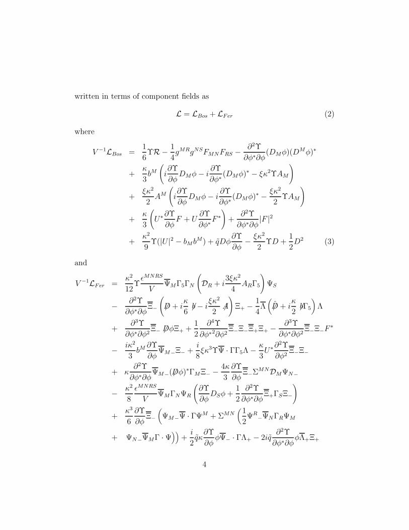
written in terms of component fields as

L = LBos + LFer (2)

where

V −1LBos =1

6ΥR− 1

4gMRgNSFMNFRS − ∂2Υ

∂φ∗∂φ(DMφ)(DMφ)∗

+κ

3bM

(

i∂Υ

∂φDMφ− i

∂Υ

∂φ∗(DMφ)∗ − ξκ2ΥAM

)

+ξκ2

2AM

(

i∂Υ

∂φDMφ− i

∂Υ

∂φ∗(DMφ)∗ − ξκ2

2ΥAM

)

+κ

3

(

U∗∂Υ

∂φF + U

∂Υ

∂φ∗F ∗

)

+∂2Υ

∂φ∗∂φ|F |2

+κ2

9Υ(|U |2 − bMb

M) + qDφ∂Υ

∂φ− ξκ2

2ΥD +

1

2D2 (3)

and

V −1LFer =κ2

12ΥǫMNRS

VΨMΓ5ΓN

(

DR + i3ξκ2

4ARΓ5

)

ΨS

− ∂2Υ

∂φ∗∂φΞ−

(

6D + iκ

66b− i

ξκ2

26A)

Ξ+ − 1

4Λ(

ˆ6D + iκ

26bΓ5

)

Λ

+∂3Υ

∂φ∗∂φ2Ξ− 6DφΞ+ +

1

2

∂4Υ

∂φ∗2∂φ2Ξ−Ξ−Ξ+Ξ+ − ∂3Υ

∂φ∗∂φ2Ξ−Ξ−F

∗

− iκ2

3bM

∂Υ

∂φΨM−Ξ− +

i

8ξκ3ΥΨ · ΓΓ5Λ − κ

3U∗∂

2Υ

∂φ2Ξ−Ξ−

+ κ∂2Υ

∂φ∗∂φΨM−( 6Dφ)∗ΓMΞ− − 4κ

3

∂Υ

∂φΞ−ΣMNDMΨN−

− κ2

8

ǫMNRS

VΨMΓNΨR

(

∂Υ

∂φDSφ+

1

2

∂2Υ

∂φ∗∂φΞ+ΓSΞ−

)

+κ3

6

∂Υ

∂φΞ−

(

ΨM−Ψ · ΓΨM + ΣMN(

1

2ΨR

−ΨNΓRΨM

+ ΨN−ΨMΓ · Ψ))

+i

2qκ∂Υ

∂φφΨ− · ΓΛ+ − 2iq

∂2Υ

∂φ∗∂φφΛ+Ξ+

4

− κ2

2

∂2Υ

∂φ∗∂φΨM−Ξ−Ψ

M+Ξ+ − ξκ2

2

∂Υ

∂φ∗Ξ+Λ+

+κ

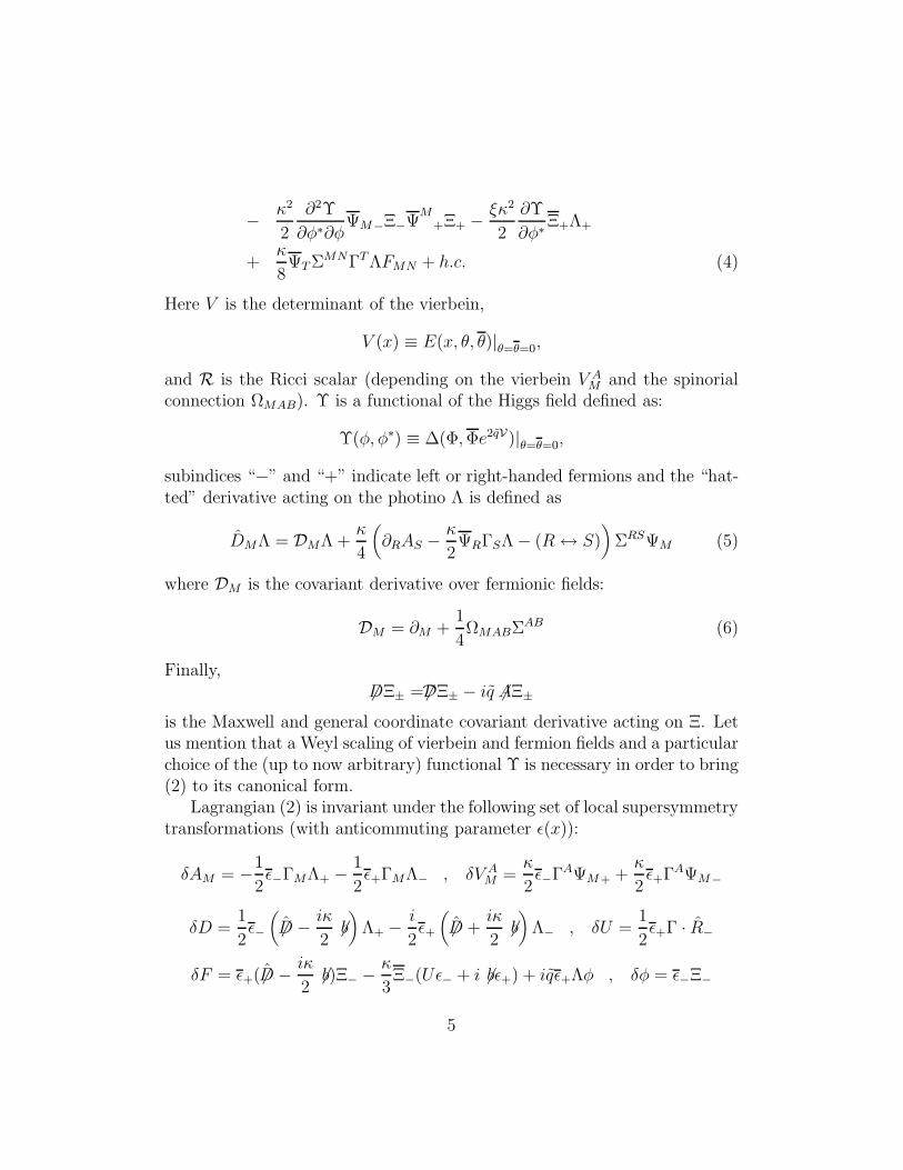
8ΨT ΣMNΓT ΛFMN + h.c. (4)

Here V is the determinant of the vierbein,

V (x) ≡ E(x, θ, θ)|θ=θ=0,

and R is the Ricci scalar (depending on the vierbein V AM and the spinorial

connection ΩMAB). Υ is a functional of the Higgs field defined as:

Υ(φ, φ∗) ≡ ∆(Φ,Φe2qV)|θ=θ=0,

subindices “−” and “+” indicate left or right-handed fermions and the “hat-ted” derivative acting on the photino Λ is defined as

DMΛ = DMΛ +κ

4

(

∂RAS − κ

2ΨRΓSΛ − (R ↔ S)

)

ΣRSΨM (5)

where DM is the covariant derivative over fermionic fields:

DM = ∂M +1

4ΩMABΣAB (6)

Finally,6DΞ± = 6DΞ± − iq 6AΞ±

is the Maxwell and general coordinate covariant derivative acting on Ξ. Letus mention that a Weyl scaling of vierbein and fermion fields and a particularchoice of the (up to now arbitrary) functional Υ is necessary in order to bring(2) to its canonical form.

Lagrangian (2) is invariant under the following set of local supersymmetrytransformations (with anticommuting parameter ǫ(x)):

δAM = −1

2ǫ−ΓMΛ+ − 1

2ǫ+ΓMΛ− , δV A

M =κ

2ǫ−ΓAΨM+ +

κ

2ǫ+ΓAΨM−

δD =1

2ǫ−

(

ˆ6D − iκ

26b)

Λ+ − i

2ǫ+

(

ˆ6D +iκ

26b)

Λ− , δU =1

2ǫ+Γ · R−

δF = ǫ+( ˆ6D − iκ

26b)Ξ− − κ

3Ξ−(Uǫ− + i 6bǫ+) + iqǫ+Λφ , δφ = ǫ−Ξ−

5

δbM =3i

4ǫ−

(

RM− − 1

3ΓMΓ · R−

)

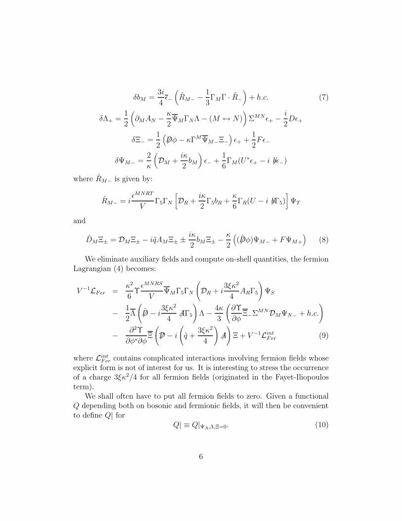
+ h.c. (7)

δΛ+ =1

2

(

∂MAN − κ

2ΨMΓNΛ − (M ↔ N)

)

ΣMN ǫ+ − i

2Dǫ+

δΞ− =1

2

(

6Dφ− κΓMΨM−Ξ−

)

ǫ+ +1

2Fǫ−

δΨM− =2

κ

(

DM +iκ

2bM

)

ǫ− +1

6ΓM(U∗ǫ+ − i 6bǫ−)

where RM− is given by:

RM− = iǫMNRT

VΓ5ΓN

[

DR +iκ

2Γ5bR +

κ

6ΓR(U − i 6bΓ5)

]

ΨT

and

DMΞ± = DMΞ± − iqAMΞ± ± iκ

2bMΞ± − κ

2

(

( ˆ6Dφ)ΨM− + FΨM+

)

(8)

We eliminate auxiliary fields and compute on-shell quantities, the fermionLagrangian (4) becomes:

V −1LFer =κ2

6ΥǫMNRS

VΨMΓ5ΓN

(

DR + i3ξκ2

4ARΓ5

)

ΨS

− 1

2Λ

(

ˆ6D − i3ξκ2

46AΓ5

)

Λ − 4κ

3

(

∂Υ

∂φΞ−ΣMNDMΨN− + h.c.

)

− ∂2Υ

∂φ∗∂φΞ

(

6D − i

(

q +3ξκ2

4

)

6A)

Ξ + V −1LintFer (9)

where LintFer contains complicated interactions involving fermion fields whose

explicit form is not of interest for us. It is interesting to stress the occurrenceof a charge 3ξκ2/4 for all fermion fields (originated in the Fayet-Iliopoulosterm).

We shall often have to put all fermion fields to zero. Given a functionalQ depending both on bosonic and fermionic fields, it will then be convenientto define Q| for

Q| ≡ Q|ΨA,Λ,Ξ=0. (10)

6

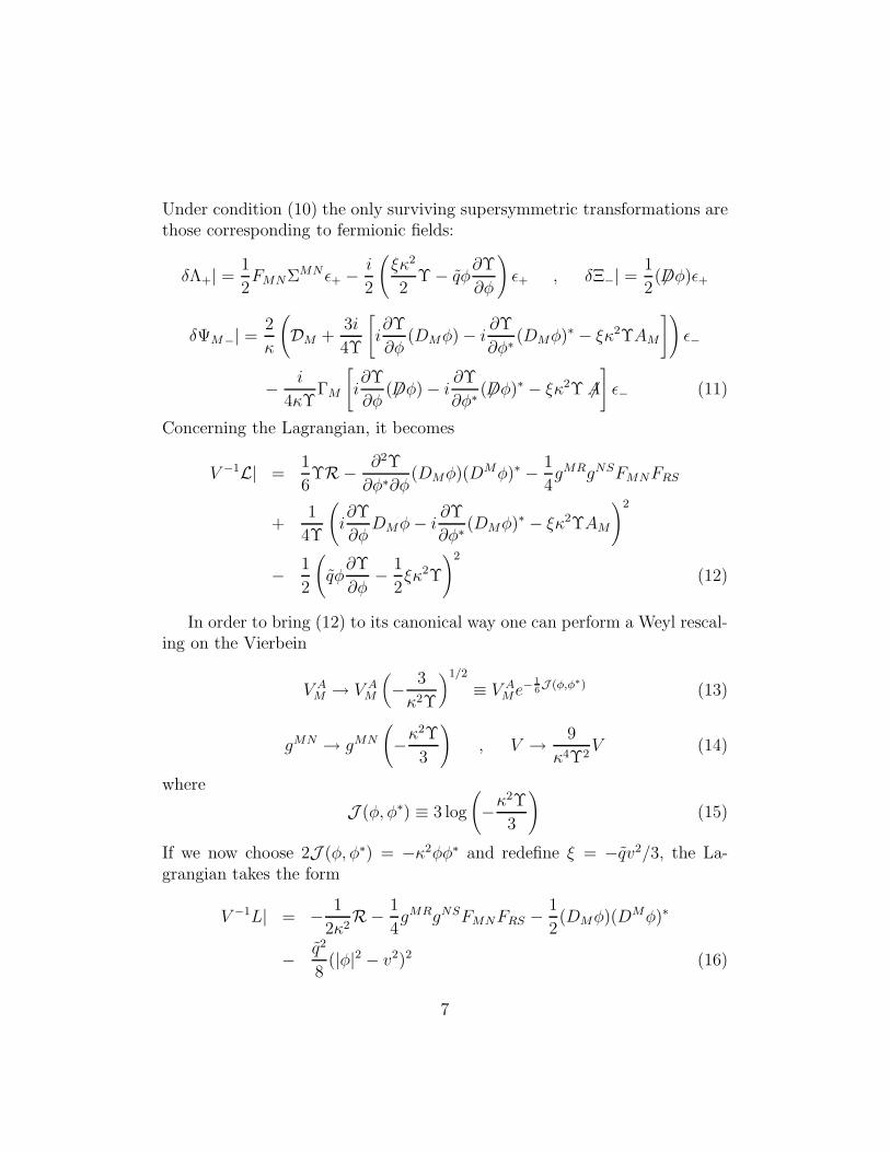
Under condition (10) the only surviving supersymmetric transformations arethose corresponding to fermionic fields:

δΛ+| =1

2FMNΣMN ǫ+ − i

2

(

ξκ2

2Υ − qφ

∂Υ

∂φ

)

ǫ+ , δΞ−| =1

2( 6Dφ)ǫ+

δΨM−| =2

κ

(

DM +3i

4Υ

[

i∂Υ

∂φ(DMφ) − i

∂Υ

∂φ∗(DMφ)∗ − ξκ2ΥAM

])

ǫ−

− i

4κΥΓM

[

i∂Υ

∂φ( 6Dφ) − i

∂Υ

∂φ∗( 6Dφ)∗ − ξκ2Υ 6A

]

ǫ− (11)

Concerning the Lagrangian, it becomes

V −1L| =1

6ΥR− ∂2Υ

∂φ∗∂φ(DMφ)(DMφ)∗ − 1

4gMRgNSFMNFRS

+1

4Υ

(

i∂Υ

∂φDMφ− i

∂Υ

∂φ∗(DMφ)∗ − ξκ2ΥAM

)2

− 1

2

(

qφ∂Υ

∂φ− 1

2ξκ2Υ

)2

(12)

In order to bring (12) to its canonical way one can perform a Weyl rescal-ing on the Vierbein

V AM → V A

M

(

− 3

κ2Υ

)1/2

≡ V AMe

− 1

6J (φ,φ∗) (13)

gMN → gMN

(

−κ2Υ

3

)

, V → 9

κ4Υ2V (14)

where

J (φ, φ∗) ≡ 3 log

(

−κ2Υ

3

)

(15)

If we now choose 2J (φ, φ∗) = −κ2φφ∗ and redefine ξ = −qv2/3, the La-grangian takes the form

V −1L| = − 1

2κ2R− 1

4gMRgNSFMNFRS − 1

2(DMφ)(DMφ)∗

− q2

8(|φ|2 − v2)2 (16)

7

which is the expected Abelian Higgs model Lagrangian minimally coupled togravity. Note that the coupling constant of the Higgs potential is related tothe electric charge by the well-known condition

λ =q2

8(17)

This condition was originally found for the globally supersymmetric model[5]. As explained in [11] it gives a necessary condition for extending N = 1to N = 2 supersymmetry and, at the same time, for finding a Bogomol’nyibound [3, 4] for the energy of the Abelian Higgs model.

It is interesting to note that Weyl transformations for fermion fields, incorrespondance with (13) bring, on the one hand the gravitino Lagrangianto its usual Rarita-Schwinger form. On the other hand, as we shall see, theHiggs potential and the Higgs current take after the scaling its usual form ascan be seen in the resulting Bogomol’nyi equations. Under this Weyl scaling

ΨM →(

− 3

κ2Υ

)1/4

ΨM , Λ →(

− 3

κ2Υ

)−3/4

Λ , Ξ →(

− 3

κ2Υ

)−1/4

Ξ

(18)

ǫ→(

− 3

κ2Υ

)1/4

ǫ

one has

δΛ+| =1

2FMNΣMNǫ+ +

iq

4(|φ|2 − v2)ǫ+ , δΞ−| =

1

2( 6Dφ)ǫ+

δΨM−| =2

κ

(

DM +iκ2

4(JM + qv2AM)

)

ǫ− (19)

where

JM =i

2(φ(DMφ)∗ − φ∗(DMφ)) (20)

is the Higgs field current.Although we will finally put all fermion fields to zero, we will need for

further calculations the explicit form of the kinetic Lagrangian for fermions.After the Weyl rescaling (18) is performed in Lagrangian (9), one can notethat the kinetic fermionic part can be diagonalized by the following shift:

ΨM− → ΨM− − 1

κΥ

∂Υ

∂φ∗ΓMΞ+ (21)

8

such that the Fermion Lagrangian can be finally written as:

V −1LFer = −1

2ǫMNRSVΨMΓ5ΓN

(

DR + iqv2κ2

4ARΓ5

)

ΨS

− 1

2Ξ

(

6D − i

(

q +qv2κ2

4

)

6A)

Ξ

− 1

2Λ

(

6D − iqv2κ2

46AΓ5

)

Λ + V −1LintFer (22)

once the above mentioned conditions for J (φ, φ∗) and ξ are adopted.

3 Dimensional Reduction and Extended su-

persymmetry

We shall now derive the d = 3, N = 2 Lagrangian by dimensional reductionof (16). To this end, we write the vierbein as:

V AM =

(

eaµ aµ

0 ϕ

)

(23)

(we use µ = 0, 1, 2 for curved coordinates and a = 0, 1, 2 for flat indices)and suppose that whole set of fields are x3-independent. We will accord-ingly choose x3 as the variable which is eliminated within the dimensionalreduction procedure. We introduce in (23) ea

µ as the dreibein of the reduced3-dimensional manifold, aµ as a vector field and ϕ as a real scalar. We havechosen the gauge V a

3 = 0, which can always be attained by a suitable localLorentz transformation [24]. Indeed, an infinitesimal field variation of V A

M

under local supersymmetry, local Lorentz and general coordinate transfor-mations reads

δV AM = −iκǫΓAΨM + ωA

BVBM + ∂Mη

RV AR + ηR∂RV

AM (24)

where ǫ, ωAB and ηR are the corresponding local parameters. Freedom associ-

ated with general coordinate invariance in four dimensions can be exploitedto put

aµ = 0 , ϕ = 1 (25)

9

without spoiling the local Einstein group of the reduced 3-dimensional space-time.

With these conditions, the metric tensor reads

gMN = V MA V N

B ηAB =

(

gµν 00 −1

)

(26)

where ηAB = diag(+ − −−). Concerning the spinorial connection, it takesthe form

Ωcab| = ωcab| = −1

2(em

c ena − em

a enc )∂nemb +

1

2em

a enb ∂nemc − (a↔ b) (27)

while all other components vanish. Then, the Ricci scalar in four dimensionsR reduces to the corresponding one in d = 3, which will be denote as R.

After dimensional reduction, Lagrangian (16) becomes

e−1L| = − 1

2κ2R− 1

4gµρgνσFµνFρσ − 1

2(Dµφ)(Dµφ)∗

+1

2∂µS∂

µS +q2

2S2|φ|2 − q2

8(|φ|2 − v2)2 (28)

where we have identifiedAM ≡ (Aµ, S) .

Lagrangian (28) describes the dynamics of the Bosonic sector for the d = 3Abelian Higgs model coupled to N = 2 supergravity. We will now focus onthe dimensional reduction of supersymmetric transformation rules written ineq.(19). To this end, let us specify our representation for the Clifford algebra

Γa = γa ⊗ τ3 , Γ3 = 1 ⊗ iτ2 , Γ5 = 1 ⊗ τ1

Σab = σab ⊗ 1 , Σa3 = −Σ3a = γa ⊗ τ1 (29)

where γa are 2 × 2 Dirac matrices for d = 3 and σab = 1/2[γa, γb]. In thisbasis the original 4-dimensional Majorana spinors take the form

Ψ =

(

Ψ1

iΨ2

)

(30)

10

where Ψ1 and Ψ2 are 2-component real spinors which can be taken as 3-dimensional Majorana fields. Finally, with these Majorana fields one canconstruct a Dirac spinor ψ in 3 dimensions

ψ = Ψ1 + iΨ2.

The dimensionally reduced supersymmetric transformations for fermionsread

δλ| =1

2Fµνσ

µνǫ+iq

4(|φ|2 − v2)ǫ+ γµ∂µSǫ

δχ| =1

2( 6Dφ+ iqSφ) ǫ , δψ3| = −i qκ

2S(|φ|2 − v2)ǫ (31)

δψµ| =2

κ

(

Dµ + iκ2

4(Jµ + qv2Aµ)

)

ǫ ≡ 2

κ∇µǫ.

Note that we have included the transformation for ψ3, a remnant of the 4dimensional starting model. However, as we shall see, S will be put to zeroto recover the Abelian Higgs model in the bosonic sector, this giving a trivialψ3 transformation rule. Being ǫ a Dirac fermion, transformations (31) areN = 2 supersymmetric ones. Supersymmetric covariant derivative ∇µ isdefined as

∇µǫ =

(

∂µ +1

4ωµabσ

ab + iκ2

4(Jµ + qv2Aµ)

)

ǫ (32)

We shall end this Section by performing the dimensional reduction of thefermionic Lagrangian (22) which is the fermionic counterpart of the N = 2bosonic Lagrangian (28). In order to achieve a diagonalized kinetic fermionicsector, we perform the following shift

ψµ → ψµ + iγµψ3

after which, the resulting fermionic Lagrangian reads:

e−1LFer = −1

2

ǫρµσ

eψρ∂µψσ − 1

2λ 6∂λ− 1

2χ 6∂χ

− iψ3 6∂ψ3 + e−1LintFer (33)

where the last term LintFer includes also gauge interactions.

11

4 Self-duality equations and the Bogomol’nyi

bound

In this Section we shall obtain a Bogomol’nyi bound for field configurationsin the d = 3 Abelian Higgs model coupled to gravity. In doing this, we shallmake explicit the relation between this bound and the supercharge algebraof the N = 2 theory.

The equations of motion for bosonic matter fields are:

1√−g∂µ(√−gF µν) = −qJν (34)

1√−gDµ(√−gDµφ) =

q2

2(|φ|2 − v2)φ− q2S2φ (35)

1√−g∂µ(√−g∂µS) = q2|φ|2S. (36)

Concerning Einstein equations

Rµν −1

2gµνR = Tmat

µν , (37)

Tmatµν = −gλτFµτFνλ −

1

2(Dµφ)(Dνφ)∗ − 1

2(Dµφ)∗(Dνφ) − ∂µS∂νS

+ gµν

[

1

4FρσF

ρσ +1

2(Dρφ)(Dρφ)∗ − 1

2∂ρS∂

ρS − q2

2S2|φ|2

+q2

8(|φ|2 − v2)2

]

(38)

Since we shall focus on the Abelian Higgs model coupled to gravity, wemake at this point S = 0. Moreover, since Bogomol’nyi equations correspondto static configurations with A0 = 0, we also impose these conditions (notethat in this case Tmat

0i = 0).Concerning the metric, let us notice that a static spacetime admits a

surface Π orthogonal everywhere to the time-like killing vector field ∂∂t

. In alocal chart adapted to ∂

∂t, the line element can be written as:

ds2 = dt2 + gijdxidxj (39)

12

where gij is a function depending only on spatial variables that span Π. Now,it is well-known that any 2-dimensional metric is Kahler and then we writethe interval in the form

ds2 = dt2 − Ω2dzdz (40)

where Ω is a function of the conformal coordinates Ω(z, z). Note that for anyfinite energy configuration, Einstein equations (37) constrain the asymptoticbehaviour of Ω to be

Ω(z, z) → (zz)−κ2

M

2 (41)

so that the metric is asymptotic to a flat cone with deficit angle δ = κ2M[27], M being related to the source mass

M =1

4π

∫

dzdzΩ2Tmattt =

1

4π

∫

dzdzΩ2[

1

2FzzF

zz

+1

2(Dzφ)(Dzφ)∗ +

1

2(Dzφ)(Dzφ)∗ +

q2

8(|φ|2 − v2)2

]

. (42)

The spacetime metric (40) can be generated by the following dreibein

e0t = e−z = 1 , e+z = Ω2 (43)

(all the other components vanishing) with the flat metric written in conformalcoordinates as

η00 = −2η+− = −2η−+ = 1.

The non-vanishing component of the spinorial connection is:

ωz+− = −∂ log Ω (44)

(here ∂ ≡ ∂z and ∂ ≡ ∂z).We shall now analyse theN = 2 algebra of supercharges for our model. To

construct these charges we shall follow the Noether method. The conservedcurrent associated with local supersymmetry is given by:

J µ[ǫ] =∑

Φ

δL

δ∇µΦδǫΦ +

∑

Ψ

δL

δ∇µΨδǫΨ − θµ[ǫ] (45)

where Φ and Ψ represent the whole set of bosonic and fermionic fields re-spectively. Concerning θµ[ǫ], it is defined through

δǫS =∫

d3x∇µθµǫ . (46)

13

In the present case we have:

θµ[ǫ] = − 3

2κ

ǫµρσ

eψρ∇σǫ−

1

2ǫ(Dµφ)χ+

1

2ǫγνF

µνλ− 1

8χγµ( 6Dφ)

− 1

4λγµ

(

1

2Fµνσ

µν +iq

4(|φ|2 − v2)

)

ǫ+ h.c. + . . . (47)

where the dots indicate terms containing products of three fermion fields,which are not relevant for our construction since, after computing the su-percharge algebra, we will put all fermions to zero. Inserting θµ in (45) weobtain the following expression for the supersymmetry current:

J µ[ǫ] = −λγµ(

1

2Fαβσ

αβ +iq

4(|φ|2 − v2)

)

ǫ− 1

2χγµ( 6Dφ)ǫ

− 2

κ

ǫρµσ

eψρ∇σǫ+ h.c. + . . . (48)

The conserved charges associated with (48),

Q[ǫ] =∫

ΣJ µ[ǫ]dΣµ ≡ Q1[ǫ] + iQ2[ǫ], (49)

are defined over a space-like surface Σ whose area element is dΣµ. Here QI ,I=1,2, are the Majorana charge generators.

Now, imposing the gravitino field equation,

2

κ

ǫµσρ

e∇σψρ = λγµ

(

1

2Fµνσ

µν +iq

4(|φ|2 − v2)

)

+1

2χγµ( 6Dφ) (50)

one can see from eqs.(48)-(49), after integration by parts, that the super-charge is nothing but the circulation of the gravitino arround the orientedboundary ∂Σ

Q[ǫ] = −2

κ

∮

∂Σǫψµdx

µ (51)

Let us stress that the expression above coincides with the results presentedby Teitelboim [13] for pure supergravity in 4-dimensional spacetime, afterdimensional reduction. Although there are well-known problems for con-structing supergravity charges in 2+1 dimensions [28]-[29], we shall see thatthey can be overcome in the present model.

As explained in [13], it is not possible to compute the supercharge algebraby (naively) evaluating Posson brackets from (51) because surface terms do

14

not have well defined functional derivatives and hence their Poisson bracketswith the various fields of the theory are not well defined. One can computeinstead the algebra by acting on the integrand of (51) with a supersymmetrytransformation:

Q[ǫ],Q[ǫ]| ≡ δǫQ[ǫ]| =2

κ

∮

∂Σǫδǫψµdx

µ =4

κ2

∮

∂Σǫ∇µǫdx

µ (52)

where Q is given by:

Q =2

κ

∮

∂Σψµǫdx

µ (53)

Now, Teitelboim [13] has proven, using Dirac formalism for constrainedsystems, that supergravity charges, which can be written as surface integralsin the form (51), obey a flat-space supersymmetry algebra

QI ,QJ = δIJγµPµ + ǫIJZ (54)

where Z is the central charge. In flat space, it is a well-known result thatthis algebra leads in several models to Bogomol’nyi bounds for the energy[7]-[11]. Indeed, squaring eq.(54) and tracing over the indices, one obtains abound

P 2 − Z2 ≥ 0

from which, after using the identity of Z with the topological charge of thefield configuration T [7]-[11], one obtains the well-known Bogomol’nyi boundfor the mass M of the configuration

M ≥ |T | (55)

Coming back to supergravity, let us see explicitely how (52) ensures thatstatic finite-energy configurations satisfy a bound of topological nature of thetype (55). To this end, let us write, using the expression for the covariantderivative given in (32)

Q[ǫ],Q[ǫ]| =4

κ2

∮

∂Σǫ∇µǫdx

µ

=4

κ2

∮

∂ΣǫDµǫdx

µ + i∮

∂Σǫǫ(Jµ + qv2Aµ)dx

µ (56)

15

We can now use the asymptotic behaviour of different fields appearing in(56). The spinorial connection which enters in the covariant derivative in thefirst term of the r.h.s. behaves as

ωz+− → κ2M

2z(57)

Concerning the electromagnetic field as well as the Higgs current, finitenessof the energy implies

Az → − inqz

, Az →in

qz, Jz → O

(

1

zz

)

, Jz → O(

1

zz

)

. (58)

(Here, the integer n is the topological number that characterizes the quantaof magnetic flux). Finally, the asymptotic behaviour of ǫ will be written inthe form:

ǫ→ Θ(zz)ǫ∞ (59)

where Θ(zz) will be determined using the so-called Witten condition[16] (seebelow).

We can now evaluate the line-integral (56). To avoid infrared divergences,it is necessary to take the contour of integration at large but finite radius R.Using the asymptotic behaviours listed above, (56) becomes:

Q[ǫ],Q[ǫ]| = (Mǫ∞γ0ǫ∞ − v2nǫ∞ǫ∞)Θ(R)2. (60)

The relation of this result with the Poisson brackets (54) which are valid, inparticular, in flat space, is, of course, no accident: as we discussed above,supersymmetry transformations at spatial infinity generate global N = 2supersymmetry algebra.

We can now prove that Q[ǫ],Q[ǫ]| is semi-positive definite and thenderive a Bogomol’nyi bound of topological origin from (60).

First, let us observe that the supercharge algebra evaluated in the purelybosonic sector is the integral over the boundary of a 1-form ω, constructedfrom a fermionic parameter:

Q[ǫ],Q[ǫ]| =4

κ2

∮

∂Σω (61)

ω = ǫ∇µǫdxµ (62)

16

Now, ω can be identified with the generalized Nester-like form [16, 17] in 3dimensional spacetime. The use of Nester form is at the root of several proofsof the positivity of gravitational energy [13]-[17] and it was also used in 4and 5-dimensional models to find Bogomol’nyi bounds [19]-[22]. In the samevein, we shall see below that the integral of ω on the contour is semi-positivedefinite and that, as a consequence, the theory posses a Bogomol’nyi bound.Let us mention at this point that the integral in the r.h.s. of (61) coincideswith the quantity ∆(r) introduced in Ref.[23]. Our construction shows thatits occurence is a consequence of the N = 2 supercharge algebra.

First, using Stokes’ theorem, we have∮

∂Σω =

∫

Σǫµνβ∇β(ǫ∇µǫ)dΣν . (63)

where the integrand in (63) can be written as

ǫµνβ∇β(ǫ∇µǫ) = ǫµνβ∇βǫ∇µǫ+1

2ǫµνβǫ[∇β, ∇µ]ǫ . (64)

Then, using

[∇µ, ∇ν ] =1

2Rµν

abΣab +iqv2κ2

2Fµν +

iκ2

2(∂µJν − ∂νJµ), (65)

Einstein equations (37) and supersymmetric transformations for the fermio-nic fields λ and χ, we arrive to the following expression

ǫµνβ∇β(ǫ∇µǫ) = ǫµνρ∇µǫ∇ρǫ+κ2

2

[

δǫλγνδǫλ+ δǫχγ

νδǫχ]

. (66)

We now specialize our spacelike integration surface Σ so that dΣµ = (dΣt,~0).Then, we only need to compute the time component of eq.(66) which, aftersome Dirac algebra, reads

ǫtνβ∇β(ǫ∇µǫ) =(

γi∇iǫ)† (

γj∇jǫ)

− gij(

∇iǫ)† (∇jǫ

)

+κ2

2

[

δǫλ†δǫλ+ δǫχ

†δǫχ]

(67)

We see at this point, that if we impose the generalized Witten condition [16]

γi∇iǫ = 0 (68)

17

the r.h.s. of eq.(67) is semi-positive definite

ǫtνβ∇β(ǫ∇µǫ) ≥ 0 (69)

and then, using (63),Q[ǫ],Q[ǫ]| ≥ 0 (70)

The bound is saturated if and only if

δǫλ = 0 (71)

δǫχ = 0 (72)

∇iǫ = 0 (73)

Condition (73) reflects our choice of surface Σ . One can easily see thata more general choice would imply, instead of (73),

∇µǫ = 0 . (74)

In explicit form, eqs.(71), (72) and (74) read:

δǫλ =1

2

[

Fµνσµν +

iq

2(|φ|2 − v2)

]

ǫ = 0 (75)

δǫχ =1

2( 6Dφ)ǫ = 0 (76)

δǫψµ =

(

Dµ + iκ2

4(Jµ + qv2Aµ)

)

ǫ = 0 (77)

We can see at this point that solutions of (75) and (76) break half of thesupersymmetry. Indeed, writting

ǫ ≡(

ǫ+ǫ−

)

(78)

One can easily see that the conditions

δǫ+λ = 0 (79)

δǫ+χ = 0 (80)

18

imply δǫ−λ 6= 0, δǫ−χ 6= 0 for nontrivial solutions. Hence if one is to searchBogomol’nyi equations for non-trivial configurations, it makes sense to con-sider that ǫ has just one independent complex component,

ǫ ≡(

ǫ+0

)

(81)

satisfying equation (68), which then reads

∇zǫ+ = 0 (82)

Let us stress on the fact that field configuration solving Bogomol’nyiequations (which as we shall see coincide with (79) and (80)) break halfof the supersymmetries, a common feature in all models presenting Bogo-mol’nyi bounds with supersymmetric extension (See for example [12, 20]).It can be understood as follows: The number of Killing spinors (those thatsolve eq.(77)) admitted by a certain spacetime coincides with the numberof remnant unbroken supersymmetries [12]. If we attempt to keep all thesupersymmetries of our model, we will find that the resulting field configu-ration has zero energy (the trivial vacuum) as it was remarked above. Then,it is evident that we must restrict the space of solutions of (77) if we wantto obtain non-trivial topological configurations (which, in this sense, requirebreaking of one of the supersymmetries).

We can now study the asymptotic behaviour of the Killing spinor ǫ+ →Θ(R)ǫ+∞. One can see that eq.(82) implies that Θ(R) is a power of theradius R:

Θ(R) = R−κ2 nv2

2 (83)

It is important, at this point, to comment on the existence of non-trivial solu-tions to eq.(82) in asymptotically conical spaces. In fact, the supercovariantderivative in (82) gets an electromagnetic contribution related to the mag-netic flux, and then, as explained in [23], leads to the existence of non-trivialsolutions, otherwise absent [16].

Now, for a parameter ǫ of the form (81), formula (60) can be written as

Q[ǫ],Q[ǫ]| = (M − v2n)ǫ†+∞ǫ+∞Θ(R)2 (84)

We can now finally write a Bogomol’nyi bound using (70) and (84):

M − nv2 ≥ 0 (85)

19

The mass of our field configuration, defined in eq.(42), is then boundedfrom below by the magnetic flux quanta. Analogous results also hold inthe 4 and 5 dimensional models studied by Kallosh et al [20] and Gibbonset al [21] where the bound reads: M ≥

√Q2 + P 2, Q and P being the

electric and magnetic charges respectively, related to the two central chargesexisting in the extended supersymmetry algebra of those models [12]. In thepresent abelian 3-dimensional model there is just one central charge and,moreover, it is not possible to have electrically charged finite energy solitonicconfigurations in the Abelian Higgs model so that Q = 0.

The bound (85) for the d = 3 Abelian Higgs model coupled to gravity coin-cides with that presented in [23]. The novelty here is that we have obtainedit from the supercharge algebra (plus the generalized Witten condition) thusshowing that the connection between global supersymmetry and Bogomol’nyibounds discussed in [7]-[11], also works for local supersymmetry.

The bound (85) is saturated whenever eqs.(75)-(77) hold and hence, weidentify them as the Bogomol’nyi equations of our model. Concerning equa-tions (75) and (76), they can be written in the usual form [3]:

ǫzzFzz +q

2(|φ|2 − v2) = 0 (86)

Dzφ = 0. (87)

They have been found previously in the study of the Einstein-Abelian Higgsmodel by Comtet and Gibbons in ref.[30] where it is shown that this set ofequations admits vortex solutions in 3+1 dimensions which can be interpretedas cosmic strings. Concerning eq.(77),

(

Dµ + iκ2

4(Jµ + qv2Aµ)

)

ǫ+ = 0, (88)

it can be thought as the Bogomol’nyi equation for the gravitational field.Indeed, it can be seen that the integrability conditions of this equation,

[

Dµ + iκ2

4(Jµ + qv2Aµ),Dν + i

κ2

4(Jν + qv2Aν)

]

ǫ+ = 0, (89)

become the Einstein equations once eqs.(86)-(87) are imposed. Even thoughconical spaces usually does not admit covariantly constant spinors, solutions

20

to eq.(88) exist as a consequence of the electromagnetic contribution to thesupercovariant derivative, as explained above. In view of the bound (85), thesolutions of the whole set of Bogomol’nyi equations satisfy the more involvedsecond order Euler-Lagrange ones.

5 Summary and discussion

We have studied Bogomol’nyi bounds for the Abelian Higgs model coupledto gravity in 2 + 1 dimensions by embedding it in an extended N = 2 super-gravity model.

Bogomol’nyi equations for the scalar and the gauge field, compatible withthe Einstein equation, were originally derived by Comtet and Gibbons [30],following the usual Bogomol’nyi approach [3]. In their work, the existenceof gravitating multi-vortex solutions saturating the Bogomol’nyi bound wasproven. These solutions can be understood as cosmic strings and the boundcan be seen to be a restriction in possible values for the deficit angle of conicalspacetime [30].

More recently, Becker, Becker and Strominger [23] considered the modelwe discussed and obtained the Bogomol’nyi bound from supersymmetry argu-ments. They followed an approach which is a variant of the methods leadingto energy positivity in gravity models [16]-[18]. This approach is close to theone we have followed in the present paper. The novelty in our work is thatwe have obtained the Bogomol’nyi bound and the self-duality equations (in-cluding the one associated with the Einstein equation) by constructing thesupercharge algebra and making explicit its relation with the (generalized)Witten-Nester-Israel form.

As it is well-known, in 2+1 dimensions, states with non-zero energy pro-duce asymptotically conical spaces and this put stringent limitations on theexistence of covariantly constant spinors which are basic in the constructionof supercharges. However, in our model, the supercovariant derivative getsa contribution related to the topological charge of the vortex and this allowsfor non-trivial solutions for Killing spinors. This is the reason why we wereable to find supercharges and determine their algebra.

A possible interest of our investigation is related to the recent discus-sion about how can supersymmetry ensure the vanishing of the cosmologicalconstant [28],[23],[29]. On the other side, since our approach provides a sys-

21

tematic way of investigating Bogomol’nyi bounds in supergravity models inarbitrary dimensions (as it is the case for global supersymmetry [7]-[11]), onecan think in finding Bogomol’nyi bounds for other gauge models coupled togravity like, for example, the Chern-Simons-Higgs model recently consideredin [31]. We hope to come back to these problems in a forthcoming work.

References

[1] R. Rajaraman, Solitons and Instantons, North Holland (1982).

[2] A.A. Belavin, A.M. Polyakov, A.S. Schwartz and Yu.S. Tyupkin, Phys.Lett. B 59 (1975) 85.

[3] E.B. Bogomol’nyi, Sov. Jour. Nucl. Phys. 24 (1976) 449.

[4] H. de Vega and F.A. Schaposnik, Phys. Rev. D 14 (1976) 1100.

[5] A. Salam and J. Strathdee, Nucl. Phys. B 97 (1975) 293;

P.Fayet, Il Nuovo Cimento A 31 (1976) 626.

[6] P. Di Vecchia and S. Ferrara, Nucl. Phys. B 130 (1977) 93.

[7] E. Witten and D. Olive, Phys. Lett. B 78 (1978) 77.

[8] Z. Hlousek and D. Spector, Nucl. Phys. B 370 (1992) 43.

[9] Z. Hlousek and D. Spector, Nucl. Phys. B 397 (1993) 173; Phys. Lett.B 283 (1992) 75; Mod. Phys. Lett. A 7 (1992) 3403.

[10] C. Lee, K. Lee and E.J. Weinberg, Phys.Lett.B243(1990)105.

[11] J.D. Edelstein, C. Nunez and F.A. Schaposnik, Phys. Lett. B 329 (1994)39.

[12] C.M. Hull, Nucl.Phys.B239(1984)541.

[13] C. Teitelboim, Phys. Lett. B 69 (1977) 240

[14] S. Deser and C. Teitelboim, Phys. Rev. Lett. 39 (1977) 249.

22

[15] M. Grisaru, Phys. Lett. B 73 (1978) 249.

[16] E. Witten, Comm. Math. Phys. 80 (1981) 381.

[17] J.M. Nester, Phys. Lett. A 83 (1981)241;

W. Israel and J.M. Nester, Phys. Lett. A 85 (1981)259

[18] G.W. Gibbons and C.M. Hull, Phys. Lett. B 109 (1982)190.

[19] G.W. Gibbons, C.M. Hull and N.P.Warner, Nucl.Phys.B218(1983)173;

D.Z.Freedman and G.W. Gibbons, Nucl.Phys.B233(1984)24.

[20] R. Kalosh, A. Linde, T. Ortin and A. Peet, Phys. Rev. D 46 (1992)5278.

[21] G.W. Gibbons, D. Kastor, L.A.J. London, P.K. Townsend and J.Traschen, Nucl.Phys.B416(1994)850.

[22] M. Cvetic, S. Griffies and S.-J. Rey, Nucl.Phys.B381(1992)301.

[23] K. Becker, M. Becker and A. Strominger, “Three-Dimensional Super-gravity And The Cosmological Constant”, hep-th/9502107.

[24] E. Cremmer and B. Julia, Nuc.Phys.B159(1979)141;

J. Scherk and J.H. Schwartz, Phys.Lett.82B(1979)60.

[25] J. Wess and J. Bagger, “Supersymmetry and Supergravity”, PrincetonUniversity Press (1990).

[26] S. Ferrara, L. Girardello, T. Kugo and A. van Proeyen, Nucl.Phys.B223

(1983)191.

[27] See for example R. Jackiw, Five Lectures on Planar Gravity, in Cocoyoc1990, Proceedings, Relativity and Gravitation: Classical and quantum,p.74 Mexico (1991).

[28] E. Witten, Int. J. Modern Physics A10 (1995) 1247.

[29] E. Witten, “Strong Coupling and the Cosmological Constant”, hep-th/9506101.

23

[30] A. Comtet and G.W. Gibbons, Nucl.Phys.B299(1988)719.

[31] L.A.J. London, “Chern-Simons Vortices Coupled to Gravity” (to appearin Phys.Lett.B);

M.E.X. Guimaraes and L.A.J. London, “Non-Abelian, Self-Dual Chern-Simons Vortices coupled to gravity”, hep-th /9506050

24