Iowa State UniversityDigital Repository @ Iowa State University

Graduate Theses and Dissertations Graduate College

2010

Modified sheet pile abutments for low volume roadbridgesRyan Richard EvansIowa State University

Follow this and additional works at: http://lib.dr.iastate.edu/etd

Part of the Civil and Environmental Engineering Commons

This Thesis is brought to you for free and open access by the Graduate College at Digital Repository @ Iowa State University. It has been accepted forinclusion in Graduate Theses and Dissertations by an authorized administrator of Digital Repository @ Iowa State University. For more information,please contact hinefuku@iastate.edu.

Recommended CitationEvans, Ryan Richard, "Modified sheet pile abutments for low volume road bridges" (2010). Graduate Theses and Dissertations. Paper11678.

Modified sheet pile abutments for low volume road bridges

by

Ryan Richard Evans

A thesis submitted to the graduate faculty

in partial fulfillment of the requirements for the degree of

MASTER OF SCIENCE

Major: Civil Engineering (Structural Engineering)

Program of Study Committee: David J. White, Major Professor

F. Wayne Klaiber Terry J. Wipf

Loren W. Zachary

Iowa State University

Ames, Iowa

2010

Copyright © Ryan Richard Evans, 2010. All rights reserved.

ii

TABLE OF CONTENTS

LIST OF FIGURES ...................................................................................................................................... iv

LIST OF TABLES ....................................................................................................................................... ix

ACKNOWLEDGMENTS ............................................................................................................................ xi

EXECUTIVE SUMMARY ........................................................................................................................ xii

CHAPTER 1. INTRODUCTION .................................................................................................................. 1

Objective and Scope ......................................................................................................................... 1

CHAPTER 2. BACKGROUND .................................................................................................................... 3

Introduction ...................................................................................................................................... 3 Application of Steel Sheet Piling Bridge Abutment Systems .......................................................... 3 Summary ........................................................................................................................................ 18

CHAPTER 3. MATERIALS ....................................................................................................................... 19

CHAPTER 4. EXPERIMENTAL APPROACH ......................................................................................... 24

Geotechnical Site Investigation and Lab Analysis ......................................................................... 24 Analysis and Design Methods ........................................................................................................ 28 Monitoring Methods and Instrumentation Selection ...................................................................... 48 Construction Methods .................................................................................................................... 50 Bridge Live Load Testing and Monitoring ..................................................................................... 53

CHAPTER 5. RESULTS AND DISCUSSION .......................................................................................... 54

Black Hawk County ....................................................................................................................... 54 Boone County ............................................................................................................................... 105 Tama County ................................................................................................................................ 166

CHAPTER 6. SUMMARY AND CONCLUSIONS ................................................................................. 179

CHAPTER 7. RECOMMENDATIONS ................................................................................................... 182

REFERENCES .......................................................................................................................................... 184

APPENDIX A: BLACK HAWK COUNTY ............................................................................................ 189

APPENDIX B: BOONE COUNTY ......................................................................................................... 213

iii

APPENDIX C: TAMA COUNTY ........................................................................................................... 247

iv

LIST OF FIGURES

Figure 2-1. Small Creek Bridge, Seward, Alaska (reproduced from Carle and Whitaker, 1989). ................ 5 Figure 2-2. Taghkanic Creek Bridge, New York (reproduced from Carle and Whitaker, 1989). ................. 5 Figure 2-3. Banks Road Bridge, New York (reproduced from Carle and Whitaker, 1989). ......................... 6 Figure 2-4. Overview of sheet pile bridge abutment in Winnebago County, Iowa. ...................................... 8 Figure 2-5. Measurements on single sheet pile in the east abutment of the Winnebago County, Iowa

bridge during live load testing. ......................................................................................................... 9 Figure 2-6. Highway bridge substructure in Russell, Massachusetts (reproduced from Carle and

Whitaker, 1989) .............................................................................................................................. 12 Figure 2-7. Full-scale GRS bridge abutment and two bridge piers (Abu-Hejleh et al., 2001b). ................. 14 Figure 2-8. GRS abutment system for Founders/Meadows Bridge in Denver, Colorado (Abu-

Hejleh et al., 2001c). ...................................................................................................................... 17 Figure 2-9. Cross-section of Founders/Meadows Bridge abutment (reproduced from Abu-Hejleh et

al., 2001c). ...................................................................................................................................... 17 Figure 3-1. PS sheet pile section. ................................................................................................................ 19 Figure 3-2. Z-profile sheet pile sections. ..................................................................................................... 20 Figure 3-3. Combination wall using specialized high-modulus shapes. ..................................................... 21 Figure 3-4. Combination wall system using standard shapes with flange adapters. ................................... 21 Figure 3-5. Diagram of geogrid material depicting MD and XMD. ........................................................... 23 Figure 4-1. Drilling rig used for collection of soil borings. ........................................................................ 25 Figure 4-2. Diagram of surcharge load effects on wall (reproduced from AASHTO, 1998). ..................... 33 Figure 4-3. Failure modes for sheet pile retaining wall (reproduced from ASCE, 1996). .......................... 36 Figure 4-4. Deformation of soil mass under applied vertical load. ............................................................. 41 Figure 4-5. Flowchart for preliminary selection of sheet pile bridge abutment system. ............................. 43 Figure 4-6. Sheet pile driving methods (NASSPA, 2005). ......................................................................... 52 Figure 5-1. Location of demonstration project outside of La Porte City in BHC, Iowa. ............................ 54 Figure 5-2. Previous bridge structure at demonstration project site in BHC, Iowa with retrofit pile. ...... 55 Figure 5-3. Cross-section of precast deck units for demonstration project in BHC, Iowa. ......................... 56 Figure 5-4. Replacement bridge deck and abutment elements for demonstration project in BHC, Iowa. .. 56 Figure 5-5. Plan view of sheet pile abutment and backfill retaining system for demonstration project

in BHC, Iowa. ................................................................................................................................. 57 Figure 5-6. Precast abutment cap and contact between bridge deck, abutment cap, and sheet piling

foundation in BHC, Iowa demonstration project. .......................................................................... 58 Figure 5-7. Plan view of CPT and soil boring locations in BHC, Iowa demonstration project. ................. 59 Figure 5-8. Results of CPT’s showing cone tip and friction resistance. ...................................................... 59 Figure 5-9. Soil behavior types determined from CPT’s. ............................................................................ 60 Figure 5-10. Shear strength and SPT correlations for CPT’s. ..................................................................... 60 Figure 5-11. Design profile and loading and support diagram for the BHC, Iowa demonstration

project. ............................................................................................................................................ 64 Figure 5-12. Deadman to sheet pile abutment and backfill retaining system connection. .......................... 65 Figure 5-13. Driving of sheet pile sections with vibratory plate equipped excavator boom. ...................... 67 Figure 5-14. Sheet pile connector for 45 degree turn (PilePro® PZ Colt). .................................................. 68 Figure 5-15. Rotation between adjacent sheet pile sections. ....................................................................... 68 Figure 5-16. Modification of guide rack to accommodate the instrumented piles. ..................................... 69 Figure 5-17. Custom sheet pile driving cap fabricated by BHC. ................................................................. 70 Figure 5-18. Drain tile installation on backfill side of west abutment in BHC, Iowa. ................................ 71 Figure 5-19. Reinforced concrete deadman placement behind east abutment. ........................................... 72 

v

Figure 5-20. Installation of wingwall tie. .................................................................................................... 72 Figure 5-21. Tie rod to H-pile connection. .................................................................................................. 73 Figure 5-22. Placement of abutment caps on sheet pile walls. .................................................................... 74 Figure 5-23. Tie rod strain gage installation................................................................................................ 74 Figure 5-24. Earth pressure cell installation. ............................................................................................... 75 Figure 5-25. Piezometer assembly for water table monitoring. ................................................................... 75 Figure 5-26. As-built profile of bridge for demonstration project in BHC, Iowa. ...................................... 76 Figure 5-27. West abutment of previous bridge remained in place (behind wall). ..................................... 77 Figure 5-28. Precast beam-in-slab bridge deck element. ............................................................................. 77 Figure 5-29. Roller assembly used to assist in placement of deck elements. .............................................. 78 Figure 5-30. Dual crane operation for placement of bridge superstructure. ................................................ 78 Figure 5-31. Finishing of bridge deck joints. .............................................................................................. 79 Figure 5-32. Completed bridge in BHC, Iowa. ........................................................................................... 79 Figure 5-33. Sheet pile instrumented with vibrating wire strain gages. ...................................................... 80 Figure 5-34. Profile of sheet pile wall showing locations of pile strain gages. ........................................... 81 Figure 5-35. Earth pressure cell and piezometer layout in west abutment. ................................................. 82 Figure 5-36. Strain (BDI) and displacement (Disp) instrumentation placed on west abutment system

wall for bridge live load testing. ..................................................................................................... 83 Figure 5-37. Strain (BDI) and displacement (Disp) instrumentation placed on superstructure for

bridge live load testing. .................................................................................................................. 84 Figure 5-38. Strain and displacement instrumentation setup for live load test. .......................................... 85 Figure 5-39. Instrumentation setup for measuring displacement of abutment cap relative to sheet pile

wall (Disp 003). .............................................................................................................................. 86 Figure 5-40. Comparison of stress level in south tie rod during live load testing and the tie rod test. ........ 88 Figure 5-41. Diagram of test trucks. ............................................................................................................ 89 Figure 5-42. Transverse location of truck(s) in live load tests. ................................................................... 90 Figure 5-43. Locations of tandem axle along the bridge. ............................................................................ 91 Figure 5-44. Bridge live load testing of BHC, Iowa demonstration project. ............................................... 92 Figure 5-45. Simulated deformations of sheet pile wall under load. ........................................................... 93 Figure 5-46. Earth pressures for Cell 9489 (1 ft below TOC) during live load testing. .............................. 94 Figure 5-47. Diagram of bridge elongation under loading due to superstructure deflections. .................... 94 Figure 5-48. Earth pressures for Cell 8503 (3 ft below TOC) during live load testing. .............................. 95 Figure 5-49. Earth pressures for Cell 9488 (5 ft below TOC) during live load testing. .............................. 95 Figure 5-50. Wall displacements during live load test Run D (see Figure 5-36 for locations). ................ 101 Figure 5-51. Long-term readings for Pressure Cell 9489 (located 1 ft below TOC). ................................ 102 Figure 5-52. Long-term readings for Pressure Cell 8503 (located 3 ft below TOC). ................................ 103 Figure 5-53. Long-term readings for Piezometer 8496 (on stream side of abutment wall) and

Piezometer 8497 (on backfill side of abutment wall). .................................................................. 103 Figure 5-54. Location of bridge replacement project outside of Madrid in BC, Iowa. ............................. 105 Figure 5-55. Previous bridge replaced by BC demonstration project. ...................................................... 106 Figure 5-56. Replacement bridge deck for demonstration project in BC, Iowa. ....................................... 107 Figure 5-57. Cross-section of sheet pile abutment foundation system designed by ISU. ......................... 108 Figure 5-58. Plan view of GRS sheet pile abutment system. .................................................................... 109 Figure 5-59. Plan view of CPT and soil boring locations for demonstration project in BC, Iowa. ........... 110 Figure 5-60. Results of CPT’s showing cone tip and friction resistance. .................................................. 110 Figure 5-61. Soil behavior types determined from CPT’s. ........................................................................ 111 Figure 5-62. Shear strength and SPT correlations for CPT’s. ................................................................... 111 Figure 5-63. Demolition of existing structure for the BC, Iowa demonstration project. ........................... 116 Figure 5-64. Pier construction activities for the BC, Iowa demonstration project. ................................... 117 

vi

Figure 5-65. Splicing of H-Pile sections for bridge piers. ......................................................................... 117 Figure 5-66. Placement of sheet pile sections. .......................................................................................... 118 Figure 5-67. West abutment after all sheet piling in place. ....................................................................... 119 Figure 5-68. Base layer of backfilling for west abutment. ........................................................................ 120 Figure 5-69. Geogrid material for GRS abutment system in west abutment. ............................................ 121 Figure 5-70. Geogrid from lower layer wrapped around backfill into upper lift....................................... 121 Figure 5-71. DCP testing results for base soils to determine adequacy for abutment construction. ......... 122 Figure 5-72. DCP test results for west abutment backfill material. ........................................................... 123 Figure 5-73. Placement of earth pressure cells in west abutment backfill. ............................................... 123 Figure 5-74. Reinforcement placement for concrete deadman. ................................................................. 125 Figure 5-75. Reinforced concrete deadman in west abutment. ................................................................. 125 Figure 5-76. Details of anchorage system for BC, Iowa demonstration project. ...................................... 126 Figure 5-77. Waler not in contact on all sheet piles in west abutment. ..................................................... 128 Figure 5-78. H-pile splice used on 90 degree wingwall waler of west abutment. ..................................... 128 Figure 5-79. Flooding of the west abutment. ............................................................................................. 129 Figure 5-80. LWD testing of backfill soil at spread footing location on east abutment. ........................... 130 Figure 5-81. Dimensions of backfill LWD and DCP test locations (see Table 5-19) on abutments. ........ 130 Figure 5-82. DCP results for backfill testing at footing elevation. ............................................................ 131 Figure 5-83. Reinforced concrete spread footing on west abutment. ........................................................ 132 Figure 5-84. Blockouts in west abutment for placement of hydraulic jacks to raise abutment in the

event of excessive differential settlement (relative to bridge piers). ............................................ 133 Figure 5-85. PVC pipe placement on east abutment for measuring differential settlement. ..................... 133 Figure 5-86. Finished west abutment and pier. ......................................................................................... 134 Figure 5-87. Construction of falsework for placement of bridge deck. ..................................................... 135 Figure 5-88. Reinforcement in place for continuous concrete slab bridge. ............................................... 135 Figure 5-89. Concrete pumping for continuous concrete slab. .................................................................. 136 Figure 5-90. Concrete placement near east abutment with pump truck. ................................................... 136 Figure 5-91. Method for forming finished 1% crown of bridge deck. ...................................................... 137 Figure 5-92. Curing compound in place. ................................................................................................... 137 Figure 5-93. Finished BC demonstration bridge. ...................................................................................... 138 Figure 5-94. Location of instrumentation in west sheet pile abutment system in BC, Iowa. .................... 140 Figure 5-95. Location of earth pressure cells in west sheet pile abutment system in BC, Iowa. .............. 141 Figure 5-96. Plan view of instrumentation locations for temporary system used during live load

testing (see Figure 5-98 for instrumentation on the abutments). .................................................. 142 Figure 5-97. Installation error for strain transducers attached to bottom of bridge deck in BC. ............... 142 Figure 5-98. Locations of instrumentation on sheet pile walls for temporary system during live load

testing. .......................................................................................................................................... 143 Figure 5-99. Prisms for surveying displacement of sheet pile wall. .......................................................... 144 Figure 5-100. Changes in earth pressure as compaction equipment passed over cells. ............................ 146 Figure 5-101. Diagram of test trucks. ........................................................................................................ 148 Figure 5-102. Transverse location of truck(s) in live load tests. ............................................................... 148 Figure 5-103. Locations of truck axles along the bridge (west to east). .................................................... 149 Figure 5-104. State of completion of the west abutment when zero readings were taken to determine

loads and deflections for Load 1. ................................................................................................. 150 Figure 5-105. Live load test Run D (trucks in approximated driving lanes) for BC. ................................ 150 Figure 5-106. Rutting of bridge approaches due to live load testing. ........................................................ 157 Figure 5-107. Vertical earth pressures recorded in Cells D1, D2, and D3 during test Run D (live load

only). ............................................................................................................................................ 158 Figure 5-108. Lateral earth pressures recorded in Cells C1, C2, and C3 during test Run D (live load

vii

only). ............................................................................................................................................ 158 Figure 5-109. Lateral earth pressures recorded in Cells B1 and B2 during test Run D (live load only). .. 159 Figure 5-110. Potential bridge surcharge load path through backfill. ....................................................... 159 Figure 5-111. Displacements of the sheet pile wall during live load test Run D in BC. ........................... 161 Figure 5-112. Bridge deck strains (stresses) during live load test Run D (refer to Figure 5-96 for

instrumentation locations). ........................................................................................................... 162 Figure 5-113. Simulated deformation of bridge superstructure with trucks at midspan causing

reduction in reaction force at abutments. ..................................................................................... 162 Figure 5-114. Truck locations providing pattern loading strains (stresses). .............................................. 163 Figure 5-115. Location of demonstration project in TC, Iowa. ................................................................. 166 Figure 5-116. Previous bridge structure at demonstration project site in TC, Iowa. ................................. 167 Figure 5-117. Cross-section of new RRFC bridge superstructure for demonstration project in TC,

Iowa. ............................................................................................................................................. 168 Figure 5-118. Design detail cross-section of TC, Iowa sheet pile bridge abutment and backfill

retaining system for demonstration project. ................................................................................. 169 Figure 5-119. Design detail plan view of TC, Iowa sheet pile abutment and backfill retaining system

for demonstration project (superstructure not shown). ................................................................. 170 Figure 5-120. Results of CPT’s showing cone tip and friction resistance. ................................................ 171 Figure 5-121. Soil behavior types determined from CPT’s. ...................................................................... 171 Figure 5-122. Shear strength and SPT correlations for CPT’s. ................................................................. 172 Figure 5-123. Plan view of CPT and soil boring locations for TC, Iowa demonstration project. ............. 172 Figure 5-124. Design alternatives for demonstration project in TC, Iowa. ............................................... 177 Figure 5-125. Variation of design bending moment with distance from top of sheet pile wall to

bottom strut for the design alternative shown in Figure 5-124a. .................................................. 178 Figure A1. Plan and section views of sheet pile abutment and backfill retaining system for

demonstration project in BHC, Iowa. ........................................................................................... 190 Figure A2. Abutment profile and cap detail of sheet pile abutment and backfill retaining system for

demonstration project in BHC, Iowa. ........................................................................................... 191 Figure A3. Section view and details of deck elements for demonstration project in BHC, Iowa. ............ 192 Figure A4. Guardrail details for demonstration project in BHC, Iowa. .................................................... 193 Figure A5. Plan view of reinforcement details of deck elements for demonstration project in BHC,

Iowa. ............................................................................................................................................. 194 Figure A6. Lateral deflection determined for second-order moment calculation. ..................................... 198 Figure A7. CPT report for BHC, Iowa demonstration project. ................................................................. 199 Figure A8. Log of soil boring SB 1 for demonstration project in BHC, Iowa. ......................................... 205 Figure A9. Log of soil boring SB 2 for demonstration project in BHC, Iowa. ......................................... 206 Figure A10. Log of soil boring SB 3 for demonstration project in BHC, Iowa. ....................................... 207 Figure A11. Log of soil boring SB 4 for demonstration project in BHC, Iowa. ....................................... 208 Figure A12. Direct shear test results on backfill material for demonstration project in BHC, Iowa. ....... 209 Figure A13. Location of Truck 48 wheel loads for Run A, location 5. ..................................................... 210 Figure A14. Lateral loading diagram for analysis of sheet pile wall. ........................................................ 211 Figure B1. Plan view of abutment for demonstration project in BC, Iowa. .............................................. 214 Figure B2. Cross-section of abutment for demonstration project in BC, Iowa. ........................................ 215 Figure B3. Plan view of abutment showing geogrid layout for demonstration project in BC, Iowa. ....... 216 Figure B4. Drainage system details for demonstration project in BC, Iowa. ............................................ 217 Figure B5. Details of blockout system in bridge abutments for demonstration project in BC, Iowa. ....... 218 Figure B6. CPT report for BC, Iowa demonstration project. .................................................................... 219 Figure B7. Soil boring log SB 1 for demonstration project in BC, Iowa. ................................................. 223 Figure B8. Diagram of load distribution from bridge abutment to footing. .............................................. 227 

viii

Figure B9. Determination of lateral earth pressure due to bridge surcharge loads. .................................. 228 Figure B10. Design profile of sheet pile wall. ........................................................................................... 229 Figure B11. Tie rod force increase due to skew of abutment. ................................................................... 229 Figure B12. Waler analysis model. ........................................................................................................... 230 Figure B13. Cross-section of waler and tie rod bearing plate. .................................................................. 230 Figure B14. Required distance of deadman from sheet pile wall. ............................................................. 231 Figure B15. Load distribution for design of internal strength of deadman. .............................................. 232 Figure B16. Critical section of spread footing for shear and flexure. ....................................................... 233 Figure B17. Wheel numbering system. ..................................................................................................... 236 Figure B18. Profile of west bridge abutment wheel loads. ....................................................................... 237 Figure B19. Loading and support diagram for analysis of sheet pile wall. ............................................... 242 Figure B20. Model of superstructure and west abutment in BC, Iowa. .................................................... 244 Figure C1. Plan view of abutment for demonstration project in TC, Iowa. .............................................. 248 Figure C2. Cross-section of abutment for demonstration project in TC, Iowa. ........................................ 249 Figure C3. Profile of abutment for demonstration project in TC, Iowa. ................................................... 250 Figure C4. Situation plan and drainage system details for demonstration project in TC, Iowa. ............... 251 Figure C5. Profile of bridge for demonstration project in TC, Iowa. ........................................................ 252 Figure C6. Abutment plan (alternative system) for demonstration project in TC, Iowa. .......................... 253 Figure C7. Abutment cross-section (alternative system) for demonstration project in TC, Iowa. ............ 254 Figure C8. Abutment profile (alternative system) for demonstration project in TC, Iowa. ...................... 255 Figure C9. Bridge plan (alternative system) for demonstration project in TC, Iowa. ............................... 256 Figure C10. Bridge profile (alternative system) for demonstration project in TC, Iowa. ......................... 257 Figure C11. CPT report for TC, Iowa demonstration project.................................................................... 258 Figure C12. Log of soil boring SB 1 for demonstration project in TC, Iowa. .......................................... 263 Figure C13. Log of soil boring SB 2 for demonstration project in TC, Iowa. .......................................... 264 Figure C14. Consolidation test results for SB 2 at a sample depth of 94 in. for demonstration project

in TC, Iowa. .................................................................................................................................. 265 Figure C15. Consolidation test results for SB 2 at a sample depth of 107 in. for demonstration project

in TC, Iowa. .................................................................................................................................. 266 Figure C16. Consolidation test results for SB 2 at a sample depth of 179 in. for demonstration project

in TC, Iowa. .................................................................................................................................. 267 Figure C17. HL-93 critical loading diagram. ............................................................................................ 270 Figure C18. Determination of lateral earth pressure due to bridge surcharge loads. ................................ 272 Figure C19. Design profile of sheet pile wall. ........................................................................................... 273 Figure C20. Tie rod force increase due to angle of rod. ............................................................................ 275 Figure C21. Determination of tie rod elongation from thermal expansion. .............................................. 277 Figure C22. Camber of bridge superstructure due to compression from tie rods. ..................................... 277 

ix

LIST OF TABLES

Table 3-1. Section dimensions and properties for commonly rolled PS sections. ...................................... 19 Table 3-2. Section properties for commonly rolled PZ sections. ................................................................ 20 Table 3-3. Section properties for commonly rolled PZC sections............................................................... 20 Table 3-4. Geogrid specifications. ............................................................................................................... 23 Table 4-1. Approximate values of relative movement required to reach minimum active and

maximum passive earth pressure conditions (AASHTO, Table C3.11.1-1, 1998). ....................... 32 Table 4-2. Equivalent soil height for vehicular loading (reproduced from AASHTO, 1998). .................... 34 Table 4-3. Total induced lateral earth pressure for compaction of 120 pcf backfill by roller in 6 in.

lifts a distance of 6 in. from the wall (8 ft total depth of compacted material). ............................. 34 Table 4-4. Total induced lateral earth pressure for compaction of 120 pcf backfill by vibratory plate in

4 in. lifts next to wall (8 ft total depth of compacted material). ..................................................... 35 Table 5-1. Results from CU lab analysis of soil borings. ............................................................................ 61 Table 5-2. Moisture content and UU test results on select soil samples. .................................................... 61 Table 5-3. Atterberg test and gradation results for select boring ranges. .................................................... 62 Table 5-4. Chronology of significant construction events for demonstration project in BHC, Iowa. ......... 66 Table 5-5. Distance of strain gages from top of wall. ................................................................................. 81 Table 5-6. Instrumentation locations with respect to dimensions shown in Figure 5-35. ........................... 82 Table 5-7. Locations of live load test instrumentation attached to west abutment system wall with

respect to coordinate system shown in Figure 5-36. ...................................................................... 85 Table 5-8. Locations of live load test instrumentation attached to superstructure at midspan relative to

center of beam on south side of bridge shown in Figure 5-37. ...................................................... 85 Table 5-9. Test truck axle loads and total weight. ....................................................................................... 89 Table 5-10. Test truck dimensions. ............................................................................................................. 89 Table 5-11. Change in earth pressure cell stresses resulting from wall movements during the tie rod

test (refer to Figure 5-35 for pressure cell locations). .................................................................... 93 Table 5-12. Comparison of actual to estimated values of selected loads and deflections for Location 3. .. 97 Table 5-13. Comparison of actual to estimated values of selected loads and deflections for Location 4. .. 98 Table 5-14. Comparison of actual to estimated values of selected loads and deflections for Location 5. .. 99 Table 5-15. Unconfined compression test results on select soil samples from SB 1. ............................... 112 Table 5-16. Atterberg test and gradation results for select boring ranges. ................................................ 112 Table 5-17. Chronology of significant construction events for the BC, Iowa demonstration project. ...... 115 Table 5-18. DCP test results for west abutment with reference to Figure 5-70b. ..................................... 123 Table 5-19. Locations of backfill LWD and DCP test locations with reference to coordinates in Figure

5-81. .............................................................................................................................................. 131 Table 5-20. LWD testing results. .............................................................................................................. 131 Table 5-21. Location of instrumentation for temporary system used during live load testing with

respect to coordinate system presented in Figure 5-98. ................................................................ 143 Table 5-22. Settlement of abutments relative to elevations recorded in November 2009. ........................ 145 Table 5-23. Change in earth pressures after performing compaction of final backfill layer on west

abutment. ...................................................................................................................................... 145 Table 5-24. Test truck axle loads and total weight. ................................................................................... 147 Table 5-25. Test truck dimensions. ........................................................................................................... 148 Table 5-26. Live load test data and analysis results from Run D at Location 5. ....................................... 151 Table 5-27. Live load test data and analysis results from Run D at Location 6. ....................................... 152 Table 5-28. Live load test data and analysis results from Run D at Location 10. ..................................... 153 Table 5-29. Live load test data and analysis results from Run A at Location 5. ....................................... 154 

x

Table 5-30. Live load test data and analysis results from Run B at Location 5. ....................................... 155 Table 5-31. Live load test data and analysis results from Run C at Location 5. ....................................... 156 Table 5-32. Change in earth pressure from November 2009 to May 2010 in BC, Iowa. .......................... 164 Table 5-33. Test results on select soil samples. ......................................................................................... 173 Table 5-34. Atterberg test and gradation results for select soil boring ranges. ......................................... 173 Table 5-35. Estimated preconsolidation pressure of select samples from SB 2. ....................................... 174 Table B1. Wheel distance from centerline bearing of the west abutment. ................................................ 237 Table B2. Strain influence factors determined from Figure 7.2 in Coduto (2001).................................... 239 Table B3. Horizontal earth pressure due to live load surcharge from the spread footing at the face of

the sheet pile wall. ........................................................................................................................ 240 Table B4. Horizontal earth pressure due to wheel loads on the backfill at the face of the sheet pile

wall. .............................................................................................................................................. 241 Table B5. Results of analysis for determining footing load distribution with both pinned and fixed

support at base of wall. ................................................................................................................. 245 

xi

ACKNOWLEDGMENTS

This investigation was conducted by the Bridge Engineering Center and the Engineering Earthworks

Research Center at Iowa State University. The authors wish to acknowledge the Iowa Department of

Transportation, Highway Division, and the Iowa Highway Research Board for sponsoring this

research (TR-568).

The authors would also like to acknowledge the assistance and involvement in this research (TR-568)

of Tom Schoellen and Mike Kindschi of the Black Hawk County Engineer’s Office; Robert Keiffer

and Scott Kruse of the Boone County Engineer’s Office; Lyle Brehm of the Tama County Engineer’s

Office; Edward Engle, Mark Dunn, and Dean Bierwagen of the Iowa Department of Transportation;

Doug Wood of the Iowa State University Structures laboratory; Iowa State University Students Caleb

Douglas and Luke Johanson; and the Black Hawk County and Tama County bridge crews for their

construction of the demonstration projects in their respective counties as well as Graves Construction

Co., Inc, for the construction of the demonstration project in Boone County.

xii

EXECUTIVE SUMMARY

Iowa Highway Research Board Project TR-568 was initiated in January 2007 to investigate the use of steel sheet piling as an alternative foundation component for Low Volume Road (LVR) bridges. A total of 14 different sites were initially investigated in several counties as potential candidates for the construction of demonstration projects utilizing steel sheet pile abutments. Based on site conditions, three sites were selected for demonstration projects; these are located in Black Hawk, Boone, and Tama Counties. Each of the demonstration projects utilizes a different experimental abutment system.

Steel sheet piling, typically used for retaining structures in the United States, has been used as bearing piles in Europe for the past 50 years and is a potential alternative for use as the primary component in LVR bridge substructures. To investigate the viability of axially-loaded sheet pile abutments, a demonstration project was constructed in Black Hawk County, Iowa. The project involved construction of a 40 ft, single-span bridge utilizing axially-loaded steel sheet piling as the primary foundation component. The site chosen for the project consisted of primarily silty clays underlain by shallow bedrock into which the sheet piling was driven. An instrumentation system (consisting of strain gages, deflection transducers, earth pressure cells, and piezometers) was installed on the bridge for obtaining live load test data as well as long term performance data.

Live load testing of the bridge structure was performed on November 3, 2008 by placing two loaded trucks (approximately 24 ton each) at various locations on the bridge and recording data. Maximum axial stresses occurring in the piles were approximately 0.5 ksi and were comparable to estimates made by analysis for a design lane-load distribution width of 10 ft. Flexural stresses, in general, were significantly less than those estimated by analysis and maximum values were approximately 0.2 ksi. Earth pressures recorded during live load testing (with maxima of approximately 100 psf) were also significantly lower than earth pressures estimated by analysis. These results suggest the method of analysis for lateral earth pressures applied to the sheet pile wall was conservative. Long-term monitoring of the bridge from November 2008 through February 2009 was also performed; the datalogging system was damaged by flooding in March 2009 and subsequent long-term monitoring was terminated. Variations in earth pressure over time were observed with the largest variations in earth pressure occurring behind the abutment cap. The earth pressures experienced cycles that varied in magnitude from 50 psf to 1500 psf, suggesting long-term loading due to freeze/thaw cycles of the soil and the thermal deformation of the superstructure elements may be the critical factors in the design of sheet pile abutment and backfill retaining systems rather than vehicular live loads.

The demonstration projects in Boone and Tama Counties were designed using a geosynthetically reinforced soil backfill with a steel sheet pile backfill retention abutment system. Each of the bridge superstructures is supported by spread footings bearing on the reinforced soil mass abutment systems. The bridge superstructure in Boone County is a 100 ft long, three span J30C-87 continuous concrete slab bridge while the superstructure for Tama County utilizes two 89 ft railroad flatcars bolted together. Structural monitoring systems (including strain gages, earth pressure cells, and piezometers) were developed for load testing and long-term monitoring of these projects as well. Construction of the project in Boone County was completed in fall 2009 and live load testing was subsequently performed on November 13, 2009. Maximum flexural stresses experienced in the sheet pile elements were 0.08 ksi and were significantly lower than estimated by analysis. Vertical and horizontal earth pressures in the backfill (with maxima of 410 psf and 50 psf, respectively) were also lower than expected, suggesting a conservative design approach. Construction of the project in Tama County was completed in August 2010 with subsequent load testing performed in October 2010.

This thesis presents a summary of the existing research on steel sheet piling, documentation of the design and construction of the demonstration bridges in Black Hawk County and Boone County, as well as an analysis of the design procedures used through information collected during live load testing of the Black Hawk County and Boone County projects. Information on the design and site investigation of the Tama County project is presented in this thesis as well. Preliminary results indicate that steel sheet piling is an effective alternative for LVR substructures. Results and analysis of live load testing for the Tama County project will be presented in the final report for project TR-568.

1

CHAPTER 1. INTRODUCTION

The state of Iowa has approximately 22,936 bridges on low volume roads (LVR). Based on the

National Bridge Inventory data, 22% of the LVR bridges in Iowa are structurally deficient while 5%

of them are functionally obsolete (Federal Highway Administration, 2008). The substructure

components (abutment and foundation elements) are known to be contributing factors for some of

these poor ratings. Steel sheet piling was identified as a possible long-term option for LVR bridge

substructures, but due to lack of experience in Iowa needed investigation with regard to vertical and

lateral load resistance, construction methods, design methodology, and load test performance. Project

TR-568 was initiated in January 2007 to investigate use of sheet pile abutments.

Objective and Scope

The primary objectives of this research were:

Investigate a design approach for sheet pile bridge abutments for short span, LVR bridges

including calculation of lateral stresses from retained soil and bearing support for the

superstructure.

Formulate an instrumentation and monitoring plan to evaluate performance of sheet pile

abutment systems including evaluation of lateral structural forces and bending stresses in the

sheet pile sections.

Produce a report and technology transfer materials that provide an understanding of the

associated costs and construction effort as well as recommendations for use and potential

limitations of sheet pile bridge abutment systems.

The resulting key tasks from this research were:

Select three sites for sheet pile abutment system demonstration projects and perform detailed

site investigations.

Design alternative abutment systems for demonstration projects utilizing steel sheet piling as

a primary foundation component. (continued)

2

Document construction activities of demonstration projects and install instrumentation for

structural monitoring and performance evaluation of sheet pile abutment system.

Perform live load testing of each demonstration project upon completion of construction.

Produce final report including analysis of live load test data and recommendations for future

sheet pile abutment systems.

A total of 14 different project sites were investigated in several different counties as potential sites for

demonstration projects. Three sites located in Black Hawk, Boone, and Tama Counties were selected

based on site conditions for demonstration projects. As of August 2010, three bridges have been

constructed in the respective counties, each utilizing different alternative sheet pile abutments. Each

bridge project was instrumented and data have been collected and analyzed from load tests. Data

collection of long-term performance is still ongoing.

Since axially loaded sheet piling is relatively new in the United States, a specific design procedure

does not currently exist. Because of this, the design approach taken by Iowa State University (ISU) is

a hybrid between sheet pile retaining walls and driven piles. For determining the lateral forces

experienced by the abutment (and thus the bending stresses) the structure is analyzed as a retaining

wall. Bending stresses induced by axial load in the piling, however, must be considered. For

determining the bearing capacity of the pile elements, the structure is analyzed as driven piling

according to the American Association of State, Highway, and Transportation Officials (AASHTO,

1998) load and resistance factor design (LRFD) bridge design specifications.

In addition to the three counties selected for the demonstration projects, several other Iowa counties

have expressed their willingness to participate in these projects and are very interested in the results

of the investigation. This thesis presents case histories for each of the demonstration projects

constructed. Information regarding site investigation, design, construction, load testing, data analysis,

an overall analysis of the applicability of the design methods used, as well as conclusions and

recommendations for additional research are included in this report.

3

CHAPTER 2. BACKGROUND

Introduction

With the current state of bridge substructures throughout the United States, particularly the secondary

road system, there exists a need for bridge repairs and replacements. Many Iowa counties, however,

need alternative solutions that are relatively low cost with adequate long-term performance. Many of

the deficient bridges exist on vital roadways that cannot afford to be out of service for long periods of

time.

Steel sheet pile bridge abutment systems were identified as one possible alternative for bridge

replacements because they allow for rapid construction and can serve the dual purpose of retaining

backfill soils and as foundation bearing elements to support the abutment. Previously in the United

States, steel sheet piling has been used for mainly retaining structures and temporary installations. In

a few states, such as Alaska and New York, steel sheet pile abutment systems have been constructed.

The purpose of this review is to summarize information pertaining to the application, design,

availability, and methods for construction and monitoring of steel sheet pile bridge abutment systems.

Application of Steel Sheet Piling Bridge Abutment Systems

For use as the primary bearing foundation component, steel sheet piling has several potential

advantages. A sheet pile abutment system can retain abutment fill while simultaneously providing a

foundation for the bridge abutment whereas driven H-piles require a separate retaining structure.

Sheet pile bridge abutment systems also do not require earth embankments in front of the upper

portion of the piles (McShane, 1991). In areas where materials such as concrete are not available

locally, steel sheet pile bridge abutment systems provide an alternative material. When used for

bridges over rivers or streams, sheet pile abutment systems can protect against scour. Along with the

potential for accelerated construction, sheet pile bridge abutment systems facilitate installation and

maintenance by county engineers and their construction crews (Carle and Whitaker, 1989).

When considering steel sheet piling for use as a bridge abutment system there are two main

alternatives for design: (1) axially loaded sheet piling, or (2) backfill retaining structures. The

backfill retaining structures allow the bridge superstructure to be supported by a shallow foundation

4

on stabilized backfill soil. The application of these two alternatives is discussed in the following

sections.

Axially Loaded Sheet Pile Foundation Elements

Most research and design for steel sheet piling to date has been focused on sheet piles as backfill

retaining structures. This means that primarily lateral forces control the design approach. A case

study on the application of sheet pile structures acting as bridge abutment systems (by computer

analysis) has shown this method to be practical for design (Chung et al., 2004). In this study, the

structure analyzed was a 68.9 ft single span bridge with 26.9 ft long sheet pile lengths (12.1 ft

embedment depth, fully backfilled) in a cohesionless soil with a 35 degree angle of internal friction;

standard penetration test (SPT) N-values ranged from 30 to 40.

The results of the analysis revealed that steel sheet piles can be designed for the combined axial and

lateral loading of a bridge abutment. The influence of bridge span length and abutment height was

also investigated. When increasing span length from 32.8 ft to 78.7 ft (with a constant abutment

height of 14.8 ft), an increase in the stress ratio (of axial and bending stresses) in the piling did occur;

the required embedment depth did not change at the maximum span length investigated. When

increasing the abutment height, anchor forces and embedment depth both increased gradually.

A second order (or P-Delta) analysis was also performed to investigate the combined loading effects

on the structure. It was found that, since the maximum deflection was only 0.15 in., stresses induced

by the eccentricity of the axial load can be considered negligible (Chung, 2004).

Consideration should be given to construction of the sheet pile abutment systems integral with the

superstructure. Though settlement and thermal changes will induce stresses into the superstructure, it

is possible that the elimination of bearings and joints will result in overall cost savings for short span

bridges (McShane, 1991).

One example of sheet piling used in bridge abutments is the Small Creek Bridge in Seward, Alaska.

This replacement bridge consists of an 80 ft single-span that bears directly on Z-pile sections that are

driven to bedrock. For this project, the connection between the piling and superstructure was made

by bolting two channels to the Z-piling and welding on a 1 in. thick steel plate. Prestressed concrete

girders were then set on elastomeric bearing pads (see Figure 2-1). To properly seat the sheet piling

5

in the bedrock, fitted cast steel tips were attached to the toe of the piles. To provide resistance for the

wingwalls, tie rods anchored to concrete deadman were attached with a wale system composed of

back-to-back channels bolted on the backfill side of the wall (Carle and Whitaker, 1989).

Figure 2-1. Small Creek Bridge, Seward, Alaska (reproduced from Carle and Whitaker, 1989).

Located in New York, the Taghkanic Creek Bridge (a 42 ft single-span) is an example of an axially

loaded sheet pile abutment utilizing a reinforced concrete cap bearing on a steel plate (see Figure

2-2). Z-profile sheet piling was driven in granular soil to a specified tip elevation (approximately 22

ft below grade) for developing the required bearing capacity through skin friction and tip resistance.

The wingwalls, which are capped with steel channels, are driven to the same depth as the abutment

walls (Carle and Whitaker, 1989).

Figure 2-2. Taghkanic Creek Bridge, New York (reproduced from Carle and Whitaker, 1989).

Bearing plate

Bolted C15x33.9's

29 ft long PZ 27

Prestressed concrete girder

Steel tip driven into bedrock

(not to scale)

Grouted anchor forshear transfer

Shear stud connectors

Steel bearing plateon bolted angles

22 ft long PZ 22

(not to scale)

6

For the Banks Road Bridge in New York, a 65 ft single-span structure, 16 sheet piles were used for

each abutment although only 10 were required for support (the remaining piles were used to provide

backfill retention and were not driven to full depth). The bridge utilizes a unique method of

eliminating the requirement for a reinforced concrete pile cap. For the interface between the

substructure and superstructure, the sheet piling is capped with a steel channel on which a steel

distribution beam is placed; the steel bridge girders are bolted to the distribution beam as shown in

Figure 2-3. The abutment and wingwalls are tied back with anchors by a steel W-shape wale system

(Carle and Whitaker, 1989).

Figure 2-3. Banks Road Bridge, New York (reproduced from Carle and Whitaker, 1989).

Four miles south of Buffalo Center in Winnebago County, Iowa, an 89 ft replacement bridge was

constructed on 390th street over Little Buffalo Creek. This bridge was designed and constructed as

part of a joint project between Iowa State University and Winnebago County (Massa, 2007).

The project consisted of a three-span bridge (66 ft main span with 11.5 ft end spans) that used railroad

flatcars for the superstructure. Although the primary purpose of this project was to investigate the use

of railroad flatcars for the bridge superstructures, steel sheet pile abutments were installed and

instrumented for preliminary investigation. The two piers consisted of steel-capped H-piles driven to

a specified depth.

(not to scale)

1 in. plate and bearing pad

W8x31 distribution beam

C15x33.9 sheet pile cap

W6x25 waler with cableties looped around

W36x150

Reinforced concrete deck

7

For the design of the abutments approximate soil properties were determined using SPT blow count

values from soil borings obtained from the county. Lateral earth pressures were calculated using “at-

rest” conditions (conservatively assumed due to the lateral restraint provided by the bridge structure)

with a factor of safety of approximately 1.5. The bearing capacity of the sheet piling, consisting of

pile tip resistance and skin friction, was determined using AASHTO (1998). For the pile tip

resistance, the cross-sectional area of a sheet pile section was used. For the computation of skin

friction, twice the width of a section multiplied by its depth was used to estimate the surface area. To

determine the axial load resisted by each pile, superstructure loads at each bearing point were initially

assumed to distribute between two sheet pile sections. Due to the uncertainty of this assumption, a

factor of safety of 3.75 was applied to axial capacity.

The bridge structure was supported by the sheet pile abutments using stiffened angles bolted to the

pile wall (see Figure 2-4). The flexibility of the sheet piling and the soil behind it was assumed to

provide adequate allotment for thermal expansion and contraction (approximately 0.5 in. assuming a

100° F temperature change); therefore, no expansion joints were used.

The selected sheet pile sections were approximately 0.21 in. thick (PZ piles). Although the sections

were sufficiently designed to resist axial and flexural loads, damage occurred to the pile sections

during driving operations due to local buckling of the portion of the piling within the jaws of the

vibratory driver. This resulted in driving to less than design depths. After driving was completed, the

abutments were backfilled using material on site. The use of granular backfill material was

recommended to allow sufficient drainage and reduce lateral earth pressures on the sheet pile

abutment system (Massa, 2007).

To evaluate design assumptions, the abutments were instrumented and tested using loaded trucks.

Results from the bridge load test are only applicable for observing general trends due to the limited

amount of data collected. Distinction between flexural and axial pile stresses are unable to be made

due to the use of strain transducers only on exposed faces of the sheet pile sections.

Although an in-depth analysis of results is beyond the scope of this report, general deflections and

strains (instrumentation located in approximately the same areas on the pile shown in Figure 2-4a) are

presented in Figure 2-5. It can be seen that the greatest loads in the pile occur as the truck is

approaching the east abutment. The strains are positive at this point, meaning the exterior face is in

8

tension, while the deflection of the pile is away from the backfill soil. The probable cause for this

situation is, as the soil is pushing the sheet pile abutment out, the relatively rigid superstructure is

restraining the top of the pile. The effect of superstructure restraint is significant and thus must be

included in theoretical analysis and design of sheet pile abutment systems.

Figure 2-4. Overview of sheet pile bridge abutment in Winnebago County, Iowa.

a.) View of abutment and pier

b.) Stiffened angles bolted to piling supporting superstructure

Instrumented sheet pile sections

9

Figure 2-5. Measurements on single sheet pile in the east abutment of the Winnebago County, Iowa bridge during live load testing.

-0.014

-0.012

-0.010

-0.008

-0.006

-0.004

-0.002

0.000

0.002

0 10 20 30 40 50 60 70

Time, T, secD

efle

ctio

n, i

nch

es

Bottom Deflection (70360) Top Deflection (70362)

We

st A

bu

tme

nt

Pie

r

Pie

r

Mid

spa

n

Eas

t Ab

utm

ent

1/4

Sp

an

3/4

Sp

an

-50

-40

-30

-20

-10

0

10

20

30

40

50

60

0 10 20 30 40 50 60 70

Time, T, sec

Mic

rost

rain

Top BDI (4825) Middle BDI (4785) Bottom BDI (4781)

Ea

st A

bu

tme

nt

Pie

r

Pie

r

Mid

spa

n

Wes

t Ab

utm

ent

1/4

Sp

an

3/4

Sp

an

a.) Deflection of sheet pile element

b.) Strains in sheet pile element

.

10

Cellular Sheet Pile Abutment Systems

Open Cell® Systems

Open Cell® sheet pile systems offer another alternative for sheet pile bridge abutment and backfill

retaining systems. Instead of deriving bearing support by axially loading the sheet pile, Open Cell®

technology uses a cellular structure (acting as a membrane) to support the soil inside, allowing the use

of a shallow foundation for supporting the bridge superstructure.

The Open Cell® geometry is a partial cellular structure that is open with a method of anchorage

attached to the free ends of the cell (Braun, Nottingham, & Thieman, 2002). This is advantageous

because the structure does not require strict driving tolerances to ensure closure of the cell as well as

providing access for earthwork and compaction equipment.

The forces in the soil (due to superstructure loads and soil weight) place an outward pressure on the

cell structure. This outward pressure develops a hoop stress in the cell, placing each individual sheet

pile along the wall in tension. For the structure to hold the soil, the tensile forces developed in the

wall must be restrained by anchoring the walls of the cell. This can be accomplished by either driving

an H-Pile anchor into the soil or extending the tail wall a length sufficient to develop skin friction

capable of resisting the tensile forces throughout the wall. According to Braun (2002), the interlocks

on flat sheet piling provide sufficient strength to resist tensile forces as well as increasing the

developed soil-sheet pile frictional resistance to almost double that calculated by classical techniques.

When designing an Open Cell® sheet pile structure, special considerations must be made for scour,

settlement, weak soils, seismic, and ice floe forces depending on site conditions (Braun, 2002).

Unlike anchored and cantilevered wall systems, Open Cell® structures do not depend on embedment

depth for stability (Gilman, Nottingham, & Pierce, 2001). The resistance to loads is developed

entirely by the wall anchorage system. In the presence of weak soils, compensation is accomplished

by increasing the tail wall length or providing an H-pile anchor at the end. By lengthening the wall,

the unit load on the soil can be reduced to acceptable limits. If the system is designed for a river

crossing, scour action from water flow can remove soil from beneath the sheet pile wall. To prevent

scour, proper embedment into the soil must be made according to expected water flow at the site. If

the system is exposed to very active water flow conditions, a mechanism to resist scour (such as

11

revetment) should be installed at the tail wall to prevent a loss of wall anchorage (Braun, 2002).

Methods to account for scour effects in design are provided by Davis and Richardson (2001).

Although Open Cell® technology is a relatively new concept for bridge abutment design several

projects have already been completed and are currently in use. Since the early 1980’s, over 40 open

cell abutment bridges have been constructed in Northern Alaska where there is exposure to scour, ice

floes, seismic activity, temperature fluctuations, and heavy vehicles (Braun, 2002).

In Hunter Creek, Alaska, a cellular abutment bridge was used as a temporary replacement for a bridge

“wiped out” in a flood. The bridge was evaluated by the Alaska Department of Transportation and

was determined to be sufficient for the permanent structure. Construction of the replacement bridge

required 17 days to complete (Braun, 2002).

In Anchorage, Alaska, the C Street Bridge was constructed over a salmon stream crossing where there

were soft clay soils. A cellular bridge abutment was selected as it was able to be built with a minimal

environmental impact on the stream (Braun, 2002).

In New Iberia, Louisiana, the Open Cell® sheet pile concept was used for the design of a wharf.

Although it is not a bridge abutment, the use of Open Cell® technology in a wharf structure presents

system benefits that are applicable to bridges. Initially, the wharf structure was to consist of a tied-

back bulkhead with a series of piles driven to support loads in the range of 6,000 tons. However, the

use of an Open Cell® structure with straight-web sheet piling was found to be a more economical

solution. Due to the high capacity for lateral loads, the Open Cell® structure was able to support the

design loads without the use of piles for support (Gilman, 2001).

A project in Venice, Illinois, involved a wharf structure that was to be constructed on layers of loose

sands and silts about 60 ft above bedrock. To account for the significant settlements expected, sheet

piling and supporting soils were placed above desired elevations before densification of the

surrounding soils. Vibratory compaction was used to compact the soils in the area; some locations

had soil settlements close to 3 ft. After this process, new soils properties were verified and final

grades were set (Gilman, 2001).

12

Closed-Cellular Systems

A highway bridge in Russell, Massachusetts spans a total of approximately 415 ft and uses 4 closed-

cell sheet pile structures (two abutments and two piers) for its foundation (see Figure 2-6). Each cell

is 21.5 ft in diameter and uses PS 28 sheet pile sections. The bridge superstructure bears directly on

the granular fill material in each cell through a reinforced concrete spread footing (Carle and

Whitaker, 1989).

According to Braun (2002), construction costs of cellular walls can be almost 50% lower than other

conventional abutment types. Since there are no tie rods and wale systems, cellular sheet pile

structures are potentially less expensive and avoid components that are difficult to inspect or replace.

Figure 2-6. Highway bridge substructure in Russell, Massachusetts (reproduced from Carle and Whitaker, 1989)

29.5 ft 41 ft20 ft

415.75 ft

21.5 ft

122.25 ft

21.5 ft21.5 ft

21.5 ft

a.) Profile view

b.) Plan view

13

Geosynthetically Reinforced Soil Abutment Systems

Another alternative to axially-loaded sheet piling is the use of a geosynthetically reinforced soil

(GRS) abutment foundation in conjunction with a traditional sheet pile retaining wall. This type of

system utilizes a spread footing that bears on a GRS backfill, retained by sheet piling, which

significantly reduces lateral earth pressures generated from bridge surcharge loads. Although

concrete facing blocks and panels are most commonly used with GRS systems, the use of sheet piling

would potentially increase scour protection and wall loading capacity over traditional facing.

Application of Shallow Foundation GRS Abutment Systems

For bridge substructures, shallow footings on soil have traditionally been avoided by designers due to

movement tolerances, uncertainty in methods of settlement calculation, uncertainty in subsurface

conditions, and other factors that are not typically concerns for driven piling. Consequently, bridge

structures with shallow footings have been constructed in very few states. A team of researchers at

Ohio University, in an attempt to promote the use of shallow footings in bridges, conducted a study of

five bridge structures to present case histories of successful shallow footing use. In general, it was

found that highway bridge structures have been successfully supported by shallow foundations given

that the soil is free of unsuitable materials and other unfavorable conditions. It is recommended that,

when designing shallow footings, the average of several methods of settlement prediction is used

(Engle et al., 1999).

GRS systems can be utilized with spread footings to further reduce settlements and provide higher

bearing capacities. GRS systems have typically been used in transportation systems for supporting

backfill and vehicular loads in roadway structures. The application as a bridge foundation, however,

is relatively new (Abu-Hejleh et al., 2001c). In the following paragraphs, several projects in which

GRS systems (or similar systems) have been utilized are presented.

Full-Scale Test of GRS Abutment and Piers

At the Havana Maintenance Yard in Denver, Colorado a full-scale test of a GRS bridge abutment and

two bridge piers was performed. The GRS systems consisted of several layers of woven

polypropylene geotextile placed between levels of concrete blocks used for facing. Concrete pads

were used to distribute loads from the steel girders to the GRS foundation systems (see Figure 2-7).

14

Figure 2-7. Full-scale GRS bridge abutment and two bridge piers (Abu-Hejleh et al., 2001b).

Although the performance of these structures was good during load testing, a failure of one of the

bridge piers occurred approximately 5 months after construction. A forensic study of the pier was

performed after removal of the surcharge loads and showed that poor compaction, not the geotextile

material, was responsible for the failure (Abu-Hejleh et al., 2001b). As a result of this study, the

following recommendations resulted for future projects:

GRS piers should not be used in the case of excessive loads and may not be economical for

typical highway projects when compared to concrete piers. GRS systems are however

beneficial when concrete is unavailable or if it is undesirable to wait for curing to open the

structure for service. It should be noted that the GRS abutment performed well over the

course of a year and only the pier experienced failure.

High-strength geosynthetic materials should be used in a relatively close spacing (6 in. to 12

in.), in conjunction with well-compacted granular backfill, to maximize strength of the GRS

system. (continued)

15

Light equipment should be used during compaction. Compaction requirements must be

enforced and controlled during construction as poor compaction will result in higher lateral

earth pressures induced on facing elements.

Geosynthetic material should be wrapped behind the retaining wall face (instead of simply

being placed in layers between facing blocks) to decrease load transfer to walls as well as

erosion susceptibility. The GRS system should also be as free-draining as possible.

Spread footings should be designed to effectively distribute surcharge loads over the entire

surface area.

Ramp Connecting I-25 to I-70

Another project in Denver, Colorado (constructed in 1996) utilized a mechanically stabilized earth

(MSE) wall that consisted of a welded wire fabric reinforced soil mass (versus the use of geotextile

material) that was independent of its concrete panel facing unit. The facing panels were designed to

be flexible enough to allow for movements of the soil mass to mobilize the resistance of the welded

wire fabric (instead of transferring loads to the facing units).

Although different than a GRS system, this system is of interest as it shows the potential for creating

a reinforced soil mass that is completely independent of its facing wall. A field inspection was

conducted after 4.5 years of service and concluded the system was still in good condition (Abu-

Hejleh et al., 2001a).

Founders/Meadows Bridge

The Founders/Meadows Bridge, a two-span structure approximately 225 ft long, was considered the

first major bridge to be supported with a GRS foundation system (Abu-Hejleh et al., 2001c). The

design of the bridge (completed in 1996) specified the use of a 12.5 ft by 2 ft reinforced concrete slab,

bearing on a GRS backfill, for both of the bridge abutments. Each abutment contains several layers

of UX6 geogrid spaced at approximately 16 in. for the bearing surface below the concrete footing.

Layers of UX3 and UX 2 geogrid (also spaced at 16 in.) are utilized for the areas below the approach

slab and roadway in the backfill. Each layer of geogrid is placed between layers of concrete blocks

16

(providing some degree of anchorage for the facing wall). One of the abutments, with an

approximately 20 ft high facing wall consisting of concrete blocks, is shown in Figure 2-8.

Embedment lengths of the geogrid layers vary from 26.25 ft (from the face of the wall) at the base

layer to 52.7 ft for the upper portion of the abutment. Excavation for the base layer was continued

until shallow bedrock was reached. Well-compacted Colorado DOT Class 1 crushed stone backfill

was used in the abutment, with a size limit of 0.75 in. within the 1 ft region behind the facing wall. A

cross-section of the abutments is shown in Figure 2-9.

As part of a research study, instrumentation was used to monitor wall movements, foundation

settlement, vertical and lateral earth pressures, as well as geogrid tensile strains during construction

and service of the GRS abutment systems. Except during construction (where geogrid tensile loads

and lateral earth pressures on the wall were twice those expected), the Founders/Meadows Bridge

abutment systems experienced loads and deflections significantly lower than those expected. Post-

construction geogrid reinforcement loads (due to traffic live loads) were found to be approximately

50% of the load expected. This project and three other GRS abutment systems were all found to have

negligible creep deformations under long-term loads and showed acceptable deformations under

service loads up to approximately 4000 psf. In all cases, lateral earth pressures experienced on facing

walls were low after construction was complete.

Due to the performance of the Founders/Meadows Bridge, the researchers suggest that GRS abutment

systems be considered as a standard alternative to deep foundation bridge abutments for future

projects. GRS abutment systems are also recommended for consideration with any project requiring a

fill retaining structure (Abu-Hejleh et al., 2001c). To maximize strength and durability, it is

recommended that a closer spacing of geogrid be used (around 6 in. to 12 in. on center), a wrap-

around procedure used when placing the geogrid, a well-compacted granular backfill (having a

friction angle of 40 degrees) used, and construction performed during warm, dry seasons.

A study performed 5 years after the Founders/Meadows Bridge was opened for service concluded

that, after accounting for long-term effects and fluctuations in measured earth pressures, the wall for a

GRS abutment system similar to the Founders/Meadows Bridge (in terms of loading and wall height)

can be designed for a uniform lateral earth pressure of approximately 730 psf (Abu-Hejleh et al.,

2006).

17

Figure 2-8. GRS abutment system for Founders/Meadows Bridge in Denver, Colorado (Abu- Hejleh et al., 2001c).

Figure 2-9. Cross-section of Founders/Meadows Bridge abutment (reproduced from Abu-Hejleh et al., 2001c).

50 ft

29.5 ft

Concretefacing blocks

Superstructure Roadway Reinforced concretefoundation

Layers of geogridat 16 in. spacing

Bedrock

18

Summary

Through a review of existing literature and construction projects, it is apparent that steel sheet piling

are increasingly being considered as alternatives for the primary foundation elements in bridge

abutments. Two main types of sheet pile abutments, axially loaded and cellular, provide alternatives

for sites with varying subsurface conditions; the use of a GRS sheet pile abutment systems is a new

alternative to be investigated. At project sites with strong soils or shallow bedrock, axially loaded

sheet pile abutments can simultaneously provide high bearing capacities and a soil retention structure.

In areas were soils are weak and driving to bedrock is not feasible, cellular abutments may provide an

economical alternative to axially loaded piles; the use of GRS with cellular abutments (or similar

systems) can provide further strength and durability.

19

CHAPTER 3. MATERIALS

Three commonly rolled Z-shaped sections are the PZ 22, PZ 27, PZ 35, and PZ 40. In sheet piling

nomenclature, “P” denotes that it is steel sheet piling, “Z” denotes that it is a Z-shaped profile, and the

remainder denotes the weight per sq ft of wall (Askar, 1988). Straight-web and Z-profile sheet piling

as well as high-modulus (combi-wall) systems are readily available in the United States in various

steel grades ranging in yield strengths from 39 ksi to 65 ksi.

Straight Web (PS) Sheet Piling

The PS pile provides minimal flexural strength as it is not designed for use in bending. PS piling is

the section that is used for construction of cellular sheet pile structures. These sections have high-

strength interlocks designed to withstand the tensile forces developed in the wall. A typical PS

section is shown in Figure 3-1 with section dimensions and properties provided in Table 3-1.

Figure 3-1. PS sheet pile section.

Table 3-1. Section dimensions and properties for commonly rolled PS sections.

Section

Width

Web

Max. Interlock Strength

Min. Cell Dia.

Cross Sectional

Area

Weight Elastic Section

Modulus

Moment of

Inertia

Coating Area

Pile Wall Single Pile

Wall Surface (w) (tw)

in. in. k/in ft in2/ft lb/ft lb/ft2 in3/sheet in4/sheet ft2/ft ft2/ft2 PS 27.5 19.69 0.4 24 30 8.09 45.1 27.5 3.3 5.3 3.65 1.11 PZ 31 19.69 0.5 24 30 9.12 50.9 31.0 3.3 5.3 3.65 1.11

Z-Profile (PZ and PZC) Sheet Piling

Z-profile steel sheet piling provides a section which is designed primarily for resisting flexural loads.

They have a higher section modulus and moment of inertia per lb of steel compared to PS sections. A

PZ-profile sheet pile section is shown in Figure 3-2a with section dimensions and properties provided

w

t w

20

in Table 3-2. PZC sections are the most recent generation of sheet piling and have a higher ratio of

section modulus to weight than traditional PZ sections. As a comparison, a PZC 17 section has a

weight of approximately 80% of a PZ 27 section with both having the same flexural strength. While

PZ sections are named for weight per sq ft of wall, PZC sections are listed by section modulus (a PZC

13 has a section modulus of 1300 cm3/m). A PZC section is shown in Figure 3-2b with section

dimensions and properties provided in Table 3-3.

Figure 3-2. Z-profile sheet pile sections.

Table 3-2. Section properties for commonly rolled PZ sections.

Section

Width

Height

Thickness Cross Sect. Area

Weight Section

Modulus Mom. of

Inertia

Coating Area

Flange Wall Pile Wall Elastic Plastic Pile

Wall Surface (w) (h) (tf) (tw)

in. in. in. in. in2/ft lb/ft lb/ft2 in3/ft in3/ft in4/ft ft2/ft ft2/ft2 PZ 22 22.0 9.0 0.375 0.375 6.47 40.3 22.0 18.1 21.79 84.38 4.48 1.22 PZ 27 18.0 12.0 0.375 0.375 7.94 40.5 27.0 30.2 36.49 184.20 4.48 1.49 PZ 35 22.6 14.9 0.600 0.500 10.29 66.0 35.0 48.5 57.17 361.22 5.37 1.42 PZ 40 19.7 16.1 0.600 0.500 11.77 65.6 40.0 60.7 71.92 490.85 5.37 1.64

Table 3-3. Section properties for commonly rolled PZC sections.

Section

Width

Height

Thickness Weight Section

Modulus Moment of Inertia Flange Wall

Wall Elastic (w) (h) (tf) (tw) in. in. in. in. lb/ft2 in3/ft in4/ft

PZC 13 27.88 12.56 0.375 0.375 21.7 24.2 152.0 PZC 18 25.00 15.25 0.375 0.375 24.2 33.5 255.5 PZC 26 27.88 17.70 0.600 0.525 31.8 48.4 428.1 PZC 36 24.80 19.93 0.655 0.600 39.6 67.0 667.4

w

h

t

t

t

th

w

w

f

w

f

a.) PZ b.) PZC

21

High Modulus Sections

Large lateral pressures caused by surcharge loading may induce significant bending stresses in the

sheet piling. The use of standard sheet pile sections would require large sections which may make the

use of a sheet pile abutment uneconomical. In such cases, Dondelinger and Sommerfield (1986)

recommend the use of combination walls. These walls combine light sheet pile sections with

elements that are more efficient for flexural resistance (such as wide flange sections). An example of

a system using a specialized high-modulus section is shown in Figure 3-3. The disadvantage to these

systems is the special fabrication required. Although many steel manufacturers provide specialized

wide-flange sections (HZ), adapters are readily available to allow the use of standard W and HP

shapes in combination walls (see Figure 3-4).

Figure 3-3. Combination wall using specialized high-modulus shapes.

Figure 3-4. Combination wall system using standard shapes with flange adapters.

Special connector

Special pilesections

Flange adapter

PZ or PZC pilesW or HP shape

22

Vinyl Sheet Piling

Although steel is the primary material used in sheet pile construction, other materials are available

which may provide benefits over steel. One alternative is vinyl sheet piling, made from polyvinyl

chloride (PVC). In general, vinyl sheet piles are approximately half the cost of steel as well as being

about 20% of the weight; these benefits have resulted in the successful construction of several

retaining structures utilizing the material (Dutta and Vaidya, 2003).

Although vinyl is lighter and cheaper, steel is the superior material when it comes to structural

properties. The average modulus of elasticity of the PVC piles is 300 ksi; vinyl sheet piles will

deflect approximately 100 times more than similar steel piles under the same loads.

An analysis of the long-term applications of vinyl sheet piling was completed by Dutta and Vaidya

(2003). Accelerated aging tests, including testing of ultraviolet radiation exposure and impact

resistance degradation, were performed on the piles. Through these tests, severe discoloration from

ultraviolet radiation and impact resistance degradation was observed. The primary concern, however,

is the visco-elastic properties of the material. Over time the modulus of elasticity will undergo

degradation under a static load, causing the piling to creep and show excessive deformation without

any failure occurring. Creep is an issue which must be accounted for in the selection of piling; creep

modulus information should be available from PVC sheet pile manufacturers (Dutta and Vaidya,

2003). Other concerns that are more prominent for PVC sheet piling than steel are vandalism and fire

damage; extra effort must be made to remove combustible materials from the abutment areas.

Geogrid for GRS Systems

One type of material used for the construction of GRS system is geogrid and is available in uniaxial,

biaxial, and triaxial designs; biaxial geogrid was utilized for project TR-568. Uniaxial geogrid

provides soil reinforcement in one direction while biaxial provides strength in both the longitudinal

cross-machine direction (XMD) and the transverse machine direction (MD). Triaxial geogrid is

constructed to have no weak axis and thus provides strength in all directions. A geogrid material with

strength in at least two directions is desirable for sheet pile bridge abutment systems to provide

reinforcement transversely for the wingwalls.

23

Biaxial geogrid is stronger in the XMD due to the nature of its fabrication. As can be seen in Figure

3-5, the XMD consists of continuous fibers throughout the length of the material; the MD is not

continuous and does not provided the same strength.

Figure 3-5. Diagram of geogrid material depicting MD and XMD.

Tensar® International Corporation provides several types of biaxial geogrid; select product

specifications are provided in Table 3-4. The damage resistance of the material is considered to be

the percentage of strength retained after installation damage (based on testing performed with gravel).

Table 3-4. Geogrid specifications.

Geogrid Type

Tensile strength @ 5% strain Ultimate tensile strength Damage Resistance MD XMD MD XMD

(lb/ft) (lb/ft) (lb/ft) (lb/ft) % BX1100 580 920 850 1300 90 BX1200 810 1340 1310 1970 90 BX1500 1200 1370 1850 2050 90

XMD

MD

24

CHAPTER 4. EXPERIMENTAL APPROACH

This section outlines the general approach to the site investigation, design, construction, and load

testing of the bridges included the project. Results and analysis for each bridge replacement project

are presented in Chapter 5.

Geotechnical Site Investigation and Lab Analysis

The geotechnical investigation for each project provided soil parameters for the design of the sheet

pile abutment foundation elements and backfill retention systems. The geotechnical investigation

included the following:

Site Reconnaissance

Cone Penetrometer Testing

Soil Borings

Laboratory Testing

Field Investigation

The field investigation included a site reconnaissance to document site characteristics pertinent to the

geotechnical investigation and development of a soil exploration program. The information collected

during each field investigation was documented by a member of the ISU Research Team.

Site Reconnaissance

The site reconnaissance consisted of a visual review and documentation of site conditions pertinent to

the geotechnical study at the time of the field exploration. Research team members walked the

project sites and documented observations that were of significance to the geotechnical investigation.

Such observations include topography, vegetation, trees, drainage, other structures present, and

surface soil conditions.

Cone Penetrometer Testing

At selected sites, electronic piezo-cone penetrometer test (CPT) soundings were advanced to depths

of interest or practical refusal. The CPT soundings were completed by Geotechnical Services, Inc.

(GSI) located in Des Moines, Iowa.

25

The CPT soundings were advanced using a 20-ton capacity truck-mounted rig. The hydraulically

advanced probe was a Hogentogler Type 2, 10-ton subtraction cone. The electronic cone has a 60o tip

angle, tip area of 10 cm2, net area ratio of 0.8, and a friction sleeve area of 150 cm2. The cone was

advanced at a rate of approximately 1 in/sec. The data collection system recorded data at 5 cm

intervals. The CPT testing was performed in accordance with ASTM D5778 (2007).

The soil behavior types, based on the Simplified Soil Classification Chart for Electric Friction Cone

(Robertson, 1989), were determined from each CPT sounding and are a general indication of the soils

encountered at each site. Behavior types are displayed as values (from 1 through 12) with 3

representing clay, 6 representing sandy to clayey silt, 9 representing sand, and 10 and above

representing stiff sand or other harder materials.

Soil Borings

Soil borings were drilled and sampled using the truck-mounted drilling rig shown in Figure 4-1. The

soil boring logs, which are the source of the field and laboratory data collected, provide details of the

conditions encountered at each boring location.

Figure 4-1. Drilling rig used for collection of soil borings.

a.) Drilling rig b.) Auger

26

Soil borings were advanced by rotating a continuous-flight earth auger (4 in. diameter) with the

drilling rig, removing the auger from the boring, and cleaning the cuttings from the auger before

sampling or reinserting the auger into the bore hole. This technique allowed for the observation of soil

cuttings and description of soil conditions encountered and also allowed for the detection of free

groundwater within the borings.

The soil sampling program included the collection of undisturbed and disturbed soil samples.

Relatively undisturbed samples were obtained by pushing a Shelby tube sampler (3 in. diameter) a

distance of 2 ft into the soil in general accordance with ASTM D1587 (2008). Depths at which these

undisturbed samples were obtained are indicated in the "Sample" column of the boring logs presented

in the Appendices.

After the Shelby tube was removed from the boring, the sample was visually classified based on the

exposed soil in the bottom of the tube. Relative strength estimates of the sample were obtained by

penetrometer readings. These penetrometer readings (in units of tsf) are given in the “Field Data"

column of the boring logs. The Shelby tube was capped and sealed in the field for transportation to

the ISU soils laboratory.

Disturbed soil samples were also collected by the auger method in accordance with ASTM D1452

(2009). The spiral-type (solid-stem) auger consisted of a flat thin metal strip in a spiral configuration

of uniform pitch capable of attaching a shaft or extension at the opposite end. Depths at which these

auger samples were obtained are indicated by the letters “AG” in the "Samples" column of the boring

logs presented in the Appendices. The soil content from the auger was visually classified, labeled,

and placed in a sealed container to prevent moisture loss during transportation to the ISU soils

laboratory. Upon completion of the field investigation phase of this study, the boreholes were filled

with soil cuttings from the exploration.

Laboratory Testing

As previously noted, the soil samples were delivered to the ISU soils laboratory for testing. The

principal investigator reviewed the soil boring logs developed in the field and assigned laboratory

testing on select samples to provide the data necessary for the anticipated designs. It should be noted

27

that laboratory testing varied for each site and the specific tests performed are outlined in the

corresponding section for each project.

Consolidated-undrained (CU) tests were performed in general accordance with ASTM D6528 (2007)

to determine engineering properties of the soils encountered in the soil borings. The shear strength of

selected undisturbed soil samples was determined by means of unconfined compression tests

performed in general accordance with ASTM D2166 (2006).

Moisture content tests were performed on select boring samples to determine the classification and

shrink/swell potential of the soils encountered. These tests were performed in general accordance

with ASTM D2216 (2005). The undrained shear strength of the selected undisturbed soil samples

was determined by means of unconsolidated undrained (UU) triaxial compression tests performed in

general accordance with ASTM D2850 (2007).

Liquid limit (LL) and plastic limit (PL) determinations were performed to assist in classification by

the Unified Soil Classification System (USCS). These tests were performed in general accordance

with ASTM D4318 (2005). The plasticity index (PI) was calculated as LL - PL for each Atterberg

limit determination. Selected soil samples were tested to determine the particle gradation to aid in

classification and to further understand the engineering characteristics; these tests were performed in

general accordance with ASTM D421 and ASTM D422.

Consolidation tests were also performed to provide parameters for consolidation settlement estimation

according to ASTM D2435 (2004).

Site Conditions

In geotechnical investigations of this nature (local topography and surface conditions), geologic

setting and site-specific soil and groundwater conditions are important. Site conditions for each

project are summarized in the corresponding sections.

28

Analysis and Design Methods

After completing a geotechnical site investigation, selection of the wall type is the first step in design.

Two common types are cantilever and anchored walls. The American Society of Civil Engineers

(ASCE, 1996) recommends the use of anchored walls whenever lateral displacements are a

consideration (which is the case in a laterally and axially loaded member such as an abutment).

Another consideration is the type of steel sheet pile section to be used. Common sections are straight-

web, arched, or Z-shaped profiles. The use of a Z-shaped profile is recommended whenever bending

is likely to be the controlling factor in design.

Bearing Capacity

The bearing capacity of steel sheet piling is assumed to be derived from end-bearing and skin friction

resistance (Chung, 2004). For the purposes of calculating ultimate bearing capacity, steel sheet pile

retaining wall abutments can be considered as driven piling. In Equations (1) through (3), the

American Association of State Highway and Transportation Officials (AASHTO, 1998) defines the

ultimate strength of driven piles:

Q Q Q (1)

Q q A (2)

Q q A (3)

where:

Q = bearing resistance of a single pile

Q = bearing resistance due to pile tip

Q = bearing resistance due to skin friction

q = unit pile tip resistance

q = unit pile shaft resistance

A = cross-sectional area of pile tip

A = surface area of pile shaft

= resistance factor for pile tip resistance

= resistance factor for pile shaft resistance

29

Pile Tip Resistance

The unit pile tip resistance, in saturated clay, is defined by Equation (4) (AASHTO, Section

10.7.3.3.3-1, 1998):

q 9S (4)

where:

S = undrained shear strength of clay (tsf)

According to the Steel Construction Institute (SCI, 1998) the development of a soil plug during

driving is negligible for sheet piling making the area of the pile tip, A , equivalent to the cross-

sectional area of the sheet pile; when H-piles are used, the presence of soil plugging may be

considered.

Pile Shaft Resistance

There are three methods outlined by AASHTO (1998) Section 10.7.3.3.2 that can be used for

estimating pile shaft resistance: the α-method, β-method, and λ-method. The α-method relates the

adhesion between the pile and the surrounding clay to the undrained shear strength of the clay by an

adhesion factor; this method is considered to provide reasonable results for displacement and non-

displacement piles in clay. The β-method relates skin friction to the vertical effective stress and is

recommended for use with piles in normally consolidated or lightly overconsolidated clays; the

method tends to overestimate skin friction for heavily overconsolidated soils (AASHTO, Section

C10.7.3.3.2, 1998). The λ-method, which relates unit skin friction to passive earth pressure based on

vertical effective stress, will be the only method outlined within this review.

Unit skin friction may be determined using Equation (5):

q λ σ 2S (5)

where:

σ 2S passive lateral earth pressure (tsf)

λ surface depth coefficient (AASHTO, Figure 10.7.3.3.2c-1, 1998)

30

For steel sheet piling, the SCI (1998) states that the coated area of the pile shaft for friction

resistance, A , can be conservatively taken as 80% of the surface area of the pile.

Because the abutment will be acting as a retaining structure during loading, consideration must be

given to the soil behavior when estimating pile capacity. According to the SCI (1998), “soil on the

active or retained side of the wall moves down relative to the wall to mobilize friction in the

beneficial direction…” On the passive side of the wall, mobilization of friction is obtained by upward

soil displacement. The significance of this difference is that, as the abutment undergoes axial

loading, the piling will displace downward and reduce the shaft friction that is mobilized on the active

(retained) side of the abutment. To account for this effect, it may be conservatively assumed that pile

shaft resistance is only developed where the pile is in contact with the passive soil zone. If sheet pile

depths are greater than those required for stability, it can be assumed that the remaining length of pile

will develop friction resistance on both faces of the pile (SCI, 1998).

Earth Pressure Loads

The amount of vertical earth pressure transferred laterally to a retaining wall is dependent on the

flexibility of the wall. AASHTO (1998) Section C3.11.1 states that a wall that can move away from

the retained soil mass shall be designed between the active and at-rest conditions depending on the

magnitude of tolerable movement of the wall; approximate top wall movements, ∆, relative to wall

height, H, required to develop minimum active and maximum passive earth pressure conditions are

provided in Table 4-1. Determination of lateral loads may be accomplished using any of the

applicable earth pressure theories: Rankine, Coulomb, and Log-Spiral. The Coulomb or Log-Spiral

theories are considered more accurate because they account for friction between the retaining wall

and soil. In the active pressure case, both Coulomb and Log-Spiral theories produce similar results.

For the passive case, however, Coulomb theory must be used with an appropriate factor of safety

since it predicts unrealistically high soil pressures compared to Log-Spiral theory (United States

Steel, 1974). The ASCE (1996) recommends Coulomb theory to be used for the design of sheet pile

walls. Coulomb theory determines lateral effective earth pressure as proportional to vertical effective

pressure (due to soil weight, pore water pressure, and any surface loading) by an earth pressure

coefficient, K, as shown in Equation (6):

K (6)

31

For the active (minimum) limit-state, the pressure is given by Equation (7):

p γzK 2c K (7) and the passive (maximum) limit-state is given by Equation (8):

p γzK 2c K (8) Where K and K (active and passive pressure coefficients) are given in Equations (9) and (10):

K (9)

K (10)

where:

σ′ lateral effective earth pressure

σ′ vertical effective earth pressure

γ unit weight of homogeneous soil

angle of internal soil friction

c cohesive strength of the soil

δ angle of wall friction

θ angle between the wall and the failure plane

z depth below the ground surface

β slope of the soil surface

Equations for earth pressure coefficient calculations are also provided by AASHTO (1998) Section

3.11.5. For active lateral earth pressure, the method is the same as presented in Equation (9). The

passive lateral earth pressure coefficient for a soil is determined using AASHTO (1998) Figure

3.11.5.4-1 and was developed using log-spiral theory which is more accurate than Equation (10).

32

Table 4-1. Approximate values of relative movement required to reach minimum active and maximum passive earth pressure conditions (AASHTO, Table C3.11.1-1, 1998).

Type of Backfill Values of ∆/H

Active Passive Dense sand 0.001 0.01

Medium-dense sand 0.002 0.02 Loose sand 0.004 0.04

Compacted silt 0.002 0.02 Compacted lean clay 0.010 0.05 Compacted fat clay 0.010 0.05

Surcharge loads also have an impact on the lateral earth pressure. The various types of surcharge

loads are uniform, strip, line, ramp, triangular, area, and point loads. While a uniform surcharge load

will increase the vertical pressure an amount equal to the magnitude of the load, the other types of

surcharge loads increase lateral pressure by multi-variable functions. These functions are provided in

AASHTO (1998) Section 3.11.6 and are presented below. For a uniformly loaded strip (parallel to

the wall) applying pressure, p (ksf), as shown in Figure 4-2a, the lateral pressure, ∆pH (ksf), is given

by Equation (11):

∆pH α sin α cos α 2δ (11)

For a point load, P (kip), as shown in Figure 4-2b, the lateral pressure is given by Equation (12):

∆pHP

R

ZX

R

R

R Z (12)

For an infinitely long line load, Q (k/ft), parallel to the wall (same dimensions as Figure 4-2b), the

lateral pressure is given by Equation (13):

∆pHQ X Z

R (13)

For a finite line load, Q (k/ft), perpendicular to the wall, as shown in Figure 4-2c, the lateral pressure

is given by Equation (14):

∆pHQ

Z A AZ

XB B

ZX

(14)

33

in which:

A 1Z

X and B 1

Z

X

where:

a angle shown in Figure 4-2a (rad)

d angle shown in Figure 4-2a (rad)

v Poisson’s ratio for the retained soil

R = radial distance from point of load application to elevation of point on wall (ft)

x = horizontal distance from wall to point of load application (ft)

Z = vertical distance from point of load application to elevation of point on wall (ft)

x1 = distance from wall to start of line load (ft)

x2 = length of live load (ft)

Figure 4-2. Diagram of surcharge load effects on wall (reproduced from AASHTO, 1998).

? pH

? pH

Z Z

1 2

? pH

Z

P

R

x x x

Qp

a

d

a.) Uniformly loaded strip b.) Point load c.) Finite line load perpendicular to wall

∆ ∆ ∆

34

For live load surcharge, ∆p (ksf), on the retained backfill (due to vehicles approaching the

superstructure), AASHTO (1998) Section 3.11.6.4 recommends the use of the Equation (15):

∆p k γ h (15)

where:

k coefficient of lateral earth pressure

γ weight of backfill material (kcf)

h equivalent height of soil for the design truck determined from Table 4-2 (ft)

Table 4-2. Equivalent soil height for vehicular loading (reproduced from AASHTO, 1998).

Wall height (ft) (ft) ≤ 5.0 5.5 10.0 4.0 20.0 2.5 ≥ 30.0 2.0

AASHTO (1998) also recommends that abutments be made free-draining whenever possible. If not,

the effect of hydrostatic water pressure must be added to earth pressure. If heavy compaction

equipment is used within the vicinity of the wall, the effect of additional earth pressures shall be taken

into account. Duncan et al., (1991) provide a method for estimating compaction induced lateral earth

pressures based on several factors. For soils compacted by rollers the compaction induced lateral

earth pressure, ∆σH, based on roller load (equivalent line load, qS D L

R W) is presented in

Table 4-3. For soils compacted by vibratory plates the compaction induced lateral earth pressure,

∆σH, based on plate load (compaction pressure, qS D L

P A) is presented in Table 4-4. To

account for other compaction conditions, the reader is referred to Duncan et al., (1991) for various

adjustment factors.

Table 4-3. Total induced lateral earth pressure for compaction of 120 pcf backfill by roller in 6 in. lifts a distance of 6 in. from the wall (8 ft total depth of compacted material).

25° 30° q (lb/in) ∆σH (psf) q (lb/in) ∆σH (psf)

200 325 200 400 400 470 400 580 600 624 600 768 800 780 800 960

35

Table 4-4. Total induced lateral earth pressure for compaction of 120 pcf backfill by vibratory plate in 4 in. lifts next to wall (8 ft total depth of compacted material).

25° 30° q (psi) ∆σH (psf) q (psi) ∆σH (psf)

4 250 4 260 8 310 8 340 12 380 12 410 16 430 16 460

Failure Mechanisms

When analyzed as a retaining structure, the ASCE (1996) presents several failure modes for a steel

sheet pile system that must be considered in design: deep-seated failure, rotational failure due to

inadequate pile penetration, overstressing of the sheet pile, and anchorage component failure (see

Figure 4-3). In the case of piles under combined axial and lateral loads, second-order bending effects

reduce the lateral load capacity of the wall; an investigation of the load capacity of piles subjected to

combined loading was performed by Greimann (1987).

Deep-seated failure occurs when the entire soil mass containing the retaining wall system rotates

along a single failure surface. This type of failure is a soil failure only, independent of the structural

capacities of the wall and any anchorage system. Another form of rotational failure occurs when the

retaining wall rotates due to the exerted soil pressures. This type of failure can be prevented by either

adequate wall penetration into the soil or by implementing an anchorage system.

Other failures that can occur in the retaining wall system are sheet pile overstressing, passive

anchorage failure, tie rod failure, and wale system failure. Overstressing of the pile due to both

lateral and axial loads will result in the development of a plastic hinge leading to a failure. A passive

anchorage failure occurs when the anchor moves laterally within the soil due to the force exerted on

it. The tie rod may fail if it does not have the required tensile capacity, and the waler system (the

method of connecting the anchor to the sheet pile wall) may have a bearing failure if loads are not

adequately distributed.

36

Figure 4-3. Failure modes for sheet pile retaining wall (reproduced from ASCE, 1996).

a.) Deep-seated failure b.) Rotational failure

c.) Flexural failure of sheet piling d.) Passive resistance failure of deadman

e.) Tensile rupture of tie rod f.) Failure of waler system component

37

Design Methods and Assumptions

The ASCE (1996) presents design methods for both cantilever and anchored walls. For analysis of

lateral loads in anchored walls, the free earth support method is recommended for its simplicity and

economy in design (Chung, 2004). The free earth method tends to overestimate maximum moments

however by using Rowe’s moment reduction curves (ASCE, 1996) one can compensate for this

overestimation.

The free earth method uses a few key assumptions to simplify analysis. The first assumption is that

the anchor acts a simple support that the entire sheet pile wall rotates about (as a rigid body). Also,

although rotation would tend to cause passive soil pressures above the anchor, the entire wall is

assumed to be subject to the net active pressure distribution. Using the free earth method, the

embedment depth is first determined by moment equilibrium about the anchor point; the anchor force

is then determined using lateral force equilibrium. Since anchor position will affect both anchor force

and wall embedment depth, multiple anchor positions must be investigated to determine the most

economic location. Methods for anchor system design are outlined in the ASCE (1996).

For structural design of the sheet piling, support conditions must be assumed for a particular wall

type. The cantilever wall is assumed to be fixed at the bottom of the wall, while the anchored wall is

composed of simple supports at the bottom of the wall and the anchor location (ASCE, 1996).

Structural Design

Methods by Allowable Stress

Once design moments and shears are determined, a section must be selected that satisfies design

criteria. For steel sheet pile walls under usual load conditions, the allowable combined bending and

axial load stresses, fb, and shear stresses, fv, are determined in Equations (16) and (17):

f 0.5f (16) f 0.33f (17)

where fy is the yield stress of the steel. For unusual and extreme loadings, the allowable stresses may

be increased by 33% and 75%, respectively (ASCE, 1996).

38

Due to effects of corrosion, abrasion, and other such problems on structural integrity, certain

requirements must be met. For anchored walls, the minimum required section modulus is given by

Equation (18):

S M T y e /f (18)

where:

Mdes = design bending moment

Tav = axial component of anchor force (if any)

ym = deflection at elevation of maximum moment

ea = eccentricity due to anchor connection

The minimum required shear area is given by Equation (19):

A , V /f (19)

where:

Av, min = minimum shear are per ft of wall

Vmax = maximum shear per ft of wall

fv = allowable shear stress of material

When combined loading is present (other than the axial load due to the anchor force), the minimum

required section modulus is given by Equation (20):

S M T y e P y y e /f (20)

where:

P = additional axial load

yp = deflection at the point of application of P

ep = eccentricity of the point of application of P

The ASCE (1996) recommends that T y e P y y e < Mmax/10 unless it can be

shown that buckling is of no concern.

39

Due to the conservative assumptions made in anchor wall design, the ASCE (1996) recommends the

use of Rowe’s moment reduction factor. The reduced design moment is given by Equation (21):

M R M (21)

where Rm is a factor obtained from ASCE (1996) Figure 6-4.

Other moment reductions are available for both granular and cohesive foundation soils. The ASCE

(1996) also provides required cross section properties for cantilever walls and design methods for tie

rod and wale systems.

Methods by LRFD

For sections under combined axial compression and flexure, AASHTO (1998) requires that, if

P

P0.2, Equation (22) must be satisfied:

P

. P

M

M

M

M1.0 (22)

If P

P0.2, then Equation (23) must be satisfied:

P

P

M

M

M

M1.0 (23)

where:

P axial compressive load

M flexural moment about the x-axis

M flexural moment about the y-axis

P compressive resistance (AASHTO, Section 6.9.2.1, 1998)

M flexural resistance about the x-axis (AASHTO, Section 6.10.4 and 6.12, 1998)

M flexural resistance about the y-axis (AASHTO, Section 6.10, 6.11 and 6.12, 1998)

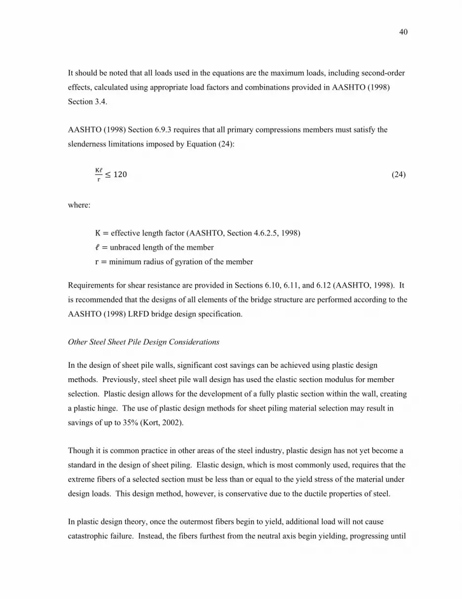
40

It should be noted that all loads used in the equations are the maximum loads, including second-order

effects, calculated using appropriate load factors and combinations provided in AASHTO (1998)

Section 3.4.

AASHTO (1998) Section 6.9.3 requires that all primary compressions members must satisfy the

slenderness limitations imposed by Equation (24):

Kℓ120 (24)

where:

K effective length factor (AASHTO, Section 4.6.2.5, 1998)

ℓ unbraced length of the member

r minimum radius of gyration of the member

Requirements for shear resistance are provided in Sections 6.10, 6.11, and 6.12 (AASHTO, 1998). It

is recommended that the designs of all elements of the bridge structure are performed according to the

AASHTO (1998) LRFD bridge design specification.

Other Steel Sheet Pile Design Considerations

In the design of sheet pile walls, significant cost savings can be achieved using plastic design

methods. Previously, steel sheet pile wall design has used the elastic section modulus for member

selection. Plastic design allows for the development of a fully plastic section within the wall, creating

a plastic hinge. The use of plastic design methods for sheet piling material selection may result in

savings of up to 35% (Kort, 2002).

Though it is common practice in other areas of the steel industry, plastic design has not yet become a

standard in the design of sheet piling. Elastic design, which is most commonly used, requires that the

extreme fibers of a selected section must be less than or equal to the yield stress of the material under

design loads. This design method, however, is conservative due to the ductile properties of steel.

In plastic design theory, once the outermost fibers begin to yield, additional load will not cause

catastrophic failure. Instead, the fibers furthest from the neutral axis begin yielding, progressing until

41

the entire section has yielded; this is the plastic limit-state. Any additional loading beyond the plastic

limit-state will induce rotation about this section known as a “plastic hinge.”

Plastic design is considered an acceptable method because, although significant deformation will

occur, design loads will only be reached in instances of extreme loading. According to Kort (2002),

designing the section to fully develop the plastic limit alone will save approximately 15% to 20% in

material costs. By allowing for rotation about the plastic hinge (and thus formation of multiple plastic

hinge locations), additional cost savings up to 20% may be achieved.

Design of GRS systems

The use of a GRS system significantly increases the bearing capacity of the backfill soil. Each layer

of geogrid in the backfill soil is analogous to steel reinforcement in concrete. When a vertical

compressive load is placed on a soil, both vertical and horizontal deformations occur. The amount of

horizontal deformation that occurs under a given vertical deformation is defined as Poisson’s Ratio

and is approximately 50% for typical soils. The presence of geogrid material reinforces the soil by

developing internal strain energy (in tension) as the soil undergoes horizontal deformation.

Essentially, for a soil that undergoes a given deformation, δ, under a vertical load, P1, the presence of

geogrid (or other similar types of soil reinforcement) would require a greater vertical load, P2, to

induce the same amount of soil deformation (see Figure 4-4); the bearing capacity of the soil has

increased (P2 > P1).

Figure 4-4. Deformation of soil mass under applied vertical load.

d

1

d

P 2P

Geogrid layerin tensile strain

a.) Unreinforced b.) Geogrid reinforced

δ δ

42

Internal Strength of Geogrid Reinforcement

Each layer of geogrid must be designed to resist the total lateral earth pressure at the corresponding

location in the GRS system. To resist the maximum lateral earth pressure, σ , for a certain vertical

spacing, S , the ultimate strength of the geogrid, T , must satisfy Equation (25):

T σ S (25)

If Equation (25) is not satisfied, an alternative to selecting stronger material would be to reduce the

vertical spacing of geogrid layers.

External Stability of Reinforcement

To develop the full strength of the geogrid material, sufficient embedment must be provided or

another means of mechanically developing the strength (such as wrapping each layer into the layer

above as shown in Figure B2 of Appendix B). To provide sufficient embedment length, the geogrid

layer must extend beyond the active zone of the backfill (shown in Figure B14 for the Boone County

project) soil a minimum length that develops the ultimate strength of the material through friction

against the surrounding soil.

Other Design Considerations

The factor of safety of the GRS mass must also be satisfied for sliding, overturning, slumping failure,

and bearing capacity on the material at the base of the excavation.

Design Summary and Recommendations

A detailed site investigation should be performed for all bridge designs considering the use of a steel

sheet pile bridge abutment and backfill retaining system to determine the type (axially loaded or GRS

system) best suited for site conditions present; the designer may refer to the selection flowchart

presented in Figure 4-5 for guidance in determining the sheet pile bridge abutment system best suited

for the project site conditions. A summary of the design of each type of sheet pile bridge abutment

and backfill retaining system is presented in this section.

43

Figure 4-5. Flowchart for preliminary selection of sheet pile bridge abutment system.

(average) (average)

44

Design Summary for Axially Loaded Sheet Pile Bridge Abutment and Backfill Retaining Systems

1. Determine design loads on the sheet pile wall. For estimating lateral earth pressure, refer to

AASHTO (1998) Section 3.11.5. Consideration must be given to the flexibility of the wall,

which is dependent on wall height and lateral restraint, when determining earth pressure (at-

rest or active); if short piles are restrained against lateral movement at the top of the wall (i.e.,

bridge superstructure), at-rest earth pressure conditions should be assumed. Effects of

surcharge loads on the backfill may be approximated using AASHTO (1998) Section 3.11.6;

the equations in this section are conservative for a flexible wall. For design according to HL-

93 loading, AASHTO (1998) Section 3.11.6.2 provides an equivalent surcharge pressure to

account for vehicular live load on the backfill soil. For all types of loading in the projects

included in this thesis, a load distribution of 10 ft width per design lane was used for live

loads; this was determined to be a conservative assumption from the test data analysis

presented later in this report.

2. Select location of the anchorage system. Various positions may be investigated to determine

the optimum location for minimizing the embedment depth and required anchor force. In

general, a distance below the top of the sheet pile wall of approximately 25% to 33% of total

wall height is the most efficient. Consideration should be given to the exclusion of an anchor

system for significant cost reduction; the need for temporary bracing of a cantilevered sheet

pile wall during construction must be investigated.

3. Determine preliminary depth of piling. If bedrock is within 40 ft of grade, piling should be

driven into bedrock; an assumed embedment depth of 5 ft is recommended for specifying pile

length. If driving to bedrock is not feasible, the minimum required embedment depth may be

determined by analyzing the wall as a beam with a single pinned support at the location of the

tie rods; the length of beam required for equilibrium of lateral forces on the wall provides the

minimum embedment depth. For an axially loaded abutment, pile length will typically be

controlled by the required depth for development of axial capacity through soil friction. As

mentioned previously in this chapter, it should be conservatively assumed that pile shaft

resistance is only developed where the pile is in contact with the passive soil zone (the

opposite side of the retained backfill). If sheet pile depths are greater than those required for

stability, it can be assumed that the remaining length of pile will develop friction (continued)

45

resistance on both faces of the pile. If the bridge is over a stream, design pile depth must

include the effects of scour; depending on local conditions, scour during flooding may be

significant (10 ft or more) and can be estimated using methods presented by Davis and

Richardson (2001).

4. Design sheet pile and superstructure interface. Reinforced concrete caps, steel channels with

plates, or the precast abutment caps developed by Black Hawk County are some alternatives.

5. Select a sheet pile section for the wall. PZC sections are recommended for piles with

significant lateral loading.

6. Design anchor system elements. How far the deadman is positioned behind the sheet pile

wall is determined by the minimum distance required so the active soil zone behind the sheet

pile wall and the passive soil zone of the deadman do not intersect; refer to Figure B14 of

Appendix B. Waler design may be performed by assuming the waler is a continuous beam

with simple supports at all tie rod locations; if the bridge is skewed, significant detailing of

the connection between tie rods, waler, and sheet pile wall is required due to translational

forces developed (see Figure B1).

7. Perform design checks. Determine if the resistance of the sheet pile section selected is

adequate for combined loading. Check local buckling of web and flange elements as well as

combined loading of the structure, including second-order bending moments. At a minimum,

all failure modes presented in Figure 4-3 must be investigated for the system. A check of the

effects on the sheet pile wall due to thermal expansion of the bridge superstructure must be

performed, as well as effects of frost heave in the backfill soil (if applicable). If overtopping

of the bridge deck during a 100-year flood will occur, the potential for unseating of the bridge

(considering force of water flow and buoyant weight of superstructure) should be

investigated.

Design Summary for GRS Sheet Pile Bridge Abutment and Backfill Retaining Systems

1. Determine design loads on the sheet pile wall. For estimating lateral earth pressure, refer to

AASHTO (1998) Section 3.11.5. Consideration must be given to the flexibility (continued)

46

of the wall, which is dependent on wall height and lateral restraint, when determining earth

pressure (at-rest or active); if short piles are restrained against lateral movement at the top of

the wall (i.e., bridge superstructure), at-rest earth pressure conditions should be assumed.

Effects of surcharge loads on the backfill may be approximated using AASHTO (1998)

Section 3.11.6; the equations in this section are conservative for a flexible wall. For design

according to HL-93 loading, AASHTO (1998) Section 3.11.6.2 provides an equivalent

surcharge pressure to account for vehicular live load on the backfill soil. For all types of

loading in the projects presented in this thesis, a load distribution of 10 ft width per design

lane was used for live loads; this was determined to be a conservative assumption from the

test data analysis presented later in this report.

2. Select location of the anchorage system. Various positions may be investigated to determine

the optimum location for minimizing the embedment depth and required anchor force. In

general, a distance below the top of the sheet pile wall of approximately 25% to 33% of total

wall height is the most efficient. Consideration should be given to the exclusion of an anchor

system for significant cost reduction; the need for temporary bracing of a cantilevered sheet

pile wall during construction must be investigated.

3. Determine preliminary depth of piling. The minimum required embedment depth may be

determined by analyzing the wall as a beam with a single pinned support at the location of the

tie rods; the length of beam required for equilibrium of lateral forces on the wall provides the

minimum embedment depth. All regions of the sheet pile wall within the GRS zone may be

considered to have no lateral forces applied to the wall. If the bridge is over a stream, design

pile depth must include the effects of scour; depending on local conditions, scour during

flooding may be significant (10 ft or more) and can be estimated using methods presented by

Davis and Richardson (2001).

4. Select a sheet pile section for the wall. PZC sections are recommended for piles with

significant lateral loading.

5. Design geogrid reinforcement. Select a geogrid type and spacing adequate to resist

maximum lateral earth pressures experienced within the backfill. It is recommended to use

biaxial or triaxial geogrid to minimize loading on wingwalls. (continued)

47

6. Design spread footing for transfer of superstructure loads to GRS backfill.

7. Design anchor system elements. How far the deadman is positioned behind the sheet pile

wall is determined by the minimum distance required so the active soil zone behind the sheet

pile wall and the passive soil zone of the deadman do not intersect; refer to Figure B14 of

Appendix B. Waler design may be performed by assuming the waler is a continuous beam

with simple supports at all tie rod locations; if the bridge is skewed, significant detailing of

the connection between tie rods, waler, and sheet pile wall is required due to translational

forces developed (see Figure B1).

8. Perform design checks. Determine if the resistance of the sheet pile section selected is

adequate for combined loading. At a minimum, all failure modes presented in Figure 4-3

must be investigated for the system. A check of the effects of frost heave in the backfill soil

(if applicable) should be performed. If overtopping of the bridge deck during a 100-year

flood will occur, the potential for unseating of the bridge (considering force of water flow and

buoyant weight of superstructure) should be investigated.

Other Design Recommendations

Design of the sheet pile and superstructure interface should be considered when using either axially

loaded, cellular, or GRS abutment systems; the shallow footings required for cellular or GRS

abutment systems may be significantly simpler to design and construct.

When designing sheet pile elements, combined loading effects must be considered due to the nature

of the loading. Design methods for typical steel piling may be used in conjunction with special

consideration for the development of soil friction as described in this section. Use of the AASHTO

(1998) LRFD bridge design specifications is recommended for the design of all elements of the

bridge structures (including equations for determination of lateral loads). Compaction-induced earth

pressures must be accounted for utilizing the methods presented in this section. When selecting steel

sheet pile shapes, the plastic section modulus should be utilized for selection; PZC piling is preferred

over PZ piling due to a greater strength to weight ratio. Epoxy coating of all steel elements exposed

to soil is recommended where feasible.

48

Monitoring Methods and Instrumentation Selection

Three main types of monitoring equipment that are applicable for steel sheet pile bridge abutments

are piezometers, earth pressure cells, and strain gages. Other equipment such as extensometers,

tiltmeters, and inclinometers may also provide valuable information about the behavior of the project

site. For long-term recording of instrumentation readouts, the use of a datalogger is necessary (as

well as other components to allow communication with computer software). Select components are

explained in the following paragraphs.

Two common types of transducers (methods for converting physical measurements into electrical

signals) used in geotechnical instrumentation are vibrating wires and semiconductors. The theory

behind vibrating wire technology is that the resonant frequency of a wire is dependent on the tension

it is subjected to. The wire is “plucked” using an electromagnetic coil and the frequency of the

vibration is then recorded. The measured frequency of vibration is proportional to the desired

information (earth pressure, strain, etc). Semiconductor transducers utilize a material that changes

resistance under strain. Vibrating wire systems are more stable over time while semiconductor

systems have significantly higher sampling rates useful for dynamic measurements.

Piezometers

The piezometer can be used to measure groundwater table elevation for long-term monitoring of the

project. By placing multiple piezometers on both the stream side and backfilled side of a retaining

wall, water height can be measured to determine the development of pore water pressure behind the

abutment. The ASCE recommends that piezometers be installed prior to driving piling and

backfilling for simplicity, although steps must be taken to prevent damage to them as a result of the

driving (ASCE, 1996).

Earth Pressure Cells

Earth pressure cells can measure the total contact soil pressure at any location. A cell essentially

consists of two steel plates separated by a fluid. As pressure on the plates change, a transducer

converts the fluid pressure into an electrical signal. The cells can be attached directly to the sheet pile

wall and measure the soil pressure due to backfill and surcharge loads. It is recommended that earth

49

pressure cells be installed in a pocket of fine-grained sand (Geokon, 2006). When used in

conjunction with a piezometer, effective soil stress can be determined at a desired point.

Strain Gages

Strain gages will measure the strain at a given point on the sheet pile wall. Since strain is

proportional to stress, the gages will indirectly provide stresses, loads, and bending-moments at the

desired locations. At a minimum, two gages must be used (on opposite sides of the neutral axis of

bending) to distinguish between axial and flexural strains in the section.

Previous field tests have shown that strain gages installed prior to construction are capable of

surviving driving operations. Further protection may be provided by welded steel angle sections over

the gages; care must be taken to avoid welding near strain gage locations (ASCE, 1996).

Extensometers

Borehole extensometers allow for measurement of the deformations of the soil mass retained by a

retaining wall. When placed behind a sheet pile bridge abutment, extensometers measure the

deformations of the soil at various points within the borehole by using up to 6 rods with anchors.

These measurements can assist in the recognition of developing failure planes within the soil

(Geokon, 2006).

Tiltmeters

The tiltmeter is capable of measuring the tilt of structures. In a vibrating wire tiltmeter, a strain gage

measures the deflection of a pendulous mass inside the tiltmeter as the center of gravity shifts due to

rotation of the structure it is attached to. The instrument can be attached via brackets to either a

vertical or horizontal face of the structure being monitored (Geokon, 2006).

Inclinometers

Inclinometers can be used to measure the deflected shape of a structure or the movement of a soil

mass. An inclinometer is essentially an accelerometer probe that is run through a tube installed on a

structure or in a soil to detect changes in deflected shape. Because of damage during driving,

50

inclinometers attached to sheet piles are limited to the length of the sheet pile. If information of soil

movements below the pile is required, a second inclinometer installed deep into the soil (deep enough

to be considered non-moving) can be used (ASCE, 1996).

Data Collection System

A system is needed to read the electrical output from the instrumentation. A datalogger system is

capable of storing information for short-term or long-term applications (depending on the type of

datalogger used). In a vibrating wire system, the datalogger sends an electrical signal (one instrument

at a time) to excite vibration of the wire and measure its resonant frequency; the frequency is then

converted to a data value (i.e. strain or pressure) and is stored for subsequent data collection. An

interface with a computer (with the appropriate software) is necessary for programming of the

datalogger as well as collection of data.

Construction Methods

For construction of sheet pile walls, the most common methods are driving, jetting, and trenching.

With steel sheet piles, it is recommended that driving be used. Various types of driving and vibratory

hammers (which can be faster and minimize damage to the piles) are available. Several driving

hammers are described below. When impact hammers are used, a protective cap should be placed to

prevent damage to the pile. Templates or guides are also used to help ensure proper placement of the

sheet pile during driving. A common vertical tolerance is plus or minus 1.5 in. from design elevation,

while sheet piling should not be more than 0.125 in/ft of wall out of plumb (either in-plane or

perpendicular to the wall) after driving (ASCE, 1996). With axially loaded abutments, these

tolerances would likely be further reduced.

When sheet piling is used as a bridge abutment, standard practice has been to use a vibratory pile

driving hammer unless difficult driving is encountered (where impact hammer driving would be

necessary). For a typical cellular sheet pile bridge abutment, previous projects have shown that

installation can be completed in less than one week with a crew of four people. After the piling has

been installed, standard earthwork equipment can be employed for soil movement and compaction

(Braun, 2002).

51

Driving Equipment

Diesel Hammers

The diesel impact hammer is a system that compresses and ignites a combination of air and diesel

fuel. As the piston falls, compressing the air inside the chamber, diesel fuel is sprayed on the impact

block. When the piston strikes the impact block the fuel-air combination ignites and simultaneously

thrusts the piston upward and drives the pile into the ground. As the piston falls back down, the

compression cycle is restarted.

Single Acting Drop Hammers

Drop hammers consist weights (up to 11 tons) dropped from variable drop heights to drive the piles

into the ground. To minimize noise and pile head damage, heavy weights with short drop heights are

recommended (NASSPA, 2005). The three main drop hammer types are cable operated, steam, and

hydraulic; the difference being the means of lifting the weight.

Double Acting Hammers

These hammers are similar to other impact hammers, with the exception that they employ means of

adding additional energy to the hammer. This is accomplished by using hydraulics or compressed

air/steam to add energy as the piston is falling.

Vibratory Pile Drivers

The principal of a vibratory pile driver is the use of eccentric oscillating weights that disturbs the soil

around the pile, decreasing soil resistance. By doing this, piles are able to be driven with little extra

applied loads such as pile self weight and the weight of the driver. According to the NASSPA

(2005), the best soils for use with vibratory drivers are water-saturated non-cohesive soils as well as

mixed and cohesive soils with high water contents. If difficult soil strata are encountered, impact

drivers may be used to finish the driving operations after vibratory drivers have been used to set piles.

Driving Methods

The North American Steel Sheet Piling Association (NASSPA, 2005) outlines two methods of pile

driving: set-and-drive and panel driving.

52

In the set and drive method, each sheet pile element is driven to its full depth until another is placed

as shown in Figure 4-6a. This method, however, is only applicable for use in loose soils with

relatively short piling, as the free-leading interlock is constantly susceptible to deviation. For more

difficult driving situations, panel driving is recommended (NASSPA, 2005).

Figure 4-6. Sheet pile driving methods (NASSPA, 2005).

a.) Set-and-drive b.) Panel driving

c.) Staggered driving

53

Panel driving is a technique that minimizes installation difficulties. The piles are driven in groups (or

panels) as shown in Figure 4-6b. The first two piles are set on the guide (pitched), aligned, and made

plumb. The rest of the group is then pitched, with driving beginning from the last pair in the panel.

After the first panel is driven to a minimum depth, the second panel is pitched and driven in a manner

like the first panel. After the second panel has reached the minimum depth, the first panel can be

driven to the design depth and the third panel should be pitched. This process continues until all piles

have been driven to design elevations. If significantly difficult driving conditions are encountered,

staggered driving of piles (see Figure 4-6c) is recommended as it minimizes the potential for

development of friction between interlocks that is developed when adjacent piles deviate due to soil

behavior or obstacles encountered during driving (NASSPA, 2005).

Bridge Live Load Testing and Monitoring

Live Load Testing

The instrumentation and monitoring systems were used in conjunction with load tests to investigate

the behavior of the structure under loading. The live load test involved driving trucks of a known

weight and axle spacing over the bridge and taking readings when the trucks were at specified

locations. Data recorded were reduced and compared to results expected by theoretical analysis to

determine the performance of the sheet pile abutment and backfill retaining systems and the viability

of the design methods utilized.

Long-Term Monitoring

For long-term monitoring of bridge behavior, the permanent instrumentation system was used.

Readings were taken at various daily intervals described in the corresponding section for each project.

The data recorded for each project were reduced and analyzed to determine the performance of the

sheet pile abutment and backfill retaining system over long time periods.

54

CHAPTER 5. RESULTS AND DISCUSSION

Black Hawk County

Project Details

The first demonstration project was constructed in Black Hawk County (BHC), Iowa. The site that

was selected was a low volume road bridge crossing Spring Creek (a tributary of the Cedar River) on

Bryan Road near La Porte City; the location of the bridge is shown in Figure 5-1.

This project was undertaken to investigate the feasibility of using sheet piling as the primary

abutment foundation element and backfill retaining system. Construction of the new bridge was

initiated on August 13, 2008 and completed on October 20, 2008. A load test of the bridge

foundation system and superstructure was subsequently performed and data were collected by Iowa

State University (ISU). This thesis presents information on the design of the new sheet pile abutment

bridge system, its construction, the instrumentation installed, load testing, as well as data analyses and

conclusions. The following sections give an overview of the previous structure and the new sheet pile

abutment bridge system.

Figure 5-1. Location of demonstration project outside of La Porte City in BHC, Iowa.

Bridge location

N

55

Previous Bridge Structure

The bridge that was replaced was a 20 ft wide, 40 ft single span originally constructed in 1942. The

structure was a pony truss bridge supported on a timber pile foundation and was constructed

approximately 10 ft above stream level. The substructure was previously retrofitted with steel piles

on each abutment. These retrofit piles were reportedly driven into the existing bedrock to provide

reinforcement for the timber abutments. One of these piles can be seen in Figure 5-2.

Figure 5-2. Previous bridge structure at demonstration project site in BHC, Iowa with retrofit pile.

New Sheet Pile Abutment Bridge System Overview

The new bridge system (a 31 ft wide, two-lane 39 ft single-span beam-in-slab bridge) was a joint

design effort between BHC and ISU. The design of the superstructure was performed by the BHC

Engineer’s Office and utilized precast elements previously developed. The substructure, which was

primarily designed by ISU, utilized steel sheet piling as the primary abutment foundation element and

backfill retaining system.

Superstructure

Custom precast beam-in-slab units (40.75 ft long) were used for the bridge superstructure. Each unit

contained two W14x61steel beams (for additional details on the BHC precast elements, refer to

Appendix A). There were a total of 6 units required for the bridge, each unit spanning the entire

Retrofit pile

56

length. Between each unit there was a closure joint that was cast in the field after the units were

placed. A cross-section of two joined deck units (exterior and interior) is presented in Figure 5-3. The

design width of the bridge was 31.8 ft. Figure 5-4a and Figure 5-4b illustrate a cross-section and side

view, respectively, of the bridge deck and abutment elements; a full set of bridge plans are provided

in Figure A1 through Figure A5 of Appendix A.

Figure 5-3. Cross-section of precast deck units for demonstration project in BHC, Iowa.

Figure 5-4. Replacement bridge deck and abutment elements for demonstration project in BHC, Iowa.

W14x61

4.87 ft 5.5 ft

1.17 ft

2.75 ft

5 in.

1.42 ft

33 ft abutment cap

Beam-in-slab deck unitsClosure joint

Abutment cap Sheet piling

39 ft

40.75 ft

GuardrailBridge deck Sheet pile wallAbutment cap

a.) Cross-section

b.) Side view

57

Substructure

Steel sheet piling was used for the abutment foundation elements of the new bridge. Each abutment

consisted of a precast abutment cap bearing on sheet pile sections driven into shallow bedrock. The

sheet piles selected were PZ 22 sections (purchased from Skyline Steel, Inc.). Dimensions of a PZ 22

are shown in Figure 3-2. A total of 64 sheet pile sections were needed for completion of both

abutments. The main wall of the abutment required 20 sheet pile elements with each of the wingwalls

consisting of 6 elements (each 15 ft long). The main wall was anchored with two 1 in. diameter tie

rods that were attached to a 14 ft by 4 ft by 2 ft cast-in-place reinforced concrete deadman placed

approximately 20 ft back from the main wall. The wingwalls were tied together using a 46 ft long 1

in. diameter tie rod (non-epoxy coated). A plan view of the abutment design is shown in Figure 5-5.

The abutment cap was a precast element designed and fabricated by BHC that consisted of a W12x65

steel beam cast in reinforced concrete. The web of the steel beam cast in the abutment cap beared

directly on top of the driven sheet piling with no connection between them. The bridge deck units

were placed on the abutment cap using bearing pads between the deck unit beams and the concrete

abutment cap. A cross-section of the beam-in-slab bridge, abutment cap, and sheet pile wall is

presented in Figure 5-6.

Figure 5-5. Plan view of sheet pile abutment and backfill retaining system for demonstration project in BHC, Iowa.

33 ft abutment cap

12 ft

14 ft

2 ft

1 in. x 20 fttie rod

CL

CL

1 in. x 46 ftwingwall tie

14 ft x 4 ft x 2 ftreinforced concretedeadman

PZ 22 steel sheet piling20 ea, @ 22 in. offset

min. 15 ton bearing

6 ea. PZ 22sheet pile wingsno bearing required

58

Figure 5-6. Precast abutment cap and contact between bridge deck, abutment cap, and sheet piling foundation in BHC, Iowa demonstration project.

Site Investigation

Field Investigation

Cone Penetrometer Testing

CPT soundings were performed east and west of the bridge abutments on August 14, 2007. The test

locations are shown in Figure 5-7. CPT 1 and CPT 2 were advanced to depths of 15.9 ft and 17.4 ft

below existing grades, respectively. Logs of the soundings, showing cone tip stress and sleeve

friction, are presented in Figure 5-8a and Figure 5-8b, respectively. The soundings were advanced to

practical refusal based on the equipment and the operator’s experience. After being withdrawn from

the CPT 2 sounding hole, the cone tip was found to be covered with light gray weathered limestone.

Soil behavior types determined from CPT 1 and CPT 2 are illustrated in Figure 5-9a and Figure 5-9b,

respectively. As can be seen these figures, the majority of material present is clay with sandy seams

occurring near stream level (from depths of 6 ft to 8 ft); the spike in resistance at the bottom of each

CPT being a strong indicator of bedrock. Soil shear strengths and SPT resistance estimates from

PZ 22

W12x65

Precast abutment cap(Note: Reinforcementin the cap beam hasbeen omitted)

W14x61 @ 40 ft

Beam-in-slab deck

59

correlations presented by Lunne, Powell, and Robertson (1997) are shown in Figure 5-10a and Figure

5-10b.

Figure 5-7. Plan view of CPT and soil boring locations in BHC, Iowa demonstration project.

Figure 5-8. Results of CPT’s showing cone tip and friction resistance.

7 ft 6 ft

28 ft

25 ft

31 ft

6 ft

12 ft

15 ft

18 ft

LRoadway C

Original bridge deckCPT 1

SB 2

SB 1SB 4

CPT 2SB 3

Cone Resistance (tsf)

0 50 100 150 200

Dep

th (

ft)

0

2

4

6

8

10

12

14

16

18

Friction Resistance (tsf)

0 1 2 3 4 5

Cone ResistanceFriction Resistance

Cone Resistance (tsf)

0 50 100 150 200

Dep

th (

ft)

0

2

4

6

8

10

12

14

16

Friction Resistance (tsf)

0 1 2 3 4 5

N

a.) CPT 1 b.) CPT 2

60

Figure 5-9. Soil behavior types determined from CPT’s.

Figure 5-10. Shear strength and SPT correlations for CPT’s.

Soil Behavior Type

0 2 4 6 8 10 12

Dep

th (

ft)

0

2

4

6

8

10

12

14

16

Soil Behavior Type

0 2 4 6 8 10 12

Dep

th (

ft)

0

2

4

6

8

10

12

14

16

18

# Soil T ype

0 Organic Material/

1 Fine Grained

2345 Clayey Silt

6 Sandy Silt to

7 Silty Sand

89

1011 Very St iff Fine Grained

12 to Clayey Sand

Clay to Silty Clay

Sand to Gravelly Sand

Shear Strength (ksf)

0 2 4 6 8 10

Dep

th (

ft)

0

2

4

6

8

10

12

14

16

18

0 20 40 60 80 100

Shear StrengthCalculated SPT Value

N60 (blows per ft)

Shear Strength (ksf)

0 2 4 6 8 10

Dep

th (

ft)

0

2

4

6

8

10

12

14

16

0 20 40 60 80 100

N60 (blows per ft)

a.) CPT 1 b.) CPT 2

a.) CPT 1 b.) CPT 2

61

Soil Borings

The soil borings were performed by members of the ISU research team on September 7, 2007. The

location of each boring is shown in Figure 5-7, while boring logs are provided in Figure A8 through

Figure A11.

Laboratory Testing

Averaged results of the CU triaxial tests performed for each boring (along with soil boring depths) are

presented in Table 5-1 Results of the moisture content and UU triaxial tests performed on select soil

samples are presented in Table 5-2. The results of the Atterberg tests and the percentage of soil

passing the No. 200 sieve (percent fines) for select samples are presented in Table 5-3. USCS

classifications determined are shown in the boring logs.

Table 5-1. Results from CU lab analysis of soil borings.

Boring Location Boring Depth Cohesion, c’ Friction Angle, φ’

(ft) (psf) (degrees) SB 1 10.3 50 35 SB 2 16.8 0 36 SB 3 16.0 125 27 SB 4 15.8 50 28

Table 5-2. Moisture content and UU test results on select soil samples.

Boring Location

Depth Range (in.)

Moisture (%)

Undrained Shear Strength (psf)

Dry Density (pcf)

Void Ratio

SB 1 20 - 30 15.3 1408 112.2 0.475

SB 2 107 - 118 23.1 1017 131.1 0.262

SB 2 180 - 202 18.5 1452 135.4 0.222

SB 3 30 - 50 18.1 1829 133.9 0.236

SB 3 114 - 123 20.6 1079 133.9 0.235

SB 3 123 - 130 16.8 1045 132.4 0.250

SB 4 168 - 176 16.8 506 136.6 0.211

SB 4 176 - 184 14.5 2688 144.3 0.146

SB 4 184 - 192 14.3 2424 143.4 0.154

62

Table 5-3. Atterberg test and gradation results for select boring ranges.

Boring Location

Depth Range (in.)

LL (%)

PL (%)

PI (%)

Passing No. 200 (%)

SB 1 12 - 40 33 20 13 48 SB 1 42 - 94 39 27 12 62 SB 2 96 - 199 23 15 8 -* SB 3 23 - 50 30 19 11 51 SB 3 119 - 180 31 17 14 - SB 4 144 - 168 30 15 15 - SB 4 168 - 192 29 16 13 -

* No data available

Site Conditions

Geologic Setting

The project site is located on the "Iowan Surface", a distinct geomorphic region limited to the

northeastern portion of Iowa. According to GSI (see Figure A7 for CPT report), transected surficial

drainage imparts the topography consisting of gently rolling hills with long slopes and gentle relief.

Prominent isolated elliptical hills, termed "pahas", tend to be concentrated along the region's southern

border and karst features, including sinkholes, are common to the northern portion of the Iowan

Surface due to the thin overburden deposits underlain by limestone bedrock formations. Overburden

deposits within the stream valleys generally consist of colluvium (slopewash) overlying alluvium of

varying thickness which is underlain by the glacial till soils over bedrock. The colluvial deposits are

derived from parent soil materials on hillsides while the underlying alluvium may consist of cohesive

clayey silt and silty clay soils and/or deposits. This project is located on a creek upland of the Cedar

River floodplain which may have deposited alluvium consisting of interbedded sand and clay soils.

Soil Conditions

Soil borings SB 1 and SB 4 encountered fill materials consisting of very stiff, tan and light gray sandy

clay (USCS symbol CL), and medium dense, red and tan clayey sand (SC) and silty sand (SM) from

the ground surface to depths of 2 ft and 4 ft. Underlying the fill materials and present from the

ground surface at the remaining three boring locations were relatively lean, stiff to hard, tan and light

gray silty clay (CL) and sandy clay (CL) soils that extended to depths ranging from 8 ft to 10 ft. Stiff,

light gray and tan, high-plasticity clay (CH) was encountered in boring SB 4 from 10 ft to 17 ft.

Loose to very dense, tan and light gray silty sand (SM) with clay seams was then encountered below a

63

depth of 12 ft to bedrock in SB 1 and SB 2. Soil borings SB 3 and SB 4 encountered dark gray and

orange silty clays from a depth of approximately 11 ft to bedrock.

Groundwater Observations

During the soil boring advancement and sampling operations, observations for free groundwater were

made. Information regarding water level observations is recorded in the “groundwater” column on the

soil boring logs. Groundwater was encountered at depths below existing grade of approximately 10 ft

in borings SB 1 and SB 2 and at 12 ft in borings SB 3 and SB 4. Where free water was encountered,

the depth of this observation is noted in the stratigraphy column of the soil boring logs. From the

CPT soundings, the observed drop in tip stress and sleeve friction near depths of 10 ft likely coincides

with the ground water surface.

Design

The bridge design was completed as a joint effort between ISU and the BHC Engineer’s Office. The

county engineer designed the superstructure while ISU was responsible for the design of the sheet pile

abutment foundation and backfill retaining system. The design of the substructure elements was

performed using the AASHTO LRFD Bridge Design Specification (1998).

Loading

According to the BHC Engineer’s Office, the precast superstructure elements were designed for HS20

loading and a permit truck with five 10 ton axles spaced at 4.17 ft on center. Substructure elements

were designed to resist HL-93 loading; the substructure was determined to be sufficient for the permit

truck loading when analyzed with no lane load, using a 33% increase in axle loads for impact, and no

live load factor. The 39 ft bridge was loaded with the design truck and lane load as per AASHTO

(1998) Section 3.6.1.2 to determine live loads that needed to be resisted by the foundation and

backfill retaining system. The design loads were determined using the critical load factors and load

combinations in AASHTO (1998) Section 3.4.

Foundation and Backfill Retaining Wall Design

Due to the nature of the loading, the sheet pile sections were analyzed as beam-columns. The

combination of piling being driven into bedrock and restraint provided by wingwalls was assumed to

64

prevent translation at the base of the wall (but not rotation). Once in place, the bridge superstructure

was assumed to provide restraint against translation at the top of the wall and thus the design element

was assumed to be simply-supported at both ends of the section.

Loads from the retained soil self-weight and surcharge on the backfill were applied laterally to the

element. For determining the amount of vertical earth pressure transferred laterally to the wall, at-rest

(Ko) conditions were assumed due to the effect of the bridge structure in resisting lateral displacement

at the top of the wall. Soil parameters and the assumed design profile are shown in Figure 5-11a.

The loading and support conditions assumed are shown in Figure 5-11b. The concentrated force, P,

represents the dead and live loads applied from the superstructure.

Figure 5-11. Design profile and loading and support diagram for the BHC, Iowa demonstration project.

Conservative assumptions were made for the behavior of the clay layer. The stream-side materials

were assumed to provide no lateral resistance to the wall due to the mobilization requirements for

passive lateral earth pressure to develop and the potential for removal of material from scouring

effects. Another assumption was that, due to the effects of creep over time, the coefficient of lateral

earth pressure (Ko) of the clay layer was assumed to be unity (full transfer of vertical stresses laterally

to the wall).

The coefficient of at-rest lateral earth pressure was determined according to AASHTO (1998) Section

3.11.5.2 for the sand layer. Vehicular live loads on the backfill were accounted for in design by using

7 ft

8 ft

15 ft

8 ft

P

Sand layer

Clay layer

Bedrock

γ = 125 pcf φ’ = 30° c’ = 0 psf

γ = 140 pcf φ’ = 0° c’ = 500 psf

a.) Design profile b.) Loading diagram

65

the equivalent surcharge loading outlined in AASHTO (1998) Section 3.11.6.2. Design axial loads in

the piling were determined by assuming superstructure dead loads were distributed evenly amongst

all piles and live loads were distributed over a 10 ft wide lane.

The pile section chosen for the wall was the PZ 22. The section was checked for combined loading

and second-order effects of an element undergoing flexure and compression as per AASHTO (1998)

Section 6.9.2.2. The pile section was also checked for the limit states of flange and web local

buckling. Flexural strength was determined using the elastic section modulus and assuming lateral-

torsional buckling was prevented through continuous bracing of the compression flange by adjacent

sheet pile members.

The final design of the abutment foundation and backfill retaining system required a total of 64 (32

per abutment) 15 ft long PZ 22 piles (Grade 50 steel). The abutment caps were to be set directly on

the top of the sheet pile wall after it was finished to grade.

As stated previously, the superstructure was assumed to provide adequate lateral restraint once in

place. During backfilling of the abutments, however, this was not the case. Because of this lack of

lateral restraint, a reinforced concrete deadman anchor system was installed on each abutment. The

system was designed by the county engineer and consists of a reinforced concrete deadman

(approximately 14 ft x 4ft x 2 ft) with two 1 in. diameter tie rods connected to a waler channel on the

exterior face of the abutment walls. The connection between the deadman and sheet pile abutment

system is shown in Figure 5-12; the tie rod (with hooked reinforcement welded on one end) was cast

into the concrete deadman. Design calculations are provided in Appendix A.

Figure 5-12. Deadman to sheet pile abutment and backfill retaining system connection.

20 ft

14 ft x 4 ft x 2 ftreinforced concretedeadman

1 in. diametertie rod

Waler channel

66

Construction

BHC used its own forces for construction of the entire project. The bridge crew primarily consisted

of three construction workers. According to the BHC engineer, average labor costs amount to

approximately $1000 each day the bridge crew was on site.

The overall time required for construction of the replacement bridge was approximately 10 weeks.

Several delays occurred due to equipment breakdowns (due to inexperience with specific pile types),

pile splicing, and weather. A chronology of major construction events is shown in Table 5-4. Details

of each significant event are also given in this section of the report.

Table 5-4. Chronology of significant construction events for demonstration project in BHC, Iowa.

Event Description Start Date Working Days Between Events Demolition 08/13/08 8

Sheet Pile Driving – East Abt. Sheet Pile Driving – West Abt.

Abutment Finishing

08/25/08 09/02/08 09/17/08

6 11 11

Deck Unit Placement Bridge Finishing

10/02/08 10/15/08

9 3

Open for Service Bridge Load Test

10/20/08 11/3/08

- -

Demolition of Existing Structure

Removal of the superstructure and east abutment was the first task of the demolition and required one

week for completion. The west abutment was left in place to assist in the construction of the

replacement bridge. The demolition was performed with a crane equipped with a wrecking ball and

an excavator. The bridge deck was crushed by dropping of a wrecking ball while the excavator was

used to remove exposed reinforcement. The excavator was also used to pull down the superstructure

and demolish the timber abutments.

The east abutment had one H-pile retrofit that had been driven into the bedrock. An initial attempt to

pull out this pile with the excavator was unsuccessful. The excavator was used to bend the pile back

and forth until it fatigued slightly below the stream level and the upper portion was removed. The

west abutment (containing two retrofitted H-piles) was never fully removed since the location of the

new bridge was slightly east of the existing abutment.

67

Sheet Pile Driving – East Abutment

For both of the abutment sheet pile walls, pile driving was completed using both vibratory and impact

hammers. The piles, after being placed in a guide rack to help ensure proper wall construction, were

initially driven as far as possible using an excavator equipped with a vibratory plate as shown in

Figure 5-13. The piles were then driven to a minimum specified 15 ton bearing capacity using a

crane equipped with a drop hammer. Bearing capacity was estimated using the Modified Engineering

News Record pile-driving formula (Das, 2006). Using a 4,120 lb hammer dropped from a height of 6

ft, less than 2 in. of observed pile penetration after 5 blows of the hammer corresponded to

approximately a 33 ton capacity. All piles were driven until a maximum of 2 in. penetration per 5

blows was observed. The wingwalls, which did not require bearing capacity, were driven to bedrock

with the vibratory plate and then trimmed. The wingwalls were placed at a 45 degree angle to the

main wall using the special connector shown in Figure 5-14.

Figure 5-13. Driving of sheet pile sections with vibratory plate equipped excavator boom.

68

Figure 5-14. Sheet pile connector for 45 degree turn (PilePro® PZ Colt).

The guide rack was 1 in. wider than the width of the sheet pile sections used to ensure the sheet piles

would fit inside the rack. As depicted in Figure 5-15a, significant rotation between adjacent sheets

occurred which resulted in extending the actual width of the wall by approximately 1.5 ft. As can be

seen in Figure 5-15b, the slightly rotated sections are wider by approximately 1 in. and have less

distance between flanges (0.6 in. less). It was realized after construction that the guide rack should

have been constructed with spacing closer to the design width of the wall. Efforts to ensure adjacent

sections are flush will result in a wall with greater flexural strength by maximizing the distance of the

sheet pile flanges from the neutral axis.

Figure 5-15. Rotation between adjacent sheet pile sections.

45°

44 in.

45 in.

9 in.

8.4 in.

Angle between sections

a.) Angle between sections b.) Comparison of flush and rotated sections

(not to scale)

69

CPT results showed refusal at 15 ft below grade. During impact driving, specified bearing capacity

(2 in. of pile penetration per 5 hammer blows) was not reached until significantly below the assumed

bedrock depth from the CPT results. This was not an issue for the east abutment since pile lengths

longer than necessary were ordered.

Sheet Pile Driving – West Abutment

The west abutment required modification of the guide rack to accommodate the width of the

instrumented piles due to the protective angles that were attached (see Figure 5-16a and Figure

5-16b). As with the east abutment, the width of the rack was wider than necessary thus introducing

undesired rotations between the adjacent pile sections and an overall lengthening of the wall.

Figure 5-16. Modification of guide rack to accommodate the instrumented piles.

The plan for driving the west abutment sheet pile wall was similar to the east abutment; vibratory and

impact driving was used. During the vibratory driving phase, one pile (Pile 2 in Figure 5-34) was

misaligned. Since the pile couldn’t be pulled back out, a field decision was made to adjust its

position by forcing it laterally with the excavator boom. While being held, the pile was welded to the

guide rack until the next pile section had been driven; this adjustment may have affected results

(creating locked-in stresses) as Pile 2 was an instrumented pile.

Angles to protectinstrumentation

Strain gages

PZ 22

Angles welded to guide rack

a.) Guide rack with angles attached b.) Instrumented sheet pile section

(not to scale)

70

CPT results for the west abutment showed refusal at approximately 17 ft below grade. During the

impact driving phase, it became evident that the lengths of piling ordered were too short. The depth

required for specified bearing capacity on the west side of the stream was significantly lower than that

predicted by the CPT results and varied from 17.9 ft to 23.9 ft along the abutment wall. All of the

sheet piles in the main wall required splicing to achieve design elevations. In some cases, piles

needed to be driven more than 1 ft lower than the adjacent section; this required splices as well for the

pile driving mechanism to fit in place. Required splice lengths ranged from 0.5 in. to 72 in.

Another issue encountered was fracturing of the pile driving cap. The BHC bridge crew had

constructed a custom driving cap for the sheet piles by welding sections of angle iron to a steel plate

(see Figure 5-17); on two occasions, the welds failed and thus the driving cap needed repair.

Figure 5-17. Custom sheet pile driving cap fabricated by BHC.

71

Completion of Abutment

After all sheet piling had been driven to the specified bearing capacity, several tasks were performed

to bring the abutments to a finished state. The major tasks that needed to be performed before

backfilling were placement of the subdrain, installation of the anchor system, placement of the

abutment cap, and installation of the monitoring instrumentation.

Subdrain

To provide drainage of the backfill, a drain tile system was placed on the backfill side of each sheet

pile wall. These systems, placed at approximately the same elevation of the stream, consisted of a

flexible, perforated pipe surrounded by porous backfill. The pipes were placed along the length of

each abutment wall and were wrapped around and exited at the end of the wingwalls downstream

from the bridge (see Figure 5-18).

Figure 5-18. Drain tile installation on backfill side of west abutment in BHC, Iowa.

Anchor System

The anchor system consisted of a cast-in-place concrete deadman that supported the wall through two

1 in. threaded rods (non-epoxy coated) connected to a steel channel waler. An overview of the anchor

system was previously presented in Figure 5-5. The deadman was cast in a trench excavated from the

existing soil as shown in Figure 5-19. After hex nuts were threaded on the main wall tie rods, another

rod was placed parallel to the wall to tie the wingwalls together (see Figure 5-20).

Perforated pipe to exit at downstream end of wingwall

72

Figure 5-19. Reinforced concrete deadman placement behind east abutment.

Figure 5-20. Installation of wingwall tie.

73

The construction of the deadman differed between the two abutments. For the east abutment, a

continuous deadman (approximately 14 ft x 4 ft x 2 ft) was used for anchoring both tie rods. On the

west abutment, however, only one tie rod was attached to the concrete deadman (approximately 6 ft x

4 ft x 2 ft) constructed. The other tie rod was welded onto a driven H-pile that was part of the

demolished bridge (see Figure 5-21).

Figure 5-21. Tie rod to H-pile connection.

Abutment Cap

The abutment cap consisted of a precast element designed by BHC. The 33 ft long cap consists of a

W12x65 section capped with reinforced concrete as shown previously in Figure 5-6a. Because the

web of the W12x65 was to bear directly on top of the driven sheet pile wall, the wall needed to be

trimmed to a precise elevation. To eliminate the process of torch-cutting and grinding, the BHC

engineer subcontracted a company (Iowa Wall Sawing Service) that cut the wall using a 2 ft diameter

circular saw. On the East abutment, the blade became misaligned and required torch-cutting for

removal causing slight delays. The cutting operation on the west abutment was completed without

error. No grinding of the sheet piling was required after the cutting operation was completed.

The abutment caps were placed on top of the sheet piling as shown in Figure 5-22. No attachment

was made between the sheet pile wall and the steel surface of the abutment cap (the web of the

W12x65).

74

Figure 5-22. Placement of abutment caps on sheet pile walls.

Instrumentation Installation

Although strain gages were attached to the sheet pile sections before driving, earth pressure cells and

tie rod strain gages needed to be installed both before and during the backfilling operations. Tie rod

strain gages were attached to each tie rod and protected by welding angle iron around them (see

Figure 5-23). Earth pressure cells were placed at various depths along the abutment wall and required

backfilling operations to be halted several times for placement. Location and information about all

instrumentation used is given later. For placement of each earth pressure cell, a small trench was

made in which the cell was placed approximately 2 in. from the sheet piling and surrounded by fine

silica sand as shown in Figure 5-24.

Figure 5-23. Tie rod strain gage installation.

75

Figure 5-24. Earth pressure cell installation.

Two piezometers were installed to monitor the height of the groundwater table. The instruments were

placed at the centerline of the west abutment on opposite sides of the sheet piling and were attached

to a specified point on a 3 ft length of PVC pipe. A pocket of fine sand was then created around each

piezometer (as shown in Figure 5-25) to prevent contact with unwanted materials. Elevations of the

top of each PVC pipe were taken after the piezometer assembly was placed in its final position.

Figure 5-25. Piezometer assembly for water table monitoring.

76

Backfilling

Before each abutment was backfilled, a layer of rip-rap was placed against the stream side face of the

sheet pile walls. The existing material within 3 ft of the stream side of the wall was first excavated to

approximately 4 ft below stream level. Rip-rap was then placed in the trench to an average thickness

of 5 ft. A profile of the bridge is shown in Figure 5-26; the as-built span length was approximately 8

in. shorter than the design span (potentially due to lateral movement of the abutments).

Both abutments were backfilled with 1 in. roadstone within a short zone (approximately 10 ft) behind

the sheet pile wall. Outside of these zones existing material was left in place. On the east abutment,

the existing material that was left consisted primarily of soil. On the west abutment, the majority of

the abutment from the previous bridge was left in place; see Figure 5-27. Backfill material was

primarily used to fill the void between the new sheet pile wall and the abutment from the previous

bridge. The backfill material was placed in 1 ft lifts and compacted using the vibratory plate attached

to the excavator boom. Laboratory analysis of a sample taken of the backfill material was performed

to determine the engineering properties of the material. After performing a direct shear test (ASTM

D3080, 2004), the backfill material was found to have a friction angle of approximately 45 degrees

thus the design assumption of 30 degrees was significantly conservative. The direct shear test report

is presented in Figure A12.

Figure 5-26. As-built profile of bridge for demonstration project in BHC, Iowa.

Placement of the Deck Units

Placement of the precast deck elements required one day to complete. As previously noted, the deck

elements were designed and constructed by BHC (see Figure A3 for details on deck elements). A

38.33 ft 10 ft

Existing abutment

Backfilled regions

Rip-rap trench

Sheet pile wall

Beam-in-slab bridge

6 ft

E

77

total of six elements were used for the entire superstructure (each 40 ft long) to create a bridge width

of 31.8 ft. Each beam-in-slab element consisted of two W14x65 beams cast within the bridge deck.

Each of the beams was set on bearing pads placed on top of the abutment caps.

Figure 5-27. West abutment of previous bridge remained in place (behind wall).

Figure 5-28. Precast beam-in-slab bridge deck element.

Existing bridge abutment

78

Each element was brought to the west abutment of the bridge where it was lifted off the truck using

the first crane. The element was then partially placed (as far across the span as the capacity of the

first crane would allow) on a temporary roller assembly which spanned the bridge as shown in Figure

5-29. At this time a second crane (at the east end of the bridge) was attached to one end of the

element to enable proper placement of the deck element (see Figure 5-30). The roller assembly

allowed the deck units to slide as they were first lifted using both cranes. For placement of the final

element, the roller assembly was set on the in-place deck elements instead of the abutment cap.

Figure 5-29. Roller assembly used to assist in placement of deck elements.

Figure 5-30. Dual crane operation for placement of bridge superstructure.

Roller assembly

79

Bridge Finishing and Summary

After all deck elements were placed, finishing of the deck required casting of the closure joints

between each element. Concrete for each joint was poured after exposed reinforcement was trimmed

and tied into position as shown in Figure 5-31. For more details on the procedure used in the

construction of the superstructure, see the final report for Iowa Highway Research Board project TR-

561 (Bigelow et al., 2009)

The remainder of construction required placement of guardrails and the grading of the roadway

approaching the bridge. The bridge was opened for service on October 20, 2008; an overview of the

bridge after completion is shown in Figure 5-32.

Figure 5-31. Finishing of bridge deck joints.

Figure 5-32. Completed bridge in BHC, Iowa.

a.) Profile view b.) End view

80

Instrumentation and Monitoring System

The bridge was instrumented with vibrating wire instruments as well as strain and displacement

transducers. The vibrating wire instruments (strain gages, earth pressure cells, and piezometers) were

installed for long-term data recording. The strain and displacement transducers were installed and

later removed after the live load test.

Permanent System (Vibrating Wire)

Strain gages were placed on four of the sheet pile sections and on each tie rod of the west abutment.

At each location instrumented on the piles, two gages were placed on opposite sides of the pile to

provide the ability to distinguish between axial and flexural stresses (strains) in the section. Strain

gages were welded on the pile flanges at various locations along the pile. Sections of angle iron were

then welded over the gages to provide protection during pile driving (shown previously in Figure

5-16b). Bending moments in the pile sections were calculated from the strains measured by the gages

using a section modulus that included the contribution of the angle iron to the stiffness of the section.

Locations of each strain gage pair are shown in Figure 5-34 (as well as a profile of the wall). Letters

A through D denote backfill side of wall while E through F denotes stream side. Table 5-5 shows the

distance to each gage measured from the top of the wall.

Figure 5-33. Sheet pile instrumented with vibrating wire strain gages.

Exposed gages

Angles welded over gages

81

A total of nine vibrating wire earth pressure cells were placed in the backfill of the west abutment to

measure lateral earth pressures. Position of the cells in side and plan views are shown in Figure 5-35

and the associated dimensions given in Table 5-6; piezometer locations are also shown in the plan

view. Four cells were placed at the centerline of the abutment at 1 ft, 3 ft, and 5 ft below the top of

the abutment cap (TOC) with other cells placed at wingwalls and various positions in the backfill.

The vibrating wire system readings were recorded using a Geokon® datalogging system that included

a Micro-10 datalogger with 3 multiplexers. This system was used for long-term monitoring of the

abutment as well as short-term datalogging during the live load test.

Figure 5-34. Profile of sheet pile wall showing locations of pile strain gages.

Table 5-5. Distance of strain gages from top of wall.

Dimension Distance from top of wall (ft)

Sheet Pile 1 Sheet Pile 2 Sheet Pile 3 Sheet Pile 4 h1 - 3.0 3.0 - h2 6.3 6.4 12.0 6.8 h3 9.8 9.9 15.5 10.3 h4 13.3 13.4 19.0 13.8

h

h

h

h

A/E

B/F

C/G

D/H

Pile #1 Pile #2 Pile #3 Pile #4

77 in.

165 in.

253 in.

341 in.

1

2

3

4

Location of splices

N

82

Figure 5-35. Earth pressure cell and piezometer layout in west abutment.

Table 5-6. Instrumentation locations with respect to dimensions shown in Figure 5-35.

Instrument x (ft) y (ft) z (ft) 8496 2.0 0.5 13.8 8497 2.0 1.0 13.4 9486 0.0 12.5 2.5 9487 20.7 2.7 4.0 9488 0.0 1.0 6.5 9489 0.0 1.0 2.5 8500 20.7 2.7 2.0 8503 0.0 1.0 4.5 8504 5.8 8.0 6.5

10674 4.3 18.0 2.5

y

z

10674 9486 8500

8504

9489

8503

9487

9488

CL

x

y

CL

CL

8496

8500948710674

8497948985039488

8504

9486

E

E

a.) Side view

b.) Plan view

83

Temporary System

To obtain structural displacements and additional strains a second (temporary) instrumentation system

was installed after construction of the bridge was completed. Deflection and strain transducers were

attached to the structure and measurements were recorded with a datalogger at a rate of one set of

readings per second (compared to the vibrating wire system rate of approximately one set per three

minutes). Instrumentation was placed at the midspan of the bridge (measuring vertical deflections as

well as strains in some of the bottom beam flanges) and on the exposed face of the west sheet pile

abutment (measuring horizontal deflections of the wall and strains on the outside face of the piles).

Locations of this instrumentation are shown in Figure 5-36 and Figure 5-37 with coordinates given in

Table 5-7 and Table 5-8, respectively. The “BDI” and “Disp” instruments measure strains and

displacements of the sheet pile wall, respectively. An overview of the instrumentation setup is

shown in Figure 5-38.

Figure 5-36. Strain (BDI) and displacement (Disp) instrumentation placed on west abutment system wall for bridge live load testing.

x

z

Line 1

Disp 001

BDI 007 BDI 008 BDI 009 BDI 010

Line 2 Line 3 Line 4 Line 5CL

Disp 006

Disp 005

Disp 003

Disp 004Disp 002

Disp 007

Disp 008

Disp 009

Disp 010

Disp 011Disp 012

= Displacement= Strain

N

84

Three of the displacement transducers (Disp 002, Disp 003, and Disp 010) were used to measure

differential movements between elements. Two transducers (Disp 003 and Disp 010) were used to

measure displacement of the abutment cap relative to the sheet pile wall and another (Disp 002) was

used to measure displacement of the abutment cap relative to the bridge deck. The setup for Disp 003

is shown in Figure 5-39; Disp 002 was fixed to the bottom of the deck with the string attached to the

abutment cap.

Coordination between datalogging systems was achieved by using an instrument to provide a marked

location in the data whenever the trucks were at the desired positions.

Figure 5-37. Strain (BDI) and displacement (Disp) instrumentation placed on superstructure for bridge live load testing.

d

19.25 ft

38.33 ft

CL

Midspanbrg.

West abutmentCL brg.

East abutment

= Displacement= Strain

BDI 006

BDI 005Disp 017

Disp 018

BDI 004Disp 016

BDI 003Disp 015

BDI 002Disp 014

BDI 001Disp 013

N

85

Figure 5-38. Strain and displacement instrumentation setup for live load test.

Table 5-7. Locations of live load test instrumentation attached to west abutment system wall with respect to coordinate system shown in Figure 5-36.

Instrument x (ft) z (ft) Disp 001 32.8 0.9 Disp 002 21.4 -1.4 Disp 003 22.2 0.6 Disp 004 21.4 -1.2 Disp 005 21.4 0.6 Disp 006 21.4 4.4 Disp 007 18.3 0.6 Disp 008 10.9 -1.1 Disp 009 10.9 0.6 Disp 010 10.3 0.6 Disp 011 10.9 4.5 Disp 012 3.3 0.6 BDI 007 29.1 2.4 BDI 008 21.4 2.4 BDI 009 14.0 2.4 BDI 010 6.5 2.4

Table 5-8. Locations of live load test instrumentation attached to superstructure at midspan relative to center of beam on south side of bridge shown in Figure 5-37.

Instrument d (ft) Disp 013/ BDI 001 2.8 Disp 014/ BDI 002 8.3 Disp 015/ BDI 003 13.8 Disp 016/ BDI 004 19.3 Disp 017/ BDI 005 24.8 Disp 018/ BDI 006 30.3

Frame supportinginstrumentation

Bridge deck

a.) View of west abutment b.) Side view of west abutment and midspan

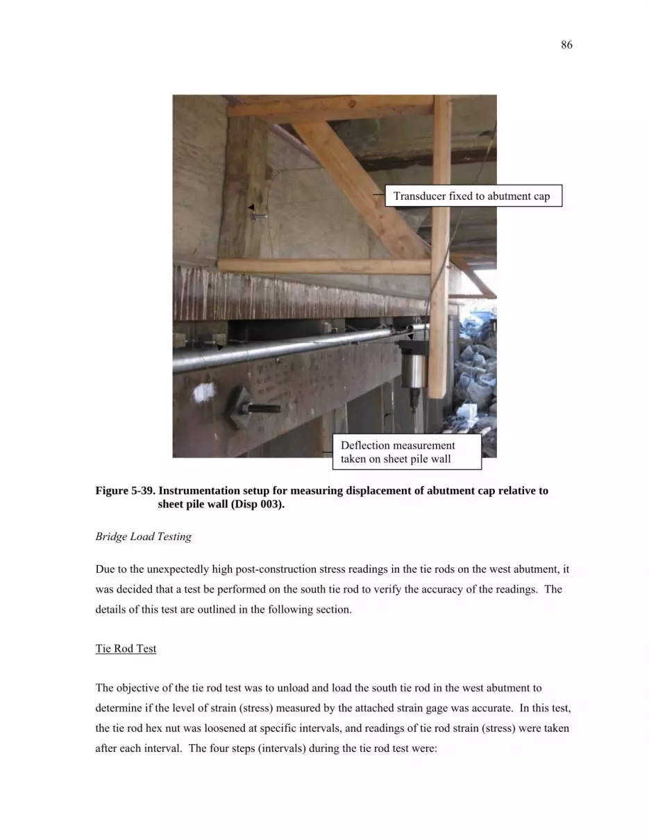
86

Figure 5-39. Instrumentation setup for measuring displacement of abutment cap relative to sheet pile wall (Disp 003).

Bridge Load Testing

Due to the unexpectedly high post-construction stress readings in the tie rods on the west abutment, it

was decided that a test be performed on the south tie rod to verify the accuracy of the readings. The

details of this test are outlined in the following section.

Tie Rod Test

The objective of the tie rod test was to unload and load the south tie rod in the west abutment to

determine if the level of strain (stress) measured by the attached strain gage was accurate. In this test,

the tie rod hex nut was loosened at specific intervals, and readings of tie rod strain (stress) were taken

after each interval. The four steps (intervals) during the tie rod test were:

Transducer fixed to abutment cap

Deflection measurement taken on sheet pile wall

87

1. Loosen hex nut 0.25 of a turn

2. Tighten 0.25 of a turn (returned to starting position)

3. Loosen hex nut in 0.50 turn intervals until 2 full turns achieved

4. Loosen at full turn intervals until a total of 4 full turns achieved

Initial stress in the south tie rod, which was calculated by the increase in strain from the initial values

measured after installation of the gage, was approximately 44 ksi. Steps 1 and 2 of the tie rod test

revealed that the stress decreased and returned to the initial level. Results of the stress readings for

Steps 3 and 4, with data taken between each test interval, are shown in Figure 5-40. Since significant

relatively linear and elastic changes in strain (stress) were observed during the tie rod test, it was

concluded that the stress levels initially indicated in the rods were reliable.

Stress levels in the tie rods were also monitored during the live load test of the bridge. Stresses

produced in the south rod during the test involving both trucks (the highest load) are also given in

Figure 5-40. Monitoring of the north tie rod in the west abutment was attempted during the bridge

load test but was unsuccessful as the strain gage on this tie rod was damaged during construction. It

should be noted that, since the north tie rod was attached to a relatively flexible steel H-pile (versus a

reinforced concrete deadman), the stresses developed in the north tie rod would have been less than

the south tie rod system (assuming each was exposed to the same levels of load).

Conclusions drawn from the tie rod test were:

The initial tie rod gage readings were reliable and high stresses were induced in the south tie

rod during the construction stages.

After performing the live load test, no significant increase in stress (less than 0.5 ksi)

occurred in the south tie rod. By theoretical analysis, the test truck was expected to induce a

maximum stress of 3 ksi assuming lateral restrain was provided by the superstructure; the low

levels of stress developed confirm this assumption made in design. The stresses initially

induced in the tie rods (approximately 45 ksi) occurred during backfilling of the abutment

before the superstructure was installed, confirming the necessity of a lateral restraint system

during construction of the abutments. (continued)

88

Since initial readings in the south tie rod indicated stress levels near the yield stress of the

steel, it is possible the tie rods experienced yielding at some point during compaction of the

abutment backfill and placement of the superstructure elements. This could also explain the

span length of the bridge being approximately 8 in. shorter than designed (due to lateral

displacements of abutments toward each other) although other construction factors may have

had an influence as well.

Figure 5-40. Comparison of stress level in south tie rod during live load testing and the tie rod test.

Distance of tandem to abutment centerline (ft)

-20 0 20 40

Tot

al s

tres

s in

tie

rod

(ks

i)

30

35

40

45

50

Turns of hex nut (loosening)

0 1 2 3 4

Bridge test Tie rod test

89

Live Load Test

Test Procedure

Test truck axle weights are given in Table 5-9; test truck dimensions are given in Table 5-10 along

with the truck diagrams shown in Figure 5-41.

Table 5-9. Test truck axle loads and total weight.

Load type Truck 48 (lbs) Truck 38 (lbs) Front axle

Tandem axle 17,460 31,360

16,980 30,260

Total weight 48,820 47,240 Table 5-10. Test truck dimensions.

Dimension Truck 48

(ft) Truck 38

(ft) A 5.17 4.75 B 4.50 4.25 C 14.58 14.50 D 2.33 2.42 E 6.08 6.08 F 8.00 8.00

Figure 5-41. Diagram of test trucks.

The live load test consisted of the four different runs shown in Figure 5-42. Each test run involved

the truck travelling from west to east and stopping at predetermined locations along the bridge.

Figure 5-43 shows the test locations along the bridge from west to east. The test positions are labeled

by a letter (corresponding to a test run in Figure 5-42) and a location number according to position

C EBA D

F

Assumed c.g.during live loadtesting

a.) Side view b.) Rear view

90

along the bridge; Figure 5-43 presents each location number and the distance of the centerline of the

tandem axle to the centerline of the west abutment.

Test Locations 6, 7 and 8 were intended for the center of gravity of the truck(s) to be positioned of the

0.25 span, midspan, and 0.75 span of the bridge; the assumed center of gravity of the truck was

determined in the field as a fixed location on each truck (the mud-flap shown in Figure 5-44b). The

dimension “B” in Table 5-10 gives the distance of this point relative to the centerline of the tandem

axle; future calculation of the exact center of gravity of the test truck determined the dimension “B”

in Table 5-10 to be 6.82 ft and 6.74 ft for Truck 48 and Truck 38, respectively; this showed field

assumed values for “B” were relatively accurate. All data are displayed as centerline of the tandem

axle locations for simplicity.

At each location, the trucks remained in position until all of the instrumentation was read and

recorded. Due to the inherent delays involved in reading vibrating wire instruments, each test

location reading required approximately three minutes to complete. Select data collected during the

bridge test are presented and analyzed within this section of the report.

Figure 5-42. Transverse location of truck(s) in live load tests.

31.8 ft

2 ft

CL

31.8 ft

CL

15.9 ft

a.) Test Run A

b.) Test Run B N

91

Figure 5-42 (continued).

Figure 5-43. Locations of tandem axle along the bridge.

31.8 ft

2 ft

8 ft

CL

31.8 ft

CL

8 ft

50 ft

Location: 1 2 3 4 65 7 8 9

5 ft

10 ft

20 ft

30 ft

9.6 ft

19.1 ft

28.7 ft

38.3 ft

CL West abutment brg. CL East abutment brg.

d.) Test Run D

c.) Test Run C

N

E

92

Figure 5-44. Bridge live load testing of BHC, Iowa demonstration project.

Data Analysis and Discussion

It should be noted that, when designing the monitoring system, it was desired to have the ability to

determine absolute values of the stress induced in the backfill soil (requiring “zero” values for earth

pressure cells be recorded just after placement and before any backfilling occurred). When initially

analyzing the data, it became apparent that, due to the movement of the wall (and release of stresses)

which occurred during the tie rod test, the “zero” values for all the cells had changed. As a result, all

data charts in this section present relative values of stress induced from the trucks; the “zero” values

used were taken after the tie rod test (which involved removal of stress in the tie rod by loosening of

the hex nut) had been performed.

The loosening of the hex nut during the tie rod test resulted in an outward movement of the sheet pile

wall and subsequently affected backfill soil stresses; changes in pressure on each of the earth pressure

cells resulting from the tie rod test are given in Table 5-11 (a negative value represents a reduction in

pressure). A reduction in stress was seen in all cell locations except at the wingwalls which

experienced little change. For the cells below TOC, special attention should be given to the

magnitudes of stress released as it gives an indication of the deflected shape of the wall as the tie rod

stress was released. Since the reduction in stress is greatest in the cell the greatest distance below the

TOC, it can be inferred that the wall “bowed” outward. The rigidity of the superstructure resisted

lateral displacement of the top of the wall at the location of the abutment cap, resulting in the

deflected shape shown in Figure 5-45.

a.) Overview of load testing b.) Side view of Truck 48

Assumed center of gravity for live load testing

93

Table 5-11. Change in earth pressure cell stresses resulting from wall movements during the tie rod test (refer to Figure 5-35 for pressure cell locations).

Pressure cell Stress released after wall movement (psf) Number Location

10674 concrete deadman - 50.1 8500 wingwall – high + 6.8 9487 wingwall – low + 1.5 9489 1 ft below TOC - 36.8 8503 3 ft below TOC - 83.1 9488 5 ft below TOC - 143.0 8504 H-pile deadman - 11.7 9486 12.5 ft back from wall - 25.3

Figure 5-45. Simulated deformations of sheet pile wall under load.

Earth pressures recorded for Cell 9489 (1ft below TOC) are shown in Figure 5-46. As can be seen,

the highest earth pressures were recorded during the test run (Run D) involving both trucks centered

over midspan of the bridge. Although pressures would initially be expected to reach maxima when

truck surcharge loads were on the abutment backfill, a potential explanation for the observed

phenomenon is the deformation of the bridge superstructure (elongation of the bridge as camber is

overcome as depicted in Figure 5-47) under load displacing the abutment caps toward the backfill,

applying pressure on the cell which is directly behind the caps. Further evidence of this is seen when

comparing Run B and Run D: although Run B shows higher stress in the cell while the tandem is on

the backfill material (which is expected since the cell is located along the centerline), Run D shows

greater stress when the two trucks are on the bridge (meaning greater deformation and elongation of

the superstructure versus Run B which involved only one truck).

Sheet pile wall

Deflected shape

a.) Plan view of wingwall deformations b.) Side view of deflected wall

94

Earth pressures during live load testing for Cells 8503 (3 ft below TOC) and 9488 (5 ft below TOC)

are presented in Figure 5-48 and Figure 5-49, respectively. At both locations, earth pressure

variations of less than 20 psf occurred; the forces transferred to the sheet pile wall due to vehicular

surcharge on the backfill are negligable.

Figure 5-46. Earth pressures for Cell 9489 (1 ft below TOC) during live load testing.

Figure 5-47. Diagram of bridge elongation under loading due to superstructure deflections.

Distance of tandem axle to centerline of west abutment wall (ft)

-20 0 20 40

Ear

th p

ress

ure

(psf

)

-20

0

20

40

60

80

100

120

140

Run ARun BRun CRun D

Δ

95

Figure 5-48. Earth pressures for Cell 8503 (3 ft below TOC) during live load testing.

Figure 5-49. Earth pressures for Cell 9488 (5 ft below TOC) during live load testing.

Distance of tandem axle to centerline of west abutment wall (ft)

-20 0 20 40

Ear

th p

ress

ure

(psf

)

-20

0

20

40

60

80

100

120

140

Run ARun BRun CRun D

Distance of tandem axle to centerline of west abutment wall (ft)

-20 0 20 40

Ear

th p

ress

ure

(psf

)

-20

0

20

40

60

80

100

120

140

Run ARun BRun CRun D

96

The expected stresses and deflections were calculated to provide a comparison for select data

obtained during the bridge test. An analysis was performed for three locations of the test trucks

(Truck 48 for single-truck Runs A, B and C): Locations 3, 4, and 5 (described previously, see Figure

5-43) with results provided in Table 5-12 through Table 5-14, respectively. Total values are given as

well as the values due to the live load test only. For the earth pressure cells listed, their locations are

given relative to TOC. Stresses in the piles (determined from strain gages) are presented as average

values for axial strains (stress) measured at multiple locations along each instrumented pile; flexural

strains (stresses) are presented for the maximum value measured in each instrumented pile.

The theoretical analysis was performed to investigate the adequacy of the design methods used. This

investigation was accomplished by applying the load distribution methods and other assumptions

utilized in design, determining expected loads and deflections by theoretical analysis, and comparing

expected results to data collected during live load testing; example analysis calculations for BHC,

Iowa are provided in Appendix A.

For the theoretical analysis, truck loads were assumed to distribute over a 10 ft width of the bridge. A

friction angle of 45° (determined from a direct shear test, see Figure A12) was used for the backfill

material in determining lateral earth pressures. Vehicular surcharge on the backfill material was

analyzed according to AASHTO (1998) Section 3.11.6.1-4 to determine the lateral loads applied to

the wall. The wall was analyzed with STAAD (2008) to determine bending moments, deflections of

the sheet pile wall, and tie rod forces. For determining flexural stresses in the sheet pile sections, a

modified section modulus of 35.2 in3/ft (calculated by ISU) was used to account for additional

resistance provided by the angles welded to the instrumented piles (angles were continuous along the

length of each pile except for negligible lengths at each end); the section modulus without the angles

was 18.1 in3/ft.

An analysis of the superstructure was also performed to estimate midspan flexural stresses and

deflections. The section modulus and moment of inertia for the deck elements used were 181.4 in.3

and 1741 in.4, respectively, for a repeating section of a width of 2.75 ft (values obtained from BHC

Engineer’s Office). The section modulus and moment of inertia calculated for the repeating section

are accurate for use with interior elements. An exterior element would have slightly higher values of

section modulus and moment of inertia due to contribution of the guardrail in stiffness; properties of

the repeating section were conservatively assumed to apply for exterior elements.

97

Location 3 west abutment brg.CL

2 ft

10 ft

Table 5-12. Comparison of actual to estimated values of selected loads and deflections for Location 3.

Load or deflection Measured (Live loads only)

Run A Run B Run C Run D

Pile 1 axial stress (avg) Pile 2 axial stress (avg) Pile 3 axial stress (avg) Pile 4 axial stress (avg)

-0.05 ksi -0.15 ksi -0.01 ksi +0.01 ksi

+0.01 ksi -0.17 ksi -0.04 ksi -0.04 ksi

+0.01 ksi -0.08 ksi -0.02 ksi -0.07 ksi

-

Pile 1 flex. stress (max) Pile 2 flex. stress (max) Pile 3 flex. stress (max) Pile 4 flex. stress (max)

0.06 ksi 0.23 ksi 0.03 ksi 0.01 ksi

0.03 ksi 0.21 ksi 0.04 ksi 0.03 ksi

0.05 ksi 0.06 ksi 0.06 ksi 0.06 ksi

-

Earth pressure (1 ft below TOC)

14 psf 60 psf 24 psf - Earth pressure

(3 ft below TOC) 1 psf 5 psf 1 psf

Earth pressure (5 ft below TOC) 0 psf 6 psf 9 psf

Midspan flex. stress (max) 0.8 ksi 0.5 ksi 0.9 ksi

- Midspan deflection (max) 0.040 in. 0.030 in. 0.015 in.

Wall deflection (max) 0.002 in. 0.001 in. 0.001 in.

Load or deflection Estimated

Total Live load only

Pile axial stress 0.80 ksi 0.21 ksi

Pile flex. stress 3.29 ksi 0.40 ksi

Earth pressure (1 ft below TOC)

139 psf 74 psf

Earth pressure (3 ft below TOC)

254 psf 119 psf

Earth pressure (5 ft below TOC) 335 psf 130 psf

Midspan flex. stress - 1.45 ksi

Midspan deflection - 0.13 in.

Wall deflection 0.13 in. 0.02 in.

Tandem axle 10 ft west of west abutment centerline during Run A

98

Location 4 west abutment brg.CL

2 ft

5 ft

Table 5-13. Comparison of actual to estimated values of selected loads and deflections for Location 4.

Load or deflection Measured (Live Loads Only)

Run A Run B Run C Run D

Pile 1 axial stress (avg) Pile 2 axial stress (avg) Pile 3 axial stress (avg) Pile 4 axial stress (avg)

-0.06 ksi -0.18 ksi -0.03 ksi +0.01 ksi

+0.02 ksi -0.20 ksi -0.05 ksi -0.05 ksi

+0.01 ksi -0.07 ksi -0.06 ksi -0.11 ksi

-0.05 ksi -0.27 ksi -0.10 ksi -0.12 ksi

Pile 1 flex. stress (max) Pile 2 flex. stress (max) Pile 3 flex. stress (max) Pile 4 flex. stress (max)

0.08 ksi 0.24 ksi 0.02 ksi 0.01 ksi

0.03 ksi 0.19 ksi 0.06 ksi 0.04 ksi

0.04 ksi 0.07 ksi 0.05 ksi 0.06 ksi

0.06 ksi 0.30 ksi 0.06 ksi 0.09 ksi

Earth pressure (1 ft below TOC)

-12 psf 89 psf 18 psf 53 psf

Earth pressure (3 ft below TOC)

0 psf 1 psf 0 psf 0 psf

Earth pressure (5 ft below TOC) 2 psf 4 psf 9 psf 0 psf

Midspan flex. stress (max) 1.3 ksi 0.8 ksi 1.4 ksi 1.5 ksi

Midspan deflection (max) 0.06 in. 0.04 in. 0.02 in. 0.08 in.

Wall deflection (max) 0.004 in. 0.002 in. 0.001 in. 0.002 in.

Load or deflection Estimated

Total Live load only

Pile axial stress 0.76 ksi 0.17 ksi

Pile flex. stress 3.40 ksi 0.53 ksi

Earth pressure (1 ft below TOC)

302 psf 237 psf

Earth pressure (3 ft below TOC)

373 psf 238 psf

Earth pressure (5 ft below TOC) 366 psf 161 psf

Midspan flex. stress - 2.2 ksi

Midspan deflection - 0.18 in.

Wall deflection 0.13 in. 0.02 in.

Tandem axle 5 ft west of west abutment centerline during Run A

99

Location 5 west abutment brg.CL

2 ft

Table 5-14. Comparison of actual to estimated values of selected loads and deflections for Location 5.

Load or deflection Measured (Live Loads Only)

Run A Run B Run C Run D

Pile 1 axial stress (avg) Pile 2 axial stress (avg) Pile 3 axial stress (avg) Pile 4 axial stress (avg)

-0.09 ksi -0.32 ksi -0.04 ksi +0.01 ksi

+0.01 ksi -0.27 ksi -0.09 ksi -0.08 ksi

+0.02 ksi -0.09 ksi -0.07 ksi -0.21 ksi

-0.05 ksi -0.43 ksi -0.14 ksi -0.22 ksi

Pile 1 flex. stress (max) Pile 2 flex. stress (max) Pile 3 flex. stress (max) Pile 4 flex. stress (max)

0.06 ksi 0.40 ksi 0.03 ksi 0.01 ksi

0.03 ksi 0.29 ksi 0.03 ksi 0.04 ksi

0.02 ksi 0.07 ksi 0.05 ksi 0.06 ksi

0.05 ksi 0.50 ksi 0.04 ksi 0.05 ksi

Earth pressure (1 ft below TOC)

-10 psf 93 psf 23 psf 66 psf

Earth pressure (3 ft below TOC)

0 psf 0 psf 0 psf 0 psf

Earth pressure (5 ft below TOC) -3 psf -4 psf 5 psf -6 psf

Midspan flex. stress (max) 2.3 ksi 1.4 ksi 2.1 ksi 2.4 ksi

Midspan deflection (max) 0.075 in. 0.050 in. 0.025 in. 0.100 in.

Wall deflection (max) 0.004 in. 0.002 in. 0.001 in. 0.002 in.

Load or deflection Estimated

Total Live load only

Pile axial stress 0.94 ksi 0.35 ksi

Pile flex. stress 3.20 ksi 0.30 ksi

Earth pressure (1 ft below TOC)

315 psf 250 psf

Earth pressure (3 ft below TOC)

215 psf 80 psf

Earth pressure (5 ft below TOC) 235 psf 30 psf

Midspan flex. stress - 3.1 ksi

Midspan deflection - 0.23 in.

Wall deflection 0.13 in. 0.01 in.

Tandem axle centered over west abutment centerline during Run A

100

From the results previously presented in Figure 5-46, Figure 5-48, and Figure 5-49 it can be seen that

earth pressures were significantly lower than estimated by theoretical analysis; conservative estimates

of soil cohesion is one potential explanation for this observation. Although more pressure cells were

used in the test (all measuring unexpectedly low earth pressures), the cell 1 ft below TOC showed the

highest variation in stress during the live load test (a magnitude of approximately 100 psf).

In general, maximum stresses in the piles (axial and flexural) were comparable to those estimated by

analysis suggesting a 10 ft wide distribution for live loads is a reasonable assumption; design of the

sheet piling for axial load used an over-conservative live load distribution of 3 piles (5.5 ft). A trend

noticed in the data presented in Table 5-12 through Table 5-14 is the minimal distribution of axial

stress to adjacent piles through friction between the sheet pile interlocks. For example, in Table 5-14

for Run A (in which the truck would be positioned over Pile 2) instrumented Pile 2 experiences an

axial compressive force of 0.32 ksi while the adjacent piles (Pile 1 and Pile 3) experience stresses

below 0.10 ksi and Pile 4 experiences negligible axial load.

All horizontal wall deflections and vertical deflections of the superstructure at midspan were

significantly less than estimated by analysis. Wall displacements for Line 2 and Line 4 are presented

in Figure 5-50 for test Run D (both trucks); the locations of Line 2 and Line 4 were previously

depicted in Figure 5-36. It should be noted that negative displacement represents an outward

movement of the wall. Although magnitudes of the wall displacements are negligible (approximately

10 times lower than expected by analysis), the nature of the displacements is of interest.

As previously mentioned, two displacement transducers (Disp 003 and Disp 010) were installed to

measure movement of the abutment cap relative to the sheet pile wall. In both Line 2 and Line 4,

movement of the abutment cap relative to the top of the sheet pile wall occurred when the centerline

of the tandem axles were 5 ft from the abutment centerline (for all test Runs) and subsequently

returned to zero when the tandem axles were on the bridge; the displacement of the top of the wall

was positive, suggesting that either (1) the abutment cap was being pushed outward or (2) the tie rod

location is acting as a fixed point about which the wall rotates (a pinned connection) and thus the top

of the wall will move inward due to lateral forces deflecting the lower portion of the wall outward

(“bowing out”). The outward displacements of Disp 008 and Disp 009 suggest that case (1) is

occurring as the entire wall moves outward (including the abutment cap); similar effects are seen in

both Line 2 and Line 4.

101

Another displacement of interest is the significant inward movement (toward the backfill) of the

abutment cap (Disp 004 and Disp 008) when the trucks are located at midspan in Run D; this can be

explained by the phenomenon described earlier in which the camber of the bridge deck units is

overcome and the superstructure expands laterally, pushing the abutments inward. On Line 2, a

displacement transducer (Disp 002) was placed to measure movements of the abutment cap relative to

the bridge deck. The significant negative displacement of Disp 002 when the trucks are at midspan

further confirms the occurrence of this phenomenon as it suggests the bridge deck elements are

expanding laterally.

Figure 5-50. Wall displacements during live load test Run D (see Figure 5-36 for locations).

Distance of tandem axle to centerline of west abutment wall (ft)

-20 -10 0 10 20 30 40 50

Dis

plac

em

ent

(in.)

-0.004

-0.002

0.000

0.002

0.004 Disp 002Disp 003Disp 004Disp 005Disp 006

Distance of tandem axle to centerline of west abutment wall (ft)

-20 -10 0 10 20 30 40 50

Dis

pla

cem

ent

(in.)

-0.004

-0.002

0.000

0.002

0.004 Disp 008Disp 009Disp 010Disp 011

a.) Line 2 instrumentation

b.) Line 4 instrumentation

102

Long-Term Monitoring

For long-term monitoring of bridge’s behavior, the permanent instrumentation system was used.

Readings were taken 4 times daily (once every 6 hours) starting November 20, 2008. The system was

set to record at 4:00am, 10:00am, 4:00pm, and 10:00pm to capture daily temperature fluctuations.

Long-term measurement of earth pressure (as well as temperature) in the cells 1 ft and 3 ft below

TOC are presented in Figure 5-51 and Figure 5-52, respectively. Although the monitoring system

was destroyed in a flooding event in the spring of 2009, long-term data were collected for 80 days

after November 20, 2008. For the cell 1 ft below TOC, significant variations of earth pressure with

time were recorded. In the cell just below it (3 ft below TOC) the variation was less. Both cells

experienced greater variations in stress during cold temperature cycles (perhaps attributable to stress

development from ground freezing in the backfill behind the abutment). It should be noted that each

pressure cell and piezometer was equipped with a thermistor for measuring temperatures therefore

each chart will present differing temperatures corresponding to the location of the instrument. The

significant variations of temperature in Cell 9489 (Figure 5-51) are most likely due to the proximity

of the cell to the surface and the concrete abutments; it experienced greater daily fluctuation of

temperature during the warmer part of the season.

Figure 5-51. Long-term readings for Pressure Cell 9489 (located 1 ft below TOC).

Date

0 20 40 60 80

Ear

th P

ress

ure

(psf

)

0

500

1000

1500

2000

Tem

pera

ture

(de

gree

s C

elsi

us)

-10

-5

0

5

10

Pressure Cell 9489Temperature

12/10/08 12/31/08 01/20/09 02/10/09 11/20/08

103

Figure 5-52. Long-term readings for Pressure Cell 8503 (located 3 ft below TOC).

Long-term groundwater table measurements, given as the distance from the bottom of the bridge deck

(at the abutments) to the water level, are shown in Figure 5-53 for both sides of the abutment.

Although the two piezometers measured different levels of groundwater, the offset is constant at

about 3 in. to 4 in. (attributable to human error in placement of the instrument) suggesting that no

significant pressure head developed behind the abutment wall.

Figure 5-53. Long-term readings for Piezometer 8496 (on stream side of abutment wall) and Piezometer 8497 (on backfill side of abutment wall).

Date

0 20 40 60 80

Ea

rth

Pre

ssur

e (

psf

)

-100

0

100

200

300

400

500

Te

mpe

ratu

re (

deg

rees

Ce

lsiu

s)

-15

-10

-5

0

5

10

Pressure Cell 8503Temperature

Date

0 20 40 60 80Dis

tanc

e f

rom

bot

tom

of

brid

ge d

eck

to w

ate

r ta

ble

(ft)

7.0

7.5

8.0

8.5

9.0

9.5

10.0

Tem

pera

ture

(d

egre

es C

els

ius)

6

8

10

12

14

Piezometer 8496 Piezometer 8497 Temperature

12/10/08 12/31/08 01/20/09 02/10/09 11/20/08

12/10/08 12/31/08 01/20/09 02/10/09 11/20/08

104

Key Findings

Analysis of the live load test data determined that maximum axial stresses occurring in the piles were

approximately 0.5 ksi and were comparable to estimates made by analysis for a load distribution

width of 10 ft. Flexural stresses, in general, were significantly less than those estimated by analysis

and maximum values were approximately 0.2 ksi. Earth pressures recorded during live load testing

(with maxima of approximately 100 psf) were also significantly lower than earth pressures estimated

by analysis. These results suggest the method of analysis for lateral earth pressures applied to the

sheet pile wall was conservative. Long-term monitoring data showed variations in earth pressure over

time with the largest variations in earth pressure occurring behind the abutment cap. The earth

pressures experienced cycles that varied in magnitude from 50 psf to 1500 psf, suggesting long-term

loading due to freeze/thaw cycles of the soil and the thermal deformation of the superstructure

elements may be the critical factors in the design of sheet pile abutment and backfill retaining systems

rather than vehicular live loads.

Through the construction and structural monitoring of the BHC demonstration bridge, axially-loaded

steel sheet piling has been shown to be a feasible alternative for bridge abutments with site conditions

similar to BHC (i.e., shallow bedrock). Although the BHC project required approximately 10 weeks

for construction, in the future the construction could be completed in a significantly shorter period if

time is critical.

According to the BHC Engineer’s Office, the total cost of this project (including labor and materials)

was $151,230. The BHC Engineer’s Office believes that a significant portion of the cost can be

attributed to the labor and equipment time involved in developing a new method of construction for

this type of bridge as well as the many associated equipment breakdowns. Future projects utilizing a

similar design and construction method with comparable site conditions could be performed at a

reduced cost.

105

Boone County

Project Details

The second demonstration project was constructed in Boone County (BC), Iowa. The site that was

selected was a LVR bridge, originally constructed in 1937, crossing Eversoll Creek (a tributary of the

Des Moines River) on Owl Avenue near the city of Madrid; the location of the bridge is shown in

Figure 5-54.

This project was undertaken to investigate the feasibility of sheet piling combined with a GRS system

for use as the primary abutment foundation element and backfill retaining system. Construction of

the new bridge was initiated on June 29, 2009 and completed on November 11, 2009. This report

presents information on the design of the new sheet pile abutment bridge system, its construction, and

the instrumentation installed. Information on load testing and data analysis will be presented in a

future report. The following sections give an overview of the previous structure and the new sheet

pile abutment bridge system.

Figure 5-54. Location of bridge replacement project outside of Madrid in BC, Iowa.

Bridge location

N

106

Previous Bridge Structure

The structure that was replaced was a 19 ft wide, 95 ft long three-span bridge. The bridge had a

timber deck on steel girders with timber pile abutments and piers (encased in concrete) and was

approximately 17 ft above stream level (see Figure 5-55). Due to the orientation of the roadway with

respect to the stream, the original structure had a 30 degree skew.

Figure 5-55. Previous bridge replaced by BC demonstration project.

a.) Side view

b.) End view

107

New Sheet Pile Abutment Bridge System Overview

The replacement bridge (a 30 ft wide, 100 ft long three-span continuous concrete slab with a 30

degree skew) was a joint design effort between ISU and the BC Engineer’s Office. The design of the

superstructure and piers was performed by the BC Engineer’s Office and utilized an Iowa DOT

bridge standard. The design of the bridge abutments was performed by Iowa State University and

utilized steel sheet piling and a GRS system.

Superstructure and Piers

The Iowa DOT standard selected by the BC Engineer’s Office was the J30C-87 county bridge

standard. The specific design selected was a 33.17 ft wide continuous concrete slab structure that

used an open concrete rail creating a 30.5 ft roadway. The depth of the bridge deck was 1.48 ft along

the spans and 2.46 ft over the piers. Cross-sections of the bridge are shown in Figure 5-56. Each pier

consisted of 8, 80 ft long HP10x42 piles made monolithic with the bridge deck. The piles were

encased in reinforced concrete for a length of approximately 20 ft below the bridge deck. For more

details on the design of the superstructure and piers refer to Iowa DOT county bridge standard J30C-

87.

Figure 5-56. Replacement bridge deck for demonstration project in BC, Iowa.

33.17 ft

30.5 ft roadway

1.48 ft

2.46 ft

CL

CL

a.) Cross-section near abutments

b.) Cross-section near piers

108

Figure 5-56. (continued).

Abutment Foundation and Backfill Retaining System

The standard abutment for the J30C-87 required six driven piles to be used. ISU designed a system

which replaced the piling with a 6 ft wide reinforced concrete spread footing that was supported by

GRS retained (and further reinforced) by a steel sheet pile wall. A cross-section of the system is

shown in Figure 5-57. The GRS system was created using 6 layers (1 ft vertical spacing) of biaxial

geogrid with a granular backfill of 1.5 in. roadstone. A plan view of the abutment (both abutments

have same layout) is shown in Figure 5-58; as previously stated, the abutment had a 30 degree skew.

Figure 5-57. Cross-section of sheet pile abutment foundation system designed by ISU.

5.5 ft

3 ft 3 ft

30.5 ft 39 ft 30.5 ft

100 ft

1.48 ft1 ft1 ft 6 ft

2.46 ft

Bridge deck

Spread footingAbutment cap

Waler

Sheet pile wall

Subdrain systemReinforced concrete deadman

GRS system

Tie rod anchors

c.) Side view

109

Figure 5-58. Plan view of GRS sheet pile abutment system.

Site Investigation

Field Investigation

Cone Penetrometer Testing

CPT soundings were performed approximately 15 ft east and west of the center of the bridge

abutments on June 10, 2008. The CPT sounding locations are shown in Figure 5-59. CPT 1 and CPT

2 were advanced to depth of 45.6 ft and 44.1 ft, respectively, below existing grades. Logs of the

soundings, showing cone tip stress and sleeve friction for both CPT 1 and CPT 2, are presented in

Figure 5-60.

30°

Roadway

Spread footing

Anchor system

GRS layer

Sheet pile wall

62.5 ft

14 ft

CL

C

110

Figure 5-59. Plan view of CPT and soil boring locations for demonstration project in BC, Iowa.

Soil behavior types determined from CPT 1 and CPT 2 are presented in Figure 5-61; as can be seen,

the majority of materials present are cohesive soils underlain by a granular base. Dense granular

materials and over-consolidated fine grained soil deposits were determined to be present below depths

of 34 ft in both soundings due to a relatively large decrease in pore water pressure (caused by soil

fracturing and dilatency). Soil shear strength and SPT resistance estimates from correlations

presented by Lunne, Powell, and Robertson (1997) for both CPT’s are presented in Figure 5-62.

Figure 5-60. Results of CPT’s showing cone tip and friction resistance.

SB 1

CPT 1 CPT 2RoadwayCL

15 ft

20 ft

15 ft

5 ft

Cone Resistance (tsf)

0 100 200 300 400 500

Dep

th (

ft)

0

10

20

30

40

Friction Resistance (tsf)

0 1 2 3 4 5 6

Cone ResistanceFriction Resistance

Cone Resistance (tsf)

0 100 200 300 400 500

Dep

th (

ft)

0

10

20

30

40

Friction Resistance (tsf)

0 1 2 3 4 5 6

a.) CPT 1 b.) CPT 2

N

111

Figure 5-61. Soil behavior types determined from CPT’s.

Figure 5-62. Shear strength and SPT correlations for CPT’s.

Soil Behavior Type

0 2 4 6 8 10 12

De

pth

(ft)

0

10

20

30

40

Soil Behavior Type

0 2 4 6 8 10 12

De

pth

(ft)

0

10

20

30

40

# Soil T ype

0 Organic Material/

1 Fine Grained

2345 Clayey Silt

6 Sandy Silt to

7 Silty Sand

89

1011 Very St iff Fine Grained

12 to Clayey Sand

Clay to Silty Clay

Sand to Gravelly Sand

Shear Strength (ksf)

0 10 20 30 40 50

Dep

th (

ft)

0

10

20

30

40

N60 (blows per ft)

0 20 40 60 80100120140

Shear StrengthCalculated SPT Value

Shear Strength (ksf)

0 10 20 30 40 50

De

pth

(ft)

0

10

20

30

40

N60 (blows per ft)

0 20 40 60 80100120140

a.) CPT 1 b.) CPT 2

a.) CPT 1 b.) CPT 2

112

Soil Borings

A soil boring was performed by members of the ISU research team on July 11, 2008. The location of

the boring is shown in Figure 5-59; the boring log is provided in Figure B7 of Appendix B.

Laboratory Testing

Unconfined compression tests were performed to determine the shear strength of the selected

undisturbed soil samples. As can be seen from the results presented in Table 5-15, the strength of the

soil decreases significantly with increasing depth. The results of the Atterberg tests, the percentage of

soil passing the No. 200 sieve (percent fines), and the USCS classification for select samples are

presented in Table 5-16; as can be seen, the soil primarily consists of clay.

Table 5-15. Unconfined compression test results on select soil samples from SB 1.

Depth Range (in.)

Undrained Shear Strength (psf)

36 - 60 1645 72 - 96 1100

102 - 126 955 144 - 168 350

Table 5-16. Atterberg test and gradation results for select boring ranges.

Depth Range (in.)

LL (%)

PL (%)

PI (%)

Passing No. 200 (%)

Soil Type (USCS)

36 – 48 31.5 20.8 10.7 72 ML 72 – 96 41.5 24.8 16.7 78 CL

120 26.5 18.4 8.1 31 SC 144 – 168 25.7 18.2 7.5 74 CL

240 -* - - 26 SM * No data available

Site Conditions

Geologic Setting

The project site is located on the "Des Moines Glacial Lobe", a region formed by significant glacial

activity. According to GSI (see Figure B6 for CPT report), the predominant surficial sediment, which

was deposited by the Wisconsinan glacier, is glacial drift. Soils commonly encountered within 15 ft

of the ground surface are variable and usually consist of very silty sandy clay with interbedded sand

113

seams, layers, and pockets. The underlying materials (deposited beneath advancing glacial ice) tend

to be homogenous compositions of silty sandy clay materials. Overburden deposits within the stream

valleys generally consist of colluvium (slopewash) overlying alluvium of varying thickness which is

underlain by the glacial till soils over bedrock. The colluvial deposits are derived from parent soil

materials on hillsides while the underlying alluvium may consist of cohesive clayey silt and silty clay

soils and/or deposits. This project is located on a creek upland of the Des Moines River floodplain

which may have deposited alluvium consisting of interbedded sand and clay soils.

Soil Conditions

During soil boring, light gray clayey sand material (used as fill for the previous bridge) was found for

the first 3 ft of depth. Very stiff black and light gray silty clays were discovered from depths of

approximately 3 ft to 11 ft. Very stiff tan and light gray sandy clays or clayey sands were

encountered after 11 ft of depth. From approximately 15 ft of depth to the end of the boring (20 ft)

primarily tan silty sand was encountered.

Groundwater Observations

During the soil boring advancement and sampling operations, observations for free groundwater were

made. Information regarding water level observations is recorded in the “Stratigraphy” column on the

soil boring log. Groundwater was encountered at depths below existing grade of approximately 16 ft

in soil boring SB 1. From the CPT soundings, the observed drop in tip stress and sleeve friction near

depths of 15 ft to 17 ft likely coincides with the ground water surface.

Design

As previously mentioned, the design of the superstructure and piers was performed by the BC

Engineer’s Office; the design selected was the county bridge standard J30C-87. ISU designed a GRS

sheet pile abutment and backfill retaining system that was used in place of the driven piling (six

HP10x42’s driven to a 25 ton bearing capacity) specified in the J30C-87 county bridge standard. The

abutment cap for the county bridge standard was designed to bear on a reinforced concrete spread

footing on a GRS system (6 layers of Tensar® BX1200 biaxial geogrid placed as shown in Figure B2

and Figure B3) retained by a sheet pile wall with an anchor system. Detailed design plans of the GRS

sheet pile abutment and backfill retaining system are provided in Figure B1 through Figure B5.

114

The GRS sheet pile abutment and backfill retaining system was designed for HL-93 loading

(AASHTO Section 3.6.1.2, 1998) of the superstructure using the critical load factors and load

combinations presented in AASHTO (1998) Section 3.4.

GRS Sheet Pile Abutment and Backfill Retaining System Design

The sheet pile wall and reinforced concrete deadman anchor system were designed to resist all loads

(including bridge and backfill surcharge loading), neglecting the contribution of the GRS system due

to the limited existing research on long-term performance of such systems.

Loads transferred through the abutment cap to the spread footing were assumed to distribute evenly

across the surface area. Dead loads were assumed to distribute over the entire length of the footing

while the live loads were distributed over a 10 ft long strip. The spread footing was designed to be 6 ft

wide to reduce the bearing pressure to a maximum factored load of 3500 psf. The surcharge loads

were applied as lateral earth pressures to the sheet pile wall according to AASHTO (1998) Section

3.11.6.1. The sheet pile section required to resists design earth pressure loads was the PZ 22. The

required depth of the sheet pile wall for stability (accounting for a 6 ft depth of scour) was

approximately 25 ft; sheet pile sections were ordered 30 ft long as an additional factor of safety.

The tie rod anchors were placed at 6 ft below the top of the sheet pile wall and were required to resist

a total force of approximately 1000 kips; seven #14, Grade 75 steel, fully-threaded epoxy-coated tie

rods (obtained from Dywidag Systems International, Inc.) were used to provide anchorage for the

wall. The tie rods were anchored to a 35 ft x 8 ft x 2 ft reinforced concrete deadman that was

approximately 45 ft from the main wall at the nearest point (distance varied due to skew as seen in

Figure B1). The method for transferring anchorage forces from the tie rods to the sheet pile wall were

through the waler system described later in this thesis. The waler system consisted of two back-to-

back C9x20 shapes with bearing plates constructed to account for the skew of the abutment. The

abutment skew created greater loads in the tie rods as well as requiring welds to be made between the

bearing plates, waler, and sheet pile wall to resist translational forces induced. Details on design

calculations are provided in Appendix B.

115

Construction

The contractor selected for construction of the demonstration project was Graves Construction Co.,

Incorporated of Spencer, Iowa. The primary bridge crew consisted of five construction workers.

Construction activities commenced on June 29, 2009 and were completed in approximately 18 weeks.

A chronology of significant construction events is presented in Table 5-17; details of each event are

given in this section of the report.

Table 5-17. Chronology of significant construction events for the BC, Iowa demonstration project.

Event description Start date Working Days Between Events Demolition 06/29/09 7

Pier construction (west) Abutment construction (west) Abutment backfilling (west)

07/08/09 07/22/09 07/28/09

10 4 3

Anchor system const. (west) Abutment flooding (west) Pier Construction (east)

Abutment demolition (east) Deck falsework assembly

Abutment construction (east) Abutment backfilling (east) Anchor system const. (east) Abutment flooding (east)

Deck reinforcement placement Concrete deck pour

Casting of guardrails Removal of falsework Finishing earthwork

Open for service Bridge Load Testing

07/31/09 08/05/09 08/17/09 08/25/09 08/31/09 09/01/09 09/08/09 09/11/09 09/17/09 09/22/09 10/07/09 10/12/09 10/19/09 10/30/09 11/10/09 11/13/09

3 8 6 4 1 5 3 4 3 11 3 5 9 7 - -

Demolition of Existing Structure

Initial construction activities involved assembly of cranes and clearing and grubbing of the project

site. Removal of the superstructure and the west abutment were the first tasks of the demolition and

required approximately 7 work days to complete. The west piers were also removed but the east pier

and abutment were left in place for later demolition after equipment was moved to the east side of the

creek. The superstructure was demolished by removing the timber decking and torch cutting sections

of the steel girders for removal (see Figure 5-63). Timber piles (in the abutment and piers) were

116

pulled if possible or cut off below ground level. Complete removal of the superstructure and the west

pier was completed in less than 3 days.

Figure 5-63. Demolition of existing structure for the BC, Iowa demonstration project.

a.) Timber decking removed (exposing steel girders)

b.) Superstructure removed

117

Pier Construction

Each pier consisted of 8, HP10x42, 80 ft long steel piles which were encased in reinforced concrete

for the upper 18 ft and cast monolithic with the bridge deck. Since the concrete encasements

extended below the existing stream bed elevation cofferdams were constructed for placement of the

piles (see Figure 5-64a). The piles were driven in 40 ft sections using a single-acting diesel hammer

and were specified a minimum 34 ton bearing capacity (approximately 0.30 in. penetration per

hammer blow). One of the battered piles being driven while the other is being held in place after

splicing on the second section is shown in Figure 5-64b. Piles were spliced by beveling the edges

with a grinder (seen in Figure 5-65a) in preparation for the full-penetration groove welds to be made

by the contractor’s certified welder (see Figure 5-65b). After all piles were driven beyond specified

bearing capacity, reinforcement and forms were placed for the 18 ft long encasement.

Figure 5-64. Pier construction activities for the BC, Iowa demonstration project.

Figure 5-65. Splicing of H-Pile sections for bridge piers.

a.) Cofferdam placement and excavation b.) Placement and driving of battered piles

a.) Preparation of piles for welding b.) Welding two 40 ft sections together

118

Sheet Pile Driving

After excavation to the base elevation of the backfill zone on the west abutment, the ISU research

team inspected and approved the existing material by performing a dynamic cone-penetrometer

(DCP) test as per ASTM D6951 (2003); the resulting data from a DCP test are an empirical value

known as the California bearing ratio (CBR) and is an indicator of the level of compaction of soil.

For the east abutment, DCP testing concluded that the existing material was unsuitable for

construction; improvement was achieved by replacing 18 in. of the existing material with 1.5 in.

roadstone placed in 9 in. lifts.

After approving the base material, 30 ft long sheet pile sections (PZ 22) were driven with a vibratory

pile driver to design elevations (shown in Figure 5-66a). No pile bearing capacity was specified as

the sheet pile sections act as a backfill retention and scour protecting structure in this application. As

an alternative to construction of a guide rack, sheet pile sections were initially set and held during

driving with the excavator boom as shown in Figure 5-66b.

Figure 5-66. Placement of sheet pile sections.

One issue encountered during driving was, due to friction in between the interlocks of adjacent sheets,

driving one pile would occasionally drive an adjacent pile further (past its design elevation); this issue

was overcome by driving future piles at a reduced rate. The west abutment after all sheet piling

(including the 35 degree and 90 degree wingwalls) had been driven to design elevations is shown in

Figure 5-67.

a.) Vibratory pile driving b.) Initially set and held with excavator boom

Vibratory driver

119

Figure 5-67. West abutment after all sheet piling in place.

Abutment Backfilling and Placement of GRS System

Backfilling operations began after the sheet pile walls had been driven and the subdrain system was in

place. The subdrain consisted of a rigid perforated PVC pipe surrounded by porous backfill and

wrapped in engineering fabric to prevent soil fines from plugging the perforations. The subdrain

system also utilized a wick drain installed along the backfill side of the sheet pile wall as a means of

quickly draining any water that came in contact with the sheet pile wall. A single layer of the wick

drain is displayed in Figure 5-68a; subsequent layers were placed with a slight overlap to provide

continuous drainage and prevent the entrance of fines. The subdrain pipes exited through the south

wingwalls in both abutments and were terminated with a 6 ft long, 6 in. diameter corrugated metal

pipe (with a rodent guard) that drained on the downstream side of the bridge.

The backfill material used within the GRS zone was 1.5 in. crushed roadstone. The geogrid material

(Tensar ® BX1200 biaxial geogrid) was delivered to the jobsite in 9.8 ft by 164 ft long rolls. The

geogrid consisted of essentially a sheet of polypropylene material with 1in. by 1in. apertures to form a

grid (see Figure 5-69).

120

Before placement of any backfill, a layer of engineering fabric (to be placed around all sides of the

GRS mass) was placed over the base of the excavation for erosion protection (see Figure 5-68a).

Backfill material was placed in 6 in. lifts and compacted to a minimum of 98% of standard effort

compaction test (ASTM D698, 2000) within 2% of optimum moisture content using several passes of

the remote-operated vibratory compactor as shown in Figure 5-70b. After two lifts of backfill

material (1 ft) a layer of geogrid was placed; a total of 6 layers of geogrid were placed in each

abutment. Geogrid layers were installed by placing strips of the material (9.8 ft wide) perpendicular

to the abutment to cover the GRS zone shown in Figure B3. Each strip placed was lapped a minimum

of 12 in. over the adjacent strip to provide continuous reinforcement (see Figure 5-69). Sufficient

length (approximately 3 ft) was provided so the ends of each layer could be wrapped over the next

layer of backfill as depicted in Figure 5-70.

Figure 5-68. Base layer of backfilling for west abutment.

Wick drain

a.) Engineering fabric placement

b.) Vibratory compaction

121

Figure 5-69. Geogrid material for GRS abutment system in west abutment.

Figure 5-70. Geogrid from lower layer wrapped around backfill into upper lift.

DCP 4DCP 3DCP 2DCP 1

DCP Base

Geogridwrap around

Geogrid wrap around

a.) View of geogrid wrapping around layer of backfill

b.) Cross-section of west abutment depicting locations of DCP tests

Minimum 12 in. overlap of geogrid layers

122

Before backfilling of the each abutment, soils at the base of the excavation were investigated to

determine adequacy for construction of the abutments by performing DCP tests. The DCP testing

provided a value of the penetration index (PI) in terms of millimeter per hammer blow; the value for

the CBR is determined as follows (Iowa Statewide Urban Design and Specifications, 2009):

CBR292PI

.

The results for the west abutment (see Figure 5-71a) showed steadily increasing strength with depth

and was determined to be adequate. The results for the east abutment (see Figure 5-71b) showed no

increase in strength with depth; ISU required that an 18 in. layer of the base material be removed and

replaced with 1.5 in. compacted roadstone to increase strength.

During backfilling, several DCP tests were performed to verify compaction efforts were meeting the

specified requirements. The locations of the DCP tests performed were depicted previously in Figure

5-70b with depths below the footing presented in Table 5-18. Through an analysis of the results of

the DCP testing of the west abutment backfill, which is presented in Figure 5-72, it was determined

the backfill met the required specifications for compaction.

Figure 5-71. DCP testing results for base soils to determine adequacy for abutment construction.

CBR

0 20 40 60 80 100

Dep

th (

in.)

0

10

20

30

CBR

0 20 40 60 80 100

De

pth

(in.)

0

5

10

15

20

25

30

a.) West abutment b.) East abutment

123

Table 5-18. DCP test results for west abutment with reference to Figure 5-70b.

DCP Location Depth below footing (ft) Base 7.0

1 4.5 2 3.0 3 2.0 4 0.0

Figure 5-72. DCP test results for west abutment backfill material.

In the backfill of the west GRS sheet pile abutment system, several earth pressure cells were installed

for measuring horizontal and vertical earth pressure. Each cell was placed in a pocket of fine silica

sand and surrounded by course sand as shown in Figure 5-73. An overview of all instrumentation and

locations is presented in the next section of this report.

Figure 5-73. Placement of earth pressure cells in west abutment backfill.

CBR

0 20 40 60 80 100

Dep

th (

in.)

0

2

4

6

8

10

12

14

16

DCP 1DCP 2DCP 3DCP 4

a.) Fine silica sand bedding for earth pressure cell

124

Figure 5-73. (continued).

Deadman Anchor System

The anchor systems used on each abutment were anchored to a large, 35 ft x 8 ft x 2 ft reinforced

concrete deadman placed approximately 50 ft behind the sheet pile wall and 6 ft below grade (see

Figure B1 and Figure B2 for details). The deadman was cast in formwork placed in a large trench

excavated 4 ft deep. The reinforcement in the deadman is shown in Figure 5-74. The deadman after

formwork was removed is shown in Figure 5-75a. Flowable grout was poured into the excavated

trench of the deadman (instead of using soil) to minimize the mobilization required to achieve full

strength of the deadman (see Figure 5-75b). The deadman was perpendicular to the centerline of the

roadway and thus the distance from the sheet pile wall to the deadman varied due to the skew of the

bridge.

Each abutment was anchored to the deadman by seven 1.75 in. diameter tie rods (grade 75 steel) that

were fully threaded and epoxy-coated (see Figure 5-76a). The bars came in two sections and required

couplers to attain full length. The tie rods provided anchorage to the sheet pile wall through a waler

system that consisted of two C9x20’s placed back-to-back with a 3 in. gap between them for the rod

to pass through (see Figure 5-76b and Figure 5-76c). Because of the skew of the abutment, the waler

b.) Coarse sand bedding for earth pressure cell

125

needed to be welded to the sheet pile wall with a minimum of 6 in. welds at every contact point

between the waler and the sheet pile to resist the translational force component (t) of the developed tie

rod force (T) depicted in Figure 5-76d. A cross-section of the waler is provided in Figure 5-76e. This

also required the bearing plates (which were constructed as shown in Figure 5-76f to compensate for

the skew of the abutment wall) to be fully welded to the waler. The wingwalls were tied together

using a 2.25 in. diameter epoxy-coated threaded tie rod and a waler system similar to that used for the

wall (with differing skews); see Figure B1 for additional details.

Figure 5-74. Reinforcement placement for concrete deadman.

Figure 5-75. Reinforced concrete deadman in west abutment.

a.) Initial cast of deadman b.) Placement of flowable grout

a.) Overview of deadman trench b.) Reinforcement and formwork being placed

126

Figure 5-76. Details of anchorage system for BC, Iowa demonstration project.

30°

T

t

b.) Side view of waler system c.) Skewed bearing plate for tie rod connection

d.) Diagram of translational force component from tie rod

a.) Deadman and tie rods anchoring the west abutment sheet pile wall

127

Figure 5-76. (continued).

Due to the construction techniques used, the alignment of the sheet pile wall and both wingwalls were

not straight which resulted in gaps between the waler and sheet piling wall in locations needed to be

in contact (see Figure 5-77). Consequently, the minimum welding requirements between the waler

and sheet pile wall previously mentioned could not be made. Attempts were made by the contractor

3 in.

Sheet pile wall

Bearing plate

Stiffened C9x20's

6 in.

3.5 in.

2.25 in.

1 in.

6 in. 2.25 in. diameter

e.) Cross-section of waler

f.) Isometric view of bearing plate

128

to eliminate the gaps using a winch, however only 2 of the 13 gaps were eliminated; the gaps varied

in thicknesses from 0.5 in. to 13 in. The solution for eliminating the remaining gaps was to order

plates to fill each gap and subsequently welding the plates to the sheet pile wall and the waler. For

any gaps over 2 in., H-Pile sections were used instead of ordering custom bearing plates. According

to the BC Engineer’s Office, the cost of this solution was approximately $2,500. Contact between the

waler and sheet pile wall was not an issue on the east abutment as a greater effort was made to ensure

proper alignment during pile driving.

Figure 5-77. Waler not in contact on all sheet piles in west abutment.

Figure 5-78. H-pile splice used on 90 degree wingwall waler of west abutment.

H-Pile section

a.) Bottom waler channel welded to sheet pile wall b.) Detail A

Detail A

129

Abutment Finishing and Footing Construction

Several tasks were required to complete construction of the abutments. After backfilling was

completed to the design elevation, the abutment was flooded with water pumped from the stream to

reduce the amount of voids in the backfill material (to minimize settlement) and test the drainage

system. Flooding of the abutment and the water successfully draining into the stream is shown in

Figure 5-79a and Figure 5-79b, respectively.

Figure 5-79. Flooding of the west abutment.

After the abutments were backfilled and compacted to the design elevation, ISU researchers

performed DCP and light weight deflectometer (LWD) testing (shown in Figure 5-80a) as per ASTM

E2583 (2007) to determine the adequacy of the backfill soil which was to support the bridge abutment

foundation. Seven LWD tests and three DCP tests were completed; the location of each test is shown

in Figure 5-81 with reference to the coordinates given in Table 5-19.

LWD testing was performed by dropping a hammer (weight approximately 22 lbs) from a specified

height several times onto a 300 mm square plate while monitoring the vertical displacement into the

soil (see Figure 5-80). The results of the LWD testing (which provides an estimate of the elastic

modulus of the soil) are presented in Table 5-20. The test performed at location LWD 7 (shown in

Figure 5-80b) was on the material present at the site (instead of the compacted backfill) to provide a

comparison for the data. The results revealed that elastic settlements were reduced more than 90%

(comparing relative modulus of elasticity) on average through the use of quality, compacted backfill

material over existing soils. The DCP testing involved dropping a 17.6 lb weight (from a height of

a.) Pumping water from stream b.) Water draining from abutment

130

22.6 in.) to drive a 20 mm diameter cone into the soil while recording the observed penetration. A

CBR value of approximately 50 was desired for the abutment backfill at the level of the footing. The

DCP testing results for the west and east abutments at the level of the spread footing are presented in

Figure 5-82a and Figure 5-82b, respectively. After analyzing the results of the DCP testing, the

abutment backfill was considered adequate for the construction of the footings.

Figure 5-80. LWD testing of backfill soil at spread footing location on east abutment.

Figure 5-81. Dimensions of backfill LWD and DCP test locations (see Table 5-19) on abutments.

xy

FootingCL

LWD 3LWD 2LWD 1

LWD 4 LWD 5 LWD 6

DCP A DCP B DCP C

LWD 7

a.) Testing on abutment backfill at base of spread footing

b.) Testing on east abutment existing soil

131

Table 5-19. Locations of backfill LWD and DCP test locations with reference to coordinates in Figure 5-81.

Test point Location

West abutment East abutment x (ft) y (ft) x (ft) y (ft)

LWD 1 4.0 5.0 12.0 5.0 LWD 2 18.0 5.0 24.0 5.0 LWD 3 40.0 5.0 36.0 5.0 LWD 4 4.0 9.0 12.0 9.0 LWD 5 18.0 9.0 24.0 9.0 LWD 6 40.0 9.0 36.0 9.0 LWD 7 - - 26.0 16.5 DCP A 4.0 7.0 12.0 7.0 DCP B 18.0 7.0 24.0 7.0 DCP C 40.0 7.0 36.0 7.0

Table 5-20. LWD testing results.

LWD Location Modulus of Elasticity (MN/m2)

West abutment East abutment 1 52.0 102.3 2 71.9 106.4 3 59.6 105.6 4 64.5 84.3 5 55.9 77.6 6 68.3 107.1 7 N/A 6.8

Figure 5-82. DCP results for backfill testing at footing elevation.

CBR

0 50 100 150 200 250

Dep

th (

in.)

0

10

20

30

CBR

0 50 100 150 200 250

Dep

th (

in.)

5

10

15

20

25

30

DCP ADCP BDCP C

a.) West abutment b.) East abutment

132

The reinforced concrete spread footing (designed by ISU) was 6 ft wide and 1 ft thick and was

constructed to provide a larger bearing surface area for the abutment caps of the J30-87 county bridge

standard which were originally designed for use with driven piling. The construction of the footing is

shown in Figure 5-83 with dimensions and reinforcement details provided in Figure B1.

Figure 5-83. Reinforced concrete spread footing on west abutment.

With the use of driven piles for the pier footings there will likely be negligible settlement; with spread

footings for the abutments on engineered fill there are some concerns about settlements. Although

steps were taken to minimize abutment settlements (compaction, flooding, etc.), ISU designed a

system to provide a means of counteracting excessive settlement. The joint between the abutment cap

and the footing was constructed to provided translational resistance (through use of shear keys as

depicted in Figure B2) without rotational resistance; this was accomplished by placing a layer of tar

paper between the footing and the abutment cap. Although the footing-abutment cap interface was

designed to prevent bending moment transfer from the superstructure to the footing, it also provided

the ability for the abutment cap and footing to be separated. Four blockouts were formed in each

abutment to provide a space for the placement of hydraulic jacks as shown in Figure 5-84a. The

spacing between the longitudinal reinforcement in the abutment cap (shown in Figure 5-84b) is

sufficient to accommodate a typical 60 ton hydraulic jack.

If significant differential settlements are observed, four 60 ton jacks will be placed in the blockout

regions to lift the abutment cap so that shims (e.g., steel plates) can be inserted between the cap and

133

footing to return the structure to a state of acceptable differential settlement. Through a stress

analysis of the bridge deck, it was determined that a maximum acceptable level of differential

settlement is 0.875 in. to prevent cracking of the bridge deck over the piers. Settlements of the

abutment caps will be monitored through use of a total station; four PVC pipes were cast into the east

and west ends the bridge deck (one at the north edge and one at the south edge) at each abutment (see

Figure 5-85) to provide a consistent reference point for future surveys.

Figure 5-84. Blockouts in west abutment for placement of hydraulic jacks to raise abutment in the event of excessive differential settlement (relative to bridge piers).

Figure 5-85. PVC pipe placement on east abutment for measuring differential settlement.

a.) Before placement of the bridge deck b.) After placement of the bridge deck

Longitudinal reinforcement

Tar paper

Abutment cap

Spread footing

a.) Overview of abutment cap and footing b.) Blockout in abutment

134

The remaining task for completion of the bridge abutments was the placement of Class E limestone

revetment around the sheet pile abutment wall for erosion protection. A total of 865 tons of

revetment was used on the project. A layer of engineering fabric was placed over the existing soil

and revetment was subsequently placed in a layer of approximately 2 ft thickness. An overview of

the completed west abutment and pier is shown in Figure 5-86.

Figure 5-86. Finished west abutment and pier.

Reinforced Concrete Bridge Deck Construction

After completion of the west abutment, construction began on the east abutment as well as the

assembly of falsework for the bridge deck (starting from the west abutment as shown in Figure 5-87).

Timber piles were driven for support of the falsework structure. The falsework for the west span and

midspan of the bridge was assembled by an independent crew specializing in deck formwork; after

completion of the east abutment, the regular bridge crew on site completed the formwork for the east

end span.

Revetment

135

Figure 5-87. Construction of falsework for placement of bridge deck.

Placement of the bridge deck reinforcement (see Figure 5-88) was also performed by and independent

crew and only required 1 day to complete. Bridge deck reinforcement was not epoxy-coated as the

BC Engineer’s Office will not be using de-icing salts on a gravel roadway. For further information

on bridge deck reinforcement and other superstructure details, a copy of the county bridge standard

J30C-87 may be obtained from the Iowa DOT or the BC Engineer’s Office.

Figure 5-88. Reinforcement in place for continuous concrete slab bridge.

136

Placing concrete in the bridge deck was performed on October 7, 2009 and required one day to

complete. The entire bridge deck required 206 cy of concrete for completion. The deck was poured

using a concrete pump truck as shown in Figure 5-89; three bridge crews were present on the day of

the pour.

Figure 5-89. Concrete pumping for continuous concrete slab.

Concrete trucks delivered concrete in 10 cy loads on a schedule of approximately 20 minutes per

delivery. The concrete was discharged into the hopper of the concrete pump truck and pumped to the

desired location on the deck as shown in Figure 5-90. One worker guided the pump hose, one

remotely controlled the rate of placement, while two others vibrated the concrete; placement

proceeded from the east end of the bridge to the west end.

Figure 5-90. Concrete placement near east abutment with pump truck.

137

Once in place, the concrete was screeded to the specified crown of 1% using the system shown in

Figure 5-91. The screeder (spinning in the opposite direction it was moving) passed back and forth

along the rail structure which varied in height to form the crown of the bridge. The plate attached to

the roller assembly assisted in finishing the concrete surface. Workers finished some areas of the

deck surface by hand and subsequently raked the surface for additional roughness.

Figure 5-91. Method for forming finished 1% crown of bridge deck.

The contractor placed a curing compound on the finished deck surface as an alternative to covering

the exposed concrete with wetted burlap sheets; as may be seen in Figure 5-92, the white curing

compound is in place. The finishing of the west end of the bridge is shown in Figure 5-92b.

Figure 5-92. Curing compound in place.

a.) Unfinished concrete after placement b.) Screeded to form 1% crown

a.) East end

138

Figure 5-92. (continued).

Bridge Finishing

Construction activities remaining to finish the bridge were placement of the guardrail, removal of

falsework, backfilling behind the abutment caps, and earthwork around project site. Backfilling and

earthwork were performed by a separate contractor. The finished bridge is presented in Figure 5-93.

Figure 5-93. Finished BC demonstration bridge.

a.) Side view b.) End view

b.) West end

139

Instrumentation and Monitoring System

The bridge was instrumented with semiconductor earth pressure cells and strain gages as well as

displacement transducers. The earth pressure cells (as well as several strain gages on the sheet piling

and tie rods) were installed at the site for recording long-term data. Several strain and displacement

transducers were installed for the live load test of the structure and were subsequently removed.

Permanent System

Strain gages were placed on one sheet pile (near centerline of the roadway) and on each tie rod in the

west sheet pile abutment system. At each instrumented location on the piles, two gages were placed

on opposite sides of the sheet pile so that axial and flexural strains (stresses) in the section could be

determined. Strain gage locations on the instrumented pile are presented in Figure 5-94b; odd

numbered gages denote backfill side of wall while even numbers denote stream side. Strain gages

were welded on the flanges at four locations along the pile. Sections of angle iron were then welded

over the gages to provide protection during pile driving (shown previously in Figure 5-33). Bending

moments in the pile sections were calculated from the flexural strains (stresses) determined by the

gages using a section modulus that included the contribution of the angle iron to the stiffness of the

section.

A total of 10 semiconductor earth pressure cells were placed in the backfill of the west sheet pile

abutment system to measure both vertical and lateral earth pressures. Three 24 in. diameter cells

were placed beneath the abutment footing (at centerline of roadway) and were oriented to measure

vertical earth pressure (Cells D1 through D3). The remaining cells were oriented for measuring

lateral earth pressure. Positions of the cells near the centerline of the roadway in a side view are

shown in Figure 5-95; the labeling system for each cell is alphanumeric. Two other pressure cells

were placed near the reinforced concrete deadman (Cell X1 located 24 in. below the top of the

deadman) and at the face of the wingwall (Cell X2 located 24 in. below the elevation of the bottom of

the abutment footing); the location of these cells in plan view is shown in Figure 5-94a. The pile

section instrumented is shown in Figure 5-94a with the locations of the gages along the pile given in

Figure 5-94b. The piezometer was placed at an elevation of 18 ft below the bottom of the bridge

deck; the location of the piezometer is near the east pier (third pile from the north edge of the bridge).

140

Measurements of the permanent instrumentation system were recorded using a Campbell Scientific,

Inc., CR9000x datalogger. This system was used for long-term monitoring of the abutment as well as

short-term datalogging during the live load test. Data were recorded at a rate of 10 hz during the live

load testing while long-term readings were to be taken 4 times per day for several months.

Figure 5-94. Location of instrumentation in west sheet pile abutment system in BC, Iowa.

A1/A2

A3/A4

A5/A6

A7/A8

CL

A1 through A8(see Detail A)

B1 and B2

C1 through C3

D1 through D3

X2

W1

6.67 ft

22 ft

6 ft

6 ft

6 ft

6 ft

6 ft

6 ft

33.17 ft

13.49 ft

14.30 ft

16.17 ft

5.25 ft

13.64 ft

1.56 ft

6.92 ft

Steel sheet pile section

30 ft

X1

T1 T2 T3 T4 T5 T6 T7 Reinforced concretedeadman

a.) Plan view

b.) Detail A

E

141

Figure 5-95. Location of earth pressure cells in west sheet pile abutment system in BC, Iowa.

Temporary Instrumentation System

To obtain structural displacements of the sheet pile wall as well as strains in the superstructure, a

second (temporary) instrumentation system was installed after construction of the bridge was

complete. Deflection and strain transducers were attached to the structure and measurements were

recorded with a datalogger at a rate of 10 hz (the same rate used for the permanent system during the

live load test).

Four strain gages were placed over the west pier (on the driving surface of the roadway 30.5 ft from

the west abutment centerline) and four strain gages were placed on the bottom of the bridge 10 ft

from the west abutment centerline to measure the approximate maximum negative and positive

bending moments in the bridge, respectively; locations of the gages are shown in Figure 5-96. The

strain gages on the bottom of the bridge deck were incorrectly installed perpendicular to the abutment

centerline as shown in Figure 5-97 (at a skew of 30 degrees) thus requiring a factor of 0.866 to be

applied to the measured strains (stresses) to determine the equivalent values if they were oriented

along the centerline of the roadway. Deflection transducers (three at each abutment) were placed on

6 ft

4.5 ft

0.5 ft

Line 1

Line 2

Line 3

D C B

0.5 ft

3.5 ft

6.5 ft

142

the sheet pile walls of both abutment systems with four strain gages also placed on the west sheet pile

abutment system as shown in Figure 5-98.

Coordination between datalogging systems was achieved by using an instrument to provide a marked

location in the data whenever the trucks were at the desired positions.

Figure 5-96. Plan view of instrumentation locations for temporary system used during live load testing (see Figure 5-98 for instrumentation on the abutments).

Figure 5-97. Installation error for strain transducers attached to bottom of bridge deck in BC.

10 ft

30.5 ft

Gages on undersideof west span

Gages on top of bridgedeck over west pier

69.5 ft

100 ft

= Displacement= Strain

4822

1293

4810

4691

4814

1966

1881

4813

East abutmentWest abutment

Desired orientation

Actual orientation

N

143

Figure 5-98. Locations of instrumentation on sheet pile walls for temporary system during live load testing.

Table 5-21. Location of instrumentation for temporary system used during live load testing with respect to coordinate system presented in Figure 5-98.

Instrument x (ft) y (ft)

BDI 1112 19.33 3.00

BDI 4811 4.33 3.00

BDI 1393 3.75 3.00

BDI 1731 22.50 3.00

Disp 001 18.67 2.17

Disp 002 0.58 2.00

Disp 003 21.75 2.08

Disp 004 21.75 2.08

Disp 005 0.58 2.00

Disp 006 18.67 2.17

x

y

BDI 1731

Disp 003 Disp 002

BDI 1393BDI 4811

Disp 001

BDI 1112

Disp 004 Disp 005

Disp 006

CL

CL

x

y

a.) Facing west abutment

b.) Facing east abutment

N

N

144

Monitoring of Abutment System Movement

Displacement of the sheet pile walls and settlement of the bridge abutment footings were monitored

through surveys performed with a total station. Utilizing several benchmarks placed around the

project site, positions of the sheet pile walls on both abutments were recorded at various stages during

construction. The positions of the walls were recorded using prisms fixed to the sheet piles at the

centerline of each abutment as depicted in Figure 5-99; each had 3 prisms placed at 2 ft, 4 ft, and 6 ft

below the top of the sheet pile.

The settlements of the bridge abutment footings were monitored using two points on each abutment.

The PVC pipe installed during the placement of the bridge deck concrete (previously shown in Figure

5-85) allowed for placement of a surveying rod. A survey of the bridge was performed on March 22,

2010; results of the survey, providing settlement at each corner of the bridge abutments (relative to a

survey performed after live load testing in November 2009), are presented in Table 5-22. Long-term

movements of the sheet pile wall were negligible and are not presented.

Figure 5-99. Prisms for surveying displacement of sheet pile wall.

145

Table 5-22. Settlement of abutments relative to elevations recorded in November 2009.

Abutment corner

Settlement – March 2010 (in.)

Settlement – July 2010 (in.)

Northwest 0.159 0.249 Southwest 0.199 0.210 Northeast 0.000 0.026 Southeast 0.040 0.013

As previously mentioned, the maximum allowable settlement for each abutment was 0.875 in. to

prevent cracking of the concrete over the bridge piers. Since all settlements were within acceptable

limit no lifting of the abutments was required at the time of the surveys. Future surveys are

recommended to ensure settlements remain within the acceptable limit.

Bridge Load Testing

Compaction Test

During backfilling of the west abutment, testing was performed to determine the effects of

compaction on the sheet pile bridge abutment system; this testing occurred during compaction of the

final layer of backfill (the layer on which the bridge abutment footing was cast). Readings were taken

of all instrumentation before and after compaction of the final layer of backfill. Changes in earth

pressure for selected cells (refer to Figure 5-95 for the location of each pressure cell) after compaction

of the final layer of backfill are presented in Table 5-23; a negative value representing a decrease in

earth pressure. High-sampling rate data (333 hz) were also taken as the compaction equipment

passed over Pressure Cells D1, D2, and D3 (oriented to measure vertical earth pressure); data results

are presented in Figure 5-100.

Table 5-23. Change in earth pressures after performing compaction of final backfill layer on west abutment.

Pressure Cell Earth pressure change due to compaction

(psf) D1 75 D2 15 D3 20 C1 30 C2 -5 C3 0 B1 25 B2 -25

146

Figure 5-100. Changes in earth pressure as compaction equipment passed over cells.

Time (sec)

0 5 10 15 20 25

Ea

rth

pre

ssu

re (

psf

)

-500

0

500

1000

1500

2000

2500

Time (sec)

0 5 10 15 20 25

Ear

th p

ress

ure

(ps

f)

-500

0

500

1000

1500

2000

2500

Time (sec)

0 5 10 15 20 25

Ear

th p

ress

ure

(ps

f)

-500

0

500

1000

1500

2000

2500

c.) Pressure Cell D3

a.) Pressure Cell D1

b.) Pressure Cell D2

147

Pressure Cell D1 experienced the maximum fluctuation in vertical earth pressure, approximately 2400

psf, as the compaction equipment passed over it. Cells D2 and D3 (below Cell D1) experienced

fluctuations of approximately 400 psf and 180 psf, respectively; as shown in Figure 5-95, Cell D2 is 3

ft below D1 and D3 is 6 ft below D1. As a result of compaction of the final layer, the only significant

increase in earth pressures was seen in the cells within the compacted layer (D1, C1, and B1).

Although a vertical pressure increase of approximately 20 psf occurred in Cells D2 and D3, the

increase can be attributed to the weight of the added backfill material. Cells C1 and B1 (measuring

horizontal earth pressure in the upper layer of backfill) recorded earth pressure increases of

approximately 30 psf and 25 psf, respectively; this indicates the geogrid material effectively reduces

lateral pressure applied to the sheet pile wall. The decrease in horizontal earth pressure that occurred

in Cells C2, C3, and B2 (below the layer of backfill being compacted) indicates movement of the

sheet pile wall during compaction of the final layer; movement of the wall away from the backfill

would reduce earth pressure in previously compacted layers.

Permanent tensile strains (stresses) induced in the tie rods (due to compaction of the backfill soil)

were a maximum of 0.09 ksi and thus considered negligible. Flexural strains (stresses) induced in the

instrumented sheet pile element (located near the centerline of the roadway) were a maximum of 0.08

ksi and thus were also considered negligible.

Live Load Test

Test Procedure

Test truck axle weights are given in Table 5-24; test truck dimensions are given in Table 5-25 along

with the truck diagrams shown in Figure 5-101.

Table 5-24. Test truck axle loads and total weight.

Load type Truck 228 (lbs) Truck 229 (lbs)

Front axle 15,400 15,420

Tandem axle 34,820 40,480

Total weight 50,220 55,900

148

Table 5-25. Test truck dimensions.

Dimension Truck 228

(ft) Truck 229

(ft) A 6.88 6.83 B 6.17 6.17 C 16.08 15.13 D 20.67 19.54

Figure 5-101. Diagram of test trucks.

The live load test consisted of the four different runs shown in Figure 5-102. Each test run involved

the truck travelling from west to east and stopping at predetermined locations (10 ft spacing between

each location) along the bridge. Test locations along the bridge from west to east are labeled by a

letter (corresponding to a test run in Figure 5-102) and a location number according to position along

the bridge; location numbers are presented in Figure 5-103. In Run A, readings were taken when the

centerline of the south tandem was positioned over the marked locations. In Runs B, C and D

readings were taken when the centerline of the north tandems were positioned over the marked

locations; this is illustrated in Figure 5-103.

Figure 5-102. Transverse location of truck(s) in live load tests.

C

B DA

2 ft

CL

c.) Side view b.) Rear view a.) Front view

a.) Test Run A

149

Figure 5-102. (continued).

Figure 5-103. Locations of truck axles along the bridge (west to east).

Data Analysis and Results

Results from the live load test are presented in terms of loads and deflections due to live load only

(zero readings taken just before live load testing began) and loads and deflections due to Load 1, a

loading in which data are presented relative to a zero reading taken after completion of the west

2 ft

6.1 ft6.1 ft

16.6 ft

CL

CL

CL

100 ft bridge length 3 spa. @ 10 ft ea.

10 spa. @ 10 ft ea.4 spa. @ 10 ft ea.

Location:1 2 3 4 5 6 7 8 9 10 11 12 13 14 15 16 17 18

West abutmentCL East abutmentCL

b.) Test Run B

c.) Test Run C

d.) Test Run D

N

150

abutment construction as shown in Figure 5-104; this loading includes test truck loads and the weight

of the superstructure but does not include the weight of the spread footing and abutment cap.

Figure 5-104. State of completion of the west abutment when zero readings were taken to determine loads and deflections for Load 1.

Analyses were performed for six different positions of the truck(s). In Run D (both trucks traveling

from west to east along driving lanes of the bridge; see Figure 5-105), analyses were performed for

Locations 5, 6, and 10 which were selected to investigate the maximum load on the west abutment

footing, approximate maximum positive bending moment in the west end span of the bridge, and the

maximum negative moment over the west pier of the bridge, respectively. The remaining three test

locations investigated were for Runs A, B, and C with Truck 229 positioned at Location 5 (maximum

load on west abutment). The results of the analyses (expected loads and deflections) and the live load

test data (measured loads and deflections) for the selected test locations are presented in Table 5-26

through Table 5-31.

Figure 5-105. Live load test Run D (trucks in approximated driving lanes) for BC.

151

Table 5-26. Live load test data and analysis results from Run D at Location 5.

Load or deflection Live load only Load 1

Expected Measured Expected Measured Vertical earth pressure

D1 560 psf 410 psf 1435 psf 1985 psf D2 450 psf 190 psf 1155 psf 1000 psf D3 305 psf 125 psf 785 psf 515 psf

Horizontal earth pressure C1 180 psf 50 psf 420 psf 590 psf C2 145 psf 0 psf 335 psf 205 psf C3 95 psf -20 psf 225 psf -280 psf B1 75 psf 15 psf 160 psf 920 psf B2 225 psf 20 psf 550 psf 520 psf

X1 (deadman) 400 psf 5 psf 640 psf 365 psf X2 (wingwall) 60 psf 20 psf 140 psf 205 psf

Wall flexural stress A1/A2 0.37 ksi 0.03 ksi 0.79 ksi 0.59 ksi A3/A4 2.61 ksi 0.08 ksi 6.43 ksi 0.33 ksi A5/A6 2.41 ksi 0.04 ksi 5.95 ksi 0.25 ksi A7/A8 1.22 ksi 0.00 ksi 3.00 ksi 0.08 ksi

2 ft below top of wall 0.00 ksi 0.02 ksi - - Tie rod axial stress

main wall (max) 5.52 ksi 0.23 ksi 11.28 ksi 11.83 ksi wingwall 6.18 ksi 0.02 ksi 14.80 ksi - 5.23 ksi

Bridge deck stress over pier (max) 0.01 ksi 0.10 ksi - - west span (max) 0.05 ksi 0.16 ksi - -

Wall displacements west (max) 0.100 in. 0.000 in. - - east (max) 0.000 in. 0.000 in. - -

West abutmentCLLocation 5

Test Run D

152

Table 5-27. Live load test data and analysis results from Run D at Location 6.

Load or deflection Live load only Load 1

Expected Measured Expected Measured Vertical earth pressure

D1 435 psf 310 psf 1305 psf 1880 psf D2 350 psf 110 psf 1050 psf 920 psf D3 235 psf 80 psf 715 psf 470 psf

Horizontal earth pressure C1 115 psf 30 psf 355 psf 570 psf C2 95 psf -5 psf 285 psf 205 psf C3 65 psf -25 psf 195 psf -285 psf B1 40 psf 10 psf 125 psf 915 psf B2 160 psf 15 psf 485 psf 520 psf

X1 (deadman) 185 psf 5 psf 555 psf 365 psf X2 (wingwall) 40 psf 10 psf 125 psf 200 psf

Wall flexural stress A1/A2 0.28 ksi 0.04 ksi 0.85 ksi 0.60 ksi A3/A4 1.74 ksi 0.03 ksi 5.04 ksi 0.28 ksi A5/A6 1.58 ksi 0.03 ksi 4.44 ksi 0.24 ksi A7/A8 0.79 ksi 0.02 ksi 2.22 ksi 0.10 ksi

2 ft below top of wall 0.00 ksi 0.01 ksi - - Tie rod axial stress

main wall (max) 3.31 ksi 0.08 ksi 9.85 ksi 11.68 ksi wingwall 4.34 ksi 0.07 ksi 12.93 ksi -5.18 ksi

Bridge deck stress over pier (max) 0.03 ksi 0.12 ksi - - west span (max) 0.18 ksi 0.55 ksi - -

Wall displacements west (max) 0.062 in. -0.003 in. - - east (max) 0.000 in. 0.001 in. - -

West abutmentCL

Location 6

10 ft

Test Run D

153

Table 5-28. Live load test data and analysis results from Run D at Location 10.

Load or deflection Live load only Load 1

Expected Measured Expected Measured Vertical earth pressure

D1 -70 psf -55 psf 805 psf 1515 psf D2 -55 psf -30 psf 645 psf 780 psf D3 -40 psf -15 psf 440 psf 375 psf

Horizontal earth pressure C1 -20 psf -10 psf 220 psf 530 psf C2 -15 psf 15 psf 175 psf 220 psf C3 -10 psf 10 psf 120 psf -250 psf B1 -5 psf -5 psf 80 psf 900 psf B2 -25 psf 0 psf 300 psf 500 psf

X1 (deadman) -30 psf 5 psf 350 psf 365 psf X2 (wingwall) -5 psf 15 psf 75 psf 205 psf

Wall flexural stress A1/A2 0.05 ksi 0.02 ksi 0.53 ksi 0.58 ksi A3/A4 0.29 ksi 0.04 ksi 3.25 ksi 0.29 ksi A5/A6 0.26 ksi 0.03 ksi 2.93 ksi 0.24 ksi A7/A8 0.13 ksi 0.00 ksi 1.48 ksi 0.08 ksi

2 ft below top of wall 0.00 ksi 0.01 ksi - - Tie rod axial stress

main wall (max) -0.54 ksi -0.05 ksi 6.16 ksi 11.55 ksi wingwall -0.71 ksi -0.10 ksi 8.08 ksi -5.35 ksi

Bridge deck stress over pier (max) 0.05 ksi 0.27 ksi - - west span (max) 0.04 ksi -0.18 ksi - -

Wall displacements west (max) 0.015 in. 0.003 in. - - east (max) 0.015 in. 0.000 in. - -

Location 10 (midspan)

50 ft

West abutmentCL

West pierCL

Test Run D

154

Table 5-29. Live load test data and analysis results from Run A at Location 5.

Load or deflection Live load only Load 1

Expected Measured Expected Measured Vertical earth pressure

D1 600 psf 195 psf 1475 psf 1770 psf D2 480 psf 75 psf 1185 psf 885 psf D3 330 psf 45 psf 805 psf 430 psf

Horizontal earth pressure C1 165 psf 30 psf 400 psf 570 psf C2 135 psf -10 psf 325 psf 200 psf C3 90 psf -10 psf 220 psf -270 psf B1 60 psf 10 psf 145 psf 915 psf B2 225 psf 20 psf 550 psf 525 psf

X1 (deadman) 265 psf -10 psf 660 psf 350 psf X2 (wingwall) 45 psf 0 psf 110 psf 190 psf

Wall flexural stress A1/A2 0.42 ksi 0.03 ksi 1.00 ksi 0.59 ksi A3/A4 2.45 ksi 0.02 ksi 5.97 ksi 0.27 ksi A5/A6 2.22 ksi 0.02 ksi 5.43 ksi 0.23 ksi A7/A8 1.12 ksi 0.00 ksi 2.73 ksi 0.08 ksi

2 ft below top of wall 0.00 ksi 0.01 ksi - - Tie rod axial stress

main wall (max) 4.74 ksi 0.08 ksi 11.69 ksi 11.68 ksi wingwall 6.22 ksi 0.13 ksi 15.35 ksi -5.12 ksi

Bridge deck stress over pier (max) 0.01 ksi 0.10 ksi - - west span (max) 0.03 ksi 0.38 ksi - -

Wall displacements west (max) 0.087 in. -0.002 in. - - east (max) 0.000 in. 0.000 in. - -

Location 5 West abutmentCL

Test Run A

155

Table 5-30. Live load test data and analysis results from Run B at Location 5.

Load or deflection Live load only Load 1

Expected Measured Expected Measured Vertical earth pressure

D1 600 psf 185 psf 1475 psf 1760 psf D2 480 psf 80 psf 1185 psf 890 psf D3 330 psf 60 psf 805 psf 445 psf

Horizontal earth pressure C1 185 psf 15 psf 420 psf 555 psf C2 145 psf 5 psf 335 psf 210 psf C3 100 psf -20 psf 225 psf -280 psf B1 70 psf 15 psf 155 psf 920 psf B2 235 psf 10 psf 560 psf 515 psf

X1 (deadman) 280 psf -5 psf 660 psf 360 psf X2 (wingwall) 50 psf 15 psf 110 psf 205 psf

Wall flexural stress A1/A2 0.48 ksi 0.02 ksi 1.05 ksi 0.58 ksi A3/A4 2.51 ksi 0.02 ksi 6.03 ksi 0.27 ksi A5/A6 2.28 ksi 0.03 ksi 5.49 ksi 0.24 ksi A7/A8 1.15 ksi 0.00 ksi 2.76 ksi 0.08 ksi

2 ft below top of wall 0.00 ksi 0.01 ksi - - Tie rod axial stress

main wall (max) 4.97 ksi 0.06 ksi 11.66 ksi 11.66 ksi wingwall 6.52 ksi -0.22 ksi 15.30 ksi -5.47 ksi

Bridge deck stress over pier (max) 0.01 ksi 0.10 ksi - - west span (max) 0.03 ksi 0.36 ksi - -

Wall displacements west (max) 0.089 in. -0.003 in. - - east (max) 0.000 in. 0.000 in. - -

Location 5 West abutmentCL

Test Run B

156

Table 5-31. Live load test data and analysis results from Run C at Location 5.

Load or deflection Live load only Load 1

Expected Measured Expected Measured Vertical earth pressure

D1 600 psf 205 psf 1475 psf 1780 psf D2 480 psf 75 psf 1185 psf 885 psf D3 330 psf 50 psf 805 psf 435 psf

Horizontal earth pressure C1 165 psf 35 psf 405 psf 570 psf C2 135 psf -15 psf 325 psf 195 psf C3 90 psf -30 psf 220 psf -290 psf B1 65 psf 15 psf 145 psf 920 psf B2 230 psf 15 psf 550 psf 520 psf

X1 (deadman) 260 psf 5 psf 640 psf 370 psf X2 (wingwall) 45 psf -10 psf 105 psf 180 psf

Wall flexural stress A1/A2 0.39 ksi 0.01 ksi 0.97 ksi 0.57 ksi A3/A4 2.41 ksi 0.03 ksi 5.94 ksi 0.28 ksi A5/A6 2.19 ksi 0.02 ksi 5.39 ksi 0.23 ksi A7/A8 1.10 ksi 0.02 ksi 2.71 ksi 0.10 ksi

2 ft below top of wall 0.00 ksi 0.01 ksi - - Tie rod axial stress

main wall (max) 4.60 ksi 0.07 ksi 11.29 ksi 11.67 ksi wingwall 6.03 ksi -0.01 ksi 14.82 ksi -5.26 ksi

Bridge deck stress over pier (max) 0.01 ksi 0.16 ksi - - west span (max) 0.03 ksi 0.31 ksi - -

Wall displacements west (max) 0.086 in. -0.001 in. - - east (max) 0.000 in. 0.000 in. - -

Location 5 West abutmentCL

Test Run C

157

During the live load testing severe rutting in the east approach occurred (see Figure 5-106) and

grading of the roadway was necessary after the testing; proper compaction of approach fill would

have likely reduced or prevented this rutting.

Figure 5-106. Rutting of bridge approaches due to live load testing.

In general, the loads and deflections measured during live load testing were significantly less than

those expected by the analyses performed which utilized the same methods and assumptions used in

the design of the sheet pile bridge abutment systems.

Maximum loading of the west sheet pile bridge abutment system was expected during Run D when

the trucks were positioned at Location 5 (north tandem of Truck 229 positioned over centerline

abutment bearing). Vertical earth pressures (due to live loads only) recorded in Cells D1, D2, and D3

during live load test Run D are presented in Figure 5-107; the results confirmed that maximum

loading of the west sheet pile bridge abutment system was experienced with the load at Location 5.

The effect of uplift on the west abutment due to truck loads positioned in the midspan of the bridge is

also apparent in Figure 5-107; negative earth pressures are recorded as the dead load of the bridge on

the west abutment is reduced due to the deformation of the bridge superstructure. Lateral earth

pressures recorded during test Run D are presented in Figure 5-108 and Figure 5-109; the lateral earth

pressures recorded were lower than expected and diminished significantly towards the sheet pile wall,

suggesting the geogrid was effective in minimizing lateral loading of the sheet piling.

158

It should be noted that, during maximum loading of the west sheet pile abutment system, a reduction

in earth pressure (negative value) occurred in Cells C2 and C3. A potential explanation for this

phenomenon is the load path of the earth pressure in the backfill. As depicted in Figure 5-110, the

surcharge loads from the superstructure may be distributed to the geogrid and sheet pile wall in a path

that does not significantly include Cells C2 and C3. As load is applied to the wall near the top, the

deformation of the sheet pile wall (outward towards stream) reduces pressure on the backfill in the

lower region containing Cells C2 and C3, resulting in the negative earth pressures recorded.

Figure 5-107. Vertical earth pressures recorded in Cells D1, D2, and D3 during test Run D (live load only).

Figure 5-108. Lateral earth pressures recorded in Cells C1, C2, and C3 during test Run D (live load only).

Distance from c.l. abutment brg. (ft)

-40 -20 0 20 40 60 80 100 120

Ear

th P

ress

ure

(psf

)

-100

0

100

200

300

400

500

Pressure Cell D1Pressure Cell D2Pressure Cell D3

Distance from c.l. abutment brg. (ft)

-40 -20 0 20 40 60 80 100 120

Ea

rth

Pre

ssu

re (

psf

)

-100

0

100

200

300

400

500

Pressure Cell C1Pressure Cell C2Pressure Cell C3

159

Figure 5-109. Lateral earth pressures recorded in Cells B1 and B2 during test Run D (live load only).

Figure 5-110. Potential bridge surcharge load path through backfill.

In terms of loading relative to completion of construction of the west sheet pile bridge abutment

system (Load 1), Cells D1, C1, and B1(all located at an elevation 6 in. below the spread footing)

recorded earth pressures greater than those expected by analysis for all of the test locations

investigated. Since these earth pressures cells are located above any geogrid reinforcement, the

results suggest that the long-term dead load surcharge of the superstructure, abutment cap, and

footing is significantly concentrated in the upper layer of the backfill (the path of least resistance) due

to the geogrid below; lateral deformation of (and thus earth pressure developed within) the backfill

soil is more significantly resisted in the geogrid reinforced layers.

Distance from c.l. abutment brg. (ft)

-40 -20 0 20 40 60 80 100 120

Ear

th P

ress

ure

(psf

)

-100

0

100

200

300

400

500

Pressure Cell B1Pressure Cell B2

Potential load path boundaries

Cells D1 to D3Cells C1 to C3

Cell B1

Cell B2

160

During live load testing, the strain gages attached to the primary tie rods recorded increases in strain

(stress) that, at a maximum, were 4.2 % of the expected values by analysis; thus, the stresses

developed in the tie rods due to live loads were negligible. In terms of Load 1, however, the primary

tie rod stresses developed since completion of the west sheet pile bridge abutment system were

significant. The recorded stresses were approximately (and in some cases greater than) those

predicted by analysis. In the wingwall tie rod, tensile stress increase due to live load only was also

significantly lower than predicted by analysis, while Load 1 stress results recorded a reduction in

stress of approximately 5 ksi. The reduction in stress suggests the wingwalls had moved inward after

construction of the superstructure; a potential explanation of this phenomenon was discussed in the

BHC project (see Figure 5-45a).

Primary tie rod stress results indicate that, although significantly over-designed in terms of vehicular

load resistance, the tie rod anchorage system (in the size designed) was necessary for construction of

the bridge. The designed size of the wingwall tie rod was significantly conservative as the tie rod

experienced a reduction in stress after construction of the superstructure and relatively negligible

stress increase during live load testing.

The minimal transfer of load (due to live load only) to the wingwalls and deadman are also confirmed

by the earth pressures recorded in Cells X1 (at the face of the concrete deadman) and X2 (in the upper

layer of backfill at the face of the southwest wingwall). In terms of Load 1 stress in the wingwall

pressure cell, however, the recorded earth pressures were larger than expected. This stress increase

may also be explained by inward movement of the wingwalls (a behavior not taken into account in

the analysis) as such movement would increase lateral earth pressure in the backfill at the face of the

sheet pile wingwall.

Flexural strains (stresses) in the instrumented sheet pile near the centerline of the roadway recorded

were significantly less than the values expected in design (due to both live load only and Load 1). In

the analysis, maximum flexural stress in the sheet pile section was assumed to occur in the gages 6 ft

below the tie rod anchor height (Gages A3 and A4) thus it can be determined that the profile of the

wall is bending outward below the anchor with the upper portion displacing inward toward the

footing. Measured flexural stresses during live load testing recorded maxima at the location of the tie

rod anchor (Gages A1 and A2), thus the top of the wall is displacing outward (away from the

footing); this behavior is confirmed by displacement transducers on the west sheet pile bridge

161

abutment system wall. Displacement transducers on both abutments recorded displacements

significantly lower than expected by analysis; displacements for all transducers during test Run D are

presented in Figure 5-111.

Figure 5-111. Displacements of the sheet pile wall during live load test Run D in BC.

Bridge deck strains (stresses) were also measured during live load testing; gages were placed to

measure strains (stresses) over the west pier (top of deck, maximum negative moment) and on the

bottom of the deck, 10 ft from the west abutment centerline of bearing (approximate maximum

positive moment). In Figure 5-112, the location of bending moment maxima in analysis are verified;

positive bending maximum moment was attained in test Run D, Location 6 (+10 ft from centerline

abutment bearing) and maximum negative bending moment was attained in test Run D, Location 10

(+50 ft from centerline abutment bearing). For all test runs, the strains measured were higher than

those expected by the analysis which utilized design assumptions that distributed lane loads over 10 ft

width (see Appendix B for example analysis calculations); this would suggest that, in the

superstructure only, the 10 ft distribution assumption is unconservative.

Distance from c.l. abutment brg. (ft)

-40 -20 0 20 40 60 80 100 120

Dis

plac

emen

t (in

.)

-0.010

-0.005

0.000

0.005

0.010

Disp 001Disp 002Disp 003Disp 004Disp 005Disp 006

162

At Location 10 in test Run D, uplift forces on the west bridge abutment (due to deformation of the

superstructure with the trucks placed at midspan) reduced dead load surcharge on the west sheet pile

abutment system backfill and subsequently reduced vertical and lateral earth pressures (as well as

other loads and deformations); see Table 5-28 for results from this test location. The mechanism by

which dead load surcharge is reduced is depicted (significantly exaggerated) in Figure 5-113. The

effect of live load on the deflection is shown; in the actual bridge there would be no net uplift since

live load would be acting in combination with the dead load.

Figure 5-112. Bridge deck strains (stresses) during live load test Run D (refer to Figure 5-96 for instrumentation locations).

Figure 5-113. Simulated deformation of bridge superstructure with trucks at midspan causing reduction in reaction force at abutments.

Distance from c.l. abutment brg. (ft)

-40 -20 0 20 40 60 80 100 120

Str

ess

(ksi

)

-0.2

0.0

0.2

0.4

0.6

BDI 4814BDI 1966BDI 1881BDI 4813BDI 4822BDI 1293BDI 4810BDI 4691

Deformed shape of bridge

Truck loads

163

To investigate the effects of pattern loading on the strain (stress) at the west span and over the west

pier, the trucks were positioned at the two locations presented in Figure 5-114. The maximum

negative bending stress over the west pier (due to the pattern loading shown in Figure 5-114a) was

0.13 ksi and the maximum positive bending stress in the west span (due to the pattern loading shown

in Figure 5-114b) was 0.17 ksi; the stresses at these locations during test Run D (with both trucks)

were greater than what was measured during the pattern loading test.

Figure 5-114. Truck locations providing pattern loading strains (stresses).

Test Runs A, B, and C were only analyzed for Location 5. The corresponding results from these test

locations differed minimally, suggesting effective load distribution through the superstructure,

abutment cap, and spread footing; the design assumption of 10 ft lane distribution for superstructure

live loads is conservative.

West abutmentCL East abutmentCL West pierCLMidspan

East pierCL

West abutmentCL East abutmentCL West pierCL East pierCL

80 ft20 ft 20 ft

50 ft20 ft

a.) Negative bending over west pier

b.) Positive bending in bottom of west span

164

Long-Term Monitoring

Due to a failure of the datalogging system during recording, all long-term data was lost and is thus

absent from this report. Earth pressures were manually recorded in May of 2010 using a voltmeter to

provide the only long-term data of the structure that were available (strains were unable to be

recorded without the datalogger); changes in backfill earth pressures between November of 2009

(after live load testing of the bridge) and May of 2010 are presented in Table 5-32.

Table 5-32. Change in earth pressure from November 2009 to May 2010 in BC, Iowa.

Pressure Cell

Long-term change in earth pressure

(psf) D1 -640 D2 -5 D3 10 C1 -95 C2 155 C3 190 B1 85 B2 -120 X1 145 X2 85

A significant decrease (negative change) in earth pressure occurred in Cells D1, C1, and B2. Several

factors may be involved in causing this effect: frost heave of the soil during the winter, arching of the

load path around the cells, and creep of the geogrid material; it is difficult to determine the exact

cause of the decreases in earth pressure. Increases in Cells X1 and X2 (placed near the deadman and

the wingwall, respectively) are likely due to long-term creep in the geogrid and settlement of the

backfill, transferring lateral loads to the sheet pile wall.

Key Findings

Through the construction and structural monitoring of the BC demonstration bridge, geosynthetically

reinforced earth steel sheet pile bridge abutment systems have been shown to be a potential

alternative for LVR bridge abutments. Several improvements and further research, however, are

necessary before sheet pile bridge abutment systems similar to the BC project are economically

feasible. The total cost of the construction of the BC demonstration project was approximately

165

$591,000, with a typical 100 ft, three-span county road J30C-87 standard bridge (with steel H-pile

abutments) expected to cost $397,000; total construction time required approximately 18 weeks.

Analyses of the live load test results concluded that the design methods used, in general, were

significantly conservative when compared to the stresses experienced due to vehicular traffic. The

Maximum flexural stress experienced in the sheet pile elements were 0.08 ksi (3% of the expected

value by analysis). Vertical and horizontal earth pressures in the backfill (with maxima of 410 psf

and 50 psf, respectively) were also lower than expected and were 73% and 28% of estimated values,

respectively. The maximum lateral earth pressure experienced at the face of the sheet pile wall was 20

psf and was 10% of the value estimated without including the geosynthetic reinforcement in the

analysis; these results indicate a significant contribution of the geosynthetic reinforcement in reducing

lateral earth pressures on the wall. The anchorage system, which increased the overall cost of the

project significantly due to extra construction time, special materials ($70,000 approximately), etc.,

was determined to be resisting negligible loads during live load testing (4% of expected load); this

suggests there are potential cost savings with a reduced (or eliminated) permanent anchorage system.

The stresses due to Load 1 on the anchorage system, however, were significant and thus the system

(or some alternative method of providing lateral restraint) was necessary for construction of the

bridge superstructure.

Stresses in the wingwall tie rod (from live load only and Load 1) were negligible and thus provide

potential for reduced material costs. Behavior of the wingwalls was not accurately accounted for by

the design methods used.

Due to the inherent potential for settlement of spread footings, use of this type of sheet pile bridge

abutment system for multiple span (statically indeterminate) structures must include strict

requirements for compaction and reduction of voids in the backfill material (such as the flooding

technique used for the abutments in the BC bridge). The demonstration project constructed in Tama

County, Iowa presents the use of a similar sheet pile bridge abutment system for a single span bridge

in which significant differential abutment settlements are not detrimental to the superstructure.

166

Tama County

Project Details

The third demonstration project was constructed in Tama County (TC), Iowa. The site that was

selected was a low volume road bridge (servicing one residence) on MM Avenue near 380th Street

crossing Richland Creek (a tributary of the Iowa River); the location of the bridge is shown in Figure

5-115.

This project was undertaken to investigate the feasibility of using sheet piling combined with a GRS

system for the primary abutment foundation element and backfill retaining system. Construction of

the new bridge was initiated on June 29, 2009 and was not completed at the time of this thesis which

presents information on the design of the new sheet pile abutment system and its construction.

Information on the instrumentation installed, load testing, and data analysis will be presented in a

future report (TR-568). The following sections give an overview of the previous structure and the

new sheet pile abutment bridge system.

Figure 5-115. Location of demonstration project in TC, Iowa.

Bridge location

N

167

Previous Bridge Structure

The structure that was replaced was an 18 ft wide, 60 ft long two-span bridge originally constructed

in 1970. The bridge (constructed approximately 16 ft above stream level) had a timber deck on steel

girders with timber pile abutments and a timber pier (see Figure 5-116).

Figure 5-116. Previous bridge structure at demonstration project site in TC, Iowa.

New Sheet Pile Abutment Bridge System Overview

Superstructure

The new bridge structure in TC utilizes two 89 ft long railroad flatcars (RRFC’s) for the

superstructure. A 10 ft x 10 ft footing (consisting of twelve, 10 ft long 10 in. x 10 in. timbers) was

bolted to both ends of each RRFC. The timber footings were attached so the RRFC’s could be used

as a temporary bridge during construction of the abutments and subsequently moved into their final

position without the need to create two separate footings. Once in place, the RRFC’s were to be

bolted together transversely and filled with roadstone to provide a driving surface on the bridge.

For more information on the research, design, application, construction, and performance of RRFC

bridge structures refer to research projects TR-444 “Demonstration Project Using Railroad Flatcars

for Low-Volume Road Bridges” and TR-498 “Field Testing of Railroad Flatcar Bridges.”

a.) Side view b.) End view

168

Figure 5-117. Cross-section of new RRFC bridge superstructure for demonstration project in TC, Iowa.

Abutment Foundation and Backfill Retaining System

The substructure for the bridge utilizes a GRS system with a steel sheet pile retaining and scour

protecting wall similar to the project in BC, Iowa. The project in TC, however, utilizes PZC 13 sheet

pile sections which are lighter and stronger than the traditional PZ 22 section. The project also avoids

the significant earthwork required from a reinforced concrete deadman by attaching the tie rods to the

RRFC superstructure as shown in Figure 5-118. With this system, the sheet pile wall is anchored by

developing axial compressive forces in the RRFC superstructure.

The replacement structure is to be constructed in front of the existing timber abutments (left in place)

which subsequently requires less demolition work. The GRS system is to have 7 layers of BX1200

geogrid and is to be constructed approximately 20 ft x 40 ft in plan (see Figure 5-119). Unlike the

structure in BC, the design of the sheet pile abutment retaining system in TC considers the

contribution of the GRS system and requires significantly smaller sheet pile sections and anchorages

than would have been traditionally required. For additional details on the structure, design plan

sheets developed by ISU are presented in Figure C1 through Figure C5 in Appendix C.

20 ft

5.67 ft

2.5 ft

1.67 ft

10 ft

Roadstone fill

Timber footing

RRFC's

b.) Over timber footing

a.) Midspan

169

Documentation on construction of the bridge structure and subsequent load testing and analysis are to

be provided in the final report for IHRB project TR-568. The following sections provide information

on the site investigation and design of the bridge structure.

Figure 5-118. Design detail cross-section of TC, Iowa sheet pile bridge abutment and backfill retaining system for demonstration project.

GRS backfill

Timber footing

Wingwall tie rodTie rods

Original timber abutment

Subdrain system

Sheet pile wall

RRFCsuperstructure

10 ft

20 ft

79 ft c.l. brg. to c.l. brg.

89 ft

59 ft c.l. wall to c.l. wall

8 ft

18 ft

170

Figure 5-119. Design detail plan view of TC, Iowa sheet pile abutment and backfill retaining system for demonstration project (superstructure not shown).

Site Investigation

Field Investigation

Cone Penetrometer Testing

Two CPT soundings were performed approximately 15 ft south and north of the center of the bridge

abutments on June 9, 2008. The CPT soundings were completed by GSI located in Des Moines,

Iowa.

CPT 1 and CPT 2 were advanced to depths of 55.5 ft and 55.8 ft, respectively, below existing grades.

Logs of the soundings, showing cone tip stress and sleeve friction, are presented in Figure 5-120.

Soil behavior types determined from CPT 1 and CPT 2 are presented in Figure 5-121. As can be seen

in this figure, the majority of materials present are cohesive soils underlain by a granular base with

very soft material in the upper 6 ft to 20 ft of each sounding. After the soft material, the profile

transitions to granular deposits that extend to approximately 37 ft below existing grades in both

soundings. Fine-grained, Pre-Illinoian glacial till was present in the remaining lower portion of each

sounding (approximately 18 ft to 19 ft). Presented in Figure 5-122 are the soil shear strength and SPT

resistance estimates from correlations presented by Lunne, Powell, and Robertson (1997).

10 ft

20 ft

40 ft

Sheet pile wall

GRS backfillzone

Timber footing

Tie rod to RRFCconnection

171

Figure 5-120. Results of CPT’s showing cone tip and friction resistance.

Figure 5-121. Soil behavior types determined from CPT’s.

Cone Resistance (tsf)

0 100 200 300 400 500

Dep

th (

ft)

0

10

20

30

40

50

Friction Resistance (tsf)

0 1 2 3 4 5 6

Cone ResistanceFriction Resistance

Cone Resistance (tsf)

0 100 200 300 400 500

Dep

th (

ft)

0

10

20

30

40

50

Friction Resistance (tsf)

0 1 2 3 4 5 6

Soil Behavior Type

0 2 4 6 8 10 12

De

pth

(ft)

0

10

20

30

40

50

Soil Behavior Type

0 2 4 6 8 10 12

De

pth

(ft)

0

10

20

30

40

50

# Soil T ype

0 Organic Material/

1 Fine Grained

2345 Clayey Silt

6 Sandy Silt to

7 Silty Sand

89

1011 Very St iff Fine Grained

12 to Clayey Sand

Clay to Silty Clay

Sand to Gravelly Sand

a.) CPT 1 b.) CPT 2

a.) CPT 1 b.) CPT 2

172

Figure 5-122. Shear strength and SPT correlations for CPT’s.

Soil Borings

The two soil borings were completed by members of the ISU research team on August 1, 2008. The

location of each boring as well as the location of the CPT soundings is shown in Figure 5-123; the

boring logs are provided in Figure C12 and Figure C13 of Appendix C.

Figure 5-123. Plan view of CPT and soil boring locations for TC, Iowa demonstration project.

Shear Strength (ksf)

0 10 20 30 40 50D

ep

th (

ft)

0

10

20

30

40

50

N60 (blows per ft)

0 20 40 60 80 100120140

Shear StrengthCalculated SPT Value

Shear Strength (ksf)

0 10 20 30 40 50

De

pth

(ft

)

0

10

20

30

40

50

N60 (blows per ft)

0 20 40 60 80 100120140

RoadwayCLCPT 1SB1 CPT 2

SB 2

South abutmentCL North abutmentCL

15 ft

30 ft

15 ft

20 ft60 ft

N

a.) CPT 1 b.) CPT 2

173

Laboratory Testing

Undrained shear strengths were determined by performing UU compression tests with varying

confining pressures to approximate in situ conditions for each sample. As can be seen from the

results presented in Table 5-33, the strength of the soil decreases significantly with increasing depth

(which is also seen in the CPT soundings). Moisture content and dry densities were also determined

for each of the samples and are provided in Table 5-33 as well.

The results of the Atterberg tests, the percentage of soil passing the No. 200 sieve (percent fines), and

the USCS classification for select samples are presented in Table 5-34.

Table 5-33. Test results on select soil samples.

Boring Sample Depth

(in.) Confining Pressure

(psf)

Undrained Shear Strength

(psf)

Moisture Content

(%)

Dry Density (pcf)

SB 2 72 700 6590 29.7 94.4 SB 2 120 1100 4475 28.5 95.3 SB 2 144 1400 4270 16.7 109.3 SB 2 180 1750 2585 45.6 75.5

Table 5-34. Atterberg test and gradation results for select soil boring ranges.

Boring Depth Range

(in.) LL (%)

PL (%)

PI (%)

Passing No. 200 (%)

Soil Type (USCS)

SB 1 36 – 42 50 20 30 98 CH SB 1 90 – 96 40 17 23 87 CL SB 1 108 – 156 -* - - 24 SM SB 2 60 – 84 32 25 7 98 ML SB 2 132 – 156 28 20 8 72 CL SB 2 216 – 240 35 18 17 59 CL SB 2 240 - - - 17 SM

* No data available

Void ratio and coefficient of consolidation versus pressure (with pressure on a logarithmic scale)

plots were created for the three samples tested and are presented in Figure C14 through Figure C16.

Preconsolidation pressures were estimated from the void ratio versus pressure plots and are given in

Table 5-35.

174

Table 5-35. Estimated preconsolidation pressure of select samples from SB 2.

Sample depth (in.) Preconsolidation pressure (psf)

94 1820

107 1880

179 2170

Site Conditions

Geologic Setting

The project site is located in the Iowa River floodplain. According to GSI, topography in this

floodplain is essentially horizontal and is typified by surficial soils of alluvial silt and clay. Below the

surficial soils, a transition to sand and gravel deposits occurs. The alluvial deposits may be underlain

by cohesive glacial till or clay shale and limestone bedrock (deposited by the Pre-Illinoian or

Devonian glacial advances, respectively). The surficial profile is highly variable due to construction

activities associated with floodplain reclamation events in the area.

Soil Conditions

Soil boring SB 1on the south end of the bridge encountered stiff, tan and light gray silty clays for the

first 8 ft. From 8 ft to the end of the boring (approximately 13 ft) tan silty sands were encountered.

On the north end of the bridge in SB 2, light gray sandy gravel was encountered in the first 3 ft of soil

exploration. For depths of 3 ft to 21 ft, primarily loose, light gray clayey silt was encountered. The

boring was terminated at the 23 ft depth after encountering tan silty sands below the water table that

could not be sampled with the Shelby tube.

Groundwater Observations

During the soil boring advancement and sampling operations, observations for free groundwater were

made. Information regarding water level observations is recorded in the “stratigraphy” column on the

soil boring log. Groundwater was encountered at a depth below existing grade of approximately

17.5 ft in soil boring SB 2. From the CPT soundings, the observed drop in tip stress and sleeve

friction near depths of 20 ft likely coincides with the ground water surface.

175

Design

As previously noted, the design of the superstructure was performed by the TC Engineer’s Office; the

design consisted of two 89 ft long RRFC’s (bolted together) that are set on a 20 ft x 10 ft x 10 in.

timber spread footing. ISU designed a GRS sheet pile abutment and backfill retaining system that

provided a design bearing capacity of 2500 psf for the spread footing of the superstructure.

The GRS system (7 layers of Tensar® BX1200 biaxial geogrid placed as shown in Figure C1 and

Figure C2) was retained by a sheet pile wall with an anchor system that provided anchorage without a

deadman by developing a compressive force in the RRFC superstructure. Detailed design plans of

the GRS sheet pile abutment and backfill retaining system are provided in Figure C1 through Figure

C5.

The GRS sheet pile abutment and backfill retaining system was designed for HL-93 loading

(AASHTO Section 3.6.1.2, 1998) of the superstructure using the critical load factors and load

combinations presented in AASHTO (1998) Section 3.4. Detailed design calculations are provided in

Appendix C.

GRS Sheet Pile Abutment and Backfill Retaining System Design

The sheet pile wall and anchor system were designed to resist all loads (including bridge and backfill

surcharge loading) but considered the contribution of the GRS system to prevent lateral loads being

applied to the abutment over the extent of the GRS system. The design profile for the sheet pile wall

is shown in Figure C19; it was analyzed as a simply supported beam with pinned supports at the

location of the anchors.

Loads transferred through the abutment cap to the spread footing were assumed to distribute evenly

across the surface area. Dead loads were assumed to distribute over the entire length of the footing

while the live loads were distributed over a 10 ft long strip. The spread footing was designed to be 6 ft

wide to reduce the bearing pressure to a maximum factored load of 3500 psf. Surcharge loads were

applied as lateral earth pressures to the sheet pile wall according to AASHTO (1998) Section

3.11.6.1. The sheet pile section selected to resist design earth pressure loads was the PZC 13. For

stability of the sheet pile wall, the required depth of penetration (accounting for a 10 ft depth of scour)

was 40 ft.

176

The controlling factor in the design of the sheet pile section was the location of the bottom anchor

relative to the top of the wall. For full resistance to HL-93 loading, the anchor must be located 20 ft

below the sheet pile wall; this may not be feasible due to constructability issues associated with the

stream elevation. After performing several analyses of different anchor locations as well as reducing

the factor of safety on the loads due to the retained soil and live load surcharge, it was determined that

the minimum specified bottom anchor depth would be 18 ft below the top of the sheet pile wall.

Monitoring of wall stresses and movements during the bridge live load test (as well as long-term

monitoring) will be performed to ensure the bridge abutment design is satisfactory.

The original design for the project in TC was desired to be an axially-loaded combination sheet pile

wall (see Figure 3-4 for an example). Due to the poor soil conditions and relatively large abutment

height required from the profile of the site, the use of axially-loaded sheet piling would have required

sections over 70 ft long; this alternative was not feasible for the project site. Other alternatives were

also investigated before the final design was selected. One design utilized a system similar to the BC

project (a GRS system with reinforced concrete deadman anchor) but required 50 ft long PZ 35

sections and thus it was not economical. A second alternative (depicted in Figure 5-124a) utilized a

series of struts to provide lateral resistance to the wall. The bottom strut, which was to span the entire

stream (approximately 60 ft), would have consisted of steel beams spliced together and mechanically

attached to the sheet pile wall. In the design of this system, it was discovered that the location of the

bottom strut had a significant influence on the design bending moment in the sheet pile wall; variation

in maximum bending moments with the distance of the bottom strut from the top of the sheet pile

wall is shown in Figure 5-125. The top of the sheet pile wall was to be braced with a small strut

bolted to the RRFC superstructure. Due to the constructability issues inherent with performing

extensive work in the stream, as well as debris collection and additional scour induced by the in-

stream strut, this alternative was not selected. Another alternative considered for the design utilized a

combination wall (50 ft long) and a reinforced concrete deadman (see Figure 5-124b). Although a

final design was completed for this alternative (full design plan sheets are presented in Figure C6

through Figure C10) it was not selected due to the cost and construction difficulties associated with

the combination W-shape and sheet pile wall design.

177

Figure 5-124. Design alternatives for demonstration project in TC, Iowa.

W-Shape strutin the stream

RRFC superstructure

W12x96

Reinforced concretedeadman

PZ 27PZ Colt

Connector

BBS Connector(Female)

BBS Connector(Male)

a.) Stream strut alternative

b.) Combination wall alternative

178

Distance from top of wall to location of bottom strut (ft)

18 19 20 21 22 23

Max

imum

ben

din

g m

ome

nt (

ft-k

ip)

50

60

70

80

90

100

110

Figure 5-125. Variation of design bending moment with distance from top of sheet pile wall to bottom strut for the design alternative shown in Figure 5-124a.

179

CHAPTER 6. SUMMARY AND CONCLUSIONS

Iowa Highway Research Board Project TR-568, initiated in January 2007, has investigated the use of

steel sheet piling as an alternative foundation component for LVR bridges through a review of

existing research as well as the development of designs, documentation of construction, and analysis

of live load test data for three demonstration projects utilizing different experimental abutment

systems. As of September 2010, bridge construction and analysis of live load test data for the

demonstration projects in Black Hawk County and Boone County were completed. Construction of

the demonstration project in Tama County was completed with live load testing scheduled for

October 2010.

The demonstration project in Black Hawk County, Iowa investigated the viability of axially-loaded

sheet pile bridge abutments. The project involved construction of a 40 ft, single-span bridge utilizing

axially-loaded steel sheet piling as the primary foundation component. An instrumentation system

(consisting of strain gages, deflection transducers, earth pressure cells, and piezometers) was installed

on the bridge for obtaining live load test data as well as long term performance data. Live load

testing of the bridge structure was performed on November 3, 2008 by placing two loaded trucks

(approximately 24 ton each) at various locations on the bridge and recording data. Maximum axial

stresses occurring in the piles were approximately 0.5 ksi and were comparable to estimates made by

analysis for a load distribution width of 10 ft. Flexural stresses, in general, were significantly less

than those estimated by analysis and maximum values were approximately 0.2 ksi. Earth pressures

recorded during live load testing (with maxima of approximately 100 psf) were also significantly

lower than earth pressures estimated by analysis. These results suggest the method of analysis for

lateral earth pressures applied to the sheet pile wall was conservative. Long-term monitoring of the

bridge from November 2008 through February 2009 was also performed; the datalogging system was

damaged by flooding in March 2009 and subsequent long-term monitoring was terminated.

Variations in earth pressure over time were observed with the largest variations in earth pressure

occurring behind the abutment cap. The earth pressures experienced cycles that varied in magnitude

from 50 psf to 1500 psf, suggesting long-term loading due to freeze/thaw cycles of the soil and the

thermal deformation of the superstructure elements may be the critical factors in the design of sheet

pile abutment and backfill retaining systems rather than vehicular live loads. Through the

construction and structural monitoring of the demonstration project, axially-loaded steel sheet piling

have been shown to be a feasible alternative for bridge abutments with site conditions similar to

180

Black Hawk County (i.e., shallow bedrock). Although the project required approximately 10 weeks

for construction, the construction time could be significantly shortened if critical to the project

timeline. According to the Black Hawk County Engineer’s Office, the total cost of the project

(including labor and materials) was $151,230. The Black Hawk County Engineer’s Office believes

that a significant portion of the cost can be attributed to the labor and equipment time involved in

developing a new method of construction for this type of bridge as well as the many associated

equipment breakdowns. Future projects utilizing a similar design and construction method with

comparable site conditions could be performed at a reduced cost.

The demonstration project in Boone County was designed using a geosynthetically reinforced soil

backfill with a steel sheet pile backfill retention system for the bridge abutments. The bridge

superstructure, a 100 ft long three span J30C-87 standard continuous concrete slab, was supported by

reinforced concrete spread footings at each end bearing on the geosynthetically reinforced backfill.

Live load testing was performed on November 13, 2009. Analyses of the live load test results

concluded that the design methods used, in general, were significantly conservative when compared

to the stresses and deflections experienced due to vehicular traffic. Maximum flexural stress

experienced in the sheet pile elements were 0.08 ksi (3% of the expected value by analysis). Vertical

and horizontal earth pressures in the backfill (with maxima of 410 psf and 50 psf, respectively) were

also lower than expected and were 73% and 28% of estimated values, respectively. The maximum

lateral earth pressure experienced at the face of the sheet pile wall was 20 psf and was 10% of the

value estimated without including the geosynthetic reinforcement in the analysis; these results

indicate a significant contribution of the geosynthetic reinforcement in reducing lateral earth

pressures on the wall. The anchorage system, which increased the overall cost of the project

significantly due to extra construction time, special materials ($70,000 approximately), etc., was

determined to be resisting negligible loads during live load testing (4% of expected load); this

suggests there are potential cost savings with a reduced (or eliminated) permanent anchorage system.

The stresses due to Load 1 on the anchorage system, however, were significant and thus the system

(or some alternative method of providing lateral restraint) was necessary for construction of the

bridge superstructure. Stresses in the wingwall tie rod (from live load only and Load 1) were

negligible and thus provide potential for reduced material costs. Through the construction and

structural monitoring of the BC demonstration bridge, geosynthetically reinforced earth steel sheet

pile bridge abutment systems have been shown to be a potential alternative for LVR bridge

abutments. Several improvements and further research, however, are necessary before sheet pile

181

bridge abutment systems similar to the BC project are economically feasible. The total cost of the

construction of the BC demonstration project was approximately $591,000, with a typical 100 ft,

three-span county road J30C-87 standard bridge (with steel H-pile abutments) expected to cost

$397,000; total construction time required approximately 18 weeks.

The Tama County demonstration project utilized a geosynthetically reinforced sheet pile abutment

system similar to Boone County with the exception that, instead of using a large reinforced concrete

deadman for anchoring the sheet pile wall, the tie rods were anchored to the superstructure (two 89 ft

railroad flatcars bolted together). The railroad flatcars are supported by 10 ft by 20 ft spread footings

constructed with several 10 in. thick timbers; each spread footing was designed to bear on the

geosynthetically reinforced backfill. The project in Tama County completed construction in August

2010 with subsequent live load testing scheduled in October 2010.

182

CHAPTER 7. RECOMMENDATIONS

Several improvements for sheet pile bridge abutment systems were determined during the

construction and load testing of the demonstration projects. It is recommended that pile lengths

determined from site investigation results be ordered a minimum of 5 ft longer than expected as

splicing of sheet pile sections will result in greater costs (associated with materials and construction

delays) if the subsurface profile is more variable than predicted.

Although the tie rod stresses were shown to be negligible once the superstructure is constructed, the

use of some form of lateral restraint is needed to resist the loads developed during abutment

construction. Tie rods are one alternative and will also provide overall system stability during large

lateral loading events that may occur. If tie rods are used, they must be attached to a relatively stiff

deadman to provide adequate anchorage to the wall; the use of a driven pile as a deadman is not

recommended as it is too flexible to develop sufficient resistance without excessive movement of the

wall. Due to the high costs of deadman anchored tie rods, temporary bracing systems should be

investigated as an alternative method of lateral restraint during construction. Additional research is

recommended to investigate the development of an economical anchorage system. Recommendations

for such research included testing of a full-scale, field constructed model with no anchorage system

(or temporary construction bracing) that could be tested to determine ultimate strength and behavior

under load of a GRS sheet pile bridge abutment system; the presence of an anchorage system

significantly alters the behavior of sheet pile wall systems.

When driving piles into bedrock, the use of a forged pile driving cap for sheet piling is another

recommendation as significant time and labor was spent repairing the custom made, welded cap used

by BHC. The width of guide racks for setting and driving of sheet pile sections should be minimized

to reduce the potential for misalignment; a width of 0.25 in. to 0.5 in. greater than the width of a sheet

pile section is recommended.

Instrumentation of sheet pile sections should be protected by welding steel angles on the inside of the

sheet pile flanges to minimize the influence on flexural stress (by minimizing the increase in flexural

stiffness of the pile) as well as improve constructability of the sheet pile wall. Redundancy of

instrumentation is important for all critical information desired; damage to some instrumentation

should be expected during construction.

183

For all projects utilizing steel sheet piling, the use of PZC sections is recommended. PZC sections

have a greater flexural resistance and require less steel per ft of wall compared to traditional PZ

sections.

For axially-loaded sheet pile structures, the use of a wall sawing service for the trimming to grade of

the sheet pile wall is recommended as it saves construction time and is economical versus torch

cutting and grinding.

Although the bridge test results showed significantly lower stresses and deflections than expected,

further testing is recommended to determine the nature of earth pressure development behind sheet

pile abutments. Development of a more accurate analysis method for sheet pile wingwalls has the

potential for significant cost savings through the reduction in sheet pile resistance as well as

anchorage systems required.

Due to the inherent potential for settlement of spread footings, utilization of a GRS sheet pile bridge

abutment system in multiple span (statically indeterminate) structures must include strict

requirements for compaction and reduction of voids in the backfill material (such as the flooding

technique used for the abutments in the BC bridge); use in simple-span bridges is ideal as significant

differential abutment settlements are not detrimental to the superstructure.

184

REFERENCES

Abu-Hejleh, N., Hearn, G., McMullen, M., and Zornberg, J. (2001a). “Design and Construction

Guidelines for MSE Walls with Independent Full-height Facing Panels.” Report No. CDOT-DTD-R-

2001-05, Colorado Department of Transportation.

Abu-Hejleh, N., McMullen, M., Outcalt, S., and Zornberg, J. (2001b). “Results and

Recommendations of Forensic Investigation of Three Full-Scale GRS Abutment and Piers in Denver,

Colorado.” Report No. CDOT-DTD-R-2001-6, Colorado Department of Transportation.

Abu-Hejleh, N., McMullen, M., Outcalt, S., Wang, T., and Zornberg, J. (2001c). “Performance of

Geosynthetic-Reinforced Walls Supporting the Founders/Meadows Bridge and Approaching

Roadway Structures, Report 2: Assessment of the Performance and Design of the Front GRS Walls

and Recommendations for Future GRS Abutments.” Report No. CDOT-DTD-R-2001-12, Colorado

Department of Transportation.

Abu-Hejleh, N., Hanneman, D., Ksouri, I., Wang, T., and White, D. J. (2006). “Flowfill and MSE

Bridge Approaches: Performance, Cost, and Recommendations for Improvements.” Report No.

CDOT-DTD-R-2006-2, Colorado Department of Transportation.

American Association of State Highway and Transportation Officials. (1998). “Load and Resistance

Factor Design Bridge Design Specifications.” 2nd ed.

American Institute of Steel Construction, Inc. (2005). “Steel Construction Manual.” USA. 13th ed.

American Society of Civil Engineers. (1996). “Design of Sheet Pile Walls.” Technical Engineering

and Design Guides as Adapted from the US Army Corps of Engineers, no. 15.

Askar, Y. I. (1988). “Safety Rating of Steel Sheet Pile Structures (Thesis).” Ames: Iowa State

University.

ASTM Standard D421. (2007). “Standard Practice for Dry Preparation of Soil Samples for Particle-

Size Analysis and Determination of Soil Constants.” ASTM International. West Conshohocken, PA,

2007, DOI: 10.1520/D421-85R07, www.astm.org.

185

ASTM Standard D422. (2007). “Standard Test Method for Particle-Size Analysis of Soils.” ASTM

International. West Conshohocken, PA, 2007, DOI: 10.1520/D422-63R07, www.astm.org.

ASTM Standard D1452. (2009). “Standard Practice for Soil Exploration and Sampling by Auger

Borings.” ASTM International. West Conshohocken, PA, 2009, DOI: 10.1520/D1452-09,

www.astm.org.

ASTM Standard D1587. (2008). “Standard for Thin-Walled Tube Sampling of Soils for Geotechnical

Purposes.” ASTM International. West Conshohocken, PA, 2008, DOI: 10.1520/D1587-08,

www.astm.org.

ASTM Standard D2166. (2006). “Standard Test Method for Unconfined Compressive Strength of

Cohesive Soil.” ASTM International. West Conshohocken, PA, 2006, DOI: 10.1520/D2166-06,

www.astm.org.

ASTM Standard D2216. (2005). “Standard Test Methods for Laboratory Determination of Water

(Moisture) Content of Soil and Rock by Mass.” ASTM International. West Conshohocken, PA, 2005,

DOI: 10.1520/D2216-05, www.astm.org.

ASTM Standard D2435. (2004). “Standard Test Methods for One-Dimensional Consolidation

Properties of Soils Using Incremental Loading.” ASTM International. West Conshohocken, PA, 2004,

DOI: 10.1520/D2435-04, www.astm.org.

ASTM Standard D2850. (2007). “Standard Test Methods for Unconsolidated-Undrained Triaxial

Compression Test on Cohesive Soils.” ASTM International. West Conshohocken, PA, 2007, DOI:

10.1520/D2850-03AR07, www.astm.org.

ASTM Standard D4318. (2005). “Standard Test Methods for Liquid Limit, Plastic Limit, and

Plasticity Index of Soils.” ASTM International. West Conshohocken, PA, 2005, DOI:

10.1520/D4318-05, www.astm.org.

186

ASTM Standard D5778. (2007). “Standard Test Method for Electronic Friction Cone and Piezocone

Penetration Testing of Soils.” ASTM International. West Conshohocken, PA, 2007, DOI:

10.1520/D5778-07, www.astm.org.

ASTM Standard D6528. (2007). “Standard Test Method for Consolidated Undrained Direct Simple

Shear Testing of Cohesive Soils.” ASTM International. West Conshohocken, PA, 2007, DOI:

10.1520/D6528-07, www.astm.org.

ASTM Standard D6951. (2003). “Standard Test Method for Use of Dynamic Cone Penetrometer in

Shallow Pavement Applications.” ASTM International. West Conshohocken, PA, 2003, DOI:

10.1520/D6951-03, www.astm.org.

ASTM Standard D698. (2000). “Standard Test Methods for Laboratory Compaction Characteristics

of Soil Using Standard Effort.” ASTM International. West Conshohocken, PA, 2000, DOI:

10.1520/D698-00AE1, www.astm.org.

ASTM Standard E2583. (2007). “Standard Test Methods for Measuring Deflections with a Light

Weight Deflectometer.” ASTM International. West Conshohocken, PA, 2007, DOI: 10.1520/E2583-

07, www.astm.org.

Bigelow, J., Bowers, R., Klaiber, F. W., Phares, B., and Wipf, T. J. (2009). “Precast Concrete

Elements for Accelerated Bridge Construction: Laboratory Testing, Field Testing, Evaluation of a

Precast Concrete Bridge, Madison County Bridge.” Report No.TR-561, Iowa Highway Research

Board. Ames, IA.

Braun, K., Nottingham, D., and Thieman, D. (2002). “Design, Construction, and Performance of

Open Cell Sheet Pile Bridge Abutments.” Cold Regions Engineering: Cold Regions Impacts on

Transportation and Infrastructure (Proceedings of the 11th International Conference), 11, 436-447.

Carle, R. J. and Whitaker, S. S. (1989). “Sheet Piling Bridge Abutments.” Realizing DFI’s Potential,

a Parallel to Baltimore’s Renaissance, 25.

Coduto, Donald P. (2001). “Foundation Design: Principles and Practices.” 2nd edition.

187

Chung, H. I., Kim, B., Oh, I. K., and Yoo, J. (2004). “Application of Steel Sheet Pile Embedded

Retaining Wall as a Bridge Abutment.” Geotechnical Engineering for Transportation Projects, 2,

2186-2194.

Das, Braja M. (2006). “Principles of Foundation Engineering.” 6th ed.

Davis, S. R. and Richardson, E. V. (2001). “Evaluating Scour at Bridges.” Hydraulic Engineering

Circular No. 18. 4th ed.

Dondelinger, M. and Sommerfield, W. J. (1986). “The World in Steel Sheet Piling.” Proceedings of

the First International Conference on Piling and Deep Foundations, 636, 52-63.

Duncan, J. M., Seed, R. B., Sehn, A. L., and Williams, G. W. (1991). “Estimation Earth Pressures due

to Compaction.” Journal of Geotechnical Engineering, American Society of Civil Engineers. Vol.

117, No. 12, 1833-1847.

Dutta, P. K. and Vaidya, U. (2003). “A Study of the Long-Term Applications of Vinyl Sheet Piles.”

Cold Regions Research and Engineering Laboratory. Hanover, NH.

Engle, R., Masada, T., and Sargand, S. M. (1999). “Spread Footing for Highway Bridge

Applications.” Journal of Geotechnical and Geoenvironmental Engineering. Vol. 125, No. 5, 373-

382.

Federal Highway Administration. (2008). National Bridge Inventory: Deficient Bridges by State and

Highway System. Office of Bridge Technology. Retrieved June 12th, 2009, from

http://www.fhwa.dot.gov/bridge/deficient.cfm

Geokon, Incorporated. (2006). “Geotechnical Instrumentation (Product Guide).” Lebanon, NH.

Gilman, J. F., Nottingham, T. S., & Pierce, D. M. (2001). “Open Cell Wharf Structures –Applications

from Coast to Coast.” Proceedings of Ports 2001, American Society of Civil Engineers.

Greimann, L.F. (1987). “Pile Design and Tests for Integral Abutment Bridges: Final Report.” Iowa

State University. Engineering Research Institute. Ames, Iowa.

188

Iowa Statewide Urban Design and Specifications. (2009). Chapter 6E-1: Subgrade Design and

Construction. Design Manual.

Kort, D. A. (2002). “Steel Sheet Pile Walls in Soft Soil.” Netherlands: DUP Science.

Lunne, T., Powell, J. J. M., and Robertson, P. K. (1997). “Cone Penetration Testing in Geotechnical

Practice.” New York, NY: Routledge.

McShane, G. (1991). “Steel Sheet Piling used in the combined role of Bearing Piles and Earth

Retaining Members.” Proceedings of the 4th International Deep Foundations Institute Conference on

Piling and Deep Foundations, Stresa, Italy, 415-420.

North American Steel Sheet Piling Association. (2005). “North American Steel Sheet Piling

Association Best Practices Sheet Piling Installation Guide.” USA.

Robertson, P. K. (1989). “Soil Classification using the Cone Penetration Test.” Department of Civil

Engineering, The University of Alberta. Edmonton, Alta., Canada.

QCONBridge. (2005). “Live Load Analysis Program for AASHTO LRFD Bridge Design

Specification HL93 Live Load Model.” Washington State Department of Transportation. Version 1.3.

May 11, 2005.

STAAD. (2008). “Structural Analysis and Design Software.” Bentley Systems, Incorporated.

STAAD.Pro Version V8i. Copyright 2008.

Steel Construction Institute. (1998). “Design Guide for Steel Sheet Pile Bridge Abutments.” United

Kingdom.

United States Steel. (1974). “Steel Sheet Piling Design Manual.” USA.

189

APPENDIX A: BLACK HAWK COUNTY

EXPERIMENTAL BRIDGE 1

190

Figure A1. Plan and section views of sheet pile abutment and backfill retaining system for demonstration project in BHC, Iowa.

191

Figure A2. Abutment profile and cap detail of sheet pile abutment and backfill retaining system for demonstration project in BHC, Iowa.

192

Figure A3. Section view and details of deck elements for demonstration project in BHC, Iowa.

193

Figure A4. Guardrail details for demonstration project in BHC, Iowa.

194

Figure A5. Plan view of reinforcement details of deck elements for demonstration project in BHC, Iowa.

195

Design Calculations

To design the sheet pile member, the loads on the element must be determined given the design

profile below:

Load Estimation

Lateral Earth Pressure Loads

First, calculate the coefficient of lateral earth pressure, Ko, for both soil layers:

K 1 sin φ

K 1 sin 30° 0.50 (sand layer)

K 1 sin 0° 1.0 (clay layer)

Determine factored loads p1 through p4:

1. Pressure from soil surcharge (1.5 factor) above wall and live load surcharge (1.75 factor)

(continued)

7 ft

8 ft

15 ft

8 ft

P

Sand layer

Clay layer

Bedrock

2.96 ft

γ = 125 pcf φ’ = 30 c’ = 0 psf

γ = 140 pcf φ’ = 0 c’ = 500 psf

p1

p3

p2 p4

196

p 1.50 γ z K 1.75 LL surcharge

LL surcharge K γ h (see Section 3.11.6.4-1, AASHTO, 1998)

where h 2.4 ft (interpolated for abutment height)

p 1.50 0.125kcf 2.96ft 0.50 1.75 0.50 0.125kcf 2.4ft 0.540 ksf

2. Surcharge in clay layer

p 1.50 K γ z 1.75 LL surcharge in clay 1.50 K γ 7 ft

1.50 0.125 ksf17.5 in. 18 in.

121.0 1.75 0.150 ksf

0.51.0

1.50 1.0 0.125 kcf 7 ft 2.393 ksf

3. Pressure due to retained backfill

p 1.50 K γ z 1.50 0.5 0.125 kcf 7 ft 0.656 ksf

4. Pressure due to retained clay

p 1.50 K γ z 1.50 1.0 0.140 kcf 8 ft 1.680 ksf

Concentrated Loads from Superstructure

The dead loads on the abutment were calculated with reference to the design plans provided by the

BHC Engineer’s Office (Figure A1through Figure A5). The weight of the deck elements (assuming a

reinforced concrete weight of 150 pcf) was calculated to be 4.98 k/ft. The dead loads were

subsequently distributed evenly across the 12 beams (2 beams per deck element) for analysis. The

beam-in-slab deck elements had a total of 12 W14x61 beams which set on the abutment cap.

Assuming 100 plf for guardrail weight, the total distributed dead load on the bridge (per beam) was:

w. /

. /

of guardrail 0.061 beam weight 0.48 k/ft per beam

197

Using a 40.75 ft bridge length, each girder was determined to deliver a concentrated force of 9.78 k

per abutment. Assuming a 20 psf future wearing surface, the force per girder was calculated to be

1.08 k per abutment. The weight of the abutment cap was 0.97 k per girder.

The factored dead loads, P DL 1.25 9.78 k 0.97 k 1.50 1.08 k 15.06 k (per girder, per

abutment)

Live loads were determined by calculating the maximum AASHTO (1998) HL-93 loading effects

using QConBridge (2005). For a 39 ft long bridge (between bearing centerlines) with both lanes

loaded, the factored live load reaction at an abutment was determined to be 298.62 k. Live load

distribution factors were calculated according to AASHTO (1998) Section 4.6.2. The critical

distribution factor was for an interior beam with a single lane loaded (gint = 0.423). The factored live

load per girder, P LL g 298.62 k 0.423 298.62 k 126.32 k.

The BHC Engineer’s Office checks all bridges for a special permit truck loading of five 10-ton axles

spaced at 4.17 ft on center. An analysis of the bridge was performed using this loading, with an

impact load factor of 1.33 and no lane load or live load factor applied, and it was determined that this

permit truck did not control the design of the substructure.

Dead loads were assumed to distribute evenly across the sheet pile wall (33 ft wide abutment cap).

Live loads were assumed to distribute over 3 piles (66 in. wide). The weight of a 15 ft long PZ 22

section was determined to be 0.33 k per ft width of wall. The concentrated load on the sheet piling

per ft width of wall, Pu, was determined to be:

P126.32 k

6612 ft

15.06 k per beam 12 beams1

33 ft0.33 k/ft 28.77 k/ft

Analysis of the model was performed using STAAD (2008) software for a PZ 22 section. The results

of the analysis showed a bending moment of 61.2 ft-kip per ft and a maximum lateral deflection, δ =

0.998 in. (depicted in Figure A6). The compressive force on the wall from the superstructure induces

a second order moment, M:

M Pu δ 28.77 .

ft 2.39 ft-kip per ft

198

The total bending moment in the section, M = 61.2 ft-kip + 2.39 ft-kip = 63.6 ft-kip per ft. The

design capacity of a PZ 22 section is 67.9 ft-kip per ft (considering elastic section modulus).

Figure A6. Lateral deflection determined for second-order moment calculation.

The compressive capacity was determined to be 243.1 k per ft of wall according to AASHTO (1998)

Section 6.9.4.2. Flange-local and web-local buckling checks of the sheet pile sections were

performed according to AISC (2005) Table B4.1 Case 14 and were determined to be sufficient.

Element slenderness was also checked according to AISC (2005) and it was determined that the

element was not slender and a fully elastic stress distribution will develop in the pile (allowing full

bending moment capacity). Lateral-torsional buckling was not considered due to full bracing of

compressive flanges by adjacent piles.

Interaction behavior of an element under flexural and compressive loads was checked according to

AISC (2005) Equation H1-16. The interaction equation yielded a value less than 1.00 thus the PZ 22

section (Grade 50 steel) was sufficient for the assumed loading.

Design of the deadman and waler systems were performed by the BHC Engineer’s Office and are not

presented in this report.

15 ft

P

0.998

199

Figure A7. CPT report for BHC, Iowa demonstration project.

200

Figure A7. (continued).

201

Figure A7. (continued).

202

Figure A7. (continued).

203

Figure A7. (continued).

204

Figure A7. (continued).

205

Figure A8. Log of soil boring SB 1 for demonstration project in BHC, Iowa.

206

Figure A9. Log of soil boring SB 2 for demonstration project in BHC, Iowa.

207

Figure A10. Log of soil boring SB 3 for demonstration project in BHC, Iowa.

208

Figure A11. Log of soil boring SB 4 for demonstration project in BHC, Iowa.

209

Figure A12. Direct shear test results on backfill material for demonstration project in BHC, Iowa.

1 2 3 4

7.0 7.0 7.0 0.099.72 99.72 99.72 0.00 C, kPa 023.89 23.22 25.30 0.00 degrees 45

Water Content, % 7.0 7.0 7.0Saturation, % 44.5% 44.1% 40.7% 0.0%Normal Stress, kPa 202.0 296.0 400.0Failure Stress, kPa 240.0 350 390.0

0.43 2.07 1.27 #REF!

Sample ID: Bulk Depth Range: NA

LL PL PI

NP NP NP 0.0% PERFORMED BY:

dmax NA OMC NA

Ames, Iowa

Strain Rate, mm./min

Diameter, mmResults

At Test

InitialSpecimen No.

PROJECT INFORMATION

LOCATION:

PROJECT NAME:

SAMPLE AND TEST DATA

CE 563 Direct Shear Project

FIGURE 1

3 Different Groups

PROJECT NO.:

10/29/2008TEST DATES:

CLIENT:

Standard Effort Density Test Results

Water Content, %

Height, mm

Material Description (ASTM D 2488)

1-Inch Road Stone

Atterberg Limits% Fines

Classification Test Results

0.0

100.0

200.0

300.0

400.0

500.0

0 100 200 300 400 500 600 700 800 900 1000

Shea

r St

ress

, kP

a

Normal Stress, kPa

Direct Shear Test ReportASTM D 3080

Note: Scale May Not Be 1H:1V

0

100

200

300

400

500

0 2 4 6 8 10

Sh

ear

Str

ess,

kP

a

Horizontal Displacement, mm

202 kPa

296 kPa

400 kPa

-0.2-0.10.00.10.20.30.40.50.60.70.80.91.01.1

0 2 4 6 8 10

Ver

tica

l Dis

pla

cem

en

t, m

m

Horizontal Displacement, mm

202 kPa

296 kPa

400 kPa

210

Example Analysis Calculations for Live Load Test Data Comparison

This section of the Appendix provides the methods and assumptions used in calculating the estimated

values in Table 5-12 through Table 5-14; calculations for test Run A at location 5 (tandem axle over

centerline of abutment bearing) are presented to demonstrate the methods used.

It should be noted that the “estimated” values are calculated using the same approach that was used

for the design of the bridge; this was done to provide a reference value (stress or deflection) for

comparison of the data collected during the live load testing. Although the load distribution and

analysis methods may not accurately predict the behavior of the structure, the comparison of the

theoretical analysis to the live load test data will provide an indication of the adequacy (i.e.,

conservative or unconservative) of the design method utilized.

The dead loads of the superstructure (bridge deck elements and abutment cap) were determined to be

approximately 3.8 k per ft width of the bridge. The cross-sectional area of a PZ 22 is 6.47 in2/ft

causing a dead load axial stress of 0.59 ksi in the sheet piling. The live loads of Truck 48 (31.4 kip

tandem axle and 17.5 kip front axle) were positioned on the bridge according to Figure A13 for

location 5; the loads on the bridge and the abutment backfill causing axial and flexural stresses in the

sheet pile wall, respectively.

Figure A13. Location of Truck 48 wheel loads for Run A, location 5.

Analyzing the superstructure as a simply-supported beam, the reaction on the west abutment is

determined to be 23 kips. Using a 10 ft wide load distribution (same as design), the resulting live

load axial stress is determined to be 0.35 ksi.

38.33 ft

17.5 k15.7 k15.7 k

19.08 ft

4 ft

Sheet pile wall

Bridge deck

211

Analysis of lateral loads was performed assuming the sheet pile wall was a rigid structure; this

assumption was made due to the resistance of the superstructure to lateral movement of the top of the

wall. For determining lateral earth pressure from the retained backfill, an earth pressure coefficient of

0.293 was used (assuming 45 degree angle of internal friction as determined from a direct shear test

on the backfill material) with a soil unit weight of 120 pcf. Live load of the wheels on the backfill

were assumed to act as a line load of 1.57 k/ft (15.7 kip wheel load distributed over 10 ft) acting 2 ft

behind the centerline of the sheet pile wall according to AASHTO (1998) Section 3.11.6.1. The

resulting lateral loads determined from the equation in AASHTO (1998) Section 3.11.6.1 were also

used to estimate live load lateral earth pressures of 250 psf, 80 psf, and 30 psf for the earth pressure

cells 1 ft, 3 ft, and 5 ft below TOC, respectively; the total loads on these cells were determined by

adding backfill earth pressures of 65 psf, 135 psf, and 205 psf to the corresponding live load lateral

earth pressures at cells 1 ft, 3 ft, and 5 ft below TOC, respectively. The resulting lateral loading

diagram for the sheet pile wall (with pinned supports assumed to act at the bottom of the wall and the

location of the tie rod) is presented in Figure A14.

Figure A14. Lateral loading diagram for analysis of sheet pile wall.

Two analyses were performed, one analysis including both live load and dead load lateral earth

pressures and the second analysis including only live load earth pressures; these resulted in maximum

bending moments of 112.64 k-in and 10.56 k-in, respectively; wall deflections were also estimated by

each analysis. Using the modified section modulus of 35.2 in3/ft for an instrumented sheet pile, the

flexural stresses due to total loads and live loads only are calculated to be 3.20 ksi and 0.30 ksi,

respectively.

15 ft

14 ft

105 psf 142 psf

615 psf

Live load earth pressure

Backfill earth pressure

212

Stresses and deflections of the superstructure at midspan were calculated assuming the bridge acted as

a simply-supported beam of 39.33 ft length (as-built length between centerlines of bearing locations).

A section modulus and moment of inertia of 659.6 in3 and 6330.91 in4 were calculated for a 10 ft

wide section (design distribution width) based on the repeating section values provided by the BHC

Engineer’s Office. Analysis of the structure resulted in a bending moment at midspan of 172.58 ft-k

corresponding to a flexural stress (at the bottom flange of the steel beams) of 3.10 ksi; the vertical

deflection at midspan was determined to be 0.23 in.

213

APPENDIX B: BOONE COUNTY

EXPERIMENTAL BRIDGE 2

214

Figure B1. Plan view of abutment for demonstration project in BC, Iowa.

5d3

All

quan

titie

s sh

own

are

per

abut

men

t.C

oncr

ete

quan

titie

s ar

e m

inim

um r

equi

red

estim

ates

.10

C.Y

. for

spr

ead

foot

ings

. 20

C.Y

. for

dea

dman

.S

truc

tura

l con

cret

e to

be

norm

al w

eigh

t = C

4WR

.R

einf

orci

ng s

teel

Gra

de 6

0. S

truc

tura

l ste

el G

rade

50.

Tie

rod

ste

el G

rade

75.

Abu

tmen

t des

igne

d fo

r H

L-9

3 lo

adin

g.

Cle

ar c

over

of

3" to

be

prov

ided

for

foo

ting

and

dead

man

rei

nfor

cem

ent.

1" m

inim

um c

lear

spa

cing

to b

e pr

ovid

ed f

or a

ll re

info

rcem

ent.

Tie

rod

s an

d co

nnec

tors

mus

t be

epox

y co

ated

.T

ie r

ods

to b

e ti

ghte

ned

and

trim

med

aft

er in

stal

latio

n w

hile

Iow

a St

ate

crew

is p

rese

nt.

For

con

stru

ctio

n of

bea

ring

pla

tes

on m

ain

wal

l and

ang

led

win

g w

all (

see

DE

TA

IL A

and

B),

tria

ngul

ar p

late

s ar

e fi

rst w

elde

d on

to w

aler

cha

nnel

s (1

4" f

illet

wel

ds a

ll ar

ound

pla

te)

and

posi

tione

d as

nea

r as

pos

sibl

e ov

er w

eb o

f ch

anne

l as

wel

ding

will

allo

w (

see

sect

ion

A-A

deta

il).

Bea

ring

pla

tes

are

then

pos

ition

ed a

nd w

elde

d on

to tr

iang

ular

pla

tes.

Wel

ds o

n w

ing

wal

ers

are

to b

e 1

4" f

illet

fie

ld w

elds

6"

long

, eac

h si

de o

f w

aler

, eac

h co

ntac

tpo

int o

n w

all.

For

all

stif

fene

r pl

ates

on

wal

ers,

pla

te m

ust b

e in

con

tact

wit

h lo

aded

fla

nge

ofw

aler

cha

nnel

and

wel

ded

to c

hann

el w

eb a

s pe

r ty

pica

l sho

wn

in s

kew

ed w

all p

late

det

ail.

The

she

etpi

les

are

to b

e to

dri

ven

afte

r de

mol

ition

of

the

exis

ting

brid

ge s

uper

stru

ctur

e an

d pr

ior

to a

ny e

xcav

atio

n.

The

exi

stin

g tim

ber

pile

s at

the

abut

men

ts c

an e

ithe

r be

ext

ract

ed d

urin

g de

mol

ition

or

afte

rex

cava

tion

to p

lace

the

geos

ynth

etic

ally

con

fine

d so

il m

ass.

The

geo

synt

hetic

ally

con

fine

d so

ilm

ass

is th

e bl

ock

of s

oil i

mm

edia

tely

beh

ind

the

shee

tpil

e w

all r

einf

orce

d w

ith g

eogr

id.

Alte

rnat

ivel

y, th

e tim

ber

pile

s ca

n be

cut

off

aft

er e

xcav

atio

n at

an

elev

atio

n eq

ual t

o or

low

erth

an th

e ba

se o

f th

e ge

osyn

thet

ical

ly c

onfi

ned

soil

mas

s.

No

tes:

5d2

BO

ON

E C

OU

NT

Y P

RO

JEC

T N

O.

BR

OS

-C0

08

(26

)--8

J-08

100

' X 3

0'-6

" C

ON

TIN

UO

US

CO

NC

RE

TE

SL

AB

BR

IDG

E

ST

A.

2+79

SH

EE

T 4

OF

13

30

°SK

EW

215

Figure B2. Cross-section of abutment for demonstration project in BC, Iowa.

** T

his

page

sho

ws

a ty

pica

l cro

ss-s

ecti

on o

f th

e ab

utm

ent w

all w

ith th

e fo

llow

ing

exce

ptio

n: T

he d

eadm

an a

nd ti

e ro

d (i

nclu

ding

bea

ring

pla

tes

and

hex

nuts

) w

ould

not a

ppea

r as

sho

wn

due

to s

kew

of

abut

men

t. T

hese

dra

win

gs h

ave

been

pres

ente

d in

this

man

ner

to s

impl

ify

the

disp

lay

of th

e af

orem

entio

ned

com

pone

nts.

BO

ON

E C

OU

NT

Y P

RO

JEC

T N

O.

BR

OS

-C0

08(2

6)--

8J-0

8

100

' X 3

0'-6

" C

ON

TIN

UO

US

CO

NC

RE

TE

SLA

B B

RID

GE

ST

A. 2

+79

SH

EE

T 5

OF

13

3

0°S

KE

W

Not

es:

All

qua

ntit

ies

are

show

n pe

r ab

utm

ent.

Bev

eled

key

way

may

be

plac

ed a

s co

ntin

uous

alo

ng le

ngth

of

foot

ing

or a

s 1"

x 8

"x

2'-0

" se

ctio

ns 3

'-0"

ctr.

to c

tr.

Tar

pap

er m

ust b

e pl

aced

ove

r fu

ll le

ngth

of

foot

ing-

abut

men

t int

erfa

ce.

38"

pre

form

ed jo

int m

ater

ial m

ust b

e pl

aced

all

arou

nd f

ootin

g-ab

utm

ent c

apin

terf

ace

(see

key

way

det

ail)

.

For

con

stru

ctio

n of

dea

dman

(se

e de

adm

an c

onst

ruct

ion

deta

il):

E

xcav

ate

back

fro

m a

butm

ent w

all t

o le

vel o

f ti

e ro

ds.

E

xcav

ate

tren

ch f

or p

lace

men

t of

dead

man

(se

e sh

eet 4

for

rei

nfor

cmen

t det

ails

).

Aft

er d

eadm

an is

cas

t, fi

ll v

oid

wit

h fl

owab

le g

rout

as

per

DO

T s

peci

fica

tion

se

ctio

n 25

06.0

2.

Exc

avat

ion

to p

lace

the

geos

ynth

etic

ally

con

fine

d so

il m

ass

shou

ld o

ccur

aft

erdr

ivin

g th

e sh

eetp

iles

. No

exca

vati

on o

n th

e st

ream

sid

e of

the

shee

tpil

es s

houl

dta

ke p

lace

unt

il th

e en

tire

dep

th o

f th

e ge

osyn

thet

ical

ly c

onfi

ned

soil

mas

s is

pla

ced

to g

rade

beh

ind

the

shee

tpili

ng.

216

Figure B3. Plan view of abutment showing geogrid layout for demonstration project in BC, Iowa.

Ten

sar

Bia

xia

l Ge

ogrid

14

'-0"

BX

12

00

(6 L

aye

rs)

CO

NS

TR

UC

TIO

N N

OT

ES

:

AP

PX

. 62'

- 6

"

BO

ON

E C

OU

NT

Y P

RO

JEC

T N

O.

BR

OS

-C0

08

(26

)--8

J-08

100

' X 3

0'-6

" C

ON

TIN

UO

US

CO

NC

RE

TE

SLA

B B

RID

GE

ST

A.

2+79

SH

EE

T 6

OF

13

30°S

KE

W

Exc

avat

e to

ele

vati

ons

show

n on

she

et 5

to a

llow

pla

cem

ent o

f en

gine

erin

g fa

bric

and

geo

grid

.E

xpos

ed s

oil w

ill b

e ev

alua

ted

by I

owa

Stat

e te

am.

Any

ove

r-ex

cava

tion

will

be

paid

at u

nit b

idpr

ice.

1.5"

cru

shed

roa

dsto

ne m

ust b

e us

ed f

or a

butm

ent b

ackf

ill in

the

exte

nt o

f th

e ge

ogri

dre

info

rcem

ent a

rea.

1.5"

roa

dsto

ne m

ust c

onfo

rm to

gra

dati

on r

equi

rem

ents

and

be

plac

ed in

a m

axim

um li

ftth

ickn

ess

of 6

".

1.5"

roa

dsto

ne m

ust b

e co

mpa

cted

to m

in. 9

8% o

f st

anda

rd e

ffor

t com

pact

ion

test

(A

ST

MD

698)

with

in 2

% o

f op

tim

um m

oist

ure

cont

ent.

Com

pact

ion

wit

hin

3' o

f sh

eet p

ile

wal

l to

be p

erfo

rmed

usi

ng a

sin

gle-

man

ope

rate

d vi

brat

ory

plat

e co

mpa

ctor

.

Geo

grid

to b

e T

ensa

r B

X12

00 (

avai

labl

e in

9.8

' x 1

64' r

olls

).E

ach

laye

r to

be

laid

in s

trip

s, p

erpe

ndic

ular

to m

ain

abut

men

t wal

l, w

ith

a 12

" m

in. o

verl

apbe

twee

n st

rips

- tr

im a

ccor

ding

to d

etai

l sho

wn.

Exc

avat

ed m

ater

ial m

ay b

e us

ed a

s fi

ll ou

tsid

e of

the

geog

rid

rein

forc

emen

t zon

e pr

ovid

ed it

ism

oist

ure

cond

ition

ed a

nd f

ree

of d

elet

erio

us m

ater

ial.

Fill

mus

t be

plac

ed in

8"

max

imum

lift

san

d co

mpa

cted

to m

inim

um 9

8% o

f st

anda

rd e

ffor

t com

pact

ion

test

(A

STM

D69

8) a

nd p

lace

dw

ithi

n 2%

of

opti

mum

moi

stur

e co

nten

t.

Aft

er b

ackf

illin

g is

com

plet

ed, a

butm

ent t

o be

flo

oded

usi

ng w

ater

pum

ped

from

str

eam

pri

or to

plac

emen

t of

rein

forc

ed c

oncr

ete

foot

ing

in c

oord

inat

ion

with

Iow

a S

tate

team

.

All

geo

synt

heti

c m

ater

ials

sho

uld

be p

lace

d ac

cord

ing

to th

e m

anuf

actu

rer's

rec

omm

enda

tion

s.T

his

is e

spec

ially

impo

rtan

t in

rega

rd to

the

over

lap

of th

e ge

osyn

thet

ic s

ectio

ns.

The

Ten

sar

BX

1200

geo

grid

will

not

be

atta

ched

to th

e sh

eetp

ile

wal

ls. T

he g

eogr

id s

houl

d be

plac

ed u

p to

the

shee

tpile

wal

l and

fie

ld c

ut to

mat

ch th

e al

ignm

ent o

f th

e sh

eetp

iles.

217

Figure B4. Drainage system details for demonstration project in BC, Iowa.

Eng

inee

ring

fab

ric w

rap

ES

TIM

AT

ED

QU

AN

TIT

IES

FO

R S

UB

DR

AIN

(T

OT

AL)

FT

OU

TLE

T D

ET

AIL

MIN

.

FO

R A

TT

AC

HM

EN

T

See

out

let d

etai

ls

CY

FT

75

CO

NT

EC

H S

DR

23.

5 4

" ri

gid

perf

. pvc

pip

e

PIN

TO

P V

IEW

FR

ON

T V

IEW

RE

MO

VA

BLE

RO

DE

NT

GU

AR

D D

ET

AIL

6"

CO

RR

UG

AT

ED

ME

TA

L P

IPE

OU

TL

ET

.T

HE

PIP

ES

SH

OU

LD

BE

CO

UP

LED

INT

HE

FO

LLO

WIN

G W

AY

:

INS

ER

T 1

'-0 O

F T

HE

4"

SU

BD

RA

IN IN

TO

TH

E 6

" M

ET

AL

OU

TL

ET

PIP

E,

TH

EN

FU

LLY

S

EA

L T

HE

EN

TIR

E O

PE

NIN

G W

ITH

GR

OU

T.

RE

MO

VA

BLE

RO

DE

NT

GU

AR

D.

SE

EM

AT

ER

IALS

I.M

. 443

.01

4" r

igid

so

lid

wal

led

pvc

subd

rain

pip

e

10'-0

"

2

FO

RE

SL

OP

E

UN

ITS

TY

PIC

AL

SE

CT

ION

OF

SU

BD

RA

IN O

UT

LET

120

SY

FT

100

CO

NT

EC

H 4

" S

olid

Wal

l RIG

ID P

VC

pip

e

CO

NT

EC

H 4

" S

olid

Wal

l RIG

ID P

VC

pip

e

CO

NT

EC

H S

DR

23

.5 4

" ri

gid

perf

. pvc

pip

e

EA

20

6" d

ia.

Cor

ruga

ted

Met

al P

ipe

(CM

P)

1/8

ben

d e

lbow

(C

ON

TE

CH

AP

G04

L45B

)1/

4 be

nd e

lbo

w (

CO

NT

EC

H A

PG

04L9

0B)

EA

20 21

SY

600

(DO

T 4

196

.01b

)

DR

ILLE

D H

OL

ES

. .

. .

(DO

T 4

131

.02)

BO

ON

E C

OU

NT

Y P

RO

JEC

T N

O.

BR

OS

-C00

8(26

)--8

J-08

100

' X 3

0'-6

" C

ON

TIN

UO

US

CO

NC

RE

TE

SLA

B B

RID

GE

ST

A. 2

+79

SH

EE

T 7

OF

13

3

0°S

KE

W

All

sub

drai

n qu

anti

ties

show

n ar

e to

tal f

or p

roje

ct.

All

sub

drai

n qu

anti

ties

are

incl

uded

in th

e co

st f

or th

eco

mpa

cted

bac

kfill

.

Ent

ire

subd

rain

ass

embl

y to

be

slop

ed a

long

abu

tmen

tw

all f

ace

- a

min

imum

of

a 2%

slo

pe m

ust b

em

aint

aine

d at

all

tim

es.

Geo

com

posi

te d

rain

mat

eria

l to

be w

ithin

wra

pped

fabr

ic a

s sh

own

in d

rain

det

ail (

see

sect

ion

B-B

). P

ipe

to b

e ru

n th

roug

h cu

t hol

es in

she

et p

ile

win

g w

alls

.H

ole

thro

ugh

win

g w

all m

ust b

e fu

lly

grou

ted.

Mus

tpl

ace

min

imum

1' l

engt

h in

to 6

" C

MP

- g

rout

all

arou

nd o

peni

ng (

see

outl

et d

etai

l).

Con

tech

SD

R 2

3.5

rigi

d pe

rfor

ated

PV

C p

ipe

to b

eus

ed b

ehin

d m

ain

wal

l of

abut

men

t as

show

n. 4

" ri

gid

soli

d w

all P

VC

pip

e to

be

used

for

dra

in s

egm

ents

outs

ide

of a

butm

ent w

alls

.

All

SD

R 2

3.5

perf

orat

ed p

ipe

not w

rapp

ed in

fab

ric

mus

t hav

e pe

rfor

atio

ns s

eale

d.

Con

trac

tor

to e

nsur

e ap

prop

riat

e nu

mbe

r of

cou

pler

sar

e or

dere

d if

max

imum

del

iver

ed d

rain

pip

e le

ngth

sar

e sh

orte

r th

an 5

0'.

SE

CT

ION

B-B

(not

to

scal

e)

EA

1

CM

P t

o da

ylig

ht o

ut o

f fin

ishe

d sl

ope,

field

mo

dify

as

requ

ired.

(no

t to

sca

le)

(not

to

scal

e)

Not

es:

.

. . . .

.

. .

.

.

. . .

. . . . . .

. . . .

Por

ous

back

fill

4" p

erfo

rate

d su

bdra

inri

gid

PV

C C

ON

TE

CH

SD

R 2

3.5

Geo

com

posi

te d

rain

(AM

ER

DR

AIN

500

)

She

et p

ile w

all

Eng

inee

ring

fabr

ic w

rap

(DO

T 4

196

.01b

)

4" p

erfo

rate

d s

ubd

rain

10"

min

. ris

e p

er 4

0' o

f su

bdr

ain

SU

BD

RA

IN S

LO

PE

RE

QU

IRE

ME

NT

S

218

Figure B5. Details of blockout system in bridge abutments for demonstration project in BC, Iowa.

PLA

N V

IEW

OF

BR

IDG

E(n

ot t

o s

cale

)

Brid

ge D

eck

SE

CT

ION

C-C

DE

TA

IL C

SE

CT

ION

D-D

(IS

OM

ET

RIC

VIE

W)

Long

itudi

nal

Ab

utm

ent

Typ

ical

Jac

king

Blo

ckou

t (se

e de

tail

C)

- ex

pose

d re

info

rcem

ent n

ot s

how

n

Jack

ing

blo

ckou

ts a

re t

o b

e fo

rme

d in

bot

h ab

utm

ents

.

Ab

utm

ent

Sp

read

Foo

ting

Cap

Rei

nfor

cem

ent

Abu

tmen

t

Spr

ead

Foo

ting

Typ

ical

Jac

king

Blo

ckou

t

a m

inim

um c

lea

r d

ista

nce

bet

wee

n lo

ng. b

ars

of 1

2"

Not

es:

Blo

ckou

ts to

be

form

ed in

bri

dge

abut

men

t cap

as

show

n.

Long

itud

ina

l ste

el r

einf

orc

emen

t in

abu

tmen

t to

rem

ain

- do

not

dam

age.

mus

t be

mai

nta

ined

alo

ng

entir

e le

ngt

h o

f the

abu

tmen

t.

Whe

n lo

ngitu

din

al s

teel

for

the

abut

men

t is

plac

ed,

Blo

ckou

ts t

o op

en o

ut o

nst

ream

sid

e of

abu

tmen

t

BO

ON

E C

OU

NT

Y P

RO

JEC

T N

O.

BR

OS

-C00

8(2

6)-

-8J-

08

100

' X 3

0'-6

" C

ON

TIN

UO

US

CO

NC

RE

TE

SLA

B B

RID

GE

ST

A. 2

+79

SH

EE

T 8

OF

13

30°S

KE

W

219

Figure B6. CPT report for BC, Iowa demonstration project.

220

Figure B6. (continued).

221

Figure B6. (continued).

222

Figure B6. (continued).

223

Figure B7. Soil boring log SB 1 for demonstration project in BC, Iowa.

Log of Soil Boring No.

1 1

Project: Owl Ave. Bridge Location: Boone County, IA Project No.:

Logged By: Ryan Evans Driller: Brian Drill Rig: JIMCO Date:

Client: Iowa DOT/Boone County Proj. Mgr.: Ryan Evans GPS: Latitude N Longitude: W

Type No.

A B Tan Sandy Gravel Tan sandy gravel fillA B Light gray clayey sand Light gray clayey 2' water content,A B Light gray clayey sand fill sand fill grain size dist.

T T Black and light gray silty clay w/ possible Very stiff black and light 3'-5' UC, ALorganic material (very stiff) gray silty clay

T T Black and light gray silty clay w/ possible 6'-8' UC, ALorganic material

T T Black and light gray silty clay w/ possible 8.5'-10.5' UC, ALorganic material Very stiff tan and light*cobble at 10.5 ft gray sandy clay or

T T Very stiff tan sandy clay or clayey sand clayey sand 14'dry out

A B Tan silty sand to slighty direct shearsilty sand 50, 100, 150 kpa

T T Wet sand

A B

Cuttings First Encountered: 16 feet Gravel Road, west of west abutment0 - 20 ft Cont. flight Ag Grout

Grout Mixture: Rise: after

Static: after Start Time: Finish Time:

240"

2.0 tsf

2.75 tsf

N/A

144" - 168"

180" - 192"

192" - 216"

36" - 60"

0" - 12"12" - 24"24" - 36"

2.0 tsf72" - 96"

102" - 126"

SB 1

July 11, 2008

Visual ClassificationContainer

Groundwater Information

ofSheet

Stratigraphy Dep

th

Assignment

BROS-C008(26)--8J-

Depth

Laboratory Assignments

Topsoil Depth / Surface Conditions:

MethodDepth RangeBoring Abandonment

Depth(feet)

Boring Advancement

Field Data

(P) SPT OVA

Sample

Depth Range Recovery

25

5

10

15

20

2.5 tsf

X

224

Design Calculations

Loading summary

Preliminary design assumptions for loading calculation:

Weight of reinforced concrete = 150 pcf

Future wearing surface = 20 psf (unlikely to be used on gravel road bridge)

6 ft wide, 12 in. thick spread footing

4 in. thick gravel surface for roadway with unit weight of 110 pcf

backfill soil weight, γ 120 pcf

backfill friction angle, φ’ = 35°

AASHTO (1998) Section 3.4 specifies the following maximum load factors for Strength I limit state

design (the critical limit state determined for this design):

Dead loads of structural components (DC): 1.25

Dead loads of wearing surfaces and utilities (DW): 1.50

Horizontal earth pressure (EH): 1.50 active and 1.35 at-rest

Earth surcharge load (ES): 1.50

Vertical pressure from earth dead load (EV): 1.35 for retaining structures

Vehicular live load (LL): 1.75

Live load surcharge (LS): 1.75

225

DC and DW Load Estimates

Abutment cap: . . .

33.2 ft wide bridge 0.150 kcf 82.2 k (each abt.)

Barrier rail: 2 2.84 ft area 0.150 kcf 0.852 klf (assumed F-shape barrier rail)

Wearing surface: 0.020 ksf 30.5 ft wide roadway 0.61 klf

Spread footing: 6 ft wide 1 ft thick 0.150 kcf 35 ft wide 31.5 k (each abt.)

Roadway gravel: ft thick 0.110 kcf 30.5 ft wide roadway 1.12 klf

Superstructure: 0.150 kcf 49.11 ft 7.37 klf

LL Estimates

The live loads applied to the abutment through the spread footing were estimated by analyzing the

superstructure for HL-93 loading using the computer program QConBridge (2005). After calculating

the live load envelopes for the bridge (by incrementally stepping HL-93 loads across the bridge

spans), maximum live load calculated at an abutment was 72.3 kips per lane.

For live load surcharge on the retained backfill (due to vehicles approaching the superstructure),

AASHTO (1998) Section 3.11.6.4 recommends the use of the following empirical formula:

LS:

p k γ h 0.271 0.120 kcf 2.0 ft 0.110 ksf equivalent lateral earth pressure

where:

k = coefficient of lateral earth pressure (active) = tan 45° 0.271

and:

226

heq = equivalent height of backfill = 2.0 ft (for retaining walls higher than 20 ft)

Factored-level Loads

Dead load on abutment, PUDL1.25 82.2 k 31.5 k 142.1 k (per abutment)

Live load on abutment, PULL1.75 72.3 k 126.5 k (per lane)

Distributed load on bridge (DC + DW):

wU 1.25 7.4 klf 0.85 klf 1.12 klf 1.50 0.61 klf 12.63 klf

To determine the amount of distributed load (wU) transferred to the abutment, an analysis was

performed using STAAD (2008) with a model consisting of rigid supports at the abutment and piers

and a beam element (rigidity of a 1.46 ft deep x 33.17 ft wide reinforced concrete beam) for the

bridge deck. The results of the analysis provided a load on the abutment of 141.5 kips due to the

contribution of the distributed loads.

Load Distribution

Concentrated loads applied to the footing, P, from the bridge abutment were assumed to distribute

evenly over a length of the footing, L, as shown in Figure B8. For the live loads, the length of one

lane was assumed to be L = 10 ft. For the dead loads (DC and DW), the length of distribution was

assumed to be the approximate length of the entire bridge (L = 35 ft). The resulting surcharge

pressures, q, were:

Live load: qULL

2.1 ksf

Dead load: qUDL. .

1.4 ksf

Therefore the total factored surcharge load on the backfill from the bridge, qU 3.5 ksf

227

Figure B8. Diagram of load distribution from bridge abutment to footing.

Sheet Pile Retaining Wall Design

To determine the lateral earth pressure associated with this surcharge pressure, the load was assumed

to act against a rigid wall (which is conservative due to the flexibility of sheet piling) and lateral earth

pressure was calculated according to AASHTO (1998) Section 3.11.6.1. A diagram showing the

analysis for the surcharge earth pressure is presented in Figure B9a. The resulting distribution of

earth pressure was simplified for analysis as shown in Figure B9b; the peak lateral earth pressure was

assumed to be 1.5 ksf at a depth of 6 ft from the top of the wall.

All of the loads applied to the sheet pile wall (from the loads associated with the abutment in profile

in Figure B10a) are described with reference to the numbered loads in Figure B10b. For the design,

the location of the anchor system was assumed to be 6 ft below the top of the wall; the location of the

anchor was assumed to be a rigid support for translation (pinned). The modeling method for the

analysis of the sheet pile wall is presented in Figure B10c. After selecting the location of the anchor,

moments of all the loads on the wall are summed about the anchor location to determine the minimum

depth of the wall for stability. For this design, the minimum required embedment depth was

approximately 25 ft; the piling length ordered was 30 ft (additional factor of safety). To determine

the most efficient location of the anchor (minimizing sheet pile length and tie rod force), several

potential anchor locations should be analyzed.

L

P

q

228

Figure B9. Determination of lateral earth pressure due to bridge surcharge loads.

Load 1 - Retained soil surcharge (behind abutment cap) and LL surcharge:

p 0.271 120 kcf 6 ft soil depth 1.50 ES load factor 0.11 ksf 0.40 ksf

Load 2 - Retained soil active pressure:

p 0.271 0.120 kcf z 1.50 EH load factor 0.049 z ksf for 0 < z ≤ 13 ft

p 0.271 0.120 kcf 0.0624 kcf z 1.50 EH load factor 0.64 ksf

0.023 z 13 ft ksf for 13 ft ≤ z

Load 3 - Bridge surcharge: p 1.50 ksf (previously calculated)

Load 4 – Passive soil pressure:

p 3.69 0.120 kcf 0.0624 kcf z 0.214 z 13 ft ksf

u

? pH

Z

q

ad

Lateral Earth Pressure (ksf)

0.0 0.5 1.0 1.5 2.0

De

pth

(ft)

0

5

10

15

20

ActualSimplified

a.) Surcharge on rigid wall b.) Analysis results

Δ

229

Figure B10. Design profile of sheet pile wall.

For analysis of the loading, the computer program STAAD (2008) was again used. The results of the

analysis showed a bending moment of 38.6 ft-kip per ft width of wall and a tie rod force of 21.0 k per

ft width of wall. The design shear force was the same as the tie rod force. The sheet pile section

selected to resist the design shear and moment was the PZ 22 (moment capacity of 67.5 ft-kip).

Anchor System Design

For the design of the tie rods and anchor system, the skew of the abutment had to be taken into

account as it required greater force in the rods as shown in Figure B11.

sin 60°

T T

°24.3 k per ft of wall

Figure B11. Tie rod force increase due to skew of abutment.

2

14

3

z

17 ft

2 ft6 ft

20 ft

6 ft

30 ft

30°

T

21.0 k/ft

b.) Loading diagram c.) Model for analysis a.) Abutment overview

230

The anchor force was assumed to act over the width of the wall (42 ft) and thus a total force of

24.3 klf 42 ft 1020.6 kips needed to be developed. The tie rods selected were #14, Grade 75

steel fully threaded rods. Each rod had a design strength φPn = 151 kips and thus 7 rods were required

spaced 6 ft on center. For the design of the waler, an analysis was performed which modeled the

waler as a beam with simple supports at each anchor location (6 ft on center) and applied a distribute

tie rod force of 24.3 k per ft across the entire beam as shown in Figure B12. The analysis yielded a

moment of 109.4 ft-kip (controlling factor in design). The sections selected to resist this load were

two C9x20’s (Grade 50 steel). The channels were spaced 3 in. apart as shown in Figure B13 and

required two 0.25 in. thick stiffeners at the location of each tie rod to increase shear resistance and

prevent flange-local buckling. The bearing plates were designed to develop the full strength of the tie

rods and were required to be 6 in. x 6 in. x 2.25 in. The triangular legs of the bearing plates (shown in

Figure B13b) needed to be 1 in. thick to prevent buckling under full tie rod loads. The design of the

wingwall anchor system was performed similar to the primary wall using only one tie rod (#18 Grade

75 fully threaded rod) and bearing plates with legs to accommodate the different angles.

Figure B12. Waler analysis model.

Figure B13. Cross-section of waler and tie rod bearing plate.

2.5 ft 6 ft (Typ.)

24.3 k/ft

2.25 in. diameter

3 in.

6 in.

3.5 in.

2.25 in.

1 in.

6 in.Sheet pile wall

Bearing plate

Stiffened C9x20's

a.) Cross-section of waler b.) Isometric view of bearing plate

231

The reinforced concrete deadman needed to develop the full strength of the tie rods (24.3 k/ft). The

anchor was located 6 ft below the top of the sheet pile wall which correlated to a depth of 10 ft below

grade behind the bridge where the deadman was located. For the deadman to develop full resistance

it had to be far enough from the sheet pile wall such that the passive soil zone of the deadman (which

develops the resistance) does not intersect with the active soil zone of the wall (the failure plane of

the backfill) as shown in Figure B14; this distance was approximately 45 ft.

Figure B14. Required distance of deadman from sheet pile wall.

The resistance of the deadman was calculated as the net effect of the active and passive earth

pressures. The selected deadman height to develop the strength of the tie rods was 8 ft. The net

resistance, Pnet, is calculated below assuming φ’ = 30° and γ = 120 pcf for the material around the

deadman:

P k γ d h 0.5 k γ h 3.0 0.120 kcf 6 ft 8 ft 0.5 3.0 0.120 kcf 8 ft

28.8 k/ft

P k γ d h 0.5 k γ h EH

0.333 0.120 kcf 6 ft 8 ft 0.5 0.333 0.120 kcf 8 ft 1.50 4.8 k/ft

Passive soil zoneh

d

44 ft min.

24 ft 20 ft

Tie rod anchor

Sheet pile wall

Bridge superstructure

Active soil zone

45°

45°

232

P P P 24.0 k/ft

Since base friction and the contribution of the flowable grout to resistance were neglected, was

considered sufficient for resisting the anchor force required for the wall. The dimensions of the

deadman were 35 ft x 8 ft x 2 ft. For the design of reinforcement in the deadman, the tie rod force to

be resisted was assumed to distribute evenly across the surface area of the deadman as shown in

Figure B15:

w24.3 k per ft

8 ft3.1 ksf

Figure B15. Load distribution for design of internal strength of deadman.

For transverse reinforcement, the design moment to be resisted was M.

24.8 ft

k per ft. The reinforcement selected to resist the transverse bending moment were #5’s at 4 in. on

center. The maximum shear force in the section (V 3.1 ksf 4 ft 12.4 k per ft) did not require

the addition of shear reinforcement (VV

. For the longitudinal direction, the deadman was

designed for the same loads as the waler; a design moment of 109.4 ft-k and a shear of 72.9 k. The

longitudinal reinforcement selected were #5’s at 4 in. on center with no shear reinforcement required.

The layout of reinforcement is presented in Figure B1 and Figure B2.

Spread Footing Design

As previously mentioned, the loads from the superstructure (transferred through the abutment cap)

were assumed to distribute evenly over the spread footing; the design bearing pressure was 3500 psf.

w

233

The critical section for shear and flexure on the spread footing is shown in Figure B16. After adding

the assumed weight of the footing to the bearing pressure, the design forces are calculated:

M3.7 ksf 1.5 ft

21ft strip width 4.1 ft k

V 3.7 ksf 1.5 ft 1 ft strip width 5.6 k

Figure B16. Critical section of spread footing for shear and flexure.

The reinforcement selected for the transverse direction were #4’s at 7 in. on center with no shear

reinforcement required. The longitudinal direction required reinforcement only for temperature and

shrinkage induced stresses and were #4’s at 8 in. on center. Details of reinforcement layouts are

presented in Figure B1 and Figure B2.

Geogrid Reinforcement Design

As previously mentioned, the contribution of the geogrid reinforcement was not considered in the

design of the sheet pile wall and anchor system thus an in depth design was not performed for this

reinforcement. The design calculations are however included in this section for future designers.

Critical section

234

Internal Strength of Geogrid Reinforcement

Each layer of geogrid must be designed to resist the total lateral earth pressure at the corresponding

location in the GRS system. In the BC project, the maximum location of lateral earth pressure (due to

bridge surcharge, live load surcharge, and retained soil) is approximately 6 ft below the top of the

wall (see Figure B10b). The total earth pressure at this location:

σ 1500 psf 110 psf 49 pcf 6 ft 1904 psf

The vertical spacing, Sv, of the geogrid layers was selected to be 1 ft. At the location of maximum

lateral earth pressure, the geogrid must resist:

T σ S 1904 psf 1 ft 1904 lb/ft

A geogrid material should be selected with an ultimate strength of 1904 lb/lf. The ultimate strength

of Tensar® BX1200 is 1310 lb/ft in the MD and 1970 lb/ft in the XMD with a 10% reduction in

strength recommended to account for installation damage with gravel backfill. Although the BX1200

is sufficient in the XMD (the strong axis of the material), a material should have been selected with

sufficient strength in both MD and XMD as earth pressure loads on the material will be the same in

each direction. An alternative to selecting stronger material would be to reduce the vertical spacing

of geogrid layers.

External Stability of Reinforcement

To develop the full strength of the geogrid material, sufficient embedment must be provided or

another means of mechanically developing the strength (such as wrapping each layer into the layer

above as shown in Figure B2). To provide sufficient embedment length, the geogrid layer must

extend beyond the active zone of the backfill (shown in Figure B14) soil a minimum length that

develops the ultimate strength of the material through friction against the surrounding soil (calculated

by an accepted method).

235

Other Design Considerations

The factor of safety of the GRS mass must also be satisfied for sliding, overturning, slumping failure,

and bearing capacity on the material at the base of the excavation.

236

Example Analysis Calculations for Live Load Test Data Comparison

This section of Appendix B provides the methods and assumptions used in calculating the values

presented in Table 5-26 through Table 5-31; calculations for test Run D, Location 5 are presented to

demonstrate the methods used.

It should be noted that the “estimated” values are calculated using the same approach that was used

for the design of the bridge; this was done to provide a reference value (stress or deflection) for

comparison of the data collected during the live load testing. Although the load distribution and

analysis methods may not accurately predict the behavior of the structure, the comparison of the

theoretical analysis to the live load test data will provide an indication of the adequacy (i.e.,

conservative or unconservative) of the design method utilized. In the following section of Appendix

B, an alternative analysis of the superstructure and spread footing is presented to provide a more

accurate estimate of the loads on the GRS backfill transmitted through the spread footing.

Locations of each of the truck wheels are determined from dimensions measured in the field and are

labeled in Figure B17. The load applied to the bridge per wheel is:

10.12 kips for wheels 1, 2, 5, and 6.

8.71 kips for wheels 3, 4, 7, and 8.

7.71 kips for wheels 9 and 10.

7.70 kips for wheels 11 and 12.

Figure B17. Wheel numbering system.

West abutment

Wheel 5Wheel 1

Wheel 6

Wheel 2

Wheel 3

Wheel 4

Wheel 7

Wheel 8

Wheel 9

Wheel 10

Wheel 11

Wheel 12

CLLocation 5

237

The longitudinal distance (x-direction) of each wheel from the centerline bearing of the west

abutment is presented in Table B1; negative values are to the west of centerline (off the bridge) and

positive values are to the east. A cross-section of the west bridge abutment showing the locations of

each wheel load is presented in Figure B18; all wheels on the bridge or within the boundary of the

spread footing (within 3 ft of bearing centerline) are assumed to be applied to the backfill through the

spread footing (only wheels 2 and 4 are not through the footing).

Figure B18. Profile of west bridge abutment wheel loads.

Table B1. Wheel distance from centerline bearing of the west abutment.

Wheel Long. Distance from

centerline of west abutment, x (ft)

1 -2.2 2 -5.8 3 -2.3 4 -5.9 5 +2.2 6 -1.4 7 +2.3 8 -1.3 9 +17.3 10 +13.8 11 +18.4 12 +14.8

To determine the dead load applied to the sheet pile bridge abutment system backfill, the

superstructure was modeled with STAAD (2008) to determine the dead load distributed to the

3 ft

2,41,3

6,8 5,7 1012 9 11

X

238

abutment. The total dead load (including weight of the superstructure, the abutment cap, and the

spread footing) was determined to be 206,500 lbs. The area of the spread footing was 229.43 ft2, thus

the dead load surcharge on the backfill applied through the spread footing is calculated to be 900 psf.

For application of wheel live loads on the bridge superstructure, the load distribution methods utilized

are the same for which the bridge was designed (10 ft width per loaded lane) to investigate the

accuracy of the design methods used. Since two trucks are present in Run D, the distribution width of

the live loads is 20 ft (2 lanes). The adequacy of this assumed load distribution is investigated in the

next section of Appendix B which presents an alternate analysis for test Run D, Location 5.

An analysis was performed considering the bridge deck to be a continuous beam with simple supports

at each abutment and both piers. The moment of inertia of the bridge deck (for the full width of the

bridge) was calculated by ISU, using an uncracked section including the contribution of the steel

reinforcement, to be:

Between supports: I 216,632 in

Over the piers: I 935,764 in

The analysis of the superstructure provided bending moments along the bridge as well as support

reactions at the abutments. The total live load reaction applied to the west abutment was 69,340 lbs.

Assuming this is distributed over the 20 ft length of the 6 ft wide spread footing, the live load

surcharge applied through the spread footing to the backfill is 578 psf.

For determination of the expected earth pressures at each pressure cell (both total and live load only),

stresses below the footing were estimated using the stress influence factor method presented by

Coduto (2001); for a continuous spread footing of 6 ft width, the strain influence factors determined

for the three vertical earth pressure cells are given in Table B2. The vertical earth pressure, ∆σ , at

each cell was then determined by:

∆σ I ∆q

where

239

∆σ = Change in vertical earth pressure due to surcharge load (psf) I Stress influence factor determined from Fig. 7.2 in Coduto (2001) ∆q Surcharge load applied by spread footing on backfill (psf)

thus the vertical earth pressure at each cell is calculated by:

∆σLL

0.97 578 psf 560.7 psf

∆σDL

0.97 900 psf 873.0 psf

∆σL

∆σDL

∆σLL

560.7 psf 873.0 psf 1433.7 psf

Table B2. Strain influence factors determined from Figure 7.2 in Coduto (2001).

Pressure Cell Stress Influence Factor D1 0.97 D2 0.78 D3 0.53

As previously mentioned, Load 1 refers to loads or deformations relative to zero readings taken after

the construction of the west sheet pile bridge abutment system (including the abutment cap and spread

footing) was completed; loads and deformations due to construction of the abutment (such as backfill

material, compaction, etc.) are therefore not included.

For earth pressure Cells C1, C2, and C3, the horizontal earth pressure, σ , was approximated using an

active earth pressure coefficient of 0.271 (φ’ = 30 degrees) with the vertical earth pressure estimated

at corresponding Cells D1, D2, and D3; the calculation is shown:

σ σ k

For Cell C1:

σ LL 560.7 psf 0.271 152.0 psf

σ DL 900 psf 0.97 0.271 236.6 psf

240

Live load surcharge effects from the wheel loads on the backfill (wheels 2 and 4) must also be

included to estimate the horizontal earth pressures; these loads are calculated using AASHTO (1998)

Equation 3.11.6.1-3. For Cell C1, the horizontal earth pressure due to wheels 2 and 4 were

determined to be 18.8 psf and 10.9 psf, respectively; the estimated earth pressure in Cell C1 is

calculated below:

σ L 152.0 psf 256.8 psf 18.8 psf 10.9 psf 439 psf

The method used to calculate the horizontal loads from the wheel loads applied to the backfill is

intended for estimating the loads on a rigid wall. Since Cells C1, C2, and C3 are 4.5 ft back from the

wall, use of this method overestimates the loads.

For horizontal loads near the sheet pile wall (acting on Cells B1 and B2 as well as the instrumented

sheet pile) a different method of analysis was used. Loads acting through the footing were applied

laterally to the sheet pile wall according to AASHTO (1998) Section 3.11.6.1 (described in the design

calculations section of this Appendix); the load distribution was approximated for analysis (refer to

Figure B9b). Partial results of the analysis for a live load surcharge of 578 are presented in

Table B3:

Table B3. Horizontal earth pressure due to live load surcharge from the spread footing at the face of the sheet pile wall.

Depth below footing (ft) (psf)

0.0 0.0 0.5 54.3 1.0 103.6 1.5 144.2 2.0 174.4 2.5 194.2 3.0 204.9 3.5 208.2

Cells B1 and B2 are 0.5 ft and 3.5 ft below the base of the spread footing and thus the horizontal earth

pressures (due to superstructure live loads applied through the footing only) at these locations are

54.3 psf and 208.2 psf, respectively. The wheel loads not applied through the footing (wheels 2 and

4) are analyzed according to AASHTO (1998) Equation 3.11.6.1-3; the resulting horizontal earth

pressures due to the wheel loads on the backfill are presented in Table B4.

241

Table B4. Horizontal earth pressure due to wheel loads on the backfill at the face of the sheet pile wall.

Depth below wheel (ft) (psf)

Wheel 2 Wheel 4

7.5 15.6 6.3

8.0 15.3 6.3

8.5 14.9 6.3

9.0 14.4 6.2

9.5 13.9 6.2

10.0 13.3 6.0

10.5 12.8 5.9

The bottom of the footing is approximately 7.0 ft below the elevation of the road (where the wheel

loads are applied) therefore Cells B1 and B2 are 7.5 ft and 10.5 ft below the road, respectively. The

estimated earth pressures (due to live loads only) in Cells B1 and B2 are calculated below:

Cell B1: σ LL σLL

σ LL 54.3 psf 15.6 psf 6.3 psf 76.2 psf

Cell B2: σ LL σLL

σ LL 208.2 psf 12.8 psf 5.9 psf 226.9 psf

It should be noted that, for the previous equations, estimation of Load 1 values are performed by

including the superstructure dead loads in the analyses.

The sheet pile wall was analyzed (for both live load and total load conditions) as a beam with simple

supports at the base and the location of the tie rod anchor system (6 ft below the top of the wall).

Figure B19 presents a loading and support diagram for the sheet pile wall; Surcharge Pressure 1

represents the horizontal earth pressure due to live loads on the superstructure and Surcharge Pressure

2 represents the horizontal earth pressure due to wheel live loads on the backfill (the upper portion of

Surcharge Pressure 2 is resisted by the superstructure). The wall analysis, performed using STAAD

(2008), provided bending moments and deflections along the length of the sheet pile wall as well as

the tie rod anchor force; all values were calculated per 1 ft width of wall.

242

Figure B19. Loading and support diagram for analysis of sheet pile wall.

The tie rod force output from the analysis was 1.765 k/ft. The tie rod stress, σT, was calculated as

shown:

σT force per widthtie rod spacing

tie rod area1.765 k/ft

6 ft2.25 in

5.52 ksi

At the location of wall strain Gages A1 and A2 (6 ft below the top of the wall), the bending moment

in the wall was 0.551 k-ft. The section modulus of a PZ 22 sheet pile is 18.1 in3/ft. The flexural

stress (at the extreme fibers) at location A1/A2 is calculated as shown:

σ A /A

MS

0.551 k ft12

18.1 in0.37 ksi

The resulting bending moments from the bridge deck analysis (described previously) were used to

determine the expected flexural stresses at the locations instrumented (the west span and over the

west pier). The calculation for flexural stress over the west pier is shown:

σM cI

77.36 k ft 12inft 29.5 in 15.33 in

935,764 in0.01 ksi

6 ft

30 ft

2 1

243

For estimating the stress in the wingwall tie rod, the force per unit width for the analysis for the main

wall was used; force was assumed to be applied over the 14 ft depth (the perpendicular distance back

from the main wall) of the wingwall. The wingwall tie rod stress is calculated below:

σT 1.765 k/ft14 ft4 in

6.18 ksi

Although the east abutment was instrumented with deflection transducers, analysis of the bridge deck

provided a live load reaction on the east abutment of 0.006 psf; wall deflection was estimated to be

0.000 in.

For the estimation of pressures on Cells X1 (at the concrete deadman face) and X2 (the southwest

wingwall face), loads in the tie rods were used to determine the corresponding distributed loads on the

deadman and wingwall, respectively; estimation for Cell X1 is shown below:

Earth pressure at Cell X1 (deadman):

T force per width spacing 7 rods 1.765lbft

6ft 7 112,150 lb

σtotal tie rod forcearea of deadman

112,150 lb8 ft 35 ft

401 psf

Earth pressure at Cell X2 (wingwall):

T force per width depth of wingwall 1,765lbft

14 ft 24,710 lb

σtotal tie rod forcearea of wingwall

24,710 lb14 ft 30 ft

59 psf

It should be noted that the tie rod force per unit width is a maximum estimate; the use of this tie rod

force for estimating the earth pressure at the deadman will overestimate loads (not all tie rods are

loaded to maximum at once); this method also is applied with the assumption that all loads applied to

the deadman are distributed evenly across the area.

244

Analysis of Spread Footing Load Distribution

In the preceding analyses, live loads on the superstructure were assumed to distribute over a 10 ft

width through the abutment cap and spread footing for calculation of loads and deflections to be

compared with data recorded during the live load testing. As previously mentioned, this analysis

assumption was the same as that which was used in the design of the sheet pile bridge abutment

system; the live load test data was subsequently compared to the theoretical analysis results to

determine the adequacy of the design approach utilized.

In this section of the Appendix, an analysis of the superstructure and spread footing, created in

STAAD (2008) using beam elements, is analyzed for test Run D, Location 5 to provide a more

accurate estimate of the loads on the GRS backfill transmitted through the spread footing. The

backfill soil was modeled as a series of springs, spaced 1 ft on center, along the length of the spread

footing. The resistance of each spring was determined using a modulus of subgrade reaction of 250

lb/in3; this value was assumed using a correlation by Iowa Statewide Urban Design and Specifications

(2009) for subgrade modulus based on crushed stone with a CBR of 50 (determined from the DCP

test results presented previously in Figure 5-82a). The spring constant utilized for each support,

representing a 1 ft long increment of the 6 ft wide footing, was determined to be 2592 k/ft.

The complete model analyzed is presented in Figure B20. The bridge deck was modeled as four lines

of beam elements (positioned corresponding to each line of test truck wheels during Run D); the

beam element properties were selected to represent tributary widths of the deck slab. The abutment

cap and spread footing was modeled as a transverse beam supported by the spring supports previously

described. The interior piers and the east abutment of the bridge were modeled as pinned supports

along the beams.

Figure B20. Model of superstructure and west abutment in BC, Iowa.

Springs representing Support from backfill

Beam elements

245

The analysis resulted in a reaction force of 2,612 lb in the spring support located over Pressure Cell

D1; dividing this force over the represented footing area of 6 ft2 resulted in a live load surcharge

pressure of 435 psf. The live load surcharge pressure calculated using the 10 ft distribution method

(described in the previous section of Appendix B) was 578 psf; the method of load distribution

utilized in design was conservative (according to this analysis and live load test data).

The remaining loads and deflections were calculated using the same methods described in the

previous section of Appendix B. Due to uncertainty in the degree of fixity at the base of the wall, two

analyses were performed; the results for both a pinned and fixed support at the base of wall are

presented in Table B5.

Table B5. Results of analysis for determining footing load distribution with both pinned and fixed support at base of wall.

Load or deflection Live Loads Only Pinned Base Fixed Base

Vertical earth pressure D1 420 psf 420 psf D2 340 psf 340 psf D3 230 psf 230 psf

Horizontal earth pressure C1 115 psf 115 psf C2 90 psf 90 psf C3 60 psf 60 psf B1 60 psf 60 psf B2 175 psf 175 psf

X1 (deadman) 210 psf 195 psf X2 (wingwall) 45 psf 45 psf

Wall flexural stress A1/A2 0.38 ksi 0.38 ksi A3/A4 1.87 ksi 1.49 ksi A5/A6 1.71 ksi 0.95 ksi A7/A8 0.86 ksi 0.54 ksi

2 ft below top of wall 0.00 ksi 0.00 ksi Tie rod axial stress

main wall (max) 3.74 ksi 3.49 ksi wingwall 4.91 ksi 4.58 ksi

Bridge deck stress over pier (max) 0.07 ksi 0.07 ksi west span (max) 0.10 ksi 0.10 ksi

Wall displacements west (max) 0.066 in. 0.040 in. east (max) 0.000 in. 0.000 in.

246

When comparing these results with the data presented in Table 5-26 (Run D, Location 5 analyzed

using the original method of a 10 ft live load distribution through the footing), the method of analysis

used in this section provides theoretical results that are, in general, more accurate. The earth pressure

calculated for Cell D1 was within 3% of the actual test data although calculations for the other

pressure cells were still significantly overestimated.

Analysis as a fixed base provided reductions in wall displacements and stresses but continued to

overestimate the test data; the contribution of the geogrid in the backfill soil (which was not

accounted for in analysis or design) significantly reduces the loading on the sheet pile wall. Stresses

in the bridge deck (over the pier and in the west span of the bridge) were more accurately estimated

with this model, suggesting that use of a 10 ft load distribution for wheel loads on the bridge deck

was not an appropriate method (the load distribution is more concentrated).

247

APPENDIX C: TAMA COUNTY

EXPERIMENTAL BRIDGE 3

248

Figure C1. Plan view of abutment for demonstration project in TC, Iowa.

E E

TA

MA

CO

UN

TY

79' x

17'

-2"

RR

FC

BR

IDG

E

AB

UT

ME

NT

PLA

N

SH

EE

T 1

OF

5

Thi

s pr

oje

ct is

par

t of

a re

sear

ch s

tudy

for

Iow

aS

tate

Un

iver

sity

(IS

U)

an

d w

ill b

e eq

uipp

ed w

ithin

stru

men

tatio

n n

ot s

how

n o

n th

ese

plan

s. I

SU

rese

arch

ers

will

be

pre

sent

for

doc

umen

tatio

np

urp

ose

s a

nd w

ill b

e p

ausi

ng c

onst

ruct

ion

atva

rio

us s

tage

s fo

r in

stal

latio

n o

f mon

itorin

ge

qui

pm

ent

. P

lea

se c

onta

ct R

yan

Eva

ns @

(952

) 2

15-4

767

with

an

y qu

estio

ns.

Ple

ase

Not

e:

249

Figure C2. Cross-section of abutment for demonstration project in TC, Iowa.

Not

es:

Sup

erst

ruct

ure

cons

ists

of

two

89

' Ra

il-R

oad

Fla

t C

ars

(RR

FC

's).

B

ridg

e ab

utm

ent

s de

sign

edfo

r H

L-93

loa

ding

.

Str

uctu

ral c

onc

rete

to

be n

orm

alw

eigh

t w

ith f'

c =

4ks

i.S

truc

tura

l ste

el G

rade

50.

Ste

el r

einf

orce

me

nt G

rade

60.

Th

read

rod

ste

el G

rade

15

0.B

earin

g p

late

ste

el G

rade

36

(unl

ess

oth

erw

ise

note

d).

Cle

ar c

over

of

3" to

be

pro

vide

d fo

r al

l re

info

rced

con

cret

e st

ruct

ures

. M

inim

um 1

" cl

ear

spac

ing

to b

e p

rovi

ded

for

all r

ein

forc

emen

t.

Win

gwal

l be

arin

g pl

ate

s re

quire

spe

cial

fab

rica

tion

(se

e D

etai

l 1).

A

ll th

read

rod

s sh

all b

eo

btai

ned

from

Dyw

ida

g S

yste

ms

Inte

rnat

iona

l, In

c.

She

et p

ile w

all

to b

e dr

iven

with

exi

stin

g ab

utm

ent

in p

lace

.

Exc

avat

ion

be

hind

exi

stin

g ab

utm

ent

to

be p

erfo

rmed

dow

n to

leve

l of t

ie r

ods.

Geo

grid

rein

forc

em

ent

zon

e to

con

sist

of

7 la

yers

of

geog

rid r

ein

forc

emen

t with

12

" of

11

2"

cru

shed

road

sto

ne b

etw

een

eac

h la

yer.

Ro

adst

one

mu

st c

onfo

rm to

gra

datio

n re

qui

rem

ent

s, b

e pl

ace

din

a m

axi

mu

m li

ft t

hick

ness

of

6",

and

be c

ompa

cted

to

min

. 9

8% s

tan

dard

effo

rt c

omp

actio

n te

st(A

ST

M D

698)

with

in 2

% o

f op

timum

moi

stur

e c

onte

nt.

Geo

grid

to

be T

ensa

r B

X1

200

(ava

ilabl

e in

9.8

' x 1

64'

rol

ls).

Ea

ch la

yer

to b

e la

id in

str

ips,

perp

endi

cula

r to

ab

utm

ent

wal

l, w

ith a

12

" m

in.

ove

rlap

bet

we

en s

trip

s. E

dges

of e

ach

laye

r to

be fo

lded

ove

r fil

l lay

er a

bov

e (

as s

how

n in

ab

utm

ent

cro

ss-s

ect

ion

) ac

cord

ing

to m

anuf

act

urer

'sre

com

me

ndat

ions

.

Exc

avat

ed m

ater

ial m

ay b

e u

sed

as f

ill o

utsi

de

of g

eogr

id r

einf

orce

men

t zon

e pr

ovid

ed it

ism

oist

ure

cond

itio

ned

an

d fr

ee o

f de

lete

riou

s m

ate

rial.

Fill

mu

st b

e pl

aced

in m

axim

um 8

" lif

tsa

nd c

om

pac

ted

to m

in.

98%

of

AS

TM

D69

8 a

nd p

lace

d w

ithin

2%

of o

ptim

um m

ois

ture

con

tent

.

Aft

er b

ackf

illin

g is

co

mp

lete

d, a

butm

ent

to

be

floo

ded

with

wa

ter

pum

ped

from

str

eam

prio

r to

pla

cem

ent

of

the

brid

ge s

uper

stru

ctur

e in

coo

rdin

atio

n w

ith Io

wa

Sta

te te

am

.

Th

e fo

ur b

ott

om w

all t

ie r

ods

are

to

be p

ositi

one

d so

the

y be

ar a

s ne

ar a

s po

ssib

le to

the

RR

FC

stru

ts a

tta

ched

to

the

supe

rstr

uctu

re.

Top

wa

ll ro

ds m

ay b

e pl

aced

in b

etw

een

RR

FC

str

uts.

Wal

l wa

ler

to b

e a

W-s

ect

ion

bent

abo

ut it

s w

eak

axis

(m

in p

last

ic m

odul

us

for

top

and

bot

tom

are

44

in^3

and

94

in^3

, re

spec

tive

ly).

T

o o

btai

n co

rrec

t an

gle

for

each

wal

er,

5 st

ruts

(pe

rw

aler

) ar

e to

be

fab

ricat

ed f

rom

W-s

ectio

ns a

s sh

ow

n in

det

ails

3 a

nd 4

. S

trut

s m

ust b

e w

eld

edto

the

shee

t pile

wal

l with

a m

inim

um le

ngt

h of

wel

d as

sho

wn.

Gua

rdra

il to

be

pro

vide

d by

Tam

a C

ount

y.

Geo

grid

zon

e to

be

wra

ppe

d on

all

sid

es w

ith la

yer

of e

ngin

eerin

g fa

bric

.

Tim

bers

for

the

brid

ge

foot

ing

are

to b

e la

gged

tog

ethe

r a

nd b

olte

d to

the

RR

FC

uni

ts (

each

ind

ivid

ual f

oot

ing

will

be

10'

by

10' i

n p

lan

). T

imbe

rs u

sed

mus

t ha

ve a

min

imu

m a

llow

able

flexu

ral s

tre

ss o

f 18

00 p

si.

An

alte

rnat

ive

rein

forc

ed c

oncr

ete

foot

ing

is s

how

n on

She

et 1

.

TA

MA

CO

UN

TY

79

' x 1

7'-2

" R

RF

C B

RID

GE

AB

UT

ME

NT

CR

OS

S-S

EC

TIO

N

SH

EE

T 2

OF

5T

his

pro

ject

is p

art

of a

re

sea

rch

stu

dy f

or

Iow

a S

tate

Uni

vers

ity (

ISU

) an

d w

ill b

e eq

uipp

ed w

ith in

stru

men

tatio

n no

t sho

wn

on th

ese

plan

s.IS

U r

esea

rch

ers

will

be

pre

sent

fo

r do

cum

ent

atio

n p

urp

oses

and

will

be

paus

ing

con

stru

ctio

n at

var

ious

sta

ges

for

inst

alla

tion

of m

onito

ring

equi

pmen

t.

Ple

ase

co

nta

ct R

yan

Eva

ns @

(95

2)

215-

4767

with

any

que

stio

ns.

Ple

ase

Not

e:

250

Figure C3. Profile of abutment for demonstration project in TC, Iowa.

TA

MA

CO

UN

TY

79'

x 1

7'-2

" R

RF

C B

RID

GE

AB

UT

ME

NT

PR

OF

ILE

SH

EE

T 3

OF

5T

his

proj

ect

is p

art

of a

res

earc

h st

udy

for

Iow

a S

tate

Uni

vers

ity (

ISU

) an

d w

ill b

e e

quip

ped

with

inst

rum

ent

atio

n n

ot s

how

n on

thes

e pl

ans.

ISU

res

earc

hers

will

be

pre

sent

for

doc

umen

tatio

n p

urpo

ses

and

will

be

pau

sing

co

nstr

uctio

n a

t va

riou

s st

ages

for

inst

alla

tion

of m

onito

ring

equ

ipm

ent

. P

leas

e co

ntac

t Rya

n E

vans

@ (

952)

215

-476

7 w

ith a

ny q

uest

ions

.

Ple

ase

Not

e:

251

Figure C4. Situation plan and drainage system details for demonstration project in TC, Iowa.

TA

MA

CO

UN

TY

79

' x 1

7'-2

" R

RF

C B

RID

GE

BR

IDG

E P

LAN

SH

EE

T 4

OF

5N

STREAM FLOW

Not

es:

All

subd

rain

qu

antit

ies

are

tota

l for

pro

ject

.

Sub

drai

n to

be

plac

ed

in v

oid

be

twee

n ex

istin

g tim

ber

abut

men

t and

she

etp

ile w

all.

Su

bdra

in a

ssem

bly

to

be p

lace

d as

clo

se to

str

eam

ele

vatio

n as

pos

sib

le f

or b

oth

abu

tmen

ts.

Sub

drai

n as

sem

bly

mus

t be

slo

ped

alo

ng

abu

tme

nt w

ing

wal

ls -

a m

in. 2

%sl

ope

mus

t be

mai

ntai

ned.

Ge

ocom

pos

ite d

rain

ma

teria

l to

be w

ithin

wra

pped

fab

ric a

s sh

own

in d

rain

det

ail (

see

Sec

tion

E-E

).

Pip

e to

be

run

par

alle

l to

win

gwal

ls a

nd d

aylig

htin

to d

rain

age

sw

ale

. F

or e

nd

port

ions

of d

rain

pip

es, m

ust p

lace

min

imum

1' l

eng

th o

f su

bdra

in p

ipe

into

6"

CM

P -

gro

ut a

ll ar

ound

ope

ning

(se

eD

eta

il 6)

.

Con

tech

SD

R 2

3.5

rig

id p

erf

ora

ted

PV

C p

ipe

to b

e us

ed w

ithin

abu

tmen

tw

alls

as

show

n.

All

pip

e no

t w

rapp

ed in

eng

inee

ring

fabr

ic to

be

solid

wa

lled. Th

is p

roje

ct is

pa

rt o

f a

re

sea

rch

stu

dy

for

Iow

a S

tate

Uni

vers

ity (

ISU

) a

nd w

ill b

e e

quip

ped

with

inst

rum

en

tatio

n n

ot s

how

n o

n th

ese

pla

ns.

IS

U r

ese

arch

ers

will

be

pre

sent

for

doc

um

enta

tion

pu

rpo

ses

and

will

be

pa

usi

ng c

on

stru

ctio

n a

t va

rious

sta

ges

for

inst

alla

tion

of m

oni

tori

ng e

qu

ipm

ent.

Ple

ase

co

nta

ct R

yan

Eva

ns

@ (

952

) 2

15-

476

7 w

ith a

ny

que

stio

ns.

Ple

ase

Not

e:

252

Figure C5. Profile of bridge for demonstration project in TC, Iowa.

TA

MA

CO

UN

TY

79

' x 1

7'-2

" R

RF

C B

RID

GE

BR

IDG

E P

RO

FIL

E

SH

EE

T 5

OF

5

No

tes: Sh

eet p

ile w

alls

to b

e dr

iven

app

roxi

ma

tely

2' i

n fr

ont

of

exis

ting

tim

ber

abut

men

ts a

ltho

ugh

exac

t dis

tan

ce w

ill d

epe

nd o

n ac

tual

loca

tion

ofex

istin

g ab

utm

ent

(to

be

dete

rmin

ed o

n si

te).

Voi

d b

etw

een

she

et p

ile w

all

to b

e fi

lled

with

por

ous

back

fill m

ater

ial.

Cen

terli

ne to

cen

terl

ine

of m

ain

shee

t pile

wal

ls to

be

59 f

eet.

Due

to c

han

ge in

ele

vatio

n fr

om s

outh

to n

orth

ab

utm

ent

, act

ual

str

uctu

rew

ill n

ot a

ppe

ar a

s sh

own.

Sup

ers

truc

ture

will

be

rot

ated

slig

htly

to m

atch

the

low

er e

xist

ing

grad

e of

the

nor

th a

butm

ent.

If th

e R

RF

C s

truc

ture

is in

con

flict

with

the

upp

er p

ortio

n o

f th

e sh

eet p

ilew

all,

it is

acc

epta

ble

to to

rch

cut

sec

tion

s of

wal

l to

allo

w p

lace

men

t of

sup

erst

ruct

ure

.

N

Th

is p

roje

ct is

pa

rt o

f a r

ese

arc

h s

tudy

fo

r Io

wa

Sta

te U

niv

ers

ity (

ISU

) an

d w

ill b

e eq

uip

pe

d w

ith in

stru

me

ntat

ion

not

sho

wn

on

thes

e pl

ans

.IS

U r

ese

arch

ers

will

be

pre

sent

for

do

cum

en

tatio

n p

urp

ose

s an

d w

ill b

e p

aus

ing

con

stru

ctio

n a

t va

rious

sta

ges

fo

r in

stal

latio

n o

f mon

itorin

ge

quip

me

nt.

Ple

ase

con

tact

Rya

n E

vans

@ (

952)

215

-47

67 w

ith a

ny q

uest

ion

s.

Ple

ase

Not

e:

253

Figure C6. Abutment plan (alternative system) for demonstration project in TC, Iowa.

Sec

tion

B-B

10"

x 10

" tim

bers

(18

00 p

si a

ll. s

tres

s)

Sec

tion

E-E

20'

E E

1'

10'

#6's

@ 5

" o.

c.

#6's

@ 1

8" o

.c.

Alt

erna

tive

Foo

ting

20'

40'

A

A

Geo

grid

zon

e

B B

W12

x96

21'-1

0"

ES

TIM

AT

ED

QU

AN

TIT

IES

FO

R S

UB

ST

RU

CT

UR

E P

ER

ON

E A

BU

TM

EN

TIT

EM

UN

ITS

LE

NG

TH

Qty

.U

NIT

SW

EIG

HT

HS

S 12

x10x

14

#14

Thr

eadr

od

Mai

n W

all P

Z27

50'

203

CW

TE

A10

Win

g W

all P

Z27

40'

227

CW

TE

A14

Win

g W

all P

Z27

W12

x96

Pile

Pro

BB

S (

M)

Pile

Pro

BB

S (

F)

20'

114

CW

TE

A14

50'

2400

0L

BE

A5

50'

2150

LB

EA

550

'22

75L

BE

A5

Pile

Pro

PZ

-CO

LT

40'

547

LB

EA

2E

ng. F

abri

c (p

er 4

196.

01b)

SY

200

Ten

sar

BX

1200

Geo

grid

SY

900

112"

Roa

dsto

neC

Y24

0P

orou

s B

ackf

illC

Y40

10"x

10"

Tim

bers

20'

EA

14

ES

TIM

AT

ED

QU

AN

TIT

IES

FO

R D

EA

DM

AN

AN

CH

OR

SY

ST

EM

ITE

MU

NIT

SL

EN

GT

HQ

ty.

UN

ITS

WE

IGH

TS

truc

tura

l Con

cret

e

HSS

12x

10x1

4

CY

1220

'21

60L

BE

A3

Flo

wab

le G

rout

(no

n-sh

rink

)C

Y3

BIL

L O

F R

EIN

FO

RC

ING

ST

EE

L P

ER

ON

E A

BU

TM

EN

TIT

EM

SH

APE

No.

BA

RW

EIG

HT

LE

NG

TH

*M

ain

Wal

l Thr

eadr

ods

14a1

1

60'

1836

14W

ingw

all T

hrea

drod

14a2

Win

gwal

l Thr

eadr

od14

a3

PL

4x4

x1 (

A36

)37

LB

EA

8A

ngle

d P

L 4

x4x1

(se

e D

etai

l 1)

109

LB

EA

8H

ex N

uts/

Was

hers

for

#14

EA

16

35'

41'

268

314

1W

ingw

all T

hrea

drod

14a4

47'

360

1W

ingw

all T

hrea

drod

14a5

53'

406

32D

eadm

an L

ongi

tudi

nal

5b1

19'-6

"65

126

Dea

dman

Tra

nsve

rse

5b2

7'-6

"20

314

Dea

dman

Tra

nsve

rse

Hoo

p5b

319

'-0"

277

Sec

tion

A-A

5"

4"

1"

Dri

ll 2

14"

hole

cen

tere

d o

n pl

ate

Det

ail 1

Flo

wab

le G

rout

20'

1'-6

"

39 s

pace

s @

6"

ea.

3"

See

Det

ail 1

See

Det

ail 1

TA

MA

CO

UN

TY

79

' x 1

7'-2

" R

RF

C B

RID

GE

AB

UT

ME

NT

PLA

N

SH

EE

T 1

OF

5

#14

Thr

eadr

od

Hex

nut

/was

her

for

#14

rod

(epo

xy c

oate

d)

E70

38

12"

E70

38

9-36

5b3

5b2

5b1

14a1

14a2

14a3

14a4

14a5

3 sp

aces

@ 3

'

10'

10"

10'

5'

c L

3'

Pla

ce r

ods

thro

ugh

web

s of

she

et p

iling

PL

4x4

x1

(A36

ste

el)

(Dri

ll 21

4" h

ole

cent

ered

on

plat

e)

Not

es:

All

quan

tity

estim

ates

are

per

abu

tmen

t.

Foo

ting

timbe

rs to

be

lagg

ed to

geth

er to

for

mtw

o 10

' by

10' b

eari

ng p

ads.

Eac

h pa

d to

then

be

bolte

d to

a R

RFC

as

show

n in

Sec

tion

D-D

(se

e S

heet

3).

See

con

tinu

ed c

onst

ruct

ion

and

desi

gn n

otes

on S

heet

2.

Sca

le

5'-0

"

7'-6

"

D=3

34"

5b3

BA

R B

EN

D D

ET

AIL

PZ

-27PZ

-Col

tC

onne

ctor

BB

S C

onne

ctor

(Fem

ale)

BB

S C

onne

ctor

(Mal

e)

55'

2'

Tot

al:

4315

Lag

ging

rod

s

Rei

nfor

ced

conc

rete

Lag

ging

rod

s

UN

ITS

LB

LB

LB

*Not

e: L

engt

hs g

iven

are

des

ired

tota

l len

gth.

Cou

pler

s m

ay b

e us

ed f

or s

plic

ing

bars

.

LB

LB

LB

LB

LB

Th

is p

roje

ct is

par

t o

f a

rese

arch

stu

dy fo

r Io

wa

Sta

te U

nive

rsity

(IS

U)

and

will

be

equi

pped

with

inst

rum

enta

tion

not

show

n on

thes

e pl

ans.

IS

Ure

sear

cher

s w

ill b

e p

rese

nt fo

r do

cum

enta

tion

purp

ose

s an

d w

ill b

e p

aus

ing

cons

truc

tion

atva

riou

s st

age

s fo

r in

stal

latio

n of

mon

itorin

geq

uip

me

nt.

Ple

ase

con

tact

Rya

n E

vans

@(9

52)

215

-476

7 w

ith a

ny q

uest

ions

.

Ple

ase

Not

e:

7'-6

"

1'-6

"

D=3

34"

5b3

BA

R B

EN

D D

ET

AIL

254

Figure C7. Abutment cross-section (alternative system) for demonstration project in TC, Iowa.

10'

50'

20'

7 la

yers

bia

xial

geo

grid

(1'-0

" la

yer s

paci

ng)

PZ

27's

and

W12

x96'

s

See

Det

ail 2

Exi

stin

g ti

mbe

r st

ruct

ure

(tri

mm

ed to

exc

avat

ion

leve

l)

2 -

89' R

RF

C's

Por

ous

back

fill

14a1

14a5

55'

Not

es:

Sup

erst

ruct

ure

cons

ists

of

two

89' R

ail-

Roa

d F

lat C

ars

(RR

FC's)

. B

ridg

e ab

utm

ents

des

igne

d fo

rH

L-9

3 lo

adin

g.

Str

uctu

ral c

oncr

ete

to b

e no

rmal

wei

ght w

ith f'

c =

4ks

i.S

truc

tura

l ste

el G

rade

50.

Ste

el r

einf

orce

men

t Gra

de 6

0.T

hrea

drod

ste

el G

rade

75.

Bea

ring

pla

te s

teel

Gra

de 3

6.

Cle

ar c

over

of

3" to

be

prov

ided

for

all

rei

nfor

ced

conc

rete

str

uctu

res.

Min

imum

1"

clea

r spa

cing

tobe

pro

vide

d fo

r al

l rei

nfor

cem

ent.

Thr

eadr

ods

(and

cor

resp

ondi

ng h

ex n

uts

and

was

hers

) to

be

epox

y co

ated

. W

ingw

all b

eari

ng p

late

sre

quir

e sp

ecia

l fa

bric

atio

n (s

ee D

etai

l 1)

. A

ll th

read

rods

and

bea

ring

pla

tes

shal

l be

obta

ined

from

Dyw

idag

Sys

tem

s In

tern

atio

nal,

Inc.

She

et p

ile

wal

l to

be

driv

en w

ith

exis

ting

abu

tmen

t in

plac

e. F

or c

ombi

natio

n w

all (

PZ

27 a

ndW

12x9

6 se

ctio

ns),

it is

rec

omm

ende

d th

e m

odif

ied

W12

x96'

s (w

ith

conn

ecto

rs a

ttach

ed)

are

plac

edfi

rst.

Exc

avat

ion

behi

nd e

xist

ing

abut

men

t to

be p

erfo

rmed

dow

n to

leve

l of

tie r

ods.

Geo

grid

rein

forc

emen

t zon

e to

con

sist

of

7 la

yers

of

geog

rid

rein

forc

emen

t with

12"

of 1

12"

cru

shed

road

ston

e be

twee

n ea

ch l

ayer

. R

oads

tone

mus

t con

form

to

grad

atio

n re

quir

emen

ts, b

e pl

aced

in a

max

imum

lif

t thi

ckne

ss o

f 6"

, and

be

com

pact

ed to

min

. 98%

sta

ndar

d ef

fort

com

pact

ion

test

(AS

TM

D69

8) w

ithi

n 2%

of

optim

um m

oist

ure

cont

ent.

Geo

grid

to

be T

ensa

r B

X12

00 (

avai

labl

e in

9.8

' x 1

64' r

olls

). E

ach

laye

r to

be

laid

in s

trip

s,pe

rpen

dicu

lar

to a

butm

ent w

all,

wit

h a

12"

min

. ove

rlap

bet

wee

n st

rips

. E

dges

of e

ach

laye

r to

befo

lded

ove

r fi

ll la

yer

abov

e (a

s sh

own

in a

butm

ent c

ross

-sec

tion)

acc

ordi

ng to

man

ufac

ture

r'sre

com

men

datio

ns.

Exc

avat

ed m

ater

ial

may

be

used

as

fill

out

side

of

geog

rid

rein

forc

emen

t zon

e pr

ovid

ed it

is m

oist

ure

cond

itio

ned

and

free

of

dele

teri

ous

mat

eria

l. F

ill

mus

t be

plac

ed in

max

imum

8"

lift

s an

d co

mpa

cted

to m

in. 9

8% o

f A

ST

M D

698

and

plac

ed w

ithi

n 2%

of

opti

mum

moi

stur

e co

nten

t.

Aft

er b

ackf

illi

ng i

s co

mpl

eted

, abu

tmen

t to

be f

lood

ed w

ith w

ater

pum

ped

from

str

eam

pri

or to

plac

emen

t of

the

brid

ge s

uper

stru

ctur

e in

coo

rdin

atio

n w

ith Io

wa

Stat

e te

am.

HS

S s

ecti

on to

be

com

plet

ely

fill

ed w

ith

flow

able

non

-shr

ink

grou

t. W

ingw

all w

aler

s ar

e to

be

wel

ded

(9"

long

38"

wel

d) a

t ea

ch c

onta

ct p

oint

on

shee

t pil

e w

all.

Mai

n w

all w

aler

nee

d on

ly b

eta

ck w

elde

d in

to p

osit

ion.

Gua

rdra

il to

be

prov

ided

by

Tam

a C

ount

y.

Geo

grid

zon

e to

be

wra

pped

on

all s

ides

wit

h la

yer

of e

ngin

eeri

ng fa

bric

.

Tim

bers

for

the

brid

ge f

ooti

ng a

re to

be

lagg

ed to

geth

er a

nd b

olte

d to

the

RR

FC u

nits

(ea

chin

divi

dual

foo

ting

wil

l be

10'

by

10' i

n pl

an).

Tim

bers

use

d m

ust h

ave

a m

inim

um a

llow

able

flex

ural

str

ess

of 1

800

psi.

An

alte

rnat

ive

rein

forc

ed c

oncr

ete

foot

ing

is s

how

n on

She

et 1

.

Tw

o (2

0' lo

ng)

tim

bers

to b

e bo

lted

to

ends

of

RR

FC's

to p

reve

nt b

ackf

ill lo

ss.

TA

MA

CO

UN

TY

79'

x 1

7'-2

" R

RF

C B

RID

GE

AB

UT

ME

NT

CR

OS

S-S

EC

TIO

N

SH

EE

T 2

OF

5S

cale

5'-0

"

14a4

14a3

14a2

89'

79' c

l brg

. to

cl. b

rg.

2'

8'

6"

5b3

5b2

5b1

Eng

inee

ring

fab

ric

laye

r(a

ll s

ides

of

geog

rid

zone

)

Sub

drai

n (s

ee S

heet

4)

8'

20' t

imbe

rs p

lace

d bo

lted

alon

g en

ds o

f R

RF

C's

59' c

l. to

cl.

Th

is p

roje

ct is

pa

rt o

f a

re

sea

rch

stu

dy

for

Iow

a S

tate

Un

ive

rsity

(IS

U)

an

d w

ill b

e eq

uipp

ed w

ith in

stru

men

tatio

n no

t sho

wn

on th

ese

plan

s.IS

U r

ese

arc

he

rs w

ill b

e p

rese

nt

for

do

cum

en

tatio

n p

urp

ose

s a

nd

will

be

pa

usi

ng

con

stru

ctio

n at

var

ious

sta

ges

for

inst

alla

tion

of m

onito

ring

eq

uip

me

nt.

P

lea

se c

on

tact

Rya

n E

van

s @

(95

2) 2

15-4

767

with

any

que

stio

ns.

Ple

ase

Not

e:D

etai

l 2

255

Figure C8. Abutment profile (alternative system) for demonstration project in TC, Iowa.

20'

40'

50'

Sec

tion

C-C

Sec

tion

D-D

20'

Bol

t tog

ethe

r

5'-8

"

17'-2

" TA

MA

CO

UN

TY

79'

x 1

7'-2

" R

RF

C B

RID

GE

AB

UT

ME

NT

PR

OF

ILE

SH

EE

T 3

OF

5

C C

D D2'

-6"

2'

1'-8

"

10"

Do

Not

Sca

le

10'

Bol

t tim

bers

to R

RFC

's(D

o no

t cen

ter

RR

FC o

n 10

'x10

' pad

)

Th

is p

roje

ct is

pa

rt o

f a r

ese

arc

h s

tud

y fo

r Io

wa

Sta

te U

niv

ers

ity (

ISU

) a

nd w

ill b

e e

qu

ipp

ed

with

inst

rum

ent

atio

n n

ot s

ho

wn

on

the

se p

lan

s.IS

U r

ese

arc

he

rs w

ill b

e p

rese

nt fo

r d

ocu

me

nta

tion

pu

rpo

ses

and

will

be

pa

usi

ng

con

stru

ctio

n a

t va

riou

s st

ag

es fo

r in

sta

llatio

n o

f mon

itorin

ge

qu

ipm

en

t. P

lea

se c

on

tact

Rya

n E

van

s @

(9

52

) 2

15

-47

67

with

an

y q

ues

tions

.

Ple

ase

No

te:

256

Figure C9. Bridge plan (alternative system) for demonstration project in TC, Iowa.

TA

MA

CO

UN

TY

79

' x 1

7'-2

" R

RF

C B

RID

GE

BR

IDG

E P

LAN

SH

EE

T 4

OF

5N

STREAM FLOW

Do

Not

Sca

le

Not

es:

All

subd

rain

qua

ntit

ies

are

tota

l for

pro

ject

.

Sub

drai

n to

be

plac

ed in

voi

d be

twee

n ex

isti

ng ti

mbe

r ab

utm

ent a

nd s

heet

pil

ew

all.

Sub

drai

n as

sem

bly

to b

e pl

aced

as

clos

e to

str

eam

ele

vatio

n as

pos

sibl

efo

r bo

th a

butm

ents

.

Sub

drai

n as

sem

bly

mus

t be

slop

ed a

long

abu

tmen

t win

g w

alls

- a

min

. 2%

slop

e m

ust b

e m

aint

aine

d.

Geo

com

posi

te d

rain

mat

eria

l to

be w

ithi

n w

rapp

ed f

abri

c as

sho

wn

in d

rain

deta

il (

see

Sec

tion

E-E

). P

ipe

to b

e ru

n pa

ralle

l to

win

gwal

ls a

nd d

ayli

ght

into

dra

inag

e sw

ale.

For

end

por

tion

s of

dra

in p

ipes

, mus

t pla

ce m

inim

um 1

'le

ngth

of

subd

rain

pip

e in

to 6

" C

MP

- g

rout

all

aro

und

open

ing

(see

Det

ail 3

).

Con

tech

SD

R 2

3.5

rigi

d pe

rfor

ated

PV

C p

ipe

to b

e us

ed w

ithin

abu

tmen

tw

alls

as

show

n. A

ll p

ipe

not w

rapp

ed in

eng

inee

ring

fab

ric

to b

e so

lidw

alle

d.Det

ail 3

Sec

tion

E-E

4" r

igid

perf

. PV

Csu

bdra

in p

ipe

6" C

orru

gate

d M

etal

Pip

e (C

MP

) ou

tlet.

Pip

es s

houl

d be

cou

pled

by

inse

rtin

g12

" of

the

4" p

ipe

into

the

CM

P,

fully

sea

ling

the

open

ing

wit

h gr

out.

Rem

ovab

le r

oden

t gua

rd(s

ee M

ater

ials

I.M

. 443

.01)

Pin

Dri

lled

hol

esfo

r at

tach

men

t

4" p

erf.

sub

drai

n(S

DR

23.

5)

4" m

in.

18"

Eng

inee

ring

fabr

ic w

rap

(DO

T 4

196.

01b)

Geo

com

posi

te d

rain

(Am

erdr

ain

500)

Por

ous

back

fill

(DO

T 4

131.

02)

E

E

89'

79'

59'

ES

TIM

AT

ED

QU

AN

TIT

IES

FO

R S

UB

DR

AIN

(T

OT

AL

)

ITE

MU

NIT

SQ

ty.

Eng

. Fab

ric

(419

6.01

b)S

Y80

4" d

ia. C

ON

TE

CH

SD

R 2

3.5

Pip

eFT

100

4" P

ipe

Cou

pler

Por

ous

Bac

kfil

l as

per

4131

.02

Am

erdr

ain

500

EA

4C

Y15

SY

250

6" C

orru

gate

d M

etal

Pip

eFT

40R

oden

t Gua

rdE

A4

Gro

ut

Pip

e S

eala

nt/G

lue

Glu

e fo

r A

mer

drai

n to

wal

l

6" d

ia. C

orru

gate

d M

etal

Pip

e(s

ee D

etai

l 3)

Exi

stin

g gr

ade

4" d

ia. S

olid

Wal

led

Pip

eFT

801 8

bend

elb

ow (

APG

04L

45B

)E

A4

4" s

olid

wal

led

pipe

4" C

ON

TE

CH

SD

R 2

3.5

rigi

dpe

rfor

ated

PV

C p

ipe

1 8 be

nd e

lbow

(CO

NT

EC

H A

PG

04L

45B

)

4" p

ipe

coup

ler

(end

of

fabr

ic w

rapp

ed s

ubdr

ain

zone

)

Exi

stin

g ab

utm

ent

(dot

ted

line

)

Thi

s pr

ojec

t is

par

t of

a r

esea

rch

stud

y fo

r Io

wa

Sta

te U

nive

rsity

(IS

U)

and

will

be

equi

pped

with

inst

rum

ent

atio

n no

t sh

own

on t

hese

pla

ns.

IS

U r

esea

rche

rs w

ill b

e pr

esen

t for

doc

umen

tatio

n p

urpo

ses

and

will

be

paus

ing

cons

truc

tion

at

vario

us

stag

es fo

r in

stal

latio

no

f m

oni

torin

g e

quip

me

nt.

Ple

ase

cont

act

Rya

n E

vans

@ (

952)

215

-476

7 w

ith a

nyq

uest

ions

.

Ple

ase

Not

e:

257

Figure C10. Bridge profile (alternative system) for demonstration project in TC, Iowa.

TA

MA

CO

UN

TY

79'

x 1

7'-2

" R

RF

C B

RID

GE

BR

IDG

E P

RO

FIL

E

SH

EE

T 5

OF

5

Exi

stin

g gr

ade/

stru

ctur

e

New

str

uctu

re

2'

59'-0

"

Not

es:

She

et p

ile

wal

ls to

be

driv

en a

ppro

xim

atel

y 2'

in f

ront

of

exis

ting

timbe

rab

utm

ents

alt

houg

h ex

act d

ista

nce

wil

l dep

end

on a

ctua

l loc

atio

n of

exi

stin

gab

utm

ent (

to b

e de

term

ined

on

site

). V

oid

betw

een

shee

t pile

wal

l to

be f

ille

dw

ith p

orou

s ba

ckfi

ll m

ater

ial.

Cen

terl

ine

to c

ente

rlin

e of

mai

n sh

eet p

ile

wal

ls to

be

59 f

eet.

Due

to c

hang

e in

ele

vati

on f

rom

sou

th to

nor

th a

butm

ent,

actu

al s

truc

ture

wil

lno

t app

ear

as s

how

n. S

uper

stru

ctur

e w

ill b

e ro

tate

d sl

ight

ly to

mat

ch th

elo

wer

exi

stin

g gr

ade

of th

e no

rth

abut

men

t.

If th

e R

RF

C s

truc

ture

is in

con

flic

t wit

h th

e up

per

port

ion

of th

e sh

eet p

ile

wal

l, it

is a

ccep

tabl

e to

torc

h cu

t sec

tion

s of

wal

l to

allo

w p

lace

men

t of

supe

rstr

uctu

re.

N

Exi

stin

g gr

ade

Str

eam

bed

Sca

le

5'-0

"

Thi

s pr

ojec

t is

par

t o

f a

res

earc

h st

udy

for

Iow

a S

tate

Uni

vers

ity (

ISU

) an

d w

ill b

e e

qui

pped

with

inst

rum

ent

atio

n no

t sho

wn

on th

ese

plan

s.IS

U r

ese

arc

hers

will

be

pre

sent

for

doc

umen

tatio

n p

urpo

ses

and

will

be

pau

sin

g co

nstr

uctio

n a

t va

riou

s st

ages

for

inst

alla

tion

of m

onito

ring

equ

ipm

ent

. P

leas

e co

ntac

t R

yan

Eva

ns @

(95

2) 2

15-4

767

with

any

que

stio

ns.

Ple

ase

Not

e:

258

Figure C11. CPT report for TC, Iowa demonstration project.

259

Figure C11. (continued).

260

Figure C11. (continued).

261

Figure C11. (continued).

262

Figure C11. (continued).

263

Figure C12. Log of soil boring SB 1 for demonstration project in TC, Iowa.

Log of Soil Boring No.1 2

Project: MM Ave. Bridge Location: Tama County, IA Project No.:Logged By: Ryan Evans Driller: Brian Drill Rig: Mobile Date:

Client: Iowa DOT/Tama County Proj. Mgr.: Ryan Evans GPS: Latitude N Longitude: W

Type No.

Tan Sandy GravelA B Stiff, black and dark gray silty clay

T T ~18" Firm tan and light gray silty clay Silty Clay

T T ~8" Stiff tan and light gray silty clayA BT T ~20" Stiff tan and light gray silty clayA B Tan silty sand

T T Tan silty sand Silty Sand

T T Tan silty sand

Terminate boring @ 13 ft

Cuttings First Encountered: N/A feet ~ 30 ft south of south abutment0 - 13 ft Cont. flight Ag Grout

Grout Mixture: Rise: after

Static: after Start Time: Finish Time:

MethodDepth RangeBoring Abandonment

Depth(feet)

Boring Advancement

Field Data

(P) SPT OVA

Sample

Depth Range Recovery

25

5

10

15

20

Groundwater Information

ofSheet

Stratigraphy Dep

th

Assignment

Tama 0801

Depth

Laboratory Assignments

Topsoil Depth / Surface Conditions:

132" - 156"

72" - 96"

108" - 132"

SB 1

August 1, 2008

Visual ClassificationContainer

2.75 tsf

1.50 tsf

1.75 tsf

12" - 24"

24" - 48"

1.25 tsf

48" - 72"72"

96" - 108"

1.25 tsf

X

264

Figure C13. Log of soil boring SB 2 for demonstration project in TC, Iowa.

Log of Soil Boring No.

2 2

Project: MM Ave. Bridge Location: Tama County, IA Project No.:Logged By: Ryan Evans Driller: Brian Drill Rig: Mobile Date:

Client: Iowa DOT/Tama County Proj. Mgr.: Ryan Evans GPS: Latitude N Longitude: W

Type No.

A B Light gray sandy gravelA B Light gray sandy gravelA B Light gray sandy gravel

A B Light gray silty sand Silty Clay/A B Tan silty sand with silty clay and organic Clayey Silt

T T Loose, light gray clayey siltA B Loose, light gray clayey silt

T T Loose, light gray clayey silt

T T Loose, light gray clayey silt

T T Loose, light gray clayey silt

Water encountered water level

T T Loose, light gray clayey silt with water

Tan silty sand - unable to sample Silty Sand(terminate boring)

Cuttings First Encountered: 17.5 feet ~ 10 ft north of north abutment0 - 23 ft Cont. flight Ag Grout

Grout Mixture: Rise: after

Static: after Start Time: Finish Time:

276"

1.00 tsf

25Boring Advancement Boring Abandonment Groundwater Information Topsoil Depth / Surface Conditions:

Depth Range Method

210"

20216" - 240"

132" - 156" 1.25 tsf

15168" - 192" 1.25 tsf

84" - 96"

1096" - 120" 1.50 tsf

548" - 60"

60" - 84" 1.50 tsf

0" - 12"12" - 24"

36" - 48"

24" - 36"

Laboratory Assignments

Depth Range Container Recovery (P) SPT OVA Stratigraphy Depth Assignment

SB 2Sheet of

Tama 0801

August 1, 2008

Depth(feet)

Sample Field DataVisual Classification

Dep

thX

265

Void Ratio vs. Log Pressure

log Pressure, kPa

1 10 100 1000 10000

Voi

d R

atio

, e

0.55

0.60

0.65

0.70

0.75

0.80

0.85

0.90

0.95

Coeff. of Consolidation, cv vs. Log Pressure

log Pressure, kPa

1 10 100 1000 10000

c v, c

m2/m

in.

0.05

0.10

0.15

0.20

0.25

0.30

0.35

0.40

Figure C14. Consolidation test results for SB 2 at a sample depth of 94 in. for demonstration project in TC, Iowa.

b.) Void ratio vs. log pressure

a.) Coefficient of consolidation, cv vs. log pressure

266

Void Ratio vs. Log Pressure

log Pressure, kPa

1 10 100 1000 10000

Voi

d R

atio

, e

0.60

0.65

0.70

0.75

0.80

0.85

0.90

0.95

Coeff. of Consolidation, cv vs. Log Pressure

log Pressure, kPa

1 10 100 1000 10000

c v, c

m2/m

in.

0.15

0.20

0.25

0.30

0.35

0.40

Figure C15. Consolidation test results for SB 2 at a sample depth of 107 in. for demonstration project in TC, Iowa.

a.) Void ratio vs. log pressure

b.) Coefficient of consolidation, cv vs. log pressure

267

Void Ratio vs. Log Pressure

log Pressure, kPa

1 10 100 1000 10000

Voi

d R

atio

, e

0.6

0.7

0.8

0.9

1.0

1.1

Coeff. of Consolidation, cv vs. Log Pressure

log Pressure, kPa

1 10 100 1000 10000

c v, c

m2/m

in.

0.2

0.3

0.4

0.5

0.6

0.7

Figure C16. Consolidation test results for SB 2 at a sample depth of 179 in. for demonstration project in TC, Iowa.

a.) Void ratio vs. log pressure

b.) Coefficient of consolidation, cv vs. log pressure

268

Design Calculations

Loading summary

Preliminary design assumptions for loading calculation (assumptions for flatcar loads taken from

previous report TR-498):

Weight of reinforced concrete = 150 pcf

Two RRFC’s for superstructure @ 472 lb/ft each

Bridge width of 20 ft

100 lb/ft guardrail system

4.5 in. thick gravel surface for roadway @ 110 pcf

retained soil: 120 pcf;, φ’ = 25°; δ = 22° from AASHTO (1998) Table 3.11.5.3-1

stream-side soil: 120 pcf;, φ’ = 20°; δ = 11°; c = 250 psf

AASHTO (1998) Section 3.4 specifies the following maximum load factors for Strength I limit state

design (the critical limit state determined for this design):

Dead loads of structural components (DC): 1.25

Horizontal earth pressure (EH): 1.50 active and 1.35 at-rest

Dynamic impact load (IM): 1.33

Earth surcharge load (ES): 1.50

Vertical pressure from earth dead load (EV): 1.35 for retaining structures (continued)

269

Vehicular live load (LL): 1.75

Live load surcharge (LS): 1.75

Coefficient of Lateral Earth Pressure Calculation

For the soil on the retained side of the sheet pile wall, the coefficient of lateral earth pressure (active)

was calculated using AASHTO (1998) Section 3.11.5.3 (a less conservative method than used for the

project in BC):

k where Γ 1

Γ 1° ° ° °

° ° ° °2.488 and k

° °

. ° ° °0.356

On the stream side of the sheet pile wall, the coefficient of lateral earth pressure (passive) for the soil

resistance to outward movement of the wall was calculated from AASHTO (1998) Figure 3.11.5.4-1

using the following values:

0.55 therefore R 0.882 (interpolated)

k R 3.0 2.645

The stream side soil also will resist movement due to cohesion and is calculated in AASHTO (1998)

Section 3.11.5.4:

2 c k 2 250psf √2.645 810 psf

Thus passive resistance, p , is calculated as the following:

p k γ z 2c k

270

DC Load Estimates

RRFC’s: 0.472 klf per RRFC 2 RRFC s 0.944 klf

Guardrail: 0.100 klf

Roadway gravel: .

ft thick 0.120 kcf 20 ft wide roadway 0.900 klf

PDL. . .

86.5 k (per abutment)

LL Estimates

The live loads applied to the abutment through the timber spread footing were estimated by analyzing

the superstructure for HL-93 loading using QConBridge (2005); the maximum live load calculated at

an abutment was 109.7 kips per lane. The critical condition was calculated as follows (loading shown

in Figure C17):

MEND

32 k 14 ft 8 k 28 ft 1.33 0.64 klf79 ft

2 R 79 ft 0

R 36.6 k

F 32k 32k 8k 1.33 0.64klf 79 ft R R

R PLL 109.7 k

Figure C17. HL-93 critical loading diagram.

R1 R 2

0.64 k/ft

32 k 32 k

8 k

14 ft 14 ft79 ft

271

For live load surcharge on the retained backfill (due to vehicles approaching the superstructure),

AASHTO (1998) Section 3.11.6.4 recommends the use of the following empirical formula:

LS: p k γ h 0.356 0.120 kcf 2.0 ft 0.085 ksf equivalent lateral earth pressure

where heq = equivalent height of backfill = 2.0 ft (for retaining walls higher than 20 ft)

Factored-level Loads

Dead load on abutment, PUDL1.25 86.5 k 108.1 k (per abutment)

Live load on abutment, PULL1.75 109.7 k 192.0 k (per lane)

Live load surcharge, p 1.75 0.085 ksf 0.150 ksf

Load Distribution

Concentrated loads applied to the timber footing from the superstructure were assumed to distribute

evenly over a length of the footing, L. For the live loads, the length of one lane was assumed to be L

= 10 ft. For the dead loads (DC), the length of distribution was assumed to be the approximate width

of the bridge (L = 20 ft). The resulting surcharge pressures, q, were:

Live load: qULL.

1.9 ksf

Dead load: qUDL.

0.5 ksf

Therefore the total factored surcharge load on the backfill from the bridge, qU 2.4 ksf

Sheet Pile Retaining Wall Design

To determine the lateral earth pressure associated with this surcharge pressure, the load was assumed

to act against a rigid wall (which is conservative due to the flexibility of sheet piling) and lateral earth

pressure was calculated according to AASHTO (1998) Section 3.11.6.1. A diagram showing the

analysis for the surcharge earth pressure is presented in Figure C18a. The resulting distribution of

272

earth pressure was simplified for analysis as shown in Figure C18b; the peak lateral earth pressure

was assumed to be 1.0 ksf at a depth of 6 ft from the top of the wall extending to a depth of 20 ft.

Figure C18. Determination of lateral earth pressure due to bridge surcharge loads.

All of the loads applied to the sheet pile wall (from the loads associated with the abutment in profile

in Figure C19a) are described with reference to the numbered loads in Figure C19b. The contribution

of the geogrid is modeled by considering no lateral earth pressures are transferred to the sheet pile

wall in the GRS zone. For the design, the location of the anchors was assumed to be 8 ft and 18 ft

below the top of the wall; the location of the anchors were assumed to be a rigid support for

translation (pinned). The modeling method for the analysis of the sheet pile wall is presented in

Figure C19c.

Load 1 - Retained soil surcharge (behind abutment cap) and LL surcharge:

p 150 psf 8 ft 120 pcf 0.356 1.50 663 psf

Load 2 - Retained soil active pressure:

u

? pH

Z

xq

ad

Lateral Earth Pressure (ksf)

0.0 0.5 1.0 1.5 2.0

De

pth

(ft

)

0

5

10

15

20

25

30

ActualSimplified

a.) Surcharge on rigid wall b.) Analysis results

Δ

273

p 1.50 120 pcf . 356 z 64.1 z

Load 3 - Bridge surcharge: p 1000 psf (previously calculated)

Load 4 – Soil cohesion resistance: p 810 psf (previously calculated)

Load 5 – Passive soil pressure:

p 2.645 120 pcf z 317.4 psf

Figure C19. Design profile of sheet pile wall.

For analysis of the loading, the computer program STAAD (2005) was used. A preliminary analysis

was performed with tie rod anchors at 5 ft and 15 ft below the top of the sheet pile wall which

resulted in a bending moment of 38.6 ft-kip per ft width of wall. The sheet pile section required to

resist the design moment was the PZ 35 (moment capacity of 214.4 ft-kip). This section is

approximately 60% heavier than a PZ 22 and was considered to be too expensive by the TC

Engineer’s Office. A subsequent analysis that was modeled with anchors at 8 ft and 20 ft below the

top of the wall resulted in a design bending moment of 71.3 ft-kip per ft, making the PZ 22 a

sufficient section (design moment capacity of 81.7 ft-kip per ft).

8 ft

30 ft

20 ft

40 ft

Z1

8 ft

18 ft

Z2

2

1

4

3

5

8 ft

18 ft

b.) Loading diagram c.) Model for analysis a.) Abutment overview

274

Additional analysis was performed on the wall to determine the influence of the factor of safety on

the design loads. Each analysis involved removing the load factors (EH, ES, and LL) from the loads

due to the retained soil; load factors on bridge surcharge loads (dead and live loads applied to the

abutment from the superstructure) remained. An analysis with anchors at 5 ft and 15 ft below the top

of the sheet pile wall resulted in a bending moment of 50.1 ft-kip/ft (a 72% reduction from an analysis

with maximum load factors). An analysis with anchors at 8 ft and 20 ft below the top of the sheet pile

wall resulted in a bending moment of 16.7 ft-kip/ft (a 77% reduction from an analysis with maximum

load factors). These results showed a significant contribution from load factors on the retained soil

loads to the design loads in the sheet pile wall.

As can be seen from the various analyses performed, location of the bottom tie rod has a significant

influence on the size of the sheet pile section required. Although placement of the bottom anchor 20

ft below the top of the sheet pile wall would make the PZ 22 section sufficient, this may not be

feasible to construct due to the level of the stream (see Figure C5 for a profile of the placement of the

proposed structure). After consultation with the TC Engineer’s Office, it was determined that

considering the design life (20 to 40 years) and functional importance (service to one residence) of

the bridge a reduction in load factors on the retained soil loads would be acceptable. As a result,

construction of the bottom anchor 20 ft below the top of the wall will be attempted; a minimum

distance of 18 ft however was specified.

Anchor System Design

To avoid the extensive excavation required for a reinforced concrete deadman, the tie rods were

designed to be connected to the RRFC superstructure as shown in Figure C1 and Figure C2. The

design tie rod anchor forces determined in the analyses were 4 k/ft and 18 k/ft for the top and bottom

anchors, respectively. Since the width of the sheet pile wall was approximately 20 ft, forces of 80 k

and 360 k needed to be resisted at the top and bottom anchor locations, respectively. To develop the

required lateral force, Ph, a tie rod force, T, which is a function of the angle of the rod, θ, shown in

Figure C20; a vertical force of Pv is also developed. The forces are given in terms of the required

force Ph (the subscripts t and b correspond to top and bottom anchors, respectively):

TP

and P P tan θ

275

TP

and P P tan θ

where:

θ tan10 ft18 ft

29°

θ tan20 ft18 ft

48°

thus:

T

°92 k and P 80 k tan 29° 44 k (uplift)

T

°538 k and P 360 k tan 48° 400 k (uplift)

Figure C20. Tie rod force increase due to angle of rod.

Additional stresses were assumed to be induced in the tie rods due to the expansion of the

superstructure. Thermal expansion of the steel RRFC’s were determined using a thermal expansion

coefficient, α = 0.00000645 in./in./°F and a temperature difference, ∆T = 150°F. The change in

length, ∆L, is calculated as follows:

8 ft

18 ft

18 ft

Ph

Pv

T

θ , θ

276

∆L 0.00000645 in./in./ °F 150°F 89 ft 12in.ft

1 in.

A thermal-induced expansion of 0.5 in. per abutment was assumed for design. The force induced in

the tie rod from this expansion was estimated using the stiffness of a 1.375 in. diameter rod assumed

to have modulus of elasticity of 30,000 ksi. The induced force, Tthermal, is calculated as follows:

T ∆ℓAEℓ

where ∆ℓ is the elongation of the tie rod and is determined using the diagram in Figure C21. Under

elongation the change in the angle φ is assumed to be negligible. It should be noted that:

φ 90° θ

φ 90° θ

For the top rod:

∆ℓ ℓ ℓ18 ft

0.512 ft

sin φ18 ft

sin φ12

in.ft

0.57 in.

T 0.57 in.1.58 in. 30,000 ksi

18 ft 12 in./ftsin φ

109 k

For the bottom rod:

∆ℓ ℓ ℓ18 ft

0.512 ft

sin φ18 ft

sin φ12

in.ft

0.72 in.

277

T 0.72 in.1.58 in. 30,000 ksi

18 ftsin φ

117 k

Figure C21. Determination of tie rod elongation from thermal expansion.

Another superstructure-induced stress in the rods is the elongation due to the release of camber in the

bridge. The compressive forces applied to the RRFC’s from the tie rods is assumed to longitudinally

shorten and camber, Δ, the bridge as shown in Figure C22. Over a period of time, there is potential

for movement of the retained soil to lock in these deformations. When a vehicle travels over the

bridge, the deflection of the superstructure will reduce the “locked in” camber and elongate the

superstructure thus inducing additional forces in the tie rods. To account for this effect, the potential

additional load is assumed to be 100% of the load determined in the initial analysis; since expected

bridge camber was unknown, this very conservative assumption was made.

Figure C22. Camber of bridge superstructure due to compression from tie rods.

18 ft0.5 in.

ℓ

ℓ

φ

Ph Ph

Δ

278

The total design load for each anchor location is calculated as follows:

T 2 T T 2 92 k 109 k 293 k

T 2 T T 2 538 k 117 k 1194 k

The tie rods selected for resisting the anchor loads were Dywidag Systems International® Threadrods

(A722 Grade 150 steel). The top anchor utilized two 1.25 in. diameter rods (design capacity of 168 k

each) and the bottom anchor utilized four 1.75 in. diameter rods (design capacity of 360 k each).

The system for connecting the tie rods to the RRFC superstructure was a series of four W-shape

struts, welded to the RRFC’s, with reinforced concrete cast between them (see Figure C1and Figure

C2 for details). The struts extended 2 ft beyond the end of the RRFC’s and thus needed to resist the

sum of the vertical components of all of the tie rods (1030 k) which created a bending moment, M =

(2 ft)(1030 k) = 2060 ft-kip. The shape sizes required to resist part of this load (with the additional

resistance provided by the reinforced concrete) were specified to have a minimum plastic section

modulus of 132 in.3; the reinforced concrete consisted of 15 #5 bars at 10 in. on center with a 28-day

concrete strength of 3,000 psi.

For the transfer of tie rod forces to the sheet pile wall, the waler system consisted of a W-shape beam

(bent about the weak axis) that set on 5 angled W-shape struts welded to the sheet pile wall. Analysis

of the waler determined a maximum bending moment of 180 ft-kip for the bottom waler and thus

required a W10x88 section (or equivalent weak-axis plastic section modulus). The W10x88 was also

(conservatively) specified for the top waler. To prevent punching shear through the webs of the

waler, 4 in. x 4 in. x 1.5 in. bearing plates were specified for each tie rod. Details of the waler

systems are shown in Figure C1and Figure C2.

For transfer of the tie rod forces to the struts attached to the RRFC, bending moment in the waler was

not a design consideration as the use of reinforced concrete between struts was assumed to provide a

continuous bearing surface; the waler had to have a minimum clear distance between flanges of 18 in.

to allow attachment to the RRFC strut. The bearing plates required 4 in. x 4 in. x 1.5 in. (A36 steel)

for the four 1.75 in. rods. Since the two 1.25 in. rods were at a different angle than the 1.75 in. rods,

skewed bearing plates were required; details are shown in Figure C2.

279

The wingwalls were assumed to be loaded with the same lateral forces as the main wall and thus the

wingwall tie rods needed to resist a load of Ph = 80 k + 360 k = 440 k; three 1.25 in. A722 Threadrods

were selected. The analysis for the waler (a W-shape to be bent about the weak axis) determined a

minimum weak-axis plastic section modulus of 31.0 in3 was required. Due to the angle of the

wingwalls, the wingwall waler needed to be welded to the sheet piling to provide resistance to the

translational force required to develop the tie rod forces. Details of the wingwall waler are presented

in Figure C1and Figure C2.

Buckling of RRFC Superstructure

Connection of the tie rods to the RRFC superstructure resists lateral loads on the sheet pile wall by

developing a compressive force in the RRFC’s. A buckling analysis of the RRFC’s was performed to

ensure the compressive loads could be resisted. To verify sufficient buckling capacity, the Euler

critical buckling load was calculated as follows:

Pπ EIkL

where:

k = 1.0 (ends of bridge assumed free to rotate)

I = 8670 in4 per RRFC

therefore:

Pπ 29,000 ksi 8670 in.

1.0 89 ft 12 in./ft2176 k per RRFC

The moment of inertia, I, was conservatively calculated assuming only interior girders resisted

buckling (neglecting deck and exterior elements) since actual section properties were unknown at the

time of design. The total tie rod force to be resisted (calculated for the full strength of the rods) is:

P4 400 k 2 187.5 k

2 RRFC s989 k per RRFC

280

Since Ptotal < Pcr buckling of the RRFC’s is not a concern and full tie rod force can be developed.

Geogrid Reinforcement Design

Internal Strength of Geogrid Reinforcement

Each layer of geogrid must be designed to resist the total lateral earth pressure at the corresponding

location in the GRS system. In the TC project, the maximum location of lateral earth pressure (due to

bridge surcharge, live load surcharge, and retained soil) is considered to be the base of the GRS

system; as mentioned previously, load factors were not included on the retained soil after consultation

with the TC Engineer’s Office. The total earth pressure at this location is:

σ 1000 psf 427 psf 1427 psf

The vertical spacing, Sv, of the geogrid layers was selected to be 1 ft. At the location of maximum

lateral earth pressure, the geogrid must resist:

T σ S 1427 psf 1 ft 1427 lb/ft

The allowable ultimate strength (after a 10% reduction for installation damage) of Tensar® BX1200 is

1773 lb/ft and is thus sufficient for design in the XMD.

The strength of the BX1200 in the MD, however, is insufficient (allowable ultimate tensile strength of

1179 lb/ft) for developing full resistance of the design loads in the direction perpendicular to the

centerline of the roadway. As previously mentioned, a reduction of factor of safety on this bridge was

considered acceptable to the TC Engineer’s Office due to the low probability of design-level

vehicular traffic loads occurring during the short design life of the structure. Neglecting the vehicular

live load surcharge on the backfill (which has a low probability of occurrence at the same instant of

full HL-93 loading on the superstructure), the lateral earth pressure in the MD of the geogrid would

be 1342 psf. Assuming full ultimate strength of the geogrid material, the factor of safety for loads in

the MD is 0.98; a failure of the geogrid would occur under full (factored) HL-93 loading of the

superstructure.

281

External Stability of Reinforcement

To develop the full strength of the geogrid material, each layer was wrapped into the layer above as

shown previously in Figure B2.

Other Design Considerations

Design checks for slumping, overturning, and sliding of the abutment system were not performed; the

anchor system is integral with the superstructure and these failure modes are not considered.